using gis to compare leading process and empirically based soil
TRANSCRIPT

Using GIS to Compare Leading Process and Empirically Based Soil Erosion Models within
Headwater Watersheds
By Alexander Peri Arkowitz
A Thesis
Submitted in Partial Fulfillment
of the Requirements for a Degree of
Master of Science
in Applied Geospatial Sciences
Northern Arizona University
May 2017
Program of Study Committee:
Mark Manone, MA., Chair
Amanda B. Stan, Ph.D.
Jackson Leonard (Rocky Mountain Research Station), Ph.D.

ProQuest Number:
All rights reserved
INFORMATION TO ALL USERSThe quality of this reproduction is dependent upon the quality of the copy submitted.
In the unlikely event that the author did not send a complete manuscriptand there are missing pages, these will be noted. Also, if material had to be removed,
a note will indicate the deletion.
ProQuest
Published by ProQuest LLC ( ). Copyright of the Dissertation is held by the Author.
All rights reserved.This work is protected against unauthorized copying under Title 17, United States Code
Microform Edition © ProQuest LLC.
ProQuest LLC.789 East Eisenhower Parkway
P.O. Box 1346Ann Arbor, MI 48106 - 1346
10283074
10283074
2017

ii
ABSTRACT
USING GIS TO COMPARE LEADING PROCESS AND EMPIRICALLY BASED SOIL EROSION MODELS
WITHIN HEADWATER WATERSHEDS
ALEXANDER PERI ARKOWITZ
Changes in North American ponderosa pine ecosystems in relation to wildland fire
severity are taking place due to human influence and the tools to asses these changes vary
greatly. These fires alter the types of vegetation, streambed composition, and cause severe
erosion events, as well as make freshwater resources harder to manage in headwater
watersheds. The purpose of this study is to analyze and investigate the differences of the two
leading GIS based soil erosion models, the Revised Universal Soil Loss Equation (RUSLE) and the
Water Erosion Prediction Project (WEPP). In particular, the models will be compared to address
which one better predicts the state of two neighboring watersheds that endured the same high
severity burn and flooding events. These watersheds reacted differently as noted by the
streambed composition. Parameters were created using a land manager’s approach. The results
of this study found that the process-based WEPP model outperforms the RUSLE model in its
ability to assess post-burn flooding events through its ease of implementation and inclusion of
climate and erosion processes in complex topography and therefore should be used by land
managers interested in studying erosion events in similar circumstances.
Keywords: WEPP, RUSLE, modeling, flooding, soil erosion, fire, forest, watershed, GIS,
geographic information systems, remote sensing, ArcMap, ENVI, Arizona, Ponderosa Pine

iii
ACKNOWLEDGEMENTS
I would like to thank my parents for supporting me throughout my endeavors. My
parents have provided me with guidance and inspiration that I will continue to carry with me. I
would also like to thank my committee. Dr. Jackson Leonard was the first person to introduce
me to the study area. This project would not have happened if it wasn’t for his interest and
passion for ecology, fire sciences, and the surrounding landscape. His continual support for my
research is greatly appreciated. Finally, the Northern Arizona University, Master of Applied
Geospatial Science program is gratefully acknowledged. Due to the continued guidance of Mark
Manone and Dr. Amanda B. Stan I would not have refined the skills or knowledge to the same
degree throughout my time here at Northern Arizona University.

iv
TABLE OF CONTENTS
Abstract ii
Acknowledgments iii
Table Contents iv
List of Tables vi
List of Figures vii
Chapter 1: Introduction
1.1 Background 1
1.2 Purpose 3
1.3 Research Questions 3
1.4 Research Objectives 3
1.5 Study Area 5
Chapter 2: Literature Review
2.1 Forest Management and Policy 10
2.2 Climate Change and Modeling 12
2.3 Dude Fire Landscape Vegetation Change 13
2.4 Soil Response to Fire 14
2.5 RUSLE Model 15
2.6 WEPP Model 17
2.7 Data Resolution Effects on Modeling Results 19

v
Chapter 3: Models and Methods
3.1 RUSLE Introduction 20
3.2 RUSLE Methodology 22
3.3 WEPP Introduction 33
3.4 WEPP Methodology 39
3.5 Model Results Comparison 42
Chapter 4: Results and Discussion
4.1 RUSLE 44
4.2 RUSLE Transect Erosion Assessment 47
4.3 Classified RUSLE Results 48
4.4 RUSLE Parameters 50
4.5 GeoWEPP Results 55
4.6 WEPP Parameters 63
Chapter 5: Comparison and Conclusion
5.1 Parameter Comparison 64
5.2 Empirical and Process-Based Results Comparison 65
5.3 Limitations, Recommendations, and Suggestions for Future Work 66
5.4 Conclusion 68
Bibliography 70
Appendix A: RUSLE Methodology 76
Appendix B: GeoWEPP Methodology 86

vi
LIST OF TABLES
Table 1 - EPA R-Factor Locations .................................................................................................. 23
Table 2 - Transect Locations ......................................................................................................... 43
Table 4 - RUSLE Transect 10 Meter Buffer Mean Cell Value ........................................................ 47
Table 3 - RUSLE Transect Single Cell Erosion Value ...................................................................... 47
Table 5 - GeoWEPP Text Report for Subcatchment and Channel Erosion of Bonita Creek ......... 59
Table 6 - GeoWEPP Text Report for Subcatchment and Channel Erosion of Dude Creek ........... 60

vii
LIST OF FIGURES
Figure 1 - Dude Fire Boundary ........................................................................................................ 5
Figure 2 - Study Area: Watersheds of Interest ............................................................................... 6
Figure 3 - Verde River Stream Gauge .............................................................................................. 7
Figure 4 - Watershed Bedrock Comparison and Streambed Pictures ............................................ 8
Figure 5 - RUSLE EPA R-Factor Locations ...................................................................................... 24
Figure 6 - RUSLE K-Factor .............................................................................................................. 25
Figure 7 - RUSLE L*S Factors ......................................................................................................... 27
Figure 8 - Land Cover Accuracy Assessment Method ................................................................... 28
Figure 9 - Dude Fire Severity Map. Adapted from USFS Rocky Mountain Research Station ....... 29
Figure 10 - RUSLE C-Factor ............................................................................................................ 30
Figure 11 - RUSLE P-Factor ............................................................................................................ 31
Figure 12 - WEPP Modify Delineation Network Comparison ....................................................... 39
Figure 13 - WEPP's TOPAZ Delineated Watershed for Bonita ...................................................... 40
Figure 14 - Weather Stations and PRISM Input Locations ............................................................ 41
Figure 15 - Estimated Stream Channel Entrenchment (Unpublished data, Jackson Leonard) .... 42
Figure 16 - RUSLE Output for Bonita Watershed .......................................................................... 44
Figure 17 - RUSLE Output for Dude Watershed ............................................................................ 45
Figure 18 - Creek Transect Locations ............................................................................................ 46
Figure 19 - Classified RUSLE Results for Bonita Watershed.......................................................... 48
Figure 20 – Classified RUSLE Results for Dude Watershed ........................................................... 49
Figure 21 - GeoWEPP Onsite Bonita Results ................................................................................. 55
Figure 22 - GeoWEPP Offsite Bonita Results ................................................................................ 56
Figure 23 - GeoWEPP Onsite Dude Results ................................................................................... 57
Figure 24 - GeoWEPP Offsite Dude Results .................................................................................. 58
Figure 25 - Bonita Creek Transect Locations ................................................................................ 59
Figure 26 - Dude Creek Transect Locations .................................................................................. 60
Figure 27 - Subcatchment Comparison......................................................................................... 61

1
Chapter 1: Introduction
1.1 Background
Assessing the conditions of public land and natural resources is challenging because of
the complexity of geographic areas, resources, and social constructs. Within ponderosa pine
ecosystems in the southwestern United States, wildland forest fires have increased in
occurrence and severity due to decades of fire suppression and climate change (Fitzgerald,
2005; Veblen et al., 2000). These fires have changed from frequent, generally low severity
events occurring on average 5-7 years, to less frequent high severity wildfires (Moore et al.,
1999). These types of events threaten to permanently alter vegetation across the landscape
(Balch et al., 2013).
High severity fire can cause soil water repellency, leading to a reduced rate of water
infiltration, severe erosion events, charring of surface fuel, increase exposure to soil, and a
large percentage of tree mortality (DeBano, 2000; Fitzgerald, 2005; McHale et al., 2005). Soil
erosion can occur over decades following a wildfire event in which it can be unnoticed and
vegetation is unaffected, or it can happen at distressingly high rates that disrupt ecosystem
function. Excessive soil erosion causes the removal of nutrient rich topsoil and affects the soil
structure, stability, and texture. Due to this change in soil characteristics, it has shown to
change large-scale landscape vegetation type (Beyers, 2004; Raison, 1979; Zedler et al., 1983).
Headwaters are composed of the tributary sources near the formation of a watershed.
Factors making up headwaters include springs and their corresponding intermittent and
tributary rills, which are crucial to the health of the stream, the watershed ecosystems in which

2
they form, as well as the ecosystems they feed downstream. Monitoring and protecting these
freshwater ecosystems provide us with vital resources, recreation areas, biodiversity and
bionetworks for flora and fauna. Often times the forests found in these watersheds provide
natural buffers protecting from contaminants or disturbances.
Using a combination of geographic information systems (GIS) and remote sensing allows
natural resource managers to utilize several inputs in a systematic way. It also allows for an
interface in which data can be edited, visualized, and analyzed at different scales. Modeling is
defined as a mathematical representation of real world processes. Models vary in scale,
accuracy, and design. The two models used in this research include the older and more
universally applied Revised Universal Soil Loss Equation (RUSLE) and the more recently created
Water Erosion Prediction Project (WEPP).
The RUSLE and WEPP are different in build and implementation commonly generating
varying results. The aim of this research is to compare the RUSLE and the WEPP within two
headwater watersheds: Dude and Bonita Creeks. While these two watersheds boarder each
other thus sharing similar topography, disturbance and weather events, they responded very
differently to the flooding that took place after a high severity burn. Using these models, input
parameters can be modified to allow land managers to study how possible changes in weather,
land management practices, vegetation and soil composition affect the watersheds. Using a
variety of methods to mimic the conditions of the watersheds directly after a high severity
burn, the characteristics of two headwater stream systems will be compared to the results of
the models to best assess which model best predicted the current conditions of the streams.

3
1.2 Purpose
This research aims to investigate differences between two leading soil erosion models
when implemented within headwater watersheds along the Mogollon Rim, Arizona. A case
study approach will be used in which the methodology applied to and results derived from each
model will be analyzed and compared. Using field collected, remotely sensed, and spatially
interpolated data, model parameters will be created, or collected from online databases to
mimic immediate post-fire flooding conditions. Subsequently, model best predicts the post-
flooding conditions of these watersheds will be determined. The results will be compared to
stream channel entrenchment estimates to deduct if the models successfully mimicked the
minor channel entrenchment of Bonita Creek or the severe erosion and deep channel
entrenchment events of Dude Creek. In addition to the results, the methodology will be
discussed to infer what model works best in these relatively small headwater watersheds for
use by land managers in similar environments.
1.3 Research Questions
1. Which soil erosion model best predicts the post-burn flooding event conditions
following a high severity wildfire event?
2. How do the methods of implementation of the models compare?
3. What model provides the most useful applications and results for land managers
studying similar post-fire conditions?

4
1.4 Research Objectives
In order to address the questions posed above, several research objectives were met.
First, a review of literature was conducted in order to provide a background in local forest
management and policy. This identified the interests of land managers in relation to modeling.
Additionally literature regarding the role of modeling to study climate change was addressed. A
case study approach was used to summarize the best methods of model parameter creation for
both models.
The soil erosion models were created and run using data gathered from prevalent online
databases or generated using remote sensing software. A model was constructed in ArcGIS to
determine the extent of soil erosion using the RUSLE methodology. The WEPP model was run
by utilizing an extension of ArcMap named GeoWEPP developed mostly in part by Department
of Geography at University of Buffalo, New York. The WEPP and RUSLE model were both run
using the parameters most likely to be used by land managers, such as the Burned Area
Emergency Response (BAER) GeoWEPP inputs database which is an interactive spatial WEPP
models input generator hosted by Michigan Technological University Research Institute.
The models were compared in their implementation, results, and their accuracy. The
results themselves were discussed in their application to land management policy stemming
from the Four Forest Initiative (4FRI). Methods of assessing the accuracy of the models was
done using data acquired from field work in which streambed pebble size was measured, and
channel area change was estimated for the creeks of interest. This data provides estimates of
the severity of the flooding events.
5
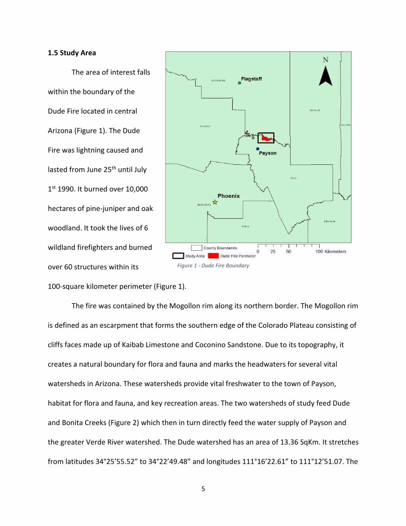
1.5 Study Area
The area of interest falls
within the boundary of the
Dude Fire located in central
Arizona (Figure 1). The Dude
Fire was lightning caused and
lasted from June 25th until July
1st 1990. It burned over 10,000
hectares of pine-juniper and oak
woodland. It took the lives of 6
wildland firefighters and burned
over 60 structures within its
100-square kilometer perimeter (Figure 1).
The fire was contained by the Mogollon rim along its northern border. The Mogollon rim
is defined as an escarpment that forms the southern edge of the Colorado Plateau consisting of
cliffs faces made up of Kaibab Limestone and Coconino Sandstone. Due to its topography, it
creates a natural boundary for flora and fauna and marks the headwaters for several vital
watersheds in Arizona. These watersheds provide vital freshwater to the town of Payson,
habitat for flora and fauna, and key recreation areas. The two watersheds of study feed Dude
and Bonita Creeks (Figure 2) which then in turn directly feed the water supply of Payson and
the greater Verde River watershed. The Dude watershed has an area of 13.36 SqKm. It stretches
from latitudes 34°25’55.52” to 34°22’49.48” and longitudes 111°16’22.61” to 111°12’51.07. The
Figure 1 - Dude Fire Boundary

6
Bonita watershed is 18.6 square
kilometers. It stretches from
latitudes 34°24’50.28 to
34°21’1.01” and longitudes
111°15’18.15” to 111°11’4.36”.
The elevation ranges from 1610
meters to 2387 meters, with the
higher portion making up the
top of the Mogollon rim.
The town of Payson, AZ
is located in Gila County and is
roughly 17km southwest from
the center of the watersheds. Payson stands at around 1,490m in elevation and has a mean
minimum and maximum temperature of 4°C and 22.9°C, respectively, with an average
temperature of 13.2°C. The average annual precipitation is 560mm with an average annual
snowfall of 59cm. The average amount of precipitation days (greater than or equal to 0.254cm)
is 69.5 per year.
Twenty years post-burn the vegetation has transitioned from a ponderosa pine forest to
a plant community almost fully made up of a manzanita/oak overstory with an understory
dominated by weeping lovegrass (Leonard, et al; 2015). Weeping lovegrass was introduced into
sections of the burn zone in an attempt to mitigate the effects of erosion, which was a widely
used post-fire treatment at the time. However, the effectiveness of this practice has been
Figure 2 - Study Area: Watersheds of Interest

7
found to be minimal in increasing soil stabilization (Beyers, 2004;Peppin, 2010). Attempts to
plant ponderosa seedlings in the burn area occurred for three years following the fire yet most
of the sites contain no evidence of pine growth twenty years later. This can possibly be
attributed to the aggressive and invasive chaparral species, a shift in soil make-up, and elk
grazing (Beyers, 2004; Raison, 1979; Leonard, 2015; Zedler et al., 1983).
Following the Dude fire, from July 1st 1990, through the end of 1993, weather stations
surrounding the study area recorded higher than average precipitation events for the region.
These three weather stations consist of: Station 1, Baker Butte (Identification code:
GHCND:USS0011R06S. Latitude: 34.46° Longitude: -111.41°. Station 2, Payson (Identification
code: GHCND:USW00093139. Latitude: 34.2326°. Longitude: -111.3446°). Station 3,
Promontory (Identification code: GHCND:USS0011R10S. Latitude: 34.37°. Longitude: -111.01°).
Figure 3 - Verde River Stream Gauge
Time of interest highlighted. Adapted from USGS National Water Information System. Site
Number: 09507980.

8
Due to the hydrophobic layer left in the top layer of soil caused by the fire, the watersheds
underwent large flooding events. Daily discharge meters located along the Verde River
recorded major regional flooding during this time period, one of which was over 10,000 cubic
feet per second (Figure 3).
After the fire, the soils of both watersheds were hydrophobic. Hydrophobicity is a result
of the formation of a waxy layer in the soil profile caused by the high severity burn (DeBano,
2000; McHale et al., 2005). The summer storms following the burn caused a large amount of
soil erosion, especially in Dude Creek. Decades later this stream can still be characterized by its
streambed consisting generally of bedrock due to the flooding (Figure 4). Bonita Creek
experienced similar precipitation events, being adjacent to Dude Creek yet this stream
Data collected within watersheds of interest in June 2014. Three transects were chosen to best mimic overall stream
conditions. Three hundred pebble size measurements were taken at each of the three transects. The comparison of
bedrock within Dude Creek versus Bonita Creek can be seen (left).. Note the blackberry found along Bonita Creek
(center) and bedrock exposed as well as Lovegrass found along the banks of Dude Creek (right).
Figure 4 - Watershed Bedrock Comparison and Streambed Pictures

9
responded differently as it did not undergo streambed erosion to a similar same scale. It has
been speculated that this was due to differences in vegetation, such as the small stands of
ponderosa pine found along the banks of the stream, stream morphology and streamflow
amount (Leonard, 2014). Decades following the burn a large increase in Himalayan Blackberry
has been noted along the stream banks (Figure 4), which may have also contributed to the
stability of the soil.

10
Chapter 2: Literature Review
2.1 Forest Management and Policy
Natural resource policy within the United States has resulted in the exclusion of forest
fire thus contributing to an altered fire regimen in ponderosa pine ecosystems. (Stephens and
Ruth, 2005). The majority of these ecosystems are now altered to support severe fire behavior
(Reiner et al., 2012), and no longer support the functions it did in pre-settlement forests
(Moore et al., 1999). Building on science based programs that use modeling will allow agencies
to better utilize information in pursuit of reducing severe wildfire (Stephens and Ruth, 2005).
National forest managers in Arizona have been working to reduce the threat of high-severity
fire using restoration treatments such as prescribed burns and the mechanical thinning of trees,
yet these costly efforts have not sufficiently reduced the threat of these severe large-scale fires
(Fitzgerald. 2005).
A ten year restoration project called the Four Forest Initiative (4FRI) has already begun
to take place within the ponderosa forests in Arizona (Fredette, 2016; Robles et al., 2014). The
overall goal of 4FRI is to plan and implement landscape-scale restoration approaches in order to
reduce fire fuels and improve forest health (USDA, n.d.). 4FRI is located within the Kaibab,
Coconino, Apache-Sitgreaves and Tonto National Forests and will utilize mechanical thinning
and prescribed burning treatments across an estimated 586,000 acres over a ten year period
with the objective to re-establish forest structure, pattern, and composition (Fredette, 2016;
Robles et al., 2014). Within the project boundary lies the Mogollon rim and several headwater
watersheds.

11
These watersheds containing ponderosa pine over-story produce 50% of the runoff in
the Salt and Verde watersheds even though it accounts for only 20% land cover of the area
(Robles et al., 2014). Model predictions in mechanically thinned forests are forecasted to
provide around 20% more runoff than unthinned forests and increase the mean annual runoff
from between 0-3%. These models run by the Nature Conservancy and Northern Arizona
University, support the idea that accelerated forest thinning at large scales could improve the
water balance and resilience of forests and sustain the ecosystem services they provide (Robles
et al., 2014). The continued use of hydrological models in which land management practices,
vegetation cover, climate, and hydrological processes are all included would further assist land
management agencies in evaluating proper management practices.
Land management agencies in the US are required to assess conditions post wildfire and
when deemed necessary implement watershed rehabilitation practices (Beyers, 2004; USDA,
1985). The Burned Area Emergency Response (BEAR) program was designed by the USFS to
address these needs. The BAER team aims to stabilize wildland fire zones to prevent further
damage by protecting life, property, and natural and cultural resources. Staffed by a specialized
team, the burn zone is rapidly evaluated and stabilization treatments are implemented. BAER
assessment and implementation plans are often a cooperative effort between federal agencies
(Forest Service, Natural Resources Conservation Service, National Park Service, Bureau of Land
Management, U.S. Fish and Wildlife Service, Bureau of Indian Affairs, U.S. Geological Survey),
and state, tribal and local forestry and emergency management departments (Witt, 1999).
To simplify the rapid response for post-fire remediation and facilitate the use of
hydrological modeling, online spatial databases offer formatted parameters using BAER

12
assessments (Flanagan et al., 2007; Miller, 2016). These modeling tools help foresee impacts of
treatments and increase the understanding of the effects of fire on watersheds. Without the
use of these modeling input generators, it is impracticable for BAER teams to apply quick and
effective watershed erosion mitigation practices (Miller, 2016).
4FRI considers all ongoing and proposed forest restoration projects under the National
Environmental Policy Act (NEPA) within these forests to be considered part of the initiative
(Fredette, 2016). Land managers working under the 4FRI objectives aim to mitigate the adverse
effects of high-severity fire on soil and water resources through the use of best management
practices. Best management practices for watersheds are defined as follows “Minimize impacts
on soil and water resources from all ground disturbing activities. Manage vegetation to achieve
satisfactory or better watershed conditions. Prepare flood hazard analyses on proposed
projects in flood prone areas per Executive Order 11988. Mitigate the adverse effects of
planned activities on the soil and water resources through the use of Best Management
Practices. Avoid channel changes or disturbance of stream channels and minimize impacts to
riparian vegetation.“ (Unites States Department of Agriculture, 1985, p. 7-8). Using these
management guidelines as objectives, modeling implementation methods and results can be
compared to assess what model preforms best.
2.2 Climate Change and Modeling
Climate change is projected to increase likeliness of extreme weather associated wildfire
intensity (Karl et al., 2008). The joined effects of climate change and high severity fires are
predicted to alter forested areas in the Southwest United States by triggering a shift from
ponderosa pine to juniper dominated forests (Bell et al., 2013; Schlaepfer et al., 2012).

13
Modeling in conjunction with GIS has proven to assist in identifying areas at-risk for
wildland fire due to changes in climate (Bell et al., 2014; Vadrevu, 2010). As climate suitability
for southwest ponderosa forests in the United States will decline, modeling provides land
managers with ideas as to what the best management practices may be. Models such as RUSLE
and WEPP can assist land managers in assessing what remediation efforts provide the most
effective results in reducing the risk of high-severity burns, soil erosion, and a shift in forest
species (Gould et al., 2016; Prasannakumar et al., 2012).
2.3 Dude Fire Landscape Vegetation Change
Fire has played a key role in ponderosa forests in the United States Southwest. These
forests have evolved to survive low-intensity wildfires that occurred typically during pre-
settlement times in which fire returned approximately every 2-47 years (Fitzgerald, 2005). This
can be attributed to evolutionary traits such as protected buds, thick bark, high-volume seed
production, highly flammable litter, basal sprouting patterns, and deep rooting (Balch et al.,
2013;, Moore et al., 1999). These low-intensity fires would consume accumulated fuels and
smaller plants, thin the younger tree populations, leaving the large, fire-resistant trees intact
(Fitzgerald, 2005)
Ponderosa pine ecosystems have changed drastically in the last 140 years due to the
disruption of fire regimes. Due to livestock grazing, logging, and fire suppression current
conditions consist of an over-abundance of fuel (Moore et al., 1999). Severe wildfires and
drought have caused up to 20% tree mortality in forests and woodlands in Arizona and New
Mexico (Robles, et al. 2014). Dense, over-stocked forests increase the risk of insect and disease
outbreaks, high-intensity wildfires, and conditions that are unsustainable for these ecosystems

14
(USDA, n.d.). Average ponderosa stand densities have increased over 1000 trees per hectare
(Fitzgerald, 2005; Moore et al., 1999) and total basal areas range from 2 to 4 times greater
(Robles et al., 2014). Research has also pointed out possible flaws in the statistical analysis of
the United States Forest Service Inventory data indicating that high severity fire frequency was
less common pre-industrialization that originally thought (Stevens et al., 2016).
The Dude Fire site provides an opportunity to study the long-term effects of high-severity
fire on the Mogollon Rim. Twenty years after the Dude Fire, findings by Leonard et al. (2015),
demonstrated that oak tree density had increased over 400% from unburned to burned sites.
Non-native weeping lovegrass now makes up 81% of the total herbaceous cover. Furthermore,
bare ground cover is 150% higher and litter cover is 50% lower in the burned area. Lead soil
erosion models can be used address the effects of large-scale vegetation change and establish
vegetation restoration models (Han et al., 2016).
2.4 Soil Response to Fire
Disrupted fire regimens have put ponderosa forests in conditions for high severity burns
and therefor at risk for severe soil erosion and flooding. Water repellency produced by low to
moderate severity fires is usually of shorter duration and intensity than that produced by high
severity fires (Cawson et al., 2016; DeBano, 2000). High severity fire in ponderosa pine forests
result in increased soil exposure causing vapor deposition of wax into the soil due to the
burning of organic material. This causes intensified water repellency in the upper level of the
soil profile (Fitzgerald, 2005; McHale et al., 2005). Soil conditions and characteristics can cause
differences in water infiltration and overland flow, thus escalating erosion (DeBano, 2000;
McHale et al., 2005). Due to the removal of the vegetation cover and the increased water

15
repellency these areas are prone to an increase in runoff and erosion during post-fire rain
events (Beyers, 2004).
In order to mitigate the effects of wildland fire on erosion and reduce the chances of
severe flooding a variety of management practices have been implemented and studied. One
method consists of using budget friendly chemical treatments to reduce erosion, yet this has
not provided noticeable results (DeBano, 2000). Techniques using heavy machinery to break up
water repellent layers are impractical when implemented at a large scale or in complex terrain.
Recent management practices introduce mulching to reduce post-fire erosion rates. Studies
conducted by Robichaud et al., (2012) found variability in its effectiveness and deemed the
method of mulching to be considered fire specific.
The Dude Fire area underwent one of the more common practices for post-wildfire
erosion remediation. Broadcast seeding consists of distributing perennial grasses to provide
quick ground cover and soil retention. Minimal data exists supporting the effectiveness of this
erosion control (Beyers, 2004). As sampling designs for the effectiveness of broadcast seeding
in the western United States has become more rigorous, the evidence of the effectiveness of
seeding has declined and additionally the seeding of invasive non-native species can have
negative effects on native vegetation recovery (Beyers, 2004; Peppin et al., 2010). Using
frequent prescribed fire treatments in ponderosa ecosystems to manage fire-induced soil
hydrophobicity is the most practical solution (DeBano, 2000).
2.5 RUSLE Model
The RUSLE is an empirically based model easily integrated with GIS (Ashiagbor et
al., 2016; Ganasri and Ramesh, 2016). Empirical observations consist of using knowledge

16
acquired by the means observation and experimentation which RUSLE does by relating
management and environmental factors directly to soil loss and sedimentary yields. RUSLE
models how climate, soil, topography, and land use affect soil erosion caused by raindrop
impact and surface runoff. Manipulating five raster formatted factors consisting of rainfall
erosivity, soil erodibility, slope, cover management, and support practice also allows the user to
view the spatial heterogeneity of soil erosion and the possible effects of each individual
parameter.
In 1965, the USDA created the Universal Soil Loss Equation (USLE). This equation proved
to be optimal and very accurate in uniform slopes, more so than WEPP (Tiwari et al., 2000). As
the equation was updated, it was adapted for other regions through the improvement of
determining factors and the implementation of new ones thus creating RUSLE. RUSLE is the
most commonly used model by scientists worldwide (Alexakis et al., 2013).
One of the characteristics of RUSLE that impedes its ability to predict soil erosion is its
limitation in properly developing factors to represent the effects of complex hydrographic
basins commonly found in mountainous watersheds (Oliveira et al., 2013). This issue has been
alleviated using data acquired through the means of remote sensing within a watershed
(Bhandari and Darnsawasdi, 2014;, Ganasri and Ramesh, 2016). Remote sensing provides a tool
for identifying land cover, elevation differences, and aspects of management with relatively
high resolution for small areas (20-50 square kilometers) that are easily integrated with GIS
(Bhandari and Darnsawasdi, 2014; Reed et al. 1994; Yaolong, Ke, Yingchun and Hong. 2012).
Remotely sensed data can identify land cover in a variety of ways. Using multi-band
imagery, NDVI indexes that indicate phonological events can be used to evaluate the variability

17
of the phenology of land cover types. Implications for land cover mapping suggest that
remotely sensed data using NDVI indexes are appropriate as input to vegetation mapping, but
needs to be cross referenced with field data for accuracy (Reed et al., 1994). Alternatively land
cover classification methods can classify vegetation types and can be used as an input
parameter for model running for fire behavior or soil erosion (Yaolong et al., 2012). When
stacked and compared over time, imagery can provide land use and cover change as well as
clues to possible causes of erosion. After creating the land cover classes, change detection can
be ran on multitemporal data sets in order to derive vegetation cover change, observe urban
development, or even make implications as to the effects of climate change (Yaolong et al.,
2012).
2.6 WEPP Model
The WEPP is a process based model which is founded upon the theoretical
understanding of relevant ecological processes. In this case, WEPP calculates erosion processes
of sediment transportation mathematically through the solutions of the equations describing
those processes. This model provides an assessment of soil loss severity and can be combined
with GIS to estimate average soil loss in watersheds (Flanagan et al., 2007). WEPP uses
quantitative data to identify critical areas where soil erosion is most anticipated within both the
watershed rills and streams (Han et al., 2016). The WEPP model has evidence to support that
with minimal parameter calibration it provides accurate and tested results demonstrating its
utility as a management tool in both gauged and ungauged basins (Brooks et al., 2015).
WEPP is based on research in which various interacting natural processes in hydrology,
plant sciences, soil physics, and erosion mechanics were studied and applied. WEPP offers

18
advantages to empirical modeling since it can accommodate spatial and temporal variability in
climate, topography, soil properties, management, as well as sediment transportation
processess. WEPP can be manipulated in order to study the effects of different parameters on
net soil loss or gain for the entire hillslope for any period of time (Tiwari et al., 2000) and
therefor can be used to measure the effects of climate change on watersheds by allowing for
the manipulation of different factors as to model future climate scenarios (Gould et al., 2016).
Since its development it has been further enhanced in order to increase its applicability
to small forested watersheds. Through the development of GeoWEPP, GeoWEPP-BAER, and
WEPP parameter databases, the model can use complex inputs provided by peer reviewed
sources in user-friendly formats (Dun et al., 2009; Flanagan et al., 2007).
When using GeoWEPP, the Parameter-elevation Regressions on Independent Slopes
Model (PRISM) and Climate Generator (CLIGEN) tools are used in order to create its
precipitation and temperature inputs. PRISM is a climate analysis system in which specified
point and digital elevation data supplied through GeoWEPP and ArcMap works with spatial
datasets to generate estimates of precipitation and climate in grid format (Daly et al., 2002).
PRISM has been designed to accommodate difficult climate mapping situations by including
vertical extrapolation of climate, reproducing gradients caused by rain shadows and coastal
effects and taking into account the possible complexity of terrain on precipitation by identifying
features that rise above the large-scale terrain and adjusting its predicted measurements for
these areas (Daly et al., 2002). CLIGEN provides the point data for the PRISM model by using
historic climate measurements (Flanagan et al., 2007; Meyer, 2010).

19
GeoWEPP uses the Topographic Parameterization (TOPAZ) digital landscape analysis
tool in order to delineate channels, watersheds and subcatchments. This model provides slope
inputs for each of the subcatchment hillslope and channel profiles for GeoWEPP (Flanagan et
al., 2013). As WEPP uses complex hillslope data and takes climate variability on hydrological
factors into account inferences as to best stormwater management practices can be made
(Landi et al., 2011; Brooks et al., 2015).
2.7 Data Resolution Effects on Modeling Results
One of the most important parameters for RUSLE and WEPP models are the Digital
Elevation Models that spatially tie the soil, weather and other factors to the study areas. DEMs
also provide the data is manipulated to identify hillslope, channels, and catchments. These
models can vary as the intervals between elevation points determines the resolution, and the
precision of ground trued points determine the accuracy. The resolution and accuracy of the
DEMs themselves can greatly affect the results of soil erosion models (Zhang et al., 2008).
When comparing publically accessed DEM data, LIDAR satellite images with finer resolution
commonly provide the most accurate results for small-scale (1000 square foot) watersheds
(Zhang et al., 2008).

20
Chapter 3: Models and Methods
3.1 RUSLE Introduction
The Revised Universal Soil Loss Equation started as the Universal Soil Loss
Equation (USLE) which was created in 1965 by the USDA with the goal of monitoring soil
erosion along agricultural type land of the Corn Belt region of the United States. Development
of USLE began with scientist Hugh Bennet, who highlighted the issue of soil erosion during the
dust bowl leading to the federal funding for related research. Stations were established for
experimental studies in which factors affecting erosion were identified and studied. The
mathematical portion began to take shape in the early 1940s (Zingg and Smith, 1940). By 1961
the general factors identified and agreed upon by the array of leading researchers were rainfall,
soil erodibility, cropping management and slope (Tiwari et al., 2000).
By 1965 two key scientists Wischmeier and Smith published a section in the USDA
Agricultural Handbook in which the completed technology for USLE was presented. With the
majority of the development coming from USDA and Peurdue University affiliated scientists, a
process in which data was analyzed in simulations using computers began to take place in the
1960s. USLE was quickly adopted as the lead soil erosion modeling tool throughout the world
(Ouyang et al., 2002; Tiwari et al., 2000; USDA, 2016)
With additional research and data, the USLE equation became RUSLE which uses the
same formula but revised several of the factors used. This model provides the same empirical
approach that predicts erosion rates and presents the spatial heterogeneity of soil erosion
using uniform flow hydraulics. The RUSLE model similarly consists of an equation that ties in
raster formatted factors that include rainfall erosivity (R factor), soil erodibility (K factor), slope

21
length and steepness (LS factors are combined), cover management (C factor), but additionally
introduced the support practice (P factor). Other key modifications consisted of the
computation of the slope length and steepness factors. When these factors are multiplied they
compute “A” which is an estimated average soil loss in tons per acre per year (Tiwari et al.,
2000).
RUSLE was completed and formatted for computer use and was re-released in 1992. As
it became more popular in studying erosion, the need to quantify the amount of erosion had
become less important than identifying the spatial distribution of erosion sources (Ashiagbor et
al., 2013). By accurately identifying the highest risk areas, land managers could then implement
the most cost effective erosion control practices. For easy integration with GIS, several factors
can be computed using variety of databases and tools such as the USDA Geospatial Data
Gateway, the United States Forest Service (USFS) Geodata Clearinghouse, the Environmental
Protection Agency (EPA) Rainfall Erosivity calculator and ArcGIS.

22
3.2 RUSLE Methodology
RUSLE Equation: A = R*K*LS*C*P
A = Soil loss in tons per acre per year
R = Rainfall-runoff erosivity
K = Soil Erodibility
L = Slope length
S = Slope Steepness
C = Cover-management factor
P = Support Practice
*For in-depth methodology for RUSLE using ArcMap see Appendix (A).
**All factors were attributed 10mX10m cell resolution as that is the lowest resolution the data
obtain contained. These factors were also all projected in the “NAD1983_utm_zone 12n” in
ArcMap.
Watershed Delineation – ArcMap Hydrology Toolset
As the RUSLE model does not provide an interface for ArcMap, the watersheds were
delineated used the ArcMap Hydrology Toolset. By using the highest resolution DEM and this
hydrological model, the watersheds were able to be accurately delineated (Figure 2), as well as
provide layers for future use such as “flow direction”, “flow accumulation”, “stream order”, and
“flow length”.

23
R Factor – Rainfall Runoff
The Rainfall Runoff factor represents the effect of raindrop impact and the amount and
rate of runoff associated with the precipitation. While the USDA RUSLE handbook (Rendard et
al.,1997) provides several equations for calculating an R-factor using weather station data, the
topographic complexity provided extremely high results when compared to other case studies.
In order to address this, the factor was created using the EPA Rainfall Erosivity Factor
Calculator. This tool is commonly used to determine if small construction projects are eligible to
waive the permitting needed through the National Pollutant Discharge Elimination Systems.
This tool takes elevation, the date range, latitude, and longitude into account and supplies the
user with point specific data (Table 1). This data was spatially interpolated to give the final R-
factor (Figure 5).
Location ID 1 2 3 4 5 6 7 8 9 10
RValue 266 290 266 240 266 240 217 217 266 266
Latitude 34.4305 34.4247 34.4165 34.4038 34.415 34.4035 34.3892 34.3852 34.4088 34.4042
Longitude -111.229 -111.223 -111.216 -111.224 -111.246 -111.24 -111.239 -111.266 -111.198 -111.208
Location ID 10 11 12 13 14 15 16 17 18
RValue 266 217 217 217 217 217 290 266 217
Latitude 34.4042 34.3886 34.3758 34.3669 34.35 34.3569 34.437 34.4064 34.3848
Longitude 111.208 111.21 111.229 111.25 111.241 111.22 111.238 111.193 111.274
Table 1 - EPA R-Factor Locations
These are the geographic points in which the R factor was calculated for. Latitude and longitude displayed in degrees

24
Figure 5 - RUSLE EPA R-Factor Locations

25
K = Soil Erodibility
This factor represents the ease of which the soil is detached by splash during rainfall and
or surface flow (Renard et al., 1997). The USDA RUSLE Guide provides methods to identify the
K-value in which soil characteristics such as particle size, organic matter content and structure is
analyzed and use an inputs in a series of equation. As this would require physical access to the
study area, timely analysis, and specific tools, an alternative method was used. The USFS
database provides K-values for RUSLE throughout the contiguous United States. This data was
used and compared to a nomograph provided by the USDA RUSLE Guide (Renard et al.,1997) in
which the dominant rock type of limestone and sandstone were compared. The K-factor of .2
was used for the entire study area (Figure 6).
Figure 6 - RUSLE K-Factor

26
LS = Slope length and steepness.
These factors aims to address the effects of topography on erosion. The slope length factor
represents the increase in erosion due to the horizontal distance in which the overland flow
either is effected by a decrease in slope causing deposition, or the flow becomes concentrated
in a defined channel. The slope steepness factor aims to reflect the influence of slope gradient
on erosion (Oliveira et al., 2013; Renard et al., 1997). While slope length and steepness is best
calculated in the field (Renard et al., 1997) it is not feasible in such large and topographically
complex areas (Oliveira et al., 2013). For this reason the highest resolution and most accurate
DEM was used in conjunction with GIS. Equations have been created to address the L and S
factors to best reflect the influence of slope gradient on erosion and have been formatted to be
used with GIS software (Oliveira et al., 2013). Subfactors for the equations chosen were
selected to best compute accurate results in accentuated slopes. These factors are combined
and computed using the Raster Calculator before being used in RUSLE.

27
Figure 7 - RUSLE L*S Factors

28
C = Cover-management factor
This factor aims to reflect the effect of vegetation and other influencing factors on
erosion rates. This factor was created using ENVI and ArcMap software. Having relatively small
watersheds high resolution data was needed in order to create the proper land cover factor.
While a land cover classification shapefile for RUSLE has already been created by the United
States Geologic Survey, it is of poor resolution as it has been created to cover all of Arizona in
order to study largescale watersheds such as the Bill Williams or the Verde.
In order to create the most accurate land cover factor, high resolution 1 meter data was
used and edited in Environment for Visualizing Images (ENVI) software. A supervised land cover
classification method allowed for the identification of three land cover types (Figure 8). As the
imagery at this resolution was available for several years, the accuracy for each year was
calculated. The 2015 imagery provided the highest accuracy data and was therefore used.
Figure 8 - Land Cover Accuracy Assessment Method

29
Having used imagery obtained 25 years after the fire, the immediate effects of the
severe burn needed to be addressed. A burn severity map was acquired from the USFS (Figure
9). The polygons representing different degrees of burn severity were digitized in ArcMap.
These polygons were then overlaid with the land classification results. The high severity
polygons were given a high C-value and eradicated any vegetation that intersected them to
represent the effects of the high severity burn. The additional land cover values were identified
using the USDA RUSLE handbook, yet the values were increased to represent the effects of the
moderate and low
severity areas. The
ponderosa pine forest
identified that did not
intersect the high
severity burn was
attributed a very low C-
value as this species has
evolved to be resistant
to low intensity fire and
is described to have
deep soil retaining roots
(Balch et al., 2013;
Fitzgerald, 2005; Moore
et al., 1999) Figure 9 - Dude Fire Severity Map. Adapted from USFS Rocky Mountain
Research Station

30
Figure 10 - RUSLE C-Factor

31
P = Support Practice
This factor represents
the ratio of soil loss with a
specific support practice in
which erosion is effected by
modifying the flow pattern or
by reducing the amount and
rate of runoff. This value
ranges from 1-0, with one
being no support practice
used. Following the burn, the
area was aerially seeded with a
variety of grasses to reduce erosion. The value 0.98 was attributed to the seeded area as very
little data exists that supports the effectiveness of seeding for erosion control (Beyers, 2004;
Peppin et al., 2010).
RUSLE Model Output Computation
The factors were multiplied providing the output for the RUSLE model for both
watersheds (Figures 17,16). Using the parameters calculated above, the ArcMap ModelBuilder
tool was used to multiply the factors to calculate the soil loss in tons per hectare per year for
each 10 by 10 meter cell. Additionally, the results were categorized into classes to identify the
areas at highest risk for erosion (Figures 18, 19).
Figure 11 - RUSLE P-Factor

32
3.3 WEPP Introduction
The Water Erosion Prediction Project (WEPP) is a computer model that was developed
largely in part by the USDA’s Agricultural Research Service, the Natural Resources Conservation
Service and the U.S. Department of the Interior’s Bureau of Land Management. Four senior
scientists G. Foster, L. Lane, J. Laflen and D. Flanagan were termed the project leaders over a
span of 22 years. WEPP simulates soil erosion processes taking a quantitative process-based
approach founded upon observed erosion mechanics and interacting natural processes using
non-geographically tied and geographically tied data to then calculate net soil loss or gain for a
hillslope for a specified amount of time.
The original software version of WEPP was difficult to manage and therefore a new
version integrated with GIS software was created (Elliot et al., 2006). With the help of the USDA
National Soil Erosion Research Laboratory, scientists from Peurdue University, and the
department of geography at the University of Buffalo led by Chris Renschler, a geospatial
interface for WEPP with ArcMap was developed and named GeoWEPP. This software allows for
the integration of personalized data allowing the user to create, assess, and study the effects of
a variety of parameters on soil erosion processes within watersheds (Elliot et al., 2006).
Through its use, users are able to define the influence of localized climate variability on
daily runoff, soil erosion, and sediment yield. The model created estimates of net detachment
and deposition using steady state sediment continuity equation. This is done by using a fixed
approach describing the movement in soil caused by overland flow in dynamic equilibrium
(Landi, 2011) and by predicting rill and interrill erosion separately. Rill erosion is defined as the
occurrence of soil removal due to water running over the soil while interrill erosion is caused by

33
raindrop impact and splash. GeoWEPP uses GIS data to first delineate the watershed based
upon a channel. Parameters needed to run GeoWEPP include climate, soil type, land cover, and
a digital elevation model (DEM). GeoWEPP used in conjunction with ArcGIS allows the user to
use a large extent of data in regards to resolution and detail. The creation and application of
these parameters will be explained in the following pages.
Before running a WEPP simulation, a DEM and optional land cover and soil data are
selected in order to create the study area. If these parameters are not selected, default values
will be assigned for them. This data selection is done outside of ArcMap, in a GeoWEPP for
ArcGIS 10.3 wizard. The DEM must be provided in ASCII format. This also is the required format
for the land cover and soil files. When providing personal land cover and soil data, description
and database text files need to be created and properly formatted. The DEM data should ideally
be limited to the area of interest, as a larger and higher resolution DEM will more likely produce
errors.
Within ArcMap GeoWEPP is used as an extension with a specific toolbar. Basic
navigation tools included in the toolbar allow the user to pan around the area of interest, zoom,
and view the full extent of the area much like the traditional tools ArcMap offers. The Modify
Channel Network Delineation Tool creates a channel network based upon the DEM supplied. It
creates these channels using two parameters. The first is the Critical Source Area (CSA) in which
the user must define (in hectares) the minimum source area needed to generate a channel. The
second parameter is the Minimum Source Channel Length (MSCL) in which the user must define
the shortest distance a first order channel needs to travel before joining another before it is

34
classified. Both of these must be met in order to be represented as a channel in the model. This
tool provides an easy way to modify the channels found in the DEM.
After having created a channel network, the Watershed/Subcatchment Generation tool
can then be used in order to identify the subcatchment of the watershed by choosing a cell
within the previously generated channel network. This cell has been termed the outlet point.
Subcatchments are a hydrologic unit that are part of the hierarchical system that make up
watersheds. This tool will generate polygons that identify the hillslopes that join together to
create the watershed that feeds up to the selected cell or “outlet point” of the watershed. The
polygons representing the subcatchments will vary in number, shading, and or color. This tool
as well as the Channel Delineation Tool is run using Topographic Parameterization (TOPAZ)
which is defined as a digital landscape analysis tool used for subcatchment parameterization,
drainage delineation, and watershed dissection. The analysis is based on the application of the
deterministic eight-neighbor method to simulate flow across a land surface represented by a
DEM, (Garbrecht and Martz, 2015).
Climate within the GeoWEPP model is modified using the Parameter-Regressions on
independent Slopes Model (PRISM). This interlinked model allows the user to easily modify the
climate for the study area. The user can either choose the closest climate station to the outlet
point, pick a separate weather station, edit existing climate stations, or the user can create
personal climate parameter files. PRISM is defined as a climate analysis system in which point
data is used along with a digital elevation model (DEM) to then give estimates in climate for
geographic areas in which point data is not sufficient (Daly, 2002). Through PRISM, point
specific climate data can be extrapolated over large areas which is easily integrated with GIS

35
(Johnson, 1998). The point data used for the PRISM are weather stations that are generated
through CLIGEN. CLIGEN provides storm parameter estimates from a single geographic point
(Meyer, 2016). This includes estimates in regards to storm time to peak, peak intensity, and
duration, all being vital in regards to soil erosion events.
When modifying climate data, the user may select to use the Climate Modification
window. Here mean maximum, mean minimum temperatures as well as mean precipitation
and number of wet days can be edited if the attributed parameters derived from PRISM are not
to the users liking. When modifying the climate the user may edit the new climate station
name, latitude and longitude, elevation, as well as the recently mentioned temperature and
precipitation parameters. In addition to modifying the climate data, users can adjust 2.5 minute
grid values for both elevation and annual precipitation in inches.
After creating and accepting the parameters, the user can begin the WEPP simulation by
clicking the Accept Watershed button located on the WEPP toolbar, this will produce results in
map and text form as well as allow the user to access a variety of new tools. When finished
running, the model will provide two different model outcomes from two different methods.
The first is named the Watershed Method, in which the model assigns one soil and one land use
for each hillslope. This hillslope profile is chosen by combining all the flow paths found in the
hillslope where they are then aggregated to create a profile that best represents the hillslope.
The dominant soil type is then chosen for the hillslope and it is assigned to its profile. This
simulation is then ran on each hillslope and is given the label “Offsite assessment” as the value
reported for each hillslope represents the sediment flux at the given outlet point. This process
better allows the user to assess which hillslopes are at the highest risk.

36
The other method that the model can use is called the Flowpath Method. This supplies
results for each flow path in the subcatchment. It differs to the Watershed Method as it does
not use generalized parameter profiles for each hillslope but allows each cell to be labeled a soil
and land use factor independently. This allows for the slope, soil and land use layers to work
together within a flow path. While no aggregation occurs at the sources of the different flow
paths, several of the flow paths share the same destination in which here the aggregation
occurs. The map produced using this method supplies the user with estimates of erosion
occurring in each raster cell and therefore shows what portion of the hillslope are the main
contributors to the erosion. Both these methods provide estimates of erosion in tons per acre
per year.
Once the WEPP has been run a variety of tools will be newly accessible. The “Remap
With New T-value” tool allows the default value of erosion loss and sediment yield threshold to
be edited. By default, this value is set to one ton per hectare per year. This change can be
toggled on the Change T-value window. The WEPP Hillslope Information tool allows the user to
identify what soil and land use parameters a certain hillslope was assigned. These parameters
can then be changed using the change WEPP hillslope parameters which will be implemented
after the model has been reran using the rerun WEPP button. Another way of running the
WEPP model is by using the WEPP on a Hillslope function in which, once the parameters are
identified, the model will be ran on only that one identified hillslope.
In addition to the editing of the results, GeoWEPP creates three text formatted reports.
The “Offsite Events” report provides estimates as to how much discharge occurred from the
user specified watershed outlet point. Only results for runoff volume > 0.005m^3 are listed.

37
This is done on the format of providing the day, month and year of each precipitation event. For
each date, precipitation Depth (mm), runoff volume (m^3), peak Runoff (m^3/s), and sediment
Yield (kg) are calculated.
The second text report that is created is the “Offsite Summary” which provides an
estimation of hillslopes Runoff Volume (m^3/yr), Subrunoff Volume (m^3/yr), Soil Loss (kg),
Sediment Deposition (kg), and Sediment Yield (kg) per each hillslope identified by the TOPAZ
model. It similarly identifies the Discharge Volume (m^3/yr) Sediment Yield (ton/yr) Soil Loss
(ton/yr) Upland Charge (��), and Subsurface Flow (��) per each channel and impoundment.
This report also provides information regarding the number of storms and amount of rainfall
(mm) produced on an average annual basis. It also informs the number of events and the
amount of produced runoff (mm) passing through the watershed outlet on an average annual
basis. It creates estimates regarding the average annual delivery from the channel outlet point,
the sediment particle leaving the channel information, as well as the distribution of primary
particles and organic matter in the eroded sediment.
The last report is named the “Onsite Summary” and it provides the four year average
annual values for the watershed. The reports identifies the hillslopes both attribute values
provided by the TOPAZ model. These values allow the user to observe the estimated runoff
volume (m^3/yr), soil loss (ton/yr), sediment yield (ton/yr), area (ha), soil loss (ton/ha/yr), and
mapped sediment yield (ton/ha/yr) calculated. The report then calculates a channel summary
watershed method off-site assessment by providing the channel WEPP and TOPAZ attribute
identification numbers, and their matching discharge volume (m^3/yr), sediment yield (ton/yr),
length (m) and Length in raster cells. Lastly, the onsite report supplies a report for the WEPP

38
watershed simulation for all flow paths averaged over subcatchments, using the Flowpath
Method as an on-site assessment. This section identifies the hillslopes using the WEPP and
TOPAZ identification numbers, and their coinciding runoff Volume (m^3/yr), soil Loss (ton/yr),
area (ha) and mapped soil loss (ton/ha/yr).
When studying soil erosion within burn areas a database hosted by Michigan
Technological Research Institute provides the DEM, land cover and soils data in proper ASCII
format as well as the necessary text formatted documents to integrate them with the
GeoWEPP software for several historical burn areas. This database was created to merge soil
burn severity maps derived from data collected from Burned Area Emergency Response (BAER)
teams with land cover and soils data in order for natural resource managers to make more
informed decisions when focusing on post fire remediation (Miller, 2016).

39
3.4 WEPP Methodology
*For in-depth methodology for usage of the WEPP model through GeoWEPP and ArcMap see
Appendix (B).
The majority of parameters needed to run GeoWEPP were downloaded from the BAER
Spatial WEPP Model Inputs Generator hosted by Michigan Technological institute. These
parameters are based upon data derived from the BAER team. Using the GeoWEPP interface for
ArcMap, adjustments were made to the delineation of the watersheds using the TOPAZ model
(Garbrecht and Martz, 2015). The channels identified were lowered in detail by adjusting the
Critical Source Area (CSA) and the Minimum Source Channel Length (MSCL) to reduce the
amount of subcatchments and channel sections identified (Figure 12). By doing this, the risk of
crashing is reduced.
Figure 12 - WEPP Modify Delineation Network Comparison

40
Subcatchments are delineated for each watershed using the Select a Watershed Outlet
Point tool. The TOPAZ model then calculates the entire perimeter and subcatchments feeding
into the selected point for each watershed (Figure 13).
Figure 13 - WEPP's TOPAZ Delineated Watershed for Bonita

41
To best represent the flooding following the fire, the PRISM model was used. The PRISM
model takes climate data from single “CLIGEN” point and spatially interpolates it (Daly et al.,
2002; Meyer, 2010). As this data needed weather measurements specifically following the fire,
three surrounding weather stations provided inputs to calculate parameters for a single CLIGEN
point that acted as the input for the PRISM (Figure 14). This CLIGEN point represented data that
was obtained by calculating weather averages for the four years following the fire, as this is
when the regional flooding occurred.
Figure 14 - Weather Stations and PRISM Input Locations

42
The model provided outputs for both simulation methods. The Flowpaths method
calculates an onsite assessment (Figures 20,22) and the Watershed method provides an offsite
assessment (Figures 21,23)
3.5 Model Results Comparison
In order to compare the results of the models, stream channel area change data was
obtained (Figure 15). This data was collected by the USFS by surveying established transects
and calculating the area of change between them over time. These estimates show that the
erosion that occurred in Dude Creek was severe as the symbol falls well below 0 when
comparing 1992 to 1996, or 1996 to 2001. Being relatively small channels, an estimated area
change of negative 7 square meters signifies a catastrophic erosion event. While Bonita did not
have transects established until 1996, the visible data shows that the channel erosion was
minimal.
Figure 15 - Estimated Stream Channel Entrenchment (Unpublished data, Jackson Leonard)
Each shape represents a different time period as well as the mean entrenchment. These shapes are
surrounded by an error bar. “n” stands for the number of transects surveyed. The predicted change
was calculated using WinXS Pro which compares different survey transects over time and calculates
the area of change between them.

43
Using field GPS recorded data, (Table 2) was created showing the location of the
relevant transects in which the stream channel erosion estimates (Figure 15) and the
streambed pebble counts (Figure 4) were calculated. The locations of the transects were
recorded in ArcMap (Figure 18).
Transect # Elevation UTM X:Meters Y:Meters
Dude Creek 1 5722 ft 12 N 476686 3806394
Dude Creek 3 5774 ft 12 N 476706 3806691
Dude Creek 5 5785 ft 12 N 476904 3806900
Bonita Creek 1 6005 ft 12 N 479841 3804646
Bonita Creek 3 6036 ft 12 N 480044 3804791
Bonita Creek 5 6134 ft 12 N 480256 3805079
Table 2 - Transect Locations
These transect points were used to identify the raster cells in which the RUSLE output
value was recorded (Table 3). Alternatively, a mean value that included all values included in a a
10 meter buffer was calculated to address possible outliers (Table 4).
The GeoWEPP model provides subcatchment and channel erosion estimations in text
format. The GPS locations of the transects were used to identify the contributing
subcatchments and channels (Figure 27). Once the channel in which the transects reside were
pinpointed (Figures 24,25), the text reports provided discharge volume (��/yr), yield (ton/yr),
length of channel (m) soil loss of the channel (kg), upland charge (��), and subsurface flow
(��) specific for each channel (Tables 5,6) . This allows a comparison of the Dude and Bonita
channel area change to the estimations made by the WEPP model. This information was then
compared to the WinXS Pro estimates.

44
Chapter 4: Results and Discussion
4.1 RUSLE
RUSLE Results for Bonita Watershed
Figure 16 - RUSLE Output for Bonita Watershed

45
RUSLE Results for Dude Watershed
Figure 17 - RUSLE Output for Dude Watershed

46
The RUSLE model successfully estimated higher rates of erosion in the Dude watershed,
yet due to its lack in including vital process-based erosion processes and inability to properly
address complex topography, the model provided inaccurate estimates of soil erosion. The
range of erosion for the Bonita watershed was between 0-9,545 tons per hectare per year. The
maximum erosion estimate for the Dude watershed was at a much higher 15,130. The majority
of this difference is attributed to the slope length and steepness factors (LS). These factors had
by far the highest influence on the results, and were much higher in the Dude watershed. While
these factors were able
to address immediate
upslope influence on
erosion, cumulative
upland charge within
the channels failed to
be included, thus not
representing the
channel entrenchment
accurately.
Figure 18 - Creek Transect Locations

47
4.2 RUSLE Transect Erosion Assessment
When observing the results of RUSLE
per cell, it is evident that precise estimations
of erosion could not be calculated for the
stream channel transect areas (Figure 18,
Tables 3,4). Stream geomorphology such as
channel slope, confinement, and flow velocity
can cause substantial changes in channel
degradation (Juracek, 2015) and were not
represented in the RUSLE model.
Additionally, key processes of sediment
transportation is not represented at all. Due
to these key differences and the complexity
of the variables, precise estimations or
predictions of erosion within these
watersheds is difficult.
Watershed Transect Value (t/yr/ha)
Dude 1 454
Dude 3 91
Dude 5 141
Bonita 1 58
Bonita 3 15
Bonita 5 1209
Table 3 - RUSLE Transect 10 Meter Buffer Mean Cell Value
*Displays the mean value of the cells of the
RUSLE model output that were located within a
10 meter buffer of the transect location.
Table 4 - RUSLE Transect Single Cell Erosion Value
*Displays the values of erosion generated by
the RUSLE model for the cell in which the
transect location fell.
Watershed Transect Mean Value (t/yr/ha)
Dude 1 118.3
Dude 3 171.4
Dude 5 74
Bonita 1 126.2
Bonita 3 41.6
Bonita 5 240.3

48
4.3 Classified RUSLE Results
As channel erosion is not properly modeled, RUSLE primality provides a guide in identifying at-
risk areas (Figure 18,19).
Figure 19 - Classified RUSLE Results for Bonita Watershed
Classified RUSLE Results for Bonita
Watershed

49
Figure 20 – Classified RUSLE Results for Dude Watershed
Classified RUSLE Results for
Dude Watershed

50
4.4 RUSLE Parameters
The methodology for creating parameters for the RUSLE model are complex and do not
incorporate vital erosion processes thus providing inaccurate results for this study. As RUSLE
was originally created to study erosion in uniform slopes of croplands, new GIS integrated
methods to address complex parameters were created yet they still do not provide accurate
results in the study area.
The slope length (L) and steepness (S) factors are usually the most difficult parameters
to create for RUSLE. As the USLE model began to be revised and reformatted with land manager
needs, several different ways of creating these factors were developed and the array of
available methods to address complex topography can provide highly variable results (Oliveira
et al., 2013). As RUSLE began to be applied to more complex terrain GIS became the primary
tool used to compute the empirical model as landscapes could be represented using elevation
models (Oliveira et al., 2013).
The L and S factors rely upon DEMs which vary in resolution and accuracy. In order to
create the parameter properly a high resolution DEM was used. As this study used
orthorectified 10 square meter resolution data for the DEM, the highest resolution data readily
available, the analyses of the development of the DEM is not an issue as it best represents the
topographic reliefs and other variations presented.
The L and S factors are missing some vital process based aspects. The equation used to
create the output of L and S took into account the flow direction and accumulation. This
addressed the immediate upslope contributing area, slope gradient, and channel length yet it

51
did not calculate the effects that stream velocity and upland charge have on the groundwater.
The hydrological process of runoff buildup in channels downstream is not represented. As this
area experienced severe flooding, the effects of groundwater movement on erosion are vital to
modeling processes within the study area. Additionally, this method assumes the process of the
loss or gain to or from groundwater is not taking place as these are also process based
concepts.
In order to properly map sediment movement the L and S factors need to incorporate
dynamics of the erosive process in complex reliefs and hydrographic basins (Oliveira et al.,
2013). The study area resides along the southern edge of the Colorado Plateau that contains
several sudden cliff edges and a dramatic changes in elevation. The L and S factors were
originally developed for uniform slopes using dependent field measurements, thus making
complex topographic regions difficult to address. With the revisions of USLE to RUSLE, came the
development of several subfactors in the equations used for calculating the L and S factors. The
“m” subfactor used in slope length equation represents general slope accentuation and ranges
from .01-1 with research attributing .4-.6 the best value for accentuated slopes (Oliveira et al.,
2013). While the study area contains portions of accentuated slope along the rim, the creek
transect locations had a general slope gradient of 13%. The value .4 was chosen for this study
as it is not considered an extreme slope such as 30%, yet ranges far from the 1-7% slope that
USLE calculations were originally created upon (Renard et al., 1997). While this research used
the most commonly used estimates for subfactor calculation, further research as to how to
compute subfactors within areas with highly variable amounts of slope in GIS is needed.

52
Developing values for the R factor was done with the EPA calculator. The benefit of
identifying the value for R this way is that it provides the user with an easy and scientifically
accepted approach as its methodology has been heavily examined (Renard, et al., 1997). While
this method only allowed for the calculation of point specific data (Table 1), the spatial
interpolation method of ordinary Kriging was used to develop a raster formatted factor through
ArcMap.
Studies have shown that ordinary Kriging provides the most accurate estimations of
precipitation data when compared with field data accuracy assessments (Xian et al., 2011).
Kriging is the most widely applied method in spatial interpolation for precipitation when using
point measurements (Ly et al., 2011). While ordinary CoKriging takes a correlating coefficient
such as elevation into account, it was not used as the EPA R-factor calculator already integrates
this important factor (Renard et al., 1997). The accuracy of this method is dependent on the
amount of point measurements used.
While several RUSLE studies have used a range of equations to calculate the R-factor
properly in relatively noncomplex terrains (Alexakis et al., 2013; Bhandari and Darnsawasdi,
2014; Prasannakumar et al., 2012) common interpolation methods that make elevation a
secondary variable encounter several problems in mountainous areas. This is due to the
complexity of the atmospheric processes such as interception and evapotranspiration (Ly et al.,
2011, Xian et al., 2011) thus leading this study to use the EPA calculator and ordinary kriging.
The other negative aspect of using the R-factor calculator is that it does not include the erosive
forces of runoff from snowmelt or rain on frozen soil (Renard et al., 1997).

53
The RUSLE model allows for a variety of methods for developing K-factor values. While
the U.S. Forest Service provides soils data for the contiguous United States including predicted
K-factors, it is relatively low resolution and attributed the value .2 for the entire study area. This
layer is derived from cross-referencing the general soil characteristics to tables found in the
USDA RUSLE Guide nomograph (Renard et al., 1997). One of the benefits of RUSLE is that it
allows for a more in-depth analysis of the soil when physical access, time and the proper tools
are available. The USDA RUSLE guide supplies methods in which seasonal variation,
orthographic influences and soil texture can be analyzed to provide proper K-factor values.
These calculations can be spatially interpolated to provide an input for RUSLE. As physical
access, data, time and soil analysis tools were limited, the USFS developed K-factor was used.
The performance of the RUSLE model in burned forests has yielded questionable results
as common methodology does not provide peer-reviewed parameter creation methods for the
Cover-Management factor (Fernández and Vega, 2016; Larsen and MacDonald, 2007). The C-
factor was created using remotely sensed imagery. As the high resolution imagery was not
collected until 25 years after the fire, the immediate effects of the fire had to be addressed to
better reflect the effects of disturbances on vegetation. The immediate effects were
represented using a burn severity map to create the estimated C-values. No nomographs or
suggested values exist for burn areas for RUSLE so the C-values were estimated thus allowing
for a wide range of interpretations from the user.
The P or Conservation Practice factor used a proposed aerial seeding map in order to
create a boundary for the value yet the effects of seeding on soil retention has since been
disputed (Beyers, 2004; Kulpa et al., 2012; Peppin et al., 2010; Pyke et al., 2013). The dominant

54
species seeded have little to no evidence supporting their effects on soil retention post-fire
(Peppin et al., 2010; Pyke et al., 2013). In order to better calibrate the P-factor for the study
area a more comprehensive review of the post-fire monitoring reports needs to be conducted
as several erosion control practices work on a per-case basis (Beyers, 2004; Robichaud et al.,
2012).

55
4.5 GeoWEPP Results
Figure 21 - GeoWEPP Onsite Bonita Results

56
Figure 22 - GeoWEPP Offsite Bonita Results

57
Figure 23 - GeoWEPP Onsite Dude Results

58
Figure 24 - GeoWEPP Offsite Dude Results

59
Channel and Subcatchment Results
Table 5 - GeoWEPP Text Report for Subcatchment and Channel Erosion of Bonita Creek
Subcatchment
Attribute ID
Discharge
Volume
(��/yr)
Yield
(ton/yr)
Channel
Length (m)
Channel
ID
Soil Loss
(kg)
Upland
Charge
(��)
Subsurface
Flow (��)
304 96,475.1 4,492.4 2,470.7 27 754,586.1 96,998.6 0.1
Figure 25 - Bonita Creek Transect Locations

60
Channel and Subcatchment Results
Subcatchment
Attribute ID
Discharge
Volume
(��/yr)
Yield
(ton/yr)
Channel
Length
(m)
Channel
ID
Soil Loss
(kg)
Upland
Charge (��)
Subsurface
Flow (��)
44 221,933 11,169.5 2,270.1 35 3,924,967.3 223,352.8 0.1
Table 6 - GeoWEPP Text Report for Subcatchment and Channel Erosion of Dude Creek
Figure 26 - Dude Creek Transect Locations

61
Dude Creek was significantly impacted by the flooding events from 1992-2001, where
the measured transects indicate it lost a lot of sediment (Figure 15). Data for Bonita Creek is not
available for 1992-1996 because transects were not established until 1996, yet judging from
data collected after 1996 and its condition following the fire in which minimal bedrock was
exposed it is hypothesized it did not undergo such extreme flooding. Using stream channel
entrenchment estimations for comparison, the WEPP model provided more useful results as it
contains channel specific data (Tables 5 and 6). These text style reports give land managers
inferences as to the discharge volume from the outlet point of the channel, the yield, estimated
soil loss, subsurface flow and upland charge. When comparing the WEPP Dude and Bonita
channel model outputs several things become apparent. The channel in which the Dude Creek
transects reside, more than doubles in its estimated discharge volume, yield and upland charge
and quadruple in its estimated soil loss when compared to that of Bonita Creek. These findings
support the stream channel area change calculations (Figure 15).

62
These results can be attributed to a number of reasons. While the channel lengths in
which the transects reside for both creeks are around 2300 meters, the contributing upstream
area and channel network for Dude is more than double that of Bonita (Figure 27). The Topaz
model was used to delineate the contributing area upstream of the lowest transect points for
the watersheds. The contributing catchment area for the Dude Creek transect was 5.12 square
kilometers while Bonita only had a contributing area of 2.15 square kilometers. Additionally,
Dude Creek had a contributing 53 subcatchments and 8 upstream channels, while Bonita Creek
had 11 subcatchments and 2 contributing upstream channels. When stream geomorphology
and its process based aspects such as its hydraulic velocity profile, flow direction, channel
roughness, substrate, and contributing landforms all play a role in determining sediment
transportation and erosion, the WEPP model proves that it is highly superior. The RUSLE model
provided little evidence
based results as to the
entrenchment
occurring at the
transects. The single
cell and mean cell
values for the creek
beds (Tables 3,4) do
not supply accurate
information for land
managers. Figure 27 - Subcatchment Comparison

63
4.6 WEPP Parameters
The TOPAZ model uses the DEM and user specified calibrations to identify
characteristics of the watershed, which had to be lowered in resolution to prevent the model
from crashing. When delineating the watershed for complex topography in GeoWEPP, the CSA
and MSCL were both lowered as to identify only the significant subcatchments and channels.
When using higher resolution data, the model could not finish computing. Upgraded hardware
allows for the usage of higher resolution data, yet in this study that used lower resolution data
the WEPP model still provided adequate results.
The climate parameter for WEPP was customized to best represent the weather four
years after the fire. By including precipitation, temperature, and storm specific weather events
using data collected from the NOAA, the model calculated storm events that led to the severe
flooding successfully.
Using the online WEPP database provided inputs that represented findings from the
BAER team yet it did not successfully label all of the data types. The land use and soil
parameters were obtained from the Michigan Technological Institute BAER Spatial WEPP Model
Inputs Generator. This data provided text labels as to what the land cover types were
throughout the study area, yet did not supply the user with soils data interpretations. Soil
inputs were created by Michigan Technological Institute and therefor had to be downloaded
and mapped into the GeoWEPP soils files. The soil types that the database supplied were
missing descriptions, not allowing for the interpretation of the varying effects of the soil
identified by the BAER team.

64
Chapter 5: Comparison and Conclusion
5.1 Parameter Comparison
The GeoWEPP and RUSLE models identified similar boundaries for the watersheds,
while GeoWEPP called for much fewer steps and additionally identified contributing hillslopes,
channels, and subcatchments. For assessing erosion and channel entrenchment in mountainous
regions the delineation of these subcatchments, hillslopes, and channels are vital. RUSLE
inadequately addresses the influences of hillslope and channels using the L and S factors.
Having an empirically based mathematical foundation, RUSLE is better applied in more uniform
slopes (Renard et al., 1997). This in turn, deems the WEPP model superior in delineating
watersheds and calculating channel entrenchment.
RUSLE took into account the seeding that took place through the P-factor, in which the
WEPP model did not take the seeding event into account at all. In order to ensure that the
effects of the post-fire seeding was represented, a thorough understanding of the WEPP
management file development is needed. Unfortunately, this is not covered in the GeoWEPP
for ArcGIS 9.x Full Version Manual.
The WEPP model allows users to modify climate parameters in an environment that
includes peer reviewed methodology. The GeoWEPP PRISM tool allows for the input of time
specific NOAA weather data that addresses the effects of complex topography and flooding
(Daly et al., 2002; Flanagan et al., 2007; Meyer, 2010). Using PRISM the vertical extrapolation of
climate and its associated effects on weather processes within complex topographic regions
provides superior results to RUSLE. Individual flooding events are modeled which provides the

65
user with more accurate results as they include erosional processes such as upland charge of
surface water in channels. This can additionally be used for managing flood events and
stormwater since the effects of land management practices on discharge can be studied.
The climate parameter in WEPP allows land managers to study the effects of climate
change better than RUSLE. GeoWEPP provides event specific weather data that better
represents the effects of an altered climate. WEPP includes the effects of winter hydrological
processes (Flanagan et al., 2007) which RUSLE does not. As climate change is predicted to lead
to severe weather events (Karl et al., 2008) the role of seasonal variability on hydrological
erosion processes should be incorporated. By including the effects of physical weathering due
to climate variation, water movement in channels, and using specific storm parameters to
model erosion events, the WEPP model used through GeoWEPP provides land manager with a
superior way to study the effects of climate change.
5.2 Empirical and Process-Based Results Comparison
RUSLE easily identifies the general areas at-risk for erosion within relatively non-
complex watersheds, while WEPP provides more applications and detailed results for a variety
of watersheds. Within this study area, consisting of a historical high severity fire taken place
within intricate terrain and land cover, the GeoWEPP interface combined with the BAER spatial
WEPP model inputs generator hosted by Michigan Technological University provided much
easier creation and adjustment of parameters as well as more feasible results within an user
friendly interface.

66
While RUSLE is generally considered less data demanding and is implemented easily in
comparison to other widely known soil erosion models, when applied to complex study areas it
requires timely processing and provides inaccurate results (Fernández and Vega, 2016; Tiwari et
al., 2000). Inputs for RUSLE supplied by USFS and USGS databases did not have the high
resolution needed for these relatively small-scale watersheds thus requiring time intensive
work to create suitable factors. These factors do not account for important characteristics such
as water infiltration and evapotranspiration, or sediment deposition and therefore influenced
the trend to develop process-based models (Tiwari et al., 2000).
A few benefits exist when using an empirically based model for similar studies. RUSLE
allows for the processing of high resolution data with a low risk of crashing. The factors are
represented as layers in raster format, therefor attributing a value to each cell. These values are
then multiplied to compute “A” soil loss in tons per hectare per year. Due to the simplicity of
the model these computations do not require specialized software and can be used with open
source GIS software.
5.3 Limitations, Recommendations, and Suggestions for Future Work
Although WEPP best predicted the post-burn erosion event for these watersheds the
methodology of this model is not without limitations. The WEPP model is missing some
influential process based factors. The study area provides an outlet for several springs evident
from the perennial existence of Dude and Bonita Creeks. While subsurface water flow due to
precipitation is already accounted for, the interface does not allow the user to edit a channel

67
network to include the processes of spring fed surface water flow. The representation of spring
fed surface water would increase modeling accuracy as it could address the effects on upland
charge and streambed composition.
GeoWEPP restricts soil and land cover options as directions to create personalized land
cover files is not available. Once users have created land and soil type polygons they are
required to pick from the management database list of soils and land use types. GeoWEPP does
not provide directions as to how to create their own. While additional management and soil
files can be downloaded, a guide describing the file creation process would assist in creating
unique parameters.
Currently the storm events generated by the GeoWEPP model cannot incorporate
precise historical storm events. While the current methods provide a way to predict future
conditions, it doesn’t allow precise modeling of past weather events. If available, using
historical weather station data to mimic exact storm parameters would provide more accurate
results as storm intensity, duration, and seasonal variability could be better represented.
If this study were to be extended, different parameters would be compared in order to
study the effects of land management and fire on erosion. Pre-fire parameters would provide
references as to the condition of the watershed beforehand. This helps assess the effects of the
fire. GeoWEPP inputs for pre-fire are available through the BAER Spatial WEPP Model Inputs
Generator. Closely comparing the results of model outputs would provide further insight as to
how fire effects erosion in ponderosa forests, as well as help study the effects of different land
management practices.

68
The RUSLE provides methodology for using field collected data to study the effects of
erosion within small uniform plots in the study area. RUSLE supplies an in-depth guide in which
soil characteristics, rainfall, vegetation type, and support practice are calculated to provide
erosion estimates for field plots with uniform slope (Renard et al., 1997). While this would not
supply data for comparing stream entrenchment, it could assess the effects of vegetation, soil,
or erosion management practices such as the aerial seeding of weeping lovegrass and its effects
on erosion. Comparing data in from a burn zone to that of a similar non-burn zone using the
field parameter calculations offered by RUSLE, scientists could better address the effects of high
severity fire.
5.4 Conclusion
RUSLE does not take important aspects such as sediment deposition or water infiltration
into account because it is an empirically based model. Thus, it creates the possibility of
supplying the user with seemingly very high estimates of erosion and inaccurate
representations of the effects of stream geomorphology and general geographic land
composition and land cover. Due to the fact that RUSLE was originally created to study erosion
on uniform slopes of croplands and not of complex terrain with varying types of land cover and
soil, the modeling of sediment deposition, water infiltration and channelization and the effects
these processes have on erosion are better analyzed through WEPP.
The WEPP model is becoming the norm for land managers assessing the effects of soil
erosion within forested mountainous regions. Its user friendly interface, peer reviewed

69
methodology of parameter creation and calibration, integration of parameter databases, ability
to identify and assess channel sediment transportation, as well as its ability to conduct
preprocessing and create text reports with ease highly outweighs the minimal benefits of
RUSLE. When applied to single land cover at basic uniform slope, RUSLE provides accurate
erosion assessments with simple processing steps, but when applied to complex geographic
locations it lacks what the WEPP model makes up. The GeoWEPP model would benefit in the
ability to change the amount of upland flow, in order to assess the effects of streams on a
watershed and channels. It additionally could benefit from supplying its users in a manual of
customized soil and land cover file creation, yet currently the database to choose from is
expansive and should meet most land manager’s needs. When comparing these models, the
WEPP model outperformed the RUSLE model in its ability to assess the post-burn flooding
events, ease of implementation, include erosion processes and should be used by land
managers interested in studying erosion events in similar circumstances.

70
BIBLIOGRAPHY
Alexakis, D. D., Hadjimitsis, D. G., & Agapiou, A. (2013). Integrated use of remote sensing, GIS
and precipitation data for the assessment of soil erosion rate in the catchment area of
“Yialias” in Cyprus. Atmospheric Research, 131, 108-124.
doi://dx.doi.org/10.1016/j.atmosres.2013.02.013
Ashiagbor, G., Forkuo, E., Laan, P., & Aabeyir, R. (2016). Modeling soil erosion using RUSLE and
GIS tools. International Journal of Remote Sensing & Geoscience, 2(4), 2-12.
Balch, J. K., Bradley, B. A., D'Antonio, C. M., & Gómez-Dans, J. (2013). Introduced annual grass
increases regional fire activity across the arid western USA (1980–2009). Global Change
Biology, 19(1), 173-183. doi:10.1111/gcb.12046
Bell, D. M., Bradford, J. B., & Lauenroth, W. K. (2014). Mountain landscapes offer few
opportunities for high-elevation tree species migration. Global Change Biology, 20(5),
1441-1451. doi:10.1111/gcb.12504
Beyers, J. L. (2004). Postfire seeding for erosion control: Effectiveness and impacts on native
plant communities. Conservation Biology, 18(4), 947-956. doi:10.1111/j.1523-
1739.2004.00523.x
Bhandari, K. P., & Darnsawasdi, R. (2015). Application of remote sensing and participatory soil
erosion assessment approach for soil erosion mapping in a watershed. Walailak Journal of
Science & Technology, 12(8), 689-702.
Brooks, E., Dobre, M., Elliot, W., Wu, J., & Boll, J. (2015). Watershed-scale evaluation of the
water erosion prediction project (WEPP) model in the lake tahoe basin. Journal of
Hydrology, 533, 389-402. Retrieved from http://dx.doi.org/10.1016/j.jhydrol.2015.12.004
Cawson, J., Nyman, P., Smith, H., Lane, P., & Sheridan, G. (2016). How soil temperatures during
prescribed burning affect soil water repellency, infiltration and erosion. Geoderma, 278,
12-22. Retrieved from www.elsevier.com/ locate/geoderma
Cooper, K. Evaluation of the relationship between the RUSLE R-factor and mean annual
precipitation
Daly, C., Taylor, G., & Gibson, W. (2002). A PRISM approach to mapping precipitation and
temperature. Climate Research, doi:10.3354/cr022099
DeBano, L. F. (2000). The role of fire and soil heating on water repellency in wildland
environments: A review. Journal of Hydrology, 231, 195-206. doi:10.1016/S0022-
1694(00)00194-3
Donovan, G. H., Butry, D. T., & Mao, M. Y. (2016). Statistical analysis of vegetation and
stormwater runoff in an urban watershed during summer and winter storms in portland,
oregon, U.S. Arboriculture & Urban Forestry, 42(5), 318-328.

71
Dun, S., Wu, J. Q., Elliot, W. J., Robichaud, P. R., Flanagan, D. C., Frankenberger, J. R., . . . Xu, A.
C. (2009). Adapting the water erosion prediction project (WEPP) model for forest
applications. Journal of Hydrology, 366(1–4), 46-54.
doi://doi.org/10.1016/j.jhydrol.2008.12.019
Elliot, W., Miller, I., & Glazer, B. (2006). Using WEPP technology to predict erosion and runoff
following wildfire. (). Portland, Oregon: American Society of Agricultural and Biological
Engineers.
EPA RUSLE rainfall erosivity factor. Retrieved from https://www.epa.gov/waterdata/rainfall-
erosivity-factor-calculator
Fernández, C., & Vega, J. A. (2016). Modelling the effect of soil burn severity on soil erosion at
hillslope scale in the first year following wildfire in NW spain. Earth Surface Processes and
Landforms, 41(7), 928-935. doi:10.1002/esp.3876
Fitzgerald, S. A. (2005). Fire ecology of ponderosa pine and the rebuilding of fire-resilient
ponderosa pine ecosystems. USDA Forest Service General Technical Reports, , 197-255.
Flanagan, D., Gilley, J. E., & Franti, T. G. (2007). Water erosion prediction project (WEPP):
Development history, model capabilities, and future enhancements. Transactions of the
ASABE, 50(5), 1603-1612. doi:10.13031/2013.23968
Flanagan, D., Frankenberger, J., Cochrane, T., Renschler, C., & Elliot, W. (2013). Geospatial
application of the water erosion prediction project (WEPP) model. Transactions of the
ASABE, 56(2), 591-601. doi:10.13031/2013.42681
Forkuo, E. K., and Adubofour. Y., 2012. Analysis of Forest Cover Change Detection. International
Journal of Remote Sensing Applications, Volume 2, Issue 4,
Fredette, A. (2016). 4fri and the nepa process. Arizona State Law Journal, 48(1), 139-143.
Ganasri, B. P., & Ramesh, H. (2016). Assessment of soil erosion by RUSLE model using remote
sensing and GIS - A case study of nethravathi basin. Geoscience Frontiers, 7(6), 953-961.
doi://dx.doi.org/10.1016/j.gsf.2015.10.007
Garbrecht, J., & Martz, L. (2015). TOPAZ: Digital topographic and watershed analysis. Retrieved
from http://homepage.usask.ca/~lwm885/topaz/
Gould, G. K., Liu, M., Barber, M. E., Cherkauer, K. A., Robichaud, P. R., & Adam, J. C. (2016). The
effects of climate change and extreme wildfire events on runoff erosion over a mountain
watershed. Journal of Hydrology, 536, 74-91.
doi://dx.doi.org/10.1016/j.jhydrol.2016.02.025
Grigar, J. J., Frederick, B., Asher, J. & Ouyang, D. (2002). RUSLE - an online soil erosion
assessment tool. Retrieved from http://www.iwr.msu.edu/rusle/

72
Han, F., Ren, L., Zhang, X., & Li, Z. (2016). The WEPP model application in a small watershed in
the loess plateau. PloS One, 11(3), e0148445. doi:10.1371/journal.pone.0148445
Huffman, D. W., Zegler, T. J., & Fule, P. Z. (2015). Fire history of a mixed conifer forest on the
mogollon rim, northern arizona, USA. International Journal of Wildland Fire, 24(5), 680-
689. doi:10.1071/WF14005
Juracek, K. (2015). Fluvial geomorphology studies in kansas. Retrieved
from https://ks.water.usgs.gov/fluvial-geomorphology
Karaburun, A., Estimation of C Factor for Soil Erosion Modeling Using NDVI in Buyukcekmece
Watershed. Ozean Journal of Applied Sciences 3(1) ,pp 77-85 (2010).
Karl, T., Meehl, G. A., Miller, C., Hassol, S., Waple, A., & Murray, W. (2008). Weather and
climate extremes in a changing climate. (). Washington, DC: U.S. Climate Change Science
Program.
Kulpa, S. M., Leger, E. A., Espeland, E. K., & Goergen, E. M. (2012). Postfire seeding and plant
community recovery in the great basin. Rangeland Ecology & Management, 65(2), 171-
181.
Landi, A., Barzegar, A. R., Sayadi, J., & Khademalrasoul, A. (2011). Assessment of soil loss using
WEPP model and geographical information system. Journal of Spatial Hydrology, 11(1), 41-
51.
Larsen, I. J., & MacDonald, L. H. (2007). Predicting postfire sediment yields at the hillslope scale:
Testing RUSLE and disturbed WEPP. Water Resources Research, 43(11), n/a.
doi:10.1029/2006WR005560
Lee, G. S., & Lee, K. H. (2006). Scaling effect for estimating soil loss in the RUSLE model using
remotely sensed geospatial data in korea. Hydrology and Earth System Sciences
Discussions, 3(1), 135-157. doi:10.5194/hessd-3-135-2006
Leonard, J., Medina, A. L., Neary, D. G., & Tecle, A. (2015). The influence of parent material on
vegetation response 15 years after the dude fire, arizona. Forests, 6, 613-635. Retrieved
from http://www.mdpi.com/journal/forests
Ly, S., Charles, C., & Degre, A. (2011). Geostatistical interpolation of daily rainfall at catchment
scale: The use of several variogram models in the ourthe and ambleve catchments,
belgium. Hydrol. Earth Syst. Sci, 15, 2259-2274. doi:10.5194/hess-15-2259-2011
Martnez-Lopez, J., Carreo, M. F., Palazn-Ferrando, J. A., Martnez-Fernndez, J., & Esteve, M. A.
(2014). Free advanced modeling and remote-sensing techniques for wetland watershed
delineation and monitoring. International Journal of Geographical Information
Science, 28(8), 1610-1625. doi:10.1080/13658816.2013.852677

73
McHale, G., Newton, M. I., & Shirtcliffe, N. J. (2005). Water-repellent soil and its relationship to
granularity, surface roughness and hydrophobicity: A materials science view. European
Journal of Soil Science, 56(4), 445-452. doi:10.1111/j.1365-2389.2004.00683.x
Meyer, C. (2010). General description of the CLIGEN model and its history. (n.d.). West
Lafayette, IN:
Miller, M., Elliot, W., Billmire, M., Robichaud, P., & Endsley, K. (2016). Rapid-response tools and
datasets for post-fire remediation: Linking remote sensing and process-based hydrological
models. International Journal of Wildland Fire, 25(10), 1061. doi:10.1071/WF15162
Miller, M., & Elliot, W. (2016, A rapid response database in support of post-fire hydrological
modeling The Technical Newsletter of the National Stream and Aquatic Ecology Center, , 1-
10.
Minkowski, M., & Renschler, C. (2008). GeoWEPP for ArcGIS 9.x full version manual. (). Buffalo,
New York:
Moore, M. M., Covington, W., & Fulé, P. Z. (1999). Reference conditions and ecological
restoration: A southwestern ponderosa pine perspective. Ecological Applications, 9(4),
1266-1277. doi:RCAERA]2.0.CO;2
Nangia, V., Wymar, P., & Klang, J. (2010). Evaluation of a GIS-based watershed modeling
approach for sediment transport. International Journal of Agricultural & Biological
Engineering, 3(3), 43-53. doi:10.3965/j.issn.1934-6344.2010.03.043-053
Nioti, F., Xystrakis, F., Koutsias, N., & Dimopoulos, P. (2015). A remote sensing and GIS approach
to study the long-term vegetation recovery of a fire-affected pine forest in southern
greece. Remote Sensing, 7(6), 7712-7731. doi:10.3390/rs70607712
Odion, D. C., Hanson, C. T., Arsenault, A., Baker, W. L., DellaSala, D. A., Hutto, R. L., . . . Williams,
M. A. (2014). Examining historical and current mixed-severity fire regimes in ponderosa
pine and mixed-conifer forests of western north america. PLoS ONE, 9(2), 1-14.
doi:10.1371/journal.pone.0087852
Oliveira, A. H., Aparecida da Silva, M., Silva, M. L. N., Curi, N., Neto, G. K., & França de Freitas,
Diego Antonio. (2013). Development of topographic factor modeling for application in soil
erosion models. Soil Processes and Current Trends in Quality Assessment, , 111-138.
doi:10.5772/54439
Pandey, A., Chowdary, V. M., & Mal, B. C. (2007). Identification of critical erosion prone areas in
the small agricultural watershed using USLE, GIS and remote sensing. Water Resources
Management, 21(4), 729-746. doi:10.1007/s11269-006-9061-z
Paparrizos, S., Maris, F., Kitikidou, K., Anastasiou, T., & Potouridis, S. (2015). Comparative
analysis of soil erosion sensitivity using various quantizations within GIS environment: An
application on sperchios river basin in central greece. International Journal of River Basin
Management, 13(4), 475-486. doi:10.1080/15715124.2015.1025274

74
Peppin, D., Fulé, P. Z., Sieg, C. H., Beyers, J. L., & Hunter, M. E. (2010). Post-wildfire seeding in
forests of the western united states: An evidence-based review. Forest Ecology and
Management, 260(5), 573-586. doi:10.1016/j.foreco.2010.06.004
Prasannakumar, V., Vijith, H., Abinod, S., & Geetha, N. (2012). Estimation of soil erosion risk
within a small mountainous sub-watershed in kerala, india, using revised universal soil loss
equation (RUSLE) and geo-information technology. Geoscience Frontiers, 3(2), 209-215.
doi://dx.doi.org/10.1016/j.gsf.2011.11.003
Pyke, D. A., Wirth, T. A., & Beyers, J. L. (2013). Does seeding after wildfires in rangelands reduce
erosion or invasive species? Restoration Ecology, 21(4), 415-421. doi:10.1111/rec.12021
Reed, B., Brown, J., VanderZee, D., Loveland, T., Merchant, J., & Ohlen, D. (1994). Measuring
phenological variability from satellite imagery. Vegetation Science, 5(5), 703-714.
RAISON, R. J. (1979). Modification of the soil environment by vegetation fires, with particular
reference to nitrogen transformations: A review. Plant and Soil, 51(1), 73-108.
Reiner, A. L., Vaillant, N. M., & Dailey, S. N. (2012). Mastication and prescribed fire influences
on tree mortality and predicted fire behavior in ponderosa pine. Western Journal of
Applied Forestry, 27(1), 36-41.
Renard, K., Foster, G., Weesies, G., McCool, D., & Yoder, D. (1997). Predicting soil erosion by
water: A guide to conservation planning with the revised universal soil loss equation
(RUSLE) (703rd ed.). Washington, DC: Agricultural Research Service.
Richards, J. (2017). ENVI maximum likelihood. Retrieved
from https://www.harrisgeospatial.com/docs/MaximumLikelihood.html
Robichaud, P. R., Lewis, S. A., Wagenbrenner, J. W., Ashmun, L. E., & Brown, R. E. (2013). Post-
fire mulching for runoff and erosion mitigation: Part I: Effectiveness at reducing hillslope
erosion rates. Catena, 105, 75-92. doi://doi.org/10.1016/j.catena.2012.11.015
Robles, M. D., Marshall, R. M., O'Donnell, F., Smith, E. B., Haney, J. A., & Gori, D. F. (2014).
Effects of climate variability and accelerated forest thinning on watershed-scale runoff in
southwestern USA ponderosa pine forests. PLoS ONE, 9(10), 1-15.
doi:10.1371/journal.pone.0111092
Schlaepfer, D., Lauenroth, W., & Bradford, J. (2012). Effects of ecohydrological variables on
current and future ranges, local suitability patterns, and model accuracy in big
sagebrush. Ecography, 35(4), 374-384. doi:10.1111/j.1600-0587.2011.06928.x
Stephens, S. L., & Ruth, L. W. (2005). Federal forest-fire policy in the United States. Ecological
Applications, 15(2), 532-542. doi:10.1890/04-0545
Stevens, J. T., Safford, H. D., North, M. P., Fried, J. S., Gray, A. N., Brown, P. M., . . . Taylor, A. H.
(2016). Average stand age from forest inventory plots does not describe historical fire
regimes in ponderosa pine and mixed-conifer forests of western north america. PLoS
ONE, 11(5), 1-20. doi:10.1371/journal.pone.0147688

75
Terranova, O., Antronico, L., Coscarelli, R., & Iaquinta, P. (2009). Soil erosion risk scenarios in
the mediterranean environment using RUSLE and GIS: An application model for calabria
(southern italy). Geomorphology, 112(3–4), 228-245.
doi://dx.doi.org/10.1016/j.geomorph.2009.06.009
Tiwari, A., Risse, L., & Nearing, M. (2000). Evaluation of WEPP and its comparison with USLE and
RUSLE. Transactions of the ASAE, 43(5), 1129-1135. doi:10.13031/2013.3005
USDA (n.d.). History of 4FRI. Retrieved May 3, 2017, from
https://www.fs.usda.gov/main/4fri/about-history
United States Department of Agriculture Forest Sevice. (1985). 4FRI planning: Tonto national
content for soils, water, riparian and roads. .USDA.
United States Geologic Survey, & Department of Agriculture Forest Service.1990 dude fire
severity. Unpublished Data
USLE history. (2016). Retrieved from https://www.ars.usda.gov/midwest-area/west-lafayette-
in/national-soil-erosion-research/docs/usle-database/usle-history/
Vadrevu, K., Eaturu, A., & Badarinath, K. (2010). Fire risk evaluation using multicriteria
analysis—a case study. Environmental Monitoring and Assessment, 166(1), 223-239.
doi:10.1007/s10661-009-0997-3
Veblen, T. T., Kitzberger, T., & Donnegan, J. (2000). Climatic and human influences on fire
regimes in ponderosa pine forests in the colorado front range. Ecological
Applications, 10(4), 1178-1195. doi:CAHIOF]2.0.CO;2
Witt, S. (1999). Watershed burned area emergency response, BAER. Retrieved
from https://www.fs.fed.us/biology/watershed/burnareas/index.html
Xinxin Zhang, J., Kang-Tsung, C., & Qiong Wu, J. (2008). Effects of DEM resolution and source on
soil erosion modelling: A case study using the WEPP model. International Journal of
Geographical Information Science, 22(8), 925-942. doi:10.1080/13658810701776817
Xian, L., Youpeng, X., & Yi, S. (2011). Comparison of interpolation methods for spatial
precipitation under diverse orographic effects. National Natural Science of China, 8(11), 1-
5. doi:978-1-61284-848-8
Yaolong, Z., Ke, Z., Yingchun, F., & Hong, Z. (2012). Examining land-use/land-cover change in the
lake dianchi watershed of the yunnan-guizhou plateau of southwest china with remote
sensing and GIS techniques: 1974–2008.9, 3843-3865. doi:10.3390/ijerph9113843
Zedler, P. H., Gautier, C. R. and McMaster, G. S. (1983), Vegetation Change in Response to
Extreme Events: The Effect of a Short Interval between Fires in California Chaparral and
Coastal Scrub. Ecology, 64: 809–818. doi:10.2307/1937204

76
APPENDIX A
DISCUSSION OF METHODS FOR RUSLE
In chapter 3 section 2, inputs were created for the RUSLE model. This methodology aimed to
mimic the most common practices that a land manager working under the objectives of the
4FRI would use.
RUSLE Preprocessing: Watershed Delineation
Before the factors for RUSLE were obtained, the watersheds of interest were identified
using the ArcMap Hydrology toolset. The 10mx10m resolution DEM raster and a line shapefile
representing creeks, streams and rivers was obtained from the USGS Geospatial Data Gateway
and loaded into ArcMap.
The select by attribute tool was used with the stream layer to identify the two creeks “Dude”
and “Bonita” through the name field provided in the attribute table. The flow direction ArcMap
hydrology tool uses a DEM as an input to create a raster showing the direction of flow out of
10x10 Meter
Cell DEM Sink
Flow
Direction Fill Sinks
Depressionless
DEM
Watersheds
Flow
Accumulation
Snap Pour
Point Stream Layer

77
each cell to its steepest downslope neighbor. The sink tool identified “sinks” in the digital
elevation model that would have otherwise resulted in an error if they were not filled; so the fill
tool was then used to fill the sinks to create a depressionless DEM. The flow accumulation tool
was then used on the new DEM. A cell that was identified as part of the flow accumulation,
was chosen using the snap pour point tool at the base of the creek of interest that was
identified using the stream line layer. The flow direction tool output raster layer was then used
in conjunction with the snap pour point output and the depressionless DEM to identify the two
watersheds of interest (Figure 2).
R-Factor: Rainfall Erosivity
As defined in the EPA R-factor Calculator manual, this parameter builder takes elevation,
dates of interest, and the latitude and longitude into account. As the study area is larger than
the average construction site, the R-factor was calculated for several point locations
throughout the watersheds (Table 1). The dates inserted into the calculator were June 1st, 1990
through December 31st, 1993 as these are the dates in which relatively heavy rainfall followed
the fire event and caused largescale regional flooding (Figure 3). A spatial interpolation method
was used in order to create estimates in raster format for the study area. Kriging works by
taking the values of the surrounding points to then derive a prediction of the unmeasured
location. ArcMap’s spatial analyst Kriging tool then allowed for these point values to interact to
create the raster formatted factor of R. Ordinary Kriging was used as opposed to CoKriging as
elevation was already accounted for in the EPA R-factor Calculator.

78
K-Factor: Soil Erodibility
The USDA USFS provides a soils layer that includes the K-factor for the watersheds of
interest. This data was used in the steps below to create a raster formatted parameter for the
RUSLE model for both watersheds.
L and S Factors: Slope Length and Steepness
The slope length (L) factor is defined as the soil-loss ratio from a 22.13 meter long plot
at a set 9% slope in continuous clean-tilled fallow (Renard et al.,1997).
The equation for L is as follows: � = (� + 1)(
.��)
Where � stands for the horizontal plot length. The variable m stands for the exponent
calculated from the ratio of rill-to-interrill erosion. As the exponent “m” varies greatly in its
value depending on the topography, the numerical value assigned was 0.4 as this provides a
Ecological
Subsections Soil
Layer
Identify
“Kfactor”
Attribute Field
in Layer
Polygon to Raster
Clip Raster Delineated Watersheds
Raster K-Values

79
better subfactor for accentuated slopes (Bhandari and Darnsawasdi, 2014; Martnez-Lopez,
2014; Oliveira et al., 2013).
S = Slope Steepness � = (�����.����������
�.��)�
The slope tool found in ArcMap was used on the DEM, in which the output was designated to
be in degrees, thus giving us the value for . The “n” value is related to the soil’s susceptibility
to erosion and was attributed 1.4 as this value has been proved to produce more accurate
results when in a mountainous and topographically complex region. (Bhandari and
Darnsawasdi, 2014; Martnez-Lopez, 2014; Oliveira et al., 2013).
The L and S factors were calculated at the same time using a variety of raster data inputs, in
which the following expression was used in the ArcMap raster calculator.
Raster calculator input: !"#$%(“'("#)**” ∗ [*$(( %$/"(012"3]/22.1,0.4) ∗
!"#$%(�23(“/(":$%)/1$%;$<” ∗ 0.01745))/0.09, 1.4) ∗ 1.4
The “flowacc” represents the values from the output from the flow accumulation tool used
previously in the ArcMap Hydrology Toolset. Cell resolution was attributed 10, as the DEM has a
10mX10m cell resolution. “Sloperasterdeg” raster input was created using the output of the
slope tool using the clipped DEM of the watershed of interest and ensuring that the output of
the slope tool was set to degrees (Figure 7).
C-Factor: Land Cover
The imagery used for this project was provided by the National Agriculture Imagery
Program (NAIP) through the USGS Earth Explorer Database. This imagery is funded by the USDA

80
and provides high resolution 1- meter aerial imagery obtained during the peak of the growing
season. For the study area, it provided images throughout the years 2007, 2010, 2013 and 2015
with 4 bands that consist of a red, green, blue and infrared. Being orthoimagery, the raster
formatted images have been geometrically corrected or orthorectified to remove distortion
caused by camera optics, camera tilt and differences in elevation. This imagery was referenced
using absolute accuracy specification in which the imagery was tied to true ground. The
contract used by the USDA issued to the private contractors states that when tested for
accuracy it must fall within 6 meters of the true ground at a 95% confidence level.
After downloading the imagery, it was opened in the ENVI software and was merged
using the mosaic tool to create a seamless image of the study area for the 4 different years. The
watersheds were outlined on the imagery using the polygons made in ArcMap with the
hydrology toolset by displaying the shapefile on the mosaicked images in ENVI. This was done
using by importing the vector file and exporting the active layers to the region of interest (ROI).
Several literature reviewed examples used land cover classification in which training
pixels were identified to allow the software to then create a map in which similar pixels were
arranged into classes of land cover type (Ashiagbor et al., 2016;Forkuo and Adubofour, 2012).
Other published studies used band math with the Normalized Difference Vegetation Index
(NDVI) was calculated and used to identify vegetation density. The NDVI values were then
categorized and attributed a C-Value from 0-1 (Ashiagbor et al., 2016; Bhandari and
Darnsawasdi, 2014; Ganasri and Ramesh, 2016; Karaburun, 2010; Prasannakumar et al., 2012),
with the higher end attributed to fallow conditions and maximum erosion. Both land cover

81
classification methods were used and compared, in which the land cover Maximum Likelihood
Classification Method through ENVI was used to create the final C-Values.
In order to test the NDVI and band math approach, the NDVI values needed to be
calculated for the study area. The band math equation (b4-b3)/(b4+b3) was applied thus
calculating the NDVI, where b3 represented the red band and b4 represented the near infrared
band. Having the NDVI values, the following band math equation was inserted in the ENVI band
math tool: exp((float(b1))/(2-(float(b1)))*(-1.0)), where @ was the NDVI band that had originally
been calculated. This equation transformed the NDVI values that ranged from .2-.8 to the
proper C-value range.
The land cover supervised classification method was then executed using the ENVI
software as well. Having four bands, three land cover classes were the limit and forest, shrub
land, and bare ground were chosen. The land cover classification was done using the maximum
likelihood classification method. This method is defined as a supervised method in which the
statistics for each class in each band are normally distributed. It calculates the probability of
each pixel belonging to the specific land cover classes using an array of discriminant functions,
(Richards, 2017). The region of interest (ROI) tool was used to create the training pixels of the
three different cover types. Each year’s imagery was scanned and land cover types were
individually identified by eye. Using these training pixels stored in the ROI tool in conjunction
with the maximum likelihood tool the land cover classes were created with a selected error
margin of .95, which allowed for the user to identify the unidentified pixels by hand. The 2013
NAIP imagery was excluded as a large portion of the cliff area was identified as forest. This was

82
due to the large amount of shadow as the imagery was obtained at a time of day in which the
sun was too low.
The resulting land cover classification for 2007, 2010 and 2015 were brought into
ArcMap in order to run an accuracy assessment to determine what image produced the most
accurate result (Figure 8). The Create Random Points tool was used within ArcMap to create
300 points within the area of interest, being the two watersheds. The watershed polygons were
combined and the resulting polygon was used as the constraining feature class. The NAIP 2007,
2010 and 2015 imagery was displayed in ArcMap using the red green and blue bands as to show
the imagery in true color. The 300 random points created were then classified by the user using
the true color maps in order to create a reference assessment matrix for the accuracy
assessment. The three different classified maps were then compared individually to the true
color imagery assessment matrix by exporting the attribute table to excel in CSV format. The
2015 classification raster was chosen as it had the highest percentage accuracy to the true color
user generated matrix at 87%.
The supervised maximum land cover classification of 2015 was chosen over the band
math classification as this method provided the ability to identify general vegetation types in
which a direct C-factor value could be attributed when supplemented with the literature review
(Ashiagbor et al., 2016; Bhandari and Darnsawasdi, 2014; Ganasri and Ramesh, 2016;
Karaburun, 2010; Prasannakumar et al., 2012). While the band math provided the knowledge of
where the vegetation was located and how dense the vegetation within each pixel was, it did
little to inform how the vegetation may differ in root structure that then may hold soil
differently. The land cover types were attributed C factor ranging 0-1, with 0 being total soil

83
retention. The pixels identified as ponderosa forest were attributed 0.05, shrub land was
attributed 0.4 and the bare ground was marked at 0.85. These values related with similar factor
values found among case studies and the USDA RUSLE guide. The ponderosa pine, which is not
included in the USDA RUSLE table, was credited a higher C-factor as ponderosa pine are deep
rooting conifers compared to other western species. Although a surface fire may heat the soil
and kill some surface roots, deeper roots remain intact and allow for continued uptake of water
and prevent soil erosion (Fitergerald, 2005).
As the land cover map created from the supervised classification was obtained from
2015 imagery, the fire’s immediate effects needed to be represented in order to make the C-
factor data better represent the land cover immediately post burn. A burn severity map (Figure
9) was acquired from the USFS. This map was brought in to ArcMap as a .tiff image. The image
was georeferenced using the Dude Fire perimeter polygon (unpublished data, Christopher
Barrett, USFS). The watershed polygons were then used to clip the image. Moderate and high
severity burn areas were digitized as polygons within the watersheds using the ArcMap editor
and the create feature tool. These polygons were then overlaid with the land cover
classification data created earlier using the merge function. As the moderate severity burn
covered a majority of these watersheds, it was not included as it would have replaced all of the
vegetation data. Alternatively, the moderate severity burn was represented by increasing the C-
factor values for the regions in which the land cover and the burn area intersected. The high
severity burn polygons were overlaid with the land cover data, and it was attributed a very C-
factor value of 0.95, due to the immediate hydrophobicity of the soil caused by the high
severity fire, (Figure 10).

84
P-Factor: Support Practice
The P-factor was created by digitizing a seeding treatment map created by the United
States Forest Service. This image was brought in to ArcMap as a .tiff file. The georeferencing
tool was then used along with the shapefiles of the streams and the watersheds created earlier
to register the image to the proper area and scale. ArcCatalog was then used to create a new
polygon in the proper coordinate system. This new polygon feature was then edited in ArcMap
to outline cross-hatched areas. These areas represented were seeding had anticipated to have
taken place. These polygons representing the seeded area was used as the update feature with
the watershed polygon being the input in the overlay toolset. A float type attribute field was
created named “Pfact” in which the seeded area was attributed a value of 0.98, and the rest
was given the value 1 as a value of 1 indicates no support practice was carried out. These
polygons with the edited attribute tables were then used as inputs with the polygon to raster
tool, with the value field input being “pfact” to create the proper input for the model.
RUSLE Model Output Computation
The factors created above were then organized into a file geodatabase through
ArcCatalog. This not only reassured that the raster formatted parameters were in the same
coordinate system, but also allowed for easy confirmation that they all had a cell size of
10mX10m. The factors were loaded into ArcMap and the ModelBuilder tool was used to allow
for a visual interpretation and geoprocessing of workflows. This tool documents the spatial
analysis and data management steps in a diagram format. It also allowed for the easy creation
of a Python script that can be edited in the programming language. The model created simply

85
used the factors provided and the raster calculator to then multiply them and to derive the
RUSLE output.
Two models were created, one for the Bonita watershed specific parameters and one
for the Dude watershed parameters. The model was run and the outputs (Figures 16,17) were
assessed for accuracy. Points were then chosen at random within the output “A” maps and
calculated by hand to ensure of proper function of the raster calculator tool. In order to do this
the ArcMap identify function was used for the areas of choice, in which the factor values where
displayed for a specific cell.
R-Factor C-Factor P-Factor K-Factor LS-Factor
Raster Calculator
A = Soil Loss in Tons Per Acre Per Year

86
APPENDIX B
DISCUSSION OF METHODS FOR WEPP
The parameters needed to run GeoWEPP were downloaded from the BAER Spatial
WEPP Model Inputs Generator hosted by Michigan Technological University. The state, year,
and fire was selected as follows AZ, 1990 and Dude_E. In this instance, the user has the option
of selecting the lower resolution 30 meter DEM or the 10 meter DEM, in which the 30 meter
DEM was used for the model as the 10 meter resulted in the crashing of the software as
discussed in chapter five. The files were mapped properly within the GeoWEPP software folder
directory for functionality as the file mapping is familiar to the software for accessing
customized soil data. The GeoWEPP for ArcGIS 10.3 wizard was opened and used to apply the
recently downloaded parameters. This was done by selecting the Use Your Own GIS ASCII Data
and creating a project name in which the current watershed of interest was applied.
The Modify Delineation Network tool was used and the value for the Critical Source Area
(CSA) was changed from its default setting at 5ha to 10ha and the Minimal Source Channel
Length (MSCL) was changed from the default 100m to 120m, in which the results can be
compared in (Figure 12). The default settings were changed as to best approximate and define
the channel network by reducing the number of small tributaries that additionally risked
crashing the TOPAZ model.
The watershed was then defined using the Select a Watershed Outlet Point tool. Having
the creek line feature shapefile created earlier, it was brought in to ArcMap in which a cell
located at the end of the identified stream of interest along the channel was selected. This then

87
used TOPAZ to delineate the watersheds and resulted in presenting the subcatchments (Figure
13).
The climate parameter created best represented the events that lead to the flooding by
using the surrounding weather station data. Weather data for Baker Butte, Promontory and
Payson weather stations was acquired from the National Oceanic and Atmospheric
Administration (NOAA) website in comma-separated values (CSV) format. An average
precipitation value was created for each month for using the date range of interest. A mean
per-month value for all three stations was calculated. This value represents an average of all
three stations for the dates of interest, for each month, in a format of one geographic location
as to be easily integrated with the PRISM GeoWEPP interface.
Identifying the location of the CLIGEN point was then computed. The latitudes and
longitudes for each weather station were recorded and used to create point shapefiles in
ArcMap using the “Go To XY” and “Create Feature” tool. Fields labeled “Latitude” and
“Longitude” were created in the attribute tables for the shapefile and the decimal degrees were
double checked for accuracy using the calculate geometry feature. The Mean Center tool was
used to identify the geographic center for the set points representing weather stations. This
point generated provided a point to then geographically tie the precipitation data and be used
with PRISM to rasterize the data (Figure 14). The CLIGEN input point is located at latitude 34.35
and longitude -111.25 with an elevation of 1625.39m and is located directly south of the areas
of interest.
This data was used with PRISM by inserting it within the Climate Modification window,
making sure to include the longitude, latitude, elevation, mean minimum temperature monthly,

88
mean maximum temperature monthly, mean precipitation monthly, and number of wet days
per month for the input CLIGEN point data. This edited data, that best represented the weather
parameters of the four years following the fire, was saved as a new PRISM climate input station
named “mod_Payson”.
The Run WEPP command was then executed where the program was set to use the
modified climate named “mod_Payson”. The WEPP Management and Soil Lookup window
appeared in which the Land use and Soil parameters were checked and could have alternatively
been edited. The WEPP/TOPAZ Translator window then prompted for an input of the number
of years simulated in which four was selected as only integers were allowed. The GeoWEPP
simulation method selected was both: “Watershed and Flowpaths”. The results of both the
onsite and offsite methods correspond to the T-Value, which is the tolerated rate of erosion (in
tons per hectare per year) which was left at its default of 1 as previous modeling runs indicated
this value as a good median.