Use of a residual distribution Euler solver to study the occurrenceof transonic flow in Wells turbine rotor blades

J. C. C. Henriques, L. M. C. Gato

Abstract The aim of the present study is to investigate theoccurrence of transonic flow in several cascade geometriesand blade sections that have been considered in the designof Wells turbine rotor blades. The calculations were per-formed using an implicit Euler solver for two-dimensionalflow. The numerical method uses a multi-dimensionalupwind matrix residual distribution scheme formulated ona new symmetrized form of the Euler equations, both intime and in space, that decouples the entropy and theenthalpy equations. Second-order accurate steady-statesolutions where obtained using a compact three-pointstencil. The results show that unwanted transonic flowmay occur in the turbine rotor at relatively low mean-flowMach numbers.

Keywords Wells turbine, Wave energy, Turbomachinery,Euler solver, Multi-dimensional matrix residualdistribution scheme

List of symbolsa speed of sound ððcp=.Þ

12Þ

AA; BB flux Jacobians, Eq. (10)c blade chordC cellCFL Courant–Friedrichs–Lewy numberCL lift coefficient, Eq. (43)Cp pressure coefficient, Eq. (1)E specific stagnation energyF blade force moduleF, G fluxes written in the oU variablesH specific stagnation entalpy ðE þ p=.ÞK disturbance propagation matrix in the n

directionL left set of eigenvectors of KM oU=oWW, transformation of variables, Eq. (34)Ma Mach number (W/a)n cell inward-scaled normal, Fig. 6ap static pressure

p0 stagnation pressureR right set of eigenvectors of KR time variation, Eq. (16)r, h, x cylindrical co-ordinate system, Fig. 2S cascade pitchs entropyðlogðp=.cÞÞT temperatureoU conservative variables�uu; �vv velocity components in the streamwise

co-ordinate systemV absolute velocity, Fig. 2o~VV, primitive variables ððo.; ou; ov; opÞtÞW relative velocity, Fig. 2oWW variables used in the residual evaluationx, y Cartesian co-ordinate system, Fig. 2x/c non-dimensional chordwise distance from

leading edgeZ Roe (1981) parameter vector

Greek symbolsa, b angle of absolute, relative velocityc cp=cv, specific heats ratioD variationU residual of the Euler equations in oU

variables, Eq. (11)W residual of the Euler equations in oWW

variables, Eq. (13)k cascade stagger angleL set of eigenvalues of Kx rotor angular speedWi mean dual cell area, Fig. 6b. density

Subscripts1, 2 inlet, outlet valuesi cell nodeisent isentropic flowm far field, cascade mean flowmax maximum valuet timetip value at blade tipx tangential componenty axial componentn streamwise componentg normal to the streamwise direction

Superscripts� critical value� mean value

Computational Mechanics 29 (2002) 243–253 � Springer-Verlag 2002

DOI 10.1007/s00466-002-0337-8

243

Received: 29 November 2001 / Accepted: 28 May 2002

J. C. C. Henriques, L. M. C. Gato (&)Mechanical Engineering Department,Instituto Superior Tecnico,Technical University of Lisbon,Av. Rovisco Pais, 1049-001 Lisboa, Portugale-mail: lgato@popsrv.ist.utl.pt

This work was partially supported by IDMEC/IST and contractsPRAXIS XXI BD/9110/96 and POCTI/EME/39717/2001.

� upwind+ downwindC value in cell Cn time stept transpose

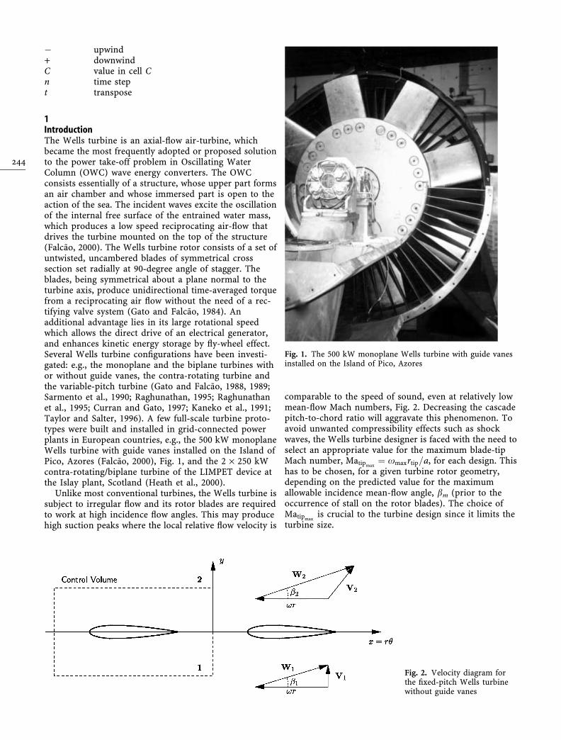
1IntroductionThe Wells turbine is an axial-flow air-turbine, whichbecame the most frequently adopted or proposed solutionto the power take-off problem in Oscillating WaterColumn (OWC) wave energy converters. The OWCconsists essentially of a structure, whose upper part formsan air chamber and whose immersed part is open to theaction of the sea. The incident waves excite the oscillationof the internal free surface of the entrained water mass,which produces a low speed reciprocating air-flow thatdrives the turbine mounted on the top of the structure(Falcao, 2000). The Wells turbine rotor consists of a set ofuntwisted, uncambered blades of symmetrical crosssection set radially at 90-degree angle of stagger. Theblades, being symmetrical about a plane normal to theturbine axis, produce unidirectional time-averaged torquefrom a reciprocating air flow without the need of a rec-tifying valve system (Gato and Falcao, 1984). Anadditional advantage lies in its large rotational speedwhich allows the direct drive of an electrical generator,and enhances kinetic energy storage by fly-wheel effect.Several Wells turbine configurations have been investi-gated: e.g., the monoplane and the biplane turbines withor without guide vanes, the contra-rotating turbine andthe variable-pitch turbine (Gato and Falcao, 1988, 1989;Sarmento et al., 1990; Raghunathan, 1995; Raghunathanet al., 1995; Curran and Gato, 1997; Kaneko et al., 1991;Taylor and Salter, 1996). A few full-scale turbine proto-types were built and installed in grid-connected powerplants in European countries, e.g., the 500 kW monoplaneWells turbine with guide vanes installed on the Island ofPico, Azores (Falcao, 2000), Fig. 1, and the 2 · 250 kWcontra-rotating/biplane turbine of the LIMPET device atthe Islay plant, Scotland (Heath et al., 2000).

Unlike most conventional turbines, the Wells turbine issubject to irregular flow and its rotor blades are requiredto work at high incidence flow angles. This may producehigh suction peaks where the local relative flow velocity is

comparable to the speed of sound, even at relatively lowmean-flow Mach numbers, Fig. 2. Decreasing the cascadepitch-to-chord ratio will aggravate this phenomenon. Toavoid unwanted compressibility effects such as shockwaves, the Wells turbine designer is faced with the need toselect an appropriate value for the maximum blade-tipMach number, Matipmax

¼ xmaxrtip=a, for each design. Thishas to be chosen, for a given turbine rotor geometry,depending on the predicted value for the maximumallowable incidence mean-flow angle, bm (prior to theoccurrence of stall on the rotor blades). The choice ofMatipmax

is crucial to the turbine design since it limits theturbine size.

Fig. 1. The 500 kW monoplane Wells turbine with guide vanesinstalled on the Island of Pico, Azores

Fig. 2. Velocity diagram forthe fixed-pitch Wells turbinewithout guide vanes

244

The present paper describes a numerical study on thecompressibility effects in Wells turbine cascades. Calcu-lations were performed with a numerical code that solvesthe system of Euler equations for two-dimensional flow.The aim of the present study is to investigate the occur-rence of transonic flow in several cascade geometries andblade sections that have been considered in the design ofWells turbine rotor blades. The numerical study assumessteady flow since the reciprocating air-flow frequency, f , ofa wave energy device is very small (<1 Hz) in comparisonwith the characteristic frequency of the blade rotation(Sf =ðxrtipÞ < 10�2) (see Raghunathan, 1995).

Section 2 gives an overview of the occurrence of com-pressibility effects in Wells turbine cascades. It is shownthat the onset of transonic flow in Wells turbine cascadescan be predicted from results from a panel method codeand from gas dynamics relationships for one-dimensionalflow. Section 3 describes a residual distribution schemewhich was applied to a new symmetrized form of the Eulerequations, both in time and in space, that decouples theentropy and the enthalpy equations. Numerical calcula-tions performed with the code developed by the authorsare shown in Sect. 4. Finally, the conclusions are presentedin Sect. 5.

2Compressibility effects in Wells turbine cascadesThe possible occurrence of compressibility effects in Wellsturbine cascades can be qualitatively predicted from theanalysis of the numerical results given by a two-dimensional panel method code for inviscid incompres-sible flow (Gato and Henriques, 1996). Figure 3 shows thepanel method code results for the non-dimensionalchordwise static pressure distribution

Cp ¼ p � pm

p0m � pm; ð1Þ

on a NACA 0015 aerofoil operating as an isolated aerofoil(S=c ! 1) at an angle of attack am ¼ 10, and as element

of 90-degree stagger angle Wells turbine cascades, withpitch-to-chord ratios S/c ¼ 1.5 and 1.25, at a mean-flowincidence angle bm ¼ 10�, Fig. 4. When selecting referenceconditions, it is first necessary to consider whether thecalculation refers to an isolated aerofoil or a cascade ofblades. The subscript m in Eq. (1) denotes the free-streamflow conditions or the mean-cascade flow conditions (seeAppendix B), respectively, for an isolated aerofoil or acascade of blades.

The blade interference effects on a Wells turbine cas-cade can induce a strong increase in the blade load and alarge decrease in pressure at the suction peak, whencompared with the pressure distribution calculated for anisolated aerofoil, at the same angle of attack. The occur-rence of non-negligible compressibility effects, in theWells turbine blade cascades, can be predicted byexpanding in power series the isentropic relation

p0m

pm¼ 1 þ 1

2ðc � 1ÞMa2

m

� � cc�1

; ð2Þ

around Mam ¼ 0, which gives

p0m � pm ¼ 1=2.mW2mwm ; ð3Þ

where

wm ¼ 1 þ 1

4Ma2

m þ 2 � c24

Ma4m

þ ð2 � cÞð3 � 2cÞ192

Ma6m þ O½Ma2

m�4: ð4Þ

Substituting Eq. (3) in Eq. (1), the expression for thesurface pressure coefficient becomes

Cp ¼ 2

cMa2mwm

p

pm� 1

� �: ð5Þ

Applying Eq. (2) twice in Eq. (5), we find the criticalsurface pressure coefficient for sonic conditions (Ma� ¼ 1)at the blade surface as

C�p ¼ 2

cMa2mwm

2 þ ðc � 1ÞMa2m

c þ 1

� � cc�1

� 1

!: ð6Þ

Equation 6 is shown plotted for air (c ¼ 1.4) in Fig. 5. Itmay be observed from Eq. (6) and Fig. 3 that the criticalsurface pressure coefficient is C�

p ¼ �6:8, for a specifiedMach number Mam ¼ 0.3. The results plotted in Fig. 3 forNACA 0015 blade cascades, with S/c ¼ 1.5 and 1.25, at

Fig. 3. Surface pressure distribution of NACA 0015 aerofoils inpotential flow: comparison between an isolated aerofoil at anangle of attack am ¼ 10� and two blade cascades, S/c ¼ 1.5 and1.25, at bm ¼ 10�, for k ¼ 90�

Fig. 4. Vector diagram showing inlet, outlet and mean velocitiesand angles for a turbine cascade in compressible flow

245

bm ¼ 10�, clearly show that transonic flow may occurin high solidity Wells turbine rotor blades even for ratherlow Mam.

3Euler solverA time-marching Euler solver based on a multi-dimensional upwind residual distribution method wasused to compute the steady flow in Wells turbine bladecascades. The motivation behind this method is to extendthe one-dimensional upwind ideas to multiple-spacedimensions without splitting the solution into several one-dimensional Riemann solutions, at the cell faces, as usuallydone in the Finite Volume and the Finite Elementmethods. The original idea was due to Roe (1982, 1994)and was subsequently developed and improved byDeconinck and co-workers (Deconinck et al., 1993;Paillere, 1995; van der Weide, 1998; Issman et al., 1996),Struijs (1994), Sidilkover (1989), Barth and Abgrall(Abgrall and Barth, 2000; Abgrall, 2001). For a review ofthe current state-of-the-art of this method see Deconincket al. (2000), Abgrall (2001) and the references therein.

3.1Euler equationsIn the absence of external body forces and heat sources,the system of Euler equations can be written in the so-called conservative formZZ

CðotU þ oxF þ oyGÞdX ¼ 0 ; ð7Þ

where U ¼ ð.; .Wx; .Wy; .EÞt is the vector of conservativevariables, F ¼ ð.Wx; .W2

x þ p; .WxWy; .WxHÞt andG ¼ ð.Wy; .WxWy; .W2

y þ p; .WyHÞt are the inviscid fluxvectors. The system is closed by using the ideal gas rela-tionship p ¼ .ðc � 1ÞðE � 1

2 W2Þ.Equation (7) can be rewritten in the following quasi-

linear form, which is more suitable to the multi-dimensional upwind method used in the calculations (seeAppendix A for details),

ZZC

otUdX þZZC

MðAAonWW þ BBogWWÞdX ¼ 0 : ð8Þ

Here (n, g) is the streamwise co-ordinate system, where thecomponents of the velocity vector are �uu ¼ W and �vv ¼ 0.The velocity derivative o�vv is in general not null althoughthe velocity component �vv is zero. The new set of variablesis defined as

oWW ¼ �uuo�vv �.�1op ðc � 1ÞTos oH�Tos� �t

: ð9ÞThe matrices AA and BB associated with the spatial terms aregiven by

AA ¼

1 0 0 0

0 Ma2 � 1 0 0

0 0 1 0

0 0 0 1

0BB@

1CCA; BB ¼

0 �1 0 0

�1 0 0 0

0 0 0 0

0 0 0 0

0BB@

1CCA ;

ð10Þand the matrix M is presented in Appendix A.

3.2Residual definitionLet us assume that the computational domain is discret-ized using an unstructured triangular mesh. At each time-step, we integrate the spatial terms of Eq. (8) in every cellC, to obtain the total cell residual

UC ¼ZZC

MðAAonWW þ BBogWWÞdX : ð11Þ

Considering the Roe (1981) linearization, which assumes alinear variation of the parameter vector Z ¼ ffiffiffi

.p ð1;Wx;Wy;

HÞt in each cell, the total cell residual can be evaluated as

UC ¼ MWC ; ð12Þwith

WC ¼X3

i¼1

KiWWi ; ð13Þ

where

Ki ¼1

2ðAAnin þ BBnigÞ

���ZZ; ð14Þ

WWi ¼ ðoWW=oZÞj�zzZi, and �ZZ ¼ 13

P3i¼1 Zi. Here ni ¼ ninenþ

nigeg are the cell inward-scaled normals, as shown inFig. 6a, and the matrix M is evaluated at the meanstate �ZZ.

3.3Multi-dimensional upwind matrix residualdistribution schemesResidual distribution schemes are built to distribute frac-tions, UC

i , of the total residual, UC, to the cell nodes(Deconinck et al., 2000), such that,

UC ¼X3

i¼1

UCi ¼

X3

i¼1

MWCi : ð15Þ

Fig. 5. Critical surface pressure coefficient as function ofmean-flow Mach number

246

All the grid cells contribute with a fraction of the totalresidual to their nodes (see Fig. 6b). Summing up thecontributions from all the surrounding cells C to node i,we get the time variation

Ri ¼XC;i2C

UCi : ð16Þ

After assembling all the local Ri in a global vector R, asusually done in the Finite Element Method, we integrate intime, using a backward Euler scheme, and obtain

1

DtðUnþ1 � UnÞ ¼ �Rnþ1 : ð17Þ

Linearizing the right-hand-side of Eq. (17) in time andintroducing the well-known Courant–Friedrichs–Lewynumber (CFL), produces the following system

1

CFLDtI þ oR

oU

����n� �

DUnþ1 ¼ �Rn ; ð18Þ

where DUnþ1 ¼ Unþ1 � Un. The linearized system is solvedby a standard GM-RES algorithm with ILU(0) precondi-tioning. The time variation derivative is evaluated (in eachcell) using a central difference approximation

oRl;m

oUi;j¼ Rl;mðUi þ eejÞ � Rl;mðUi � eejÞ

2e; ð19Þ

with l; i ¼ 1; . . . ; 3 e m; j ¼ 1; . . . ; 4. The vector ej is givenby the jth column of the identity matrix and e is evaluatedas e ¼ 10�7 maxðjUi � ejj; 10�5Þ. A residual distributionscheme needs to be introduced to solve Eq. (18). Severalmulti-dimensional upwind matrix residual distributionschemes for systems of equations have been proposed inthe literature (Paillere, 1995; van der Weide, 1998; Abgrall,2001). Most of them constitute an extension of earlierschemes that where applied to scalar conservation laws.One of these extensions, due to van der Weide (1998), isthe N (Narrow) matrix scheme, that has the property ofbeing non-oscillatory across discontinuities (Abgrall,2001). When applied to the system (11) it gives

WNi ¼ Kþ

i WWi � WW�� �

; ð20Þ

where WW� ¼ ðP3

j¼1 K�j Þ

�1ðP3

j¼1 K�j WWjÞ. The matrix Ki is

decomposed by means of a similarity transformation,

K�i ¼ 1

2RiðKi � jKijÞLi ; ð21Þ

with Li ¼ R�1i being defined as the set of left eigenvectors

of Ki:For practical applications the N scheme shows excessive

diffusion and it is only 1st order accurate. The simplestlinearity-preserving (2nd order accurate at steady-state)multi-dimensional upwind matrix residual distributionscheme is the LDA (Low Diffusion scheme A) schemedefined in van der Weide (1998) as

WLDAi ¼ Kþ

i ðWWþ � WW

�Þ ; ð22Þwhere WW

þ ¼ ðP3

j¼1 Kþj Þ

�1ðP3

j¼1 Kþj WWjÞ: This scheme is

less dissipative than the N scheme and, as a consequence,the LDA scheme generates spurious oscillations aroundflow discontinuities (see Abgrall, 2001). To overcome thisundesirable behaviour, blended N/LDA schemes wereproposed by Deconinck et al. (2000), Csık et al. (2000) andAbgrall (2001),

WBlendi ¼ ðI � HÞWLDA

i þ HWNi ; ð23Þ

where H is a weighting diagonal matrix. We consider analternative definition of the blended scheme. Let us write theN scheme as being the LDA scheme with the addition of amulti-dimensional upwind artificial viscosity term

WNi ¼ WLDA

i þ WAVi ; ð24Þ

where

WAVi ¼ Kþ

i ðWWi � WWþÞ ; ð25Þ

andP3

i¼1 WAVi ¼ 0: Substituting Eq. (24) in Eq. (23), we

find

WBlendi ¼ WLDA

i þ HWAVi : ð26Þ

Following Deconinck et al. (2000) and Csık et al. (2000), wedefine the blending parameter H as

Hj ¼

��WC��jP3

i¼1

��WLDAi þ WAV

i

��j

: ð27Þ

The jth components of H are bounded by 0 £ Hj £ 1. Atsteady-state, O½Hj� � 1 in the vicinity of discontinuities,whereas in smooth flow regions Hj tends to zero. Nu-merical experiments show that this scheme produces al-most monotonic solutions across discontinuities, althoughthe resulting scheme cannot be proved to be monotonic.Due to the non-linearity introduced in Eq. (27), Hj is notinvariant to a similarity transformation (as the one used toobtain Eq. (32)), i.e., it depends on the choice of variablesused in the nodal residual evaluation Wi.

3.4Boundary conditionsThe boundary conditions for the Euler calculations werebased on the weak formulation that uses a ghost cell ap-proach (Paillere, 1995). The wall boundary condition isimposed by rotating the velocity vector to become tan-gential to the wall, without changing the entropy and the

Fig. 6. a Definition of the cell inward-scaled normals. b Residu-al distribution from the surrounding cells to the node i. Theshaded area is the median dual cell area Wi

247

specific stagnation enthalpy. The inlet conditions are thestagnation pressure and enthalpy, p01 and H1, and the inletflow angle, b1, far upstream from the cascade. The outletcondition is the static pressure, p2, far downstream fromthe blades.

For cascade flow, we define the incidence angle from thedirection of the cascade mean-flow velocity Wm (seeAppendix B). Therefore, we consider the cascade mean-flowangle, bm, and Mach number, Mam, as reference conditions.For compressible flow, these depend on the inflow andoutflow directions, the inlet Mach number, Ma1, and thestagnation pressure ratio p01/p02 (see Appendix B). (Forflow without losses we must have p01/p02 ¼ 1.) The latter arenot explicitly known at starting, since they are an outcomefrom the Euler calculation. In view of this, results from thepanel method code were used to provide an initial guess forthe inlet and the outlet boundary conditions as follows: for agiven cascade geometry and known bm, the panel methodcalculation yields a first estimate of the tangential forcecoefficient, Cx ¼ 2Fx=ðqmW2

mcÞ ¼ CL sin bm; then the inletflow angles b1 and b2 are calculated, as a first approxima-tion, by solving Eqs. (39) and (40) taking qm ¼ q1 ¼ q2.Assuming p01 = p02, the outlet pressure p2 is obtained usingthe isentropic relationships. The calculated values for b1

and p2, together with the prescribed values for p01 and H1,are given as an input to the compressible flow calculation.The Euler results for bm and Mam are then compared withthe initially prescribed values. The values for b1 and p2 arethen adjusted until the convergence criterion is achieved.

4ResultsTwo reference computations are presented to show theaccuracy of the above numerical scheme. The first caseexamined is the well-know transonic flow over an isolatedNACA 0012 aerofoil section, at a free-stream Machnumber Mam ¼ 0.85 and a flow incidence angle bm ¼ 1�.For these conditions, the flow is mainly characterized bythe occurrence of two oblique shock waves emanatingfrom the aerofoil’s suction and pressure surfaces. Thegrids used for the Euler calculations were generated ap-plying an advancing frontal method developed by theauthors. This example uses an unstructured grid consist-ing of 16302 cells and 8316 nodes (251 on the aerofoilsurface), which was defined as a circular domain aroundthe aerofoil, with a diameter of 30 chords. The Machnumber isolines given by the Euler calculation are plottedin Fig. 7a. In Fig. 7b we compare the numerical results forthe Mach number distributions, along the pressure andsuction sides of the aerofoil, with the second-order refer-ence finite-volume solution given in AGARD AR211(1985). The numerical results plotted in Fig. 7b are in goodagreement when analyzing the position and the strength ofthe two shock-waves. The major improvement clearly seenin the residual distribution Euler solution is the shock-wave spread reduction to a maximum of two cells. It maybe observed from Fig. 7a and b that the present blendedscheme (Eq. (26)) produces a seemingly monotone solu-tion when computing the flow discontinuities.

The objective of the second test case is to show therobustness of the numerical scheme by calculating a low-

speed flow. The numerical calculations were performed forthe standard symmetrical NACA 0015 Wells turbine cas-cade. The grid consists of about 28000 cells and 14500nodes (201 on the aerofoil surface), as shown in Fig. 8. Thecomputational domain was extended 6 chords upstreamand 8 chords downstream of the cascade. We considered amean-flow Mach number Mam ¼ 0.01, k ¼ 90� andS/c ¼ 1.79, at an incidence bm ¼ 10�. Table 1 summarizesthe prescribed isentropic flow conditions and the Eulerresults for the cascade flow Mach number, incidence angle,lift coefficient (as given by Eq. (43)), maximum Machnumber at the blade surface and the relative mean stag-nation pressure drop between the inlet and the outlet ofthe computational domain. The results for the blade-sur-face pressure-coefficient distribution from the Euler solverand the panel method are in good agreement, as shown inFig. 9. Small differences between the two sets of results canbe observed at the suction peak and at the trailing edge.This is attributed to the numerical dissipation inherent tothe Euler solver.

Fig. 7. NACA 0012 isolated aerofoil section at Mam ¼ 0.85 andam ¼ 1�. a Mach number contours. Here (–•–) for Ma ¼ 0.8 and(–I–) for Ma ¼ 1.2; increment: 0.05. b Surface Mach numberdistribution (Mamax ¼ 1.435)

248

Numerical calculations were performed for the Wellsturbine cascades considering the standard symmetricalNACA 0012 and 0015 aerofoils and the optimized 15%relative-thickness HSIM 15-459932-1323 symmetrical sec-tion (Gato and Henriques, 1996; Henriques and Gato,1998). The grids used in the computations are similar tothat of the previous example. The prescribed isentropicflow conditions and the Euler results for the present cal-culations are also summarized in Table 1. Results shownin Figs. 10–13 were calculated for the reference conditionsk ¼ 90�, S/c ¼ 1.79, bm ¼ 10� and Mam ¼ 0.32. The plottedresults from the Euler calculations are the Mach numberand the pressure coefficient distributions at the bladesurface. For comparison, we also present the correspond-ing pressure coefficient distributions given by the panelmethod.

The Mach number distributions clearly show a regionaround the suction peak where supersonic flow occurs. Ascan be seen from Figs. 10 and 12, thicker (larger leadingedge radius) NACA Four-digit sections produce smallersuction peaks and, consequently, the results show lowervalues of the maximum Mach number than the corre-sponding thinner sections. Results in Fig. 10a show ashock-wave downstream of the suction peak for the NACA

0012 section, whereas Fig. 12a presents shock-free flow forthe NACA 0015 section, at the same mean-flow conditions.To illustrate the flow pattern, the Mach number isolinesare plotted in Fig. 11 for the NACA 0015 section. Thedistortion of the isolines shows the presence of the bladewake across the periodic boundary.

Comparing the results represented in Figs. 12 and 13,we notice that the HSIM section has lower pressure gra-dients in the vicinity of the suction peak than the corre-sponding NACA 0015 section, due to its larger leadingedge radius. Furthermore, non-negligible compressibilityeffects are seen in Figs. 12b and 13b, as given by the de-viation of the suction-surface pressure distributions fromthe Euler solver compared with the panel method results.To exemplify the effect of decreasing the cascade pitch-to-chord ratio, calculations were also performed for a NACA0015 cascade of blades with k ¼ 90�, S/c ¼ 1.5, bm ¼ 10�and Mam ¼ 0.32. The numerical results show an increasein the blade load that originates a shock-wave downstreamof the suction peak, Figs. 12 and 14.

5ConclusionsResults from a panel method code and from gas dynamicsrelationships for one-dimensional flow indicated thattransonic flow could occur in Wells turbine cascades atlow mean-flow Mach numbers.

A two-dimensional implicit Euler solver incorporatinga compact multi-dimensional upwind matrix residualdistribution scheme was successfully applied to the studyof transonic flow through Wells turbine blade cascades.

Fig. 8. Zoom-in of the grid used for the NACA 0015 cascade ofblades with k ¼ 90� and S/c ¼ 1.79

Table 1. Prescribed isentropicflow conditions (b1,isent,Ma2,isent) and Euler results forthe cascade flow properties, liftcoefficient and maximumMach number

Bladesection

S/c b1,isent Ma2,isent Ma1 Ma2 Mamax Mam bm CL 1 � �pp02=�pp01

0015 1.79 13.3� 0.012 0.008 0.012 0.03 0.010 10.2� 1.72 2.2 · 10)6

0012 1.79 13.2� 0.413 0.249 0.405 1.55 0.321 10.4� 1.83 4.2 · 10)3

0015 1.79 13.3� 0.417 0.240 0.412 1.17 0.321 10.2� 1.96 2.4 · 10)3

HSIM 1.79 13.4� 0.417 0.239 0.413 1.18 0.320 10.2� 1.99 2.4 · 10)3

0015 1.50 16.0� 0.472 0.202 0.462 1.46 0.319 10.5� 3.08 6.4 · 10)3

Fig. 9. Surface pressure distribution for NACA 0015 cascade ofblades with k ¼ 90�, S/c ¼ 1.79 at bm ¼ 10.2� and Mam ¼ 0.01

249

This study confirmed that transonic flow may occur inWells turbine cascades at high incidence angles, for rela-tively low mean-flow Mach numbers. Under such condi-tions, supersonic flow and shock-waves were detected in aregion around the suction peak. Decreasing the cascadepitch-to-chord ratio may aggravate this undesired com-pressibility effect.

The numerical results also demonstrate that the oc-currence of supersonic flow is strongly related to the bladesection geometry, the pitch-to-chord ratio, incidence angleand mean-flow Mach number.

Appendix AThe system of the Euler equations written in the set ofprimitive variables, o~VV, can be symmetrized by changingthe co-ordinate system from the Cartesian (x, y) to the so-called streamwise co-ordinate system (n, g) (van Leer et al.,1992; Paillere, 1995), which gives

ot�UU þ �AAon�UU þ �BBog�UU ¼ 0 : ð28Þ

We define the set of variables, o�UU, as

o�UU ¼ o�UU

o~VVo~VV ¼ .�1op ao�uu ao�vv .�1ðop � a2o.Þ

� �t;

ð29Þ

Fig. 10. NACA 0012 cascade of blades with k ¼ 90�, S/c ¼ 1.79 atbm ¼ 10.4� and Mam ¼ 0.32. a Surface Mach number distribution(Mamax ¼ 1.55). b Surface pressure distribution

Fig. 11. Mach number contours for the NACA 0012 cascade ofblades with k ¼ 90�, S/c ¼ 1.79 at bm ¼ 10.4� and Mam ¼ 0.32.Here (–•–) for Ma ¼ 0.25 and (–I–) for Ma ¼ 0.45; increment: 0.05

Fig. 12. NACA 0015 cascade of blades with k ¼ 90�, S/c ¼ 1.79 atbm ¼ 10.2� and Mam ¼ 0.32. a Surface Mach number distribution(Mamax ¼ 1.17). b Surface pressure distribution

250

with

o�UU

o~VV¼

0 0 0 .�1

0 a cos d a sin d 0

0 �a sin d a cos d 0

�a2.�1 0 0 .�1

0BBB@

1CCCA : ð30Þ

Multiplying both sides of Eq. (28) by the matrix

�PP ¼ W�1

Ma2 �Ma 0 0

�Ma 2 0 0

0 0 1 0

0 0 0 1

0BBB@

1CCCA ; ð31Þ

and applying the change of variables given by the left set ofeigenvectors, oWW=o~UU; of �PP�AA, we obtain

PPotWW þ AAonWW þ BBogWW ¼ 0 ; ð32Þwhere AA and BB are given by Eq. (10) and

PP ¼ W�1

1 0 0 0

0 Ma2 þ 1 0 1

0 0 1 0

0 1 0 1

0BB@

1CCA : ð33Þ

The matrix M, that relates Eq. (32) to the differential formof Eq. (8), is given by

M ¼ oU

oWWPP�1 ¼ oU

o~VV

o~VV

o�UU

o�UU

oWWPP�1

: ð34Þ

The derivation criterion of the matrix PP (31) was tosymmetrize the system of equations (32), both in time andin space, and, simultaneously, to decouple the entropy andthe enthalpy equations. As a result of using Eq. (32), thematrices Ki (14) are diagonal for the variables (oWW3; oWW4)and, consequently, the enthalpy and the entropy are bothconvected along stream lines by the numerical scheme.Comparing with the hyperbolic/elliptic splitting of Paillere(1995), we do not decouple the acoustic sub-system forsupersonic flow, but we obtain a symmetric positive-defi-nite matrix for the time term. We note that the matrix PP(31) is not used as a local pre-conditioner (van Leer et al.,1992; Paillere, 1995; van der Weide, 1998) and it is notsingular at the sonic point. In order to obtain the samedimensions for all the variables o�UU (29) and oWW (9), thematrix (30) takes a different form from that used by vanLeer et al. (1992).

Fig. 13. HSIM 15-459932-1323 cascade of blades with k ¼ 90�,S/c ¼ 1.79 at bm ¼ 10.2� and Mam ¼ 0.32. a Surface Mach numberdistribution (Mamax ¼ 1.18). b Surface pressure distribution

Fig. 14. High-loaded NACA 0015 cascade of blades with k ¼ 90�,S/c ¼ 1.5 at bm ¼ 10.5� and Mam ¼ 0.32. a Surface Mach numberdistribution (Mamax ¼ 1.46). b Surface pressure distribution

251

Appendix BFor a compressible flow calculation we have to distin-guish the density .1, upstream, from .2, downstream ofthe cascade, and from the density .m, for the cascademean-flow conditions. When the fluid passes throughthe cascade, Figs. 2 and 4, its tangential velocity com-ponent experiences a change DWx, in addition to thatof its axial component DWy, for which the continuityequation yields

.1Wy1S ¼ .2Wy2

S ¼ .mWymS : ð35Þ

Applying the momentum equation to the control surfaceshown in Fig. 2, consisting of two periodic lines parallel tothe y-axis, and two lines parallel to the x-axis, far awayupstream and downstream from the cascade, where theflow may be assumed uniform, we obtain the force com-ponents per unit of span exerted by the fluid on the blade,in the axial direction

Fy ¼ Sð.1W2y1� .2W2

y2Þ þ Sðp1 � p2Þ ; ð36Þ

and in the tangential direction

Fx ¼ Sð.1Wy1Wx1

� .2Wy2Wx2

Þ : ð37Þ

As reference conditions, we define the direction of thecascade mean-flow velocity, Wm, from the vectorial meanof the mass fluxes upstream and downstream of the cas-cade,

qmWm ¼ 1

2ðq1W1 þ q2W2Þ : ð38Þ

To satisfy the mass balance, the angle of Wm with thetangential direction, bm (Fig. 4), is calculated fromEq. (35) as

cot bm ¼ 1

2ðcot b1 þ cot b2Þ : ð39Þ

From Eqs. (35) and (37), the blade tangential force coef-ficient Cx ¼ 2Fx=ðqmW2

mcÞ can be written as

Cx ¼ 2S

c

cot b1

q1

� cot b2

q2

� �qm sin2 bm : ð40Þ

To define the reference mean cascade-flow state, we as-sume p01

¼ p0mand relate the mean-flow angle, bm, to the

inlet conditions, 1, using the isentropic relations

.m ¼ cp01

ðc � 1ÞH11 þ ðc � 1Þ

2Ma2

m

� � 1c�1

; ð41Þ

Mam ¼ Ma1 sin b1

sin bm

1 þ 12 ðc � 1ÞMa2

1

1 þ 12 ðc � 1ÞMa2

m

! cþ12ðc�1Þ

: ð42Þ

From Eqs. (36) and (37) , the lift coefficient is given by

CL ¼2ðF2

x þ F2yÞ

12

c.mW2m

: ð43Þ

ReferencesAbgrall R (2001) Toward the ultimate conservative scheme: fol-

lowing the quest. J. Comput. Phys. 167: 277–315Abgrall R, Barth TJ (2000) Residual distribution schemes for

conservation laws via adaptive quadrature. NASA Tech. Rep.NAS-00-016

AGARD AR211 (1985) Test cases for inviscid flow fields methods.AGARD Adv. Rep. No. 211

Csık A, Sterck H, Ricchiuto M, Poedts S, Deconinck H, Roose D(2000) Explicit and implicit parallel upwind monotone re-sidual distribution solver for the time dependent ideal 2D and3D magnetohydrodynamic equations on unstructured grids.Proc. 2nd Int. Conf. Engng. Comput. Tech., Leuven

Curran R, Gato LMC (1997) The energy conversion performanceof several types of Wells turbine designs. Proc. Inst. Mech.Eng. A, 211(A2): 133–145

Falcao AF de O (2000) The shoreline OWC wave power plant atthe Azores. Proc. 4th European Wave Energy Conf. AalborgUniversity, Denmark: 42–48

Deconinck H, Paillere H, Struijs R, Roe P (1993) Multidimen-sional upwind schemes based on fluctuation-splitting forsystems of conservation laws. Comput. Mech. 11(5/6)

Deconinck H, Sermeus K, Abgrall R (2000) Status of multidi-mensional upwind residual distribution schemes and appli-cations in aeronautics. AIAA Paper 2000–2328: 1–19

Gato LMC, Falcao AF de O (1984) On the theory of the Wellsturbine. J. Eng. Gas Turbines Power, 106: 628–633

Gato LMC, Falcao AF de O (1988) Aerodynamics of the Wellsturbine. Int. J. Mech. Sci. 30(6): 383–395

Gato LMC, Falcao AF de O (1989) Aerodynamics of the Wellsturbine: control by swinging rotor blades. Int. J. Mech. Sci.31(6): 425–434

Gato LMC, Henriques JCC (1996) Optimization of symmetricalprofiles for Wells turbine rotor blades. Proc. ASME FluidsEngng. Division Summer Meeting, FED-238(3): 623–630

Heath T, Whittaker TJT, Boake CB (2000) The Design, con-struction and operation of the LIMPET wave energy con-verter (Islay, Scotland). Proc. 4th European Wave EnergyConf. Aalborg University, Denmark: 49–55

Henriques JCC, Gato LMC (1998) Numerical optimization of thesymmetrical blade sections for the variable-pitch turbine. JouleIII Project JOR-CT95-0002 – Variable pitch turbine and high-speed stop-valve, Instituto Superior Tecnico, Lisbon, Portugal

Issman E, Degrez G, Deconinck H (1996) Implicit upwind re-sidual distribution Euler and Navier–Stokes solver on un-structured meshes. AIAA J. 34(10): 2021–2028

Kaneko K, Setoghuchi T, Raghunathan S (1991) Self-rectifyingturbines for wave energy. Int. J. Offshore Polar Eng. 1(2):122–128

Paillere H (1995) Multidimensional upwind residual distributionschemes for the Euler and Navier–Stokes equations on un-structured grids. Ph.D. thesis, Free University of Brussels,Brussels, Belgium

Raghunathan S (1995) The Wells air turbine for wave energyconversion. Prog. Aerospace Sci. 31: 335–386

Raghunathan S, Curran R, Whittaker TJT (1995) Performance ofthe Islay Wells air turbine. Proc. Inst. Mech. Eng. A, 209: 55–62

Roe P (1981) Approximate Riemann solvers, parameter vectors,and difference schemes. J. Comput. Phys. 43: 157–172

Roe P (1982) Fluctuations and signals, a framework for numericalevolution problems. Numer. Meth. Fluid Dynamics AcademicPress: 219–257

Roe P (1994) Multidimensional upwinding – motivation andconcepts. von Karman Institute for Fluid Dynamics LectureSeries 5

Sarmento AJNA, Gato LMC, Falcao AF de O (1990) Turbine-controlled wave energy absorption by oscillating water col-umn devices. Ocean Eng. 17(5): 481–497

252

Sidilkover D (1989) Numerical solution to steady-state problemswith discontinuities. Ph.D. thesis, The Weizmann Institute ofScience, Rehovot, Israel

Struijs R (1994) A multi-dimensional upwind discretizationmethod for the Euler equations on unstructured grids. Ph.D.thesis, The University of Delft, The Netherlands

Taylor JRM, Salter SH (1996) Design and testing of a plano-convex bearing for a variable pitch turbine. Proc. 2nd Euro-pean Wave Power Conf. European Commission: 240–247

van der Weide E (1998) Compressible flow simulation on un-structured grids using multi-dimensional upwind schemes.Ph.D. thesis, Technishe Universiteit Delft, The Netherlands

van Leer B, Lee W, Roe P, Powell K, Tai C (1992) Design ofoptimally smoothing multistage schemes for the Euler equa-tions. Comm. App. Num. Meth. 8: 761–769

253