us ary ehia rp~il9-
TRANSCRIPT
US ARY EHIA RP~IL9-
Roer M. Ebeling
I n2
Destroy this report when no longer needed. Do not returnit to the originator.
The findings in this report ore not to be construec as an officialDepartment of the Army position unless so desiorated
by other authorized documents.
This report is furnished by the Government and is accepted and usedby the recipient with the express understanding that the United StatesGovernment makes no warranties, expressed or implied, concerning theaccuracy, completeness, reliability, usability, or suitability for anyparticular purpose of the information and data contained in this re-
port or furnished in connection therewith, and the United States shall
be under no liability whatsoever to any person by reason of any usemode thereof.
The contents of this report are not to be used foradvertising, publication, or promotional purposes.
Citation of trade names does not constitute anofficial endorsement or approval of the use of
such commercial products.
[ _
REPORT DOCUMENTATION PAGE Form Approved
Publilc repoding bur~den for thin collecion of information it ettimatedl to average I hour por ret'c1W, includilng the time for reviewintg inttrutictont, artlrhing4 emoingl~ dlat wvarlcee.
colklecion of informateoo, ,ncludil. tiugge~ltont for ,edu' this burden. to Washingt•n Hommid nelbtirvices, O .re•O•t• .0 ,f nor nlomatiOn Operations and 1i l
U ai H i gh w ay , Su i t e 1 20 4. A rlin g to n , V A * * 0 130 2 . a n to th e O ffi ce O~ f M a n ag e m in t a n d l u d g t . P a p e r w o r k N 1 d u cion•P r• o l c (0 7 0 4 . 0 i s .W a s h .in g to n , D C 20.0.3 .
1. AGENCY USE ONLY (Leave blank) 2. REPORT DATE J. REPORT TYPE AND DATES COVERED
I November 1992 Final report4. TITLE AND SUBTITLE S. FUNDING NUMBERS
The Seismic Design of Waterfront RetainingStructures
6. AUTHOR(S)
Robert M. Ebeling and Ernest E. Morrison, Jr.7. PERFORMII".G ORGANIZATION NAME(S) AND ADDRESS(ES) 6. PERFORMING ORGANIZATION
REPORT NUMBER
See reverse.Technical ReportITL-92-11NCEL TR-939
9. SPONSORING/MONITORING AGENCY NAME(S) AND ADDRESS(ES) 10. SPONSORING/MONITORINGAGENCY REPORT NUMBER
See reverse.
11. SUPPLEMENTARY NOTES
Available from National Technical Information Service, 5285 Port Royal Road,Springfield, VA 22161.
12a. DISTRIBUTION /AVAILABILITY STATEMENT 12b. DISTRIBUTION CODE
Approved for public release; distribution is unlimited.
13. ABSTRACT (Maximum 200 words)
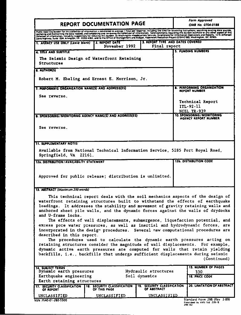
This technical report deals with the soil mechanics aspects of the design ofwaterfront retaining structures built to withstand the effects of earthquakeloadings. It addresses the stability and movement of gravity retaining walls andanchored sheet pile walls, and the dynamic forces against the walls of drydocksand U-frame locks.
The effects of wall displacements, submergence, liquefaction potential, andexcess pore water pressures, as well as inertial and hydrodynamic forces, areincorporated in the desig- procedures. Several new computational procedures aredescribed in this report.
The procedures used to calculate the dynamic earth pressures acting onretaining structures consider the magnitude of wall displacements. For example,dynamic active earth pressures are computed for walls that retain yieldingbackfills, i.e., backfills that undergo sufficient displacements during seismic
(Continued)
14. SUBJECT TERMS 15. NUMBER OF PAGES
Dynamic earth pressures Hydraulic structures 330Earthquake engineering Soil dynamics 16. PRICE CODE
Earth retaining structures
17. SECURITY CLASSIFICATION 18. SECURITY CLASSIFICATION 19. SECURITY CLASSIFICATION 20. LIMITATION OF ABSTRACTOF REPORT OF THIS PAGE OF ABSTRACT
UNCLASSIFIED UNCLASSIFIED UNCLASSIFIEDNSN 7540-01-280-5500 Standard Form 298 (Rev 2-89)
Preicribed by ANSI Std zsg.1e298.102
7. (Concluded).
USAE Waterways Experiment StationInformation Technology Laboratory3909 Halls Ferry Road, Vicksburg, MS 39180-6199
9. (Concluded).
DEPARTMENT OF THE AMYUS Army Corps of EngineersWashington, DC 20314-1000
DEPARTMENT OF THE NAVYNaval Civil Engineering LaboratoryPort Hueneme, CA 93043
13. (Concluded).
events to mobilize fully the shear resistance of the soil. For smaller wallmovements, the shear resistance of the soil is not fully mobilized and the dynamicearth pressures acting on those walls are greater because the soil comprising thebackfill does not yield, i.e., a nonyielding backfill. Procedures forincorporating the effects of submergence within the earth pressure computations,including consideration of excess pore water pressures, are described.
PREFACE
This report describes procedures used in the seismic design ofwaterfront retaining structures, Funding for the preparation of this reportwas provided by the US Naval Civil Engineering Laboratory through the follow-ing instruments: NAVCOMPT Form N6830591WR00011, dated 24 October 1990; Amend-ment #1 to that form, dated 30 November 1990; NAVCOMPT Form N6830592WROO013,dated 10 October 1991; Amendment #1 to the latter, dated 3 February 1992; andthe Computer-Aided Structural Engineering Program sponsored by the Director-ate, Headquarters, US Army Corps of Engineers (HQUSACE), under the StructuralEngineering Research Program. Supplemental support was also provided by theUS Army Civil Works Guidance Update Program toward cooperative production ofgeotechnical eeismic design guidance for the Corps of Engineers. Generalproject management was provided by Dr. Mary Ellen Hynes and Dr. Joseph P.Koester, both of the Earthquake Engineering and Seismology Branch (EESB),Earthquake Engineering and Geosciences Division (EEGD), Geotechnical Labora-tory (GL), under the general supervision of Dr. William F. Marcuson III,Director, GL. Mr. John Ferritto of the Naval Civil Engineering Laboratory,Port Hueneme, CA, was the Project Monitor.
The work was performed at the US Army Engineer Waterways ExperimentStation (WES) by Dr. Robert M. Ebeling and Mr. Ernest E. Morrison,Interdisciplinary Research Group, Computer-Aided Engineering Division (CAED),Information Technology Laboratory (ITL). This report was prepared byDr. Ebeling and Mr. Morrison with contributions provided by Professor RobertV. Whitman of Massachusetts Institute of Technology and Professor W. D. LiamFinn of University of British Columbia. Review commentary was also providedby Dr. Paul F. Hadala, Assistant Director, GL, Professor William P. Dawkins ofOklahoma State University, Dr. John Christian of Stone & Webster EngineeringCorporation, and Professor Raymond B. Seed of University of California,Berkeley. The work was accomplished under the general direction of Dr. ReedL. Mosher, Acting Chief, CAED and the general supervision of Dr. N.Radhakrishnan, Director, ITL.
At the time of publication of this report, Director of WES wasDr. Robert W. Whalin. Commander was COL Leonard G. Hassell, EN.
LAooesson For
NTIS CRA&IDTIC TAB [1Uuannounced 0Just ir t ation.
SuWJX, Distrjbut1iou/
Availability Codes
Avail jj/r.'Dist Speoola
93-06471 5,93lo 022 iEIllI0E1111nIlEE1Il11
PROCEDURAL SUMMARY
This section summarizes the computational procedures described in this reportto compute dynamic earth pressures. The procedures for computing dynamicearth pressures are grouped according to the expected displacement of thebackfill and wail during seismic events. A yielding backfill displacessufficiently (refer to the values given in Table 1, Chapter 2) to mobilizefully the shear resistance of the soil, with either dynamic active earth pres-sures or dynamic passive earth pressures acting on the wall, depending uponthe direction of wall movement. When the displacement of the backfill (andwall) is less than one-fourth to one-half of the Table 1 values, the term non-yielding backfill is used because the shear strength of the soil is not fullymobilized.
The procedures for computing dynamic active and passive earth pressuresfor a wall retaining a dry yielding backfill or a submerged yielding backfillare discussed in detail in Chapter 4 and summarized in Table i and Table ii,respectively. The procedures for computing dynamic earth pressures for a wallretaining a non-yielding backfill are discussed in Chapter 5 and summarized inTable i.
The assignment of the seismic coefficient in the design procedures forwalls retaining yielding backfills are discussed in detail in Chapter 6 andsummariz3d in Table iii. The assignment of the seismic coefficient in thedesign procedures for walls retaining non-yielding backfills are discussed indetail in Chapter 8 and summarized in Table iii.
ii
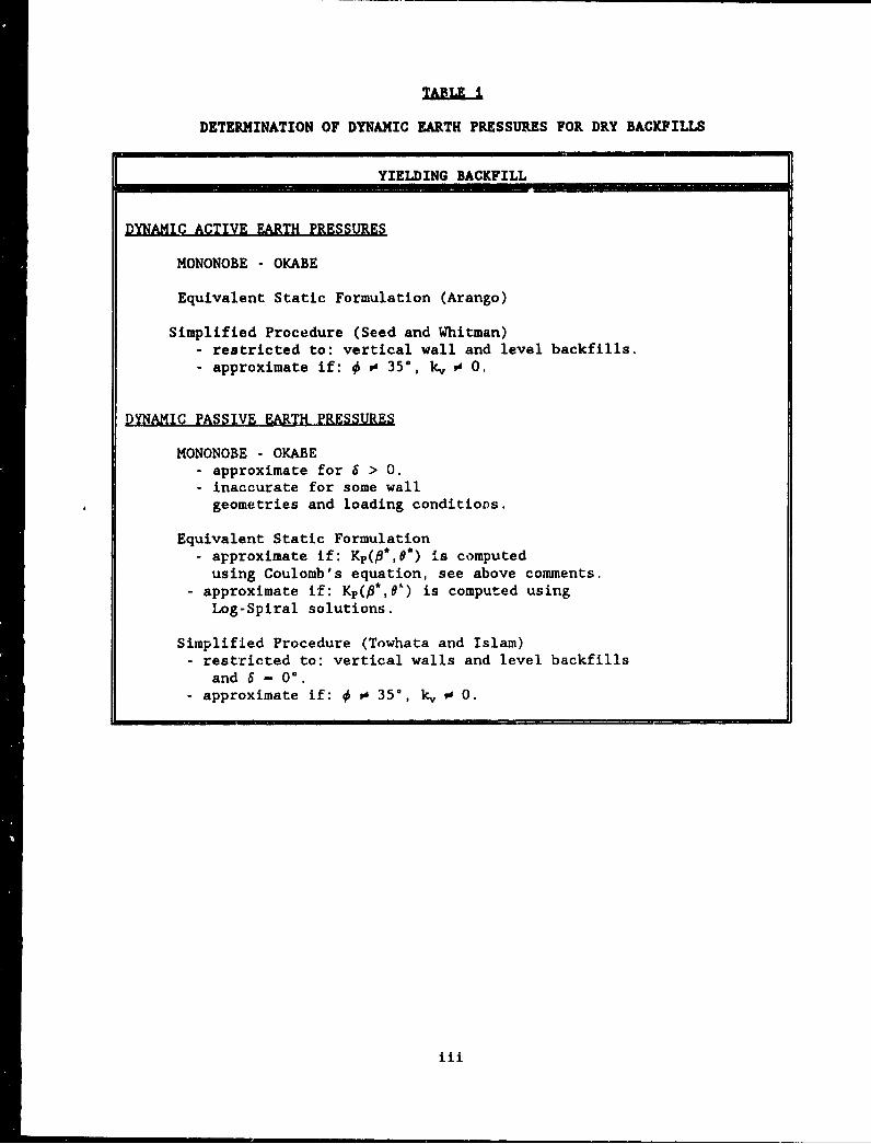
DETERMINATION OF DYNAMIC EARTH PRESSURES FOR DRY BACKFILLS
YIELDING BACKFILL
DYNAMIC ACTIVE EARTH PRESSURES
MONONOBE - OKABE
Equivalent Static Formulation (Arango)
Simplified Procedure (Seed and Whitman)- restricted to: vertical wall and level backfills.- approximate if: 0 o 350, k, o 0.
DYNAMIC PASSIVE EARTH PRESSURES
MONONOBE - OKABE- approximate for 6 > 0.- inaccurate for some wall
geometries and loading conditions.
Equivalent Static Formulationapproximate if: Kp(#*,e*) is computedusing Coulomb's equation, see above comments.
approximate if: Kp(fi*,0•) is computed usingLog-Spiral solutions.
Simplified Procedure (Towhata and Islam)- restricted to: vertical walls and level backfills
and 6 - 0'.- approximate if: 0 o 350, k, o 0.
iii
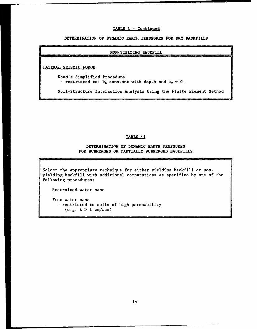
TABLE I - Continued
DETERMINATION OF DYNAMIC EARTH PRESSURES FOR DRY BACKFILLS
NON-YIELDING BACKFILL
ZATERAL SEISMIC FORCE
Wood's Simplified Procedure- restricted to: kh constant with depth and k, - 0.
Soil-Structure Interaction Analysis Using the Finite Element Method
TABLE ii
DETERMINATION OF DYNAMIC EARTH PRESSURESFOR SUBMERGED OR PARTIALLY SUBMERGED BACKFILLS
Select the appropriate technique for either yielding backfill or non-yielding backfill with additional computations as specified by one of thefollowing procedures:
Restrained water case
Free water case- restricted to soils of high permeability
(e.g. k > 1 cm/sec)
iv
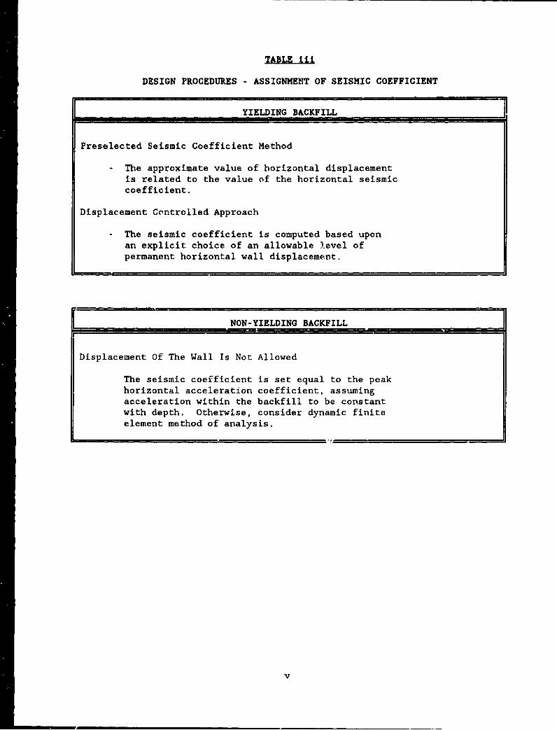
TABLE Ii±
DESIGN PROCEDURES - ASSIGNMENT OF SEISMIC COEFFICIENT
YIELDING BACKFILL
Preselected Seismic Coefficient Method
- The approximate value of horizontal displacementis related to the value of the horizontal seismiccoefficient.
Displacement Controlled Approach
The seismic coefficient is computed based uponan explicit choice of an allowable level ofpermanent horizontal wall displacement.
NON-YIELDING BACKFILL
Displacement Of The Wall Is Not Allowed
The seismic coefficient is set equal to the peakhorizontal acceleration coefficient, assumingacceleration within the backfill to be constantwith depth. Otherwise, consider dynamic finiteelement method of analysis.
v
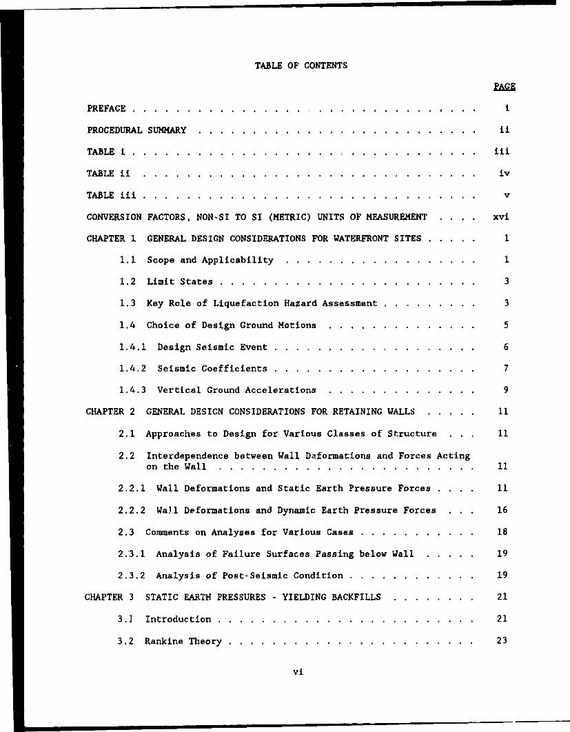
TABLE OF CONTENTS
PREFACE .......................... . ............................... i
PROCEDURAL SUMMARY ................... ............................ ii
TABLE i .. ...................... ...................... .. .. .. . .....
TABLE ii ........................ ............................... ... iv
TABLE iii .......................... ............................... v
CONVERSION FACTORS, NON-SI TO SI (METRIC) UNITS OF MEASUREMENT . . .. xvi
CHAPTER 1 GENERAL DESIGN CONSIDERATIONS FOR WATERFRONT SITES ... ..... 1
1.1 Scope and Applicability .............. .................. 1
1.2 Limit States ..................... ........................ 3
1.3 Key Role of Liquefaction Hazard Assessment.............. 3
1.4 Choice of Design Ground Motions ............ .............. 5
1.4.1 Design Seismic Event ............... ................... 6
1.4.2 Seismic Coefficients ............... ................... 7
1.4.3 Vertical Ground Accelerations ............ .............. 9
CHAPTER 2 GENERAL DESIGN CONSIDERATIONS FOR RETAINING WALLS ..... . 11
2.1 Approaches to Design for Various Classes of Structure . . . 11
2.2 Interdependence between Wall Daformations and Forces Actingon the Wall ................ ........................ ... 11
2.2.1 Wall Deformations and Static Earth Pressure Forces . . .. 11
2.2.2 Wall Deformations and Dynamic Earth Pressure Forces . . 16
2.3 Comments on Analyses for Various Cases ... ........... ... 18
2.3.1 Analysis of Failure Surfaces Passing below Wall ...... 19
2.3.2 Analysis of Post-Seismic Condition .... ............ ... 19
CHAPTER 3 STATIC EARTH PRESSURES - YIELDING BACKFILLS ... ........ .. 21
3.1 Introduction ............... ........................ ... 21
3.2 Rankine Theory ............. ....................... .... 23
vi
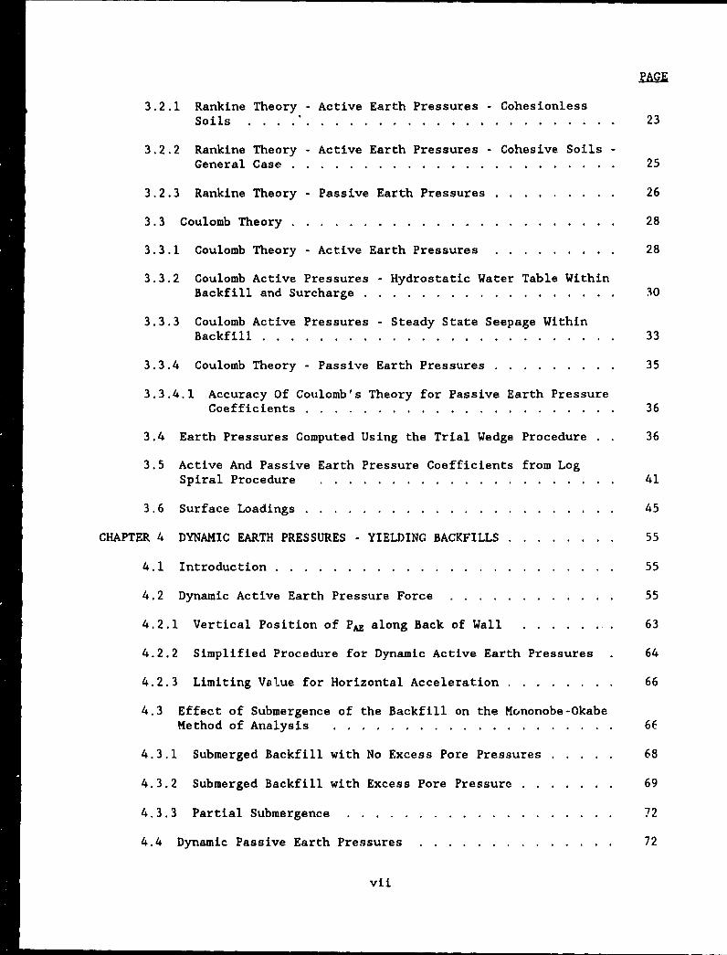
EAUE
3.2.1 Rankine Theory - Active Earth Pressures - CohesionlessSoils ...... . ............. ...................... .... 23
3.2.2 Rankine Theory - Active Earth Pressures - Cohesive Soils -
General Case ............. ....................... .... 25
3.2.3 Rankine Theory - Passive Earth Pressures ... ......... ... 26
3.3 Coulomb Theory ............. ....................... .... 28
3.3.1 Coulomb Theory - Active Earth Pressures .. ......... ... 28
3.3.2 Coulomb Active Pressures - Hydrostatic Water Table WithinBackfill and Surcharge ........... .................. ... 30
3.3.3 Coulomb Active Pressures - Steady State Seepage WithinBackfill ............... ......................... .... 33
3.3.4 Coulomb Theory - Passive Earth Pressures ... ......... ... 35
3.3.4.1 Accuracy Of Coulomb's Theory for Passive Earth Pressure
Coefficients ............. ...................... ... 36
3.4 Earth Pressures Computed Using the Trial Wedge Procedure 36
3.5 Active And Passive Earth Pressure Coefficients from LogSpiral Procedure ............. ..................... ... 41
3.6 Surface Loadings ............. ...................... ... 45
CHAPTER 4 DYNAMIC EARTH PRESSURES - YIELDING BACKFILLS .......... ... 55
4.1 Introduction ............... ........................ ... 55
4.2 Dynamic Active Earth Pressure Force .... ............ .. 55
4.2.1 Vertical Position of PAE along Back of Wall ......... 63
4.2.2 Simplified Procedure for Dynamic Active Earth Pressures 64
4.2.3 Limiting Value for Horizontal Acceleration .......... ... 66
4.3 Effect of Submergence of the Backfill on the Mononobe-OkabeMethod of Analysis .................. .................... 6E
4.3.1 Submerged Backfill with No Excess Pore Pressures ..... ... 68
4.3.2 Submerged Backfill with Excess Pore Pressure ......... ... 69
4.3.3 Partial Submergence ................ ................... 72
4.4 Dynamic Passive Earth Pressures ...... .............. .. 72
vii
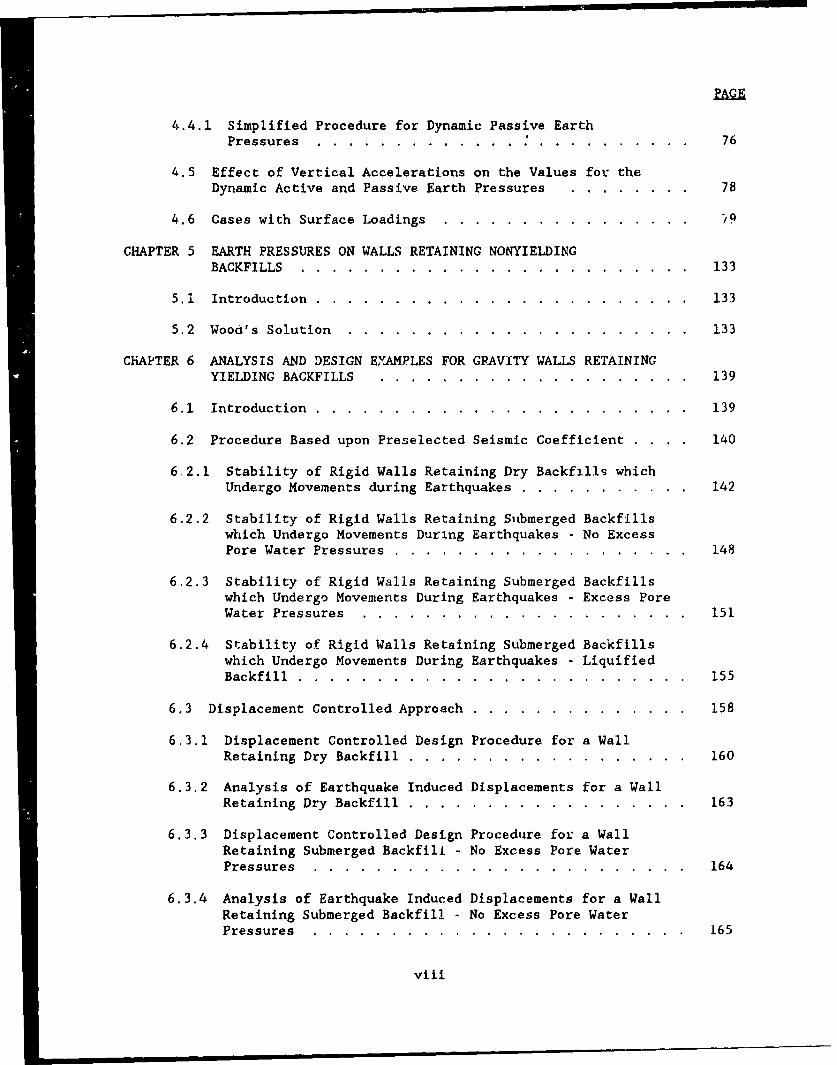
4.4.1 Simplified Procedure for Dynamic Passive EarthPressures . ........ ............................. 76
4.5 Effect of Vertical Accelerations on the Values for theDynamic Active and Passive Earth Pressures .. ........ .. 78
4.6 Cases with Surface Loadings ........... ................ i9
CHAPTER 5 EARTH PRESSURES ON WALLS RETAINING NONYIELDINGBACKFILLS ......... ..... ......................... .... 133
5.1 Introduction ............. ........................ .... 133
5.2 Wood's Solution ..... ....... ...................... ... 133
CHAPTER 6 ANALYSIS AND DESIGN EYAMPLES FOR GPAVITY WALLS RETAININGYIELDING BACKFILLS ........ ......... .................... 139
6.1 Introduction ............. ........................ .... 139
6.2 Procedure Based upon Preselected Seismic Coefficient . . . . 140
6 2.1 Stability of Rigid Walls Retaining Dry Backfills whichUndergo Movements during Earthquakes ...... ........... 142
6.2.2 Stability of Rigid Walls Retaining Submerged Backfillswhich Undergo Movements During Earthquakes - No ExcessPore Water Pressures .......... ................... ... 148
6.2.3 Stability of Rigid Walls Retaining Submerged Backfillswhich Undergo Movements During Earthquakes - Excess PoreWater Pressures ........... ..................... .... 151
6.2.4 Stability of Rigid Walls Retaining Submerged Backfillswhich Undergo Movements During Earthquakes - LiquifiedBackfill .......... ... ......................... .... 155
6.3 Displacement Controlled Approach ..... .............. ... 158
6.3.1 Displacement Controlled Design Procedure for a WallRetaining Dry Backfill ........ .................. ... 160
6.3.2 Analysis of Earthquake Induced Displacements for a WallRetaining Dry Backfill. ....... .................. ... 163
6.3.3 Displacement Controlled Design Procedure for a WallRetaining Submerged Backfill - No Excess Pore WaterPressures ......... ..... ........................ ... 164
6.3.4 Analysis of Earthquake Induced Displacements for a WallRetaining Submerged Backfill - No Excess Pore WaterPressures ......... ..... ........................ ... 165
viii
6.3.5 Displacement Controlled Design Procedure for a WallRetaining Submerged Backfill - Excess Pore WaterPressures .................. ........................ ... 166
6.3.6 Analysis of Earthquake Induced Displacements for a WallRetaining Submerged Backfill - Excess Pore WaterPressures .................. ........................ ... 167
CHAPTER 7 ANALYSIS AND DESIGN OF ANCHOPED SHEET PILE WALLS .... ...... 203
7.1 Introduction ............... ........................ ... 203
7.2 Background ................. ......................... ... 204
7.2.1 Summary of the Japanese Code for Design of Anchored SheetPile Walls ............... ........................ ... 205
7.2.2 Displacements of Anchored Sheet Files duringEarthquakes ................ ....................... ... 206
7.3 Design of Anchored Sheet Pile Walls - Static Loadings 207
7.4 Design of Anchored Sheet Pile Walls for EarthquakeLoadings ................... ......................... ... 210
7.4.1 Design of Anchored Sheet Pile Walls - No Excess Pore WaterPressures .................. ........................ ... 217
7.4.2 Design of Anchored Sheet Pile Walls - Excess Pore WaterPressures .................. ........................ ... 227
7.5 Use of Finite Element Analyses ....... ............... ... 231
CHAPTER 8 ANALYSIS AND DESIGN OF WALLS RETAINING NONYIELDINGBACKFILLS .................. .......................... ... 233
8.1 Introduction ............... ........................ ... 233
8.2 An Example ................. ......................... ... 234
REFERENCES ....................... ............................. .. 247
APPENDIX A: COMPUTATION OF THE DYNAMIC ACTIVE AND PASSIVE EARTH PRESSUREFORCES FOR PARTIALLY SUBMERGED BACKFILLS USING THE WEDGEMETHOD ...................... .......................... Al
A.1 Introduction .................... ........................ Al
A.2 Active Earth Pressures ............. ................... .
A.2.1 Calculation of Water Pressure Forces for a HydrostaticWater Table .............. ....................... ... A2
ix
A.2.2 Static Water Pressure Forces Acting on the Wedge ..... .. A3
A.2.3 Excess Pore Water Pressures due to Earthquake Shaking withConstant ru .................... ....................... A3
A.2.4 Excess Pore Water Pressure Forces Acting on the wedge . A4
A.2.5 Equilibrium of Vertical Forces ....... .............. ... A4
A.2.6 Equilibrium of Forces in the Horizontal Direction . A5
A.2.7 Surcharge Loading .................. .................... A6
A.2.8 Static Active Wedge Analysis ....... ............... ... A7
A.3 Passive Earth Pressures .......... .................. ... A8
A.3.1 Calculation of Water Pressure Forces for a HydrostaticWater Table .............. ....................... ... A9
A.3.2 Equilibrium of Vertical Forces ....... .............. ... AIO
A.3.3 Equilibrium of Forces in the Horizontal Direction . . .. A1O
A.3.4 Surcharge Loading .............. .................... ... A12
A.3.5 Static Passive Wedge Analysis ............ .............. A13
APPENDIX B: THE WESTERGAARD PROCEDURE FOR COMPUTING HYDRODYNAMICWATER PRESSURES ALONG VERTICAL WALLS DURINGEARTHQUAKES .............. ......................... Bl
B.l The Westergaard Added Mass Procedure .... ............ ... B2
APPENDIX C: DESIGN EXAMPLE FOR AN ANCHORED SHEET PILE WALL .... ...... Cl
C.A Design of An Anchored Sheet Pile Wall For Static Loading . C,.
C.1.1 Active Earth Pressure Coefficients KA ...... .......... Cl
C.1.2 "Factored" Passive Earth Pressure Coefficient K. ........ C2
C.1.3 Depth of Penetration ......... ................... .... C2
C.1.4 Tie Rod Force TFES ................. .................... C5
C.1.5 Maxi.,uum Moment MFES .................................... C6
C.1.6 Design Moment Mdesign .................................... C7
X
C.1.7 Selection of the Sheet Pile Section ........ ........... C8
C.1.8 Design Tie Rod ............. ...................... ... C8
C.1.9 Design Anchorage ........... ..................... .... C9
C.1.10 Site Anchorage ................. ..................... Cli
C.2 Design of An Anchored Sheet Pile Wall for SeismicLoading ................... .......................... .. C12
C.2.1 Static Design (Step 1) ........... .................. .. C12
C.2.2 Horizontal Seismic Coefficient, kb (Step 2) .. ....... .. C12
C.2.3 Vertical Seismic Coefficient, k, (Step 3) .. ........ ... C12
C.2.4 Depth of Penetration (Steps 4 to 6) .... ............. C12
C.2.5 Tie Rod Force TIs (Step 7) ......... ................ C18
C.2.6 Maximum Moment MFIs (Step 8) ........ ................. C19
C.2.7 Design Moment Md.,j& (Step 9) ......... ............... C21
C.2.8 Design Tie Rods (Step 10) .......... ................. C23
C.2.9 Design of Anchorage (Step 11) ...... ................ C24
C.2.10 Size Anchor Wall (Step 12) ........ ................. C24
C.2.11 Site Anchorage (Step 13) .......... ................. C27
APPENDIX D: COMPUTER-BASED NUMERICAL ANALYSES .......... ............ Dl
D.i Some Key References ............ .................... ... D2
D.2 Principal Issues ............. ..................... ... D2
D.2.1 Total Versus Effective Stress Analysis ... .......... ... D3
D.2.2 Modeling Versus Nonlinear Behavior .... ............ ... D3
D.2.3 Time Versus Frequency Domain Analysis ... .......... .. D3
D.2.4 1-D Versus 2-D Versus 3-D ........ ................ ... D4
D.2.5 Nature of Input Ground Motion ...... .............. ... D4
D.2.6 Effect of Free Water ......... ................... .... D4
D.3 A Final Perspective ............ .................... ... D4
APPENDIX E: NOTATION .................... ......................... El
xi
LIST OF TABLES
No. A
1 Approximate Magnitudes of Movements Required to Reach MinimumActive and Maximum Passive Earth Pressure Conditions ...... 16
2 Ultimate Friction Factors for Dissimilar Materials ....... ... 313 Valves of KA and K. for Log-Spiral Failure Surface .. ....... .. 444 Section Numbers That Outline Each of the Two Design Procedures
for Yielding Walls for the Four Categories of RetainingWalls Identified in Figure 6.1 ............. ................ 142
5 Minimum Factors of Safety When Using the Preselected SeismicCoefficient Method of Analysis ............. ................ 143
6 Qualitative and Quantitative Description of the ReportedDegrees of Damage ............ ....................... .... 207
7 Ten Stages of the Analyses in the Design of Anchored Wallsfor Seismic Loadings ............. ..................... ... 218
C.1 Horizontal Force Components ........ ................... .... C3C.2 Moments About Tie Rod Due to Active Earth Pressures ......... ... C4C.3 Moments About Tie Rod Due to Passive Earth Pressures ...... .. C4C.4 Calculation of the Depth of Penetration ........ ............. C5C.5 Horizontal Force Components for D - 10 Feet ... ........... ... C5C.6 Moment Internal to the Sheet Pile at y - 12.79 Feet Below
the Water Table and About the Elevation of the Tie Rod .... C6C.7 Design Moment for Sheet Pile Wall in Dense Sand ..... ......... C7C.8 Allowable Bending Moment for Four ASTM A328 Grade Sheet Pile
Sections (a,1oabI.l - 0.65 . ayi.ed) ......... .... .............. C8C.9 Five Horizontal Static Active Earth Pressure Force Components
of PA with D - 20.24 Feet .......... .................. ... C14C.10 Summary of Depth of Penetratioa Calculations ... ............ C18C.11 Tie Rod Force TFES ................... ... ....................... C19C.12 Moment of Forces Acting Above y - 15.32 Feet Below the Water
Table and About the Tie Rod .......... .................... C21C.13 Design Moment for Sheet Pile Wall in Dense Sand ... ......... ... C22C.14 Allowable Bending Moment for Four ASTM A328 Grade Sheet
Pile Sections (aiowajj..l - 0.9 . oyield) ... ............ C22C.15 Required Geometry of Tie Rod ........... .................. ... C23D.1 Partial Listing of Computer-Based Codes for Dynamic Analysis
of Soil Systems .................... ......................... Dl
LIST OF FIGURES
No.
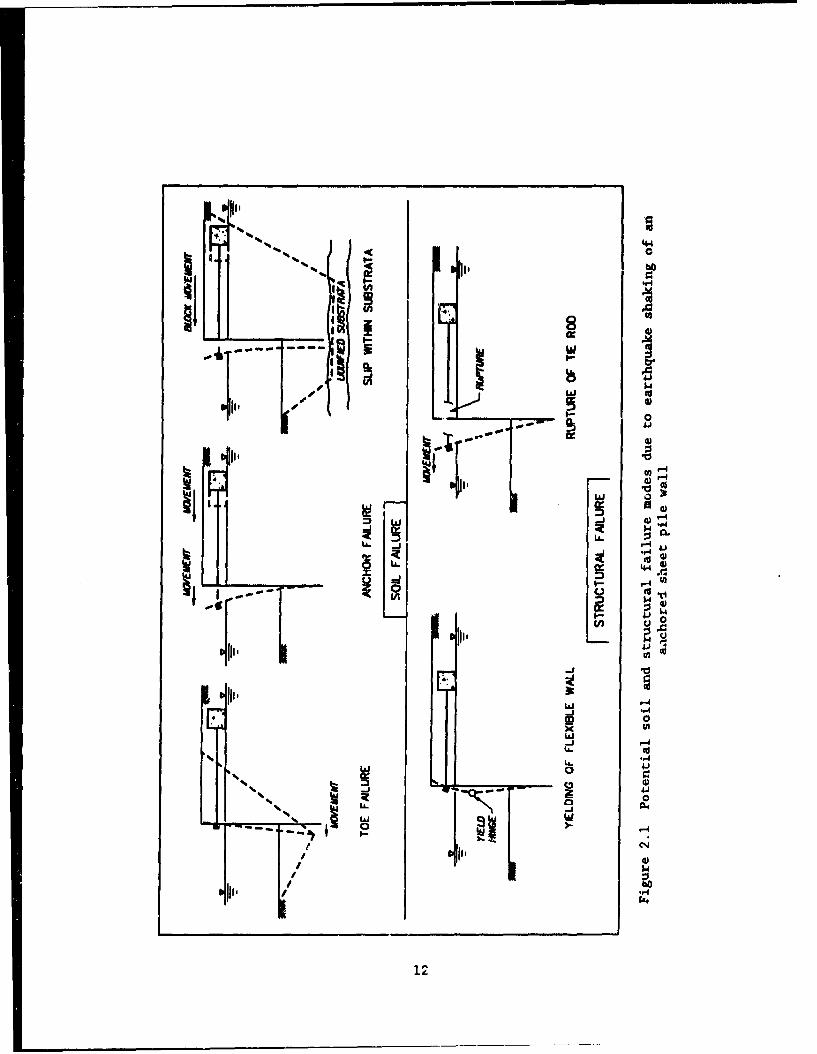
1.1 Overall limit states at waterfronts .......... ............... 42.1 Potential soil and structural failure modes due to earthquake
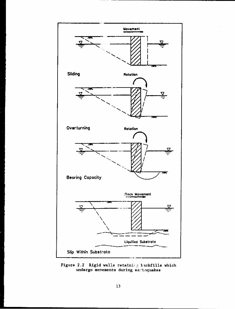
shaking of an anchored sheet pile wall .... ............ .. 122.2 Rigid walls retaining backfills which undergo movements during
earthquakes ................ .......................... .... 132.3 Horizontal pressure components and anchor force acting on
sheet pile wall .............. ......................... .... 142.4 Effect of wall movement on static horizontal earth pressures 15
xii
2.5 Effect of wall movement on static and dynamic horizontal earthpressures ...................... ........................... 17
2.6 Effect of wall movement on static and dynamic horizontalearth pressures ............ ...................... ..... 18
2.7 Failure surface below wall ........ ................... .. 193.1 Three earth pressure theories for active and passive earth
pressures .......................... 223.2 Computation of Rankine active and passive earth pressures for
level backfills ............ ........................ ..... 243.3 Rankine active and passive earth pressures for inclined
backfills .............. . ............................ 263.4 Coulomb active and passive earth pressures for inclined
backfills and inclined walls ...... ................. 293.5 Coulomb active earth pressures for a partially submerged
backfill and a uniform surcharge ...... ............... ... 323.6 Coulomb active earth pressures for a backfill subjected to
steady state flow ............ ....................... .... 343.7 Coulomb and log-spiral passive earth pressure coefficients
with 6-./2 - vertical wall and level backfill ... ......... ... 373.8 Coulomb and log-spiral passive earth pressure coefficients
with 6-0 - vertical wall and level backfill .... .......... 373.9 Example of trial wedge procedure ............. ................ 383.10 Example of trial wedge procedure, hydrostatic water table .. 403.11 Active and passive earth pressure coefficients with wall
friction-sloping wall .......... ..................... .... 423.12 Active and passive earth pressure coefficients with wall
friction-sloping backfill ........ ................... .... 433.13 Theory of elasticity equations for pressures on wall due to
surcharge loads .............. ........................ ... 463.14 Use of an imaginary load to enforce a zero-displacement
condition at the soil-structure interface ... .......... .. 474.1 Driving and resisting seismic wedges, no saturation ......... ... 564.2 Variation in KA and KA .cos 6 with kh .... ............. ... 584.3 Variation in KA.cos 6 with kh, 0, and .... ............ ... 584.4 Variation in aA with 4 for 6 equal to 0/2, vertical wall and
level backfill ............................................ ... 604.5 Variation in aA with 4 for 6 equal to zero degrees, vertical
wall and level backfill .......... .................... ... 604.6 Variation in dynamic active horizontal earth pressure
coefficient with peak horizontal acceleration ... ......... ... 614.7 Equivalent static formulation of the Mononobe-Okobe active
dynamic earth pressure problem ....... ................ ... 624.8 Values of factor FA for determination of KA. ... .......... ... 634.9 Point of action of PA. ........... ..................... .... 654.10 Static active earth pressure force and incremental dynamic
active earth pressure force for dry backfill .. ......... ... 664.11 Limiting values for horizontal acceleration equal to kh . g 674.12 Modified effective friction angle ....... ................ ... 714.13 Effective unit weight for partially submerged backfills ... ..... 734.14 Variation aPE with 4 for 6 equal to 0/2, vertical wall and
level backfill ........................ 754.15 Variation in aPE with i for 6 equal to zero degrees, vertical
wall and level backfill .......... .................... ... 75
xiii
4.16 Equivalent static formulation of the Mononobe-Okabe passivedynamic earth pressure problem ............. ................ 76
4.17 Values of factor FpZ . . .. .. .. .. .. .. .. .. .. . . . . . . . . . . .. . . . . . . . . . . 774.18 Mononobe-Okabe active wedge relationships including surcharge
loading ........................ ............................ 804.19 Static active earth pressure force including surcharge ..... .. 814.20 Static active earth pressure force and incremental dynamic
active earth pressure force including surcharge .......... ... 835.1 Model of elastic backfill behind a rigid wall .... .......... ... 1345.2 Pressure distributions on smooth rigid wall for 1-g static
horizontal body force ............ ..................... ... 1355.3 Resultant force and resultant moment on smooth rigid wall
for 1-g static horizontal body force .... .... ......... ... 1366.1 Rigid walls retaining backfills which undergo movements during
earthquakes .................. .......................... ... 1416.2 Rigid walls retaining dry backfill which undergo movements
during earthquakes ............... ...................... ... 1446.3 Linear and uniform base pressure distributions ... ......... ... 1476.4 Rigid wall retaining submerged backfill which undergo movements
during no excess pore water pressures ..... ............. ... 1506.5 Rigid wall retaining submerged backfill which undergo movements
during earthquakes, including excess pore water pressures . 1536.6 Rigid wall retaining submerged backfill which undergo
movements during earthquakes-liquified backfill ........... ... 1566.7 Gravity retaining wall and failure wedge treated as a sliding
block ........................ ............................. 1596.8 Incremental displacement ............. .................... ... 1596.9 Forces acting on a gravity wall for a limiting acceleration
equal to N*.g ................ ......................... ... 1627.1 Decrease in failure surface slope of the active and passive
sliding wedges with increasing lateral accelerations ..... .. 2077.2 Reduction in bending 'ioments in anchored bulkhead from wall
flexibility .................. .......................... ... 2097.3 Free earth support analysis distribution of earth pressures,
moments and displacamerts, and design moment distributions 2107.4 Two distributions for .inbalanced water pressures .. ........ ... 2117.5 Measured distributions of bending moment in three model tests
on anchored bulkhead ............. ..................... ... 2137.6 Anchored sheet pile walls retaining backfills which undergo
movements during eartaquakes .......... ................. ... 2157.7 Anchored sheet pile wall '-iith no excess pore water pressure due
to earthquake shakin.g ........... ..................... .... 2177.8 Static and inertial horizontal force components of the Mononobe-
Okabe earth pressure ,'orces .............. .................. 2197.9 Distributions of horizontal stresses corresponding to APA . 2227.10 Horizontal pressure co~i ponents and anchor force acting on
sheet pile wall .............. ........................ ... 2227.11 Dynamic forces acting cn an anchor block .... ............ ... 2247.12 Anchored sheet pile wail with excess pore water pressures
generated during earl rýuake shaking ....... .............. ... 2268.1 Simplified procedure fo I-vnamic analysis of a wall
retaining nonyieldirng ba~kfill .......... ................ ... 2328.2 Linear and uniform base ptessure distributions ... ......... ... 234
xiv
A.1 Dynamic active wedge analysis with excess pore water pressures AlA.2 Equilibrium of horizontal hydrostatic water pressure forces
acting on backfill wedge ......... ................... ... A3A.3 Dynamic active wedge analysis including a surcharge loading . A7A.4 Dynamic active wedge analysis including a surcharge loading . A8A.5 Dynamic passive wedge analysis with excess pore water
pressure .... ........................... A9A.6 Dynamic passive wedge analysis including a surcharge load . ... A12A.7 Dynamic passive wedge analysis including a surcharge load . ... A13B.1 Hydrostatic and westergeard hydrodynamic water pressures
acting along vertical wall during earthquakes ... ......... ... B2C.1 Anchored sheet pile wall design problem ........ ............. C1C.2 Horizontal earth pressure components in free earth support
design ................... ............................ ... C3C.3 Horizontal active and passive earth pressure components acting
on a continuous slender anchor ............. ................ CloC.4 Design criteria for deadman anchorage ....... ............... ClIC.5 Distribution of horizontal stresses corresponding to APAE . ... C20C.6 Seismic design problem for a continuous anchor blast ..... C24C.7 Simplified procedure for siting a continuous anchor wall . ... C28D.1 Earth retaining structure, soil-structure interaction ...... ... D5
xv
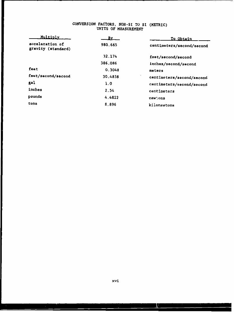
CONVERSION FACTORS, NON-SI TO SI (METRIC)UNITS OF MEASUREMENT
Multiply - By To Obtainacceleration of 980.665 centimeters/second/secondgravity (standard)
32.174 feet/second/second386.086 inches/second/second
feet 0.3048 metersfeet/second/second 30.4838 centimeters/second/secondgal 1.0 centimeters/second/secondinches 2.54 centimeterspounds 4.4822 newtonstons 8.896 kilonewtons
xvi
CHAPTER 1 GENERAL DESIGN CONSIDERATIONS FOR WATERFRONT SITES
1.1 Scope and Applicability
This manual deals with the soil mechanics aspects of the seismic designof waterfront earth retaining structures. Specifically, this reportaddresses:
"* The stability and movement of gravity retaining walls andanchored bulkheads.
"* Dynamic forces against subsurface structures such aswalls of dry docks and U-frame locks.
The report does not address the seismic design of structural frameworks ofbuildings or structures such as docks and cranes. It also does not coDsiderthe behavior or design of piles or pile groups.
The design of waterfront retaining structures against earthquakes isstill an evolving art. Mhe soils behind and beneath such structures often arecohesionless and saturated with a relatively high water table, and hence thereis a strong possibility of pore pressure buildup and associated liquefactionphenomena during strong ground shaking. There have been numerous instances offailure or unsatisfactory performance. However, there has been a lack ofdetailed measurements and observations concerning such failures. There alsoare very few detailed measurements at waterfront structures that have per-formed well during major earthquakes. A small number of model testing pro-grams have filled in some of the blanks in the understanding of dynamic;response of such structures. Theoretical studies have been made, but withvery limited opportunities to check the results of these calculations againstactual, observed behavior. As a result, there are still major gaps in know-ledge concerning proper methods for analysis and design.
The methods set forth in this report are hence based largely uponjudgement. It is the responsibility of the reader to judge the validity ofthese methods, and no responsibility is assumed for the design of any struc-ture based on the methods described herein.
The methods make use primarily of simplified procedures for evaluatingforces and deformations. There is discussion of the use of finite elementmodels, and use of the simpler finite element methods is recommended in somecircumstances. The most sophisticated analyses using finite element codes andcomplex stress-strain relations are useful mainly for understanding patternsof behavior, but quantitativa results from such analyses should be used withconsiderable caution.
This report is divided into eight chapters and five appendixes. Thesubsequent sections in Chapter 1 describe the limit states associated with theseismic stability of waterfront structures during earthquake loadings, the keyrole of liquefaction hazard assessment, and the choice of the design groundmotion(s).
Chapter 2 describes the general design considerations for retainingstructures, identifying the interdependence between wall dejormations andforces acting on the wall. Additional considerations such is failure surfaces
I
passing below the wall, failure of anchoring systems for sheet pile wa].ls, andanalysis of the post-seismic condition are also discussed.
The procedures for calculating static earth pressures acting on wallsretaining yielding backfills are described in Chapter 3. A wall retaining ayielding backfill is defined as a wall with movements greater than or equal tothe values given in Table 1 (Chapter 2). These movements allow the fullmobiliz.cion of the shearing resistance within the backfill. For a wall thatmoves away from t 1'e backfill, active earth pressures act along the soil-wallinterface. In the case of a wall that moves towards the backfill, displacingthe soil, passive earth pressures act along the interface.
Chapter 4 describes the procedures for calculating seismic earth pres-sures acting on walls retaining yielding backfills. The Mononobe-Okabe theoryfor calculating the dynamic active earth pressure force and dynamic passiveearth pressure force is described. Two limiting cases used to incorporate theeffect of submergence of the backfill in the Mononobe-Okabe method of analysisare discussed: (1) the restrained water case and (2) the free water case.These procedures include an approach for incorporating excess pore water pres-sures generated during earthquake shaking within each of the analyses.
The procedures for -alculating dynamic earth pressures acting on wallsretaining nonyielding backfi.lls are described in Chapter 5. A wall retaininga nonyielding backfill is one that does not develop the limiting dynamicactive or passive earth pressures because sufficient wall movements do notoccur and the shear strength of the backfill is not fully mobilized - wallmovements that are less than one-fourth to one-half of Table I (Chapter 2)wall movement values. The simplified analytical procedure due to Wood (1973)and a complete soil-structure interaction analysis using the finite elementmethod are discussed.
The analysis and design of gravity walls retaining yielding backfill aredescribed in Chapter 6. Both the preselected seismic coefficient method ofanalysis and the Richards and Elms (1979) procedure based on displacementcontrol are discussed.
Chapter 7 discusses the analysis and design of anchored sheet pilewalls.
The analysis and design of gravity walls retaining nonyielding backfillusing the Wood (1973) simplified procedure is described in Chapter 8.
Appendix A describes the computation of the dynamic active and passiveearth pressure forces for partially submerged backfills using the wedgemethod.
Appendix B describes the Westergaard procedure for computing hydro-dynamic water pressures along vertical walls during earthquakes.
Appendix C contains a design example of an anchored sheet pile wall.
Appendix D is a brief guide to the several types of finite elementmethods that might be used when considered appropriate.
Appendix E summarizes the notation used in this report.
2
1.2 Limit States
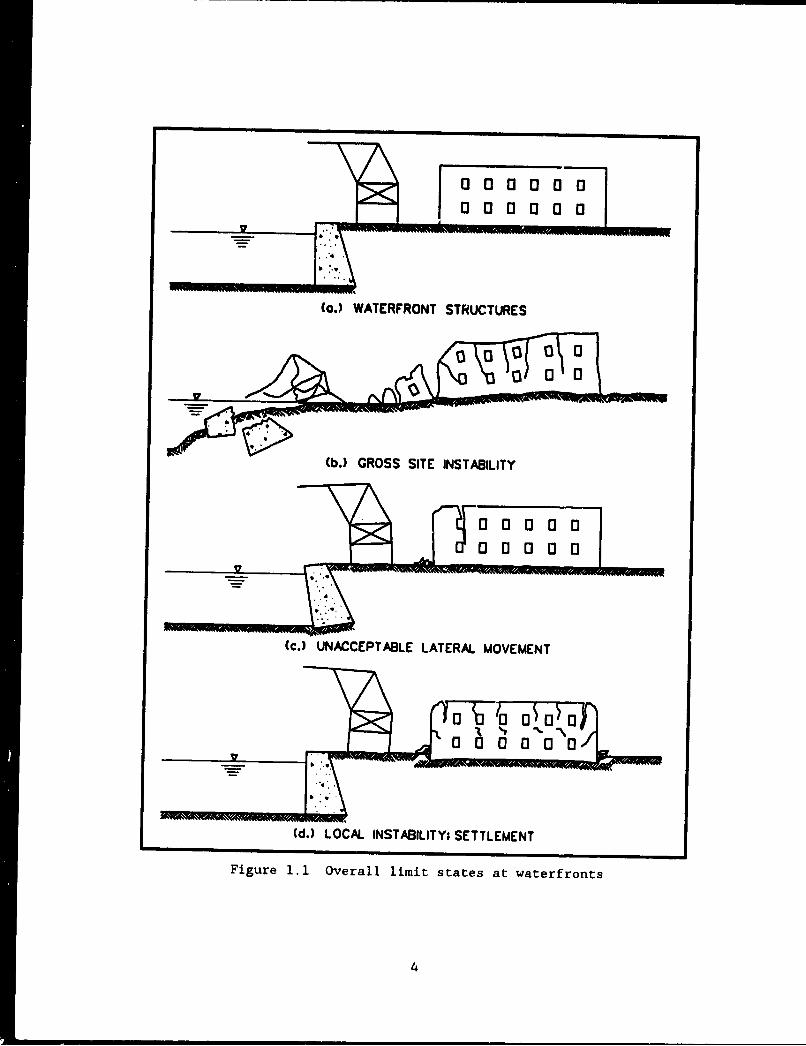
A broad look at the problem of seismic safety of waterfront structuresinvolves the three general limit staces shown in Figure 1.1 which should beconsidered in design.
1) Gross site instability: This limit state involves lateral earthmovements exceeding several feet. Such instability would be the result ofliquefaction of a site, together with failure of an edge retaining structureto hold the liquefied soil mass in place. Liquefaction of backfill is a prob-lem associated with the site, mostly independent of the type of retainingstructure. Failure of the retaining structure might result from overturning,sliding, or a failure surface passing beneath the structure. Any of thesemodes might be triggered by liquefaction of soil beneath or behind the retain-ing structure. There might also be a structural failure, such as failure ofan anchorage which is a common problem if there is liquefaction of thebackfill.
2) Unacceptable movement of retaining structure: Even if a retainingstructure along the waterfront edge of a site remains essentially in place,too much permanent movement of the structure may be the cause of damage tofacilities immediately adjacent to the quay. Facilities of potential concerninclude cranes and crane rails, piping systems, warehouses, or otherbuildings. An earthquake-induced permanent movement of an inch will seldom beof concern. There have been several cases where movements as large as4 inches have not seriously irýerrupted operations or caused material damage,and hence have not been considered failures. The level of tolerable displace-ment is usually specific to the planned installation.
Permanent outward movement of retaining structures may be caused bytilting and/or sliding of massive walls or excessive deformations of anchoredbulkheads. Partial liquefaction of backfill will make such movements morelikely, but this limit state is of concern even if there are no problems withliquefaction.
3) Local instabilities and settlements: If a sice experiences liquefac-tion and yet is contained against major lateral flow, buildings and otherstructures founded at the site may still experience unacceptable damage.Possible modes cf failure include bearing capacity failure, excessive settle-ments, and tearing apart via local lateral spreading. Just the occurrence ofsand boils in buildings can seriously interrupt operations and lead to costlyclean-up operations.
This document addresses the first two of these limit states. The thirdlimit state is discussed in the National Research Council (1985), Seed (1987),and Tokimatsu and Seed (1987).
1.3 Key Role of Liquefaction Hazard Assessment
The foregoing discussion of general limit states has emphasized problemsdue to soil liquefaction. Backfills behind waterfront retaining structuresoften are cohesionless soils, and by their location have relatively high watertables. Cohesionless soils may also exist beneath the base or on the water-side of such structures. Waterfront sites are often developed by hydraulicfilling using cohesionless soils, resulting in low density fills that are
3
(a.) WATERFRONT STRUCTURES
(b.) GROSS SITE INSTABILITY
(c.) UNACCEPTABLE LATERAL. MOVEMENT
(d.) LOCAL. INSTABILITY: SETTLEMENT
Figure 1.1 Overall limit states at waterfronts
4
su3ceptible to liquefaction. Thus, liquefaction may be a problem for build-ings or other structures located well away from the actual waterfront.Hence, evaluation of potential liquefaction should be the first step in analy-sis of any existing or new site, and the first step in establishing criteriafor control of newly-placed fill. Methods for such evaluation are set forthin numerous articles, including the National Research Council (1985) and Seed,Tokimatsu, Harder and Chung (1985).
The word "liquefaction" has been applied to different but relatedphenomena (National Research Council 1985). To some, it implies a flow fail-ure of an earthen mass in the form of slope failure or lateral spreading,bearing capacity failure, etc. Others use the word to connote a number ofphenomena related to the buildup of pore pressures within soil, including theappearance of sand boils and excessive movements of buildings, structures, orslopes. Situations in which there is a loss of shearing resistance, resultingin flow slides or bearing capacity failures clearly are unacceptable. How-ever, some shaking-induced increase in pore pressure may be acceptable, pro-vided it does not lead to excessive movements or settlements.
Application of the procedures set forth in this manual may require eval-uation of: (a) residual strength for use in analyzing for flow or bearingcapacity failure; or (b) buildup of excess pore pressure during shaking. As ageneral design principle, the predicted buildup of excess pore pressure shouldnot exceed 30 to 40 percent of the initial vertical effective stress, exceptin cases where massive walls have been designed to resist larger pore pres-sures and where there are no nearby buildings or other structures that wouldbe damaged by excessive settlements or bearing capacity failures. With veryloose and contractive cohesionless soils, flow failures occur when the resid-ual excess pore pressure ratio reaches about 40 percent (Vasquez and Dobry1988, or Marcuson, Hynes, and Franklin 1990).* Even with soils lesssusceptible to flow failures, the actual level of pore pressure buildupbecomes uncertain and difficult to predict with confidence when the excesspore pressure ratio reaches this level.
Remedial measures for improving seismic stability to resistliquefaction, the buildup of excess pore water pressures, or unacceptablemovements, are beyond the scope of this report. Remedial measures are dis-cussed in numerous publications, including Chapter 5 of the National ResearchCouncil (1985).
1.4 Choice of Design Ground Motions
A key requirement for any analysis for purposes of seismic design is aquantitative specification of the design ground motion. In this connection,
* The word "contractive" reflects the tendency of a soil specimen to decreasein volume during a drained shear test. During undrained shearing of a con-tractive soil specimen, the pore water pressure increases, in excess of thepre-sheared pore water pressure value. "Dilative" soil specimens exhibitthe opposite behavior; an increase in volume during drained shear testingand negative excess pore water pressures during undrained shear testing.Loose sands and dense sands are commonly used as examples ofsoils exhibiting contractive and dilative behavior, respectively, duringshear.
5
it is important to distinguish between the level of ground shaking that astructure or facility is to resist safely and a parameter, generally called aseismic coefficient that i; used as input to a simplified, pseudo-staticanalysis.
1.4.1 Design Seismic Event
Most often a design seismic event is specified by a peak acceleration.However, m3re information concerning the ground motion often is necessary.Duration of shakirg is an important parameter for analysis of liqueiaction.Magnitude is used as an indirect measure of duration. For estimatingpermanent displacements, specification of either peak ground velocity orpredomiuant period of the ground motion is essential. Both duration andpredominant periods are influenced strongly by the magnitude of the causativeearthquake, and hence magnitude sometimes is used as a parameter in analyses.
Unless the design event is prescribed for the site in question, peakaccelerations and peak velocities may be selected using one of the followingapproaches:
(1) By using available maps for the contiguous 48 states. Such maps maybe found in National Earthquake Hazards Reduction Program (1988). Such mapsare available for several different levels of risk, expressed as probabilityof non-exceedance in a stated time interval or mean recurrence interval. Aprobability of non-exceedance of 90 percent in 50 years (mean recurrenceinterval of 475 years) is considered normal for ordinary buildings.
(2) By using attenuation relations giving ground motion as a function ofmagnitude and distance (e.g. attenuation relationships for various tectonicenvironments and site conditions are summarized in Joyner and Boore (1988).This approach requires a specific choice of a magnitude of the causativeearthquake, requiring expertise in engineering seismology. Once this choiceis made, the procedure is essentially deterministic. Generally it is neces-sary to consider various combinations of magnitude and distance.
(3) By a site-specific probabilistic seismic hazard assessment (e.g.National Research Council 1988). Seismic source zones must be identified andcharacterized, and attenuation relations must be chosen. Satisfactory accom-plishment of such an analysis requires considerable expertise and experience,with input from both experienced engincers and seismulogists. This approachrequires selection of a level of risk.
It is of greatest importance to recognize that, for a given site, theground motion description suitable for design of a building may not be appro-priate for analysis of liquefaction.
Local soil conditions: The soil conditions at a site should be con-sidered when selecting the design ground motion. Attenuation relations areavailable for several different types of ground conditions, and hence theanalyses in items (2) and (3) might be made for any of these particular siteconditions. However, attenuation relations applicable to the soft groundconditions often found at waterfront sites are the least reliable. The mapsreferred to under item (1) apply for a specific type of ground condition:soft rock. More recent maps will apply for deep, firm alluvium, afterrevision of the document referenced in item (1). Hence, it generally is nec-
6
essary to make a special analysis to establish the effects of local soil con-ditions.
A site-specific site response otudy is made using one-dimensional analy-ses that model the vertical propagation of shear waves through a column ofsoil. Available models include the computer codes SHAKE (Schnabel, Lysmer,and Seed 1972), DESRA (Lee and Finn 1975, 1978) and CHARSOL (Streeter, Wylie,and Richart 1974). These programs differ in that SHAKE and CHARSOL are for-mulated using the total stress proc'edures, while DESRA is formulated usingboth total and effective stress procedures. All three computer codesincorporate the nonlinear stress-strain response of the soil during shaking intheir analytical formulation, which has been shown to be an essentialrequirement in the dynamic analysis of soil sites.
For any site-specific reaponse study, it first will be necessary todefine the ground motion at the base of the soil column. This will require anestablishment of a peak acceleration for firm ground using one of the threemethods enumerated above, and the selection of several representatives timehistories of motion scaled to the selected peak acceleration. These timehistories must be selected with considerable care, taking into account themagnitude of the causative garthquake and the distance from the epicenter.Procedures for choosing suitable time histories &- set forth in Seed andIdriss (1982), Green (1992), and procedures are also under development by theUS Army Corps of Engineers
If a site response analysis is made, the peak ground motions will ingeneral vary vertically along the soil coliuan. Depending upon the type ofanalysis being made, it may be desirable to average the motions over depth toprovide a single input value. At each depth, the largest motion computed inany of the several analyses using different time histories should be used.
If finite element analyses are made, it will again be necessary toselect several time histories to use as input at the base of the grid, or atime history corresponding to a target spectra (refer to page 54 of Seed andIdriss 1982 or Green 1992).
1.4.2 Seismic Coefficients
A seismic coefficient (typical symbols are kh and k,) is a dimensionlessntunber that, when multiplied times the weight of some body, gives a pseudo-static inertia force for use in analysis and design. The coefficients kh andk, are, in effect, decimal fractions of the acceleration of gravity (g). Forsome analyses, it is appropriate to use values of khg or kvg smaller than thepeak accelerations anticipated during the design earthquake event.
For analysis of liquefaction, it is conventional to use 0.65 times thepeak acceleration. The reason is that liquefaction is controlled by theamplitude of a succession of cycles of motion, rather than just by the singlelargest peak. The most common, empirical methods of analysis described in theNational Research Council (1985) and Seed, Tokimatsu, Harder, and Chung (1985)presume use of this reduction factor.
In design of buildings, it is common practice to base design upon aseismic coefficient corresponding to a ground motion smaller than the designground motion. It is recognized that a building designed on this basis may
7
likely yield and even experience some nonlife-threatening damage if the designground motion actually occurs. The permitted reduction depends upon the duc-tility of the structiral system; that is, the ability of the structure toundergo yielding and yet remain intact so as to continue to support safely thenormal dead and live loads. This approach represents a compromise betweendesirable performance and cost of earthquake resistance.
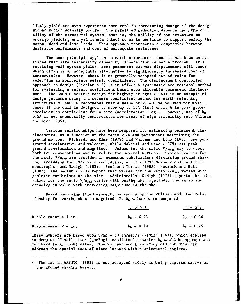
The same principle applies to earth structures, once it has been estab-lished that site instability caused by liquefaction is not a problem. If aretaining wall system yields, some permanent outward displacement will occur,which often is an acceptable alternative to significantly increased cost ofconstruction. However, there is no generally accepted set of rules forselecting an appropriate seismic coefficient. The displacement cuntrolledapproach to design (Section 6.3) is in effect a systematic and rational methodfor evaluating a seismic coefficient based upon allowable permanent displace-ment. The AASHTO seismic design for highway bridges (1983) is an example ofdesign guidance using the seismic coefficient method for earth retainingstructures.* AASHTO recommends that a value of kh - 0.5A be used for mostcases if the wall is designed to move up to 10A (in.) where A is peak groundacceleration coefficient for a site (acceleration - Ag). However, use of kh -0.5A is not necessarily conservative for areas of high seismicity (see Whitmanand Liao 1985).
Various relationships have been proposed for estimating permanent dis-placements, as a function of the ratio kh/A and parameters describing theground motion. Richards and Elms (1979) and Whitman and Liao (1985) use penkground acceleration and velocity, while Makdisi and Seed (1979) use peakground acceleration and magnitude. Values for the ratio V/am.x may be used,both for computations and to relate the several methods. Typical values forthe ratio V/ama, are provided in numerous publications discussing ground shak-ing, including the 1982 Seed and Idriss, and the 1983 Newmark and Hall EERImonographs. and Sadigh (1983). Seed and Idriss (1982), Newmark and Hall(1983), and Sadigh (1973) report that values for the ratio V/amax varies withgeologic conditions at the site. Additionally, Sadigh (1973) reports that thevalues for the ratio V/a.ax varies with earthquake magnitude, the ratio in-creasing in value with increasing magnitude earthquake.
Based upon simplified assumptions and using the Whitman and Liao rela-tionship for earthquakes to magnitude 7, kh values were computed:
A 0,2 A -0.4
Displacement < 1 in. kh -0.13 kh -0.30
Displacement < 4 in. kh - 0.10 kh - 0.25
These numbers are based upon V/Ag - 50 in/sec/g (Sadigh 1983), which appliesto deep stiff soil sites (geologic condition); smaller kh would be appropriatefor hard (e.g. rock) sites. The Whitman and Liao study did not directlyaddress the special case of sites located within epicentral regions.
* The map in AASHTO (1983) is not accepted widely as being representative ofthe ground shaking hazard.
8
The value assigned to kh is to be established by the seismic design teamfor the project considering the seismotectonic structures within the region,or as specified by the design agency.
1.4.3 Vertical Ground Accelerations
The effect of vertical ground accelerations upon response of waterfrontstructures is quite complex. Peak vertical accelerations can equal or exceedpeak horizontal accelerations, especially in epicentral regions. However, thepredominant frequencies generally differ in the vertical and horizontal com-ponents, and phasing relationships are very complicated. Where retainingstructures support dry backfills, studies have shown that vertical motionshave little overall influences (Whitman and Liao 1985). However, the Whitmanand Liao study did not directly address the special case of site& locatedwithin epicentral regions. For cases where water is present within soils oragainst walls, the possible influence of vertical motions have received littlestudy. It is very difficult to represent adequately the effect of verticalmotions in pseudo-static analyses, such as those set forth in this manual.
The value assigned to k, is to be established by the seismic design teamfor the project considering the seismotectonic structures within the region,or as specified by the design agency. However, pending the results of furtherstudies and in the absence of specific guidance for the choice of k, forwaterfront structures the following guidance has been expressed in literature:A vertical seismic coefficient be used in situations where the horizontalseismic coefficient is 0.1 or greater for gravity walls and 0.05 or greaterfor anchored sheet pile walls. This rough guidance excludes the special caseof structures located within epicentral regions for the reasons discussedpreviously. It is recommended that three solutions should be made: one assum-ing the acceleration upward, one assuning it downward, and the other assumingiero vertical acceleration. If the vertical seismic coefficient is found tohave a major effect and the use of the most conservative assumption has amajor cost implication, more sophisticated dynamic analyses should probably beconsidered.
9
CHAPTER 2 GENERAL DESIGN CONSIDERATIONS FOR RETAINING WALLS
2.1 Approaches to Design for Various Classes of Structure
The basic elements of seismic design of waterfront retaining structuresare a set of design criteria, specification of the static and seismic forcesacting on the structure in terms of magnitude, direction and point of applica-tion, and a procedure for estimating whether the structure satisfies thedesign criteric.
The criteria are related to the type of structure and its function.Limits of tolerable deformations may be specified, or it may be sufficient toassure the gross stability of the structure by specifying factors of safetyagainst rotational and sliding failure and overstressing the foundation. Inaddition, the structural capacity of the wall to resist internal moments andshears with adequate safety margins must be assured. Structural capacity is acontrolling factor in design for tied.back or anchored walls of relativelythin section such as sheet pile walls. Crib walls, or gravity walls composedof blocks of rock are examples of structures requiring a check for safetyagainst sliding and tipping at each level of interface between structuralcomponents.
Development of design criteria begins with a clear concept of the fail-ure modes of the retaining structure. Anchored sheet pile walls display themost varied modes of failure as shown in Figure 2.1, which illustrates bothgross stability problems and potential structural failure modes. The morerestricted failure modes of a gravity wall are shown in Figure 2.2. A failuresurface passing below a wall can occur whenever there is weak soil in thefoundation, and not just when there is a stratum of liquified soil.
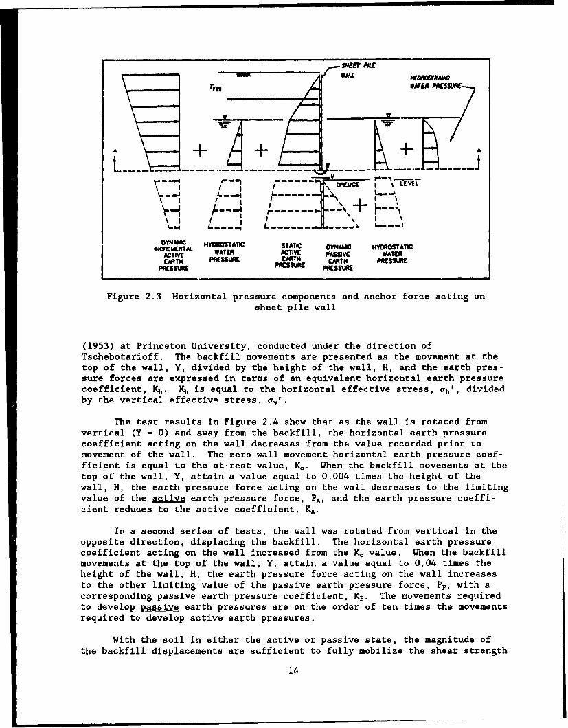
Retaining structures must be designed for the static soil and waterpressures existing before the earthquake and for superimposed dynamic andinertia forces generated by seismic excitation, and for post seismic condi-tions, since strengths of soils may be altered as a result of an earthquake.Figure 2.3 shows the various force components using an anchored sheet pilewall example from Chapter 7. With massive walls, it is especially importantto include the inertia force acting on the wall itself. There are super-imposed inertia forces from water as well as from soil. Chapters 3, 4, and 5consider the evaluation of static and dynamic earth and water pressures.
2.2 Interdependence between Wall Deformations and Forces Acting on the Wall
The interdependence betieen wall deformations and the static and dynamicearth pressure forces acting on the wall has been demonstrated in a number oftests on model retaining walls at various scales. An understanding of thisinterdependence is fundamental to the proper selection of earth pressures foranalysis and design of walls. The results from these testing programs aresummarized in the following two sections.
2.2.1 Wall Deformations and Static Earth Pressure Forces
The relationships between the movement of the sand backfills and themeasured static earth pressure forces acting on the wall are shown in Fig-ure 2.4. The figure is based on data from the model retaining wall tests con-ducted by Terzaghi (1934, 1936, and 1954) at MIT and the tests by Johnson
11
II44
4.4
54 U)
. 44 0
w 4J.
0
IIW
'4 1. ~I~t 4-
004)
cl; 0
Movement
/A I/ZA
Sliding Rotation
- N
N I
Over turning Rotation
NN
IN
Bearing Capacity
LS;ck Movement
S/7
Liquified Substrata
Slip Within Substrata
Figure 2.2 Rigid walls retaini : o L ,ckfills whichundergo movements during eafltnrquakes
13
n m I WATER PRESSII I
A
' I I
--------------- - --- ,----
OYAMC HYDROSTATIC STATIC ONA1C HYDROSTATICINCREMENTAL WATER ACTIVE WATCH
ACTIVE 0SV AEEARTH PRESSURE EARTH EARTH PRESSURE
PESSURE PRESSURE PRESSURE
Figure 2.3 Horizontal pressure components and anchor force acting onsheet pile wall
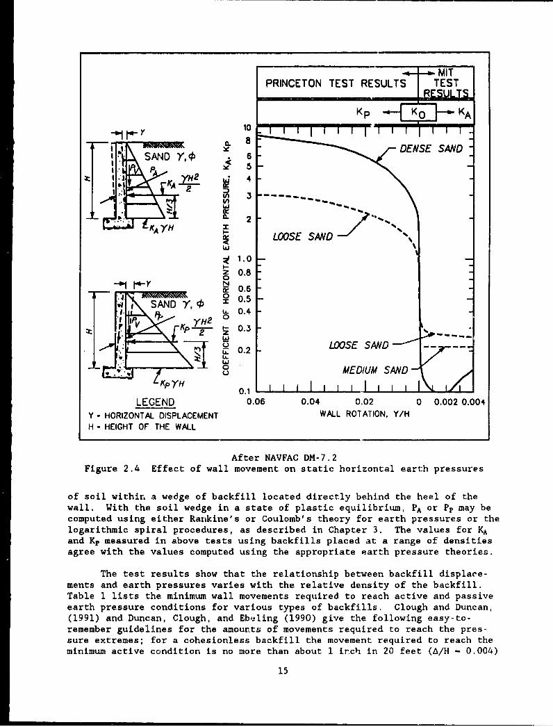
(1953) at Princeton University, conducted under the direction ofTschebotarioff. The backfill movements are presented as the movement at thetop of the wall, Y, divided by the height of the wall, H, and the earth pres-sure forces are expressed in terms of an equivalent horizontal earth pressurecoefficient, Kh. Kh is equal to the horizontal effective stress, ah', dividedby the vertical effective stress, a,'.
The test results in Figure 2.4 show that as the wall is rotated fromvertical (Y - 0) and away from the backfill, the horizontal earth pressurecoefficient acting on the wall decreases from the value recorded prior tomovement of the wall. The zero wall movement horizontal earth pressure coef-ficient is equal to the at-rest value, K.. When the backfill movements at thetop of the wall, Y, attain a value equal to 0.004 times the height of thewall, H, the earth pressure force acting on the wall decreases to the limitingvalue of the active earth pressure force, PA, and the earth pressure coeffi-cient reduces to the active coefficient, KA.
In a second series of tests, the wall was rotated from vertical in theopposite direction, displacing the backfill. The horizontal earth pressurecoefficient acting on the wall increased from the Ko value. When the backfillmovements at the top of the wall, Y, attain a value equal to 0.04 times theheight of the wall, H, the earth pressure force acting on the wall increasesto the other limiting value of the passive earth pressure force, Pp, with acorresponding passive earth pressure coefficient, Kp. The movements requiredto develop Rassive earth pressures are on the order of ten times the movementsrequired to develop active earth pressures.
With the soil in either the active or passive state, the magnitude of
the backfill displacements are sufficient to fully mobilize the shear strength
14
- MIPRINCETON TEST RESULTS TESTr RESULTS-
Kp " Ko "KA
,"~~ DE -1• 8 NSE SAND"
SAND Y.0 65 5
i: yH2 4
.3 --- -- -- ..U,
C. 2, KA Y"H X 2
LOOSE SAND-%
S1.0z 0.80
,Y Uw 0.6
SZýKp Z1o.
.e SANDEDIUM SA0.
TKp YH 0.13
LEGEND 0.06 0.04 0.02 0 0.002 0.004Y- HORIZONTAL DISPLACEMENT WALL ROTATION, Y/HH- HEIGHT OF THE WALL
After NAVFAC DM-7.2Figure 2.4 Effect of wall movement on static horizontal earth pressures
of soil withir. a wedge of backfill located directly behind the heel of thewall. With the soil wedge in a state of plastic equilibrium, PA or Pp may becomputed using either Rankine's or Coulomb's theory for earth pressures or thelogarithmic spiral procedures, as described in Chapter 3. The values for KAand Kp measured in above tests using backfills placed at a range of densitiesagree with the values computed using the appropriate earth pressure theories.
The test results show that the relationship between backfill displace-ments and earth pressures varies with the relative density of the backfill.Table 1 lists the minimum wall movements required to reach active and passiveearth pressure conditions for various types of backfills. Clough and Duncan,(1991) and Duncan, Clough, and Ebeling (1990) give the following easy-to-remember guidelines for the amounts of movements required to reach the pres-sure extremes; for a cohesionless backfill the movement required to reach theminimum active condition is no more than about 1 inch in 20 feet (A/H - 0.004)
15
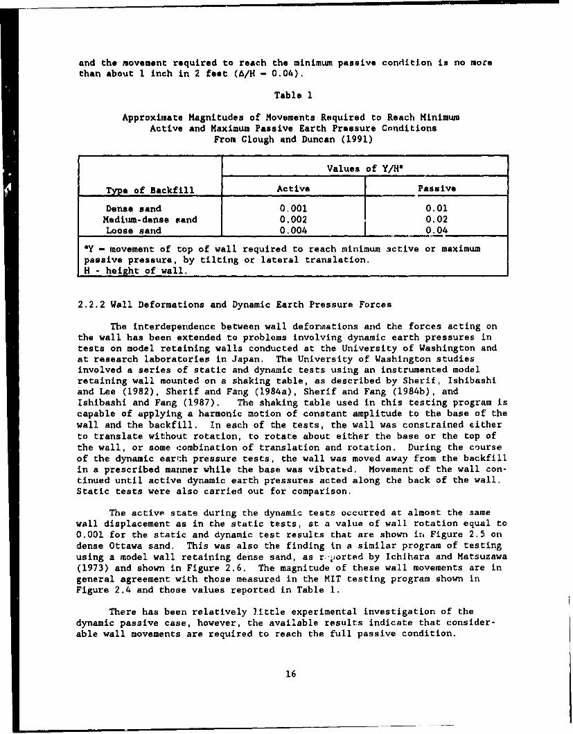
and the movement required to reach the minimum passive condition is no more
than about 1 inch in 2 feet (A/H - 0.04).
Table 1
Approximate Magnitudes of Movements Required to Reach MinimumActive and Maximum Passive Earth Pressure Conditions
From Clough and Duncan (1991)
Values of Y/H4
Type of Backfill Active Passive
Dense sand 0.001 0.01Medium-dense sand 0.002 0.02Loose sand 0.004 0.04
'Y - movement of top of wall required to reach minimum active or maximumpassive pressure, by tilting or lateral translation.H - height of wall.
2.2.2 Wall Deformations and Dynamic Earth Pressure Forces
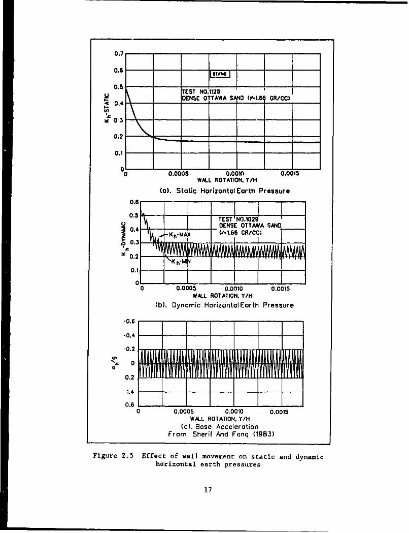
The interdependence between wall deformations and the forces acting onthe wall has been extended to problems involving dynamic earth pressures intests on model retaining walls conducted at the University of Washington andat research laboratories in Japan. The University of Washington studiesinvolved a series of static and dynamic tests using an instrumented modelretaining wall mounted on a shaking table, as described by Sherif, Ishibashiand Lee (1982), Sherif and Fang (1984a), Sherif and Fang (1984b), andIshibashi and Fang (1987). The shaking table used in this testing program iscapable of applying a harmonic motion of constant amplitude to the base of thewall and the backfill. In each of the tests, the wall was constrained eitherto translate without rotation, to rotate about either the base or the top ofthe wall, or some combination of translation and rotation. During the courseof the dynamic eari:h pressure tests, the wall was moved away from the backfillin a prescribed manner while the base was vibrated. Movement of the wall con-tinued until active dynamic earth pressures acted along the back of the wall.Static tests were also carried out for comparison.
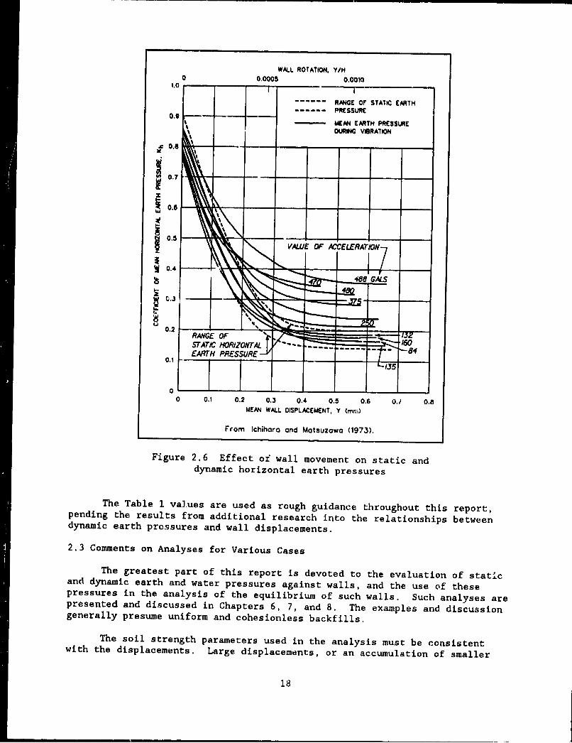
The active state during the dynamic tests occurred at almost the samewall displacement as in the static tests, at a value of wall rotation equal to0.001 for the static and dynamic test results that are shown ir, Figure 2.5 ondense Ottawa sand. This was also the finding in a similar program of testingusing a model wall retaining dense sand, as r, orted by Ichihara and Matsuzawa(1973) and shown in Figure 2.6. The magnitude of these wall movements are ingeneral agreement with those measured in the MIT testing program shown inFigure 2.4 and those values reported in Table 1.
There has been relatively little experimental investigation of thedynamic passive case, however, the available results indicate that consider-able wall movements are required to reach the full passive condition.
16
0.7
0.6 - -.-..
0.5 -"
TENST NO.1125____ EN•E OTTAWA S 0N (Y-1.61 CR/CC) ___
C 0.4I-,- 03
0.2 -- _ ___-
0.2
0.1
00 0.0005 0.0010 0.0015WALL ROTATION, Y/H
(a). Static Horizontal Earth Pressure
0.6
0.4"0. TEST NO.1029
"0.1
0.4 ES TTW A
0 0.0005 0.0010 0.0015WALL ROTATION. Y/H
(b). Dynamic HorizontalEarth Pressure
-0.6
-0.4
-0.2
- 0
0.2
1.40.6
0 0.0005 0.0010 0.0015WALL ROTATION, Y/H
(c). Base AccelerationFrom Sherif And Fon~q (1983)
Figure 2.5 Effect of wall movement on static and dynamichorizontal earth pressures
17
WALL ROTATION. Y/H0 0.0005 0.0010
I I
RANGE or STATIC EARTH.9- - PRESSURE
SMEAN EARTH PRESSUREDURING VIBRATION
V A L U E O F A C&"A T 0 7 5
TAC0.4 -RI -ONTA- - -
S 07 -, . 0,3 - . - . -, . 0.S0.4
U%
0.2
EARTH PRESSURE 80.1
1___
___
00 0.1 0.2 0.3 0.4 0.5 0.6 0./ 0.8
MEAN WALL DISPLACEMENT, Y (mr)
From Ichihara and Motsuzawo (1973).
Figure 2.6 Effect of wall movement on static anddynamic horizontal earth pressures
The Table 1 values are used as rough guidance throughout this report,pending the results from additional research into the relationships betweendynamic earth pressures and wall displacements.
2.3 Comments on Analyses for Various Cases
The greatest part of this report is devoted to the evaluation of staticand dynamic earth and water pressures against walls, and the use of thesepressures in the analysis of the equilibrium of such walls. Such analyses arepresented and discussed in Chapters 6, 7, and 8. The examples and discussiongenerally presume uniform and cohesionless backfills.
The soil strength parameters used in the analysis must be consistentwith the displacements. Large displacements, or an accumulation of smaller
18
Ar INERA FORCES
IV - POTENTIAL
/ FAKWRESURFACE
ýWEAK ýSTRATUýM
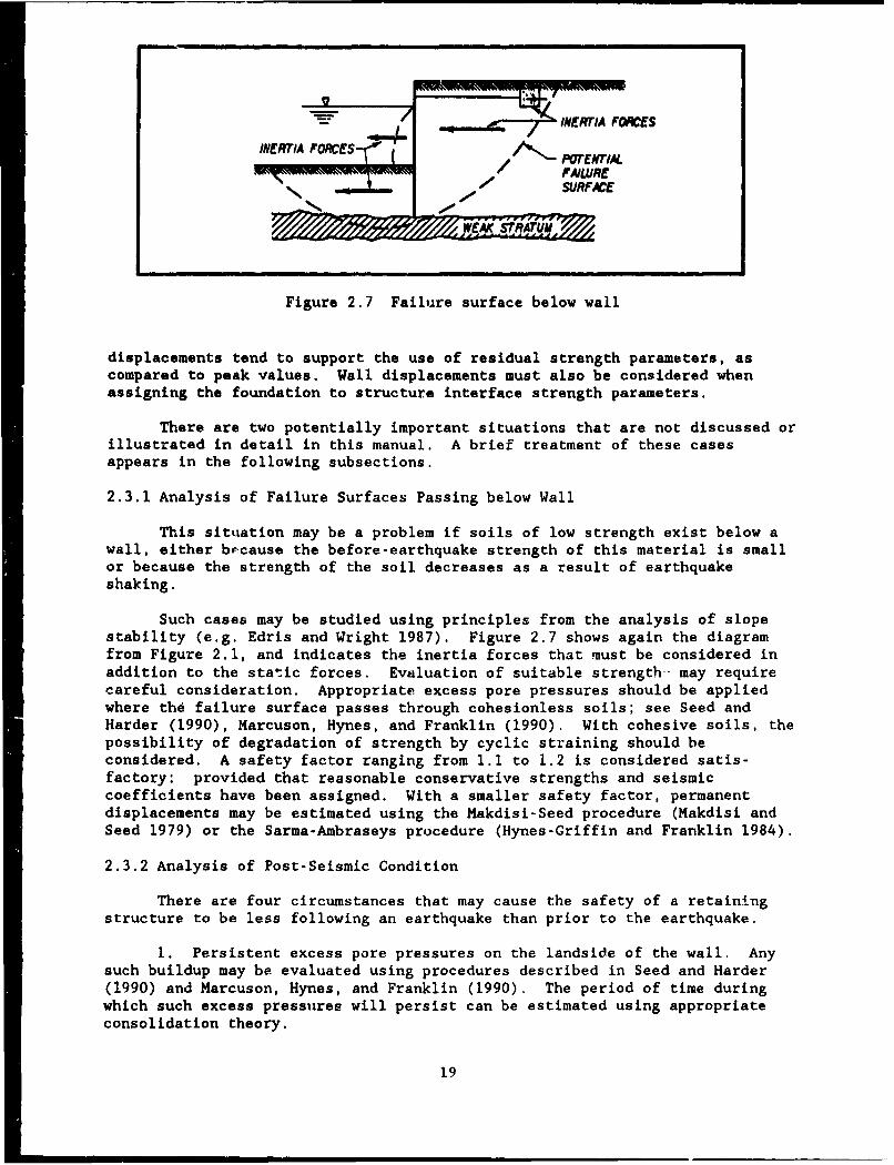
Figure 2.7 Failure surface below wall
displacements tend to support the use of residual strength parameters, ascompared to peak values. Wall displacements must also be considered whenassigning the foundation to structure interface strength parameters.
There are two potentially important situations that are not discussed orillustrated in detail in this manual. A brief treatment of these casesappears in the following subsections.
2.3.1 Analysis of Failure Surfaces Passing below Wall
This situation may be a problem if soils of low strength exist below awall, either because the before-earthquake strength of this material is smallor because the strength of the soil decreases as a result of earthquakeshaking.
Such cases may be studied using principles from the analysis of slopestability (e.g. Edris and Wright 1987). Figure 2.7 shows again the diagramfrom Figure 2.1, and indicates the inertia forces that must be considered inaddition to the static forces. Evaluation of suitable strength- may requirecareful consideration. Appropriate excess pore pressures should be appliedwhere the failure surface passes through cohesionless soils; see Seed andHarder (1990), Marcuson, Hynes, and Franklin (1990). With cohesive soils, thepossibility of degradation of strength by cyclic straining should beconsidered. A safety factor ranging from 1.1 to 1.2 is considered satis-factory: provided that reasonable conservative strengths and seismiccoefficients have been assigned. With a smaller safety factor, permanentdisplacements may be estimated using the Makdisi-Seed procedure (Makdisi andSeed 1979) or the Sarma-Ambraseys procedure (Hynes-Criffin and Franklin 1984).
2.3.2 Analysis of Post-Seismic Condition
There are four circumstances that may cause the safety of a retainingstructure to be less following an earthquake than prior to the earthquake.
1. Persistent excess pore pressures on the landside of the wall. Anysuch buildup may be evaluated using procedures described in Seed and Harder(1990) and Marcuson, Hynes, and Franklin (1990). The period of time duringwhich such excess pressures will persist can be estimated using appropriateconsolidation theory.
19
2. Residual earth pressures as a result of seismic straining. There isevidence that such residual pressures may reach those associated with theat-rest condition (see Whitman 1990).
3. Reduction in strength of backfill (or soils benieath or outside oftoe of wall) as a result of earthquake shaking. In the extreme case, only theresidual strength (see the National Research Council 1985; Seed 1987; Seed andHarder 1990; Marcuson, Hynes, and Franklin 1990; Poulos, Castro, and France1985; and Stark and Mesrn 1992) may be available in some soils. Residualstrengths may be treated as cohesive shear strengths for evaluation of corre-sponding earth pressures.
4. Lowering of water level on waterside of wall during the fallingwater phase of a tsunami. Estimates of possible water level decrease duringtsunamis require expert input.
The possibility that each of these situations may occur must be considered,and where appropriate the adjusted earth and fluid pressures must beintroduced into an analysis of static equilibrium of the wall. Safety factorssomewhat less than those for the usual static case are normally consideredappropriate.
20
CHAPTER 3 STATIC EARTH PRESSURES - YIELDING BACKFILLS
3.1 Introduction
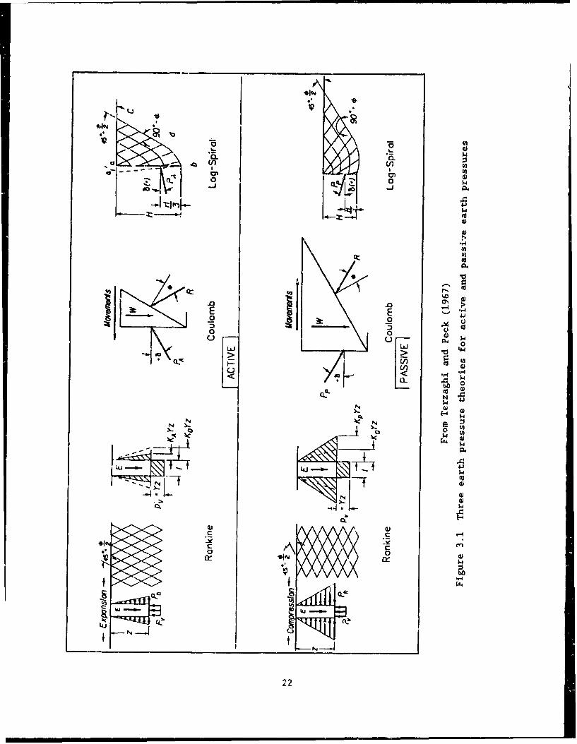
Methods for evaluating static earth pressures are essential for design.They also form the basis for simplified methods for determining dynamic earthpressures associated with earthquakes. This chapter describes analyticalprocedures for computing earth pressures for earth retaining structures withstatic loadings. Three methods are described: the classical earth pressuretheories of Rankine and Coulomb and the results of logarithmic spiral failuresurface analyses. The three failure mechanisms are illustrated in Figure 3.1.
The Rankine theory of active and passive earth pressures (Rankine 1857)determines the state of stress within a semi-infinite (soil) mass that,because of expansion or compression of the (soil) mass, is transformed from anelastic state to a state of plastic equilibrium. The orientation of thelinear slip lines within the (soil mass) are also determined in the analysis.The shear stress at failure within the soil is defined by a Mohr-Coulomb shearstrength relationship. The resulting failure surfaces within the soil massand the corresponding Rankine active and passive earth pressures are shown inFigure 3.1 for a cohesionless soil.
The wedge theory, as developed by Coulomb (1776), looks at the equili-brium of forces acting upou a soil wedge without regard to the state of stresswithin the soil mass. This wedge theory assumes a linear slip plane withinthe backfill and the full mobilization of the shear strength of the soil alongthis plane. Interface friction between the wall and the backfill may be con-sidered in the analysis.
Numerous authors have developed relationships for active and passiveearth pressure coefficients based upon an assumption of a logarithmic failuresurface, as illustrated in Figure 3.1. One of the most commonly used sets ofcoefficients was tabulated by Caquot and Kerise] (1948). Representative KAand Kp values from that effort are illustrated in Table 3 and discussed inSection 3.5. NAVFAC developed nomographs from the Caquot and Keri.,el efforts,and are also included in this chapter (Figures 3.11 and 3.12).
Rankine's theory, Coulomb's wedge theory, and the logarithmic spiralprocedure result in similar values for active and passive thrust when theinterface friction between the wall and the backfill is equal to zero. Forinterface friction angles greater than zero, the wedge method and the loga-rithmic spiral procedure result in nearly the same values for active thrust.The logarithmic spiral procedure results in accurate values for passive thrustfor all values of interface friction between the wall and the backfill. Theaccuracy of the passive thrust values computed using the wedge methoddiminishes with increasing values of interface friction because the boundaryof the failure block becomes increasingly curved.
This procedure is illustrated in example I at the end of this chapter.
21
4.3
0)00
40 do
4ý
E E'o0(
00-44.
1-J LL. 44ICd
-4 Wa Z
0 (n
030_ '-4\
*-r4
.i3
22
3.2 Rankine Theory
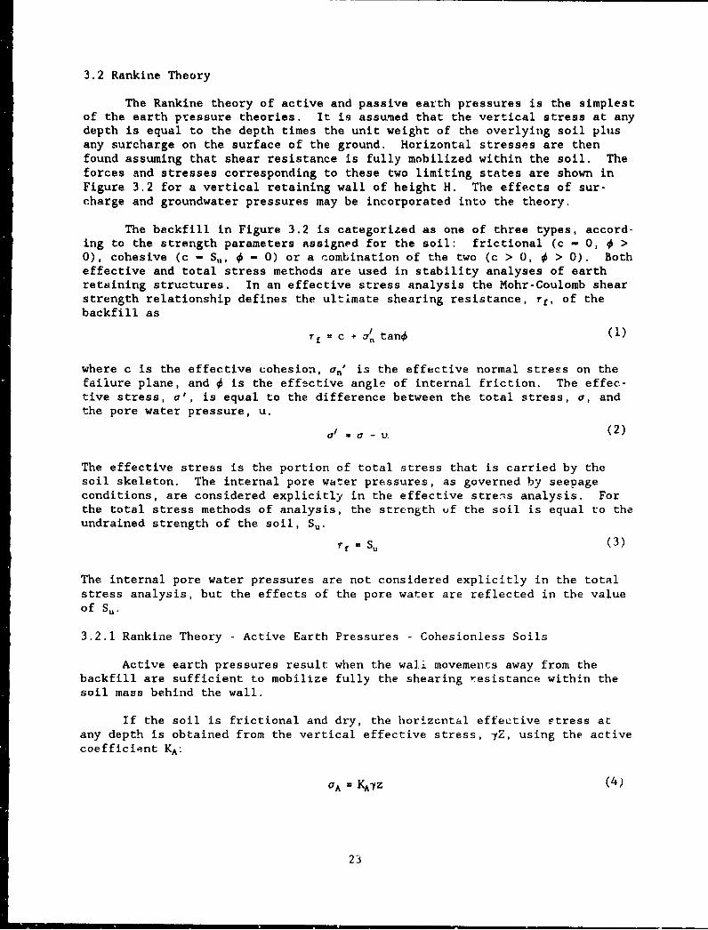
The Rankine theory of active and passive earth pressures is the simplestof the earth pressure theories. It is assumed that the vertical stress at anydepth is equal to the depth times the unit weight of the overlying soil plusany surcharge on the surface of the ground. Horizontal stresses are thenfound assuming that shear resistance is fully mobilized within the soil. Theforces and stresses corresponding to these two limiting states are shown inFigure 3.2 for a vertical retaining wall of height H. The effects of sur-charge and groundwater pressures may be incorporated into the theory.
The backfill in Figure 3.2 is categorized as one of three types, accord-ing to the strength parameters assigned for the soil: frictional (c - 0, 0 >0), cohesive (c - S,,, 0 - 0) or a combination of the two (c > 0, 0 > 0). Botheffective and total stress methods are used in stability analyses of earthretaining structures. In an effective stress analysis the Mohr-Coulomb shearstrength relationship defines the ultimate shearing resistance, rf, of thebackfill as
rf = c +/ tano (1)
where c is the effective cohesion, ant is the effective normal stress on theEaiiure plane, and 0 is the effective angle of internal friction. The effec-tive stress, a', is equal to the difference between the total stress, a, andthe pore water pressure, u.
al . a - U (2)
The effective stress is the portion of total stress that is carried by thesoil skeleton. The internal pore water pressures, as governed by seepageconditions, are considered explicitly in the effective stress analysis. Forthe total stress methods of analysis, the strength uf the soil is equal to theundrained strength of the soil, S,.
rf = S. (3)
The internal pore water pressures are not considered explicitly in the totalstress analysis, but the effects of the pore water are reflected in the valueof SU.
3.2.1 Rankine Theory - Active Earth Pressures - Cohesionless Soils
Active earth pressures result when the wall movements away from thebackfill are sufficient to mobilize fully the shearing resistance within thesoil mass behind the wall.
If the soil is frictional and dry, the horizcntal effective stress atany depth is obtained from the vertical effective stress, IZ, using the activecoefficient KA:
a^ - KA^z (4)
23
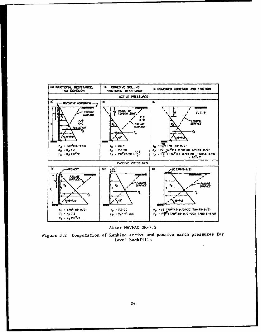
let FRICTIONAL RESISr,4E IW COHESIVE SOIL, NO ltCMIE OEINADFITONO COMESION FRICTIONAL RESISTANCE (iCME OSN*0FITO
ACTIVE PRESSURES
to) &WIr~ lei
I 'FA * -/ C-0 -PR 6A / SURFACEAESUTN4T -01 WC
KA TAN 2(45**/2) Zo-2C/Y Z* 2-C)TN45#2CI AZ ` Z-2C CA VZ JAN2(45-0/2)-2C TAN(4S40/2)
PA KAM1 A - YH2/2-2CH.LC- PA Of'.) TM$I45*/0-2C11 TAN(45-0/2)
PASSIVE PRESSURES
WRE AW-FMW
A.A
AfWr A FACE alp-7.2CFigre3. Cmpta2.n f Ank, atv n asv at rsue o
lee. .kfil
24iii \5
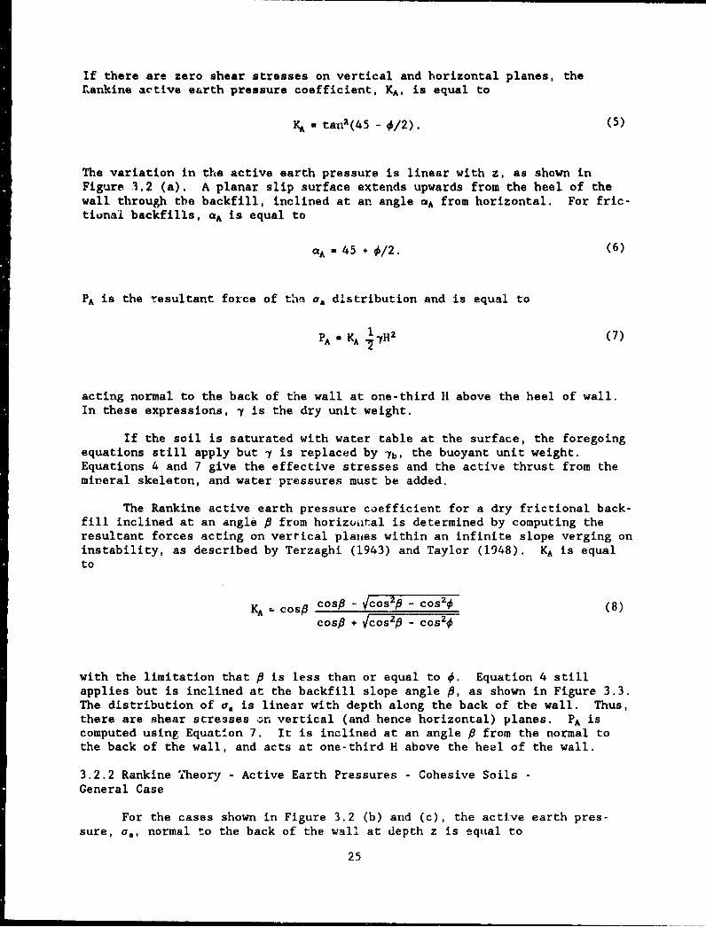
If there are zero shear stresses on vertical and horizontal planes, theLankine active earth pressure coefficient, KA, is equal to
Kh * tan2 (45 - u/2). (5)
The variation in the active earth pressure is linear with z, as shown inFigure 3.2 (a). A planar slip surface extends upwards from the heel of thewall through the backfill, inclined at an angle CA from horizontal. For fric-tional backfills, aa is equal to
A 45 + 0/2. (6)
PA is the resultant force of thn a. distribution and is equal to
PA KA 7 yH2 (7)
acting normal to the back of the wall at one-third 11 above the heel of wall.In these expressions, y is the dry unit weight.
If the soil is saturated with water table at the surface, the foregoingequations still apply but 7 is replaced by 7b, the buoyant unit weight.Equations 4 and 7 give the effective stresses and the active thrust from themineral skeleton, and water pressures must be added.
The Rankine active earth pressure coefficient for a dry frictional back-fill inclined at an angle P from horizoatal is determined by computing theresultant forces acting on vertical planes within an infinite slope verging oninstability, as described by Terzaghi (1943) and Taylor (1948). KA is equalto
KA - cosp cos# - Vcos 2# - cos 2 0 (8)cosp + cos 2p - cos 20
with the limitation that P is less than or equal to 0. Equation 4 stillapplies but is inclined at the backfill slope angle f9, as shown in Figure 3.3.The distribution of oa is linear with depth along the back of the wall. Thus,there are shear stresses :;n vertical (and hence horizontal) planes. PA iscomputed using Equation 7. It is inclined at an angle P from the normal tothe back of the wall, and acts at one-third H above the heel of the wall.
3.2.2 Rankine Theory - Active Earth Pressures - Cohesive Soils -General Case
For the cases shown in Figure 3.2 (b) and (c), the active earth pres-
sure, a., normal to the back of the wall at depth z is equal to
25
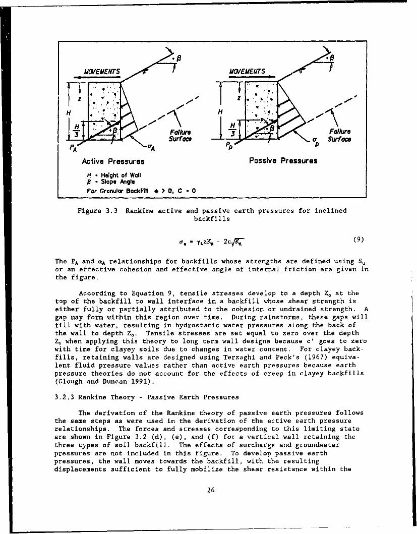
IE ... I I IllS
Active Pressures Passive Pressures
H H Height of WHll.0 Slope 0gle
For Granulor SackFul * > 0, C - 0
Figure 3.3 Rankine active and passive earth pressures for inclinedbackfills
sa = PtzI - 2cSfa (9)
The PA and PA relationships for backfills whose strengths are defined using Ssor an effective cohesion and effective angle of internal friction are given in
the figure.
According to Equation 9, tensile stresses develop to a depth Zr at thetop of the backfill to wall interface in a backfill whose shear strength is
either fully or partially attributed to the cohesion or undrained strength. Agap may form within this region over time. During rainstorms, these gaps willfill with water, resulting in hydrostatic water pressures along the back ofthe wall to depth Zo. Tensile stresses are set equal to zero over the depthZ. when applying this theory to long term wall designs because c' goes to zerowith time for clayey soils due to changes in water content. For clayey back-fills, retaining walls are designed using Terzaghi and Peck's (1967) equiva-lent fluid pressure values rather than active earth pressures because earthpressure theories do not account for the effects of creep in clayey backfills(Clough and Duncan 1991).
3.2.3 Rankine Theory - Passive Earth Pressures
The derivation of the Rankine theory of passive earth pressures followsthe same steps as were used in the derivation of the active earth pressurerelationships. The forces and stresses corresponding to this limiting stateare shown in Figure 3.2 (d), (e), and (f) for a vertical wall retaining thethree types of soil backfill. The effects of surcharge and groundwaterpressures are not included in this figure. To develop passive earthpressures, the wall moves towards the backfill, with the resultingdisplacements sufficient to fully mobilize the shear resistance within the
26
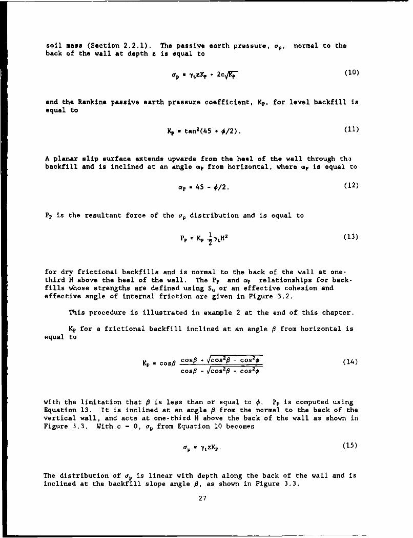
soil mass (Section 2.2.1). The passive earth pressure, op, normal to theback of the wall at depth z is equal to
O -ytz+p + 2cX- (10)
and the Rankine passive earth pressure coefficient, Kp, for level backfill isequal to
*p- tan2(45 + 0/2). (11)
A planar slip surface extends upwards from the heel of the wall through th.backfill and is inclined at an angle ap from horizontal, where ap is equal to
cf - 45 - 0/2. (12)
Pp is the resultant force of the up distribution and is equal to
Pp - Kp -TtH2 (3P Kllz(13)
for dry frictional backfills and is normal to the back of the wall at one-third H above the heel of the wall. The Pp and ap relationships for back-fills whose strengths are defined using S, or an effective cohesion andeffective angle of internal friction are given in Figure 3.2.
This procedure is illustrated in example 2 at the end of this chapter.
Kp for a frictional backfill inclined at an angle P from horizontal isequal to
Kp a cos# cosp + Vcos 2# - CoS 20 (14)cos# - Vcos 2p - cos 2 0
with the limitation that 6 is less than or equal to 0. Pp is computed usingEquation 13. It is inclined at an angle P from the normal to the back of thevertical wall, and acts at one-third H above the back of the wall as shown inFigure 3.3. With c - 0, up from Equation 10 becomes
p - 7tzlp. (15)
The distribution of ap is linear with depth along the back of the wall and is
inclined at the backfill slope angle P, as shown in Figure 3.3.
27
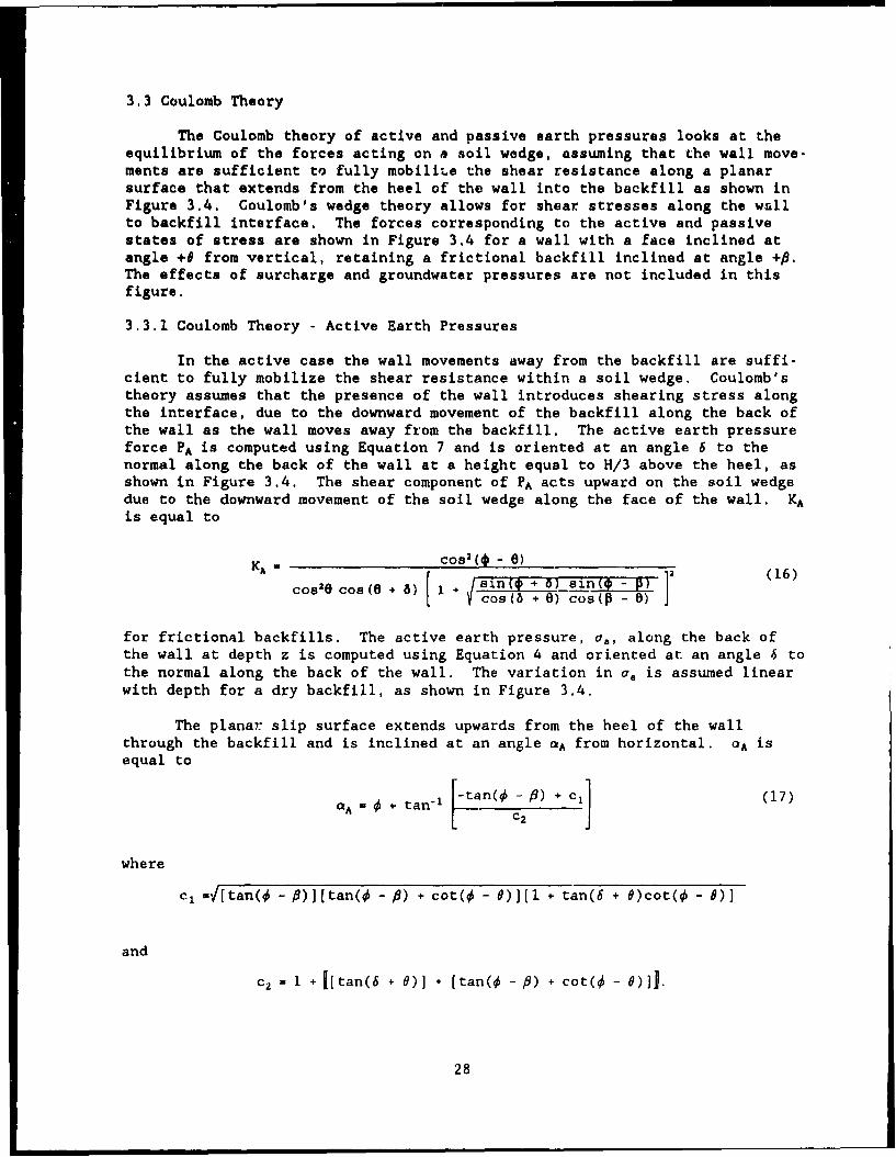
3.3 Coulomb Theory
The Coulomb theory of active and passive earth pressures looks at theequilibrium of the forces acting on a soil wedge, assuming that the wall move-ments are sufficient to fully mobiliLe the shear resistance along a planarsurface that extends from the heel of the wall into the backfill as shown inFigure 3.4. Coulomb's wedge theory allows for shear stresses along the wallto backfill interface. The forces corresponding to the active and passivestates of stress are shown in Figure 3.4 for a wall with a face inclined atangle +0 from vertical, retaining a frictional backfill inclined at angle +f,The effects of surcharge and groundwater pressures are not included in thisfigure.
3.3.1 Coulomb Theory - Active Earth Pressures
In the active case the wall movements away from the backfill are suffi-cient to fully mobilize the shear resistance within a soil wedge. Coulomb'stheory assumes that the presence of the wall introduces shearing stress alongthe interface, due to the downward movement of the backfill along the back ofthe wall as the wall moves away from the backfill. The active earth pressureforce PA is computed using Equation 7 and is oriented at an angle 6 to thenormal along the back of the wall at a height equal to H/3 above the heel, asshown in Figure 3.4. The shear component of PA acts upward on the soil wedgedue to the downward movement of the soil wedge along the face of the wall. KAis equal to
K- cos( e) 2 (16)0 Co (•n ) sin(+ - ) ] T-6Icos 20coa(0 + 8) 1V~ os(b + 9) Cos(P - 0)
for frictional backfills. The active earth pressure, a., along the back ofthe wall at depth z is computed using Equation 4 and oriented at an angle 6 tothe normal along the back of the wall. The variation in a. is assumed linearwith depth for a dry backfill, as shown in Figure 3.4.
The planar slip surface extends upwards from the heel of the wallthrough the backfill and is inclined at an angle CA from horizontal. OA isequal to
a^ + tan- an( -[) + ci (17)C2
where
cl -/[tan(o - P)][tan(o - P) + cot(o - 0)](I + tan(6 + O)cot(o - 0)]
and
c- + [tan(6 + 0)] * [tan(4 - f) + cot(• - 6)]J.
28
H
Active Pressures
,0vemeds '" /,
"1..: b,.
p
.00 -01 S, .,,,.a
Passive Pressures
H - Height of Wall* - Slope Angle
0 - Inclination of Wallb - Angle of Interface FrictionPositive angles shown for Coulomb's equationsfor KA, Kp. OA and O*p
Figure 3.4 Coulomb active and passive earth pressures for inclinedbackfills and inclined walls
One widely quoted reference for effective angles of friction alonginterfaces between various types of materials, 6, is Table 2. Potyondy (1961)and Peterson et. al. (1976) also provide recommendations for 6 values fromstatic direct shear test results.
This procedure is illustrated in example 3 at the end of this chapter.
29
3.3.2 Coulomb Active Pressures - Hydrostatic Water Table Within Backfill andSurcharge
The distribution of Coulomb active earth pressures for a partially sub-merged wall retaining a frictional backfill and supporting a uniform sur-charge, q, is shown in Figure 3.5. With a hydrostatic water table at heightH, above the base of the wall, the resulting pressures acting along the backof the wall are equal to the sum of (1) the thrust of the soil skeleton as aresult of its unit weight, (2) the thrust of the soil skeleton as a result ofthe surcharge, q, and (3) the thrust of the pore water. The effective weightof the backfill, c'.t, above the water table is equal to
1 (18)Owt U •t*Z
and below the water table, a'.t is equal to
a*t M Y.(H - H,,) +'.[z - (H - H.)] (19)
where -y' is the effective unit weight at depth z. For hydrostatic pore waterpressures, 7' is equal to the buoyant unit weight, 7b.The buoyant unit weight, 7b, is equal to
"Yb 0 7t - 7w (20)
a, is equal to the sum of the thrust of the soil skeleton as a result of itsunit weight and the thrust of the soil skeleton as a result of the surcharge,
a. = (a't + q).KA (21)
and is inclined at an angle 6 from the normal to the back of the wall. KA iscomputed using Equation 16 for a level backfill (,0 - 0) and a vertical wallface (0 - 0). The hydrostatic water pressures are equal to
u = -f.(z - (H - H.w)] (22)
and is normal to the back of the wall. The total thrust on the wall, P, isequal to the sum of the equivalent forces for the three pressure distribu-tions. Due to the shape of the three pressure distributions, its point ofaction is higher up the back of the wall than one-third H above the heel. Theorientation of the failure surface is not affected by the hydrostatic waterpressures and is calculated using Equation 17.
30
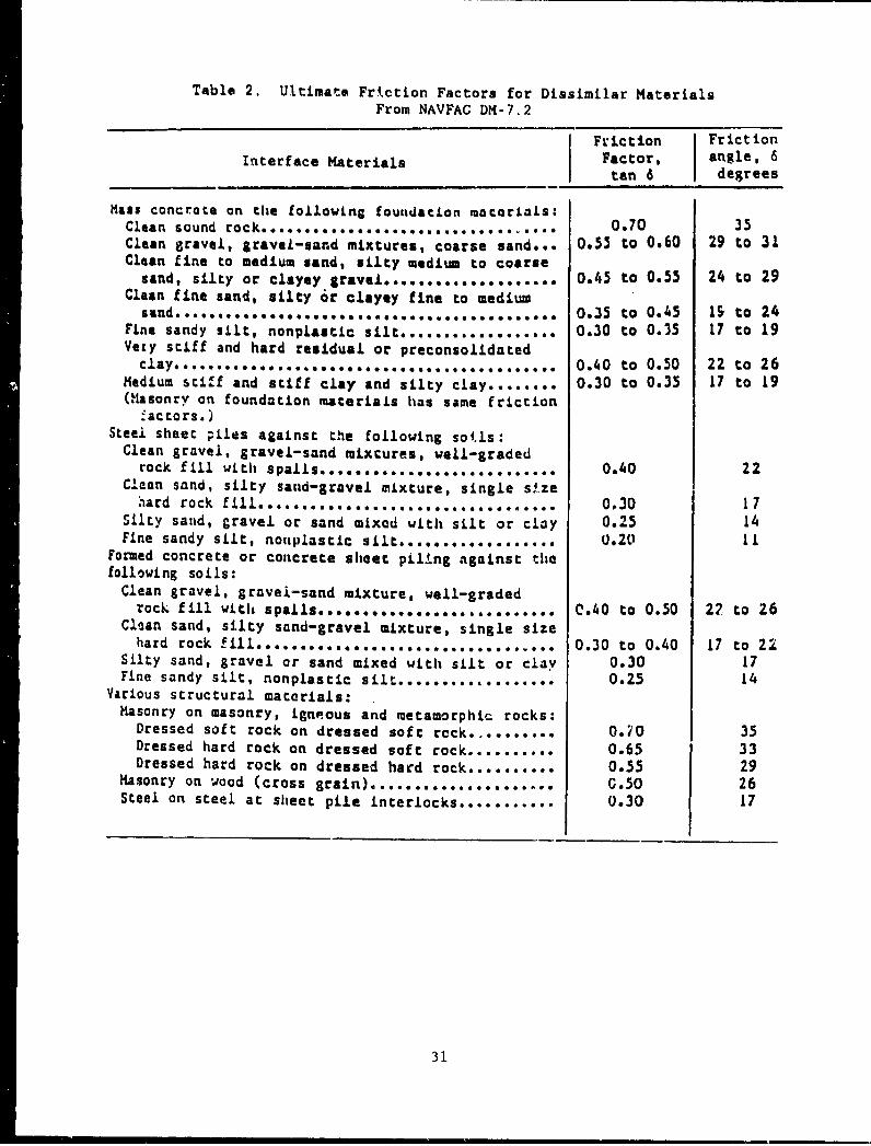
Table 2. Ultimate Friction Factors for Dissimilar MaterialsFrom NAVFAC DM-7.2
Friction FrictionInterface Materials Factor, angle, 6
tan 6 degrees
Mass concrete on the following foundation macarials:Clean sound rock...... ... ........................ 0.70 35Clean gravel, gravel-sand mixtures, coarse sand... 0.55 to 0.60 29 to 31Clean fine to medium sand, silty medium to coarse
sand, silty or clayey gravel .................... 0.45 to 0.55 24 to 29Clean fine sand, silty or clayey fine to medium
sand............................................ 0.35 to 0.45 1 to 24Fine sandy silt, nonplastic silt.................. 0.30 to 0.35 17 to 19Vezy stiff and hard residual or preconsolidated
clay. .......... ................................. 0.40 to 0.50 22 to 26Medium stiff and stiff clay and silty clay ........ 0.30 to 0.35 17 to 19(Masonry on foundation materials has same friction
faccors.)Steei sheet piles against the following sol.ls:
Clean gravel, gravel-sand mixtures, well-gradedrock fill withspi ls ......................... 0.40 22
Clean sand, silty sand-gravel mixture, single sizeh a r d r o c k f i l l . . . . . . . . . . . . . . . . . . . . . 0 . 3 0 1 7
Silty sand, gravel or sand mixed with slit or clay 0.25 14Fine sandy silt, nonplastic silt.................. U.20 11
Formed concrete or concrete sheet piling against thefollowing soils:
Clean gravel, gravei-sand mixture, well-gradedrock fill with spoils........................... C.40 to 0.50 27 to 26
Clean sand, silty sand-gravel mixture, single sizehard rock fill.... 0.30 to 0.40 17 to 22
Silty sand, gravel or sand mixed with silt or clay 0.30 17Fine sandy silt, nonpiastic silt .................. 0.25 14
Various structural materials:Masonry on masonry, igneous and metamorphic rocks:
Dressed soft rock on dressed soft rcck......... 0.10 35Dressed hard rock on dressed soft rock .......... 0.65 33Dressed hard rock on dressed hard rock.......... 0.55 29
Masonry on wood (cross grain).................... G.50 26Steel on steel at sheet pile interlocks........... 0.30 17
31
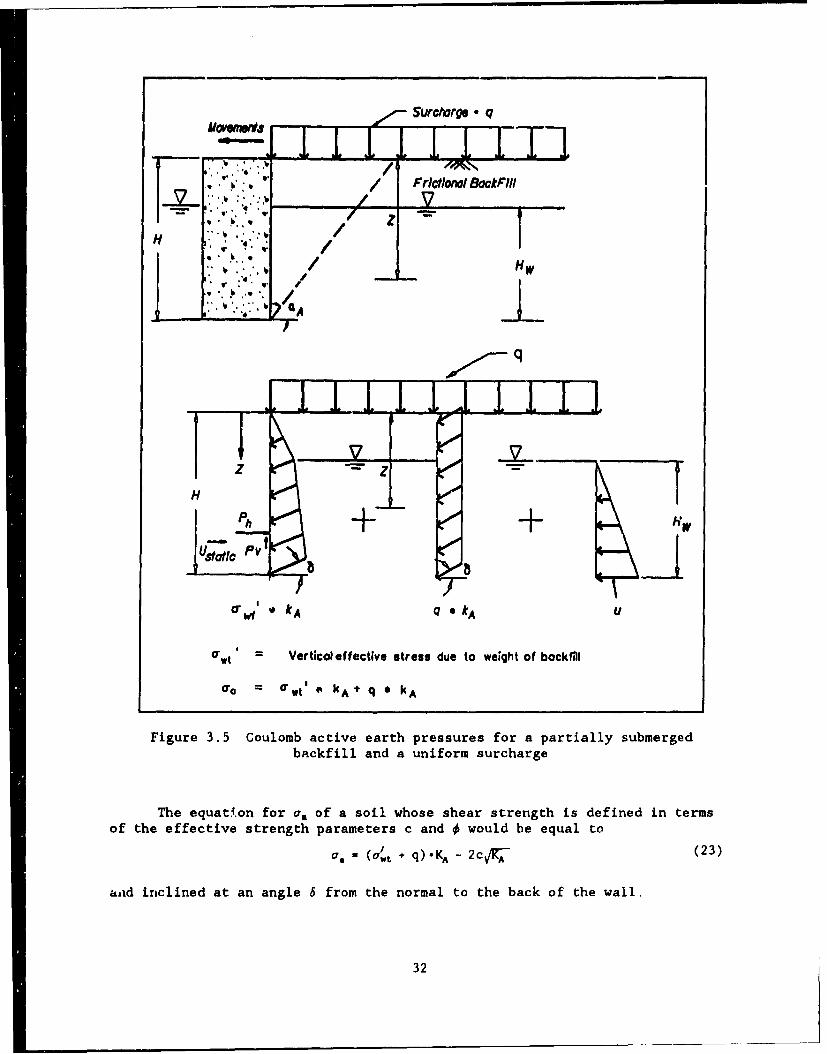
Surciarge- q
WLLW"" " / Frlctional UQoKUIII
f- . b .-''" /
94A
w.. / HW
H
a' "t kA kA U
owt = Vertical effective stress due to weight of backfill
=r *rt k A q 0 k A
Figure 3.5 Coulomb active earth pressures for a partially submergedbackE ill arnd a uniform surcharge
The equatl.on for a. of a soil whose shear strength is defined in termsof the effective strength parameters c and would be equal to
a- (lt -q) KKA 2cVZA- (23)
jjid inclined at an angle 6 from the normal to the back of the wall.
32
3.3.3 Coulomb Active Pressures - Steady rtate Seepage Within Backfill
This section summarizes the equations for deterrnin'ng the Coulomb activeearth pressure forces and p're water pressures acting on the back of a wallretaining a drained backfill that is subjected to steady state flow. Fig-ure 3.6 shows a wall with a vertical face retaining a lev-l backfill, support-ing a uniform surcharge Load, q, and subjected to a constant water infiltra-tion. The wall has a drainage system consisting of a gravel drain below thesand backfill, with weep holes through the wall. Steady state tlow maydevelop during a rainstorm of sufficient intensity and duration. The result-ing flownet io shown in Figure 3.6, consisting of vertical flow lines andhorizontal equipotential lines, assuming the drain has sufficient permeabilityand thickness to be free draining (i.e. with zero pressure head wit'in thedrain). Adjacent to the back of the wall, the flow net has five head drops.With the datum at the base of the wall, the total head at the top of the back-fill is equal to the height of the wall, H, and a total head is equal to zeroat the weep holes. The drop in total head between each of the five equipoten-tial lines is equal to H/5. Neglecting the velocity head, the total head, h,is equal to
h = h. + hp (24)
where h. is the elevation head, and hp is the pressure head equal to
i - _.U (25)
With the total head equal to the elevation head for each of the equipotentiallines, hp and the pore water pressure, u, are equal to zero. The seepagegradient, i, at any point in the baickfill is equal to
i = Ah (26)
where ah is the change in total head and Ai the length of the flowpath over which the incremental head drop occurs. With horizontalequipotential lines, the flow is vertical and directed downward (iY - +i).For steady state seepage conditions, the effective unit weight is equal to
7' = 7b ± I"- ' -. (27)
The seepage force is added to the buoyant unit weight when flow is downwardand subtracted with upward flow. For the example shown in Figure 3.6 with iequal to positive unity and directed downward, I' is equal to the total unitweight, It. The effective weight of the backfill, a'wt, is equal to
awt = -z = (Ob + 1w) *z = t z (28)
An alternative procedure for calculating a'wt is using the total overburdenpressure, awt, and pore water pressures, u. By Equation 7, we see that with
33
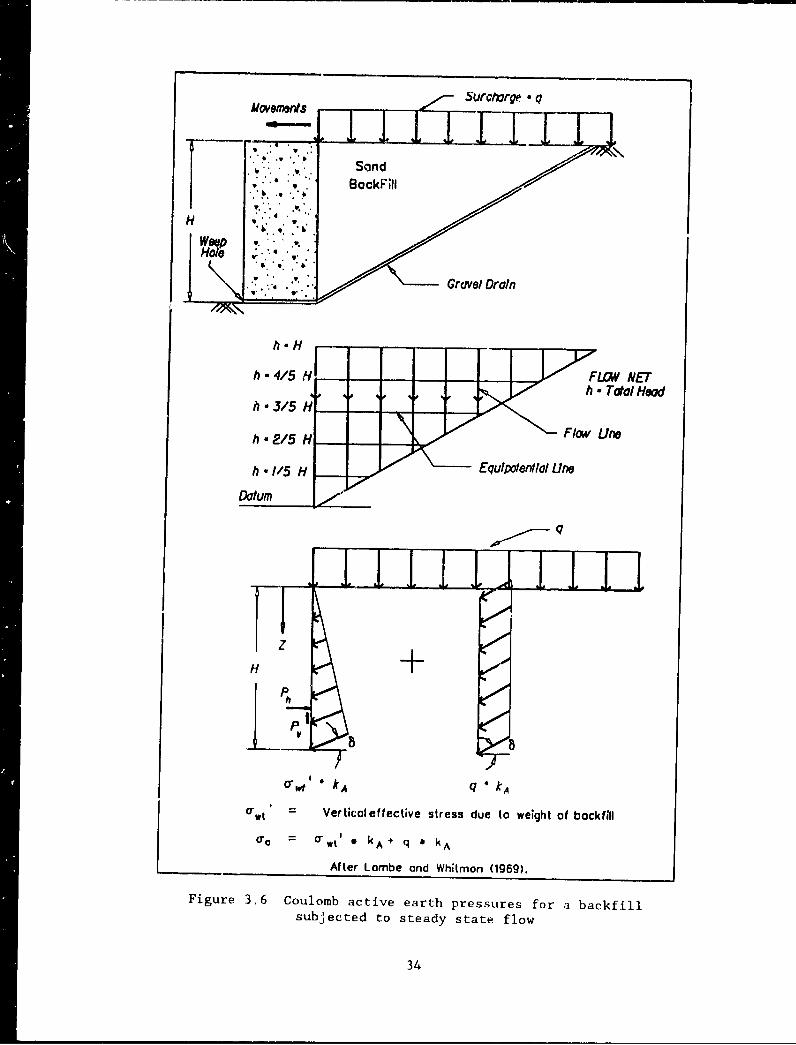
Ovemnts Surcharge q
Sand
H*hW/5 A LO
h3/H. - -
-4 0., h. ' To ol"
h .' "/ 7
"h"2/H•- - Flow Un"
h - 1/5 H Equipo.ental ine
Datum
•IT 1. .. It-
V 1 jil
zH "
Ph
Pttu
p V
wt Ver tical effective stress due to weight of backfill
a, a" t*' 9 k A+ q k kA
After Lambe and Whitman (1969).
Figure 3.6 Coulomb active earth pressures for a backfillsubjected to steady state flow
34
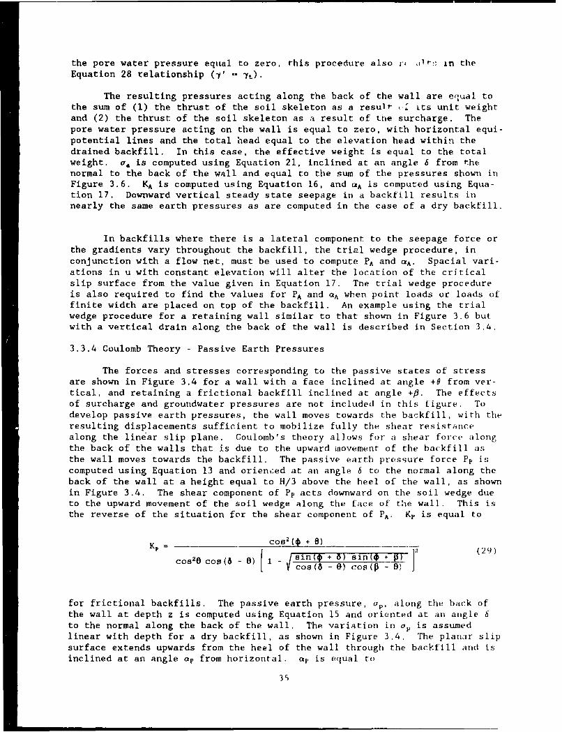
the pore water pressure equal to zero, this procedure also r' .l t- in theEquation 28 relationship (y' -- -t)
The resulting pressures acting along the back of the wall are equal tothe sum of (1) the thrust of the soil skeleton as a result ,L its unit weightand (2) the thrust of the soil skeleton as a result of the surcharge. Thepore water pressure acting on the wall is equal to zero, with horizontal equi-potential lines and the total head equal to the elevation head within thedrained backfill. In this case, the effective weight is equal to the totalweight. a. is computed using Equation 21, inclined at an angle 6 from thenormal to the back of the wall and equal to the sum of the pressures shown inFigure 3.6. KA is computed using Equation 16, and "A is computed using Equa-tion 17. Downward vertical steady state seepage in a backfill results innearly the same earth pressures as are computed in the case of a dry backfill.
In backfills where there is a lateral component to the seepage force orthe gradients vary throughout the backfill, the trial wedge procedure, inconjunction with a flow net, must be used to compute PA and aA. Spacial vari-ations in u with constant elevation will alter the location of the criticalslip surface from the value given in Equation 17. The trial wedge procedureis also required to find the values for PA and QA when point loads or loads offinite width are placed on top of the backfill. An example using the trialwedge procedure for a retaining wall similar to that shown in Figure 3.6 butwith a vertical drain along the back of the wall is described in Section 3.4.
3.3.4 Coulomb Theory - Passive Earth Pressures
The forces and stresses corresponding to the passive states of stressare shown in Figure 3.4 for a wall with a face inclined at angle +0 from ver-tical, and retaining a frictional backfill inclined at angle +f-. The effectsof surcharge and groundwater pressures are not included in this figure. Todevelop passive earth pressures, the wall moves towards the ba'ckfill, with theresulting displacements sufficient to mobilize fully the shear resistancealong the linear slip plane. Coulomb's theory allows for a shear force alongthe back of the walls that is due to the upward movement of the backfill asthe wall moves towards the backfill. The passive earth pressure force Pp iscomputed using Equation 13 and orien,:ed at an angle 6 to the normal along theback of the wall at a height equal to H/3 above the heel of the wall, as shownin Figure 3.4. The shear component of Pp acts downward on the soil wedge dueto the upward movement of the soil wedge along the face of the wall. This isthe reverse of the situation for the shear component of PA- Kp is equal to
KP = Cos, (41 + 8)- -Ssin(, + OF sin(o + 8) 12 (29)
cos 2 C cos(8 - 0) C os( - 0)
for frictional backfills. The passive earth pressure, ap, along the back ofthe wall at depth z is computed using Equation 15 and oriented at an angle 6to the normal along the back of the wall. The variation in ap is assumedlinear with depth for a dry backfill, as shown in Figure 3.4. The planar slipsurface extends upwards from the heel of the wall through the backfill and isinclined at an angle ap from horizontal. ap is equal to
35
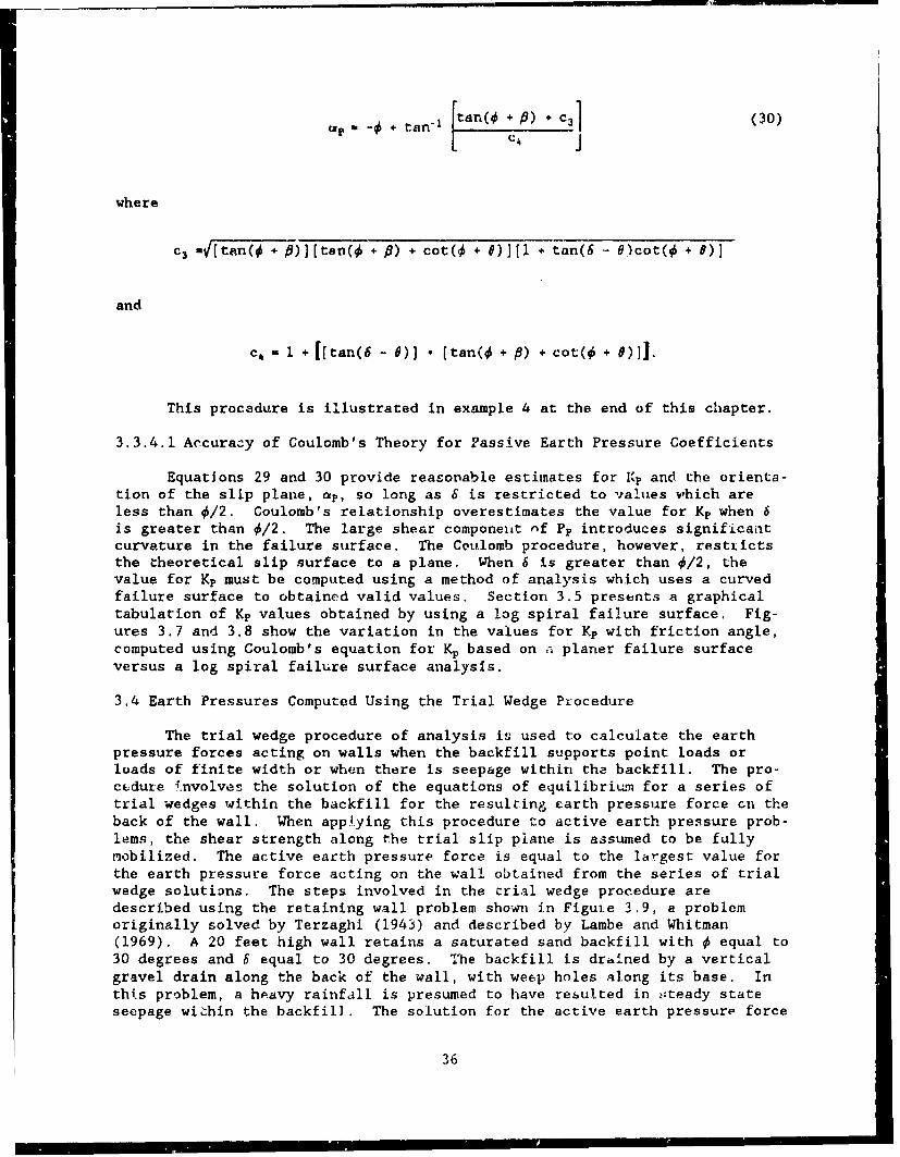
UP, _, + tan.1 tan(O + )+ C3+ (30)C4
where
c3 -*[tan(o + f)] (tan(O + P) + cot(O + j)][1 + tan(6 - O)cot(O + 8)1
and
c = + [[tan(6 - 0)] • [tan(# + P) + cot(O + $)I].
This procedure is illustrated in example 4 at the end of this chapter.
3.3.4.1 Accuracy of Coulomb's Theory for Passive Earth Pressure Coefficients
Equations 29 and 30 provide reasonable estimates for Kp and the orienta-tion of the slip plane, ap, so long as 6 is restricted to values which areless than 0/2. Coulomb's relationship overestimates the value for Kp when 6is greater than 0/2. The large shear componeiit of Pp introduces significantcurvature in the failure surface. The Coulomb procedure, however, resttictsthe theoretical slip surface to a plane. When 6 is greater than 0/2, thevalue for Kp must be computed using a method of analysis which uses a curvedfailure surface to obtained valid values. Section 3.5 presents a graphicaltabulation of Kp values obtained by using a log spiral failure surface. Fig-ures 3.7 and 3.8 show the variation in the values for Kp with friction angle,computed using Coulomb's equation for KP based on a. planer failure surfaceversus a log spiral failure surface analysis.
3.4 Earth Pressures Computed Using the Trial Wedge Procedure
The trial wedge procedure of analysis is used to calculate the earthpressure forces acting on walls when the backfill supports point loads orloads of finite width or when there is seepage within the backfill. The pro-cedure involves the solution of the equations of equilibriu.m for a series oftrial wedges within the backfill for the resulting earth pressure force cn theback of the wall. When applying this procedure to active earth pressure prob-lems, the shear strength along the trial slip plane is assumed to be fullymobilized. The active earth pressure force is equal to the largest value forthe earth pressure force acting on the wall obtained from the series of trialwedge solutions. The steps involved in the trial wedge procedure aredescribed using the retaining wall problem shown in Figui.e 3.9, a problemoriginally solved by Terzaghi (1943) and described by Lambe and Whitman(1969). A 20 feet high wall retains a saturated sand backfill with 0 equal to30 degrees and 6 equal to 30 degrees. The backfill is drained by a verticalgravel drain along the back of the wall, with weep holes along its base. Inthi.s problem, a heavy rainfall is presumed to have resulted in ,.teady stateseepage within the backfil]. The solution for the active earth pressure force
36
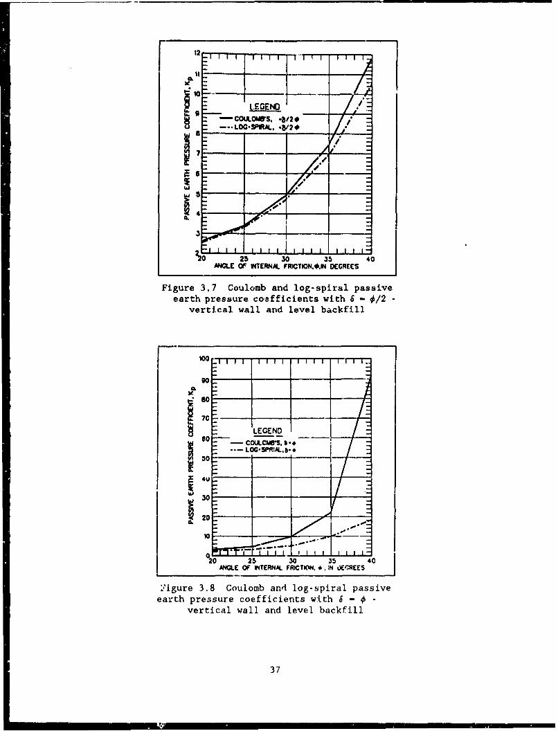
12 I TI I' I l 1 I -F r | -
1 LEGEND-- COUtOMIUS. -/20 /0 -.,Lo-SPIM.. -*V20 /-"
7 /II -- ,--
6 //-
25 30 35 40ANGLE Of INTERNAL. FRICTION.*,IN DEGREES
Figure 3.7 Coulomb and log-spiral passiveearth pressure coefficients with 6 - 0/2
vertical wall and level backfill
I°0 •i~~~~ -T-T- i i I I I I .
go -.- -
7C
LEGEND
~ 50 COLLC.a.ca -#.LOG-SPRIAL. B-
500
4U '
w3 0 -
C20
25 30 35 40ANGLE OF ITERNA. FRICTKIN, #,,N i',•REES
2'1gure 3.8 Coulomb and log-spiral passiveearth pressure coefficients with 6 - 0
vertical wall and level backfill
37
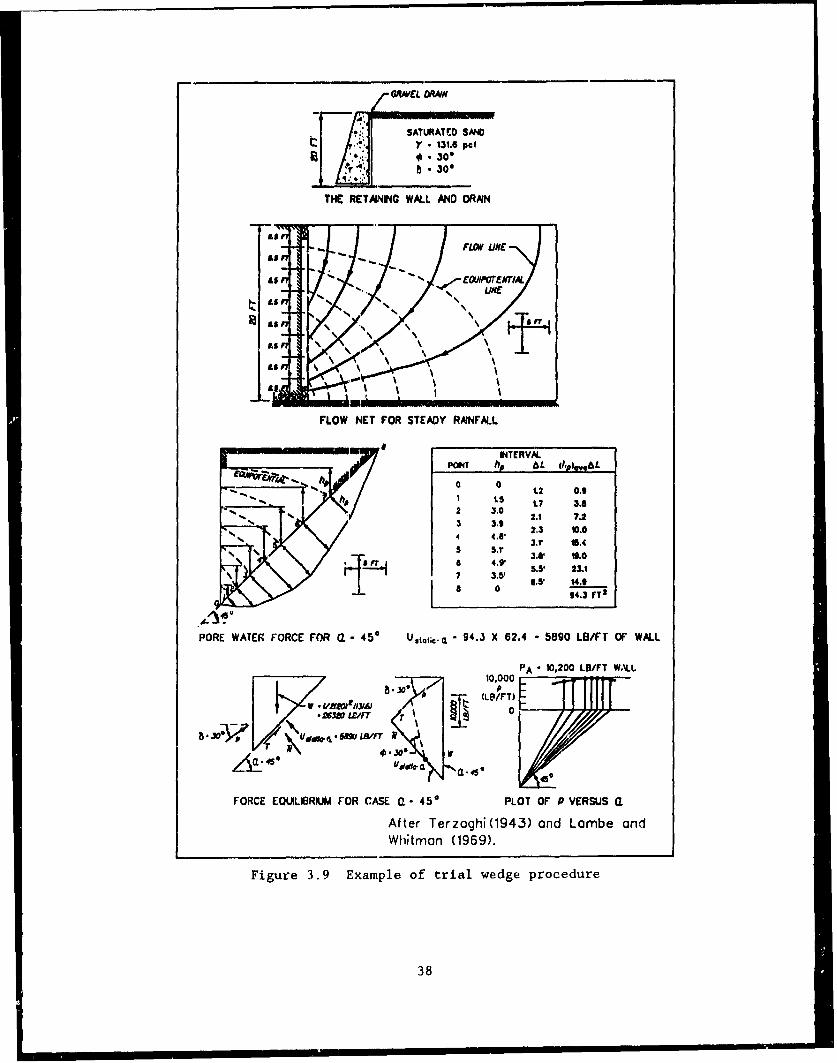
IG AVEL D"N
SATURATED SANDV *1.31.6 pcf*30*
THE RETAIN•NG WALL ANDRAIN
TLOW R ET WOR US A RA NF
asa
NITERVNALPO Li 7 p' AL __.,p,,,&L
Z 1.0 2 C.ihal-1 1•s- 07 3.8
"-2 •.0 2. 7.23 3.1
4 .1 .3 10.0O 3.T O.R, ,_ .3.6' .. 0
B 4.V 5.51 23.17 3.5' O. 14.9
0-L 94.3 IrT2
PORE WATER FORCE FOR a- 450 U.tt•-. " 94.3 X 62.4 5890 LB/FT OF WALL
PA 10,200 LB/FT WAL10, 10,000, -- 5.xo~ooo
I / , 8.,DotAII _ -•,,,*LtLtOLG/F r
I. ' /I? .,' r 0e. I 1-
FORCE EQUILIBRIUM FOR CASE a - 450 PLOT OF P VERSUS Aa
After Terzaghi (1943) and Lambe arndWhitman (1969).
Figure 3.9 Example of trial wedge procedure
38
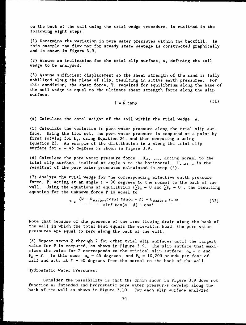
on the back of the wall using the trial wedge procedure, is outlined in thefollowing eight steps.
(1) Determine the variation in pore water pressures within the backfill. Inthis example the flow net for steady state seepage is constructed graphicallyand is shown in Figure 3.9.
(2) Assume an inclination for the trial slip surface, a, defining the soilwedge to be analyzed.
(3) Assume sufficient displacement so the shear strength of the sand is fullymobilized along the plane of slip, resulting in active earth pressures. Forthis condition, the shear force, T, required for equilibrium along the base ofthe soil wedge is equal to the ultimate shear strength force along the slipsurface.
T = N tan4 (31)
(4) Calculate the total weight of the soil within the trial wedge, W.
(5) Calculate the variation in pore water pressure along the trial slip sur-face. Using the flow net, the pore water pressure is computed at a point byfirst solving for hp, using Equation 24, and then computing u usingEquation 25. An example of the distribution in u along the trial slipsurface for a - 45 degrees is shown in Figure 3.9.
(6) Calculate the pore water pressure force , Ust.tjc_*, acting normal to thetrial slip surface, inclined at angle a to the horizontal. Ust~tic-* is theresultant of the pore water pressures calculated in step (5).
(7) Analyze the trial wedge for the corresponding effective earth pressureforce, P, acting at an angle 6 - 30 degrees to the normal to the back of Lhewall. Using the equations of equilibrium (XF. - 0 and XFY - 0), the resultingequation for the unknown force P is equal to
p = (W - Ustaticacosa) tan(a - 4) + Ustatica sina (32)sin6 tan(a - 4) + cos6
Note that because of che presence of the free flowing drain along the back ofthe wall in which the total head equals the elevation head, the pore waterpressures are equal to zero along the back of the wall.
(8) Repeat steps 2 through 7 for other trial slip surfaces until the largestvalue for P is computed, as shown in Figure 3.9. The slip surface that maximizes the value for P corresponds to the critical slip surface, aA - a andPA - P. In this case, aA - 45 degrees, and PA - 10,200 pounds per foot ofwall and acts at 6 - 30 degrees from the normal to the back of the wall.
Hydrostatic Water Pressures:
Consider the possibility is that the drain shown in Figure 3.9 does notfunction as intended and hydrostatic pore water pressures develop along theback of the wall as shown in Figure 3.10. For each slip surface analyzed
39
h\YDAOSrfTATC ORNAL DRAINWATER T"ALE UNCFFECTAN"-\
SATURATED SAND p* 131.6 pcf *"f*30*
o - 30*
RETAINING WALL WITH HYDROSTATICWATER TABLE AT TOP OF BACKFILL
FOR HYDROSTATIC WATER TABLE
U Static V V2 Y' H 2
. Vl(62.4)(20)2 . 12.480 LB/FT OF WALL
NORMAL TO SLIP PLANE C.L- 54.3*(Refer to Figure A.2)
Ustatic.- " U static g; 54
si 54.30
Ustatic." - 15.368 LB/FT OF WALL
PLOT OF P VERSUS a
4500 - PA - 4113 LB/FT
4000
3500
3000
2500
j 2000
1500 -
1000
500 - a - 54.30 I I I I I I I80 75 70 65 60 55 50 45 40 35 30
a.. DEGREES
Figure 3.10 Example of trail wedge procedure, hydrostaticwater table
40
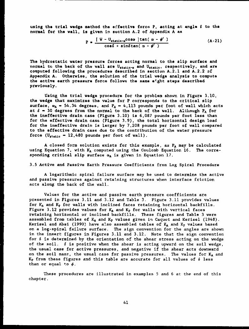
using the trial wedge method the eirfective forcit P, acting at angle 6 to the
normal for the wall, is given in section A.2 of Appendix A as
p [ W - Uutetit..cosa I tan( a - •' ) (A-21)
cos6 + sin6tan( a - 0 )
The hydrostatic water pressure forces acting normal to the slip surface andnormal to the back of the wall are Ust,•tic. and Umtitc, respectively, and arecomputed following the procedures described in section A.2.1 and A.2.2 ofAppendix A. Otherwise, the solution of the trial wedge analysis to computethe active earth pressure force follows the same e.ght steps describedpreviously.
Using the trial wedge procedure for the problem shown in Figure 3.10,the wedge that maximizes the value for P corresponds to the critical slipsurface, cA - 54.34 degrees, and PA - 4,113 pounds per foot of wall which actsat 6 - 30 degrees from the normal to the back of the wall. Although PA forthe ineffective drain case (Figure 3.10) is 6,087 pounds per foot less thanfor the effective drain case (Figure 3.9), the total horizontal design loadfor the ineffective drain is larger by 7,208 pounds per foot of wall comparedto the effective drain case due to the contribution of the water pressureforce (Ustati. - 12,480 pounds per foot of wall).
A closed form solution exists for this example, as PA may be calculatedusing Equation 7, with KA computed using the Coulomb Equation 16. The corre-sponding critical slip surface aA is given in Equiation 17.
3.5 Active and Passive Earth Pressure Coefficients from Log Spiral Procedure
A logarithmic spiral failure surface may be used to determine the activeand passive pressures against retaining structures when interface frictionacts along the back of the wall.
Values for the active and passive earth pressure coefficients arepresented in Figures 3.11 and 3.12 and Table 3. Figure 3.11 provides valuesfor KA and Kp for walls with inclined faces retaining horizontal backfills.Figure 3.12 provides values for KA and Kp for walls with vertical facesretaining horizontal or inclined backfills. These figures and Table 3 wereassembled from tables of KA and Kp values given in Caquot and Kerisel (1948).Kerisel and Absi (1990) have a!so assembled tables of KA and Kp values basedon a log-spiral failure surface. The sign convention for the angles are shownin the insert figures in Figures 3.11 and 3.12. Note that the sign conventionfor 6 is determined by the orientation of the shear stress acting on the wedgeof the soil. 6 is positive when the shear is acting upward on the soil wedge,the usual case for active pressures, and negative if the shear acts downwardon the soil masE, the usual case for passive pressures. The values for KA andKp from these figures and this table are accurate for all values of 6 lessthan or equal to 4.
These procedures are illustrated in examples 5 and 6 at the end of thischapter.
41
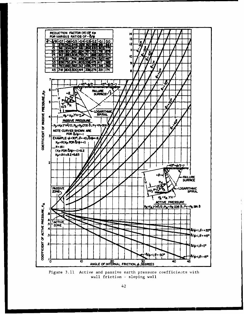
REDUCTION )OVPFOR VARIOUS RATIOS OF - a/# 13 1 y V
ANý 1-07 1 1-041-0 Q0 -1 141375 12 _4.9611 11 - 00 1
20 MmIli 5,04 1 0,0 - % I
25 W4
ft I10
41,9 's
45 YIS .1,
7 117I Jr I I6 A1A F
5-
46Wt5WpzKpMM MESSUREFOSSIVE PRESSURE
-Pp-KPYH2V2;MNxMP0()S BiPTapp!SIN
NOTE:CURYES S"DWN ARE3 FOR
OFKpxR(KpFQR8V#z-I)
_R2.811 A / 01' 100'IKPFDR84z-l)s&2 00or OF F
KpahlimS.2a 5
2 '.000 Ll -1 1
?0 t!ý -
I
P"AILURE14
PfA SU
FASSIVE LOGARITHMIC
"I SPIRAL
Or CIA a KA YMACTIVE PRESSURE
PA'KAYH2MPNrPA 2PA SIN 8
'5 -ZONE OMAN -ftm mmm;z,-Nam I-AM
on nu-
ft*Aft
_.q -1, :003/4
0 10 20 30 40 45ANGLE OF INTERNAL FRICTIOIN, #,DEGREES
Figure 3.11 Active and passive earth pressure coefficieats V)ith
wall friction - sloping wall
42
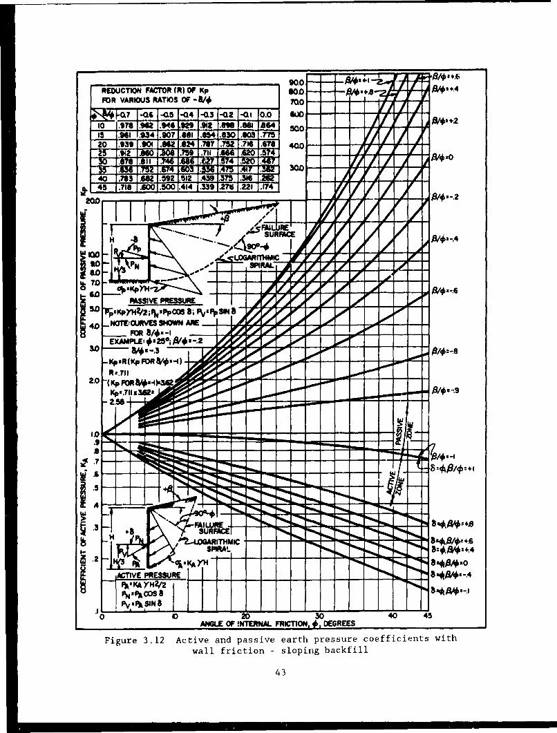
REDUCTION FACTOR (R) OF Kp 90.0FOR VARIOUS RATIOS OF-/ Too � A
0.7 .Q6-C05 -04-0.3 -02 -010.0 &jo -- -- A4*+2410 -978 1 "2 .944 .929 912 M1 .84 1364 500- --- _
15 1.961 .934 .907 .6681 .054 .830 60M3 77520 .939 1.901 .6ft .624 .767 .752 .716 676 .0 - - -
25 1.912 .660 JI .711 .620 1.57 ".030 .178 .o 0~ 11 "G..m .57n4 1. 1 64
40 .763 66 .I~512 1.439 .375 .346 .2a
45 .718 i .414 1.3391.27 rrr 17
200 OF A4--.
20
/Zw0R-M~ 1 - .00-
5, .2 Fl'KAYH/2;P'P ;P -P I .0OO 10- 00
40GL O- NOTE.CURVE FRICTO AEGEE
Fig Re 3.212 Acie n0psiv0athpesr cofienswtwaLE frcto 250 slpigbakfl
&0 - &*X43
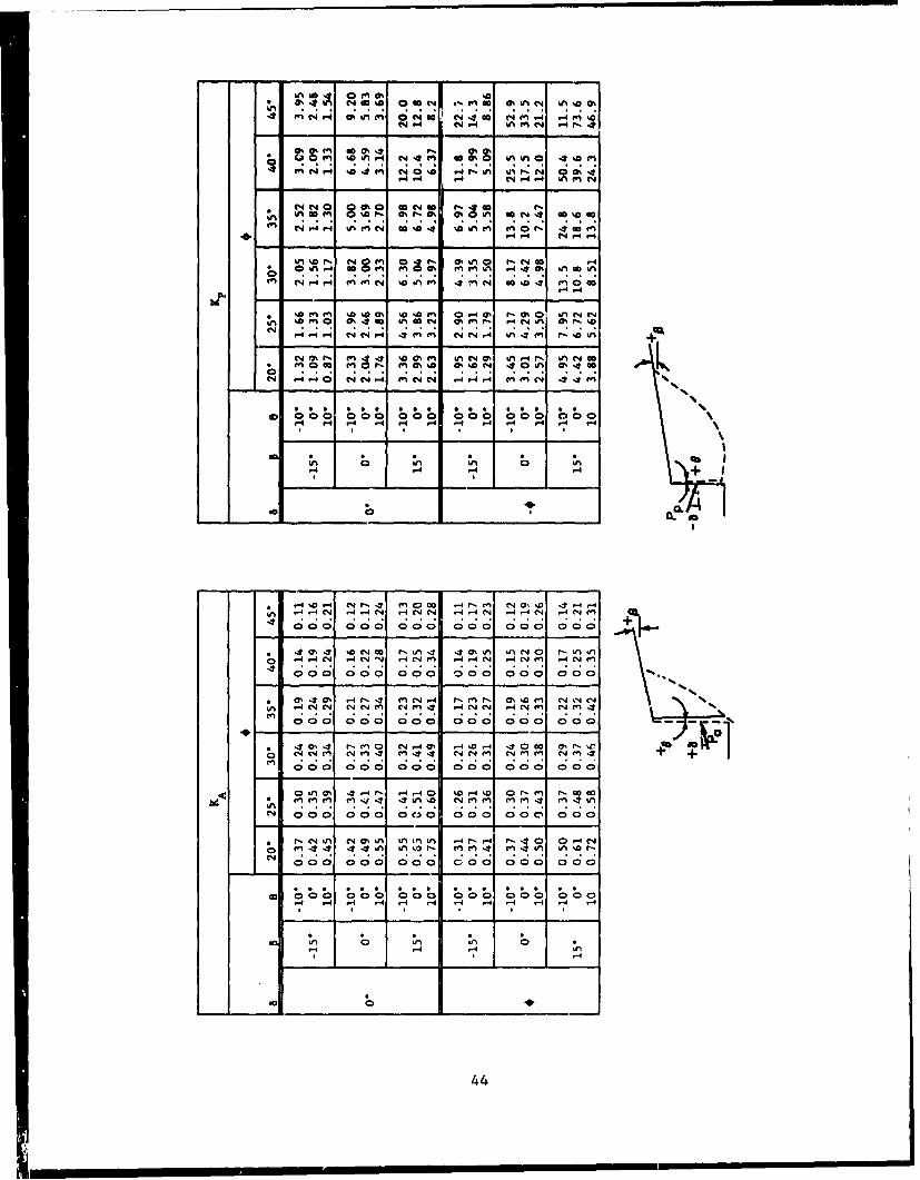
fnNP4 ik 0 N 40 M N ~ IA 00 4 14 %IN P4 N.."4 kVn n4 -4 rl4
(4n C4 %D en U 0%0 4 P* o 1%A % 4
C4 N 0 4 8 VA OR ~ C440 r o ra*m % r.l~ I0 rý Et % V, cc C,4t .- 40' %D so1
f4 m m
%O 460 ccNUt1 .4 A Ut%
I-.-. en ~ aý o ud 4 arn f.-4 Ut4 % a r-.~l %
0 0. %n 0 .
i .! ý .i e! . ý ý . ý . ! . . .* . *
14 4 - .4 V - ý.4 ..4 14 M. 4 M
I4 %D -I C4r 00 - Ifn C
C% %0 C4c Utn mu~ nV 0 Ir- Ik4 40 I 4 -4 I -4 1-0 4 4e 4 N.&I
* 4 .-410.- 4 NIJ C E 1t0 -4 C49 C-4% M C-4..fn
,1 0 0 0 ,M0 000 000 00o 4 0 0003,rIrv
* -~4 C4 N6 A ~ t 4U"u .rt'J mi4ý .. .4 li-4 .- E-4 .- 4'4 .- 4NE"! 7
000 000 00C,0 Q Q0 0 00 000
Q 0.40 4-r- 0 koJ~ r.I'4~ %D fe~ 0 P m P'Goco
000 000 00C)0 000 000 000
*4 0. 4 Nr -4 C~ 40 .-4.. 4 -40 -4 4
0 '4 ~ cJ~4 M4 NNkNI~ n~.
aI ~ ~ 000 00 00 0 0 00 00
Ut M~I *u-'O NE~I' etI~444iI
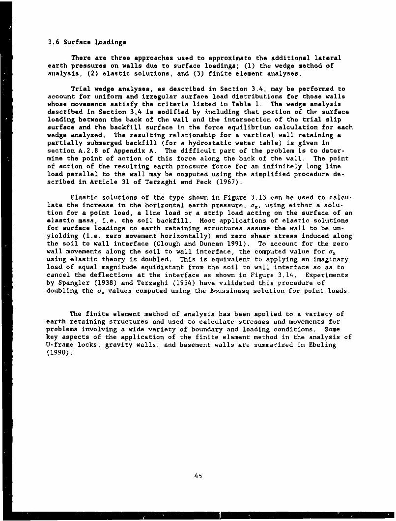
3.6 Surface Loadings
There are three approaches used to approximate the additional lateralearth pressures on walls due to surface loadings; (1) the wedge method ofanalysis, (2) elastic solutions, and (3) finite element analyses.
Trial wedge analyses, as described in Section 3.4, may be performed toaccount for uniform and irregular surface load distributions for those wallswhose movements satisfy the criteria listed in Table 1. The wedge analysisdescribed in Section 3,4 is modified by including that portion of the surfaceloading between the back of the wall and the intersection of the trial slipsurface and the backfill surface in the force equilibrium calculation for eachwedge analyzed. The resulting relationship for a vertical wall retaining apartially submerged backfill (for a hydrostatic water table) is given insection A.2.8 of Appendix A. The difficult part of the problem is to deter-mine the point of action of this force along the back of the wall. The pointof action of the resulting earth pressure force for an infinitely long lineload parallel to the wall may be computed using the simplified procedure de-scribed in Article 31 of Terzaghi and Peck (1967).
Elastic solutions of the type shown in Figure 3.13 can be used to calcu-late the Increase in the horizontal earth pressure, a., using either a solu-tion for a point load, a line load or a strip load acting on the surface of anelastic mass, i.e. the soil backfill. Most applications of elastic solutionsfor surface loadings to earth retaining structures assume the wall to be un-yielding (i.e. zero movement horizontally) and zero shear stress induced alongthe soil to wall interface (Clough and Duncan 1991). To account for the zerowall movements along the soil to wall interface, the computed value for a.using elastic theory is doubled. This is equivalent to applying an imaginaryload of equal magnitude equidistant from the soil to wall interface so as tocancel the deflections at the interface as shown in Figure 3.14. Experimentsby Spangler (1938) and Terzaghi (1954) have vilidated this procedure ofdoubling the a, values computed using the Boussinesq solution for point loads.
The finite element method of analysis has been applied to a variety ofearth retaining structures and used to calculate stresses and movements forproblems involving a wide variety of boundary and loading conditions. Somekey aspects of the application of the finite element method in the analysis ofU-frame locks, gravity walls, and basement walls are summarized in Ebeling(1990).
45
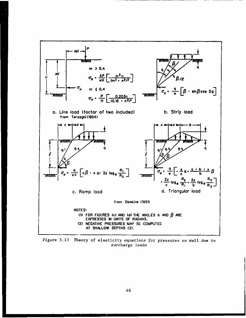
1 m 0o.4 q
H m•0." Pnv .N L(0.6 n2)2 J
a. Line load (factor of two included) b. Strip loadfrom Torzoghi (1954)
2 R2 2q1 R
OH~~2 vog [c l a z oog2e
7- lo o - V + 02 R 2 2 zR 2c. Ramp load d. Triangular load
from Dowkins (1991)
NOTES:
(1) FOR FIGURES (c) AND (d) THE ANGLES a AND R AREEXPRESSED IN UNITS OF RADIANS.
(2) NEGATIVE PRESSURES MAY BE COMPUTEDAT SHALLOW DEPTHS (Z).
Figure 3.13 Theory of elasticity equations for pressures on wall due to
surcharge loads
46
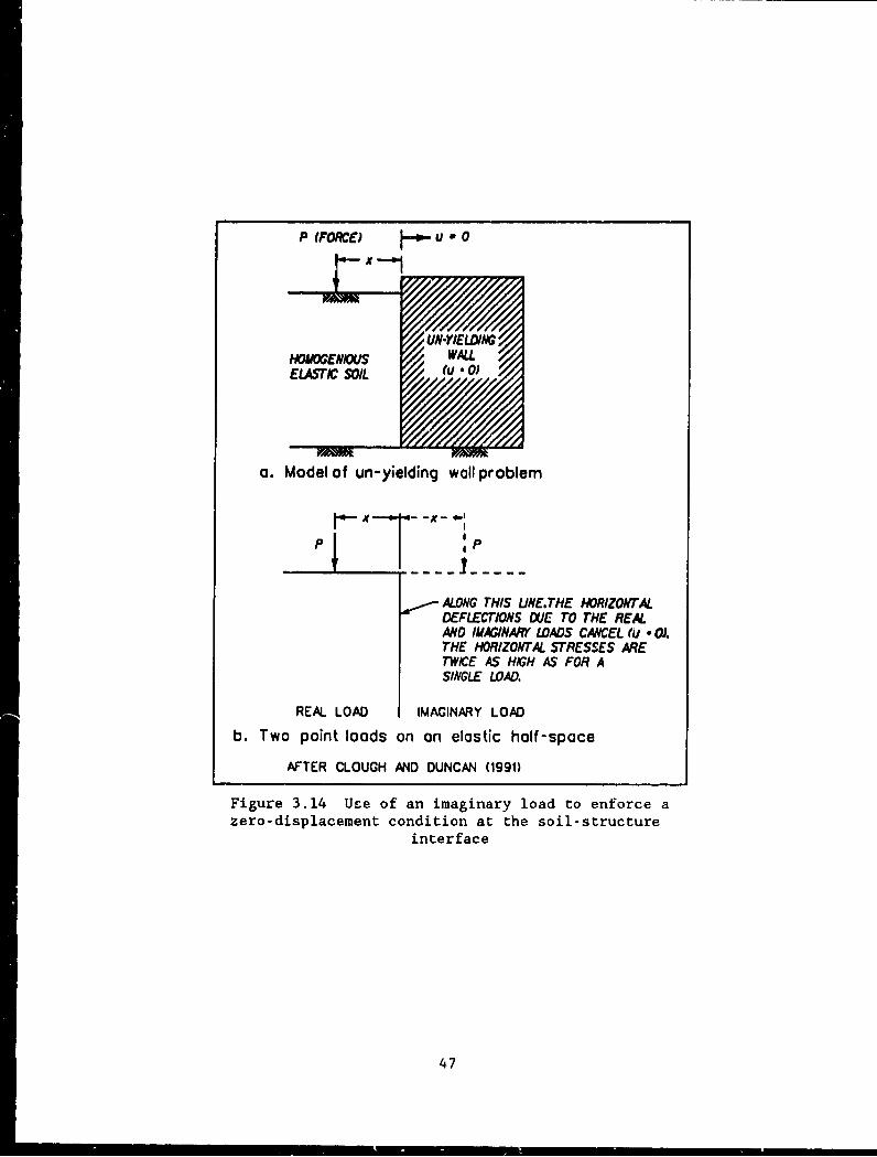
P (FORMC) U a 0
UN.YIELDINGHOOGENIOUS , WALLELASTIC SOIL (u 0)
a. Model of un-yielding wall problem
P _T ip
ALONG THIS UNE.THE HORIZONTALDEFLECTIONS DUE TO THE REALAND IMAGINARY LOADS CANCEL (u - 0).THE HORIZONTAL 5TrESSES ARETWICE AS HIGH AS FOR ASINGLE LOAD.
REAL LOAD IMAGINARY LOAD
b. Two point loads on an elastic half-space
AFTER CLOUGH AND DUNCAN (1991)
Figure 3.14 Use of an imaginary load to enforce azero-displacement condition at the soil-structure
interface
47
CHAPTER 3 - EXAMPLES
Contents
Example Problems 1 through 6.
Commentary
The following examples illustrate the proceduresdescribed in Chapter 3. The results of the computa-tions shown are rounded for ease of checking calcula-tions and not to the appropriate number of significantfigures. Additionally, the values assigned to vari-ables in these problems were selected for ease ofcomputations.
48
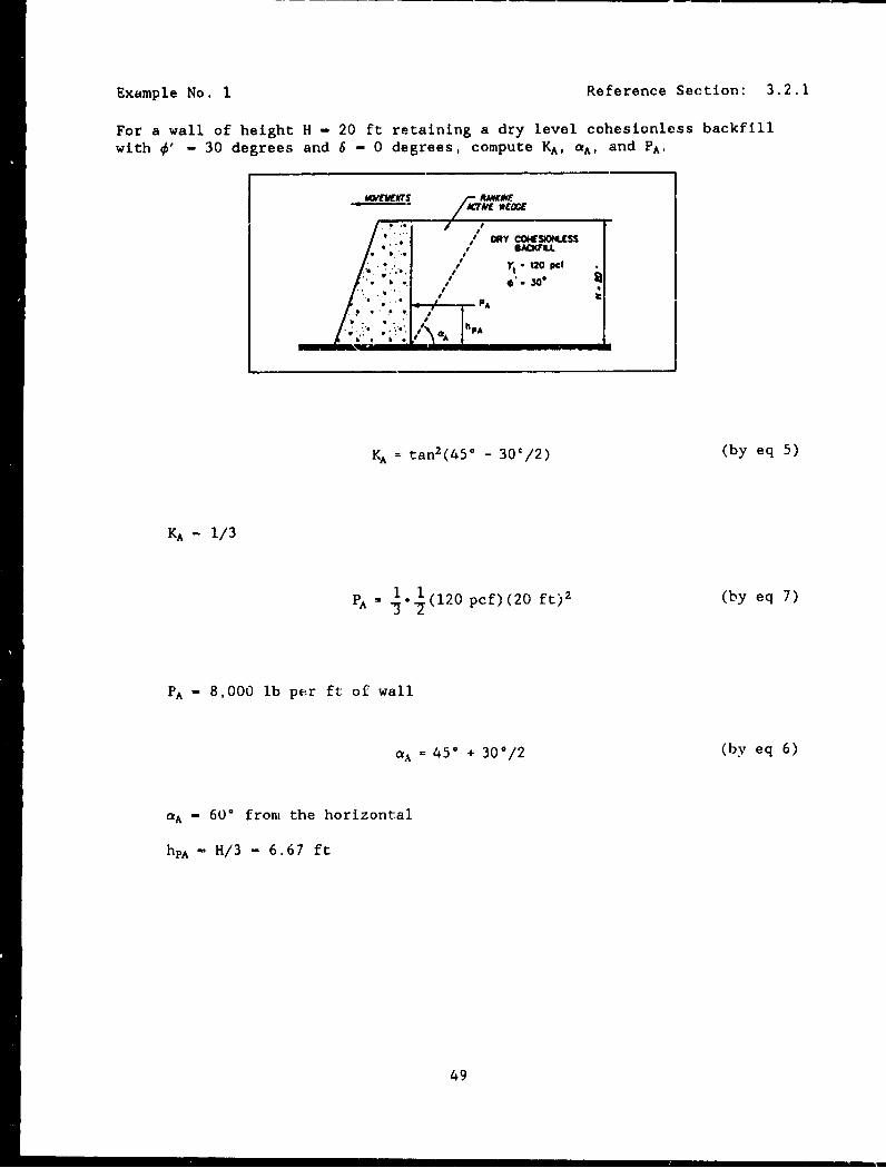
Example No. 1 Reference Section: 3.2.1
For a wall of height H - 20 ft retaining a dry level cohesionless backfillwith ' - 30 degrees and 6 - 0 degrees, compute KA, aA, and PA.
sORqY COWSOUNLSSSACKFTLL
(120120 PiI 0 ° 30*
•. ... F--PA
KA :tan2(45o - 30'/2) (by eq 5)
KA - 1/3
PA - -j -(120 pcf) (20 ft)2 (by eq 7)
PA - 8,000 lb per ft of wall
A= 450 + 300/2 (by eq 6)
aA - 60° from the horizontal
hpA- H/3 - 6.67 ft
49

Example No. 2 Reference Section: 3.2.2
For a wall of height H - 20 ft retaining a dry level cohesionless backfillwith 4" - 30 degrees and 6 - 0 degrees, compute Kp, ap, and Pp.
SPASSAE WWD2•
t," i 120 Pe .. ,,
'',,, • " .30"
.v - tan2 (450 + 300/2) (by eq 11)
Kp - 3.0
S= 3.0 - 1(120 pcf)(201) 2 (by eq 13)
Pp- 72,000 lb per ft of wall
up = 450 - 30o/2 (by cq 12)
up - 300 from the horizontal
hpp - H/3 - 6.67 ft
50
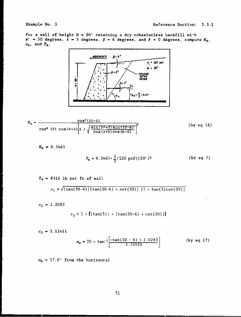
Example No. 3 Reference Section: 3.3.1
For a wall of height H - 201 retaining a dry cohesionless backfill wi*-h0' - 30 degrees, 6 - 3 degrees, f - 6 degrees, and 0 - 0 degrees, compute KA,
QA, and PA.
UW•EUE•rS • = B
Yt -120 Pd# - 300
7 o90 W 20 p
A 3
KA - 0. 3465
S= 0.3465. (120 pcf)(20' ) (by eq 7)
PA - 8316 lb per ft of wall
.cl = j/[tan(30-6)][tan(30-6) + cot(30)] [I + tan(3)cot(30)]
cl - 1.3283
c2 = I + [[tan(3)] • [tan(30-6) + cot(30)]]
c2 - 1.11411
aA = 30 + tan-i -tan(30 - 6) + 1.0283 (by eq 17)
a - 57.6' from the horizontal
51
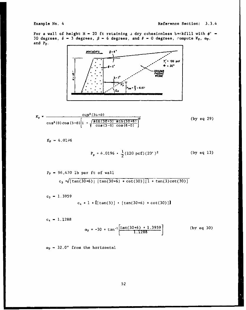
Example No. 4 Reference Section: 3,3.4
For a wall of height H - 20 ft retaining a dry cohesionless bmr.kfill with 0' -30 degrees, 6 - 3 degrees, / - 6 degrees, and 9 - 0 degrees, (-'ompute Kp, akp,
and Pp.
", 0"0* 30"
* i. Y* PA2S O* * * * e ,, P H .,
* Q l -- , 4$~
Kp --
co1() s c"O) -si(3 0÷3}0 si(06cos(O)OS(3~) 1 1 - COS(3-0) Cos (6-O)2 ll3$)Bf(0+6 bye 9
Kp- 4.0146
S= 4.0196 * 1(120 pcf)(20' )2 (by eq 13)
Pp - 96,470 lb per ft of wall
c3 =[tan(30+6)j [tan(30+6) + cot(30)][l + tan(3)cot(30)]
c3- 1. 3959
c4= 1 + [[tan(3)] • [tan(30+6) + cot(30)]J
c4- 1. 1288
= 3 a [tan(30+6).28 + 1.3959] (by eq 30)
•p- 32.00 from the horizontal
52
Example No. 5 Roference Section: 3.4
For the Example No. 3 problem of a wall retaining a dry cohesionless backfillwith 0' - 30 degrees, 6 - +3 degrees, P - +6 degrees, and e - 0 degrees,compute KA using the log rpiral procedure of Figure 3.12. Compare this valuewith tho KA value computed in Example No. 3 using che Coulomb relationship.
610 - +0,1 and #/1 - +0.2
KA - 0.35 from Figure 3.12 with 0/0 - '0.2 and using the curve for 6 -
This value for KA agrees with the value computed using Coulomb's theory foractive earth pressures in Example No. 3 ( K^ - 0.3465).
53
Example No. 6 Reference Section: 3.4
For the Example No. 4 problem of a wall retaining a dry cohesionless backfillwith 0 - 30 degrees, 6 - -3 degrees*, P - +6 degrees, and 9 - 0 degrees, com-pute Kp. Compare this value with the Kp value computed in Example No. 4.
6 - -0.1 and P/4 - +0.2
R (for 6/1 - -0.1) - 0.52 and Kp (for // - +0.2) - 8 from Figure 3.12
Kp (for 6/1 -0.1) - [R (for 6/1 - -0.l)]'[Kp (for P/0 - +0.2)]- 0.52 8- 4.16
The value for Kp is nearly the same as the value computed using Coulomb's the-ory for passive earth pressures in Example No. 4 (K1 - 4.0196) because 6 < 0/2(Section 3.3.4.1). The resultant force vector Pp acts in the same directionas shown in the Enample No. 4 figure.
* Note the difference in sign for 6 in the passive earth pressure solution
using the Figure 3.12 log spiral solution procedure compared to that used inthe Coulomb's solution, with sign convention as shown in Figure 3.4.
54
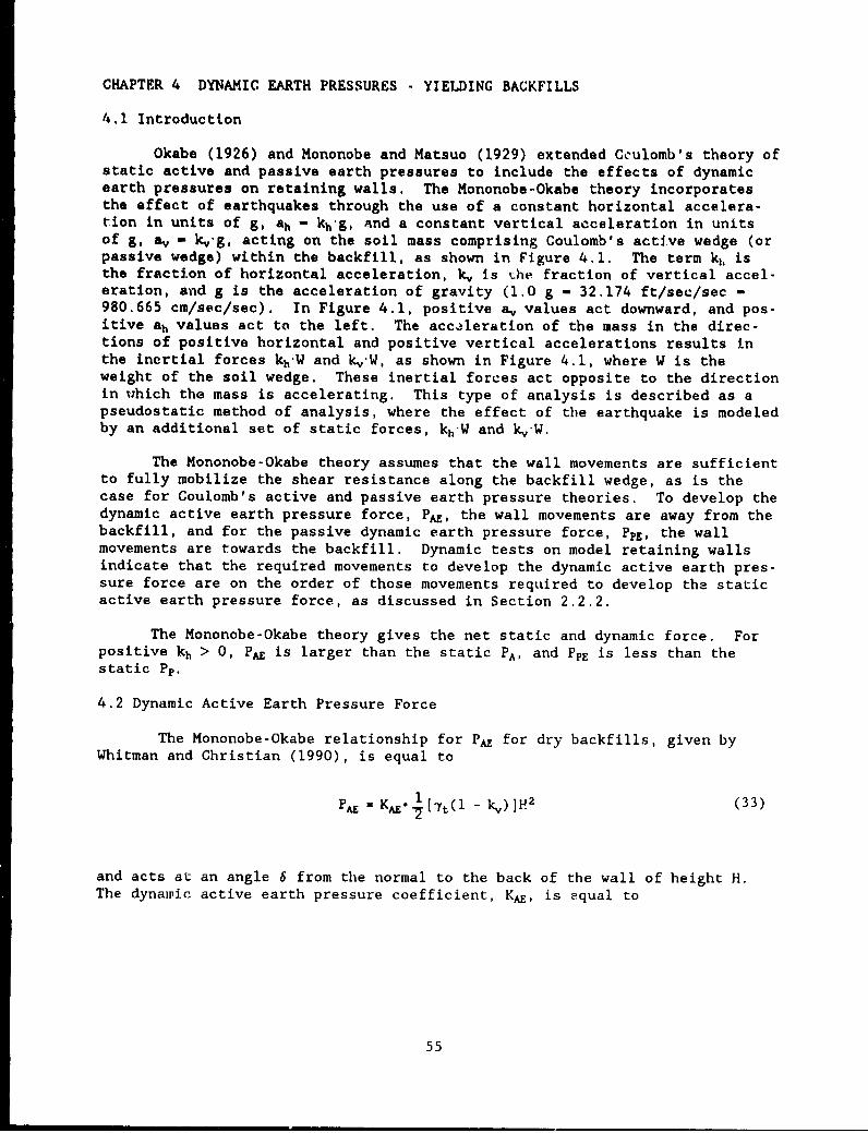
CHAPTER 4 DYNAMIC EARTH PRESSURES - YIELDING BACKFILLS
4.1 Introduction
Okabe (1926) and Mononobe and Matsuo (1929) extended Cculomb's theory ofstatic active and passive earth pressures to include the effects of dynamicearth pressures on retaining walls. The Mononobe-Okabe theory incorporatesthe effect of earthquakes through the use of a constant horizontal accelera-tion in units of g, ah - kh'g, and a constant vertical acceleration in unitsof g, av - k,-g, acting on the soil mass comprising Coulomb's active wedge (orpassive wedge) within the backfill, as shown in Figure 4.1. The term ki, isthe fraction of horizontal acceleration, k, is Ohe fraction of vertical accel-eration, and g is the acceleration of gravity (1.0 g - 32.174 ft/sec/sec -980.665 cm/sec/sec). In Figure 4.1, positive a, values act downward, and pos-itive ah values act to the left. The acceleration of the mass in the direc-tions of positive horizontal and positive vertical accelerations results inthe inertial forces kh'W and kv'W, as shown in Figure 4.1, where W is theweight of the soil wedge. These inertial forces act opposite to the directionin which the mass is accelerating. This type of analysis is described as apseudostatic method of analysis, where the effect of the earthquake is modeledby an additional set of static forces, kh-W and kv-W.
The Mononobe-Okabe theory assumes that the wall movements are sufficientto fully mobilize the shear resistance along the backfill wedge, as is thecase for Coulomb's active and passive earth pressure theories. To develop thedynamic active earth pressure force, PA, the wall movements are away from thebackfill, and for the passive dynamic earth pressure force, PPE, the wallmovements are towards the backfill. Dynamic tests on model retaining wallsindicate that the required movements to develop the dynamic active earth pres-sure force are on the order of those movements required to develop the staticactive earth pressure force, as discussed in Section 2.2.2.
The Mononobe-Okabe theory gives the net static and dynamic force. Forpositive kh > 0, PA is larger than the static PA, and PPE is less than thestatic Pp.
4.2 Dynamic Active Earth Pressure Force
The Mononobe-Okabe relationship for PA for dry backfills, given byWhitman and Christian (1990), is equal to
S= KA. [Tt(l - k")]p 2 (33)
and acts at an angle 6 from the normal to the back of the wall of height H.The dynawic active earth pressure coefficient, KA, is equal to
55
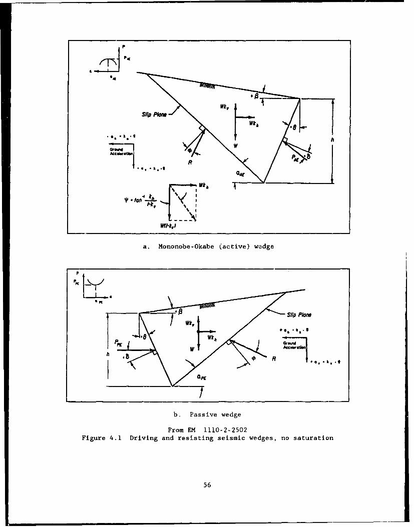
Pit
slip Plcn
.* .W *e
BW
a. Mononobe-Okabe (active) wedge
aP
b. Passive wedge
From EM 1110-2-2502Figure 4.1 Driving and resisting seismic wedges, no saturation
56
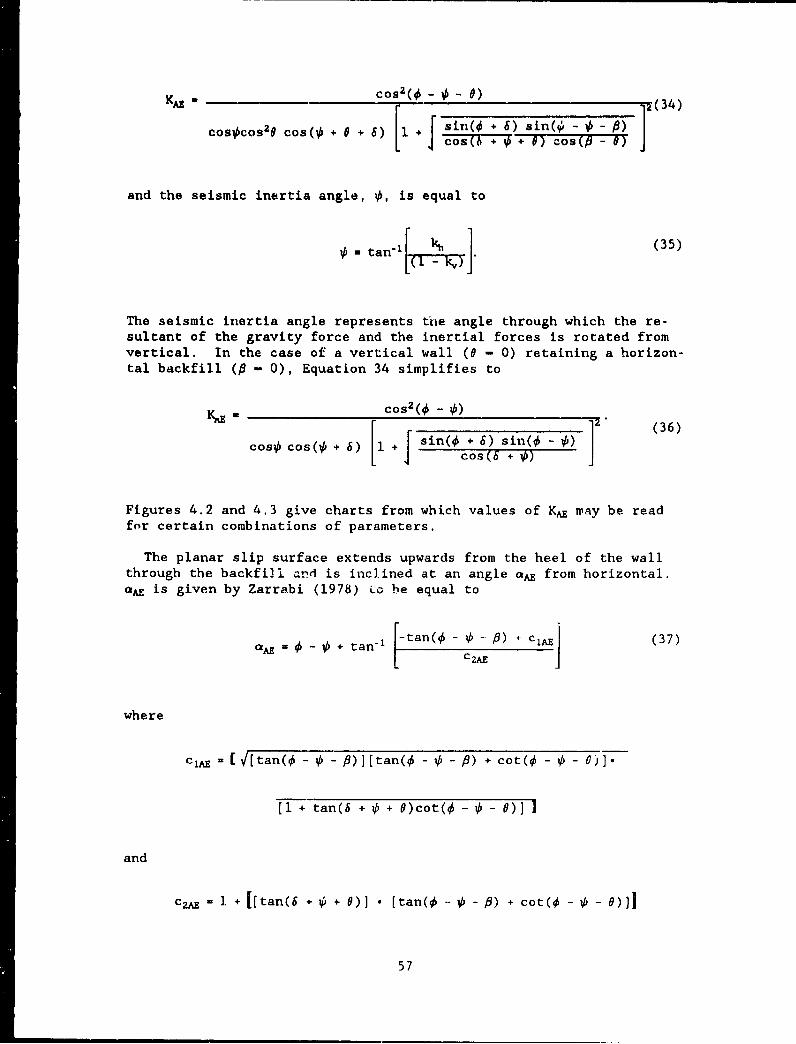
KAS ___ _ cosa(O 0 -6)
Coso'cos2 p COS(Oi + a 6) 1. + [sin(O + 6) sin(O - 0- P)
JCos ( + 0 77) Cos (P - 9
and the seismic inertia angle, 0, is equal to
0 - ta-1 1.(35)
The seismic inertia angle represents the angle through which the re-sultant of the gravity force and the inertial forces is rotated fromvertical. In the case of a vertical wall (8 - 0) retaining a horizon-tal backfill (8 " 0), Equation 34 simplifies to
KSE - cos 2 (0 - )6)
cosO cos( + 6) 1 + sin(O + 6) sin(3 - 6)I t ~Cos (5 + 0) 1
Figures 4.2 and 4.3 give charts from which values of KA way be readfor certain combinations of parameters.
The planar slip surface extends upwards from the heel of the wallthrough the backfill and is inclined at an angle aA from horizontal.aA is given by Zarrabi (1978) Lo be equal to
a= - 0 - 0 + tan-' [tan(O - - ) + C1AE] (37)C2AE
where
cj=[ y[tan(O - 0- •)][tan(O - 1 - P) + cot(O - 0 - 0)].
[I + tan(6 + 0 + 0)cot( -4 - 9)] 1
and
C2M + [[tan(6 + 4 + 0)] • [tan(O --4 - 8) + cot(4 - 4 - 0)11
57

0.7 - 0.7 -
ke .0/8. U kv 0O.--• -35" / -35'
0.6 0-6
0.5 - - -- 0.5 - - -
0.4 0.4 0.
0. 3 0.3
0.2 0.2DRY SANSeY -,a. h tnY S(9,0Y
p: p. .
0.1p p
o., o.,/ K /27
(a) I / I 0 1(0) 1
0 0.1 0.2 0.3 0.4 0.5 0 0.1 0.2 0.3 0.4 0.5
kh kh
From Seed and Whitman (1970).
Figure 4.2 Variation in KAE and KAE cos 6 with kh
07k%# -0-0- 0 .
1/2 q6 30 000.6 -- 0.6 - -
/!.350 0-00.5 -0.5
7
I 0.4 -7 -40 0.4--
0.3 - 0.3- - - -
0.20.350
0.1 0.11 /20
0(a) (b) .0 0.1 0.2 0.3 0.4 0.5 0 0.1 0.2 0.3 0.4 0.5
kh k
From Seed and Whitman (1970).
Figure 4.3 Vari.ation in KAZ'cos 6 with kh, 4', and fi
58
Figures 4.4 and 4,5 give aA as a function of 0 for several values of 0 forvertical walls retaining level backfills.
A limited number of dynamic model retaining wall tests by Sherif andFang (1983) and Ichihara and Matsuzawa (1973) on dry sands show 6 to rangefrom 0/2 to 20/3, depending upon the magnitude of acceleration.
These procedures are illustrated in examples 7 and 8 at the end of thischapter.
The validity of the Mononobe-Okabe theory has been demonstrated by theshaking table tests described in Section 2.2.1. These tests were conducted atfrequencies much less than the fundamental frequency of the backfill, so thataccelerations were essentially constant throughout the backfill. Figure 4.6gives a comparison between predicted and measured values of the seismic activepressure coefficient K•.
An alternati.ve method for determining the value of KAE using tabulatedearth pressures was developed by Dr. I. Arango in a personal communication, asdescribed by Seed and Whitman (1970). Dr. Arango recognized that by rotatinga soil wedge with a planar slip surface through the seismic inertia angle, theresultant vector, representing vectorial sums of W, kh'W and k W, be-omes ver-tical, and the dynamic problem becomes equivalent to the static problem, asshown in Figure 4.7. The seismic active pressure force is given by
f = [KA(f. .).FA].E [t(l - k,)]H2 (38)
where
H - actual height of the wall* -+ '0
and
cos2 (a + •) (39)cosO cos2o
Sis computed using Equation 35. Values of FA are also given as a functionof 0 and 0 in Figure 4.8. KA(P*,O*) is determined from the Coulomb static KAvalues by Equation 16. An alternative procedure is to approximata KA(#*,O*)by using the static KA values that were tabulated by Caquot and Kerisel (1948)or Kerisel and Absi (1990) as given in Table 3. The product of KA(p*,O*)times FA is equal to KA.
These procedures are illustrate in examples 9 and 10 at the end of thischapter.
59
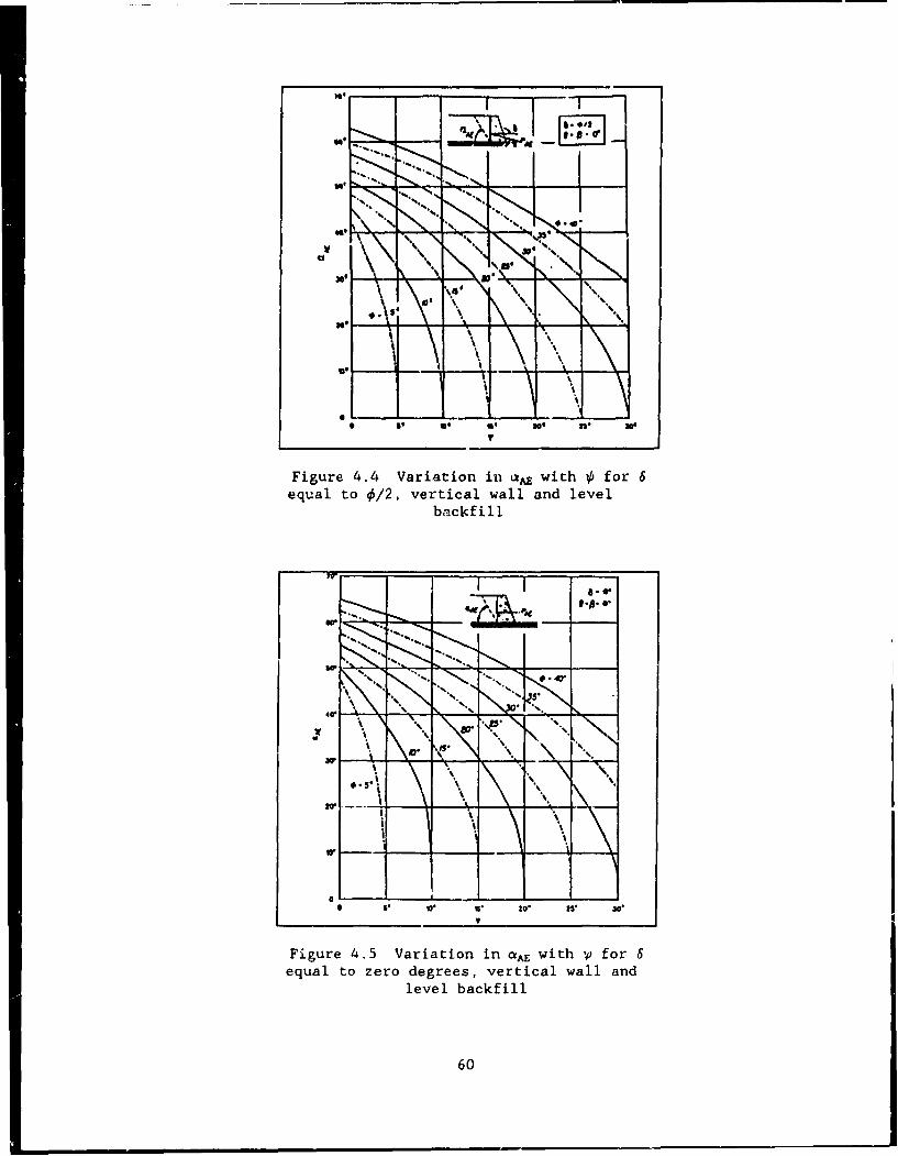
4- WF
Figure 4.4 Variation in *A with 0' for 6equal to 0/2, vertical wall and level
backf ill
o0 W 20, is, I
Figure 4.5 Variation in aA with ,p for 6equal to zero degrees, vertical wall and
level backfill
60
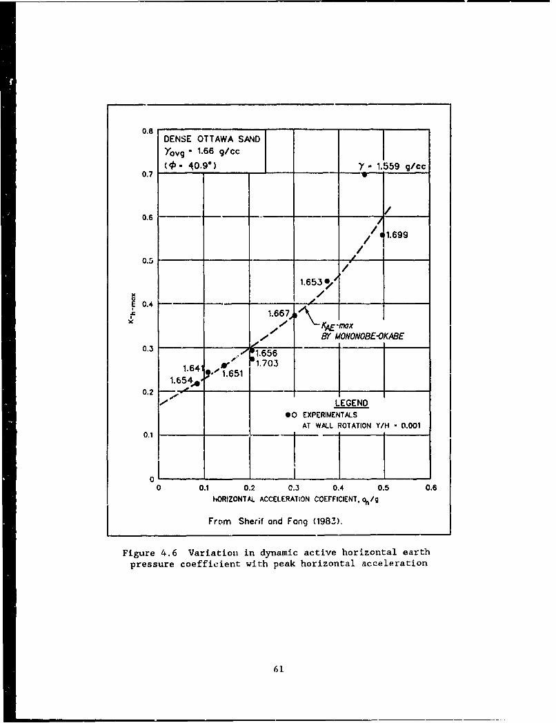
0.8DENSE OTTAWA SANDYovg"- 1.66 g/cc(jb. 4,0.9*) _"- 1.559 g/cc
0.7 -
0.6 -
/ 41.699/
o.• /0.3 ~'~ /
1.653,N /
E 0.4 -
1.667.A1\ E"I' "A -max
0 BY MONONOBE-OKABE0.3 - l.656
1.64 1.7031.654 , 1.651
0.2 - -100, LEGEND
00 EXPERIMENTALSAT WALL ROTATION Y/H 0.001
0.1
0I0.1 0.2 0.3 0.4 0.5 0.6
hORIZONTAL ACCELERATION COEFFICIENT, qn/g
From Sherif and Fang (1983).
Figure 4.6 Variation in dynamic active horizontal earthpressure coefficient with peak horizontal acceleration
61
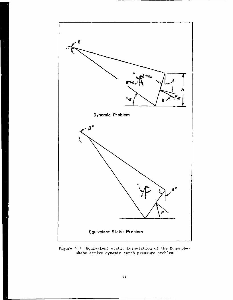
Dynamic Problem
P
Equivalent Static Problem
Figure 4.7 Equivalent static formulation of the Mononobe-Okabe active dynamic earth pressure problem
62
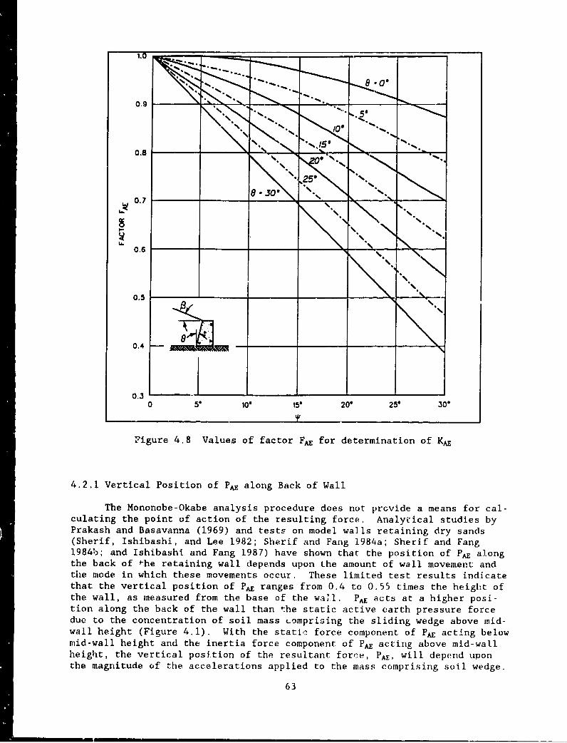
1.0
0.9 • "••
0.8
0.7
0.6
0.5
0. 4 •m ,
0.30 5* 10, 15e 20* 25V 30*
Figure 4.8 Values of factor FAE for determination of KAE
4.2.1 Vertical Position of PAE along Back of Wall
The Mononobe-Okabe analysis procedure does not prcvide a means for cal-culating the point of action of the resulting force. Analy-ical studies byPrakash and Basavanna (1969) and tests on model walls retaining dry sands(Sherif, Ishibashi, and Lee 1982; Sherif and Fang 1984a; Sherif and Fang198413; and Ishibashi and Fang 1987) have shown that the position of PAE alongthe back of the retaining wall depends upon the amount of wall movement andthe mode in which these movements occur. These limited test results indicatethat the vertical position of PAE ranges from 0.4 to 0.55 times the height ofthe wall, as measured from the base of the wai.l. PAE acts at a higher posi-tion along the back of the wall than the static active earth pressure forcedue to the concentration of soil mass Lomprising the sliding wedge above mid-wall height (Figure 4.1). With the static force component of PAE acting belowmid-wall height and the inertia force component of PAE acting above mid-wallheight, the vertical position of the resultant force, PAE, will depend uponthe magnitude of the accelerations applied to the mass comprising soil wedge.
63
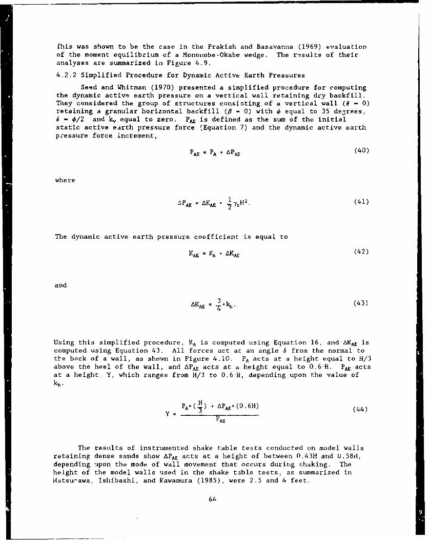
This was shown to be the case in the Prakish and Basavanna (1969) evaluationof the moment equilibrium of a Monoinobe-Okabe wedge. The results of theiranalyses are summarized in Figure 4.9.
4.2.2 Simplified Procedure for Dynamic Active Earth Pressures
Seed and Whitman (1970) presented a simplified procedure for computingthe dynamic active earth pressure on a vertical wall retaining dry backfill.They considered the group of structures consisting of a vertical wall (8 - 0)retaining a granular horizontal backfill (8 - 0) with 4 equal to 35 degrees,6 - 4/2 and k, equal to zero. PA is defined as the sum of the initialstatic active earth pressure force (Equation 7) and the dynamic active earthpressure force increment,
PAE = PA + APA (40)
where
.PA = AKA•2 lyHI . (41)
The dynamic active earth pressure coefficient is equal to
KA = KA + AKAE (42)
and
.= k (43)
Using this simplified procedure, KA is computed using Equation 16, and AKA iscomputed using Equation 43. All forces act at an angle 6 from the normal toti'e back of a wall, as shown in Figure 4.10. PA acts at a height equal to H/3above the heel of the wall, and APA acts at a height equal to 0.6'H. PA actsat a height, Y, which ranges from H/3 to 0.6-H, depending upon the value ofkh•
PA'() + APE-(0.6H) (44)
The resuilts of instrumented shake table tests conducted on model walls
retaining dense sands show APA acts at a height of between 0.43H and 0.58d,depending upon the mode of wall movement that occurs during shaking. Theheight of the model walls used in the shake table tests, as summarized inI4atsu~awa, Ishibashi, and Kawamura (1985), were 2.5 and 4 feet.
66
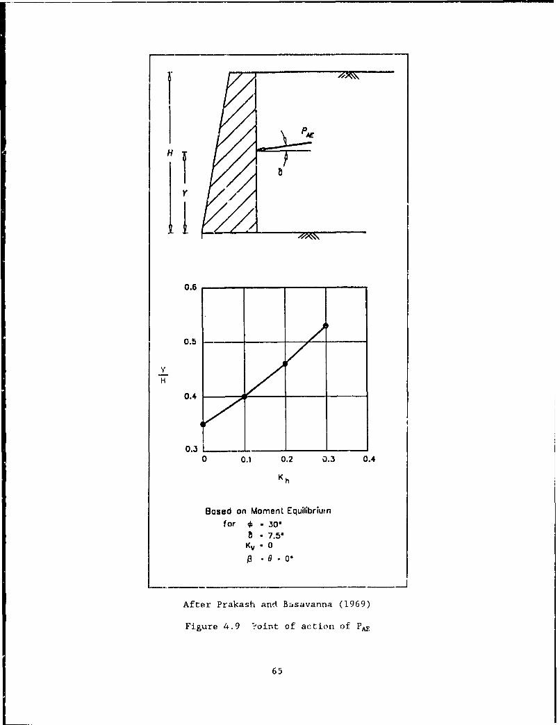
p
H
0.6
0.5 - ___
0.4
0.30 0.1 0.2 0.3 0.4
Kh
8ased on Moment Equilibriumnfor o - 30o
S- 7.50Kv - 0
.0 - -09
After Prakash and Basavanna (1969)
Figure 4.9 ?oint of action of PAE
65
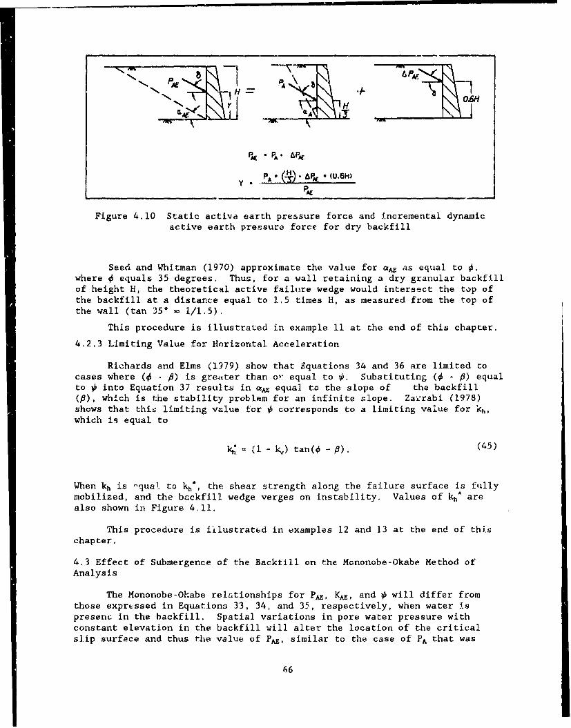
N A A
0.6H6
AP (()* H)P
Figure 4.10 Static active earth pressure force and incremental dynamicactive earth pressure force for dry backfill
Seed and Whitman (1970) approximate the value for cA as equal to 4,where 0 equals 35 degrees. Thus, for a wall retaining a dry granular backfillof height H, the theoretical active failure wedge would intersect the top ofthe backfill at a distance equal to 1.5 times H, as measured from the top ofthe wall (tan 35* - 1/1.5).
This procedure is illustrated in example 11 at the end of this chapter.
4.2.3 Limiting Value for Horizontal Acceleration
Richards and Elms (1979) show that Equations 34 and 36 are limited tocases where (0 - P) is greater than or equal to 0. Substituting (0 - f) equalto 0 into Equation 37 results in o equal to the slope of the backfill(P), which is the stability problem for an infinite slope. Zaýrabi (1978)shows that this limiting value for # corresponds to a limiting value for kh,which is equal to
c =( k)ta (45)
When kh is -qua! to kh*, the shear strength along the failure surface is fullymobilized, and the backfill wedge verges on instability. Values of kh* arealso shown in Figure 4.11.
This procedure is iilustrated in examples 12 and 13 at the end of thischapter.
4.3 Effect of Submergence of the Backtill on the Mononobe-Okabe Method ofAnalysis
The Mononobe-Ohabe relationships for PA, KA, and 0 will differ fromthose expressed in Equations 33, 34, and 35, respectively, when water ispresent in the backfill. Spatial variations in pore water pressure withconstant elevation in the backfill will alter the location of the criticalslip surface and thus the value of PA, similar to the case of PA that was
66
0.5
0.4 ATV
- / (ACVLCLERATIONUPWARD,INERTI FORCE
0.3
- 0 TIkO I .K /(ACELERATION
INERTIA FORCE
0.2
0.1
0 100 150 0 0
Figure 4.11 Limiting -alues for horizontal acceleration equals kh g
67
discussed in Section 3.3.3. In addition, the pore water pressures mayincrease above their steady state values in response to the shear strainsinduced within the saturated portion of the backfill during earthquake shak-ing, as discussed in Tokimatsu and Yoshimi (1983), Tokimatsu and Seed (1987),Seed and Harder (1990), and Marcuson, Hynes, and Franklin (1990). The trialwedge procedure of analysis is used to locate the critical slip surface withinthe backfill and to compute PA, following the steps described in Section 3.4and including the excess pore water pressures due to earthquake shaking in theanalysis are described in Appendix A. In some situations, such as the case ofa hydrostatic water table within the backfill or the case of excess pore waterpressures equal to a constant fraction of the pre-earthquake effective over-burden pressures throughout the backfill (ru - constant), modified Mononobe-Okabe relationships may be used to compute PAE.
4.3.1 Submerged Backfill with No Excess Pore Pressures
In this section it is assumed that shaking causes no associated buildupof excess pore pressure. The most complete study of this case appears inMatsuzawa, Ishibashi, and Kawamura (1985), Ishibashi, Matsuzawa, and Kawamura(1985), and Ishibashi and Madi (1990). They suggest two limiting conditionsfor design: (a) soils of low permeability - say k < 1 x 10⁻³ cm/sec where porewater moves with the mineral skeleton; and (b) soils of high permeability -say k > 1 cm/sec, where pore water can move independently of the mineralskeleton. Matsuzawa, Ishibashi, and Kawamura (1985) also suggest a parameterthat can be used to interpolate between these limiting cases. However, under-standing of case (b) and the interpolation parameter is still very incomplete.
Restrained water case: Here Matsuzawa Ishibaski, and Kawamura (1985)make the assumption that pore pressures do not change as a result of horizon-tal accelerations. Considering a Coulomb wedge and subtracting the staticpore pressures, there is a horizontal inertia force proportional to yt-kh anda vertical force proportional to 7b. Thus, in the absence of vertical accel-erations, the equivalent seismic angle is:
tan-1 Ytki, (46)Yb
and the equivalent horizontal seismic coefficient is:
Ltk,. (47)
Using kh,1 in the Mononobe-Okabe theory together with a unit weight lb willgive PA, to which the static water pressures must be added.
If vertical accelerations ate present, Matsuzawa, Ishibashi, andKawamura (1985) recommend using:
68
"tan-1 (48)
This is equivalent to assuming that vertical accelerations do affect porepressures, and then it is not strictly correct to use the Mononobe-Okabetheory. However, the error in evaluating total thrust is small.
This procedurejis illustrated in example 14 at the end of this chapter.
Free water case: It is difficult to come up with a completely logicalset of assumptions for this case. Matsuzawa, Ishibaski, and Kawamura (1985)suggest that the total active thrust is made up of:
(1) A thrust from the mineral skeleton, computed using:
kh. 2 = -I (49)
and
O°2 = tanl1 (5 ) (
where G. is the specific gravity of the solids. A unit weight of lb is usedin the equation for PA.
(2) The hydrodynamic water pressure force for the free water within the back-fill, Pwd, is given by the Westergaard (1931) relationship (Appendix B)
7wd .kh. YwH2 (51)
and acts at 0.4 H above the base of the wall.
The total force beL.id the wall would also include the hydrostatic water pres-sure. This procedure is not totally consistent, since the effect of theincreased pore pressures is ignored in the computation of the thrust from themineral skeleton as is the effect of vertical acceleration upon pore pressure.
This procedure is illustrated in example 15 at the end of this chapter.
4.3.2 Submerged Backfill with Excess Pore Pressure
Excess pore pressures generated by cyclic shaking can be represented byr, - Au/a,', where Au is the excess pore pressure and a,' is the initial
69
vertical stress. While there is no rigorous approach for adapting theMononobe-Okabe solution, the following approaches are suggested.
Restrained water case: Ignoring vertical accelerations, the effectiveunit weight of soil becomes:
7.3 - 7b( 1 - r.) (52)
while zhe effective unit weight of water is
7w3 ' Yw + Ib*ru (53)
The thrust from the soil skeleton, PA, is computed using
kh. 3 - 7t % (54)
and
0. 3 = tan-[kh. 31 (55)
together with a unit weight from Equation 52. The effective unit weight ofwater, Equation 53, is used to compute the "static" pore pressure. The effectof vertical acceleration may be accounted for by inserting (l-k,) in thedenominator of Equation 55.
As ru approaches unity, -Y. 3 -> 0 and -YW3 - -Yt, so that the fully-lique-fied soil is a heavy fluid. It would now be logical to add a dynamic porepressure computed using Equations 51 and 53.
This procedure is illustrated in example 16 at the end of this chapter.
Alternate Procedure:
An alternative approach is to use a reduced effective stress frictionangle in which the effects of the excess pore water pressures are approximatedwithin the analysis using a simplified shear strength relationship. In aneffective stress analysis, the shear resistance on a potential failure surfaceis reduced by reducing the effective normal stress on this plane by the amountof excess residual pore water pressure, assuming the effective friction angleis unaffected by the cyclic loading. This is equivalent to using the initial,static effective normal stress and a modified effective friction angle, 4.q,where
tan/q = (1 - ru)tan@/ (56)
as shown in Figure 4.12. in the case of ru equal to a constant within thefully submerged backfill, the use of ý.q in Equatiuns 34 and 38 for KAE andKA(#*, #*) approximating the effects of these excess pore water pressures
70
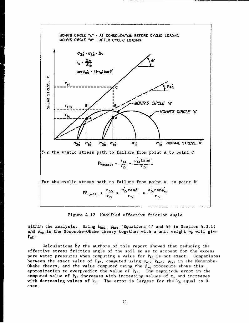
MOHR'S CIRCLE "C" - AT CONSOLIDATION BEFORE CYCLIC LOADINGMOHR'S CIRCLE "a" - •FTER CYCLIC LOADING
-3 Cr3a' Au
Au we
ton 00 - (0-ru)tanO'
°mrf
U, -
SB- MOH.'5 CIRCLE OttX rffa ,0-- MOHA'S CIRCLE "c'
a3 n (Tfo 0.3 1 f CIO (T If NORMAL STRESS. 0
Fur. the static stress path to failure from point A to point C
FSstatic = __ ff . afctano'T fc 'c
For the cyclic stress path to failure from point A' to point B'
Fffa afatano' -fctano.qFScyclic =
T fc /'fc fc
Figure 4.3.2 Modified effective friction angle
within the analysis. Using kh.1, Oh., (Equations 47 and 46 in Section 4.3.1)and O.q in the Mononobe-Okabe theory together with a unit weight Jb will give
PAE.
Calculations by the authors of this report showed that reducing theeffective stress friction angle of the soil so as to account for the excesspore water pressures when computing a value for PAE is not exact. Comparisonsbetween the exact value of PA, computed using 7.3, kl,3, Oh.3 in the Mononobe-Okabe theory, and the value computed using the 0.,, procedure shows thisapproximation to overpcedict the value of PAE. The magnitude error in thecomputed value of PAE increases with increasing values of ru and increaseswith decreasing values of kh. The error is largest for the kh equal to 0c3se.
71
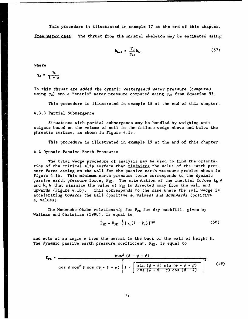
This procedure ia illustrated in example 17 at the end of this chapter.
Free water case: The thrust from the mineral skeleton may be estimated using:
k,-d (57)793
where
To this thrust are added the dynamic Westergaard water pressure (computed
using 7,) and a "static" water pressure computed using T,3 from Equation 53.
This procedure is illustrated in example 18 at the end of this chapter.
4.3.3 Partial Submergence
Situations with partial submergence may be handled by weighing unitweights based on the volume of soil in the failure wedge above and below thephreatic surface, as shown in Figure 4.13.
This procedure is illustrated in example 19 at the end of this chapter.
4.4 Dynamic Passive Earth Pressures
The trial wedge procedure of analysis may be used to find the orienta-tion of the critical slip surface that minimizes the value of the earth pres-sure force acting on the wall for the passive earth pressure problem shown inFigure 4.1b. This minimum earth pressure force corresponds to the dynamicpassive earth pressure force, PFE. The orientation of the inertial forces kh'Wand kW that minimize the value of PpE is directed away from the wall andupwards (Figure 4.1b). This corresponds to the case where the soil wedge isaccelerating towards the wall (positive ah values) and downwards (positivea, values).
The Mononobe-Okabe relationship for PPE for dry backfill, given byWhitman and Christian (1990), is equal to
P= KpE.I[7y(l - k.)]H2 (5F)
and acts at an angle 6 from the normal to the back of the wall of height H.The dynamic passive earth pressure coefficient, KPE, is equal to
KpE Cos 2 -0+80)
cos O cos 2 0 cos (0 -0 + 6) 1 - sin (0 + 6) sin (0'-' + P) (59)
[ cos (U + 0 --) cos (P -0)
72
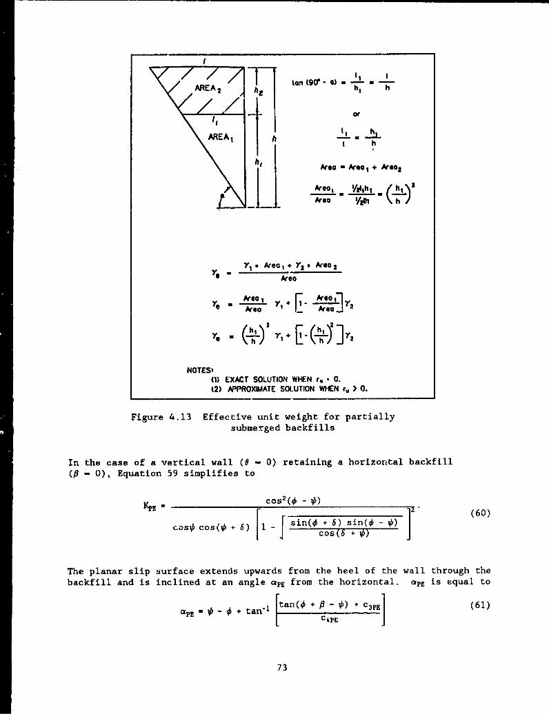
to(9n M - a)AREA 2 he h I h
""/I or
AREA 1 h h,
/h
h ArI Ico A hI + hlea
Ag c 1 *Area 212h h
-e Y, AreaI.+?2. Area 2 _Area
Arco --Area
NOTESt(1) EXACT SOLUTION WHEN ru. 0.(2) APPROXIMATE SOLUTION WHEN r, > 0.
Figure 4.13 Effective unit weight for partiallysubmerged backfills
In the case of a vertical wall (8 - 0) retaining a horizontal backfill- 0), Equation 59 simplifies to
KE-cos 2(0 0 (60)
coso os~o 6) r sin(o + 6) sin(o - 0s s1 cos(6 + 0)
The planar slip surface extends upwards from the heel of the wall through thebackfill and is inclined at an angle apE from the horizontal, aPE is equal to
aPE " - + tan-l tan(o +P- 0-) + C3PE] (61)
73
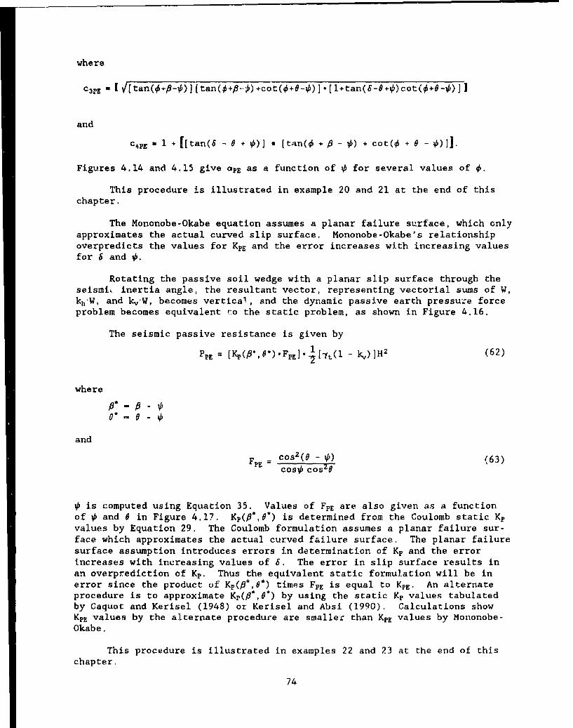
where
CUM 0 [ Vtan(o+•-O) ]tan(o+#-•) +cot(0+8-0)]•[l+tan(8-8+0)cot(0+8-0) ]
and
COPE + 1 o [[tan(6 - 6 + ) [tan(4 + -+ ) + cot(• + 6 -
Figures 4.14 and 4.15 give aPE as a function of b for several values of @.
This procedure is illustrated in example 20 and 21 at the end of thischapter.
The Mononobe-Okabe equation assumes a planar failure surface, which onlyapproximates the actual curved slip surface. Mononobe-Okabe's relationshipoverpredicts the values for KPE and the error increases with increasing valuesfor 6 and 0.
Rotating the passive soil wedge with a planar slip surface through theseismiL inertia angle, the resultant vector, representing vectorial sums of W,kh'W, and k,'W, becomes vertical, and the dynamic passive earth pressuce forceproblem becomes equivalent to the static problem, as shown in Figure 4.16.
The seismic passive resistance is given by
Fe = [Kp(p*,O*),FPE].4[vt(l - k.)]HI (62)
where
O*- e -
and
FPE = cos 2 (O - (63)coso cos 2 0
tis computed using Equation 35. Values of FPE are also given as a functionof 0 and 6 in Figure 4.17. Kp(fi*,O*) is determined from the Coulomb static Kpvalues by Equation 29. The Coulomb formulation assumes a planar failure sur-face which approximates the actual curved failure surface. The planar failuresurface assumption introduces errors in determination of Kp and the errorincreases with increasing values of 6. The error in slip surface results inan overprediction of Kp. Thus the equivalent static formulation will be inerror since the product of Kp(p*,O*) times FpE is equal to KPE. An alternateprocedure is to approximate Kp(fi*,O*) by using the static Kp values tabulatedby Caquot and Kerisel (1948) or Kerisel and Absi (1990). Calculations showKPE values by the alternate procedure are smaller than KPE values by Mononobe-Okabe.
This procedure is illustrated in examples 22 and 23 at the end of thischapter.
74
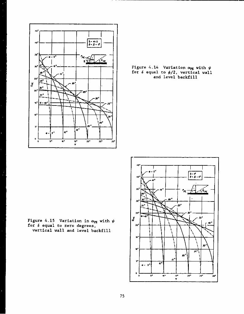
35.
3- 0 Figure 4. 14 Variation ap withfor 6 equal to 4/2, vertical wall
____________and level backfill
30-
20,
330@
0 S. 1. Is 20' 25* 30,
415
30*
Figure 4.15 Variation in apE with ?k C1. /
for 6 equal to zero degrees,20. l
vertical wall and level backfill
0 'Vol I
75
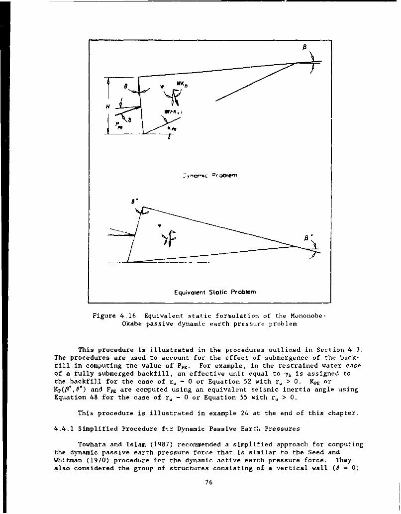
H
9.
Equivalent Static Problem
Figure 4.16 Equivalent static formulation of the Mononobe-Okabe passive dynamic earth pressure problem
This procedure is illustrated in the procedures outlined in Section 4.3.The procedures are used to account for the effect of submergence of the back-fill in computing the value of PPE. For example, in the restrained water caseof a fully submerged backfill, an effective unit equal to Yb is assigned tothe backfill for the case of ru - 0 or Equation 52 with ru > 0. KPE orKp(i*,O*) and FPE are computed using an equivalent seismic inertia angle usingEquation 48 for the case of ru - 0 or Equation 55 with ru > 0.
This procedure is illustrated in example 24 at the end of this chapter.
4.4.1 Simplified Procedure f-r Dynamic Passive Earth Pressures
Towhata and Islam (1987) recommended a simplified approach for computingthe dynamic passive earth pressure force that is similar to the Seed andWhitman (1970) procedure fcr the dynamic active earth pressure force. Theyalso considered the group of structures consisting of a vertical wall (8 - 0)
76
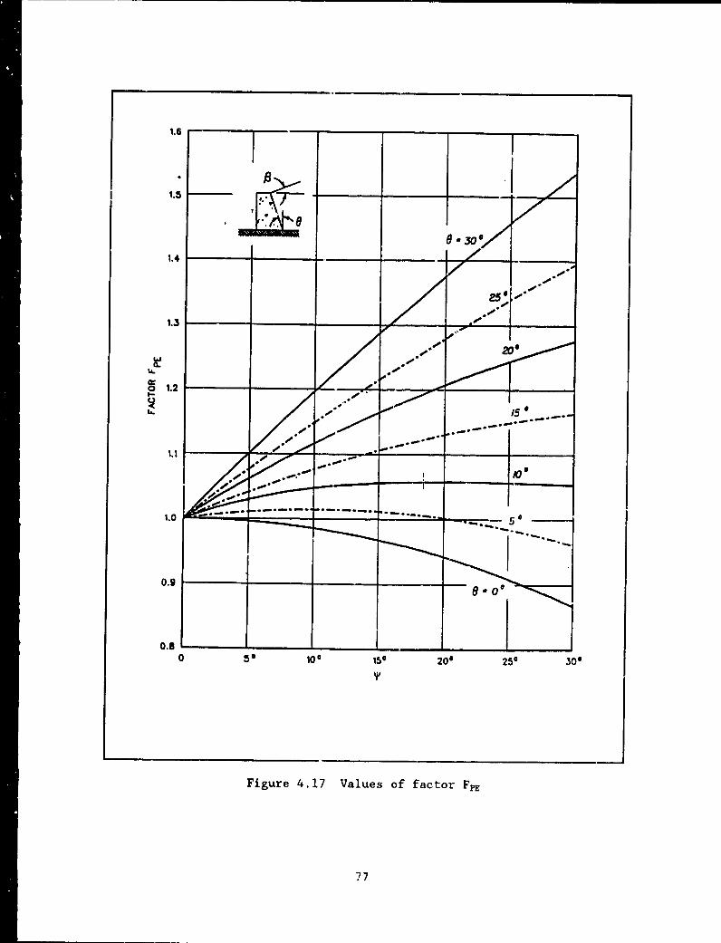
1.6
0G,3001.4 - - -
1.3
a.v
5 1.2
1.0
0.9
0.80 50 100 150 200 25* 300
y'
Figure 4.17 Values of factor FPE
77
retaining a granular horizontal backfill (6 - 0) with 4 equal to 35 degrees,6 equal to 0, and k, equal to zero. Equation 65 is presented as developed byTowhata and Islam, while Equations 64, 66, and 67 have been modified by theauthors of this report. Pps is defined as
PM - PP - 8PE (64)
where the reduction in the static passive earth pressure value Pp due toearthquake shaking is given by
SPII alyH*ap (65)
for a dry granular backfill. The dynamic passive earth pressurecoefficient is equal to
K-E 0 KP - AKPE (66)
and
S- ' 17-k. (67)
Using this simplified procedure, Kp is computed using Equation 11(Rankine), and AKpE is computed using Equation 67. The incremental dynamicforce APp acts counter to the direction of Pp, reducing the contribution ofthe static passive pressure force to PPE . The resulting forces Pp (Equa-tion 13) and APpE (Equation 65) act normal to the back of a wall.
This procedure is illustrated in example 25 at the end of this chapter.
The simplified procedure was developed for vertical walls retaininghorizontal backfills with 6 - 0. This simplified procedure should not beapplied to dynamic passive earth pressure problems involving values of 6 > 0,due to the magnitude of the error involved.
4.5 Effect of Vertical Accelerations on the Values for the Dynamic Active andPassive Earth Pressures
In a pseudo-static analysis the horizontal and vertical accelerations ofthe soil mass during an earthquake are accounted for by applying equivalentinertial forces kh'W and kv-W to the soil wedge, which act counter to thedirection of the accelerating soil wedges, as shown in Figure 4.1. A positivehorizontal acceleration value increases the value of PA and decreases thevalue of PZ. The vertical component of acceleration impacts the computedvalues of both PAE and PpE and KA and KpE.
Upward accelerations (-k,-g) result in smaller values of KAZ and largervalues of PAZ as compared to the KA and PA values when kv is set equal tozero. Upward accelerations (-kv'g) increase the value of PA due to the con-tribution of the term (1 - k,) in Equation 33. This trend is reversed when
78
the vertical acceleration acts downward (+kvg). Seed and Whitman (1970) andChang and Chen (1982) showed that; the change in the KA value varied with boththe value of k, and kh. Calculations with k, ranging from 1/2 to 2/3 of the khvalue show that the difference between the computed values of KZ with anonzero k, value and k, equal to zero is less than 10 percent, Seed andWhitman (1970) concluded that for typical gravity retaining wall design prob-lems, vertical accelerations can be ignored when computing KAE. The k, valuehas a greater impact on the computed value of PEZ than on the value of PA.
Chang and Chen (1982) show that the change in the KFE value varies withboth the value of k, and kh. The difference between the values of KPE with anonzero k, value and k, set equal to zero increases with increasing magnitudesof both kv and kh. This difference can easily be greater than 10 percent. Ingeneral, vertical accelerations acting downward (+kv'g) will decrease the KPE
and PPE values from the corresponding Kpz and PPE values for which k, is setequal to zero. The trend Is reversed when the vertical acceleration actsupward (-k.,g). When Pp1 acts as a stabilizing force for a structure, verticalaccelerations should be considered in the computations of the value for PPE.An examplo is the soil region below the dredge level and in front of ananchored sheet pile wall (refer to the design example in Section C.2 ofAppendix C).
4.6 Cases with Surface Loadings
There are two approaches used to approximate the additional lateralearth pressures on walls due to surface loadings: (1) the wedge method ofanalysis Pnd (2) finite element analyses.
In the case of a uniform surcharge q., the value of the dynamic activeearth pressure force is computed using the modified Mononobe-Okabe relation-ships listed in Figure 4.18 and Equation 34 (or Equation 36 for a verticalwall retaining a horizontal backfill) for KA. The point of application of PAalong the back of the wall is computed using the procedure outlined in Fig-ures 4.19 and Figure 4.20. In this approximate procedure, the surcharge q. isreplaced by the addition of a layer of soil of height h. equal to q,/It. Theresulting problem is analyzed by adapting the Seed and Whitman's simplifiedprocedure (of section 4.2.2) to the problem of a uniform surcharge loading asoutlined in Figure 4.20.
This procedure is illustrated in example 26 at the end of this chapter.
Pseudo-static trial wedge analyses may be performed to accountapproximately for both uniformly and non-uniformly distributed surfaceloadings, as described in Section A.2 of Appendix A for dynamic active earthpressure problems. These analyses may be performed on walls whose movementssatisfy the criteria listed in Table 1. Such analyses will give the totalthrust against a wall. The effects of surface loading is included within thewedge analysis by including that portion of the surface loading between theback of the wall and the intersection of the slip surface and the backfillsurface in the force equilibrium calculation for each wedge analyzed, asdescribed in Section 3.6 for the static problem. The effect of the earthquakeis modeled in the pseudo-static trial wedge analysis by an additional set ofstatic forces, kh-W, k.,W, kh-W., and kvW,, where W is equal to the weight ofthe soil contained within the trial wedge and W, is equal to the weight ofsurcharge contained within the region located above the trial wedge as shownin Figure A.3 for the active earth pressure problem. The difficult part of
79
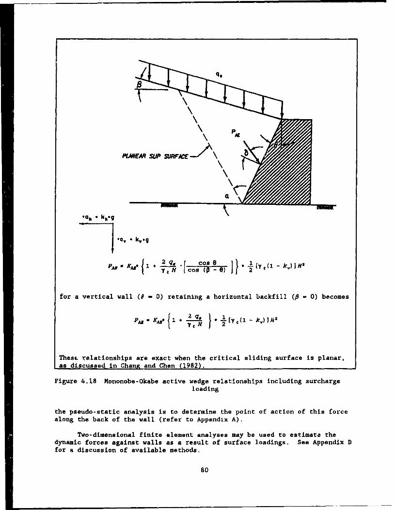
t q'
PLM(EAR SUP SURFACE
, 2k. Co .[g,)H
'7* coa
PAN -K 4 e1, 1 YC H [Cos (03- p) 2I.* Yil-k)H
for a vertical wall (8 - 0) retaining a horizontal backfill (i-0) becomes
Thes.c relationships are exact when the critical sliding surface is planar,as discussed in Chaniz and Chen (1982).
Figure 4.18 Nononobe-Okabe active wedge relationships including surchargeloading
the pseudo-static analysis is to determine the point of action of this forcealong the back of the wall (refer to Appendix A).
Two-dimensional finite element. analyses may be used to estimate thedynamic forces against walls as a result of surface loadings. See Appendix Dfor a discussion of available methods.
80
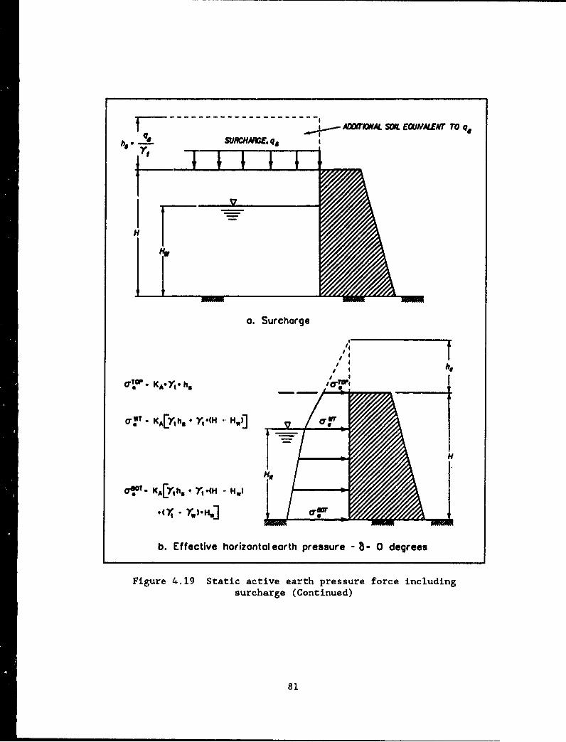
T AD4DTMOA SOIL EOUWNALN~ TO
-- - I ----h*ho
Hf
a. Surcharge
81'
'
S2-
I
• 040. K A[ Vih. V,., H - H, )
• • - V,,.H,] ,
b. Effective horizontal earth pressure - B= 0 degrees
Figure 4.19 Static active earth pressure force including
surcharge (Continued)
81
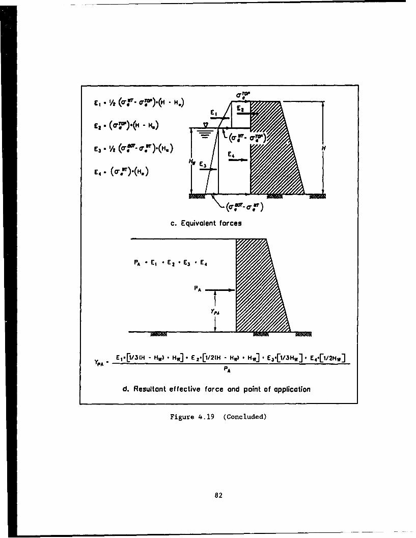
E1 i/(of-0q)-(H -H)
El. - ((a)-.(H - ,H)
E4. (cG.`.).(H..)
c. Equivalent forces
PA ° E, * E2 E £3 * E4
PAV
YPA
YPA E [,{/3 (H H.) *H,] E -[¶i/2(H -H.) H,]. E,-[1/3H.]. E4{[1/2Hw]
d. Resultant effective force and point of application
Figure 4.19 (Concluded)
82
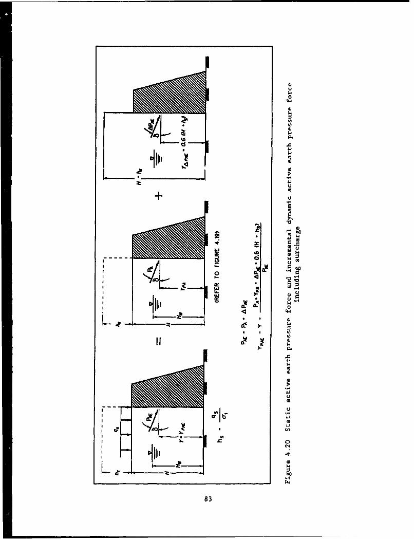
U)
Ile.
41
1123
'a'
II
ý4.
83U
CHAPTER 4 - EXAMPLES
Contents
Example Problems 7 through 26.
Commentary
The following examples illustrate the proceduresdescribed in Chapter 4. The results of the computa-tions shown are rounded for ease of checkingcalculations and not to the appropriate number ofsignificant figures. Additionally, the valuesassigned to variables in these problems were selectedfor ease of computations.
84
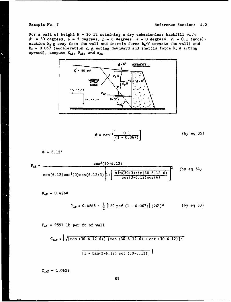
Example No. 7 Reference Section: 4.2
For a wall of height H - 20 ft retaining a dry cohesionless backfill with0' - 30 degrees, 6 - 3 degrees, P - 6 degrees, 9 - 0 degrees, kh - 0.1 (accel-eration kh-g away from the wall and inertia force kh'W towards the wall) andk, - 0.067 (acceleration k,'g acting downward and inertia force k,'W actingupward), compute KAE, PAZ, and aA.
Yt 120 pcf
CO~tOM8 /" V•-"% 'e W t" :.7'
PAL 9
... \ ' .. • 0
- 6.120
KAE COS 2 (30-6.12) (by eq 34)
cos(6.12)cos2(0)cos(6.12+3) [ sin(30+3)sin(30-6.12-6)"* * ]cos(3+6, 12)cos(6)
KAE - 0.4268
PAE - 0.4268 • 1 [120 pcf (1 - 0.067)] (20')2 (by eq 33)
PA - 9557 lb per ft of wall
Cl- [[tan (30-6.12-6)] [tan (30-6.12-6) + cot (30-6.12)].
[1 + tan(3+6. 12) cot (30-6.12)] 1
Cla - 1.0652
85
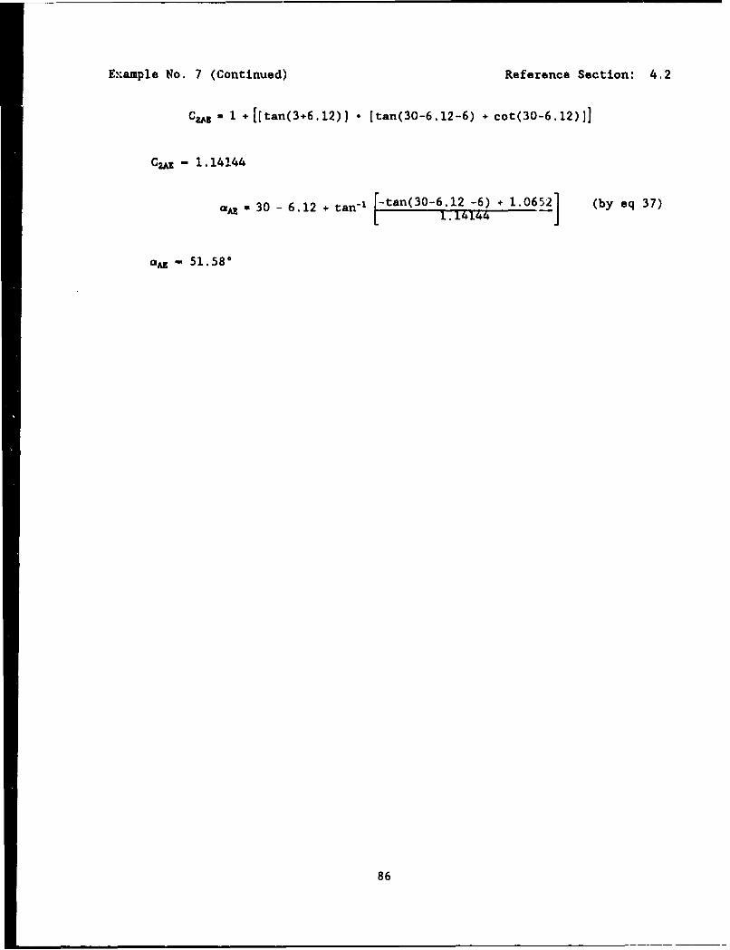
Example No. 7 (Continued) Reference Section: 4.2
C * - 1 + [[tan(3+6.12)] * (tan(30-6.12-6) + cot(30-6.12)]]
C• - 1.14144
a 30 - 6.12 + tan 1 [-tan(30-6.12 -6) + 1.0652] (by eq 37)a•- 0 612+ anIL 1. 14144
a- 51.580
86
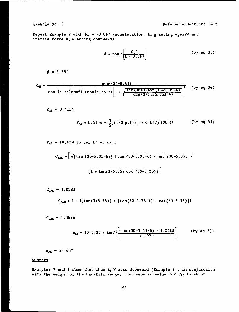
Example No. 8 Reference Section: 4.2
Repeat Example 7 with k, - -0.067 (acceleration k,'g acting upward andinertia force kvW acting downward).
•m-tan'- [] (by eq 35)
S- 5.350
KAX C082 (0 COS(cos2 0(30-5.35) sin(30-5.35 2 (by eq 34)
cos (5.35)cos2(0)co (5.35+3) 1 + y cos( 3 +5. 3 5 )cos(6 )
KAE - 0.4154
PA- 0.4154 • 4[(120 pcf) (1 + 0.067)1(20/)2 (by eq 33)
PA - 10,639 lb per ft of wall
Cia - [ [[tan (30-5.35-6)] (tan (30-5.35-6) + cot (30-5.35)].
[1 + tan(3+5.35) cot (30-5.35)] 1
Cl -- 1.0588
C2AE - 1 + [[tan(3+5.35)] • [tan(30-5.35-6) + cot(30-5.35)]]
CUE - 1.3696
-AE- 30-5.35 + tanl[-tan(30-5"35-6) + 1.0588] (by eq 37)
aAE- 52.45*
Summalry
Examples 7 and 8 show that when kvW acts downward (Example 8), in conjunctionwith the weight of the backfill wedge, the computed value for PAE is about
87
Example No. 8 (Continued) Reference Section: 4.2
11 percent larger than the value of PA computed for the case when k,'W actsupward (Example 7).
88
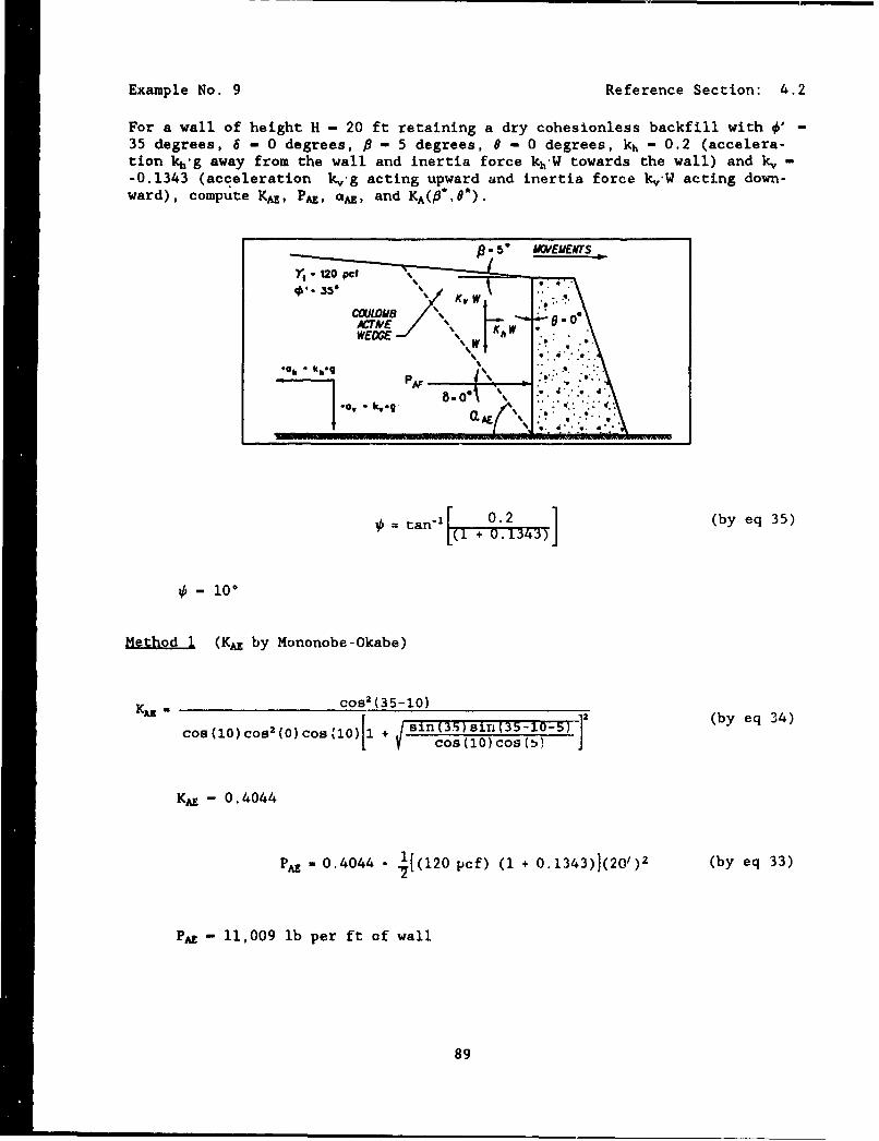
Example No. 9 Reference Section: 4.2
For a wall of height H - 20 ft retaining a dry cohesionless backfill with 0' -35 degrees, 6 - 0 degrees, $ - 5 degrees, 9 - 0 degrees, kh - 0.2 (accelera-tion kh-g away from the wall and inertia force kh-W towards the wall) and k, --0.1343 (acceleration k,'g acting upward and inertia force k,-W acting down-ward), compute KAE, PAE, aAE, and KA(#*,O*).
•-35" %•,coumee / ", L.._ .J.•,_,
•cr,,+ ,,j-•-w i- "" o
= tan. 1 [ 0,2 ~7:~ ] (by' e~q 3.5)
COULOM % % . 0.0
•- 100
Me.thodI (KAE by Mononobe-Okabe)
K - cosa (35-10)2
cos (10) cos (0) cos •1 0)[1 + i n 3 ) i ( 5-0 5+ cos (10) cos (•)
. - 0.4044
-•, 0.4044 • .l[(l20 pcf) (1 + 0.1343)](20/)2 (by eq 33)
- 11,009 lb per ft of wall
89
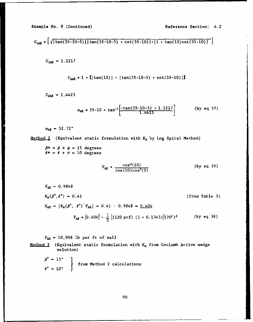
Example No. 9 (Continued) Reference Section: 4.2
Ci [a tan(35-10-5)] tan(35-10-5) + cot(35-10)]. 1 + tan(10)cot(35-10)]
cla - 1.1217
G -= 1 + [[tan(10)] * [tan(35-l0-5) + cot(35-i0)]I
CzM - 1.4423
aAz - 35-10 + tan'lL-tan(35-10-5) + 1.1217] (by eq 37)
aA - 52.72'
Method 2 (Equivalent static formulation with KA by Log Spiral Method)
#" - 6 + 4 - 15 degrees
6* - 0 + 1 - 10 degrees
FM cos2(10) (by eq 39)cos(l0)cos2 (O)
FAE - 0.9848
KA(P*,O*) - 0.41 (from Table 3)
Y,, - [KA(#*, 8*)'FAE] - 0.41 0.9848 - 0,404
PA -[0.404] * 1 [(120 pcf) (1 + 0.1343)](20/)2 (by eq 38)
.7
PA - 10,998 lb per ft of wall
Method 3 (Equivalent static formulation with KA from Coulomb Active wedgesolution)
~15-0* "100 from Method 2 calculations
90
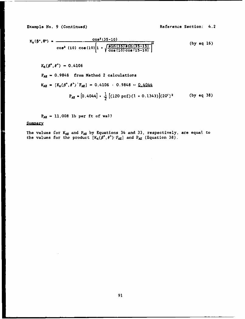
Example No. 9 (Continued) Reference Section: 4.2
Cosa (35-10) a' (by eq 16)Ssin (35 ,T"6(3-riTsCosla (10) Cos (10) 1 + ncs 1 ) os 1 -0
KA(P*,O*) - 0.4106
FAM - 0.9848 from Method 2 calculations
KAE - [KA(8*,O*)'FAz] - 0.4106 • 0.9848 * 0.4044
PA,, -[0.4044] • 1 [(120 pcf)(I + 0.1343)](20102 (by eq 38)
PA - 11,008 lb per ft of wail
The values for KM and PAE by Equations 34 and 33, respectively, are equal tothe values for the product [KA(P*,O*)'FMz] and PAE (Equation 38).
91
Example No. 10 Reference Section: 4.2
For the example 9 problem, compute the increase in magnitude for the dynamicactive earth pressure forco above the static active earth pressure value,APAg.
KA cosa (35) (by eq 16)
cosa (0) cos (0) 1 "sn (35) sin (35-5)L COB (0) coB (5)
KA - 0.2842
P 0.2842 • 1 (120 pcf) (20Y)2 (by eq 7)
PA - 6,821 lb per ft of wall
PA 11,008 lb per ft of wall (from example 9)
AP P - PA"PA
APAX - 11.008 - 6,821
APAE- 4,187 lb per ft of wall
Summary
The dynamic active earth pressure force is 61 percent greater than the staticactive earth pressure force for the example 9 problem.
92
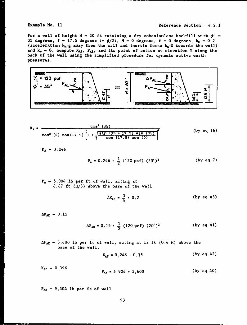
Example No. 11 Reference Section: 4.2.1
For a wall of height H - 20 ft retaining a dry cohesionless backfill with 0' -35 degrees, 6 - 17.5 degrees (- 0/2), ft - 0 degrees, 9 - 0 degrees, kh - 0.2(acceleration kh'g away from the wall and inertia force kh-W towards the wall)and k, - 0, compute KAI, PAZ, and its point of action at elevation Y along theback of the wall using the simplified procedure for dynamic active earthpressures.
Yt - 120Opcf =FAb '' .
I• gall (35)91111
C0s2 (35 )in- r (by eq 16)
cos 2 (0) cos(17.5) 1 17 .5) s(3)
KA - 0.246
- 0.246 • (120 pcf) (201)2 (by eq 7)-7
PA - 5,904 lb per ft of wall, acting at6.67 ft (H/3) above the base of the wall,
3 . 0.2 (by eq 43)
AKA - 0. 15
S- 0.15 • 1 (120 pcf) (201)2 (by eq 41)
APA - 3,600 lb per ft of wall, acting at 12 ft (0.6 H) above thebase of the wall.
KAE 0.246 + 0.15 (by eq 42)
K•- 0. 396 PA -5,904 + 3,600 (by eq 40)
PAE - 9,504 lb per ft of wall
93
Example No. 11 (Continued) Reference Section: 4.2.1
5904 2•o + 3600 (0.6 - 20) (by eq 44)09504
Y - 8.69 ft (0.43 H) above the base of the wall
94
Example No. 12 Reference Section: 4.2.3
For a wall retaining a dry cohesionless backfill with 0' - 35 degrees, 6 - 0degrees, f - 15 degrees, 0 - 0 degrees, and k, - - kh/ 2 (acceleration kv-gacting upward and inertia force k.&W acting downward), compute kh*, 0, *, KA,and PA.
Introducing k, - - kh*/2 and rearranging, Equation 45 becomes
2 tan(ý-~2 - tan(O -
For (€ ) - 20 degrees,
kh" - 0.44494
and k, - - 0.22247
Note that the use of Figure 4.11 results in the same value for kh*.
By Equation 35, 0 - 20 degreesBy Equation 37, aAE - 15 degreesBy Equation 34, KAZ - 1.05
95
Example No. 13 Reference Section: 4.2.3
Repeat example 12 with k, - + kh/ 2 (acceleration k,'g acting downward andinertia force k,.W acting upward).
Introducing It, - + kh*/2 and rearranging, Equation 45 becomes
k; 2 tan (t .- 0)2 + tan P-P)
For (# - •) - 20 degrees,
• - 0.307931
and k, - 0.153966
By Equation 35, 0 - 20 degreesBy Equation 37, cA- 15 degreesBy Equation 34, KAZ - 1.05
Examples 12 and 13 show that for the limiting case of (0 - P) equal to 0, themagnitude of kh* is dependent upon the orientation of the vertical inertiaforce. Both analyses result in the same values for 0, KAE, and aAz. For theselimiting cases the slip plane is orientated parallel to the slope of the back-fill, aAE - P. Additionally, when the inertia force kv'W acts downward (exam-ple 12) in conjunction with the weight of the backfill wedge, the valuecomputed for PAE is 44 percent greater than the value for PA when kv.W actsupward (example 13) due to the term (I - kv) in Equation 33.
96
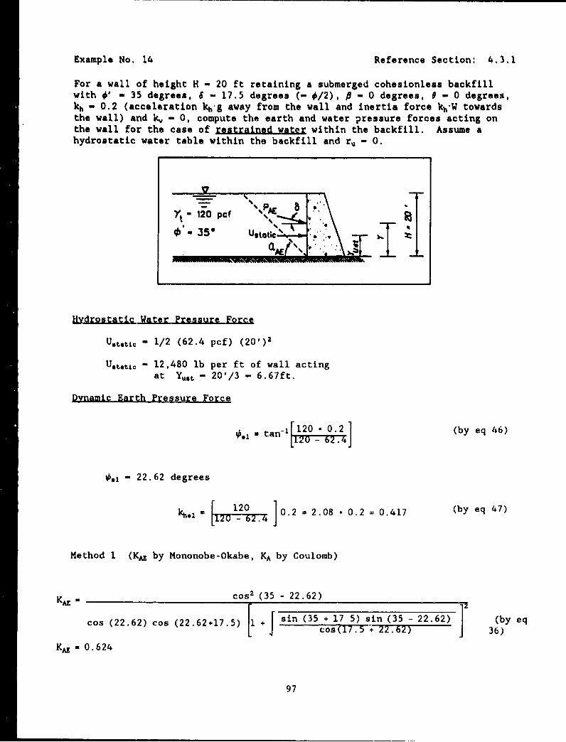
Example No. 14 Reference Section: 4,3.1
For a wall of height H - 20 ft retaining a submerged cohesionless backfillwith 0' - 35 degrees, 6 - 17,5 degrees (- 0/2), P - 0 degrees, 0 - 0 degrees,kh - 0.2 (acceleration kh'g away from the wall and inertia force kh'W towardsthe wall) and k, - 0, compute the earth and water pressure forces acting onthe wall for the case of restrained water within the backfill. Assume ahydrostatic water table within the backfill and ru - 0.
- ' ow
- 120 pcf %1E 9
*35* Ust 0ti' :b.6
Hydrostatic Water Pressure Force
U.t.tic - 1/2 (62.4 pcf) (20')2
Ustatic - 12,480 lb per ft of wall actingat Yut - 20'/3 - 6.67ft.
Dynamic Earth Pressure Force
0 tan-1 129 0.2] (by eq 46)
-.1 - 22.62 degrees
k.1 - 12 ]0.2 - 2.08 . 0.2 = 0.417 (by eq 47)
Method 1 (KAE by Mononobe-Okabe, KA by Coulomb)
KA- - cos2 (35 - 22.62)
cos (22.62) cos (22.62+17.5) [ r sin (35 + 17 5) sin (35 - 22.62) (by eqcos(17.5 +"22.62) 36)
- 0. 624
97
Example No. 14 (Continued) Reference Section: 4.3.1
~M *0.62 * [(10 -(adapted fromPAZ- 0.614 1 [(120 - 62.4) (1 - 0)] (201)2 eq 33)
PAN - 7,188 lb per ft of wall
(PAS), - PA (cos 6) - 6,855 lb per ft of wall
Determine Point of Application of PM
KA a cos2 (35)
c032 (0) . COS (17. 5)[1 ,1 sin (35 + 17.5) sin (35) (by eq 16)1 .1 cos (17.5) cos (0)
.-0.246
P 0.246 • (120 - 62.4) (20)2 (by eq 7).7
S- 2,834 lb per ft of wall, acting at
6.67 ft (H/3) above the base of the wall.
PAE - PA + APE (adapted from eq 40)
APAE - PA - PA
APAE - 7,188 2,834 - 4,354 lb per ft of wall acting at12 ft (0.6H) above the base of the wall.
2834 201+ 4354 (0.6 " 20) (by eq 44)
7188
Y - 9.9 ft. (0.49 H)
Method 2 Simplified Procedure (adapted from Seed and Whitman 1970)
Substitute kh.l for kh in Equation 43:
3- 0.417 = 0.313
(adapted fromAP 70.313 • 1 [120 -62.4] (20/)2 eq 41)
98

Example No. 14 (Continued) Reference Section: 4.3.1
APA - 3606 lb per ft of wall, acting at12 ft (0.6 H) above the base of the wall.
From Method 1 calculations,
P- 2,834 lb per ft of wall acting at6.67 ft abive the base of the wall.
PA- 2,834 + 3,606 - 6,440 lb per ft of wall (by eq 40)
2834 [20 + 3606 (0.6 " 20) (by eq 44)(6440)
Y - 9.65 ft (0.48 H)
S~ummary
The simplified procedure of analysis underestimates the PA value com-puted using the Mononobe-Okabe relationship by 10 percent due to the accuracyof the simplified relationship for large kh.1 values (refer to the discussionon page 134 of Seed and Whitman 1970).
Static pore water pressures must be added for both methods.
99
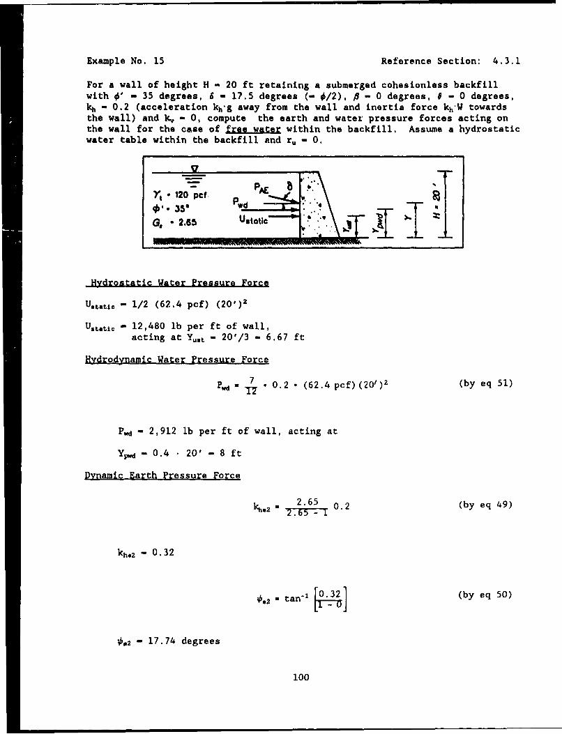
Example No. 15 Reference Section: 4.3.1
For a wall of height H - 20 ft retaining a submerged cohesionless backfillwith 4' - 35 degrees, 6 - 17.5 degrees (- 0/2), P - 0 degrees, P - 0 degrees,kh - 0.2 (acceleration kh'g away from the wall and inertia force kh'W towardsthe wall) and k, - 0, compute the earth and water pressure forces acting onthe wall for the case of f within the backfill. Assume a hydrostaticwater table within the backfill and r, - 0.
- ~ PAErt -120 pc1 w
01. 35'G, 2.65 sac
Hydrostatic Water Pressure Force
Ustatic - 1/2 (62,4 pcf) (20')2
Ustatic - 12,480 lb per ft of wall,acting at Yu.t - 20'/3 - 6.67 ft
Hvdrodynamic Water Pressure Force
Pwd 7 . 0.2 • (62.4 pcf) (20/)2 (by eq 51)
P.d 2,912 lb per ft of wall, acting at
YPd- 0.4 • 20' - 8 ft
Dynamic Earth Pressure Force
2.65 0.2 (by eq 49)T7z 265 -77
kh.2 - . 32
0.2 = tan-1 [3 (by eq 50)
0- 17.74 degrees
100
Example No. 15 (Continued) Reference Section: 4.3.1
KAI = cos 2 (35 - 17.74)
cos (17.74) cos (17.74 + 17.5) [1 sin (35 + 17.5) sin (35 - 17.74) (by eqcos (17.5 + 17.74)
KA- - 0.4965 36)
(adapted
PA 0.4965 * .• [(120 pcf - 62.4 pcf) (1 - 0)] (20/)2 from7 eq 33)
PAZ - 5,720 lb per ft of wall
(PAE), - PAZ (cos 6) - 5,455 lb per ft of wall
Determine Point of Application of PAE
From the Method 1 calculations in Example 14,
KA - 0.246 and PA - 2,834 lb per ft of wall.
PAE -P + APAE (eq 40)
APAE - PAE - PA
APAX - 5,720 - 2,834 - 2,886 lb per ft of wall, acting at 12 ft(0.6 H) above the base of the wall.
2,834 20) + 2,886 (0.6 " 20)5,720
Y - 9.4 ft (0.47 H)
Summary
For the restrained water case (Example 14, Method 1), the total force
acting normal to the wall - PAE(cos6) + Ust.ti.
- 6,855 + 12,480
- 19,335 lb per ft of wall.
For the free water case (Example 15), the total force acting on thewall - PAE(cos6) + Pd + Utati, - 5,455 + 2,912 + 12,480 - 20,847 lb per ft ofwall
For this dynamic problem, the free water analysis results in an8 percent larger total dynamic earth pressure force acting normal to the wall.
101
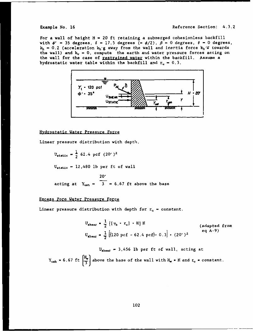
Example No. 16 Reference Section: 4.3.2
For a wall of height H - 20 ft retaining a submerged cohesionless backfillwith 0' - 35 degrees, 6 - 17.5 degrees (- 0/2), 6 - 0 degrees, 0 - 0 degrees,kh - 0.2 (acceleration kh'g away from the wall and inertia force kh'W towardsthe wall) and k, - 0, compute the earth and water pressure forces acting onthe wall for the case of restrained water within the backfill. Assume ahydrostatic water table within the backfill and r, - 0.3.
rP
't.-12o pcf *[ -50
Hydrostatic Water Pressure Force
Linear pressure distribution with depth.
Ustatic - 21 62.4 pcf (20')22)
U.tatic - 12,480 lb per ft of wall
20'
acting at Yst - 3 - 6.67 ft above the base
Excess Pore Water Pressure Force
Linear pressure distribution with depth for ru - constant.
IIUshtar N 4 [b " ru] H) H (adapted from
Usha [(120 pcf- 62.4 pcf). 0.3] * (20' )2 eq A-9)
Uah..r - 3,456 lb per ft of wall, acting at
Yu.h - 6.67 ft (--• above the base of the wall with H. = H and ru a constant.
102
Example No. 16 (Continued) Reference Section: 4.3 2
Dynamic Earth Pressur Force
--.3 u (120 pcf - 62.4 pcf) (1 - 0.3) (by eq 52)7.3 - 40.32 pcf
703 a 62.4 pof + (120 pcf - 62.4 pcf) • 0.3 (by eq 53)
70 3 79.68 pcf
kh.3 - 120 pcf . 0.240.32 pcf (by eq 54)
fKh* 3 = 0.595
0.3= tan- [0.595] (by eq 55)
0.7 - 30.75 degrees
Z - cos 2 (35 - 30.75)
Cos (30.75) cos (30.75 + 17.5) [l + [ sin (35 + 17.5) sin (35 - 30.75)cos (17.5 + 30.75) (by eq
KAZ - 1.033 36)
- K. - ( 1- (adapted from
PAE - 1.033 - 1 [40.32 pcf (1 - 0)] (20")2 eq 33)
PA- - 8,331 lb per ft of wall(PA). - PA(cos6) - 7,921 lb per ft of wall
Determine Point of Application of PAE
KA - COS 2 (35) (by eq 16)
cos 2 (0) cos (17.5) 1 + sin (35 + 17.5) sin (35)11 cos (17.5) cos (0)
KA - 0.246
P1-0.246 - 1 (40.32 pcf) (201)2 (adapted from( eq 7)
103
Example No. 16 (Continued) Reference Section: 4.3.2
PA 1,984 lb per ft of wall, acting at 6.67 ft above the base of the wall.
Ap* - PA (solve eq 40 for AFE)
APA - 8,331 - 1,984 - 6,347 lb per ft of wall, acting at 12 ft (0.6 H) above
the base of the wall.
1,984 201 6,347 (0.6 " 20')
8,331
Y - 10.7 ft (0.54 • H)
Summary
Excess pore water pressures within the submerged portion of the backfillincreased both the effective earth pressures and the total earth and waterpressures acting along the back of the wall.
P• increased by 16 percent, from a value equal to 7,188 lb per ft ofwall for the case of ru - 0 (Method 1, example 14), to a value equal to 8,331lb per ft of wall for the case of ru - 0.3 (example 16).
The total force acting normal to the wall for the case of r, equal to 0(Method 1, example 14) - PA (cos 6) + Ustatj, - 6,855 + 12,480 - 19,355 lb perft of wall.
The total force acting normal to the wall for the case of ru equal to0.3 (example 16) - PA (cos 6) + Ult*tir + Uhea, - 7,921 + 12,480 + 3,456- 23,857 lb per ft of wall.
The total force acting normal to the back of the wall increased by 23percent from the case of ru equal to 0, in the case of ru equal to 0.3.
104
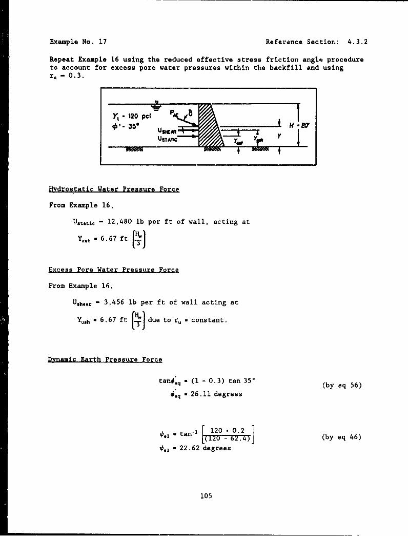
Example No. 17 Reference Section: 4.3.2
Repeat Example 16 using the reduced effective stress friction angle procedureto account for excess pore water pressures within the backfill and usingr,- 0.3.
* 120 pcf
Hydrostatic Water Pressure Force
From Example 16,
Ustatic - 12,480 lb per ft of wall, acting at
Yu,t" -6.67 ft (-)
Excess Pore Water Pressure Force
From Example 16,
Ughar - 3,456 lb per ft of wall acting at
Y-,h = 6.67 ft ff-] due to ru U constant.
Dynamic Earth Pressure Force
tano.q - (1 - 0.3) tan 35 (by eq 56)
Orq - 26.11 degrees
k.1 - tan-I 1 - 62 (by eq 46)
#10. - 22.62 degrees
105
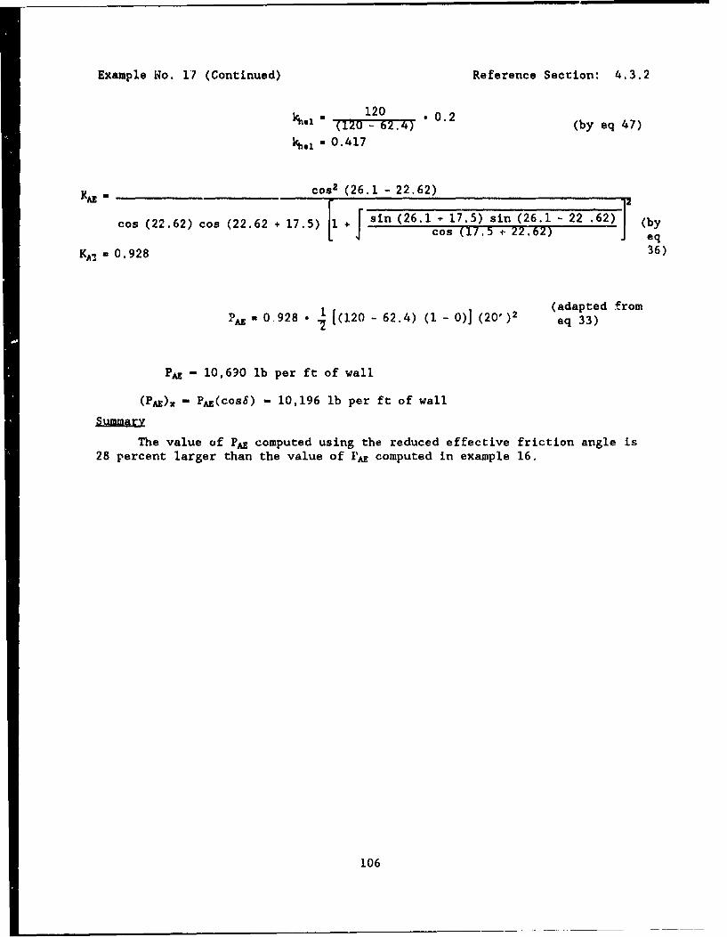
Example No. 17 (Continued) Reference Section: 4.3.2
120 - 0.2S220 - 62.47 (by eq 47)
1%.1 w 0.417
g cos 2 (26.1 - 22.62)
cOS (22.62) cos (22.62 17.5) [1 + [sin (26.1 , 17.5) sin (26.1 - 22 .62) (by1 [l cos (17.5 + 22.62) eq
KA^z .0.928 36)
P , 0, 928 • 1[(120 - 62.4) (1 - 0)] (20')2 (adapted from
9 28*-6.) 01 ) eq 33)
PAZ- 10,690 lb per ft of wall
(PAE),- PAE(cos5) - 10,196 lb per ft of wall
Summary
The value of PAE computed using the reduced effective friction angle is28 percent larger than the value of 'AE computed in example 16.
106
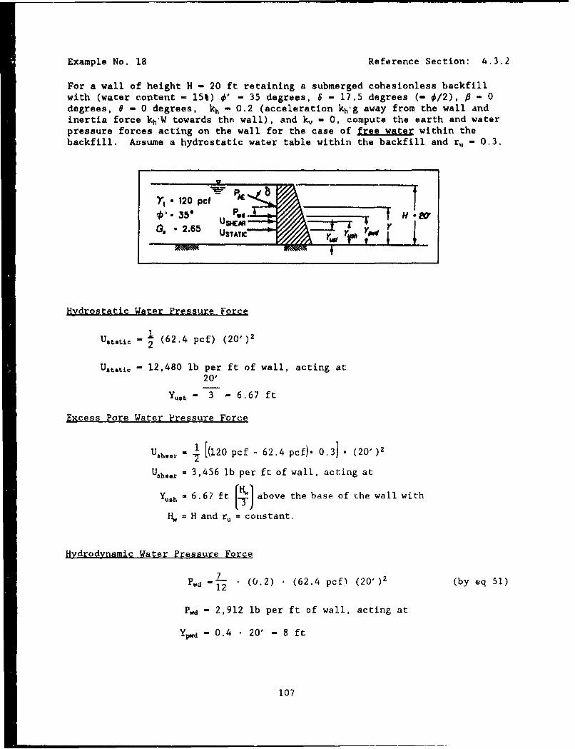
Example No. 18 Reference Section: 4.3.2
For a wall of height H - 20 ft retaining a submerged cohesionless backfillwith (water content - 15%) 9' - 35 degrees, 6 - 17.5 degrees (- 0/2), P - 0degrees, 0 - 0 degrees, kh - 0.2 (acceleration kh'g away from the wall andinertia force kh-W towards thn wall), and k, - 0, compute the earth and waterpressure forces acting on the wall for the case of free water within thebackfill. Assume a hydrostatic water table within the backfill and r. - 0.3.
P
YYt 120 pcf M
G 2.65 UST ATy
Hydrostatic Water Pressure Force
Ustatic - 1 (62.4 pcf) (20')22)
Ust.tic - 12,480 lb per ft of wall, acting at20'
Yst "- 3 - 6.67 ft
Excess Pore Water Pressure Force
Usheal. n i [(120 pcf - 62.4 pcf). 0.3] . (20' )2
Ushear = 3,456 lb per ft of wall, acting at
Yuh = 6.67 ft - above the base of the wall with
H, = H and ru = constant.
Hydrodynamic Water Pressure Force
P -d 12 (0.2) , (62.4 pcf) (20')2 (by eq 51)
P.d " 2,912 lb per ft of wall, acting at
Yped " 0.4 . 20' - 8 ft
107
Example No. 18 (Continued) Reference Section: 4.3.2
Dynamic Earth Presaure Force
7.3 = (120 pcf - 62.4 pcf) (1 - 0.3) (by eq 52)
7.3 w 40.32 pcf
Y,3 a 62.4 pcf + (120 pcf - 62.4 pcf) * 0.3 (by eq 53)
713 a 79.68 pcf
with a water content equal to 15 percent,
7 td " +
7 120 pcf . 104.3 pcfd"I +0.M'S
104.35 pcf . 0. 240.32 PE (by eq 57)
kh*4 0. 518
. tan-1 ,rO.1]
a14 27.38 degrees
KA - cos 2 (35 - 27.38)
cos (27.38) cos (27.38 + 17.5) [+ [ sin (35 + 17.5) sin (35 - 27.38)
O s cos (17.5 + 27'YT.) (by eq
36)KA, - 0. 8136
-AE = 0.8136 1 1 [(40.32 pcf) (1 - 0)] f20')2 (adapted from eq 33)
PAZ 6,561 lb per ft of wall
(PAZ). PAF (cos6) - 6,257 lb per ft of wall
108
Example No. 18 (Continued) Reference Section: 4.3.2
Determine Point of Application of PA
From example 16,
KA o. 2 4 6
PA a 1,984 lb per ft of wall, acting at
6.67 ft -T above the bas. of the wall.
APAI - AZ - PA (solve eq 40 for APz)
AP• - 6,561 - 1,984 - 4,577 lb per ft of wall, acting at 12 ft(0.6H) above the base of the wall.
1,984 [2)-14,577 (0.6 • 20')6,561
Y a 10.4 ft (0.52 H) above the base of the wall
For the restrained water case (example 16), the total force actingnormal to the wall
- PA (cosO) + Ust.tic + Ushoar
- 7,921 + 12,480 + 3,456
- 23,857 lb per ft of wall
For the free water case (example 18), the total force acting normal tothe wall
- PA (COS6) + Uatatit + Ushear + Pwd
- 6,257 + 12,480 + 3,456 + 2,912
- 25,105 lb per ft of wall
For this problem, the fiee water analysis results in a 5 percent larger totaldynamic earth pressure force acting normal to the wall, as compared againstthe restrained water case.
109
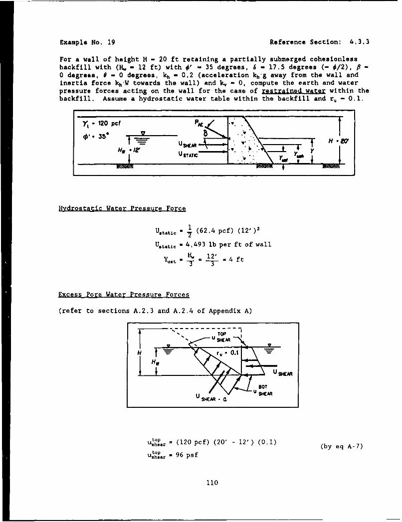
Example No. 19 Reference Section: 4.3.3
For a wall of height H - 20 ft retaining a partially submerged cohesionlessbackfill with (H. - 12 ft) with 0' - 35 degrees, 6 - 17.5 degrees (- 0/2), f? -0 degrees, 9 - 0 degrees, kh - 0.2 (acceleration kh'g away from the wall andinertia force kh'W towards the wall) and k, - 0, compute the earth and waterpressure forces acting on the wall for the case of restrained water within thebackfill. Assume a hydrostatic water table within the backfill and ru - 0.1.
*Y 120 pcf PI,,35" 0
Hw ~ uUTATC I ; :
Hydrostatic Water Pressure Force
Ustatic = (62.4 pcf) (12' )1
U.tatic - 4,493 lb per ft of wall
= Hw . 12' 4 ft
Excess Pore Water Pressure Forces
(refer to sections A.2.3 and A.2.4 of Appendix A)
USHEAR
UshIar : (120 pcf) (20' -12') (0.1 (be)A7top -9
Ushear = 9psf
110
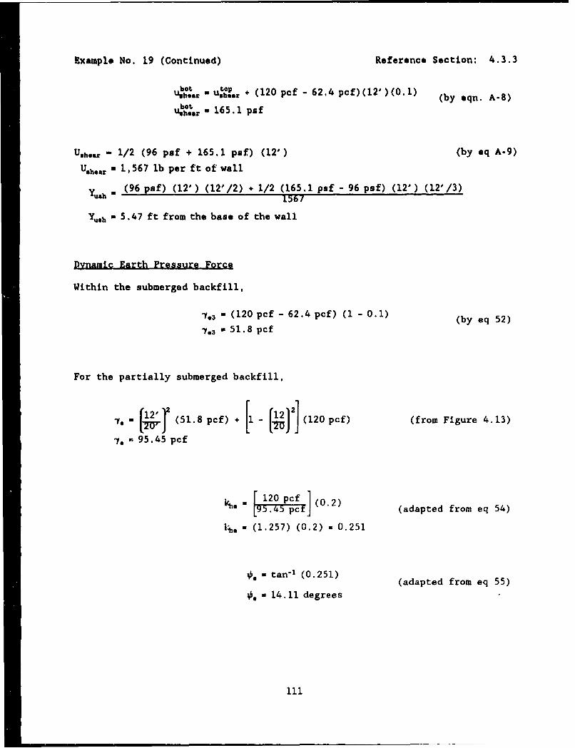
Example No. 19 (Continued) Reference Section: 4.3.3
bot , Lop (10 -6,
u,,1 *P,,, + (120 pcf - 62.4 pcf) (12" ) (0.1) (by eqn. A-8)
4hsste 165.1 psf
Ush.er - 1/2 (96 psf + 165.1 psf) (12') (by eq A-9)
U~h.., * 1,567 lb per ft of wall
Yu~h - (96 psf) (12') (12'/2) + 1/2 (165.1 psf - 96 psf) (12') (12'/3)1567
Yah - 5.47 ft from the base of the wall
Dynamic Earth Pressure Force
Within the submerged backfill,
7.3 = (120 pcf - 62.4 pcf) (1 - 0.1) (by eq 52)
7.3 a 51.8 pcf
For the partially submerged backfill,
74 , 12" f (51.8 pcf) + [1 -(2)] (120 pcf) (from Figure 4.13)
,e M 95.45 pcf
C.P [95.4 5 pf (0.2) (adapted from eq 54)
1 h,. - (1.257) (0.2) - 0.251
a tan-' (0. 251) (adapted from eq 55)
00 - 14.11 degrees
1I1
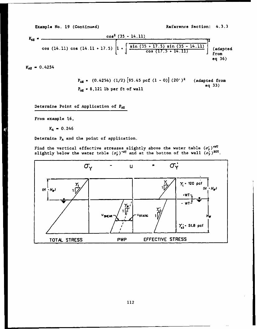
Example No. 19 (Continued) Reference Section: 4.3.3
cos' (35 - 14.11)
cos (14. 11) cos (14.11 + 17.5) [ sin (35 + 17.5) sin (35 - 14.11) (adapted1 4 cos (17.5 + 14.11) from
eq 36)
KA- 0.4254
P~z = (0.4254) (1/2) [95.45 pcf (1 - 0)] (20' )2 (adapted from
PA - 8,121 lb per ft of wall eq 33)
Determine Point of Application of PA
From example 16,
KA - 0.246
Determine PA and the point of application.
Find the vertical effective stresses slightly above the water table (0;)+WTslightly below the water te.ble (a' )'r and at the bottom of the wall (o,) BOT .
- U
A 1120 17 iV (H -HWJ
U M 1"WT J
)~51.8 pcf
TOTAL STRESS PWP EFFECTIVE STRESS
112
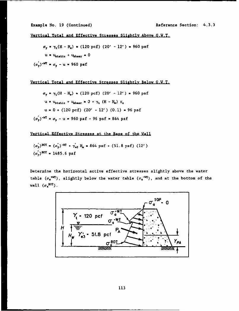
Example No. 19 (Continued) Reference Section: 4.3.3
Vertical Total and Effective Stresses Slightly Above G.W.T.
Oy = yt(H - Hi.) - (120 pcf) (20' - 12') * 960 paf
U 0 UJetati + Ushear 0 0
(O;)*wT - ay - u = 960 psf
Vertical Total and Effective Stresses Slightly Below G.W.T.
ay - yt(H - H,) a (120 pcf) (20' - 12') - 960 psf
u - u1 tatic + u.h.ar - 0 + 7t (H - H.) r.
u - 0 + (120 pcf) (20' - 12') (0.1) - 96 psf
(a,)wT - o - u a 960 psf - 96 psf - 864 psf
Vertical Effective Stresses at the Base of the Wall
(a;)°Ta" (;)"T + 7.3 H, - 864 psf + (51.8 psf) (12')
(o;)BOT a 1485.6 psf
Determine the horizontal active effective stresses slightly above the water
table (o.+WT), slightly below the water table (oa-WT), and at the bottom of the
wall (aBOT).
TOP
J )j 120 pcf o'.WT '"""
PAI v .4 51.8 pcf f _' "
113
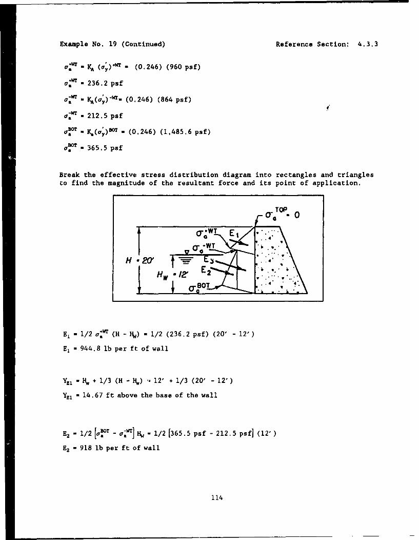
Example No. 19 (Continued) Reference Section: 4.3.3
*W. a (a')' - (0.246) (960 psf)
a.* - 236.2 psf
*WT - K(ao) -WT. (0.246) (864 psf)4
,*wT - 212.5 psf
aa°T - K,(ay)BrT - (0.246) (1,485.6 psf)
ao - 365.5 psf
Break the effective stress distribution diagram into rectangles and trianglesto find the magnitude of the resultant force and its point of application.
TOP0 0
S~. "."H-2 t -_/2 '- E E .
E1 - 1/2 o~w (H -. lL) - 1/2 (236.2 psf) (20' - 12')
E 944.8 lb per ft of wall
t -HE3
l H 1/3 (H -H) ;12" ÷H1/3 (20' -12')
YEl - 14.67 ft above the base of the wall
E 1 - 1/2 [0aT - tý-;wTJ NW - 1/2 [365.5 psf -212.5 psf] (12' )
E, - 918 lb per ft of wall
114
Exahiple No. 19 (Continued) Reference Section: 4.3.3
Y-2 - 1/3 (H.) - 1/3 (12' )Y22 - 4.00 ft above the base of the wall
E3 - u?,• (1•) - (212.5 psf) (12')
E3 - 2,550 psf
YVE - 1/2 (H.,) - 1/2 (12')
YEa - 6.00 ft above the base of the wall
PA - E1+ E2 + E3 = 944.8 + 918 + 2,550
PA - 4,413 lb per ft of wall
Sum moments about the base of the wall and solve for:
yPA a El (YNE) + E2 (YE2) + E3 (YE3)PA
yPA , (944.8) (14.67') + (918) (4.00') + (2,550) (6.00')4,413
YpA - 7.44 ft above the base of the wall
APA - PAE - PA (solve eq 40 for APE)
APA - 8,121 - 4,413
APAE - 3,708 lb per ft of wall, acting at 12ft (0.6H) above the base of the wall.
y PA (YpA) + APAE (0.6H)
PAZ
y (4,413) (7.44') + (3,708) (0.6) (20')8121
Y = 9.52 ft (0.48H) above the base of the wall.
115
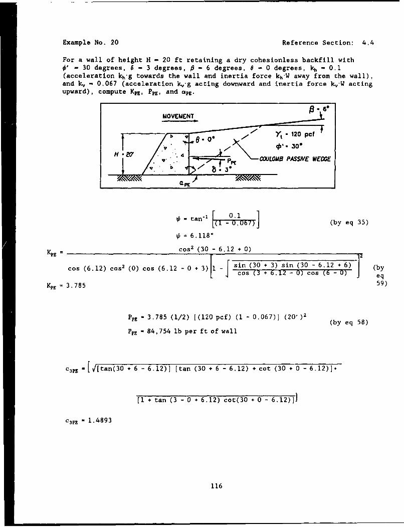
Example No. 20 Reference Section: 4.4
For a wall of height H - 20 ft retaining a dry cohesionless backfill with0' - 30 degrees, 6 - 3 degrees, P - 6 degrees, e - 0 degrees, kh - 0.1(acceleration kh-g towards the wall and inertia force kh'W away from the wall),and k, - 0.067 (acceleration kv'g acting downward and inertia force kv'W actingupward), compute KPE, PpE, and CPE.
MOVEMENT_
iH 4/ COULOMB PASSIVE WEDGE
~Fpc
= tan 1 0-.Y] (by eq 35)
= 6.118°
KPE = COS 2 (30 - 6.12 + 0)
cos (6.12) cos 2 (0) cos (6. 12 - 0 + 3 ) - sin (30 + 3) sin (30 - 6.12 + 6) (by[ Cos (3 + 6.12 - 0) cos ( )eq
KPE - 3. 785 59)
PPE - 3.785 (1/2) [(120 pcf) (1 - 0.067)] (20' )2 (by eq 58)
PPE - 84,754 lb per ft of wall
c3P1 '[ ytan(30 + 6 - 6.12)] [tan (30 + 6 - 6.12) + cot (30 + 0 - 6.12)].
[1 + tan (3 -0 + 6.12) cot(30 + 0 - 6.12)]]
C3PE - 1.4893
116
Example No. 20 (Continued) Reference Section: 4.4
COPE - 1 + [[tan (3 - 0 + 6.12)] ° [tan (30 + 6 - 6.12) + cot (30 + 0 - 6.12)]]
c 4 pz - 1.4547
, 6.12 - 30 ÷ tan" an (30 + 6 - 6.12) + 1.4893O. 1.4547 J (by eq 61)
a- 30.9°
117
Evample No. 21 Reference Section: 4.4
Repeat Example 20 with k, - -0.067 (acceleration k•,g acting upward and
inertia force k,-W acting downward).
#-tan' [ 0.I1tn [ (-0.U67)) (by eq 35)
- 5.3540
KpE - cos 2 (30 - 5.35 + 0) (by eq
cos (5. 35) cos 2 (0) cos (5 35 - 0 * 3) - sin (30 + 3) sin (30 - 5.35 * 6) 59)S.... . cos (3 + 5.35 -'0) cos (6-')
Kp - 3. 815
PPE - 3.815 (1/2) [(120 pcf) (I - (-0.067))] (20' )2 (by eq 58)
PPE U 97,695 lb per ft of wall
C3PE [V[tan(30 + 6 - 5.35)] (tan (30 + 6 - 5.35) + cot (30 + 0 - 5.35)],
[1 + tan (3 - 0 + 5.35) cot (30 + 0 - 5.35)]]
C3PE - 1.4724
C4PE u 1 + [[tan (3 - 0 + 5.35)] * (tan (30 + 6 - 5.35) + cot (10 + 0 - 5.35)]]
C4PE - 1.4071
*PE - 5.35 - 30 + tan-1 [tan (30 + 6 - 5.35) + 1.47241
ST.4071 (by eq 61)
QPE - 31.10
118
Example No. 21 (Continued) Reference Section: 4.4
Summary
Examples 20 and 21 show that when the inertial force k .- W acts downward(example 21) the computed value for PRE is 15 percent larger than PPE for thecase when kv . W acts upward (example 20).
119
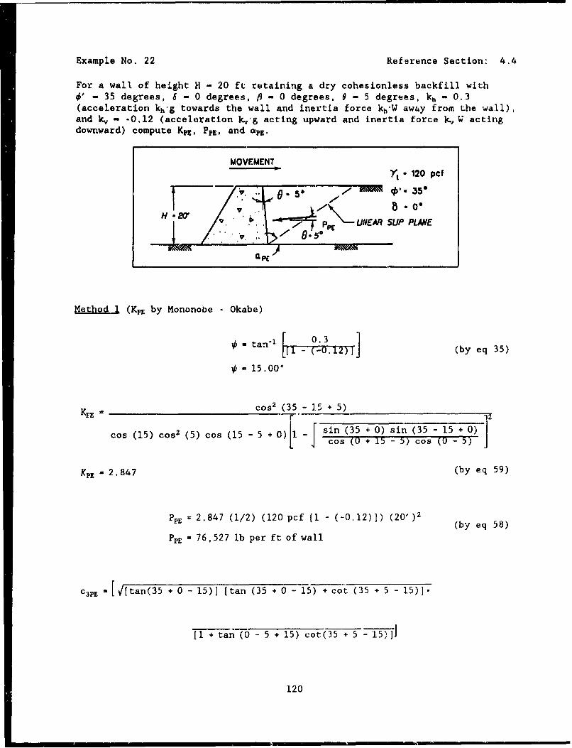
Example No. 22 Reference Section: 4.4
For a wall of height H - 20 ft retaining a dry cohesionless backfill with0' - 35 degrees, 6 - 0 degrees, )9 - 0 degrees, 0 - 5 degrees, kh - 0.3(acceleration kh'g towards the wall and inertia force kh'W away from the wall),and k, - -0.12 (acceleration kv'g acting upward and inertia force kvW actingdownward) compute KpE, PPE, and apt.
MOVEMENT-j 120 pcf
H .E' LINEAR SUP PLANEV.K
Method 1 (KpE by Mononobe - Okabe)
Sfitan•-i 0.3 ]
[[I - (-0.12)] (by eq 35)
1 15.00'
KFE cos 2 (35 - 15 + 5)
Cos (15) cos2 (5) cos (15 - 5 +40) [1 - [ sin (35 + 0) sin (35 - 15 + 0)~ Jcos (0 + 15 - 5) cos (0 - 5) J
KP, 2. 847 (by eq 59)
PPE = 2.847 (1/2) (120 pcf [1 - (-0.12)]) (20' )2 (by eq 58)
PpE - 76,527 lb per ft of wall
c3PE - [ 4[tan(35 + 0 - 15)] [tan (35 + 0 - 15) + cot (35 + 5 - 15)].
[I + tan (0 -- 5 + 15) cot(35 + 5 - 15)]
120
Example No. 22 (Continued) Reference Section: 4A4
c,% - 1.1217
c4Pz "1 *[[tan (0-5 ÷ 15)] • [tan (35 + 0- 15) + cot (35 +5 - 15)J]
*N - 1.4420
.(15 - 35) + tan-I [tan (35 +0 - 15)+ 1.121711.4420 (by eq 61)
tEz -25.85050
Method 2 (Equivalent Static Formulation with Kp by l.og-Spiral Method)
0 - 06 - -15*
"- - - -10.
2.52 (frnm Table 3)
FPE a cOs 2 (5 - 15)cos (15) cos' (5)
F*- 1.0117
Ppg - [2.52 (1.0117)] (1/2) [(120 [1 - (-0.12)])] (20)2 (by eq 62)
P,, - 68,530 lb per ft of wall
S~summary
The values for KPE and PPE computed using Mononobe - Okabe (by Equations 58 and59) are 12 percent larger than the values for [K. (#*, 0*) FpE] and PpE byEquation 62.
121
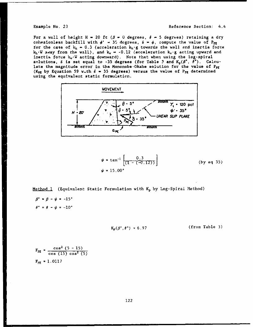
Example No. 23 Reference Section: 4.4
For a wall of height H - 20 ft (9 - 0 degrees, e - 5 degrees) retaining a drycohesionlesa backfill with 0' - 35 degrees, 6 - 4, compute the value of Pp1for the case of kh - 0.3 (acceleration kh'g towards the wall and inertia forcekh'W aoay from the wall), and k, - -0.12 (acceleration k.,g acting upward andinertia force kvW acting downward). Note that when using the log-spiralsolutions, 6 is set equal to -35 degrees (for Table 3 and K,(#*, 6*). Calcu-late the magnitude error in the Mononobe-Okabe solution for the value of Pp1
(Kpg by Equation 59 w.th 6 - 35 degrees) versus the value of PpE determinedusing the equivalent static formulation.
MOVEMENT
T / 'l.0 50 12 pcfo o. I,..
aPE
= tan-1 ( (0.32) (by eq 35)
= 15.00'
Method 1 (Equivalent Static Formulation with Kp by Log-Spiral Method)
•..•-,/,-15'-"= -• = -lo°
= 6.97 (from Table 3)
cos2 (5 - 15)
cos (15) cos 2 (5)
FpE = 1.0117
122
Example No. 23 (Continued) Reference Section: 4.4
*p, [(6.97) (1.0117)] (1/2) [120 (1 - (-0.12))] (20)2 (by eq 62)
P* a 189,546 lb per ft of wall
M (Kpz by Mononobe-Okabe Method)
Kpz w cos 2 (35 - 15.0 + 5) 2
cos (15) cos 2 (5) cos (15 - 5 + 35) - sin (35 + 35) sin (35 - 15 + 0)J cos (35 + 15 - 5) cos (0 - 5)
KpE - 11.507 (by eq 59)
PpE - 11.507 (1/2) [(120 pcf) (1 - (-0.12))] (20')2 (by eq 58)
PpE - 309,308 lb per ft of wall
Summnary
The Mononobe-Okabe procedure over predicts the value for Ppr by 63 percent.The accuracy of the Mononobe-Okabe solution decreases with increasing valuesof 6.
123
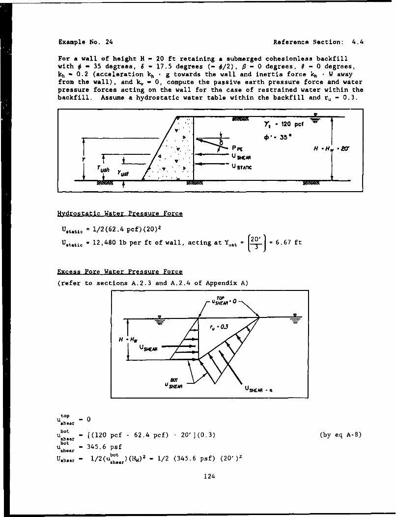
Example No. 24 Reference Section: 4.4
For a wall of height H - 20 ft retaining a submerged cohesionless backfillwith 0 - 35 degrees, 6 - 17.5 degrees (- 0/2), P - 0 degrees, 0 - 0 degrees,kh - 0.2 (acceleration kh . g towards the wall and inertia force kh . W awayfrom the wall), and k, - 0, compute the passive earth pressure force and waterpressure forces acting on the wall for the case of restrained water within thebackfill. Assume a hydrostatic water table within the backfill and r, - 0.3.
Y," "120 pOf q'
-35*'" •. PC H.-Hw. W
Y U SHEAR
Y U STATIC
Hydrostatic Water Pressure Force
Ustatic = 1/2(62.4 pcf)(20) 2
- 12,480 lb per ft of wall, acting at Yust,= ' = 6.67 ft
Excess Pore Water Pressure Force
(refer to sections A.2.3 and A.2.4 of Appendix A)
TOP
U --
r..JH -
W UH E
0
USHEAM -"USH -AR
top -- 0
shear
bot" "shear - [(120 pcf - 62.4 pcf) 20'](0.3) (by eq A-8)
"U hot- 345.6 psf
Usher - 1/ 2 (u hor )(Hw) 2 1/2 (345.6 psf) (20')2
124
Example No. 24 (Continued) Reference Section: 4.4
Uch..r - 3,456 lb per ft of wall
Y,.h - 1/3(H) - 6.67 ft from the base of the wall
Dynamic Earth Pressure Force
Within the submerged backfill,
7.3 - (120 pcf - 62.4 pcf) (1 - 0.3) (by eq 52)
Y.3 - 40.32 pcf
kh. 0f 20pcf (02kb.3 (40.32 pctF (0.2) (by eq 54)
kh.3 - 0. 595
0.3 - tan'I (0.595] (by eq 55)
0.3 - 30.75*
Kpz a cos 2 (35 - 30.75 + 0)
cos (30.75) cos2(0) cos (30.75 - 0 + 17.5) 1 [sin (35 + 17.5) sin (35 - 30.75 + 0)[(51 - os (17.5 + 30.75 - U) cos (0 - 0)J
K* - 3.518 (by eq 59)
Pp. - 3.518 (1/2) (40.32 pcf [1 - 0]) (20')2 (adapted from eq 58)
PpE - 28,369 lb per ft of wall
125
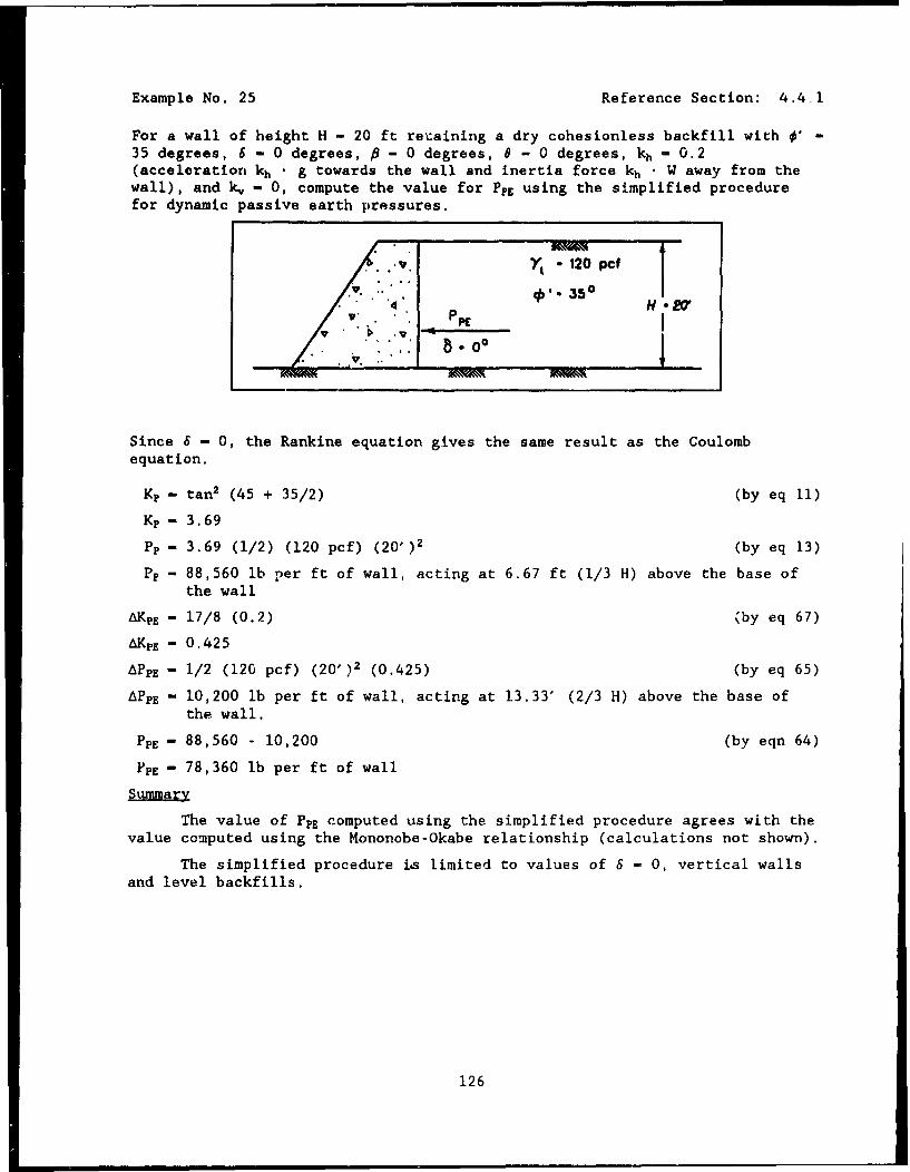
Example No. 25 Reference Section: 4.4.1
For a wall of height H - 20 ft retaining a dry cohesionless backfill with €' -35 degrees, 6 - 0 degrees, • - 0 degrees, e - 0 degrees, kh - 0.2(acceleration kh . g towards the wall and inertia force kh • W away from thewall), and k, - 0, compute the value for Ppz using the simplified procedurefor dynamic passive earth pressures.
Sv Yl "120 pef
•.. .. '. ,. 3504 P H - 2V
V. V
Since 6 - 0, the Rankine equation gives the same result as the Coulombequation.
Kp - tan2 (45 + 35/2) (by eq 11)
Kp - 3.69
Pp - 3.69 (1/2) (120 pcf) (20')2 (by eq 13)
Pp - 88,560 lb per ft of wall, acting at 6.67 ft (1/3 H) above the base of
the wall
AKPE - 17/8 (0.2) (by eq 67)
AKPE - 0.425
APPE - 1/2 (120 pcf) (20')2 (0.425) (by eq 65)
APPE - 10,200 lb per ft of wall, acting at 1.3.33' (2/3 H) above the base ofthe wall.
PPE - 88,560 - 10,200 (by eqn 64)
PPE - 78,360 lb per ft of wall
Summary
The value of PPE computed using the simplified procedure agrees with thevalue computed using the Mononobe-Okabe relationship (calculations not shown).
The simplified procedure is limited to values of 6 - 0, vertical wallsand level backfills.
126
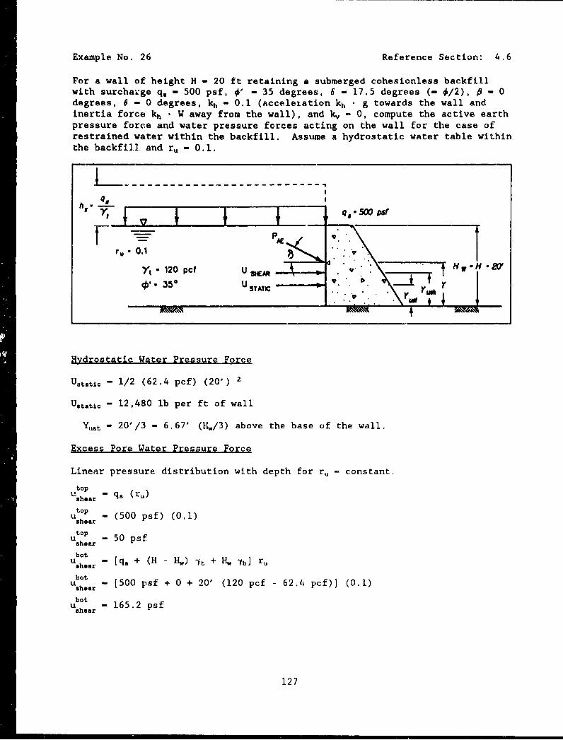
Example No. 26 Reference Section: 4.6
For a wall of height H - 20 ft retaining a submerged cohesionless backfillwith surcha'ge q. - 500 psf, 0' - 35 degrees, 6 - 17.5 degrees (- 0/2), P - 0degrees, 0 - 0 degrees, kh - 0.1 (acceletation kh . g towards the wall andinertia force kh - W away from the wall), and k, - 0, compute the active earthpressure force and water pressure forces acting on the wall for the case ofrestrained water within the backfill. Assume a hydrostatic water table withinthe backfil]. and r, - 0.1.
1~- PAEr , 0.1 . 7 '.
Y* 120 pcf U .t•qS' - 350 U sYx:--)*4 35*STATICI
**.v* Y
Hydrostatic Water Pressure Force
Ustatic - 1/2 (62.4 pcf) (20') 2
Ustatjo - 12,480 lb per ft of wall
YUSt - 20'/3 - 6.67' (11,/3) above the base of the wall.
Excess Pore Water Pressure Force
Linear pressure distribution with depth for r, - constant.
topU Ushear "q. (r.)
Uetop - (500 psf) (0.1)
utop - 50 psfUshear
bot
Ushear - [q. + (H - Hw) -vt + H. Yb] rY
u bor - [500 psf + 0 + 20' (120 pcf - 62.4 pcf)] (0.1)
uhot - 165.2 psf
127
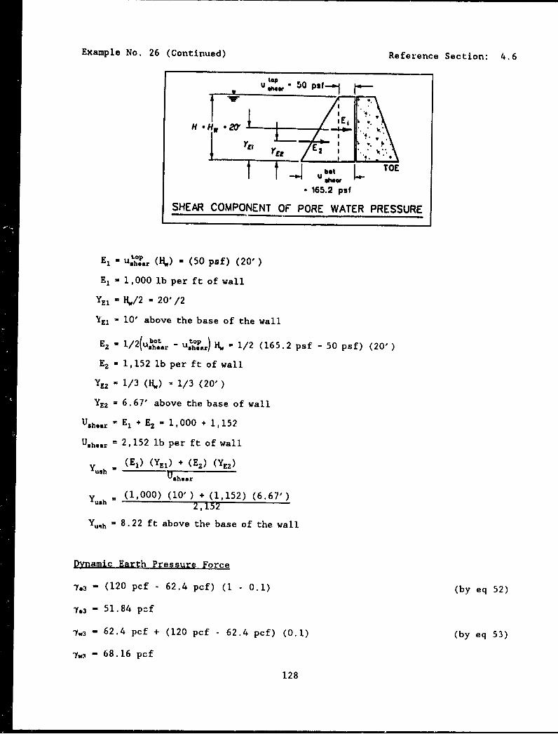
Example No. 26 (Continued) Reference Section: 4.6
top p f-.,
H-.H.2O' it* 4E
YE, F,. ,.:
- 165.2 psi
SHEAR COMPONENT OF PORE WATER PRESSURE
mL
El ush*.r (H.) - (50 psf) (20')
E, - 1,000 lb per ft of wall
YE, = H./2 - 20'/2
YE, - 10' above the base of the wall
"E2 - 1/2( shear - usear) H. - 1/2 (165.2 psf - 50 psf) (20')
E2 - 1,152 lb per ft of wall
YE2 = 1/3 (H,) - 1/3 (20' )
YE2 = 6.67' above the base of wall
Ushear El + E2 - 1,000 + 1,152
Ushear = 2, 152 lb per ft of wall
Yush C(E1) (YzE) + (EZ) (YEz)Ushmar
Y..h= (1,000) (10') + (1,152) (6.67')2,152
Yu.h -8.22 ft above the base of the wall
Dynamic Earth Pressure Force
7Y3 - (120 pcf - 62.4 pcf) (I - 0.1) (by eq 52)
7Y3 - 51.84 pzf
-.3 - 62.4 pcf + (120 pcf - 62.4 pcf) (0.1) (by eq 53)
-.,4 - 68.16 pcf
128
Example No. 26 (Continued) Reference Section: 4.6
kho.3 -120 pcf (0.1)51.84 pcf (by eq 54)
kl. 3 - 0.2315
0.3 - tan' 1 (0.2315) (by eq 55)
0,3 - 13.03 degrees
KAS - cos 2 (35 - 13.03)
cos (13.03) cos (13.03 + 17.5) + sin (35 + 17.5) sin (35 - 13.03) (adaptedL1 cos (17.5 + 13.03) from
KAE - 0.4069 eq 36)
P1 + [h2q - 1 .(0. 3) [1 1,,)] H2 (adapted3V fromr 2 1Fig 4.18)
*A (.4069) + 2(500 psf) I . ( 51.84 pcf) [1 - 01 (20' )2Fi4.8
1 (5)1. 84 pct) (20') T
PAZ - 8,288 lb per ft of wall
Determine Point of Application of PAE
KYA cos2 (35 - 0)
cos 2 (0) cos (0 + 17.5) + sin (35 + 17.5) sin (35 - 0)cos (17.5 + 0) cos (0 -0) (by eq 16)
KA - 0.2461
Determine PA and the point of application.
Find the vertical cffective stress at the ground surface.
129
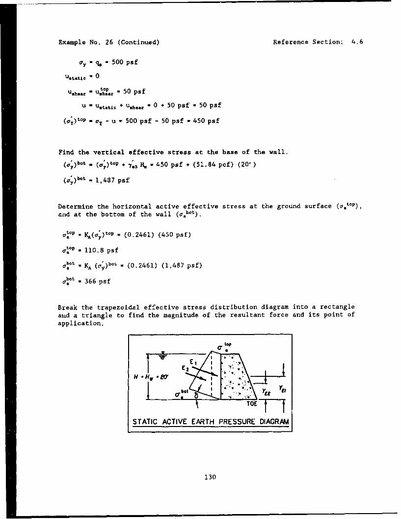
Example No. 26 (Continued) Reference Section: 4.6
ay - q. - 500 psf
Ustatic W 0top
Ushear - Ushlar - 50 psf
U - U. tati + Ushear - 0 + 50 psf - 50 psf
(cy)top may - U 500 psf - 50 psf - 450 psf
Find the vertical effective stress at the base of the wall.
(U;)bat " (O;)top + 7.3 H, - 450 psf + (51.84 pcf) (20')
(ay)bat - 1,437 psf
Determine the horizontal active effective stress at the ground surface (oatoP),
and at the bottom of the wall (aa bt).
top - KA(ay)tOP - (0.2461) (450 psf)
t.*P - 110.8 psfbot
at -, KA (cv')bol - (0.2461) (1,487 psf)
-bt - 366 psf
Break the trapezoidal effective stress distribution diagram into a rectangleand a triangle to find the magnitude of the resultant force and its point ofapplication.
'op
I ~., ...b ýI2__1 ba Yr .,'".E.I.
TOE
STATIC ACTIVE EARTH PRESSURE DIAGRAM
130
Example No. 26 (Continued) Reference Section: 4.6
E, - a."P(H) - (110.8 psf) (20')
E, - 2,216 lb per ft of wall
YE, - 1/2(H) - 1/2 (20' )
Y•E - 10 ft above the base of the wall
E2- 1/2 (abuot - at.ip) (H) - 1/2 (366 psf - 110.8 psf) (20')
E2 - 2,552 lb per ft of wall
YE2 - 1/3 (H) - 1/3 (20' )
Y*2 - 6.67 ft above the base of the wall
PA - E1 + E2 - 4,768 lb per ft of wall
YPA = E1 (YEj) + E2 (YE2) (2216) (10') + (2552) (6.67')4768
YpA - 8.22 ft above the base of the wall
APAE - PAE - PA - 8288 - 4768 (solve eq 40 for APAE)
APAE - 3,520 lb per ft of wall
Find the Point of Application of APAE
hS a-qs L 500 psf
I t 120 pcf
h, =-4.17 ft
Y -pAE - 0.6 (H + h,) - 0.6 (20' + 4.17') (from Figure 4.20)
YApAE - 14.5 ft above the base of the wall
y a YPAE = PA (YpA) + APA (Y&pAE) . (4768) (8.22') + (3520) (14.5')PA •'8,288
Y - 10.89 ft (0.54 H) above the base of the wall
131
CHAPTER 5 EARTH PRESSURES ON WALLS RETAINING NONYIELDING BACKFILLS
5.1. Introduction
This part of the report describes two procedures that are used to com-pute the dynamic earth preswAres acting along the back of walls retainingnonyielding backfills due to earthquake shaking. In practical terms, a wallretaining a nonyielding backfill is one that does not develop the limitingdynamic active or passive earth pressures because sufficient wall movements donot occur and the shear strength of the backfill is not fully mobilized - wallmovements that are less than one-fourth to one-half of Table 1 wall movementvalues. Because of this, earth retaining structures such as massive concretegravity retaining walls founded on firm rock or U-frame locks and dry docksare sometimas referred to as structures retaining "nonyielding" backfills inthe literature. Two procedures for analyzing such cases are a simplifiedanalytical procedure due to Wood (1973) and a complete soil-structure interac-tion analysis using the finite element method (see Appendix D).
5.2 Wood's Solution
Wood (1973) analyzed the response of a wall retaining nonyielding back-fill to dynamic excitation assuming the soil backfill to be an elasticmaterial. He provided normal wode solutions for the case of both a uniformmodulus and a modulus varying linearly with depth. Since these solutions areslowly convergent for practical problems Wood (1973) presented approximateprocedures based on findings from the normal mode solutions. Wood showed thata static elastic solution for a uniform 1-g horizontal body force gave veryaccurate results for the pressures, forces, and moments on the wall underharmonic excitation of frequency f (cyclic frequency) when dynamic amplifica-tion effects were negligible. This occurs when Q - f/f. is less than about0.5 where f is the frequency of motion and f, - V,/4H is the cyclic frequencyof the first shear mode of the backfill considered as a semi-infinite layer ofdepth H. The limiting 0 depends on the value of V. and the geometry of theelastic backfill but the value 0 < 0.5 covers many practical cases.
In cases of wide backfills, the lateral seismic force against the wallwhen 0 < 0.5 is given b)
Fsr I H2 • , (68)
acting at a height of 0.63"H above the back of the wall.
The normal stress distributions along the back of the wall were shown tobe a function of (1) Poisson's ratio, u, and (2) the lateral extent of theelastic medium behind the wall, expressed in terms of the ratio of the widthof the elastic backfill divided by the height of the wall, L/H (see Fig-ure 5.1). Two examples of the variation in the values for the normalizedhorizontal stresses with normalized elevations above the base of the wall areshown in Figure 5.2. A L/H value equal to 1 corresponds to a narrow backfillplaced within rigid containment and a L/H value equal co 10 corresponds to abackfill of great width. The horizontal stresses at any elevation Y along theback of the wall, ax, are normalized by the product of I-H in this figure.
133

y HOMOYEAWUS ELASTC SOIL(PLNE STRAIN) .If j. 0 DISPLACEMENTr X -0
, /
H RIGIDWALL
DISPLACEMENr X - 0
Figure 5.1 Model of elastic backfill behind a rigid wall
The resulting distributions for the horizontal stresses are parabolic, withlarger values computed along the upper half of the wall, as compared to thevalues computed along the lower half. In addition, the results show o, to belarger for wide elastic backfills, as compared to those values computed fornarrow elastic backtills. Figure 5.3 shows the corresponding resultant hori-zontal force, Far, along the back of the rigid wall anti the correspondingseismic moment about the base of the rigid wall, Mar, as a function of v andL/H. Figure 5.3 presents the resultant force and moment in terms of theirdimensionless values. F., acts at a height
M. (69)
The stresses shown in Figure 5.2 and the forces and mnoments shown in Fig-ure 5.3 result from the application of a 1-g static horizontal body force.The values for ax and Far corresponding to other constant honi(zontal accelera-tion values are computed by multiplying the oa. value from Figure 5.2 and theFar value from Figure 5.3 by the ratio of the new acceleration valuecoefficient, kh.
Shaking table tests by Yong (1985) using dry sand backfill and one-halfmeter high walls have confirmed the applicability of Wood's simplifiedprocedure when the predominant frequency of shaking is significantly less thanthe fundamental frequency of the backfill. The measured forces exceeded by afactor of 2 to 3 those predicted by the Moncinobe-Okabe theory. The tests
134
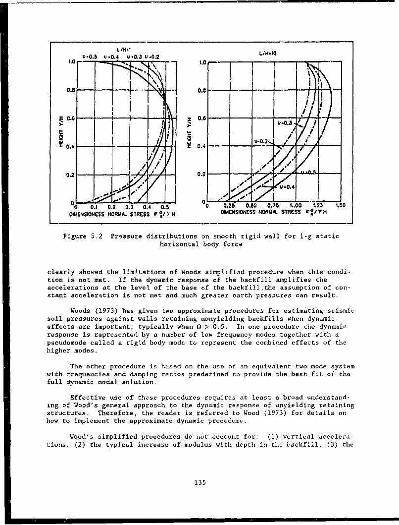
U-0.5 u0.4 U -0,3 U -0O,2
).8 - O"X01 •0. 0- .0 - - Li4t :i I
I Ut-0.3,
0.4 - 0.4
.. 0
0.2 " oo* .,, 0.2 .00!...L
0-0.
0 1 0.2 0.3 0.4 0.5 0 0.25 0.50 0.75 1..00 1.23 1.50
DIMENSIONESS INORMA. STRESS 4" */1' H OlMENSIONESS NORMA, STRESS U X0/YH
Figure 5.2 Pressure distributions 3n smooth rigid wall for l-g statichorizontal body force
clearly showed the limitations of Woods simplified procedure when this condi-tion is not met. If the dynamic response of the backfill amplifies theaccelerations at the level of the base of the backfill,the assumption of con-stant acceleration is not met and much greater earth pressures can result.
Woods (1973) has given two approximate procedures for estimating seismicsoil pressures against walls retaining nonyielding backfills when dynamiceffects are important; typically when 0 > 0.5. In one procedure che dynamicresponse is represented by a number of low frequency modes together with apseudomode called a rigid body mode to represent the combined effects of thehigher modes.
The other procedure is based on the use of an equivalent two mode systemwith frequencies and damping ratios predefined to provide the best fit of thefull dynamic modal. solution.
Effective use of these procedures requires at least a broad understand-ing of Wood's general approach to the dynamic response of unyielding retainingstructures. Therefore, the reader is referred to Wood (1973) for details onhow to implement the approximate dynamic procedure.
Wood's simplified procedures do not account for: (1) vertical accelera-tions, (2) the typical increase of modulus with depth in the backfill, (3) the
135
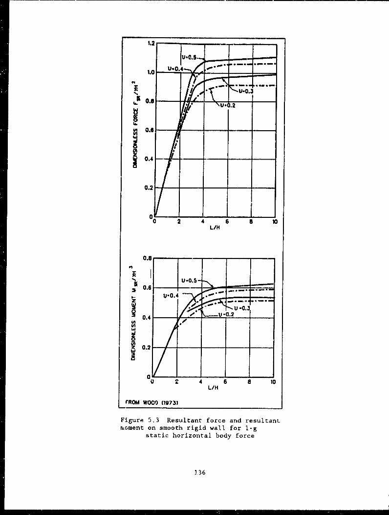
1.2
1.0c U
4 4
0. 8
01
10 2-.- 4 '"m e 6 ali i 0
L/H
0.8
SIu..o.s-40.6 ---
u*0. . ______U -0
o• 0.4
En
W 0.2
0 -- -0 2 4 6 8 10
L/H
FROM WOO'0 (1973)
Figure 5.3 Resultant force and resultantmoment on smooth rigid wall for 1-g
static horizontal body force
1.36
influence of structures or other loads on the surface of the backfill, (4) thephased response at any given time for the accelerations and the dynamic earthpressures with elevation along the back of the wall, and (5) the effect of thereduced soil stiffness with the level of shaking induced in both the soilbackfill and soil foundation. These and many other factors are addressed inthe procedurea used to simulate the dynamic response of earth reaining struc-tures by a complete soil-structuro interaction analysis.
137
CHAPTER 6 ANALYSIS AND DESIGN EXAMPLES FOR GRAVITY WALLS RETAINING YIELDING
BACKFILLS
6,1 Introduction
Gravity walls generally are designed assuming that some permanent dis-placement will occur during the design seismic event. This assumption isimplicit in procedures using a seismic coefficient significantly less than theacceleration coefficient corresponding to the design event. Newer methods,such as the displacement controlled approach developed by Richards and Elms(1979) explicitly consider such permanent displacements. If permanent dis-placements greater than about 1 inch per 20 foot height of wall (Y/H - 0.004,see Table 1) are not permissible, the analyses described in Chapter 8 shouldbe used.
The procedures described in this chapter quantify the effect of earth-quakes on the backfill by means of inertial forces acting on the soil masscomprising the sliding wedge within the backfill using the Mononobe-Okaberelationships for dynamic active and passive earth pressures. Where signifi-cant permanent displacements do occur, it is appropriate to use the Mononobe-Okabe theory to evaluate static and dynamic earth pressures. As discussed inChapter 4, there is ample evidence that this theory is correct for dry sandbackfills, although supporting evidence is very weak in the case of submergedbackfills. With gravity walls, the dynamic increments of earth pressure gen-erally are small compared to the inertia force on the wall itself and changesin water pressure on the poolside of the wall. Hence the exact values fordynamic earth pressures usually are not crucial. The procedures outlined inthis chapter assume that all dynamic forces act simultaneously in the worstpossible direction. This assumption is likely conservative (Whitman 1990;Anderson, Whitman, and Germaine 1987; Al Homound 1990), but is retainedpending more complete studies of case histories from earthquakes.
Dynamic finite element analyses seldom are suitable for use duringdesign of gravity walls, but will prove very useful for further research intoissues such as the phasing of the various earth and water pressures actingupon a wall. When such studies are made, the wall should be modeled as mov-able in response to the forces acting upon it, and not as a rigid, nondisplac-ing wall.
The Mononobe-Okabe theory for computing PA and PPE is described in Chap-ter 4. The presence of water within the backfill affects not only the staticpressures acting on the wall, as discussed in Chapter 3, but also the dynamicpressures. During an earthquake, the saturated portion of the backfill thatis below the water table may experience the development of additional porewater pressures due to the shear strains that occur within the backfill duringearthquake shaking. These excess pote water pressures reduce the effectivestresses within the backfill, resulting in both a reduction in the strength ofthe soil and adding to the destabilizing forces which act along the back ofthe wall. The magnitude of the excess pore water pressures generated withinthe soil during an earthquake can range from zero to the extreme case of pres-sures that are equal to the pre-earthquake vertical effective stresses, astate that corresponds to the liquefaction of the backfill. For those wallsthat have a pool of water in front of the wall, the earthquake shaking resultsin hydrodynamic pressures acting along the submerged portion at the front ofthe wall. The Westergaard procedure is used for computing the hydrodynamic
139
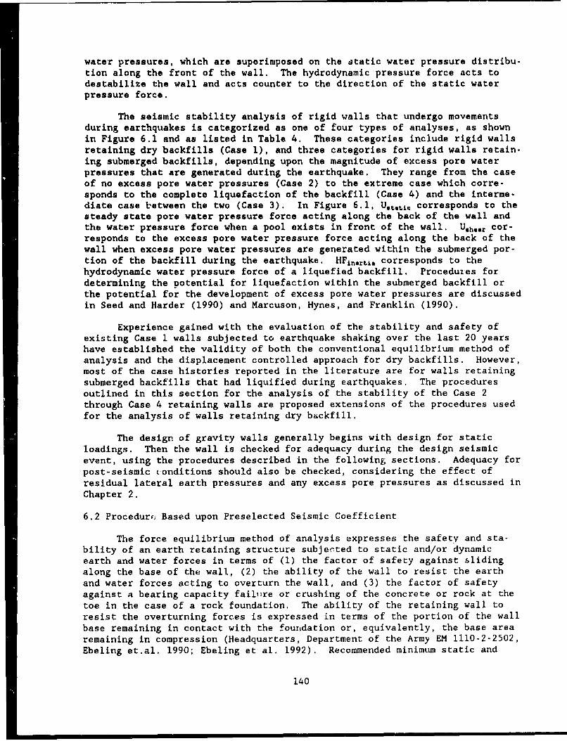
water pressures, which are superimposed on the static water pressure distribu-tion along the front of the wall. The hydrodynamic pressure force acts todestabilize the wall and acts counter to the direction of the static waterpressure force.
The seismic stability analysis of rigid walls that undergo movementsduring earthquakes is categorized as one of four types of analyses, as shownin Figure 6.1 and as listed in Table 4. These categories include rigid wallsretaining dry backfills (Case 1), and three categories for rigid walls retain-ing submerged backfills, depending upon the magnitude of excess pore waterpressures that are generated during the earthquake. They range from the caseof no excess pore water pressures (Case 2) to the extreme case which corre-sponds to the complete liquefaction of the backfill (Case 4) and the interme-diate case between the two (Case 3). In Figure 6.1, Utati. corresponds to thesteady state pore water pressure force acting along the back of the wall andthe water pressure force when a pool exists in front of the wall. Ushear cor-responds to the excess pore water pressure force acting along the back of thewall when excess pore water pressures are generated within the submerged por-tion of the backfill during the earthquake. HF±p.rti. corresponds to thehydrodynamic water pressure force of a liquefied backfill. Procedures fordetermining the potential for liquefaction within the submerged backfill orthe potential for the development of excess pore water pressures are discussedin Seed and Harder (1990) and Marcuson, Hynes, and Franklin (1990).
Experience gained with the evaluation of the stability and safety ofexisting Case 1 walls subjected to earthquake shaking over the last 20 yearshave established the validity of both the conventional equilibrium method ofanalysis and the displacement controlled approach for dry backfills. However,most of the case histories reported in the literature are for walls retainingsubmerged backfills that had liquified during earthquakes. The proceduresoutlined in this section for the analysis of the stability of the Case 2through Case 4 retaining walls are proposed extensions of the procedures usedfor the analysis of walls retaining dry backfill.
The design of gravity walls generally begins with design for staticloadings. Then the wall is checked for adequacy during the design seismicevent, using the procedures described in the following sections. Adequacy forpost-seismic conditions should also be checked, considering the effect ofresidual lateral earth pressures and any excess pore pressures as discussed inChapter 2.
6.2 Procedurr; Based upon Preselected Seismic Coefficient
The force equilibrium method of analysis expresses the safety and sta-bility of an earth retaining structure subjerted to static and/or dynamicearth and water forces in terms of (1) the factor of safety against slidingalong the base of the wall, (2) the ability of the wall to resist the earthand water forces acting to overturn the wall, and (3) the factor of safetyagainst a bearing capacity failiire or crushing of the concrete or rock at thetoe in the case of a rock foundation. The ability of the retaining wall toresist the overturning forces is expressed in terms of the portion of the wallbase remaining in contact with the foundation or, equivalently, the base arearemaining in compression (Headquarters, Department of the Army EM 1110-2-2502,Ebeling et.al. 1990; Ebeling et al. 1992). Recommended minimum static and
140
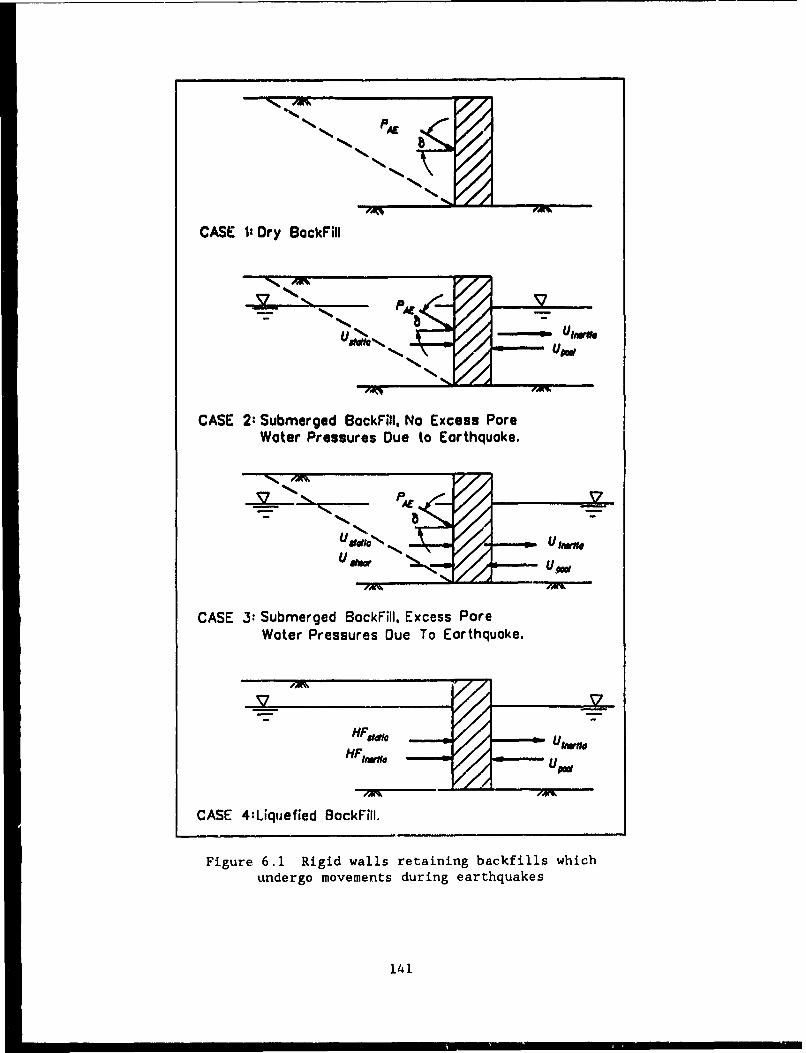
MI
CASE 11 Dry BackFill
S, p - U0
N bj
CASE 2: Submerged BackFill, No Excess PoreWater Pressures Due to Earthquake.
CASE 3: Submerged BackFill. Excess Pore
Water Pressures Due To Earthquake.
-rtjN -_" U _ M
u//N
CASE 4:Liquefied BackFill.
Figure 6.1 Rigid walls retaining backfills which
undergo movements during earthquakes
141
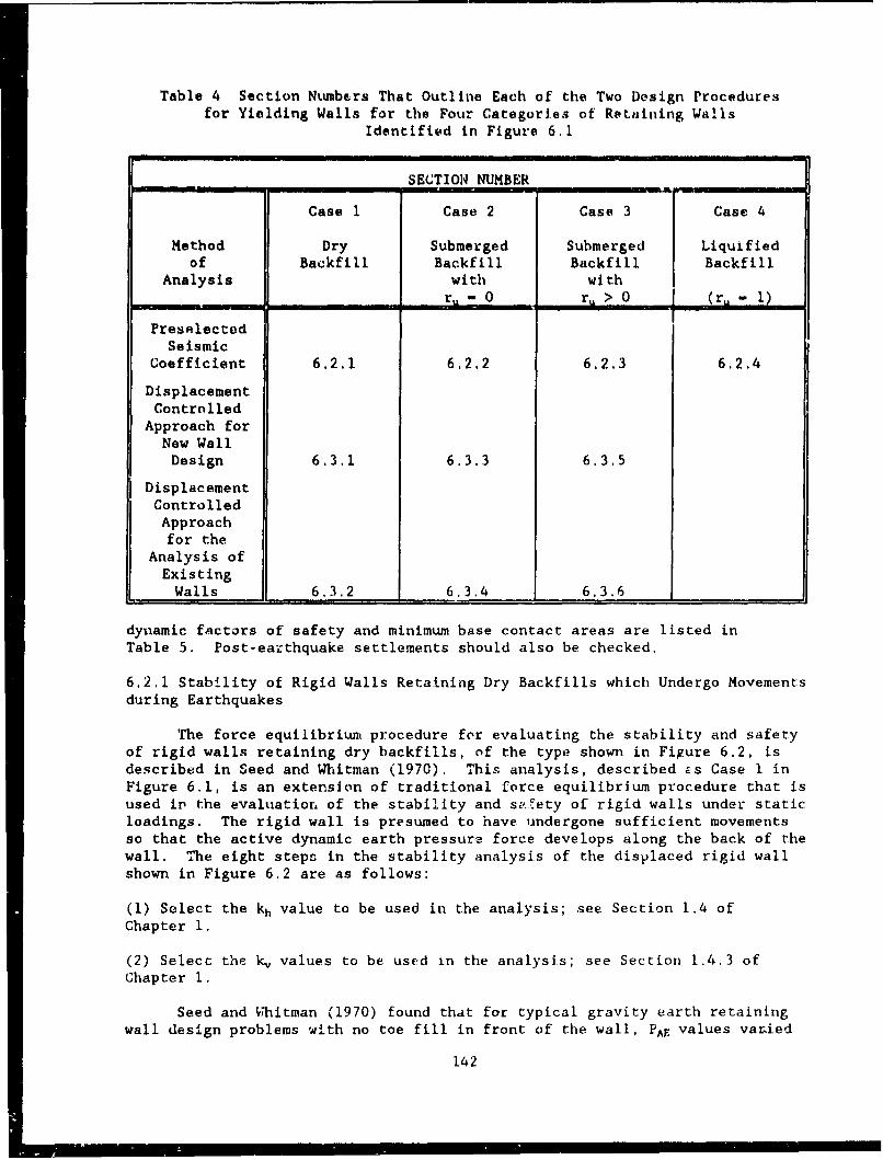
Table 4 Section NLunb.rs That Outline Each of the Two Design Proceduresfor Yielding Walls for the Four Categories of Retaining Walls
Identified in Figure 6.1
SECTION NUMBER
Case 1 Case 2 Case 3 Case 4
Method Dry Submerged Submerged Liquifiedof Backfill Backfill Backfill Backfill
Analysis with with- 0 r,>0 (r> - 1)
PreselectedSeismic
Coefficient 6.2.1 6.2.2 6.2.3 6.2.4
DisplacementControlled
Approach forNew WallDesign 6.3.1 6.3.3 6.3.5
DisplacementControlledApproachfor the
Analysis ofExisting
Walls 6.3.2 6.3.4 6.3.6
dynamic factors of safety and minimum base contact areas are listed inTable 5. Post-earthquake settlements should also be checked.
6.2.1 Stability of Rigid Walls Retaining Dry Backfills which Undergo Movementsduring Earthquakes
The force equilibrium procedure for evaluating the stability and safetyof rigid walls retaining dry backfills, of the type shown in Figure 6.2, isdescribed in Seed and Whitman (1970). This analysis, described zs Case I inFigure 6.1, is an extension of traditional force equilibrium procedure that isused in the evaluation of the stability and sefety of rigid walls under staticloadings. The rigid wall is presumed to have undergone sufficient movementsso that the active dynamic earth pressure force develops along the back of thewall. The eight steps in the stability analysis of the displaced rigid wallshown in Figure 6,2 are as follows:
(1) Select the kh value to be used in the analysis; see Section 1.4 ofChapter 1.
(2) Select the k, values to be used in the analysis; see Section 1.4.3 ofChapter 1.
Seed and Whitman (1970) found that for typical gravity earth retaining
wall design problems with no toe fill in front of the wall, PAE values vanied
142
Table 5 Minimum Factors of Safety When lUsingthe Preselected Seismic Coefficient Method
of Analysis
From U.S. Army Corps of Engineers EM 1110-2-2502 (1989)
Factor of Safety Factor of Safety
Failure Mode Static Earthquake
Sliding 1.5 1.1 - 1.2
BE/9 100% 75%(50%-Rock)
Bearing* 3 >2
*Check for settlements, including differential settlements.
by less than 10 percent (as discussed in Section 4.5). In other casesvertical accelerations can contribute to the forces attempting to destabilize
the wall (e.g. slender walls). In general, k, values other than zero would be
included in the analysis when vertical accelerations impact wall stability.
(3) Compute the dynamic active pressure force using the Mononobe-Okabe rela-
tionships as described in Chapter 4. PhA is computed using equation number33, with KAE given by Equation 34 and acting at the height as given in Fig-
ure 4.7. For a vertical wall retaining a horizontal backfill, PAZ may be com-
puted directly or defined in, terms of the static force PA and the incremental
inertial force APAE. PA is computed using Equation 7 with KA given by Equa-tion 16, using the Seed and Whitman's simplified procedure,and APA is com-puted using Equation 41 with AKA given by Equation 43. PA is equal to the
sum of these two forces (Equation 40) with a point of action, Y, given by
Equation 44, as shown in Figure 4.8. For most enginecred granular backfills,6 equal to 0/2 is a reasonable value. Table 2 provides a list of ultimatefriction angles for a variety of dissimilar materials that may interface with
one another.
(4) Compute the weight of the wall W and point of application, and using theforce PA and its point of application as determined in step 3, solve for the
unknown forces N and T which act along the base of the wall using the horizon-
tal and vertical force equilibrium equations.
The force W is computed per lineal foot of wall by multiplying the unit
cross-sectional area of the wall by a representative value for the unit weightof the section. The resultant force acts at the center of mass for the cross
section.
The total normal force between the wall and the foundation is equal to
N = W + (PAu) y (70)
143
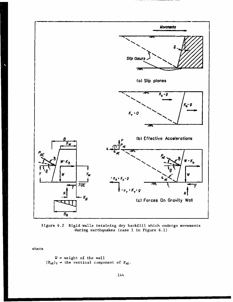
(S) Slip planes
(b) Effective Accelerations
NL -
.A W' Kh PAE W. ' w .KA
Y , I I _ _ .j .o n a K i .l o
Nt1 TOE 6V a "7 9A
"'XN (c) Forces On Gravity Wall
figure 6.2 Rigid walls retaining dry backfill, which undergo movementsduring earthquakes (case 1 in Figure 6.1)
where
W - weight of the wall(PAE)y - the vertical component of PAE.
144
The point of action of the force N, X" is computed by summing momentsabout the coe of the wall
XU" W(Xv) + (Px) (Xp, ) - ( I)x (YI,,) - W(kh) YW (71)
where
(PA)X - PAZ cos( 6 + 9 )(PAZ)y - PAZ sin( 6 + 9 )
XpAE - B - (YpM) tan 9YeAZ - Y
XW, Yw - center of mass for the wall, as measured from the toe of thewall and the base of the wall, respectively.
The horizontal force T is the shear force required for slidingequilibrium of the wall and is equal to
T - (PAR) x + Wokh (72)
where
W'kh - horizontal inertia force of the wall.
(5) Compute the factor of safety against sliding, F,.
F- a ultimcte shear force (73)shear force required for equilibrium
The ultimate shear force along the base, TUlt, is given by
Tuft - N.tan6b (74)
where
6 b - the base interface friction angle.
(6) Compare the computed factor of safety against sliding to the requiredfactor of safety. Many retaining walls are designed using static active earthpressures with a factor of safety of 1.5 against sliding along the base. Fortemporary loading cases, such as earthquakes, the minimum required factor ofsafety is equal to 1.1 or 1.2 (Table 5). For a ductile wall to foundationinterface, as the value of F. approaches the minimum required value, the mag-nitude of the translation of the structure will increase as the value of F.decreases (Newmark 1965). For a bonded interface, the displacements will besmall until the bond is ruptured (at F. - 1.0) and a brittle failure results.
145
(7) The overturning criterion is expressed in cerms of the percentage of basecontact area B,/B, where Be is the width of the area of effective base con-tact. Assuming that the bearing pressure varies linearly between the base ofthe wall and the foundation, the normal stress is a maximum at the toe (q -qm.) and a minimum at the inner edge (q - 0) as shown in Figure 6.3.
Be a 3.xW (75)
An alternative assumption regarding base pressure distribution and contactarea was suggested by Meyerhof (1953). Meyerhof assumed a uniform distribu-tion of pressure along the base, resulting in an effective base contact equalto
B. - 2.x,. (76)
Meyerhof's pressure distribution has been used widely for foundations on soiland is most appropriate for foundation materials that exhibit ductile mecha-nisms of failure. The assumption is less appropriate for brittle materials.
Many retaining walls are designed using static active earth pressureswith full contact along the base, B./B ( or B',/B), equal to 100 percent. Fortemporary loading cases, such as earthquakes, this criteria is relaxed to aminimum value of 75 percent, 50 percent for rock foundations (Table 5).
(8) For those structures founded on rock, the factor of safety against bearingcapacity failure, or crushing of the concrete or the rock at the toe, can beexpressed as
F, - q 12___t (77)qmax
where qult is the ultimate bearing capacity or compressive strength of theconcrete or the rock at the toe and qmax is the maximum bearing pressure atthe toe. For brittle materials like unconfined concrete, the ultimate bearingcapacity is equal to the compressive strength of the material. Building codesare commonly used to obtain values for the allowable bearing stress on rock,qazL. Alternately, a large factor of safety is applied to the unconfined com-pressive strength of intact samples. The maximum bearing pressure qmax isrestricted to an allowable bearing capacity q.1I1 For ductile foundationmaterials that undergo plastic failure, the ultimate bearing capacity isgreater than the compressive strength of the material, excluding those founda-tion materials exhibiting a loss In shear resistance due to earthquake-induceddeformations or due to the development of residual excess pore water pres-sures. In these cases, a conventional bearing capacity evaluation isconducted to establish the post-earthiuake stahility of the structure.
In stability analyses in which the vertical accelerations are consid-ered, the force acting downward through the center of mass of the wall thatrepresents the weight of the wall, W, in Figure 6.2, is replaced by the force
146
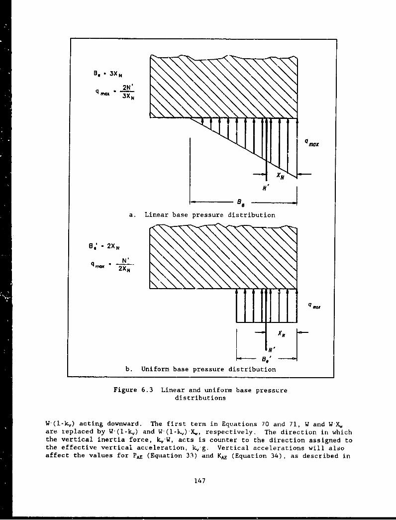
B,•3XN
2N'
N°
-o N
a. Linear base pressure distribution
B,30- 2XN
q _ :2XN
q •
iN'
b. Uniform base pressure distribution
Figure 6.3 Linear and uniform base pressuredistributions
W(1-(k,) acting downward. The first term in Equations 70 and 71, W and W'Xare replaced by W'(l-k) and W'(l-K)4X, respectively. The direction in whichthe vertical inertia force, k.,W, acts is counter to the direction assigned tothe effective vertical acceleration, k g. Vertical accelerations will alsoaffect the values for PA (Equation 33) and KA (Equation 34), as described in
147
Section 4.2. The stability should be checked for the possibility of k, actingin either direction.
Thl.s procedure is illustrated in example 27 at the end of this chapter.
6.2.2 Stability of Rigid Walls Retaining Submerged Backfills which UndergoMovements During Earthquakes - No Excess Pore Water Pressures
The presence of water within the backfill and in front of the wallresults in additional static and dynamic forces acting on the wall and altersthe distribution of forces within the active soil wedge developing behind thewall. This section describes the first of three proposed force equilibriumprocedures used in the evaluation of the stability and safety of rigid wallsretaining submerged or partially submerged backfills and including a pool ofwater in front of the wall, as shown in Figure 6.4. This analysis, describedas Case 2 in Figure 6.1, assumes that no excess pore water pressures are gen-erated within the submerged portion of the backfill or within the foundationduring earthquake shaking. The evaluation of the potential for the generationof excess pore water pressures during the shaking of the submerged soilregions is determined using the procedure described in Seed and Harder (1990)or Marcuson, Hynes, and Franklin (1990). The rigid wall is presumed to haveundergone sufficient movements so that the active dynamic earth pressure forcedevelops along the back of the wall. Many of the details regarding the pro-cedures used in the eight steps of the stability analysis of walls retainingdry backfills (Section 6.2.1) are similar to those procedures used for sub-merged backfills, and the explanations for these common steps are not repeatedin this section. The eight steps in the stability analysis of the displacedrigid wall retaining submerged backfill as shown in Figure 6.4 are as follows:
(1) Select the kh value to be used in the analysis; see Section 1.4 ofChapter 1.
(2) Consider kv, as discussed in Section 1.4.3.
(3) Compute PA using the p-:ocedure described in Section 4.3. Ustatic is deter-mined from the steady state flow net for the problem. By definition, onlysteady state pore water pressures exist within the submerged backfill andfoundation of a Case 2 retaining structure (r, - 0). In the restrained watercase of a fully submerged soil wedge with a hydrostatic water table, PA iscomputed (Equations 33 and 38) using an effective unit weight equal to lb.
KA (Equation 34) or KA(P*,8*) (Equation 38) are computed using an equivalenthorizontal acceleration, kh,1, and an equivalent seismic inertia angle, Oel,
given by Equation 47 and 48. In the case of a partially submerged backfill,this simplified procedure will provide approximate results by increasing thevalue assigned to the effective unit weight based upon the proportion of Chesoil wedge that is above and below the water table. A more refined analysismay be conducted using the trial wedge procedure (Section ".4) for the forcesshown in Figure 6.4. For most engineered granular backfill3, 6 equal. to 0/2is a reasonable value (Table 2).
(4) Compute the weight of the wall W and point of application, and using theforce PA and the point of application as determined in step 3, solve for theunknown forces N' and T which act along the base of the wall using the hori-zontal and vertical force equilibrium equations
148
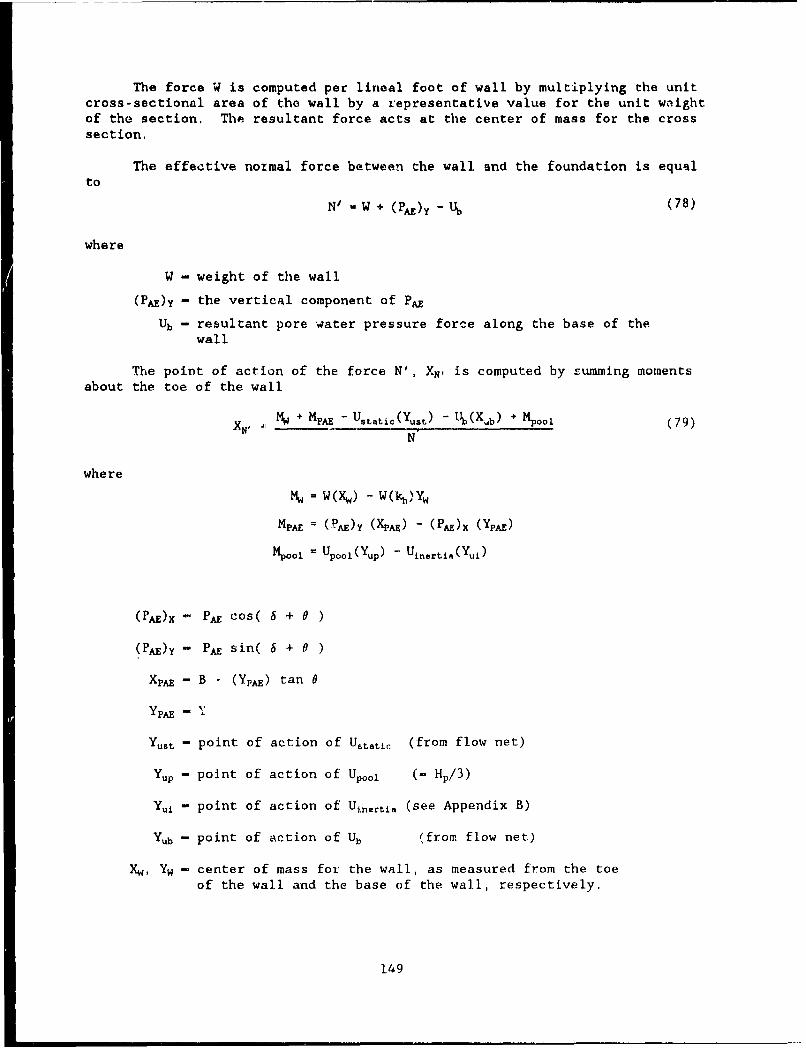
The force W is computed per lineal foot of wall by multiplying the unitcross-sectional area of tho wall by a representative value for the unit weightof the section. The resultant force acts at the center of mass for the crosssection,
The effective normal force between the wall and the foundation is equalto
N' " W + (P*)Y - Lb (78)
where
W - weight of the wall
(PAE)y- the vertical component of PAE
Ub - resultant pore water pressure force along the base of thewall
The point of action of the force N', XN. is computed by summing momentsabout the toe of the wall
XN- MW + ME - U5• 8tic(Yu'5 ) - Ub(X~b) + 14p°°1 (79)N
where
Mw = W(Xw) - W(kh)Yw
MPAE = (PAE)Y (XPAE) - (PAE)X (YPAE)
MPool = U pool(Y.P) - Uinertia(Yui)
(PAE)X - PAE cos( 6 + 0 )
(PA)Y"- PAE sin( 6 + 0 )
XpA -- B - (YPAE) tan 0
YPAE - ,A
Yut - point of action of Utatic (from flow net)
Y -p - point of action of Upoo, (- Hp/3)
Yu- - point of action of Uinertia (see Appendix B)
Yub - point of action of Ub (from flow net)
Xw, Yw - center of mass for the wall, as measured from the toeof the wall and the base of the wall, respectively.
149
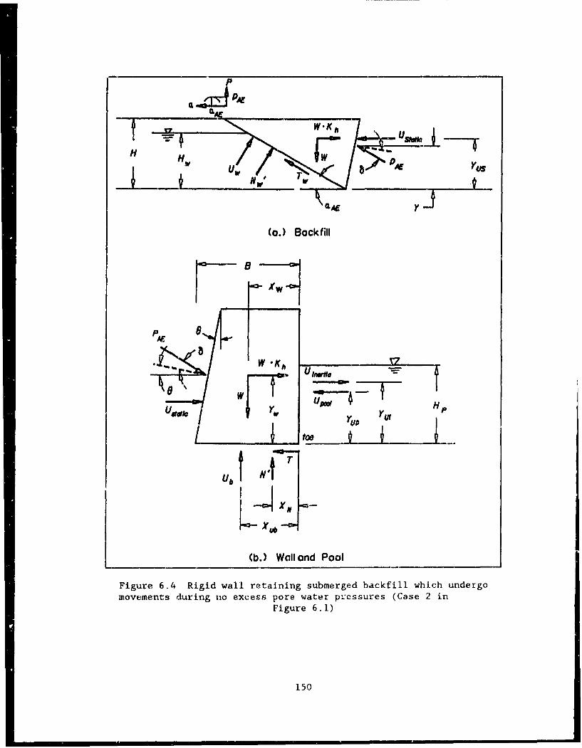
PAEE
T7 W-,, / " vw _ ,..
"e..LAE y
(a.) Backfill
XWh
Pp
(b)Y yWl H P
Nov-U6 N
X--
S l(b.) Wall and Pool
Figure 6.4 Rigid wall retaining submerged backfill which undergomovements during no excess pore water pressures (Case 2 in
Figure 6.1)
150
Thm horizontal force T is the shear force required for equilibrium ofthe wall and is equal to
T = (PE)X + W(Ih) + U4t..ti. - Upool + Uin*rtio (80)
where
W'kh - horizontal inertia force of the wall.
Ustatic - resultant steady state pore water pressure force alongthe back of the wall,
U.l - resultant hydrostatic water pressure force for the pool
Uinerti. - hydrodynamic water pressure force for the pool directed awayfrom the wall (see Appendix B).
(5) Compute the factor of safety against sliding, F., using Equation 73, Theultimate shear force along the base, Tult, is given by
T *lt - N'.tan6b (81)
where
6 b - the effective base interface friction angle.
(6) Compare the computed factor of safety against sliding to the requiredfactor of safety of 1.1 or 1.2 for temporary loading cases (Table 5).
(7) The stability against overturning is expressed in t-rms of the base areain compression, B.. B. is computed by either Equation 75 or 76, as describedin Section 6.2.1. Many retaining walls are designed using static active earthpressures with full contact along the base, B./B ( or B'./B), equal to100 percent. For temporary loading cases, such as earthquakes, this criteriais relaxed to a minimum value of 75 pcrcent, 50 percent for rock foundations(Table 5).
(8) Check the stability of the wall against a bearing capacity failure, asdiscussed in step 8 of Section 6.2.1.
6.2.3 Stability of Rigid Walls Retaining Submerged Backfills which UndergoMovements During Earthquakes - Excess Pore Water Pressures
This section describes the second of three proposed force equilibriumprocedures for evaluating the stability and safety of rigid walls retainingsubmerged or partially submerged backfills and including a pool of water infront of the wall, as shown in Figure 6.5. This analysis, described as Case 3in Figure 6.1, assumes that excess pore water pressures, in addition to thesteady state pore water pressures, are generated within the submerged portionof the backfill or within the foundation during earthquake shaking. The mag-nitude and distribution of these excess pore water pressures depend upon sev-eral factors, including 'he magnitude of the earthquake, the distance from the
151
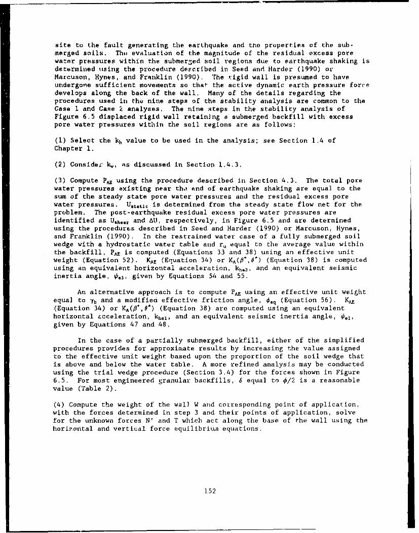
site to the fault generating the earthquake and tno properties of the sub-merged soils. Thii evaluation of the magnitude of the residual excess porewater pressures within the submerged soil regions due to earthquake shaking isdetermined using the procedure described in Seed and Harder (1990) orMarcuson, Hynes, and Franklin (1990). The rigid wall is presumed to haveundergone sufficient movements so that- the active dynamic earth pressure forcedevelops along the back of the wall. Many of the details regarding theprocedures used in the nine steps of the stability analysis are common to theCase I and Cape 2 analyses, The nine steps in the stability analysis ofFigure 6.5 displaced rigid wall retaining a submerged backfill with excesspore water pressures within the soil regions are as follows:
(1) Select the kh value to be used in the analysis; see Section 1.4 ofChapter 1.
(2) Considev kv, As discussed in Section 1.4.3.
(3) Compute PAE using the procedure described in Section 4.3. The total porewater pressures existing near tho end of earthquake shaking are equal. to thesum of the steady state pore water pressures and the residual excess porewater pressures. U5 t 0tjý is determined from the steady state flow net for theproblem. The post-earthquake residual excess pore water pressures areidentified as Ushear and AU, respectively, in Figure 6.5 and are determinedusing the procedures described in Seed and Harder (1990) or Marcuson, Hynes,and Franklin (1990). In the restrained water case of a fully submerged soilwedge with a hydrostatic water table and ru equal to the average value withinthe backfill, PAE is computed (Equations 33 and 38) using an effective unitweight (Equation 52). KAE (Equation 34) or KA(fi*,O*) (Equation 38) is computedusing an equivalent horizontal acceleration, khe3, and an equivalent seismicinertia angle, 0.3, given by Equations 54 and 55.
An alternative approach is to compute PA using an effective unit weightequal to 7b and a modified effective friction angle, O.q (Equation 56). KpE(Equation 34) or KA(P*,O*) (Equation 38) are computed using an equivalenthorizontal acceleration, kl1,., and an equivalent seismic inertia angle, e.1,
given by Equations 47 and 48.
In the case of a partially submerged backfill, either of the simplifiedprocedures provides for approximate results by increasing the value assignedto the effective unit weight based upon the proportion of the soil wedge thatis above and below the water table. A more refined analysis may be conductedusing the trial wedge procedure (Section 3.4) for the forces shown in Figure6.5. For most engineered granular backfills, 6 equal to 0/2 is a reasonablevalue (Table 2).
(4) Compute the weight of the wall W and corresponding point of application,with the forces determined in step 3 and their points of application, solvefor the unknown forces N' and T which act along the base of the wall using thehorizontal and vertical force equilibriumn equations.
1.52
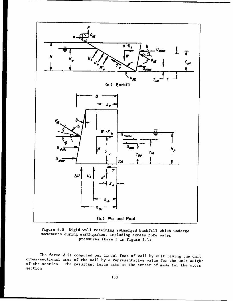
PA
(a.) Backfill
t CMW
HN SKI V7
-~ 1UI to&
AU1 U 1 Nt T
K•XD
(b.) Wall and Pool
Figure 6.5 Rigid wall retaining submerged backfill which undergomovements during earthquakes, including excess pore water
pressures (Case 3 in Figure 6.1)
The force W is computed per lineal foot of wall by multiplying the unitcross-sectional area of the wall by a representative value for the unit weightof the section. The resultant force acts at the center of mass for the crosssection.
153
The effective normal force between the wall and the foundation is equalto
N' a W + (PAZ)Y - Ub - AU (82)
where
AU - resultant excess pore water pressure force along the baseof the wall
The point of action of the force N' , XN' is computed by summing momentsabout the toe of the wall
W MW + MPA ,' MW - AU(XDU) - Ub(Xub) + MP00 1 (83)N Nr
where
S- w(Xw) - W(kh)Yw
M~pA = (PAE)Y (XPAE) - (PM)x (YPAE)
Mpool " Up0 0i(Yup) - Uti.rtia(Yui)
Mpn a -Ustaust) - UShear(YuSh)
and
(PAZ)X - PAE cos( 6 + 0 )
(PAE)Y - PAE sin( 6 + 9 )
XpAE - B - (YPAE) tan 9
YPAZ " Y
Yush - point of action of Ushear
XDU - point of action of AU
The horizontal force T is the shear force required for equilibrium ofthe wall and is equal to
T = (PAE)x + W((kh) + U*tatic + Ushear - Up00o + Uinertia (84)
where
Ushoat - resultant excess pore water pressure force along the back ofthe wall.
Procedures for the computation of values for Ushear, Yush, AU, and XDU are dis-cussed in Seed and Harder (1990) or Marcuson, Hynes, and Franklin (1990).
(5) Compute the factor of safety against sliding, F,, using Equation 73. Theultimate shear force along the base, Tult, is given by Equation 81.
(6) Compare the computed factor of safety against sliding to the requiredfactor of safety of 1.1 or 1.2 for temporary loading cases (Table 5).
154
--- ----
(7) The stability against overturning is expressed in terms of the base areain compression, B,. B, is computed by either Equaticn 75 or 76, as describedin Section 6.2.1. Many retaining walls are designed using static active earthpressures with full contact along the base, B./B ( or B'./B), equal to100 percent. For temporary loading cases, such as earthquakes, this criteriais relaxed to a minimum value of 75 percent, 50 percent for rock foundations(Table 5).
(8) Check the stability of the wall against a bearing capacity failure:, aisdiscussed in step 8 of Section 6.2.1.
(9) Additional stability considerations for the retaining wall are discussedin Chapter 2. Some of the factors to be considered are the potential forstrength loss within looser foundation materials and the post-earthquakeredistribution of excess pore water pressures. Post-earthquake stability ofthe wall and post-earthquake settlements should also be considered.
This procedure is illustrated in example 28 at the end of this chapter.
6.2.4 Stability of Rigid Walls Retaining Submerged Backfills which UndergoMovements During Earthquakes - Liquified Backfill
This section describes the force equilibrium procedure used in the eval-uation of the stability and safety of displaced rigid walls retaining sub-merged or partially submerged backfills and including a pool of water in frontof the wall, as shown in Figure 6.6. This analysis, described as Case 4 inFigure 6.1, assumes that the submerged portion of the backfill has liquified(ru - 100%) during the earthquake and that excess pore water pressures (ru <100%) are generated within the foundation during earthquake shaking. Theevaluation of the liquefaction potential for the backfill and the magnitude ofthe residual excess pore water pressures within the foundation are determinedusing the procedure described in Seed and Harder (1990) or Marcuson, Hynes,and Franklin (1990). Many of the details regarding tOe procedures used in thenine steps of the stability analysis are common to the previously describedanalyses. The steps in the stability analysis of Figure 6.6 displaced rigidwall retaining a liquified backfill with excess pore water pressures withinthe soil foundation are as follows:
(1) Select the kh value to be used in the analysis; see Section 1.4 ofChapter 1.
(2) Consider kv, as discussed in Section 1.4.3.
(3) Compute the forces acting along the back of the wall,
HF t =u lYtH2 (85)
identified as HFstatic and HFinertia in Figure 6.6. Upon liquefaction of thebackfill during the earthquake, the earth pressure forces acting along theback of the wall are equivalent to a heavy fluid with a density equal to thetotal unit weight of the backfill, 7t. The inertial force of the heavy fluidduring shaking is approximated using the Westergaard procedure (Appendix B)for the inertia force of a fluid as acting at 0.4-H above the base of thewall.
155
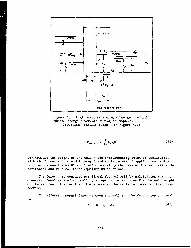
[W.K T 7
• ra
w• xY~V -00,
(b.) Wall and Pool
Figure 6.6 Rigid wall retaining submerged backfillwhich undergo movements during earthquakes -
liquified 'ackfil] (Case 4 in Figure 6.1)
HFinertia 7 (86)
(4) Compute the weight of the wall W and coirresponding point of applicationwith the forces determined in step 3 and their points of application; solvefor the unknown forces N' and T which act along the base of the wall using thehorizontal and vertical force equilibrium equations.
The force W is computed per lineal foot of wall by multiplying the unitcross-sectional area of the wall by a representative value for the unit weightof the section. The resultant force acts at the center of mass for the crosssection.
The effective normal force between the wel] and the foundation is equalto
N' - W - Ub - AU t%87)
156
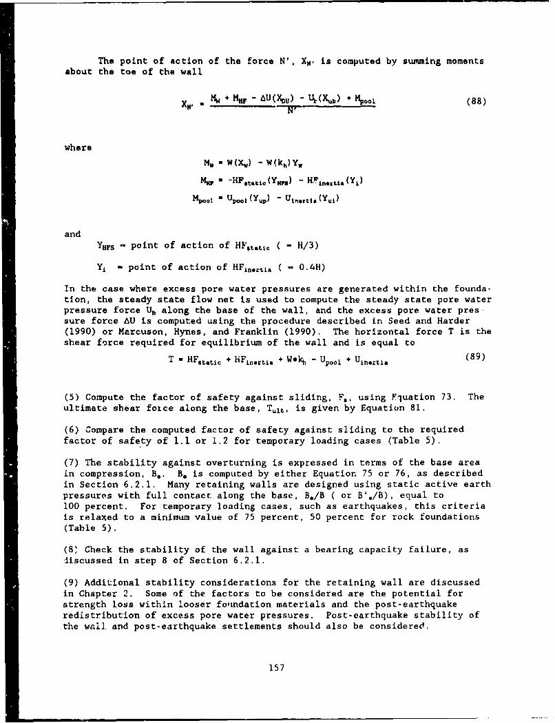
The point of action of the force N', X". is computed by summing momentsabout the toe of the wall
XN. aM + M" - AU(xu) - ,(Xb) * Kpoo (88)N'-
where
Mw - W(X,) - W(kh)Y,
MUp a -HF~t.tt (YK") - Hpin.,tLt (Yd)
1Po0 - Uo01 (YUP) -Utneti (Yud
and
YHFS - point of action of HFt.t ( - H/3)
Yj - point of action of HFn . - 0.4H)
In the case where excess pore water pressures are generated within the founda-tion, the steady state flow net is used to compute the steady state pore waterpressure force Ub along the base of the wall, and the excess pore water pres-sure force AU is computed using the procedure described in Seed and Harder(1990) or Marcuson, Hynes, and Franklin (1990). The horizontal force T is theshear force required for equilibrium of the wall and is equal to
T - HFstatic + HFin.rtja + Wokb - UPool + Uinertia (89)
(5) Compute the factor of safety against sliding, F., using Fuation 73. Theultimate shear foice along the base, Tu1 t, is given by Equation 81.
(6) Compare the computed factor of safety against sliding to the requiredfactor of safety of 1.1 or 1.2 for temporary loading cases (Table 5).
(7) The stability against overturning is expressed in terms of the base areain compression, B.. B. is computed by either Equation 75 or 76, as describedin Section 6.2.1. Many retaining walls are designed using static active earthpressures with full contact along the base, B./B ( or B'./B), equal to100 percent. For temporary loading cases, such as earthquakes, this criteriais relaxed to a minimum value of 75 percent, 50 percent for rock foundations(Table 5),
(8' Check the stability of the wall against a bearing capacity failure, asdiscussed in step 8 of Section 6.2.1.
(9) Additional stability considerations for the retaining wall are discussedin Chapter 2. Some of the factors to be considered are the potential forstrength loss within looser foundation materials and the post-earthquakeredistribution of excess pore water pressures. Post-earthquake stability ofthe wall and post-earthquake settlements should also be considered.
157
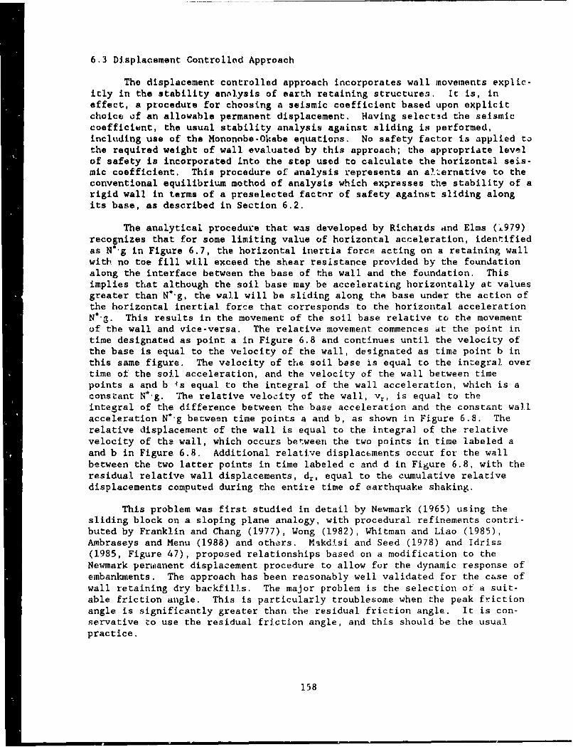
6.3 Displacement Controlled Approach
The displacement controlled approach incorporates wall movements explic-itly in the stability anolysis of earth retaining structures, It is, ineffect, a proceduze for choosing a seismic coefficient based upon explicitchoice of an allowable permanent displacement. Having selectad the seismiccoefficient, the usual stability analysis against sliding is performed,including use of the Mononobe-Okabe equations. No safety factor is applied tothe required weight of wall evaluated by this approach; the appropriate levelof safety is incorporated Into the step used to calculate the horizontal seis-mic coefficient. This procedure of analysis represents an aliernative to theconventional equilibrium method of analysis which expresses the stability of arigid wall in terms of a preselected factnr of safety against sliding alongits base, as described in Section 6.2.
The analytical procedure that was developed by Richards and Elms (1979)recognizes that for some limiting value of horizontal acceleration, identifiedas N*'g in Figure 6.7, the horizontal inertia force acting on a retaining wallwith no toe fill will exceed the shear resistance provided by the foundationalong the interface between the base of the wall and the foundation. Thisimplies that although the soil base may be accelerating horizontally at valuesgreater than N*'g, the wal.l will be sliding along the base under the action ofthe horizontal inertial force that corresponds to the horizontal accelerationN*'g. This results in the movement of the soil base relative to the movementof the wall and vice-versa. The relative movement commences at the point intime designated as point a in Figure 6.8 and continues until the velocity ofthe base is equal to the velocity of the wall, designated as time point b inthis same figure. The velocity of the soil base is equal to the integral overtime of the soil acceleration, and the velocity of the wall between timepoints a and b 4s equal to the integral of the wall acceleration, which is aconstant N*.g. The relative velocity of the wall, Vr, is equal to theintegral of the difference between the base acceleration and the constant wailacceleration N*'g between time points a and b, as shown in Figure 6.8. Therelative displacement of the wall is equal to the integra] of the relativevelocity of ths wall, which occurs between the two points in time labeled aand b in Figure 6.8. Additional relative displacements occur for the wallbetween the two latter points in time labeled c and d in Figure 6.8, with theresidual relative wall displacements, dr, equal to the cumulative relativedisplacements computed during the entire time of earthquake shaking.
This problem was first studied in detail by Newmark (1965) using thesliding block on a sloping plane analogy, with procedural refinements contri-buted by Franklin and Chang (1977), Wong (1982), Whitman and Liao (1985),Ambraseys and Menu (1988) and others. Makdisi and Seed (1978) and Idriss(1985, Figure 47), proposed relationships based on a modification to theNewmark perwlanent displacement procedure to allow for the dynamic response ofembankinents. The approach has been reasonably well validated for the case ofwall retaining dry backfills. The major problem is the selection of a suit-able friction angle. This is particularly troublesome when the peak frictionangle is significantly greater than the residual friction angle. It is con-servative to use the residual friction angle, and this shoula be the usualpractice.
158
PAW -t O VWI 0 0A) mpg
No-N
%%
From Whitman (1990)
Figure 6.7 Gravity retaining wall and fal]ure wedge
treated as a sliding block
WALL " _
ABSOLUTE RELATIVE bbc dN VELOCITY VELOCITY
0. --- 0 0 R 0 Vr 0 -- • da < 0. _o-I RELATIVE DISPLACEMENT
1 -. b b iSOI
St t i t t• _
KXELERAT ION I d_" . . dI .. .
From Elms and Richards (1990)
Figure 6.8 Incremental displacement
The Richards and Elms procedure was developed usi~ng a sliding blockanalogy to calculate the magnitude of wall displatements in sliding during
earthquake shaking. Whitman and Liao improved this procedure by using
statistical, methods to address the several sources of uncertainty in the
159
I ap I-I - m I '• II II •;:
displacement controlled procedure. However, the reader Is cautioned egainstrelying solely upon this simplified procedure for waterfront structureslocated within severe seismic environments or epicentral regions, structureswith significant deformations, or critical structures. It does not includewall displacements due to post-earthquake settlem'ents or due to creepdisplacements. The method has not yet been extended to take into accounttilting of walls; this matter is discussed by Whitman (1990).
Among the uncertainties are the effects of vertical and transverseaccelerations, including their influence upon the passive stabilizing forcefor walls with toe fill. Results of studies by Sharama (1989), as describedby Elms and Richards (1990), indicate that the effect of the verticalacceleration component is negligible. Other research as described by Whitman(1979) indicated that the effect of vertical acceleration can be to increasethe total displacement by 50 to 100 percent for N*/A > 0.6. Whitman and Liao(1985) determined that the detrimental effects of vertical accelerations onwall stability were offset by consideration of other variables. Sharama(1989), as reported by Elms and Richards (1990), determined that transverseaccelerations oriented along the length of the wall contribute to wall dis-placement. Sliding block displacements must always increase due to transverseaccelerations. Displacement increases of 70 percent or higher for N*/A valuesbetween 0.5 and 0.9 were found. These additional displacements are based onanalysis of a wall with no transverse support other than base friction. Amore sophisticated analysis is required to investigate, or to consider theeffects of k, (or vertical acceleration) in the deformations of waterfrontstructures.
The stabilizing force for sliding resistance may be less than the fullpassive earth pressure force because of insufficient wall displacements. Aconservative evaluation of this resistance should be used.
The displacement controlled procedure for the analysis of earth retain-ing structures is categorized as one of four types of analyses, as was donefor the conventional equilibrium method of analysis. These categories, thatare shown in Figure 6.1, include rigid walls retaining dry backfills (Case 1)and three categories for rigid walls retaining submerged backfills, dependingupon the magnitude of excess pore water pressures that are generated duringthe earthquake. They range from the case of no excess pore water pressures(Case 2) to the extreme case which corresponds to the complete liquefaction ofthe backfill (Case 4) and the intermediate case between the two (Case 3).This proposed procedure for submerged backfills is not applied to the case ofliquified backfills due to the complexity of the post-earthquake behaviorwithin the soil regions. In addition, the steps in the application of thedisplacement controlled approach to the design of a new wall are distinguishedfrom the steps in the application of the displacement contrelled approach tothe analysis of an existing wall. Table 4 identifies the appropriate Chapter6 section that describes either the design of a new wall or the analysis of anexisting wall for the first thre. Figure 6.1 categories of displacement con-trolled analyses.
6.3.1 Displacement Controlled Design Procedure for a Wall Retainirg DryBackfill
This section describes the application of the displacement controlledapproach to the design of a wall retaining dry backfill identified as Case 1
160
in Figure 6.1. Richards and Elms (1979) first applied this analysis procedureto walls that retain dry backfill. The eight steps in the design of the earthretaining structure shown in Figure 6.9 are as follows:
(1) Decide upon the value for the permanent relative displacement dr that isacceptable for the wall. For most walls, displacements on the order ofseveral inches would be acceptable. The value for d, must be consistent withthe dynamic active earth pressure used in step 5 during the design of the wall(see the discussions in Sections 6.1 and 2.2.2).
(2) Select the site specific average peak horizontal acceleration, A'g, andthe site specific average peak horizontal velocity, V, within the soil back-fill comprising the dynamic active wedge and the retaining structure. Referto the discussion in Section 1.4 of Chapter 1.
(3) In typical earth retaining wall design problems, by Whitman and Liao dis-placement controlled procedure, k, - 0.
(4) Calculate the maximum transmissible acceleration, N*'g, coefficient N*using the Whitman and Liao (1985) relationship
N A {0.66 - 1 ln r (Aig)V (90)
where
A'g - base acceleration in units of in/sec2
V is expressed in units of inches per seconddr is expressed in units cf inchesg - 386 in/sec2
According to Whitman and Liao, this relationship for the maximum transmissibleacceleration coefficient, N*, ensures that there will be 95 percent confidencethat the prescribed allowable permanent displacement will not be exceededduring an earthquake for the assigned A and V values. Equation 90 was derivedusing 14 earthquake records. All but two of the records were for earthquakeswith magnitudes between 6.3 and 6.7. For severe seismic environments, struc-tures located in epicentral rcgions, significant deformations, or criticalstructures, additional calculations should be made using other relationships(see Section 6.2).
(5) Compute the value for the dynamic active earth pressure force P• usingthe Mononobe-Okabe relationship described in Section 4.2, or for verticalwalls .id level backfills, in terms of PA and APAE using the simplifiedMononobe-Okabe procedure described in Section 4.2.2. When using the relation.ships for 0, KA, AKA, and aE, N* is substituted for kh, and k, is set equalto zero. Additional comments regarding these calculations are given in step 3in Section 6.2.1.
(6) Compute the required weight of wall. Horizontal force equilibriumfequires that the shear stress required for equilibriau, T, (Equation 72) beequal to the ultimate shear force along the base of the wall, Tult (Equa-tion 74). Setting Equation 72 equal to Equation 74, and introducing thenormal force N (Equation 70) and solving for W results in the relationship
161.
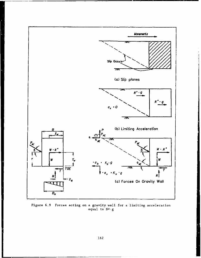
slip Occu~rlz,- "
(a) Slip planes
N N
"N "
Sp .0 N
-. B = p (b) Limitinp Accelerstion
N NN
A N -
equ No *.
162N
/A
Figre .9 orcs atin ona (b)it w llfo aimiting A ccelerationeqa oN-g-
N6

W (PAE)x - (PAY)Y(tan 6 b) (91)tan6b - N*
where
(PAE)X - PA cos( 6 + 0 )
(PAE)Y - PA sin( 6 + 9 )
(7) No factor of safety noeds to be applied to the wall weight W computed instep 6 when using Equation 90 (FSW - 1.0).
(8) Proportion the geometry of the wall so that the overturning criterion issatisfied. This is expressed in terms of the percentage of base contact areaB./B, where B. is the width of the area of effective base contact, asdescribed in step 7 in Section 6.2 1. For a given trial geometry, the pointof action of the normal force along the base, xN, i.s computed using Equationnumber 71, followed by the computation of the value of B. using either Equa-tion 75 or 76, depending upon the foundation material. This B. value is thencompared to the minimum B. value, which is equal to 75 percent of the basewidth B for earthquake loading conditions (50 percent for rock foundations).
Tbis procedure is illustrated in example 29 at the end of this chapter.
6.3.2 Analysis of Earthquake Induced Displacements for a Wall Retaining DryBackfill
This section describes the analysis of the earthquake induced displace-ments of an existing wall retaining dry backfill, identified as Case 1 inFigure 6.1. The four steps in the analysis of the earth retaining structureshown in Figure 6.9 are as follows;
(1) Determine the value for the average site specific peak horizontal acceler-ation, A-g, and the value for the average peak horizontal velocity, V, at thesite. Refer to the discussfon in step 2 of Section 6.3.1.
(2) In typical earth retaining wall design problems by Whitman and Liao dis-placement controlled procedure, k, - 0.
(3) Compute the value for the maximum transmissible acceleration, N*-g, coef-ficient N*. An iterative method consisting of the following five steps isused to determine the value for N*.
(3-A) Using the assumed value for N*, compute the value for thedynamic active earth pressure force PAE using either thp Mononobe-Okabe relationship described in Section 4.2 or in terms of PA andAPA assuming the simplified Mononobe-Okabe procedure described inSection 4.2.2 applies. When using the relationships for 0, KA,AKA, and cA, N* is substituted for kh, and k, is set equal tozero. Additional comments regarding these calculations are givenin step 3 in Section 6.2.1.
163
(3-B) Calculate the value of the shear force required for equilib-rium along the base of the wall, T, using EqL'ation 72.
(3-C) Calculate the value for the normal force, N, usingEquation 70.
(3-D) Calculate the value for the ultimate shear force along thebase of the wall, Tult, using Equation 74.
(3-E) If the value for T is not equal to the value for Tult,adjust the value used for N* and repeat steps 3-A through step 3-Duntil T - Tult. Te resulting value for N* is equal to the limitacceleration.
(4) Calculate the permanent relative displacement d, usiug the Whitman andLiao (1985) relationship
2r~ +P x (9.4 - N (92)d" (A-g) ep
where
N*'g - maximum transmissible acceleration in units of in/sec 2
A'g - base acceleration in units of in/sec2
V is expressed in units of inches per secondd. is expressed in units of inchesg - 386 in/sec2 .
The value of d. must be consistent with those movements that are required todevelop the dynamic active earth pressure (used in step 3-A). Refet to thediscussiun in Section 2.2.2. The actual earthquake induced displacement willbe of the same relative magnitude as the computed d, value.
This procedure is illustrated in example 30 at the end of this chapter.
6.3.3 Displacement Controlled Design Procedure for a Wall Retaining SubmergedBackfill - No Excess Pore Water Pressures
The displacement controlled approach was originally formulated by Rich-ards and Elms (1979) for gravity walls retaining dry backfills. This 'ectionoutlines a proposed procedure for extending this method of analysis tQ prob-lems involving walls retaining submerged backfills that do not develop ex'cesspore water pressures during earthquake shaking, the Case 2 structure ofFigure 6.1. A pool of water is also present in front of the retaining wall.The same procedures that were described in the conventional torce equilibriummethod of analysis to compute the effective earth pressures (PAE) and bothsteady state pore water pressure forces, U,tati, and Ub, and residual excesswater pressure forces, Ush.ar and AU, acting on the wall, are used in the dis-placement controlled design approach. The procedure used to evaluate theliquefaction potential within the backfill and foundation and the magnitude ofthe residual excess pore water pressures after shaking are described in Seedand Harder (1990) or Marcuson, Hynes, and Franklin k1990).
164
This section describes Lhe application of the displacemetXt controlledapproach to the design of a wall retaining submerged backfill, identified asCase 2 in Figure 6.1. No excess pore water pressures result from earthquakeshaking. There are eight steps in the design of the earth retaining structureshown in Figure 6.4. The first four steps are the same as those listed inSection 6.3.1, with the first being the selection of the value for the perma-nent relative displacement d, that is acceptable for the wall.
For steps (1) through (4), see Section 6.3.1.
(5) Compute the value for the cffective dynamic active earth pressuro forcePE using the procedure described in step 3 of Section 6.2.2. When using therelationships for 0, KAE, and o, N* is substituted for kh, and kv is setequal to zero (a more sophisticated analysis is required to consider kv).
(6) Compute the required weight of wall. Horizontal force equilibrium re-quires that the shear stress required for equilibrium, T, (Equation 80) beequal to the ultimatc shear force along the base of the wall, Tult (Equation81). Setting Equation 80 equal to Equation 81, and introducing the effectivenormal force N' (Equation 78) and solving for W results in the relationship
W M (PAz)X - (PAE)y(tan 6 b) + U.Atatic - Upo + tinertia + Ub (93)tan6 b - N'
where
(PA)x - PAE cos( 6 + 0 )
(PAE)Y - PAE sin( 6 + 0 )
(7) No factor of safety needs to be applied to the wall weight W computed instep 6 when using Equation 90 (FSw - 1.0).
(8) Proportion the geometry of the wall so that the overturning criterion issatisfied. This is expressed in terms of the percentage of base contact ares.B./B, where B. is the width of the area of effective base contact, asdescribed in step 7 in Section 6.2.2. For a given trial geometry, the pointof action of the effective normal force along the base, xv,, is computed usingEquation 79, followed by the computation of the value for Be using 3itherEquation 75 or 76, depending upon the foundation material. This B. value isthen compared to the minimwu B. %ralue, equji to 75 percent of the base width Bfor earthquake loading conditions.
With no residual excess pore water pressures generated within the back-fill nor the soil foundation during earthquake shaking, there is no redistri-bution of excess pore water pressures arter the earthquake. This implies thatthe wall displacements :.re due entirely to inertial effects during the earth-quake (and not due to any post earthquake ionsolidation). Additional wallmovements would occur should the foundation soils exhibit creep behavior asdiscussed in Seed (1987) and Whitman (1985). Creep displacements are notincluded in this procedure.
6.3.4 Analysis of Earthquake Induced Displacements for a Wall Retaining Sub-merged Backfill - No Excess Pore Water Pressures
165
This section describes the proposed procedure for the analysis of theearthquake induced displacements of an existing wall retaining submerged back-fill, identified as Case 2 in Figure 6,1. No excess pore water pressures aregenerated within the backfill and the foundation during earthquake shaking,The four steps in the analysis of Figure 6.4 retaining wall are as follows:
For steps (1) and (2), see Section 6.3.2,
(3) Compute the value for the maximum transmissible acceleration, N*'g, coef-ficient N*. An iterative method consisting of the following five steps areused to determine the value for N*.
(3-A) Using the assumed value for N*, compute the value for thedynamic active earth pressure force PA using the proceduredescribed in step 3-A of Section 6.2.2. When using the relation-ships for 0., KAE, AKAE, and aAE, N' is substituted for kh, and kvis set equal to zero.
(3-B) Calculate the value the shear force requires for equilibriumalong the base of the wall, T, using Equation 80.
(3-C) Calculate the value for the effective normal force, N',using Equation 78.
(3-D) Calculate the value for the ultimate shear force along thebase of the wall, Tult, using Equation 31.
(3-E) If the value for T is not equal to the value for Tut,adjust the value used for N* and repeat steps 3-A through 3-Duntil T - Tult. The resulting value for N* is equal to the limitacceleration.
(4) Calculate the permanent relative displacement dr using Equation 92. Thevalue of dr must be consistent with those movements that are required todevelop the dynamic active earth pressure (used in step 3-A), as described inSection 2.2.2. The commentary following step 8 in Section 6.3.3 also appliesin this case.
6.3.5 Displacement Controlled Design Procedure for a Wall Retaining SubmergedBackfill - Excess Pore Water Pressures
This section describes the application of the proposed displacementcontrolled approach to the design of a wall retaining a submerged backfillthat develops excess pore water pressures within the backfill or within thefoundation during earthquake shaking, the Case 3 structure of Figure 6.1. Apool of water is also present in front of the retaining wall. There are nine3teps in the design of the earth retaining structure shown in Figure 6.5. Thefirst four steps are the same as those listed in Section 6.3.1, with the firstbeing the selection of the value for the permanent relative displacement d,that is acceptable for the wall.
For steps (1) through (4) see Section 6.3.1.
(5) Compute the value for the effective dynamic active earth pressure forcePAE using the procedure described in step 3 of Section 6.2.3. When using the
166
relationships for 0,, K•, and a•, N* is substituted for kh, and k, is setequal to zero (a more sophisticated analysis is required to consider kv).
(6) Compute the required weight of wall. Horizontal force equilibriumrequires that the shear stress required for equilibrium, T, (Equation 84) beequal to the ultimate shear force along the base of the wall, Tult(Equation 81). Setting Equation 84 equal to Equation 81, and introducing theeffective normal force N' (Equation 82) and solving for W results in therelationship
W M (P))x - (PA)y(tan6 b) + Ustatic + Ushear - UPool + Uin.rtia + Ub + AU (94)tan6 b - N*
where
(PA)x - PA cos( 6 + 0 )
(PA)Y - PAE sin( 6 + 9 )
(7) No factor of safety needs to be applied to the wall weight W computed instep 6 when using Equation 90 (FSw - 1.0).
(8) Proportion the geometry of the wall so that the overturning criterion issatisfied. This is expressed in terms of the percentage of base contact areaB./B, where B. is the width of the area of effective base contact, asdescribed in step 7 in Section 6.2.2. For a given trial geometry, the pointof action of the effective normal force along the base, xN,, is computed usingEquation 83, followed by the computation of the value for B. using eitherEquation 75 or 76, depending upon the foundation macerial. This B. value isthen compared to the minimum B, value, which is equal to 75 percent of thebase width B for earthquake loading conditions.
(9) Compute the additional wall movements that occur as a result of thedissipation of the residual excess pore water pressures. In this problem,residual excess pore water pressures are generated during earthquake shakingwithin the backfill and/or the soil foundation, resulting in a redistributionof excess pore water pressures after the earthquake. The design wall dis-placement selected in step I results from the inertial forces acting duringthe earthquake and do not include the post earthquake settlements.
The cautions expressed regarding wall stability during the dissipationof these excess pore water pressures as expressed in step 9 of Section 6.2.3remain applic:able.
This procedure is illustrated in Example 31 at the end of this chapter.
6.3.6 Analysis of Earthquake Induced Displacements for a Wall Retaining Sub-merged Backfill - Excess Pore Water Pressures
This section describes the proposed procedure for the analysis of theearthquake induced displacements of an existing wall retaining a submergedbackfill that develops excess pore water pressures within the backfill orwithin the foundation during earthquake shaking, the Case 3 structure of
167
Figure 6.1. A pool of water is also present in front of the retaining wall.
The five steps in the analysis of Figure 6.4 rctaining wall are as follows:
For steps (1) and (2) see Section 6.3.2.
(3) Compute the va'ue for the maximum transmissible acceleration, N*'g, coef-ficient N*. An iterative method consisting of the following five steps areused to determine the value for N*.
(3-A) Using the assumed value for N*, compute the value for thedynamic active earth pressure force PA using the proceduredescribed in step 3 of Section 6.2.3. When using the relation-ships for 0.2, KA, AKAE, and aAE, N* is substituted for kh, and k,is set equal to zero.
(3-B) Calculate the value the shear force requires for equilibriumalong the base of the wall, T, using Equation 84.
(3-C) Calculate the value for the effective normal force, N',using Equation 81.
(3-D) Calculate the value for the ultimate shear force along thebase of the wall, Tult, using Equation 81.
(3-E) If the value for T is not equal to the value for Tult,adjust the value used for N* and repeat steps 3-A through step 3-Duntil T - Tult. The resulting value for N* is equal to the limitacceleration.
(4) Calculate the permanent relative displacement dr using Equation 92.
(5) Compute the additional settlements that occur during the dissipation ofthe excess pore water pressures and add these computed values to the lateraldisplacement value calculated in step 4. Note that this value of displacementdoes not include any creep displacements that may occur within the foundationsoils. The resulting displacements must be consistent with those movementsthat are required to develop the dynamic active earth pressure (used instep 3-A), as described in Section 2.2.2.
The commentary included in step 9 of Section 6.2.3 also applies in thiscase.
168
CHAPTER 6 - EXAMPLES
Contents
Example Problems 27 through 31.
Commentary
The following examples illustrate the proceduresdescribed in Chapter 6. The results of the computa-tions shown are rounded for ease of checking calcula-tions and not to the appropriate number of significantfigures. Additionally, the wall geometry and valuesfor the material properties were selected for ease ofcomputations.
169
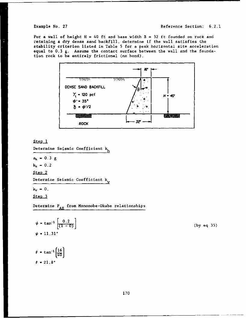
Example No. 27 Reference Section: 6,2.1
For a wall of height H - 40 ft and base width B - 32 ft founded on rock andretaining a dry dense sand backfill, determine if the wall satisfies thestability criterion listed in Table 5 for a peak horizontal site accelerationequal to 0.3 g. Assume the contact surface between the wall and the founda-tion rock to be entirely frictional (no bond).
I -- r__DENSE SAND BACKFILL 6 1
X, "120 pcf H- 4'-35" 0.d
ROCK "
Step 1
Determine Seismic Coefficient
ah - 0.3 g
kh - 0.2
SteD 2
Determine Seismic Coefficient kv
kv- 0.
Step 3
Determine P from Mononobe-Okabe relationships
-tanf F-' :~- (by eq 35)
S- 11.31o
, tan-1 6)
O - 21.8'
170
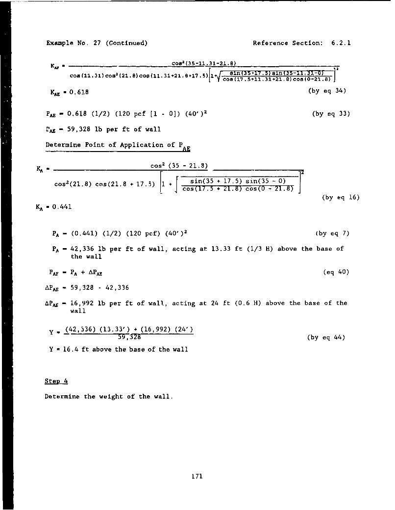
Example No. 27 (Continued) Reference Section: 6.2,1
K - coa 2 (35-11.31-21.8)
coo (11.31) cos2(21.8) cos (11.31+21.8+17.5) 1+ s 7n(35;i7.5)sin135-11.31-0)'os [(17.5+11,31+21.8) cos (0-21.8)
KAE - 0.618 (by eq 34)
PA - 0.618 (1/2) (120 pcf [1 - 0]) (40')) (by eq 33)
PA - 59,328 lb per ft of wall
Determine Point of Application of PAE
KA cos2 (35 - 21.3) 2
cos2(21.8) cos(21.8 + 17.5) [ sin(35 + 17.5) sin(35 - 0)o cos(17.5 + 21.8) cos(0 - 21.8)
(by eq 16)
KA - 0.441
S- (0.441) (1/2) (120 pcf) (40')2 (by eq 7)
PA - 42,336 lb per ft of wall, acting at 13.33 ft (1/3 H) above the base ofthe wall
PPA - PA + APA (eq 40)
APA - 59,328 - 42,336
APAE - 16,992 lb per ft of wall., acting at 24 ft (0.6 H) above the base of thewall
y ff(42,336) (13.33') + (16,992) (24')59,328 (by eq 44)
Y 16.4 ft above the base of the wall
Determine the weight of the wall.
171
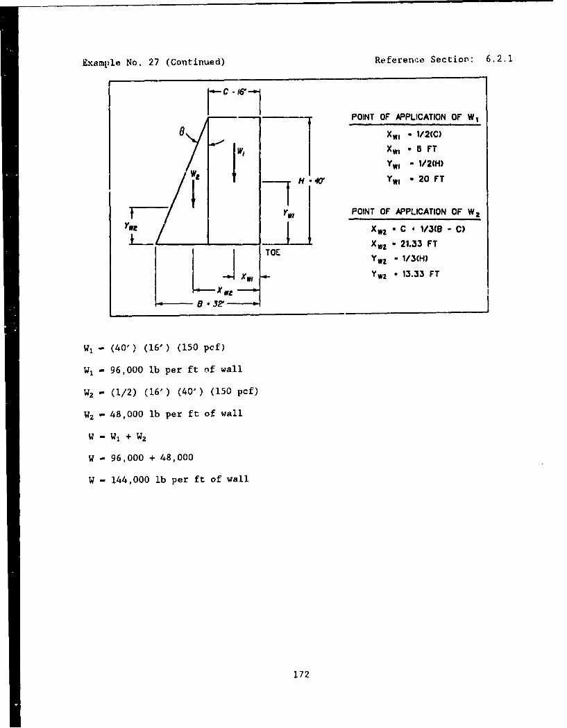
Example No. 27 (Continued) Reference Section: 6.2.1
POINT OF APPLICATION OF W,
XB 1/2(C)
• Wi Xw1 - 8 FT
YW1 - 1/2(H)H 41Y Yw1 - 20 FT
SYwi POINT OF APPLICATION OF W2
Y. X~ w - C 1/3(5 - C)
TOE X w - 21.33 FTJ• TOE w 1/3(H)
Ywz - 13.33 FT
x ir8 * 32z
W, - (40') (16') (150 pcf)
W, - 96,000 lb per ft of wall
W2 - (1/2) (16') (40') (150 pcf)
W2 - 48,000 lb per ft of wall
W - W1 + W2
W - 96,000 + 48,000
W - 144,000 lb per ft of wall
172
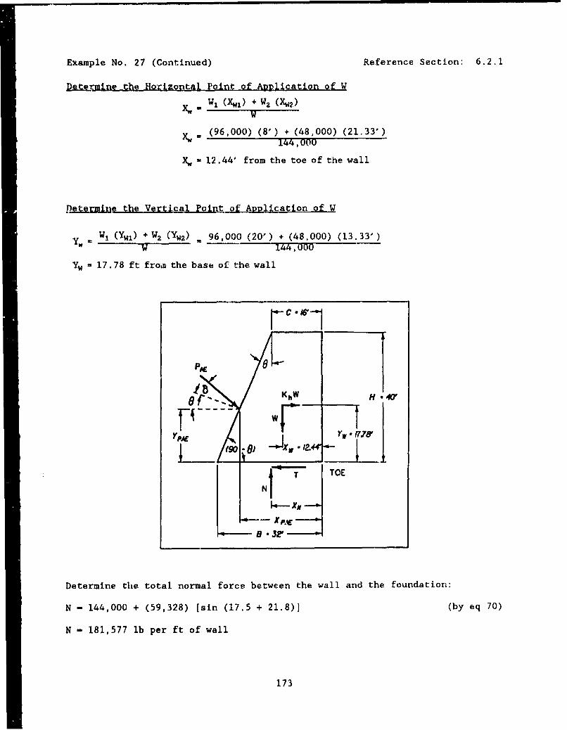
Example No. 27 (Continued) Reference Section: 6.2.1
Determine the Horizontal Point of ADDlIcation of W
- W1 (XN•) + W2 (X)W
(96,000) (8') + (48,000) (21.33')144,000
Xw- 12.44' from the toe of the wall
Petermine the Vertical Point of ARplication of W
y,,. W (Yw) +W 2 (yw 2 ) 96,000 (20') + (48.000) (13.33')
Yw = 17.78 ft froin the base of the wall
14-/KhW H 4V
YPAE YW " ff.7'"
N l•'•'- TOE
B " 31'
Determine the total normal force between the wall and the foundation:
N - 144,000 + (59,328) [sin (17.5 + 21.8)] (by eq 70)
N - 181,577 lb per ft of wall
173
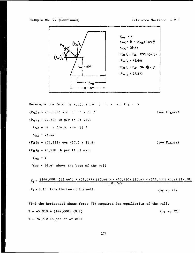
Example No. 27 (Continued) Reference Section: 6.2.1
AE ( yXpAC - 6 - (YpA) TAN B
5!ý y X pAC 25.44'
(P,) PM Cos (b8.)(pow
(PA, 45.9,0
_ _(PAK 1 , 37.577
Determine the Fo . s: A-,;.. - %. •
( ) - (9,328) sr " " - (see Figure)
(PA)y- 37,577 ib per t ' ir
XpA[ - 32' - (16.4) ran •21 8,
XpAE- 25.44'
(PA)x - (59,328) cos (17.5 + 21.8) (see Figure)
(PAE)X- 45,910 lb per ft of wall
YPAE - Y
YPAE - 16.4' above the base of the wall
XK = (144,000) (12.44') + (37,577) (25.44') - (45,910) (16.4) - (144,000) (0.2) (17.78)181,577
- 8.16' from the toe of the wall (by eq 71)
Find the horizontal shear force (T) required for equilibrium of the wall.
T - 45,910 + (144,000) (0.2) (by eq 72)
T - 74,710 lb per ft of wall
174
Example No. 27 (Continued) Reference Section: 6.2.1
Find the ultimate shear force along the base (Tult)
6 b - 35°, for clean sound rock. (fcom Table 2)
Tult - (181,577) tan (35) (by eq 74)
Tult - 127,142 lb per ft of wall
Compute the factor of safety against sliding (F,)
F. 127,14274,71T (by eq 73)
(F5 )actual = 1.70
SteR 6
Compare the computed factor of safety against sliding to the required factorof safety
(F,) required - 1.2 (from Table 5.)
(F,) actual > (Fa) required, therefore o.k
SteR 7
Determine the width of the area of effective base contact (Be)
Be - 3 (8.16') (by eq 75)
B, - 24.48
For temporary loading cases, such as earthquakes, B./B should be greater thanor equal to 0.5 (rock foundation, Table 5) to avoid overturning of the
structure.
]B , u 24.48actual -
B. 0.765actual
(B./B)actuai > (Ba/B)r.quirad, therefore o.k.
175
Example No. 27 (Continued) Reference Section: 6.2.1
Determine the factors of safety against bearing capacity failure, or crushingof both the concrete and rock at the toe.
Compute ax
- (2/3) (NI/XM) - (2/3) [(181,577)/(8.16)] (see Figure 6.3)
q,=" 14,835 lb per ft of wall
Check Fb for concrete
Assume for concrete:
quit - (4,000 psi) (144 in. 2 /ft 2)
qult - 576,000 lb per ft of wall
(Fb)ooncrete 0 quit . 576,000qa 47M=35 (by eq 77)
(Fk)cono~t, m 38.8
Values of Fb for concrete is adequate.
Check Fb for rock
Calculations omitted.
Stummary
The effect of vertical accelerations on the wall are summarized in the follow-
ing table.
Example 27 with varying kv
kh - 0.2kv - 0, +0.1, -0.1
176
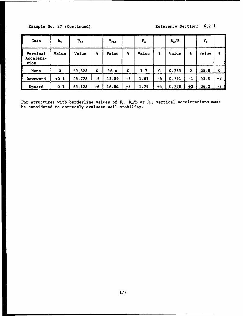
Example No. 27 (Continued) Reference Section: 6.2.1
-i m - - i- -
Case kv PAZ YP F, B./B Fb
Vertical Value Value % Value Value % Value % Value %Accelera-tion
None 0 59,328 0 16.4 0 1.7 0 0.765 0 38.8 0
Downward +0.1 55,728 -6 15.89 -3 1.61 o5 0.751 -1 42.0 +8
Upward -0.1 63,128 +6 16.84 +3 1.79 +5 0.778 +2 36.2 -7
For structures with borderline values of F,, B,/B or Fb, vertical accelerations mustbe considered to correctly evaluate wall stability.
177
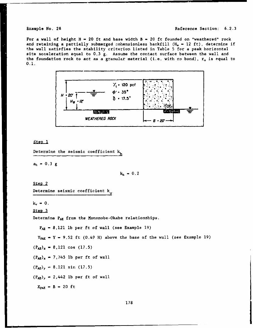
EPcample No. 28 Reference Section: 6.2.3
For a wall of height H - 20 ft and base width B - 20 ft founded on "weathered" rockand retaining a partially submerged zohensionless backfill (H, - 12 ft), determine ifthe wall satirfies the stability criterion listed in Table 5 for a peak horizontalsite acceleration equal to 0.3 g, Assume the contact surface between the wall andthe foundation rock to act as a granul&r material (i.e. with no bond), ru is equal to0.1.
•"120 pOf .':, :
H.EOI' _ ••.: :
WEATHERED RCK
Determine the seismic coefficient
ah - 0.3 g
kh- 0.2
Determine seismic coefficient k
k,- 0.
Determine PA from the Mononobe-Okabe relationships.
PAE - 8,121 lb per ft of wall (see Example 19)
YpA - Y - 9.52 ft (0.49 H) above the base of the wall (see Example 19)
(PAE). - 8,121 cos (17.5)
(PAE). - 7,745 lb per ft of wall
(PE)y - 8,121 sin (17.5)
(PE)y - 2,442 lb per ft of wall
XpA - B - 20 ft
178
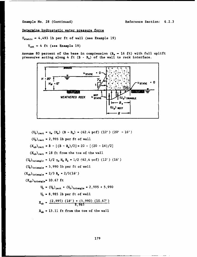
Example No. 28 (Continued) Reference Section: 6.2.3
Determine hydrostatic water pressure force
Uo•.ti- 4,493 lb per ft of wall (see Example 19)
Yust- 4 ft (see Example 19)
Assume 80 percent of the base in compression (Be - 16 ft) with full upliftpressures acting along 4 ft (B - Be) of the wall to rock interface.
U STATIC 0...
i ,WH" -" 12 1•*' U " " S T A TIC " 0
SOT
WEATHERED ROK U STATI (Ub) TMMLE
(U)KCT
(Ub).et " '1W (H,,) (B - B.) - (62.4 pcf) (12' ) (20' - 16')
(Ub)rect - 2,995 lb per ft of wall
(Xb) rect - B - [(B - Be)/2] - 20 - [(20 - 16)/2]
(XMu)rect - 18 ft from the toe of the wall
(Ub)trianI," - 1/2 y,, H., Be - 1/2 (62.4 pcf) (12') (16')
(M)tr.•nl. - 5,990 lb per ft of wall
(Xub) tz~ a,. - 2/3 Be - 2/3(16' )
(Xub)tri., 61.- 10.67 ft
Lý - (V)*ect + (Ub)triansi. - 2,995 + 5,990
Ub - 8,985 lb per ft of wall
- (2,995) (18') + (5,990) (10.67')8,985
X, - 13.11 ft from the toe of the wall
179
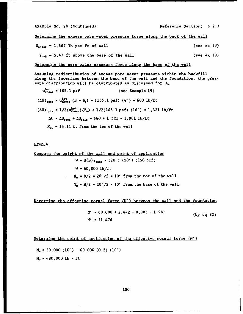
Example No. 28 (Continued) Reference Section: 6.2.3
Determine the excess Dote water pressure force along the back of the wall
U.h..r - 1,567 lb per ft of wall (see ex 19)
Yu.h - 5.47 ft above the base of the wall (see ex 19)
Determine the pore water pressure force along the base of the wall
Assuming redistribution of excess pore water pressure within the backfillalong the interface between the base of the wall and the foundation, the pres-sure distribution will be distributed as discussed for Ub.
uboa - 165.1 psf (see Example 19)
bot(AU)r"ct -ushear (B -B,) - (165.1 psf) (4') - 660 lb/ft
(AU)tri. - 1/2( Uh..r)(B.) - 1/2(165.1 psf) (16') - 1,321 lb/ft
A•U - AU ..t + AUtri. - 660 + 1,321 - 1,981 lb/ft
XDU - 13.11 ft from the toe of the wall
.O_ Ute the weight of the wall and Point of aovlication
W - H(B)-Ycoo - (20') (20' ) (150 pcf)
W - 60,000 lb/ft
& - B/2 - 20'/2 - 10' from the toe of the wall
Y. - H/2 - 20'/2 - 10' from the base of the wall
Determine the effective normal force (N') between the wall and the foundation
N' - 60,000 + 2,442 - 8,985 - 1,981 (by eq 82)
N' - 51,476
Determine the voint of aoolication of the effective normal force (N')
Mw - 60,000 (10') - 60,000 (0.2) (10')
S- 480,000 lb - ft
180
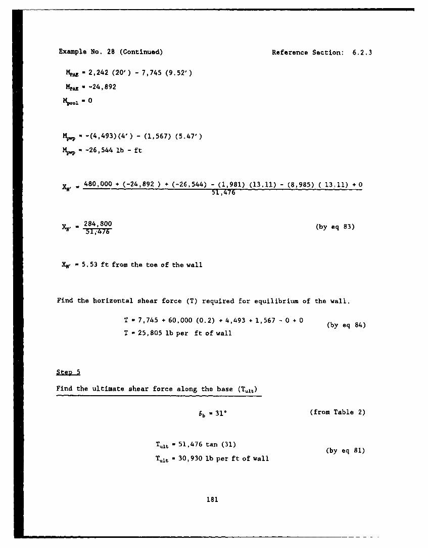
Example No. 28 (Continued) Reference Section: 6.2.3
MZ - 2,242 (20') -7,745 (9.52')
M * - -24,892Hpoo1 u 0
1r - -(4,493)(4') - (1,567) (5.47')
m - -26,544 lb - ft
XN, - 480,000 + (-24,892 ) + (-26,544) - (1,981) (13,11) - (8,985) (13.11) + 051,476
284,800 (by eq 83)
XH, - 5.53 ft from the toe of the wall
Find the horizontal shear force (T) required for equilibrium of the wall.
T - 7,745 + 60,000 (0.2) + 4,493 + 1,567 - 0 + 0 (by eq 84)
T - 25,805 lb per ft of wall
Find the ultimate shear force along the base (TuIt)
6b - 31° (from Table 2)
Tlt - 51,476 tan (31) (by eq 81)
T*1t - 30,930 lb per ft of wall
181
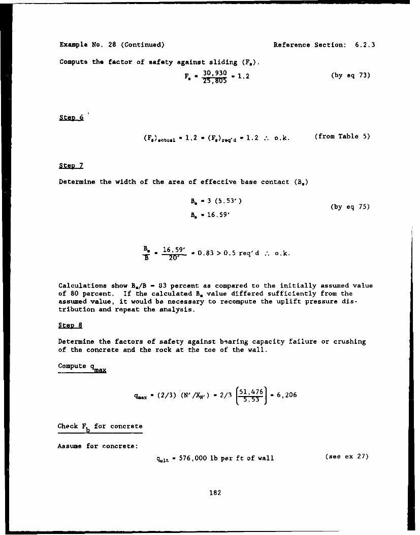
Example No. 28 (Continued) Reference Section: 6.2.3
Compute the factor of safety against sliding (F.).
F 30,930• 1.2 (by eq 73)
(F, 1.2 - Us)r.qd - 1.2 ". o.k. (from Table 5)
Determine the width of the area of effective base contact (B,)
Be - 3 (5.53') (by eq 75)
Be V 16.59'
B, e 16.59' .0.83 > 0.5 req'd .. o. k.
Calculations show B*/B - 83 percent as compared to the initially assumed valueof 80 percent. If the calculated Be value differed sufficiently from theassumed value, it would be necessary to recompute the uplift pressure dis-tribution and repeat the analysis.
steR 8
Determine the factors of safety against biaring capacity failure or crushingof the concrete and the rock at the toe of the wall.
Compute qmax
q.,, - (2/3) (N'IXN,) - 2/3 (51,476 6,206
Check Fb for concrete
Assume for concrete:
qu-t - 576,000 lb per ft of wall (see ex 27)
182
Example No. 28 (Continued) Reference Section: 6.2.3
(Fb)COncret. e qu = 576,000 = 92.8 (by eq 77)qm 6,7106
Value for Fb for concrete is adequate.
Check F for rock
Calculations omitted.
183
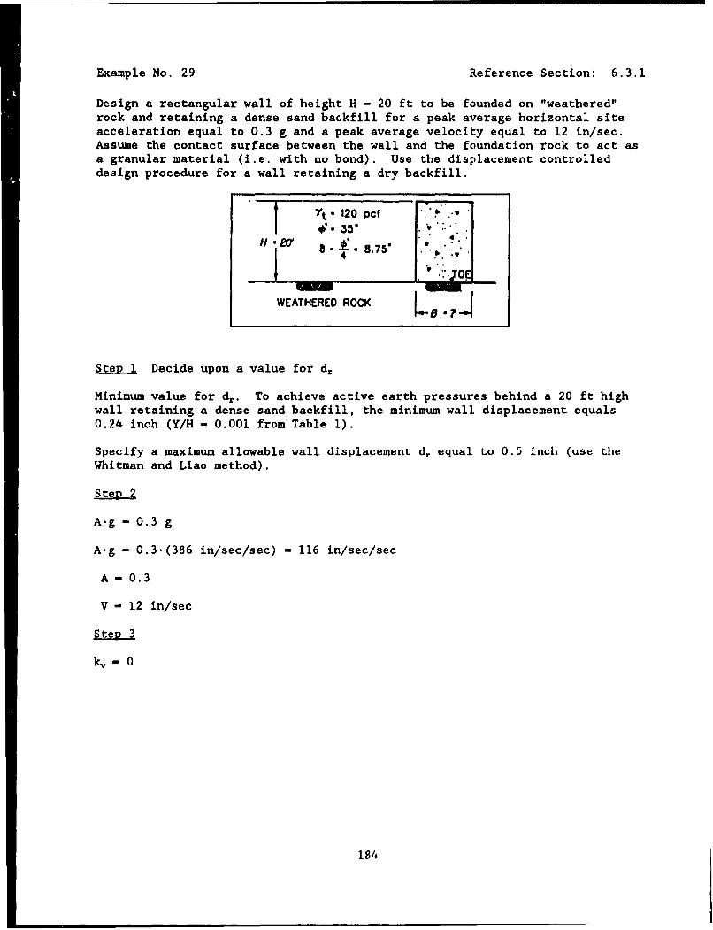
Example No. 29 Reference Section: 6.3.1
Design a rectangular wall of height H - 20 ft to be founded on "weathered"rock and retaining a dense sand backfill for a peak average horizontal siteacceleration equal to 0.3 g and a peak average velocity equal to 12 in/sec.Assume the contact surface between the wall and the foundation rock to act asa granular material (i.e. with no bond). Use the displacement controlleddesign procedure for a wall retaining a dry backfill.
S- 120 pcf "
H.•1 8-• 8.75" "44
WEATHERED ROCK VB
Step 1 Decide upon a value for d4
Minimum value for d.. To achieve active earth pressures behind a 20 ft highwall retaining a dense sand backfill, the minimum wall displacement equals0.24 inch (Y/H - 0.001 from Table 1).
Specify a maximum allowable wall displacement d, equal to 0.5 inch (use theWhitman and Liao method).
A.g - 0.3 g
A.g - 0.3.(386 in/sec/sec) - 116 in/sec/sec
A - 0.3
V - 12 in/sec
k - 0
184
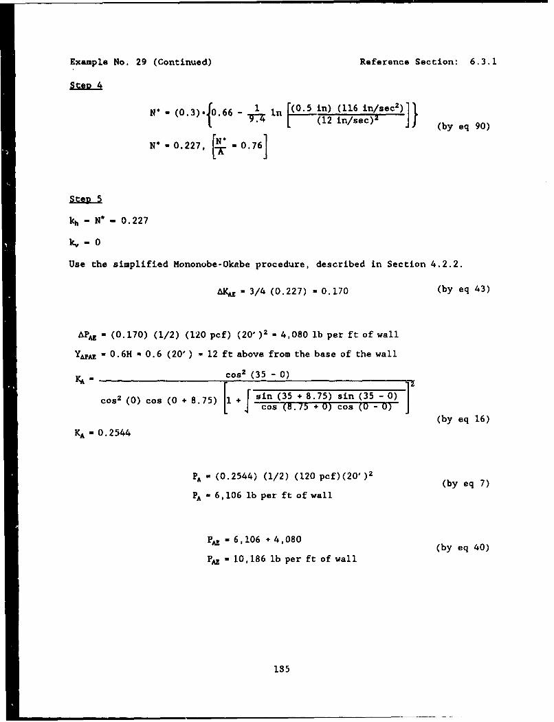
Example No. 29 (Continued) Reference Section: 6.3.1
N' -(0.3- 66- 1in in) (116__________
" (0.27o. -(2 in) e c) (by eq 90)
kh - N* - 0.227
k•-0
Use the simplified Mononobe-Okabe procedure, described in Section 4.2.2.
S- 3/4 (0.227) - 0.170 (by eq 43)
APAE - (0.170) (1/2) (120 pcf) (20' )2 - 4,080 lb per ft of wall
YAPAZ - 0.6H - 0.6 (20') - 12 ft above from the base of the wall
KA - cos 2 (35 - 0)
cos 2 (0) cos (0 + 8.75) 1 + sin (35 + 8.75) sin (35 - 0)cos (8.75 + O) Cos (0 -O)
KA - 0.2544 (by eq 16)
PA - (0.2544) (1/2) (120 pcf)(20' )2 (by eq 7)
PA - 6, 106 lb per ft of wall
PA - 6,106 + 4,080
PAE - 10,186 lb per ft of wall
185
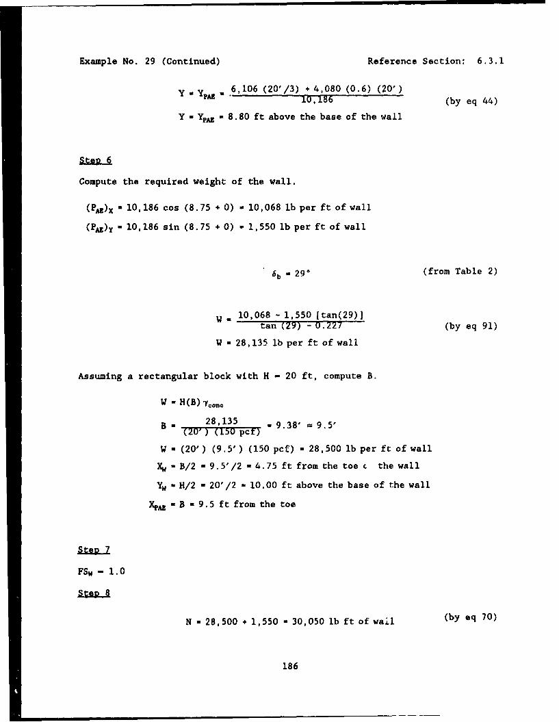
Example No. 29 (Continued) Reference Section: 6.3.1
Y .w Y =*6,106 (20'/3) + 4,080 (0.6) (20')60,186 (by eq 44)
Y - YpA- 8.80 ft above the base of the wall
Compute the required weight of the wall.
(PAE)X - 10,186 cos (8.75 + 0) - 10,068 lb per ft of wall
(PAE)y - 10,186 sin (8.75 +0) - 1,550 lb per ft of wall
6 b - 290 (from Table 2)
W - 10,068 - 1,550 [tan(29)]tan (29) - 0.227 (by eq 91)
W - 28,135 lb per ft of wall
Assuming a rectangular block with H - 20 ft, compute B.
W H (B)
B = 28,135 - 9.38' = 9.5'(20') (150 pcf)
W - (20') (9.5') (150 pcf) - 28,500 lb per ft of wall
Xw B/2 - 9.5'/2 - 4.75 ft from the toe c the wall
Yw - H/2 - 207/2 - 10.00 ft above the base of the wall
4AZ - B - 9.5 ft from the toe
FSw - 1.0
N w 28,500 + 1,550 - 30,050 lb ft of wall (by eq 70)
186
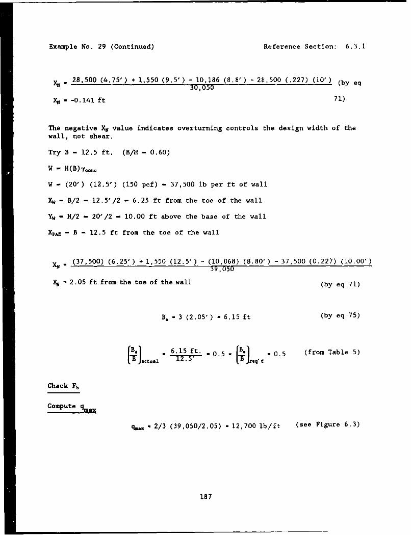
Example No. 29 (Continued) Reference Section: 6.3.1
X" - 28,500 (4.75') + 1,550 (9.5') - 10,186 (8.8') 28,500 (.227) (10') (by eq30,050
M -0.141 ft 71)
The negative XN value indicates overturning controls the design width of the
wall, not shear.
Try B - 12.5 ft. (B/H - 0.60)
W - H(B)7.on.
W - (20') (12.5') (150 pcf) - 37,500 lb per ft of wall
Xw - B/2 - 12.5'/2 - 6.25 ft from the toe of the wall
Yw - H/2 - 20'/2 - 10.00 ft above the base of the wall
XpAz- B - 12.5 ft from the toe of the wall
XN (37,500) (6.25') + 1,550 (12.5') - (10,068) (8.80') -37,500 (0.227) (10.00')39,050
XK 2.05 ft from the toe of the wall (by eq 71)
Be - 3 (2.05') - 6.15 ft (by eq 75)
- 6.15 ft. - 0. 5 -B.) 0.5 (from Table 5)123' = 05= JrsqOd
Check Fb
Compute qmax
q.. - 2/3 (39,050/2.05) - 12,700 lb/ft (see Figure 6.3)
187
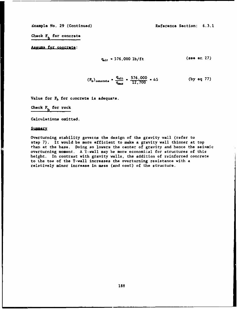
Example No. 29 (Continued) Reference Section: 6.3.1
Check F for concrete
Assuma for concrete:
qo.t 576,000 lb/ft (see ex: 27)
(Fb)conorete. qt - 576,000 45 (by eq 77)
Value for Fb for concrete is adequate.
Check Fb for rock
Calculations omitted.
Overturning stability goveins the design of the gravity wall (refer tostep 7). It would be more efficient to make a gravity wall thinner at topthan at the base. Doing so lowers the center of gravity and hence the seiqmicoverturning moment. A T-wall may be more economical for structures of thisheight. In contrast with gravity walls, the addition of reinforced concreteto the toe of the T-wall increases the overturning resistance with arelatively minor increase in mass (and cost) of the structure.
188
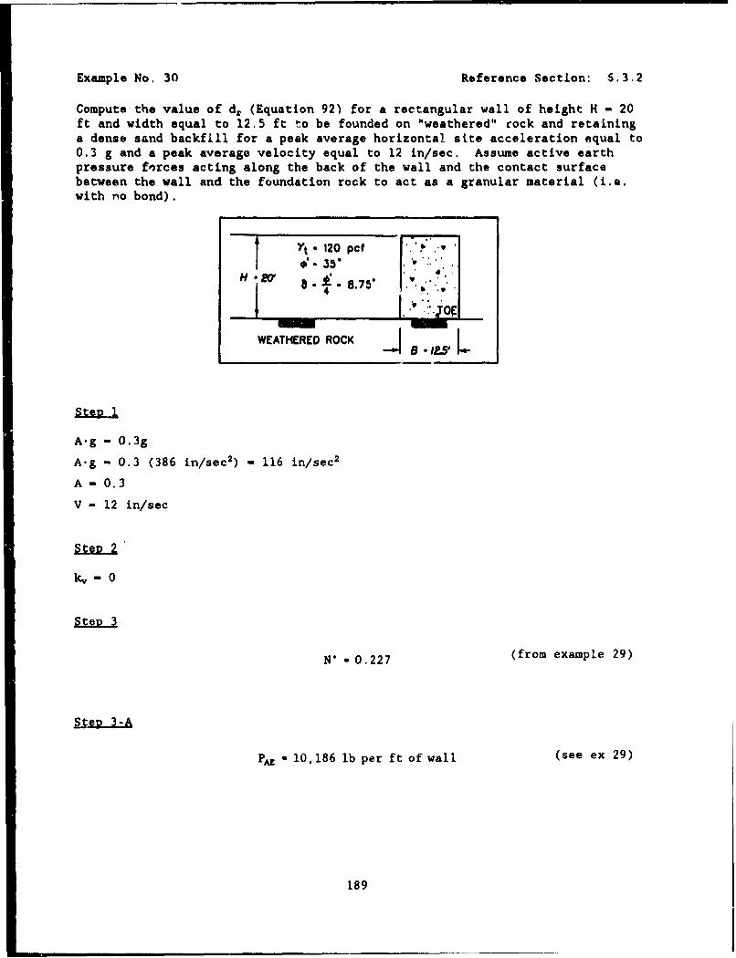
Example No. 30 Reference Section: 6.3.2
Compute the value of d4 (Equation 92) for a rectangular wall of height H - 20ft and width equal to 12.5 ft to be founded on "weathered" cock and retaininga dense sand backfill for a peak average horizontal stte acceleration equal to0.3 g and a peak average velocity equal to 12 in/sec. Assume active earthpressure forces acting along the back of the wall and the contact surfacebetween the wall and the foundation rock to act as a granular material (i.e.with no bond).
t t . 120 pcf .0!'- 35" 0
44
WEATHERED ROCK - ,~I.
A-g - 0. 3 g
A-g - 0.3 (386 in/sec 2 ) - 116 in/sec 2
A - 0.3
V - 12 in/sec
kv ,- 0
N" - 0.227 (from example 29)
PAE - 10,186 lb per ft of wall (see ex 29)
189
Example No. 30 (Continued) Reference Section: 6.3.2
¥ *• - 8.80 ft above the base of the wall (see Ex 29)
T - 10,068 + (37,500) (0.227) (by eq 72)
T - 18,581 lb per ft of wall
Step 3-C
N - 37,500 + 1,550 (by eq 70)
N - 39,050 Ib per ft of wall
Step 3-D
6b - 29° (from Table 2)
Tu l t -39,050 tan (29) (by eq 74)
Tult - 21,646 lb per ft of wall
Adjust the value used for N*
F. - Tut . 21,646 -1.165
kh - N* - (N*)Od (F.) - (0.227) (1.165)
kh - N* - 0.264
Step 3-A 2nd Iteration
AKAE - 3/4 (0.264) - 0.198 (by eq 43)
190
Example No. 30 (Continued) Reference Section: 6.3.2
UA - (0.198) (1/2) (120 pcf) (20')2 (by eq 41)
AP~z - 4,752 lb per ft of wall
PA - 6,106 lb per ft of wall (see ex 29)
PAZ - 6,106 + 4,752 (by eq 40)
PAE - 10,858 lb per ft of wall
(PA)x - 10,858 cos (8.75 + 0) - 10,732 lb per ft of wall
(PAX)y a 10,858 sin (8.75 + 0) - 1,652 lb per ft of wall
SteD 3-B 2nd Iteration
T - 10,732 + 37,500 (0.264) (by eq 72)T - 20,632 lb per ft of wall
Step 3-C 2nd Iteration
N - 37,500 + 1,652 (by eq 70)
N - 39,152 lb per ft of wall
Steo 3-D 2nd Iteration
6b - 29° (see ex 29)
TULT - 39,152 tan (29) - 21,702 lb per ft of wall (by eq 74)
teo 3-E 2nd Iterati2n
Adjust the value used for N*
191
Example No. 30 (Continued) Reference Section: 6.3.2
P, TULT - 21,702 .1.05a1.1'If- 767
1% U N'. (N*)od, ( 2(.J.2) (1.1) - 0.290
Stv -3-a&Jr IteratiJn
AKA - 3/4 (0.290) - 0.218 (by eq 43)
APAýr - (0.218) (1/2) (120 pcf) (20')2 - 5,232 lb per ft of wall (by eq 41)
PA - 6,106 lb per ft of wall (see ex 29)
PAZ - 6,106 + 5,232 = 11,338 lb per ft of wall (by eq 40)
(PAE)X - 11,338 cos (8.75 + 0) - 11,206 lb per ft of wall
(PE)y =- 1.1,338 sin (8.75 + 0) - 1,725 lb per ft of wall
SteR 3-B 3rd Iteration
T - 11,206 + 37,500 (0.290) (by eq 72)T - 22,081 lb per ft of wall
Step 3-C 3rd Iteration
N - 37,500 + 1,725 - 39,225 lb per ft of wall (by eq 70)
Steg 3-D 3rd Iteration
6 b - 290 (see ex 29)
192
Example No. 30 (Continued) Reference Section: 6.3.2
TULT - 39,225 -an (29) - 21,743 lb per ft of wall (by eq 74)
SteR 3-E 3rd Iteration
Adjust the value used for N*
Fa TT 21.743 . 0.985
Assume TT - T since F. is less than 2 percent from a value of 1.0 and useN* - 0.290.
N" 0.290 0.967
_495 (12 in/sec)2] exp(-. 4 ,* 0.967) (by eq 92)L (116 in/sec2) ]
d,- 0.07 inches
d of .inch, ooinchu 0.001 H
Check Fb
Calculation omitted.
Summa•
The calculated earthquake induced displacement (approximately 1/10 inch)is less than 1/4 inch displacement, the minimum value that is required todevelop active earth pressures in a dense sand backfill of 20 ft height (referto Example 29). The computed dr value is less than this required minimumvalue due to the fact that to satisfy the stability criterion against over-turning, the required width of the gravity wall was increased. The additionalconcrete mass increased the shear resistance along the base of the wall andthus reduced the magnitude of wall displacement for the design earthquakeload.
Since the computed displacement of the rectangular gravity wall is lessthan that minimum value required to develop active earth pressures for thedesign earthquake by a factor of four, the procedures discussed in Chapter 5
193
Example No. 30 (Continued) Reference Section: 6.3.2
(walls retaining nonyielding backfills) would be used to compute the dynamicearth pressure acting on tha gravity wall. In general, the dynamic earthpressures for "nonyielding backfills" are two to three times larger than thedynamic active earth pressure force. Analysis and design of walls retainingnonyielding backfills are discussed in Chapter 8.
If the wall had been made thinner at the top than at the base, as dis-cussed in the summary to Example 29, then the necessity to design the wall toretain a nonyielding backfill might be avoided.
194
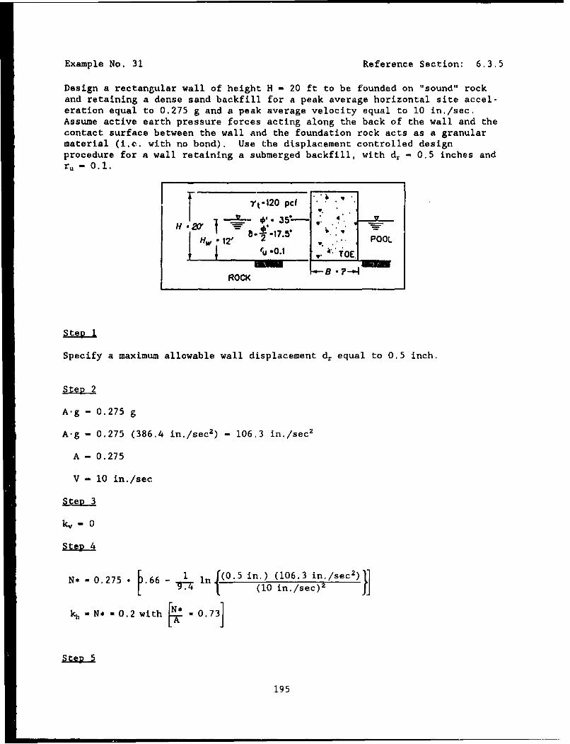
Example No. 31 Reference Section: 6.3.5
Design a rectangular wall of height H - 20 ft to be founded on "sound" rockand retaining a dense sand backfill for a peak average horizontal site accel-eration equal to 0.275 g and a peak average velocity equal to 10 in./sec.Assume active earth pressure forces acting along the back of the wall and thecontact surface between the wall and the foundation rock acts as a granularmaterial (i.e. with no bond). Use the displacement controlled designprocedure for a wall retaining a submerged backfill, with dr - 0.5 inches andr -- 0.1.
*-2 yt- 120 pcf
H 220' .1 . -
Hw 12' 2 1. , POOLru -0.1 TOE.
ROCK
SteD 1
Specify a maximum allowable wall displacement d, equal to 0.5 inch.
steR 2
A-g - 0.275 g
A.g - 0.275 (386.4 in./sec2 ) - 106.3 in./sec2
A - 0.275
V - 10 in./sec
k, - 0
N* - 0.275 • p.66 - 1¾ ln{(0.5 in.) (106.3 in./sec 2 )
kh - N* - 0.2 with - 0.73]
195
Example No. 31 (Continued) Reference Section: 6.3.5
khe - 0.251 (see ex 19)
A'•X) - 8,121 coo 17.5' (see ex 19)
kPA)x - 7,745 lb per ft of wall (se* ex 19)
Xp, z- B
(PA)y - 8,121 sin 17.5' (see ex 19)
(P•)y - 2,442 lb per ft of wall (see ex 19)
Ypzs - Y - 9.52 ft (0.49 H) above the base of the wall (see ex 19)
Determine hydrostatic water pressure force
Us - 4,493 lb per ft of wall (soe ex 19)
Yu~t 4 ft from the base of the wall (see ex 19)
Assume full hydrostatic pressure beneath the base of the wall.
Ub - (Hw) (-y.) (B) - (12') (62.4 pcf) B
Ub - 748.8 B
- B/2 - 0.5 B
Determine the excess yore water pressure force along the back of the wall.
Uuh..r - 1,567 lb per ft of wall (see ex 19)
Yuh - 5.47 ft (see ex 19)
Determine the excess 2ore water pressure force along the base of the wall
Assume B /B - 0.5
Assume the excess pore water pressure generated in the backfill during earth-quake shaking will propagate under the wall at a constant value in the baseseparation zone (B - B.). The pore water pressure in the base undercompression (B.) will linearly decrease from the maximum value to zero at thetoe of the wall.
196
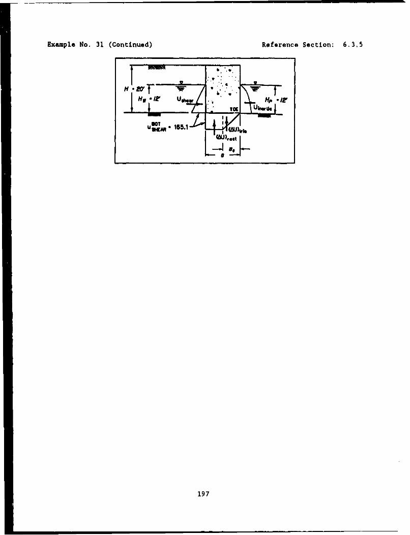
Example No. 31 (Continued) Reference Section: 6.3,5
f- "2, ,sm H ..
UrM 185.1
U44w
197
Example No. 31 (Continued) Reference Section: 6.3.5
ubat - 165.1 psf (see ex 19)sheaz
A Ushar (B - B,) (165.1 psf) (1/2) (B)
(AU)r,,t - 82.55 B
(MU)tri.- 1/2(us,,r) Be 1/2 (165.1 psf) (1/2) (B)
(AU) ti. - 41.28 B
AU - AU ..t + AUtj,, 82.55 B + 41.28 B - 123.83 B
(82.55 B) [Be + ((B - B,)/2)] + 41.28 B [2/3 B,]XIDU =123.83 B
with B, - 0.5 B,
- (82.55 B) (0.75 B) + (41.28 B) (2/3) (B/2) = 0.6111 BXDU - ~123M8 BS.61
Determine the hydrostatic water pressure force in front of the wall (due tothe pool)
Up,,, - 1/2 -,y HP2 - 1/2 (62.4 pcf) (12 )2
up,,, - 4,493 lb per ft of wall
Y-p - Hp/3 - 12'/3 - 4.00' above the base of the wall
Determine the inertia force in front of the wall
(see Appendix B)
Pwd " (7/12) (0.2) (62.4 pcf) (12')2
Uin.rti - Pd - 1,048 lb per ft of wall [1Jniti" 0.231
YUI - 0.4 Hp - (0.4) (12') U 4.8 ft above the base of the wall
198
Example No. 31 (Continued) Reference Section: 6.3.5
Compute the required weight of wall.
6 b - 350 (Table 2)
W -7,745 - 2,442[tan (35)] + 4,493 + 1,567 - 4,493 + 1,048 + 748.8 B + 123.8 B (by
tan (35) - 0.20 eq 94)
W - 8,650.1 + 872.6 B
W - B (H) o
withW - W, B - 17,293[(20) (150T- 1,744.•5
B - 13.77'
Let B - 14.0 ft
W - B(H)7vro.. - (14') (20') (150 pcf) - 42,000 lb per ft of wall
X, - B/2 - 14'/2 - 7.0 ft from the toe of the wall
Y. - H/2 - 20'/2 - 10.0 ft from the base of the wall
FS. - 1.0
AU - 123.83 B - 123.83 (14') - 1,734 lb per ft of wall
XDU - 0.6111 B - 0.6111 (14') - 8.56 ft from the toe of the wall
Ub - 748.8 B - 748.8 (14') - 10,483 lb per ft of wall
X• - 0.5 B - 0.5 (14') - 7.00 ft from the toe of the wall
N' - 42,000 + 2,442 - 748.8 (14') - 123.8 (14') (by eq 82)
N' - 32,226 lb per ft of wall
M, - 42,000 (7.0') - 42,000 (0.2) (10.0') - 210,000
199
Example No. 31 (Continued) Reference Section: 6.3.5
m A- 2,442 (14') - 7,745 (9.52') - -39,544
Mpo, - 4,493 (4') - 1,048 (4.8') - 12,942
M6p- -4,493 (4) - 1,567 (5.47) -- 26,544
- 210,000 + (-39,544) + (-26,544) - (1,734) (8.56') - (10,483) (7') + 12,942 eq
32,226 83)
X, - 2.13' from the toe of the wall
B, - 3( 2.13') - 6.39 ft (by eq 75)
6.39 ft -0. 46 Be 0.5 (from TableS5)L aotuL. 14 ft T Jq'd
overturning controls the design
The wall must be designed to resist overturning forces. Start from the mini-mum overturning stability requirement,
Be'- -o0.5 (from Table 5)
Be a 3X4, (adapted from eq 75)
200
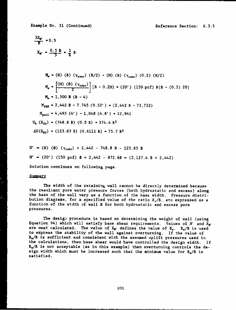
Example No. 31 (Continued) Reference Section: 6.3.5
3X-, 0.5
X 05 _B . 1 B
M. - (H) (B) (Ocono) (B/2) - (H) (B) (Oo) (0.2) (H/2)
SM [(H) (B)2(7•)OC] [B - 0.2H] - (20') (150 pcf) B[B - (0.2) 20]
t% - 1,500 B (B -4)
MpA - 2,442 B - 7.745 (9.52') - (2,442 8 - 73,732)
MpooZ - 4,493 (4') - 1,048 (4.8') - 12,942
Ub (Xub) - (748.8 B) (0.5 B) - 374.4 B2
AU(4Du) - (123.83 3) (0.6111 B) - 75.7 B2
N' - (H) (B) (.on.) + 2,442 - 748.8 B - 123.83 B
N' - (20') (150 pcf) B + 2,442 - 872.6B - (2,127.4 B + 2,442)
Solution continues on following page.
The width of the retaining wall cannot be directly determined becausethe resultant pore water pressure forces (both hydrostatic and excess) alongthe base of the wall vary as a function of the base width. Pressure distri-bution diagrams, for a specified value of the ratio B,/B, are expressed as afunction of the width of wall B for both hydrostatic and excess porepressures.
The desigo procedure is based on determining the weight of wall (usingEquation 94) which will satisfy base shear requirements. Values of N' and XM.are next calculated. The value of X, defines the value of B.. B./B is usedto express the stability of the wall against overturning. If the value ofB./B is sufficient and consistent with the assumed uplift pressures used inthe calculations, then base shear would have controlled the design width. IfB./B is not acceptable (as in this example) then overturning controls the de-sign width which must be increased such that the minimum value for B./B issatisfied.
201
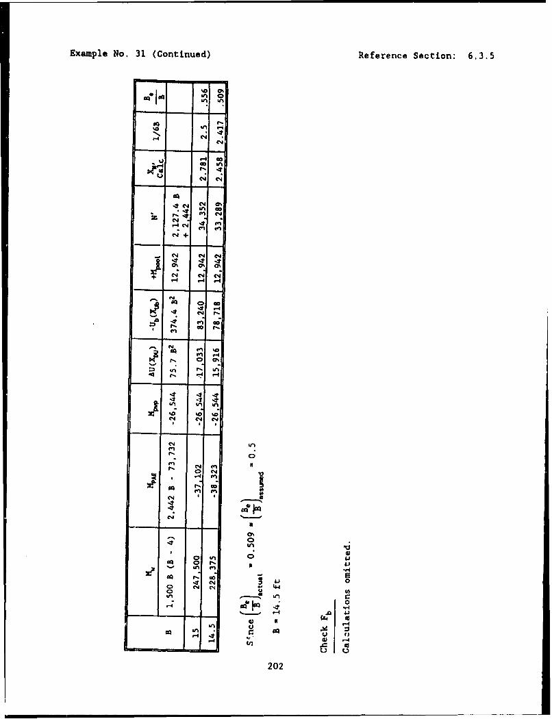
Example No. 31 (Continued) Reference Section: 6.3.5
V -
•OO
C4 0%
10 _
T- W-4 0
C4
".-4V4- t tI
P44
•+1
O10 O% 0%
,.4 ,.-4
-' oEI aO t.
4-4)
o4 41
494W
S 000
r-r-u
N r-4-
In,
O 0 0
ON•
202
.* o' o ' 0 *
%- U.' C..' --4
,--.
41 O
CHAPTER 7 ANALYSIS AND DESIGN OF ANCHORED SHEET PILE WALLS
7.1 Introduction
This section describes the procedures for evaluating the stability andsafety of anchored sheet pile walls during earthquakes. Anchored sheet pilewalls are comprised of interconnected flexible sheet piles that form a contin-uous and permanent waterfront structure. The free earth support method isused to determine the required depth of sheet pile penetration below thedredge level and the force the anchor must resist so that excessive sheet pilewall movements do not occur during earthquake shaking. The forces acting onboth the sheet pile wall and anchor during the earthquake include the staticand dynamic earth pressure forces, the static and hydrodynamic pool waterpressure forces and the steady state and residual excess pore water pressureforces within the submerged backfill and foundation soils. Because anchoredwalls are flexible and because it is difficult to prevent some permanent dis-placement during a major seismic event, it is appropriate to use active andpassive earth pressure theories to evaluate dynamic as well as static earthpressures. The Mononobe-Okabe theory is used to evaluate the dynamic earthpressures.
There have been very few documented cases of waterfront anchored wallsthat have survived earthquakes or of walls that have failed for reasons otherthan liquefaction. Hence uncertainty remains concerning the procedures out-lined in this chapter and the difficulty of ensuring adequacy of anchoredsheet pile walls during strong earthquake shaking (e.g. one rough index isseismic coefficients above 0.2).
One of the few seismic design procedures for anchored sheet pile wallsis the Japanese Code, which is summarized in Section 7.2.1. Using the obser-vations regarding the performance of anchored sheet pile walls during earth-quake s'-iaking (summarized in Section 7.2), the following improvements overpast practice are recommended:
(1) Anchors must be placed further away from the wall.
(2) Larger seismic coefficients are required. They are to be assignedwith consideration of the seismotectonic structures as well as thecharacteristics of soil and structural features comprising the wall, theanchorage and its foundation.
(3) There is a limitation upon the build-up of excess pore pressures inbackfill.
The procedures outlined in this chapter are to be viewed as interimguidance, an improvement over past practice. An anchored sheet pile wall is acomplex structure and its performance (e.g. displacements) during earthquakeshaking depends upon the interactions between the many components of thestructural system (e.g. sheet pile wall, backfill, soil below dredge level,foundation, and anchorage), which impact overall wall performance. Theseismic design of anchored sheet pile walls using the procedures described inthis chapter requires considerable judgement during the course of design by anearthquake engineer experienced in the problems associated with the seismicdesign of anchored sheet pile walls.
203
As a general design principle, anchored sheet pile walls sited inseismic environments should be founded in dense and dilative cohesionlesssoils with no silt or clay size parti,:les. The proposed design procedurepresume this to be the case. Strength parameters are to be assigned inaccordance with the criteria in Section 2.3. Additionally, the designprocedure is limited to the case where excess pore water pressures are lessthan 30 percent of the initial vertical effective stress (see Section 1.3,Chapter 1).
7.2 Background
Agbabian Associates (1980) summarize the performance of anchored sheetpile walls at 26 harbors during earthquakes in Japan, the United States, andSouth America. Their survey indicates that the catastrophic failures of sheetpile walls are due to the large-scale liquefaction of the backfill and/or thefoundatloi , including the foundation soil located in front of the sheet pilewall and below the dredge level. For those structures that underwent exces-sive movements but did not suffer a catastrophic failure, there was little orno evidence of damage due to the vibrations of structures themselves. Forthose walls whose backfill and foundation soils did not liquify but didexhibit excessive wall moments during the earthquake, the survey identifiedthe source of these excessive sheet pile wall movements as (1) the soil infront of the sheet pile wall and below the dredge level moved outward (toefailure), (2) the anchor block moved towards the pool (anchor failure), or(3) the entire soil mass comprising the sheet pile structure and the anchorblock moved as one towards the pool (block movement). These three potentia]failure modes within the backfill and the foundation soils are idealized inFigure 2.1, along with the two potential structural failure modes duringearthquake shaking of anchored sheet pile walls. The report identified anumber of factors which may contribute to the excessive wall movements,including (1) a reduction in soil strength due to the generation of excesspore water pressures within the submerged soils during the earthquake shaking,(2) the action of the inertial forces due to the acceleration of the soilmasses in front and behind the sheet pile wall and the anchor block, and(3) the hydrodynamic water pressures along the front of the wall during theearthquake.
The Japanese Ports and Harbors commissioned a study by Kitajima andUwabe (1979) to summarize the performance of 110 quay walls during variousearthquakes that occurred in Japan during the past several decades. Thissurvey included a tally of both damaged and undamaged waterfront structuresand the dates on which the earthquakes occurred. Most of these waterfrontstructures were anchored bulkheads, according to Gazetas, Dakoulas, andDennehy (1990). In their survey, Kitajima and Uwabe were able to identify thedesign procedure that was used for 45 of the bulkheads. This is identified asthe Japanese code. Their survey showed that (1) the percentage of damagedbulkheads was greater than 50 percent, including those designed using theJapanese design procedure and (2) the percentage of bulkhead failures did notdiminish with time. These two observations indicate that even the more :e-cently enacted Japanese code is not adequate. To understand the poor perfor-mance of anchored sheet pile walls during earthquakes, it is useful to reviewthe Japanese code that was used in the design of the most recent sheet pilewalls that were included in the Kitajima and Uwabe survey.
204
7.2.1 Summary of the Japanese Code for Design of Anchored Sheet Pile Walls
Most of the case histories regarding the performance of anchored sheetpile walls during earthquakes that were included in the Agbabian Associates(1980) and the Kitajima and Uwabe (1979) surveys are for Japanese waterfrontstructures. To understand the performance of these Japanese waterfront struc-tures, it is useful to review the Japanese design procedures that were usedfor the most recently constructed waterfront structures included in the sur-veys. The Japanese code for the design of anchored sheet pile walls as de-scribed by Gazetas, Dakoulas, and Dennehy (1990) consists of the followingfive steps:
(1) Estimate the required sheet pile embedment depth using the freeearth support method, with the factor of safety that is applied to theshear strength of the soil reduced from 1.5 for static loadings to 1.2for dynamic loadings. The effect of the earthquake is incorporated inthe analysis through the inertial forces acting on the active and pas-sive soil wedges by using the Mononobe-Okabe method to compute PA andPPE.
(2) The horizontal seismic coefficient, kh, used in the Mononobe-Okaberelationships for PAZ and PpE is a product of three factors: a regionalseismicity factor (0.10 ± 0.05), a factor reflecting the subsoil condi-tions (1 ± 0.2), and a factor reflecting the importance of the structure(1 ± 0.5).
(3) Design the tie rod using a tension force value computed on theassumption that the sheet pile is a simple beam supported at the dredgeline and by the tie rod connection. Allowable stress in the tie rodsteel is increased from 40 percent of the yield stress in a design forstatic loadings to 60 percent of the yield stress in the design fordynamic loadings.
(4) Design the sheet pile section. Compute the maximum bending moment,referred to as the free earth support moment, in the sheet pile usingthe simple beam of step 3. In granular soils Rowe's procedure is usedto account for flexure of the sheet pile below the dredge level. Areduction of 40 to 50 percent in the free earth support moment value isnot unusual. Allowable stress in the sheet pile steel is increased from60 percent of the yield stress in a design for static loadings to90 percent of the yield stress in the design for dynamic loadings.
(5) Design the anchor using the tie rod force of step 2 increased by afactor equal to 2.5 in the design for both static and dynamic loadingsand assume the slip plane for the active wedge starts at the dredgeline.
From the modes of failure observed in the Kitajima and Uwabe study of anchoredsheet pile walls that were designed using the Japanese code, Gazetas, Dakoulasand Dennehy (1990) identified the following as the primary deficiencies in theJapanese code procedure:
(1) The values for the seismic coefficients, kv and kh, used in theMononobe-Okabe relationships for PA and PPE are not determined from asite response analysis but are specified within the Japanese code (kv -
205
0, and kh is within a narrow range of values for most of the waterfrontstructures involved in the study).
(2) The resistance provided by the anchor is over estimated because thecode allows the anchor to be placed too close to the sheet piYe wallsuch that the passive wedge that develops in front of thb anchor inter-feres with the a-'tive wedge developing within the backfill behind thesheet pile wall.
(3) The code does not account for the earthquake induced excess porewater pressures within the submerged soils and the corresponding reduc-tion in the shear strength for the submerged soil regions, nor the ex-cess water pressure forces and hydrodynamic forces acting on the sheetpile structure.
Gazetas, Dakoulas, and Dennehy (1990) listed only one of the failures ofthe sheet pile walls designed using the Japanese Code as a general flexuralfailure. In this case, the structural failure was attributed to corrosion ofthe steel at the dredge level.
Each of these deficiencies is addressed in the steps used in the design r'fanchored sheet pile walls using the free earth support method of analysis asdescribed in Section 7.4.
7.2.2 Displacements of Anchored Sheet Piles during Earthquakes
In the Kitajima and Uwyabe (1979) survey of damage to anchored 3heet pilewalls during earthquakes, the level of damage to the waterfront structure wasshown to be a function of the movement of the top of the sheet pile during theearthquake. Kitajima and Uwabe (1979) ':ategorized the damlage as one of fivelevels as given In Table 6 and reported in Gazetas, Dakoulas, and Dennehy(1990). Their survey shows that for sheet pile wall displacements of 10 cm(4 inches) or less, there was little or no damage to the Japanese waterfrontstructures as a result of the earthquake shaking. Conversely, the level ofdamage to the waterfront structure increased in proportion to the magnitude ofthe displacements above 10 cm (4 inches). Using the information on theanchored sheet pile walls survey reported in Kitajima and Uwabe (1979) andusing simplified theories and the free earth support method of analysis,Gazetas, Dakoulas, and Dennehy (1990) showed that the post-earthquake dis-placoments at the top of the sheet pile wall correlated to (1) the depth ofsheet pile embedment below the dredge level and (2) the distance between theanchor and the sheet pile.
Tuo anchored bulkheads were in place in the harbor of San Antnnio,Chile, during the very large earthquake of 1985. A peak horizontal accelera-tion of about 0,6g was recorded within 2 km of the site. One experienced apermanent displacement of nearly a meter, and use of the quay was seveiely
restricted. There was evidence of liquefaction or at least poor compaction ofthe backfill, and tie rods may not have been preloaded. The second bulkheaddeveloped a permanent displacement of 15 cm, but. the quay remained functional
after the earthquake. This bulkhead had been designed using the Japaneseprocedure with a seismic coefficient of 0.15, but details concerning compac-tion of the backfill are unknown.
206
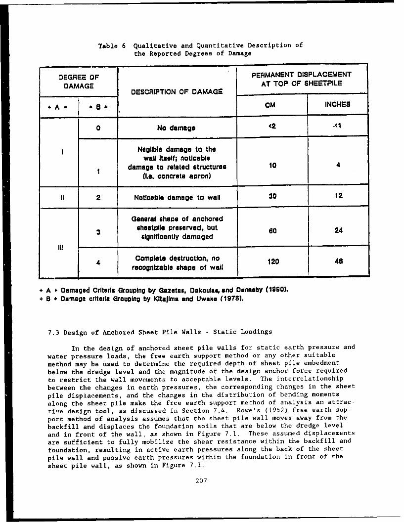
Table 6 Qualitative and Quantitative Description ofthe Reported Degrees of Damage
DEGREE OF PERMANENT DISPLACEMENT
DAMAGE AT TOP OF SHEETPILEDESCRIPTION OF DAMAGE ....
A + 13 CM INCHES
0 No damage <2 -01
Neglible damage to thewag Itself; noticeble
damage to related structures 10 4
(I.e. concrete apron)
11 2 Notlcable damage to wall 30 12
General shape of anchored3 sheetplle preserved, but so 24
significantly damaged
4 Complete destruction, no 120 48
recognizable shape of wall
+ A + Damaged Criteria Grouping by Gazeta., Dakoulas, and Denneby (1990).+ B + Damage criteria Grouping by Kitajlmr and Uwake (1978).
7.3 Design of Anchored Sheet Pile Walls - Static Loadings
In the design of anchored sheet pile walls for static earth pressure and
water pressure loads, the free earth support method or any other suitable
method may be used to determine the required depth of sheet pile embedment
below the dredge level and the magnitude of the design anchor force required
to restrict the wall movements to acceptable levels. The interrelationshipbetween the changes in earth pressures, the corresponding changes in the sheet
pile displacements, and the changes in the distribution of bending momentsalong the sheet pile make the free earth support method of analysis an attrac-tive design tool, as discussed in Section 7.4. Rowe's (1952) free earth sup-
port method of analysis assumes that the sheet pile wall moves away from the
backfill and displaces the foundation soils that are below the dredge leveland in front of the wall, as shown in Figure 7.1. These assumed displacements
are sufficient to fully mobilize the shear resistance within the backfill and
foundation, resulting in active earth pressures along the back of the sheet
pile wall and passive earth pressures within the foundation in front of the
sheet pile wall, as shown in Figure 7.1.
207
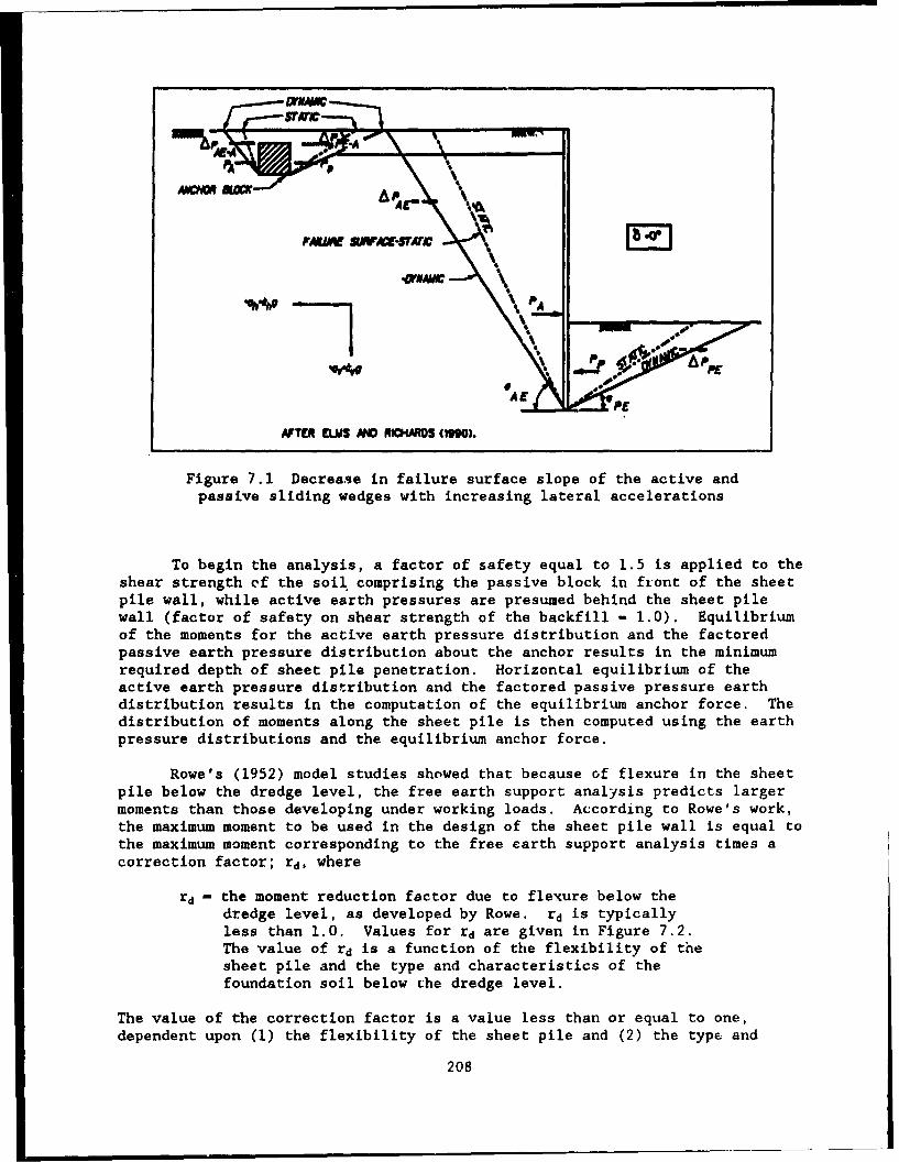
PMVW StAC-Sff
AFTER ELMS AND ROUNOS (ISO).
Figure 7.1 Decrease in failure surface slope of the active andpassive sliding wedges with increasing lateral accelerations
To begin the analysis, a factor of safety equal to 1.5 is applied to theshear strength cf the soil comprising the passive block in front of the sheetpile wall, while active earth pressures are presumed behind the sheet pilewall (factor of safety on shear strength of the backfill - 1.0). Equilibriumof the moments for the active earth pressure distribution and the factoredpassive earth pressure distribution about the anchor results in the minimumrequired depth of sheet pile penetration. Horizontal equilibrium of theactive earth pressure distribution and the factored passive pressure earthdistribution results in the computation of the equilibrium anchor force. Thedistribution of moments along the sheet pile is then computed using the earthpressure distributions and the equilibrium anchor force.
Rowe's (1952) model studies showed that because of flexure in the sheetpile below the dredge level, the free earth support analysis predicts largermoments than those developing under working loads. According to Rowe's work,the maximum moment to be used in the design of the sheet pile wall is equal tothe maximum moment corresponding to the free earth support analysis times acorrection factor; rd, where
rd - the moment reduction factor due to flexure below thedredge level, as developed by Rowe. rd is typicallyless than 1.0. Values for rd are given in Figure 7.2.The value of rd is a function of the flexibility of thesheet pile and the type and characteristics of thefoundation soil below the dredge level.
The value of the correction factor is a value less than or equal to one,
dependent upon (1) the flexibility of the sheet pile and (2) the type and
208
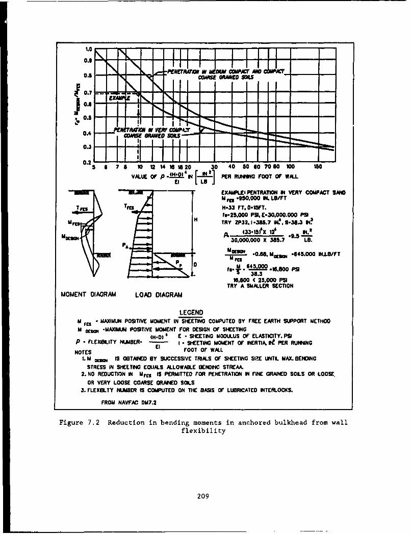
o. -l•1/1 zz~ I:IzI IaI-I
10.6 L
I "• • I-t. ME'rWr, Nv NEW CmW A,,r ANDm,,,c
0.5
0.4 Nf8a yEff ODUP4.0.4, • • A, SE ~/IEO S KS- -
0.3
V45 11 735 1012 14 0 1620 30 40 5060o70380100 IS0
VALUE Of i.(*0 IN -Ita PER RUNNING FOOT OF WALLEI L LOSj
-1111--'---1" W EXAPLE, PENTRATION IN VERY COMPACT SANDM In -950,000 I4. LO/FT
T Tm H-33 FT. 0.15FT.fI-25.000 PS. E-30.000.000 PSI
u ,H TRY ZP32, .1-385.7 IN!, 5.30.3 IN!
M N (33.15X1'I .5. t.'30,000,000 X 385.7 -'LB.
AMoMLm .0.68, M .Sn -645.000 IN.LB/FT
16,800 ( 25,000 PSITRY A SMALLER SECTION
MOMENT DIAGRAM LOAD DIAGRAM
LEGENDM - MAXIMUN POSITIVE MOMENT IN SHEETING COMPUTED BY FREE EARTH SUPPORT METHODM OEM *MAXIMUM POSITIVE MOMENT FOR DESIGN OF SHEETING
(H.D) 4 E - SHEETING MODULUS OF ELASTICITY. PSIP - FLEXIBLITY NUMMER" - I * SHEETING MOMENT OF INERTIA, iPt PER RUNNINGEl F O F W .
NOTES FOT OF WAL1. M oan IS OBTANEO BY SUCCESSIVE TRIALS OF SHEETING SIZE UNTL MAX. BENOING
STRESS IN SHEETING EQUALS ALLOWABLE BENOINC STREAA.2. NO REDUCTION IN MUn IS PERMITTED FOR PENETRATION IN FINE GRAINED SOLS OR LOOSE
OR VERY LOOSE COARSE GRAINED SOILS3. FLEXO.TY NUMBER IS COMPUTED ON THE BASIS OF LUBRICATED INTERLOCKS.
FROM NAVFAC DM7.2
Figure 7.2 Reduction in bending moments in anchored bulkhead from wallflexibility
209
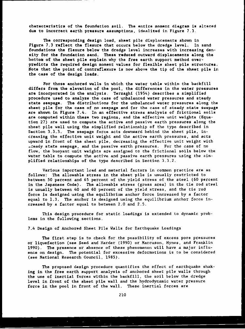
characteristics of the foundation soil. The entire moment diagram is altereddue to incorrect earth pressure assumptions, idealized in Figure 7.3.
The corresponding design load, sheet pile displacements shown inFigure 7.3 reflect the flexure that occurs below the dredge level. In sandfoundations the flexure below the dredge level increases with increasing den-sity for the foundation sand. These reduced outward displacements along thebottom of the sheet pile explain why the free earth support method over-predicts the required design moment values for flexible sheet pile structures.Note that the point of contraflexure is now above the tip of the sheet pile inthe case of the design loads.
For those anchored walls in which the water table within the backfilldiffers from the elevation of the pool, the differences in the water pressuresare incorporated in the analysis. Terzaghi (1954) describes a simplifiedprocedure used to analyze the case of unbalanced water pressures and steadystate seepage. The distributions for the unbalanced water pressures along thesheet pile for the case of no seepage and for the case of steady state seepageare shown in Figure 7.4. In an effective stress analysis of frictional soilsare computed within these two regions, and the effective unit weights (Equa-tion 27) are used to compute the active and passive earth pressures along thesheet pile wall using the simplified relationship of the type described inSection 3.3.3. The seepage force acts downward behind the sheet pile, in-creasing the effective unit weight and the active earth pressures, and actsupward in front of the sheet pile, decreasing the effective unit weight with.'eady state seepage, and the passive earth pressures. For the case of noflow, the buoyant unit weights are assigned to the frictional soils below thewater table to compute the active and passive earth pressures using the sim-plified relationships of the type described in Section 3.3.2.
Various important lead and material factors in common practice are asfollows: The allowable stress in the sheet pile is usually restricted tobetween 50 percent and 65 percent of the yield stress of the steel (60 percentin the Japanese Code). The allowable stress (gross area) in the tie rod steelis usually between 40 and 60 percent of the yield stress, and the tie rodforce is designed using the equilibrium anchor force increased by a factorequal to 1.3. The anchor is designed using the equilibrium anchor force in-creased by a factor equal to between 2.0 and 2.5.
This design procedure for static loadings is extended to dynamic prob-lems in the following sections.
7.4 Design of Anchored Sheet Pile Walls for Earthquake Loadings
The first step is to check for the possibility of excess pore pressuresor liquefaction (see Seed and Harder (1990) or Marcuson, Hynes, and Franklin1990). The presence or absence of these phenomenon will have a major influ-ence on design. The potential for excessive deformations is to be considered(see National Research Council, 1985).
The proposed design procedure quantifies the effect of earthquake shak-ing in the free earth support analysis of anchored sheet pile walls throughthe use of inertial forces within the backfill, the soil below the dredgelevel in front of the sheet pile wall and the hydrodynamic water pressureforce in the pool in front of the wall. These inertial forces are
210
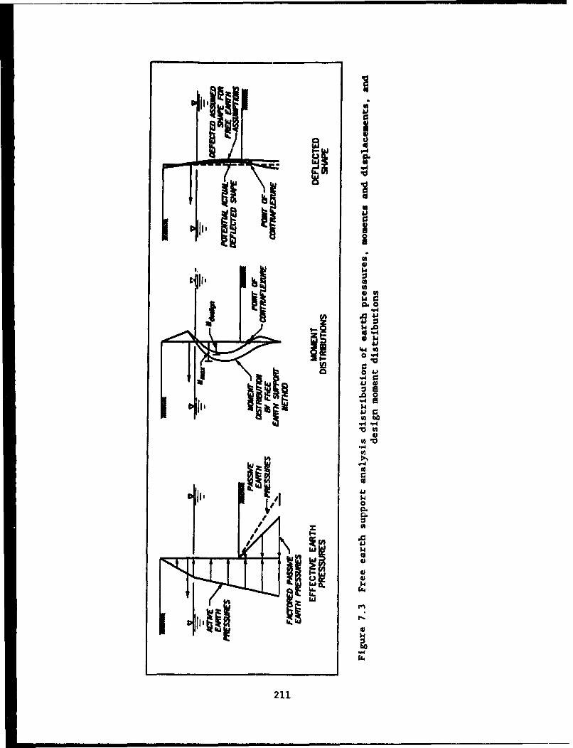
ad0
44 0
.0 0"4'
LAJl,f 0
II" II!I a211
__ __ _ __ _ __ ii
NO FLOW FLOW NET
WHU YVYwHu
HU H
"BOTOMu OF WAL BOTTOM OF WALL
(a). NET WATER PRESSURE (b). NET WATER PRESSUREWITHOUT SZEPAGE WITH SEEPAGE
FROM TERZAGHI (1954) AND DAWK!NS (1991)
Figure 7.4 Two distributions for unbalanced water pressures
superimposed on the static forces along the sheet pile wall. Certain adjust-ments are made to the load and material factors, as is detailed in the follow-ing sections, when earthquake loads are included in the analysis.
An important design consideration is the placement of the anchor. Itshould be located far enough from the wall such that the active wedge from thewall (starting at the bottom of the wall) and the passive wedge from the
212
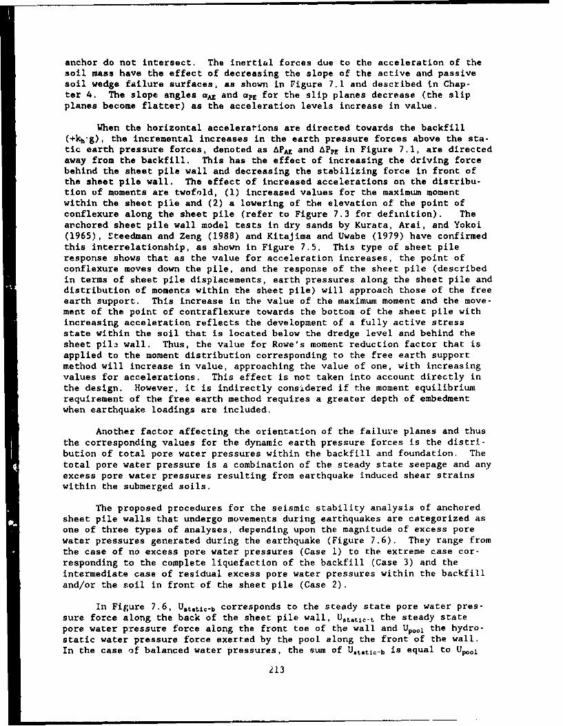
anchor do not intersect. The inertial forces due to the acceleration of thesoil mass have the effect of decreasing the slope of the active and passivesoil wedge failure surfaces, as shown in Figure 7.1 and described in Chap-ter 4. The slope angles at and OPE for the slip planes decrease (the slipplanes become flatter) as the acceleration levels increase in value.
When the horizontal accelerations are directed towards the backfill(+kh'g), the incremental increases in the earth pressure forces above the sta-tic earth pressure forces, denoted as APAE and APPE in Figure 7.1, are directedaway from the backfill. This has the effect of increasing the driving forcebehind the sheet pile wall and decreasing the stabilizing force in front ofthe sheet pile wall. The effect of increased accelerations on the distribu-tion of moments are twofold, (1) increased values for the maximum momentwithin the sheet pile and (2) a lowering of the elevation of the point ofconflexure along the sheet pile (refer to Figure 7.3 for definition). Theanchored sheet pile wall model tests in dry sands by Kurata, Arai, and Yokoi(1965), Steedman and Zeng (1988) and Kitajima and Uwabe (1979) have confirmedthis interrelationship, as shown in Figure 7.5. This type of sheet pileresponse shows that as the value for acceleration increases, the point ofconflexure moves down the pile, and the response of the sheet pile (describedin terms of sheet pile displacements, earth pressures along the sheet pile anddistribution of moments within the sheet pile) will approach those of the freeearth support. This increase in the value of the maximum moment and the move-ment of the point of contraflexure towards the bottom of the sheet pile withincreasing acceleration reflects the development of a fully active stressstate within the soil that is located below the dredge level and behind thesheet pil3 wall. Thus, the value for Rowe's moment reduction factor that isapplied to the moment distribution corresponding to the free earth supportmethod will increase in value, approaching the value of one, with increasingvalues for accelerations. This effect is not taken into account directly inthe design. However, it is indirectly considered if the moment equilibriumrequirement of the free earth method requires a greater depth of embedmentwhen earthquake loadings are included.
Another factor affecting the orientation of the failure planes and thusthe corresponding values for the dynamic earth pressure forces is the distri-bution of total pore water pressures within the backfill and foundation. Thetotal pore water pressure is a combination of the steady state seepage and anyexcess pore water pressures resulting from earthquake induced shear strainswithin the submerged soils.
The proposed procedures for the seismic stability analysis of anchoredsheet pile walls that undergo movements during earthquakes are categorized asone of three types of analyses, depending upon the magnitude of excess porewater pressures generated during the earthquake (Figure 7.6). They range fromthe case of no excess pore water pressures (Case 1) to the extreme case cor-responding to the complete liquefaction of the backfill (Case 3) and theintermediate case of residual excess pore water pressures within the backfilland/or the soil in front of the sheet pile (Case 2).
In Fig:ure 7.6, Utaticb corresponds to the steady state pore water pres-sure force along the back of the sheet pile wall, Utatic-t the steady statepore water pressure force along the front toe of the wall and Up.,, the hydro-static water pressure force exerted by the pool along the front of the wall.In the case of balanced water pressures, the sum of Utatic-b is equal to Upoo
213
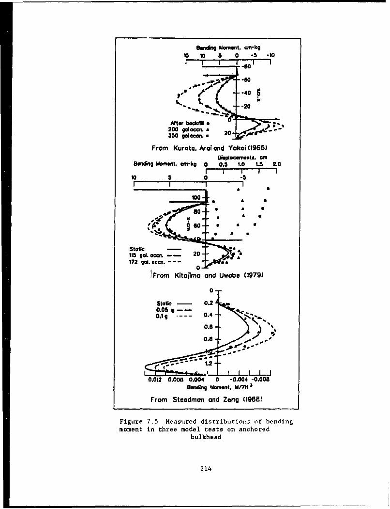
Bending Moment. cm-kg15 10 5 0 -5 -10
-60
,. , +,o-40
-- 20
Nter backfll e200 tIdIOI am0 ~350 gal a:c2. 0
From Kurato, Arla and Yokoi (1965)
Oilulacements, anBending Moment, cm-kg 0 0.5 1.0 1.5 2.0
I I I I 110 5 0 -5
S" •10=0
Static -
113 gal. cc:n. 20172 gal. O¢€:n. - &
0
From Kitojimo and Uwobe (1979)
0-
Static - 0.20.05 g--O.lg ....- 0.4-
0.6 d)0.6 - +*
0.8- a
0.012 0.00. 0.004 0 -0.004 -0.008Bending Moment. M/M 3
From Steedman and Zeng (19855
Figure 7.5 Measured distributions• of bendingmoment in three model tests on anchored
bulkhead
214
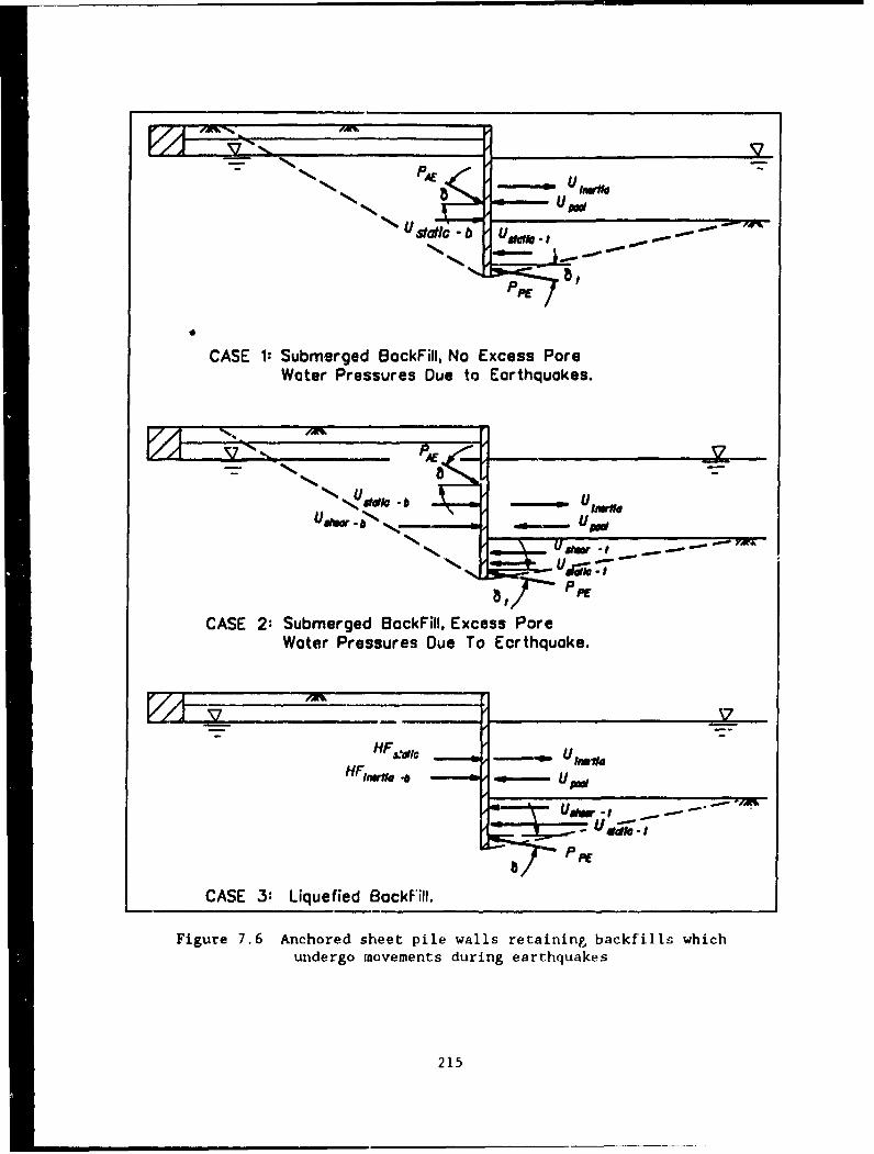
- U
st ti _b U•* ..
PPE0ý".lE
CASE 1: Submerged BackFill, No Excess PoreWater Pressures Due to Earthquakes.
N0 8qx_~ PE 3
CASE 2: Submerged BackFill, Excess PoreWater Pressures Due To Earthquake.
HFe.atk ---- o ---- Uto p
SArd - 1
CASE 3: Liquefied BackFill.
Figure 7.6 Anchored sheet pile walls retaining backfills whichundergo movements during earthquakes
215
and Ustatic-t. Uin.rtis corresponds to the hydrodynamic water pressure forcealong the front of the wall due to earthquake shaking of the pool. Ush.hr-band Uihear-t correspond to the excess pore water pressure force acting alongthe back of the wall and along the front of the wall (Case 2). In the case ofa liquified backfill, HF.tatiL 'ind HFin.rti..b ara equal to the equivalent heavyfluid hydrostatic pressure of the liquified backfill and the inertia force dueto the acceleration of a liquified backfill,
An anchored sheet pile wall cannot be designed to retain a liquifiedbackfill. and foundation, and hence Case 3 is only of academic interest, Siteimprovement techniques (the National Research Council 1985) or the use ofalternative structures should be investigated in this situation. A proced, refor determining the potential for liquefaction within the submerged backfillor the potential for the development of excess pore water pressures is dis-cussed in numerous articles, including the National Research Council t1995),Seed, Tokimatsu, Harder, and Chung (1985), Seed and Harder (1990) or Marcuson,Hynes, and Franklin (1990). The design procedure (Section 7.4.2) is limitedto the case where excess pore water pressures are less than 30 percent of theinitial vertical effective stress.
Flexure of the Sheet Pile Wall Below the Dredge Level:
Justification of the use of Rowe's moment reduction factor values,obtained from static tests (Rowe 1952) on dynamic problems, is empirical. Thedamage surveys of anchored sheet pile walls that failed due to earthquakeshaking listed one sheet pile wall that exhibited a general flexural failure(Section 7.2.1). The structural failure of this wall, designed using theJapanese Code, was attributed to corrosion at the dredge level. The JapaneseCode uses the Rowe's reduction factor values to reduce the maximum free earthsupport moment in the design of the sheet pile section, thus relying onflexure of the sheet pile wall below the dredge level during earthquake shak-ing. Flexure of the sheet pile below the dredge level is caused by severalfactors, including the depth of penetration and flexural stiffness of thesheet pile wall and the strength and compressibility of the soil (Rowe 1952,1956, and 1957, Tschebotarioff 1973). In Rowe's procedure, the dependence ofthe value of rd on the soil type incorporates the dependence of the level ofmoment reduction on the compressibility and strength of the soil as well asthe magnitude and distribution of sheet pile displacements below the dredgelevel.
The ability of the system to develop flexure below the dredge levelduring earthquake shaking must be carefully evaluated prior to application ofRowe's moment reduction factor or any portion of the reduction factor. Thisis especially true when analyzing the seismic stability of an existing sheetpile wall founded in a contractive soil. A sheet pile wall founded in densegranular soils is far more likely to develop flexure below the dredge levelduring earthquake shaking than one founded in loose soils. Dense soils thatdilate during shearing are far less susceptible to large displacements duringearthquake shaking than are loose soilr (Seed, 1987 and Seed, Tokimatsu,Harder, and Chung, 1985). Loose soils contract during shearing and are sus-ceptible to large displacements and even flow failures caused by earthquakeshaking (National Research Council, 1985, and Whitman, 1985). As a generaldesign principle, anchored sheet pile walls sited in seismic environmentsshould be founded in dense and dilative cohesionless soils with no silt orclay site particles.
216
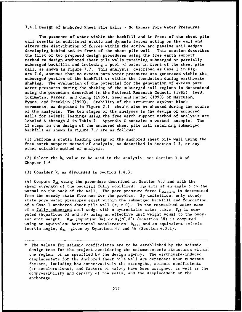
7.4.1 Design of Anchored Sheet Pile Walls - No Excess Pore Water Pressures
The presence of water within the backfill and in front of the sheet pilewall results in additional static and dynamic forces acting on the wall andalters the distribution of forces within the active and passive soil wedgesdeveloping behind and in front of the sheet pile wall. This section describesthe first of twc proposed design procedures using the free earth supportmethod to design anchored sheet pile walls retaining submerged or partiallysubmerged backfills and including a pool of water in front of the sheet pilewall, as shown in Figure 7.7. This analysis, described as Case 1 in Fig-ure 7.6, assumes that no excess pore water pressures are generated within thesubmerged portion of the backfill or within the foundation during earthquakeshaking. The evaluation of the potential for the generation of excess porewater pressures during the shaking of the subnmerged soil regions is determinedusing the procedure described In the National Research Council (1985), Seed,Tokimatsu, Harder, and Chung (1985), Seed and Harder (1990) or Marcuson,Hynes, and Franklin (1990). Stability of the structure against blockmovements, as depicted in Figure 2.1, should also be checked during the courseof the analysis. The ten stages of the analyses in the design of anchoredwalls for seismic loadings using the free earth support method of analysis arelabeled A through J in Table 7. Appendix C contains a worked example. The13 steps in the design of the anchored sheet pile wall retaining submergedbackfill as shown in Figure 7.7 are as follows:
(1) Perform a static loading design of the anchored sheet pile wall using thefree earth support method of analysis, as described in Section 7.3, or anyother suitable method of analysis.
(2) Select the kh value to be used in the analysis; see Section 1.4 ofChapter ].*
(3) Consider k, as discussed in Section 1.4.3.
(4) Compute PAE using the procedure described in Section 4.3 and with theshear strength of the backfill fully mobilized. PAE acts at an angle 6 to thenormal to the back of the wall. The pore pressure force Utatic~b is determinedfrom the steady state flow net for the problem. By definition, only steadystate pore water pressures exist within the submerged backfill and foundationof a Case 1 anchored sheet pile wall (ru - 0). In the restrained water caseof a fully submerge.d soil wedge with a hydrostatic water table, PAE is com-puted (Equations 33 and 38) using an effective unit weight equal to the buoy-ant unit we).ght. KA (Equation 34) or KA(p*,O*) (Equation 38) is computedusing an equivalent horizontal acceleration, kh.1, and an equivalent seismicinertia angle, 0.1, given by Equations 47 and 46 (Section 4.3.1).
* The values for seismic coefficients are to be established by the seismicdesign team for the project considering the seismotectonic structures withinthe region, or as specified by the design agency. The earthquake-induceddisplacements for the anchored sheet pile wall are dependent upon numerousfactors, including how conservatively the strengths, seismic coefficients(or accelerations), and factors of safety have been assigned, as well as thecompressibility and density of the soils, and the displacement at theanchorage.
217
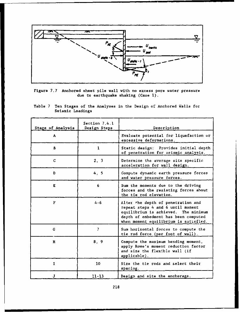
nIPA UN -
-:' 4 11-"
Figure 7.7 Anchored sheet pile wall with no excess pore water pressuredue to earthquake shaking (Case 1).
Table 7 Ten Stages of the Analyses in the Design of Anchored Walls forSeismic Loadings
Section 7.4.1Stage of Analysis Design Steps Description
A Evaluate potential for liquefaction orexcessive deformations.
B 1 Static design: Provides initial depth_...._ of penetration for seismic analysis.
C 2, 3 Determine the average site specificacceleration for wall design.
D 4, 5 Compute dynamic earth pressure forcesand water pressure forces.
E 6 Sum the moments due to the drivingforces and the resisting forces aboutthe tie rod elevation.
F 4-6 Alter the depth of penetration andrepeat steps 4 and 6 until momentequilibrium is achieved. The minimumdepth of embedment has been computed
_ ........ _ _ when moment equilibrium is satisfied.
C 7 Sum horizontal forces to compute thetie rod force (per foot of wall).
H 8, 9 Compute the maximum bending moment,apply Rowe's moment reduction factorand size the flexible wall (if
____applicable).
1 10 Size the tie rods and select theirspacing.
J 11-13 Design and site the anchorage.
218
In the case of a Dartially submerged bAckfill, this simplifiedprocedure will provide approximate results by increasing the valueassigned to the effective unit weight, 7,, based upon the proportion ofthe soil wedge that is above and below the water table (see Figure 4.13in Section 4.3.3). PA is computed (Equations 33 and 38) with 7t replacedby -y, KA (Equation 34) or KA(fi*,e*) (Equation 38) is computed using anequivalent horizontal acceleration, kh.1, and an equivalent seismicinertia angle, 0.1, given by Equations and 46 in Section 4.3.1 with 1breplaced by 7.. A more refined analysis may be conducted using the trialwedge procedure (Appendix A) for the forces shown in Figure 7.7.
To compute the point of action of PA in the case of a partially sub-merged backfill, redefine PA in terms of the static force, PA, and thedynamic active earth pressure increment, APA, using Equation 40. Thisprocedure is demonstrated in Figure 7.8. First compute KA and the staticeffective earth pressure distribution along the back of sheet pile wallusing one of the procedures described in Chapter 3. PA is equal to theresultant force for this static effective stress distribution along theback of the wall, which also provides for the point of action for PA.Solve for the force APA as equal to the difference between PA and PA.Assume that APA acts at a height equal to 0.6'H above the base of thesheet pile. Compute the point of action of force PAE using Equation 44and correcting this relationship for the new locations along the back ofthe sheet pile for the forces PA and APA (refer to Example 19).
(5) Compute PpE acting in front of the sheet pile using the proceduredescribed in Section 4.4 (Chapter 4) and using a factor of safety, FSp,applied to both thi shear strength of the soil and the effective angle offriction along the interface. 6 equal to 0'/2 (Section 3.3.1) is areasonable value for dense frictional soils. In a static free earth sup-port method of analysis, FSp is set equal to 1.5, and in a dynamic earthpressure analysis, the minimum value assigned to FSp is 1.2. Usttj,-, isdetermined from the steady state flow net for the problem. By defini-tion, only steady state pore water pressures exist within the submergedbackfill and foundation of a Case I anchored sheet pile
tanot - tano' (95)
and
tan6t tan6 (96)
wall (ru - 0). In the restrained water case of a fully submerged soilwedge with a hydrostatic water table, PpE is computed (Equations 58 and62) using an effective unit weight equal to the buoyant unit weight. Forlow to moderate levels of earthquake shaking, assume that PPE acts at aheight equal to approximately 1/3 of the height of the soil in front ofthe sheet pile wall and at an angle 6t to the normal to the face of the
219
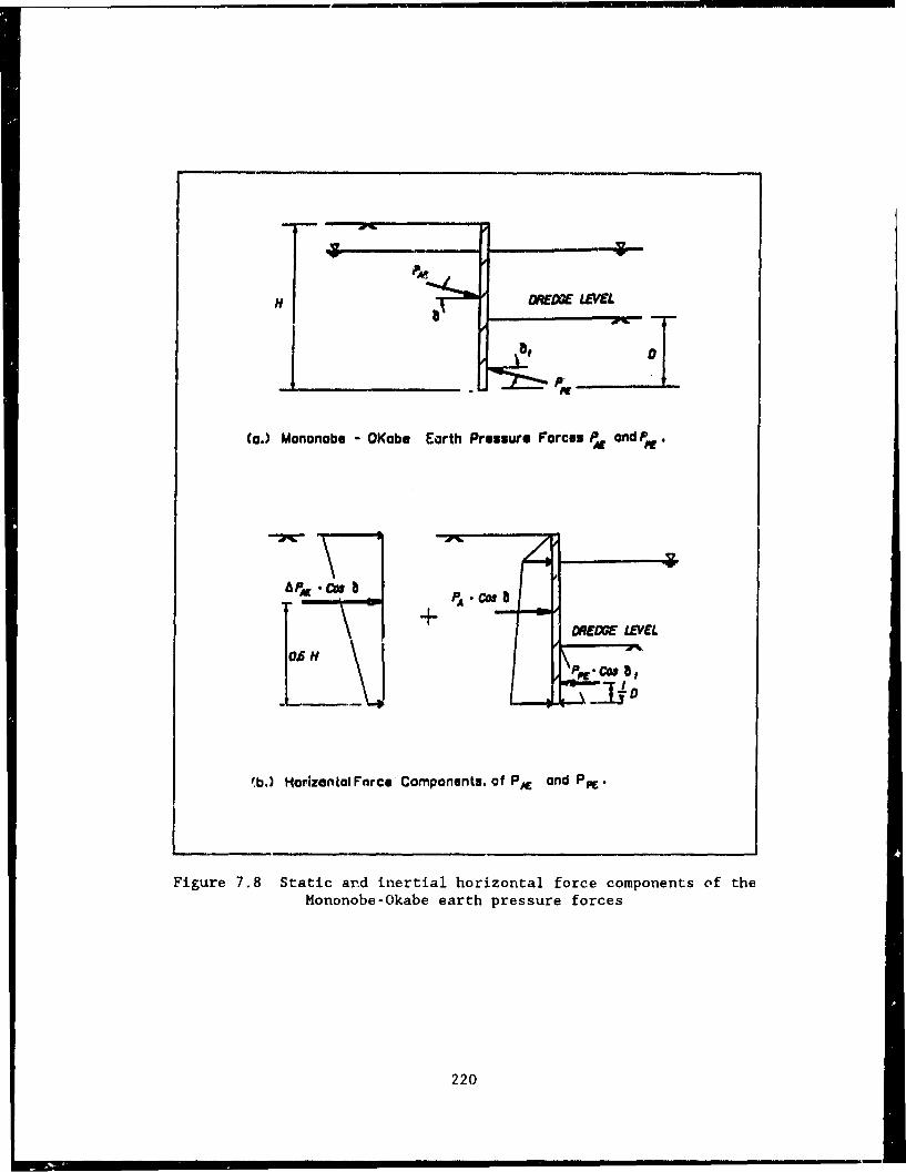
H DREXE LEVEL
a7
(a.) Mononobs - OKobe Earth Pressure Forces IN andPFE
JDMR~ELDE LEVEL
j 3D
'b.) Horizontal Farce Components. of PK and PK.
Figure 7.8 Static and inertial horizontal force components of theMononobe-Okabe earth pressure forces
220
wall.* Kpz (Equation 59) or Kp(•*,6*) (Equation 62) is computed using anequivalent horizontal acceleration, kh.l, and an equivalent seismic inertiaangle, 0,, given by Equations 47 and 46. In the case of a steady stateseepage, this simplified procedure will provide approximate results bydecreasing the value assigned to the effective unit woight (Equation 27)according to the magnitude of the upward seepage gradient (Equation 26).
Equation 59 for KpE is restricted to cases where the value of 0 (Equa-tion 95) is greater than 0.1 (Equation 46). This limiting case may occur incases of high accelerations and/or low shear strengths. One contributingfactor is the submergence of the soil in front of the anchored wall, whichapproximately doubles the value of the equivalent seismic inertia angle overthe corresponding dry soil case.
(6) To determine the minimum required depth of sheet pile penetration, theclockwise and counterclockwise moments of the resultant earth pressure forcesand resultant water pressure forces about Figure 7.7 anchor are computed asfollows:
Counterclockwise Moment 0 PACOS 6 b.(Y, - YAE) + Utaic-b'(Ya - Yub)(97)
+ Uinertia" (Ya - Yi)
and
Clockwise Moment = - I ,.(Y. - Yup) - PpE'C°S 6 t'(Ya - YPE)
(98)
- Ustatic-t" (Y. - YU0
In a static design by the free earth support method of analysis, atriangular earth pressure is assumed along the front of the wall, with theresulting force Pp assigned to the lower third point. Experience has shownthat reasonable static designs resulted when the appropriate strengthparameters and adequate factors of safety were used in conjunction with thissimplified assumption. A similar approach is used in the dynamic design.The point of application of PPE may move downward from its static point ofapplication for anchored sheet pile walls as the value for kh increases.However, no satisfactory procedure was found for computing the point ofapplication of PPE for this structure. In the interim, the assumption of PPEacting at approximately 1/3 of the height of the soil in front of the wallis restricted to low to moderate levels of earthquake shaking (e.g. onerough index is kh < 0.1) and with conservative assumptions regarding allparameters used in the analysis. For higher levels of shaking and lessconservative assumptions for parameters, a larger value for FSp than 1.2and/or a lower point of application would be assigned.
221
where6b - effective angle of friction along the backfill to sheet pile wall
interface6t - effective angle of friction along the toe foundation to sheet pile
wall interfaceUutatio.b - resultant steady state pore water pressure force along the
back of the wallUtatjc.t - resultant steady state pore water pressure force below the
dredge level along the front of the wallUpe.1 - resultant hydrostatic water pressure force for the poolUtnertia - hydrodynamic water pressure force for the pool, directed away
from the wall (see Appendix B)Y- distance from the base of sheet pile to the anchorYAZ distance from the base of sheet pile to PAZY - distance from the base of sheet pile to Ustatia.b (from a flow net)Y- distance from the base of sheet pile to Uin.rtia (see Appendix B)Y -• distance from the base of sheet pile to Up,,.YpE distance from the base of sheet pile to Pp1Y-t distance from the base of sheet pile to U*tatic-t (from a flow net).
The value for the Clockwise Moment about Figure 7.7 anchor is compared to thevalue for the Counterclockwise Moment, resulting in the following threepossibilities:
(6a) If the value of the Clockwise Moment is equal to the value of theCounterclockwise Moment, the sheet pile wall is in moment equilibrium,and the depth of penetration below the dredge level is correct for theapplied forces.
(6b) If the value of the Clockwise Moment is greater than the value ofthe Counterclockwise Moment, the trial sheet pile embedment depth belowthe dredge level is too deep and should be reduced.
(6c) If the value of the Clockwise Moment is less than the value of theCounterclockwise Moment, the trial sheet pile embedment depth below thedredge level is shallow and should be increased.
Note that the sheet pile wall is in moment equilibrium for only one depth ofsheet pile penetration within the foundation. For those trial sheet pilepenetration depths in which moment equilibrium is not achieved, a new trialdepth of sheet pile penetration is assumed, and step 4 through step 6 arerepeated.
(7) Once the required depth of sheet pile penetration is determined in step 6,the equilibrium anchor force per foot width of wall, TFES, is computed usingthe equations for horizontal force equilibrium.
TFES " PPEcOs6t + Ustatic_+ ÷Upool - Uinertia - PAcos 6 b - Ustatic.b (99)
In some situations the value for TFES computed in a seismic analysis canbe several times the value computed in the static analysis due to the effectof the inertial forces acting on both the active and passive soil wedges andthe pool of water. Large anchor forces per foot width of wall will impact
222
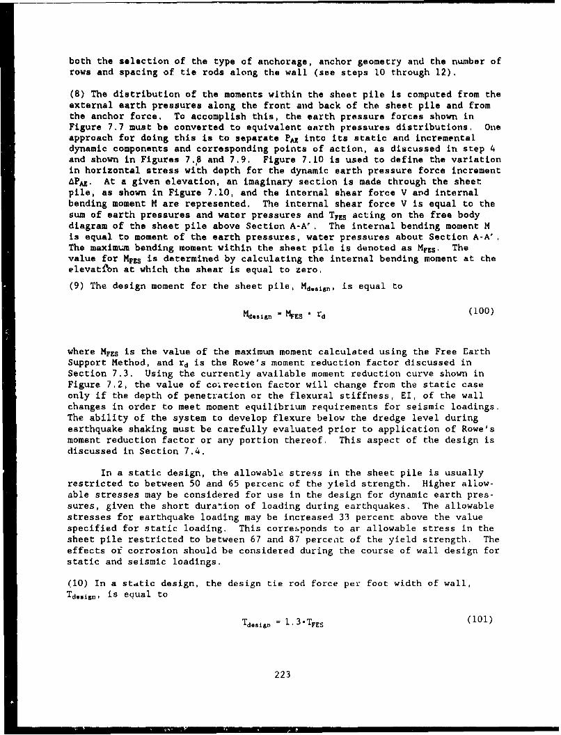
both the selection of the type of anchorage, anchor geometry and the number ofrows and spacing of tie rods along the wall (see steps 10 through 12).
(8) The distribution of the moments within the sheet pile is computed from theexternal earth pressures along the front and back of the sheet pile and fromthe anchor force. To accomplish this, the earth pressure forces shown inFigure 7.7 must be converted to equivalent earth pressures distributions. Oneapproach for doing this is to separate PA into its static and incrementaldynamic components and corresponding points of action, as discussed in step 4and shown in Figures 7.,8 and 7.9. Figure 7.10 is used to define the variationin horizontal stress with depth for the dynamic earth pressure force increment6PA. At a given elevation, an imaginary section is made through the sheetpile, as shown in Figure 7.10, and the internal shear force V and internalbending moment M are represented. The internal shear force V is equal to thesum of earth pressures and water pressures and TFZs acting on the free bodydiagram of the sheet pile above Section A-A'. The internal bending moment Mis equal to moment of the earth pressures, water pressures about Section A-A',The maximum bending moment within the sheet pile is denoted as MFES. Thevalue for MFES is determined by calculating the internal bending moment at theelevation at which the shear is equal to zero.
(9) The design moment for the sheet pile, Md,,±sn, is equal to
Mdsign - MFES rd (100)
where MFES is the value of the maximum moment calculated using the Free EarthSupport Method, and rd is the Rowe's moment reduction factor discussed inSection 7.3. Using the currently available moment reduction curve shown inFigure 7.2, the value of coirection factor will change from the static caseonly if the depth of penetration or the flexural stiffness, EI, of the wallchanges in order to meet moment equilibrium requirements for seismic loadings.The ability of the system to develop flexure below the dredge level duringearthquake shaking must be carefully evaluated prior to application of Rowe'smoment reduction factor or any portion thereof. This aspect of the design isdiscussed in Section 7.4.
In a static design, the allowable stress in the sheet pile is usuallyrestricted to between 50 and 65 percent of the yield strength. Higher allow-able stresses may be considered for use in the design for dynamic earth pres-sures, given the short duration of loading during earthquakes. The allowablestresses for earthquake loading may be increased 33 percent above the valuespecified for static loading. This corresponds to ar allowable stress in thesheet pile restricted to between 67 and 87 percent of the yield strength. Theeffects of corrosion should be considered during the course of wall design forstatic and seismic loadings.
(10) In a stdtic design, the design tie rod force per foot width of wall,Tdsissn, is equal to
TdoSigS = 1. 3 TFES (101)
223
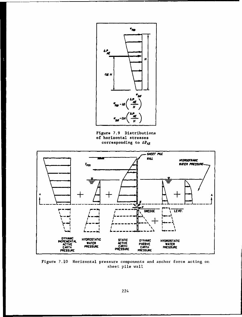
"4.
Ap
""•d H
tlAA.
IAl
- /
+/ A
f \. H
Figure 7.9 Distributionsof horizontal stresses
corresponding to •P~
L - ,-- - -_- ... 1- ... .-- E
\ -- I /
I--., - --- ....L...-- -- -- -- ,1- -)
DYNAMIC HYDROSTATIC STATIC OVNAK/C HYDROSTATIC4MCREIENTA.
ACTIVE WATER ACTIVE PASSIVE WATEREARTH PRESSURE EARTH EARTH PRESSURE
PRESSURE PRESSURE PRESSURE
Figure 7.10 Horizontal pressure components and anchor force acting onsheet pile wall
224
and the allowable stress in the tie rods is usually restricted to between 40and 60 percent of the yield strength. The factor 1.3 is also recommended forearthquake loading conditions, The Japanese code restricts the allowablestresses to 60 percent of the yield strength for earthquake loading (see thediscussion at the end of step 9). The value of 60 purcent is recommended.The eftects of corrosion should be considered during the course of wall designfor both static and seismic loadings.
(11) The design of the anchorage for seismic loadings follows the approachthat is proposed for the design of the flexible wall and differs from theapproach used when designing for static loadings. In the case of staticloads, the ultimate force (per foot width of wall) which the anchor is to bedesigned, Tult-a, is equal to
Tuft-8 " 2.5"Tr~s (102)
and the static earth pressure forcas PA and Pp on the front and back of theanchor block are computed using the ultimate shear strength with 6 - 0* forslender anchorage (refer to discussion in bection C.1.9 of Appendix C or toDismuke (1991). The proposed design procedure for seismic loadings isdescribed in steps 12 and 13. Seismic loads usually control the anchoragedesign.
(12) For those waterfront structures in which the anchor consists of a plateor a concrete block, a major contribution to the forces resisting the pullingforce Tulta is provided by the formation of a passive soil wedge in front ofthe block, as shown in Figure 7.11a. In a seismic analysis, Tult-. is setequal to TFES. The Mononobe-Okabe equations 33 and 58 are used to compute thedynamic active earth pressure force, PA, and the dynamic passive earth pres-sure force, Pp1 , acting on the anchor block during earthquake shaking(Figure 7.11b). PE is computed with the shear strength of the backfill fullymobilized and 6 - 0* for slender anchorage and 6 : 0/2 for mass concreteanchorage (Section C.1.9 of Appendix C). PPE is computed using a factor ofsafety FSp applied to the shear strength of the soil (Equation 95) and theeffective angle of friction along the interface (Equation 96). At a minimum,FSp is set equal to a value between 1.2 and 1.5, depending on the allowabledisplacement and on how conservatively the strengths and seismic coefficientshave been assigned. In general and with all parameters constant, the largerthe factor of safety, the smaller the anchorage displacement due to earthquakeshaking.
Water pressure forces are not included along the sides of the blockbecause most anchor blocks are constructed on or just above the water table,as idealized in this figure. If the water table extends abov6 the base of theblock, these forces are to be included in the analysis.
The size of the block is proportioned such that
225
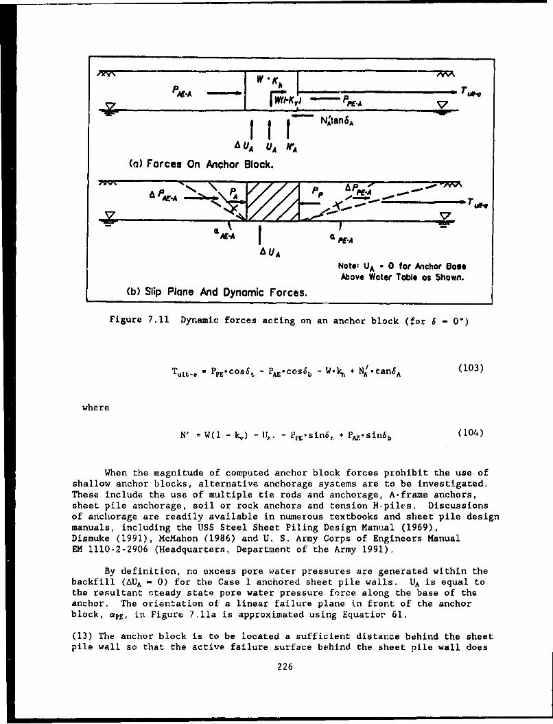
"PA&A W OKA
~UA UA N'A
(a) Forces On Anchor Block.
AL T
WA~ Pp PL-AP AE-A .!4
S-------
SA-A a. PE.A
UANotez UA • 0 for Anchor BassAbove Water Table as Shown.
(b) Slip Plane And Dynamic Forces.
Figure 7.11 Dynamic forces acting on an anchor block (for 6 - 0°)
Tult-, = PpE.cos 6 t - PAE.cos6b - W.kh + NA/otan 6 A (103)
where
N' = W(l - k,) - 1TI,. - pEsin6t, + PApeSin 6b (104)
When the magnitude of computed anchor block forces prohibit the use ofshallow anchor blocks, alternative anchorage systems are to be investigated.These include the use of multiple tie rods and anchorage, A-frame anchors,sheet pile anchorage, soil or rock anchors and tension H-piles. Discussionsof anchorage are readily available in numerous textbooks and sheet pile designmanuals, including the USS Steel Sheet Piling Design Manual (1969),Dismuke (1991), McMahon (1986) and U. S. Army Corps of Engineers ManualEM 1110-2-2906 (Headquarters, Department of the Army 1991).
By definition, no excess pore water pressures are generated within thebackfill (AUA - 0) for the Case 1 anchored sheet pile walls. UA is equal tothe resultant steady state pore water pressure force along the base of theanchor. The orientation of a linear failure plane in front of the anchorblock, apE, in Figure 7.11a is approximated using Equatior 61.
(13) The anchor block is to be located a sufficient distance behind the sheet
pile wall so that the active failure surface behind the sheet pile wall does
226
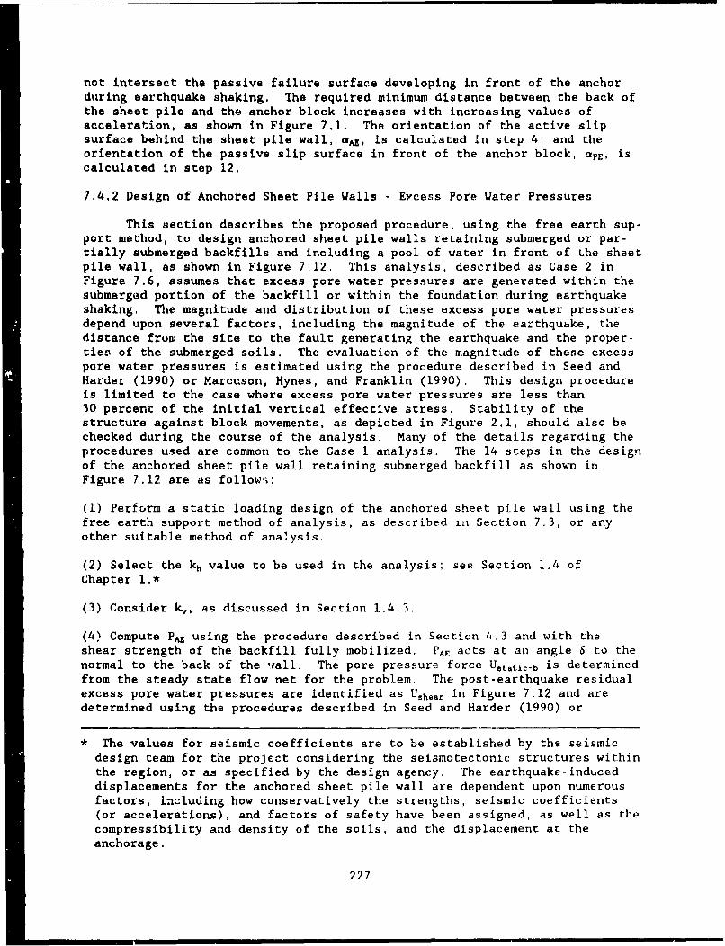
not intersect the passive failure surface developing in front of the anchorduring earthquake shaking. The required minimum distance between the back ofthe sheet pile and the anchor block increases with increasing values ofacceleration, as shown in Figure 7.1. The orientation of the active slipsurface behind the sheet pile wall, cA, is calculated in step 4, and theorientation of the passive slip surface in front of the anchor block, apE, iscalculated in step 12.
7.4.2 Design of Anchored Sheet Pile Walls Excess Pore Water Pressures
This section describes the proposed procedure, using the free earth sup-port method, to design anchored sheet pile walls retaining submerged or par-tially submerged backfills and including a pool of water in front of the sheetpile wall, as shown in Figure 7.12. This analysis, described as Case 2 inFigure 7.6, assumes that excess pore water pressures are generated within thesubmerged portion of the backfill or within the foundation during earthquakeshaking. The magnitude and distribution of these excess pore water pressuresdepend upon several factors, including the magnitude of the earthquake, thedistance frum the site to the fault generating the earthquake and the proper-ties of the submerged soils. The evaluation of the magnitude of these excesspore water pressures is estimated using the procedure described in Seed andHarder (1990) or Marcuson, Hynes, and Franklin (1990). This design procedureis limited to the case where excess pore water pressures are less than30 percent of the initial vertical effective stress. Stability of thestructure against block movements, as depicted in Figure 2.1, should also bechecked during the course of the analysis. Many of the details regarding theprocedures used are common to the Case 1 analysis. The 14 steps in the designof the anchored sheet pile wall retaining submerged backfill as shown inFigure 7.12 are as follows:
(1) Perform a static loading design of the anchored sheet pile wall using thefree earth support method of analysis, as described in Section 7.3, or anyother suitable method of analysis.
(2) Select the kh value to be used in the analysis; see Section 1.4 ofChapter l.*
(3) Consider kv, as discussed in Section 1.4.3.
(4) Compute PAE using the procedure described in Section 4.3 and with theshear strength of the backfill fully mobilized. PA acts at an angle 6 to thenormal to the back of the wall. The pore pressure force Ustatic-b is determinedfrom the steady state flow net for the problem. The post-earthquake residualexcess pore water pressures are identified as Ush.ar in Figure 7.12 and aredetermined using the procedures described in Seed and Harder (1990) or
The values for seismic coefficients are to be established by the seismicdesign team for the project considering the seismotectonic structures withinthe region, or as specified by the design agency. The earthquake-induceddisplacements for the anchored sheet pile wall are dependent upon numerousfactors, including how conservatively the strengths, seismic coefficients(or accelerations), and factors of safety have been assigned, as well as thecompressibility and density of the soils, and the displacement at theanchorage.
227
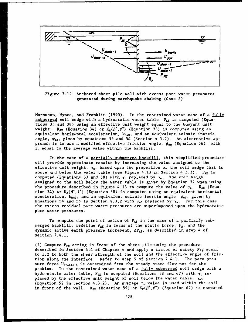
NAi II PA -- _ _
U %..~7-a b - U f
PPE
Figure 7.12 Anchored sheet pile wall with excess pore water pressuresgenerated during earthquake shaking (Case 2)
Marcuson, Hynes, and Franklin (1990). In the restrained water case of a fullysmeLqA soil wedge with a hydrostatic water table, Pr is computed (Equa-tions 33 and 38) using an effective unit weight equal to the buoyant unitweight. KA (Equation 34) or KA(P*,8*) (Equ.-tion 38) is computed using anequivalent horizuntal acceleration, kh.3, and an equivalent seismic inertiaangle, 0.3, given by equations 55 and 54 (Section 4.3.2). An alternative ap-proach is to use a modified effective friction angle. O.q (Equation 56), withr, equal to the average value within the backfill.
In the case of a partially submerged backfill, this simplified procedurewill provide approximate results by increasing the value assigned to theeffective unit weight, I., based upon the proportion of the soil wedge that isabove and below the water table (see Figure 4.13 in Section 4.3.3). PA iscomputed (Equations 33 and 38) with It replaced by 7.. The unit weighLassigned to the soil below the water table is given by Equation 59 when usingthe procedure described in Figure 4.13 to compute the value of 7,. KA (Equa-tion 34) or KA(p*,e*) (Equation 38) is computed using an equivalent horizontalacceleration, kh.3, and an equivalent seismic inertia angle, 0.3, given byEquations 54 and 55 in Section 4.3.2 with 7.3 replaced by I.. For this case,the excess residual pore water pressures are superimposed upon the hydrostaticpore water pressures.
To compute the point of action of PA in the case of a partially sub-merged backfill, redefine PAE in terms of the static force, PA, and thedynamic active earth pressure increment, APAF, as described in step 4 ofSection 7.4.1.
(5) Compute PFE acting in front of the sheet pile usiung the proceduredescribed in Section 4.4 of Chapter 4 and apply a factor of safety FSp equalto 1.2 to both the shear strength of the soil and the effective angle of fric-tion along the interface. Refer to step 5 of Section 7,4.1. The pore pres-sure force Ust.tc-t is determined from the steady state flow net for theproblem. In the restrained water case of a fully submerged soil wedge with ahydrostatic water table, PPE is computed (Equations 58 and 62) with It re-placed by the effective unit weight of soil below the water table, 1.3
(Equation 52 in Section 4.3.2). An average ru value is used within the soilin front of the wall. KPE (Equation 59) or Kp(,8*,O*) (Equation 62) is computed
228
using an equivalent horizontal acceleration, kh.3, and an e1i''-aLeut seismicinertia angle, 0.3, given by Equations 54 and 55 in Section 4.3.2. In thecase of a steady state seepage, this simplified procedure will provide approx-imate results by decreasing the value assigned to the effective unit weight(Equation 27) according to the magnitude of the upward seepr,, gradient (Equa-tion 26). For low to moderate levels of earthquake shaking, assume that PPEacts at a height equal to approximately 1/3 of the height of the soil in frontof the sheet pile wall and at an angle St to the normal to the face of thewall.*
(6) To determine the required depth of sheet pile penetration, the clockwiseand counterclockwise moments of the resultant earth pressure forces and resul-tant water pressure foi-ces about Figure 7.12 anchor are computed as follows:
Counterclockwise Moment PAEcos6b. (Y. - YA.) + Ustatic-b" (Ya - Yub)
(105)
+ Ushear-b* (Ya - Yutaub) + Uinertia* (Ya - Yi)
and
Clockwise Moment - - Upoo* (Ya - Yup) - PpE-cOs 6t" (Ya - YPE)
(106)
- Ustatic-to (Y. - Yut) - Ushear-t" (Ya - Yutaut)
where
Ushear-b - resultant excess pore water pressure force along the back ofthe wall
1Tshoer-t - resultant excess pore water pressure force below the dredgelevel along the front of the wall
Yut.,, - distance from the base of sheet pile to Ushear-bYutaut - distance from the base of sheet pile to Ushear.t
Values for Yuta~uj, Uh.,ar-b, Yutaut and Ushear.t are computed using the proceduredescribed in Seed and Harder (1990) or Marcuson, Hynes, and Franklin (1990).
In a static design by the free earth support method of analysis, atriangular earth pressure is assumed along the front of the wall, with theresulting force Pp assigned to the lower third point. Experience has shownthat reasonable static designs resulted when the appropriate strengthparameters and adequate factors of safety were used in conjunction with thissimplified assumption. A similar approach is used in the dynamic design.The point of application of PpE may move downward from its static point ofapplication for anchored sheet pile walls as the value for kh increases.However, no satisfactory procedure was found for computing the point ofapplication of Ppr for this structure. In the interim, the assumption of PPEacting at approximately 1/3 of the height of the sail in front of the wallis restricted to low to moderate lt.vels of earthquake shaking (e.g. onerough index is kh < 0.1) and with conservative assumptions regarding allparameters used in the analysis. For higher levels of shaking and lessconservative assumptions for parameters, a larger value for FSp than 1.2and/or a lower point of application would be assigned.
229
The value for the Clockwise Moment is compared to the value for the Counter-clockwise Moment, resulting in one of three possibilities listed in steps 6athrough step 6c in Section 7.4.1. The sheet pile wall is in moment equili-brium for only one depth of sheet pile penetration within the foundation. Forthose trial sheet pile penetration depths in which moment equilibrium is notachieved, a new trial depth of sheet pile penetration is assumed, and step 4through step 6 is repeated.
(7) Once the required depth of sheet pile penetration is determined in step 6,the equilibrium anchor force per foot width of wall, TFES, is computed usingthe equations for horizontal force equilibrium.
TFES - PPECOS 6 t + I5tatic-t + Ushear-t + Upool(107)
- Uinertia - PE cos 6b - Ustatic-b - Uuheor-b
Additional commentary is provided in step 7 of Section 7.4.1.
(8) The distribution of the moments within the sheet pile, MFES, is computedusing the procedure described in step 8 of Section 7.4.1.
(9) The computation of the design moment for the sheet pile, Mdesign, isdescribed in step 9 of Section 7.4.1.
(10) The design tie rod force, Td.5 ign, is computed using the proceduredescribed in step 10 of Section 7.4.1.
(11) Thc design of the anchor block for seismic loadings differs from theapproach used when designing for static loadings. The reader is referred tothe discussion in step 11 of Section 7.4.1.
(12) For those waterfront structures in which the anchor consists of slenderanchorage or mass concrete anchorage, a major contribution to the forces re-sisting the pulling force TuIt-.a Is provided by the formation of a passive soilwedge in front of the block, as shown in Figure 7.11a. The procedure de-scribed in step 12 of Section 7.4.1 is used to compute PA, PPE, and apE(Figure 7.11b). The size of the block is proportioned using Equation 103relationship, where N' is equal to
N' - W( - kv) - UA - AUA. - PPE.sin 6 t + PA.sin6b (108)
The excess pore water pressure force along the base of the block is equal toAUA (sce Seed and Harder (1990) or Marcuson, L:ynes, and Franklin (1990)).
An alternative procedure for incorporating residual excess pore water pres-sures in the analysis is by using r, and an equivalent angle of interfacefriction along the base of block, 6A.
tan6A.q - (1 - rU)tan6A (109)
In this case, the value for N' in Equation 103 is given by
230
N' - W(l - k,) - UA. - PpE.sind, + PAE5sInb (110)
Reducing the effective stress friction angle along the soil to concrete inter-face so as to account for the excess pore water pressures is not an exactprocedure (see discussion in Section 4.3.2).
(13) The required minimum distance between the back of the sheet pile and theanchor block is computed following the procedure described in step 13 ofSection 7.4.1.
(14) The residual excess pore water pressures within the submerged backfilland foundation will be redistzibuted after earthquake shaking has ended. Thepost earthquake static stability (kh and k, equal to zero) of any earthretaining structure should be evaluated during the redistribution of theexcess pore water pressures within the soil regions (see discussions in theNational Research Council 1985 or Seed 1987).
7.5 Use of Finite Element Analyses
Finite element analyses should be considered only if: (a) the costimplications of the simplified design procedures indicate that more detailedstudy is warranted, (b) it is necessary to evaluate permanent displacementsthat might result from the design seismic event, or (c) there is concern aboutthe influence of surface loadings. It is particularly difficult to model wellthe various features of an anchored wall, especially when there is concernabout excess pore pressures. One example of a detailed analysis of an actualfailure is given by iai and Kameoka (1991).
231
CHAPTER 8 ANALYSIS AND DESIGN OF WALLS RETAINING NONYIELDING BACKFILLS
8.1 Introduction
This chapter applies to design problems in which the allowable movementof a wall is small - less than one-fourth to one-half of Table 1 wall movementvalues. Typical situations include the walls of U-shaped structures such asdry docks, walls of basements, and the lateral walls of underground struc-tures. Under these conditions it may be inappropriate to base design uponearth pressures computed using the Mononobe-Okabe theory, which assumes thatactive stress conditions are achieved. Hence, earth pressures generallyshould be computed using the theory set forth in Chapter 5.
Design criteria for such situations will involve permissible combinedstatic plus dynamic bending stresses within the wall. In many cases it may benecessary to ensure that such moments do not cause yielding of the materialcomposing the wall. If the wall is free-standing, then avoidance of slidingor overturning will be design criteria.
In many cases it may be appropriate to use Wood's simplified theory tocompute the dynamic increment of stresses. In this case, a key decision willbe the choice of the horizontal acceleration coefficient kh. Important con-siderations are:
* If displacement of the wall is not permissible, the assigned peakacceleration coefficient should be used. Use of a seismic coefficient lessthan the peak acceleration coefficient implies that some displacement of thebackfill is acceptable during the design earthquake event.
* The acceleration at ground surface should be used to define kh. Thisis a conservative assumption. If the peak acceleration varies significantlyover the height of the backfill, which may often be the situation when thehigh side walls of dry docks are involved, consideration should be givento the use of dynamic finite element studies (see Appendix D).
Use of finite element studies should also be considered when there are impor-tant surface loadings. In many cases an elastic analysis using soil moduliand damping adjusted for expected levels of strain will suffice.
There may be cases in which it is overly conservative to design struc-tures using lateral pressures from the theory far walls retaining nonyieldingbackfills. If the structure is founded upon soil with the same stiffnesz asthe backfill (see Figure 8.1), the structure itself will experience movementsthat may be sufficient to develop active stress conditions. Finite elementstudies, and measurements as large scale field models in Taiwan (Chang et al.1990), have showrn this to be the case. However, in such situations, it wouldseem that larger, passive-type stresses should develop on the opposite wall.If there are large cost implications for design using stresses computed ass~un-ing nonyielding backfills, finite element studies should again be considered.
If liquefaction is of concern, methods for evaluating residual porepressures may be found in Seed and Harder (i990) or Marcuson, Hynes, andFranklin (1990). In princinle it is possible to design walls to resist thepressures from full, liquetied soil, including Westergaard's dynainic pressure
233
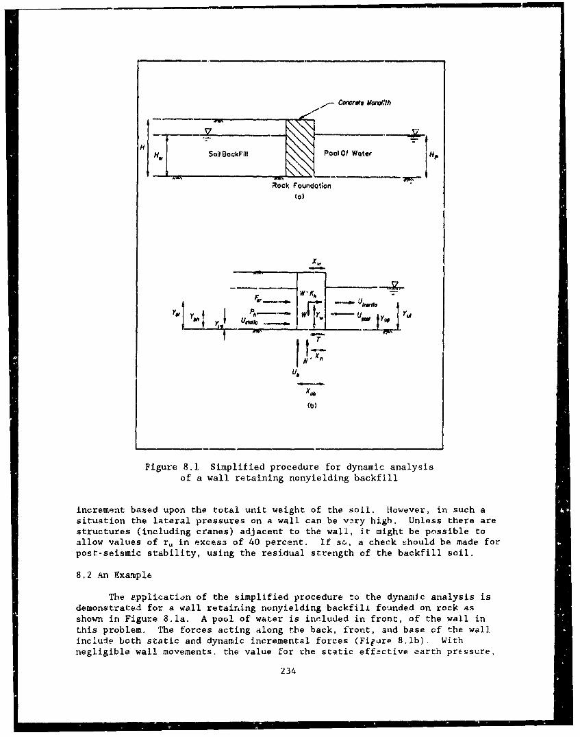
Cocrde Alowvith
H Soii BackFill Pool 1 WateHp
Rock Foundation
(o)
xI v
F, W--;
SU b )
Figure 8.1. Simplified procedure for dynamic analysisof a wall retaining nonyielding backfill
increment based upon the total unit weight of the soil. However, in such asituation the lateral pressures on a wall can be v~ry high. Unless there arestructures (including cranes) adjacent to the wall, it might be possible toallow values of r, in excess of 40 percent. If so, a check should be made forpost-seismic stability, using the residual strength of the backfill soil.
8.2 An Example
The epplication of the simplified procedure to the dynamic analysis isdemonstrated for a wall retaining nonyielding backfill founded on rock asshown in Figure 8.1a. A pool of water is included in front, of the wall inthis problem. The forces acting along the back, front, and base cf the wallinclude both static and dynamic incremental forces (Figure 8.lb). Withnegligible wall movements, the value for uhe static effective earth pressure,
234
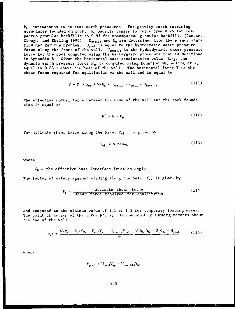
Ph, corresponds to at-rest earth pressures. For gravity earth retainingstrurtures founded on rock, K, usually ranges in value from 0.45 for com-pacted granular backfilll to 0.55 for uncompacted granulac backfills (Duncan,Clnugh, and Ebeling 1990). UI3~tjt and Uk, are determined from the steady state
flow net for tL.e problem. Up,,. is equal to the hydrostatic water pressurefor~e along the front of the wall, Uinertia is the hydrodynamic water pressureforce for the pool computed using the Westergaard procedure that is describedin Appendix B. Given the horizontal base acceleration value, k1 hg, thedynamic earth pressure force F., is computed using Equation 68, acting at Y.,equal to 0.63,H above the base of the wall. The horizontal force T is theshear force required for equilibrium of the wall and is equal to
T - PI, + F.r + W .kh + U~t,.ti. - Up.., + Ujn.rtj.. (111)
The effective normal foice between the base of the wall and the rock founda-t.on is equal to
NI - W - Ub. (112)
Th.i ultimate shear force along the base, Tuft, is given by
Tuft - N'tan6b (113)
where
6 b - the effective base interface friction angle.
The factor of safety against sliding along the base, F5 , is given by
F ultimate shear force
Fs ear force req,_iired foFiejuilibr um
and comparer to the minimum value of 1.1 or 1.2 for temporary loading cases.The point of acticn of the force N', xN,, is computed by summing moments aboutthe toe of the wall.
W.v- - Ph'YP) - FSr-yer - U ~taticYust - W'kh'Yw - UbXub + MVoo1 (115)
where
Mpooi = UpoolYup -UinertiaYui
235
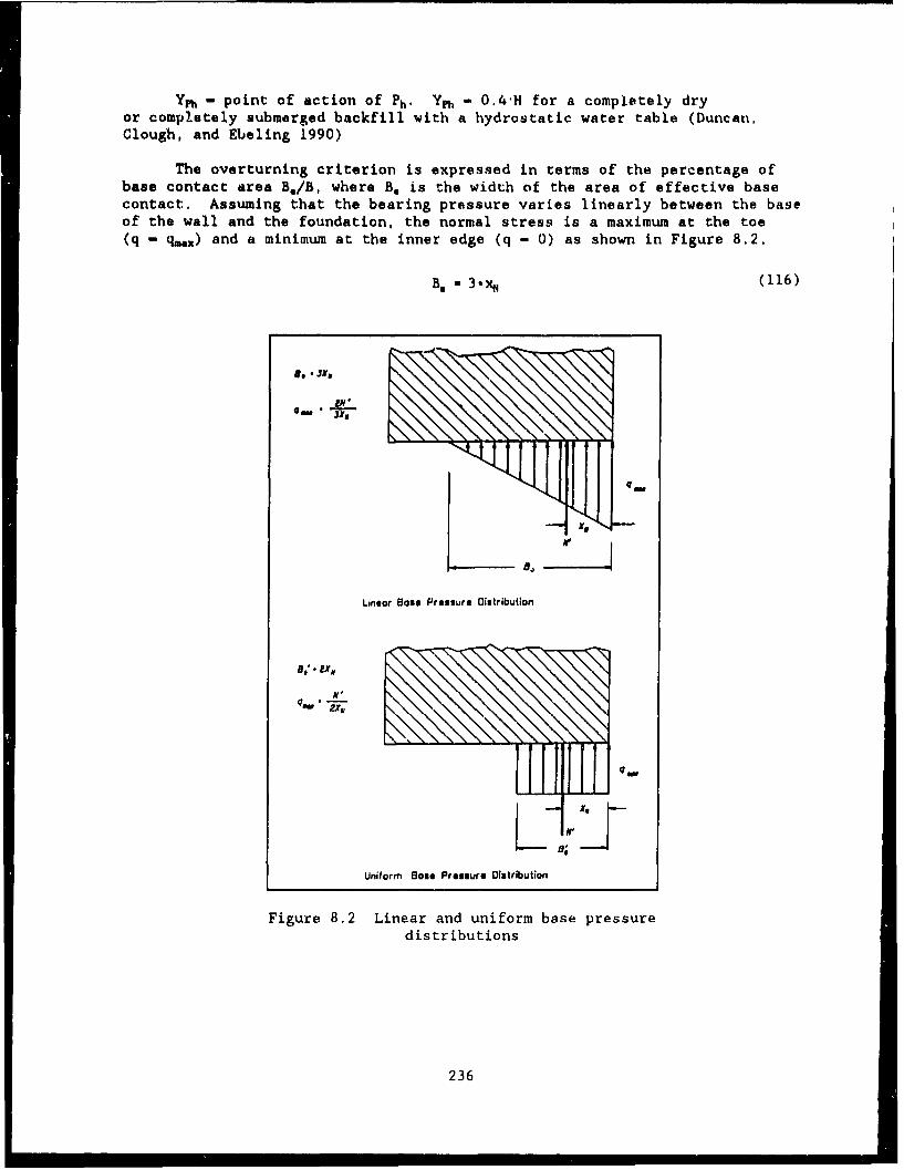
Yp - point of action of Ph- Yph - 0.4-H for a completely dryor completely submerged backfill with a hydrostatic water table (Duncan,Clough, and Ebeling 1990)
The overturning criterion is expressed in terms of the percentage ofbase contact area B,/B, where Be is the width of the area of effective basecontact. Assuming that the bearing pressure varies linearly between the baseof the wall and the foundation, the normal stress is a maximum at the toe(q q ,.ax) and a minimum at the inner edge (q - 0) as shown in Figure 8.2.
Be I 3"X5 (116)
a, ,
Linear Boae Pressure ODitribution
q !
LIVUniform Boae Pressure Distribution
Figure 8.2 Linear and uniform base pressuredistributions
236
An alternative assumption regarding base pressure distribution and contactarea was suggested by Meyerhof (1953). Meyerhof assumed a uniform distribu-tion of pressure along the base, resulting in the effective base contact equalto
B' - 2.x., (117)
Meyerhof's presoure distribution has been used widely for foundations on soil,and is most appropriate for foundation materials that exhibit ductile mechan.,isms of failtire. The assumption is less appropriate for brittle materials.
Many retaining walls are designed using static active earth pressureswith full contact along the base, B./B ( or B'*/B), equal to 100 percent. Fortemporary loading cases, such as earthquakes, this criteria is relaxed to aminimum value of 75 percent (50 percent for rock foundations, Table 5).
For those structures founded on rock, the factor of safety against bear-ing capacity failure, or crushing of the concrete or the rock at the toe canbe expressed as
Fb qt (118)
where qult is the ultimate bearing capacity or compressive strength of theconcrete or the rock at the toe, and q., is the maximum bearing pressure atthe toe. For brittle materials like unconfined concrete, the ultimate bearingcapacity is equal to the compressive strength of the material. Building codesare commonly used to obtain values for the allowable bearing stress on rock,qg1 1. Alternately, a large factor of safety is applied to the unconfined com-pressive strength of intact samples. The maximum bearing pressure qmax isrestricted to an allowable bearing capacity qall. For ductile foundationmaterials that undergo plastic failure, the ultimate bearing capacity is larg-er than the compressive strength of the material, excluding those foundationmaterials exhibiting a loss in shear resistance due to earthquake induceddeformations or due to the development of residual excess pore water pres-sures. In these cases, a conventional bearing capacity evaluation is con-ducted to establish the post-earthquake stability of the structure.
In those stability analyses where the vertical accelerations are con-sidered, the force acting downward through the center of mass of the wall thatrepresents the weight of the wall, W, in Figure 8.1, is replaced by the force(l-kv,)W acting downward. The first term in equations 112 and 115, W and W'x,,are replaced by (l-kv)'W and (l-k,)-W'x., respectively. The direction in whichthe vertical inertia force, k.'W, acts is counter to the direction assigned tothe effective vertical acceleration, kv-g. A kv'W force acting upward destabi-lizes the wall, while a kv'W acting downward increases the stability of thewall.
This procedure is illustrated in example 32 at the end of this chapter.
237
CHAPTER 8 - EIAMPLE
Content
Example Problem 32.
Commentary
The following example illustrates the proceduresdescribed in Chapter 8. The results of the computa-tions shown are rounded for ease of checking calcula-tions and not to the appropriate number of significantfigures. Additionally, the wall geometry and valuesfor the material properties were selected for ease ofcomputations.
238
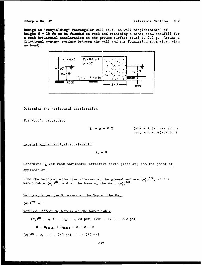
Example No. 32 Reference Section: 8.2
Design an "nonyielding" rectangular wall (i.e. no wall displacements) ofheight H - 20 ft to be founded on rock and retaining a dense sand backfill fora peak horizontal acceleration at the ground surface equal to 0.2 g. Assume africtional contact surface between the wall and the foundation rock (i.e. withno bond).
Ko- 0.45 Yt-120 pcf . ,
H - 217 -. ' .
S4. . "
r ru. 0 A-0.2Ag
Determine the horizontal acceleratioL
For Wood's procedure:
kh - A - 0.2 (where A is peak groundsurface acceleration)
Determine the vertical acceleration
k - 0
Determine Ph (at rest horizontal effective earth pressure) and the point of
application.
Find the vertical effective stresses at the ground surface (ac)TOP, at thewater table (ac)r, and at the base of the wall (a,)°OT.
Vertical Effective Stresses at the Top of the Wall
(ay)TOP - 0
Vertical Effective Stress at the Water Table
(ay)W - 7t (H - Hw) - (120 pcf) (20' - 12') - 960 psf
U - Ustatic + Ushear - 0 + 0 - 0
(a)• - - u-- 960 psf - 0 - 960 psf
239
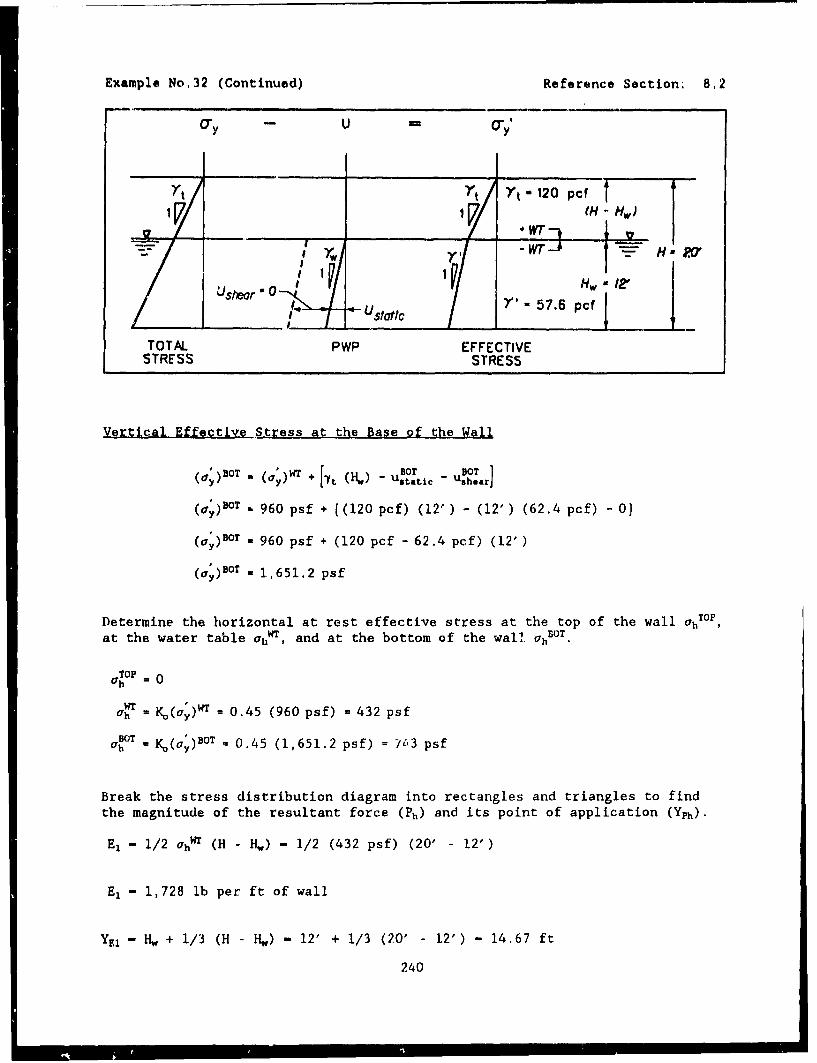
Example No.32 (Continued) Reference Section. 8,2
.O y -- U O 'ys
T Yt 120 pc0
1VIV(H Hw)
Y "L - H, ,0
U s h o -0 H w 1 ,2 "
Us...tt_ "Y' - 5 7.6 per
TOTAL, PWP EFFECTIVESTRESS STRESS
Vertical Effective S-tress at-the Base of the Waill
(cry,) BOT (0',.)W + [-y, (H.,) - .,o .,o, 1c-uy statc - shlarl
(Ory)BOT - 960 psf + [ (120 pcf) (12') (12" ) (62.4 pcf) 01O
(cry)8°7 - 960 psf + (120 pcf - 62.4 pcf) (12")
(a'y)BOT - 1,651.2 psf
Determine the horizontal at rest effective stress at the top of the wall ahT°at the water table ahwT, and at the bottom of the wall. ahE.
(7hTOP =0
ah K,,(ory)wT = 0.45 (960 psf) = 432 psf
BOT I
o•rh a K<0(0)B°T - 0.45 (1,651.2 psf) =?--7,3 psf
Break the stress distribution diagram into rectangles and triangles to findthe magnitude of the resultant force (Ph) and its point of application (Yph).
El - 1/2 0rhWT (H - H,) - 1/2 (432 psf) (20' - 12")
El - 1,728 lb per ft of wall
YE, - H, + 1/3 (H -H) - 12" + 1/3 (20p - 12c- 14.67 ft
240
I __
TOTAI L IPIWiP IEI"EITIVI I1E I I ,
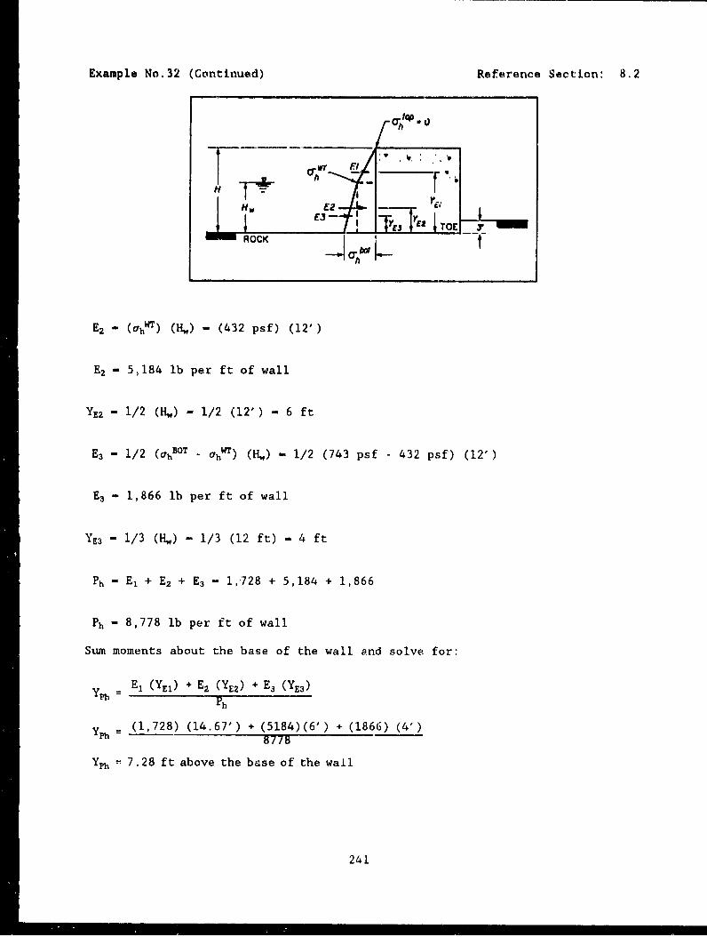
Example No.32 (Continued) Reference Section: 8.2
top~
ROK E .....T ,.,I..~ Oht
E2 - (Uhwr) (H,,) - (432 psf) (12' )
E2 - 5,184 lb per ft of wall
E2 - 1/2 (HE) - 1/2 (12') - 6 ft
E3 - 1/2 (H.)T - 'hw) (H,) - 1/2 (743 psf - 432 psf) (12')
E3 - 1,866 lb per ft of wall
YE3 " 1/3 (H,) - 1/3 (12 ft) - 4 ft
Ph "E + E2 + E3 - 1,728 + 5,184 + 1,866
Ph 8,778 lb per ft of wall
Sum moments about the base of the wall and solve for:
E, (YEj) + E2 (YE2) + E3 (YE3)
Ph
YPh M (1,728) (14.67') + (5184)(6') + (1866) (4')8778
Yph ý 7.28 ft above the base of the wail
241
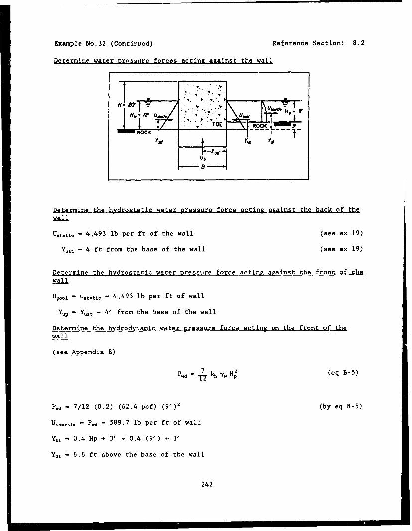
Example No.32 (Continued) Reference Section: 8.2
Determine water Dressure forces acting against the wall
H 1S4'Hw ,'1 ':i.*,' .. 9
'C TOE ROCKROCK
Determinei.the hydrostatic water pressure force acting against the back of-the
U~t~ti, - 4,493 lb per ft of the wall (see ex 19)
Y,-t - 4 ft from the base of the wall (see ex 19)
Determine the hydrostatic water pressure force acting against the front of the
Upoo, - 03ttic - 4,493 lb per ft of wall
YUP - Y,,t - 4' from the base of the wall
Determine the hydrodynamic water gressure force acting on the front of the
wall
(see Appendix B)
7wd kh - HP (eq B-5)
Pwd " 7/12 (0.2) (62.4 pcf) (9,)2 (by eq B-5)
Uinertia - Pwd - 589.7 lb per ft of wall
Yu± - 0.4 Hp + 3' - 0.4 (9') + 3'
Yuw - 6.6 ft above the base of the wall
242
Example No.32 (Continued) Reference Section: 8.2
Determine the hydrostatic water pressure force acting on the base of the wall
Assume full hydrostatic pressure beneath the base of the wall.
Ub - H. (-.) B
Uk, - (12') (62.4 pcf) B - 748.8 (B)
Xu - B/2 - 0.5 B
Determine the dynamic incremental earth Dressures (total stress based
F., - (120 pcf) (20')2 (0.2) (by eq 68)
F., - 9,600 lb per ft of wall
Y,, - 0.63 H - 0.63 (20')
Yar - 12.6 above the base of the wall, acting horizontally
SDetermine the weight of the wall
W - (H) (B) (Tvo 0 c) (20' ) (B) (150 pcf)
W - 3,000 B
4 - B/2 - 0.5 B
Y.- H/2 - 20'/2 - 10'
Determine the effective normal force between the base of the wall and the
foundation
N' - 3,000 B - 748.8 B - 2,251.2 B (by eq 112)
Determine the ultimate shear force along the base
6b - 35' (from Table 2)
Tult - (2,251.2 B) tan (35) - 1,576.3 B
Determine the shear force reguired for equilibrium
Let F. - 1. 2
Solving Equation 114 for T,
243
Example No.32 (Continued) Reference Section: 8.2
T - Tuit . 1,576.3 B - 1.313.6 BF 1.2
Solve Eauation 111 forB re uired for shear force equilibrium
1,313.6 B - 8,778 + 9,600 + 3,000 B (0.2) + 4,493 - 4,493 + 589.7
B = 18,968 . 9.9"
Let B - 10' for F. - 1.2.
Solve Eouation 115 such that ovelrturning criteria are met
B* = 0.5 (from Table 5)
Be * 3 XN, (adapted from eq 116)
3 XN, =0.5
0.5B
M1 - W Xw - W kh Y. - 1,500 B (B - 4) (see ex 31)
M2 - Mpooi "' Ustatc (Yust) - Upool (Yup) - Uinertia (Yu) - Ustatic (Yust)
M2 - "Uinertia (YMa) - -589.7 (6.6' - 3,892
M3 - "Ph (Yph) -8,778 (7.28') - -63,904
M4 - -Fsr (Y.r) " -(9,600) (12.6') - -120,960
M5 - -Ub (Xub) - -(748.8 B) (0.5 B) - -374.4 B2
244
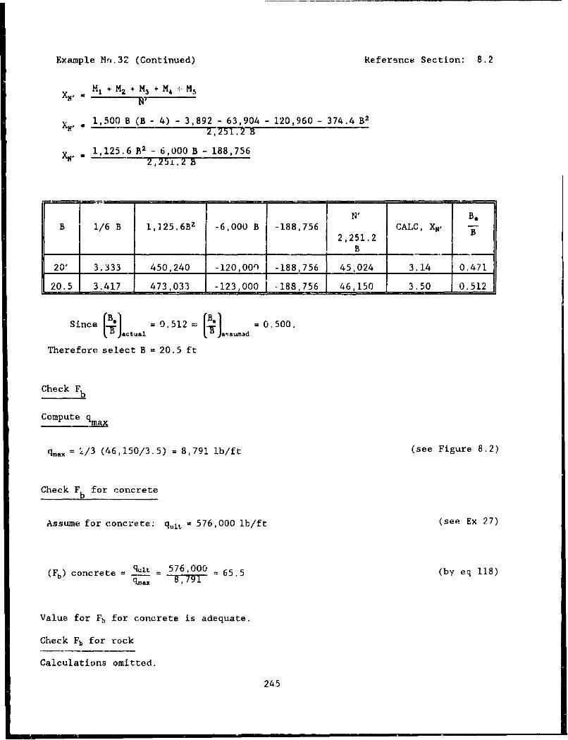
Example Nrj,.32 (Continued) Reference Section: 8.2
MI * M2 + M3 + M4 M5XN' "no
x 1,500 B (B - 4) - 3,892 - 63,904 - 120,960 - 374.4 B2
=I 2,251.2 B
X,. = 1,125.6 B2 - 6,000 B - 188,7562,251.2 B
NP B.B 1/6 B 1,125.6B2 -6,000 B -188,756 CALC, XN, -B
2,251.2B
20' 3.333 450,240 -120,00n -188,756 45,024 3.14 0.471
20.5 3.417 473,033 -123,000 -188,756 46,150 3.50 0.512
Since B__ = 0.512 B{i = 0.500.actual iasumad
Therefore select B = 20.5 ft
Check Fb
Compute qmax
qmax = 2/3 (46,150/3.5) = 8,791 lb/ft (see Figure 8.2)
Check Fb for concrete
Assume for concrete: q,,t, = 576,000 lb/ft (see Ex 27)
(Fb) concrete = quit = 576,000 = 65.5 (by eq 118)qmax 97=~
Value for Fb for concrete is adequate.
Check Fb for rock
Calculations omitted.
245
REFERENCES
Al Homound, A. 1990. "Evaluating Tilt of Gravity Retaining Well DuringEarthquakes," ScD Thesis, Department of Civil Engineering, MassachusettsInstitute of Technology, Cambridge, MA.
American Association of State Highway and Transportation Officials. 1983."Guide Specifications for Seismic Design of Highway Bridges," AASHTO,Washington, DC.
Anderson, G., Whitman, R., and Germaine, J. 1987. "Tilting Response ofCentrtfuge-Modeled Gravity Retaining Wall to Seismic Shaking: Description ofTests and Initial Analysis of Results," Report No. R87-14, Department of CivilEngineering, Massachusetts Institute of Technology, Cambridge, MA.
Agbabian Associates. 1980. "Seismic Response (f Port and Harbor Facilities,"Report P80-109-499, El Segundo, CA.
Ambraseys, N. N., and Menu, J. M. 1988. Earthquake-Induced Ground Displace-ments, Earthquake Engineering and Structural Dynamics, Vol. 16, pp. 985-1006.
Amono, R., Azuma, H., and Ishii, Y. 1956. "A Seismic Design of Walls inJapan," Proceedings .st World Conference on Earthquake Engineering, pp. 32-1to 32-17.
ASGE Report by the Ad Hoc Group on Soil-Structure Interaction of the Committeeon Nuclear Structures and Materials of the Structural Division. 1979."Analysis for Soil-Structure Interaction Effects for Nuclear Power Plants."
ASCE-Standard. 1986 (Sep), "Seismic Analysis of Safety Related NuclearStructures and Commentary on Standard for Seismic Analysis of Safety RelatedNuclear Structures, 91 p.
Bakeer, R., Bhatia, S., and Ishibashi, S. 1990. "Dynamic Earth Pressure withVarious Gravity Wail Movements," Proceedings of ASCE Specialty Conference onDesign and Performance of Earth Recaining Structures, Geotechnical SpecialPublication No. 25., pp, 8 8 7 - 8 9 9 .
Booker, J., Rahman, M., and Seed, H.B. 1976 (Oct). "GADFLEA - A ComputerProgram for the Analysis of Pore Pressure Generation and Dissipation DuringCyclic or Earthquake Loading," Report No. EERC 76-24, Earthquake EngineeringResearch Center, University of California-Berkeley, Berkeley, CA.
Caquot, A., and Kerisel, F. 1948. "Tables for the Calculation of PassivePressure. Active Pressure and Bearing Capacity of Foundations," Gauthier-Villars, Paris.
Chang, M., and Chen, W. 1982. "Lateral Earth Pressures on Rigid RetainingWalls Subjected to Earthquake Forces," Solid Mechanics Archives, Vol. 7,No. 4, pp. 315-362.
Chang, C., Power, M., Mok, C., Tang, Y., and Tang, H. 1990 (May). "Analysisof Dynamic Lateral Earth Pressures Recorded on Lotung Reactor ContainmentModel Structure," Proceedings 4th US National Conference on Earthquake Engi-neering, EERI, Vol. 3, Palm Springs, CA.
247
Chopra, A. K. 1967 (Doc). "Hydrodynamic Pressures on Dams During Earth-quakes," ASCE, Journal of Engineering Mechanics Division, Vol. 93, No. E146,pp 205-223.
Clough, G. W. and Duncan, J. M. 1991. Chapter 6: Earth Pressures, in Founda-tion EnjineerLn dbo.k, Sccond Edition, edited by H. Y, Fang, Van NostrandReinhold, NY, pp. 223-235.
Committee on Earthquake Engineering, Commission on Engineering and TechnicalSystems, National Research Council. 1985. Liouefaction of Soil. DurinjEatbuae, National Academy Press, WA.
Coulomb, C. A. 1776. Essai sur une application des rhgles des maximis etmininis A quelques problAmes de statique relatifs A l'architecture, Mim._acad.ry rks divers savants, Vol. 7, Paris.
Dawkins, W. P. 1991 (Mar). "User's Guide: Computer Program for Design andAnalysis of Sheet-Pile Walls by Classical Methods (CWALSHT) with Ruwe's MomentReduction," Instruction Report ITL 91-1, Information Technology Laboratory,US Army Engineer Waterways Experiment Station, Vicksburg, MS.
Department of the Navy. 1982 (May). "NAVAC DH-7.2. Fo tions And EarthStructures. Design Manual 7.2," Department of the Navy, Faval FacilitiesEngineering Command, 200 Stovall Street, Alexandria, VA.
1983 (Apr). "NAVFAC DM-7.3. Soil Dynamics. Deed Stabilization.and Sgeclal Geotechnical Construction. Design Manual 7.3," Department of theNavy, Naval Facilities Engineering Command, 200 Stovall Street, Alexandria,VA.
Dismuke, T. 1991. Chapter 12: Retaining Structures And Excavations, Founda-tion Engineering Handbook, Second Edition, edited by H.Y. Fang, Van NostrandReinhold, NY, pp. 447-510.
Duncan, J. M. 1985. Lecture Notes Regarding the Design of AnchoredBulkheads.
Duncan, J. M., Clough, G. W., and Ebeling, R. M. 1990. "Behavior and Designof Gravity Earth Retaining Structures," ASCE Specialty Conference on Designand Performance of Earth Retaining Structures, Geotechnical Special Publica-tion 25, pp. 251-277.
Earthquake Engineering Technology, Inc. 1983. "Super FLUSH - ComputerResponse Analysis Of Soil-Structure Systems Under Various Input Environments."
Ebeling, R. 1990 (Dec). "Review Of Finite Element Procedures for Earth Re-taining Structures," Miscellaneous Paper ITL-90-5, Information TechnologyLaboratory, US Army Engineer Waterways Experiment Station, Vicksburg, MS.
Ebeling, R. M., Duncan, J. H., and Clough, G. W. 1990 (Oct). "Methods ofEvaluating the Stability and Safety of Gravity Earth - Retaining StructuresFounded on Rock, Phase 2 Study," Technical Report ITL-90-7, Information Tech-nology Laboratory, US Army Engineer Waterways Experiment Station, Vicksburg,MS.
248
Ebeling, R. M., Clough, G, W., Duncan, J. M., and Brandon, T. L. 1992 Muay)."Methods of Evaluating the Stability and Safety of Gravity Earth RetainingStructures Founded on Roak," Technical Report REMB-CS-29, Information Tech-nology Laboratory, US Army Engineer Waterways Expcrtmeyt Stetion, Vicksburg,MS.
Edris, EQ V., and Wright, S.G. 1987 (Aug). "User's Gi6ide: UTEXAS2 Slope-Stability Package, Vclume 1: User's Manual," Instruction Report CL-87-1,Geotechnical LaboratQry, US Army Engineer Watecways Experiment Statimr,Vicksburg, MS.
Elms, D., and Richards, R. 1990. '"Soismic Design of Retahiing WalIl,"Proceeding of ASCE Specialty Confevence on Design and Purfcrmance of Enr&hRetaining Structures, Gootechnical Special Publication No. 25., pp.854-871.
Finn, W., and Liam, D. 1987. Chapter 3: Geomechanics of Part 3 Finite Fle-ment Method Applications in gnitc Elemn.n andbook, edited by 5, Kardestuncerand D. Norrie, McGraw-Hill, Inc., pp 3.157-3.216.
Finn, W., Liam, P., Yogendrakumar, M., Otsu, H., and Steedmar, R.S. 1989.":'Seismic Response of a Cantilever Rettining Wall: Centriiuga Model Tests andDynamic Analysis". Proceedings, 4th Internatinnal Conference on Soil Dynamicsand Earthquake Engineering, Mexico City, JtrucaualDrti__lure Interaction, Editors A.S. Cakmok and I. Heriera, Computational MechanicsPublications, Boston, HA, pp. 39-52.
Finn, W,, Liam, D., Yogendrakumar, M., Yoshida, N., and Yushida, H. 1986."TARA-3: A Program for Non-Linear Static and Dynamic Effective Stress Analy-sis," Soil Dynamics Gromp, University of British Columibia, Vancruver, B.C.
Franklin, C. and Chang, F. 1977 (Nov). "Earthquak, Resistance of Earth andRockfill Dams: Ruport 5: Permanent Displacement of Earth Embankments by New-mark Sliding Block Analysis," Miscellaneous Papor S-71-17, Soils And PavementsLaboratory, US Army Engineer Waterways Experimenu Station, Vicksburg, MS.
Gazetas, G., Dakoulas, P., and Dennehy, K. 1990. "Emperical Seismic DesignMethod for Waterfront Anchored Sheetpile Walls," Proceedings of ASCE SpecialtyConference on Design and Performance of Earth Retaining Structures, Geotechni-cal Special Publication No. 25., pp. 232-250.
Green, R. 1992. "Selection of Ground Motions for thp Seismic Evaluation otEmbankments," ASCE Specialty Conference on Stability and Performance of Slopesand Embankments II, A 25-Yeor Perspective, Geotechnical Special PublicationNo. 31, Vol. I, pp. 593-607.
Hallquist, J. 1982. "User's Manual for DYNA2D - An Explicit Two-DimensionalHydrodynamic Finite Element Code With Interactive Rezoning," University ofCalifornia, LawrencE Livermore National Laboratory, Report UCID-18756, Rev. 1.
Headquarters, Department of the Army. 1989. "Retaining and Flood Walls,"Engineer Manual 1110-2-2502, Washington, DC.
. 1991. "Design of Pil- Foundations," Engineer Manual 1110-2-2906,Washington, DC.
249
Hung, S., ind Werner, S. 1982, "An Assessment: of Earthquake Response Chelace,teristics and Design Procedures for Port and Harbor Facilities," Proceeding3rd International 4arthquake Microzonation Conference, Report No. SF/CEE-82070Seattle, WA, pp. 15.
Hyncs-Gr,•~.fin, M. E,, and Fronklin, A. G, 1984. "Rationalizing the SeismicCoefficient Method," Miscellaneous Paper S-84-13, US Army Engineer WaterwaysExpAriment Station, Vicksburg, MS.
Iai, S., and Kamooka T. 1991. "Effective Stress Analysis of a Sheet PileQuaywall," Procceding of Second International Conference on Recent Advances inGeocechnical Earthquake Engine9ring and Soil Dynamics, Paper No. 4.14, Vol. I.St. Louis, MO, pp. 649-656.
Ichihara, M., and Natsuzawa, H. 19/3 (Dec). "Earth Pressure DuringEarthquake," Soils and Foundations, Vol. 13, No. 4, pp. 7 5 - 8 6 .
Idriss, I. M. !!85. Evaluating Seismic Risk in Engineering Practice, Pro-ceeding 1.1th International Conference on Soil Mechanics and Foundation Engi-neering, Vol. 1, pp. 2 5 5 - 3 2 0 .
Ishibashi, I., and Fang, Y. 1987 (Dec). "Dynamic Earth Pressures with Dif-ferent Wall Modes," Soils and Foundations, Vol. 27, No. 4, pp. 11-22.
Ishibashi, I., and Madi, L. 1990 (May). "Case Studies On Quaywall'sStability With Liquefied Backfills," Proceeding of 4t]1 U.S. Conference onEarthquake Engineering, EERT, Vol. 3, Palm Springs, CA, pp. 725-734.
Ishibashi, I., Matsuzawa, H., and Kawamura, M. 1985. "Generalized ApparentSeismic Coefficient for Dynamic Lateral Earth Pressure Determination,"Proceeding of 2nd International Conference on Soil Dynamics and EarthquakeEngineering, edited by C. Brebbia, A. Cakmak, and A. Ghaffer, QE2, pp. 6-33 to6-42.
Johnson, E. 1953 (Apr). "The Effects of Restraining Boundries on the PassiveResistance of Sand, Results of a Series of Tests with a Medium-Scale TestingApparatus," Masters of Science Thesis In Engineering, Princetun University.
Joyner, W. B., and Boore, D. M. 1988. "Measurement, Charactization and Pre-diction of Strong Ground Motion," Earthquake Engineering and SoilDynamics II - Recent Advances in Ground Motion Evaluation, ASCE GeotechnicalSpecial Publication No. 20, pp. 43-102.
Kerisel, J., and Absi, E. 1990 (May). Active and Passive Earth PressureTables." A. A. Balkema International Publishers, pp. 234.
Kitajima, S., and Uwabe, T. 1979 (Mar). "Analysis on Seismic Damage inAnchored Sheet-Piling Bulkheads," Report of the Japanese Port and HarborResearch Institute, Vol. 18, No. 1, pp. 67-130. (in Japanese).
Kurata, S., Arai, H. and Yokoi, T. (1965). "On the Earthquake Resistance ofAnchored Sheet Pile Bulkheads," Proceedings, 3rd World Conference On Earth-quake Engineering, New Zealand.
250
Ladd, C. 1991 (Apr). "Stability Evaluation During Staged Construction,"ASCE, Journal of Geotechnical Engineering, Vol. 117, No. 4, pp. 540-615.
Lambs, T. and Whitman, R. 1969. "Soil Mechanics," John Wiley & Sons, Inc.,New York, Chapters 13 and 23.
Lee, M., and Finn, W. D. Liam. 1975. "DESRA-l: Program for the DynamicEffective Stress Response Analysis of Soil Deposits including LiquefactionEvaluation," Report No. 36, Soil Mechanic Service, Department of Civil Engi-neering, University of British Columbia, Vancouver, B.C.
_ 1978. "DESRA-2: Dynamic Effective Stress Response Analysis ofSoil Deposits with Energy Transmitting Boundary Including Assessment of Lique-faction Potential," Report No. 38, Soil Mechanic Service, Department Of CivilEngineering, University of British Columbia, Vancouver, B.C.
Li, X. 1990. "Free-Field Soil. Response under Multi-Directional EarthquakALoading, Ph.D. Thesis, Department of Civil Engineering, University of Califor-nia, Davis, CA.
Lysmer, J., Udaka, T., Tsai, C., and Seed, H. B. 1975. "FLUSH: A ComputerProgram For Approximate 3-D Analysis of Soil-Structure Interaction Programs,"Report No. EERC 75-30, Earthquake Engineering Research Center, University ofCalifornia, Berkeley, CA.
Makdisi, F. I., and Seed, H. B. 1979. "Simplified Procedure for EstimatingDam and Embankment Earthquake-Induced Deformations," ASCE, Journal of the Geo-technical Engineering Division, Vol. 104, No. GT7, pp. 849-867.
Marcuson, W., Hynes, M., and Franklin, A. 1990 (Aug). "Evaluation and Use ofResidual Strength in Seismic Safety Analysis of Embankments," EarthquakeSpectra, pp. 529-572.
Matsuo, H., and Ohara, S. 1965. "Dynamic Pore Water Pressure Acting on QuayWalls During Earthquakes," Proceedings of the Third World Conference on Earth-quake Engineering, Vol 1, New Zealand, pp. 130-140.
Matsuzawa, H., Ishibashi, I., and Kawamura, M. 1985 (Oct). "Dynamic Soil andWater Pressures of Submerged Soils," ASCE, Journal of Geotechnical Engineer-ing, Vol. 111, No. 10, pp. 1161-1176.
McMahon, D. 1986. Tiebacks for Bulkheads, Collection of Five Papers,Proceeding of a Session Sponsored by the Geotechnical Engineering Division ofthe ASCE in Conjunction with the ASCE Convention in Seattle, WA., GeotechnicalSpecial Publication No. 4., 90 p.
Meyerhof, G. 1953. "The Bearing Capacity of Foundation Under Inclined andEccentric Loads," 3rd International Conierence Of Soil Mechanics And Founda-tion Engineering, Vol. 1, pp 440-445.
Mononobe, N., and Matsuo, H. 1929. "On the Determination of Earth PressuresDuring Earthquakes," Proceedings, World Engineering Congress, 9.
251
National Earthquake Hazards Reduction Program (NEHRP). 1988. RecommendedProvisions for the Development of Seismic Regulations for New Buildings:Building Seismic Safety Council.
National Research Council. 1988. Probabilistic Seismic Hazard Analysis:National Academy Press, Washington, DC, 97 p.
. 1985. Liquefaction of Soils During Earthquakes: NationalAcademy Press, Washington, DC, 240 p.
Nadiem, F., and Whitman, R. 1983 (May). "Seismically Induced Movement ofRetaining Walls," ASCE, Journal of Geotechnical Engineering, Vol. 109, No. 7,pp. 915-931.
Newmark, N. 1965. Effects of Earthquakes on Dams and Embankments,"Geotechnique, Vol. 15., No. 2, pp. 139-160.
Newmark, N. N., and Hall, W. J. 1983. Earthauake Spectra and Design. Earth-quake Engineering Research Institute, 499 14th Street, Oakland, CA, 103 p.
Okabe, S. 1926. "General Theory of Earth Pressures," Journal Japan Societyof Civil Engineering, Vol. 12, No. 1.
Okamoto, S. 1984. "Introduction to Earthquake Engineerin ," second edition,University of Tokyo Press, 629 p.
Peter.,on. M. S., Kulhawy, F. H., Nucci, L. R., and Wasil, B. A. 1976."Stre,.s-reformation Beh&vior o" Soil-tConcrete Interfaces," Contract ReportB-49, Department of Civil Engineering, Syracuse University, Syracuse, NY.
Potyondy, J. G. 1961 (Dec). "Skin Friction Between Various Soils and Con-struction Materials," Geotechnicue, Vol II, No. 4, pp 339-353.
Poulos, S. J., Castro, G., and France, W. (1985). "Liquefaction EvaluationProcedutre." ASCE Journal of Geotechnical Engineering Division, Vol. 111,No. 6, pp. 772-792.
Prakash, S., and Basavanna, B. 1969. "Earth Pressure Distribution BehindRetaining Wall During Earthquake," Proceeding. 4th World Conference onEarthquake Engineering, Santiago, Chile.
Provost, J. 1981 (Jan). "DYNAFLOW - A Nonlinear Transient Finite ElementAnalysis Program, Report No. 81-SM-l, Princeton University, Princeton, NJ.
Provost, J. 1989. "DYNAlD - A Computer Program For Nonlinear Seismic SiteResponse Analysis, Technical Report NCEER-89-0025, National Center for Earth-quake Engineering Research, University of Buffalo.
Rankine, W. (1857). On the Stability of Loose Earth, Phil, Trans, Roy, Soc.
London, Vol. 147.
Roth, W. H., Scott, F. F., and Cundall, P. A. 1986. "Nonlinear DynamicAnalysis of a Centrifuge Model Embankment," Proceedings of the ThirdUS National Conference on Earthquake Engineering, Vol. I, Charleston, SC,pp. 505-516.
252
Richards, R., and Elms, D. 1979 (April), "Seismic Behavior of GravityRetaining Walls," ASCE, Journal of the Geotechnical Engineering Division, Vol.105, No. GT4, pp. 449-464.
Richards, R., and Elms, D. 1990. "Seismic Design of Retaining Walls," Pro-ceedings of ASCE Specialty Conference on Design and Performance of EarthRetaining Structures, Geotechnical Special Publication No. 25., pp. 854-871.
Rowe, P. W. 1952. "Anchored Sheet Pile Walls," Proceedings of Institution ofCivil Engineers. Vol 1, Part 1, pp 27-70.
Rowe, P. W. 1956. "Sheet Pile Walls at Failure," Proceedings InstructionCivil Engineers London, Vol. 5, Part I, pp. 276-315.
Rowe, P. W. 1957 (Feb). "Limit Design of Flexible Walls," Proceedings MidlandSoil Mechanic and Foundation Engineering Society, Vol. 1, pp. 29-40.
Sadigh, K. 1983. "Considerations in the development of site-specificspectra," in proceedings of Conference XXII, site-specific effects of soil androck on ground motion and the implications for earthquake resistant design:U.S. Geological Survey Open File Report 83-845.
Sarma, S. K. 1979. "Response and Stability of Earth Dams During StrongEarthquakes," Miscellaneous Paper GL-79-13, US Army Engineer WaterwaysExperiment Station, Vicksburg, MS.
Schnabel, P., L-,smer, J., ornd Seed, H. B. 1972 (Dec). "SHAKE: A ComputerProgram for Earthquake Response Analysis of Horizontally Layered Sites,"Report No. EERC 72-12, Earthquake Engineering Research Center, University OfCalifornia, Berkeley, CA.
Seed, H. B. 1987 (Aug). "Design Problems in Soil Liquefaction," ASCE,Journal of the Geotechnical Engineering Division, Vol. 113, No. 8,pp. 827-845.
_ _ 1971. "Simplified Procedure for Evaluating Soil LiquefactionPotential," ASCE, Journal of the Soil Mechanics and Foundations Division, Vol.97, No. sM9, pp. 1249-1273.
Seed, H. B. and Idriss, I. M. 1982. Ground Motions and Soil LiquefactionDuring Earthquakes, Earthquake Engineering Research Institute, 499 14thStreet, Oakland, CA, pp 134.
Seed, H. B., Idriss, I. M., Arango, I. 1983. "Evaluation of LiquefactionPotential Using Field Performance Data," ASCE, Journal of the GeotechnicalEngineering Division, Vol. 109, No. GT3, pp 458-482.
Seed, H. B., Tokimatsu, K. Harder, L. F., and Chung, R. M. 1985 (Dec)."Influence of SPT Procedures in Soil Liquefaction Resistance Evaluations,"ASCE, Journal of the Geotechnical Engineering Division, Vol. 111, No. 12,pp. 1425-1445.
Seed, H., and Whitman, R. 1970. "Design of Earth Retaining Structures forDynamic Loads," ASCE Specialty Conference on Lateral Stresses in the Groundand Design of Earth Retaining Structures, pp. 103-147.
253
Seed, R. B. and HIarder, L. F. (1990). "SPT-Basod Analysis of Cyclic PorePressu~re Ganeration and Undrained Strength," Proceedings of the H. B. SeedMemorial Symposium, Bi Tech Publishing, Vol. II, pp. 351-376,
Sharmiz, N. (1989), "Refinement of Newmark Sliding Block Model and Applica.tion to New Zealand Conditions," Master Thesis, Department of Civil Engineer-ing, University of Cantorbury, NZ, 237p.
Sherif, M., Ishibashi, I., and Lee, C. 1982. "Earth Preasure Against RigidRetaining Walls," ASCE, Journal of the Geotechnical Engineering Division,Vol. 108, No. GT5, pp. 679-695.
Sherif, M., and Fang, Y. 1983 (Nov). "Dynamic Earth Pressure:i Against Rotat-j~i~d Non-Yielding Retaining Wallj", Soil Engineering Research ReportNo. 23, Department of Civil Engineering, University of Washington, Seattle,WA, pp. 45-47,
_ . 1984a. "Dynamic Earth Pressures on Rigid Walls Rotating Aboutthe Base," P Eighth World Conference on Earthquake Engineering,Vol. 6, San Francisco, CA, pp. 993-100.
_ 1984b. "Dynamic Earth Pressures on Walls Rotating About theTop," Soils and Foundations, Vol. 24, No. 4, pp. 1 0 9 - 1 1 7 .
Spangler, M. 1938. "Lateral Earth Pressures on Retaining Walls Caused bySuperimposed Loads," Proceedings of the 18th Annual Meeting of the HighwayResearch Board. Part II, pp. 57-65.
Stark, T. D., and Mesri, G. 1992 (Nov). "Undrained Shear Strength of Lique-fied Sands for Stability Analysis," ASCE, Journal of the GeotechnicalEngineering Division, Vol. 118, No. 11.
Steedman, R., and Zeng, X. 1988. "Flexible Anchored Walls Subject to BaseShaking," Report CUED/D-soils TR 217, Engineering Department CambridgeUniversity, UK
Steedman, R., and Zeng, X. 1990. "The Influence of Phase on the Calculationof Pseudo-Static Earth Pressure on a Retaining Wall," Geotechnique, Vol. 10,No. 1, pp. 103-112.
Steedman, R., and Zeng, X. 1990. "Hydrodynamic Pressures on a Flexible QuayWall," Report CUED/D-soils TR 233, Engineering Department, CambridgeUniversity, UK.
Steedman, R., and Zeng, X. 1990. "The Response of Waterfront RetainingWalls," Proceedings of ASCE Specialty Conference on Design and Performance ofEarth Retaining Structures, Geotechnical Special Publication No. 25.,pp. 872-886.
Streeter, V., Wylie, and Richart, F. 1974. "Soil Motion Computations byCharacteristics Method," Journal of the Geotechnical Engineering Division.ASCE, Vol. 100, No. GT3, pp. 247-263.
Taylor, D. 1948. "Fundamentals of Soil Mechanics." John Wiley & Sons, Inc.,New York, pp. 488-491.
254
Terzaghi, K. 1934 (Feb). "Large Retaining Wall Tests. I. Pressure of DrySand," Engineering News Record, Vol III, pp. 136-140,
. 1936 (Apr). "A Fundamental Fallacy in Earth Pressure Calcula-
tions," Boston Society of Civil Engineers, pp. 71-88.
1943. "Theoretical Soil Mechanics", John Wiley & Sons, New York.
1954. "Anchored Bulkheads," Transactions of the American Societyof Civil Engineers, Vol. 119, pp. 1243-1324.
Terzaghi, K., and Peck, R. 1967. "Soil Mechanics in ngi nerineerng Practige,"Second Edition, John Wilay & Sons, Inc., New York.
Tokimatsu, A. H., and Seed, H. B. 1987 (Aug). "Evaluation of Settlements InSands Due to Earthquake Shaking," ASCE, Journal of the Geotechnical Division.Vol. 113, No. 8, pp. 861-878.
Tokimatsu. K., and Yoshimi, Y. 1983. "Emperical Correlation of Soil Lique-faction Based on SPT N-Value and Fines Content," Soils and Foundations,Vol. 23, No. 4, pp 56-74.
Towhata, I., and Islam, S. 1987 (Dec.). "Prediction of Lateral Movament ofAnchored Bulkheads Induced by Seismic Liquefaction," Soils and Foundations,Vol. 27, No. 4, pp. 137-147.
Tschebotarioff, G. P. 1973. Foundations, Retaining and Earth Structures,
McGraw-Hill, Second Edition, 642 p.
USS Steel Sheet Piling Design Manual 1969, 132p.
Vasquez-Herrera, A., and Dobry, R. 1988. "The Behavior of Undrained Contrac-tive Sand and Its Effect oin Seismic Liquefaction Flow Failures of EarthStructures," Rensselaer Polytechnic Institute, Troy, NY.
Westergaard, H. 1931. "Water Pressure on Dams During Earthquakes," Transac-tions of ASCE, Paper No. 1835, pp. 418-433
Whitman, R. 1979 (Dec). "Dynamic Behavior of Soils and Its Application toCivil Engineering Projects," State of the Art Reports and Special Lectures,6th Panamerican Conference on Soil Mechanics and Foundation Engineering, Lima,Peru, pp. 59-105.
. 1985. "On Liquefaction," Proceedings. l1th International Confer-ence on Soil Mechanism and Foundation Engineering, Vol. 7, San Francisco, CA.pp. 1923-1926.
. 1990. "Seismic Design Behavior of Gravity Retaining Walls," Pro-ceedings of ASCE Specialty Conference on Design and Performance of EarthRetaining Structures, Geotechnical Special Publication No. 25., pp. 817-842.
Whitman, R. V. 1992 (Jul). Predicting Earthquake - Caused Permanent Deforma-tions of Earth Structures, Proceedings Wroth Memorial Symposium on PredictiveSoil Mechanics, Oxford University (in press).
255
Whitman, J., and Christian, J. 1990. "Seismic Response of Retaining Struc-tures," Symposium Seismic Design for World Port 2020, Port of Los Angeles, LosAngeles, CA.
Whitman, R., and Liao, S. 1935. "Seismic Design of Retaining Walls," Miscel-laneous Paper GL-85-1, US Army Engineer Waterways Expcriinent Station,Vicksburg, MS.
Wong, C. 1982. "Seismic Analysis ant Improved Seismic Design Procedure forGravity Retaining Walls," Research Report 82-32, Department Of Civil Engineer-ing, Massachusetts Institute of Technology, Cambridge, MA.
Wood, J. 1973. "Earthquake-Induced Soil Pressures on Structures, ReportNo. EERL 73-05, California Institute of Technology, Pasadena, CA, pp. 311.
Yong, P. M. F. 1985. "Dynamic Earth Pressures Against A Rigid Earth Retain-ing Wall, Central Laboratories Report 5-8515, Ministry of Works and Develop-ment, Lower Hutt, New Zealand.
Zarrabi, K. 1973. "Sliding of Gravity Retaining Wall During Earthquakes Con-sidering Vertical Acceleration and Changing Inclination of Failure Surface, SMThesis, Department of Civil Engineering, MIT, Cambr.-dge, MA, pp. 140.
Zienkiewicz, 0. C., and Xie, Y. M. 1991 (Nov.) "Analysis of the Lower SanFernando Dam Failure Under Earthquake," Dam Engineering, Vol. II, Issue 4,pp. 307-322.
256
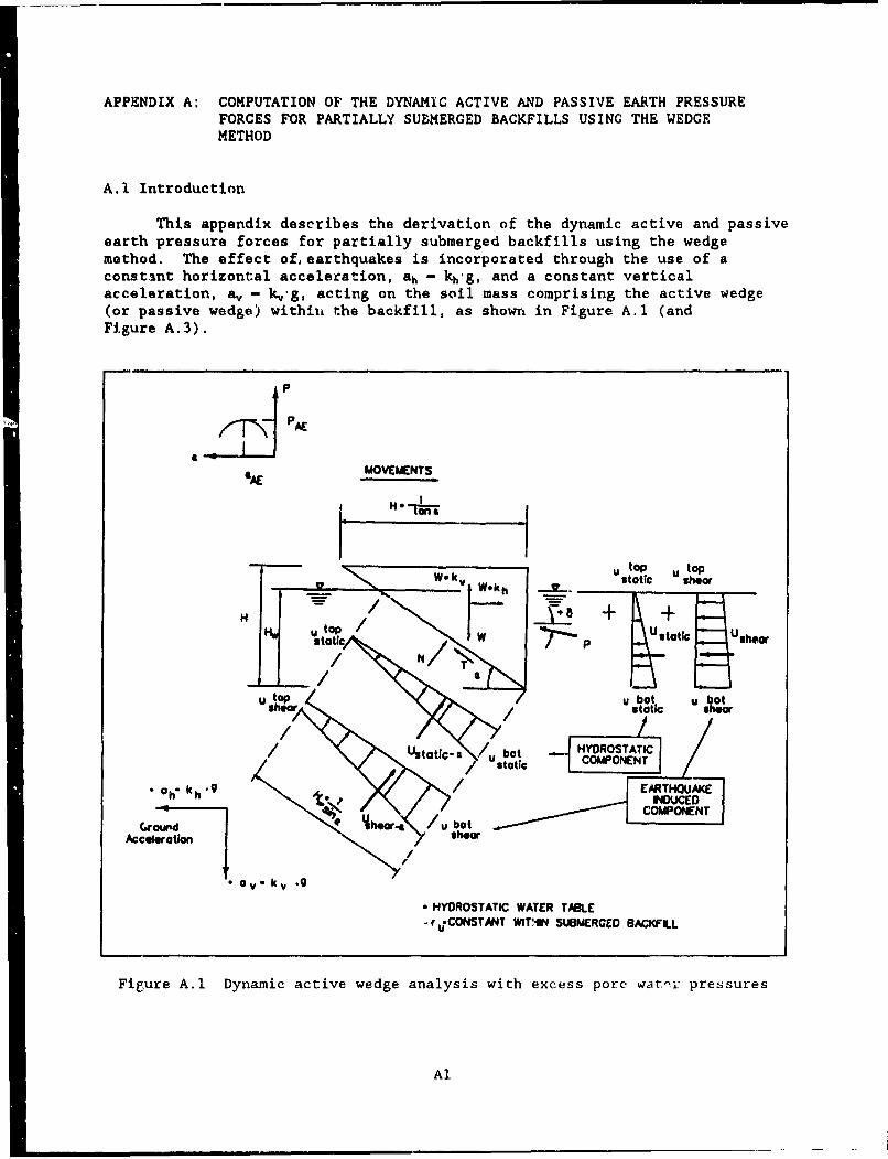
APPENDIX A: COMPUTATION OF THE DYNAMIC ACTIVE AND PASSIVE EARTH PRESSUREFORCES FOR PARTIALLY SUBMERGED BACKFILLS USING THE WEDGEMETHOD
A.1 Introduction
This appendix describes the derivation of the dynamic active and passiveearth pressure forces for partially submerged backfills using the wedgemethod. The effect of, earthquakes is incorporated through the use of aconstant horizontal acceleration, ah - kh-g, and a constant verticalacceleration, a, - k,-g, acting on the soil mass comprising the active wedge(or passive wedge) withixA the backfill, as shown in Figure A.1 (andFigure A.3).
P
,/rN AE
SAE MOVEMENTS
, H.- -•
tonp at
uto Thp UtoWo/[_-hstatic s~ttc*hear
+ +st a ti top W t
Uha static Ashearu top, u ",b>.--- ot U o
Sstatic a b HYDROSTATIC• |atlc" U s• taicI " COMPONENT I/
0 h kh 9 /ATOIK* Oh kh"g '* JINDUCED
Ground /u b.tAcceleration shear
* Ov- kv .9
* HYDROSTATIC WATER TABLE-. u-CONSTANT WIT4IN SWUMERGED BACKFILL
Figure A.1 Dynamic active wedge analysis with excess pore watnr pressures
Al
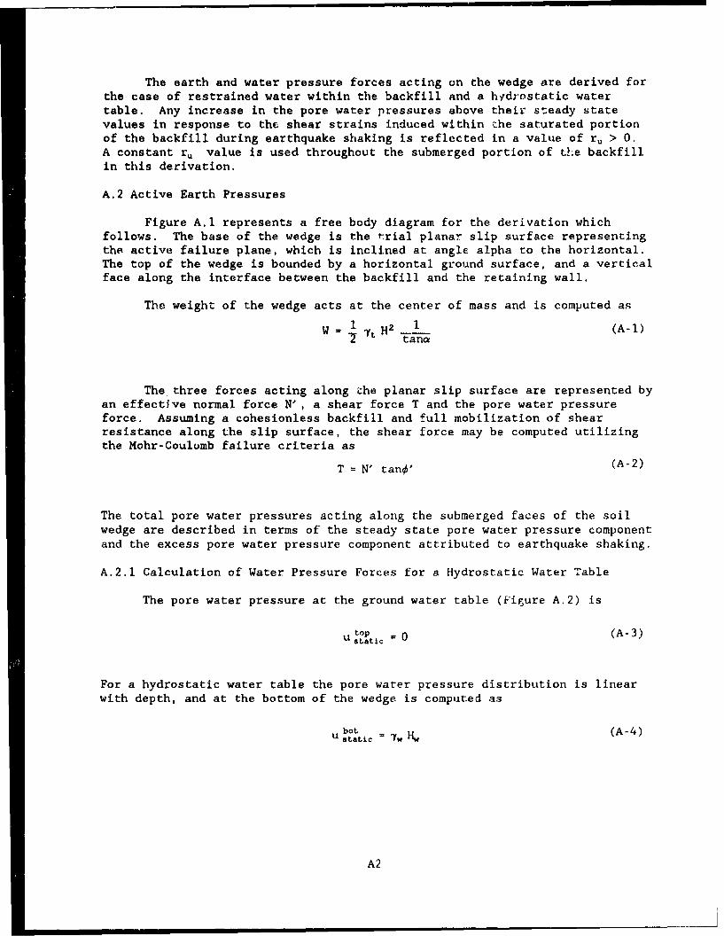
The earth and water pressure forces acting on the wedge are derived forthe case of restrained water within the backfill and a hvdrostatic watertable. Any increase in the pore water pressures above their steady statevalues in response to the shear strains induced within cthe saturated portionof the backfill during earthquake shaking is reflected in a value of ru > 0.A constant ru value is used throughout the submerged portion of the backfillin this derivation.
A.2 Active Earth Pressures
Figure A.1 represents a free body diagram for the derivation whichfollows. The base of the wedge is the trial planar slip surface representingthe active failure plane, which is inclined at angle alpha to the horizontal.The top of the wedge is bounded by a horizontal ground surface, and a verticalface along the interface between the backfill and the retaining wall.
The weight of the wedge acts at the center of mass and is computed as
W = It H2 1 (A-l)2 tana
The three forces acting along the planar slip surface are represented byan effective normal force N', a shear force T and the pore water pressureforce. Assuming a cohesionless backfill and full mobilization of shearresistance along the slip surface, the shear force may be computed utilizingthe Mohr-Coulomb failure criteria as
T = N' tanO' (A-2)
The total pore water pressures acting along the submerged faces of the soilwedge are described in terms of the steady state pore water pressure componentand the excess pore water pressure component attributed to earthquake shaking.
A.2.1 Calculation of Water Pressure Forces for a Hydrostatic Water Table
The pore water pressure at the ground water table (Figure A.2) is
utop =0 (A-3)Ustatic
For a hydrostatic water table the pore water pressure distribution is linearwith depth, and at the bottom of the wedge is computed as
bot i (A-4)U static
A2
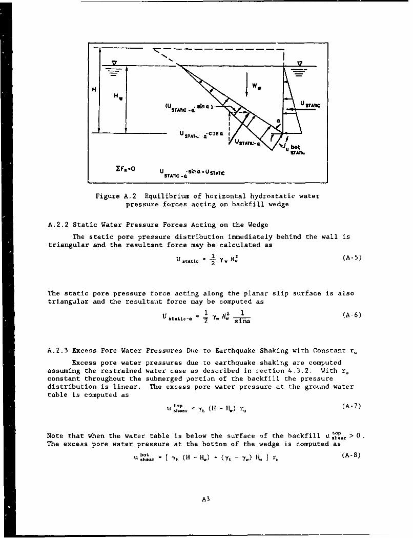
H WwW
(U U USTATICSTATIC -G
prssrefocsYacting on '3acfl wedgeUU--44
WW 4L STT~ j~Vu bat
1ITAMk
XFh-O0 U S- L-USAISTATIC -a
Figure A.2 Equilibrium of horizontal hydrostatic waterpressure forces acting on backfill wedge
A.2.2 Static Water Pressure Forces Acting on the Wedge
The static pore pressure distribution immediately behind the wall istriangular and the resultant force may be calculated as
U static 1 2 (A-5)
The static pore pressure force acting along the planar slip surface is alsotriangular and the resultant force may be computed as
1 2 1 (A-6)U static-&, 7 -Y H; s'/ • n
A.2.3 Excess Pore Water Pressures Due to Earthquake Shaking with Constant r"
Excess pore water pressures due to earthquake shaking are computedassuming the restrained water case as described in !,ection 4.3.2. With r"constant throughout the submerged portion of the backfill the pressuredistribution is linear. The excess pore water pressure at the ground watertable is computed as
Utoar = -ry (H - 1J.) r(A7)
Note that when the water table is below the surface of the backfill u par > 0.The excess pore water pressure at the bottom of the wedge is computed as
hot (A- 8)U shear - Yt (H -H-) + (-yt - H.) ii ] (
A3
The total pore water prnssures are equal to the sum of the hydrostatic pore
water pressures plus the excess pore water pressures.
A.2.4 Excess Pore Water Pressuze Forces Acting on the Wedge.
The resultant excess pore water pressure force of a trapezoidal pressure
distribution acting normal to the back of the wall ;s equal to
I top hot
U shear w hear [u U shear I I (A-9)
The resultant excess pore water pressure force of the trapezoidal pressure
distribution acting notmal to the planar slip surface is equal to
1 [ tap uboa 1 (-0U shear.a = U sheer + shear IHw (A-10)
A.2.5 Equilibrium of Vertical Forces
Equilibrium of vertical forces acting on the Figure A.1 soil wedgeresults in the relationship
- P sin6 + W( I - k, ) - T sine - N'cosa
- ( UstItica + Ushear-a )coscr = 0 (A-11)
Introducing Equation A-2 into A-11 results in
- P sinS + W( 1 - k, ) - N' tan' sina
- N' cosa - ( Ustatica + Ushear-a )cosa = 0 (A-12)
and solving for the normal effective force, N' , becomes
sin6 + 1 I- k,tanO' sina + cosa W- , sin + cosa
(Utatic-a + shmar-a ) coso (A-13)r FtanF' sina + cosa
A4
A.2.6 Equilibrium of Forces in the Horizonal Direction
Equilibrium of horizontal forces acting oTI the Figure A.1 s-il wedgeresults in the relationship
Pcos6 - N'sin- (Usta~t.a + Ushoar-_ )sina
+ Tcosot - WkI + ( \ Ut,, U ) U (A-14)
Substitutin- Equation A-2 into A-14, and with the horizontal components ofwater pressure forces of equal magnitude and opposite direction, (refer toFigure A.2), Equation A-14 simplifies to
Pcos6 - N'sina + N'tan"'ccsa -Wh 0 (A-15)
Combining the N' terms results in
Pcos6 - N' ( •ina - tano'cosa ) - Wk= 0 (A-16)
Multiplying Equation A-13 (for N') by - ( sina - tano'cosa ) ]and simplifying becomes
- N' ( - tan4'cosa + sina ) = + Psin6tan( a - 0' )
- W( I - k, )tan( a - 0' )
+ ( Ustatic.a + Usheara )cosatan( a - 4' ) (A-17)
Substituting Equation A-17 into A-16 gives
Pcos6 + Psin6tan( a - 0' )
- W( 1 - k )tanA( a -0' )
+ ( Ustatic.. + Ush~er_, )cosatan( a - 0' ) - Wk, = 0 (A-18)
Combining tp.rms results in
P [ cos6 + sin6tan( a - 0' )I=
W[ ( 1 - k, )tan( a - 0' ) + k ]
( Ustatic- + Ush,,r_. )cosatan( a - 0' ) (A-19)
A5
Solving for the resultant force P which acts at angle 6
P . CONSTANTA1 - CONSTANTA2 (A-20)
cos6 + sin6tan(a -
where
CONSTANTA^ W [ ( 1 - k, )tan( a - ,' ) + k]
and
CONSTANTA - (U- t t¢r, U+heer.O) cosatan( a - 4" )
The dynamic active earth pressure force PAE is equal to the maximum value of Pfor the trial wedges analyzed and aA - a for this critical wedge, as discussedin Section 3.4 and shown in Figure 3.10.
A.2.7 Surcharge Loading
The presence of an additional mass located on top of the backfill duringearthquake shaking can increase the magnitude of the dynamic active earthpressures acting on the wall. The effects of an additional surcharge massidealized in Figure A.3, or a surcharge loading idealized in Figure A.4, maybe incorporated within the dynamic active wýdge analysis of Section A.2.6 byexpanding Equation A-20. For each slip surface analyzed, that portion of thesurcharge loading contained within the wedge is included within the equationsof equilibrium of forces acting on the wedge. When the surcharge isrepresented as a uniform pressure distribution q%, that portion of thesurcharge loading contained above the wedge is replaced by an equivalent forceWe acting at its center of mass. The uniformly distributed surcharge pressureq, shown in Figure A.4 is replaced by the equivalent force (per foot of wall)
W. - q. 1. (A-21)
whereis - 1 - ((H/tana) - x) for lq > 1 (refer to Figure A-4),
otherwise1. - lq
The variable 1, represents the effective lengtn of the surcharge load.
Equation A-20 becomes
E a CONSTANTA1 + CONSTANT• 1 - CONSTANTA2 (A-22)
cos6 + sin6tan( a - P'')
A6
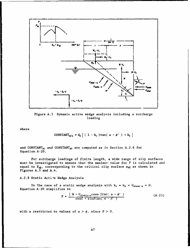
'Id
W* It.
W, W.k'
L
Figure A.3 Dynamic active wedge analysis including a surchargeloading
where
CONSTANTA-1 - Ws 1 - k, )tan( a~-4i + kh
and CONSTANTA, and CONSTANTA2 are computed as in Section A.2.6 forEquation A-20.
For surcharge loadings of finite length, a wide range of slip surfacesmust be investigated to ensure that the maximut-' value for P is calculated andequal to PAE, corresponding to the critical slip surface aAE as shown inFigures A.3 and A.4.
A.2.8 Static Acti're Wedge Analysis
In the case of a stat.c wedge analysis with k, - .--- 0,Equation A . Dn20 simplifies to
OS W -, t -U ws[ i1-- c , Itan( a ' (A-23)cos m + sin6tan( SA
with a restricted to values of a > 0, since P > 0.
A7

pIPAC
H.--
0 l (AI CL
---- "---
('i \hUFO U'WU•B..U
Figure A.4 Dynamic active wedge analysis including a surchargeloading
PA P and aA - a for the static critical wedge as well. For asurcharge loading, Equation A-22 simplifies to
p [W + S - Ustat1 c..cosa I tan( a - 4" ) (A-24)cos6 + sin6tan( a - T'-"
where W. is computed using Equation A-21.
A.3 Passive Earth Pressures
Figure A.5 represents a free body diagram that is used in the derivationof the wedge procedure for computing the value of the dynamic passive earthpressure force PPE. The base of the wedge represents the trial planar slipsurface and is inclined at angle a to the horizontal. The top of the wedge isdefined by a horizontal ground surface, and the vertical face is located alongthe interface between the backfill and the retaining wall.
The weight of the wedge acts at the center of mass and is computed usingEquation A-1. The three forces acting along the planar slip surface are thenormal force N', the shear force T, and the pore waiter pressure force. Theshear force T shown in Figure A.3 for the passive case acts opposite to theshear force shown in Figure A.1 for the active case. Assuming a cohesionless
A8

PP MOVEMENTS
PPE He"
SPEu apE•IIWk
shear Ito We
+ W Wek T toatic Hw
U shear Ustot
Sbat ubal tshear static ho
JHYDROSTATIC |
I staticto
"* HYDROSTATIC WATER TABLECOU-CONSTANT WTH SUBMERGED BACKFLL * k v
Figuze A.5 Dynamic passive wedge analysis with excess pore waterpressures
backfill and full mobilizatioai of shear resistance along the slip surface, theshear force may be computed utilizing the Mohr-Coulomb failure criteria asgiven by Equation A-2.
A.3.1 Calculation of Water Pressure Forces for a Hydrostatic Water Table
The total water pressure forces are equal to the sum of the steady statewater pressures plus the excess water pressures due to earthquake shaking.Steady state water pressure forces for a hydrostatic water table are computedusing the procedures described in Sections A.2.1 and A.2.2. Excess pore waterpressures due to earthquake loads with constant r, throughout the submergedportion oi the backfill are computed using the procedures described inSections A.2.3 and A.2.4.
A9
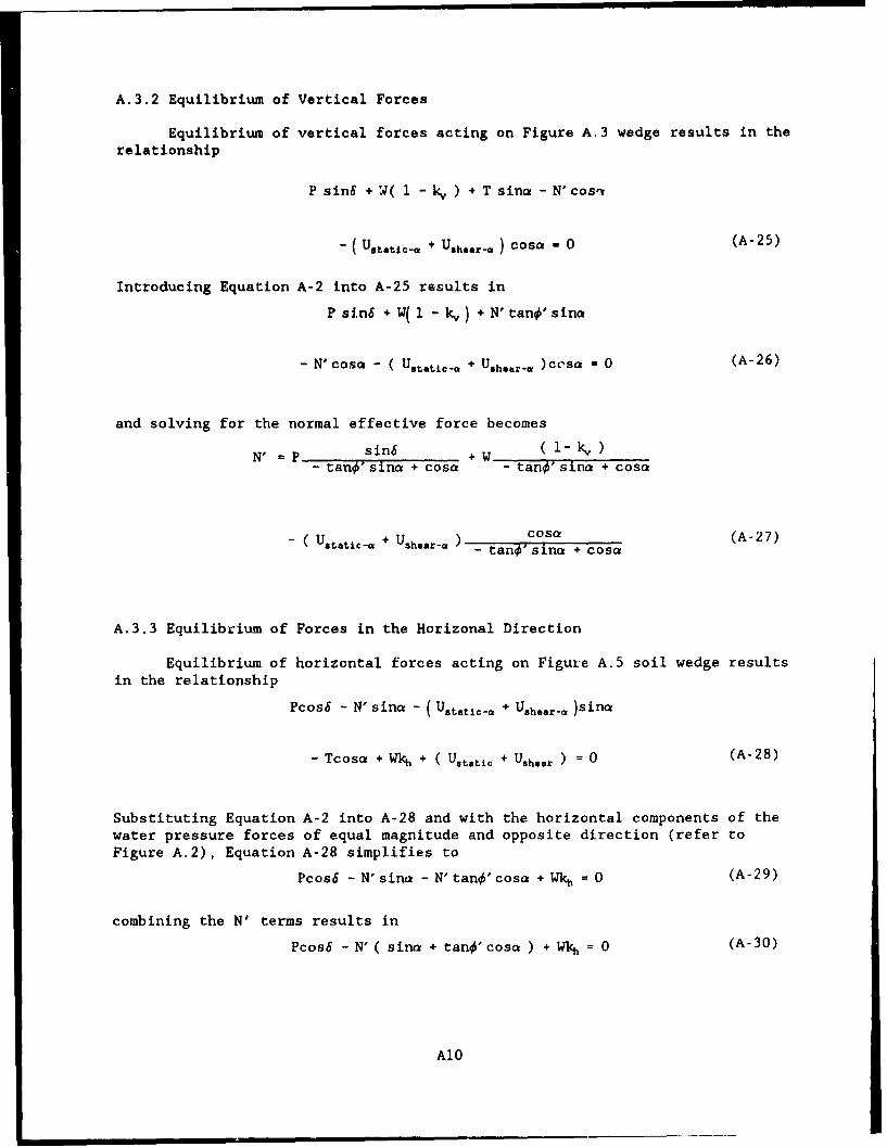
A.3.2 Equilibrium of Vertical Forces
Equilibrium of vertical forces acting on Figure A.3 wedge results in therelationship
P sin6 + W( 1 - kv ) + T sina - N'cosx
- ( Ustatica + Ushear-a ) cosa - 0 (A-25)
Introducing Equation A-2 into A-25 results in
P sin6 + W(1 - k,) + N' tanO'sina
- N' cosa - ( Ustatic.a + Ushear-& )Cosa - 0 (A-26)
and solving for the normal effective force becomes
N' = P sin6 + W ( I- k )- tano" sinc + cosq - tanO' sina + cosa
-c( i - + Ushear- osa (A-27)U'•tlc• U'~r' )- tanO" s ina + Cosa
A.3.3 Equilibrium of Forces in the Horizonal Direction
Equilibrium of horizontal forces acting on Figure A.5 soil wedge resultsin the relationship
Pcos6 - N' sina - (Ustatic_ + Uhar-. )sina
- Tcosa + Wkh + ( Ustatir + Ushear ) = (A-28)
Substituting Equation A-2 into A-28 and with the horizontal components of thewater pressure forces of equal magnitude and opposite direction (refer toFigure A.2), Equation A-28 simplifies to
Pcos6 - N' sina - N' tanO'cosa + Vkh =0 (A-29)
combining the N' terms results in
Pcos6 - N' ( sina + tanO'cosa ) + W1% - 0 (A-30)
A1O
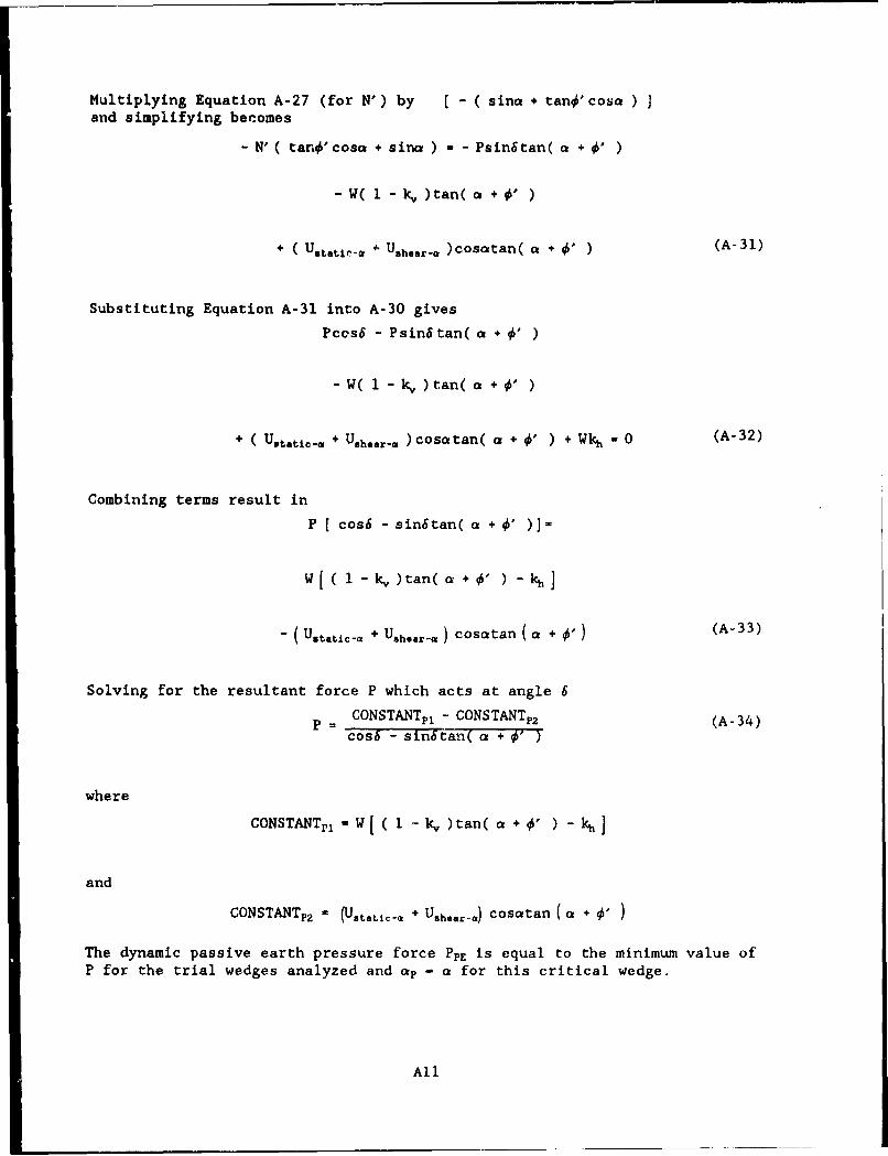
Multiplying Equation A-27 (for N') by [ - ( sina + tano'cosa ) jand simplifying becomes
- N' ( tanr'cosa + sina ) = - Psin6tan( a + 4' )
- W( 1 - k, )tan( a + 0' )
+ ( Ustatir-a ". Ushear-a )cosatan( a ÷ 4" ) (A-31)
Substituting Equation A-31 into A-30 gives
Pcos6 - Psin6tan( a + 4' )
-W( 1 - k, )tan( a +4' )
+ ( Utatic.qa + Ushear.a ) cosatan( a + 4' ) + Wkh = 0 (A-32)
Combining terms result in
P [ cos6 - sin6tan( a + 4' )]=
W 1 - k )tan( a + 4' ) - kh
- (U tatc_ + Usheara ) cosatan ( a + 4') (A-33)
Solving for the resultant force P which acts at angle 6
p = CONSTANTP1 - CONSTANTP2 (A-34)
cos6 - sin6tan( a +'
where
CONSTANTri = W[ ( 1 - k, )tan( a + 4, ) - kh
and
CONSTANTp 2 (Ustatic-a + Ushear-a) cosatan (a + 4'
The dynamic passive earth pressure force PPE is equal to the minimum value ofP for the trial wedges analyzed and ap - a for this critical wedge.
All
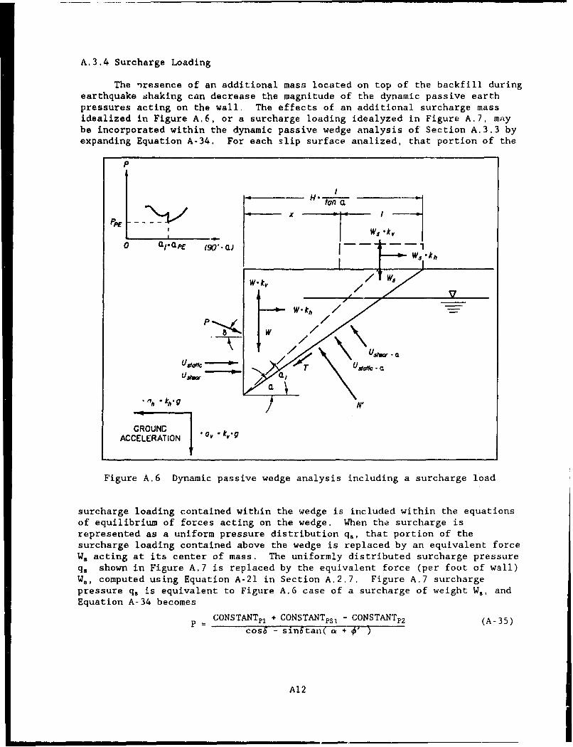
A.3.4 Surcharge Loading
The nresence of an additional mass located on top of the backfill duringearthquake shaking can decrease the magnitude of the dynamic passive earthpressures acting on the wall. The effects of an additional surcharge massidealized in Figure A.6, or a surcharge loading idealyzed in Figure A.7, mnybe incorporated within the dynamic passive wedge analysis of' Section A.3.3 byexpanding Equation A-34. For each slip surface analized, that portion of the
P
X ~Wj,*ky0 fIIJ.GD (90 - a)
W* W$
~'h khQ
Figure A.6 Dynamic passive wedge analysis including a surcharge load
surcharge loading contained within the wedge is included within the equations
of equilibrium of forces acting on the wedge. When the surcharge is
represented as a uniform pressure distribution q5 , that portion of the
surcharge loading contained above the wedge is replaced by an equivalent force
W, acting at its center of mass. The uniformly distributed surcharge pressure
q, shown in Figure A.7 is replaced by the equivalent force (per foot of wall)
W8 , computed using Equation A-21 in Section A.2.7. Figure A.7 surcharge
pressure q, is equivalent to Figure A.6 case of a surcharge of weight W8 , and
Equation A-34 becomes
p=CONSTANTp1 ÷ CONSTANTps1 - CONSTANTpz (A-35)
cos6 -'sin6tan( c• + •')
AI2

____________ Ton a_
PPE - x ••'
P W
cij at: (9gO - (3.1
W / T
* ~ ~ ~ ~ L a~ ~,g~1
GROUNDACCELERATION
Figure A.7 Dynamic passive wedge analysis including a surcharge load
where
CONSTANTpsI - Ws[ ( 1 - k, )tan( a 4" ) - kh ]
and CONSTANT1 Ip and CONSTANTP2 are computed as in Section A. 3.3 for EquationA-34.
For surcharge loads of finite length, a wide range of slip surfaces mustbe investigated to ensure that the minimum value for P is calculated an( equalto PpE, corresponding to the critical slip surface aPE as shown in Figures A.6and A.7.
A.3.5 Static Passive Wedge Analysis
Note that for static problems with k, - kh - Uzhoar-* - 0 Equation A-34simplifies to
p. W - U.t.~ticcosa j tan( a + 4' ) (A-36)cos6 - sin6tan ( a + 4' )
A13
with a restricted to values of % > 0 and 6 < 0/2.
Pp - P and ap - a for this critical wedge. For a surcharge loading, EquationA-35 simplifies to
p [W + W. - Uat.tia._cosa J tan( a ÷ €' ) (A-37)cos6 - sin6tan ( + ÷' )
A14
APPENDIX B: THE WESTERGAARD PROCEDURE FOR COMPUTING HYDRODYNAMIC WATERPRESSURES ALONG VERTICAL WALLS DURING EARTHQUAKES
This section describes the Westergaard procedure for computing the mag-nitude of the hydrodynamic water pressures along rigid vertical walls duringearthquake shaking. The solution developed by Westergaard (1931) is for thecase of a semi-infinite long water reservoir retained by a concrete dam andsubjected to a horizontal earthquake motion. The fundamental period of theconcrete dam is assumed to be much smaller than the fundamental period of theearthquake so that the acceleration for the massive structure is approximatedas the acceleration of the earthquake motion along the rigid base. Thisallows the problem of a very stiff concrete dam to be simplified to the caseof a rigid vertical face moving at the same horizontal acceleration as thebase horizontal acceleration. Using the equations of elasticity of a solid todescribe the propagation of sounds in liquids (waves which propagate withoutshear distortions) and with the water considered to be compressible, a solu-tion to the equation of motion of the water was developed for a harmonicmotion applied along the base of the reservoir. This solution ignores theeffects of surface waves and is valid only when the period of the harmonicexcitation is greater than the fundamental natural period of the reservoir(Chopra 1967). The fundamental period for the reservoir, T,, is equal to
T (B-l)
where the velocity of sound in water, C, is given by
C =Vfi (B-2)
and the mass density of water, p, is given by
P 7W (B-3)
With the bulk modulus of elasticity of water, K, equal to 4.32 X 10⁷ lb perft 2 , the unit weight for v'ater, yw, equal to 62.4 lb per ft 3 and the accelera-tion due to gravity, g, equal to 32.17 ft per sec2 , C is equal to 4,720 ft persec. For example, with a depth of pool of water, Hp, equal to 25 ft, T. isequal to 0.02 seconds (47 Hz) by Equation B-1.
The resulting relationship for hydrodynamic pressure on the face of thedam is a function of the horizontal seismic coefficient, kh, the depth ofwater, Y,, the total depth of the pool of water, HP, the fundamental period ofthe earthquake, and the compressibility of the water, K. The hydrodynamicpressure is opposite in phase to the base acceleration and for positive baseaccelerations the hydrodynamic pressure is a tensile. Westergaard proposedthe following approximate solution for the hydrodynamic water pressure distri-bution: a parabolic dynamic pressure distribution, Pwd, described by therelationship
BI
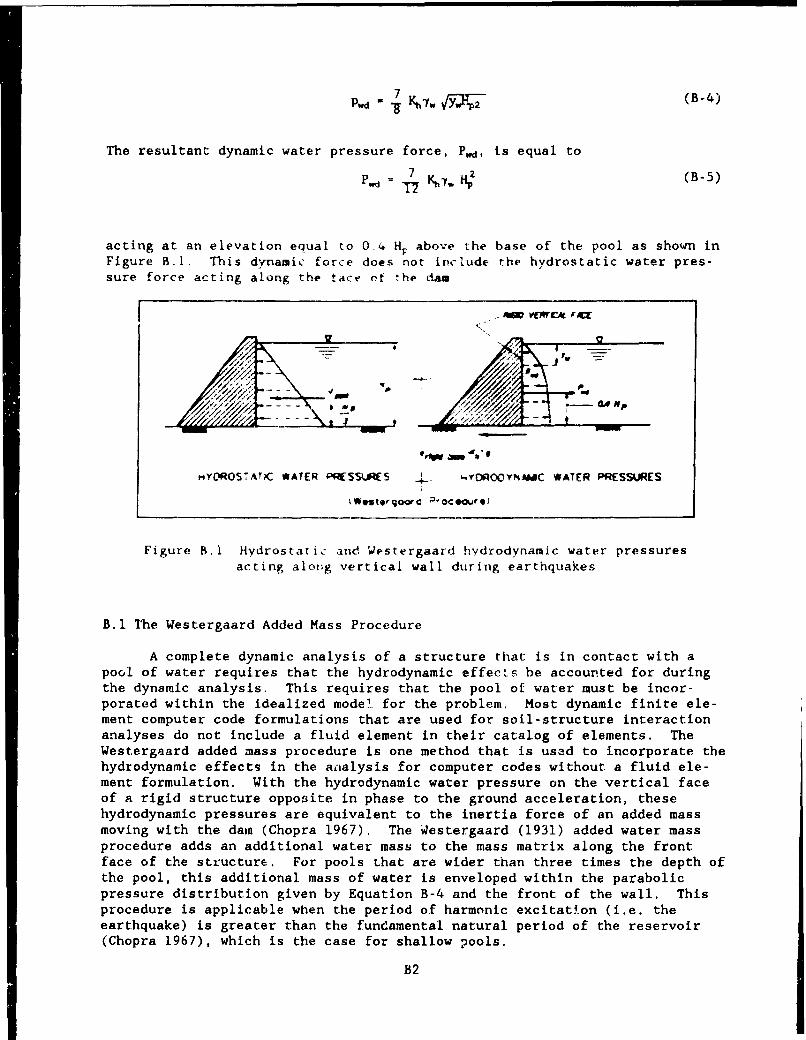
Pwj-7 (B-4)
The resultant dynamic water pressure force, Pd, is equal to
P 7K 2 (B-5)
acting at an elevation equal to 0 4 H. above the base of the pool as shown inFigure B.I. This dynanic force does not include the hydrostatic water pres-sure force acting along the face of the dam
I~u -a,,.(M
HY01ROSTArC WATER ';,WSSLWPS -5vOROmYNAAaC WATER PRESSURES
Figure B.1 Hydrostatic and Westergaard hvdrodynamic water pressuresacting along vertical wall during earthquakes
B.1 The Westergaard Added Mass Procedure
A complete dynamic analysis of a structure that is in contact with apool of water requires that the hydrodynamic effects be accounted for duringthe dynamic analysis. This requires that the pool of water must be incor-porated within the idealized model. for the problem. Most dynamic finite ele-ment computer code formulations that are used for soil-structure interactionanalyses do not include a fluid element in their catalog of elements. TheWestergaard added mass procedure is one method that is used to incorporate thehydrodynamic effects in the analysis for computer codes without a fluid ele-ment formulation. With the hydrodynamic water pressure on the vertical faceof a rigid structure opposite in phase to the ground acceleration, thesehydrodynamic pressures are equivalent to the inertia force of an added massmoving with the darn (Chopra 1967). The Westergaard (1931) added water massprocedure adds an additional water mass to the mass matrix along the frontface of the structure. For pools that are wider than three times the depth ofthe pool, this additional mass of water is enveloped within the parabolicpressure distribution given by Equation B-4 and the front of the wall. Thisprocedure is applicable when the period of harmonic excitation (i.e. theearthquake) is greater than the fundamental natural period of the reservoir(Chopra 1967), which is the case for shallow pools.
B2
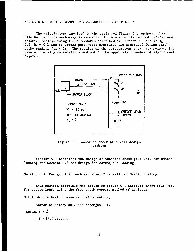
APPENDIX C: DESIGN EXAMPLE FOR AN ANCHORED SHEET PILE WALL
The calculations involved in the design of Figure C.1 anchored sheetpile wall and its anchorage is described in this appendix for both static andseismic loadingb using the procedures described in Chapter 7. AssLune kh -
0.2, k, - 0.1 and no excess pore water pressures are generated during earth-quake shaking (ru - 0). The results of the computations shown are rounded forease of checking calculations and not to the appropriate number of significantfigures.
SHEET PILE WALL
STIE ROD Hr* - 7'
\-ANCHOR BLOCK 1DENSE SAND Hpo -2O'
Yt - 120 pcf DREDGE LEVEL
b'- 35 degrees WM-,N
ru . 0 D
Figure C.1 Anchored sheet pile wall designproblem
Section CA describes the design of anchored sheet pile wall for statizloading and Section C.2 the design for earthquake loading.
Section C.1 Design of An Anchored Sheet Pile Wall for Static Loading
This section describus the design of Figure C.1 anchored sheet pile wallfor static loads using the free earth support method of analysis.
C.1.1 Active Earth Pressures Coefficients KA
Factor of Safety on shear strength - 1.0
Assume 6 = 2
6 = 17.5 degree.ý
Cl
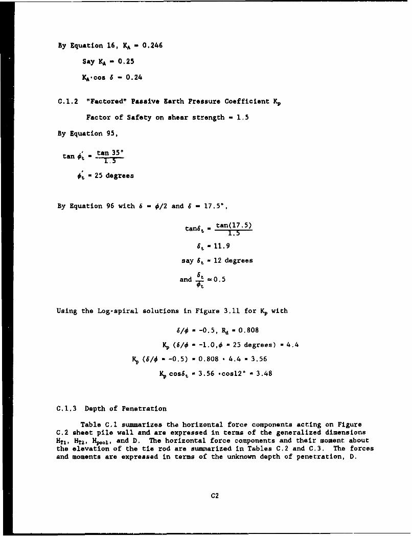
By Equation 16, KA - 0.246
Say KA - 0.25
KA*cos 6 - 0.24
C.1.2 "Factored" Passive Earth Pressure Coefficient Kp
Factor of Safety on shear strength - 1,5
By Equation 95,
Stan 35*tan -
* 25 degrees
By Equation 96 with 6 - 0/2 and 6 - 17.50,
tan6t M tan(17.5)1.5
6t - 11. 9
say 6t - 12 degrees
and t0.5
Using the Log-spiral solutions in Figure 3.11 for Kp with
610- -0. 5, Rd - 0. 808
K, (6/0 - -1.0,0 - 25 degrees) - 4.4
KP (6/4. - -0.5) - 0.808 - 4.4 - 3.56
K, cos6, - 3.56 ,cosl2° - 3.48
C.1.3 Depth of Penetration
Table CA summarizes the horizontal force components acting on FigureC.2 sheet pile wall and are expressed in terms of the generalized dimensionsHT1, HT2, Hool, and D. The horizontal force components and their moment aboutthe elevation of the tie rod are summarized in Tables C.2 and C.3. The forcesand moments are expressed in terms of the unknown depth of penetration, D.
C2
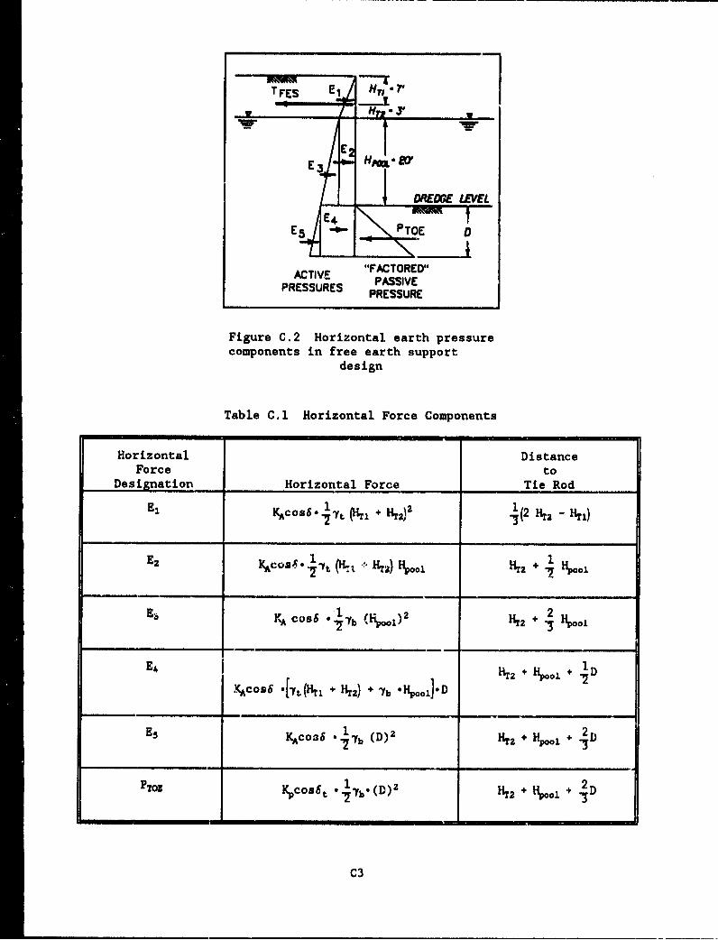
T FES ¶ 1- L
_ _ _,_.___._.'AETIVE
PR UE P DREDE LEVEL
E TOE D
ACTIVE "FACTORED"*PRESURES PASSIVEPRESSURE
Figure C.2 Horizontal earth pressurecomponents in free earth support
design
Table CA Horizontal Force Components
Horizontal DistanceForce to
Designation Horizontal Force Tie Rod
E, 1 1po1
KA cos6 *7t (HTS HT)2 1(2G H. Hltt412 +
E4 11T2 + Hpool + 1D,KA,,o os .['Yt(HT1 + H 2) ÷+ fb .Hp oo ] .D "2
73
C3
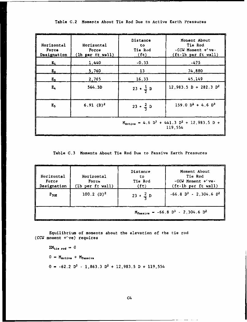
Table C.2 Moments About Tie Rod Due to Active Earth Pressures
Distance Montent AboutHorizontal Horizontal to Tie Rod
Force Force Tie Rod -CCW Moment +'ve-Designation (lb per ft wall) (ft) (ft-lb per ft wall)
EX 1,440 -0.33 -475
E2 5,760 13 74,880
E3 2,765 16.33 45,149
E4 564.5D 23 + I D 12,983.5 D + 282.3 D2
.7
ES 6.91 (D) 2 23 + 2 D 159.0 D2 + 4.6 D3
MCtLv - 4.6 D) + 441.3 D? + 12,983.5 D +119,554
Table C.3 Moments About Tie Rod Due to Passive Earth Pressures
Distance Moment AboutHorizontal Horizontal to Tie Rod
Force Force Tie Rod -CCW Moment +'ve-Designation (lb per ft wall) (ft) (ft-lb per ft wall)
PToE 100.2 (D) 2 23 + 2 D -66.8 D3 - 2,304.6 02
Mp..av,. - 66.8 D3 - 2,304.6 D2
Equilibrium of moments about the elevation of the tie rod(CCW moment +'ve) requires
Mtio rod - 0
0 - MACtive + Mpassive
0 - -62.2 D' - 1,863.3 D2 + 12,983.5 D + 119,554
C4
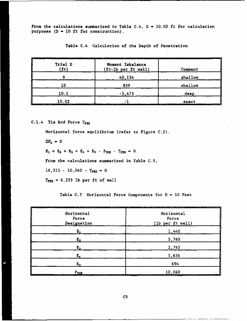
From the calculations summarized in Table C.4, D - 10.02 ft for calculationpurposes (D - 10 ft for construction).
Table C.4 Calculation of the Depth of Penetration
Trial D Moment Imbalance
(ft) (ft-lb per ft wall) Comment
9 40,134 shallow
10 859 shallow
10.1 -3,473 deep
10.02 -1 exact
C.i.4 Tie Rod Force TFES
Horizontal force equilibrium (refer to Figure C.2).
Fh - 0
E, + E2 + E3 + E4 + E5 - PTOE - TFES " 0
From the calculations summarized in Table C.5,
16,315 - 10,060 - TF7 s - 0
TFES - 6,255 '.b per ft of wall
Table C.5 Horizontal Force Components for D - 10 Feet
Horizontal HorizontalForce Force
Designation (lb per ft wall)
E, 1,440
E2 5,760
E3 2,765
E4 5,656
Es 694
PTO* 10,060
C5
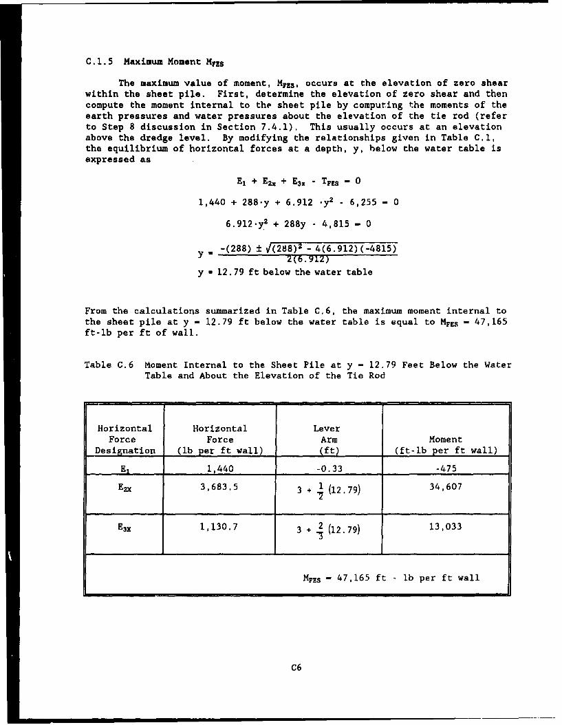
C.1.5 Maximum Moment MFzs
The maximum value of moment, MFEs, occurs at the elevation of zero shearwithin the sheet pile. First, determine the elevation of zero shear and thencompute the moment internal to the sheet pile by computing the moments of theearth pressures and water pressures about the elevation of the tie rod (referto Step 8 discussion in Section 7.4.1). This usually occurs at an elevationabove the dredge level. By modifying the relationships given in Table C.1,the equilibrium of horizontal forces at a depth, y, below the water table isexpressed as
El + E2x + E3x - TFES - 0
1,440 + 288.y + 6.912 .y 2 - 6,255 - 0
6.912.y 2 + 288y - 4,815 - 0
- -(288) ± V(288)2 - 4(6.912)(-4815)2(6.912)
y - 12.79 ft below the water table
From the calculations summarized in Table C.6, the maximum moment internal tothe sheet pile at y - 12.79 ft below the water table is equal to MFES - 47,165ft-lb per ft of wall.
Table C.6 Moment Internal to the Sheet Pile at y - 12.79 Feet Below the WaterTable and About the Elevation of the Tie Rod
Horizontal Horizontal LeverForce Force Arm Moment
Designation (lb per ft wall) (ft) (ft-lb per ft wall)
El 1,440 -0.33 -475
E• 3,683.5 3 + 1 (12.79) 34,607
E3x 1,130.7 3 + 2 (12.79) 13,033
MFES - 47,165 ft - lb per ft wall
C6
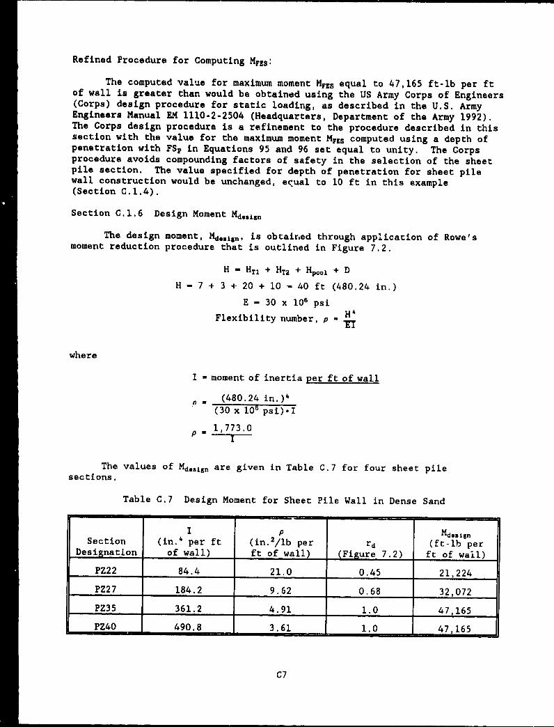
Refined Procedure for Computing MFES:
The computed value for maximum moment MFES equal to 47,165 ft-lb per ftof wall is greater than would be obtained using the US Army Corps of Engineers(Corps) design procedure for static loading, as described in the U.S. ArmyEngineers Manual EM 1110-2-2504 (Headquarters, Department of the Army 1992).The Corps design procedure is a refinement to the procedure described in thissection with the value for the maximum moment MFEs computed using a depth ofpenetration with FSp in Equations 95 and 96 set equal to unity. The Corpsprocedure avoids compounding factors of safety in the selection of the sheetpile section. The value specified for depth of penetration for sheet pilewall construction would be unchanged, equal to 10 ft in this example(Section C.1.4).
Section C.1.6 Design Moment Md,,isn
The design moment, Md.,ign, is obtained through application of Rowe'smoment reduction procedure that is outlined in Figure 7.2.
H - HT1 + HT2 + Hpool + D
H - 7 + 3 + 20 + 10 - 40 ft (480.24 in.)
E - 30 x 106 psi
Flexibility number, p - H•'
where
I - moment of inertia per ft of wall
- (480.24 in.)4
(30 x 101 psi).I
1,773.0I
The values of Md. 5 ign are given in Table C.7 for four sheet pilesections.
Table C.7 Design Moment for Sheet Pile Wall in Dense Sand
IIp Mdesa•n
Section (in.4 per ft (in. 2/lb per rd (ft-lb perDesignation of wall) ft of wall) (Figure 7.2) ft of wail)
PZ22 84.4 21.0 0.45 21,224
PZ27 184.2 9.62 0.68 32,072
PZ35 361.2 4.91 1.0 47,165
PZ40 490.8 3.61 1.0 47,165
C7
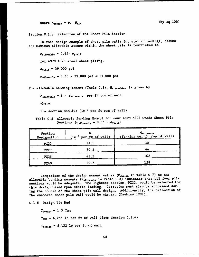
where Md,.•,, - rd *'Ns (by eq 100)
Section C.1.7 Selection of the Sheet Pile Section
In this design example of sheet pile walls for static loadings, assume
the maximum allowable stress within the sheet pile is restricted to
0 4Ilowable - 0. 65.- ayield
for ASTM A328 steel. sheet piling,
Oyi.ld - 39,000 psi
0 allowable - 0.65 • 39,000 psi - 25,000 psi
The allowable bending moment (Table C.8), Majjowabj,, is given by
Mallowgble - S . aU11O.bl. per ft run of wall
where
S - section modulus (in. 3 per ft run of wall)
Table C.8 Allowable Bending Moment for Four ASTM A328 Grade Sheet PileSections (a.1Lowebl. - 0.65 ' Oyield)
Section S Mallowablo
Designation (in. 3 per ft of wall) (ft-kips per ft run of wall)
PZ22 18.1 38
PZ27 30.2 64
PZ35 48.5 102
PZ40 60.7 128
Comparison of the design moment values (Md..isn in Table C.7) to theallowable bending moments (Majjow10 j, in Table C.8) indicates that all four pile
sections would be adequate. The lightest section, PZ22, would be selected for
this desigr based upon static loading. Corrosion must also be addressed dur-
ing the course of the sheet pile wall design. Additionally, the deflection of
the anchored sheet pile wall would be checked (Dawkins 1991).
C.1.8 Design Tie Rod
Tdgu £gn - 1. 3 TFES
TIEs - 6,255 lb per ft of wall (from Section C.1.4)
TdosaLn - 8,132 lb per ft of wall
C8

Assume
(a) 6 ft spacing of anchors
(b) ayil.d - 36,000 psi
"allowable - 0.4 cyield (40 % of yield)
Minimum area of rod - 6 ft • 8,132 lb per ft of wall0.4 .36,000 rnsi
Gross Area - 3.39 in. 2
Diameter - 4 . Area - 2.08 in.
C.1.9 Design Anchorage
Tu lt.a -2.5 .TFES (by eq 102)
with
TFES - 6,255 lb per ft of wall (from Section C.1.4)
Tult-a 15,638 lb per ft of wall
Details regarding the design of anchorage are provided in numerous ref-erences including Dismuke (1991) and the USS Steel Sheet Piling Design Manual(1969). If the overall height of the anchor, h., is not less than about 0.6times the depth from the ground surface to the bottom of anchorage, designatedda in Figure C.3, the anchor behaves as if it extended to the ground surface.
ha > 0.6 'd.
The full angle of interface friction, 6, used in computing Kp can only bemobilized if the anchor has sufficient dead weight or, in general, isrestrained against upward movement (Dismuke 1991). For a slender anchor theultimate capacity for a c anchor is required to satisfy theexpression
Tul.t-a 5 Pp - PA
with 6 - 0 degrees (refer to Figure C.3).
C9
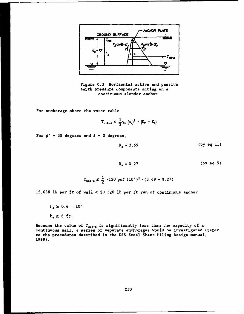
- ANCOR PLATECROUNO SURFACE
W O ,d I -I 0\KAWI800'y
Figure C.3 Horizontal active and passiveearth pressure components acting on a
continuous slender anchor
For anchorage above the water table
For s' - 35 degrees and 6 - 0 degrees,
*P - 3.69 (by eq 11)
KA = 0.27 (by eq 5)
T .u .120 pcf (10")2 .(3.69 - 0.27)
15,638 lb per ft of wall < 20,520 lb per ft run of ctu anchor
h, 0.6 1 10'
h, 6 ft.
Because the value of Tult-a is significantly less than the capacity of acontinuous wall, a series of separate anchorages would be investigated (referto the procedures described in the USS Steel Sheet Piling Design manual,1969).
ClO
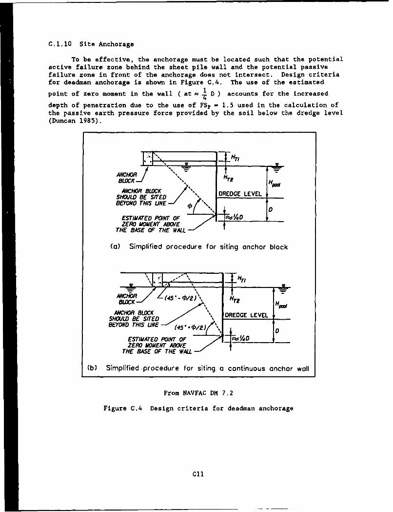
C.1.10 Site Anchorage
To be effective, the anchorage must be located such that the potentialactive failure zone behind the sheet pile wall and the potential passivefailure zone in front of the anchorage does not intersect. Design criteriafor deadman anchorage is shown in Figure C.4. The use of the estimated
point of zero moment in the wall ( at 1 D ) accounts for the increased
depth of penetration due to the use of FSp - 1.5 used in the calculation ofthe passive earth pressure force provided by the soil below the dredge level(Duncan 1985).
ANCHOR8LC %% HT2"BOC HpWtANCHOR BLOCK ,D LV
SHO(/LD BE SITED DREDGE LEVELBEYONO THIS LINE .. , % D
ESTIMATED POINT OF D 'ADZERO MOMENT ABOVE
THE BASE OF THE WALL
(a) Simplified procedure for siting anchor block
,~ - . Hr,AA // R -ANCHOR 44 ,2,
BLOCK . NT H%ANCHOR BLOCK % E V
SHOULD BE SITED \ DREDGE LEVELBEYOND THIS LINE %c%, ,
ESTImATEo POINT OF V D___O__
ZERO MOMENT ASOVETHE BASE OF THE WALL
(b) Simplified -procedure for siting a continuous anchor wall
From NAVFAC DM 7.2
Figure C.4 Design criteria for deadman anchorage
C1l
C.2 Design of an Anchored Sheet Pile Wall for Seismic Loading
This section describes the calculations involved in the design of Fig-ure C.A anchored sheet pile wall for earthquake loading using the free earthsupport method of analysis (13 steps) described in Section 7.4.1 with r, - 0.
C.2.1 Static Design (Step 1)
The static loading design of Figure C.1 anchored sheet pile wall is describedin Section C.l. The calculated depth of penetration D equals 10.02 ft(Section C.1.3).
C.2.2 Horizontal Seismic Coefficient, kh (Step 2)
1%- 0.2
C.2.3 Vertical Seismic Coefficient, kv (Step 3)
1v - +0.1, 0 and -0.1
according to Section 1.4.3. This appendix contains details regarding the casefor 1k - +0.1 only due to the length of the calculations involved.
C.2.4 Depth of Penetration (Steps 4 to 6)
The depth of penetration, D, equal to 10 ft was found not to be stableunder earthquake loading. The required minimum depth of penetration is bestdetermined by the trial and error procedure of first assuming a value for Dand checking if moment equilibrium of the earth and water pressure forcesabout the elevation of the tie rod is satisfied (steps 4 through 6).
This iterative procedure results in a minimum required depth of pene-tration equal to 20.24 ft. The calculations involved in Steps 4 through 6 aresummarized in the following paragraphs for the case of D set equal to20.24 ft.
C12
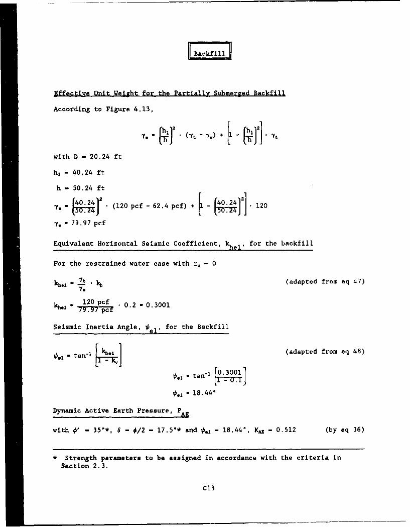
cf ill
Effecti-ve Unit Weight for the Partially Submerged Backfill
According to Figure 4.13,
lye(Tt - 7 )2 [ - • t
with D - 20.24 ft
h, - 40.24 ft
h - 50.24 ft
le W • (120 pcf - 62.4 pcf) + [1 - •.24.2] 120
Z 79.97 pcf
Equivalent Horizontal Seismic Coefficient, khl, for the backfill
For the restrained water case with r,, - 0
kh.1 - .LL. kb (adapted from eq 47)te
* 120 pcf . 0.2 - 0.3001T7T.E."T
Seismic Inertia Angle, 0el' for the Backfill
- tan.1 [.] (adapted from eq 48)
a•. a tan-1 [•3001
*,• - 18.44°
Dynamic Active Earth Pressure, !AE
with •" - 35*, 6 - 0/2 - 17.5"* and 0.1 - 18.44°, KAS - 0.512 (by eq 36)
* Strength parameters to be assigned in accordance with the criteria inSection 2.3.
C13
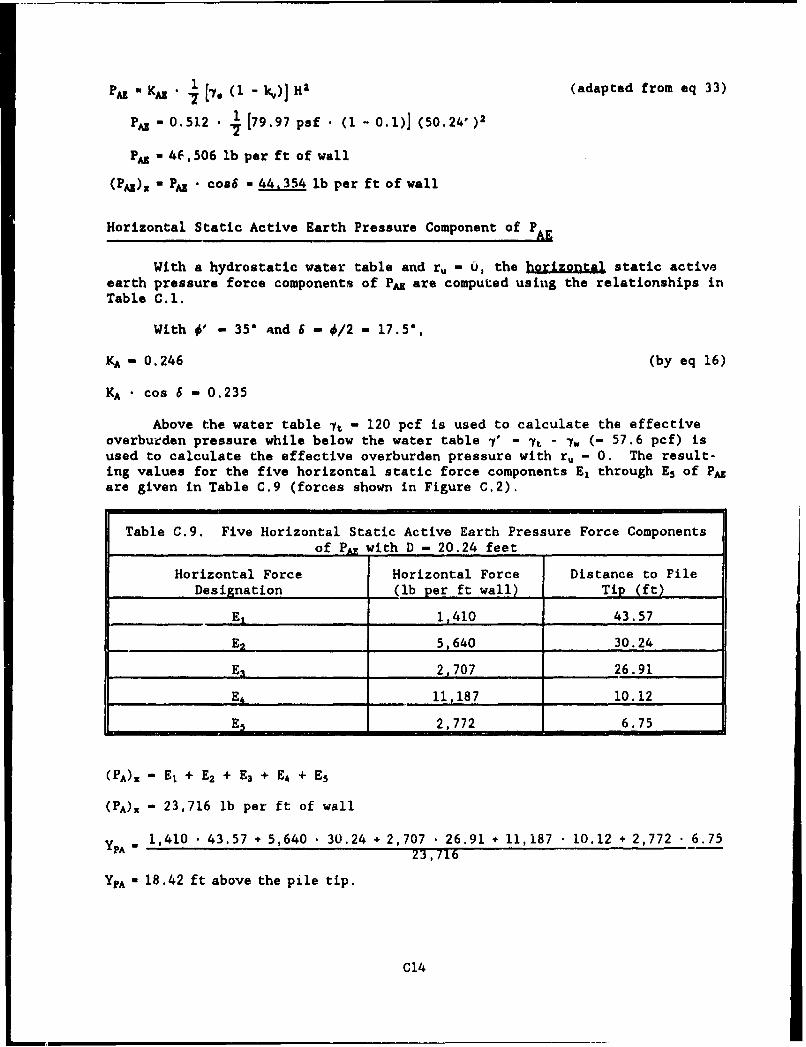
P KAS' l[, (1 k) ] H2 (adapted from eq 33)
- 0.512 . [79.97 psf . (1 - 0.1)] (50.24' )2-7
PAX 40,506 lb per ft of wall
(P•g)x PA ' cos6 - 44.354 lb per ft of wall
Horizontal Static Active Earth Pressure Component of PAE
With a hydrostatic water table and r, - 0, the hor•izgnta static activeearth pressure force components of PAE are computed using the relationships inTable C.l.
With 0' - 350 and 6 - 0/2 - 17.5',
KA - 0.246 (by eq 16)
KA cos 6 - 0.235
Above the water table It - 120 pcf is used to calculate the effectiveoverburden pressure while below the water table 7' - It - 7, (- 57.6 pcf) isused to calculate the effective overburden pressure with r, - 0. The result-ing values for the five horizontal static force components E, through E5 of PAEare given in Table C.9 (forces shown in Figure C.2).
Table C.9. Five Horizontal Static Active Earth Pressure Force Componentsof PR with D - 20.24 feet
Horizontal Force Horizontal Force Distance to PileDesignation (lb per ft wall) Tip (ft)
E, 1,410 43.57
E2 5,640 30.24
SE3 2,707 26.91
E4 11,187 10.12
E5 2,772 6.75
(PA), - E, + E2 + E3 + E4 + E.
(PA)x - 23,716 lb per ft of wall
YPA - 1,410 • 43.57 + 5,640 . 30.24 + 2,707 . 26.91 + 11,187 10.12 + 2,772 6.7523,716
YpA - 18.42 ft above the pile tip.
C14
Horizontal Component of the IncrementalDynamic Active Earth Pressure Force, (P AE)x
(APAX)x - (PA)x" (PA), (adapted from eq 40)
(APAZ)X - 44,354 - 23,716 - 20.638 lb per ft of wall
YApAZ - 0.6 . H - 0.6 • 50.24' - 30.14 ft above the pile tip.Y -AZ ' (PA)= YPA + (APAR)x 'YPAR (adapted from eq 44)
(PAZ)
YPAZ N 23,716 • 18.42 + 20,638 • 30.1444,354-
YpAZ - 23.87 ft above the pile tip.
IIBelow Dredge Level IEquivalent Horizontal Seismic Coefficient, k hel' Used in Front of Wall
For the restrained water case with r, - 0
kh.1 - L_ . k (by eq 47)7b
kh.1 - 120 pcf 0.2-120 pcf - 62.4 pcf)
kh., - 0.4167
Seismic Inertia Angle, t' Used in Front of Wall
0.1 - tan-1[rlJ (adapted from eq 48)
0.1 - tan-, r0'4167
-.1 - 24.84*
"Factored" Strengths Used in Front of Wall
By equation 95 with FS, - 1.2,*
tanot - tan 350
Ot - 30.30
By equation 96 with 6 - 0/2
* FSp - 1.2 for illustration purposes only. See discussion in footnote tostep 5.
C15
tan64 w tan 17.5'
st a 14.7"
"Factored" Dynamic Passive Earth Pressure Coefficient KPE
Method 1: Using the equivalent static formulation with Kp by Log-Spiralmethod (Section 4.4).
P* - " - -24.84"
9* - 9 - " -24.84"
Kp (0' - -24.84, 0* - -24.84, 0 - 30.3, 6 - -4) - 3.56 and R - 0.746 from
Caquot and Kerisel (1948). For 0 - 30.3' and 6 - -4/2,
Kp (f 0*, 6 -- /2) - 3.56 • 0.746
K, ((p 0', % , 6 -4/2) -2.66
F a cos 2 (9 - '.1) (eq 63)cos . cos 2 9
Fp = cos 2 [0 - (-24.84)] - 0.907cos (24.84) cosz (0)
KU Kp (#*, 9', 0, 6 = -0/2) . Fp'z (adapted from eq 62)
K* - 2.66 . 0.907 • 2.41
K *z cos 6t • 2.41 , cos(14.7) a 2.33
--------------------------------- Reference ------------------------------------
Method 2: Kp by Mononobe-Okabe.
with •" - 30.30, 6 - 14.7", 0,1 - 24.84*, P - 0* and 9 - 0*
K11 - 2.85 (by eq 60)
and
Kpz ' cos 6t - 2.76
The value of Kp by Hononobe-Okabe is 18 percent larger than the valuecalculated using the log-spiral method. Use the values computed by the Log-spiral method in the calculations that follow.
----------------------------------- End Reference ..............................
C16
"Factored" Horizontal Dynamic Passive Earth Pressure Force PPE
(Pz)1 . Kp . cos 6t [b ' (1 - kv)] D2 (adapted from eq 58)
- 2.33 . 4 [(120 pcf- 62.4 pcf) • (1 - 0.1)] (20.24)2
(P)a 24740 lb per ft of wall
•s D* .20.24 w 6.75 ft above the pile tip.
Pool In Front of Wall
Hydrodynamic Water rressure Force Pd
p. k_7%Y,. K001) 2 (by eq B-5)
1 .0.2 -62.4 pcf (21)2
P.d - 2.912 lb per ft of wall
Ypw - 0.4 . Hp.. - 8 ft above the dredge level.
Depth of Penetration
Eguilibrium of Moments About The Elevation of the Tie Rod
Mcc • (PAz)- x (1z + Hpool + D - YpAS)
+ Pwd" (HT2 + Hpoo, - 0.4.pool)
- 44,354 *(3' + 20' + 20.24' - 23.87')
+ 2,912 .(3' + 20' - 8')
* 859,137 + 43,680
PE for illustration purposes only, See discussion in footnote to
step 5.
C17
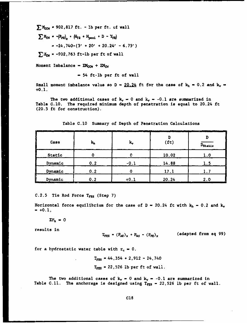
E•cc - 902,817 ft. - lb per ft. of wall
E * -(ýPp,) . - * H~1ý, + D - YM)
S-24,740#(3' + 20' + 20.24' - 6.75')
Efcw - -902,763 ft-lb per ft of wall
Moment Imbalance - +
- 54 ft-lb per ft of wall
Small moment imbalance value so D - 2Q,24 ft for the case of kh - 0.2 and k, -+0.1.
The two additional cases of v1 - 0 and k. - -0.1 are summarized inTable C.l0. The required minimum depth of penetration is equal to 20.24 ft(20.5 ft for construction).
table C.l0 Summary of Depth of Penetration Calculations
D DCase kh kv (ft) Dstatto
Static 0 0 10.02 1.0
Dynamic 0.2 -0.1 14.88 1.5
Dynamic 0.2 0 17.1 1.7
Dynamic 1 0.2 +0.1 20.24 2.0
C.2.5 Tie Rod Force Tns (Step 7)
Horizontal force equilibrium for the case of D - 20.24 ft with kh - 0.2 and k,- +0.1,
EFh - 0
results in
TFES - (PAz). + Pwd - (PPE)x (adapted from eq 99)
for a hydrostatic water table with r,, - 0.
Trzs - 44,354 + 2,912 - 24,740
TFZ3 - 22,526 lb per ft of wall.
The two additional cases of kv - 0 and kv - -0.1 are summarized inTable C.ll. The anchorage is designed using TFzs - 22,526 lb per ft of wall.
C18
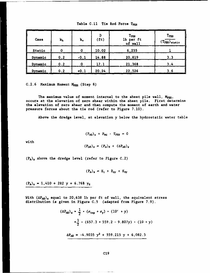
Table C.11 Tie Rod Force TIEs
D TrEs TFEsCase kh k., (ft) lb per ft (TFES).t.t±.
of wall _(T____-____
Static 0 0 10.02 1 6,255 1
Dynamic 0.2 -0.1 14.88 20,819 3.3
Dynamic 0.2 0 17.1 21,368 3.4
Dynamic 0.2 +0.1 20.24 22,526 3.6
C.2.6 Maximum Moment MFES (Step 8)
The maximum value of moment internal to the sheet pile wall, MFZs,occurs at the elevation of zero shear within the sheet pile. First determinethe elevation of zero shear and then compute the moment of earth and waterpressure forces about the tie rod (refer to Figure 7.10).
Above the dredge level, at elevation y below the hydrostatic water table
(PAZ). + Pwd - TFES - 0
with(PA~X"- (PA)x + (APA)X
(PA), above the dredge level (refer to Figure C.2)
(PA). - E1 + E2Y + E3Y
(PA), - 1,410 + 282 y + 6.768 Y2
With (APAE), equal to 20,638 lb per ft of wall, the equivalent stressdistribution is given in Figure C.5 (adapted from Figure 7.9).
S1 *. (Otp + Oy) * (10' + y)
= (657.3 + 559.2 - 9.807y) • (10 + y)
APAZ - .4.9035 y2 + 559.215 y + 6,082.5
C19
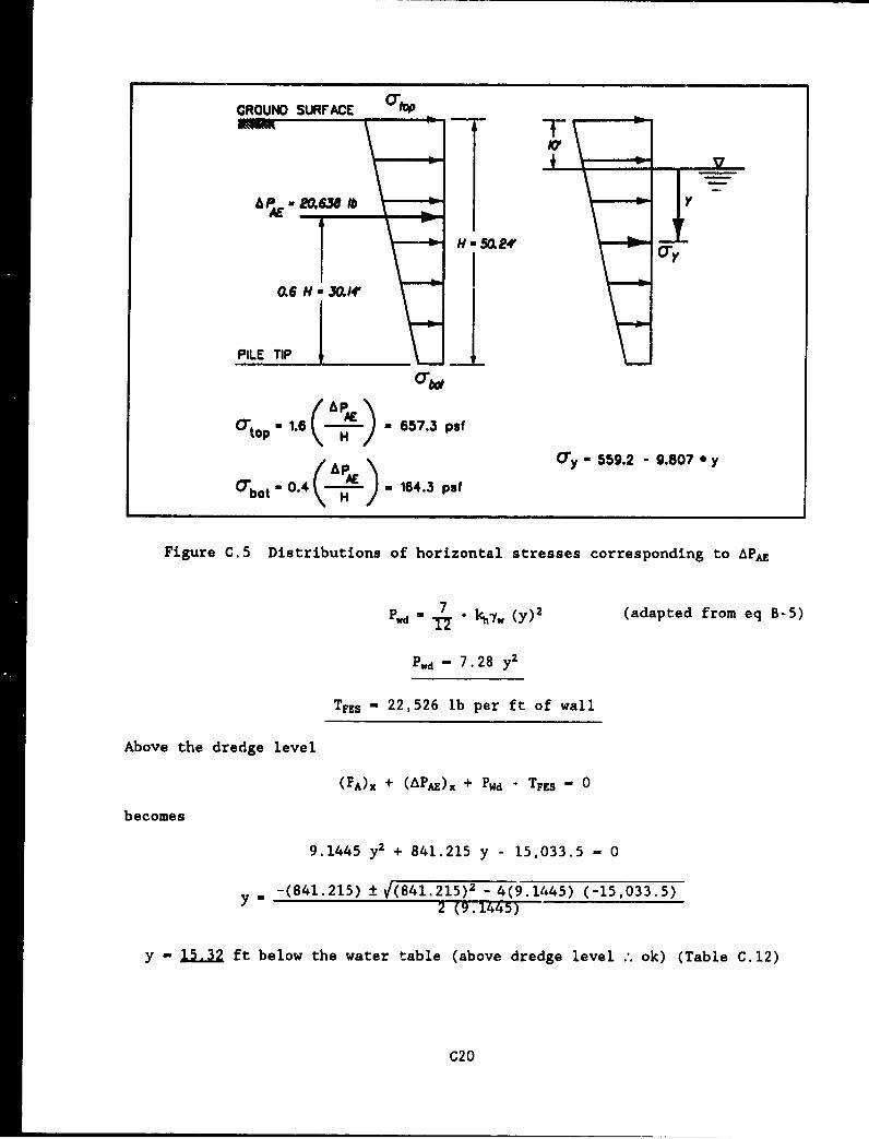
GROUND SURFACE
TV
211 -E,31b yAAE -M
I- 50.24' ,
0.6 N- 30./4"
PILE TIP
'top - 1.6 (HAE - 657.3 psf
AE O'y- 559.2 - 9.807 sy
~bt-0.4 _ s 164.3 put
Figure C.5 Distributions of horizontal stresses corresponding to APAE
.w - .* 7. (Y)Z (adapted from eq B-5)
Pwd - 7.28 y2
TFES - 22,526 lb per ft of wall
Above the dredge level
(FA)x + (APAE). + PWd - TFES - 0
becomes
9.1445 y2 + 841.215 y - 15,033.5 - 0
-(841.215) _±•/(841.215)2 - 4(9.1445) (-15,033.5)2 (9.1445)
y - 15.32 ft below the water table (above dredge level .*. ok) (Table C.12)
C20
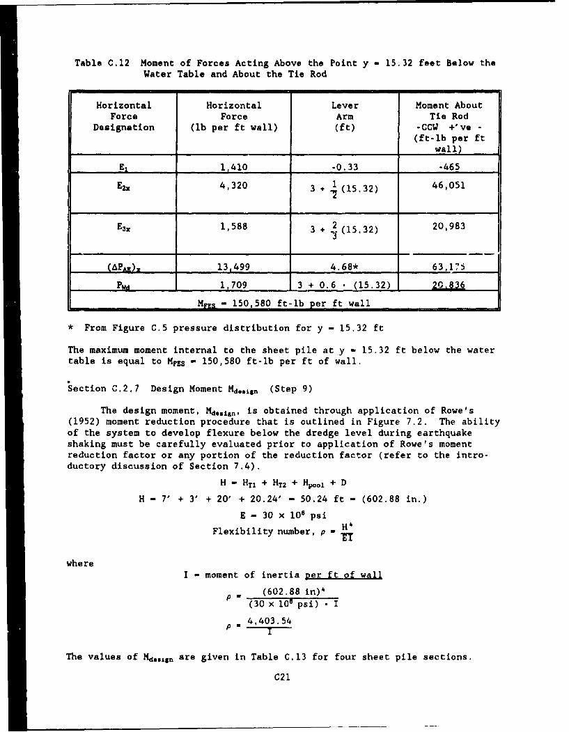
Table C.12 Moment of Forces Acting Above the Point y - 15.32 feet Below theWater Table and About the Tie Rod
Horizontal Horizontal Lever Moment AboutForce Force Arm Tie Rod
Designation (lb per ft wall) (ft) -CCW +'ve(ft-lb per ft
__wall)
E 1,410 -0.33 -465
E2x 4,320 3 + 1 (15.32) 46,051
E3, 1,588 3 + 2 (15.32) 20,983
___PA_)____- 13,499 4.68* 63,175
PWd 1,709 3 + 0.6 . (15.32) 20.836
MFES - 150,580 ft-lb per ft wall
* From Figure C.5 pressure distribution for y - 15.32 ft
The maximum moment internal to the sheet pile at y - 15.32 ft below the watertable is equal to MFzs - 150,580 ft-lb per ft of wall.
Section C.2.7 Design Moment Md..ign (Step 9)
The design moment, Md..n,, is obtained through application of Rowe's(1952) moment reduction procedure that is outlined in Figure 7.2. The abilityof the system to develop flexure below the dredge level during earthquakeshaking must be carefully evaluated prior to application of Rowe's momentreduction factor or any portion of the reduction factor (refer to the intro-ductory discussion of Section 7.4).
H - HT1 + HT2 + Hpool + D
H - 7' + 3' + 20' + 20.24' - 50.24 ft - (602.88 in.)
E - 30 x 106 psi
Flexibility number, p - H
whereI - moment of inertia per ft of wall
P (602.88 in)'(30 x 101 psi) • I
4,403.54
The values of Md..,sn are given in Table C.13 for four sheet pile sections.
C21
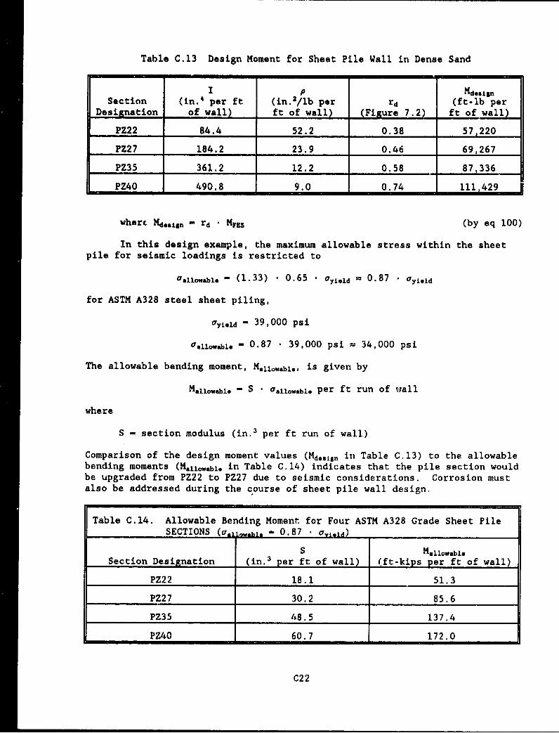
Table C.13 Design Moment for Sheet Pile Wall in Dense Sand
I p MdesignSection (in.' per ft (in. 2/lb per rd (ft-lb per
Designation of wall) ft of wall) (Figure 7.2) ft of wall)
PZ22 84.4 52.2 0.38 57,220
PZ27 184.2 23.9 0.46 69,267
PZ35 361.2 12.2 0.58 87,336
PZ40 490.8 9.0 0.74 111,429
wherc Mdesin - rd ' MFES (by eq 100)
In this design example, the maximum allowable stress within the sheetpile for seismic loadings is restricted to
Oallowabl. - (1.33) . 0.65 , ayield 2 0.87 ' ayigld
for ASTM A328 steel sheet piling,
ayi.ld - 39,000 psi
Oa1Imo.•o - 0.87 ' 39,000 psi - 34,000 psi
The allowable bending moment, Mallw0 bl., is given by
Mallowablo - S ' Oallowable per ft run of wall
where
S - section modulus (in. 3 per ft run of wall)
Comparison of the design moment values (Md.ssn in Table C.13) to the allowablebending moments (Ma.1o.able in Table C.14) indicates that the pile section wouldbe upgraded from PZ22 to PZ27 due to seismic considerations. Corrosion mustalso be addressed during the course of sheet pile wall design.
Table C.14. Allowable Bending Moment for Four ASTM A328 Grade Sheet PileSECTIONS (a awao0 blo - 0.87 , ovitid)
S MalowableSection Designation (in. 3 per ft of wall) (ft-kips per ft of wall)
PZ22 18.1 51.3
PZ27 30.2 85.6
PZ35 48.5 137.4
PZ40 60.7 172.0
C22
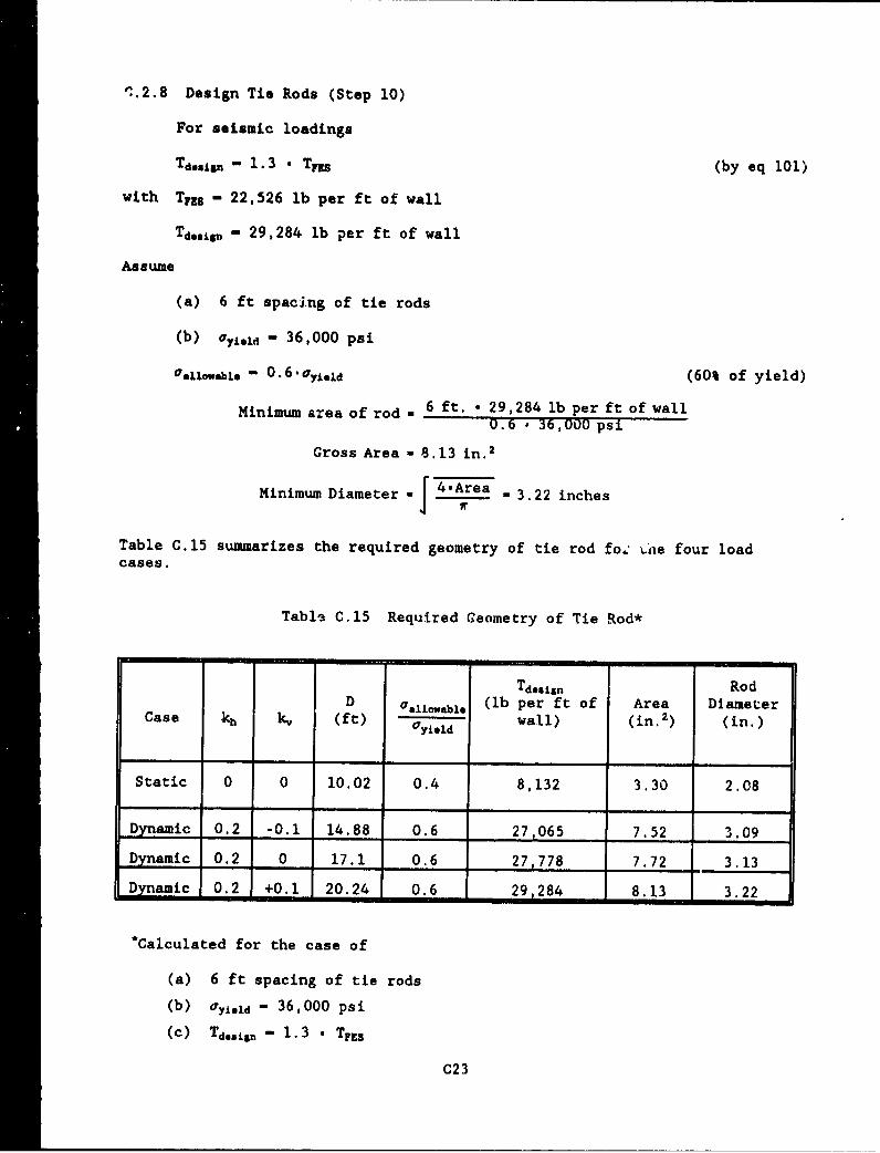
'..2.8 Design Tie Rods (Step 10)
For seismic loadings
Td.geig - 1.3 • Tru (by eq 101)
with TFU - 22,526 lb per ft of wall
Td..isn - 29,284 lb per ft of wall
Assume
(a) 6 ft spacing of tie rods
(b) ayi.,, - 36,000 psi
17a.lowabIe - 0. 6 '.yield (60% of yield)
Minimum area of rod - 6 ft. • 29,284 lb per ft of wall0.6 - 36,000 psi
Gross Area - 8.13 in. 2
Minimum Diameter - 4.Area - 3.22 inchesIr
Table C.15 summarizes the required geometry of tie rod fo.: .he four loadcases.
Table C.15 Required Geometry of Tie Rod*
Tdesian RodD gallowable (lb per ft of Area Diameter
Case kh k, (ft) Oyld wall) (in. 2 ) (in.)
Static 0 0 10.02 0.4 8,132 3.30 2.08
Dynamic 0.2 -0.1 14.88 0.6 27,065 7.52 3.09
Dynamic 0.2 0 17.1 0.6 27,778 7.72 3.13
Dynamic 0.2 +0.1 20.24 0.6 29,284 8.13 3.22
*Calculated for the case of
(a) 6 ft spacing of tie rods
(b) O'yi.ld - 36,000 psi
(c) Td..sn - 1. 3 - TFES
C23
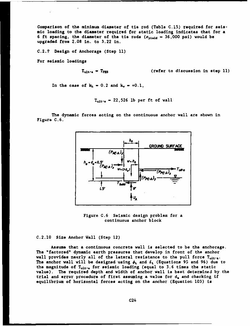
Comparison of the minimum diameter of tie rod (Table C.15) required for seis-mic loading to the diameter required for static loading indicates that for a6 ft spacing, the diameter of the tie rods (oyo1.d - 36,000 psi) would beupgraded from 2.08 in. to 3.22 in.
C.2.9 Design of Anchorage (Step 11)
For seismic loadings
Tult-. " Tns (refer to discussion in step 11)
In the case of kh - 0.2 and kI, - +0.1,
Tult- - 22,526 lb per ft of wall
The dynamic forces acting on the continuous anchor wall are shown inFigure C.6.
_TKGROUND SURFACE
AEM); e 4t YP P E.y - A~
tTN'
ULA
Figure C.6 Seismic design problem for acontinuous anchor block
C.2.10 Size Anchor Wall (Step 12)
Assume that a continuous concrete wall is selected to be the anchorage.The "factored" dynamic earth pressures that develop in front of the anchorwall provides nearly all of the lateral resistance to the pull force Tlt-...The anchor wall will be designed using Ot and 6t (Equations 95 and 96) due tothe magnitude of Tult-. for seismic loading (equal to 3.6 times the staticvalue). The required depth and width of anchor wall is best determined by thetrial and error procedure of first assuming a value for d, and checking ifequilibrium of horizontal forces acting on the anchor (Equation 103) is
C24
satisfied (step 12). Once the value of d, is determined, equilibrium of thevertical forces r_.ting on the anchor wall (Equation 104) will dictate theminimum value of wall width b.. Refer to Section C.1.9 in this appendix foradditional discussion of anchorage design.
This iterative procedure results in a minimum required depth ofanchorage equal to 11.5 ft and a minimum width of anchor wall equal to 4.5 ftThe calculations involved in Step 12 are summarized in the followingparagraphs for d, - 11.5 ft and (b,),,, - 4.5 ft in Figure C.6
Dynamic Active Earth Pressure Force PAE-A
For the case of d. - 11.5 ft (the anchor submerged 1.5 ft below thewater table), the effective unit weight is equal to
- 118.94 pcf
with hi - 1.5 ft and h - 11.5 ft in Figure 4.13.
The equivalent horizontal seismic coefficient kh., is equal to 0.2018(obtained by substituting 7, for 7b in Equation 47). A value of kh.1 equal to0.2 is used in the subsequent calculations.
For the case of kh., - 0.2 and k, - +0.1
0. tan-1 [I~.](adapted from eq 48)
-.1 - 12.529°
With €" - 350, 6 - 17.50 and 0.1 - 12.5290
K- 0.3987
andKA "cos 6 - 0.38
KAZ sin 6 - 0.12
With d. - 11.5 ft in Figure C.6.
(adapted from
(PAZ-A) 1 . KA *cos6 - 1 [i.(l - k,,)] (d.)z eq 33)
(PAZ-a). - 0.38 .1 [ 118.94 pcf (I - 0.1) 1 (11.5' 2)
(PAEA - 2,690 lb per ft of wall
C25
by a similar calculation
(Pjz-A)y - 849 lb per ft of wall
Dynamic Passive Earth Pressure Force PpE-A
With 0' - 35" and with FSp set equal to 1.2 in this example (see step 12discussion regarding the relationship between anchorage displacement and FSp)
O't - 30.3* (by eq 95)
and 6 - 17.5*,
6t - 14.7*
For 1 - 12.529* (refer to PAE-A calculations), t -30.3 and 6 t - 14.7
KpZ - 4.06 (by eq 60)
KpE cos 6t - 3.93
and
KpE sin 6t - 1.03
With da - 11.5 ft in Figure C.6
(adapted from eq
(PpE-A) 1 KpE *cos6 - 1Z[ -.* ( 1 - k ,)J (d.)2 58)
(Pt•.Ax - 3.93 .1 [118.94 pcf (1 -0.1) 1 (11.5' )2
(PPEA). - 27,818 lb per ft of wall
by a similar calculation
(Pp.EY - 7,291 lb per ft of wall
The depth of the continuous anchor wall is, governed by the equilibriumof horizontal forces. Ignoring the contribution of the shear force along thebase of the wall, Equation 103
T.It. - (Pn. - (PAZJ- W-%
For Figure C.6 concrete wall, the weight W per foot run of wall with d. -11.5 ft and 7 " 150 pcf is given by
C26
W = fcanc " ba"* s 1,725 .ba
Introducing this relationship for W and
kh - 0.2
TuIt-a - 22,526 lb per ft of wall (k, - +0.1)
(Pp-,)x - 27,818 lb per ft of wall
(PAR-A), - 2,690 lb per ft of wall
into the modified equation of horizontal equilibrium results in a Maximumvalue of b, equal to 7.5 ft for d. - 11.5 ft. Larger b, values would resultin excessive horizontal inerti- forces acting on the concrete block, requiringrevisions of the previous calculations.
Mobilization of friction along interface bf-tween the front of the anchorwall and the passive wedge requir-as that the w1ll have sufficient dead weightto restrain against upward movement as it displaces the soil in front of thewall (Dismuke 1991). The equation of equilibrium of vertical forces acting onthe wall is used to compute the minimum width of anchor wall. With N' setequal to zero, Equation 104 becomes
0 - W (1 - k,) - UA - (Ppg-A)y + (PAZA)
withW - 1,725 'ba
k, 0.1
UA 62.4 pcf "1.5"' b, - 93.6.ba
(Pn-A)y - 7,291 lb per ft of wall
(PAZ.A)y - 849 lb per ft of wall
the modified equation of vertical equilibrium results in a inimin value of b.equal to 4.4 ft or (b,)ei, - 4.5 ft.
Alternative Anchorage:
Other types of anchorages to be considered include slender anchorage,multiple tie rods and anchorage, A-frame anchors, sheet pile anchorage, soilor rock anchors and tension H-piles. Slender anchorage refers to a slenderwall designed using the procedure described in this section with 6 set equalto 0 degrees.
C.2.11 Site Anchorage (Step 13)
The anchor wall is to be located a sufficient distance behind the sheetpile wall so that the dynamic active failure surface does not intersect thepassive failure developing in front of the anchor wall. Figure C.7 outlinesthe aLjj required distances for this design problem.
C27
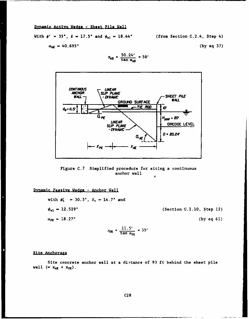
Dynamic Active Waedge - Sheat Pile Wall1
With 0' - 35", 6 - 17.5* and e " 18.44" (from Section C.2.4, Step 4)
Ax - 40.695" (by eq 37)
50.24' - 58'tan az
LCONTINOUS LINEARANCHOR EuNIG
WALL --.1, S-HEET PILE
GROUND SURFACE WWLc
~~~P~TI A 8.70(y q 1
1•1..5 T35j SP LNEAR DREDGE LEVELSU LANEA
" DYNAMC
Figure C.7 Simplified procedure for siting a continuous
anchor wall
Dynamic Passive Wedge - A lahor Wall
with 0' - 30.30, 6t - 14.7* and
, "12. 529° (Section C.2.10, Step 12)
oapz -18.27° (by eq 61)
11. 5" 5AEtan "apy
Site Anchorare
Site concrete anchor wall at a distance of 93 ft behind the sheet pile
wall (- xAz + xp).
C28
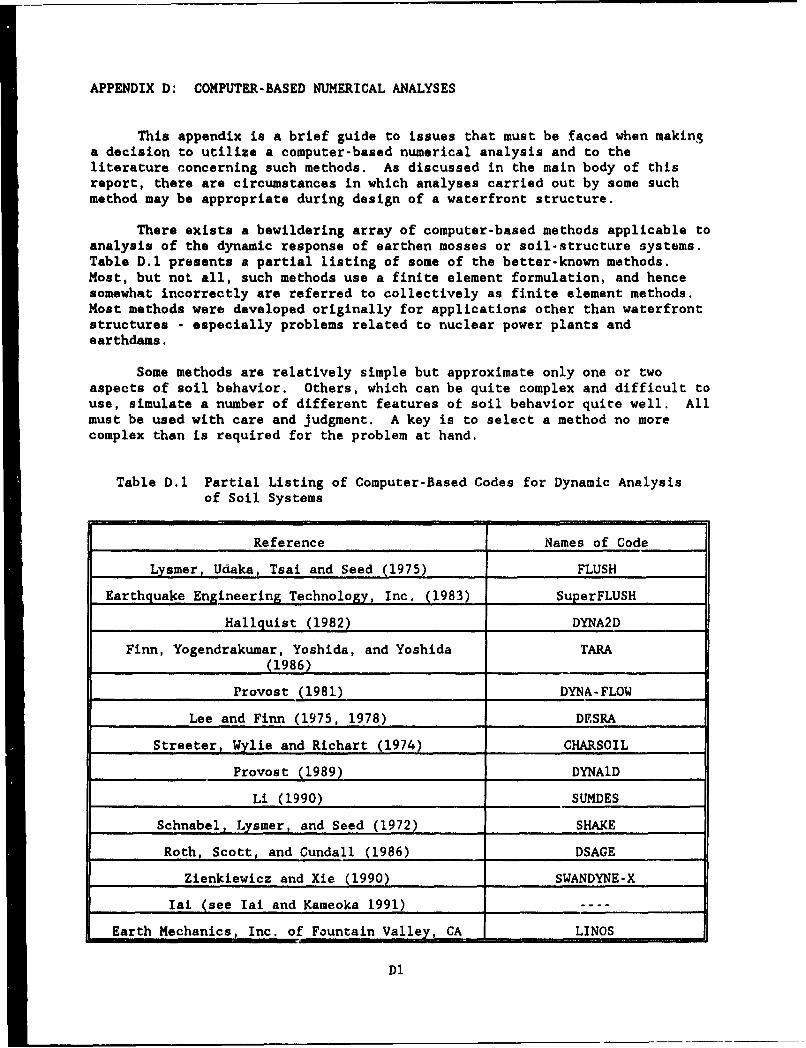
APPENDIX D: COMPUTER-BASED NUMERICAL ANALYSES
This appendix is a brief guide to issues that must be faced when makinga decision to utilize a computer-based numerical analysis and to theliterature concerning such methods. As discussed in the main body of thisreport, there are circumstances in which analyses carried out by some suchmethod may be appropriate during design of a waterfront structure.
There exists a bewildering array of computer-based methods applicable toanalysis of the dynamic response of earthen mosses or soil-structure systems.Table D.1 presents a partial listing of some of the better-known methods.Most, but not all, such methods use a finite element formulation, and hencesomewhat incorrectly are referred to collectively as finite element methods.Most methods were developed originally for applications other than waterfrontstructures - especially problems related to nuclear power plants andearthdams.
Some methods are relatively simple but approximate only one or twoaspects of soil behavior. Others, which can be quite complex and difficult touse, simulate a number of different features of soil behavior quite well. Allmust be used with care and judgment. A key is to select a method no morecomplex than is required for the problem at hand.
Table D.1 Partial Listing of Computer-Based Codes for Dynamic Analysisof Soil Systems
Reference Names of Code
Lysmer, Udaka, Tsai and Seed (1975) FLUSH
Earthquake Engineering Technology, Inc. (1983) SuperFLUSH
Hallquist (1982) DYNA2D
Finn, Yogendrakumar, Yoshida, and Yoshida TARA(1986) ... ...
Provost (1981) DYNA-FLOW
Lee and Finn (1975, 1978) DESRA
Streeter, Wylie and Richart (1974) CHARSOIL
Provost (1989) DYNAID
Li (1990) SUMDES
Schnabel, Lysmer, and Seed (1972) SHAKE
Roth, Scott, and Cundall (1986) DSAGE
Zienkiewicz and Xie (1990) SWANDYNE-X
Iai (see Iai and Kameoka 1991) ----
Earth Mechanics, Inc. of Fountain Valley, CA LINOS
Dl
D.l Some Key References
For dynamic soil-structure interaction analysis related to heavybuildings resting on earth, a concise summary of the various proceduresavailable is reported in the 1979 ASCE report by the Ad Hoc Group on Soil-Structure Interaction of the Committee on Nuclear Structures and Materials ofthe Structural Division. While in many ways out-of-date, this is still auseful reference concerning basic principles.
Several different finite element formulations are described in detail inChapter 3, titled Geomechanics and written in part and edited by W. D. L. Finnin the Finite Element Handbook, edited by H. Kardestuncer. The scope and typeof laboratory and/or field testing program used to characterize the soil modelparameters will vary among the computer codes, as discussed by Finn, theCommittee on Earthquake Engineering of the National Research Council (1985),and others.
Whitman (1992) has suggested a scheme for categorizing the various typesof methods, and has discussed the status of validation of various methods bycomparison to observations during actual earthquakes or to results from modeltests.
D.2 Principal Issues
According to the guidelines set forth by the ASCE Ad Hoc Group on Soil-Structure Interaction of the Committee on Nuclear Structures and Materials ofthe Structural Division 1979 report on the "Analysis For Soil-StructureInteraction Effects For Nuclear Power Plants" and the ASCE Standard (1986), toperform a complete soil-structure interaction analysis the analyticalprocedure must (1) account for the variation of soil properties with depth,(2) give appropriate consideration to the inaterial nonlinear behavior of soil,(3) consider the three-dimensional nature of the problem, (4) consider thecomplex nature of wave propagation which produced the ground motions, and(5) consider possible interaction with neighboring structures.
The reference to a "complete" analysis results from the existence of twodistinguishable aspects of soil-structure interaction: (1) the relativemotion of the foundation of the structure with respect to the surrcunding soilas a result of the inertial forces in the structure being transmitted to thecompliant soil foundation and backfill and/or (2) the inability of the stifferstructural foundation and walls to conform to the distortions of the soilgenerated by the ground motion. The former is referred to as inertialinteraction and the latter is referred to as kinematic interaction. Bothfeatures co-exist in most actual problems. However, several analyticalprocedures available to perform the soil-structure interaction analysis ofearth retaining structures take advantages of this separation of behavior intheir numerical formulation.
Specific feature that must be accounted fur in some problens includesoftening the soil stiffness during shaking, the material and geometricaldamping and the separation of portions of the backfill from the structure,followed by recontact or `:slap," that can occur during shaking. It may benecessary to use special interface elements at boundailes between soil andstructure. It also may be necessary to model the actual process ofconstruction as accurately as possible.
D2
D.2.1 Total versus Effective Stress Analysis
Effective stress analyses explicitly predict and take into account theeffects of excess pore pressures caused by the cyclic shearing of soil duringearthquake shaking. The generation of significant excess pore pressurescauses the stiffness of soil to degrade and may lead to a nearly-total loss ofshear strength. TARA, DYNAFLOW, DESRA, and DSAGE are examples of effectivestress analyses. 0s a general rule, such analyses should be used ifsignificant excess pore pressures are anticipated.
Total stress analyses do not explicitly account for the effects ofexcess pore pressures, although some may consider this effect indirectly byadjusting stiffness for the anticipated intensity of cyclic shear strains.FLUSH and SHAKE are examples of total stress analyses. Total stress analysesare appropriate when cohesionless soils are dry or very coarse, with mostcohesive soils, and for problems such as analyzing lateral earth pressurescaused by surface loadings.
D.2.2 Modeling Nonlinear Behavior
Using an effective stress analysis accounts partially, but not fully,for the nonlinear behavior of soils, in addition, it is necessary to considerthe effect of shear strain upon stiffness at a given effective stress.
As somewhat of an oversimplification, three ways of introducing suchnon-linearity have been utilized. (1) By using a linear analysis in whichshear modulus is linked, via an iterative procedure, to a measure of cyclicshear strain during shaking. FLUSH and SHAKE are examples of this approach.(2) By introducing a nonlinear stress-strain law, such as a hyperbolicbackbone curve together with Masing rules for strain reversals. DESRA andTARA are examples. (3) By utilizing concepts and principles from the theoryof plasticity. DYNAFLOW is an example of this approach.
It is not really possible to say that one way is better than another.All involve some degree of approximation. The choice involves a trade-offbetween accuracy and convenience/cost, and perhaps the availability of a code.
D.2.3 Time versus Frequency Domain Analysis
Problems involving nonlinear material behavior can be solved in either(1) the time domain or (2) the frequency domain by using equivalent linearmaterial property approximations for the nonlinear material(s). The one-dimensional computer programs DESRA, CHARSOIL, DYNAlD, and SUMDES and the two-dimensional programs TARA, DYNA-FLOW, and DYNA2D are examples of the timedomain procedure. The one-dimensional computer program SHAKE and the two-dimensional programs FLUSH and SuperFLUSH are examples of the frequency domainsolutions.
Frequency-domain techniques formerly favored owing to greatercomputational efficiency. However, the growth in the power of relativelyinexpensive computers has diminished this advantage.
D3
D.2.4 1-D versus 2-D versus 3-D
Today it in, in principle possible to model the three-dimensionalaspects of soil responae problems, but seldom is the effort Justified. Inmany cases the responses of a soil profile can be modeled satibfactorily usinagone-dimensional programs such as SHAKE, CHARSOIL, or DESRA. For most problemsinvolving retaining structures, a 2-D analysis (such as TARA, DYNAFLOW,DYNA2D, or DSAGE) will be necessary. The code FLUSH approximates some aspectsof 3-D response,
D.2.5 Nature of Input Ground Motion
Typically analyses use the idealization that the patterns of groundmotion are simple mechanisms; the most common procedures use verticallypropagating shear waves or dilatation waves. While it is possible to considermore general forms of input with horizontally traveling waves, seldom willsuch an effort be warranted for waterfront structures.
D.2.6 Effect of Free Water
Consider the problem of a complete soil-structure interaction analysisof the earth retaining structure shown in Figure D.la. The finite elementmesh used to model this problem includes the retaining structure, the soilbackfill and the pool of water in front of the wall, as shown in Figure D.lb.The mass and stiffness effects are included within the analysis for both thestructure and the soil backfill by incorporating these regimes within thefinite element mesh that is used to model the problem. Most computer codes donot include within their formulation a water element among their catalog offinite elements, so the Westergaard (1931) added water mass procedure is usedto account for the effect of the hydrodynamic water pressures on the dynamicresponse of the retaining wall (see Appendix B). One computer code that doesinclude a fluid element within its catalog of elements is SuperFLUSH.
D.3 A Final Perspective
The preparation time for developing the finite element mesh, assigningmaterial properties, selecting the ground motion, performing the analysis, andinterpreting the computed results is much greater than the time required forperforming a simplified analysis. However, the information provided by adynamic finite element analysis is much more complete and extensive. Thecomputed results include: the variation in computed accelerations with timeand the variation in computed dynamic normal and shear stresses with timethroughout the wall and the soil regime(s). Thus, a complete soil-structureinteraction analysis, when done properly, provides much more accurate anddetailed information regarding the dynamic behavior of the earth retainingstructure being analyzed.
In a complete soil-structure interaction analysis, the total earthpressures along the back of the wall at any time during the earthquake areequal to the sum of the computed dynamic earth pressures and the 3tatic earthand water pressures. At any elevation along the back of the wall, theeffective stress component (static + dynamic) of this total pressure isrestricted to range in values between the static active earth pressure valueand the static passive earth pressure value. Exceedence of these values mayoccur where in actuality separation way occur during earthquake shaking.
D4
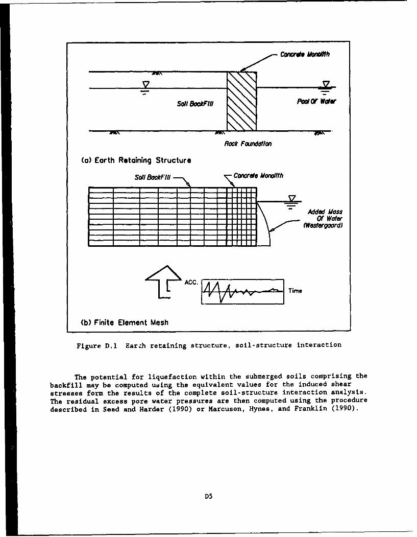
iil
f ~Cowde JMx~th
"Soil 6ockFIII L\ \ F '
Rock FoundotIon
(a) Earth Retoining Structure
Soil/ Bakf'Il \Cmwer Monolith
- " -Added Moss- -or Water
"- -'- - - - -tesergoard)
- -- c d- - ---
<AcCC.AA Time
(b) Finite Element Mesh
Figure D.1 Earch retaining structure, soil-structure interaction
The potential for liquefaction within the submerged soils comprising thebackfill may be computed using the equivalent values for the induced shearstresses form the results of the complete soil-structure interaction analysis.The residual excess pore water pressures are then computed using the procedure
described in Seed and Harder (1990) or Marcuson, Hynes, and Franklin (1990).
D5
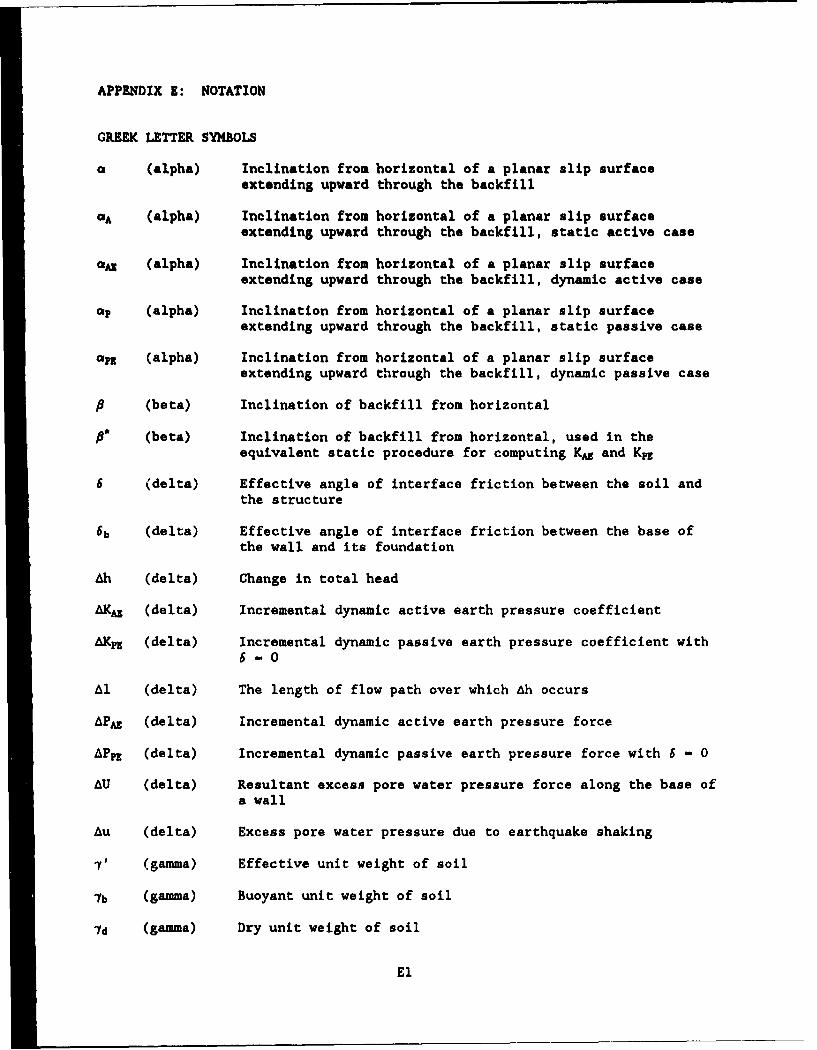
APPENDIX E: NOTATION
GREEK LETTER SYMBOLS
a (alpha) Inclination from horizontal of a planar slip surfaceextending upward through the backfill
A (alpha) Inclination from horizontal of a planar slip surfaceextending upward through the backfill, static active case
aS (alpha) Inclination from horizontal of a planar slip surfaceextending upward through the backfill, dynamic active case
ap (alpha) Inclination from horizontal of a planar slip surfaceextending upward through the backfill, static passive case
an (alpha) Inclination from horizontal of a planar slip surfaceextending upward through the backfill, dynamic passive case
(beta) Inclination of backfill from horizontal
(beta) Inclination of backfill from horizontal, used in the
equivalent static procedure for computing KAZ and Kp
6 (delta) Effective angle of interface friction between the soil andthe structure
6b (delta) Effective angle of interface friction between the base of
the wall and its foundation
Ah (delta) Change in total head
AKAZ (delta) Incremental dynamic active earth pressure coefficient
AKpj (delta) Incremental dynamic passive earth pressure coefficient with6 - 0
Al (delta) The length of flow path over which Ah occurs
APAE (delta) Incremental dynamic active earth pressure force
APpZ (delta) Incremental dynamic passive earth pressure force with 6 - 0
AU (delta) Resultant excess pore water pressure force along the base ofa wall
Au (delta) Excess pore water pressure due to earthquake shaking
7 (gamma) Effective unit weight of soil
lb (gamma) Buoyant unit weight of soil
'd (gamma) Dry unit weight of soil
El
7. (gamma) Effective unit weight of & partially submerged backfill forthe restrained water case
70s (gamma) Effective unit weight of soil for the restrained water case
with r, > 0
7t (gamma) Total unit weight of soil
7W (gamma) Unit weight of water
7w3 (gamma) Effective unit weight of water for the restrained water casewith ru, > 0
* (phi) Effective angle of internal friction for soil
*' (phi) Equivalent angle of internal friction for soil with r. > 0
(psi) Seismic inertia angle
(psi) Seismic inertia angle
0.1 (psi) Equivalent seismic inertia angle for the restrained watercase with ru - 0
0.z (psi) Equivalent seismic inertia angle for the free water casewith ru - 0
0.3 (psi) Equivalent seismic inertia angle for the restrained watercase with ru > 0
0.4 (psi) Equivalent seismic inertia angle for the free water case
with ru > 0
a (sigma) Total normal stress
at (sigma) Effective normal stress
ae (sigma) Active earth pressure (effective stress)
up (sigma) Passive earth pressure (effective stress)
a' V (sigma) Vertical effective stress
a#v-initjal Pre-earthquake vertical effective stress
a t' (sigma) Effective weight of backfill, excluding surcharge
S(tau) Shear stress
T (tau) Shear stress at failure
0 (theta) Inclination of the back of wall to soil interface fromvertical
E2
0* (theta) Inclination of the back of the wall to soil interface from
vertical, used in the equivalent static procedure forcomputing KA and Kp1
ROMAN LETTER SYMBOLS
A Maximum ground acceleration as a fraction of g (dimensionless)
ah Maximum horizontal ground acceleration, equal to kh-g
a& Maximum ground acceleration, equal to A'g
av Maximum vertical ground acceleration, equal to kv'g
B Width of wall base
B, Effective base width of the wall in contact with the foundation
c Effective cohesion
c1 Constant used to compute aA
c2 Constant used to compute aA
c3 Constant used to compute ap
c4 Constant used to compute op
CeM Constant used to compute aA
CUE Constant used to compute aA
c3U Constant used to compute ap1
COE Constant used to compute ap
dr Maximum displacement
FAZ Factor used in the equivalent static procedure to compute KA
Fb Factor of safety against bearing capacity failure of a wall
Fps Factor used in the equivalent static procedure to compute KpE
F, Factor of safety against sliding along the base of a wall
For Lateral seismic force component by Woods procedure
FSP Factor of safety applied to both the shear strength of the soil and theeffective angle of friction along the interface when computing PpE fora sheet pile wall and the anchorage.
g Acceleration of gravity
H Height of wall
E3
h Total head
h. Elevation head
hp Pressure head
HFstatic Static component of heavy fluid force behind a wall retaining liquefiedbackfill
HF1 .. ti, Inertial component of heavy fluid force behind a wall retainingliquefied backfill during shaking
L Seepage gradient, equal to Ah/A1
KA Static active earth pressure coefficient
KAE Dynamic active earth pressure coefficient
Kh Horizontal earth pressure coefficient
kh Horizontal seismic coefficient as a fraction of g (dimensionless.
kh* Limiting value for the horizontal seismic coefficient as a fraction ofg (dimensionless)
kh. Equivalent horizontal seismic coefficient as a fraction of g(dimensionless)
kh.1 Equivalent horizontal seismic coefficient as a fraction of g(dimensionless) for the restrained water case with r, - 0
kh.2 Equivalent horizontal seismic coefficient as a fraction of g(dimensionless) for the free water case with r, - 0
kh.3 Equivalent horizontal seismic coefficient as a fraction of g(dimensionless) for the restrained water case with r, > 0
kh.4 Equivalent horizontal seismic coefficient as a fraction of g(dimensionless) for the free water case with r, > 0
rp Static passive earth pressure coefficient
KpZ Dynamic passive earth pressure coefficient
kv Vertical seismic coefficient as a fraction of g (dimensionless)
K. At-rest horizontal earth pressure coefficient
Md~sign Design moment for a sheet pile wall
MFES Maximum moment computed using the Free Earth Support method for a sheetpile wall
N Total normal force oetween the wall and the foundation
E4
N' Effective normal force between the wall and the foundation
N* Maximum transmissible acceleration coefficient, as a fraction of g(dimensionless)
P Resultant earth pressure force acting on a wall
PA Active earth pressure force acting on a wall for static loading
PA Active earth pressure force acting on a wall for pseudo-static loading
Pp Passive earth pressure force acting on a wall for static loading
PE Passive earth pressure force acting on a wall for pseudo-static loading
P~d Westergaard hydrodynamic water pressure force
q Vertical surcharge stress
qaj1 allowable bearing pressure of rock
q,= maximum bearing pressure below toe of wall
qu. ultimate bearing capacity or unconfined compressive strength ofconcrete
rd Moment reduction factor due to Rowe
ru Excess pore water pressure ratio, equal to Au/o'v-initial
Su Undrained shear strength of soil
T Horizontal shear force along the base of the wall required forequilibrium
Td.sisn Design tie rod force for a sheet pile wall
Tns Tie rod force computed using the Free Earth Support method for a sheetpile wall
T.It Ultimate horizontal shear force along the base of the wall
Tuft. Ultimate force for which the sheet pile wall anchorage is to bedesigned
Ub resultant steady state pore water pressure force normal to the base ofthe wall
Uin.rtis Hydrodynamic water pressure force for the pool, directed away from thewall
UPOOL Resultant hydrostatic water pressure force for the pool
E5
Ushear Resultant excess pore water pressure force due to earthquake shakingacting normal to the backfill to wall interface
Ushear.b Resultant excess pore water pressure force due to earthquake shakingacting normal to the backfill to sheet pile wall interface
Ushsar.t Resultant excess pore water pressure force due to earthquake shakingacting normal to the dredge level soil to sheet pile wall interface
Ushear.a Resultant excess pore water pressure force due to earthquake shakingacting normal to planar slip surface inclined at a from vertical
Ustatic Resultant steady state pore water pressure force acting normal to thebackfill to wall interface
Ustati 0cb Resultant steady state pore water pressure force acting normal to thebackfill to sheet pile wall interface
Ustatic.t Resultant steady state pore water pressure force acting normal to thedredge level soil to sheet pile wall interface
Uutatic.. Resultant steady state pore water pressure force acting normal to
planar slip surface inclined at a from vertical
u Steady-state pore water pressure
V Maximum ground velocity
W Weight of rigid body (e.g. wall or soil wedge)
w Water content of soil
XN Point of action of normal force N
E6
Waterways Experiment Station Cataloglng-ln-Publioatlon Data
Ebeling, Robert M.The seismic design of waterfront retaining structures / by Robert M.
Ebeling and Ernest E. Morrison, Jr. ; prepared for Department of theArmy, US Army Corps of Engineers and Department of the Navy, NavalCivil Engineering Laboratory.
325 p. : Ill. ; 28 cm. - (Technical report ; ITL-92-1 1) (Technical reportNCEL TR-939)
Includes bibliographical references.1. Breakwaters - Design and construction. 2. Soil-structure
Interaction. 3. Retaining walls - Earthquake effects. 4. Earthquake en-gineering. I. Morrison, Ernest E. II. United States. Army. Corps of Engi-neers. III. Naval Civil Engineering Laboratory (Port Hueneme, Calif.)IV. U.S. Army Engineer Waterways Experiment Station. V. Computer-aided Structural Engineering Project. VI. Title. VII. Series: Technical re-port (U.S. Army Engineer Waterways Experiment Station) ; ITL-92-1 1.Viii. Series: Technkml report (Naval Civil Engineering Laboratory (PortHueneme, Calif)) ; 939.TA7 W34 no.ITL-92-11

WATERWAYS EXPERIMENT STATION REPORTSPUBLISHED UNDER THE COMPUTER-AIDED
STRUCTURAL ENGINEERING (CASE) PROJECT
Title Date
Technical Report K-78-1 List of Computer Programs for Computer.Aide"n Structural Engineering Feb 1978
Instruction Report 0-79-2 User's Guide: Computer Program with Interactive Graphics for Mar 1979Analysis of Plane Frame Structures (CFRAME)
Technical Report K-80-1 Survey of Bridge-Oriented Design Software Jan 1980
Technical Report K-80-2 Evaluatinn of Computer Programs for the Design/Analysis of Jan 1980Highway and Railway Bridges
Instruction Report K-80-1 User's Guide: Computer Program for Design/Review of Curvi- Feb 1980linear Conduits/Culverts (CURCON)
Instruction Report K-80-3 A Three-Dimensional Finite Element Data Edit Program Mar 1980
Instruction Report K-80-4 A Three-Dimensional Stability Analysis/Design Program (3DSAD)Report 1: General Geometry Module Jun 1980Report 3: General Analysis Module (CGAM) Jun 1982Report 4: Special-Purpose Modules for Dams (CDAMS) Aug 1983
Instruction Report K-80-6 Basic User's Guide: Computer Program for Design and Analysis Dec 1980of lnverteJ-T Retaining Walls and Floodwalls (TWDA)
Instruction Report K-80-7 User's Reference Manual: Computer Program for Design and Dec 1980Analysis of Inverted-T Retaining Walls and Floodwalls (TWDA)
Technical Report K-80-4 Documentation of Finite Element AnalysesReport 1: Longview Outlet Works Conduit Dec 1980Report 2: Anchored Wall Monolith, Ray Springs Lock Dec 1980
Technical Report K-80-5 Basic Pile Group Behavior Dec 1980
Instruction Report K-81-2 User's Guide: Computer Program for Design and Analysis of SheetPile Walls by Classical Methods (CSHTWAL)
Report 1: Computational Processes Feb 1981Report 2: Interacive Graphics Options Mar 1981
Instruction Report K-81-3 Validation Report: Computor Program for Design and Analysis of Feb 1981Inverted-T Retaining Walls and Floodwalls (TWDA)
Instruction Report K-81-4 User's Guide: Computer Program for Design and Analysis of Mar 1981Cast-in-Place Tunnel Linings (NEWTUN)
Instruction Report K-81-6 User's Guide: Computer Program for Optimum Nonlinear Dynamic Mar 1981Design of Reinforced Concrete Slabs Under Blast Loading(CBARCS)
Instruction Report K-81-7 User's Guide: Computer Program for D'•sign or Investigation of Mar 1981Onhogonal Culverts (CORTCUL)
Instruction Report K-81-9 User's Guide: Computer Program for Th-ee-Diniensional Analysis Aug 1981of Building Systems (CTABS80)
Technical Report K-8 -2 Theoretical Basis for CTABS8a: A C;omputer Program for Sep 1981Three-Dimensional Analvsis of Building Systems
Instruction Report K-82-6 User's Guide: Computer 1- rogiamn for Analysis of Beam-Column Jun 1982Structures with Nor'linea, Supports (CBEAMC)
(Continued)
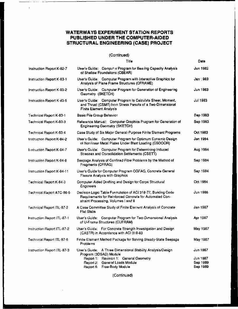
WATERWAYS EXPERIMENT STATION REPORTSPUBLISHED UNDER THE COMPUTER-AIDED
STRUCTURAL ENGINEERING (CASE) PROJECT
(Continued)
Title Date
Instruction Report K-82-7 User's Guide: Compu,-r Program for Bearing Capacity Analysis Jun 1982of Shallow Foundations (CBEAR)
Instruction Report K-83-1 User's Guide: Computer Program with Interactive Graphics for Jan ', 983Analysis of Plane Frame Structures (CFRAME)
Instruction Report K-83-2 User's Guide: Computer Program for Generation of Englneerlng Jun 1983Geometry (SKETCH)
Instruction Report K-83-5 User's Guide: Computer Program to Calculate Shear, Moment, Jul 1983and Thrust (CSMT) from Stress Pesults of a Two-DimensionalFinite Element Analysis
Technical Report K-83-1 Basic Pile Group Behavior Sep 1983
Technical Report K-83-3 Reference Manual: Computer Graphics Program for Generation of Sep 1983Engineering Geometry (SKETCH)
Technical Report K-83-4 Case Study of Six Major General-Purpose Finite Element Programs Oct 1983
Instruction Report K-84-2 User's Guide: Computer Program for Optimum Dynamic Design Jan 1984of Nonlinear Metal Plates Under Blast Loading (CSDOOR)
Irstruction Report K-84-7 User's Guide: Computer Program for Determining Induced Aug 1984Stresses and Consolidation Settlements (CSETT)
Instruction Repol K-84-8 Seepage Analysis of Confined Flow Problems by the Method of Sep 1984Fragments (CFRAG)
Instruction Report K-84-11 User's Guide for Computer Program CGFAG, Concrete General Sep 1984Flexure Analysis with Graphics
Technical Report K-84-3 Computer-Aided Drafting and Design for Corps Structural Oct 1984Engineers
Technical Report ATC-86-5 Decision Logic Table Formulation of ACI 318-77, Building Codo Jun 1986Requirements for Reinforced Concrete for Automated Con-straint Processing, Volumes I and II
Technical Report ITL-87-2 A Case Committee Study of Finite Eleroent Analysis of Concrete Jan 1987Flat Slabs
Instruction Report ITL-87-1 User's Guide: Computer Program for Two-Dimensional Analysis Apr 1987of U-Frame Structures (CUFRAM)
Instruction Report ITL-87-2 User's Guide: For Concrete Strength Investigation and Design May 1987(CASTR) in Accordance with ACI 318-83
Technical Report ITL.87-6 Finite-Element Method Package for Solving Steady-State Seepage May 1987Problems
Instruction Report ITL-87-3 User's Guide: A Three Dimensional Stab;lity Analysis/Design Jun 1987Program 13DSAD) Module
Report 1: Revision 1: General Geometry Jun 1987Report 2: General Loads Module Sep 1989Report 6: Free-Body Module Sep 1989
(Continued)

WATERWAYS EXPERIMENT STATION REPORTSPUBLISHED UNDER THE COMPUTER-AIDED
STRUCTURAL ENGINEERING (CASE) PROJECT
(Continued)Title Date
Instruction Report ITL-87-4 User's Guide: 2-D Frame Analysis Link Program (LINK2D) Jun 1987
Technical Report ITL-87-4 Finite Element Studies of a Horizontally Fremed Miter Gate Aug 1987Report 1: Initial and Refined Finite Element Models (Phases
A, B, And C0, Volumes I and IIReport 2: 3implifled Frame Model (Phase D)Report 3: Alternate Configuration Miter Gate Finite Element
Stud'es.-Open SectionReport 4: Alternate Configuration Miter Gate Finitc Element
Studies-Closed SectionsReport 5: Alternate Configuration Miter Gate Finite Element
Studies-Additional Closed SectionsReport 6: Elastic Buckling of Girders in Horizontally Framed
Miter GatesReport 7: Applicatior and Summary
Instr•uction Roport GL-87-1 User's Guide- UTEXAS2 Slope-Stability Package; Volume I. Aug 1987User's Manual
Instruction Report ITL-87-5 Sliding Stability of Concrete Structures (CSLIDE) Oct 1987
Instruction Report ITL-87-6 Criteria Specifications for and Validation of a Computer Program Dec 1987for the Design cr Investigation of Horizontally Framed MiterGates (CMITER)
Technical Report ITL-87-8 Procedure for Static Analysis of Gravity Dans Using the Finite Jan 1988Element Method - Phase 1 a
Instruction Report ITL-88-1 User's Guide: Computer Program for Analysis of Planar Grid Feb 1988Structures (CGRID)
Technical Report ITL-88-1 Development of Design Formulas for Ribbed Mat Foundations Apr 1988on Expansiv ,3oils
Technical Report iTL-e8-2 User's Guide: Pile Group Graphics Display (CPGG) Post- Apr 1988processor to CPGA Program
Instruction Report ITL-88-2 User's Guide fur Design and Investigation cf Horizontally Framed Jun 1988Miter Gates (CMITER)
Instruction Report iTL-88-4 User's Guide for Revised Computer Program to Calculate Shear, Sep 1988Moment, and Thrust (CSMT)
Instruction Report GL-87-1 User's Guide: UTEXAS2 Slope-Stahility Package; Volume II, Feb 1989Theory
Technical Report ITL-89-3 User's Guide: Pile Group Analysis (CPGA) Computer Group Jul 1989
Technical Report ITL-89-4 CBASIN-Structural Design of Saint Anthony Falls Sti~ling Basins Aug 1989According to Corps of Enginners Criteria for HydraulicStructures; Computer Program X0098
(Continued)
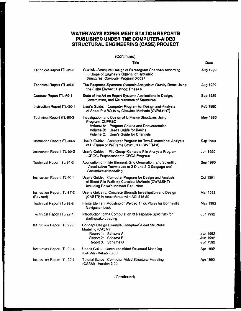
WATERWAYS EXPERIMENT STATION REPORTSPUBLISHED UNDER TWE COMPUTER-AIDED
STRUCTURAL ENGINEERING (CASE) PROJECT
(Continued)
Title Date
Technical Report ITL-89-5 CCHAN-Structural Design of Rectangular Channels Aocording Aug 1989ij Cops of Engineers Criteria for HydrauiicStructures; Computer Program X0097
Technical Report ITL-89-6 The Response-Spectrum Dynamic Analysis of Gravity Dams Using Aug 1989the Finite Element Mlethod; Phase II
Contract Report ITL-89-1 State of the Art on Expert Systems Applications In Design, Sep 1989Oonstruclion, and Maintenance of Structures
Instruction Report ITL-90-1 User's Guide: (.omputer Program for Design and Analysis Feb 1990of Sheet Pile Walls by Clasbical Methods (OWALSHT)
Technical Report ITL-90-3 Invostigation and Design of U-Frame Structures Using May 1990Program CUFRBC
Volume A: Program Criteria and DocumentationVolume B: User's Guide for BasinsVolume C: User's Guide for Channels
Instruction Report ITL-90-6 Usei's Guide: Computer Program for Two-Dimensional Aralysis Sep 1990of U-Frame or W-Frame Structures (CWFRAM)
Instruction Report ITL-90-2 User's Guide: Pile Group-Concrete Pile Analysis Program Jun 1990(CPGC) Prepmocessor to CPGA Program
Technical Report ITL-91-3 Application of Finite Element, Grid Generation, and Scientific Sep 1990Visualization Techniques to 2-D and 3-D Seepage andGroundwater Modeling
Instruction Report ITL-91-1 User's Guide: Computer Program for Dosign and Analysis Oct 1'991of Sheet-Pile Walis by Classical Mothods (CWAI.SHT)Including Rowe's Moment Reduction
Instruction Report ITL-87-2 User's Guide for Concrete Strength Investigation and Design Mar 1992(Revised) (CASTR) in Accordance with ACI 318-89
Technical Report ITL-92-2 Fiinite Element Modeling of Welded Thick Plates for Bonneville May 1992Navigation Lock
Technical Rgport ITL.92-4 Introduction to the Computation of Response Spectrum for Jun '992Earthquake Loading
Instrut.:ion Report ITL-92-3 Concept Design Example, Computer'Aided StructuralModeling (CA3M)
Report 1" Scheme A Jun 1992Report 2: Scheme B Jun 1992Report 3: Scheme C Jun 1992
Instruction Report iTL-92-4 User's Guide: Computer-Aided Structurnl Modeling Apr 1992(CASM) - Version 3.00
instruction Report IT.-92-5 Tutorial Guide: Computer-Aided Structural Modeling Apr 1992(CASM) - Version 3.00
(Continued)
WATERWAYS EXPERIMENT STATION REPORTSPUBLISHED UNDER THE COMPUTER-AIDED
STRUCTURAL ENGINEERING (CASE) PROJECT
(Concluded)Title Date
Contract Report ITL-92-1 Optimization of Steel Pile Foundations Using Optlmality Criteria Jun 1992
Technical Report ITL-92-7 Refined Stress Analysis of Melvin Price Locks and Dam Sep 1992
Contract Report ITL-92-2 knowledge-Based Expert System lor Selection and Design Sep 1992of Retaining Structures
Contract Report ITL-92-3 Evaluation of Thermal and Incremental Construction Effects Sep 1992for Monoliths AL-3 and AL-6 of the Melvin Price Locksand Dam
Instruction Report GL-97-1 Use!'s Guide: UTEXAS3 Slope-Stability Package; Volume IV, Nov 1992User's Manual
Technical Report ITL-92-1 I The Seismic Design of Waterfiont Retaining Structures Nov 1992
Technical Report ITL-92-12 Computer-Aided, Field-Verffied Structural EvaluationReport 1: Development of Computer Modeling Techniques Nov 1992
for Miter Lok GatesReport 2' Field Test and Analysis Correlation at John Hollis Dec 1992
Bankhead Lock and Dam