uniform approximation of sgn x by polynomials and entire functions
TRANSCRIPT

Uniform approximation of sgnx bypolynomials and entire functions
Alexandre Eremenko∗and Peter Yuditskii†
2nd June 2006
In 1877, E. I. Zolotarev [19, 2] found an explicit expression, in terms ofelliptic functions, of the rational function of given degree m which is uni-formly closest to sgn (x) on the union of two intervals [−1,−a] ∪ [a, 1]. Thisresult was subject to many generalizations, and it has applications in electricengineering.
Surprisingly, to the best of our knowledge, the similar problem for poly-nomials was not solved yet, so we investigate it in this paper.
For comparison, we mention here the results on the uniform approxima-tion of |x|α, α > 0 on [−1, 1]. Polynomial approximation was studied byS. Bernstein [3, 4] who found that for the error Em(α) of the best approxi-mation by polynomials of degree m the following limit exists:
limm→∞
mαEm(α) = µ(α) > 0.
This result for α = 1 was obtained by Bernstein in 1914, and he asked thequestion, whether one can express µ(1) in terms of some known transcenden-tal functions. This question is still open. Bernstein also obtained in [4] theasymptotic relation
limα→0
µ(α) = 1/2.
The analogous problem of uniform rational approximation of |x|α, α > 0on [−1, 1] was recently solved by H. Stahl [14], who completed a long line of
∗Supported by NSF grants DMS-0555279, DMS-244547.†Partially supported by Marie Curie Intl. Fellowship within the 6-th EC Framework
Progr. Contract MIF1-CT-2005-006966.
1

development with a remarkably explicit answer:
limm→∞
exp(π√αm)Er
m = 22+α| sin(πα/2)|,
where Erm is the error of the best rational approximation.
Now we state our results. Let pm be the polynomial of degree at most2m + 1 of least deviation from sgn (x) on X(a) = [−1,−a] ∪ [a, 1] where0 < a < 1. It follows from the general theory of Chebyshev that suchpolynomial is unique. Put Lm(a) = maxX(a) |pm(x)− sgn (x)|. Then we have
Theorem 1 The following limit exists
limm→∞
√m
(1 + a
1− a
)mLm(a) =
1− a√πa
.
Remark. When approximating an odd function on a symmetric set, poly-nomials of even degrees are useless. Indeed, if q is a polynomial of degree atmost 2m which deviates least from our function, then (q(z)− q(−z))/2 is anodd polynomial, and its deviation is at most that of q. Thus q has to be ofodd degree.
Our approximation problem is equivalent to a problem of weighted ap-proximation on a single interval. Indeed, pm can be written as pm(x) =xqm(x2), where qm is the polynomial of degree m that minimizes the weighteduniform distance
sup[a2,1]
√x|q(x)− 1/
√x|. (1)
over all polynomials q of degree at most m.It is useful to compare our result with the result of Bernstein [6], see also
[1, Additions and Problems, 44], that gives the rate of the best unweighteduniform polynomial approximation of 1/
√x:
limm→∞
√m
(1 + a
1− a
)minf
deg r=msup[a2,1]
|r(x)− 1/√x| = 1
2√π
(1− a2)a−3/2. (2)
In our proof of Theorem 1, the asymptotics of the error term is obtainedin the form
limm→∞
√m
(1 + a
1− a
)mLm(a) =
√2(1− a)√
ae−c, (3)
2

with
c =1
π
∫ ∞0
(=H(t)− π
2χ[2,∞)(t)
)dt
t, (4)
where χ[2,∞) is the characteristic function of the ray [2,∞), and H is theconformal map of the upper half-plane onto the region in the upper halfplane above the curve
t+ i arccos e−t : t ≥ 0 ∪ t : t < 0,
normalized by H(0) = 0 and H(z) ∼ z, z → ∞. Then the numerical valuec = (1/2) log(2π) is derived from comparison of (3) with (2) for a → 1. So,as a curious corollary from (3) and the result of Bernstein (2), we evaluatethe integral (4).
Following Bernstein, we also consider approximation by entire functionsof exponential type. Let L(A) be the error of the best uniform approximationof sgn (x) by entire functions of exponential type one, on the set (−∞,−A]∪[A,+∞).
Theorem 2 The following limit exists
limA→∞
√A exp(A)L(A) =
√2/π.
The proof of Theorem 2 is similar to (and simpler than) that of Theorem 1.On the best L1 approximation of sgn (x) by entire functions of exponentialtype we refer to [16].
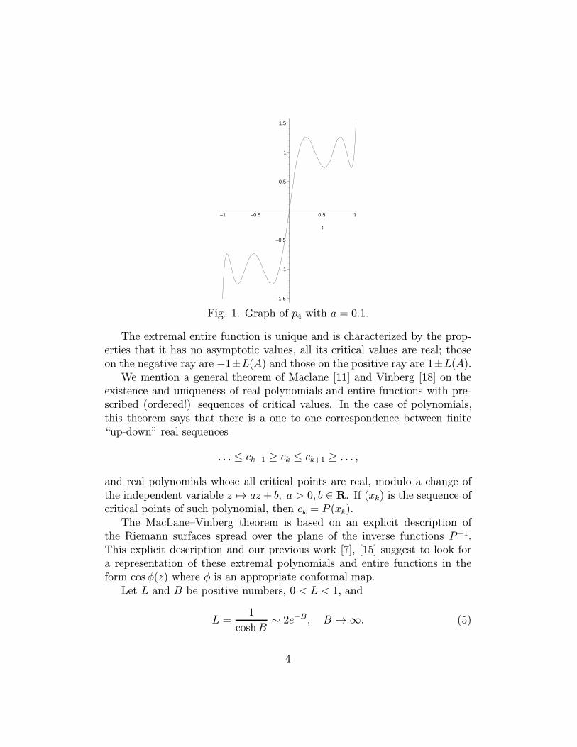
Our proofs are based on special representations of polynomials and entirefunctions of best approximation which are of independent interest. It followsfrom Chebyshev’s theory (see, for example, [1, Ch. II]) that polynomials pmare characterized by the property that the difference pm(x) − sgn (x) takesits extreme values ±Lm(a) on X(a) 2m+ 4 times intermittently, so that thegraph of pm looks like this:
3
–1.5
–1
–0.5
0.5
1
1.5
–1 –0.5 0.5 1
t
Fig. 1. Graph of p4 with a = 0.1.
The extremal entire function is unique and is characterized by the prop-erties that it has no asymptotic values, all its critical values are real; thoseon the negative ray are −1±L(A) and those on the positive ray are 1±L(A).
We mention a general theorem of Maclane [11] and Vinberg [18] on theexistence and uniqueness of real polynomials and entire functions with pre-scribed (ordered!) sequences of critical values. In the case of polynomials,this theorem says that there is a one to one correspondence between finite“up-down” real sequences
. . . ≤ ck−1 ≥ ck ≤ ck+1 ≥ . . . ,
and real polynomials whose all critical points are real, modulo a change ofthe independent variable z 7→ az+ b, a > 0, b ∈ R. If (xk) is the sequence ofcritical points of such polynomial, then ck = P (xk).
The MacLane–Vinberg theorem is based on an explicit description ofthe Riemann surfaces spread over the plane of the inverse functions P−1.This explicit description and our previous work [7], [15] suggest to look fora representation of these extremal polynomials and entire functions in theform cosφ(z) where φ is an appropriate conformal map.
Let L and B be positive numbers, 0 < L < 1, and
L =1
coshB∼ 2e−B, B →∞. (5)
4

Consider the component γB ⊂ z : <z ∈ [0, π], =z > 0 of the preimage ofthe ray
w : <w = 1/L, =w < 0under w = cos z. It is easy to see that this curve γB can be parametrized as
γB = arccos(coshB/cosh t) + it : B ≤ t <∞.
This curve begins at iB and then goes to infinity approaching the line π/2+it, t > 0 with exponential rate.
Let ΩB be the region in the upper half-plane whose boundary consistsof the positive ray, the vertical segment [0, iB] and the curve γB. For fixedB > 0, let φB be the conformal map of the first quadrant onto ΩB such thatφB(z) ∼ z, z → ∞ and φB(0) = iB. Let A = A(B) = φ−1
B (0). Then A is acontinuous strictly increasing function of B, and we may consider the inversefunction B(A).
Theorem 3 The approximation error in Theorem 2 is L(A) = 1/coshB(A),and the extremal function can be defined in the first quadrant by the formula
1− L(A) cosφB(A).
Let ΩB,m be the region in the half-strip z : <z ∈ (0, π(m+ 1)), =z > 0bounded on the left by γB. Let φB,m be the conformal map of the firstquadrant onto ΩB,m such that φB,m(0) = iB, φB,m(1) = π(m + 1) andφB,m(∞) = ∞. Let a = a(B,m) = φ−1
B,m(0). Then a(B,m) is a continuousincreasing function of B for fixed m, so it has the inverse Bm(a).
Theorem 4 The error term in Theorem 1 is Lm(a) = 1/coshBm(a), and theextremal polynomial is given in the first quadrant by
1− Lm(a) cosφB,m, where B = Bm(a).
Discontinuous functions cannot be uniformly approximated by polynomi-als with arbitrarily small precision, however, in our situation we can obtainan approximation which seems to be the second best thing to the uniformapproximation.
5

We introduce the notation1
L(f, g) = infh : f(x− h)− h ≤ g(x) ≤ f(x+ h) + h, −1 ≤ x ≤ 1.
Thus the statement that L(sgn , g) ≤ εmeans that the graph of the restrictionof g on [−1, 1] belongs to a “rectangular corridor” of width ε around the“completed graph” of sgn (x), which consists of the graph of sgn (x) and thevertical segment [(0,−1), (0, 1)].
−1
−1
−1
1
Fig. 2. Levy’s neighborhood of the function sgn .
It is easy to see that if a = Lm(a) then our polynomial pm from Theorem 1is the unique polynomial of degree 2m + 1 which minimizes L(sgn , p). Wehave
Theorem 5
limm→∞
m
logmL(sgn , pm) =
1
2.
Remarks. One could also use the Hausdorff distance between the com-pleted graphs. In the case of sgn (x), the Hausdorff distance will differ fromL(sgn , pm) by a factor of
√2. Approximation of functions with respect to
Hausdorff distance between their completed graphs was much studied bySendov [12] and his followers. An arbitrary bounded function on [0, 1] can beapproximated in this sense by polynomials of degree n with errorO((logn)/n)[13].
1If [−1, 1] is replaced by (−∞,∞) this becomes the Levy distance. It is really a distanceon the set of bounded increasing functions on the real line [10, Ch. VIII].
6

Proof of Theorems 3 and 4. Let φ be either φB or φB,m. By inspectionof the boundary correspondence, we conclude that f = 1 − L cosφ is realon the positive ray and pure imaginary on the positive imaginary ray. Sof extends to an entire function by two reflections. The extended functionevidently satisfies
f(z) = f(z) and − f(−z) = f(z),
so we conclude that f is odd. In the case of Theorem 1, the region ΩB,m
is close to the strip z : <z ∈ (π/2, π(m + 1)) as =z → ∞, so φB,m ∼i(2m+1) log z, z →∞, so f is a polynomial of degree 2m+1. In Theorem 2,φ(z) ∼ z, so f has exponential type one. In both theorems, differentiationshows that the only critical points of f in the closed right half-plane arepreimages of the critical points of the cosine under φ. So the graph of fhas the required shape. That a polynomial with such graph is the uniqueextremal for Theorem 1 follows from the general theorem of Chebyshev onthe uniform approximation of continuous functions [1, Ch. II].
The proof that the entire function f we just constructed is the uniqueextremal for Theorem 2 might not be so well-known, so we include this proofwhich we learned from B. Ya. Levin (compare [7, 15]).
All critical points of our entire function f are real. Let x1 < x2 < . . . bethe sequence of positive critical points of f , Then we have x1 > a, and
f(xk) = 1 + (−1)k−1L, and f(A) = 1− L. (6)
Let g be another real entire function of exponential type 1 such that
sup |g(x)− 1| ≤ L for x ≥ A. (7)
We may assume without loss of generality that g is odd (otherwise replace itby (g(x)−g(−x))/2 which also satisfies (7)). Equations (6) and (7) imply thatthe graph of g intersects the graph of f on every interval [xk, xk+1], k ≥ 1.More precisely, there is a sequence of zeros yk of f − g (where multiple zerosare repeated according to their multiplicity), which is interlacent with xk,that is
x1 ≤ y1 ≤ x2 ≤ y2 ≤ . . . ,
and in addition to those yj, f−g has at least one zero in (0, x1]. By the well-known theorem [9, VII, Thm. 1], it follows that the meromorphic function
F (z) =1
z
∏k∈Z\0
1− z/xk1− z/yk
7

has imaginary part of constant sign in the upper half-plane, and of oppositesign in the lower half-plane. This implies that
F (reiθ) = O(r), (8)
when r → +∞, uniformly with respect to θ for ε ≤ θ ≤ π − ε, for everyε > 0. Similar estimate holds in the lower half-plane.
As (f − g)(yk) = 0, we have
f − gf ′
= P/F, (9)
where P is an entire function of exponential type.It is easy to see that the left hand side of (9) is bounded for |=z| ≥ 1.
Indeed, Phragmen and Lindelof give |f(z)−g(z)| ≤ C1 exp |=z|, while f ′ hasonly real zeros and approaches L cos(x ± α)) as x → ±∞, where α is somereal constant. It follows that |f ′(z)| ≥ C2 exp |=z| for |=z| > 1, so (f − g)/f ′
is bounded for |=z| > 1.So we conclude from (8) that P (z) = O(|z|) and this contradicts the fact
that P has at least two zeros, unless P = f − g = 0. This completes theproof.
Proof of Theorem 1. We recall that Bm = Bm(a), Ωm = ΩBm,m andthe conformal maps of the first quadrant Q onto Ωm were defined beforeTheorem 4. We are going to prove (3) first, which is the same as
Bm =(m+
1
2
)log
1 + a
1− a +1
2logm+
1
2log
2a
1− a2+ c+ o(1), (10)
as m→∞ and a is fixed. Here c is an absolute constant.We need some auxiliary conformal maps. Let ψ : Q→ Q be defined by
ψ(z) =Am
a
√z2 − a2
1− z2,
where
Am =(m+
1
2
)log
1 + a
1− a > 0 (11)
The reason for such choice of Am will be seen later. Then ψ gives the followingboundary points correspondence:
ψ : (0, a, 1,∞) 7→ (iAm, 0,∞, iAm/a).
8

The function Φm(z) = iφm ψ−1(−iz) maps the second quadrant onto iΩm,and sends the positive imaginary axis onto the interval ` = (0, iπ(m + 1)).By reflection, we extend Φm to a map from the upper half-plane onto theregion i(Ωm ∪Ωm) ∪ `. This extended map Φm gives the following boundarycorrespondence:
Φm : (−Cm,−Am, 0, Am, Cm) 7→ (−∞,−Bm, 0, Bm,+∞),
where we set Cm = Am/a.Now we introduce the map hm(z) = Φm(z + Am) − Bm. Our first goal
is to show that the sequence hm tends to a limit, and to describe this limit.The boundary correspondence under hm is this:
hm : (−Cm −Am,−2Am,−Am, 0, Cm − Am) 7→ (−∞,−2Bm,−Bm, 0,+∞).
We represent hm as the Schwarz integral of its imaginary part:
hm(z) =(m +
1
2
)log
1 + za/((1 + a)Am)
1− za/((1− a)Am)+
1
π
∫ ∞−∞
(1
t− z −1
t
)vm(t)dt,
(12)where
vm(t) =
=hm(t), t ∈ [−Cm − Am, Cm − Am],π/2, t /∈ [−Cm − Am, Cm − Am].
Our choice of Am in (11) implies that the first summand in the right handside of (12) has a limit
limm→∞
(m+
1
2
)log
1 + za/((1 + a)Am)
1− za/((1− a)Am)= σz,
where
σ =2a
(1− a2) log((1 + a)/(1− a)). (13)
It is easy to see that the integral in (12) converges to a bounded function ofthe form
1
π
∫ (1
t− z −1
t
)ρσ(t)dt,
where ρσ is a bounded positive function which we will describe shortly. Theimage of hm has a limit Ω∗ in the sense of Caratheodory; Ω∗ is the region inthe upper half-plane above the graph of the function arccos e−x, x ≥ 0. So
9

hm → Hσ, where Hσ is the conformal map of the upper half-plane onto Ω∗,Hσ(0) = 0 and Hσ(z) ∼ σz as z →∞.
Thus we have a Schwarz representation
Hσ(z) = σz +1
π
∫ (1
t− z −1
t
)ρσ(t)dt,
and ρσ(t) = =Hσ(t) for real t. Our next goal is to study asymptotics ofBm = −hm(−Am). We use the following comparison function
gm(z) =(m+
1
2
)log
1 + za/((1 + a)Am)
1− za/((1− a)Am)+
1
2
∫ ∞0
(1
t− z −1
t
)χm(t)dt,
where χm is the characteristic function of the set (−∞,−2(Am+1)]∪[2,+∞).We have
limm→∞
(hm(−Am)− gm(−Am)) = −1
π
∫ ∞0
(ρσ(t)− π
2χ[2,∞)(t)
)dt
t,
and using (11),
gm(−Am) = −Am −1
2log(Am + 1).
Combining these two equations we obtain that
Bm = −hm(−Am) = Am +1
2logAm +
1
π
∫ ∞0
(ρσ(t)− π
2χ[2,∞)(t)
)dt
t+ o(1).
Using the evident transformation law Hσ(λz) = Hσλ(z) we obtain ρσ(λt) =ρσλ(t), and therefore,
Bm = Am +1
2logAm +
1
2log σ +
1
π
∫ ∞0
(ρ1(t)− π
2χ[2,∞)(t)
)dt
t+ o(1).
Substituting the values of Am and σ from (11) and (13) we obtain (10) with
c =1
π
∫ ∞0
(ρ1(t)− π
2χ[2,∞)(t)
)dt
t. (14)
The numerical valuec = (1/2) log(2π)
is obtained from comparison with Bernstein’s result (2).
10

Indeed, in view of (1), (5) and (10) we have
Lm(a) = infdeg q=m
sup[a2,1]
√x|q(x)− 1/
√x| ∼ 2e−Bm
= 2(e−c + o(1))1− a√
2a
(1− a1 + a
)m 1√m.
Comparing this expression for Lm(a) with the expression (2) when a → 1,we obtain (10) with c = (1/2) log(2π).
Proof of Theorem 2. We have to prove that B = A+(1/2) logA+c+o(1)as A→∞, where c = (1/2) log(2π).
Let f1(z) =√z2 −A2 be the conformal map of the first quadrant Q onto
itself, sending A to 0, and f1(z) ∼ z as z →∞. Then f1(0) = iA. Let f2 bethe conformal map of Q onto ΩB, f2(0) = 0 and f2(z) ∼ z, as z → ∞. Weextend f2 by symmetry, reflecting both domains in the positive ray. So fromnow on f2 is defined in the right half-plane. The condition that f2(iA) = iB
defines the number B uniquely. It is easy to see that
B ∼ A
as A→∞.Now put h(z) = if2(−iz) for convenience. This h maps the upper half-
plane onto a subregion of the upper halfplane. The boundary of this subre-gion is asymptotic to the line =z = π/2 as |<z| → ∞.
We have B = h(A), and we wish to find asymptotics of h(A) as A→∞.To do this, we use the following comparison function
g(z) = z +∫ ∞A+2
z
t2 − z2dt.
The integral in the right hand side is the Schwarz formula for an analyticfunction in the upper half-plane whose imaginary part equals
(π/2)χ(−∞,−A−2]∪[A+2,∞).
Our function h has a similar representation in terms of its imaginary parton the real line. Subtracting these two representations, we obtain
g(A)− h(A) =2A
π
∫ ∞0
v(t+ A)
2At+ t2dt,
11

where v(t) = =(g(t) − h(t)). Now we claim that v(t + A) tends to a limitv0, as A → +∞. This limit is (π/2)χ[2,∞)(t) − =H(t), where and H(z) =limA→+∞(h(z+A)−B(A)) is the conformal map of the upper half-plane ontothe region in the upper half-plane above the graph y = arccos e−x, x ≥ 0 andy = 0, x ≤ 0. Notice that H = H1, where H1 was defined in the proof ofTheorem 1.
Thus g(A)− h(A)→ const where the constant is given by
1
π
∫ ∞0
v0(t)
tdt =
1
π
∫ ∞0
(π
2χ[2,∞)(t)− =H(t))
dt
t. (15)
The integral is convergent because v0(t) = O(√t), t → 0 and v0(t) =
O(e−t), t → ∞. It remains to find the asymptotic behavior of g(A) asA→∞. We have
g(A) = A+∫ ∞
2
A
2tA + t2dt = A +
1
2log(A+ 1).
Combining these results we obtain
B = h(A) = A+1
2logA+
1
π
∫ ∞0
(=H(t)− π
2χ[2,∞)(t)
)dt
t+ o(1)
= A+1
2logA+ c+ o(1),
where c is the constant from (14). This proves Theorem 2.
Proof of Theorem 5. We choose
B = logm− log logm + log 4, (16)
so that L ∼ (logm)/(2m) in view of (5). Consider the conformal map ofΩB,m onto the half-strip Π = z : <z ∈ (0, (m+ 1)π) by a function f1 suchthat f1(0) = 0, f1((m + 1)π) = (m + 1)π and f1(∞) = ∞. Let B′ = f1(B).The function f1(z/B) tends to the identity as m→∞, so
B′ ∼ B, B →∞.Let f2 be the (elementary) conformal map of Π onto the first quadrant nor-malized by f2(B′) = 0, f2(π(m+ 1)) = 1 and f2(∞) =∞. Then
a := f2(0) =1− exp(B′/(m + 1))
1 + exp(B′/(m+ 1))= B′/2(m+ 1) ∼ B/2m ∼ (logm)/(2m).
The authors thank Doron Lubinsky, Misha Sodin and Andrei Gabrielovfor their help and useful comments.
12

References
[1] N. Akhiezer, Theory of approximation, Dover, NY, 1992.
[2] N. Akhiezer, Elements of the theory of elliptic functions, AMS, Provi-dence, RI, 1990.
[3] S. Bernstein, Sur la meilleure approximation de |x| par des polynomesdes degres donnes, Acta math. 27 (1914) 1–57.
[4] S. Bernxte@in, O nailuqxem priblienii |x|p pri pomowimnogoqlenov ves~ma vysoko@i stepeni, Izvesti Akad. NaukSSSR (1938) 169-180 (Russian). [On the best approximation of |x|pby polynomials of very high degree, Izvestiya Akad. Nauk SSSR (1938)169–180.]
[5] S. Bernstein, Sur le probleme inverse de la theorie de la meilleure ap-proximation des fonctions continue, C.R. 206 (1938) 1520–1523.
[6] S. N. Bernxte@in, kstremal~nye svo@istva polinomov inailuqxee priblienie nepreryvno@i funkcii odno@i vew-estvenno@i peremenno@i, ONTI, 1937 (Russian) [S. N. Bernstein,Extremal properties of polynomials and best approximation of a contin-uous function of one real variable, ONTI, Moscow, 1937.]
[7] A. Eremenko, On the entire functions bounded on the real axis, SovietMath Dokl., 37, 3 (1988) 693–695.
[8] M. A. Lavrent~ev, B. V. Xabat, Metody teorii funkci@i kom-pleksnogo peremennogo, Moskva, \Nauka", 1987. (Russian) [M.Lavrent’ev and B. Shabat, Methods of the theory of functions of a com-plex variable, Fifth edition. “Nauka”, Moscow, 1987.]
[9] B. Levin, Distribution of zeros of entire functions, AMS, Providence, RI,multiple editions.
[10] Ju. Linnik and I. Ostrovskii, Decomposition of random variables andvectors, AMS, Providence, R. I., 1977.
[11] G. MacLane, Concerning the uniformization of certain Riemann surfacesallied to the inverse-cosine and inverse-gamma surfaces, Trans. AMS, 62(1947) 99–113.
13

[12] B. Sendov, Some questions of the theory of approximation of functionsand sets in the Hausdorff metric, Russian Math. Surveys, 24 (1969) 5,143–183.
[13] B. Sendov, Exact asymptotic behavior of the best approximation byalgebraic and trigonometric polynomials in the Hausdorff metric (Rus-sian), Mat. Sbornik 89 (1972) 138–147, 167.
[14] H. Stahl, Best uniform rational approximation of xα on [0, 1], Actamath., 190 (2003) 241–306.
[15] M. Sodin and P. Yuditskii, Functions that deviate least from zero onclosed subsets of the real axis, St. Petersburg Math. J. 4 (1993), 201–249.
[16] J. Vaaler, Some extremal functions in Fourier analysis, Bull. Amer.Math. Soc. 12 (1985), no. 2, 183–216.
[17] E. T. Whittaker and G. N. Watson, A course of modern analysis, Cam-bridge UP 1927.
[18] . B. Vinberg, Vewestvennye celye funkcii s predpisanny-mi kritiqeskimi znaqenimi, Problemy teorii grupp i gomo-logiqesko@i algebry, rosl. Gos. Un-t, roslavl~, 1989, 127138 (Russian) [E. B. Vinberg, Real entire functions with prescribed criti-cal values, Problems of group theory and homological algebra, Yaroslavl.Gos. U., Yaroslavl, 1989, 127-138].
[19] E. I. Zolotarev, Primenenie lliptiqeskih funkci@i k vo-prosam o funkcih naimenee ili naibolee uklonwihs otnul, Bull. de l’Academie de Sciences de St.-Petersbourg, 3-e serie, 24(1878) 305–310; Melanges math. 15, (1877) 419–426. (Russian) Anwen-dung der elliptischen Funktionen auf Probleme uber Funktionen, die vonNull am wenigsten oder am meisten abweichen, Abh. St. Petersb. XXX(1877).
A. E.: [email protected] of Mathematics, Purdue University,West Lafayette, IN 47907-2067U. S. A.
14
