Unexpected Event during Surveys Design:Promise and Pitfalls for Causal Inference ∗

Jordi MuñozUniversity of Barcelona

Albert Falcó-GimenoUniversity of Barcelona

Enrique HernándezUniversitat Autònoma de Barcelona

Published at Political Analysis (2019)DOI: 10.1017/pan.2019.27

Abstract

An increasing number of studies exploit the occurrence of unexpected events during thefieldwork of public opinion surveys to estimate causal effects. In this paper we discuss the useof this identification strategy based on unforeseen and salient events that split the sample ofrespondents into treatment and control groups: the Unexpected Event during Surveys Design(UESD). In particular we focus on the assumptions under which unexpected events can beexploited to estimate causal effects and we discuss potential threats to identification, payingespecial attention to the observable and testable implications of these assumptions. Wepropose a series of best practices in the form of various estimation strategies and robustnesschecks that can be used to lend credibility to the causal estimates. Drawing on data fromthe European Social Survey we illustrate the discussion of this method with an original studyof the impact of the Charlie Hebdo terrorist attacks (Paris, 01/07/2015) on French citizens’satisfaction with their national government.

∗This research has received financial support from the Spanish Ministry of Science, Innovation, and Universitiesthrough the research grant CSO2017-89085-P. We are grateful to Lucas Leeman, Silja Häusermann, Macarena Ares,Guillem Rico, Salomo Hirvonen, the editor and anonymous reviewers of Political Analysis, and participants at theUniversity of Zurich IPZ publication seminar, the Autonomous University of Barcelona DEC Seminar, and the 2018EPSA conference for helpful comments and suggestions. We are especially grateful to Erik Gahner Larsen for hisdetailed and insightful comments, and for generously sharing with us his collection of UESD references. EnriqueHernández also thanks the University of Zurich Political Science Department for hospitality during the springof 2018. Replication materials are available at the Political Analysis Dataverse: doi.org/10.7910/DVN/RDIIVL(Muñoz et al., 2019).

1 IntroductionNatural disasters, violence outbreaks, political scandals or sports results are examples of

unexpected events that can occur during the fieldwork of public opinion surveys. Survey re-

searchers traditionally considered that a changing context could threaten the validity of their

measurement instruments. Other scholars, though, have identified these occurrences as an

opportunity to identify the causal effect of these events on public opinion.

Already in 1969 The Public Opinion Quarterly published a series of articles aimed at study-

ing the effect of unexpected events such as Martin Luther King’s assassination (Hofstetter,

1969) or an explosion in Johannesburg (Lever, 1969) on multiple outcomes. More recently, the

influence of the so-called identification revolution has led to a significant increase in the number

of publications that exploit these unexpected events as opportunities to conduct design-based

studies that can yield valid causal estimates of theoretically relevant shocks.

In this paper we discuss the strengths and limitations of this identification strategy, which

we call the “Unexpected Event during Survey Design” (UESD). In particular, we focus on

the assumptions under which unexpected events can yield valid causal estimates. We discuss

these assumptions and their observable and testable implications in detail. Next, we present

several strategies to address potential violations of the assumptions, as well as a series of

robustness checks that can be used to assess and establish their plausibility. Our review of

over 40 published studies that rely on this identification strategy shows wide variation in the

estimation strategies, tests and robustness checks that are performed to substantiate causal

claims. While most researchers acknowledge some of the key identifying assumptions of this

design, there is still no apparent consensus on the empirical strategy and the robustness checks

that should be performed.Our aim is that this paper will help set a standard of good practices

that should increase the credibility of causal claims based on the UESD.

We illustrate the strengths and weaknesses of the UESD through an original study of the

impact of the Charlie Hebdo terrorist attacks (Paris, 01/07/2015) on satisfaction with govern-

ment in France, relying on the 7th round of the European Social Survey (ESS), that was being

fielded at the time of the attacks.

2

2 The Unexpected Event during Surveys DesignWe define the UESD as the research design that exploits the occurrence of an unexpected

event during the fieldwork of a public opinion survey to estimate its causal effect on a relevant

outcome by comparing responses of the individuals interviewed before the event ti < te (control

group) to those of respondents interviewed after the event ti > te (treatment group).

This identification strategy relies on the assumption that the moment at which each re-

spondent is interviewed during the fieldwork of a given survey is independent from the time

when the unexpected event occurs. The occurrence of the event should, therefore, assign survey

respondents into treatment and control groups as good as randomly. Hence, a UESD study

relies on the use of cross-sectional survey data in which time provides exogenous variation in a

substantively relevant variable, such as exposure to some experience or information. Formally,

the timing of the survey t is exploited as an instrument of exposure to the event T the effects

of which the researchers are interested in.

A crucial feature of the UESD is, therefore, that the event occurs unexpectedly, since pre-

dictable events might lead to violations of the key assumptions of this design (excludability

and ignorability). Foreseeable events (e.g. an election result) might be anticipated by respon-

dents, who might change their attitudes in response to the event even before it has occurred.

This could be especially problematic if certain respondents are more/less likely to anticipate

the event and they are, at the same time, more/less likely to be interviewed after the event.

Moreover, if an event is foreseeable some respondents might postpone their participation in the

survey and self-select into the treatment group.1

This identification strategy has been frequently exploited to study the effects of important

phenomena that cannot be directly manipulated through controlled experiments. This is for

example the case of violent events such as the assassination of political leaders (Boomgaarden

and de Vreese, 2007), or terrorist attacks (Boydstun et al., 2018; Silva, 2018; Balcells and

Torrats-Espinosa, 2018; Coupe, 2017; Dinesen and Jæger, 2013; Finseraas and Listhaug, 2013;

Geys and Qari, 2017; Jakobsson and Blom, 2014; Legewie, 2013; Metcalfe et al., 2011; Perrin

and Smolek, 2009) Researchers have also analyzed the effects of other theoretically relevant1For example, in online surveys respondents might wait until the event has occurred to complete to question-

naire, and in face-to-face or telephone surveys respondents might delay their interview (by refusing or makingan appointment for a later date)

3

events such as political scandals (Ares and Hernández, 2017; De Vries, 2018; Solaz et al., 2018),

protests and demonstrations (Branton et al., 2015; Motta, 2018; Silber Mohamed, 2013; Zepeda-

Millán and Wallace, 2013), presidential candidates speeches (Flores, 2018), Nobel prize awards

(De Vries, 2018), the announcement of election results and election fraud (Pierce et al., 2016),

policy reforms (Larsen, 2018), or flu epidemics (Jensen and Naumann, 2016).2

Some of these events commonly analyzed through the UESD such as terrorist attacks should

a priori be unexpected for most respondents. However, there are others that might be more

foreseeable like for example election results or a scheduled legal demonstration. In fact, the

same type of event might be unexpected in some contexts but not in others. For example, while

in some cases the victory of a particular party or candidate in an election might be expected

(e.g. CDU victory in the 2017 German election), in some others the election results might come

as a surprise by being more unexpected (e.g. the victory of Donald Trump in 2016 analyzed by

Minkus et al. (2018)). Researchers should, therefore, make a compelling argument about the

plausibility of unexpectedness on a case-by-case basis.

The increasing popularity of the UESD can be attributed to its capacity to provide cred-

ible estimates of the causal effects of unexpected events on theoretically relevant outcomes.

This capacity is based on three crucial features of this design. First, in contrast to standard

observational survey studies, exogenous assignment to treatment and control groups increases

the internal validity of the estimates, as it can shield them from biases related to unobserved

confounders or reverse causality. Second, the fact that the UESD relies on naturally occurring

events (not manufactured by researchers) provides a level of external validity that goes well be-

yond what controlled experiments can offer. Third, in contrast to most analyses of the impact

of events that use longitudinal data or different surveys stacked around the date of an event,

UESD studies employ a single survey to focus on the immediate period of time surrounding

the event, which ensures that the impact of other macro-level confounders is less of a concern.

However, the absence of true random assignment and the lack of control by the researchers also

pose challenges to identification that need to be addressed upfront if this strategy is to be used

to substantiate causal claims.2See Section B in Supporting Information for an overview of 44 published UESD studies

4

2.1 The UESD in context

The UESD shares some properties with other research designs commonly used in social

sciences, such as the Regression Discontinuity Design (RDD), the Interrupted Time Series

(ITS) design or event studies, which are common in economics and finance. While these research

designs can provide relevant cues for the use of the UESD, this design has a range of unique

features and particularities that warrant some specific methodological considerations.

Under some specific conditions, the UESD might be analogous to the RDD in which an

observation is treated if the forcing or running variable exceeds some predetermined cutoff. In

the case of an unexpected event occurred during the fieldwork of a survey, the running variable

would be the fieldwork days when interviews took place, and the cutoff the moment when the

event occurred. However, there are several important differences. First, unlike the RDD, in

the UESD the receipt of the treatment is not linked to a given score of the running variable

in any predetermined or known way. Moreover, in most applications of the RDD the running

variable will be substantively related to the potential outcomes and, therefore, inference will be

restricted to the cases just below and above the cutoff. While in some UESD applications this

might also be the case, in most of its empirical applications the specific day when a respondent

is interviewed is not related to the potential outcomes, other than through the unforeseen event.

As a consequence, the need to rely on narrow bandwidths (and the estimation of local effects)

is generally less stringent.

The UESD also bears some resemblance to the ITS design (St. Clair et al., 2014). This

design, commonly used in epidemiology and health policy, is based on repeated measurements

of an outcome (e.g. hospital admissions) for the same units before and after a given intervention

(e.g. the approval of a policy). The measurements before the intervention are used to build

expectations on the outcome trend in the absence of the intervention. An effect is identified if

the postintervention observations deviate significantly from this counterfactual trend.

The core challenges to causal identification in the ITS design are related to the aggregated

and times-series nature of the data: the presence of seasonality, temporal autocorrelation, and

time-varying confounders. While in some cases ITS designs have been applied to the analysis

of survey data, these data were recorded or used at the aggregate level (see e.g. Tiokhin and

Hruschka, 2017). In these examples, the (often few) respondents interviewed each specific day

5

(or period) of the fieldwork are treated as a measurement of the same unit and, therefore, the

data set is essentially a time-series. The reduced number of daily observations might create a

problem of high variance and, depending on the organization of the fieldwork, also of bias in the

measurements. In the examples we discuss in this paper the survey data is primarily analyzed

at the individual level, so we do not deal with repeated measurements of the same unit, but

with different observations in the pre and post event periods. This is the core difference between

the ITS and the UESD designs, and it has implications for the type of concerns and threats to

identification, as well as for the estimation strategies.

On similar grounds, one could also mention event studies used in finance, which analyze the

behavior of firms’ stock prices in response to corporate events (MacKinlay, 1997). But, again,

the nature of the data used in the UESD and the comparison across different units interviewed

before and after the event makes the UESD a distinct type of research design.

3 Assumptions and threats to causal identificationThe identification of valid causal estimates based on the comparison of respondents in-

terviewed before and after the day of the event te hinges on several identifying assumptions.

Arguably, there are two key and potentially problematic assumptions in this design.

The first one is excludability: any difference between respondents interviewed before and

after the event shall be the sole consequence of the event. That is, the timing of the interview

t should affect the outcome variable Y only through the event T . In the case we are dealing

with, together with the theoretically relevant event, other things could happen that make the

pre- and postevent contexts different and, therefore, influence the respondents’ outcome.

The second key assumption is temporal ignorability: for any individual, the potential out-

comes must be independent from the moment of the interview. Therefore, assignment to

different values of time t should be independent from the potential outcomes of Y . This means

that, in order to obtain an unbiased estimator, selection of the moment of the interview should

be as good as random.3

3The Stable Unit Treatment Value Assumption (SUTVA) does also apply here. However, it is probably anunproblematic assumption. The only way one could think of interference across subjects is in the unlikely caseof two individuals (i1 and i2) who know each other and who have discussed the content of the survey after i1was interviewed and before i2’s interview (after the event).

6

3.1 Excludability

To estimate the causal effect of the event one must assume that the timing of the survey

interview does not affect the outcome through any other channel except for the event of interest.

Any factor, other than the event itself that correlates with time can potentially bias the causal

estimates. We consider three potential threats to the exclusion restriction: collateral events,

simultaneous events, and unrelated time trends. We also discuss another particular case in

which the exclusion restriction might be violated: the endogenous timing of the event.

3.1.1 Collateral events

We define collateral events as the succession of reactions triggered by the unexpected event

of interest. For example, in the case of a terrorist attack, generally the government will issue

public statements and adopt specific policy responses. The opposition then will decide whether

to back the government or criticize it for the security failure, and the news media will shape

the width and tone of the coverage.

All these reactions and counter-reactions, rather than the unexpected event per se, might

drive the public opinion’s response. This can be seen as a problem of an imprecise treatment.

Under these circumstances, it is impossible to narrowly interpret the effect as a consequence

of the event itself, and it should rather be interpreted as the joint effect of the event and the

subsequent reactions. In fact, it is often legitimate to question, counterfactually, if we would

observe the same effect on Y had some of these collateral events not occurred.

In some applications the presence of collateral events might not be a problem because the

event did not spur any relevant reactions, or because the reactions are a constitutive character-

istic of the class of events being analyzed, or they are part of the researchers’ focus of interest.

However, they often pose a generalizability problem: the estimated causal effect of the event

(e.g. a specific terrorist attack) may not be generalizable to the class of events of the same

type (e.g. terrorism in general) had the collateral events been different. In such cases, it may

be advisable to analyze additional events of the same class to average out the specificities of

each individual event (see e.g. Balcells and Torrats-Espinosa, 2018, for an analysis of multiple

terrorist attacks).

7

3.1.2 Simultaneous events

A potentially more troublesome situation can arise when other, unrelated events, take place

at the same time. This might pose a problem of compound treatments, that violates the

Compound Treatment Irrelevance Assumption.4 Applied to the UESD this assumption implies

that out of all the treatments that covary with the timing of the interview, the event of interest

is the only treatment that affects the potential outcomes. If, instead, there are reasons to

believe that any of these other events might have had an effect on the outcome of interest,

the exclusion restriction would be violated. For example, the 2016 Nice terrorist attack in

France took place during Bastille Day celebrations, so any effect on a political outcome might

be caused both by the attack and the national commemoration.

Unlike the case of collateral events, this problem cannot be reduced to an issue of precision,

interpretation, and generalizability of the treatment effects. It is true, however, that in most

existing applications of the UESD, the events analyzed were highly salient episodes. Therefore,

it is often unlikely that the observed effect would have been driven by other, relatively minor

events that were not nearly as salient.

3.1.3 Unrelated time trends

Another violation of the exclusion restriction can be generated by the presence of time-

varying variables that, aside from the event itself, are systematically related to the outcome

(temporal stability assumption). Let t be a continuous time variable, and T a dichotomous

variable that takes value 1 if the respondent was interviewed after the event, and 0 otherwise.

In the presence of a monotonic effect of t on Y , many arbitrary partitions of t will yield

statistically significant effects in the same direction as the preexisting trend. Time trends

can exist for many different reasons, often unrelated to the unexpected event. For example,

variables such as subjective well-being are related to calendar effects (Csikszentmihalyi and

Hunter, 2003).

3.1.4 Endogenous timing of the event

A particular case in which some of the aforementioned threats to excludability can emerge is

if the timing of the event is endogenous. Most unexpected events of interest are human-crafted4See Keele and Titiunik (2016) and Eggers et al. (2018) for a discussion of compound treatments in the

context of geographical borders and population thresholds.

8

and, therefore, an actor decides when does the event take place. For example, the precise time

at which a corruption scandal breaks in the news, or the moment at which a terrorist group

perpetrates an attack are events that, although unexpected for almost all citizens, might be

actually planned by politically motivated actors.

If the decision about the moment when the event occurs is endogenous to the outcome

variable Y , and therefore T is correlated with the error term, the excludability assumption

will be violated. Take for example the case of a partisan news media outlet. Once they

receive information about a corrupt act committed by the incumbent, they might strategically

manipulate the moment at which the information is disclosed in order to maximize (or minimize)

damage to the incumbents’ popularity. They might, for example, break the news at a time in

which another, more salient event is taking place to play a diversionary strategy and reduce the

effect. If this is the case, assignment to treatment and control cannot be treated as exogenous,

and, most probably, either a preexisting trend or some other events that correlate with t are

having an effect on Y .

3.2 Ignorability

Formally, the ignorability assumption states that respondents’ treatment status is indepen-

dent of their potential outcomes Yi(0), Yi(1) ⊥⊥ Ti. However, in the UESD assignment to the

treatment and control groups is not under the researchers’ control, and not random. Treatment

assignment is the result of a combination of the unexpected event and a set of decisions related

to data collection taken by the fieldwork operative.

In simple random samples with full response all individuals would have an identical prob-

ability of being interviewed at any time during the fieldwork, before or after te. A suitable

setting for this to hold would be a telephone survey with random digit dialing, a simple ran-

dom sampling design and full response. In this case, any temporal partition of the sample would

be as good as random. However, this is seldom the case in most surveys. Another favorable

survey design for the ignorability assumption to hold is the rolling cross-section design, used

in surveys such as the National Annenberg Election Survey (NAES) or the Canadian Election

Study (CES), that explicitly guarantees that the date in which each respondent is interviewed is

random (Johnston and Brady, 2002). Next we discuss how variation in survey sampling meth-

ods, fieldwork procedures, and the propensity and availability of sampled citizens to respond

9

will, in most cases, lead to violations of the ignorability assumption.

3.2.1 Fieldwork organization: Imbalances on observables

Threats to the ignorability assumption often stem from complex sampling designs, such as

cluster, stratified, or multi-stage samples. In these designs the primary sampling units are often

contacted and interviewed sequentially. For example, in face-to-face surveys the fieldwork often

follows a geographical pattern for efficiency reasons. Respondents in area A are interviewed

first, then interviewers move to area B, and so on. Any correlation between subject location and

time of the interview will lead to a violation of the ignorability assumption, since the location

can be correlated with many other respondents’ characteristics that might bias the findings.5

Quota sampling is another strategy that can generate imbalances. Often the fieldwork goes

on until a given quota is completed. Then, researchers seek to complete the remaining quotas

and, therefore, any additional interview (or invitation to respond) will target the respondents

with profiles that match the incomplete quotas. Often, there is a systematic pattern in the

pace of quota completion, and the quotas corresponding to the types of respondents that are

easier to reach and survey (such as inactive population that stays at home) will fill up earlier.

If this is the case, timing of the interview will be correlated with respondents’ characteristics

and, therefore, splitting the sample at a specific point in time might not satisfy the ignorability

assumption.

When information on how the fieldwork unfolded is available, researchers can use relevant

observed characteristics of the respondents (e.g. place of residence or the variables used to set

up the quotas) to relax the ignorability assumption and rely on a more plausible Conditional

Ignorability Assumption. This assumption states that treatment status is independent of indi-

viduals’ potential outcomes conditional on a set of covariates: Yi(0), Yi(1) ⊥⊥ Ti | Xi. This is

similar to the common practice of observational studies in which statistical control of potential

confounders is the only strategy to ensure conditional ignorability. However, in the case of the

UESD the exogenous nature of the cutoff point increases the plausibility that, once we take

into account the relevant observables related to how the fieldwork was organized, treatment

status is orthogonal to the potential outcomes.5Another potentially problematic situation emerges when the unexpected event of interest causes changes in

the fieldwork, and, for example, leads to temporary suspension or delay of data collection in certain areas.

10

3.2.2 Unobservable confounders: reachability

Another threat to causal identification originates from potential imbalances between the

treatment and control groups on unobservable characteristics. In the context of the UESD, this

is likely to be related to the different levels of reachability of sampled units. Some respondents

are more elusive to survey researchers and require a greater effort to be contacted. Differences

in reachability are related to respondents’ ease of contact and their inability or reluctance to

participate. For example, those who are older and out of the labor market are likely to be

interviewed early during the fieldwork period because they are more often at home and have

fewer time constraints (Brehm, 1993; Stoop, 2004). Similarly those who are more interested in

the topics covered in the survey should be more willing to respond when they are first contacted

(Brehm, 1993). As a consequence, those who respond early to the survey might be different

than those who respond later.

The extent to which these differences in respondents’ reachability might pose a threat for the

UESD will depend on the survey design. For example, in the case of rolling cross-section designs

confounders related to reachability should be less of a concern, since this design guarantees that

the day when respondents are interviewed is in principle random. In any survey in which the

sampled units have any possibility to opt into the survey at different points in time, though,

reachability will lead to differences between those who are interviewed early and late. Take as

an example an online survey in which a link is distributed among all the sampled units and

respondents can decide when they answer the survey (within a specified time frame). Biases

related to reachability can also arise due to the common practice of making repeated attempts

to recontact and interview sampled households/individuals that were not found or refused to

cooperate when they were first contacted. 6

We illustrate this point through the 2014 round of the ESS, a survey in which substitution

of sampled units is not allowed and, therefore, interviewers make repeated attempts to contact

nonresponding units.7 Figure 1 summarizes the relationship between the number of attempted

contacts with sampled units and the time during the fieldwork when these units were finally

interviewed. In 17 out of the 21 countries included in the ESS this relationship is positive6A similar situation will arise if nonresponding units are not recontacted but simply substituted by units

with similar characteristics (e.g. with the same gender or living in the same block).7Replication materials for all the analyses conducted in this paper are available at the Political Analysis

Dataverse: doi.org/10.7910/DVN/RDIIVL (Muñoz et al., 2019).

11

and statistically significant. In most cases, the higher the number of contact attempts needed

to survey a subject, the higher the likelihood that she will be interviewed later during the

fieldwork. Therefore, the subjects who are more elusive and harder to reach will have a higher

probability of being interviewed after any unexpected event. If reachability is correlated with

the potential outcomes, its correlation with treatment assignment will bias the estimates of the

causal effect.

To exemplify the potential biases that the differential reachability of respondents might

generate, in Table A1 in the Supporting Information we assess the relationship between the

timing of the interview and respondents’ observable characteristics in the ESS. As expected,

those who were older, less educated, and out of the labor market (unemployed, retired, or

doing housework) were interviewed earlier during the fieldwork of this survey. In contrast,

when we conduct a similar analysis with the 2015 rolling cross-section of the CES and the 2008

NAES respondents’ characteristics appear to be less related to the timing of their interview.

However, even in these surveys interview timing is related to some demographic characteristics

of respondents (see Section A.2 in the Supporting Information for a discussion of these findings).

Therefore, it is advisable to always account for potential biases related to rechability, even in

the a priori most favorable sampling conditions.

3.2.3 Attrition

Survey research suffers from severe and increasing problems of nonresponse (Berinsky, 2017).

This is particularly problematic when nonresponse is correlated with potential outcomes. In

UESD studies, this might be even more troublesome if nonresponse is triggered by the treat-

ment. As a result of being exposed to certain events some people might become more likely

to refrain from responding to particular survey questions (item nonresponse), or even be less

likely to participate in surveys altogether (unit nonresponse). The opposite can also happen

when events unevenly increase the willingness of particular individuals to respond. In such

cases, the general problem of nonresponse being correlated with the outcome is aggravated, as

this correlation might be, in turn, different in the treatment and control groups. Take, as an

illustration, the example of a coup that topples an autocratic government. There would be

reasons to believe that individuals with certain political preferences –correlated with the out-

come variable of interest– are now more (less) likely to respond to the survey than they were

12

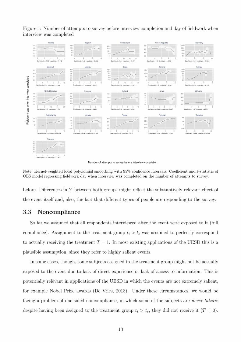
Figure 1: Number of attempts to survey before interview completion and day of fieldwork wheninterview was completed

100

110

120

130

140

1 2 3 4 5

Coefficient = −1.33 t−statistic = −1.112

Austria

40

60

80

100

120

0 5 10 15

Coefficient = 7.42 t−statistic = 23.882

Belgium

0

50

100

150

200

0 5 10 15 20

Coefficient = 9.44 t−statistic = 25.497

Swtizerland

35

40

45

50

1 2 3 4 5

Coefficient = −.91 t−statistic = −2.161

Czech Republic

50

100

150

200

250

0 20 40 60

Coefficient = 3.18 t−statistic = 20.644

Germany

20

40

60

80

0 2 4 6 8 10

Coefficient = 5.49 t−statistic = 22.448

Denmark

30

40

50

60

70

80

0 2 4 6 8 10

Coefficient = 4.27 t−statistic = 13.215

Estonia

20

40

60

80

100

120

0 5 10 15 20

Coefficient = 5.08 t−statistic = 25.527

Spain

0

50

100

150

0 10 20 30

Coefficient = 5.78 t−statistic = 30.64

Finland

20

40

60

80

100

120

0 5 10 15

Coefficient = 8.44 t−statistic = 41.252

France

100

120

140

160

180

0 5 10 15 20

Coefficient = 1.95 t−statistic = 1.739

United Kingdom

30

40

50

60

70

0 2 4 6 8 10

Coefficient = 2.59 t−statistic = 8.456

Hungary

0

50

100

150

0 2 4 6 8 10

Coefficient = 5.56 t−statistic = 8.084

Ireland

−50

0

50

100

150

200

0 2 4 6 8 10

Coefficient = −9.46 t−statistic = −8.227

Israel

20

40

60

80

1 2 3 4 5

Coefficient = 1.87 t−statistic = 3.501

Lithuania

0

50

100

150

0 5 10 15

Coefficient = 9.71 t−statistic = 26.078

Netherlands

−50

0

50

100

150

0 2 4 6 8 10

Coefficient = 6.19 t−statistic = 10.124

Norway

20

40

60

80

0 2 4 6 8 10

Coefficient = 6.62 t−statistic = 24.7

Poland

150

200

250

300

0 5 10 15

Coefficient = 13.54 t−statistic = 13.463

Portugal

−100

0

100

200

0 20 40 60

Coefficient = 2.96 t−statistic = 32.529

Sweden

30

40

50

60

70

80

0 2 4 6 8 10

Coefficient = 5.67 t−statistic = 18.987

Slovenia

Fie

ldw

ork

day w

hen inte

rvie

w c

om

ple

ted

Number of attempts to survey before interview completion

Note: Kernel-weighted local polynomial smoothing with 95% confidence intervals. Coefficient and t-statistic ofOLS model regressing fieldwork day when interview was completed on the number of attempts to survey.

before. Differences in Y between both groups might reflect the substantively relevant effect of

the event itself and, also, the fact that different types of people are responding to the survey.

3.3 Noncompliance

So far we assumed that all respondents interviewed after the event were exposed to it (full

compliance). Assignment to the treatment group ti > te was assumed to perfectly correspond

to actually receiving the treatment T = 1. In most existing applications of the UESD this is a

plausible assumption, since they refer to highly salient events.

In some cases, though, some subjects assigned to the treatment group might not be actually

exposed to the event due to lack of direct experience or lack of access to information. This is

potentially relevant in applications of the UESD in which the events are not extremely salient,

for example Nobel Prize awards (De Vries, 2018). Under these circumstances, we would be

facing a problem of one-sided noncompliance, in which some of the subjects are never-takers :

despite having been assigned to the treatment group ti > te, they did not receive it (T = 0).

13

Since exposure to information or direct experience with the event might be correlated with

potential outcomes, in the presence of this type of non-compliance the difference between the

subjects interviewed before and after the event (Yi(ti > te)− Yi(ti < te)) cannot be interpreted

as the average treatment effect (ATE).

3.4 Heterogeneous effects and posttreatment bias

UESD studies commonly present heterogeneous effects as their central findings. This is

often for good reasons, as these will be the theoretically relevant effects: the unconditional

effect of an event might be of little theoretical interest. Moreover, the heterogeneous effects are

often relevant to shed light on the causal mechanisms at work.

While general concerns about the causal interpretation of heterogeneous effects in exper-

imental research might apply here (Stokes, 2014), in the case of the UESD special attention

should be paid to potential posttreatment biases (Montgomery et al., 2018). In cross-sectional

surveys the conditioning variables will always be measured after the event has occurred for the

treatment group. While it is unlikely that some of the variables that could be used as modera-

tors (e.g. gender or age) are affected by an event, many other theoretically relevant moderators

could be shaped by it. If this is the case, the estimation of heterogeneous effects can be biased.

Think, as an illustration, of a study about the impact of a terrorist attack on trust in

government, which tests whether the effect is different among those who identify with the in-

cumbent party. In the unconditional comparison, the respondents interviewed before the attack

might represent a valid counterfactual. However, once we condition for party identification we

compare those that identified with the party in government before the attack and those that

identify with it in spite of or because of the attack. If the attack had an effect on government

support, the group of government identifiers (the moderator variable) would be different before

and after the event, and therefore the estimate would not have a valid causal interpretation.

4 Estimation and assessment of assumptionsIn the absence of threats to ignorability and excludability, a difference in means between the

groups interviewed before and after the event would yield an unbiased estimation. However,

this naive approach ignores the potential violations of these assumptions. Next, we propose a

series of best practices in the form of various estimation strategies and robustness checks that

can be used to lend credibility to the causal estimates.

14

4.1 Event description and qualitative assessment of assumptions

In-depth background knowledge is fundamental in order to validate the ignorability and

excludability assumptions. A close and substantive examination of the event itself, of the

circumstances surrounding it, and of the survey instrument should be the first step in any

UESD study. Quantitative information will often prove useful for this, but researchers need

to acquire in-depth case-based knowledge focused especially on the macro-level dynamics that

generated the event and assigned units into treatment (see Kocher and Monteiro, 2016).

4.1.1 Event characterization

To understand the process of treatment assignment the event should be thoroughly charac-

terized, paying special attention to its timing and salience. Assessing the salience of the event

is of the utmost importance to assess the likelihood of noncompliance. The circumstances and

causal chain leading to the event should also be discussed, paying special attention to the need

of assessing and validating the definitional claim of the unexpected nature of the event. This

examination should also address the possibility that, even if unexpected for most citizens, the

event could have been strategically timed. Researchers should also describe the reactions that

it generated in order to understand the role of collateral events.

Contextualizing the event and describing the circumstances surrounding its occurrence is

also relevant in order to rule out the presence of other, simultaneous, events that might confound

the effect of time. Sources such as Internet search trends and an analysis of print media

can provide valuable evidence about the salience of the event and the potential presence of

simultaneous events that could confound the estimation.

4.1.2 Background information on the survey

Detailed background knowledge about how the survey was conducted is also relevant to

understand the process by which units are assigned to treatment. Special attention should

be paid to the survey sampling procedure, the procedures to contact sampled units, and its

strategy to deal with unit nonresponse. In the case of multi-stage sampling and/or quota

sampling, researchers must collect information about how the fieldwork unfolded because that

might create systematic differences in the type of respondents that are interviewed before and

after te. In the case of disruptive events, one should also check if the event generated any

changes in the fieldwork organization. Researchers must also asses if the survey procedures for

15

recontacting individuals or for refusal conversion might produce systematic biases, especially

if refusal conversion strategies start at a specific point in time during the fieldwork. All these

questions should be discussed in relation to the way in which the survey is administered –either

in person, by phone, mail, or online–, as each of these methods will have particularities when

it comes to the procedures to contact and re-contact sampled units.

4.2 Assessing and addressing violations of the ignorability assumption

4.2.1 Balance tests

To assess the plausibility of the ignorability assumption one can analyze balance on pre-

treatment covariates between treatment and control groups. A difference of means between

them provides information on whether assignment to treatment and control is statistically in-

dependent of these covariates. If imbalances appear in characteristics related to the outcome

of interest, this might generate a statistical dependence between treatment assignment and the

average outcome. Case-specific considerations should drive the decision of which covariates

to include in these tests. Usually one would consider the sociodemographic characteristics of

respondents, as well as their place of residence (e.g. region, municipality).

4.2.2 Bandwidths and statistical power

Selecting the appropriate bandwidth is of central concern in the literature on Regression

Discontinuity (Imbens and Lemieux, 2008). Generally, in most RDD applications the bandwidth

will be as narrow as possible, given that the forcing variable is substantively related to the

potential outcomes. In the UESD, the equivalent to the RDD forcing variable is the timing

of the interview, and in most applications it will not be related to the potential outcomes.

Therefore, individuals interviewed around the day of the event will not necessarily be more

similar to each other, and narrower bandwidths will increase variance (reduce N and statistical

power), but not necessarily reduce bias. There are other downsides to the use of narrow

bandwidths. First, they might compromise the generalizability of the results, as the effects will

tend to be very local. Second, the effects of certain types of events can take some time to unfold,

and a narrow bandwidth might miss part of the effect, or even lead to a false negative. All

these considerations should be taken into account when deciding on the appropriate bandwidth

of days considered around the event date.

Under certain conditions, though, narrower bandwidths might reduce bias. In the presence

16

of time trends, collateral events, or confounders correlated with time of the interview, the UESD

will present an analogous situation to the RDD. In these cases, and especially in surveys with

prolonged fieldworks, researchers can narrow down the bandwidth h around the cutoff point and

only use respondents interviewed during a certain period before and after the event to increase

the plausibility of the ignorability assumption, and the exclusion restriction. In these situations,

a narrower bandwidth could be an effective way of achieving conditional independence, since

the potential outcomes of those interviewed around the day of the event should be more likely

to be independent from treatment assignment: Yi(0), Yi(1) ⊥⊥ Ti | hi → 0, where hi is unit’s i

absolute distance (in days) from the day when the event took place. Therefore, in some cases

narrower bandwidths might provide an effective way to substantiate the as-if random treatment

assignment assumption for that specific subset of the sample. Narrower bandwidths can also

reduce the probability that other events or time trends drive the estimated effects. Narrower

bandwidths should, therefore, be presented as a robustness check whenever possible. In surveys

with prolonged fieldwork, where there is a greater potential for a correlation between the time of

the interview and potential outcomes, this might even become the primary estimation strategy.

When conducting this robustness check, or when estimating the effects with a sub-sample

around the event date, one should always consider the trade-off between narrower bandwidths

and statistical power. In the UESD the sample is always split into pre- and postevent subgroups.

As a consequence, the power of statistical tests is lower, and the study can be under-powered.

This is especially the case if we are dealing with small samples, when the event occurs early/late

during prolonged fieldworks, or when narrowing the bandwidth of days considered around the

event date. Therefore, in all UESD studies, but especially in these cases, we recommend

conducting power analyses to determine how many cases in the control and treatment groups

would be adequate in order to detect a meaningful effect in each specific case. Hence, when

discussing results based on multiple bandwidths we recommend a graphical representation that

beyond the effect estimates, summarizes for each bandwidth the number of units included in the

treatment and control groups and their corresponding statistical power (for meaningful effect

sizes).

17

4.2.3 Covariate adjustment

The UESD might not always satisfy the ignorability assumption, even after narrowing the

bandwidth around the date of the event. Therefore, to satisfy the Conditional Ignorability As-

sumption one can either preprocess the data through matching techniques to improve covariate

balance between treatment and control groups, and/or use controls in a regression framework.

Matching techniques might be preferable in most situations, as they make less assumptions

on the functional form of the relationships, and in some cases, such as the entropy balancing

method (Hainmueller, 2012) can balance the mean, variance and skewness of the covariates

across groups.

This is a quite common practice in the literature. However, it is important to carefully select

the covariates Xi that are included in the analyses. The covariates Xi used will generally be

the same as those included in the balance tests. It is very important also to consider all those

covariates that can take into account the survey design and the unfolding of the fieldwork, such

as those related to the reachability and place of residence of respondents, as well as to their

willingness to participate in the survey process. In the case of surveys using quota or stratified

samples researchers must consider all the variables that are used to establish the quotas or

strata. However, it is also important to pay attention to the covariates that shall be avoided.

In the UESD all covariates are measured posttreatment, so variables that can be potentially

affected by the event should not be included to avoid posttreatment bias (Montgomery et al.,

2018). For example, in studies analyzing the effects of a scandal on the attitudes toward

the incumbent (e.g. Ares and Hernández, 2017), researchers might wish to include a covariate

measuring if respondents identify with that party. However, precisely as a result of the scandal,

respondents might be less likely to identify with the incumbent party, and introducing such a

covariate could generate posttreatment bias.

4.2.4 Attrition

Events might alter respondents’ likelihood of providing a valid answer to the questions mea-

suring the outcome of interest (item nonresponse). Differences in the proportion of respondents

who offer a don’t know answer or refuse to answer the question measuring the outcome of

interest across the control and treatment groups should be analyzed.If that is the case, re-

searchers should carefully investigate whether there is any particular group of respondents that

18

has modified their nonresponse pattern.

Events might also alter individuals’ likelihood of responding to the survey altogether (unit

nonresponse). Analyzing unit nonresponse patterns before and after the event poses greater

challenges, as it requires access to survey paradata containing information about the moment

when nonrespondents were contacted. If this is available, one can first assess if the event affects

the rates of failed interview attempts. However, a higher rate of unit nonresponse after the

event might just reflect the fact that as the fieldwork progresses survey operatives are more

likely to recontact those who are more difficult to reach or less willing to participate in the

first place. Likewise, similar rates of nonresponse before and after the event might still pose a

problem for causal identification if the profiles of nonrespondents are different. A comparison

of the characteristics of nonrespondents before and after the event will provide valuable clues

as to whether the event might have altered the likelihood of participating in the survey for a

particular group.

4.3 Assessing and addressing violations of the exclusion restriction

The exclusion restriction implies that the timing of the survey only affects the outcome

of interest through exposure to the event. The most relevant threats to this assumption are

generated by simultaneous events and preexisting time trends. One can assess the plausibility

of this assumption through falsification tests, which test for the presence of an effect of the

event and of the timing of the survey where it should not exist.

4.3.1 Inspection of preexisting time trends

To address the possibility that preexisting time trends, unrelated to the event of interest,

could bias the findings researchers can test for the existence of such a trend before the event

took place. Placebo treatments constructed at arbitrary points at the left of the cutoff point

(tp < te) should not affect the outcome. We follow the RDD literature and suggest to split

the control group subsample at its empirical median and test for the absence of an effect at

that point (Imbens and Lemieux, 2008). This strategy has the advantage of producing control

(ti < tp) and treatment placebo (tp < ti < te) groups with a similar number of respondents.

More generally, it is also advisable to examine the relationship between the timing of interviews

and the outcome variable all throughout the preevent period, to check that these two variables

are not systematically related during that period.

19

4.3.2 Falsification tests based on other surveys or units

Researchers can also conduct falsification tests that increase the plausibility of the exclud-

ability assumption by relying on other surveys. Many surveys are repeated periodically. This

provides the opportunity for conducting a falsification test of the effect of a placebo event that

occurs on the same date as the event of interest but, for example, one year before/after it.

These tests can help rule out that the effects of the event of interest are caused by aspects

related to the timing of the survey fieldwork or to any other cyclical trends.

If the effects of the event of interest should be restricted to a specific region or country and

contagion effects can be theoretically ruled out, one can also conduct placebo tests that exploit

this circumstance. Surveys are generally conducted at the same time in different regions of a

country or, also, in different countries. If this is the case, researchers can use these units as

additional counterfactuals by testing for the effect of the event in a location where it should

not exist (see Pollock et al., 2015). This test can be used to rule out that a global time-trend

or any other simultaneous event that might be affecting the outcome of interest in different

countries or regions bias the causal estimates. This of course does not apply to cases in which

global or contagion effects are to be expected (see Legewie’s (2013) study of the impact of a

terror attack on citizens’ attitudes toward immigrants in various distant countries).

4.3.3 Effects of the event on other outcome variables

One relevant threat for the excludability assumption is the occurrence of simultaneous

events. While a thorough qualitative analysis will be useful to assess the plausibility of the

assumption, researchers can also conduct falsification tests that involve testing for the effect of

the timing of the event on variables that, theoretically, should not be affected by it.

The crucial question here is how to select these variables. Recall that t (timing of the

interview) is an instrument for the event T , and therefore it should only affect Y through T .

If one suspects that another event T ′ is driving the effect, a good falsification test would imply

looking for an alternative outcome Y ′ that is theoretically unrelated to T but susceptible of

being affected by other events T ′ that might also have an effect on Y . Therefore, ideally one

would like to have variables that are as close as possible to Y except for the fact that we should

expect them not to be affected by T . If we find an effect of t on Y ′, this might be an indication

of a violation of the exclusion restriction. While this test might lend additional plausibility to

20

assumption, it is not, by itself, either necessary nor sufficient to rule out the possibility that

the estimated results for Y are being driven by another event.

4.4 Assessing compliance

The one-sided non-compliance problem discussed above refers to the situation in which

the subjects in the treatment group have not been exposed to the treatment. In the UESD

framework, all respondents interviewed after the event will be exposed, provided that they were

aware of it. Unfortunately, this is not directly testable, as the unexpected nature of the event

of interest means that survey questionnaires will not include specific manipulation checks.

However, sometimes one can rely on indirect pseudo-manipulation checks. Salient events

often have an impact on the types of problems that respondents perceive to be important in their

countries, and this might be reflected in their responses to the “most important problem(s)”

questions, which are routinely asked in public opinion surveys (see e.g. Boomgaarden and

de Vreese, 2007). If this is the case, a perceptible increase in the salience attributed to the

problems to which the event is related should be observed for all types of respondents, regardless

of their pretreatment characteristics.

If non-compliance is a real possibility, the difference between the treatment and control

groups should be interpreted as an Intent-To-Treat (ITT) effect, rather than as an ATE or an

Average Treatment effect on the Treated (ATT). The subjects in the group interviewed after

the event “have been given the opportunity” to receive the treatment, but often we cannot be

entirely certain that they have been effectively exposed to it, and thus the interpretation as

an ITT seems more appropriate. This is especially important for less salient events or in poor

information environments, where the likelihood of noncompliance is higher.

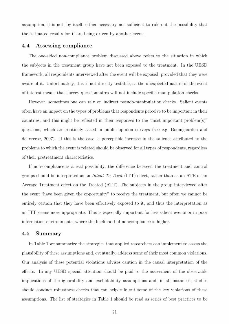
4.5 Summary

In Table 1 we summarize the strategies that applied researchers can implement to assess the

plausibility of these assumptions and, eventually, address some of their most common violations.

Our analysis of these potential violations advises caution in the causal interpretation of the

effects. In any UESD special attention should be paid to the assessment of the observable

implications of the ignorability and excludability assumptions and, in all instances, studies

should conduct robustness checks that can help rule out some of the key violations of these

assumptions. The list of strategies in Table 1 should be read as series of best practices to be

21

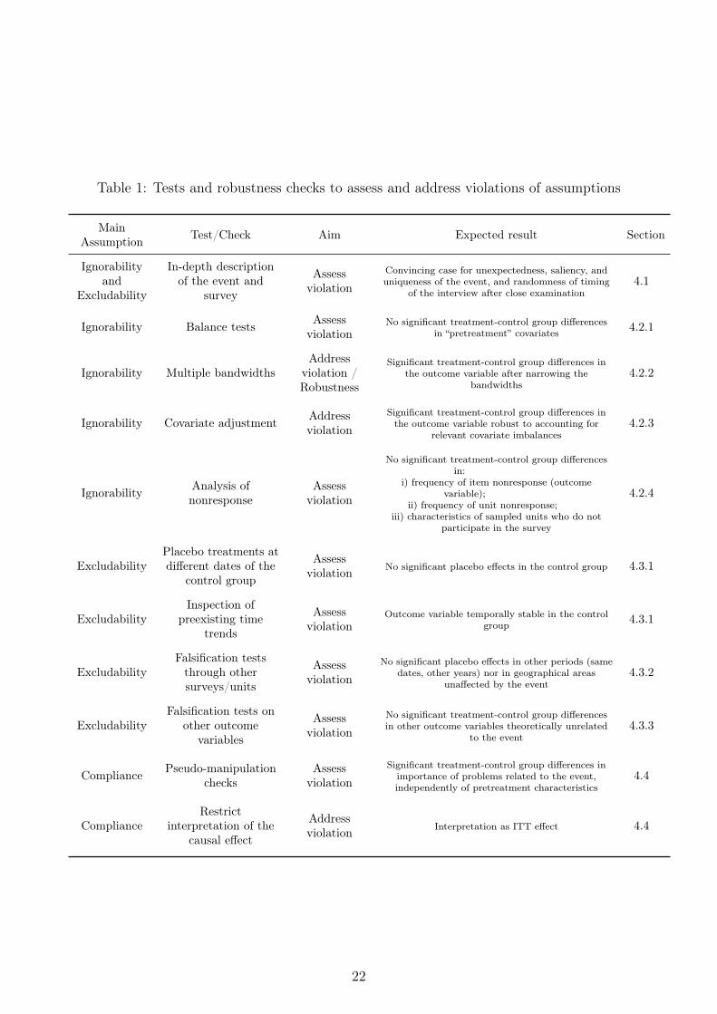
Table 1: Tests and robustness checks to assess and address violations of assumptions

MainAssumption Test/Check Aim Expected result Section

Ignorabilityand

Excludability

In-depth descriptionof the event and

survey

Assessviolation

Convincing case for unexpectedness, saliency, anduniqueness of the event, and randomness of timing

of the interview after close examination4.1

Ignorability Balance tests Assessviolation

No significant treatment-control group differencesin “pretreatment” covariates 4.2.1

Ignorability Multiple bandwidthsAddress

violation /Robustness

Significant treatment-control group differences inthe outcome variable after narrowing the

bandwidths4.2.2

Ignorability Covariate adjustment Addressviolation

Significant treatment-control group differences inthe outcome variable robust to accounting for

relevant covariate imbalances4.2.3

Ignorability Analysis ofnonresponse

Assessviolation

No significant treatment-control group differencesin:

i) frequency of item nonresponse (outcomevariable);

ii) frequency of unit nonresponse;iii) characteristics of sampled units who do not

participate in the survey

4.2.4

ExcludabilityPlacebo treatments atdifferent dates of the

control group

Assessviolation No significant placebo effects in the control group 4.3.1

ExcludabilityInspection of

preexisting timetrends

Assessviolation

Outcome variable temporally stable in the controlgroup 4.3.1

ExcludabilityFalsification teststhrough othersurveys/units

Assessviolation

No significant placebo effects in other periods (samedates, other years) nor in geographical areas

unaffected by the event4.3.2

ExcludabilityFalsification tests on

other outcomevariables

Assessviolation

No significant treatment-control group differencesin other outcome variables theoretically unrelated

to the event4.3.3

Compliance Pseudo-manipulationchecks

Assessviolation

Significant treatment-control group differences inimportance of problems related to the event,independently of pretreatment characteristics

4.4

ComplianceRestrict

interpretation of thecausal effect

Addressviolation Interpretation as ITT effect 4.4

22

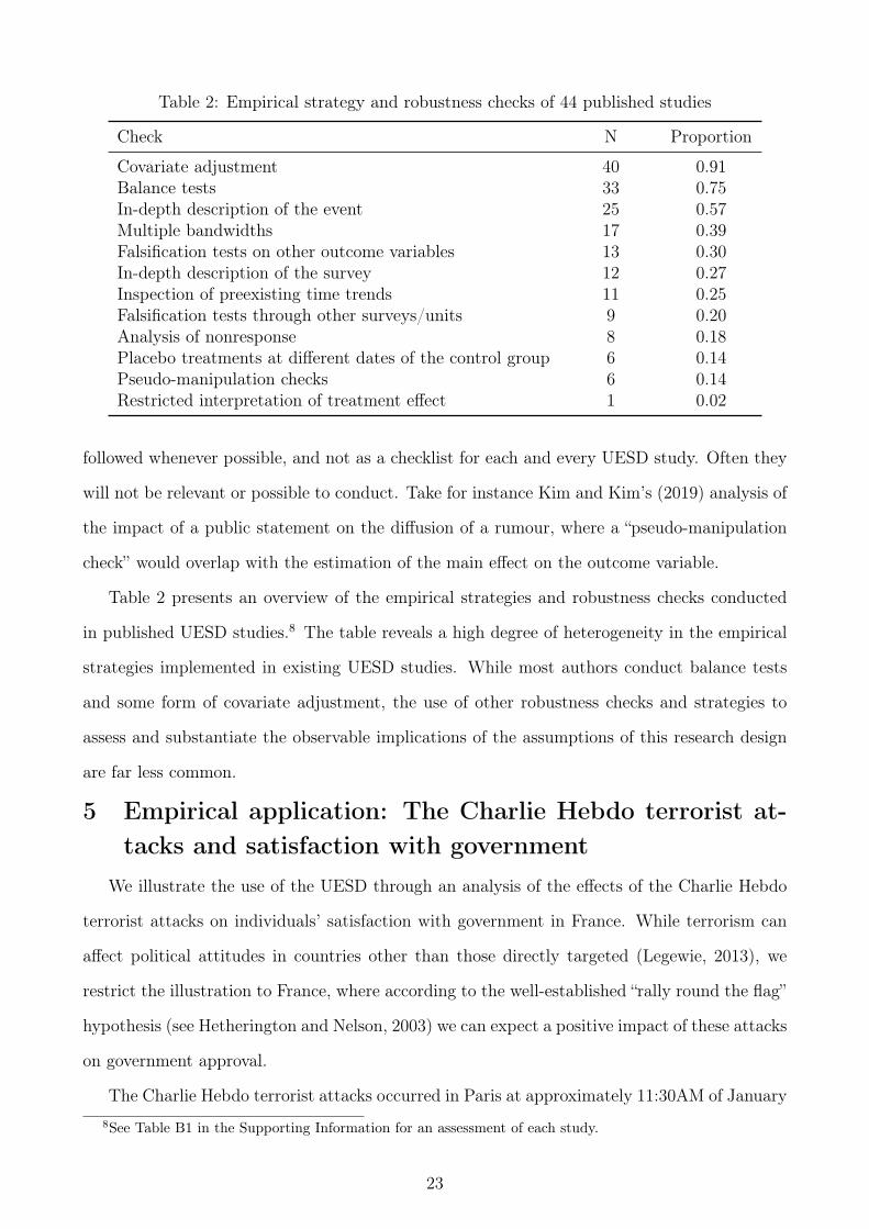
Table 2: Empirical strategy and robustness checks of 44 published studies

Check N Proportion

Covariate adjustment 40 0.91Balance tests 33 0.75In-depth description of the event 25 0.57Multiple bandwidths 17 0.39Falsification tests on other outcome variables 13 0.30In-depth description of the survey 12 0.27Inspection of preexisting time trends 11 0.25Falsification tests through other surveys/units 9 0.20Analysis of nonresponse 8 0.18Placebo treatments at different dates of the control group 6 0.14Pseudo-manipulation checks 6 0.14Restricted interpretation of treatment effect 1 0.02

followed whenever possible, and not as a checklist for each and every UESD study. Often they

will not be relevant or possible to conduct. Take for instance Kim and Kim’s (2019) analysis of

the impact of a public statement on the diffusion of a rumour, where a “pseudo-manipulation

check” would overlap with the estimation of the main effect on the outcome variable.

Table 2 presents an overview of the empirical strategies and robustness checks conducted

in published UESD studies.8 The table reveals a high degree of heterogeneity in the empirical

strategies implemented in existing UESD studies. While most authors conduct balance tests

and some form of covariate adjustment, the use of other robustness checks and strategies to

assess and substantiate the observable implications of the assumptions of this research design

are far less common.

5 Empirical application: The Charlie Hebdo terrorist at-tacks and satisfaction with government

We illustrate the use of the UESD through an analysis of the effects of the Charlie Hebdo

terrorist attacks on individuals’ satisfaction with government in France. While terrorism can

affect political attitudes in countries other than those directly targeted (Legewie, 2013), we

restrict the illustration to France, where according to the well-established “rally round the flag”

hypothesis (see Hetherington and Nelson, 2003) we can expect a positive impact of these attacks

on government approval.

The Charlie Hebdo terrorist attacks occurred in Paris at approximately 11:30AM of January8See Table B1 in the Supporting Information for an assessment of each study.

23

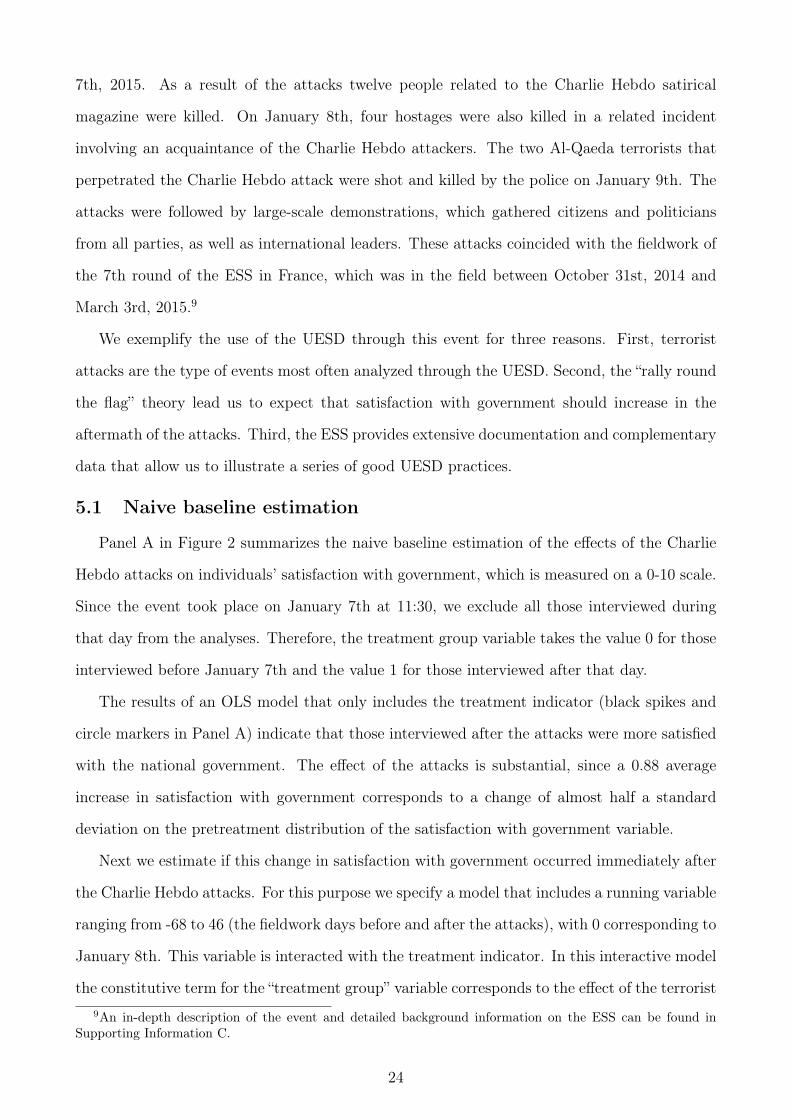
7th, 2015. As a result of the attacks twelve people related to the Charlie Hebdo satirical

magazine were killed. On January 8th, four hostages were also killed in a related incident

involving an acquaintance of the Charlie Hebdo attackers. The two Al-Qaeda terrorists that

perpetrated the Charlie Hebdo attack were shot and killed by the police on January 9th. The

attacks were followed by large-scale demonstrations, which gathered citizens and politicians

from all parties, as well as international leaders. These attacks coincided with the fieldwork of

the 7th round of the ESS in France, which was in the field between October 31st, 2014 and

March 3rd, 2015.9

We exemplify the use of the UESD through this event for three reasons. First, terrorist

attacks are the type of events most often analyzed through the UESD. Second, the “rally round

the flag” theory lead us to expect that satisfaction with government should increase in the

aftermath of the attacks. Third, the ESS provides extensive documentation and complementary

data that allow us to illustrate a series of good UESD practices.

5.1 Naive baseline estimation

Panel A in Figure 2 summarizes the naive baseline estimation of the effects of the Charlie

Hebdo attacks on individuals’ satisfaction with government, which is measured on a 0-10 scale.

Since the event took place on January 7th at 11:30, we exclude all those interviewed during

that day from the analyses. Therefore, the treatment group variable takes the value 0 for those

interviewed before January 7th and the value 1 for those interviewed after that day.

The results of an OLS model that only includes the treatment indicator (black spikes and

circle markers in Panel A) indicate that those interviewed after the attacks were more satisfied

with the national government. The effect of the attacks is substantial, since a 0.88 average

increase in satisfaction with government corresponds to a change of almost half a standard

deviation on the pretreatment distribution of the satisfaction with government variable.

Next we estimate if this change in satisfaction with government occurred immediately after

the Charlie Hebdo attacks. For this purpose we specify a model that includes a running variable

ranging from -68 to 46 (the fieldwork days before and after the attacks), with 0 corresponding to

January 8th. This variable is interacted with the treatment indicator. In this interactive model

the constitutive term for the “treatment group” variable corresponds to the effect of the terrorist9An in-depth description of the event and detailed background information on the ESS can be found in

Supporting Information C.

24

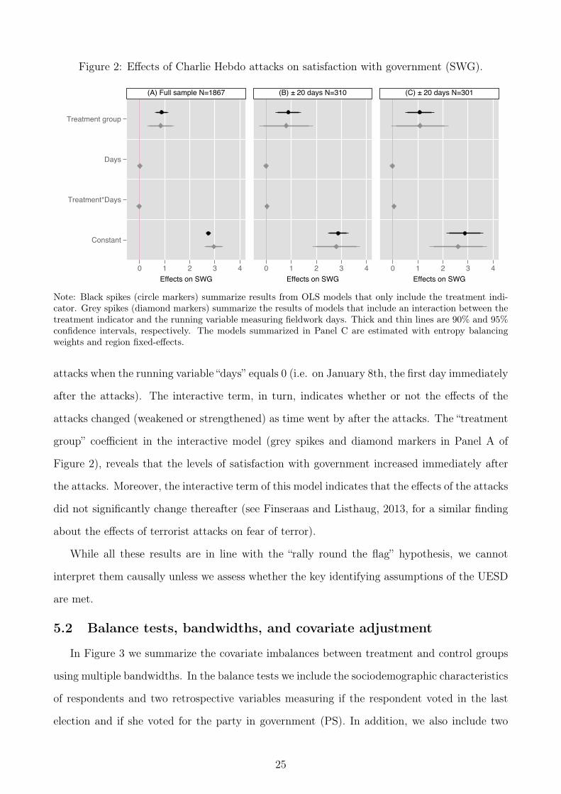
Figure 2: Effects of Charlie Hebdo attacks on satisfaction with government (SWG).

Treatment group

Days

Treatment*Days

Constant

0 1 2 3 4 0 1 2 3 4 0 1 2 3 4Effects on SWG Effects on SWG Effects on SWG

(A) Full sample N=1867 (B) ± 20 days N=310 (C) ± 20 days N=301

Note: Black spikes (circle markers) summarize results from OLS models that only include the treatment indi-cator. Grey spikes (diamond markers) summarize the results of models that include an interaction between thetreatment indicator and the running variable measuring fieldwork days. Thick and thin lines are 90% and 95%confidence intervals, respectively. The models summarized in Panel C are estimated with entropy balancingweights and region fixed-effects.

attacks when the running variable “days” equals 0 (i.e. on January 8th, the first day immediately

after the attacks). The interactive term, in turn, indicates whether or not the effects of the

attacks changed (weakened or strengthened) as time went by after the attacks. The “treatment

group” coefficient in the interactive model (grey spikes and diamond markers in Panel A of

Figure 2), reveals that the levels of satisfaction with government increased immediately after

the attacks. Moreover, the interactive term of this model indicates that the effects of the attacks

did not significantly change thereafter (see Finseraas and Listhaug, 2013, for a similar finding

about the effects of terrorist attacks on fear of terror).

While all these results are in line with the “rally round the flag” hypothesis, we cannot

interpret them causally unless we assess whether the key identifying assumptions of the UESD

are met.

5.2 Balance tests, bandwidths, and covariate adjustment

In Figure 3 we summarize the covariate imbalances between treatment and control groups

using multiple bandwidths. In the balance tests we include the sociodemographic characteristics

of respondents and two retrospective variables measuring if the respondent voted in the last

election and if she voted for the party in government (PS). In addition, we also include two

25

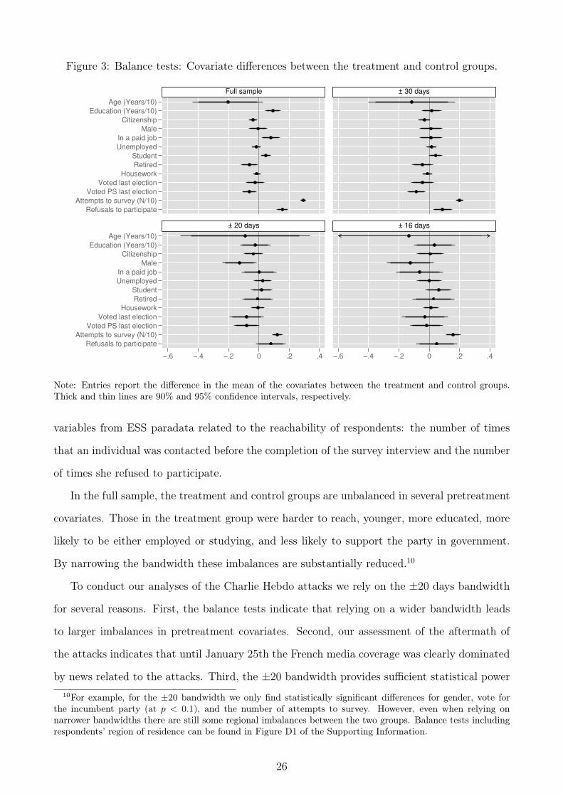
Figure 3: Balance tests: Covariate differences between the treatment and control groups.

Age (Years/10)

Education (Years/10)

Citizenship

Male

In a paid job

Unemployed

Student

Retired

Housework

Voted last election

Voted PS last election

Attempts to survey (N/10)

Refusals to participate

Age (Years/10)

Education (Years/10)

Citizenship

Male

In a paid job

Unemployed

Student

Retired

Housework

Voted last election

Voted PS last election

Attempts to survey (N/10)

Refusals to participate

−.6 −.4 −.2 0 .2 .4 −.6 −.4 −.2 0 .2 .4

Full sample ± 30 days

± 20 days ± 16 days

Note: Entries report the difference in the mean of the covariates between the treatment and control groups.Thick and thin lines are 90% and 95% confidence intervals, respectively.

variables from ESS paradata related to the reachability of respondents: the number of times

that an individual was contacted before the completion of the survey interview and the number

of times she refused to participate.

In the full sample, the treatment and control groups are unbalanced in several pretreatment

covariates. Those in the treatment group were harder to reach, younger, more educated, more

likely to be either employed or studying, and less likely to support the party in government.

By narrowing the bandwidth these imbalances are substantially reduced.10

To conduct our analyses of the Charlie Hebdo attacks we rely on the ±20 days bandwidth

for several reasons. First, the balance tests indicate that relying on a wider bandwidth leads

to larger imbalances in pretreatment covariates. Second, our assessment of the aftermath of

the attacks indicates that until January 25th the French media coverage was clearly dominated

by news related to the attacks. Third, the ±20 bandwidth provides sufficient statistical power10For example, for the ±20 bandwidth we only find statistically significant differences for gender, vote for

the incumbent party (at p < 0.1), and the number of attempts to survey. However, even when relying onnarrower bandwidths there are still some regional imbalances between the two groups. Balance tests includingrespondents’ region of residence can be found in Figure D1 of the Supporting Information.

26

to detect a meaningful increase in satisfaction with government (equivalent to one third of the

standard deviation of this variable in the control group).11.12

The effects of the terrorist attacks drawing on the ±20 bandwidth are summarized in Panel

B of Figure 2. Results indicate that the average level of satisfaction with government was

significantly higher after the attack. Moreover, the interactive model (grey spikes) suggests

that the boost in satisfaction occurred immediately after the attack, although, in this case, the

“treatment group” coefficient does not reach conventional levels of statistical significance.

Regarding covariate adjustment, we rely on entropy balancing to preprocess the data and

produce covariate balance between the treatment and control groups by re-weighting units

appropriately (Hainmueller, 2012).

To re-weight the observations we consider all covariatesXi included in the balance tests, with

the exception of the variable measuring the number of attempts to survey and the respondent’s

region of residence.13 When re-weighting the sample through entropy balancing and including

region fixed-effects the average effect of the Charlie Hebdo attacks is of 1.07 (Panel C in

Figure 2). Moreover, the “treatment group” coefficient of the interactive model indicates that the

average increase in satisfaction with government was almost of the same magnitude immediately

after the attacks.

5.3 Additional robustness checks

In the Supporting Information we conduct a set of analyses to assess the plausibility of

the temporal stability assumption through a placebo treatment (Table D3), analyze the rela-

tionship between the timing of interviews and the outcome variable during the whole survey

fieldwork period (Figure D9), rule out that the attacks caused a problem of attrition (Table D4

and Table D5), perform falsification tests based on other rounds of the ESS to rule out that11A narrower bandwidth might not provide enough power to detect an effect of this size. See the power

analysis in Figure D2 of the Supporting Information12In Figure D3 of the Supporting Information we replicate the estimation of the effects using multiple band-

widths.13We exclude the former variable from the entropy balancing because the distribution of attempts to survey

is radically different between the control and treatment groups. Including this variable imposes an unrealisticconstraint that produces re-balancing weights in the control group that lead to results that end up being drivenby a few respondents from the control group (see section D.3 in the Supporting Information for further details).Concerning the respondents’ region of residence, the entropy balancing algorithm fails to converge when thisvariable is included (tolerance level of 0.015).To prevent biases related to regional imbalances, the modelssummarized in Panel C of Figure 2 estimate the effect of the attacks through specifications that besides theentropy balancing weights also include region fixed-effects. Finally, one could argue that the vote recall questionmight be affected by the terrorist attacks and could, therefore, induce posttreatment bias. In Figure D8 of theSupporting Information we replicate the analyses without balancing the two groups with regard to vote recall.

27

the identified effects are driven by seasonal trends (Figure D10), assess the threat posed by

simultaneous events through falsification tests using alternative outcomes (Figure D11).14

6 Concluding RemarksIn this paper we have described and systematized the UESD, focusing on the assumptions

under which unexpected events that occur during the fieldwork of surveys can yield valid causal

estimates. The impact of political events on public opinion can be analyzed through different

designs. For example, one can correlate the recall of an event (or the importance attributed

to it) and the outcome of interest through a cross-sectional survey. However, this empirical

strategy is likely to be affected by endogeneity biases. Longitudinal studies with repeated

observations of the same individuals can overcome some of these biases. Yet in these studies

the outcomes of interest are often measured a long time after the event occurred. This might

lead to an underestimation of the effects and a greater potential for bias due to the occurrence

of other unrelated events. Priming survey experiments are an alternative in which researchers

have full control over treatment assignment and administration. Therefore, they are more

immune to the type of threats discussed here. However, they are generally based on artificially

designed treatments, and subject to potentially short-lived effects (Gaines et al., 2006), which

may raise concerns about their external validity (Barabas and Jerit, 2010). The UESD, this

paper has argued, can be a compelling alternative, provided its key assumptions are shown to

hold.

One of the drawbacks of most UESD studies is that they are event specific, and this can

limit the generalizability of the findings. Each event is in some regards unique. With a single-

event study we cannot rule out the possibility that the estimated effect is driven by one of its

specific characteristics, or by collateral events. This can be addressed if the timing of collateral

events allows for a separate estimation based on the change in the outcome of interest at the

exact time in which the event took place. However, this is not always possible or advisable.

Therefore, it is always necessary to discuss how the event analyzed might deviate from a typical

case of that class of events.14There are further tests and robustness checks that we recommended but we cannot conduct in our applica-

tion. Salient terrorist attacks, especially those perpetrated by international terror groups, produce attitudinaleffects beyond the borders of the country directly affected by them (Legewie, 2013). Hence, using other surveysadministered simultaneously in other countries to conduct placebo tests does not seem advisable. Moreover, wecannot assess non-compliance through the ‘most important problem(s)’ questions as it is not included in theESS.

28

The ideal way to increase the generalizability of UESD studies is to analyze more than one

event of the same class in order to establish some regularities (e.g. Legewie, 2013). However,

this alternative will often not be feasible, simply because no other event of the same class

coincided with the fieldwork of a survey. A good alternative in these cases is to complement

UESD studies with lab or survey experiments, which can be designed to study the effect of a

similar event in isolation (e.g. Flores, 2018).

One question that remains is whether surveys with a short or prolonged fieldwork are more

adequate to conduct UESD studies. The main benefit of a prolonged fieldwork is that one can

assess in detail the existence of preexisting time trends. However, when compared to shorter

fieldworks, they have clear drawbacks as the differential reachability of respondents is likely

to generate grater differences between the control and treatment groups. Like in our Charlie

Hebdo example, this often imposes the need to focus on a subset of the sample interviewed

around the day of the event, which might limit the generalizability of the findings. Moreover,

in surveys with prolonged fieldworks we will generally find a smaller number of observations

around the event date, and the likelihood of the occurrence of simultenous events that might

confound the effects is higher. On the contrary, in short fieldworks, the as-if random assignment

to treatment is more likely to be plausible without the need for further adjustments, and the

threat of simultaneous events is also likely to be lower. Therefore, the benefits of surveys with

short fieldwork periods clearly outweigh those of surveys with prolonged fieldworks.

Awareness of the potential threats to causal identification affecting the UESD should not lead

researchers to dismiss it as a potentially fruitful identification strategy. While it certainly falls

short of a randomized controlled trial, the fact that it is based on naturally occurring treatments

and often relies on representative population samples makes UESD studies potentially strong

in terms of external validity. The tests and robustness checks we propose should lead to a more

careful implementation of this design, which shall, in turn, increase the credibility of causal

claims based on UESD studies.

29

ReferencesAres, Macarena and Enrique Hernández. 2017. “The corrosive effect of corruption on trust inpoliticians: Evidence from a natural experiment.” Research & Politics 4(2):1–8.

Balcells, Laia and Gerard Torrats-Espinosa. 2018. “Using a natural experiment to estimate theelectoral consequences of terrorist attacks.” Proceedings of the National Academy of Sciences115(42):10624–10629.

Barabas, Jason and Jennifer Jerit. 2010. “Are survey experiments externally valid?” AmericanPolitical Science Review 104(2):226–242.

Berinsky, Adam J. 2017. “Measuring Public Opinion with Surveys.” Annual Review of PoliticalScience 20:309–329.

Boomgaarden, Hajo G. and Claes H. de Vreese. 2007. “Dramatic Real-world Events and PublicOpinion Dynamics: Media Coverage and its Impact on Public Reactions to an Assassination.”International Journal of Public Opinion Research 19(3):354–366.

Boydstun, Amber E., Jessica T. Feezell and Rebecca A. Glazier. 2018. “In the wake of a terroristattack, do Americans’ attitudes toward Muslims decline?” Research & Politics 5(4):1–7.

Branton, Regina, Valerie Martinez-Ebers, Tony E. Carey and Tetsuya Matsubayashi. 2015.“Social Protest and Policy Attitudes: The Case of the 2006 Immigrant Rallies.” AmericanJournal of Political Science 59(2):390–402.

Brehm, John. 1993. The Phantom Respondents: Opinion Surveys and Political Representation.University of Michigan Press.

Coupe, Tom. 2017. “The impact of terrorism on expectations, trust and happiness – the caseof the November 13 attacks in Paris, France.” Applied Economics Letters 24(15):1084–1087.

Csikszentmihalyi, Mihaly and Jeremy Hunter. 2003. “Happiness in everyday life: The uses ofexperience sampling.” Journal of happiness studies 4(2):185–199.

De Vries, Catherine E. 2018. Euroscepticism and the Future of European Integration. OxfordUniversity Press.

Dinesen, Peter Thisted and Mads Meier Jæger. 2013. “The effect of terror on institutional trust:New evidence from the 3/11 Madrid terrorist attack.” Political Psychology 34(6):917–926.

Eggers, Andrew C, Ronny Freier, Veronica Grembi and Tommaso Nannicini. 2018. “Regres-sion discontinuity designs based on population thresholds: Pitfalls and solutions.” AmericanJournal of Political Science 62(1):210–229.

ESS Round 7: European Social Survey Round 7 Data. Data file edition 2.1. NSD - NorwegianCentre for Research Data, Norway – Data Archive and distributor of ESS data for ESS ERIC.N.d.

Finseraas, Henning and Ola Listhaug. 2013. “It can happen here: the impact of the Mumbaiterror attacks on public opinion in Western Europe.” Public Choice 156(1-2):213–228.

Flores, René D. 2018. “Can Elites Shape Public Attitudes Toward Immigrants?: Evidence fromthe 2016 US Presidential Election.” Social Forces 96(4):1649–1690.

Gaines, Brian J, James H Kuklinski and Paul J Quirk. 2006. “The logic of the survey experimentreexamined.” Political Analysis 15(1):1–20.

30

Geys, Benny and Salmai Qari. 2017. “Will you still trust me tomorrow? The causal effect ofterrorism on social trust.” Public Choice 96(3-4):289–305.

Hainmueller, Jens. 2012. “Entropy balancing for causal effects: A multivariate reweightingmethod to produce balanced samples in observational studies.” Political Analysis 20(1):25–46.

Hetherington, Marc J and Michael Nelson. 2003. “Anatomy of a rally effect: George W. Bushand the war on terrorism.” PS: Political Science & Politics 36(1):37–42.

Hofstetter, C. Richard. 1969. “Political Disengagement and the Death of Martin Luther King.”The Public Opinion Quarterly 33(2):174–179.

Imbens, Guido W. and Thomas Lemieux. 2008. “Regression discontinuity designs: A guide topractice.” Journal of Econometrics 142(2):615–635.

Jakobsson, Niklas and Svein Blom. 2014. “Did the 2011 Terror Attacks in Norway ChangeCitizens’ Attitudes Toward Immigrants?” International Journal of Public Opinion Research26(4):475–486.

Jensen, Carsten and Elias Naumann. 2016. “Increasing pressures and support for public health-care in Europe.” Health Policy 120(6):698–705.

Johnston, Richard and Henry E Brady. 2002. “The rolling cross-section design.” ElectoralStudies 21(2):283–295.

Keele, Luke and Rocío Titiunik. 2016. “Natural Experiments Based on Geography.” PoliticalScience Research and Methods 4(1):65–95.

Kim, Jin Woo and Eunji Kim. 2019. “Identifying the effect of political rumor diffusion usingvariations in survey timing.” Quarterly Journal of Political Science forthcoming.

Kocher, Matthew A. and Nuno P. Monteiro. 2016. “Lines of Demarcation: Causation, Design-Based Inference, and Historical Research.” Perspectives on Politics 14(4):952–975.

Larsen, Erik Gahner. 2018. “Welfare Retrenchments and Government Support: Evidence froma Natural Experiment.” European Sociological Review 34(1):40–51.

Legewie, Joscha. 2013. “Terrorist Events and Attitudes toward Immigrants: A Natural Exper-iment.” American Journal of Sociology 118(5):1199–1245.

Lever, H. 1969. “The Johannesburg Station Explosion and Ethnic Attitudes.” The PublicOpinion Quarterly 33(2):180–189.

MacKinlay, A Craig. 1997. “Event studies in economics and finance.” Journal of economicliterature 35(1):13–39.

Metcalfe, Robert, Nattavudh Powdthavee and Paul Dolan. 2011. “Destruction and distress:Using a quasi-experiment to show the effects of the September 11 attacks on mental well-being in the United Kingdom.” The Economic Journal 121(550):F81–F103.

Minkus, Lara, Emanuel Deutschmann and Jan Delhey. 2018. “A Trump effect on the EU’spopularity? The US presidential election as a natural experiment.” Perspectives on Politicsforthcoming:1–18.

31

Montgomery, Jacob M., Brendan Nyhan and Michelle Torres. 2018. “How Conditioning onPosttreatment Variables Can Ruin Your Experiment and What to Do about It.” AmericanJournal of Political Science 62(3):760–775.

Motta, Matthew. 2018. “The Polarizing Effect of the March for Science on Attitudes towardScientists.” PS: Political Science amp; Politics 51(4):782–788.

Muñoz, Jordi, Albert Falcó-Gimeno and Enrique Hernández. 2019. “Replication Data for:Unexpected Event during Surveys Design: Promise and Pitfalls for Causal Inference.”.doi.org/10.7910/DVN/RDIIVL.

Perrin, Andrew J. and Sondra J. Smolek. 2009. “Who trusts? Race, gender, and the September11 rally effect among young adults.” Social Science Research 38(1):134–145.

Pierce, Lamar, Todd Rogers and Jason A. Snyder. 2016. “Losing Hurts: The Happiness Impactof Partisan Electoral Loss.” Journal of Experimental Political Science 3(1):44–59.

Pollock, William, Jason Barabas, Jennifer Jerit, Martijn Schoonvelde, Susan Banducci andDaniel Stevens. 2015. “Studying media events in the European social surveys across researchdesigns, countries, time, issues, and outcomes.” European Political Science 14(4):394–421.

Silber Mohamed, Heather. 2013. “Can protests make Latinos “American”? Identity, immigrationpolitics, and the 2006 marches.” American Politics Research 41(2):298–327.

Silva, Bruno Castanho. 2018. “The Non-Impact of the 2015 Paris Terrorist Attacks on PoliticalAttitudes.” Personality and Social Psychology Bulletin 44(6):838–850.

Solaz, Hector, Catherine E. De Vries and Roosmarijn A. de Geus. 2018. “In-Group Loyalty andthe Punishment of Corruption.” Comparative Political Studies OnlineFirst:1–31.

St. Clair, Travis, Thomas D Cook and Kelly Hallberg. 2014. “Examining the internal validityand statistical precision of the comparative interrupted time series design by comparison witha randomized experiment.” American Journal of Evaluation 35(3):311–327.

Stokes, Susan C. 2014. A defense of observational research. In Field experiments and theircritics: Essays on the uses and abuses of experimentation in the social sciences, ed. DawnTeele. New Haven: Yale University Press pp. 33–57.

Stoop, Ineke A. L. 2004. “Surveying Nonrespondents.” Field Methods 16(1):23–54.

Tiokhin, Leonid and Daniel Hruschka. 2017. “No evidence that an Ebola outbreak influencedvoting preferences in the 2014 elections after controlling for time-series autocorrelation: Acommentary on Beall, Hofer, and Schaller (2016).” Psychological science 28(9):1358–1360.

Zepeda-Millán, Chris and Sophia J Wallace. 2013. “Racialization in times of contention: Howsocial movements influence Latino racial identity.” Politics, Groups, and Identities 1(4):510–527.

32