Two Essays on Corporate Finance: Financing Frictions and Corporate Decisions

Joon Ho Kim

A dissertation submitted in partial fulfillment of the requirements for the degree of

Doctor of Philosophy

University of Washington

2013

Reading Committee: Jarrad Harford, Chair

Jonathan Karpoff Edward Rice

Program Authorized to Offer Degree: Foster School of Business

All rights reserved

INFORMATION TO ALL USERSThe quality of this reproduction is dependent upon the quality of the copy submitted.

In the unlikely event that the author did not send a complete manuscriptand there are missing pages, these will be noted. Also, if material had to be removed,

a note will indicate the deletion.

Microform Edition © ProQuest LLC.All rights reserved. This work is protected against

unauthorized copying under Title 17, United States Code

ProQuest LLC.789 East Eisenhower Parkway

P.O. Box 1346Ann Arbor, MI 48106 - 1346

UMI 3588742

Published by ProQuest LLC (2013). Copyright in the Dissertation held by the Author.

UMI Number: 3588742

University of Washington

Abstract

Two Essays on Corporate Finance: Financing Frictions and Corporate Decisions

Joon Ho Kim

Chair of the Supervisory Committee: Professor Jarrad Harford

Department of Finance and Business Economics

My dissertation focuses on the effect of financial market frictions on firm value in the context of

corporate mergers, capital structure and growth. The first chapter explores how financing

frictions faced by potential buyers of industry specific real assets affect the transaction value of

merger targets that consist of such assets. I find that shareholders of target firms with highly

specialized assets receive a significantly smaller premium than targets with generic assets when

industry peer firms are financially constrained. Further investigation reveals that firms with

specialized assets reduce leverage more than other firms when the risk of liquidation loss is

high. The second chapter explores how frictions in the financial market affect corporate capital

structure and growth. I present evidence that firms that have experienced financing frictions prior

to entering the public debt market undergo significant changes in capital structure and investment

as they gain access to the new sources of capital. Overall, the findings in this dissertation

highlight the importance of financing frictions as key determinants of capital structure and firm

value.

i

Table of Contents

Page

List of Figures ............................................................................................................................... ii List of Tables................................................................................................................................ iii

Chapter 1: Asset Specificity and Firm Value: Evidence from Mergers ................................. 1 Section 1.1: Introduction ....................................................................................................... 1

Section 1.2: Hypothesis ......................................................................................................... 5 Section 1.3: Data.................................................................................................................... 8

Asset Specificity Measure .............................................................................................. 8 Sample Data and Summary Statistics ............................................................................13

Section 1.4: Empirical Results..............................................................................................15 Test Results for Liquidity Discount...............................................................................15 Test Results for Asset Illiquidity and Financial Distress ...............................................24 Test Results for Changes in Optimal Leverage .............................................................26

Cyclicality of Asset Liquidity........................................................................................28 Section 1.5: Conclusion ........................................................................................................31

Chapter 2: Debt Financing Frictions and Access to Public Debt...........................................54 Section 2.1: Introduction ......................................................................................................54

Section 2.2: Hypothesis ........................................................................................................57 Section 2.3: Data...................................................................................................................62 Section 2.4: Empirical Results..............................................................................................66

Test Results for Public Debt Access and Leverage Change ..........................................66

Test Results for Public Debt Access and Firm Growth .................................................70 Test Results for Public Debt Access and Payout ...........................................................72

Section 2.5: Conclusion ........................................................................................................73 References....................................................................................................................................74

Appendix A ..................................................................................................................................79 Appendix B ..................................................................................................................................80

ii

List of Figures

Figure Number Page

1. Cyclicality of Liquidity Discount ............................................................................................53 2. Capital Structure and Firm Growth Around Rating Years .......................................................83 3. Changes in Capital Structure and Firm Growth in Relation to Ex Ante Frictions ...................84

iii

List of Tables Table Number Page

1. Summary Statistics: Asset Specificity by Industry ..................................................................33 2. Summary Statistics: Merger Returns for Target Shareholders .................................................35 3. Summary Statistics: Target Returns by Target Size and Asset Specificity...............................36 4. Target Returns and Target Asset Specificity ............................................................................37

5. Joint Effect of Low Interest Coverage and Asset Specificity on Target Returns .....................39 6. Joint Effect of Low Altman Z-Score and Asset Specificity on Target Returns........................41 7. Joint Effect of High C&I Loan Spread and Asset Specificity on Target Returns ....................43 8. Joint Effect of Low Industry Cash Flow and Asset Specificity on Target Returns ..................45

9. Joint Effect of Recessions and Asset Specificity on Target Returns ........................................47 10. Joint Effect of Low Interest Coverage and Asset Liquidity on Target Returns......................49 11. Changes in Leverage and Asset Illiquidity.............................................................................50 12. Summary Statistics: Sample Group Comparison...................................................................81

13. Likelihood of Entering the Public Debt Market.....................................................................85 14. Accessing Public Debt and the Overall Credit Market Condition .........................................86 15. Sensitivity of Rating-Year Changes in Leverage to Ex Ante Frictions ..................................87 16. Heckman Selection Model .....................................................................................................88

17. Sensitivity of the Rating-Year Firm Growth Rate to Ex Ante Financing Frictions................89 18. Sensitivity of the Rating-Year Payout to Ex Ante Financing Frictions..................................91

iv

Acknowledgements

I am deeply grateful to Chair of my dissertation committee, Jarrad Harford, for his invaluable guidance and support throughout my doctoral studies. I also wish to sincerely thank the other members of my committee, Edward Rice and Jonathan Karpoff, for their advice and encouragement over the years.

Finally, I would like to thank my family members for their continuous support and care, which made all this possible.

1

Chapter 1: Asset Specificity and Firm Value: Evidence from Mergers

1.1 Introduction

Real assets built for specific purposes have few alternative uses. When facing financial

distress, owners of such assets may be forced to raise funds through quick asset deployment

into an illiquid asset market, causing inefficient allocation of the assets at a price below the

assets’ fundamental value. Rational owners of specialized assets foresee the potential private

cost of such distressed sales and adjust their leverage to mitigate their exposure to such risk.

Prior studies in the literature have focused on identifying the value effect of real asset

liquidity on the asset price in specific industries, such as airlines, (Pulvino (1998) and

Gavazza (2011)), aerospace manufacturing (Ramey and Shapiro (2001)), and housing

(Campbell, Giglio and Pathak (2011)).

The main purpose of this paper is to examine the effect of real asset specificity on the

value of the entire firm in a merger. I use a comprehensive sample of completed merger deals

between publicly traded targets and publicly traded acquiring firms across industries over a

30-year period to examine the sensitivity of proxies for target firms’ premiums to the degree

of target firms’ asset specificity.

I derive my testable implications from the predictions of the asset liquidity model in

Shleifer and Vishny (1992). Shleifer and Vishny define asset liquidity (or illiquidity) as the

difference between the realized sales price of an asset and its fundamental value in best use.

They highlight two key components that jointly determine the liquidity of an asset. The first

component is the degree of asset specificity, which is essentially the difference between the

asset’s value in best use and its value in second best use. The second component of asset

liquidity is the degree of financial constraints faced by potential high valuation buyers, e.g.

within-industry peers, at the time of sales. Shleifer and Vishny theoretically show that the

2

combination of a high degree of target firms’ asset specialization and the inability of highest

valuation buyers to finance the purchase of the assets leads to a sales discount for financially

distressed sellers of the assets and inefficient asset reallocation.

Empirically measuring asset liquidity as defined by Shleifer and Vishny (1992) is

challenging for two reasons. First, sellers’ valuation on their assets is unobservable. Second,

direct estimation of the gap between sellers’ valuation on the assets and the actual sales price

requires detailed transaction records of the assets, which are largely private information. For

this reason, the literature has been mostly limited to specific industries in which sales data is

publically available (Pulvino (1998), Gavazza (2011), Ramey and Shapiro (2001) and

Campbell, Giglio and Pathak (2011)).

This paper takes a different approach. Rather than attempting to directly measure asset

liquidity for a single industry, I use proxies that can measure asset specificity for all industries

as well as proxies for the degree of buyers’ financial constraints separately. With these

proxies, I then show that liquidity discount is a common phenomenon and can occur in any

industries where these two components of asset illiquidity along with selling firms’ financial

distress are jointly at work.

To generate a proxy for the degree of asset specificity, I follow the method by Kim and

Kung (2011) using the US Bureau of Economic Analysis (BEA) industry survey data on new

capital asset leases and purchases. This measure is constructed by first estimating the

potential valuation gap among the 123 user industries on the 180 fixed asset types tracked in

the BEA report. I proxy for this potential valuation gap by gauging how narrow the demand

for each fixed asset type is across using industries. Then, I generate a weighted average of

this cross-industry demand for all fixed asset types within each using industry based on the

dollar amount spent on each fixed asset type by the industry. This measure is designed to

capture the degree of specialization of assets for each using industry.

As for the second component of asset liquidity, which is the degree of financial

3

constraints faced by potential highest valuation buyers, I use the following three proxies

drawn from Shleifer and Vishny (1992) and Harford (2005): annual median industry cash

flows, the average annual commercial and industrial (C&I) loan spread over the Federal

Funds rate, and recessions. Lastly, I use firm interest coverage ratio and Altman Z-score from

Almeida, Campello and Hackbarth (2011) and Altman (1968, 2000), as the proxies for target

firms’ financial condition. I then empirically examine the joint effect of target firms’ asset

specificity and the financing capability of potential highest valuation buyers on target

shareholder returns of financially distressed targets using three-day cumulative abnormal

returns (CAR) as the primary measure of the purchase price paid to sellers. To address the

concern that the stock market may anticipate sales of firms with specialized assets and adjust

the firm value before merger deals are made public, I also use the total offer premium paid to

target shareholders as the secondary proxy.

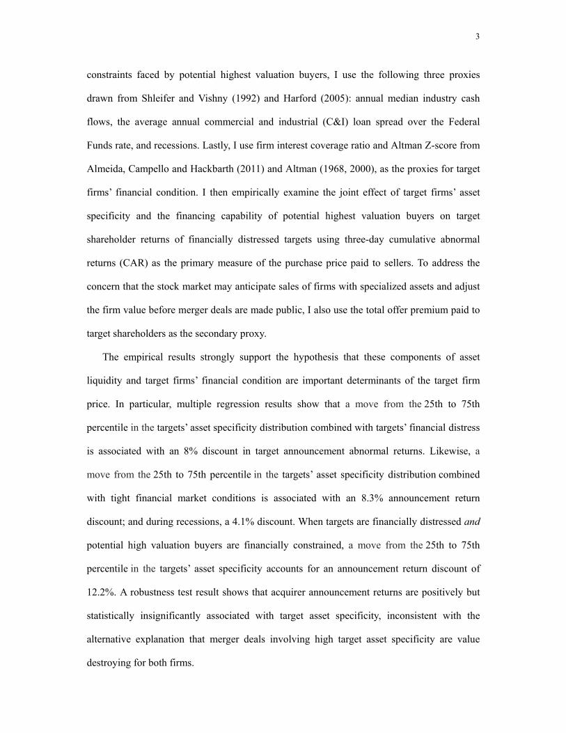
The empirical results strongly support the hypothesis that these components of asset

liquidity and target firms’ financial condition are important determinants of the target firm

price. In particular, multiple regression results show that a move from the 25th to 75th

percentile in the targets’ asset specificity distribution combined with targets’ financial distress

is associated with an 8% discount in target announcement abnormal returns. Likewise, a

move from the 25th to 75th percentile in the targets’ asset specificity distribution combined

with tight financial market conditions is associated with an 8.3% announcement return

discount; and during recessions, a 4.1% discount. When targets are financially distressed and

potential high valuation buyers are financially constrained, a move from the 25th to 75th

percentile in the targets’ asset specificity accounts for an announcement return discount of

12.2%. A robustness test result shows that acquirer announcement returns are positively but

statistically insignificantly associated with target asset specificity, inconsistent with the

alternative explanation that merger deals involving high target asset specificity are value

destroying for both firms.

4

Another important and related prediction made by Shleifer and Vishny (1992) and also by

Williamson (1988) is that firms with specialized assets, when faced with the prospect of real

asset sales at a large discount due to asset illiquidity, reduce leverage more than firms with

generic assets in order to mitigate the risk of such loss. I empirically test this hypothesis as an

additional check, and the test results are consistent with their prediction. Multiple regression

results show that a move from the 25th to 75th percentile in the targets’ asset specificity

distribution combined with tight financial market conditions is associated with a 2.2% annual

reduction in book leverage. Finally, I present evidence supporting Shleifer and Vishny

(1992)’s prediction in a time-series context that the sales price of real assets is closely related

to the overall capital liquidity in the economy.

There are a few studies in the literature that explore the joint effect of asset specificity and

the availability of highest valuation buyers on the liquidation price (Pulvino (1998), Gavazza

(2011), Ramey and Shapiro (2001) and Campbell, Giglio and Pathak (2011)) but the scope of

the literature is mostly limited to particular industries due to difficulty in measuring the

valuation differences among sellers and potential buyers of assets. While Brown, James and

Mooradian (1994) and Lang, Poulsen and Stulz (1995) find a link between target firms’ asset

illiquidity and their announcement returns on asset sales, they do not separate the valuation

effect from other information affecting stock market reactions to merger announcements. One

key contribution of this paper is that it offers a way of isolating the valuation effect from

other determinants of the target price through a measure of asset specificity. To my

knowledge, this is the first paper that documents direct evidence of the joint effect between

real asset specificity and the degree of potential buyers’ financial capacity on asset price

using the comprehensive US merger sample. This paper adds to the literature related to

optimal capital structure and asset redeployability (Almeida and Campello (2007) and

Sibilkov (2009)) by providing a link between firms’ optimal leverage and the firms’ sales

value. Finally, the implications from this study are also linked to the findings by Custódio,

5

Ferreira and Matos (2012) who examine the effect of CEOs’ human capital specificity on

CEO pay in light of their relative bargaining power in the labor market.

The rest of the paper is outlined as follows. Section 1 derives testable implications.

Section 2 explains empirical methods and provides descriptive statistics. Section 3 reports

main empirical results and robustness checks. Section 4 concludes.

1.2 Hypothesis

In this section, I briefly motivate the main predictions and testable implications of this

study using the Shleifer and Vishny (1992) model.

In their model, Shleifer and Vishny consider a firm that consists of highly specialized

assets. The specific nature of the firm’s assets limits the size of the highest valuation buyer

pool. The firm faces two possible industrywide states of the world for the future period,

prosperity and depression. The firm’s shareholders determine the optimal capital structure

based on the balance between the benefits and the costs of leverage. In their model, debt is

beneficial because it reduces the agency costs of free cash flow in a prosperous state. The cost

of using debt is the potential private cost from forced partial or complete liquidation of the

firm to raise funds for creditors when the depression state occurs. Specifically, the expected

cost of debt is equal to the probability of occurrence of the depression state times the

difference between the future cash flows generated by the firm assets in best use and the

firm’s liquidation price to potential buyers.

An increase in the probability of future financial distress affects the firm’s cost of using

leverage in two ways. First, a high probability of financial distress means a high probability

of forced asset sale. Second, if the reason for financial distress is not idiosyncratic but

industrywide, the potential highest valuation buyers of the firm’s assets, e.g. industry insiders,

are also likely to be financially constrained, unable to buy the selling firm. Then the firm may

6

be sold to lower valuation buyers, e.g. industry outsiders, who place a low value on the firm’s

assets because of 1) the adverse selection problem from lacking knowledge necessary to

properly value the assets, or 2) the potential agency costs from having to hire specialists to

manage the acquired firm’s assets. This prospect undermines the potential sales price of the

firm’s assets and drives up the ex ante cost of leverage further.

If the depression state occurs, the firm may raise funds for the creditors by either issuing

new securities, rescheduling debt payments or selling its real assets. The opportunity cost of

selling the assets declines in the degree of financial distress because potential investors for

new securities will demand a reward for taking extra risk from potential asset substitutions

(Jensen and Meckling (1976)) and the adverse selection problem (Myers and Majluf (1984)),

or because coordinating creditors with varying seniorities and conflicting interests to

reschedule debt is difficult (Gertner and Scharfstein (1991)). Potential debt overhang

problems may further increase the cost of debt (Myers (1977)).

When the financially distressed firm is sold, two factors determine the extent of the

discount in the sales price. First, if the firm assets are so specialized that very few potential

highest valuation buyers exist and that the gap between primary and secondary user valuation

on the assets is wide, the sale will fetch a price below fundamental value on average. On the

other hand, if the firm consists of generic assets with many alternative uses, the price of the

assets will be close to the fundamental value. Second, the financing capability of highest

valuation buyers at the time of firm sales affects the sales price because they are willing to

match or pay more than the price the low valuation buyers are willing to pay, if they are

financially unconstrained to acquire the assets.

I apply these predictions to the context of full firm mergers and construct the following

testable hypotheses. First, the prediction that asset specificity of the firm’s assets limits the

size of the highest valuation buyer pool leads to the first hypothesis of this study.

Ha1: Target announcement returns are negatively related to the target firms’ degree of asset

7

specificity.

The opportunity cost of selling a firm declines in the severity of financial distress because

the cost of raising funds through alternative channels increases as financial distress deepens.

Distressed firms with highly specialized assets are more likely to be sold at a discount

because there are fewer high valuation buyers competing for the assets. Pulvino (1998) makes

a similar argument that an increasing default probability raises the airline firms’ cost of

external capital and this in turn makes the airlines more willing to liquidate their airplanes at

a deeper discount. Also, if the financial distress is rooted in industrywide factors, the potential

high valuation buyers of the assets may be in financial distress as well and so unable to buy

the target assets. This prediction leads to the second hypothesis of the study.

Ha2: The negative sensitivity of target announcement returns to target firms’ asset specificity

is more pronounced when targets are in financial distress.

Shleifer and Vishny (1992, 2011) highlight debt capacity of potential high valuation

buyers as one of the key determinants for sellers’ liquidation prices. The low borrowing cost

increases debt capacity of highest valuation buyers and their ability to invest, and competition

among the financially unconstrained buyers drives up the prices of specialized assets,

narrowing the gap between fundamental value and the sales price. Similarly, Harford (2005)

provides evidence that overall capital liquidity in the economy facilitates the clustering of

real asset transactions.

Besides low costs of external financing, internally generated funds are another source of

financing for potential highest valuation buyers of the target assets. Low overall industry cash

flows indicate that potential highest valuation buyers of specialized assets are likely to be

financially constrained and unable to finance mergers. These arguments lead to the third

hypothesis.

Ha3: The negative sensitivity of target announcement returns to target firms’ asset specificity

is more pronounced when the potential highest valuation buyers are financially constrained.

8

The fourth hypothesis naturally follows the predictions in Ha2 and Ha3.

Ha4: The negative sensitivity of target announcement returns to target firms’ asset specificity

is most pronounced when the two following conditions are jointly met: (1) targets are in

financial distress; (2) the potential highest valuation buyers are financially constrained.

In addition to these main hypotheses, I test for the following implications regarding ex

ante leverage response to increased risk of distressed asset sales. When the potential buyers of

the assets with highest valuation are financially constrained, the prospect of firms with high

asset specificity being sold at a discount increases and this increased risk causes the firms to

lower their optimal leverage.

Ha5: Changes in a firm's leverage are negatively related to the firm’s asset specificity when

the potential buyers of the firm assets are financially constrained.

1.3 Data

1.3.1 Asset specificity measure

The key variable in this study is the measure of asset specificity. I follow the procedure

by Kim and Kung (2011) to construct an asset specificity measure. The data come from the

1997 Capital Flow Table (CFT) published by the US Bureau of Economic Analysis (BEA).1

The BEA produced one CFT every 5 years from 1967 to 1997 except for 1987. Among them,

the 1997 CFT provides the most complete estimation for purchases and leases of fixed asset

types by using industries. CFT differs from the Input-Output Use tables (IOT), also published

by the BEA, in that CFT follows each industry’s fixed capital investment while IOT tracks

general flows of materials and services not limited to fixed assets. This particular feature 1 The data are available at www.bea.gov/industry/index.htm and the full description of the data, including the detailed comparisons between CFT and IOT, can be found at the following link: www.bea.gov/scb/pdf/2003/11November/1103%20Investment.pdf.

9

makes CFT more relevant to this study than IOT because the predictions in this paper involve

asset specificity of pledgeable assets.

The CFT columns consist of 123 industry classifications that include not only

manufacturing sectors but also mining, retail, service, financial, utility and public sectors.

The table rows cover 180 different types of fixed assets that include equipment, vehicles,

buildings and structures. Land is not included in the CFT table.2 Each cell in the table shows

the total dollar amount of a particular fixed asset type paid by the using industry in producers’

prices. If a fixed asset type is not used by an industry, then the corresponding cell is left blank.

There is a substantial variation in terms of how widely each asset type is used across different

industries. For example, a fixed asset class associated with “drilling gas and oil wells” is used

only by two out of the 123 industry categories (“Oils and gas extraction” and “Support

activities for mining” sectors), while the “computer terminal” asset class is widely used

across industries, 110 out of the 123 industries in total.

As in Kim and Kung (2011), I use the following formula to construct the asset specificity

score for each industry:3

, )(A

i i a aa

Industry asset specificity ASpecificityω=∑

where i represents each of the 123 industries and a represents each of the 180 fixed asset

types. aASpecificity gauges how narrow the demand for fixed asset type a by different

industries is, and the measure is constructed by dividing the number of industries that do not 2 Kim and Kung (2011) use a second measure of asset specificity that includes land owned by firms. The formula is as below:

( ), 1 land

j with land j indSpecificity Specificityα= −

where , j with landSpecificity is the firm-level asset specificity measure for firm j;

indSpecificity is the industry-level asset specificity measure; and land

jα is the sum of the value of land divided by the sum of the value of properties, plant, and equipment (PP&E) for firm j. Repeating all the tests in this paper using this alternative measure in place of the original variable yields results almost identical to the initial results and so I do not report them. 3 A minor difference between the method used in Kim and Kung (2011) and the one used in this paper is that they exclude an asset from a using industry if the industry’s expenditure on the given asset constitutes less than 1% of the total expenditure in the asset in the economy while I do not exclude any asset based on industries’ relative expenditure size.

10

use commodity a by the total number of industries, which is 123. For example, aASpecificity

for the fixed asset type “drilling gas and oil wells” is 121/123 or 0.98 (= (123-2)/123) which

indicates a high degree of specificity, while aASpecificity for “computer terminal” is only

13/123 or 0.10, which indicates that computer terminals are generic assets. In essence,

aASpecificity conveys information about how specialized an asset type is to a particular

using industry, indirectly capturing the extent of the gap between the asset’s value in best use

and value in second best use. ,i aω measures the relative importance of fixed asset type a to

the industry i and is constructed by dividing industry i’s dollar expenditure on a by its total

dollar expenditures on all fixed asset types in a given year. Finally, iIndustry asset specificity

is the asset specificity score for industry i, and it captures how much of industry i’s resources

is allocated to industry-specific assets. As the final step in compiling the asset specificity

score, I convert the BEA industry specification into the 2-digit SIC code by using the

concordance tables provided by the BEA and the US Census Bureau in order to make the

variable compatible to other data used in this study.4

Next, in order to construct a firm level asset specificity measure, I use the firm segment

data provided by COMPUSTAT. Specifically, a firm’s asset specificity score is compiled as

the weighted average of the segments’ industry asset specificity score, with the ratio of each

segment’s book asset value to the firm’s total book value used as the weight for the segment.5

I remove firm observations from the sample if a firm has segments operating in financial and

utility sectors (SIC in 6000s and 4900s) because of the concern that government regulations

may affect shareholders’ or management’s incentives surrounding asset liquidation. I also

4 I first convert the BEA industry code into the North American Industry Classification System (NAICS) code using the concordance tables provided by the BEA. Then, the 1997 NAICS – 1987 SIC concordance table provided by the US Census Bureau allows me to map the code to the two-digit SIC code. The concordance table can be found at www.census.gov/eos/www/naics/concordances/concordances.html. 5 I implicitly assume that the true real asset specificity of firm segments is correlated with real asset specificity of segment industries at the two-digit SIC level.

11

exclude observations if acquirers are operating in financial and utility sectors for the same

reason.

The 1997 CFT data is based on new investment in that year rather than assets already in

use, and I make two assumptions in using this measure as the proxy for asset specificity of

assets-in-place over time. The first assumption is that the types of assets in which an industry

invests are similar to the assets the industry already has in place for operation.6 Another

assumption I make about the measure is that an industry’s asset specificity does not vary

substantially over time. I argue that this is a reasonable assumption, because what determines

asset specificity is asset composition and not the total volume of assets used. For example,

when demand for crude oil falls and the low demand state continues, the oil extraction

industry’s total output will be reduced and along with it the absolute volume of fixed assets

used for operation, e.g. oil rigs. However, the industry’s asset specificity will change little

over time as long as the industry shrinks the amount of other types of fixed assets, e.g. office

buildings for staff, roughly in the same proportion. Similarly, Ahern (2012) assumes time

invariability of buyer-seller industry bargaining power for his time-invariant measure of

industry interdependence, constructed from the 1997 BEA Use and Makes tables.

As an indirect way of testing my assumptions on the asset specificity measure, I construct

the industry asset specificity measure using the 1992 CFT table and estimate the correlation

coefficient between the scores compiled using the 1992 table and the 1997 table.7 The

correlation coefficient between the two scores is over 84% and statistically different from

zero at the 0.1% level, even though the BEA used different definitions for commodities and

industries to produce these two tables. This result provides support for my argument that

industries’ asset composition is persistent over time. The results of this paper do not change

6 Almeida and Campello (2007) make a similar assumption in their study of asset tangibility and financial constraints. My assumption is a bit stronger than theirs in that my sample includes firms in non-manufacturing sectors whereas their study concerns manufacturing firms only. 7 The 1992 CFT table is available at www.bea.gov/industry/index.htm. BEA does not provide 1987 data.

12

qualitatively even if I use the asset specificity score generated using the 1992 data instead of

the 1997 data, or use the average score of the two scores from the 1992 and 1997 tables.

Throughout this paper, I use the asset specificity score from the 1997 data as the time-

invariant measure of industry asset specificity for the sample period because the 1997 table

provides the most comprehensive industry coverage.

One may argue that while the concept of asset specificity in mining, manufacturing,

construction, and retail industries are straightforward to grasp, the concept of asset specificity

in service sectors and how it may affect firms’ sales price may not be as clear. To address this

concern, I conduct all tests in the paper using a subset of the data excluding firms in the

service industry (SIC in 7000s and 8000s). The test results are robust to this alternative

sampling. I also repeat the same tests on the data excluding any a one-digit SIC sector, one at

a time, from the initial sample. The results and the implications still hold qualitatively.8

Table 1 reports a list of non-service industry categories and their asset specificity score,

sorted by the score. The ranking is intuitive in that the machine-intensive industries such as

mining, manufacturing and transportation are assigned a high asset specificity score while

other industries such as retailing and farming rank low, consistent with the assumptions made

in the literature (Almeida, Campello and Hackbarth (2011)).

As a further check, I repeat the regression tests in this study using the asset

redeployability measure similar to the one used in Almeida and Campello (2007) as the key

independent variable (results not tabulated). They construct the measure by compiling the

ratio of used to total fixed depreciable capital expenditures in industries based on the four-

digit SIC code.9 I replicate their measure using the 1997 data at the three-digit SIC level to

make it comparable to the asset specificity measure of this paper and use it in model 8 I acknowledge and emphasize that there is no reason to believe that the “real” asset specificity measure used in this paper is correlated with the specificity of firms’ intangible assets, which is another substantial source of firm value. All results and implications presented in this paper are strictly limited to tangible fixed assets. 9 The data is from the Bureau of Census' Economic Census and available at www.census.gov/econ/aces /historic_releases_ace.html.

13

estimation. The resulting coefficient estimates on the variable are consistent with the results

from using the asset specificity measure of this paper, although estimates with their measure

show weaker statistical significance. I argue that the measure used in this paper is a more

direct representation of asset specificity and thus produces sharper results because this

measure captures how specialized each fixed asset type is to the using industries and also

how each industry distributes its resources among the fixed asset types with the varying

degree of specialization.

1.3.2 Sample data and summary statistics

The merger data is from the Securities Data Corporation (SDC) US Mergers and

Acquisitions database. The initial sample includes all completed mergers between publicly

traded acquirers and publicly traded targets with deal announcement dates between January 1,

1980 and December 31, 2011. Repurchases, recapitalizations, minority share purchases,

exchange offers, spin-offs and privatizations are all excluded from the sample. Deals with

transaction values less than $10 million or deals involving bankrupt targets are also excluded

from the sample.10 These restrictions give 2,324 unique completed merger deals as the initial

sample. The sample used in the actual analysis has smaller size due to missing stock returns

and data on firm characteristics.

The goal of this study is to examine the effect of target firms’ asset specificity on their

sales prices in mergers. I use two proxies to measure the target returns in merger deals. The

primary proxy is the three-day cumulative abnormal returns (CAR) surrounding merger

announcements estimated using the standard CAPM market model as in Brown and Warner

10 I drop bankrupt targets to avoid unobserved institutional details of the auction process affecting the results. However, inclusion of the firms makes little difference.

14

(1985).11 I also use the total offer premium paid to target shareholders, developed by Schwert

(1996), as the secondary proxy for target shareholder returns to address the concern that the

stock market may anticipate sales of firms with specialized assets and adjust the firm value

before merger deals are made public. The measure is constructed in the following way. First,

I estimate a market model for a (-316, -64) estimation period, requiring minimum 200 non-

missing days for the estimation. The next step generates Runup, which consists of cumulative

target abnormal returns from day -42 to day -1 relative to the announcement date and also

Markup, which is cumulative target abnormal returns from day 0 through the day of delisting

or day 126, whichever comes first. The total premium paid to target shareholders by an

acquirer is equal to the sum of Runup and Markup.12

Table 2 reports initial summary statistics for the target returns. Row (1) shows the average

CAR and total offer premium for all target firms. Both values are statistically different from

zero at the 0.01% level. I split the sample into two groups by the median asset specificity

score of the COMPUSTAT universe over the sample period and report each group’s average

returns in rows (2) and (3). The result shows that targets with highly specialized assets

receive a lower announcement return and offer premium compared to the targets with low

asset specificity, and the difference is statistically significant at the 1% and 5% levels,

respectively.

Table 3 presents the average target returns based on a more detailed sample breakdown by

target size. The first row shows target returns without size breakdown. Consistent with Table

11 I use (-239, -6) days relative to the announcement days as the estimation window and require 100 minimum non-missing observations. The estimation uses CRSP daily stock return data and the value-weighted market index. 12 I repeat all the tests in the paper using two more proxies for target shareholder returns but do not report the results in the interest of space; the third proxy is the difference between the final target share price paid to target shareholders by an acquirer and target share price 4-weeks prior to the deal announcement day, divided by the target share price 4-weeks prior to the deal announcement day. I construct the proxy using the variables provided by SDC. The test results from using this proxy are statistically and economically similar to those obtained from using the total offer premium. The fourth proxy tested is the measure for the division of merger gains developed by Ahern (2012). The results with this proxy are consistent with the results from using the other three proxies but statistical significance is weaker.

15

2, high target asset specificity is associated with low target returns. The target returns for the

lowest asset specificity group are significantly larger than those for the highest specificity

group at the 1% level, as indicated by the difference-in-means test results in the far right

column. The table also shows that targets with low asset specificity are generally smaller than

the firms with high asset specificity, consistent with the notion that large firms in capital-

intensive industries use specialized assets.

Moeller, Schlingemann and Stulz (2003) present evidence that there is a persistent size

effect associated with merger returns. To control for the target size effect, I split the target

firms by quartiles for beginning-of-year market equity size and then further divide each size

group into four subgroups by asset specificity. The table shows that target returns for the

lowest asset specificity groups are still higher than the returns for the highest asset specificity

groups in all cases even after controlling for target size, and the statistical significance still

holds in three out of eight tests despite the low statistical power due to reduced sample size.

The initial summary statistics support Ha1 but there are many other factors that affect

target merger returns. The next section presents multiple regression results.

1.4 Empirical Results

1.4.1 Test results for liquidity discount

For the regression analysis, I use two model specifications to control for firm and deal

characteristics that are known in the literature to be associated with target shareholder returns.

The base model is from Moeller, Schlingemann and Stulz (2003), and I include the target

asset specificity measure in it. This base setting contains deal characteristic variables

reflecting payment methods, existence of toeholds, competing deals and target termination

fees, whether the deal is a tender offer, whether it is a diversifying merger, and relative deal

16

size. It also includes firm specifics such as acquirer and target market capitalization and

proxies for Q. The “extended” model includes all the variables in the base model plus an

additional set of variables that might be correlated with target asset specificity and returns.

Firms with highly specialized assets are typically machine intensive (Almeida, Campello and

Hackbarth (2011)) and tend to hold a greater portion of their assets in tangible form. Because

the main interest of this study is to test the effect of asset specificity on target returns rather

than the effect of size of specialized assets, I include the ratio of tangible assets to total assets

as a control variable.

Shleifer and Vishny (1992) suggest that assets owned by technology-intensive firms may be

illiquid. This view also implies that asset specificity may be correlated with the firm’s growth

opportunities, which in turn is likely to be correlated with target announcement returns for

reasons other than the specificity of the firm assets. To address this issue, I include the ratio

of target R&D expenditures to target assets as a proxy for the firms’ growth opportunities. I

also include the R&D ratio of acquiring firms to capture the synergy effect correlated with

growth opportunities not picked up by the target R&D ratio.

Industries using specialized assets such as natural resource extraction or durable goods

manufacturing may require high startup costs and this feature may work as an entry barrier,

causing some of these industries to be concentrated. Consequently, the level of target industry

concentration may affect target shareholder returns for reasons related to industrial

organization (Kim and Singal (1993), Singal (1996) and Hackbarth and Miao (2011)), but

unrelated to target asset specificity. I control for target industry concentration using the eight-

firm concentration ratio provided by the US Census Bureau from the same year as the data

used for the asset specificity measure. I also include the eight-firm concentration ratio for

acquirer industries to control for the possibility that acquirer industries are closely related to

target industries and reflect target industry concentration. Finally, all models control for year

and Fama-French twelve industry fixed effects for both acquirer and target industries. The

17

regression model used in this section is as follows:

Proxy for Target SH Premium = Target's asset specificity score + Xb+φ ε× (1)

Table 4 presents the estimation results. The three-day abnormal returns of target firm

stocks surrounding merger announcements is the dependent variable for column (1) and (2)

and the total offer premium received by target shareholders is the dependent variable for

Column (3) and (4).13 The coefficient estimates on target asset specificity across all models

are negative and statistically significant, consistent with the prediction in Ha1. Based on the

estimate in column (2), an increase in targets’ asset specificity from the 25th to 75th

percentile accounts for a 3.3% smaller target announcement return, or a 6.1% smaller total

offer premium if based on the column (4) results, holding other variables constant. Estimates

for other coefficients are consistent with the estimates reported in Moeller et al (2003) and the

literature.

The models for Table 5 test Ha2 that predicts that the negative sensitivity of target

announcement returns to target firms’ asset specificity is more pronounced when targets are

in financial distress. I follow Almeida, Campello and Hackbarth (2011) and classify a

financially distressed target firm as a firm with its interest coverage ratio lower than the

industry-year median interest coverage ratio.14 The odd-numbered columns in Table 5 report

the estimation results for the deals involving financially distressed targets, and the even-

numbered columns report the results for the rest of the sample.

The estimation results are consistent with Ha2. Across all model settings, the coefficients

for target asset specificity in the odd-numbered columns are all negative and their absolute

values greater than the estimates for financially healthy target firm groups. The differences in

13 Note that the sample size for estimation using the premium as the dependent variable is a bit smaller than the sample size for estimation using the CAR. This is because estimation of the premium requires more stock return data and this leads to more observations with missing values. 14 Pulvino (1998) identifies financially constrained firms as firms with book leverage higher than the industry-year median book leverage and their current ratio lower than the industry-year median current ratio. Tests based on the Pulvino’s classification yield similar results.

18

the target asset specificity coefficients between the distressed target group and the healthy

group are statistically significant for the results with the three-day CAR as the dependent

variable, as reported in the coefficient comparison test P-values next to each set of estimation.

The results based on the total offer premium as the dependent variable in column (5) and (7)

show economically significant but statistically insignificant coefficients. This may be so

because the size of standard errors in the long-run return measure is large enough so that the

effect of target distress is lost in the noise.

The economic magnitude of the coefficients is substantial. Results in column (3) indicate

that a financially distressed target firm whose assets are more specialized (i.e. the 75th

percentile relative to 25th percentile in the target asset specificity score distribution) will

experience an 8.6% lower announcement return. We can also interpret the result in a different

light; even if a firm is financially distressed, if the firm consists of generic assets, the firm

owners experience a minimal price discount because generic assets have many potential high

valuation buyers inside or outside the target’s own industry. These buyers will compete for

the firm assets and drive up the sales price close to the fundamental value. This is precisely

one of the central predictions made by Shleifer and Vishny (1992).

As an alternative classification, I define a financially distressed target firm to be a target

firm with an Altman Z-score below 2.99 at the beginning of the announcement year.15 As in

the previous part, I estimate the regression models for the subgroup separately from the rest

of the sample. The odd-numbered columns in Table 6 report estimation results for the firms

with a low Altman Z-score, and the even-numbered columns report estimates for the rest of

the sample.

The results in Table 6 show the same pattern as in Table 5 that the coefficients on target

asset specificity for the distressed firm group are negative and their absolute values are

15 Altman (1968) suggests the Z-score 2.99 as the threshold that divides healthy firms from firms with some probability of default in the near future. Using 1.81, another threshold under which Altman calls the “distressed” zone, as the cutoff point does not change the results qualitatively.

19

greater than the counterparts for the financially healthy group. As in Table 5, the differences

in the target asset specificity coefficients between the distressed group and the healthy group

are statistically significant for the results based on the three-day CAR. As in Table 5, the

results based on the total offer premium as the dependent variable in column (5) and (7) show

economically significant but statistically insignificant coefficients. This may be so because

the size of standard errors in the long-run return measure is large enough so that the effect of

target distress is lost in the noise. Overall, these results are consistent with the prediction in

Ha2 and also with the implications from Table 5.

The result in column (3) suggests that the shareholders of a financially distressed target

firm consisting of specialized assets (i.e. the 75th percentile relative to 25th percentile with

respect to the target asset specificity score) will experience a 7.2% lower merger

announcement return than shareholders of targets with generic assets.

There is a concern that the sensitivity of the target merger announcement return to target

asset specificity may be positive if an eventual target firm is in deep financial distress and the

market anticipates with near certainty that the firm will go through bankruptcy and

subsequent costly restructuring. To address this possibility, I repeat the tests for Ha2 with a

sample excluding deals involving target firms with the interest coverage or the Z-score below

the 10th percentile of each industry year. The results do not change qualitatively from using

the original sample.

According to Ha3, the negative sensitivity of target announcement returns to target

firms’ asset specificity is more pronounced when the potential highest valuation buyers are

financially constrained. Following Harford (2005), I use the spread between the average

interest rate on commercial and industrial loans and the Federal Funds rate (C&I loan spread)

as a proxy for the overall capital liquidity in the economy. I define high C&I loan spread

regimes as the periods when the C&I loan spread is above the 67th percentile (i.e. the spread

greater than 1.75) in its time series over the sample period and consider potential buyers in

20

the regimes to be financially constrained.16

Table 7 presents the estimation results. The odd-numbered columns report estimation

results for target returns in the high C&I loan spread regimes and the even-numbered

columns report the results for the rest of the sample. The results are consistent with the

prediction in Ha3. The coefficients on target asset specificity are significantly negative and

their absolute values are greater in the high C&I loan spread than those in the low spread

regimes. The results from coefficient comparison tests between the two regimes reject the

null hypothesis that the two estimates are the same, except for one case.

The results also show that the impact of asset illiquidity on the target price is

economically substantial. The coefficient estimate in Column (3) suggests that when the

credit market tightens, firms with more highly specialized assets (i.e. the 75th percentile

relative to 25th percentile in the target asset specificity score distribution) will experience an

8.2% lower announcement return and an 11.1% smaller premium, according to column (7).

Two key implications emerge from the results. The first implication is that when low

borrowing costs increase the financing capacity of highest valuation potential buyers, the

shareholders of target firms consisting of highly specialized assets will experience a minimal

merger discount because competition among the buyers will drive up the asset price. The

statistically insignificant coefficients of target asset specificity in the even-numbered columns

highlight this point. The second implication is that even if the credit market tightens and high

valuation potential buyers of the target firm are financially constrained, there will be little

price discount on target firms consisting of generic assets that have very little gap between

value in best use and value in second best use. These two implications are consistent with the

16 This cutoff point allocates about a one third of the sample into the high cost of external financing regime. The results are robust to alternative cutoff points such as the time series median or the 75th percentile. In a separate test, I divide the sample into the tightening capital market regimes and the loosening capital market regimes according to whether the concurrent changes in the C&I spread are positive or negative, and then I estimate the regression models separately for each subgroup. The results still hold qualitatively under this classification scheme.

21

central prediction by Shleifer and Vishny (1992) and provide direct evidence to their theory

of asset illiquidity and liquidation discount.

As an alternative classification for financially constrained buyers, I define low industry

cash flow regimes as the periods when the annual median cash flow of a target industry is

below the 25th percentile in its time series over the sample period.17

Table 8 presents the estimation results. The odd-numbered columns report the results for

target firms in the low target industry cash flow regimes and the even-numbered columns

report the results for the rest of the sample. The coefficients on target asset specificity in the

low industry cash flow regimes are negative and statistically significant, and their absolute

values are greater than the coefficients for the rest of the sample across all the model settings.

The results from coefficient comparison tests between the two regimes reject the null

hypothesis that the two estimates are the same in all cases. Overall, the results presented in

Table 8 are consistent with the prediction in Ha3 and the implications from Table 7.

The economic implication based on the asset specificity coefficients in column (3) and

column (7) is that when the cash flow of a target firm’s industry is low and the target’s asset

specificity is high (i.e. the 75th percentile relative to 25th percentile with respect to the target

asset specificity score), the target shareholders are to experience a 8.4% lower announcement

return and a severe discount of 23.2% in the total offer premium.

The results in Table 8 and Table 7 show two different channels through which asset

liquidity of specialized assets can be realized. Table 7 provides evidence that the ease of

external financing increase the highest valuation buyers’ financial capacity, allowing them to

compete over target firms. On the other hand, table 8 provides evidence that an increase in

the internally generated funds within the target industries can also relieve the financial

constraints of the highest valuation buyers and drive up the targets’ asset price close to the

17 This cutoff point allocates about a one third of the sample into the low industry cash flow regimes. The results are robust to alternative cutoff points such as the time series median or the 33rd percentile. The results are also unaffected to using industry cash flows at the three-digit SIC level instead of the two-digit level.

22

highest fundamental value. Shleifer and Vishny (1992) suggest that these two effects can

reinforce each other. High industry cash flows increase the financing ability of highest

valuation users. Competition among such buyers over the specialized assets pushes up the

liquidation price of these assets. For the holders of these assets, this means that the potential

cost of using leverage drops partly because the liquidation price increases but also because

the assets’ fundamental value itself increases, opening up more debt capacity. The low

borrowing costs allow the firms to invest more in these assets, knowing that there will be

other financially unconstrained high valuation buyers of their assets available when it is

optimal for the firms to sell their assets.

As another classification for financially distressed potential buyers, I follow the definition

of The National Bureau of Economic Research (NBER) to identify merger deals during the

recession years, which are 1980, 1981, 1982, 1990, 1991, 2001, 2008 and 2009 in my sample

period.18 I estimate the regression models for the recession group separately from the rest of

the sample. The odd-numbered columns in Table 9 report estimation results for the recession

group, and the even-numbered columns report results for the rest of the sample.

The coefficients on target asset specificity for the recession group are negative and

statistically significant, and their absolute values are greater than the coefficients for the off-

recession group. The results from coefficient comparison tests between the two regimes reject

the null hypothesis that the two estimates for asset specificity are the same in one case with

another P-value being close to the 10% level at 11.1%. The rejection rate being lower than the

ones in other previous tests is not surprising considering that the sample size for the recession

group is small. Besides, as implied in Mitchell and Mulherin (1996), slowdowns in

industrywide real asset transactions can occur not only during the economywide recession

periods but also outside recessions as well, and this may explain the negative and statistically

significant coefficients on target asset specificity in some of the off-recession columns. 18 A year is identified as a recession year if at least three months of the calendar year is in recession periods.

23

Nevertheless, the estimation results are generally consistent with the prediction in Ha3.

One alternative explanation for the Ha2 and Ha3 test results so far is that perhaps the

merger deals involving targets with specialized assets are shareholder value destroying for

both target and acquiring firms. That is, some unobserved factors may be positively

correlated with target firms’ asset specificity and negatively correlated with perceived deal

quality. To check this possibility, I estimate the models using acquiring firms’ announcement

returns as the dependent variable (results not reported). If this alternative explanation is

driving the original results, the test outcome should reveal a negative relation between

targets’ asset specificity and the acquirers’ announcement returns. Instead, the test results

indicate that acquirer returns are positively related with target firms’ asset specificity,

although the coefficients are mostly statistically insignificant. In fact, the sensitivity of

acquiring firms’ returns to target firms’ asset specificity is also positive for subgroups of all

target financial distress and constrained financing classifications tested earlier in this section.

This result provides some support to the argument that value is transferred from target

shareholders to acquiring shareholders when such targets are in financial distress and the

liquidity of target assets is low.

Another possible explanation is that the results may be driven by other firm and industry

characteristics not included in the models tested. In untabulated tests, I augment the initial

models to further include additional target firm and industry variables such as firm

profitability, firm book leverage, firm age, industry profitability, industry interest coverage

ratio, industry cash flow volatility and average industry book leverage. The results are not

qualitatively different from the original results, with the implications from the original tests

mostly unchanged.

Lastly, I test whether the results in this section are dependent on the way the regression

tests are set up (results not tabulated). For example, in testing Ha2, instead of dividing the

initial sample into two groups according to the target firms’ financial condition and

24

estimating the model separately for each subgroup, I create a dummy variable reflecting the

target firms’ financial condition and include the variable as a stand-alone control along with

an interaction term between the variable and target asset specificity. I set up a model for the

Ha3 tests involving financially constrained buyers in the same way. The results using the

three-day CAR as the dependent variable show that the coefficients on the interaction terms

are all negative and statistically significant at the conventional level, consistent with the

predictions in Ha2 and Ha3. This outcome suggests that the initial results are not conditional

on the test setting.

1.4.2 Test results for asset illiquidity and financial distress

The tests in the previous section examined the joint effect of target firms’ asset specificity

and financial distress on target shareholder returns and the joint effect of target firms’ asset

specificity and financially constrained potential buyers on target shareholder returns,

separately. However, the Shleifer and Vishny model predicts that the discount effect of asset

illiquidity on target shareholder value is the greatest when the following three conditions are

jointly met: (1) a target firm is financially distressed; (2) the target firm consists of highly

specialized assets; and (3) the potential high valuation buyers are financially constrained.

This section tests the prediction in Ha4.

First, I split the initial sample into four subgroups. Subgroup 1 includes merger deals

involving financially distressed target firms (e.g. the target interest coverage ratio below the

industry-year median or the target Altman Z-score below 2.99) with financially constrained

potential buyers (e.g. the C&I spread above the time series median or the annual target

industry median cash flows below their time series medians). Subgroup 2 includes deals

involving financially distressed targets with financially unconstrained potential buyers.

Subgroup 3 includes deals involving financially healthy targets with financially constrained

25

potential buyers. Lastly, Subgroup 4 includes deals involving financially healthy targets with

financially unconstrained potential buyers. The prediction is that the target announcement

return should be most negatively associated with target asset specificity in subgroup 1 and

least negatively associated with it in subgroup 4. I estimate the extended regression model (1)

on the four subgroups.

Table 10 presents the regression results for each group. I only report the coefficient

estimates on target asset specificity in the interest of space. Both tables in Panel A use targets’

industry-year median interest coverage ratio to classify financially distressed targets. In the

upper table of Panel A, potential high valuation buyers are considered financially constrained

if the C&I spread is above its time series median and unconstrained otherwise. In the lower

table of Panel A, potential high valuation buyers are considered financially constrained if the

annual target industry median cash flows are below their time series median and

unconstrained otherwise. As before, the dependent variable is the target firms’ three-day CAR

on merger announcements. Tests using the total offer premium as the dependent variable

yield results with essentially the same implications. The four columns (1) through (4) in each

table correspond to the estimation results for the four subgroups with the same number.

Inspecting the coefficients across the four subgroups confirms the prediction that the

target announcement return is most negatively associated with target asset specificity both

when a target firm is financially distressed and the potential buyers are financially

constrained, as shown in column (1). The results are also consistent with the prediction that

the target announcement return is least negatively associated with target asset specificity

when a target firm is financially healthy and when the potential buyers are financially

unconstrained, as shown in column (4). In fact, the coefficient comparison test results

reported in the far right column confirm that the estimates in column (1) and column (4) are

statistically different at the 1% level.

Models in Panel B use the Altman Z-score instead of the targets’ interest coverage ratio to

26

classify financially distressed target group and healthy target group. The rest of the test

setting is the same as the models in Panel A. The results reported in Panel B are consistent

with the prediction and also with the results in Panel A.

Note that coefficients in odd-numbered columns are generally more negative and more

statistically significant than the coefficients in even-numbered columns. This suggests that

potential highest valuation buyers’ financing capacity, rather than target firms’ financial

condition, may be the primary factor determining the sales price of specialized assets. This

implication is intuitive in that when many potential high valuation buyers of the target assets

are financially unconstrained, competition among the buyers over the target firms will drive

up the price regardless of target firms’ financial conditions, and vice versa.

1.4.3 Test results for changes in optimal leverage

The results on target shareholder returns so far provide evidence supporting the prediction

that targets’ high asset specificity combined with financially constrained potential high

valuation buyers severely undermines the target price in mergers. Shleifer and Vishny (1992)

hypothesize that the prospect of such ex post liquidation loss gives ex ante incentives for the

firms to reduce leverage to mitigate the possibility of such loss, because the expected costs of

using leverage becomes greater than the benefits of using leverage. I draw Ha5 from this

prediction.

To test this hypothesis, I construct a dataset containing target firms’ annual changes in

leverage over the entire sample period before the years in which they are acquired. The

dataset also includes control variables that the capital structure literature identifies as key

determinants of changes in firm leverage.19 I classify subgroups of asset illiquidity based on

19 The control variables used in this section are similar to the ones in Sibilkov (2009).

27

the three different conditions in which potential highest buyers are financially constrained,

estimate the regression models separately for each group, and compare the estimation results

from these groups with the results from subsamples with financially unconstrained buyers. To

ensure the firms have little financial slack, I require all firms in the subgroups to have book

leverage greater than the industry-year medians. The test uses the following regression

model:

= + X +Changes in leverage Firm asset specificity score φ β ε× (2)

As in Sibilkov (2009), I include industry-year adjusted book leverage as an independent

variable to control for the leverage level prior to changes. Table 11 presents the estimation

results for the regression model (2). Columns (1), (2), (5) and (6) in Panel A and columns (1)

and (2) in Panel B report the estimation results using changes in leverage from the current

year to the following year as the dependent variable. Columns (3), (4), (7) and (8) in Panel A

and columns (3) and (4) in Panel B report the results using changes in leverage over a two-

year period starting the current year as the dependent variable. The subgroups for which the

models are estimated appear at the table header. All models include year fixed effects and

industry fixed effects with the Fama-French 12 industry specifications.

The results in Panel A of Table 11 are consistent with Shleifer and Vishny (1992)’s

predictions that firms facing the prospect of a liquidity loss due to high asset specificity

adjust leverage more to reduce such risk. The estimation results for illiquid groups are

presented in columns (1), (3), (5) and (7) in Panel A and they report that the coefficients on

asset specificity are all negative and statistically significant, except for one case. Their

absolute values are greater than those of the healthy counterparts reported in the even-

numbered columns, and the coefficient comparison tests reject the null hypothesis that the

coefficients on asset specificity of the two groups are the same in two out of four cases. The

regression results for the recession sample presented in Panel B are not as consistent with the

prediction as the results in Panel A, and I argue that this is because slowdowns in

28

industrywide asset transactions can occur outside the economywide recession periods, adding

noise to the results. Finally, the results hold qualitatively when the models are tested on the

entire sample of COMPUSTAT firm year observations with the required data.

The central implications from the ex ante leverage change results in this section combined

with the ex post liquidity discount results in the previous section are the following. The

coefficient estimates for asset specificity in the even-numbered columns being mostly

statistically insignificant and greater than the estimates in odd-numbered columns suggest

that even if a firm consists of highly specialized assets, as long as there are many financially

unconstrained highest valuation users of the assets ready to compete for the firm assets, the

firm’s asset specificity plays no role in determining its optimal leverage. The negative

coefficient estimates on asset specificity in the odd-numbered columns provide support to the

prediction that when the market condition changes so that the high valuation users of the

assets are no longer available as potential buyers, the firm’s expected liquidation value drops

in the degree of the firm’s asset specificity. Facing the increasing cost of holding leverage, the

firm adjusts its leverage lower to mitigate the probability of a loss from selling its assets

when the market is illiquid.

1.4.4 Cyclicality of asset liquidity

For this final section, I briefly discuss the procyclicality of asset liquidity proposed by

Shleifer and Vishny (1992). They predict that liquidity of specialized assets is pro-cyclical

because the financial capacity of the assets’ highest valuation potential buyers is procyclical.

There have been a few studies in the literature that tested this procyclicality prediction of

asset liquidity in light of the clustering of asset transactions. Mitchell and Mulherin (1996)

relate merger waves to industrywide economic and regulatory shocks. Harford (2005)

provides evidence that merger waves are triggered by industrywide economic and regulatory

29

shocks and are facilitated by overall capital liquidity in the economy. Eisfeldt and Rampini

(2005) show that the amount of capital reallocation is procyclical. Dittmar and Dittmar

(2008) and Rau and Stouraitis (2011) also highlight the importance of industry and

economywide shocks for occurrence of merger waves.

Expanding on the findings of these papers, I provide some evidence that sales prices for

specialized assets may follow a cyclical pattern as well. First, I estimate the base model (1)

for each year separately over the sample period. Because some years have only a small

number of completed mergers, I combine two consecutive years to form a unit subperiod. For

example, merger observations in 1992 and in 1993 are combined to form a subgroup for year

1993, and the next period subgroup for year 1994 is formed by combining observations from

1993 and 1994, and so on. This process yields thirty one initial subgroups and I drop the

groups between 1980 and 1984 because the sample size is too small.

The model estimation using each subgroup gives one estimate for the coefficient on target

asset specificity for each of the 26 sample groups. I plot the point estimate values in Figure 1

and call the time series price coefficient. A low price coefficient value indicates that there is

an overall price discount on asset specificity. The caveat is that only a few coefficient

estimates plotted in the graphs are statistically significant at the conventional level, due

partially to small sample size. I also exclude the industry fixed effects for acquirers and

targets because their inclusion further reduces sample size.

Panel A in Figure 1 displays the price coefficient along with the annual average C&I

spread. Panel B plots the price coefficient along with the annual median cash flow over book

assets. Panel C plots the price coefficients along with and the annual average GDP growth

rate.

The price cyclicality hypothesis predicts that there is a negative relation between the price

coefficient and the C&I spread. Tests for unit roots on the variables indicate that the C&I

spread has a unit root. An Engle-Granger test on the residuals from regressing the price

30

coefficient on the C&I spread and a time trend indicates that the price coefficient and the C&I

spread are cointegrated.20 This result is consistent with the prediction that real asset price is

determined in equilibrium and the level of financial constraints faced by potential buyers of

the assets is an important determinant of the price. A Durbin-Watson test on the residuals

rejects the serial correlation hypothesis. The OLS estimation result is shown below:

*Price coefficient = - 26.434 - 0 .309 C & I spread + 0.013 Tim e trend× ×

The * indicates a statistical significance at the 10% level. The adjusted R2 is 0.06. The

coefficient suggests that a one standard deviation increase in the annual C&I spread accounts

for a 0.150 drop in the price coefficient. Economically, this means that every one standard

deviation increase in the C&I spread is associated with a 2.74% additional asset specificity

discount on target announcement returns, based on the coefficient estimate reported in

Column (2) of Table 4.21

Similar tests on the annual median cash flow show that the variable and the price

coefficient are also cointegrated and the residual not serially correlated. Regressing the price

coefficient on the annual median cash flow yields the estimation results below:

*Price coefficient = - 15.276 + 7.405 M edian CF + 0.007 Tim e trend× ×

The adjusted R2 is 0.04. The coefficient on Median CF is positive and statistically

significant and the result indicates that a one standard deviation increase in the annual median

cash flow accounts for a 0.118 increase in the price coefficient. Economically, this means that

every one standard deviation decrease in the overall median cash flow is associated with a

2.15% additional asset specificity discount on target returns. These results from the two

regressions are consistent with the argument that the price discount on asset specificity is 20 To conduct the Engle-Granger test, I first estimate the residuals from an OLS estimation of the price coefficient on the C&I spread and a time trend, and then I test for a unit root on the residuals using the augmented Dickey-Fuller test. The resulting test statistic is -4.630 and it rejects the unit root hypothesis on the residuals at the 1% level. 21 The standard deviation of the annual C&I spread for the sample period is 0.487, and so - 0.309 × 0.487 = - 0.150. Multiplying this by 0.183, the difference in the specificity scores between the 25th percentile and the 75th percentile, gives the said - 2.74%.

31

large when the overall financing in the economy is tight and small when there is an overall

financial slack in the economy. This provides some support to the prediction that the asset

liquidation value for specialized assets is procyclical.

Interestingly, a similar test on the real GDP growth rate reveals a positive but statistically

insignificant relation between the price coefficient and the GDP growth rate. This result may

be consistent with the findings by Harford (2005) that overall capital liquidity in the economy

is a necessary condition for the clustering of asset transactions and a liquid asset market to

form. This result is not conclusive and warrants further investigation.

1.5 Conclusion

The main purpose of this paper is to examine the effect of asset specificity on firms’ sales

value in mergers. Using US merger data, I identify two key factors that jointly determine the

extent of liquidity discount of target firms: target firms’ asset specificity and the degree of

financial constraints faced by highest valuation buyers of target assets at the time of

liquidation.

The empirical results strongly support the prediction that the target announcement returns

are negatively related to the target firms’ degree of asset specificity. In particular, multiple

regression results show that a move from the 25th to 75th percentile in targets’ asset

specificity distribution accounts for a 3.4% smaller target announcement abnormal returns.

Results also indicate that the asset specificity discount in target premium is more pronounced

if target firms are financially distressed or high valuation buyers of target assets are

financially constrained. The average economic magnitude of the target firm price effect is -

7.7% at merger announcements when targets’ high asset specificity is combined with

financial distress of the target firms or with tight financing conditions for potential buyers, or

-12.2% when both target firms and potential high valuation buyers are in tight financial

32

conditions.

Another important and related prediction made by Shleifer and Vishny (1992) and

Williamson (1988) is that firms with specialized assets, when faced with the prospect of an

illiquid asset market condition, reduce leverage rapidly in an attempt to mitigate the risk. The

test results are consistent with their prediction. After controlling for other factors, the results

show that a one standard deviation increase in targets’ asset specificity combined with illiquid

market conditions is associated with a 2.2% annual reduction in book leverage. Finally, I

present evidence supporting the Shleifer and Vishny (1992)’s prediction that the degree of

asset liquidity of specialized assets is pro-cyclical. Overall, the results presented in this paper

are consistent with the hypothesis that asset liquidity plays an important role in determining

an asset’s selling value as well as its value as pledgeable collateral.

33

Table 1: Summary statistics: Asset specificity by industry (non-service sectors)

This table presents asset specificity score for each of the two-digit industry specification excluding banking, utility and service sectors. The industry asset specificity score is constructed using the following formula:

, )(A

i i a aa

Industry asset specificity ASpecificityω=∑

where i represents each of the 123 industries and a represents each of the 180 fixed asset types provided in the 1997 Capital Flow Table published by the US Bureau of Economic Analysis. ASpecificitya measures the intensity of demand for fixed asset type a by different industries and is constructed by dividing the number of industries that do not use commodity a by the total number of industries. ωi,a measures the relative importance of fixed asset type a to the industry i and is constructed by dividing industry i’s dollar expenditure on a by its total dollar expenditures on all fixed asset types in the survey year.

34

2-digit SIC Industry description Asset specificity score13 Oil and gas extraction 0.78640 Railroad transportation 0.63844 Water transportation 0.59909 Fishing, hunting, trapping 0.59607 Agricultural services 0.47830 Rubber and misc. plastics products 0.47012 Coal mining 0.45410 Metal mining 0.41822 Textile mill products 0.39423 Apparel and other textile products 0.39426 Paper and allied products 0.36724 Lumber and wood products 0.36225 Furniture and fixtures 0.33614 Nonmetallic minerals, except fuels 0.32445 Air transportation 0.31939 Misc. manufacturing industries 0.31046 Pipelines, except natural gas 0.29651 Wholesale trade - nondurable goods 0.29633 Primary metal industries 0.29120 Food and kindred products 0.29136 Electronic & other electric equipment 0.28334 Fabricated metal products 0.28132 Stone, clay, and glass products 0.26229 Petroleum and coal products 0.25835 Industrial machinery and equipment 0.25537 Transportation equipment 0.25048 Communication 0.24238 Instruments and related products 0.23608 Forestry 0.23131 Leather and leather products 0.20601 Agricultural production crops 0.20352 Building materials & garden supplies 0.20002 Agricultural production - livestock 0.19928 Chemicals and allied products 0.17327 Printing and publishing 0.16521 Tobacco products 0.16250 Wholesale trade - durable goods 0.15042 Trucking and warehousing 0.14953 General merchandise stores 0.10356 Apparel and accessory stores 0.10359 Miscellaneous retail 0.10354 Food stores 0.10055 Automotive dealers & service stations 0.10058 Eating and drinking places 0.10041 Local and interurban passenger transit 0.09715 General buildling contractors 0.06116 Heavy construction, except building 0.06117 Special trade contractors 0.06147 Transportation services 0.028

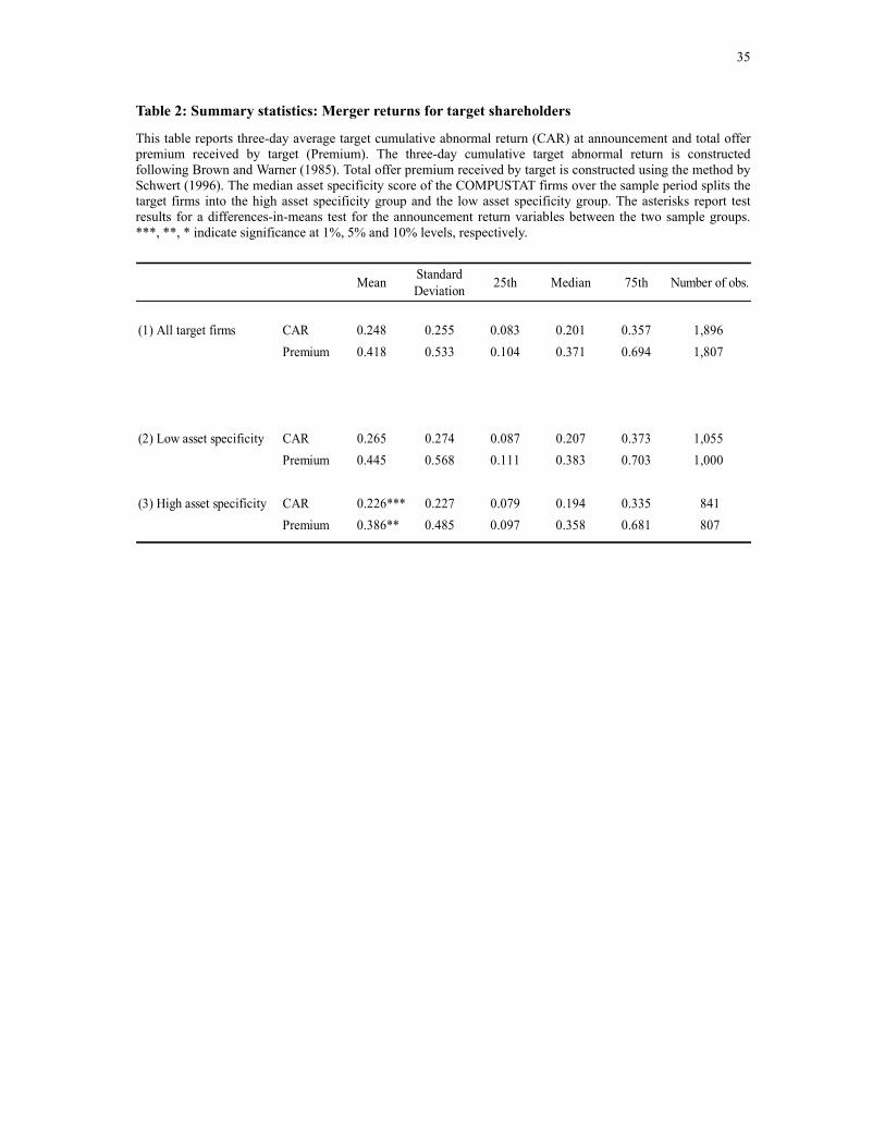
35

Table 2: Summary statistics: Merger returns for target shareholders

This table reports three-day average target cumulative abnormal return (CAR) at announcement and total offer premium received by target (Premium). The three-day cumulative target abnormal return is constructed following Brown and Warner (1985). Total offer premium received by target is constructed using the method by Schwert (1996). The median asset specificity score of the COMPUSTAT firms over the sample period splits the target firms into the high asset specificity group and the low asset specificity group. The asterisks report test results for a differences-in-means test for the announcement return variables between the two sample groups. ***, **, * indicate significance at 1%, 5% and 10% levels, respectively.

Mean StandardDeviation 25th Median 75th Number of obs.

(1) All target firms CAR 0.248 0.255 0.083 0.201 0.357 1,896Premium 0.418 0.533 0.104 0.371 0.694 1,807

(2) Low asset specificity CAR 0.265 0.274 0.087 0.207 0.373 1,055Premium 0.445 0.568 0.111 0.383 0.703 1,000

(3) High asset specificity CAR 0.226*** 0.227 0.079 0.194 0.335 841Premium 0.386** 0.485 0.097 0.358 0.681 807

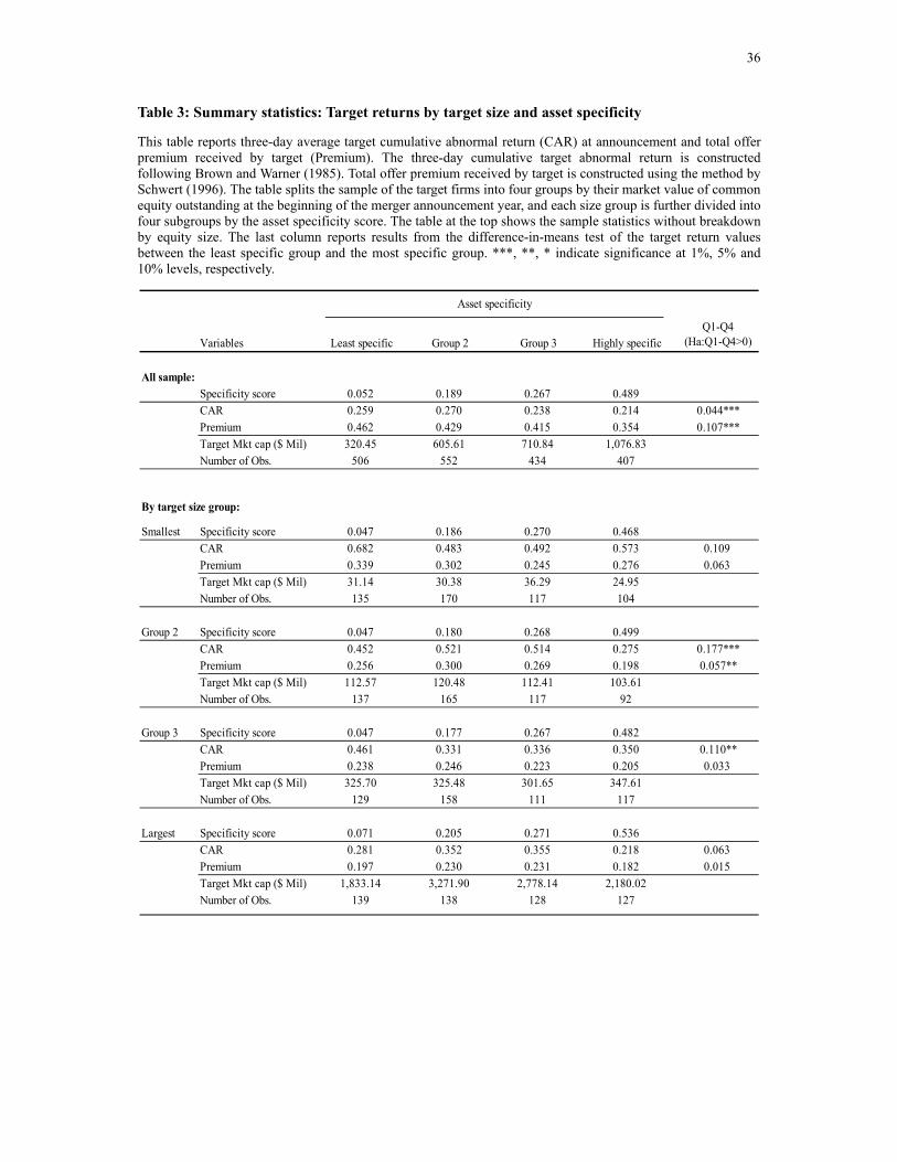
36

Table 3: Summary statistics: Target returns by target size and asset specificity

This table reports three-day average target cumulative abnormal return (CAR) at announcement and total offer premium received by target (Premium). The three-day cumulative target abnormal return is constructed following Brown and Warner (1985). Total offer premium received by target is constructed using the method by Schwert (1996). The table splits the sample of the target firms into four groups by their market value of common equity outstanding at the beginning of the merger announcement year, and each size group is further divided into four subgroups by the asset specificity score. The table at the top shows the sample statistics without breakdown by equity size. The last column reports results from the difference-in-means test of the target return values between the least specific group and the most specific group. ***, **, * indicate significance at 1%, 5% and 10% levels, respectively.

Variables Least specific Group 2 Group 3 Highly specific

All sample:Specificity score 0.052 0.189 0.267 0.489CAR 0.259 0.270 0.238 0.214 0.044***Premium 0.462 0.429 0.415 0.354 0.107***Target Mkt cap ($ Mil) 320.45 605.61 710.84 1,076.83Number of Obs. 506 552 434 407

By target size group:

Smallest Specificity score 0.047 0.186 0.270 0.468CAR 0.682 0.483 0.492 0.573 0.109Premium 0.339 0.302 0.245 0.276 0.063Target Mkt cap ($ Mil) 31.14 30.38 36.29 24.95Number of Obs. 135 170 117 104

Group 2 Specificity score 0.047 0.180 0.268 0.499CAR 0.452 0.521 0.514 0.275 0.177***Premium 0.256 0.300 0.269 0.198 0.057**Target Mkt cap ($ Mil) 112.57 120.48 112.41 103.61Number of Obs. 137 165 117 92

Group 3 Specificity score 0.047 0.177 0.267 0.482CAR 0.461 0.331 0.336 0.350 0.110**Premium 0.238 0.246 0.223 0.205 0.033Target Mkt cap ($ Mil) 325.70 325.48 301.65 347.61Number of Obs. 129 158 111 117

Largest Specificity score 0.071 0.205 0.271 0.536CAR 0.281 0.352 0.355 0.218 0.063Premium 0.197 0.230 0.231 0.182 0.015Target Mkt cap ($ Mil) 1,833.14 3,271.90 2,778.14 2,180.02Number of Obs. 139 138 128 127

Asset specificity

Q1-Q4(Ha:Q1-Q4>0)

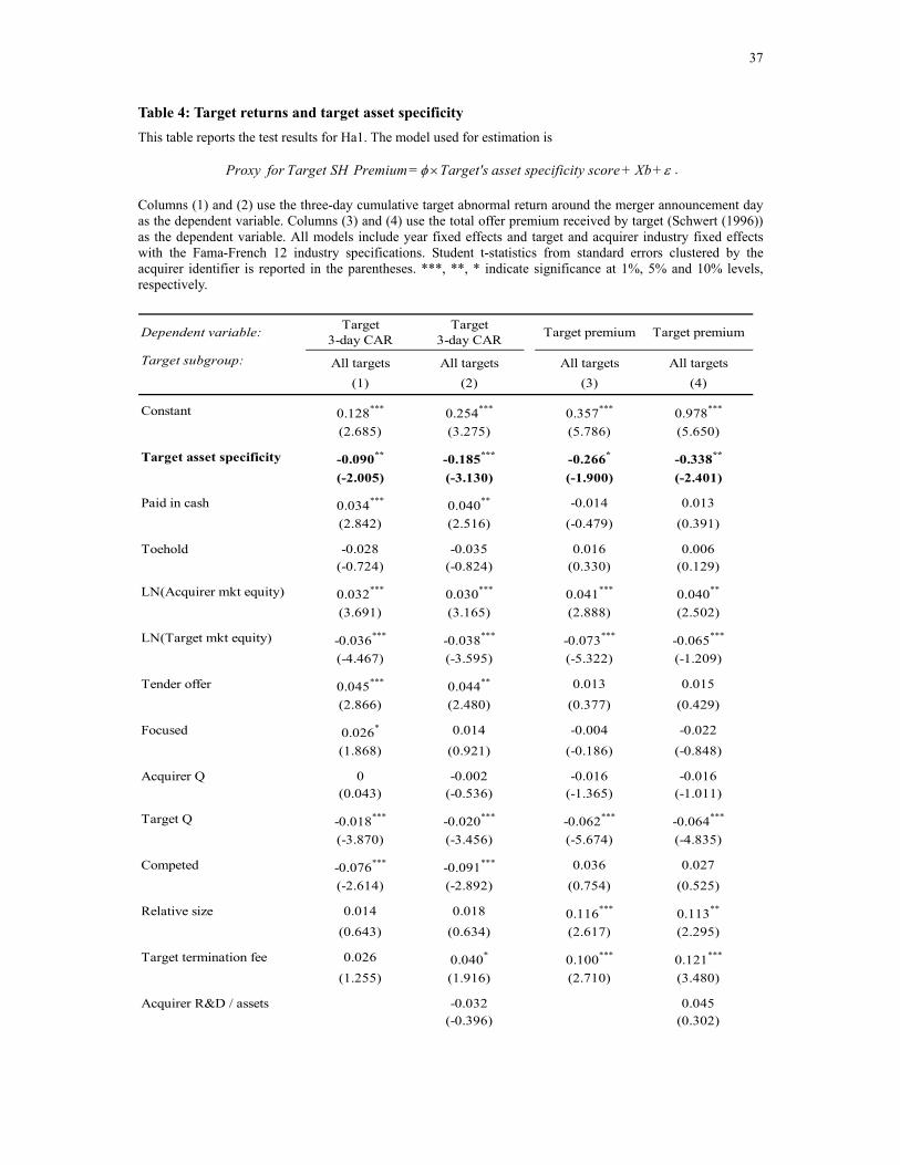
37

Table 4: Target returns and target asset specificity

This table reports the test results for Ha1. The model used for estimation is

Proxy for Target SH Premium = Target's asset specificity score + Xb+φ ε× .

Columns (1) and (2) use the three-day cumulative target abnormal return around the merger announcement day as the dependent variable. Columns (3) and (4) use the total offer premium received by target (Schwert (1996)) as the dependent variable. All models include year fixed effects and target and acquirer industry fixed effects with the Fama-French 12 industry specifications. Student t-statistics from standard errors clustered by the acquirer identifier is reported in the parentheses. ***, **, * indicate significance at 1%, 5% and 10% levels, respectively.

Dependent variable: Target3-day CAR

Target3-day CAR Target premium Target premium

Target subgroup: All targets All targets All targets All targets(1) (2) (3) (4)

0.128*** 0.254*** 0.357*** 0.978***

(2.685) (3.275) (5.786) (5.650)

-0.090** -0.185*** -0.266* -0.338**

(-2.005) (-3.130) (-1.900) (-2.401)

0.034*** 0.040** -0.014 0.013(2.842) (2.516) (-0.479) (0.391)

-0.028 -0.035 0.016 0.006(-0.724) (-0.824) (0.330) (0.129)

0.032*** 0.030*** 0.041*** 0.040**

(3.691) (3.165) (2.888) (2.502)

-0.036*** -0.038*** -0.073*** -0.065***

(-4.467) (-3.595) (-5.322) (-1.209)

0.045*** 0.044** 0.013 0.015(2.866) (2.480) (0.377) (0.429)

0.026* 0.014 -0.004 -0.022(1.868) (0.921) (-0.186) (-0.848)

0 -0.002 -0.016 -0.016(0.043) (-0.536) (-1.365) (-1.011)

-0.018*** -0.020*** -0.062*** -0.064***

(-3.870) (-3.456) (-5.674) (-4.835)

-0.076*** -0.091*** 0.036 0.027(-2.614) (-2.892) (0.754) (0.525)

0.014 0.018 0.116*** 0.113**

(0.643) (0.634) (2.617) (2.295)

0.026 0.040* 0.100*** 0.121***

(1.255) (1.916) (2.710) (3.480)

-0.032 0.045(-0.396) (0.302)

Constant

Target asset specificity

Paid in cash

Toehold

LN(Acquirer mkt equity)

LN(Target mkt equity)

Tender offer

Focused

Acquirer Q

Target Q

Competed

Relative size

Target termination fee

Acquirer R&D / assets

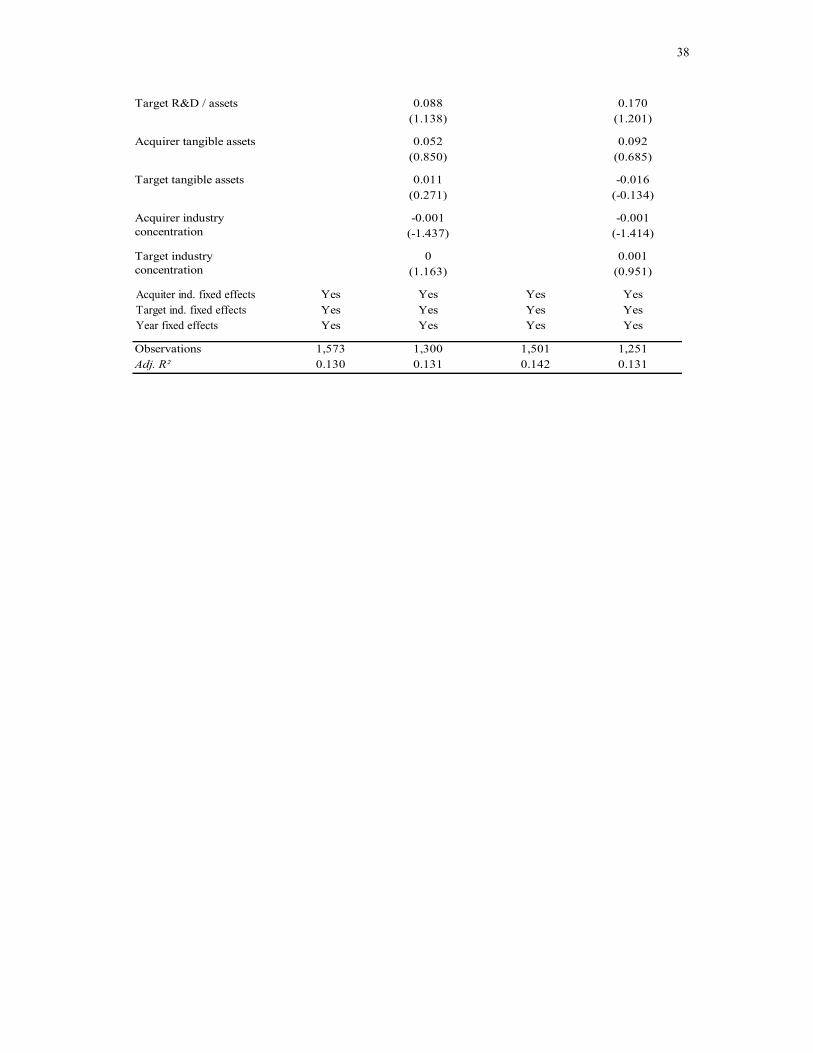
38

0.088 0.170(1.138) (1.201)

0.052 0.092(0.850) (0.685)

0.011 -0.016(0.271) (-0.134)

-0.001 -0.001(-1.437) (-1.414)

0 0.001(1.163) (0.951)

Acquirer industry fixed Yes Yes Yes YesTarget industry fixed effects Yes Yes Yes YesYear fixed effects Yes Yes Yes Yes

Observations 1,573 1,300 1,501 1,251Adj. R² 0.130 0.131 0.142 0.131

Target tangible assets

Acquirer industryconcentration

Target industryconcentration

Target R&D / assets

Acquirer tangible assets

Acquiter ind. fixed effectsTarget ind. fixed effectsYear fixed effects

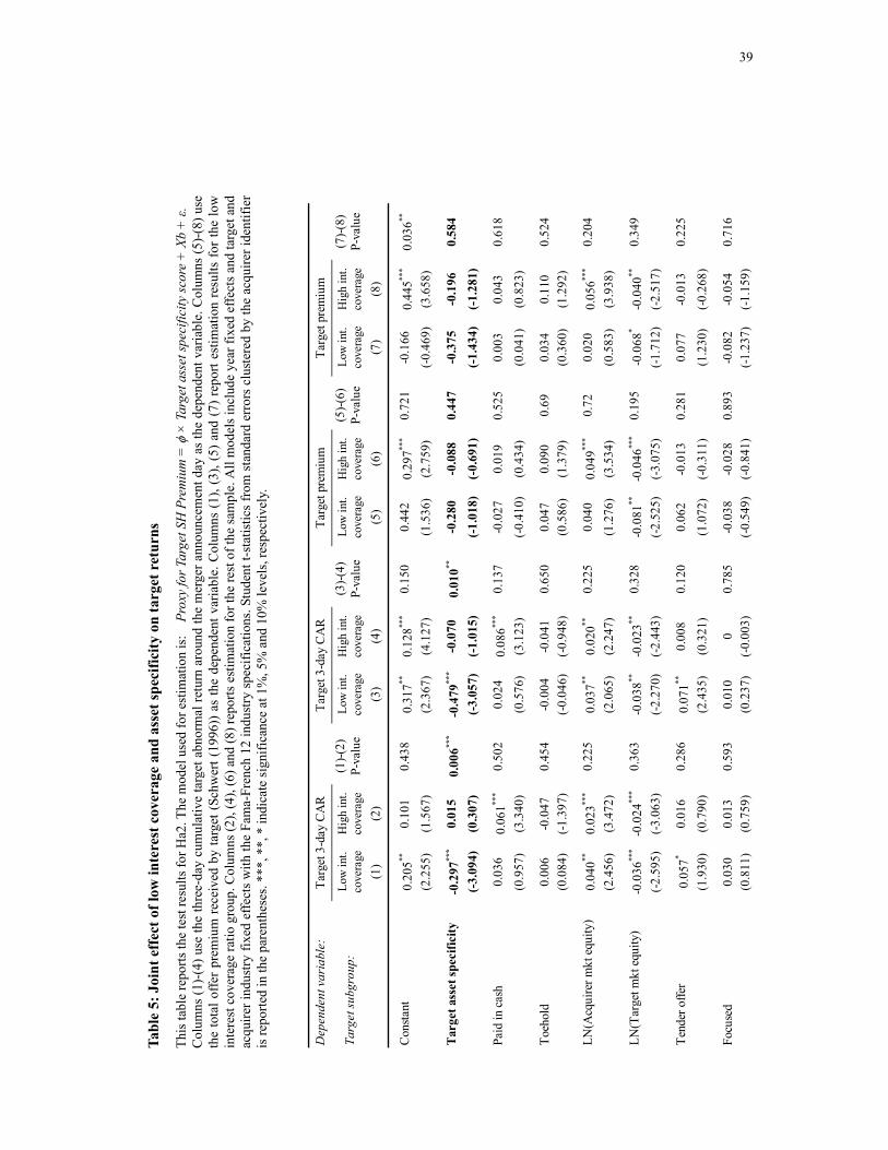
39

Tabl

e 5:

Joi

nt e

ffec

t of l

ow in

tere

st c

over

age

and

asse

t spe

cific

ity o

n ta

rget

ret

urns

Th

is ta

ble

repo

rts th

e te

st re

sults

for H

a2. T

he m

odel

use

d fo

r est

imat

ion

is:

Pro

xy fo

r Tar

get S

H P

rem

ium

= φ

× T

arge

t ass

et sp

ecifi

city

scor

e +

Xb

+ ε.

C

olum

ns (1

)-(4

) use

the

thre

e-da

y cu

mul

ativ

e ta

rget

abn

orm

al re

turn

aro

und

the

mer

ger a

nnou

ncem

ent d

ay a

s th

e de

pend

ent v

aria

ble.

Col

umns

(5)-

(8) u

se

the

tota

l offe

r pr

emiu

m re

ceiv

ed b

y ta

rget

(Sch

wer

t (19

96))

as

the

depe

nden

t var

iabl

e. C

olum

ns (1

), (3

), (5

) and

(7) r

epor

t est

imat

ion

resu

lts fo

r the

low

in

tere

st c

over

age

ratio

gro

up. C

olum

ns (2

), (4

), (6

) and

(8) r

epor

ts e

stim

atio

n fo

r the

rest

of t

he sa

mpl

e. A

ll m

odel

s inc

lude

yea

r fix

ed e

ffect

s and

targ

et a

nd

acqu

irer i

ndus

try fi

xed

effe

cts

with

the

Fam

a-Fr

ench

12

indu

stry

spe

cific

atio

ns. S

tude

nt t-

stat

istic

s fr

om s

tand

ard

erro

rs c

lust

ered

by

the

acqu

irer i

dent

ifier

is

repo

rted

in th

e pa

rent

hese

s. **

*, *

*, *

indi

cate

sign

ifica

nce

at 1

%, 5

% a

nd 1

0% le

vels

, res

pect

ivel

y.

Dep

ende

nt v

aria

ble:

Targ

et su

bgro

up:

Low

int.

cove

rage

Hig

h in

t.co

vera

geLo

w in

t.co

vera

geH

igh

int.

cove

rage

Low

int.

cove

rage

Hig

h in

t.co

vera

geLo

w in

t.co

vera

geH

igh

int.

cove

rage

(1)

(2)

(3)

(4)

(5)

(6)

(7)

(8)

0.20

5**0.

101

0.43

80.

317**

0.12

8***

0.15

00.

442

0.29

7***

0.72

1-0

.166

0.44

5***

0.03

6**

(2.2

55)

(1.5

67)

(2.3

67)

(4.1

27)

(1.5

36)

(2.7

59)

(-0.4

69)

(3.6

58)

-0.2

97**

*0.

015

0.00

6***

-0.4

79**

*-0

.070

0.01

0**-0

.280

-0.0

880.

447

-0.3

75-0

.196

0.58

4(-

3.09

4)(0

.307

)(-3

.057

)(-

1.01

5)(-1

.018

)(-0

.691

)(-1

.434

)(-

1.28

1)

0.03

60.

061**

*0.

502

0.02

40.

086**

*0.

137

-0.0

270.

019

0.52

50.

003

0.04

30.

618

(0.9

57)

(3.3

40)

(0.5

76)

(3.1

23)

(-0.4

10)

(0.4

34)

(0.0

41)

(0.8

23)

0.00

6-0

.047

0.45

4-0

.004

-0.0

410.

650

0.04

70.

090

0.69

0.03

40.

110

0.52

4(0

.084

)(-1

.397

)(-0

.046

)(-0

.948

)(0

.586

)(1

.379

)(0

.360

)(1

.292

)

0.04

0**0.

023**

*0.

225

0.03

7**0.

020**

0.22

50.

040

0.04

9***

0.72

0.02

00.

056**

*0.

204

(2.4

56)

(3.4

72)

(2.0

65)

(2.2

47)

(1.2

76)

(3.5

34)

(0.5

83)

(3.9

38)

-0.0

36**

*-0

.024

***

0.36

3-0

.038

**-0

.023

**0.

328

-0.0

81**

-0.0

46**

*0.

195

-0.0

68*

-0.0

40**

0.34

9(-2

.595

)(-3

.063

)(-2

.270

)(-2

.443

)(-2

.525

)(-3

.075

)(-1

.712

)(-2

.517

)

0.05

7*0.

016

0.28

60.

071**

0.00

80.

120

0.06

2-0

.013

0.28

10.

077

-0.0

130.

225

(1.9

30)

(0.7

90)

(2.4

35)

(0.3

21)

(1.0

72)

(-0.3

11)

(1.2

30)

(-0.2

68)

0.03

00.

013

0.59

30.

010

00.

785

-0.0

38-0

.028

0.89

3-0

.082

-0.0

540.

716

(0.8

11)

(0.7

59)

(0.2

37)

(-0.0

03)

(-0.5

49)

(-0.8

41)

(-1.2

37)

(-1.1

59)

Cons

tant

Targ

et a

sset

spec

ifici

ty

Paid

in ca

sh

Toeh

old

LN(A

cqui

rer m

kt e

quity

)

LN(T

arge

t mkt

equ

ity)

Tend

er o

ffer

Focu

sed

Targ

et 3

-day

CA

R(1

)-(2)

P-va

lue

Targ

et 3

-day

CA

R(3

)-(4)

P-va

lue

Targ

et p

rem

ium

(5)-(

6)P-

valu

e

Targ

et p

rem

ium

(7)-(

8)P-

valu

e

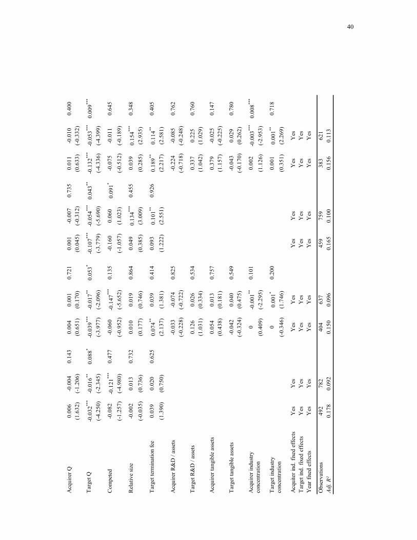
40

0.00

6-0

.004

0.14

30.

004

0.00

10.

721

0.00

1-0

.007

0.73

50.

011

-0.0

100.

400

(1.6

32)

(-1.

206)

(0.6

51)

(0.1

70)

(0.0

45)

(-0.

312)

(0.6

33)

(-0.

332)

-0.0

32**

*-0

.016

**0.

088*

-0.0

39**

*-0

.017

**0.

053*

-0.1

07**

*-0

.054

***

0.04

3**-0

.132

***

-0.0

53**

*0.

009**

*

(-4.

250)

(-2.

345)

(-3.

977)

(-2.

096)

(-3.7

79)

(-5.

690)

(-4.

336)

(-4.

399)

-0.0

82-0

.121

***

0.47

7-0

.060

-0.1

47**

*0.

135

-0.1

600.

060

0.09

1*-0

.075

-0.0

110.

645

(-1.

257)

(-4.

980)

(-0.

952)

(-5.

652)

(-1.0

57)

(1.0

23)

(-0.

512)

(-0.

189)

-0.0

020.

013

0.73

20.

010

0.01

90.

864

0.04

90.

134**

*0.

455

0.03

90.

154**

*0.

348

(-0.

035)

(0.7

36)

(0.1

77)

(0.7

46)

(0.3

85)

(3.0

09)

(0.2

85)

(2.9

35)

0.03

90.

020

0.62

50.

074**

0.03

90.

414

0.09

30.

101**

0.92

60.

189**

0.11

4**0.

405

(1.3

90)

(0.7

50)

(2.1

37)

(1.3

81)

(1.2

22)

(2.5

51)

(2.2

17)

(2.5

81)

-0.0

33-0

.074

0.82

5-0

.224

-0.0

850.

762

(-0.

228)

(-0.

722)

(-0.

718)

(-0.

248)

0.12

60.

026

0.53

40.

337

0.22

50.

760

(1.0

31)

(0.3

34)

(1.0

42)

(1.0

29)

0.05

40.

013

0.75

70.

379

-0.0

250.

147

(0.4

38)

(0.1

81)

(1.1

57)

(-0.

225)

-0.0

420.

040

0.54

9-0

.043

0.02

90.

780

(-0.

324)

(0.4

75)

(-0.

170)

(0.2

62)

0-0

.001

**0.

101

0.00

2-0

.003

***

0.00

8***

(0.4

09)

(-2.

295)

(1.1

26)

(-2.

953)

00.

001*

0.20

00.

001

0.00

1**0.

718

(-0.

346)

(1.7

46)

(0.3

51)

(2.2

69)

Acq

uire

r ind

ustry

fixe

dY

esY

esY

esY

esY

esY

esY

esY

esT

arge

t ind

ustry

fixe

d ef

fect

sY

esY

esY

esY

esY

esY

esY

esY

esY

ear f

ixed

effe

cts

Yes

Yes

Yes

Yes

Yes

Yes

Yes

Yes

Obs

erva

tions

492

782

404

637

459

759

383

621

Adj.

R²0.

178

0.09

20.

150

0.09

60.

165

0.10

00.

156

0.11

3

Acq

uire

r R&

D /

asse

ts

Acq

uire

r Q

Tar

get Q

Com

pete

d

Rel

ativ

e si

ze

Tar

get t

erm

inat

ion

fee

Tar

get i

ndus

tryco

ncen

tratio

n

Tar

get R

&D

/ as

sets

Acq

uire

r tan

gibl

e as

sets

Tar

get t

angi

ble

asse

ts

Acq

uire

r ind

ustry

conc

entra

tion

Acq

uite

r ind

. fix

ed e

ffec

tsT

arge

t ind

. fix

ed e

ffec

tsY

ear f

ixed

eff

ects

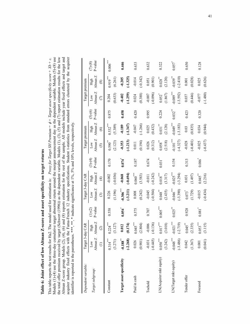
41

Tabl

e 6:

Joi

nt e

ffec

t of l

ow A

ltman

Z-s

core

and

ass

et sp

ecifi

city

on

targ

et r

etur

ns

This

tabl

e re

ports

the

test

resu

lts fo

r Ha2

. The

mod

el u

sed

for e

stim

atio

n is

: P

roxy

for T

arge

t SH

Pre

miu

m =

φ ×

Tar

get a

sset

spec

ifici

ty sc

ore

+ X

b +

ε.

Mod

els

(1)-

(4) u

se th

e th

ree-

day

cum

ulat

ive

targ

et a

bnor

mal

retu

rn a

roun

d th

e m

erge

r ann

ounc

emen

t day

as

the

depe

nden

t var

iabl

e. M

odel

s (5

)-(8

) use

th

e to

tal o

ffer p

rem

ium

rece

ived

by

targ

et (S

chw

ert (

1996

)) a

s th

e de

pend

ent v

aria

ble.

Mod

els

(1),

(3),

(5) a

nd (7

) rep

ort e

stim

atio

n re

sults

for t

he lo

w

Altm

an Z

-sco

re g

roup

. Mod

els

(2),

(4),

(6)

and

(8)

repo

rts e

stim

atio

n fo

r th

e re

st o

f th

e sa

mpl

e. A

ll m

odel

s in

clud

e ye

ar f

ixed

effe

cts

and

targ

et a

nd

acqu

irer

indu

stry

fix

ed e

ffect

s w

ith t

he F

ama-

Fren

ch 1

2 in

dust

ry s

peci

ficat

ions

. St

uden

t t-s

tatis

tics

from

sta

ndar

d er

rors

clu

ster

ed b

y th

e ac

quire

r id

entif

ier i

s rep

orte

d in

the

pare

nthe

ses.

***,

**,

* in

dica

te si

gnifi

canc

e at

1%

, 5%

and

10%

leve

ls, r

espe

ctiv

ely.

Dep

ende

nt v

aria

ble:

Targ

et su

bgro

up:

Low

A

ltman

ZH

igh

Altm

an Z

Low

A

ltman

ZH

igh

Altm

an Z

Low

A

ltman

ZH

igh

Altm

an Z

Low

A

ltman

ZH

igh

Altm

an Z

(1)

(2)

(3)

(4)

(5)

(6)

(7)

(8)

0.31

4***

0.22

4***

0.55

80.

226

-0.0

020.

170

0.59

0**0.

532**

*0.

875

0.20

40.

919**

*0.

006**

*

(3.2

71)

(3.1

27)

(1.1

96)

(-0.0

36)

(2.1

23)

(5.3

89)

(0.6

33)

(6.2

61)

-0.1

88**

0.01

20.

054*

-0.3

06**

*-0

.068

0.07

4*-0

.353

-0.1

890.

458

-0.4

02-0

.205

0.44

6(-2

.268

)(0

.174

)(-3

.211

)(-0

.694

)(-1

.213

)(-1

.347

)(-1

.259

)(-1

.325

)

0.02

60.

045**

*0.

575

0.00

80.

060**

*0.

187

0.01

1-0

.047

0.42

00.

024

-0.0

140.

633

(0.9

01)

(2.8

04)

(0.2

42)

(3.5

83)

(0.1

94)

(-1.2

66)

(0.3

88)

(-0.3

42)

-0.0

31-0

.006

0.70

7-0

.045

-0.0

110.

674

0.02

60.

025

0.99

5-0

.007

0.05

10.

632

(-0.4

45)

(-0.1

36)

(-0.5

04)

(-0.2

42)

(0.3

12)

(0.4

32)

(-0.0

96)

(0.9

01)

0.05

0***

0.01

7***

0.00

5***

0.04

8**0.

018**

*0.

031**

0.05

8**0.

031**

0.22

40.

052*

0.02

8**0.

322

(3.2

42)

(3.0

18)

(2.4

35)

(3.3

17)

(2.5

18)

(2.1

28)

(1.8

67)

(2.1

20)

-0.0

48**

*-0

.021

***

0.02

5**-0

.046

***

-0.0

25**

*0.

154

-0.1

01**

*-0

.049

***

0.03

2**-0

.089

***

-0.0

39**

0.05

7*

(-3.4

86)

(-2.7

19)

(-3.3

90)

(-3.2

94)

(-4.3

27)

(-3.1

83)

(-3.5

92)

(-2.4

10)

0.04

20.

045**

0.92

80.

073*

0.03

10.

313

-0.0

280.

030.

423

0.03

70.

001

0.65

0(1

.367

)(2

.335

)(1

.729

)(1

.497

)(-0

.401

)(0

.835

)(0

.446

)(0

.028

)

0.00

10.

053**

*0.

081*

-0.0

150.

045**

0.08

6*-0

.025

0.03

40.

320

-0.0

770.

025

0.12

8(0

.041

)(3

.115

)(-0

.434

)(2

.216

)(-0

.437

)(0

.944

)(-1

.480

)(0

.626

)

Targ

et p

rem

ium

(5)-(

6)P-

valu

e

Targ

et p

rem

ium

(7)-(

8)P-

valu

e

Targ

et 3

-day

CA

R(1

)-(2)

P-va

lue

Targ

et 3

-day

CA

R(3

)-(4)

P-va

lue

LN(A

cqui

rer m

kt e

quity

)

LN(T

arge

t mkt

equ

ity)

Tend

er o

ffer

Focu

sed

Cons

tant

Targ

et a

sset

spec

ifici

ty

Paid

in c

ash

Toeh

old

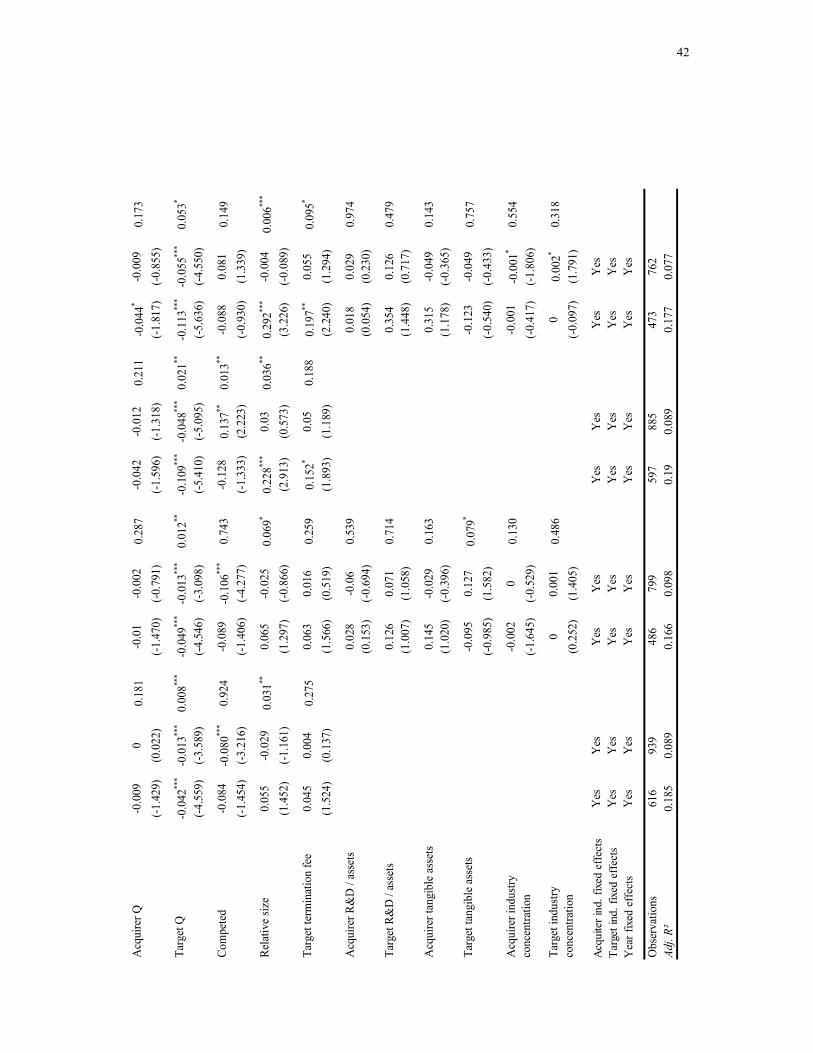
42

-0.0

090

0.18

1-0

.01

-0.0

020.

287

-0.0

42-0

.012

0.21

1-0

.044

*-0

.009

0.17

3(-1

.429

)(0

.022

)(-1

.470

)(-0

.791

)(-1

.596

)(-1

.318

)(-1

.817

)(-0

.855

)

-0.0

42**

*-0

.013

***

0.00

8***

-0.0

49**

*-0

.013

***

0.01

2**-0

.109

***

-0.0

48**

*0.

021**

-0.1

13**

*-0

.055

***

0.05

3*

(-4.5

59)

(-3.5

89)

(-4.5

46)

(-3.0

98)

(-5.4

10)

(-5.0

95)

(-5.6

36)

(-4.5

50)

-0.0

84-0

.080

***

0.92

4-0

.089

-0.1

06**

*0.

743

-0.1

280.

137**

0.01

3**-0

.088

0.08

10.

149

(-1.4

54)

(-3.2

16)

(-1.4

06)

(-4.2

77)

(-1.3

33)

(2.2

23)

(-0.9

30)

(1.3

39)

0.05

5-0

.029

0.03

1**0.

065

-0.0

250.

069*

0.22

8***

0.03

0.03

6**0.

292**

*-0

.004

0.00

6***

(1.4

52)

(-1.1

61)

(1.2

97)

(-0.8

66)

(2.9

13)

(0.5

73)

(3.2

26)

(-0.0

89)

0.04

50.

004

0.27

50.

063

0.01

60.

259

0.15

2*0.

050.

188

0.19

7**0.

055

0.09

5*

(1.5

24)

(0.1

37)

(1.5

66)

(0.5

19)

(1.8

93)

(1.1

89)

(2.2

40)

(1.2

94)

0.02

8-0

.06

0.53

90.

018

0.02

90.

974

(0.1

53)

(-0.6

94)

(0.0

54)

(0.2

30)

0.12

60.

071

0.71

40.

354

0.12

60.

479

(1.0

07)

(1.0

58)

(1.4

48)

(0.7

17)

0.14

5-0

.029

0.16

30.

315

-0.0

490.

143

(1.0

20)

(-0.3

96)

(1.1

78)

(-0.3

65)

-0.0

950.

127

0.07

9*-0

.123

-0.0

490.

757

(-0.9

85)

(1.5

82)

(-0.5

40)

(-0.4

33)

-0.0

020

0.13

0-0

.001

-0.0

01*

0.55

4(-1

.645

)(-0

.529

)(-0

.417

)(-1

.806

)

00.

001

0.48

60

0.00

2*0.

318

(0.2

52)

(1.4

05)

(-0.0

97)

(1.7

91)

Acq

uire

r ind

ustry

fixe

d Y

esY

esY

esY

esY

esY

esY

esY

esTa

rget

indu

stry

fixed

Y

esY

esY

esY

esY

esY

esY

esY

esY

ear f

ixed

effe

cts

Yes

Yes

Yes

Yes

Yes

Yes

Yes

Yes

Obs

erva

tions

616

939

486

799

597

885

473

762

Adj.

R²0.

185

0.08

90.

166

0.09

80.

190.

089

0.17

70.

077

Targ

et in

dustr

y co

ncen

tratio

n

Targ

et R

&D

/ as

sets

Acq

uire

r tan

gibl

e as

sets

Targ

et ta

ngib

le as

sets

Acq

uire

r ind

ustry

conc

entra

tion

Acq

uire

r R&

D /

asse

ts

Acq

uire

r Q

Targ

et Q

Com

pete

d

Rela

tive

size

Targ

et te

rmin

atio

n fe

e

Acq

uite

r ind

. fix

ed e

ffec

tsT

arge

t ind

. fix

ed e

ffec

tsY

ear f

ixed

eff

ects

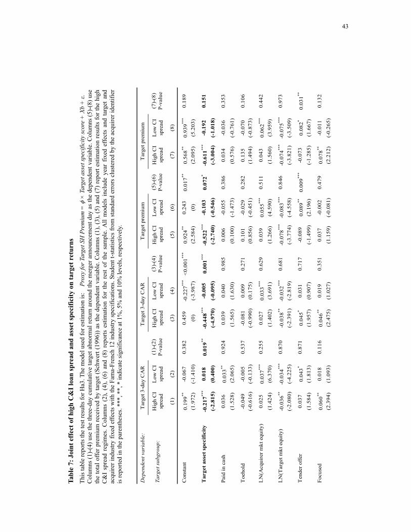
43

Ta

ble

7: J

oint

eff

ect o

f hig

h C

&I l

oan

spre

ad a

nd a

sset

spec

ifici

ty o

n ta

rget

ret

urns

Th

is ta

ble

repo

rts th

e te

st re

sults

for H

a3. T

he m

odel

use

d fo

r est

imat

ion

is:

Pro

xy fo

r Tar

get S

H P

rem

ium

= φ

× T

arge

t ass

et sp

ecifi

city

scor

e +

Xb

+ ε.

C

olum

ns (1

)-(4

) use

the

thre

e-da

y cu

mul

ativ

e ta

rget

abn

orm

al re

turn

aro

und

the

mer

ger a

nnou

ncem

ent d

ay a

s th

e de

pend

ent v

aria

ble.

Col

umns

(5)-

(8) u

se

the

tota

l offe

r pre

miu

m re

ceiv

ed b

y ta

rget

(Sch

wer

t (19

96))

as

the

depe

nden

t var

iabl

e. C

olum

ns (1

), (3

), (5

) and

(7) r

epor

t est

imat

ion

resu

lts fo

r the

hig

h C

&I

spre

ad r

egim

es. C

olum

ns (

2), (

4), (

6) a

nd (

8) r

epor

ts e

stim

atio

n fo

r th

e re

st o

f th

e sa

mpl

e. A

ll m

odel

s in

clud

e ye

ar f

ixed

effe

cts

and

targ

et a

nd

acqu

irer i

ndus

try fi

xed

effe

cts

with

the

Fam

a-Fr

ench

12

indu

stry

spe

cific

atio

ns. S

tude

nt t-

stat

istic

s fro

m s

tand

ard

erro

rs c

luste

red

by th

e ac

quire

r ide

ntifi

er

is re

porte

d in

the

pare

nthe

ses.

***,

**,

* in

dica

te si

gnifi

canc

e at

1%

, 5%

and

10%

leve

ls, r

espe

ctiv

ely.

D

epen

dent

var

iabl

e:

Targ

et s

ubgr

oup:

Hig

h C

Isp

read

Low

CI

spre

adH

igh

CI

spre

adL

ow C

Isp

read

Hig

h C

Isp

read

Low

CI

spre

adH

igh

CI

spre

adL

ow C

Isp

read

(1)

(2)

(3)

(4)

(5)

(6)

(7)

(8)

0.19

9**-0

.067

0.38

20.

459

-0.2

27**

*<0

.001

***

0.92

4**0.

243

0.01

7**0.

568**

0.93

9***

0.18

9(1

.972

)(-

1.41

0)(0

)(-

3.98

7)(2

.584

)(0

)(2

.095

)(5

.203

)

-0.2

17**

*0.

018

0.01

9**-0

.448

***

-0.0

050.

001**

*-0

.522

***

-0.1

030.

072*

-0.6

11**

*-0

.192

0.15

1

(-2.

815)

(0.4

00)

(-4.

970)

(-0.

095)

(-2.

740)

(-0.

546)

(-3.

004)

(-1.

018)

0.03

60.

033**

0.92

40.

039

0.04

00.

985

0.00

6-0

.055

0.38

60.

034

-0.0

360.

353

(1.5

28)

(2.0

65)

(1.5

65)

(1.6

30)

(0.1

00)

(-1.

473)

(0.5

76)

(-0.

761)

-0.0

49-0

.005

0.53

7-0

.081

0.00

90.

271

0.10

1-0

.029

0.28

20.

135

-0.0

700.

106

(-0.

616)

(-0.

133)

(-0.

990)

(0.1

75)

(0.8

56)

(-0.

451)

(1.4

94)

(-0.

873)

0.02

50.

037**

*0.

255

0.02

70.

033**

*0.

629

0.03

90.

055**

*0.

511

0.04

30.

062**

*0.

442

(1.4

24)

(6.3

70)

(1.4

02)

(3.6

91)

(1.2

66)

(4.5

90)

(1.5

60)

(3.9

59)

-0.0

36**

-0.0

34**

*0.

870

-0.0

38**

-0.0

32**

*0.

681

-0.0

78**

*-0

.083

***

0.84

6-0

.074

***

-0.0

75**

*0.

973

(-2.

080)

(-4.

225)

(-2.

391)

(-2.

819)

(-3.

774)

(-4.

558)

(-3.

821)

(-3.

509)

0.03

70.

043*

0.87

10.

045*

0.03

10.

717

-0.0

890.

089**

0.00

9***

-0.0

730.

082*

0.03

1**

(1.5

84)

(1.8

13)

(1.9

57)

(0.9

07)

(-1.

499)

(2.1

96)

(-1.

285)

(1.6

67)

0.06

0**0.

018

0.11

60.

046**

0.01

90.

351

0.03

7-0

.002

0.47

90.

078**

-0.0

110.

132

(2.3

94)

(1.0

93)

(2.4

75)

(1.0

27)

(1.1

59)

(-0.

081)

(2.2

12)

(-0.

265)

Tar

get p

rem

ium

(5)-

(6)

P-va

lue

Tar

get p

rem

ium

(7)-

(8)

P-va

lue

Tar

get 3

-day

CA

R

(1)-

(2)

P-va

lue

Tar

get 3

-day

CA

R

(3)-

(4)

P-va

lue

Con

stan

t

Tar

get a

sset

spe

cifi

city

Paid

in c

ash

Toe

hold

LN

(Acq

uire

r mkt

equ

ity)

LN

(Tar

get m

kt e

quity

)

Ten

der o

ffer

Focu

sed

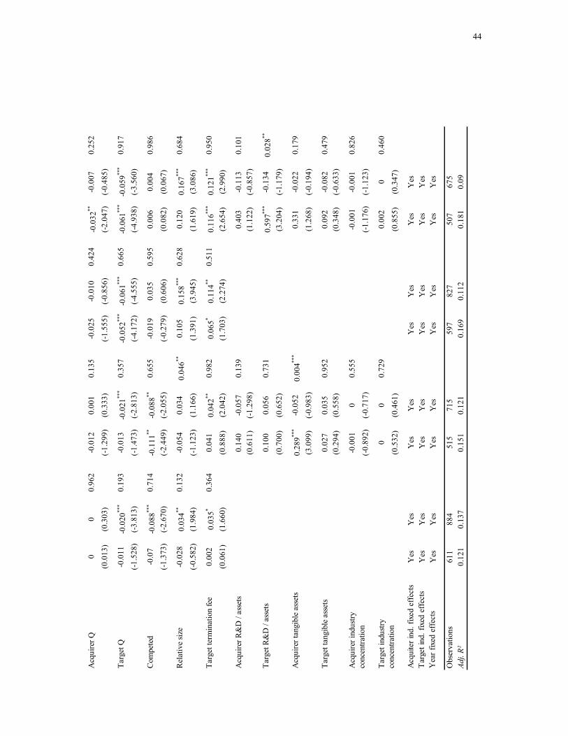
44

00

0.96

2-0

.012

0.00

10.

135

-0.0

25-0

.010

0.42

4-0

.032

**-0

.007

0.25

2(0

.013

)(0

.303

)(-1

.299

)(0

.333

)(-1

.555

)(-0

.856

)(-2

.047

)(-0

.485

)

-0.0

11-0

.020

***

0.19

3-0

.013

-0.0

21**

*0.

357

-0.0

52**

*-0

.061

***

0.66

5-0

.061

***

-0.0

59**

*0.

917

(-1.5

28)

(-3.8

13)

(-1.4

73)

(-2.8

13)

(-4.1

72)

(-4.5

55)

(-4.9

38)

(-3.5

60)

-0.0

7-0

.088

***

0.71

4-0

.111

**-0

.088

**0.

655

-0.0

190.

035

0.59

50.

006

0.00

40.

986

(-1.3

73)

(-2.6

70)

(-2.4

49)

(-2.0

55)

(-0.2

79)

(0.6

06)

(0.0

82)

(0.0

67)

-0.0

280.

034**

0.13

2-0

.054

0.03

40.

046**

0.10

50.

158**

*0.

628

0.12

00.

167**

*0.

684

(-0.5

82)

(1.9

84)

(-1.1

23)

(1.1

66)

(1.3

91)

(3.9

45)

(1.6

19)

(3.0

86)

0.00

20.

035*

0.36

40.

041

0.04

2**0.

982

0.06

5*0.

114**

0.51

10.

116**

*0.

121**

*0.

950

(0.0

61)

(1.6

60)

(0.8

88)

(2.0

42)

(1.7

03)

(2.2

74)

(2.6

54)

(2.9

90)

0.14

0-0

.057

0.13

90.

403

-0.1

130.

101

(0.6

11)

(-1.2

98)

(1.1

22)

(-0.8

57)

0.10

00.

056

0.73

10.

597**

*-0

.134

0.02

8**

(0.7

00)

(0.6

52)

(3.2

04)

(-1.1

79)

0.28

9***

-0.0

520.

004**

*0.

331

-0.0

220.

179

(3.0

99)

(-0.9

83)

(1.2

68)

(-0.1

94)

0.02

70.

035

0.95

20.

092

-0.0

820.

479

(0.2

94)

(0.5

58)

(0.3

48)

(-0.6

33)

-0.0

010

0.55

5-0

.001

-0.0

010.

826

(-0.8

92)

(-0.7

17)

(-1.1

76)

(-1.1

23)

00

0.72

90.

002

00.

460

(0.5

32)

(0.4

61)

(0.8

55)

(0.3

47)

Acq

uire

r ind

ustry

fixe

dY

esY

esY

esY

esY

esY

esY

esY

esTa

rget

indu

stry

fixed

effe

cts

Yes

Yes

Yes

Yes

Yes

Yes

Yes

Yes

Yea

r fix

ed e

ffect

sY

esY

esY

esY

esY

esY

esY

esY

es

Obs

erva

tions

611

884

515

715

597

827

507

675

Adj.

R²0.

121

0.13

70.

151

0.12

10.

169

0.11

20.

181

0.09

Acq

uire

r R&

D /

asse

ts

Acq

uire

r Q

Targ

et Q

Com

pete

d

Rel

ativ

e siz

e

Targ

et te

rmin

atio

n fe

e

Targ

et in

dustr

yco

ncen

tratio

n

Targ

et R

&D

/ as

sets

Acq

uire

r tan

gibl

e as

sets

Targ

et ta

ngib

le a

sset

s

Acq

uire

r ind

ustry

conc

entra

tion

Acq

uite

r ind

. fix

ed e

ffec

tsT

arge

t ind

. fix

ed e

ffec

tsY

ear f

ixed

eff

ects

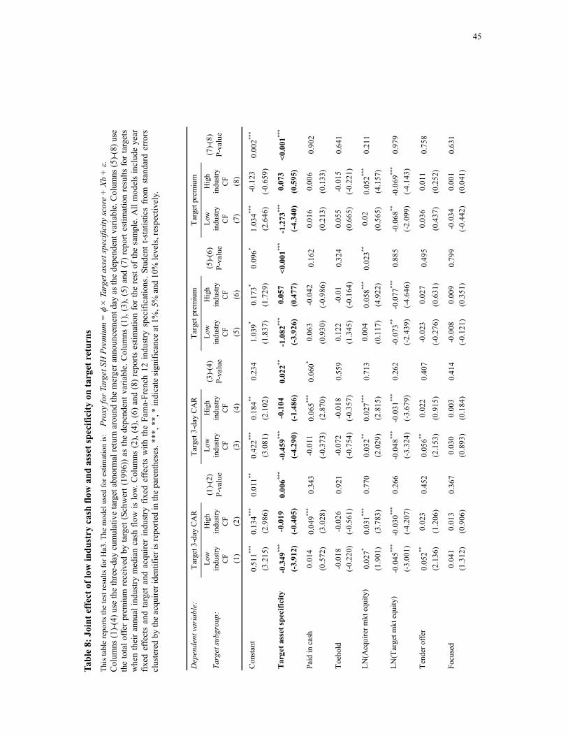
45

Ta

ble

8: J

oint

eff

ect o

f low

indu

stry

cas

h flo

w a

nd a

sset

spec

ifici

ty o

n ta

rget

ret

urns

Th

is ta

ble

repo

rts th

e te

st re

sults

for H

a3. T

he m

odel

use

d fo

r est

imat

ion

is:

Pro

xy fo

r Tar

get S

H P

rem

ium

= φ

× T

arge

t ass

et sp

ecifi

city

scor

e +

Xb

+ ε.

C

olum

ns (1

)-(4

) use

the

thre

e-da

y cu

mul

ativ

e ta

rget

abn

orm

al re

turn

aro

und

the

mer

ger a

nnou

ncem

ent d

ay a

s the

dep

ende

nt v

aria

ble.

Col

umns

(5)-(

8) u

se

the

tota

l offe

r pr

emiu

m re

ceiv

ed b

y ta

rget

(Sch

wer

t (19

96))

as

the

depe

nden

t var

iabl

e. C

olum

ns (1

), (3

), (5

) and

(7) r

epor

t est

imat

ion

resu

lts fo

r tar

gets

w

hen

thei

r ann

ual i

ndus

try m

edia

n ca

sh fl

ow is

low.

Col

umns

(2),

(4),

(6) a

nd (8

) rep

orts

est

imat

ion

for t

he re

st o

f the

sam

ple.

All

mod

els

incl

ude

year

fix

ed e

ffect

s an

d ta

rget

and

acq

uire

r in

dustr

y fix

ed e

ffect

s w

ith t

he F

ama-

Fren

ch 1

2 in

dust

ry s

peci

ficat

ions

. Stu

dent

t-s

tatis

tics

from

sta

ndar

d er

rors

cl

uste

red

by th

e ac

quire

r ide

ntifi

er is

repo

rted

in th

e pa

rent

hese

s. **

*, *

*, *

indi

cate

sign

ifica

nce

at 1

%, 5

% a

nd 1

0% le

vels

, res

pect

ivel

y.

Dep

ende

nt v

aria

ble:

Targ

et su

bgro

up:

Low

indu

stry

CF

Hig

hin

dustr

yC

F

Low

indu

stry

CF

Hig

hin

dustr

yC

F

Low

indu

stry

CF

Hig

hin

dustr

yC

F

Low

indu

stry

CF

Hig

hin

dustr

yC

F(1

)(2

)(3

)(4

)(5

)(6

)(7

)(8

)

0.51

1***

0.13

4***

0.01

1**0.

422**

*0.

184**

0.23

41.

039*

0.17

3*0.

096*

1.03

4***

-0.1

230.

002**

*

(3.2

15)

(2.9

86)

(3.0

81)

(2.1

02)

(1.8

37)

(1.7

29)

(2.6

46)

(-0.6

59)

-0.3

49**

*-0

.019

0.00

6***

-0.4

59**

*-0

.104

0.02

2**-1

.082

***

0.05

7<0

.001

***

-1.2

73**

*0.

073

<0.0

01**

*

(-3.

912)

(-0.

405)

(-4.

290)

(-1.

486)

(-3.

926)

(0.4

77)

(-4.

340)

(0.5

95)

0.01

40.

049**

*0.

343

-0.0

110.

065**

*0.

060*

0.06

3-0

.042

0.16

20.

016

0.00

60.

902

(0.5

72)

(3.0

28)

(-0.3

73)

(2.8

70)

(0.9

30)

(-0.9

86)

(0.2

13)

(0.1

33)

-0.0

18-0

.026

0.92

1-0

.072

-0.0

180.

559

0.12

2-0

.01

0.32

40.

055

-0.0

150.

641

(-0.2

20)

(-0.5

61)

(-0.7

54)

(-0.3

57)

(1.3

45)

(-0.1

64)

(0.6

65)

(-0.2

21)

0.02

7*0.

031**

*0.

770

0.03

2**0.

027**

*0.

713

0.00

40.

058**

*0.

023**

0.02

0.05

2***

0.21

1(1

.901

)(3

.783

)(2

.029

)(2

.815

)(0

.117

)(4

.922

)(0

.565

)(4

.157

)

-0.0

45**

*-0

.030

***

0.26

6-0

.048

***

-0.0

31**

*0.

262

-0.0

73**

-0.0

77**

*0.

885

-0.0

68**

-0.0

69**

*0.

979

(-3.0

01)

(-4.2

07)

(-3.3

24)

(-3.6

79)

(-2.4

39)

(-4.6

46)

(-2.0

99)

(-4.1

43)

0.05

2**0.

023

0.45

20.

056**

0.02

20.

407

-0.0

230.

027

0.49

50.

036

0.01

10.

758

(2.1

36)

(1.2

06)

(2.1

53)

(0.9

15)

(-0.2

76)

(0.6

31)

(0.4

37)

(0.2

52)

0.04

10.

013

0.36

70.

030

0.00

30.

414

-0.0

080.

009

0.79

9-0

.034

0.00

10.

631

(1.3

12)

(0.9

06)

(0.8

93)

(0.1

84)

(-0.1

21)

(0.3

51)

(-0.4

42)

(0.0

41)

Targ

et 3

-day

CA

R

Con

stant

Tar

get a

sset

spec

ifici

ty

Paid

in c

ash

(1)-(

2)P-

valu

e

Toeh

old

LN(A

cqui

rer m

kt e

quity

)

LN(T

arge

t mkt

equ

ity)

Tend

er o

ffer

Focu

sed

Targ

et p

rem

ium

(7)-(

8)P-

valu

e

Targ

et 3

-day

CA

R

(3)-(

4)P-

valu

e

Targ

et p

rem

ium

(5)-(

6)P-

valu

e

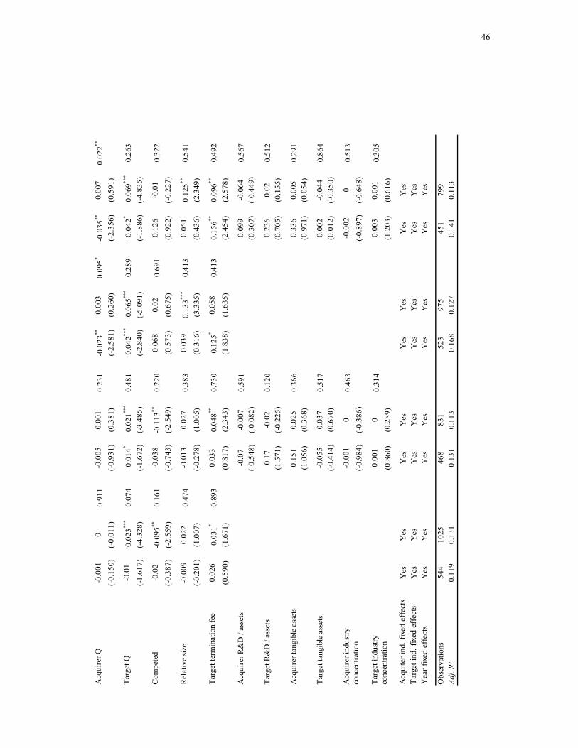
46

-0.0

010

0.91

1-0

.005

0.00

10.

231

-0.0

23**

0.00

30.

095*

-0.0

35**

0.00

70.

022**

(-0.

150)

(-0.

011)

(-0.

931)

(0.3

81)

(-2.

581)

(0.2

60)

(-2.

356)

(0.5

91)

-0.0

1-0

.023

***

0.07

4-0

.014

*-0

.021

***

0.48

1-0

.042

***

-0.0

65**

*0.

289

-0.0

42*

-0.0

69**

*0.

263

(-1.

617)

(-4.

328)

(-1.

672)

(-3.

485)

(-2.

840)

(-5.

091)

(-1.

886)

(-4.

835)

-0.0

2-0

.095

**0.

161

-0.0

38-0

.113

**0.

220

0.06

80.

020.

691

0.12

6-0

.01

0.32

2(-

0.38

7)(-

2.55

9)(-

0.74

3)(-

2.54

9)(0

.573

)(0

.675

)(0

.922

)(-

0.22

7)

-0.0

090.

022

0.47

4-0

.013

0.02

70.

383

0.03

90.

133**

*0.

413

0.05

10.

125**

0.54

1(-

0.20

1)(1

.007

)(-

0.27

8)(1

.005

)(0

.316

)(3

.335

)(0

.436

)(2

.349

)

0.02

60.

031*

0.89

30.

033

0.04

8**0.

730

0.12

5*0.

058

0.41

30.

156**

0.09

6**0.

492

(0.5

90)

(1.6

71)

(0.8

17)

(2.3

43)

(1.8

38)

(1.6

35)

(2.4

54)

(2.5

78)

-0.0

7-0

.007

0.59

10.

099

-0.0

640.

567

(-0.

548)

(-0.

082)

(0.3

07)

(-0.

449)

0.17

-0.0

20.

120

0.23

60.

020.

512

(1.5

71)

(-0.

225)

(0.7

05)

(0.1

55)

0.15

10.

025

0.36

60.

336

0.00

50.

291

(1.0

56)

(0.3

68)

(0.9

71)

(0.0

54)

-0.0

550.

037

0.51

70.

002

-0.0

440.

864

(-0.

414)

(0.6

70)

(0.0

12)

(-0.

350)

-0.0

010

0.46

3-0

.002

00.

513

(-0.

984)

(-0.

386)

(-0.

897)

(-0.

648)

0.00

10

0.31

40.

003

0.00

10.

305

(0.8

60)

(0.2

89)

(1.2

03)

(0.6

16)

Acq

uire

r ind

ustry

fixe

dY

esY

esY

esY

esY

esY

esY

esY

esT

arge

t ind

ustry

fixe

d ef

fect

sY

esY

esY

esY

esY

esY

esY

esY

esY

ear f

ixed

effe

cts

Yes

Yes

Yes

Yes

Yes

Yes

Yes

Yes

Obs

erva

tions

544

1025

468

831

523

975

451

799

Adj.

R²0.

119

0.13

10.

131

0.11

30.

168

0.12

70.

141

0.11

3

Acq

uire

r ind

ustry

conc

entra

tion

Tar

get i

ndus

tryco

ncen

tratio

n

Tar

get t

angi

ble

asse

ts

Acq

uire

r Q

Rel

ativ

e si

ze

Tar

get t

erm

inat

ion

fee

Acq

uire

r R&

D /

asse

ts

Tar

get R

&D

/ as

sets

Acq

uire

r tan

gibl

e as

sets

Tar

get Q

Com

pete

d

Acq

uite

r ind

. fix

ed e

ffec

tsT

arge

t ind

. fix

ed e

ffec

tsY

ear f

ixed

eff

ects

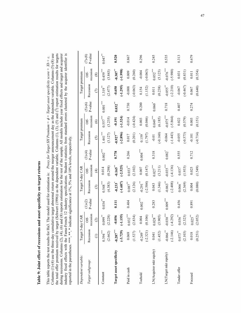
47

Ta

ble

9: J

oint

eff

ect o

f rec

essi

ons a

nd a

sset

spec

ifici

ty o

n ta

rget

ret

urns

Th

is ta

ble

repo

rts th

e te

st re

sults

for H

a3. T

he m

odel

use

d fo

r est

imat

ion

is:

Pro

xy fo

r Tar

get S

H P

rem

ium

= φ

× T

arge

t ass

et sp

ecifi

city

scor

e +

Xb

+ ε.

C

olum

ns (1

)-(4)

use

the

thre

e-da

y cu

mul

ativ

e ta

rget

abn

orm

al re

turn

aro

und

the

mer

ger a

nnou

ncem

ent d

ay a

s the

dep

ende

nt v

aria

ble.

Col

umns

(5)-

(8) u

se

the

tota

l offe

r pr

emiu

m r

ecei

ved

by ta

rget

(Sc

hwer

t (19

96))

as

the

depe

nden

t var

iabl

e. C

olum

ns (

1), (

3), (

5) a

nd (7

) re

port

estim

atio

n re

sults

for

targ

ets

durin

g re

cess

ions

. Col

umns

(2),

(4),

(6) a

nd (8

) rep

orts

est

imat

ion

for t

he re

st o

f the

sam

ple.

All

mod

els

incl

ude

year

fixe

d ef

fect

s an

d ta

rget

and

acq

uire

r in

dust

ry f

ixed

effe

cts

with

the

Fam

a-Fr

ench

12

indu

stry

spe

cific

atio

ns. S

tude

nt t

-sta

tistic

s fr

om s

tand

ard

erro

rs c

lust

ered

by

the

acqu

irer

iden

tifie

r is

re

porte

d in

the

pare

nthe

ses.

***,

**,

* in

dica

te si

gnifi

canc

e at

1%

, 5%

and

10%

leve

ls, r

espe

ctiv

ely.

Dep

ende

nt v

aria

ble:

Targ

et su

bgro

up:

Rec

essio

nO

ff-re

cess

ion

Rec

essio

nO

ff-re

cess

ion

Rec

essio

nO

ff-re

cess

ion

Rec

essio

nO

ff-re

cess

ion

(1)

(2)

(3)

(4)

(5)

(6)

(7)

(8)

0.39

4***

0.09

9**0.

034**

0.54

8***

0.01

40.

002**

*1.

441**

*0.

557**

*0.

001**

*1.

319**

0.45

9***

0.04

7**

(2.6

62)

(2.2

28)

(4.3

83)

(0.2

98)

(3.1

27)

(3.2

35)

(2.4

77)

(3.8

43)

-0.2

87**

*-0

.056

0.11

1-0

.233

*-0

.165

**0.

778

-0.9

27**

*-0

.191

0.03

2**-0

.650

-0.3

07**

0.52

0(-

3.72

9)(-

1.15

5)(-

1.68

7)(-

2.52

5)(-

2.89

6)(-

1.32

4)(-

1.29

5)(-

1.99

8)

0.06

90.

032**

*0.

404

0.08

7**0.

033**

0.26

60.

017

-0.0

140.

730

-0.0

080.

009

0.86

7(1

.527

)(2

.834

)(2

.126

)(2

.102

)(0

.201

)(-0

.424

)(-0

.063

)(0

.260

)

-0.2

49**

0.00

40.

002**

*-0

.291

**0.

007

0.00

4***

0.15

9*0.

003

0.2

000.

154

-0.0

040.

296

(-2.3

21)

(0.1

06)

(-2.5

04)

(0.1

47)

(1.7

97)

(0.0

46)

(1.1

52)

(-0.0

63)

0.04

10.

028**

*0.

283

0.04

30.

027**

*0.

318

-0.0

10.

049**

*0.

060*

0.01

10.

052**

*0.

245

(1.4

52)

(3.9

05)

(1.3

46)

(3.2

11)

(-0.1

60)

(6.1

85)

(0.2

38)

(5.1

23)

-0.0

66**

-0.0

30**

*0.

009**

*-0

.063

**-0

.035

***

0.08

2*-0

.064

-0.0

75**

*0.

718

-0.0

55**

-0.0

76**

*0.

535

(-2.1

46)

(-4.2

92)

(-2.4

08)

(-4.1

36)

(-1.4

43)

(-5.8

64)

(-2.2

10)

(-5.9

80)

0.07

3**0.

036**

0.45

60.

066**

0.03

7*0.

555

-0.0

550.

022

0.40

7-0

.067

0.03

10.

313

(2.1

03)

(2.3

23)

(2.3

69)

(1.9

33)

(-0.5

73)

(0.5

79)

(-0.4

67)

(0.8

31)

0.01

80.

025**

0.89

10.

004

0.02

50.

712

-0.1

010.

003

0.27

40.

067

0.01

10.

679

(0.2

51)

(2.0

52)

(0.0

80)

(1.5

49)

(-0.7

14)

(0.1

51)

(0.6

40)

(0.3

54)

Targ

et p

rem

ium

(5)-(

6)P-

valu

e

Targ

et p

rem

ium

(7)-(

8)P-

valu

e

Targ

et 3

-day

CA

R(1

)-(2)

P-va

lue

Targ

et 3

-day

CA

R(3

)-(4)

P-va

lue

Con

stant

Tar

get a

sset

spec

ifici

ty

Paid

in c

ash

Toeh

old

LN(A

cqui

rer m

kt e

quity

)

LN(T

arge

t mkt

equ

ity)

Tend

er o

ffer

Focu

sed

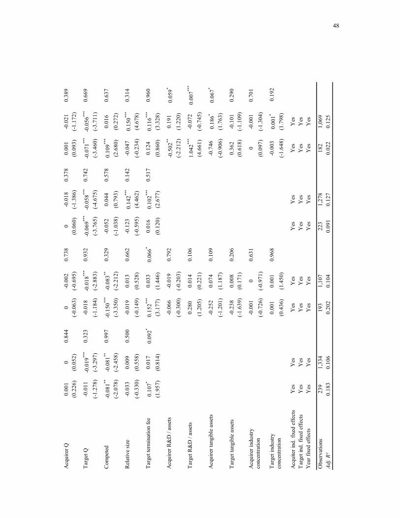
48

0.00

10

0.84

40

-0.0

020.

738

0-0

.018

0.37

80.

001

-0.0

210.

389

(0.2

26)

(0.0

52)

(-0.0

63)

(-0.6

95)

(0.0

60)

(-1.3

86)

(0.0

93)

(-1.1

72)

-0.0

11-0

.019

***

0.32

3-0

.018

-0.0

18**

*0.

932

-0.0

69**

*-0

.058

***

0.74

2-0

.071

***

-0.0

56**

*0.

669

(-1.2

78)

(-3.2

97)

(-1.1

84)

(-2.8

83)

(-3.7

65)

(-4.6

75)

(-3.4

60)

(-3.7

11)

-0.0

81**

-0.0

81**

0.99

7-0

.150

***

-0.0

83**

0.32

9-0

.052

0.04

40.

578

0.10

9***

0.01

60.

637

(-2.0

78)

(-2.4

58)

(-3.3

50)

(-2.2

12)

(-1.0

38)

(0.7

93)

(2.6

80)

(0.2

72)

-0.0

330.

009

0.50

0-0

.019

0.01

30.

662

-0.1

230.

142**

*0.

142

-0.0

470.

150**

*0.

314

(-0.3

30)

(0.5

58)

(-0.1

49)

(0.5

28)

(-0.5

95)

(4.4

62)

(-0.2

34)

(4.6

78)

0.10

7*0.

017

0.09

2*0.

152**

*0.

033

0.06

6*0.

016

0.10

2***

0.51

70.

124

0.11

6***

0.96

0(1

.957

)(0

.814

)(3

.177

)(1

.446

)(0

.120

)(2

.677

)(0

.860

)(3

.328

)

-0.0

66-0

.019

0.79

2-0

.502

**0.

191

0.05

9*

(-0.3

00)

(-0.2

03)

(-2.2

12)

(1.2

20)

0.28

00.

014

0.10

61.

042**

*-0

.072

0.00

7***

(1.2

05)

(0.2

21)

(4.6

61)

(-0.7

45)

-0.2

520.

074

0.10

9-0

.746

0.18

6*0.

067*

(-1.2

01)

(1.1

87)

(-0.9

06)

(1.7

63)

-0.2

380.

008

0.20

60.

362

-0.1

010.

290

(-1.6

39)

(0.1

71)

(0.6

18)

(-1.1

09)

-0.0

010

0.63

10

-0.0

010.

701

(-0.7

26)

(-0.9

71)

(0.0

97)

(-1.3

04)

0.00

10.

001

0.96

8-0

.003

0.00

1* 0

.192

(0.4

36)

(1.4

50)

(-1.6

48)

(1.7

98)

Acq

uire

r ind

ustry

fixe

dY

esY

esY

esY

esY

esY

esY

esY

esTa

rget

indu

stry

fixed

effe

cts

Yes

Yes

Yes

Yes

Yes

Yes

Yes

Yes

Yea

r fix

ed e

ffect

sY

esY

esY

esY

esY

esY

esY

esY

es

Obs

erva

tions

239

1,33

419

31,

107

223

1,27

818

21,

069

Adj.

R²0.

183

0.10

60.

202

0.10

40.

091

0.12

70.

022

0.12

5

Acq

uire

r R&

D /

asse

ts

Acq

uire

r Q

Targ

et Q

Com

pete

d

Rel

ativ

e siz

e

Targ

et te

rmin

atio

n fe

e

Targ

et in

dustr

yco

ncen

tratio

n

Targ

et R

&D

/ as

sets

Acq

uire

r tan

gibl

e as

sets

Targ

et ta

ngib

le a

sset

s

Acq

uire

r ind

ustry

conc

entra

tion

Acq

uite

r ind

. fix

ed e

ffec

tsT

arge

t ind

. fix

ed e

ffec

tsY

ear f

ixed

eff

ects

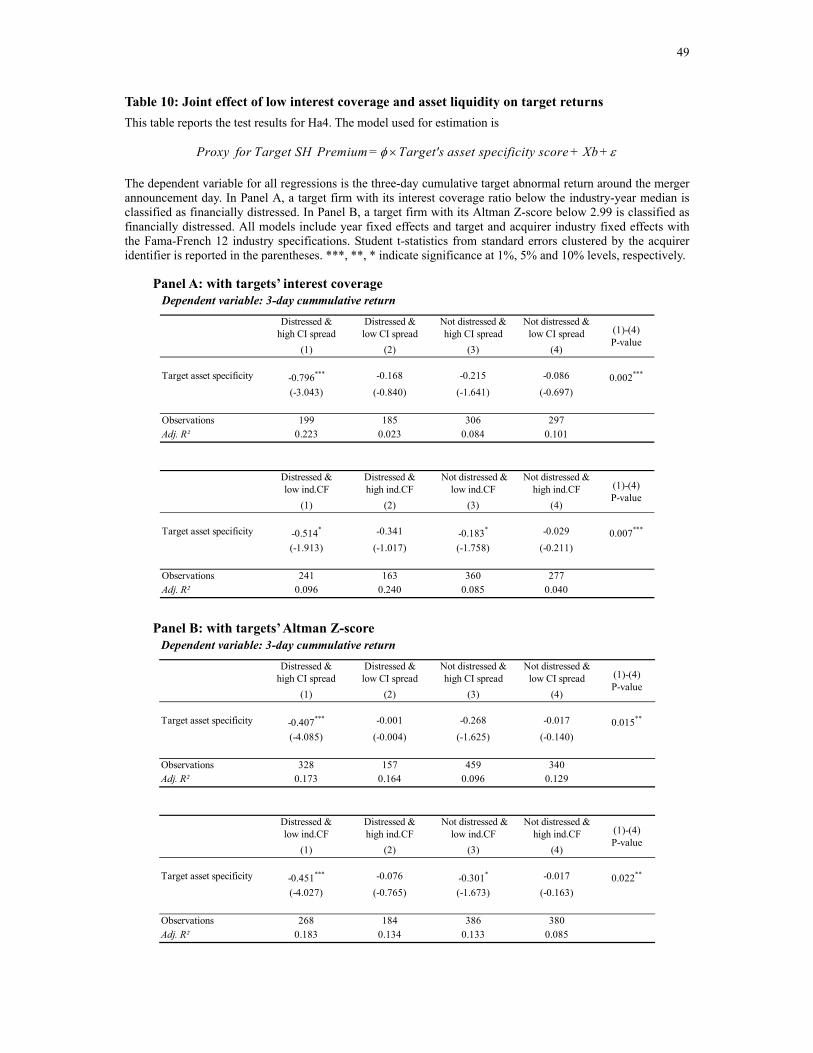
49

Table 10: Joint effect of low interest coverage and asset liquidity on target returns

This table reports the test results for Ha4. The model used for estimation is

Proxy for Target SH Premium = Target's asset specificity score + Xb +φ ε×

The dependent variable for all regressions is the three-day cumulative target abnormal return around the merger announcement day. In Panel A, a target firm with its interest coverage ratio below the industry-year median is classified as financially distressed. In Panel B, a target firm with its Altman Z-score below 2.99 is classified as financially distressed. All models include year fixed effects and target and acquirer industry fixed effects with the Fama-French 12 industry specifications. Student t-statistics from standard errors clustered by the acquirer identifier is reported in the parentheses. ***, **, * indicate significance at 1%, 5% and 10% levels, respectively.

Panel A: with targets’ interest coverage Dependent variable: 3-day cummulative return

Distressed &high CI spread

Distressed &low CI spread

Not distressed &high CI spread

Not distressed &low CI spread

(1) (2) (3) (4)

-0.796*** -0.168 -0.215 -0.086 0.002***

(-3.043) (-0.840) (-1.641) (-0.697)

Observations 199 185 306 297Adj. R² 0.223 0.023 0.084 0.101

Distressed &low ind.CF

Distressed &high ind.CF

Not distressed &low ind.CF

Not distressed &high ind.CF

(1) (2) (3) (4)

-0.514* -0.341 -0.183* -0.029 0.007***

(-1.913) (-1.017) (-1.758) (-0.211)

Observations 241 163 360 277Adj. R² 0.096 0.240 0.085 0.040

Target asset specificity

Target asset specificity

(1)-(4)P-value

(1)-(4)P-value

Panel B: with targets’ Altman Z-score Dependent variable: 3-day cummulative return

Distressed &high CI spread

Distressed &low CI spread

Not distressed &high CI spread

Not distressed &low CI spread

(1) (2) (3) (4)

-0.407*** -0.001 -0.268 -0.017 0.015**

(-4.085) (-0.004) (-1.625) (-0.140)

Observations 328 157 459 340Adj. R² 0.173 0.164 0.096 0.129

Distressed &low ind.CF

Distressed &high ind.CF

Not distressed &low ind.CF

Not distressed &high ind.CF

(1) (2) (3) (4)

-0.451*** -0.076 -0.301* -0.017 0.022**

(-4.027) (-0.765) (-1.673) (-0.163)

Observations 268 184 386 380Adj. R² 0.183 0.134 0.133 0.085

(1)-(4)P-value

Target asset specificity

(1)-(4)P-value

Target asset specificity

50

Ta

ble

11: C

hang

es in

leve

rage

and

ass

et il

liqui

dity

Th

is ta

ble

repo

rts th

e te

st re

sults

for H

a5. T

he re

gres

sion

mod

el u

sed

for e

stim

atio

n is

: C

hang

e in

Lev

erag

e =

θ ×

Tar

get a

sset

spec

ifici

ty sc

ore

+ Xβ

+ ε

Col

umns

(1),

(2),

(5) a

nd (6

) in

Pane

l A a

nd c

olum

ns (1

) and

(2) i

n Pa

nel B

repo

rt m

odel

est

imat

ion

usin

g ch

ange

s in

leve

rage

from

the

curr

ent y

ear t

o th

e fo

llow

ing

year

as

the

depe

nden

t var

iabl

e. C

olum

ns (3

), (4

), (7

) and

(8) i

n Pa

nel A

and

col

umns

(3) a

nd (4

) in

Pane

l B re

port

mod

el e

stim

atio

n us

ing

a tw

o-ye

ar le

vera

ge c

hang

e st

artin

g th

e cu

rren

t yea

r as

the

depe

nden

t var

iabl

e. T

he s

ubgr

oups

for

whi

ch th

e m

odel

s ar

e es

timat

ed a

ppea

r at

the

tabl

e he

ader

. All

mod

els i

nclu

de y

ear f

ixed

effe

cts a

nd in

dust

ry fi

xed

effe

cts w

ith th

e Fa

ma-

Fren

ch 1

2 in

dust

ry sp

ecifi

catio

ns. S

tude

nt t-

stat

istic

s fro

m st

anda

rd e

rror

s clu

ster

ed

by th

e ac

quire

r ide

ntifi

er is

repo

rted

in th

e pa

rent

hese

s. **

*, *

*, *

indi

cate

sign

ifica

nce

at 1

%, 5

% a

nd 1

0% le

vels

, res

pect

ivel

y

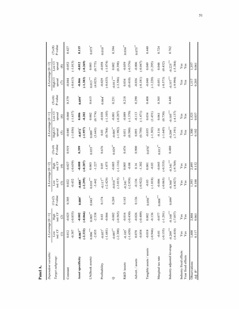
51

Dep

ende

nt v

aria

ble:

Targ

et s

ubgr

oup:

Low

ind.

CF

Hig

hin

d. C

FL

owin

d. C

FH

igh

ind.

CF

Hig

h C

I sp

read

Low

CI

spre

adH

igh

CI

spre

adL

ow C

I sp

read

(1)

(2)

(3)

(4)

(5)

(6)

(7)

(8)

Con

stan

t0.

012

-0.0

250.

305

0.02

2-0

.027

0.91

9-0

.040

-0.0

600.

379

-0.0

44-0

.052

0.42

7-0

.387

(-0.

855)

-0.4

52(-

0.65

9)(-

1.03

6)(-

1.63

7)(-

0.61

3)(-

1.01

3)

Ass

et s

peci

fici

ty-0

.067

**-0

.002

0.08

9*-0

.085

**-0

.008

0.39

9-0

.072

*0.

006

0.05

9*-0

.066

-0.0

120.

115

(-2.

332)

(-0.

066)

(-2.

295)

(-0.

207)

(-1.

957)

-0.2

02(-

1.38

3)(-

0.26

9)

LN

(Boo

k as

sets

)0.

006**

*0.

005**

0.04

3**0.

010**

*0.

003

0.03

5**0.

009**

*0.

002

0.61

50.

013**

*0.

003

0.07

5*

-2.8

55-2

.538

-3.4

42-1

.227

(3.6

43)

(0.7

74)

(4.0

25)

(0.7

75)

Prof

itabi

lity

-0.0

57*

0.03

0.17

4-0

.117

**0.

050.

676

0.03

-0.0

380.

064*

-0.0

29-0

.058

0.01

0**

(-1.

681)

-0.8

66(-

2.42

9)-1

.075

(0.7

84)

(-1.

105)

(-0.

635)

(-1.

074)

Q-0

.007

**-0

.002

0.26

9-0

.010

***

-0.0

050.

029**

-0.0

05**

-0.0

010.

251

-0.0

11**

*0.

002

0.39

4(-

2.30

0)(-

0.56

5)(-

3.01

5)(-

1.11

6)(-

1.98

2)(-

0.20

7)(-

3.58

6)(0

.398

)

R&

D /a

sset

s-0

.105

*-0

.016

0.14

3-0

.241

***

0.00

50.

476

0.03

1-0

.089

0.21

80.

034

-0.0

590.

034**

(-1.

650)

(-0.

430)

(-2.

939)

-0.0

8(0

.580

)(-

1.37

0)(0

.410

)(-

0.57

6)

Adv

ert.

/ ass

ets

0.07

8-0

.026

0.13

6-0

.136

0.16

0.90

00.

093

-0.1

130.

290

-0.0

36-0

.006

0.07

5**

-0.8

54(-

0.40

9)(-

0.92

2)-1

.302

(0.7

50)

(-1.

471)

(-0.

181)

(-0.

047)

Tan

gibl

e as

sets

/ as

sets

-0.0

180.

002

0.05

0**-0

.03

0.00

10.

070*

-0.0

350.

034

0.40

8-0

.048

0.04

90.

440

(-0.

946)

-0.1

36(-

1.01

8)-0

.03

(-1.

303)

(1.4

51)

(-1.

220)

(1.2

95)

Mar

gina

l tax

rate

-0.0

1-0

.077

0.00

8***

-0.0

06-0

.045

0.01

3**-0

.116

0.06

10.

305

-0.0

510.

048

0.72

4(-

0.15

5)(-

1.20

1)(-

0.06

3)(-

0.53

5)(-

1.64

5)(0

.730

)(-

0.57

3)(0

.432

)

Indu

stry

adj

uste

d le

vera

ge-0

.209

***

-0.1

68**

*0.

099*

-0.3

60**

*-0

.341

***

0.48

0-0

.209

***

-0.1

05**

*0.

448

-0.3

57**

*-0

.225

***

0.76

2(-

6.41

0)(-

7.05

7)(-

8.02

7)(-

9.76

9)(-

7.19

1)(-

4.13

7)(-

9.99

4)(-

5.38

4)

Indu

stry

fixe

d ef

fect

sY

esY

esY

esY

esY

esY

esY

esY

esY

ear f

ixed

eff

ects

Yes

Yes

Yes

Yes

Yes

Yes

Yes

Yes

Obs

erva

tions

1,60

0 2,

804

1,39

3 2,

495

1,30

0 1,

523

1,11

7 1,

357

Adj

. R²

0.11

70.

061

0.18

80.

132

0.10

20.

037

0.20

30.

061

Δ L

ever

age

[0 +

2](7

)-(8

)P-

valu

e(3

)-(4

)P-

valu

e

Δ L

ever

age

[0 +

1](5

)-(6

)P-

valu

e

Δ L

ever

age

[0 +

1](1

)-(2

)P-

valu

e

Δ L

ever

age

[0 +

2]

Pane

l A.

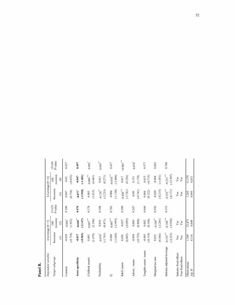
52

Pa

nel B

.

Dep

ende

nt v

aria

ble:

Targ

et su

bgro

up:

Rec

essio

nO

ff-re

cess

ion

Rec

essio

nO

ff-re

cess

ion

(1)

(2)

(3)

(4)

Con

stant

-0.0

290.

044*

0.10

00.

047

-0.0

20.

427

(-0.7

38)

(1.9

22)

(0.7

54)

(-0.6

52)

Ass

et sp

ecifi

city

-0.0

17-0

.040

**0.

476

-0.0

77*

-0.0

470.

497

(-0.

583)

(-2.

147)

(-1.

918)

(-1.

481)

LN(B

ook

asse

ts)0.

003

0.00

7***

0.17

80.

003

0.00

9***

0.09

2*

(1.4

79)

(5.1

96)

(1.0

15)

(4.4

61)

Prof

itabi

lity

-0.0

70*

0.01

60.

108

-0.1

20**

0.01

10.

043**

(-1.7

61)

(0.4

71)

(-2.2

33)

(0.2

71)

Q-0

.006

-0.0

07**

*0.

702

-0.0

06-0

.010

***

0.41

7(-1

.644

)(-2

.993

)(-1

.130

)(-3

.406

)

R&

D /a

sset

s0.

056

-0.0

270.

399

-0.4

45**

*0.

017

<0.0

01**

*

(0.6

03)

(-0.8

95)

(-3.7

41)

(0.3

56)

Adv

ert.

/ ass

ets

-0.0

560.

069

0.24

7-0

.09

0.15

10.

070*

(-0.7

35)

(0.8

88)

(-0.7

41)

(1.1

78)

Tang

ible

ass

ets /

ass

ets

-0.0

030.

002

0.84

60.

004

-0.0

150.

577

(-0.1

18)

(0.1

84)

(0.1

22)

(-0.7

15)

Mar

gina

l tax

rate

0.03

3-0

.109

**0.

556

-0.0

28-0

.068

0.66

2(0

.366

)(-2

.201

)(-0

.215

)(-1

.051

)

Indu

stry

adju

sted

leve

rage

-0.1

55**

*-0

.180

***

0.15

3-0

.352

***

-0.3

31**

*0.

780

(-4.2

23)

(-9.9

38)

(-8.1

71)

(-12.

507)

Indu

stry

fixed

effe

cts

Yes

Yes

Yes

Yes

Yea

r fix

ed e

ffect

sY

esY

esY

esY

es

Obs

erva

tions

1,34

912

,473

1,26

511

,179

Adj.

R²0.

116

0.04

80.

095

0.03

3

Δ Le

vera

ge [0

+1]

(1)-(

2)P-

valu

e

Δ Le

vera

ge [0

+2]

(3)-(

4)P-

valu

e

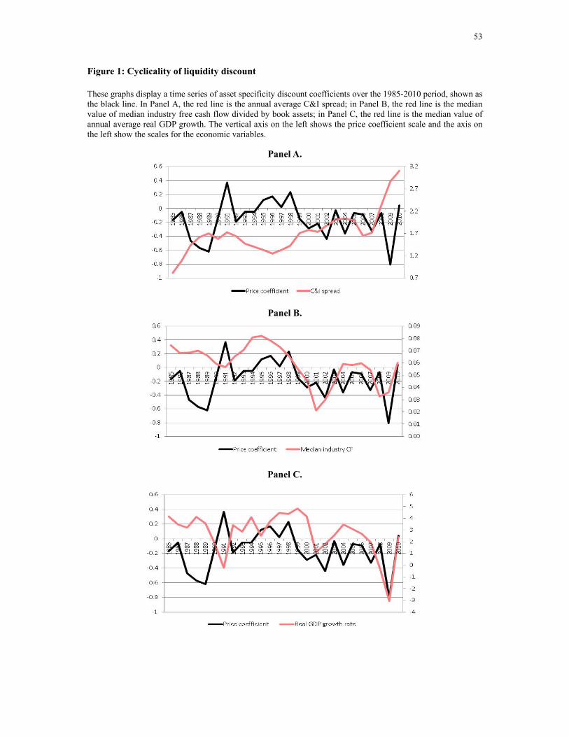
53

Figure 1: Cyclicality of liquidity discount These graphs display a time series of asset specificity discount coefficients over the 1985-2010 period, shown as the black line. In Panel A, the red line is the annual average C&I spread; in Panel B, the red line is the median value of median industry free cash flow divided by book assets; in Panel C, the red line is the median value of annual average real GDP growth. The vertical axis on the left shows the price coefficient scale and the axis on the left show the scales for the economic variables.

Panel A.

Panel B.

Panel C.

54

Chapter 2: Debt Financing Frictions and Access to Public Debt

2.1 Introduction

Imperfect and segmented financial markets create frictions in the supply of external capital,

and these frictions affect corporate activities that require external financing. The objective of

this study is to investigate a causal relationship between debt financing frictions and their

effects on corporate capital structure and firm growth.

The main predictions of this paper have three parts. First, firms having characteristics

associated with greater information asymmetries between firm insiders and outside investors,

e.g. small firm size and weak third-party information production, are more likely to be unable

to access public debt and so remain in the private debt market. Second, firms that were

previously unable to access public debt due to such debt financing frictions undergo a

substantial increase in leverage once the firms gain access to public debt. Third, because their

growth has been constrained due to costly private financing, firms entering the public debt

market, experience a rapid increase in asset size as the new financing source for growth

becomes available to them.

The identification strategy of this paper comes from relating firms’ ex post reaction to the

reduction in financial constraints to the ex ante extent of financing frictions. Following

Faulkender and Peterson (2006), I use the event of unrated firms’ securing a public debt

rating for the first time as a proxy for the firms’ gaining access to a cheaper means of

financing, which eases the firms’ financial constraints through reduction in borrowing costs.

This approach differs from studies using true natural experiments in a few aspects. The

advantage of using the securing of a debt rating as the event of the study is that the events are

scattered across time so that it is possible to draw time-controlled implications. On the other

hand, unlike a true natural experiment that provides an exogenous event that randomly

55

assigns treatment to the population, the securing of a debt rating occurs only to firms that

both choose to participate and are qualified to participate, i.e. only the firms that have access

and seek access to public debt. In order to mitigate this endogeneity issue I use fixed effects

and the Heckman two-step selection model. The empirical results support the existence of a

causal relation between financing frictions and the post-rating changes in capital structure and

firm growth even after addressing the endogeneity issues.

The constrained investment literature has shown that firm size is strongly correlated with

the extent of financial constraints (Gilchrist and Himmelberg (1995), Erickson and Whited

(2000)). Basing on this finding, I divide the pre-rating sample firms into two groups, ex ante

small firm group consisting of more financially constrained firms and ex ante large firm

group consisting of less constrained firms, by firms’ total book asset size measured one year

prior to their rating years.22 For another proxy for financing frictions, I follow Chang,

Dasgupta and Hilary (2007) and Lang and Lundholm (1993) and use the annual average

number of analyst following to capture the intensity of third-party information production

surrounding each sample firm. As in the firm size variable, I divide the sample firms into two

groups, ex ante less analyst coverage group and ex ante more coverage group, based on the

number of analyst reports on year prior to the firms’ rating year.

The empirical results strongly support the causal relation between debt financing frictions

and capital structure and also firm growth. First, a multivariate probit regression reveals that

the likelihood of gaining access to the debt market is significantly greater for firms having

asset size greater than the median size of firms accessing public debt for the first time and

having analyst coverage greater than the median amount of coverage on the firms entering the

debt market.

22 Hadlock and Pierce (2007) find firm size and age are the two measures that perform consistently well in identifying financially constrained firms. The findings of Whited and Wu (1996) also confirm that firm size is one of the most reliable measures of financial constraints. Similarly, Beck, Demirgüç-Kunt and Maksimovic (2005)’s survey study shows that firm size is perceived by firm management as a variable most strongly associated with financial and legal constraints, not only in the United States but in other countries as well.

56

Second, a multivariate regression test on changes in leverage reveals that firms accessing

public debt for the first time sharply increase leverage in the rating years and more so if the

firms are from more constrained groups, e.g. small and less covered firms, by 27% and by

11% of the total asset, respectively.

Third, a test result from a panel data regression indicates that the leverage increase in the

rating years explains more about firm growth in that year if the firms were exposed to greater

financing frictions before they entered the public debt market. For example, for firms in the

small and less analyst coverage group, each unit of debt increase is responsible for that of

asset growth by 0.6 in the rating year. As for firms in the large and more coverage group, the

sensitivity is -0.04. I present evidence that this discrepancy is at least partially because

unconstrained firms distribute the raised cash to investors rather than use it to finance growth.

While the literature on stock IPO is extensive, studies on firms’ initial access to public

debt is relatively rare. To my knowledge, this paper is one of few attempts to document the

effect of financial market segmentation on corporate financing and growth by investigating

the changes the firms undergo entering the public debt market. Hale and Santos (2008)

explore firms’ timing of entering the public bond market for the first time. Datta, Iskandar-

Datta, and Patel (2000) study the stock market reactions to the news of firms entering the

debt market in the agency context. This paper is also closely related to the literature on debt

supply frictions (Faulkender and Peterson (2006), Sufi (2009), Lemmon and Roberts (2010)

and others).

Implications from my paper are also related to the findings of Chang, Dasgupta and

Hilary (2006). Motivating their study in the context of information asymmetry and market

timing surrounding seasoned equity offerings, the authors empirically show that small firms

with low analyst coverage are financially more constrained because of high cost of equity

stemming from severe information asymmetry. They find that such firms less frequently issue

equity and time the market more, but when the market conditions change so that equity

57

issuance is available at a low cost, they raise funds through large SEOs.

The rest of the paper is outlined as follows. Section 1 derives testable implications.

Section 2 provides descriptive statistics. Section 3 reports empirical test results. Section 4

concludes.

2.2 Hypothesis

In this section, I develop a simple two-period model in order to illustrate how firm size

and third-party information production may affect firms’ ability to finance their growth. The

model’s main implication is that financing frictions impede firms’ ability to draw private

financing as well as their access to public debt financing, and the wedge between the optimal

amount of external financing to support firms’ investment opportunities and the firms’

inability to fully raise the amount through equity, internal financing and private loans forces

firms to forgo a part of positive net present value (NPV) projects.

A firm with an investment technology ( )g ⋅ invests an amount I at the beginning of a

period and receives ( )g I at the end of the period. There are largely two sources for I : W ,

a non-debt financing source; D , debt financing that includes bank debt B and public debt

sources A (public bond market and certified syndicate bank loans (Sufi, 2007, 2009)), such

that D B A= + .23

To simplify the analysis, I make the following assumptions regarding bank debt B and

arm’s length financing A . First, a firm can borrow an optimal bank loan B from its banks at

a price that fairly reflects the riskiness of the firm’s investment as long as B is below a

certain value B , a maximum loan amount due to credit rationing (Stiglitz and Weiss (1981)). 23 This setting is applicable to both the pecking order and the trade-off contexts depending on how one interprets W ; in the pecking order context, W is an internal financing source with the least information asymmetry costs; in the trade-off context, W reflects some optimized combination of internal and equity financing before the firm considers debt financing as an additional source for next investment projects in an attempt to maximize firm value.

58

B is an inverse function of a firm-level variable f that negatively affects the firm’s credit

status to potential lenders, such that and 0Bf

∂<

∂. Examples of such “friction variables”

could be proxies for credit worthiness or for the level of information opacity. We may also

resort to Faulkender and Peterson (2006) to interpret the inverse relation in another way:

information production that reduces adverse selection and moral hazard for borrowing firms

is a prerequisite for attracting outside investors. Information production through private

intermediaries such as banks is costly and the expense is imposed on the borrowing firms in

the form of increased borrowing costs. In that context, f is correlated with the unit cost of

producing information about the firm to attract additional dollar of external financing from

potential investors.

A firm issues public debt through an investment bank. There are two types of

underwriting costs: the fixed cost φ and the variable cost ( , )c A f such that 0cf∂

>∂

and

2

0cA f∂

>∂ ∂

. The variable cost is a function of both the amount raised and the firm’s friction

variable, reflecting the implications from Altinkihc and Hansen (2000). I use ( , )c A f A f= ⋅

to simplify the model and assume 0 1f< < . The underwriting market is competitive and

each investment bank earns a zero economic profit from their underwriting service. For

simplicity, I assume a zero discount rate, no implicit underpricing cost, and no incremental

distress cost from increasing leverage. The model does not distinguish the events of a firm’s

entering a public debt market for the first time and of a firm’s securing its credit debt rating

for the first time separately, as in Faulkender and Peterson (2006).

Let us assume first that the firm used up all other means of financing and is to finance its

investment opportunity entirely with the public debt A . The firm hires an investment bank

for its debt issuance and looks to enter the debt market for the first time. The cost of

underwriting, which will be fully paid by the issuing firm, is the sum of the fixed and the

59

variable cost of underwriting service, C A f φ= ⋅ + . The investment bank is a price taker and

charges a service fee at a fixed market rate 0 1α< < such that its service generates A α⋅

for the investment bank. Assuming zero economic profit, the bank will not contract unless

Af

φα

≥−

. Let A Af

φα

≡ =−

, the minimum target issue amount for which the bank is

willing to contract. Then, it follows that 0Af∂

>∂

and 2

2 0Af

∂>

∂.

The issuing firm’s goal is to maximize the following objective function:

max ( ) ( ),

. . ( ) , and (1)

(2)

Ag A A A f

s t g A A A f

Af

φ

φ

φα

− − ⋅ +

− − ⋅ ≥

≥−

The constraint term (1) captures the firm’s incentive to not participate if investing through

public debt financing results in negative profit, and term (2) is the investment bank’s

participation condition. Which one of the two conditions binds depends on the relative size of

( )g A and (1 )Aα+ . If the condition (1) binds, the optimal *A for the issuing firm is such

that *( ) 1g A f′ = + and it follows that *

0Af

∂<

∂. If the left-hand side of (1) is less than φ at

*A , then the firm opts not to borrow and forgoes the investment opportunity. There is a

maximum threshold for f , f , for a given investment technology ( )g ⋅ that makes

* * *( )g A A A f φ− − ⋅ = . If the condition (2) binds, then the maximum f for the given ( )g ⋅

forms not at *A but at A , such that ( )g A A A f φ− − ⋅ = , where A > *A .

Several implications emerge from the model. First, firm size is an important determinant

for whether an unrated firm’s investment is financially constrained. If the issuing firm is too

small or the issue size is not large enough so that the investment bank can not cover the fixed

cost with the service revenue, it may be difficult for an issuer to hire an investment bank for

underwriting and distribution service even if the issuing firm has firm characteristics

60

desirable to investors.

Second, firm characteristics f that is correlated with the firm’s internalized information

production cost is another important determinant of constrained financing. Firms perceived to

be opaque, i.e. with high f such that f f> for a given size and investment

technology ( )g ⋅ , will face issue costs not low enough to make the investment profitable, and

thus forgo the investment.

Third, exogenous shocks such as technological or economic conditions can affect ( )g ⋅ ,

W or the overall f in the economy as well as firms’ ability and incentives to access public

debt. Specifically, if the marginal cost of debt issuance is a function of γ such that ( )f γ ,

instead of just f , where γ reflects the financial market conditions such as overall

illiquidity in the market, then 0fγ∂

<∂

and 0Aγ∂

>∂

, i.e. poor financial market conditions

reduce firms’ likelihood of tapping into public debt.

Let us relax the restricting assumption on other financing means and allow the firm to

finance through equity, internal and bank loans. To determine changes in the firm when rated,

I examine a two-period world in which the firm is unrated in the first period and rated and

thus financially unconstrained in the second period. The subscript 1 and 2 denotes the first

and the second periods.

If a firm’s optimal investment in the first period, *1I , is financially unconstrained due to

high 1( )B f , abundant internal funding 1W or low investment opportunities, so that

*1 1 1( )I W B f≤ + , the changes in the firm’s leverage in the second period does not reflect the

existence of any credit supply frictions because the firm was not constrained in the first

period.

On the other hand, if the firm’s financing in the first period is constrained because its

funding needs for investment is greater than the maximum internal and external funds the

61

firm is able to raise, i.e. 1 1f f> and *1 1 1( )I W B f> + , then changes in leverage observed in

the second period should reflect the financing frictions during the first period because the

second period shift in leverage is equal to 12 2 1 2 2 1( )D D D B A B f≡ − = + − . Because of the

earlier assumption 1

1

0Bf

∂<

∂, it follows that 12

1

0Df

∂>

∂, i.e. the sensitivity of the leverage shift

in the second period to the ex ante friction variable is positive. Similarly, because

2 2 2I W D= + ( )2 1 12W D D= + + , it follows that 2

12 1

0( | )

ID f∂

>∂

.

The overall implication is that corporate financing and growth may be constrained by

small size and the high cost of information production. Guided by the implications from the

model, I construct the following propositions:

▪ P1-1: Small firm size and weak information production negatively affects firms’

likelihood of accessing public debt.

▪ P1-2: Poor financial market conditions make the negative relation in P1-1 more

pronounced.

▪ P2-1: 12

1

0DS

∂<

∂, i.e. the effect of ex ante small firm size on the leverage shift after

securing access to public debt is positive.

▪ P2-2: 12

1

0Df

∂>

∂, i.e. the effect of ex ante weak third –party information production on the

leverage shift after securing access to public debt is positive.

▪ P3-1: 2

12 1

0( | )

ID S∂

>∂ −

, i.e. the marginal effect of an increased borrowing in the rating

year on firm growth is positive and the effect is more pronounced with ex ante small firm

size.

62

▪ P3-2: For ex ante financially unconstrained firms, 2

12 1

0( | )

ID f∂

>∂

, i.e. the marginal effect

of an increased borrowing in the rating year on firm growth is positive and the effect is

more pronounced with weak third-party information production.

The model I present in this paper only focuses on supply side implications in a static two-

period world and assumes away important determinants of financing decisions such as

growth, tax and financial distress cost. I also acknowledge that the effect of financing

frictions alone certainly does not fully explain firms’ capital structure decisions and growth.

The point of this exercise is to show two possible sources of frictions, i.e., firm size that

implies an economically feasible minimum issue size for underwriters and the cost of

information production that affect the firms’ borrowing ability.

2.3 Data

The test sample consists of publically traded firms that obtain their issuer credit ratings

for the first time during the 1987-2011 period. COMPUTSTAT began populating Standards

and Poor’s (S&P) issuer credit rating (item 288) from 1986, which I set as the beginning year

of my sample period. COMPUSTAT maintains the firm-level credit rating record every

month since 1986. From the dataset, I indentify the month and the year in which a firm

receive a rating score for the first time and consider it as the time of entering the public debt

market. If the matching calendar year’s fiscal year end date comes after the rating month, the

year is set as the fiscal year that links to the annual COMPUSTAT data. If a fiscal year end

date comes before the rating month, then the next fiscal year is set as the firm’s rating year.

One of the key explanatory variables in this paper is the number of analyst following. I

compile this variable using the analyst coverage data from Thomson Reuters I/B/E/S

Historical Summary. To construct the variable, I take a fiscal-year average of the monthly

63

analyst count reporting on earning-per-share and use it as the extent of analyst coverage for

that year. As in Chang, Dasgupta and Hilary (2007), I use the raw count or a binary variable

throughout this paper without log-transforming it. I also treat missing analyst following value

as not having coverage.24

I discard firms that already have issuer ratings entering year 1986 because there is no way

of verifying from the dataset whether these firms received the ratings in 1986 for the first

time or did so before 1986. Following the literature convention, I exclude firms in the

financial (SIC in 6000s) and utility sectors (SIC in 4900-4999) and also firms with book asset

value smaller than 10 million dollars.

I consider missing values in R&D expenditure, advertising expenditure, capital

expenditure, short term and long term debt as zero. Following the literature, I winsorize the

variables at the 1% and 99% level in order to prevent a few extreme values from driving the

test results. I also winsorize the book and market leverage ratios exceeding 1.00.

The constrained investment literature implements various approaches to assign firms into

financially constrained and unconstrained groups. Almeida and Campello (2007, p.1441) give

a good review of the methods used in the literature. I divide the pre-rating sample firms into

two groups, ex ante small firm group for more financially constrained firms and ex ante large

firm group for less constrained firms, by firms’ total book asset size measured one year prior

to their rating years. For a proxy for the ex ante unit cost of information production, I follow

Chang, Dasgupta and Hilary (2007) and Lang and Lundholm (1993) and use the annual

average number of analyst forecasts on a firm to capture the intensity of third-party

information producing activities surrounding each sample firm. As in the firm size variable, I

divide the sample firms into two groups, ex ante less analyst coverage group and ex ante

more coverage group, based on the annual average number of analyst reports on the years

24 The regression results are qualitatively unaffected when log-transformed values are used or when observations with missing analyst coverage are excluded from the tests.

64

prior to the firms’ rating years.

Panel A in Table 12 compares the firm characteristics of the firms accessing public debt

for the first time prior to the rating years (shown in column (2)) to those of the two other firm

groups, one consisting of unrated firms (shown in column (1)) and the other group consisting

of rated firms (shown in column (3)). A mean comparison test and a Wilcoxon rank-sum test

among the firm groups show that firms entering the public debt market grow faster than the

firms in the other two groups, and the growth rate accelerates significantly in the rating year

(from 0.56 to 0.59) while firms in the other groups display diminishing growth rates (from

0.33 to 0.19 for group (1) and from 0.10 to 0.06 for group (3)). Firms entering the public debt

market also accelerate the annual rate of leverage increase (from 0.01 to 0.07) and the amount

of net debt issued (from 0.13 to 0.25), while other groups show little year-to-year changes for

the same variables. Firms entering the public debt market have larger asset size and greater

analyst coverage than unrated firms, consistent with the prediction that the likelihood of

accessing public debt is positively correlated with firm size and also with the intensity of

third-party information production. Rated firms are older, larger, more levered, have lower Q

and grow slower than firms entering the public debt market. The unrated firms are smaller,

less levered, with higher Q and more R&D intensive than the firms being rated.

Panel B compares the cost of issuing public bonds to firms entering the public debt

market to the cost to the rated firms. I use the bond yield spread over the treasury yield of the

same maturity, provided by the Thomson Reuters’ Securities Data Corporation (SDC) new

security data service, as a proxy for issue cost. Row (1) reports the summary statistics for the

yield spread of bonds issued by firms entering the public debt market, and the row (2) reports

the statistics for yield spread of bonds issued by rated firms. The number of observations for

group (1) is smaller than actual number of firms being rated because the SDC data does not

cover other sources of public or semi-public debt types such as syndicated loans.

The results from the mean comparison test and the Wilcoxon rank sum test on the two

65

groups show that the debt issue cost is higher for newly rated firms than that for rated firms.

Panel C further divides the firms issuing public bonds around rating years into four groups by

firm size and analyst coverage. Comparison among the groups reveals that firm size and

analyst coverage are inversely correlated with the cost of debt issuance, and this is consistent

with the earlier assumption that third-party information production and firm size are

negatively correlated with the cost of borrowing.

Panels in Figure 2 illustrate the changes the firms entering the public debt market undergo

in their capital structure and asset size. Panel A in Figure 2 presents the firm-year average

book leverage of the sample firms during [-6 +6] panel years surrounding the rating years

(year 0). I only include observations of firms having no missing year observations for the

panel period. There is a substantial upward shift in leverage in the rating year, consistent with

the summary statistics in Table 12. Panel B shows average asset size of firms around the

rating years. The asset growth rate appears to increase in the rating years, consistent with the

findings from the Table 12.

P2 and P3 predict that firms that had greater financing frictions are more financially

constrained in terms of both capital structure and growth, and so they would increase

leverage more and grow faster as they gain access to the new and cheaper financing source.

Figure 3 highlights this positive relation between the extent of ex ante financing frictions and

changes in leverage as well as financing frictions and firm growth in the rating years. The

first column reports annual changes in leverage and growth rate during the years surrounding

the rating years for small and large firm groups. Propositions P2 and P3 predict a higher

rating-year (year 0) increase for the small firm group in each category than for the large firm

group, and that is precisely what the graphs show.

The graphs in the second column report average annual changes in each category for the

less analyst coverage group as well as for the more coverage group. As in column 1, the

pattern in column 2 is consistent with P2 and P3 in that a higher rating-year (year 0) increase

66

for the less covered firm group in every category compared to the more covered group, but

the effect in column 2 is smaller than that in column 1.

2.4 Empirical Results

2.4.1 Public debt access and leverage change

In this section, I report the empirical results examining the relation between financing

frictions and the likelihood of unrated firms’ entering the public debt market. There are two

main explanatory variables in the regression. The first one is Asset Size < median dummy, a

binary variable that takes the value 1 if book asset size of a firm is smaller than the median

asset size of firms securing a debt rating for the first time and 0 if the book asset size of the

firm is greater than the median. The second key variable is Number of analyst forecasts <

median dummy, a binary variable that takes the value 1 if the annual average number of

analyst forecasts of a firm is fewer than the median count of analyst forecasts of firms

securing a debt rating for the first time and 0 if the forecast count of the firm is greater than

the median.

Proposition P1-1 states that small firm size and weak third-party information production

negatively affects firms’ likelihood of accessing public debt. The empirical prediction is that

there is a negative relation between the likelihood of accessing public debt and the two key

explanatory variables, small firm size and weak analyst coverage.

Table 13 reports the regression results on all unrated firm observations with non-missing

data during the sample period. The first three columns are estimated using probit models with

year fixed effects, and the latter three columns are estimated using linear probability models

with firm and year fixed effects. The dependent variable for the models is a binary variable

that takes the value 1 if a firm secures a debt rating for the first time in the observed year and

67

0 otherwise, and all explanatory variables are lagged by one year.

Consistent with the predictions, all columns report negative and statistically significant

coefficients on the two key explanatory variables. Coefficients on other variables are also

consistent with the findings in the literature (Datta, Iskandar-Datta, Patel (2000) and

Faulkender and Petersen (2006)). In untabulated logit estimation, the coefficients for the two

explanatory variables expressed in odds ratios are 0.186 and 0.716 respectively, indicating a

significant reduction in the probability of securing a debt rating for small firms and firms

with low analyst coverage.

Proposition P1-2 states that poor financial market conditions make the negative relation

between the two friction variables and the likelihood of securing a debt rating shown in P1-1

more pronounced. In order to test this prediction, I estimate the following regression model

for a sample of firms entering the public debt market:

1 1 1 yr yr yr tFriction variable Proxies for Economic Conditions X eα β− − −= + ×Β + × +

Friction variable is either the firm size or the number of analyst following on the firms

receiving a debt rating in the following year. Proxies for economic conditions are variables

that are correlated with the overall conditions in the financial market and the economy.

Following Harford (2005), I use the C&I loan spread, which is the spread between the

average interest rate on commercial and industrial loans and the Federal Funds rate, as a

proxy for credit tightening in the economy. 25 Another proxy used for the economic

conditions is the industry-year median cash flow compiled at the three-digit SIC code level.

The prediction is that there is a positive relation between the overall credit tightness in the

financial market and the firm size and information production (thus low information

asymmetry) required for accessing public debt.

25 The data is available in the Federal reserve’s Survey of Terms of Business Lending at http://www.federalreserve.gov/releases/e2/e2chart.htm.

68

Table 14 presents the estimation results. The dependent variable for the first column is the

analyst coverage variable in raw number. Because the dependent variable’s discreteness

violates OLS assumptions, I estimate a negative binomial model instead of an OLS model for

the test. The model setting is similar to that of the empirical setting used in Chang et. al. The

result shown in the first column is consistent with the prediction in that the coefficient on the

C&I loan spread, 1.52, expressed in the incidence rate ratio, indicates a positive correlation

between the spread and the number of analyst following. The coefficient on the industry

median cash flow variable is less than 1 and indicates that the level of industry cash flows,

which is correlated with easing of liquidity in the economy, is negatively related with the

number of analyst following of firms entering the public debt market.

The second column presents results from OLS regression estimation. In order to achieve

normality of the residuals, I log-transform the dependent variable, which is the book asset

size of firms entering the public debt market. Again, the positive and statistically significant

coefficient on the C&I spread and the negative coefficient on the industry median cash flow

are consistent with the prediction. In both models the substantial statistical significance of the

coefficient on the C&I spread and relatively weak coefficient on the industry cash flow may

suggest that the C&I spread is strongly associated with the financing frictions in the credit

market.

Proposition P2-1 and P2-2 state that the effect of ex ante small firm size and weak

information production on leverage after securing access to public debt is positive. I test this

prediction on the firms receiving a debt rating in the following year, using OLS regressions.

Table 15 reports the results from the following model:

0 1 1 2 1 1 yr yr yr yr tBook Leverage Small size Low analyst coverage X eα γ γ β− − −Δ = + × + × + × +

The firm characteristics variables in the lagged 1yrX − are from the reduced form

69

leverage models in the capital structure literature.26 The dependent variable for the first three

columns is annual changes in book leverage and constructed as

0 1 year yearBook lverage book leverage −− . Column (1) shows that the coefficient on Small size is

positive and statistically significant, consistent with P2-1. Column (2) reports that the

coefficient on the Low analyst following is also positive and statistically significant,

consistent with P2-2. Column (3) reports results having both variables in the regression,

displaying little changes in the coefficients compared to the previous models. The models in

the latter three columns use Net debt issued, the net debt issues amount deflated by firm asset

size with a one year lag, as an alternative dependent variable. Following Chang et. al. I define

net debt issues amount as long term debt issuance – long term debt reduction + current

portion of long term debt. The empirical models in columns (4), (5) and (6) estimated using

this dependent variable are all consistent with the predictions in P2-1 and P2-2 with the

strong positive coefficients.

The economic magnitude of ex ante frictions on the rating-year changes in leverage is

substantial. Considering the mean leverage for the firms acquiring a debt rating in the years

leading to the rating year is 0.34, the small and less covered firms increase leverage by more

than 40% in their rating years ((0.09 + 0.04) / 0.34) and raise net debt by 49% of their book

asset value one year before the rating years.

Individual firms’ entering the public debt market and thus into the sample is not a random

event. To mitigate the potential self-selection problem, I use the Heckman two-step selection

method to control for unobservable factors that may simultaneously affect the sample

selection process and the outcome variable. The censored group consists of the firms being

rated from column (3) and (6) in Table 15, and the uncensored group consists of firm year

observations of unrated firms from column (3) in Table 14. Column (1) and (3) report the

26 Frank and Goyal (2009) provide a good review of the empirical models.

70

outcome model estimates and column (2) and (4) report the selection model estimates.27 The

coefficients on the inverse Mills ratios are statistically insignificant and the coefficients on

small size and weak analyst coverage continue to be statistically and economically significant.

Overall, test results presented in this section provide evidence consistent with the

prediction that segmented financial markets and financing frictions are important factors that

influence corporate capital structure decisions.

2.4.2 Public debt access and firm growth

This section focuses on the relation between firms’ growth and the changes in leverage in

the rating year. Proposition P3-1 and P3-2 state that the marginal effect of an increased

borrowing in the rating year on firm growth is positive and the effect is more pronounced

with ex ante small firm size and weak information production.

The main empirical model is similar to the constrained investment models in the literature:

( )1 1 2 1

1

2 3

Assets = /

+

t t t t

t t

CF asset Q

Leverage Rating year dummy u

α β βγγ γ ν ε

− −Δ + × + ×

+ × ∗+ Δ × + + +

tΔ Leverage Rating year dummy×

I use the panel data of firms that are being rated for the first time during the sample period.

In the model, Rating year is a dummy variable that takes the value 1 if an observation is from

the rating years and 0 otherwise. As in the previous section, I use changes in book leverage

and net debt issued as two proxies for changes in debt financing. The dependent variable

ΔAssets is compiled as the changes in book asset from the previous year to the concurrent

year deflated by book asset in the previous year. All estimation includes year and firm fixed

27 The Heckman model does not include an industry fixed effect to avoid the well-documented incidental parameter problem associated with maximum likelihood estimation and fixed length of a panel. The model uses firm age as the exclusion restriction, following the implication from the literature that firm age is one of the determinants of firms’ having a debt rating (Faulkender and Peterson (2006)).

71

effects. I divide the sample observations into four subgroups by firm size and the number of

analyst following measured in the year preceding the rating years. Namely, the four groups

are (1) small size and less analyst coverage group, (2) small size and more coverage group,

(3) large size and less coverage group, and (4) large size and more coverage group. I then

estimate the regression model on each of the four subgroups separately.

The coefficient of interest is 1γ , which captures the sensitivity of asset growth to the

leverage change in the rating year. The testable implication drawn from Propositions P3-1

and P3-2 is that the sensitivity is more pronounced for firm groups with more severe frictions

because ex ante financially constrained firms would use the proceeds from debt issuance to

finance their asset growth that were previously constrained. Specifically, the hypothesis is

that 1γ from the financially constrained firms, e.g. firms in group (1), is different from zero

and also greater than 1γ of the financially unconstrained firms, e.g. firms in group (4).

Panel A and Panel B in Table 17 report the test results, with the changes in book leverage

and net debt issued as the main explanatory variable of Panel A and Panel B, respectively.

The key coefficient estimates 1γ are positive and statistically different from 0 in both Panel

A and Panel B, consistent with P3-1 and P3-2 that the sensitivity of firm growth to the rating

year debt financing is more pronounced for firms with severe financing frictions. In both

tables the coefficient 1γ in the unconstrained firm group, e.g. group (4), is negative,

indicating that the speed of asset growth in unconstrained firms may actually slow down

during their rating years. Another result worth noting is that 2γ , the coefficient of the stand-

alone changes in leverage variable, is economically smaller in the most constrained group

than 2γ in the unconstrained firm group. Finally, the cash flow sensitivity coefficient 1β is

larger in the most constrained group than 1β in the unconstrained group in both tables.

These observations imply that, compared to unconstrained firms, firms constrained due to

financing frictions use internal financing more and rely relatively less on external financing

to fund their growth during normal times, but as they become mature enough to gain access

72

to new and cheaper means of financing in public debt, the firms issue debt for growth that

was previously constrained due to costly financing.

2.4.3 Public debt access and payout

A result in the previous section indicates that the asset growth rate of unconstrained firms

may actually slow down as the firms raise debt in the rating years. There could be other

reasons for the observed pattern, but one possible explanation that fits nicely with the

predictions from the earlier model is that the unconstrained firms, having little unresolved

growth opportunity, enter and raise public debt to distribute some of the proceeds to

shareholders instead of financing growth.

To test this prediction, I compile a measure for annual total cash payout, which is equal to

annual cash dividends plus repurchase of common stock. Following Grullon and Michaely

(2002), I define common stock repurchase as total expenditure on the purchase of common

and preferred stocks minus any reduction in the value of preferred stocks outstanding. To

observe the relation between cash inflow from debt issuance and cash outflow through payout

more directly, I only use Net debt issued for the regression model, which is as follows:

1

2 3

4 1

=

t

t

t-1 t t

PayoutNet debt issued Rating year dummyPayout X u

α γγ γγ ν ε−

Δ + × ∗+ × + ×

+ × + Β+ + +

tNet debt issued Rating year dummy

where ΔPayoutt = Payoutt – Payoutt-1. The empirical prediction is that the key coefficient

1γ is positive and statistically significant for the unconstrained firm group while it shows no

significant sensitivity in the constrained group.

The results in Table 18 present evidence that is consistent with this prediction. The

estimate for 1γ in column (4) is significant at the 10% level and the size of the coefficient,

0.051, is greater than that of the coefficient on the stand-alone net debt issue, which as 0.016.

73

This implies that an average unconstrained firm may enter and raise public debt to pay out a

substantial portion of the proceeds to shareholders, and this distribution of firm assets along

with other reasons may contribute to the slow down of the asset growth rate seen in the

previous section. As expected, 1γ in the constrained group shows no sensitivity.

Overall, this result combined with the findings in the previous section provide support for

the prediction that financial market frictions negatively affect firms’ growth and that when a

new and cheap financing source becomes available to the previously constrained firms, they

allocate the funds raised from the new financing source heavily on growth.

2.5 Conclusion

The goal of this paper is to study the sources of financial market frictions and investigate

how the financial market segmentation due to such frictions affects firms’ capital structure

and growth. The findings from this study are as follows. First, small firms with weak third-

party information production have a low likelihood of entering the public debt market, and

more so when the overall economic condition is poor. Next, firms that enter the public debt

market increase their leverage proportional to the extent of financing constraints they

experience prior to gaining access to it. For instance, a small firm with low information

production would increase leverage in the rating year by 39% relative to its pre-rating level.

Then, the previously constrained firms use the proceeds acquired from the new and cheaper

funding source to finance growth that was previously more costly, accelerating the speed of

growth.

Together, the findings in this paper highlight the importance of financial market

segmentation due to financing frictions in shaping corporate capital structure as well as

investment.

74

References Ahern, K. R., 2012. “Bargaining Power and Industry Dependence in Mergers.” Journal of Financial Economics 103, 530-550. Almeida, H., Campello, M., 2007. Financial Constraints, Asset Tangibility, and Corporate Investment. Review of Financial Studies 20, 1429-1460. Almeida, H., Campello, M., Hackbarth, D., 2011. “Liquidity Mergers.” Journal of Financial Economics 102, 526-558. Altinkihc, O., Hansen, R.S., 2000. Are There Economies of Scale in Underwriting Fees? Evidence of Rising External Financing Costs. Review of Financial Studies 13, 191-218. Altman, E. I., 1968. “Financial Ratios, Discriminant Analysis and the Prediction of Corporate Bankruptcy.” Journal of Finance 24, 589-609. Altman, E. I., 2000. "Predicting Financial Distress of Companies: Revisiting the Z-SCORE and ZETA Models." Working paper. Ball, C., Hoberg, G., Maksimovic, V., 2011. Redefining Financial Constraints: a Text-Based Analysis, Working paper. Bates, T., Kahle, K., Stulz, R., 2009. Why do US firms Hold So Much More Cash than They Used to? Journal of Finance 64, 1985-2021. Beck, T., Demirgüç-Kunt, A., Maksimovic, V., 2005. Financial and Legal Constraints to Growth: Does Firm Size Matter? Journal of Finance 60, 137-177. Benmelech, E., Bergman N. K., 2009. “Collateral pricing.” Journal of Financial Economics 91, 339–360. Berger, P. G., Ofek, E., 1995. Diversification’s Effect on Firm Value. Journal of Financial Economics 37, 39-65. Brown, D. T., James, C.M., Mooradian, R. M., 1994. “Asset Sales by Financially Distressed Firms.” Journal of Applied Corporate Finance 2, 233-258.

75

Brown, S. J., Warner, J. B., 1985. “Using Daily Stock Returns: The Case of Event Studies.” Journal of Financial Economics 14, 3-31. Campbell, J. Y., Giglio, S., Pathak, P., 2011. “Forced Sales and House Prices.” American Economic Review 101, 2108–2131. Campello, M., Graham, J. R., Harvey, C. R., 2010. The Real Effects of Financial Constraints: Evidence from a Financial Crisis. Journal of Financial Economics 97, 470-487. Custódio, C, Ferreira, M. A., Matos, P., 2012. “Generalists versus Specialists: Lifetime Work Experience and CEO Pay.” Working paper. Chang, X., Dasgupta, S., Hilary, G. 2006. Analyst Coverage and Financing Decisions. Journal of Finance 61, 3009-3047. Dittmar, A. K., Dittmar, R. F., 2006. “The timing of Financing Decisions: An Examination of the Correlation in Financing Waves.” Journal of Financial Economics 80, 59-83. Datta, S., Iskandar-Datta, M., Patel A., 2000. Some Evidence on the Uniqueness of Initial Public Debt Offerings. Journal of Finance 55, 715-743. Diamond, D., 1991. Monitoring and Reputation: The Choice between Bank Loans and Directly Place Debt. Journal of Political Economy 99, 689-721. Eisfeldt, A. L., Rampini, A. A., 2006. “Capital Reallocation and Liquidity.” Journal of Monetary Economics 53, 369-399. Erickson, T., Whited, T., 2000. Measurement Error and Relationship between Investment and Q. Journal of Political Economy 108, 1027-1057. Frank, Z. M., Goyal, V. K., 2009. Capital Structure Decisions: Which Factors Are Reliably Important? Journal of Financial Management 38, 1-37. Faulkender, M., Petersen, M. A., 2006. Does the Source of Capital Affect Capital Structure? Review of Financial Studies 19, 45-49. Gilchrist, S., Himmelberg C., 1995. Evidence on the Role of Cash Flow for Investment, Journal of Monetary Economics 36, 541-572.

76

Grullon, G., Michaely, R., 2002. Dividends, Share Repurchases, and the Substitution Hypothesis. Journal of Finance 57, 1649-1684. Gavazza, A., 2011. "Leasing and Secondary Markets: Theory and Evidence from Commercial Aircraft." Journal of Political Economy 119, 325 - 377. Gertner, R., Scharfstein, D., 1991. “A Theory of Workouts and the Effects of Renegotiation Law.” Journal of Finance 46, 1189-1222. Hackbarth, D., Miao, J., 2012. “The Dynamics of Mergers and Acquisitions in Oligopolistic Industries.” Journal of Economic Dynamics & Control 36, 585–609. Harford, J., 2005. “What Drives Merger Waves?” Journal of Financial Economics 77, 529-560. Hadlock, C. J., Pierce, J. R., 2010. New Evidence on Measuring Financial Constraints: Moving beyond the KZ Index. Review of Financial Studies 23, 1909-1940. Hale, G., Santos, J. A. C., 2008. The Decision to First Enter the Public Bond Market: The Role of Firm Reputation, Funding Choices, and Bank Relationships. Journal of Banking and Finance 32, 1928-1940. Jensen, M., Meckling, W., 1976. “Theory of the Firm: Managerial Behavior,, Agency Costs and Ownership Structure.” Journal of Financial Economics 3, 305-360. Kim, H., Kung, H., 2011. “Asset Specificity, Economic Uncertainty, and Corporate Investment.” Working paper. Kim, E., Singal, V., 1993. “Mergers and Market Power: Evidence from the Airline Industry.” American Economic Review 83, 549–569. Lang, L., Poulsen, A., and Stulz, R. M., 1995. “Asset Sales, Firm Performance, and the Agency Costs of Managerial Discretion.” Journal of Financial Economics 37, 3-37. Lemmon, M. L., Roberts, M. R., 2010. The Response of Corporate Financing and Investment to Changes in the Supply of Credit. Journal of Financial and Quantitative Analysis 45, 555–587.

77

Moeller, S. B., Schlingemann, F. P., Stulz, R. M., 2003. “Firm Size and the Gains from Acquisitions.” Journal of Financial Economics 73, 201-228. Myers, S., 1977. “Determinants of Corporate Borrowing.” Journal of Financial Economics 5, 147-175. Myers, S., Majluf, N., 1984. “Corporate Financing and Investment Decisions When Firms Have Information That Investors do not Have.” Journal of Financial Economics 13, 187-221. Petersen, M. A., 2009. Estimating Standard Errors in Financing Panel Data Sets: Comparing Approaches. Review of Financial Studies 22, 435-480. Pulvino, T. C., 1998. “Do Asset Fire Sales Exist? An Empirical Investigation of Commercial Aircraft Transactions.” Journal of Finance 53, 939-978. Ramey, V. A., Shapiro, M. D., 2001. “Displaced Capital: A Study of Aerospace Plant Closings.” Journal of Political Economy 109, 958-992. Rau, P. R., Stouraitis, A., 2011. “Patterns in the Timing of Corporate Event Waves.” Journal of Financial and Quantitative analysis 46, 209-246. Sibilkov, V., 2009. “Asset Liquidity and Capital Structure.” Journal of Financial and Quantitative Analysis 44, 1173-1196. Shleifer, A., Vishny, R. W., 1992. “Liquidation Values and Debt Capacity: A Market Equilibrium Approach.” Journal of Finance 47, 1343-1366 Shleifer, A., Vishny, R. W., 2011. “Fire Sales in Finance and Macroeconomics.” Journal of Economic Perspectives 25, 29-48. Schwert, G. W., 1996. “Markup Pricing in Mergers and Acquisitions.” Journal of Financial Economics 41, 153-192. Singal, V., 1996. “Airline Mergers and Competition: an Integration of Stock and Product Price Effects.” Journal of Business 69, 233–268. Stiglitz, J., Weiss, A., 1981. Credit Rationing in Markets with Imperfect Information.

78

American Economic Review 71, 393-410. Sufi, A., 2007. Information Asymmetry and Financing Arrangements: Evidence from Syndicated Loans. Journal of Finance 62, 629-268. Sufi, A., 2009. The real Effects of Debt Certification: Evidence from the Introduction of Bank Loan Ratings. Review of Financial Studies 22, 1659-1691. Williamson, O. E., 1988. “ Corporate Finance and Corporate Governance.” Journal of Finance 43, 567-591. White, H., 1980. A Heteroskedasticity-Consistent Covariance Matrix Estimator and A Direct Test for Heteroskedasticity. Econometrica 48, 817-838.

79

Appendix A: Variable descriptions

Paid in cash is a dummy variable that takes the value 1 if the SDC indicates that only cash is used for the acquisition and takes 0 otherwise.

Toehold is a dummy variable that takes the value 1 if the SDC indicates that the acquirer holds shares of the target firm prior to the merger announcement and takes 0 otherwise.

LN(Mkt equity) is the natural log of the inflation-adjusted share price times the number of shares outstanding at the beginning of the fiscal year in which the merger announcements are made.

Tender offer is a dummy variable that takes the value 1 if the SDC indicates that the deal is a tender offer.

Focused is a dummy variable that takes the value 1 if the two-digit SIC code of the target firm and that of the acquiring firm is the same and takes 0 otherwise.

Q is the ratio of book liability plus the market value of common stock to book assets. Competed is a dummy variable that takes the value 1 if the SDC indicates more than one

bidder for the target and takes 0 otherwise. Relative size is the ratio of the total transaction value to the market value of the acquirer

at the beginning of the fiscal year. Target termination fee is a dummy variable that takes the value 1 if the SDC indicates that

a merger contract includes a target termination fee agreement. R&D/assets is the ratio of research and development expense to book assets of an acquirer. Tangible assets is the ratio of net property, plant and equipment to book assets. Industry concentration is the eight-firm concentration ratio provided by the US Census

Bureau for the 1997 report. Book leverage is the ratio of short term debt plus long term debt to book assets. Profitability is the ratio of operating income before depreciation to book assets. Advert./assets is the ratio of advertising expenses to book assets.

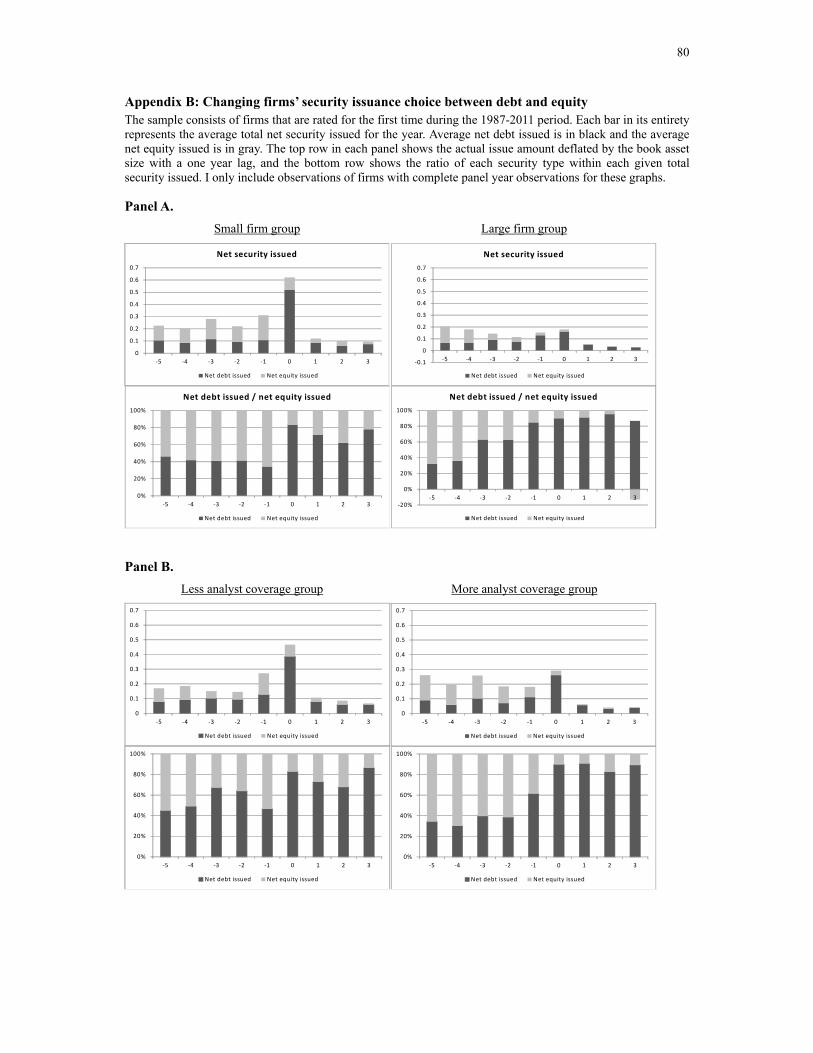
80

Appendix B: Changing firms’ security issuance choice between debt and equity The sample consists of firms that are rated for the first time during the 1987-2011 period. Each bar in its entirety represents the average total net security issued for the year. Average net debt issued is in black and the average net equity issued is in gray. The top row in each panel shows the actual issue amount deflated by the book asset size with a one year lag, and the bottom row shows the ratio of each security type within each given total security issued. I only include observations of firms with complete panel year observations for these graphs.

Panel A. Small firm group Large firm group

0

0.1

0.2

0.3

0.4

0.5

0.6

0.7

‐5 ‐4 ‐3 ‐2 ‐1 0 1 2 3

Net security issued

Net debt issued Net equity issued

0%

20%

40%

60%

80%

100%

‐5 ‐4 ‐3 ‐2 ‐1 0 1 2 3

Net debt issued / net equity issued

Net debt issued Net equity issued

‐20%

0%

20%

40%

60%

80%

100%

‐5 ‐4 ‐3 ‐2 ‐1 0 1 2 3

Net debt issued / net equity issued

Net debt issued Net equity issued

‐0.1

0

0.1

0.2

0.3

0.4

0.5

0.6

0.7

‐5 ‐4 ‐3 ‐2 ‐1 0 1 2 3

Net security issued

Net debt issued Net equity issued

Panel B. Less analyst coverage group More analyst coverage group

0%

20%

40%

60%

80%

100%

‐5 ‐4 ‐3 ‐2 ‐1 0 1 2 3

Net debt issued Net equity issued

0

0.1

0.2

0.3

0.4

0.5

0.6

0.7

‐5 ‐4 ‐3 ‐2 ‐1 0 1 2 3

Net debt issued Net equity issued

0%

20%

40%

60%

80%

100%

‐5 ‐4 ‐3 ‐2 ‐1 0 1 2 3

Net debt issued Net equity issued

0

0.1

0.2

0.3

0.4

0.5

0.6

0.7

‐5 ‐4 ‐3 ‐2 ‐1 0 1 2 3

Net debt issued Net equity issued

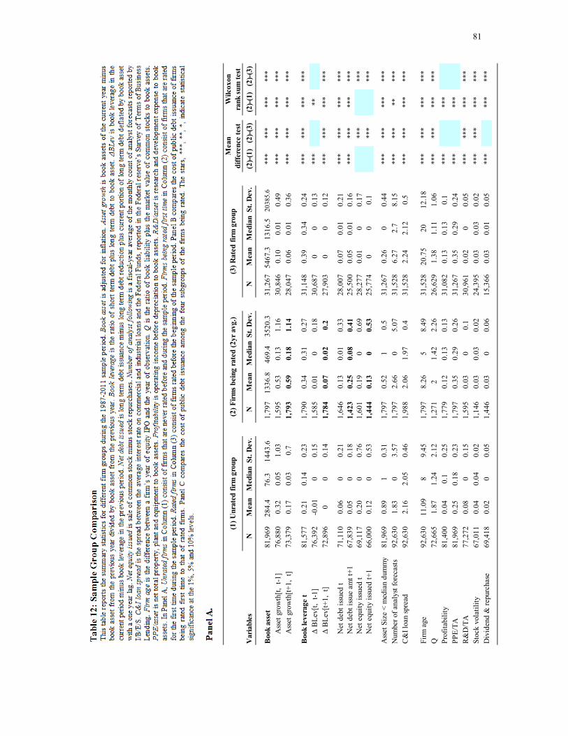
81

Var

iabl

esN

Mea

nM

edia

nSt

. Dev

.

N

Mea

nM

edia

nSt

. Dev

.N

Mea

nM

edia

nSt

. Dev

.

(2

)-(1)

(2)-(

3)(2

)-(1)

(2)-(

3)

Boo

k as

set

81,9

6928

4.4

76.3

1443

.6

1,79

713

36.8

469.

435

20.3

31,2

6754

67.3

1316

.520

385.

6

***

***

***

***

A

sset

gro

wth

[t, t

-1]

76,8

800.

320.

051.

03

1,59

50.

530.

131.

1630

,846

0.10

0.01

0.49

**

***

***

***

*

Ass

et g

row

th[t+

1, t

]73

,379

0.17

0.03

0.7

1,

793

0.59

0.18

1.14

28,0

470.

060.

010.

36

***

***

***

***

Boo

k le

vera

ge t

81,5

770.

210.

140.

23

1,79

00.

340.

310.

2731

,148

0.39

0.34

0.24

**

***

***

***

*

Δ B

Lev[

t, t-

1]76

,392

-0.0

10

0.15

1,

585

0.01

00.

1830

,687

00

0.13

**

***

Δ

BLe

v[t+

1, t

]72

,896

00

0.14

1,

784

0.07

0.02

0.2

27,9

030

00.

12

***

***

***

***

N

et d

ebt i

ssue

d t

71,1

100.

060

0.21

1,64

60.

130.

010.

3328

,007

0.07

0.01

0.21

***

***

***

***

N

et d

ebt i

ssue

am

t t+1

67,8

390.

050

0.18

1,42

30.

250.

080.

4125

,500

0.05

0.01

0.16

***

***

***

***

N

et e

quity

issu

ed t

69,1

170.

200

0.76

1,60

10.

190

0.69

28,2

770.

010

0.17

***

***

N

et e

quity

issu

ed t+

166

,000

0.12

00.

531,

444

0.13

00.

5325

,774

00

0.1

***

***

Ass

et S

ize

< m

edia

n du

mm

y81

,969

0.89

10.

31

1,79

70.

521

0.5

31,2

670.

260

0.44

**

***

***

***

*N

umbe

r of a

naly

st fo

reca

sts92

,630

1.83

03.

57

1,79

72.

660

5.07

31,5

286.

272.

78.

15

***

***

****

*C

&I l

oan

spre

ad92

,630

2.16

2.05

0.46

1,98

82.

061.

970.

431

,528

2.24

2.12

0.5

***

***

***

***

Firm

age

92,6

3011

.09

89.

45

1,79

78.

265

8.49

31,5

2820

.75

2012

.18

**

***

***

***

*Q

72,6

651.

871.

242.

12

1,27

12

1.42

2.26

26,6

291.

381.

111.

06

***

***

***

***

Prof

itabi

lity

81,4

000.

040.

10.

25

1,77

90.

120.

130.

1331

,082

0.13

0.13

0.1

**

***

*PP

E/TA

81,9

690.

250.

180.

23

1,79

70.

350.

290.

2631

,267

0.35

0.29

0.24

**

***

*R

&D

/TA

77,2

720.

080

0.15

1,

595

0.03

00.

130

,961

0.02

00.

05

***

***

***

***

Stoc

k vo

latil

ity67

,011

0.04

0.04

0.02

1,

146

0.03

0.03

0.02

24,3

950.

030.

030.

02

***

***

***

***

Div

iden

d &

repu

rcha

se69

,418

0.02

00.

051,

446

0.03

00.

0615

,366

0.03

0.01

0.05

***

***

***

Wilc

oxon

rank

sum

test

(1) U

nrat

ed fi

rm g

roup

(2) F

irms b

eing

rate

d (2

yr a

vg.)

(3) R

ated

firm

gro

upM

ean

diffe

renc

e te

st

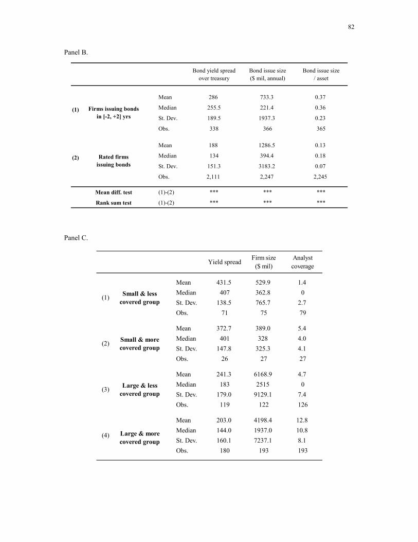
82

Panel B.

Bond yield spreadover treasury

Bond issue size($ mil, annual)

Bond issue size/ asset

Mean 286 733.3 0.37

Median 255.5 221.4 0.36

St. Dev. 189.5 1937.3 0.23

Obs. 338 366 365

Mean 188 1286.5 0.13

Median 134 394.4 0.18

St. Dev. 151.3 3183.2 0.07

Obs. 2,111 2,247 2,245

Mean diff. test (1)-(2) *** *** ***

Rank sum test (1)-(2) *** *** ***

Firms issuing bondsin [-2, +2] yrs

Rated firmsissuing bonds

(1)

(2)

Panel C.

Yield spread Firm size($ mil)

Analystcoverage

Mean 431.5 529.9 1.4Median 407 362.8 0St. Dev. 138.5 765.7 2.7Obs. 71 75 79

Mean 372.7 389.0 5.4Median 401 328 4.0St. Dev. 147.8 325.3 4.1Obs. 26 27 27

Mean 241.3 6168.9 4.7Median 183 2515 0St. Dev. 179.0 9129.1 7.4Obs. 119 122 126

Mean 203.0 4198.4 12.8Median 144.0 1937.0 10.8St. Dev. 160.1 7237.1 8.1Obs. 180 193 193

Small & lesscovered group

Small & morecovered group

Large & lesscovered group

Large & morecovered group

(1)

(2)

(3)

(4)

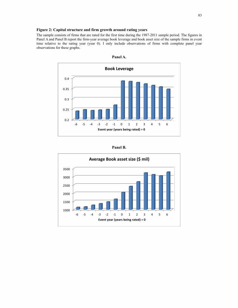
83

Figure 2: Capital structure and firm growth around rating years The sample consists of firms that are rated for the first time during the 1987-2011 sample period. The figures in Panel A and Panel B report the firm-year average book leverage and book asset size of the sample firms in event time relative to the rating year (year 0). I only include observations of firms with complete panel year observations for these graphs.

Panel A.

0.2

0.25

0.3

0.35

0.4

‐6 ‐5 ‐4 ‐3 ‐2 ‐1 0 1 2 3 4 5 6

Event year (years being rated) = 0

Book Leverage

Panel B.

1000

1500

2000

2500

3000

3500

‐6 ‐5 ‐4 ‐3 ‐2 ‐1 0 1 2 3 4 5 6

Event year (years being rated) = 0

Average Book asset size ($ mil)

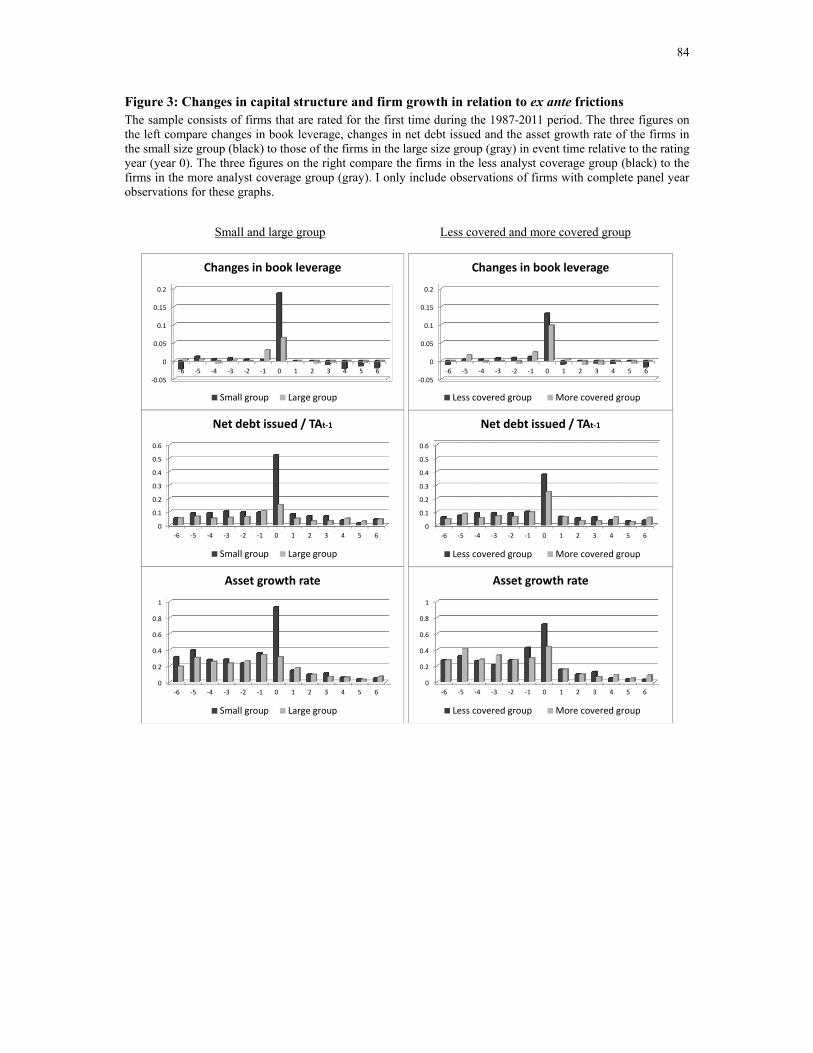
84

Figure 3: Changes in capital structure and firm growth in relation to ex ante frictions The sample consists of firms that are rated for the first time during the 1987-2011 period. The three figures on the left compare changes in book leverage, changes in net debt issued and the asset growth rate of the firms in the small size group (black) to those of the firms in the large size group (gray) in event time relative to the rating year (year 0). The three figures on the right compare the firms in the less analyst coverage group (black) to the firms in the more analyst coverage group (gray). I only include observations of firms with complete panel year observations for these graphs. Small and large group Less covered and more covered group

0

0.2

0.4

0.6

0.8

1

‐6 ‐5 ‐4 ‐3 ‐2 ‐1 0 1 2 3 4 5 6

Asset growth rate

Less covered group More covered group

‐0.05

0

0.05

0.1

0.15

0.2

‐6 ‐5 ‐4 ‐3 ‐2 ‐1 0 1 2 3 4 5 6

Changes in book leverage 

Less covered group More covered group

0

0.1

0.2

0.3

0.4

0.5

0.6

‐6 ‐5 ‐4 ‐3 ‐2 ‐1 0 1 2 3 4 5 6

Net debt issued / TAt‐1

Less covered group More covered group

0

0.2

0.4

0.6

0.8

1

‐6 ‐5 ‐4 ‐3 ‐2 ‐1 0 1 2 3 4 5 6

Asset growth rate

Small group Large group

‐0.05

0

0.05

0.1

0.15

0.2

‐6 ‐5 ‐4 ‐3 ‐2 ‐1 0 1 2 3 4 5 6

Changes in book leverage 

Small group Large group

0

0.1

0.2

0.3

0.4

0.5

0.6

‐6 ‐5 ‐4 ‐3 ‐2 ‐1 0 1 2 3 4 5 6

Net debt issued / TAt‐1

Small group Large group

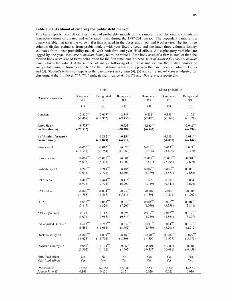
85

Table 13: Likelihood of entering the public debt market This table reports the coefficient estimates of probability models on the sample firms. The sample consists of firm observations of unrated and to be rated firms during the 1987-2011 period. The dependent variable is a binary variable that takes the value 1 if a firm is rated in the observation year and 0 otherwise. The first three columns display estimates from probit models with year fixed effects, and the latter three columns display estimates from linear probability models with both firm and year fixed effects. All explanatory variables are lagged by one year. Asset size < median dummy takes the value 1 if the book asset of a firm is smaller than the median book asset size of firms being rated for the first time, and 0 otherwise. # of Analyst forecasts < median dummy takes the value 1 if the number of analyst following of a firm is smaller than the median number of analyst following of firms being rated for the first time. z-statistics appear in the parenthesis in column (1), (2) and (3). Student’s t-statistics appear in the parentheses in column (4), (5) and (6). Standard error is adjusted for clustering at the firm level. ***, **, * indicate significance at 1%, 5% and 10% levels, respectively.

Probit Linear probability

Dependent variable: Being rated 0/1

Being rated 0/1

Being rated 0/1 Being rated

0/1 Being rated

0/1 Being rated

0/1 (1) (2) (3) (4) (5) (6) Constant -2.350*** -2.605*** -2.343*** -0.231** -0.338*** -0.172* (-9.469) (-10.952) (-9.436) (-2.496) (-3.340) (-1.821) Asset Size < -0.775*** -0.733*** -0.043*** -0.042*** median dummy (-22.532) (-20.384) (-6.942) (-6.794) # of Analyst forecast < -0.292*** -0.154*** -0.013*** -0.011*** mean dummy (-10.048) (-4.912) (-6.890) (-6.144) Firm age t-1 -0.020*** -0.017*** -0.020*** 0.010*** 0.013*** 0.008** (-11.591) (-9.754) (-11.263) (2.964) (3.469) (2.339) Book asset t-1 <0.001*** <0.001*** <0.001*** <0.001*** <0.001*** <0.001*** (5.037) (5.498) (5.007) (2.627) (2.799) (2.629) Profitability t-1 0.246*** 0.218*** 0.186** 0.007*** 0.006*** 0.005*** (3.045) (2.778) (2.306) (3.189) (2.873) (2.652) PPE/TA t-1 0.418*** 0.444*** 0.416*** 0.005 0.002 0.004 (6.973) (7.724) (6.900) (0.739) (0.347) (0.626) R&D/TA t-1 -0.845*** -1.034*** -0.939*** -0.007 -0.006 -0.006 (-4.785) (-5.467) (-5.116) (-1.591) (-1.211) (-1.202) Q t-1 0.045*** 0.040*** 0.043*** 0.001*** 0.001*** 0.001*** (7.847) (6.320) (7.200) (4.079) (3.358) (3.848) Δ BLev [t-1, t-2] 0.125 0.112 0.096 0.019*** 0.017*** 0.017*** (1.071) (0.985) (0.814) (4.249) (3.864) (3.877) Ind. adjusted BLev t-1 0.613*** 0.767*** 0.637*** 0.011** 0.014*** 0.012*** (8.486) (11.054) (8.762) (2.489) (3.201) (2.712) Stock volatility t-1 -8.840*** -11.890*** -8.189*** -0.090*** -0.084*** -0.075*** (-9.625) (-11.754) (-8.808) (-4.300) (-3.977) (-3.675) Dividend dummy t-1 0.057* 0.124*** 0.060* -0.001 >-0.000 -0.001 (1.802) (4.102) (1.902) (-0.557) (-0.081) (-0.458) Firm fixed effects No No No Yes Yes Yes Year fixed effects Yes Yes Yes Yes Yes Yes Observations 67,358 67,358 67,358 67,533 67,533 67,533 Pseudo R2 or R2 0.168 0.130 0.171 0.029 0.025 0.030

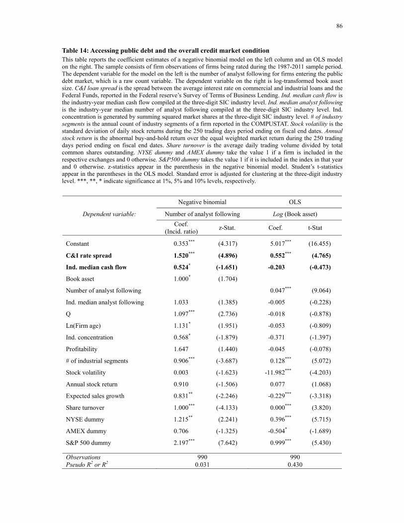
86

Table 14: Accessing public debt and the overall credit market condition This table reports the coefficient estimates of a negative binomial model on the left column and an OLS model on the right. The sample consists of firm observations of firms being rated during the 1987-2011 sample period. The dependent variable for the model on the left is the number of analyst following for firms entering the public debt market, which is a raw count variable. The dependent variable on the right is log-transformed book asset size. C&I loan spread is the spread between the average interest rate on commercial and industrial loans and the Federal Funds, reported in the Federal reserve’s Survey of Terms of Business Lending. Ind. median cash flow is the industry-year median cash flow compiled at the three-digit SIC industry level. Ind. median analyst following is the industry-year median number of analyst following compiled at the three-digit SIC industry level. Ind. concentration is generated by summing squared market shares at the three-digit SIC industry level. # of industry segments is the annual count of industry segments of a firm reported in the COMPUSTAT. Stock volatility is the standard deviation of daily stock returns during the 250 trading days period ending on fiscal end dates. Annual stock return is the abnormal buy-and-hold return over the equal weighted market return during the 250 trading days period ending on fiscal end dates. Share turnover is the average daily trading volume divided by total common shares outstanding. NYSE dummy and AMEX dummy take the value 1 if a firm is included in the respective exchanges and 0 otherwise. S&P500 dummy takes the value 1 if it is included in the index in that year and 0 otherwise. z-statistics appear in the parenthesis in the negative binomial model. Student’s t-statistics appear in the parentheses in the OLS model. Standard error is adjusted for clustering at the three-digit industry level. ***, **, * indicate significance at 1%, 5% and 10% levels, respectively.

Negative binomial OLS

Dependent variable: Number of analyst following Log (Book asset) Coef.

(Incid. ratio) z-Stat. Coef. t-Stat

Constant 0.353*** (4.317) 5.017*** (16.455)

C&I rate spread 1.520*** (4.896) 0.552*** (4.765)

Ind. median cash flow 0.524* (-1.651) -0.203 (-0.473)

Book asset 1.000* (1.704)

Number of analyst following 0.047*** (9.064)

Ind. median analyst following 1.033 (1.385) -0.005 (-0.228)

Q 1.097*** (2.736) -0.018 (-0.878)

Ln(Firm age) 1.131* (1.951) -0.053 (-0.809)

Ind. concentration 0.568* (-1.879) -0.371 (-1.397)

Profitability 1.647 (1.440) -0.045 (-0.078)

# of industrial segments 0.906*** (-3.687) 0.128*** (5.072)

Stock volatility 0.003 (-1.623) -11.982*** (-4.203)

Annual stock return 0.910 (-1.506) 0.077 (1.068)

Expected sales growth 0.831** (-2.246) -0.229*** (-3.318)

Share turnover 1.000*** (-4.133) 0.000*** (3.820)

NYSE dummy 1.215** (2.241) 0.396*** (5.715)

AMEX dummy 0.706 (-1.325) -0.504* (-1.689)

S&P 500 dummy 2.197*** (7.642) 0.999*** (5.430)

Observations 990 990 Pseudo R2 or R2 0.031 0.430

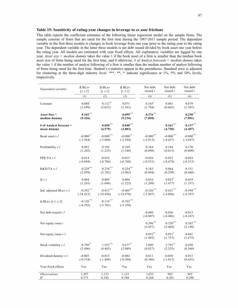
87

Table 15: Sensitivity of rating-year changes in leverage to ex ante frictions This table reports the coefficient estimates of the following linear regression model on the sample firms. The sample consists of firms that are rated for the first time during the 1987-2011 sample period. The dependent variable in the first three models is changes in book leverage from one year prior to the rating year to the rating year. The dependent variable in the latter three models is net debt issued divided by book asset one year before the rating year. All models are estimated with year fixed effects. All explanatory variables are lagged by one year. Asset size < median dummy takes the value 1 if the book asset of a firm is smaller than the median book asset size of firms being rated for the first time, and 0 otherwise. # of Analyst forecasts < median dummy takes the value 1 if the number of analyst following of a firm is smaller than the median number of analyst following of firms being rated for the first time. Student’s t-statistics appear in the parentheses. Standard error is adjusted for clustering at the three-digit industry level. ***, **, * indicate significance at 1%, 5% and 10% levels, respectively.

Dependent variable: Δ BLev [t, t-1]

Δ BLev [t, t-1]

Δ BLev [t, t-1]

Net debt issued t

Net debt issued t

Net debt issued t

(1) (2) (3) (4) (5) (6) Constant 0.088* 0.112** 0.071 0.165* 0.041 0.079 (1.699) (2.033) (1.361) (1.784) (0.665) (1.367) Asset Size < 0.102*** 0.099*** 0.276*** 0.258*** median dummy (9.426) (9.234) (7.850) (7.801) # of Analyst forecast < 0.050*** 0.040*** 0.161*** 0.137*** mean dummy (4.579) (3.803) (4.750) (4.407) Book asset t-1 -0.000** -0.000*** -0.000** -0.000*** -0.000*** -0.000*** (-2.564) (-3.688) (-2.594) (-2.813) (-4.427) (-3.687) Profitability t-1 0.093 0.105 0.109 0.184 0.184 0.170 (1.202) (1.225) (1.348) (0.898) (0.813) (0.809) PPE/TA t-1 -0.014 -0.016 -0.015 -0.026 -0.023 -0.024 (-0.694) (-0.786) (-0.768) (-0.551) (-0.474) (-0.513) R&D/TA t-1 0.229*** 0.234*** 0.254*** 0.183 0.064 0.151 (2.859) (2.782) (3.062) (0.694) (0.298) (0.660) Q t-1 0.004 0.005* 0.004 0.016 0.023* 0.019 (1.263) (1.686) (1.223) (1.209) (1.677) (1.357) Ind. adjusted BLev t-1 -0.392*** -0.413*** -0.405*** -0.326*** -0.421*** -0.394*** (-18.412) (-19.450) (-18.978) (-3.947) (-4.896) (-4.707) Δ BLev [t-1, t-2] -0.126*** -0.116*** -0.103*** (-4.392) (-3.701) (-3.350) Net debt issued t-1 -0.040 -0.026 -0.013 (-0.807) (-0.486) (-0.247) Net equity issue t 0.296*** 0.320*** 0.282*** (5.457) (5.469) (5.199) Net equity issue t-1 0.052** 0.051* 0.041 (1.982) (1.737) (1.475) Stock volatility t-1 0.799** 1.552*** 0.677** 1.009 2.793** 0.450 (2.496) (4.483) (2.089) (0.827) (2.235) (0.368) Dividend dummy t-1 -0.003 -0.013 -0.002 0.011 -0.030 0.013 (-0.334) (-1.409) (-0.204) (0.386) (-1.013) (0.452) Year fixed effects Yes Yes Yes Yes Yes Yes Observations 1,207 1,123 1,123 1,033 965 965 R2 0.373 0.342 0.388 0.268 0.203 0.290

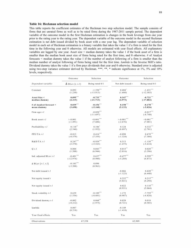
88

Table 16: Heckman selection model This table reports the coefficient estimates of the Heckman two step selection model. The sample consists of firms that are unrated firms as well as to be rated firms during the 1987-2011 sample period. The dependent variable of the outcome model in the first Heckman estimation is changes in the book leverage from one year prior to the rating year to the rating year. The dependent variable of the outcome model in the second Heckman estimation is net debt issued divided by book asset with a one year lag. The dependent variable of selection model in each set of Heckman estimation is a binary variable that takes the value 1 if a firm is rated for the first time in the following year and 0 otherwise. All models are estimated with year fixed effects. All explanatory variables are lagged by one year. Asset size < median dummy takes the value 1 if the book asset of a firm is smaller than the median book asset size of firms being rated for the first time, and 0 otherwise. # of Analyst forecasts < median dummy takes the value 1 if the number of analyst following of a firm is smaller than the median number of analyst following of firms being rated for the first time. lambda is the Inverse Mill’s ratio. Dividend dummy takes the value 1 if a firm pays dividends that year and 0 otherwise. Standard error is adjusted using two-step variance estimator derived by Heckman. ***, **, * indicate significance at 1%, 5% and 10% levels, respectively.

O utcom e Selection O utcom e Selection

D ependent variable: Δ B Lev [t, t-1 ] B eing rated 0 /1 N et debt issued t B eing rated 0 /1

C onstant 0 .092 -1 .350 *** 0 .404 * -1 .431 *** (1 .230) (-13.913) (1 .680) (-12.585) A sset S ize < 0 .095 *** -0 .733 *** 0 .347 *** -0 .721 *** m edian dum m y (4 .215) (-21.713) (4 .973) (-17.882) # of A nalyst forecast < 0 .039 *** -0 .154 *** 0 .158 *** -0 .178 *** m ean dum m y (3 .698) (-5 .160) (5 .133) (-5 .026) Firm age t-1 -0 .020 *** -0 .017 *** (-11 .697) (-8 .740) B ook asset t-1 > -0 .001 <0.001*** >-0 .001 *** <0.001*** (-1 .491) (7 .606) (-2 .676) (7 .081) Profitability t-1 0 .110 ** 0 .186 * 0 .124 0.332 *** (2 .540) (1 .952) (0 .897) (2 .701) PPE/TA t-1 -0 .013 0 .416 *** -0 .090 0.478 *** (-0 .579) (7 .355) (-1 .324) (7 .304) R & D /T A t-1 0 .247 *** -0 .939 *** 0 .313 -1 .138 *** (3 .570) (-5 .523) (1 .475) (-5 .614) Q t-1 0 .004 0 .043 *** 0 .015 ** 0 .028 *** (1 .508) (6 .944) (2 .016) (3 .396) Ind . adjusted B Lev t-1 -0 .401 *** 0 .637 *** -0 .477 *** 0 .599 *** (-12 .976) (8 .980) (-5 .284) (6 .873) Δ B Lev [t-1 , t-2] -0 .103 *** 0 .096 (-3 .508) (0 .961) N et debt issued t-1 -0 .066 0 .420 *** (-1 .123) (6 .448) N et equity issued t 0 .252 *** 0 .215 *** (5 .021) (4 .294) N et equity issued t-1 0 .022 0 .118 *** (0 .931) (5 .064) S tock volatility t-1 0 .639 -8 .189 *** 1 .172 -7 .759 *** (1 .536) (-8 .601) (0 .987) (-6 .828) D ividend dum m y t-1 -0 .002 0 .060 ** 0 .020 0 .018 (-0 .212) (1 .975) (0 .721) (0 .503) lam bda 0 .007 -0 .149 (0 .218) (-1 .410) Y ear fixed effects Y es Y es Y es Y es

O bservations 67,358 62,909

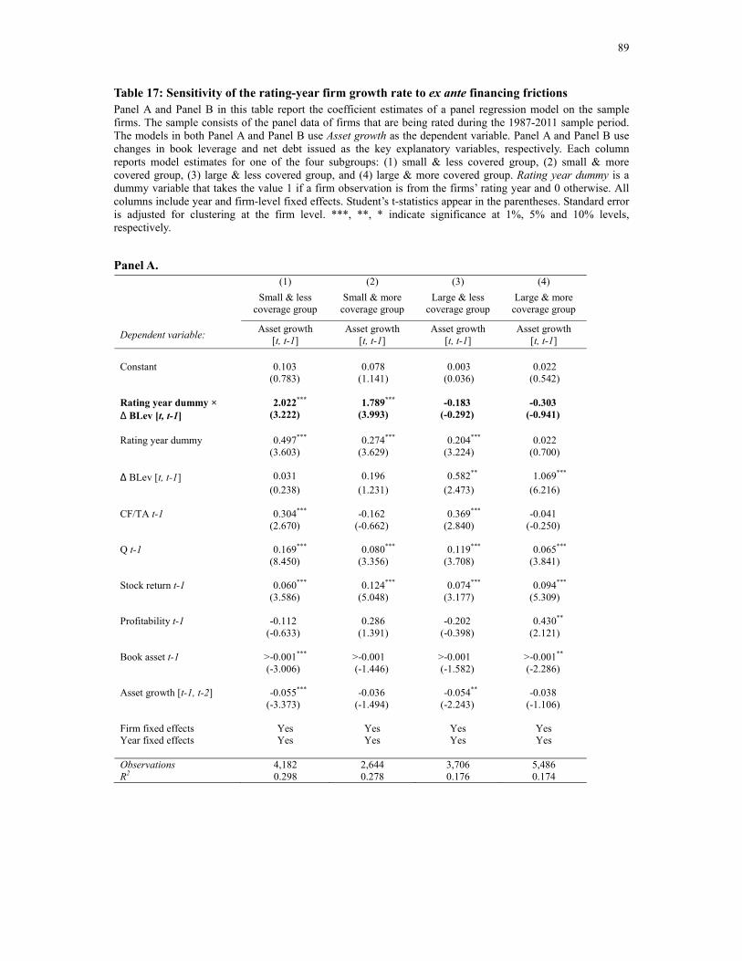
89

Table 17: Sensitivity of the rating-year firm growth rate to ex ante financing frictions Panel A and Panel B in this table report the coefficient estimates of a panel regression model on the sample firms. The sample consists of the panel data of firms that are being rated during the 1987-2011 sample period. The models in both Panel A and Panel B use Asset growth as the dependent variable. Panel A and Panel B use changes in book leverage and net debt issued as the key explanatory variables, respectively. Each column reports model estimates for one of the four subgroups: (1) small & less covered group, (2) small & more covered group, (3) large & less covered group, and (4) large & more covered group. Rating year dummy is a dummy variable that takes the value 1 if a firm observation is from the firms’ rating year and 0 otherwise. All columns include year and firm-level fixed effects. Student’s t-statistics appear in the parentheses. Standard error is adjusted for clustering at the firm level. ***, **, * indicate significance at 1%, 5% and 10% levels, respectively.

Panel A. (1) (2) (3) (4) Small & less

coverage group Small & more

coverage group Large & less

coverage group Large & more

coverage group

Dependent variable: Asset growth [t, t-1]

Asset growth [t, t-1]

Asset growth [t, t-1]

Asset growth [t, t-1]

Constant 0.103 0.078 0.003 0.022 (0.783) (1.141) (0.036) (0.542) Rating year dummy × 2.022*** 1.789*** -0.183 -0.303 Δ BLev [t, t-1] (3.222) (3.993) (-0.292) (-0.941) Rating year dummy 0.497*** 0.274*** 0.204*** 0.022 (3.603) (3.629) (3.224) (0.700) Δ BLev [t, t-1] 0.031 0.196 0.582** 1.069*** (0.238) (1.231) (2.473) (6.216) CF/TA t-1 0.304*** -0.162 0.369*** -0.041 (2.670) (-0.662) (2.840) (-0.250) Q t-1 0.169*** 0.080*** 0.119*** 0.065*** (8.450) (3.356) (3.708) (3.841) Stock return t-1 0.060*** 0.124*** 0.074*** 0.094*** (3.586) (5.048) (3.177) (5.309) Profitability t-1 -0.112 0.286 -0.202 0.430** (-0.633) (1.391) (-0.398) (2.121) Book asset t-1 >-0.001*** >-0.001 >-0.001 >-0.001** (-3.006) (-1.446) (-1.582) (-2.286) Asset growth [t-1, t-2] -0.055*** -0.036 -0.054** -0.038 (-3.373) (-1.494) (-2.243) (-1.106) Firm fixed effects Yes Yes Yes Yes Year fixed effects Yes Yes Yes Yes Observations 4,182 2,644 3,706 5,486 R2 0.298 0.278 0.176 0.174  

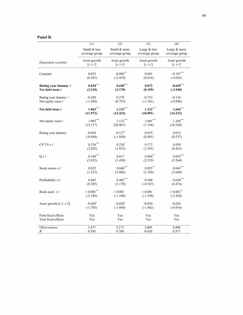
90

Panel B. (1) (2) (3) (4) Small & less

coverage group Small & more

coverage group Large & less

coverage group Large & more

coverage group

Dependent variable: Asset growth [t, t-1]

Asset growth [t, t-1]

Asset growth [t, t-1]

Asset growth [t, t-1]

Constant 0.032 -0.098** 0.001 -0.107*** (0.201) (-2.424) (0.014) (-4.026) Rating year dummy × 0.654*** 0.650*** 0.072 -0.659*** Net debt issue t (3.210) (3.170) (0.199) (-3.940) Rating year dummy × -0.289 0.278 -0.723 -0.136 Net equity issue t (-1.568) (0.793) (-1.361) (-0.848) Net debt issue t 1.063*** 1.132*** 1.232*** 1.644*** (11.972) (12.424) (10.091) (14.232) Net equity issue t 1.003*** 1.135*** 1.001*** 1.268*** (15.137) (20.967) (7.194) (10.528) Rating year dummy -0.054 -0.127* 0.019 0.012 (-0.694) (-1.844) (0.401) (0.537) CF/TA t-1 0.236*** 0.234* 0.172 0.059 (2.825) (1.933) (1.391) (0.425) Q t-1 0.108*** 0.017 0.084** 0.035*** (3.953) (1.438) (2.535) (5.564) Stock return t-1 0.022 0.048*** 0.055** 0.043*** (1.533) (3.086) (2.189) (3.648) Profitability t-1 0.045 0.402*** -0.300 0.630*** (0.305) (3.170) (-0.547) (4.476) Book asset t-1 >-0.001** >-0.001 >-0.001 >-0.001** (-2.186) (-1.180) (-1.349) (-2.428) Asset growth [t-1, t-2] -0.029* -0.030* -0.030 -0.026 (-1.703) (-1.804) (-1.462) (-0.934) Firm fixed effects Yes Yes Yes Yes Year fixed effects Yes Yes Yes Yes Observations 3,477 2,173 3,005 4,496 R2 0.595 0.708 0.420 0.577

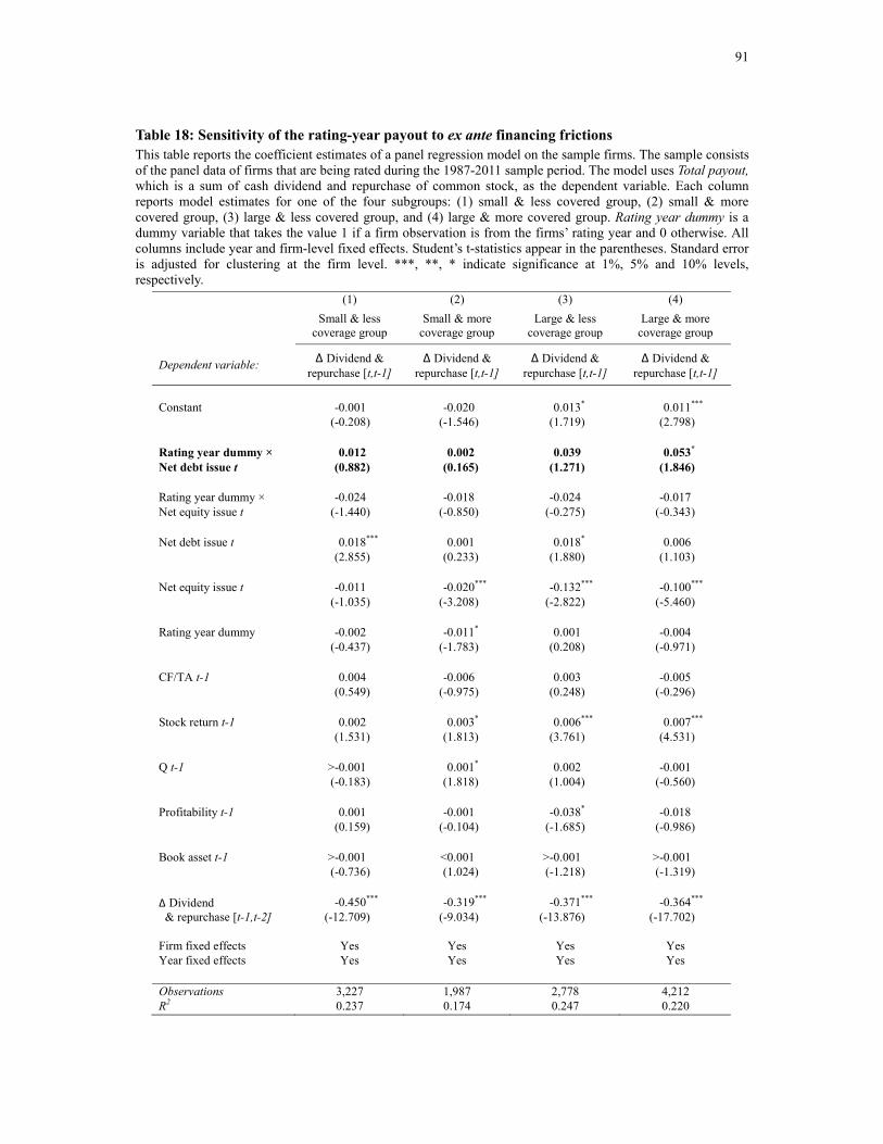
91

Table 18: Sensitivity of the rating-year payout to ex ante financing frictions This table reports the coefficient estimates of a panel regression model on the sample firms. The sample consists of the panel data of firms that are being rated during the 1987-2011 sample period. The model uses Total payout, which is a sum of cash dividend and repurchase of common stock, as the dependent variable. Each column reports model estimates for one of the four subgroups: (1) small & less covered group, (2) small & more covered group, (3) large & less covered group, and (4) large & more covered group. Rating year dummy is a dummy variable that takes the value 1 if a firm observation is from the firms’ rating year and 0 otherwise. All columns include year and firm-level fixed effects. Student’s t-statistics appear in the parentheses. Standard error is adjusted for clustering at the firm level. ***, **, * indicate significance at 1%, 5% and 10% levels, respectively.

(1) (2) (3) (4) Small & less

coverage group Small & more

coverage group Large & less

coverage group Large & more

coverage group

Dependent variable: Δ Dividend & repurchase [t,t-1]

Δ Dividend & repurchase [t,t-1]

Δ Dividend & repurchase [t,t-1]

Δ Dividend & repurchase [t,t-1]

Constant -0.001 -0.020 0.013* 0.011*** (-0.208) (-1.546) (1.719) (2.798) Rating year dummy × 0.012 0.002 0.039 0.053* Net debt issue t (0.882) (0.165) (1.271) (1.846) Rating year dummy × -0.024 -0.018 -0.024 -0.017 Net equity issue t (-1.440) (-0.850) (-0.275) (-0.343) Net debt issue t 0.018*** 0.001 0.018* 0.006 (2.855) (0.233) (1.880) (1.103) Net equity issue t -0.011 -0.020*** -0.132*** -0.100*** (-1.035) (-3.208) (-2.822) (-5.460) Rating year dummy -0.002 -0.011* 0.001 -0.004 (-0.437) (-1.783) (0.208) (-0.971) CF/TA t-1 0.004 -0.006 0.003 -0.005 (0.549) (-0.975) (0.248) (-0.296) Stock return t-1 0.002 0.003* 0.006*** 0.007*** (1.531) (1.813) (3.761) (4.531) Q t-1 >-0.001 0.001* 0.002 -0.001 (-0.183) (1.818) (1.004) (-0.560) Profitability t-1 0.001 -0.001 -0.038* -0.018 (0.159) (-0.104) (-1.685) (-0.986) Book asset t-1 >-0.001 <0.001 >-0.001 >-0.001 (-0.736) (1.024) (-1.218) (-1.319) Δ Dividend -0.450*** -0.319*** -0.371*** -0.364*** & repurchase [t-1,t-2] (-12.709) (-9.034) (-13.876) (-17.702) Firm fixed effects Yes Yes Yes Yes Year fixed effects Yes Yes Yes Yes Observations 3,227 1,987 2,778 4,212 R2 0.237 0.174 0.247 0.220

92

VITA

Joon Ho Kim was born in Seoul, South Korea and lived there before coming to the U.S. He obtained his bachelor’s degree in Economics and a GEMBA degree from the University of Washington. He had industry experience as a product market researcher in Korea. In 2007, he joined the finance doctoral program of the Foster School of Business at the University of Washington, where he earned a Doctor of Philosophy in 2013.