arX

iv:a

stro

-ph/

0303

587v

2 1

0 D

ec 2

003

February 2, 2008

Triple Experiment Spectrum of the Sunyaev-Zeldovich Effect in

the Coma Cluster: H0

E.S. Battistelli 1, M. De Petris, L. Lamagna, G. Luzzi, R. Maoli, A. Melchiorri, F.

Melchiorri, A. Orlando, E. Palladino, G. Savini

Department of Physics, University ”La Sapienza”, P.le A. Moro 2, 00185, Rome, Italy

Y. Rephaeli, M. Shimon

School of Physics and Astronomy, Tel Aviv University, Tel Aviv, Israel

M. Signore

LERMA, Observatoire de Paris, Paris, France

S. Colafrancesco

INAF - Osservatorio Astronomico di Roma, Via Frascati 33, 00040, Monteporzio, Italy

ABSTRACT

The Sunyaev-Zeldovich (SZ) effect was previously measured in the Coma

cluster by the Owens Valley Radio Observatory and Millimeter and IR Testa

Grigia Observatory experiments and recently also with the Wilkinson Microwave

Anisotropy Probe satellite. We assess the consistency of these results and their

implications on the feasibility of high-frequency SZ work with ground-based tele-

scopes. The unique data set from the combined measurements at six frequency

bands is jointly analyzed, resulting in a best-fit value for the Thomson optical

depth at the cluster center, τ0 = (5.35 ± 0.67) × 10−3. The combined X-ray and

SZ determined properties of the gas are used to determine the Hubble constant.

For isothermal gas with a β density profile we derive H0 = 84±26 km/(s ·Mpc);

the (1σ) error includes only observational SZ and X-ray uncertainties.

Subject headings: cosmology: cosmic microwave background – observations –

galaxies: clusters: individual (A1656)

1elia.stefano.battistelli@roma1.infn.it

– 2 –

1. Introduction

The Sunyaev-Zeldovich (SZ) effect (Sunyaev & Zel’dovich 1972) constitutes a unique

and powerful cosmological tool (for reviews, see Rephaeli 1995a, Birkinshaw 1999, Carlstrom,

Holder, & Reese 2002). Many tens of high quality images of the effect have already been

obtained with interferometric arrays operating at low frequencies on the Rayleigh-Jeans side

of the spectrum. Multifrequency SZ measurements were made of only very few clusters, so

the potential power of spectral diagnostics has not yet been sufficiently exploited to reduce

signal confusion and other errors. Systematic uncertainties are the main hindrance to the

use of the effect as a precise cosmological probe. These can be most optimally reduced when

high spatial resolution X-ray and spectral SZ measurements of a large sample of nearby

clusters are available in the near future. The multifrequency capability of many upcoming

ground-based bolometric array projects is crucially important for the separation of the SZ

signal from the large confusing atmospheric signals.

The SZ effect was measured in the Coma Cluster with the ground-based Owens Val-

ley Radio Observatory (OVRO; Herbig, Lawrence, & Readhead 1995) and Millimeter and

IR Testa Grigia Observatory (MITO; De Petris et al. 2002) telescopes. The Wilkinson Mi-

crowave Anisotropy Probe (WMAP) team has recently reported measurement of the effect in

Coma at 61 and 94 GHz (Bennett et al. 2003b); this is the first measurement of the SZ effect

from a satellite. Together, these measurements yield the first SZ spectrum with six spectral

bands. The relatively wide spectral coverage obtained with ground- and space-based tele-

scopes allows a much-needed gauge of the impact of atmospheric emission on high-frequency

ground-based observations of the SZ effect. The quality of the spectral results allows a

meaningful determination of the Hubble constant, H0. Even though this important parame-

ter is thought to have been determined quite precisely from the WMAP first-year sky survey

(Bennett et al. 2003a), it is, of course, very much of interest to measure it independently by

various methods. The determination of H0 from cluster SZ and X-ray measurements yields

additional insight beyond what is offered by an all-sky cosmic microwave background (CMB)

anisotropy survey: in principle, the cluster SZ & X-ray (SZ-X) method provides a test of

both the isotropy of the cosmological expansion and its temporal character. In this Letter we

briefly discuss the qualitative deductions that can be drawn from the general agreement be-

tween the ground-based and WMAP results, and use the full database on Coma to determine

H0.

– 3 –

2. SZ Measurements of the Coma Cluster

The rich nearby Coma Cluster has long been a prime target of SZ observations (e.g.,Birkinshaw,

Gull, & Northover 1981, Silverberg 1997); the effect was detected towards Coma with the 5.5

m OVRO telescope, with a 7’.3 beam, operating at 32 GHz. A long series of drift scans with

the MITO 2.6 m telescope, which had a 16’ beam, led to the detection of the effect at three

spectral bands centered on 143, 214, and 272 GHz. Even though the WMAP telescope is not

optimized for SZ observations, the effect was detected with the W- and V-band radiometers

at 61 and 94 GHz, with beam sizes of 20’ and 13’, respectively (Bennett et al. 2003b). The

predicted SZ size of Coma is more than ∼ 30′, so these measurements were not substantially

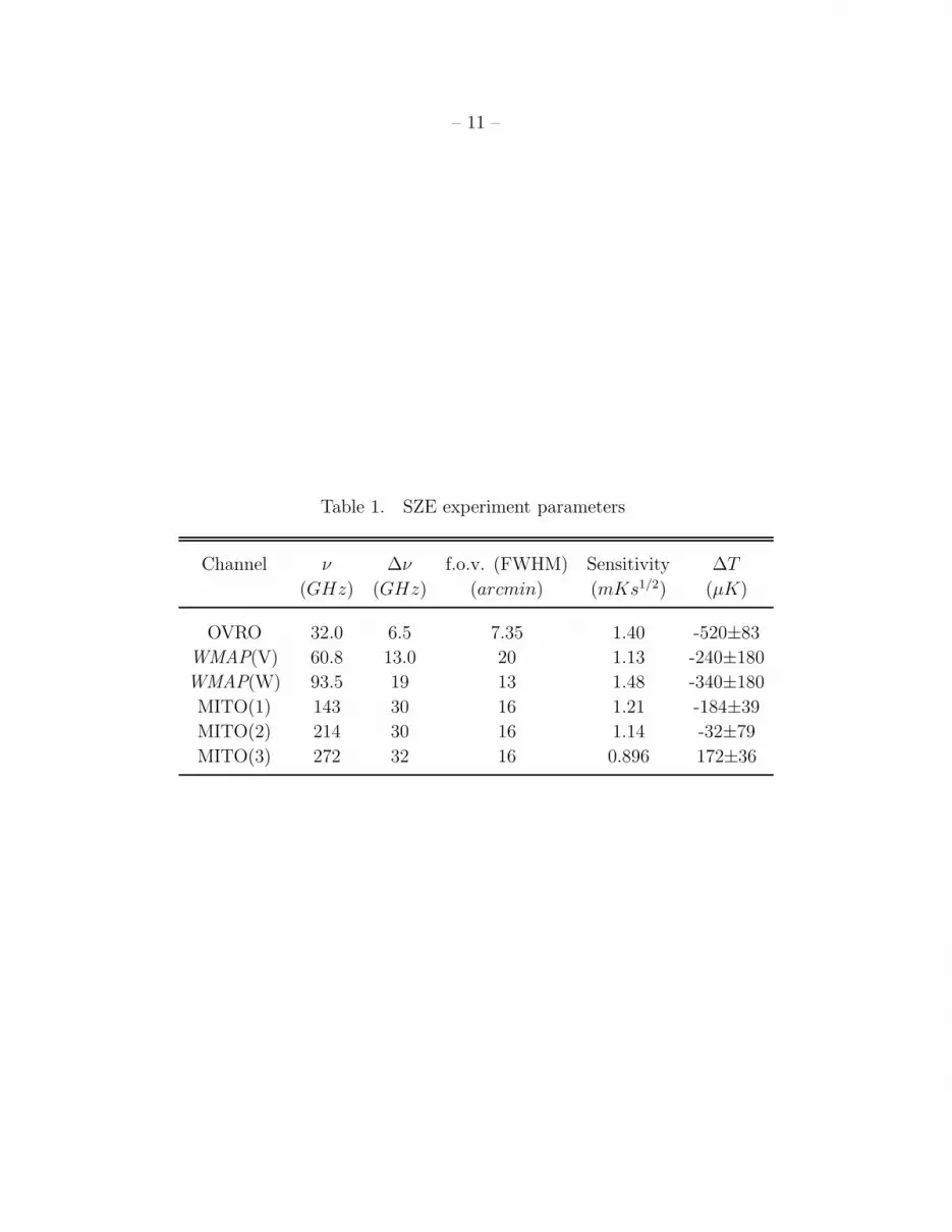
affected by beam dilution. Results of the measurements are listed in Table 1; these reflect

a slight revision of our previously reported SZ signals as result of an improved calibration

of the the MITO measurements (Savini et al. 2003). The SZ spectrum of Coma is shown in

figure 1.

Note that the MITO error bars are about a factor 3 smaller than those of the WMAP

data; this is mainly due to the difference in observing time. Given the low signal-to-noise

ratios (S/Ns) of the two WMAP data, the main advantage of these satellite observations lies

in the capability of relatively precise calibration through measurements of the modulation

of the CMB dipole anisotropy. This is estimated to be ∼ 0.5% by the WMAP team, as

compared with ∼ 10% for MITO and from ∼ 3% to ∼ 10% for OVRO. It is interesting

that the relative calibration of MITO and WMAP are in agreement to within ∼ 10%. This

result provides further support for ground-based SZ observations, which are susceptible of

substantial uncertainties because of atmospheric emission and use of planetary emission for

signal calibration. However, because of the poor S/N of the WMAP data, the situation with

regard to this calibration method is still far from being satisfactory. We also note that an

attempt to explain the (small) discrepancy between the MITO and OVRO measurements as

due to confusing CMB anisotropy signal (De Petris et al. 2002) seems less likely in light of

the WMAP results which imply that such a signal is relatively insignificant.

In the relativistically accurate calculation of ∆I, the intensity change in Compton scat-

tering, its dependence on the gas temperature is no longer linear (Rephaeli 1995b), and can

be written in the form (Battistelli et al. 2002)

∆I =2k3T 3σT

h2c2

x4ex

(ex − 1)2

∫

ne

[ kTe

mc2f1(x) −

vr

c+ R(x, Te, vr)

]

dl , (1)

where T is the CMB temperature, σT is the Thomson cross section, x = hν/kT is the

nondimensional frequency, ne and Te are the electron density and temperature, vr is the

line of sight (LOS) component of the cluster (peculiar) velocity in the CMB frame, and

f1(x) = x(ex + 1)/(ex− 1) − 4. The integral is over the LOS through the cluster. Both the

– 4 –

thermal and kinematic components of the effect are included in equation (1), separately in

the first two terms, and jointly in the function R(x, Te, vr). Analytic approximations to the

results of the relativistic calculations have been derived to various degrees of accuracy by

expansion in powers of kTe/mc2 and vr/c (e.g., ,, Itoh et al. 1998; Nozawa, Itoh, & Kohyama

1998; Shimon & Rephaeli 2003; Colafrancesco, Marchegiani, & Palladino 2003). If the gas is

isothermal and the cluster velocity is sufficiently small so that the velocity-dependent terms

are negligible (at the relevant frequencies), then ∆I ∝ τ , and a one parameter fit can be

performed to the spectral SZ measurements in order to determine the value of τ . Since the

cluster velocity is unknown, the contribution of the kinematic terms can then be treated as

a source of systematic error.

The Coma cluster was observed by all X-ray experiments; we use values of the gas

parameters as deduced by Mohr, Mathiesen, & Evrard (1999) from ROSAT observations.

The emission-weighted gas temperature is kTe = 8.21± 0.16, and the gas core radius, index

of the β-model density profile, ne(θ) = ne0(1 + (θ/θc)2)−3β/2 (where θ is the angular radial

variable), and central surface brightness are θc = 9′.97 ± 0′.67, β = 0.705 ± 0.046, and

SX,0 = (4.65±0.14)×10−13 erg s−1 cm−2 arcmin−2, respectively. These values are consistent

with the results from more recent XMM measurements.

Best fitting the six data points in Figure 1 by the calculated spectrum (taking kTe =

8.21± 0.16) we obtain the central value of the Thomson optical depth, τ0 = (5.35± 0.67)×

10−3, where the error reflects a 68% confidence level uncertainty associated with the χ2 mini-

mization procedure and the uncertainty due to the error in the observed electron temperature

which contributes ∼ 0.10.

3. The Hubble constant, H0

As is well known, the combination of SZ and X-ray measurements yields a determination

of the cluster angular diameter distance, dA, from which H0 can then be deduced by a

comparison with the theoretical expression for dA. The equation used to determine dA is

obtained by combining the formulae for ∆I and the X-ray surface brightness, SX , through

the elimination of the dependence of these quantities on the central electron density. This

procedure has been discussed in detail in numerous works (e.g.,Holzapfel et al. 1997, Hughes

& Birkinshaw 1998, Furuzawa et al. 1998, Reese et al. 2000, Mason, Myers, & Readhead

2001) and has by now become standard. Here we employ this method to determine H0 for

the first time from multispectral measurements of the Coma cluster.

Assuming an isothermal gas with a β-model density profile (Cavaliere & Fusco-Femiano

– 5 –

1976), the intensity change is ∆I ∝ τ0(1 + (θ/θc)2)1/2−3/2β , and its explicit dependence on

x and Te is determined by the form of the analytic approximation to the exact relativistic

calculation. The X-ray surface brightness is

SX =dA

4π(1 + z)4

∫

∑

j

nenjZ2j ΛBjdζ = SX,0[1 + (θ/θc)

2](1/2−3β), (2)

where z is the cluster redshift, and ζ = l/dA is the cluster path length along the LOS in

terms of the angular diameter distance. The sum is over the various ionic species (j), with

densities nj and charges Zj. The thermal bremmstrahlung emissivity in units of erg s−1 cm3

is

ΛBj = 1.426 × 10−27T 1/2e

∫ ǫ2

ǫ1

e−ǫGZj(Te, ǫ)dǫ, (3)

where ǫ = E/kTe, E is the emitted X-ray photon energy, and GZjis the Gaunt factor. We

have used the accurate analytic formula for the Gaunt factor given by Itoh et al. (2000,

2002).

A comparison of the deduced value of dA with the theoretical expression in a cosmological

model with a cosmological constant then yields the value of H0 when the values of the

cosmological density parameters ΩM and ΩΛ are specified. The final expression for H0 is

H0 = 4πc(1 + z)4 σ2T SX,0θc

ΛB

(∫

Fn)2

τ 2∫

F 2n

g(z, ΩM , ΩΛ), (4)

where the integrals over the LOS have been performed up to a maximal radius of 10(θc), by

defining Fn = (1 + ξ2)−3β/2 where ξ = ζ/θc. The function g(z, ΩM , ΩΛ) is defined as

g(z, ΩM , ΩΛ) =

∫ z

0

dz′√

ΩM(1 + z′)3 + ΩΛ

. (5)

The values ΩM = 0.27 and ΩΛ = 0.73 have been adopted in the computation. Doing so we

obtain

H0 = 84 ± 26 km/(s Mpc), (6)

where the error is determined combining the observed SZ (1σ) uncertainty and the uncer-

tainties in the X-ray data. These errors contribute comparably to the overall observational

uncertainty in the deduced value of H0.

To account for the possibility of a nonisothermal profile, we consider a polytropic gas

model such that the temperature spatial distribution is Te(r) = Te0[1 + (r/rc)2]−3β(γ−1)/2,

with the (’polytropic’) index γ considered as a free parameter to be determined (mostly)

from X-ray measurements. Ideally, when spatially resolved measurements are available of

– 6 –

the X-ray spectrum and surface brightness profile, it is possible to determine values of the

central temperature, central density, core radius, and the indices of the β and polytropic

profiles by direct fits to the data. This complete procedure will be feasible when the full

XMM data set on Coma becomes available. For now, we use the previously determined

ROSAT parameters to estimate the implied change in the value of H0 for an assumed range

of values of γ. For a given value of γ we determine the central temperature by keeping the

emissivity-weighted temperature at its observed value (which was deduced by assuming an

isothermal model). Since the observed surface brightness profile is still fitted by a β-model,

but now with the value 0.705±0.046 identified as βiso (corresponding to the isothermal case,

γ = 1), it follows that the γ-dependent value of β is

β(γ) = 4βiso/(3 + γ).

We have considered values of γ in the range 1 - 5/3. Repeating the above procedure for the

determination of H0 for values of γ in this range, we find that H0 changes by at most 5%

with respect to the value computed with γ = 1. This variation is well within the observa-

tional error quoted above, and the overall estimated level of known systematic uncertainties

stemming from additional simplification in the modeling of the gas, such as spherical sym-

metry, unclumped gas distribution, negligible impact of CMB anisotropy, and the kinematic

SZ component, as well as other confusing signals. The additional level of systematic uncer-

tainties in the value of H0 (deduced from SZ-X measurements) is estimated to be ∼ 30%

(e.g.,Rephaeli 1995a, Holzapfel et al. 1997, Birkinshaw 1999).

4. Discussion

Our deduced value for H0 is about ∼ 30% higher than the current mean value from 33

individual results from the full data set currently available (Carlstrom et al. 2002). Given

the (relatively) large error, it is fully consistent with the recent value derived by Spergel et

al. (2003) from the first year WMAP measurements. Clearly, the interest in using the SZ-X

method to determine H0 is not diminished by the high quality WMAP result. In addition

to the need for alternative independent methods to CMB sky maps, measurement of this

basic parameter at many redshifts and directions on the sky yields important additional

information on its variation over cosmological time, and test of its predicted isotropy.

The full potential of the SZ-X method to determine H0 has not yet been realized.

As has often been stated by Rephaeli (e.g.,Rephaeli 1999), results from this method will

be optimized when a large sample of nearby clusters will be measured by multi-frequency

bolometric arrays, and with the availability of high quality X-ray results from the XMM and

– 7 –

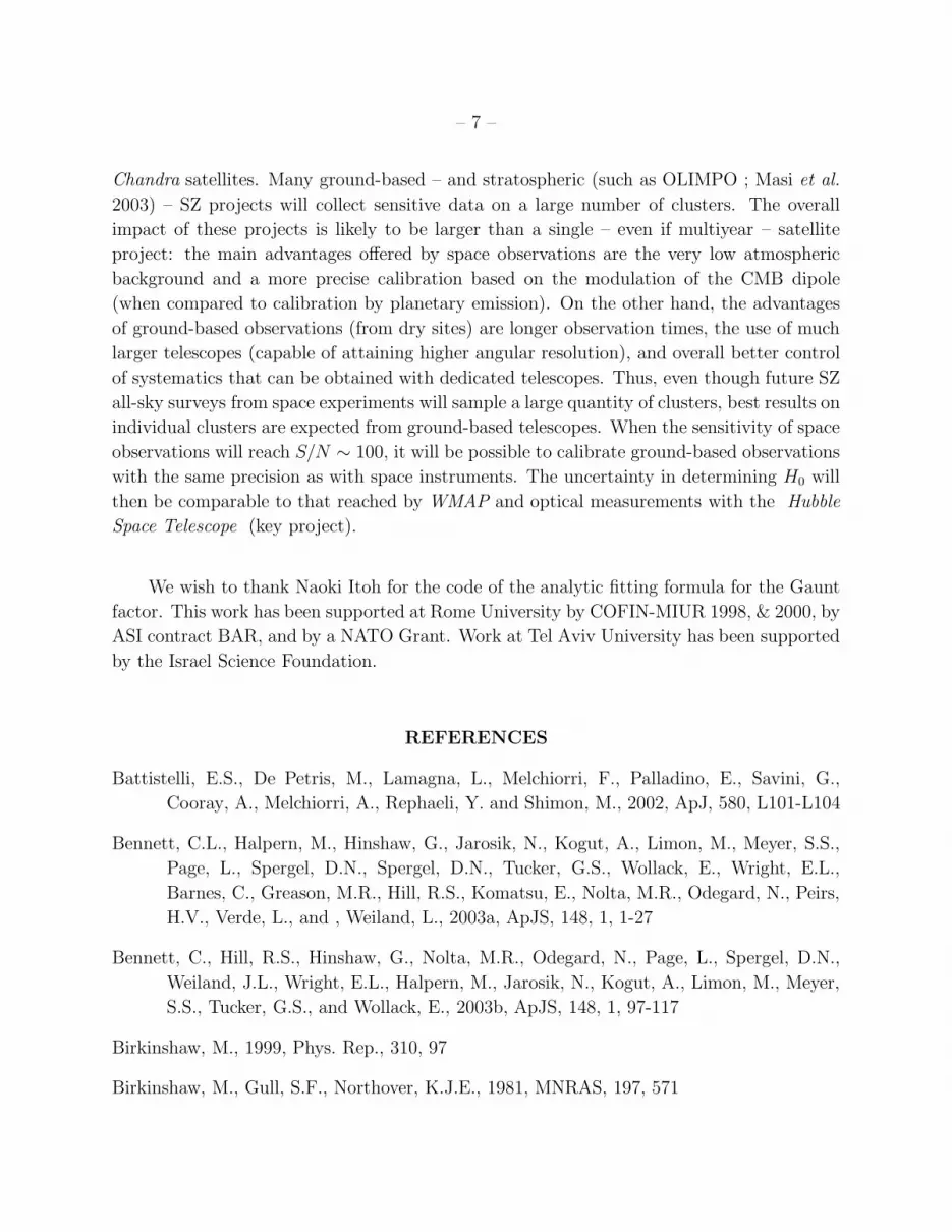
Chandra satellites. Many ground-based – and stratospheric (such as OLIMPO ; Masi et al.

2003) – SZ projects will collect sensitive data on a large number of clusters. The overall

impact of these projects is likely to be larger than a single – even if multiyear – satellite

project: the main advantages offered by space observations are the very low atmospheric

background and a more precise calibration based on the modulation of the CMB dipole

(when compared to calibration by planetary emission). On the other hand, the advantages

of ground-based observations (from dry sites) are longer observation times, the use of much

larger telescopes (capable of attaining higher angular resolution), and overall better control

of systematics that can be obtained with dedicated telescopes. Thus, even though future SZ

all-sky surveys from space experiments will sample a large quantity of clusters, best results on

individual clusters are expected from ground-based telescopes. When the sensitivity of space

observations will reach S/N ∼ 100, it will be possible to calibrate ground-based observations

with the same precision as with space instruments. The uncertainty in determining H0 will

then be comparable to that reached by WMAP and optical measurements with the Hubble

Space Telescope (key project).

We wish to thank Naoki Itoh for the code of the analytic fitting formula for the Gaunt

factor. This work has been supported at Rome University by COFIN-MIUR 1998, & 2000, by

ASI contract BAR, and by a NATO Grant. Work at Tel Aviv University has been supported

by the Israel Science Foundation.

REFERENCES

Battistelli, E.S., De Petris, M., Lamagna, L., Melchiorri, F., Palladino, E., Savini, G.,

Cooray, A., Melchiorri, A., Rephaeli, Y. and Shimon, M., 2002, ApJ, 580, L101-L104

Bennett, C.L., Halpern, M., Hinshaw, G., Jarosik, N., Kogut, A., Limon, M., Meyer, S.S.,

Page, L., Spergel, D.N., Spergel, D.N., Tucker, G.S., Wollack, E., Wright, E.L.,

Barnes, C., Greason, M.R., Hill, R.S., Komatsu, E., Nolta, M.R., Odegard, N., Peirs,

H.V., Verde, L., and , Weiland, L., 2003a, ApJS, 148, 1, 1-27

Bennett, C., Hill, R.S., Hinshaw, G., Nolta, M.R., Odegard, N., Page, L., Spergel, D.N.,

Weiland, J.L., Wright, E.L., Halpern, M., Jarosik, N., Kogut, A., Limon, M., Meyer,

S.S., Tucker, G.S., and Wollack, E., 2003b, ApJS, 148, 1, 97-117

Birkinshaw, M., 1999, Phys. Rep., 310, 97

Birkinshaw, M., Gull, S.F., Northover, K.J.E., 1981, MNRAS, 197, 571

– 8 –

Carlstrom, J.R., Holder, G.P., and Reese, E.D., 2002, ARA&A, 40, 643

Cavaliere, A., & Fusco-Femiano, R., 1976, A&A, 49, 137

Colafrancesco, S., Marchegiani, P., and Palladino, E., 2003, A&A, 397, 27

De Petris, M., D’Alba, L., Lamagna, L., Melchiorri, F., Orlando, A., Palladino, E., Rephaeli,

Y., Colafrancesco, S., Kreysa, E., and Signore, M., 2002, ApJ, 574, L119-L122

Furuzawa, A., Tawara, Y., Kunieda, H., Yamashita, K., Sonobe, T., Tanaka, Y., and

Mushotzky, R., 1998, ApJ, 504, 35-41

Herbig, T., Lawrence, C.R., and Readhead, A.C.S., 1995, ApJ, 449, L5

Holzapfel, W.L., Arnaud, M., Ade, P.A.R., Church, S.E., Fischer, M.L., Mauskopf, P.D.,

Rephaeli, Y., Wilbanks, T.M., and Lange, A.E., 1997, ApJ, 480, 449

Hughes, J.P., & Birkinshaw, M., 1998, ApJ, 501, 1

Itoh, N., Kohyama, Y., and Nozawa, S., 1998, ApJ, 502, 7-15

Itoh, N., Sakamoto, T., Kusano, Y., Kawana, Y., and Nozawa, S., 2002, A&A, 382, 722-729

Itoh, N., Sakamoto, T., Kusano, Y., Nozawa, S.,and Kohyama, Y., 2000, ApJS, 128, 125-138

Masi, S., Ade, P.A.R., Boscaleri, A., de Bernardis, P., De Petris, M., De Troia, G., Fabrini,

M., Iacoangeli, A., Lamagna, L., Lange, A.E., Lubin, P., Mauskopf, P.D., Melchiorri,

A., Melchiorri, F., Nati, F., Nati, L., Orlando, A., Piacentini, F., Pierre, F., Pisano,

G., Polenta, G., Rephaeli, Y., Romeo, G., Salvaterra, L., Savini, G., Valiante, E.,

and Yvon, D., 2003, to appear in the proceedings of the 4th National Conference on

Infrared Astronomy, 4-7 December 2001, Perugia, eds. S. Ciprini, M. Busso, G. Tosti

and P. Persi, ”Memorie della Societa’ Astronomica Italiana”, 74, 1

Mason, B.S., Myers, S.T., and Readhead, A.C.S., 2001, ApJ, 555, L11

Mohr, J.J., Mathiesen, B., and Evrard, A.E., 1999, ApJ, 517, 2, 627

Nozawa, S., Itoh, N., & Kohyama, Y., 1998, ApJ, 508, 17

Reese, E.D., Carlstrom, J.E., Joy, M., Mohr, J.J., Grego, L., and Holzapfel, W.L., 2002,

ApJ, 581, 53

Reese, E.D., Mohr, J.J., Carlstrom, J.E., Joy, M., Grego, L., Holder, G.P., Holzapfel, W.L.,

Hughes, J.P., Patel, S.K., and Donahue, M., 2000, ApJ, 533, 38

– 9 –

Rephaeli, Y., 1995a, ARA&A, 33, 541

Rephaeli, Y., 1995b, ApJ, 445, 33

Rephaeli, Y., 1999, ‘3K cosmology’, L. Maiani, F. Melchiorri, & N. Vittorio, eds., AIP, 476,

310

Savini, G., Orlando, A., Battistelli, E.S., De Petris, M., Lamagna, L., Luzzi, G., and Pal-

ladino, E., 2003, New Astronomy, 8, 7, 727-736

Shimon, M. & Rephaeli, Y., 2003, New Astronomy, in press, (astro-ph/0309098)

Silverberg, R. Cheng, E.S., Cottingham, D.A., Fixsen, D.J., Inman, C.A., Kowitt, M.S.,

Meyer, S.S., Page, L.A., Puchalla, J.L., Rephaeli, Y., 1997, ApJ, 485, 22

Spergel, D.N., Verde, L., Peiris, H.V., Komatsu, E., Nolta, M.R., Bennett, C.L., Halpern,

M., Hinshaw, G., Jarosik, N., Kogut, A., Limon, M., Meyer, S.S., Page, L., Tucker,

G.S., Weiland, J.L., Wollack, E., and Wright, E.L. 2003, ApJS, 148, 1, 175-194

Sunyaev, R.A. & Zel’dovich, Ya. B., 1972, Comm. Astrphys. Space Phys., 4, 173

This preprint was prepared with the AAS LATEX macros v5.0.

– 10 –

Fig. 1.— SZ spectrum of the Coma cluster. Solid line: best fit spectrum (assuming

isothermal gas with kT = 8.21 keV) to the combined MITO (diamonds), OVRO (square),

and WMAP (triangles) measurements, corresponding to τ = (5.35 ± 0.67) × 10−3.

– 11 –

Table 1. SZE experiment parameters

Channel ν ∆ν f.o.v. (FWHM) Sensitivity ∆T

(GHz) (GHz) (arcmin) (mKs1/2) (µK)

OVRO 32.0 6.5 7.35 1.40 -520±83

WMAP(V) 60.8 13.0 20 1.13 -240±180

WMAP(W) 93.5 19 13 1.48 -340±180

MITO(1) 143 30 16 1.21 -184±39

MITO(2) 214 30 16 1.14 -32±79

MITO(3) 272 32 16 0.896 172±36