transport between multiple users in complex networks

Eur. Phys. J. B 57, 165–174 (2007)DOI: 10.1140/epjb/e2007-00129-0 THE EUROPEAN

PHYSICAL JOURNAL B

Transport between multiple users in complex networks

S. Carmi1,a, Z. Wu2, E. Lopez3, S. Havlin1,2, and H. Eugene Stanley2

1 Minerva Center & Department of Physics, Bar-Ilan University, Ramat Gan 52900, Israel2 Center for Polymer Studies, Boston University, Boston, MA 02215, USA3 Theoretical Division, Los Alamos National Laboratory, Mail Stop B258, Los Alamos, NM 87545, USA

Received 31 August 2006 / Received in final form 22 February 2007Published online 16 May 2007 – c© EDP Sciences, Societa Italiana di Fisica, Springer-Verlag 2007

Abstract. We study the transport properties of model networks such as scale-free and Erdos-Renyi net-works as well as a real network. We consider few possibilities for the trnasport problem. We start bystudying the conductance G between two arbitrarily chosen nodes where each link has the same unitresistance. Our theoretical analysis for scale-free networks predicts a broad range of values of G, with apower-law tail distribution ΦSF(G) ∼ G−gG , where gG = 2λ − 1, and λ is the decay exponent for thescale-free network degree distribution. The power-law tail in ΦSF(G) leads to large values of G, therebysignificantly improving the transport in scale-free networks, compared to Erdos-Renyi networks where thetail of the conductivity distribution decays exponentially. We develop a simple physical picture of thetransport to account for the results. The other model for transport is the max-flow model, where conduc-tance is defined as the number of link-independent paths between the two nodes, and find that a similarpicture holds. The effects of distance on the value of conductance are considered for both models, and somedifferences emerge. We then extend our study to the case of multiple sources ans sinks, where the transportis defined between two groups of nodes. We find a fundamental difference between the two forms of flowwhen considering the quality of the transport with respect to the number of sources, and find an optimalnumber of sources, or users, for the max-flow case. A qualitative (and partially quantitative) explanationis also given.

PACS. 89.75.Hc Networks and genealogical trees – 05.60.Cd Classical transport

1 Introduction

Transport in many random structures is “anomalous,” i.e.,fundamentally different from that in regular space [1–3].The anomaly is due to the random substrate on whichtransport is constrained to take place. Random struc-tures are found in many places in the real world, from oilreservoirs to the Internet, making the study of anomaloustransport properties a far-reaching field. In this problem,it is paramount to relate the structural properties of themedium with the transport properties.

An important and recent example of random sub-strates is that of complex networks. Research on this topichas uncovered their importance for real-world problems asdiverse as the World Wide Web and the Internet to cel-lular networks and sexual-partner networks [4]. Networksdescribe also economic systems such as financial marketsand banks systems [5–7]. Transport of goods and informa-tion in such networks is of much interest.

Two distinct models describe the two limiting cases forthe structure of the complex networks. The first of these is

a e-mail: [email protected]

the classic Erdos-Renyi model of random networks [8], forwhich sites are connected with a link with probability pand are disconnected (no link) with probability 1− p (seeFig. 1a). In this case the degree distribution P (k), theprobability of a node to have k connections, is a Poisson

P (k) =

(k)k

e−k

k!, (1)

where k ≡ ∑∞k=1 kP (k) is the average degree of the

network. Mathematicians discovered critical phenomenathrough this model. For instance, just as in percolation onlattices, there is a critical value p = pc above which thelargest connected component of the network has a massthat scales with the system size N , but below pc, there areonly small clusters of the order of log N . At p = pc, thesize of the largest cluster is of order of N2/3. Anothercharacteristic of an Erdos-Renyi network is its “small-world” property which means that the average distanced (or diameter) between all pairs of nodes of the networkscales as log N [9]. The other model, recently identifiedas the characterizing topological structure of many real

166 The European Physical Journal B

(a) (b)

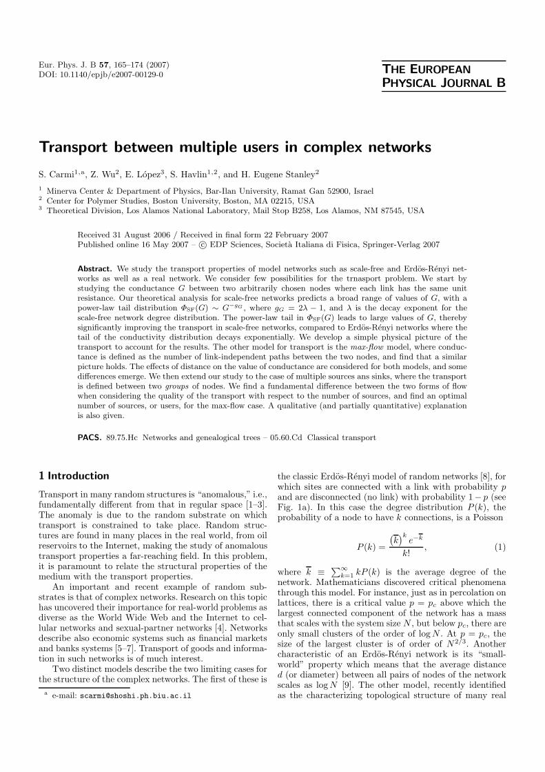
Fig. 1. (a) Schematic of an Erdos-Renyi network of N = 12and p = 1/6. Note that in this example ten nodes have k =2 connections, and two nodes have k = 1 connections. Thisillustrates the fact that for Erdos-Renyi networks, the rangeof values of degree is very narrow, typically close to k. (b)Schematic of a scale-free network of N = 12, kmin = 2 andλ ≈ 2. We note the presence of a hub with kmax = 8 which isconnected to many of the other nodes of the network.

world systems, is the Barabasi-Albert scale-free networkand its extensions [10–12], characterized by a scale-freedegree distribution:

P (k) ∼ k−λ [kmin ≤ k ≤ kmax]. (2)

The cutoff value kmin represents the minimum allowedvalue of k on the network (kmin = 2 here), and kmax ≡kminN1/(λ−1), the typical maximum degree of a networkwith N nodes [13,14]. The scale-free feature allows a net-work to have some nodes with a large number of links(“hubs”), unlike the case for the Erdos-Renyi model ofrandom networks [8,9] (see Fig. 1b). Scale-free networkswith λ > 3 have d ∼ log N , while for 2 < λ < 3they are “ultra-small-world” since the diameter scales asd ∼ log log N [13].

Here we extend our recent study of transport in com-plex networks [15–17], where we have found that for scale-free networks with λ ≥ 2, transport properties character-ized by conductance display a power-law tail distributionthat is related to the degree distribution P (k). The ori-gin of this power-law tail is due to pairs of nodes of highdegree which have high conductance. Thus, transport inscale-free networks is better because of the presence oflarge degree nodes (hubs) that carry much of the traffic,whereas Erdos-Renyi networks lack hubs and the trans-port properties are controlled mainly by the average de-gree k [9,18]. We have presented a simple physical pictureof the transport properties and tested it through simula-tions. We also studied a form of frictionless transport, inwhich transport is measured by the number of indepen-dent paths between source and destination. These laterresults are in part similar to those in [19]. We tested ourfindings on a real network, a recent map of the Internet.Here we study the properties of the transport where sev-eral sources and sinks are involved. We find a principaldifference between the two forms of transport mentionedabove, and find an optimal number of sources in the fric-tionless case. We also develop a simple theory for the totalflow for small number of sources.

10−1 100 101 102

Conductance G

10−6

10−4

10−2

100

Cu

mu

lati

ve D

istr

ibu

tion

F(G

)

Erdos−Renyi(λ=2.5) SF(λ=3.3) SF(a)

’’’

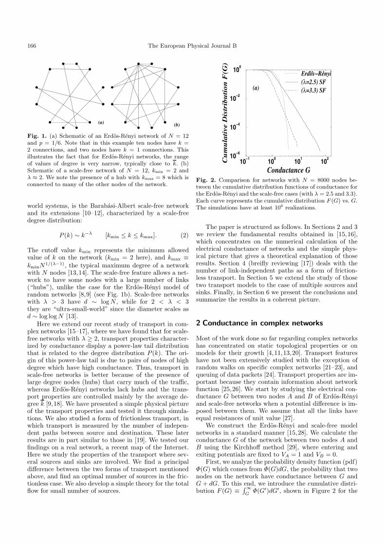
Fig. 2. Comparison for networks with N = 8000 nodes be-tween the cumulative distribution functions of conductance forthe Erdos-Renyi and the scale-free cases (with λ = 2.5 and 3.3).Each curve represents the cumulative distribution F (G) vs. G.The simulations have at least 106 realizations.

The paper is structured as follows. In Sections 2 and 3we review the fundamental results obtained in [15,16],which concentrates on the numerical calculation of theelectrical conductance of networks and the simple phys-ical picture that gives a theoretical explanation of thoseresults. Section 4 (breifly reviewing [17]) deals with thenumber of link-independent paths as a form of friction-less transport. In Section 5 we extend the study of thosetwo transport models to the case of multiple sources andsinks. Finally, in Section 6 we present the conclusions andsummarize the results in a coherent picture.

2 Conductance in complex networks

Most of the work done so far regarding complex networkshas concentrated on static topological properties or onmodels for their growth [4,11,13,20]. Transport featureshave not been extensively studied with the exception ofrandom walks on specific complex networks [21–23], andqueuing of data packets [24]. Transport properties are im-portant because they contain information about networkfunction [25,26]. We start by studying the electrical con-ductance G between two nodes A and B of Erdos-Renyiand scale-free networks when a potential difference is im-posed between them. We assume that all the links haveequal resistances of unit value [27].

We construct the Erdos-Renyi and scale-free modelnetworks in a standard manner [15,28]. We calculate theconductance G of the network between two nodes A andB using the Kirchhoff method [29], where entering andexiting potentials are fixed to VA = 1 and VB = 0.

First, we analyze the probability density function (pdf)Φ(G) which comes from Φ(G)dG, the probability that twonodes on the network have conductance between G andG + dG. To this end, we introduce the cumulative distri-bution F (G) ≡ ∫ ∞

GΦ(G′)dG′, shown in Figure 2 for the

S. Carmi et al.: Transport of multiple users in complex networks 167

100 101 102

Conductance G

10−4

10−3

10−2

10−1

100

Co

nd

uct

an

ce p

df

ΦS

F(G

|kA,k

B)

G*

kB=4 8 16 32 64 128

(a)

101 102

kB, degree of node B

101

102

Mo

st P

rob

. C

on

du

cta

nce

G*

α

(b)

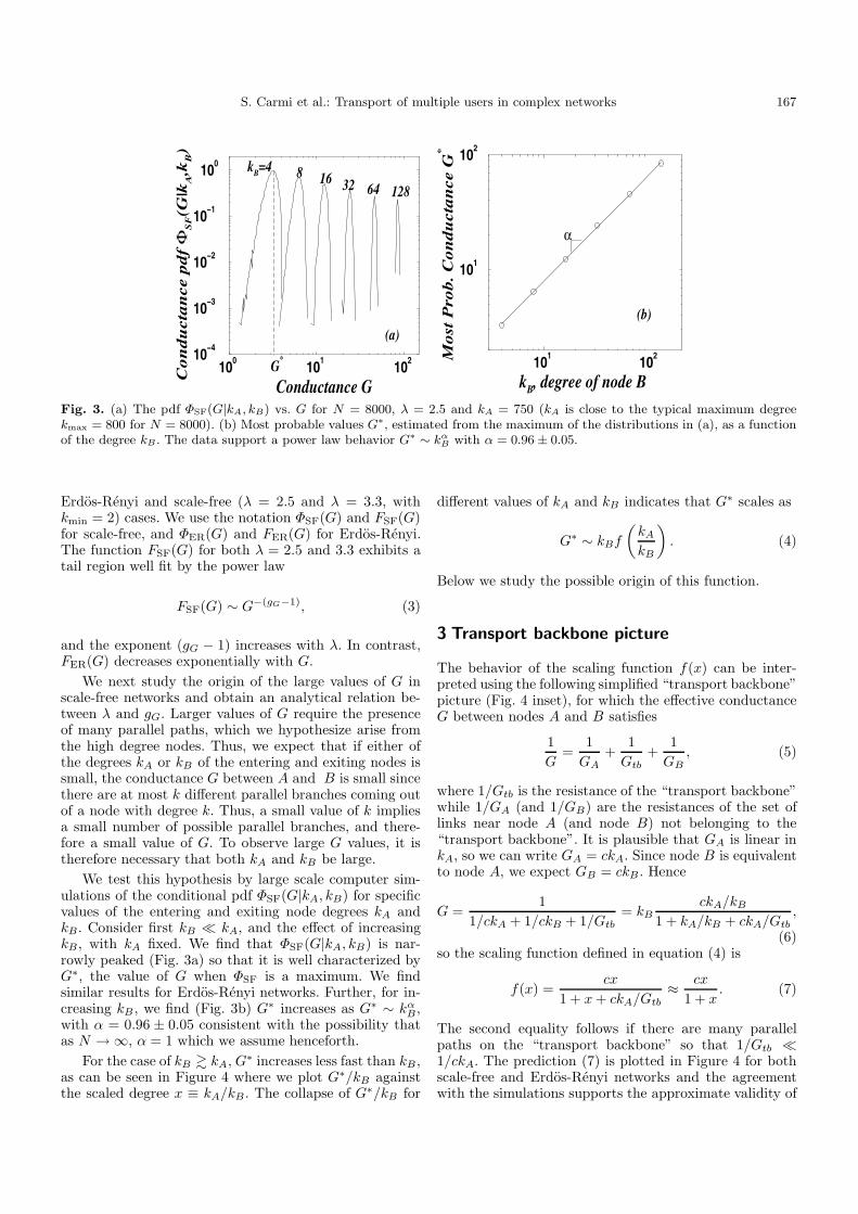
Fig. 3. (a) The pdf ΦSF(G|kA, kB) vs. G for N = 8000, λ = 2.5 and kA = 750 (kA is close to the typical maximum degreekmax = 800 for N = 8000). (b) Most probable values G∗, estimated from the maximum of the distributions in (a), as a functionof the degree kB . The data support a power law behavior G∗ ∼ kα

B with α = 0.96 ± 0.05.

Erdos-Renyi and scale-free (λ = 2.5 and λ = 3.3, withkmin = 2) cases. We use the notation ΦSF(G) and FSF(G)for scale-free, and ΦER(G) and FER(G) for Erdos-Renyi.The function FSF(G) for both λ = 2.5 and 3.3 exhibits atail region well fit by the power law

FSF(G) ∼ G−(gG−1), (3)

and the exponent (gG − 1) increases with λ. In contrast,FER(G) decreases exponentially with G.

We next study the origin of the large values of G inscale-free networks and obtain an analytical relation be-tween λ and gG. Larger values of G require the presenceof many parallel paths, which we hypothesize arise fromthe high degree nodes. Thus, we expect that if either ofthe degrees kA or kB of the entering and exiting nodes issmall, the conductance G between A and B is small sincethere are at most k different parallel branches coming outof a node with degree k. Thus, a small value of k impliesa small number of possible parallel branches, and there-fore a small value of G. To observe large G values, it istherefore necessary that both kA and kB be large.

We test this hypothesis by large scale computer sim-ulations of the conditional pdf ΦSF(G|kA, kB) for specificvalues of the entering and exiting node degrees kA andkB. Consider first kB � kA, and the effect of increasingkB, with kA fixed. We find that ΦSF(G|kA, kB) is nar-rowly peaked (Fig. 3a) so that it is well characterized byG∗, the value of G when ΦSF is a maximum. We findsimilar results for Erdos-Renyi networks. Further, for in-creasing kB , we find (Fig. 3b) G∗ increases as G∗ ∼ kα

B,with α = 0.96 ± 0.05 consistent with the possibility thatas N → ∞, α = 1 which we assume henceforth.

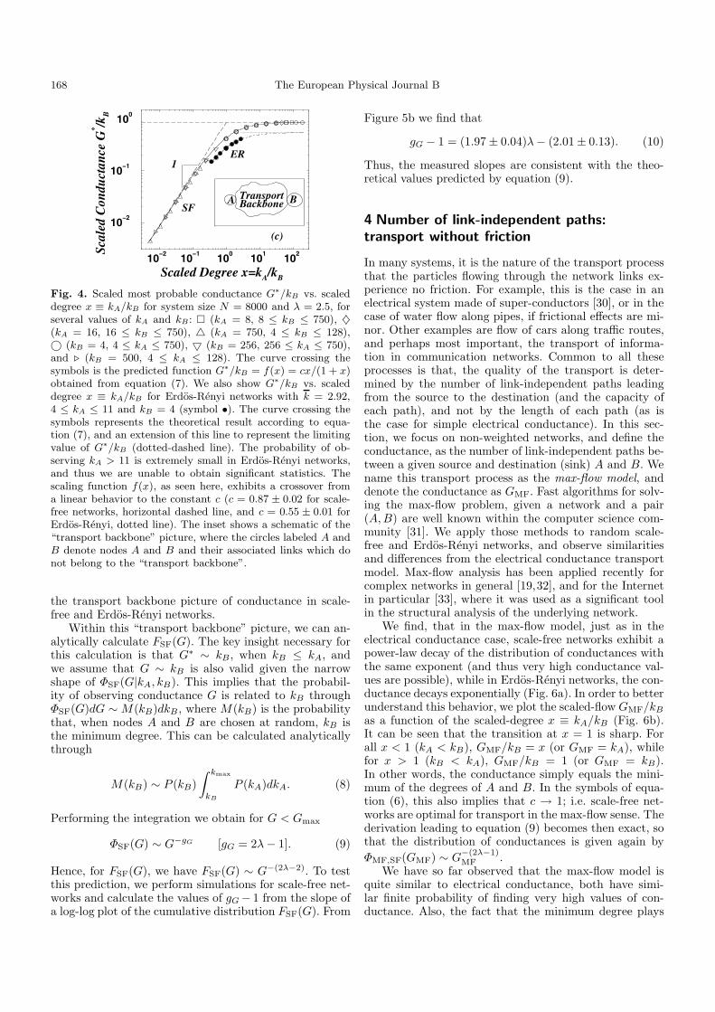
For the case of kB � kA, G∗ increases less fast than kB,as can be seen in Figure 4 where we plot G∗/kB againstthe scaled degree x ≡ kA/kB. The collapse of G∗/kB for

different values of kA and kB indicates that G∗ scales as

G∗ ∼ kBf

(kA

kB

). (4)

Below we study the possible origin of this function.

3 Transport backbone picture

The behavior of the scaling function f(x) can be inter-preted using the following simplified “transport backbone”picture (Fig. 4 inset), for which the effective conductanceG between nodes A and B satisfies

1G

=1

GA+

1Gtb

+1

GB, (5)

where 1/Gtb is the resistance of the “transport backbone”while 1/GA (and 1/GB) are the resistances of the set oflinks near node A (and node B) not belonging to the“transport backbone”. It is plausible that GA is linear inkA, so we can write GA = ckA. Since node B is equivalentto node A, we expect GB = ckB. Hence

G =1

1/ckA + 1/ckB + 1/Gtb= kB

ckA/kB

1 + kA/kB + ckA/Gtb,

(6)so the scaling function defined in equation (4) is

f(x) =cx

1 + x + ckA/Gtb≈ cx

1 + x. (7)

The second equality follows if there are many parallelpaths on the “transport backbone” so that 1/Gtb �1/ckA. The prediction (7) is plotted in Figure 4 for bothscale-free and Erdos-Renyi networks and the agreementwith the simulations supports the approximate validity of


10−2 10−1 100 101 102

Scaled Degree x=kA/kB

10−2

10−1

100

Scal

ed C

ondu

ctan

ce G

* /kB

(c)

A BTransportBackbone

1ER

SF

Fig. 4. Scaled most probable conductance G∗/kB vs. scaleddegree x ≡ kA/kB for system size N = 8000 and λ = 2.5, forseveral values of kA and kB : � (kA = 8, 8 ≤ kB ≤ 750), ♦(kA = 16, 16 ≤ kB ≤ 750), � (kA = 750, 4 ≤ kB ≤ 128),© (kB = 4, 4 ≤ kA ≤ 750), � (kB = 256, 256 ≤ kA ≤ 750),and � (kB = 500, 4 ≤ kA ≤ 128). The curve crossing thesymbols is the predicted function G∗/kB = f(x) = cx/(1 + x)obtained from equation (7). We also show G∗/kB vs. scaleddegree x ≡ kA/kB for Erdos-Renyi networks with k = 2.92,4 ≤ kA ≤ 11 and kB = 4 (symbol •). The curve crossing thesymbols represents the theoretical result according to equa-tion (7), and an extension of this line to represent the limitingvalue of G∗/kB (dotted-dashed line). The probability of ob-serving kA > 11 is extremely small in Erdos-Renyi networks,and thus we are unable to obtain significant statistics. Thescaling function f(x), as seen here, exhibits a crossover froma linear behavior to the constant c (c = 0.87 ± 0.02 for scale-free networks, horizontal dashed line, and c = 0.55 ± 0.01 forErdos-Renyi, dotted line). The inset shows a schematic of the“transport backbone” picture, where the circles labeled A andB denote nodes A and B and their associated links which donot belong to the “transport backbone”.

the transport backbone picture of conductance in scale-free and Erdos-Renyi networks.

Within this “transport backbone” picture, we can an-alytically calculate FSF(G). The key insight necessary forthis calculation is that G∗ ∼ kB, when kB ≤ kA, andwe assume that G ∼ kB is also valid given the narrowshape of ΦSF(G|kA, kB). This implies that the probabil-ity of observing conductance G is related to kB throughΦSF(G)dG ∼ M(kB)dkB , where M(kB) is the probabilitythat, when nodes A and B are chosen at random, kB isthe minimum degree. This can be calculated analyticallythrough

M(kB) ∼ P (kB)∫ kmax

kB

P (kA)dkA. (8)

Performing the integration we obtain for G < Gmax

ΦSF(G) ∼ G−gG [gG = 2λ − 1]. (9)

Hence, for FSF(G), we have FSF(G) ∼ G−(2λ−2). To testthis prediction, we perform simulations for scale-free net-works and calculate the values of gG − 1 from the slope ofa log-log plot of the cumulative distribution FSF(G). From

Figure 5b we find that

gG − 1 = (1.97 ± 0.04)λ − (2.01 ± 0.13). (10)

Thus, the measured slopes are consistent with the theo-retical values predicted by equation (9).

4 Number of link-independent paths:transport without friction

In many systems, it is the nature of the transport processthat the particles flowing through the network links ex-perience no friction. For example, this is the case in anelectrical system made of super-conductors [30], or in thecase of water flow along pipes, if frictional effects are mi-nor. Other examples are flow of cars along traffic routes,and perhaps most important, the transport of informa-tion in communication networks. Common to all theseprocesses is that, the quality of the transport is deter-mined by the number of link-independent paths leadingfrom the source to the destination (and the capacity ofeach path), and not by the length of each path (as isthe case for simple electrical conductance). In this sec-tion, we focus on non-weighted networks, and define theconductance, as the number of link-independent paths be-tween a given source and destination (sink) A and B. Wename this transport process as the max-flow model, anddenote the conductance as GMF. Fast algorithms for solv-ing the max-flow problem, given a network and a pair(A, B) are well known within the computer science com-munity [31]. We apply those methods to random scale-free and Erdos-Renyi networks, and observe similaritiesand differences from the electrical conductance transportmodel. Max-flow analysis has been applied recently forcomplex networks in general [19,32], and for the Internetin particular [33], where it was used as a significant toolin the structural analysis of the underlying network.

We find, that in the max-flow model, just as in theelectrical conductance case, scale-free networks exhibit apower-law decay of the distribution of conductances withthe same exponent (and thus very high conductance val-ues are possible), while in Erdos-Renyi networks, the con-ductance decays exponentially (Fig. 6a). In order to betterunderstand this behavior, we plot the scaled-flow GMF/kB

as a function of the scaled-degree x ≡ kA/kB (Fig. 6b).It can be seen that the transition at x = 1 is sharp. Forall x < 1 (kA < kB), GMF/kB = x (or GMF = kA), whilefor x > 1 (kB < kA), GMF/kB = 1 (or GMF = kB).In other words, the conductance simply equals the mini-mum of the degrees of A and B. In the symbols of equa-tion (6), this also implies that c → 1; i.e. scale-free net-works are optimal for transport in the max-flow sense. Thederivation leading to equation (9) becomes then exact, sothat the distribution of conductances is given again byΦMF,SF(GMF) ∼ G

−(2λ−1)MF .

We have so far observed that the max-flow model isquite similar to electrical conductance, both have simi-lar finite probability of finding very high values of con-ductance. Also, the fact that the minimum degree plays


10−1 100 101 102

Conductance G

10−6

10−4

10−2

100

Cum

ulat

ive

Dis

trib

utio

n F

SF(G

)

λ=2.52.72.93.13.33.5

(a)

2.4 3.4 4.4Exponent λ

2.5

3.5

4.5

5.5

6.5

Exp

onen

t gG−

1

(b)

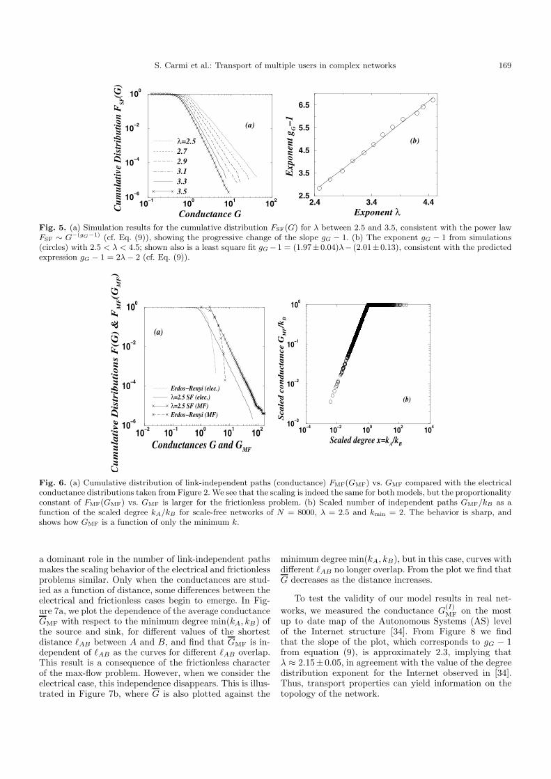
Fig. 5. (a) Simulation results for the cumulative distribution FSF(G) for λ between 2.5 and 3.5, consistent with the power lawFSF ∼ G−(gG−1) (cf. Eq. (9)), showing the progressive change of the slope gG − 1. (b) The exponent gG − 1 from simulations(circles) with 2.5 < λ < 4.5; shown also is a least square fit gG −1 = (1.97±0.04)λ− (2.01±0.13), consistent with the predictedexpression gG − 1 = 2λ − 2 (cf. Eq. (9)).

10−2 10−1 100 101 102

Conductances G and GMF

10−6

10−4

10−2

100

Cu

mu

lati

ve D

istr

ibu

tio

ns

F(G

) &

FM

F(G

MF)

Erdos−Renyi (elec.)λ=2.5 SF (elec.)λ=2.5 SF (MF)Erdos−Renyi (MF)

(a)

10−4 10−2 100 102 104

Scaled degree x=kA/kB

10−3

10−2

10−1

100

Sca

led

co

nd

uct

an

ce G

MF/k

B

(b)

Fig. 6. (a) Cumulative distribution of link-independent paths (conductance) FMF(GMF) vs. GMF compared with the electricalconductance distributions taken from Figure 2. We see that the scaling is indeed the same for both models, but the proportionalityconstant of FMF(GMF) vs. GMF is larger for the frictionless problem. (b) Scaled number of independent paths GMF/kB as afunction of the scaled degree kA/kB for scale-free networks of N = 8000, λ = 2.5 and kmin = 2. The behavior is sharp, andshows how GMF is a function of only the minimum k.

a dominant role in the number of link-independent pathsmakes the scaling behavior of the electrical and frictionlessproblems similar. Only when the conductances are stud-ied as a function of distance, some differences between theelectrical and frictionless cases begin to emerge. In Fig-ure 7a, we plot the dependence of the average conductanceGMF with respect to the minimum degree min(kA, kB) ofthe source and sink, for different values of the shortestdistance �AB between A and B, and find that GMF is in-dependent of �AB as the curves for different �AB overlap.This result is a consequence of the frictionless characterof the max-flow problem. However, when we consider theelectrical case, this independence disappears. This is illus-trated in Figure 7b, where G is also plotted against the

minimum degree min(kA, kB), but in this case, curves withdifferent �AB no longer overlap. From the plot we find thatG decreases as the distance increases.

To test the validity of our model results in real net-works, we measured the conductance G

(I)MF on the most

up to date map of the Autonomous Systems (AS) levelof the Internet structure [34]. From Figure 8 we findthat the slope of the plot, which corresponds to gG − 1from equation (9), is approximately 2.3, implying thatλ ≈ 2.15±0.05, in agreement with the value of the degreedistribution exponent for the Internet observed in [34].Thus, transport properties can yield information on thetopology of the network.


100 101 102 103

Minimum degree min(kA,kB)

100

101

102

103

Ave

rage

Con

du

ctan

ce G

MF

l=1l=2l=3l=4l=5l=6

(a)

101

Mimimum degree min(kA,kB)

101

Ave

rage

Con

du

ctan

ce G

l=1l=3

(b)

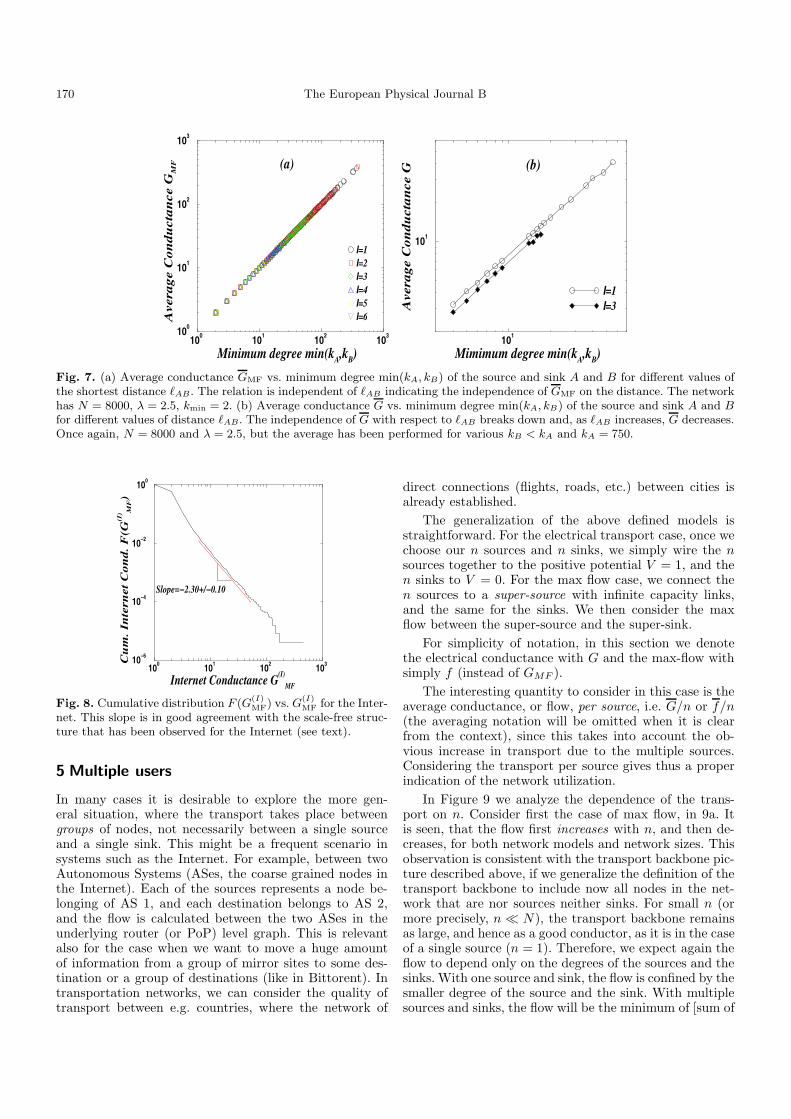
Fig. 7. (a) Average conductance GMF vs. minimum degree min(kA, kB) of the source and sink A and B for different values ofthe shortest distance �AB. The relation is independent of �AB indicating the independence of GMF on the distance. The networkhas N = 8000, λ = 2.5, kmin = 2. (b) Average conductance G vs. minimum degree min(kA, kB) of the source and sink A and Bfor different values of distance �AB. The independence of G with respect to �AB breaks down and, as �AB increases, G decreases.Once again, N = 8000 and λ = 2.5, but the average has been performed for various kB < kA and kA = 750.

100 101 102 103

Internet Conductance G(I)

MF

10−6

10−4

10−2

100

Cu

m.

Inte

rnet

Co

nd

. F

(G(I

) MF)

Slope=−2.30+/−0.10

Fig. 8. Cumulative distribution F (G(I)MF) vs. G

(I)MF for the Inter-

net. This slope is in good agreement with the scale-free struc-ture that has been observed for the Internet (see text).

5 Multiple users

In many cases it is desirable to explore the more gen-eral situation, where the transport takes place betweengroups of nodes, not necessarily between a single sourceand a single sink. This might be a frequent scenario insystems such as the Internet. For example, between twoAutonomous Systems (ASes, the coarse grained nodes inthe Internet). Each of the sources represents a node be-longing of AS 1, and each destination belongs to AS 2,and the flow is calculated between the two ASes in theunderlying router (or PoP) level graph. This is relevantalso for the case when we want to move a huge amountof information from a group of mirror sites to some des-tination or a group of destinations (like in Bittorent). Intransportation networks, we can consider the quality oftransport between e.g. countries, where the network of

direct connections (flights, roads, etc.) between cities isalready established.

The generalization of the above defined models isstraightforward. For the electrical transport case, once wechoose our n sources and n sinks, we simply wire the nsources together to the positive potential V = 1, and then sinks to V = 0. For the max flow case, we connect then sources to a super-source with infinite capacity links,and the same for the sinks. We then consider the maxflow between the super-source and the super-sink.

For simplicity of notation, in this section we denotethe electrical conductance with G and the max-flow withsimply f (instead of GMF ).

The interesting quantity to consider in this case is theaverage conductance, or flow, per source, i.e. G/n or f/n(the averaging notation will be omitted when it is clearfrom the context), since this takes into account the ob-vious increase in transport due to the multiple sources.Considering the transport per source gives thus a properindication of the network utilization.

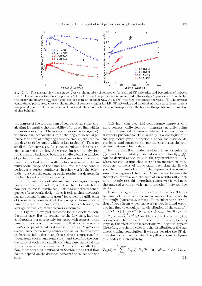
In Figure 9 we analyze the dependence of the trans-port on n. Consider first the case of max flow, in 9a. Itis seen, that the flow first increases with n, and then de-creases, for both network models and network sizes. Thisobservation is consistent with the transport backbone pic-ture described above, if we generalize the definition of thetransport backbone to include now all nodes in the net-work that are nor sources neither sinks. For small n (ormore precisely, n � N), the transport backbone remainsas large, and hence as a good conductor, as it is in the caseof a single source (n = 1). Therefore, we expect again theflow to depend only on the degrees of the sources and thesinks. With one source and sink, the flow is confined by thesmaller degree of the source and the sink. With multiplesources and sinks, the flow will be the minimum of [sum of


0 200Number of sources n

1

2

3

4

Avera

ge flo

w p

er

sourc

e f/n

ER, N=1024 ER, N=4096 SF, N=1024 SF, N=4096 (a)

n*

0 500 1000 1500 2000number of sources n

0.0

0.5

1.0

1.5

2.0

2.5

Ave

rag

e c

on

du

cta

nce

pe

r so

urc

e G

/n

ER, N=1024 ER, N=4096 SF, N=1024 SF, N=4096

(b)

Fig. 9. (a) The average flow per source, f/n vs. the number of sources n, for ER and SF networks, and two values of networksize N . For all curves there is an optimal n∗, for which the flow per source is maximized. Obviously, n∗ grows with N such thatthe larger the network is, more users can use it in an optimal way. Above n∗, the flow per source decreases. (b) The averageconductance per source, G/n vs. the number of sources n again for ER, SF networks, and different network sizes. Here there isno optimal point — the more users in the network the more useful it is for transport. See the text for the qualitative explanationof this behavior.

the degrees of the sources, sum of degrees of the sinks] (ne-glecting for small n the probability of a direct link withinthe sources or sinks). The more sources we have (larger n),the more chances for the sum of the degrees to be larger(since for a sum of many degrees to be smaller, we need allthe degrees to be small, which is less probable). Thus forsmall n, f/n increases. An exact calculation for this re-gion is carried out below. As n grows larger, not only thatthe transport backbone becomes smaller, but the numberof paths that need to go through it grows too. Therefore,many paths that were parallel before now require the si-multaneous usage of the same link, and the backbone isno longer a perfect conductor. In other words, the inter-action between the outgoing paths results in a decrease inthe backbone transport capability.

From these two contradicting trends emerges the ap-pearance of an optimal n∗, which is the n for which theflow per source is maximized. This has important conse-quences for networks design, since it tells us that a networkhas an optimal “number of users” for which the utilizationof the network is maximized. Increasing or decreasing thenumber of nodes in each group, will force each node, onaverage, to use less of the network resources.

In Figure 9b, we plot the same for the electrical con-ductance case. But, in contrast to the flow case, here theconductance per source only increases with respect to thenumber of sources n. The reason is, that for large n, thenumber of parallel paths decrease, but their lengths de-crease (since for so many sources and sinks, there is moreprobability for a direct or almost direct connection be-tween some source and some sink), and therefore the con-ductance of each path significantly increase, such that thetotal conductance increases too. All this did not affect theflow, since there, as mentioned in Section 4, the total flowdo not depend on the distance between the source and thesink.

This fact, that electrical conductance improves withmore sources, while flow only degrades, actually pointsout a fundamental difference between the two types oftransport phenomena. This actually is a consequence ofthe arguments given in Section 4 as for the distance de-pendence, and completes the picture considering the com-parison between the models.

For the max-flow model, a closed form formulas forf(n) and the probability distribution of the flow ΦMF,n(f)can be derived analytically in the region where n � N ,where we can assume that there is no interaction at allbetween the paths of the n pairs, such that the flow isjust the minimum of [sum of the degrees of the sources,sum of the degrees of the sinks]. A comparison between thetheoretical formula and the simulation results will enableus to directly test this hypothesis; moreover it will markthe range of n values with “no interaction” between flowpaths.

Denote by kn the sum of degrees of n nodes. The to-tal flow between n sources and n sinks is then given byf = min[kn(sources), kn(sinks)]. To calculate the distribu-tion of flows (from which the average flow is found easily)one has first to calculate the distribution of the sum of niidrv’s k1: Pk1(k) ∼ k−λ, [kmin ≤ k ≤ kmax], for SF graphs,or Pk1(k) =

(k)k

e−k/k! for ER graphs. For n 1, thisis easy with the central limit theorem. However, for verylarge n, the effect of the interactions will begin to appear.Therefore, one should calculate the distribution of the sumdirectly, using convolution. If we consider also the SF de-gree distribution as discrete, The pdf of a sum of degreesof 2 nodes is then given by

Pk2(k) =k−kmin∑

j=kmin

Pk1(j) ·Pk1 (k− j); 2kmin ≤ k ≤ 2kmax,

(11)


0 50Flow f

0

0.05

0.1

Pro

bab

ilit

y Φ

(f)

n=4 - Simulationn=4 - Theoryn=8 - Simulationn=8 - Theoryn=16 - Simulationn=16 - Theory

(a)

0 10 20 30 40 50 60 70Number of sources n

2

3

4

5

6

7

8

Flo

w p

er

sourc

e f

/n

ER - SimulationER - TheorySF - SimulationSF - Theory

(b)

Interactions appear

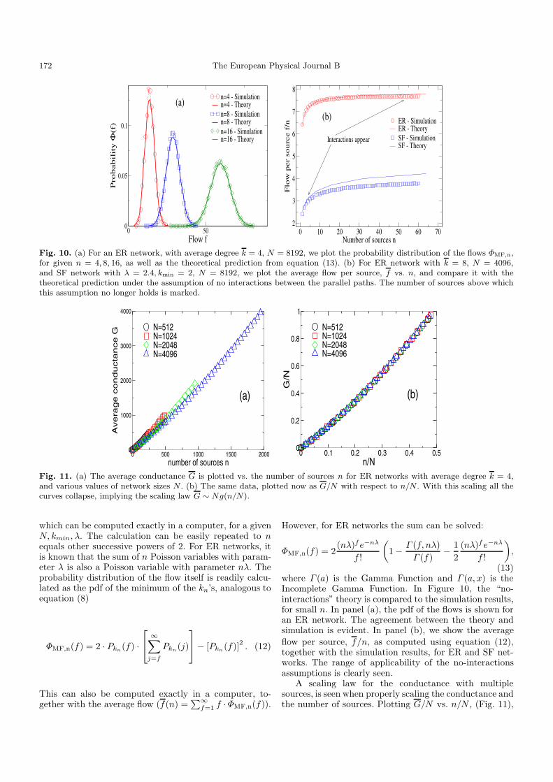
Fig. 10. (a) For an ER network, with average degree k = 4, N = 8192, we plot the probability distribution of the flows ΦMF,n,for given n = 4, 8, 16, as well as the theoretical prediction from equation (13). (b) For ER network with k = 8, N = 4096,and SF network with λ = 2.4, kmin = 2, N = 8192, we plot the average flow per source, f vs. n, and compare it with thetheoretical prediction under the assumption of no interactions between the parallel paths. The number of sources above whichthis assumption no longer holds is marked.

0 500 1000 1500 2000number of sources n

0

1000

2000

3000

4000

Ave

rag

e c

on

du

cta

nce

G

N=512N=1024N=2048N=4096

(a)

0 0.1 0.2 0.3 0.4 0.5n/N

0

0.2

0.4

0.6

0.8

1

G/N

N=512N=1024N=2048N=4096

(b)

Fig. 11. (a) The average conductance G is plotted vs. the number of sources n for ER networks with average degree k = 4,and various values of network sizes N . (b) The same data, plotted now as G/N with respect to n/N . With this scaling all thecurves collapse, implying the scaling law G ∼ Ng(n/N).

which can be computed exactly in a computer, for a givenN, kmin, λ. The calculation can be easily repeated to nequals other successive powers of 2. For ER networks, itis known that the sum of n Poisson variables with param-eter λ is also a Poisson variable with parameter nλ. Theprobability distribution of the flow itself is readily calcu-lated as the pdf of the minimum of the kn’s, analogous toequation (8)

ΦMF,n(f) = 2 · Pkn(f) ·⎡

⎣∞∑

j=f

Pkn(j)

⎤

⎦ − [Pkn(f)]2 . (12)

This can also be computed exactly in a computer, to-gether with the average flow (f(n) =

∑∞f=1 f ·ΦMF,n(f)).

However, for ER networks the sum can be solved:

ΦMF,n(f) = 2(nλ)fe−nλ

f !

(1 − Γ (f, nλ)

Γ (f)− 1

2(nλ)f e−nλ

f !

),

(13)where Γ (a) is the Gamma Function and Γ (a, x) is theIncomplete Gamma Function. In Figure 10, the “no-interactions” theory is compared to the simulation results,for small n. In panel (a), the pdf of the flows is shown foran ER network. The agreement between the theory andsimulation is evident. In panel (b), we show the averageflow per source, f/n, as computed using equation (12),together with the simulation results, for ER and SF net-works. The range of applicability of the no-interactionsassumptions is clearly seen.

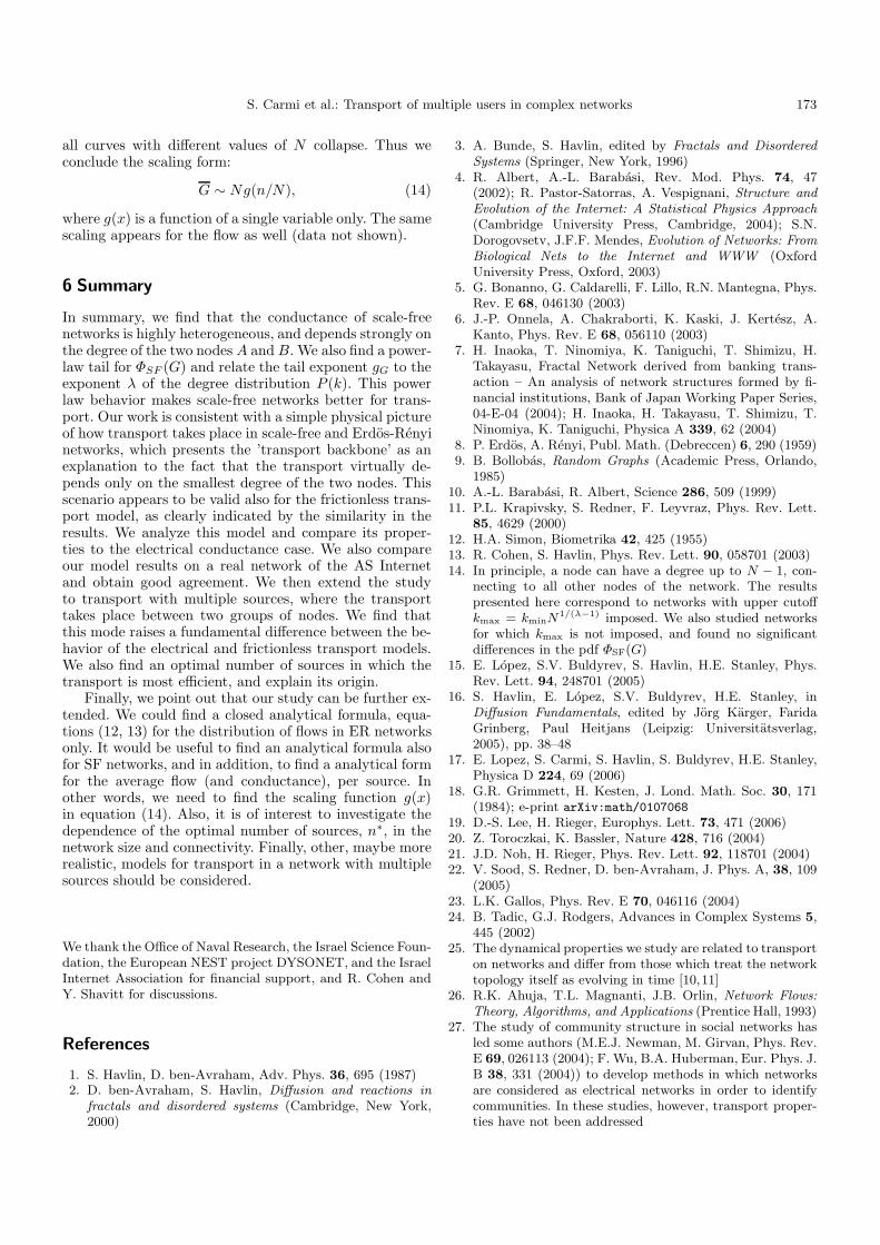
A scaling law for the conductance with multiplesources, is seen when properly scaling the conductance andthe number of sources. Plotting G/N vs. n/N , (Fig. 11),


all curves with different values of N collapse. Thus weconclude the scaling form:

G ∼ Ng(n/N), (14)

where g(x) is a function of a single variable only. The samescaling appears for the flow as well (data not shown).

6 Summary

In summary, we find that the conductance of scale-freenetworks is highly heterogeneous, and depends strongly onthe degree of the two nodes A and B. We also find a power-law tail for ΦSF (G) and relate the tail exponent gG to theexponent λ of the degree distribution P (k). This powerlaw behavior makes scale-free networks better for trans-port. Our work is consistent with a simple physical pictureof how transport takes place in scale-free and Erdos-Renyinetworks, which presents the ’transport backbone’ as anexplanation to the fact that the transport virtually de-pends only on the smallest degree of the two nodes. Thisscenario appears to be valid also for the frictionless trans-port model, as clearly indicated by the similarity in theresults. We analyze this model and compare its proper-ties to the electrical conductance case. We also compareour model results on a real network of the AS Internetand obtain good agreement. We then extend the studyto transport with multiple sources, where the transporttakes place between two groups of nodes. We find thatthis mode raises a fundamental difference between the be-havior of the electrical and frictionless transport models.We also find an optimal number of sources in which thetransport is most efficient, and explain its origin.

Finally, we point out that our study can be further ex-tended. We could find a closed analytical formula, equa-tions (12, 13) for the distribution of flows in ER networksonly. It would be useful to find an analytical formula alsofor SF networks, and in addition, to find a analytical formfor the average flow (and conductance), per source. Inother words, we need to find the scaling function g(x)in equation (14). Also, it is of interest to investigate thedependence of the optimal number of sources, n∗, in thenetwork size and connectivity. Finally, other, maybe morerealistic, models for transport in a network with multiplesources should be considered.

We thank the Office of Naval Research, the Israel Science Foun-dation, the European NEST project DYSONET, and the IsraelInternet Association for financial support, and R. Cohen andY. Shavitt for discussions.

References

1. S. Havlin, D. ben-Avraham, Adv. Phys. 36, 695 (1987)2. D. ben-Avraham, S. Havlin, Diffusion and reactions in

fractals and disordered systems (Cambridge, New York,2000)

3. A. Bunde, S. Havlin, edited by Fractals and DisorderedSystems (Springer, New York, 1996)

4. R. Albert, A.-L. Barabasi, Rev. Mod. Phys. 74, 47(2002); R. Pastor-Satorras, A. Vespignani, Structure andEvolution of the Internet: A Statistical Physics Approach(Cambridge University Press, Cambridge, 2004); S.N.Dorogovsetv, J.F.F. Mendes, Evolution of Networks: FromBiological Nets to the Internet and WWW (OxfordUniversity Press, Oxford, 2003)

5. G. Bonanno, G. Caldarelli, F. Lillo, R.N. Mantegna, Phys.Rev. E 68, 046130 (2003)

6. J.-P. Onnela, A. Chakraborti, K. Kaski, J. Kertesz, A.Kanto, Phys. Rev. E 68, 056110 (2003)

7. H. Inaoka, T. Ninomiya, K. Taniguchi, T. Shimizu, H.Takayasu, Fractal Network derived from banking trans-action – An analysis of network structures formed by fi-nancial institutions, Bank of Japan Working Paper Series,04-E-04 (2004); H. Inaoka, H. Takayasu, T. Shimizu, T.Ninomiya, K. Taniguchi, Physica A 339, 62 (2004)

8. P. Erdos, A. Renyi, Publ. Math. (Debreccen) 6, 290 (1959)9. B. Bollobas, Random Graphs (Academic Press, Orlando,

1985)10. A.-L. Barabasi, R. Albert, Science 286, 509 (1999)11. P.L. Krapivsky, S. Redner, F. Leyvraz, Phys. Rev. Lett.

85, 4629 (2000)12. H.A. Simon, Biometrika 42, 425 (1955)13. R. Cohen, S. Havlin, Phys. Rev. Lett. 90, 058701 (2003)14. In principle, a node can have a degree up to N − 1, con-

necting to all other nodes of the network. The resultspresented here correspond to networks with upper cutoffkmax = kminN1/(λ−1) imposed. We also studied networksfor which kmax is not imposed, and found no significantdifferences in the pdf ΦSF(G)

15. E. Lopez, S.V. Buldyrev, S. Havlin, H.E. Stanley, Phys.Rev. Lett. 94, 248701 (2005)

16. S. Havlin, E. Lopez, S.V. Buldyrev, H.E. Stanley, inDiffusion Fundamentals, edited by Jorg Karger, FaridaGrinberg, Paul Heitjans (Leipzig: Universitatsverlag,2005), pp. 38–48

17. E. Lopez, S. Carmi, S. Havlin, S. Buldyrev, H.E. Stanley,Physica D 224, 69 (2006)

18. G.R. Grimmett, H. Kesten, J. Lond. Math. Soc. 30, 171(1984); e-print arXiv:math/0107068

19. D.-S. Lee, H. Rieger, Europhys. Lett. 73, 471 (2006)20. Z. Toroczkai, K. Bassler, Nature 428, 716 (2004)21. J.D. Noh, H. Rieger, Phys. Rev. Lett. 92, 118701 (2004)22. V. Sood, S. Redner, D. ben-Avraham, J. Phys. A, 38, 109

(2005)23. L.K. Gallos, Phys. Rev. E 70, 046116 (2004)24. B. Tadic, G.J. Rodgers, Advances in Complex Systems 5,

445 (2002)25. The dynamical properties we study are related to transport

on networks and differ from those which treat the networktopology itself as evolving in time [10,11]

26. R.K. Ahuja, T.L. Magnanti, J.B. Orlin, Network Flows:Theory, Algorithms, and Applications (Prentice Hall, 1993)

27. The study of community structure in social networks hasled some authors (M.E.J. Newman, M. Girvan, Phys. Rev.E 69, 026113 (2004); F. Wu, B.A. Huberman, Eur. Phys. J.B 38, 331 (2004)) to develop methods in which networksare considered as electrical networks in order to identifycommunities. In these studies, however, transport proper-ties have not been addressed


28. M. Molloy, B. Reed, Random Struct. Algorithms 6, 161(1995)

29. G. Kirchhoff, Ann. Phys. Chem. 72 497 (1847); N.Balabanian, Electric Circuits (McGraw-Hill, New York,1994)

30. S. Kirkpatrick, Proceedings of InhomogeneousSuperconductors Conference, Berkeley Springs, W.Va, edited by S.A. Wolf, D.U. Gubser, A.I.P. Conf. Procs.58, 79 (1979)

31. B.V. Cherkassky, Algorithmica 19, 390 (1997)32. Z. Wu, L.A. Braunstein, S. Havlin, H.E. Stanley, Phys.

Rev. Lett. 96, 148702 (2006)33. S. Carmi, S. Havlin, S. Kirkpatrick, Y. Shavitt, E. Shir,

MEDUSA - New Model of Internet Topology Using k-shellDecomposition, arXiv:cond-mat/0601240

34. Y. Shavitt, E. Shir, ACM SIGCOMM ComputerCommunication Review, 35, 71 (2005)

transport between multiple users in complex networks

Documents