transient response to increasing river runoff and precipitation

Arctic Ocean Freshwater Dynamics: Transient Responseto Increasing River Runoff and Precipitation

Nicola Jane Brown1 , Johan Nilsson2 , and Per Pemberton3

1Ocean and Earth Science, University of Southampton, Southampton, UK, 2Department of Meteorology, StockholmUniversity, Stockholm, Sweden, 3Oceanographic Research Unit, Swedish Meteorological and Hydrological Institute,Gothenburg, Sweden

Abstract Simulations from a coupled ice-ocean general circulation model are used to assess the effectson Arctic Ocean freshwater storage of changes in freshwater input through river runoff and precipitation.We employ the climate response function framework to examine responses of freshwater content to abruptchanges in freshwater input. To the lowest order, the response of ocean freshwater content is linear, withan adjustment time scale of approximately 10 years, indicating that anomalies in Arctic Ocean freshwaterexport are proportional to anomalies in freshwater content. However, the details of the transient responseof the ocean depend on the source of freshwater input. An increase in river runoff results in a fairly smoothresponse in freshwater storage consistent with an essentially linear relation between total freshwatercontent and discharge of excess freshwater through the main export straits. However, the response to achange in precipitation is subject to greater complexity, which can be explained by the localized formationand subsequent export of salinity anomalies which introduce additional response time scales. The resultspresented here suggest that future increases in Arctic Ocean freshwater input in the form of precipitationare more likely to be associated with variability in the storage and release of excess freshwater than areincreases in freshwater input from river runoff.

Plain Language Summary This paper shows that the Arctic Ocean adjusts to changes infreshwater input over time scales of about one decade. How much of the added freshwater is stored in theArctic depends, however, on how the freshwater enters the ocean. If it arrives as additional river runoff, theresponse in Arctic freshwater storage is relatively smooth and predictable. If it falls, instead, as increasedprecipitation, the response is less easy to predict because it is complicated by interactions between theocean and sea ice. This is important because the part of the freshwater that is not stored in the Arctic Oceanis exported to the North Atlantic, where it can affect the global ocean circulation.

1. IntroductionThe Arctic Ocean has a major influence on global circulation through the provision of dense waters to supplydeep convection in the Nordic and Labrador seas (Yang et al., 2016). The net effect of the Arctic is to cool andfreshen relatively warm, saline water flowing in via the Fram Strait or Barents Sea from the Atlantic (Rudelset al., 2013), before it returns southward either through the Fram Strait or the Canadian Arctic Archipelago(CAA). Some water returns denser than it entered, some lighter, a two-fold influence that has been describedas driving a double estuarine circulation (Eldevik & Nilsen, 2013).

Densification of inflowing Atlantic Water occurs mainly through surface heat loss in the Barents Sea (Rudels,2010). Across most of the rest of the Arctic Ocean, the Atlantic Water layer is overlain by a lighter, freshersurface layer, formed through the influx of freshwater. The largest source of freshwater input is runoff fromrivers around the continental margins of Siberia and North America, amounting to ∼4,200 km3/year dur-ing the period 2000–2010. Net precipitation contributes a further ∼2200 km3/year (Haine et al., 2015). Theinflow of Pacific Water through the Bering Strait also serves as a source of freshwater, since its salinity islower than that of Atlantic Water; it contributed∼2,600 km3/year with respect to a reference salinity of 34.80in 2000–2010 (Haine et al., 2015; Woodgate et al., 2005).

Sources and sinks of freshwater are not typically in constant balance, and the proportion of freshwater inputretained within the Arctic Ocean rather than being exported directly varies on time scales of O(1–10) years

RESEARCH ARTICLE10.1029/2018JC014923

Special Section:Forum for Arctic Modeling andObservational Synthesis (FAMOS)2: Beaufort Gyre phenomenon

Key Points:• Response of freshwater content

to change in freshwater inputapproximated by a response functionwith e-folding time scale of about10 years

• Detail of the response depends onthe source of freshwater input and itsassociated spatial anomalies, whichintroduce secondary time scales

• Response for precipitation is morecomplex than for river runoff becauseof a more complex footprint that alsoinfluences net sea ice growth

Correspondence to:N. J. Brown,[email protected]

Citation:Brown, N. J., Nilsson, J., &Pemberton, P. (2019). Arctic Oceanfreshwater dynamics: Transientresponse to increasing river runoff andprecipitation. Journal of GeophysicalResearch: Oceans, 124, 5205–5219.https://doi.org/10.1029/2018JC014923

Received 28 DEC 2018Accepted 15 JUN 2019Accepted article online 21 JUN 2019Published online 25 JUL 2019

©2019. American Geophysical Union.All Rights Reserved.

BROWN ET AL. 5205

Journal of Geophysical Research: Oceans 10.1029/2018JC014923

(Proshutinsky et al., 2009). This periodic storage and release has been linked to variation in circulationdriven by cyclical changes in wind patterns both in the Beaufort Sea region and across the Siberian shelves(Haine et al., 2015; Morison et al., 2012; Polyakov et al., 2008). More generally, Johnson et al. (2018) find thatthe variability of Arctic freshwater content (FWC) in recent years can be explained chiefly by the influenceof sea level pressure variations on sources, sinks, and storage of freshwater. Proshutinsky et al. (2009) notethat the range of variation of freshwater storage has increased since 2003 and suggest that it could continueto do so as climate change intensifies.

The warming global climate is also driving increasing freshwater input to the Arctic Ocean (Bintanja &Selten, 2014; Vavrus et al., 2012). River runoff is projected to reach 5,500 km3/year and net precipitation2,500 km3/year by 2100 (Haine et al., 2015), and increases in Pacific Water inflow are also expected. Whilethe influence of wind patterns on freshwater storage has benefitted from much recent investigation, the roleof freshwater as a modifier of ocean circulation in its own right, rather than as a passive tracer of wind-drivencurrents, has received less attention. As Morison et al. (2012) observed, variation in the wind-driven Ekmanpumping over the Beaufort Gyre region might be the main factor controlling the freshwater storage in theGyre, but additional processes such as baroclinic eddies and mechanical ice-ocean feedbacks (Dewey et al.,2018; Manucharyan & Spall, 2016; Meneghello et al., 2017) influence the FWC of the Gyre.

A steady-state modeling study by Pemberton and Nilsson (2016) showed that increased freshwater supplyfrom runoff and precipitation results in a weakening of the Beaufort Gyre and a redirection of some fresh-water export from the CAA to the Fram Strait. Nummelin et al. (2016) found a similar weakening of theanticyclonic surface circulation in simulations of increased runoff while noting also that the strengthen-ing of the Arctic Ocean stratification caused by the increased freshwater input leads to a reduction in thetransfer of anticyclonic atmospheric momentum to the Atlantic Water layer below the halocline and thusa strengthening of the cyclonic Atlantic Water circulation. Increased runoff has also been shown (Lambertet al., 2019) to affect various processes associated with the diffusion of heat and salt, leading ultimately toan increase in the advective heat and salt import into the Arctic. Given the influence that increasing fresh-water input appears to have on circulation patterns, there is a need for an improved understanding of theeffect that enhanced freshwater input is likely to have on Arctic storage of freshwater and its release to thenorth Atlantic.

Previous studies have considered the long-term response of the ocean to changes in forcing. For that reason,we focus here on the transient response: We draw on the “climate response function” (CRF) frameworkdescribed by Marshall et al. (2017), using simulations from a coupled ice-ocean general circulation model(GCM) to investigate the relationship between changes in freshwater input to the ocean and the responseof the ocean in terms of storage and export of freshwater. The rationale for the CRF methodology is that ifthe transient response (the CRF) of an observable to step function forcing is known, the CRF may then beconvolved with any more realistic time history of forcing to determine a predicted linear response for thatobservable. Note that the CRF is convolved with the time derivative of the forcing (Marshall et al., 2017).The impulse response function, which is the time derivative of the CRF, is convolved with the forcing itselfto give the response. We take as our observables here the FWC of the Arctic Ocean in liquid and sea ice formand the export of freshwater through key straits. We apply step change perturbations to the freshwater inputfrom river runoff and precipitation to examine the time scales, pathways, and mechanisms governing thelikely response of the ocean to changes in freshwater input.

2. Method and Theoretical Background2.1. General Circulation ModelIn this study we have used a coupled ice-ocean model, the Massachusetts Institute of Technology generalcirculation model (MITgcm), in a regional configuration covering the Arctic Ocean and parts of the NorthAtlantic and North Pacific oceans north of ∼ 55◦N. This model setup has been used in a number of previ-ous studies (e.g., Condron et al., 2009; Manizza et al., 2009; Nguyen et al., 2011), and Condron et al. (2009)showed that it reasonably reproduces the Arctic Ocean freshwater budget. The horizontal grid spacingwithin the model domain (see Figure 1) is ∼18 km, and the model grid has 50 vertical layers with thicknessranging from 10 m at the surface to ∼450 m for the deepest layer. Further details of the model setup are

BROWN ET AL. 5206


Figure 1. The boundaries of the model domain within which perturbationsof surface freshwater input were made are indicated by red lines. Theshading shows bathymetry. AG = Amundsen Gulf; MS = McClure Strait;CAA = Canadian Arctic Archipelago; NS = Nares Strait; FS = Fram Strait;BSO = Barents Sea Opening).

given in Pemberton and Nilsson (2016), and the model parametersemployed are as described in Nguyen et al. (2011).

2.2. Model SimulationsOcean forcing for the majority of the simulations described here was pro-vided by the Japanese 25-year Reanalysis (JRA-25; Onogi et al., 2007),which covers the period 1979–2004, extended for a further 9 years to2013 using operational analysis from the same model system. For asmall number of additional simulations, the model was instead forcedwith a repeating annual cycle of atmospheric forcing (the CoordinatedOcean-Ice Reference Experiments (CORE) II corrected normal year forc-ing; Griffies et al., 2009). For river runoff data, we used a monthlyclimatology derived from Arctic Runoff Database raw data and adjustedto account for ungauged river flows, as described in Nguyen et al. (2011).The model was initialized for each simulation using sea ice conditionsfrom the Polar Science Center (Zhang & Rothrock, 2003) and ocean con-ditions from the World Ocean Atlas 2005 (Antonov et al., 2006; Locarniniet al., 2006).

The model was first run for 35 years in a control simulation, using theforcing described above to represent the state of the Arctic in the latetwentieth century. To test the response of the ocean to an abrupt change infreshwater input, further simulations were then run in which river runoffor precipitation was increased or decreased by a fixed proportion (−30%to +100% for runoff and −30% or +30% for precipitation) of the controlforcing for the duration of the simulation. The larger increases are greaterthan those expected to be seen in the real future Arctic but were includedin the suite of simulations to test the linearity of the response. Evapora-

tion and sea ice formation and melt were not perturbed directly through forcing but evolved during thesimulations in response to the perturbation of runoff or precipitation.

For each simulation, monthly means of freshwater height (HF) and liquid FWC (VF) were calculated:

HF(x, 𝑦, t) = ∫0

−H0

Sref − S(x, 𝑦, z, t)Sref

dz, (1)

VF(t) = ∫AHF(x, 𝑦, t)dA, (2)

where z is depth, S salinity, and A the horizontal area of the basin. The reference salinity, Sref, was taken tobe 35.0 g/kg. The integrations were performed to a depth −H0 of −277 m, indicative of the upper surface ofthe Atlantic Water layer. Where storage of freshwater in sea ice is discussed, an equivalent FWC has beencalculated from stored sea ice volumes assuming a sea ice density of 900 kg/m3 and salinity of 6.0 g/kg.

2.3. A Conceptual Model for Rotationally Controlled ExportWe have compared the ocean freshwater response in the model simulations described above to theoreticalpredictions given by a simple conceptual model such as described by Stigebrandt (1981), Nilsson and Walin(2010), and Rudels (2010). A key issue is whether the CRF to perturbations in freshwater input will, to thelowest order, depend only on the anomaly of the total FWC, as assumed in the conceptual model, or if spatialvariations matter. Further, is the response independent of wind-forcing regimes over the Arctic Ocean?

The version of the conceptual model that we have adopted here represents the Arctic Ocean as stratifiedby salinity into two layers separated by a halocline at constant depth H: a fresher, upper layer of salinity S1above the halocline and a layer of Atlantic Water with salinity SA below. In the model, the freshwater exportdepends on the net Arctic FWC and a simple representation of wind forcing in the basin. The final resultis a further simplified linearized model, in which perturbations in freshwater export and net content arelinearly related. Despite these simplifications, the model yields a leading-order description of how the netArctic Ocean FWC in the ocean circulation model responds to changes in the freshwater input, as will beshown below.

BROWN ET AL. 5207


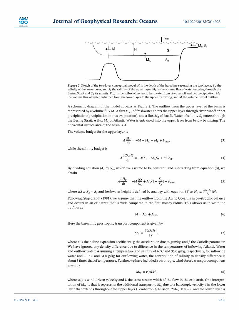
Figure 2. Sketch of the two-layer conceptual model. H is the depth of the halocline separating the two layers, SA thesalinity of the lower layer, and S1 the salinity of the upper layer. MB is the volume flux of water entering through theBering Strait and SB its salinity. Fmet is the influx of meteoric freshwater from river runoff and net precipitation, MAthe volume flux of water entrained from the lower layer to the upper by mixing, and M the volume flux of outflow.

A schematic diagram of the model appears as Figure 2. The outflow from the upper layer of the basin isrepresented by a volume flux M. A flux Fmet of freshwater enters the upper layer through river runoff or netprecipitation (precipitation minus evaporation), and a flux MB of Pacific Water of salinity SB enters throughthe Bering Strait. A flux MA of Atlantic Water is entrained into the upper layer from below by mixing. Thehorizontal surface area of the basin is A.

The volume budget for the upper layer is

A dHdt

= −M + MA + MB + Fmet, (3)

while the salinity budget is

Ad(S1H)

dt= −MS1 + MASA + MBSB. (4)

By dividing equation (4) by SA, which we assume to be constant, and subtracting from equation (3), weobtain

AdHF

dt= −MΔS

SA+ MB(1 −

SB

SA) + Fmet, (5)

where ΔS ≡ SA − S1 and freshwater height is defined by analogy with equation (1) as HF ≡ ( SA−S1SA

)H.

Following Stigebrandt (1981), we assume that the outflow from the Arctic Ocean is in geostrophic balanceand occurs in an exit strait that is wide compared to the first Rossby radius. This allows us to write theoutflow as

M = MG + MW. (6)

Here the baroclinic geostrophic transport component is given by

MG =𝛽ΔSgH2

2𝑓, (7)

where 𝛽 is the haline expansion coefficient, g the acceleration due to gravity, and f the Coriolis parameter.We have ignored any density difference due to difference in the temperatures of inflowing Atlantic Waterand outflow water: Assuming a temperature and salinity of 6 ◦C and 35.0 g/kg, respectively, for inflowingwater and −1 ◦C and 31.0 g/kg for outflowing water, the contribution of salinity to density difference isabout 5 times that of temperature. Further, we have included a barotropic, wind-forced transport componentgiven by

MW = v(t)LH, (8)

where v(t) is wind-driven velocity and L the cross-stream width of the flow in the exit strait. One interpre-tation of MW is that it represents the additional transport to MG due to a barotropic velocity v in the lowerlayer that extends throughout the upper layer (Pemberton & Nilsson, 2016). If v = 0 and the lower layer is

BROWN ET AL. 5208


at rest, then the outflow is given solely by the baroclinic component MG. A more general view is that v(t)reflects how wind forcing over the basin influences the outflow and storage of freshwater. In periods withmore cyclonic wind forcing over the Arctic Ocean, the FWC tends to decrease and vice versa (Haine et al.,2015). Crudely, the effect of changing wind forcing can be represented by making v(t) larger for cyclonicwind regimes and smaller for anticyclonic regimes. We write

v(t) = v0 + Δv(t), (9)

where v0 is related to the long-term time mean winds and Δv(t) to time-varying winds. Observations andmodeling suggest that low-frequency wind variations over the Arctic Ocean result in relative changes in theFWC of some 10% to 20% (Haine et al., 2015; Johnson et al., 2018; Pemberton & Nilsson, 2016; Stewart &Haine, 2013). Accordingly, we expect that |Δv(t)|∕v(t) in this simple model should also be allowed to vary byabout 10% to 20%, implying that |Δv(t)| should be small compared to v0. Substituting into equation (5) anddefining F ≡ MB(1 − SB

SA) + Fmet yields

AdHF

dt= −

𝛽gSAHF2

2𝑓− v(t)LHF + F. (10)

Now consider the effect of a perturbation,ΔF, in freshwater input, leading to an anomaly, 𝛥HF, in freshwaterheight. Equation (10) as applied to the perturbed state becomes

Ad(HF + ΔHF)

dt= −

𝛽gSA(HF + ΔHF)2

2𝑓− v(t)L(HF + ΔHF) + F + ΔF. (11)

We assume that if the perturbation ΔF is small, the resultant anomaly will also be HF ≫ ΔHF, so that

(HF + ΔHF)2 ≈ HF2 + 2HFΔHF. (12)

Linearizing equation (11) accordingly and subtracting equation (10), we have

dΔHF

dt= −

𝛽gSAHFΔHF

A𝑓−

(v0 + Δv(t))LΔHF

A+ ΔF

A. (13)

If we further assume that v0 ≫ |Δv(t)|, this equation simplifies to

dΔHF

dt= −𝜏−1ΔHF + ΔF

A, (14)

where we have introduced the response time scale 𝜏:

𝜏 ≡(𝛽gSAHF𝑓

−1 + v0LA

)−1

. (15)

The (climate) response function to equation (14), describing the response to a step function freshwaterperturbation (Marshall et al., 2017), is

CRF(t) = 1 − exp(−t∕𝜏) (16)

for t ≥ 0 and 0 for t < 0. Thus, in this limit of weak wind variations (i.e., v0 ≫ |Δv(t)|), the conceptual modelpredicts an exponential adjustment of forced freshwater perturbations over a time scale that is essentiallyindependent of the variations of the wind field. Note that the time scale depends on the background statefreshwater height HF, which according to equation (10) responds to wind variations represented by the term𝛥v(t). As noted above, observed fractional changes of FWC on interannual to decadal scales, presumablydriven by wind variations, are only about 10% to 20% (Haine et al., 2015; Morison et al., 2012). This suggeststhat in the present conceptual model, a climatological constant value of HF can be used to approximate 𝜏.

Next, we consider the time scale of the response function predicted by the conceptual model. In the lim-iting case when v0 = 0, the response time scale defined by equation (17) is set by the geostrophic flow(Rudels, 2010):

𝜏G = A𝑓

𝛽gSAHF. (17)

BROWN ET AL. 5209


Figure 3. Time-mean freshwater height, HF, in meters for the final decade of the reference simulation, integrated to adepth of −277 m, with Sref = 35.0 g/kg. White arrows indicate major currents in the upper 100 m.

Inserting typical values for the Arctic (𝛽 = 8 × 10−4, f = 1.4 × 10−4s−1,A = 9 × 1012m2, g = 10 m/s2, SA =

35.0 g/kg) into this expression and estimating HF by dividing a freshwater volume of 8 × 104 km3 fromPemberton and Nilsson (2016) by A give a predicted time scale of 16 years.

We may compare this predicted time scale with that implied by steady state in any system involving storageand flux, the ratio of the two giving a mean residence time. From the steady-state version of equation (10),still with v = 0, the geostrophic adjustment time scale in equation (17) may be written as

𝜏G =AHF

2F= 1

2×

Liquid FWCNet freshwater supply

. (18)

(The factor of a half derives from the assumption that outflow from the Arctic is governed by geostrophy.)An increase in HF increases both the volume export and the salinity export anomaly, which yields a shorter𝜏. Adopting estimates of net freshwater input from meteoric sources and from Bering Strait inflow fromPemberton and Nilsson (2016) leads to an alternative predicted time scale of 12 years.

Equation (15) shows that 𝜏 decreases with the wind-related velocity v0. In the limit when the geostrophiccontribution becomes negligible compared to the wind-driven component, the steady-state version ofequation (10) yields

𝜏W =AHF

F=

Liquid FWCNet freshwater supply

, (19)

implying a predicted 𝜏 of 24 years if the same estimates of net freshwater input as for the case of geostrophicexport are assumed. This confirms that 𝜏 in the conceptual model is proportional to the FWC dividedby the net freshwater supply regardless of the relative magnitudes of the geostrophic transport MG andthe wind-driven transport MW; however, the constant of proportionality varies depending on whethergeostrophic or wind-driven transport dominates, being 1/2 for purely geostrophic flow and 1 for purelybarotropic wind-driven flow.

We compare these predictions of the net FWC with the response seen in the experiments performed usingthe general circulation model and investigate neglected physics that might lead to any departure from thepredictions of the conceptual model.

BROWN ET AL. 5210


3. ResultsTypical spatial variability in liquid FWC, VF, can be seen in Figure 3, which shows mean depth-integratedfreshwater height, HF, for the final 10 years of the control simulation. The concentration of freshwater inthe Canada Basin, and in particular in the region occupied by the Beaufort Gyre, is clearly visible.

3.1. Reference SimulationThe evolution of liquid FWC, VF, for the reference simulation over the simulation period is shown inFigure 4a. Monthly mean VF is denoted by the thinner line, while the heavier line represents a 12-monthrunning mean. Annual mean volumes range from around 75 × 103 to 85 × 103 km3 over the 35-year period.There is a marked seasonal cycle of amplitude around 7×103 km3, or about 9% of the mean volume, with VFreaching a seasonal maximum in September/October and minimum in May/June of each year; we attributethis to the seasonal storage of freshwater in sea ice.

As has been discussed briefly by Pemberton and Nilsson (2016), we also note significant variability in VF overdecadal scales. The annual mean volume is at the upper end of its range at the beginning of the simulationperiod and remains reasonably level for the first decade. It then falls by about 10×103 km3 between years 10and 18 (representing the period 1989 to 1997), accompanied by a decline in sea ice FWC (see Figure 5a). Fromyear 18 to year 33 (1997 to 2012), a steady increase in VF is seen, partially compensated by a continued fallin sea ice FWC. The pattern seen in the latter half of the simulation is consistent with an increase in ArcticOcean liquid FWC seen in observations (Haine et al., 2015) since the 1990s. Rabe et al. (2011) accountedfor an increase in the central Arctic basin through strengthened regional Ekman pumping lowering thelower halocline (as described by Proshutinsky et al., 2009) and freshening of the water above the haloclinethrough sea ice melt, as we find in the current simulations. (Rabe et al., 2011, also discussed the advectionof extra river water from the Siberian shelves to the deep Arctic Ocean, but the integrated VF totals quotedhere include the shelf areas, and so such a redistribution of freshwater does not affect them.)

We investigate the response of the ocean to changing freshwater input by running further simulations inwhich runoff or precipitation is increased or decreased by a fixed proportion of the control forcing. Thesechanges are introduced without specifically addressing what atmospheric circulation regime changes orclimate change patterns may cause the perturbations of the freshwater supply. Global warming, whichamplifies the hydrological cycle and decreases the Arctic sea ice export (Haine et al., 2015; Held & Soden,2006), can increase the freshwater input to the Arctic Ocean essentially without any change in the time-meanatmospheric circulation. Through natural variability, river runoff is observed to increase primarily underthe atmospheric anticyclonic circulation regime, when trajectories of cyclones with moisture from theNorth Atlantic are shifted toward Siberia and runoff from Siberian rivers increases (Haine et al., 2015;Proshutinsky et al., 1999, 2015). Conversely, increased precipitation over the Arctic Ocean is expectedprimarily under cyclonic wind forcing regimes (Proshutinsky et al., 1999, 2015).

Rather than introducing combined step function changes in freshwater forcing and wind forcing consis-tent with the observed natural variability, we have performed freshwater perturbation experiments on abackground forcing provided by the observationally based time-varying JRA-25 (Onogi et al., 2007). Anunderlying assumption is that, to the lowest order, the response to changes in freshwater input is controlledby the time-mean features of the Arctic atmosphere-ocean circulation and hence can be studied using CRFsspecific to freshwater forcing. The linear response of the Arctic FWC to natural variability, or forced cli-mate change, can in principle be described by convolutions of the time history of wind and freshwaterforcing with their respective CRFs (Marshall et al., 2017). Hence, our simulations may reveal informationon aspects of the CRFs for freshwater forcing that depend primarily on the time-mean state of the atmo-spheric circulation. To examine the sensitivity to variations in atmospheric forcing, we also briefly report theresult of additional simulations forced with a repeating annual cycle of atmospheric forcing: the CORE-IIcorrected normal year forcing (Griffies et al., 2009). Here the freshwater perturbations in the simulationsevolve under an atmospheric forcing without any interannual variations, which may help to reveal the sen-sitivity of the freshwater response to wind variations. Note that the freshwater inputs from river runoff andprecipitation have seasonal cycles. Thus, in the simulations with step function increases of the freshwaterinputs, there will be changes of both the time mean and seasonality of the freshwater forcing. As will be dis-cussed below, however, the change of the time mean freshwater input tends to dominate the response of theFWC anomalies.

BROWN ET AL. 5211


Figure 4. Time evolution in years of (a) VF in the reference simulation; (b) anomaly of VF with respect to the referencesimulation in the simulations involving perturbation of river runoff; and (c) anomaly of VF with respect to thereference simulation in the simulations involving perturbation of precipitation. In (a), monthly mean VF is shown bythe thinner black line, while the heavier line denotes a 12-month running mean. In (b), the solid lines indicate VFanomalies resulting from runoff perturbations as indicated in the panel, normalized by the proportionate size of theperturbation to be equivalent to a 30% increase. The dashed gray line represents an averaged ideal exponentialevolution fitted to the first 10 years of the simulations. In (c), the blue and red solid lines relate to simulations forced, asfor the runoff simulations, with JRA-25 data, while the green and purple lines relate to the equivalent simulationsusing CORE-II forcing, which has an annual cycle but no interannual variability. As in (b), negative anomalies fromexperiments involving decreased freshwater input have been flipped to the positive y axis. CORE = CoordinatedOcean-Ice Reference Experiments; JRA-25 = Japanese 25-year Reanalysis.

BROWN ET AL. 5212


Figure 5. Time evolution in years of (a) sea ice FWC in the reference simulation; (b) anomaly of sea ice FWC withrespect to the reference simulation in the simulations involving perturbation by ±30% of river runoff or precipitation.In (a), monthly mean FWC is shown by the thinner black line, while the heavier line denotes a 12-month runningmean. In (b), anomalies from experiments involving decreased freshwater input have been flipped on the y axis.FWC = freshwater content.

3.2. RunoffFigure 4b shows the evolving anomaly in liquid FWC relative to the control for the series of simulationsinvolving perturbed river runoff. Values for the anomalies are normalized by the sign and scale of perturba-tion to a 30% increase, that is to say, 𝛥VF = (VF(expt) − VF(control)) × (30%∕percentage increase in runoff).

As expected, a decrease in freshwater input results in a negative anomaly in VF compared to the control,while increases generate positive anomalies. The anomaly is close to proportional in magnitude to theperturbation of freshwater input, even for comparatively large perturbations. However, there is some asym-metry between negative and positive perturbations, and larger increases in runoff lead to proportionallyslightly smaller increases in VF anomaly, implying that an increasing proportion of the added freshwater isexported from the Arctic as freshwater input increases. In contrast to the precipitation experiments describedbelow, except in the earliest years of the simulations, when a signal of the strongly seasonal river input canbe detected, no annual cycle is apparent in the anomalies. Anomalies in sea ice volumes (Figure 5b) arenegligible, indicating that perturbation of freshwater input through river runoff has minimal effect on theseasonal storage of freshwater in sea ice. This is consistent with the linear freshwater dynamics describedby equation (14), which act as a low-pass filter: The seasonal change of the freshwater forcing is reducedroughly by a factor 𝜏year∕𝜏 relative to time mean change (see equation (5) and the ensuing discussion inMarshall et al., 2017), where 𝜏year is a year divided by 2𝜋. Taking 𝜏 ∼ 10 years and 𝜏year ∼ 1∕(2𝜋) years givesan amplitude of the seasonally varying response that is only a few percent of the time mean response.

The 35-year period of integration is not sufficiently long for a new equilibrium to be reached in each simula-tion, but we see that the adjustment is to first-order exponential. The mean time scale, calculated by fitting

BROWN ET AL. 5213


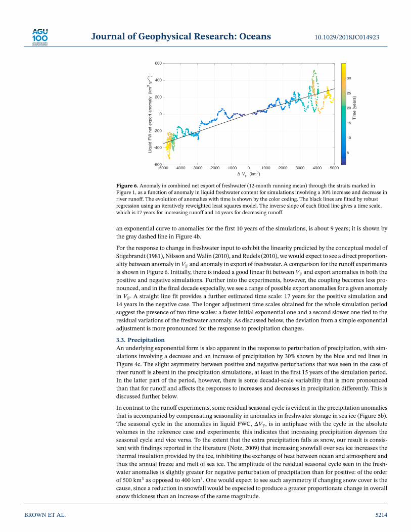
Figure 6. Anomaly in combined net export of freshwater (12-month running mean) through the straits marked inFigure 1, as a function of anomaly in liquid freshwater content for simulations involving a 30% increase and decrease inriver runoff. The evolution of anomalies with time is shown by the color coding. The black lines are fitted by robustregression using an iteratively reweighted least squares model. The inverse slope of each fitted line gives a time scale,which is 17 years for increasing runoff and 14 years for decreasing runoff.

an exponential curve to anomalies for the first 10 years of the simulations, is about 9 years; it is shown bythe gray dashed line in Figure 4b.

For the response to change in freshwater input to exhibit the linearity predicted by the conceptual model ofStigebrandt (1981), Nilsson and Walin (2010), and Rudels (2010), we would expect to see a direct proportion-ality between anomaly in VF and anomaly in export of freshwater. A comparison for the runoff experimentsis shown in Figure 6. Initially, there is indeed a good linear fit between VF and export anomalies in both thepositive and negative simulations. Further into the experiments, however, the coupling becomes less pro-nounced, and in the final decade especially, we see a range of possible export anomalies for a given anomalyin VF. A straight line fit provides a further estimated time scale: 17 years for the positive simulation and14 years in the negative case. The longer adjustment time scales obtained for the whole simulation periodsuggest the presence of two time scales: a faster initial exponential one and a second slower one tied to theresidual variations of the freshwater anomaly. As discussed below, the deviation from a simple exponentialadjustment is more pronounced for the response to precipitation changes.

3.3. PrecipitationAn underlying exponential form is also apparent in the response to perturbation of precipitation, with sim-ulations involving a decrease and an increase of precipitation by 30% shown by the blue and red lines inFigure 4c. The slight asymmetry between positive and negative perturbations that was seen in the case ofriver runoff is absent in the precipitation simulations, at least in the first 15 years of the simulation period.In the latter part of the period, however, there is some decadal-scale variability that is more pronouncedthan that for runoff and affects the responses to increases and decreases in precipitation differently. This isdiscussed further below.

In contrast to the runoff experiments, some residual seasonal cycle is evident in the precipitation anomaliesthat is accompanied by compensating seasonality in anomalies in freshwater storage in sea ice (Figure 5b).The seasonal cycle in the anomalies in liquid FWC, ΔVF, is in antiphase with the cycle in the absolutevolumes in the reference case and experiments; this indicates that increasing precipitation depresses theseasonal cycle and vice versa. To the extent that the extra precipitation falls as snow, our result is consis-tent with findings reported in the literature (Notz, 2009) that increasing snowfall over sea ice increases thethermal insulation provided by the ice, inhibiting the exchange of heat between ocean and atmosphere andthus the annual freeze and melt of sea ice. The amplitude of the residual seasonal cycle seen in the fresh-water anomalies is slightly greater for negative perturbation of precipitation than for positive: of the orderof 500 km3 as opposed to 400 km3. One would expect to see such asymmetry if changing snow cover is thecause, since a reduction in snowfall would be expected to produce a greater proportionate change in overallsnow thickness than an increase of the same magnitude.

BROWN ET AL. 5214


In the latter half of the period, as mentioned above, the response to perturbation of precipitation is lessclean than that to changing runoff. The more pronounced variability over interannual and decadal timescales apparent in the evolution of ΔVF is only in small part accounted for by variation in annual mean seaice freshwater storage. As we discussed in section 2.3, changes in the storage of freshwater in the BeaufortGyre are known to be associated with variation in atmospheric circulation over these time scales (severalauthors, summarized by Haine et al., 2015). We have therefore investigated whether the variability in ΔVFmight derive from the historical interannual variability in the JRA-25 reanalysis wind forcing by rerunningthe precipitation simulations with the climatological CORE-II forcing, which lacks interannual variability.Anomalies in VF from these further simulations are shown in green and purple in Figure 4c. Some of the vari-ability between 1989 and 1994, a period dominated by cyclonic atmospheric circulation, is eliminated, buta notable divergence in behavior in the positive and negative simulations is still apparent in the years 1998to 2002. In the simulations involving increased precipitation, ΔVF declines at this time because of enhancedexport of freshwater through the Fram Strait. This coincides with the appearance of a region of enhancedfreshwater height, HF, to the north of Greenland and just upstream of the Fram Strait. No correspondingsalinity anomaly or reduction in freshwater export is seen in the freshwater decrease experiments.

4. DiscussionA necessary condition for the applicability of the CRF methodology is a linear relationship between appliedforcing and observed response. The results of the simulations presented in section 3 demonstrate that thiscondition is well met, at least for the runoff simulations. We find that the CRF for the response of ArcticOcean FWC to a perturbation of river runoff approximates to an exponential equilibration with a time scaleof about 10 years. This figure accords with the bulk residence time (freshwater volume divided by rate ofinflow) for Eurasian runoff of 10 years determined by Pemberton et al. (2014) using tracer simulations andis in line with the comparator studies they quote, including Jahn et al. (2010).

The 10-year time scale of the CRF estimated from our simulations also corresponds reasonably well to the12- to 16-year estimates implied by the two-layer conceptual model for geostrophically controlled outflow(see equations (17) and (18)). As equation (19) indicated, were the outflow to be dominated instead by themean background wind state, the time scale predicted by the conceptual model would be longer than seenin the simulations. Haine et al. (2015) found that such a geostrophic model, when forced with observedvariations in freshwater supply, had only limited skill in explaining observed changes in Arctic Ocean FWC.Their results—and those we report here (see Figure 4a)—suggest that the observed changes were drivenby wind variations rather than by changes in freshwater input. (Even if outflow is not controlled by thelong-term mean wind state, its time-varying component may still be significant.) Consequently, the observedevolution of the FWC is expected to be controlled, primarily, by the forcing history of winds over the Arcticand their associated CRFs (Johnson et al., 2018). However, the current simulations have been designed toisolate CRFs for freshwater input, which illuminate different aspects of Arctic freshwater dynamics.

The first effects of changed freshwater input appear rapidly in the anomalies of freshwater export. A purelyexponential CRF would require freshwater export to respond immediately to changes in input, but in the realocean, we would of course expect a delay to allow a signal to be transmitted from the main input regions—theSiberian and Mackenzie River outflows in the case of runoff—to the export straits many hundreds of kilo-meters away. We have estimated the minimum time required for water of altered salinity to be advectedfrom the Siberian shelf to the Fram Strait by tracking salinity anomalies in the model along the TranspolarDrift. This is the most direct route and one along which higher than average current speeds are typicallyseen (see, e.g., Pemberton & Nilsson, 2016, Figure 3). Our estimates average about 4 years. Inspection ofthe transient VF anomalies shown in Figure 4b, however, reveals some curvature, implying that freshwaterexports start to respond and partially offset the perturbation of freshwater input, within the first 4 years ofthe simulations. An early evolution of export anomalies is also apparent in Figure 6, particularly for the sim-ulation involving increasing runoff. It is not possible to attribute these early export anomalies conclusivelyto a response to changing freshwater input, but our results do provide an indication of a response in exportsthat is triggered faster than an advection signal could be transmitted. Enhancements in freshwater exportcan have two possible causes: anomalously low salinity in the water flowing out through the straits and anincrease in the volumetric export of water of unchanged salinity. The first cannot explain the early changesin export, since salinity anomalies cannot travel faster than advection speed; however, the second could, if

BROWN ET AL. 5215


changes in freshwater input in the basin generated a dynamical signal that changed the outflow velocity atthe borders of the Arctic. This might propagate as a baroclinic Kelvin wave. Assuming a mode 1 baroclinicRossby radius, a1, of 10 km (Nurser & Bacon, 2014) and a Coriolis parameter, f , of 1.4 × 10−4 s−1, the propa-gation speed of such a wave, given by c1 = a1f (Gill, 1982), would be 1.4 m/s, allowing it to circumnavigatethe Arctic basin in about 60 days.

While the underlying form of the transient responses to changing runoff and precipitation is the same,there are also some differences which could offer some pointers to the processes responsible for deviationsfrom the first-order exponential form of the CRFs. A seasonal signal in VF anomaly due to changes to seaice growth is apparent only in the precipitation simulations, which exhibit more marked variability overdecadal scales than those involving perturbation of runoff. Could it be, therefore, that variability in liquidfreshwater storage is linked to changing storage of freshwater in sea ice form? Analysis of sea ice volumesin the precipitation experiments (Figure 5b) shows that this is not the case. After rapid adjustment over thefirst 2 to 3 years, anomalies in seasonally averaged sea ice freshwater storage remain largely constant overthe simulation period, and the annual mean anomalies do not, at any point, increase beyond 700 km3 inmagnitude for an increase in precipitation and 800 km3 for a decrease. This is smaller than the 1,300 km3

by which the anomaly in liquid freshwater storage decreases between years 20 and 27 in the simulation ofincreasing precipitation, indicating that the temporary shortfall in liquid freshwater cannot be accountedfor entirely by storage in sea ice.

The influence of changing wind patterns on VF in the control simulation (Figure 4a) leads us to considerwhether, alternatively, the variation in freshwater anomalies could be wind-driven. We note some departurefrom exponential form between years 10 and 18 in the JRA-25 forced simulations which is not reproducedin those forced with the climatological wind fields. This coincides with the rapid discharge in the controlsimulation; it is accompanied by enhanced net freshwater exports in the precipitation increase experimentsand depressed exports in the decrease experiments. In the terms of the conceptual model described in section2.3, the variability in FW export is consistent with a nonnegligible variation (Δv(t)) in wind-driven exportflow (see equation (13)). This would be expected initially to retard the growth in magnitude of the freshwaterheight anomaly,ΔHF; a decrease in background freshwater height, HF, would then cause the geostrophicallydriven component of freshwater export to decline, partially compensating for the increase in wind-drivenflow. Nevertheless, the more pronounced variability seen over the following decade is common to both thesimulations employing the observationally based, interannually varying JRA-25 forcing and those using theCORE-II climatology. This indicates that winds are not the primary cause of the variability and that we mustagain look elsewhere for an explanation.

As we showed in section 3.3, enhanced export of freshwater through the Fram Strait in the positive precip-itation experiment between years 19 and 23 was accompanied by the appearance of a region of enhancedHF just upstream of the strait. This leads us to consider a final hypothesis for the cause of the second orderform of the VF responses, which is suggestive of a secondary time scale: That it is due to the advection ofsalinity anomalies from source regions to the borders of the Arctic, where they lead to variability in fresh-water export. Some further insight may be gained by inspection of the evolving spatial variability in ΔVF.Figure 7 shows time mean ΔVF for the first and last decades of the JRA-25-forced simulations. Pembertonand Nilsson (2016) noted both the profound effect on freshwater height north of the CAA and Greenland,and the changes in the circulation and location of the Beaufort Gyre, that perturbation of freshwater inputcould generate. We observe from Figure 7 that these effects arise with differing time scales.

In the early stages of the runoff simulations (Figures 7a and 7c), we see an increase and decrease in fresh-water height in response to increasing and decreasing runoff, respectively, that are largely confined to theSiberian shelves where the bulk of the freshwater input occurs; later in the simulations (Figures 7e and 7g),a salinity signal is seen to spread along the main advection pathways. Marshall et al. (2017) had observedthat the FWC of the Beaufort Gyre is insensitive to an increase in river runoff, even when it is 3 times thesize of the largest we have introduced here. They inferred that most of the extra freshwater, rather than beingaccumulated in the Gyre, is transported via the Transpolar Drift to the Fram and Canadian straits. Our sim-ulation shows that ultimately much of the increase in freshwater height is seen upstream of these straits,supporting the conclusion of Marshall et al. (2017). In contrast, in computing the CRF for the FWC of theArctic basin as a whole, we find that sufficient freshwater is retained in other areas of the Arctic Ocean not

BROWN ET AL. 5216


Figure 7. Anomaly in freshwater height for simulations involving increases and decreases of river runoff and precipitation of 30%. (a) to (d) show time meansfor the first 10 years; (e) to (h) show time means for the last 10 years (colormap from cmocean, Thyng et al., 2016).

subject to large variability in storage conditions to show exponential relaxation toward a new, elevated levelof FWC.

This finding has implications for predictions of the effect on freshwater storage of future changes to windpatterns, both those driving Ekman pumping in the Beaufort Gyre region and those in the vicinity of theArctic straits which control the local currents exporting freshwater from the Arctic. Increasing freshwaterinput is expected to change the distribution of the freshwater pool on which those winds will act, shiftingfreshwater away from the Gyre and toward the main export straits.

The largest future change projected for the Arctic Ocean freshwater budget is reduced sea ice export (Hollandet al., 2007). Although we have not perturbed sea ice formation directly in the current simulations, we notethat observed reduction in new ice formation has a large signal over the Siberian shelf (Comiso, 2012). Wewould expect, therefore, that the footprint of the response of liquid freshwater to declining sea ice formationwill be similar to that of river runoff.

In the precipitation simulations, anomalies in freshwater height are seen in the early years in the Barentsand Kara seas where precipitation is the highest and the perturbations thus have the greatest magnitude;however, more pronounced changes are apparent across much of the Canada Basin and the region to thenorth of Greenland, areas where less precipitation occurs but sea ice tends to be the thickest. The rapidappearance of anomalies in this area contrasts with the runoff experiments, where the early response waslimited to the freshwater source regions. The pattern of the precipitation response accords with Pembertonand Nilsson (2016), who found that a decrease in precipitation ultimately leads to an increase in sea icethickness north of Greenland. As the salinity anomalies accumulating in these regions due to interactionswith sea ice are advected through the various export straits just to the south, they would be expected to leadto the variability in freshwater exports visible in Figure 6. They can thus explain several of the features seenin the CRFs, including the slight decline in ΔVF after 10–15 years in Figure 4c and the more pronounceddeclines in the latter part of the simulation period.

BROWN ET AL. 5217


A further potential source of complexity in the response is the time scale associated with alteration of themajor Arctic circulation pathways. Pemberton and Nilsson (2016) found that increasing freshwater inputleads to a decrease in the strength of the Beaufort Gyre circulation and a shift in export from the CAA tothe Fram Strait; Figure 7 shows that indications of these changes in the form of altered freshwater storagein the region of the Gyre are apparent only in the later years of the simulations.

5. ConclusionsWe have investigated the transient response of FWC in the Arctic Ocean to changing freshwater input, com-paring the effects of perturbation of river runoff and precipitation. We offer a CRF for river runoff, whichtakes the form of a simple exponential relaxation with a time scale of approximately 10 years. This agreeswith the predictions of a simple two-layer conceptual model for rotationally controlled export of freshwater.Although to first order sharing the exponential form of the runoff response, the response to changing pre-cipitation shows additional complexity consistent with a secondary time scale. We suggest that this is duein part to the greater importance of ocean-ice interactions in the precipitation case; these give rise to local-ized salinity anomalies which cause variability in freshwater exports when they are advected through thestraits at the boundaries of the Arctic. Regardless of the source of freshwater input, the response is largelyindependent of the wind-forcing regime over the Arctic Ocean.

Our results suggest that the fate of enhanced freshwater input to the Arctic and the proportion of extrafreshwater stored within the Arctic rather than being discharged immediately to the subpolar seas dependon the mode and footprint of this input. Although river runoff is projected to contribute a greater share offuture increases in freshwater input than is precipitation, we find that runoff produces a simpler transientresponse in terms of storage and export of freshwater. In the case of precipitation, a greater proportion ofthe supplied freshwater enters regions of the Arctic where interactions between the freshwater anomaliesand the sea ice and the mean circulation are more complicated. As a result, the transient response of thefreshwater storage to changes in precipitation is more complex than that related to changes in runoff. Suchis the importance of nonlinear interactions between the ocean and sea ice in the precipitation response thataccurate projections of the effect of future increases in precipitation will require models that can captureice-ocean interactions well.

ReferencesAntonov, J. I., Locarnini, R. A., Boyer, T. P., Mishonov, A. V., & Garcia, H. E. (2006). World Ocean Atlas 2005, volume 2: Salinity. In S.

Levitus (Ed.), NOAA Atlas NESDIS 62. Washington, DC: U.S. Government Printing Office.Bintanja, R., & Selten, F. M. (2014). Future increases in Arctic precipitation linked to local evaporation and sea-ice retreat. Nature,

509(7501), 479–482. https://doi.org/10.1038/nature13259Comiso, J. C. (2012). Large decadal decline of the Arctic multiyear ice cover. Journal of Climate, 25(4), 1176–1193. https://doi.org/10.1175/

JCLI-D-11-00113.1Condron, A., Winsor, P., Hill, C., & Menemenlis, D. (2009). Simulated response of the Arctic freshwater budget to extreme NAO wind

forcing. Journal of Climate, 22(9), 2422–2437. https://doi.org/10.1175/2008jcli2626.1Dewey, S., Morison, J., Kwok, R., Dickinson, S., Morison, D., & Andersen, R. (2018). Arctic ice-ocean coupling and gyre equilibration

observed with remote sensing. Geophysical Research Letters, 45, 1499–1508. https://doi.org/10.1002/2017gl076229Eldevik, T., & Nilsen, J. E. O. (2013). The Arctic-Atlantic thermohaline circulation. Journal of Climate, 26(21), 8698–8705. https://doi.org/

10.1175/JCLI-D-13-00305.1Gill, A. (1982). Atmosphere-ocean dynamics. San Diego, CA: Academic Press.Griffies, S. M., Biastoch, A., Boning, C., Bryan, F., Danabasoglu, G., Chassignet, E. P., et al. (2009). Coordinated Ocean-ice Reference

Experiments (COREs). Ocean Modelling, 26(1-2), 1–46. https://doi.org/10.1016/j.ocemod.2008.08.007Haine, T. W. N., Curry, B., Gerdes, R., Hansen, E., Karcher, M., Lee, C., et al. (2015). Arctic freshwater export: Status, mechanisms, and

prospects. Global and Planetary Change, 125, 13–35. https://doi.org/10.1016/j.gloplacha.2014.11.013Held, I. M., & Soden, B. J. (2006). Robust responses of the hydrological cycle to global warming. Journal of Climate, 19(21), 5686–5699.

https://doi.org/10.1175/Jcli3990Holland, M. M., Finnis, J., Barrett, A. P., & Serreze, M. C. (2007). Projected changes in Arctic Ocean freshwater budgets. Journal of

Geophysical Research, 112, G04S55. https://doi.org/10.1029/2006JG000354Jahn, A., Tremblay, L. B., Newton, R., Holland, M. M., Mysak, L. A., & Dmitrenko, I. A. (2010). A tracer study of the Arctic Ocean's liquid

freshwater export variability. Journal of Geophysical Research, 115, C07015. https://doi.org/10.1029/2009JC005873Johnson, H. L., Cornish, S. B., Kostov, Y., Beer, E., & Lique, C. (2018). Arctic Ocean freshwater content and its decadal memory of sea-level

pressure. Geophysical Research Letters, 45, 4991–5001. https://doi.org/10.1029/2017GL076870Lambert, E., Nummelin, A., Pemberton, P., & Ilicak, M. (2019). Tracing the imprint of river runoff variability on Arctic water mass

transformation. Journal of Geophysical Research: Oceans, 124, 302–319. https://doi.org/10.1029/2017jc013704Locarnini, R. A, Mishonov, A. V., Antonov, J. I., Boyer, T. P., & Garcia, H. E. (2006). World Ocean Atlas 2005, volume 1: Temperature. In S.

Levitus (Ed.), NOAA Atlas NESDIS 61. Washington, DC: U.S. Government Printing Office.Manizza, M., Follows, M. J., Dutkiewicz, S., McClelland, J. W., Menemenlis, D., Hill, C. N., et al. (2009). Modeling transport and fate of

riverine dissolved organic carbon in the Arctic Ocean. Global Biogeochemical Cycles, 23, GB4006. https://doi.org/10.1029/2008gb003396

AcknowledgmentsN. J. B. was supported by the UKNatural Environmental ResearchCouncil (Grant NE/L002531/1). J. N.acknowledges the support of theSwedish National Space Board. P. P. isfunded by NordForsk project NordicCenter of Excellence Arctic ClimatePrediction: Pathways to Resilient,Sustainable Societies (ARCPATH),Grant 76654. The model output used inthe analysis described in this paper isavailable online (http://doi.org/10.5281/zenodo.2648763). Analysis scriptscan be found online (https://github.com/njb1n12/Arctic-freshwater). Theauthors are grateful to AndreyProshutinsky and to the Editor andtwo anonymous reviewers whosecomments greatly improved the paper.

BROWN ET AL. 5218


Manucharyan, G. E., & Spall, M. A. (2016). Wind-driven freshwater buildup and release in the Beaufort Gyre constrained by mesoscaleeddies. Geophysical Research Letters, 43, 273–282. https://doi.org/10.1002/2015gl065957

Marshall, J., Scott, J., & Proshutinsky, A. (2017). “Climate response functions” for the Arctic Ocean: A proposed coordinated modellingexperiment. Geoscientific Model Development, 10(7), 2833–2848. https://doi.org/10.5194/gmd-10-2833-2017

Meneghello, G., Marshall, J., Cole, S. T., & Timmermans, M. L. (2017). Observational inferences of lateral eddy diffusivity in the haloclineof the Beaufort Gyre. Geophysical Research Letters, 44, 12,331–12,338. https://doi.org/10.1002/2017gl075126

Morison, J., Kwok, R., Peralta-Ferriz, C., Alkire, M., Rigor, I., Andersen, R., & Steele, M. (2012). Changing Arctic Ocean freshwaterpathways. Nature, 481(7379), 66–70. https://doi.org/10.1038/nature10705

Nguyen, A. T., Menemenlis, D., & Kwok, R. (2011). Arctic ice-ocean simulation with optimized model parameters: Approach andassessment. Journal of Geophysical Research, 116, C04025. https://doi.org/10.1029/2010JC006573

Nilsson, J., & Walin, G. (2010). Salinity-dominated thermohaline circulation in sill basins: Can two stable equilibria exist? Tellus SeriesA-Dynamic Meteorology and Oceanography, 62(2), 123–133. https://doi.org/10.1111/j.1600-0870.2009.00428.x

Notz, D. (2009). The future of ice sheets and sea ice: Between reversible retreat and unstoppable loss. Proceedings of the National Academyof Sciences of the United States of America, 106(49), 20,590–20,595. https://doi.org/10.1073/pnas.0902356106

Nummelin, A., Ilicak, M., Li, C., & Smedsrud, L. H. (2016). Consequences of future increased Arctic runoff on Arctic Ocean stratification,circulation, and sea ice cover. Journal of Geophysical Research: Oceans, 121, 617–637. https://doi.org/10.1002/2015jc011156

Nurser, A. J. G., & Bacon, S. (2014). The Rossby radius in the Arctic Ocean. Ocean Science, 10(6), 967–975. https://doi.org/10.5194/Os-10-967-2014

Onogi, K., Tslttsui, J., Koide, H., Sakamoto, M., Kobayashi, S., Hatsushika, H., et al. (2007). The JRA-25 reanalysis. Journal of theMeteorological Society of Japan, 85(3), 369–432. https://doi.org/10.2151/jmsj.85.369

Pemberton, P., & Nilsson, J. (2016). The response of the central Arctic Ocean stratification to freshwater perturbations. Journal ofGeophysical Research: Oceans, 121, 792–817. https://doi.org/10.1002/2015jc011003

Pemberton, P., Nilsson, J., & Meier, H. E. M. (2014). Arctic Ocean freshwater composition, pathways and transformations from a passivetracer simulation. Tellus Series A-Dynamic Meteorology and Oceanography, 66, 23988. https://doi.org/10.3402/tellusa.v66.23988

Polyakov, I. V., Alexeev, V. A., Belchansky, G. I., Dmitrenko, I. A., Ivanov, V. V., Kirillov, S. A., et al. (2008). Arctic Ocean freshwater changesover the past 100 years and their causes. Journal of Climate, 21(2), 364–384. https://doi.org/10.1175/2007JCLI1748.1

Proshutinsky, A., Dukhovskoy, D., Timmermans, M. L., Krishfield, R., & Bamber, J. L. (2015). Arctic circulation regimes. PhilosophicalTransactions of the Royal Society a-Mathematical Physical and Engineering Sciences, 373(2052), 20140160. https://doi.org/10.1098/rsta.2014.0160

Proshutinsky, A., Krishfield, R., Timmermans, M. L., Toole, J., Carmack, E., McLaughlin, F., et al. (2009). Beaufort Gyre freshwaterreservoir: State and variability from observations. Journal of Geophysical Research, 114, C00A10. https://doi.org/10.1029/2008JC005104

Proshutinsky, A. Y., Polyakov, I. V., & Johnson, M. A. (1999). Climate states and variability of Arctic ice and water dynamics during1946–1997. Polar Research, 18(2), 135–142. https://doi.org/10.1111/j.1751-8369.1999.tb00285.x

Rabe, B., Karcher, M., Schauer, U., Toole, J. M., Krishfield, R. A., Pisarev, S., et al. (2011). An assessment of Arctic Ocean freshwater contentchanges from the 1990s to the 2006–2008 period. Deep-Sea Research Part I-Oceanographic Research Papers, 58(2), 173–185. https://doi.org/10.1016/j.dsr.2010.12.002

Rudels, B. (2010). Constraints on exchanges in the Arctic mediterranean—Do they exist and can they be of use? Tellus Series A-DynamicMeteorology and Oceanography, 62(2), 109–122. https://doi.org/10.1111/j.1600-0870.2009.00425.x

Rudels, B., Schauer, U., Bjork, G., Korhonen, M., Pisarev, S., Rabe, B., & Wisotzki, A. (2013). Observations of water masses and circulationwith focus on the Eurasian Basin of the Arctic Ocean from the 1990s to the late 2000s. Ocean Science, 9(1), 147–169. https://doi.org/10.5194/Os-9-147-2013

Stewart, K. D., & Haine, T. W. N. (2013). Wind-driven Arctic freshwater anomalies. Geophysical Research Letters, 40, 6196–6201. https://doi.org/10.1002/2013gl058247

Stigebrandt, A. (1981). A model for the thickness and salinity of the upper layer in the Arctic Ocean and therelationship between the ice thickness and some external parameters. Journal of Physical Oceanography, 11(10), 1407–1422.https://doi.org/10.1175/1520-0485(1981)011<1407:AMFTTA>2.0.CO;2

Thyng, K. M., Greene, C. A., Hetland, R. D., Zimmerle, H. M., & DiMarco, S. F. (2016). True colors of oceanography guidelines for effectiveand accurate colormap selection. Oceanography, 29(3), 9–13. https://doi.org/10.5670/oceanog.2016.66

Vavrus, S. J., Holland, M. M., Jahn, A., Bailey, D. A., & Blazey, B. A. (2012). Twenty-first-century Arctic climate change in CCSM4. Journalof Climate, 25(8), 2696–2710. https://doi.org/10.1175/Jcli-D-11-00220.1

Woodgate, R. A., Aagaard, K., Swift, J. H., Falkner, K. K., & Smethie, W. M. (2005). Pacific ventilation of the Arctic Ocean's lowerhalocline by upwelling and diapycnal mixing over the continental margin. Geophysical Research Letters, 32, L18609. https://doi.org/10.1029/2005GL023999

Yang, Q., Dixon, T. H., Myers, P. G., Bonin, J., Chambers, D., van den Broeke, M. R., et al. (2016). Recent increases in Arctic freshwaterflux affects Labrador Sea convection and Atlantic overturning circulation. Nature Communications, 7, 10525. https://doi.org/10.1038/ncomms10525

Zhang, J. L., & Rothrock, D. A. (2003). Modeling global sea ice with a thickness and enthalpy distribution model in generalized curvilinearcoordinates. Monthly Weather Review, 131(5), 845–861. https://doi.org/10.1175/1520-0493(2003)131<0845:MGSIWA>2.0.CO;2

BROWN ET AL. 5219

transient response to increasing river runoff and precipitation

Documents