trajectory based simulations of quantum-classical systems

Trajectory Based Simulations ofQuantum-Classical Systems

S. Bonella, D. F. Coker, D. Mac Kernan, R. Kapral, and G. Ciccotti

1 Dipartimento di Fisica, Universita “La Sapienza”, Piazzale Aldo Moro, 2, 00185Roma, Italy. [email protected]

2 Department of Chemistry, Boston University, 590 Commonwealth Avenue,Boston, Massachusetts, 02215, U.S.A. and School of Physics, University CollegeDublin, Belfield, Dublin 4, Ireland [email protected]

3 School of Physics, University College Dublin, Belfield, Dublin 4, [email protected]

4 Chemical Physics Theory Group, Department of Chemistry, University ofToronto, Toronto, Ontario M5S3H6, Canada [email protected]

5 Dipartimento di Fisica, Universita “La Sapienza”, Piazzale Aldo Moro, 2, 00185Roma, Italy [email protected]

Abstract. In this Chapter we review the core ingredients of a class of mixedquantum-classical methods that can naturally account for quantum coherence ef-fects. In general, quantum-classical schemes partition degrees of freedom betweena quantum subsystem and an environment. The various approaches are based ondifferent approximations to the full quantum dynamics, in particular in the waythey treat the environment. Here we compare and contrast two such methods: theQuantum Classical Liouville (QCL) approach, and the Iterative Linearized DensityMatrix (ILDM) propagation scheme. These methods are based on evolving ensem-bles of surface-hopping trajectories in which the ensemble members carry weightsand phases and their contributions to time-dependent quantities must be added co-herently to approximate interference effects. The side by side comparison we offerhighlights similarities and differences between the two approaches and serves as astarting point to explore more fundamental connections between such methods. Themethods are applied to compute the evolution of the density matrix of a challengingcondensed phase model system in which coherent dynamics plays a critical role: theasymmetric spin-boson. Various implementation questions are addressed.

1 Introduction

The difficulty in simulating the full quantum dynamics of large many-bodysystems has stimulated the development of mixed quantum-classical dynami-cal schemes. In such approaches, the quantum system of interest is partitionedinto two subsystems, which we term the quantum subsystem, and quantumbath. Approximations to the full quantum dynamics are then made such that

© Springer-Verlag Berlin Heidelberg 2009

, I. Burghardt et al. (eds.), Energy Transfer Dynamics in Biomaterial SystemsSpringer Series in Chemical Physics 93, DOI 10.1007/978-3-642-02306-4_13,

415

416 S. Bonella et al.

the bath or environmental degrees of freedom are treated classically. The man-ner in which approximations are made to achieve this limit, and the resultingnature of the coupling between the quantum and classical subsystems dis-tinguish the various quantum-classical schemes. While there are fundamentalissues and difficulties that must be addressed when attempting to combinequantum and classical dynamics, quantum-classical schemes are, at present,the most useful and practical methods for treating realistic physical systems.A variety of such methods has been proposed [1,2]. Some of the most popularquantum-classical methods are based on surface-hopping dynamics, where thesystem evolves classically on single adiabatic surfaces, with quantum transi-tions between these surfaces to account for nonadiabatic effects [3]. An im-portant issue concerning the validity and implementation of surface-hoppingschemes is the manner in which quantum coherence is treated.

In this chapter we describe two quantum-classical schemes that accountfor quantum coherence and involve simulations using ensembles of surface-hopping trajectories: the Quantum Classical Liouville (QCL) approach, andthe iterative linearized density matrix (ILDM) propagation scheme. Thesemethods are based on different approximations to the full quantum dynam-ics, in particular in the way they treat the environment. The QCL approachstarts from an expansion of the quantum Liouville operator and developsapproximate evolution equations for the density, while the ILDM approachemploys a linearized path integral expression for the same quantity. Previouswork has been done that begins to explore the relationship between these ap-proaches [4] but more theoretical analysis is needed to understand the preciseconnection. In this chapter we present a side by side comparison of the twotheoretical approaches, the algorithmic issues needed to implement them, andexplore their performances on a common benchmark problem as a prelude forthe analysis of this connection. Rather than give complete and detailed deriva-tions of these two approaches, here we summarize the conceptual frameworkunderlying the different methods and, where appropriate, point the reader tothe original articles for complete details.

A complete and detailed analysis of the formal properties of the QCL ap-proach [5] has revealed that while this scheme is internally consistent, incon-sistencies arise in the formulation of a quantum-classical statistical mechanicswithin such a framework. In particular, the fact that time translation invari-ance and the Kubo identity are only valid to O(~) have implications for thecalculation of quantum-classical correlation functions. Such an analysis hasnot yet been conducted for the ILDM approach. In this chapter we adoptan alternative prescription [6, 7]. This alternative approach supposes that westart with the full quantum statistical mechanical structure of time correlationfunctions, average values, or, in general, the time dependent density, and de-velop independent approximations to both the quantum evolution, and to theequilibrium density. Such an approach has proven particularly useful in manyapplications [8, 9]. As was pointed out in the earlier publications [6, 7], theconsistency between the quantum equilibrium structure and the approximate

Trajectory Based Simulations of Quantum-Classical Systems 417

dynamics is lost with such an approach, though we gain the ability exploredifferent independent approximations to the evolution and the equilibriumstructure.

The focus of this chapter is exploration of the ability of mixed quantumclassical approaches to capture the effects of interference and coherence in theapproximate dynamics used in these different mixed quantum classical meth-ods. As outlined below, the expectation values of computed observables arefundamentally non-equilibrium properties that are not expressible as equilib-rium time correlation functions. Thus, the chapter explores the relationshipbetween the approximations to the quantum dynamics made in these differentapproaches that attempt to capture quantum coherence.

The main goal in the development of mixed quantum classical methodshas as its focus the treatment of large, complex, many-body quantum sys-tems. While applications to models with many realistic elements have beencarried out [10,11], here we test the methods and algorithms on the spin-bosonmodel, which is the standard test case in this field. In particular, we focus onthe asymmetric spin-boson model and the calculation of off-diagonal densitymatrix elements, which present difficulties for some simulation schemes. Weshow that both of the methods discussed here are able to accurately andefficiently simulate this model.

The chapter is organized as follows: The quantum-classical Liouville dy-namics scheme is first outlined and a rigorous surface hopping trajectory al-gorithm for its implementation is presented. The iterative linearized densitymatrix propagation approach is then described and an approach for its im-plementation is presented. In the Model Simulations section the comparableperformance of the two methods is documented for the generalized spin-bosonmodel and numerical convergence issues are mentioned. In the Conclusions wereview the perspectives of this study.

2 Quantum-Classical Liouville Dynamics

In quantum-classical Liouville (QCL) dynamics the partition of the systeminto bath and subsystem is motivated by the observation that for many con-densed phase processes it is essential to account for the quantum mechanicalcharacter of only a few light (characteristic mass m) degrees of freedom; theremaining heavy (characteristic mass M) degrees of freedom may be treatedclassically to a high degree of accuracy.

2.1 Evolution equation

In this scheme, for a system with hamiltonian H, the starting point is thequantum Liouville equation for the density matrix, ρ(t),

∂

∂tρ(t) = − i

~[H, ρ(t)]. (1)


The quantum-classical Liouville equation is obtained from this equation byintroducing scaled variables such that the characteristic momenta of the lightand heavy degrees of freedom are comparable. This scaling introduces a smallparameter µ = (m/M)1/2 in the equations of motion. Expansion of the quan-tum Liouville operator to O(µ) yields the quantum-classical Liouville equa-tion [2, 4, 12–20],

∂ρW (R,P, t)∂t

= − i~

[HW (R,P ), ρW (R,P, t)

]+

12

(HW (R,P ), ρW (R,P, t) − ρW (R,P, t), HW (R,P ))= −iLρW (R,P, t). (2)

The last line defines the mixed quantum-classical Liouville operator L. TheW subscripts denote a partial Wigner transform of an operator or densitymatrix. The phase space variables of the bath are (R,P ) and the partialWigner transform of the total hamiltonian is given by,

HW (R,P ) =P 2

2M+

p2

2m+ VW (q, R), (3)

where p is the set of momentum operators for the quantum subsystem withcoordinate operators q, and VW (q, R) is the partial Wigner transform of thetotal potential energy operator of the system. As usual, square brackets denotequantum commutators and curly brackets denote Poission brackets. Similarly,the quantum-classical Liouville equation of motion for an operator B is

dBW (R,P, t)dt

= iLBW (R,P, t). (4)

One noteworthy feature of Eqs. (2) and (4) is that they provide an exactquantum description for an arbitrary quantum subsystem bilinearly coupled toa quantum harmonic bath. Other aspects of this equation have been discussedpreviously in the literature [2, 5].

2.2 Simulation of expectation values

The expectation value of an operator B is given by

B(t) = TrBρ(t) = TrB(t)ρ(0) = Tr′∫dRdP BW (R,P, t)ρW (R,P ). (5)

In the last equality here we have introduced the partial Wigner transformsof the density matrix and operator. The prime on the trace indicates a traceover the subsystem degrees of freedom. All information on the quantum initialdistribution is contained in ρW (R,P, 0). In the evaluation of this expressionwe assume that the time evolution of BW (R,P, t) is given by Eq. (4). This


equation may be simulated in a variety of representations, using various al-gorithms [2,21]. Here we focus on a representation in the adiabatic basis anda Trotter-based scheme which leads to a simulation algorithm involving anensemble of surface-hopping trajectories [22].

Given that the total hamiltonian may be written as HW = P 2/2M +hW (R), the adiabatic eigenfunctions |α;R〉 are the solutions of the eigenvalueproblem, hW (R)|α;R〉 = Eα(R)|α;R〉. In this adiabatic basis the quantum-classical Liouville operator has matrix elements [12],

iLαα′,ββ′ = (iωαα′ + iLαα′)δαβδα′β′ − Jαα′,ββ′≡ iL0

αα′δαβδα′β′ − Jαα′,ββ′ . (6)

Here ωαα′(R) = (Eα(R) − Eα′(R))/~ and iLαα′ is the Liouville operatorthat describes classical evolution determined by the mean of the Hellmann-Feynman forces corresponding to adiabatic states α and α′,

iLαα′ =P

M· ∂∂R

+12

(FαW + Fα

′W

)· ∂∂P

, (7)

where FαW = −〈α;R|∂HW (q,R)∂R |α;R〉 is the Hellmann-Feynman force for state

α. The operator Jαα′,ββ′ is responsible for nonadiabatic transitions and asso-ciated changes in the bath momentum and can be written as the sum of twoterms,

Jαα′,ββ′ = J1αα′,ββ′ + J2αα′,ββ′ , (8)

where

J1αα′,ββ′ = − (dαβδα′β′ + d∗α′β′δαβ) · PM

, (9)

J2αα′,ββ′ = −12

((Eα − Eβ)dαβδα′β′ + (Eα′ − Eβ′)d∗α′β′δαβ

)· ∂∂P

, (10)

and dαβ(R) =< α;R| ∂∂R |β;R > is the nonadiabatic coupling matrix element.The matrix elements of the quantum-classical propagator in the adiabaticbasis are

(exp (iLt))

αα′,ββ′ . The superoperator notation involving pairs ofquantum states can be eliminated by associating an index s = αN + α′ withthe pair (αα′), where 0 ≤ α, α′ < N for an N -state quantum subsystem [22].The quantum-classical propagator then takes the form

(exp (iLt))

ss′ whereiLss′ = iL0

sδss′ − Jss′ .Since the Liouville operator is time independent and commutes with it-

self we may write the propagator exactly as the product of N short timepropagators as

(eiLt

)s0sN

=∑

s1s2...sN−1

N∏j=1

(eiL(tj−tj−1)

)sj−1sj

, (11)


where tj = jδ and t = Nδ. The propagator for each of the small time intervalstj − tj−1 = δ may be computed by using a Trotter factorization as(

eıL(tj−tj−1))sj−1sj

≈ eıL0sj−1

δ/2 (e−J δ

)sj−1sj

eıL0sjδ/2 +O(δ3) , (12)

where we have used the fact that iL0 is diagonal in the adiabatic basis. Thepropagator eiL

0s(tj−tj−1) can be written as the product of a phase factor and

a classical evolution operator as [12]

eiL0s(tj−tj−1) = e

iR tjtj−1

dτ ωs(Rs,τ )eiLs(tj−tj−1) (13)

≡ Ws(tj−1, tj)eiLs(tj−tj−1),

where Rs,τ denotes the value of R at time τ obtained by classical evolutionunder the Hellmann-Feynman force with quantum state index s.

The propagator(e−J δ

)ss′ is responsible for quantum transitions and bath

momentum changes. In order to compute its action, we use the momentum-jump approximation [12, 23] that replaces the small continuous momentumchanges with momentum jumps that accompany each quantum transition. Inthis approximation, the matrix elements of e−J δ can be written in terms of amatrix M to O(δ2),(

e−J δ)ss′≈ (Q1)ss′eCss′ ·

∂∂P +O(δ2) =Mss′(δ) +O(δ2). (14)

The explicit forms of the Q1 and C matrices may be written for any N -statequantum system. For a two-level system they have the forms,

Q1 =

cos2(a) − cos(a) sin(a) − cos(a) sin(a) sin2(a)

sin(a) cos(a) cos2(a) − sin2(a) − sin(a) cos(a)sin(a) cos(a) − sin2(a) cos2(a) − sin(a) cos(a)

sin2(a) sin(a) cos(a) sin(a) cos(a) cos2(a)

, (15)

where a = PM · d10(R)δ and

C =

0 S01 S01 2S01

S10 0 0 S01

S10 0 0 S01

2S10 S10 S10 0

, (16)

where Sαβ = ~ωαβdαβ/(2(P/M) · dαβ). The momentum jump operators canbe evaluated as

eSαβ ·∂/∂P f(P ) = e~ωαβM∂/∂(dαβ ·P )2)f

(P⊥ + dαβsgn(dαβ · P)

√(dαβ · P)2

)= f(P +∆Pαβ).

where


∆Pαβ = dαβ

(sgn(dαβ · P )

√(dαβ · P )2 + ~ωαβM − (dαβ · P )

)(17)

and P has been decomposed into its components along and normal to dαβ asP = (1− dαβ dαβ) ·P + dαβ(dαβ ·P ) ≡ P⊥+ dαβ(dαβ ·P ) = P⊥+ dαβsgn(dαβ ·P)√

(dαβ · P)2.Using these expressions in the Trotter expansion (12) we obtain(eıL(tj−tj−1)

)sj−1sj

≈ eiL0sj−1

δ/2Msj−1sj (δ)eiL0sjδ/2 (18)

=Wsj−1(tj−1, tj − δ/2)eiLsj−1δ/2Msj−1sj (δ)Wsj (tj − δ/2, tj)eiLsj δ/2 .From left to right, the short-time propagator describes classical propagationon the sj−1 surface through a time interval δ/2, a transition sj−1 → sj deter-mined by the elements ofM and classical propagation on the sj surface for atime interval δ/2.

Short time segments may be concatenated to obtain the time evolution forany time. Using Eq. (18), we may write the expression for B(t) more explicitlyas

B(t) =∑s0

∫dRdP Bs0W (R,P, t)ρs

′0W (R,P )dRdP (19)

=∑s0

∫ρs′0W (R,P )

∑s1,...,sN

[ N∏j=1

Wsj−1(tj−1, tj − δ/2)eiLsj−1δ/2

× Msj−1sj (δ)Wsj (tj − δ/2, tj)eiLsj δ/2]BsNW (R,P ),

where s′0 = (α′0, α0) is obtained from s0 = (α0, α′0) by the interchange

α0 α′0. The summations on quantum indices and phase space integralscan be performed through Monte Carlo sampling. The simulation algorithmconsists of three steps based on the structure of Eq. (19). The total time ofthe simulation is divided into t/δ = N short time segments. Given the formof the short time propagator in Eq. (18) we can rearrange Eq. (19) into theform

B(t) =N 2

K

K∑κ=1

ρs′κ0W (Rκ, Pκ)

|ρs′κ0W (Rκ, Pκ)|[ N∏j=1

(Wsκj−1

(tj−1, tj − δ/2)eiLsκj−1

δ/2

×∑sκj|(Q1)sκj−1s

κj(δ)|

|(Q1)sκj−1sκj(δ)| Msκj−1s

κj(δ)Wsκj

(tj − δ/2, tj)eiLsκj δ/2)sκj−1s

κj

]×BsκNW (Rκ, Pκ), (20)

that can be evaluated by Monte Carlo sampling. Here the index κ refers tothe Monte Carlo sampling of the elementary event (Rκ, Pκ, s′κ0 , s

κ1 , . . . , s

κN ),


and results are averaged over K such events. The N 2 factor arises from theuniform sampling for the sum on the initial states s0. Phase space is impor-tance sampled according to |ρs′0W (R,P )|, which leaves in the sum the phasefactor, σ = ρ

s′0W (R,P )/|ρs′0W (R,P )|.

Evaluation of Eq. (20) involves a combination of Monte Carlo sampling andpropagation steps. For (j = 1) the phase space point (R,P ) is propagated clas-sically to eiLs0δ/2(R,P ) = (R′, P ′). The phase factorWs0 and all of the matrixelements and operators, including the observable, at the value of this evolvedphase point, are updated. The value of the index s1 in the matrix Ms0s1(δ)is chosen by sampling with probability |(Q1)sκ0 sκ1 (δ)|/∑sκ1

|(Q1)sκ0 sκ1 (δ)|. Thisintroduces the factor

∑sκ1 =0 |(Q1)sκ0 sκ1 (δ)|/|(Q1)sκ0 sκ1 (δ)|. Once the index s1 is

selected, the momentum jump (if any) specified by Ms0s1(δ) is applied to allfunctions and operators to its right so that the new bath phase space point is(R′, P ′), where the overline denotes the momentum after the momentum-jumpoperation. The phase factorWs1 is then computed and the evolution operatoreiLs1δ/2 is used to propagate the bath phase space coordinates (R′, P ′) to timet1: eiLs1δ/2(R′, P ′) = (R′′, P ′′). The procedure is then repeated starting fromthe index j = 2 in the product in Eq. (20) with the updated value of the bathphase space point.

An important additional part of the algorithm is the use of a filter. Es-timates of averages are dominated by large fluctuations which come fromunusually large values of the summand of Eq. (20) and exacerbate the signproblem that comes from the phase factors in the evolution. The use of afilter can eliminate improperly large biasing fluctuations which should notcontribute to the averaged quantity. A simple filter involves putting an upperbound, Z, on the magnitude of the factor in the square brackets appearing inthe summand in Eq. (20). When, at step j in the calculation of the productin the summand, the running summand exceeds the bound, the factor in theupdating of the running product is put to unity and the index sj is set tosj−1. The reader can find details of this approach in reference [10,22].

3 Iterative Linearized Density Matrix Propagation

Rather than starting from the exact quantum Liouville equation for the den-sity matrix and approximating it by the mixed quantum-classical Liouvilleequation as in the QCL scheme outlined above, the iterative linearized den-sity matrix propagation approach, in contrast, starts from an exact expressionfor the evolution of the density operator and then uses the time composi-tion property of the quantum propagators to write this evolution in termsof concatenated time segments. In much the same way as with the formaldevelopment of path integral expressions, a short time approximation for thepropagating density matrix in each segment is developed. With in each in-dividual time segment evolution occurs according to the prescriptions of the


linearized approximation as outlined in the literature [24–28]. The basic ideabehind this alternative approximate scheme is that, for sufficiently short times,the forward and backward paths of the environmental degrees of freedom thatare used to represent the evolving density matrix must remain close to oneanother. Truncating an expansion in the difference between forward and back-ward paths for these degrees of freedom at linear order should provide a goodshort time approximation. With this approach, contributions from forwardand backward paths of the quantum subsystem degrees of freedom are in-cluded to all orders. The time segments in the iterative implementation of thisshort time approximation are joined by a stochastic mechanism that samplesthe relevant contributions to the evolving density matrix at any given time.Thus, linearization becomes a tool to obtain a satisfactory approximation fora sequence of propagators in the spirit of a “finite time” path integral expres-sion for the density operator in which the length of the “time slices” is notnecessarily infinitesimal. Since the approximations underlying the linearizedexpression for the propagators are more accurate for short times, the perfor-mance of the overall dynamics is expected to improve with the number of timeslices. During each individual propagation leg, non adiabaticity is describedthrough the evolution of quantum amplitudes represented in the mapping for-mulation [29–33]. At the end of each finite time slice, the quantum subsystemrepresentation is refreshed by a Monte Carlo selection of the most importantterm in the density matrix at that particular time in a similar fashion to thatoutlined in the previous section. In the following we summarize the resultsneeded to derive the approach and present an algorithm that combines evo-lution of classical trajectories and Monte Carlo sampling to implement thetheory.

3.1 Theory

The time evolution of density operator ρ(t) in the Heisenberg picture is givenby

ρ(t = n∆) = e−i~ H∆ . . . e−

i~ H∆ρ(0)e

i~ H∆ . . . e

i~ H∆ (21)

where, to set the stage for the approach to be described, the total time prop-agation to t has been broken up into n time intervals of finite duration ∆.

Inserting resolutions of the identity written in terms of tensor productstates |Rj∆αj∆〉 (with 0 ≤ j ≤ (n − 1)) in the coordinate and diabatic staterepresentation, matrix elements of the time dependent density operator areconveniently written as


〈Rn∆αn∆|ρ(n∆)|R′n∆α′n∆〉 =∑α(n−1)∆,α

′(n−1)∆

∫dR(n−1)∆dR

′(n−1)∆ · · ·

∑α0,α′0

∫dR0dR

′0

×〈Rn∆αn∆|e− i~ H∆|R(n−1)∆α(n−1)∆〉 . . . 〈R∆α∆|e− i

~ H∆|R0α0〉×〈R0α0|ρ(0)|R′0α′0〉×〈R′0α′0|e

i~ H∆|R′∆α′∆〉 . . . 〈R′(n−1)∆α

′(n−1)∆|e

i~ H∆|R′n∆α′n∆〉

(22)

In this expression, each individual sum extends over all the N diabatic basisstates.

A convenient expression for the incremental time evolution of the densitymatrix in the time interval 0 ≤ τ ≤ ∆, for example, can be obtained as de-scribed in detail in references [34–36]. Briefly, a hybrid coordinate-momentumpath integral representation of the forward and backward propagators for theenvironmental degrees of freedom is introduced, together with the mappinghamiltonian representation of the evolution of the quantum subsystem [29–33].The latter can be evaluated explicitly and exactly as a parametric functionof the paths of the bath variables by averaging the contributions of a set ofauxiliary classical trajectories for the mapping variables (pτ,λ, qτ,λ) obtainedby solving the following equations:

qτ,λ = hλ,λ(Rτ )pτ,λ +∑µ6=λ

hλ,µ(Rτ )pτ,µ

pτ,λ = −hλ,λ(Rτ )qτ,λ −∑µ 6=λ

hλ,µ(Rτ )qτ,µ

(23)

Here hλ,µ(Rτ ) is the matrix element of the quantum subsystem hamiltonian inthe diabatic basis, including its interaction with the environment (see reference[37] for details). These manipulations transform the integrand in Eq. (22) intoan explicit complex function of the bath and mapping variables. A changeof variables is introduced that transforms the integration over forward, Rτ ,and backward, R′τ environmental paths into integration over the mean Rτ =(Rτ + R′τ )/2 and difference paths Zτ = (Rτ − R′τ ). The total phase of thenew path integral expression is then expanded to linear order in the bathdifference path. This approximation makes it possible to evaluate all differenceintegrals analytically to arrive at the following result for the reduced densitymatrix elements for the first time increment ∆ which is divided into K discreteenvironmental path integral time steps of duration δ, i.e. ∆ = Kδ.


〈RK +ZK2α∆|ρ(∆)|RK − ZK

2α′∆〉 =∑

α0,α′0

∫dR0dq0dp0dq

′0dp′0r′0,α′0

e−iΘ′0,α′0G′0r0,α0e

iΘ0,α0G0

×∫ K−1∏

k=1

dRkdPk2π

dPK2π

[ρ]α0,α′0

W (R0, P1)eiPKZK (24)

×r∆,α∆(Rk)r′∆,α′∆(Rk)e−iδPKk=1(θα∆ (Rk)−θα′

∆(Rk))

×K−1∏k=1

δ

(Pk+1 − Pk

δ− Fα∆,α′∆k

) K∏k=1

δ

(PkM− Rk − Rk−1

δ

)here, the notation δ(·) in the last line of Eq.(24) is the Dirac δ-function,G0 = e−

12

Pλ(q20,λ+p20,λ), r∆,α∆(Rk) =

√q2∆,α∆

(Rk) + p2∆,α∆

(Rk), and

Θ∆,α∆(Rk) = tan−1

(p0,α∆

q0,α∆

)+∫ ∆

0

dτhα∆,α∆(Rτ )

+∫ ∆

0

dτ∑λ 6=α∆

[hα∆,λ(Rτ )

(pτα∆pτλ + qτα∆qτλ)(p2τα∆ + q2

τα∆)

]

= tan−1

(p0,α∆

q0,α∆

)+∫ ∆

0

θα∆(Rτ )dτ (25)

The partial Wigner transform of the initial density matrix element (2nd lineof Eq.(24)) is

(ρ)α0,α′0

W (R0, P1) =∫dZ0〈R0 +

Z0

2α0|ρ|R0 − Z0

2α′0〉e−

i~ P1Z0 (26)

and the “force” is

Fα∆,α

′∆

k = −12∇Rkhα∆,α∆(Rk) +∇Rkhα′∆,α′∆(Rk)

(27)

−12

∑λ6=α∆

∇Rkhα∆,λ(Rk)

(pα∆kpλk + qα∆kqλk)

(p2α∆k

+ q2α∆k

)

−12

∑λ6=α′∆

∇Rkhα′∆,λ(Rk)

(p′α′∆kp

′λk + q′α′∆kq

′λk)

(p′2α′∆k + q′2α′∆k)

A detailed description of the derivation of these results can be found in refer-ences [34,36].

Using Eq.(24) in Eq.(22) gives the iterative scheme developed in reference[37].


3.2 Implementation

In the iterative scheme outlined above, the evolution of all degrees of freedomhas been reduced to classical trajectory propagation that can be efficientlyperformed. However, the number of terms included in the multiple sums inEq. (22) grows exponentially with the number of time segments. This expo-nential growth can be controlled using an importance sampled Monte Carloapproach (see step (3) below). This involves implementing a trajectory surfacehopping -like technique similar to that adopted in Ref. [39] and outlined underEq. (20) above. The Monte Carlo induces hops between density matrix ele-ments, i.e. pairs of state labels, and generates dynamical information aboutboth populations (diagonal elements of the density matrix) and coherences(off-diagonal density matrix elements).

To demonstrate the algorithm let us consider two segments. There are fiverelevant times or time intervals:

(1) τ = 0: The sum over initial quantum states α0, α′0 is performed ex-

plicitly. For each pair of initial quantum states selected, initial conditions forthe bath variables are sampled from a probability density derived from thepartial Wigner transform [ρ]α0,α

′0

W [25,38]. The initial conditions for the map-ping variables are specified by focusing on the occupied states for the forwardand backward propagation [33,37]. This initializes the occupied state mappingvariables at the phase space point (poα0

, qoα0) = (1/

√2, 1/√

2), while the un-occupied state mapping variables originate from (puα0

, quα0) = (0, 0) (a similar

set of conditions, with reversed initial momentum, is used to propagate themapping variables in the backward propagator).

(2) τ ∈ (0, ∆): The forces that evolve the initial conditions specified in(1), Fα∆,α

′∆ , depend on the labels of the quantum states at the end of the

first time segment. According to Eq. (22) we must sum over all these labelsas the starting states for the second propagation leg. Our approach thus gen-erates N ×N = Nρ trajectories, each governed by a different force Fα∆,α

′∆ ,

for the first propagation leg. The characteristics of the individual trajectoriesdepend on the pair of indexes selected as the final quantum states and on thecoupling between the electronic states during the propagation. In particular,if α∆ = α′∆, Eq. (27) induces evolution on a single diabatic surface (first termon the right hand side) modulated by the coupling matrix elements and themapping variables (second and third terms). On the other hand, if α∆ 6= α′∆,the first term in the definition of the force amounts to propagation on a meansurface, while the second and third terms include modulation from couplingsand mapping evolution as in the previous situation. Along the trajectories,the polynomial phase weights r∆,α∆r

′∆,α′∆

exp[−i ∫∆0dτ(θα∆(τ)−θα′∆(τ))] es-

timate the contributions of the different evolutions to the various density ma-trix elements. Note that, due to the focusing, initially occupied states startwith weight equal to one, while unoccupied states begin with zero weight.These weights change, in the presence of couplings between the electronic


states, due to the amplitude transfer described by the evolution of the map-ping variables.

(3) τ = ∆: At the end of the first segment, the Nρ trajectories have movedto different bath and mapping phase space points. In order to propagate thenext leg we should, for each final point, propagate a new set of Nρ trajectoriesthat experience different forces Fα2∆,α

′2∆ . If we were to propagate all these

alternatives, the number of trajectories would grow as N σρ where there are σ

trajectory segments. To tame the exponential growth of the number of trajec-tories we implement a Monte Carlo (MC) procedure that substitutes the bruteforce sum over the quantum states at the intermediate time points along thepropagation with an importance sampling of the different terms contributingto the value of the density matrix at the given time. The approach exploitsthe observation that during a given trajectory segment many of the quantumamplitudes that start out at zero at the beginning of the segment, remain verysmall at the end of the segment and this results in small polynomial weightsand therefore small contributions to the integrals in Eq. (22). An MC branch-ing procedure, whose probability distribution is based on the change in thequantum amplitudes during the current segment, is then used to decide whichterm in the double sum over states at the intermediate time is the most im-portant. Thus, at the end of the first segment we compute the magnitudes ofthe contribution of the particular initial phase space point (R0, P1, α0, α

′0) to

the density matrix elements for the new time, ∆, when this point has evolvedto the Nρ final points (R(α∆,α

′∆)

K , P(α∆,α

′∆)

K , α∆, α′∆) under the influence of

the different forces Fα∆,α′∆ . As described above, the magnitudes of these dif-

ferent contributions are r∆,α∆r′∆,α′∆

, so we define the normalized probabilitydistribution

Mα∆,α′∆ = r∆,α∆r′∆,α′∆

/η(∆) (28)

with η(∆) =∑α∆,α′∆

r∆,α∆r′∆,α′∆

. We define the cumulative probabilities

Cβ∆,β′∆ =∑β∆α∆=1

∑β′∆α′∆=1Mα∆,α′∆ . A uniform random number ξ on the inter-

val (0 < ξ < 1) is then selected. If the cumulative probability first becomeslarger than ξ for indexes β∆ = α∗∆ and β′∆ = α′∗∆, the trajectory segment gen-erated with forces Fα

∗∆,α

′∗∆ which evolves the density matrix from (α0, α

′0) to

(α∗∆, α′∗∆) over the current segment is used as the MC sampled representative

for the double sum∑α∆,α′∆

in Eq. (22). Since the Monte Carlo branchingprocess is normalized by dividing by η(∆) we must multiply out this time de-pendent normalization to preserve the true weight of the sampled trajectorysegment. The sampled trajectory segment thus carries a weight and phase fac-tor η(∆) exp[−i ∫∆

0dτ(θα∆(τ)−θα′∆(τ))] which multiplies its contributions to

the ensemble averages. Once the new pair of quantum state labels (α∗∆, α′∗∆) is

selected, the integrals over the corresponding mapping variables are again per-formed by focusing and this may introduce discontinuities in the polynomialweights and in the forces acting on the bath variables.


(4) τ ∈ (∆, 2∆): The new propagation segment evolves as in (2) with forcesFα2∆,α

′2∆ .

(5) τ = 2∆: At the final time of the propagation, the “measurement” time,the overall weight of each contribution to the Monte Carlo in the initial condi-tions and state labels is computed. In the case of two segments, this is given byη(∆) exp[−i ∫∆

0dτ(θα∆(τ)−θα′∆(τ))]r2∆,α2∆r

′2∆,α′2∆

exp[−i ∫ 2∆

∆dτ(θα2∆(τ)−

θα′2∆(τ))]. The different elements of the evolved density matrix can be evalu-ated by averaging these contributions over a set of repetitions of the MonteCarlo (and molecular dynamics) procedure described in (1)-(4).

The approach outlined above can be immediately generalized to the caseof n propagation segments simply by iterating points (3) and (4). In this case,the weight at the final time n∆ becomes

Ωn =

n−1∏k=1

η(k∆) exp[−i∫ k∆

(k−1)∆

dτ(θαk∆(τ)− θα′k∆(τ))]

× rn∆,αn∆r′n∆,α′n∆

exp[−i∫ n∆

(n−1)∆

dτ(θαn∆(τ)− θα′n∆(τ))] (29)

The combination of these phase factors and the weights that come from re-normalizing after implementing the Monte Carlo density matrix element sam-pling lead to the same sorts of statistical convergence problems observed withthe QCL implementation. Filtering techniques have not been implemented inthese ILDM calculations so far, however, an approach inspired by the methodoutlined at the end of section 2 could be used to mitigate these convergencedifficulties that can be particularly serious at longer times.

4 Model Simulations

In this section we present results using the two approaches described in theprevious sections: the Trotter factorized QCL (TQCL), and iterative linearizeddensity matrix (ILDM) propagation schemes, to study the spin-boson modelconsisting of a two level system that is bi-linearly coupled to a bath with Mh

harmonic modes. This popular model of a quantum system embedded in anenvironment is described by the following general hamiltonian:

H =12

Mh∑j=1

(P 2j + ω2

j R2j ) + εσz + σz

Mh∑j=1

gjRj −Ωσx (30)

where mass scaled coordinates have been used for the bath. We choose thecouplings, gj , and mode frequencies, ωj , to be consistent with the exponen-tially truncated ohmic spectral density model for which the spectral density isJ(ω) = ξωe−ω/ωc [34,39], where ξ is the friction or Kondo parameter and ωc isthe peak frequency in the spectral density. All the calculations outlined below


employ 20 bath modes coupled to the two level spin system. In this modelhamiltonian Ω is the off-diagonal coupling strength between the two diabaticstates of the quantum subsystem, and the parameter ε controls the asymme-try in energy between these states. This term acts like a “driving force” whenthe spin-boson model is applied to study charge transfer reactions in solution.

As noted earlier, the fundamental equations of the QCL dynamics ap-proach are exact for this model, however, in order to implement these equa-tions in the approach detailed in section 2 the momentum jump approximationof Eq.(14) is made in addition to the Trotter factorization of Eq.(12). Bothapproximations become more accurate as the size of the time step δ is reduced.Consequently, the results presented below primarily serve as tests of the va-lidity and utility of the momentum-jump approximation. For a discussionof other simulation schemes for QCL dynamics see Ref. [21] in this volume.The linearized approximate propagator is not exact for the spin-boson model.However when used as a short time approximation for iteration as outlinedin section 3 the approach can be made accurate with a sufficient number ofiterations [37].

Figure 1 presents results for the time dependence of the diabatic state pop-ulation difference, B(t) = 〈σz〉(t), for the symmetric spin-boson model (ε = 0)for two interesting sets of conditions corresponding to low temperature-lowfriction, and intermediate temperature-high friction cases (see captions for de-tails). Results from calculations employing the approximate methods outlinedabove are compared with exact benchmark results. Generally the agreementbetween results from the different approaches is quite reasonable though somesystematic differences are apparent. The results obtained with the TQCL ap-proach for the low temperature - low friction conditions show coherent pop-ulation oscillations that have a slightly higher frequency and a slower decaythan those obtained with the ILDM propagation scheme which generally showvery good agreement with the exact results under these conditions. Muchsmaller differences between the various results are found at higher temper-atures and frictions. The results presented here are converged with Trottertimestep (TQCL), number of attempted hops (ILDM), and ensemble size.Given that the QCL formulation should be exact for the spin-boson modelthe systematic differences observed in the low temperature-low friction resultsfor TQCL approach can be attributed to the momentum-jump approximationthat is made when implementing the formulation. This approximation seemsto have the most noticeable effect under weak coupling conditions. If simula-tions of QCL dynamics for these system parameters are carried out using amapping hamiltonian basis, the results are indistinguishable from exact quan-tum dynamics [40]. This again suggests that the small discrepancies are dueto the use of the momentum-jump approximation.

The asymmetric spin boson model presents a significantly more challengingnon-adiabatic condensed phase test problem due to the asymmetry in forcesfrom the different surfaces. Approximate mean field methods, for example, willfail to reliably capture the effects of these different forces on the dynamics.


0 10 20 30t

-0.5

0

0.5

1

B(t

)

0 2 4 6 8 10t

-0.2

0

0.2

0.4

0.6

0.8

B(t

)

Fig. 1: Plots of B(t) = population difference = 〈σz〉(t) for the symmetric spin-boson(ε = 0) as functions of time: Exact quantum results from Ref. [41] (solid circles),TQCL algorithm (squares), ILDM propagation (open circles). Upper panel presentsresults for low temperature, weak system-bath coupling case: β = 12.5, ξ = 0.09 andΩ = 0.4. Lower panel presents exact quantum results from Ref. [42] (solid circles),TQCL algorithm (squares), and ILDM propagation (open circles) for intermediatetemperature and strong system-bath coupling: β = 3, ξ = 0.5 and Ω = 0.333.

In Fig. 2 we compare results using ε = 0.4 for the two mixed quantum-classical methods outlined in this chapter with exact results obtained fromMCTDH wavepacket dynamics calculations. To make a reliable comparisonthe approximate finite temperature calculations were performed at very lowtemperatures (β = 25), though a product of ground state wave functions forthe independent harmonic oscillator modes could have been used to make theinitial conditions identical to those used in the MCTDH calculations.

From the upper panel in Fig. 2 we see that both the ILDM, and TQCLresults reproduce those obtained from MCTDH wavepacket propagation. TheILDM calculations were run with 2 attempted hops per time unit and results


0 2 4 6 8 10t

-0.4

0

0.4

0.8

B(t

)

0 5 10 15t

-0.4

0

0.4

0.8

B(t

)

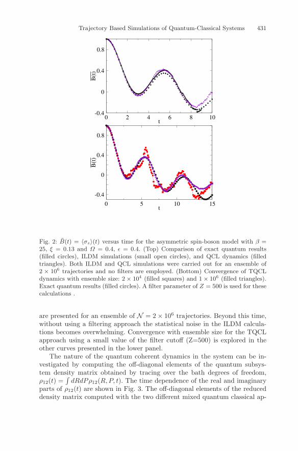
Fig. 2: B(t) = 〈σz〉(t) versus time for the asymmetric spin-boson model with β =25, ξ = 0.13 and Ω = 0.4, ε = 0.4. (Top) Comparison of exact quantum results(filled circles), ILDM simulations (small open circles), and QCL dynamics (filledtriangles). Both ILDM and QCL simulations were carried out for an ensemble of2 × 106 trajectories and no filters are employed. (Bottom) Convergence of TQCLdynamics with ensemble size: 2 × 104 (filled squares) and 1× 106 (filled triangles).Exact quantum results (filled circles). A filter parameter of Z = 500 is used for thesecalculations .

are presented for an ensemble of N = 2× 106 trajectories. Beyond this time,without using a filtering approach the statistical noise in the ILDM calcula-tions becomes overwhelming. Convergence with ensemble size for the TQCLapproach using a small value of the filter cutoff (Z=500) is explored in theother curves presented in the lower panel.

The nature of the quantum coherent dynamics in the system can be in-vestigated by computing the off-diagonal elements of the quantum subsys-tem density matrix obtained by tracing over the bath degrees of freedom,ρ12(t) =

∫dRdPρ12(R,P, t). The time dependence of the real and imaginary

parts of ρ12(t) are shown in Fig. 3. The off-diagonal elements of the reduceddensity matrix computed with the two different mixed quantum classical ap-


0 5 10t

-0.5

-0.25

0

0.25

B(t

)

0 5 10t

-0.25

0

0.25

0.5

B(t

)

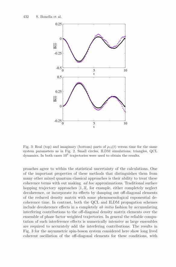
Fig. 3: Real (top) and imaginary (bottom) parts of ρ12(t) versus time for the samesystem parameters as in Fig. 2. Small circles, ILDM simulations; triangles, QCLdynamics. In both cases 106 trajectories were used to obtain the results.

proaches agree to within the statistical uncertainty of the calculations. Oneof the important properties of these methods that distinguishes them frommany other mixed quantum classical approaches is their ability to treat thesecoherence terms with out making ad hoc approximations. Traditional surfacehopping trajectory approaches [1, 3], for example, either completely neglectdecoherence, or incorporate its effects by damping out off-diagonal elementsof the reduced density matrix with some phenomenological exponential de-coherence time. In contrast, both the QCL and ILDM propagation schemesinclude decoherence effects in a completely ab initio fashion by accumulatinginterfering contributions to the off-diagonal density matrix elements over theensemble of phase factor weighted trajectories. In general the reliable compu-tation of such interference effects is numerically intensive as large ensemblesare required to accurately add the interfering contributions. The results inFig. 3 for the asymmetric spin-boson system considered here show long livedcoherent oscillation of the off-diagonal elements for these conditions, with


no evidence of exponential decay assumed in the phenomenological modelsof condensed phase decoherence processes. The dephasing is at least as longlived as the population relaxation dynamics for this model system.

5 Conclusion

The two quantum-classical dynamical schemes discussed in this Chapter pro-vide ways to investigate the dynamics of large, many-body systems wherequantum degrees of freedom are coupled to an environment. The results pre-sented here have shown that both schemes yield good agreement with exactcalculations for the symmetric and asymmetric spin-boson models for a widerange of system parameters. In particular coherences are accurately described.Our simulation results have documented the performances of the algorithmswith respect to quantities such as the number of trajectories in the ensem-ble needed to obtain good results, the use of filters and the utility of themomentum-jump approximation. The QCL formulation can be shown to beexact for the spin-boson model so our comparison with numerically exactresults for this model tests only the approximations in the implementationscheme. Calculations on models for which this formulation is not exact wouldoffer more challenging tests and may provide a more stringent basis for com-paring the different methods in future studies.

While the two methods are, at face value, quite different in the ways inwhich full quantum dynamics is reduced to quantum-classical dynamics, thereare common elements in the manner in which they are simulated. The Trotter-based scheme for QCL dynamics makes use of the adiabatic basis and is basedon surface-hopping trajectories where transitions are sampled by a MonteCarlo scheme that requires reweighting. Similarly, ILDM calculations makeuse of the mapping hamiltonian basis and also involve a similar Monte Carlosampling with reweighting of trajectories in the ensemble used to obtain theexpectation values of quantum operators.

As noted above, however, the theoretical frameworks of the two approachesappear quite different. This is a common situation in mixed quantum-classicalsimulations: many methods exist, and they may have very different ranges ofapplicability. A systematic assessment of differences and similarities, of theaccuracy of various approximations, and in general of their relative meritspresents a significant challenge. Investigating the relationships between dif-ferent methods, however, can provide a better understanding of the nature,advantages and limitations of mixed quantum-classical methods in general,and may lead to a more firm theoretical foundation on which to base thedevelopment of new methods, as well as more efficient algorithms for imple-mentation.

The two methods described in this Chapter are good candidates for suchcomparative investigation. They are both derived employing well-defined ap-proximations to exact quantum expressions and they can be used to study


the same set of, general, observables. Furthermore, it has already been shownthat, for some choices of the quantum sub-system basis set, QCL can be ob-tained via a linearization procedure that shares some similarities with thelinerization used to derive the ILDM propagation [4]. Future work will inves-tigate the theoretical connections between the methods that, as a first step,we have compared in their existing formulations in this Chapter.

Acknowledgements

The research of RK was supported in part by a grant from the Natural Sciencesand Engineering Research Council of Canada. DFC acknowledges support forthis research from the US National Science Foundation under grant numberCHE-0616952, as well as his Stokes Professorship from Science FoundationIreland, and funding from University College Dublin. A grant from Ministerodell’Ambiente e della Tutela del Territorio e del Mare is acknowledged by SBand GC.

References

1. Tully JC. Mixed quantum-classical dynamics: mean-field and surface-hopping.In Classical and Quantum Dynamics in Condensed Phase Simulations, ed. B.J.Berne, G. Ciccotti, D.F. Coker. Chapter 21. Singapore: World Scientific, 1998.

2. For a review with references to the literature on this topic, see, R. Kapral.Progress in the theory of mixed quantum-classical dynamics. Annu. Rev. Phys.Chem., 57:129, 2006.

3. J. C. Tully. Molecular dynamics with electronic transitions. J. Chem. Phys.,93(2):1061, 1990.

4. Q. Shi and E. Geva. A derivation of the mixed quantum-classical Liouvilleequation from the influence functional formalism. J. Chem. Phys., 121(8):3393,2004.

5. S. Nielsen, R. Kapral, and G. Ciccotti. Statistical mechanics of quantum-classical systems. J. Chem. Phys., 115(13):5805, 2001.

6. H. Kim and R. Kapral. Transport properties of quantum-classical systems. J.Chem. Phys., 122:214105, 2005.

7. G. Ciccotti, D.F. Coker, and R. Kapral, Quantum statistical dynamics withtrajectories, in Quantum dynamics of complex molecular systems, David Michaand Irene Burghardt, Chemical Physics series vol. 83, (Springer, Berlin), p. 275,2006.

8. H. Kim and R. Kapral. Nonadiabatic quantum-classical reaction rates withquantum equilibrium structure. J. Chem. Phys., 123:194108, 2005.

9. R. Grunwald, H. Kim and R. Kapral. Surface hopping and decoherence withquantum equilibrium structure. J. Chem. Phys., 128:164110, 2008.

10. G. Hanna and R. Kapral. Quantum-classical Liouville dynamics of nonadiabaticproton transfer. J. Chem. Phys., 122(24):244505, 2005.


11. G. Hanna and R. Kapral. Quantum-classical Liouville dynamics of protonand deutron transfer rates in a hydrogen bonded complex. J. Chem. Phys.,128:164520, 2008.

12. R. Kapral and G. Ciccotti. Mixed quantum-classical dynamics. J. Chem. Phys.,110:8919, 1999.

13. I. V. Aleksandrov. The statistical dynamics of a system consisting of a classicaland a quantum subsystem. Z. Naturforsch., 36:902, 1981.

14. V. I. Gerasimenko. Correlation-less equations of motion of quantum-classicalsystems. Repts. Acad. Sci. Ukr.SSR, (10):64, 1981.

15. V. I. Gerasimenko. Dynamical equations of quantum-classical systems. Theor.Math. Phys., 50:49, 1982.

16. W. Boucher and J. Traschen. Semiclassical physics and quantum fluctuations.Phys. Rev. D, 37(12):3522, 1988.

17. W.Y. Zhang and R. Balescu. Statistical mechanics of a spin polarized plasma.J. Plasma Physics, 40:199, 1988.

18. Y. Tanimura and S. Mukamel. Multistate quantum Fokker–Planck approachto nonadiabatic wave packet dynamics in pump–probe spectroscopy. J. Chem.Phys., 101:3049, 1994.

19. C. C. Martens and J. Y. Fang. Semiclassical-limit molecular dynamics on mul-tiple electronic surfaces. J. Chem. Phys., 106(12):4918, 1997.

20. I. Horenko, C. Salzmann, B. Schmidt, and C. Schutte. Quantum-classical li-ouville approach to molecular dynamics: Surface hopping gaussian phase-spacepackets. J. Chem. Phys., 117(24):11075, 2002.

21. R. Grunwald, A. Kelly and R. Kapral. Quantum dynamics in almost classicalenvironments. this volume , 2009.

22. D. Mac Kernan, G. Ciccotti, and R. Kapral. Trotter-based simulation ofquantum-classical dynamics. J. Phys. Chem. B, 112:424, 2008.

23. R. Kapral and G. Ciccotti, A Statistical Mechanical Theory of Quantum Dy-namics in Classical Environments, in Bridging Time Scales: Molecular Simula-tions for the Next Decade, eds. P. Nielaba, M. Mareschal, G. Ciccotti, (Springer,Berlin), p. 445, 2002.

24. R. Hernandez and G. Voth. Quantum time correlation functions and classicalcoherence. Chem. Phys., 223:243, 1998.

25. J.A. Poulsen and G. Nyman and P.J. Rossky. Practical evaluation of condensedphase quantum correlation functions: A Feynman-Kleinert variational linearizedpath integral method. J. Chem. Phys., 119:12179, 2003.

26. Q. Shi and E. Geva. Vibrational energy relaxation in liquid oxygen from asemiclassical molecular dynamics simulation. J. Phys. Chem. A, 107:9070, 2003.

27. Q. Shi and E. Geva. Semiclassical theory of vibrational energy relaxation in thecondensed Phase. J. Phys. Chem. A, 107:9059, 2003.

28. Q. Shi and E. Geva. Nonradiative electronic relaxation rate constants fromapproximations based on linearizing the path-integral forward-backward action.J. Phys. Chem. A, 108:6109, 2004.

29. X. Sun and W.H. Miller. Semiclassical initial value representation for electron-ically nonadiabatic molecular dynamics. J. Chem. Phys., 106:6346, 1997.

30. G. Stock and M. Thoss. Semiclassical description of nonadiabatic quantumdynamics. Phys. Rev. Lett., 78:578, 1997.

31. G. Stock and M. Thoss. Mapping approach to the semiclassical description ofnonadiabatic quantum dynamics. Phys. Rev. A, 59:64, 1999.


32. S. Bonella and D.F. Coker. A semi-classical limit for the mapping Hamiltonianapproach to electronically non-adiabatic dynamics. J. Chem. Phys., 114:7778,2001.

33. S. Bonella and D.F. Coker. Semi-classical implementation of the mapping Hamil-tonian approach for non-adiabatic dynamics: Focused initial distribution sam-pling. J. Chem. Phys., 118:4370, 2003.

34. S. Bonella and D.F. Coker. LAND-map, a linearized approach to nonadiabaticdynamics using the mapping formalism. J. Chem. Phys., 122:194102, 2005.

35. S. Bonella, D. Montemayor, and D.F. Coker. Linearized path integral approachfor calculating nonadiabatic time correlation functions. Proc. Natl. Acad. Sci.,102:6715, 2005.

36. D.F. Coker and S. Bonella, Linearized path integral methods for quantum timecorrelation functions, in Computer simulations in condensed matter: From ma-terials to chemical biology, eds. M. Ferrario and G. Ciccotti and K. Binder,Lecture Notes in Physics 703, (Springer-Verlag, Berlin), p. 553, 2006.

37. E. Dunkel, S. Bonella, and D.F. Coker. Iterative linearized approach to non-adiabatic dynamics. J. Chem. Phys., 129:114106, 2008.

38. Z. Ma and D.F. Coker. Quantum initial condition sampling for linearized densitymatrix dynamics: Vibrational pure dephasing of iodine in krypton matrices. J.Chem. Phys., 128:244108, 2008.

39. D. Mac Kernan, G. Ciccotti, and R. Kapral. Surface-hopping dynamics of aspin-boson system. J. Chem. Phys., 116(6):2346, 2002.

40. H. Kim, A. Nassimi, and R. Kapral. Quantum-classical Liouville dynamics inthe mapping basis. J. Chem. Phys., 129:084102, 2008.

41. D. E. Makarov and N. Makri, Chem. Phys. Lett., 221:482, 1994.42. K. Thompson and N. Makri. Rigorous forward-backward semiclassical formula-

tion of many-body dynamics. Phys. Rev. E, 59(5):R4729, 1999.

trajectory based simulations of quantum-classical systems

Documents