traffic jams induced by rare switching events in two-lane transport
TRANSCRIPT

arX
iv:c
ond-
mat
/070
2022
v2 [
cond
-mat
.sta
t-m
ech]
5 J
un 2
007
Traffic jams induced by rare switching events in
two-lane transport
Tobias Reichenbach, Erwin Frey, and Thomas Franosch
Arnold Sommerfeld Center for Theoretical Physics (ASC) and Center for
NanoScience (CeNS), Department of Physics, Ludwig-Maximilians-Universitat
Munchen, Theresienstrasse 37, D-80333 Munchen, Germany
E-mail: [email protected]
Abstract. We investigate a model for driven exclusion processes where internal
states are assigned to the particles. The latter account for diverse situations, ranging
from spin states in spintronics to parallel lanes in intracellular or vehicular traffic.
Introducing a coupling between the internal states by allowing particles to switch from
one to another induces an intriguing polarization phenomenon. In a mesoscopic scaling,
a rich stationary regime for the density profiles is discovered, with localized domain
walls in the density profile of one of the internal states being feasible. We derive the
shape of the density profiles as well as resulting phase diagrams analytically by a mean-
field approximation and a continuum limit. Continuous as well as discontinuous lines
of phase transition emerge, their intersections induce multicritical behavior.
PACS numbers: 05.40.-a, 05.60.-k 64.60.-i, 72.25.-b

Traffic jams in two-lane transport 2
1. Introduction
Non-equilibrium critical phenomena arise in a broad variety of systems, including non-
equilibrium growth models [1], percolation-like processes [2], kinetic Ising models [3],
diffusion limited chemical reactions [4], and driven diffusive systems [5]. The latter
provide models for transport processes ranging from biological systems, like the motion
of ribosomes along a m-RNA chain [6] or processive motors walking along cytoskeletal
filaments [7, 8], to vehicular traffic [9, 10]. In this work, we focus on the steady-
state properties of such one-dimensional transport models, for which the Totally
Asymmetric Simple Exclusion Process (TASEP) has emerged as a paradigm (for reviews
see e.g. [11, 12, 13]). There, particles move unidirectionally from left to right on a one-
dimensional lattice, interacting through on-site exclusion. The entrance/exit rates at
the open left/right boundary control the system’s behavior; tuning them, one encounters
different non-equilibrium phases for the particle densities [14].
Intense theoretical research has been devoted to the classification of such non-
equilibrium phenomena. For example, within the context of reaction-diffusion systems,
there is strong evidence that phase transitions from an active to an absorbing state can
be characterized in terms of only a few universality classes, the most important being
the one of directed percolation (DP) [15]. To search for novel critical behavior, fruitful
results have been obtained by coupling two reaction-diffusion systems [16, 17], each
undergoing the active to absorbing phase transition. Due to the coupling, the system
exhibits a multicritical point with unusual critical behavior.
We want to stress that already in equilibrium physics seminal insights have been
gained by coupling identical systems. For instance, spin-ladders incorporate several
Heisenberg spin chains [18]. There, quantum effects lead to a sensitive dependence on
the chain number: for even ones a finite energy gap between the ground state and the
lowest excitation emerges whereas gapless excitations dominate the low-temperature
behavior if the number of spin chains is odd.
In this work, we generalize the Totally Asymmetric Exclusion Process (TASEP)
in a way that particles possess two internal states; we have recently published a short
account of this work in Ref. [19]. Allowing particles to occasionally switch from one
internal state to the other induces a coupling between the latter; indeed, the model may
alternatively be regarded as two coupled TASEPs. When independent, each of them
separately undergoes boundary-induced phase transitions [14]. The coupling is expected
to induce novel phenomena, which are the subject of the present work.
Exclusion is introduced by allowing multiple occupancy of lattice sites only if
particles are in different internal states. Viewing the latter as spin-1/2 states, i.e spin-
up (↑) and spin-down (↓), this directly translates into Pauli’s exclusion principle; see
Fig. 1. Indeed, the exclusion process presented in this work may serve as a model for
semiclassical transport in mesoscopic quantum systems [20], like hopping transport in
chains of quantum dots in the presence of an applied field [21]. Our model incorporates
the quantum nature of the particles through Pauli’s exclusion principle, though phase
Traffic jams in two-lane transport 3
α↑
α↓
β↑
β↓
ω
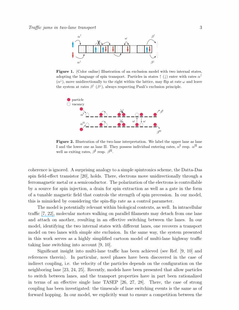
Figure 1. (Color online) Illustration of an exclusion model with two internal states,
adopting the language of spin transport. Particles in states ↑ (↓) enter with rates α↑
(α↓), move unidirectionally to the right within the lattice, may flip at rate ω and leave
the system at rates β↑ (β↓), always respecting Pauli’s exclusion principle.
particle
vacancy
αI
αII
βI
βII
ω ω
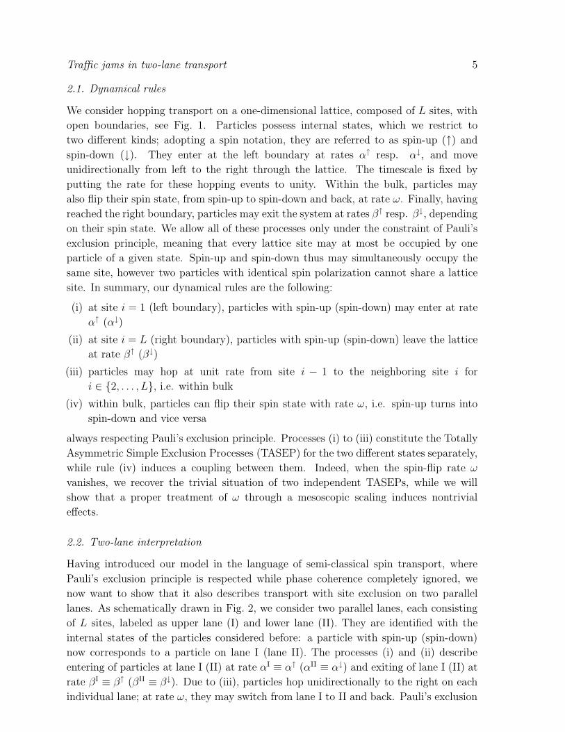
Figure 2. Illustration of the two-lane interpretation. We label the upper lane as lane
I and the lower one as lane II. They possess individual entering rates, αI resp. αII as
well as exiting rates, βI resp. βII.
coherence is ignored. A surprising analogy to a simple spintronics scheme, the Datta-Das
spin field-effect transistor [20], holds. There, electrons move unidirectionally through a
ferromagnetic metal or a semiconductor. The polarization of the electrons is controllable
by a source for spin injection, a drain for spin extraction as well as a gate in the form
of a tunable magnetic field that controls the strength of spin precession. In our model,
this is mimicked by considering the spin-flip rate as a control parameter.
The model is potentially relevant within biological contexts, as well. In intracellular
traffic [7, 22], molecular motors walking on parallel filaments may detach from one lane
and attach on another, resulting in an effective switching between the lanes. In our
model, identifying the two internal states with different lanes, one recovers a transport
model on two lanes with simple site exclusion. In the same way, the system presented
in this work serves as a highly simplified cartoon model of multi-lane highway traffic
taking lane switching into account [9, 10].
Significant insight into multi-lane traffic has been achieved (see Ref. [9, 10] and
references therein). In particular, novel phases have been discovered in the case of
indirect coupling, i.e. the velocity of the particles depends on the configuration on the
neighboring lane [23, 24, 25]. Recently, models have been presented that allow particles
to switch between lanes, and the transport properties have in part been rationalized
in terms of an effective single lane TASEP [26, 27, 28]. There, the case of strong
coupling has been investigated: the timescale of lane switching events is the same as of
forward hopping. In our model, we explicitly want to ensure a competition between the

Traffic jams in two-lane transport 4
boundary processes and the switching between the internal states. We therefore employ
a mesoscopic scaling, i.e. we consider the case where the switching events are rare as
compared to forward hopping. This is the situation encountered in intracellular traffic
[7] where motors nearly exclusively remain on one lane and switch only very rarely. In
the context of spin transport, it corresponds to the case where forward hopping occurs
much faster than spin precession (weak external magnetic field).
The outline of the present paper is the following. In Sec. 2 we introduce the model
in the context of spin transport as well as two-lane traffic. Symmetries and currents
are discussed, which play a key role in the following analysis. Section 3 describes in
detail the mean-field approximation and the differential equations for the densities
obtained therefrom through a continuum limit. The mesoscopic scaling is motivated
and introduced, the details of the analytic solution for the spatial density profiles
being condensed in Appendix A. We obtain the generic form of the density profiles
in Sec. 4, and compare our analytic results to stochastic simulations. We find that
they agree excellently, suggesting the exactness of our analytic approach in the limit
of large systems. As our main result, we encounter the polarization phenomenon,
where the density profiles in the stationary non-equilibrium state exhibit localized
‘shocks’. Namely, the density of one spin state changes abruptly from low to high
density. The origin of this phenomenon is rationalized in terms of singularities in
coupled differential equations. We partition the full parameter space into three distinct
regions, and observe a delocalization transition. The methods to calculate the phase
boundaries analytically are developed simultaneously. Section 5 presents details on the
stochastic simulations which we have carried out to corroborate our analytic approach.
The central result of this work is then addressed in Sec. 6, where two-dimensional
analytic phase diagrams are investigated. Our analytic approach identifies the phases
where the polarization phenomenon occurs, as well as the continuous and discontinuous
transitions that separate the phases. The nature of the transitions is explained by the
injection/extraction limited current which is conserved along the track. As a second
remarkable feature of the model, we uncover multi-critical points, i.e. points where
two lines of phase boundaries intersect or the nature of a phase transition changes
from discontinuous to a continuous one. Although multi-critical point are well-known
in equilibrium statistical mechanics, a fundamental description for such a behavior for
systems driven far from equilibrium still constitutes a major challenge. A brief summary
and outlook concludes this work.
2. The model
In this section, we describe our model in terms of spin transport as well as two-lane
traffic. Though we will preferentially use the language of spins in the subsequent
sections, the two-lane interpretation is of no lesser interest, and straightforwardly
obtained. Furthermore, we introduce two symmetries which are manifest on the level of
the dynamical rules.
Traffic jams in two-lane transport 5
2.1. Dynamical rules
We consider hopping transport on a one-dimensional lattice, composed of L sites, with
open boundaries, see Fig. 1. Particles possess internal states, which we restrict to
two different kinds; adopting a spin notation, they are referred to as spin-up (↑) and
spin-down (↓). They enter at the left boundary at rates α↑ resp. α↓, and move
unidirectionally from left to the right through the lattice. The timescale is fixed by
putting the rate for these hopping events to unity. Within the bulk, particles may
also flip their spin state, from spin-up to spin-down and back, at rate ω. Finally, having
reached the right boundary, particles may exit the system at rates β↑ resp. β↓, depending
on their spin state. We allow all of these processes only under the constraint of Pauli’s
exclusion principle, meaning that every lattice site may at most be occupied by one
particle of a given state. Spin-up and spin-down thus may simultaneously occupy the
same site, however two particles with identical spin polarization cannot share a lattice
site. In summary, our dynamical rules are the following:
(i) at site i = 1 (left boundary), particles with spin-up (spin-down) may enter at rate
α↑ (α↓)
(ii) at site i = L (right boundary), particles with spin-up (spin-down) leave the lattice
at rate β↑ (β↓)
(iii) particles may hop at unit rate from site i − 1 to the neighboring site i for
i ∈ 2, . . . , L, i.e. within bulk
(iv) within bulk, particles can flip their spin state with rate ω, i.e. spin-up turns into
spin-down and vice versa
always respecting Pauli’s exclusion principle. Processes (i) to (iii) constitute the Totally
Asymmetric Simple Exclusion Processes (TASEP) for the two different states separately,
while rule (iv) induces a coupling between them. Indeed, when the spin-flip rate ω
vanishes, we recover the trivial situation of two independent TASEPs, while we will
show that a proper treatment of ω through a mesoscopic scaling induces nontrivial
effects.
2.2. Two-lane interpretation
Having introduced our model in the language of semi-classical spin transport, where
Pauli’s exclusion principle is respected while phase coherence completely ignored, we
now want to show that it also describes transport with site exclusion on two parallel
lanes. As schematically drawn in Fig. 2, we consider two parallel lanes, each consisting
of L sites, labeled as upper lane (I) and lower lane (II). They are identified with the
internal states of the particles considered before: a particle with spin-up (spin-down)
now corresponds to a particle on lane I (lane II). The processes (i) and (ii) describe
entering of particles at lane I (II) at rate αI ≡ α↑ (αII ≡ α↓) and exiting of lane I (II) at
rate βI ≡ β↑ (βII ≡ β↓). Due to (iii), particles hop unidirectionally to the right on each
individual lane; at rate ω, they may switch from lane I to II and back. Pauli’s exclusion
Traffic jams in two-lane transport 6
principle translates into simple site exclusion: all the above processes are allowed under
the constraint of admitting at most one particle per site. Again, we clearly observe that
it is process (iv) that couples two TASEPs, namely the ones on each individual lane, to
each other.
2.3. Symmetries
Already on the level of the dynamical rules (i)-(iv) presented above, two symmetries are
manifest that will prove helpful in the analysis of the system’s behavior. We refer to
the absence of particles with certain state as holes with the opposite respective state ‡.Considering their motion, we observe that the dynamics of the holes is governed by
the identical rules (i) to (iv), with “left” and “right” interchanged, i.e. with a discrete
transformation of sites i ↔ L− i as well as rates α↑,↓ ↔ β↓,↑. The system thus exhibits
a particle-hole symmetry. Even more intuitively, the two states behave qualitatively
identical. Indeed, the system remains invariant upon changing spin-up to spin-down
states and vice versa with a simultaneous interchange of α↑ ↔ α↓ and β↑ ↔ β↓,
constituting a spin symmetry (in terms of the two-lane interpretation, it translates
into a lane symmetry).
When analyzing the system’s behavior in the five-dimensional phase space, constituted
of the entrance and exit rates α↑,↓, β↑,↓ and ω, these symmetries allow to connect
different regions in phase space, and along the way to simplify the discussion.
3. Mean-field equations, currents, and the continuum limit
In this section, we shall make use of the dynamical rules introduced above to set up a
quantitative description for the densities and currents in the system. Within a mean-
field approximation, their time evolution is expressed through one-point functions only,
namely the average occupations of a lattice site. Such mean-field approximations have
been successfully applied to a variety of driven diffusive systems, see e.g. Ref. [12]. We
focus on the properties of the non-equilibrium steady state, which results from bound-
ary processes (entering and exiting events) as well as bulk ones (hopping and spin-flip
events). Both types of processes compete if their time-scales are comparable; we ensure
this condition by introducing a mesoscopic scaling for the spin flip rate ω. Our focus is
on the limit of large system sizes L, which is expected to single out distinct phases. To
solve the resulting equations for the densities and currents, a continuum limit is then
justified, and it suffices to consider the leading order in the small parameter, viz. the
ratio of the lattice constant to system size. Such a mesoscopic scaling has been already
successfully used in [34, 35] in the context of TASEP coupled to Langmuir dynamics.
‡ The convention to flip the spin simultaneously is natural in the language of solid-state physics. In
the context of two-lane traffic, it appears more natural to consider vacancies moving on the same lane
in the reverse direction.
Traffic jams in two-lane transport 7
3.1. Mean field approximation and currents
Let n↑i (t) resp. n↓
i (t) be the fluctuating occupation number of site i for spin-up resp.
spin-down state, i.e. n↑,↓i (t) = 1 if this site is occupied at time t by a particle with
the specified spin state and n↑,↓i (t) = 0 otherwise. Performing ensemble averages, the
expected occupation, denoted by ρ↑i (t) and ρ↓
i (t), is obtained. Within a mean-field
approximation, higher order correlations between the occupation numbers are neglected,
i.e. we impose the factorization approximation
〈nri (t)n
sj(t)〉 = ρr
i (t)ρsj(t) ; r, s ∈ ↑, ↓ . (1)
Equations of motion for the densities can by obtained via balance equations: The
time-change of the density at a certain site is related to appropriate currents. The
spatially varying spin current j↑i (t) quantifies the rate at which particles of spin state
↑ at site i − 1 hop to the neighboring site i. Within the mean-field approximation, Eq.
(1), the current is expressed in terms of densities as
j↑i (t) = ρ↑i−1(t)[1 − ρ↓
i (t)] , i ∈ 2, . . . , L , (2)
and similarly for the current j↓i (t). The sum yields the total particle current Ji(t) ≡j↑i (t) + j↓i (t). Due to the spin-flip process (iv), there also exists a leakage current j↑↓i (t)
from spin-up state to spin-down state. Within mean-field
j↑↓i (t) = ωρ↑i (t)[1 − ρ↓
i (t)] , (3)
and similarly for the leakage current j↓↑i (t) from spin-down to spin-up state. Now, for
i ∈ 2, . . . , L − 1 we can use balance equations to obtain the time evolution of the
densities,
d
dtρ↑
i (t) = j↑i (t) − j↑i+1(t) + j↓↑i (t) − j↑↓i (t) . (4)
This constitutes an exact relation. Together with the mean field approximation for the
currents, Eqs. (2, 3), one obtains a set of closed equations for the local densities
d
dtρ↑
i (t) = ρ↑i−1(t)[1 − ρ↑
i (t)] − ρ↑i (t)[1 − ρ↑
i+1(t)] + ωρ↓i (t) − ωρ↑
i (t) . (5)
At the boundaries of the track, the corresponding expressions involve also the entrance
and exit events, which are again treated in the spirit of a mean-field approach
d
dtρ↑
1(t) = α↑[1 − ρ↑1(t)] − ρ↑
1(t)[1 − ρ↑2(t)] + ωρ↓
1(t) − ωρ↑1(t) , (6)
d
dtρ↑
L(t) = ρ↑
L−1(t)[1 − ρ↑
L(t)] − β↑ρ↑
L(t) + ωρ↓
L(t) − ωρ↑
L(t) . (7)
Due to the spin symmetry, i.e. interchanging ↑ and ↓, an analogous set of equations
hods for the time evolution of the density of particles with spin-down state.
In the stationary state, the densities ρ↑(↓)i (t) do not depend on time t, such that the
time derivatives in Eqs. (5)-(7) vanish. Therefrom, we immediately derive the spatial
Traffic jams in two-lane transport 8
conservation of the particle current: Indeed, summing Eq. (4) with the corresponding
equation for the density of spin-down states yields
Ji = Ji+1 , i ∈ 2, . . . , L − 1 , (8)
such that the particle current does not depend on the spatial position i. Note that this
does not apply to the individual spin currents, they do have a spatial dependence arising
from the leakage currents.
In a qualitative discussion, let us now anticipate the effects that arise from the
non-conserved individual spin currents as well as from the conserved particle current.
The latter has its analogy in TASEP, where the particle current is spatially conserved
as well. It leads to two distinct regions in the parameter space: one where the current
is determined by the left boundary, and the other where it is controlled by the right
one. Both regions are connected by the discrete particle-hole symmetry. Thus, in
general, discontinuous phase transitions arise when crossing the border from one region
to the other. In our model, we will find similar behavior: the particle current is either
determined by the left or by the right boundary. Again, both regions are connected by
the discrete particle-hole symmetry, such that we expect discontinuous phase transitions
at the border between both. Except for a small, particular region in the parameter space,
this behavior is captured quantitatively by the mean-field approach and the subsequent
analysis, which is further corroborated by stochastic simulations. The phenomena linked
to the particular region will be presented elsewhere [29].
On the other hand, the non-conserved spin currents may be compared to the current
in TASEP coupled to Langmuir kinetics; see Refs. [34, 35]. Due to attachment and
detachment processes, the in-lane current is only weakly conserved, allowing for a
novel phenomena, namely phase separation into a low-density and a high-density region
separated by a localized domain wall. The transitions to this phase are continuous
considering the domain wall position xw as the order parameter. In our model, an
analogous but even more intriguing phase will appear as well, with continuous transitions
being possible.
3.2. Mesoscopic scaling and the continuum limit
3.2.1. Mesoscopic scaling. Phases and corresponding phase transitions are expected to
emerge in the limit of large system size, L → ∞, which therefore constitutes the focus
of this work. We expect interesting phase behavior to arise from the coupling of spin-up
and spin-down states via spin-flip events, in addition to the entrance and exit processes.
Clearly, if spin-flips occur on a fast time-scale, comparable to the hopping events, the
spin degree of freedom is relaxed, such that the system’s behavior is effectively the
one of a TASEP. Previous work on related two-lane models [27, 26] focused on the
physics in that situation. In this work, we want to highlight the dynamical regime
where coupling through spin-flips is present, however not sufficiently strong to relax the
system’s internal degree of freedom. In other words, we consider physical situations
Traffic jams in two-lane transport 9
where spin-flips occur on the same time-scale as the entrance/exit processes. Defining
the gross spin-flip rate Ω = ωL yields a measure of how often a particle flips its spin state
while traversing the system. To ensure competition between spin-flips with boundary
processes, a mesoscopic scaling of the rate ω is employed by keeping Ω fixed, of the same
order as the entrance/exit rates, when the number of lattice sites becomes large L → ∞.
3.2.2. Continuum limit and first order approximation. The total length of the lattice
will be fixed to unity and one may define consistently the lattice constant ǫ = 1/L.
In the limit of large systems ǫ → 0, a continuum limit is anticipated. We introduce
continuous functions ρ↑(x) resp. ρ↓(x) through ρ↑(xi) = ρ↑i resp. ρ↓(xi) = ρ↓
i at the
discrete points xi = iǫ. Expanding these to first order in the lattice constant,
ρ↑(↓)(xi±1) = ρ↑(↓)(xi ± ǫ) = ρ↑(↓)(xi) ± ǫ∂xρ↑(↓)(xi) , (9)
the difference equations (5)-(7) turn into differential equations. Observing that ω = ǫΩ
is already of order ǫ, we find that the zeroth order of Eq. (5) vanishes, and the first
order in ǫ yields
[2ρ↑(x) − 1]∂xρ↑(x) + Ωρ↓(x) − Ωρ↑(x) = 0 . (10)
Similarly, the same manipulations for ρ↓ yield
[2ρ↓(x) − 1]∂xρ↓(x) + Ωρ↑(x) − Ωρ↓(x) = 0 . (11)
The expansion of Eqs. (6) and (7) in powers of ǫ, yields in zeroth order
ρ↑(0) = α↑ , ρ↑(1) = 1 − β↑ ,
ρ↓(0) = α↓ , ρ↓(1) = 1 − β↓ , (12)
which impose boundary conditions. Since two boundary conditions are enough to specify
a solution of the coupled first order differential equations, the system is apparently
over-determined. Of course, the full analytic solution, i.e. where all orders in ǫ are
incorporated, will be only piecewise given by the first-order approximation, Eqs. (10)-
(12). Between these branches, the solution will depend on higher orders of ǫ, therefore,
these intermediate regions scale with order ǫ and higher. They vanish in the limit of
large systems, ǫ → 0, yielding domain walls or boundary layers.
Let us explain the latter terms. At the position of a domain wall, situated in bulk, the
density changes its value discontinuously, from one of a low-density region to one of a
high-density. Boundary layers are pinned to the boundaries of the system. There as well,
the density changes discontinuously: from a value that is given by the corresponding
boundary condition to that of a low- or high-density region which is imposed by the
opposite boundary .
3.2.3. Symmetries and currents revisited. In the following, we reflect important
properties of the system, symmetries and currents, on the level of the first-order
approximation, Eqs. (10)-(12). The explicit solution of the latter can be found in
Appendix A.

Traffic jams in two-lane transport 10
The particle-hole symmetry, already inferred from the dynamical rules, now takes
the form
ρ↑(↓)(x) ↔ 1 − ρ↑(↓)(1 − x) ,
α↑(↓) ↔ β↑(↓) . (13)
Interchanging ↑ and ↓ in the densities as well as the in- and outgoing rates yields the
spin symmetry,
ρ↑(x) ↔ ρ↓(x) ,
α↑ ↔ α↓ ,
β↑ ↔ β↓ . (14)
The individual spin currents as well as the particle current have been anticipated
to provide further understanding of the system’s behavior. In the continuum limit the
zeroth order of the spin currents is found to be j↑(↓)(x) = ρ↑(↓)(x)[1−ρ↑(↓)(x)], such that
Eqs. (10), (11) may be written in the form
∂xj↑ = Ω[ρ↓ − ρ↑] , ∂xj
↓ = Ω[ρ↑ − ρ↓] . (15)
The terms on the right-hand side, arising from the spin-flip process (iv), are seen to
violate the spatial conservation of the spin currents. However, due to the mesoscopic
scaling of the spin flip rate ω, the leakage currents between the spin states are only
weak, see Eq. (3), locally tending to zero when ǫ → 0, such that the spin currents
vary continuously in space. This finding imposes a condition for the transition from one
branch of first-order solution to another, as described above: such a transition is only
allowed when the corresponding spin currents are continuous at the transition point,
thus singling out distinct positions for a possible transition.
Finally, summing the two equations in Eq. (15) yields the spatial conservation of the
particle current: ∂xJ = 0.
4. Partition of the parameter space and the generic density behavior
The parameter space of our model, spanned by the five rates α↑,↓, β↑,↓, and Ω, is of
high dimensionality. However, in this section, we show that it can be decomposed
into only three basic distinct regions: the maximal-current region (MC) as well as the
injection-limited (IN) and the extraction-limited one (EX). While trivial phase behavior
occurs in the MC region, our focus is on the IN and EX region (connected by particle-
hole symmetry), where a striking polarization phenomenon occurs. The generic phase
behavior in these regions is derived, exhibiting this effect.
4.1. Effective rates
The entrance and exit rates as well as the carrying capacity of the bulk impose
restrictions on the particle current. For example, the capacity of the bulk limits the
individual spin currents j↑(↓) to a maximal values of 1/4. The latter occurs at a density
Traffic jams in two-lane transport 11
ρ↓ρ↓ρ↓ρ↓ρ↓ρ↓ρ↓ρ↓ρ↓
ρ↑ρ↑ρ↑ρ↑ρ↑ρ↑ρ↑ρ↑ρ↑
ρeρeρeρeρeρeρeρeρe
α↓α↓α↓α↓α↓α↓α↓α↓α↓
α↑α↑α↑α↑α↑α↑α↑α↑α↑
0 = 1−β↑ =1 − β↓
0 = 1−β↑ =1 − β↓
0 = 1−β↑ =1 − β↓
0 = 1−β↑ =1 − β↓
0 = 1−β↑ =1 − β↓
0 = 1−β↑ =1 − β↓
0 = 1−β↑ =1 − β↓
0 = 1−β↑ =1 − β↓
0 = 1−β↑ =1 − β↓000000000 1
1
1
1
1
1
1
1
1
1
1
1
1
1
1
1
1
1
(den
sity
)ρ
(den
sity
)ρ
(den
sity
)ρ
(den
sity
)ρ
(den
sity
)ρ
(den
sity
)ρ
(den
sity
)ρ
(den
sity
)ρ
(den
sity
)ρ
(spatial position) x(spatial position) x(spatial position) x(spatial position) x(spatial position) x(spatial position) x(spatial position) x(spatial position) x(spatial position) x
0.50.50.50.50.50.50.50.50.5
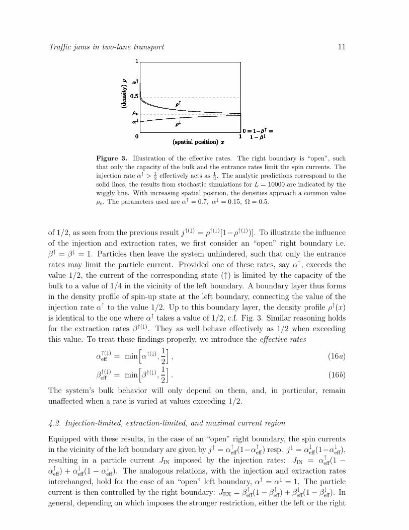
Figure 3. Illustration of the effective rates. The right boundary is “open”, such
that only the capacity of the bulk and the entrance rates limit the spin currents. The
injection rate α↑ > 12 effectively acts as 1
2 . The analytic predictions correspond to the
solid lines, the results from stochastic simulations for L = 10000 are indicated by the
wiggly line. With increasing spatial position, the densities approach a common value
ρe. The parameters used are α↑ = 0.7, α↓ = 0.15, Ω = 0.5.
of 1/2, as seen from the previous result j↑(↓) = ρ↑(↓)[1−ρ↑(↓))]. To illustrate the influence
of the injection and extraction rates, we first consider an “open” right boundary i.e.
β↑ = β↓ = 1. Particles then leave the system unhindered, such that only the entrance
rates may limit the particle current. Provided one of these rates, say α↑, exceeds the
value 1/2, the current of the corresponding state (↑) is limited by the capacity of the
bulk to a value of 1/4 in the vicinity of the left boundary. A boundary layer thus forms
in the density profile of spin-up state at the left boundary, connecting the value of the
injection rate α↑ to the value 1/2. Up to this boundary layer, the density profile ρ↑(x)
is identical to the one where α↑ takes a value of 1/2, c.f. Fig. 3. Similar reasoning holds
for the extraction rates β↑(↓). They as well behave effectively as 1/2 when exceeding
this value. To treat these findings properly, we introduce the effective rates
α↑(↓)eff = min
[
α↑(↓),1
2
]
, (16a)
β↑(↓)eff = min
[
β↑(↓),1
2
]
. (16b)
The system’s bulk behavior will only depend on them, and, in particular, remain
unaffected when a rate is varied at values exceeding 1/2.
4.2. Injection-limited, extraction-limited, and maximal current region
Equipped with these results, in the case of an “open” right boundary, the spin currents
in the vicinity of the left boundary are given by j↑ = α↑
eff(1−α↑
eff) resp. j↓ = α↓
eff(1−α↓
eff),
resulting in a particle current JIN imposed by the injection rates: JIN = α↑
eff(1 −α↑
eff) + α↓
eff(1 − α↓
eff). The analogous relations, with the injection and extraction rates
interchanged, hold for the case of an “open” left boundary, α↑ = α↓ = 1. The particle
current is then controlled by the right boundary: JEX = β↑
eff(1 − β↑
eff) + β↓
eff(1− β↓
eff). In
general, depending on which imposes the stronger restriction, either the left or the right
Traffic jams in two-lane transport 12
boundary limits the particle current: J ≤ min(JIN, JEX). Indeed, J = min(JIN, JEX)
holds except for an anomalous situation, where the current is lower than this value §.Depending on which of both cases applies, two complementary regions in phase space are
distinguished: JIN < JEX is termed injection-limited region (IN), while JIN > JEX defines
the extraction-limited region (EX). Since they are connected by discrete particle-hole
symmetry, we expect discontinuous phase transitions across the border between both,
to be referred as IN-EX boundary.
Right at the IN-EX boundary, the system exhibits coexistence of low- and high-
density phases, separated by domain walls. Interestingly, this phase coexistence emerges
on both lanes (states), which may be seen as follows. Recall that a domain wall
concatenates a region of low and another of high density. However, while the densities
exhibit a discontinuity, the spin currents must be continuous. In other words, the spin
currents, and therefore the particle currents, imposed by the left and right boundary
must match each other. This yields the condition JIN = JEX, which is nothing but
the relation describing the IN-EX boundary. Actually, what we have shown with this
argument is that domain walls on both lanes (states) are at most feasible at the IN-EX
boundary. However, it turns out that there, they do indeed form, and are delocalized.
We refer to our forthcoming publication [29] for a detailed discussion of this phenomenon.
Away from the IN-EX boundary, it follows that at most on one lane (state) a domain
wall may appear.
When both entrance rates α↑, α↓ as well as both exit rates β↑, β↓ exceed the value
1/2, the particle current is limited by neither boundary, but only through the carrying
capacity of the bulk, restricting it to twice the maximal value 1/4 of the individual
spin currents: J = 1/2. The latter situation therefore constitutes the maximal current
region (MC).
4.3. The generic state of the densities
As we have seen in the previous section, particularly simple density profiles emerge in
the MC region. There, up to boundary layers, the density profiles remain constant at
a value 1/2 for each spin state. Another special region in parameter space is the IN-
EX boundary, characterized by the simultaneous presence of domain walls in both spin
states, as we discuss elsewhere [29].
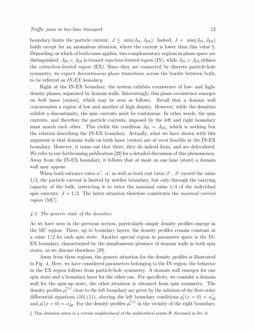
Away from these regions, the generic situation for the density profiles is illustrated
in Fig. 4. Here, we have considered parameters belonging to the IN region; the behavior
in the EX region follows from particle-hole symmetry. A domain wall emerges for one
spin state and a boundary layer for the other one. For specificity, we consider a domain
wall for the spin-up state, the other situation is obtained from spin symmetry. The
density profiles ρ↑(↓)l close to the left boundary are given by the solution of the first-order
differential equations (10),(11), obeying the left boundary conditions ρ↑
l (x = 0) = α↑
eff
and ρ↓
l (x = 0) = α↓
eff. For the density profiles ρ↑(↓)r in the vicinity of the right boundary,
§ This situation arises in a certain neighborhood of the multicritical points B, discussed in Sec. 6
Traffic jams in two-lane transport 13
(a)(a)(a)(a)(a)(a)(a)(a)(a)(a)(a)(a)(a)(a)(a)(a)(a)
(b)(b)(b)(b)(b)(b)(b)(b)(b)(b)(b)(b)(b)(b)
xwxwxwxwxwxwxwxwxwxwxwxwxwxwx 1
2
x 1
2
x 1
2
x 1
2
x 1
2
x 1
2
x 1
2
x 1
2
x 1
2
x 1
2
x 1
2
x 1
2
x 1
2
x 1
2
ρ↓ρ↓ρ↓ρ↓ρ↓ρ↓ρ↓ρ↓ρ↓ρ↓ρ↓ρ↓ρ↓ρ↓ρ↓ρ↓ρ↓
ρ↑ρ↑ρ↑ρ↑ρ↑ρ↑ρ↑ρ↑ρ↑ρ↑ρ↑ρ↑ρ↑ρ↑ρ↑ρ↑ρ↑
α↓α↓α↓α↓α↓α↓α↓α↓α↓α↓α↓α↓α↓α↓α↓α↓α↓
α↑α↑α↑α↑α↑α↑α↑α↑α↑α↑α↑α↑α↑α↑α↑α↑α↑
1 − β↑1 − β↑1 − β↑1 − β↑1 − β↑1 − β↑1 − β↑1 − β↑1 − β↑1 − β↑1 − β↑1 − β↑1 − β↑1 − β↑1 − β↑1 − β↑1 − β↑
1 − β↓1 − β↓1 − β↓1 − β↓1 − β↓1 − β↓1 − β↓1 − β↓1 − β↓1 − β↓1 − β↓1 − β↓1 − β↓1 − β↓1 − β↓1 − β↓1 − β↓
00000000000000000
00000000000000
11111111111111111
11111111111111
0.250.250.250.250.250.250.250.250.250.250.250.250.250.25
0.150.150.150.150.150.150.150.150.150.150.150.150.150.15 j↓j↓j↓j↓j↓j↓j↓j↓j↓j↓j↓j↓j↓j↓j↑j↑j↑j↑j↑j↑j↑j↑j↑j↑j↑j↑j↑j↑
(den
sity
)ρ
(den
sity
)ρ
(den
sity
)ρ
(den
sity
)ρ
(den
sity
)ρ
(den
sity
)ρ
(den
sity
)ρ
(den
sity
)ρ
(den
sity
)ρ
(den
sity
)ρ
(den
sity
)ρ
(den
sity
)ρ
(den
sity
)ρ
(den
sity
)ρ
(den
sity
)ρ
(den
sity
)ρ
(den
sity
)ρ
(curr
ent)
j(c
urr
ent)
j(c
urr
ent)
j(c
urr
ent)
j(c
urr
ent)
j(c
urr
ent)
j(c
urr
ent)
j(c
urr
ent)
j(c
urr
ent)
j(c
urr
ent)
j(c
urr
ent)
j(c
urr
ent)
j(c
urr
ent)
j(c
urr
ent)
j
(spatial position) x(spatial position) x(spatial position) x(spatial position) x(spatial position) x(spatial position) x(spatial position) x(spatial position) x(spatial position) x(spatial position) x(spatial position) x(spatial position) x(spatial position) x(spatial position) x
0.50.50.50.50.50.50.50.50.50.50.50.50.50.50.50.50.5
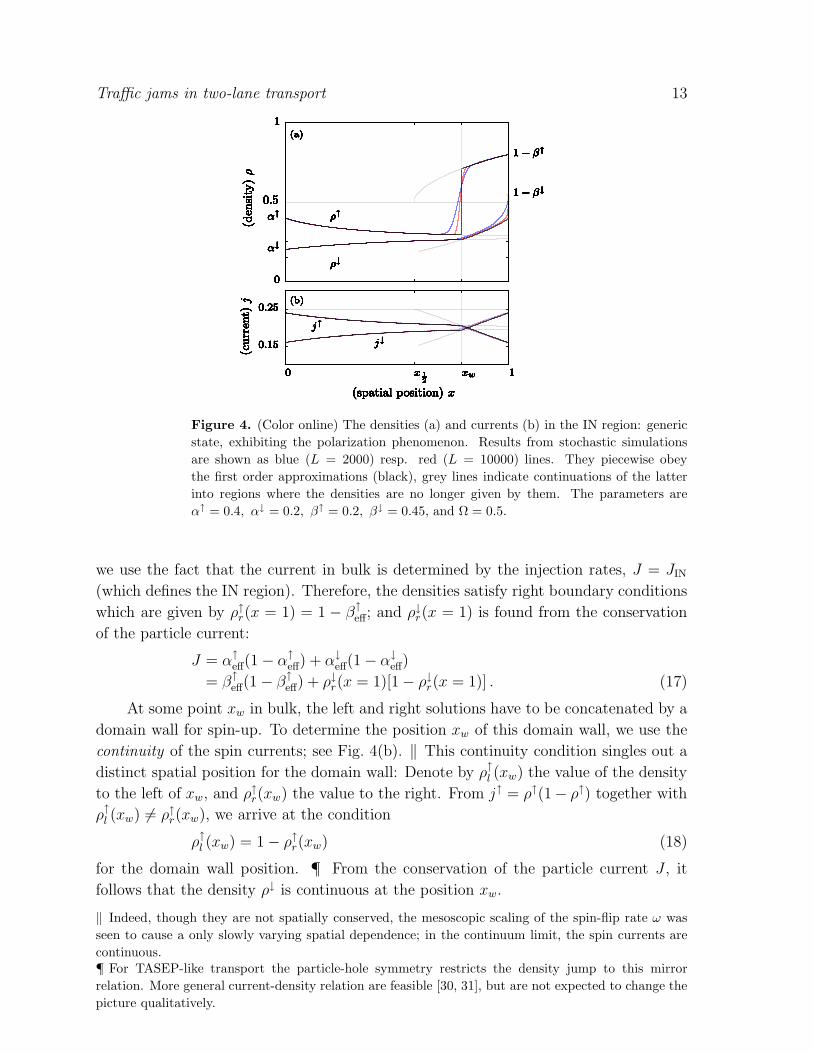
Figure 4. (Color online) The densities (a) and currents (b) in the IN region: generic
state, exhibiting the polarization phenomenon. Results from stochastic simulations
are shown as blue (L = 2000) resp. red (L = 10000) lines. They piecewise obey
the first order approximations (black), grey lines indicate continuations of the latter
into regions where the densities are no longer given by them. The parameters are
α↑ = 0.4, α↓ = 0.2, β↑ = 0.2, β↓ = 0.45, and Ω = 0.5.
we use the fact that the current in bulk is determined by the injection rates, J = JIN
(which defines the IN region). Therefore, the densities satisfy right boundary conditions
which are given by ρ↑r(x = 1) = 1 − β↑
eff; and ρ↓r(x = 1) is found from the conservation
of the particle current:
J = α↑
eff(1 − α↑
eff) + α↓
eff(1 − α↓
eff)
= β↑
eff(1 − β↑
eff) + ρ↓r(x = 1)[1 − ρ↓
r(x = 1)] . (17)
At some point xw in bulk, the left and right solutions have to be concatenated by a
domain wall for spin-up. To determine the position xw of this domain wall, we use the
continuity of the spin currents; see Fig. 4(b). ‖ This continuity condition singles out a
distinct spatial position for the domain wall: Denote by ρ↑
l (xw) the value of the density
to the left of xw, and ρ↑r(xw) the value to the right. From j↑ = ρ↑(1− ρ↑) together with
ρ↑
l (xw) 6= ρ↑r(xw), we arrive at the condition
ρ↑
l (xw) = 1 − ρ↑r(xw) (18)
for the domain wall position. ¶ From the conservation of the particle current J , it
follows that the density ρ↓ is continuous at the position xw.
‖ Indeed, though they are not spatially conserved, the mesoscopic scaling of the spin-flip rate ω was
seen to cause a only slowly varying spatial dependence; in the continuum limit, the spin currents are
continuous.¶ For TASEP-like transport the particle-hole symmetry restricts the density jump to this mirror
relation. More general current-density relation are feasible [30, 31], but are not expected to change the
picture qualitatively.
Traffic jams in two-lane transport 14
When considering the internal states as actual spins, the appearance of a domain
wall in the density profile of one of the spin states results in a spontaneous polarization
phenomenon. Indeed, while both the density of spin-up and spin-down remain at
comparable low values in the vicinity of the left boundary, this situation changes upon
crossing the point xw. There, the density of spin-up jumps to a high value, while the
density of spin-down remains at a low value, resulting in a polarization in this region.
Comparing the generic phase behavior to the one of TASEP, we observe that the
IN region can be seen as the analogue to the low-density region there: within both,
a low-density phase accompanied by a boundary layer at the right boundary arises.
Following these lines, the EX region has its analogue in the high-density region, while
the MC region is straightforwardly generalized from the one of TASEP. Furthermore,
the delocalization transition across the IN-EX boundary is similar to the appearance of
a delocalized domain wall at the coexistence line in TASEP.
4.4. Phases and phase boundaries
In the generic situation of Fig. 4, the density of spin-down is in a homogeneous low-
density (LD) state, while for spin-up, a low-density and a high-density region coexist.
We refer to the latter as the LD-HDIN phase, as the phase separation arises within the
IN region, to be contrasted from a LD-HDEX phase which may arise within the EX
region. Clearly, the LD-HDIN phase is only present if the position xw of the domain
wall lies within bulk. Tuning the system’s parameter, it may leave the system through
the left or right boundary, resulting in a homogeneous phase. Indeed, xw = 1 marks
the transition between the LD-HDIN phase and the pure LD state, while at xw = 0
the density changes from the LD-HDIN to a homogeneous high-density (HD) state.
Regarding the domain wall position xw as an order parameter, these transitions are
continuous. Implicit analytic expressions for these phase boundaries, derived in the
following, are obtained from the first-order approximation, Eqs. (10) and (11).
Spin symmetry yields the analogous situation with a domain wall appearing in
the density profile of spin-down, while particle-hole symmetry maps it to the EX
region, where a pure HD phase arises for one of the spins. Discontinuous transitions
accompanied by delocalized domain walls appear at the submanifold of the IN-EX
boundary (see [29] for a detailed discussion).
The phase boundaries may be computed from the condition xw = 0 and xw = 1 in
the situation of Fig. 4. Consider first the case of xw = 0. There, the density profiles are
fully given by the first-order approximation ρ↑(↓)r satisfying the boundary conditions at
the right. The condition (18) translates to
ρ↑r(x = 0) = 1 − ρ↑
l (x = 0) = 1 − α↑
eff (19)
which yields an additional constraint on the system’s parameters. This defines the
hyper-surface in the IN region where xw = 0 occurs, and thus the phase boundary
between the LD-HDIN and the pure HD phase.

Traffic jams in two-lane transport 15
Similarly, if xw = 1, the densities follow the left solution ρ↑(↓)l (x), determined by the left
boundary conditions, within the whole system. From Eq. (18) we obtain
ρ↑
l (x = 1) = 1 − ρ↑r(x = 1) = β↑
eff . (20)
Again, the latter is a constraint on the parameters and defines the hyper-surface in the
IN region where xw = 1 is found, being the phase boundary between the LD-HDIN and
the homogeneous LD phase.
The conditions (19), (20) yield implicit equations for the phase boundaries. The
phase diagram is thus determined up to solving algebraic equations, which may be
achieved numerically. Further insight concerning the phase boundaries is possible and
may be obtained analytically, which we discuss next.
First, we note that in the case of equal injection rates, α↑ = α↓, the density profiles
in the vicinity of the left boundary are constant. If in addition α↑ = α↓ = β↑ < 1/2,
we observe from Eq. (20) that a domain wall at xw = 1 emerges. Therefore, this set of
parameters always lies on the phase boundary xw = 1, independent of the value of Ω.
Second, we investigate the phase boundary determined by xw = 0. Comparing with
Fig. 4, we observe that the first-order approximation ρ↑r for the density of spin-up may
reach the value 12
at a point which is denoted by x 12: ρ↑
r(x 12) = 1
2. This point corresponds
to a branching point of the first-order solution. Increasing Ω, the value of x 12
increases
as well. The domain wall in the density of spin-up can only emerge at a value xw ≥ x 12.
At most, xw = x 12, in which case a domain wall with infinitesimal small height arises.
For the phase boundary specified by xw = 0, this implies that it only exists as long as
x 12≤ 0. The case xw = x 1
2= 0 corresponds to a domain wall of infinitesimal height,
which is only feasible if α↑
eff = 12. Now, for given rates α↑
eff = 12, α↓, β↑, the condition
x 12
= 0 yields a critical rate Ω∗(α↓, β↑), depending on the rates α↓, β↑. The situation
xw = 0 can only emerge for rates Ω ≤ Ω∗(α↓, β↑). Varying the rates α↑, α↓ and β↑, the
critical rate Ω∗(α↓, β↑) changes as well. In Appendix A, we show that its largest value
occurs at α↓ = β↑ = 0. They yield the rate ΩC ≡ Ω∗(α↓ = β↑ = 0), which is calculated
to be
ΩC = 1 +1
4
√2 ln (3 − 2
√2) ≈ 0.38 . (21)
The critical Ω∗(α↓, β↑) are lying in the interval between 0 and ΩC : Ω∗(α↓, β↑) ∈ [0, ΩC ],
and all values in this interval in fact occur. The rate ΩC defines a scale in the spin-
flip rate Ω: For Ω ≤ ΩC , the phase boundary determined by xw = 0 exists, while
disappearing for Ω > ΩC .
Third, we study the form of the phase boundaries for large Ω, meaning Ω ≫ ΩC .
In this case, the phase boundary specified by xw = 0 is no longer present. Furthermore,
it turns out that in this situation, the densities close to the left boundary quickly
approximate a common value ρe. The latter is found from conservation of the particle
current: 2ρe(1 − ρe) = J . We now consider the implications for the phase boundary
determined by xw = 1. With ρ↑
l (x = 1) = ρe, Eq. (20) turns into ρe = β↑
eff, yielding
2β↑
eff(1 − β↑
eff) = α↑
eff(1 − α↑
eff) + α↓
eff(1 − α↓
eff) . (22)

Traffic jams in two-lane transport 16
This condition specifies the phase boundary xw = 1, asymptotically for large Ω. It
constitutes a simple quadratic equation in the in- and outgoing rates, independent of
β↓, and contains the set α↑ = α↓
eff = β↑.
5. Stochastic simulations
To confirm our analytic findings from the previous section, we have performed stochastic
simulations. The dynamical rules (i)-(iv) described in Subsec. 2.1 were implemented
using random sequential updating. In our simulations, we have performed averages
over typically 105 time steps, with 10 × L steps of updating between successive ones.
Finite size scaling singles out the analytic solution in the limit of large system sizes, as
exemplified in Figs. 3 and 4.
For all simulations, we have checked that the analytic predictions are recovered
upon approaching the mesoscopic limit. We attribute the apparent exactness of our
analytic approach in part to the exact current density relation in the steady state of the
TASEP [32]. The additional coupling of the two TASEPs in our model is only weak:
the local exchange between the two states vanishes in the limit of large system sizes.
Correlations between them are washed out, and mean-field is recovered.
The observed exactness of the analytic density profiles within the mesoscopic limit
implies that our analytic approach yields exact phase diagrams as well. The latter are
the subject of the subsequent section.
6. Two-dimensional phase diagrams
In this section, we discuss the phase behavior on two-dimensional cuts in the whole five-
dimensional parameter space. Already the simplified situation of equal injection rates,
α↑ = α↓, yields interesting behavior. There as well as in the general case, we investigate
the role of the spin-flip rate Ω by discussing the situation of small and large values of
Ω.
6.1. Equal injection rates
For simplicity, we start our discussion of the phase diagram with equal injection rates,
α↑ = α↓. Then, the spin polarization phenomenon, depicted in Fig. 4, becomes even
more striking. Starting from equal densities at the left boundary, and hence zero
polarization, spin polarization suddenly switches on at the domain wall position xw.
The particular location of xw is not triggered by a cue on the track, but tuned through
the model parameters.
The phase transitions from LD to the LD-HDIN arising in the IN region take a
remarkably simple form. Their location is found from xw = 1, and is determined by
Eq. (20) (if phase coexistence arises for spin-up). Since ρ↑(x) = ρ↓(x) = α = const.
for x < xw, Eq. (20) turns into α = β↑. The latter transition line intersects the IN-EX
boundary, given by JIN = JEX, at β↑ = β↓ = α, i.e. at the point where all entrance

Traffic jams in two-lane transport 17
(a)(a)(a)(a)(a)(a) (b)(b)(b)(b)(b)spin-upspin-upspin-upspin-upspin-upspin-up spin-downspin-downspin-downspin-downspin-down
000000 000000.5
0.5
0.5
0.5
0.5
0.5
0.5
0.5
0.5
0.5
0.5
0.5
0.50.50.50.50.51
1
1
1
1
1
1
1
1
1
1
1
11111
LDLDLDLDLDLD LDLDLDLDLD
HDHDHDHDHDHD HDHDHDHDHD
LD-HDINLD-HDINLD-HDINLD-HDINLD-HDINLD-HDIN
LD-HDINLD-HDINLD-HDINLD-HDINLD-HDINLD-HDEXLD-HDEXLD-HDEXLD-HDEXLD-HDEXLD-HDEX
LD-HDEXLD-HDEXLD-HDEXLD-HDEXLD-HDEX
β↑β↑β↑β↑β↑β↑
β↓
β↓
β↓
β↓
β↓
β↓
β↓
β↓
β↓
β↓
β↓
β↓
β↓β↓β↓β↓β↓αααααα ααααα
AAAAAA AAAAA
(c)(c)(c)(c)(c) (d)(d)(d)(d)(d)spin-upspin-upspin-upspin-upspin-up spin-downspin-downspin-downspin-downspin-down
0000000000 0.50.50.50.50.50.50.50.50.50.5 111111
1
1
1
1
1
1
1
1
1
LDLDLDLDLDLDLDLDLDLD
HDHDHDHDHDHDHDHDHDHD
MCMCMCMCMCMCMCMCMCMC
LD-HDEXLD-HDEXLD-HDEXLD-HDEXLD-HDEXLD-HDEXLD-HDEXLD-HDEXLD-HDEXLD-HDEX
β↑β↑β↑β↑β↑
β↓β↓β↓β↓β↓
αααααααααα
AAAAAAAAAA
Figure 5. Phase diagrams in the situation of equal entrance rates α↑ = α↓ ≡ α and
large Ω. The phases of the densities of spin-up (spin-down) state are shown in (a) resp.
(b) for a value β↓ = 0.3. At a multicritical point A, continuous lines (thin) intersect
with a discontinuous line (bold), the IN-EX boundary. If β↓ ≥ 12 , the maximal current
phase appears for spin-up, see (c), as well for spin-down, drawn in (d). In the first
situation, the switching rate is Ω = 0.15, while Ω = 0.2 in the second.
and exit rates coincide. At this multicritical point A, a continuous line intersects a
discontinuous one. The same transition in the density of spin-down state is, from
similar arguments, located at α = β↓, and also coincides with the IN-EX boundary
in A. Neither the multicritical point A nor these phase boundaries depend on the
magnitude of the gross spin flip rate Ω. Therefore, qualitatively tuning the system’s
state is possible only upon changing the injection or extraction rates. The other phase
transitions within the IN region, namely from the HD to the LD-HDIN phase, are more
involved. The analytic solution (A.12), (A.13) has to be considered together with the
condition (19) for the transition. However, at the end of Subsec. 4.4, we have found
that these transitions (determined by xw = 0) disappear for sufficiently large Ω > ΩC .
6.1.1. Large values of Ω. In the situation of large Ω > ΩC , phase transitions arising
from xw = 0 in the IN region or from the analogue in the EX region do not emerge, as
discussed at the end of Subsec. 4.4. We have drawn resulting phase diagrams in Fig. 5,
showing the phase of spin-up (spin-down) in the left (right) panels, depending on α and
β↑. Along the IN-EX boundary, being the same line (shown as bold) in the left and right
panels, a delocalization transitions occur. At the multicritical point A, it is intersected
by continuous lines emerging within the IN resp. the EX region. When β↓ > 1/2, a
Traffic jams in two-lane transport 18
(a)(a)(a)(a)(a)(a)(a)(a)(a)(a)(a)(a) (b)(b)(b)(b)(b)(b)(b)(b)(b)(b)spin-upspin-upspin-upspin-upspin-upspin-upspin-upspin-upspin-upspin-upspin-upspin-up spin-downspin-downspin-downspin-downspin-downspin-downspin-downspin-downspin-downspin-down
0000000000000000000000 0.50.50.50.50.50.50.50.50.50.50.5
0.5
0.5
0.5
0.5
0.5
0.5
0.5
0.5
0.5
0.5
0.5
0.5
0.5
0.5
0.5
0.5
0.5
0.5
0.5
0.5
0.5
0.5
0.5
11111111111
1
1
1
1
1
1
1
1
1
1
1
1
1
1
1
1
1
1
1
1
1
1
1
LDLDLDLDLDLDLDLDLDLDLDLDLDLDLDLDLDLDLDLDLDLD
HDHDHDHDHDHDHDHDHDHD
HDHDHDHDHDHDHDHDHDHDHDHD
LD-HDINLD-HDINLD-HDINLD-HDINLD-HDINLD-HDINLD-HDINLD-HDINLD-HDINLD-HDIN
LD-HDINLD-HDINLD-HDINLD-HDINLD-HDINLD-HDINLD-HDINLD-HDINLD-HDINLD-HDINLD-HDINLD-HDIN LD-HDEXLD-HDEXLD-HDEXLD-HDEXLD-HDEXLD-HDEXLD-HDEXLD-HDEXLD-HDEXLD-HDEX
LD-HDEXLD-HDEXLD-HDEXLD-HDEXLD-HDEXLD-HDEXLD-HDEXLD-HDEXLD-HDEXLD-HDEXLD-HDEXLD-HDEX
β↑β↑β↑β↑β↑β↑β↑β↑β↑β↑β↑β↑
β↓β↓β↓β↓β↓β↓β↓β↓β↓β↓β↓
β↓
β↓
β↓
β↓
β↓
β↓
β↓
β↓
β↓
β↓
β↓
β↓
β↓
β↓
β↓
β↓
β↓
β↓
β↓
β↓
β↓
β↓
β↓
αααααααααααααααααααααα
AAAAAAAAAAAAAAAAAAAAAA
BINBINBINBINBINBINBINBINBINBINBINBINBINBINBINBINBINBINBINBINBINBIN
BEXBEXBEXBEXBEXBEXBEXBEXBEXBEXBEXBEXBEXBEXBEXBEXBEXBEXBEXBEXBEXBEX
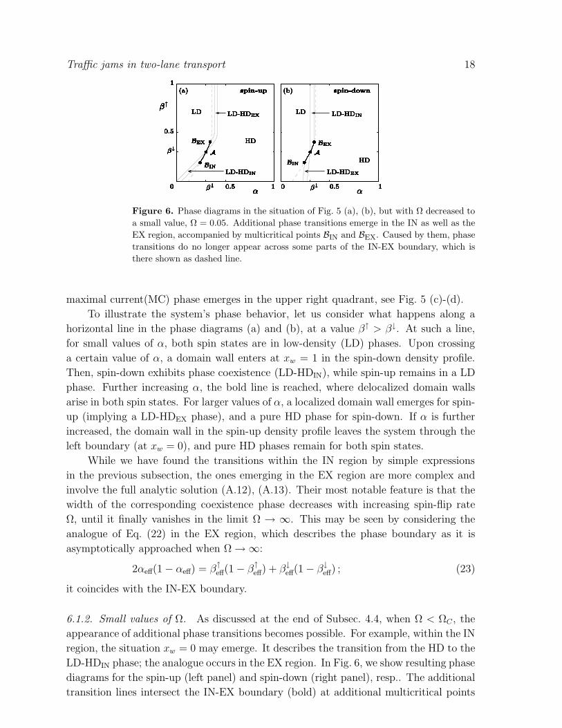
Figure 6. Phase diagrams in the situation of Fig. 5 (a), (b), but with Ω decreased to
a small value, Ω = 0.05. Additional phase transitions emerge in the IN as well as the
EX region, accompanied by multicritical points BIN and BEX. Caused by them, phase
transitions do no longer appear across some parts of the IN-EX boundary, which is
there shown as dashed line.
maximal current(MC) phase emerges in the upper right quadrant, see Fig. 5 (c)-(d).
To illustrate the system’s phase behavior, let us consider what happens along a
horizontal line in the phase diagrams (a) and (b), at a value β↑ > β↓. At such a line,
for small values of α, both spin states are in low-density (LD) phases. Upon crossing
a certain value of α, a domain wall enters at xw = 1 in the spin-down density profile.
Then, spin-down exhibits phase coexistence (LD-HDIN), while spin-up remains in a LD
phase. Further increasing α, the bold line is reached, where delocalized domain walls
arise in both spin states. For larger values of α, a localized domain wall emerges for spin-
up (implying a LD-HDEX phase), and a pure HD phase for spin-down. If α is further
increased, the domain wall in the spin-up density profile leaves the system through the
left boundary (at xw = 0), and pure HD phases remain for both spin states.
While we have found the transitions within the IN region by simple expressions
in the previous subsection, the ones emerging in the EX region are more complex and
involve the full analytic solution (A.12), (A.13). Their most notable feature is that the
width of the corresponding coexistence phase decreases with increasing spin-flip rate
Ω, until it finally vanishes in the limit Ω → ∞. This may be seen by considering the
analogue of Eq. (22) in the EX region, which describes the phase boundary as it is
asymptotically approached when Ω → ∞:
2αeff(1 − αeff) = β↑
eff(1 − β↑
eff) + β↓
eff(1 − β↓
eff) ; (23)
it coincides with the IN-EX boundary.
6.1.2. Small values of Ω. As discussed at the end of Subsec. 4.4, when Ω < ΩC , the
appearance of additional phase transitions becomes possible. For example, within the IN
region, the situation xw = 0 may emerge. It describes the transition from the HD to the
LD-HDIN phase; the analogue occurs in the EX region. In Fig. 6, we show resulting phase
diagrams for the spin-up (left panel) and spin-down (right panel), resp.. The additional
transition lines intersect the IN-EX boundary (bold) at additional multicritical points
Traffic jams in two-lane transport 19
BIN and BEX. Also, they partly substitute the IN-EX boundary as a phase boundary:
across some parts of the latter, phase transitions do not arise. This behavior reflects
the decoupling of the two states for decreasing spin-flip rate Ω. Indeed, for Ω → 0, the
states become more and more decoupled, such that the IN-EX boundary, involving the
combined entrance and exit rates of both states, loses its significance.
6.1.3. Multicritical points. Although the shapes of most of the transition lines
appearing in the phase diagrams shown in Fig. 6 are quite involved, they also exhibit
simple behavior. Pairwise, namely one line from a transition in spin-up and another from
a related transition in spin-down states, they intersect the IN-EX boundary in the same
multicritical point. This intriguing phenomenon may be understood by considering the
multicritical points: e.g., at A, the transition line from the LD to the LD-HDIN phase in
the density profile of spin-up intersects the IN-EX boundary, which implies that there
we have a domain wall in the density profile of spin-up at the position xw = 1. However,
being on the IN-EX boundary, the condition JIN = JEX implies that in this situation a
domain wall forms as well in the density of spin-down states, also located at xw = 1.
Consequently, A also marks the point where the transition line specified by xw = 1
for spin-down states intersects the IN-EX boundary. Due to the special situation of
equal entrance rates, one more pair of lines intersects in this point. Similarly, at BIN,
the transition line from the HD to LD-HDIN phase in the density profile of spin-up
intersects the IN-EX boundary, such that a domain wall forms in the density of spin-up
at xw = 0. Again, as JIN = JEX holds on the IN-EX boundary, this implies the formation
of a domain wall in the density of spin-down at xw = 1, corresponding to the transition
from the LD to the LD-HDEX phase for spin-down in the EX region.
6.2. The general case
Having focused on the physically particularly enlightening case of equal entering rates in
the previous subsection, we now turn to the general case. To illustrate our findings, we
show phase diagrams depending on the injection and extraction rates for spin-up states,
α↑ and β↑. Similar behavior as for equal entrance rates is observed. The multicritical
point A now splits up into two distinct points AIN and AEX.
6.2.1. Large values of Ω: Asymptotic results. Again, large Ω prohibit the emergence
of the phase transition from the HD to the LD-HDIN phase in the IN region as well
as from the LD to the LD-HDEX phase within the EX region, see end of Subsec. 4.4.
In this paragraph, we consider phase diagrams which are approached asymptotically
when Ω → ∞. Convergence is fast in Ω, and the asymptotic phase boundaries yield an
excellent approximation already for Ω & 2ΩC .
The transition from LD to the LD-HDIN phase in the IN region asymptotically
takes the form of Eq. (22), and the one from HD to the LD-HDEX phase in the EX
Traffic jams in two-lane transport 20
0000000000000000 0.50.50.50.50.50.50.50.50.5
0.5
0.5
0.5
0.5
0.5
0.5
0.5
0.5
0.5
0.5
0.5
0.5
0.5
0.5
0.5
111111111
1
1
1
1
1
1
1
1
1
1
1
1
1
1
1(a)(a)(a)(a)(a)(a)(a)(a) (b)(b)(b)(b)(b)(b)(b)(b)spin-upspin-upspin-upspin-upspin-upspin-upspin-upspin-up spin-downspin-downspin-downspin-downspin-downspin-downspin-downspin-down
LDLDLDLDLDLDLDLD
LDLDLDLDLDLDLDLD
HDHDHDHDHDHDHDHDHDHDHDHDHDHDHDHD
LD-HDINLD-HDINLD-HDINLD-HDINLD-HDINLD-HDINLD-HDINLD-HDIN
LD-HDINLD-HDINLD-HDINLD-HDINLD-HDINLD-HDINLD-HDINLD-HDIN
LD-HDEXLD-HDEXLD-HDEXLD-HDEXLD-HDEXLD-HDEXLD-HDEXLD-HDEX
LD-HDEXLD-HDEXLD-HDEXLD-HDEXLD-HDEXLD-HDEXLD-HDEXLD-HDEX
α↑α↑α↑α↑α↑α↑α↑α↑α↑α↑α↑α↑α↑α↑α↑α↑
β↑β↑β↑β↑β↑β↑β↑β↑
α↓α↓α↓α↓α↓α↓α↓α↓α↓α↓α↓α↓α↓α↓α↓α↓
β↓β↓β↓β↓β↓β↓β↓β↓
xw = 0xw = 0xw = 0xw = 0xw = 0xw = 0xw = 0xw = 0
xw = 1xw = 1xw = 1xw = 1xw = 1xw = 1xw = 1xw = 1
AINAINAINAINAINAINAINAINAINAINAINAINAINAINAINAIN
AEXAEXAEXAEXAEXAEXAEXAEX
AEXAEXAEXAEXAEXAEXAEXAEX
0000000000000 0.50.50.50.50.50.50.5
0.5
0.5
0.5
0.5
0.5
0.5
0.5
0.5
0.5
0.5
0.5
0.5
0.5
1111111
1
1
1
1
1
1
1
1
1
1
1
1
1(c)(c)(c)(c)(c)(c)(c) (d)(d)(d)(d)(d)(d)spin-upspin-upspin-upspin-upspin-upspin-upspin-up spin-downspin-downspin-downspin-downspin-downspin-down
LDLDLDLDLDLD
LDLDLDLDLDLDLD
HDHDHDHDHDHDHDHDHDHDHDHDHD
LD-HDINLD-HDINLD-HDINLD-HDINLD-HDINLD-HDINLD-HDIN
LD-HDEXLD-HDEXLD-HDEXLD-HDEXLD-HDEXLD-HDEX
LD-HDEXLD-HDEXLD-HDEXLD-HDEXLD-HDEXLD-HDEXLD-HDEX
α↑α↑α↑α↑α↑α↑α↑α↑α↑α↑α↑α↑α↑
β↑β↑β↑β↑β↑β↑β↑
α↓α↓α↓α↓α↓α↓α↓α↓α↓α↓α↓α↓α↓
β↓β↓β↓β↓β↓β↓β↓
AEXAEXAEXAEXAEXAEX
AEXAEXAEXAEXAEXAEXAEX
000000000000 0.50.50.50.50.50.50.5
0.5
0.5
0.5
0.5
0.5
0.5
0.5
0.5
0.5
0.5
0.5
1111111
1
1
1
1
1
1
1
1
1
1
1(e)(e)(e)(e)(e)(e) (f)(f)(f)(f)(f)(f)spin-upspin-upspin-upspin-upspin-upspin-up spin-downspin-downspin-downspin-downspin-downspin-down
LDLDLDLDLDLDLDLDLDLDLDLD
HDHDHDHDHDHDHDHDHDHDHDHD
LD-HDINLD-HDINLD-HDINLD-HDINLD-HDINLD-HDIN
LD-HDINLD-HDINLD-HDINLD-HDINLD-HDINLD-HDIN
α↑α↑α↑α↑α↑α↑α↑α↑α↑α↑α↑α↑
β↑β↑β↑β↑β↑β↑
α↓α↓α↓α↓α↓α↓α↓α↓α↓α↓α↓α↓
β↓β↓β↓β↓β↓β↓
AINAINAINAINAINAIN
AINAINAINAINAINAIN
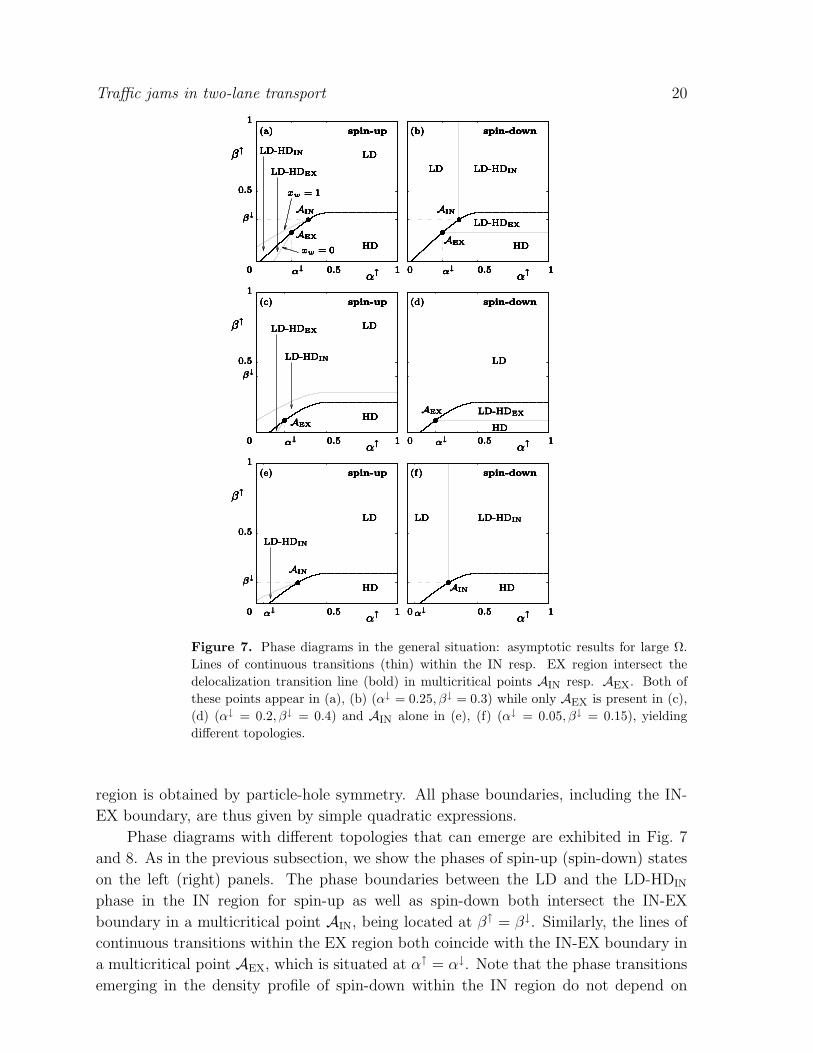
Figure 7. Phase diagrams in the general situation: asymptotic results for large Ω.
Lines of continuous transitions (thin) within the IN resp. EX region intersect the
delocalization transition line (bold) in multicritical points AIN resp. AEX. Both of
these points appear in (a), (b) (α↓ = 0.25, β↓ = 0.3) while only AEX is present in (c),
(d) (α↓ = 0.2, β↓ = 0.4) and AIN alone in (e), (f) (α↓ = 0.05, β↓ = 0.15), yielding
different topologies.
region is obtained by particle-hole symmetry. All phase boundaries, including the IN-
EX boundary, are thus given by simple quadratic expressions.
Phase diagrams with different topologies that can emerge are exhibited in Fig. 7
and 8. As in the previous subsection, we show the phases of spin-up (spin-down) states
on the left (right) panels. The phase boundaries between the LD and the LD-HDIN
phase in the IN region for spin-up as well as spin-down both intersect the IN-EX
boundary in a multicritical point AIN, being located at β↑ = β↓. Similarly, the lines of
continuous transitions within the EX region both coincide with the IN-EX boundary in
a multicritical point AEX, which is situated at α↑ = α↓. Note that the phase transitions
emerging in the density profile of spin-down within the IN region do not depend on

Traffic jams in two-lane transport 21
00000000000000000 0.50.50.50.50.50.50.50.50.5
0.50.50.50.50.50.50.50.5
1111111111
1
1
1
1
1
1
1
1
1
1
1
1
1
1
1(a)(a)(a)(a)(a)(a)(a)(a) (b)(b)(b)(b)(b)(b)(b)(b)(b)spin-upspin-upspin-upspin-upspin-upspin-upspin-upspin-up spin-downspin-downspin-downspin-downspin-downspin-downspin-downspin-downspin-down
LDLDLDLDLDLDLDLDLD
LDLDLDLDLDLDLDLD
HDHDHDHDHDHDHDHDHDHDHDHDHDHDHDHDHD
LD-HDINLD-HDINLD-HDINLD-HDINLD-HDINLD-HDINLD-HDINLD-HDIN
LD
-HD
in
LD
-HD
in
LD
-HD
in
LD
-HD
in
LD
-HD
in
LD
-HD
in
LD
-HD
in
LD
-HD
in
LD
-HD
in
LD-HDEXLD-HDEXLD-HDEXLD-HDEXLD-HDEXLD-HDEXLD-HDEXLD-HDEXLD-HDEX
LD-HDEXLD-HDEXLD-HDEXLD-HDEXLD-HDEXLD-HDEXLD-HDEXLD-HDEX
Deloc.Deloc.Deloc.Deloc.Deloc.Deloc.Deloc.Deloc.Deloc.Deloc.Deloc.Deloc.Deloc.Deloc.Deloc.Deloc.Deloc.
α↑α↑α↑α↑α↑α↑α↑α↑α↑α↑α↑α↑α↑α↑α↑α↑α↑
β↑β↑β↑β↑β↑β↑β↑β↑
α↓ = β↓α↓ = β↓α↓ = β↓α↓ = β↓α↓ = β↓α↓ = β↓α↓ = β↓α↓ = β↓α↓ = β↓α↓ = β↓α↓ = β↓α↓ = β↓α↓ = β↓α↓ = β↓α↓ = β↓α↓ = β↓α↓ = β↓
β↓β↓β↓β↓β↓β↓β↓β↓
AIN = AEXAIN = AEXAIN = AEXAIN = AEXAIN = AEXAIN = AEXAIN = AEXAIN = AEXAIN = AEX
AIN = AEXAIN = AEXAIN = AEXAIN = AEXAIN = AEXAIN = AEXAIN = AEXAIN = AEX
000000000000000 11111111
1
1
1
1
1
1
1
1
1
1
1
1
1
1
1(c)(c)(c)(c)(c)(c)(c)(c) (d)(d)(d)(d)(d)(d)(d)spin-upspin-upspin-upspin-upspin-upspin-upspin-upspin-up spin-downspin-downspin-downspin-downspin-downspin-downspin-down
LDLDLDLDLDLDLDLDLDLDLDLDLDLDLD
HDHDHDHDHDHDHDHDHDHDHDHDHDHDHD
LD-HDINLD-HDINLD-HDINLD-HDINLD-HDINLD-HDINLD-HDINLD-HDIN
LD-HDEXLD-HDEXLD-HDEXLD-HDEXLD-HDEXLD-HDEXLD-HDEXLD-HDEX
MCMCMCMCMCMCMCMCMCMCMCMCMCMCMC
α↑α↑α↑α↑α↑α↑α↑α↑α↑α↑α↑α↑α↑α↑α↑
β↑β↑β↑β↑β↑β↑β↑β↑
α↓ =β↓ = 0.5
α↓ =β↓ = 0.5
α↓ =β↓ = 0.5
α↓ =β↓ = 0.5
α↓ =β↓ = 0.5
α↓ =β↓ = 0.5
α↓ =β↓ = 0.5
α↓ =β↓ = 0.5
α↓ =β↓ = 0.5
α↓ =β↓ = 0.5
α↓ =β↓ = 0.5
α↓ =β↓ = 0.5
α↓ =β↓ = 0.5
α↓ =β↓ = 0.5
α↓ =β↓ = 0.5
β↓β↓β↓β↓β↓β↓β↓β↓
AIN = AEXAIN = AEXAIN = AEXAIN = AEXAIN = AEXAIN = AEXAIN = AEXAIN = AEXAIN = AEXAIN = AEXAIN = AEXAIN = AEXAIN = AEXAIN = AEXAIN = AEX
Figure 8. Delocalization as well as maximal current phase (MC). When α↓ = β↓ <
1/2 and α↑, β↑ ≥ 1/2 [upper right quadrant in (a), (b)], delocalized domain walls form
in the density profiles of both spin states. If instead α↓, β↓ ≥ 1/2, the maximal current
phase emerges, see (c), (d).
β↑, thus being horizontal lines in the phase diagrams. Within the EX region they are
independent of α↑, yielding vertical lines.
For α↓, β↓ < 1/2, Fig. 7 shows different topologies of phase diagrams, which only
depend on which of the multicritical points AIN, AEX is present. If both appear, see
Fig. 7 (a), (b), the LD-HDIN and the LD-HDEX phase for spin-up are adjacent to each
other, separated by the IN-EX boundary. Although in both phases localized domain
walls emerge, their position changes discontinuously upon crossing the delocalization
transition. E.g., starting within the LD-HDIN phase, the domain wall delocalizes when
approaching the IN-EX boundary, and, having crossed it, relocalizes again, but at a
different position.
When α↓ = β↓ < 1/2, a subtlety emerges, see Fig. 8 (a), (b). If both α↑ ≥ 1/2 and
β↑ ≥ 1/2, i.e. in the upper right quadrant of the phase diagrams, these rates effectively
act as 1/2, and the condition JIN = JEX for the IN-EX boundary is fulfilled in this whole
region. Therefore, delocalized domain walls form on both lanes within this region, as is
confirmed by our stochastic simulations [29].
The maximal current phase (MC) emerges when all rates exceed or equal the value
1/2, corresponding to the upper left quadrant of the phase diagrams in Fig. 8 (c), (d).

Traffic jams in two-lane transport 22
(a)(a)(a)(a)(a)(a)(a)(a)(a)(a)(a)(a)(a)(a) (b)(b)(b)(b)(b)(b)(b)(b)spin-upspin-upspin-upspin-upspin-upspin-upspin-upspin-upspin-upspin-upspin-upspin-upspin-upspin-up spin-downspin-downspin-downspin-downspin-downspin-downspin-downspin-down
0000000000000000000000 0.50.50.50.50.50.50.50.50.5
0.5
0.5
0.5
0.5
0.5
0.5
0.5
0.5
0.5
0.5
0.5
0.5
0.5
0.5
0.5
0.5
0.5
0.5
0.5
0.5
0.5
0.5
0.5
0.5
0.5
0.5
0.5
111111111
1
1
1
1
1
1
1
1
1
1
1
1
1
1
1
1
1
1
1
1
1
1
1
1
1
1
1
LDLDLDLDLDLDLDLDLDLDLDLDLDLDLDLDLDLDLDLDLDLD
HDHDHDHDHDHDHDHD
HDHDHDHDHDHDHDHDHDHDHDHDHDHD
LD-HDINLD-HDINLD-HDINLD-HDINLD-HDINLD-HDINLD-HDINLD-HDINLD-HDINLD-HDINLD-HDINLD-HDINLD-HDINLD-HDIN
LD-HDEXLD-HDEXLD-HDEXLD-HDEXLD-HDEXLD-HDEXLD-HDEXLD-HDEX
LD-HDEXLD-HDEXLD-HDEXLD-HDEXLD-HDEXLD-HDEXLD-HDEXLD-HDEXLD-HDEXLD-HDEXLD-HDEXLD-HDEXLD-HDEXLD-HDEX
α↑α↑α↑α↑α↑α↑α↑α↑α↑α↑α↑α↑α↑α↑α↑α↑α↑α↑α↑α↑α↑α↑
β↑β↑β↑β↑β↑β↑β↑β↑β↑β↑β↑β↑β↑β↑
α↓α↓α↓α↓α↓α↓α↓α↓
α↓
α↓
α↓
α↓
α↓
α↓
α↓
α↓
α↓
α↓
α↓
α↓
α↓
α↓
α↓
α↓
α↓
α↓
α↓
α↓
α↓
α↓
α↓
α↓
α↓
α↓
α↓
α↓
xw = 0xw = 0xw = 0xw = 0xw = 0xw = 0xw = 0xw = 0xw = 0xw = 0xw = 0xw = 0xw = 0xw = 0
xw = 1xw = 1xw = 1xw = 1xw = 1xw = 1xw = 1xw = 1xw = 1xw = 1xw = 1xw = 1xw = 1xw = 1
AEXAEXAEXAEXAEXAEXAEXAEX
AEXAEXAEXAEXAEXAEXAEXAEXAEXAEXAEXAEXAEXAEX
BINBINBINBINBINBINBINBIN
BINBINBINBINBINBINBINBINBINBINBINBINBINBIN
NINNINNINNINNINNINNINNINNINNINNINNINNINNIN
(c)(c)(c)(c)(c)(c)(c)(c)(c) (d)(d)(d)(d)(d)spin-upspin-upspin-upspin-upspin-upspin-upspin-upspin-upspin-up spin-downspin-downspin-downspin-downspin-down
00000000000000 0.50.50.50.50.50.5
0.5
0.5
0.5
0.5
0.5
0.5
0.5
0.5
0.5
0.5
0.5
0.5
0.5
0.5
0.5
0.5
0.5
111111
1
1
1
1
1
1
1
1
1
1
1
1
1
1
1
1
1
LDLDLDLDLDLDLDLDLDLDLDLDLDLD
HDHDHDHDHDHDHDHDHD
LD-HDINLD-HDINLD-HDINLD-HDINLD-HDINLD-HDINLD-HDINLD-HDINLD-HDIN
LD-HDEXLD-HDEXLD-HDEXLD-HDEXLD-HDEX
α↑α↑α↑α↑α↑α↑α↑α↑α↑α↑α↑α↑α↑α↑
β↑β↑β↑β↑β↑β↑β↑β↑β↑
α↓α↓α↓α↓α↓
α↓
α↓
α↓
α↓
α↓
α↓
α↓
α↓
α↓
α↓
α↓
α↓
α↓
α↓
α↓
α↓
α↓
α↓
BINBINBINBINBIN
BINBINBINBINBINBINBINBINBIN
NINNINNINNINNINNINNINNINNIN
Figure 9. Phase diagrams in the general case and small values of Ω. The nodal point
NIN remains unchanged when Ω is varied. The appearance of the multicritical point
BIN is accompanied by the non-occurrence of phase transitions across parts of the IN-
EX boundary, then shown as dashed line. The multicritical point AEX emerges in (a),
(b), but not in the situation of (c)(, (d). Parameters are Ω = 0.08, α↓ = 0.35, β↓ =
0.45 in (a), (b) and Ω = 0.2, α↓ = 0.15, β↓ = 0.4 in (c), (d).
6.2.2. Small values of Ω. When Ω < ΩC , the transitions from LD to LD-HDIN within
the IN region as well as the analogue in the EX region are possible. As in the case
of equal entering rates, the corresponding transition lines pairwise intersect the IN-EX
boundary in multicritical points BIN and BEX. As all transitions between phases of the
spin-down density within the IN region are independent of β↑, the corresponding lines
are simply horizontal; and within the EX region, their independence of α↑ implies that
they yield vertical lines. The phase diagram for the density of spin-down is thus easily
found from the IN-EX boundary given by JIN = JEX together with the locations of the
multicritical points AIN, AEX, BIN and BEX. The latter follow from the intersection of
phase transition lines for the density of spin-up, involving the whole analytic solution
(A.12), (A.13), with the IN-EX boundary.
In Fig. 9 two interesting topologies that may arise are exemplified. Induced by the
presence of the multicritical point BIN, phase transitions do not occur across all the
IN-EX boundary, which is then only shown as dashed line. In Fig. 9 (a), (b), the points
AEX and BIN are present. The LD-HDIN phase for spin-up intervenes the LD and the
HD phase; the LD-HDEX phase for spin-up is also present, though very tiny. In the
phase diagram of spin-down, the LD-HDIN phase intervenes the LD and the HD phase
accompanied by continuous as well as discontinuous transitions. Again, the presence of
Traffic jams in two-lane transport 23
the multicritical points induces the topology; e.g. in Fig. 9 (c), (d), only BIN appears.
For the discussion of the possible topologies, we encounter the restriction that AIN and
BIN cannot occur together, as well as AEX and BEX exclude each other (otherwise, the
lines determined by xw = 0 and xw = 1 would cross).
We now discuss the influence of the spin-flip rate Ω on the continuous transition
lines for spin-up. In Subsec. 4.4 the manifold defined by α↑ = β↑ = α↓
eff was found to be a
sub-manifold of the phase boundary specified by xw = 1 in the IN region. Independent
of Ω, the point α↑ = β↑ = α↓
eff, denoted by NIN, thus lies on the boundary between
the LD and the LD-HDIN phase (determined by xw = 1). For large Ω, this boundary
approaches the one given by Eq. (22).
Regarding the transition from the HD to the LD-HDIN within the IN region (determined
by xw = 0), Subsec. 4.4 revealed that for increasing Ω it leaves the IN region at a critical
transfer rate Ω∗(α↓, β↑). In the limit Ω → 0, the densities ρ↑(x) and ρ↓(x) approach
constant values, and both the curve xw = 1 as xw = 0 for spin-up in the IN region
approach the line β↑ = α↑ for α↑ ≤ 12; The phase in the upper right quadrant in the
phase diagram converges to the MC phase, such that in this limit, the case of two
uncoupled TASEPs is recovered.
7. Conclusions
We have presented a detailed study of an exclusion process with internal states recently
introduced in [19]. The Totally Asymmetric Exclusion Process (TASEP) has been
generalized by assigning two internal states to the particles. Pauli’s exclusion principle
allows double occupation only for particles in different internal states. Occasional
switches from one internal state to the other induce a coupling between the transport
processes of the separate states. Such a dynamics encompasses diverse situations,
ranging from vehicular traffic on multiple lanes to molecular motors walking on
intracellular tracks and future spintronics devices.
We have elaborated on the properties of the emerging non-equilibrium steady state
focusing on density and current profiles. In a mesoscopic scaling of the switching rate
between the internal states, nontrivial phenomena emerge. A localized domain wall in
the density profile of one of the internal states induces a spontaneous polarization effect
when viewing the internal states as spins. We provide an explanation based on the
weakly conserved currents of the individual states and the current-density relations. A
quantitative analytic description within a mean-field approximation and a continuum
limit has been developed and solutions for the density and current profiles have been
presented. A comparison with stochastic simulations revealed that our analytic approach
becomes exact in the limit of large system sizes. We have attributed this remarkable
finding to the exact current-density relation in the TASEP, supplemented by the locally
weak coupling of the two TASEPs appearing in our model: ω → 0 in the limit of large
system sizes. Local correlations between the two internal states are thus obliterated, as
particles hop forward on a much faster timescale than they switch their internal state.
Traffic jams in two-lane transport 24
Furthermore, the parameter regions that allow for the formation of a localized
domain wall have been considered. Analytic phase diagrams for various scenarios, in
particular the case of equal entrance rates, have been derived. The phase diagrams
have been found to exhibit a rich structure, with continuous as well as discontinuous
non-equilibrium phase transitions. The discontinuous one originates in the conserved
particle current, which is either limited by injection or extraction of particles. At the
discontinuous transition between both regimes, delocalized domain walls emerge in the
density profiles of both internal states. Multicritical points appear at the intersections
of different transition lines organizing the topology of the phase diagrams. Two classes
of multicritical points are identified, one of them arises only for sufficiently small gross
spin-flip rate Ω < ΩC . The value ΩC , calculated analytically, provides a natural scale
for the rate Ω.
It would be of interest to see which of the described phenomena qualitatively remain
when generalizing the model to include more than two internal states. Indeed, within
the context of molecular motors walking on microtubuli [7], between 12 and 14 parallel
lanes are relevant. Also, the internal states might differ in the sense of different switching
rates from one to another [28] and the built-in asymmetry may result in different
phases. In the context of intracellular transport it appears worthwhile to investigate
the consequences of a coupling to a bulk reservoir, c.f. [33, 34, 35]; in particular, to
study the interplay of domain wall formation induced by attachment and detachment
processes as well as rare switching events.
8. Acknowledgements
The authors are grateful for helpful discussions with Felix von Oppen, Ulrich Schollwock,
Paolo Pierobon and Mauro Mobilia. Financial support of the German Excellence
Initiative via the program “Nanosystems Initiative Munich (NIM)” is gratefully
acknowledged.
Appendix A. The densities in the first order approximation and the critical
value ΩC
In this Appendix, we give details on the derivation of the analytic solution of the
mean-field approximation in the continuum limit to first order in ǫ, i.e. the system
of differential equations (10), (11).
Summing them we find
∂x[2ρ↑(xi) − 1]2 + ∂x[2ρ
↓(xi) − 1]2 = 0 , (A.1)
such that
[2ρ↑(xi) − 1]2 + [2ρ↓(xi) − 1]2 = J , (A.2)
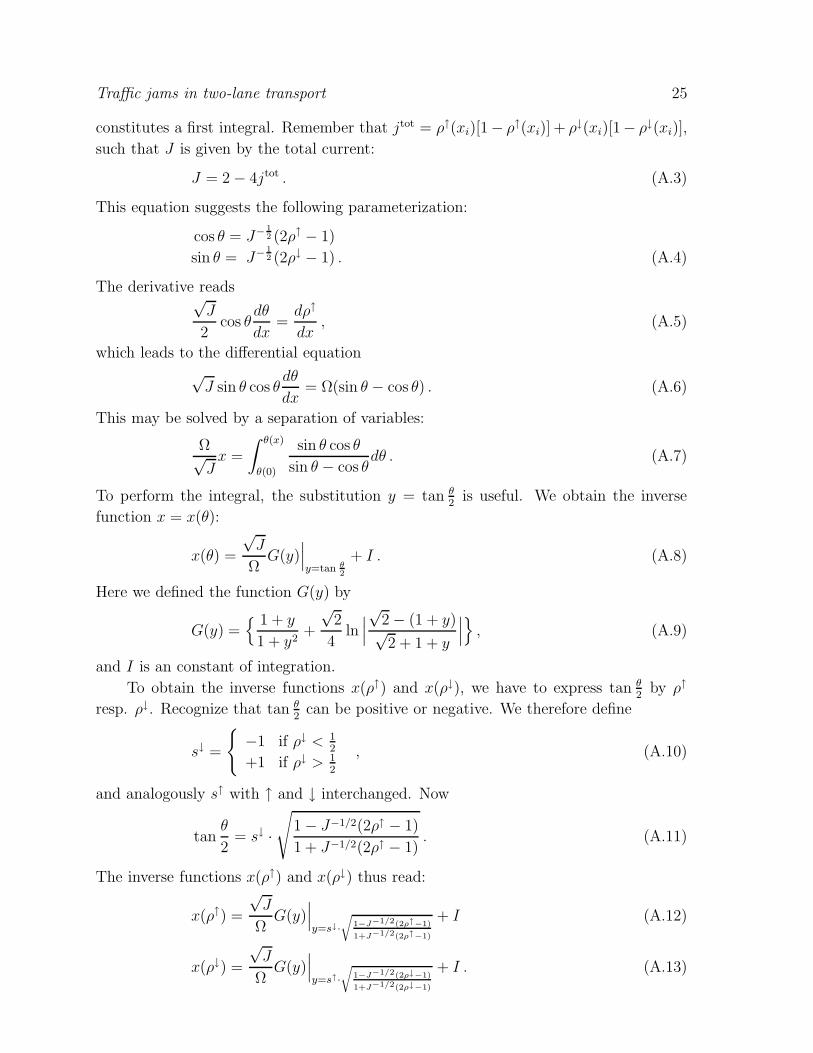
Traffic jams in two-lane transport 25
constitutes a first integral. Remember that jtot = ρ↑(xi)[1− ρ↑(xi)] + ρ↓(xi)[1− ρ↓(xi)],
such that J is given by the total current:
J = 2 − 4jtot . (A.3)
This equation suggests the following parameterization:
cos θ = J− 12 (2ρ↑ − 1)
sin θ = J− 12 (2ρ↓ − 1) . (A.4)
The derivative reads√J
2cos θ
dθ
dx=
dρ↑
dx, (A.5)
which leads to the differential equation
√J sin θ cos θ
dθ
dx= Ω(sin θ − cos θ) . (A.6)
This may be solved by a separation of variables:
Ω√J
x =
∫ θ(x)
θ(0)
sin θ cos θ
sin θ − cos θdθ . (A.7)
To perform the integral, the substitution y = tan θ2
is useful. We obtain the inverse
function x = x(θ):
x(θ) =
√J
ΩG(y)
∣
∣
∣
y=tan θ2
+ I . (A.8)
Here we defined the function G(y) by
G(y) = 1 + y
1 + y2+
√2
4ln
∣
∣
∣
√2 − (1 + y)√2 + 1 + y
∣
∣
∣
, (A.9)
and I is an constant of integration.
To obtain the inverse functions x(ρ↑) and x(ρ↓), we have to express tan θ2
by ρ↑
resp. ρ↓. Recognize that tan θ2
can be positive or negative. We therefore define
s↓ =
−1 if ρ↓ < 12
+1 if ρ↓ > 12
, (A.10)
and analogously s↑ with ↑ and ↓ interchanged. Now
tanθ
2= s↓ ·
√
1 − J−1/2(2ρ↑ − 1)
1 + J−1/2(2ρ↑ − 1). (A.11)
The inverse functions x(ρ↑) and x(ρ↓) thus read:
x(ρ↑) =
√J
ΩG(y)
∣
∣
∣
y=s↓·
r
1−J−1/2(2ρ↑−1)
1+J−1/2(2ρ↑−1)
+ I (A.12)
x(ρ↓) =
√J
ΩG(y)
∣
∣
∣
y=s↑·
r
1−J−1/2(2ρ↓−1)
1+J−1/2(2ρ↓−1)
+ I . (A.13)

Traffic jams in two-lane transport 26
The constants of integration I and J = 2−4jtot are determined by matching the bound-
ary conditions. The inverse functions of Eqs. (A.12), (A.13) constitute the solution to
Eqs. (10) and (11), within the first-order approximation to the mean-field equations for
the densities in the continuum limit.
Next, we derive the result on ΩC given at the end of Subsec. 4.4. Therefore, consider
Fig. 4. We are interested in the point x 12, and thus in the right branch of the spin-up
density profile. As the spin-down density is in the LD phase, i.e. it is smaller than 12, we
have s↓ = −1 in the above solution for ρ↑. Thus, y ≤ 0 in Eq. (A.12). At the branching
point of the analytic solution, i.e. the point x 12, we have the density 1
2, such that there
y = −1, implying G(y) = 0. Now, if this branching point lies on the right boundary,
x 12
= 0, as it does for the critical Ω∗, this yields I = 0 in Eq. (A.12). On the other hand,
the right branch satisfies the boundary condition on the right: ρ↑(x = 1) = 1 − β↑.
Upon substitution into Eq. (A.12), we obtain
1 = x(1 − β↑) =
√J
Ω∗G(y)
∣
∣
∣
y=−
r
1−J−1/2(1−2β↑)
1+J−1/2(1−2β↑)
. (A.14)
which for given α↓, β↑ is an equation for Ω∗(α↓, β↑). In particular, Ω∗(α↓, β↑) is
monotonically increasing in G. Investigating G(y), it turns out that G(y) is in turn
increasing in y. Since y is bounded from above by y = 0, the maximal value for G(y)
is provided by G(y = 0) = 1 + 14
√2 ln (3 − 2
√2). Next, we note that Ω∗(α↓, β↑) is
an increasing function of√
J . With the constraint that α↑
eff = 12, which is necessary
for x 12
= 0, the largest√
J arises for α↓ = 0, i.e.√
J = 1. Combining both results,
the maximal value for the critical rates Ω∗(α↓, β↑) occurs for α↓ = 0 and y = 0. Both
conditions together yield
ΩC = 1 +1
4
√2 ln (3 − 2
√2) . (A.15)
Finally, we note that α↓ = 0 and y = 0 implies β↑ = 0, such that ΩC arises if α↓ = 0
and β↑ = 0.
References
[1] A. Barabasi and H. Stanley, Fractal Concepts in Surface Growth (Cambridge University Press,
Cambridge, England, 1995).
[2] G. Deutscher, R. Zallan, and J. Adler, eds., Percolation Structures and Processes, vol. 5 of Annals
of the Israel Physical Society (Adam Hilger, Bristol, 1983).
[3] M. Droz, Z. Racz, and J. Schmidt, Phys. Rev. A 39, 2141 (1989).
[4] D. C. Mattis and M. L. Glasser, Rev. Mod. Phys. 70, 979 (1998).
[5] B. Schmittmann and R. Zia, in Phase Transitions and Critical Phenomena, edited by C. Domb
and J. Lebowitz (Academic Press, London, 1995), vol. 17.
[6] C. MacDonald, J. Gibbs, and A. Pipkin, Biopolymers 6, 1 (1968).
[7] J. Howard, Mechanics of Motor Proteins and the Cytoskeleton (Sinauer Press, Sunderland,
Massachusetts, 2001).
[8] N. Hirokawa, Science 279, 519 (1998).

Traffic jams in two-lane transport 27
[9] D. Helbing, Rev. Mod. Phys. 73, 1067 (2001).
[10] D. Chowdhury, L. Santen, and A. Schadschneider, Physics Reports 329, 199 (2000).
[11] B. Derrida and M. Evans, in Nonequilibrium Statistical Mechanics in One Dimension, edited by
V. Privman (Cambridge University Press, Cambridge, 1997), pp. 277–304.
[12] D. Mukamel, in Soft and Fragile Matter, edited by M. Cates and M. Evans (Institute of Physics
Publishing, Bristol, 2000), pp. 237–258.
[13] G. Schutz, in Phase Transitions and Critical Phenomena, edited by C. Domb and J. Lebowitz
(Academic Press, San Diego, 2001), vol. 19, pp. 3–251.
[14] J. Krug, Phys. Rev. Lett. 67, 1882 (1991).
[15] G. Odor, Rev. Mod. Phys. 76, 663 (2004).
[16] U. C. Tauber, M. J. Howard, and H. Hinrichsen, Phys. Rev. Lett. 80, 2165 (1998).
[17] J. D. Noh and H. Park, Phys. Rev. Lett. 94, 145702 (2005).
[18] E. Dagotto and T. M. Rice, Science 271, 618 (1996).
[19] T. Reichenbach, T. Franosch, and E. Frey, Phys. Rev. Lett. 97, 050603 (2006).
[20] I. Zutic, J. Fabian, and S. D. Sarma, Rev. Mod. Phys. 76, 323 (2004).
[21] C. K. Hahn, Y. J. Park, E. K. Kim, and S. Min, Appl. Phys. Lett. 73, 2479 (1998).
[22] H. Hinsch, R. Kouyos, and E. Frey, in Traffic and Granular Flow ’05, edited by A. Schadschneider,
T. Poschel, R. Kuhne, M. Schreckenberg, and D. E. Wolf (Springer, 2006).
[23] V. Popkov and I. Peschel, Phys. Rev. E 64, 026126 (2001).
[24] V. Popkov and G. M. Schutz, J. Stat. Phys 112, 523 (2003).
[25] V. Popkov, J. Phys. A: Math. Gen. 37, 1545 (2004).
[26] E. Pronina and A. B. Kolomeisky, J. Phys. A: Math. Gen. 37, 9907 (2004).
[27] T. Mitsudo and H. Hayakawa, J. Phys. A: Math. Gen. 38, 3087 (2005).
[28] E. Pronina and A. B. Kolomeisky, Physica A 372, 12 (2006).
[29] T. Reichenbach, T. Franosch, and E. Frey, in preparation.
[30] L. B. Shaw, R. K. P. Zia, and K. H. Lee, Phys. Rev. E 68, 021910 (2003).
[31] P. Pierobon, T. Franosch, and E. Frey, Phys. Rev. E 74, 031920 (2006).
[32] B. Derrida, Phys. Rep. 301, 65 (1998).
[33] S. Klumpp and R. Lipowsky, J. Stat. Phys. 113, 233 (2003).
[34] A. Parmeggiani, T. Franosch, and E. Frey, Phys. Rev. Lett. 90, 086601 (2003).
[35] A. Parmeggiani, T. Franosch, and E. Frey, Phys. Rev. E 70, 046101 (2004).