towards optimal power control via ensembling deep neural

arX

iv:1

807.

1002

5v2

[ee

ss.S

P] 1

0 M

ar 2

019

1

Towards Optimal Power Control via

Ensembling Deep Neural Networks

Fei Liang, Cong Shen, Senior Member, IEEE, Wei Yu, Fellow, IEEE,

and Feng Wu, Fellow, IEEE

Abstract

A deep neural network (DNN) based power control method is proposed, which aims at solving

the non-convex optimization problem of maximizing the sum rate of a fading multi-user interference

channel. Towards this end, we first present PCNet, which is a multi-layer fully connected neural network

that is specifically designed for the power control problem. A key challenge in training a DNN for

the power control problem is the lack of ground truth, i.e., the optimal power allocation is unknown.

To address this issue, PCNet leverages the unsupervised learning strategy and directly maximizes the

sum rate in the training phase. We then present PCNet+, which enhances the generalization capacity of

PCNet by incorporating noise power as an input to the network. Observing that a single PCNet(+) does

not universally outperform the existing solutions, we further propose ePCNet(+), a network ensemble

with multiple PCNets(+) trained independently. Simulation results show that for the standard symmetric

K-user Gaussian interference channel, the proposed methods can outperform all state-of-the-art power

control solutions under a variety of system configurations. Furthermore, the performance improvement

of ePCNet comes with a reduced computational complexity.

I. INTRODUCTION

The capacity region of the multi-user interference channel is among the longest outstanding open

problems in information theory [1], [2]. Progress on solving this problem has profound impact on

today’s wireless networks, as interference management has become the bottleneck of the overall system

performance due to the broadcast nature of wireless communications and the dense deployment of base

stations and mobiles, which create a heavily interfering environment.

F. Liang, C. Shen and F. Wu are with the Laboratory of Future Networks, School of Information Science and Technology,

University of Science and Technology of China.

W. Yu is with the Electrical and Computer Engineering Department, University of Toronto.

http://arxiv.org/abs/1807.10025v2

2

In this paper, we make progress on the power control problem that maximizes the sum rate of a multi-

user interference channel, where each receiver is restricted to treating interference as noise (TIN). This

problem (including some variations) is generally NP-hard, and has been investigated for decades. Due

to its non-convex nature, state-of-the-art solutions in the literature often involve either exhaustive search

(explicitly or implicitly) [3], [4] or iterative optimization of some approximate sub-problems [5]–[8].

Performance, convergence, and complexity issues hinder the practicality of these solutions. In particular,

how to achieve efficient power control when the number of users is large remains an open problem.

This work addresses power control from a different perspective. Instead of directly tackling the non-

convex optimization problem in an analytical fashion, we leverage the recent advances in deep learning

to investigate whether a data-driven method can achieve better performance with lower complexity. In

particular, the proposed approach establishes a connection between the sum-rate maximization problem

and minimizing a loss function in training a deep neural network (DNN), and relies on the efficient

network training and ensembling mechanism to achieve near-optimal power control.

Deep learning has had great success in computer vision, natural language processing and some other

applications. Recent results also show that deep learning can be a promising tool in solving difficult

communication problems, such as channel decoding [9], [10], radio signal classification [11], and channel

estimation [12]. For the considered power control problem, Sun et. al. [13] recently proposed a neural

network based method, in which the network is trained with the power control results of WMMSE [8]

serving as the ground truth. This method has lower computational complexity compared to the original

WMMSE, but the sum rate is also upper bounded by it. A natural question thus arises: in addition to the

benefit of low complexity, can we also achieve better performance (in terms of larger sum rate) than the

existing power control methods?

In this paper, we answer this question affirmatively by proposing a novel family of methods, called

ensemble Power Control Network (ePCNet). There are two key ingredients in ePCNet. The first is that

in order to simultaneously achieve higher sum rate and lower computation complexity than existing

methods, we move away from the supervised learning method used in [13] and adopt an unsupervised

learning strategy. The resulting PCNet is trained to directly maximize the system sum rate, as opposed to

minimizing the loss against any sub-optimal method (such as WMMSE). This idea lifts the performance

upper bound limitation of [13] and allows us to approach the ultimate ground truth, i.e., the globally

optimal power control. A variation to PCNet, called PCNet+, further enhances its generalization capacity

by allowing a single trained network to handle a range of noise power levels.

The second component is ensemble learning. This is particularly useful as we observe that a single

PCNet may not universally outperform all existing methods. The proposed ePCNet, however, creates

3

multiple independent “copies” of PCNet and trains them separately, before forming an ensemble that

selects the power profile which leads to the largest sum rate. We show via numerical simulations that

combining DNN with ensemble learning results in a high-performance and low-complexity power control

method that outperforms state-of-the-art methods in a variety of system configurations. Furthermore, this

method is especially efficient when the number of users is large, for which traditional methods do not

always provide satisfactory results.

The rest of this paper is organized as follows. Related works are discussed in Section II. The system

model is introduced in Section III. In Section IV, the main contributions of this paper, including the

PCNet(+) and ePCNet(+), are explained in detail. Simulation results are given in Section VI and VII.

The paper is concluded in Section VIII.

To honor the tradition in the machine learning community and support reproducible research, we have

made our source code publicly available at: https://github.com/ShenGroup/PCNet-ePCNet.

II. RELATED WORKS

A. Power control for interference management

Interference management via power control is a critical technique towards efficient frequency reuse in

both wireless networks (such as cellular systems [7]) and wired networks (such as Digital Subscriber Lines

[14]). This problem has several variations, including min-rate maximization [15], sum-rate or weighted

sum-rate maximization (SRM or WSRM) [16], [17], QoS constrained power minimization [18], and some

hybrid formulations [6]. Different channel models are also considered, including the scalar interference

channel (IC) model, the parallel IC model and the MIMO IC model [14]. However, regardless of the

specific problem formulation, the resulting optimization problem is generally non-convex, which makes

the solution non-trivial and has sparked a lot of research. In this section, we give a brief overview of

related literature. A comprehensive survey can be found in [14], [19].

The sum rate or weighted sum rate maximization problem is one of the most fundamental formulations

of power control problems, and has been thoroughly investigated in the literature. For the scalar IC model,

Chen et al. [5] proposed a round-robin power control method to determine the transmit power user-by-

user, by solving a polynomial system equation. Binary power control was carefully investigated in [7].

The authors found that binary power control can provide near-optimal performance and a low-complexity

greedy binary power control algorithm was proposed. Noting that binary power control can be equivalently

viewed as a scheduling problem, the authors in [20] studied user scheduling and proposed a distributed

algorithm called ITLinQ, which implicitly maximizes the sum rate by activating a subset of links in which

TIN can approach the capacity region with a provable gap.

https://github.com/ShenGroup/PCNet-ePCNet

4

For the parallel IC model where the spectrum is divided into several independent non-overlapping bands,

the problem is more complicated. In [16], [21], this problem was addressed via Lagrangian dualization.

However, due to the non-convex nature of the primal problem, a duality gap exists. This gap vanishes

when the number of channels goes to infinity [16]. Noting that if the power allocation of all other users

is fixed, power control of the present user can be effectively solved via water-filling, the authors of [22]

proposed to execute water-filling iteratively until convergence. A modified iterative water-filling method

was later proposed for resource allocation in the presence of crosstalk [23]. For MIMO IC channels, Shi

et al. transformed the original problem into an equivalent weighted sum mean-square error minimization

(WMMSE) problem [8]. The WMMSE problem is convex for each individual variable when others are

fixed, which makes it easier to find a local optimal solution. The authors of [24] further adopted the

WMMSE method to study the full-duplex MIMO interference channel. The WMMSE algorithm turns

out to be related to a more powerful fractional programming approach that can be used for the joint

power control, scheduling and beamforming optimization problem [25]–[27].

The power control problem becomes more complex if additional QoS constraints are incorporated. In

[6], the authors proposed to maximize the weighted sum rate with explicit QoS constraints via geometric

programming (GP). Under the high-SNR assumption, the original problem can be approximated as a

standard GP. Without the high-SNR assumption, it can be transformed into a series of GP problems,

where the SCALE algorithm was proposed in [17] to solve a series of approximated convex problems.

B. Applications of deep learning in communications

Inspired by its success in many areas, researchers have begun to study whether deep learning can help

improve the design of communication algorithms [28], [29]. In recent years, many works in this field

have appeared, targeting different aspects of physical-layer and MAC-layer designs.

Channel decoding is the first topic that researchers have attempted to leverage deep learning for better

error performance and lower complexity. The authors in [9] carried out a thorough investigation on

deep learning decoding of linear codes. Based on the belief-propagation (BP) decoding architecture, they

adopted the feed-forward and recurrent neural network models to build channel decoders by assigning

different weights to the edges in the Tanner graph. With careful training, the neural network decoder can

achieve better performance than the traditional BP decoder [9]. Since BP decoding has high complexity,

neural network decoding has also been investigated for min-sum decoding [30]. Combined with the

modified random redundant (mRRD) iterative algorithm [31], further performance improvement can be

obtained. For channel decoding under colored noise, Liang et. al. proposed an iterative BP-CNN structure

in which one convolutional neural network is concatenated with a standard BP decoder for noise estimation

5

[10]. To handle long block length, [32] proposed to divide the Polar coding graph into sub-blocks, and

the decoder for each sub-codeword can be trained separately to reduce the overall complexity.

Besides channel decoding, deep learning has the potential to improve the state of the art in other areas.

Toward the end-to-end learning of communication systems, Dorner et al. [33] have demonstrated the

feasibility to design a communication system whose transmitter and receiver are entirely implemented

with neural networks. The authors of [34] applied deep neural networks to MIMO detection, which results

in comparable detection performance but with much lower complexity. To address the excessive feedback

overhead, Wen et. al. designed CsiNet, which learns a transformation from CSI to a codeword and a

corresponding inverse transformation [35]. In [36], neural networks have been used to design an encoder

and decoder for sparse coded multiple access (SCMA). The resulting encoder if [36] can automatically

construct efficient codebooks. Deep learning is also considered for radio signal classification [11], traffic

type recognition [37], channel estimation [38], and optical fiber communications [39].

Narrowing down to the power control problem, the authors in [13] have proposed a power control

algorithm that is based on training a deep neural network with WMMSE as benchmarks. They showed

that the new solution can approach WMMSE in terms of the sum rate performance, but with much

lower complexity. However, with WMMSE serving as the ground truth, the performance of the neural

network is also upper bounded by the achievable sum rate of WMMSE, which is not the global optimum.

This limitation has motivated us to abandon the supervised learning strategy in training DNN, and resort

to various new techniques, such as unsupervised learning, ensemble learning and batch normalization.

The goal is to simultaneously improve the sum-rate performance over state-of-the-art algorithms while

reducing the online computational complexity.

III. SYSTEM MODEL

A. K-User single-antenna interference channel

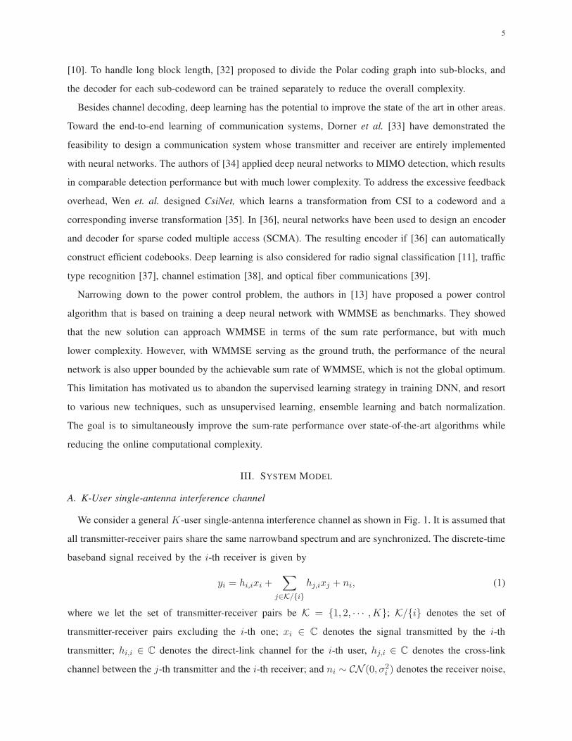
We consider a general K-user single-antenna interference channel as shown in Fig. 1. It is assumed that

all transmitter-receiver pairs share the same narrowband spectrum and are synchronized. The discrete-time

baseband signal received by the i-th receiver is given by

yi = hi,ixi +∑

j∈K/{i}

hj,ixj + ni, (1)

where we let the set of transmitter-receiver pairs be K = {1, 2, · · · ,K}; K/{i} denotes the set of

transmitter-receiver pairs excluding the i-th one; xi ∈ C denotes the signal transmitted by the i-th

transmitter; hi,i ∈ C denotes the direct-link channel for the i-th user, hj,i ∈ C denotes the cross-link

channel between the j-th transmitter and the i-th receiver; and ni ∼ CN (0, σ2i ) denotes the receiver noise,

6

TX 2

TX K

+

+

+

TX 1

y1

x2 y2

xK yK

x1

n1

RX 1

RX 2

RX 3

n2

nK...

.

..

Fig. 1. The K-user interference channel.

which is independent across both time and users. Receiver i only intends to decode xi. For simplicity,

we assume that all receivers have the same noise power σ2. We note that this model has been widely

studied in the literature; see [3], [5], [8], [13].

A block fading channel model is assumed, i.e., the channel coefficients remain unchanged in one

time slot but change independently from one time slot to another. We do not pose any limitation on

the distribution of hi,i, as our method is generic enough to handle different channel models. Random

Gaussian codebooks are assumed. Encoding is independent across users and no interference cancellation is

performed at each receiver. Thus, the transmitter-receiver pairs do not cooperate and multiuser interference

is treated as additive noise, i.e., TIN [20]. Therefore, the effective received noise power at the i-th receiver

is σ2i +

∑j∈K/{i} Pj‖hj,i‖

2.

The transmit power Pi for user i can be chosen from set Pi ⊆ R+. In this work, for simplicity, we

consider Pi = {P : 0 ≤ P ≤ Pmax},∀i ∈ K, where Pmax is the maximum power that transmitters can use.

Note that 0 ∈ Pi. Thus, a user may choose not to transmit1. The joint power profile of all users is denoted

by P = (P1, P2, · · · , PK)T ∈ P, where P = P1 × P2 × · · · × PK and (·)T denotes matrix transpose.

For a given profile P and channel realizations {hij}i,j∈K, the achievable rate of the i-th receiver under

Gaussian codebooks is

Ri(P) = log

(1 +

Pi‖hi,i‖2

σ2i +

∑j∈K/{i} Pj‖hj,i‖2

). (2)

For each slot, the channel coefficients are fixed, and the power control algorithm outputs a power profile

P based on the channel realization.

1Hence, user scheduling is implicitly considered.

7

B. Problem formulation

The objective of power control for interference management is to find the optimal power profile P for

all users to maximize system performance under some specific constraints. With different performance

measures and under different constraints, the power control problem has different formulations. In this

paper, we focus on two specific power control problems: (1) sum rate maximization; and (2) sum rate

maximization under QoS constraints. We comment that both formulations are widely researched in the

literature; see [19] for a comprehensive survey.

1) Sum Rate Maximization (SRM): The sum rate maximization (SRM) problem is formally given as

maximizeP

K∑

i=1

Ri(P)

subject to 0 ≤ Pi ≤ Pmax,∀i ∈ K.

(3)

Problem (3) is the simplest formulation among various power control problems. However, it is very

difficult to solve due to its non-convex nature with respect to the power profile. The optimization problem

(3) is known to be NP-hard [19].

2) Sum Rate Maximization under QoS Constraints (SRM-QC): A more complicated variation of (3)

is to maximize the sum rate while satisfying the minimum rate requirement of all receivers, which can

be formally presented as

maximizeP

K∑

i=1

Ri(P)

subject to Ri(P) ≥ ri,min,∀i ∈ K,

0 ≤ Pi ≤ Pmax,∀i ∈ K,

(4)

where ri,min is the minimum required rate of the i-th receiver. For simplicity, we define

rmin = (r1,min, · · · , rK,min).

Obviously, if we set ri,min = 0,∀i ∈ K, the SRM-QC problem (4) degenerates to the SRM problem (3).

If the target rates are large, the SRM-QC problem may have no feasible solution. It is not difficult to

derive a criterion to check its feasibility [3], [19]. Define matrix B as:

Bi,j =

0, i = j

γi,min‖hj,i‖2

‖hi,i‖2 , i 6= j,

(5)

where Bi,j denotes the (i, j)-th element of B, and γi,min is the minimum signal-to-interference-plus-noise

ratio (SINR) of the i-th receiver that is required to satisfy the minimum rate constraint, i.e. γi,min =

8

��

� ��

��maxP

maxP

maxP

1P

2P

×

×

×

KP

1 ,1h

1 , 2h

,� �h

0

(1)1,��

0

(1)2,��

1 0

(1),� ��

( )1,1

( )2,1�

�( )

,1 �� ( )

1,2�

�

( )2,2�

�

( ),2��

1

( )1, ��

−

1

( )2, ��

−

1

( ),! "#$ %&

−

(1)1,1'

(1)2,1(

1

(1),1)* (1)

1,2+(1)2,2,

1

(1),2-.

Fig. 2. Illustration of PCNet.

2ri,min − 1. If the maximum eigenvalue of B is larger than 1, it is possible to find a feasible power

allocation P as

P = (I−B)−1u, (6)

where I denotes an K ×K identity matrix and u is a K × 1 column vector with the i-th element ui as

ui =γi,minσ

2i

‖hi,i‖. (7)

If all elements in P are in the range between 0 and Pmax, then the power profile P is a feasible solution

of the problem (4). Otherwise (4) is not feasible. Notes that P may not be the optimal solution.

IV. PCNET AND PCNET+: TRAINING DNN FOR POWER CONTROL

We describe the proposed PCNet, and a simple variation PCNet+, in this section, including details of

the DNN design and the training mechanism based on unsupervised learning. As mentioned before, the

SRM problem (3) is a special format of the SRM-QC problem (4). We thus describe the proposed design

that is universal to both problem (3) and (4), and only highlight the differences when applicable.

A. Network design

We propose to exploit a fully connected deep neural network to address the power control problem

(3). The network structure is illustrated in Fig. 2. More specifically, the network consists of one input

layer of K2 nodes, one output layer of K nodes, and L− 1 fully connected hidden layers. These layers

are indexed from 0 to L. The input layer of PCNet is formed by aligning all ‖hi,j‖ as a column vector,

9

denoted as h. The input vector is processed by the L fully connected layers, including L − 1 hidden

layers and one output layer.

The reason that a fully connected DNN is adopted, other than more sophisticated networks such as

convolutional neural networks (CNN) or recurrent neural networks (RNN), is that there is little structure

to explore for the general problem (3) and (4). On the other hand, if the problem exhibits certain features,

such as the existence of correlation among different channel coefficients, then a more structured neural

network such as CNN may be useful. This topic is left for consideration in a future work.

We denote the number of nodes in the k-th layer as lk. If the k-th layer is a hidden layer, its output

is calculated as follows:

ck = ReLU (BN (Wkck−1 + bk)) , (8)

where ck−1 and ck are the output vectors of the previous and current layers; their dimensions are lk−1×1

and lk×1 respectively; Wk is the lk× lk−1 weight matrix and bk is the lk×1 bias vector; BN(·) denotes

the batch normalization [40]; ReLU(·) is the Rectified Linear Unit function (max(x, 0)) which introduces

nonlinearity to the network [41]. For the first hidden layer, we define c0 = h and l0 = K2.

The output layer decides the transmit power of all transmitters. Here, the calculation is different from

previous layers and is given as follows:

cL = Sig (WLcL−1 + bL) , (9)

where Sig(x) denotes the standard sigmoid function:

Sig(x) =1

1 + exp(−x).

Note that because the transmit power must be within the range [0, Pmax], the sigmoid function is used

as the activation function instead of ReLU to regulate the output. Batch normalization is not used in

the output layer as we have empirically observed that it would degrade the network performance in our

problem. Finally, the transmit power of user i is obtained by

Pi = PmaxcL,i, (10)

where cL,i is the ith element of cL.

We note that the fully connected DNN structure can be completely captured by the number of nodes

in each layer and it is concisely denoted as:

{l0, l1, l2, ..., lL}. (11)

10

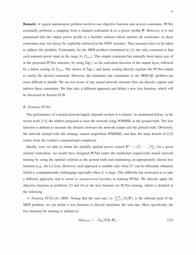
Remark: A typical optimization problem involves one objective function and several constraints. PCNet

essentially performs a mapping from a channel realization h to a power profile P. However, it is not

guaranteed that the output power profile is a feasible solution which satisfies all constraints, as these

constraints may not always be explicitly enforced in the DNN structure. Thus measures have to be taken

to address this problem. Fortunately, for the SRM problem formulated in (3), the only constraint is that

each transmit power must in the range [0, Pmax]. This simple constraint has naturally been taken care of

in the proposed PCNet structure, by using Sig(·) as the activation function of the output layer, followed

by a linear scaling of Pmax. The choice of Sig(·) and linear scaling directly regulate the PCNet output

to satisfy the desired constraint. However, the minimum rate constraints in the SRM-QC problem are

more difficult to handle. We are not aware of any neural network structure that can directly capture and

enforce these constraints. We thus take a different approach and define a new loss function, which will

be discussed in Section IV-B.

B. Training PCNet

The performance of a neural network largely depends on how it is trained. As mentioned before, in the

recent work [13], the authors proposed to train the network using WMMSE as the ground truth. The loss

function is defined to measure the distance between the network output and the ground truth. Obviously,

the network trained with this strategy cannot outperform WMMSE, and thus the main benefit of [13]

comes from the (online) computational complexity.

Ideally, were we able to obtain the globally optimal power control P∗ = (P ∗1 , · · · , P

∗K) for a given

channel realization, we would have designed PCNet under the traditional (supervised) neural network

training by using the optimal solution as the ground truth and minimizing an appropriately chosen loss

function (e.g., the L2 loss). However, such approach is suitable only when P ∗i can be efficiently obtained,

which is computationally challenging especially when K is large. This difficulty has motivated us to take

a different approach, and to resort to unsupervised learning in training PCNet. We directly apply the

objective function in problems (3) and (4) as the loss function for PCNet training, which is detailed in

the following.

1) Training PCNet for SRM: Noting that the sum rate, i.e.∑K

i=1 Ri(P), is the ultimate goal of the

SRM problem, we can define a loss function to directly maximize the sum rate. More specifically, the

loss function for training is defined as:

lossSRM = −Eh [R(h,θ)] , (12)

11

where θ denotes the set of trainable network parameters for PCNet. R(h,θ) is the sum rate under a

specific channel realization h and network parameters θ. Obviously, this loss function is differentiable

with respect to θ and can be used to train the network via stochastic gradient descent (SGD).

Note that the loss function (12) is with respect to the distribution of h, whose direct evaluation is

quite challenging. We adopt a widely used method, mini-batch gradient descent, to train PCNet under

the loss function (12). In each iteration of the training, multiple channel realizations h are generated

from its distribution and we use H to denote the set of these channel realizations. The training loss is

then approximated as

lossSRM ≈ −1

|H|

∑

h∈H

R(h,θ), (13)

where |H| denotes the number of samples in H and its choice should balance complexity and accuracy.

Therefore, in each iteration, (13) is used instead of (12) to calculate the gradients and update the network

parameters.

2) Training PCNet for SRM-QC: For the SRM-QC problem, the loss function defined in (12) is not

applicable. Our proposed solution to address the minimum rate constraints in SRM-QC is to define a

new loss function that penalizes the constraint violation. More specifically, the new loss function for

SRM-QC is defined as:

lossSRM-QC = Eh

[−R(h,θ) + λ ·

K∑

i=1

ReLU (ri,min −Ri(h,θ))

], (14)

where Ri(h,θ) is the rate of i-th receiver under a specific channel realization h and network parameters

θ.

Different from the loss function (12), penalty terms are introduced to incentive the network output

to meet the minimum rate constraints. If ri,min > Ri(h,θ), i.e. a rate constraint is not satisfied,

ReLU (ri,min −Ri(h,θ)) > 0 and the corresponding penalty term will force the network parameters

to be updated in the direction where the constraint is satisfied. On the contrary, if ri,min ≤ Ri(h,θ),

ReLU (ri,min −Ri(h,θ)) = 0 and the penalty term will not influence the network training. In this case,

the training process will focus on making the network output satisfy the rate constraints of other receivers

and increasing the system sum rate. The scaling factor λ balances the trade-off of different terms in the

loss function, which is a hyperparameter and needs to be tuned carefully: if it is too large, the network

would focus on meeting the rate constraints while sacrificing the sum rate performance; if it is too small,

the network may not output a feasible power profile. We will discuss how λ influences the performance

using numerical results in Section VII.

It should be noted that even with the new loss function (14), PCNet may still output a power profile

that is not a feasible solution. There are two possibilities when this happens. The first is that the original

12

SRM-QC problem under this specific parameter setting is infeasible. In this case, there is no valid power

profile anyway. The second is that feasible solutions exist but PCNet for SRM-QC fails to produce one.

In this case, we note that the power profile given in (6) is already a feasible solution. Therefore, we can

obtain a feasible solution as

P = P ·Pmax

max(P), (15)

where max(P) denotes the maximum power allocated to one user in P. Obviously, P is also a feasible

solution and there is at least one user whose power is Pmax. Previous result has shown that the achieved

rate of P is no smaller than P [7]. If max(P) < Pmax, the power profile P would outperform P.

C. PCNet+: enhance the generalization capacity of PCNet

One PCNet needs to be trained for a given background noise power, because it only takes channel

coefficients as the input. In practical applications, this means that multiple network models of PCNet

have to be separately trained for different noise power (e.g., a range of SNRs), and the system controller

needs to store multiple models and select one for power control based on its estimation of the noise

power. This limits the generalization capability of PCNet. What is more desirable is a single trained

PCNet which can handle a wide range of noise power levels.

Motivated by this limitation, we propose PCNet+, which is a minor variation to PCNet but offers

significantly better generalization capacity. The key idea of PCNet+ is to take the noise power σ2, in

addition to the channel coefficients, as another input to the network. In this case, the network input layer

contains K2 + 1 nodes: ‖hi,j‖, i = 1, · · · ,K, j = 1, · · · ,K, and σ2. In this way, a single PCNet+ can

be trained to handle a range of noise power levels. In training PCNet+, the training data is generated

equally under multiple levels of noise power, and the aggregated data is used. Simulation results, which

are given in Section VI, will show that this method will enhance the generalization capacity of PCNet

at the cost of very little performance loss.

V. EPCNET: ENSEMBLING PCNETS

Training PCNet with sufficiently representative data and the new loss functions defined in (12) (for

SRM) or (14) (for SRM-QC) cannot guarantee that PCNet outputs the globally optimal power profile

P(h)∗ for a given channel realization h. Due to the inherent deficiency of gradient descent, the trained

PCNet may fall into a local optimum. As will be corroborated in the numerical experiments, a single

PCNet does not universally outperform existing methods.

13

��

/012345

6789:;<=>?@ h

��

��

��

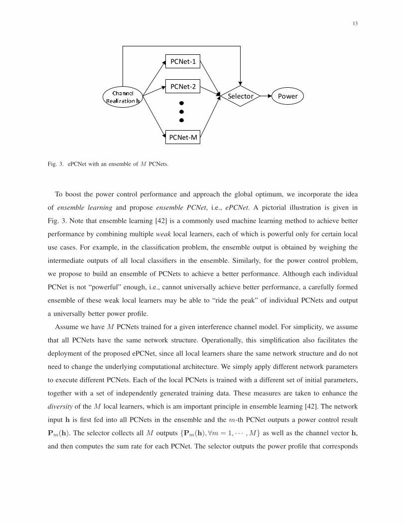
Fig. 3. ePCNet with an ensemble of M PCNets.

To boost the power control performance and approach the global optimum, we incorporate the idea

of ensemble learning and propose ensemble PCNet, i.e., ePCNet. A pictorial illustration is given in

Fig. 3. Note that ensemble learning [42] is a commonly used machine learning method to achieve better

performance by combining multiple weak local learners, each of which is powerful only for certain local

use cases. For example, in the classification problem, the ensemble output is obtained by weighing the

intermediate outputs of all local classifiers in the ensemble. Similarly, for the power control problem,

we propose to build an ensemble of PCNets to achieve a better performance. Although each individual

PCNet is not “powerful” enough, i.e., cannot universally achieve better performance, a carefully formed

ensemble of these weak local learners may be able to “ride the peak” of individual PCNets and output

a universally better power profile.

Assume we have M PCNets trained for a given interference channel model. For simplicity, we assume

that all PCNets have the same network structure. Operationally, this simplification also facilitates the

deployment of the proposed ePCNet, since all local learners share the same network structure and do not

need to change the underlying computational architecture. We simply apply different network parameters

to execute different PCNets. Each of the local PCNets is trained with a different set of initial parameters,

together with a set of independently generated training data. These measures are taken to enhance the

diversity of the M local learners, which is am important principle in ensemble learning [42]. The network

input h is first fed into all PCNets in the ensemble and the m-th PCNet outputs a power control result

Pm(h). The selector collects all M outputs {Pm(h),∀m = 1, · · · ,M} as well as the channel vector h,

and then computes the sum rate for each PCNet. The selector outputs the power profile that corresponds

14

to the highest sum rate, i.e.,

PePCNet(h) = argmaxPm(h)

RPCNet(h,Pm (h)) , (16)

where PePCNet(h) denotes the output power profile of ePCNet, RPCNet(h,Pm (h)) denotes the achieved

sum rate of PCNet with the channel realization h and the power profile Pm(h).

There are three important remarks on the proposed ePCNet. First, it is well-known that training a neural

network with SGD may often lead to local optima. Thus, combining several local weak DNNs effectively

looks at multiple local optima and leads to significantly improved sum rate performance. Second, PCNet

only requires a few matrix multiplications and is of low computational complexity2. Therefore, combining

several PCNets only increases the online complexity in a linear fashion with respect to the total number

of local learners, which does not affect the order of complexity with respect to the problem size (i.e., K).

Last but not the least, creating diversity by training multiple PCNets with different sets of parameters

and training data is applicable not just to DNN. Some existing methods for power control may also

benefit from such diversity. For example, a random initialization is often needed to start an algorithm

that iteratively converges to a solution. Giving such algorithms multiple random initializations may also

produce multiple local optima and selecting one with the best performance would also achieve better

performance. However, such performance improvement is often achieved while sacrificing computational

efficiency. In Section VI, we will compare the performance of ePCNet with that of WMMSE with multiple

random initializations.

Finally, we remark that ePCNet+ can be easily obtained by ensembling several trained models of

PCNet+, in the same fashion as constructing ePCNet from PCNets.

VI. NUMERICAL EVALUATIONS FOR SRM

In the next two sections, we will conduct numerical simulations to verify the effectiveness of the

proposed family of PCNets, and compare them with the state-of-the-art power control methods. More

specifically, we intend to evaluate and compare the performance (for SRM and SRM-QC) and the

computational complexity of various methods. Besides PCNet(+) and ePCNet(+), we also implement

Round-Robin Power Control (RR), WMMSE and Greedy Binary Power Control (GBPC) for the SRM

problem and the geometric programming (GP) based method [6] for the SRM-QC problem. In this section,

we first focus on evaluations for SRM.

2This is also observed and numerically validated in [13].

15

A. Compared schemes

1) PCNet(+) and ePCNet(+): We implement the proposed PCNet and ePCNet in TensorFlow, with the

design following the detailed descriptions in Section IV and V. Following the common practice to train

a neural network, we use Xavier initialization [43] to initialize the network parameters and ADAM [44]

to train the network. The stochastic gradient descent is used to calculate the gradient and the mini-batch

size is set to 103. To track the network performance during training, a validation data set containing

104 samples is used to evaluate the network performance. This is done for every 50 iterations and the

model with the best performance is saved. A total of 105 iterations are executed to train the network. The

training data is randomly generated based on the channel model. As the mini-batch size is 103 and total

iteration number is 105, a total of 108 channel samples have been generated for training the network.

For SRM, it is observed that PCNet almost always outputs power profiles that are close to binary

power control. Therefore, we round the power profiles of PCNet to binary ones. Binary power control

facilitates practical implementation as it is easy for transmitters to configure binary transmit power. In

addition, theoretical studies [7] have shown that binary power control is optimal when K = 2, and offers

good performance when K > 2 (although no longer optimal). Our result is consistent with these studies.

However, for SRM-QC, we do not have these observations and the output of PCNet is used as the power

profile directly.

2) Round-Robin Power Control (RR): The RR algorithm proposed for SRM in [5] is implemented for

comparison. The basic idea of RR is to update the power of one user while keeping others fixed. This

sub-problem is addressed by solving a polynomial function optimization. The algorithm stops when the

following condition is satisfied,

|R(P(t))−R(P(t−1))|

R(P(t−1))≤ 10−4, (17)

where R(P(t)) and R(P(t−1)) denotes the sum rates in the current and last iterations respectively.

3) The Iteratively Weighted MMSE Approach (WMMSE): WMMSE is proposed to solve the sum-

utility maximization problem for a MIMO interfering broadcast channel [8]. Its simplified version can

be used to solve the considered SRM problem. In the literature, WMMSE is also used to generate the

ground truth for the network training in [13]. Therefore, we also incorporate WMMSE for comparison.

Note that the same stopping condition (17) is also used for WMMSE.

4) Greedy Binary Power Control (GBPC): The greedy binary power control method in [7] is also

implemented for comparison. It has been shown in [7] that GBPC can provide desirable performance

that approaches the optimal binary power control.

16

Binary power control is actually a scheduling algorithm. There still exist some works addressing

interference management via scheduling, such as [20], [45]. The method proposed in [46] tries to activate

a subset of links in which TIN can achieve the whole capacity region to within a constant gap. We

empirically find it does not perform well in our simulations and the results are omitted in this paper. The

work in [45] maximizes the weighted sum generalized degrees of freedom, which is different from our

target. Therefore we do not consider this work in comparison either.

B. Performance comparison

In majority of the simulations that follow, we focus on the symmetric interference channel model

with i.i.d. Rayleigh fading for all channels. We also report performance comparison with Ricean fading

and large-scale pathloss in Section VI-E. For the symmetric Rayleigh fading IC model, we have hi,j ∼

CN (0, 1),∀i, j ∈ K. The noise power at each receiver is set to the same σ2. These settings are widely

used in the literature [3], [5], [8], [13]. Without loss of generality, we assume Pmax = 1 and define the

signal-to-noise ratio (SNR) as

EsN0 = 10 log

(Pmax

σ2

). (18)

For PCNet/ePCNet, we present the results under three typical values of EsN0, 0dB, 5dB and 10dB.

For PCNet+/ePCNet+, the network is trained using the data generated with EsN0 selected from the set

{0, 1, 2, · · · , 10}dB. In each epoch of training, the numbers of training samples under different EsN0 are

the same. We then test the performance of PCNet+/ePCNet+ with EsN0 as 0dB, 5dB and 10dB and the

results are presented for comparison with PCNet/ePCNet trained for one speicific EsN0.

We first focus on evaluating ePCNet for the SRM problem. In this case, the considered compared

algorithms include RR, WMMSE and GBPC. We use RPN (h) to denote the achievable sum rate of

one PCNet or ePCNet, given channel coefficients h. Correspondingly, Rc(h) denotes the sum-rate of a

compared scheme. We evaluate the performance of ePCNet from different perspectives.

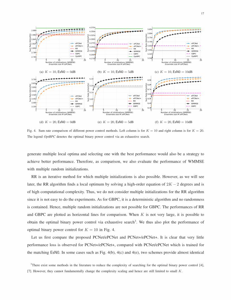
First, we focus on comparing the achievable average sum rates of all methods, i.e., Eh(RPN (h)) and

Eh(Rc(h)). The results are shown in Fig. 4 under different system settings. Specifically, for evaluating

ePCNet, we show the performance of a network ensemble of different sizes to highlight how the overall

performance of ePCNet (the ensemble) scales with the number of PCNets (its local learners). The

network structures for PCNet are {400, 400, 200, 20} and {100, 200, 100, 10} for K = 20 and K = 10,

respectively.

As we mention before, WMMSE is an iterative method and it needs a random initialization to start

the algorithm. If complexity is not an issue, giving WMMSE multiple random initializations would also

17

1 5 10 15 20Number of intializations (WMMSE)Ensemble size M (ePCNet)

2.76

2.78

2.80

2.82

2.84

2.86

2.88Sum Rate (bits/s/Hz)

ePCNetePCNet+RRWMMSEGBPCOptBPC

(a) K = 10,EsN0 = 0dB

1 5 10 15 20Number of intializations (WMMSE)

Ensemble size M (ePCNet)

4.175

4.200

4.225

4.250

4.275

4.300

4.325

4.350

4.375

Sum Rate (bits/s/Hz)


(b) K = 10,EsN0 = 5dB



5.50

5.55

5.60

5.65

5.70

5.75

5.80

5.85



(c) K = 10,EsN0 = 10dB



3.35

3.40

3.45

3.50

3.55

3.60

3.65

3.70


ePCNetePCNet+RRWMMSEGBPC

(d) K = 20,EsN0 = 0dB



4.9

5.0

5.1

5.2

5.3



(e) K = 20,EsN0 = 5dB



6.3

6.4

6.5

6.6

6.7

6.8

6.9



(f) K = 20,EsN0 = 10dB

Fig. 4. Sum rate comparison of different power control methods. Left column is for K = 10 and right column is for K = 20.

The legend OptBPC denotes the optimal binary power control via an exhaustive search.

generate multiple local optima and selecting one with the best performance would also be a strategy to

achieve better performance. Therefore, as comparison, we also evaluate the performance of WMMSE

with multiple random initializations.

RR is an iterative method for which multiple initializations is also possible. However, as we will see

later, the RR algorithm finds a local optimum by solving a high-order equation of 2K− 2 degrees and is

of high computational complexity. Thus, we do not consider multiple initializations for the RR algorithm

since it is not easy to do the experiments. As for GBPC, it is a deterministic algorithm and no randomness

is contained. Hence, multiple random initializations are not possible for GBPC. The performances of RR

and GBPC are plotted as horizontal lines for comparison. When K is not very large, it is possible to

obtain the optimal binary power control via exhaustive search3. We thus also plot the performance of

optimal binary power control for K = 10 in Fig. 4.

Let us first compare the proposed PCNet/ePCNet and PCNet+/ePCNet+. It is clear that very little

performance loss is observed for PCNet+/ePCNet+, compared with PCNet/ePCNet which is trained for

the matching EsN0. In some cases such as Fig. 4(b), 4(c) and 4(e), two schemes provide almost identical

3There exist some methods in the literature to reduce the complexity of searching for the optimal binary power control [4],

[7]. However, they cannot fundamentally change the complexity scaling and hence are still limited to small K.

18

2 4 6 8 10 12Sum Rate (bits/s/Hz)

0.0

0.2

0.4

0.6

0.8

1.0CD

FePCNetRRWMMSEGBPC

(a) K = 10,EsN0 = 10dB

2 4 6 8 10 12Sum Rate (bits/s/Hz)

0.0

0.2

0.4

0.6

0.8

1.0

CDF

ePCNetRRWMMSEGBPC

(b) K = 20,EsN0 = 10dB

2 4 6 8 10Sum Rate (bits/s/Hz)

0.0

0.2

0.4

0.6

0.8

1.0

CDF

ePCNetRRWMMSEGBPC

(c) K = 20,EsN0 = 5dB

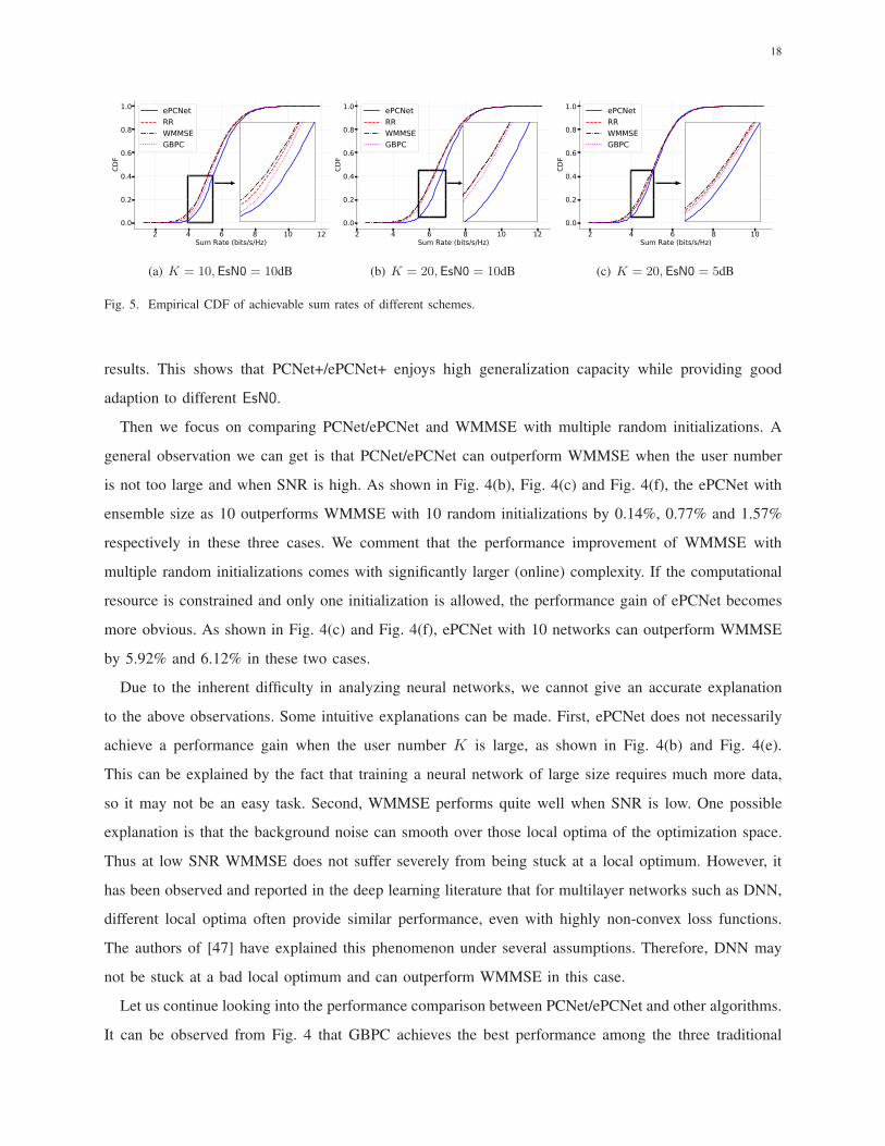
Fig. 5. Empirical CDF of achievable sum rates of different schemes.

results. This shows that PCNet+/ePCNet+ enjoys high generalization capacity while providing good

adaption to different EsN0.

Then we focus on comparing PCNet/ePCNet and WMMSE with multiple random initializations. A

general observation we can get is that PCNet/ePCNet can outperform WMMSE when the user number

is not too large and when SNR is high. As shown in Fig. 4(b), Fig. 4(c) and Fig. 4(f), the ePCNet with

ensemble size as 10 outperforms WMMSE with 10 random initializations by 0.14%, 0.77% and 1.57%

respectively in these three cases. We comment that the performance improvement of WMMSE with

multiple random initializations comes with significantly larger (online) complexity. If the computational

resource is constrained and only one initialization is allowed, the performance gain of ePCNet becomes

more obvious. As shown in Fig. 4(c) and Fig. 4(f), ePCNet with 10 networks can outperform WMMSE

by 5.92% and 6.12% in these two cases.

Due to the inherent difficulty in analyzing neural networks, we cannot give an accurate explanation

to the above observations. Some intuitive explanations can be made. First, ePCNet does not necessarily

achieve a performance gain when the user number K is large, as shown in Fig. 4(b) and Fig. 4(e).

This can be explained by the fact that training a neural network of large size requires much more data,

so it may not be an easy task. Second, WMMSE performs quite well when SNR is low. One possible

explanation is that the background noise can smooth over those local optima of the optimization space.

Thus at low SNR WMMSE does not suffer severely from being stuck at a local optimum. However, it

has been observed and reported in the deep learning literature that for multilayer networks such as DNN,

different local optima often provide similar performance, even with highly non-convex loss functions.

The authors of [47] have explained this phenomenon under several assumptions. Therefore, DNN may

not be stuck at a bad local optimum and can outperform WMMSE in this case.

Let us continue looking into the performance comparison between PCNet/ePCNet and other algorithms.

It can be observed from Fig. 4 that GBPC achieves the best performance among the three traditional

19

−2 0 2 4Increased Sum-Rate(bits/s/Hz)

0.0

0.2

0.4

0.6

0.8

1.0

CDF

K=20,EsN0=10dBK=20,EsN0=5dBK=10,EsN0=10dB

(a) ePCNet v.s. RR

−3 −2 −1 0 1 2 3 4 5Increased Su -Rate(bits/s/Hz)

0.0

0.2

0.4

0.6

0.8

1.0

CDF


(b) ePCNet v.s. WMMSE

−3 −2 −1 0 1 2 3 4 5Increased Su -Rate(bits/s/Hz)

0.0

0.2

0.4

0.6

0.8

1.0

CDF


(c) ePCNet v.s. GBPC

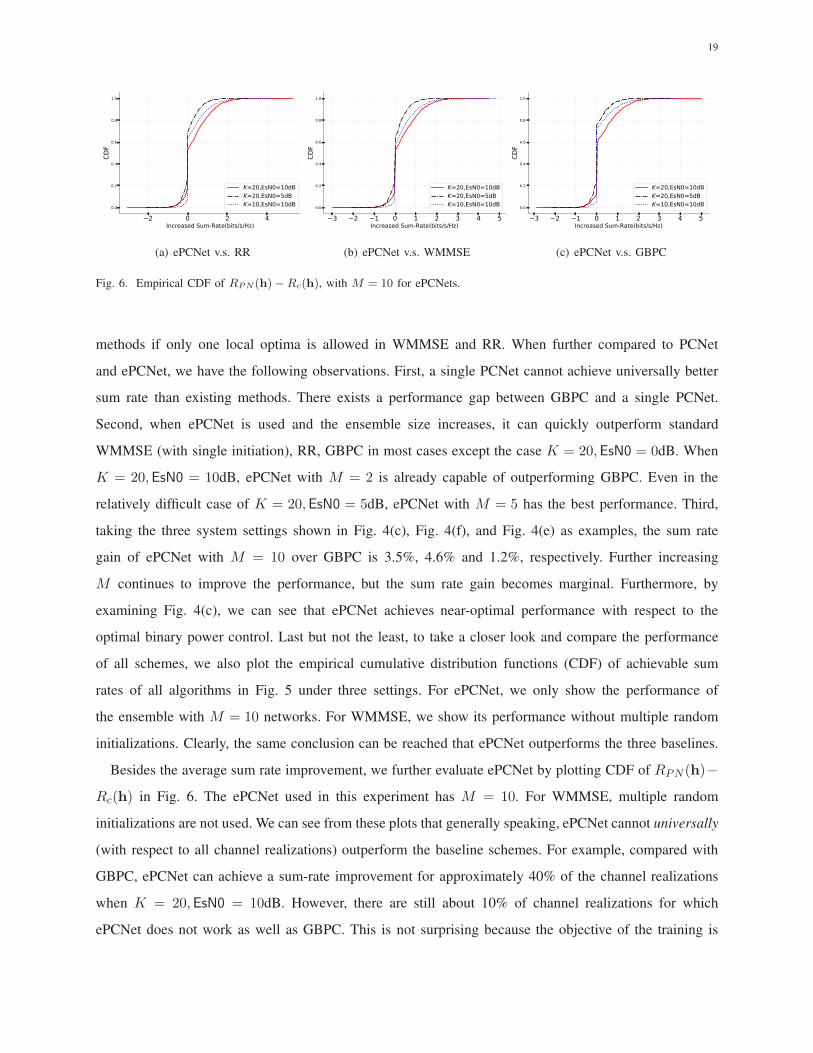
Fig. 6. Empirical CDF of RPN(h)−Rc(h), with M = 10 for ePCNets.

methods if only one local optima is allowed in WMMSE and RR. When further compared to PCNet

and ePCNet, we have the following observations. First, a single PCNet cannot achieve universally better

sum rate than existing methods. There exists a performance gap between GBPC and a single PCNet.

Second, when ePCNet is used and the ensemble size increases, it can quickly outperform standard

WMMSE (with single initiation), RR, GBPC in most cases except the case K = 20,EsN0 = 0dB. When

K = 20,EsN0 = 10dB, ePCNet with M = 2 is already capable of outperforming GBPC. Even in the

relatively difficult case of K = 20,EsN0 = 5dB, ePCNet with M = 5 has the best performance. Third,

taking the three system settings shown in Fig. 4(c), Fig. 4(f), and Fig. 4(e) as examples, the sum rate

gain of ePCNet with M = 10 over GBPC is 3.5%, 4.6% and 1.2%, respectively. Further increasing

M continues to improve the performance, but the sum rate gain becomes marginal. Furthermore, by

examining Fig. 4(c), we can see that ePCNet achieves near-optimal performance with respect to the

optimal binary power control. Last but not the least, to take a closer look and compare the performance

of all schemes, we also plot the empirical cumulative distribution functions (CDF) of achievable sum

rates of all algorithms in Fig. 5 under three settings. For ePCNet, we only show the performance of

the ensemble with M = 10 networks. For WMMSE, we show its performance without multiple random

initializations. Clearly, the same conclusion can be reached that ePCNet outperforms the three baselines.

Besides the average sum rate improvement, we further evaluate ePCNet by plotting CDF of RPN (h)−

Rc(h) in Fig. 6. The ePCNet used in this experiment has M = 10. For WMMSE, multiple random

initializations are not used. We can see from these plots that generally speaking, ePCNet cannot universally

(with respect to all channel realizations) outperform the baseline schemes. For example, compared with

GBPC, ePCNet can achieve a sum-rate improvement for approximately 40% of the channel realizations

when K = 20,EsN0 = 10dB. However, there are still about 10% of channel realizations for which

ePCNet does not work as well as GBPC. This is not surprising because the objective of the training is

20

1 2 3 4 5 6 7 8 9 10Network Id

0.0

0.1

Prob

abilit

y

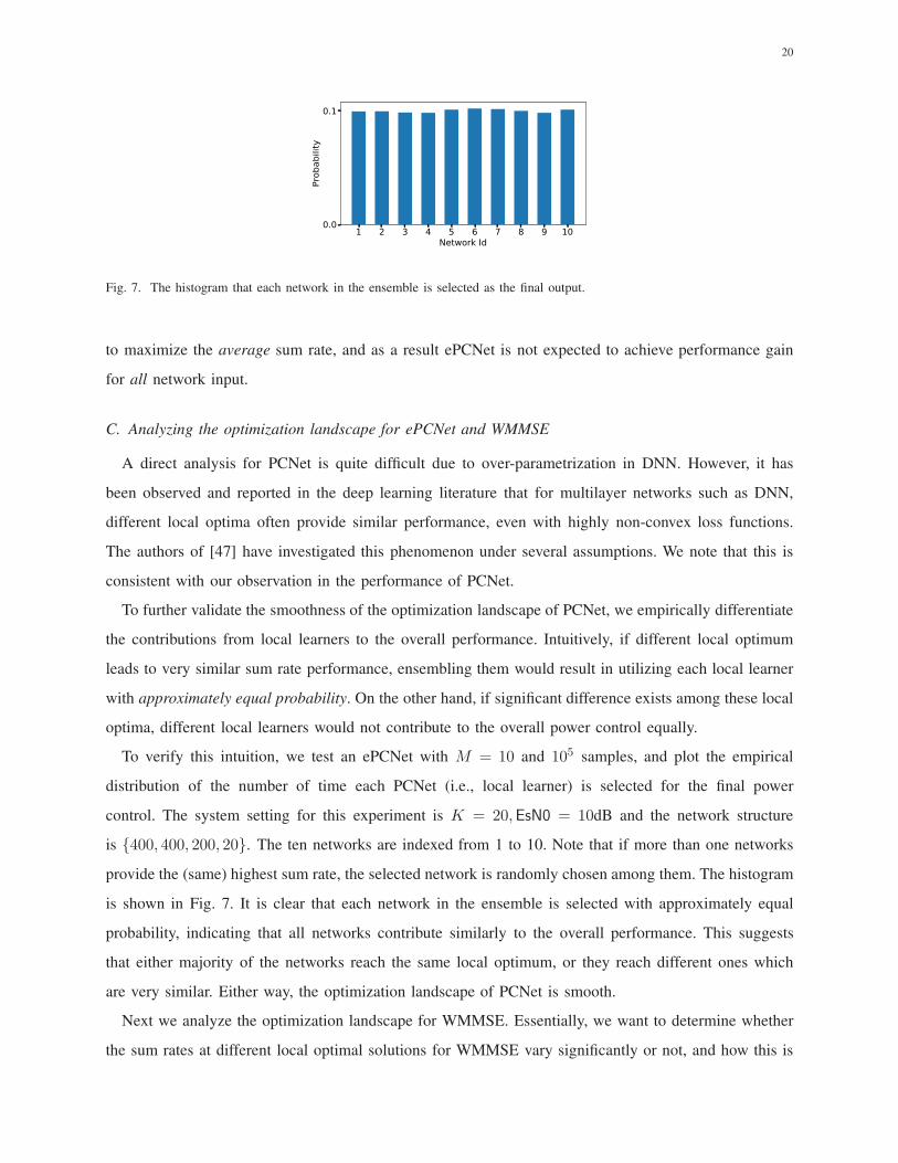
Fig. 7. The histogram that each network in the ensemble is selected as the final output.

to maximize the average sum rate, and as a result ePCNet is not expected to achieve performance gain

for all network input.

C. Analyzing the optimization landscape for ePCNet and WMMSE

A direct analysis for PCNet is quite difficult due to over-parametrization in DNN. However, it has

been observed and reported in the deep learning literature that for multilayer networks such as DNN,

different local optima often provide similar performance, even with highly non-convex loss functions.

The authors of [47] have investigated this phenomenon under several assumptions. We note that this is

consistent with our observation in the performance of PCNet.

To further validate the smoothness of the optimization landscape of PCNet, we empirically differentiate

the contributions from local learners to the overall performance. Intuitively, if different local optimum

leads to very similar sum rate performance, ensembling them would result in utilizing each local learner

with approximately equal probability. On the other hand, if significant difference exists among these local

optima, different local learners would not contribute to the overall power control equally.

To verify this intuition, we test an ePCNet with M = 10 and 105 samples, and plot the empirical

distribution of the number of time each PCNet (i.e., local learner) is selected for the final power

control. The system setting for this experiment is K = 20,EsN0 = 10dB and the network structure

is {400, 400, 200, 20}. The ten networks are indexed from 1 to 10. Note that if more than one networks

provide the (same) highest sum rate, the selected network is randomly chosen among them. The histogram

is shown in Fig. 7. It is clear that each network in the ensemble is selected with approximately equal

probability, indicating that all networks contribute similarly to the overall performance. This suggests

that either majority of the networks reach the same local optimum, or they reach different ones which

are very similar. Either way, the optimization landscape of PCNet is smooth.

Next we analyze the optimization landscape for WMMSE. Essentially, we want to determine whether

the sum rates at different local optimal solutions for WMMSE vary significantly or not, and how this is

21

0 5 10 15 20Variance of local optimal rates

0.3

0.4

0.5

0.6

0.7

0.8

0.9

1.0

CDF

0dB10dB30dB

(a) Empirical CDF of variance of local optimal rates

0.0 0.1 0.2 0.3 0.4 0.5Coefficient of variation of local optimal rates

0.2

0.4

0.6

0.8

1.0

CDF

0dB10dB30dB

(b) Empirical CDF of coefficient of variation of local

optimal rates

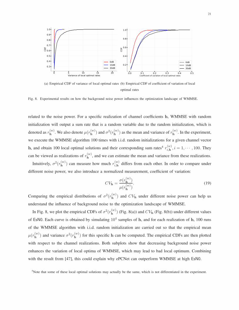
Fig. 8. Experimental results on how the background noise power influences the optimization landscape of WMMSE.

related to the noise power. For a specific realization of channel coefficients h, WMMSE with random

initialization will output a sum rate that is a random variable due to the random initialization, which is

denoted as r(w)h

. We also denote µ(r(w)h

) and σ2(r(w)h

) as the mean and variance of r(w)h

. In the experiment,

we execute the WMMSE algorithm 100 times with i.i.d. random initializations for a given channel vector

h, and obtain 100 local optimal solutions and their corresponding sum rates4 r(w)i,h , i = 1, · · · , 100. They

can be viewed as realizations of r(w)h

, and we can estimate the mean and variance from these realizations.

Intuitively, σ2(r(w)h

) can measure how much r(w)i,h differs from each other. In order to compare under

different noise power, we also introduce a normalized measurement, coefficient of variation:

CVh =σ(r

(w)h

)

µ(r(w)h

). (19)

Comparing the empirical distributions of σ2(r(w)h

) and CVh under different noise power can help us

understand the influence of background noise to the optimization landscape of WMMSE.

In Fig. 8, we plot the empirical CDFs of σ2(r(w)h

) (Fig. 8(a)) and CVh (Fig. 8(b)) under different values

of EsN0. Each curve is obtained by simulating 104 samples of h, and for each realization of h, 100 runs

of the WMMSE algorithm with i.i.d. random initialization are carried out so that the empirical mean

µ(r(w)h

) and variance σ2(r(w)h

) for this specific h can be computed. The empirical CDFs are then plotted

with respect to the channel realizations. Both subplots show that decreasing background noise power

enhances the variation of local optima of WMMSE, which may lead to bad local optimum. Combining

with the result from [47], this could explain why ePCNet can outperform WMMSE at high EsN0.

4Note that some of these local optimal solutions may actually be the same, which is not differentiated in the experiment.

22

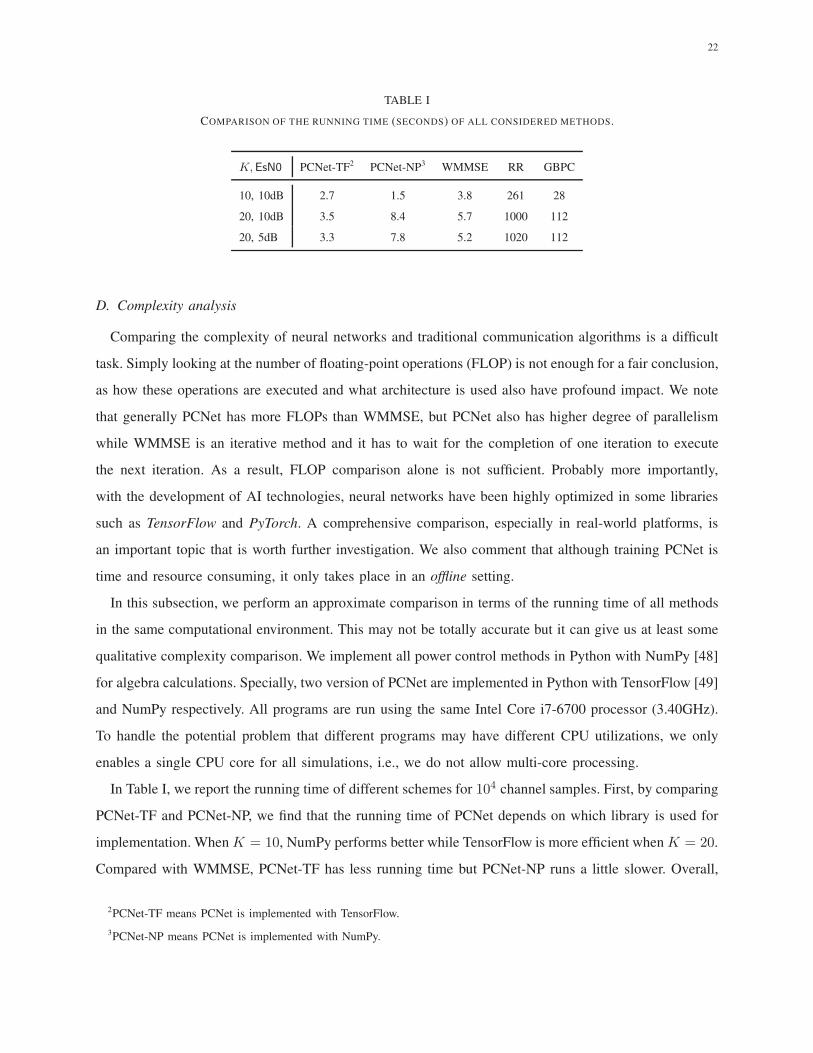
TABLE I

COMPARISON OF THE RUNNING TIME (SECONDS) OF ALL CONSIDERED METHODS.

K,EsN0 PCNet-TF2 PCNet-NP3 WMMSE RR GBPC

10, 10dB 2.7 1.5 3.8 261 28

20, 10dB 3.5 8.4 5.7 1000 112

20, 5dB 3.3 7.8 5.2 1020 112

D. Complexity analysis

Comparing the complexity of neural networks and traditional communication algorithms is a difficult

task. Simply looking at the number of floating-point operations (FLOP) is not enough for a fair conclusion,

as how these operations are executed and what architecture is used also have profound impact. We note

that generally PCNet has more FLOPs than WMMSE, but PCNet also has higher degree of parallelism

while WMMSE is an iterative method and it has to wait for the completion of one iteration to execute

the next iteration. As a result, FLOP comparison alone is not sufficient. Probably more importantly,

with the development of AI technologies, neural networks have been highly optimized in some libraries

such as TensorFlow and PyTorch. A comprehensive comparison, especially in real-world platforms, is

an important topic that is worth further investigation. We also comment that although training PCNet is

time and resource consuming, it only takes place in an offline setting.

In this subsection, we perform an approximate comparison in terms of the running time of all methods

in the same computational environment. This may not be totally accurate but it can give us at least some

qualitative complexity comparison. We implement all power control methods in Python with NumPy [48]

for algebra calculations. Specially, two version of PCNet are implemented in Python with TensorFlow [49]

and NumPy respectively. All programs are run using the same Intel Core i7-6700 processor (3.40GHz).

To handle the potential problem that different programs may have different CPU utilizations, we only

enables a single CPU core for all simulations, i.e., we do not allow multi-core processing.

In Table I, we report the running time of different schemes for 104 channel samples. First, by comparing

PCNet-TF and PCNet-NP, we find that the running time of PCNet depends on which library is used for

implementation. When K = 10, NumPy performs better while TensorFlow is more efficient when K = 20.

Compared with WMMSE, PCNet-TF has less running time but PCNet-NP runs a little slower. Overall,

2PCNet-TF means PCNet is implemented with TensorFlow.

3PCNet-NP means PCNet is implemented with NumPy.

23

1 5 10Number of intializations (WMMSE)


5.20

5.25

5.30

5.35

5.40

5.45

5.50

5.55

5.60Su

m Rate (bits/s/Hz)

ePCNetRRWMMSEGBPCOptBPC

(a) K = 10,EsN0 = 10dB



5.9

6.0

6.1

6.2

6.3

6.4

6.5


ePCNetRRWMMSEGBPC

(b) K = 20,EsN0 = 10dB



4.55

4.60

4.65

4.70

4.75

4.80

4.85

4.90


ePCNetRRWMMSEGBPC

(c) K = 20,EsN0 = 5dB

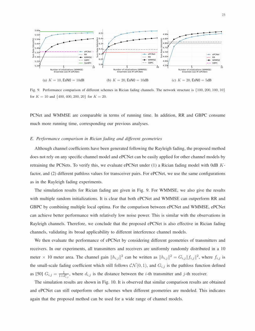
Fig. 9. Performance comparison of different schemes in Rician fading channels. The network structure is {100, 200, 100, 10}

for K = 10 and {400, 400, 200, 20} for K = 20.

PCNet and WMMSE are comparable in terms of running time. In addition, RR and GBPC consume

much more running time, corresponding our previous analyses.

E. Performance comparison in Rician fading and different geometries

Although channel coefficients have been generated following the Rayleigh fading, the proposed method

does not rely on any specific channel model and ePCNet can be easily applied for other channel models by

retraining the PCNets. To verify this, we evaluate ePCNet under (1) a Rician fading model with 0dB K-

factor, and (2) different pathloss values for transceiver pairs. For ePCNet, we use the same configurations

as in the Rayleigh fading experiments.

The simulation results for Rician fading are given in Fig. 9. For WMMSE, we also give the results

with multiple random initializations. It is clear that both ePCNet and WMMSE can outperform RR and

GBPC by combining multiple local optima. For the comparison between ePCNet and WMMSE, ePCNet

can achieve better performance with relatively low noise power. This is similar with the observations in

Rayleigh channels. Therefore, we conclude that the proposed ePCNet is also effective in Rician fading

channels, validating its broad applicability to different interference channel models.

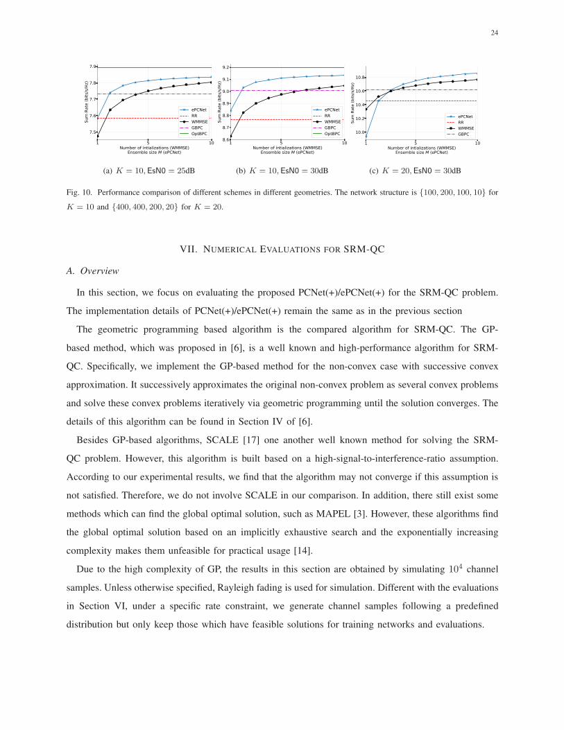
We then evaluate the performance of ePCNet by considering different geometries of transmitters and

receivers. In our experiments, all transmitters and receivers are uniformly randomly distributed in a 10

meter × 10 meter area. The channel gain ‖hi,j‖2 can be written as ‖hi,j‖

2 = Gi,j‖fi,j‖2, where fi,j is

the small-scale fading coefficient which still follows CN (0, 1), and Gi,j is the pathloss function defined

as [50] Gi,j =1

1+d2

i,j

, where di,j is the distance between the i-th transmitter and j-th receiver.

The simulation results are shown in Fig. 10. It is observed that similar comparison results are obtained

and ePCNet can still outperform other schemes when different geometries are modeled. This indicates

again that the proposed method can be used for a wide range of channel models.

24



7.5

7.6

7.7

7.8

7.9



(a) K = 10,EsN0 = 25dB



8.6

8.7

8.8

8.9

9.0

9.1

9.2



(b) K = 10,EsN0 = 30dB



10.0

10.2

10.4

10.6

10.8

Sum Rate (bits

/s/Hz)

ePCNetRRWMMSEGBPC

(c) K = 20,EsN0 = 30dB

Fig. 10. Performance comparison of different schemes in different geometries. The network structure is {100, 200, 100, 10} for

K = 10 and {400, 400, 200, 20} for K = 20.

VII. NUMERICAL EVALUATIONS FOR SRM-QC

A. Overview

In this section, we focus on evaluating the proposed PCNet(+)/ePCNet(+) for the SRM-QC problem.

The implementation details of PCNet(+)/ePCNet(+) remain the same as in the previous section

The geometric programming based algorithm is the compared algorithm for SRM-QC. The GP-

based method, which was proposed in [6], is a well known and high-performance algorithm for SRM-

QC. Specifically, we implement the GP-based method for the non-convex case with successive convex

approximation. It successively approximates the original non-convex problem as several convex problems

and solve these convex problems iteratively via geometric programming until the solution converges. The

details of this algorithm can be found in Section IV of [6].

Besides GP-based algorithms, SCALE [17] one another well known method for solving the SRM-

QC problem. However, this algorithm is built based on a high-signal-to-interference-ratio assumption.

According to our experimental results, we find that the algorithm may not converge if this assumption is

not satisfied. Therefore, we do not involve SCALE in our comparison. In addition, there still exist some

methods which can find the global optimal solution, such as MAPEL [3]. However, these algorithms find

the global optimal solution based on an implicitly exhaustive search and the exponentially increasing

complexity makes them unfeasible for practical usage [14].

Due to the high complexity of GP, the results in this section are obtained by simulating 104 channel

samples. Unless otherwise specified, Rayleigh fading is used for simulation. Different with the evaluations

in Section VI, under a specific rate constraint, we generate channel samples following a predefined

distribution but only keep those which have feasible solutions for training networks and evaluations.

25

1 5 10Ensemble size M (ePCNet)

0.825

0.850

0.875

0.900

0.925

0.950

0.975

1.000

Hit R

ate

rmin= (0.5, 0, 0, 0, 0)rmin= (0.5, 0.5, 0, 0, 0)rmin= (0.5, 0.5, 0.5, 0, 0)

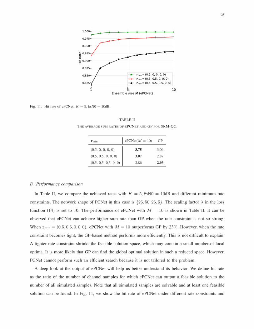
Fig. 11. Hit rate of ePCNet. K = 5,EsN0 = 10dB.

TABLE II

THE AVERAGE SUM RATES OF EPCNET AND GP FOR SRM-QC.

rmin ePCNet(M = 10) GP

(0.5, 0, 0, 0, 0) 3.75 3.04

(0.5, 0.5, 0, 0, 0) 3.07 2.87

(0.5, 0.5, 0.5, 0, 0) 2.86 2.93

B. Performance comparison

In Table II, we compare the achieved rates with K = 5,EsN0 = 10dB and different minimum rate

constraints. The network shape of PCNet in this case is {25, 50, 25, 5}. The scaling factor λ in the loss

function (14) is set to 10. The performance of ePCNet with M = 10 is shown in Table II. It can be

observed that ePCNet can achieve higher sum rate than GP when the rate constraint is not so strong.

When rmin = (0.5, 0.5, 0, 0, 0), ePCNet with M = 10 outperforms GP by 23%. However, when the rate

constraint becomes tight, the GP-based method performs more efficiently. This is not difficult to explain.

A tighter rate constraint shrinks the feasible solution space, which may contain a small number of local

optima. It is more likely that GP can find the global optimal solution in such a reduced space. However,

PCNet cannot perform such an efficient search because it is not tailored to the problem.

A deep look at the output of ePCNet will help us better understand its behavior. We define hit rate

as the ratio of the number of channel samples for which ePCNet can output a feasible solution to the

number of all simulated samples. Note that all simulated samples are solvable and at least one feasible

solution can be found. In Fig. 11, we show the hit rate of ePCNet under different rate constraints and

26

0 20 40 60 80 100λ

2.4

2.5

2.6

2.7

2.8

2.9

Rate

rmin= (0.5, 0.5, 0, 0, 0)rmin= (0.5, 0.5, 0.5, 0, 0)

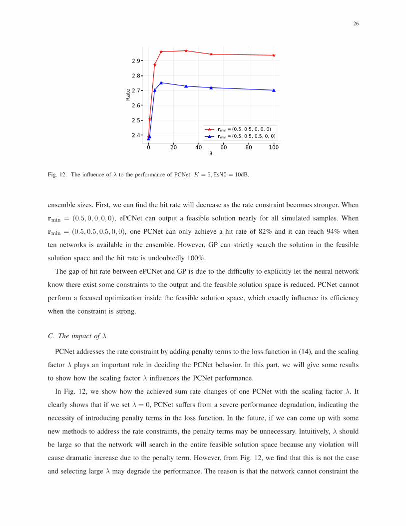
Fig. 12. The influence of λ to the performance of PCNet. K = 5,EsN0 = 10dB.

ensemble sizes. First, we can find the hit rate will decrease as the rate constraint becomes stronger. When

rmin = (0.5, 0, 0, 0, 0), ePCNet can output a feasible solution nearly for all simulated samples. When

rmin = (0.5, 0.5, 0.5, 0, 0), one PCNet can only achieve a hit rate of 82% and it can reach 94% when

ten networks is available in the ensemble. However, GP can strictly search the solution in the feasible

solution space and the hit rate is undoubtedly 100%.

The gap of hit rate between ePCNet and GP is due to the difficulty to explicitly let the neural network

know there exist some constraints to the output and the feasible solution space is reduced. PCNet cannot

perform a focused optimization inside the feasible solution space, which exactly influence its efficiency

when the constraint is strong.

C. The impact of λ

PCNet addresses the rate constraint by adding penalty terms to the loss function in (14), and the scaling

factor λ plays an important role in deciding the PCNet behavior. In this part, we will give some results

to show how the scaling factor λ influences the PCNet performance.

In Fig. 12, we show how the achieved sum rate changes of one PCNet with the scaling factor λ. It

clearly shows that if we set λ = 0, PCNet suffers from a severe performance degradation, indicating the

necessity of introducing penalty terms in the loss function. In the future, if we can come up with some

new methods to address the rate constraints, the penalty terms may be unnecessary. Intuitively, λ should

be large so that the network will search in the entire feasible solution space because any violation will

cause dramatic increase due to the penalty term. However, from Fig. 12, we find that this is not the case

and selecting large λ may degrade the performance. The reason is that the network cannot constraint the

27

2 4 6 8 10Ensemble size M (ePCNet)

2.702.722.742.762.782.802.822.842.86

Rate

λ=5λ=10λ=30λ=100

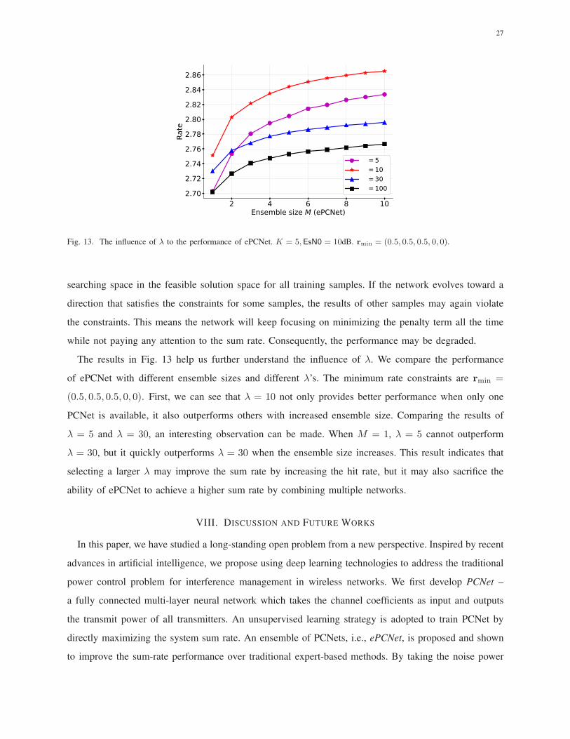
Fig. 13. The influence of λ to the performance of ePCNet. K = 5,EsN0 = 10dB. rmin = (0.5, 0.5, 0.5, 0, 0).

searching space in the feasible solution space for all training samples. If the network evolves toward a

direction that satisfies the constraints for some samples, the results of other samples may again violate

the constraints. This means the network will keep focusing on minimizing the penalty term all the time

while not paying any attention to the sum rate. Consequently, the performance may be degraded.

The results in Fig. 13 help us further understand the influence of λ. We compare the performance

of ePCNet with different ensemble sizes and different λ’s. The minimum rate constraints are rmin =

(0.5, 0.5, 0.5, 0, 0). First, we can see that λ = 10 not only provides better performance when only one

PCNet is available, it also outperforms others with increased ensemble size. Comparing the results of

λ = 5 and λ = 30, an interesting observation can be made. When M = 1, λ = 5 cannot outperform

λ = 30, but it quickly outperforms λ = 30 when the ensemble size increases. This result indicates that

selecting a larger λ may improve the sum rate by increasing the hit rate, but it may also sacrifice the

ability of ePCNet to achieve a higher sum rate by combining multiple networks.

VIII. DISCUSSION AND FUTURE WORKS

In this paper, we have studied a long-standing open problem from a new perspective. Inspired by recent

advances in artificial intelligence, we propose using deep learning technologies to address the traditional

power control problem for interference management in wireless networks. We first develop PCNet –

a fully connected multi-layer neural network which takes the channel coefficients as input and outputs

the transmit power of all transmitters. An unsupervised learning strategy is adopted to train PCNet by

directly maximizing the system sum rate. An ensemble of PCNets, i.e., ePCNet, is proposed and shown

to improve the sum-rate performance over traditional expert-based methods. By taking the noise power

28

as an additional network input, we obtain PCNet+/ePCNet+ which provides the desirable generalization

capacity. Extensive experiments have been carried out to verify the performance of ePCNet(+) and to

analyze its behavior under different system settings. Sum rate and complexity comparison show that

ePCNet(+) achieves better power control while consuming less computational resources.

The key ingredient that has enabled our new solutions is leveraging training deep neural networks

to solve non-convex optimization problems. Hence, the proposed framework is not limited to the two

specific problems discussed in this paper. By generalizing the optimized objective and constraints, deep

learning technologies have the potential to tackle other non-convex optimization problems which are

often encountered in wireless communications. However, this generalization may not always be easy, as

we have seen in SRM-QC versus SRM. It is difficult to optimize discrete objective functions and address

general constraints with neural networks, which calls for more research in the future.

There are some other challenges remaining to be solved to make the DNN-based power control ready

for practice. First, in this work, we have shown that PCNet provides desirable generalization capacity for

background noise power if it is also fed into the network. However, there are other system parameters

such as the number of users K and the distribution of channel coefficients, which are not generalized.

How can we generalize PCNet to incorporate these system parameters is an important research direction.

Second, we currently assume ideal channel estimation, which is not realistic in practice. How to make

PCNet robust against channel estimation errors should be further investigated. Last but not the least, the

proposed scheme is a centralized framework. How to devise a distributed version of PCNet with little

performance loss is another interesting but challenging topic.

REFERENCES

[1] T. Han and K. Kobayashi, “A new achievable rate region for the interference channel,” IEEE Trans. Inf. Theory, vol. 27,

no. 1, pp. 49–60, Jan 1981.

[2] R. H. Etkin, D. N. C. Tse, and H. Wang, “Gaussian interference channel capacity to within one bit,” IEEE Trans. Inf.

Theory, vol. 54, no. 12, pp. 5534–5562, Dec 2008.

[3] L. Qian, Y. Zhang, and J. Huang, “MAPEL: Achieving global optimality for a non-convex wireless power control problem,”

IEEE Trans. Wireless Commun., vol. 8, no. 3, pp. 1553–1563, 2009.

[4] L. Liu, R. Zhang, and K.-C. Chua, “Achieving global optimality for weighted sum-rate maximization in the K-user Gaussian

interference channel with multiple antennas,” IEEE Trans. Wireless Commun., vol. 11, no. 5, pp. 1933–1945, 2012.

[5] C. S. Chen, K. W. Shum, and C. W. Sung, “Round-robin power control for the weighted sum rate maximisation of wireless

networks over multiple interfering links,” Transactions on Emerging Telecommunications Technologies, vol. 22, no. 8, pp.

458–470, 2011.

[6] M. Chiang et al., “Power control by geometric programming,” IEEE Trans. Wireless Commun., vol. 6, no. 7, 2007.

[7] A. Gjendemsjø, D. Gesbert, G. E. Øien, and S. G. Kiani, “Binary power control for sum rate maximization over multiple

interfering links,” IEEE Trans. Wireless Commun., vol. 7, no. 8, 2008.

29

[8] Q. Shi et al., “An iteratively weighted MMSE approach to distributed sum-utility maximization for a MIMO interfering

broadcast channel,” IEEE Trans. Signal Process., vol. 59, no. 9, pp. 4331–4340, 2011.

[9] E. Nachmani et al., “Deep learning methods for improved decoding of linear codes,” IEEE J. Sel. Topics Signal Process.,

vol. 12, no. 1, pp. 119–131, 2018.

[10] F. Liang, C. Shen, and F. Wu, “An iterative BP-CNN architecture for channel decoding,” IEEE J. Sel. Topics Signal

Process., vol. 12, no. 1, pp. 144–159, 2018.

[11] T. J. O’Shea, T. Roy, and T. C. Clancy, “Over-the-air deep learning based radio signal classification,” IEEE J. Sel. Topics

Signal Process., vol. 12, no. 1, pp. 168–179, 2018.

[12] H. Ye, G. Y. Li, and B.-H. Juang, “Power of deep learning for channel estimation and signal detection in OFDM systems,”

IEEE Wireless Commun. Lett., 2017.

[13] H. Sun et al., “Learning to optimize: Training deep neural networks for wireless resource management,” in IEEE SPAWC,

July 2017, pp. 1–6.

[14] M. Hong and Z.-Q. Luo, “Signal processing and optimal resource allocation for the interference channel,” in Academic

Press Library in Signal Processing. Elsevier, 2014, vol. 2, pp. 409–469.

[15] G. J. Foschini and Z. Miljanic, “A simple distributed autonomous power control algorithm and its convergence,” IEEE

Trans. Veh. Technol., vol. 42, no. 4, pp. 641–646, 1993.

[16] Z.-Q. Luo and S. Zhang, “Duality gap estimation and polynomial time approximation for optimal spectrum management,”

IEEE Trans. Signal Process., vol. 57, no. 7, pp. 2675–2689, 2009.

[17] J. Papandriopoulos and J. S. Evans, “SCALE: A low-complexity distributed protocol for spectrum balancing in multiuser

dsl networks,” IEEE Trans. Inf. Theory, vol. 55, no. 8, pp. 3711–3724, 2009.

[18] R. D. Yates and C.-Y. Huang, “Integrated power control and base station assignment,” IEEE Trans. Veh. Technol., vol. 44,

no. 3, pp. 638–644, 1995.

[19] M. Chiang et al., “Power control in wireless cellular networks,” Foundations and Trends R© in Networking, vol. 2, no. 4,

pp. 381–533, 2008.

[20] N. Naderializadeh and A. S. Avestimehr, “ITLinQ: A new approach for spectrum sharing in device-to-device communication

systems,” IEEE J. Sel. Areas Commun., vol. 32, no. 6, pp. 1139–1151, 2014.

[21] Z.-Q. Luo and S. Zhang, “Dynamic spectrum management: Complexity and duality,” IEEE J. Sel. Topics Signal Process.,

vol. 2, no. 1, pp. 57–73, 2008.

[22] W. Yu, G. Ginis, and J. M. Cioffi, “Distributed multiuser power control for digital subscriber lines,” IEEE J. Sel. Areas

Commun., vol. 20, no. 5, pp. 1105–1115, 2002.

[23] W. Yu, “Multiuser water-filling in the presence of crosstalk,” in Information Theory and Applications Workshop. IEEE,

2007, pp. 414–420.

[24] A. C. Cirik, R. Wang, Y. Hua, and M. Latva-aho, “Weighted sum-rate maximization for full-duplex MIMO interference

channels,” IEEE Trans. Commun., vol. 63, no. 3, pp. 801–815, 2015.

[25] K. Shen and W. Yu, “Fractional programming for communication systems – part I: Power control and beamforming,” IEEE

Trans. Signal Process., vol. 66, no. 10, pp. 2616–2630, May 2018.

[26] ——, “Fractional programming for communication systems – part II: Uplink scheduling via matching,” IEEE Trans. Signal

Process., vol. 66, no. 10, pp. 2631–2644, May 2018.

[27] ——, “FPLinQ: A cooperative spectrum sharing strategy for device-to-device communications,” in 2017 IEEE International

Symposium on Information Theory (ISIT), June 2017, pp. 2323–2327.

30

[28] T. J. O’Shea and J. Hoydis, “An introduction to machine learning communications systems,” arXiv preprint, 2017.

[Online]. Available: http://arxiv.org/abs/1702.00832

[29] T. Wang, C.-K. Wen, H. Wang, F. Gao, T. Jiang, and S. Jin, “Deep learning for wireless physical layer: Opportunities and

challenges,” China Communications, vol. 14, no. 11, pp. 92–111, 2017.

[30] L. Lugosch and W. J. Gross, “Neural offset min-sum decoding,” in Proc. ISIT. IEEE, 2017, pp. 1361–1365.

[31] I. Dimnik and Y. Be’ery, “Improved random redundant iterative HDPC decoding,” IEEE Trans. Commun., vol. 57, no. 7,

pp. 1982–1985, 2009.

[32] S. Cammerer, T. Gruber, J. Hoydis, and S. ten Brink, “Scaling deep learning-based decoding of polar codes via

partitioning,” arXiv preprint, 2017. [Online]. Available: http://arxiv.org/abs/1702.06901

[33] S. Dorner, S. Cammerer, J. Hoydis, and S. ten Brink, “Deep learning based communication over the air,” IEEE J. Sel.

Topics Signal Process., vol. 12, no. 1, pp. 132–143, 2018.

[34] N. Samuel, T. Diskin, and A. Wiesel, “Deep MIMO detection,” in IEEE SPAWC, 2017.

[35] C.-K. Wen, W.-T. Shih, and S. Jin, “Deep learning for massive MIMO CSI feedback,” IEEE Wireless Commun. Lett., 2018.

[36] M. Kim, N.-I. Kim, W. Lee, and D.-H. Cho, “Deep learning aided SCMA,” IEEE Commun. Lett., 2018.

[37] T. J. O’Shea, S. Hitefield, and J. Corgan, “End-to-end radio traffic sequence recognition with recurrent neural networks,”

in IEEE GlobalSIP. IEEE, 2016, pp. 277–281.

[38] D. Neumann, T. Wiese, and W. Utschick, “Learning the MMSE channel estimator,” IEEE Trans. Signal Process., 2018.

[39] B. Karanov et al., “End-to-end deep learning of optical fiber communications,” arXiv preprint arXiv:1804.04097, 2018.

[40] S. Ioffe and C. Szegedy, “Batch normalization: Accelerating deep network training by reducing internal covariate shift,”

in Proc. ICML, 2015, pp. 448–456.

[41] V. Nair and G. E. Hinton, “Rectified linear units improve restricted Boltzmann machines,” in Proc. ICML, 2010, pp.

807–814.

[42] T. G. Dietterich, “Ensemble learning,” The handbook of brain theory and neural networks, vol. 2, pp. 110–125, 2002.

[43] X. Glorot and Y. Bengio, “Understanding the difficulty of training deep feedforward neural networks,” in Proc. Inter. Conf.

on Arti. Intell. and Stat., 2010, pp. 249–256.

[44] D. P. Kingma and J. Ba, “Adam: A method for stochastic optimization,” in Proc. ICLR, 2015.

[45] X. Yi and G. Caire, “Optimality of treating interference as noise: A combinatorial perspective,” IEEE Trans. Inf. Theory,

vol. 62, no. 8, pp. 4654–4673, 2016.

[46] E. Nachmani, Y. Be’ery, and D. Burshtein, “Learning to decode linear codes using deep learning,” in The 54th Annual

Allerton Conference on Communication, Control, and Computing, Sept 2016, pp. 341–346.

[47] A. Choromanska et al., “The loss surfaces of multilayer networks,” in AISTATS, 2015, pp. 192–204.

[48] “http://www.numpy.org/.”

[49] M. Abadi et al., “TensorFlow: A system for large-scale machine learning.” in OSDI, vol. 16, 2016, pp. 265–283.

[50] H. Inaltekin, M. Chiang, H. V. Poor, and S. B. Wicker, “On unbounded path-loss models: effects of singularity on wireless

network performance,” IEEE J. Sel. Areas Commun., vol. 27, no. 7, 2009.

http://arxiv.org/abs/1702.00832

http://arxiv.org/abs/1702.06901

towards optimal power control via ensembling deep neural

Documents