towards a unified modelling framework for adaptive
TRANSCRIPT
TOWARDS A UNIFIED MODELLING FRAMEWORKFOR ADAPTIVE NETWORKS
By
Xiaoming Liu
A Thesis Submitted to the Faculty of Natural
Science of University of the Western Cape
in Fulfillment of the Requirements
for the Degree of
DOCTOR OF PHILOSOPHY
Major Subject: Computer Science
Ian Cloete, Thesis Supervisor
Boleslaw K. Szymanski, Thesis Co-Supervisor
Yongxin Xu, Thesis Co-Supervisor
University of the Western CapeBellville, Cape Town
November 2014
CONTENTS
LIST OF TABLES . . . . . . . . . . . . . . . . . . . . . . . . . . . . . . . . . vi
LIST OF FIGURES . . . . . . . . . . . . . . . . . . . . . . . . . . . . . . . . vii
ACKNOWLEDGMENT . . . . . . . . . . . . . . . . . . . . . . . . . . . . . . x
ABSTRACT . . . . . . . . . . . . . . . . . . . . . . . . . . . . . . . . . . . . xi
1. Introduction . . . . . . . . . . . . . . . . . . . . . . . . . . . . . . . . . . . 1
1.1 Modelling Complex Systems with Adaptive Networks . . . . . . . . . 1
1.2 Motivation . . . . . . . . . . . . . . . . . . . . . . . . . . . . . . . . . 2
1.3 Aims and Objectives . . . . . . . . . . . . . . . . . . . . . . . . . . . 3
1.4 Contributions and Organization . . . . . . . . . . . . . . . . . . . . . 4
2. Concepts and Tools . . . . . . . . . . . . . . . . . . . . . . . . . . . . . . . 9
2.1 Modelling Complex Systems with Network Models . . . . . . . . . . . 9
2.1.1 Notions and Notations . . . . . . . . . . . . . . . . . . . . . . 10
2.1.2 Network Sampling . . . . . . . . . . . . . . . . . . . . . . . . 12
2.1.3 Network Measurements . . . . . . . . . . . . . . . . . . . . . . 13
2.1.4 Network Modelling . . . . . . . . . . . . . . . . . . . . . . . . 14
2.1.4.1 Modelling Formation of Networks . . . . . . . . . . . 14
2.1.4.2 Modelling Dynamics on Networks . . . . . . . . . . . 14
2.1.4.3 Agent-Based Modelling . . . . . . . . . . . . . . . . 16
2.1.5 Model Validation . . . . . . . . . . . . . . . . . . . . . . . . . 17
2.2 Adaptive Networks . . . . . . . . . . . . . . . . . . . . . . . . . . . . 19
2.2.1 Robust Self-Organization . . . . . . . . . . . . . . . . . . . . . 22
2.2.2 Spontaneous Division of Labour . . . . . . . . . . . . . . . . . 22
2.2.3 Formation of Complex Topologies . . . . . . . . . . . . . . . . 23
2.2.4 Complex System-Level Dynamics . . . . . . . . . . . . . . . . 25
2.3 Adaptive Control . . . . . . . . . . . . . . . . . . . . . . . . . . . . . 26
2.3.1 Parameter Adaptation with Self-Tuning Regulators . . . . . . 28
2.3.2 Model Reference Adaptive Control with Learning Machines . . 30
2.3.3 Multiple Model Adaptive Control with Switching . . . . . . . 31
2.4 Summary . . . . . . . . . . . . . . . . . . . . . . . . . . . . . . . . . 33
ii
3. A Unified Framework for Modelling and Simulation of Complex Systems . 34
3.1 A Unified Framework for Modelling and Simulation of Complex Systems 34
3.2 Generalized Methodology . . . . . . . . . . . . . . . . . . . . . . . . . 36
3.3 Adaptive Control Structures . . . . . . . . . . . . . . . . . . . . . . . 42
3.3.1 Iterative Parameter Identification . . . . . . . . . . . . . . . . 42
3.3.2 Multiple Model Adaptive Control . . . . . . . . . . . . . . . . 44
3.3.3 Support Vector Machine-Based Adaptive Control . . . . . . . 46
3.4 Modelling Real-World Complex Systems with A Unified Framework . 47
3.4.1 Fracture Network Systems . . . . . . . . . . . . . . . . . . . . 48
3.4.2 Social Network Systems . . . . . . . . . . . . . . . . . . . . . 49
3.4.3 Wireless Ad Hoc Network Systems . . . . . . . . . . . . . . . 50
4. Towards A Unified Framework for Modelling and Simulation of Fractured-Rock Aquifer Systems . . . . . . . . . . . . . . . . . . . . . . . . . . . . . 53
4.1 Modelling and Simulation of Fractured-Rock Aquifer Systems . . . . 53
4.2 A Unified Framework for Modelling and Simulation of Fractured-RockAquifer Systems . . . . . . . . . . . . . . . . . . . . . . . . . . . . . . 56
4.3 Fracture3D, An Automatic 3–D Fracture Modelling Tool by UsingField Fracture Measurements . . . . . . . . . . . . . . . . . . . . . . 59
4.3.1 Geometrical State Update of Fractures . . . . . . . . . . . . . 60
4.3.2 Interconnection State Update of Fractures . . . . . . . . . . . 65
4.3.3 Label-Propagation Based Cluster Identification . . . . . . . . 65
4.3.4 Topological Measure with FMRI . . . . . . . . . . . . . . . . . 67
4.3.5 Adaptive-Control Based Iterative Parameter Identification . . 70
4.3.5.1 Adjustable Controller . . . . . . . . . . . . . . . . . 71
4.3.5.2 Recursive Topological Estimator . . . . . . . . . . . 73
4.3.6 Programming . . . . . . . . . . . . . . . . . . . . . . . . . . . 74
4.4 Experiments on Fracture Field Measurement Dataset . . . . . . . . . 74
4.4.1 Field Data and Control Parameters . . . . . . . . . . . . . . . 75
4.4.2 Performance Metrics . . . . . . . . . . . . . . . . . . . . . . . 76
4.4.3 Comparison of the Generated Instances . . . . . . . . . . . . . 77
4.4.3.1 Comparison of the Generated Network Models . . . . 84
4.5 Summary . . . . . . . . . . . . . . . . . . . . . . . . . . . . . . . . . 87
iii
5. Towards A Unified Framework for Modelling and Simulation of Social Net-work Systems . . . . . . . . . . . . . . . . . . . . . . . . . . . . . . . . . . 89
5.1 Modelling and Simulation of Social Network Systems . . . . . . . . . 89
5.2 A Unified Framework for Modelling and Simulation of Social NetworkSystems with Mobile-Phone-Centric Data . . . . . . . . . . . . . . . . 93
5.3 SMRI, An Automatic Social Network Modelling Tool by Using Mobile-phone-centric Multimodal Data . . . . . . . . . . . . . . . . . . . . . 96
5.3.1 Behavioural State Update . . . . . . . . . . . . . . . . . . . . 98
5.3.1.1 Voice-Call Based Contact Data . . . . . . . . . . . . 100
5.3.1.2 Detailed-Proximity Based Contact Data . . . . . . . 100
5.3.1.3 Coarse-Proximity Based Contact Data . . . . . . . . 100
5.3.2 Link Weight Update . . . . . . . . . . . . . . . . . . . . . . . 101
5.3.2.1 Contact Frequency Strength . . . . . . . . . . . . . . 101
5.3.2.2 Direct Contact Strength . . . . . . . . . . . . . . . . 102
5.3.2.3 Indirect Contact Strength . . . . . . . . . . . . . . . 103
5.3.2.4 Contact Trust Strength . . . . . . . . . . . . . . . . 103
5.3.2.5 Propagation Trust Strength . . . . . . . . . . . . . . 103
5.3.2.6 Trust Frequency Strength . . . . . . . . . . . . . . . 104
5.3.2.7 Social Pressure Strength . . . . . . . . . . . . . . . . 104
5.3.2.8 Relative Social Pressure Strength . . . . . . . . . . . 105
5.3.2.9 Feature-Fused Social Contact Strength . . . . . . . . 106
5.3.3 Community Identification . . . . . . . . . . . . . . . . . . . . 107
5.3.4 Dissimilarity Estimation . . . . . . . . . . . . . . . . . . . . . 108
5.3.4.1 Data for Similarity-Comparing Measures . . . . . . . 109
5.3.4.2 Degree-Based Dissimilarity Measure . . . . . . . . . 110
5.3.4.3 Labelling-Based Dissimilarity Measure . . . . . . . . 110
5.4 Experiments on Mobile-phone-centric Multimodal Dataset . . . . . . 111
5.4.1 Mobile-Phone-Centric Multimodal Dataset . . . . . . . . . . . 112
5.4.2 Self-Report Data . . . . . . . . . . . . . . . . . . . . . . . . . 113
5.4.3 Modelling with Periodic Social Contact Data . . . . . . . . . . 113
5.4.3.1 Input Data . . . . . . . . . . . . . . . . . . . . . . . 114
5.4.3.2 Modelling with SMRI . . . . . . . . . . . . . . . . . 114
5.4.3.3 Simulation Results . . . . . . . . . . . . . . . . . . . 115
5.4.4 Modelling with Fused Data and Fused Features . . . . . . . . 121
5.4.4.1 Input Data . . . . . . . . . . . . . . . . . . . . . . . 121
5.4.4.2 Modelling with SMRI . . . . . . . . . . . . . . . . . 122
iv
5.4.4.3 Simulation Results . . . . . . . . . . . . . . . . . . . 122
5.5 Summary . . . . . . . . . . . . . . . . . . . . . . . . . . . . . . . . . 128
6. Towards A Unified Framework for Modelling and Simulation of Mobile AdHoc Network Systems . . . . . . . . . . . . . . . . . . . . . . . . . . . . . . 130
6.1 Multicast Congestion in Mobile Ad Hoc Network Systems . . . . . . . 130
6.2 A Unified Framework for Modelling Multicast Congestion in MobileAd Hoc Network Systems . . . . . . . . . . . . . . . . . . . . . . . . 132
6.3 WMCD, A Multicast Congestion Detection Scheme for the UnifiedModelling Framework . . . . . . . . . . . . . . . . . . . . . . . . . . . 133
6.3.1 MAC Layer Congestion State Measure . . . . . . . . . . . . . 139
6.3.2 Interpolation Estimation . . . . . . . . . . . . . . . . . . . . . 141
6.3.3 Situation Information Generation . . . . . . . . . . . . . . . . 142
6.3.3.1 Congestion Situation Information Generation for Train-ing Set . . . . . . . . . . . . . . . . . . . . . . . . . . 142
6.3.3.2 Situation Information Generation for Working Set . . 143
6.3.4 Support Vector Classification . . . . . . . . . . . . . . . . . . 144
6.4 Simulations and Experiments . . . . . . . . . . . . . . . . . . . . . . 144
6.4.1 Stream Situation Information Collection . . . . . . . . . . . . 145
6.4.2 Training Set Generation and SVM Training . . . . . . . . . . 145
6.4.3 Classification Accuracy Estimation for WMCD . . . . . . . . 148
6.4.4 Congestion Control with Group Structure Adaptation . . . . . 148
6.5 Summary . . . . . . . . . . . . . . . . . . . . . . . . . . . . . . . . . 158
7. Conclusion and Future Work . . . . . . . . . . . . . . . . . . . . . . . . . . 161
List of Abbreviations . . . . . . . . . . . . . . . . . . . . . . . . . . . . . . . . 169
REFERENCES . . . . . . . . . . . . . . . . . . . . . . . . . . . . . . . . . . . 170
APPENDICES
A. Measurement of Structure Properties in Complex Networks . . . . . . . . . 196
B. Network Models . . . . . . . . . . . . . . . . . . . . . . . . . . . . . . . . . 199
C. Adaptive Control . . . . . . . . . . . . . . . . . . . . . . . . . . . . . . . . 200
v
LIST OF TABLES
2.1 Real-world examples of adaptive networks in which the states and thetopologies interact with each other and coevolve. . . . . . . . . . . . . . 21
4.1 Example of field data. . . . . . . . . . . . . . . . . . . . . . . . . . . . . 62
5.1 Formats of mobile-phone-centric multimodal data. . . . . . . . . . . . . 99
5.2 Formats of various social contact data. . . . . . . . . . . . . . . . . . . 99
5.3 Statistics of the enhanced social adaptive network models generated byusing various periodic social contact data. . . . . . . . . . . . . . . . . . 116
5.4 Statistics of the enhanced social adaptive network models generated byusing various social contact data with/without feature enhancement. . . 124
6.1 Statistics of the generated training sets in various scenarios, includingID of the slowest group member, number of congestions, number ofsamples, SVM control parameters c and g, and classification accuracyat the slowest group member. . . . . . . . . . . . . . . . . . . . . . . . . 147
6.2 Statistics of average receiving rates (Mbps) at the slowest group mem-bers generated by the simulations with WMCD scheme and MAC layerqueue state measurement scheme in various scenarios, including localcongestion detection, global congestion detection, and local congestionloss detection. The maximum values of average receiving rates and per-centage increase between two congestion detection schemes (increment)in the three scenarios are highlighted in bold. . . . . . . . . . . . . . . . 151
vi

LIST OF FIGURES
1.1 Road map of the thesis. . . . . . . . . . . . . . . . . . . . . . . . . . . . 8
2.1 General network science research process for modelling of complex sys-tems. . . . . . . . . . . . . . . . . . . . . . . . . . . . . . . . . . . . . . 11
2.2 Real-world examples of adaptive networks whose states and topologiesinteract with each other and coevolve. . . . . . . . . . . . . . . . . . . . 20
2.3 Block diagram of an adaptive system. . . . . . . . . . . . . . . . . . . . 27
2.4 Basic configuration for an adaptive control system. Adapted from. . . . 28
2.5 Block diagram of a self-tuning regulator. . . . . . . . . . . . . . . . . . 29
2.6 Block diagram of a model reference adaptive control. . . . . . . . . . . . 30
2.7 Block diagram of a multiple-model adaptive control approach. . . . . . 32
3.1 A network structure-centred research paradigm. . . . . . . . . . . . . . 37
3.2 Modelling and simulation of complex systems with network models. . . 38
3.3 Model of the unified modelling framework. . . . . . . . . . . . . . . . . 41
3.4 Block diagram of an adaptive control structure with iterative parameteridentification. . . . . . . . . . . . . . . . . . . . . . . . . . . . . . . . . 43
3.5 Block diagram of a multiple model adaptive control structure. . . . . . 45
3.6 Block diagram of a support vector machine-based adaptive control struc-ture for modelling and simulation of complex systems with adaptivemodels. . . . . . . . . . . . . . . . . . . . . . . . . . . . . . . . . . . . . 47
4.1 Block diagram of a unified framework for modelling and simulation offractured-Rock aquifer systems. . . . . . . . . . . . . . . . . . . . . . . 58
4.2 Model of Fracture3D. . . . . . . . . . . . . . . . . . . . . . . . . . . . . 61
4.3 Relationship between fracture orientation and profile direction. . . . . . 63
4.4 Block diagram of Geometrical State Update Scheme. . . . . . . . . . . . 64
4.5 Algorithm for vertex calculations. . . . . . . . . . . . . . . . . . . . . . 64
4.6 Multiple fracture intersection test operations. . . . . . . . . . . . . . . . 66
vii
4.7 An example for the measurement of the Clustered Fracture Density ofa generated instance by using FMRI. . . . . . . . . . . . . . . . . . . . 69
4.8 3–D fracture network model. . . . . . . . . . . . . . . . . . . . . . . . . 72
4.9 A TMG sandstone outcrop for fracture measurement. . . . . . . . . . . 75
4.10 Matching degree (M) of 1-9 instances with different model sizes. . . . . 78
4.11 Interconnection rate (P ) of 1-9 instances with different model sizes. . . 78
4.12 Interconnection rate of the maximum fracture cluster (Pmax) of 1-9 in-stances with different model sizes. . . . . . . . . . . . . . . . . . . . . . 79
4.13 Matching degree (M) of 10-18 instances with different model sizes. . . . 79
4.14 Interconnection rate (P ) of 10-18 instances with different model sizes. . 80
4.15 Interconnection rate of maximum fracture cluster (Pmax) of 10-18 in-stances with different model sizes. . . . . . . . . . . . . . . . . . . . . . 80
4.16 Comparison of topological characteristics of instances of the enhanced3–D fracture adaptive network models with various model sizes. . . . . 82
4.17 Comparison of topological characteristics of the different 3–D fracturenetwork models with various model sizes. . . . . . . . . . . . . . . . . . 85
5.1 Block diagram of a unified framework for modelling social network sys-tems. . . . . . . . . . . . . . . . . . . . . . . . . . . . . . . . . . . . . . 95
5.2 Model of SMRI . . . . . . . . . . . . . . . . . . . . . . . . . . . . . . . 97
5.3 Two social behaviours as an expression of trust. . . . . . . . . . . . . . 104
5.4 Social contacts for social pressure strength measure. . . . . . . . . . . . 105
5.5 Social contacts for relative social pressure strength measure . . . . . . . 106
5.6 The final configurations of the enhanced social adaptive networks gen-erated by using different periodic social contact data and social contactstrength measures. . . . . . . . . . . . . . . . . . . . . . . . . . . . . . . 117
5.7 The comparison of the mean normalized penalty of the generated in-stances for three periodic types social contact data. . . . . . . . . . . . 118
5.8 The comparison of the mean normalized penalty of the generated in-stances for eight social contact strength measures. . . . . . . . . . . . . 119
5.9 The comparison of the mean normalized penalty of the generated in-stances for four time periods. . . . . . . . . . . . . . . . . . . . . . . . . 120
viii
5.10 The final configurations of the enhanced social adaptive networks gen-erated by using various social contact data with/without feature en-hancement and social contact strength measures. . . . . . . . . . . . . . 125
5.11 The comparison of the mean normalized penalty of the generated in-stances for the five social contact data with/withouth feature enhance-ment. . . . . . . . . . . . . . . . . . . . . . . . . . . . . . . . . . . . . . 126
5.12 The comparison of the normalized penalty of the generated instancesfor five social contact data with/withouth feature enhancement. . . . . 127
6.1 Wireless adaptive network model for multicast congestion control withloss-based and support vector machine-based congestion detection meth-ods. . . . . . . . . . . . . . . . . . . . . . . . . . . . . . . . . . . . . . . 134
6.2 Block diagram of a unified framework for modelling of multicast con-gestion. . . . . . . . . . . . . . . . . . . . . . . . . . . . . . . . . . . . . 135
6.3 The unified modelling framework with WMCD scheme. . . . . . . . . . 137
6.4 Model of WMCD . . . . . . . . . . . . . . . . . . . . . . . . . . . . . . 138
6.5 Block diagram of MAC layer congestion state measure. . . . . . . . . . 139
6.6 Flowchart of MAC layer congestion state measure. . . . . . . . . . . . . 140
6.7 Training set generation by using congestion situation information. . . . 143
6.8 Mesh-based topology. . . . . . . . . . . . . . . . . . . . . . . . . . . . . 146
6.9 Statistics of classification accuracy estimation of WMCD scheme in var-ious scenarios. . . . . . . . . . . . . . . . . . . . . . . . . . . . . . . . . 149
6.10 Average of the receiving rate at the slowest group member. . . . . . . . 152
6.11 Two average receiving rate curves generated by ten simulations withWMCD scheme and MAC layer queue state measure scheme at theslowest group member in local congestion loss detection scenario. . . . . 157
ix

ACKNOWLEDGMENT
I would like to thank all the people that continuously support and encourage me
during my graduate study at UWC. Without their help, I would not be able to
complete my thesis.
I would first like to thank my supervisor Prof. Cloete for his advice, guidance,
and encouragement during this research. He has given me a very high degree of
freedom to work on topics of my choice. I am very grateful to his firm belief and
constant support, without which this thesis would not been possible.
I would also like to thank my co-supervisor Prof. Szymanki, who has been
giving me a lot of guidance. Prof. Szymanski has not only high academic standard,
but also pleasant and friendly personality. He inspires many ideas and models in
this thesis. I also acknowledge the assistance of my co-supervisor Prof. Xu on the
fracture network project. He is very nice and always accessible. I have learned a lot
from him. I am also grateful to James Connan and Verna Connan that support and
help me during the long years.
I am deeply grateful to many people who helped me along the journey, in ways
both big and small. It has been a pleasure to get to know and to work with all of
them. I would like to thank Jierui Xie, a very active and talented researcher. He
has been giving me a lot of helps on the social network project. I would also like
to thank Prof. Venter, Prof. Tucker, Liang Xiao, Lixiang Lin, Haili Jia, Sahin Cem
Geyik, Wen Dong, Long Yi, Changhong Luo, Fatima Jacobs, Rene Abbott, and
Caroline Barnard. I also thank Jing Ma, a friend who give me a lot of support.
I would especially like to thank Prof. Nyongesa for giving me the opportunity
to work on this research project and his continued support and help throughout this
research.
Last but not least, I thank my parents for their endless love, support, and care.
Although they were thousands of miles away from me, I always felt their presence
in my heart. I dedicate this thesis to them.
x
ABSTRACT
Adaptive networks are complex networks with nontrivial topological features and
connection patterns between their elements which are neither purely regular nor
purely random. Their applications are in sociology, biology, physics, genetics, epi-
demiology, chemistry, ecology, materials science, the traditional Internet and the
emerging Internet-of-Things. For example, their applications in sociology include
social networks such as Facebook which have recently raised the interest of the re-
search community. These networks may hide patterns which, when revealed, can be
of great interest in many practical applications. While the current adaptive network
models remain mostly theoretical and conceptual, however, there is currently no
unified modelling framework for implementing the development, comparison, com-
munication and validation of agent-based adaptive network models through using
proper empirical data and computation models from different research fields.
In this thesis, a unified framework has been developed that combines agent-
based adaptive network models and adaptive control structures. In this framework,
the control parameters of adaptive network models are included as a part of the state-
topology coevolution and are automatically adjusted according to the observations
obtained from the system being studied. This allows the automatic generation of
enhanced adaptive networks by systematically adjusting both the network topology
and the control parameters at the same time to accurately reflect the real-world
complex system.
We develop three different applications within the general framework for agent-
based adaptive network modelling and simulation of real-world complex systems in
different research fields. First, a unified framework which combines adaptive net-
work models and adaptive control structures is proposed for modelling and simu-
lation of fractured-rock aquifer systems. Moreover, we use this unified modelling
framework to develop an automatic modelling tool, Fracture3D, for automatically
building enhanced fracture adaptive network models of fractured-rock aquifer sys-
tems, in which the fracture statistics and the structural properties can both follow
xi
the observed statistics from natural fracture networks. We show that the coupling
between the fracture adaptive network models and the adaptive control structures
with iterative parameter identification can drive the network topology towards a
desired state by dynamically updating the geometrical states of fractures with a
proper adaptive control structure.
Second, we develop a unified framework which combines adaptive network
models and multiple model adaptive control structures for modelling and simula-
tion of social network systems. By using such a unified modelling framework,
an automatic modelling tool, SMRI, is developed for automatically building the
enhanced social adaptive network models through using mobile-phone-centric mul-
timodal data with suitable computational models of behavioural state update and
social interaction update. We show that the coupling between the social adaptive
network models and the multiple model adaptive control structures can drive the
community structure of a social adaptive network models towards a desired state
through using the suitable computational models of behavioural state update and
social interaction update predetermined by the multiple model adaptive control
structure.
Third, we develop a unified framework which combines adaptive network mod-
els and support vector machine-based adaptive control structures for modelling and
simulation of multicast congestion in mobile ad hoc network systems. Moreover,
a multicast congestion detection scheme, WMCD, has been developed for the uni-
fied modelling framework, in which the incipient congestions of group members can
be predicted by using support vector machine-based prediction models and current
traffic states. We show that the network’s throughput capacity is efficiently im-
proved through using the unified modelling framework, which dynamically adjusting
the group structures according to the updated congestion states of group members
generated by the WMCD scheme in order to relieve the high load.
xii
CHAPTER 1
Introduction
1.1 Modelling Complex Systems with Adaptive Networks
This chapter introduces the background and the motivation for the research
addressed in this thesis. Complex systems with different nature of the interacting
components can generally be considered as an intricate network or physical network
whose abstract nodes represent the interacting elements of the system and in which
the set of connecting links represent the relations or interactions among the nodes
(Zschalera, 2012). Thus, networks provide a powerful abstraction framework to a
wide array of complex systems with either physical (real) and/or logical (virtual)
interconnected components. The global properties of a complex system can be con-
densed into a simplified network model which contains the abstract nodes and links
by considering its network structure. A network model focuses on the interactions
between the components of complex systems and their implications for system be-
haviour, instead of focusing on their internal details. Such simple, often conceptual
network models can help researchers to uncover the generic properties of the studied
complex systems and thus build a bridge between different fields and applications
(Borner et al., 2007; Zschaler, 2012).
Traditionally, a given network model either describes the dynamics on a certain
network (the states of the nodes change in a given network structure) or the dy-
namics of a certain network (the processes generating particular network structures).
Nevertheless, both types of dynamics occur simultaneously in most real-world com-
plex systems. Furthermore, a feedback loop can be established where the states of
the nodes and their interaction topology are interdependent (Zschaler, 2012). Net-
works which exhibit such a feedback loop are called adaptive networks (Gross &
Blasius, 2008; Gross & Sayama, 2009).
In most real-world complex systems, many instances of adaptive networks can
be found whose states and topologies coevolve. For example, in a computer net-
work, the pattern of data links (the topology of the network) influences the through-
1
2
put over a link (the dynamic state). But if network congestions are common on a
given link, new links will be created to relieve the high load on the congested nodes.
Further examples include power grids (Scire et al., 2005), the mail network, the
Internet or wireless communication networks (Glauche et al., 2004; Krause et al.,
2005; Lim et al., 2007), biological networks (Schaper & Scholz, 2003), and chemical
networks (Jain & Krishna, 2001). In these adaptive networks, the coupling between
state transition of each component and topological transformation of networks can
give rise to novel emergent behaviour. Due to their ubiquity, modelling and sim-
ulation of complex systems with adaptive network models have been implemented
in different scientific domains (Gross & Blasius, 2008; Blasius & Gross, 2009; Gross
& Sayama, 2009; Do, 2011; Zschaler, 2012; Sayama et al., 2013; and references
therein). However, there is currently no adaptive-network based unified framework
for implementing the development, comparison, communication and validation of
complex system models across different scientific domains.
1.2 Motivation
In the past few years, network-based modelling and simulation of complex sys-
tems have received a boost from the ever-increasing availability of high performance
computers and large data collections. These developments have primarily advanced
vertically in different scientific disciplines with a variety of discipline-specific ap-
proaches and applications (Niazi, 2011). Thus, a set of theories can be used for
modelling different aspects of a certain complex system according to various em-
pirical data and various types of network models. However, the nature of many
interaction patterns and structure patterns observed both in natural and artifi-
cial complex systems are more complicated than their network models (Holthoefer,
2011). A few possibilities have been proposed to improve the performance of the
network models, such as collecting a richer set of network data from real-world com-
plex systems with more informative measurements, adjusting parameter regions of
the models properly, measuring functional, behavioural and structural features of
the models efficiently, and comparing the realizations generated by the models with
reference data more comprehensively etc.
3
Adaptive networks are complex networks with nontrivial topological features
and connection patterns between their elements which are neither purely regular
nor purely random. Their applications are in sociology, biology, physics, genetics,
epidemiology, chemistry, ecology, materials science, the traditional Internet and the
emerging Internet-of-Things. For example, their applications in sociology include
social networks such as Facebook which have recently raised the interest of the re-
search community. These networks may hide patterns which, when revealed, can be
of great interest in many practical applications. In recent years, the rapidly growing
research on adaptive networks has opened new avenues to modelling and simulation
of complex systems. The adaptive interplay between local and topological dynamics
can drive an adaptive network model towards desired target states. Nevertheless,
there is no existing unified modelling framework allowing for automatically shaping
the network data and the adaptive network models in terms of the observations of a
real-world complex system. Having such an automated modelling framework would
greatly reduce the human effort and provide a valuable tool for better understand-
ing, description, prediction, and control of the real-world complex systems around
us.
1.3 Aims and Objectives
The aim of this research is to developed a unified framework that combines
agent-based adaptive network models and adaptive control structures. In this frame-
work, the control parameters of adaptive network models are included as a part
of the state-topology coevolution and are automatically adjusted according to the
observations obtained from the system being studied. This allows the automatic
generation of enhanced adaptive networks by systematically adjusting both the net-
work topology and the control parameters at the same time to accurately reflect the
real-world complex system.
This unified framework was applied for modelling and simulation of three dif-
ferent real-world problems, namely fractured-rock aquifer systems, the social com-
munity structure generated by mobile phone interactions, and multicast congestion
in mobile ad hoc networks. In all cases the unified framework demonstrated im-

4
proved understanding of the adaptive networks and the capability to model differ-
ent phenomena using a generalized approach. The key research objectives of this
research are listed as follows:
1. Outline the concepts and terminology of adaptive networks as background,
2. Present a critical survey of relevant literature for identifying common elements
in different application (case studies) of adaptive networks,
3. Development of a unified modelling framework inspired by the combination of
an adaptive network modelling approach and an adaptive control approach,
and,
4. Apply the proposed framework to three different applications as case studies
to demonstrate that the unified model can accommodate design variants with
different features in the same model.
1.4 Contributions and Organization
In this work, a unified framework with the combination of adaptive network
models and adaptive control structures is presented for modelling and simulation
of real-world complex systems. In this modelling framework, a real-world complex
system is represented by an adaptive network model, and the feedback loop formed
by the interplay between state and topology is viewed as a dynamical system. An
adjustable controller is then used for automatically shaping the network data and
the adaptive network models according to the observations of the studied system.
By using such a unified modelling framework, the enhanced adaptive network mod-
els with desired network structures are built automatically. Further insights into the
essential properties of the real-world complex systems can be gained from these adap-
tive network models, because they present more realistic coevolutionary dynamics
between the node states and the network topology in the same framework. More-
over, the modelling framework also provides a guideline for developing the adaptive
network models of complex systems spanning multiple scientific disciplines.
In the main part of this thesis, we propose three different applications within
the general framework for agent-based adaptive network modelling and simulation
5
of real-world complex systems in different research fields, such as developing a uni-
fied framework which combines adaptive network models and adaptive-control based
model parameter identification for modelling fractured-rock aquifer systems, devel-
oping a unified framework which combines adaptive network models and multi-
ple model adaptive control for modelling social network systems, and developing
a unified framework which combines adaptive network models and support vector
machine-based adaptive control structures for modelling wireless ad hoc network
systems. Moreover, three automatic adaptive network modelling tools, namely Frac-
ture3D, SMRI, and WMCD have been developed based on this unified modelling
framework for different real-world complex systems. With the concept “tool,” the
meaning is that it is a specific model within the unified framework for a particular
application. A tool adapts the parameters and structure of the model automati-
cally based on observational data. Each of the three models have been named for
easy reference. These tools demonstrate that the enhanced adaptive network mod-
els created by the combination of adaptive network models and adaptive control
structures are able to gain more insights in the studied systems. They also show
that the unified modelling framework can help multidisciplinary researchers better
understand, describe, predict, and control complex systems.
We start in Chapter 2 with a brief overview of the basic concepts and tools
from graph and network science used in this work. We introduce adaptive networks
with a review of the recent research in this field. In addition, we summarize the
basic concepts about adaptive control.
In Chapter 3, the unified modelling framework is introduced. It can auto-
matically shape the network data and the adaptive network models based on the
observations of the studied complex system through combining adaptive network
models and adaptive control structures. We then introduce three adaptive control
structures for modelling complex systems with adaptive network models. Further,
a brief introduction of three real-world complex systems will is given.
A unified framework which combines adaptive network models and adaptive
control structures with iterative parameter identification is proposed for modelling
and simulation of fractured-rock aquifer systems in Chapter 4. In this framework,
6
the adaptive control structures with iterative parameter identification are used to
identify an instance of an adaptive network model with desired topological charac-
teristics, while the natural fracture networks are represented by an adaptive net-
work models with “geometrical state–fracture cluster” coevolution. By using this
modelling framework, an automatic modelling tool, Fracture3D, is developed for au-
tomatically building the enhanced 3–D fracture adaptive network models, in which
the fracture statistics and the structural properties can both follow the observed
statistics from natural fracture networks. Through using simple field data and
measurements taken on site or in-situ such as length, orientation, and density of
measured fractures, the enhanced fracture adaptive network models can be built
for rapidly evaluating the connectivity of the studied aquifers on a broad range of
scales.
In Chapter 5, we propose a unified framework which combines adaptive net-
work models and multiple model adaptive control structures is proposed for mod-
elling and simulation of social network systems. In this framework, a real-world so-
cial network system can be represented as an agent-based adaptive network which is
defined by a feedback loop between behavioural state of individuals and community
structure of the studied system, where a multiple model adaptive control structure is
used for the predetermination of suitable computational models of behavioural state
update and social interaction update in order to improve the performance of mod-
elling and simulation. By using such a unified modelling framework, an automatic
modelling tool, SMRI, is developed for automatically building the enhanced social
adaptive network models whose community structures are similar to the studied
real-world social network systems through using mobile-phone-centric multimodal
data with suitable computational models of behavioural state update and social
interaction update.
In Chapter 6, a unified framework which combines adaptive network models
and support vector machine-based adaptive control structures is proposed for mod-
elling and simulation of multicast congestion in mobile ad hoc network systems. In
this framework, a mobile ad hoc network system can be represented as an agent-
based adaptive network which is defined by a feedback loop between congestion
7
states of group members and group structure of the network, where the support
vector machine-based adaptive control structures are used for the prediction of in-
cipient congestions. Moreover, a multicast congestion detection scheme, WMCD,
has been developed for the unified modelling framework, in which the incipient con-
gestions of group members can be predicted by using support vector machine-based
prediction models and current traffic states. In this scheme, a congestion prediction
model is created by SVMs which quantifies the dynamics of multicast packet flows.
The multicast group members then automatically update their congestion states
based on the congestion prediction model. By using the updated congestion states,
a set of instances of the adaptive network model with updated group structures are
generated for dynamically adjusting the network topology and group structure of
the mobile ad hoc network system and relieving the high load.
Finally, we summarize our results in Chapter 7. Moreover, we discuss the pos-
sible extension of the unified modelling framework and suggest directions for future
work. Some additional related works about measurement of structure properties in
complex networks , complex network models, and adaptive control are introduced in
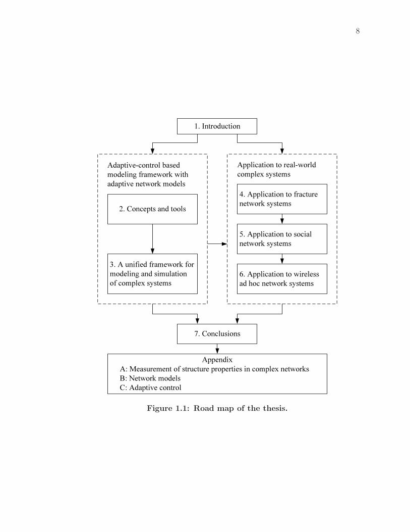
Appendix A, B, and C respectively. Figure 1.1 illustrates a grouping of the chapters
in related subjects.
8
1. Introduction
2. Concepts and tools
3. A unified framework for modeling and simulation of complex systems
4. Application to fracture network systems
5. Application to social network systems
6. Application to wireless ad hoc network systems
7. Conclusions
Application to real-world complex systems
Adaptive-control based modeling framework with adaptive network models
AppendixA: Measurement of structure properties in complex networksB: Network modelsC: Adaptive control
Figure 1.1: Road map of the thesis.

CHAPTER 2
Concepts and Tools
In this chapter we introduce the relevant concepts and approaches. The purpose
of this work is to develop a unified modelling framework that automatically shapes
the network data and the network models by the combination of adaptive net-
work models and adaptive control structures. Moreover, the real-world applications
need to be developed in order to demonstrate how the unified modelling framework
can automatically build the enhanced adaptive network models with desired net-
work structures in different real-world complex systems. We chose the pragmatic
paradigm as the appropriate research paradigm for this research which spans multi-
ple scientific disciplines. Thus, the selected topics are “research objective-centred.”
They are presented here for understanding of the thesis and to achieve mathematical
rigour. We begin in this chapter with a brief overview of the basic concepts from
graph theory and network science. In Section 2.2, we introduce adaptive networks,
and review the recent research on adaptive networks. Finally, in Section 2.3 we
review the relevant notions from adaptive control.
2.1 Modelling Complex Systems with Network Models
Complex systems, as their name implies, are typically difficult to understand,
and hard to control. Traditionally the simplified mathematical models are created
and studied by more mathematically oriented sciences such as physics, chemistry,
and mathematical biology. These models try to abstract the studied complex sys-
tems into a solvable framework, rather than mimic the behaviour of real systems
exactly. The rise of interest in understanding global properties of complex systems
has paralleled the rise of network science, because the network based approach can
create more comprehensive and realistic models of complex systems in nature (New-
man, 2011). Networks that represent the interactions between the system’s compo-
nents can be found in each complex system, such as friendship and acquaintance
networks in social systems, power grids in electric power systems, trade networks in
9
10
economic systems, etc. (Barrat et al., 2008; Boccaletti et al., 2010). As Barabasi
points out (Barabasi et al., 2014), we will never understand complex systems un-
less we gain a deep understanding of the networks behind them. Network science
provides a language through which different research theories, approaches, and ap-
plications, from a wide range of research fields can seamlessly interact with each
other. This interaction has led to a cross-disciplinary fertilization of tools and ideas
which increase our understanding of natural and artificial complex systems (Borner
et al., 2007; Barabasi et al., 2014).
In the next section, we will review network science by following a conceptual
framework, in which a network science approach is used for modelling complex
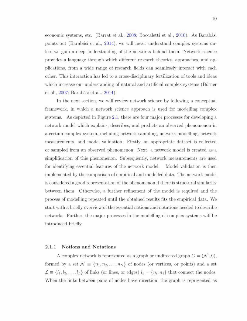
systems. As depicted in Figure 2.1, there are four major processes for developing a
network model which explains, describes, and predicts an observed phenomenon in
a certain complex system, including network sampling, network modelling, network
measurements, and model validation. Firstly, an appropriate dataset is collected
or sampled from an observed phenomenon. Next, a network model is created as a
simplification of this phenomenon. Subsequently, network measurements are used
for identifying essential features of the network model. Model validation is then
implemented by the comparison of empirical and modelled data. The network model
is considered a good representation of the phenomenon if there is structural similarity
between them. Otherwise, a further refinement of the model is required and the
process of modelling repeated until the obtained results fits the empirical data. We
start with a briefly overview of the essential notions and notations needed to describe
networks. Further, the major processes in the modelling of complex systems will be
introduced briefly.
2.1.1 Notions and Notations
A complex network is represented as a graph or undirected graph G = (N ,L),
formed by a set N ≡ {n1, n2, . . . , nN} of nodes (or vertices, or points) and a set
L ≡ {l1, l2, . . . , lL} of links (or lines, or edges) lk = {ni, nj} that connect the nodes.
When the links between pairs of nodes have direction, the graph is represented as
11
Modelling��� �������� ����� � ������� �Measurement�� ��������� ��� ����������� �� �������� �������� �������� � �!��"� �� �������
Validation��� ����# �� ��� ������� Sampling�� ��������� ������� �������� � "$�� � �������
Figure 2.1: General network science research process for modelling ofcomplex systems. There are four major processes for develop-ing a network model which explains, describes, and predictsan observed phenomenon in a certain complex system, in-cluding network sampling, network modelling, network mea-surements, and model validation.
a directed graph G→ = (N ,L→), where N is the set of nodes and L→ is the set of
ordered pairs of arcs (or arrows). Each arc can be identified by a pair (i, j) that
represents a connection going to node i. In undirected graphs, if nodes i and j are
connected and nodes j and k are connected, i and k are also connected. A set of
non-overlapping subsets of connected nodes can be found in a graph based on the
property. A cluster is one of the subsets. A graph G? = (N ?,L?) is a subgraph
of G = (N ,L) if N ? ⊆ N , L? ⊆ L and the links in L? connect nodes in N ?.
The network is called connected if there exists a path between any pair of nodes;
otherwise it is called disconnected. A weighted graph Gw = (N ,L,W) is formed
by a set of N nodes and L links, the set of W ≡ {w1, w2, . . . , wL} weights that
represent the intensity of connections. If the nodes are linked by arcs, the weighted
graph Gw→ is directed. A geographical network G = (N ,L,D) can be defined by a
set N of nodes, a set L of links, and a set D ≡ {−→p 1,−→p 2, . . . ,
−→p N}, where −→p i is an
n-dimensional coordinate vector of the node i (Costa et al., 2011).
12
A graph can be represented by using adjacency lists or adjacency matrices.
In the case of using adjacency lists, the graph is represented in terms of a list of
links (represented through head and tail). The graph can be also represented by an
adjacency matrix A, so that each element aij = 1 expresses an link connecting nodes
i and j, and aij = 0 otherwise. A weighted digraph can be represented by a weight
matrix W , where the matrix element wij represents the weight of the connection
from node i to node j. The operation of thresholding, represented as A = δT (W ),
can be used to produce an unweighted counterpart from a weighted digraph; in case
|wij| > T we have aij = 1, otherwise aij = 0, where T is a specified threshold.
(Costa et al., 2007).
2.1.2 Network Sampling
In the past few years, network science has received a boost from the ever-
increasing availability of high performance computers and large data collections.
However, the size, type and richness of empirical data, which consist of observations
and measurements of a complex system, are very different in various application
domains (Borner et al., 2007). In many cases, the sheer size of empirical data makes
it computationally infeasible to study the entire system. In other cases, the size of
empirical data may not be large but measurements are required to observe the un-
derlying phenomenon. To create a reliable dataset which demonstrates major prop-
erties of a studied complex system, network sampling techniques are used. Thus,
network sampling can be considered as the process of acquiring network datasets
from gathered empirical data. There are three classes of sampling methods, in-
cluding node sampling, edge sampling, and topology-based sampling. The sampled
subsets may be generated by choosing nodes and/or links which match or exceed
a certain threshold, while a sample can also be constructed by using breath-first
search (i.e. sampling without replacement) or random walks (i.e. sampling with
replacement) over a graph (Borner et al., 2007; Airoldi et al., 2011). To reduce the
sampling bias, a large number of techniques have been developed for improving the
quality of the recovered samples. More detailed discussion of these approaches can
be found in (Borner et al., 2007; Airoldi et al., 2011; Maiya, 2011; and references
13
therein).
2.1.3 Network Measurements
In order to describe the topology of a network, a large set of measurements
have been developed (Costa et al., 2007). By using the measurements described in
Appendix A, local analysis can be implemented based on node measurements, while
global analysis can be performed based on average measurements for the whole net-
work (Costa et al., 2011). Community identification methods and measurements on
complex network are used for intermediate analysis. Community structures can be
represented by set of groups whose nodes are more densely interconnected to one
another than with the rest of the network (Costa et al., 2007). Many community
identification algorithms have been proposed because uncovering the community
structure can deepen our understanding of complex systems. After traditional hi-
erarchical clustering methods (Podani et al., 2001; Girvan & Newman, 2002; Ravasz
et al., 2002) were applied in some early research (Eckmann et al., 2002; Girvan
& Newman, 2002; Maslov & Sneppen, 2002), a quality function called modularity
(Newman & Girvan, 2004) was introduced for choosing the optimal partition. A few
methods with optimal quality function were then proposed by applying a new heuris-
tic or modifying the quality function (Fortunato, 2010). More alternative methods
were also proposed based on different principles, such as percolating cliques (Palla
et al., 2005), information compressing (Rosvall & Bergstrom, 2007), and elementary
physical dynamics (Raghavan et al., 2007), etc. Multiresolution methods (Danon
et al., 2005; Reichardt & Bornholdt, 2006; Delvenne et al., 2010) with a tunable
parameter were proposed to resolve clusters under a quite large, network-dependent
size, while the original modularity method suffers from an intrinsic resolution limit
problem (Fortunato & Barthelemy, 2007; Kumpula et al., 2007). To find clusters
inside a cluster, several hierarchical methods (Sales-Pardo et al., 2007; Ruan &
Zhang, 2008; Kovacs et al., 2010; Rosvall & Bergstrom, 2011) were introduced. Be-
sides communities, there are other types of subgraphs in complex networks, such as
motifs (Milo et al., 2002), cycles (Bagrow et al., 2006) and chains (Villas Boas et
al., 2008).
14
2.1.4 Network Modelling
In this section, a brief review of network modelling approaches is provided. The
first sub-section starts with an introduction of network formation models. The next
sub-section introduces that aim to model the dynamical processes on networks. The
third sub-section provides a brief overview of an agent-based modelling approach.
A detailed introduction of diverse network modelling approaches can be found in
(Wasserman & Faust, 1994; Kumar et al., 2000; Newman, 2003; Carrington et al.,
2004; Pastor-Satorras & Vespignani, 2004; Newman et al., 2006; Borner et al., 2007;
Newman, 2010; Newman, 2011).
2.1.4.1 Modelling Formation of Networks
In order to study the structure of complex systems, a few statistical models of
network formation have been developed based on a set of graphs matching certain
statistical threshold of the studied systems. Some structural features observed
in complex systems can be reproduced by the network formation models, such as
small average path lengths, strong clustering, and scale-free degree distributions
(Bollobas, 1998; Zschaler, 2012). Several network models have become a subject
of great interest, including Erdos-Renyi random graph, small-world model of Watts
and Strogatz, Barabasi-Albert scale-free model, and Waxman geographical model
(see Appendix B).
2.1.4.2 Modelling Dynamics on Networks
The dynamics of interactions between the constituting elements of a certain
complex system can be investigated based on the structure or certain network prop-
erties of the system. . In many cases, the evolution of a network’s structure is
determined by some internal dynamics of the nodes and the interactions between
them. Diffusion modelling has been implemented in various applications, includ-
ing the spreading of diseases, viruses, fashion, rumours, or knowledge (Daley et al.,
1999; Tabah, 1999; Liljeros et al., 2001; Pastor-Satorras & Vespignani, 2001; Bet-
tencourt et al., 2005; Keeling & Eames, 2005). In these models, the master equation
approach is used for analysis of dynamical processes on networks. This approach
15
assumes that the states of the nodes can be described by one or more dynamical vari-
ables. Transitions of the states are probabilistically obtained from contacts among
nodes. Thus, the contact networks provide the underlying interaction geometry in
which diffusion occurs (Boccaletti et al., 2006; Borner et al., 2007; Barrat et al.,
2008; Zschaler, 2012).
Other dynamical processes have also been studied in artificial complex systems,
such as power grid, the Internet, communication systems, for understanding the
dynamics of information flow, data flow, and traffic flow. In these systems, the nodes
and links are often sensitive to overloading. The failure of one node or one link may
increases the burden on other network components, and eventually leading to an
avalanche of overloads on them. Modelling dynamics on these networks can provide
indications to decrease the undesired effects. Other examples of dynamical processes
on networks can be found in neuronal networks and food webs. Synchronization
phenomena have been investigated by using an interaction network model which
contains a coupled oscillator in conceptual models of neuronal networks. (Kuramoto,
2003; Moreno & Pacheco, 2004). In food webs, dynamical processes are studied
by modelling the flow of biomass between predators and their prey. (Camacho et
al., 2002; Gross et al., 2009; collective dynamics-Pimm, 2002)(Camacho et al., 2002;
Pimm, 2002; Gross et al., 2009).
Most recently modelling dynamical processes often entails using one of two
basic methods of developing computational models which use for modelling dynam-
ical process i.e. either use of master equation approach for analysis of dynamical
processes on networks or else use of agent-based modelling approach to develop sim-
ulation models. In more complicated models, the master equation approach might
not lead to solvable equations. Moreover, this approach cannot provide a complete
picture of studied system because individual heterogeneity or other possible fluctu-
ations are ignored. In this situation, agent-based models can be applied (Borner
et al., 2007; Barrat et al., 2008).
16
2.1.4.3 Agent-Based Modelling
If analytical solutions cannot be found by the master equation approach in
more complicated models, an agent-based modelling approach can be applied for
the simulation of complex and varied interactions among the nodes. This approach
separately and individually simulate the agents in a complex system and their inter-
actions, allowing the emergent behaviours of the system to appear naturally (Borner
et al., 2007; Barrat et al., 2008; Newman, 2011). Agent-based models (Bankes, 2002)
have become fashionable in a wide variety of complex systems (Bonabeau, 2002),
ranging from biological systems (Folcik et al., 2007; Huang et al., 2007; Devillers et
al., 2008; Galvao et al., 2008; Guo et al., 2008; Kiran et al., 2008; Lao & Kamei,
2008; Odell & Foe, 2008; Rubin et al., 2008; Robinson et al., 2008; Santoni et al.,
2008; Bailey et al., 2009; Carpenter & Sattenspiel, 2009; Dancik et al., 2010; Gal-
vao & Miranda, 2010; Itakura et al., 2010) to social systems (Gilbert & Troitzsch,
2005; Batty et al., 2007; Chen & Zhan, 2008; Quera et al., 2010), from financial
systems (Streit & Borenstein, 2009) to ecosystems (Grimm et al., 2006; Railsback
& Grimm, 2011), from supply chains (Zarandi et al., 2008) to modelling of traffic
lights (Gershenson, 2005). When modelling dynamical processes using an agent-
based modelling approach, each individual node is assumed to be in one of several
possible states. A model-specific update procedure that depends on the microscopic
dynamics is applied to each node in each discrete time step. The state of a node is
changed depending on the state of neighbouring nodes or other dynamic rules. The
dynamics of each individual element can be simulated through using Monte Carlo
methods, where the random events of the dynamical process are simulated with
the use of random number generators. The agent-based modelling approach can be
used to reproduce the dynamics occurring in networks, and provides access to the
microscopic dynamics of the system that is in general hindered by the mathemat-
ical complexity and the large number of degrees of freedom inherent to real-world
complex systems. In addition, this approach allows extremely detailed information
to be obtained and provide a way to monitor the single state of each agent at any
time (Borner et al., 2007; Barrat et al., 2008; Newman, 2011).
A variety of software packages are available for performing agent-based mod-
17
elling and simulation of complex systems (Newman, 2011; Niazi, 2011). Some of
them, such as Repast (North & Macal, 2007) and Mason (Panait & Luke, 2005),
are highly advanced programming libraries suitable for cutting edge research, while
others are designed as easy-to-use tools requiring little prior knowledge, such as
StarLogo (Resnick, 1996), NetLogo (Wilensky, 1999) etc. In addition, some simu-
lators have been developed for the simulation of communication systems, such as
NS-2, OPNET (Garrido et al., 2008), J-Sim (Sobeih et al., 2006), TOSSIM (Levis
et al., 2003) etc. TOSSIM is a TinyOS simulator. J-Sim and NS-2 have been com-
pared in (Sobeih et al., 2006) and J-Sim is more scalable than NS-2. SensorSim
is a simulation framework for wireless sensor networks (Park et al., 2000), while
ATEMU (Polley et al., 2004) focuses on simulation of particular sensors. Further
examples include Oversim (Baumgart et al., 2007) and PeerSim (Montresor & Je-
lasity, 2009) for simulation of peer-to-peer networks, Swarm-Bot (Mondada et al.,
2004), WebotsTM (Michel, 2004), and LaRosim (Sahin et al., 2008) for simulation
of robotic swarms, etc.
Although an agent-based modelling approach can simulate very intricate dy-
namical processes while fully incorporating stochastic effects, agent-based models
are often very complicated. Moreover, it is difficult to study the impact of any given
modelling assumption or parameter. Thus, a careful trade-off between the level of
details and the interpretation of results is important to modelling and simulation
of real-world complex systems. (Borner et al., 2007; Barrat et al., 2008; Newman,
2011).
2.1.5 Model Validation
All models make implicit assumptions about the real-world complex systems
based on our understanding of world, while model a certain complex system with
all details is impossible. Suitable approximations need to be made according to the
corresponding research study objectives and expected outcomes. Dynamic mod-
elling is more suited for modelling large-scale and evolutionary complex systems,
while statistical modelling is well suited for modelling the complex systems with the
statistical observables. However, all these models need to be validated through the

18
comparison of modelled data and empirical data for real-world complex systems. By
using statistical modelling, the parameters of the statistical models can be obtained
based on the statistical measures derived from the empirical data. Moreover, the
statistical predictions derived from the generated distributions can be tested by new
measurements on the empirical data. In the dynamical approach, the properties of
empirical data are used to validate models, while their local dynamic rules normally
take no account of the statistical observables (Borner et al., 2007, Barrat et al.,
2008). However, agent-based models can be difficult to validate because both the
structure of underlying network and local dynamic rules are related to the statistical
observables of the studied complex systems. As Niazi points out (Niazi, 2011), a
number of issues need to be handled for validation of agent-based models as follows:
• There is no standard way of building agent-based models.
• There is no standard and formal way of validation of agent-based models.
• Agent-based modelling and agent-based simulations are considered in the same
manner because there is no formal methodology of agent-based modelling
(Macal & North, 2007).
• Agent-based models are primarily pieces of software however no software pro-
cess is available for development of such models.
• All validation paradigms for agent-based models are based on quantifying and
measurable values but none caters for emergent behaviour (Axtell, 1999; Axtell
et al., 1999) such as traffic jams, structure formation or self-assembly as these
complex behaviours cannot be quantified easily in the form of single or a vector
of numbers.
A variety of approaches have been proposed for validation of agent-based mod-
els. For example, in the case of Agents in Computation Economics (ACE), empirical
validation of agent-based models has been developed by Fagiolo et al. in (Fagiolo et
al., 2007). Alternate approaches to empirical validation have been showed by Moss
in (Moss, 2008). In Wilensky and Rand’s work (Wilensky & Rand, 2007), it has
19
been found that validation of models is closely related to model replication as noted.
An iterative participatory approach, “companion modelling”, has been developed by
Barreteau et al. in (Barreteau, 2003) where multidisciplinary researchers and stake-
holders work together throughout a four-stage cycle. An approach of validation has
been discussed in which philosophical truth theories are used in simulations (Schmid,
2005). In addition, agent-based simulation can be used as a means of validation and
calibration of other models (Makowsky, 2006).
The general network science research approach has been used for modelling
and simulation of complex systems in different real-world applications. However, in
this research, the network based approaches (network sampling, modelling, measur-
ing, and validating) are applied to four domains of the adaptive network modelling
process for dynamically adjusting their control parameters. Moreover, such a “net-
work structure-centred” modelling framework allows the automatic generation of
enhanced adaptive networks by systematically adjusting both the network topology
and the control parameters at the same time to accurately reflect the real-world
complex system.
2.2 Adaptive Networks
In recent years, the study of networks has received a rapidly increasing amount
of attention, with many applications in social, biological and technical systems. Tra-
ditionally, most research has taken into account “dynamics of networks” or “dynam-
ics on networks” independently. While the “dynamics of networks” approach focuses
on the emergence and evolution of particular network structures, the “dynamics on
networks” approach emphasizes on the state transition of nodes on a network with
a fixed topology. In this case the network topology can have a strong impact on
the dynamics of the nodes (Leidl & Hartmann, 2009; Zschaler, 2012, Sayama et al.,
2013).
In real-world complex systems, the underlying networks can provide a static
interaction topology for local dynamical process. In many cases, however, these
networks also evolve and change due to the ongoing local dynamical process. More-
over, a feedback loop among the dynamics of the network and the dynamics on the
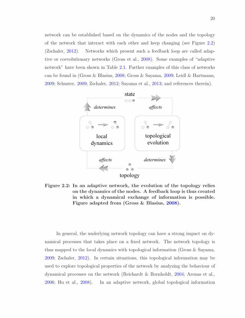
20
network can be established based on the dynamics of the nodes and the topology
of the network that interact with each other and keep changing (see Figure 2.2)
(Zschaler, 2012). Networks which present such a feedback loop are called adap-
tive or coevolutionary networks (Gross et al., 2008). Some examples of “adaptive
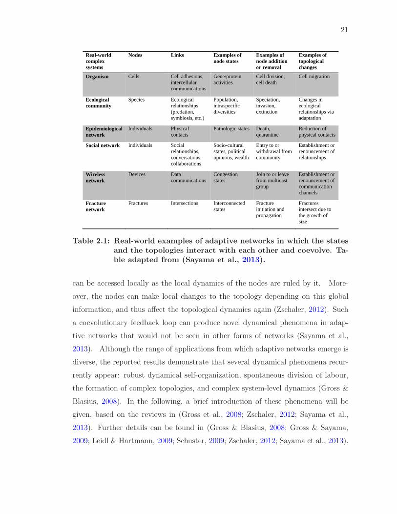
network” have been shown in Table 2.1. Further examples of this class of networks
can be found in (Gross & Blasius, 2008; Gross & Sayama, 2009; Leidl & Hartmann,
2009; Schuster, 2009; Zschaler, 2012; Sayama et al., 2013; and references therein).
state
local dynamics
topologicalevolution
topology
determines affects
affects determines
Figure 2.2: In an adaptive network, the evolution of the topology relieson the dynamics of the nodes. A feedback loop is thus createdin which a dynamical exchange of information is possible.Figure adapted from (Gross & Blasius, 2008).
In general, the underlying network topology can have a strong impact on dy-
namical processes that takes place on a fixed network. The network topology is
thus mapped to the local dynamics with topological information (Gross & Sayama,
2009; Zschaler, 2012). In certain situations, this topological information may be
used to explore topological properties of the network by analyzing the behaviour of
dynamical processes on the network (Reichardt & Bornholdt, 2004; Arenas et al.,
2006; Hu et al., 2008). In an adaptive network, global topological information
21
Real-world complex systems
Nodes Links Examples of node states
Examples of node addition or removal
Examples of topological changes
Organism Cells Cell adhesions, intercellular communications
Gene/protein activities
Cell division, cell death
Cell migration
Ecological community
Species Ecological relationships (predation, symbiosis, etc.)
Population, intraspecific diversities
Speciation, invasion, extinction
Changes in ecological relationships via adaptation
Epidemiological network
Individuals Physical contacts
Pathologic states Death, quarantine
Reduction of physical contacts
Social network Individuals Social relationships, conversations, collaborations
Socio-cultural states, political opinions, wealth
Entry to or withdrawal from community
Establishment or renouncement of relationships
Wireless network
Devices Data communications
Congestion states
Join to or leave from multicast group
Establishment or renouncement of communication channels
Fracture network
Fractures Intersections Interconnected states
Fracture initiation and propagation
Fractures intersect due to the growth of size
Table 2.1: Real-world examples of adaptive networks in which the statesand the topologies interact with each other and coevolve. Ta-ble adapted from (Sayama et al., 2013).
can be accessed locally as the local dynamics of the nodes are ruled by it. More-
over, the nodes can make local changes to the topology depending on this global
information, and thus affect the topological dynamics again (Zschaler, 2012). Such
a coevolutionary feedback loop can produce novel dynamical phenomena in adap-
tive networks that would not be seen in other forms of networks (Sayama et al.,
2013). Although the range of applications from which adaptive networks emerge is
diverse, the reported results demonstrate that several dynamical phenomena recur-
rently appear: robust dynamical self-organization, spontaneous division of labour,
the formation of complex topologies, and complex system-level dynamics (Gross &
Blasius, 2008). In the following, a brief introduction of these phenomena will be
given, based on the reviews in (Gross et al., 2008; Zschaler, 2012; Sayama et al.,
2013). Further details can be found in (Gross & Blasius, 2008; Gross & Sayama,
2009; Leidl & Hartmann, 2009; Schuster, 2009; Zschaler, 2012; Sayama et al., 2013).
22
2.2.1 Robust Self-Organization
The adaptive feedback with the coevolution of the local dynamics and network
topologies provides a robust mechanism for global self-organization. It allows an
adaptive network to robustly organize into a state with special topological or dynam-
ical properties (Leidl & Hartmann, 2009). Moreover, the coupling of local dynamics
and network topologies can provide a dynamical self-organization, in which the local
dynamics drives the network topologies towards a critical point (Christensen et al.
(1998.
Bornholdt and Rohlf (2000) considered a Boolean threshold network, where
a topological update rule determined the local dynamics. Their investigation
illustrated that the topological information can be accessed locally and affect the
local dynamics of the topology. The local dynamics then drove the topological
dynamics towards the critical state. Thus, the interplay of two local processes can
give rise to a highly robust global self-organization without the impact of the initial
conditions and the specific control parameters. (Gross et al., 2008; Zschaler, 2012;
Sayama et al., 2013;). This dynamical self-organization behaviour has also been
found in different complex network models (Christensen et al., 1998; Bornholdt &
Roehl, 2003; Liu & Bassler, 2006), including some models for the investigation of
self-organized criticality in adaptive neural systems (Chialvo & Bak, 1999; Beggs &
Plenz, 2003; Liu & Bassler, 2006; Kitzbichler et al., 2009; Levina et al., 2009; Meisel
& Gross, 2009; Pearlmutter & Houghton, 2009; Meisel et al., 2012), in which the
generality of the underlying mechanism is highlighted.
2.2.2 Spontaneous Division of Labour
In adaptive networks, the adaptive interplay between the node states and
the network topology can produce different classes of nodes from an initially ho-
mogeneous population (Gross et al., 2008). This spontaneous “division of labour”
phenomenon was shown by Ito and Kaneko (Ito & Kaneko, 2001) in an adaptive
network of coupled oscillators. They investigated a weighted directed network which
consists of a few one-dimensional chaotic oscillators. The states of the nodes were
updated based on the states of the their neighbours, while the network topology
23
can be modified through using a update rule of link weights. Moreover, this update
rule increases link weights between oscillators with similar states, and still keeps the
total weight of all incoming links of each node constant at the same time (Zschaler,
2012; Gross et al., 2008).
In a certain parameter region, two classes of nodes with distinct effective out-
degree (high/low) can be observed. Moreover, a node generally remain in one
class over a long period of time despite the ongoing rewiring of individual links.
Thus, the nodes with high out-degree have more influences on other nodes than the
low out-degree nodes because all nodes are impacted by their incoming connections
(Gross et al., 2008; Zschaler, 2012). In this regard, the two classes of nodes in a
system can be considered as a spontaneous “division of labour” with “leaders” and
“followers”. Similar phenomena have also observed in different complex networks.
In some dynamical models of neural network, the topology is changed through a
strengthening of connections among nodes with similar state (Gong & van Leeuwen,
2004; van den Berg & van Leeuwen, 2004). In addition, emergent “leadership” has
also been found when researchers studied the Prisoner’s Dilemma game on adaptive
network 2004; Eguıluz et al., 2005). In these models, the nodes generally follow
other nodes in self-organized hierarchical structures (Zschaler, 2012).
2.2.3 Formation of Complex Topologies
In adaptive networks, heterogeneous structures can arise from initially homoge-
neous conditions through the coevolution of the local dynamics and the topological
dynamics. Furthermore, highly complex topologies produced by this coevolution
have been observed in different complex network models (Zschaler, 2012). For
example, Holme and Newman (2006) and Zanette and Gil (2006) have studied col-
lective opinion formation on adaptive networks. In these models, the agents can
have many possible opinions and update their states depending on their neighbours’
opinions, when the competing opinions are diffused in a social network. More-
over, the adaptive voter model (Kozma & Barrat, 2008) shown that the coevolution
of state and topology can drive the population towards consensus or a fragmenta-
tion. In order to investigate the fragmentation transition, in which the long term
24
outcomes change from consensus to fragmentation, several approaches (Kimura &
Hayakawa, 2008; Bohme & Gross, 2011; Zschaler et al., 2012) have been proposed
for the analytical computation of the transition point. Detailed discussion of the
fragmentation transition can be found in the work of Vazquez et al. (2008) and
Kimura and Hayakawa (2008).
Similar fragmentation transition phenomena have also been found in agent-
based adaptive network models (Centola et al., 2007; Centola, 2010; Centola, 2011)
of more realistic cultural drift and dissemination processes, in which social network
structures interact with human behaviours. Further examples include the works of
Huepe et al. (2011) and Couzin et al. (2011) which have demonstrated voter-like
models can deep our understanding of the dynamics of decision making.
Complex topologies have also been observed in different game-theoretic mod-
els of cooperation in adaptive networks. For instance, the minority game on adap-
tive networks has been investigated by Paczuski, Bassler, and Corral (2000), while
Skyrms and Pemantle (2000) have studied the various coordination and cooperation
games on adaptive networks. In addition, a study of the Prisoner’s dilemma on
adaptive networks has been implemented by Zimmermann et al. (2000). Further,
the interactive between coevolutionary dynamics and the evolution of cooperation in
adaptive networks have been investigated in different works. For example, Pacheco
et al. (2006) and van Segbroeck et al. (2011) have shown that coevolution can
increase levels of cooperation by combining the underlying beneficial structures and
the dynamics of cooperation. Zschaler et al. (2010) have demonstrated that full
cooperation can be achieved by an unconventional dynamical mechanism.
Another class of games in adaptive networks has also been investigated, in
which nodes aim to obtain an advantageous position instead of some optimal ben-
efit (Bala & Goyal, 2001; Holme & Ghoshal, 2006). In these models, the nodes use
locally available information to maximize their centralities with reasonable costs
(i.e., maintaining reasonable connections) through adaptively modifying their links
(Sayama et al., 2013). The coupling between the states of nodes and network topolo-
gies can drive the network state towards a critical point of the transition between
well-connected and fragmented states. Furthermore, Do et al. (2010) has also found
25
that the local dynamics can give rise to emergent global topology in a game-theoretic
model of cooperation.
2.2.4 Complex System-Level Dynamics
In many adaptive networks, the state-topology coevolution can give rise to
new dynamical phenomena. The resulting interplay can describe complex dynamics
and produce new phase transitions. This has been shown in a number of epidemio-
logical models on adaptive networks, where the agents rewire their social contacts in
response to the epidemic state of other agents (Gross et al., 2006; Zschaler, 2012).
Gross et al. (2006) proposed the adaptive Susceptible-Infected-Susceptible
(SIS) model, in which the transition points can be computed analytically through
using moment closure approximation. In this model, the node-level coevolution
can give rise to the emergence of system-level dynamics. This model has been
used as a performance baseline in different adaptive network research (Gross &
Kevrekidis, 2008; Guerra & Gomez-Gardenes, 2010; Marceau et al., 2010; Wieland
et al., 2012). Moreover, inspired by the SIS model, social impact and policy
responses to epidemics on disease propagation has been investigated in (Wang et
al., 2007; Shaw & Schwartz, 2008; Zanette & Risau-Gusman, 2008).
In addition, several applications (Epstein et al., 2008; Funk et al., 2009; Shaw
& Schwartz, 2010) of adaptive networks have also been developed for real-world
epidemiological practice. These adaptive social models can present more realistic
dynamics of social network, while people change their social behaviours depending
on epidemiological states of their neighbours (Funk et al., 2010). The node-
level dynamics can give rise to the emergence of complex system-level dynamics
in adaptive networks has also been found in many different models. For instance,
the fragmentation transition between well-connected and fragmented states can be
driven by the state-topology coevolution has been observed in the voter-like models
and models of opinion formation. (Gil & Zanette, 2006; Kimura & Hayakawa, 2008;
Bohme & Gross, 2011).
In a number of models from game-theory, phase transitions driven by network
adaptivity has also been observed (Pacheco et al., 2006; Santos et al., 2006; Szolnoki
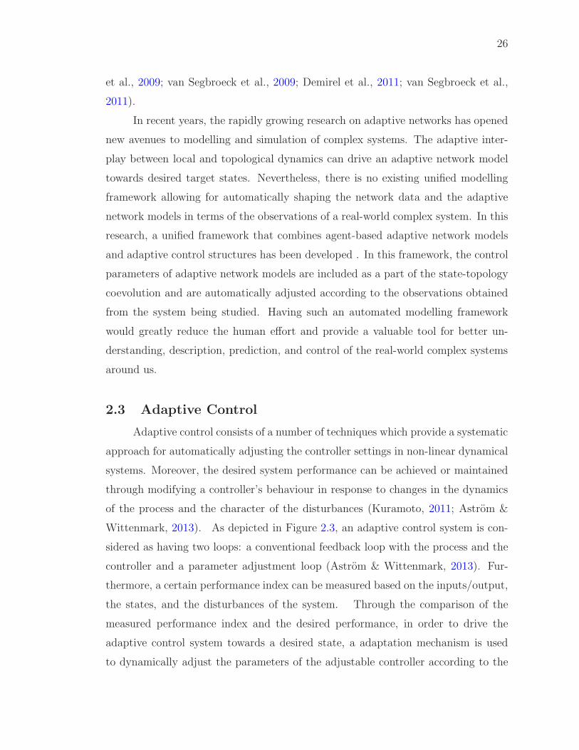
26
et al., 2009; van Segbroeck et al., 2009; Demirel et al., 2011; van Segbroeck et al.,
2011).
In recent years, the rapidly growing research on adaptive networks has opened
new avenues to modelling and simulation of complex systems. The adaptive inter-
play between local and topological dynamics can drive an adaptive network model
towards desired target states. Nevertheless, there is no existing unified modelling
framework allowing for automatically shaping the network data and the adaptive
network models in terms of the observations of a real-world complex system. In this
research, a unified framework that combines agent-based adaptive network models
and adaptive control structures has been developed . In this framework, the control
parameters of adaptive network models are included as a part of the state-topology
coevolution and are automatically adjusted according to the observations obtained
from the system being studied. Having such an automated modelling framework
would greatly reduce the human effort and provide a valuable tool for better un-
derstanding, description, prediction, and control of the real-world complex systems
around us.
2.3 Adaptive Control
Adaptive control consists of a number of techniques which provide a systematic
approach for automatically adjusting the controller settings in non-linear dynamical
systems. Moreover, the desired system performance can be achieved or maintained
through modifying a controller’s behaviour in response to changes in the dynamics
of the process and the character of the disturbances (Kuramoto, 2011; Astrom &
Wittenmark, 2013). As depicted in Figure 2.3, an adaptive control system is con-
sidered as having two loops: a conventional feedback loop with the process and the
controller and a parameter adjustment loop (Astrom & Wittenmark, 2013). Fur-
thermore, a certain performance index can be measured based on the inputs/output,
the states, and the disturbances of the system. Through the comparison of the
measured performance index and the desired performance, in order to drive the
adaptive control system towards a desired state, a adaptation mechanism is used
to dynamically adjust the parameters of the adjustable controller according to the
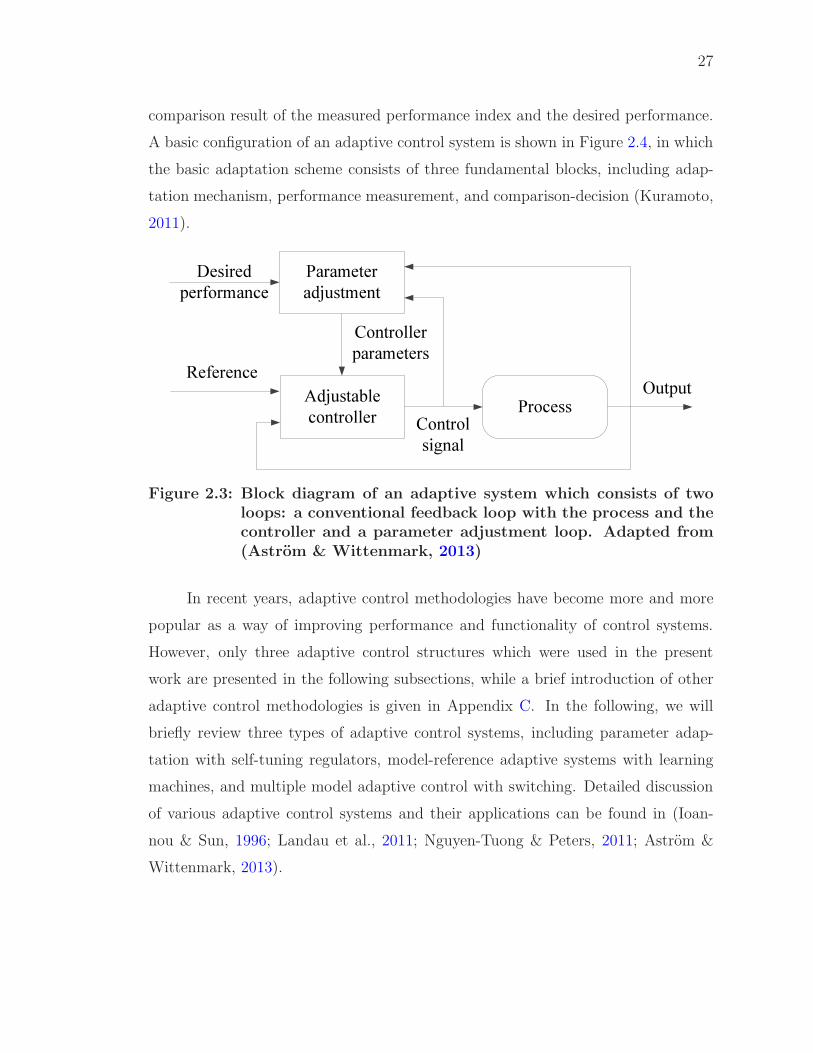
27
comparison result of the measured performance index and the desired performance.
A basic configuration of an adaptive control system is shown in Figure 2.4, in which
the basic adaptation scheme consists of three fundamental blocks, including adap-
tation mechanism, performance measurement, and comparison-decision (Kuramoto,
2011).
Adjustable controller
Controllerparameters
Reference
Controlsignal
Output
Desiredperformance
Process
Parameteradjustment
Figure 2.3: Block diagram of an adaptive system which consists of twoloops: a conventional feedback loop with the process and thecontroller and a parameter adjustment loop. Adapted from(Astrom & Wittenmark, 2013)
In recent years, adaptive control methodologies have become more and more
popular as a way of improving performance and functionality of control systems.
However, only three adaptive control structures which were used in the present
work are presented in the following subsections, while a brief introduction of other
adaptive control methodologies is given in Appendix C. In the following, we will
briefly review three types of adaptive control systems, including parameter adap-
tation with self-tuning regulators, model-reference adaptive systems with learning
machines, and multiple model adaptive control with switching. Detailed discussion
of various adaptive control systems and their applications can be found in (Ioan-
nou & Sun, 1996; Landau et al., 2011; Nguyen-Tuong & Peters, 2011; Astrom &
Wittenmark, 2013).
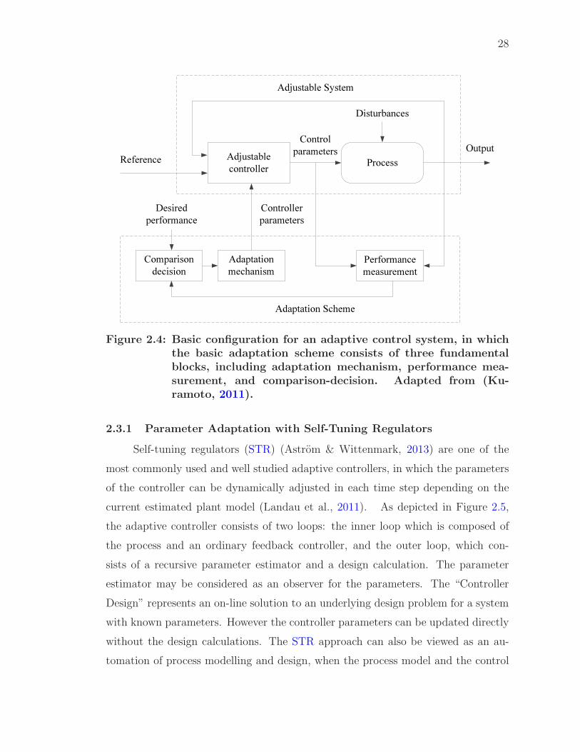
28
Adjustable controller
Controllerparameters
ReferenceControl
parameters Output
Desiredperformance
Comparisondecision
Performancemeasurement
Adaptationmechanism
Process
Adjustable System
Adaptation Scheme
Disturbances
Figure 2.4: Basic configuration for an adaptive control system, in whichthe basic adaptation scheme consists of three fundamentalblocks, including adaptation mechanism, performance mea-surement, and comparison-decision. Adapted from (Ku-ramoto, 2011).
2.3.1 Parameter Adaptation with Self-Tuning Regulators
Self-tuning regulators (STR) (Astrom & Wittenmark, 2013) are one of the
most commonly used and well studied adaptive controllers, in which the parameters
of the controller can be dynamically adjusted in each time step depending on the
current estimated plant model (Landau et al., 2011). As depicted in Figure 2.5,
the adaptive controller consists of two loops: the inner loop which is composed of
the process and an ordinary feedback controller, and the outer loop, which con-
sists of a recursive parameter estimator and a design calculation. The parameter
estimator may be considered as an observer for the parameters. The “Controller
Design” represents an on-line solution to an underlying design problem for a system
with known parameters. However the controller parameters can be updated directly
without the design calculations. The STR approach can also be viewed as an au-
tomation of process modelling and design, when the process model and the control
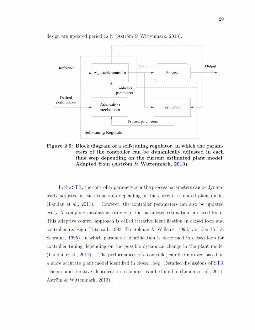
29
design are updated periodically (Astrom & Wittenmark, 2013).
Adjustable controller
Controllerparameters
Reference Input Output
Desiredperformance
EstimatorAdaptationmechanism
Process
Self-tuning Regulator
Process parameters
Figure 2.5: Block diagram of a self-tuning regulator, in which the param-eters of the controller can be dynamically adjusted in eachtime step depending on the current estimated plant model.Adapted from (Astrom & Wittenmark, 2013).
In the STR, the controller parameters or the process parameters can be dynam-
ically adjusted in each time step depending on the current estimated plant model
(Landau et al., 2011). However, the controller parameters can also be updated
every N sampling instants according to the parameter estimation in closed loop,.
This adaptive control approach is called iterative identification in closed loop and
controller redesign (Bitmead, 1993; Trentelman & Willems, 1993; van den Hof &
Schrama, 1995), in which parameter identification is performed in closed loop for
controller tuning depending on the possible dynamical change in the plant model
(Landau et al., 2011).. The performances of a controller can be improved based on
a more accurate plant model identified in closed loop. Detailed discussions of STR
schemes and iterative identification techniques can be found in (Landau et al., 2011;
Astrom & Wittenmark, 2013).
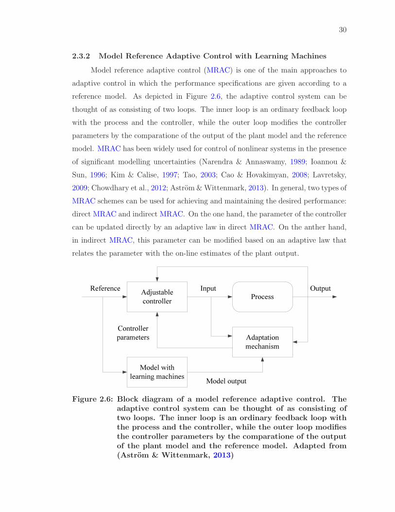
30
2.3.2 Model Reference Adaptive Control with Learning Machines
Model reference adaptive control (MRAC) is one of the main approaches to
adaptive control in which the performance specifications are given according to a
reference model. As depicted in Figure 2.6, the adaptive control system can be
thought of as consisting of two loops. The inner loop is an ordinary feedback loop
with the process and the controller, while the outer loop modifies the controller
parameters by the comparatione of the output of the plant model and the reference
model. MRAC has been widely used for control of nonlinear systems in the presence
of significant modelling uncertainties (Narendra & Annaswamy, 1989; Ioannou &
Sun, 1996; Kim & Calise, 1997; Tao, 2003; Cao & Hovakimyan, 2008; Lavretsky,
2009; Chowdhary et al., 2012; Astrom & Wittenmark, 2013). In general, two types of
MRAC schemes can be used for achieving and maintaining the desired performance:
direct MRAC and indirect MRAC. On the one hand, the parameter of the controller
can be updated directly by an adaptive law in direct MRAC. On the anther hand,
in indirect MRAC, this parameter can be modified based on an adaptive law that
relates the parameter with the on-line estimates of the plant output.
Adjustable controller
Controller parameters
Reference Input Output
Adaptationmechanism
Model with learning machines
Process
Model output
Figure 2.6: Block diagram of a model reference adaptive control. Theadaptive control system can be thought of as consisting oftwo loops. The inner loop is an ordinary feedback loop withthe process and the controller, while the outer loop modifiesthe controller parameters by the comparatione of the outputof the plant model and the reference model. Adapted from(Astrom & Wittenmark, 2013)
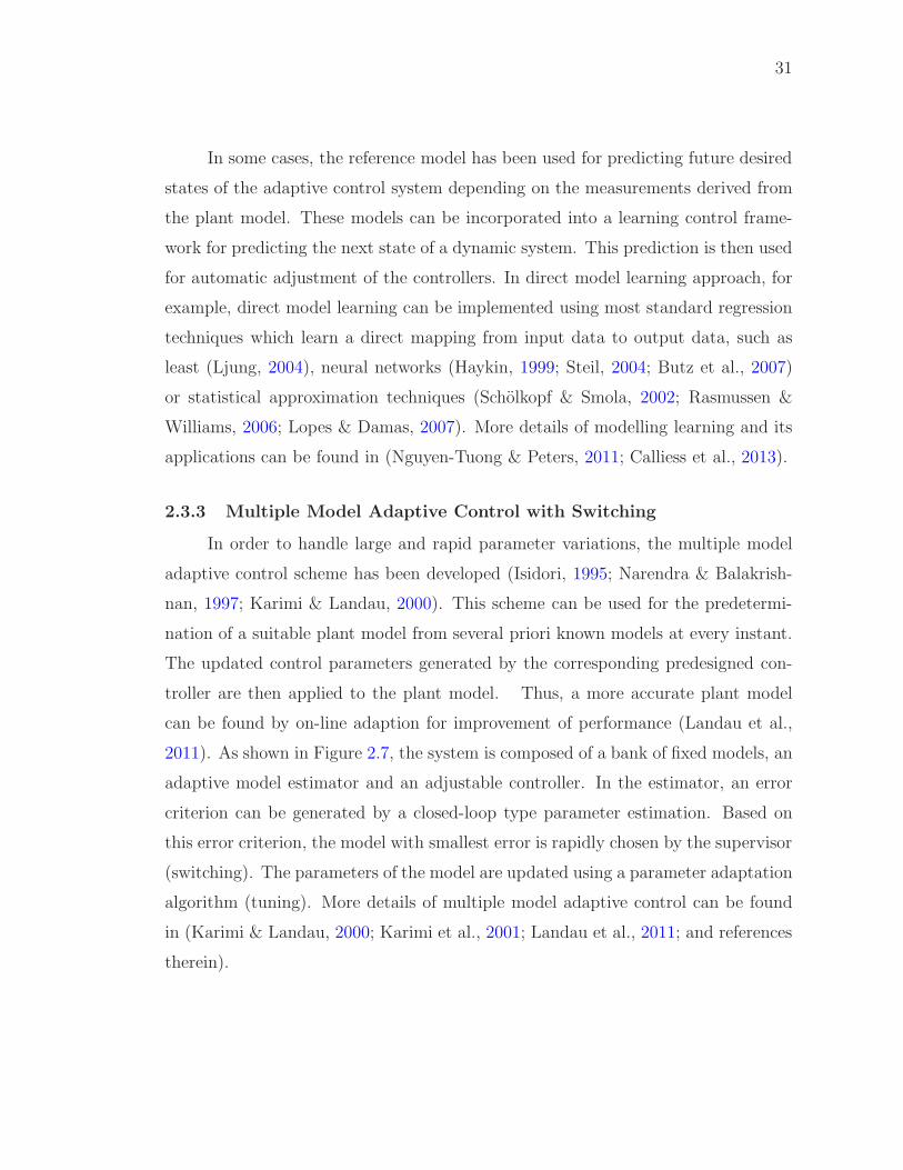
31
In some cases, the reference model has been used for predicting future desired
states of the adaptive control system depending on the measurements derived from
the plant model. These models can be incorporated into a learning control frame-
work for predicting the next state of a dynamic system. This prediction is then used
for automatic adjustment of the controllers. In direct model learning approach, for
example, direct model learning can be implemented using most standard regression
techniques which learn a direct mapping from input data to output data, such as
least (Ljung, 2004), neural networks (Haykin, 1999; Steil, 2004; Butz et al., 2007)
or statistical approximation techniques (Scholkopf & Smola, 2002; Rasmussen &
Williams, 2006; Lopes & Damas, 2007). More details of modelling learning and its
applications can be found in (Nguyen-Tuong & Peters, 2011; Calliess et al., 2013).
2.3.3 Multiple Model Adaptive Control with Switching
In order to handle large and rapid parameter variations, the multiple model
adaptive control scheme has been developed (Isidori, 1995; Narendra & Balakrish-
nan, 1997; Karimi & Landau, 2000). This scheme can be used for the predetermi-
nation of a suitable plant model from several priori known models at every instant.
The updated control parameters generated by the corresponding predesigned con-
troller are then applied to the plant model. Thus, a more accurate plant model
can be found by on-line adaption for improvement of performance (Landau et al.,
2011). As shown in Figure 2.7, the system is composed of a bank of fixed models, an
adaptive model estimator and an adjustable controller. In the estimator, an error
criterion can be generated by a closed-loop type parameter estimation. Based on
this error criterion, the model with smallest error is rapidly chosen by the supervisor
(switching). The parameters of the model are updated using a parameter adaptation
algorithm (tuning). More details of multiple model adaptive control can be found
in (Karimi & Landau, 2000; Karimi et al., 2001; Landau et al., 2011; and references
therein).
32
Adjustable controller
Controller parameters
Reference
Input
Output
Adaptive model estimator
Model n
Process
Model outputAdjustable controller
Model 2
Model 1
Adaptive model estimator
Parameter adaptation algorithms
…
Model input
Figure 2.7: Block diagram of a multiple-model adaptive control ap-proach. The adaptive control system is composed of a bank offixed models, an adaptive model estimator and an adjustablecontroller. In the estimator, an error criterion can be gener-ated by a closed-loop type parameter estimation. Based onthis error criterion, the model with smallest error is rapidlychosen by the supervisor (switching). The parameters of themodel are updated using a parameter adaptation algorithm(tuning). Adaptive from (Landau et al., 2011)
In recent years, adaptive controllers have become more and more popular as a
way of improving performance and functionality of control systems, because it pro-
vides a systematic approach for automatic adjustment of controllers in non-linear
dynamical systems. Nevertheless, there is no existing unified modelling framework
allowing for automatically shaping the network data and the adaptive network mod-
els in terms of the observations of a real-world complex system. In the present
work, a unified framework has been proposed for modelling and simulation of com-
plex systems using a combination of adaptive network models and adaptive control

33
structures. While the process of modelling and simulation is considered as a control
system with a state-topology feedback, this framework is not only able to auto-
matically generate enhanced adaptive network models based on the observations
of real-world complex systems, but also provide a systematic approach for auto-
matic adjustment of control parameters in order to achieve or to maintain a desired
topological property for the corresponding adaptive network models.
2.4 Summary
The review of various approaches presented above now permits the identifica-
tion of common elements of a unified framework that combines adaptive network
models and adaptive control structures. This idea is developed in Chapter 3 based
on the reviews presented in this chapter.
CHAPTER 3
A Unified Framework for Modelling and Simulation of
Complex Systems
In this chapter, we propose a unified framework for modelling and simulation of
complex systems using a combination of adaptive network models and adaptive
control structures. This framework is not only able to automatically generate adap-
tive network models that are based on information which is extracted from the data
streams accessible to multidisciplinary researchers, but also provide a systematic
approach for automatic adjustment of controllers in order to achieve or to main-
tain a desired topological property for the corresponding adaptive network models,
while the process of modelling and simulation of complex systems is considered as
a control system with a state-topology feedback. Moreover, through tracing various
reference values, the generated adaptive network models can have different struc-
tures which are similar to the studied complex systems when the systems change.
While this chapter can be considered a generalized methodology, we discuss how this
unified framework can be useful for modelling and simulation of complex systems
by combining adaptive network models and adaptive control structures.
3.1 A Unified Framework for Modelling and Simulation of
Complex Systems
The adaptive network model-based approach provides a powerful abstrac-
tion of many different real-world complex systems, which targets the interplay be-
tween local dynamics and topological coevolution and its implications for system
behaviour. More insights of complicated system behaviours can be gained from
the adaptive network models because they present more realistic coevolutionary
dynamics between the node states and the network topology in the complex sys-
tems. In order to generate meaningful adaptive network models from observations
34
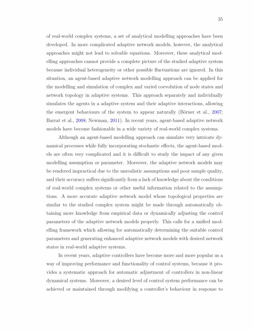
35
of real-world complex systems, a set of analytical modelling approaches have been
developed. In more complicated adaptive network models, however, the analytical
approaches might not lead to solvable equations. Moreover, these analytical mod-
elling approaches cannot provide a complete picture of the studied adaptive system
because individual heterogeneity or other possible fluctuations are ignored. In this
situation, an agent-based adaptive network modelling approach can be applied for
the modelling and simulation of complex and varied coevolution of node states and
network topology in adaptive systems. This approach separately and individually
simulates the agents in a adaptive system and their adaptive interactions, allowing
the emergent behaviours of the system to appear naturally (Borner et al., 2007;
Barrat et al., 2008; Newman, 2011). In recent years, agent-based adaptive network
models have become fashionable in a wide variety of real-world complex systems.
Although an agent-based modelling approach can simulate very intricate dy-
namical processes while fully incorporating stochastic effects, the agent-based mod-
els are often very complicated and it is difficult to study the impact of any given
modelling assumption or parameter. Moreover, the adaptive network models may
be rendered impractical due to the unrealistic assumptions and poor sample quality,
and their accuracy suffers significantly from a lack of knowledge about the conditions
of real-world complex systems or other useful information related to the assump-
tions. A more accurate adaptive network model whose topological properties are
similar to the studied complex system might be made through automatically ob-
taining more knowledge from empirical data or dynamically adjusting the control
parameters of the adaptive network models properly. This calls for a unified mod-
elling framework which allowing for automatically determining the suitable control
parameters and generating enhanced adaptive network models with desired network
states in real-world adaptive systems.
In recent years, adaptive controllers have become more and more popular as a
way of improving performance and functionality of control systems, because it pro-
vides a systematic approach for automatic adjustment of controllers in non-linear
dynamical systems. Moreover, a desired level of control system performance can be
achieved or maintained through modifying a controller’s behaviour in response to
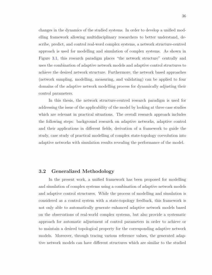
36
changes in the dynamics of the studied systems. In order to develop a unified mod-
elling framework allowing multidisciplinary researchers to better understand, de-
scribe, predict, and control real-word complex systems, a network structure-centred
approach is used for modelling and simulation of complex systems. As shown in
Figure 3.1, this research paradigm places “the network structure” centrally and
uses the combination of adaptive network models and adaptive control structures to
achieve the desired network structure. Furthermore, the network based approaches
(network sampling, modelling, measuring, and validating) can be applied to four
domains of the adaptive network modelling process for dynamically adjusting their
control parameters.
In this thesis, the network structure-centred research paradigm is used for
addressing the issue of the applicability of the model by looking at three case studies
which are relevant in practical situations. The overall research approach includes
the following steps: background research on adaptive networks, adaptive control
and their applications in different fields, derivation of a framework to guide the
study, case study of practical modelling of complex state-topology coevolution into
adaptive networks with simulation results revealing the performance of the model.
3.2 Generalized Methodology
In the present work, a unified framework has been proposed for modelling
and simulation of complex systems using a combination of adaptive network models
and adaptive control structures. While the process of modelling and simulation is
considered as a control system with a state-topology feedback, this framework is
not only able to automatically generate enhanced adaptive network models based
on the observations of real-world complex systems, but also provide a systematic
approach for automatic adjustment of control parameters in order to achieve or
to maintain a desired topological property for the corresponding adaptive network
models. Moreover, through tracing various reference values, the generated adap-
tive network models can have different structures which are similar to the studied
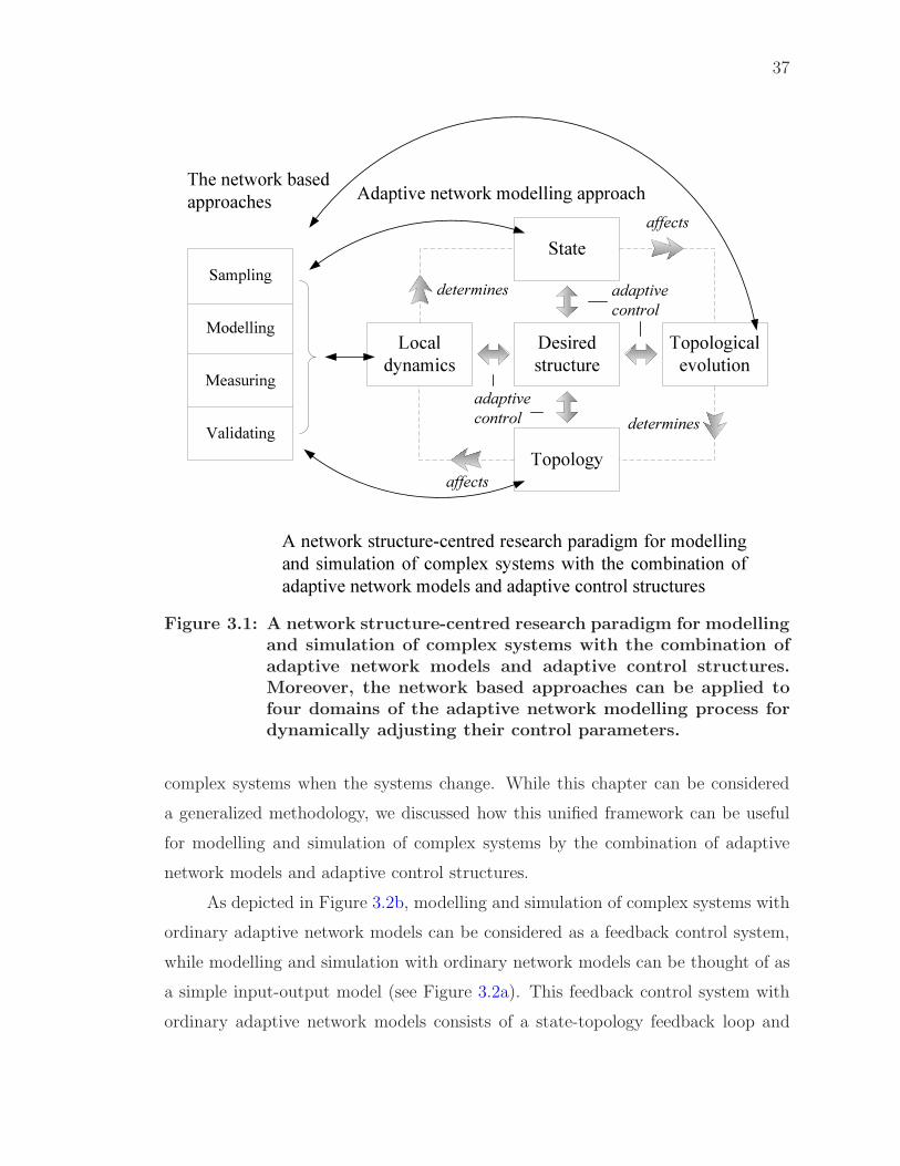
37
determines
affects
affects
determines
Local dynamics
Desired structure
Topologicalevolution
State
Topology
%&'( adaptive control
adaptive control
The network based approaches
Sampling
Modelling
Validating
Measuring
Adaptive network modelling approach
A network structure-centred research paradigm for modelling and simulation of complex systems with the combination of adaptive network models and adaptive control structures
Figure 3.1: A network structure-centred research paradigm for modellingand simulation of complex systems with the combination ofadaptive network models and adaptive control structures.Moreover, the network based approaches can be applied tofour domains of the adaptive network modelling process fordynamically adjusting their control parameters.
complex systems when the systems change. While this chapter can be considered
a generalized methodology, we discussed how this unified framework can be useful
for modelling and simulation of complex systems by the combination of adaptive
network models and adaptive control structures.
As depicted in Figure 3.2b, modelling and simulation of complex systems with
ordinary adaptive network models can be considered as a feedback control system,
while modelling and simulation with ordinary network models can be thought of as
a simple input-output model (see Figure 3.2a). This feedback control system with
ordinary adaptive network models consists of a state-topology feedback loop and
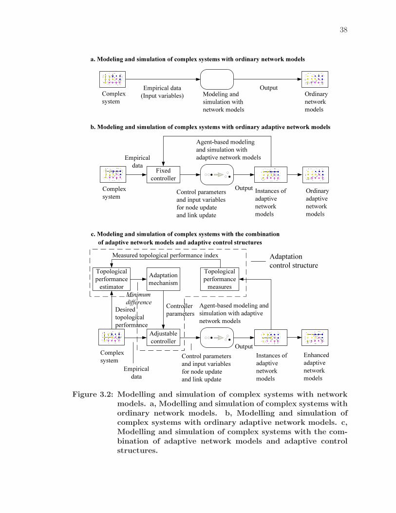
38
Adjustable controller
Empirical data
Empirical data (Input variables)
Output
OutputControl parameters and input variables for node update and link update
Desired topological performance
Topological performance estimator
Topological performancemeasures
Adaptationmechanism
Adaptation control structure
Controller parameters
Enhanced adaptive network models
Instances of adaptive network models
Agent-based modeling and simulation with adaptive network models
Agent-based modeling and simulation with adaptive network models
a. Modeling and simulation of complex systems with ordinary network models
b. Modeling and simulation of complex systems with ordinary adaptive network models
c. Modeling and simulation of complex systems with the combination of adaptive network models and adaptive control structures
Fixed controller
Empirical data
Control parameters and input variablesfor node update and link update
Instances of adaptive network models
Complex system
Modeling and simulation with network models
Ordinary adaptive network models
Ordinary network models
OutputComplex system
Complex system
Measured topological performance index
Minimum difference
Figure 3.2: Modelling and simulation of complex systems with networkmodels. a, Modelling and simulation of complex systems withordinary network models. b, Modelling and simulation ofcomplex systems with ordinary adaptive network models. c,Modelling and simulation of complex systems with the com-bination of adaptive network models and adaptive controlstructures.
39
a fixed controller. When applying adaptive network models to agent-based mod-
elling and simulation of complex systems, it is necessary to specify how the states of
nodes will be changed to generate new topologies of the network. Adaptive network
models may have control parameters for node update and link update which greatly
determine the quality of the generated network models. Choosing suitable control
parameter values is, frequently, a problem-dependent task and requires previous ex-
perience of the multidisciplinary researchers (Maruo et al., 2005). However, there
is no consistent methodology for determining the control parameters of an adaptive
network model, which are arbitrarily selected within some predefined ranges most
of the time (Maruo et al., 2005). In ordinary adaptive network models, these con-
trol parameters are not included as a part of the state-topology coevolution, when
they are considered as external fixed parameters. Moreover, the adaptive network
models make implicit assumptions for modelling and simulation of complex systems.
The adaptive network models may be rendered impractical due to these unrealistic
assumptions and poor sample quality, and their accuracy suffers significantly from
a lack of knowledge about the conditions of real-world complex systems or other
useful information related to the assumptions.
In order to achieve or to maintain a desired topological property for the cor-
responding adaptive network models, we propose a unified framework for modelling
and simulation of complex systems using a combination of adaptive network mod-
els and various adaptive control structures. As shown in Figure 3.2c and 3.3, the
unified modelling framework can be thought of as having two loops. One loop is
an ordinary state-topology feedback with the process of modelling and simulation
and the adjustable controller. The other loop is the parameter adjustment loop, in
which control parameters are included into the state-topology coevolution and up-
dated according to the topological performance estimation of the difference between
the generated instances of an adaptive network model and the desired topological
performance. The input variables of the adaptive control system can be generated
from the empirical data derived from the studied complex systems. These empirical
data may be some summarized statistical data or detailed records which are gener-
ated by using different data collection methods. Typically such data would present
40
important relations of some kind between various components of a certain complex
system (Niazi, 2011). Moreover, the desired topological performance can also be
generated from the empirical data for a comparative evaluation of the generated
adaptive network models, such as the desired topologies of networks, the desired
values of links, or desired classes of nodes.
To achieve or maintain a level of desired topological performance, the process of
adaptive-network based modelling and simulation is controlled by a controller that
has adjustable parameters. Through using a suitable adaptive control structure,
the controller can be adjusted properly for node update and link update, when the
characteristics of the process of modelling and simulation and the studied complex
system are unknown or changing. The process of adaptive-network based modelling
and simulation typically consists of two types of operations: state update of nodes
and weight update of links, whose control parameters can be modified in the ad-
justable controller. Given the current states of the nodes and the current weights
of the links, the instance of the adaptive network model in a certain discrete time
step can be generated. A performance index can then be established according to
the topological measurements of the generated instances for topological performance
estimation. The measured performance index will be compared to the desired per-
formance index which is desired topological characteristics of a reference network
model, and their difference can be used for the adjustment of the adaptation mech-
anism. The parameters of the controller will be updated based on the output of the
adaptation mechanism in order to improve the performance of modelling and simu-
lation (Landau et al., 2011). The adaptive state-topology feedback loop will stop
at some point once a certain level of desired topological performance is achieved. An
enhanced adaptive network model can then be created based on an instance with
desired topological characteristics. This procedure can be repeated.
In general, through combining adaptive network models and adaptive con-
trol structures, the unified modelling framework measures a certain performance
index of the adaptive control system which is the topological characteristics of an
instance generated by the current input valuables and control parameters. In or-
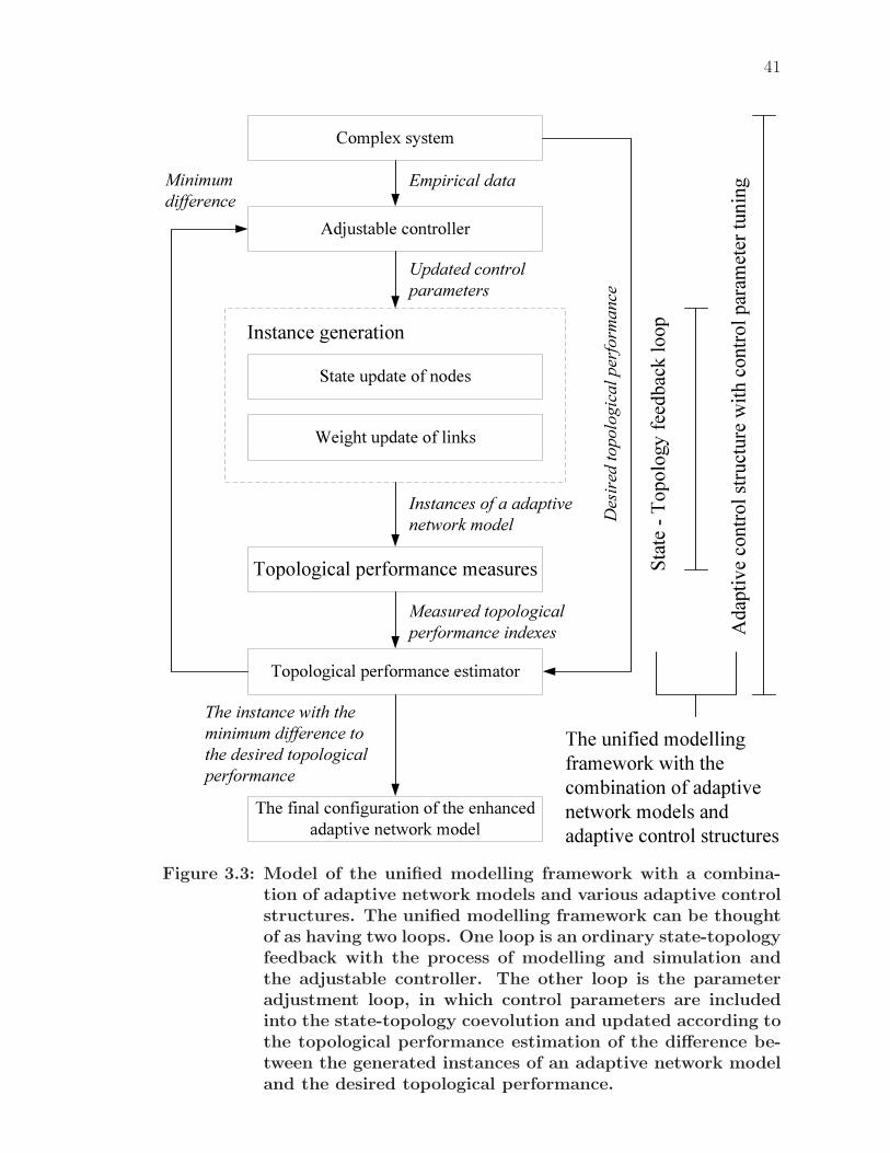
41
Topological performance estimator
State update of nodes
Weight update of links
Topological performance measures
The final configuration of the enhanced adaptive network model
Instance generation
Empirical data
Instances of a adaptive network model
Measured topological performance indexes
The instance with the minimum difference to the desired topological performance
Updated control parameters
Adjustable controller
State
-Top
ology
feed
back
loop
Adap
tive c
ontro
l struc
ture w
ith co
ntrol
param
eter tu
ningMinimum
difference
The unified modelling framework with the combination of adaptive network models and adaptive control structures
Complex system
Desir
ed to
polog
ical p
erform
ance
Figure 3.3: Model of the unified modelling framework with a combina-tion of adaptive network models and various adaptive controlstructures. The unified modelling framework can be thoughtof as having two loops. One loop is an ordinary state-topologyfeedback with the process of modelling and simulation andthe adjustable controller. The other loop is the parameteradjustment loop, in which control parameters are includedinto the state-topology coevolution and updated according tothe topological performance estimation of the difference be-tween the generated instances of an adaptive network modeland the desired topological performance.
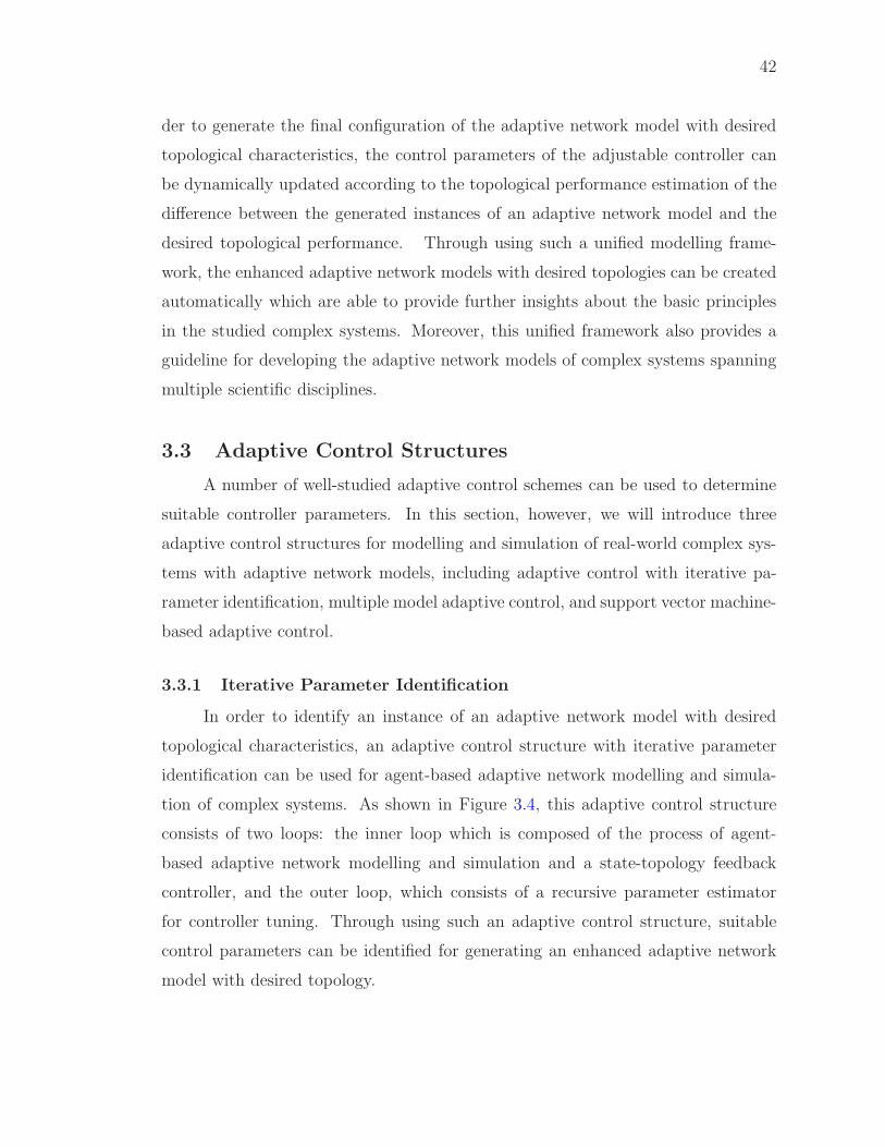
42
der to generate the final configuration of the adaptive network model with desired
topological characteristics, the control parameters of the adjustable controller can
be dynamically updated according to the topological performance estimation of the
difference between the generated instances of an adaptive network model and the
desired topological performance. Through using such a unified modelling frame-
work, the enhanced adaptive network models with desired topologies can be created
automatically which are able to provide further insights about the basic principles
in the studied complex systems. Moreover, this unified framework also provides a
guideline for developing the adaptive network models of complex systems spanning
multiple scientific disciplines.
3.3 Adaptive Control Structures
A number of well-studied adaptive control schemes can be used to determine
suitable controller parameters. In this section, however, we will introduce three
adaptive control structures for modelling and simulation of real-world complex sys-
tems with adaptive network models, including adaptive control with iterative pa-
rameter identification, multiple model adaptive control, and support vector machine-
based adaptive control.
3.3.1 Iterative Parameter Identification
In order to identify an instance of an adaptive network model with desired
topological characteristics, an adaptive control structure with iterative parameter
identification can be used for agent-based adaptive network modelling and simula-
tion of complex systems. As shown in Figure 3.4, this adaptive control structure
consists of two loops: the inner loop which is composed of the process of agent-
based adaptive network modelling and simulation and a state-topology feedback
controller, and the outer loop, which consists of a recursive parameter estimator
for controller tuning. Through using such an adaptive control structure, suitable
control parameters can be identified for generating an enhanced adaptive network
model with desired topology.
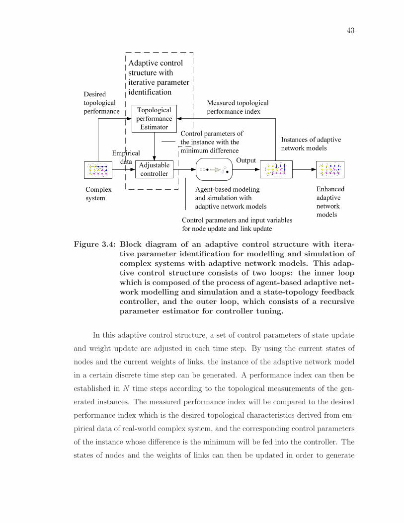
43
Adjustable controller
Empirical data Output
Control parameters and input variables for node update and link update
Desired topological performance
Complex system
Instances of adaptive network models
Enhanced adaptive network models
Agent-based modeling and simulation with adaptive network models
Adaptive control structure with iterative parameter identification
Topological performance Estimator
Measured topological performance index
Control parameters of the instance with the minimum difference
Figure 3.4: Block diagram of an adaptive control structure with itera-tive parameter identification for modelling and simulation ofcomplex systems with adaptive network models. This adap-tive control structure consists of two loops: the inner loopwhich is composed of the process of agent-based adaptive net-work modelling and simulation and a state-topology feedbackcontroller, and the outer loop, which consists of a recursiveparameter estimator for controller tuning.
In this adaptive control structure, a set of control parameters of state update
and weight update are adjusted in each time step. By using the current states of
nodes and the current weights of links, the instance of the adaptive network model
in a certain discrete time step can be generated. A performance index can then be
established in N time steps according to the topological measurements of the gen-
erated instances. The measured performance index will be compared to the desired
performance index which is the desired topological characteristics derived from em-
pirical data of real-world complex system, and the corresponding control parameters
of the instance whose difference is the minimum will be fed into the controller. The
states of nodes and the weights of links can then be updated in order to generate
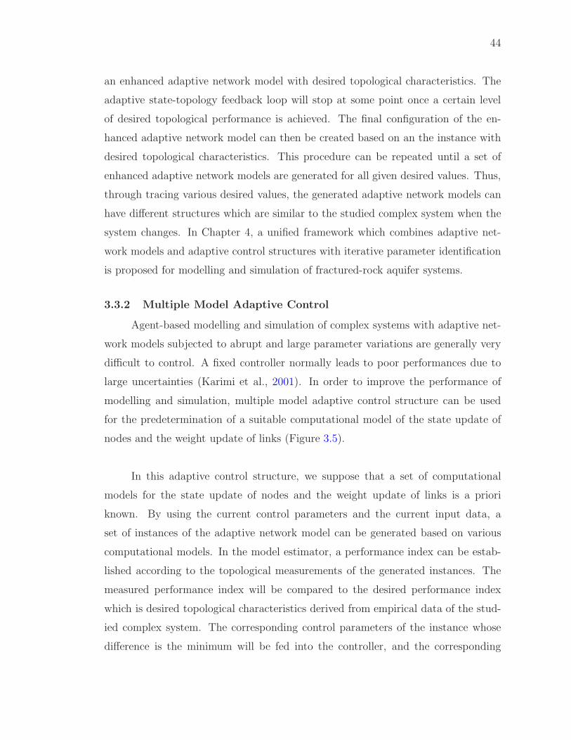
44
an enhanced adaptive network model with desired topological characteristics. The
adaptive state-topology feedback loop will stop at some point once a certain level
of desired topological performance is achieved. The final configuration of the en-
hanced adaptive network model can then be created based on an the instance with
desired topological characteristics. This procedure can be repeated until a set of
enhanced adaptive network models are generated for all given desired values. Thus,
through tracing various desired values, the generated adaptive network models can
have different structures which are similar to the studied complex system when the
system changes. In Chapter 4, a unified framework which combines adaptive net-
work models and adaptive control structures with iterative parameter identification
is proposed for modelling and simulation of fractured-rock aquifer systems.
3.3.2 Multiple Model Adaptive Control
Agent-based modelling and simulation of complex systems with adaptive net-
work models subjected to abrupt and large parameter variations are generally very
difficult to control. A fixed controller normally leads to poor performances due to
large uncertainties (Karimi et al., 2001). In order to improve the performance of
modelling and simulation, multiple model adaptive control structure can be used
for the predetermination of a suitable computational model of the state update of
nodes and the weight update of links (Figure 3.5).
In this adaptive control structure, we suppose that a set of computational
models for the state update of nodes and the weight update of links is a priori
known. By using the current control parameters and the current input data, a
set of instances of the adaptive network model can be generated based on various
computational models. In the model estimator, a performance index can be estab-
lished according to the topological measurements of the generated instances. The
measured performance index will be compared to the desired performance index
which is desired topological characteristics derived from empirical data of the stud-
ied complex system. The corresponding control parameters of the instance whose
difference is the minimum will be fed into the controller, and the corresponding
45
Control parameters and input variables for node update and link update
Adjustable controller
Empirical data Output
Complex system Enhanced
adaptive network models
Agent-based modeling and simulation with adaptive network models
Topological performance estimator
Update model 1
Instance 2
Instance n
Control parameters and input variables for node update and link update
Desired topological performance
Update model 2
Update model n
Instance 1
Multiple model adaptive control structure
Control parameters of the instance with the minimum difference
Measu
red to
polog
ical
perfo
rman
ce ind
ex
Figure 3.5: Block diagram of a multiple model adaptive control structurefor modelling and simulation of complex systems with adap-tive network models. This adaptive control structure is com-posed of a set of update models, a topological performanceestimator and an adjustable controller. In the model estima-tor, a performance index can be established according to thetopological measurements of the generated instances. Themeasured performance index will be compared to the desiredperformance index which is desired topological characteristicsderived from empirical data of the studied complex system.The corresponding control parameters of the instance whosedifference is the minimum will be fed into the controller, andthe corresponding computational model of the instance willbe applied to the process of agent-based adaptive networkmodelling and simulation.
46
computational model of the instance will be applied to the process of agent-based
adaptive network modelling and simulation. The states of nodes and the weights of
links can then be updated with a suitable computational model in order to generate
an enhanced adaptive network model with desired topological characteristics. By
using such a multiple model adaptive control structure, the adaptive state-topology
feedback loop can be performed for modelling and simulation of the studies complex
system with a suitable a suitable computational model of the state update of nodes
and the weight update of links. In Chapter 5, we propose a unified framework which
combines adaptive network models and multiple model adaptive control structures
is proposed for modelling and simulation of social network systems.
3.3.3 Support Vector Machine-Based Adaptive Control
While it has been widely used for control of complex systems in the presence of
significant modelling uncertainties, a support vector machine-based adaptive control
structure can be used for agent-based modelling and simulation of complex systems
with adaptive network models. As depicted in Figure 3.6, this adaptive control
structure can be thought of as consisting of two loops. The inner loop is composed
of the process of agent-based adaptive network modelling and a state-topology feed-
back controller, while the outer loop modifies the controller parameters based the
output of a support vector machine-based prediction model. In this adaptive control
structure, future behaviour of the system can be predicted by using a support vector
machine-based prediction model depending on empirical data of the studied complex
system. An instance with desired topology can be generated in each time step by us-
ing the current input variables and control parameter, while the states of the nodes
and weights of the links are dynamically adjusted according to the future behaviour
of the studied system. Moreover, a set of control actions will be implemented based
on the generated instances in order to improve the system performance. In Chapter
6, a unified framework which combines adaptive network models and support vector
machine-based adaptive control structures is proposed for modelling and simulation
of multicast congestion in mobile ad hoc network systems.
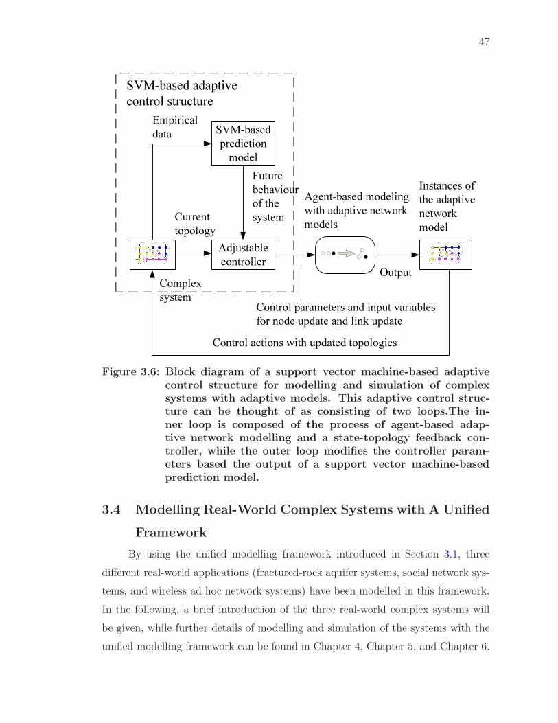
47
Current topology
Output
Control parameters and input variables for node update and link update
Empirical data
Complex system
Instances of the adaptive network model
Agent-based modeling with adaptive network models
Control actions with updated topologies
Adjustable controller
SVM-based prediction model
Future behaviour of the system
SVM-based adaptive control structure
Figure 3.6: Block diagram of a support vector machine-based adaptivecontrol structure for modelling and simulation of complexsystems with adaptive models. This adaptive control struc-ture can be thought of as consisting of two loops.The in-ner loop is composed of the process of agent-based adap-tive network modelling and a state-topology feedback con-troller, while the outer loop modifies the controller param-eters based the output of a support vector machine-basedprediction model.
3.4 Modelling Real-World Complex Systems with A Unified
Framework
By using the unified modelling framework introduced in Section 3.1, three
different real-world applications (fractured-rock aquifer systems, social network sys-
tems, and wireless ad hoc network systems) have been modelled in this framework.
In the following, a brief introduction of the three real-world complex systems will
be given, while further details of modelling and simulation of the systems with the
unified modelling framework can be found in Chapter 4, Chapter 5, and Chapter 6.
48
3.4.1 Fracture Network Systems
A fracture network is a set of fractures (cracks) in brittle materials. Two ap-
proaches are used for generating fracture networks. The first approach gives the
fracture’s path of propagation by inducing disorder into the studied system (say in-
tact rock) (Kachanov, 1987; Renshaw & Pollard, 1994; Alava et al., 2006; Bonamy
& Bouchaud, 2011). The second approach generates fracture networks based on the
statistics derived from controllable laboratory tests and field data. The orientation,
the size and the aperture are assigned to the fracture based on the statistical dis-
tribution functions, while the centre of a fracture is located at random according
to the Poisson distribution (Ghaffari et al., 2011). The number of generated frac-
tures is determined based on the density of the fracture network and the size of
model space. The generated fracture networks should satisfy the same characteris-
tics (features or attributes) for the fracture system (Ghaffari et al., 2011), such as
distribution law over density, length, directionality, distance, fractal dimension, and
permeability (Sornette et al., 1993; Berkowitz & Adler, 1998; Berkowitz et al., 2000;
Bour, 2002). In a fracture network, the fractures represented by the nodes occupy
a precise position in two or three-dimensional Euclidean space, and the connections
of the fractures represented by the links are real physical connections. Fracture net-
works thus can be also called geographical or spatial networks. An excellent review
on spatial networks has been presented in (Barthelemy, 2010).
Fracture networks research can be conceptualized as lying at the intersection
between graph theory and statistical mechanics. In (Ghaffari et al., 2011), fracture
networks were mapped into graphs, and the characteristics of the generated graphs
were compared with the main spatial fracture networks. However, there is no exist-
ing unified modelling framework allowing for automatically shaping the fracture data
and the fracture network models in terms of the observations of a real-world fracture
network. In this research, we focus on using a unified modelling framework, which
combines adaptive network models and adaptive control structures, to automati-
cally search for desired configurations of the adaptive network models based on the
observations of natural fractured-rock aquifer systems. Having such an automated
modelling framework would greatly reduce the human effort and provide a valuable
49
tool for better understanding, description, and prediction of the groundwater flow
and transport processes in fractured-rock aquifer systems.
3.4.2 Social Network Systems
A social network is a set of people (individuals or social groups) and different
types of relationships (friendship, trust, kinship, status, sexual, business or political)
among them (Wasserman & Faust, 1994; Scott, 2012). Different social, diplomatic,
commercial and even cultural networks can be defined by hidden and clear relation-
ships or interactions between any groups of people (Costa et al., 2011). Although
many sociometric researches (Wellman, 1926; Simon, 1955; Price, 1965; Milgram,
1967; Travers & Milgram, 1969; Price, 1976; Freeman, 1977; Freeman, 1979; Wasser-
man & Faust, 1994; Degenne & Forse, 1999; Ball, 2002; Baldi et al., 2003; Watts,
2003; Social Network Journal, 2007; Scott, 2012) have contributed to the under-
standing of society, traditional social network studies often suffer from problems
of inaccuracy, subjectivity, and small sample size (Newman, 2003). In the conven-
tional studies, social contacts were established based on extensive questionnaires
and cross comparison of the responses. However, new forms of social contacts have
been generated due to the fast development of communication systems, such as the
telephone or the Internet (Wellmanet et al., 1996; Wellman, 2001). With tools like
blogs, photoblogs, messengers, emails, and social network services, a large amount
of extensive electronic databases can provide extremely abundant statistical sample
and a complete picture of the complex social system they represent (Costa et al.,
2011). Benefiting from the massive amounts of online data, reliable social networks
can be generated faster and more accurately than ever (Gonzalez & Barabasi, 2007;
Watts, 2007).
Recent developments in sensing technologies have enabled us to examine the
nature of human social behaviour in greater detail. However, there is no existing
unified modelling framework allowing for automatically obtaining more knowledge
from multidimensional mobile sensing data and adjusting the control parameters of
the adaptive network models properly. In this thesis, we propose a unified framework
which combines adaptive network models and multiple model adaptive control struc-
50
tures for modelling and simulation of social network systems. In this framework,
a real-world social network system can be represented as an agent-based adaptive
network which are defined by a feedback loop between the behavioural state of indi-
viduals and the community structure of the studied system, when a multiple model
adaptive control structure is used for the predetermination of suitable computa-
tional models of behavioural state update and social interaction update in order to
improve the performance of modelling and simulation.
3.4.3 Wireless Ad Hoc Network Systems
In real systems, modelling the dynamics of flows of the physical quantities is
also important, because a completed characterization of a network need to consider
the relationship between structure and dynamic of complex networks (Boccaletti
et al., 2006). The dynamics models of a complex network can be generated by
quantifying the transmission capacities and loads of its components (Boccaletti et
al., 2006). In the present work, we focus on multicast congestion in mobile ad hoc
networks (MANETs).
Mobile ad hoc networks use a shared broadcast medium. All the nodes within
a collision domain share the medium capacity, which is therefore a scarce resource.
Multicast communication is thus of particular interest in these networks, since it
helps saving resources when delivering data to multiple destinations. Congestion
is one of the most important issues impeding the development and deployment of
Internet Protocol multicast and multicast applications in MANETs. Congestion
phenomena are common in wireless communication networks, where some nodes
occasionally malfunction or they are overloaded. A few congestion control models
have been proposed to tackle multicast congestion for MANETs. However, most
of these congestion control models (Lee et al., 1999; Tang et al., 2002; Tang et al.,
2002; Tang et al., 2003; Baumung et al., 2004; Gossain et al., 2004; Baumung, 2005;
Jain & Das, 2006; Scheuermann et al., 2007; Kang et al., 2009) suffer from the same
problems as Transmission Control Protocol model suffers in wireless networks, which
is unnecessarily reducing the transmission rate in response to link errors. This is
because they use losses as the indication of the congestions but cannot distinguish
51
between wireless losses and congestion losses. In wireless networks, packet losses are
not only caused by overflow but can also be caused by link errors. In these models,
the MANETs react in the same way to losses due to congestion losses and due to
wireless losses. They reduce their transmission rate systematically at each packet
loss. Thus, the sending rate can be restricted even when there is no congestion.
To increase its throughput, the multicast sender should prevent it from reduc-
ing its rate when it faces a loss due to a link error. One strategy is to suppress
wireless losses with the support of the network by splitting the multicast connection
or retransmitting in link layer. Another strategy is to classify the packet loss causes
by using a classification algorithm at the receiver. The transmission rate is re-
duced only if the loss is classified as a congestion loss. Several congestion detection
models, with classification algorithms for packet loss causes, have been proposed
for MANETs multicast. In Peng and Sikdar (2003) and Rajendran et al. (2004)’s
models, congestion loss is detected by monitoring MAC layer queue state, while
congestion can be detected by monitoring network queuing delay in Kang et al.’s
work (Kang et al., 2009).
In order to capture more realistic dynamics of wireless communication net-
works with the interplay between network state and topology, several adaptive-
network based models have also been developed for routing and congestion control
in wireless communication networks. In these adaptive network models, the control
parameters are not included as a part of the state-topology coevolution, because they
are considered as external fixed parameters. Moreover, the adaptive network models
make implicit assumptions for modelling and simulation of wireless communication
network systems. The adaptive network models may be rendered impractical due
to the unrealistic assumptions and poor sample quality, and their accuracy suffers
significantly from a lack of knowledge about the conditions of the networks or other
useful information related to the assumptions. However, we use a unified frame-
work which combines adaptive network models and support vector machine-based
adaptive control structures for modelling and simulation of multicast congestion in
mobile ad hoc network systems. In this framework, a mobile ad hoc network system
can be represented as an agent-based adaptive network which is defined by a feed-

52
back loop between the congestion states of group members and the group structure
of the network, when the support vector machine-based adaptive control structures
are used for the prediction of incipient congestions.

CHAPTER 4
Towards A Unified Framework for Modelling and
Simulation of Fractured-Rock Aquifer Systems
In this chapter, the unified framework which combines adaptive network models
and adaptive control structures has been applied for modelling and simulation of
fractured-rock aquifer systems. We start in Section 4.1 with brief introduction
to the background of modelling and simulation of fractured-rock aquifer systems.
In Section 4.2, we propose a unified framework which combines adaptive network
models and adaptive control structures with iterative parameter identification for
modelling and simulation of fractured-rock aquifer systems. In this framework, the
adaptive control structures with iterative parameter identification are used to iden-
tify an instance of an adaptive network model with the desired topological character-
istics, while the natural fracture network can be represented by an adaptive network
model with “state-topology” coevolution. In Section 4.3, by using this modelling
framework, an automatic modelling tool, Fracture3D, is developed for automatically
building the enhanced 3–D fracture adaptive network models, in which the fracture
statistics and the structural properties can both follow the observed statistics from
natural fracture networks. In Section 4.4, a set of experiments and simulations are
conducted in order to verify the validity of the proposed unified modelling framework
and modelling tool Fracture3D.
4.1 Modelling and Simulation of Fractured-Rock Aquifer
Systems
The fractured-rock aquifer systems that would carry and circulate water gen-
erally contain a set of fractures in rocks. Fractures control the magnitude and
direction of hydraulic conductivity in the aquifer systems. They can act as conduits
or barriers to groundwater flow; and the understanding of fracture connectivity is
critical for understanding subsurface flow and transport processes (Margolin et al.,
53
54
1998). Although it is an intrinsic factor controlling groundwater flow and trans-
port processes, the connectivity of fractured-rock aquifer systems has no generally
accepted definition. It is normally used to describe the subjective appearance of a
fractured-rock aquifer system; and highly connected fractures tend to be more per-
meable (National Research Council, 1996). Generally, the connectivity of a certain
fractured-rock aquifer system can be determined by orientation, length and density
of fractures, which is the probability that any specific fracture is connected to the
conducting portion of the aquifer system (Berkowitz, 1995).
In order to study the connectivity of fractured-rock aquifer systems, a number
of network-based applications for modelling and simulation have been developed. In
these applications, fractured-rock aquifer systems were generally viewed as intricate
networks that encode the interactions between the fractures. These applications
often entail using one of two basic methods of developing computational models for
modelling fractured-rock aquifer systems i.e. either use a master equation approach
for analysis of groundwater flow and transport processes on networks or else use
an agent-based modelling approach to develop simulation models. For example,
a master equation-based mathematical model of connectivity and conductivity in
underground reservoirs has been developed in (Nayak et al., 2012), in which perco-
lation theory (Stauffer & Aharony, 1992) was used to delineate the connectivity of
a fracture network system. In these models, an occupancy function “p” is used to
describe mathematically how the number and the size of the clusters of fractures
vary in a certain natural fracture network system, and the finite size clusters bridged
and grow in size as this occupancy probability is increased (Nayak et al., 2012). A
critical value exists (called the percolation threshold, pc) at which one large cluster
(so called the spanning, percolating or infinite cluster) spans the whole region and
allows flow to move from one side to the other.
In more complicated models, the master equation approach might not lead to
solvable equations. Moreover, this approach cannot provide a complete picture of a
studied fracture-rock aquifer system, because it is intrinsically considering a coarse
grained perspective that does not take into account the heterogeneity of fractures
or other possible fluctuations. In this situation, agent-based models can be applied
55
(Borner et al., 2007; Barrat et al., 2008). The discrete fracture network (DFN) mod-
els have been applied to the research of natural fracture network systems in (Baecher,
1983; Rouleau & Gale, 1985; Cacas et al., 1990a; Cacas et al., 1990b; Willis-Richards
et al., 1996; Lin & Xu, 2006). Spatial statistics derived from observed fracture data
can be measured and used to generate 3–D fracture network models with the similar
spatial properties. By using agent-based modelling approach with DFN models, the
estimation of connectivity of the studied fracture networks can provide vital infor-
mation for studying the hydrological behaviour in fractured-rock aquifer systems.
Several stochastic fracture simulators, such as FracMan (Golder Associates), Meyer
(Baker Hughes), FracaFlow (Beicip-Franlab) etc., have been developed for generat-
ing stochastic DFN models. By using these simulators, the statistical data derived
from field measurements such as orientation, length, and density of fractures can
be used for studying 3D-connectivity of the studied fractured-rock aquifer systems
(Bradbury & Muldoon, 1994). When these statistical data are incorporated with
other parameters such as aperture and particularly connectivity of fractures, the hy-
draulic properties of the studied fractured-rock aquifer systems could be estimated
(Mourzenko et al., 1998; de Dreuzy et al., 2000).
Although agent-based modelling and simulation approach can simulate very
complicated groundwater flow and transport processes with fully incorporating stochas-
tic effects, agent-based models are often very intricate and the impact of any given
modelling assumption or parameter is difficult to study. A poor fracture network
model may be generated because of parameter uncertainty and poor or incorrect
geological and hydrological assumptions, in which the fracture statistics can follow
the observed statistics, but the structural properties are totally different with obser-
vations. In the study of fracture system at a uranium mine in France, for instance,
Long and Billaux (1987) found that only 0.1% fractures out of 65,740 generated ones
contribute to flow at the site scale. In other cases (Karasaki et al., 2000; Halihan
et al., 2005), situ borehole tests have also shown that fractures developed in a rock
mass are not always fully connected. Fracture interconnection may depend on both
geometric and physical properties such as orientation, aperture, length, termination,
and fracture filling. This calls for a unified modelling framework which allows for
56
automatically determining the suitable control parameters and generating the 3–D
fracture adaptive network models with desired structure in terms of field data and
measurements taken on site or in-situ. Having such an automated modelling frame-
work would greatly reduce the human effort and provide a valuable tool for better
understanding, description, and prediction of the groundwater flow and transport
processes in fractured-rock aquifer systems.
In the following sections, we present a framework for modelling and simula-
tion of fractured-rock aquifer systems based on the unified modelling framework
described in Chapter 3. In this framework, the adaptive control structures with
iterative parameter identification are used to identifying an instance of an adap-
tive network model with the desired topological characteristics, while the natural
fracture network can be represented by adaptive network models with “geometrical
state–fracture cluster” coevolution. Moreover, we use this modelling framework to
develop an automatic modelling tool for automatically building the enhanced frac-
ture adaptive network models of fractured-rock aquifer systems, in which the fracture
statistics and the structural properties can both follow the observed statistics from
natural fracture networks.
4.2 A Unified Framework for Modelling and Simulation of
Fractured-Rock Aquifer Systems
Most of fracture network modelling tools make implicit assumptions for mod-
elling and simulation of fractured-rock aquifer systems, such as shape of fractures,
size scale between field data and simulated data, and size of the stochastic fractures,
while these properties cannot be easily determined in the field by any direct mea-
surements. The fracture network models may be rendered impractical due to these
impractical assumptions and poor sample quality, and their accuracy suffers signif-
icantly from a lack of knowledge about real geological and hydrological conditions
of natural fracture networks or other useful information related to the assumptions.
The control parameters of the network models, such as, profile of fractures, size
of fractures, position of fractures, and scale of fracture network models, may vary
greatly depending on different geological and hydrological conditions. In order to
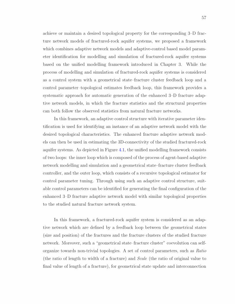
57
achieve or maintain a desired topological property for the corresponding 3–D frac-
ture network models of fractured-rock aquifer systems, we proposed a framework
which combines adaptive network models and adaptive-control based model param-
eter identification for modelling and simulation of fractured-rock aquifer systems
based on the unified modelling framework introduced in Chapter 3. While the
process of modelling and simulation of fractured-rock aquifer systems is considered
as a control system with a geometrical state–fracture cluster feedback loop and a
control parameter–topological estimates feedback loop, this framework provides a
systematic approach for automatic generation of the enhanced 3–D fracture adap-
tive network models, in which the fracture statistics and the structural properties
can both follow the observed statistics from natural fracture networks.
In this framework, an adaptive control structure with iterative parameter iden-
tification is used for identifying an instance of an adaptive network model with the
desired topological characteristics. The enhanced fracture adaptive network mod-
els can then be used in estimating the 3D-connectivity of the studied fractured-rock
aquifer systems. As depicted in Figure 4.1, the unified modelling framework consists
of two loops: the inner loop which is composed of the process of agent-based adaptive
network modelling and simulation and a geometrical state–fracture cluster feedback
controller, and the outer loop, which consists of a recursive topological estimator for
control parameter tuning. Through using such an adaptive control structure, suit-
able control parameters can be identified for generating the final configuration of the
enhanced 3–D fracture adaptive network model with similar topological properties
to the studied natural fracture network system.
In this framework, a fractured-rock aquifer system is considered as an adap-
tive network which are defined by a feedback loop between the geometrical states
(size and position) of the fractures and the fracture clusters of the studied fracture
network. Moreover, such a “geometrical state–fracture cluster” coevolution can self-
organize towards non-trivial topologies. A set of control parameters, such as Ratio
(the ratio of length to width of a fracture) and Scale (the ratio of original value to
final value of length of a fracture), for geometrical state update and interconnection
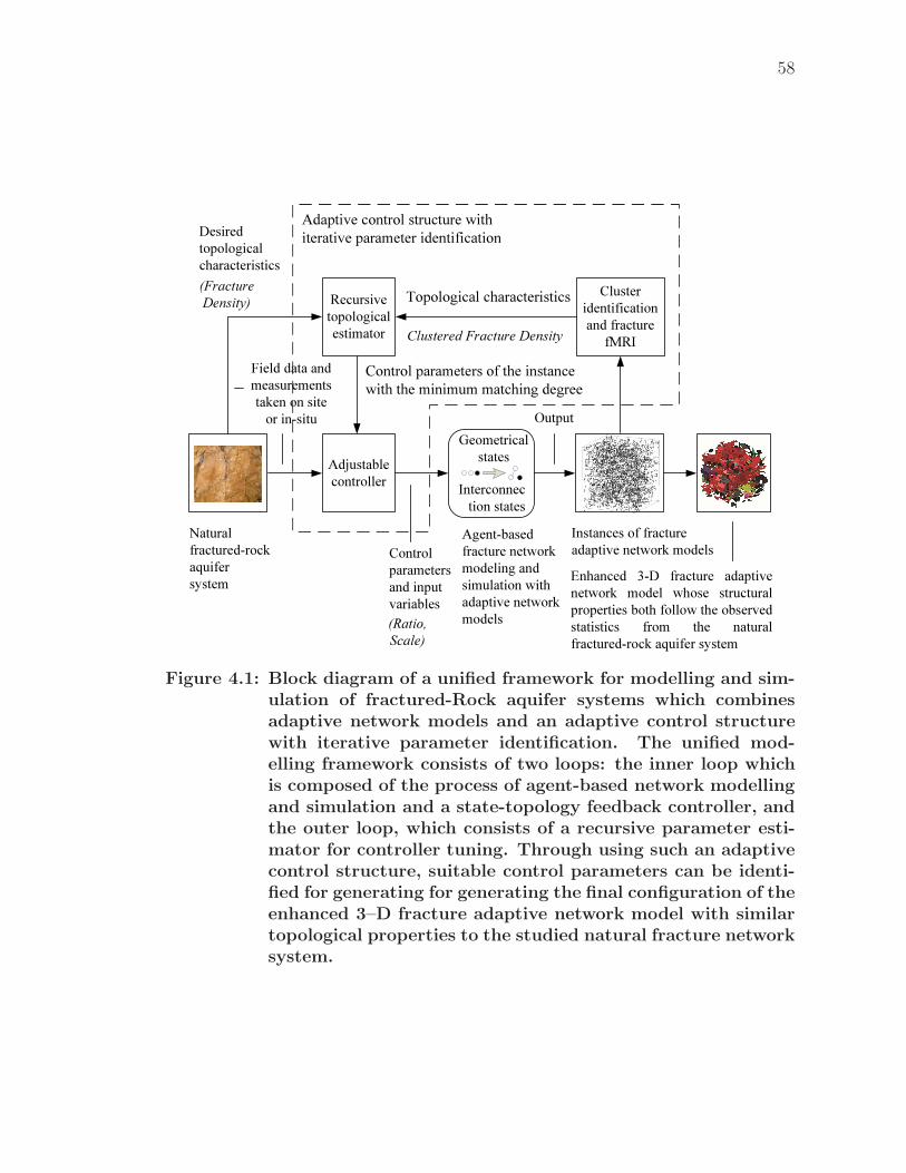
58
Adjustable controller
Field data and measurements taken on site
or in-situ Output
Control parameters and input variables
Desired topological characteristics
Recursive topological estimator
Agent-based fracture network modeling and simulation with adaptive network models
Adaptive control structure with iterative parameter identification
Cluster identification and fracture
fMRI
Interconnection states
Geometrical states
Enhanced 3-D fracture adaptive network model whose structural properties both follow the observed statistics from the natural fractured-rock aquifer system
Instances of fracture adaptive network models
Natural fractured-rock aquifer system
Clustered Fracture Density
(Fracture Density)
(Ratio, Scale)
Control parameters of the instance with the minimum matching degree
Topological characteristics
Figure 4.1: Block diagram of a unified framework for modelling and sim-ulation of fractured-Rock aquifer systems which combinesadaptive network models and an adaptive control structurewith iterative parameter identification. The unified mod-elling framework consists of two loops: the inner loop whichis composed of the process of agent-based network modellingand simulation and a state-topology feedback controller, andthe outer loop, which consists of a recursive parameter esti-mator for controller tuning. Through using such an adaptivecontrol structure, suitable control parameters can be identi-fied for generating for generating the final configuration of theenhanced 3–D fracture adaptive network model with similartopological properties to the studied natural fracture networksystem.
59
state update of fractures are adjusted in each time step. Based on the statistical
data derived from field data such as length, orientation, and density of measured
natural fractures and the updated control parameters, the size and position of frac-
tures are determined. The intersection analysis is then implemented for determining
if two fractures intersect. By using the current sizes, positions and intersections of
fractures, the instance of the adaptive network model in a certain discrete time
step can be generated, in which the fractures can be represented by abstract nodes
and the intersections among them by links. A performance index (clustered frac-
ture density of the generated 3–D instances) can then be established in N time
steps according to the topological measurements of the generated instances. The
measured performance index is compared to the desired topological characteristics
(area density of a 3–D reference fracture network) derived from field data, and the
corresponding control parameters of the instance whose matching degree is the max-
imum is fed into the adjustable controller. The sizes, positions and intersections of
fractures can be updated in order to generate an enhanced adaptive network model
with similar topological properties to the studied natural fracture network system.
This procedure can be repeated until a set of enhanced fracture adaptive network
models are automatically generated for all given input variables, such as various field
measurements, model sizes, seeds of random number generator, etc. Thus, through
tracing various desired values, the generated 3–D fracture adaptive network models
can have different structures which are similar to the studied fractured-rock aquifer
systems with different geological and hydrological conditions.
4.3 Fracture3D, An Automatic 3–D Fracture Modelling Tool
by Using Field Fracture Measurements
Through using the unified framework which combines adaptive network mod-
els and adaptive control structures, Fracture3D, an automatic 3–D fracture adaptive
network modelling tool is conceptualized and programmed in spreadsheets for mod-
elling and simulation of fractured-rock aquifer systems and connectivity analysis.
Based on a limited amount of field data and suitable control parameters, the en-
hanced 3–D fracture adaptive network models can be created by Fracture3D, in
60
which the fracture statistics and the structural properties can both follow the ob-
served statistics from natural fracture networks. The model of Fracture3D is shown
in Figure 4.2. The simple field data can be gathered from field measurements of
natural fractures, including fracture density, fracture orientation (dip angle and
dip direction), and fracture diameter (length) (Table 4.1). The statistical data of
the field data will be used as input variables of the process of modelling and sim-
ulation, when the mean and standard deviation of “Dip direction”, “Dip angle”,
and “Length” are calculated respectively according to varied “Density”. According
to the input variables and the given control parameters, the size and position of
fractures and the intersections among them can be determined in the process of
agent-based adaptive network modelling and simulation. An instance of the adap-
tive network model is thus built. The label-propagation based cluster identification
and Fracture Mapping and Realization Imaging (FMRI) are used for generating
topological characteristics (clustered fracture density) of the 3–D instance. The
adaptive-control based iterative parameter identification is implemented in order to
identify an instance with the minimum topological difference to field data from a set
of instances of the fracture adaptive network models, while the instances are auto-
matically generated through using a set of adjustable control parameters. The final
configuration of the enhanced 3–D fracture adaptive network model is then built
through using the control parameters of the identified instance. In the following,
several key algorithms of Fracture3D will be introduced, including geometrical state
update, interconnection state update, label-propagation based cluster identification,
topology measurement with FMRI, and adaptive-control based iterative parameter
identification.
4.3.1 Geometrical State Update of Fractures
In the present work, an agent-based adaptive network modelling approach is
used for modelling and simulation of fractured-rock aquifer systems with adaptive
network models, when each individual fracture is assumed to be one possible ge-
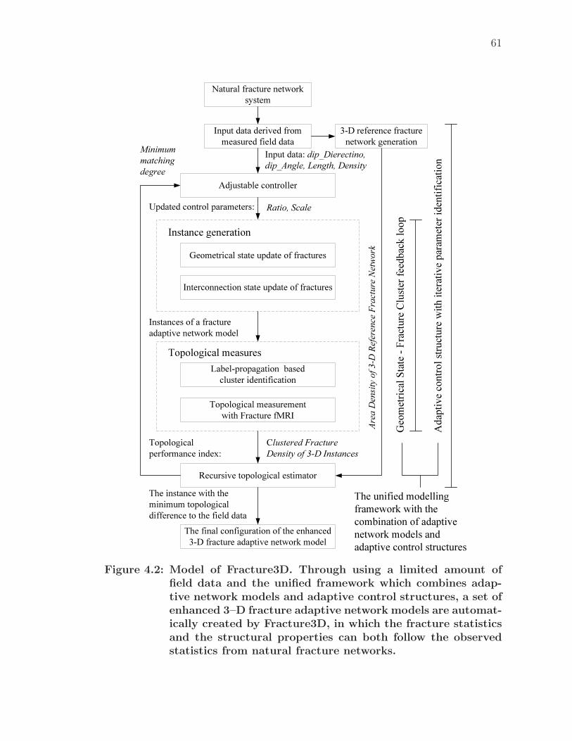
61
Input data derived from measured field data
Topological measurement with Fracture fMRI
Recursive topological estimator
Geometrical state update of fractures
Interconnection state update of fractures
Label-propagation based cluster identification
The final configuration of the enhanced 3-D fracture adaptive network model
Instance generation
Topological measures
Input data: dip_Dierectino,dip_Angle, Length, Density
Instances of a fracture adaptive network model
Clustered Fracture Density of 3-D Instances
The instance with the minimum topological difference to the field data
Updated control parameters: Ratio, Scale
Adjustable controller
Geom
etrica
l Stat
e -Fra
cture
Clust
er fee
dback
loop
Adap
tive c
ontro
l struc
ture w
ith ite
rative
param
eter id
entifi
cation
Minimum matching degree
Area
Den
sity o
f 3-D
Refer
ence
Frac
ture N
etwork
The unified modelling framework with the combination of adaptive network models and adaptive control structures
3-D reference fracture network generation
Natural fracture network system
Topological performance index:
Figure 4.2: Model of Fracture3D. Through using a limited amount offield data and the unified framework which combines adap-tive network models and adaptive control structures, a set ofenhanced 3–D fracture adaptive network models are automat-ically created by Fracture3D, in which the fracture statisticsand the structural properties can both follow the observedstatistics from natural fracture networks.
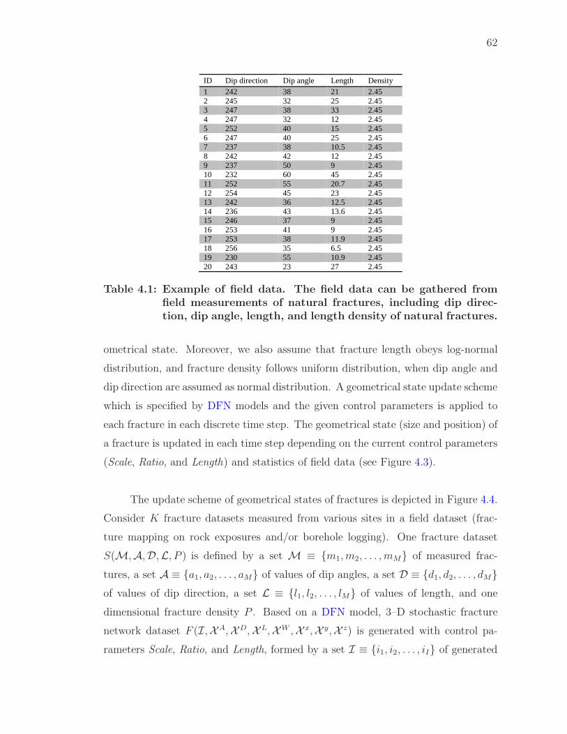
62
ID Dip direction Dip angle Length Density
1 242 38 21 2.45 2 245 32 25 2.45 3 247 38 33 2.45 4 247 32 12 2.45 5 252 40 15 2.45 6 247 40 25 2.45 7 237 38 10.5 2.45 8 242 42 12 2.45 9 237 50 9 2.45 10 232 60 45 2.45 11 252 55 20.7 2.45 12 254 45 23 2.45 13 242 36 12.5 2.45 14 236 43 13.6 2.45 15 246 37 9 2.45 16 253 41 9 2.45 17 253 38 11.9 2.45 18 256 35 6.5 2.45 19 230 55 10.9 2.45 20 243 23 27 2.45
Table 4.1: Example of field data. The field data can be gathered fromfield measurements of natural fractures, including dip direc-tion, dip angle, length, and length density of natural fractures.
ometrical state. Moreover, we also assume that fracture length obeys log-normal
distribution, and fracture density follows uniform distribution, when dip angle and
dip direction are assumed as normal distribution. A geometrical state update scheme
which is specified by DFN models and the given control parameters is applied to
each fracture in each discrete time step. The geometrical state (size and position) of
a fracture is updated in each time step depending on the current control parameters
(Scale, Ratio, and Length) and statistics of field data (see Figure 4.3).
The update scheme of geometrical states of fractures is depicted in Figure 4.4.
Consider K fracture datasets measured from various sites in a field dataset (frac-
ture mapping on rock exposures and/or borehole logging). One fracture dataset
S(M,A,D,L, P ) is defined by a set M ≡ {m1, m2, . . . , mM} of measured frac-
tures, a set A ≡ {a1, a2, . . . , aM} of values of dip angles, a set D ≡ {d1, d2, . . . , dM}of values of dip direction, a set L ≡ {l1, l2, . . . , lM} of values of length, and one
dimensional fracture density P . Based on a DFN model, 3–D stochastic fracture
network dataset F (I,XA,XD,X L,XW ,X x,X y,X z) is generated with control pa-
rameters Scale, Ratio, and Length, formed by a set I ≡ {i1, i2, . . . , iI} of generated
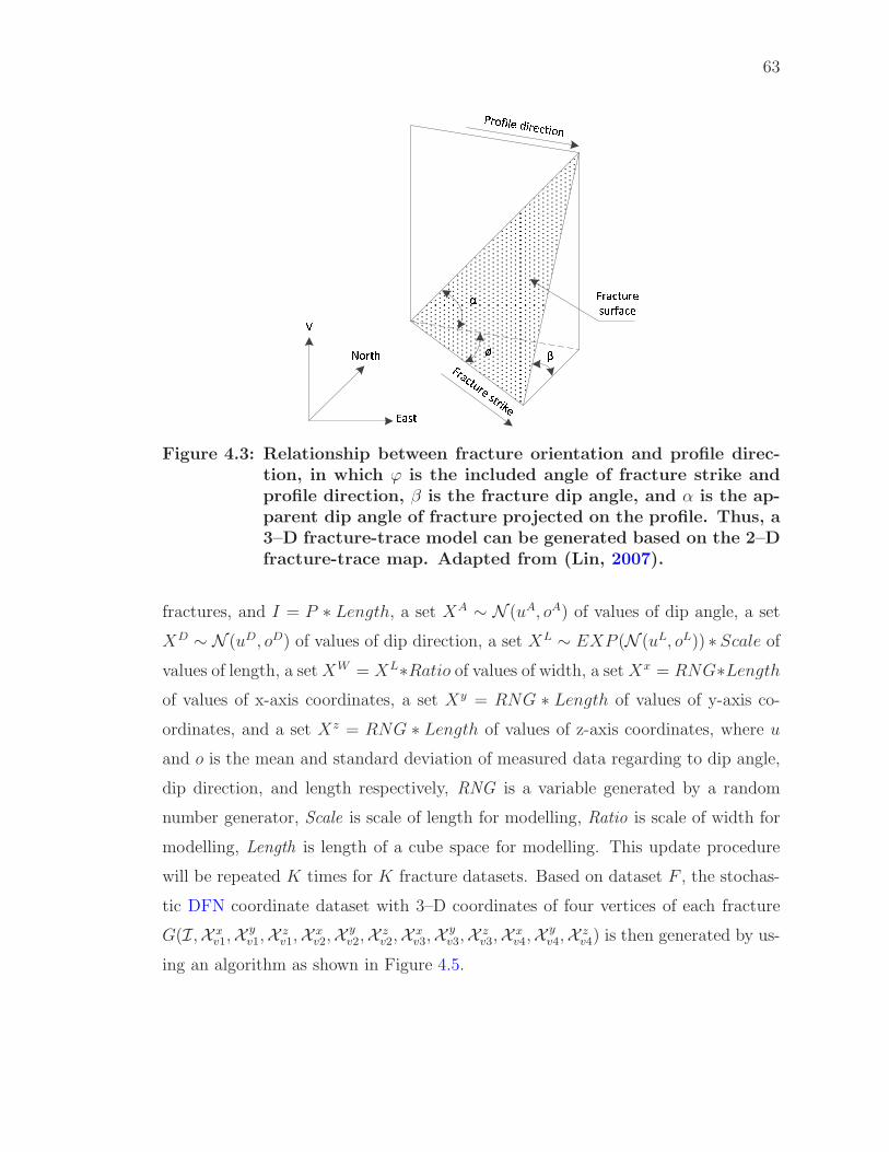
63)*+,-./ 0-*/12-+3
4567895:;85<=:>?@ABC?DEC?F@ADG
H@EBIJ?BK L MNFigure 4.3: Relationship between fracture orientation and profile direc-
tion, in which ϕ is the included angle of fracture strike andprofile direction, β is the fracture dip angle, and α is the ap-parent dip angle of fracture projected on the profile. Thus, a3–D fracture-trace model can be generated based on the 2–Dfracture-trace map. Adapted from (Lin, 2007).
fractures, and I = P ∗ Length, a set XA ∼ N (uA, oA) of values of dip angle, a set
XD ∼ N (uD, oD) of values of dip direction, a set XL ∼ EXP (N (uL, oL)) ∗ Scale of
values of length, a set XW = XL∗Ratio of values of width, a set Xx = RNG∗Length
of values of x-axis coordinates, a set Xy = RNG ∗ Length of values of y-axis co-
ordinates, and a set Xz = RNG ∗ Length of values of z-axis coordinates, where u
and o is the mean and standard deviation of measured data regarding to dip angle,
dip direction, and length respectively, RNG is a variable generated by a random
number generator, Scale is scale of length for modelling, Ratio is scale of width for
modelling, Length is length of a cube space for modelling. This update procedure
will be repeated K times for K fracture datasets. Based on dataset F , the stochas-
tic DFN coordinate dataset with 3–D coordinates of four vertices of each fracture
G(I,X xv1,X y
v1,X zv1,X x
v2,X yv2,X z
v2,X xv3,X y
v3,X zv3,X x
v4,X yv4,X z
v4) is then generated by us-
ing an algorithm as shown in Figure 4.5.
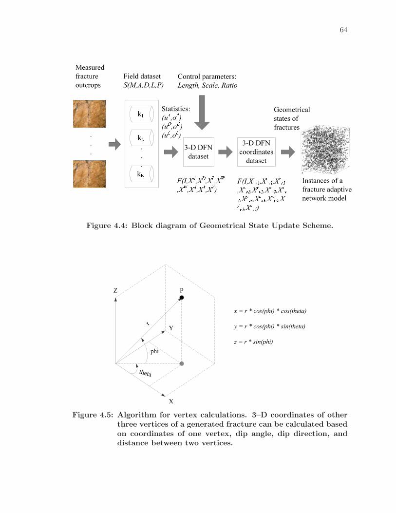
64
3-D DFN dataset
kOkPkQ 3-D DFN
coordinates dataset
Field dataset S(M,A,D,L,P)
.
.
.
Statistics:(uR,oR)(uS,oS)(uT,oT)
Control parameters:Length, Scale, Ratio
.
.
.
Measured fracture outcrops
Instances of a fracture adaptive network model
F(I,XR,XS,XT,XU,XU,XV,XW,XX) F(I,XYZ[,X\Z[,X]Z[
,XYZ^,X\Z^,X]Z^,XYZ_,X\Z_,X]Z_,XYZ`,X\Z`,X]Z`)
Geometrical states of fractures
Figure 4.4: Block diagram of Geometrical State Update Scheme.
X
Y
Z
phi
t he t a
r
P
x = r * cos(phi) * cos(theta)
y = r * cos(phi) * sin(theta)
z = r * sin(phi)
Figure 4.5: Algorithm for vertex calculations. 3–D coordinates of otherthree vertices of a generated fracture can be calculated basedon coordinates of one vertex, dip angle, dip direction, anddistance between two vertices.
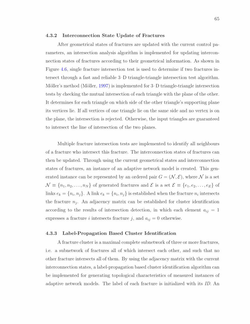
65
4.3.2 Interconnection State Update of Fractures
After geometrical states of fractures are updated with the current control pa-
rameters, an intersection analysis algorithm is implemented for updating intercon-
nection states of fractures according to their geometrical information. As shown in
Figure 4.6, single fracture intersection test is used to determine if two fractures in-
tersect through a fast and reliable 3–D triangle-triangle intersection test algorithm.
Moller’s method (Moller, 1997) is implemented for 3–D triangle-triangle intersection
tests by checking the mutual intersection of each triangle with the plane of the other.
It determines for each triangle on which side of the other triangle’s supporting plane
its vertices lie. If all vertices of one triangle lie on the same side and no vertex is on
the plane, the intersection is rejected. Otherwise, the input triangles are guaranteed
to intersect the line of intersection of the two planes.
Multiple fracture intersection tests are implemented to identify all neighbours
of a fracture who intersect this fracture. The interconnection states of fractures can
then be updated. Through using the current geometrical states and interconnection
states of fractures, an instance of an adaptive network model is created. This gen-
erated instance can be represented by an ordered pair G = (N , E), where N is a set
N ≡ {n1, n2, . . . , nN} of generated fractures and E is a set E ≡ {e1, e2, . . . , eE} of
links ek = {ni, nj}. A link ek = {ni, nj} is established when the fracture ni intersects
the fracture nj. An adjacency matrix can be established for cluster identification
according to the results of intersection detection, in which each element aij = 1
expresses a fracture i intersects fracture j, and aij = 0 otherwise.
4.3.3 Label-Propagation Based Cluster Identification
A fracture cluster is a maximal complete subnetwork of three or more fractures,
i.e. a subnetwork of fractures all of which intersect each other, and such that no
other fracture intersects all of them. By using the adjacency matrix with the current
interconnection states, a label-propagation based cluster identification algorithm can
be implemented for generating topological characteristics of measured instances of
adaptive network models. The label of each fracture is initialized with its ID. An
66
Current Fracure (Vertex0(x0,y0,z0), Vertex1(x1,y1,z1), Vertex2(x2,y2,z2), Vertex3(x3,y3,z3))
Current Test Fracure (Vertex0(x0,y0,z0), Vertex1(x1,y1,z1), Vertex2(x2,y2,z2), Vertex3(x3,y3,z3))
Triangle_1 (Vertex0(x0,y0,z0), Vertex1(x1,y1,z1), Vertex2(x2,y2,z2)) Triangle_2(Vertex0(x0,y0,z0), Vertex3(x3,y3,z3), Vertex2(x2,y2,z2))
test_Triangle_1 (Vertex0(x0,y0,z0), Vertex1(x1,y1,z1), Vertex2(x2,y2,z2)) test_Triangle_2 (Vertex0(x0,y0,z0), Vertex3(x3,y3,z3), Vertex2(x2,y2,z2))
2-D profile rectangle-rectangle intersection test operations
2-D profile triangles generation
2-D profile triangle-triangle intersection test
Triangle_1 intersect test_Triangle_1?
Triangle_1 intersects test_Triangle_2?
Triangle_2 intersects with test_Triangle_1?
Triangle_2 intersects with test_Triangle_2?
Yes
Yes
Yes
No
No
No
NoThe current fracture doesn’t intersect the current test fracture.
The current fracture intersects the current test fracture.
Yes
Figure 4.6: Multiple fracture intersection test operations.

67
originator of a cluster can be a fracture with an initial label. The neighbours of an
originator are called the propagators. The neighbours of a propagator can be new
propagators. The label propagating process ends when no more new propagators are
found. All propagators update their initialized ID with the label of their originator.
Next fracture that had an initial label is a new originator. This procedure can
be repeated until there is no more new originator and new propagator. In this
iterative process, the fracture clusters are identified when interconnected fractures
(directed or undirected) are labelled with a unique ID. A simple example of the
label propagating processes will be given in the following.
Suppose that a fracture n is an originator and carries its initial label Ln = IDn.
If the fracture n intersects its neighbours n1,n2,. . . ,ni, the fractures n1,n2,. . . ,ni can
then be propagators and update their labels to IDn. If the fracture ni intersects
ni1, ni
2,. . . ,nij , the fractures ni
1, ni2,. . . ,n
ij can also be propagators and update their
labels to IDn. This procedure can be repeated until there is no more new originator
and new propagator. At the end of the propagation process, fractures what have
the same label are grouped together as one cluster.
4.3.4 Topological Measure with FMRI
In order to identify an instance with the similar structural properties to field
data from a set of generated instances, the topological characteristics of the gen-
erated instances need to be extracted and compared with field data. In this work,
we assume that the fracture density of the maximum fracture cluster in a “good”
instance of a 3–D fracture adaptive network model should be similar with the 1–D
fracture density obtained from the 2–D fracture outcrops. Moreover, a topological
measure algorithm, FMRI, has been used in Fracture3D for measuring the fracture
density of each generated instance.
Functional magnetic resonance imaging is a brain-scanning technique for mon-
itoring the flow of blood to different areas of the brain. In this work, a similar idea,
Fracture Mapping and Realization Imaging, or FMRI, is used for measuring topo-
logical characteristics of the instances of fracture adaptive network models. The
FMRI technique uses Clustered Fracture Density (CFD) as indicators of hydraulic
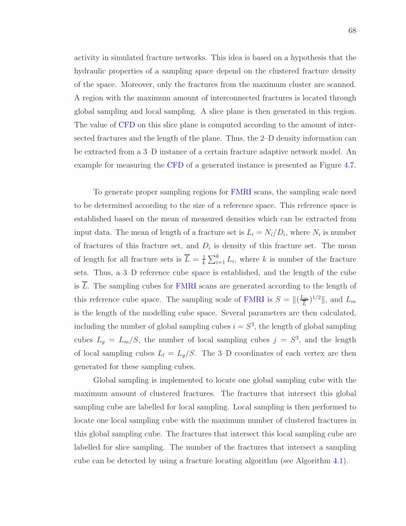
68
activity in simulated fracture networks. This idea is based on a hypothesis that the
hydraulic properties of a sampling space depend on the clustered fracture density
of the space. Moreover, only the fractures from the maximum cluster are scanned.
A region with the maximum amount of interconnected fractures is located through
global sampling and local sampling. A slice plane is then generated in this region.
The value of CFD on this slice plane is computed according to the amount of inter-
sected fractures and the length of the plane. Thus, the 2–D density information can
be extracted from a 3–D instance of a certain fracture adaptive network model. An
example for measuring the CFD of a generated instance is presented as Figure 4.7.
To generate proper sampling regions for FMRI scans, the sampling scale need
to be determined according to the size of a reference space. This reference space is
established based on the mean of measured densities which can be extracted from
input data. The mean of length of a fracture set is Li = Ni/Di, where Ni is number
of fractures of this fracture set, and Di is density of this fracture set. The mean
of length for all fracture sets is L = 1k
∑ki=1 Li, where k is number of the fracture
sets. Thus, a 3–D reference cube space is established, and the length of the cube
is L. The sampling cubes for FMRI scans are generated according to the length of
this reference cube space. The sampling scale of FMRI is S = ‖(Lm
L)1/2‖, and Lm
is the length of the modelling cube space. Several parameters are then calculated,
including the number of global sampling cubes i = S3, the length of global sampling
cubes Lg = Lm/S, the number of local sampling cubes j = S3, and the length
of local sampling cubes Ll = Lg/S. The 3–D coordinates of each vertex are then
generated for these sampling cubes.
Global sampling is implemented to locate one global sampling cube with the
maximum amount of clustered fractures. The fractures that intersect this global
sampling cube are labelled for local sampling. Local sampling is then performed to
locate one local sampling cube with the maximum number of clustered fractures in
this global sampling cube. The fractures that intersect this local sampling cube are
labelled for slice sampling. The number of the fractures that intersect a sampling
cube can be detected by using a fracture locating algorithm (see Algorithm 4.1).
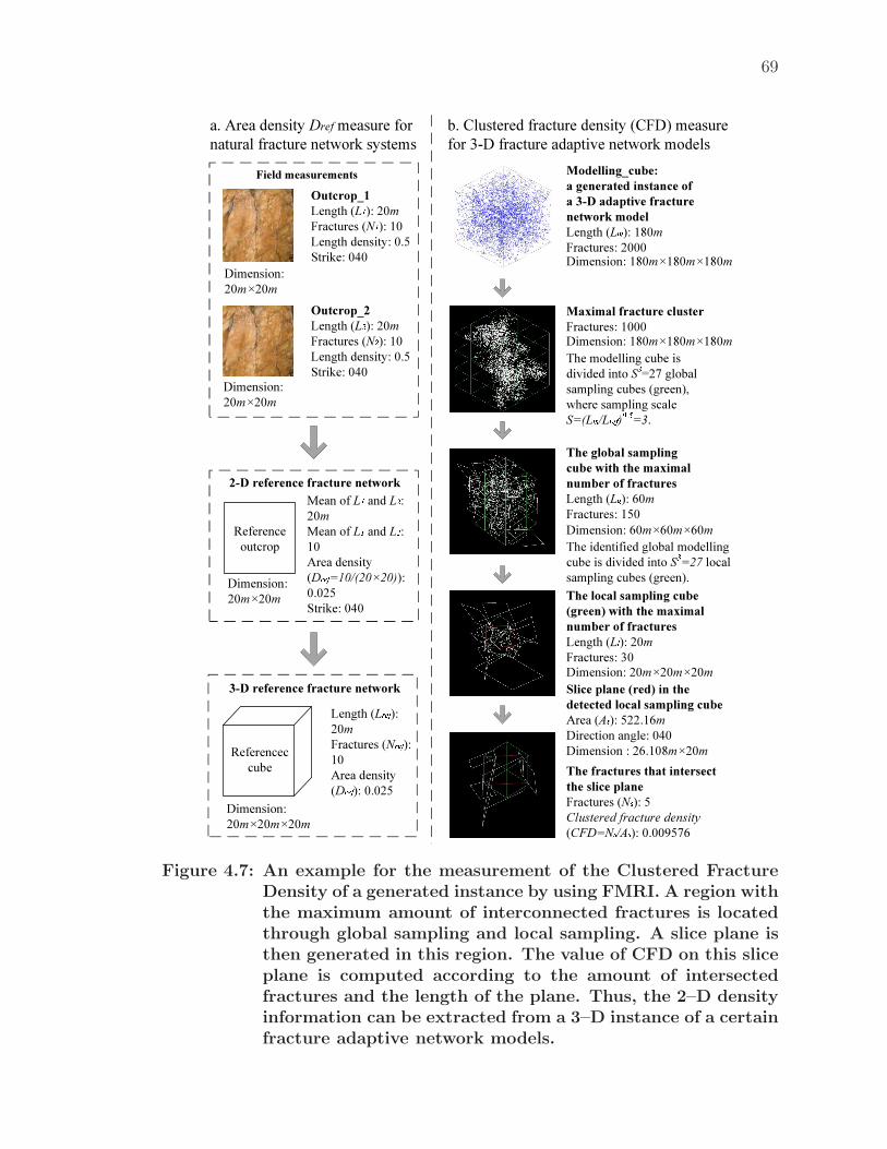
69
Modelling_cube:a generated instance of a 3-D adaptive fracture network modelLength (La): 180mFractures: 2000
Maximal fracture clusterFractures: 1000
The global sampling cube with the maximal number of fracturesLength (Lb): 60mFractures: 150
The modelling cube is divided into Sc=27 global sampling cubes (green), where sampling scale S=(La/Ldef )ghi=3.The identified global modelling cube is divided into Sc=27 local sampling cubes (green).The local sampling cube (green) with the maximal number of fracturesLength (Lj): 20mFractures: 30
The fractures that intersect the slice planeFractures (Nk): 5Clustered fracture density (CFD=Nk/Ak): 0.009576Slice plane (red) in the detected local sampling cube Area (Ak): 522.16mDirection angle: 040Dimension : 26.108m×20m
b. Clustered fracture density (CFD) measure for 3-D fracture adaptive network models
Field measurements
Outcrop_1Length (Ll): 20mFractures (Nl): 10Length density: 0.5Strike: 040
Outcrop_2Length (Lm): 20mFractures (Nm): 10Length density: 0.5Strike: 040
Mean of Ll and Lm: 20mMean of Ll and Lm: 10Area density (Ddef=10/(20×20)): 0.025Strike: 040
Length (Ldef ): 20mFractures (Ndef ): 10Area density (Ddef ): 0.025
Referenceoutcrop
Referenceccube
a. Area density Dref measure for natural fracture network systems
3-D reference fracture network
Dimension:20m×20m
Dimension:20m×20m×20m
Dimension:20m×20m
Dimension:20m×20m
Dimension: 180m×180m×180m
Dimension: 60m×60m×60m
Dimension: 20m×20m×20m
Dimension: 180m×180m×180m
2-D reference fracture network
Figure 4.7: An example for the measurement of the Clustered FractureDensity of a generated instance by using FMRI. A region withthe maximum amount of interconnected fractures is locatedthrough global sampling and local sampling. A slice plane isthen generated in this region. The value of CFD on this sliceplane is computed according to the amount of intersectedfractures and the length of the plane. Thus, the 2–D densityinformation can be extracted from a 3–D instance of a certainfracture adaptive network models.

70nopqrstuv wx yz{|}~z� ��|{}��� �� { �{������ |~��� ������ ������� ������� ����� ����������� ��� ����� ������ �� � �� ¡¢��� �£¤�¥�� ����£¤�� �� ����£¤�� �� ����£¤�� ��� �¢ ����� ����������� �� � �� ¡¢��� �£¤�¥�� ���¦� �� ���¦� �����¦�� ����� ����������� ��� ��£� ������ �� � �¢£������ �����£��¥�� �������� �� �������� �� �������� ��� �¢ ����� ����������� �� � �¢£������ �����£��¥§¨© ���� �£¤�� ª¨«¬®«¬¯°±² ³ ®« «¬µ¶· «¬µ¸· ¹· «¬µº»¼¬®«¬¯°±² ³ ®« ¼¬µ¶· ¼¬µ¸· ¹· ¼¬µº»½¬®«¬¯°±² ³ ®« ½¬µ¶· ½¬µ¸· ¹· ½¬µº»§¨© ���� �����£�� ª¨«¬®«¬¾ ¿®¯ ³®« «¬¾ ¶· «¬¾ ¸· «¬¾ À· «¬¾ Á»¼¬®«¬¾ ¿®¯ ³®« ¼¬¾ ¶· ¼¬¾ ¸· ¼¬¾ À· ¼¬¾ Á»½¬®«¬¾ ¿®¯ ³ ®« ¼¬¾ ¶· ¼¬¾ ¸· ¼¬¾ À· ¼¬¾ Á»Â§ «¬®«¬¾ ¿®¯ à «¬ÄŬ¯°±² ÆÆ «¬ÄŬ¾ ¿®¯ à «¬®«¬¯°±² ÆƼ¬®«¬¾ ¿®¯ ü¬ÄŬ¯°±² ÆƼ¬ÄŬ¾ ¿®¯Ã¼¬®«¬¯°±² Æƽ¬®«¬¾ ¿®¯ à ½¬ÄŬ¯°±² ÆÆ ½¬ÄŬ¾ ¿®¯ à ½¬®«¬¯°±² ÇÈÉʯ°¿¿²Åˬ¾ ¿®¯Ë°¿² Ì ¯°¿¿²Åˬ¯°±²Éʪ §Éʪ §¨©Éʪ §¨©A vertical slice plane is generated in the local sampling cube with the maximum
amount of clustered fractures. The direction angle of reference cube space is given
according to the strike angle of the measured fracture plane from field measurements.
The direction angle of this slice plane is the same as the direction angle of reference
cube space. The fractures labelled by local sampling are detected if they intersect
the slice plane. The clustered fracture density is then calculated as: CFD = Ns/As,
where Ns is the number of labelled fractures, and As is the area of slice plane.
4.3.5 Adaptive-Control Based Iterative Parameter Identification
While an instance of a 3–D fracture adaptive network model can be gener-
ated and its topological characteristics are measured by using the algorithms men-
tioned above, an adaptive-control based iterative parameter identification algorithm
is used for automatically generating a set of instances of a 3–D fracture adaptive
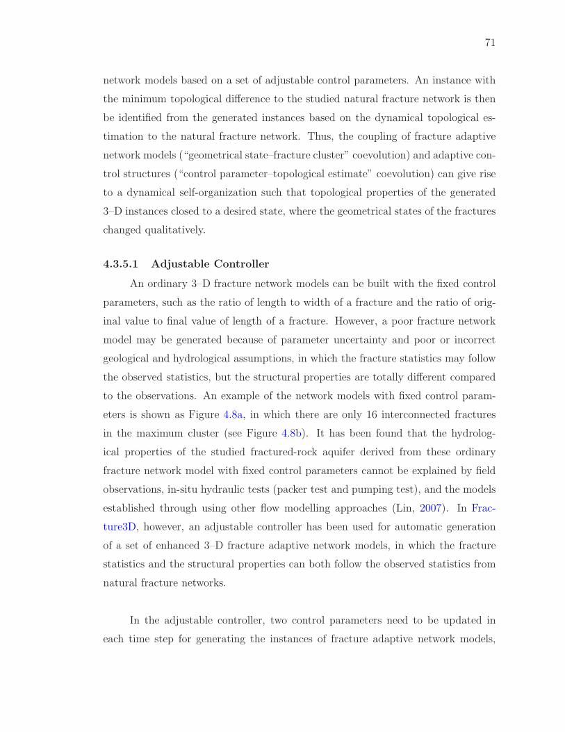
71
network models based on a set of adjustable control parameters. An instance with
the minimum topological difference to the studied natural fracture network is then
be identified from the generated instances based on the dynamical topological es-
timation to the natural fracture network. Thus, the coupling of fracture adaptive
network models (“geometrical state–fracture cluster” coevolution) and adaptive con-
trol structures (“control parameter–topological estimate” coevolution) can give rise
to a dynamical self-organization such that topological properties of the generated
3–D instances closed to a desired state, where the geometrical states of the fractures
changed qualitatively.
4.3.5.1 Adjustable Controller
An ordinary 3–D fracture network models can be built with the fixed control
parameters, such as the ratio of length to width of a fracture and the ratio of orig-
inal value to final value of length of a fracture. However, a poor fracture network
model may be generated because of parameter uncertainty and poor or incorrect
geological and hydrological assumptions, in which the fracture statistics may follow
the observed statistics, but the structural properties are totally different compared
to the observations. An example of the network models with fixed control param-
eters is shown as Figure 4.8a, in which there are only 16 interconnected fractures
in the maximum cluster (see Figure 4.8b). It has been found that the hydrolog-
ical properties of the studied fractured-rock aquifer derived from these ordinary
fracture network model with fixed control parameters cannot be explained by field
observations, in-situ hydraulic tests (packer test and pumping test), and the models
established through using other flow modelling approaches (Lin, 2007). In Frac-
ture3D, however, an adjustable controller has been used for automatic generation
of a set of enhanced 3–D fracture adaptive network models, in which the fracture
statistics and the structural properties can both follow the observed statistics from
natural fracture networks.
In the adjustable controller, two control parameters need to be updated in
each time step for generating the instances of fracture adaptive network models,
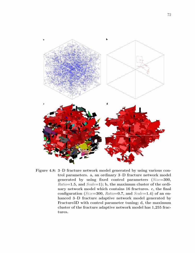
72
Í Î
Ï Ð
Figure 4.8: 3–D fracture network model generated by using various con-trol parameters. a, an ordinary 3–D fracture network modelgenerated by using fixed control parameters (Size=300,Ratio=1.5, and Scale=1); b, the maximum cluster of the ordi-nary network model which contains 16 fractures. c, the finalconfiguration (Size=300, Ratio=0.7, and Scale=1.4) of an en-hanced 3–D fracture adaptive network model generated byFracture3D with control parameter tuning; d, the maximumcluster of the fracture adaptive network model has 1,255 frac-tures.
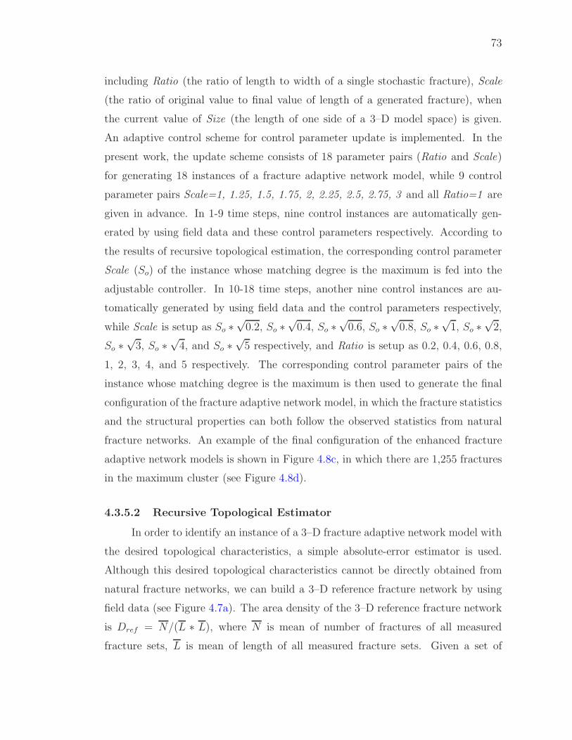
73
including Ratio (the ratio of length to width of a single stochastic fracture), Scale
(the ratio of original value to final value of length of a generated fracture), when
the current value of Size (the length of one side of a 3–D model space) is given.
An adaptive control scheme for control parameter update is implemented. In the
present work, the update scheme consists of 18 parameter pairs (Ratio and Scale)
for generating 18 instances of a fracture adaptive network model, while 9 control
parameter pairs Scale=1, 1.25, 1.5, 1.75, 2, 2.25, 2.5, 2.75, 3 and all Ratio=1 are
given in advance. In 1-9 time steps, nine control instances are automatically gen-
erated by using field data and these control parameters respectively. According to
the results of recursive topological estimation, the corresponding control parameter
Scale (So) of the instance whose matching degree is the maximum is fed into the
adjustable controller. In 10-18 time steps, another nine control instances are au-
tomatically generated by using field data and the control parameters respectively,
while Scale is setup as So ∗√
0.2, So ∗√
0.4, So ∗√
0.6, So ∗√
0.8, So ∗√
1, So ∗√
2,
So ∗√
3, So ∗√
4, and So ∗√
5 respectively, and Ratio is setup as 0.2, 0.4, 0.6, 0.8,
1, 2, 3, 4, and 5 respectively. The corresponding control parameter pairs of the
instance whose matching degree is the maximum is then used to generate the final
configuration of the fracture adaptive network model, in which the fracture statistics
and the structural properties can both follow the observed statistics from natural
fracture networks. An example of the final configuration of the enhanced fracture
adaptive network models is shown in Figure 4.8c, in which there are 1,255 fractures
in the maximum cluster (see Figure 4.8d).
4.3.5.2 Recursive Topological Estimator
In order to identify an instance of a 3–D fracture adaptive network model with
the desired topological characteristics, a simple absolute-error estimator is used.
Although this desired topological characteristics cannot be directly obtained from
natural fracture networks, we can build a 3–D reference fracture network by using
field data (see Figure 4.7a). The area density of the 3–D reference fracture network
is Dref = N/(L ∗ L), where N is mean of number of fractures of all measured
fracture sets, L is mean of length of all measured fracture sets. Given a set of
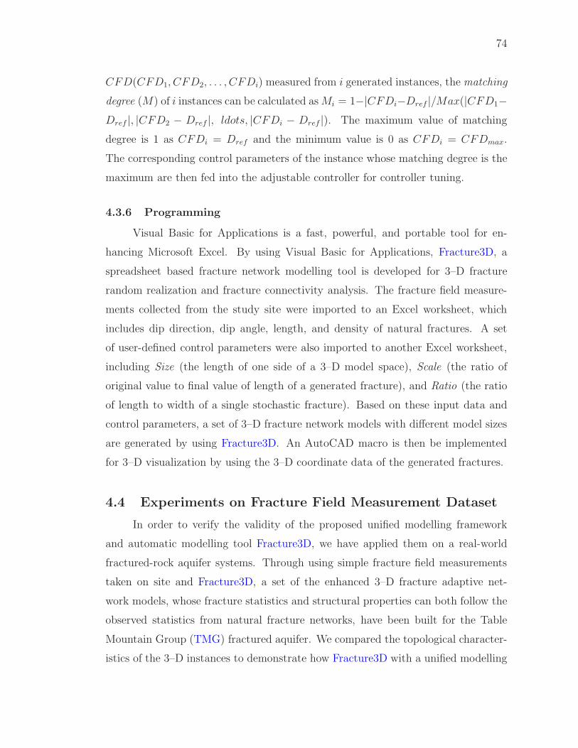
74
CFD(CFD1, CFD2, . . . , CFDi) measured from i generated instances, the matching
degree (M) of i instances can be calculated as Mi = 1−|CFDi−Dref |/Max(|CFD1−Dref |, |CFD2 − Dref |, ldots, |CFDi − Dref |). The maximum value of matching
degree is 1 as CFDi = Dref and the minimum value is 0 as CFDi = CFDmax.
The corresponding control parameters of the instance whose matching degree is the
maximum are then fed into the adjustable controller for controller tuning.
4.3.6 Programming
Visual Basic for Applications is a fast, powerful, and portable tool for en-
hancing Microsoft Excel. By using Visual Basic for Applications, Fracture3D, a
spreadsheet based fracture network modelling tool is developed for 3–D fracture
random realization and fracture connectivity analysis. The fracture field measure-
ments collected from the study site were imported to an Excel worksheet, which
includes dip direction, dip angle, length, and density of natural fractures. A set
of user-defined control parameters were also imported to another Excel worksheet,
including Size (the length of one side of a 3–D model space), Scale (the ratio of
original value to final value of length of a generated fracture), and Ratio (the ratio
of length to width of a single stochastic fracture). Based on these input data and
control parameters, a set of 3–D fracture network models with different model sizes
are generated by using Fracture3D. An AutoCAD macro is then be implemented
for 3–D visualization by using the 3–D coordinate data of the generated fractures.
4.4 Experiments on Fracture Field Measurement Dataset
In order to verify the validity of the proposed unified modelling framework
and automatic modelling tool Fracture3D, we have applied them on a real-world
fractured-rock aquifer systems. Through using simple fracture field measurements
taken on site and Fracture3D, a set of the enhanced 3–D fracture adaptive net-
work models, whose fracture statistics and structural properties can both follow the
observed statistics from natural fracture networks, have been built for the Table
Mountain Group (TMG) fractured aquifer. We compared the topological character-
istics of the 3–D instances to demonstrate how Fracture3D with a unified modelling
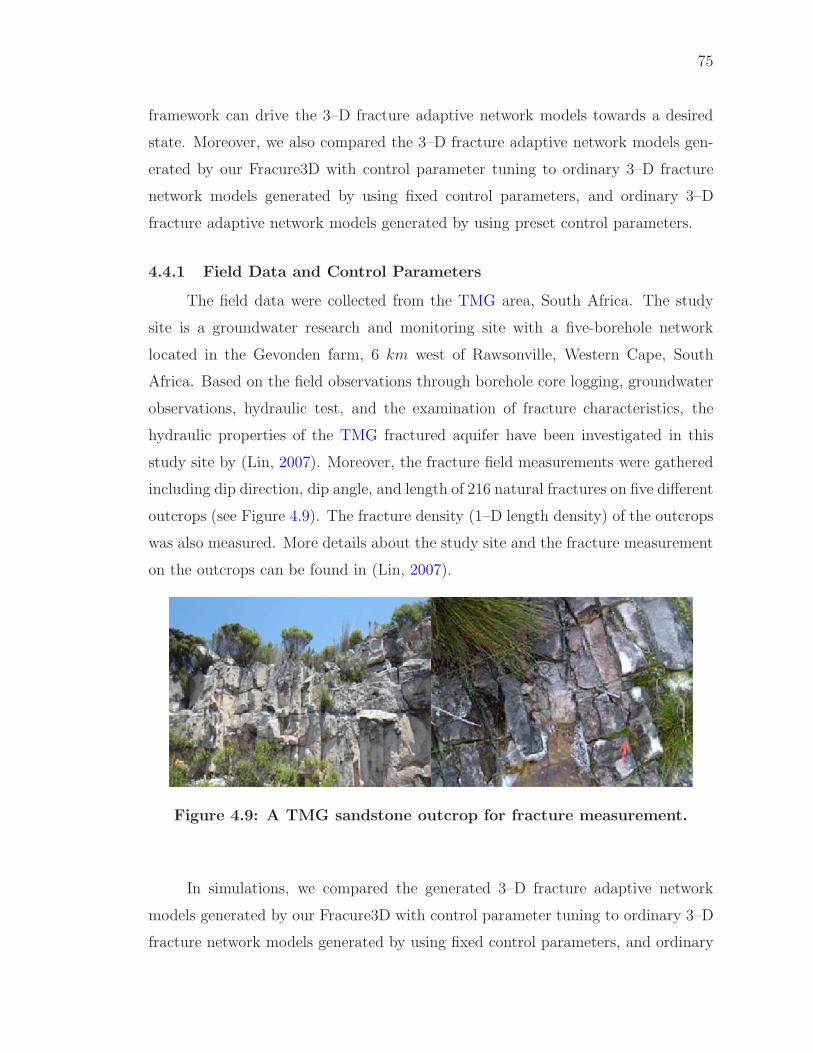
75
framework can drive the 3–D fracture adaptive network models towards a desired
state. Moreover, we also compared the 3–D fracture adaptive network models gen-
erated by our Fracure3D with control parameter tuning to ordinary 3–D fracture
network models generated by using fixed control parameters, and ordinary 3–D
fracture adaptive network models generated by using preset control parameters.
4.4.1 Field Data and Control Parameters
The field data were collected from the TMG area, South Africa. The study
site is a groundwater research and monitoring site with a five-borehole network
located in the Gevonden farm, 6 km west of Rawsonville, Western Cape, South
Africa. Based on the field observations through borehole core logging, groundwater
observations, hydraulic test, and the examination of fracture characteristics, the
hydraulic properties of the TMG fractured aquifer have been investigated in this
study site by (Lin, 2007). Moreover, the fracture field measurements were gathered
including dip direction, dip angle, and length of 216 natural fractures on five different
outcrops (see Figure 4.9). The fracture density (1–D length density) of the outcrops
was also measured. More details about the study site and the fracture measurement
on the outcrops can be found in (Lin, 2007).
Figure 4.9: A TMG sandstone outcrop for fracture measurement.
In simulations, we compared the generated 3–D fracture adaptive network
models generated by our Fracure3D with control parameter tuning to ordinary 3–D
fracture network models generated by using fixed control parameters, and ordinary
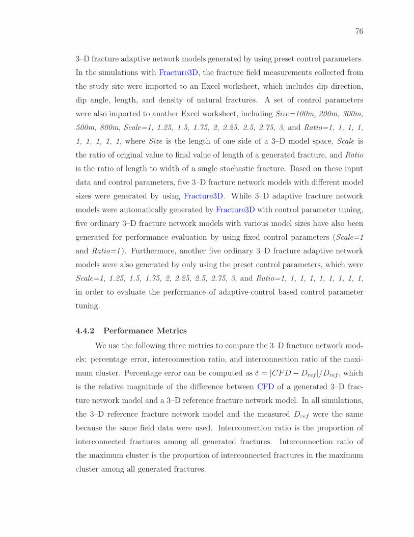
76
3–D fracture adaptive network models generated by using preset control parameters.
In the simulations with Fracture3D, the fracture field measurements collected from
the study site were imported to an Excel worksheet, which includes dip direction,
dip angle, length, and density of natural fractures. A set of control parameters
were also imported to another Excel worksheet, including Size=100m, 200m, 300m,
500m, 800m, Scale=1, 1.25, 1.5, 1.75, 2, 2.25, 2.5, 2.75, 3, and Ratio=1, 1, 1, 1,
1, 1, 1, 1, 1, where Size is the length of one side of a 3–D model space, Scale is
the ratio of original value to final value of length of a generated fracture, and Ratio
is the ratio of length to width of a single stochastic fracture. Based on these input
data and control parameters, five 3–D fracture network models with different model
sizes were generated by using Fracture3D. While 3–D adaptive fracture network
models were automatically generated by Fracture3D with control parameter tuning,
five ordinary 3–D fracture network models with various model sizes have also been
generated for performance evaluation by using fixed control parameters (Scale=1
and Ratio=1 ). Furthermore, another five ordinary 3–D fracture adaptive network
models were also generated by only using the preset control parameters, which were
Scale=1, 1.25, 1.5, 1.75, 2, 2.25, 2.5, 2.75, 3, and Ratio=1, 1, 1, 1, 1, 1, 1, 1, 1,
in order to evaluate the performance of adaptive-control based control parameter
tuning.
4.4.2 Performance Metrics
We use the following three metrics to compare the 3–D fracture network mod-
els: percentage error, interconnection ratio, and interconnection ratio of the maxi-
mum cluster. Percentage error can be computed as δ = |CFD −Dref |/Dref , which
is the relative magnitude of the difference between CFD of a generated 3–D frac-
ture network model and a 3–D reference fracture network model. In all simulations,
the 3–D reference fracture network model and the measured Dref were the same
because the same field data were used. Interconnection ratio is the proportion of
interconnected fractures among all generated fractures. Interconnection ratio of
the maximum cluster is the proportion of interconnected fractures in the maximum
cluster among all generated fractures.
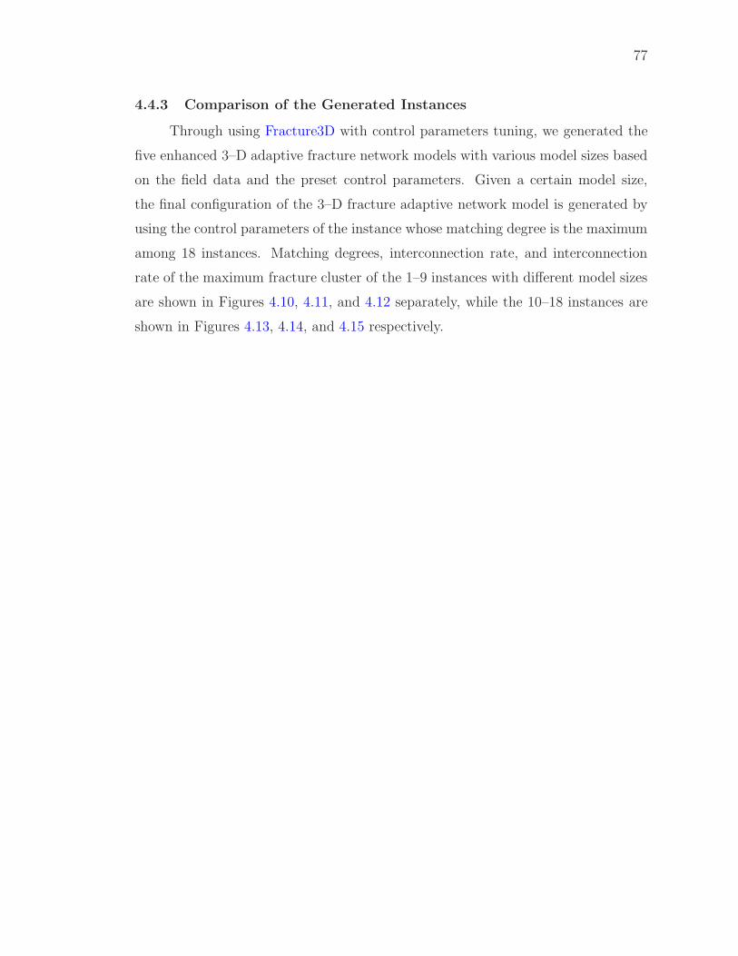
77
4.4.3 Comparison of the Generated Instances
Through using Fracture3D with control parameters tuning, we generated the
five enhanced 3–D adaptive fracture network models with various model sizes based
on the field data and the preset control parameters. Given a certain model size,
the final configuration of the 3–D fracture adaptive network model is generated by
using the control parameters of the instance whose matching degree is the maximum
among 18 instances. Matching degrees, interconnection rate, and interconnection
rate of the maximum fracture cluster of the 1–9 instances with different model sizes
are shown in Figures 4.10, 4.11, and 4.12 separately, while the 10–18 instances are
shown in Figures 4.13, 4.14, and 4.15 respectively.
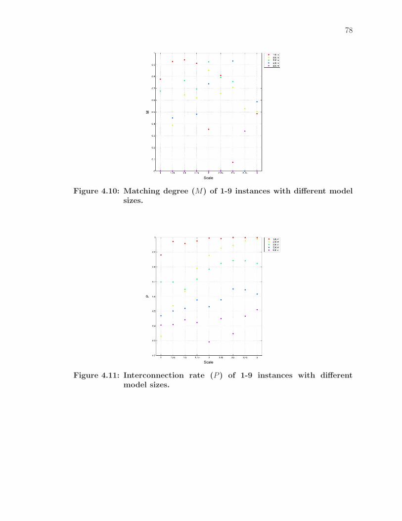
78
Scale
M
Figure 4.10: Matching degree (M) of 1-9 instances with different modelsizes.
Scale
P
Figure 4.11: Interconnection rate (P ) of 1-9 instances with differentmodel sizes.
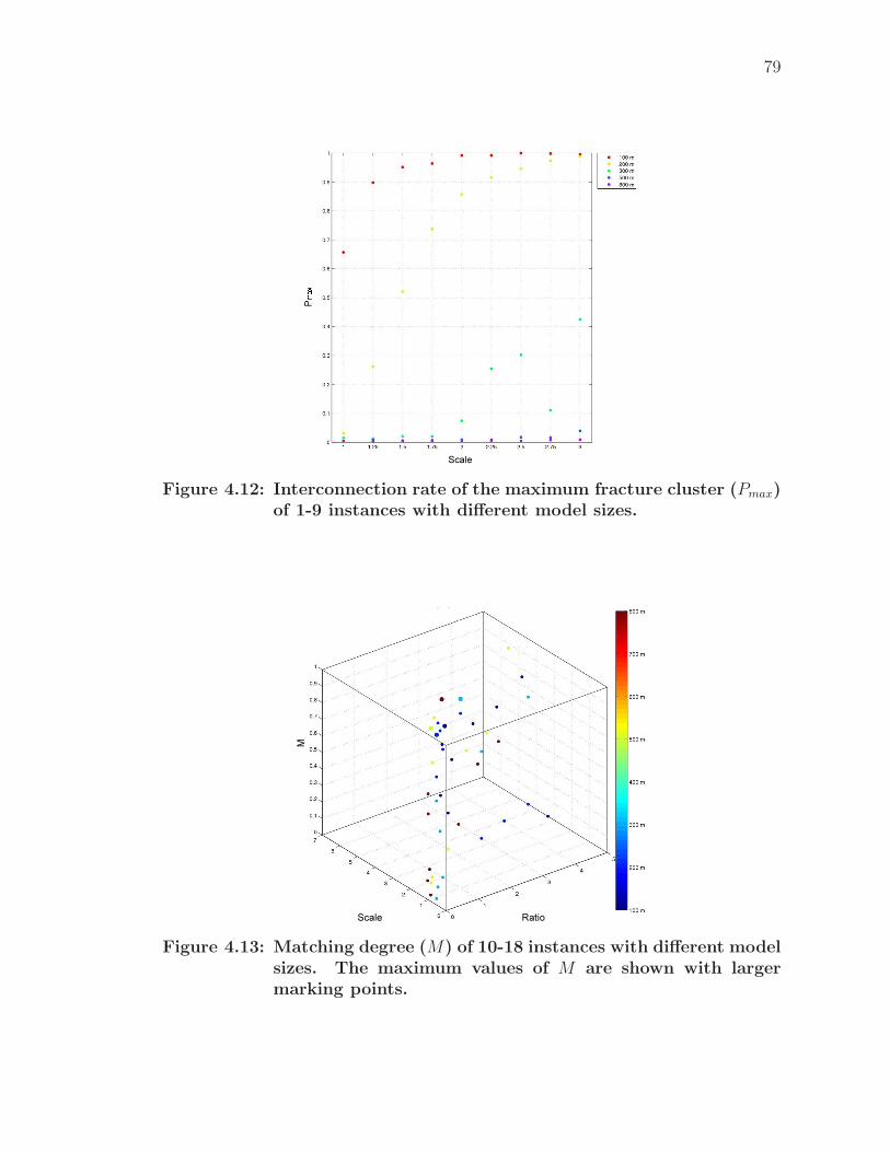
79
Scale
PÑÒÓ
Figure 4.12: Interconnection rate of the maximum fracture cluster (Pmax)of 1-9 instances with different model sizes.
M
Scale Ratio
Figure 4.13: Matching degree (M) of 10-18 instances with different modelsizes. The maximum values of M are shown with largermarking points.
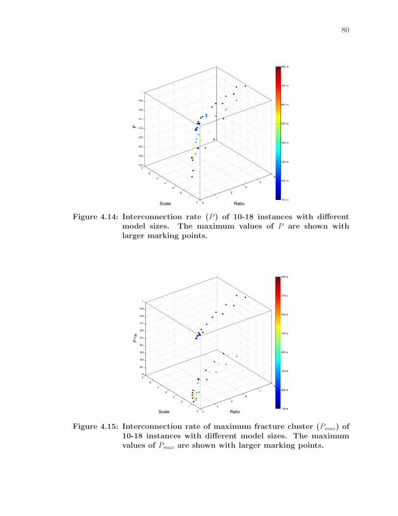
80
P
Scale Ratio
Figure 4.14: Interconnection rate (P ) of 10-18 instances with differentmodel sizes. The maximum values of P are shown withlarger marking points.
P
ÔÕÖScale Ratio
Figure 4.15: Interconnection rate of maximum fracture cluster (Pmax) of10-18 instances with different model sizes. The maximumvalues of Pmax are shown with larger marking points.
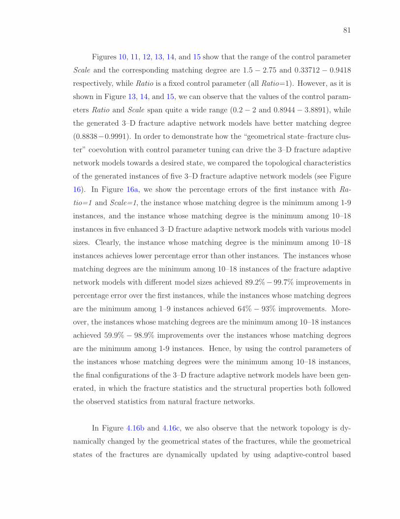
81
Figures 10, 11, 12, 13, 14, and 15 show that the range of the control parameter
Scale and the corresponding matching degree are 1.5 − 2.75 and 0.33712 − 0.9418
respectively, while Ratio is a fixed control parameter (all Ratio=1). However, as it is
shown in Figure 13, 14, and 15, we can observe that the values of the control param-
eters Ratio and Scale span quite a wide range (0.2 − 2 and 0.8944 − 3.8891), while
the generated 3–D fracture adaptive network models have better matching degree
(0.8838−0.9991). In order to demonstrate how the “geometrical state–fracture clus-
ter” coevolution with control parameter tuning can drive the 3–D fracture adaptive
network models towards a desired state, we compared the topological characteristics
of the generated instances of five 3–D fracture adaptive network models (see Figure
16). In Figure 16a, we show the percentage errors of the first instance with Ra-
tio=1 and Scale=1, the instance whose matching degree is the minimum among 1-9
instances, and the instance whose matching degree is the minimum among 10–18
instances in five enhanced 3–D fracture adaptive network models with various model
sizes. Clearly, the instance whose matching degree is the minimum among 10–18
instances achieves lower percentage error than other instances. The instances whose
matching degrees are the minimum among 10–18 instances of the fracture adaptive
network models with different model sizes achieved 89.2%− 99.7% improvements in
percentage error over the first instances, while the instances whose matching degrees
are the minimum among 1–9 instances achieved 64% − 93% improvements. More-
over, the instances whose matching degrees are the minimum among 10–18 instances
achieved 59.9% − 98.9% improvements over the instances whose matching degrees
are the minimum among 1-9 instances. Hence, by using the control parameters of
the instances whose matching degrees were the minimum among 10–18 instances,
the final configurations of the 3–D fracture adaptive network models have been gen-
erated, in which the fracture statistics and the structural properties both followed
the observed statistics from natural fracture networks.
In Figure 4.16b and 4.16c, we also observe that the network topology is dy-
namically changed by the geometrical states of the fractures, while the geometrical
states of the fractures are dynamically updated by using adaptive-control based
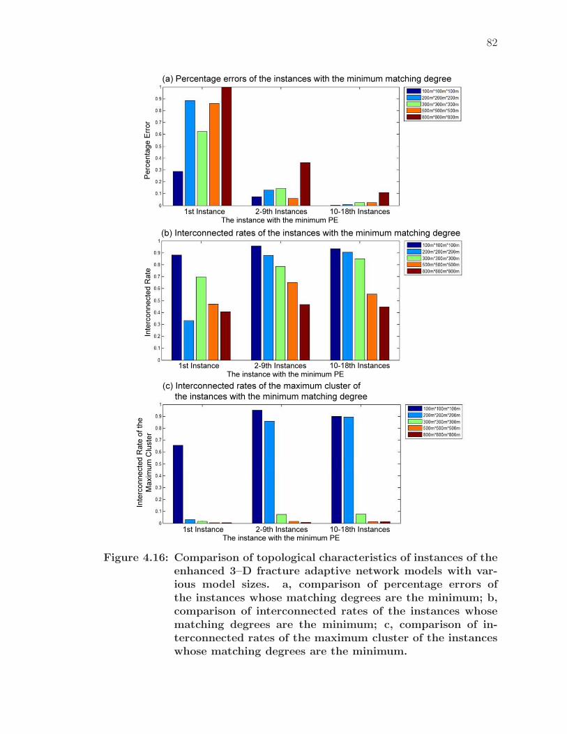
82
Perce
ntage
Error
Interc
onne
cted R
ate of
the
Maxim
um C
luster
Interc
onne
cted R
ate
(c) Interconnected rates of the maximum cluster of the instances with the minimum matching degree
(a) Percentage errors of the instances with the minimum matching degree
1st Instance 2-9th Instances 10-18th InstancesThe instance with the minimum PE
(b) Interconnected rates of the instances with the minimum matching degree
1st Instance 2-9th Instances 10-18th InstancesThe instance with the minimum PE
1st Instance 2-9th Instances 10-18th InstancesThe instance with the minimum PE
Figure 4.16: Comparison of topological characteristics of instances of theenhanced 3–D fracture adaptive network models with var-ious model sizes. a, comparison of percentage errors ofthe instances whose matching degrees are the minimum; b,comparison of interconnected rates of the instances whosematching degrees are the minimum; c, comparison of in-terconnected rates of the maximum cluster of the instanceswhose matching degrees are the minimum.
83
control parameter tuning. The interconnected rates of the instances whose match-
ing degrees are the minimum among 1–9 instances were higher than the first in-
stances 8.8% − 165.5%, while the instances whose matching degrees are the min-
imum among 10–18 instances were higher than the first instances 6.1% − 173.5%.
Moreover, the interconnected rates of the maximum cluster of the instances whose
matching degrees are the minimum among 1–9 instances were higher than the first
instances 44.9%−2684.4%, while the instances whose matching degrees are the min-
imum among 10–18 instances were higher than the first instances 35.9%− 2803.1%.
However, the difference of the interconnected rates and the interconnected rates
of the maximum cluster between the two types of instances are relatively small
(−14.9% − +8.1% and −18.7% − +59.9%). These results show that the adaptive
control structures modify the network topology in a wide range by using the preset
control parameters at first, and then dynamically adjust the network topology in
a narrow range by using control parameter tuning such that topological properties
of the generated 3–D instances closed to a desired state. For example, given a
model size 300m × 300m × 300m, the first instance (Ratio = 1 and Scale = 1) has
2210 interconnected fractures in 186 fracture clusters respectively, 47 fractures in
the maximum cluster, 11 fractures that intersect the slice plane, and its percentage
error is 62.4%. The eighth instance (Ratio = 1 and Scale = 2) whose matching
degree is the minimum among 1–9 instances has 2484 interconnected fractures in
139 clusters, 234 fractures in the maximum cluster, 25 fractures that intersect the
slice plane, and its percentage error is 14.6%. The fifteenth instance (Ratio = 2
and Scale = 2.83) whose matching degree is the minimum among 10–18 instances
has 2686 interconnected fractures in 103 clusters, 244 fractures in the maximum
cluster, 30 fractures that intersect the slice plane, and its percentage error is 2.5%.
While the number of total fractures is 3166 in all 18 instances, the instance whose
matching degree is the minimum among 10–18 instances achieved 96.0% and 83.0%
improvements over the first instance and the instance whose matching degree is the
minimum among 1–9 instances respectively by using adaptive-control based iterative
parameter identification.
84
4.4.3.1 Comparison of the Generated Network Models
In order to evaluate the performance of our Fracture3D, we generated five
enhanced 3–D fracture adaptive network models with various model sizes by us-
ing Fracure3D with control parameter tuning, five ordinary 3–D fracture network
models by using fixed control parameters, and five ordinary 3–D fracture adaptive
network models by using preset control parameters. We ran each simulation 10 times
with different seeds and collected statistics in each run. All results plotted in Figure
4.17 show the averages of results obtained in all runs. Figure 4.17a compares the
percentage errors of three types of 3–D fracture network models with various model
sizes. We can observe that the enhanced 3–D fracture adaptive network models gen-
erated by using Fracure3D with control parameter tuning achieves lower percentage
error than other network models. The enhanced 3–D fracture adaptive network
models achieved 49.3% − 97.1% improvements over the ordinary 3–D fracture net-
work models, while the ordinary 3–D fracture adaptive network models achieved
35.0% − 88.0% improvements. Furthermore, the enhanced 3–D fracture adaptive
network models also achieved 19.2% − 73.3% improvements over the ordinary 3–D
fracture adaptive network models.
As shown in Figure 4.17b and 4.17c, we can observe the impact of the geo-
metrical states of the fractures on fracture network topology, while the geometrical
states are updated based on fixed or adjustable control parameters. The average
interconnected rates of the enhanced 3–D fracture adaptive network models were
higher than the ordinary 3–D fracture network models (10.5%− 150.2%), while the
ordinary 3–D fracture adaptive network models were higher than the ordinary 3–
D fracture network models 10.2% − 147.7%. Moreover, the average interconnected
rates of the maximum cluster of the enhanced 3–D fracture adaptive network mod-
els were higher than the ordinary 3–D fracture network models 103.6% − 2419.8%,
while the ordinary 3–D fracture adaptive network models were higher than the or-
dinary 3–D fracture network models 102.1% − 2376.6%. However, the difference of
the average interconnected rates and the average interconnected rates of the max-
imum cluster between the ordinary and enhanced 3–D fracture adaptive network
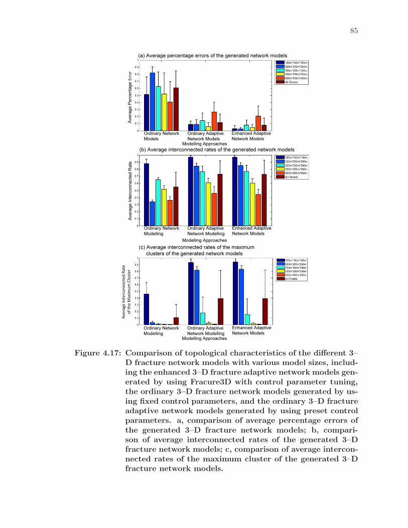
85
Avera
ge Pe
rcenta
ge Er
rorAv
erage
Inter
conn
ected
Rate
of the
Max
imum
Clus
terAv
erage
Inter
conn
ected
Rate
(c) Average interconnected rates of the maximum clusters of the generated network models
(a) Average percentage errors of the generated network models
Ordinary Network Models
Ordinary Adaptive Network Models
Enhanced Adaptive Network Models
Modelling Approaches(b) Average interconnected rates of the generated network models
Ordinary Network Modelling
Ordinary Adaptive Network Modelling
Modelling Approaches
Ordinary Network Modelling
Ordinary Adaptive Network Modelling
Modelling Approaches
Enhanced Adaptive Network Models
Enhanced Adaptive Network Models
Figure 4.17: Comparison of topological characteristics of the different 3–D fracture network models with various model sizes, includ-ing the enhanced 3–D fracture adaptive network models gen-erated by using Fracure3D with control parameter tuning,the ordinary 3–D fracture network models generated by us-ing fixed control parameters, and the ordinary 3–D fractureadaptive network models generated by using preset controlparameters. a, comparison of average percentage errors ofthe generated 3–D fracture network models; b, compari-son of average interconnected rates of the generated 3–Dfracture network models; c, comparison of average intercon-nected rates of the maximum cluster of the generated 3–Dfracture network models.
86
models were relatively small (−3.3% − +0.4% and −12.8% − +12.7%). These re-
sults show that our Fracture3D can drive the network topology towards a desired
state by dynamically updating the geometrical states of fractures (size and profile
of fractures) with a proper adaptive control structure. For example, given a model
size 800m × 800m × 800m, the ordinary 3–D fracture network model with fixed
control parameters has 3,425 interconnected fractures in 202 fracture clusters re-
spectively, 35 fractures in the maximum cluster, 0 fracture that intersect the slice
plane, and its percentage error is 100%. The ordinary 3–D fracture adaptive net-
work model with preset control parameters has 3,933 interconnected fractures in
219 clusters, 62 fractures in the maximum cluster, 28 fractures that intersect the
slice plane, and its percentage error is 36.0%. The enhanced 3–D fracture adaptive
network model with control parameter tuning has 3,758 interconnected fractures in
211 clusters, 99 fractures in the maximum cluster, 39 fractures that intersect the
slice plane, and its percentage error is 10.8%. While the number of total fractures
was 8,442 in all three types of 3–D fracture network models, the enhanced 3–D
fracture adaptive network model with control parameter tuning achieved 89.2% and
69.9% improvements over the ordinary 3–D fracture network model and the ordi-
nary 3–D fracture adaptive network model separately. The ordinary 3–D fracture
network model shows that only 0.4% of fractures at the measurement scale are prob-
ably involved in the groundwater flow system. However, the connectivity pattern of
this model cannot be explained by in-situ hydraulic tests (packer test and pumping
test), although its fracture statistics are similar to the field data. In the enhanced
3–D fracture adaptive network model whose fracture statistics and the structural
properties both follow the observed statistics from natural fracture networks, the
maximum fracture cluster has more fractures (282.9% increase in the number of
fractures in the maximum cluster) than the ordinary 3–D fracture adaptive network
model. Moreover, the results from the estimation of the aquifers’ hydraulic proper-
ties (hydraulic conductivity and transmissibility) based on the connectivity pattern
of the enhanced 3–D fracture adaptive network model can be interpreted by in-situ
pumping test results and packer test results. Hence, the enhanced 3–D fracture
adaptive network model generated by Fracture3D may help researchers have better
87
understanding, description, and prediction of the groundwater flow and transport
processes in fractured-rock aquifer systems without relevant hydraulic test data.
4.5 Summary
We have described a unified framework which combines adaptive network mod-
els and adaptive control structures for modelling and simulation of fractured-rock
aquifer systems. In this framework, an adaptive control structure with iterative
parameter identification is used to identify an instance of a fracture adaptive net-
work model with the desired topological characteristics, while the natural fracture
network can be represented by fracture adaptive network models with “geometrical
state–fracture cluster” coevolution. By using this modelling framework, an auto-
matic modelling tool, Fracture3D, has been developed for automatically building the
enhanced fracture adaptive network models, in which the fracture statistics and the
structural properties can both follow the observed statistics from natural fracture
networks. Through using simple field data and measurements taken on site or in-situ
such as length, orientation, and density of measured fractures, the enhanced frac-
ture adaptive network models can be built for rapidly evaluating the connectivity of
the studied aquifers on a broad range of scales, especially in the early groundwater
development state when data are very limited. Moreover, having such an automated
3–D fracture adaptive network modelling tool would greatly reduce the human effort
and improve the 3–D fracture network model which might be affected by parameter
uncertainty and varied geological and hydrological conditions.
For illustration purpose, a set of simulations and experiments have been con-
ducted for verifying the validity of the proposed unified modelling framework and
modelling tool Fracture3D. A set of the enhanced 3–D fracture adaptive network
models with the desired topological characteristics have been have been built for
the TMG fractured aquifer by using Fracture3D. We compared the topological
characteristics of the 3–D instances to demonstrate how Fracture3D with a unified
modelling framework can drive the 3–D fracture adaptive network models towards
a desired state. Moreover, we also compared the 3–D fracture adaptive network
models generated by our Fracure3D with control parameter tuning to ordinary 3–D

88
fracture network models generated by using fixed control parameters, and ordinary
3–D fracture adaptive network models generated by using preset control parame-
ters. The simulations have clearly shown that our Fracture3D can drive the network
topology towards a desired state by dynamically updating the geometrical states of
fractures (size and profile of fractures) with a proper adaptive control structure.
The unified modelling framework and the automatic 3–D fracture adaptive
network modelling tool can be used to conceptualize an order magnitude of the
fracture connectivity of the fractured-rock aquifer of interest. It can also serve
as crosscheck for other results obtained from conventional software and methods
when fracture connectivity must be assessed within reasonable accuracy. Moreover,
it provides a starting point for future research in this direction for TMG type of
aquifer systems.
CHAPTER 5
Towards A Unified Framework for Modelling and
Simulation of Social Network Systems
In this chapter, the unified framework which combines adaptive network models and
adaptive control structures has been applied for modelling and simulation of social
network systems. We start in Section 5.1 with brief introduction to the background
of modelling and simulation of social network systems. In Section 5.2, we propose
a unified framework which combines adaptive network models and multiple model
adaptive control structures for modelling and simulation of social network systems.
In this framework, a real-world social network system can be represented as an agent-
based adaptive network which is defined by a feedback loop between the behavioural
state of individuals and the community structure of the studied system, where a
multiple model adaptive control structure is used for the predetermination of suitable
computational models of behavioural state update and social interaction update in
order to improve the performance of modelling and simulation. In Section 5.3,
by using such a unified modelling framework, an automatic modelling tool, SMRI,
is developed for automatically building enhanced social adaptive network models
through using mobile-phone-centric multimodal data with suitable computational
models of behavioural state update and social interaction update. In Section 5.4, a
set of simulations and experiments on real-world mobile-phone-centric multimodal
dataset are conducted in order to verify the validity of the proposed unified modelling
framework and modelling tool SMRI.
5.1 Modelling and Simulation of Social Network Systems
Recent developments in sensing technologies have enabled us to examine the
nature of human social behaviour in greater detail. Especially, the pervasiveness of
mobile phones has made them ubiquitous social sensors of location, proximity and
communications (Aharony et al., 2011a). Because of this, extremely detailed sensing
and imaging of social network systems can be implemented through mobile-phone-
89
90
centric social and behavioural sensing system (Aharony et al., 2011a; Aharony et al.,
2011b). Thus, mobile phone records have proven to be particularly valuable. The
mobile-phone-centric datasets enable us to construct multiple network modalities of
the studied social network system, such as the phone communication network, physi-
cal face-to-face encounters network, online social network, self-reported network, and
more. Similar to Magnetic Resonance Imaging in the medical realm, social relation-
ship imaging (Social MRI) has been used to sense and image the social systems
based on various network modalities of the social network system (Aharony et al.,
2011a; Aharony et al., 2011b). A few schemes have been developed for various social
network analysis requirements according to different mobile-phone-centric datasets.
For example, Gonzales et al. showed that cellular-tower location information can
be used to characterize human mobility and that humans follow simple reproducible
mobility patterns (Gonzalez et al., 2008). Eagle et al. found that the diversity
of individuals’ relationships is strongly correlated with the economic development
of communities (Eagle et al., 2010). Eagle and Pentland (2006) defined the term
“Reality Mining” to describe collection of sensor data pertaining to human social
behaviour. They showed that using call records, cellular-tower IDs, and Bluetooth
proximity logs, collected via mobile phones, the subjects’ social network can be accu-
rately detected, as well as regular patterns in daily activity (Eagle & Pentland, 2006;
Eagle et al., 2009). This initial study was then expanded by Madan et al. (2010),
who conducted a similar experiment and showed that mobile social sensing can be
used for measuring and predicting the health status of individuals based on mobility
and communication patterns. They also investigate the spread of political opinion
within the community (Madan et al., 2011). Aharony et al. (2011a) developed a
mobile-phone-centric social and behavioural sensing system that is deployed with
130 adult members of a young-family living community for over a year. A dataset
with 25 phone-based signals is generated which includes location, accelerometry,
Bluetooth-based device proximity, communication activities etc. Other examples
for using mobile phones for social sensing are those by Montoliu and Gatica-Perez
(2010) and Lu et al. (2010). However, there is currently no adaptive-network based
unified framework for implementing the development, comparison, communication
91
and validation of social network models though using mobile-phone-centric data.
Adaptive networks have produced significant implications for studying real-
world social network systems, as they can present more realistic dynamics of social
network, while people change their social behaviours depending on epidemiologi-
cal states of their neighbours (Funk et al., 2010). The effect of social responses to
epidemics on social networks has been investigated in detail in a class of adaptive-
network based epidemic models. As a pioneering model in this direction, the adap-
tive Susceptible-Infected-Susceptible model studied by Gross et al. (Gross et al.,
2006) can provide detailed analytical insights into the emergence of system-level
phenomena from the node-level coevolution by a so-called moment closure approxi-
mation. In order to investigate opinion formation and collective behaviour in social
network systems, adaptive-network based models have been developed (Holme &
Newman, 2006; Zanette & Gil, 2006). In these models, the diffusion of competing
opinions occurs through a networked population, when agents modify their contacts
depending on the opinions held by their neighbours (Sayama et al., 2013). More-
over, the fragmentation transition in opinion formation has also been investigated
by using adaptive-network based model (Kozma & Barrat, 2008; Vazquez et al.
2008; Zimmermann et al. 2000), in which the social network breaks into distinct
components of opposing agents. Besides opinion formation, different classes of so-
cial games have also been investigated on adaptive networks. For example, the work
of Pacheco et al. (2006) and van Segbroeck et al. (2011) showed clearly that co-
evolution can lead to increased levels of cooperation, where agents aim to optimize
some abstract payoff by building up beneficial structure. The work of Poncela et
al. (2009) demonstrated that coevolutionary dynamics can also facilitate coopera-
tion through the dynamics of growth itself. In other cases, adaptive-network based
models have been proposed for studying social games, in which agents struggle for
an advantageous position in the network (Bala & Goyal, 2001; Holme & Ghoshal,
2006; 2010). In addition, organizational dynamics on adaptive networks have also
been investigated by Buskens and van de Rijt (2008), when social network evolution
was described by actors striving for structural holes.
In some cases, these mathematical models above fall short of the complexity
92
of the studied real-world social network systems, and that hence no connection to
real-world observations and experiments can be made. In this situation, agent-based
adaptive network models can be applied, where mechanisms of the coevolution of
social network topologies and individuals’ behavioural states can be a lot more com-
plex and detailed than other more abstract mathematical models (Sayama et al.,
2013). In the work of Centola et al. (2007), for example, similar dynamics includ-
ing the fragmentation transition have been found by using agent-based adaptive
network models of more realistic cultural drift and dissemination processes. The
interactions between the social network structures and the human behaviours have
also been experimentally examined by Centola (2010; 2011) when voter-like mod-
els have been used to investigate the dynamics of decision making in the collective
motion of swarms of locusts (Huepe et al., 2011) and schools of fish (Couzin et al.,
2011). Agent-based models have also been used for computational modelling of com-
plex organizational behaviour, including the evolution of organizational networks,
information/knowledge/culture sharing and trust formation within a group or corpo-
ration (Sayama et al., 2013). For example, the work of Dionne et al. (2010) showed
the nontrivial effects of team network topology and other parameters on the overall
team performance after the team development process. In this work, an agent-based
model of team development dynamics have been developed, in which agents exchange
their knowledge through social ties and then update their self-confidence and trust
to other team members dynamically. Moreover, the self-confidence (node state) and
trust (link weight) were represented by a complex function defined over a continuous
knowledge domain (modelling complex systems). Another example can be found in
the work of Lin and Desouza (2010), which showed that knowledgeable individu-
als do not necessarily gain many connections in the network, and that when high
knowledge diversity exists in the organization, the network tends to evolve into one
with small characteristic path lengths. In this work, an agent-based computational
model has been used for addressing organizational dynamics at a larger scale on the
coevolution of informal organizational network and individual behaviour, where a
node state includes behavioural patterns and knowledge an individual has, and the
knowledge is transferred through informal social links that are changed adaptively
93
(Sayama et al., 2013).
Although an agent-based modelling and simulation approach can simulate very
complicated state-topology coevelution processes in social network systems, agent-
based models are often very intricate and the impact of any given modelling assump-
tion or parameter is difficult to study. When applying adaptive network models to
agent-based modelling and simulation of social network systems, it is necessary to
specify how the states of nodes will be changed to generate new topologies of the
network. Adaptive network models may have control parameters for node update
and link update which greatly determine the quality of the generated network mod-
els. Choosing suitable parameter values is, frequently, a problem-dependent task
and requires previous experience of the researchers (Maruo et al., 2005). In ordi-
nary adaptive network models, these control parameters are not included as a part
of the state-topology coevolution, because they are considered as external fixed pa-
rameters. In real-world applications, however, the control parameters of the social
adaptive network models may vary greatly depending on different assumptions and
conditions. In the present work, we used a multiple model adaptive control structure
for modelling real-world social network system through using mobile-phone-centric
behavioural data and adaptive-network based modelling approach, where the prede-
termination of suitable computational models is implemented for the state update
of nodes and the weight update of links.
5.2 A Unified Framework for Modelling and Simulation of
Social Network Systems with Mobile-Phone-Centric Data
Recent developments in sensing technologies have enabled us to examine the
nature of human social behaviour in greater detail. However, the social network
models may be rendered impractical due to these impractical assumptions and poor
sample quality, and their accuracy suffers significantly from a lack of knowledge
about real social network conditions or other useful information related to the as-
sumptions. Moreover, mechanisms of the coevolution of community structures and
individuals’ behavioural states can be a lot more complex and detailed than other
more abstract mathematical models, when computational models of adaptive net-
94
works are hybrids of dynamical networks and agent-based models. Such models
subjected to abrupt and large parameter variations are generally very difficult to
control.
Based on the unified modelling framework described in Chapter 3, a unified
framework which combines adaptive network models and multiple model adaptive
control structures has been developed in this work in order to achieve a desired
topological property for the corresponding adaptive network models of social net-
work systems. Through using mobile-phone-centric behavioural data, the studied
social network system can be represented as an adaptive network which contains
a feedback loop between the behavioural states of individuals and the community
structures of the system. Moreover, a multiple model adaptive control structure has
been used for the predetermination of suitable computational models of behavioural
state update and social interaction update in order to improve the performance of
modelling and simulation. The modelling framework then automatically identifies
desired configurations of the adaptive network models based on a benchmark net-
work model derived from collected self-report data. The generated enhanced social
adaptive network models can promote better understanding of the inner workings of
the studied social network system. Having such an automated modelling framework
would greatly reduce the human effort and provide a valuable systematic modelling
tool for understanding, description, prediction, and control of the real-world social
network systems through using mobile-phone-centric behavioural data.
As depicted in Figure 5.1, a real-world social network system is considered as
an agent-based adaptive network which are defined by a feedback loop between the
behavioural state of individuals and the community structure of the studied system.
Moreover, such a state-topology coevolution can self-organize towards non-trivial
topologies. The input data are obtained from different measurements through using
various mobile-phone-centric behavioural data such as call logs, Bluetooth proxim-
ity logs, cellular-tower transition logs, which quantify different behavioural states
of people or various types of social interactions between people. We suppose that
a set of computational models for behavioural state update and social interaction
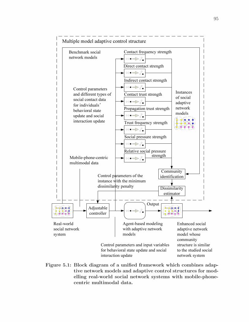
95
Control parameters and input variables for behavioral state update and social interaction update
Adjustable controller
Mobile-phone-centric multimodal data
Output
Real-world social network system
Instances of social adaptive network models
Enhanced social adaptive network model whose community structure is similar to the studied social network system
Agent-based modeling with adaptive network models
Dissimilarity estimator
Benchmark social network models
Control parameters and different types of social contact data for individuals’behavioral state update and social interaction update
Contact frequency strength
Direct contact strength
Indirect contact strength
Contact trust strength
Propagation trust strength
Trust frequency strength
Social pressure strength
Relative social pressurestrength
Control parameters of the instance with the minimum dissimilarity penalty
Community identification
Multiple model adaptive control structure
Figure 5.1: Block diagram of a unified framework which combines adap-tive network models and adaptive control structures for mod-elling real-world social network systems with mobile-phone-centric multimodal data.
96
update is a priori known. By using the current control parameters and the current
input data, a set of instances of an adaptive network model are generated based on
various computational models. In the model estimator, the dissimilarity between
the discovered communities of a generated instances and the discovered communi-
ties of benchmark network model built by using self-report data is measured. A
performance index is established according to the dissimilarity measurements of the
generated instances. The corresponding control parameters of the instance whose
dissimilarity score is the minimum are fed into the controller, and the correspond-
ing computational model of the instance is applied to the process of agent-based
modelling and simulation. The behavioural states of individuals and social interac-
tions among them are then updated with a suitable computational model in order
to generate an enhanced social adaptive network model whose community structure
is similar to the studied social network system. By using such a multiple model
adaptive control structure, the adaptive-network based framework can be used for
modelling and simulation of the studied social network system with suitable com-
putational models of behavioural state update and social interaction update.
5.3 SMRI, An Automatic Social Network Modelling Tool
by Using Mobile-phone-centric Multimodal Data
Through using the mobile-phone-centric multimodal data and the unified frame-
work which combines adaptive network models and multiple model adaptive con-
trol structures, an automatic modelling tool, SMRI, is developed for automatically
building the enhanced social adaptive network models whose community structures
are similar to the real-world social network systems. Moreover, a multiple model
adaptive control structure is used for the predetermination of suitable computa-
tional models of behavioural state update and social interaction update in order to
achieve a desired topological property for the social adaptive network models. The
model of SMRI is shown in Figure 5.2. A mobile-phone-centric multimodal dataset
which contains call logs, Bluetooth proximity logs and cellular-tower transition logs
is used for modelling of social network systems with adaptive network models, when
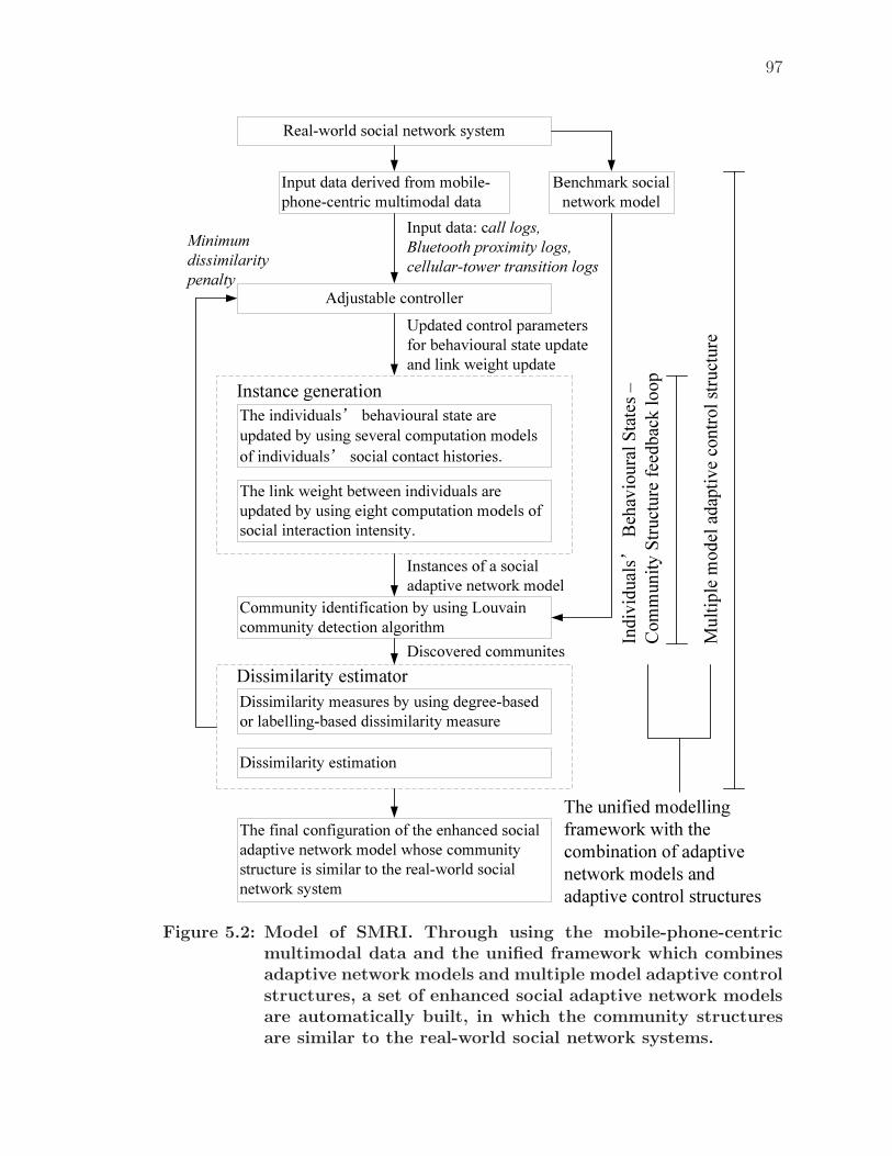
97
Input data derived from mobile-phone-centric multimodal data
Dissimilarity measures by using degree-based or labelling-based dissimilarity measure
The individuals’ behavioural state are updated by using several computation models of individuals’ social contact histories. The link weight between individuals are updated by using eight computation models of social interaction intensity.
Community identification by using Louvain community detection algorithm
The final configuration of the enhanced social adaptive network model whose community structure is similar to the real-world social network system
Instance generation
Dissimilarity estimator
Input data: call logs,Bluetooth proximity logs, cellular-tower transition logs
Instances of a socialadaptive network model
Updated control parametersfor behavioural state updateand link weight update
Adjustable controller
Indivi
duals
’Be
havio
ural S
tates
–Co
mmun
ity St
ructur
efeed
back
loop
Multip
le mo
del a
dapti
ve co
ntrol
struc
ture
The unified modelling framework with the combination of adaptive network models and adaptive control structures
Benchmark social network model
Real-world social network system
Dissimilarity estimation
Minimum dissimilarity penalty
Discovered communites
Figure 5.2: Model of SMRI. Through using the mobile-phone-centricmultimodal data and the unified framework which combinesadaptive network models and multiple model adaptive controlstructures, a set of enhanced social adaptive network modelsare automatically built, in which the community structuresare similar to the real-world social network systems.
98
individuals’ behavioural states are extracted from these data. In the process of
agent-based modelling, individuals’ behavioural states are updated by using several
computation models of indivduals’ social contract histories through using the cur-
rent control parameters and certain sampled data, while the link weight between
the individuals update by using eight computation models of social interaction in-
tensity. A set of instances of a social adaptive network model are then generated
by using various computation models of behavioural state update and link weight
update. The Louvain community detection algorithm (Blondel et al., 2008) is used
for community identification of the generated instances and the benchmark social
network model built by using self-report data. In the dissimilarity estimator, the dis-
covered communities are used for the measurement of dissimilarity penalty between
the generated instances and the benchmark network model by using degree-based
network model dissimilarity measure or labelling-based network model dissimilarity
measure. The corresponding control parameters and computation models of the
instance whose dissimilarity penalty is the minimum are then used for generating
the final configuration of the enhanced social adaptive network model with desired
topological characteristics. In the following, several key algorithms of this modelling
framework will be introduced, including behavioural states update, link weight up-
date, community identification, and dissimilarity estimation.
5.3.1 Behavioural State Update
In the past few years, mobile-phone-centric behavioural data such as call log
data, GPS-based location data, and mobile-sensing based detailed proximity data
have been used for agent-based social network modelling. In the present work, we
assume that a social action occurs when a direct/indirect contact is recorded by
using different mobile sensing techniques. Thus, a mobile-phone-centric multimodal
dataset which contains call logs, Bluetooth proximity logs and cellular-tower transi-
tion logs can be used for modelling of social network systems with adaptive network
models (Table 5.1), when individuals’ behavioural states are extracted from these
data. Such a behavioural state can be represented by a vector which contains a set of
social contacts with four tuples: 〈contactID, timestamp, duration, direction〉. The
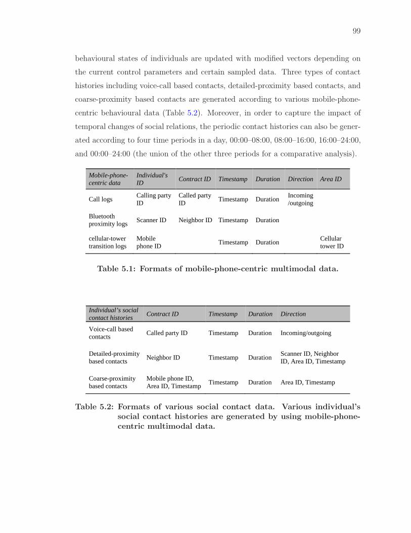
99
behavioural states of individuals are updated with modified vectors depending on
the current control parameters and certain sampled data. Three types of contact
histories including voice-call based contacts, detailed-proximity based contacts, and
coarse-proximity based contacts are generated according to various mobile-phone-
centric behavioural data (Table 5.2). Moreover, in order to capture the impact of
temporal changes of social relations, the periodic contact histories can also be gener-
ated according to four time periods in a day, 00:00–08:00, 08:00–16:00, 16:00–24:00,
and 00:00–24:00 (the union of the other three periods for a comparative analysis).
Mobile-phone-centric data
Individual's ID
Contract ID Timestamp Duration Direction Area ID
Call logs Calling party ID
Called party ID
Timestamp Duration Incoming/outgoing
Bluetooth proximity logs
Scanner ID Neighbor ID Timestamp Duration
cellular-tower transition logs
Mobile phone ID
Timestamp Duration Cellular tower ID
Table 5.1: Formats of mobile-phone-centric multimodal data.
Individual’s social contact histories
Contract ID Timestamp Duration Direction
Voice-call based contacts
Called party ID Timestamp Duration Incoming/outgoing
Detailed-proximity based contacts
Neighbor ID Timestamp Duration Scanner ID, Neighbor ID, Area ID, Timestamp
Coarse-proximity based contacts
Mobile phone ID, Area ID, Timestamp
Timestamp Duration Area ID, Timestamp
Table 5.2: Formats of various social contact data. Various individual’ssocial contact histories are generated by using mobile-phone-centric multimodal data.
100
5.3.1.1 Voice-Call Based Contact Data
The ordinary call detail records (CDR) can be specified by a set of communica-
tion 5-tuples: 〈callingpartyID, calledpartyID, T imestamp, Duration, Direction〉.The voice-call based contacts are directly generated from CDR data. However, in
some cases, the called party ID of each record may not be available due to techni-
cal difficulties or privacy concerns. In this work, the called party ID is identified
through comparing the timestamps of all voice call events. We sorted all voice call
events over all individuals by timestamp, and match the incoming/outgoing calls
occurring within a small time window (4t).
5.3.1.2 Detailed-Proximity Based Contact Data
The detailed-proximity based contact data can be built according to Blue-
tooth proximity logs and cellular-tower transition logs. Bluetooth proximity logs
can provide encounter information of people. However, the movement direction of
people can not be measured directly in an encounter event without accurate position
information. In this work, the coarse location information (Area ID) derived from
cellular-tower transition logs was used for measuring the movement direction of peo-
ple. The movement status of a mobile phone is labelled as “static” for each record in
Bluetooth proximity logs if the mobile phone is still in the range of the same cellular
tower for a specific time period (five minutes); otherwise “active” is labelled. The
records of Bluetooth proximity logs can then be labelled with “incoming/outgoing”
when the movement status labels of scanner ID and neighbour ID are different. Fur-
thermore, we assume that a social action occurs when a Bluetooth scan record is
labelled with “incoming/outgoing”. Thus, a set of detailed-proximity based contacts
can be established based on Bluetooth proximity logs and cellular-tower transition
logs.
5.3.1.3 Coarse-Proximity Based Contact Data
In this work, we assume that a social contact happens when two persons who
know each other are in the same area. Thus, a set of coarse-proximity based contacts
can be created according to cellular-tower transition logs. Although movement
direction of people can not be directly obtained from cellular-tower transition logs,
101
the movement direction may be detected by using coarse location information (Area
ID) derived from cellular-tower transition logs. Through comparing Timestamp and
Area ID of each record in cellular-tower transition logs, the coarse-proximity based
contacts are labelled with “incoming/outgoing” by detecting who enters this area
earlier.
5.3.2 Link Weight Update
Social contact happens when one person communicates with another person.
In Hossmann et al.’s work (Hossmann et al., 2011), they represented the complex
resulting pattern of who meets whom, how often and for how long, in a compact and
tractable way. We borrow their idea for measuring social contact strength based on
mobile-phone-centric data. This allows us to quantify structural properties beyond
pairwise statistics such as inter-contact and contact time distributions. We aggregate
the entire sequence of social contacts of all individuals to a weighted instance of a
social adaptive network model. In this instance, the weight of a link represents the
strength of the relationship between two persons. A key question is how to derive
the tie strength between two persons, i.e., what metric to use for computing the
weight of a link in a social network model, based on the observed social interactions.
This weight should represent the amount of social interactions between two persons.
Various metrics, such as the age of last contact (Dubois-Ferriere et al., 2003), contact
frequency (Hui et al., 2011), or aggregate contact duration (Hui et al., 2011) have
been used as tie strength indicators in delay-tolerant-networking routing. In this
work, we suppose that a set of computational models for measuring the intensity
of social interactions is a priori known. By using the current control parameters
and the current behavioural states of individuals, an instances of the social adaptive
network model can be generated in a time step based on a certain computational
model of social interaction intensity. A brief introduction of the computational
models will be given subsequently:
5.3.2.1 Contact Frequency Strength
Traditionally, contact frequency strength (CFS) has been considered as an
important metric for modelling real-world social networks. Frequent contacts may
102
imply many meetings and hence many information forwarding opportunities (short
delays). In this work, we mapped this feature to a scalar weight according to current
behavioural states of individuals. Each pair of individuals i, j is assigned to a feature
vector wCFSij , which is the number of social contacts between individuals i and j.
5.3.2.2 Direct Contact Strength
Similar to (Hossmann et al., 2011), we consider both contact frequency and
contact duration, when direct contact strength (DCS) is computed. They capture
different aspects, both of which are important for modelling social networks. Fre-
quent contacts imply many meetings and hence many information forwarding op-
portunities (short delays) and long contacts imply meetings where a large amount of
information can be transferred (high throughput). Since most community detection
algorithms require one dimensional tie strengths, we map these two features to a
scalar weight. We first assign each pair of individuals i, j a two-dimensional feature
vector, zij = (fij−f
σf,
tij−t
σt), where fij is the number of contacts in the log between
individuals i and j, and tij is the sum of the durations of all contacts between the
two individuals. f and t are the respective empirical means, and σf and σt, the
empirical standard deviations. We normalize the values by their standard devia-
tions to make the scales of the two metrics comparable. We then transform the
two-dimensional feature vector to a scalar feature value, using the principal com-
ponent, i.e., the direction in which the feature vectors of all node pairs Z = {zij},i, j ∈ N has the largest variance. This is the direction of the eigenvector v1 (with
the largest corresponding eigenvalue) of the 2×2 covariance matrix of frequency and
duration. We then define the tie strength between i and j as the projection of zij on
the principal component wDCSij = vT
1 zij +w0, where we add w0 = vT1 (− f
σf,− t
σt) (the
projection of the feature value for a pair without contacts) in order to have positive
tie strengths. The obtained weight is a generic metric that combines the frequency
and duration in a scalar value and captures the heterogeneity of node pairs with
respect to frequency and duration of various social contacts (Hossmann et al., 2011).
103
5.3.2.3 Indirect Contact Strength
By applying an information theoretic method to the conversation event log,
Takaguchi et al. (2011) found that sequences of conversation events have deter-
ministic components. Long contacts may imply meetings where a large amount
of information can be transferred. We thus assume that individual l has an indi-
rect contact with individual j, when individual i contacts with individual l after
contacting with individual j. Thus, indirect contact strength (ICS) of a pair of indi-
viduals (wICSij ) can be measured, which is the number of indirect contacts between
individuals i and j.
5.3.2.4 Contact Trust Strength
Behavioural trust in social networks has been studied by Adali et al. in (Adali
et al., 2010; Adali et al., 2012). Based on the sender-receiver-time data derived from
the communication stream of a social network, trusting relationships among people
can be captured and quantified, when text analysis is in general expensive and fairly
sophisticated tools are needed (see Figure 5.3). Suppose we are working on a set
of social contacts C = {C1, C2, . . . , Cl} between individuals A and B; contract trust
strength (CTS) can be measured as follows: wCTSij = l ·H(C), where l is the number
of the social contacts, and H(C) is a measure of the balance in the set of contacts.
We use the entropy function to measure balance: H(C) = −p log p−(1−p) log(1−p),
where p(C) is the fraction of contacts in the set of contacts C that were sent by
individual A.
5.3.2.5 Propagation Trust Strength
A measure of propagation trust has been developed based on the propaga-
tion of information in (Adali et al., 2010; Adali et al., 2012). In the present work,
a similar measure was implemented through using various social contact histories.
We assume that indirect trust is established and information is propagated, when
individual A makes a contact with individual B, and B makes another contact with
some third person X within some time interval δ. Thus, the valid propagations can
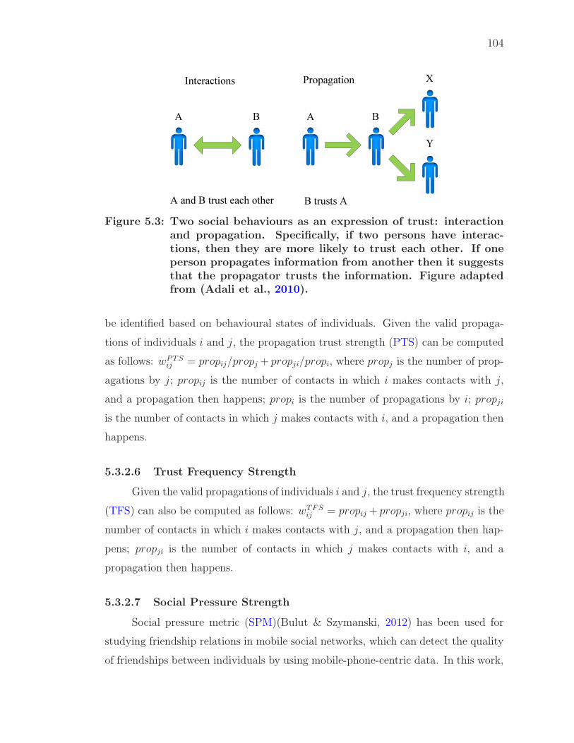
104
Interactions Propagation
A B A B
X
Y
A and B trust each other B trusts AFigure 5.3: Two social behaviours as an expression of trust: interaction
and propagation. Specifically, if two persons have interac-tions, then they are more likely to trust each other. If oneperson propagates information from another then it suggeststhat the propagator trusts the information. Figure adaptedfrom (Adali et al., 2010).
be identified based on behavioural states of individuals. Given the valid propaga-
tions of individuals i and j, the propagation trust strength (PTS) can be computed
as follows: wPTSij = propij/propj + propji/propi, where propj is the number of prop-
agations by j; propij is the number of contacts in which i makes contacts with j,
and a propagation then happens; propi is the number of propagations by i; propji
is the number of contacts in which j makes contacts with i, and a propagation then
happens.
5.3.2.6 Trust Frequency Strength
Given the valid propagations of individuals i and j, the trust frequency strength
(TFS) can also be computed as follows: wTFSij = propij + propji, where propij is the
number of contacts in which i makes contacts with j, and a propagation then hap-
pens; propji is the number of contacts in which j makes contacts with i, and a
propagation then happens.
5.3.2.7 Social Pressure Strength
Social pressure metric (SPM)(Bulut & Szymanski, 2012) has been used for
studying friendship relations in mobile social networks, which can detect the quality
of friendships between individuals by using mobile-phone-centric data. In this work,
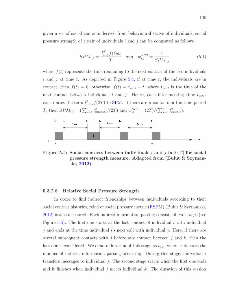
105
given a set of social contacts derived from behavioural states of individuals, social
pressure strength of a pair of individuals i and j can be computed as follows
SPMi,j =
∫ T
t=0f(t)dt
Tand wSPS
i,j =1
SPMi,j
(5.1)
where f(t) represents the time remaining to the next contact of the two individuals
i and j at time t. As depicted in Figure 5.4, if at time t, the individuals are in
contact, then f(t) = 0, otherwise, f(t) = tnext − t, where tnext is the time of the
next contact between individuals i and j. Hence, each inter-meeting time tinter
contributes the term t2inter/(2T ) to SPM. If there are n contacts in the time period
T , then SPMi,j = (∑n
x=1 t2inter,x)/(2T ) and wSPSij = (2T )/(
∑nx=1 t2inter,x).
× × × ×Ø ÙÚÛÜ ÛÝ ÛÞ Ûß Ûà Ûá ÛØâãÛäåæçèÝ ÛäåæçèÞ Ûäåæçèß
Figure 5.4: Social contacts between individuals i and j in [0, T ] for socialpressure strength measure. Adapted from (Bulut & Szyman-ski, 2012).
5.3.2.8 Relative Social Pressure Strength
In order to find indirect friendships between individuals according to their
social contact histories, relative social pressure metric (RSPM) (Bulut & Szymanski,
2012) is also measured. Each indirect information passing consists of two stages (see
Figure 5.5). The first one starts at the last contact of individual i with individual
j and ends at the time individual i’s next call with individual j. Here, if there are
several subsequent contacts with j before any contact between j and k, then the
last one is considered. We denote duration of this stage as ta,x, where x denotes the
number of indirect information passing occurring. During this stage, individual i
transfers messages to individual j. The second stage starts when the first one ends
and it finishes when individual j meets individual k. The duration of this session
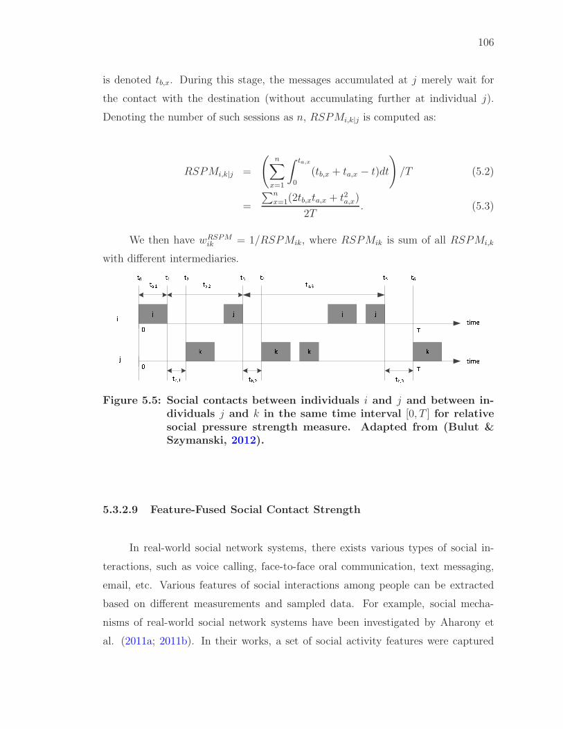
106
is denoted tb,x. During this stage, the messages accumulated at j merely wait for
the contact with the destination (without accumulating further at individual j).
Denoting the number of such sessions as n, RSPMi,k|j is computed as:
RSPMi,k|j =
(
n∑
x=1
∫ ta,x
0
(tb,x + ta,x − t)dt
)
/T (5.2)
=
∑nx=1(2tb,xta,x + t2a,x)
2T. (5.3)
We then have wRSPMik = 1/RSPMik, where RSPMik is sum of all RSPMi,k
with different intermediaries.éé é éê ê ê êë é ìííîï îð îñ îò îó îô îõ îëö÷îëö÷
îøùðîúùð îúùñ îúùò
îøùñ îøùòì
Figure 5.5: Social contacts between individuals i and j and between in-dividuals j and k in the same time interval [0, T ] for relativesocial pressure strength measure. Adapted from (Bulut &Szymanski, 2012).
5.3.2.9 Feature-Fused Social Contact Strength
In real-world social network systems, there exists various types of social in-
teractions, such as voice calling, face-to-face oral communication, text messaging,
email, etc. Various features of social interactions among people can be extracted
based on different measurements and sampled data. For example, social mecha-
nisms of real-world social network systems have been investigated by Aharony et
al. (2011a; 2011b). In their works, a set of social activity features were captured
107
through using mobile-sensing based social fMRI technique and mobile-phone-centric
multimodal datasets. A set of social network models can then be built respectively
according to the features derived from different types of mobile sensing data. How-
ever, some social interaction information is typically lost in such social network
models since it is rarely possible to represent the features of all types of social in-
teractions at once. In order to lose as little as possible interaction information for
modelling real-world social network systems, information-based feature enhance-
ment is performed by using voice-call based contact data, detailed-proximity based
contact data, and the features of social interaction introduced above.
In this work, we suppose that social interaction information can be measured
based on the quantity of the social contacts. The higher frequency of social con-
tacts contains more social interaction information. The information content can be
expressed by the equation: I(f) = log(f), where f is the frequency of the social
contacts. Through the log function the information I(f) is higher for a type social
contact with a higher frequency. The feature fusion can then be implemented in a
way to weight voice-call based contacts and detailed-proximity based contacts. To
formalize this weighting we introduce the equation: γ(f , f) = I(f)
I(f)+I(f), where f is
the number of all voice-call based contacts, and f is the number of all voice-call
based contacts. If the value of γ is 0.5, both types of social contacts contain the
same amount of social interaction information.
Given a pair of values wCFSij and wCFS
ij which are contact frequency strength of
individual i and j derived from voice-call based contact data and detailed-proximity
based contact data respectively, the fusion of two values can be implemented by the
following equation: wfCFSij = (1−γ)∗ wCFS
ij +γ ∗ wCFSij . Thus, feature-fused contact
strength can be generated for each type of the various social interaction features.
5.3.3 Community Identification
In real-world social network systems, people naturally tend to form groups
within their work environment, family, and friends (Fortunato, 2010). Such sub-
groups are called social communities whose members are all “friends” to each other
(Luce & Perry, 1949). Communities are typical for the structure of social networks,
108
which contain a set of individuals with stronger social connections between them
than towards other individuals. The existence of strong communities in the con-
tact based social network models may imply high potential for human cooperation
and community-based trust mechanisms (Hossmann et al., 2011). Since community
structure is one of the most relevant features of network models representing real-
world complex systems, a few community detection algorithms have been developed
by a large interdisciplinary community of scientists (Fortunato, 2010). A thorough
introduction of community detection in network models has been given by Fortunato
(2010).
In the present work, the widely used Louvain community detection algorithm
(Blondel et al., 2008) has been used for community identification according to various
instances of social adaptive network models and the social network model built by
using self-report data. The Louvain community detection algorithm is a modularity-
based method with greedy optimization technique for the general case of weighted
network models. This algorithm has two steps that are repeated iteratively. In
the first step, every node is assigned to the local community that yields the largest
modularity increase. The second step consists of a successive transformation of the
communities into nodes of a smaller communities (Fortunato, 2010). According to a
comparative analysis of community detection methods carried out by Lancichinetti
and Fortunato (2009), the Louvain algorithm has good performance, and can be
deployed to large systems.
5.3.4 Dissimilarity Estimation
In the dissimilarity estimator, the discovered communities are used for the
measurement of dissimilarity penalty between the generated instances and the bench-
mark network model by using degree-based network model dissimilarity measure or
labelling-based network model dissimilarity measure. The corresponding control pa-
rameters and computation models of the instance whose dissimilarity penalty is the
minimum are then used for generating the final configuration of the enhanced social
adaptive network model with desired topological characteristics.
In order to check the performance of a community detection algorithm, several
109
measures for comparing community structure have been developed. As discussed in
(Traud et al., 2011), these methods can be classified roughly into three categories:
measures based on pair counting, cluster matching and information theory. Pair-
counting methods (Rand, 1971; Fowlkes & Mallows, 1983; Wallace, 1983; Mirkin,
1996; Meila, 2007; Traud et al., 2011) depend on the number of pairs of nodes which
fall in the same or in different groups in the two partitions, when similarity mea-
sures based on cluster matching (Meila & Heckerman, 2001; van Dongen, 2000) try
to find the largest overlaps between pairs of clusters of different partitions (Fortu-
nato, 2010). In addition, similarity measures with information-theoretic techniques
(Stanley, 1997; Gusfield, 2002; Mackay, 2003; Donon et al., 2005; Gustafsson et al.,
2006; Zhang et al., 2006; Fan et al., 2007; Meila, 2007; Palla et al., 2007; Karrer et
al., 2008; Lancichinetti et al., 2009) have also been developed based on the assump-
tion that very little information is needed to infer one partition given the other if
they are similar (Fortunato, 2010). In this work, however, we focus on pair-counting
methods due to their convenient algebraic description and computational simplicity.
To estimate the performance of computational models of social interaction strength,
two dissimilarity-comparing measures based on pair counting have been developed in
this work: degree-based measure and labelling-based measure. The implementation
details of these two measures are presented in the following subsections.
5.3.4.1 Data for Similarity-Comparing Measures
A set C ≡ {c1, c2, . . . , cC} of communities can be generated through using
Louvain community detection algorithm and an instance generated by a ceratin
social interaction strength measure. Each community Ci is formed by a set C∗ ≡{v1, v2, . . . , vC∗} of nodes and a set F∗ ≡ {f1, f2, . . . , fF ∗} of links es = {vi, vj}. We
can also get a set KC ≡ {kC1 , kC
2 , . . . , kCK} of number of nodes in each community.
By using the Louvain community detection algorithm and a benchmark net-
work model built by using self-report data, a set T ≡ {t1, t2, . . . , tT} of communities
can be generated. Each community Ti forms by a set T ∗ ≡ {u1, u2, . . . , uT ∗} of
nodes and a set E∗ ≡ {e1, e2, . . . , eE∗} of links er = {ui, uj} that connect the nodes.
A set KT ≡ {kT1 , kT
2 , . . . , kTK} of the number of nodes in each community can be also
110
obtained.
5.3.4.2 Degree-Based Dissimilarity Measure
The degree-based method is a measure of dissimilarity between the discovered
communities of generated instances (“discovered” communities) and the discovered
communities of benchmark network model built by using self-report data (“true”
communities). The dissimilarity penalty to an instance which contains a set of
“discovered” communities P is composed of two parts, split penalty Ps for breaking
links in “true” communities, and merge penalty Pm for imposing non-existent links
in “true” communities. If an instance has the same community structure with
the benchmark network model (same number of communities with same members),
the penalty is Ps = 0. If any node in a benchmark network model can not be
found in an instance, the penalty is the maximum possible number of links in the
benchmark network model: Ps = uT (uT − 1), where uT is number of nodes in
a “true” community. If uT nodes in a certain “true” community are split into c
“discovered” communities with vi nodes in the i-th “discovered” community, thus
uT =∑c
i=1 vi, the split penalty of the “true” community is P Ts =
∑ci=1 vi(uT − vi).
The split penalty of an instance which contains t “true” communities can then be
calculated as: Ps =∑t
h=1 P hs .
If vC nodes in a “discovered” community are split into t “true” communities
with kj nodes in the j-th “true” community, so that vC =∑t
j=1 kj, the merge penalty
of the “discovered” community is P Cm =
∑tj=1 kj ·
∑ti6=j ki/2 =
∑tj=1 kj(nc − kj)/2.
The merge penalty of an instance which contains c “discovered” communities can
then be calculated as: Pm =∑c
h=1 P hm. The total penalty to an instance is P =
Ps + Pm.
5.3.4.3 Labelling-Based Dissimilarity Measure
In this work, the dissimilarity between the generated instances and the bench-
mark network model can also be measured by a labelling-based method. The dis-
similarity penalty to an instance which contains a set of “discovered” communities
P is composed of two parts as well, split penalty Ps for splitting links in “true”
communities, and merge penalty Pm for merging two disjoint “true” communities

111
within one “discovered” community. A set of labels LC ≡ {lC1 , lC2 , . . . , lCn } which are
community ID of the nodes can be generated through using the Louvain community
detection algorithm and an instance built by a ceratin social interaction strength
measure. We can also obtain a set of labels LT ≡ {lT1 , lT2 , . . . , lTn} from a benchmark
network model with the same nodes, when different community IDs are assigned to
each node. The split penalty Ps can then be computed by using a labelling-based
algorithm (see Algorithm 5.1).
Algorithm 5.1: Calculation of Split Penalty (Ps) for labeling-based measure
n: number of nodes in a benchmark network model
ûüý: community ID of node j derived from an instance with a social interaction strength
ûþý: community ID of node i derived from an instance with a social interaction strength
ûüÿ: community ID of node j derived from a benchmark network model for i = 1 to n
for j = 1 to n
if ûüý �� ûþý and ûüý �� ûüÿ and ûüý �� � then
Ps++
end if
next j
If the nodes in a certain “discovered” community come from t “true” com-
munities, the merge penalty of the “discovered” community is Pm = t(t − 1)/2.
The merge penalty of an instance which contains c “discovered” communities can
then be calculated as: Pm =∑c
h=1 P hm. Thus, the total penalty to an instance is
P = Ps + Pm.
5.4 Experiments on Mobile-phone-centric Multimodal Dataset
In order to verify the validity of the proposed unified modelling framework and
automatic modelling tool SMRI, we have applied it on a real-world social network
112
system. In this work, the studied real-world social network system is considered as
an agent-based adaptive network which are defined by a feedback loop between the
behavioural state of individuals and the community structure of the studied system,
when mobile phones are used as in-situ social sensors to map social interactions
and social relations of users. Two experiments have been implemented through
using MIT Reality Mining multimodal dataset and our automatic modelling tool
SMRI, namely modelling of social network system based on periodic social con-
tact data and modelling of social network system based on fused data and fused
features. Through using SMRI, a set of enhanced social adaptive network models
whose community structure is similar to the studied social network system were
automatically built based on various mobile-phone-centric social contact data and
computational models of social interaction strength. In the first experiment, the
generated social adaptive network models helped us evaluate the performance of
social adaptive network modelling with the temporal changes of individuals’ social
interactions. In the second experiment, the performances of the proposed data and
feature enhancement methods were evaluated based on the generated social adaptive
network models. Moreover, the performance of the computational models for mod-
elling and simulation of real-world social network systems, such as mobile-sensing
based social contact data generation, periodic social contact data generation, social
interaction strength measure, network dissimilarity measures, were also evaluated
based on these enhanced social adaptive network models.
5.4.1 Mobile-Phone-Centric Multimodal Dataset
Traditionally, the study of social network systems has been an arduous process,
involving extensive surveys, interviews, ethnographic studies, or analysis of online
behaviour. However, more insights about the dynamics of both individual and group
behaviour can be obtained through using the unprecedented amount of information,
such as continuous proximity, location, communication and activity data, generated
by pervasive mobile phones, which are used as in-situ social sensors to map social
interactions and social relations of users. The MIT Reality Mining project (Eagle &
Pentland, 2006; Eagle et al., 2009) was conducted from 2004–2005 at the MIT Media
113
Laboratory for the study of human social behaviour with mobile sensing techniques.
There are 83 participants who are either students or faculty at MIT. Through using
a custom logging software and various mobile sensing techniques, a mobile-phone-
centric multimodal dataset, MIT Reality Mining dataset (Eagle & Pentland, 2006;
Eagle et al., 2009), has been generated which includes call logs, Bluetooth proximity
logs and cellular-tower transition logs (Eagle, 2005).
5.4.2 Self-Report Data
In the MIT Reality Mining project (Eagle & Pentland, 2006; Eagle et al.,
2009), self-report relational data which contains their friendship with others were
also collected from each user. The relationship between two users is labelled as “1”
if they are friends. A benchmark network model which contains 52 nodes and 57
links was generated based on these self-report data.
5.4.3 Modelling with Periodic Social Contact Data
Considering the fact that main activities of people are periodic in a social
network system, mobile-phone based social interactions often change periodically
with time. Normally, the social interactions among people happen in some specific
periods of the day. If two persons were frequently in contact in a particular time
period, then they are likely to make next contact in the same time period. For
example, in MIT Reality dataset, human subject 28 meets with subject 38 usually
between 9am to 7pm while subject 28 meets with subject 48 usually between 1pm
to 7pm (Bulut & Szymanski, 2012). Similar behaviour is also seen in the Haggle
dataset (Haggle, 2006–2010). Temporal correlation of social interactions has been
used for making routing decisions in delay tolerant networks (Bulut & Szymanski,
2012; Bulut et al., 2014). However, there is no analysis and explicit usage of periodic
mobile-sensing data for modelling real-world social network systems with adaptive
network models.
In order to capture the impact of temporal changes of social interactions among
people on the performance of network models, a set of enhanced social adaptive net-
work models have been automatically generated by using SMRI according to various
periodic social contact data and different social interaction strength measures. The
114
temporal correlation between the behaviour dynamics of individuals and the struc-
ture of social networks can then be analyzed based on the generated social adaptive
network models.
5.4.3.1 Input Data
By using the MIT Reality Mining multiple model dataset, three types of so-
cial contact histories were generated, including voice-call based contacts, detailed-
proximity based contacts, and coarse-proximity based contacts. Because of privacy
concerns, the called party ID in each voice call record is not available in the MIT
Reality Mining dataset. However, we sorted all voice call records over all individu-
als by their timestamp, and matched the incoming/outgoing calls occurring within
a small time window 4t. In this work, 11,899 voice-call contacts were generated,
when 4t is setup as 120.96s. We also generated 172,568 detailed-proximity based
contacts by using the Bluetooth proximity logs and the cellular-tower transition
logs, and 231,074 coarse-proximity based contacts through using the cellular-tower
transition logs. Four periodic social contact data can then be generated for each
type of social contacts, including the contacts in period (00:00–24:00), the contacts
in period (00:00–08:00), the contacts in period (08:00–16:00), and the contacts in
period (16:00-24:00). Thus, twelve periodic social contact data were used as input
data in this experiment.
5.4.3.2 Modelling with SMRI
By using SMRI, a set of enhanced social adaptive network models were auto-
matically generated based on various periodic social contact data. The behavioural
state of each node is updated with a certain periodic contact history which is ex-
tracted from current input data. In each time step, the weights of links are updated
based on one of eight measures of social interaction strength. Thus, eight instances
of the social adaptive network model are generated for each periodic social contact
data. In the dissimilarity estimator, the dissimilarity between the discovered com-
munities of the generated instances and the discovered communities of benchmark
network model built by using self-report data is measured. The corresponding con-
trol parameters of the instance whose dissimilarity penalty is the minimum are fed
115
into the controller, and the corresponding computational model of the instance are
applied to the generation of the final configuration of the enhanced social adaptive
network model of the studied real-world social network system.
5.4.3.3 Simulation Results
Through using 12 periodic social contact data and SMRI, we generated 24
enhanced social adaptive network models. The adaptive network model generated by
using contact trust strength measure and periodic detailed-proximity contact data
(16:00-24:00), and the social adaptive network model obtained through using direct
contact strength measure and periodic detailed-proximity contact data (00:00-08:00)
have the greatest similarity to the community structure of the benchmark network
model according to corresponding dissimilarity measures (see Table 5.3). This means
that friendship relations can be efficiently captured by measuring behavioural trust
among people based on periodic detailed proximity mobile-sensing data (00:00–
08:00), and measuring contact strength combined frequency and duration based
on periodic detailed proximity mobile-sensing data (16:00–24:00). Moreover, this
is a further indication that when more longer contacts and more contacts occur
in 00:00–08:00 and 16:00–24:00, they imply closer relationships between people.
As shown in Figure 5.6a and 5.6b, the final configuration of the enhanced social
adaptive network model generated by using contact trust strength measure and
periodic detailed-proximity contact data (00:00–08:00) has 29 nodes, 32 links, and
7 communities, and its modularity is 0.45, degree-based dissimilarity penalty is 624
(normalized value is 0.23), labelling-based dissimilarity penalty is 39 (normalized
value is 0.28), while the final configuration generated by using contact trust strength
measure and periodic detailed-proximity contact data (16:00–24:00) has 49 nodes,
239 links, and 7 communities, and its modularity is 0.35, degree-based dissimilarity
penalty is 502 (normalized value is 0.18), and labelling-based dissimilarity penalty
is 40 (normalized value is 0.28). The final configuration generated by using contact
trust strength measure and periodic detailed-proximity contact data (00:00–24:00)
has 52 nodes, 368 links, and 5 communities, and its modularity is 0.37, degree-
based dissimilarity penalty is 602 (normalized value is 0.22), while labelling-based
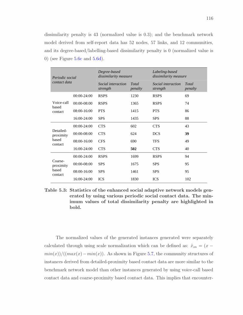
116
dissimilarity penalty is 43 (normalized value is 0.3); and the benchmark network
model derived from self-report data has 52 nodes, 57 links, and 12 communities,
and its degree-based/labelling-based dissimilarity penalty is 0 (normalized value is
0) (see Figure 5.6c and 5.6d).
Periodic social contact data
Degree-based dissimilarity measure
Labeling-based dissimilarity measure
Social interaction strength
Total penalty
Social interaction strength
Total penalty
Voice-call based contact
00:00-24:00 RSPS 1230 RSPS 69
00:00-08:00 RSPS 1365 RSPS 74
08:00-16:00 PTS 1415 PTS 86
16:00-24:00 SPS 1435 SPS 88
Detailed-proximity based contact
00:00-24:00 CTS 602 CTS 43
00:00-08:00 CTS 624 DCS 39
08:00-16:00 CFS 690 TFS 49
16:00-24:00 CTS 502 CTS 40
Coarse-proximity based contact
00:00-24:00 RSPS 1699 RSPS 94
00:00-08:00 SPS 1675 SPS 95
08:00-16:00 SPS 1461 SPS 95
16:00-24:00 ICS 1830 ICS 102
Table 5.3: Statistics of the enhanced social adaptive network models gen-erated by using various periodic social contact data. The min-imum values of total dissimilarity penalty are highlighted inbold.
The normalized values of the generated instances generated were separately
calculated through using scale normalization which can be defined as: xsn = (x −min(x))/((max(x)−min(x)). As shown in Figure 5.7, the community structures of
instances derived from detailed-proximity based contact data are more similar to the
benchmark network model than other instances generated by using voice-call based
contact data and coarse-proximity based contact data. This implies that encounter-
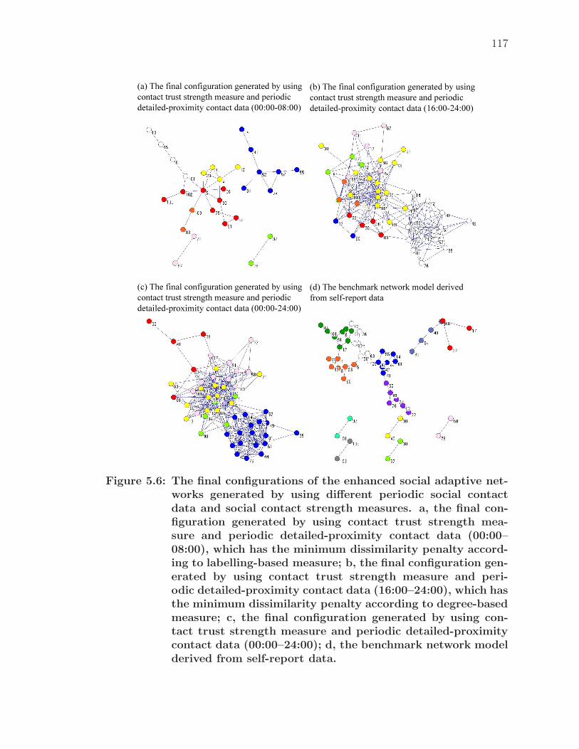
117
(a) The final configuration generated by using contact trust strength measure and periodic detailed-proximity contact data (00:00-08:00)
(b) The final configuration generated by using contact trust strength measure and periodic detailed-proximity contact data (16:00-24:00)
(c) The final configuration generated by using contact trust strength measure and periodic detailed-proximity contact data (00:00-24:00)
(d) The benchmark network model derived from self-report data
Figure 5.6: The final configurations of the enhanced social adaptive net-works generated by using different periodic social contactdata and social contact strength measures. a, the final con-figuration generated by using contact trust strength mea-sure and periodic detailed-proximity contact data (00:00–08:00), which has the minimum dissimilarity penalty accord-ing to labelling-based measure; b, the final configuration gen-erated by using contact trust strength measure and peri-odic detailed-proximity contact data (16:00–24:00), which hasthe minimum dissimilarity penalty according to degree-basedmeasure; c, the final configuration generated by using con-tact trust strength measure and periodic detailed-proximitycontact data (00:00–24:00); d, the benchmark network modelderived from self-report data.
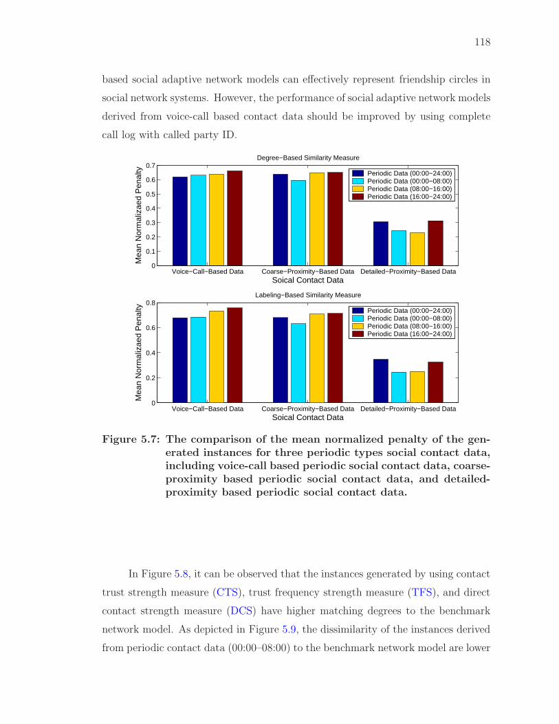
118
based social adaptive network models can effectively represent friendship circles in
social network systems. However, the performance of social adaptive network models
derived from voice-call based contact data should be improved by using complete
call log with called party ID.
Voice−Call−Based Data Coarse−Proximity−Based Data Detailed−Proximity−Based Data0
0.1
0.2
0.3
0.4
0.5
0.6
0.7Degree−Based Similarity Measure
Soical Contact Data
Mea
n N
orm
aliz
aed
Pen
alty Periodic Data (00:00−24:00)
Periodic Data (00:00−08:00)Periodic Data (08:00−16:00)Periodic Data (16:00−24:00)
Voice−Call−Based Data Coarse−Proximity−Based Data Detailed−Proximity−Based Data0
0.2
0.4
0.6
0.8Labeling−Based Similarity Measure
Soical Contact Data
Mea
n N
orm
aliz
aed
Pen
alty Periodic Data (00:00−24:00)
Periodic Data (00:00−08:00)Periodic Data (08:00−16:00)Periodic Data (16:00−24:00)
Figure 5.7: The comparison of the mean normalized penalty of the gen-erated instances for three periodic types social contact data,including voice-call based periodic social contact data, coarse-proximity based periodic social contact data, and detailed-proximity based periodic social contact data.
In Figure 5.8, it can be observed that the instances generated by using contact
trust strength measure (CTS), trust frequency strength measure (TFS), and direct
contact strength measure (DCS) have higher matching degrees to the benchmark
network model. As depicted in Figure 5.9, the dissimilarity of the instances derived
from periodic contact data (00:00–08:00) to the benchmark network model are lower
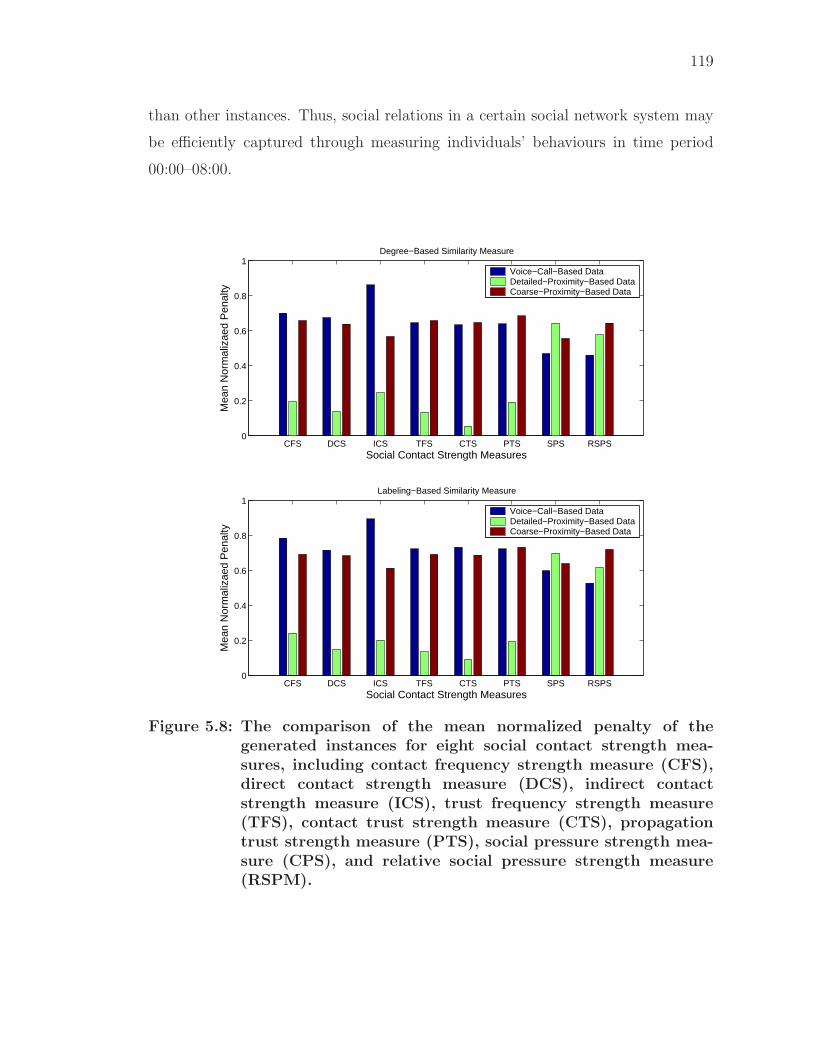
119
than other instances. Thus, social relations in a certain social network system may
be efficiently captured through measuring individuals’ behaviours in time period
00:00–08:00.
CFS DCS ICS TFS CTS PTS SPS RSPS0
0.2
0.4
0.6
0.8
1Degree−Based Similarity Measure
Social Contact Strength Measures
Mea
n N
orm
aliz
aed
Pen
alty
Voice−Call−Based DataDetailed−Proximity−Based DataCoarse−Proximity−Based Data
CFS DCS ICS TFS CTS PTS SPS RSPS0
0.2
0.4
0.6
0.8
1Labeling−Based Similarity Measure
Social Contact Strength Measures
Mea
n N
orm
aliz
aed
Pen
alty
Voice−Call−Based DataDetailed−Proximity−Based DataCoarse−Proximity−Based Data
Figure 5.8: The comparison of the mean normalized penalty of thegenerated instances for eight social contact strength mea-sures, including contact frequency strength measure (CFS),direct contact strength measure (DCS), indirect contactstrength measure (ICS), trust frequency strength measure(TFS), contact trust strength measure (CTS), propagationtrust strength measure (PTS), social pressure strength mea-sure (CPS), and relative social pressure strength measure(RSPM).
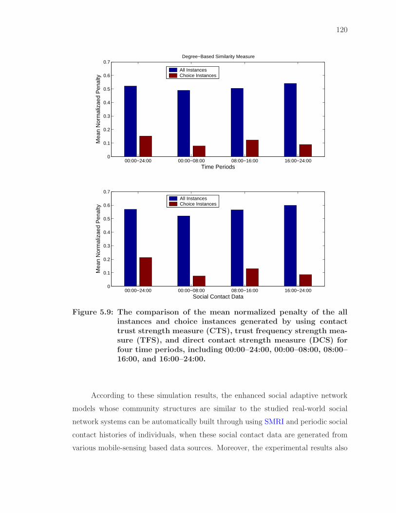
120
00:00−24:00 00:00−08:00 08:00−16:00 16:00−24:000
0.1
0.2
0.3
0.4
0.5
0.6
0.7Degree−Based Similarity Measure
Time Periods
Mea
n N
orm
aliz
aed
Pen
alty
All InstancesChoice Instances
00:00−24:00 00:00−08:00 08:00−16:00 16:00−24:000
0.1
0.2
0.3
0.4
0.5
0.6
0.7
Social Contact Data
Mea
n N
orm
aliz
aed
Pen
alty
All InstancesChoice Instances
Figure 5.9: The comparison of the mean normalized penalty of the allinstances and choice instances generated by using contacttrust strength measure (CTS), trust frequency strength mea-sure (TFS), and direct contact strength measure (DCS) forfour time periods, including 00:00–24:00, 00:00–08:00, 08:00–16:00, and 16:00–24:00.
According to these simulation results, the enhanced social adaptive network
models whose community structures are similar to the studied real-world social
network systems can be automatically built through using SMRI and periodic social
contact histories of individuals, when these social contact data are generated from
various mobile-sensing based data sources. Moreover, the experimental results also
121
demonstrated that the coupling between the social adaptive network model and the
multiple model adaptive control structures can drive the community structure of
a social adaptive network models towards a desired state through using suitable
computational models of behavioural state update and social interaction update
predetermined by the multiple model adaptive control structure.
5.4.4 Modelling with Fused Data and Fused Features
Social network models can be established based on mobile-phone-centric mul-
timodal dataset which provides large amount of information about the studied social
network system. Thus, the extraction of useful information from raw data is a major
goal. This can be achieved by quantifying the information content or importance
of a certain part of the data set. Fused data and features are chosen in a way to
enhance parts of the data which may contain more information about the social net-
work system. A set of enhanced social adaptive network models can then be built
based on these fused data and features. In this experiment, the performances of the
data and feature enhancement methods were evaluated according to the enhanced
social adaptive network models generated by our automatic modelling tool SMRI.
5.4.4.1 Input Data
By using the periodic voice-call-based contact data (00:00–24:00) and the peri-
odic detailed-proximity-based contact data (00:00–24:00) as original datasets, fused
voice-call-based contact data and fused detailed-proximity-based contact data were
generated in a way to enhance parts of the data which may contain more information
about the studied social network system.
The raw data of the call logs and Bluetooth proximity logs are normally noisy
when they are used for studying of social relations among people. For example, a
person call/meet another person several times does not mean they must be friends.
However, the noise of voice-call based contact data may be filtered by using the so-
cial interactions derived from detailed-proximity based contact data and vice versa.
The fused voice-call-based contact data only involves matched voice-call based social
contacts between two persons when there exists social interactions between these two
persons according to the original detailed-proximity-based contact data. Further-
122
more, we also generated the fused detailed-proximity-based contact data by using
the same method based on the original voice-call-based contact data.
5.4.4.2 Modelling with SMRI
We generated a set of enhanced social adaptive network models by using SMRI
and four social contact datasets, including original/fused voice-call-based contact
datasets, and original/fused detailed-proximity-based contact datasets. The be-
havioural state of each node is updated with a certain periodic contact history
which is extracted from current input data. In each time step, the weights of links
are updated based on a certain social interaction strength measure. Thus, eight
instances of the social adaptive network model are then generated for a certain so-
cial contact data. Moreover, by using the information-based feature fusion method
with γ = 0.56236 (see Section 5.3.2.9), fused social interaction strength are gener-
ated based on the measurements of social interaction strength derived from fused
voice-call-based contact data and fused detailed-proximity-based contact data re-
spectively. Thus, extra eight instances are generated based on these fused social
interaction strength. In the dissimilarity estimator, the dissimilarity between the
discovered communities of the generated instances and the discovered communi-
ties of benchmark network model built by using self-report data is measured. The
corresponding control parameters of the instance whose dissimilarity penalty is the
minimum are fed into the controller, and the corresponding computational model of
the instance are applied to the generation of the final configuration of the enhanced
social adaptive network model.
5.4.4.3 Simulation Results
We have generated ten enhanced social adaptive network models when the
four social contact datasets and two dissimilarity measures were used. As shown
in Table 5.4, the social adaptive network models generated by using original/fused
detailed-proximity-based contact data have the greatest similarity to the community
structure of benchmark network model according to the labelling-based dissimilar-
ity measure, while the dissimilarity penalty of the social adaptive network model
generated by using the original detailed-proximity-based contact data is the mini-
123
mum according to degree-based dissimilarity measure. In Figure 5.10a and 5.10b,
the final configuration of the enhanced social adaptive network model generated by
using propagation trust strength measure and fused detailed-proximity-based con-
tact data has 52 nodes, 477 links, and 7 communities, and its modularity is 0.31,
the degree-based dissimilarity penalty is 686 (normalized value is 0.23), and the
labelling-based dissimilarity penalty is 43 (normalized value is 0.3), while the fi-
nal configuration generated by using contact trust strength measure and original
detailed-proximity-based contact data has 52 nodes, 368 links, and 5 communities,
and its modularity is 0.37, degree-based dissimilarity penalty is 602 (normalized
value is 0.2), and labelling-based dissimilarity penalty is 43 (normalized value is
0.3). The final configuration generated by using direct contact strength measure
and feature-fused contact data has 51 nodes, 487 links, and 2 communities, and
its modularity is 0.26, degree-based dissimilarity penalty is 745 (normalized value is
0.25), and labelling-based dissimilarity penalty is 45 (normalized value is 0.31); while
the benchmark network model derived from self-report data has 52 nodes, 57 links,
and 12 communities, and its degree-based/labelling-based dissimilarity penalty is 0
(normalized value is 0) (see Figure 5.10c and 5.10d). We also observed that the mean
dissimilarity penalties of all generated instances with fused data and features to the
benchmark network model are higher than the network models with original social
contact data in Figure 5.11. They could be the possible reasons that the contact
frequencies of original voice-call based contact data and original detailed-proximity
based contact data are similar (γ = 0.56236), and the raw voice call data are in-
complete (without called party ID). However, through using data fusion and feature
fusion, the similarity values of instances generated by direct contact strength mea-
sure, trust frequency strength measure, and social pressure strength measure can be
improved (see Figure 5.12).
The experiment results with different social adaptive network models having
different computation models of data and feature processing show that our auto-
matic modelling tool SMRI with data-fusion based and feature-fusion based feature
enhancement methods can be used for improving the performance of ceratin com-
putational models when raw data are noisy. Moreover, it also demonstrates that
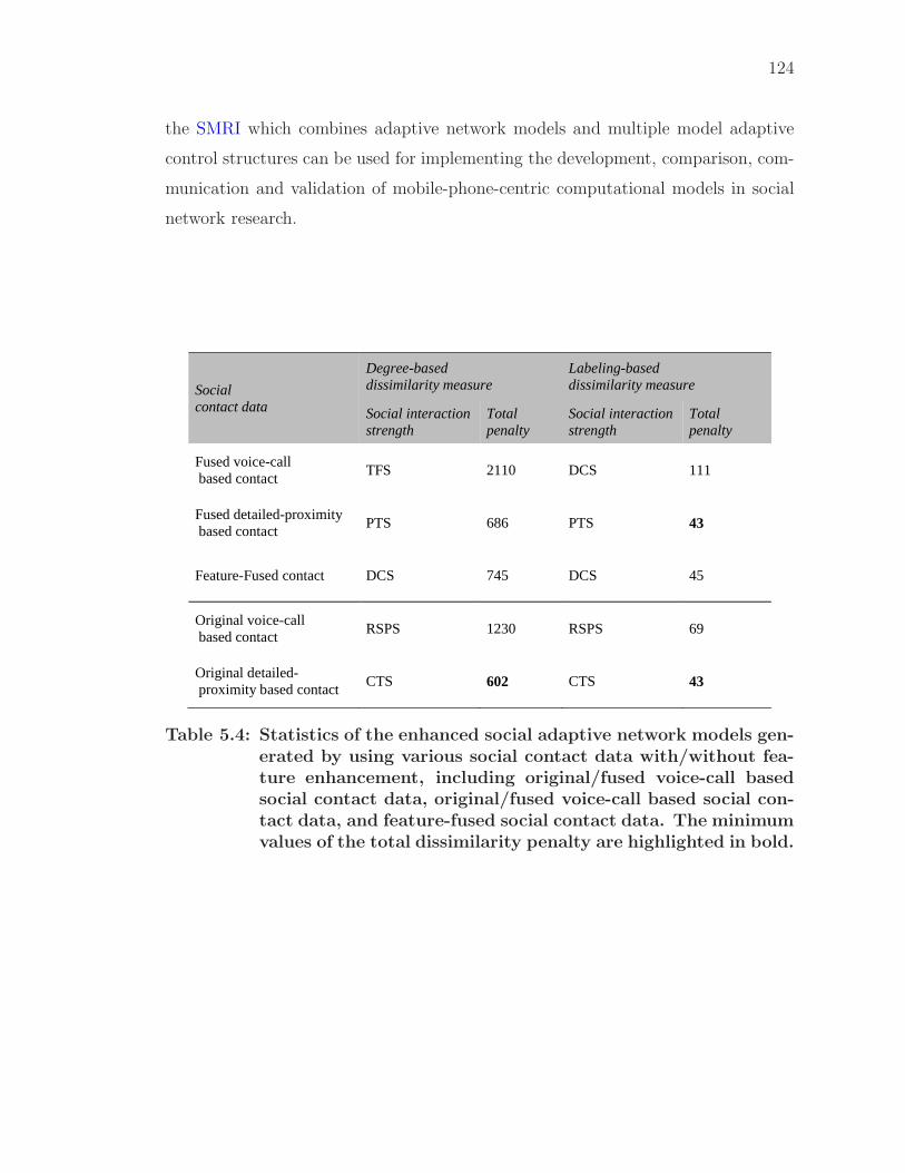
124
the SMRI which combines adaptive network models and multiple model adaptive
control structures can be used for implementing the development, comparison, com-
munication and validation of mobile-phone-centric computational models in social
network research.
Social contact data
Degree-based dissimilarity measure
Labeling-based dissimilarity measure
Social interaction strength
Total penalty
Social interaction strength
Total penalty
Fused voice-call based contact TFS 2110 DCS 111
Fused detailed-proximity based contact
PTS 686 PTS 43
Feature-Fused contact DCS 745 DCS 45
Original voice-call based contact RSPS 1230 RSPS 69
Original detailed- proximity based contact
CTS 602 CTS 43
Table 5.4: Statistics of the enhanced social adaptive network models gen-erated by using various social contact data with/without fea-ture enhancement, including original/fused voice-call basedsocial contact data, original/fused voice-call based social con-tact data, and feature-fused social contact data. The minimumvalues of the total dissimilarity penalty are highlighted in bold.
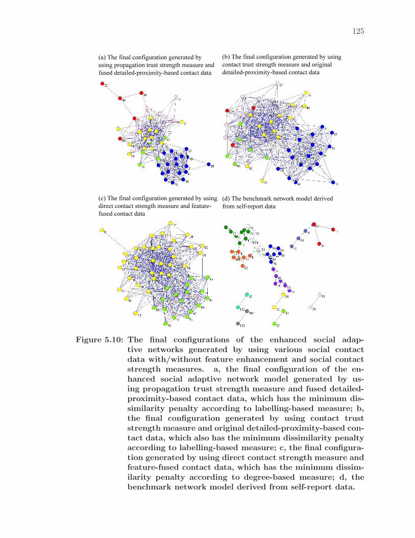
125
(c) The final configuration generated by using direct contact strength measure and feature-fused contact data
(d) The benchmark network model derived from self-report data
(a) The final configuration generated by using propagation trust strength measure and fused detailed-proximity-based contact data
(b) The final configuration generated by using contact trust strength measure and original detailed-proximity-based contact data
Figure 5.10: The final configurations of the enhanced social adap-tive networks generated by using various social contactdata with/without feature enhancement and social contactstrength measures. a, the final configuration of the en-hanced social adaptive network model generated by us-ing propagation trust strength measure and fused detailed-proximity-based contact data, which has the minimum dis-similarity penalty according to labelling-based measure; b,the final configuration generated by using contact truststrength measure and original detailed-proximity-based con-tact data, which also has the minimum dissimilarity penaltyaccording to labelling-based measure; c, the final configura-tion generated by using direct contact strength measure andfeature-fused contact data, which has the minimum dissim-ilarity penalty according to degree-based measure; d, thebenchmark network model derived from self-report data.
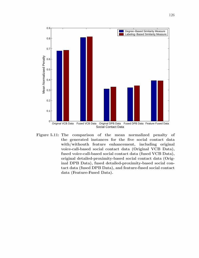
126
Original VCB Data Fused VCB Data Original DPB Data Fused DPB Data Feature Fused Data0
0.1
0.2
0.3
0.4
0.5
0.6
0.7
0.8
0.9
Social Contact Data
Mea
n N
orm
aliz
aed
Pen
alty
Degree−Based Similarity MeasureLabeling−Based Similarity Measure
Figure 5.11: The comparison of the mean normalized penalty ofthe generated instances for the five social contact datawith/withouth feature enhancement, including originalvoice-call-based social contact data (Original VCB Data),fused voice-call-based social contact data (fused VCB Data),original detailed-proximity-based social contact data (Orig-inal DPB Data), fused detailed-proximity-based social con-tact data (fused DPB Data), and feature-fused social contactdata (Feature-Fused Data).
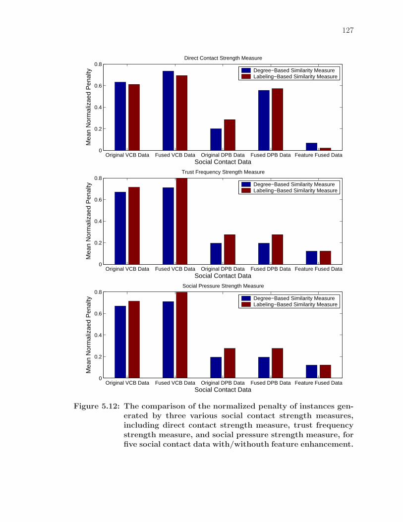
127
Original VCB Data Fused VCB Data Original DPB Data Fused DPB Data Feature Fused Data0
0.2
0.4
0.6
0.8Direct Contact Strength Measure
Social Contact Data
Mea
n N
orm
aliz
aed
Pen
alty Degree−Based Similarity Measure
Labeling−Based Similarity Measure
Original VCB Data Fused VCB Data Original DPB Data Fused DPB Data Feature Fused Data0
0.2
0.4
0.6
0.8Trust Frequency Strength Measure
Social Contact Data
Mea
n N
orm
aliz
aed
Pen
alty Degree−Based Similarity Measure
Labeling−Based Similarity Measure
Original VCB Data Fused VCB Data Original DPB Data Fused DPB Data Feature Fused Data0
0.2
0.4
0.6
0.8Social Pressure Strength Measure
Social Contact Data
Mea
n N
orm
aliz
aed
Pen
alty Degree−Based Similarity Measure
Labeling−Based Similarity Measure
Figure 5.12: The comparison of the normalized penalty of instances gen-erated by three various social contact strength measures,including direct contact strength measure, trust frequencystrength measure, and social pressure strength measure, forfive social contact data with/withouth feature enhancement.
128
5.5 Summary
In this chapter, we have described a unified framework which combines adap-
tive network models and multiple model adaptive control structures for modelling
and simulation of real-world social network systems. In this modelling frame-
work, the studied social network system can be represented as an adaptive network
which contains a feedback loop between the behavioural states of the individuals
and the community structures of the system, while a multiple model adaptive con-
trol structure was used for the predetermination of suitable computational models
of behavioural state update and social interaction update in order to drive the com-
munity structures of the social adaptive network model towards a desired state.
By using this modelling framework, an automatic modelling tool, SMRI, has been
developed for automatically generating the enhanced social adaptive network mod-
els whose community structures are similar to real-world social network systems by
using mobile-phone-centric multimodal data. Having such an automated modelling
tool would greatly reduce the human effort and provide a valuable systematic mod-
elling tool for understanding, description, prediction, and control of the real-world
social network systems through using mobile-phone-centric behavioural data.
We have applied our SMRI on a real-world social network system by using
a mobile-phone-centric multimodal dataset. Two experiments were performed for
demonstrating how to conduct a research case study on social network modelling
by using the automatic modelling tool. In the first experiment, the simulation
results demonstrate that the enhanced social adaptive network models whose com-
munity structures are similar to the studied real-world social network systems can
be automatically built through using SMRI and periodic social contact histories of
individuals derived from various mobile-sensing based data sources. In the second
experiment, the experiment results with different social adaptive network models
having different computation models of data and feature processing show that our
automatic modelling tool SMRI with data-fusion based and feature-fusion based
feature enhancement methods can be used for improving the performance of ceratin
computational models when raw data are noisy. Moreover, the results of both ex-
periments also demonstrated that the coupling between the social adaptive network

129
models and the multiple model adaptive control structures can drive the community
structure of a social adaptive network models towards a desired state through using
suitable computational models of behavioural state update and social interaction
update predetermined by the multiple model adaptive control structure.
By using the multimodal datasets with richer and more complete social be-
haviour data and our automatic modelling tool SMRI, we would like to do more
work in the future in order to investigate temporal correlation between the social
behaviours of individuals for better modelling and simulation of evolving social net-
work systems. As a future work of our study, we would also like to apply the unified
modelling framework and the automatic modelling tool SMRI to more real-world
social network systems. Moreover, through using richer and more accurate mo-
bile sensing data and more computational models derived from different scientific
disciplines, a more complete picture of the studied social network systems can be
captured based on the enhanced social adaptive network models which are automat-
ically generated by SMRI.
CHAPTER 6
Towards A Unified Framework for Modelling and
Simulation of Mobile Ad Hoc Network Systems
In this chapter, the unified framework which combines adaptive network models
and adaptive control structures has been applied for modelling and simulation of
multicast congestion in mobile ad hoc network systems (MANETs). We start in Sec-
tion 6.1 with a brief introduction to the background of modelling and simulation of
multicast congestion in mobile ad hoc network systems. In Section 6.2, we propose
a unified framework which combines adaptive network models and support vector
machines for modelling and simulation of multicast congestion in MANETs. In this
framework, a mobile ad hoc network system can be represented as an agent-based
adaptive network which is defined by a feedback loop between the congestion states
of group members and the group structure of the network, where the support vector
machine-based adaptive control structures are used for the prediction of incipient
congestions. In Section 6.3, a multicast congestion detection scheme, WMCD, is
developed for the unified modelling framework, in which the incipient congestions of
group members can be predicted by using support vector machine-based prediction
models and current traffic states. In Section 6.4, a set of simulations and experi-
ments are conducted in order to verify the validity of the proposed unified modelling
framework and modelling tool WMCD.
6.1 Multicast Congestion in Mobile Ad Hoc Network Sys-
tems
In real systems, modelling the dynamics of flows of the physical quantities is
also important, because a completed characterization of a network need to consider
the relationship between structure and dynamics of complex networks (Boccaletti
et al., 2006). The dynamics model of a complex network can be generated by
quantifying the transmission capacities and loads of its components (Boccaletti et
130
131
al., 2006). However, in the present work, we focus on modelling multicast congestion
based on the adaptive interplay between the dynamics of the packet streams and
the dynamics of the network structure in mobile ad hoc networks.
Several adaptive-network based models have been developed for routing and
congestion control in wireless communication networks, where they captured more
realistic dynamics of wireless communication networks with the interplay between
network state and topology. In these models, network congestion caused by high
load on a given component can be handled through the adjustment of communi-
cation routes. For example, in the work of Glauche et al., (Glauche et al., 2004),
end-to-end routes were dynamically adjusted according to the congestion state of
each node which can be measured based on end-to-end time delay of packets and
single-node relaxation times. In the work Krause et al. (Krause et al., 2006), the
network structures and end-to-end routes can be modified according to the number
of routes that pass through a node and it’s neighbours. A pruning-based network
formation adjustment mechanism has been developed by Lim et al., (Lim et al.,
2007) which allows for reducing the transition distances by automatically adjusting
the transmission radii of nodes. Although the adaptive-network-based modelling
and simulation approach can simulate very complicated state-topology coevelution
processes in wireless communication network systems, adaptive network models are
often very intricate and the impact of any given modelling assumption or parame-
ter is difficult to study. When applying adaptive network models to modelling and
simulation of wireless communication network systems, it is necessary to specify
how the states of nodes will be changed to generate new topologies of the network.
The adaptive network models may have control parameters for node update and
link update which greatly determine the quality of the generated network mod-
els. Choosing suitable parameter values is, frequently, a problem-dependent task
and requires previous experience of the researchers (Maruo et al., 2005). In or-
dinary adaptive network models, these control parameters are not included as a
part of the state-topology coevolution, because they are considered as external fixed
parameters. Moreover, the adaptive network models make implicit assumptions for
modelling and simulation of wireless communication network systems. The adaptive
132
network models may be rendered impractical due to the unrealistic assumptions and
poor sample quality, and their accuracy suffers significantly from a lack of knowl-
edge about the conditions of the networks or other useful information related to
the assumptions. A more accurate wireless network model might be made through
obtaining more knowledge from empirical data or adjusting the control parameters
of the adaptive network models properly. In the present work, we use a unified
framework with the combination of adaptive network models and adaptive control
structures for modelling the multicast congestion in wireless ad hoc networks, where
the incipient congestions of group members can be predicted by using support vec-
tor machine-based prediction models and current traffic states. The group structure
of the network is then anatomically adjusted according to the updated congestion
states of group members in order to relieve the high load.
6.2 A Unified Framework for Modelling Multicast Conges-
tion in Mobile Ad Hoc Network Systems
Based on the unified modelling framework described in Chapter 3, a unified
framework which combines adaptive network models and support vector machine-
based adaptive control structures is proposed for modelling multicast congestion in
mobile ad hoc network systems. In this framework, a mobile ad hoc network system
can be represented as an agent-based adaptive network which are defined by a feed-
back loop between the congestion states of group members and the group structure
of the system, where the support vector machine-based adaptive control structures
are used for the prediction of incipient congestions in this network. Moreover, the
group structure of the network is anatomically adjusted according to the updated
congestion states of group members in order to relieve the high load. For example,
a set of nodes in a multicast network can be assigned to three multicast groups with
fixed transmission rate (high, moderate, and low) according to the end-to-end time
delay of control packets in time step T1 (see Figure 6.1). The incipient congestion at
a group member in the group with high transmission rate is detected by using the
samples of packet streams and the support vector machine-based prediction model
in time step T2. According to the updated congestion state, all group members
133
in the group with high transmission rate leave this group and join the group with
moderate transmission rate in time step T3 through the modification of their group
memberships in order to relieve the high load. In addition, the nodes can also leave
the current group and join another group with higher transmission rate in order
to improve the network’s throughput capacity if there is no congestion in a certain
time period. By using such a unified modelling framework, a set of instances of
a wireless adaptive network model with updated group structures can be gener-
ated through using structural situation information derived from multicast packet
streams. Moreover, such a wireless adaptive network model can make the multi-
cast congestion control protocols “cognitive” in mobile ad hoc network systems by
perceiving current network conditions and making adjustment and actions properly.
As depicted in Figure 6.2, this adaptive control structure can be thought of
as consisting of two loops. The inner loop is composed of the process of agent-
based modelling with wireless adaptive network models and a congestion state–
group structure feedback controller, while the outer loop modifies the controller
parameters through using the updated congestion states of group members. In this
adaptive control structure, the incipient congestions of group members are predicted
by using support vector machine-based prediction models and current traffic states.
By using the current congestion states of group memberships, the current network
topology and group structure, and the current control parameters, an instance of
the wireless adaptive network model with updated group structure is generated in
each time step. Thus, depending on the generated instance, the network topology
and group structure of the mobile ad hoc network system are modified in order to
relieve the high load.
6.3 WMCD, A Multicast Congestion Detection Scheme for
the Unified Modelling Framework
In the present work, we focus on using support vector machines (SVMs) to
detect incipient multicast congestion in advance which is the first step towards to the
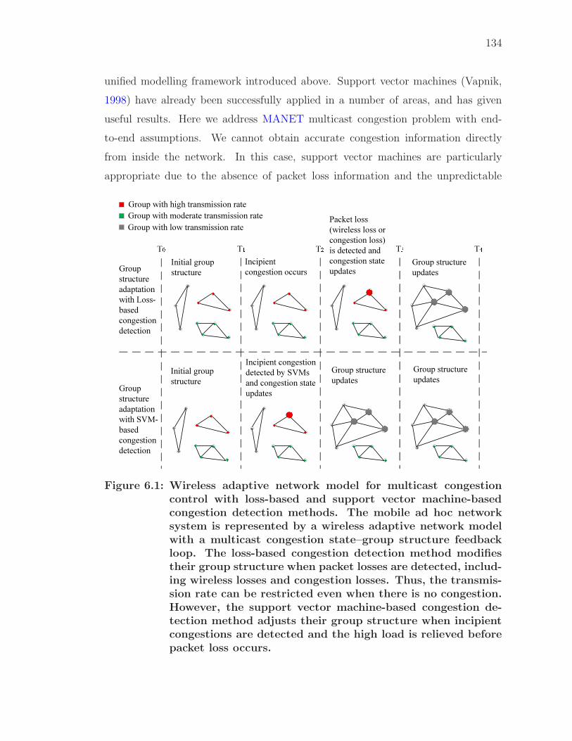
134
unified modelling framework introduced above. Support vector machines (Vapnik,
1998) have already been successfully applied in a number of areas, and has given
useful results. Here we address MANET multicast congestion problem with end-
to-end assumptions. We cannot obtain accurate congestion information directly
from inside the network. In this case, support vector machines are particularly
appropriate due to the absence of packet loss information and the unpredictable
Group structure adaptation with Loss-based congestion detection
Group structure adaptation with SVM-based congestion detection
Packet loss (wireless loss orcongestion loss)is detected and congestion state updates
Incipient congestion detected by SVMs and congestion state updates
Group structure updates
Group structure updates
Initial group structure
Initial group structure
Group with high transmission rate Group with moderate transmission rate Group with low transmission rate
T� T� T� T�T�Incipient congestion occurs
Group structure updates
Figure 6.1: Wireless adaptive network model for multicast congestioncontrol with loss-based and support vector machine-basedcongestion detection methods. The mobile ad hoc networksystem is represented by a wireless adaptive network modelwith a multicast congestion state–group structure feedbackloop. The loss-based congestion detection method modifiestheir group structure when packet losses are detected, includ-ing wireless losses and congestion losses. Thus, the transmis-sion rate can be restricted even when there is no congestion.However, the support vector machine-based congestion de-tection method adjusts their group structure when incipientcongestions are detected and the high load is relieved beforepacket loss occurs.
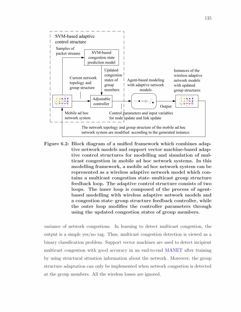
135
Adjustable controller Output
Control parameters and input variables for node update and link update
Samples of packet streams SVM-based
congestion state prediction model
Updated congestion states of group members
Mobile ad hoc network system
Instances of the wireless adaptivenetwork models with updated group structures
Agent-based modeling with adaptive network
models
The network topology and group structure of the mobile ad hoc network system are modified according to the generated instance.
Current network topology and group structure
SVM-based adaptive control structure
Figure 6.2: Block diagram of a unified framework which combines adap-tive network models and support vector machine-based adap-tive control structures for modelling and simulation of mul-ticast congestion in mobile ad hoc network systems. In thismodelling framework, a mobile ad hoc network system can berepresented as a wireless adaptive network model which con-tains a multicast congestion state–multicast group structurefeedback loop. The adaptive control structure consists of twoloops. The inner loop is composed of the process of agent-based modelling with wireless adaptive network models anda congestion state–group structure feedback controller, whilethe outer loop modifies the controller parameters throughusing the updated congestion states of group members.
variance of network congestions. In learning to detect multicast congestion, the
output is a simple yes/no tag. Thus, multicast congestion detection is viewed as a
binary classification problem. Support vector machines are used to detect incipient
multicast congestion with good accuracy in an end-to-end MANET after training
by using structural situation information about the network. Moreover, the group
structure adaptation can only be implemented when network congestion is detected
at the group members. All the wireless losses are ignored.
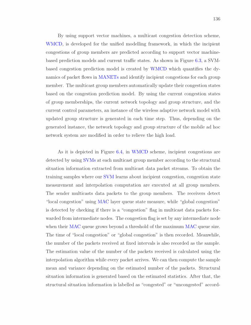
136
By using support vector machines, a multicast congestion detection scheme,
WMCD, is developed for the unified modelling framework, in which the incipient
congestions of group members are predicted according to support vector machine-
based prediction models and current traffic states. As shown in Figure 6.3, a SVM-
based congestion prediction model is created by WMCD which quantifies the dy-
namics of packet flows in MANETs and identify incipient congestions for each group
member. The multicast group members automatically update their congestion states
based on the congestion prediction model. By using the current congestion states
of group memberships, the current network topology and group structure, and the
current control parameters, an instance of the wireless adaptive network model with
updated group structure is generated in each time step. Thus, depending on the
generated instance, the network topology and group structure of the mobile ad hoc
network system are modified in order to relieve the high load.
As it is depicted in Figure 6.4, in WMCD scheme, incipient congestions are
detected by using SVMs at each multicast group member according to the structural
situation information extracted from multicast data packet streams. To obtain the
training samples where our SVM learns about incipient congestion, congestion state
measurement and interpolation computation are executed at all group members.
The sender multicasts data packets to the group members. The receivers detect
“local congestion” using MAC layer queue state measure, while “global congestion”
is detected by checking if there is a “congestion” flag in multicast data packets for-
warded from intermediate nodes. The congestion flag is set by any intermediate node
when their MAC queue grows beyond a threshold of the maximum MAC queue size.
The time of “local congestion” or “global congestion” is then recorded. Meanwhile,
the number of the packets received at fixed intervals is also recorded as the sample.
The estimation value of the number of the packets received is calculated using the
interpolation algorithm while every packet arrives. We can then compute the sample
mean and variance depending on the estimated number of the packets. Structural
situation information is generated based on the estimated statistics. After that, the
structural situation information is labelled as “congested” or “uncongested” accord-
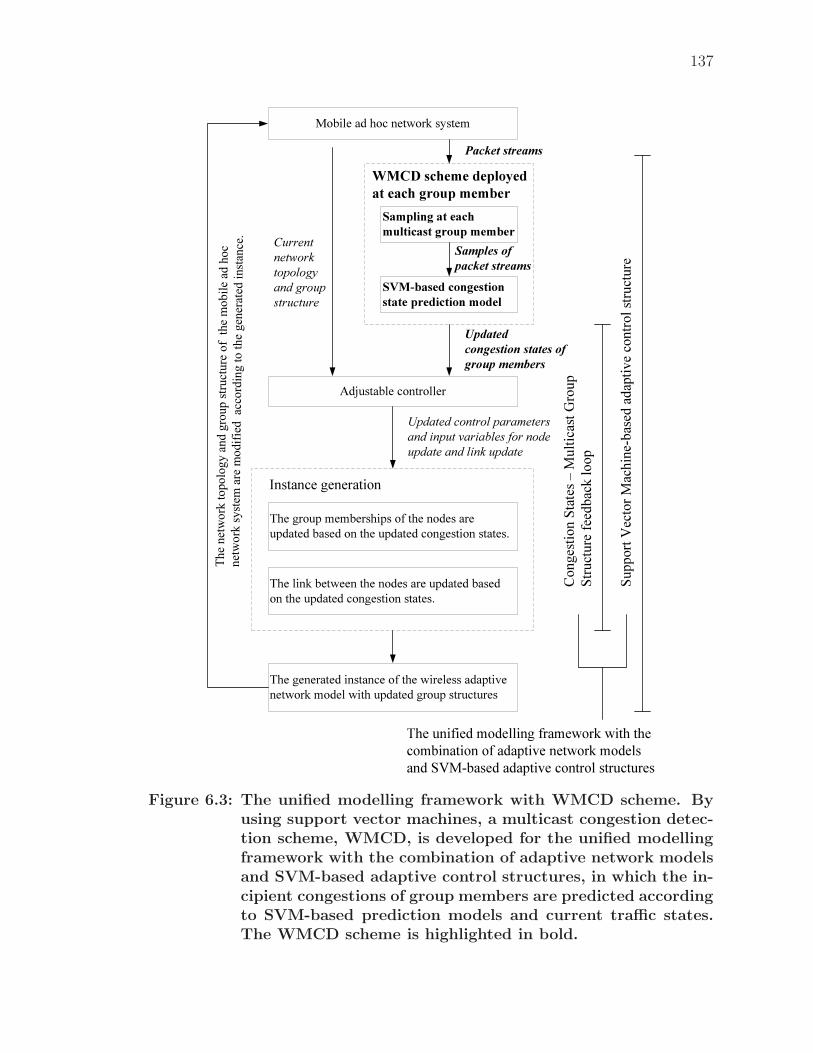
137
Sampling at each multicast group member
The group memberships of the nodes are updated based on the updated congestion states.
The link between the nodes are updated based on the updated congestion states.
The generated instance of the wireless adaptivenetwork model with updated group structures
Instance generation
Samples of packet streams
Updated control parameters and input variables for node update and link update
Adjustable controller
Cong
estion
State
s–Mu
lticast
Grou
p Str
uctur
e feed
back
loop
Supp
ort V
ector
Mach
ine-ba
sed ad
aptiv
e con
trol st
ructur
e
The unified modelling framework with the combination of adaptive network models and SVM-based adaptive control structures
SVM-based congestion state prediction model
Mobile ad hoc network system
Updated congestion states of group members
Current network topology and group structure
T he n
e two rk
t op o
lo gy a
n d g r
o up s
t ruc tu
re o f
the m
o bile
a d h o
c ne
two r k
syst e
m a re
mo d
ifi ed
a cco rd
in g to
t he g
e ner a
t ed i n
s tan c
e .
Packet streamsWMCD scheme deployed at each group member
Figure 6.3: The unified modelling framework with WMCD scheme. Byusing support vector machines, a multicast congestion detec-tion scheme, WMCD, is developed for the unified modellingframework with the combination of adaptive network modelsand SVM-based adaptive control structures, in which the in-cipient congestions of group members are predicted accordingto SVM-based prediction models and current traffic states.The WMCD scheme is highlighted in bold.
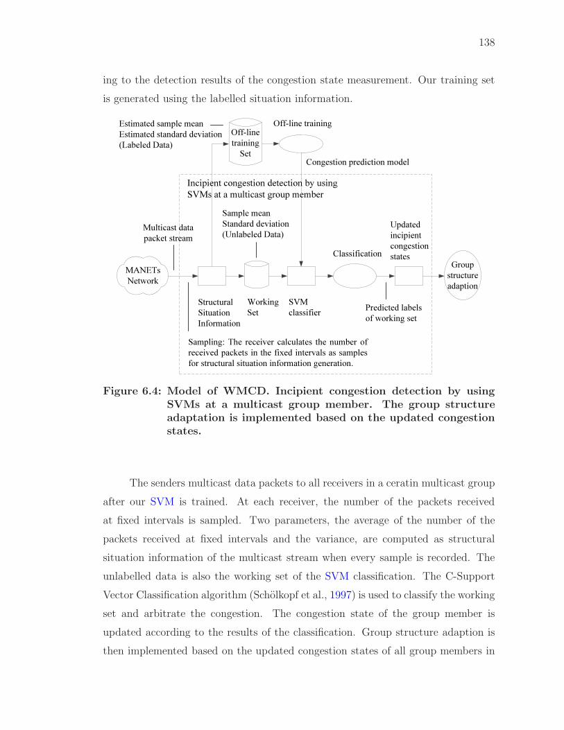
138
ing to the detection results of the congestion state measurement. Our training set
is generated using the labelled situation information.
Estimated sample meanEstimated standard deviation(Labeled Data)
Sample meanStandard deviation (Unlabeled Data)
Sampling: The receiver calculates the number of received packets in the fixed intervals as samples for structural situation information generation.
Off-line training
Set
MANETs Network
Predicted labels of working set
Multicast data packet stream
Incipient congestion detection by using SVMs at a multicast group member
Group structure adaption
Congestion prediction model
Classification
SVM classifier
Updated incipient congestion states
Structural Situation Information
Working Set
Off-line training
Figure 6.4: Model of WMCD. Incipient congestion detection by usingSVMs at a multicast group member. The group structureadaptation is implemented based on the updated congestionstates.
The senders multicast data packets to all receivers in a ceratin multicast group
after our SVM is trained. At each receiver, the number of the packets received
at fixed intervals is sampled. Two parameters, the average of the number of the
packets received at fixed intervals and the variance, are computed as structural
situation information of the multicast stream when every sample is recorded. The
unlabelled data is also the working set of the SVM classification. The C-Support
Vector Classification algorithm (Scholkopf et al., 1997) is used to classify the working
set and arbitrate the congestion. The congestion state of the group member is
updated according to the results of the classification. Group structure adaption is
then implemented based on the updated congestion states of all group members in
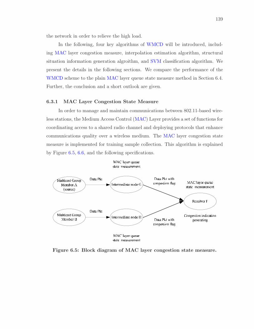
139
the network in order to relieve the high load.
In the following, four key algorithms of WMCD will be introduced, includ-
ing MAC layer congestion measure, interpolation estimation algorithm, structural
situation information generation algroithm, and SVM classification algorithm. We
present the details in the following sections. We compare the performance of the
WMCD scheme to the plain MAC layer queue state measure method in Section 6.4.
Further, the conclusion and a short outlook are given.
6.3.1 MAC Layer Congestion State Measure
In order to manage and maintain communications between 802.11-based wire-
less stations, the Medium Access Control (MAC) Layer provides a set of functions for
coordinating access to a shared radio channel and deploying protocols that enhance
communications quality over a wireless medium. The MAC layer congestion state
measure is implemented for training sample collection. This algorithm is explained
by Figure 6.5, 6.6, and the following specifications.
��� ��� ���������� ���� ��� ���������� ����� �� ������������ ���� �
������������ ���� � �� �� �� !"��� #$�"��� #$�
��% �&�� '������� ����������
��% �&�� '������� ����������
��% �&�� '������� ����������"��� #$� (��) ��*������ +�*"��� #$� (��) ��*������ +�* %��*������ ���� �����*��������*
Figure 6.5: Block diagram of MAC layer congestion state measure.
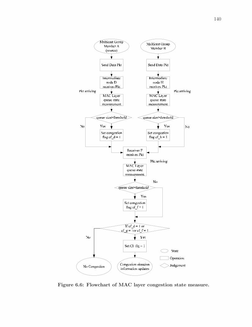
140
,-./ 0121 3425.2-67-/812-.9/- 06-:-8;-< 342 5.2-67-/812-.9/- =6-:-8;-< 342>?@28:1<2 A69?B>-7C-6 D>EF G1H-6I?-?- <212-7-1<?6-7-.2,-2 :9.J-<289.K@1J :KLM N OP-:-8;-6 Q6-:-8;-< 342>EF G1H-6I?-?- <212-7-1<?6-7-.2
,-2 :9.J-<289.K@1J :KLK N O,-2 F5LK@J N OF9.J-<289. <82?1289.8.K9671289. ?B/12-<R9 F9.J-<289.
>EF G1H-6I?-?- <212-7-1<?6-7-.2,-2 :9.J-<289.K@1J :KL/ N O
342 1668;8.J342 1668;8.JS-< R9R9 S-<
342 1668;8.JS-< R9
S-<R9
,-./ 0121 342>?@28:1<2 A69?B>-7C-6 ET<9?6:-U
,212-VB-61289.W?/J-7-.25K :KL/ N O96:KLJ N O96 :KLK N O
I?-?- <8X-Y2M6-<M9@/
I?-?- <8X-Y2M6-<M9@/ I?-?- <8X-Y2M6-<M9@/
Figure 6.6: Flowchart of MAC layer congestion state measure.
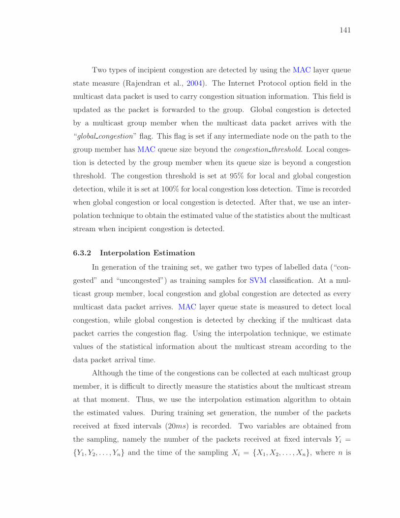
141
Two types of incipient congestion are detected by using the MAC layer queue
state measure (Rajendran et al., 2004). The Internet Protocol option field in the
multicast data packet is used to carry congestion situation information. This field is
updated as the packet is forwarded to the group. Global congestion is detected
by a multicast group member when the multicast data packet arrives with the
“global congestion” flag. This flag is set if any intermediate node on the path to the
group member has MAC queue size beyond the congestion threshold. Local conges-
tion is detected by the group member when its queue size is beyond a congestion
threshold. The congestion threshold is set at 95% for local and global congestion
detection, while it is set at 100% for local congestion loss detection. Time is recorded
when global congestion or local congestion is detected. After that, we use an inter-
polation technique to obtain the estimated value of the statistics about the multicast
stream when incipient congestion is detected.
6.3.2 Interpolation Estimation
In generation of the training set, we gather two types of labelled data (“con-
gested” and “uncongested”) as training samples for SVM classification. At a mul-
ticast group member, local congestion and global congestion are detected as every
multicast data packet arrives. MAC layer queue state is measured to detect local
congestion, while global congestion is detected by checking if the multicast data
packet carries the congestion flag. Using the interpolation technique, we estimate
values of the statistical information about the multicast stream according to the
data packet arrival time.
Although the time of the congestions can be collected at each multicast group
member, it is difficult to directly measure the statistics about the multicast stream
at that moment. Thus, we use the interpolation estimation algorithm to obtain
the estimated values. During training set generation, the number of the packets
received at fixed intervals (20ms) is recorded. Two variables are obtained from
the sampling, namely the number of the packets received at fixed intervals Yi =
{Y1, Y2, . . . , Yn} and the time of the sampling Xi = {X1, X2, . . . , Xn}, where n is
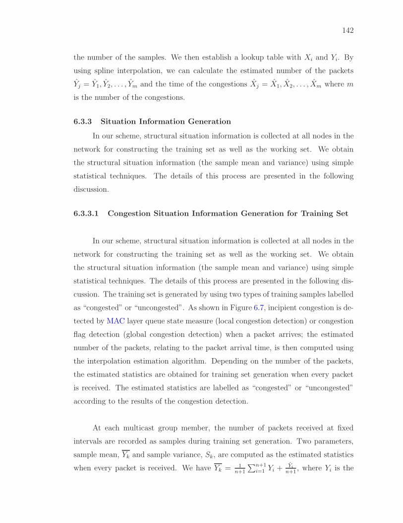
142
the number of the samples. We then establish a lookup table with Xi and Yi. By
using spline interpolation, we can calculate the estimated number of the packets
Yj = Y1, Y2, . . . , Ym and the time of the congestions Xj = X1, X2, . . . , Xm where m
is the number of the congestions.
6.3.3 Situation Information Generation
In our scheme, structural situation information is collected at all nodes in the
network for constructing the training set as well as the working set. We obtain
the structural situation information (the sample mean and variance) using simple
statistical techniques. The details of this process are presented in the following
discussion.
6.3.3.1 Congestion Situation Information Generation for Training Set
In our scheme, structural situation information is collected at all nodes in the
network for constructing the training set as well as the working set. We obtain
the structural situation information (the sample mean and variance) using simple
statistical techniques. The details of this process are presented in the following dis-
cussion. The training set is generated by using two types of training samples labelled
as “congested” or “uncongested”. As shown in Figure 6.7, incipient congestion is de-
tected by MAC layer queue state measure (local congestion detection) or congestion
flag detection (global congestion detection) when a packet arrives; the estimated
number of the packets, relating to the packet arrival time, is then computed using
the interpolation estimation algorithm. Depending on the number of the packets,
the estimated statistics are obtained for training set generation when every packet
is received. The estimated statistics are labelled as “congested” or “uncongested”
according to the results of the congestion detection.
At each multicast group member, the number of packets received at fixed
intervals are recorded as samples during training set generation. Two parameters,
sample mean, Yk and sample variance, Sk, are computed as the estimated statistics
when every packet is received. We have Yk = 1n+1
∑n+1i=1 Yi + Yi
n+1, where Yi is the
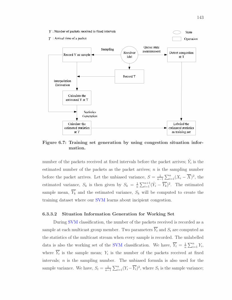
143
Z[\[]\ ]^_`[a\b^_c\ de\c\[fg[hc\b^_i[]^hj k ca aclgm[
i[]^hj declgmb_`noplq[h ^r gc]s[\a h[][bt[j b_ rbu[j b_\[htcmaY
T n vhhbtcm \bl[ ^r c gc]s[\w_\[hg^mc\b^_xa\blc\b^_
yp[p[ a\c\[l[caph[l[_\zcm]pmc\[ \{[[a\blc\[j k c\ d
|cq[m[j \{[[a\blc\[j a\c\ba\b]aca \hcb_b_` a[\zcm]pmc\[ \{[[a\blc\[j a\c\ba\b]ac\ de\c\ba\b]a}[_[hc\b^_
i[][bt[hwj[m
Figure 6.7: Training set generation by using congestion situation infor-mation.
number of the packets received at fixed intervals before the packet arrives; Yi is the
estimated number of the packets as the packet arrives; n is the sampling number
before the packet arrives. Let the unbiased variance, S = 1n−1
∑ni=1(Xi − X)2, the
estimated variance, Sk is then given by Sk = 1n
∑n+1i=1 (Yi − Yk)
2. The estimated
sample mean, Yk and the estimated variance, Sk will be computed to create the
training dataset where our SVM learns about incipient congestion.
6.3.3.2 Situation Information Generation for Working Set
During SVM classification, the number of the packets received is recorded as a
sample at each multicast group member. Two parameters Yt and St are computed as
the statistics of the multicast stream when every sample is recorded. The unlabelled
data is also the working set of the SVM classification. We have, Yt = 1n
∑ni=1 Yi,
where Yt is the sample mean; Yi is the number of the packets received at fixed
intervals; n is the sampling number. The unbiased formula is also used for the
sample variance. We have, St = 1n−1
∑ni=1(Yi−Yt)
2, where St is the sample variance;
144
Yi is the number of the packets received at the fixed intervals; Yt is the sample mean
and n is the sampling number.
6.3.4 Support Vector Classification
Support Vector Machines (Vapnik, 1998) is one type of learning method con-
structed by Vapnik and Cortes. It is used in our scheme to detect incipient conges-
tion that occurs within a time series. We chose to use the SVM since it has been
successfully applied in many fields, such as word sense disambiguation, text classi-
fication, part-of-speech tagging, web page classification, and question classification
(Vapnik, 1998). SVM first maps input space into some high dimensional feature
space, then constructs a linear decision surface in this feature space that relates to
a non-linear decision surface in the original input space. The comparison between
SVM and other classification methods is given by (Rumelhart & Hinton, 1986; Ben-
nett & Blue, 1997; Chang & Lin, 2001). In our scheme, a congestion prediction
model generated by using Scholkopf et al.’s C–Support Vector Classification algo-
rithm (Scholkopf et al., 1997) is used to classify the statistics of multicast stream
and arbitrate the congestion according to the dynamics of multicast packet streams.
6.4 Simulations and Experiments
To evaluate our WMCD scheme, we performed a set of simulations for different
scenarios that may affect the performance of the proposed scheme. First of all, we
collected congestion situation information of packet streams from several QualNet
(Scalable Networks) simulations, and established a training set by using the situation
information. After off-line training, the generated SVM-based congestion prediction
model was used for congestion detection in different simulation scenarios. In order
to estimate the classification accuracy of the WMCD scheme, a set of simulations
was implemented which compared the classification results of the WMCD scheme
to the detection results of the MAC layer queue state measure method. We also
performed a set of simulations with group structure adaptation for evaluating the
performance of our WMCD scheme, while the unified modelling framework was used
for multicast congestion control in MANETs.
145
6.4.1 Stream Situation Information Collection
In all QualNet (Scalable Networks) simulations, on-demand multicast rout-
ing protocol (ODMRP) (Lee et al., 1999) and ad hoc on-demand distance vector
routing (AODV) (Perkins & Royer, 1999) are used as the underlying multicast and
unicast routing protocols, respectively. The link bandwidth is 112,000 bps. The
MAC protocol used is IEEE Standard 802.11b, (1999). The simulation time is 60
seconds. We first collect the samples and record each packet’s arrival time on the
simple topology in Figure 6.8. Ten multicast group members are placed randomly
in a 100m × 100m field and they can join or leave the two multicast groups with
different transmission rates (high and low) in the same time according to the up-
dated congestion states. Five randomly selected group members continuously send
multicast constant bit rate (MCBR) traffic throughout the whole duration of the
simulation with payload size of 512 bytes, while another five group members are
receivers. The results are averaged over 10 runs and presented with 95% confidence.
Three QualNet (Scalable Networks) simulation scenarios are established for WMCD
performance evaluation, including local congestion detection, global congestion de-
tection, and local congestion loss detection. At this group member, the number of
the packets received at fixed intervals (20ms), is recorded as a sample. The arrival
time of each packet is also gathered for training set generation. The time samples
are labelled as “congested” or “uncongested” based on the results of the congestion
detection.
6.4.2 Training Set Generation and SVM Training
After obtaining the congestion situation information from QualNet (Scalable
Networks), we generate the training set for our SVM using statistical methods (see
Section 6.3.3.1). Chang and Lin’s LIBSVM (Chang & Lin, 2001) is used to train
and optimize our SVM. LIBSVM is an integrated software package for support
vector classification (C-SVC, nu-SVC), regression (epsilon-SVR, nu-SVR) and dis-
tribution estimation (one-class SVM). To choose the best parameters of our SVM,
grid.py, a model selection tool in LIBSVM is used for C-SVM classification. It
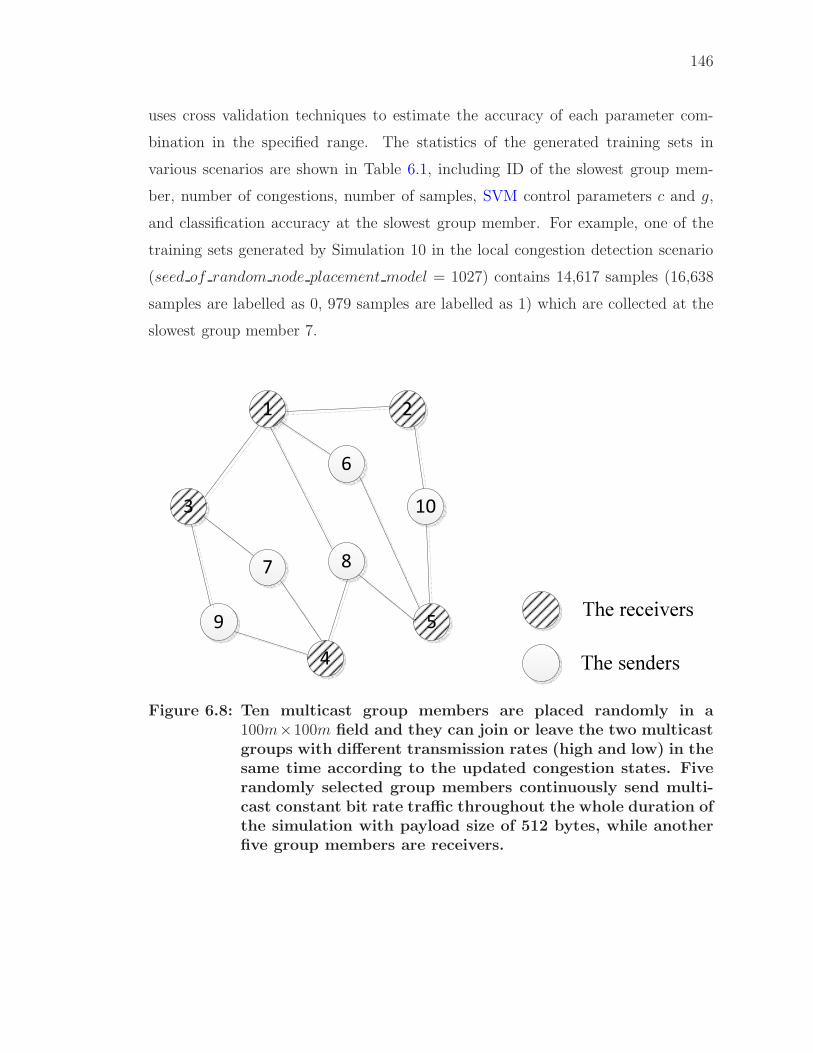
146
uses cross validation techniques to estimate the accuracy of each parameter com-
bination in the specified range. The statistics of the generated training sets in
various scenarios are shown in Table 6.1, including ID of the slowest group mem-
ber, number of congestions, number of samples, SVM control parameters c and g,
and classification accuracy at the slowest group member. For example, one of the
training sets generated by Simulation 10 in the local congestion detection scenario
(seed of random node placement model = 1027) contains 14,617 samples (16,638
samples are labelled as 0, 979 samples are labelled as 1) which are collected at the
slowest group member 7.
1 2
6
4
7 8
3
59
10
The receivers
The senders
Figure 6.8: Ten multicast group members are placed randomly in a100m×100m field and they can join or leave the two multicastgroups with different transmission rates (high and low) in thesame time according to the updated congestion states. Fiverandomly selected group members continuously send multi-cast constant bit rate traffic throughout the whole duration ofthe simulation with payload size of 512 bytes, while anotherfive group members are receivers.
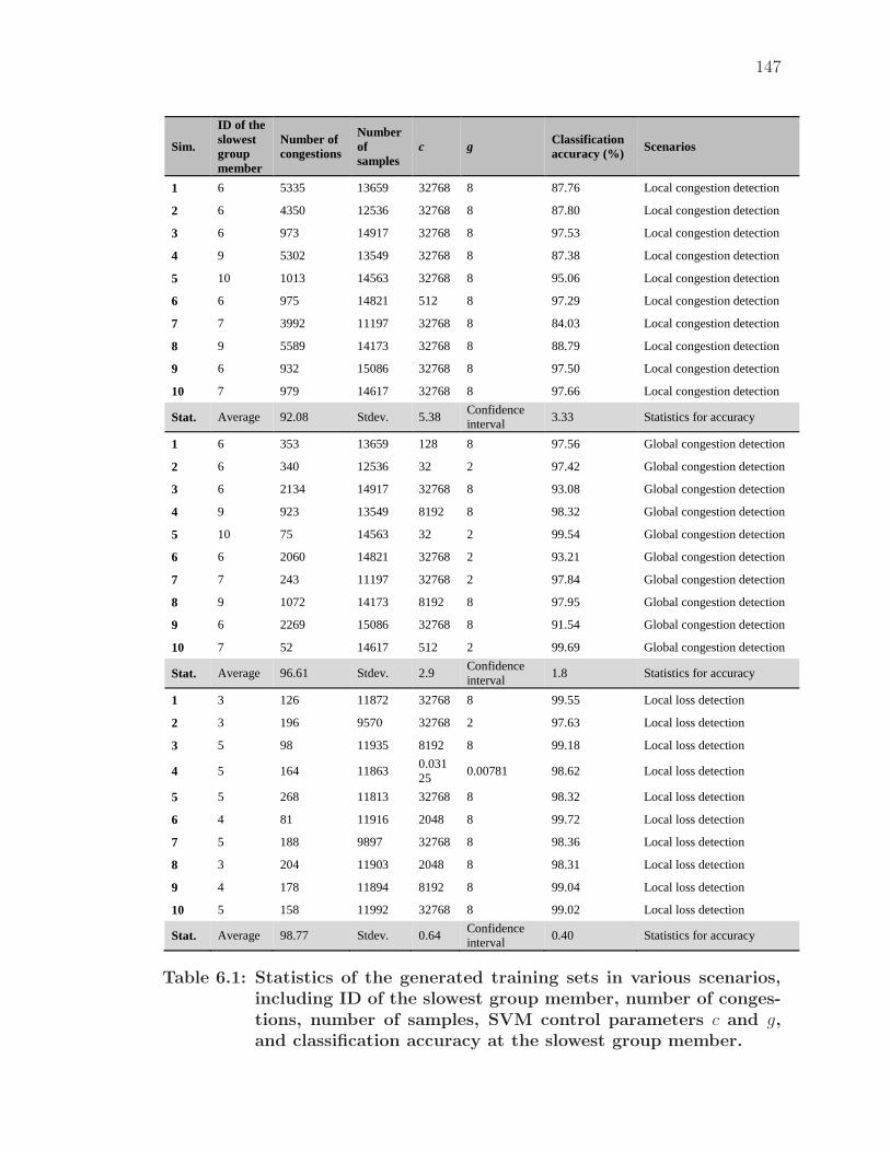
147
Sim.
ID of the slowest group member
Number of congestions
Number of samples
c g Classification accuracy (%) Scenarios
1 6 5335 13659 32768 8 87.76 Local congestion detection
2 6 4350 12536 32768 8 87.80 Local congestion detection
3 6 973 14917 32768 8 97.53 Local congestion detection
4 9 5302 13549 32768 8 87.38 Local congestion detection
5 10 1013 14563 32768 8 95.06 Local congestion detection
6 6 975 14821 512 8 97.29 Local congestion detection
7 7 3992 11197 32768 8 84.03 Local congestion detection
8 9 5589 14173 32768 8 88.79 Local congestion detection
9 6 932 15086 32768 8 97.50 Local congestion detection
10 7 979 14617 32768 8 97.66 Local congestion detection
Stat. Average 92.08 Stdev. 5.38 Confidence interval
3.33 Statistics for accuracy
1 6 353 13659 128 8 97.56 Global congestion detection
2 6 340 12536 32 2 97.42 Global congestion detection
3 6 2134 14917 32768 8 93.08 Global congestion detection
4 9 923 13549 8192 8 98.32 Global congestion detection
5 10 75 14563 32 2 99.54 Global congestion detection
6 6 2060 14821 32768 2 93.21 Global congestion detection
7 7 243 11197 32768 2 97.84 Global congestion detection
8 9 1072 14173 8192 8 97.95 Global congestion detection
9 6 2269 15086 32768 8 91.54 Global congestion detection
10 7 52 14617 512 2 99.69 Global congestion detection
Stat. Average 96.61 Stdev. 2.9 Confidence interval
1.8 Statistics for accuracy
1 3 126 11872 32768 8 99.55 Local loss detection
2 3 196 9570 32768 2 97.63 Local loss detection
3 5 98 11935 8192 8 99.18 Local loss detection
4 5 164 11863 0.03125
0.00781 98.62 Local loss detection
5 5 268 11813 32768 8 98.32 Local loss detection
6 4 81 11916 2048 8 99.72 Local loss detection
7 5 188 9897 32768 8 98.36 Local loss detection
8 3 204 11903 2048 8 98.31 Local loss detection
9 4 178 11894 8192 8 99.04 Local loss detection
10 5 158 11992 32768 8 99.02 Local loss detection
Stat. Average 98.77 Stdev. 0.64 Confidence interval
0.40 Statistics for accuracy
Table 6.1: Statistics of the generated training sets in various scenarios,including ID of the slowest group member, number of conges-tions, number of samples, SVM control parameters c and g,and classification accuracy at the slowest group member.
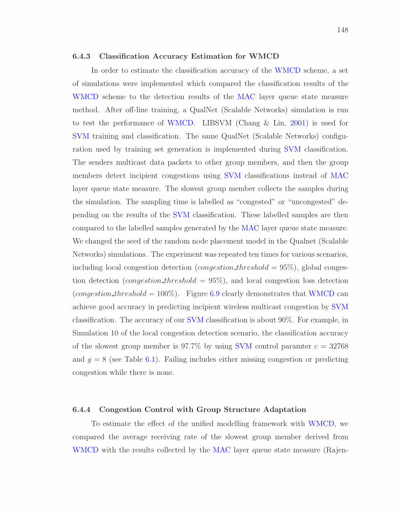
148
6.4.3 Classification Accuracy Estimation for WMCD
In order to estimate the classification accuracy of the WMCD scheme, a set
of simulations were implemented which compared the classification results of the
WMCD scheme to the detection results of the MAC layer queue state measure
method. After off-line training, a QualNet (Scalable Networks) simulation is run
to test the performance of WMCD. LIBSVM (Chang & Lin, 2001) is used for
SVM training and classification. The same QualNet (Scalable Networks) configu-
ration used by training set generation is implemented during SVM classification.
The senders multicast data packets to other group members, and then the group
members detect incipient congestions using SVM classifications instead of MAC
layer queue state measure. The slowest group member collects the samples during
the simulation. The sampling time is labelled as “congested” or “uncongested” de-
pending on the results of the SVM classification. These labelled samples are then
compared to the labelled samples generated by the MAC layer queue state measure.
We changed the seed of the random node placement model in the Qualnet (Scalable
Networks) simulations. The experiment was repeated ten times for various scenarios,
including local congestion detection (congestion threshold = 95%), global conges-
tion detection (congestion threshold = 95%), and local congestion loss detection
(congestion threshold = 100%). Figure 6.9 clearly demonstrates that WMCD can
achieve good accuracy in predicting incipient wireless multicast congestion by SVM
classification. The accuracy of our SVM classification is about 90%. For example, in
Simulation 10 of the local congestion detection scenario, the classification accuracy
of the slowest group member is 97.7% by using SVM control paramter c = 32768
and g = 8 (see Table 6.1). Failing includes either missing congestion or predicting
congestion while there is none.
6.4.4 Congestion Control with Group Structure Adaptation
To estimate the effect of the unified modelling framework with WMCD, we
compared the average receiving rate of the slowest group member derived from
WMCD with the results collected by the MAC layer queue state measure (Rajen-
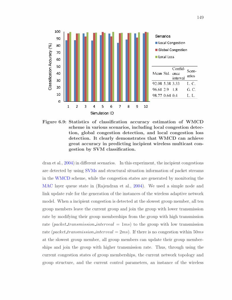
149
~�~�~�~�~�~�~�~�~�~�~~
� � � � � � � � � �~
����� ���������������� ��������������� ������������
���� �¡��� ¢£¤¥¦§§©ª¦«¬®ªª°¦ª±²³
µ¶·¸ ¹º»¼ ½¾¸¿ÀÁ»¶¸Â¶ ¹¶¸·ÁÃÀ¾ÄÅƼÇÈ É¼ÊÈ Ê¼ÊÊ Ë¼ ½¼Å̼ÌÍ Æ¼Å Í¼È Î¼ ½¼ÅȼÏÏ Ç¼ÌРǼР˼ ˼Figure 6.9: Statistics of classification accuracy estimation of WMCD
scheme in various scenarios, including local congestion detec-tion, global congestion detection, and local congestion lossdetection. It clearly demonstrates that WMCD can achievegreat accuracy in predicting incipient wireless multicast con-gestion by SVM classification.
dran et al., 2004) in different scenarios. In this experiment, the incipient congestions
are detected by using SVMs and structural situation information of packet streams
in the WMCD scheme, while the congestion states are generated by monitoring the
MAC layer queue state in (Rajendran et al., 2004). We used a simple node and
link update rule for the generation of the instances of the wireless adaptive network
model. When a incipient congestion is detected at the slowest group member, all ten
group members leave the current group and join the group with lower transmission
rate by modifying their group memberships from the group with high transmission
rate (packet transmission interveal = 1ms) to the group with low transmission
rate (packet transmission interveal = 2ms). If there is no congestion within 50ms
at the slowest group member, all group members can update their group member-
ships and join the group with higher transmission rate. Thus, through using the
current congestion states of group memberships, the current network topology and
group structure, and the current control parameters, an instance of the wireless
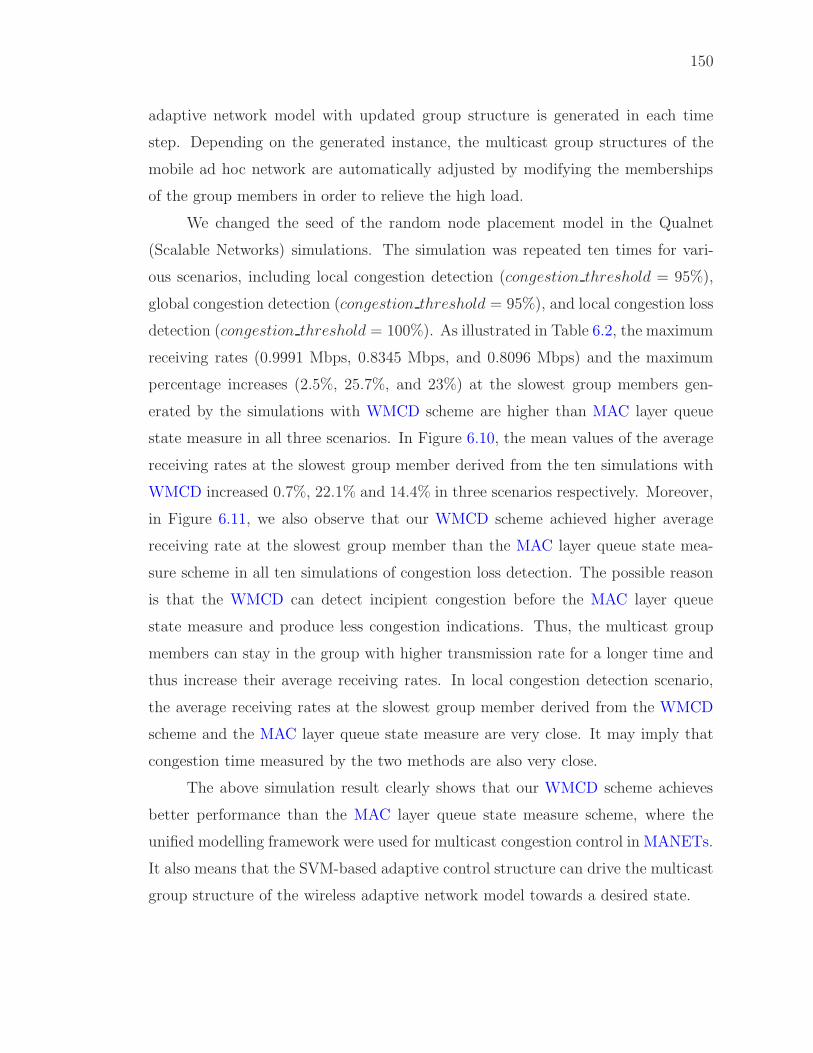
150
adaptive network model with updated group structure is generated in each time
step. Depending on the generated instance, the multicast group structures of the
mobile ad hoc network are automatically adjusted by modifying the memberships
of the group members in order to relieve the high load.
We changed the seed of the random node placement model in the Qualnet
(Scalable Networks) simulations. The simulation was repeated ten times for vari-
ous scenarios, including local congestion detection (congestion threshold = 95%),
global congestion detection (congestion threshold = 95%), and local congestion loss
detection (congestion threshold = 100%). As illustrated in Table 6.2, the maximum
receiving rates (0.9991 Mbps, 0.8345 Mbps, and 0.8096 Mbps) and the maximum
percentage increases (2.5%, 25.7%, and 23%) at the slowest group members gen-
erated by the simulations with WMCD scheme are higher than MAC layer queue
state measure in all three scenarios. In Figure 6.10, the mean values of the average
receiving rates at the slowest group member derived from the ten simulations with
WMCD increased 0.7%, 22.1% and 14.4% in three scenarios respectively. Moreover,
in Figure 6.11, we also observe that our WMCD scheme achieved higher average
receiving rate at the slowest group member than the MAC layer queue state mea-
sure scheme in all ten simulations of congestion loss detection. The possible reason
is that the WMCD can detect incipient congestion before the MAC layer queue
state measure and produce less congestion indications. Thus, the multicast group
members can stay in the group with higher transmission rate for a longer time and
thus increase their average receiving rates. In local congestion detection scenario,
the average receiving rates at the slowest group member derived from the WMCD
scheme and the MAC layer queue state measure are very close. It may imply that
congestion time measured by the two methods are also very close.
The above simulation result clearly shows that our WMCD scheme achieves
better performance than the MAC layer queue state measure scheme, where the
unified modelling framework were used for multicast congestion control in MANETs.
It also means that the SVM-based adaptive control structure can drive the multicast
group structure of the wireless adaptive network model towards a desired state.
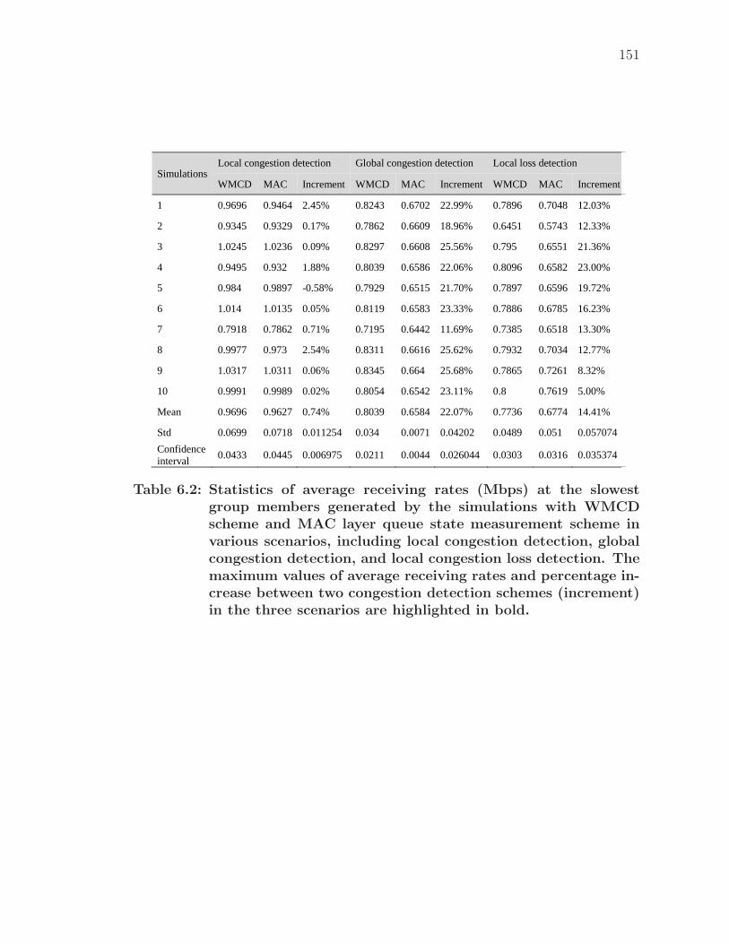
151
Simulations Local congestion detection Global congestion detection Local loss detection
WMCD MAC Increment WMCD MAC Increment WMCD MAC Increment
1 0.9696 0.9464 2.45% 0.8243 0.6702 22.99% 0.7896 0.7048 12.03%
2 0.9345 0.9329 0.17% 0.7862 0.6609 18.96% 0.6451 0.5743 12.33%
3 1.0245 1.0236 0.09% 0.8297 0.6608 25.56% 0.795 0.6551 21.36%
4 0.9495 0.932 1.88% 0.8039 0.6586 22.06% 0.8096 0.6582 23.00%
5 0.984 0.9897 -0.58% 0.7929 0.6515 21.70% 0.7897 0.6596 19.72%
6 1.014 1.0135 0.05% 0.8119 0.6583 23.33% 0.7886 0.6785 16.23%
7 0.7918 0.7862 0.71% 0.7195 0.6442 11.69% 0.7385 0.6518 13.30%
8 0.9977 0.973 2.54% 0.8311 0.6616 25.62% 0.7932 0.7034 12.77%
9 1.0317 1.0311 0.06% 0.8345 0.664 25.68% 0.7865 0.7261 8.32%
10 0.9991 0.9989 0.02% 0.8054 0.6542 23.11% 0.8 0.7619 5.00%
Mean 0.9696 0.9627 0.74% 0.8039 0.6584 22.07% 0.7736 0.6774 14.41%
Std 0.0699 0.0718 0.011254 0.034 0.0071 0.04202 0.0489 0.051 0.057074
Confidence interval
0.0433 0.0445 0.006975 0.0211 0.0044 0.026044 0.0303 0.0316 0.035374
Table 6.2: Statistics of average receiving rates (Mbps) at the slowestgroup members generated by the simulations with WMCDscheme and MAC layer queue state measurement scheme invarious scenarios, including local congestion detection, globalcongestion detection, and local congestion loss detection. Themaximum values of average receiving rates and percentage in-crease between two congestion detection schemes (increment)in the three scenarios are highlighted in bold.
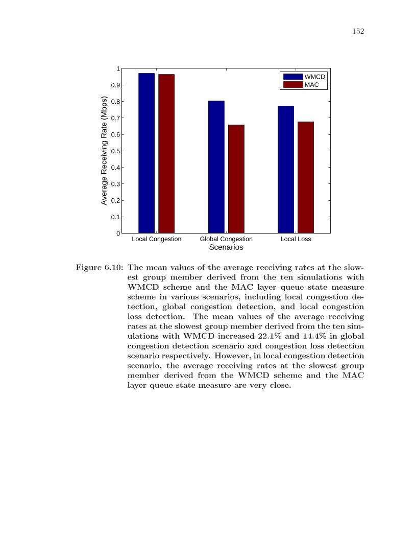
152
Local Congestion Global Congestion Local Loss0
0.1
0.2
0.3
0.4
0.5
0.6
0.7
0.8
0.9
1
Scenarios
Ave
rage
Rec
eivi
ng R
ate
(Mbp
s)
WMCDMAC
Figure 6.10: The mean values of the average receiving rates at the slow-est group member derived from the ten simulations withWMCD scheme and the MAC layer queue state measurescheme in various scenarios, including local congestion de-tection, global congestion detection, and local congestionloss detection. The mean values of the average receivingrates at the slowest group member derived from the ten sim-ulations with WMCD increased 22.1% and 14.4% in globalcongestion detection scenario and congestion loss detectionscenario respectively. However, in local congestion detectionscenario, the average receiving rates at the slowest groupmember derived from the WMCD scheme and the MAClayer queue state measure are very close.
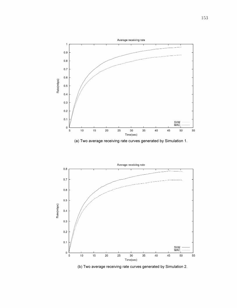
153
(a) Two average receiving rate curves generated by Simulation 1.
(b) Two average receiving rate curves generated by Simulation 2.
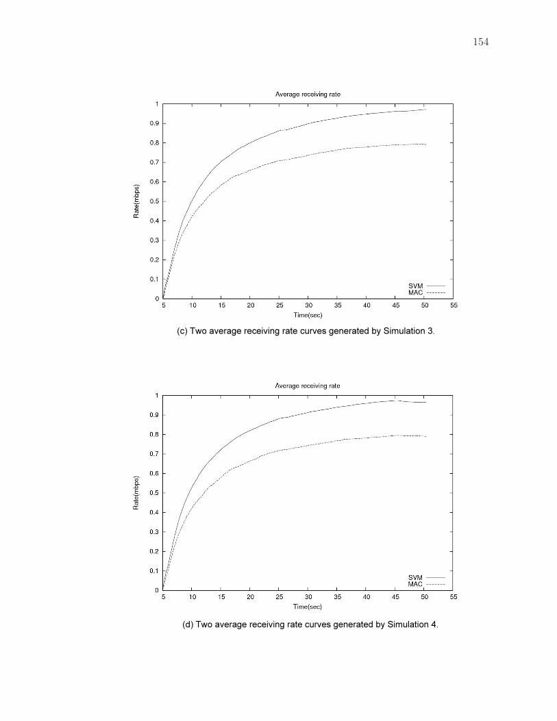
154
(c) Two average receiving rate curves generated by Simulation 3.
(d) Two average receiving rate curves generated by Simulation 4.
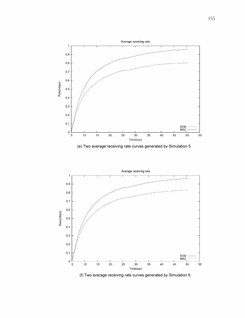
155
(e) Two average receiving rate curves generated by Simulation 5.
(f) Two average receiving rate curves generated by Simulation 6.
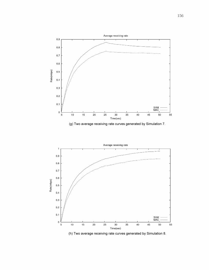
156
(g) Two average receiving rate curves generated by Simulation 7.
(h) Two average receiving rate curves generated by Simulation 8.
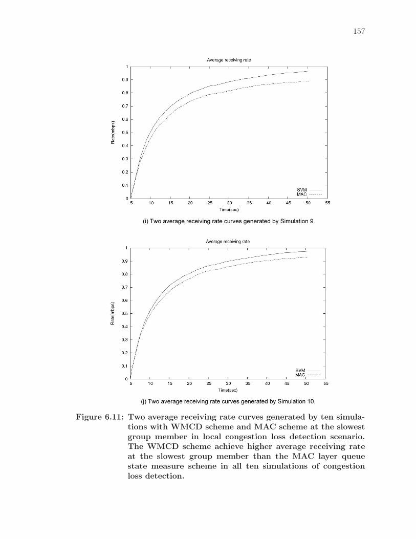
157
(i) Two average receiving rate curves generated by Simulation 9.
(j) Two average receiving rate curves generated by Simulation 10.
Figure 6.11: Two average receiving rate curves generated by ten simula-tions with WMCD scheme and MAC scheme at the slowestgroup member in local congestion loss detection scenario.The WMCD scheme achieve higher average receiving rateat the slowest group member than the MAC layer queuestate measure scheme in all ten simulations of congestionloss detection.
158
6.5 Summary
In this work, we have described a unified framework which combines adaptive
network models and support vector machine-based adaptive control structures for
modelling and simulation of multicast congestion in mobile ad hoc network systems.
By automatically adjusting network structures according to the dynamics of multi-
cast packet streams, this framework allows researchers to adopt a suitable framework
level on the basis of available network performance metrics, computational models
of network management, their research study objectives and expected outcomes,
thus allowing them to better understand, describe, predict, and control the multi-
cast congestion in mobile ad hoc network systems. In this framework, a mobile ad
hoc network system can be represented as an agent-based adaptive network which is
defined by a feedback loop between the congestion states of group members and the
group structure of the network, where the support vector machine-based adaptive
control structures are used for driving the group structure of the wireless adaptive
network model towards a desired state based on the prediction of incipient conges-
tions. By using such a unified modelling framework, a set of instances of the wireless
adaptive network model can be automatically generated through using structural
situation information about the multicast packet streams. The generated instances
with various group structures can improve the multicast transport performance in
mobile ad hoc network systems because the high load can be relieved by group
structure adaptation.
In the present work, a multicast congestion detection scheme, WMCD, has
been developed for the unified modelling framework, in which the incipient conges-
tions of group members can be predicted by using support vector machine-based
prediction models and current traffic states. In this scheme, a congestion predic-
tion model is created by SVMs which quantifies the dynamics of multicast packet
flows. The multicast group members then automatically update their congestion
states based on the congestion prediction model. By using the updated congestion
states, a set of instances of the wireless adaptive network model with updated group
structures are generated for dynamically adjusts the network topology and group
structure of the mobile ad hoc network system and relieving the high load.
159
Our WMCD scheme can estimate the congestions before packet loss occurs at
each group member using a SVM. Therefore, WMCD does not require acknowl-
edge equivalent and negatively acknowledge equivalent feedbacks from receivers.
Additionally, WMCD scheme requires no computation procedure for congestion es-
timation at the multicast source. While our scheme detects the congestion without
introducing packet loss, other congestion control approaches only do the simplest
packet loss detection at the group members. WMCD only updates the congestion
states of group members for group structure adaptation according to the results of
the SVM classification. Wireless losses are suppressed to prevent adjusting group
structure improperly. The simulation results illustrate that our SVM-based WMCD
scheme achieves great accuracy in predicting multicast congestion. Furthermore,
the network’s throughput capacity is efficiently improved through using the unified
modelling framework, which dynamically adjusting the group structures according
to the updated congestion states of group members generated by the WMCD scheme
in order to relieve the high load.
Some approaches with machine learning have been applied to tackle network
congestion management problems, such as Wang et al.’s scheme (Wang et al., 2007),
Kang et al.’s work (Kang et al., 2009), and EI Khayat et al.’s work (EI Khayat et
al., 2010). In comparison, our scheme is a receiver-based end-to-end multicast con-
gestion detection scheme for MANETs. It does not require special support from
other network management protocols. Furthermore, WMCD uses structural situ-
ation information (average number of the packets and variance) as the input data
for SVM, while the methods mentioned above collect the traffic patterns (including
packet delay, link quality indication metrics, etc.) for supervised learning. Our pre-
vious work (Liu & Omlin, 2010) also uses structural stream information to detect
incipient multicast congestion. However it only works in wired networks. We realize
that many problems still exist for which this approach is applicable, however, pre-
dicting congestion is the first step towards a unified framework for modelling and
simulation of multicast congestion in mobile ad hoc network systems.
Wireless network congestion is a problem that changes very quickly. Any algo-
rithm detecting congestion would have to render the decision before the problem has
160
changed to a degree that the decision is no longer relevant to the environment. Once
trained, a SVM can render decisions very quickly. Therefore, the SVM is an ap-
propriate mechanism for decision making in proactive wireless multicast congestion
detection, and should be the target of more research. Moreover, the network perfor-
mance can be effectively improved through using the unified modelling framework
which combines adaptive network models and support vector machine-based adap-
tive control structures. Although the interaction between the dynamics of packet
streams and the complex topologies in mobile ad hoc networks has not been studied
in much detail in this work, it seems to provide a powerful modelling tool to build
up large-scale structures from simple building blocks .
In the future work, we will investigate how different machine learning algo-
rithms affect the performance of WMCD, such as neural networks, decision tree, etc.
We will also investigate the temporal correlation of network congestions and improve
the performance of WMCD with better congestion prediction models. Moreover, we
also plan to update the WMCD scheme with a cost estimator, in which the routing
and congestion control costs of a set of instances are measured, in order to gener-
ate the enhanced wireless adaptive network models with the minimum routing and
congestion control costs.
CHAPTER 7
Conclusion and Future Work
This thesis represents the first steps towards the solution of modelling and simulation
of various real-world adaptive networks within a unified framework which combines
adaptive network models and adaptive control structures. In this framework, the
state-topology coevolution of an adaptive network model is specified by various
adaptive control structures. Moreover, through dynamically adjusting the controller
parameters in terms of the observations of a real-world complex system, the adaptive
interplay between state and topology as a dynamic feedback can drive an adaptive
network model towards desired target states. Having such an automated modelling
framework would greatly reduce the human effort and provide a valuable tool for
better understanding, description, prediction, and control of the real-world complex
systems around us. This unified modelling framework can also allow implementing
comprehensive complex network system inter-/multi-disciplinary research studies
based on available empirical data and computation models from different research
fields. It has brought a unique approach to modelling and simulation of real-world
complex systems.
In Chapter 3, a unified framework was proposed for modelling and simulation
of complex systems using a combination of adaptive network models and adaptive
control structures. While the process of modelling and simulation is considered as a
control system with a state-topology feedback, this framework is not only able to au-
tomatically generate enhanced adaptive network models based on the observations
of real-world complex systems, but also provide a systematic approach for automatic
adjustment of control parameters in order to achieve or to maintain a desired topo-
logical property for the corresponding adaptive network models. Moreover, through
tracing various reference values, the generated adaptive network models can have
different structures which are similar to the studied complex systems when the sys-
tems change. While this chapter can be considered a generalized methodology, we
discussed how this unified framework can be useful for modelling and simulation
161
162
of complex systems by the combination of adaptive network models and adaptive
control structures.
In Chapter 4, a unified framework which combines adaptive network mod-
els and adaptive control structures was proposed for modelling and simulation of
fractured-rock aquifer systems. In this framework, the adaptive control structures
with iterative parameter identification were used to identifying an instance of an frac-
ture adaptive network model with the desired topological characteristics, where the
natural fracture network can be represented by the fracture adaptive network mod-
els with “state-topology” coevolution. By using this modelling framework, a user-
friendly modelling tool, Fracture3D, has been developed for automatically building
enhanced fracture adaptive network models, in which the fracture statistics and the
structural properties can both follow the observed statistics from natural fracture
networks. Through using simple field data and measurements taken on site or in-
situ such as length, orientation, and density of measured fractures, the enhanced
fracture adaptive network models can be built for rapidly evaluating the connectiv-
ity of the studied aquifers on a broad range of scales. For illustration purpose, we
have applied the proposed unified modelling framework and automatic modelling
tool Fracture3D on a real-world fractured-rock aquifer systems, and a set of the
enhanced 3–D fracture adaptive network models with desired topological character-
istics has been created by using Fracture3D. Through using label-propagation based
cluster identification and Fracture fMRI techniques, the quantitative topological in-
formation extracted from these fracture adaptive network models have been used
for understanding, description, and prediction of the groundwater flow and trans-
port processes. Moreover, these quantitative data have also been used for studying
parameter uncertainty of modelling and simulation in the studied fractured-rock
aquifer systems. The simulations clearly show that the coupling between the frac-
ture adaptive network models and the adaptive control structures with iterative
parameter identification can drive the network topology towards a desired state by
dynamically updating the geometrical states of fractures (size and profile of frac-
tures) with a proper adaptive control structure.
In Chapter 5, a unified framework which combines adaptive network models
163
and multiple model adaptive control structures was proposed for modelling and sim-
ulation of social network systems. In this framework, a real-world social network
system can be represented as an agent-based adaptive network which are defined by
a feedback loop between behavioural state of individuals and community structure of
the studied system, where a multiple model adaptive control structure is used for the
predetermination of suitable computational models of behavioural state update and
social interaction update in order to improve the performance of modelling and sim-
ulation. By using such a unified modelling framework, an automatic modelling tool,
SMRI, is developed for automatically building enhanced social adaptive network
models through using mobile-phone-centric multimodal data with suitable compu-
tational models of behavioural state update and social interaction update. We have
applied our SMRI on a real-world social network system by using a mobile-phone-
centric multimodal dataset. Two experiments were performed for demonstrating
how to conduct a research case study on social network modelling by using the
automatic modelling tool. In the first experiment, a set of enhanced social adap-
tive network models were automatically generated based on various periodic social
contact data and different computation models of social interaction strength. The
simulation results demonstrate that the enhanced social adaptive network models
whose community structures are similar to the studied real-world social network
systems can be automatically built through using SMRI and periodic social contact
histories of individuals, when these social contact data are generated from various
mobile-sensing based data sources. In the second experiment, the experimental
results with different social adaptive network models having different computation
models of data and feature processing show that our automatic modelling tool SMRI
with data-fusion based and feature-fusion based feature enhancement methods can
be used for improving the performance of certain computational models when raw
data are noisy. Moreover, the results of both two experiments also demonstrated that
the coupling between the social adaptive network models and the multiple model
adaptive control structures can drive the community structure of a social adaptive
network model towards a desired state through using suitable computational mod-
els of behavioural state update and social interaction update predetermined by the
164
multiple model adaptive control structure.
In Chapter 6, a unified framework which combines adaptive network models
and support vector machine-based adaptive control structures for modelling and
simulation of multicast congestion in mobile ad hoc network systems was intro-
duced. In this framework, a mobile ad hoc network system can be represented as an
agent-based adaptive network which is defined by a feedback loop between conges-
tion states of group members and group structure of the network, where the support
vector machine-based adaptive control structures are used for the prediction of in-
cipient congestions. Moreover, a multicast congestion detection scheme, WMCD,
has been developed for the unified modelling framework, in which the incipient con-
gestions of group members can be predicted by using support vector machine-based
prediction models and current traffic states. In this scheme, a congestion predic-
tion model is created by SVMs which quantifies the dynamics of multicast packet
flows. The multicast group members then automatically update their congestion
states based on the congestion prediction model. By using the updated congestion
states, a set of instances of the wireless adaptive network model with updated group
structures are generated for dynamically adjusting the network topology and group
structure of the mobile ad hoc network system and relieving the high load. In order
to estimate the classification accuracy of the WMCD scheme, a set of simulations
was implemented which compared the classification results of the WMCD scheme
to the detection results of the MAC layer queue state measure method. We also
performed a set of simulations with group structure adaptation for evaluating the
performance of our WMCD scheme, while the unified modelling framework was
used for multicast congestion control in MANETs. The simulation results illustrate
that our SVM-based WMCD scheme achieves great accuracy in predicting multicast
congestion. Furthermore, the network’s throughput capacity is efficiently improved
through using the unified modelling framework, which dynamically adjusts the group
structures according to the updated congestion states of group members generated
by the WMCD scheme in order to relieve the high load.
The results represented in this work demonstrated the applicability and use
of the unified framework with the combination of adaptive network models and
165
adaptive control structures for modelling and simulation of different real-world com-
plex systems, including fractured-rock aquifer systems, social network systems, and
mobile ad hoc network systems. Moreover, adaptive control techniques provide a
systematic approach for automatic adjustment of control parameters of adaptive
network models in order to generate a set of the enhanced adaptive network models
which follow the observations from real-world complex systems, while the adaptive
network models provide an abstraction of complex systems allowing to draw high-
level analogies between seemingly different research fields and phenomena. We have
used this unified modelling framework to develop three automatic modelling tool for
different real-world complex systems, namely Fracture3D for fractured-rock aquifer
systems, SMRI for social network systems, and WMCD for mobile ad hoc network
systems. In all these case studies, our unified modelling framework has provided
a systematic approach for automatically generating the enhanced adaptive network
models, which follow the observations of studied systems, on the basis of available
empirical data and computational models from different research fields, research
study objectives, and expected outcomes.
The adaptive network model-based approach provides a powerful abstraction
of many different real-world complex systems, which targets the interplay between
local dynamics and topological coevolution and its implications for system be-
haviour. More insights of complicated system behaviours can be gained from the
adaptive network modes because it present more realistic coevolutionary dynamics
between the node states and the network topology in the system. In this work,
a unified modelling framework is established by considering different complex sys-
tems as adaptive networks, while a suitable adaptive control structure can drive
the dynamical network structure towards a desired state. Moreover, the combina-
tion of adaptive network models and adaptive control structures can deepen our
understanding of complex systems.
Although an agent-based modelling approach can simulate very intricate dy-
namical processes while fully incorporating stochastic effects, the agent-based mod-
els are often very complicated and it is difficult to study the impact of any given
modelling assumption or parameter. Moreover, the adaptive network models may be
166
rendered impractical due to the unrealistic assumptions and poor sample quality, and
their accuracy suffers significantly from a lack of knowledge about the conditions of
real-world complex systems or other useful information related to the assumptions.
In order to improve the performance of the adaptive network models, a set of adap-
tive control technologies have been used for automatic control parameter adjustment
of the adaptive network models to drive the network structures towards a desired
state. In recent years, adaptive control methodologies have become more and more
popular as a way of improving performance and functionality of control systems,
because it provides a systematic approach for automatic adjustment of controllers
in non-linear dynamical systems. Moreover, a desired level of control system perfor-
mance can be achieved or maintained through modifying a controller’s behaviour in
response to changes in the dynamics of the studied systems. In the present work,
three different adaptive control structures, including iterative parameter identifica-
tion, multiple model adaptive control, and support vector machine-based adaptive
control, have been used for automatically generating enhanced adaptive network
models with suitable control parameters in various complex systems. In these case
studies, the control parameters of adaptive network models were included as a part
of the state-topology coevolution, while they are considered as internal parameters
and automatically adjusted according to the observations of the studied complex
systems. We conducted a set of experiments and simulations in different real-world
complex systems in order to verify the validity of the proposed unified modelling
framework and three automatic modelling tools, namely Fracture3D, SMRI, and
WMCD. The simulation results demonstrated that the adaptive control approach
is a useful tool for the performance improvement of the adaptive network models
which allows us to gain more insights into the dynamical mechanisms behind the
observed system behaviour in these models.
In order to generate meaningful adaptive network models from large-scale tem-
poral network data, a set of analytical modelling approaches have been developed.
In more complicated adaptive network models, however, the analytical approaches
might not lead to solvable equations. Moreover, these analytical modelling ap-
proaches cannot provide a complete picture of the studied complex system because
167
individual heterogeneity or other possible fluctuations are ignored. In this situa-
tion, agent-based models can be applied. In this work, we have presented detailed
agent-based modelling and simulations with the combination of adaptive network
models and adaptive control structures in various real-world complex systems. A
set of enhanced adaptive network models was generated based on the coevolution
of the node (agent) state dynamics and topological dynamics with suitable control
parameters. Through using the generated enhanced adaptive network models, bet-
ter understanding, description, prediction, and control of the complicated system
behaviours can be gained in the studied complex systems.
While the current adaptive network models remain mostly theoretical and con-
ceptual, how to consolidate these models with empirical data of real-world complex
systems is one of key challenges in adaptive network research. In this work, our
unified modelling framework and three automatic modelling tools have shown how
to generate meaningful adaptive network models from empirical data of real-world
complex systems. Furthermore, network sampling, network measuring, network
modelling, and model validation can be automatically implemented within this uni-
fied framework for modelling and simulation of different real-world complex systems.
Although small-scale simulations with relatively simple operation rules of the models
were performed in the present work, we hope that the techniques presented here may
help multidisciplinary researchers for developing more complex and more accurate
adaptive network models through using appropriate empirical data and computation
models from different research fields.
Many areas of complex system research have adopted the “network perspec-
tive” and are advancing the state of the art. However, one of the biggest chal-
lenges that has to be faced in the future is how to make the real world complex
systems “cognitive” by perceiving current network conditions and automatically
adjusting system behaviour appropriately in order to improve the system perfor-
mance. To address this challenge, “network learning” might be a key technology.
We have demonstrated network sampling, network measuring, network modelling,
and model validation can be automatically implemented within a unified framework
which combines adaptive network models and adaptive control structures. Thus,

168
the performance of the studied complex systems can be improved by topological
adaptation according to the enhanced adaptive network models. We expect that
further integrating adaptive network models with adaptive control theory will open
new avenues to transform “complex networks” towards “cognitive networks”.
List of Abbreviations
AODV ad hoc on-demand distance vector routing
CDR call detail records
CFD clustered fracture density
CFS contact frequency strength
CTS contract trust strength
DCS direct contact strength
DFN discrete fracture network
FMRI fracture mapping and realization imaging
Fracture3D 3–D fracture adaptive network modelling
GPS global positioning system
ICS indirect contact strength
MAC media access control
MANET mobile ad hoc network
MCBR multicast constant bit rate
MRAC model reference adaptive control
ODMRP on-demand multicast routing protocol
PTS propagation trust strength
RSPM relative social pressure metric
SMRI social relationship mapping and realization imaging
SIS susceptible-infected-susceptible
Social MRI social relationship imaging
SPM social pressure metric
STR self-tuning regulators
SVC support vector classification
SVM support vector machine
SVR support vector regression
TFS trust frequency strength
WMCD wireless multicast congestion detection
169
REFERENCES
Adali, S., Escriva, R., Goldberg, M. K., Hayvanovych, M., Magdon-Ismail, M.,Szymanski, B. K., Wallace, W. A., & Williams, G. (2010). Measuring behavioraltrust in social networks. In Proceedings of the IEEE International Conference onIntelligence and Security Informatics (pp. 150–152). Vancouver, Canada.
Adali, S., Sisenda, F., & Magdon-Ismail, M. (2012). Actions speak as loud aswords: Predicting relationships from social behavior data. In In Proceedings of the21st International Conference on World Wide Web (pp 689–698). Lyon, France.
Aharony, N., Pan, W., Ip, C., Khayal, I., & Pentland, A. (2011a). Social fMRI:Investigating and shaping social mechanisms in the real world. Pervasive andMobile Computing, 7 (6), 643–659.
Aharony, N., Pan, W., Ip, C., Khayal, I., & Pentland, A. (2011b). The socialfmri: measuring, understanding, and designing social mechanisms in the realworld. In Proceedings of the 13th International Conference on UbiquitousComputing (pp. 445–454). Beijing, China.
Airoldi, E. M., Bai, X., & Carley, K. M. (2011). Network sampling andclassification: An investigation of network model representations. DecisionSupport Systems.51 (3) 506–518.
Alava, M. J., Nukala, P. K. V. V., & Zapperi, S. (2006). Statistical models offracture, Advances in Physics, 55 (3–4), 349–476.
alla, G., Barabasi, A. L., & Vicsek, T. (2007). Quantifying social group evolution.Nature, 446 (7136), 664–667.
Arenas, A., Dıaz-Guilera, A., & Perez-Vicente, C. J. (2006). Synchronizationreveals topological scales in complex networks. Physical Review Letters, 96,114102 .
Astrom, K. J., & Wittenmark, B. (2013). Adaptive control (2nd ed.). Mineola,NY: Dover Publications, Inc.
Axtell, R. L. (1999). The emergence of firms in a population of agents: Localincreasing returns to scale, unstable nash equilibria, and power law sizedistributions. Center on Social and Economic Dynamics, Brookings Institution,Washington, D.C.
Axtell, R. L., Epstein, J., & Young, H. (1999). The emergence of classes in amultiagent bargaining model. Social Dynamics, 191–211.
170
171
Bohme, G. A., & Gross, T. (2011). Analytical calculation of fragmentationtransitions in adaptive networks. Physical Review E, 83, 035101.
Borner, K., Sanyal S., & Vespignani, A. (2007). Network science. Annual Reviewof Information Science & Technology, 41, 537–607.
Baecher, G. B. (1983). Statistical analysis of rock mass fracturing. MathematicalGeology, 15 (2), 329–348.
Bagrow, J., Bollt, E., & Costa, L. d. F. (2006). Network structure revealed byshort cycles. eprint arXiv:cond-mat/0612502.
Bailey, A. M., Lawrence, M. B., Shang, H., Katz, A. J., & Peirce, S. M. (2009).Agent-based model of therapeutic adipose-derived stromal cell trafficking duringischemia predicts ability to roll on P-selectin. PLoS Computational Biology, 5 (2),e1000294.
Bala, V. & Goyal, S. (2001). Conformism and diversity under social learning.Economic Theory, 17, 101–120.
Baldi, P., Frasconi, P., & Smyth, P. (2003). Modeling the Internet and the Web:Probabilistic methods and algorithms. Hoboken, NJ: Wiley.
Ball, P. (2002). The physics of society. Nature, 415, 371.
Bankes, S. C. (2002). Agent-based modeling: A revolution? proceedings of thenational academy of sciences, 99 (Suppl 3), 7199–7200.
Barabasi, A. L., & Albert, R. (1999). Emergence of scaling in random networks.Science, 286 (5439), 509–512.
Barabasi, A. L., Hovel, P., Musella, G., & Martino, M. (2014). Network science.http://barabasilab.neu.edu/networksciencebook/.
Barrat, A., Barthelemy, M., & Vespignani, A. (2008). Dynamical processes oncomplex networks. New York, NY: Cambridge University Press.
Barrat, A., Barthelemy, M., Pastor-Satorras, R., & Vespignani, A. (2004). Thearchitecture of complex weighted network. /emphProceedings of the NationalAcademy of Sciences, 101 (11), 3747–3752.
Barreteau, O. (2003). Our companion modelling approach. Journal of ArtificialSocieties and Social Simulation, 6 (1).
Barthelemy, M. (2010). Spatial networks. Physics Reports, 499 (1–3), 1–101.
Batty, M. (2007). Cities and complexity: Understanding cities with cellularautomata, agent-based models, and fractals. Cambridge, MA: MIT Press.
172
Baumgart, I., Heep, B., Krause, S. (2007). Oversim: A flexible overlay networksimulation framework. In Proceedings of the 10th IEEE Global InternetSymposium (pp. 79–84). Anchorage, AK.
Baumung, P. (2005). Stable, congestion-controlled application-layer multicastingin pedestrian ad-hoc networks. In Proceedings of the Sixth IEEE InternationalSymposium on World of Wireless Mobile and Multimedia Networks (pp. 57–64).Taormina, Italy.
Baumung, P., Zitterbart, M., & Kutzner, K. (2004). Improving delivery ratios forapplication layer multicast in mobile ad-hoc networks. Computercommunications, 28 (14), 1669–1679.
Beggs, J., & Plenz, D. (2003). Neuronal avalanches in neocortical circuits.Journal of Neuroscience, 23, 11167-11177.
Bennett, K., & Blue, J. (1997). A Support Vector Machine Approach to DecisionTree. (Math report), Rensselaer Polytechnic Institute, Troy, NY.
Berkowitz B., & Adler, P. M. (1998). Stereological analysis of fracture networkstructure in geological formations. Journal of Geophysical Research: Solid Earth,103 (B7), 15339–15360.
Berkowitz, B. (1995). Analysis of fracture network connectivity using percolationtheory. Mathematical Geology, 27 (4), 467–483.
Berkowitz, B., Bour, O., Davy, P., & Odling, N. (2000). Scaling of fractureconnectivity in geological formations. Geophysical Research Letters, 27 (14),2061–2064.
Bettencourt, L. M. A., Cintron-Arias, A., Kaiser, D. I., & Castillo-Chavez, C.(2005). The power of a good idea: quantitative modeling of the spread of ideasfrom epidemiological models. eprint arXiv:physics/0502067.
Bitmead, R. R. (1993). Iterative control design approaches. In Proceedings of the12th IFAC World Congress, 9, 381–384.
Blasius, B., & Gross, T. (2009). Dynamic and topological interplay in adaptivenetworks. Annual Reviews of Nonlinear Dynamics and Complexity, 2, 63–106.
Blondel, V. D., Guillaume, J. -L., Lambiotte, R. & Lefebvre, E. (2008). Fastunfolding of communities in large networks. Journal of Statistical Mechanics:Theory and Experiment, 2008 (10), P10008.
Boccaletti, S., Latora, V., Moreno, Y., Chavez, M., & Hwang, D. (2006).Complex networks: Structure and dynamics.Physics Reports. 424 (4–5), 175–308.
173
Boccaletti, S., Latora, V., & Moreno, Y. (2010). Handbook on BiologicalNetworks. Singapore, SN: World Scientific Publishing Company.
Bollobas, B. (1998) Modern graph theory. Berlin, Germany: Springer-VerlagGmbH, 1998.
Bonabeau, E. (2002). Agent-based modeling: Methods and techniques forsimulating human systems.Proceedings of the National Academy of Sciences,99 (Suppl 3), 7280–7287.
Bonamy D., & Bouchaud, E. (2011). Failure of heterogeneous materials: Adynamic phase transition? Physics Reports, 498 (1), 1–44.
Bornholdt, S., & Roehl, T. (2003). Self-organized critical neural networks.Physical Review E, 67, 066118.
Bornholdt, S., & Rohlf, T. (2000). Topological evolution of dynamical networks:Global criticality from local dynamics. Physical Review Letters, 84, 6114–6117.
Bour, O. (2002). A statistical scaling model for fracture network geometry, withvalidation on a multiscale mapping of a joint network (Hornelen Basin, Norway).Journal of Geophysical Research, 107 (B6), 2113.
Bradbury, K. R., & Muldoon, M. A. (1994). Effect of fracture density andanisotropy on delineation of wellhead protection area in fractured-rock aquifers.Applied Hydrogeology, 2 (3), 17–23.
Brandes, U., & Wagner, D. (2000). Graph-Theoretic concepts in computerscience: 26th international workshop, WG 2000 Konstanz, Germany, June 15–17,2000 Proceedings. New York, NY: Springer,
Bulut, E., & Szymanski, B. K. (2012). Exploiting friendship relations for efficientrouting in mobile social networks. IEEE Transactions onParallel and DistributedSystems, 23 (12), 2254–2265.
Bulut, E., Geyik, S. C., & Szymanski, B. K. (2014). Utilizing correlated nodemobility for efficient DTN routing. Pervasive and Mobile Computing, 13,150–163.
Buskens, V., & van de Rijt, A. (2008). Dynamics of networks if everyone strivesfor structural holes. American Journal of Sociology, 114 (2), 371–407.
Butz, M. V., Herbort, O., & Hoffmann J. (2007). Exploiting redundancy forexible behavior: Unsupervised learning in a modular sensorimotor controlarchitecture. Psychological Review, 114 (3), 1015-1046.
Cacas, M. C., Ledoux, E., de Marsily, G., & Tilli, B. (1990a). Modeling fractureflow with a stochastic discrete fracture network: Calibration and validation: 1.The flow model. Water Resources Research, 26 (3), 479–489.

174
Cacas, M. C., Ledoux, E., de Marsily, G., Barbreau, A., Calmels, P., Gaillard, B.,& Margritta, R. (1990b). Modeling fracture flow with a stochastic discretefracture network: Calibration and validation: 2. The transport model. WaterResources Research, 26 (3), 491–500.
Calise, A. J., Hovakimyan, N., & Idan, M. (2001). Adaptive output feedbackcontrol of nonlinear systems using neural networks. Automatica, 37 (8),1201–1211.
Calliess, J., Papachristodoulou, A., & Roberts, S. J. (2013). Stochastic processesand feedback-linearisation for online identification and Bayesian adaptive controlof fully-actuated mechanical systems. In Proceedings of the Advances in MachineLearning for Sensorimotor Control. Stateline, NV.
Camacho, J., Guimera, R., & Amaral, L. A. N. (2002). Robust patterns in foodweb structure. Physical Review Letters, 88, 228102.
Cao C., & Hovakimyan, N. (2007). Novel L1 neural network adaptive controlarchitecture with guaranteed transient performance. IEEE Transactions onNeural Networks, 18 (4), 1160–1171.
Cao, C., & Hovakimyan, N. (2008). Design and analysis of a novel adaptivecontrol architecture with guaranteed transient performance. IEEE Transactionson Automatic Control, 53 (2), 586–591.
Carpenter, C., & Sattenspiel, L. (2009). The design and use of an agent-basedmodel to simulate the 1918 influenza epidemic at Norway House, Manitoba.American Journal of Human Biology, 21 (3), 290–300.
Carrington, P., Scott, J., & Wasserman, S. (2004). Models and methods in socialnetwork analysis. New York: Cambridge University Press.
Centola, D. (2010). The spread of behavior in an online social networkexperiment. Science, 329, 1194–1197.
Centola, D. (2011). An experimental study of homophily in the adoption ofhealth behavior. Science, 334, 1269–1272.
Centola, D., Gonzalez-Avella, J. C., Eguiluz, V. M., & San Miguel, M. (2007).Homophily, cultural drift, and the co-evolution of cultural groups. Journal ofConflict Resolution, 51, 905–929.
Chang, C. & Lin, C. (2001–2004). LIBSVM: A library for support vectormachines. (Technical report), National Taiwan University, Republic of China.http://www.csie.ntu.edu.tw/ cjlin/libsvm/.
175
Chen, X., & Zhan, F. (2008). Agent-based modelling and simulation of urbanevacuation: Relative effectiveness of simultaneous and staged evacuationstrategies. Journal of the Operational Research Society, 59 (1), 25–33.
Chialvo, D. R., & Bak, P. (1999). Learning from mistakes. Neuroscience, 90,1137–1148.
Chowdhary, G., How, J. P., & Kingravi, H. (2012). Model reference adaptivecontrol using nonparametric adaptive elements. In Proceedings of the Conferenceon Guidance Navigation and Control (pp. 1–24). Minneapolis, MN.
Christensen, K., Donangelo, R., Koiller, B., & Sneppen, K. (1998). Evolution ofrandom networks. Physical Review Letters, 81, 2380–2383.
Costa, L. d. F., Oliveira, O. N., Travieso, G., Rodrigues, F. A., Villas Boas, P. R.,Antiqueira, L.,Viana, M. , & Correa Rocha, L. E. (2011). Analyzing andmodeling real-world phenomena with complex networks: a survey of applications.Advances in Physics. 60 (3), 329–412.
Costa, L. d. F., Rodrigues, F. A., Travieso, G., & Villas Boas, P. R. (2007).Characterization of complex networks: A survey of measurements. Advances inPhysics. 56 (1), 167–242.
Couzin, I. D., Ioannou, C. C., Demirel, G., Gross, T., Torney, C. J., Hartnett, A.,Conradt, L., Levin, S. A., & Leonard, N. E. (2011). Uninformed individualspromote democratic consensus in animal groups. Science, 334, 1578–1580.
Daley, D. J., Gani, J., & Cannings, C. (1999). Epidemic modeling: Anintroduction. Cambridge, UK: Cambridge University Press.
Dancik, G. M., Jones, D. E., & Dorman, K. S. (2010). Parameter estimation andsensitivity analysis in an agent-based model of Leishmania majorinfection.Journal of Theoretical Biology, 262 (3), 398–412.
Danon, L., Diaz-Guilera, A., Duch, J., & Arenas, A. (2005). Comparingcommunity structure identification. Journal of Statistical Mechanics: Theory andExperiment, /emph2005(09), P09008.
de Dreuzy, J. R., Davy, P., & Bour, O. (2000). Percolation parameter andpercolation-threshold estimates for three-dimensional random ellipses with widelyscattered distributions of eccentricity and size. Physical Review, 62 (5),5948–5952.
Degenne A., & Forse, M. (1999). Introducing social networks. London, UK: SagePublications Ltd.

176
Delvenne, J. C., Yaliraki, S. N., & Barahona, M. (2010). Stability of graphcommunities across time scales. Proceedings of the National Academy of Sciences,107 (29), 12755–12760.
Demirel, G., Prizak, R., Reddy, P. N., & Gross, T. (2011). Opinion formation andcyclic dominance in adaptive networks. European Physical Journal B, 84,541–548.
Devillers, H., Lobry, J. R., & Menu, F. (2008). An agent-based model forpredicting the prevalence of Trypanosoma cruzi I and II in their host and vectorpopulations.Journal of Theoretical Biology, 255 (3), 307–315.
Dionne, S. D., Sayama, H., Hao, C., & Bush, B. J. (2010). The role of leadershipin shared mental model convergence and team performance improvement: Anagent-based computational model. The Leadership Quarterly, 21 (6), 1035–1049.
Do A.-L. (2011). Self-organization in continuous adaptive networks (Doctoraldissertation). University of Oldenburg, Germany.
Do, A.-L., Rudolf, L., & Gross, T. (2010). Patterns of cooperation: Fairness andcoordination in networks of interacting agents. New Journal of Physics, 12,063023.
Dorogovtsev, S. N., Goltsev, A.V., & Mendes, J. F. F. (2002). Ising model onnetworks with an arbitrary distribution of connections. Physical Review E, 66,016104.
Dorogovtsev, S. N., Goltsev, A.V., & Mendes, J. F. F. (2008). Mendes, Criticalphenomena in complex networks. Reviews of Modern Physics, 80, 1275–1335.
Dorogovtsev, S., & Mendes, J. (2002). Evolution of networks. Advances inphysics, 52 (4), 1079–1187.
Dubois-Ferriere, H., Grossglauser, M. & Vetterli, M. (2003). Age matters:Efficient route discovery in mobile ad hoc networks using contact ages. InProceedings of the ACM International Symposium on Mobile Ad Hoc Networkingand Computing (pp. 257–266). Annapolis, MD.
Eagle, N. N. (2005). Machine perception and learning of complex social systems(Doctoral dissertation). Massachusetts Institute of Technology, Cambridge, MA.
Eagle, N. N., & Pentland, A. S. (2006). Reality mining: sensing complex socialsystems. Personal and Ubiquitous Computing, 10 (4), 255–268.
Eagle, N. N., Macy, M., & Claxton, R. (2010). Network diversity and economicdevelopment. Science, 328 (5981), 1029–1031.
177
Eagle, N. N., Pentland A. S., & Lazer, D. (2009). Inferring friendship networkstructure by using mobile phone data. Proceedings of the National Academy ofSciences, 106 (36), 15274–15278.
Eckmann, J. P., & Moses, E. (2002). Curvature of co-links uncovers hiddenthematic layers in the World Wide Web. Proceedings of the National Academy ofSciences, 99 (9), 5825–5829.
Eguıluz, V. M., Zimmermann, M. G., Cela-Conde, C. J., & San Miguel, M.(2005). Emergence of role differentiation in the dynamics of social networks.American Journal of Sociology, 110 (4), 977–1008.
El Khayat, I., Geurts, P., & Leduc, G. (2010). Enhancement of TCP overwired/wireless networks with packet loss classifiers inferred by supervisedlearning. Wireless Networks, 16 (2), 273–290.
Epstein, J. M., Parker, J., Cummings, D., & Hammond, R. A. (2008). Coupledcontagion dynamics of fear and disease: mathematical and computationalexplorations. PLoS one, 3 (12), e3955.
Erdos, P., & Renyi, A. (1959). On random graphs, I. Publ. Math. Debrecen, 6,290–297.
Erdos, P., & Renyi, A. (1960). On the evolution of random graphs. Publ. Math.Inst. Hungar. Acad. Sci, 5, 17–61.
Fagiolo, G., Birchenhall, C., & Windrum, P. (2007). Empirical validation inagent-based models: Introduction to the special issue. Computational Economics,30 (3), 189–194.
Fan, Y., Li, M., Zhang, P., Wu, J., & Di, Z. (2007). Accuracy and precision ofmethods for community identification in weighted networks. Physica A: StatisticalMechanics and its Applications. 377 (1), 363–372.
Folcik, V. A., An, G. C., & Orosz, C. G. (2007). The basic immune simulator: Anagentbased model to study the interactions between innate and adaptiveimmunity. Theoretical Biology and Medical Modelling, 4, 39.
Fortunato, S. (2010). Community detection in graphs. Physics Reports, 486 (3–5),75–174.
Fortunato, S., & Barthelemy, M. (2007). Resolution limit in communitydetection. Proceedings of the National Academy of Sciences, 104 (1), 36–41.
Fowlkes, E. B., & Mallows, C. L. (1983). A method for comparing two hierarchicalclusterings. Journal of the American Statistical Association, 78 (383), 553–569.

178
Freeman, L. C. (1977). A set of measures of centrality based on betweenness.Sociometry, 40, 35–41.
Freeman, L. C. (1979). Centrality in social networks: Conceptual clarification.Social Networks, 1, 215–239.
Funk, S., Gilad, E., Watkins, C., & Jansen, V. A. A. (2009). The spread ofawareness and its impact on epidemic outbreaks, Proceedings of the NationalAcademy of Sciences, 106, 6872–6877.
Funk, S., Salathe, M., & Jansen, V. A. A. (2010). Modelling the influence ofhuman behaviour on the spread of infectious diseases: a review. Journal of theRoyal Society Interface, 7, 1247–1256.
Galvao, V., & Miranda, J. G. (2010). A three-dimensional multi-agent-basedmodel for the evolution of Chagas disease. Biosystems, 100 (3), 225–230.
Galvao, V., Miranda, J. G., & Ribeiro-dos-Santos, R. (2008). Development of atwodimensional agent-based model for chronic chagasic cardiomyopathy afterstem cell transplantation Bioinformatics, 24 (18), 2051–2056.
Garrido, P. P., Malumbres, M. P., & Calafate, C. T. (2008). ns-2 vs. OPNET: acomparative study of the IEEE 802.11 e technology on MANET environments. InProceedings of the First International Conference on Simulation Tools andTechniques for Communications, Networks and Systems (p. 37). Marseille,France.
Gershenson, C. (2005). Self-organizing traffic lights. Complex Systems, 16 (1),29–53.
Ghaffari, H. O., Nasseri, M. H. B., & Young, R. -P. (2011). Fluid FlowComplexity in Fracture Networks: Analysis with Graph Theory and LBM. e-printarXiv:1107.4918.
Gil, S., & Zanette, D. (2006). Coevolution of agents and networks: Opinionspreading and community disconnection. Physics Letters, 356 (2), 89–94.
Gilbert, N., & Troitzsch, K. G. (2005) Simulation for the social Scientist (2nded.). Columbus, OH: McGraw Hill Education.
Girvan, M., & Newman, M. E. J. (2002). Community structure in social andbiological networks. Proceedings of the National Academy of Sciences. 99 (12),7821–7826.
Glauche, I., Krause, W., Sollacher, R. & Greiner, M. (2004). Distributive routingand congestion control in wireless multihop ad hoc communication networks.Physica A, 341, 677–701.
179
Gong, P., & van Leeuwen, C. (2004).Evolution to a small-world network withchaotic units. Europhysics Letters, 67 (2), 328–333.
Gonzalez M. C., & Barabasi, A. L. (2007). Complex network: From data tomodels. Nature Physics, 3, 224–225.
Gonzalez, M. C., Hidalgo, C. A., & Barabasi, A. L. (2008). Understandingindividual human mobility patterns. Nature, 453 (7196), 779–782.
Gossain, H., Nandiraju, N., Anand, K., & Agrawal, D. (2004). Supporting MAClayer multicast in IEEE 802.11 based MANETs: issues and solutions. InProceedings of the 29th Annual IEEE International Conference on LocalComputer Networks (pp. 172–179). Tampa, FL.
Grimm, V., Berger, U., Bastiansen, F., Eliassen, S., Ginot, V., Giske, J., ... &DeAngelis, D. L. (2006). A standard protocol for describing individual-based andagent-based models. Ecological Modelling. 198 (1–2), 115–126.
Gross, T., & Blasius, B. (2008). Adaptive coevolutionary networks: a review.Journal of the Royal Society Interface, 5 (20), 259–271.
Gross, T., & Kevrekidis, I. G. (2008). Robust oscillations in SIS epidemics onadaptive networks: Coarse graining by automated moment closure. EurophysicsLetters, 82, 38004.
Gross, T., & Sayama, H. (2009). Adaptive networks: Theory, models andapplications (Understanding Complex Systems). New York, NY: Springer.
Gross, T., Dommar D’Lima, C., & Blasius, B. (2006). Epidemic dynamics on anadaptive network. Physical Review Letters, 96, 208701.
Gross, T., Rudolf, L., & Levin, S. A. (2009). Generalized models reveal stabilizingfactors in food webs. Science, 325, 747–750.
Guerra, B., & Gomez-Gardenes, J. (2010). Annealed and mean-field formulationsof disease dynamics on static and adaptive networks. Physical Review E, 82,035101.
Guo, Z., Sloot, P. M. A., & Tay, J. C. (2008). A hybrid agent-based approach formodeling microbiological systems. Journal of Theoretical Biology, 255 (2),163–175.
Gusfield, D. (2002). Partition-distance: A problem and class of perfect graphsarising in clustering. Information Processing Letters, 82 (3), 159–164.
Gustafsson, M., Hornquist, M., & Lombardi, A. (2006). Comparison andvalidation of community structures in complex networks. Physica A: StatisticalMechanics and its Applications. 367, 559–576.
180
Haggle, (2006-2010). A European Union funded project in Situated andAutonomic Communications, www.haggleproject.org.
Halihan, T., Love, A., & Sharp, J. M. (2005). Identifying connections in afractured rock aquifer using ADFTs. Ground Water, 43 (3), 327–335.
Haykin, S. (1999). Neural networks: A comprehensive foundation. Upper SaddleRiver, NJ: Prentice Hall.
Holme, P., & Ghoshal, G. (2006). Dynamics of networking agents competing forhigh centrality and low degree. Physical Review Letters, 96, 098701.
Holme, P., & Newman, M. E. J. (2006). Nonequilibrium phase transition in thecoevolution of networks and opinions. Physical Review E, 74, 056108.
Holthoefer, J. B. (2011). Complex networks theory and its application to language(Doctoral dissertation). Universitat Rovira i Virgili, Spain.
Hossmann, T., Spyropoulos, T., & Legendre, F. (2011). A complex networkanalysis of human mobility. In Proceedings of the Third International Workshopon Network Science for Communication Networks (pp. 876–881). Shanghai,China.
Hovakimyan N., & Cao, C. (2010). L1 adaptive control theory: Guaranteedrobustness with fast adaptation. Philadelphia, PA: SIAM.
Hu, Y., Li, M., Zhang, P., Fan, Y., & Di, Z. (2008). Community detection bysignaling on complex networks. Physical Review E, 78, 016115.
Huang, C. F., Kaur, J., Maguitman, A., & Rocha, L. M. (2007). Agent-basedmodel of genotype editing. Evolutionary Computation, 15 (3), 253–289.
Huepe, C., Zschaler, G., Do, A.-L., & Gross, T. (2011). Adaptive-network modelsof swarm dynamics. New Journal of Physics, 13, 073022.
Hui, P., Crowcroft, J., & Yoneki, E. (2011). Bubble rap: Social-based forwardingin delay tolerant networks. IEEE Transactions on Mobile Computing, 10 (11),1576–1589.
IEEE Standard 802.11b, (1999). IEEE: Wireless LAN medium access control(MAC) and physical layer specifications. (ANSI/IEEE Standard), IEEE, NewYork, NY.
Ioannou, P. A., & Kokotovic, P. V. (1984). Instability analysis and improvementof robustness of adaptive control. Automatica, 20 (5), 583–594.
Ioannou, P. A., & Kokotovic, P. V. (1984). Robust redesign of adaptive control.IEEE Transactions on Automatic Control, 29 (3), 202–211.
181
Ioannou, P. A., & Sun, J., (1996). Robust adaptive control. Upper Saddle River,NJ: Prentice Hall.
Isidori, A. (1995). Trends in control: A European perspective, Heidelberg,Germany: Springer-Verlag GmbH.
Itakura, J., Kurosaki, M., & Itakura, Y. (2010). Reproducibility and usability ofchronic virus infection model using agent-based simulation; comparing with amathematical model. Biosystems, 99 (1), 70–78.
Ito, J., & Kaneko, K. (2011).Spontaneous structure formation in a network ofchaotic units with variable connection strengths. Physical Review Letters, 88,028701.
Jain S., & Krishna S. (2001). A model for the emergence of cooperation,interdependence, and structure in evolving networks. Proceedings of the NationalAcademy of Sciences, 98, 543–547.
Jain, S. & Das, S. (2006). MAC layer multicast in wireless multihop networks. InProceedings of the First International Conference on Communication SystemSoftware and Middleware (pp. 1–10). Delhi, India.
Kachanov, M. (1987). Elastic solids with many cracks: A simple method ofanalysis, International Journal of Solids and Structures, 23 (1), 23–43.
Kang, Q., Wang, J., & Meng, X. (2009). TCP Vegas-like expert-controlledmulticast congestion control algorithm for wireless networks. In Proceedings of theInternational Conference on Artificial Intelligence and ComputationalIntelligence, 4, 50–54.
Karasaki, K., Freifeld, B., Cohen, A., Grossenbacherb, K., Cook, P., & Vasco, D.,(2000). A multidisciplinary fractured rock characterization study at Raymondfield site, Raymond, CA. Journal of Hydrology, 236 (1–2), 17–34.
Karimi, A., & Landau, I. D., (2000) Robust adaptive control of a flexibletransmission system using multiple models. IEEE Transactions on ControlSystems Technology, 8 (2), 321–331.
Karimi, A., Landau, I. D., & Motee, N. (2001). Effects of the design parameters ofmultimodel adaptive control on the performance of a flexible transmission system.International Journal of Adaptive Control Signal Process, 15 (3), 335–352.
Karrer, B., Levina, E., & Newman, M. E. J. (2008). Robustness of communitystructure in networks. Physical Review E, 77 (4), 046119.
Keeling, M. J., & Eames, K. T. D. (2005). Networks and epidemic models.Journal of the Royal Society Interface, 2 (4), 295–307.

182
Kim, B. S. & Calise, A. J., (1997). Nonlinear flight control using neural networks.AIAA Journal of Guidance, Control, and Dynamics, 20 (1), 26–33.
Kimura, D., & Hayakawa, Y. (2008). Coevolutionary networks with homophilyand heterophily. Physical Review E, 78, 016103.
Kiran, M., Coakley, S., Walkinshaw, N., McMinn, P., & Holcombe, M. (2008).Validation and discovery from computational biology models. Biosystems,93 (1–2), 141–150.
Kitzbichler, M., Smith, M., Christensen, S., & Bullmore, E. (2009). Broadbandcriticality of human brain network synchronization. PLoS Computational Biology,5, e1000314.
Kovacs, I. A., Palotai, R., Szalay, M. S., & Csermely, P. (2010). Communitylandscapes: an integrative approach to determine overlapping network modulehierarchy, identify key nodes and predict network dynamics. PloS one, 5 (9), 25.
Kozma, B., & Barrat, A. (2008). Consensus formation on adaptive networks. .Physical Review E, 77, 016102.
Krause, W., Scholz, J., & Greiner, M. (2006). Optimized network structure androuting metric in wireless multihop ad hoc communication. Physica A: StatisticalMechanics and its Applications, 361 (2), 707–723.
Krstic, M., Kanellakopoulos, I. & Kokotovic, P. (1995). Nonlinear and adaptivecontrol design. New York, NY: John Wiley & Sons, Inc.
Kumar, R., Raghavan, P., Rajagopalan, S., Sivakumar, D., Tomkins, A., &Upfall, E. (2000). Stochastic models for the Web graph. In Proceedings of the 41stAnnual Symposium on Foundations of Computer Science (pp. 57–65). RedondoBeach, CA.
Kumpula, J. M., Saramaki, J., Kaski, K., & Kertesz, J. (2007). Limited resolutionin complex network community detection with Potts model approach. EuropeanPhysical Journal B, 56, 41–45.
Kuramoto, Y. (2003). Chemical oscillations, waves, and turbulence. Mineola, NY:Dover Publications, Inc.
Lancichinetti, A., & Fortunato, S. (2009). Community detection algorithms: Acomparative analysis. Physical review E, 80 (5), 056117.
Lancichinetti, A., Fortunato, S., & Kertesz, J. (2009). Detecting the overlappingand hierarchical community structure in complex networks. New Journal ofPhysics, 11 (3), 033015.
183
Lancichinetti, A., Radicchi, F., & Ramasco, J. J. (2010). Statistical significance ofcommunities in networks. Physical Review E, 81 (4), 046110.
Landau, I. D., Lozano, R., M’Saad, M. & Karimi, A. (2011). Adaptive Control:Algorithms, Analysis and Applications (2nd ed.). London, UK: Springer London,Limited, 2011.
Lao, B. J., & Kamei, D. T. (2008). Investigation of cellular movement in theprostate epithelium using an agent-based model. Journal of Theoretical Biology,250 (4), 642–654.
Lavretsky, E. (2009). Combined/Composite model reference adaptive control.IEEE Transactions on Automatic Control, 54 (11), 2692–2697.
Lee, S., Gerla, M., & Chiang, C. (1999). On-demand multicast routing protocol.In Proceedings of the IEEE Wireless Communications and NetworkingConference, 3, 1298–1302.
Leidl, R., & Hartmann, A. K. (2009). Modern computational science 09.Oldenburg, Germany: University of Oldenburg Press.
Levina, A., Herrmann, J. M., & Geisel, T. (2009). Phase transitions towardscriticality in a neural system with adaptive interactions. Physical Review Letters,102, 118110.
Levis, P., Lee, N., Welsh, M., & Culler, D. (2003). TOSSIM: Accurate andscalable simulation of entire TinyOS applications. In Proceedings of the ACMConference on Embedded Networked Sensor Systems (pp. 126–137). Los Angeles,CA.
Liljeros, F., Edling, C. R., Amaral, L. A. N., Stanley, H. E., & Aberg, Y. (2001).The web of human sexual contacts. Nature.411, 907 .
Lim, M., Braha, D., Wijesinghe, S., Tucker, S. & Bar-Yam, Y. (2007).Preferential detachment in broadcast signaling networks: connectivity and costtrade-off. Europhysics Letters, 79 (5), 58005.
Lin, L. (2007). Hydraulic properties of the Table Mountain Group (TMG)aquifers (Doctoral dissertation). University of the Western Cape, South Africa.
Lin, L. & Xu, Y. (2006). A tensor approach to the estimation of hydraulicconductivities in Table Mountain Group aquifers of South Africa. Water SA,32 (3), 371–378.
Lin, Y., & Desouza, K. C. (2010). Co-evolution of organizational network andindividual behavior: An agent-based model of interpersonal knowledge transfer.In Proceedings of the International Conference on Information Systems. SaintLouis, MO.
184
Liu X. & Omlin, C. (2010). MCD: An end-to-end multicast congestion schemeusing Support vector machines. In Proceedings of the Southern AfricaTelecommunication Networks and Applications Conference. Cape Town, SouthAfrica.
Liu, M., & Bassler, K. E. (2006). Emergent criticality from coevolution in randomBoolean networks. Physical Review E, 74, 041910.
Ljung, L. (2004). System identification: Theory for the user. Upper Saddle River,NJ: Prentice Hall.
Long, J. C. S., & Billaux, D. H. (1987). From field data to fracture networkmodeling: an example incorporating spatial structure. Water Resources Research,23 (7), 1201–1216.
Lopes, M., Damas, B. (2007). A learning framework for generic sensory-motormaps. In Proceedings of the IEEE/RSJ International Conference on IntelligentRobots and Systems. San Diego, CA.
Lu, H., Yang, J., Liu, Z., Lane, N. D., Choudhury, T., & Campbell, A. T. (2010).The jigsaw continuous sensing Engine for mobile phone applications. InProceedings of the ACM Conference on Embedded Networked Sensor Systems (pp.71–84). Zurich, Switzerland.
Luce, R. D., & Perry, A. D. (1949). A method of matrix analysis of groupstructure. Psychometrika, 14 (2), 95–116.
Luo. J. (2013). Adaptive control for distributed multi-agent coordination(Doctoral dissertation). University of Connecticut, Storrs, CT.
Moller, T. (1997). A fast triangle-triangle intersection test. Journal of GraphicsTools, 2 (2), 25–30.
Macal, C. M. & North, M. J. (2007). Agent-based modeling and simulation:desktop ABMS. In Proceedings of the 39th conference on Winter simulation (pp.95–106). Washington, DC.
Mackay, D. J. C. (2003). Information theory, inference, and learning algorithms.Cambridge, UK: Cambridge University Press.
Madan, A., Cebrian, M., Lazer, D., & Pentland, A. S. (2010). Social sensing forepidemiological behavior change. In Proceedings of the 12th ACM InternationalConference on Ubiquitous Computing (pp. 291–300). Copenhagen, Denmark.
Madan, A., Farrahi, K., Gatica-Perez, D., & Pentland, A. S. (2011). Pervasivesensing to model political opinions in face-to-face networks. In Proceedings of theNinth International Conference on Pervasive Computing (pp. 214–231). SanFrancisco, CA.
185
Maiya, A. S. (2011). Sampling and inference in complex networks (Doctoraldissertation). University of Illinois at Chicago, Chicago, IL.
Makowsky, M. (2006). An agent-based model of mortality shocks,intergenerational effects, and Urban Crime. Journal of Artificial Societies andSocial Simulation, 9 (2).
Marceau, V., Noel, P. -A., Hebert-Dufresne, L., Allard, A., & Dube, L. J. (2010).Adaptive networks: coevolution of disease and topology. Physical Review E, 82,036116.
Margolin, G., Berkowitz, B., & Scher, H. (1998). Structure, flow, and generalizedconductivity scaling in fracture networks. Water Resources Research, 34 (9),2103–2121.
Maruo, M. H., Lopes, H. S., & Delgado, M. R. (2005). Self-adapting evolutionaryparameters: Encoding aspects for combinatorial optimization problems. LectureNotes in Computer Science, 3448, 155–166.
Maslov, S., & Sneppen, K. (2002). Specificity and stability in topology of proteinnetworks.Science. 296 (5569), 910–913.
Meila, M. (2007). Comparing clusterings–An information based distance.Journalof Multivariate Analysis, 98 (5), 873–895.
Meila, M., & Heckerman, D. (2001). An experimental comparison of model-basedclustering methods. Machine learning, 42 (1-2), 9–29.
Meisel, C., & Gross, T. (2009). Adaptive self-organization in a realistic neuralnetwork model. Physical Review E, 80, 061917.
Meisel, C., Storch, A., Hallmeyer-Elgner, S., Bullmore, E., & Gross, T. (2012).Failure of adaptive self-organized criticality during epileptic seizure attacks. PLoSComputational Biology, 84, e1002312.
Michel, O. (2004). WebotsTM: Professional mobile robot simulation.International Journal of Advanced Robotic Systems, 1 (1), 39–42.
Milgram, S. (1967). The small world problem. Psychology Today, 1 (1), 61–67.
Milo, R., Shen-Orr, S., Itzkovitz, S., Kashtan, N., Chklovskii, D., & Alon, U.(2002). NetworkMotifs: Simple building blocks of complex networks. Science,298 (5594), 824.
Mirkin, B. G. (1996). Mathematical classification and clustering. Norwell, MA:Kluwer Academic Publishers.
Mitchell, M. (2006). Complex systems: Network thinking. Artificial Intelligence,170 (18), 1194–1212.

186
Mondada, F., Pettinaro, G. C., & Guignard A. (2004). SWARM-BOT: A newdistributed robotic concept. Autonomous Robots, 17 (2), 193–221.
Montoliu, R., & Gatica-Perez, D. (2010). Discovering human places of interestfrom multimodal mobile phone data. In Proceedings of the 9th InternationalConference on Mobile and Ubiquitous Multimedia (pp. 12:1–12:10). Limassol,Cyprus.
Montresor, A., & Jelasity, M. (2009). PeerSim: A scalable P2P simulator. InProceedings of the Ninth International Conference on Peer-to-Peer Computing(pp. 99–100). Seattle, WA.
Moreno, Y., & Pacheco, A. F. (2004). Synchronization of Kuramoto oscillators inscale-free networks. Europhysics Letters, 68 (4), 603–609.
Morse, A. (1980). Global stability of parameter-adaptive control systems. IEEETransactions on Automatic Control, 25 (3), 433–439.
Moss, S. (2008). Alternative approaches to the empirical validation of agent-basedmodels. Journal of Artificial Societies and Social Simulation, 11 (1), 5.
Mourzenko, V. V., Thovert, J. F., & Adler, P. M. (1998). Percolation andconductivity of self-affine fractures. Physical Review, 59 (4), 4266–4284.
Narendra, K. S., & Annaswamy, A. M. (1989). Stable adaptive systems, UpperSaddle River, NJ: Prentice Hall.
Narendra, K. S., & Balakrishnan, J. (1997). Adaptive control using multiplemodels. IEEE Transactions on Automatic Control, 42, 171–187.
Narendra, K., & Annaswamy, A. (1987). A new adaptive law for robustadaptation without persistent excitation. IEEE Transactions on AutomaticControl, 32 (2), 134–145.
Narendra, K., Lin, Y. H., & Valavani, L. (1980) Stable adaptive controller design,part II: Proof of stability. IEEE Transactions on Automatic Control, 25 (3),440–448.
National Research Council, (1996). Rock fractures and fluid flow: Contemporaryunderstanding and applications. Washington D.C.: National Academy Press.
Nayak, P. C., Sudheer K. P., & Jain, S. K. (2012). Water resources managementand modeling. Rijeka, Croatia: InTech Europe.
Newman M. E. J. (2003). The structure and function of complex networks. SIAMReview, 45, 167–256 .
Newman, M. E. J. (2002). Assortative mixing in networks. Physical ReviewLetters, 89 (20), 208701.
187
Newman, M. E. J. (2010). Networks: An introduction. Oxford, UK: OxfordUniversity Press.
Newman, M. E. J. (2011). Complex Systems: A Survey. American Journal ofPhysics, 79 (10), 800–810.
Newman, M. E. J., Barabasi, A. L., Watts, D. J. (2006). The structure anddynamics of networks. Princeton, NJ: Princeton University Press.
Newman, M., & Girvan, M. (2004). Finding and evaluating community structurein networks. Physical Review E, 69 (2), 026113.
Nguyen-Tuong, D., & Peters, J. (2011). Model learning for robot control: Asurvey. Cognitive Processing, 12 (4), 319–340.
Niazi, M. A. K. (2011). Towards a novel unified framework for developing formal,network and validated agent-based simulation models of complex adaptive systems(Doctoral dissertation). University of Stirling, UK.
North, M. J., & Macal, C. M. (2007). Managing business complexity: Discoveringstrategic solutions with agent-based modeling and simulation. Oxford, UK: OxfordUniversity Press.
Odell, G. M., & Foe, V. E. (2008). An agent-based model contrasts oppositeeffects of dynamic and stable microtubules on cleavage furrow positioning.Journal of Cell Biology, 183 (3), 471–483.
Pacheco J. M., Traulsen, A., & Nowak, M. A. (2006). Active linking inevolutionary games. Journal of Theoretical Biology, 243 (3), 437–443.
Pacheco, J. M., Traulsen, A., & Nowak, M. A. (2006). Coevolution of strategyand structure in complex networks with dynamical linking, Physical ReviewLetters, 97, 258103.
Paczuski, M., Bassler, K. E., & Corral, A. (2000) Self-organized network ofcompeting Boolean agents. Physical Review Letters, 84, 3185–3188.
Palla, G., Derenyi, I., Farkas, I., & Vicsek, T. (2005). Uncovering the overlappingcommunity structure of complex networks in nature and society. Nature.435 (7043), 814–818.
Panait, L., & Luke, S. (2005). Cooperative multi-agent learning: The state of theart. Autonomous Agents and Multi-Agent Systems, 11 (3), 387–434.
Park, S., Savvides, A., & Srivastava, M. B. (2000). SensorSim: a simulationframework for sensor networks. In Proceedings of the 3rd ACM InternationalWorkshop on Modeling, Analysis and Simulation of Wireless and Mobile Systems(pp. 104–111). Boston, MA.
188
Pastor-Satorras, R., & Vespignani, A. (2001). Epidemic spreading in scale-freenetworks. Physical Review Letters. 86, 3200–3203.
Pastor-Satorras, R., & Vespignani, A. (2004). Evolution and structure of theInternet: A statistical physics approach. Cambridge, UK: Cambridge UniversityPress.
Pearlmutter, B. A., & Houghton, C. J. (2009). Tuning for criticality: A newhypothesis for sleep. Neural Computation. 21, 1622–1641.
Peng, J., & Sikdar, B. (2003). A multicast congestion control scheme for mobilead-hoc networks. In Proceedings of the Global Telecommunications Conference(pp. 2860–2864). San Francisco, CA.
Perkins, C. E., & Royer, E. M. (1999). Ad-hoc on-demand distance vectorrouting. In Proceedings of the 2nd Workshop on Mobile Computing Systems andApplications (pp. 90–100). New Orleans, LA.
Pimm, S. L. (2002). Food webs. Chicago, IL: University of Chicago Press.
Podani, J., Oltvai, Z. N., Jeong, H., Tombor, B., Barabaasi, A. L., & Szathmary,E. (2001). Comparable system-level organization of Archaea and Eukaryotes.Nature Genetics, 29 (1), 54–56.
Polley, J., Blazakis, D., McGee, J., Rusk, D., & Baras, J. S. (2004). ATEMU: afine-grained sensor network simulator. In Proceedings of the First Annual IEEECommunications Society Conference on Sensor and Ad Hoc Communications andNetworks (pp. 145–152). Santa Clara, CA.
Poncela, J., Gomez-Gardenes, J., Traulsen, A., & Moreno, Y. (2009).Evolutionary game dynamics in a growing structured population. New Journal ofPhysics, 11, 083031.
Price, D. J. D. S. (1965). Networks of scientific papers. Science, 149, 510–515.
Price, D. J. D. S. (1976). A general theory of bibliometric and other cumulativeadvantage processes. Journal of the American Society for Information Science,27, 292–306.
Quera, V., Beltran, F. S., & Dolado, R. (2010) Flocking behaviour: Agent-basedsimulation and hierarchical leadership. Journal of Artificial Societies and SocialSimulation, 13 (2), 8.
Raghavan, U., Albert, R., & Kumara, S. (2007). Near linear time algorithm todetect community structures in large-scale networks. Physical Review E, 76 (3),036106.
189
Railsback, S. F., & Grimm, V. (2011). Agent-based and individual-based modeling:A practical introduction. Princeton, NJ: Princeton University Press.
Rajendran, V., Obraczka, K., Yi, Y., Lee, S., Tang, K., & Gerla, M. (2004).Combining source- and localized recovery to achieve reliable multicast inmulti-hop ad hoc networks. In Proceedings of the Networking Technologies,Services, and Protocols; Performance of Computer and Communication Networks;Mobile and Wireless Communication, Third International IFIP-TC6 NetworkingConference (pp. 112–124). Athens, Greece.
Rand, W. M. (1971). Objective criteria for the evaluation of clusteringmethods.Journal of the American Statistical Association, 66 (336), 846–850.
Rasmussen, C. E., Williams, C. K. (2006). Gaussian processes for machinelearning. Cambridge, MA: MIT Press.
Ravasz, E., Somera, A. L., Mongru, D. A., Oltvai, Z. N., & Barab, A. L. (2002).Hierarchical organization of modularity in metabolic networks. Science.297 (5586), 1551–1555.
Reichardt, J., & Bornholdt, S. (2004). Detecting fuzzy community structures incomplex networks with a potts model. Physical Review Letters, 93, 218701.
Reichardt, J., & Bornholdt, S. (2006). Statistical mechanics of communitydetection. Physical Review E, 74 (1), 16110.
Renshaw C. E., & Pollard, D. D., (1994). Numerical simulation of fracture setformation: A fracture mechanics model consistent with experimentalobservations. Journal of Geophysical Research: Solid Earth, 99 (B5), 9359–9372.
Resnick, M. (1996). StarLogo: An environment for decentralized modeling anddecentralized thinking. In Proceedings of the Conference on Human Factors inComputing Systems (pp. 11–12). Vancouver, Canada.
Robinson, E. J., Ratnieks, F. L., & Holcombe, M. (2008). An agent-based modelto investigate the roles of attractive and repellent pheromones in ant decisionmaking during foraging. Journal of Theoretical Biology, 255 (2), 250–258.
Rohrs, C., Valavani, L., Athans, M., & Stein, G. (1985). Robustness ofcontinuoustime adaptive control algorithms in the presence of unmodeleddynamics. IEEE Transactions on Automatic Control, 30 (9), 881–889.
Rosvall, M., & Bergstrom, C. T. (2007). An information-theoretic framework forresolving community structure in complex networks. Proceedings of the NationalAcademy of Sciences, 104 (18), 7327–7331.
190
Rosvall, M., & Bergstrom, C. T. (2011). Multilevel compression of random walkson networks reveals hierarchical organization in large integrated systems. PloSone, 6 (4), e18209.
Rouleau, A., & Gale, J. (1985). Statistical characterization of the fracture systemin the Stripa granite, Sweden. International Journal of Rock Mechanics andMining Science & Geomechanics Abstracts, 22 (6), 353–367.
Ruan, J., & Zhang, W. (2008). Identifying network communities with a highresolution. Physical Review E, 77 (1), 016104.
Rubin, M. A., Mayer, J., Greene T. (2008). An agent-based model for evaluatingsurveillance methods for catheter-related bloodstream infection. AMIA AnnualSymposium Proceedings, 631–635.
Rumelhart, D. E., & Hinton, G. E. (1986). Parallel distributed processing:explorations in the microstructure of cognition (Volume 1). Cambridge, MA: MITPress.
Sahin, E., Girgin, S., Bayindir, L., & Turgut, A. E. (2008). Swarm robotics.Swarm Intelligence, 1, 87–100.
Sales-Pardo, M., Guimera, R., Moreira, A. A., Amaral, L. A .N. (2007).Extracting the hierarchical organization of complex systems. Proceedings of theNational Academy of Sciences, 104 (39), 15224–15229.
Santoni, D., Pedicini, M., & Castiglione, F. (2008). Implementation of aregulatory gene network to simulate the TH1/2 differentiation in an agent-basedmodel of hypersensitivity reactions. Bioinformatics, 24 (11), 1374–1380.
Santos, F. C., Pacheco, J. M., & Lenaerts, T. (2006). Cooperation prevails whenindividuals adjust their social ties. PLoS Computational Biology, 2 (10), e140.
Sayama, H., Pestov, I., Schmidt, J., Bush, B. J., Wong, C., Yamanoi, J., & Gross,T. (2013). Modeling complex systems with adaptive networks. Computers &Mathematics with Applications, 65, 1645–1664.
Scholkopf, B., Smola, A. (2002). Learning with kernels: Support vector machines,regularization, optimization and beyond. Cambridge, MA: MIT Press.
Scholkopf, B., Sung, K. K., Burges, C. J. C., Girosi, F., Niyogi, P., Poggio, T., &Vapnik, V. (1997). Comparing support vector machines with gaussian kernel toradial basis function classifiers. IEEE Transactions on Signal Processing, 45 (11),2758–2765.
Schaper, W., & Scholz, D. (2003). Factors regulating arteriogenesis.Arteriosclerosis, Thrombosis, and Vascular Biology, 23, 1143–1151.
191
Scheuermann, B., Transier, M., Lochert, C., Mauve, M., & Effelsberg, W. (2007).Backpressure Multicast congestion control in mobile ad-hoc networks. InProceedings of the 3rd International Conference on Emerging NetworkingExperiments and Technologies (pp. 265–275). New York, NY.
Schmid, A. (2005). What is the Truth of Simulation? Journal of ArtificialSocieties and Social Simulation, 8 (4), 5.
Schuster, H. G. (2009), Reviews of nonlinear dynamics and complexity (Volume2). Berlin, Germany: Wiley-VCH.
Scire, A., Tuval, I., & Eguluz, V. M. (2005). Dynamic modeling of the electrictransportation network. Europhysics Letters, 71, 318–424.
Scott, J. (2012). Social network analysis. Thousand Oaks, CA: SAGEPublications.
Shaw, L. B., & Schwartz, I. B. (2008). Fluctuating epidemics on adaptivenetworks. Physical Review E, 77, 066101.
Shaw, L. B., & Schwartz, I. B. (2010). Enhanced vaccine control of epidemics inadaptive networks. Physical Review E, 81, 046120.
Simon, H. A. (1955). On a class of skew distribution functions. Biometrika,42 (3–4), 425–440.
Skyrms, B., & Pemantle, R. (2000). A dynamic model of social networkformation, Proceedings of the National Academy of Sciences, 97, 9340–9346.
Sobeih, A., Hou, J. C., Kung, L. C., Li, N., Zhang, H., Chen, W. P., Tyan, H. Y.,& Lim, H. (2006). J-Sim: A simulation and emulation environment for wirelesssensor networks. Wireless Communications, 13 (4), 104–119.
Social Network Journal, 2007. http://www.elsevier.com/locate/inca/505596.
Sornette, A., Davy, P., & Sornette, D. (1993). Fault growth in brittle-ductileexperiments and the mechanics of continental collisions. Journal of GeophysicalResearch: Solid Earth, 98 (B7), 12111–12139.
Stanley, R. P. (1997). Enumerative combinatorics (Volume 1). Cambridge, UK:Cambridge University Press.
Stauffer, D. & Aharony, A., (1992). Introduction to percolation theory. London,UK: Taylor and Francis.
Steil, J. J. (2004). Backpropagation-decorrelation: online recurrent learning withO(N) complexity. In Proc. IJCNN Conf.
192
Streit, R. E., & Borenstein, D. (2009). An agent-based simulation model foranalyzing the governance of the Brazilian Financial System. Expert Systems withApplications, 36 (9), 11489–11501.
Szolnoki, A., & Perc, M. (2009). Resolving social dilemmas on evolving randomnetworks. Europhysics Letters, 86 (3), 30007.
Tabah, A. N. (1999). Literature dynamics: Studies on growth, diffusion, andepidemics. Annual Review of Information Science & Technology, 34, 249–286.
Takaguchi, T., Nakamura, M., Sato, N., Yano, K., & Masuda, N. (2011).Predictability of conversation partners. Physical Review X 1 (1), 011008.
Tang, K., Obraczka, K., Lee, S., & Gerla, M. (2002). A reliable,congestion-controlled multicast transport protocol in multimedia multi-hopnetworks, In proceedings of the 5th International Symposium on WirelessPersonal Multimedia Communications (pp. 252–256). Honolulu, HI.
Tang, K., Obraczka, K., Lee, S., & Gerla, M. (2002). Congestion controlledadaptive lightweight multicast in wireless mobile ad hoc networks. In Proceedingsof the Seventh IEEE Symposium on Computers and Communications (pp.967–972). Taormina, Italy.
Tang, K., Obraczka, K., Lee, S., & Gerla, M. (2003). Reliable adaptivelightweight multicast protocol. In Proceedings of the International Cnference onCommunications (pp. 1054–1058). Anchorage, AK.
Tao, G. (2003). Adaptive control design and analysis. Hoboken, NJ: Wiley.
Traud, A. L., Kelsic, E. D., Mucha, P. J., & Porter, M. A. (2011). Comparingcommunity structure to characteristics in online collegiate social networks. SIAMReview, 53 (3), 526–543.
Travers, J., & Milgram, S. (1969). An experimental study of the small worldproblem. Sociometry, 32 (4), 425–443.
Trentelman H. L., Willems J. C. (1993). Essays on control: Perspectives in thetheory and its applications.Cambridge, MA: Birkhauser Boston.
van den Berg, D., & van Leeuwen, C. (2004). Adaptive rewiring in chaoticnetworksrenders small-world connectivitywith consistent clusters. EurophysicsLetters, 65 (4), 459–464.
van den Hof, P., Schrama, R. (1995). Identification and control–closed-loop issues.Automatica, 31 (12), 1751–1770.
van Dongen, S. (2000). Performance criteria for graph clustering and Markovcluster experiments. (Technical report), National Research Institute forMathematics and Computer Science in the Netherlands, Netherlands.
193
van Segbroeck, S., Santos, F. C., Lenaerts, T., & Pacheco, J. M. (2011). Selectionpressure transforms the nature of social dilemmas in adaptive networks. NewJournal of Physics, 13, 013007.
van Segbroeck, S., Santos, F. C., Lenaerts, T., & Pacheco, J. M., (2009). Reactingdifferently to adverse ties promotes cooperation in social networks. PhysicalReview Letters, 102 (5), 058105.
Vapnik, V. (1998). Statistical Learning Theory. New York, NY: WileyInter-Science.
Vazquez, F., Eguıluz, V. M., & San Miguel, M. (2008). Generic absorbingtransition in coevolution dynamics. Physical Review Letters, 100, 08702.
Villas Boas, P. R., Rodrigues, F. A., Travieso, G., & Costa, L. d. F. (2008). Chainmotifs: The tails and handles of complex networks. Physical Review E, 77 (2),026106.
Volz, E., Frost, S. D. W., Rothenberg, R., & Meyers, L.A. (2010).Epidemiological bridging by injection drug use drives an early HIV epidemic.Epidemics, 2, 155–164.
Wallace, D. L. (1983). A method for comparing two hierarchical clusterings:Comment. Journal of the American Statistical Association, 78 (383), 569–576.
Wang, L., Yan, J., Zhang, J., & Liu, Z. (2007). Controlling disease spread onnetworks with feedback mechanism. Chinese Physics, 16 (9), 2498–2502.
Wang, Y., Martonosi, M., & Peh, L. (2007). Predicting link quality usingsupervised learning in wireless sensor networks. ACM SIGMOBILE MobileComputing and Communications Review, 11 (3), 71–83.
Wasserman, S., & Faust, K. (1994). Social network analysis: Methods andapplications. Cambridge, UK: Cambridge University Press.
Watts, D. J. (1999). Small Worlds: The dynamics of networks between order andrandomness. Princeton, NJ: Princeton University Press.
Watts, D. J. (2003). Six degrees: The science of a connected age. New York, NY:W. W. Norton and Company.
Watts, D. J., & Strogatz, S. H. (1998). Collective dynamics of ‘small-world’networks. Nature. 393 (6684), 440–442.
Watts, J. D. (2007). A twenty-first century science. Nature, 445, 489.
Waxman, B. M. (1988). Routing of multipoint connections. IEEE Journal onSelected Areas in Communications, 6 (9), 1617–1622.
194
Wellman, B. (1926). The school child’s choice of companions. Journal ofEducational Research, 14, 126–132.
Wellman, B. (2001). Computer networks as social networks. Science, 293 (5537),2031–2034.
Wellman, B., Salaff, J., Dimitrova, D., Garton, L., Gulia, M., & Haythornthwaite,C. (1996). Computer networks as social networks: collaborative work, telework,and virtual community. Annual Review of Sociology, 22 (1), 213–238.
Wieland, S., Aquino, T., & Nunes, A. (2012). The structure of coevolvinginfection networks. Europhysics Letters, 97, 18003.
Wilensky, U. (1999). NetLogo. Center for Connected Learning andComputer-Based Modeling, Northwestern University, Evanston, IL.
Wilensky, U., & Rand, W. (2007). Making models match: Replicating anagent-based model. Journal of Artificial Societies and Social Simulation, 10 (4), 2.
Willis-Richards, J., Watanabe, K., & Takahashi, H. (1996). Progress toward astochastic rock mechanics model of engineered geothermal systems. Journal ofGeophysical Research, 101 (B8), 17481–17496.
Zanette, D. H., & Gil, S. (2006). Opinion spreading and agent segregation onevolving networks. Physica D, 224, 156–165.
Zanette, D. H., & Risau-Gusman, S. (2008). Infection spreading in a populationwith evolving contacts. Journal of Biological Physics, 34, 135–148.
Zarandi, M. H. F., Pourakbar, M., & Turksen, I. B. (2008). A fuzzy agent-basedmodel for reduction of bullwhip effect in supply chain systems. Expert Systemswith Applications, 34 (3), 1680-1691.
Zhang, P., Li, M., Wu, J., Di, Z., & Fan, Y. (2006). The analysis and dissimilaritycomparison of community structure. Physica A: Statistical Mechanics and itsApplications, 367, 577–585.
Zimmermann, M. G., Eguıluz, V. M., & San Miguel, M. (2004). Coevolution ofdynamical states and interactions in dynamic networks. Physical Review E, 69,065102R.
Zimmermann, M. G., Eguıluz, V. M., San Miguel, M., & Spadaro, A. (2000).Cooperation in an adaptive network. Advances in Complex Systems, 3, 283–297.
Zschaler, G. (2012). Adaptive-network models of collective dynamics. EuropeanPhysical Journal Special Topics, 211, 1–101.

195
Zschaler, G., Bohme, G. A., Seißinger, M., Huepe, C., & Gross, T. (2012). Earlyfragmentation in the adaptive voter model on directed networks. Physical ReviewE, 85, 046107.
Zschaler, G., Traulsen, A., & Gross, T. (2010). A homoclinic route to fullcooperation in adaptive networks and its failiure. New Journal of Physics, 12,93015.
APPENDIX A
Measurement of Structure Properties in Complex Networks
In this section, we review only some basic quantities of network measurement,
such as average node degree, average clustering coefficient and average shortest path
length, etc. The degree (or connectivity (Dorogovtsev & Mendes, 2002)) ki of a node
i is the number of links connected to the node. For undirected networks, using the
adjacency matrix, it can be computed as
ki =
N∑
j=1
aij . (A.1)
The average node degree of a network is the average of ki for all nodes in the
network,
〈k〉 =1
N
N∑
i=1
ki. (A.2)
In the case of directed networks, for each node i, its in-degree is
kini =
N∑
j=1
aji, (A.3)
and out-degree is
kouti =
N∑
j=1
aij . (A.4)
The total degree of a node i is ki = kini +kout
i . The average in- and out-degrees
are the same
〈kout〉 = 〈kin〉 =1
N
∑
ij
aij . (A.5)
Degree distribution P (k) is another important measurement related to con-
196
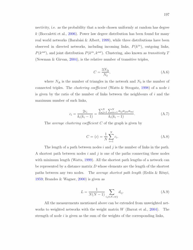
197
nectivity, i.e. as the probability that a node chosen uniformly at random has degree
k (Boccaletti et al., 2006). Power law degree distribution has been found for many
real world networks (Barabasi & Albert, 1999), while three distributions have been
observed in directed networks, including incoming links, P (kin), outgoing links,
P (kout), and joint distribution P (kin, kout). Clustering, also known as transitivity T
(Newman & Girvan, 2004), is the relative number of transitive triples,
C =3N∆
N3, (A.6)
where N∆ is the number of triangles in the network and N3 is the number of
connected triples. The clustering coefficient (Watts & Strogatz, 1998) of a node i
is given by the ratio of the number of links between the neighbours of i and the
maximum number of such links,
ci =2ei
ki(ki − 1)=
∑Nj=1
∑Nm=1 aijajmami
ki(ki − 1). (A.7)
The average clustering coefficient C of the graph is given by
C = 〈c〉 =1
N
N∑
i=1
ci. (A.8)
The length of a path between nodes i and j is the number of links in the path.
A shortest path between nodes i and j is one of the paths connecting these nodes
with minimum length (Watts, 1999). All the shortest path lengths of a network can
be represented by a distance matrix D whose elements are the length of the shortest
paths between any two nodes. The average shortest path length (Erdos & Renyi,
1959; Brandes & Wagner, 2000) is given as
L =1
N(N − 1)
∑
i,j∈N ,i6=j
dij. (A.9)
All the measurements mentioned above can be extended from unweighted net-
works to weighted networks with the weight matrix W (Barrat et al., 2004). The
strength of node i is given as the sum of the weights of the corresponding links,

198
si =N∑
i=1
wij . (A.10)
The average strength is given as:
〈s〉 =1
N
N∑
i=1
si. (A.11)
The weighted clustering coefficient (Barrat et al., 2004) of a node i is given by,
Cwi =
1
si(ki − 1)
∑
j>k
wij + wik
2aijaikajk, (A.12)
where the normalizing factor si(ki − 1) assures that 0 ≤ Cwi ≤ 1. The average
weighted clustering coefficient is,
〈Cw〉 =1
N
∑
i
Cwi . (A.13)
The correlations between the degrees of different nodes can be quantified by
considering the Pearson correlation coefficient of the degrees at both ends of the
links (Newman, 2002):
r =1M
∑
j>i kikjaij − [ 1M
∑
j>i12(ki + kj)aij]
2
1M
∑
j>i12(k2
i + k2j )aij − [ 1
M
∑
j>i12(ki + kj)aij]2
, (A.14)
where M is the total number of links. If r > 0 the network is assortative; if
r < 0, the network is disassortative; for r = 0 there are no correlation between node
degrees.
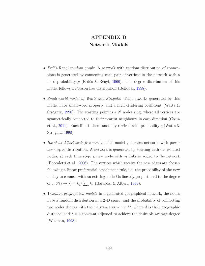
APPENDIX B
Network Models
• Erdos-Renyi random graph: A network with random distribution of connec-
tions is generated by connecting each pair of vertices in the network with a
fixed probability p (Erdos & Renyi, 1960). The degree distribution of this
model follows a Poisson like distribution (Bollobas, 1998).
• Small-world model of Watts and Strogatz : The networks generated by this
model have small-word property and a high clustering coefficient (Watts &
Strogatz, 1998). The starting point is a N nodes ring, where all vertices are
symmetrically connected to their nearest neighbours in each direction (Costa
et al., 2011). Each link is then randomly rewired with probability q (Watts &
Strogatz, 1998).
• Barabasi-Albert scale-free model : This model generates networks with power
law degree distribution. A network is generated by starting with m0 isolated
nodes, at each time step, a new node with m links is added to the network
(Boccaletti et al., 2006). The vertices which receive the new edges are chosen
following a linear preferential attachment rule, i.e. the probability of the new
node j to connect with an existing node i is linearly proportional to the degree
of j, P(i → j) = kj/∑
u ku (Barabasi & Albert, 1999).
• Waxman geographical model : In a generated geographical network, the nodes
have a random distribution in a 2–D space, and the probability of connecting
two nodes decays with their distance as p = e−λd, where d is their geographic
distance, and λ is a constant adjusted to achieve the desirable average degree
(Waxman, 1998).
199
APPENDIX C
Adaptive Control
In the section, a brief introduction of these methodologies and some examples
will be given, closely following and summarizing the review in (Luo, 2013). Further
details can be found in (Kuramoto, 2011; Astrom & Wittenmark, 2013; Luo, 2013;).
The early development of adaptive control theory was motivated by stability
theory and system identification (Luo, 2013). Model Reference Adaptive Control
scheme, for instance, was developed and analyzed by using the Lyapunov theory for
stability analysis (Morse, 1980; Narendra et al., 1980). Adaptive control schemes
were traditionally classified as two classes: “Lyapunov-based schemes” in which
adaptive laws were derived from the Lyapunov stability analysis, and “estimation-
based schemes” in which adaptive laws were generated from gradient or least-squares
optimization algorithms (Krstic et al., 1995). Although they were able to provide
stability and asymptotical tracking, these traditional schemes may lack robustness in
the presence of unmodeled dynamics or bounded disturbances (Rohrs et al., 1985).
Some modifications have been proposed for the improvement of robustness, such
as σ-modification (Ioannou & Kokotovic, 1984a; Ioannou & Kokotovic, 1984b) and
e-modification. In addition, an adaptive-control based backstepping approach has
been proposed for more complex nonlinear systems with parametric uncertainty
(Krstic et al., 1995), in which a recursive Lyapunov-based scheme was used for
adaptive control. Although it can provide global or regional regulations as well as
tracking capabilities for systems in a strict-feedback form, this approach fails to
address the handling of non-smooth nonlinearities (Narendra & Annaswamy, 1987;
Luo, 2013). In order to control nonlinear unknown systems with guaranteed closed-
loop performance, neural network-based adaptive control scheme has been developed
because of its excellent universal function approximation ability (Calise et al., 2001;
Cao & Hovakimyan, 2007). In time-varying systems, however, this approach cannot
be implemented directly because the desired weights of the neural network changes
200

201
over time (Luo, 2013).
To solve the problem of the trade-off between fast adaptation and robustness,
the L1 adaptive control theory was introduced by Hovaimyan and Cao (2010). The
trade-off occurs when high frequencies were introduced to the control signals by fast
adaption which increases the systems sensitivity to time delays, and thus decreases
the systems robustness. However, L1 adaptive control can provide a decoupling
between robustness and the fast adaptation by using a low-pass filtering system to
resolve robustness, as well as using the computational ability of hardware to limit
the adaptation (Luo, 2013). A detailed review of L1 adaptive control theory and its
applications can be found in (Hovakimyan & Cao, 2010).