tor analysis on repeated cross- sectional surveys with binary re
TRANSCRIPT
Linköpings universitetSE–581 83 Linköping+46 13 28 10 00 , www.liu.se
Linköping University | Department of Computer and Information Science
Master’s thesis, 30 ECTS | Computer Science
2020 | LIU-IDA/LITH-EX-A--20/007--SE
Using Primary Dynamic Fac-tor Analysis on repeated cross-sectional surveys with binary re-sponsesPrimär Dynamisk Faktoranalys för upprepade tvärsnittsunder-sökningar med binära svar
Arvid Edenheim
Supervisor : Martin SingullExaminer : Cyrille Berger

Upphovsrätt
Detta dokument hålls tillgängligt på Internet - eller dess framtida ersättare - under 25 år från publicer-ingsdatum under förutsättning att inga extraordinära omständigheter uppstår.Tillgång till dokumentet innebär tillstånd för var och en att läsa, ladda ner, skriva ut enstaka kopior förenskilt bruk och att använda det oförändrat för ickekommersiell forskning och för undervisning. Över-föring av upphovsrätten vid en senare tidpunkt kan inte upphäva detta tillstånd. All annan användningav dokumentet kräver upphovsmannens medgivande. För att garantera äktheten, säkerheten och till-gängligheten finns lösningar av teknisk och administrativ art.Upphovsmannens ideella rätt innefattar rätt att bli nämnd somupphovsman i den omfattning som godsed kräver vid användning av dokumentet på ovan beskrivna sätt samt skydd mot att dokumentet än-dras eller presenteras i sådan form eller i sådant sammanhang som är kränkande för upphovsmannenslitterära eller konstnärliga anseende eller egenart.För ytterligare information om Linköping University Electronic Press se förlagets hemsidahttp://www.ep.liu.se/.
Copyright
The publishers will keep this document online on the Internet - or its possible replacement - for aperiod of 25 years starting from the date of publication barring exceptional circumstances.The online availability of the document implies permanent permission for anyone to read, to down-load, or to print out single copies for his/hers own use and to use it unchanged for non-commercialresearch and educational purpose. Subsequent transfers of copyright cannot revoke this permission.All other uses of the document are conditional upon the consent of the copyright owner. The publisherhas taken technical and administrative measures to assure authenticity, security and accessibility.According to intellectual property law the author has the right to be mentioned when his/her work isaccessed as described above and to be protected against infringement.For additional information about the Linköping University Electronic Press and its proceduresfor publication and for assurance of document integrity, please refer to its www home page:http://www.ep.liu.se/.
© Arvid Edenheim

Abstract
With the growing popularity of business analytics, companies experience an increasingneed of reliable data. Although the availability of behavioural data showing what theconsumers do has increased, the access to data showing consumer mentality, what the con-sumers actually think, remain heavily dependent on tracking surveys. This thesis inves-tigates the performance of a Dynamic Factor Model using respondent-level data gatheredthrough repeated cross-sectional surveys. Through Monte Carlo simulations, the modelwas shown to improve the accuracy of brand tracking estimates by double digit percent-ages, or equivalently reducing the required amount of data by more than a factor 2, whilemaintaining the same level of accuracy. Furthermore, the study showed clear indicationsthat even greater performance benefits are possible.

Acknowledgments
I would first like to thank Nepa for giving me the opportunity to write this thesis at theircompany. I would also like to direct my sincerest gratitude towards my supervisors at Nepa,Goran Dizdarevic and Patrik Björkholm, for providing great support and expertise, withoutwhom this thesis would not have seen the light of day. A special mention to the Data Sci-ence team for putting up with my vigorous gesticulation and verbal confusion with ggplot.Furthermore, I want to thank Martin Singull and Cyrille Berger at Linköping University forproviding valuable feedback. Finally, a very special thanks to Lisa Yuen, my devoted cheer-leader, for encouragement and listening to endless monologues about this thesis.
iv

Contents
Abstract iii
Acknowledgments iv
Contents v
List of Figures vii
List of Tables viii
List of Algorithms ix
1 Introduction 21.1 Motivation . . . . . . . . . . . . . . . . . . . . . . . . . . . . . . . . . . . . . . . . 31.2 Aim . . . . . . . . . . . . . . . . . . . . . . . . . . . . . . . . . . . . . . . . . . . . 41.3 Research Questions . . . . . . . . . . . . . . . . . . . . . . . . . . . . . . . . . . . 41.4 Delimitations . . . . . . . . . . . . . . . . . . . . . . . . . . . . . . . . . . . . . . 4
2 Theory 52.1 Factor Analysis . . . . . . . . . . . . . . . . . . . . . . . . . . . . . . . . . . . . . 52.2 Dynamic Factor Analysis . . . . . . . . . . . . . . . . . . . . . . . . . . . . . . . . 112.3 State-Space Model . . . . . . . . . . . . . . . . . . . . . . . . . . . . . . . . . . . . 112.4 Kalman Filter . . . . . . . . . . . . . . . . . . . . . . . . . . . . . . . . . . . . . . 132.5 Kalman Smoother . . . . . . . . . . . . . . . . . . . . . . . . . . . . . . . . . . . . 142.6 Estimating Model Parameters . . . . . . . . . . . . . . . . . . . . . . . . . . . . . 152.7 Evaluation Metrics . . . . . . . . . . . . . . . . . . . . . . . . . . . . . . . . . . . 16
3 Method 193.1 Data Sources . . . . . . . . . . . . . . . . . . . . . . . . . . . . . . . . . . . . . . . 193.2 Primary DFA Model . . . . . . . . . . . . . . . . . . . . . . . . . . . . . . . . . . 223.3 Algorithm . . . . . . . . . . . . . . . . . . . . . . . . . . . . . . . . . . . . . . . . 233.4 Evaluation . . . . . . . . . . . . . . . . . . . . . . . . . . . . . . . . . . . . . . . . 26
4 Results 294.1 Simulated Data . . . . . . . . . . . . . . . . . . . . . . . . . . . . . . . . . . . . . 294.2 Real Data . . . . . . . . . . . . . . . . . . . . . . . . . . . . . . . . . . . . . . . . . 34
5 Discussion 375.1 Results . . . . . . . . . . . . . . . . . . . . . . . . . . . . . . . . . . . . . . . . . . 375.2 Method . . . . . . . . . . . . . . . . . . . . . . . . . . . . . . . . . . . . . . . . . . 415.3 Source Criticism . . . . . . . . . . . . . . . . . . . . . . . . . . . . . . . . . . . . . 445.4 The work in a wider context . . . . . . . . . . . . . . . . . . . . . . . . . . . . . . 44
6 Conclusion 45
v

6.1 Future Work . . . . . . . . . . . . . . . . . . . . . . . . . . . . . . . . . . . . . . . 46
Bibliography 48
A Appendix 52A.1 Excerpts from Simulated Data . . . . . . . . . . . . . . . . . . . . . . . . . . . . . 52A.2 Fitted DFA Models . . . . . . . . . . . . . . . . . . . . . . . . . . . . . . . . . . . 53
vi
List of Figures
2.1 Common Factor Model . . . . . . . . . . . . . . . . . . . . . . . . . . . . . . . . . . . 62.2 Comparison of Factor Rotations . . . . . . . . . . . . . . . . . . . . . . . . . . . . . . 92.3 Graphical Representation of a State-Space Model . . . . . . . . . . . . . . . . . . . . 122.4 Prediction, Filtering and Smoothing . . . . . . . . . . . . . . . . . . . . . . . . . . . 132.5 Update cycle of the Kalman Filter . . . . . . . . . . . . . . . . . . . . . . . . . . . . . 14
4.1 Example of a fitted DFA model on simulated (binary) data . . . . . . . . . . . . . . 304.2 Distribution of results with simulated continuous data . . . . . . . . . . . . . . . . 314.3 Distribution of test results with simulated discrete data . . . . . . . . . . . . . . . . 314.4 Distribution of test results with simulated binary data . . . . . . . . . . . . . . . . . 324.5 Distribution of test results with diagonal error-covariance matrix . . . . . . . . . . 334.6 Distribution of results with simulation from real data - One brand . . . . . . . . . . 354.7 Distribution of results with simulation from real data - Multiple brands . . . . . . . 36
5.1 Visualization of DFA and Sample Mean over different sample sizes . . . . . . . . . 385.2 DFA with diagonal error covariance matrix fitted on real data . . . . . . . . . . . . 395.3 DFA fitted on simulated binary data generated from real respondent data . . . . . 405.4 Comparison of sample sizes: 25 vs. 200 respondents . . . . . . . . . . . . . . . . . . 415.5 Convergence of the DFA model - Log-likelihood and Parameter difference . . . . . 43
A.1 Fitted DFA on binary respondent data . . . . . . . . . . . . . . . . . . . . . . . . . . 53A.2 Fitted DFA on binary respondent data . . . . . . . . . . . . . . . . . . . . . . . . . . 54A.3 Fitted DFA on binary respondent data with included covariates . . . . . . . . . . . 54
vii
List of Tables
2.1 Factor Extraction Techniques . . . . . . . . . . . . . . . . . . . . . . . . . . . . . . . 8
3.1 Example Survey Questions . . . . . . . . . . . . . . . . . . . . . . . . . . . . . . . . 213.2 Closed-ended question - Which brand do you prefer? . . . . . . . . . . . . . . . . . . . 223.3 Model configurations . . . . . . . . . . . . . . . . . . . . . . . . . . . . . . . . . . . . 27
4.1 Comparison of moving averages with different order . . . . . . . . . . . . . . . . . 294.2 Results with simulated continuous data . . . . . . . . . . . . . . . . . . . . . . . . . 304.3 Results with simulated discrete data . . . . . . . . . . . . . . . . . . . . . . . . . . . 324.4 MAE and RMSE scores with simulated binary data . . . . . . . . . . . . . . . . . . 334.5 MAE and RMSE scores with simulated binary data and diagonal error-covariance
matrix . . . . . . . . . . . . . . . . . . . . . . . . . . . . . . . . . . . . . . . . . . . . . 344.6 RMSE and MAE scores from real-time estimation at step T and T-1 . . . . . . . . . 344.7 MAE and RMSE scores with simulation from real data - One brand . . . . . . . . . 354.8 MAE and RMSE scores with simulation from real data - Multiple brands . . . . . . 35
5.1 Summary of test results . . . . . . . . . . . . . . . . . . . . . . . . . . . . . . . . . . 375.2 MAE and RMSE scores with simulated binary data over 100 timesteps . . . . . . . 42
viii

List of Algorithms
2.1 Kalman Filter . . . . . . . . . . . . . . . . . . . . . . . . . . . . . . . . . . . . . . 132.2 Kalman Smoother . . . . . . . . . . . . . . . . . . . . . . . . . . . . . . . . . . . . 152.3 Expectation Maximization . . . . . . . . . . . . . . . . . . . . . . . . . . . . . . . 163.1 Modified Kalman Filter . . . . . . . . . . . . . . . . . . . . . . . . . . . . . . . . . 243.2 Modified Kalman Smoother . . . . . . . . . . . . . . . . . . . . . . . . . . . . . . 24
ix
Acronyms
AIC Akaike Information Criterion. 43, 46
DFA Dynamic Factor Analysis. vii, 3, 4, 19, 29, 30, 32–35, 37–42, 45, 46
DLM Dynamic Linear Model. 12
EM Expectation Maximization. 42, 43
FA Factor Analysis. 4, 5
KF Kalman Filter. 44
KPI Key Performance Indicator. 4, 27, 35, 40
M Measure. 30, 32–35, 42
MA Moving Average. 30–35, 37, 42
MAD Mean Absolute Deviation. 17
MAE Mean Absolute Error. viii, 17, 18, 29, 30, 32–35, 37–43, 46
MAPE Mean Absolute Percentage Error. 17, 18, 38, 43
ML Maximum Likelihood. 8
MLE Maximum Likelihood Estimate. 8, 15, 23
RMSE Root Mean Squared Error. viii, 17, 18, 29, 30, 32–35, 37, 38, 40, 42, 43, 46
SDFA Structural Dynamic Factor Analysis. 46
SM Sample Mean. 29–35, 37, 39, 42
SSM State-Space Model. 11, 12
W Week. 34
1

1 Introduction
When conducting social survey research with the aim of tracking the state of and changesin population sentiment, researchers and businesses typically resort to two methods: Longi-tudinal surveys and Repeated cross-sectional surveys [10]. A longitudinal study aims to followthe same panel composition of respondents over time, whereas a cross-sectional design studyimplies collecting data on different measures from multiple respondents at a single point intime [2]. Consequently, a repeated cross-sectional study follows the same survey structure foreach measurement, but gathers data from panels with varying respondent composition overtime.
As the longitudinal study requires the respondents to be the same for all timesteps, it is sig-nificantly more costly and relies on high respondent retention [46, 17]. However, an apparentadvantage (among others) of using longitudinal panel data is the ability to observe changesat the individual level [17]. Although lacking some of the benefits of longitudinal data, re-peated cross-sectional surveys are by far the most prevalent in the marketing context [10].The advantages of said method includes lower costs, the possibility to introduce additionalrespondents and the option to aggregate multiple measurements in order to obtain a largersample size over a coarser interval [46, 17].
Considering the benefits above and the relevance in the context of tracking consumer effectsof marketing efforts, this thesis will focus on repeated cross-sectional surveys performed byrepeated sampling from non-overlapping respondents. The general purpose of such studiesis not on tracking changes at the individual level, but on observing changes in the state of thepopulation from which the respondent was sampled, henceforth referred to as the populationmean. A key assumption made in these studies is that while the individuals may be differentfor each point of measurement, they, when aggregated, still represent estimates of the samepopulation mean [10]. This aggregated sample, computed by calculating the average of all re-spondents surveyed in the same time period, is referred to as the sample mean and constitutesthe estimate of the population mean at that point in time.
An issue with using data gathered from repeated cross-sectional surveys is sampling error.The objective of performing tracking studies can be reduced to this one significant challengeof discerning real changes in population mean from changes related to differences in panel
2
1.1. Motivation
composition or common method bias, a problem that becomes increasingly difficult whenthe population is heterogeneous and sample sizes are small [10]. In order to mitigate this,the current industry standard method is to impose a moving average on the sample means,resulting in a generally smoother fit at the expense of increasingly inert dynamics.
An alternative method that has gained traction in the marketing literature is Dynamic FactorAnalysis (DFA). The proposed models differ significantly in their implementations, and in-clude both secondary analysis models such as [11] and primary analysis models such as [29, 28,10], where secondary refers to models taking the sample mean as input and primary modelsutilizes individual level data in an attempt to capture dynamics at the respondent level [34].The use of a primary model can be motivated by considering three structures, or patterns,that typically are present in repeated cross-sectional data [10]:
1. Within-measure inter-temporal dependence. As the population mean reflect the collectivestate of the population, it is intuitive to imagine that it will not change drastically fromone time period to the next, a property referred to as temporal dependence.
2. Between-measure co-movements in population means. Different measures gathered from thesame survey should be correlated on an aggregated level over time. By considering cor-relations between population means, it is possible to compare a measures’ movementwith the expected movement according to the dynamics of the correlation.
3. Between-measure cross-sectional co-variations (also referred to as individual-level responseheterogeneity [28]). This refers to correlation on the primary level, stating that measurescan be correlated on the respondent level due to factors such as common method bias,halo effect 1, panel composition or other respondent characteristics. When aggregated,changes related to these sampling errors could be mistaken for real between-measureco-movements in population means.
By leveraging the information above, the primary model can borrow information across timeand between measures in order to filter idiosyncratic movements in sample means and betterdiscern real changes in population means from those related to sampling error.
This thesis applies a Primary Dynamic Factor model on repeated cross-sectional survey data.It investigates the fitness and capacity of the model when the individual level data is contin-uous, discrete and binary. Furthermore, the model is evaluated and compared with industrystandard methods and the implications of this comparison is presented.
1.1 Motivation
Respondent data can take different forms depending on the type of question and the contextin which the data will be used. It may be interval or ratio-scaled as in surveys followingcustomer satisfaction for instance, where the questions often are designed to be answeredwith a rank or score of sorts. The data may also be entirely binary, which is often the casein brand awareness tracking. If the study follows a number of different brands, each brand’soccurrence in a respondent’s answer would then be indicated with a one or a zero. However,when aggregated, this data would still be converted to a ratio-scaled sample mean, enablingthe use of DFA models.
While existing studies stress the superiority of DFA models and puts them to use in real en-vironments (see [28, 10] for examples), they overlook the presence of binary respondent data,
1The tendency for positive impressions of a person, company, brand or product in one area to positively influenceone’s opinions or feelings in other areas - https://en.wikipedia.org/wiki/Halo_effect
3

1.2. Aim
in addition to lacking rigorous simulation studies of the model’s performance in differentconditions. This thesis evaluates the performance of the DFA model proposed by Du andKamakura [10] using Monte Carlo simulations with a wide range of settings in collaborationwith Nepa, a consumer research company located in Stockholm.
1.1.1 Nepa
Nepa is a Swedish consumer science company founded in 20062. One of their core businesspillars is Brand Tracking, that is, measuring the performance of a specific brand over timethrough Key Performance Indicator (KPI)s. These KPIs are assumed to reflect the consumer’sattitude towards and awareness about the brand and is typically used to evaluate the effectsof marketing campaigns. In the context of Nepa, this is performed with data gathered weeklyby repeated cross-sectional studies.
1.2 Aim
The aim of this research is to investigate the benefit of using Primary Dynamic Factor Analy-sis on data obtained from repeated sampling on non-overlapping panels of respondents andstudy the impact on estimation error when the sampled data is continuous, discrete and bi-nary.
1.3 Research Questions
1. Can a lower estimation error be obtained when using a Dynamic Factor Analysis modelon respondent data gathered from repeated cross-sectional surveys, compared to amoving average?
2. What estimation error can be achieved with a Dynamic Factor Analysis model whenthe respondent data is binary and how does this compare to numerical values?
1.4 Delimitations
As the model subject to evaluation was administered by Nepa, and this evaluation in itselfprovides a sufficient scope, no alternative models other than those used as baseline will beconsidered. Furthermore, although DFA shares conceptual similarities with conventionalFactor Analysis (FA), only those areas of FA with relevance to DFA will be described, asthey solely constitute a means to an end. Finally, Monte Carlo simulations based on realrespondent data, as opposed to simulated, require a sample population more substantial thanthat available in this research, which is why it is left for further research.
2https://nepa.com/about/
4
2 Theory
This chapter presents the theoretical concepts upon which this research is based.
2.1 Factor Analysis
Factor Analysis (FA) is a multivariate statistical method for dimension reduction and struc-ture detection. The general idea for factor analysis in terms of dimension reduction is todescribe a set of M of observed variables, or indicators, with the covariance of a set of com-mon N latent factors, such that M " N [19, 10]. By doing this, factor analysis means to describeevery observed variable as a linear combination of latent factors, which together compose amore parsimonious representation of the observed data [40, 12]. These factors are commonin the sense that each factor is describing the covariance of multiple observed variables, andlatent in the sense that they are not observed, but inferred from the values of the observedvariables [12]. Furthermore, the latent factors are derived in such a way that they align withsubsets of variables that are highly correlated within the subset, but featuring relatively smallcorrelations with variables in other subsets. This facilitates interpretation of said factors as arepresentation of underlying constructs that is causing the correlation [19].
2.1.1 Model
A basic model describing the relation between observed variable and latent factor is
xi = λi1F1 + λi2F2 + ... + λiN FN + εi, (2.1)
where xi is the ith observed variable, λij is the loading factor from factor j on variable i, de-scribing the linear dependencies between the observed and latent factors, that is, the strengthof the association between the factor and the variable, and ε is the unique factor which exertslinear influence on a single variable, sometimes referred to as specific error [19, 4, 13]. Thisis deceivingly similar to, but is not to be mistaken for, the multivariate regression model,
5
2.1. Factor Analysis
FactorFactor Factor
Variable
λ1 λ2 λ3
UniqueFactor
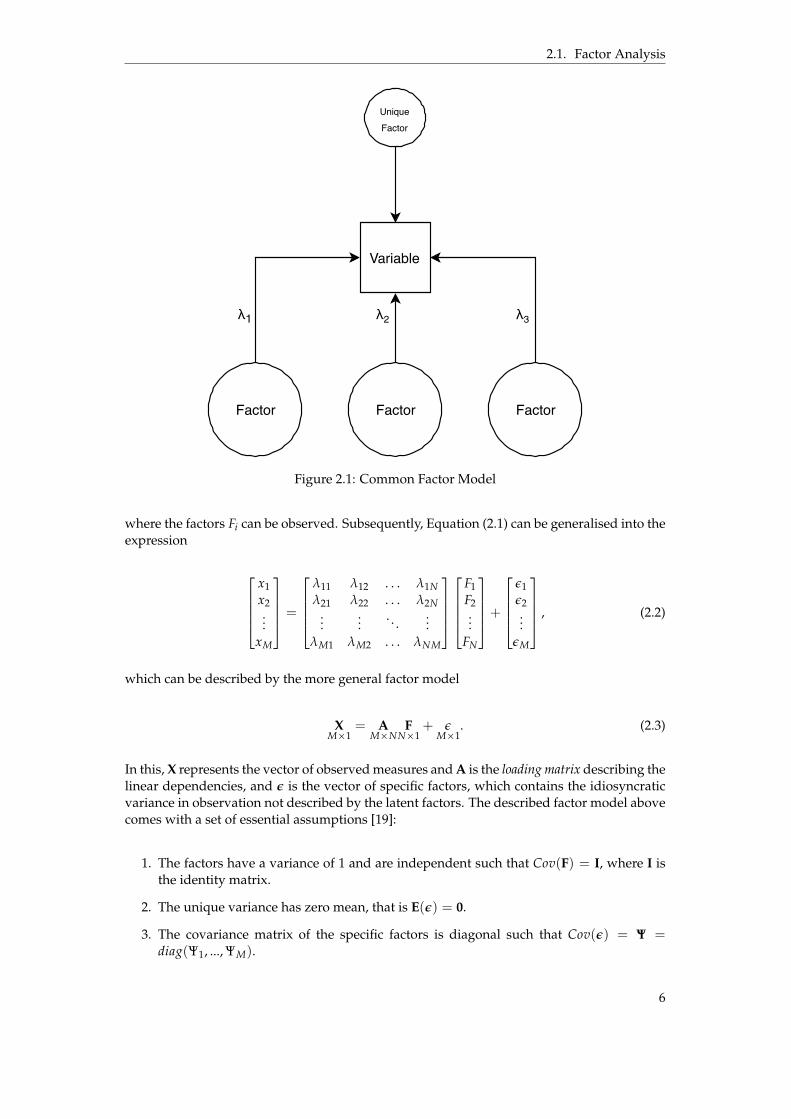
Figure 2.1: Common Factor Model
where the factors Fi can be observed. Subsequently, Equation (2.1) can be generalised into theexpression
x1x2...
xM
=
λ11 λ12 . . . λ1Nλ21 λ22 . . . λ2N
......
. . ....
λM1 λM2 . . . λNM
F1F2...
FN
+
ε1ε2...
εM
, (2.2)
which can be described by the more general factor model
XMˆ1
= AMˆN
FNˆ1
+ εMˆ1
. (2.3)
In this, X represents the vector of observed measures and A is the loading matrix describing thelinear dependencies, and ε is the vector of specific factors, which contains the idiosyncraticvariance in observation not described by the latent factors. The described factor model abovecomes with a set of essential assumptions [19]:
1. The factors have a variance of 1 and are independent such that Cov(F) = I, where I isthe identity matrix.
2. The unique variance has zero mean, that is E(ε) = 0.
3. The covariance matrix of the specific factors is diagonal such that Cov(ε) = Ψ =diag(Ψ1, ..., ΨM).
6
2.1. Factor Analysis
It is important to note that the assumptions above are based on the notion of the orthogonalfactor model where the factors are independent, in contrast to the oblique factor model whichdoes not enforce a diagonal factor covariance matrix [19]. However, that model is out of scopefor this research and will not be considered any further.
Given these assumptions and the notations above, the covariance for the observed variablescan be derived as
Cov(X) = Σ = AA’ + Ψ,
Cov(X, F) = A.(2.4)
For future purposes, it is useful to introduce additional notation related to (2.4). We estimatethe covariance matrix Σ and correlation matrix by
Σ = S,ˆCor(X) = R,
(2.5)
where S denotes the sample covariance matrix and R the sample correlation matrix obtained fromthe observations [19]. For a factor analysis to prove useful, it is necessary that the samplecovariance matrix S, thus including R, deviate distinctively from a diagonal matrix. If thatis not the case, it indicates that the observed variables are not related and an underlyingconstruct will not be identifiable [19].
The sum of the squared factor loadings for each variable, that is for each row in the loadingmatrix A, is called the communality for that variable. This is a measurement of the amount ofvariance in the observed variable explained by the latent factor [4]. Conversely, the variancenot described by the communality is called the unique variance, denoted Ψi [19]
Var(xi) = λ2i1 + ... + λ2
iN + Ψi, i = 1, .., M. (2.6)
2.1.2 Factor Extraction
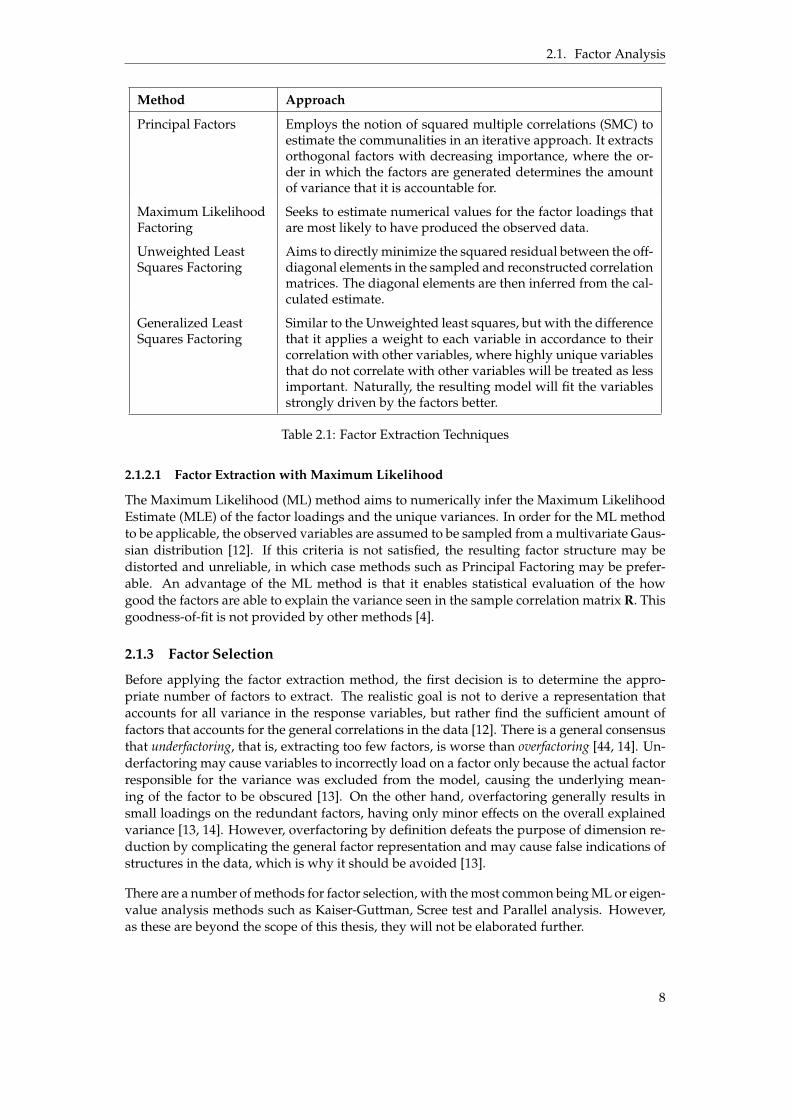
In order to compute the model parameters listed in the common factor model (2.3), factoranalysis resorts to a considerable number of different methods. An extensive, but not com-prehensive, list of factor extraction techniques as compiled by [38] can be found in Table 2.1.However, as a the majority of these methods has little relevance for this research, they willonly be introduced briefly to inform the reader of the alternatives and promote future read-ing. Common for all of them is that they intend to calculate the factor loadings in the loadingmatrix A that most accurately reproduce the sample correlation matrix R according to (2.4)and (2.5). While every method comes with its set of advantages and drawbacks, they all tendto generate similar factor solutions when the underlying constructs in the data are fairly clear[13].
7
2.1. Factor Analysis
Method Approach
Principal Factors Employs the notion of squared multiple correlations (SMC) toestimate the communalities in an iterative approach. It extractsorthogonal factors with decreasing importance, where the or-der in which the factors are generated determines the amountof variance that it is accountable for.
Maximum LikelihoodFactoring
Seeks to estimate numerical values for the factor loadings thatare most likely to have produced the observed data.
Unweighted LeastSquares Factoring
Aims to directly minimize the squared residual between the off-diagonal elements in the sampled and reconstructed correlationmatrices. The diagonal elements are then inferred from the cal-culated estimate.
Generalized LeastSquares Factoring
Similar to the Unweighted least squares, but with the differencethat it applies a weight to each variable in accordance to theircorrelation with other variables, where highly unique variablesthat do not correlate with other variables will be treated as lessimportant. Naturally, the resulting model will fit the variablesstrongly driven by the factors better.
Table 2.1: Factor Extraction Techniques
2.1.2.1 Factor Extraction with Maximum Likelihood
The Maximum Likelihood (ML) method aims to numerically infer the Maximum LikelihoodEstimate (MLE) of the factor loadings and the unique variances. In order for the ML methodto be applicable, the observed variables are assumed to be sampled from a multivariate Gaus-sian distribution [12]. If this criteria is not satisfied, the resulting factor structure may bedistorted and unreliable, in which case methods such as Principal Factoring may be prefer-able. An advantage of the ML method is that it enables statistical evaluation of the howgood the factors are able to explain the variance seen in the sample correlation matrix R. Thisgoodness-of-fit is not provided by other methods [4].
2.1.3 Factor Selection
Before applying the factor extraction method, the first decision is to determine the appro-priate number of factors to extract. The realistic goal is not to derive a representation thataccounts for all variance in the response variables, but rather find the sufficient amount offactors that accounts for the general correlations in the data [12]. There is a general consensusthat underfactoring, that is, extracting too few factors, is worse than overfactoring [44, 14]. Un-derfactoring may cause variables to incorrectly load on a factor only because the actual factorresponsible for the variance was excluded from the model, causing the underlying mean-ing of the factor to be obscured [13]. On the other hand, overfactoring generally results insmall loadings on the redundant factors, having only minor effects on the overall explainedvariance [13, 14]. However, overfactoring by definition defeats the purpose of dimension re-duction by complicating the general factor representation and may cause false indications ofstructures in the data, which is why it should be avoided [13].
There are a number of methods for factor selection, with the most common being ML or eigen-value analysis methods such as Kaiser-Guttman, Scree test and Parallel analysis. However,as these are beyond the scope of this thesis, they will not be elaborated further.
8
2.1. Factor Analysis
2.1.4 Factor Rotation
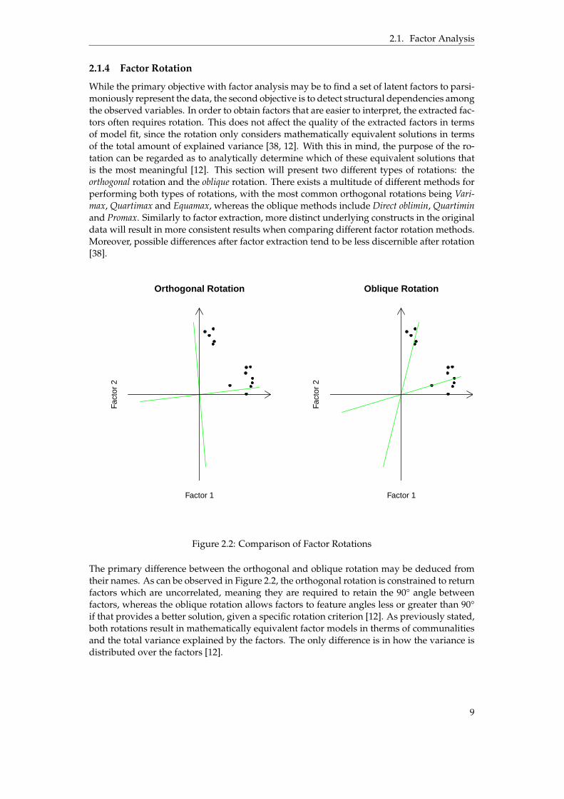
While the primary objective with factor analysis may be to find a set of latent factors to parsi-moniously represent the data, the second objective is to detect structural dependencies amongthe observed variables. In order to obtain factors that are easier to interpret, the extracted fac-tors often requires rotation. This does not affect the quality of the extracted factors in termsof model fit, since the rotation only considers mathematically equivalent solutions in termsof the total amount of explained variance [38, 12]. With this in mind, the purpose of the ro-tation can be regarded as to analytically determine which of these equivalent solutions thatis the most meaningful [12]. This section will present two different types of rotations: theorthogonal rotation and the oblique rotation. There exists a multitude of different methods forperforming both types of rotations, with the most common orthogonal rotations being Vari-max, Quartimax and Equamax, whereas the oblique methods include Direct oblimin, Quartiminand Promax. Similarly to factor extraction, more distinct underlying constructs in the originaldata will result in more consistent results when comparing different factor rotation methods.Moreover, possible differences after factor extraction tend to be less discernible after rotation[38].
Orthogonal Rotation
Factor 1
Fact
or 2
Oblique Rotation
Factor 1
Fact
or 2
Figure 2.2: Comparison of Factor Rotations
The primary difference between the orthogonal and oblique rotation may be deduced fromtheir names. As can be observed in Figure 2.2, the orthogonal rotation is constrained to returnfactors which are uncorrelated, meaning they are required to retain the 90° angle betweenfactors, whereas the oblique rotation allows factors to feature angles less or greater than 90°if that provides a better solution, given a specific rotation criterion [12]. As previously stated,both rotations result in mathematically equivalent factor models in therms of communalitiesand the total variance explained by the factors. The only difference is in how the variance isdistributed over the factors [12].
9

2.1. Factor Analysis
2.1.4.1 Orthogonal Rotation
The reasoning behind orthogonal rotations is that factors are more interpretable if they areuncorrelated, which makes the factor loadings represent correlations between the factors andthe observed variables [4]. This property facilitates the identification of an underlying mean-ing of a factor, since the variation of a variable can be traced directly to the factors on whichit loads highly on [38]. However, this reasoning is potentially deceptive if the factors in factare expected to correlate. Enforcing an orthogonal structure on the factors does not alter thetrue underlying constructs in the data, but may cause a misrepresentation wherein variablesare forced to correlate with a specific factor only because the factor in turn correlates withanother factor that influences the variable [12]. Orthogonal rotations should thus be usedsensibly unless the underlying processes are known to be somewhat independent [38].
Orthogonal rotations are based on the notion that there exists a simplicity criterion, that is, aproperty of the loading matrix, that describes the ability of the matrix to produce a simplefactor structure. In the case of the Varimax rotation, this property is defined as the sum of thevariance of the squared factor loadings, which typically results in the factor loadings beingeither near one or zero. The rotation then seeks a solution of factor loadings which maximizesthis property [12].
2.1.4.2 Oblique Rotation
The oblique rotation can be regarded as the more general factor rotation. While the orthog-onal rotation seeks the mathematically equivalent solution that maximizes the simplicity cri-terion among the orthogonal factor solutions, the oblique rotation maximizes this criterionover all equivalent solutions. If the best solution lies in the orthogonal solution space, theoblique rotation will identify it, otherwise it will generate an inter-correlated factor structure.Contrary to popular belief, the oblique rotation neither causes or requires the factors to becorrelated, but instead generates a factor structure more true to the underlying structures inthe data by allowing correlations among factors to exist. As such, the oblique rotation pro-vides additional information about the underlying structures in the data, which is ignoredwhen enforcing an orthogonal representation [12]. Bearing this in mind, the oblique rotationgenerally causes a more complex factor structure. Although the solution is simpler in regardsto the criterion, two factors may correlate to a degree that it will be difficult to differentiatebetween them in terms of underlying significance [38].
2.1.5 Factor Scores
Factor scores are the estimated values of the factors F. As they are unobservable, they canbe thought of as the score that would have been observed if it would have been possible toobserve the factor directly [4].
2.1.6 Factor Interpretation
After acquiring a factor model, it might be of interest to interpret the meaning of the fac-tors in terms of the latent constructs in the data that they are describing. This is performedby examining which variables load substantially on which factors and interpreting thematicmeaning in the grouped variables, that is, the variables significantly driven by changes inthe same factors, but also potential significance of the variables not explained by said factors.Determining the meaning of groups of variables requires knowledge of the data and of thecontext from which the data is gathered [12]. However, when using FA solely for dimensionreduction, the need to interpret the factors is reduced.
10
2.2. Dynamic Factor Analysis
2.2 Dynamic Factor Analysis
Dynamic Factor Analysis (DFA) is conceptually similar to FA in terms of it being a methodfor dimension reduction and structure detection. However, it comes with a key distinction.FA assumes that all observations are independently sampled, which means that it is indiffer-ent to the order in which the observations are arranged and will disregard any longitudinaldependencies, which is not a desirable trait in time-series analysis [11]. To mitigate this,DFA assumes temporal interdependencies in the latent factors. In DFA, each latent factor ismodelled to follow an AR(1) process, meaning that the state of the latent factor at a certaintimestep t is a consequence of the state of the factor at the previous timestep t´ 1 and a stateshock containing the state change, according to the state equation
zt = zt´1 + ξt, ξt „ N (0, Ω), (2.7)
where zt is the vector of latent factor states at timestep t and ξt denotes the latent state shocksat timestep t. Theoretically, the order is not bound to be 1, as described by [27, 26], but is setto 1 per convention and relevance for this research. In the context of factor analysis, the statevector zt can be incorporated into the factor model (2.3), resulting in the observation equation
xt = Azt + εt, εt „ N (0, Σ), (2.8)
where xt contains the observed variables at timestep t, A is the loading matrix and εt containsthe unique factors at timestep t.
The methods used for extracting the factors differs from those used in traditional factor anal-ysis and typically (see [27, 10, 11, 47, 31, 41]) involves techniques from state-space modellingsuch as the Kalman filter and smoother as well as the Expectation Maximization algorithm out-lined in Section 2.4, 2.5 and 2.6.1, respectively.
2.3 State-Space Model
A State-Space Model (SSM) is based on the notion that the behaviour of a dynamic systemcan be described by a set of two equations: a state equation describing the transition dynamicsbetween consecutive states, and an observation equation representing the uncertainty intro-duced by observation [3]. The concept of state is key to this description, articulately definedby Haykin [16] as “the minimal set of data that is sufficient to uniquely describe the unforceddynamical behavior of the system”. It is often denoted zt, meaning the specific state at timet. Typically, the state is latent, that is it can’t be quantified directly, but is inferred throughmeasurements xt containing some amount of measurement noise [16].
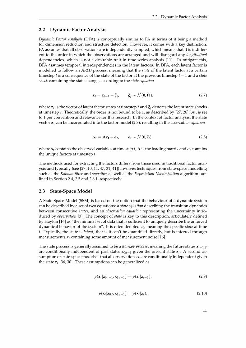
The state process is generally assumed to be a Markov process, meaning the future states zt+1:Tare conditionally independent of past states z0:t´1 given the present state zt. A second as-sumption of state-space models is that all observations xt are conditionally independent giventhe state zt [36, 30]. These assumptions can be generalized as
p(zt|z0:t´1, x1:t´1) = p(zt|zt´1), (2.9)
p(xt|z0:t, x1:t´1) = p(xt|zt), (2.10)
11
2.3. State-Space Model
zt-1 zt
xt-1 xt
... ...
Figure 2.3: Graphical Representation of a State-Space Model
where (2.9) is called the transition probability and (2.10) the emission probability [40, 3].
If the state and observation variables are discrete, the state-space model is often referred toas a hidden markov model [3], whereas the continuous case simply is described as SSM, orspecified as one of its variants, such as Dynamic Linear Model (DLM) [36].
2.3.1 Dynamic Linear Model
A Dynamic Linear Model (DLM) is a special continuous case of the general state-space model,assuming linear dependencies and Gaussian transition and emission models [3]. An exampleof a DLM, as defined in [39, 42], is
p(zt|zt´1) = N (zt|Azt´1 + But, R), (2.11)
p(xt|zt) = N (xt|Czt, Q). (2.12)
The analogous general formulation of the DLM described above is the state equation
zt = Azt´1 + But + εt, εt „ N (0, R), (2.13)
and observation equation
xt = Czt + δt, δt „ N (0, Q). (2.14)
In the equations above, A is a square matrix that relates the previous state into the new stateaccording to dynamics of the model. Similarly, B incorporates inputs from the control variableut into the new state [42]. As the problem at hand does not require any control inputs, Btand ut will not be considered any further. Similar to A and B, C is the measurement matrixthat relates the state to the measurement [16], similar to the loading matrix in factor analysis.Finally, Q is the measurement covariance matrix, describing the measurement noise, and R isthe process covariance matrix, representing the uncertainty introduced by the state transition[39].
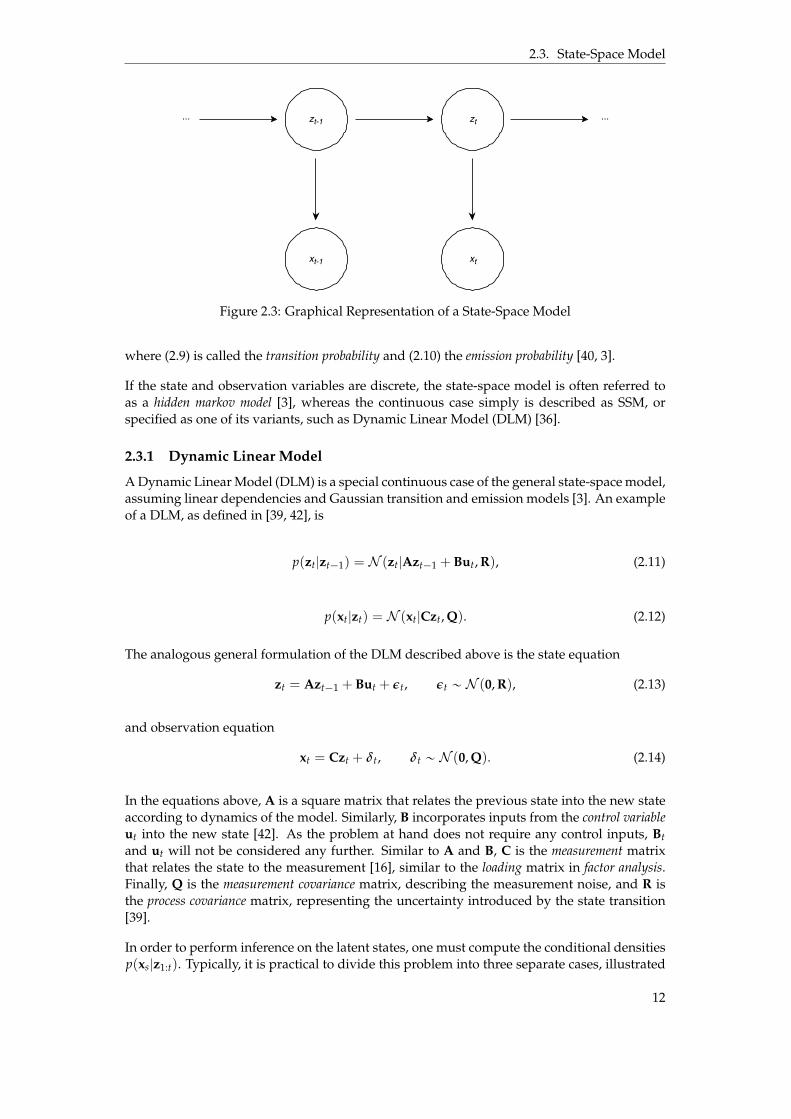
In order to perform inference on the latent states, one must compute the conditional densitiesp(xs|z1:t). Typically, it is practical to divide this problem into three separate cases, illustrated
12
2.4. Kalman Filter
Prediction
Filtering
Smoothing
s T0 t
Figure 2.4: Prediction, Filtering and Smoothing
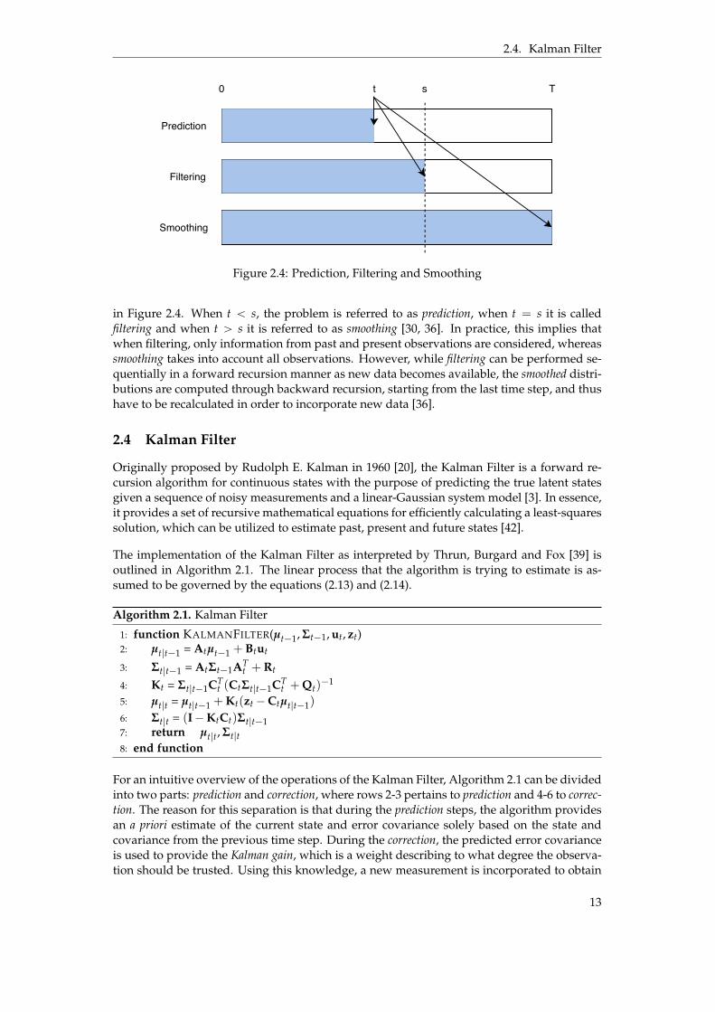
in Figure 2.4. When t ă s, the problem is referred to as prediction, when t = s it is calledfiltering and when t ą s it is referred to as smoothing [30, 36]. In practice, this implies thatwhen filtering, only information from past and present observations are considered, whereassmoothing takes into account all observations. However, while filtering can be performed se-quentially in a forward recursion manner as new data becomes available, the smoothed distri-butions are computed through backward recursion, starting from the last time step, and thushave to be recalculated in order to incorporate new data [36].
2.4 Kalman Filter
Originally proposed by Rudolph E. Kalman in 1960 [20], the Kalman Filter is a forward re-cursion algorithm for continuous states with the purpose of predicting the true latent statesgiven a sequence of noisy measurements and a linear-Gaussian system model [3]. In essence,it provides a set of recursive mathematical equations for efficiently calculating a least-squaressolution, which can be utilized to estimate past, present and future states [42].
The implementation of the Kalman Filter as interpreted by Thrun, Burgard and Fox [39] isoutlined in Algorithm 2.1. The linear process that the algorithm is trying to estimate is as-sumed to be governed by the equations (2.13) and (2.14).
Algorithm 2.1. Kalman Filter
1: function KALMANFILTER(µt´1, Σt´1, ut, zt)2: µt|t´1 = Atµt´1 + Btut
3: Σt|t´1 = AtΣt´1ATt + Rt
4: Kt = Σt|t´1CTt (CtΣt|t´1CT
t + Qt)´1
5: µt|t = µt|t´1 + Kt(zt ´Ctµt|t´1)
6: Σt|t = (I´KtCt)Σt|t´17: return µt|t, Σt|t8: end function
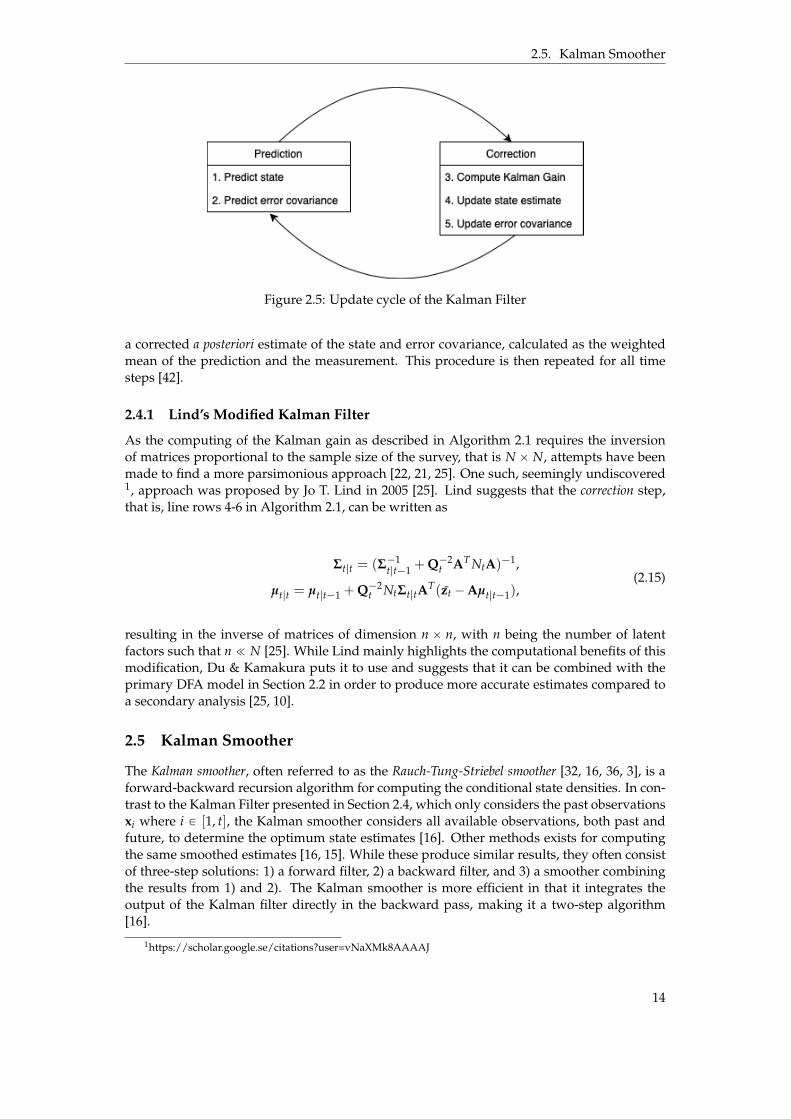
For an intuitive overview of the operations of the Kalman Filter, Algorithm 2.1 can be dividedinto two parts: prediction and correction, where rows 2-3 pertains to prediction and 4-6 to correc-tion. The reason for this separation is that during the prediction steps, the algorithm providesan a priori estimate of the current state and error covariance solely based on the state andcovariance from the previous time step. During the correction, the predicted error covarianceis used to provide the Kalman gain, which is a weight describing to what degree the observa-tion should be trusted. Using this knowledge, a new measurement is incorporated to obtain
13
2.5. Kalman Smoother
Figure 2.5: Update cycle of the Kalman Filter
a corrected a posteriori estimate of the state and error covariance, calculated as the weightedmean of the prediction and the measurement. This procedure is then repeated for all timesteps [42].
2.4.1 Lind’s Modified Kalman Filter
As the computing of the Kalman gain as described in Algorithm 2.1 requires the inversionof matrices proportional to the sample size of the survey, that is N ˆ N, attempts have beenmade to find a more parsimonious approach [22, 21, 25]. One such, seemingly undiscovered1, approach was proposed by Jo T. Lind in 2005 [25]. Lind suggests that the correction step,that is, line rows 4-6 in Algorithm 2.1, can be written as
Σt|t = (Σ´1t|t´1 + Q´2
t AT NtA)´1,
µt|t = µt|t´1 + Q´2t NtΣt|tA
T(zt ´Aµt|t´1),(2.15)
resulting in the inverse of matrices of dimension n ˆ n, with n being the number of latentfactors such that n ! N [25]. While Lind mainly highlights the computational benefits of thismodification, Du & Kamakura puts it to use and suggests that it can be combined with theprimary DFA model in Section 2.2 in order to produce more accurate estimates compared toa secondary analysis [25, 10].
2.5 Kalman Smoother
The Kalman smoother, often referred to as the Rauch-Tung-Striebel smoother [32, 16, 36, 3], is aforward-backward recursion algorithm for computing the conditional state densities. In con-trast to the Kalman Filter presented in Section 2.4, which only considers the past observationsxi where i P [1, t], the Kalman smoother considers all available observations, both past andfuture, to determine the optimum state estimates [16]. Other methods exists for computingthe same smoothed estimates [16, 15]. While these produce similar results, they often consistof three-step solutions: 1) a forward filter, 2) a backward filter, and 3) a smoother combiningthe results from 1) and 2). The Kalman smoother is more efficient in that it integrates theoutput of the Kalman filter directly in the backward pass, making it a two-step algorithm[16].
1https://scholar.google.se/citations?user=vNaXMk8AAAAJ
14
2.6. Estimating Model Parameters
The complete update equations as presented in [3, 16, 36] are given in Algorithm 2.2, followedby clarifications of each step, where
Algorithm 2.2. Kalman Smoother
1: function KALMANSMOOTHER(µt+1, Σt+1)2: Kt´1 = Σt´1|t´1A1Σ´1
t|t´13: µt´1|T = µt´1|t´1 + Kt´1(µt|T ´ µt|t´1)
4: Σt´1|T = Σt´1|t´1 + Kt´1(Σt|T ´ Σt|t´1)K1t´1
5: return µt, Σt6: end function
Σt|t, Σt+1|t, µt|t and µt+1|t are given from the Kalman filter. The complete smoothing processproceeds as follows [16]:
1. The Kalman filter is applied to the observations using forward recursion as describedin Section 2.4.
2. The recursive smoother equations as described in Algorithm 2.2 are applied to the out-put from 1., starting at time step T and propagating backwards.
As the algorithm starts from the last timestep and propagates backwards, it never updatesthe state estimates at that specific timestep, resulting in estimates possibly less true to thedynamics of the model in comparison to the other timesteps.
2.6 Estimating Model Parameters
Consider the problem of finding the MLE given the likelihood function
L(θ, X) = p(X|θ) =ż
p(X, Z|θ)dZ, (2.16)
where X is a set of observed data, Z is a set of latent data and θ are the model parameters. Formathematical convenience, it is custom to consider the corresponding log likelihood function`(θ) = ln L(θ, X). The MLE can then be found as
θMLE = argmaxθ
`(θ). (2.17)
As it turns out, this is not a trivial task when the integral in (2.16) does not have closed formsolution [8]. The presence of the integral prevents the logarithm from acting directly on thejoint distribution, resulting in non-trivial expressions of the MLE [3]. This problem requiresiterative methods in order to estimate the likelihood.
2.6.1 Expectation Maximization
The Expectation Maximization (EM) algorithm is a general two-step iterative technique forcomputing maximum likelihood estimates for probabilistic models with latent variables, thatis, missing data or unknown parameters [8]. It is general in that it provides a probabilisticframework for performing inference on the missing variables with a variety of implementa-tions, and has been used widely in a multitude of applications [3].
15
2.7. Evaluation Metrics
Consider the problem outlined in (2.17). In order to solve this, it is practical to introduce thenotation θold, θnew and Q(θ, θold), where
Q(θ, θold) =
ż
p(Z|X, θold) ln p(X, Z|θ)dZ. (2.18)
Let the set tX, Zu denote the complete data set, which makes the complete data log-likelihoodfunction ln p(X, Z|θ). Since the complete data is not given, it is necessary to refer to comput-ing the posterior distribution for the latent data, that is p(Z|X, θ), which hopefully bringssome clarity to the definition of Q(θ, θold). This is where the ingeniousness of the EM-algorithm takes place. By dividing this problem into two steps: the Expectation (E) step andthe Maximization (M) step, it is possible to iteratively converge to a distribution for the com-plete data log likelihood. In the E-step, the posterior for the latent data is evaluated usingthe parameters θold. This distribution is then used to find the expectation of the completedata log likelihood, which corresponds to evaluating the expression in (2.18). In the sub-sequent M-step, this distribution is maximized in order to obtain the new parameters θnew,corresponding to the expression
θnew = argmaxθ
Q(θ, θold). (2.19)
In order to start the algorithm, it is necessary to choose initial values for the parameters θold.The true key to why this method is viable is the property that each iteration, as it turns out,will increase the likelihood of the incomplete data. Convergence is thus evaluated as whenthe likelihood is increased with less than some chosen interruption criterion, or similarlywhen the parameters θnew « θold [3].
In order to summarize the conclusions presented in this section, the general EM-algorithm aspresented by [3] is rendered in its entirety below.
Algorithm 2.3. Expectation Maximization
1: Choose initial settings for the parameters θold
2: E step: Evaluate p(Z|X, θold)
3: M step: Evaluate θnew given by Equation (2.19), where Q(θ, θold) is given in Equation(2.18).
4: Check for convergence of either the log likelihood or the parameter values. If the conver-gence criterion is not satisfied, then let θold Ð θnew and return to step 2.
2.7 Evaluation Metrics
This section will present three different performance metrics commonly used in time seriesanalysis and forecasting to evaluate model accuracy; Root Mean Squared Error, Mean AbsoluteError and Mean Absolute Percentage Error [1, 24, 6]. There exists multiple other performancemeasures that could have proved useful to this study, but since the evaluation process initself only requires one or two indicators, the ones presented in this chapter are the ones oftenused for similar analysis and subject to between-metric comparisons due to their differentcharacteristics [18, 43, 6, 24].
16
2.7. Evaluation Metrics
2.7.1 Mean Absolute Error
Mean Absolute Error (MAE), or Mean Absolute Deviation (MAD) when the measure of cen-tral tendency is chosen to be the mean, is a measure of the average magnitude of the error
MAE =1T
Tÿ
t=1
|yt ´ yt|. (2.20)
It is calculated by taking the sum of the residuals of the mean yt and the prediction yt andaveraging it by the number of predictions. It is a linear score in that it assigns equal weightsto all errors, disregarding of magnitude [24].
2.7.2 Mean Absolute Percentage Error
Mean Absolute Percentage Error (MAPE) is a generic measure obtained by computing theerror relative to the magnitude of the measurement
MAPE =1T
Tÿ
t=1
|yt ´ yt
yt|. (2.21)
It is generic in that it is expressed as intuitive percentages and thus can be compared overdifferent datasets, a property commonly referred to as scale-independent. An evident flawwith this approach is that it is not applicable for measures yt = 0 and results in a skeweddistribution for measures in the vicinity of zero [18].
2.7.3 Root Mean Squared Error
RMSE is a measure of the mean of the squared errors
RMSE =
g
f
f
e
1T
Tÿ
t=1
(yt ´ yt)2. (2.22)
By taking the root square, the unit of the metric is obtained on the same scale as the unit of themeasurement [37]. By squaring the errors, RMSE penalizes variance as it gives more weightto errors with higher magnitude and less weight to errors with smaller magnitude [6].
2.7.4 Comparison of Performance Metrics
In the research of evaluation metrics, there has been substantial debate regarding the charac-teristics and suitability of certain metrics, as well as their performance [6, 43, 18]. Consideringthe metrics presented in this section, the debate on MAE vs. RMSE is particularly polarized.Following an article published by Willmott and Matsuura in 2005 [43], where they proposedavoidance of RMSE in favor of MAE, many researchers chose to follow their advice [6]. Whileacknowledging some of the criticism of RMSE to be valid, Chai and Draxler [6] argued the el-igibility of both metrics, as well as proposing RMSE to be the superior metric when the errordistribution is expected to be Gaussian.
Considering the practical properties of the measures, a generally accepted premise is thatMAEď RMSE. Although both metrics will indicate increased variance, RMSE is considerablymore sensitive to outliers compared to MAE and will grow to be increasingly larger than
17

2.7. Evaluation Metrics
MAE as the error variance increases [6, 43]. As such, RMSE should prove to be the moreuseful metric if large variance is particularly undesirable [24].
Due to its methodical similarities, MAE and MAPE will generally be correlated [24]. WhileMAPE has the advantage in terms of interpretability and comparability of the results, it comeswith considerable disadvantages in terms of applicability [37].
18
3 Method
This chapter will present the methodical approaches used in this research. The first sectiondescribes the data used, as well as the methods used for simulating the data. The secondSection presents the DFA model derived by combining the techniques presented in Chapter2. Finally, Section 3.3 defines the EM algorithm as well as the update equations used in theM step of the EM algorithm and Section 3.4 describes the methods used for evaluating theresults.
The terms population and respondent will be used frequently throughout this chapter, wherepopulation refers to the complete information of a variable represented by a typically largeset of samples, with population mean describing the assumed true state of a variable. Arespondent pertains to a single entity of the population.
3.1 Data Sources
3.1.1 Simulation
In order to evaluate the performance of the model, it’s necessary to know the true means foreach timestep. This was achieved by simulation, where each simulated time-series yit P ytwas assumed to follow a random walk according to the transition model
yt = yt´1 + εt εt „ N (ξ, Ω) (3.1)
where ξi P ξ is a random drift component unique to each generated time-series and Ω is agenerated positive semi-definite covariance matrix common for all time-series. In order toreplicate authentic conditions, the simulated data was required to satisfy the three patternsof correlation mentioned in Section 1.1,
1. within-measure inter-temporal dependence,
2. between-measure co-movements in population means,
19
3.1. Data Sources
3. between-measure cross-sectional co-variance.
By following the Markov process in equation (3.1), within-measure inter-temporal depen-dencies were incorporated into the data. Between-measure co-movements were imposed bygenerating a non-diagonal transition matrix for the step εt, resulting in correlated populationmeans. Correlated population means is a prerequisite in order to represent the data witha factor structure [10]. Finally, in order to introduce between-measure cross-sectional co-variations on the respondent level, the primary respondent data was sampled from emissionmodels with a non-diagonal covariance matrix. This also allowed evaluation of the perfor-mance of the model with different levels of correlation on cross-sectional measures. The exactmodels used can be found in Section 3.1.1.1 and 3.1.1.2.
A population was generated through repeated multivariate sampling from the model de-scribed in equation (3.1), where each timestep was sampled N times corresponding to thepopulation size. A panel of respondents could then be generated by randomly selectingn samples from the population at each timestep, where both n and N where selected suchthat n ! N, and N was typically large. This made it possible to re-sample from the samepopulation and evaluate performance on the same time-series with different sample sizes,simulating different number of respondents.
The key assumption that is made is that although the panel composition of respondents mayvary for each timestep, they still represent the same population mean at the aggregated level.In contrast to a longitudinal study, where the individual respondents are the same for eachtimestep and thus constitute the total population, the approach used in this research focuseson reproducing the structures 1. and 2. described above, under the assumption that the re-spondents are sampled from the same population as per [10]. The specific processes for whichthe different types of data were sampled from the time-series differs somewhat between nu-merical and binary respondent data, but remain continuous when aggregated to a populationmean.
3.1.1.1 Numerical Data Sampling
The numerical data can be divided into two categories: discrete and continuous. The processthrough which they were generated differed only in that the discrete data was obtained byrounding the continuous data to the closest integer. The actual sampling was performedusing the multivariate Gaussian emission model
yjt = yt + ψjt ψjt „ N (0, Σ), (3.2)
where yit P yt is the value of the time-series i at time t and Σ is the generated covariancematrix imposing between-measure cross-sectional co-variations at the primary level. Thus,yijt corresponds to respondent j’s answer to measure i at time t. Excerpts from the simulatedcontinuous and discrete respondent level data can be found in Appendix A.1.1 and A.1.2respectively.
3.1.1.2 Binary Data Sampling
Although binary distributions technically are a special case of discrete distributions, limitedto only two values, the binary case required a slightly different approach. In order to imposebetween-measure cross-sectional co-variance on the primary level, the population had to besampled with covariance from the generated time-series and result in binary response vari-ables. This was no trivial task as the standard binary distributions such as Poisson, Bernoulli
20
3.1. Data Sources
and Binomial, does not incorporate a multivariate covariance structure out of the box. Per-sisting with the analogy that each respondent could be regarded as a multivariate Bernoullitrial, each time-series was normalized to the interval [a, b], where a, b P [0, 1], which enabledthe use of the actual time-series as the probability in a Bernoulli trial. The property thatE(X) = p if X „ Bernoulli(p) implied that the population mean would approximately yieldthe probability by which each respondent was sampled with, which was the time-series it-self. Multivariate Bernoulli sampling is not a standard feature in most statistical softwareand thus had to be simulated through sampling from a multivariate Gaussian distributionand binarization of the output. Although this approach was a result of reasoning in combi-nation with trial and error, support for it can be found in [23], who presents a conceptuallysimilar method utilizing a Gaussian approximation to simulate correlated binary variables.The complete process proceeded as follows:
1. Select the marginal probabilities pi for each binary variable and the covariance matrixΣ describing the desired covariance between the binary variables.
2. Set µi = Φ´1(pi), where Φ´1(p) is the Probit function.
3. Draw a sample s from N (µ, Σ).
4. Binarize the sample such that xi = 0 ðñ si < 0 and xi = 1 ðñ si > 0. For si = 0, xiwas assigned uniformly.
The steps outlined above allowed the use of a covariance structured matrix when samplingfrom a multivariate Bernoulli distribution, resulting in between-measure co-variance on therespondent level. An excerpt from the simulated binary respondent level data can be foundin Appendix A.1.3.
3.1.2 Panelist Data
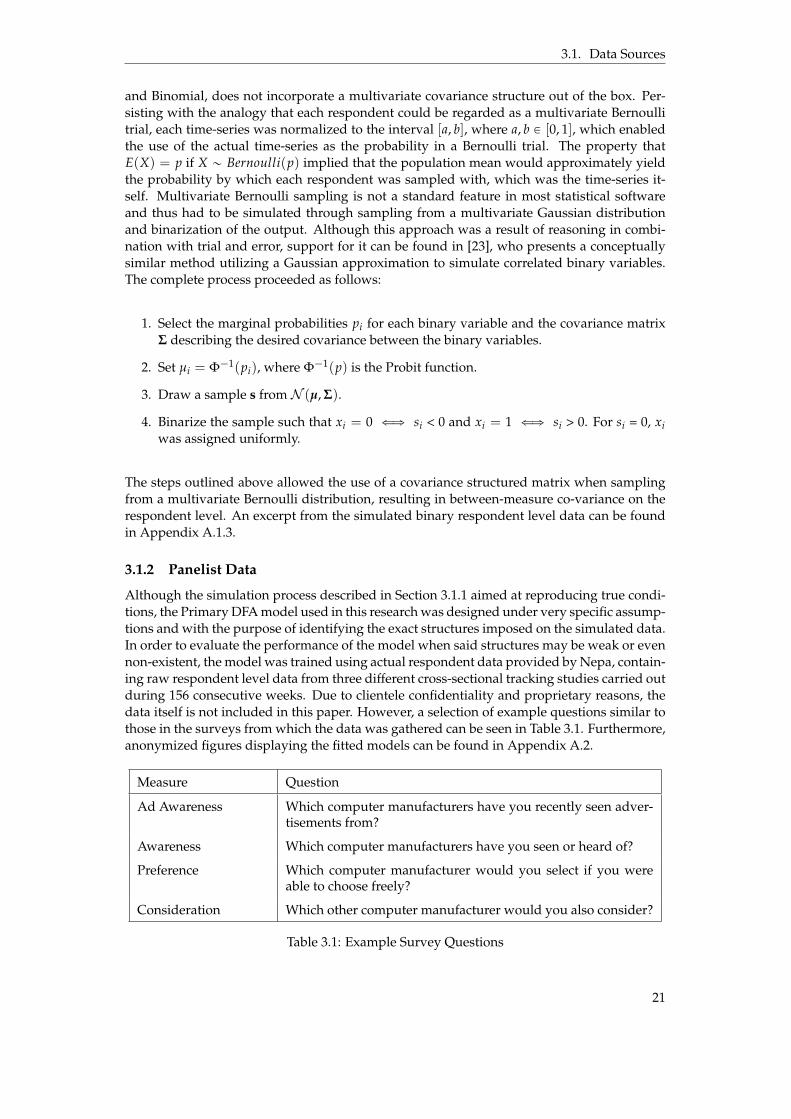
Although the simulation process described in Section 3.1.1 aimed at reproducing true condi-tions, the Primary DFA model used in this research was designed under very specific assump-tions and with the purpose of identifying the exact structures imposed on the simulated data.In order to evaluate the performance of the model when said structures may be weak or evennon-existent, the model was trained using actual respondent data provided by Nepa, contain-ing raw respondent level data from three different cross-sectional tracking studies carried outduring 156 consecutive weeks. Due to clientele confidentiality and proprietary reasons, thedata itself is not included in this paper. However, a selection of example questions similar tothose in the surveys from which the data was gathered can be seen in Table 3.1. Furthermore,anonymized figures displaying the fitted models can be found in Appendix A.2.
Measure Question
Ad Awareness Which computer manufacturers have you recently seen adver-tisements from?
Awareness Which computer manufacturers have you seen or heard of?
Preference Which computer manufacturer would you select if you wereable to choose freely?
Consideration Which other computer manufacturer would you also consider?
Table 3.1: Example Survey Questions
21
3.2. Primary DFA Model
The respondent data was exclusively binary and also contained closed-ended questions suchas Preference, which resulted in a single response. If the output from a closed-ended ques-tion was translated into the desired format where each respondent’s answers pertains to arow of binary outputs as in Appendix A.1.3, each row would contain a single one with theremaining entries being zero. This scenario differed slightly from those described previously,where each row could have multiple non-zero entries. Due to no actual covariance occurringon the respondent level, the use of a non-diagonal cross-sectional covariance matrix Σ wasimpractical, possibly even nonsensical, and required a slightly modified model in which Σ
was constrained to be diagonal.
Respondent Brand 1 Brand 2 Brand 31 0 1 02 0 0 13 1 0 0
Table 3.2: Closed-ended question - Which brand do you prefer?
3.1.3 Sampling from Panelist Data
In an attempt to provide sample conditions indisputably more true to actual conditions, whilemaintaining the possibility to evaluate performance, the provided panelist data was used togenerate the parameters from which a population could be sampled according to the methodsdescribed in Section 3.1.1. The means yit were generated by evaluating a moving averageof the four most recent measurements for each measure, which guaranteed within-measureinter-temporal dependencies as well as imposing between-measure co-movements accordingto the structures contained in the data. Instead of generating a random respondent covariancematrix Σ as in Section 3.1.1, it was generated by computing the covariance matrix of the rawrespondent data.
3.2 Primary DFA Model
The Primary DFA model used was that proposed by Du and Kamakura [10], which is animplementation of the model presented in Section 2.2. In addition to the original model, italso includes a covariate term similar to the input control variable from the Kalman Filter inSection 2.4. This term enabled the option to include known covariates such as seasonalityand marketing investments related to the analyzed measure.
The state equations for the DFA model is given by
µt = Azt + But, (3.3)
zt = zt´1 + ξt, ξt „ N (0, Ω), z0 „ N (a0, Ω0), (3.4)
where µt denotes the Nˆ 1 population mean vector at timestep t, zt denotes the Mˆ 1 vectorof latent states, A is the N ˆ M loading matrix that translates the M latent states into theN population means, ut is a N ˆ 1 vector of known covariates and B is the N ˆ M loadingmatrix that translates the covariates into the population means µt [10]. ξt is the Mˆ 1 vectorof latent state chocks, i.e., containing the real state changes from step t´ 1 to step t. Finally, Ω
is the state covariance matrix, which was diagonal in order to maintain independent factorsand thus facilitate interpretability of the extracted factors.
The corresponding observation equation was
yit = µt + εit, εit „ N (0, Σ), (3.5)
22
3.3. Algorithm
where yit denotes the vector of responses from respondent i at timestep t, εit denotes thesample noise representing respondent i’s deviation from the population mean, and Σ is theerror covariance matrix incorporating the cross-sectional between-measure co-variations.
In order to make the analogy to state-space modelling more explicit, the equations (3.3), (3.4)and (3.5) can be generalized into the state-space representation with the state equation
zt = zt´1 + ξt, ξt „ N (0, Ω), (3.6)
and observation equation
yt = JtAzt + JtBut + ε, εt „ N (0, INt b Σ), (3.7)
where
yt ” (y11t y12t . . . y1Ntt)1, (3.8)
Jt ” 1Nt b IM, (3.9)
and Nt denotes the number of respondents at timestep t, not to be confused with the numberof latent factors N. In equation (3.9)b denotes the Kronecker product, giving Jt the dimensions(MNtˆM). Thus, the model parameters that needed to be estimated were A (NˆM), B (NˆM), Σ (N ˆ N), Ω (MˆM), Ω0 (MˆM) and a0 (Mˆ 1).
3.3 Algorithm
This Section describes, part by part, the complete algorithm used in this research, start-ing with the Expectation Maximization (EM) algorithm used for inference, moving on to themethod for selecting the number of latent factors, after which all parts are compiled into asequential list in the order of which they were carried out.
3.3.1 EM
A number of different approaches have been proposed in order to perform inference on themodel parameters in the context of state space models, including examples such as PrincipalComponent Analysis in combination with a Kalman Smoother [9] and a univariate KalmanFilter and Smoother aiming to mitigate the curse of dimensionality [21]. However, the mostwidely used approach in DFA, as well as state-space modelling in general, is the EM algo-rithm introduced in Section 2.6.1 (see [10, 11, 35, 31, 27] for successful examples). The imple-mentation of the EM algorithm used in this research utilizes a Kalman Filter and Smootheras the E-step following the research of [10, 25], and parameter update equations based on thelikelihood function of [35] in the M-step, which are equivalent to the MLE of the Q-functiondescribed in equation (2.18).
3.3.1.1 E-step
The Kalman Filter used in the forward pass of the E-step was that proposed by [10], which isan implementation of Lind’s modified Kalman Filter described in Section 2.4.1.
23
3.3. Algorithm
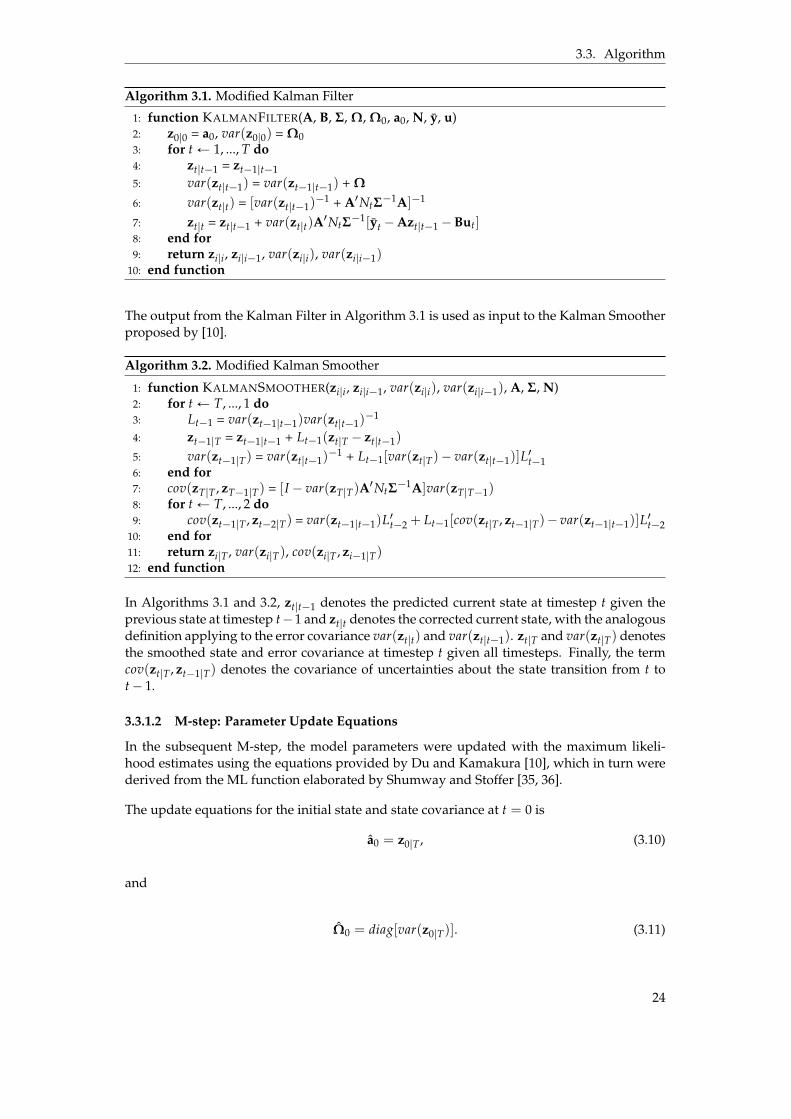
Algorithm 3.1. Modified Kalman Filter
1: function KALMANFILTER(A, B, Σ, Ω, Ω0, a0, N, y, u)2: z0|0 = a0, var(z0|0) = Ω03: for t Ð 1, ..., T do4: zt|t´1 = zt´1|t´15: var(zt|t´1) = var(zt´1|t´1) + Ω
6: var(zt|t) = [var(zt|t´1)´1 + A1NtΣ
´1A]´1
7: zt|t = zt|t´1 + var(zt|t)A1NtΣ
´1[yt ´Azt|t´1 ´But]8: end for9: return zi|i, zi|i´1, var(zi|i), var(zi|i´1)
10: end function
The output from the Kalman Filter in Algorithm 3.1 is used as input to the Kalman Smootherproposed by [10].
Algorithm 3.2. Modified Kalman Smoother
1: function KALMANSMOOTHER(zi|i, zi|i´1, var(zi|i), var(zi|i´1), A, Σ, N)2: for t Ð T, ..., 1 do3: Lt´1 = var(zt´1|t´1)var(zt|t´1)
´1
4: zt´1|T = zt´1|t´1 + Lt´1(zt|T ´ zt|t´1)
5: var(zt´1|T) = var(zt|t´1)´1 + Lt´1[var(zt|T)´ var(zt|t´1)]L1t´1
6: end for7: cov(zT|T , zT´1|T) = [I ´ var(zT|T)A
1NtΣ´1A]var(zT|T´1)
8: for t Ð T, ..., 2 do9: cov(zt´1|T , zt´2|T) = var(zt´1|t´1)L1t´2 + Lt´1[cov(zt|T , zt´1|T)´ var(zt´1|t´1)]L1t´2
10: end for11: return zi|T , var(zi|T), cov(zi|T , zi´1|T)12: end function
In Algorithms 3.1 and 3.2, zt|t´1 denotes the predicted current state at timestep t given theprevious state at timestep t´ 1 and zt|t denotes the corrected current state, with the analogousdefinition applying to the error covariance var(zt|t) and var(zt|t´1). zt|T and var(zt|T) denotesthe smoothed state and error covariance at timestep t given all timesteps. Finally, the termcov(zt|T , zt´1|T) denotes the covariance of uncertainties about the state transition from t tot´ 1.
3.3.1.2 M-step: Parameter Update Equations
In the subsequent M-step, the model parameters were updated with the maximum likeli-hood estimates using the equations provided by Du and Kamakura [10], which in turn werederived from the ML function elaborated by Shumway and Stoffer [35, 36].
The update equations for the initial state and state covariance at t = 0 is
a0 = z0|T , (3.10)
and
Ω0 = diag[var(z0|T)]. (3.11)
24
3.3. Algorithm
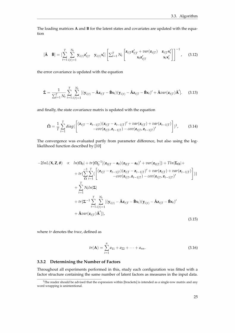
The loading matrices A and B for the latent states and covariates are updated with the equa-tion
[A B] = [T
ÿ
t=1
Ntÿ
i(t)=1
yi(t)z1t|T yi(t)x
1t]
[řT
t=1 Nt
[zt|Tz1t|T + var(zt|T) zt|Tx1t
xtz1t|T xtx1t
]]´1
, (3.12)
the error covariance is updated with the equation
Σ =1
řTt=1 Nt
Tÿ
t=1
Ntÿ
i(t)=1
[(yi(t) ´ Azt|T ´ Bxt)(yi(t) ´ Azt|T ´ Bxt)1 + Avar(zt|T)A
1]. (3.13)
and finally, the state covariance matrix is updated with the equation
Ω =1T
Tÿ
t=1
diag(
[(zt|T ´ zt´1|T)(zt|T ´ zt´1|T)
1 + var(zt|T) + var(zt´1|T)
´cov(zt|T , zt´1|T)´ cov(zt|T , zt´1|T)1
])1, (3.14)
The convergence was evaluated partly from parameter difference, but also using the log-likelihood function described by [10]
´2lnL(X, Z, θ) 9 ln|Ω0|+ trtΩ´10 [(z0|T ´ a0)(z0|T ´ a0)
1 + var(z0|T ]u+ Tln|ΣΩ|+
+ trt´1ÿ
Ω
Tÿ
t=1
(
[(zt|T ´ zt´1|T)(zt|T ´ zt´1|T)
1 + var(zt|T) + var(zt´1|T)
´cov(zt|T , zt´1|T)´ cov(zt|T , zt´1|T)1
])u
+T
ÿ
t=1
Ntln|Σ|
+ trtΣ´1T
ÿ
t=1
Ntÿ
i(t)=1
[(yi(t) ´ Azt|T ´ Bxt)(yi(t) ´ Azt|T ´ Bxt)1
+ Avar(zt|T)A1]u,
(3.15)
where tr denotes the trace, defined as
tr(A) =n
ÿ
i=1
a11 + a22 + ¨ ¨ ¨+ ann. (3.16)
3.3.2 Determining the Number of Factors
Throughout all experiments performed in this, study each configuration was fitted with afactor structure containing the same number of latent factors as measures in the input data.
1The reader should be advised that the expression within [brackets] is intended as a single-row matrix and anyword wrapping is unintentional.
25
3.4. Evaluation
The reason for this was that the appropriate number of factors is determined by the under-lying structures and no method for performing this dynamically without supervision wasfound. The experiments involved a large number of simulated datasets and none of the fittedmodels were inspected manually, so in order to reduce the risk of unintentionally passing thethreshold for underfactoring, which would have affected the results drastically, the numberof factors was set to the maximum amount of possible latent structures in the data.
3.3.3 Factor Rotation
Before generating the fitted estimates through µt = Azt + But, the loading matrix matrix Awas rotated using a Varimax rotation. The factor scores zt were corrected with the inversetransformation matrix in order to retain the same fitted values. Consequently, this step didnot affect the actual model fit and results, but was implemented solely to facilitate factorinterpretation.
3.3.4 Algorithm Summary
1. Determine the number of latent factors N.
2. Initialize A, B, Σ, Ω, Ω0 and a0 with random values.
3. E-step according to Section 3.3.1.1.
4. M-step according to Section 3.3.1.2 using the output from 3) as input.
5. Evaluate convergence by likelihood and model parameter difference according to a con-vergence tolerance.
6. Repeat step 3) - 5) until convergence.
7. Apply Varimax factor rotation to A.
8. Fit µt = Azt + But.
3.4 Evaluation
As the simulated data, with the exception of that obtained from the panelist data, only con-tained structures that were present by design and not actually related to any real significance,to try to determine such structures would have proven meaningless. Furthermore, the use ofa latent factor structure was merely a method for reducing dimensionality and deriving amore parsimonious representation of the data. Thus, the evaluation of the model solely fo-cused on the performance in terms of re-creating the population mean.
3.4.1 Baseline
In order to present a just benchmark for the model, it was compared to two different baselines:the sample mean at each timestep, and the moving average evaluated as the unweightedmean of the n most recent sample means. The order n was determined as two after evaluatingwhich order had the best performance on the simulated data, where order is equivalent tothe number of weeks.
3.4.2 Metrics
The model was evaluated using the three different metrics presented in Section 2.7: MAE,MAPE and RMSE. Combined, these metrics presented a comprehensive proving groundwhich evaluated different aspects of the model performance. Each metric was calculated
26
3.4. Evaluation
by averaging over all individual scores for each measure. For instance, if the input datacomprised of two measures, the metric was calculated for each measure separately and thenaveraged over both measures.
3.4.3 Tests
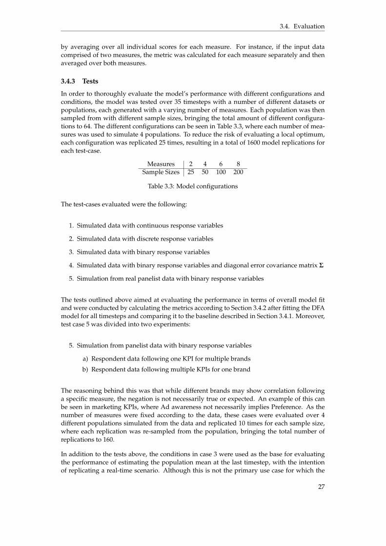
In order to thoroughly evaluate the model’s performance with different configurations andconditions, the model was tested over 35 timesteps with a number of different datasets orpopulations, each generated with a varying number of measures. Each population was thensampled from with different sample sizes, bringing the total amount of different configura-tions to 64. The different configurations can be seen in Table 3.3, where each number of mea-sures was used to simulate 4 populations. To reduce the risk of evaluating a local optimum,each configuration was replicated 25 times, resulting in a total of 1600 model replications foreach test-case.
Measures 2 4 6 8Sample Sizes 25 50 100 200
Table 3.3: Model configurations
The test-cases evaluated were the following:
1. Simulated data with continuous response variables
2. Simulated data with discrete response variables
3. Simulated data with binary response variables
4. Simulated data with binary response variables and diagonal error covariance matrix Σ
5. Simulation from real panelist data with binary response variables
The tests outlined above aimed at evaluating the performance in terms of overall model fitand were conducted by calculating the metrics according to Section 3.4.2 after fitting the DFAmodel for all timesteps and comparing it to the baseline described in Section 3.4.1. Moreover,test case 5 was divided into two experiments:
5. Simulation from panelist data with binary response variables
a) Respondent data following one KPI for multiple brands
b) Respondent data following multiple KPIs for one brand
The reasoning behind this was that while different brands may show correlation followinga specific measure, the negation is not necessarily true or expected. An example of this canbe seen in marketing KPIs, where Ad awareness not necessarily implies Preference. As thenumber of measures were fixed according to the data, these cases were evaluated over 4different populations simulated from the data and replicated 10 times for each sample size,where each replication was re-sampled from the population, bringing the total number ofreplications to 160.
In addition to the tests above, the conditions in case 3 were used as the base for evaluatingthe performance of estimating the population mean at the last timestep, with the intentionof replicating a real-time scenario. Although this is not the primary use case for which the
27

3.4. Evaluation
model is designed, any reduction of the delay caused by the dynamics of the moving averagewould be beneficial. Thus, both the estimation error at timestep T and T-1 was evaluatedand compared to the baseline, where T P [5, 50]. Due to the model being re-fitted for eachtimestep, the number of test iterations was limited to 30 in order to reduce total runtime.The sample size and number of measures were randomly sampled from [25, 100] and [2, 8]respectively for each test iteration.
6. Real-time estimation at timestep T-1
7. Real-time estimation at timestep T
28
4 Results
This chapter presents the results from implementing the DFA model and evaluating it onsimulated as well as real respondent data. The results are divided into two parts, whereSection 4.1 will outline the results of fitting the model on simulated data and Section 4.2describes the results gathered from the experiments using real data.
4.1 Simulated Data
This section describes the results of the tests performed on the simulated data, starting withdetermining the order of the moving average that was used as baseline in the subsequenttests and continuing with the results of the test cases 1 - 4 described in Section 3.4.3.
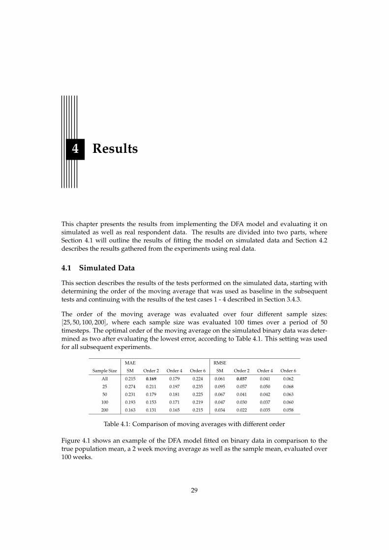
The order of the moving average was evaluated over four different sample sizes:[25, 50, 100, 200], where each sample size was evaluated 100 times over a period of 50timesteps. The optimal order of the moving average on the simulated binary data was deter-mined as two after evaluating the lowest error, according to Table 4.1. This setting was usedfor all subsequent experiments.
MAE RMSE
Sample Size SM Order 2 Order 4 Order 6 SM Order 2 Order 4 Order 6
All 0.215 0.169 0.179 0.224 0.061 0.037 0.041 0.062
25 0.274 0.211 0.197 0.235 0.095 0.057 0.050 0.068
50 0.231 0.179 0.181 0.225 0.067 0.041 0.042 0.063
100 0.193 0.153 0.171 0.219 0.047 0.030 0.037 0.060
200 0.163 0.131 0.165 0.215 0.034 0.022 0.035 0.058
Table 4.1: Comparison of moving averages with different order
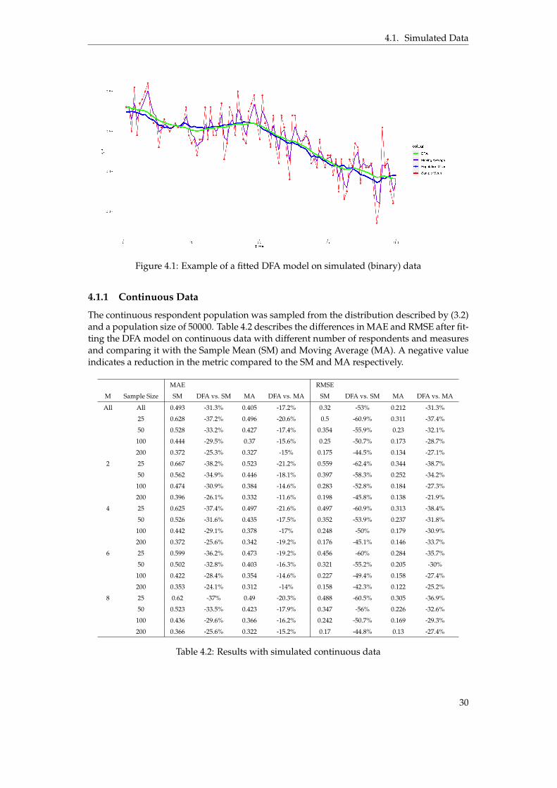
Figure 4.1 shows an example of the DFA model fitted on binary data in comparison to thetrue population mean, a 2 week moving average as well as the sample mean, evaluated over100 weeks.
29
4.1. Simulated Data
Figure 4.1: Example of a fitted DFA model on simulated (binary) data
4.1.1 Continuous Data
The continuous respondent population was sampled from the distribution described by (3.2)and a population size of 50000. Table 4.2 describes the differences in MAE and RMSE after fit-ting the DFA model on continuous data with different number of respondents and measuresand comparing it with the Sample Mean (SM) and Moving Average (MA). A negative valueindicates a reduction in the metric compared to the SM and MA respectively.
MAE RMSE
M Sample Size SM DFA vs. SM MA DFA vs. MA SM DFA vs. SM MA DFA vs. MA
All All 0.493 -31.3% 0.405 -17.2% 0.32 -53% 0.212 -31.3%
25 0.628 -37.2% 0.496 -20.6% 0.5 -60.9% 0.311 -37.4%
50 0.528 -33.2% 0.427 -17.4% 0.354 -55.9% 0.23 -32.1%
100 0.444 -29.5% 0.37 -15.6% 0.25 -50.7% 0.173 -28.7%
200 0.372 -25.3% 0.327 -15% 0.175 -44.5% 0.134 -27.1%
2 25 0.667 -38.2% 0.523 -21.2% 0.559 -62.4% 0.344 -38.7%
50 0.562 -34.9% 0.446 -18.1% 0.397 -58.3% 0.252 -34.2%
100 0.474 -30.9% 0.384 -14.6% 0.283 -52.8% 0.184 -27.3%
200 0.396 -26.1% 0.332 -11.6% 0.198 -45.8% 0.138 -21.9%
4 25 0.625 -37.4% 0.497 -21.6% 0.497 -60.9% 0.313 -38.4%
50 0.526 -31.6% 0.435 -17.5% 0.352 -53.9% 0.237 -31.8%
100 0.442 -29.1% 0.378 -17% 0.248 -50% 0.179 -30.9%
200 0.372 -25.6% 0.342 -19.2% 0.176 -45.1% 0.146 -33.7%
6 25 0.599 -36.2% 0.473 -19.2% 0.456 -60% 0.284 -35.7%
50 0.502 -32.8% 0.403 -16.3% 0.321 -55.2% 0.205 -30%
100 0.422 -28.4% 0.354 -14.6% 0.227 -49.4% 0.158 -27.4%
200 0.353 -24.1% 0.312 -14% 0.158 -42.3% 0.122 -25.2%
8 25 0.62 -37% 0.49 -20.3% 0.488 -60.5% 0.305 -36.9%
50 0.523 -33.5% 0.423 -17.9% 0.347 -56% 0.226 -32.6%
100 0.436 -29.6% 0.366 -16.2% 0.242 -50.7% 0.169 -29.3%
200 0.366 -25.6% 0.322 -15.2% 0.17 -44.8% 0.13 -27.4%
Table 4.2: Results with simulated continuous data
30
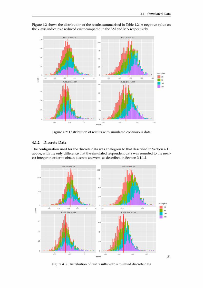
4.1. Simulated Data
Figure 4.2 shows the distribution of the results summarised in Table 4.2. A negative value onthe x-axis indicates a reduced error compared to the SM and MA respectively.
RMSE: DFA vs. MA RMSE: DFA vs. SM
MAE: DFA vs. MA MAE: DFA vs. SM
−50 −25 0 −80 −60 −40 −20
−40 −30 −20 −10 0 10 −50 −40 −30 −20 −10
0
25
50
75
100
0
20
40
60
80
0
30
60
90
120
0
20
40
60
score
coun
t
samples
25
50
100
200
Figure 4.2: Distribution of results with simulated continuous data
4.1.2 Discrete Data
The configuration used for the discrete data was analogous to that described in Section 4.1.1above, with the only difference that the simulated respondent data was rounded to the near-est integer in order to obtain discrete answers, as described in Section 3.1.1.1.
RMSE: DFA vs. MA RMSE: DFA vs. SM
MAE: DFA vs. MA MAE: DFA vs. SM
−50 −25 0 −80 −60 −40 −20
−40 −30 −20 −10 0 10 −60 −40 −20
0
25
50
75
100
0
20
40
60
0
50
100
0
25
50
75
score
coun
t
samples
25
50
100
200
Figure 4.3: Distribution of test results with simulated discrete data
31
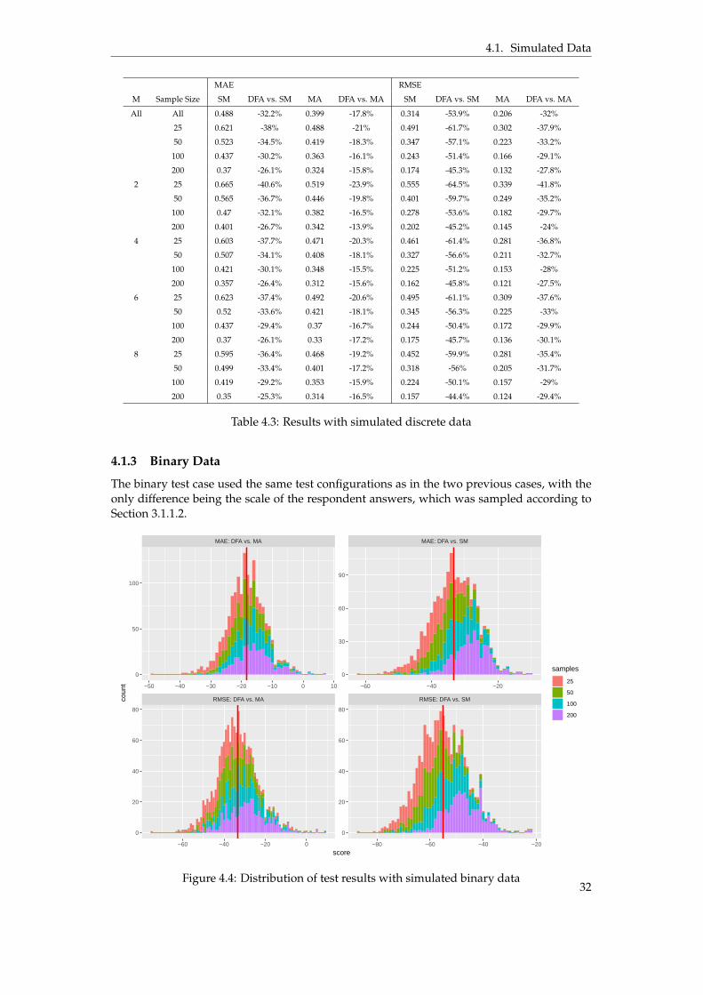
4.1. Simulated Data
MAE RMSE
M Sample Size SM DFA vs. SM MA DFA vs. MA SM DFA vs. SM MA DFA vs. MA
All All 0.488 -32.2% 0.399 -17.8% 0.314 -53.9% 0.206 -32%
25 0.621 -38% 0.488 -21% 0.491 -61.7% 0.302 -37.9%
50 0.523 -34.5% 0.419 -18.3% 0.347 -57.1% 0.223 -33.2%
100 0.437 -30.2% 0.363 -16.1% 0.243 -51.4% 0.166 -29.1%
200 0.37 -26.1% 0.324 -15.8% 0.174 -45.3% 0.132 -27.8%
2 25 0.665 -40.6% 0.519 -23.9% 0.555 -64.5% 0.339 -41.8%
50 0.565 -36.7% 0.446 -19.8% 0.401 -59.7% 0.249 -35.2%
100 0.47 -32.1% 0.382 -16.5% 0.278 -53.6% 0.182 -29.7%
200 0.401 -26.7% 0.342 -13.9% 0.202 -45.2% 0.145 -24%
4 25 0.603 -37.7% 0.471 -20.3% 0.461 -61.4% 0.281 -36.8%
50 0.507 -34.1% 0.408 -18.1% 0.327 -56.6% 0.211 -32.7%
100 0.421 -30.1% 0.348 -15.5% 0.225 -51.2% 0.153 -28%
200 0.357 -26.4% 0.312 -15.6% 0.162 -45.8% 0.121 -27.5%
6 25 0.623 -37.4% 0.492 -20.6% 0.495 -61.1% 0.309 -37.6%
50 0.52 -33.6% 0.421 -18.1% 0.345 -56.3% 0.225 -33%
100 0.437 -29.4% 0.37 -16.7% 0.244 -50.4% 0.172 -29.9%
200 0.37 -26.1% 0.33 -17.2% 0.175 -45.7% 0.136 -30.1%
8 25 0.595 -36.4% 0.468 -19.2% 0.452 -59.9% 0.281 -35.4%
50 0.499 -33.4% 0.401 -17.2% 0.318 -56% 0.205 -31.7%
100 0.419 -29.2% 0.353 -15.9% 0.224 -50.1% 0.157 -29%
200 0.35 -25.3% 0.314 -16.5% 0.157 -44.4% 0.124 -29.4%
Table 4.3: Results with simulated discrete data
4.1.3 Binary Data
The binary test case used the same test configurations as in the two previous cases, with theonly difference being the scale of the respondent answers, which was sampled according toSection 3.1.1.2.
RMSE: DFA vs. MA RMSE: DFA vs. SM
MAE: DFA vs. MA MAE: DFA vs. SM
−60 −40 −20 0 −80 −60 −40 −20
−50 −40 −30 −20 −10 0 10 −60 −40 −20
0
30
60
90
0
20
40
60
80
0
50
100
0
20
40
60
80
score
coun
t
samples
25
50
100
200
Figure 4.4: Distribution of test results with simulated binary data32
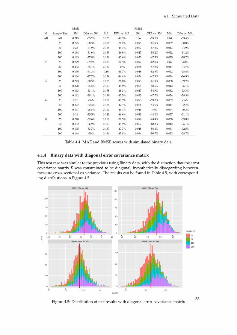
4.1. Simulated Data
MAE RMSE
M Sample Size SM DFA vs. SM MA DFA vs. MA SM DFA vs. SM MA DFA vs. MA
All All 0.215 -33.2% 0.175 -18.3% 0.06 -55.1% 0.04 -33.4%
25 0.275 -38.3% 0.216 -21.7% 0.095 -61.8% 0.059 -38.8%
50 0.23 -34.9% 0.185 -19.1% 0.067 -57.8% 0.043 -34.9%
100 0.194 -31.6% 0.159 -16.9% 0.047 -53.2% 0.032 -31.2%
200 0.163 -27.8% 0.139 -15.6% 0.033 -47.5% 0.025 -28.7%
2 25 0.279 -39.2% 0.218 -22.5% 0.097 -62.8% 0.06 -40%
50 0.233 -35.1% 0.187 -19% 0.068 -57.9% 0.044 -34.7%
100 0.196 -31.3% 0.16 -15.7% 0.048 -52.9% 0.032 -28.8%
200 0.164 -27.7% 0.139 -14.4% 0.034 -47.5% 0.024 -26.9%
4 25 0.273 -38.5% 0.215 -21.8% 0.093 -61.9% 0.058 -39.2%
50 0.228 -35.5% 0.183 -19.9% 0.065 -58.6% 0.042 -36.1%
100 0.193 -33.1% 0.158 -18.3% 0.047 -54.9% 0.032 -33.3%
200 0.162 -28.1% 0.138 -15.5% 0.033 -47.7% 0.024 -28.3%
6 25 0.27 -36% 0.216 -19.9% 0.093 -59.2% 0.059 -36%
50 0.227 -32.3% 0.186 -17.4% 0.066 -54.6% 0.044 -32.7%
100 0.191 -28.5% 0.162 -16.1% 0.046 -49% 0.034 -30.3%
200 0.16 -25.5% 0.143 -16.6% 0.033 -44.2% 0.027 -31.1%
8 25 0.278 -39.6% 0.216 -22.5% 0.096 -63.4% 0.058 -39.8%
50 0.232 -36.9% 0.183 -19.9% 0.067 -60.2% 0.042 -36.1%
100 0.195 -33.7% 0.157 -17.7% 0.048 -56.1% 0.031 -32.5%
200 0.164 -30% 0.136 -15.8% 0.034 -50.7% 0.023 -28.7%
Table 4.4: MAE and RMSE scores with simulated binary data
4.1.4 Binary data with diagonal error covariance matrix
This test case was similar to the previous using Binary data, with the distinction that the errorcovariance matrix Σ was constrained to be diagonal, hypothetically disregarding between-measure cross-sectional co-variance. The results can be found in Table 4.5, with correspond-ing distributions in Figure 4.5.
RMSE: DFA vs. MA RMSE: DFA vs. SM
MAE: DFA vs. MA MAE: DFA vs. SM
−75 −50 −25 0 −80 −60 −40
−50 −40 −30 −20 −10 0 10 −60 −50 −40 −30 −20
0
25
50
75
100
125
0
25
50
75
0
25
50
75
100
0
20
40
60
score
coun
t
samples
25
50
100
200
Figure 4.5: Distribution of test results with diagonal error-covariance matrix33
4.2. Real Data
MAE RMSE
M Sample Size SM DFA vs. SM MA DFA vs. MA SM DFA vs. SM MA DFA vs. MA
All All 0.217 -32.8% 0.173 -16.2% 0.061 -54.4% 0.039 -29.7%
25 0.277 -37.6% 0.216 -19.9% 0.096 -60.8% 0.059 -35.9%
50 0.233 -34.8% 0.184 -17.4% 0.068 -57.1% 0.043 -31.5%
100 0.196 -31.2% 0.157 -14.5% 0.048 -52.5% 0.031 -27.1%
200 0.164 -27.5% 0.136 -12.9% 0.034 -47% 0.024 -24.1%
2 25 0.282 -40.5% 0.217 -23% 0.099 -64.6% 0.059 -41.2%
50 0.236 -37.7% 0.183 -19.6% 0.07 -61.1% 0.042 -35.5%
100 0.197 -33.1% 0.154 -14.5% 0.049 -55.6% 0.03 -27.7%
200 0.164 -29.3% 0.132 -12.1% 0.034 -49.7% 0.022 -22.5%
4 25 0.279 -37.8% 0.217 -20.2% 0.097 -61.1% 0.059 -36.5%
50 0.235 -35.1% 0.184 -17.4% 0.069 -57.6% 0.043 -31.6%
100 0.197 -31.7% 0.159 -15% 0.049 -53.2% 0.032 -27.7%
200 0.166 -27.3% 0.137 -11.7% 0.035 -46.9% 0.023 -22%
6 25 0.274 -36% 0.215 -18.5% 0.094 -58.7% 0.058 -33.2%
50 0.23 -33.1% 0.184 -16.4% 0.067 -54.9% 0.043 -29.6%
100 0.193 -29.7% 0.157 -13.4% 0.047 -50.2% 0.031 -24.9%
200 0.162 -26.6% 0.137 -13.1% 0.033 -45.5% 0.024 -24.8%
8 25 0.274 -36.1% 0.213 -18.1% 0.094 -58.9% 0.057 -32.8%
50 0.23 -33.2% 0.183 -16.1% 0.067 -54.8% 0.043 -29.4%
100 0.194 -30.2% 0.16 -15.1% 0.047 -51% 0.032 -27.9%
200 0.162 -26.7% 0.139 -14.6% 0.033 -45.9% 0.025 -27.2%
Table 4.5: MAE and RMSE scores with simulated binary data and diagonal error-covariancematrix
4.1.5 Real-time estimation
Table 4.6 describes the results of real-time estimation, performed by incrementally and re-peatedly fitting the DFA model and evaluating the ability to reproduce the population meanat timestep T´ 1 and T, for T P [5, 50].
Metric Time SM 2W MA 4W MA DFA vs. SM DFA vs. 2W MA DFA vs. 4W MA
RMSE T 0.063 0.037 0.041 -50.7% -16.7% -20.0%
T - 1 0.064 0.037 0.041 -56.7% -26.9% -28.8%
MAE T 0.224 0.172 0.178 -30.0% -8.9% -11.6%
T - 1 0.224 0.172 0.178 -34.6% -14.8% -16.9%
Table 4.6: RMSE and MAE scores from real-time estimation at step T and T-1
4.2 Real Data
This section describes the results following the experiments performed on the data simulatedfrom true respondent data, starting with the test results of the case with one brand and mul-tiple measures, followed by the case with one measure and multiple brands.
34
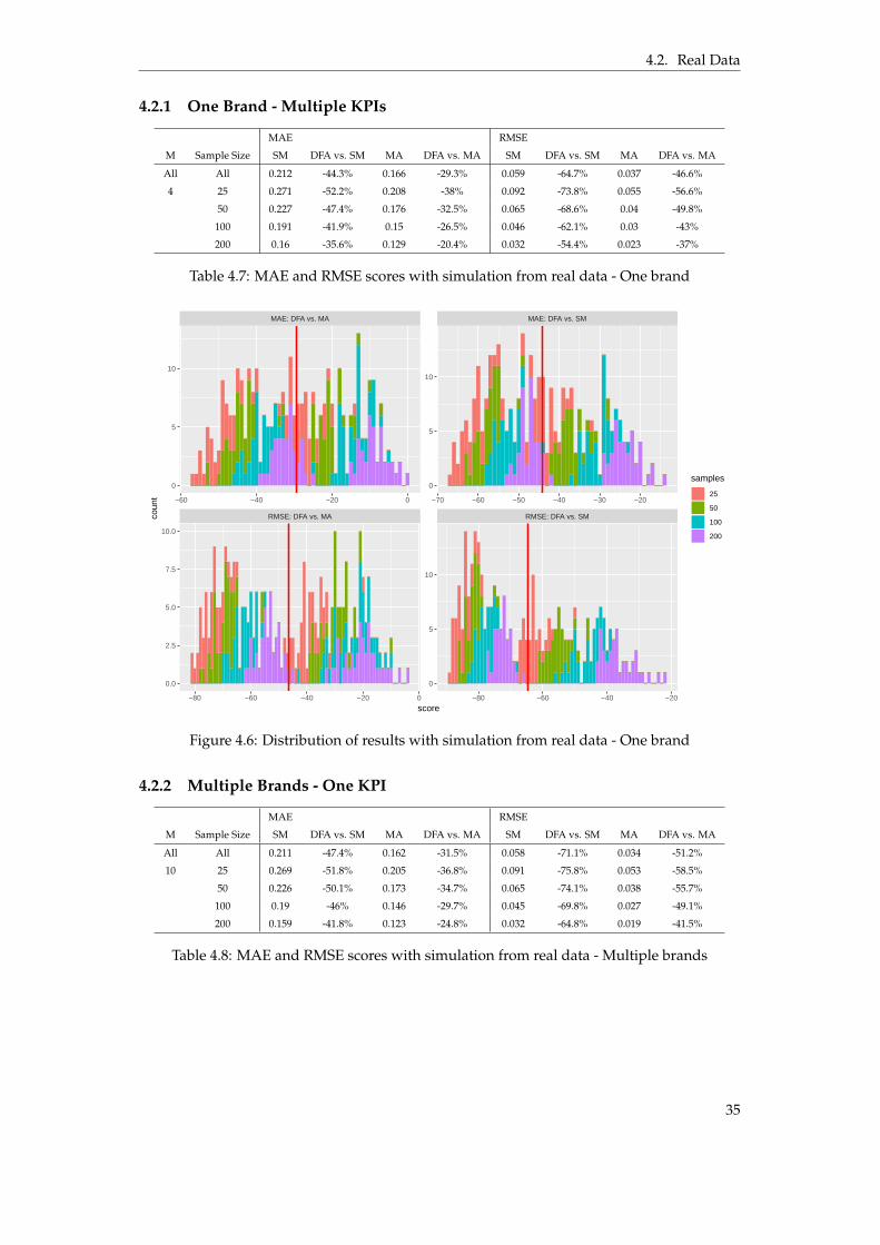
4.2. Real Data
4.2.1 One Brand - Multiple KPIs
MAE RMSE
M Sample Size SM DFA vs. SM MA DFA vs. MA SM DFA vs. SM MA DFA vs. MA
All All 0.212 -44.3% 0.166 -29.3% 0.059 -64.7% 0.037 -46.6%
4 25 0.271 -52.2% 0.208 -38% 0.092 -73.8% 0.055 -56.6%
50 0.227 -47.4% 0.176 -32.5% 0.065 -68.6% 0.04 -49.8%
100 0.191 -41.9% 0.15 -26.5% 0.046 -62.1% 0.03 -43%
200 0.16 -35.6% 0.129 -20.4% 0.032 -54.4% 0.023 -37%
Table 4.7: MAE and RMSE scores with simulation from real data - One brand
RMSE: DFA vs. MA RMSE: DFA vs. SM
MAE: DFA vs. MA MAE: DFA vs. SM
−80 −60 −40 −20 0 −80 −60 −40 −20
−60 −40 −20 0 −70 −60 −50 −40 −30 −20
0
5
10
0
5
10
0
5
10
0.0
2.5
5.0
7.5
10.0
score
coun
t
samples
25
50
100
200
Figure 4.6: Distribution of results with simulation from real data - One brand
4.2.2 Multiple Brands - One KPI
MAE RMSE
M Sample Size SM DFA vs. SM MA DFA vs. MA SM DFA vs. SM MA DFA vs. MA
All All 0.211 -47.4% 0.162 -31.5% 0.058 -71.1% 0.034 -51.2%
10 25 0.269 -51.8% 0.205 -36.8% 0.091 -75.8% 0.053 -58.5%
50 0.226 -50.1% 0.173 -34.7% 0.065 -74.1% 0.038 -55.7%
100 0.19 -46% 0.146 -29.7% 0.045 -69.8% 0.027 -49.1%
200 0.159 -41.8% 0.123 -24.8% 0.032 -64.8% 0.019 -41.5%
Table 4.8: MAE and RMSE scores with simulation from real data - Multiple brands
35
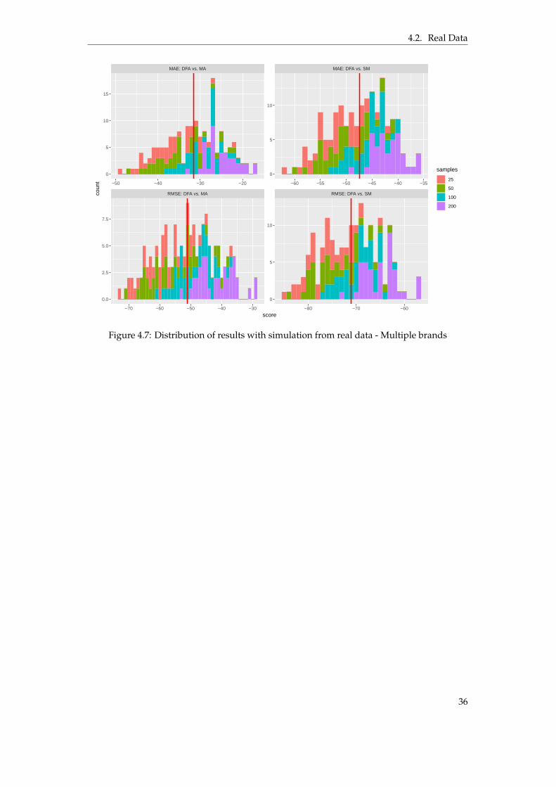
4.2. Real Data
RMSE: DFA vs. MA RMSE: DFA vs. SM
MAE: DFA vs. MA MAE: DFA vs. SM
−70 −60 −50 −40 −30 −80 −70 −60
−50 −40 −30 −20 −60 −55 −50 −45 −40 −35
0
5
10
0
5
10
0
5
10
15
0.0
2.5
5.0
7.5
score
coun
t
samples
25
50
100
200
Figure 4.7: Distribution of results with simulation from real data - Multiple brands
36
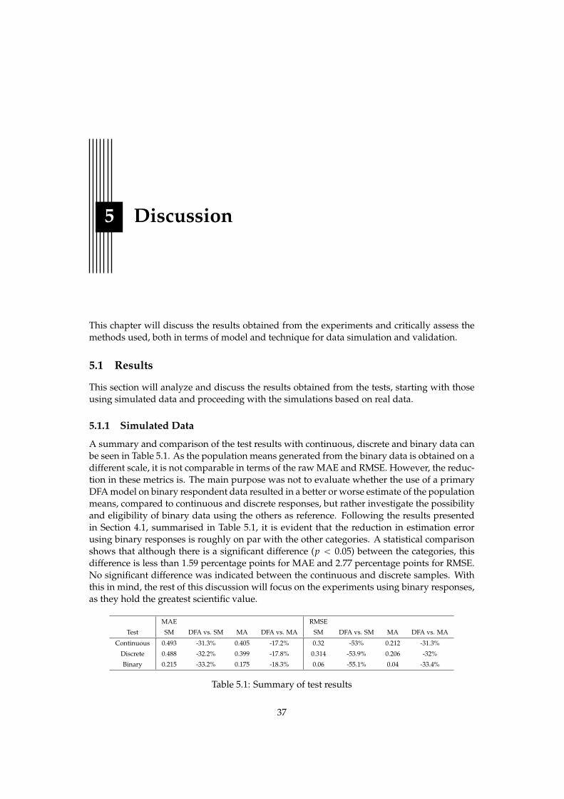
5 Discussion
This chapter will discuss the results obtained from the experiments and critically assess themethods used, both in terms of model and technique for data simulation and validation.
5.1 Results
This section will analyze and discuss the results obtained from the tests, starting with thoseusing simulated data and proceeding with the simulations based on real data.
5.1.1 Simulated Data
A summary and comparison of the test results with continuous, discrete and binary data canbe seen in Table 5.1. As the population means generated from the binary data is obtained on adifferent scale, it is not comparable in terms of the raw MAE and RMSE. However, the reduc-tion in these metrics is. The main purpose was not to evaluate whether the use of a primaryDFA model on binary respondent data resulted in a better or worse estimate of the populationmeans, compared to continuous and discrete responses, but rather investigate the possibilityand eligibility of binary data using the others as reference. Following the results presentedin Section 4.1, summarised in Table 5.1, it is evident that the reduction in estimation errorusing binary responses is roughly on par with the other categories. A statistical comparisonshows that although there is a significant difference (p ă 0.05) between the categories, thisdifference is less than 1.59 percentage points for MAE and 2.77 percentage points for RMSE.No significant difference was indicated between the continuous and discrete samples. Withthis in mind, the rest of this discussion will focus on the experiments using binary responses,as they hold the greatest scientific value.
MAE RMSE
Test SM DFA vs. SM MA DFA vs. MA SM DFA vs. SM MA DFA vs. MA
Continuous 0.493 -31.3% 0.405 -17.2% 0.32 -53% 0.212 -31.3%
Discrete 0.488 -32.2% 0.399 -17.8% 0.314 -53.9% 0.206 -32%
Binary 0.215 -33.2% 0.175 -18.3% 0.06 -55.1% 0.04 -33.4%
Table 5.1: Summary of test results
37
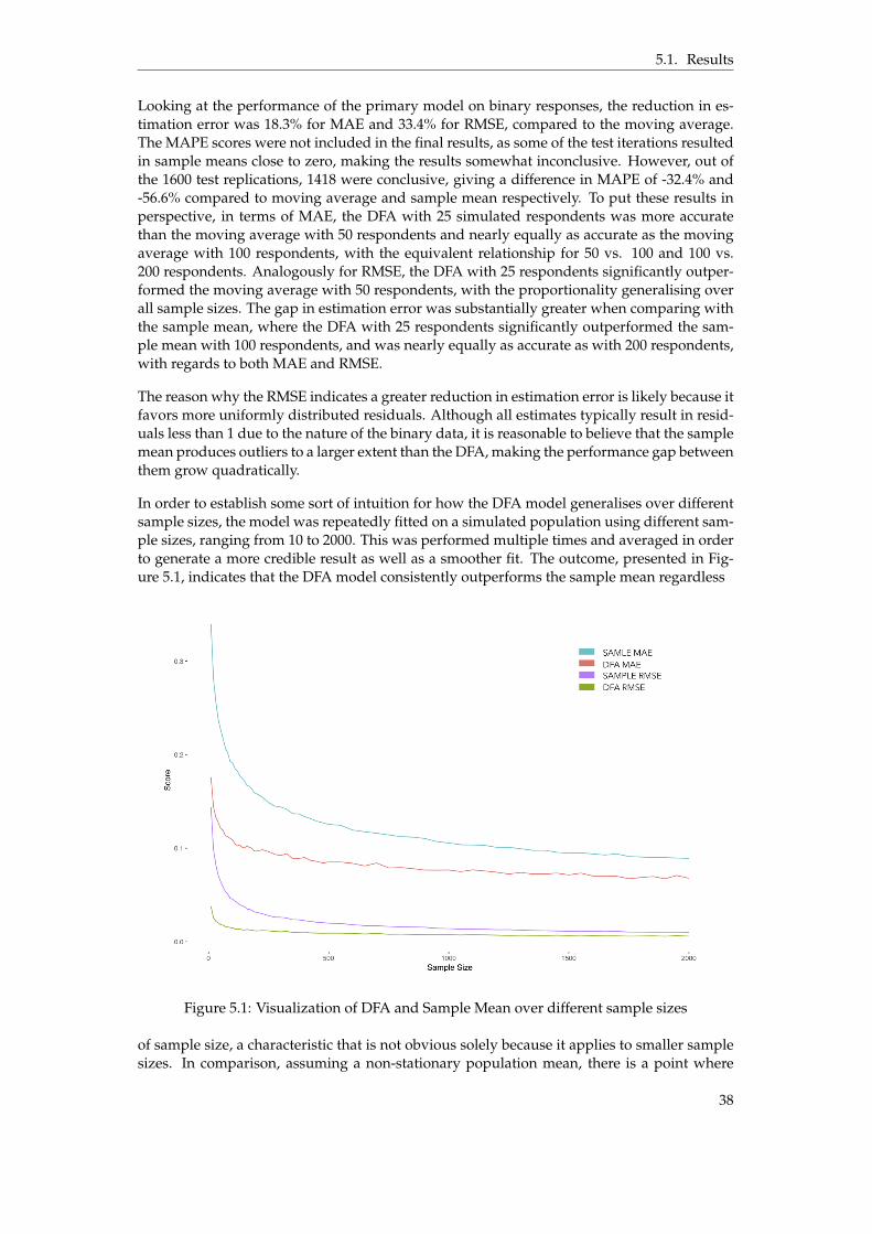
5.1. Results
Looking at the performance of the primary model on binary responses, the reduction in es-timation error was 18.3% for MAE and 33.4% for RMSE, compared to the moving average.The MAPE scores were not included in the final results, as some of the test iterations resultedin sample means close to zero, making the results somewhat inconclusive. However, out ofthe 1600 test replications, 1418 were conclusive, giving a difference in MAPE of -32.4% and-56.6% compared to moving average and sample mean respectively. To put these results inperspective, in terms of MAE, the DFA with 25 simulated respondents was more accuratethan the moving average with 50 respondents and nearly equally as accurate as the movingaverage with 100 respondents, with the equivalent relationship for 50 vs. 100 and 100 vs.200 respondents. Analogously for RMSE, the DFA with 25 respondents significantly outper-formed the moving average with 50 respondents, with the proportionality generalising overall sample sizes. The gap in estimation error was substantially greater when comparing withthe sample mean, where the DFA with 25 respondents significantly outperformed the sam-ple mean with 100 respondents, and was nearly equally as accurate as with 200 respondents,with regards to both MAE and RMSE.
The reason why the RMSE indicates a greater reduction in estimation error is likely because itfavors more uniformly distributed residuals. Although all estimates typically result in resid-uals less than 1 due to the nature of the binary data, it is reasonable to believe that the samplemean produces outliers to a larger extent than the DFA, making the performance gap betweenthem grow quadratically.
In order to establish some sort of intuition for how the DFA model generalises over differentsample sizes, the model was repeatedly fitted on a simulated population using different sam-ple sizes, ranging from 10 to 2000. This was performed multiple times and averaged in orderto generate a more credible result as well as a smoother fit. The outcome, presented in Fig-ure 5.1, indicates that the DFA model consistently outperforms the sample mean regardless
Figure 5.1: Visualization of DFA and Sample Mean over different sample sizes
of sample size, a characteristic that is not obvious solely because it applies to smaller samplesizes. In comparison, assuming a non-stationary population mean, there is a point where
38
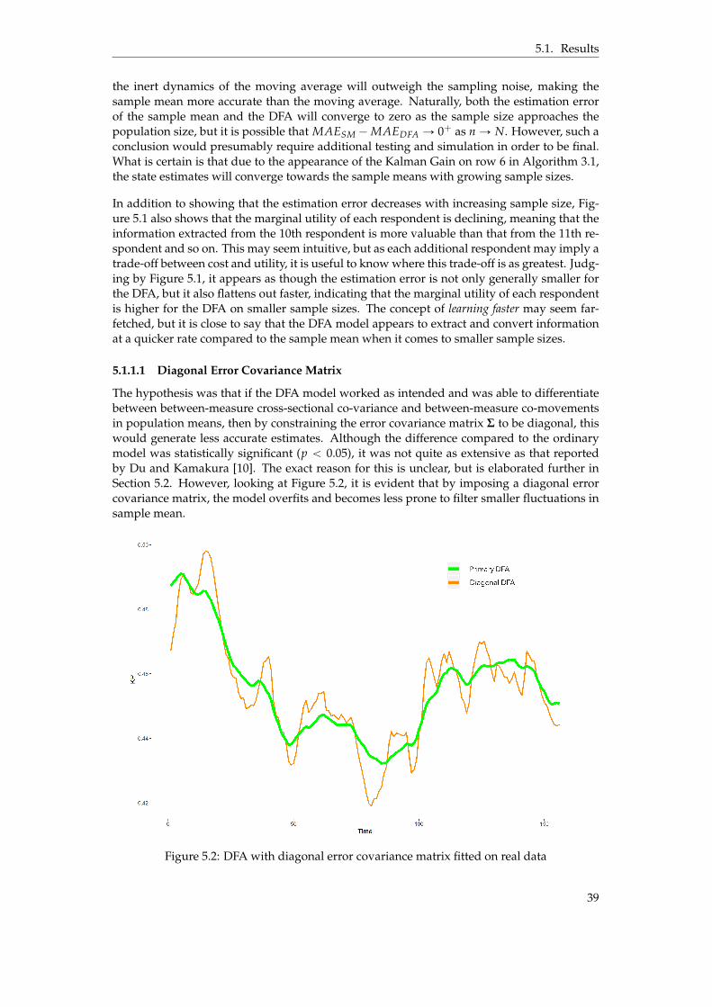
5.1. Results
the inert dynamics of the moving average will outweigh the sampling noise, making thesample mean more accurate than the moving average. Naturally, both the estimation errorof the sample mean and the DFA will converge to zero as the sample size approaches thepopulation size, but it is possible that MAESM ´MAEDFA Ñ 0+ as n Ñ N. However, such aconclusion would presumably require additional testing and simulation in order to be final.What is certain is that due to the appearance of the Kalman Gain on row 6 in Algorithm 3.1,the state estimates will converge towards the sample means with growing sample sizes.
In addition to showing that the estimation error decreases with increasing sample size, Fig-ure 5.1 also shows that the marginal utility of each respondent is declining, meaning that theinformation extracted from the 10th respondent is more valuable than that from the 11th re-spondent and so on. This may seem intuitive, but as each additional respondent may imply atrade-off between cost and utility, it is useful to know where this trade-off is as greatest. Judg-ing by Figure 5.1, it appears as though the estimation error is not only generally smaller forthe DFA, but it also flattens out faster, indicating that the marginal utility of each respondentis higher for the DFA on smaller sample sizes. The concept of learning faster may seem far-fetched, but it is close to say that the DFA model appears to extract and convert informationat a quicker rate compared to the sample mean when it comes to smaller sample sizes.
5.1.1.1 Diagonal Error Covariance Matrix
The hypothesis was that if the DFA model worked as intended and was able to differentiatebetween between-measure cross-sectional co-variance and between-measure co-movementsin population means, then by constraining the error covariance matrix Σ to be diagonal, thiswould generate less accurate estimates. Although the difference compared to the ordinarymodel was statistically significant (p ă 0.05), it was not quite as extensive as that reportedby Du and Kamakura [10]. The exact reason for this is unclear, but is elaborated further inSection 5.2. However, looking at Figure 5.2, it is evident that by imposing a diagonal errorcovariance matrix, the model overfits and becomes less prone to filter smaller fluctuations insample mean.
Figure 5.2: DFA with diagonal error covariance matrix fitted on real data
39
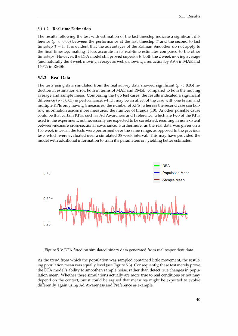
5.1. Results
5.1.1.2 Real-time Estimation
The results following the test with estimation of the last timestep indicate a significant dif-ference (p ă 0.05) between the performance at the last timestep T and the second to lasttimestep T ´ 1. It is evident that the advantages of the Kalman Smoother do not apply tothe final timestep, making it less accurate in its real-time estimates compared to the othertimesteps. However, the DFA model still proved superior to both the 2 week moving average(and naturally the 4 week moving average as well), showing a reduction by 8.9% in MAE and16.7% in RMSE.
5.1.2 Real Data
The tests using data simulated from the real survey data showed significant (p ă 0.05) re-duction in estimation error, both in terms of MAE and RMSE, compared to both the movingaverage and sample mean. Comparing the two test cases, the results indicated a significantdifference (p ă 0.05) in performance, which may be an affect of the case with one brand andmultiple KPIs only having 4 measures: the number of KPIs, whereas the second case can bor-row information across more measures: the number of brands (10). Another possible causecould be that certain KPIs, such as Ad Awareness and Preference, which are two of the KPIsused in the experiment, not necessarily are expected to be correlated, resulting in nonexistentbetween-measure cross-sectional covariance. Furthermore, as the real data was given on a155 week interval, the tests were performed over the same range, as opposed to the previoustests which were evaluated over a simulated 35 week interval. This may have provided themodel with additional information to train it’s parameters on, yielding better estimates.
Figure 5.3: DFA fitted on simulated binary data generated from real respondent data
As the trend from which the population was sampled contained little movement, the result-ing population mean was equally level (see Figure 5.3). Consequently, these test merely provethe DFA model’s ability to smoothen sample noise, rather than detect true changes in popu-lation mean. Whether these simulations actually are more true to real conditions or not maydepend on the context, but it could be argued that measures might be expected to evolvedifferently, again using Ad Awareness and Preference as example.
40
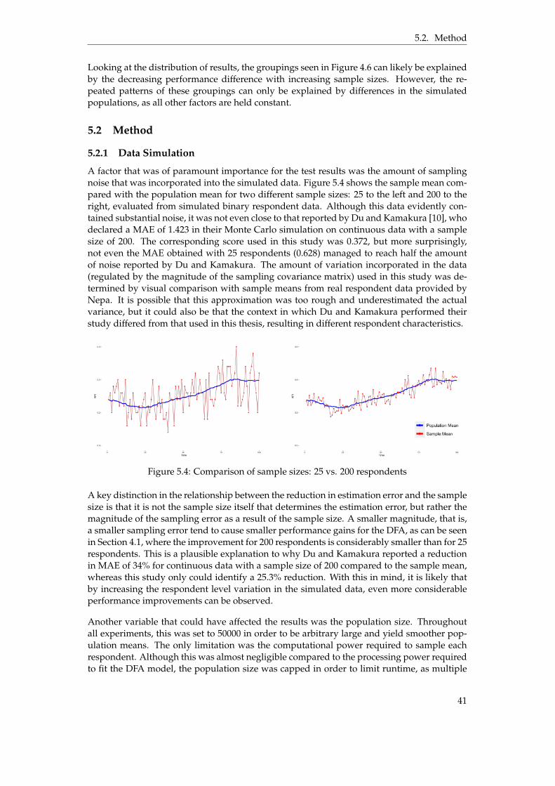
5.2. Method
Looking at the distribution of results, the groupings seen in Figure 4.6 can likely be explainedby the decreasing performance difference with increasing sample sizes. However, the re-peated patterns of these groupings can only be explained by differences in the simulatedpopulations, as all other factors are held constant.
5.2 Method
5.2.1 Data Simulation
A factor that was of paramount importance for the test results was the amount of samplingnoise that was incorporated into the simulated data. Figure 5.4 shows the sample mean com-pared with the population mean for two different sample sizes: 25 to the left and 200 to theright, evaluated from simulated binary respondent data. Although this data evidently con-tained substantial noise, it was not even close to that reported by Du and Kamakura [10], whodeclared a MAE of 1.423 in their Monte Carlo simulation on continuous data with a samplesize of 200. The corresponding score used in this study was 0.372, but more surprisingly,not even the MAE obtained with 25 respondents (0.628) managed to reach half the amountof noise reported by Du and Kamakura. The amount of variation incorporated in the data(regulated by the magnitude of the sampling covariance matrix) used in this study was de-termined by visual comparison with sample means from real respondent data provided byNepa. It is possible that this approximation was too rough and underestimated the actualvariance, but it could also be that the context in which Du and Kamakura performed theirstudy differed from that used in this thesis, resulting in different respondent characteristics.
Figure 5.4: Comparison of sample sizes: 25 vs. 200 respondents
A key distinction in the relationship between the reduction in estimation error and the samplesize is that it is not the sample size itself that determines the estimation error, but rather themagnitude of the sampling error as a result of the sample size. A smaller magnitude, that is,a smaller sampling error tend to cause smaller performance gains for the DFA, as can be seenin Section 4.1, where the improvement for 200 respondents is considerably smaller than for 25respondents. This is a plausible explanation to why Du and Kamakura reported a reductionin MAE of 34% for continuous data with a sample size of 200 compared to the sample mean,whereas this study only could identify a 25.3% reduction. With this in mind, it is likely thatby increasing the respondent level variation in the simulated data, even more considerableperformance improvements can be observed.
Another variable that could have affected the results was the population size. Throughoutall experiments, this was set to 50000 in order to be arbitrary large and yield smoother pop-ulation means. The only limitation was the computational power required to sample eachrespondent. Although this was almost negligible compared to the processing power requiredto fit the DFA model, the population size was capped in order to limit runtime, as multiple
41
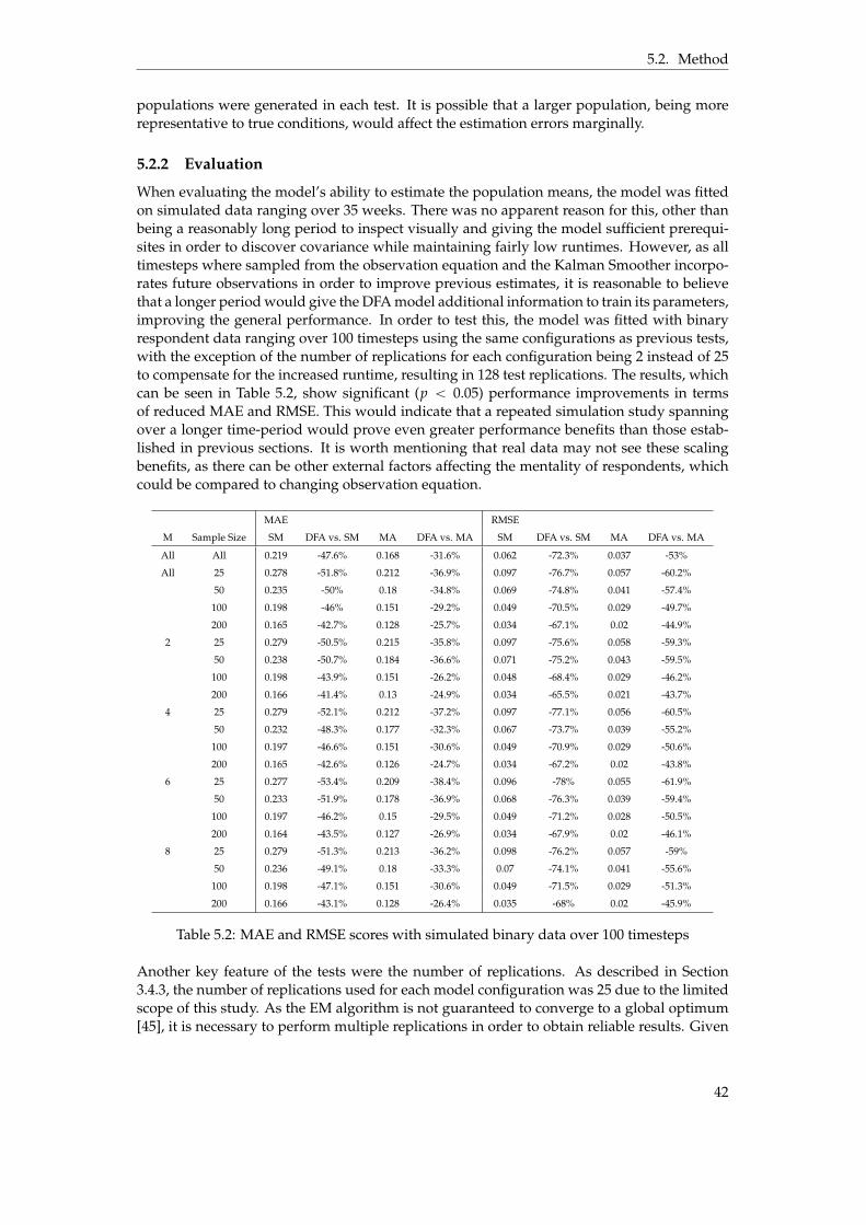
5.2. Method
populations were generated in each test. It is possible that a larger population, being morerepresentative to true conditions, would affect the estimation errors marginally.
5.2.2 Evaluation
When evaluating the model’s ability to estimate the population means, the model was fittedon simulated data ranging over 35 weeks. There was no apparent reason for this, other thanbeing a reasonably long period to inspect visually and giving the model sufficient prerequi-sites in order to discover covariance while maintaining fairly low runtimes. However, as alltimesteps where sampled from the observation equation and the Kalman Smoother incorpo-rates future observations in order to improve previous estimates, it is reasonable to believethat a longer period would give the DFA model additional information to train its parameters,improving the general performance. In order to test this, the model was fitted with binaryrespondent data ranging over 100 timesteps using the same configurations as previous tests,with the exception of the number of replications for each configuration being 2 instead of 25to compensate for the increased runtime, resulting in 128 test replications. The results, whichcan be seen in Table 5.2, show significant (p ă 0.05) performance improvements in termsof reduced MAE and RMSE. This would indicate that a repeated simulation study spanningover a longer time-period would prove even greater performance benefits than those estab-lished in previous sections. It is worth mentioning that real data may not see these scalingbenefits, as there can be other external factors affecting the mentality of respondents, whichcould be compared to changing observation equation.
MAE RMSE
M Sample Size SM DFA vs. SM MA DFA vs. MA SM DFA vs. SM MA DFA vs. MA
All All 0.219 -47.6% 0.168 -31.6% 0.062 -72.3% 0.037 -53%
All 25 0.278 -51.8% 0.212 -36.9% 0.097 -76.7% 0.057 -60.2%
50 0.235 -50% 0.18 -34.8% 0.069 -74.8% 0.041 -57.4%
100 0.198 -46% 0.151 -29.2% 0.049 -70.5% 0.029 -49.7%
200 0.165 -42.7% 0.128 -25.7% 0.034 -67.1% 0.02 -44.9%
2 25 0.279 -50.5% 0.215 -35.8% 0.097 -75.6% 0.058 -59.3%
50 0.238 -50.7% 0.184 -36.6% 0.071 -75.2% 0.043 -59.5%
100 0.198 -43.9% 0.151 -26.2% 0.048 -68.4% 0.029 -46.2%
200 0.166 -41.4% 0.13 -24.9% 0.034 -65.5% 0.021 -43.7%
4 25 0.279 -52.1% 0.212 -37.2% 0.097 -77.1% 0.056 -60.5%
50 0.232 -48.3% 0.177 -32.3% 0.067 -73.7% 0.039 -55.2%
100 0.197 -46.6% 0.151 -30.6% 0.049 -70.9% 0.029 -50.6%
200 0.165 -42.6% 0.126 -24.7% 0.034 -67.2% 0.02 -43.8%
6 25 0.277 -53.4% 0.209 -38.4% 0.096 -78% 0.055 -61.9%
50 0.233 -51.9% 0.178 -36.9% 0.068 -76.3% 0.039 -59.4%
100 0.197 -46.2% 0.15 -29.5% 0.049 -71.2% 0.028 -50.5%
200 0.164 -43.5% 0.127 -26.9% 0.034 -67.9% 0.02 -46.1%
8 25 0.279 -51.3% 0.213 -36.2% 0.098 -76.2% 0.057 -59%
50 0.236 -49.1% 0.18 -33.3% 0.07 -74.1% 0.041 -55.6%
100 0.198 -47.1% 0.151 -30.6% 0.049 -71.5% 0.029 -51.3%
200 0.166 -43.1% 0.128 -26.4% 0.035 -68% 0.02 -45.9%
Table 5.2: MAE and RMSE scores with simulated binary data over 100 timesteps
Another key feature of the tests were the number of replications. As described in Section3.4.3, the number of replications used for each model configuration was 25 due to the limitedscope of this study. As the EM algorithm is not guaranteed to converge to a global optimum[45], it is necessary to perform multiple replications in order to obtain reliable results. Given
42
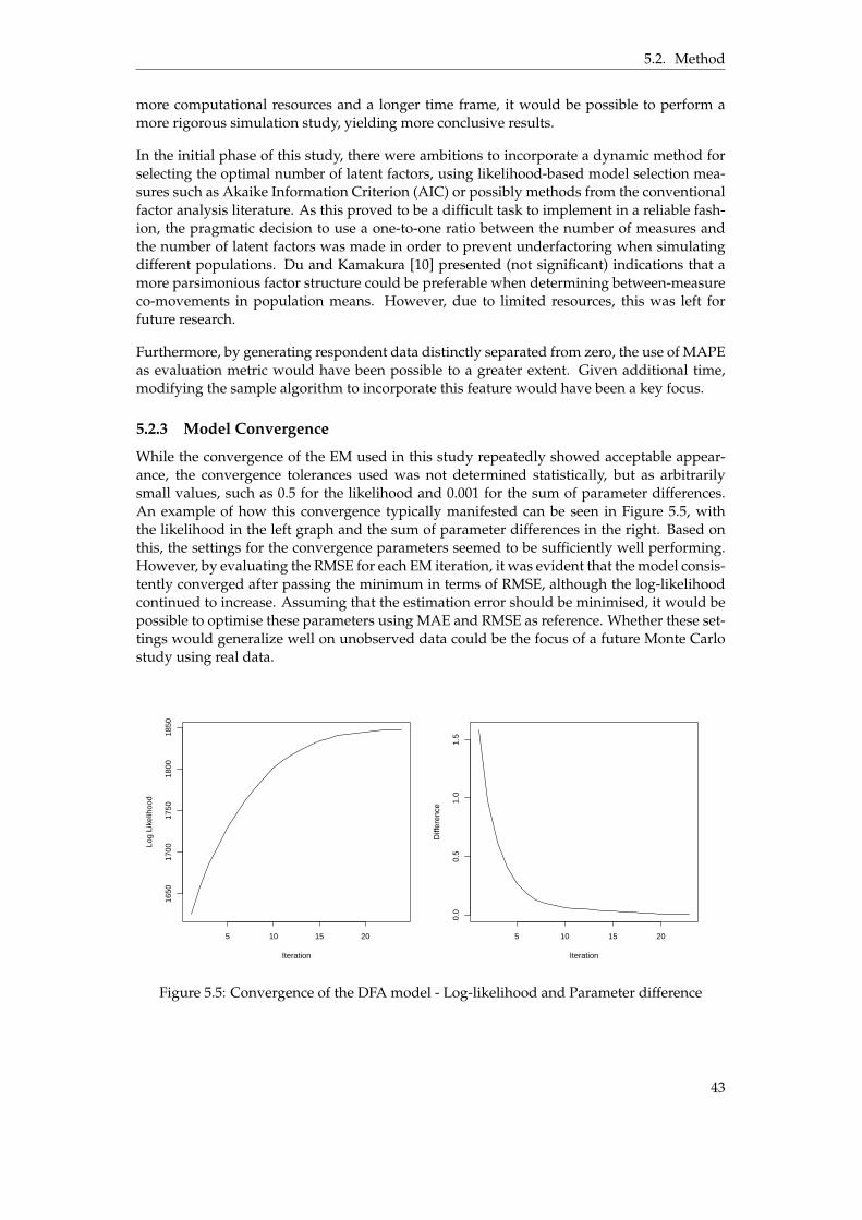
5.2. Method
more computational resources and a longer time frame, it would be possible to perform amore rigorous simulation study, yielding more conclusive results.
In the initial phase of this study, there were ambitions to incorporate a dynamic method forselecting the optimal number of latent factors, using likelihood-based model selection mea-sures such as Akaike Information Criterion (AIC) or possibly methods from the conventionalfactor analysis literature. As this proved to be a difficult task to implement in a reliable fash-ion, the pragmatic decision to use a one-to-one ratio between the number of measures andthe number of latent factors was made in order to prevent underfactoring when simulatingdifferent populations. Du and Kamakura [10] presented (not significant) indications that amore parsimonious factor structure could be preferable when determining between-measureco-movements in population means. However, due to limited resources, this was left forfuture research.
Furthermore, by generating respondent data distinctly separated from zero, the use of MAPEas evaluation metric would have been possible to a greater extent. Given additional time,modifying the sample algorithm to incorporate this feature would have been a key focus.
5.2.3 Model Convergence
While the convergence of the EM used in this study repeatedly showed acceptable appear-ance, the convergence tolerances used was not determined statistically, but as arbitrarilysmall values, such as 0.5 for the likelihood and 0.001 for the sum of parameter differences.An example of how this convergence typically manifested can be seen in Figure 5.5, withthe likelihood in the left graph and the sum of parameter differences in the right. Based onthis, the settings for the convergence parameters seemed to be sufficiently well performing.However, by evaluating the RMSE for each EM iteration, it was evident that the model consis-tently converged after passing the minimum in terms of RMSE, although the log-likelihoodcontinued to increase. Assuming that the estimation error should be minimised, it would bepossible to optimise these parameters using MAE and RMSE as reference. Whether these set-tings would generalize well on unobserved data could be the focus of a future Monte Carlostudy using real data.
5 10 15 20
1650
1700
1750
1800
1850
Iteration
Log
Like
lihoo
d
5 10 15 20
0.0
0.5
1.0
1.5
Iteration
Diff
eren
ce
Figure 5.5: Convergence of the DFA model - Log-likelihood and Parameter difference
43
5.3. Source Criticism
5.3 Source Criticism
The research presented in this thesis was almost exclusively based on research papers andacademical books, with the exception of the newspaper articles discussed in section 5.4. Mostof the ideas specific to Dynamic Factor Analysis, with emphasis on the Primary model evalu-ated in this thesis, was acquired from the papers presented by Rex Du and Wagner Kamakura[11, 10], which in turn used ideas proposed by Jo Thori Lind [25]. As of December 2019, thefirst two articles have received 951 and 52 citations respectively, while Lind’s paper has re-ceived 203 citations. However, the fairly modest academical recognition is not a reason toraise question regarding the validity of said articles, as Kamakura, Du and Lind are all rep-utable researchers within Marketing and Economics, with 2046664, 9685 and 13476 citationsrespectively as of December 2019. As Lind presents a mathematical proof for his proposedmodifications to the Kalman Filter, it is likely that this work simply has gone unnoticed inthe marketing context, as discussed by Du and Kamakura [10]. Furthermore, most areas inwhich the KF is applied, such as object tracking and navigation, would see insignificant per-formance benefits from using Lind’s modifications, if any, which may explain the modestreception in other contexts.
As brand tracking models such as the one evaluation in this research may implicate substan-tial cost reductions related to data collection, it is likely that similar models exist outside ofthe marketing literature, but are kept proprietary. Additionally, as the evaluation of suchmodels requires access to extensive amounts of survey data, typically only available to thetype of company that would benefit from said models, it is unlikely that any results followingcollaborations with these companies would be openly accessible.
5.4 The work in a wider context
In December 2015, The Guardian published an article describing how an American politicianused personal data gathered illicitly from 40+ million Facebook users to create psychographicprofiles of voters, in order to focus campaign efforts and create advertisement tailored to theindividual voter [7]. In 2017 and 2018, the UK based company Cambridge Analytica responsi-ble for gathering and processing the data, was reported to have been involved with Americanpresident Donald Trump’s election campaign as well the 2016 Brexit referendum, in a seriesof articles published by The Observer and The New York Times [5, 33]. The psychographicprofiles were reported to have been used for "designing target audiences for digital ads and fund-raising appeals, modeling voter turnout, ..., and determining where Mr. Trump should travel to bestdrum up support." [33].
As the model evaluated in this research may enable further segmentation of respondents,it is evident that such techniques, when available to authorities acting out of self-interest asopposed to altruism, may impair the individual’s integrity. However, in the context examinedin this research, the possibility to customize advertisement and customer offerings impliesthat only information relevant to the unique customer is shown, reducing the general amountof information that is needed to be filtered when navigating everyday life. Whether this canhave other effects, individual or societal, is a question closely related to ethics in marketingand is left for future discussion.
1https://scholar.google.se/scholar?cites=148246520678890210702https://scholar.google.se/scholar?cites=117709671652117630863https://scholar.google.se/scholar?cites=140621521775341092284https://scholar.google.se/citations?user=Jhg2DPwAAAAJ15https://scholar.google.se/citations?user=_eojm3UAAAAJ6https://scholar.google.se/citations?user=vNaXMk8AAAAJ
44
6 Conclusion
This study has evaluated the performance of a primary Dynamic Factor Analysis (DFA)model when fitted on binary survey data and compared it with industry standard methodsfor brand tracking. This was possible due to the key assumption that while the individualsin a tracking study may be different for each point of measurement, they, when aggregated,still represent estimates of the same population mean. Furthermore, the data was assumed tohold three critical dependencies:
1. Within-measure inter-temporal dependence, assuming that the population means will notchange drastically from one time period to the next, making it possible to borrow infor-mation within the measure across timesteps.
2. Between-measure co-movements in population means. Different measures gathered from thesame survey should be correlated on an aggregated level over time. By considering cor-relations between population means, it is possible to compare a measures’ movementwith the expected movement according to the dynamics of the correlation.
3. Between-measure cross-sectional co-variations. This refers to correlation on the primarylevel, stating that measures can be correlated on the respondent level, correlations thateasily can be mistaken for real between-measure co-movements in population means ifnot analysed appropriately.
The research was divided into two research questions:
1. Can a lower prediction error be obtained when using a Dynamic Factor Analysis modelon respondent data gathered from repeated cross-sectional surveys, compared to amoving average?
2. What prediction error can be achieved with a Dynamic Factor Analysis model when therespondent data is binary and how does this compare to numerical values?
45
6.1. Future Work
In order to answer these questions a series of tests were performed using both simulateddata and real respondent data. The tests evaluated the performance of the model in termsof retrospectively fitting historical data as well as making real-time estimates of the popula-tion means. Initially, a best performing baseline on the simulated data was determined as amoving average of order 2. The results following the tests were that the DFA reduced theestimation error with 18-33%, depending on the error metric (MAE vs. RMSE), compared tothe moving average. This improvement in accuracy was equivalent to reducing the requiredamount of data by more than a factor 2, while maintaining the same level of accuracy. Regard-ing the real-time estimation, the model indicated a significant performance improvement, butwas not equally accurate at the final timestep as the second to last timestep. Furthermore, thetests showed that the benefits of using the model was larger for smaller sample sizes, as themarginal utility of each respondent was decreasing. Additional simulations indicated thatthe DFA scales considerably better than the moving average, consistently outperforming thesample mean even for larger sample sizes.
Possible implications of said improvements are reduced data gathering costs, improved es-timation accuracy and increased ability to segment respondents according to demographics.As the primary model requires smaller sample sizes to maintain the same level of accuracy, itis possible to divide respondents into sub-groups, enabling brand tracking on subsets of thepopulation.
Finally, the results presented in this study should be regarded as a pessimistic estimation ofthe capabilities of the primary model. After comparison with similar Monte Carlo studies, anumber of tentative experiments were performed, indicating that even greater performancebenefits are possible.
6.1 Future Work
As discussed in Section 5.2.2, two improvements to the evaluation method used in this studywas found. First, the DFA model indicated significant performance improvements when itwas fitted over a larger number of time periods. A first step would therefore be to performa detailed study focusing on evaluating the performance over different timeframes, for in-stance by simulating a typically large number of timesteps to subsample from. Second, asit likely would entail both performance and accuracy improvements, as opposed to usinga one-to-one ratio between the number of measures and latent factors, the number of fac-tors could be determined analytically using likelihood-based model selection methods suchas AIC, possibly in combination with factor selection techniques from conventional factoranalysis.
In addition to validation with a simulation study, it would be of interest to evaluate the sta-tistical performance of the model in a Monte Carlo study based on real respondent data, afeat that would require a substantial population tracked over a reasonably long period.
It is evident that the weakest part of the primary DFA model used in this study is its abilityto perform real-time estimates of the population means. A possible modification to mitigatethis would be to combine the model with the Structural Dynamic Factor Analysis (SDFA) pro-posed by Du and Kamakura [11], resulting in a primary SDFA. By dividing the state changesinto a seasonal and non-seasonal component, it is possible that the model would performbetter at detecting recent dynamics in population means, in order to make more accurateestimates of the present state.
Finally, following the work of Du and Kamakura [11], which has been referenced extensivelyin this research, Park and Dillon [28] proposed a Multilevel Dynamic Factor Model with the
46

6.1. Future Work
aim of identifying respondent level cross-sectional covariance. Although their model neglectsbetween-measure co-movements in population means by assuming the evolution of the la-tent factors to be independent across measures in order to utilize a multilevel structure, acomparative study of these methods would still be of great interest.
47

Bibliography
[1] George S. Atsalakis and Kimon P. Valavanis. “Surveying stock market forecasting tech-niques - Part II: Soft computing methods”. In: Expert Systems with Applications 36.3 PART2 (2009), pp. 5932–5941. ISSN: 09574174. DOI: 10.1016/j.eswa.2008.07.006. URL:http://dx.doi.org/10.1016/j.eswa.2008.07.006.
[2] Emma Bell, Alan Bryman, and Bill Harley. Business research methods. Oxford universitypress, 2018.
[3] Christopher M. Bishop. Pattern recognition and machine learning. springer, 2006.
[4] Timothy A. Brown. Confirmatory factor analysis for applied research. Guilford Publications,2015. ISBN: 9781462515363.
[5] Carole Cadwalladr. The great British Brexit robbery: how our democracy was hijacked. 2017.URL: https://www.theguardian.com/technology/2017/may/07/the-great-british-brexit-robbery-hijacked-democracy.
[6] Tianfeng Chai and Roland R. Draxler. “Root mean square error (RMSE) or mean abso-lute error (MAE)? -Arguments against avoiding RMSE in the literature”. In: GeoscientificModel Development 7.3 (2014), pp. 1247–1250. ISSN: 19919603. DOI: 10.5194/gmd-7-1247-2014.
[7] Harry Davies. Ted Cruz using firm that harvested data on millions of unwitting Facebookusers. 2015. URL: https://www.theguardian.com/us-news/2015/dec/11/senator-ted-cruz-president-campaign-facebook-user-data.
[8] Arthur P. Dempster, Nan M. Laird, and Donald B. Rubin. “Maximum Likelihood fromIncomplete Data Via the EM Algorithm”. In: Journal of the Royal Statistical Society: SeriesB (Methodological) (1977). DOI: 10.1111/j.2517-6161.1977.tb01600.x.
[9] Catherine Doz and Domenico Giannone. “A two-step estimator for large approximatedynamic factor models based on Kalman filtering”. In: Statistics (2006), pp. 1–44.
[10] Rex Y. Du and Wagner A. Kamakura. “Improving the statistical performance of trackingstudies based on repeated cross-sections with primary dynamic factor analysis”. In:International Journal of Research in Marketing 32.1 (2015), pp. 94–112. ISSN: 01678116. DOI:10.1016/j.ijresmar.2014.10.002. URL: http://dx.doi.org/10.1016/j.ijresmar.2014.10.002.
48
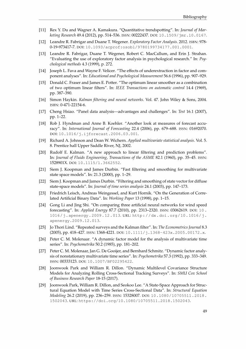
Bibliography
[11] Rex Y. Du and Wagner A. Kamakura. “Quantitative trendspotting”. In: Journal of Mar-keting Research 49.4 (2012), pp. 514–536. ISSN: 00222437. DOI: 10.1509/jmr.10.0167.
[12] Leandre R. Fabrigar and Duane T. Wegener. Exploratory Factor Analysis. 2012. ISBN: 978-0-19-973417-7. DOI: 10.1093/acprof:osobl/9780199734177.001.0001.
[13] Leandre R. Fabrigar, Duane T. Wegener, Robert C. MacCallum, and Erin J. Strahan.“Evaluating the use of exploratory factor analysis in psychological research.” In: Psy-chological methods 4.3 (1999), p. 272.
[14] Joseph L. Fava and Wayne F. Velicer. “The effects of underextraction in factor and com-ponent analyses”. In: Educational and Psychological Measurement 56.6 (1996), pp. 907–929.
[15] Donald C. Fraser and James E. Potter. “The optimum linear smoother as a combinationof two optimum linear filters”. In: IEEE Transactions on automatic control 14.4 (1969),pp. 387–390.
[16] Simon Haykin. Kalman filtering and neural networks. Vol. 47. John Wiley & Sons, 2004.ISBN: 0-471-22154-6.
[17] Cheng Hsiao. “Panel data analysis—advantages and challenges”. In: Test 16.1 (2007),pp. 1–22.
[18] Rob J. Hyndman and Anne B. Koehler. “Another look at measures of forecast accu-racy”. In: International Journal of Forecasting 22.4 (2006), pp. 679–688. ISSN: 01692070.DOI: 10.1016/j.ijforecast.2006.03.001.
[19] Richard A. Johnson and Dean W. Wichern. Applied multivariate statistical analysis. Vol. 5.8. Prentice hall Upper Saddle River, NJ, 2002.
[20] Rudolf E. Kalman. “A new approach to linear filtering and prediction problems”.In: Journal of Fluids Engineering, Transactions of the ASME 82.1 (1960), pp. 35–45. ISSN:1528901X. DOI: 10.1115/1.3662552.
[21] Siem J. Koopman and James Durbin. “Fast filtering and smoothing for multivariatestate space models”. In: 21.3 (2000), pp. 1–29.
[22] Siem J. Koopman and James Durbin. “Filtering and smoothing of state vector for diffusestate-space models”. In: Journal of time series analysis 24.1 (2003), pp. 147–173.
[23] Friedrich Leisch, Andreas Weingessel, and Kurt Hornik. “On the Generation of Corre-lated Artificial Binary Data”. In: Working Paper 13 (1998), pp. 1–15.
[24] Gong Li and Jing Shi. “On comparing three artificial neural networks for wind speedforecasting”. In: Applied Energy 87.7 (2010), pp. 2313–2320. ISSN: 03062619. DOI: 10.1016/j.apenergy.2009.12.013. URL: http://dx.doi.org/10.1016/j.apenergy.2009.12.013.
[25] Jo Thori Lind. “Repeated surveys and the Kalman filter”. In: The Econometrics Journal 8.3(2005), pp. 418–427. ISSN: 1368-4221. DOI: 10.1111/j.1368-423x.2005.00172.x.
[26] Peter C. M. Molenaar. “A dynamic factor model for the analysis of multivariate timeseries”. In: Psychometrika 50.2 (1985), pp. 181–202.
[27] Peter C. M. Molenaar, Jan G. De Gooijer, and Bernhard Schmitz. “Dynamic factor analy-sis of nonstationary multivariate time series”. In: Psychometrika 57.3 (1992), pp. 333–349.ISSN: 00333123. DOI: 10.1007/BF02295422.
[28] Joonwook Park and William R. Dillon. “Dynamic Multilevel Covariance StructureModels for Analyzing Rolling Cross-Sectional Tracking Surveys”. In: SMU Cox Schoolof Business Research Paper 18-15 (2017).
[29] Joonwook Park, William R. Dillon, and Seokoo Lee. “A State-Space Approach for Struc-tural Equation Model with Time Series Cross-Sectional Data”. In: Structural EquationModeling 26.2 (2019), pp. 236–259. ISSN: 15328007. DOI: 10.1080/10705511.2018.1502043. URL: https://doi.org/10.1080/10705511.2018.1502043.
49
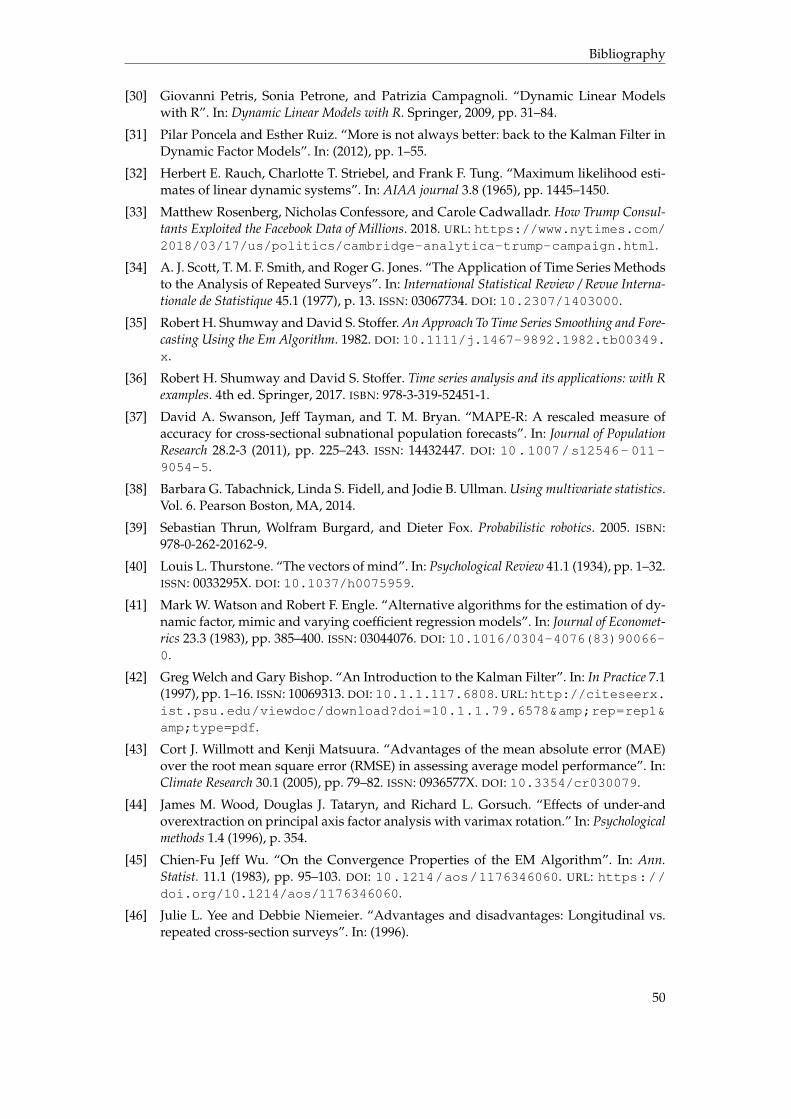
Bibliography
[30] Giovanni Petris, Sonia Petrone, and Patrizia Campagnoli. “Dynamic Linear Modelswith R”. In: Dynamic Linear Models with R. Springer, 2009, pp. 31–84.
[31] Pilar Poncela and Esther Ruiz. “More is not always better: back to the Kalman Filter inDynamic Factor Models”. In: (2012), pp. 1–55.
[32] Herbert E. Rauch, Charlotte T. Striebel, and Frank F. Tung. “Maximum likelihood esti-mates of linear dynamic systems”. In: AIAA journal 3.8 (1965), pp. 1445–1450.
[33] Matthew Rosenberg, Nicholas Confessore, and Carole Cadwalladr. How Trump Consul-tants Exploited the Facebook Data of Millions. 2018. URL: https://www.nytimes.com/2018/03/17/us/politics/cambridge-analytica-trump-campaign.html.
[34] A. J. Scott, T. M. F. Smith, and Roger G. Jones. “The Application of Time Series Methodsto the Analysis of Repeated Surveys”. In: International Statistical Review / Revue Interna-tionale de Statistique 45.1 (1977), p. 13. ISSN: 03067734. DOI: 10.2307/1403000.
[35] Robert H. Shumway and David S. Stoffer. An Approach To Time Series Smoothing and Fore-casting Using the Em Algorithm. 1982. DOI: 10.1111/j.1467-9892.1982.tb00349.x.
[36] Robert H. Shumway and David S. Stoffer. Time series analysis and its applications: with Rexamples. 4th ed. Springer, 2017. ISBN: 978-3-319-52451-1.
[37] David A. Swanson, Jeff Tayman, and T. M. Bryan. “MAPE-R: A rescaled measure ofaccuracy for cross-sectional subnational population forecasts”. In: Journal of PopulationResearch 28.2-3 (2011), pp. 225–243. ISSN: 14432447. DOI: 10.1007/s12546- 011-9054-5.
[38] Barbara G. Tabachnick, Linda S. Fidell, and Jodie B. Ullman. Using multivariate statistics.Vol. 6. Pearson Boston, MA, 2014.
[39] Sebastian Thrun, Wolfram Burgard, and Dieter Fox. Probabilistic robotics. 2005. ISBN:978-0-262-20162-9.
[40] Louis L. Thurstone. “The vectors of mind”. In: Psychological Review 41.1 (1934), pp. 1–32.ISSN: 0033295X. DOI: 10.1037/h0075959.
[41] Mark W. Watson and Robert F. Engle. “Alternative algorithms for the estimation of dy-namic factor, mimic and varying coefficient regression models”. In: Journal of Economet-rics 23.3 (1983), pp. 385–400. ISSN: 03044076. DOI: 10.1016/0304-4076(83)90066-0.
[42] Greg Welch and Gary Bishop. “An Introduction to the Kalman Filter”. In: In Practice 7.1(1997), pp. 1–16. ISSN: 10069313. DOI: 10.1.1.117.6808. URL: http://citeseerx.ist.psu.edu/viewdoc/download?doi=10.1.1.79.6578&rep=rep1&type=pdf.
[43] Cort J. Willmott and Kenji Matsuura. “Advantages of the mean absolute error (MAE)over the root mean square error (RMSE) in assessing average model performance”. In:Climate Research 30.1 (2005), pp. 79–82. ISSN: 0936577X. DOI: 10.3354/cr030079.
[44] James M. Wood, Douglas J. Tataryn, and Richard L. Gorsuch. “Effects of under-andoverextraction on principal axis factor analysis with varimax rotation.” In: Psychologicalmethods 1.4 (1996), p. 354.
[45] Chien-Fu Jeff Wu. “On the Convergence Properties of the EM Algorithm”. In: Ann.Statist. 11.1 (1983), pp. 95–103. DOI: 10.1214/aos/1176346060. URL: https://doi.org/10.1214/aos/1176346060.
[46] Julie L. Yee and Debbie Niemeier. “Advantages and disadvantages: Longitudinal vs.repeated cross-section surveys”. In: (1996).
50

Bibliography
[47] Alain F. Zuur, Rob J. Fryer, Ian T. Jolliffe, Rob Dekker, and Jan J. Beukema. “Estimatingcommon trends in multivariate time series using dynamic factor analysis”. In: Environ-metrics 14.7 (2003), pp. 665–685. ISSN: 11804009. DOI: 10.1002/env.611.
51
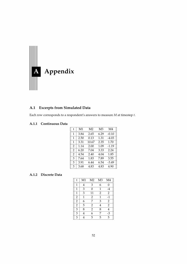
A Appendix
A.1 Excerpts from Simulated Data
Each row corresponds to a respondent’s answers to measure M at timestep t.
A.1.1 Continuous Datat M1 M2 M3 M4
1 3.84 2.65 6.29 -0.101 2.50 0.13 1.31 -4.031 3.31 10.67 2.35 1.702 1.14 2.00 1.09 -1.192 6.20 7.04 3.33 2.242 4.54 2.40 4.04 1.853 7.64 1.83 7.89 3.553 3.91 6.44 6.54 -3.493 3.68 4.83 4.83 4.90
A.1.2 Discrete Datat M1 M2 M3 M4
1 4 3 6 01 3 0 1 -41 3 11 2 22 1 2 1 -12 6 7 3 22 5 2 4 23 8 2 8 43 4 6 7 -33 4 5 5 5
52
A.2. Fitted DFA Models
A.1.3 Binary Data
t M1 M2 M3 M4
1 0 1 1 11 0 1 1 11 1 0 1 02 1 0 1 12 0 0 1 12 0 1 1 13 1 0 1 13 0 0 1 13 1 0 0 1
A.2 Fitted DFA Models
Figure A.1: Fitted DFA on binary respondent data
53
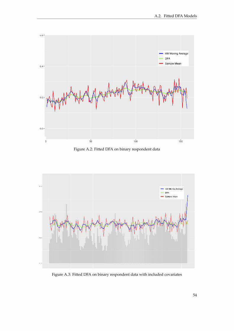
A.2. Fitted DFA Models
Figure A.2: Fitted DFA on binary respondent data
Figure A.3: Fitted DFA on binary respondent data with included covariates
54