tony hÜrlimann - matmod
TRANSCRIPT
TONY HÜRLIMANN
COMPUTER-BASED MATHEMATICAL
MODELING
An Essay for the Design
of Computer-Based Modeling Tools

Habilitation, Universität Freiburg
COMPUTER-BASED MATHEMATICAL
MODELING
An Essay for the Design
of Computer-Based Modeling Tools
TONY HÜRLIMANN
Institute of Informatics
Site Regina Mundi
University of Fribourg
printed by Mechanographie, Universität Freiburg
Computer-Based Mathematical Modeling
An Essay for the Design
of Computer-Based Modeling Tools
Von der Wirtschafts- und Sozialwissenschaftlichen Fakultät der
Universität Freiburg zu genehmigende Habilitationsschrift zur Erlangung
der Venia Legendi für das Fach “Informatik”.
Vorgelegt von
Dr. rer. pol. Tony Hürlimann
aus Walchwil/ZG
Gutachter: Prof. Dr. Jacques Pasquier,
Institut für Informatik, Universität Freiburg, 1700 Freiburg, Schweiz
Zweiter Gutachter: Prof. Dr. Johannes J. Bisschop,
Faculteit der Toegepaste Wiskunde, Universiteit Twente, 7500 AE Enschede, The Nederlands
Habilitationsabgabe: 21. Juli 1997


I
Preface
Computer-based mathematical modeling – the technique of representing and
managing models in machine-readable form – is still in its infancy despite the
many powerful mathematical software packages already available which can
solve astonishingly complex and large models. On the one hand, using
mathematical and logical notation, we can formulate models which cannot be
solved by any computer in reasonable time – or which cannot even be solved by
any method. On the other hand, we can solve certain classes of much larger
models than we can practically handle and manipulate without heavy
programming. This is especially true in operations research where it is common
to solve models with many thousands of variables. Even today, there are no
general modeling tools that accompany the whole modeling process from start
to finish, that is to say, from model creation to report writing.
This book proposes a framework for computer-based modeling. More precisely,
it puts forward a modeling language as a kernel representation for mathematical
models. It presents a general specification for modeling tools. The book does
not expose any solution methods or algorithms which may be useful in solving
models, neither is it a treatise on how to build them. No help is intended here
for the modeler by giving practical modeling exercises, although several models
will be presented in order to illustrate the framework. Nevertheless, a short
introduction to the modeling process is given in order to expound the necessary
background for the proposed modeling framework.
Therefore, this work is not primarily intended for the model user or the modeler
– the mathematician, physicist, or operation research model builder who use
software to solve a given problem. Ultimately, this research is done for them, of
course, and I hope I have created and implemented a useful software tool (LPL)
to this end – at least for educational purposes.
Nor is this book about implementation topics. I do not describe here how I have
concretely implemented my own modeling tools. This would have considerably
augmented the number of pages and it would have been of scarce interest, since
there are many excellent books on compiler construction already available.

This work offers concepts and a general framework for modeling and is mainly
intended to help other designers of modeling tools. It details my views on ‘why
and how’ we should create such tools and which utilities and functionalities
they should contain in order to be useful for “practitioners”. In that sense, this
work is more a research programme than the presentation of an already
established domain. I think that we are only at the beginning of a new
development in “modeling with the aid of computers” and that I am able to
barely scratch the surface of this new and exciting research field. I am,
however, firmly convinced that there is a bright future for this topic – just as
there was for word processors and spreadsheets fifteen years ago; or just as
there was forty years ago when the first high level programming language was
developed.
To grasp the main ideas, the reader should have some background in applied
mathematics, logic, operations research, and computer science, as I rarely
explain basic notions from these disciplines (like, for example, the concepts of
“computational complexity” from the theoretical computer science, “cutting
planes” for the polyhedral theory, and others), although these notions are
fundamental to this book. I assume that the reader is familiar with these
concepts. However, further references are always given.
My own background is, in order of importance, computer science, operations
research and economics. This ordering also corresponds to the weight the three
fields take in this book. Developing ideas merely on how modeling tools should
be implemented is either easy or too far away from what is really needed; at
least it is only a small part of the task as a whole to elaborate on all kinds of
neat concepts without actually going through the thorny work of
implementation. Only the process of implementation teaches you what works
and what does not work.
My motivation for this research came initially from practical modeling: a
research group under the direction of Dr. Hättenschwiler and Prof. Kohlas at
the Institute of Informatics of the University of Fribourg (IIUF) had to build
and maintain – at that time – large LP models. Although I was never directly
engaged in the management of these models, I followed closely what they did
and what they needed, and I created a first version of LPL (Linear

III
Programming Language) which enabled them to formulate their models better.
That was 1987 and LPL was in its infancy. Nevertheless I got a Ph.D. for it and
it encouraged me to extend and generalize it in several directions. Since then I
have worked more or less intensely on the language. This book is the result of
this “project LPL”.
The book is made up of three parts. In Part I, the concept of model and related
notions are defined, the modeling life cycle is outlined, and different model
types and paradigms are presented. Part II gives an overview of what actually
exists in the line of computer-based modeling tools, explains why we need
more, and presents a general modeling framework. Part III describes my own
concrete contribution to this field: the modeling language LPL. A more
complete survey of this book is given at the end of the Introduction.
Acknowledgements
There are many people who have directly or indirectly participated in the
successful completion of this book. I particularly wish to thank the individuals
who were invaluable in the process of making this work a reality:
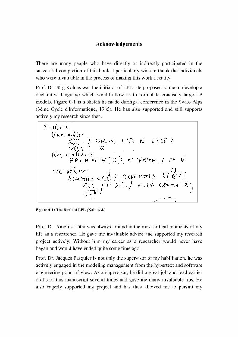
Prof. Dr. Jürg Kohlas was the initiator of LPL. He proposed to me to develop a
declarative language which would allow us to formulate concisely large LP
models. Figure 0-1 is a sketch he made during a conference in the Swiss Alps
(3ème Cycle d'Informatique, 1985). He has also supported and still supports
actively my research since then.
Figure 0-1: The Birth of LPL (Kohlas J.)
Prof. Dr. Ambros Lüthi was always around in the most critical moments of my
life as a researcher. He gave me invaluable advice and supported my research
project actively. Without him my career as a researcher would never have
began and would have ended quite some time ago.
Prof. Dr. Jacques Pasquier is not only the supervisor of my habilitation, he was
actively engaged in the modeling management from the hypertext and software
engineering point of view. As a supervisor, he did a great job and read earlier
drafts of this manuscript several times and gave me many invaluable tips. He
also eagerly supported my project and has thus allowed me to pursuit my
V
research an additional two years.
Prof. Dr. Pius Hättenschwiler, the project manager of several large LPs, was
and is still an intense interlocutor when it come to the practical use of LPL.
Without him, LPL would be quite different or would probably even vegetate as
a theoretical tool without much practical use. Marco Moresino, working under
the direction of Pius, was and is probably the most intense and fiercest user of
LPL. He found many subtle bugs.
Rare are the people in one's life who – when you meet them for the first time –
seem to be like old friends who you have known years. Prof. Dr. Johannes
Bisschop from the University Twente of Enschede is one of thee people for me.
This is probably because we share a similar dream of a modeling system. Not
only is he the second referee for my habilitation, but he also encouraged me to
continue with my small (compared to the titans available on the markets) LPL
implementation project when I was at the point of abandoning the whole thing
(in Budapest 1994). A seemingly minor event might be of special interest in
this context. When I first met Johannes, I asked him what he thought about the
expressive power of modeling languages, whether they should include the
whole power of a Turing Machine or not. His answer was a simple yes, and had
an inestimable influence on what I now think should be a modeling language
(the answer is in Chapter 7).
Prof. Dr. Arthur Geoffrion of UCLA allowed me to stay with him for one year.
I owe him a great deal of credit when it comes to many of my ideas in modeling
management systems.
Daniel Raemi, my old friend, has given extravagantly of his time to read earlier
drafts of this book. His many corrections and suggestions have been very
valuable. I also wish to thank Simon Lacey for his help in proof-reading the
finished manuscript. Mitra Packham did a excellent job in reading the finished
manuscript and greatly improved my English.
I also owe a depth of gratitude to many other colleagues and teachers from
whom I have learned so much over the years. I thank them all.
None of the mentioned (or not mentioned) persons, however, is responsible for
the defects in what follows. I alone am to blame for all and any errors which

may remain or for the type setting of this document.1
Finally, I wish to thank the following institutions for their financial support and
the use of their infrastructure. The first is the Swiss National Science
Foundation who financed my stay at UCLA in Los Angeles with Prof. Arthur
Geoffrion for one year in 1989, and still supports my research (under Project
No. 1217-45922.95). The second is the Institute of Informatics at the University
of Fribourg in Switzerland (IIUF) where I developed and implemented most of
my ideas in a favourable and agreeable atmosphere of collaboration. The
Institute also let me use all the necessary equipment over many years to
accomplish this work.
Tony Hürlimann
Freiburg, Switzerland
July 1997
1 This document was written on different Macintoshes using the word processor of MSWord 5.0
(not 6.0 – which I never will use!), trademarked by MicroSoft. With exception of the formula
editor, I was quite happy with this software, but I would use Latex2e if I had to begin again.
VII
Availability of the LPL System
Part III of this book presents software called LPL.2 LPL is my own
contribution to the field of computer-based mathematical modeling and is
available free of charge from the Institute of Informatics at the University of
Fribourg (IIUF), Switzerland. Currently, there are implementations on
MS/DOS, Windows 95 and NT and Macintosh PowerPC. The version used in
this book is 4.20.
LPL – the software – together with documentation containing the Reference
Manual, several papers and many models written in LPL syntax, can be
obtained here (updated link 2018) :
lpl.unifr.ch or
lpl.virtual-optima.com
From these link, the reader can also find the software of LPL and instructions
on how to obtain it.
2 Initially, LPL was an abreviation of Linear Programming Language, since it was designed
exclusively for Linear Programs. During the intervening years, LPL's capability in logical
modeling has become so important that one could also call it Logical Programming Language.
My intention, however, is to offer a tool for full model documentation too. Therefore, in the
futur it may be called Literate Programming Language (see [Knuth 1984]).
VIII
Table of Contents
1. Introduction 1
1.1. Models and their Functions 2
1.2. The Advent of the Computer 5
1.3. New Scientific Branches Emerge 6
1.4. Mathematical Modeling – the Consequences 10
1.5. Computer-Based Modeling Management 13
1.6. About this Book 15
PART I: FOUNDATIONS OF MODELING 17
2. What is Modeling? 19
2.1. Model: a Definition 19
2.1. Mathematical Models 27
2.2. Model Theory 30
2.3. Models and Interpretations 33
2.4. Related Concepts 35
2.5. Declarative versus Procedural Knowledge 38
3. The Modeling Life Cycle 43
3.1. Stage 1: Specification of the Real Problem 45
3.2. Stage 2: Formulation of the Mathematical Model 46
3.3. Stage 3: Solution of the Model 51
3.4. Stage 4: Validation of the Model and its Solution 52
3.4.1. Logical Consistency 58
3.4.2. Data Type Consistency 59
3.4.3. Unit Type Consistency 60
3.4.4. User Defined Data Checking 61
3.4.5. Simplicity Considerations 61
3.4.6. Solvability Checking 62
3.4.7. Numerical Stability and Sensitivity Analysis 62
3.4.8. Checking the Correspondence 64
3.5. Stage 5: Writing a Report 66
3.6. Two Case Studies 67
4. Model Paradigms 77
IX
4.1. Model Types 78
4.1.1. Optimization Models 78
4.1.2. Symbolical –– Numerical Models 78
4.1.3. Linear –– Nonlinear Models 79
4.1.4. Continuous –– Discrete Models 79
4.1.5. Deterministic –– Stochastic Models 80
4.1.6. Analytic –– Simulation Models 81
4.2. Models and their Purposes 82
4.3. Models in their Research Communities 84
4.3.1. Differential Equation Models 84
4.3.2. Operations Research 84
4.3.3. Artificial Intelligence 87
4.3.3.1. Search Techniques 88
4.3.3.2. Heuristics 91
4.3.3.3. Knowledge Representation 91
4.4. Modeling Uncertainty 92
4.4.1. Mathematical Models and Uncertainty 93
4.4.2. General Approaches in Modeling Uncertainty 95
4.4.3. Classical Approaches in OR 97
4.4.4. Approaches in Logical Models 100
4.4.5. Fuzzy Set Modeling 107
4.4.6. Outlook 111
PART II: A GENERAL MODELING FRAMEWORK 113
5. Problems and Concepts 115
5.1. Present Situation in MMS 116
5.2. What MMS is not 117
5.3. MMS, what for? 121
5.4. Models versus Programs 124
6. An Overview of Approaches 131
6.1. Spreadsheet 131
6.2. Relational Database Systems 136
6.3. Graphical Modeling 143
6.4. Constraint Logic Programming Languages (CLP) 149
6.5. Algebraic Languages 158
6.5.1. AIMMS 160
6.5.2. AMPL 166
6.5.3. Summary 169
6.6. General Remarks 171
6.6.1. Structured Modeling 172
6.6.2. Embedded Language Technique 174
X
6.6.3. Multi-view Architecture 174
6.6.4. A Model Construction and Browsing Tool 175
6.6.5. Conclusion 176
7. A Modeling Framework 177
7.1. The Requirements Catalogue 178
7.1.1. Declarative and Procedural Knowledge 178
7.1.2. The Modeling Environment 180
7.1.3. Informal Knowledge 182
7.1.4. Summary 183
7.2. The Modeling Language 184
7.2.1. The Adopted Approach 186
7.2.2. The Overall Structure of the Modeling Language 192
7.2.3. Entities and Attributes 198
7.2.4. Index-sets 203
7.2.5. Expression 210
7.2.6. The Instruction Entities 212
7.2.7. The Complete Syntax Specification 213
7.2.8. Semantic Interpretation 215
7.2.8. Summary 217
7.3. Four Examples 218
7.4. Modeling Tools 230
7.4.1. A Textual-Based Tool 231
7.4.2. A Tool Based on Graphs 233
7.5. Outlook 234
PART III: LPL – AN IMPLEMENTED FRAMEWORK 237
8. The Definition of the Language 239
8.1. Introduction 239
8.2. An Overview of the LPL-Language 240
8.2.1. The Entities and the Attributes 240
8.2.2. Index-Sets 243
8.2.3. Data 244
8.2.3.1. LPL's own Data Format 244
8.2.3.2. The Import Generator 247
8.2.3.2. The Report Generator 249
8.2.4. Expressions 250
8.2.5. Logical Modeling 251
8.2.5.1. Predicate Variables 254
8.2.5.2. Logical Constraints 255
8.2.5.3. Proceeding the T1–T6 rules 257
8.3. The Backus-Naur Specification of LPL (4.20) 264
9. The Implementation 267
XI
9.1. The Kernel 268
9.2. The Environment (User Interface) 269
9.3. The Text Browser 270
9.4. The Graphical Browser 275
10. Selected Applications 283
10.1. General LP-, MIP-, and QP-Models 283
10.2. Goal Programming 294
10.3. LP's with logical constraints 297
10.5. Problems with Discontinuous Functions 316
10.6. Modeling Uncertainty 318
11. Conclusion 325
APPENDICES 331
References 333
Glossary 353
Index 359
XII
Model Examples
Example 2-1: The Intersection Problem 22
Example 3-1: The Frustum Problem 47
Example 3-2: Theory of Learning 49
Example 3-3: The 3-jug Problem 56
Example 3-4: Cooling a Thermometer 68
Example 3-5: A Production Problem 69
Example 4-1: A Letter Game Problem 89
Example 4-2: A PSAT Problem 102
Example 4-3: Probabilistic Entailment 103
Example 4-4: PSAT versus ATMS 105
Example 4-5: Modeling Dynamic Systems 109
Example 4-6: Fuzzy LPs 111
Example 5-1: An Energy Import Problem 128
Example 6-1: A Portfolio Problem 132
Example 6-2: A Transhipment-Assignment Problem 137
Example 6-3: The Transportation Problem 145
Example 6-4: The Car Sequencing Problem 155
Example 6-5: The Cutting Stock Problem 160
Example 6-6: The Diet Problem 167
Example 7-1: The n-Queen Problem 218
Example 7-2: The Cutting Stock Problem (again) 221
Example 7-3: The n-Bit-Adder 223
Example 7-4: A Budget Allocation Problem 228
Example 10-1: Determine Workforce Level 283
Example 10-2: “Rhythmed” Flow-Shop 287
Example 10-3: Assignment of Players to Teams 290
Example 10-4: Portfolio Investment 293
Example 10-5: Book Acquirements for a Library 294
Example 10-6: The Intersection Problem 298
Example 10-7: A Satisfiability Problem (SAT) 302
Example 10-8: How to Assemble a Radio 304
Example 10-9: An Energy Import Problem 305
Example 10-10: Finding Magic Squares 311
Example 10-11: The Capacitated Facility Location Problem 313
Example 10-12: A Two-Persons Zero-Sum Game 316
Example 10.13. A Stochastic Model 318
Example 10.13. A Model Using Fuzzy-sets 320
XIII
Figures
Figure 0-1: The Birth of LPL (Kohlas J.) IV
Figure 2-1: El torro 21
Figure 2-2: The Intersection Problem 22
Figure 2-3: Topological Deformation 22
Figure 2-4: Solution to the Intersection Problem 23
Figure 2-5: The Intersection Problem, an Interpretation 27
Figure 2-6: Similarities between Theories 34
Figure 2-7: Model Structure versus Model Instance 38
Figure 3-1 : The Model Life Cycle 44
Figure 3-2: The Frustum Problem 48
Figure 3-3: The Frustrum Problem, an Intermediate Step 48
Figure 3-4: The Frustrum Problem, the Solution 48
Figure 3-5: A Learning Model based on Markov Chain 50
Figure 3-6: Validation of a Model 53
Figure 3-7: The 3-jug Problem 56
Figure 3-8: The 3-jug Problem, the Search Path 57
Figure 3-9: Sensitivity Analysis 63
Figure 3-10: The Correspondence Problem 65
Figure 3-11: The Temperature Plot 69
Figure 4-1: Different Optimizing Criteria 85
Figure 4-2: The Search Path of the Letter Game Problem 90
Figure 4-3: Fuzzy Sets for small, medium, and tall 109
Figure 4-4: The Inverted Pendulum 110
Figure 5-1: Different Model Representations 123
Figure 5-2: Different Representations with many Links 123
Figure 6-1: A Plot of the Reinvestment Flow 133
Figure 6-2: A Spreadsheet for the Portfolio Model 134
Figure 6-3: Product Flow in the Transhipment-Assignment Problem 139
Figure 6-4: Netform of a Transportation Model 147
Figure 6-5: Aggregated Netform for the Transportation Model 148
Figure 6-6: Multi-view Architecture 175
Figure 7-1: An Architecture for Modeling Tools 184
Figure 7-2: Modeling Language Embedding 185
Figure 7-3: An Index-tree 205
Figure 7-4: An Index-tree with Collapsing Paths 206
Figure 7-5: An Index-tree Viewed as a Compound Index-set 206
Figure 7-6: A tagged Index-tree 207
Figure 7-7: A Marked Index-tree 209
Figure 7-8: A Solution for the 4- and the 8-Queen Problem 219
Figure 7-9: The n-Bit-Adder 223
Figure 7-10: AND-, OR-, NOT-Gates 223
XIV
Figure 7-11: The XOR-Gate 224
Figure 7-12: A Half-Adder 224
Figure 7-13: A Full-Adder 225
Figure 7-14: A 3-bit Adder 226
Figure 7-15: Architecture of a Text Browser/Editor 232
Figure 9-1: Overall Architecture 267
Figure 9-2: The LPL Environment 270
Figure 9-3: LPL's text browser, a Variable Entity 274
Figure 9-4: The Text Browser, a Parameter Entity 275
Figure 9-5: The A-C Graph of EGYPT.LPL 276
Figure 9-6: The Value-dependency Graph of EGYPT.LPL 278
Figure 9-7: The Index-dependency Graph of EGYPT.LPL 280
Figure 10-1: The Intersection Problem 298
Figure 10-2: Initial Assignment of Colours 298
Table 10-5: The Intersection Model 299
Figure 10-3: Crossing Paths 300
Figure 10-4: A Solution to the Intersection Problem 301
XV
Tables
Table 3-1: A Production Problem 71
Table 5-1: The Energy Import Problem 129
Table 6-1: A Portfolio Model 132
Table 6-2: A Model for the Transhipment-Assignment Problem 138
Table 6-3: A Model for the Transportation Problem 146
Table 6-4: A Model for the Car Sequencing Problem 157
Table 6-5: A Model for the Declarative Part of the Cutting Stock Problem 161
Table 6-6: An Algorithm for the Column Generation 162
Table 7-1: The n-Queen (declarative) Model 219
Table 7-2: The Half-Adder Model 225
Table 7-3: The Full-Adder Model 225
Table 7-4: The n-Bit-Adder Model 226
Table 7-5: The Budget Allocation Model 229
Table 8-1: Logical Operators in LPL 252
Table 8-2: Binary Boolean Connectors 253
Table 8-2: Algorithm for Transforming a Logical Constraint 256
Table 8-3: T1-rules: Eliminate Operators at Parse-Time 256
Table 8-4: T2-rules: Eliminate Operators at Evaluation-Time 257
Table 8-5: T3-rules: Push the NOT Operator 258
Table 8-6: T4-rules: Pull ANDs outwards 260
Table 8-7: Parent/Child Pair for a Detachable Subexpression 261
Table 8-8: T6-rules 263
Table 10-1: The Workforce Level Model 285
Table 10-2: The “Rhythmed” Flow-Shop Model 288
Table 10-3: The Portfolio Model 293
Table 10-4: Acquisitions for a Library, a Model 295
Table 10-6: A Small SAT Model 303
Table 10-7: The Radio Model 305
Table 10-8: The Magic-Square Model 312
Table 10-9: The Capacitated Facility Location Model 313
Table 10-10: A 2-Persons-Zero-Sum Game 317
Table 10-11: A Stochastic Model 319

1
1. INTRODUCTION
“Dass alle unsere Erkenntnis mit der Erfahrung anfange, daran ist gar kein Zweifel. ... Wenn aber gleich alle unsere Erkenntnis mit der Erfahrung anhebt, so entspringt sie darum doch nicht eben alle aus der Erfahrung.” — Kant I., Kritik der reinen Vernunft, 1877.
“Model-building is the essence of the operations research approach.” — Wagner H.M., Principles of Operations Research, 1975.
“Today mathematicians are generally part of a project team – as such they develop expertise about the process of system being analysed rather than act merely as solvers of mathematical equations.” — Cross/Moscardini, 1985.
Observation is the ultimate basis for our understanding of the world around us.
But observation alone only gives information about particular events; it
provides little help for dealing with new situations. Our ability and aptitude to
recognize similarities in different events, to distil the important factors for a
specific purpose, and to generalize our experience enables us to operate
effectively in new environments. The result of this skill is knowledge, an
essential resource for any intelligent agent.
Knowledge varies in sophistication from simple classification to understanding
and comes in the form of principles and models. A principle is simply a general
assertion and is expressed in a variety of ways ranging from saws to equations. ,
and are examples of principles. They can vary in their validity and their
precision. A model is, roughly speaking, an analogy for a certain object,
process, or phenomenon of interest. It is used to explain, to predict, or to
control an event or a process. For example, a miniature replica of a car, placed
in a wind tunnel, allows us to predict the air resistance or air eddy of a real car;
2 Chapter 1
a globe of the world allows us to estimate distances between locations; a graph
consisting of nodes (corresponding to locations) and edges (corresponding to
streets between the locations) enables us to find the shortest path between any
two locations without actually driving between them; and a differential
equation system enables us to balance an inverted pendulum by calculating at
short intervals the speed and direction of the car on which the pendulum is
fixed.
A model is a powerful means of structuring knowledge, of presenting
information in an easily assimilated and concise form, of providing a
convenient method for performing certain computations, of investigating and
predicting new events. The ultimate goal is to make decisions, to control our
environment, to predict events, or just to explain a phenomenon.
1.1. Models and their Functions
Models can be classified in several ways. Their characteristics vary according
to different dimensions: function, explicitness, relevance, formalization. They
are used in scientific theories or in a more pragmatic context. Here are some
examples classified by function, but also varying in other aspects. They
illustrate the countless multitude of models and their importance in our life.
Models can explain phenomena. Einstein's special relativity explains the
Michelson–Morley experiment of 1887 in a marvellously simple way and
overruled the ether model in physics. Economists introduced the IS-LM or
rational expectation models to describe a macroeconomical equilibrium.
Biologists build mathematical growth models to explain and describe the
development of populations. Modern cosmologists use the big-bang model to
explain the origin of our world, etc.
There are also models to control our environment. A human operator, e.g.,
controls the heat process in a kiln by opening and closing several valves. He or
she knows how to do this thanks to a learned pattern (model); this pattern could
be formulated as a list of instructions as follows: “IF the flame is bluish at the
entry port, THEN open valve 34 slightly”. The model is not normally explicitly
Introduction 3
described, but it was learnt implicitly from another operator and maybe
improved, through trial and error, by the operator herself. The resulting
experience and know-how is sometimes difficult to put into words; it is a kind
of tacit knowledge. Nevertheless one could say that the operator acts on the
basis of a model she has in mind.
On the other hand, the procedure for aeroplane maintenance, according to a
detailed checklist, is thoroughly explicit. The model is possibly a huge guide
that instructs the maintenance staff on how to proceed in each and every
situation.
Chemical processes can be controlled and explained using complex
mathematical models. They often contain a set of differential equations which
are difficult to solve (see [Rabinovich 1992]). These models are also explicit
and written in a formalized language.
Other models are used to control a social environment and often contain
normative components. Brokers often try, with more or less success, to use
guidelines and principles such as the FED publicizes a high government deficit
provision, the dollar will come under pressure, so sell immediately. Such
guidelines often don't have their roots in a sophisticated economic theory; they
just prove true because many follow them. Many models in social processes are
of that type. We all follow certain principles, rules, standards, or maxims which
control or influence our behaviour.
Still other models constitute the basis for making decisions. The famous
waterfall model in the software development cycle says that the implementation
of a new software has to proceed in stages: analysis, specification,
implementation, installation and maintenance. It gives software developers a
general idea of how to proceed when writing complex software and offers a
rudimentary tool to help them decide in which order the tasks should be done. It
does not say anything about how long the software team have to remain at any
given stage, nor what they shoud do if earlier tasks have to be revised: It
represents a rule-of-thumb.
An example of a more formal and complex decision-making-model would be a
mathematical production model consisting typically of thousands of constraints
and variables as used in the petroleum industry to decide how to transform
crude oil into petrol and fuel. The constraints – written as mathematical
4 Chapter 1
equations (or inequalities) – are the capacity limitations, the availability of raw
materials etc. The variables are the unknown quantities of the various
intermediate and end products to be produced. The goal is to assign numerical
values to the variables so that the profit is maximized or some other goal is
attained.
Both models are tools in the hand of an intelligent agent and guide her in her
activities and support her in her decisions. The two models are very different in
form and expression; the waterfall model contains only an informal list of
actions to be taken, the production model, on the other hand, is a highly
sophisticated mathematical model with thousands of variables which needs to
be solved by a computer. But the degree of formality or complexity is not
necessarily an indication of the “usefulness” of the model, although a more
formal model is normally more precise, more concise, and more consistent.
Verbal and pictorial models, on the other hand, give only a crude view of the
real situation.
Models may or may not be pertinent for some aspects of reality; they may or
may not correspond to reality, which means that models can be misleading. The
medieval model of human reproduction suggesting that babies develop from
homunculi – fully developed bodies within the woman's womb – leads to the
absurd conclusion that the human race would become extinct after a finite
number of generations (unless there is an infinit number of homunculi nested
within each other). The model of a flat, disk-shaped earth prevented many
navigators from exploring the oceans beyond the nearby coastal regions
because they were afraid of “falling off” at the edge of the earth disk. The
model of the falling profit rate in Marx's economic theory predicted the self-
destruction of capitalism, since the progress of productivity is reflected in a
decreasing number of labour hours relative to the capital. According to this
theory, labour is the only factor that adds plus-value to the products.
Schumpeter agreed on Marx's prediction, but based his theory on a very
different model: Capitalism will produce less and less innovative entrepreneurs
who create profits! The last two examples show that very different
sophisticated models can sometimes lead to the same conclusions.
In neurology, artificial neural networks, consisting of a connection weight
matrix, could be used as models for the functioning of the brain. Of course,
Introduction 5
such a model abstracts from all aspects except the connectivity that takes place
within the brain. However, some neurologists believe that only 5%(!) of
information passes through the synapses. If this turned out to be true, artificial
neural nets would indeed be inappropriate models for the functioning of the
brain.
One can see from these examples that models are ubiquitous and omnipresent
in our lives. “The whole history of man, even in his most non-scientific
activities, shows that he is essentially a model-building animal” [Rivett 1980,
p. 1]. We live with “good” and “bad”, with “correct” and “incorrect” models.
They govern our behaviour, our beliefs, and our understanding of the world
around us. Essentially, we see the world by means of the models we have in
mind. The value of a model can be measured by the degree to which it enables
us to answer questions, to solve problems, and to make correct predictions.
Better models allow us to make better decisions, and better decisions lead us to
better adaptation – the ultimate “goal” of every being.
1.2. The Advent of the Computer
This work is not about models in general, their variety of functions and
characteristics. It is about a special class thereof: mathematical models.
Mathematics has always played a fundamental role in representing and
formulating our knowledge. As sciences advance they become increasingly
mathematical. This tendency can be observed in all scientific areas irrespective
of whether they are application- or theory-oriented. But it was not until this
century that formal models were used in a systematic way to solve practical
problems. Many problems were formulated mathematically long ago, of course.
But often they failed to be solved because of the amount of calculation
involved. The analysis of the problem – from a practical point of view at least –
was usually limited to considering small and simple instances only.
The computer has radically changed this. Since a computer can calculate
extremely rapidly, we are spurred on to cast problems in a form which they can
manipulate and solve. This has led to a continuous and accelerated pressure to
formalize our problems. The rapid and still ongoing development of computer
technologies, the emergence of powerful user environment software for
geometric modeling and other visualizations, and the development of numerical
6 Chapter 1
and algebraic manipulation on computers are the main factors in making
modeling – and especially mathematical modeling – an accessible tool not only
for the sciences but for industry and commerce as well.
Of course, this does not mean that by using the computer we can solve every
problem – the computer has only pushed the limit between practically solvable
and practically unsolvable ones a little bit further. The bulk of practical
problems which we still cannot, and never will be able, to solve efficiently,
even by using the most powerful parallel machine, is overwhelming.
Nevertheless, one can say that many of the models solved routinely today
would not be thinkable without the computer. Almost all of the manipulation
techniques in mathematics, currently taught in high-schools and universities,
can now be executed both more quickly and more accurately on even cheap
machines – this is true not only for arithmetic calculations, but also for
algebraic manipulations, statistics and graphics. It is fairly clear that all of these
manipulations will become standard tools on every desktop machine in the very
near future. Twenty years ago, the hand calculator replaced the slide rule and
the logarithm tables, now the computer replaces most of those mathematical
manipulations which we learnt in high-school and even at university.
1.3. New Scientific Branches Emerge
Some research communities such as operations research (OR) owe their very
existence to the development of the computer. Their history is intrinsically
linked to the development of methods applicable on a computer. The driving
force behind this development in the late 1940s was the Air Force and their
Project SCOOP. Numerical methods for linear programming (LP) were
stimulated by two problems they had to solve: one was a diet problem. Its
objective is to find the minimum cost of providing the daily requirement of nine
nutrients from a selection of seventy-seven different foods. Initially, the
calculations were carried out by five computers3 in 21 days using
electromechanical desk calculators. The simplex method for linear
3 Human calculators carrying out extended reckoning were called “computers” until the end of the
1940's. Many research laboratories utilized often poorly paid human calculators – most of them
were women.
Introduction 7
programming (LP), discovered and developed by Dantzig in 19474, was and
still is one of the greatest successes in OR. Together with good presolve
techniques we can now solve almost any LP problems up to 250,000 variables
and 300,000 constraints (or alternatively 1,000,000 variables and 100,000
constraints) by a direct method. Problems with 800 constraints and 12 million
variables have been solved using column generation methods. Problem
belonging to the particular class of transportation problems and consisting of
10’s of thousands of constraints and 20 million variables are routinely solved
today. LPs containing special structures with 1050 variables are solved
frequently.5 Unfortunately, this success story does not prove true for most other
interesting problems. On the contrary, it was discovered that almost all integer
and combinatorial problems are algorithmically hard to solve. No efficient
procedure is yet known despite intensive research over the last 40 years. There
seems to be little hope of ever finding an efficient one. There are even problems
that cannot be solved, neither efficiently nor inefficiently, but that is another
story...
Artificial intelligence (AI) is also thoroughly dependent on the progress in
computer science. Initially, many outstanding researchers in this domain
believed that it would only be a question of decades before the intelligence of a
human being could be matched by machines. Even Turing was confident that it
would be possible for a machine to pass the Turing Test by the end of the
century. Some scientists believe that we are not far from that point. Even
though most problems in AI turned out to be algorithmically hard, since they
are closely related to combinatorial problems. This led to an intensive research
of heuristics and “soft” procedures – methods we humans use daily to solve
complex problems. The combination of these methods and the computer's
extraordinary speed in symbolic manipulation produces a powerful means to
implement complex problems in AI.
4 See: Dantzig G.B. [1991], Linear Programming, in: History of Mathematical Programming, A
Collection of Personal Reminiscences, edited by Lenstra J.K., Rinnooy Kann A.H.G., Schrijver
A., CWI, North-Holland, Amsterdam, 1991.
5 See: Infanger G., [1992], Planning under Uncertainty: solving large-scale stochastic linear
programs, Techn. Univ. Wien. See also: Hansen P., [1991], Column Generation Methods for
Probabilistic Logic, in: ORSA Journal on Computing, Vol. 3, No. 2, pp. 135–148.
8 Chapter 1
Other scientific communities had already developed highly efficient procedures
for solving sophisticated numerical problems before the first computer was
built. This is especially true in physics and engineering. For example, Eugène
Delaunay (1816–1872) made a heroic effort to calculate the moon's orbit. He
dedicated 20 years to this pursuit, starting in 1847. During the first ten years he
carried out the hand calculation by expressing the differential system as a
lengthy algebraic expression in power series, then during the second ten years
he checked the calculations. His work made it possible to predict the moon's
position at any given time with greater precision than ever before, but it still
failed to match the accuracy of observational data from ancient Greece. A
hundred year later, in 1970, André Deprit, Jacques Henrard and Arnold Rom
revised Delaunay's calculation using a computer-algebra system. It took 20
hours of computer time to duplicate Delaunay's effort. Surprisingly, they found
only 3 minor errors in his entire work. Calculations in celestial mechanics was
the most challenging task in the 19th century and no engineer's education was
complete without a course in it.6
Many numerical algorithms, such as the Runge-Kutta algorithm and the Fast
Fourier Transform (FFT), were already known – the later even by Gauss7 –
before the invention of the computer and they were much used by human
“computers”. But for many problems these efforts were hopeless, for the simple
reason that the human computer was too slow to execute the simple but lengthy
arithmetics.
An interesting illustration of this point is the origin of numerical meteorology.8
Prior to World War II, weather forecasting was more of an art, depending on
subjective judgement, than a science. Although, in 1904, Vilhelm Bjerknes had
already elaborated a system of 6 nonlinear partial differential equations, based
6 See: Peterson I, [1993], Newton's Clock, Chaos in the Solar System, W.H. Freeman, New York,
pp. 215, see also: Pavelle R., Rothstein M., Fitch J., [1981], Computer Algebra, in: Scientific
American, Dec. 1981, p. 151.
7 See: Cooley J.W., [1990], How the FFT Gained Acceptance, in: Nash S.G. (ed.), A History of
Scientific Computing, ACM Press, New York, pp. 133–140. See also [Heideman al. 1985].
8 An excellent account of its origins is given in Chapter 6 of: Aspray W., [1990], John von
Neumann and the Origins of Modern Computing, The MIT Press, Cambridge.
Introduction 9
on hydro- and thermodynamic laws, to describe the behaviour of the
atmosphere, he recognized that it would take at least three months to calculate
three hours of weather. He hoped that methods would be found to speed up this
calculation. The state of the art did not fundamentally change until 1949 when a
team of meteorologists – encouraged by John von Neumann, who regarded
their work as a crucial test of the usefulness of computers – fed the ENIAC9
with a model and got a 24-hour “forecast”, after 36 hours of calculations, which
turned out to be surprisingly good. Four years later, the Joint Numerical
Weather Prediction Unit (JNWPU) was officially established; they bought the
most powerful computer available at that time, the IBM 701, to calculate their
weather predictions. Since then, many more complex models have been
introduced. The computer has transformed meteorology into a mathematical
science.10
In still other scientific communities, until very recently, mathematical modeling
was not even a topic or was used in a purely academic manner. Economics is a
good example of this. Economists produced many nice models without practical
implications. Sometimes, such models have even been developed just to give
more credence to policy proposals. But mathematical models are not more
credible simply because they are expressed in a mathematical way. On the other
hand, important theoretical frameworks – such as game theory going back to
the late twenties when John von Neumann published his first article on this
topic – have been developed. Realistic n-person games of this theory cannot be
solved analytically. They need to be simulated on computers. So the attitude
9 ENIAC (Electronic Numerical Integrator and Computer) was one of the first electronic general-
purpose computers built at the Moore School of Engineering, University of Pennsylvania, in
1946.
10 Meterology is only one representative of a large problem class that can be formulated as
differential systems, fluid dynamics being another. These applications are still regarded as
"grand challenge" problems in comtemporary supercomputing. It is estimated that a direct
simulation of air flow past a complete aircraft will require at least an exaflop (1018) computer.
The supercomputer Cray YMP is running at 200 megaflops (106). See: COVENEY P.,
HIGHFIELD R., [1995], Frontiers of Complexity, Fawcett Columbine, New York, p. 68-69.
However, Intel has announced (December 1996) the first teraflop (1012) computer consisting of
more than 7000 Pentium Pro processors.
10 Chapter 1
towards these formal methods is also gradually changing in these other sciences
as well. Today, no portfolio manager works without optimizing software.
Branches such as evolutionary biology which have been more philosophical,
are also increasingly penetrated by mathematical models and methods.
1.4. Mathematical Modeling – the Consequences
We should not underestimate the significance of the development of computers
for mathematical modeling. Their capacity to solve mathematical problems has
already changed the way in which we deal with and teach applied mathematics.
The relative importance of skills for arithmetic and symbolic manipulation will
further decrease. This does not mean that we will no longer need applied
mathematicians. On the contrary, we will need even more people qualified to
translate real-life problems into formal language, and what activity is more
rewarding and intellectually more challenging in applied mathematics than –
modeling? While relatively fewer mathematicians are needed to solve a system
of differential equations or to manipulate certain mathematical objects, more
and more are needed who are skilled and expert in modeling.
This development is by no means confined to science. Since World War II, a
growing interest has been shown in formulating mathematical models
representing physical processes. These kinds of models are also beginning to
pervade our industrial and economical processes. In several key industries, such
as chip production or flight traffic, optimizing software is an integral part of
their daily activities. In many other industrial sectors, companies are beginning
to formalize their operations. GeoRoute, for instance, a transportation company
in the United States who delivers more than 10 millions items a year all over
the USA using 500 trucks, is literally built on a computer program, called
NETOPT, which optimizes the deliveries in real-time. Mathematical models are
beginning to be an essential part of our highly developed society.
But the use of models in an industrial context still demands a highly specialized
team of experts; experts in operations research, in computer science as well as
in management. These teams are costly. Is it imaginable that for many modeling
tasks these teams could one day be replaced by a small group or even a single
person who uses a highly sophisticated computer-based modeling tool? The
question seems to be a little bit naive! But one has to look to the problem in
another way: In practice, many operations are not formalized, and highly
Introduction 11
developed optimizing software is not used, because the set-up of the
mathematical model is too costly. So a large amount of the precious time of
these highly qualified people is wasted to express the model in a way that the
solver can use.
The dream of such a miraculous software has already got a name: “Expert
Systems” or “Decision Support Systems (DSS)”. According to the philosophy
of these new technologies, the idea that only experts can perform complex work
is outdated. Certainly, experts are needed to assure progress in their special
fields. But in order to solve more and more complex problems efficiently,
experts can be replaced by generalists. The argument is: “… the real value of
expert systems technology lies in its allowing relatively unskilled people to
operate at nearly the level of highly trained experts. … Generalists supported by
integrated systems can do the work of many specialists, and this fact has
profound implications for the ways in which we can structure work.”
[Hammer/Champy 1994, p. 93]. While the treatise of Hammer/Champy is not
about DSS, the quotation expresses very well the underlying philosophy. There
is a vast amount of literature about DSS. But, as is often the case, quantity is
not necessarily a sign of quality. Too much expectation has been sown, and too
few results have been harvested. The main limitation of most DSS – as built
and used today – is that they are not general tools for modeling, but can only be
applied in a restrictive way only and for narrowly specified problems.
Nonetheless, the need for such tools is evident.
An important prerequisite for the widespread use of DSS tools is a change in
the mathematical curriculum in school: A greater part of the manipulation of
mathematical structures should be left to the machine, but more has to be learnt
about how to recognize a mathematical structure when analyzing a particular
problem. It should be an important goal in applied mathematics to foster
creative attitudes towards solving problem and to encourage the students'
acquisition and understanding of mathematical concepts rather than drumming
purely mechanical calculation into their heads. Only in this way can the student
be prepared for practical applications and modeling.11
11 A desperate teacher of applied mathematics wrote: “If one fights for applied mathematics
teaching, one can actually promise only ’blood, sweat and tears’ and, moreover, must already
12 Chapter 1
But how can modeling be learnt? Problems, in practice, do not come neatly
packaged and expressed in mathematical notation; they turn up in messy,
confused ways, often expressed, if at all, in somebody else's terminology.
“Whereas problem solving can generally be approached by more or less well-
defined techniques, there is seldom such order in the problem posing mode”
[Thompton 1989, p. 2]. Therefore, a modeler needs to learn a number of skills.
She must have a good grasp of the system or the situation which she is trying to
model; she has to choose the appropriate mathematical tools to represent the
problem formally; she must use software tools to solve the models; and finally,
she should be able to communicate the solutions and the results to an audience,
who is not necessarily skilled in mathematics.
It is often said that modeling skills can only be acquired in a process of
learning-by-doing; like learning to ride a bike can only be achieved by getting
on the saddle. It is true that the case study approach is most helpful, and many
university courses in (mathematical) modeling use this approach [Clements
1989], [Ersoy 1994]. But it is also true – once some basic skills have been
acquired – that theoretical knowledge about the mechanics of bicycles can
deepen our understanding and enlarge our faculty to ride it. This is even more
important in modeling industrial processes. It is not enough to exercise these
skills, one should also acquire methodologies and the theoretical background to
modeling. In applied mathematics, more time than is currently spent, should be
given to the study of discovery, expression and formulation of the problem,
initially in non-mathematical terms.
So, the novice needs first to be an observer and then, very quickly, a do-er.
Modeling is not learnt only by watching others build models, but also by being
actively and personally involved in the modeling process (case study approach).
As a consequence of these needs, which became evident in the seventies, a
“movement of model-building” in applied mathematics education has emerged,
marked by an increasing number of publications, see [Clements 1989, p. 10].
The journal Teaching Mathematics and Its Applications was founded in 1982
(as a successor of the UMAP Journal), and regular conferences have been
organized in this field since 1983.
fear one more wave (the computer wave) which will be supported as widely and extensively as
that first” [Schupp H., in: Blum al., 1989, p. 36].
Introduction 13
The use of computer modeling tools to simulate, visualize, and analyze
mathematical structures has spread steadily. In the eighties, the “micro-
computer” – a word which disappeared as quickly as it emerged – was the
archetype of a whole generation of self-made quick and dirty models. Everyone
produced their own simulation tool, mathematical toolbox, etc. This phenomena
has now almost vanished. We have powerful packages such as Mathematica
[Wolfram 1991], Maple [Char et al., 1991], MatLab [MatLab 1993], Axiom
[Jenks, 1992], the NAG-library [NAG], to mention but a few, for solving
complex problems. But the modeling process still needs more than easy-to-use
solving tools: It also needs tools to integrate different tasks: such as data
manipulation tools, representation tools for the model structure, viewing tools
to represent the data and structure in different ways, reporting tools, etc. Some
tasks can be done by different software packages: data is best manipulated in
databases and spreadsheets, and is best viewed by different graphic tools.
1.5. Computer-Based Modeling Management
This brings us to the heart of this work: Modeling is still an art with tools and
methods built in an ad hoc way for a specific context and for a particular type
of model. Whilst I believe that modeling will always be an art in the sense of a
creative process, I also firmly believe that we can build general computer-based
modeling tools that can be used not only to help find the solution to a
mathematical model, but also to support the modeling process itself. The
extraordinary advances in science, on one hand, and computing performance,
on the other hand, leave a cruel gap that can be bridged by general and efficient
modeling management systems. Only when we reach this point, will the new
technologies be fully exploited.
There are three main reasons, in my opinion, why DSS have not fulfilled their
promise.
• The first reason has to do with the modeling process itself. Every problem
needs its own model specification, and making good models is difficult. No
modeling management system however sophisticated can do the job on its
own. A major difficulty in developing such a system is that the modeling of
knowledge representation involves a wide range of activities. Modeling is
done by people with very different backgrounds and in various contexts,
14 Chapter 1
and it is difficult to develop modeling tools which can be used by almost
everyone.
Therefore, most modelers still develop and use their own ad hoc tools to
manage their models. There are important disadvantages in doing so.
Models are difficult to maintain with a changing crew. Model transparency
may suffer, and portability to different environments is limited. Often a
model, or parts of it, could also be used in another context, but reusability is
almost impossible. Operations research and artificial intelligence journals
are full of articles describing a special implementation of a model and its
environment. The cost of developing such ad hoc tools should not be
underestimated. This is one of the main reasons why decision makers still
tend to use rules-of-thumb rather than the troublesome path of model
building.
• The second reason has to do with the solution complexity of many
problems. While the specification of the problem is sometimes
straightforward, the solution is not. This is especially true for discrete
problems. In this case, we need tools which assist the modeler in
reformulating and translating the model in such a way that different
methods or heuristics can be used to solve it. The model structure must be
easy to manipulate. We need flexibility in manipulating model structures in
the same way as we are able to manipulate data – using databases for
instance. None of the tools available today are suited for these tasks.
• The third reason concerns coping with uncertainty and inconsistency. In
real problems, uncertainty is ubiquitous, and eliminating inconsistencies
from a model is one of the modeler's main task. Both aspects have not
received the attention they deserve, at least in the field of mathematical
modeling. Chapter 4 explains, to some extent, why I think that these aspects
are important.
It would be of great use, if decision makers owned some universally usable
modeling tools and methods to do their job. Not only are we sorely in need of
them, but – I am convinced – they are also feasible. Actually, there are
important research activities going on in the realm of modeling management
systems.
Introduction 15
1.6. About this Book
This book does not propose (computer-based) solution methods for
mathematical models, nor does it give suggestions on how to build
mathematical models. It proposes a framework for representing and specifying
mathematical models on computers in machine-readable form. It suggests a
modeling language in contrast to a programming language.
The “ultimate” modeling language is in many senses a superset of a
programming language: it specifies what the model is in a declarative way and
it encodes how the model has to be solved in a procedural (algorithmic) way. A
programming language only represents the second, algorithmic part. I shall
concentrate on the first, declarative part of how mathematical models can be
specified.
Part I explores fundamental features of models. It consists of three chapters.
Chapter 2 defines the notion of “mathematical model” and other related
concepts. It begins with general considerations about models and ends with a
few thoughts about declarative and procedural knowledge. Chapter 3 gives a
comprehensive overview of the modeling life cycle, wherein the different steps
from building to solving models are traced. Chapter 4 summarizes different
paradigms of models, different model types and their purposes. It also suggests
a short introduction to modeling uncertainty – an important and all too often
neglected topic in real life modeling.
Part II presents more thorough justifications for the need for modeling
management systems, and especially for a modeling language. It also contains
three chapters. Chapter 5 presents the current situation in model management
systems as well as the problems linked to it. Different approaches and systems
in computer-based modeling are exposed in Chapter 6. The five most frequently
used methodologies are reviewed. Finally, Chapter 7 proposes my own view of
a general framework in computer-based modeling. This Chapter is the core of
this book.
Part III displays my own concrete contribution to this field of research: the
modeling language LPL. Chapter 8 shows how the general framework exposed

16 Chapter 1
in the previous chapter is implemented. An exact syntax notation of the
language is given in extended Backus-Naur form. Chapter 9 exposes in which
modeling environment the language has been embedded. Model browser and
different graphical tools are presented. Finally, Chapter 10 gives different
applications of the framework. Several examples used in previous chapters are
restated in LPL, others explain various aspects such as units, modeling of
logical constraints, and others.
The glossary summarizes the specific vocabulary used in this book.
Many examples are used in this text to illustrate different aspects of modeling.
They are all clearly numbered and listed after the table of contents. The symbol
character ¤ is used to indicate in the text where the example ends.
Part I
FOUNDATIONS OF MODELING
Part I presents fundamental properties of models, particularly mathematical
models. It is a necessary prerequisite for the rest of the book, as it defines the
basic concepts related to mathematical modeling. A justification is given why
we need computer-based modeling tools and for why these tools cannot be
substituted by present programming languages which miss the declarative
aspects, i.e. the model structure. In order to grasp this central point, we also
need a deepened understanding of how models are built and maintained, and
which tasks are implied in this process. There are different types of models
(linear–nonlinear, continuous–discrete and others) and a short overview of
model types is given. An important aspect is how to model uncertainty.
Therefore, a brief introduction to this topic is presented at the end of this part.
19
2. WHAT IS MODELING?
“Der Satz ist ein Modell der Wirklichkeit, so wie wir sie uns denken.” — Wittgenstein, Tractatus logico-philosophicus, 4.01.
This work is about computer-based mathematical modeling tools. But before
we can implement these tools, we have to understand modeling and, above all,
mathematical modeling. The purpose of this chapter is to give a precise
definition of the term model. The overview will begin with general, unspecified
notions, and then proceed to more formal concepts. Finally, a short historical
digression will be presented to suggest further arguments for the importance of
mathematical modeling.
2.1. Model: a Definition
The term model has a variety of meanings and is used for many different
purposes. We use modeling clay to form small replica of physical objects;
children – and sometimes also adults – play with a model railway or model
aeroplane; architects build (scale) model houses or (real-size) model apartments
in order to show them to new clients; some people work as photo models,
others take someone for a model, many would like to have a model friend.
Models can be much smaller than the original (an orrery, a mechanical model
of the solar system) or much bigger (Bohr's model of the atom). A diorama is a
three-dimensional representation showing lifelike models of people, animals, or
plants. A cutaway model shows its prototype as it would appear if part of the
exterior had been sliced away in order to show the inner structure. A sectional
20 Chapter 2
model is made in such a way that it can be taken apart in layers or sections,
each layer or section revealing new features (e.g. the human body). Working
models have moving parts, like their prototypes. Such models are very useful
for teaching human anatomy or mechanics.
The ancient Egyptians put small ships into the graves of the deceased to enable
them to cross the Nile. But it was not until the 16th century that exact three-
dimensional miniature models for all kinds of objects were used systematically
as construction tools. Ship models, for instance, were crucial for early ship
construction. In 1679, Colbert, minister of the French navy under Louis XIV,
ordered the superintendents of all royal naval yards to build an exact model of
each ship. The purpose was to have a set of models that would serve as precise
standards for any ships built in the future. (Today, the models are exposed in
the Musée de la Marine in Paris.) Until recently, a new aeroplane was first
planned on paper. The next step was to build a small model that was placed in a
wind-tunnel to test its aerodynamics. Nowadays, aeroplanes are designed on
computers, and sophisticated simulation tools are used to test them.12
The various meanings of model in the previous examples all have a common
feature: a model is an imitation, a pattern, a type, a template, or an idealized
object which represents the real physical or virtual object of interest. In the
example, both the original and the model are physical objects. In the example,
the original object only exists in the mind of the person who wants to aspire to
this ideal. The purpose is always to have a copy of some original object,
because it is impossible, or too costly, to work with the original itself. Of
course, the copy is not perfect in the sense that it reproduces all aspects of the
object. Only some of the particularities are duplicated. So an orrery is useless
for the study of life on Mars. Sectional models of the human body cannot be
used to calculate the body's heat production. Colbert's ship models were built so
accurately that they have supplied invaluable data for historical research, this
was not their original purpose. Apparently, the use made of these ship models
has changed over time.
12 A short history of the concept of model and the use of several type of models in the past can be
found in: Müller R., Zur Geschichte des Modelldenkens und des Modellbegriffs, in:
[Stachowiak 1983, p. 17–86].
Foundations: What is Modeling 21
Besides these physical models, there are also mental ones. These are intuitive
models which exist only in our minds. They are usually fuzzy, imprecise, and
difficult to communicate.
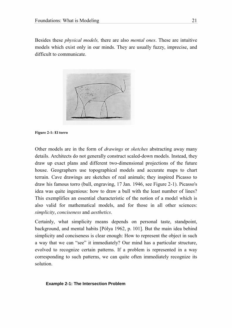
Figure 2-1: El torro
Other models are in the form of drawings or sketches abstracting away many
details. Architects do not generally construct scaled-down models. Instead, they
draw up exact plans and different two-dimensional projections of the future
house. Geographers use topographical models and accurate maps to chart
terrain. Cave drawings are sketches of real animals; they inspired Picasso to
draw his famous torro (bull, engraving, 17 Jan. 1946, see Figure 2-1). Picasso's
idea was quite ingenious: how to draw a bull with the least number of lines?
This exemplifies an essential characteristic of the notion of a model which is
also valid for mathematical models, and for those in all other sciences:
simplicity, conciseness and aesthetics.
Certainly, what simplicity means depends on personal taste, standpoint,
background, and mental habits [Pólya 1962, p. 101]. But the main idea behind
simplicity and conciseness is clear enough: How to represent the object in such
a way that we can “see” it immediately? Our mind has a particular structure,
evolved to recognize certain patterns. If a problem is represented in a way
corresponding to such patterns, we can quite often immediately recognize its
solution.
Example 2-1: The Intersection Problem
22 Chapter 2
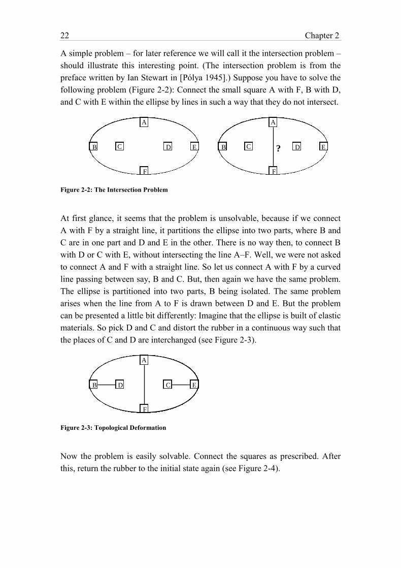
A simple problem – for later reference we will call it the intersection problem –
should illustrate this interesting point. (The intersection problem is from the
preface written by Ian Stewart in [Pólya 1945].) Suppose you have to solve the
following problem (Figure 2-2): Connect the small square A with F, B with D,
and C with E within the ellipse by lines in such a way that they do not intersect.
A
F
D ECB
A
F
D ECB ?
Figure 2-2: The Intersection Problem
At first glance, it seems that the problem is unsolvable, because if we connect
A with F by a straight line, it partitions the ellipse into two parts, where B and
C are in one part and D and E in the other. There is no way then, to connect B
with D or C with E, without intersecting the line A–F. Well, we were not asked
to connect A and F with a straight line. So let us connect A with F by a curved
line passing between say, B and C. But, then again we have the same problem.
The ellipse is partitioned into two parts, B being isolated. The same problem
arises when the line from A to F is drawn between D and E. But the problem
can be presented a little bit differently: Imagine that the ellipse is built of elastic
materials. So pick D and C and distort the rubber in a continuous way such that
the places of C and D are interchanged (see Figure 2-3).
A
F
D ECB
Figure 2-3: Topological Deformation
Now the problem is easily solvable. Connect the squares as prescribed. After
this, return the rubber to the initial state again (see Figure 2-4).
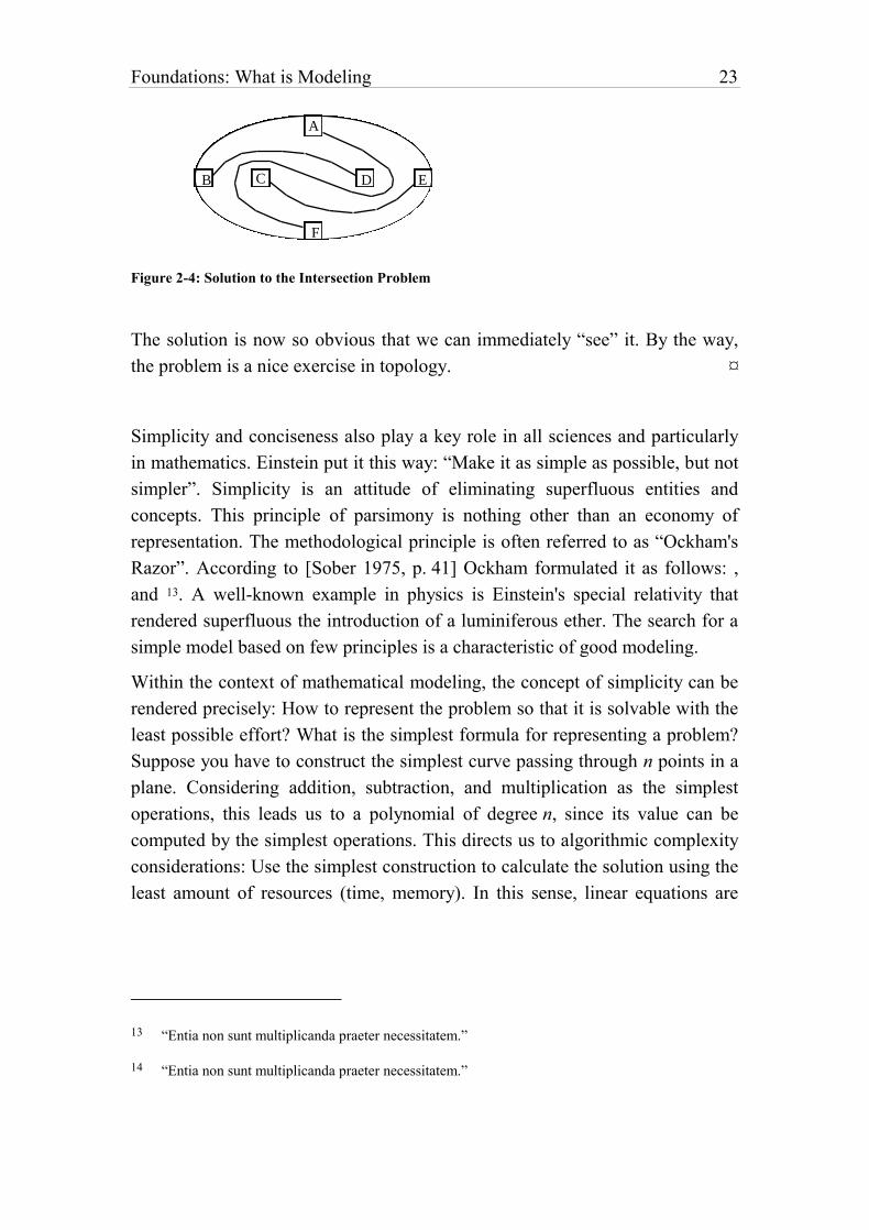
Foundations: What is Modeling 23
A
F
D ECB
Figure 2-4: Solution to the Intersection Problem
The solution is now so obvious that we can immediately “see” it. By the way,
the problem is a nice exercise in topology. ¤
Simplicity and conciseness also play a key role in all sciences and particularly
in mathematics. Einstein put it this way: “Make it as simple as possible, but not
simpler”. Simplicity is an attitude of eliminating superfluous entities and
concepts. This principle of parsimony is nothing other than an economy of
representation. The methodological principle is often referred to as “Ockham's
Razor”. According to [Sober 1975, p. 41] Ockham formulated it as follows: ,
and 13. A well-known example in physics is Einstein's special relativity that
rendered superfluous the introduction of a luminiferous ether. The search for a
simple model based on few principles is a characteristic of good modeling.
Within the context of mathematical modeling, the concept of simplicity can be
rendered precisely: How to represent the problem so that it is solvable with the
least possible effort? What is the simplest formula for representing a problem?
Suppose you have to construct the simplest curve passing through n points in a
plane. Considering addition, subtraction, and multiplication as the simplest
operations, this leads us to a polynomial of degree n, since its value can be
computed by the simplest operations. This directs us to algorithmic complexity
considerations: Use the simplest construction to calculate the solution using the
least amount of resources (time, memory). In this sense, linear equations are
13 “Entia non sunt multiplicanda praeter necessitatem.”
14 “Entia non sunt multiplicanda praeter necessitatem.”
24 Chapter 2
simpler than non-linear ones.15
Here, the degree of simplicity is intrinsically linked to complexity (in the sense
of algorithmic complexity). A problem is often simplified to a point at which it
can be solved by a particular procedure within reasonable time. A model which
represents the problem as accurately as possible, but which cannot be processed
or manipulated because of its complexity is useless from a practical point of
view. With this in mind, it sometimes makes sense to “bend” the problem until
it fits a model methodology in a lower category of complexity.
The idea behind aesthetics might be less obvious. What have aesthetics to do
with models? Human perception is an active process of searching for order, of
categorizing, and interpreting. Our mind is biased towards specific patterns
which we perceive as aesthetic or beautiful. It is, therefore, natural to exploit
these propensities to catch and retain the attention of the observer to convey
encoded messages. This is especially true in visual art. But it also holds true in
all other domains of behaviour. Aesthetics have the function of putting the mind
in a particular state that motivates it to concentrate on specific aspects of an
object.16 A “beautiful” model that pleases and captures our mind seems to be
much more attractive and useful than a graceless, albeit accurate one.17
Therefore, aesthetics is an essential feature of all models we build and use, to
explain phenomena and to control our environment.
15 Popper criticizes this manner of defining simplicity. He thinks that such considerations are
entirely arbitrarily [Popper 1976, p. 99]. He also refuses the aesthetic-pragmatic concept of
simplicity. Popper identifies these concepts with the concept of degree of falsification [p. 101].
16 Aesthetics, being an emotional reaction to simplicity, have an important adaptive function which
is in no way the unique privilege of human beings. Charles Darwin stated that some female birds
have an aesthetic preference for bright markings on males. For a biological foundation of
aesthetics see: Rentschler I., Herzberger B., Epstein D., [1988], Beauty and Brain, Biological
Aspects of Aesthetics, Birkhäuser, Basel.
17 The American Eliseo Vivas' theory of disinterested perception, which asserts that the key
concept in aesthetics is disinterestedness does not necessarily contradict the above theory of
aesthetics as a motivating force. We have all had the experience that when we concentrate
consciously on a problem by forcing an issue, it does not work. Sometimes, we have to relax, to
step back from the problem in order to make some progress.
Foundations: What is Modeling 25
Aesthetics also plays an important role in sciences and mathematics. It is
interesting to note, for instance, that Copernicus' early defence of the
heliocentric system was based entirely on aesthetic considerations.18 Kepler
considered the three laws he discovered – and for which he is famous today –
as only a by-product of a much more universal cosmology. He was so
fascinated by the beauty of the five Platonic solids that he tried to construct the
solar system after them. Newton's often-quoted evaluation of himself says: “I
do not know what I may appear to the world, but to myself I seem to have been
only like a boy playing on the sea-shore, and diverting myself in now and then
finding a smoother pebble or a prettier shell than ordinary, whilst the great
ocean of truth lay all undiscovered before me.” [Chandrasekhar 1987, p. 47].
The French mathematician H. Poincaré (1854–1912) stated it this way: “The
Scientist does not study nature because it is useful to do so. He studies it
because he takes pleasure in it; and he takes pleasure in it because it is
beautiful.” The German mathematician Weyl (1885–1955), once asked whether
he preferred a true or a beautiful theory, chose the beautiful one
[Chandrasekhar 1987, p. 65]. He gave the example of his gauge theory of
gravitation which he considered not true, but so beautiful that he did not want
to abandon it. Much later, the theory turned out to be true after all!
Is science similar to art, since both are in quest of aesthetics? It is a common
view that “When Science arrives, it expels Literature.” (Lowes Dickinson); but
also “…when literature arrives, it expels science…” (Peter Medawar)
[Chandrasekhar 1987, p. 55]. “The distinction between art and science seems
all too clear. Art is emotional, science factual; art is subjective, science
objective; art is pleasant, science is useful. So goes the common distinction…“
[Agassi J., Art and Science, in: Scientia, Vol. 114, p. 127]. And Agassi
continues: “…I can, on the contrary, see much more in common between the
bunglings of a Beethoven and the bunglings of a Newton. I can compare their
zeal; their sense of perfection; their experimentation and search for something
objective, overruling the merely subjective and the accidental as much as
possible and even hoping against all common-sense to eliminate it altogether.”
Certainly, there are important differences between art and science. Whilst in
18 See, for instance, Thompson M., The Process of Applied Mathematics, p. 10, in:
[Brams/Lucas/Straffin 1983]; see also [Feyerabend Paul, 1986, Wider den Methodenzwang,
Suhrkamp, p. 113 and p. 133].
26 Chapter 2
science aesthetics are only a means to find or to represent good models (or
knowledge), in art it is an end in itself. In science, we use the biased patterns of
the mind to recognize and capture the structure of the problem, the final goal
being its solution. In art we do not necessarily make such utilitarian demands,
art has no need to produce something, but rather to put the mind in a certain
emotional state.
This different, rather common-sense conception of model could be summarized
using the following definition:
A model is a real or virtual object that substitutes another real or
virtual object (the original) – on the base of some structural,
functional, or behavioural analogy – to solve problems. This
solution could not have been attained directly from the original
because it would have been too costly, or it would have destroyed
the object.
Four aspects are contained in this definition:
1 There is some mapping between the model and the object or
phenomenon of interest;
2 the model is an abstraction, i.e. only some aspects of the objects of
interest are mapped, all others are ignored (abstrahere = leaving
out);
3 the aspects that enter the model are of special interest for an
intelligent actor (the model-builder and the model-user): The
model is used for a certain purpose;
4 a model has some simple, concise (and aesthetic) structure that
captures the focused aspects of the object.
It is of paramount importance to recognize that the model is not the same as the
object or phenomenon it represents. Normally, it is a simplification, but it must
be interesting enough to capture the mind. Hence, the model is something
relative, there is no single absolute representation of the problem at hand. It is
not only a model of something, but also for someone and for some purpose.
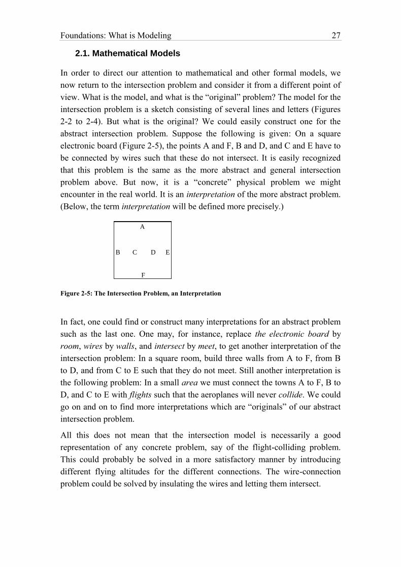
Foundations: What is Modeling 27
2.1. Mathematical Models
In order to direct our attention to mathematical and other formal models, we
now return to the intersection problem and consider it from a different point of
view. What is the model, and what is the “original” problem? The model for the
intersection problem is a sketch consisting of several lines and letters (Figures
2-2 to 2-4). But what is the original? We could easily construct one for the
abstract intersection problem. Suppose the following is given: On a square
electronic board (Figure 2-5), the points A and F, B and D, and C and E have to
be connected by wires such that these do not intersect. It is easily recognized
that this problem is the same as the more abstract and general intersection
problem above. But now, it is a “concrete” physical problem we might
encounter in the real world. It is an interpretation of the more abstract problem.
(Below, the term interpretation will be defined more precisely.)
A
F
D ECB
Figure 2-5: The Intersection Problem, an Interpretation
In fact, one could find or construct many interpretations for an abstract problem
such as the last one. One may, for instance, replace the electronic board by
room, wires by walls, and intersect by meet, to get another interpretation of the
intersection problem: In a square room, build three walls from A to F, from B
to D, and from C to E such that they do not meet. Still another interpretation is
the following problem: In a small area we must connect the towns A to F, B to
D, and C to E with flights such that the aeroplanes will never collide. We could
go on and on to find more interpretations which are “originals” of our abstract
intersection problem.
All this does not mean that the intersection model is necessarily a good
representation of any concrete problem, say of the flight-colliding problem.
This could probably be solved in a more satisfactory manner by introducing
different flying altitudes for the different connections. The wire-connection
problem could be solved by insulating the wires and letting them intersect.

28 Chapter 2
This power of abstraction, this ability to leave out some or many details about a
concrete problem in order to use the “distillate” for a multitude of similar
problems, is one of the most striking characteristics of our mind. A concrete,
“real” problem need not even be there: We can make some useful
considerations without a specific application in mind, as we have seen with the
intersection problem. Mathematics and logic are essential tools in this process
of abstraction. They are powerful languages to express and represent real
phenomena.19 We could even define mathematics as the science of finding and
representing patterns and structures in concrete or abstract problems. It is these
patterns that are expressed in a mathematical model.
Unlike a scale model, a mathematical model is a symbolic and abstract
representation of the problem at hand. It can now no longer be recognized “at
first glance”. On the other hand, formal models are easy to manipulate, analyze,
and optimize. Furthermore, an extremely wide variety of problems can be
represented by mathematical notation, and what is even more interesting, they
can be manipulated by computers.
Abstraction is an essential process for all kind of mathematics. We may even
build infinite hierarchical orders of ever more abstract levels: Abstract algebra
is a model of our everyday algebra; this in turn is a model of the number
system, and numbers are models of quantities.
It is a striking fact that simple mathematical entities, such as group or vector
space, can be applied over and over again to the analysis of the most diverse
theoretical and applied problems. “…mathematical concepts turn up in entirely
unexpected connections” [Wigner 1960].
There is yet another aspect that makes mathematics so powerful. It is the ability
to infer statements. “What distinguishes a mathematical model from these other
models is that we use the deductive power of mathematics to learn about the
model, and so about the process we are studying” [Roberts 1976, p. 18]. By
19 It is said that the outstanding American physicist J.W. Gibbs (1839–1903), during a discussion
on the question of whether more attention should be given to ancient languages or to
mathematics, pronounced in irritation: “But mathematics is also a language.”
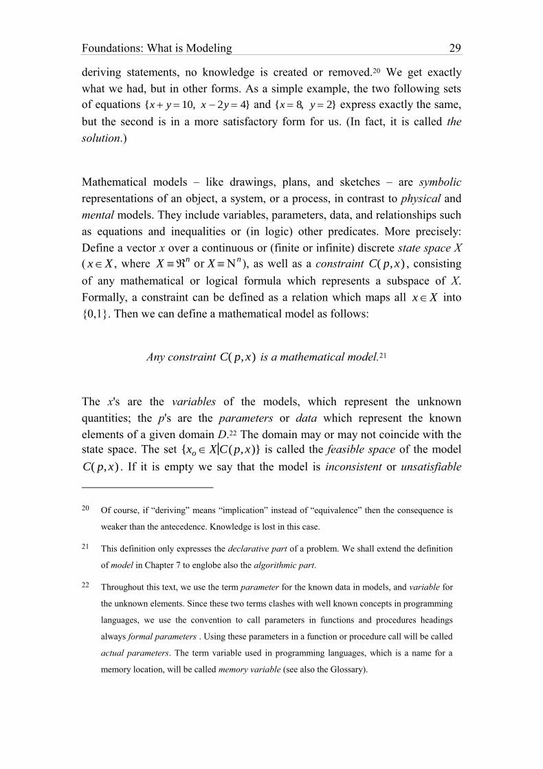
Foundations: What is Modeling 29
deriving statements, no knowledge is created or removed.20 We get exactly
what we had, but in other forms. As a simple example, the two following sets
of equations {x y 10, x 2y 4} and {x 8, y 2} express exactly the same,
but the second is in a more satisfactory form for us. (In fact, it is called the
solution.)
Mathematical models – like drawings, plans, and sketches – are symbolic
representations of an object, a system, or a process, in contrast to physical and
mental models. They include variables, parameters, data, and relationships such
as equations and inequalities or (in logic) other predicates. More precisely:
Define a vector x over a continuous or (finite or infinite) discrete state space X
( x X , where X n
or X n), as well as a constraint C( p,x) , consisting
of any mathematical or logical formula which represents a subspace of X.
Formally, a constraint can be defined as a relation which maps all x X into
{0,1}. Then we can define a mathematical model as follows:
Any constraint C( p,x) is a mathematical model.21
The x's are the variables of the models, which represent the unknown
quantities; the p's are the parameters or data which represent the known
elements of a given domain D.22 The domain may or may not coincide with the
state space. The set {xo X C(p,x)} is called the feasible space of the model
C( p,x) . If it is empty we say that the model is inconsistent or unsatisfiable
20 Of course, if “deriving” means “implication” instead of “equivalence” then the consequence is
weaker than the antecedence. Knowledge is lost in this case.
21 This definition only expresses the declarative part of a problem. We shall extend the definition
of model in Chapter 7 to englobe also the algorithmic part.
22 Throughout this text, we use the term parameter for the known data in models, and variable for
the unknown elements. Since these two terms clashes with well known concepts in programming
languages, we use the convention to call parameters in functions and procedures headings
always formal parameters . Using these parameters in a function or procedure call will be called
actual parameters. The term variable used in programming languages, which is a name for a
memory location, will be called memory variable (see also the Glossary).
30 Chapter 2
otherwise we say that it is consistent or satisfiable. Building a mathematical
model of a phenomenon means defining a vector x X and finding the
constraint C together with the parameters p such that C( p,x) represents the
phenomenon. Solving a mathematical model means finding at least one vector
xo X such that C( p,xo) is satisfied. Note the difference between data,
parameters and variables: While data are explicit elements of a domain,
parameters are symbolic place holders for the data. Variables, on the other
hand, are unknowns. They have no given initial value assigned to them.
The concepts of the mathematical model are historically recent ones. According
to Tarski, “the invention of variables constitutes a turning point in the history of
mathematics.” Greek mathematicians used them rarely and in an ad hoc way.
Vieta (1540–1603) was the first who made use of variables on a systematic
way. He introduced vowels to represent variables and consonants to represent
known quantities (parameters) [Eves 1992, p 278]. “Only at the end of the 19th
century, however, when the notion of a quantifier had become firmly
established, was the role of variables in scientific language and especially in the
formulation of mathematical theorems fully recognized” [Tarski 1994, p. 12].
2.2. Model Theory
To specify the term interpretation, we need to digress briefly in model theory.
In classical logic the term model has a different, well-defined meaning. The
syntax of a well-formed formula (wff) consists of symbols such as constants,
variables, and operators. An interpretation of a wff A consists of (1) a non-
empty set D, called the domain, (2) an assignment cD, for each constant c in A
(3) the assignment of a mapping DnD, for each n-ary function f in A, and (4)
the assignment of a mapping Dn{0,1}, for each n-ary predicate p in A. An
interpretation for which the wff expresses a true statement is called a model of
the formula [Tarski 1994, pp. 112]. A theory is a set of formulas with an
intended interpretation. Of course, the intended interpretation should be a
model.
As an example, consider the following formula from second order logic (the
example is from [Manna 1974, p. 77]):
F((F(a) b)x(p(x) (F(x) g(x, F( f (x)))))) , (1)
It may be interpreted as follows:
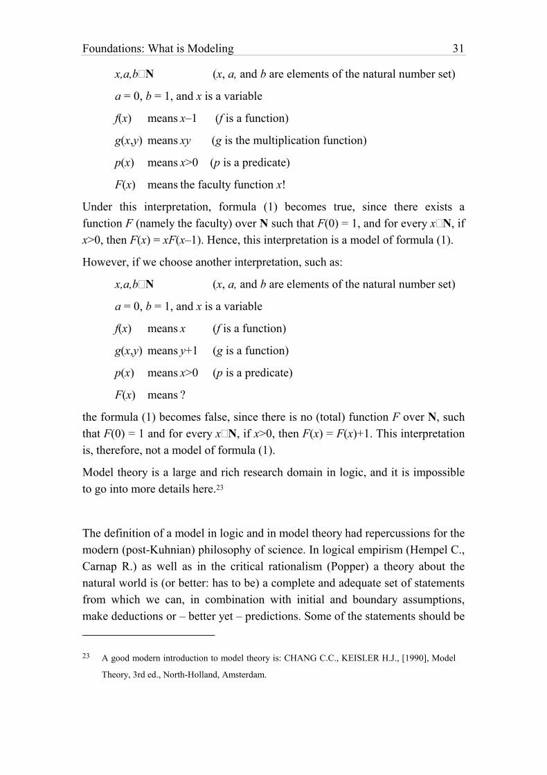
Foundations: What is Modeling 31
x,a,bN (x, a, and b are elements of the natural number set)
a = 0, b = 1, and x is a variable
f(x) means x–1 (f is a function)
g(x,y) means xy (g is the multiplication function)
p(x) means x>0 (p is a predicate)
F(x) means the faculty function x!
Under this interpretation, formula (1) becomes true, since there exists a
function F (namely the faculty) over N such that F(0) = 1, and for every xN, if
x>0, then F(x) = xF(x–1). Hence, this interpretation is a model of formula (1).
However, if we choose another interpretation, such as:
x,a,bN (x, a, and b are elements of the natural number set)
a = 0, b = 1, and x is a variable
f(x) means x (f is a function)
g(x,y) means y+1 (g is a function)
p(x) means x>0 (p is a predicate)
F(x) means ?
the formula (1) becomes false, since there is no (total) function F over N, such
that F(0) = 1 and for every xN, if x>0, then F(x) = F(x)+1. This interpretation
is, therefore, not a model of formula (1).
Model theory is a large and rich research domain in logic, and it is impossible
to go into more details here.23
The definition of a model in logic and in model theory had repercussions for the
modern (post-Kuhnian) philosophy of science. In logical empirism (Hempel C.,
Carnap R.) as well as in the critical rationalism (Popper) a theory about the
natural world is (or better: has to be) a complete and adequate set of statements
from which we can, in combination with initial and boundary assumptions,
make deductions or – better yet – predictions. Some of the statements should be
23 A good modern introduction to model theory is: CHANG C.C., KEISLER H.J., [1990], Model
Theory, 3rd ed., North-Holland, Amsterdam.
32 Chapter 2
universal or general laws, e.g. the gas equation in physics. Following these
methodologies, many scientific activities, such as biology or economics, have
no theory at all because they contain “only empirical generalizations”, no truly
universal laws.24 After much criticism of this view in philosophy of science
(Kuhn, Lakatos, Feyerabend) , alternative methodologies have been proposed.
One of them, the structuralist view, is especially interesting in our context.25 In
this view, the term model is at the heart of the analysis. A theory is no longer
considered to be a single coherent set of statements, but a set of models.26 What
sets a scientific community apart from another one are the models it uses and
modifies, rather than a forced attachment to general laws that it desperately
tries to falsify. Models are the primary theoretical tools used in all scientific
communities. But they have no empirical content in themselves, only their
interpretations link them to objects and make them interesting in a particular
24 For instance, Karl Popper claims that there is no universal law in evolutionary theory, that this
theory is merely “historical” (Popper K, [1979], Objective Knowledge: An evolutionary
approach, Clarendon, Oxford, pp. 267–270). (Popper revoked this judgement later in [Popper
K., Letter to new Scientist, 21 Aug. 1980 p. 611].)
25 For an introduction and further references (Sneed, Suppes, etc.) on the structuralist view of
theories see: Stegmüller W. [1979], The Structuralist View of Theories, A Possible Analogue of
the Bourbaki Programme in Physical Science, Springer, Berlin. A consequent approach of the
structuralist view – the author calls it the “semantic view” – in evolutionary theory is worked
out in: Lloyd E.A., [1988], The Structure and Confirmation of Evolutionary Theory, Princeton
University Press, Princeton. An up-to-date and comprehensive discussion of the subject can also
be found in [Herfel al., 1995]. (I am grateful to Daniel Raemi who drew my attention again to
the structuralist view of theories.)
26 The misleading view, that the distinction between model and theory is only a gradual one, is
widespread in many scientific communities outside of the philosophy of the science community.
According to this view, it is certainly not the complexity nor the size (considering models in
operations research which contain many thousands of variables and constraints), nor is it the
language, nor the purposes that makes the difference. It is rather the stability over time that
distinguishes theories from models. Models are more volatile, subject to frequent changes and
modifications [Zimmermann 1987, p. 4].
Foundations: What is Modeling 33
scientific community.27 Models always refer to ideal and simplified systems.
The differential equation system, dx
dt ax by ,
dy
dt cx dy , for instance,
could be interpreted as an oscillating system in physics, or as a model in combat
analysis, or as a prey-predator model in ecology [Braun al. 1983]. The
structuralist view has the further advantage that it can be applied to many other
disciplines (not only scientific ones).
This short digression into model theory and philosophy of science demonstrates
the importance the modeling concept has gained in the last few decades. In the
next section, we will show that it is compatible with the mathematical concept
of models, as defined above.
2.3. Models and Interpretations
It seems that the term model, as it was defined before and as it is used in model
theory, have opposite meanings. Whereas a mathematical model is a
representation of an “original” problem, in logic an interpretation of a formula
– i.e. a concrete application – is called the model. This apparent contradiction
can be resolved if the relation “x is a model of y” is interpreted as a symmetric
and transitive relation. The solar system, e.g., is just as much a model of
Newton's law of universal gravitation as the law of gravitation is a model of the
solar system. In this sense, we could “interpret” the solar system as a large
analogue computer to solve a specific case of Newton's law [Herfel W. E. in:
Herfel 1995, p. 80]. Certainly, such a model would not be very interesting,
since the solar system solves only a specific instance of Newton's law, and the
solution process is rather slow. Nevertheless, depending on your standpoint,
each could be taken as the model of the other.
This has important implications for the explanation of how laws can be
discovered: by postulating or using similarities between system. Assume we
have analyzed the behaviour of a collection of billiards balls (the physical
27 David Hilbert (1862–1943) once noted that the content of geometry does not change if we
replace the words point, line, and plane by, for example, chair, table, and bar [cited in: Yaglom
p. 7]. Wigner [1960] in his famous article stated that “mathematics is the science of skilful
operations with concepts and rules invented just for this purpose.”
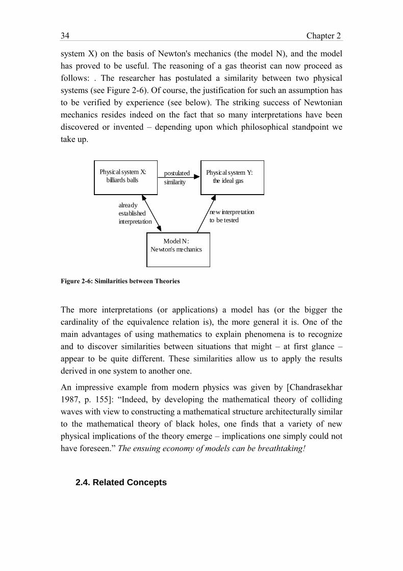
34 Chapter 2
system X) on the basis of Newton's mechanics (the model N), and the model
has proved to be useful. The reasoning of a gas theorist can now proceed as
follows: . The researcher has postulated a similarity between two physical
systems (see Figure 2-6). Of course, the justification for such an assumption has
to be verified by experience (see below). The striking success of Newtonian
mechanics resides indeed on the fact that so many interpretations have been
discovered or invented – depending upon which philosophical standpoint we
take up.
Physical system X:
billiards balls
Model N:
Newton's mechanics
Physical system Y:
the ideal gas
new interpretation
to be tested
similarity
postulated
already
established
interpretation
Figure 2-6: Similarities between Theories
The more interpretations (or applications) a model has (or the bigger the
cardinality of the equivalence relation is), the more general it is. One of the
main advantages of using mathematics to explain phenomena is to recognize
and to discover similarities between situations that might – at first glance –
appear to be quite different. These similarities allow us to apply the results
derived in one system to another one.
An impressive example from modern physics was given by [Chandrasekhar
1987, p. 155]: “Indeed, by developing the mathematical theory of colliding
waves with view to constructing a mathematical structure architecturally similar
to the mathematical theory of black holes, one finds that a variety of new
physical implications of the theory emerge – implications one simply could not
have foreseen.” The ensuing economy of models can be breathtaking!
2.4. Related Concepts
Foundations: What is Modeling 35
For practical purposes, it is useful to define briefly some other related terms.
The creator of a model is called the modeler. She needs to have a profound
knowledge of the object to be modeled, as well as an extensive understanding
of mathematical structures in order to match them to the problem at hand. To
create a model is and will always remain a complex and involved activity, even
if computer based modeling tools can support the modeler in her operations, it
cannot replace the creative work a modeler does. Of course, the modeler can be
a team rather than a single person, as is often the case in big projects. In this
case, the different activities such as data collection, setting up the model,
solving the model, and verifying it, etc. can be distributed between the
modelers.
The modeler is in many repects different from the model user. The user does
not necessarily need to understand the model. Her main task is to solve several
instances of the model in various contexts by changing parameters and data.
The model itself is like a black box. Surely, the user needs to know the context
in which the model works, and she must be able to interpret the results.
It is essential to distinguish clearly between the modeler and the model user. In
our context of implementing computer based modeling tools, this distinction is
essential even when the modeler and the model user are the same person. Many
modeling tool builders28 have unclear ideas about the users or their tools, which
often leads to poorly designed modeling environments. The modeler does not
need the same tools as the user. The modeler needs a powerful specification
mechanism, that supports her in the creative modeling process of building the
final model. The user, on the other hand, needs tools that allow her to switch
quickly between the model parameters, the solver and the results. She must
work with the whole modeling environment on a much higher level than the
modeler. The interaction between the computer and the user is more important
than this interaction is for the modeler. In this book, I present tools essentially
28 I shall not cite any examples here. But a short look into many “easy to use” decision tools (or
their prototypes), that are “natural” for any “non-expert user” or "naive user" with a “nice user
interface” are praised in many DSS journals. While easy-to-use should certainly be an important
aspect of any software – not only for model decision systems – it is misleading to believe that a
"naive-user", i.e. a user without profound knowledge about the problem to model, could ever
use modeling tools intelligently. Modeling is difficult and a highly creative process. There is no
way to bypass the thinking process.
36 Chapter 2
for the modeler.
Another concept is modeling. The term is difficult to define because it is used
in so many different contexts. In art, it is used to express the process of working
with plastic materials by hand to build up forms. In contrast to sculpturing,
modeling allows corrections to be made on the forms. They can be
manipulated, built and rebuilt until its creator feels happy with the result. In
sculpturing, the objective cannot be formed, it must be cut out. Once finished,
the form cannot be modified. Scientific activities are more like modeling than
sculpturing, and therefore the common-sense meaning of modeling is used in
various research communities.
In database technology, for instance, data modeling designates the design,
validation, and implementation of databases by applying well-known methods
and approaches such as the entity-relationship (ER) approach and the object-
role modeling (ORM) method. From a practical point of view, data modeling
could be considered as part of mathematical modeling. It is a set of tasks which
consists of collecting, verifying, and ordering data.
In engineering, geometric modeling is the design stage – nowadays mostly done
on computers – of building solid bodies. It is interesting to notice that
geometric modeling is normally a graphical way of modeling a set of
differential equations. They are not modeled explicitly, however, but the mesh
of the object is built directly, which is then used by the finite element method
(FEM). In this sense, geometric modeling is mathematical modeling, and the
model is formulated in a graphical way.
The term modeling has, since World War II, also had strong links to the term
simulation, following the first successful use of the so-called Monte Carlo
method by John von Neumann and Stanislaw Ulaw to solve neutron diffusion
problems. Since then, simulation and modeling have been applied to virtually
every discipline. Until recently, modeling in this context meant writing a
computer program that simulated a mathematical model which was not easily
amenable to conventional analytic or numeric solutions. Today, many software
packages exist, such as Extend or Stella,29 which allow the user to model a
29 Extend is a simulation package produced by Imagine That Inc., 6830 Via Del Oro, San Jose
CA. Stella is copyrighted by High Performance Systems Inc.
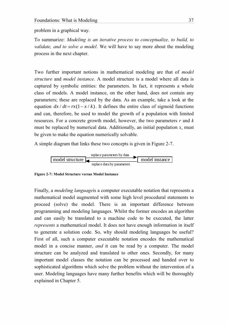
Foundations: What is Modeling 37
problem in a graphical way.
To summarize: Modeling is an iterative process to conceptualize, to build, to
validate, and to solve a model. We will have to say more about the modeling
process in the next chapter.
Two further important notions in mathematical modeling are that of model
structure and model instance. A model structure is a model where all data is
captured by symbolic entities: the parameters. In fact, it represents a whole
class of models. A model instance, on the other hand, does not contain any
parameters; these are replaced by the data. As an example, take a look at the
equation dx / dt rx(1 x / k) . It defines the entire class of sigmoid functions
and can, therefore, be used to model the growth of a population with limited
resources. For a concrete growth model, however, the two parameters r and k
must be replaced by numerical data. Additionally, an initial population xo must
be given to make the equation numerically solvable.
A simple diagram that links these two concepts is given in Figure 2-7.
model structure model instancereplace parameters by data
replace data by parameters
Figure 2-7: Model Structure versus Model Instance
Finally, a modeling languageis a computer executable notation that represents a
mathematical model augmented with some high level procedural statements to
proceed (solve) the model. There is an important difference between
programming and modeling languages. Whilst the former encodes an algorithm
and can easily be translated to a machine code to be executed, the latter
represents a mathematical model. It does not have enough information in itself
to generate a solution code. So, why should modeling languages be useful?
First of all, such a computer executable notation encodes the mathematical
model in a concise manner, and it can be read by a computer. The model
structure can be analyzed and translated to other ones. Secondly, for many
important model classes the notation can be processed and handed over to
sophisticated algorithms which solve the problem without the intervention of a
user. Modeling languages have many further benefits which will be thoroughly
explained in Chapter 5.
38 Chapter 2
Note that we shall distinguish the three notions of modeling language,
algebraic language, and mathematical language. While modeling language is
used in the sense of a general representation scheme of the state space, an
algebraic language is an instance of a modeling language, normally limited to
purely mathematical operators. The best known examples are AMPL
[Fourer/Gay/Kernighan, 1993], and GAMS [Brooke/Kendrick/Meeraus, 1988].
Mathematical languages, on the other hand, are not modeling languages in our
sense. They are programming languages that can be used to solve mathematical
problems symbolically or numerically. Examples are Mathematica, [Wolfram
1991], MatLab [MatLab 1993].
2.5. Declarative versus Procedural Knowledge
The model structure represents the problem in a declarative way without any
indication on how to solve the model. The constraints only describe the feasible
subspace in a concise way. This is in sharp contrast to a procedural method –
also called an algorithm – which represents the problem in a form that can be
solved by means of a step-by-step procedure. Declarative and procedural
representation are two fundamentally different kinds of modeling knowledge.
Declarative knowledge answers the question “what is?”, whereas procedural
knowledge asks “how to?” [Feigenbaum 1996]. An algorithm gives an exact
recipe of how to solve a problem. A mathematical model, on the other hand,
defines the problem as a subspace of the state space, as explained above. No
algorithm is given to find all or a single element of the feasible subspace. Of
course, there exists always a trivial algorithm to do so: enumerate the space.
Except for trivial cases, however, this algorithm is inefficient and useless.
Procedural knowledge is easy to handle on a computer. Indeed, the algorithmic
languages reflects the von Neumann architecture: memory variables (in the
sense of programming languages, not in the sense of mathematical models, see
footnote 21) are used to imitate the computer's storage cells, control statements
reflect its jump and test instructions, and assignment statements mimic its
fetching, storing and arithmetic [Backus 1978]. In fact, every program
(algorithm) can be expressed as an ordered list of three instructions only: the
increment, decrement, and the conditional branch instruction [Davis/Weyuker
1983, p. 16].
Declarative knowledge, on the other hand, is not so easy to implement on a
Foundations: What is Modeling 39
computer. Ultimately, it must be translated into a procedure to solve the
underlying problem. This is a challenging task, since no general algorithm
exists to do the job. Yet the declarative way to represent knowledge is
nonetheless very powerful and often more concise.
The distinction between declarative and procedural knowledge is by no means
an obvious one. It is also a rather recent one. Interestingly enough, algorithmic
knowledge arose much earlier in the history of mathematics than declarative
knowledge. The ancient Babylonians (19th–6th century B.C.) had the most
advanced mathematics in the Middle East. They easily handled quadratic and
even some cubic equations. They knew many primitive Pythagorean triples.30
They mastered the calculation of the volume of the truncated pyramid and many
more impressive computations [Eves 1992], [Yaglom 1986]. Arithmetics was
highly developed to ensure their calculations for architectural and astronomical
purposes. But we cannot find a single instance of what we nowadays call a
demonstration using symbolic variables and constraints. Only the process of the
calculation – today we may say the procedure or the algorithm – was described
[Knuth 1976]. It is therefore not surprising that all records from this period
contain only numerical problems. Essentially, the same could be said of
Chinese and Hindu mathematics. The algorithms for our elementary arithmetic
operations, e.g., were primarily developed in India about the tenth century
(A.D.) [Eves 1992, p. 213 and p. 225].
Declarative and demonstrative mathematics originated in Greece during the
Hellenic Age (as late as ca. 800–336 B.C.). The three centuries from about 600
(Thales) to 300 B.C. (Elements of Euclid) constitute a period of extraordinary
achievement. In an economical context where free farmers and merchants
traded and met in the most important marketplace of the time – the Agora in
Athens – to exchange their products and ideas, it became increasingly natural to
ask why some reasoning must hold and not just how to process knowledge. The
reasons for this are simple enough: When free people interact and disagree on
30 Primitive Pythagorean triples are positive integers (a,b,c) such that:
a 2uv, b u2v
2, c u
2 v
2, where u v, uv .
These formulas allows the generation of all triples such that a2 b
2 c
2. There is no
evidence that they were known by the Greeks at the time of Plato [Eves, 1990, p. 82].
40 Chapter 2
some subjects, then one asks the question of how to decide who is right. The
answers must be justified on some grounds. This laid the foundations for a
declarative knowledge based on axioms and deductions. Despite this amazing
triumph of Greek mathematics, it is not often realized that much of the
symbolism of our elementary algebra is less than 400 years old [Eves 1992,
p. 179].
It is interesting to note that this long history of mathematics with respect to
algorithmic and the declarative representation of knowledge is mirrored in the
short history of computer science and the development of programming
languages. The very first attempt to devise an algorithmic language was
undertaken in 1948 by K. Zuse [Naur 1981]. Soon, FORTRAN became
standard, and many procedural languages have been implemented since then.
The first step towards a declarative language was done by LISP. It is a well
known fact that every algorithm can be expressed as a recursive function. LISP
is based entirely on the -calculus. But LISP is not a fully-fletched declarative
language, since a recursive function is nothing other than a different way to
code an algorithm. Prolog [Sterling/Shapiro 1986], which became popular in
the late seventies, was one of the first attempts to make use of a declarative
language. Unfortunately, it proved inefficient for mathematical problems,
mainly because it was entirely based on resolution and unification. To be useful
in a practical context, several “procedural” predicates were added to the
language, such as cut and fail to guide the trivial enumeration algorithm
mentioned above. But Prolog had an invaluable influence on the recent
development of constraint logic programming (CLP), today a fast growing
paradigms in the computer language community. We will have more to say
about this development in Chapter 6.
The difficulties of implementing declarative model languages in order to
describe mathematical models are manifold [Jacoby/Kowalik 1980, p. 7]:
(1) It is sometimes impossible to express the original problem in
mathematical relationships due to either a poor theoretical understanding of
the problem, or, to different kinds of uncertainties. However, this does not
necessarily mean that the problem is inaccessible to formal treatment. We
will see in the section Modeling Nncertainty in the Chapter 4, how such
Foundations: What is Modeling 41
problems can be approached.
(2) Even if the problem can be formulated mathematically, it may be
unsolvable. It is well-known that mathematical notation (in its full
generality) is not implementable, because in this notation it is possible to
formulate problems that cannot be solved by a Turing machine (or by any
computer). This is basically due to the expressive power of mathematical
notation. The most famous specific decision problem is Hilbert's Tenth
Problem, which was proposed by Hilbert at the International Congress of
Mathematicians in 1900. The problem consists of finding an algorithm that
will determine whether or not a polynomial equation with integer
coefficients has a solution in integers or not. The solution to this decision
problem was only found in 1970 by Matijasevitch, who proved its
undecidability, i.e. no algorithm exists to decide the problem.
The last Fermat Conjecture, a solvable problem as it now seems, can easily
be stated in a declarative way as the decision problem whether the set
a,b,c n an b
n c
n} is empty or not. But the problem was
unanswered for more than 350 years. Even seemingly simple Diophantine
equations can be arbitrarily difficult to solve. The integer equation in the
unknowns x and y, x2 991y
21 has the smallest positive solution with x
30 and y 29 digits. Even the set of theorems in first-order logic, a restricted
subset of classical logic (FOL), are undecidable. This can be shown by
reducing the halting problem to the problem of deciding which logical
statements are theorems [Floyd/Beigel pp. 520]. More precisely, FOL is
semi-decidable, since we can prove a valid formula, but we cannot disprove
an unsatisfiable one. A recent and very comprehensive account on
undecidability can be found in [Rozenberg/Salomaa 1994].
(3) Even if the problem is solvable, it may not be practically solvable due to
its computational complexity. Most interesting problems are hard to solve
even by the most powerful computer; the cost of computations may be
prohibitive, as so many sophisticated method and heuristics have to be used
to handle the problem.
(4) Even if the problem is practically solvable, sufficiently detailed data for
the model may not be available.
(5) Additionally, it may be difficult to validate a mathematical model. (I will
have more to say on this point later on.)

42 Chapter 2
Certainly, all these drawbacks are not only limited to mathematical models. All
forms of models have similar disadvantages.
The consequence of these drawbacks for the implementation of modeling
languages is clear: Either we need to (greatly) restrict the expressive power of
the language so that it can only be used for “easy” problems, or we allow it to
have the full power while accepting that unsolvable problems may be
formulated. But there are also many intermediate solutions between these two
extremes. The point is to find a compromise between expressive power and
computability, or in other words, to find language entities that allow the
modeler to express the problem concisely and let her translate it into an
efficient form to be solved.
43
3. THE MODELING LIFE CYCLE
“Seek simplicity and distrust it.” — Whitehead N.
In this chapter, the modeling life cycle will briefly be presented. The goal is not
to give detailed information for the modeler on how to create and maintain
models, but rather to offer a short survey for the modeling tool implementor in
order to make her aware of the different tasks in the model building process.
Modeling tools should not only support the solution process, but the whole life
cycle of a model as well.
Early methodologies in mathematical modeling describe the phases of the
modeling life cycle as a linear stage process, consisting of:
recognition – formulation – solution – validation and interpretation.
Recognition is the stage where the problem is identified and the importance of
the issue is perceived; formulation is the most difficult step: the model is set up
and a mathematical structure is established; solution is the stage where an
algorithm is chosen or conceived to solve the problem; finally, the model must
be interpreted and validated in the light of the original problem.
This linear stage approach may be a first approximation to describe the model
building process. Modeling, however, is essentially an iterative process as
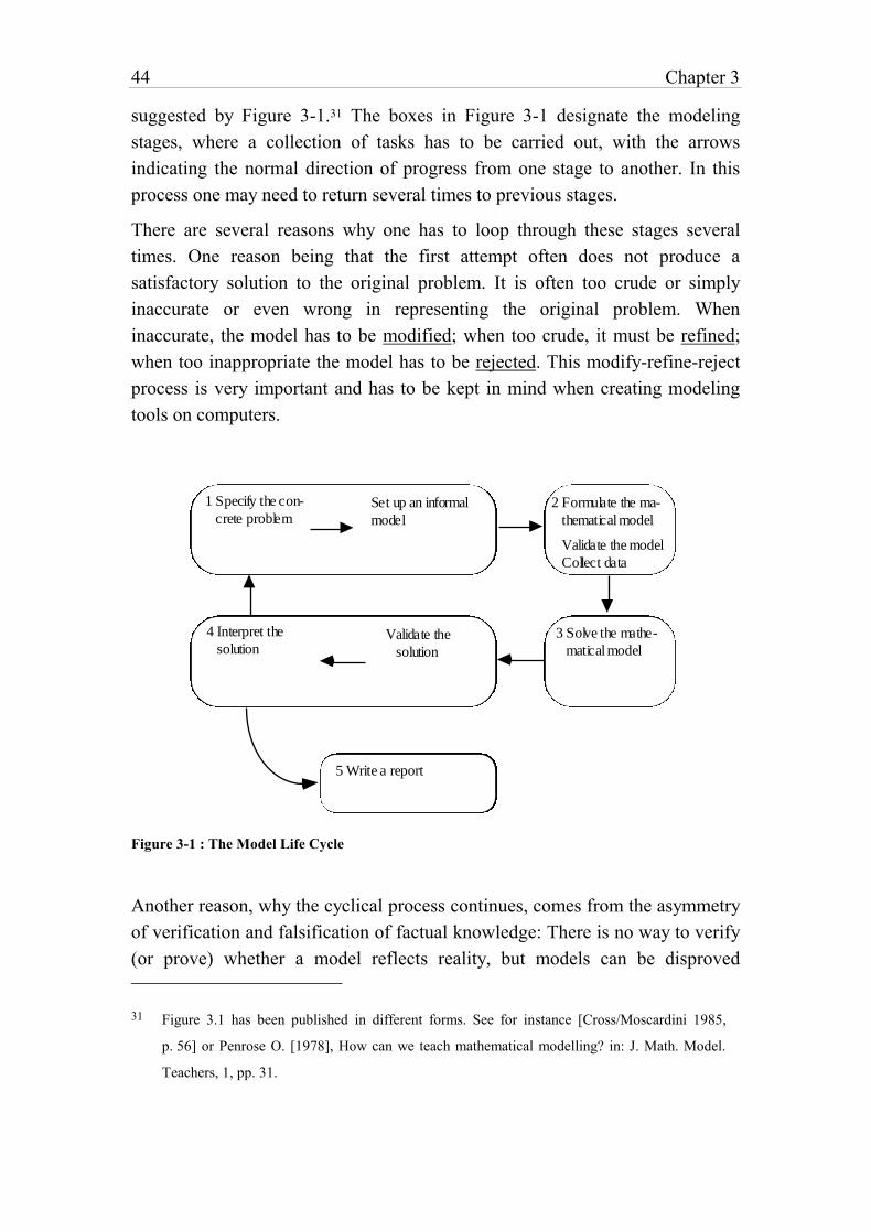
44 Chapter 3
suggested by Figure 3-1.31 The boxes in Figure 3-1 designate the modeling
stages, where a collection of tasks has to be carried out, with the arrows
indicating the normal direction of progress from one stage to another. In this
process one may need to return several times to previous stages.
There are several reasons why one has to loop through these stages several
times. One reason being that the first attempt often does not produce a
satisfactory solution to the original problem. It is often too crude or simply
inaccurate or even wrong in representing the original problem. When
inaccurate, the model has to be modified; when too crude, it must be refined;
when too inappropriate the model has to be rejected. This modify-refine-reject
process is very important and has to be kept in mind when creating modeling
tools on computers.
1 Specify the con-
crete problemSet up an informal
model
3 Formulate the ma-
thematical model
Validate the
solution
4 Interpret the
solution3 Solve the mathe-
matical model
5 Write a report
2 Formulate the ma-
thematical model
Validate the model
Collect data
Figure 3-1 : The Model Life Cycle
Another reason, why the cyclical process continues, comes from the asymmetry
of verification and falsification of factual knowledge: There is no way to verify
(or prove) whether a model reflects reality, but models can be disproved
31 Figure 3.1 has been published in different forms. See for instance [Cross/Moscardini 1985,
p. 56] or Penrose O. [1978], How can we teach mathematical modelling? in: J. Math. Model.
Teachers, 1, pp. 31.
Foundations: The Modeling Life Cycle 45
[Popper 1976]. Thus, the modeling process can go on forever.
A third reason is that a model may well reflect the objectives of some but not
all of the decision makers involved. There must be an ongoing process in
“harmonizing” conflicting goals that sometimes leads to a poorer model from
the point of view of one of the individuals involved.
Yet another reason lays at the heart of modeling process: going from stage to
stage also means discovering – uncovering – new structures and connections
that were previously unknown to the model builder. This is unavoidable as the
modeling process is not a mechanical activity, where the intermediate and final
goals are known in advance. The process is fundamentally non-predictable.
The evolution of a model is not unlike that of paradigms described by the
history of science [Kuhn 1962]. “Normal” periods of successive small
improvements and corrections are followed by “periods of crisis”, during which
the basic statements are radically questioned and eventually replaced.
For these reasons, models should always be regarded as tentative and subject to
continued evaluation and validation.
Let us take a closer look at the model building process itself.
3.1. Stage 1: Specification of the Real Problem
First of all, it must be said that very little progress can be made in modeling
without fully understanding the problem that has to be modeled. If the modeler
is not familiar with the real problem, she will never be able to build a model of
it. Traditionally, not much mathematics is involved at this stage. The problem is
studied for an extended time, data is collected and empirical laws or guidelines
are formulated before a systematic effort is made to provide a supporting
model. It is still not uncommon that problems are solved on the basis of
experience and ad hoc techniques, prior to the recognition that mathematical
methods might be beneficial. This attitude towards problem solving is gradually
changing. The advantages of formal methods are increasingly appreciated,
especially as more and more sophisticated modeling tools and powerful
solution techniques are available on cheap machines. Hence, problems become
increasingly quickly formulated in mathematical form.
But this “mathematization” of problem solving has also produced some
46 Chapter 3
negative spin-offs. There are two common errors to be found at the beginning
of the modeling process. The first is hurriedly collecting too much inadequate
or incomplete data and irrelevant relationships, and the other is deciding
prematuerly on the methods to be used to solve the problem. The first mistake
comes from an erroneous idea that the final and formalized model and its
solution are more important than this “preliminary” stage, although a careful
and accurate study of the problem is essential. The second mistake often arises
because many modelers think that using some formalism is more important than
using an appropriate notation that reflects the problem. Yet the most
sophisticated formalism is useless if it does not mirror some significant features
of the underlying problem. Often, the modelers only have access to a limited
arsenal of modeling tools, and they apply what they have at hand.
Appropriateness comes second.
Hence, the very beginning of the modeling process needs expertise and a good
eye to filter out unimportant factors. As difficult, and sometimes as tedious as
the a modeling process may be, there is no way around it: It is impossible to
specify a problem without setting up an informal model. Any specification is a
model using some language or symbolism. The first formulation is mostly in
natural language. Sketches or drawings usually accompany the formulation. At
this stage, the objectives should be clearly stated. A plan on how to attack the
problem has to be put forward. In textbooks on problem solving in applied
mathematics, this first stage is assumed, but in facing a real problem, it is often
not even clear what the problem consists of. Unless the modeler gets this right
at the start, it is of little use to build a formalized model.
3.2. Stage 2: Formulation of the Mathematical Model
This is the most crucial and difficult stage in the modeling process. It is
undoubtedly creative. It uses mathematical knowledge and skills as well as
problem expertise. But it also requires something more: the talent to recognize
what is essential and to discard the irrelevant, as well as an intuition as to which
mathematical structure is best suited to the problem. This intuition cannot be
learned as we learn how to solve mathematical equations. Like swimming, this
skill can be acquired by observing others and then trying by oneself. Hence, it is
difficult to provide an adequate formal description on the model formulation
process. On an abstract level, there is no doubt about what has to be done:
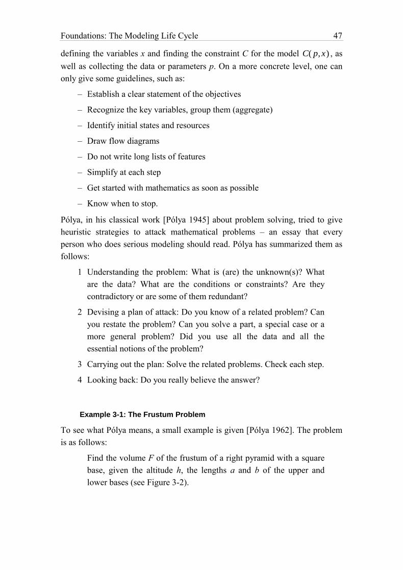
Foundations: The Modeling Life Cycle 47
defining the variables x and finding the constraint C for the model C( p,x) , as
well as collecting the data or parameters p. On a more concrete level, one can
only give some guidelines, such as:
– Establish a clear statement of the objectives
– Recognize the key variables, group them (aggregate)
– Identify initial states and resources
– Draw flow diagrams
– Do not write long lists of features
– Simplify at each step
– Get started with mathematics as soon as possible
– Know when to stop.
Pólya, in his classical work [Pólya 1945] about problem solving, tried to give
heuristic strategies to attack mathematical problems – an essay that every
person who does serious modeling should read. Pólya has summarized them as
follows:
1 Understanding the problem: What is (are) the unknown(s)? What
are the data? What are the conditions or constraints? Are they
contradictory or are some of them redundant?
2 Devising a plan of attack: Do you know of a related problem? Can
you restate the problem? Can you solve a part, a special case or a
more general problem? Did you use all the data and all the
essential notions of the problem?
3 Carrying out the plan: Solve the related problems. Check each step.
4 Looking back: Do you really believe the answer?
Example 3-1: The Frustum Problem
To see what Pólya means, a small example is given [Pólya 1962]. The problem
is as follows:
Find the volume F of the frustum of a right pyramid with a square
base, given the altitude h, the lengths a and b of the upper and
lower bases (see Figure 3-2).
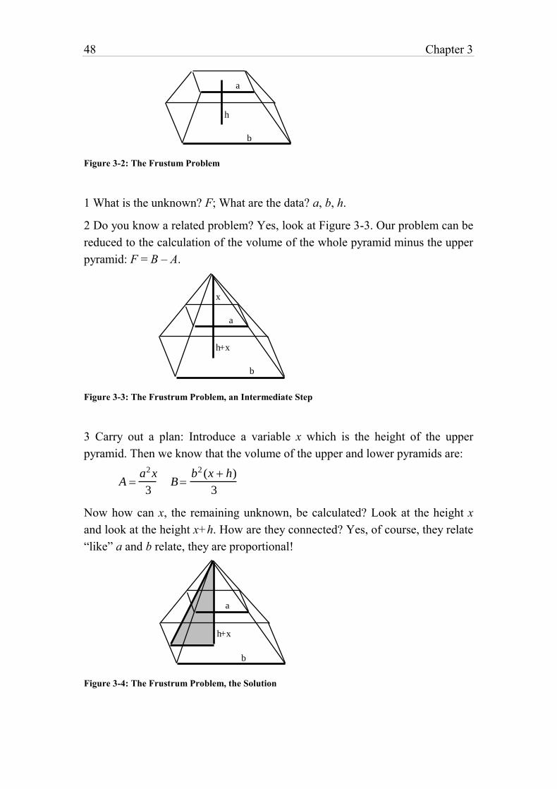
48 Chapter 3
h
a
b
Figure 3-2: The Frustum Problem
1 What is the unknown? F; What are the data? a, b, h.
2 Do you know a related problem? Yes, look at Figure 3-3. Our problem can be
reduced to the calculation of the volume of the whole pyramid minus the upper
pyramid: F = B – A.
h+x
a
b
x
Figure 3-3: The Frustrum Problem, an Intermediate Step
3 Carry out a plan: Introduce a variable x which is the height of the upper
pyramid. Then we know that the volume of the upper and lower pyramids are:
A a2 x
3B
b2 (x h)
3
Now how can x, the remaining unknown, be calculated? Look at the height x
and look at the height x+h. How are they connected? Yes, of course, they relate
“like” a and b relate, they are proportional!
h+x
a
b
Figure 3-4: The Frustrum Problem, the Solution
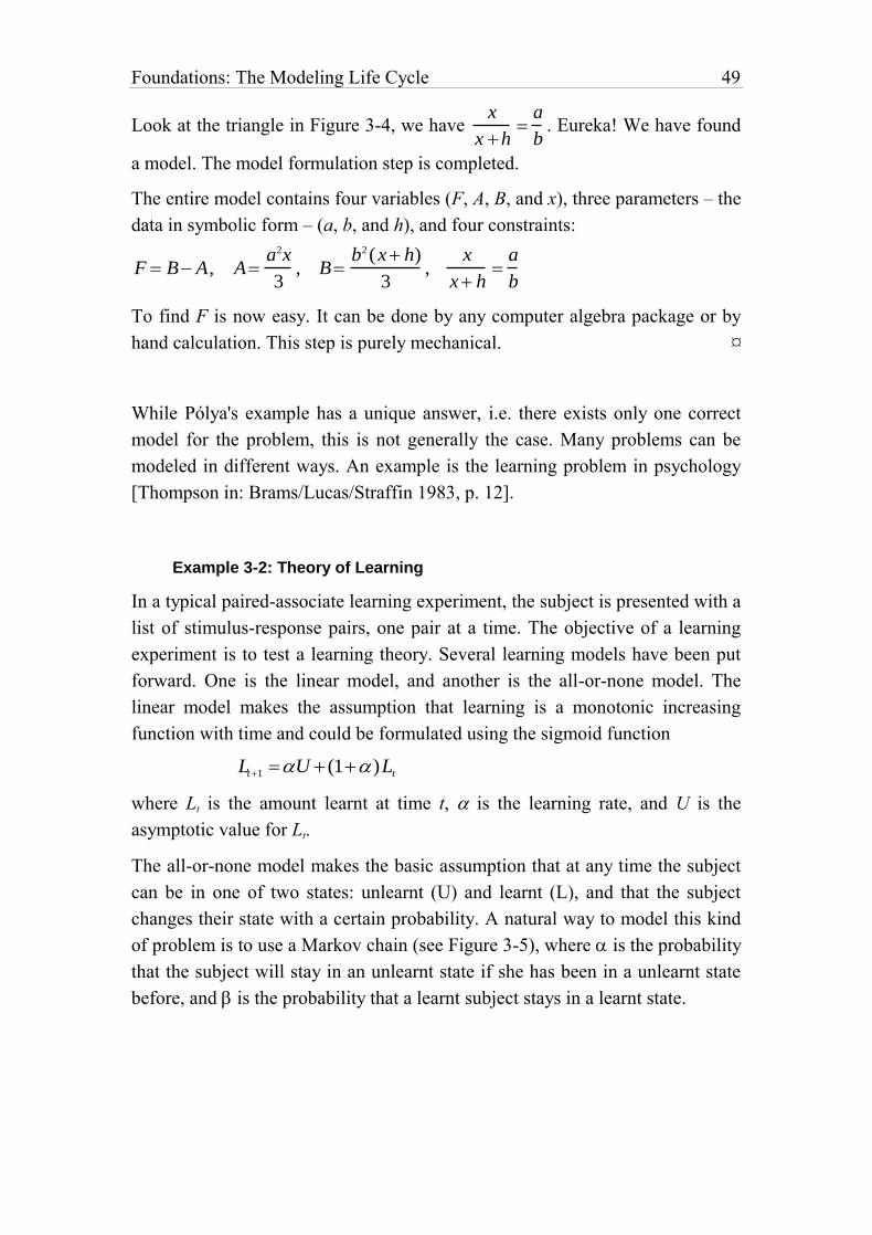
Foundations: The Modeling Life Cycle 49
Look at the triangle in Figure 3-4, we have x
x h
a
b. Eureka! We have found
a model. The model formulation step is completed.
The entire model contains four variables (F, A, B, and x), three parameters – the
data in symbolic form – (a, b, and h), and four constraints:
F B A, Aa2x
3, B
b2 (x h)
3,
x
x h
a
b
To find F is now easy. It can be done by any computer algebra package or by
hand calculation. This step is purely mechanical. ¤
While Pólya's example has a unique answer, i.e. there exists only one correct
model for the problem, this is not generally the case. Many problems can be
modeled in different ways. An example is the learning problem in psychology
[Thompson in: Brams/Lucas/Straffin 1983, p. 12].
Example 3-2: Theory of Learning
In a typical paired-associate learning experiment, the subject is presented with a
list of stimulus-response pairs, one pair at a time. The objective of a learning
experiment is to test a learning theory. Several learning models have been put
forward. One is the linear model, and another is the all-or-none model. The
linear model makes the assumption that learning is a monotonic increasing
function with time and could be formulated using the sigmoid function
Lt1 U (1)Lt
where Lt is the amount learnt at time t, is the learning rate, and U is the
asymptotic value for Lt.
The all-or-none model makes the basic assumption that at any time the subject
can be in one of two states: unlearnt (U) and learnt (L), and that the subject
changes their state with a certain probability. A natural way to model this kind
of problem is to use a Markov chain (see Figure 3-5), where is the probability
that the subject will stay in an unlearnt state if she has been in a unlearnt state
before, and is the probability that a learnt subject stays in a learnt state.
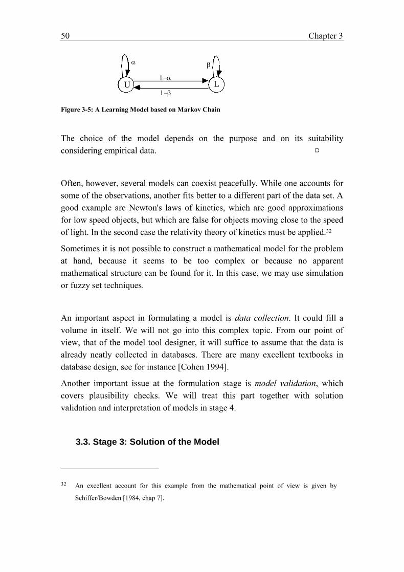
50 Chapter 3
U L
Figure 3-5: A Learning Model based on Markov Chain
The choice of the model depends on the purpose and on its suitability
considering empirical data. ¤
Often, however, several models can coexist peacefully. While one accounts for
some of the observations, another fits better to a different part of the data set. A
good example are Newton's laws of kinetics, which are good approximations
for low speed objects, but which are false for objects moving close to the speed
of light. In the second case the relativity theory of kinetics must be applied.32
Sometimes it is not possible to construct a mathematical model for the problem
at hand, because it seems to be too complex or because no apparent
mathematical structure can be found for it. In this case, we may use simulation
or fuzzy set techniques.
An important aspect in formulating a model is data collection. It could fill a
volume in itself. We will not go into this complex topic. From our point of
view, that of the model tool designer, it will suffice to assume that the data is
already neatly collected in databases. There are many excellent textbooks in
database design, see for instance [Cohen 1994].
Another important issue at the formulation stage is model validation, which
covers plausibility checks. We will treat this part together with solution
validation and interpretation of models in stage 4.
3.3. Stage 3: Solution of the Model
32 An excellent account for this example from the mathematical point of view is given by
Schiffer/Bowden [1984, chap 7].
Foundations: The Modeling Life Cycle 51
Once the model formulation step has been completed, the mathematical model
has to be solved, i.e. the model must be transformed using the mathematical
axioms and deduction rules in such a way as to eliminate the unknowns. We say
that a model is solved if a numerical or symbolical expression containing only
parameters and numbers is assigned to each variable so that all constraints are
fulfilled.
The solution step can be very straightforward, as in the example of the frustum
(Example 3-1). But it is easy to formulate innocent looking models that lead to
extremely difficult mathematical problems. Sometimes a well understood
mathematical framework exists to solve them, more often it does not. At the
research level, this will often lead to the creation of new mathematics. At the
modeling level, the model must be reformulated to be tractable. Occasionally, it
is not necessary to reformulate an intractable model; one may use simulation
techniques or heuristics to find approximate – hopefully good – solutions to the
model. In all but trivial cases the solution cannot be carried out by hand, and
one must develop computer programs to execute the lengthy calculations. But
even if the mathematical theory of a problem is straightforward, the invention
of an appropriate algorithm can require considerable ingenuity. Furthermore, it
is not easy to write numerically stable and reliable software. Therefore, for
many problem classes available software packages – called solvers – have been
built by expert numerical analysts since the late 1950's.
The quality of mathematical modeling is greatly enhanced by the use of such
optimal software. Besides the evident benefits, there are however some
drawbacks for the modeler. The benefits are clear: that the modeler does not
need to develop and implement algorithms to solve the problem. On the other
hand, once the problem is formulated, the model must be put into a form that
can be read by the appropriate solver. Often this is no easy task. Data must be
read and filtered correctly from databases, the model structure must be
implemented, and the generated output must be a correct form for input into the
solver. For large models with huge data sets it is likely that such a data-driven
model generator is prone to errors, and debugging tends to be tedious.
Today it is not uncommon that the model building steps (stage 1 and 2) are
carried out by hand or by writing ad hoc programs to generate the appropriate
model input form for the solver. While the model building step as well as the
development of ad hoc generators can take several weeks or even months, the
solution step is executed almost instantly by an appropriate solver. There are
52 Chapter 3
several reasons for this discrepancy. First of all, to find the right formulation is
difficult, the collection of the data takes time. Furthermore, much repetitive
work is done by writing ad hoc programs to generate the right input for an
appropriate solver. An alternative would be to have modeling tools which allow
the specification of the model by using a high level language. From such a
formulation the appropriate solver input form could then be produced
automatically [Fourer 1983]. One of the main purpose of this work is to study
the feasibility of such tools.
3.4. Stage 4: Validation of the Model and its Solution
Validation is a continuous process and takes place at every stage. But we shall
summarize its different aspects in this section.
Normally, by validation we mean the process of checking the model against
reality, i.e. to examine whether the model is isomorphic in certain respects to
the original problem. Figure 3-6 demonstrates another way of representing the
modeling stages. In a first stage, the fundamental structure is tentatively
formulated. This means essentially conjecturing the general pattern from
observation or from other sources. How this is done is not important for the
validation of the model. “Everything goes”, i.e. any method, procedure or
heuristic that produces some model can be used. From this model consisting of
mathematical statements other statements are derived by mathematical
deduction in a second stage. This can be denoted as the solution stage.
Deduction is nothing other than the mathematical transformation of the model.
Nothing is added and nothing is lost in this process, i.e., the validity of the
model cannot change during this process – except, of course, if the solution
process is erroneous. This remark is not as trivial as it may at first seem. Since
the solution process for mathematical models is executed in general by very
complex software, its correctness can often not be verified. In the final stage,
the general structure is confirmed or refuted by experience. One of the strongest
types of validation is prediction.33
33 The discovery of the planet Neptune is an often quoted example. Since the discovery of the
planet Uranus in 1781, perturbations had been noted in its orbit. An explanation within
Newton's gravitational model which could fit these observations was the presence of a
previously unobserved planet. A telescope at Berlin was then pointed in the right direction at the
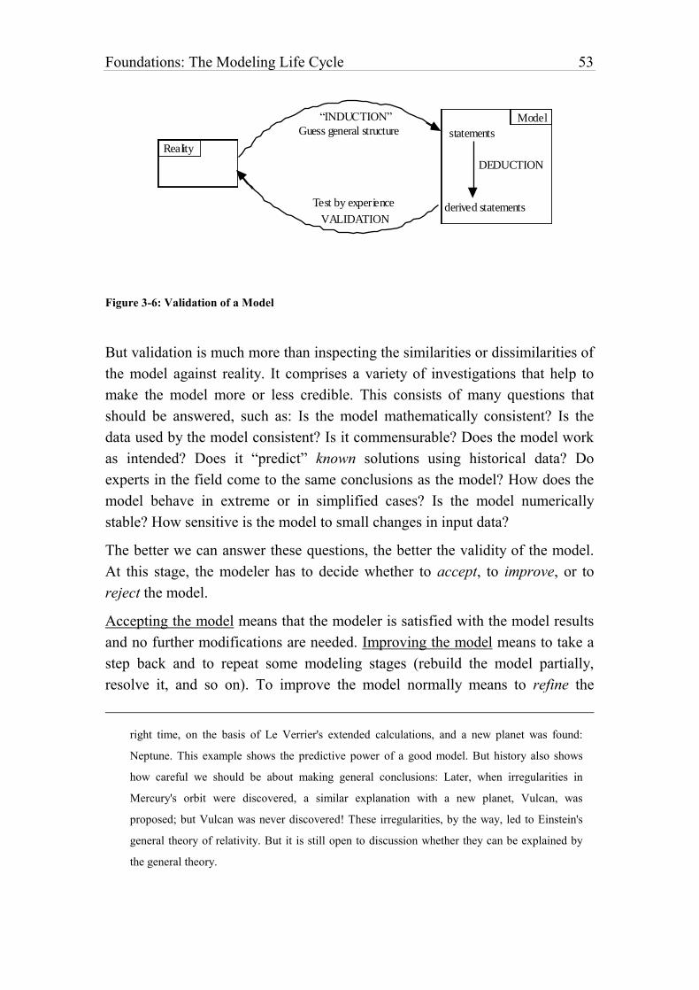
Foundations: The Modeling Life Cycle 53
Reality
Model
DEDUCTION
Test by experience
“INDUCTION”
Guess general structure
VALIDATION
statements
derived statements
Figure 3-6: Validation of a Model
But validation is much more than inspecting the similarities or dissimilarities of
the model against reality. It comprises a variety of investigations that help to
make the model more or less credible. This consists of many questions that
should be answered, such as: Is the model mathematically consistent? Is the
data used by the model consistent? Is it commensurable? Does the model work
as intended? Does it “predict” known solutions using historical data? Do
experts in the field come to the same conclusions as the model? How does the
model behave in extreme or in simplified cases? Is the model numerically
stable? How sensitive is the model to small changes in input data?
The better we can answer these questions, the better the validity of the model.
At this stage, the modeler has to decide whether to accept, to improve, or to
reject the model.
Accepting the model means that the modeler is satisfied with the model results
and no further modifications are needed. Improving the model means to take a
step back and to repeat some modeling stages (rebuild the model partially,
resolve it, and so on). To improve the model normally means to refine the
right time, on the basis of Le Verrier's extended calculations, and a new planet was found:
Neptune. This example shows the predictive power of a good model. But history also shows
how careful we should be about making general conclusions: Later, when irregularities in
Mercury's orbit were discovered, a similar explanation with a new planet, Vulcan, was
proposed; but Vulcan was never discovered! These irregularities, by the way, led to Einstein's
general theory of relativity. But it is still open to discussion whether they can be explained by
the general theory.
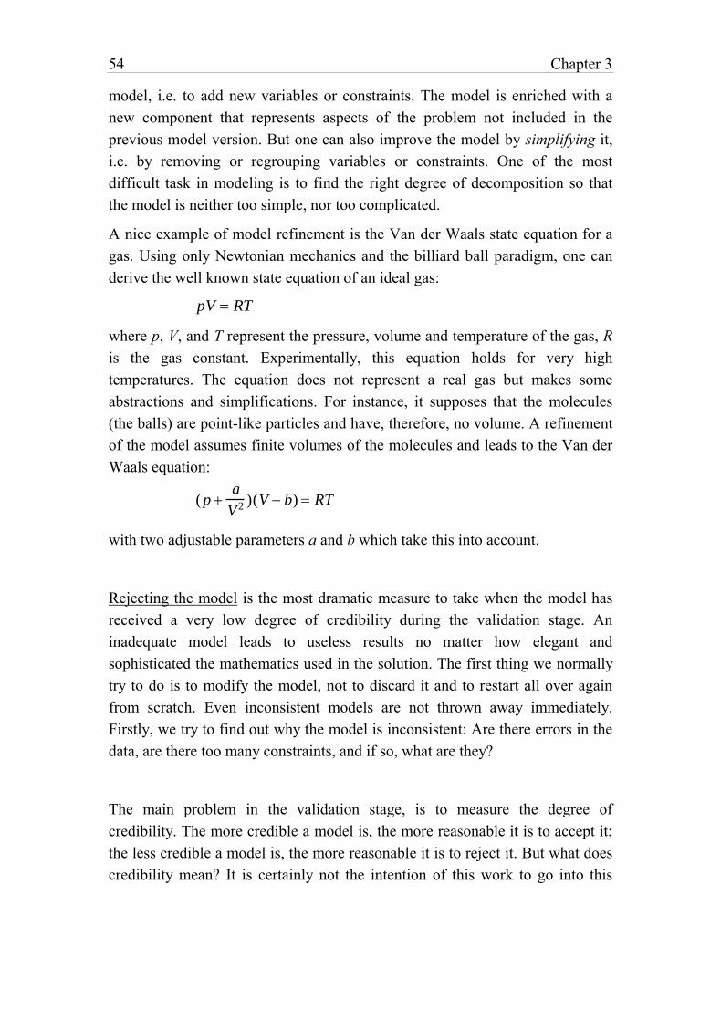
54 Chapter 3
model, i.e. to add new variables or constraints. The model is enriched with a
new component that represents aspects of the problem not included in the
previous model version. But one can also improve the model by simplifying it,
i.e. by removing or regrouping variables or constraints. One of the most
difficult task in modeling is to find the right degree of decomposition so that
the model is neither too simple, nor too complicated.
A nice example of model refinement is the Van der Waals state equation for a
gas. Using only Newtonian mechanics and the billiard ball paradigm, one can
derive the well known state equation of an ideal gas:
pV RT
where p, V, and T represent the pressure, volume and temperature of the gas, R
is the gas constant. Experimentally, this equation holds for very high
temperatures. The equation does not represent a real gas but makes some
abstractions and simplifications. For instance, it supposes that the molecules
(the balls) are point-like particles and have, therefore, no volume. A refinement
of the model assumes finite volumes of the molecules and leads to the Van der
Waals equation:
( p a
V2 )(V b) RT
with two adjustable parameters a and b which take this into account.
Rejecting the model is the most dramatic measure to take when the model has
received a very low degree of credibility during the validation stage. An
inadequate model leads to useless results no matter how elegant and
sophisticated the mathematics used in the solution. The first thing we normally
try to do is to modify the model, not to discard it and to restart all over again
from scratch. Even inconsistent models are not thrown away immediately.
Firstly, we try to find out why the model is inconsistent: Are there errors in the
data, are there too many constraints, and if so, what are they?
The main problem in the validation stage, is to measure the degree of
credibility. The more credible a model is, the more reasonable it is to accept it;
the less credible a model is, the more reasonable it is to reject it. But what does
credibility mean? It is certainly not the intention of this work to go into this
Foundations: The Modeling Life Cycle 55
question in any depth. Only a few hints are given. Since we are interested in
modeling tools implementation on a computer that supports the whole life cycle
of a model, the question is answered from a pragmatic point of view.
First of all, credibility – and hence validity – is not binary: a model is not
simply credible or incredible, valid or invalid. The degrees of credibility can be
represented by a continuous function. The more tests and checks the model
passes, the higher the degree of credibility. These checks comprise
– Internal consistency of the model:
– Logical consistency: is the model logically consistent?
– Data type consistency: is the data used type-consistent?
– Unit type consistency: is the data in the expressions commensurable?
– User defined data checking: does the data satisfy imposed conditions?
– Simplicity considerations: is the model as simple as possible?
– Solver behaviour checks:
– Numerical stability: is the model well-conditioned?
– Solvability: is the model solvable?
– Sensitivity analysis: how sensitive is the model to data changes?
– Correspondence checks (does the model correspond to reality?)
– Checking by using simplified data
– Checking by using random data test beds
– Checking by using verified data
– Checking by using experimental data
– Checking by simplifying the model
– Check the limitations of the model.
The list is not exhaustive. Now what happens if a model fails a validity test? Do
we throw it away? In reality, failures in validity tests happen all the time.
Normally, the model is changed and the tests are repeated. This process is
repeated until the model passes them. Certainly, the model must be at least
56 Chapter 3
consistent. For some correspondence checks, on the other hand, there is another
way to validate a model: by changing the validity test bed: If the model fails a
test, it may also be excluded for all future validity testing, and we may say that
the model is not applicable in this test case. “Playing around” with the model
sometimes quickly reveals whether it is useful or not. Furthermore, if the
model's vocabulary stimulates others undiscovered aspects of the problem or
guides the research to similar problems, then the model might be reasonably
good. If, however, the vocabulary is “sticky” or artificial then the model is
probably not very useful. A small classical example, the 3-jug problem, from
artificial intelligence will explain what is meant by these remarks.
Example 3-3: The 3-jug Problem
The 3-jug problem is as follows: There are three jugs with capacities of 8, 5,
and 3 liters. The 8-liter jug is full of water, whereas the others are empty. Find a
sequence for pouring the water from one jug to another such that the end result
is to have 4 liters in the 8-liter jug and the other 4 liters in the 5-liter jug. When
pouring the water from a jug A into another jug B, either jug A must be emptied
or B must be filled (Figure 3-7).
initial state goal
8 5 3 8 5 3
Figure 3-7: The 3-jug Problem
A good model for this problem is to map each possible state of the problem into
a triple (x, y, z) such that x {0K 8}, y{0K 5}, z {0K 3}. The initial state
could now be modeled as (8,0,0) and the goal state as (4,4,0). This initial idea
(of mapping a state into a triple) leads us directly to calculate the number of all
possible states: there are 9*6*4 = 216. Since no water is lost or added, the sum
of the three numbers must be 8 ( x y z 8). This condition limits the number
of all possible states to 24, this can easily be checked by full enumeration. A
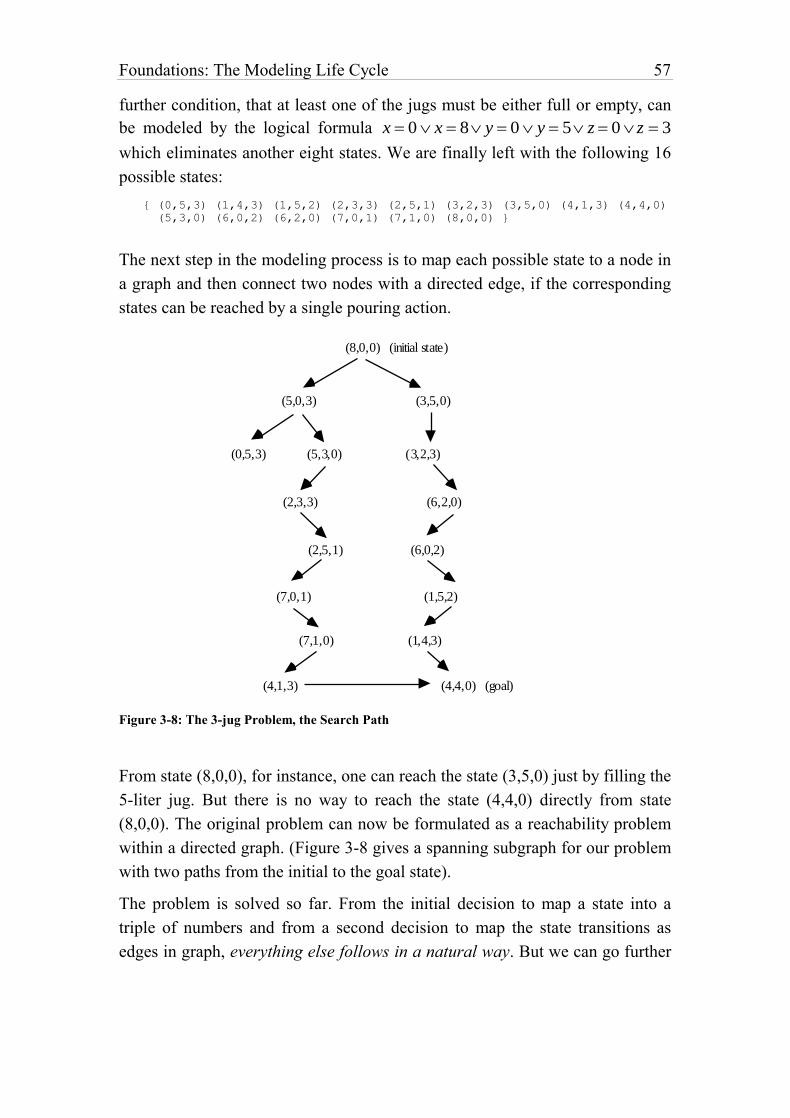
Foundations: The Modeling Life Cycle 57
further condition, that at least one of the jugs must be either full or empty, can
be modeled by the logical formula x 0 x 8 y 0 y 5 z 0 z 3
which eliminates another eight states. We are finally left with the following 16
possible states:
{ (0,5,3) (1,4,3) (1,5,2) (2,3,3) (2,5,1) (3,2,3) (3,5,0) (4,1,3) (4,4,0)
(5,3,0) (6,0,2) (6,2,0) (7,0,1) (7,1,0) (8,0,0) }
The next step in the modeling process is to map each possible state to a node in
a graph and then connect two nodes with a directed edge, if the corresponding
states can be reached by a single pouring action.
(8,0,0) (initial state)
(5,0,3) (3,5,0)
(0,5,3) (5,3,0) (3,2,3)
(2,3,3) (6,2,0)
(2,5,1) (6,0,2)
(7,0,1) (1,5,2)
(7,1,0) (1,4,3)
(4,1,3) (4,4,0) (goal)
Figure 3-8: The 3-jug Problem, the Search Path
From state (8,0,0), for instance, one can reach the state (3,5,0) just by filling the
5-liter jug. But there is no way to reach the state (4,4,0) directly from state
(8,0,0). The original problem can now be formulated as a reachability problem
within a directed graph. (Figure 3-8 gives a spanning subgraph for our problem
with two paths from the initial to the goal state).
The problem is solved so far. From the initial decision to map a state into a
triple of numbers and from a second decision to map the state transitions as
edges in graph, everything else follows in a natural way. But we can go further
58 Chapter 3
and play around with the model. For example, we may vary the initial state or
the goal state. Or we may change the capacities of the jugs. Of course, the last
variation leads to different state spaces, but the procedures are essentially the
same. Or we could take a different number of jugs: what about ten jugs with
given capacities! Again the model is still essentially the same. The model is
good, because the vocabulary used leads to the discovery of many variations of
the initial problem in a natural way. ¤
The jug example suggests that building good models is easy, but in general this
is not true. Building good models is difficult. The success of the 3-jug problem
depended on the two ingenious ideas of mapping the state space into a triple of
numbers and mapping each state into a node of a directed graph. It is quite
common to go through stages 1–3 and then to find at stage 4 that the results are
not useful for the original problem. In which case, we normally can assume that
the computations in phase 3 were correct and we have to revise the model at
steps 1 and 2.
The model building process does not take place in a vacuum. In an industrial
organization, many pressures are exercised on the model builder(s); many goals
and objectives coexist, and conflicts are unavoidable. The verification process
must take this into account.
Going through the mentioned checking list will allow us to emphasize several
points:
3.4.1. Logical Consistency
Logical consistency is said to be a necessary condition that every model must
fulfil. This is underpinned by the somewhat childish34 notion that anything
34 “... Solche Betrachtungen werden gewöhnlich mit dem kindischen (childish TH) Hinweis
kritisiert, aus einem Widerspruch folge jede beliebige Aussage. Das stimmt – aber nur in den
stark vereinfachten Modellen, die unsere Logiker entwickelt haben.“ Feyerabend P., [1986],
Wider den Methodenzwang, shurkamp, Frankfurt a.M., p. 22. Imre Lakatos, a Hungarian
philosopher of science teaching at LSE, (1922–1974), coined the famous statement that “it may
Foundations: The Modeling Life Cycle 59
follows from an inconsistent statement (“ex falso quodlibet”). This is trivially
true. But in a practical model building process, inconsistencies arise in a natural
way. It is rare, except for the most simplistic mathematical models, that the first
attempt leads to models free of contradictions. For many problem classes, it is,
at least, as difficult – from an algorithmic complexity point of view – to check
for consistency as it is to solve a consistent model. There are many possibilities
and techniques to handle inconsistent models in practice. We will see in the
next chapter how to treat inconsistency in models. Of course, ultimately the
modeler must eliminate any inconsistencies. But this elimination process often
leads to a better understanding of the underlying problem itself.
Logical inconsistency is often an indication (or symptom) of the fact that
something went wrong in the modeling building process (wrong data,
inadequate constraints, etc.). Such errors clearly need to be eliminated. But
sometimes there are other reasons why a model is inconsistent, such as
conflicting constraints or goals, uncertainty in the data, or “soft” constraints
that have been erroneously coded as “hard” ones. In a budget planning context,
for instance, one would restrict the budget to about 3 million dollars, but not to
exactly 3 million. Since the mathematical model asks for some number, the
model could easily become infeasible because of this hard restriction.
3.4.2. Data Type Consistency
This issue has been discussed in detail and over many years by the
programming language community. Data type checking means to check the
domain membership of a value before it is assigned to a storage object in
computers. If the domain does not match with the domain (or a subdomain) of
the storage object, then the assignment must not take place, lest the memory
space be corrupted. The question is whether to undertake type checking at
compile- or at runtime. I could now renumerate the advantages and the
drawbacks of strong-type checking, but these arguments are well known. It is
rather my intention to emphasize the importance of type checking in the realm
of computer-based modeling. In this respect, modeling languages are submitted
to the same arguments as programming languages.
be rational to put the inconsistency into some temporary, ad hoc quarantine, and carry on with
the positive heuristics of the programme.” [quoted by Hartmann S. in: Herfel al. 1995].
60 Chapter 3
3.4.3. Unit Type Consistency
Another issue is to check whether the data in expressions are commensurable.
This sort of checking has been, surprisingly, neglected in computer-based
modeling. I found only one reference in the literature [Bradley/Clemence
1987]. Several papers, however, have been written to discuss units in
programming languages. They are [Baldwin 1987], [Dreiheller al. 1986],
[House 1983], [Karr al. 1978], [Mankin 1987], and [Männer 1986]. But little
has been implemented.
In a modeling context, dimensional checking is of utmost importance, since
most quantities are measured in units (dollar, hour, meter, etc.). Experiences in
teaching operations research reveal that one of the most frequent errors made
by students when modeling is inconsistency in the units of measurement. In
physics and other scientific applications, as well as technical and commercial
ones, using units of measure in calculating has a long tradition. It increases both
the reliability and the readability of calculations.
A nice example comes from dynamic systems [Mesterton 1989, p. 52]:
Consider the pollution of a lake over time. Let V be the volume of the lake, x(t)
the concentration of pollutants at time t, r the rate at which the water flows out
of the lake, and P the quantity of new pollutants entering per time unit. Then
we have:
Rate of change of pollutants = pollutants inflow – pollutants outflow:
dV x(t)
dt P r x(t) (1)
Let us see whether this formula is correct from a dimensional point of view. On
the left hand side, we have the dimension [V ][x] / [t ] m3
g
m3 / s g / s . On
the right hand side, we have: [P][r][x]gs
m3
s g
m3 gs
gs g / s . The
expressions are commensurable which suggests that they are correct.
Now the solution of (1) is:
x(t) P
r x(0)
P
r
e
rt /V (2)
Again we can check the validity from the dimensional point of view. The
dimension of the left hand side is: [ x] g
m3 ; the right side also gives
[P][r] ([x]
[P][r] ) e
[r ][t ]/[V ]
g/ s
m3 /s (
g
m3 g /s
m3 / s) e
m3 /ss /m3
g
m3 .e1
g
m3 .
Foundations: The Modeling Life Cycle 61
Again the two expressions are commensurable.
The benefits of unit type checking are obvious: One can keep track of the units
for all entities in the models, more errors can be removed and, therefore,
reliability can be enhanced. Moreover, units can also be used to scale the data
automatically. A more complete account on units and their use in modeling
languages can be found in [Hürlimann 1991].
3.4.4. User Defined Data Checking
Sometimes it is essential that data satisfy certain conditions. Examples are
lower and upper bounds of parameters or variables. One could regard this as
extended type checking, but the conditions could be arbitrary expressions.
Another example are stochastic matrices of Markov chains. These matrices
must satisfy the condition that all row sums amount to one. In computer-based
modeling these conditions can and should be checked automatically. Data and
parameters are frequently submitted to changes, it is, therefore, extremely
important to check their integrity in a systematic manner. One way of doing
this, is to define a set of conditions on the data and parameters in the form of
expressions and to add them to the model. They must be an integral part of the
model itself. This permits a regular and periodic check for data errors.
3.4.5. Simplicity Considerations
These considerations have already been expounded. The principle of Ockham's
Razor also applies to modeling. To paraphrase Einstein: The model should be
as simple as possible, but not simpler. It should contain the smallest possible
number of variables, constraints and data. Bigger models tend to be more
difficult to solve. In general, however, it is difficult to decide whether a set of
constraints are the smallest possible. Even in linear programming, one has to
solve the model completely in order to see which constraints are redundant.
3.4.6. Solvability Checking
Solvability has two aspects: As noted before, in mathematics one can formulate
models that cannot possibly be solved on any computer, even theoretically,
because the problem is undecidable. Such models do not make sense and
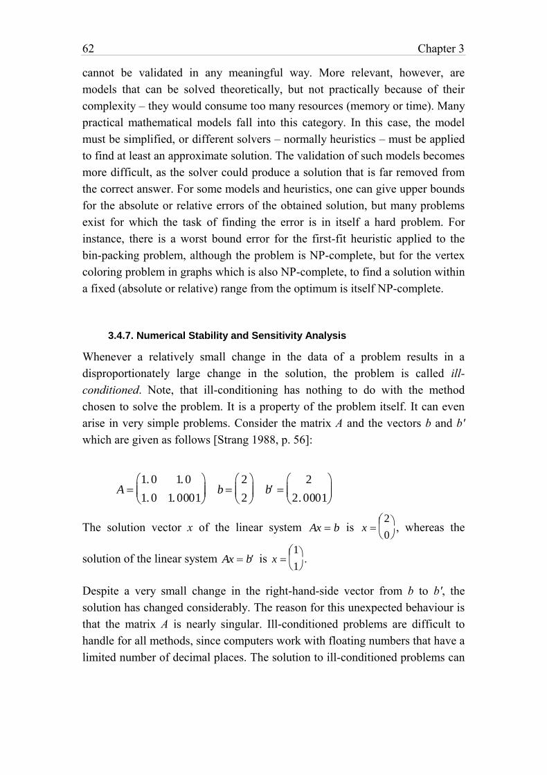
62 Chapter 3
cannot be validated in any meaningful way. More relevant, however, are
models that can be solved theoretically, but not practically because of their
complexity – they would consume too many resources (memory or time). Many
practical mathematical models fall into this category. In this case, the model
must be simplified, or different solvers – normally heuristics – must be applied
to find at least an approximate solution. The validation of such models becomes
more difficult, as the solver could produce a solution that is far removed from
the correct answer. For some models and heuristics, one can give upper bounds
for the absolute or relative errors of the obtained solution, but many problems
exist for which the task of finding the error is in itself a hard problem. For
instance, there is a worst bound error for the first-fit heuristic applied to the
bin-packing problem, although the problem is NP-complete, but for the vertex
coloring problem in graphs which is also NP-complete, to find a solution within
a fixed (absolute or relative) range from the optimum is itself NP-complete.
3.4.7. Numerical Stability and Sensitivity Analysis
Whenever a relatively small change in the data of a problem results in a
disproportionately large change in the solution, the problem is called ill-
conditioned. Note, that ill-conditioning has nothing to do with the method
chosen to solve the problem. It is a property of the problem itself. It can even
arise in very simple problems. Consider the matrix A and the vectors b and b'
which are given as follows [Strang 1988, p. 56]:
A 1. 0 1. 0
1. 0 1. 0001
b
2
2
b
2
2. 0001
The solution vector x of the linear system Ax b is x 2
0
, whereas the
solution of the linear system Ax b is x 1
1
.
Despite a very small change in the right-hand-side vector from b to b', the
solution has changed considerably. The reason for this unexpected behaviour is
that the matrix A is nearly singular. Ill-conditioned problems are difficult to
handle for all methods, since computers work with floating numbers that have a
limited number of decimal places. The solution to ill-conditioned problems can
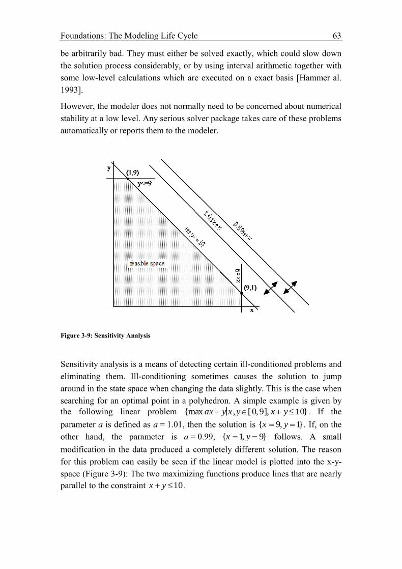
Foundations: The Modeling Life Cycle 63
be arbitrarily bad. They must either be solved exactly, which could slow down
the solution process considerably, or by using interval arithmetic together with
some low-level calculations which are executed on a exact basis [Hammer al.
1993].
However, the modeler does not normally need to be concerned about numerical
stability at a low level. Any serious solver package takes care of these problems
automatically or reports them to the modeler.
Figure 3-9: Sensitivity Analysis
Sensitivity analysis is a means of detecting certain ill-conditioned problems and
eliminating them. Ill-conditioning sometimes causes the solution to jump
around in the state space when changing the data slightly. This is the case when
searching for an optimal point in a polyhedron. A simple example is given by
the following linear problem {max ax y x ,y[0,9], x y10}. If the
parameter a is defined as a = 1.01, then the solution is {x 9, y 1}. If, on the
other hand, the parameter is a = 0.99, {x 1, y 9} follows. A small
modification in the data produced a completely different solution. The reason
for this problem can easily be seen if the linear model is plotted into the x-y-
space (Figure 3-9): The two maximizing functions produce lines that are nearly
parallel to the constraint x y 10 .
64 Chapter 3
Such model behaviour is undesirable at least from a practical point of view.
Unfortunately, it occurs quite frequently. The modeler needs to avoid it.
Sometimes the hardest part in model building is to find additional constraints so
that the model remains reasonably stable when varying the data sets.
3.4.8. Checking the Correspondence
A model, even after having passed all ’internal’ tests, could still be useless if its
structure does not correspond in relevant way to the “real” problem. The model
results should not clash with that empirical data which had been previously
observed or which had been derived from experience. Whether the amount of
discrepancy between the model results and the observed data is still acceptable
depends upon the context and on the beliefs, as well as on the theoretical
background, of the modeler or the model user. But there must be some
accordance as to some matching rules, although an absolute measure of validity
does not exist. “The appropriate form of quality assurance for a model depends
fundamentally on how the model is used, so any attempt to define a single
validation standard and procedure for all models in all uses will surely fail.”
[Hodges/Dewar 1992]. One has to keep in mind that the model is always no
more than an approximation of the problem.
There are many ways of checking the correspondence between reality and the
model. One is to use simplified data sets. For example, what happens, if the
learning rate in the learning model Lt1 U (1)Lt is zero? Then
nothing is learnt, nothing is forgotten, this is verified by the simplified model
Lt1 Lt . The model behaves as expected in this case. Another method is to
generate data randomly or in a systematic manner in order to observe whether
the model performs as expected. If the model does not respond as intended, this
is still no absolute criterion for rejecting it. Perhaps the modeler needs to
change her expectation! Established rules can hardly be given in this context.
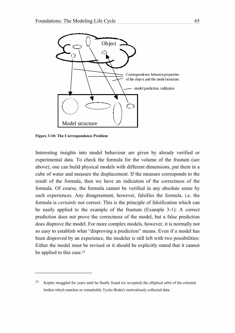
Foundations: The Modeling Life Cycle 65
Object
Model structure
Correspondence between properties
of the object and the model structure.
model prediction, validation
Figure 3-10: The Correspondence Problem
Interesting insights into model behaviour are given by already verified or
experimental data. To check the formula for the volume of the frustum (see
above), one can build physical models with different dimensions, put them in a
cube of water and measure the displacement. If the measure corresponds to the
result of the formula, then we have an indication of the correctness of the
formula. Of course, the formula cannot be verified in any absolute sense by
such experiences. Any disagreement, however, falsifies the formula, i.e. the
formula is certainly not correct. This is the principle of falsification which can
be easily applied to the example of the frustum (Example 3-1): A correct
prediction does not prove the correctness of the model, but a false prediction
does disprove the model. For more complex models, however, it is normally not
so easy to establish what “disproving a prediction” means. Even if a model has
been disproved by an experience, the modeler is still left with two possibilities:
Either the model must be revised or it should be explicitly stated that it cannot
be applied to this case.35
35 Kepler struggled for years until he finally found (or accepted) the elliptical orbit of the celestial
bodies which matches so remarkably Tycho Brahe's meticulously collected data.
66 Chapter 3
Simplifying the model structure can help to gain familiarity with both the model
and the problem. As a rule, one should begin with simplified versions of the
model. They assist the modeler in concentrating on the essentials and avoid
bringing in too much complexity at the beginning.
Finally, all cases for which the model did not pass the verification checks,
should be reported in detail. There is no perfect model. Every model has its
limitations. Again, these limitations cannot be whitewashed by a more
sophisticated degree of formalism. Often it is better to have several simple and
poor models with a restricted application range than to maintain a complex and
sophisticated model that, at first, seems to cover every case.
3.5. Stage 5: Writing a Report
After the model has been accepted, the results have to be reported. They can be
displayed in tables, graphs, response surfaces, charts, diagrams, or simply in
texts. Generally, it is not sufficient merely to give the solver output, this must
be edited and processed. The values and data must be regrouped, compressed,
expanded, and often further calculations are needed to obtain the results in the
form the modeler wants. This is especially important for bigger models. When
the model contains hundreds or thousands of variables, their values, together
with other data, must be displayed in a comprehensive way. Writing good
reports is a time-consuming and tedious task and requires considerable
maintenance. But most of the work could be automated if the right tools were
available.
Today, it is quite common that the modeler must write a program to process the
output of the solver – in the same way that she must write a program to produce
the solver input. Such programs tend to be error-prone and difficult to maintain,
because the dimension of the data tables and the variables can easily change.
Therefore reports have to be defined in a very flexible way. A tool that could
produce a report automatically starting from a high level declarative
specification is called a report generator, and the specification is labelled a
report generator language.
Advanced report generators have already been presented in the seventies when
big LPs (linear programs) were solved in practice [Palmer 1984]. They were
entirely data driven and based mainly on filtering data via character matching
Foundations: The Modeling Life Cycle 67
of column and row names. But even today, report generators are not very
common. Two prototypes have been presented in [Gerten/Jacob 1989] and
[Stöckle/Polster 1980].
The main features of a report generator are: filtering or joining data from larger
data sets, recombining the data using numerical or string operations, and
representing them in a predefined well laid out form using mask definitions.
Filtering data means selecting or projecting data from one or several data tables
in different ways, normally by defining a condition. Joining data is to build the
Cartesian product on tables. Select, project and join are three well-defined
operations in database theory. Recombining data means to derive values from
data by automatic computation (building the average, the sum, etc.).
Today, most of these tasks can be done using database systems. But the
modeler still needs to write code to import the data in the right order into the
database system. Additionally, specific reports are difficult to design in
databases. A particular standalone report generator language would be more
appropriate to do the job. This is especially true where the model is big, but
where only a few data are implied. Under these circumstances, it would not be
worthwhile to design a database.
The five stages in modeling have now been exposed briefly from the point of
view of modeling tool implementation. In the next section, two models and
their modeling stages are presented.
3.6. Two Case Studies
To highlight the different stages in a model building process, we expose two
problems: The first is the easy problem of cooling a physical object, and the
second is a simplistic production model.
Example 3-4: Cooling a Thermometer
A thermometer, reading T0 degrees, is placed outdoors where the temperature is
m degree. How does the display of the thermometer change over time? The
formulation step is straightforward when we apply Newton's law of cooling:
68 Chapter 3
When an object of any temperature T is placed in a surrounding medium at
constant temperature m, then T changes at a rate which is proportional to the
difference of T–m. This leads us to the function dT / dt k(T m) . The
formulation step is now complete. We could solve this simple differential
equation by hand, but an alternative would be to use a solver. We use
Mathematica. So the next step is to put the problem into a statement
Mathematica can understand. The correct syntax for our problem is:
DSolve[T'[t] == k*(T[t]-m),T[t],t]
The solving step consists now of a single keystroke that lets Mathematica
execute the statement. It immediately replies by:
k t
{{T[t] -> m + E C[1]}}
which is the solution to our problem in symbolic form when replacing C[1] by
T0–m.
How do we validate the model? The model passes all consistency checks: it is
consistent, the data type of all parameters is numeric, the expressions are
commensurable as can be verified, and the model is simple. No numerical
stability checks are necessary since the model is solved symbolically. But the
function will produce an overflow very quickly if k > 1, since it grows
exponentially without limit. This is a limitation to our model: k must be smaller
than one. Normally it is chosen to be negative. We have to add this condition
explicitly to the model. Does the solution correspond to some real problem? To
answer this question, we first do some simple checks: How does the
temperature T change, if m = T0? In this case, T(t) should stay constant at m at
any time t. This is indeed true, since C[1] is zero. What about m > T0 (m < T0)?
Then T(t) is a monotonic increasing (decreasing) function, as expected. How
does the function behave when t? Then the exponential term disappears, i.e.
as time goes on the temperature of the thermometer display approaches m, as
expected. To check for concrete examples, we need to replace the symbolic
parameters k, m, and T0 by numeric data, to measure the temperature at different
times t, and to compare the results with the numerical output of the model. If
they are close enough, we can accept the model. The report of a model instance
consists simply of a graph showing the progress of the temperature.
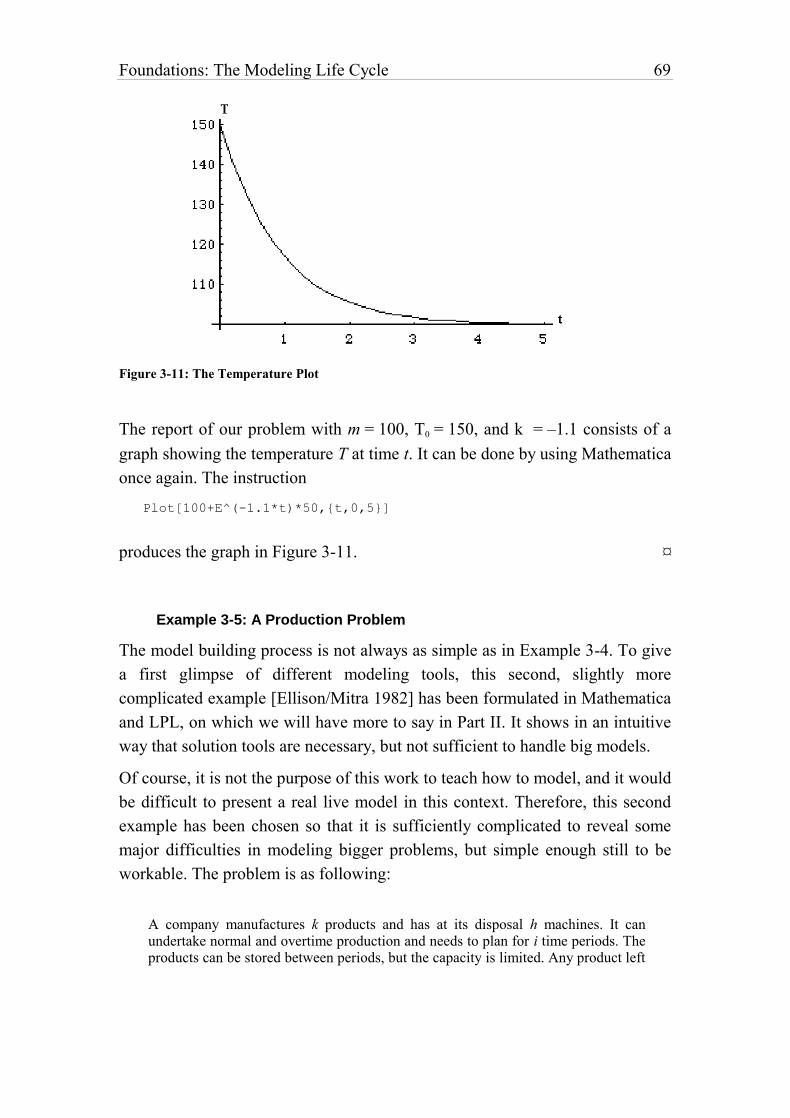
Foundations: The Modeling Life Cycle 69
Figure 3-11: The Temperature Plot
The report of our problem with m = 100, T0 = 150, and k = –1.1 consists of a
graph showing the temperature T at time t. It can be done by using Mathematica
once again. The instruction
Plot[100+E^(-1.1*t)*50,{t,0,5}]
produces the graph in Figure 3-11. ¤
Example 3-5: A Production Problem
The model building process is not always as simple as in Example 3-4. To give
a first glimpse of different modeling tools, this second, slightly more
complicated example [Ellison/Mitra 1982] has been formulated in Mathematica
and LPL, on which we will have more to say in Part II. It shows in an intuitive
way that solution tools are necessary, but not sufficient to handle big models.
Of course, it is not the purpose of this work to teach how to model, and it would
be difficult to present a real live model in this context. Therefore, this second
example has been chosen so that it is sufficiently complicated to reveal some
major difficulties in modeling bigger problems, but simple enough still to be
workable. The problem is as following:
A company manufactures k products and has at its disposal h machines. It can undertake normal and overtime production and needs to plan for i time periods. The products can be stored between periods, but the capacity is limited. Any product left
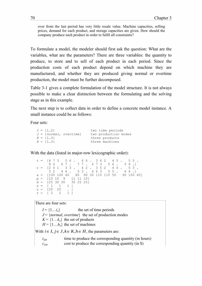
70 Chapter 3
over from the last period has very little resale value. Machine capacities, selling prices, demand for each product, and storage capacities are given. How should the company produce each product in order to fulfil all constraints?
To formulate a model, the modeler should first ask the question: What are the
variables, what are the parameters? There are three variables: the quantity to
produce, to store and to sell of each product in each period. Since the
production costs of each product depend on which machine they are
manufactured, and whether they are produced giving normal or overtime
production, the model must be further decomposed.
Table 3-1 gives a complete formulation of the model structure. It is not always
possible to make a clear distinction between the formulating and the solving
stage as in this example.
The next step is to collect data in order to define a concrete model instance. A
small instance could be as follows:
Four sets:
I = {1…2} two time periods
J = {normal, overtime} two production modes
K = {1…3} three products
H = {1…3} three machines
With the data (listed in major-row lexicographic order):
t = [4 7 3 5 6 . 6 6 . 3 6 2 4 5 . 5 5 .
8 4 6 7 . 7 7 . 4 7 3 5 6 . 5 6 .]
c = [2 4 1 3 3 . 4 2 . 3 5 2 4 4 . 5 3 .
5 2 4 4 . 5 3 . 4 6 3 5 5 . 6 4 .]
a = [100 100 40 80 90 30 110 110 50 90 100 40]
p = [10 10 9 11 11 10]
d = [25 30 30 30 25 25]
s = [ 1 1 1 ]
u = [20 20 . ]
r = [ 2 2 1 ]
There are four sets:
I = {1…in} the set of time periods
J = {normal, overtime} the set of production modes
K = {1…kn} the set of products
H = {1…hn} the set of machines
With i I, jJ,kK,hH , the parameters are:
tijkh time to produce the corresponding quantity (in hours)
cijkh cost to produce the corresponding quantity (in $)
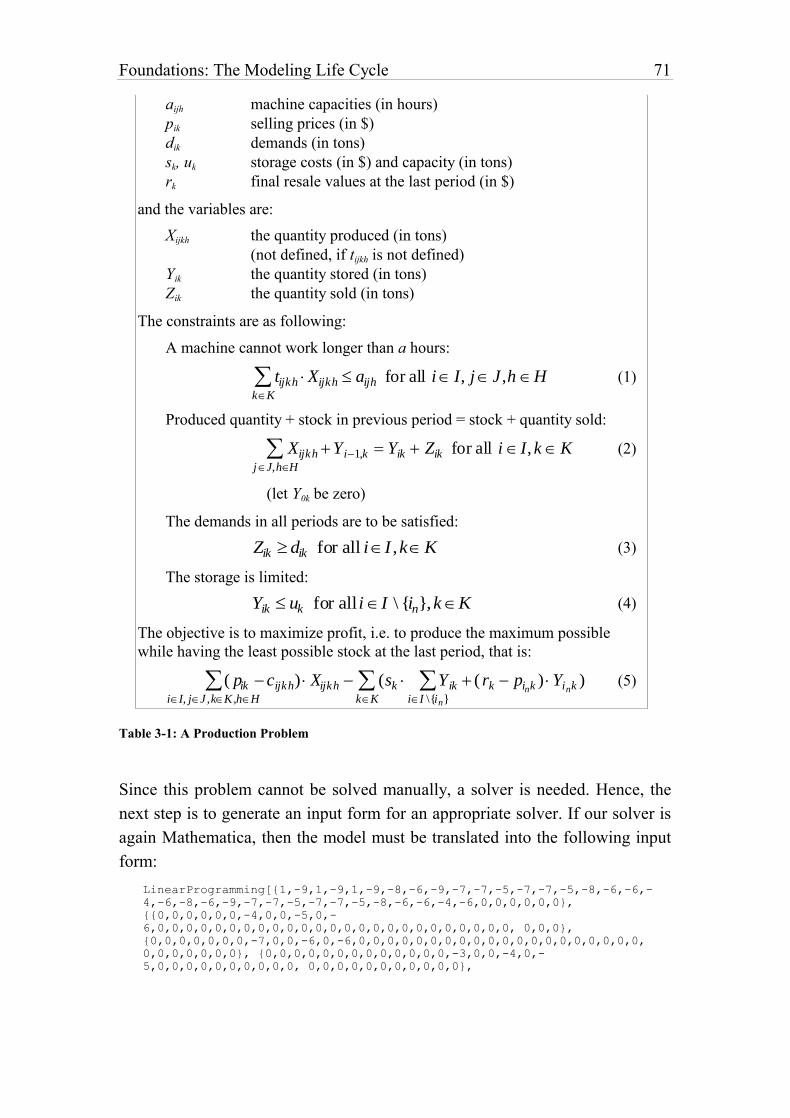
Foundations: The Modeling Life Cycle 71
aijh machine capacities (in hours)
pik selling prices (in $)
dik demands (in tons)
sk, uk storage costs (in $) and capacity (in tons)
rk final resale values at the last period (in $)
and the variables are:
Xijkh the quantity produced (in tons)
(not defined, if tijkh is not defined)
Yik the quantity stored (in tons)
Zik the quantity sold (in tons)
The constraints are as following:
A machine cannot work longer than a hours:
tijkh XijkhkK
aijh for all i I, jJ ,h H (1)
Produced quantity + stock in previous period = stock + quantity sold:
XijkhjJ,hH
Yi1,k Yik Zik for all i I, k K (2)
(let Y0k be zero)
The demands in all periods are to be satisfied:
Zik dik for all iI ,kK (3)
The storage is limited:
Yik uk for all i I \ {in},k K (4)
The objective is to maximize profit, i.e. to produce the maximum possible
while having the least possible stock at the last period, that is:
( pik cijkh) XijkhiI, jJ ,kK ,hH
(sk YikiI \{in}
( rk pink ) Yink )kK
(5)
Table 3-1: A Production Problem
Since this problem cannot be solved manually, a solver is needed. Hence, the
next step is to generate an input form for an appropriate solver. If our solver is
again Mathematica, then the model must be translated into the following input
form:
LinearProgramming[{1,-9,1,-9,1,-9,-8,-6,-9,-7,-7,-5,-7,-7,-5,-8,-6,-6,-
4,-6,-8,-6,-9,-7,-7,-5,-7,-7,-5,-8,-6,-6,-4,-6,0,0,0,0,0,0},
{{0,0,0,0,0,0,-4,0,0,-5,0,-
6,0,0,0,0,0,0,0,0,0,0,0,0,0,0,0,0,0,0,0,0,0,0,0,0,0, 0,0,0},
{0,0,0,0,0,0,0,-7,0,0,-6,0,-6,0,0,0,0,0,0,0,0,0,0,0,0,0,0,0,0,0,0,0,0,
0,0,0,0,0,0,0}, {0,0,0,0,0,0,0,0,0,0,0,0,0,-3,0,0,-4,0,-
5,0,0,0,0,0,0,0,0,0,0, 0,0,0,0,0,0,0,0,0,0,0},
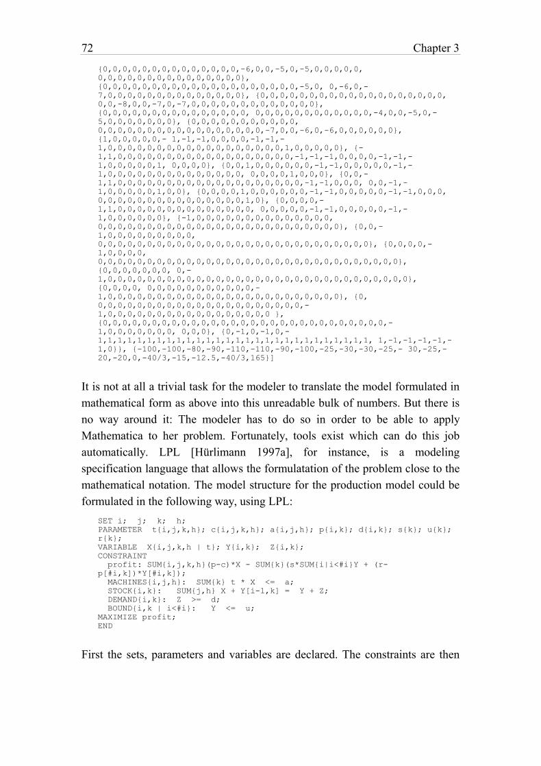
72 Chapter 3
{0,0,0,0,0,0,0,0,0,0,0,0,0,0,-6,0,0,-5,0,-5,0,0,0,0,0,
0,0,0,0,0,0,0,0,0,0,0,0,0,0,0},
{0,0,0,0,0,0,0,0,0,0,0,0,0,0,0,0,0,0,0,0,-5,0, 0,-6,0,-
7,0,0,0,0,0,0,0,0,0,0,0,0,0,0}, {0,0,0,0,0,0,0,0,0,0,0,0,0,0,0,0,0,0,0,
0,0,-8,0,0,-7,0,-7,0,0,0,0,0,0,0,0,0,0,0,0,0},
{0,0,0,0,0,0,0,0,0,0,0,0,0,0,0, 0,0,0,0,0,0,0,0,0,0,0,0,-4,0,0,-5,0,-
5,0,0,0,0,0,0,0}, {0,0,0,0,0,0,0,0,0,0,0,
0,0,0,0,0,0,0,0,0,0,0,0,0,0,0,0,0,-7,0,0,-6,0,-6,0,0,0,0,0,0},
{1,0,0,0,0,0,- 1,-1,-1,0,0,0,0,-1,-1,-
1,0,0,0,0,0,0,0,0,0,0,0,0,0,0,0,0,0,0,1,0,0,0,0,0}, {-
1,1,0,0,0,0,0,0,0,0,0,0,0,0,0,0,0,0,0,0,-1,-1,-1,0,0,0,0,-1,-1,-
1,0,0,0,0,0,1, 0,0,0,0}, {0,0,1,0,0,0,0,0,0,-1,-1,0,0,0,0,0,-1,-
1,0,0,0,0,0,0,0,0,0,0,0,0,0,0, 0,0,0,0,1,0,0,0}, {0,0,-
1,1,0,0,0,0,0,0,0,0,0,0,0,0,0,0,0,0,0,0,0,-1,-1,0,0,0, 0,0,-1,-
1,0,0,0,0,0,1,0,0}, {0,0,0,0,1,0,0,0,0,0,0,-1,-1,0,0,0,0,0,-1,-1,0,0,0,
0,0,0,0,0,0,0,0,0,0,0,0,0,0,0,1,0}, {0,0,0,0,-
1,1,0,0,0,0,0,0,0,0,0,0,0,0,0,0, 0,0,0,0,0,-1,-1,0,0,0,0,0,-1,-
1,0,0,0,0,0,0}, {-1,0,0,0,0,0,0,0,0,0,0,0,0,0,0,
0,0,0,0,0,0,0,0,0,0,0,0,0,0,0,0,0,0,0,0,0,0,0,0,0}, {0,0,-
1,0,0,0,0,0,0,0,0,0,
0,0,0,0,0,0,0,0,0,0,0,0,0,0,0,0,0,0,0,0,0,0,0,0,0,0,0,0}, {0,0,0,0,-
1,0,0,0,0,
0,0,0,0,0,0,0,0,0,0,0,0,0,0,0,0,0,0,0,0,0,0,0,0,0,0,0,0,0,0,0},
{0,0,0,0,0,0,0, 0,-
1,0,0,0,0,0,0,0,0,0,0,0,0,0,0,0,0,0,0,0,0,0,0,0,0,0,0,0,0,0,0,0},
{0,0,0,0, 0,0,0,0,0,0,0,0,0,0,0,-
1,0,0,0,0,0,0,0,0,0,0,0,0,0,0,0,0,0,0,0,0,0,0,0,0}, {0,
0,0,0,0,0,0,0,0,0,0,0,0,0,0,0,0,0,0,0,0,0,-
1,0,0,0,0,0,0,0,0,0,0,0,0,0,0,0,0,0 },
{0,0,0,0,0,0,0,0,0,0,0,0,0,0,0,0,0,0,0,0,0,0,0,0,0,0,0,0,0,-
1,0,0,0,0,0,0,0, 0,0,0}, {0,-1,0,-1,0,-
1,1,1,1,1,1,1,1,1,1,1,1,1,1,1,1,1,1,1,1,1,1,1,1,1,1,1,1, 1,-1,-1,-1,-1,-
1,0}}, {-100,-100,-80,-90,-110,-110,-90,-100,-25,-30,-30,-25,- 30,-25,-
20,-20,0,-40/3,-15,-12.5,-40/3,165}]
It is not at all a trivial task for the modeler to translate the model formulated in
mathematical form as above into this unreadable bulk of numbers. But there is
no way around it: The modeler has to do so in order to be able to apply
Mathematica to her problem. Fortunately, tools exist which can do this job
automatically. LPL [Hürlimann 1997a], for instance, is a modeling
specification language that allows the formulatation of the problem close to the
mathematical notation. The model structure for the production model could be
formulated in the following way, using LPL:
SET i; j; k; h;
PARAMETER t{i,j,k,h}; c{i,j,k,h}; a{i,j,h}; p{i,k}; d{i,k}; s{k}; u{k};
r{k};
VARIABLE X{i,j,k,h | t}; Y{i,k}; Z{i,k};
CONSTRAINT
profit: SUM{i,j,k,h}(p-c)*X - SUM{k}(s*SUM{i|i<#i}Y + (r-
p[#i,k])*Y[#i,k]);
MACHINES{i,j,h}: SUM{k} t * X <= a;
STOCK{i,k}: SUM{j,h} X + Y[i-1,k] = Y + Z;
DEMAND{i,k}: Z >= d;
BOUND{i,k | i<#i}: Y <= u;
MAXIMIZE profit;
END
First the sets, parameters and variables are declared. The constraints are then
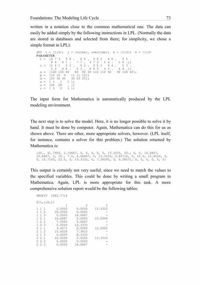
Foundations: The Modeling Life Cycle 73
written in a notation close to the common mathematical one. The data can
easily be added simply by the following instructions in LPL. (Normally the data
are stored in databases and selected from there; for simplicity, we chose a
simple format in LPL):
SET i = /1:2/; j = /normal, overtime/; k = /1:3/; h = /1:3/
PARAMETER t = [4 7 3 5 6 . 6 6 . 3 6 2 4 5 . 5 5 .
8 4 6 7 . 7 7 . 4 7 3 5 6 . 5 6 .];
c = [2 4 1 3 3 . 4 2 . 3 5 2 4 4 . 5 3 .
5 2 4 4 . 5 3 . 4 6 3 5 5 . 6 4 .];
a = [100 100 40 80 90 30 110 110 50 90 100 40];
p = [10 10 9 11 11 10];
d = [25 30 30 30 25 25];
s = [ 1 1 1 ];
u = [20 20 . ];
r = [ 2 2 1 ];
The input form for Mathematica is automatically produced by the LPL
modeling environment.
The next step is to solve the model. Here, it is no longer possible to solve it by
hand. It must be done by computer. Again, Mathematica can do this for us as
shown above. There are other, more appropriate solvers, however. (LPL itself,
for instance, contains a solver for this problem.) The solution returned by
Mathematica is:
{20., 41.7905, 2.16667, 0, 0, 0, 0, 0, 13.3333, 20., 0, 0, 16.6667,
16.6667, 0, 15., 7.5, 4.66667, 0, 13.3333, 3.45714, 0, 12.5, 15.4524, 0,
0, 15.7143, 22.5, 0, 13.3333, 0, 7.38095, 0, 9.28571, 0, 0, 0, 0, 0, 0}
This output is certainly not very useful, since we need to match the values to
the specified variables. This could be done by writing a small program in
Mathematica. Again, LPL is more appropriate for this task. A more
comprehensive solution report would be the following tables:
PROFIT 1842.7714
X{I,J,K,L}
1 2 3
1 1 1 0.0000 0.0000 13.3333
1 1 2 20.0000 0.0000 -
1 1 3 0.0000 16.6667 -
1 2 1 16.6667 0.0000 15.0000
1 2 2 7.5000 4.6667 -
1 2 3 0.0000 13.3333 -
2 1 1 3.4571 0.0000 12.5000
2 1 2 15.4524 7.3810 -
2 1 3 0.0000 8.3333 -
2 2 1 22.5000 0.0000 13.3333
2 2 2 0.0000 0.0000 -
2 2 3 0.0000 16.6667 -
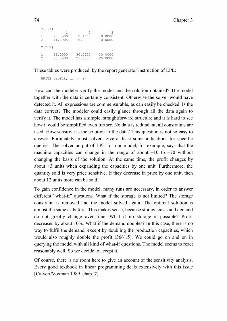
74 Chapter 3
Y{I,K}
1 2 3
1 20.0000 2.1667 0.0000
2 41.7905 0.0000 0.0000
Z{I,K}
1 2 3
1 25.0000 30.0000 30.0000
2 30.0000 25.0000 25.0000
These tables were produced by the report generator instruction of LPL:
WRITE profit; x; y; z;
How can the modeler verify the model and the solution obtained? The model
together with the data is certainly consistent. Otherwise the solver would have
detected it. All expressions are commensurable, as can easily be checked. Is the
data correct? The modeler could easily glance through all the data again to
verify it. The model has a simple, straightforward structure and it is hard to see
how it could be simplified even further. No data is redundant, all constraints are
used. How sensitive is the solution to the data? This question is not so easy to
answer. Fortunately, most solvers give at least some indications for specific
queries. The solver output of LPL for our model, for example, says that the
machine capacities can change in the range of about –10 to +70 without
changing the basis of the solution. At the same time, the profit changes by
about +3 units when expanding the capacities by one unit. Furthermore, the
quantity sold is very price sensitive. If they decrease in price by one unit, then
about 12 units more can be sold.
To gain confidence in the model, many runs are necessary, in order to answer
different “what-if” questions. What if the storage is not limited? The storage
constraint is removed and the model solved again. The optimal solution is
almost the same as before. This makes sense, because storage costs and demand
do not greatly change over time. What if no storage is possible? Profit
decreases by about 10%. What if the demand doubles? In this case, there is no
way to fulfil the demand, except by doubling the production capacities, which
would also roughly double the profit (3661.5). We could go on and on in
querying the model with all kind of what-if questions. The model seems to react
reasonably well. So we decide to accept it.
Of course, there is no room here to give an account of the sensitivity analysis.
Every good textbook in linear programming deals extensively with this issue
[Calvert/Voxman 1989, chap. 7].
Foundations: The Modeling Life Cycle 75
Once the model has been validated, the results have to be reported. They can be
given in tabular forms as above. More appropriate forms would be bar charts
and other graphical outputs for vector data. In practice, the solution values are
reintroduced into databases, where they can undergo further treatment.
¤
In this chapter, we took a look at the modeling process. Our analysis was in no
way exhaustive and complete, but we have looked at a number of features from
the point of view of designing modeling tools. As we will see, these features
must be integrated into each modeling system, since the whole life-cycle of a
model must and can be supported. Such tools are very effective if implemented
in a unified way. A number of excellent primers are at the modeler's disposal to
practice model building. A huge number of valuable models for all kind of
applications can be found in [Mesterton-Gibbons 1989] and in the four volume
series [Brams al. 1982], [Braun al. 1982], [Marcus-Roberts al. 1982], and
[Lucas al. 1982]. Other textbooks are [Bellomo al. 1995], [Berry al. 1986],
[Boyce 1980], [Blum al. 1989], [Clements 1989], [Cross al. 1985], [Dym al.
1980], [Ersoy al. 1994], [Jacoby al. 1980], [Rivett 1980], [Roberts 1976], and
[Thompson 1989]. To learn a certain number of techniques in operations
research modeling, the textbook of [Williams 1993] may be consulted.

77
4. MODEL PARADIGMS
“And suppose we solve all the problems...? What happens? We end up with more problems than we started with. Because that's the way problems propagate their species. A problem left to itself dries up or goes rotten. But fertilize a problem with a solution – you'll hatch out dozens.” — Simpson N.F., A Resounding Tinkle, Act I, Sc. I
The objective of this chapter is to present a brief – by no means complete –
overview of different model types and paradigms. It is certainly not the goal to
give a thorough account of all types of mathematical models and their solution
procedures. That would by itself fill several volumes. I shall present only
certain model types and approaches that from my point of view seem important
– especially in the light of the ongoing vast unification in mathematical
modeling that is taking place at different levels today.
However, since this work is intended for the benefit of the modeling tools
builder, it is appropriate for her to be aware of the large variety of mathematical
models and their solution procedures. These are so different from type to type,
that it seems difficult to imagine general tools for mathematical model
building. Yet, all models have common features: (1) they can be represented in
the unified notation of variables, constraints, parameters and data as declarative
mathematical structures; (2) more importantly, in many cases models with a
certain structure can be automatically transformed into models with a very
different structure. As an example, probabilistic satisfiability models can be
translated into linear programs (see Chapter 4.4). These transformations might
be used to apply different solvers to a model, or to represent it in another way.
This important feature can only be exploited within a unified framework.
78 Chapter 4
4.1. Model Types
Mathematical models can be classified according to several criteria: their
complexity, their application field, their purpose, the mathematics applied, or
their affiliation to a research community. This chapter will not give a systematic
classification. We are more interested in the modeling process of large models
that have emerged especially in the operations research and artificial
intelligence communities. Since the modeling of uncertainty is an important
aspect, the last part of this chapter is dedicated to this topic.
From a purely abstract point of view, a model C(p,x) is a subset of a state space
X, as we have seen in Chapter 2. Finding a solution is normally interpreted as
finding one single arbitrary point xo C(p, x); but sometimes all or at least
several such points must be found. We will mention briefly some model classes
from an abstract point of view.
4.1.1. Optimization Models
An optimization model (a maximizing or minimizing model) is a special model
of the form C( p,x) {max f (x) C' (p' , x)}, (or
C( p,x) {min f (x) C' (p' , x)}) where f(x) is called the objective function and
C'(p',x) is called the constraint. C'(p',x) may be empty, in which case we have
an unconstrained optimization model. If a further function has to be maximized
or minimized within the constraints C'(p',x) then we get a bi-level model.
Optimization models occur in many situations, but are common in economic
decision problems. Maximizing output or profit, minimizing costs or the
amount of resources used are prevailing objectives.
4.1.2. Symbolical –– Numerical Models
In Chapter 2, the terms model structure and model instance have been
introduced. Symbolical models are similar to model structure: the known
quantities are given by placeholders (the parameters), whereas in model
instances (numerical models respectively) no parameters appear; they are
replaced by (numerical) data. The purpose of the two pairs of terms, however,
diverge. The model structure–model instance pair is used in the context of
Foundations: Model Types and Paradigmas 79
representation of a model. For large models, the data is most profitably stored
in separate databases so that the model structure is not scrambled by data. For
small models such considerations are less important.
The symbolical–numerical pair, on the other hand, is frequently used in the
context of the solver. A model is solved symbolically, if the parameters remain
within the model even at solve time. The solution is an expression containing
(numerical) data and parameters. For a concrete problem, the parameters are
only replaced by data after the solution step, if ever. More and more
mathematical software packages allow a model to be solved symbolically if an
analytical solution is available. Nevertheless, it goes without saying that, in
general, much larger numerical than symbolical models can be solved.
4.1.3. Linear –– Nonlinear Models
Models that contain only linear constraints are called linear models, otherwise
they are called nonlinear. Linear models are much easier to solve, and thus they
prevail in some research fields such as operations research. For the same
reason, non-linear models are often linearized, i.e. approximated by linear ones.
It is perhaps worthwhile to note that the most difficult differential equations are
numerically solved by discretization which makes the model very large but
linear.36
4.1.4. Continuous –– Discrete Models
If the state space X is an enumerable set then the model is called a discrete
model, otherwise it is called a continuous one. Certain situations require integer
values. The number of aeroplanes in a company to be scheduled, or the number
of trucks to be dispatched along different routes is integral. But even either/or-
decision problems necessitate discrete values. However, in many circumstances
36 Although “we all know the world is nonlinear” as the distinguished mathematician Hotelling
pronounced after listening to a talk given by Dantzig in 1947 (who presented the concepts of
linear programming), it is a fact that we solve many problems by linearization. (from Dantzig
G.B. [1991], pp. 25, in: History of Mathematical Programming, A Collection of Personal
Reminiscences, edited by Lenstra J.K., Rinnooy Kann A.H.G., Schrijver A., CWI, North-
Holland, Amsterdam, 1991.)
80 Chapter 4
where discrete values would be correct, such as the number of atoms in a gas or
the number of cattle in a country, continuous ones might be more appropriate
from the point of view of the solver. Sometimes a model contains a mixture of
both. The modeler must carefully consider when to use discrete and when to
use continuous variables and data. The choice may determine the feasibility or
infeasibility of a solution. Discrete models are, in general, much more difficult
to solve then continuous ones.
If the state space X of a model is {0,1}n and the operators in C(p,x) are logical
operators such as , , , etc. then the model is called purely logical. Such
models are sometimes also called knowledge bases. If the operators are limited
to mathematical operations it is purely mathematical. The distinction is
somewhat arbitrary since purely logical models can be expressed as purely
mathematical ones, as we will see in Part II. Of course, we may have mixed
models in which logical and mathematical operators appear at the same time.
4.1.5. Deterministic –– Stochastic Models
If the model contains stochastic components, such as stochastic parameters or
variables, it is called a stochastic model, otherwise it is deterministic.
Deterministic models are models in which all data and relations are crisp,
whereas in stochastic models only the probability distribution for the data and
relations – if at all – is given. It is often said that the physical sciences and
engineering mainly use deterministic models, whereas social sciences mainly
use stochastic ones. But more and more statistical methods are successfully
applied in physics (e.g. in statistical mechanics); on the other hand,
deterministic models (the Lotka-Volterra growth model, e.g.) have been used in
social and life sciences. Many political models – on voting systems or
coalitions building problems – are also deterministic [Brams/Lucas/Straffin
1983]. One should not assume that deterministic models are inherently “better”
than stochastic ones. A precise result produced by an accurate but faulty model
may be useless compared to the approximate outcome of a correct model that is
based on uncertain data. The decision as to which type of model to use depends
on the situation to be studied and the goals to be attained.
Foundations: Model Types and Paradigmas 81
4.1.6. Analytic –– Simulation Models
If the problem can be formulated and solved analytically then the problem is
normally expressed in formal notation, and an algorithm is implemented to
solve the problem. In many situations, however, a model cannot be solved
analytically, or worse, the problem can not even be formulated in an analytical
way. In this case, one can simulate the formulated mathematical model or the
original problem directly. Simulation is the process of imitating the behaviour
of the real system by building and experimenting with a model. It is an iterative
problem-solving technique not unlike laboratory experiments conducted by
scientists to gain insight into existing or new theories. This indirect method is
strongly recommended when other alternatives are unavailable, inappropriate or
inefficient. Dynamic control systems or models with a random behaviour
component are frequently simulated. A good example is that of traffic lights at
a road junction, since no simple analytical method is available for finding the
best traffic signaling policy. In this case, real-live simulation is not possible (or
at least not recommended).
Simulation is often considered as a “last resort” solution, but one should keep
in mind that it is – if used carefully – a powerful method. Frequently it is also
applied as a first approach or as a prototype in order to get an initial feeling for
the problem at hand, even if an analytical solution exists. Nevertheless, one
could give some recommendations as to when to use simulation models:
1 Experimentation with the real system is impossible, expensive, time-
consuming, or dangerous (solar system, nuclear reactor, prototype
lights at a traffic junction);
2 The real system must be studied in real time, expanded time or
compressed time (slow-motion studies, population growth);
3 An explicitly formulated mathematical model is impossible (world
economy);
4 A mathematical model is possible but not practically solvable
(nonlinear differential equations);
5 Implementation of a simulation model is straightforward, validation
is possible, and the required accuracy is guaranteed.
It should be noted that a model must be numerical in order to be simulated.
There are alternatives to simulation models: fuzzy set models [Zadeh 1965],
rough set models [Pawak 1982], to mention but two. Whereas simulation
82 Chapter 4
models are normally coded in a programming language, fuzzy and rough set
models join neatly the declarative framework of mathematical models: The
model is a set of (fuzzy or rough) rules which are similar to mathematical
formulas. (We will have more to say on fuzzy set models later on.)
Which model type is appropriate for the problem at hand depends on many
factors and questions that have to be answered prior to modeling. Is the model
to be used for simulating a system or simply for describing it? Who will use the
final model and for what purpose? What budget and time is available to build
it? What questions should the model answer? Is numeric data involved or is
qualitative information all one needs to express the problem? How detailed
should the model be? Is time essentially involved or should the model be static?
Is the model the base for better decisions, or for deeper insights into the original
problem?
4.2. Models and their Purposes
A mathematical model serves different purposes, and the modeler pursues
different goals. It is not uncommon to build a model purely for gaining insight
into a problem. In this case, the modeler only wants to identify the basic
structures and processes. The result of this modeling process – the model – is a
by-product; its application is not of prime importance. Another but similar
purpose of the model is to use it as some sort of book keeping device, to
condense masses of data or to represent the problem pattern as a mathematical
structure. Mathematical abstraction has the sole merit of making the problem
concise. No solution is needed. Such models are designed to clarify ideas or to
document a finding.
The concise structure of mathematics allows the modeler to produce a model
which can be used as a communication tool – to transmit ideas to other people.
Complex relations are best presented in compact mathematical form so that
they can be quickly grasped by others. Often a model is built to sell an idea (of
which it is only an illustration or a prototype) in the context of presenting a
future project. Later on, such models might be refined and enriched with
concrete data to be used in solving problems.
Foundations: Model Types and Paradigmas 83
Mathematical models can also be used as training aids, as a means of learning
how to model and how to translate a real problem into a formal notation. The
production model which was presented in Chapter 3 (Example 3-5) is not a
fully-fletched model ready to be used in a production context. For that purpose
it is much too simple. But it is an interesting training example as it shows some
fundamental patterns common in many production problems. This function
alone justifies the development of computer-based modeling tools.
Of course, most mathematical models serve not as objects of contemplation;
their main function is to help to understand the underlying problem, to aid in a
decision process, or to prove or disprove a new theory. Such models are
decision tools intended to improve the quality of an action. The model is then
the basis for further calculations in the modeler's decision process. The model
itself does not say anything on how to choose the course of action. It is only an
analysis tool that answers certain questions: The modeler specifies the
constraints, and the consequences are calculated by the solver. No decision can
result from these specifications alone. The decision itself also depends on the
preference scales of the user or the modeler. In the production model, for
instance, many actions may be taken on the basis of the model results: expand
the capacity in order to produce more, buy temporary products from a third
party, etc. Of course, the preferences themselves – in the form of an utility
function – can be modeled as an objective function in a optimization problem.
But even in this case, the model is still only an aid in a decision. It describes the
consequences of certain preferences – nothing else. The user can then decide to
change her preference ordering and reconsider the consequences. It is important
to see that the model can never replace the decision of an actor; it can only
support her by rescaling the outcome and by highlighting the repercussions. In
this way, a model motivates the user to clarify the pertinent questions, makes
explicit the different outcomes, and generates transparency.
From the point of view of model building tools such considerations are very
important: To be able to “play around” with the model and the preferences, the
user needs to have a computer-based system at her disposal. It is not sufficient
just to be able to solve model instances using a powerful solver, the model
modification and manipulation are likewise important in this highly interactive
process.
84 Chapter 4
4.3. Models in their Research Communities
Many research communities have developed different collections of
mathematical models. Methods to solve them are often elaborated in parallel by
mathematicians or by researchers within the specific community. It was, and
still is, not uncommon that similar models and/or their solution procedures
emerge independently in several communities. Sooner or later, however,
somebody will notice their similarities; and this gives rise to an intense
exchange between the communities. In this way, the models and their methods
spread over different research domains.
4.3.1. Differential Equation Models
In physics, chemistry, biology, and engineering, the large bulk of models are
differential equation models that describe the behaviour of a system over time
or space. From the point of view of modeling, they are normally small, and
almost no data is involved. Model manipulation and adaptation is an easy job.
But they are hard to solve. Only for the simplest ones is an analytical solution
possible. To solve them numerically, they are presented in the form of large
linear equations systems consisting of sparse symmetric matrices which can
then be solved by Gaussian elimination or other, similar methods. In practice,
the differential equations do not usually appear anywhere explicitly. The matrix
is constructed directly, by using a graphical CAD37 environment. The CAD
system is the modeling tool for such applications. (An overview and
classification of differential equation models can be found in [Bellomo al.
1995].)
4.3.2. Operations Research
Operations research (OR) has developed a large body of well established
optimization models together with their solution techniques. A cautionary note
about the term optimal, however, is appropriate right at the beginning. The term
has no absolute meaning: A solution is always optimal relative to the intended
goals of the modeler. In a problem where three towns must be linked by roads
37 CAD = Computer Aided Design. The item – normally a physical object – is designed (modeled)
on the screen using different pointing devices.
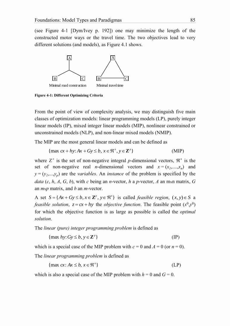
Foundations: Model Types and Paradigmas 85
(see Figure 4-1 [Dym/Ivey p. 192]) one may minimize the length of the
constructed motor ways or the travel time. The two objectives lead to very
different solutions (and models), as Figure 4.1 shows.
A
B C B C
A
Minimal travel timeMinimal road construction
Figure 4-1: Different Optimizing Criteria
From the point of view of complexity analysis, we may distinguish five main
classes of optimization models: linear programming models (LP), purely integer
linear models (IP), mixed integer linear models (MIP), nonlinear constrained or
unconstrained models (NLP), and non-linear mixed models (NMIP).
The MIP are the most general linear models and can be defined as
{max cx hy: Ax Gy b, x n, y Z
p} (MIP)
where n is the set of non-negative integral p-dimensional vectors,
n is the
set of non-negative real n-dimensional vectors and x = (x1,....,xn) and
y = (y1,...,yp) are the variables. An instance of the problem is specified by the
data (c, h, A, G, b), with c being an n-vector, h a p-vector, A an mxn matrix, G
an mxp matrix, and b an m-vector.
A set S {Ax Gy b, x Zp, y
n} is called feasible region, (x, y)S a
feasible solution, z cx hy the objective function. The feasible point (x0,y0)
for which the objective function is as large as possible is called the optimal
solution.
The linear (pure) integer programming problem is defined as
{max hy:Gy b, y Zp} (IP)
which is a special case of the MIP problem with c = 0 and A = 0 (or n = 0).
The linear programming problem is defined as
{max cx : Ax b, x n} (LP)
which is also a special case of the MIP problem with h = 0 and G = 0.
86 Chapter 4
Nonlinear models can be defined as (where f , g:n ):
{max f (x): x n} (unconstrained NLP)
{max f (x):g(x) 0, x n} (constrained NLP)
(NMIP are defined correspondingly, and we mention them only for the sake of
completeness since no unified framework for this general class containing all
others is known.)
There exists a rich body of solution techniques for all classes (except the last
one), but only LPs are solvable in polynomial time. IPs and MIPs both belong
to the non-deterministic polynomial class (NP-complete). Nonlinear models are
not solvable in the general case, but many special classes are solved efficiently
by using particular methods. Large LPs (n ≥ 250,000, m ≥ 300,000) are solved
frequently today, whereas certain IP and MIP problems of only 50 discrete
variables (p = 50) may resist all general methods. On the other hand, IPs of
p ≥ 10,000 have been solved using a general MIP-solver. Usually, bigger IPs
and MIPs must be solved using special techniques or heuristics.
From the point of view of modeling, it would, in many cases, be convenient to
formulate the model in a notation close to the mathematical one, since it is a
natural way to represent such a model. Fortunately, several algebraic languages
have been developed in the last decade to state the model in this form (see next
chapter) from which it is handed over to a (separate) solver software package.
However, with the exception of LP models, this has, up to now, not been very
successful from the point of view of the solution process. A lot of research
work still has to be done to use the paradigm of declarative model
representation in the case of bigger discrete models (IP and MIP). But the effort
might be worthwhile. An extremely large set of problems can be formulated as
MIP models. To be successful, techniques must be developed to translate the
declarative form into a form that can be solved efficiently. Interesting research
work is on the way in this vast domain, and certain methods will be presented
in Part III.
In the realm of combinatorics and graph theory, a rich set of models has been
developed that could be represented as IP or MIP models. For the most part,
however, this representation is neither natural nor efficient. They are more
naturally formulated using logical constraints or graph theoretic concepts. Here
Foundations: Model Types and Paradigmas 87
again, the same problem arises as before with IPs and MIPs: A declarative
representation normally does not say anything about how to solve the problem.
Such formulations could, however, be used to translate the models
automatically or semi-automatically into an efficient input for a solver.
From an application-oriented point of view [Rivett, p. 42], an important
problem class is comprised of the so-called queuing problems, which arise in
all server–client relationships where clients arrive, are served, and leave (e.g. a
post office). At the service point, conflicts come about between the client who
wants to be served immediately and the server who wants high productivity at
the service point. Such problems are normally formulated as simulation models.
In simple processes, analytical solutions exist. A large part of these queuing
problems can be classified by the Kendall's notation, a code of six terms
separated by slashes [Ravindran/Phillips/Solberg, 1987, p. 311]. Inventory
problems arise whenever there is a need to uncouple fluctuations in supply from
fluctuations in demand (liquidity in a bank). Allocation problems occur when a
set of jobs compete over a set of limited resources (assignment). Scheduling
and routing problems appear when deciding the way in which a task should be
approached (critical path, round tours, etc.). In replacement and maintenance
problems, units in a system deteriorate during time. The objective is then to
determine the probability of failure and to replace the deteriorated parts at the
right time (aeroplane maintenance). Competition problems arise when two or
more independent actors, called players, compete for resources. (One of the
player could also be Nature.) These problems are different from the others in
the sense that some variables are not controlled by the decision maker but by an
opponent.
4.3.3. Artificial Intelligence
In the artificial intelligence (AI) community, certain methods and models
emerge which are also interesting to consider in our context. These are search
techniques and heuristics used to solve hard problems as well as methods for
representing and encoding knowledge. Of course, under AI we may subsume
many other techniques used in natural language recognition, commonsense
reasoning and the like. Certain heuristics and search methods were discovered
and are also used outside the AI community. For our purpose, however, it is
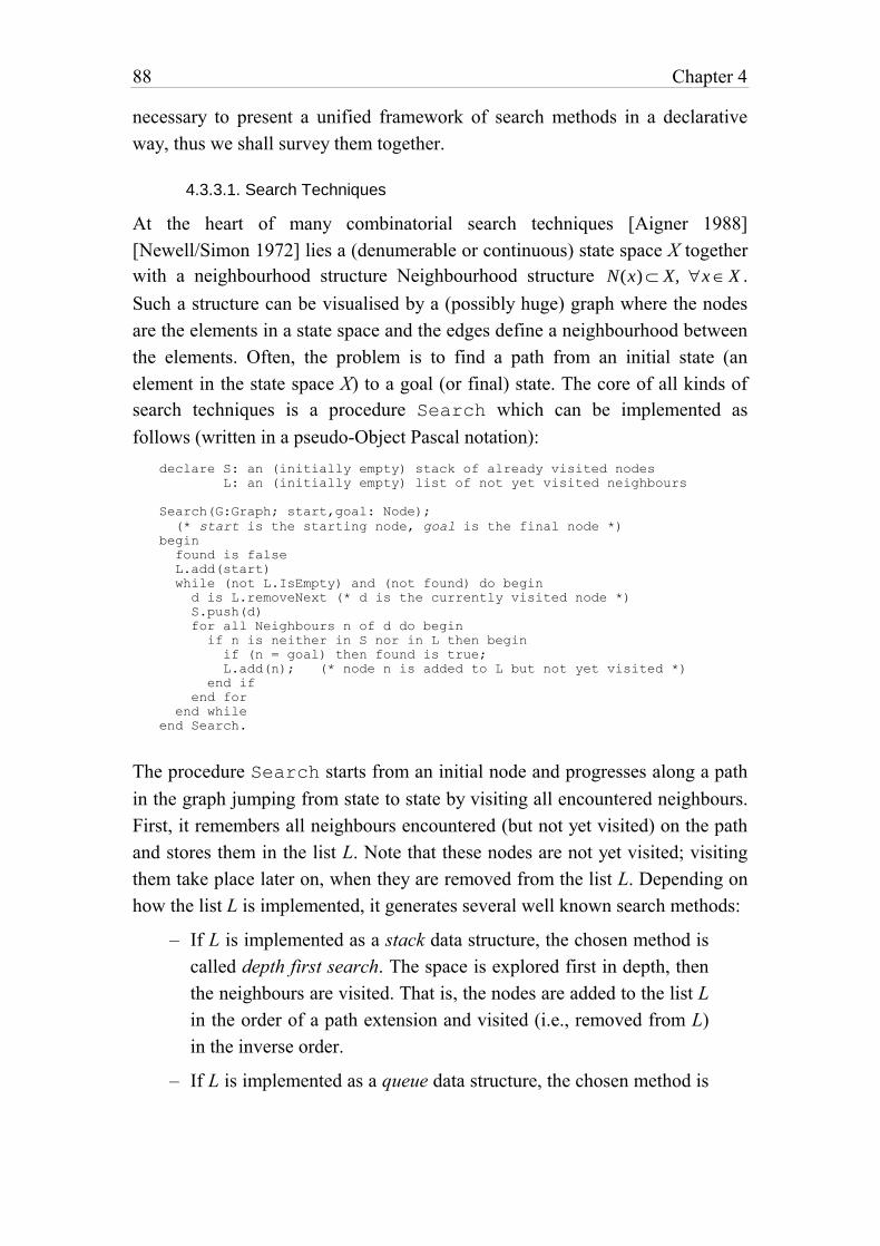
88 Chapter 4
necessary to present a unified framework of search methods in a declarative
way, thus we shall survey them together.
4.3.3.1. Search Techniques
At the heart of many combinatorial search techniques [Aigner 1988]
[Newell/Simon 1972] lies a (denumerable or continuous) state space X together
with a neighbourhood structure Neighbourhood structure N(x) X, x X .
Such a structure can be visualised by a (possibly huge) graph where the nodes
are the elements in a state space and the edges define a neighbourhood between
the elements. Often, the problem is to find a path from an initial state (an
element in the state space X) to a goal (or final) state. The core of all kinds of
search techniques is a procedure Search which can be implemented as
follows (written in a pseudo-Object Pascal notation):
declare S: an (initially empty) stack of already visited nodes
L: an (initially empty) list of not yet visited neighbours
Search(G:Graph; start,goal: Node);
(* start is the starting node, goal is the final node *)
begin
found is false
L.add(start)
while (not L.IsEmpty) and (not found) do begin
d is L.removeNext (* d is the currently visited node *)
S.push(d)
for all Neighbours n of d do begin
if n is neither in S nor in L then begin
if (n = goal) then found is true;
L.add(n); (* node n is added to L but not yet visited *)
end if
end for
end while
end Search.
The procedure Search starts from an initial node and progresses along a path
in the graph jumping from state to state by visiting all encountered neighbours.
First, it remembers all neighbours encountered (but not yet visited) on the path
and stores them in the list L. Note that these nodes are not yet visited; visiting
them take place later on, when they are removed from the list L. Depending on
how the list L is implemented, it generates several well known search methods:
– If L is implemented as a stack data structure, the chosen method is
called depth first search. The space is explored first in depth, then
the neighbours are visited. That is, the nodes are added to the list L
in the order of a path extension and visited (i.e., removed from L)
in the inverse order.
– If L is implemented as a queue data structure, the chosen method is
Foundations: Model Types and Paradigmas 89
called breadth first search. The immediate neighbourhood is
visited first completely before progressing to a more distant
neighbourhood. That is, the nodes are visited in the order they are
entered into the list L.
– If L is implemented as a heap (or priority queue) data structure, the
chosen method is called best first search. The nodes are visited
(removed from L) in the order which depends on a weight assigned
to the nodes. The node (state) in L with the lowest weight is
selected and is added to the final path S.38
Prolog, a programming language in AI, is essentially an implementation of such
a search method. (Most Prolog interpreters implement depth first search by
default.)
Many puzzles and games can be viewed as search problems and can be solved
using one of these techniques. The 3-jug problem (Example 3-3) is a typical
example which has a very small state space. The following Diophantine
problem is another example [Newell/Simon 1972, p. 154].
Example 4-1: A Letter Game Problem
Consider the puzzle where distinct digits for all letters have to be found such
that the numerical operations of the resulting numbers holds.
With the constraints that ci {0,1} for i {2K 6} and that each letter is
assigned a distinct digit, the six following equations constitute a complete
statement of the problem.
{2D T 10c2 , c2 2L R10c3 , c3 2A E 10c4 ,
c4 N R B10c5, c5 O E O10c6 , c6 D G R}
This problem is solved using a search tree of which Figure 4-2 shows only a
small part. In the initial state no assignment takes place to any of the variables.
38 The best known variant of a priority-first search is the A*–algorithm. The idea is to assign a
weight w to the state s as follows: w(s) = g(s) + h(s), where g(s) is the actual cost of going from
the initial state to the actual state s and h(s) represents the (estimated) cost of going from state s
to the goal state.
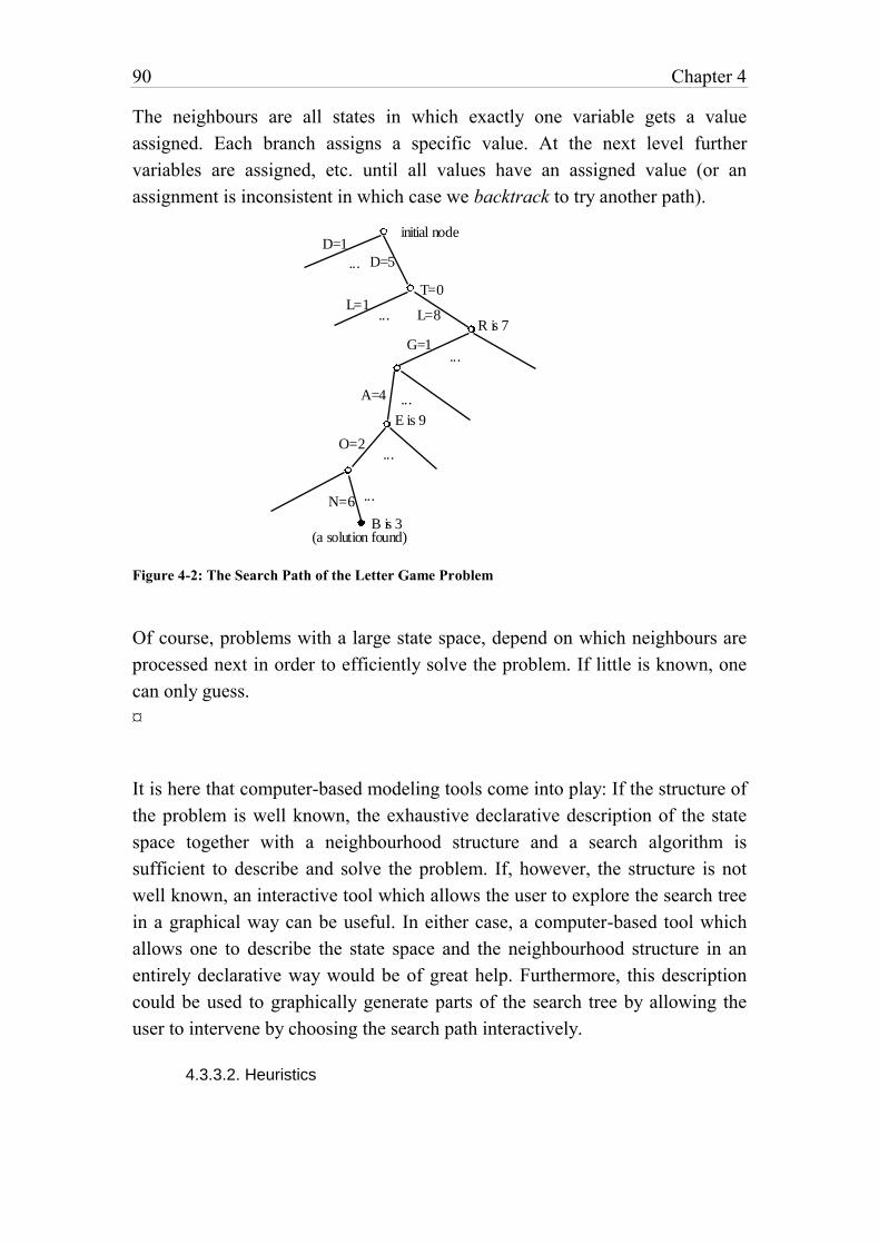
90 Chapter 4
The neighbours are all states in which exactly one variable gets a value
assigned. Each branch assigns a specific value. At the next level further
variables are assigned, etc. until all values have an assigned value (or an
assignment is inconsistent in which case we backtrack to try another path).
...
D=1
D=5
initial node
T=0
...L=1
L=8R is 7
G=1
A=4
...
...
E is 9
O=2
N=6
...
B is 3(a solution found)
...
Figure 4-2: The Search Path of the Letter Game Problem
Of course, problems with a large state space, depend on which neighbours are
processed next in order to efficiently solve the problem. If little is known, one
can only guess.
¤
It is here that computer-based modeling tools come into play: If the structure of
the problem is well known, the exhaustive declarative description of the state
space together with a neighbourhood structure and a search algorithm is
sufficient to describe and solve the problem. If, however, the structure is not
well known, an interactive tool which allows the user to explore the search tree
in a graphical way can be useful. In either case, a computer-based tool which
allows one to describe the state space and the neighbourhood structure in an
entirely declarative way would be of great help. Furthermore, this description
could be used to graphically generate parts of the search tree by allowing the
user to intervene by choosing the search path interactively.
4.3.3.2. Heuristics
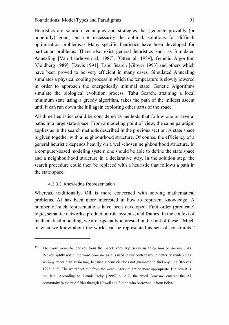
Foundations: Model Types and Paradigmas 91
Heuristics are solution techniques and strategies that generate provably (or
hopefully) good, but not necessarily the optimal, solutions for difficult
optimization problems.39 Many specific heuristics have been developed for
particular problems. There also exist general heuristics such as Simulated
Annealing [Van Laarhoven al. 1987], [Otten al. 1989], Genetic Algorithm
[Goldberg 1989], [Davis 1991], Tabu Search [Glover 1993] and others which
have been proved to be very efficient in many cases. Simulated Annealing
simulates a physical cooling process in which the temperature is slowly lowered
in order to approach the energetically minimal state. Genetic Algorithms
simulate the biological evolution process. Tabu Search, attaining a local
minimum state using a greedy algorithm, takes the path of the mildest ascent
until it can run down the hill again exploring other parts of the space.
All three heuristics could be considered as methods that follow one or several
paths in a large state space. From a modeling point of view, the same paradigm
applies as in the search methods described in the previous section: A state space
is given together with a neighbourhood structure. Of course, the efficiency of a
general heuristic depends heavily on a well-chosen neighbourhood structure. In
a computer-based modeling system one should be able to define the state space
and a neighbourhood structure in a declarative way. In the solution step, the
search procedure could then be replaced with a heuristic that follows a path in
the state space.
4.3.3.3. Knowledge Representation
Whereas, traditionally, OR is more concerned with solving mathematical
problems, AI has been more interested in how to represent knowledge. A
number of such representations have been developed: First order (predicate)
logic, semantic networks, production rule systems, and frames. In the context of
mathematical modeling, we are especially interested in the first of these. “Much
of what we know about the world can be represented as sets of constraints.”
39 The word heuristic derives from the Greek verb meaning find or discover. As
Reeves rightly noted, the word heuristic as it is used in our context would better be rendered as
seeking rather than as finding, because a heuristic does not guarantee to find anything [Reeves
1993, p. 5]. The word “zetetic“ from the word might be more appropriate. But now it is
too late. According to Dennis/Cathy [1995] p. 212, the word heuristic entered the AI
community in the mid fifties through Newell and Simon who borrowed it from Pólya.
92 Chapter 4
[Rich/Knight 1991, p. 301]. These constraints often take the form of logical
statements. Most of the time, predicate logic is used in AI to represent
knowledge in a declarative way. It was, and still is, the source of inspiration for
the design of many logic programming languages such as Prolog. There is a
new revival of such languages under the name of constraint logic programming
(CLP) (see [Sarawat 1995] and [Tsang 1993]). Such representations are often
called knowledge bases.
From the point of view of mathematical modeling, they are nothing other than
mathematical models consisting of variable propositions and predicates (the
variables in our terminology of mathematical models), constants (the
parameters), and a set of well formed formula (wff) (the constraints). The
elements of the set are linked together with a conjunction in order to produce a
single large constraint. This connection between knowledge bases and
mathematical models is still not widely known or taken into consideration,
although a number of researchers exposed them extensively [Jeroslow 1989].
The links are deeper than they at first glance might seem. Techniques which
have been known in AI for a long time correspond one to one to methods
commonly accepted in OR. For instance, the resolution method [Robinson
1965] to solve satisfiability problems developed in AI correspond to certain
cutting plane methods (Chvátal cuts) [Hooker 1988] to solve hard IP problems
in OR. From the computer-based modeling view, very little has been done to
unify these two approaches. Part III will expose systematically how these two
ways of representing knowledge as a model can be merged into a single
framework.
4.4. Modeling Uncertainty
In many problem domains, uncertain, incomplete or even inconsistent
knowledge arises in a natural way. The semantics of a mathematical model,
however, must be univocal, complete, and consistent. How can this discrepancy
be handled? There are a wide range of different methods for specifying and
treating uncertainty. In this section, a sketch of these largely neglected but
important aspects of mathematical modeling is given. Several techniques are
presented and it will be shown how these methods can be integrated into the
model-building process itself.
Our knowledge of the world is partial or incomplete, because complete
Foundations: Model Types and Paradigmas 93
information about an object would be too expensive or impossible to collect.
Our linguistic notions are vague or fuzzy, because the objects we describe with
our natural language have no clear boundary; but we do not consider this as a
major shortcoming of our natural language, on the contrary – it gives us an
efficient and flexible instrument to organize our mental world. Furthermore,
our perceptions of the world are often inconsistent with our theories and
models, because one observation gives us evidence for the truth of a statement,
but another observation provides to evidence of the contrary. There are many
reasons to account for this phenomenon: the sources of our information may be
unreliable, there may be imperfect or malfunctioning sensors that give rise to
conflicting perceptions, there may be an unreliable informant, or an uncertain
rule based on guesses due to incomplete knowledge.
Incompleteness, vagueness, and inconsistency – which in this paper I shall
subsume under the broad notion of uncertainty – are three main topics in
human commonsense and plausible reasoning. Uncertainty is an ubiquitous
aspect in the formulation and revision of a model.
4.4.1. Mathematical Models and Uncertainty
What has uncertainty got to do with mathematical models? Isn't mathematical
knowledge antipodal to uncertain knowledge? Of course, a mathematical
formula always has a precise interpretation. This, however, does not guarantee
that the formula reflects the real problem to be modeled. Furthermore, the
modeling process itself is exposed to all kinds of uncertainties. Everybody who
builds large mathematical models knows the most probable answer from the
solver at the very beginning of the model building process: “the model is
infeasible!” Infeasible? From the point of view of logic this response is
disastrous because an infeasible model has no solution and is completely
useless as is anything that follows from it. But what is the reaction of the model
builder to such a situation? Does she throw the model away? Not at all!
Infeasibility or inconsistency does not necessarily mean that the model does not
reflect the knowledge of the modeler about the problem at hand. The
knowledge as well as the set goals might be – and frequently are – inconsistent.
Inconsistency arises not only at the beginning of the modeling process when the
model structure and data have not yet been “stabilized”. It also occurs
frequently in the model revision process when new constraints are added to an
94 Chapter 4
otherwise well-behaved and feasible model. And there are still other
circumstances in which uncertainty pops up: Certain constraints only hold with
a given probability, numerical data are not known exactly, only their
probabilistic distribution is – or not even that. Hence, uncertainty is a natural
companion to all real-life models.
Human decision makers perform, in general, very well when making decisions
under vague, incomplete or even inconsistent knowledge. They do not need a
mathematical representation, and they rarely calculate to get a reasonable result.
They estimate a situation using their “feelings” and reason by “intuition”. In
contrast to human-based reasoning, computer-based decision making is (still)
rigid and inflexible. How is human reasoning distinguished from automated,
computer-based, or logic-based reasoning? Why is human commonsense based
reasoning so powerful, and why does logic-based reasoning sometimes behave
so poorly in practical decision making and in solving problems? Is it because
the computers' capacity in speed and memory is still very limited compared
with the human brain, or is it because commonsense reasoning is not based on
the classical logic paradigm? Experiences over the last 50 years show that faster
computers and more efficient algorithms – grounded on logic – have greatly
enlarged the class of problems (in the sense of complexity, not in the sense of
computability) we can practically handle and eventually solve on a computer.
This is a remarkable fact, since today's most sophisticated computer can be
reduced to a simple Turing Machine, a mathematical abstraction invented by A.
Turing sixty years ago, before the first computer was even manufactured. But it
is probably also true that in the future improved computers and better
algorithms will still not be able to solve most problems a human brain can
“solve”. This is, I think, not because the human brain seemingly can solve
uncomputable functions (in the sense of Turing), as some researchers have
suggested (Penrose, Eccles),40 but because the human brain does not necessarily
make use of a deductive inference when finding new results or when updating
its “knowledge base”; it rather uses what some have called an “inductive
inference”, although this term is difficult to define precisely. An important
40 It has recently been advanced from an exponent of the theoretical computer science [Wegner
1997], that interaction “is more powerful” than algorithms. It remains to be seen how this
concept can be formalized.
Foundations: Model Types and Paradigmas 95
difference between computer-based and commonsense-based reasoning is that
humans can reason under conditions of incomplete and inconsistent knowledge.
Uncertainty is not a new paradigm of academic research, neither is it a very
original one. It has been studied extensively by decision analysts, statisticians,
logicians, philosophers, (cognitive) psychologists, gamblers, insurance
companies, and – of course – by practitioners in artificial intelligence.
It would be audacious to give even a superficial overview of the representation
of uncertain knowledge within this section. Rather I will select certain
approaches that seemed especially promising to me in modeling uncertainty in
mathematical and logical models. That the selection is a tentative one is
unavoidable in a domain that is still in rapid development. The main goal here
is to show how uncertainty could be integrated into the declarative modeling
language paradigm, not to give a complete survey on how to model or treat
uncertainty.
4.4.2. General Approaches in Modeling Uncertainty
There has been, and continues to be, a lot of debate around the question of
which is the most general formalism for measuring or handling uncertainty.
Many researchers have defended the view that there is no adequate general
formalism and that using a multitude of different specialized formalisms is a
better way to tackle the concept of uncertainty. Some defend the position that
the right approach is numerical (i.e. using probability theory), others argue that
the only approach is symbolical (i.e. using non-monotonic logic).
Disputes even arise about how to classify various approaches. Depending on
the criteria and goals one adheres to, various classifications of approaches
could be very different.
Pearl [1988] classifies the approaches to uncertainty into three “schools”:
logicists, neo-calculists, and neo-probabilists. The logicists try to deal with
uncertainty using non-numerical techniques, typically non-monotonic logic; the
neo-calculists use numerical representations of uncertainty but regard
probability calculus as inadequate and propose entirely new calculi, like
Dempster-Shafer theory, fuzzy set theory, and others; the neo-probabilists
remain within the traditional framework of probability theory.
96 Chapter 4
The viewpoint adopted in this section is centered around the question: How can
uncertainty be integrated into mathematical and logical modeling tools as a
declarative language? From this perspective, one might distinguish three
paradigms:
– the paradigm of probability theory,
– the paradigm of argumentation theory,
– the paradigm of fuzzy set theory.
The paradigm of probability theory is based on the assumption that uncertainty
can be ranged in degrees which are expressed as numbers. The paradigm is very
powerful. All classical approaches to statistics and stochastics (stochastic
programming), as well as Bayesian theory and nets [Pearl 1988] and probability
logic [Nilsson 1986] can be covered by this approach. The second approach of
argumentation theory might not be known widely under this term. It subsumes
most symbolical approaches, such as argumentative systems, non-monotonic
logics, evidence theory, and hint theory; somewhat unexpectedly, one might
also subsume the numerous goal programming techniques under this approach.
The reason for this will be explained later on. The third approach, fuzzy set
theory, developed by [Zadeh 1965], has already proven its usefulness in
dynamic systems. Two examples will be given at the end of this chapter, to
illustrate this approach.
Uncertainty can appear in very different contexts within mathematical and
logical models: In mathematical models, the data is representable by random
distributions instead of crisp quantities, the constraints are soft, that is, they
may be violated to a certain extent, constraints are true with a certain
probability, and even inconsistent objectives can enter the model. Logical
models can be inconsistent, or become inconsistent by adding new knowledge,
they may contain formulas that are not strictly true or false, but only true with a
certain probability.
Random or vague data in mathematical models can be approached by stochastic
programming or fuzzy programming. Soft constraints, multiple objectives and
infeasible models are addressed by different variants of goal programming.
Probabilistic logical formulas can be treated using Bayesian networks or
probabilistic logic. Finally, argumentative bases systems are suitable to handle
Foundations: Model Types and Paradigmas 97
inconsistent knowledge bases.
For each kind of uncertainty we will give examples, making use of a unified
framework for representing the model in a declarative way.
4.4.3. Classical Approaches in OR
There are two well known methods to handle particular uncertainty types in
linear models in OR: goal programming and stochastic programming. Goal
programming [Ignizio 1976], [Zionts 1988], [Schniederjans 1995] can
– discover and eliminate infeasibilities,
– handle conflicting objectives or goals,
– be used to include soft constraints into the model,
– and to add aspiration levels.
by introducing additional slack variables.
It is probably the most common method to eliminate infeasibilities from a
mathematical model. The added slack variables can be interpreted as penalties
for violating the constraints. The objective is then to minimize the “amount of
infeasibilities” by a weighted vector of the slack variables. Many variants are in
use. The simplest consists of replacing the linear model min cx Ax b by
min cx wp vn Ax p n b where p and n are the positive and negative
slack variable vectors and w and v are two weight vectors.
The method of adding slacks can also be used for handling conflicting
objectives or goals in mathematical modeling. Suppose there are two
objectives, one is to maximize cx and the other is to minimize dx. The modeler
introduces two aspiration levels C and D (defined as scalars), which indicate
the desired goals, one for the first, the other for the second objective. The
objectives are now converted into constraints containing additional positive and
negative slack variables as follows:
cx slackCpos slackCneg C
dx slackDpos slackDneg D
The new objective function is to minimize a weighted sum of the four slack
variables, or to minimize the largest slack variable.
Another way to look at slack variables is to interpret them as “softening” the
98 Chapter 4
constraint. Instead of having precise, “hard” constraints, which is almost never
the case in practical modeling, one has constraints that can be violated to a
certain degree. In this way, the modeler can formulate all kinds of fuzzy or
uncertain situations. An example is the constraint that fixes the budget at about
1000. One could formulate this as Budget ˜ 1000 or, using a positive and
negative slack variable p and n, as Budget p n 1000.
Another situation where slack variables are useful, is when interpreting the
constraints as goals to be attained. The right-hand-side of the constraint is now
considered as an aspiration level. Every constraint, in fact, is now restated as an
objective, and the approach of conflicting goals outlined above can be applied.
This fourth approach is also known as goal programming.
All four applications of goal programming show how useful this simple
technique of introducing slack variables can be. We will see that this technique
has an analogue in the procedure of logical knowledge bases for eliminating
inconsistencies by introducing new propositions, called assumptions. Hence,
this method is very general, and can easily be integrated into a modeling
language.
Of course, there are also other methods to eliminate infeasibilities from a linear
model. One method is to find an irreducibly inconsistent set of constraints (IIS).
If one member of a IIS is dropped, then the set becomes feasible. (For further
details see [Chinneck/Dravnieks 1991] or [Tamiz/Mardle/Jones 1995].) Some
commercial solvers include procedures to find the IISs. Other methods order
the constraints according to certain preferential criteria and select a maximally
feasible subset of constraints in this order. This can also be interpreted as
priority ordering of constraints.
Stochastic programming [Sengupta 1972], [Kall 1976], [Ermoliev/Wets 1988],
[Birge/Wets 1991], [Wets 1991], [Kall/Wallace 1994] is used to include one or
several random components (data). It handles uncertainties about data. Crisp
data is not very realistic in most practical decision models. Stochastic
programming provides a means for replacing the uncertainty about data by a
probability distribution. Insofar, this approach can be subsumed under the
numerical approaches mentioned above.
As a rule, stochastic models are much more difficult to solve, and it is unlikely
a single efficient solver will be found to handle all of them. A lot of effort has
Foundations: Model Types and Paradigmas 99
been concentrated on finding efficient solvers for the stochastic linear programs
(SLP), and many are known for special model cases [Kall/Mayer 1993],
whereas in integer programs or non-linear models almost no progress has been
made.
If some of the data within an LP, such as min cx Ax b, x 0 , is replaced by
random distributions, as in min c()x A( )x b( ),x 0 , where
(, 2
, p ) is a probability space with , then the model becomes, strictly
speaking, meaningless, since it is no longer clear what to minimize in this case.
There are, however, several ways of interpreting such models. Two main
interpretations can be distinguished and are often used [Kall 1976, Kall/Mayer
1992]. The first is the so-called two-stage model where the model above is
interpreted as min E[c( )x Q(Ax b,)] x 0 where E[•] is the
expectation of the random quantity and Q is a penalty function for violating
the constraints; the second is the chance-constrained model, which can be
formulated as: min E[c( )x] P{| A( )x b( )} ,x 0 if there is a
single joint chance constraint. It can be formulated as:
min E[c( ) x] P{ | Ai ( )x bi ( )} i , x 0 if each constraint i is
defined as a separate change constraint.
In the simplest case, where only the right-hand-side vector b is a random
quantity, one can translate the SLP into a (much bigger) crisp LP. This
transformation process can be automatized. Models containing stochastic
parameters and variables can smoothly be integrated into a declarative
modeling framework simply by declaring the parameters to be stochastic. We
shall see a classical example in Part III. The same is the case for chance
constraints: we only need to declare the probabilities with which they hold.
The next two sections describe numerical and symbolic approaches for
specifying logical models.
4.4.4. Approaches in Logical Models
It is interesting that the most general problems that arise in probabilistic logical
models were already stated as early as the nineteenth century by George Boole
(1815–1864).
Boole was the first to make any real progress in classical logic since the time of
100 Chapter 4
Aristotle. His idea was to apply the laws of algebra to logic. In doing so, he
sought a way to analyze Aristotle's syllogistic logic.41 But his main goal was
even more ambitious, it was “to investigate the fundamental laws of those
operations of the mind by which reasoning is performed”, or in modern terms:
given the truth or falsity of any proposition, what is the truth of a compound
statement, or the more difficult problem – known as satisfiability problem
(SAT): Given several compound statements, which assignment makes them all
true.
This is now well known. But Boole did much more: He was probably the only
logician for more than a hundred years who tried to unify logic with probability
theory. He intended to base the theory of probability on this logical calculus by
identifying “event” with “proposition”. Suppose – he said – all propositions are
not simply true (1) or false (0), but a probability between zero and one is
attached to them, where the propositions must be some “unconditioned simple
event” (as he said) (see [Hailperin, 1986, p. 223]), how could the probability of
any compound statement now be calculated? Or in modern terms: Given a set
of compound statements, what probabilities must the proposition have to make
the system consistent? Again, just apply the laws of algebra, he said. Given, for
example, the probabilities of the propositions x and y as p(x) and p(y), then the
probability of xy is p(x)p(y), if the events are independent, the probability of
x+y is p(x)+p(y), if the events are incompatible, and the probability of –x is 1–
p(x). Conditional probability was seen by Boole as only another probability of a
compound statement: the probability that the event y will occur supposing the
41 As Devlin [Delvin K, 1994, Mathematics, The Science of Pattern, Scientific American Library,
NewYork, p. 45] noted, two syllogisms found in Aristotle's original treatment were false and
they went undiscovered for 2000 years! The first has the form:
All M are P
All M are S
-----------
Some S is P
Using Boolean logic, it is a matter of simple algebra to verify that this syllogism is false: From
m(1–p) = 0 and m(1–s) = 0, it does not follow that sp ≠ 0. If m=0 then the first two equations
are true, whatever s and p denote. Consequently, it is possible for the two premises to be true
when the conclusion is false. We could also check this using Venn diagrams. An example:
Suppose the two premises to be true: “All clever people are clever” and “all clever people are
people”; could we then conclude that “some people are clever”? Certainly not!
Foundations: Model Types and Paradigmas 101
event x has already occurred is p(xy)/p(x). Clearly this gives the correct value of
the conditional probability, noted today as p(y|x). But it is not clear whether
Boole mixed up the conditional probability with the probability of a condition
(if x then y, or in Boole's notation: –x+y = 0). He didn't seem to have a clear
view on this point (for further material see [Hailperin 1986, chap 4]).42
Hailperin [1986], who gives a complete reconstruction of Boole's reasoning,
found that Boole had already formulated two fundamental problems that have
been rediscovered several times in the last 50 years. They are:
– Problem A: Given a set W = { w1, w2, ... , wm } of wffs (well formed
formulas) over the propositions P = {p1, p2, ... , pn }, and each wff wi
is true with probability i. Are these probabilities consistent?
– Problem B: Given a set W = { w1, w2, ... , wm } of wffs, again over P,
and each wff wi is true with probability i. What is the consistent
probability range of a wff wm+1 W?
Both these problems also appear in the probability theory of De Finetti
[German edition 1981] and in Nilsson [1986]. Following the terminology of
Hansen/Jaumard/al. [1995], we call problem A probabilistic satisfiability
(PSAT); and problem B is called the probabilistic entailment problem. The
PSAT problem can be formulated as a linear system with an exponential
42 There is still much confusion between “conditional probability” and “probability of a condition
(implication)”. It is easy to see that the conditional probability is not identical to the probability
of an implication. Supposing they were equal, we can then make the following deductions:
p(a b) p(b| a)
p(a b) p(a b)
p(a)
p(a) [1 p(a b )] p(a b)
[ p(a b) p(a b )] [1 p(a b )] p(a b)
p(a b) p(a b ) p(a b) p(a b ) [ p(a b )]2 p(a b)
p(a b ) p(a b) p(a b ) [p(a b )]2 0
p(a b ) [1 p(a b) p(a b )] 0
p(a b ) [1 p(a)] 0
[1 p(a b)] [1 p(a)] 0
Thus, the conditional probability is equal to the probability of a condition (implication) if and
only if either p(a) 1 or p(ab) 1 (or both).
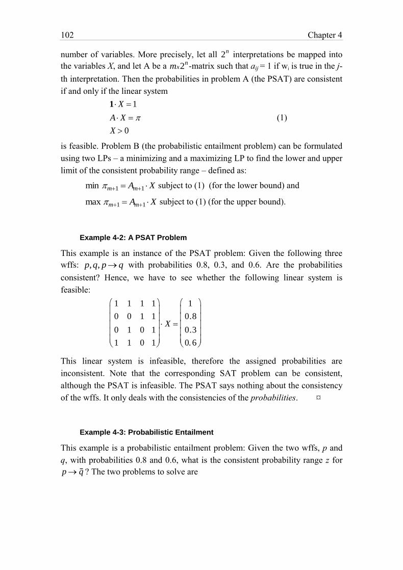
102 Chapter 4
number of variables. More precisely, let all 2n interpretations be mapped into
the variables X, and let A be a mx2n-matrix such that aij = 1 if wi is true in the j-
th interpretation. Then the probabilities in problem A (the PSAT) are consistent
if and only if the linear system
1 X 1
A X
X 0
(1)
is feasible. Problem B (the probabilistic entailment problem) can be formulated
using two LPs – a minimizing and a maximizing LP to find the lower and upper
limit of the consistent probability range – defined as:
min m1 Am1 X subject to (1) (for the lower bound) and
max m1 Am1 X subject to (1) (for the upper bound).
Example 4-2: A PSAT Problem
This example is an instance of the PSAT problem: Given the following three
wffs: p,q, p q with probabilities 0.8, 0.3, and 0.6. Are the probabilities
consistent? Hence, we have to see whether the following linear system is
feasible:
1 1 1 1
0 0 1 1
0 1 0 1
1 1 0 1
X
1
0.8
0.3
0. 6
This linear system is infeasible, therefore the assigned probabilities are
inconsistent. Note that the corresponding SAT problem can be consistent,
although the PSAT is infeasible. The PSAT says nothing about the consistency
of the wffs. It only deals with the consistencies of the probabilities. ¤
Example 4-3: Probabilistic Entailment
This example is a probabilistic entailment problem: Given the two wffs, p and
q, with probabilities 0.8 and 0.6, what is the consistent probability range z for
p q ? The two problems to solve are
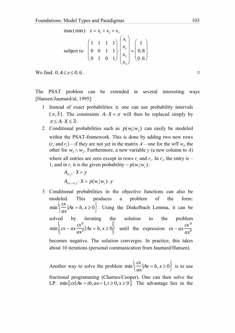
Foundations: Model Types and Paradigmas 103
max( min) z x1 x2 x3
subject to
1 1 1 1
0 0 1 1
0 1 0 1
x1
x2
x3
x4
1
0. 8
0. 6
We find: 0.4 z 0.6 . ¤
The PSAT problem can be extended in several interesting ways
[Hansen/Jaumard/al, 1995]:
1 Instead of exact probabilities one can use probability intervals
[,] . The constraints A X will then be replaced simply by
A X .
2 Conditional probabilities such as p(wi |w j ) can easily be modeled
within the PSAT-framework. This is done by adding two new rows
(rx and ry) – if they are not yet in the matrix A – one for the wff wj, the
other for wi w j . Furthermore, a new variable y (a new column to A)
where all entries are zero except in rows rx and ry. In rx, the entry is –
1, and in ry it is the given probability p(wi |wj ) :
A(wj ) X y
A(wi wj ) X p(wi |wj ) y
3 Conditional probabilities in the objective functions can also be
modeled. This produces a problem of the form:
mincx
axAx b, x 0
. Using the Dinkelbach Lemma, it can be
solved by iterating the solution to the problem
min cx axcx0
ax0 Ax b, x 0
until the expression cx ax
cx 0
ax0
becomes negative. The solution converges. In practice, this takes
about 10 iterations (personal communication from Jaumard/Hansen).
Another way to solve the problem mincx
axAx b, x 0
is to use
fractional programming (Charnes/Cooper). One can then solve the
LP: min cx Ax tb,ax1, t 0,x 0 . The advantage lies in the
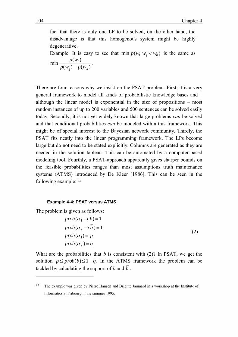
104 Chapter 4
fact that there is only one LP to be solved; on the other hand, the
disadvantage is that this homogenous system might be highly
degenerative.
Example: It is easy to see that min p(wi |w j wk ) is the same as
minp(wi )
p(w j ) p(wk ).
There are four reasons why we insist on the PSAT problem. First, it is a very
general framework to model all kinds of probabilistic knowledge bases and –
although the linear model is exponential in the size of propositions – most
random instances of up to 200 variables and 500 sentences can be solved easily
today. Secondly, it is not yet widely known that large problems can be solved
and that conditional probabilities can be modeled within this framework. This
might be of special interest to the Bayesian network community. Thirdly, the
PSAT fits neatly into the linear programming framework. The LPs become
large but do not need to be stated explicitly. Columns are generated as they are
needed in the solution tableau. This can be automated by a computer-based
modeling tool. Fourthly, a PSAT-approach apparently gives sharper bounds on
the feasible probabilities ranges than most assumptions truth maintenance
systems (ATMS) introduced by De Kleer [1986]. This can be seen in the
following example: 43
Example 4-4: PSAT versus ATMS
The problem is given as follows:
prob (1 b) 1
prob (2 b ) 1
prob (1) p
prob (2 ) q
(2)
What are the probabilities that b is consistent with (2)? In PSAT, we get the
solution p prob(b) 1 q . In the ATMS framework the problem can be
tackled by calculating the support of b and b :
43 The example was given by Pierre Hansen and Brigitte Jaumard in a workshop at the Institute of
Informatics at Fribourg in the summer 1995.
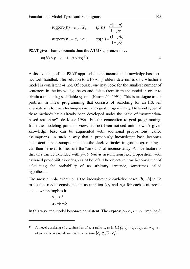
Foundations: Model Types and Paradigmas 105
support (b) 1 2 , sp(b) p(1 q)
1 pq
support (b ) 1 2 , sp(b ) (1 p)q
1 pq
PSAT gives sharper bounds than the ATMS approach since
sp(b ) p 1q sp(b ). ¤
A disadvantage of the PSAT approach is that inconsistent knowledge bases are
not well handled: The solution to a PSAT problem determines only whether a
model is consistent or not. Of course, one may look for the smallest number of
sentences in the knowledge bases and delete them from the model in order to
obtain a remaining satisfiable system [Hansen/al. 1991]. This is analogue to the
problem in linear programming that consists of searching for an IIS. An
alternative is to use a technique similar to goal programming. Different types of
these methods have already been developed under the name of “assumption-
based reasoning” [de Kleer 1986], but the connection to goal programming,
from the modeling point of view, has not been noticed until now. A given
knowledge base can be augmented with additional propositions, called
assumptions, in such a way that a previously inconsistent base becomes
consistent. The assumptions – like the slack variables in goal programming –
can then be used to measure the “amount” of inconsistency. A nice feature is
that this can be extended with probabilistic assumptions, i.e. propositions with
assigned probabilities or degrees of beliefs. The objective now becomes that of
calculating the probability of an arbitrary sentence, sometimes called
hypothesis.
The most simple example is the inconsistent knowledge base: {b,b}.44 To
make this model consistent, an assumption (1 and 2) for each sentence is
added which implies it:
1 b
2 b
In this way, the model becomes consistent. The expression 1 2 implies b,
44 A model consisting of a conjunction of constraints ci as in C( p,x) c1 c2K cn is
often written as a set of constraints in the form {c1,c2 ,K ,cn}.
106 Chapter 4
and is called the support of b; whereas the expression 1 2 implies b as
stated above in (2).
A further drawback of the PSAT (as well as the Bayesian) approach is that we
cannot model ignorance, which might be considered as a special type of
uncertainty. Ignorance arises in many situations. If we want to buy a Chinese
vase, we are ignorant to a certain extent whether a specific vase is authentic or
forged. This situation seems to be difficult to model using the classical
framework of probabilities, since the opposite degrees of beliefs do not
necessarily sum up to one: We may believe with degree p that the vase is
authentic, with degree q that it is not, but p+q may be less than one. The
number 1–(p+q) may be a measure of our ignorance. There exist promising
frameworks [Shafer 1976], [Kohlas al. 1995] which deal with this problem.
Further motivation for these interesting and relatively new approaches is given
in [Kohlas al. 1994] and in [Shafer 1978].
4.4.5. Fuzzy Set Modeling
Modeling using fuzzy set theory is yet another very different manner to model
specific uncertainties. It too fits well into the pattern of the declarative way of
modeling. In the probability paradigm and in the paradigm of logic, a number
of well defined events or propositions are given, even if it is in general not
known exactly which events truly take place, or if the knowledge is
probabilistic only. The fuzzy set theory, on the other hand, deals with
propositions which have vague meaning. Some events or propositions are not
well defined or fuzzy. A vague description of an object or a process seems to be
easier to remember by humans and is apparently more economical and hence
more efficient. The reality itself might not be fuzzy, but our knowledge and the
contents of our theories about reality may be so. Fuzziness is vagueness, which
makes it a central element in human thought and perceptions, as well as in
human language. “The theory of fuzzy sets enables us to structure and describe
activities and observations which differ from each other only vaguely, to
formulate them in models and to use these models for various purposes – such
as problem-solving and decision-making” [Zimmermann al. 1984, p. 18].
Foundations: Model Types and Paradigmas 107
Furthermore, as systems get more complex, it becomes increasingly difficult to
make analytical statements about them which are both meaningful and precise.
In complex problem situations in which human beings are involved, much of
the knowledge about the situation is expressible in linguistic terms
[Zimmermann al. 1984, p. 11] only – a concept which is explained below.
We use fuzzy concepts and words to describe the object of our world, because
the boundary of an object is uncertain, unclear, or unreliable (e.g. “all trees in
Canada”). The natural language is full of words with vague or fuzzy meaning.
There is, for example, no such thing as a boundary to the Swiss Alps; any such
boundary would be artificial. That does not mean that one cannot fix a
boundary for a special purpose and work with that “precise definition”. But this
is not always entirely satisfactory. An illustrative example is the ancient
Sorites45 paradox: If there is a heap of sand, and a single grain of sand is taken
away, then one could say that the remaining grains still form a heap of sand.
But by induction one could then take away all the sand and still have a heap of
sand – an absurdity. The question then arises how many grains of sand a heap
must contain so that it could still be called “heap”. This is a question that
cannot be answered in a satisfactory manner. Despite this situation, it is an
astonishing fact that human beings are doing very well by using the notion of “a
heap of sand” without ever knowing and defining the relevant number of
grains.
Almost every sentence in a natural language contains fuzzy concepts. Some
simple examples are:
– “Peter is roughly about 40 years old”, “Paul has little money”.
– “Mary is tall”. “If the growth is quite large, then there is a good
chance the tumour is cancerous”.
In the first two examples, the exact age of Peter or the amount of money Paul
has, are uncertain. In the second kind of examples, the exact meaning of “tall”
is unclear, but most would agree on a range between 1.75 m–2.30 m with a
most likely value between 1.80 m and 1.90 m.
But unclear meaning and uncertainty are to a certain extent only two sides of
45 Sorites: from the Greek word which simply means “heap”.
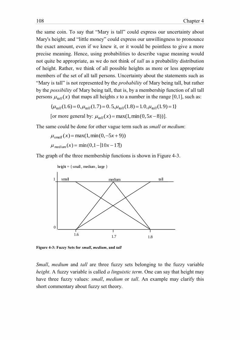
108 Chapter 4
the same coin. To say that “Mary is tall” could express our uncertainty about
Mary's height; and “little money” could express our unwillingness to pronounce
the exact amount, even if we knew it, or it would be pointless to give a more
precise meaning. Hence, using probabilities to describe vague meaning would
not quite be appropriate, as we do not think of tall as a probability distribution
of height. Rather, we think of all possible heights as more or less appropriate
members of the set of all tall persons. Uncertainty about the statements such as
“Mary is tall” is not represented by the probability of Mary being tall, but rather
by the possibility of Mary being tall, that is, by a membership function of all tall
persons tall (x) that maps all heights x to a number in the range [0,1], such as:
{tall(1.6) 0,tall(1.7) 0.5,tall(1.8) 1.0,tall(1.9) 1}
[or more general by: tall(x) max(1,min(0,5x 8))].
The same could be done for other vague term such as small or medium:
small (x) max(1,min(0,5x 9))
medium (x) min(0,1 10x 17)
The graph of the three membership functions is shown in Figure 4-3.
1
0
1.61.7 1.8
tallsmall medium
height = { small , medium , large }
Figure 4-3: Fuzzy Sets for small, medium, and tall
Small, medium and tall are three fuzzy sets belonging to the fuzzy variable
height. A fuzzy variable is called a linguistic term. One can say that height may
have three fuzzy values: small, medium or tall. An example may clarify this
short commentary about fuzzy set theory.
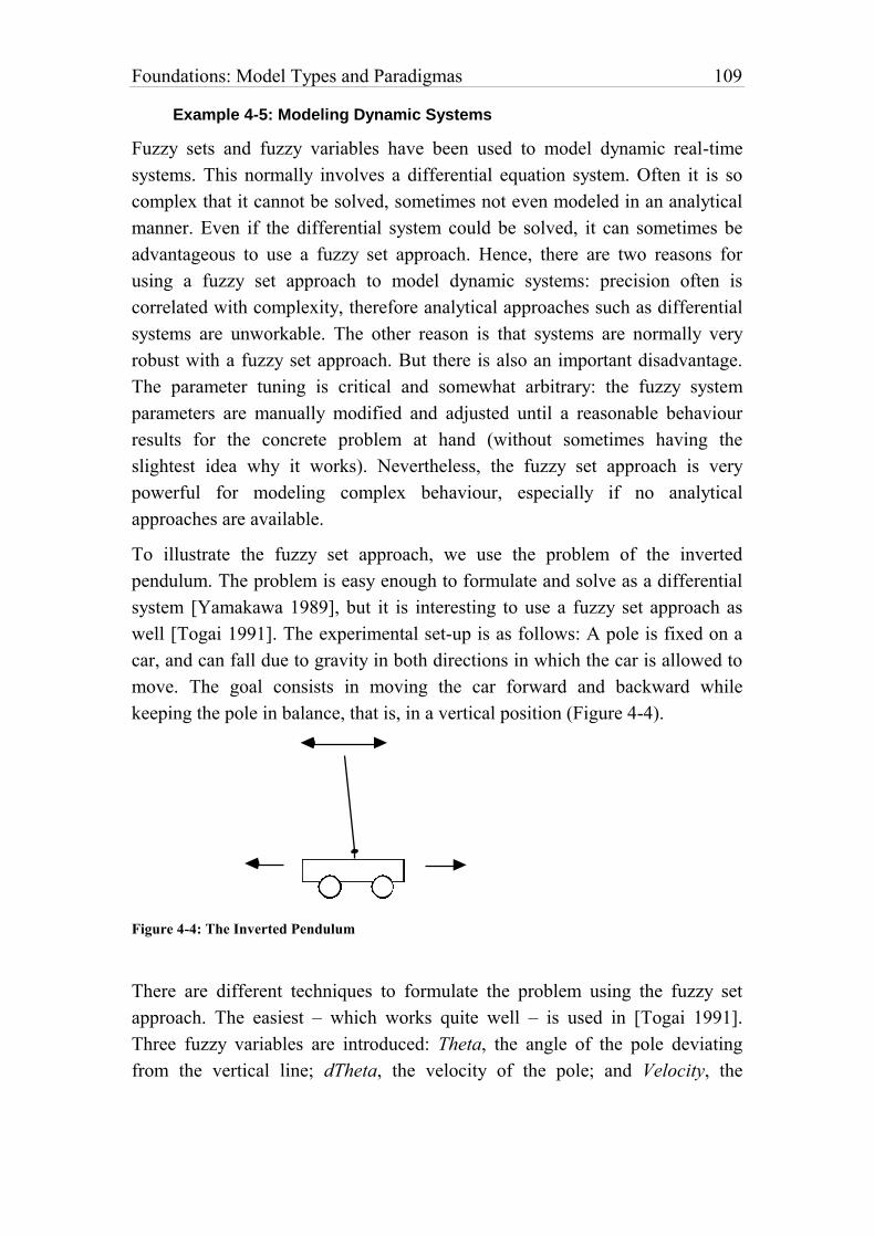
Foundations: Model Types and Paradigmas 109
Example 4-5: Modeling Dynamic Systems
Fuzzy sets and fuzzy variables have been used to model dynamic real-time
systems. This normally involves a differential equation system. Often it is so
complex that it cannot be solved, sometimes not even modeled in an analytical
manner. Even if the differential system could be solved, it can sometimes be
advantageous to use a fuzzy set approach. Hence, there are two reasons for
using a fuzzy set approach to model dynamic systems: precision often is
correlated with complexity, therefore analytical approaches such as differential
systems are unworkable. The other reason is that systems are normally very
robust with a fuzzy set approach. But there is also an important disadvantage.
The parameter tuning is critical and somewhat arbitrary: the fuzzy system
parameters are manually modified and adjusted until a reasonable behaviour
results for the concrete problem at hand (without sometimes having the
slightest idea why it works). Nevertheless, the fuzzy set approach is very
powerful for modeling complex behaviour, especially if no analytical
approaches are available.
To illustrate the fuzzy set approach, we use the problem of the inverted
pendulum. The problem is easy enough to formulate and solve as a differential
system [Yamakawa 1989], but it is interesting to use a fuzzy set approach as
well [Togai 1991]. The experimental set-up is as follows: A pole is fixed on a
car, and can fall due to gravity in both directions in which the car is allowed to
move. The goal consists in moving the car forward and backward while
keeping the pole in balance, that is, in a vertical position (Figure 4-4).
Figure 4-4: The Inverted Pendulum
There are different techniques to formulate the problem using the fuzzy set
approach. The easiest – which works quite well – is used in [Togai 1991].
Three fuzzy variables are introduced: Theta, the angle of the pole deviating
from the vertical line; dTheta, the velocity of the pole; and Velocity, the
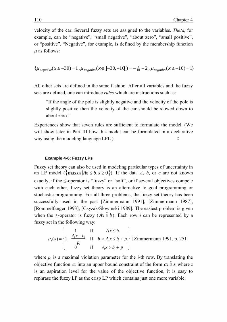
110 Chapter 4
velocity of the car. Several fuzzy sets are assigned to the variables. Theta, for
example, can be “negative”, “small negative”, “about zero”, “small positive”,
or “positive”. “Negative”, for example, is defined by the membership function
as follows:
{negative(x 30) 1, negative(x 30,10 ) x10 2 , negative(x 10) 1}
All other sets are defined in the same fashion. After all variables and the fuzzy
sets are defined, one can introduce rules which are instructions such as:
“If the angle of the pole is slightly negative and the velocity of the pole is
slightly positive then the velocity of the car should be slowed down to
about zero.”
Experiences show that seven rules are sufficient to formulate the model. (We
will show later in Part III how this model can be formulated in a declarative
way using the modeling language LPL.) ¤
Example 4-6: Fuzzy LPs
Fuzzy set theory can also be used in modeling particular types of uncertainty in
an LP model ( maxcx Ax b,x 0 ). If the data A, b, or c are not known
exactly, if the ≤-operator is “fuzzy” or “soft”, or if several objectives compete
with each other, fuzzy set theory is an alternative to goal programming or
stochastic programming. For all three problems, the fuzzy set theory has been
successfully used in the past [Zimmermann 1991], [Zimmermann 1987],
[Rommelfanger 1993], [Czyzak/Slowinski 1989]. The easiest problem is given
when the ≤-operator is fuzzy ( Ax ˜ b ). Each row i can be represented by a
fuzzy set in the following way:
i(x)
1 if Aix bi
1Ai x bi
pi
if bi Aix bi pi
0 if Aix bi pi
[Zimmermann 1991, p. 251]
where pi is a maximal violation parameter for the i-th row. By translating the
objective function cx into an upper bound constraint of the form cx ˜ z where z
is an aspiration level for the value of the objective function, it is easy to
rephrase the fuzzy LP as the crisp LP which contains just one more variable:
Foundations: Model Types and Paradigmas 111
max p0 cx z p0 , p Ax b p
The multi-objective problem can be approach by a similar procedure.
The main advantage of this fuzzy set approach in contrast to the stochastic one
is that the former produces a crisp LP which is as easy to solve as the original
model, whereas a stochastic model is much harder to solve. In Part II we will
show how fuzzy LP modeling can be integrated into the general framework of a
declarative modeling environment. ¤
4.4.6. Outlook
In this chapter, we have described a number of model types from a modeler's
point of view. One of the most interesting and promising aspects of computer-
based mathematical modeling is to find a common framework in order to
enable a modeler to formulate her model in a general way permitting automatic
or semi-automatic translation in an appropriate form for solving the model with
the most promising solver. Many such transformations could be conceived, as
we have seen, so the PSAT-model could be translated into an LP of exponential
size in terms of the number of propositions. Without such a framework these
translations would be impossible without heavy programming efforts.
Therefore, the ultimate goal of every modeling system should be to offer a
number of very general translation methods which allow the modeler to use the
appropriate solver.
Special emphasis has been given to model uncertainty. This is justified by the
fact that many types of uncertainty can be evenly integrated into a general
declarative modeling framework as we shall display it in Part II and III more
concretely. Another reason is the bewildering variety of ways of representing
uncertainty. I have tried to show that a common scheme for several of them is
conceivable and beneficial.
In the next chapter, certain features of a general modeling tool system will be
offered. I shall endeavour to further justify the assertion that a model
management system is necessary and to give a sketch of its structure.

Part II
A GENERAL MODELING
FRAMEWORK
This Part II gives an overview of the present situation and problems in
modeling management systems. It carefully elaborates the difficulties linked
with present modeling management systems. The most common approaches in
computer-based modeling are surveyed and examples are given, so that we can
concretely compare how they tackle problems, and to evaluate their limitations,
pitfalls and strengths. At the end, I propose my own view on the architecture of
a modeling environment and on how to integrate the different heterogeneous
aspects of modeling into one single homogenous framework.
115
5. PROBLEMS AND CONCEPTS
“Insight, not Numbers.” — Hamming R. W.
From the more mathematical aspects of modeling, we now switch to the
implementation aspects of computer-based modeling tools. Therefore, this
chapter is more relevant for the designer of modeling tools than for the modeler
or the model user. The previous chapters detail important prerequisites for
understanding what modeling is, what components are necessary to implement
modeling tools, and what model types should be part of the framework. In a
word, from mathematics we switch to computer science. From a computer
science point of view, this book could be viewed as the presentation of a large
software project: The first four chapters describe the functionality and the
“software requirement catalogue” from the user's point of view. This chapter
summarizes these requirements and presents the formal specifications. Finally,
Part III presents a concrete implementation; the LPL system.
All of the steps in the modeling process (described in Chapter 3) are essential
for building and manipulating models effectively. Furthermore, in each stage
the modeler or the model user has to carry out a variety of very different tasks;
tasks which could be partially or completely automated, or at least supported by
computer-based modeling tools. In the present chapter, further arguments are
presented from a computer science point of view as to why we are sorely in
need of these tools. Thereafter, a number of current tools are briefly described.
Finally, an extensive “requirement catalogue” for such tools, as well as a
general framework of computer-based modeling tools is put forth which is the
116 Chapter 5
basis for Part III of this book in which a concrete implementation of this
framework is proposed.
Let us give a definition of the term model management system (MMS). A
model management system46 is a set of tools “to provide computer-based
assistance to the decision maker for creating, solving, manipulating, and
integrating a variety of models.” [Shetty 1992, Preface]. Hence, MMS should
support the various modeling activities and tasks involved in the entire
modeling life cycle described in Chapter 3. MMS has been called “the
operating system for models” (Dolk), a comparison that I find especially
stimulating. An operating system is made up of several components such as
disk and file management, memory organization, network administration, and
others – tasks which are very different from each other but which should be
integrated consistently. A MMS has the same heterogeneous structure. It is built
of different modules such as model building, browsing, checking, solving, etc.
But these parts should be integrated into a single framework. Besides assisting
decision makers, an MMS should also support the modeler in her efforts to
modify and document a model. In this chapter, the present situation in MMS is
briefly exposed.
5.1. Present Situation in MMS
MMS is not a new branch of science. It is as old as operations research, since it
was OR that introduced large mathematical models as early as the fifties. The
model designer and user had to use programming languages, such as
FORTRAN, to implement the model on a computer. This was an arduous
process. Nevertheless, it allowed one to formulate and solve large models for
the first time, and it is still the most frequently used approach today. It is
possible that people use FORTRAN less than other languages such as Prolog or
C++ for this task. But it does not make a big difference – as we shall see later
46 The term Model Management System seems to have been coined by Will H.J., [1975], Model
Management Systems, in: Information Systems and Organization Structure, Grochla E.,
Szyperspi N., (eds.), W.d.Gruyter, Berlin.
Framework: Problems and Concepts 117
on. The crucial point is that models are coded in a procedural language.47
Incidently, the roots of MMS also reveal how intrinsically the modeling of
large-sized mathematical systems is interwoven into computer science. Without
the computer it would be impossible to carry out modeling within a reasonable
time.
The idea, that the construction and manipulation of a model – independent of
its size – does not necessarily need to be a painful and tedious process of
cumbersome computer programming, is a relatively new one. Of course, I am
not talking about the creative process of inventing or finding a model for a real-
life problem. This process is difficult and sometimes onerous. Although it
would be nice to have supporting tools for this creative process, I fear that we
are still a long way from having them. I'm talking here about those repetitive or
technical tasks that occur when we manipulate and build a model on a
computer. The progress in computer speed as well as the advances in software
design have lead to a new generation of MMS. However, let us first talk about
the delusions as to what these advances have brought us relative to MMS. This
“digression” is important, because it clarifies what MMS should not be.
5.2. What MMS is not
Progress in computer language design has led to the popular fallacy that MMS
can be reduced to programming in modern high-level, possibly object-oriented
languages. The consequence of this fallacy is the fatal misbelief that no special
modeling tools need to be developed since every task can be done using these
languages or environments! A first disadvantage resulting from such a
misbelief would be, of course, that the model designer must learn a procedural
programming language, but this is considered unavoidable anyway if one wants
to “implement” a model on a computer.
Unfortunately, while applying such an approach, the declarative model
components (model data and structure) are mingled with the procedural part of
the model manipulation process. Certainly, some models have very little
47 Prolog is not a procedural language. However, more often than not it is (mis)used to code
algorithms and procedures – especially in the business of modeling – by means of plenty of
cuts and fails.
118 Chapter 5
structure if the structure is the solution process which in any case must be
formulated as an algorithm. However, many models are profitably formulated
in a declarative form by describing it as a subset of a state space as presented
in Chapter 2. Even a well designed object-oriented program hides the
essentially declarative structure of such a model. In fact, this method boils
down to the same ad hoc methods that have always been used: Every modeler
uses her methods developed from scratch to create and implement a new model
on the computer! The disadvantages are enormous: The model structure is not
reusable nor is it easy to maintain; worse, the model is not itself an independent
piece of information that can be manipulated.
Closely linked to the stated opinion is the belief that implementing a MMS can
essentially be reduced to user interface design. It will do – so goes the argument
– to implement a neat (maybe graphical) interface to the underlying models in
order to capture the essence of what can be done with models on a computer.
Such an approach is even worse, since it spreads the model structure throughout
the program – with parts of it being interlaced with the interface, and other
parts of it being woven into the underlying algorithms. How can such a
program be maintained when one changes (even slightly) the model structure or
data? There are many nice examples in the OR literature praising as excellent,
user-friendly modeling tools; but they soon started gathering dust, then they
sank into anonymity because the model structure was not reusable.
It is certainly not my claim that the human-machine interface aspects of
modeling are not important. On the contrary: They are important, but they
should clearly be separated from model definition and representation, in the
same way as in every computer application the user interface should be a
detachable code part – a module – separate from the internal data structures and
algorithms of a concrete application. A model – represented in whatever form –
should be viable without a specific user interface, in exactly the same way as
algorithms and data structures should be designed without a specific computer
or interface in mind. Of course, this principle in programming cannot always be
carried through to the end if efficiency is the absolute criterion. Nevertheless,
experience in software engineering shows that the more a complex system is
decomposable into several loosely coupled components, the better it can be
maintained and reused. Implementing models on a computer is no exception:
The structure of a model should be clearly separable from the data as well as
from the methods to solve it.
Framework: Problems and Concepts 119
Another widespread misconception of MMS is to say that modeling should be
reduced to its bare mathematical structure and its solution process: parameters,
variables, and constraints – that's about it! We have all we need, and there are
several mathematical languages, e.g., Maple, Mathematica and Matlab, which
allow us to formulate the model, so goes the argument. Certainly, these tools
are – and will become even more – powerful in solving a wide range of
complex models, but they have virtually no features for managing the model.
This aspect is of special importance if a lot of data is involved which can and
must be administrated independently from the model structure. This raises the
problem of how to interface the data with the model itself. Furthermore,
modeling includes other features, such as writing reports, documenting it, and
eventually automatically generating model explanations, etc. To handle all of
these tasks, a unified framework for model specification is needed.
Misunderstandings closely related to these considerations are widespreaded in
the constraint logic programming (CLP) community too.48 The CLP approach
has goals which are similar to ours, namely to create computer-based tools in
mathematical modeling. It also states the model in a declarative manner, but
augments the formulation with different searching and other methods to solve
the model. In fact, in the CLP approach each model and its solution is
implemented from scratch. The main advantage is clearly that the solution can
be implemented in the CLP language itself. Therefore, the modeler does not
need to learn two languages, one for specifying the model and another to solve
it. But what at first glance seems to be an advantage, could turn out to be the
most significant cloven hoof: No efficient general solver can possibly exist for
all mathematical models, therefore, a single framework to implement solvers is
probably a hopeless undertaking unless the models are small and trivial.
48 Jaffar al. in their up-to-date document [1996], giving a broad survey of CLP, commented upon
recently developed modeling languages such as GAMS, AMPL, and others (we will have more
to say on them later) with the single sentence: “Languages for linear programming provide little
more than a primitive documentation facility for the array of coefficients which is input into a
linear programming module” (p.4). I think that the authors completely underestimate the real
state of affairs as well as the potential of these approaches. It is interesting to note that it is
common within the CLP community to ignore most of the powerful methods developed in the
OR community to solve combinatorial problems.
120 Chapter 5
Furthermore, implementing good and robust solvers for highly special classes
of models is very complex. An example is the simplex method for solving
linear models: It is easy and not very time consuming to implement the simplex
algorithm in almost any computer language, it works well for most small
models, but it is very difficult and takes many man-years to implement a
numerically stable and efficient code to solve large linear models. What is true
for linear programming models is even more so for non-linear and discrete
models. Therefore, we are left with only two alternatives: Either the model is
brought into the input form of an appropriate solver by means of a
(considerable) programming effort, or various general modeling tools help in
doing so, this requires that the model be stated in a solver independent form.
In spite of the fact that no efficient general solver can exist, a general
computer-based representation framework of mathematical models seems to be
possible: The common mathematical notation is such a system. Our approach,
as we will present it later on, is partially based on this dichotomy of
representing the model by a homogeneous apparatus on the one hand, and
solving it by very different tools on the other. The model is formulated
independently of a solver as a stand-alone piece of code which represents the
whole model and which can be handled by a compiler; the appropriate solver is
then chosen to solve it. This requires a translation procedure from the model in
its standalone form to the data structures the solver needs. Certainly, such a
translation can be difficult in a particular case, nevertheless I am convinced that
a great number of models need a relatively small collection of methods and
principles for efficient translations to many solvers.
A partial proof that such a procedure is feasible has been displayed by the now
existing algebraic languages (see Chapter 6.5) which are very successful in the
domain of linear and partially successful in non-linear, continuous models.
Unfortunately, discrete models are more difficult to handle because the
translation to an appropriate data structure for a solver might be much more
involved. For these models, the formulation process is often difficult to separate
clearly from the solution process. Sometimes the formulation process is the
solution process and there seems to be no need to represent the model in
another independent form. Nevertheless, there are indications that a great
number of discrete models, can also be tackled using modeling languages. In
Part III, we shall see examples and outline further advantages in doing so.
Framework: Problems and Concepts 121
Another misleading belief is that MMS can be reduced to database
management. It is true that many tasks in modeling can be accomplished using
database tools, especially where a lot of data is involved, as is mostly the case
in real life models. The data used by a model usually serve other purposes.
When modeling in practice, the modeler spends most of their time in gathering,
organizing, and maintaining the data. Model management, however, is not the
same as data management as will be shown in Chapter 6. There is an important
difference: the structure of the model – the “glue” that holds all the different
pieces together – cannot easily be stored as data.
In view of all of these difficulties, it is no exaggeration to say that the need for
a real model management system which integrates all the tasks in an unified
framework is still not widely acknowledged. It implies that a common and
compatible representation of a model exists. Many have failed to recognize this
essential point. “Virtually no attempt was made for providing computer-based
support for all of the steps in the modeling process.” [Bharadwaj A., Choobineh
J., LO A., Shetty B. 1992, Model Management Systems: A Survey, in: Shetty,
pp. 17–67].
For about ten years, however, a slowly growing awareness of the need for
general modeling tools has developed at least in the OR community. This is
exemplified in an increasing number of papers. Interesting references in model
management such as [Balci al. 1989], [Mitra 1988], [Sharda al. 1989], and
[Shetty al. 1992] all contain a large number of articles from many researchers.
A series of other papers are collected in [Blanning al. 1993], [Hürlimann 1994],
and [Kendrick al. 1989]. An overview of the literature in model management
can be found in [Chung Q.B., O'Keefe M., in: Shetty 1992, pp. 137–176].
[Greenberg 1995] and [Geoffrion 1995]. They also give up-to-date
bibliographies.
5.3. MMS, what for?
In Chapter 3, a great diversity of tasks for getting a model set up has been
exposed; in Chapter 4, different, apparantly unrelated, model paradigms and
types were presented. It seems difficult to unify them in a single framework.
Moreover, why do we long for this “great unification”? The reasons are
122 Chapter 5
obvious:
1 In all modeling activities, certain tasks turn up again and again –
independent of the kind of model we are building. For instance, the
modeler must document the model, and the solution result must be
reported. Neither task is trivial for a large model, but both are often
similar for very different types of models.
2 Models developed in one research domain can be used in many
other domains. The reuse of models would be simplified if a
common framework of model representation existed.
3 There exists a very general approach that allows one to represent
all kinds of models – the one that uses the mathematical and
logical notation to describe the state space. How expressive this
notation is, depends, of course, on the set of operators that are
allowed within the adopted framework.
4 The different modeling tasks are not independent of each other. In
a typical modeling process, the output of one stage is the input of
another. A unified framework in modeling should thus facilitate
the transition from one stage to another.
5 In its life cycle, a model – or parts of it – must be translated into
many forms. The solver needs an algorithmic form; for
documenting we need a document form; browsing the model
necessitates putting it into various graphical forms; expressing the
structure might be done in an algebraic form; etc.
Automatic or semi-automatic translation between the forms is only
possible if there exists some “kernel form” in which all information
relevant to the the model can be stored in a single, machine-
readable notation (see Figure 5-1).
MMS cannot be reduced to those modeling tools available today. Of course, an
alternative to a true MMS – and this is the present state of affairs – would be to
use a set of disjointed or overlapping tools for the different tasks in the
modeling process. Ad hoc interfaces and communication programs between the
tools must then be written again and again. The translations between the model
forms must also be implemented for each model from scratch (see Figure 5-2).
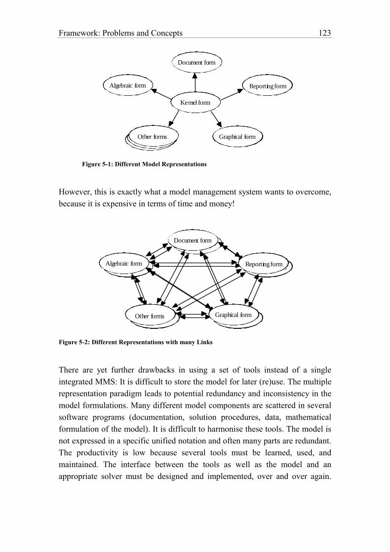
Framework: Problems and Concepts 123
Kernel form
Algebraic form
Document form
Reporting form
Graphical formOther forms
Figure 5-1: Different Model Representations
However, this is exactly what a model management system wants to overcome,
because it is expensive in terms of time and money!
Algebraic form
Document form
Reporting form
Graphical formOther forms
Algebraic form
Document form
Reporting form
Graphical formOther forms
Figure 5-2: Different Representations with many Links
There are yet further drawbacks in using a set of tools instead of a single
integrated MMS: It is difficult to store the model for later (re)use. The multiple
representation paradigm leads to potential redundancy and inconsistency in the
model formulations. Many different model components are scattered in several
software programs (documentation, solution procedures, data, mathematical
formulation of the model). It is difficult to harmonise these tools. The model is
not expressed in a specific unified notation and often many parts are redundant.
The productivity is low because several tools must be learned, used, and
maintained. The interface between the tools as well as the model and an
appropriate solver must be designed and implemented, over and over again.
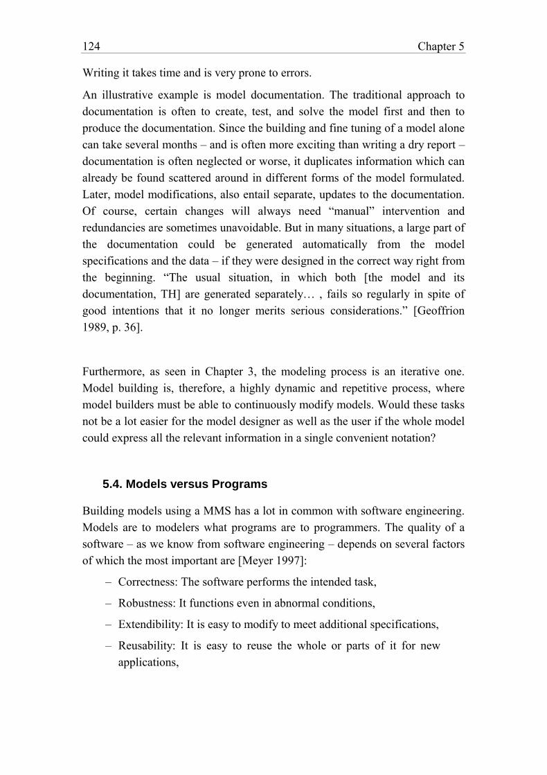
124 Chapter 5
Writing it takes time and is very prone to errors.
An illustrative example is model documentation. The traditional approach to
documentation is often to create, test, and solve the model first and then to
produce the documentation. Since the building and fine tuning of a model alone
can take several months – and is often more exciting than writing a dry report –
documentation is often neglected or worse, it duplicates information which can
already be found scattered around in different forms of the model formulated.
Later, model modifications, also entail separate, updates to the documentation.
Of course, certain changes will always need “manual” intervention and
redundancies are sometimes unavoidable. But in many situations, a large part of
the documentation could be generated automatically from the model
specifications and the data – if they were designed in the correct way right from
the beginning. “The usual situation, in which both [the model and its
documentation, TH] are generated separately… , fails so regularly in spite of
good intentions that it no longer merits serious considerations.” [Geoffrion
1989, p. 36].
Furthermore, as seen in Chapter 3, the modeling process is an iterative one.
Model building is, therefore, a highly dynamic and repetitive process, where
model builders must be able to continuously modify models. Would these tasks
not be a lot easier for the model designer as well as the user if the whole model
could express all the relevant information in a single convenient notation?
5.4. Models versus Programs
Building models using a MMS has a lot in common with software engineering.
Models are to modelers what programs are to programmers. The quality of a
software – as we know from software engineering – depends on several factors
of which the most important are [Meyer 1997]:
– Correctness: The software performs the intended task,
– Robustness: It functions even in abnormal conditions,
– Extendibility: It is easy to modify to meet additional specifications,
– Reusability: It is easy to reuse the whole or parts of it for new
applications,
Framework: Problems and Concepts 125
– Compatibility: It can easily be combined with others.
Correctness and robustness can be achieved by clear formal specifications and
requirements that software has to satisfy. Language designers have, therefore,
introduced different schemes, such as the type system, which checks not only
the syntax but also parts of the semantics of a program. Extendibility,
reusability, and compatibility call for flexible techniques to decompose the
problem into clearly defined software modules and components. Structured
programming, object-oriented design, and programming by components are all
paradigms in achieving these goals.
The quality of models also depends on similar criteria:
– Validity (correctness): The model expresses the state space, that is
intended by the problem,
– Sensitivity (robustness): The model is not ill-conditioned in the
sense that small variations in the data entail large shifts in the
solution,
– Extendibility: It is easy to modify and extend the model to meet
additional specifications and constraints,
– Reusability: It is easy to reuse whole or parts of the model for
different problems,
– Compatibility: It can easily be combined with other models at least
in a technical sense.
Model correctness can be obtained by a unique notation in which the whole
model can be formally specified and verified syntactically as well as
semantically by using compiler techniques. Model sensitivity is more delicate. It
is often difficult to achieve robust models. They must be solved over and over
again to gain insight into their behaviour. This process can only be assisted by a
tool that allows one to generate many model variations quickly and to solve
them automatically. Generating model variations, however, means that the
model structure and data must be displayed in an explicit specification – again
in a unique notation that can be modified and compiled quickly. Model
extendibility, reusability, and compatibility are achieved by a modular design
decomposing the model in several model components. This is especially
important for complex models which often consist of several loosely connected
126 Chapter 5
sub-models. It is natural to develop them independently from each other. In this
light, “model engineering” needs a similar framework to software engineering:
Both are in search of the ideal notation of problems for humans and computers.
Both are essentially frameworks for building components (modules) that
encapsulate a “piece of knowledge”. Whether these components are built using
a text editor or graphical tools is irrelevant in this context.
There is, however, an important difference between programming languages
and modeling languages. Models contain declarative knowledge that maps a
state space as defined in Chapter 2, whereas programs hold procedural
knowledge which maps an algorithm. Hence, programs can be executed but
model must be solved. The model specification does not say how to solve it.
Solving a model ultimately means, of course, applying a program, i.e.
translating the declarative specification into an algorithmic form that can be
executed by a procedure. A model seems to be “handicapped” when compared
with a program in the sense that it has not enough knowledge to process itself
in finding a solution, whereas a program is a complete specification of a
solution process.
On the other hand, describing a problem state space by a set of constraints
(which is the essence of a model) is a powerful means for formulating the
problem concisely and compactly. The reader only has to look at the energy
model (Example 5-1) at the end of this chapter to convince herself of this point.
Such a formulation is of great help if the modeler and the model user need to
modify the model, especially if constraints have to been added or removed.
More importantly, certain mathematical structures can be automatically derived
from the constraints and exploited for a solution. For example, certain cuts can
be generated automatically. Moreover, for many problem classes there exist
highly efficient commercial solvers and it would be pointless to reimplement
the whole solver. What the modeler needs in this case is a modeling
environment that allows her to translate the model specification into an
appropriate input stream for the solver at hand.
The above arguments lead to the following consequence: a MMS should be
based on a modeling language for representing models. Others have also
reached this conclusion: “To see why one language is so desirable, one need
only look at the current situation with its profusion of paradigm-specific styles
Framework: Problems and Concepts 127
for model representation …” [Geoffrion 1989, p. 36].
“Based on our experience we have concluded that the key to success is a
modeling technology where only one model representation is needed to
communicate with both humans and machines. The language should be a
powerful notation which can express all the relevant partitioning and structural
information contained in the real-world problem. In addition, the information
content of the model representation should be such that a machine can take over
the responsibility for verifying the algebraic correctness and completeness of
the model.” [Bisschop al. 1982, p. 13].
Of course, the usefulness of such a lingua franca for model representation, as
Geoffrion calls it, depends on the language entities to express a problem
concisely on the one hand, and translation procedures to restate it in efficient
forms for a solution process on the other. It is not sufficient to offer equation-
like notation as many algebraic languages do. Special operators and functions
must be implemented into the language in order to formulate various problem
patterns.
The postulated “kernel form” does not entail that all of details of an
instanciated model must necessarily be stated in this notation (although this
should be possible at least for small models). On the contrary, data is preferably
stored in databases, solver relevant information might be kept separately, and
solution reports can use the powerful database reporting capabilities, etc. The
kernel form however should hold these tools together. Thus, it should be
possible to read the data from and write to databases easily, to dispatch the
“bare bone” mathematical model to a chosen solver to be solved, to send the
report-relevant information of the model to a report generating tool, etc.
To convince the reader of how concise a declarative formulation of a model in
a well designed model language might be, we present the following example.
The critical reader might still not be convinced of that such a formulation is
useful in the sense that it can be efficiently translated in a form a solver can
handle. We shall have more to say about this in Part III of this book. To end this
section, an example is presented which clearly shows the advantages of a
concise, declarative formulation of certain problems.

128 Chapter 5
Example 5-1: An Energy Import Problem
The example presented is from [Mitra/Lucas/Moody 1994]. The formal
specification of the model also gives a foretaste of LPL (see Part III). Let us
formulate a “simple” energy import problem as follows:
Coal, gas and nuclear fuel can be imported in order to satisfy the energy demands of a country. Three grades of gas and coal (low, medium, high) and one grade of nuclear fuel may be imported. The costs are known. Furthermore, there are upper and lower limits in the imported quantities from a country. What quantities should be imported to meet the demand if the import costs have to be minimized?
In addition, three further conditions must be fulfilled:
1 The supply condition: Each country can supply either up to three (non-nuclear) low or medium grade fuels or nuclear fuel and one high grade fuel.
2 The environmental restriction: Environmental regulations require that nuclear fuel can be used only if medium and low grades of gas and coal are excluded.
3 The energy mixing condition: If gas is imported then either the amount of gas energy imported must lie between 40–50% and the amount of coal energy must be between 20–30% of the total energy imported or the quantity of gas energy must lie between 50–60% and coal is not imported.
Using mathematical and logical notation to present the state space of the
problem, the model can be formalized as in Table 5-1:
Three sets must be declared
I = {low, medium, high} the quality grades of energy
J = {gas, coal} non-nuclear energy sources
K = {GB FR IC} countries from which energy is imported
With i I, j J, k K , the parameters are:
cijk (non-nuclear) energy unit costs imported,
lijk, uijk minimum and maximum amount of non-nuclear energy,
nck nuclear energy unit costs,
nlk, nuk minimum and maximum amount of nuclear energy,
e desired energy amount to import (the demand),
lRj , uRj minimum and maximum percentage of non-nuclear
energy if coal and gas are imported (40–50, 20–30%),
lA, uA minimum and maximum gas take if gas energy only
is imported (50–60%).
The numerical variables are:
Xijk quantity of non-nuclear energy imported,
Yk quantity of nuclear energy imported.
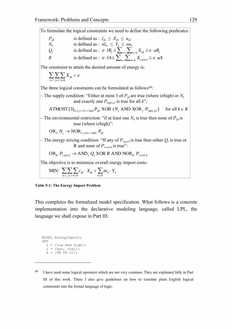
Framework: Problems and Concepts 129
To formulate the logical constraints we need to define the following predicates:
Pijk is defined as : lijk ≤ Xijk ≤ uijk
Nk is defined as : nlk, ≤ Yk ≤ nuk
Qj is defined as : e lRj XijkkKiI e uRj
R is defined as : e lA Xi, gas,kkKiI e uA
The constraint to attain the desired amount of energy is:
X ijk
kK
jJ
iI
e
The three logical constraints can be formulated as follows49:
– The supply condition: “Either at most 3 of Pijk are true (where i≠high) or Nk
and exactly one Phigh,j,k is true for all k”:
ATMOST (3)iI , jJ |i high Pijk XOR (N j AND XOR j Phigh, j,k ) for all k K
– The environmental restriction: “if at least one Nk is true then none of Pijk is
true (where i≠high)”:
ORk N j NORi , j ,k |i high Pijk
– The energy mixing condition: “If any of Pi,gas.k is true then either Qj is true or
R and none of Pi,coal,k is true”:
ORik Pi, gas,k AND j Qj XOR R AND NORik Pi,coal ,k
The objective is to minimize overall energy import costs:
MIN: cijk Xijk
kK
jJ
iI
nck Yk
kK
Table 5-1: The Energy Import Problem
This completes the formalized model specification. What follows is a concrete
implementation into the declarative modeling language, called LPL, the
language we shall expose in Part III.
MODEL EnergyImport;
SET
i = /low med high/;
j = /gas, coal/;
k = /GB FR IC/;
49 I have used some logical operators which are not very common. They are explained fully in Part
III of this work. There I also give guidelines on how to translate plain English logical
constraints into the formal language of logic.
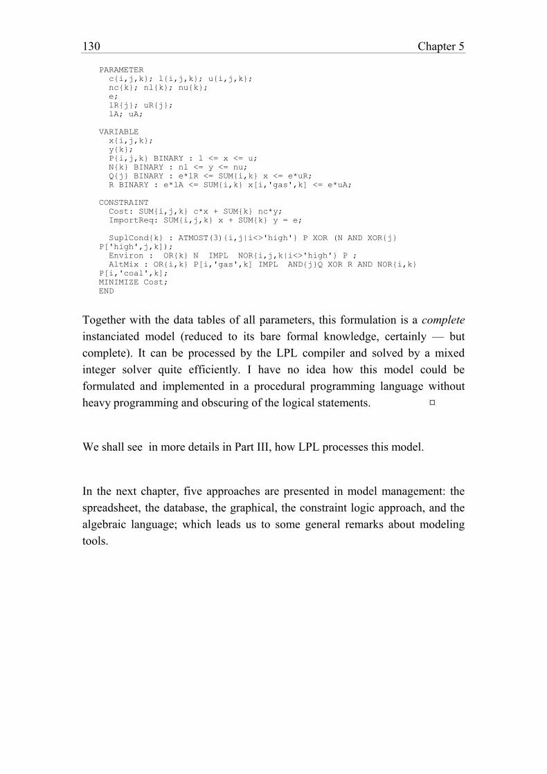
130 Chapter 5
PARAMETER
c{i,j,k}; l{i,j,k}; u{i,j,k};
nc{k}; nl{k}; nu{k};
e;
lR{j}; uR{j};
lA; uA;
VARIABLE
x{i,j,k};
y{k};
P{i,j,k} BINARY : l <= x <= u;
N{k} BINARY : nl <= y <= nu;
Q{j} BINARY : e*lR <= SUM{i,k} x <= e*uR;
R BINARY : e*lA <= SUM{i,k} x[i,'gas',k] <= e*uA;
CONSTRAINT
Cost: SUM{i,j,k} c*x + SUM{k} nc*y;
ImportReq: SUM{i,j,k} x + SUM{k} y = e;
SuplCond{k} : ATMOST(3){i,j|i<>'high'} P XOR (N AND XOR{j}
P['high',j,k]);
Environ : OR{k} N IMPL NOR{i,j,k|i<>'high'} P ;
AltMix : OR{i,k} P[i,'gas',k] IMPL AND{j}Q XOR R AND NOR{i,k}
P[i,'coal',k];
MINIMIZE Cost;
END
Together with the data tables of all parameters, this formulation is a complete
instanciated model (reduced to its bare formal knowledge, certainly — but
complete). It can be processed by the LPL compiler and solved by a mixed
integer solver quite efficiently. I have no idea how this model could be
formulated and implemented in a procedural programming language without
heavy programming and obscuring of the logical statements. ¤
We shall see in more details in Part III, how LPL processes this model.
In the next chapter, five approaches are presented in model management: the
spreadsheet, the database, the graphical, the constraint logic approach, and the
algebraic language; which leads us to some general remarks about modeling
tools.
131
6. AN OVERVIEW OF APPROACHES
Different approaches and modeling tools have been proposed. A quick tour is
given which makes no claim of being complete. Rather the aim is to get an idea
of what can be considered as the present state of mathematical modeling.
6.1. Spreadsheet
The approach which uses various spreadsheet technologies for modeling is
appealing and often straightforward. It offers many advantages by integrating
modeling tasks such as immediate evaluation, linking of data and expressions
and user defined tabular representation of various model parts. Recently, linear
and non-linear solvers can be easily attached to the models and the solution
algorithm can be triggered from the spreadsheet directly without leaving the
application. Furthermore, all these functionalities are neatly integrated in an
easy user interface. Today spreadsheets are sufficiently flexible and powerful to
represent even large models. It is also possible to call directly on external
solvers for these models. This approach to modeling seems to have a bright
future and its development has by no means reached its ultimate limits.
Although spreadsheets normally include a complete macro language and many
facilities to copy-paste cells and formulas, their main disadvantage in the
context of mathematical modeling is their lack of genericity: It is not easy to
extend a model having n variables, e.g., to a model of n+1 variables. Various
cells must be updated or copied and the overview of such an operation is
quickly lost. Another important disadvantage is that the structure of the
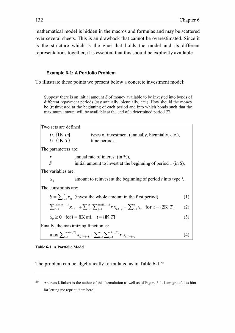
132 Chapter 6
mathematical model is hidden in the macros and formulas and may be scattered
over several sheets. This is an drawback that cannot be overestimated. Since it
is the structure which is the glue that holds the model and its different
representations together, it is essential that this should be explicitly available.
Example 6-1: A Portfolio Problem
To illustrate these points we present below a concrete investment model:
Suppose there is an initial amount S of money available to be invested into bonds of different repayment periods (say annually, biennially, etc.). How should the money be (re)invested at the beginning of each period and into which bonds such that the maximum amount will be available at the end of a determined period T?
Two sets are defined:
i{1K m} types of investment (annually, biennially, etc.),
t {1K T} time periods.
The parameters are:
ri annual rate of interest (in %),
S initial amount to invest at the beginning of period 1 (in $).
The variables are:
xit amount to reinvest at the beginning of period t into type i.
The constraints are:
S xi1i1
m
(invest the whole amount in the first period) (1)
xi, tii1
min{m,t1}
rixi, t jj1
min{i,t1}
i1
m
xiti1
m
for t {2K T} (2)
xit 0 for i {1K m}, t {1K T} (3)
Finally, the maximizing function is:
max xi, T1 ii1
min{m, T}
ri xi ,T1 jj1
min{i,T }
i1
m
(4)
Table 6-1: A Portfolio Model
The problem can be algebraically formulated as in Table 6-1.50
50 Andreas Klinkert is the author of this formulation as well as of Figure 6-1. I am grateful to him
for letting me reprint them here.
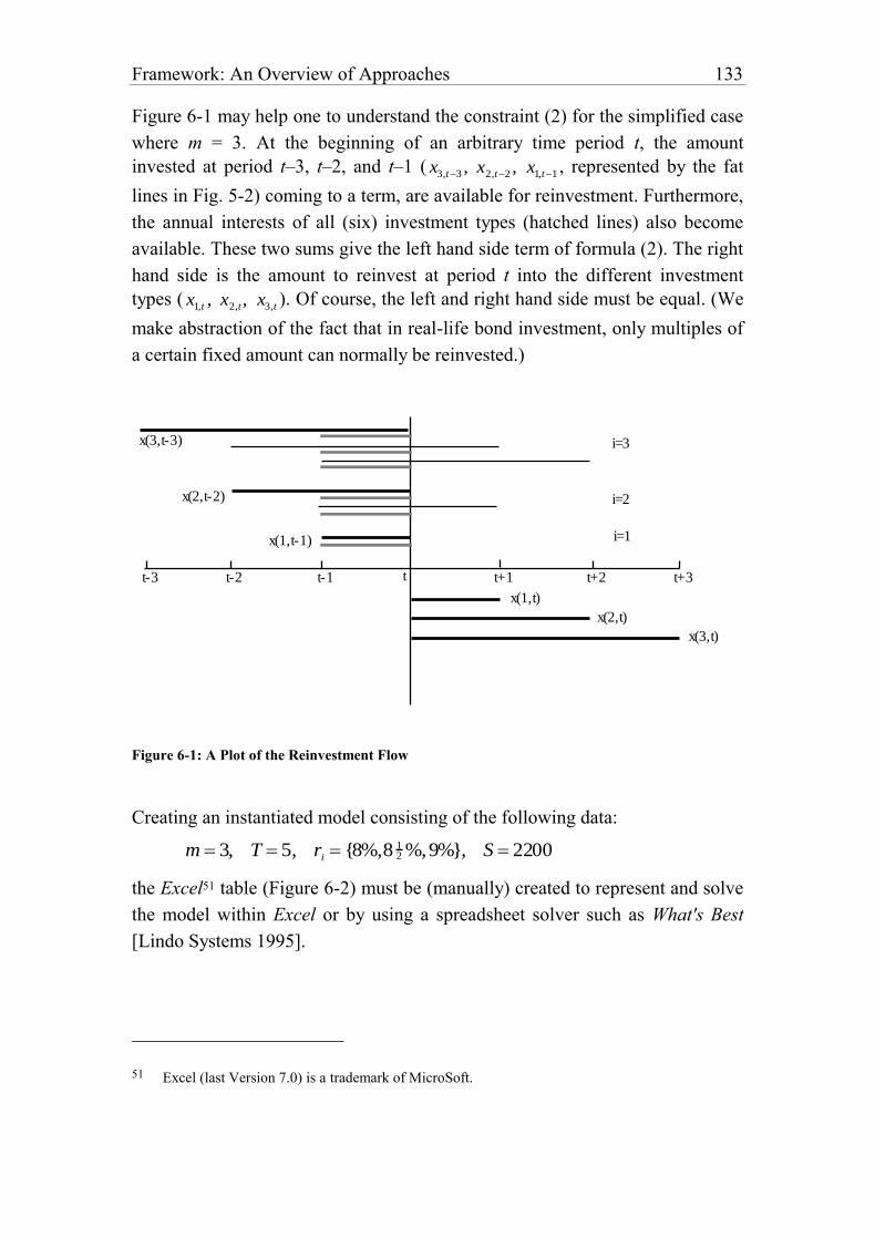
Framework: An Overview of Approaches 133
Figure 6-1 may help one to understand the constraint (2) for the simplified case
where m = 3. At the beginning of an arbitrary time period t, the amount
invested at period t–3, t–2, and t–1 ( x3,t3 , x2,t2 , x1,t1, represented by the fat
lines in Fig. 5-2) coming to a term, are available for reinvestment. Furthermore,
the annual interests of all (six) investment types (hatched lines) also become
available. These two sums give the left hand side term of formula (2). The right
hand side is the amount to reinvest at period t into the different investment
types ( x1,t , x2,t, x3,t). Of course, the left and right hand side must be equal. (We
make abstraction of the fact that in real-life bond investment, only multiples of
a certain fixed amount can normally be reinvested.)
t-3 t-2 t-1 t t+1 t+2 t+3
i=3
i=2
i=1
x(1,t)
x(2,t)
x(3,t)
x(3,t-3)
x(2,t-2)
x(1,t-1)
Figure 6-1: A Plot of the Reinvestment Flow
Creating an instantiated model consisting of the following data:
m 3, T 5, ri {8%,8 12 %,9%}, S 2200
the Excel51 table (Figure 6-2) must be (manually) created to represent and solve
the model within Excel or by using a spreadsheet solver such as What's Best
[Lindo Systems 1995].
51 Excel (last Version 7.0) is a trademark of MicroSoft.
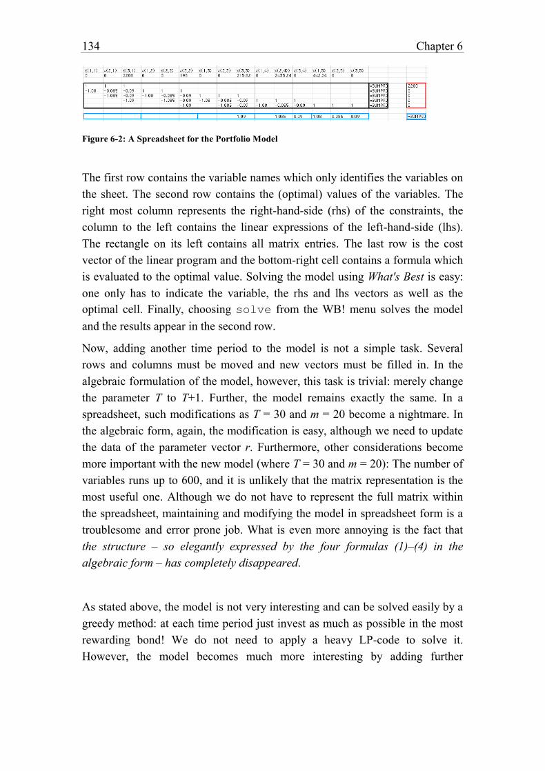
134 Chapter 6
Figure 6-2: A Spreadsheet for the Portfolio Model
The first row contains the variable names which only identifies the variables on
the sheet. The second row contains the (optimal) values of the variables. The
right most column represents the right-hand-side (rhs) of the constraints, the
column to the left contains the linear expressions of the left-hand-side (lhs).
The rectangle on its left contains all matrix entries. The last row is the cost
vector of the linear program and the bottom-right cell contains a formula which
is evaluated to the optimal value. Solving the model using What's Best is easy:
one only has to indicate the variable, the rhs and lhs vectors as well as the
optimal cell. Finally, choosing solve from the WB! menu solves the model
and the results appear in the second row.
Now, adding another time period to the model is not a simple task. Several
rows and columns must be moved and new vectors must be filled in. In the
algebraic formulation of the model, however, this task is trivial: merely change
the parameter T to T+1. Further, the model remains exactly the same. In a
spreadsheet, such modifications as T = 30 and m = 20 become a nightmare. In
the algebraic form, again, the modification is easy, although we need to update
the data of the parameter vector r. Furthermore, other considerations become
more important with the new model (where T = 30 and m = 20): The number of
variables runs up to 600, and it is unlikely that the matrix representation is the
most useful one. Although we do not have to represent the full matrix within
the spreadsheet, maintaining and modifying the model in spreadsheet form is a
troublesome and error prone job. What is even more annoying is the fact that
the structure – so elegantly expressed by the four formulas (1)–(4) in the
algebraic form – has completely disappeared.
As stated above, the model is not very interesting and can be solved easily by a
greedy method: at each time period just invest as much as possible in the most
rewarding bond! We do not need to apply a heavy LP-code to solve it.
However, the model becomes much more interesting by adding further
Framework: An Overview of Approaches 135
constraints or bounds on investment in various time periods. Such
modifications are straightforward in the algebraic formulation.
What makes the algebraic form superior is its use of indices for presenting the
genericity. In this way, sets of parameters, variables, and constraints can be
grouped together without being concerned about the cardinality of the index
sets. The structure of the model can clearly be separated from the instantiated
model. This is not the case in spreadsheets: the model is always represented as
an instance. It cannot represent a whole model class. This also becomes clear,
when we imagine an algorithm which reads an algebraic specification of the
model and returns the corresponding spreadsheet as output. (The other way
round – to read a spreadsheet and to output an algebraic specification – would
be much more involving.) Therefore, the algebraic form has the merit of being
the more general form, from which the spreadsheet form can be automatically
generated.
By the way, the above spreadsheet was partially produced by an add-in tool of
LPL. The input was the following LPL model which is close to the algebraic
notation given above. It is a complete formulation of the model:
MODEL Reinvestment;
SET i ALIAS j = /1:3/; (* the types of investments *)
t = /1:5/; (* the time periods *)
PARAMETER
S = 2200; (* initial amount to invest *)
r{i} = (7.5+0.5*i)/100; (* the interest rates *)
VARIABLE x{i,t};
CONSTRAINT
Per_1: SUM{i} x[i,1] = S;
Per_t{t | t>1} : SUM{i} x[i,t] = SUM{i | i<t} x[i,t-i]
+ SUM{i} (SUM {j | (j<t) and (j<=i)} r[i]*x[i,t-j]);
MAXIMIZE
Ret: SUM{i | i<=#t} x[i,#t+1-i]
+ SUM{i} (SUM{j | j<=#t and j<=i} r[i]*x[i,#t+1-j]);
END
The output of the add-on tool was the full matrix, the cost vector and the rhs
vector which would be used directly by the spreadsheet software. ¤
From Example 6-1 an important property of a fully-fletched indexed algebraic
form becomes obvious: Even if it is not an appropriate representation form for
many “end user modelers”, it can be used as a “nucleus form” (“kernel form”
above) from which many other representation forms can be automatically
136 Chapter 6
generated. This is an essential aspect which must be taken into account when
implementing modeling tools.
6.2. Relational Database Systems
Another approach to modeling that has gained great popularity in the last
decade is the use of relational databases. The relationships between relational
database and predicate calculus are well known [Ullman 1988]. (We assume
here that the reader is familiar with the relevant database terminology.) A
database consists of a set of tables, each containing a number of records (the
rows) and a number of attributes (the columns). If the table has the name
table and the attributes are called attr1, attr2, etc., then we may specify
a table by the notation
table(attr1,attr2,...)
Each record is an instance in which the attributes are assigned to a specific
value from a predefined domain. The whole table can be interpreted as a
(possibly sparse) subset of the Cartesian product over all attributes. Tables can
be linked together by well understood operations such as selection,
projection, join and others. In logic and logic programming (Prolog) a
predicate can be interpreted as a table in this sense and vice-versa.
Many researchers have insisted on the similarities between the declarative
model representation and the relational database approach [Dolk 1988],
[Johnson 1989], [Müller-Merbach 1990], [Lenard 1988]. Many tasks for
creating the model can be achieved by using the data definition language
(DDL) in database environments; and the tasks for manipulating, modifying,
and maintaining the model can be accomplished using the data manipulation
language (DML). Some researchers have even reduced modeling management
to database design and manipulation [Dolk al. 1984].
It is true that the database approach has an important advantage compared with
the spreadsheet approach: Genericity is an essential component of all databases.
Furthermore, if the database is well-designed, the data integrity is inherent. For
models with a large amount of data, most of the modeling time is probably
consumed by designing and manipulating the database. Nevertheless, model
management cannot be reduced to data management, it is not simply “storage,
retrieval, and updating”. One essential component is still missing: The model
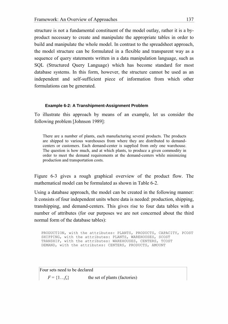
Framework: An Overview of Approaches 137
structure is not a fundamental constituent of the model outlay, rather it is a by-
product necessary to create and manipulate the appropriate tables in order to
build and manipulate the whole model. In contrast to the spreadsheet approach,
the model structure can be formulated in a flexible and transparent way as a
sequence of query statements written in a data manipulation language, such as
SQL (Structured Query Language) which has become standard for most
database systems. In this form, however, the structure cannot be used as an
independent and self-sufficient piece of information from which other
formulations can be generated.
Example 6-2: A Transhipment-Assignment Problem
To illustrate this approach by means of an example, let us consider the
following problem [Johnson 1989]:
There are a number of plants, each manufacturing several products. The products are shipped to various warehouses from where they are distributed to demand-centers or customers. Each demand-center is supplied from only one warehouse. The question is how much, and at which plants, to produce a given commodity in order to meet the demand requirements at the demand-centers while minimizing production and transportation costs.
Figure 6-3 gives a rough graphical overview of the product flow. The
mathematical model can be formulated as shown in Table 6-2.
Using a database approach, the model can be created in the following manner:
It consists of four independent units where data is needed: production, shipping,
transhipping, and demand-centers. This gives rise to four data tables with a
number of attributes (for our purposes we are not concerned about the third
normal form of the database tables):
PRODUCTION, with the attributes: PLANTS, PRODUCTS, CAPACITY, PCOST
SHIPPING, with the attributes: PLANTS, WAREHOUSES, SCOST
TRANSHIP, with the attributes: WAREHOUSES, CENTERS, TCOST
DEMAND, with the attributes: CENTERS, PRODUCTS, AMOUNT
Four sets need to be declared
F = {1…fn} the set of plants (factories)
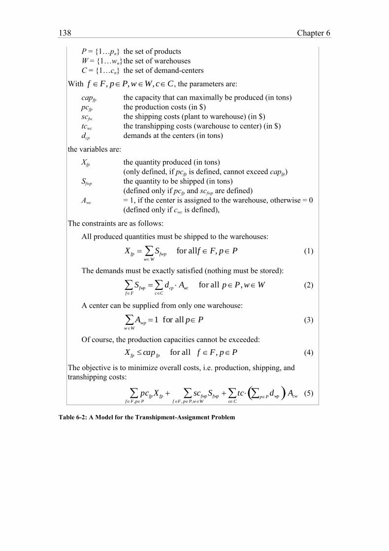
138 Chapter 6
P = {1…pn} the set of products
W = {1…wn} the set of warehouses
C = {1…cn} the set of demand-centers
With f F, pP,w W,cC , the parameters are:
capfp the capacity that can maximally be produced (in tons)
pcfp the production costs (in $)
scfw the shipping costs (plant to warehouse) (in $)
tcwc the transhipping costs (warehouse to center) (in $)
dcp demands at the centers (in tons)
the variables are:
Xfp the quantity produced (in tons)
(only defined, if pcfp is defined, cannot exceed capfp)
Sfwp the quantity to be shipped (in tons)
(defined only if pcfp and scfwp are defined)
Awc = 1, if the center is assigned to the warehouse, otherwise = 0
(defined only if cwc is defined),
The constraints are as follows:
All produced quantities must be shipped to the warehouses:
X fp Sfwp
wW
for all f F, pP (1)
The demands must be exactly satisfied (nothing must be stored):
Sfwp
fF
dcp Awc
cC
for all pP , wW (2)
A center can be supplied from only one warehouse:
Awp
wW
1 for all pP (3)
Of course, the production capacities cannot be exceeded:
X fp cap fp for all f F, pP (4)
The objective is to minimize overall costs, i.e. production, shipping, and
transhipping costs:
pcfp X fp
fF ,pP
scfwp Sfwp
f F , pP,wW
tc dwppP cC
Acw (5)
Table 6-2: A Model for the Transhipment-Assignment Problem
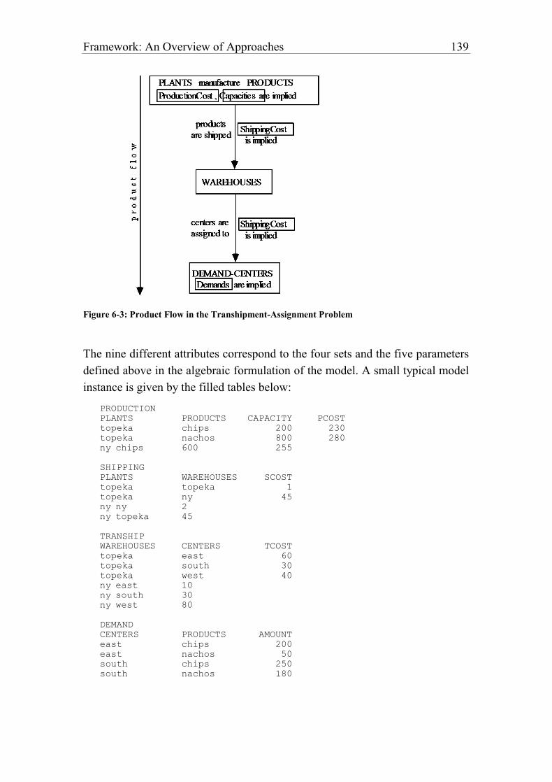
Framework: An Overview of Approaches 139
Figure 6-3: Product Flow in the Transhipment-Assignment Problem
The nine different attributes correspond to the four sets and the five parameters
defined above in the algebraic formulation of the model. A small typical model
instance is given by the filled tables below:
PRODUCTION
PLANTS PRODUCTS CAPACITY PCOST
topeka chips 200 230
topeka nachos 800 280
ny chips 600 255
SHIPPING
PLANTS WAREHOUSES SCOST
topeka topeka 1
topeka ny 45
ny ny 2
ny topeka 45
TRANSHIP
WAREHOUSES CENTERS TCOST
topeka east 60
topeka south 30
topeka west 40
ny east 10
ny south 30
ny west 80
DEMAND
CENTERS PRODUCTS AMOUNT
east chips 200
east nachos 50
south chips 250
south nachos 180
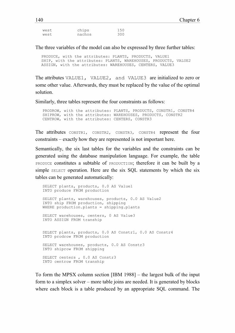
140 Chapter 6
west chips 150
west nachos 300
The three variables of the model can also be expressed by three further tables:
PRODUCE, with the attributes: PLANTS, PRODUCTS, VALUE1
SHIP, with the attributes: PLANTS, WAREHOUSES, PRODUCTS, VALUE2
ASSIGN, with the attributes: WAREHOUSES, CENTERS, VALUE3
The attributes VALUE1, VALUE2, and VALUE3 are initialized to zero or
some other value. Afterwards, they must be replaced by the value of the optimal
solution.
Similarly, three tables represent the four constraints as follows:
PRODROW, with the attributes: PLANTS, PRODUCTS, CONSTR1, CONSTR4
SHIPROW, with the attributes: WAREHOUSES, PRODUCTS, CONSTR2
CENTROW, with the attributes: CENTERS, CONSTR3
The attributes CONSTR1, CONSTR2, CONSTR3, CONSTR4 represent the four
constraints – exactly how they are represented is not important here.
Semantically, the six last tables for the variables and the constraints can be
generated using the database manipulation language. For example, the table
PRODUCE constitutes a subtable of PRODUCTION; therefore it can be built by a
simple SELECT operation. Here are the six SQL statements by which the six
tables can be generated automatically:
SELECT plants, products, 0.0 AS Value1
INTO produce FROM production
SELECT plants, warehouses, products, 0.0 AS Value2
INTO ship FROM production, shipping
WHERE production.plants = shipping.plants
SELECT warehouses, centers, 0 AS Value3
INTO ASSIGN FROM tranship
SELECT plants, products, 0.0 AS Constr1, 0.0 AS Constr4
INTO prodrow FROM production
SELECT warehouses, products, 0.0 AS Constr3
INTO shiprow FROM shipping
SELECT centers , 0.0 AS Constr3
INTO centrow FROM tranship
To form the MPSX column section [IBM 1988] – the largest bulk of the input
form to a simplex solver – more table joins are needed. It is generated by blocks
where each block is a table produced by an appropriate SQL command. The
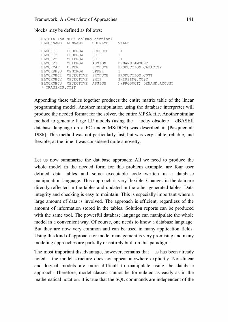
Framework: An Overview of Approaches 141
blocks may be defined as follows:
MATRIX (as MPSX column section)
BLOCKNAME ROWNAME COLNAME VALUE
BLOCK11 PRODROW PRODUCE -1
BLOCK12 PRODROW SHIP 1
BLOCK22 SHIPROW SHIP -1
BLOCK23 SHIPROW ASSIGN DEMAND.AMOUNT
BLOCKCAP UPPER PRODUCE PRODUCTION.CAPACITY
BLOCKRHS3 CENTROW UPPER 1
BLOCKOBJ1 OBJECTIVE PRODUCE PRODUCTION.COST
BLOCKOBJ2 OBJECTIVE SHIP SHIPPING.COST
BLOCKOBJ3 OBJECTIVE ASSIGN ∑(PRODUCT) DEMAND.AMOUNT
* TRANSHIP.COST
Appending these tables together produces the entire matrix table of the linear
programming model. Another manipulation using the database interpreter will
produce the needed format for the solver, the entire MPSX file. Another similar
method to generate large LP models (using the – today obsolete – dBASEII
database language on a PC under MS/DOS) was described in [Pasquier al.
1986]. This method was not particularly fast, but was very stable, reliable, and
flexible; at the time it was considered quite a novelty.
Let us now summarize the database approach: All we need to produce the
whole model in the needed form for this problem example, are four user
defined data tables and some executable code written in a database
manipulation language. This approach is very flexible. Changes in the data are
directly reflected in the tables and updated in the other generated tables. Data
integrity and checking is easy to maintain. This is especially important where a
large amount of data is involved. The approach is efficient, regardless of the
amount of information stored in the tables. Solution reports can be produced
with the same tool. The powerful database language can manipulate the whole
model in a convenient way. Of course, one needs to know a database language.
But they are now very common and can be used in many application fields.
Using this kind of approach for model management is very promising and many
modeling approaches are partially or entirely built on this paradigm.
The most important disadvantage, however, remains that – as has been already
noted – the model structure does not appear anywhere explicitly. Non-linear
and logical models are more difficult to manipulate using the database
approach. Therefore, model classes cannot be formulated as easily as in the
mathematical notation. It is true that the SQL commands are independent of the
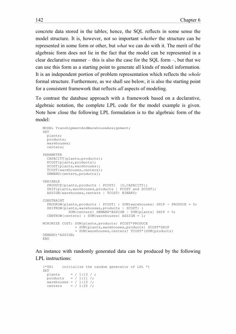
142 Chapter 6
concrete data stored in the tables; hence, the SQL reflects in some sense the
model structure. It is, however, not so important whether the structure can be
represented in some form or other, but what we can do with it. The merit of the
algebraic form does not lie in the fact that the model can be represented in a
clear declarative manner – this is also the case for the SQL form –, but that we
can use this form as a starting point to generate all kinds of model information.
It is an independent portion of problem representation which reflects the whole
formal structure. Furthermore, as we shall see below, it is also the starting point
for a consistent framework that reflects all aspects of modeling.
To contrast the database approach with a framework based on a declarative,
algebraic notation, the complete LPL code for the model example is given.
Note how close the following LPL formulation is to the algebraic form of the
model:
MODEL TranshipmentAndWarehouseAssignment;
SET
plants;
products;
warehouses;
centers;
PARAMETER
CAPACITY{plants,products};
PCOST{plants,products};
SCOST{plants,warehouses};
TCOST{warehouses,centers};
DEMAND{centers,products};
VARIABLE
PRODUCE{plants,products | PCOST} [0,CAPACITY];
SHIP{plants,warehouses,products | PCOST and SCOST};
ASSIGN{warehouses,centers | TCOST} BINARY;
CONSTRAINT
PRODROW{plants,products | PCOST} : SUM{warehouses} SHIP - PRODUCE = 0;
SHIPROW{plants,warehouses,products | SCOST} :
SUM{centers} DEMAND*ASSIGN - SUM{plants} SHIP = 0;
CENTROW{centers} : SUM{warehouses} ASSIGN = 1;
MINIMIZE COST: SUM{plants,products} PCOST*PRODUCE
+ SUM{plants,warehouses,products} SCOST*SHIP
+ SUM{warehouses,centers} TCOST*(SUM{products}
DEMAND)*ASSIGN;
END
An instance with randomly generated data can be produced by the following
LPL instructions:
(*$R1 initialize the random generator of LPL *)
SET
plants = / 1:13 / ;
products = / 1:11 /;
warehouses = / 1:10 /;
centers = / 1:20 /;
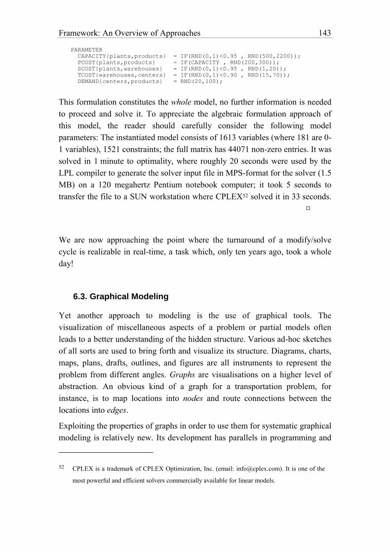
Framework: An Overview of Approaches 143
PARAMETER
CAPACITY{plants,products} = IF(RND(0,1)<0.95 , RND(500,2200));
PCOST{plants,products} = IF(CAPACITY , RND(200,300));
SCOST{plants,warehouses} = IF(RND(0,1)<0.95 , RND(1,20));
TCOST{warehouses,centers} = IF(RND(0,1)<0.90 , RND(15,70));
DEMAND{centers,products} = RND(20,100);
This formulation constitutes the whole model, no further information is needed
to proceed and solve it. To appreciate the algebraic formulation approach of
this model, the reader should carefully consider the following model
parameters: The instantiated model consists of 1613 variables (where 181 are 0-
1 variables), 1521 constraints; the full matrix has 44071 non-zero entries. It was
solved in 1 minute to optimality, where roughly 20 seconds were used by the
LPL compiler to generate the solver input file in MPS-format for the solver (1.5
MB) on a 120 megahertz Pentium notebook computer; it took 5 seconds to
transfer the file to a SUN workstation where CPLEX52 solved it in 33 seconds.
¤
We are now approaching the point where the turnaround of a modify/solve
cycle is realizable in real-time, a task which, only ten years ago, took a whole
day!
6.3. Graphical Modeling
Yet another approach to modeling is the use of graphical tools. The
visualization of miscellaneous aspects of a problem or partial models often
leads to a better understanding of the hidden structure. Various ad-hoc sketches
of all sorts are used to bring forth and visualize its structure. Diagrams, charts,
maps, plans, drafts, outlines, and figures are all instruments to represent the
problem from different angles. Graphs are visualisations on a higher level of
abstraction. An obvious kind of a graph for a transportation problem, for
instance, is to map locations into nodes and route connections between the
locations into edges.
Exploiting the properties of graphs in order to use them for systematic graphical
modeling is relatively new. Its development has parallels in programming and
52 CPLEX is a trademark of CPLEX Optimization, Inc. (email: [email protected]). It is one of the
most powerful and efficient solvers commercially available for linear models.
144 Chapter 6
database design where many specific graphical case tools have been developed
and are in use. Also in simulation modeling, it is today common practice to set
up the model by placing different icons on the screen and connecting them
together with links of varying semantics. While doing so, the mathematical
model is automatically created in the background.
The fundamental idea of graphical modeling tools is exactly the same: By
means of a graphical editor, the model is built and modified, and the
mathematical model – in whatever form – is automatically generated.
Furthermore, graphical tools are excellent devices for browsing a model. This
greatly assists in keeping an overview of a large model.
Several implementations of graphical modeling tools have been presented in
recent years for specific model classes. For the transportation models a system
called GIN [Steiger al. 1992] is based on the well known NETFORM concept
[Glover al. 1977] which will be the object of the example below. GNGEN is
another system also based on the same ideas [Forster al. 1994]. For linear
models [Collaud/Pasquier 1994] has implemented the well-known A-C graph
(the activity-constraint graph), a bipartite graph where each variable and
constraint is represented as a node; a variable node is linked to a constraint
node by an edge if the variable occurs in the corresponding constraint. Other
more general graphs have been proposed by [Geoffrion 1987] in the framework
of structured modeling. He suggested three graphs for presenting different
aspects of a model: the modular graph, the genus graph, and the elemental
graph, each of which corresponds to a well-defined structure in his framework.
(I shall have more to say about them later.) An entirely graph-based
methodology was proposed by [Jones 1990, 1991, and 1996]. This approach is
founded on the concepts of attributed graphs and graph grammars.
While it is interesting to generate the model from a graphical form, generating
different graphical representations from a mathematical model – represented in
algebraic form, for instance – has received surprisingly little attention. This is
something even more useful especially for large models. Graphical layouts of
partial aspects of the mathematical model are very helpful not only in
visualizing certain relationships which are more difficult to see in the algebraic
formulation but also for quickly browsing the model. A computer-based MMS
should certainly offer several browsing tools and the modeler should be able to
Framework: An Overview of Approaches 145
switch from one to another without too much difficulty. We will see more
concrete examples in Part III when presenting the LPL environment and
modeling tools. For now, let us explain by means of an example showing the
intended ideas behind a specific type of graphical modeling tool – note however
that there are many others.
Example 6-3: The Transportation Problem
We can use the transportation problem to illustrate the relationships between
the mathematical formulation and a specific graphical representation of the
model.
The problem is to transport commodities from supply centers to demand centers (by using intermediate storage centers eventually). On which routes and in how large a quantity should the commodity be transported in order to minimize the overall transportation costs?
The formulation of the transportation problem is as shown in Table 6-3.
If bi is positive in (1), the node is said to be a source (or a supply node). If it is
negative, it is a sink (or demand node). If bi is zero, the node is just an
intermediate storage location where nothing is produced or consumed. What
goes in at the node must also go out.
The structure of the problem can also be represented as a directed graph where
the nodes correspond to the locations and the arcs to the routes. At each node
the net in- or outflow (b) must be given. On each arc, three parameters are
given: the lower (lij) and upper (uij) capacities as well as the costs (cij). Since
on each arc an unknown amount must be transported, each arc (i,j) also has an
unknown quantity Xij assigned.
A small model instance is depicted in Figure 6-4. Four locations are given
where one is a source, another is the sink and two nodes are intermediate nodes.
The transportation routes are shown as arcs.
The sets of locations and links are defined as:
N = {1…n} the set of locations,
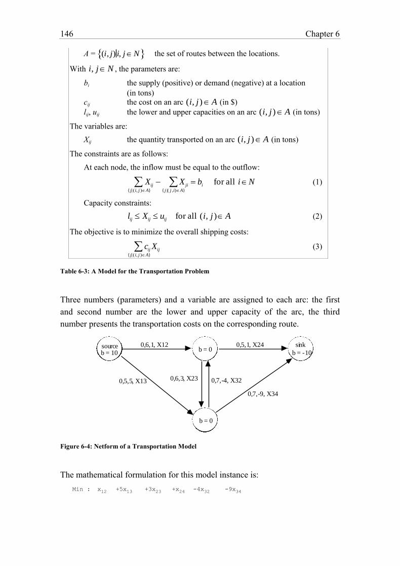
146 Chapter 6
A = (i, j) i, jN the set of routes between the locations.
With i, jN , the parameters are:
bi the supply (positive) or demand (negative) at a location
(in tons)
cij the cost on an arc (i, j)A (in $)
lij, uij the lower and upper capacities on an arc (i, j)A (in tons)
The variables are:
Xij the quantity transported on an arc (i, j)A (in tons)
The constraints are as follows:
At each node, the inflow must be equal to the outflow:
Xij
{ j| ( i, j )A}
X ji bi
{ j |( j ,i)A}
for all iN (1)
Capacity constraints:
lij Xij uij for all (i, j )A (2)
The objective is to minimize the overall shipping costs:
cij Xij
{ j| ( i, j )A}
(3)
Table 6-3: A Model for the Transportation Problem
Three numbers (parameters) and a variable are assigned to each arc: the first
and second number are the lower and upper capacity of the arc, the third
number presents the transportation costs on the corresponding route.
source sinkb = 0
b = 10 b = -10
0,6,1, X12
b = 0
0,5,1, X24
0,6,3, X23
0,7,-9, X34
0,5,5, X13 0,7,-4, X32
Figure 6-4: Netform of a Transportation Model
The mathematical formulation for this model instance is:
Min : x12 +5x
13 +3x
23 +x
24 -4x
32 -9x
34
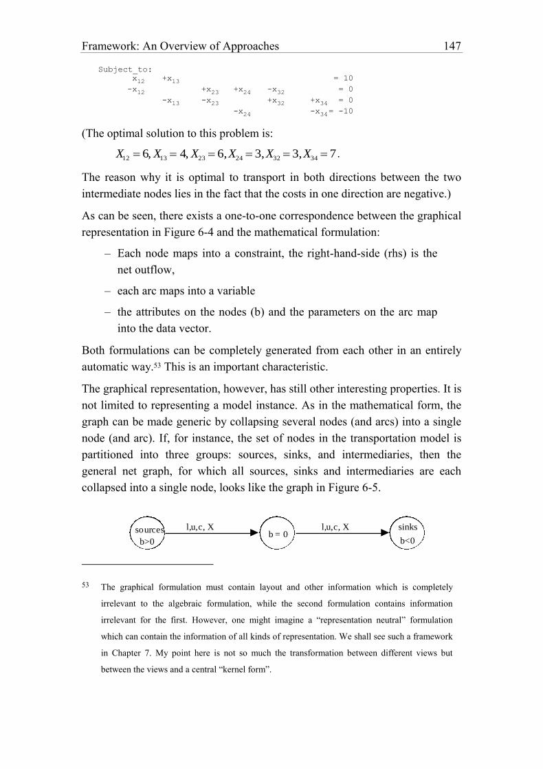
Framework: An Overview of Approaches 147
Subject_to:
x12 +x
13 = 10
-x12 +x
23 +x
24 -x
32 = 0
-x13 -x
23 +x
32 +x
34 = 0
-x24 -x
34 = -10
(The optimal solution to this problem is:
X12 6, X13 4, X23 6,X24 3,X32 3,X34 7 .
The reason why it is optimal to transport in both directions between the two
intermediate nodes lies in the fact that the costs in one direction are negative.)
As can be seen, there exists a one-to-one correspondence between the graphical
representation in Figure 6-4 and the mathematical formulation:
– Each node maps into a constraint, the right-hand-side (rhs) is the
net outflow,
– each arc maps into a variable
– the attributes on the nodes (b) and the parameters on the arc map
into the data vector.
Both formulations can be completely generated from each other in an entirely
automatic way.53 This is an important characteristic.
The graphical representation, however, has still other interesting properties. It is
not limited to representing a model instance. As in the mathematical form, the
graph can be made generic by collapsing several nodes (and arcs) into a single
node (and arc). If, for instance, the set of nodes in the transportation model is
partitioned into three groups: sources, sinks, and intermediaries, then the
general net graph, for which all sources, sinks and intermediaries are each
collapsed into a single node, looks like the graph in Figure 6-5.
sources sinksb = 0
b>0 b<0
l,u,c, X l,u,c, X
53 The graphical formulation must contain layout and other information which is completely
irrelevant to the algebraic formulation, while the second formulation contains information
irrelevant for the first. However, one might imagine a “representation neutral” formulation
which can contain the information of all kinds of representation. We shall see such a framework
in Chapter 7. My point here is not so much the transformation between different views but
between the views and a central “kernel form”.
148 Chapter 6
Figure 6-5: Aggregated Netform for the Transportation Model
This collapsing operation will be called folding in the remaining part of this
book. The inverse operation is also of interest: a node representing a group of
objects can be unfolded. We will see another more interesting example of
graphical modeling in Part III.
¤
Let us quickly summarize the pros and cons of graphical tools: Graphical
modeling tools seem to be very attractive because they can reveal the structure
in a way which is “closer” to a particular user. The NETFORM graph, for
instance, is similar to a geographical network of routes on the one hand, but on
the other hand it maps the mathematical structure bijectively – which can be
generated automatically. Certain aspects of the model can be visualized. Of
course, the NETFORM graph is a lucky exception in the sense that it can be
interpreted as a mathematical structure as well as a visual picture of the route
map. Other graphs, that are not so easily interpreted can also be interesting
when it comes to visualizing certain abstract aspects of the model, as will be
seen in Part III by the different LPN-graphs of a model.
However, modeling exclusively with the aid of graphical tools also has its
disadvantages. No graphical structure is actually known, which could represent
all kind of mathematical models. Graphical modeling is not general enough.
Each model class needs another specific set of graphical tools. This poses the
problem of how to represent the model in a unified framework. We are now at
the point where we offer different tools for different model types and
subclasses. Neither reusability nor communication between them is possible
any longer. If, for instance, we have a transportation model and we want to add
a new (arbitrary) constraint, the NETFORM graph can no longer be used as a
representation tool of the whole model since it is no longer a pure
transportation model. How should the transportation part of the model be
translated into another graphical representation appropriate to the new
structure? We need a representation or a form, in which the model can be stored
in a unified way. The algebraic form is such a form. In our example, we just
have to add the constraint in algebraic notation. (The model, of course, must
eventually be sent to another solver in order to be efficiently solved – but that is
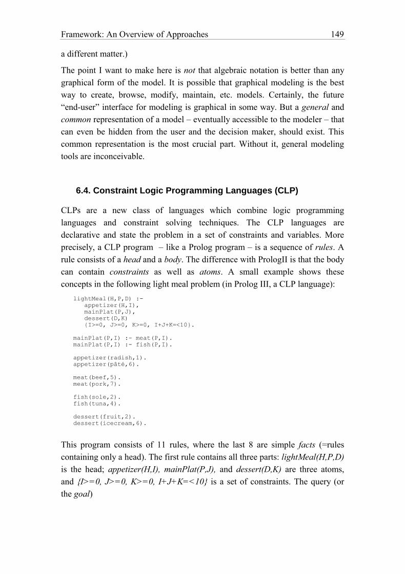
Framework: An Overview of Approaches 149
a different matter.)
The point I want to make here is not that algebraic notation is better than any
graphical form of the model. It is possible that graphical modeling is the best
way to create, browse, modify, maintain, etc. models. Certainly, the future
“end-user” interface for modeling is graphical in some way. But a general and
common representation of a model – eventually accessible to the modeler – that
can even be hidden from the user and the decision maker, should exist. This
common representation is the most crucial part. Without it, general modeling
tools are inconceivable.
6.4. Constraint Logic Programming Languages (CLP)
CLPs are a new class of languages which combine logic programming
languages and constraint solving techniques. The CLP languages are
declarative and state the problem in a set of constraints and variables. More
precisely, a CLP program – like a Prolog program – is a sequence of rules. A
rule consists of a head and a body. The difference with PrologII is that the body
can contain constraints as well as atoms. A small example shows these
concepts in the following light meal problem (in Prolog III, a CLP language):
lightMeal(H,P,D) :-
appetizer(H,I),
mainPlat(P,J),
dessert(D,K)
{I>=0, J>=0, K>=0, I+J+K=<10}.
mainPlat(P,I) :- meat(P,I).
mainPlat(P,I) :- fish(P,I).
appetizer(radish,1).
appetizer(pâté,6).
meat(beef,5).
meat(pork,7).
fish(sole,2).
fish(tuna,4).
dessert(fruit,2).
dessert(icecream,6).
This program consists of 11 rules, where the last 8 are simple facts (=rules
containing only a head). The first rule contains all three parts: lightMeal(H,P,D)
is the head; appetizer(H,I), mainPlat(P,J), and dessert(D,K) are three atoms,
and {I>=0, J>=0, K>=0, I+J+K=<10} is a set of constraints. The query (or
the goal)
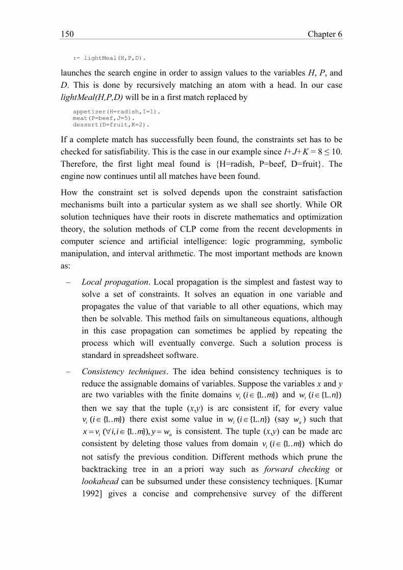
150 Chapter 6
:- lightMeal(H,P,D).
launches the search engine in order to assign values to the variables H, P, and
D. This is done by recursively matching an atom with a head. In our case
lightMeal(H,P,D) will be in a first match replaced by
appetizer(H=radish,I=1).
meat(P=beef,J=5).
dessert(D=fruit,K=2).
If a complete match has successfully been found, the constraints set has to be
checked for satisfiability. This is the case in our example since I+J+K = 8 ≤ 10.
Therefore, the first light meal found is {H=radish, P=beef, D=fruit}. The
engine now continues until all matches have been found.
How the constraint set is solved depends upon the constraint satisfaction
mechanisms built into a particular system as we shall see shortly. While OR
solution techniques have their roots in discrete mathematics and optimization
theory, the solution methods of CLP come from the recent developments in
computer science and artificial intelligence: logic programming, symbolic
manipulation, and interval arithmetic. The most important methods are known
as:
– Local propagation. Local propagation is the simplest and fastest way to
solve a set of constraints. It solves an equation in one variable and
propagates the value of that variable to all other equations, which may
then be solvable. This method fails on simultaneous equations, although
in this case propagation can sometimes be applied by repeating the
process which will eventually converge. Such a solution process is
standard in spreadsheet software.
– Consistency techniques. The idea behind consistency techniques is to
reduce the assignable domains of variables. Suppose the variables x and y
are two variables with the finite domains vi (i{1..m}) and wi (i{1..n})
then we say that the tuple (x,y) is arc consistent if, for every value
vi (i{1..m}) there exist some value in wi (i{1..n}) (say wa ) such that
x vi (i,i{1..m}), y wa is consistent. The tuple (x,y) can be made arc
consistent by deleting those values from domain vi (i{1..m}) which do
not satisfy the previous condition. Different methods which prune the
backtracking tree in an a priori way such as forward checking or
lookahead can be subsumed under these consistency techniques. [Kumar
1992] gives a concise and comprehensive survey of the different
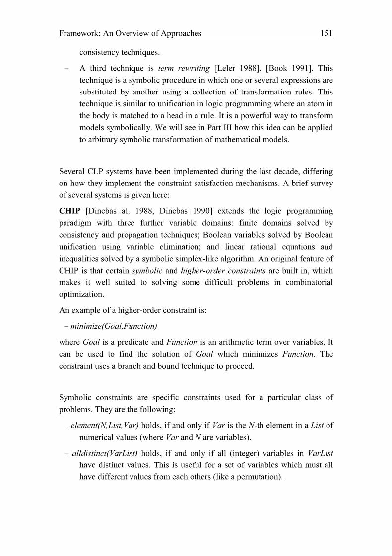
Framework: An Overview of Approaches 151
consistency techniques.
– A third technique is term rewriting [Leler 1988], [Book 1991]. This
technique is a symbolic procedure in which one or several expressions are
substituted by another using a collection of transformation rules. This
technique is similar to unification in logic programming where an atom in
the body is matched to a head in a rule. It is a powerful way to transform
models symbolically. We will see in Part III how this idea can be applied
to arbitrary symbolic transformation of mathematical models.
Several CLP systems have been implemented during the last decade, differing
on how they implement the constraint satisfaction mechanisms. A brief survey
of several systems is given here:
CHIP [Dincbas al. 1988, Dincbas 1990] extends the logic programming
paradigm with three further variable domains: finite domains solved by
consistency and propagation techniques; Boolean variables solved by Boolean
unification using variable elimination; and linear rational equations and
inequalities solved by a symbolic simplex-like algorithm. An original feature of
CHIP is that certain symbolic and higher-order constraints are built in, which
makes it well suited to solving some difficult problems in combinatorial
optimization.
An example of a higher-order constraint is:
– minimize(Goal,Function)
where Goal is a predicate and Function is an arithmetic term over variables. It
can be used to find the solution of Goal which minimizes Function. The
constraint uses a branch and bound technique to proceed.
Symbolic constraints are specific constraints used for a particular class of
problems. They are the following:
– element(N,List,Var) holds, if and only if Var is the N-th element in a List of
numerical values (where Var and N are variables).
– alldistinct(VarList) holds, if and only if all (integer) variables in VarList
have distinct values. This is useful for a set of variables which must all
have different values from each others (like a permutation).
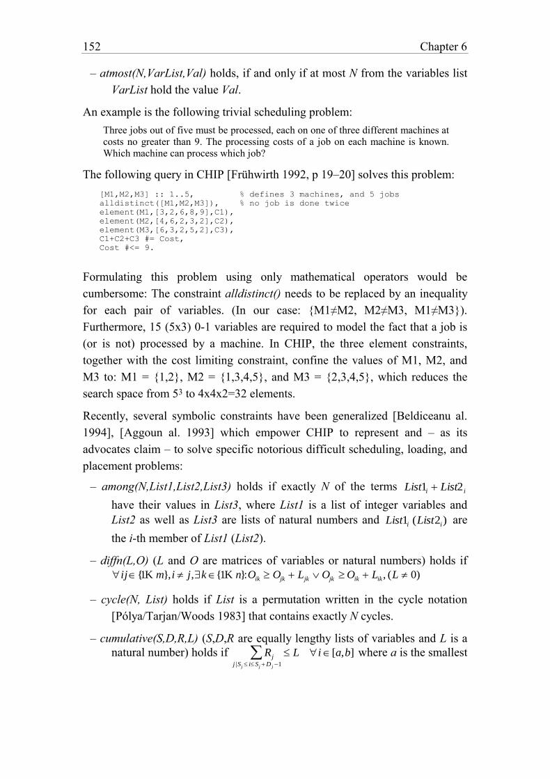
152 Chapter 6
– atmost(N,VarList,Val) holds, if and only if at most N from the variables list
VarList hold the value Val.
An example is the following trivial scheduling problem:
Three jobs out of five must be processed, each on one of three different machines at costs no greater than 9. The processing costs of a job on each machine is known. Which machine can process which job?
The following query in CHIP [Frühwirth 1992, p 19–20] solves this problem:
[M1,M2,M3] :: 1..5, % defines 3 machines, and 5 jobs
alldistinct([M1,M2,M3]), % no job is done twice
element(M1,[3,2,6,8,9],C1),
element(M2,[4,6,2,3,2],C2),
element(M3,[6,3,2,5,2],C3),
C1+C2+C3 #= Cost,
Cost #<= 9.
Formulating this problem using only mathematical operators would be
cumbersome: The constraint alldistinct() needs to be replaced by an inequality
for each pair of variables. (In our case: {M1≠M2, M2≠M3, M1≠M3}).
Furthermore, 15 (5x3) 0-1 variables are required to model the fact that a job is
(or is not) processed by a machine. In CHIP, the three element constraints,
together with the cost limiting constraint, confine the values of M1, M2, and
M3 to: M1 = {1,2}, M2 = {1,3,4,5}, and M3 = {2,3,4,5}, which reduces the
search space from 53 to 4x4x2=32 elements.
Recently, several symbolic constraints have been generalized [Beldiceanu al.
1994], [Aggoun al. 1993] which empower CHIP to represent and – as its
advocates claim – to solve specific notorious difficult scheduling, loading, and
placement problems:
– among(N,List1,List2,List3) holds if exactly N of the terms List1i List2 i
have their values in List3, where List1 is a list of integer variables and
List2 as well as List3 are lists of natural numbers and List1i (List2i) are
the i-th member of List1 (List2).
– diffn(L,O) (L and O are matrices of variables or natural numbers) holds if
ij{1K m},i j,k {1K n}:Oik Ojk Ljk Ojk Oik Lik, (L 0)
– cycle(N, List) holds if List is a permutation written in the cycle notation
[Pólya/Tarjan/Woods 1983] that contains exactly N cycles.
– cumulative(S,D,R,L) (S,D,R are equally lengthy lists of variables and L is a
natural number) holds if Rj
j |Sj i Sj D j 1
L i [a,b] where a is the smallest
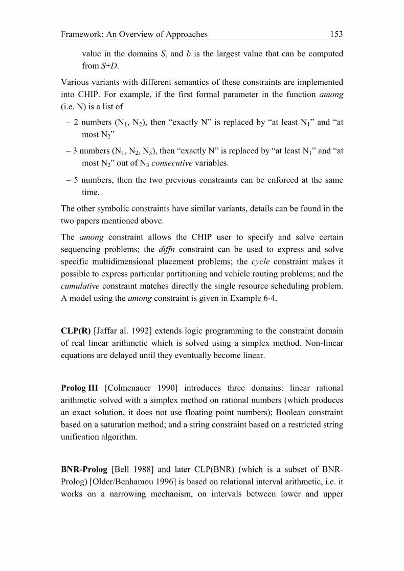
Framework: An Overview of Approaches 153
value in the domains S, and b is the largest value that can be computed
from S+D.
Various variants with different semantics of these constraints are implemented
into CHIP. For example, if the first formal parameter in the function among
(i.e. N) is a list of
– 2 numbers (N1, N2), then “exactly N” is replaced by “at least N1” and “at
most N2”
– 3 numbers (N1, N2, N3), then “exactly N” is replaced by “at least N1” and “at
most N2” out of N3 consecutive variables.
– 5 numbers, then the two previous constraints can be enforced at the same
time.
The other symbolic constraints have similar variants, details can be found in the
two papers mentioned above.
The among constraint allows the CHIP user to specify and solve certain
sequencing problems; the diffn constraint can be used to express and solve
specific multidimensional placement problems; the cycle constraint makes it
possible to express particular partitioning and vehicle routing problems; and the
cumulative constraint matches directly the single resource scheduling problem.
A model using the among constraint is given in Example 6-4.
CLP(R) [Jaffar al. 1992] extends logic programming to the constraint domain
of real linear arithmetic which is solved using a simplex method. Non-linear
equations are delayed until they eventually become linear.
Prolog III [Colmenauer 1990] introduces three domains: linear rational
arithmetic solved with a simplex method on rational numbers (which produces
an exact solution, it does not use floating point numbers); Boolean constraint
based on a saturation method; and a string constraint based on a restricted string
unification algorithm.
BNR-Prolog [Bell 1988] and later CLP(BNR) (which is a subset of BNR-
Prolog) [Older/Benhamou 1996] is based on relational interval arithmetic, i.e. it
works on a narrowing mechanism, on intervals between lower and upper
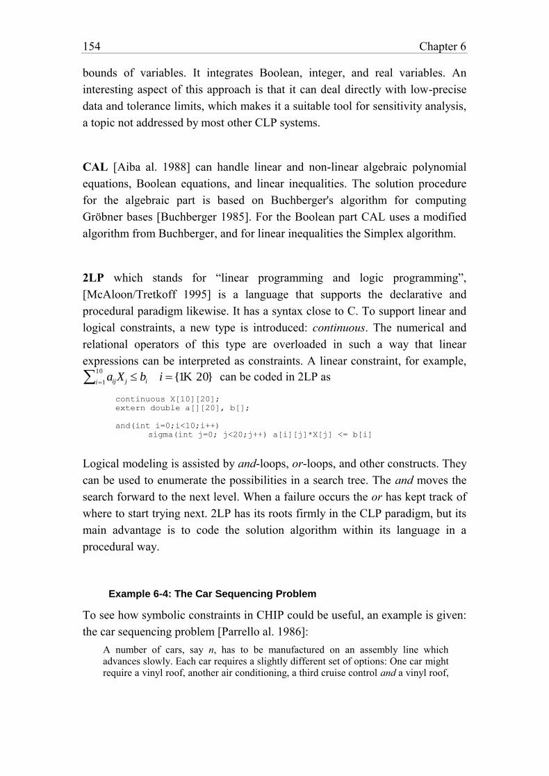
154 Chapter 6
bounds of variables. It integrates Boolean, integer, and real variables. An
interesting aspect of this approach is that it can deal directly with low-precise
data and tolerance limits, which makes it a suitable tool for sensitivity analysis,
a topic not addressed by most other CLP systems.
CAL [Aiba al. 1988] can handle linear and non-linear algebraic polynomial
equations, Boolean equations, and linear inequalities. The solution procedure
for the algebraic part is based on Buchberger's algorithm for computing
Gröbner bases [Buchberger 1985]. For the Boolean part CAL uses a modified
algorithm from Buchberger, and for linear inequalities the Simplex algorithm.
2LP which stands for “linear programming and logic programming”,
[McAloon/Tretkoff 1995] is a language that supports the declarative and
procedural paradigm likewise. It has a syntax close to C. To support linear and
logical constraints, a new type is introduced: continuous. The numerical and
relational operators of this type are overloaded in such a way that linear
expressions can be interpreted as constraints. A linear constraint, for example,
aijX ji1
10
bi i {1K 20} can be coded in 2LP as
continuous X[10][20];
extern double a[][20], b[];
and(int i=0;i<10;i++)
sigma(int j=0; j<20;j++) a[i][j]*X[j] <= b[i]
Logical modeling is assisted by and-loops, or-loops, and other constructs. They
can be used to enumerate the possibilities in a search tree. The and moves the
search forward to the next level. When a failure occurs the or has kept track of
where to start trying next. 2LP has its roots firmly in the CLP paradigm, but its
main advantage is to code the solution algorithm within its language in a
procedural way.
Example 6-4: The Car Sequencing Problem
To see how symbolic constraints in CHIP could be useful, an example is given:
the car sequencing problem [Parrello al. 1986]:
A number of cars, say n, has to be manufactured on an assembly line which advances slowly. Each car requires a slightly different set of options: One car might require a vinyl roof, another air conditioning, a third cruise control and a vinyl roof,
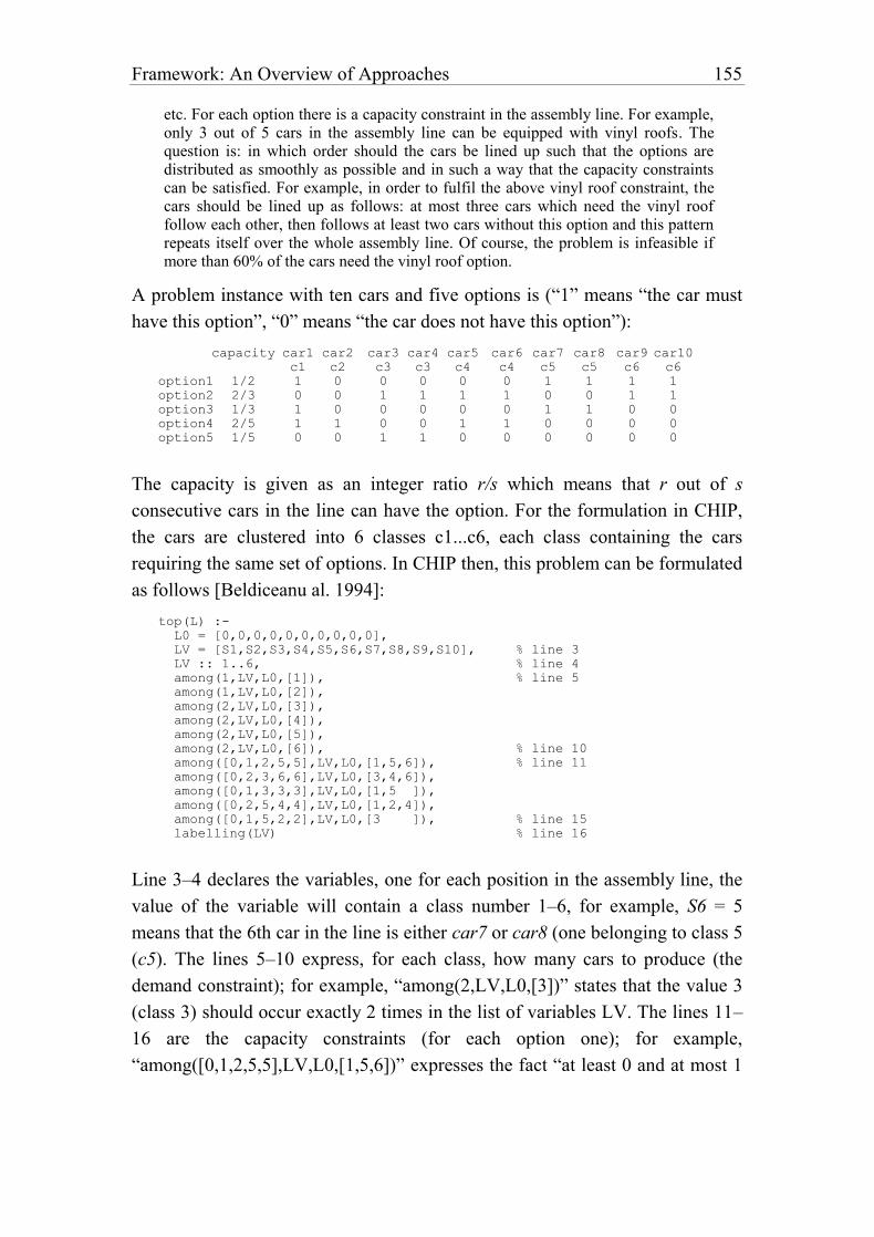
Framework: An Overview of Approaches 155
etc. For each option there is a capacity constraint in the assembly line. For example, only 3 out of 5 cars in the assembly line can be equipped with vinyl roofs. The question is: in which order should the cars be lined up such that the options are distributed as smoothly as possible and in such a way that the capacity constraints can be satisfied. For example, in order to fulfil the above vinyl roof constraint, the cars should be lined up as follows: at most three cars which need the vinyl roof follow each other, then follows at least two cars without this option and this pattern repeats itself over the whole assembly line. Of course, the problem is infeasible if more than 60% of the cars need the vinyl roof option.
A problem instance with ten cars and five options is (“1” means “the car must
have this option”, “0” means “the car does not have this option”):
capacity car1 car2 car3 car4 car5 car6 car7 car8 car9 car10
c1 c2 c3 c3 c4 c4 c5 c5 c6 c6
option1 1/2 1 0 0 0 0 0 1 1 1 1
option2 2/3 0 0 1 1 1 1 0 0 1 1
option3 1/3 1 0 0 0 0 0 1 1 0 0
option4 2/5 1 1 0 0 1 1 0 0 0 0
option5 1/5 0 0 1 1 0 0 0 0 0 0
The capacity is given as an integer ratio r/s which means that r out of s
consecutive cars in the line can have the option. For the formulation in CHIP,
the cars are clustered into 6 classes c1...c6, each class containing the cars
requiring the same set of options. In CHIP then, this problem can be formulated
as follows [Beldiceanu al. 1994]:
top(L) :-
L0 = [0,0,0,0,0,0,0,0,0,0],
LV = [S1,S2,S3,S4,S5,S6,S7,S8,S9,S10], % line 3
LV :: 1..6, % line 4
among(1,LV,L0,[1]), % line 5
among(1,LV,L0,[2]),
among(2,LV,L0,[3]),
among(2,LV,L0,[4]),
among(2,LV,L0,[5]),
among(2,LV,L0,[6]), % line 10
among([0,1,2,5,5],LV,L0,[1,5,6]), % line 11
among([0,2,3,6,6],LV,L0,[3,4,6]),
among([0,1,3,3,3],LV,L0,[1,5 ]),
among([0,2,5,4,4],LV,L0,[1,2,4]),
among([0,1,5,2,2],LV,L0,[3 ]), % line 15
labelling(LV) % line 16
Line 3–4 declares the variables, one for each position in the assembly line, the
value of the variable will contain a class number 1–6, for example, S6 = 5
means that the 6th car in the line is either car7 or car8 (one belonging to class 5
(c5). The lines 5–10 express, for each class, how many cars to produce (the
demand constraint); for example, “among(2,LV,L0,[3])” states that the value 3
(class 3) should occur exactly 2 times in the list of variables LV. The lines 11–
16 are the capacity constraints (for each option one); for example,
“among([0,1,2,5,5],LV,L0,[1,5,6])” expresses the fact “at least 0 and at most 1
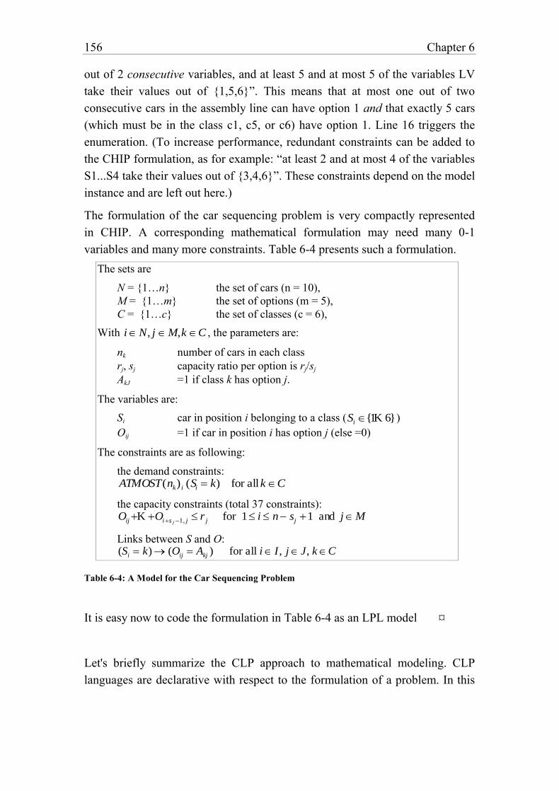
156 Chapter 6
out of 2 consecutive variables, and at least 5 and at most 5 of the variables LV
take their values out of {1,5,6}”. This means that at most one out of two
consecutive cars in the assembly line can have option 1 and that exactly 5 cars
(which must be in the class c1, c5, or c6) have option 1. Line 16 triggers the
enumeration. (To increase performance, redundant constraints can be added to
the CHIP formulation, as for example: “at least 2 and at most 4 of the variables
S1...S4 take their values out of {3,4,6}”. These constraints depend on the model
instance and are left out here.)
The formulation of the car sequencing problem is very compactly represented
in CHIP. A corresponding mathematical formulation may need many 0-1
variables and many more constraints. Table 6-4 presents such a formulation.
The sets are
N = {1…n} the set of cars (n = 10),
M = {1…m} the set of options (m = 5),
C = {1…c} the set of classes (c = 6),
With i N, j M,k C , the parameters are:
nk number of cars in each class
rj, sj capacity ratio per option is rj/sj
AkJ =1 if class k has option j.
The variables are:
Si car in position i belonging to a class ( Si {1K 6})
Oij =1 if car in position i has option j (else =0)
The constraints are as following:
the demand constraints: ATMOST(nk) i (Si k) for all k C
the capacity constraints (total 37 constraints):
OijK Ois j 1, j r j for 1 i n sj 1 and j M
Links between S and O: (Si k) (Oij Akj ) for all i I , j J, k C
Table 6-4: A Model for the Car Sequencing Problem
It is easy now to code the formulation in Table 6-4 as an LPL model ¤
Let's briefly summarize the CLP approach to mathematical modeling. CLP
languages are declarative with respect to the formulation of a problem. In this
Framework: An Overview of Approaches 157
sense they are different from programming languages, because they introduce
variables – a concept completely absent from programming languages.54 The
advantages are evident: The representation can be made very concise,
development time is greatly reduced, and expressiveness is powerful and
flexible. On the other hand, high-level constructs such as certain symbolic
constraints in CHIP have mixed benefits. They allow the modeler to formulate
many combinatorial problems very concisely, but they encapsulate too much
combinatorial structure which although efficient for some problems is
inefficient for others, dependent upon how they are implemented into the CLP
system.
From the solution point of view, all CLP languages replace resolution and
unification – which is typical in logic programming – by constraint solving
mechanisms. Of course, the specific methods determine whether a problem can
be solved or not. Since we know with a high degree of probability that there is
no unique efficient method, to solve all mathematical models, we must admit
that the CLP system has to already contain a specific method of solving a
particular problem. A typical example is on how linear models (LPs) are solved
in CLP: they implement the simplex algorithm as a black-box! CHIP and
Prolog III even use an exact simplex solver – using only rational numbers,
which is only practical for small models.55 There is nothing wrong with
implementing a simplex algorithm within a CLP system, of course. However,
specialized and sophisticated commercial LP solvers exist which have been
developed by investing many man-years. It is doubtful whether such an effort
can be doubled in a short time. Of course, the best LP code could always be
purchased and integrated into a CLP system, but that is hardly the point. The
point is that every method which solves a specific class of problems must be
integrated into the CLP system as a black-box procedure or it cannot handle
the class efficiently.
Another drawback of the CLP paradigm in our context of mathematical
54 The reader should recall how the term variable is used in this context (footnote 21 at page 29).
55 Rational solution avoids the instability of certain ill-conditioned LP problems at the cost of a
much longer computation. On the other hand, one can show that the rational solution xo of the
LP {max cx | Ax≤b} where all numbers in A, b, and c are rational, where n is the length of the
vector x, and where d is the largest of all absolute values in A, then the number of binary digits
of the rational solution xo of this LP is bounded by O(n2*log nd) [Nemhauser/Wolsey p. 123].
158 Chapter 6
modeling is its mixing up of declarative and procedural knowledge. This
observation is crucial, because to express the problem structure as a state space
is of interest regardless of the solution process. Another critical point is that
these languages merge the data with the program structure, as is the case in
most programming languages. Certainly, one can group the data in a computer
program or import all numerical data from tables. However, there is often no
need nor any uniform way of doing so. In modeling, it is crucial to state the
problem independently of the data.
Whether the CLP approach will have a “bright future”, as many of its advocates
predict, will depend on its capacity to integrate the solution techniques
developed in OR and other communities.
Further references to CLP are [Benhamou/Colmenauer 1993], or [Mayoh al.
1994]. Brief survey article are [Cohen 1990], [Frühwirth al. 1992], and
[Jaffar/Maher 1996]. From the point of view of OR the paper [Brown al, 1989]
is recommended.
6.5. Algebraic Languages
The forerunners of algebraic languages in operations research were matrix
generators which are similar in many ways to modern database approaches in
modeling. They were entirely data-driven tools to generate the matrix – the
input form for the Simplex solver – of a linear model from data in tabular
formats. The model was built by reference to tables representing the problem
data, i.e. sets of data are mapped into a matrix. One of the most advanced
systems in the seventies was PLATOFORM produced at Exxon, which was
used in hundreds of big projects [Palmer 1984]. The system was highly modular
and supported a wide range of linear models as well as the whole life cycle of
modeling management. The main component of such matrix generators was the
block. This is a vector or a matrix of data with a given width and height. These
blocks can be used to build larger blocks by operators that are well known
today in database theory: select, join etc. The simplex tableau – the input form
to a linear solver – is itself a block and can, therefore, be built using these
operations.
All modern algebraic languages in operations research have inherited these two
characteristics from matrix generators: they are data-driven and they are index-
Framework: An Overview of Approaches 159
driven. Data-driven means that the data blocks and their dimension determine
the data of the final instantiated model. The term “index-driven” has to be
explained a little bit further. An index – from the point of view of matrix
generators – is just a name of a row or a column in a block. The set of the
names of all rows or columns is called index-set. Their cardinalities control the
dimension of blocks. The Cartesian Product of several index-sets defines a
multi-dimensional block. The indexes and the index-sets can, therefore, be used
to implement the different database operations such as select, join and others.
This is how all algebraic languages work.
Many algebraic languages have been invented in the last decade. An overview
can be found in [Kuip 1992], [Greenberg H.J., Murphy F.H., A Comparison of
Mathematical Programming Modeling Systems, in: Shetty al., 1992, p 177–238]
or in [Sharda/Rampal 1995]. An up-to-date list appears regularly on the Usenet
in the LP FAQ maintained by [Gregory]. In the beginning of the eighties,
GAMS – the first fully-fletched language still available – was developed at the
World Bank, see [Bisschop/Meeraus 1982] and [Brooke/Kendrick/Meeraus
1988]. Fourer's seminal paper articulated the need for a “modeler's form” in
contrast to the “algorithm's form” [Fourer 1983].
In this section, only the two most advanced (besides LPL, of course!) languages
currently available commercially are reported: AIMMS [Bisschop/Entriken
1993] and AMPL [Fourer/Gay/Kernighan 1993]. For full documentation, the
reader should consult their user guides. (Low cost educational versions are
available.)
The two algebraic languages are similar: A model consists of a sequence or
collection of statements, declaring and defining sets, parameters, variables and
model constraints. These statements are close to the common mathematical
notation usually found in textbooks of the OR community. Further instructions
extend the functionality, such as data check or reporting capability. Both allow
one to formulate linear as well as non-linear models. Let us take them one after
the other.
6.5.1. AIMMS
AIMMS was developed (and is still being further developed) by Paragon
Decision Technology [Bisschop/Entriken 1993] headed by Johannes Bisschop,
who also contributed to the development of GAMS. It is one of the most
160 Chapter 6
advanced modeling systems currently on the market. It integrates a powerful
algebraic language, a well designed graphical interface, and several linear and
non-linear solvers. To present the language of AIMMS, let's use the well
known cutting stock problem described in [Chvátal 1983].
Example 6-5: The Cutting Stock Problem
The problem is the following:
Paper is manufactured in rolls of 100 inches width. The following orders have to be fulfilled:
97 rolls of 45 inches width 610 rolls of 36 inches width 395 rolls of 31 inches width 211 rolls of 14 inches width
How should the initial rolls of 100 inches width be cut into slices such that paper waste is minimized?
Using the common mathematical notation the declarative part of the problem
can be formulated as in Table 6-5.56
The sets are:
W the different widths that have been ordered,
P all possible cutting patterns (the are 37 in our example)
With w W, p P, the parameters are:
awp number of cut rolls of width w in pattern p
bw width of the cut (ordered) rolls
dw demand for the cut rolls
B width of the initial rolls
The variables are:
Xp number of the initial rolls cut according to pattern p,
56 There is no room here to explain the technicalities of the cutting stock problem. It is well known
that the model is solved using column generating techniques. Otherwise the model would
contain a huge number of variables, because there is in general a large number of patterns. See
Chvátal [1983], Chapter 13 for an extensive treatise of this model. Note also that for the sake of
simplicity the heuristic procedure to make the solution integer has been left out here. Integer
solutions are not needed if fractional parts of rolls are allowed which makes sense for silk, for
example.
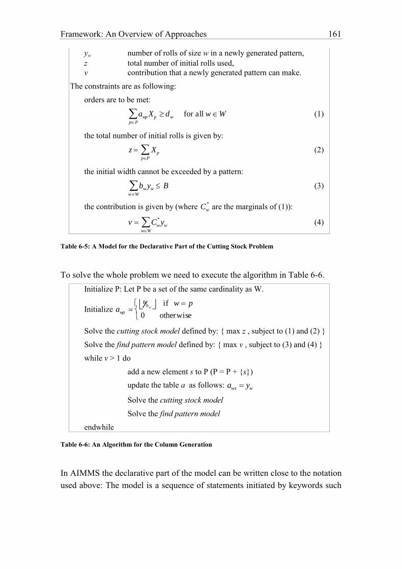
Framework: An Overview of Approaches 161
yw number of rolls of size w in a newly generated pattern,
z total number of initial rolls used,
v contribution that a newly generated pattern can make.
The constraints are as following:
orders are to be met:
awp Xp
pP
dw for all w W (1)
the total number of initial rolls is given by:
z Xp
pP
(2)
the initial width cannot be exceeded by a pattern:
bw yw
wW
B (3)
the contribution is given by (where Cw
* are the marginals of (1)):
v Cw
*yw
wW
(4)
Table 6-5: A Model for the Declarative Part of the Cutting Stock Problem
To solve the whole problem we need to execute the algorithm in Table 6-6.
Initialize P: Let P be a set of the same cardinality as W.
Initialize awp B
bw if w p
0 otherwise
Solve the cutting stock model defined by: { max z , subject to (1) and (2) }
Solve the find pattern model defined by: { max v , subject to (3) and (4) }
while v > 1 do
add a new element s to P (P = P + {s})
update the table a as follows: aws yw
Solve the cutting stock model
Solve the find pattern model
endwhile
Table 6-6: An Algorithm for the Column Generation
In AIMMS the declarative part of the model can be written close to the notation
used above: The model is a sequence of statements initiated by keywords such
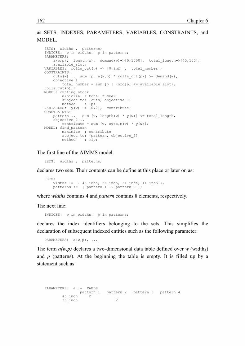
162 Chapter 6
as SETS, INDEXES, PARAMETERS, VARIABLES, CONSTRAINTS, and
MODEL.
SETS: widths , patterns;
INDICES: w in widths, p in patterns;
PARAMETERS:
a(w,p), length(w), demand(w)->[0,1000], total_length->[45,150],
available_slot;
VARIABLES: rolls_cut(p) -> [0,inf) , total_number ;
CONSTRAINTS:
cuts(w) .. sum [p, a(w,p) * rolls_cut(p)] >= demand(w),
objective_1 ..
total_number = sum [p | (ord[p] <= available_slot),
rolls_cut(p)];
MODEL: cutting_stock
minimize : total_number
subject to: {cuts, objective_1}
method : lp;
VARIABLES: y(w) -> {0,7}, contribute;
CONSTRAINTS:
pattern .. sum [w, length(w) * y(w)] <= total_length,
objective_2 ..
contribute = sum [w, cuts.m(w) * y(w)];
MODEL: find_pattern
maximize : contribute
subject to: {pattern, objective_2}
method : mip;
The first line of the AIMMS model:
SETS: widths , patterns;
declares two sets. Their contents can be define at this place or later on as:
SETS:
widths := { 45_inch, 36_inch, 31_inch, 14_inch },
patterns := { pattern_1 .. pattern_9 };
where widths contains 4 and pattern contains 8 elements, respectively.
The next line:
INDICES: w in widths, p in patterns;
declares the index identifiers belonging to the sets. This simplifies the
declaration of subsequent indexed entities such as the following parameter:
PARAMETERS: a(w,p), ...
The term a(w,p) declares a two-dimensional data table defined over w (widths)
and p (patterns). At the beginning the table is empty. It is filled up by a
statement such as:
PARAMETERS: a := TABLE
pattern_1 pattern_2 pattern_3 pattern_4
45_inch 2
36_inch 2
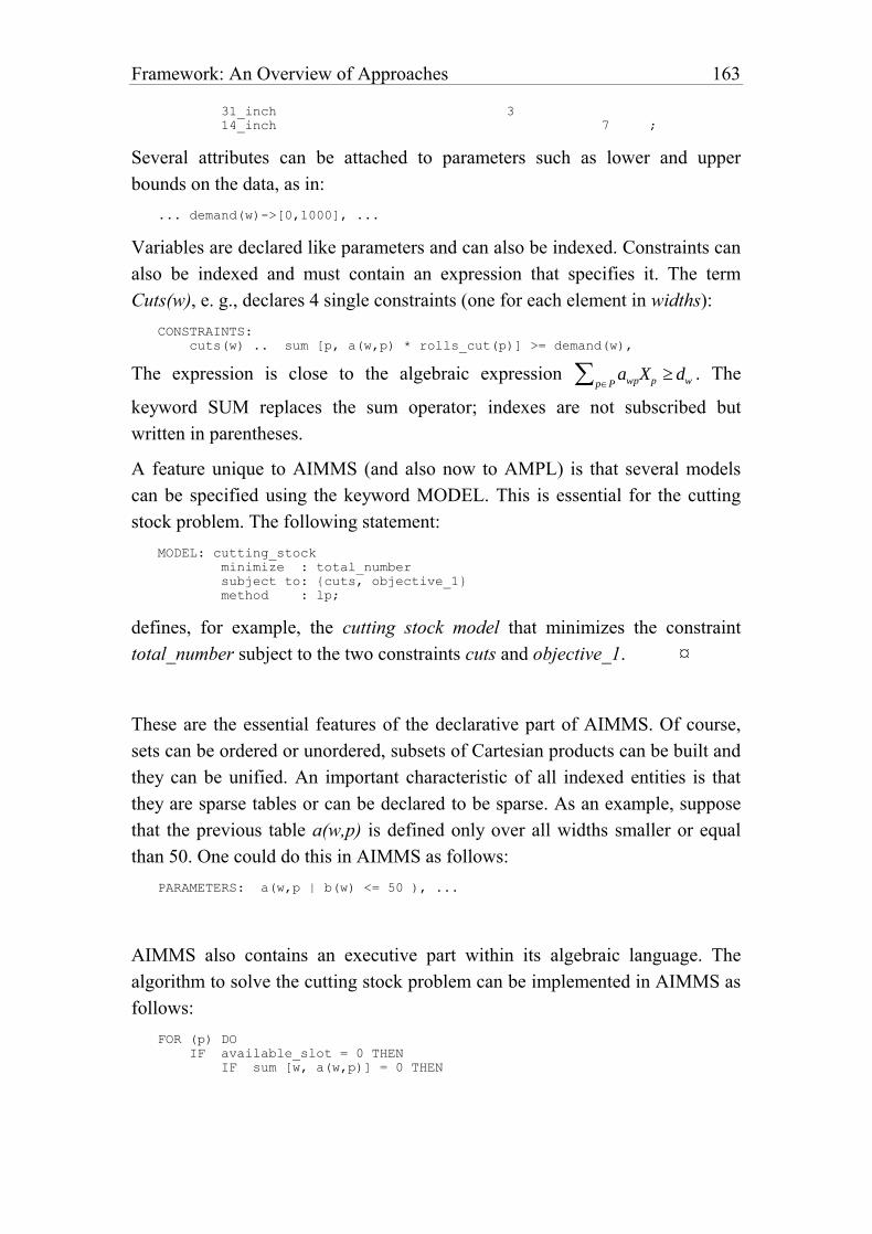
Framework: An Overview of Approaches 163
31_inch 3
14_inch 7 ;
Several attributes can be attached to parameters such as lower and upper
bounds on the data, as in:
... demand(w)->[0,1000], ...
Variables are declared like parameters and can also be indexed. Constraints can
also be indexed and must contain an expression that specifies it. The term
Cuts(w), e. g., declares 4 single constraints (one for each element in widths):
CONSTRAINTS:
cuts(w) .. sum [p, a(w,p) * rolls_cut(p)] >= demand(w),
The expression is close to the algebraic expression awpXppP dw . The
keyword SUM replaces the sum operator; indexes are not subscribed but
written in parentheses.
A feature unique to AIMMS (and also now to AMPL) is that several models
can be specified using the keyword MODEL. This is essential for the cutting
stock problem. The following statement:
MODEL: cutting_stock
minimize : total_number
subject to: {cuts, objective_1}
method : lp;
defines, for example, the cutting stock model that minimizes the constraint
total_number subject to the two constraints cuts and objective_1. ¤
These are the essential features of the declarative part of AIMMS. Of course,
sets can be ordered or unordered, subsets of Cartesian products can be built and
they can be unified. An important characteristic of all indexed entities is that
they are sparse tables or can be declared to be sparse. As an example, suppose
that the previous table a(w,p) is defined only over all widths smaller or equal
than 50. One could do this in AIMMS as follows:
PARAMETERS: a(w,p | b(w) <= 50 ), ...
AIMMS also contains an executive part within its algebraic language. The
algorithm to solve the cutting stock problem can be implemented in AIMMS as
follows:
FOR (p) DO
IF available_slot = 0 THEN
IF sum [w, a(w,p)] = 0 THEN
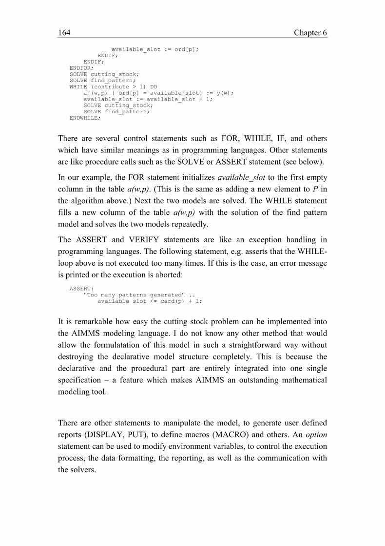
164 Chapter 6
available_slot := ord[p];
ENDIF;
ENDIF;
ENDFOR;
SOLVE cutting_stock;
SOLVE find_pattern;
WHILE (contribute > 1) DO
a[(w,p) | ord[p] = available_slot] := y(w);
available_slot := available_slot + 1;
SOLVE cutting_stock;
SOLVE find_pattern;
ENDWHILE;
There are several control statements such as FOR, WHILE, IF, and others
which have similar meanings as in programming languages. Other statements
are like procedure calls such as the SOLVE or ASSERT statement (see below).
In our example, the FOR statement initializes available_slot to the first empty
column in the table a(w,p). (This is the same as adding a new element to P in
the algorithm above.) Next the two models are solved. The WHILE statement
fills a new column of the table a(w,p) with the solution of the find pattern
model and solves the two models repeatedly.
The ASSERT and VERIFY statements are like an exception handling in
programming languages. The following statement, e.g. asserts that the WHILE-
loop above is not executed too many times. If this is the case, an error message
is printed or the execution is aborted:
ASSERT:
"Too many patterns generated" ..
available_slot <= card(p) + 1;
It is remarkable how easy the cutting stock problem can be implemented into
the AIMMS modeling language. I do not know any other method that would
allow the formulatation of this model in such a straightforward way without
destroying the declarative model structure completely. This is because the
declarative and the procedural part are entirely integrated into one single
specification – a feature which makes AIMMS an outstanding mathematical
modeling tool.
There are other statements to manipulate the model, to generate user defined
reports (DISPLAY, PUT), to define macros (MACRO) and others. An option
statement can be used to modify environment variables, to control the execution
process, the data formatting, the reporting, as well as the communication with
the solvers.
Framework: An Overview of Approaches 165
An important part of AIMMS is its graphical interface. AIMMS is not only a
language, it is a entire well designed modeling system with a complete
graphical user interface. Its interface is open and can be extended by the
modeler. She can even tailor the interface for each model. The philosophy
behind this interface designer is not unlike that of modern software
development systems: The modeler has to design forms – called pages in
AIMMS – and places components – called objects – on them. An object is an
area within the page that can contain graphics, figures, text, tables, and buttons.
Tables are fixed or updateable spreadsheets defining sets, parameters and
variables. Data can also be presented as (ev. updateable) bar charts or
parametric curves which visualize the interdependencies between data. Buttons
are used to launch a procedure (solve a model, go to next page, etc.). Several
model variants (with different data sets) – called cases – can be maintained at
the same time.
AIMMS, especially the embedded modeling language, has also several
weaknesses. No hierachical index-sets (see Chapter 7) are possible; models
cannot be organized in a structured way, neither can they be nested; the
executable part is limited and not well separated from the declarative part of the
model. Nevertheless, one of the fundamental aspects of a modeling language,
having an algorithmic and declarative part, is clearly taking form in this
framework.57
6.5.2. AMPL
The algebraic language AMPL was developed by Robert Fourer (Northwestern
University), David Gay and Brian Kernighan (AT&T Bell Labs)
[Fourer/Gay/Kernighan 1993]. A modeling system built around AMPL is
actually commercialized by Compass Modelling Solutions Inc.,
http://www.modeling.com. AMPL too, is still being developed and recent
57 The new AIMMS Version 3.0, available in 1998, will contain many extensions. The most
important of them are a clearer separation between declarative and procedural knowledge; an
instruction SECTION to subdivide models recursively into sections; and a powerful hierarchical
outline-browser which allows the modeler to browse and even to create the model interactively
without entering the code in the language syntax. (I am grateful to Prof. J. Bisschop who let me
take a glimse into the new version of AIMMS.)
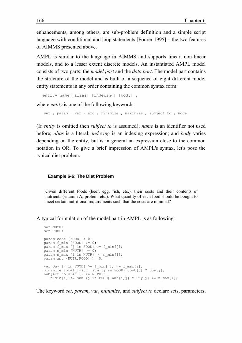
166 Chapter 6
enhancements, among others, are sub-problem definition and a simple script
language with conditional and loop statements [Fourer 1995] – the two features
of AIMMS presented above.
AMPL is similar to the language in AIMMS and supports linear, non-linear
models, and to a lesser extent discrete models. An instantiated AMPL model
consists of two parts: the model part and the data part. The model part contains
the structure of the model and is built of a sequence of eight different model
entity statements in any order containing the common syntax form:
entity name [alias] [indexing] [body] ;
where entity is one of the following keywords:
set , param , var , arc , minimize , maximize , subject to , node
(If entity is omitted then subject to is assumed); name is an identifier not used
before; alias is a literal; indexing is an indexing expression; and body varies
depending on the entity, but is in general an expression close to the common
notation in OR. To give a brief impression of AMPL's syntax, let's pose the
typical diet problem.
Example 6-6: The Diet Problem
Given different foods (beef, egg, fish, etc.), their costs and their contents of nutrients (vitamin A, protein, etc.). What quantity of each food should be bought to meet certain nutritional requirements such that the costs are minimal?
A typical formulation of the model part in AMPL is as following:
set NUTR;
set FOOD;
param cost {FOOD} > 0;
param f_min {FOOD} >= 0;
param f_max {j in FOOD} >= f_min[j];
param n_min {NUTR} >= 0;
param n_max {i in NUTR} >= n_min[i];
param amt {NUTR,FOOD} >= 0;
var Buy {j in FOOD} >= f_min[j], <= f_max[j];
minimize total_cost: sum {j in FOOD} cost[j] * Buy[j];
subject to diet {i in NUTR}:
n_min[i] <= sum {j in FOOD} amt[i,j] * Buy[j] <= n_max[i];
The keyword set, param, var, minimize, and subject to declare sets, parameters,
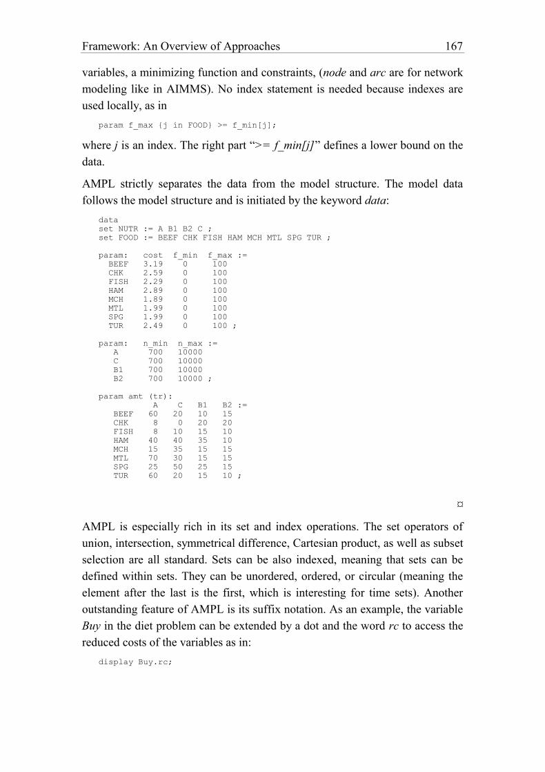
Framework: An Overview of Approaches 167
variables, a minimizing function and constraints, (node and arc are for network
modeling like in AIMMS). No index statement is needed because indexes are
used locally, as in
param f_max {j in FOOD} >= f_min[j];
where j is an index. The right part “>= f_min[j]” defines a lower bound on the
data.
AMPL strictly separates the data from the model structure. The model data
follows the model structure and is initiated by the keyword data:
data
set NUTR := A B1 B2 C ;
set FOOD := BEEF CHK FISH HAM MCH MTL SPG TUR ;
param: cost f_min f_max :=
BEEF 3.19 0 100
CHK 2.59 0 100
FISH 2.29 0 100
HAM 2.89 0 100
MCH 1.89 0 100
MTL 1.99 0 100
SPG 1.99 0 100
TUR 2.49 0 100 ;
param: n_min n_max :=
A 700 10000
C 700 10000
B1 700 10000
B2 700 10000 ;
param amt (tr):
A C B1 B2 :=
BEEF 60 20 10 15
CHK 8 0 20 20
FISH 8 10 15 10
HAM 40 40 35 10
MCH 15 35 15 15
MTL 70 30 15 15
SPG 25 50 25 15
TUR 60 20 15 10 ;
¤
AMPL is especially rich in its set and index operations. The set operators of
union, intersection, symmetrical difference, Cartesian product, as well as subset
selection are all standard. Sets can be also indexed, meaning that sets can be
defined within sets. They can be unordered, ordered, or circular (meaning the
element after the last is the first, which is interesting for time sets). Another
outstanding feature of AMPL is its suffix notation. As an example, the variable
Buy in the diet problem can be extended by a dot and the word rc to access the
reduced costs of the variables as in:
display Buy.rc;
168 Chapter 6
Several suffixes are defined for variables as well as for constraints. There are
also dot instructions that facilitate communication with the solver.
AMPL contains several commands to manipulate the model. The include
command can be used to include other files to the model. Four output
commands guide the reporting: display, print, printf, and write. The first three
can be used to print arbitrary expressions and tables. The display commands
formats the output in various tables or lists, whereas the print command writes
a raw list of data. The printf command is the same as print except that one can
format in a similar manner as in C's printf function. The command write can be
used to produces various files like the MPS-file. Several options (through an
option statement) guide the format of the output. A newly introduced read
command reads raw ASCII file data.
There are several commands to modify an already instantiated model. The
command drop removes a constraint; the command restore adds a previously
dropped constraint again to the model. The commands fix and unfix can be used
to freeze and unfreeze the value of variables. To change data one can use the
update or let command. But they can only change values of variables or data
entered in the data part. Entries in the model part cannot be changed.
A check statement can be used to check data consistency. To assign or modify
the environment variables, AMPL uses the option statement. Piece-wise linear
functions are also supported: a non-linear function can be noted as a list of
breakpoints (defining intervals) and slopes as follows:
<<breakpoints; slopes>> variable
A recent update of standard AMPL has added several new features, such as
looping and if-then-else statements described in [Fourer 1995] which allow the
modeler to write executable scripts within AMPL. The algorithm to solve the
cutting stock problem can now be formulated in a similar way as in AIMMS.
String operations and dot suffix notations have also been enhanced.
6.5.3. Summary
There are about two dozen algebraic languages – most of them in a prototypical
stage of development. The outstanding and most developed have been
presented. They are new and have as yet not been widely used. A common trait
Framework: An Overview of Approaches 169
with the CLP languages is their introduction of variables and constraints into a
computer-readable language. This is a unique feature of these languages. No
other programming language can declare model variables or constraints –
which makes them all unsuitable for representing mathematical models.
However, algebraic languages on their own have three fundamental features
which make them potentially an extremely interesting modeling tool:
• representation of the model in an index-based mathematical notation;
• separation between data and model structure;
• separation between model representation and solution.
Algebraic languages use indexes and indexed sets to declare model parts.
Hence, they can be used as languages that can manipulate sets – a fundamental
entity to declare and define large multidimensional objects. Sets can also be
used for looping in the executable part of an algebraic language which makes
them suitable for writing algorithms.
The separation between data and model structure is another unique feature.
This is extremely important for larger models since the data represent the more
volatile parts of the model. Modifying data does not entail any corrections or
modifications for the model structure. The data can be stored in more
appropriate software such as databases. A significant consequence of this
option is that the model structure itself can be treated and manipulated as an
entity without concern for the data. This is most convenient since the model
structure normally expresses the fundamental properties of the problem in a
compact way.
The third notable (controversial) feature is a clear separation between the model
and its solution process. It is said that the model representation depends on the
algorithm used to solve it and, therefore, no solver-independent formulation
and representation can exist. It is true that the representation of a problem
significantly influences the way a problem is solved. Sometimes the solution
process itself is the representation. On the other hand, while a large class of
models can be formulated in such a way, others need little additional
knowledge to solve an algebraically formulated model efficiently. In general,
however, it is fair to say that the algebraic language approach still has to prove
that this problem can somehow be circumnavigated. There is evidence that this
approach is attractive for a large class of models.
A manifest advantage of separating the model representation and the solution
170 Chapter 6
process would be that the model can be solved by different solvers without (or
only slightly) modifying the model structure. The possibility of trying different
methods for solving a problem is not only academically interesting to find out
which method works best for different problems, but it is also sometimes
essential to obtain a – and an often enough only approximate – solution to the
problem. Most (interesting) problems are provably so complex that it is, in any
case, worthwhile trying different techniques to solve them. Representing the
problem as a state space has another advantage: we can – using cutting plane
techniques – transform the state space in such a way that it can be more easily
be handled by a specific solver. If the problem is formulated as an algorithm,
such modifications normally imply redesigning the whole or at least a
significant part of the implementation.
As mentioned above, it still has to be shown whether or not the algebraic
approach of separating representation and solution processes for a specific
problem class has a significant advantage. Independently of how this difficulty
will be overcome, there are other considerations in modeling which are widely
ignored and neglected by most currently available algebraic languages. These
languages, in general, are confined to a bare-bones representation of the
mathematical model. Many other aspects of the modeling knowledge are absent
or overlooked. Let us name two.
First of all, all entities in a model are globally defined and globally accessible.
Neither scoping nor locality considerations have found their way into the design
of algebraic languages as they are common in almost all programming
languages today. This makes the encapsulation or the inheritance of model parts
impossible. Submodels, for example, cannot be properly defined.
Another point concerns the knowledge of a problem not directly needed by the
formal specification of the mathematical model, but which is required for the
explanation or a graphical representation of the model. Comments, user
specified attributes, and other semantic features which could be used to
semantically check, explain, or document parts of the model, are still not well
integrated into algebraic modeling languages. It is interesting to note that there
was and is an ongoing debate in “the” programming languages community on
whether a computer program should be augmented with more semantic
information. Several propositions were made, for example, to integrate units of
Framework: An Overview of Approaches 171
measurement (see Chapter 3, Section 4); or to enhance a program with
explanation text (“Literate Programming”) as proposed by [Knuth 1984],
[Knuth/Levy 1994] (see also [Baecker al. 1997]). These aspects seem to be
even more important in modeling than in programming.
Algebraic languages are still in their infancy with respect to their structural
specifications. Models can only be defined as a “spaghetti” code without
information hiding, hierarchical structuring, and real modular decomposition.
However, they have great potential for development.
6.6. General Remarks
In this Chapter, several techniques of model representation have been
presented. These approaches are not alternative, but complementary. However,
this is exactly where the difficulties begin: Suppose that part of an unfinished
model is created in a spreadsheet, that most of the data are organized in
databases, that there is a representation of the model structure in an algebraic
notation (on paper), and that several drawings display the model
interdependencies. Such a starting point is not uncommon. The modeler can
now continue in this heterogeneous way and update the different components as
the model moves on. At the same time, she must also update the links between
them – all this ending in heavy programming, prone to errors.
An alternative is to write the model specification in one single notation and use
several tools to generate the desired spreadsheets, the graphical forms, and even
the (empty) database tables –– or to use the different integrated tools (e.g. a
graphical design tool) to generate one single notation. Unfortunately, this
alternative does not yet exist – otherwise it would not have been necessary to
write this book.
For reasons that will become clear in the next chapter, I believe that the
approach adopted by algebraic languages is the most apt starting point for a
general modeling notation. That is not to say that prevailing languages already
have all the necessary features and properties to be indispensable for a general
modeling notation. On the contrary, most algebraic languages – AMPL and
AIMMS being no exception – restrict their syntax to the bare mathematical
structure of the model, just enough to formulate the purely formal aspects of the
172 Chapter 6
model in order to solve it. If this is all a modeler wants, that's fine; but more
often than not, the model is embedded in a broader structure of knowledge and
it should be possible to take this into account in a consistent and uniform way
within the language.
Several research programmes try to include further aspects of modeling
activities into the modeling environment. Let's briefly mention some
frameworks and ideas that have been proposed for integrating different aspects
in modeling.
6.6.1. Structured Modeling
A pioneering work was achieved by Geoffrion with his Structured Modeling
[Geoffrion 1988, 1994]. He proposed a formal framework for representing a
wide variety of models on the basis of a definitional system. It establishes the
basic elements of a model and distinguishes three levels of structure for
capturing the relationships between these elements. The three levels are the
elemental structure, the generic structure, and the modular structure. The
elemental structure contains five different types of elements: primitive
elements, compound elements, attributes, functions, and tests. Primitive and
compound elements are entities in the sense of database theory, i.e. they
represent things or concepts postulated as primitives or are defined in terms of
primitives (in the case of compound elements). These entities do not have
values. Attributes represent properties of things or concepts. Functions and tests
define a value according to a rule, often a calculable expression based on other
elements. The elemental structure catches the definitional detail of all elements
in a model and their definitional dependencies. These must be representable by
an acyclic graph, since circular definitions are not allowed. The generic
structure aims to capture the concept of collections of entities. Elements ”of the
same type” are represented together, defining an indexing structure as already
seen in the algebraic languages. The modular structures tackle the hierarchy.
Several (generic or nongeneric) elements are grouped into modules. These are
represented hierarchically in a rooted tree structure.
Structured Modeling (SM) is a complete and consistent framework for
conceptual modeling. It also includes an executable modeling language. Several
prototypical implementations have been presented during the last years. SM is
in many respects similar to the algebraic language approach: it states the model
in a declarative (not procedural) way. Entities and their properties must be
Framework: An Overview of Approaches 173
defined before they can be used in the constraints (functions and tests). In
several respects, SM goes beyond a pure algebraic language approach. This is
the case for the modular concept which tries to organize the model in a
hierarchical way, or the documentation part which attempts to capture model
description and documentation. Unfortunately, the modular structure seems not
to be fundamental for information hiding, locality and scoping as in
programming languages; documentation seems to have a rather cosmetic
function. This does not mean that these aspects are not important, it only means
that these concepts must be elaborated further. In other respects, SM fails to get
close to the expressive power a modern algebraic language such as AMPL or
AIMMS. This is mainly due to the lack of procedural aspects of the language. It
would, for example, be difficult to formulate the cutting stock problem
(Example 6-5) in the SM framework. One could also demur the rigidity of the
SM dependency structure: it is not possible, for example, to declare constants
and values at the same time. To declare (the mathematical constant
3.14159...) in SM, one must declare the entity “Phi” and in a second step its
value as an attribute (in Geoffrion's terminology). This difficulty is intrinsic to
SM, since every component must be part of the acyclic order where the leaves
of this structural tree must be primitive elements.
6.6.2. Embedded Language Technique
A different approach to model management is is the “embedded language
technique” [Bhargava/Kimbrough 1993 and 1995]. The authors propose an
embedding language that is “put over” an executable (algebraic) language, the
embedded language. The last is used to define the formal, mathematical aspects
of the language, while the first expresses the information about the model
which cannot (easily) be formulated in the embedded language (in the authors
view). The idea seems intriguing at first sight, since we can then separate
qualitative (documentation, explanations, etc.) and formal information within
the model. Often the formal model becomes less readable as it is overcharged
with information. The art of writing a good model (or any computer-readable
code) consists of using in-place comments sparingly. However, it is not clear
why two different languages should be used, and their example is everything
but convincing. Why not use the same language and separate the formal from
the informal part in some way? It remains to be seen whether the embedded
language approach is viable. To ate, no implementation, only ideas have been
presented.
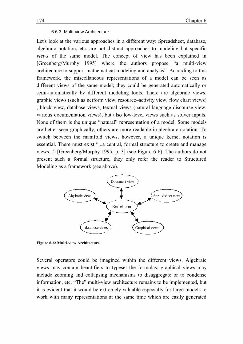
174 Chapter 6
6.6.3. Multi-view Architecture
Let's look at the various approaches in a different way: Spreadsheet, database,
algebraic notation, etc. are not distinct approaches to modeling but specific
views of the same model. The concept of view has been explained in
[Greenberg/Murphy 1995] where the authors propose “a multi-view
architecture to support mathematical modeling and analysis”. According to this
framework, the miscellaneous representations of a model can be seen as
different views of the same model; they could be generated automatically or
semi-automatically by different modeling tools. There are algebraic views,
graphic views (such as netform view, resource–activity view, flow chart views)
, block view, database views, textual views (natural language discourse view,
various documentation views), but also low-level views such as solver inputs.
None of them is the unique “natural” representation of a model. Some models
are better seen graphically, others are more readable in algebraic notation. To
switch between the manifold views, however, a unique kernel notation is
essential. There must exist “...a central, formal structure to create and manage
views...” [Greenberg/Murphy 1995, p. 3] (see Figure 6-6). The authors do not
present such a formal structure, they only refer the reader to Structured
Modeling as a framework (see above).
Kernel form
Algebraic view
Document view
Spreadsheet view
Graphical viewsdatabase views
Figure 6-6: Multi-view Architecture
Several operators could be imagined within the different views. Algebraic
views may contain beautifiers to typeset the formulas; graphical views may
include zooming and collapsing mechanisms to disaggregate or to condense
information, etc. “The” multi-view architecture remains to be implemented, but
it is evident that it would be extremely valuable especially for large models to
work with many representations at the same time which are easily generated
Framework: An Overview of Approaches 175
from each other.
6.6.4. A Model Construction and Browsing Tool
Mousavi, Mitra and Lucas have proposed and inplemented another modeling
tool which integrates several tasks in a consistent environment based on
browsing through several views [Mousavi al. 1995]. It supports stepwise model
construction from parameter definition to individual constraint terms
interactively in a graphical manner. At each action the model consistency for
missing components is checked. Every model entity (index-sets, parameters,
variables, constraints, etc.) is entered and organized in pick-up lists which
contain cross references to other entities. These hypertext links are
implemented as hot spots on the screen. An indexed parameter, for example,
has links to a table where the data is defined or can be edited; it also has a link
to the index-set where the set is defined.
6.6.5. Conclusion
Many more approaches have been presented in the literature, but those
presented above seem – in my opinion – the most promising. What we need is
not a multitude of tools but an integrated framework with the different tools as
single modules. It is only with such an architecture that we can ensure a
consistent modeling environment. The “kernel form” of such an environment –
the modeling language – is of central importance. Contrary to what has been
said in most of the literature, however, I think we are still a long way from the
“ideal” language. Nothing could be further from the truth then the following
remark: “The real challenge has moved from the question of modelling
language design to that of an integrated environment for application
construction, modelling and solving.” [Mitra G., in: Sharda 1989, pp. 484–496].
Of course, developing an integrated environment is important. However, before
we can accomplish this step, we need a consistent, powerful and extensible
kernel form.

177
7. A MODELING FRAMEWORK
After having investigated and criticized various approaches in the last chapter,
it is time to present my own view of a computer-based modeling framework. As
one might expect, it has been inspired from many sources. The different
algebraic languages have had a certain influence, although at least the initial
versions of LPL were developed completely independently from any other
algebraic language. Structured Modeling too, influenced me, helping to shape
the point of view presented in this chapter. More conceptual and
implementation specific aspects were influenced by computer science and
especially programming language design, as taught by Wirth [Wirth 1996],
[Wirth/Gutknecht 1992].
Although I have done my best to integrate many – also my own – ideas and to
blend them into a single framework, I do not consider this framework as a final
design of a modeling language and its environment. The research is simply too
new to offer a final formal specification. However, there are several new
concepts, put forth for the first time.
This chapter begins by summarizing the requirements for a modeling
framework. It then presents the most important part, the modeling language.
My conclusion is that the ideal modeling language must be able to express
declarative and procedural knowledge, therefore, it must be a proper superset of
programming languages. Although the modeling language is the most
fundamental element in computer-based modeling, other tools must surround it.
They are high level data manipulation tools, graphical or text-oriented browser
178 Chapter 7
and editor tools, analysing and documentation tools, as well as reformulation
tools.
7.1. The Requirements Catalogue
“The principal role of a language designer is that of a judicious collector of features or concepts...” — Wirth N., 1993.
Let us now first outline the goals and objectives of a computer-based
environment for modeling. We want:
1 a notation to formulate a problem in a declarative and a procedural way,
2 an environment to support the entire life-cycle of models,
3 tools to express also informal knowledge (documentation, e.g.).
The remaining part of this section suggests further justification of these three
goals.
7.1.1. Declarative and Procedural Knowledge
The first goal is motivated by the following argumentation. A model is defined
– as we have seen in Chapter 2 – as a constraint58 which describes a subspace in
a given state space. Parameters, data, variables and operators are needed to
form such a constraint. How can this be expressed? Mathematics and logic have
developed a powerful notation to write down constraints in a compact form. It
is an obvious idea to use and bring it in a machine-readable form for expressing
models within computers – although such a restatement is not a completely
straightforward task. The big question is: What can be done with such a
representation? Well, first of all, this computer-readable form is useful
independently of whether the model is to be solved or not. Since it is a compact
notation, it can be applied to document the model. A mathematical type-text
editor can use it to automatically “beautify” the formulae, a graphical editor can
exploit it to depict the dependencies between the components, a browser can
make use of its structure to view and access the different parts of the model
58 Since the AND-operator makes part of a constraint, “a constraint” might also mean “a set of
constraints”, of course.
Framework: A Modeling Framework 179
quickly. Especially for large models such browsing and editing tools are
extremely useful.
Certainly, the primary purpose of such a notation is to transform the model into
a form that can be solved by a particular solver. However, a declarative
statement of a model does not have enough knowledge to restate or even to
solve the model. Therefore, algebraic languages, as presented in Chapter 6.5.,
implicitly contain predefined translation procedures which are automatically
called upon when the problem is to be solved. To generate the MPSX form is
but one example of such a predefined high-level transformation procedure of a
linear model. Other model classes require other transformation procedures
which may or may not be integrated by the language designer. In any case, it
should be possible for the modeler to write her own translation operations.
Hence, algorithmic knowledge is needed in order to formulate them. While a
declarative notation is powerful in expressing what the problem is (i.e. its state
space), a procedural notation is apt in formulating algorithms. Do we have
languages that combine both of them? No! Most computer languages are purely
procedural languages. Hence, they are inadept at stating the model in a
declarative way. The CLP languages come closest to the combined declarative-
procedural paradigm. However, these languages mingle the declarative and the
procedural part of a model. Existing algebraic languages do contain some
procedural elements as Example 6-5 has shown. However, they are not fully-
fletched programming languages. What is needed, is a language that allows the
modeler to state the structure of the problem in a declarative, and the solution
process in an algorithmic way using the same notation without intermixing
them. Such a language will subsequently be called modeling language.
From the first goal the primary requirement can be derived: we need an
executable modeling language containing a declarative and an algorithmic
part. The main benefit of such a language is to provide a coherent framework
based on a single model representation which can be used for different
purposes: communication, manipulation, viewing, storage, solution. Well-
known compiler techniques can be applied to check the syntax and to avoid
many formulation errors.
7.1.2. The Modeling Environment
The second goal is an environment which supports the entire life-cycle of a
180 Chapter 7
model. This means that the user should be able to switch quickly between the
different modeling stages as presented in Chapter 3. A modular structure of the
modeling language facilitates the extendibility, the reuse, and the compatibility
of models – three prerequisites to attain this objective. Semantic analysis, such
as type and unit checking, helps in examining the validity of the model, an
important step in the modeling process. Other verification checks are data
validation and consistency checks. This can be attained by integrating high-
level data checking procedures into the language.
Tools for model analysis [Greenberg 1995a] together with an interface allow
the modeler to work quickly through the formulate-solve-validate stages and
assist the modeler in obtaining a robust and stable model. Therefore, we need
browsing and editing tools. To reduce the complexity of the modeling process,
especially for large models, a neat separation between the data and the model
structure is needed. Most of the data should reside in database tables, while the
structure is expressed in the modeling language. This assures that the data,
which is the more volatile part of a model, can be modified without altering the
structure of the model. This implies that communication between a modeling
language and a database system must be an integrated part of the language
itself. Such an interface could also be used on its own, to generate the data
tables automatically in the (third) normal form. A further aspect in this context
is the reporting of the results of a model which can then be uniformly integrated
into this part. Without a clear instance-structure separation of models, the report
generation could not be based on a high level generic pattern. All these
requirements (data/structure separation, read/write to databases, reporting) lead
to integrated high-level import/export procedures, subsequently also called
import and report generator.
A further element for mastering the complexity of large models is indexing. All
elements in a model, such as variables, parameters, and constraints can appear
in groups, in the same way they are indexed in the mathematical notation. It is
common to define a variable x, say, for every product in a set of n products as
follows:
xi i{1K n}
xi expresses the quantity, the price or some other property of the i-th product.

Framework: A Modeling Framework 181
The part “ i {1K n}” is called index-set, i being the index and {1K n} the set.
A similar construct is used in database theory. A database table Price can be
defined as
Price(Product, Amount)
where Price is the table name, Product and Amount are two field names for the
products and the amount. Product (the key) can be mapped to the index-set
{1K n} and Amount to x in the previous example. It is, therefore, not surprising
that the manipulation of indexed entities can be based on a database calculus:
similar operation such as join, projection, selection, and others are needed.
The expressive power of a modeling language, at least in its declarative part,
depends fundamentally on index-sets. Mapping between database tables and
indexed parameters (or variables), and hence a clear separation between the
structure and the instance of a model (its data) is only possible by making use
of index-sets (see Example 6-2). At first sight, it seems that index-sets could be
implemented by directly adopting the data structure of array, available in most
programming languages. This is not the case! An index-set is a much more
complex structure than an array. While multi-dimensional sets (the Cartesian
Products) are not difficult for arrays, subsets of Cartesian Products are quite
annoying. In modeling, it is common to declare large multi-dimensional tables
containing ultimately only a small fractional part of entries. They are called
sparse tables. Mapping such tables in a straightforward manner into arrays
wastes precious memory. To manage efficiently (in time and space) such sparse
tables is one of the most essential tasks of a modeling language.59
Another delicate and critical issue in designing a modeling language, is the
independence between the structure of the model and the solver: Since a solver
can abruptly change its complexity behaviour due to a slight modification of the
59 From the point of view of algorithmic complexity, accessing a value in a sparse table (which
means reading and writing an entry) can be guaranteed in time proportional to O(log n) using a
binary tree structure, if n is the cardinality of the full table. Using hash tables, the average time
can be made constant, but many insert/remove operations can seriously degrade the efficiency.
Sorting a sparse table can be done in linear time of n by applying the counting sort. Nonetheless,
it uses an unacceptably large number of O(n) memory cells. We are often better off by using a
O(m log m) sorting algorithm, where m is the actual size of the sparse table.
182 Chapter 7
model, it should also be possible to declare the model independently from a
particular solver. Only in this way can a smooth replacement of the solver be
ensured. Ideally, to change a solver within a model means to replace a single
instruction in the modeling language, the high-level solver call.
Aiding the modeler in the entire life-cycle also means to support many
modeling paradigms. A small change in the model structure can turn a linear
model into a non-linear one, a continuous into a discrete one. Certainly, such
modifications represent a radical change from the point of view of the solution
process, but not from the point of view of the modeling process. At the very
least, the modeler should be alerted by the modeling environment system when
such alterations have occurred.
7.1.3. Informal Knowledge
The third goal, the expression of extra-formal (or informal) knowledge of
models, seems to be of minor importance to many modelers although it is vital
for maintaining and documenting large models. It is interesting that these
aspects have also been badly neglected in software engineering. “For years,
theory had little interest in maintenance, believing it was either an uninteresting
subset of development, or a nonintellectually challenging task.” [Glass 1996,
p 13]. This grievance seems to be changing only slowly. In modeling, however,
– even more than in programming – the users depend on sophisticated tools
which provide automated documentation and aid in “explaining” the model
structure, as well as in interpreting model results. As a model can be expressed
in an extremely compact notation, specific tools are needed to elucidate the
modeler about the inner workings of the model, otherwise it can simply not be
maintained with a reasonable effort.
Considering the novelty of such ideas, the framework presented in this chapter
contains only marginal improvements concerning the informal knowledge of a
model (see [Greenberg 1995a]). Nevertheless, by means of qualified comments
within the modeling language as well as multiple declaration of model entities,
the problem can be alleviated, although multiple declaration introduces other
drawbacks.
7.1.4. Summary
Let us summarize the different features. We need:
– a modeling language, that is a notation which can express declarative and
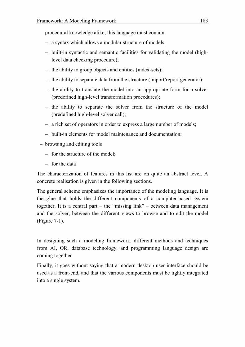
Framework: A Modeling Framework 183
procedural knowledge alike; this language must contain
– a syntax which allows a modular structure of models;
– built-in syntactic and semantic facilities for validating the model (high-
level data checking procedure);
– the ability to group objects and entities (index-sets);
– the ability to separate data from the structure (import/report generator);
– the ability to translate the model into an appropriate form for a solver
(predefined high-level transformation procedures);
– the ability to separate the solver from the structure of the model
(predefined high-level solver call);
– a rich set of operators in order to express a large number of models;
– built-in elements for model maintenance and documentation;
– browsing and editing tools
– for the structure of the model;
– for the data
The characterization of features in this list are on quite an abstract level. A
concrete realisation is given in the following sections.
The general scheme emphasizes the importance of the modeling language. It is
the glue that holds the different components of a computer-based system
together. It is a central part – the “missing link” – between data management
and the solver, between the different views to browse and to edit the model
(Figure 7-1).
In designing such a modeling framework, different methods and techniques
from AI, OR, database technology, and programming language design are
coming together.
Finally, it goes without saying that a modern desktop user interface should be
used as a front-end, and that the various components must be tightly integrated
into a single system.
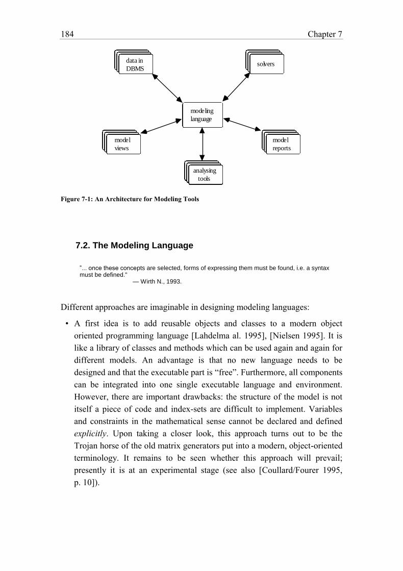
184 Chapter 7
modeling
language
model
views
model
reports
solversdata in
DBMS
analysing
tools
Figure 7-1: An Architecture for Modeling Tools
7.2. The Modeling Language
”... once these concepts are selected, forms of expressing them must be found, i.e. a syntax must be defined." — Wirth N., 1993.
Different approaches are imaginable in designing modeling languages:
• A first idea is to add reusable objects and classes to a modern object
oriented programming language [Lahdelma al. 1995], [Nielsen 1995]. It is
like a library of classes and methods which can be used again and again for
different models. An advantage is that no new language needs to be
designed and that the executable part is “free”. Furthermore, all components
can be integrated into one single executable language and environment.
However, there are important drawbacks: the structure of the model is not
itself a piece of code and index-sets are difficult to implement. Variables
and constraints in the mathematical sense cannot be declared and defined
explicitly. Upon taking a closer look, this approach turns out to be the
Trojan horse of the old matrix generators put into a modern, object-oriented
terminology. It remains to be seen whether this approach will prevail;
presently it is at an experimental stage (see also [Coullard/Fourer 1995,
p. 10]).
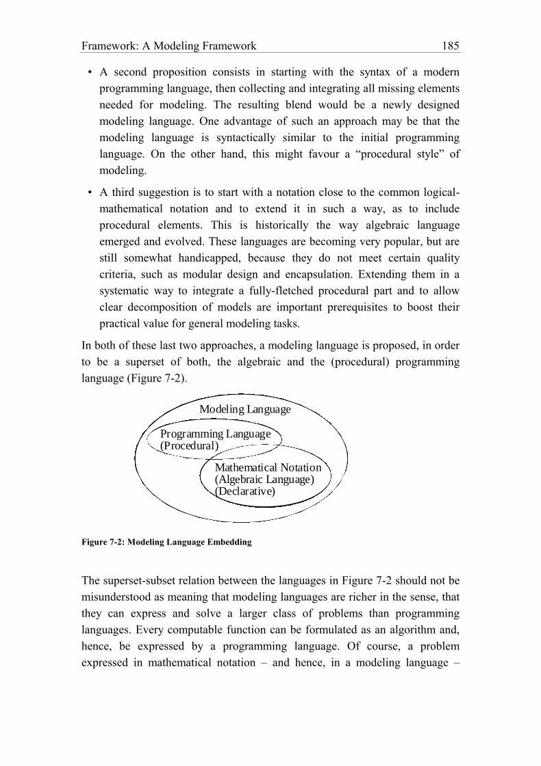
Framework: A Modeling Framework 185
• A second proposition consists in starting with the syntax of a modern
programming language, then collecting and integrating all missing elements
needed for modeling. The resulting blend would be a newly designed
modeling language. One advantage of such an approach may be that the
modeling language is syntactically similar to the initial programming
language. On the other hand, this might favour a “procedural style” of
modeling.
• A third suggestion is to start with a notation close to the common logical-
mathematical notation and to extend it in such a way, as to include
procedural elements. This is historically the way algebraic language
emerged and evolved. These languages are becoming very popular, but are
still somewhat handicapped, because they do not meet certain quality
criteria, such as modular design and encapsulation. Extending them in a
systematic way to integrate a fully-fletched procedural part and to allow
clear decomposition of models are important prerequisites to boost their
practical value for general modeling tasks.
In both of these last two approaches, a modeling language is proposed, in order
to be a superset of both, the algebraic and the (procedural) programming
language (Figure 7-2).
Modeling Language
Programming Language (Procedural)
Mathematical Notation (Algebraic Language) (Declarative)
Figure 7-2: Modeling Language Embedding
The superset-subset relation between the languages in Figure 7-2 should not be
misunderstood as meaning that modeling languages are richer in the sense, that
they can express and solve a larger class of problems than programming
languages. Every computable function can be formulated as an algorithm and,
hence, be expressed by a programming language. Of course, a problem
expressed in mathematical notation – and hence, in a modeling language –
186 Chapter 7
could eventually be unsolvable, because it expresses a non-computable
function. In this sense, the expressiveness of a mathematical notation is richer
than the one of a Turing Machine.
The intended meaning of Figure 7-2 concerning the relationship between the
two classes of languages is merely that – syntactically speaking – a modeling
language should not only contain a programming language, but its syntax
should be extended by additional declarative elements – especially
mathematical variables and constraints – which allow the formulation of
models in a compact mathematical notation.
7.2.1. The Adopted Approach
The approach adopted here is as follows: In a first stage, the algebraic notation
was augmented with constructs to call predefined high-level procedures (data
checking, import/report generator, translation, solving). In a second stage, a
modern programming language based on modular design is examined to distil
the constructs useful for a decomposable scheme in modeling. The third stage
integrates the procedural part of a programming language: control statement (if-
then-else, loops), procedure and type declaration.
Let us begin with an informal presentation of the algebraic notation. Each
model contains parameters, variables and constraints. They are called model
entities. We adopt the principle that they must be declared.60 The different
entities have several common properties. For example, they have a name, a
value (which can be an expression containing mathematical operators and entity
names as operands), a data type, a unit, etc.; these properties are called
attributes. Entities can be indexed, therefore we need a forth entity: index-sets.
The algebraic notation can now be summarized as follows. The model is a
collection of:
Index-set declarations (= a list of set attributes),
Parameter declarations (= a list of parameter attributes),
Variable declarations (= a list of variable attributes), and
60 The discussion as to whether all identifiers should be explicitly declared before their use, has a
long history in programming languages. It is not the purpose to rediscuss it in this book. See, for
example, [Hoare 1974] for a synopsis of related problems.
Framework: A Modeling Framework 187
Constraint declarations (= a list of constraint attributes)
The order of the declarations should not influence the semantic of the language
in any way, except that an identifier must be declared before it can be used.
This formulation must now be augmented with predefined high-level
procedures in order to “do something” with the declarative model. The five
following instructions are indispensable for every model: data checking, data
import and export, transforming, and solving the model. Therefore, besides the
four declarations above, a model should contain the five instructions
CHECK data etc.
READ data or other parts into the model from other devices
WRITE data or other parts from the model to other devices
TRANSFORM parts of the model
SOLVE this model
Each of the five instructions might be interpreted as a procedure call containing
several formal parameters. Such a view, however, would be misleading for
several reasons. First of all, in programming languages, the sequence of
procedure calls is given by the sequence in the source code. In a modeling
language, however, the order should not have any meaning. There is no need to
treat these five instructions differently from the four entities above. On the
contrary, it is more consistent and simplifies the design to consider the five
instructions as entities too, consisting of several specific attributes. The main
reason for doing so, is the fact that semantically these “instructions” are really
declarations. When and how a Check, for example, is executed is determined by
the language not by the modeler; therefore, a Check instruction only defines
what to check but not how and when. The same observation holds for the other
four instructions. This means that it is insignificant where and in which order
these instructions are placed within the whole model. The sequence of
declarations has no influence on the execution order, except on the requirement
that the identifiers used in these instructions must have been declared before in
the model. Ultimately, of course, a definite order of execution must be
established, but this must be settled by the semantic of the modeling language,
the modeler must not be concerned by such issues. For future reference, the five
instructions will be called instruction entities.
At this stage, a modeling language consists informally of a set of nine different
entities each consisting of a list of attributes. Everything is declared at the same
188 Chapter 7
level, there is no modular design or encapsulation. We shall see in several
model examples below, that a structured, decomposable design can greatly
augment the transparency of large models in the same way as does modular
design in programming languages. In order to introduce these aspects into a
modeling language, let us switch over and take a brief look at a well designed
programming language to see how these concepts are implemented.
The language Oberon [Wirth/Gutknecht 1993] is chosen because it is object-
oriented, it has a simple syntax and it is one of the few programming languages
that explicitly includes the concept of module. This concept was introduced at
the beginning of the seventies and was one of the basic components of the
language Modula [Wirth 1977]. It found its way into Ada where it is called
package. (Today the notion of software component is more common.) A
module is like a procedure: Both encapsulate a piece of code (information
hiding)61 and introduce the principle of spatial and temporal scoping, that is,
identifiers defined within a procedure are local and cannot be accessed or
modified from outside in any way. While identifiers in procedures only exist as
long as the procedure is running, in modules they exist as long as the module is
loaded. Hence, an important feature of modules is to introduce (local)
identifiers the temporal existence of which can be extended over that of the run-
time of procedures.
Procedures do not need to communicate mutually, except by calling each other
and by returning values. Their local identifiers stay local and their existence has
no significance for the surrounding world. This is different for modules.
Temporally persistent objects within modules are not only interesting because
they can maintain their state as long as the module exists (is loaded), but also
because they need to “inform” other modules about their state. Hence, in order
for modules to communicate with each other, the principle of information
hiding must be relaxed somewhat. Modern languages have introduced different
mechanism for this purpose. The implementor (server) of modules decides
which identifiers to export, i.e. to make visible to other modules; the user
(client) determines which identifiers from which modules to import. This
export/import abstraction defines the interface between modules and reduces it
to a well confined point of interaction. In this way, the supplier (server) of a
61 According to Wirth [1996, p 126], the term information hiding which is now an essential notion
in software engineering, was introduced by [Parnas 1972].

Framework: A Modeling Framework 189
module has full control over what a client can do with a module, while the user
(client) of the module does not need to know its inner workings.
Modules should be distinguished from classes and objects, two other important
concepts in modern object-oriented languages. A class encapsulates a data
structure together with its access and other methods which make it possible to
change the state of an object – an instance of a class. The concept of class could
be seen as an extension of the concept of type. Both – classes and types –
declare domains of elements to which memory variables (objects) can be
assigned. Data structure can be refined and, therefore, classes should be
organized in hierarchies, in such a way that a refined structure inherits all (or
parts of) the features of a less refined one.
Using both concepts of modules and classes, one can cleanly keep apart the
principle of scoping and visibility on the one hand, and the refinement of data
types on the other. Languages like C++ and Eiffel that co-mingle these
concepts into one class concept, render the syntax of classes more cumbersome.
C++, especially overloads its class with so many features, that it is difficult to
maintain an overview for an occasional, as well as a professional programmer.
This is a clear disadvantage for maintaining code, and time will tell whether the
millions of lines of code written today in C++ will be a pleasure for the coming
generation of programmers, or whether they will freeze into those program
dinosaurs that nobody wants to touch, like the Cobol today.62
62 The programming languag Eiffel [Meyer, 1992] also merges the two concepts of module and
class into a single one: the class. This is an intentional design choice as Meyer notes on page 34.
Module (“a group of related services”) and class (“the description of similar run-time data
elements, or objects”) have different “roles”, but it is “natural to support them through a single
concept”. Meyer gives no further justification why this is “natural”. Of course, “we can build the
class in such a way that the services it offers as a module are precisely the operations available
on the objects.” A stronger argument for merging these two concepts would be: “do not use two
concepts when one is enough” (Ockham's Razor). However, as was exposed above, the two
concepts not only have different “roles” but they have very different functions: the module
controls the visibility while the class declares an abstract data type. Maybe in algorithmic
languages it is less important to distinguish between these functions, in modeling languages
(where the concept of module will be replaced by the one of model, see below) it is crucial,
since a model is more than a data structure: it also contains the declarative part (in contrast to
the procedural part).
190 Chapter 7
In Oberon, module and class are two strictly distinct concepts. Each module is a
complete program stored in a separate file. Its syntax is as follows:
MODULE ModuleName;
IMPORT <ModuleImportList>
CONST <constant declarations>
TYPE <type declaration>
VAR <memory variable declaration>
PROCEDURE <procedure declaration>
BEGIN
<executable statements>
END ModuleName.
A class in Oberon is nothing more than a record type with the syntax:
TYPE
aClass RECORD ( predecessorClass )
<FieldListSequence>
END
A module may contain several classes, all having the same (module-wide)
scope. If a class and its fields should not, or only partially, be visible from
another class, then these two classes must be placed in different modules.
Exportable identifiers from a module are simply marked by a star ('*') or a dash
('–'), where the star means “full read and write access” and the dash means
“read access” only.
The principle of spatial and temporal scoping realised by the concept of module
in Oberon can be captured in modeling languages by another entity called
model entity which encapsulates any number of entities as follows:
MODEL model entity attributes
entity declarations
END
where the convention is as follows: a model is enclosed between the keywords
MODEL and END. This syntax also includes nested models since model itself
is an entity which must be declared. Exportable identifiers are marked by a star
or a dash, anything else is private (i.e. hidden from outside) to a specific model.
Imported models are declared by an Import instruction (in a similar way as in
Oberon) which can be considered again as another entity.
If the SOLVE instruction would be general enough to solve any model (in this
Framework: A Modeling Framework 191
case the TRANSFORM instruction would not be needed either) then the
(informal) design of the modeling language would be complete at this point.
Now, the model consists of a hierarchical set of 11 different entities:
set, parameter, variable, constraint, model, import entities, as well as
the five instruction entities (check, read, write, transform, solve).
Unfortunately, no general procedure exists to solve every (mathematical)
model. Often it is preferable to exploit the special structure of a model to solve
it. This means that the (skilled) modeler must have the opportunity to write her
own solution procedures. This need not be a complete implementation of the
solver from scratch. In many discrete problems, for example, it is preferable
that the modeler can write her own branch-and-bound procedure, while the
solution of the LP, say, at each node can be triggered by a Solve entity
instruction. In any case, the modeler must have a complete programming
language integrated within the modeling language, in order to write her own
algorithms.
These considerations lead us to a modeling language that contains two distinct
parts, a declarative part – which was informally described above – and an
executable part explained below. The overall structure of a model is now:
MODEL model attributes
entity declarations (declarative part)
BEGIN
executable statements (executable part)
END
where BEGIN is a keyword separating the two parts. The executable part
contains well-known constructs such as if-then-else and loop statements,
assignments, procedure calls, as well as the instruction entity calls.
Furthermore, the declarative part must be extended by the type declaration and
the procedure declaration. We shall also introduce an additional entity to
declare units.63
63 Units cannot be reduced to types. The question of whether a (numeric) value represents – say –
time, length, speed, or voltage is not addressed by the concept of type. They are all floating
point numbers. Even a strict form of name equivalence between types would not solve the
problem. The declaration
type LENGTH = REAL; SPEED = REAL;
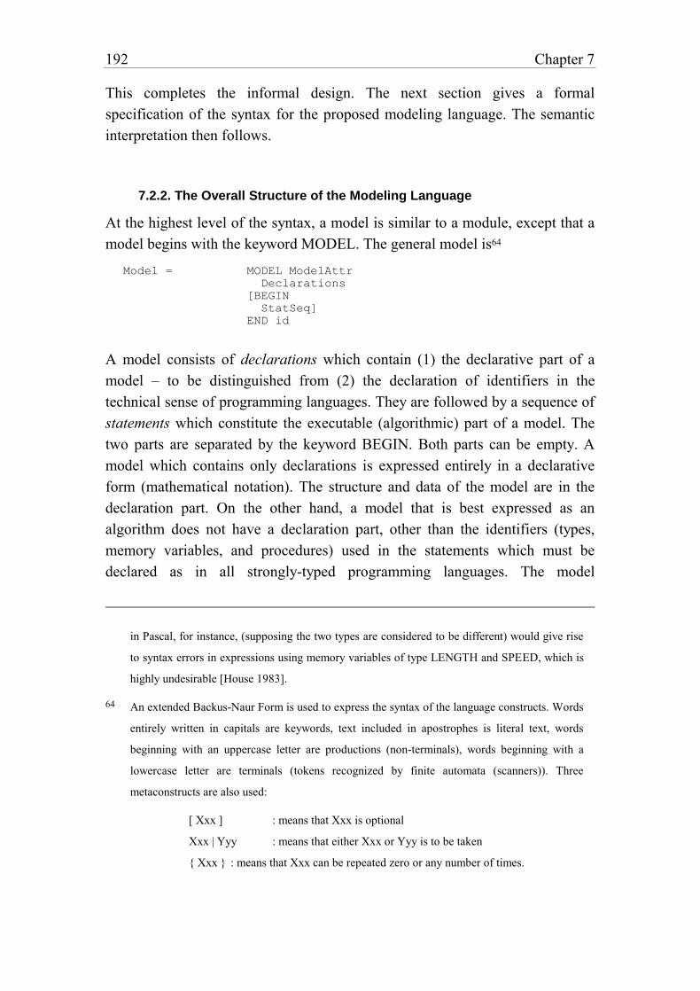
192 Chapter 7
This completes the informal design. The next section gives a formal
specification of the syntax for the proposed modeling language. The semantic
interpretation then follows.
7.2.2. The Overall Structure of the Modeling Language
At the highest level of the syntax, a model is similar to a module, except that a
model begins with the keyword MODEL. The general model is64
Model = MODEL ModelAttr
Declarations
[BEGIN
StatSeq]
END id
A model consists of declarations which contain (1) the declarative part of a
model – to be distinguished from (2) the declaration of identifiers in the
technical sense of programming languages. They are followed by a sequence of
statements which constitute the executable (algorithmic) part of a model. The
two parts are separated by the keyword BEGIN. Both parts can be empty. A
model which contains only declarations is expressed entirely in a declarative
form (mathematical notation). The structure and data of the model are in the
declaration part. On the other hand, a model that is best expressed as an
algorithm does not have a declaration part, other than the identifiers (types,
memory variables, and procedures) used in the statements which must be
declared as in all strongly-typed programming languages. The model
in Pascal, for instance, (supposing the two types are considered to be different) would give rise
to syntax errors in expressions using memory variables of type LENGTH and SPEED, which is
highly undesirable [House 1983].
64 An extended Backus-Naur Form is used to express the syntax of the language constructs. Words
entirely written in capitals are keywords, text included in apostrophes is literal text, words
beginning with an uppercase letter are productions (non-terminals), words beginning with a
lowercase letter are terminals (tokens recognized by finite automata (scanners)). Three
metaconstructs are also used:
[ Xxx ] : means that Xxx is optional
Xxx | Yyy : means that either Xxx or Yyy is to be taken
{ Xxx } : means that Xxx can be repeated zero or any number of times.
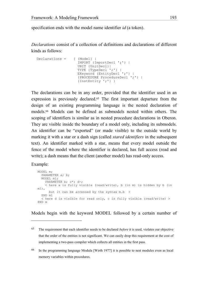
Framework: A Modeling Framework 193
specification ends with the model name identifier id (a token).
Declarations consist of a collection of definitions and declarations of different
kinds as follows:
Declarations = { {Model} |
IMPORT {ImportDecl ';'} |
UNIT {UnitDecl}|
TYPE {TypeDecl ';'} |
EKeyword {EntityDecl ';'} |
{PROCEDURE ProcedureDecl ';'} |
{InstEntity ';'} }
The declarations can be in any order, provided that the identifier used in an
expression is previously declared.65 The first important departure from the
design of an existing programming language is the nested declaration of
models.66 Models can be defined as submodels nested within others. The
scoping of identifiers is similar as in nested procedure declarations in Oberon.
They are visible inside the boundary of a model only, including its submodels.
An identifier can be “exported” (or made visible) to the outside world by
marking it with a star or a dash sign (called stared identifiers in the subsequent
text). An identifier marked with a star, means that every model outside the
fence of the model where the identifier is declared, has full access (read and
write); a dash means that the client (another model) has read-only access.
Example:
MODEL m;
PARAMETER a; b;
MODEL m1;
PARAMETER b; c*; d-;
< here a is fully visible (read/write), b (in m) is hidden by b (in
m1),
but it can be accessed by the syntax m.b >
END m1
< here d is visible for read only, c is fully visible (read/write) >
END m
Models begin with the keyword MODEL followed by a certain number of
65 The requirement that each identifier needs to be declared before it is used, violates our objective
that the order of the entities is not significant. We can easily drop this requirement at the cost of
implementing a two-pass compiler which collects all entities in the first pass.
66 In the programming language Modula [Wirth 1977] it is possible to nest modules even as local
memory variables within procedures.
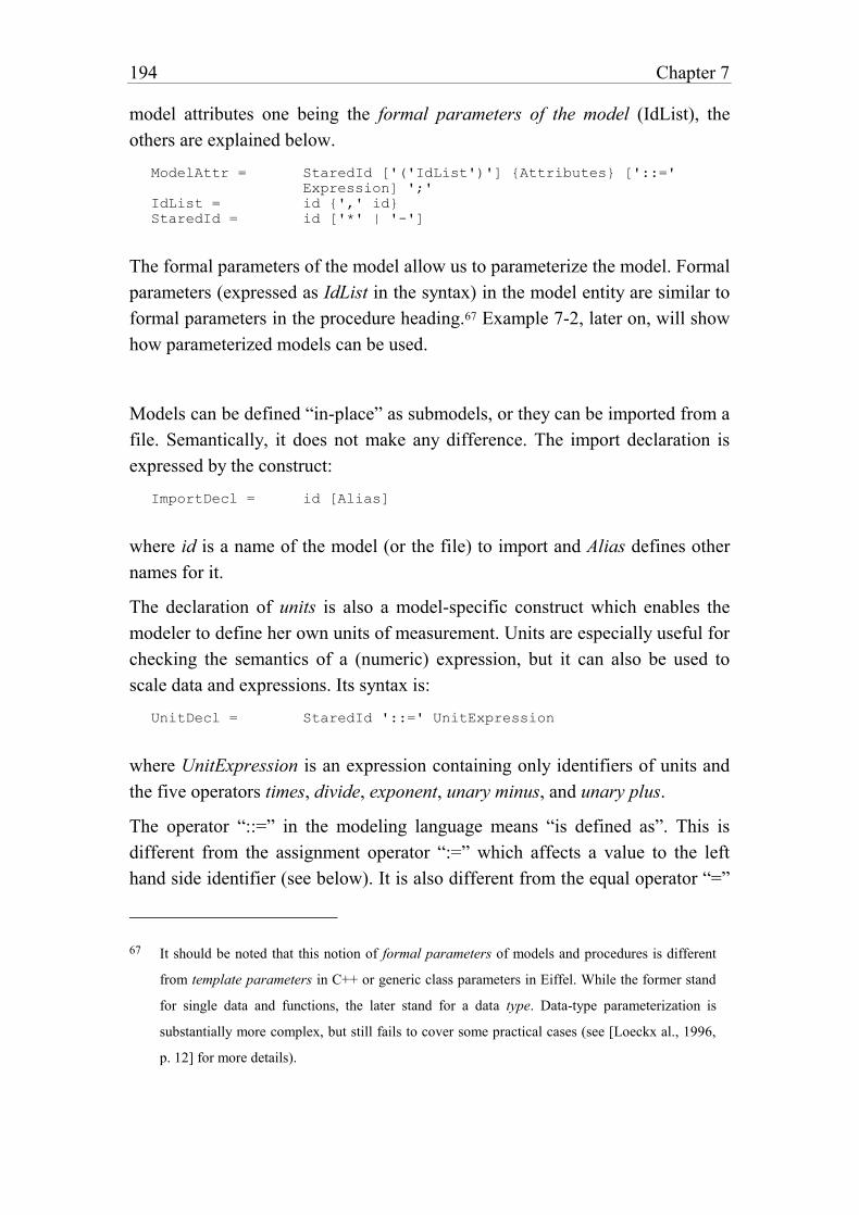
194 Chapter 7
model attributes one being the formal parameters of the model (IdList), the
others are explained below.
ModelAttr = StaredId ['('IdList')'] {Attributes} ['::='
Expression] ';'
IdList = id {',' id}
StaredId = id ['*' | '-']
The formal parameters of the model allow us to parameterize the model. Formal
parameters (expressed as IdList in the syntax) in the model entity are similar to
formal parameters in the procedure heading.67 Example 7-2, later on, will show
how parameterized models can be used.
Models can be defined “in-place” as submodels, or they can be imported from a
file. Semantically, it does not make any difference. The import declaration is
expressed by the construct:
ImportDecl = id [Alias]
where id is a name of the model (or the file) to import and Alias defines other
names for it.
The declaration of units is also a model-specific construct which enables the
modeler to define her own units of measurement. Units are especially useful for
checking the semantics of a (numeric) expression, but it can also be used to
scale data and expressions. Its syntax is:
UnitDecl = StaredId '::=' UnitExpression
where UnitExpression is an expression containing only identifiers of units and
the five operators times, divide, exponent, unary minus, and unary plus.
The operator “::=” in the modeling language means “is defined as”. This is
different from the assignment operator “:=” which affects a value to the left
hand side identifier (see below). It is also different from the equal operator “=”
67 It should be noted that this notion of formal parameters of models and procedures is different
from template parameters in C++ or generic class parameters in Eiffel. While the former stand
for single data and functions, the later stand for a data type. Data-type parameterization is
substantially more complex, but still fails to cover some practical cases (see [Loeckx al., 1996,
p. 12] for more details).
Framework: A Modeling Framework 195
which is used in a Boolean expression to check whether two expressions are
equal in the mathematical sense. StaredId is a stared identifier defined above.
The declaration of types is the same as in Oberon, except that the array type is
not needed. Arrays are defined over index-sets (explained in the section 7.2.4).
The syntax is similar to [Wirth 1996, p. 160]:
TypeDecl = StaredId '=' Type
Type = DotId | RecordType | PointerType | ProcType
DotId = id {'.' id}
RecordType = RECORD ['(' DotId ')'] FieldListSeq END
PointerType = POINTER TO Type
ProcType = PROCEDURE [FormalParam]
FieldListSeq = FieldList {';' FieldList}
FieldList = [IdentList ':' Type]
IdentList = StaredId {',' StaredId}
FormalParam = '(' [FPSection {';' FPSection}] ')' [':' DotId]
FPSection = [VAR] id{',' id} ':' FormalType
FormalType = DotId | ProcedureType
It is remarkable, that the entire object-oriented part of the language Oberon can
be expressed with these 12 lines! Here the proverb “Make it as simple as
possible, but not simpler” (Einstein) finds its proof. It goes beyond the scope of
this work to explain in detail the semantics behind the type statement. It can be
found in [Reiser 1992] or [Mössenböck 1994].
Declaration of procedures, again, are similar to those in Oberon, except that the
declaration part of the procedure body can contain any declaration. The syntax
is:
ProcedureDecl = ProcHeading ';' ProcBody id
ProcHeading = StaredId [FormalParam]
ProcBody = Declarations [BEGIN StatSeq] END
It should be noted that an entire model can be declared as a local memory
variable of a procedure. This make sense, with one exception: Stared identifiers
within the body of procedures cannot be visible outside the procedure, since
they are created when the procedure is called and destroyed when it returns.
Hence, stared identifiers within model nested in procedures are visible in the
boundary of the surrounding procedure but not outside.
The essential construct of the declarative part of a model is the declaration of
entities. What an entity is and how they are used, will be explained shortly; here
only the syntax is given:
196 Chapter 7
EKeyword = SET | PARAMETER | VARIABLE | CONSTRAINT
EntityDecl StaredId [IndexList] {Attributes} ['::='
Expression]
An entity declaration begins with one of the four keywords EKeyword which
defines the genus of the entity. The set entity starting with a keyword SET
declares set and relations (index-sets) which can be used to declare vectors,
matrices, and higher-dimensional tables of entities. The parameter entity
beginning with the keyword PARAMETER declares the data of the model. The
variable entity starts with VARIABLE and declares the variables of the model.
There is no difference between parameter and variable entities except that the
latter are normally assigned under the control of a solver, while the first are
given inside the model specification. Both entities also can be used as memory
variables, which are really memory slots, used in programming language (see
footnote 21 on page 29). The constraint entity begins with the keyword
CONSTRAINT and declares the model constraints.
Finally, there are five instruction entities in the declaration parts: the Check,
Read, Write, Transform, and the Solve instruction.
InstEntity = CheckStat | ReadStat | WriteStat | TransfStat |
SolveStat
CheckStat = CHECK [id] [IndexList] {CheckAttr} ['::='
Expression]
ReadStat = READ [id] [IndexList] {ReadAttr} ['::='
Expression]
WriteStat = WRITE [id] [IndexList] {WriteAttr} ['::='
Expression]
TransfStat = TRANSFORM IdList
SolveStat = SOLVE [id] {SolveAttr}
CheckAttr = Comment
ReadAttr = FROM ['*'] FileName | BLOCK FROM id TO id
WriteAttr = TO ['+'] FileName | FORMAT FormatSpecifier
SolveAttr = USING id | BY MAXIMIZING id | BY MINIMIZING id
The Check statement can be used to check the validity of the data and other
parts of the model The Read statement is a high-level import generator, i.e. a
generic way to import data into the model either from databases, or other
sources. The Write statement is a complete report generator, i.e. a generic
method to export data tables to either databases or other destinations. The
Transform statement instructs the executable module of the modeling language
how to translate the declarative form into a solver readable form. The solve
statement also instructs the run-time module on how to solve the model. Note
Framework: A Modeling Framework 197
that at most one Solve and one Transform instruction are allowed in the
declarative part of the model, and that the Check, Read, and Write instruction
have a similar syntax to the four other entities. The semantic of the instruction
entities is explained in 7.2.6.
The executable part of a model consists of a sequence of statements. Its syntax
is as follows:
StatSeq = {Statement ';'}
Statement = InstEntity | RunStat | IfStat | LoopStat |
Assignment | ProcCall
RunStat = RUN id
IfStat = IF Expression THEN StatSeq [ELSE StatSeq] END
LoopStat = WHILE Expression DO StatSeq END
Assignment = DotId [IndexList] ':=' Expression
ProcCall = DotId [ActualParam]
ActualParam = '(' [Expression {',' Expression}] ')'
The instruction entities can also be placed within the sequence of statements. In
this case, contrary to those placed in the declaration part, they are executed as
indicated by the sequence and are, therefore, fully controllable by the modeler.
The Run statement runs the executable part of a model (or an external process).
If a model is instructed to run itself, the modeler should care for termination
conditions, otherwise the execution enters an infinite loop. The Run statement
can also be used to run the executable part of another model or a submodel
provided that the model is visible.
The other statements (if, loop, assignment, and procedure call) are well-known
constructs from programming languages and their semantics do not need to be
explained here.
This concludes the overall structure of the modeling language. In the next
sections, we will concentrate on particular aspects of the language and their
semantics.
7.2.3. Entities and Attributes
The declarative part of a model consists of a collection of entities. An entity is
what the modeler considers as an indivisible fragment of the model. Variables,
constraints, and parameters are entities. An entity consists of attributes which
define its state and its behaviour. In this respect, an entity is much like an object
198 Chapter 7
in object-oriented languages. An object, however, is an instance of a class,
while an entity is defined on its own. It is a more rigid and inflexible concept
than an object. Furthermore, an entity always has a value, whereas an object
contains fields (or features in Eiffel) which have values. The object itself does
not have a value. Of course, since “everything” can be an object, an entity could
be viewed and implemented as an object. However, the structure of an object is
too general to serve the same specific purposes as an entity. An object has a
rich “inner life” containing many components which have been carefully put
together in order to encapsulate a concept. An entity is a monolithic block that
cannot be split into components.
I have tried several times to subsume the concept of entity under the concept of
object; but it seemed rather artificial. First, the modeler would need to declare a
class of, say, binary variables; then, in a second step, she would have to declare
the object of that type. Surely, one could say that the modeler does not need to
declare specific classes, this should be done by the modeling language designer;
these classes must be an integrated part of the language. In fact, this is exactly
the scheme adopted in this chapter. One could, of course, replace “entity” with
“a specific object based on predefined classes of the language in order to
express the indivisible parts of a model”. The genus of an entity expresses only
to which class (set, parameter, variable etc.) it belongs. Let us use the term
“entity” uniquely for this purpose.
An entity consists of a collection of predefined and optional attributes68 which
define its state and behaviour, as noted above. An attribute is a trait, a property
of the entity. Each entity belongs to a genus and has a name. These two
attributes are mandatory for all entities. Other attributes are optional, such as
the unit, the alias, or the comment attribute. The unit attribute defines the unit
of measurement of the entity's value, the alias declares a second or third name
for the entity, and the comment is a string which explains the entity. The
following phrase expresses the fact that the entity is a collection of attributes:
GenusAttr NameAttr [IndexAttr] {Other_attributes} '::=' ValueAttr
68 The term attribute is used throughout this text to denote explicit properties of an entiy, which
have a well defined syntax within the modeling language.
Framework: A Modeling Framework 199
where GenusAttr is the same as EKeyword, NameAttr is StaredId, IndexAttr is
IndexList, Other_attributes is Attributes, and ValueAttr is an Expression in the
EBNF syntax shown above and summarized in Section 7.2.7.
Strictly speaking, the model, the unit and the type declaration are themselves
entities with a different list of attributes. Even the instruction entities can be
subsumed under the concept of entities (as outlined above), since they consist
of a number of – still different – attributes too. The concept of attributes is very
flexible from the point of view of language design: If we feel that a specific
attribute should be added to the language or removed from it in order to
investigate various language extensions, it can easily be done. The feature is
especially interesting in the present state of modeling languages which are still
in an experimental stage.
Several optional attributes have already proved their value in mathematical
models. Their syntax is the following:
Attributes = PreDefAttr | UserDefAttr
PreDefAttr = AliasAttr | SimpTypeAttr | DefaultAttr |
RangeAttr | UnitAttr | NomenAttr | CommentAttr
AliasAttr = ALIAS id [',' id]
SimpTypeAttr = REAL | INTEGER | BINARY | STRING | PointerType |
ProcType
DefaultAttr = DEFAULT DefaultValue
RangeAttr = '[' Expression ']'
UnitAttr = UNIT UnitExpression
NomenAttr = ''' String '''
CommentAttr = '"' String '"'
UserDefAttr = RecordType
The alias-attribute allots the entity one or several other names (besides the
mandatory name-attribute) which must also be unique model-wide. Why would
the modeler want several names for the same entity? One advantage is that she
no longer needs to choose between a long, expressive and a short, cryptic name;
at key points in the model the long name can be used, in lengthy expressions the
short name is more appropriate. A more convincing argument, however, is that
in some contexts several names are needed. This is the case in defining several
indices for the same set.
An example is:
SET sites ALIAS s1, s2;
PARAMETER links{s1,s2};
where a set sites is declared together with two aliases, s1 and s2. The second
line declares a two-dimensional data-table, called links, where the rows and
200 Chapter 7
column both run through the same set of sites. Using links in subsequent
expressions simplifies considerably the expressions when we need to access the
first or the second index individually.
The type attribute defines the type of the entity's value. It must be one of the
simple type REAL (floating point numbers), INTEGER, BINARY ({0,1}),
STRING, a pointer, or a pointer to a procedure. Only the numerical types are
permitted for the variable genus. None is allowed for sets, and constraints are
always of type BINARY.
The default attribute assigns a default value or expression to the entity's value.
This is interesting particularly for parameter entities.
The range attribute specifies a lower and an upper bound value for the entity's
value. Defined for variables, this attribute can (should) be translated into an
upper and lower bound constraint; for parameters it gives additional data
checking capabilities. The range attribute only makes sense for numerical
entities.
The unit attribute imposes a unit on the entity. The correctness of units are
checked in subsequent expressions. Units are a strong semantic check for the
exactness of an expression. Experience in class room modeling have shown that
many formulation errors can be detected and eliminated simply by checking the
commensurability of two expressions. This attribute too, makes sense for
entities of numerical types only.
The nomenclature attribute indicates how indexed entities should be mapped to
names recognized by the solver. Normally the modeling system should take
care to generate single and unique variable and constraint names in order to
distinguish them. Sometimes, however, the user wants to produce her names.
This option has more applications than one might think at first sight. To begin
with, most solvers only accept names of limited size. Debugging and viewing
the solver's input/output would be difficult with cryptic names. Another
application is the graphical representation of entities. In short, user generated
names may be easier to draw in the plane than long ones.
The comment attribute is a string that explains the entity. This attribute can be
more complex then just a multi-line text. It may contain place-holders for the
different attributes of an entity, for example the indices (see also [Greenberg
1994]).
Framework: A Modeling Framework 201
The user-defined attribute is a record type that allocates further attributes
defined by the modeler. An example is:
PARAMETER a RECORD x,y:INTEGER; END ;
The parameter a (which is of type REAL and has itself a value) is extended by
two attributes of type INTEGER (x and y).
Model entities cannot contain user-defined attributes.
Attributes can be accessed and changed eventually in expressions using the dot
notation. For example, the comment attribute in
VARIABLE x "Comment for x" ;
can be accessed in an expression by
... x.comment ...
For each mandatory and optional attribute, a keyword is defined to access its
value. User-defined attributes are also accessed using the dot notation.
The entity/attribute framework is a simple and flexible concept. New entities or
attributes can easily be added to or removed from the language specification.
For example, the Solve instruction can be augmented by two other attributes
saying that a feasible solution, or all solution should be found. One could then
extend the attributes as follows:
SolveAttr = USING id | BY MAXIMIZING id | BY MINIMIZING id |
FIND ANY | FIND ALL
Another example is the attribute “position of the entity on the screen when
viewed as graphical form”. We shall see in Part III how large models can be
displayed as graphs where each node is an entity. Depending mainly on where
each entity is placed, the drawing can be a well-ordered, clearly arranged
shapes, or an impervious mess. The positioning can be performed automatically
by using placement algorithms, but manual readjustments are necessary most of
the time, in order to obtain a well disposed picture. It is easy to store the
information of the positions as an attribute of the entity itself. In LPL, for
example, it is implemented as:
202 Chapter 7
PositionAttr = COOR xPos ',' yPos
(where xPos and yPos are numbers). Since in LPL each entity can be declared
several times, each time with a different set of attributes, this solution is
especially attractive: the lists of entities, together with the position attribute can
be located in a separate file, thereby, not interfering with the structure of the
model.
A further enrichment of the entity/attribute concept is the extension of the
competence of one or several attributes. An example, is the introduction of
further special types for variables. For example, in many discrete problems we
want to find a permutation which optimizes a function. A famous example is
the travelling sales person problem, in which a tour is searched that visits each
location exactly once while minimizing the traveling distance. A concise
formulation is to declare a set {1...n} where n is the degree of the permutation
and to define a variable as follows:
VARIABLE x{i} DISTINCT [1..n];
which means that the n variables must be of type DISTINCT (integers, but all
different from each other) in the range [1..n]. This is the same as a permutation.
It is important to note that such a declaration does not anticipate any specific
solver. It should also be noted, that such a construct is similar in expressive
power to the alldistinct() predicate of the constraint language CHIP.
Another type can be SYMBOLIC, which is a finite integer type where the
numbers are replaced by names.
Still other special types of a very different kind are STOCHASTIC parameters
or FUZZY variables to formulate specific sorts of uncertainty. This seems to be
somewhat speculative since it is, at the moment, unclear how fuzzy variables
should be combined with non-fuzzy ones in the same model. At the end of Part
III, further ideas and two hypothetical models that use these two types will be
discussed.
7.2.4. Index-sets
One of the most interesting, thorny, but absolutely indispensable constructs in
modeling languages are index-sets. By using index-sets, the modeler can
express a set of expressions in a concise way as is common in algebraic
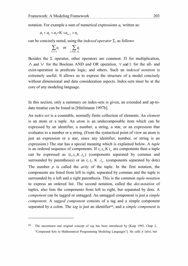
Framework: A Modeling Framework 203
notation. For example a sum of numerical expressions ai written as:
a1 a2 a3K an1 an
can be concisely noted, using the indexed operator , as follows
ai
1 i n
or
ai
i{1,K ,n}
Besides the operator, other operators are common: for multiplication,
and for the Boolean AND and OR operation, and for the all- and
exist-operation in predicate logic, and others. Such an indexed notation is
extremely useful. It allows us to express the structure of a model concisely
without dimensional and data consideration aspects. Index-sets must be at the
core of any modeling language.
In this section, only a summary on index-sets is given, an extended and up-to-
date treatise can be found in [Hürlimann 1997b].
An index-set is a countable, normally finite collection of elements. An element
is an atom or a tuple. An atom is an undecomposable item which can be
expressed by an identifier, a number, a string, a star, or an expression that
evaluates to a number or a string. (From the syntactical point of view an atom is
just an expression or a star, since any identifier, number, or string is an
expression.) The star has a special meaning which is explained below. A tuple
is an ordered sequence of components. If t1,t2 ,K tp are components then a tuple
can be expressed as (t1,t2 ,K ,tp ) (components separated by commas and
surrounded by parentheses) or as t1.t2 . K .tp . (components separated by dots)
The number p is called the arity of the tuple. In the first notation, the
components are listed from left to right, separated by commas and the tuple is
surrounded by a left and a right parenthesis. This is the common tuple-notation
to express an ordered list. The second notation, called the dot-notation of
tuples, also lists the components from left to right, but separated by dots. A
component can be tagged or untagged. An untagged component is just a simple
component. A tagged component consists of a tag and a simple component
separated by a colon. The tag is just an identifier69, and a simple component is
69 The uncommon and original concept of tag has been introduced by [Kuip 1992, Chap 2,
“Compound Sets in Mathematical Programming Modeling Languages”]. He calls it label, but
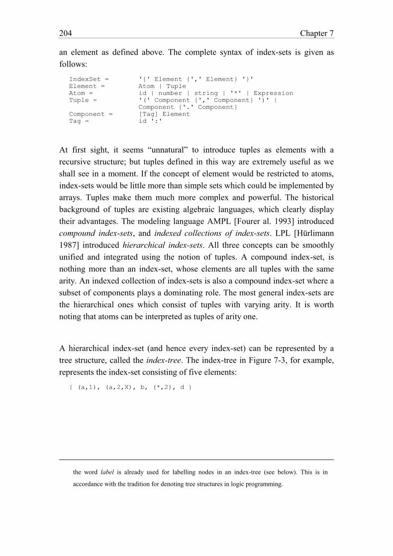
204 Chapter 7
an element as defined above. The complete syntax of index-sets is given as
follows:
IndexSet = '{' Element {',' Element} '}'
Element = Atom | Tuple
Atom = id | number | string | '*' | Expression
Tuple = '(' Component {',' Component} ')' |
Component {'.' Component}
Component = [Tag] Element
Tag = id ':'
At first sight, it seems “unnatural” to introduce tuples as elements with a
recursive structure; but tuples defined in this way are extremely useful as we
shall see in a moment. If the concept of element would be restricted to atoms,
index-sets would be little more than simple sets which could be implemented by
arrays. Tuples make them much more complex and powerful. The historical
background of tuples are existing algebraic languages, which clearly display
their advantages. The modeling language AMPL [Fourer al. 1993] introduced
compound index-sets, and indexed collections of index-sets. LPL [Hürlimann
1987] introduced hierarchical index-sets. All three concepts can be smoothly
unified and integrated using the notion of tuples. A compound index-set, is
nothing more than an index-set, whose elements are all tuples with the same
arity. An indexed collection of index-sets is also a compound index-set where a
subset of components plays a dominating role. The most general index-sets are
the hierarchical ones which consist of tuples with varying arity. It is worth
noting that atoms can be interpreted as tuples of arity one.
A hierarchical index-set (and hence every index-set) can be represented by a
tree structure, called the index-tree. The index-tree in Figure 7-3, for example,
represents the index-set consisting of five elements:
{ (a,1), (a,2,X), b, (*,2), d }
the word label is already used for labelling nodes in an index-tree (see below). This is in
accordance with the tradition for denoting tree structures in logic programming.
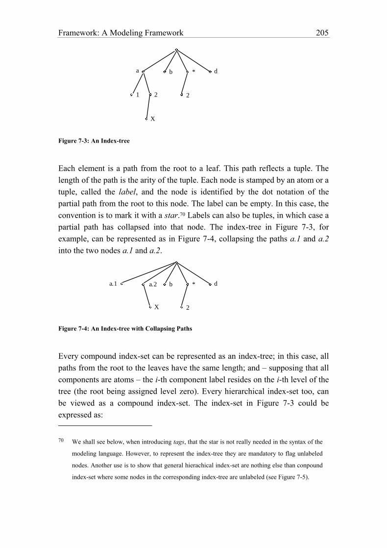
Framework: A Modeling Framework 205
a b * d
1 2 2
X
Figure 7-3: An Index-tree
Each element is a path from the root to a leaf. This path reflects a tuple. The
length of the path is the arity of the tuple. Each node is stamped by an atom or a
tuple, called the label, and the node is identified by the dot notation of the
partial path from the root to this node. The label can be empty. In this case, the
convention is to mark it with a star.70 Labels can also be tuples, in which case a
partial path has collapsed into that node. The index-tree in Figure 7-3, for
example, can be represented as in Figure 7-4, collapsing the paths a.1 and a.2
into the two nodes a.1 and a.2.
a.1 b * d
X 2
a.2
Figure 7-4: An Index-tree with Collapsing Paths
Every compound index-set can be represented as an index-tree; in this case, all
paths from the root to the leaves have the same length; and – supposing that all
components are atoms – the i-th component label resides on the i-th level of the
tree (the root being assigned level zero). Every hierarchical index-set too, can
be viewed as a compound index-set. The index-set in Figure 7-3 could be
expressed as:
70 We shall see below, when introducing tags, that the star is not really needed in the syntax of the
modeling language. However, to represent the index-tree they are mandatory to flag unlabeled
nodes. Another use is to show that general hierachical index-set are nothing else than conpound
index-set where some nodes in the corresponding index-tree are unlabeled (see Figure 7-5).
206 Chapter 7
{ (a,1,*), (a,2,X), (b,*,*), (*,2,*), (*,d,*) }
and the corresponding index-tree is shown in Figure 7-5. The convention is,
that stared leaves can simply be removed or added anywhere without changing
the semantic of the index-set.
a b * d
1 2 2
X
*
**
*
**
Figure 7-5: An Index-tree Viewed as a Compound Index-set
An important property of this collapsing and expanding operation is that the
number of leaves in the index-tree and hence the number of elements in the
corresponding index-set does not change. Only the way the tree is represented
changes.
There is another way to look at the index-set: as sets of sets. The set in Figure
7-3 could be represented as:
{ a{1,2{X}}, b, {2}, d }
To capture this syntax, only the non-terminal symbol IndexSet must be
modified slightly to:
IndexSet = '{' ElementOrSet {',' ElementOrSet} '}'
ElementOrSet = Element | [Label] IndexSet
Label = Element
This makes the concept of index-set recursive, and sets can be nested within
each other. The last example can now be interpreted as follows: The index-set
contains four branches at the root level, the first is itself an index-set containing
two branches and the name a (its label), the third is a index-set without a name,
and the others are simple elements (atoms).
All this does not explain the benefits of tags. Tuples are – as we have seen –
ordered list of components which reflect the levels in the index-tree. Tags have
two benefits: the order of components within tuples can be permuted and, for
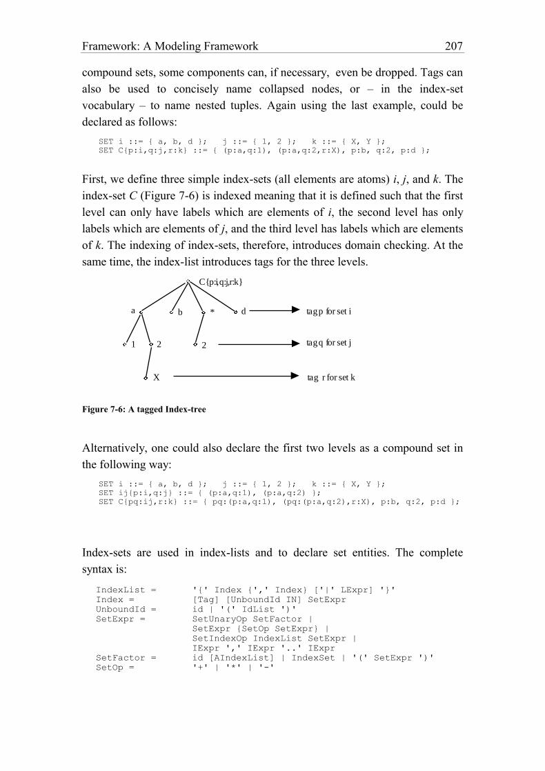
Framework: A Modeling Framework 207
compound sets, some components can, if necessary, even be dropped. Tags can
also be used to concisely name collapsed nodes, or – in the index-set
vocabulary – to name nested tuples. Again using the last example, could be
declared as follows:
SET i ::= { a, b, d }; j ::= { 1, 2 }; k ::= { X, Y };
SET C{p:i,q:j,r:k} ::= { (p:a,q:1), (p:a,q:2,r:X), p:b, q:2, p:d };
First, we define three simple index-sets (all elements are atoms) i, j, and k. The
index-set C (Figure 7-6) is indexed meaning that it is defined such that the first
level can only have labels which are elements of i, the second level has only
labels which are elements of j, and the third level has labels which are elements
of k. The indexing of index-sets, therefore, introduces domain checking. At the
same time, the index-list introduces tags for the three levels.
a b * d
1 2 2
X
C{p:i,q:j,r:k}
tag p for set i
tag q for set j
tag r for set k
Figure 7-6: A tagged Index-tree
Alternatively, one could also declare the first two levels as a compound set in
the following way:
SET i ::= { a, b, d }; j ::= { 1, 2 }; k ::= { X, Y };
SET ij{p:i,q:j} ::= { (p:a,q:1), (p:a,q:2) };
SET C{pq:ij,r:k} ::= { pq:(p:a,q:1), (pq:(p:a,q:2),r:X), p:b, q:2, p:d };
Index-sets are used in index-lists and to declare set entities. The complete
syntax is:
IndexList = '{' Index {',' Index} ['|' LExpr] '}'
Index = [Tag] [UnboundId IN] SetExpr
UnboundId = id | '(' IdList ')'
SetExpr = SetUnaryOp SetFactor |
SetExpr {SetOp SetExpr} |
SetIndexOp IndexList SetExpr |
IExpr ',' IExpr '..' IExpr
SetFactor = id [AIndexList] | IndexSet | '(' SetExpr ')'
SetOp = '+' | '*' | '-'
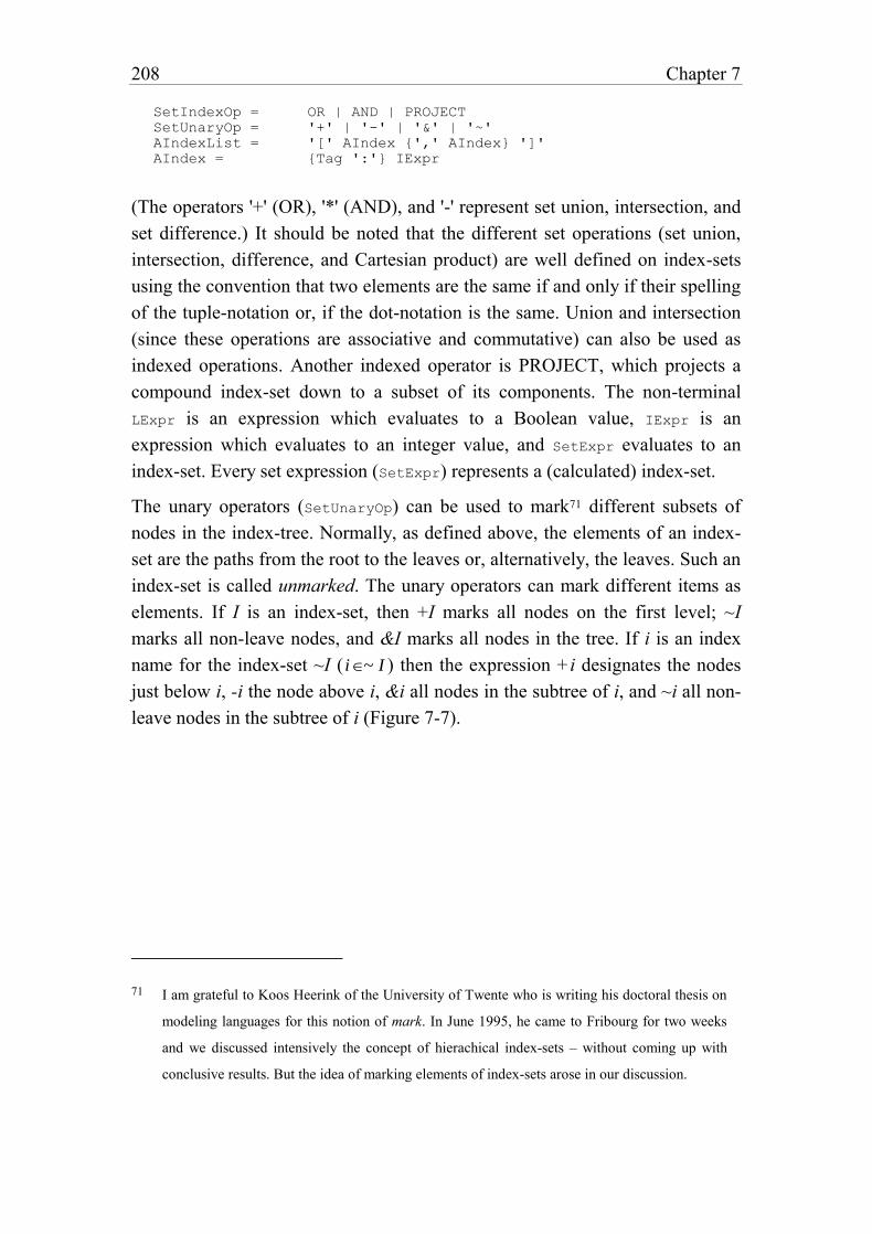
208 Chapter 7
SetIndexOp = OR | AND | PROJECT
SetUnaryOp = '+' | '-' | '&' | '~'
AIndexList = '[' AIndex {',' AIndex} ']'
AIndex = {Tag ':'} IExpr
(The operators '+' (OR), '*' (AND), and '-' represent set union, intersection, and
set difference.) It should be noted that the different set operations (set union,
intersection, difference, and Cartesian product) are well defined on index-sets
using the convention that two elements are the same if and only if their spelling
of the tuple-notation or, if the dot-notation is the same. Union and intersection
(since these operations are associative and commutative) can also be used as
indexed operations. Another indexed operator is PROJECT, which projects a
compound index-set down to a subset of its components. The non-terminal
LExpr is an expression which evaluates to a Boolean value, IExpr is an
expression which evaluates to an integer value, and SetExpr evaluates to an
index-set. Every set expression (SetExpr) represents a (calculated) index-set.
The unary operators (SetUnaryOp) can be used to mark71 different subsets of
nodes in the index-tree. Normally, as defined above, the elements of an index-
set are the paths from the root to the leaves or, alternatively, the leaves. Such an
index-set is called unmarked. The unary operators can mark different items as
elements. If I is an index-set, then +I marks all nodes on the first level; ~I
marks all non-leave nodes, and &I marks all nodes in the tree. If i is an index
name for the index-set ~I (i ~ I ) then the expression +i designates the nodes
just below i, -i the node above i, &i all nodes in the subtree of i, and ~i all non-
leave nodes in the subtree of i (Figure 7-7).
71 I am grateful to Koos Heerink of the University of Twente who is writing his doctoral thesis on
modeling languages for this notion of mark. In June 1995, he came to Fribourg for two weeks
and we discussed intensively the concept of hierachical index-sets – without coming up with
conclusive results. But the idea of marking elements of index-sets arose in our discussion.
Framework: A Modeling Framework 209
a b * d
1 2 2
X
C
=i
-i
+i
&i
i~
Figure 7-7: A Marked Index-tree
It is important to note, that these unary operators only mark elements, but do
not modify the index-set. A simple example shows how useful these operations
are: Let I be a hierarchical structure representable by an index-set, and let A be
a numerical vector indexed over all nodes in I. Suppose the entries for the
leaves in A have already been assigned. Now we want to assign recursively the
sum of the descendants to each non-leave entry. How can this be done? The
following statement would suffice72:
A{i IN ~I} := SUM{j IN +i} A[j];
7.2.5. Expression
Expressions are the most fundamental constructs of the modeling language. In
the last section, expressions that return index-sets (SetExpr) have already been
presented. There are also expressions of type Boolean (logical), numerical
(integer or real), and of type string. Since identifiers must be declared, for each
subexpression the type can be evaluated at compile time. This is important in
order to interpret every expression semantically in a correct way. In this section,
first, the syntax is given separately for each type: Boolean, numerical, and
72 In the first version of LPL [Hürlimann 1987, p. 23], it was already possible to use such a
construct for generating recursively defined constraints. However, that construct was limited in
several respects and, therefore, has been removed in subsequent versions. I wanted to integrate a
general concept of hierchical index-sets or leave it entirely.
210 Chapter 7
string expressions. At the end, the general syntax for expressions is exposed.
The Boolean (logical or binary) type is considered as a subtype of the numerical
type, but with a well defined number of operators. The syntax of Boolean
expressions is as follows:
LExpr = LUnaryOp LFactor |
LExpr {LOp LExpr} |
LIndexOp IndexList LExpr
LFactor = id [AIndexList] |
number ['[' UnitExpression ']'] |
'(' LExpr ')' |
LOp = '<' | '<=' | '=' | '<>' | '>' | '>=' | IN |
SUBSET | AND | OR | '->' | XOR | IFF | NAND | NOR
LIndexOp = EXIST | FORALL | XOR | NAND | NOR | AND | OR |
ATLEAST '(' IExpr ')' | ATMOST '(' IExpr ')' |
EXACTLY '(' IExpr ')'
LUnaryOp = '~'
The six relational operators are <, <=, =, <>, >, >= with the usual meaning
while the operands must be numerical. IN is the -operator to check whether an
element is within a set. SUBSET is the subset operator ( ), the operands must
both be index-sets. AND and OR are the usual operators, ~ denotes the
negation, -> the implication, XOR the exclusive or, IFF the equivalence,
NAND the not-and, and NOR the not-or operation. Several of them can also be
used as indexed operators. EXIST is the -, FORALL the -operator in
predicate logic. In fact they are the same as the indexed OR and AND. Three
other indexed operators are ATLEAST, ATMOST, and EXACTLY, which
have the meaning that at least (at most, or exactly) IExpr out of the following
indexed expressions must be true, where IExpr is an expression returning an
integer.
Numerical (integer or real) expressions have the following syntax:
NumExpr = NumUnaryOp NumFactor |
NumExpr {NumOp NumExpr} |
NumIndexOp IndexList NumExpr
NumFactor = id [AIndexSet] |
number ['[' UnitExpression ']'] |
'(' NumExpr ')' |
NumFunc '(' Expression ')'
NumOp = '+' | '-' | '*' | '/' | '%' | '^'
NumIndexOp = SUM | PROD | MIN | MAX | PMIN | PMAX | COL | ROW
NumUnaryOp = '+' | '-' | '#'
NumFunc = <built-in math. functions (abs, ceil, ...)>
String expressions have the following syntax:
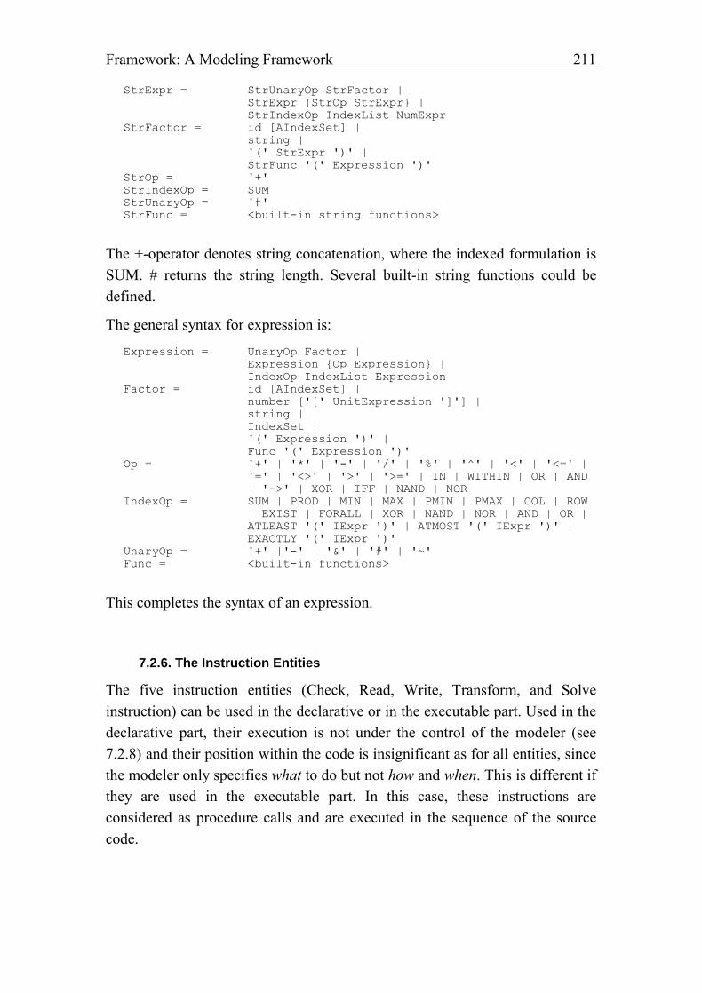
Framework: A Modeling Framework 211
StrExpr = StrUnaryOp StrFactor |
StrExpr {StrOp StrExpr} |
StrIndexOp IndexList NumExpr
StrFactor = id [AIndexSet] |
string |
'(' StrExpr ')' |
StrFunc '(' Expression ')'
StrOp = '+'
StrIndexOp = SUM
StrUnaryOp = '#'
StrFunc = <built-in string functions>
The +-operator denotes string concatenation, where the indexed formulation is
SUM. # returns the string length. Several built-in string functions could be
defined.
The general syntax for expression is:
Expression = UnaryOp Factor |
Expression {Op Expression} |
IndexOp IndexList Expression
Factor = id [AIndexSet] |
number ['[' UnitExpression ']'] |
string |
IndexSet |
'(' Expression ')' |
Func '(' Expression ')'
Op = '+' | '*' | '-' | '/' | '%' | '^' | '<' | '<=' |
'=' | '<>' | '>' | '>=' | IN | WITHIN | OR | AND
| '->' | XOR | IFF | NAND | NOR
IndexOp = SUM | PROD | MIN | MAX | PMIN | PMAX | COL | ROW
| EXIST | FORALL | XOR | NAND | NOR | AND | OR |
ATLEAST '(' IExpr ')' | ATMOST '(' IExpr ')' |
EXACTLY '(' IExpr ')'
UnaryOp = '+' |'-' | '&' | '#' | '~'
Func = <built-in functions>
This completes the syntax of an expression.
7.2.6. The Instruction Entities
The five instruction entities (Check, Read, Write, Transform, and Solve
instruction) can be used in the declarative or in the executable part. Used in the
declarative part, their execution is not under the control of the modeler (see
7.2.8) and their position within the code is insignificant as for all entities, since
the modeler only specifies what to do but not how and when. This is different if
they are used in the executable part. In this case, these instructions are
considered as procedure calls and are executed in the sequence of the source
code.
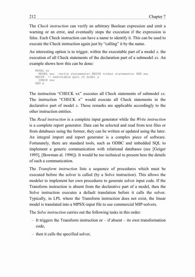
212 Chapter 7
The Check instruction can verify an arbitrary Boolean expression and emit a
warning or an error, and eventually stops the execution if the expression is
false. Each Check instruction can have a name to identify it. This can be used to
execute the Check instruction again just by “calling” it by the name.
An interesting option is to trigger, within the executable part of a model x, the
execution of all Check statements of the declaration part of a submodel xx. An
example shows how this can be done:
MODEL x;
MODEL xx; <write statements> BEGIN <other statements> END xx;
BEGIN -- executable part of model y
CHECK xx;
END x
The instruction “CHECK xx” executes all Check statements of submodel xx.
The instruction “CHECK x” would execute all Check statements in the
declarative part of model x. These remarks are applicable accordingly to the
other instruction entities.
The Read instruction is a complete input generator while the Write instruction
is a complete report generator. Data can be selected and read from text files or
from databases using the former, they can be written or updated using the later.
An integral import and report generator is a complex piece of software.
Fortunately, there are standard tools, such as ODBC and imbedded SQL to
implement a generic communication with relational databases (see [Geiger
1995], [Bowman al. 1996]). It would be too technical to present here the details
of such a communication.
The Transform instruction lists a sequence of procedures which must be
executed before the solver is called (by a Solve instruction). This allows the
modeler to implement her own procedures to generate solver input code. If the
Transform instruction is absent from the declarative part of a model, then the
Solve instruction executes a default translation before it calls the solver.
Typically, in LPL where the Transform instruction does not exist, the linear
model is translated into a MPSX-input file to use commercial MIP-solvers.
The Solve instruction carries out the following tasks in this order:
– It triggers the Transform instruction or – if absent – its own transformation
code,
– then it calls the specified solver,
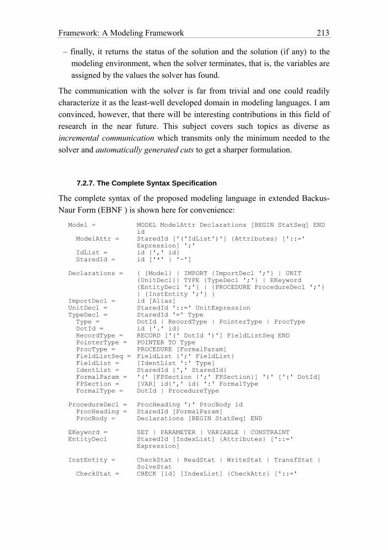
Framework: A Modeling Framework 213
– finally, it returns the status of the solution and the solution (if any) to the
modeling environment, when the solver terminates, that is, the variables are
assigned by the values the solver has found.
The communication with the solver is far from trivial and one could readily
characterize it as the least-well developed domain in modeling languages. I am
convinced, however, that there will be interesting contributions in this field of
research in the near future. This subject covers such topics as diverse as
incremental communication which transmits only the minimum needed to the
solver and automatically generated cuts to get a sharper formulation.
7.2.7. The Complete Syntax Specification
The complete syntax of the proposed modeling language in extended Backus-
Naur Form (EBNF ) is shown here for convenience:
Model = MODEL ModelAttr Declarations [BEGIN StatSeq] END
id
ModelAttr = StaredId ['('IdList')'] {Attributes} ['::='
Expression] ';'
IdList = id {',' id}
StaredId = id ['*' | '-']
Declarations = { {Model} | IMPORT {ImportDecl ';'} | UNIT
{UnitDecl}| TYPE {TypeDecl ';'} | EKeyword
{EntityDecl ';'} | {PROCEDURE ProcedureDecl ';'}
| {InstEntity ';'} }
ImportDecl = id [Alias]
UnitDecl = StaredId '::=' UnitExpression
TypeDecl = StaredId '=' Type
Type = DotId | RecordType | PointerType | ProcType
DotId = id {'.' id}
RecordType = RECORD ['(' DotId ')'] FieldListSeq END
PointerType = POINTER TO Type
ProcType = PROCEDURE [FormalParam]
FieldListSeq = FieldList {';' FieldList}
FieldList = [IdentList ':' Type]
IdentList = StaredId {',' StaredId}
FormalParam = '(' [FPSection {';' FPSection}] ')' [':' DotId]
FPSection = [VAR] id{',' id} ':' FormalType
FormalType = DotId | ProcedureType
ProcedureDecl = ProcHeading ';' ProcBody id
ProcHeading = StaredId [FormalParam]
ProcBody = Declarations [BEGIN StatSeq] END
EKeyword = SET | PARAMETER | VARIABLE | CONSTRAINT
EntityDecl StaredId [IndexList] {Attributes} ['::='
Expression]
InstEntity = CheckStat | ReadStat | WriteStat | TransfStat |
SolveStat
CheckStat = CHECK [id] [IndexList] {CheckAttr} ['::='
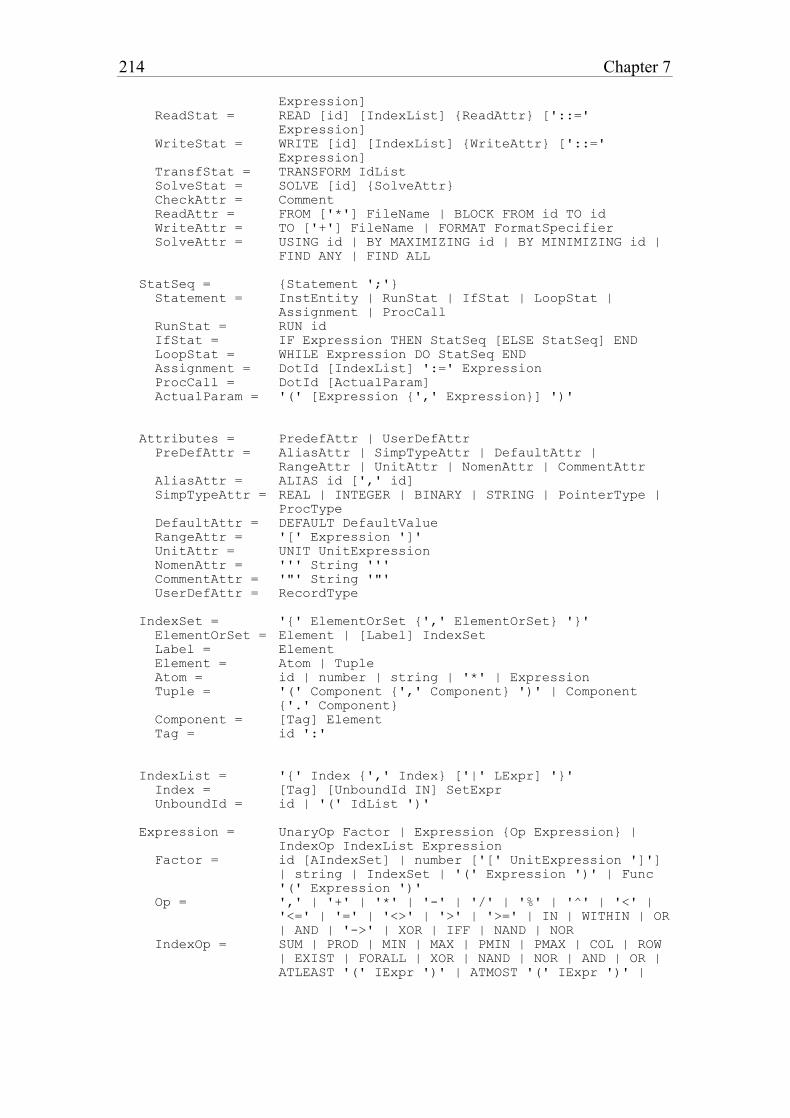
214 Chapter 7
Expression]
ReadStat = READ [id] [IndexList] {ReadAttr} ['::='
Expression]
WriteStat = WRITE [id] [IndexList] {WriteAttr} ['::='
Expression]
TransfStat = TRANSFORM IdList
SolveStat = SOLVE [id] {SolveAttr}
CheckAttr = Comment
ReadAttr = FROM ['*'] FileName | BLOCK FROM id TO id
WriteAttr = TO ['+'] FileName | FORMAT FormatSpecifier
SolveAttr = USING id | BY MAXIMIZING id | BY MINIMIZING id |
FIND ANY | FIND ALL
StatSeq = {Statement ';'}
Statement = InstEntity | RunStat | IfStat | LoopStat |
Assignment | ProcCall
RunStat = RUN id
IfStat = IF Expression THEN StatSeq [ELSE StatSeq] END
LoopStat = WHILE Expression DO StatSeq END
Assignment = DotId [IndexList] ':=' Expression
ProcCall = DotId [ActualParam]
ActualParam = '(' [Expression {',' Expression}] ')'
Attributes = PredefAttr | UserDefAttr
PreDefAttr = AliasAttr | SimpTypeAttr | DefaultAttr |
RangeAttr | UnitAttr | NomenAttr | CommentAttr
AliasAttr = ALIAS id [',' id]
SimpTypeAttr = REAL | INTEGER | BINARY | STRING | PointerType |
ProcType
DefaultAttr = DEFAULT DefaultValue
RangeAttr = '[' Expression ']'
UnitAttr = UNIT UnitExpression
NomenAttr = ''' String '''
CommentAttr = '"' String '"'
UserDefAttr = RecordType
IndexSet = '{' ElementOrSet {',' ElementOrSet} '}'
ElementOrSet = Element | [Label] IndexSet
Label = Element
Element = Atom | Tuple
Atom = id | number | string | '*' | Expression
Tuple = '(' Component {',' Component} ')' | Component
{'.' Component}
Component = [Tag] Element
Tag = id ':'
IndexList = '{' Index {',' Index} ['|' LExpr] '}'
Index = [Tag] [UnboundId IN] SetExpr
UnboundId = id | '(' IdList ')'
Expression = UnaryOp Factor | Expression {Op Expression} |
IndexOp IndexList Expression
Factor = id [AIndexSet] | number ['[' UnitExpression ']']
| string | IndexSet | '(' Expression ')' | Func
'(' Expression ')'
Op = ',' | '+' | '*' | '-' | '/' | '%' | '^' | '<' |
'<=' | '=' | '<>' | '>' | '>=' | IN | WITHIN | OR
| AND | '->' | XOR | IFF | NAND | NOR
IndexOp = SUM | PROD | MIN | MAX | PMIN | PMAX | COL | ROW
| EXIST | FORALL | XOR | NAND | NOR | AND | OR |
ATLEAST '(' IExpr ')' | ATMOST '(' IExpr ')' |
Framework: A Modeling Framework 215
EXACTLY '(' IExpr ')'
UnaryOp = '+' |'-' | '&' | '#' | '~'
Func = <built-in functions>
Note that the comma is also an operator. It allows one to define lists of
expressions.
7.2.8. Semantic Interpretation
A model is different from a program with respect to its declarations. The
declarative part must be processed and translated into a form that a solver can
handle. Therefore, when the modeling language compiler is triggered, the code
cannot simply be translated into machine code. This section summarizes the
sequence of steps that must be executed in order to process a model source code
and to solve the model.
Step 1: The model is parsed, the syntax is checked, and the code is translated
into an internal format whichever is appropriate for further processing.
While parsing, IMPORT instructions redirect the scanner and read other
models directly as if they were included file.
Step 2: If the parsing step complets successfully, then the model can be
processed. First, all READ instructions are “executed” in the declaration
part of the model and in all of the submodels in their order of appearance in
the source code, i.e. all data is imported into the internal structure. This
might require a paging mechanism in which the data is temporarily stored in
files. An alternative would be to read the data only when needed which
might entail a lot of work. Especially, if the data is in databases, this might
imply connecting and eventually logging-in to several times. In any case,
the language designer has to balance the execution speed against the storage
amount. In our proposition, speed is the primary criterion.
Step 3: All parameters in the model and all submodels are calculated and
stored in tables. This implies that parameters cannot be recursively
dependent upon each other, the compiler must check for this. Again, an
alternative is to calculate the parameters only when needed. This can be
more efficient if a lot of data is involved and the parameters are used only
once. The compiler could check for this most of the time and take the
appropriate decision.

216 Chapter 7
Step 4: All CHECK instructions in the declarative part of the model and all
submodels are executed and all RANGE constraints are checked within the
model and all submodels. (Unit checking takes place while parsing). In this
step the data is validated.
Now the model has been instantiated: all the data has been read, the model has
been validated. It is now ready to be processed. This includes the following
steps.
Step 5: If the declarative part of the main model contains a TRANSFORM
and a SOLVE instruction, then they are executed in this order (first the
TRANSFORM and then the SOLVE, regardless of how they are ordered in
the source code). Note that a declarative part can contain at most one
TRANSFORM and one SOLVE instruction.
Step 6: If the main model contains an empty executable part, then all WRITE
instructions in the declarative part are executed in the order in which they
appear in the source code, and then the execution terminates.
Step 7: If the executable part is not empty, then this part is executed,
instruction by instruction in the order of the sequence in the source code,
and then the execution terminates.
The executable parts as well as the TRANSFORM, the SOLVE, and the
WRITE instructions in the declarative part of the submodels are not executed.
They must be triggered from outside by an appropriate RUN, TRANSFORM,
SOLVE, or WRITE instruction. For example, the statement
WRITE m ;
where m is a model entity identifier, will trigger the execution of all WRITE
instructions of (sub)model m.
The READ and the CHECK instructions in the declarative part of a (sub)model
can also be triggered by an appropriate call placed in the executable part. For
example, the statement
READ m ;
where m is again a model entity name, will execute all READ instructions of
the model m, while overwriting all data. This instruction also entails the
execution of steps 3 and 4. Since the data has changed, and it must be validated.
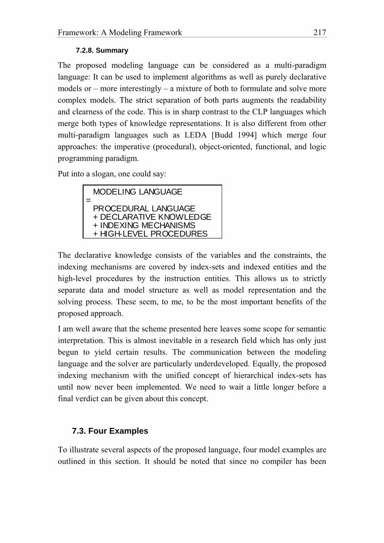
Framework: A Modeling Framework 217
7.2.8. Summary
The proposed modeling language can be considered as a multi-paradigm
language: It can be used to implement algorithms as well as purely declarative
models or – more interestingly – a mixture of both to formulate and solve more
complex models. The strict separation of both parts augments the readability
and clearness of the code. This is in sharp contrast to the CLP languages which
merge both types of knowledge representations. It is also different from other
multi-paradigm languages such as LEDA [Budd 1994] which merge four
approaches: the imperative (procedural), object-oriented, functional, and logic
programming paradigm.
Put into a slogan, one could say:
MODELING LANGUAGE = PROCEDURAL LANGUAGE + DECLARATIVE KNOWLEDGE + INDEXING MECHANISMS + HIGH-LEVEL PROCEDURES
The declarative knowledge consists of the variables and the constraints, the
indexing mechanisms are covered by index-sets and indexed entities and the
high-level procedures by the instruction entities. This allows us to strictly
separate data and model structure as well as model representation and the
solving process. These seem, to me, to be the most important benefits of the
proposed approach.
I am well aware that the scheme presented here leaves some scope for semantic
interpretation. This is almost inevitable in a research field which has only just
begun to yield certain results. The communication between the modeling
language and the solver are particularly underdeveloped. Equally, the proposed
indexing mechanism with the unified concept of hierarchical index-sets has
until now never been implemented. We need to wait a little longer before a
final verdict can be given about this concept.
7.3. Four Examples
To illustrate several aspects of the proposed language, four model examples are
outlined in this section. It should be noted that since no compiler has been
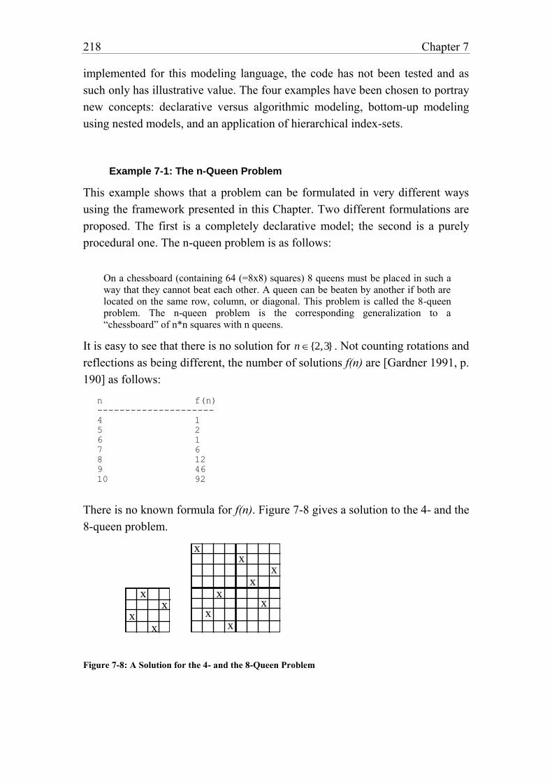
218 Chapter 7
implemented for this modeling language, the code has not been tested and as
such only has illustrative value. The four examples have been chosen to portray
new concepts: declarative versus algorithmic modeling, bottom-up modeling
using nested models, and an application of hierarchical index-sets.
Example 7-1: The n-Queen Problem
This example shows that a problem can be formulated in very different ways
using the framework presented in this Chapter. Two different formulations are
proposed. The first is a completely declarative model; the second is a purely
procedural one. The n-queen problem is as follows:
On a chessboard (containing 64 (=8x8) squares) 8 queens must be placed in such a way that they cannot beat each other. A queen can be beaten by another if both are located on the same row, column, or diagonal. This problem is called the 8-queen problem. The n-queen problem is the corresponding generalization to a “chessboard” of n*n squares with n queens.
It is easy to see that there is no solution for n {2,3} . Not counting rotations and
reflections as being different, the number of solutions f(n) are [Gardner 1991, p.
190] as follows:
n f(n)
---------------------
4 1
5 2
6 1
7 6
8 12
9 46
10 92
There is no known formula for f(n). Figure 7-8 gives a solution to the 4- and the
8-queen problem.
xx
x
x
x
x
x
xx
xx
x
Figure 7-8: A Solution for the 4- and the 8-Queen Problem
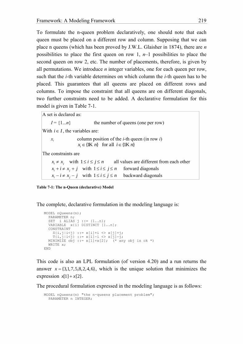
Framework: A Modeling Framework 219
To formulate the n-queen problem declaratively, one should note that each
queen must be placed on a different row and column. Supposing that we can
place n queens (which has been proved by J.W.L. Glaisher in 1874), there are n
possibilities to place the first queen on row 1, n–1 possibilities to place the
second queen on row 2, etc. The number of placements, therefore, is given by
all permutations. We introduce n integer variables, one for each queen per row,
such that the i-th variable determines on which column the i-th queen has to be
placed. This guarantees that all queens are placed on different rows and
columns. To impose the constraint that all queens are on different diagonals,
two further constraints need to be added. A declarative formulation for this
model is given in Table 7-1.
A set is declared as:
I = {1...n} the number of queens (one per row)
With i I , the variables are:
xi column position of the i-th queen (in row i)
xi {1K n} for all i{1K n}
The constraints are
xi x j with 1 i j n all values are different from each other
xi i x j j with 1 i j n forward diagonals
xi i x j j with 1 i j n backward diagonals
Table 7-1: The n-Queen (declarative) Model
The complete, declarative formulation in the modeling language is:
MODEL nQueens(n);
PARAMETER n;
SET i ALIAS j ::= {1..n};
VARIABLE x{i} DISTINCT [1..n];
CONSTRAINT
S{i,j|i<j} ::= x[i]+i <> x[j]+j;
T{i,j|i<j} ::= x[i]-i <> x[j]-j;
MINIMIZE obj ::= x[1]+x[2]; (* any obj is ok *)
WRITE x;
END
This code is also an LPL formulation (of version 4.20) and a run returns the
answer x {3,1,7,5,8,2,4,6}, which is the unique solution that minimizes the
expression x[1] x[2] .
The procedural formulation expressed in the modeling language is as follows:
MODEL nQueens(n) "the n-queens placement problem";
PARAMETER n INTEGER;
220 Chapter 7
SET i ::= {1..n};
PARAMETER x{i} INTEGER [1..n];
PROCEDURE PrintSolution;
PARAMETER i INTEGER;
BEGIN
FOR i:=1 TO n DO Write(x[i],','); END; Writeln;
END PrintSolution;
PROCEDURE Feasible (actRow, actCol: INTEGER): BINARY;
PARAMETER row, colDiff INTEGER [0..n];
BEGIN
row:=0;
REPEAT row:=row+1;
colDiff := Abs(x[row]-actCol);
UNTIL (colDiff = 0) OR (colDiff=actRow-row);
RETURN (row = actRow)
END Feasible;
PROCEDURE Occupy (row: INTEGER);
PARAMETER i INTEGER;
PROCEDURE Swap (i,j:INTEGER); PARAMETER k INTEGER;
BEGIN k:=x[i]; x[i]:=x[j]; x[j]:=k; END Swap;
BEGIN
FOR i := row TO n DO
Swap(row,i);
IF Feasible(row,x[row]) THEN
IF row < n THEN Occupy(row+1) END ELSE PrintSolution; END
Swap(row,i);
END
END
END Occupy
BEGIN
Writeln(n, '-queens problem');
Occupy(1);
END nQueens.
This code is not executable. By changing it slightly (replacing PARAMETER
by VAR, and other minor changes) it can be executed by an Oberon compiler. It
returns all feasible solutions.
The n-queen example shows that the proposed modeling language can express
the same problem using different programming language paradigms. A purely
declarative model, or at the other extreme, a purely algorithmic model
(program).
¤
Example 7-2: The Cutting Stock Problem (again)
The cutting stock problem has already been presented in Chapter 6.5.1
(Example 6-5). Here it is used to outline the way of which declarative and
procedural knowledge can be used in the same model without mingle them. The
last example (7-1) showed how the same problem can be formulated
Framework: A Modeling Framework 221
declaratively or procedurally in the same language. More interestingly,
however, are models which use both types at the same time. The cutting stock
example is an instructive example with this respect. It can be solved (as it has
been described already) by the method of column generation, i.e. by solving
repeatedly two linear models, an LP model and a Knapsack model, until a
condition is fulfilled.
Using The language framework described in this Chapter, we can formulate the
model by defining two submodels and a executable part as follows:
MODEL CuttingStock "The (fractional) cutting stock problem" ;
MODEL cutting_stock; <define the model>
MODEL find_pattern; <define the model>
BEGIN (* executable part *)
SOLVE cutting_stock;
SOLVE find_pattern;
WHILE <condition> DO
<add a new pattern, found in find_pattern>
SOLVE cutting_stock(w,p);
SOLVE find_pattern(w,p,cs.cuts);
END;
END CuttingStock
It is important to note that the declarative and the procedural part of the model
are disjoint in a natural way. The declaration of the two submodels is
completely self-contained. They could even be used independently from the
cutting stock problem. A code of the complete structure of this model is as
follows:
MODEL CuttingStock "The (fractional) cutting stock problem" ;
SET
widths ALIAS w "the different ordered smaller rolls";
patterns ALIAS p "possible cutting patterns";
MODEL cutting_stock ALIAS cs(w,p);
PARAMETER
a*{w,p} "number of w rolls in p";
demand{w} "the demand for small roll w";
VARIABLE
rolls_cut{p} "number of initial rolls cut according to p";
total_number "the total number of initial rolls to be
cut";
CONSTRAINT
cuts-{w} ::= SUM{p} a * rolls_cut >= demand;
objective ::= total_number = SUM{p} rolls_cut;
MINIMIZE obj ::= total_number;
WRITE rolls_cut; total_number;
END cutting_stock
MODEL find_pattern ALIAS fp(w,p,c);
PARAMETER
length{w} "the length of small roll w";
total_length "the width of the initial (uncut) roll";
VARIABLE
y-{w} INTEGER "the number of rolls of size w in new
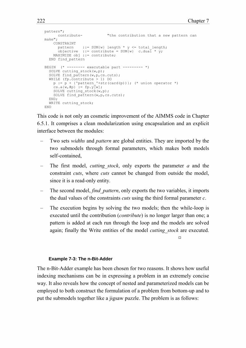
222 Chapter 7
pattern";
contribute- "the contribution that a new pattern can
make";
CONSTRAINT
pattern ::= SUM{w} length * y <= total_length;
objective ::= contribute = SUM{w} c.dual * y;
MAXIMIZE obj ::= contribute;
END find_pattern
BEGIN (* -------- executable part --------- *)
SOLVE cutting_stock(w,p);
SOLVE find_pattern(w,p,cs.cuts);
WHILE (fp.contribute > 1) DO
p := p + {'pattern_'+str(card(p))}; (* union operator *)
cs.a{w,#p} := fp.y[w];
SOLVE cutting_stock(w,p);
SOLVE find_pattern(w,p,cs.cuts);
END;
WRITE cutting_stock;
END
This code is not only an cosmetic improvement of the AIMMS code in Chapter
6.5.1. It comprises a clean modularization using encapsulation and an explicit
interface between the modules:
– Two sets widths and pattern are global entities. They are imported by the
two submodels through formal parameters, which makes both models
self-contained,
– The first model, cutting_stock, only exports the parameter a and the
constraint cuts, where cuts cannot be changed from outside the model,
since it is a read-only entity.
– The second model, find_pattern, only exports the two variables, it imports
the dual values of the constraints cuts using the third formal parameter c.
– The execution begins by solving the two models; then the while-loop is
executed until the contribution (contribute) is no longer larger than one; a
pattern is added at each run through the loop and the models are solved
again; finally the Write entities of the model cutting_stock are executed.
¤
Example 7-3: The n-Bit-Adder
The n-Bit-Adder example has been chosen for two reasons. It shows how useful
indexing mechanisms can be in expressing a problem in an extremely concise
way. It also reveals how the concept of nested and parameterized models can be
employed to both construct the formulation of a problem from bottom-up and to
put the submodels together like a jigsaw puzzle. The problem is as follows:
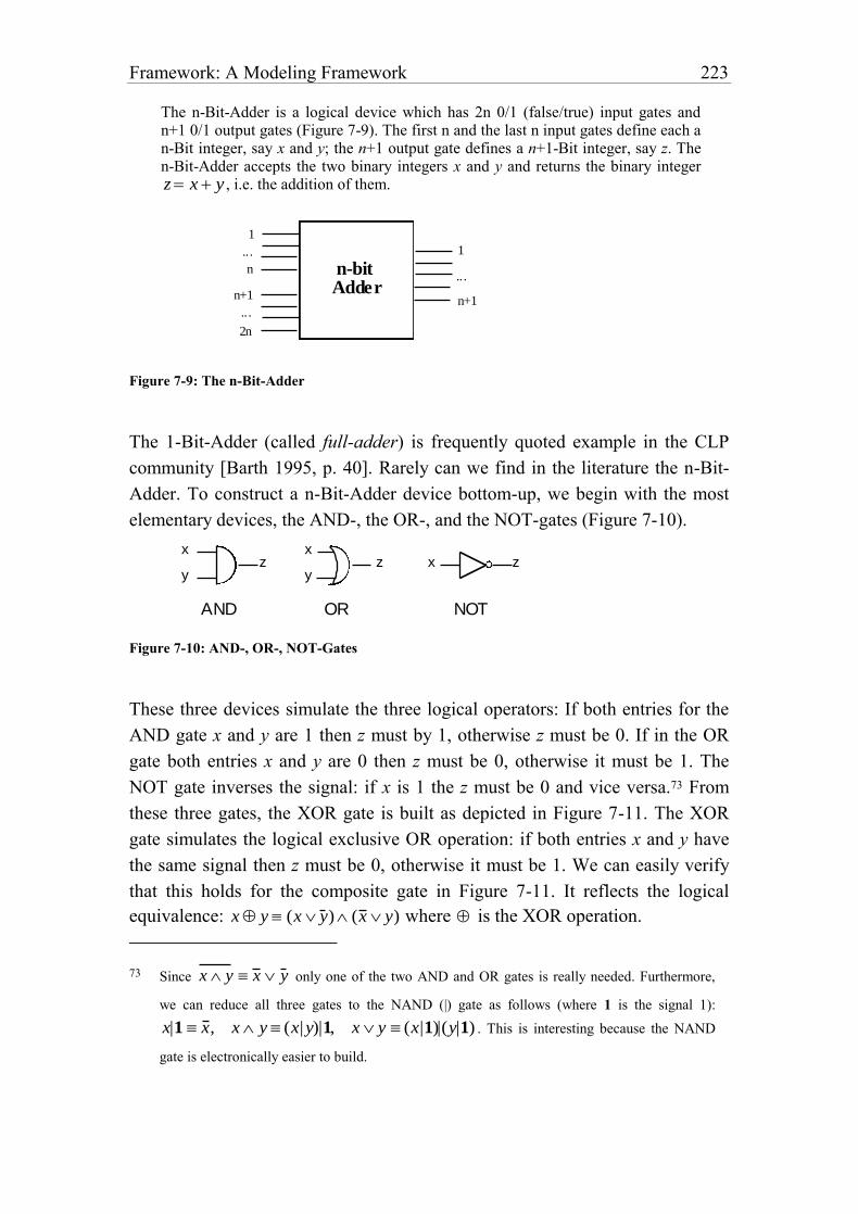
Framework: A Modeling Framework 223
The n-Bit-Adder is a logical device which has 2n 0/1 (false/true) input gates and n+1 0/1 output gates (Figure 7-9). The first n and the last n input gates define each a n-Bit integer, say x and y; the n+1 output gate defines a n+1-Bit integer, say z. The n-Bit-Adder accepts the two binary integers x and y and returns the binary integer
z x y , i.e. the addition of them.
1
n+1
1
n-bit Adder
.. .
n+1...
2n
...
n
Figure 7-9: The n-Bit-Adder
The 1-Bit-Adder (called full-adder) is frequently quoted example in the CLP
community [Barth 1995, p. 40]. Rarely can we find in the literature the n-Bit-
Adder. To construct a n-Bit-Adder device bottom-up, we begin with the most
elementary devices, the AND-, the OR-, and the NOT-gates (Figure 7-10).
x
y
x
yxz zz
AND OR NOT
Figure 7-10: AND-, OR-, NOT-Gates
These three devices simulate the three logical operators: If both entries for the
AND gate x and y are 1 then z must by 1, otherwise z must be 0. If in the OR
gate both entries x and y are 0 then z must be 0, otherwise it must be 1. The
NOT gate inverses the signal: if x is 1 the z must be 0 and vice versa.73 From
these three gates, the XOR gate is built as depicted in Figure 7-11. The XOR
gate simulates the logical exclusive OR operation: if both entries x and y have
the same signal then z must be 0, otherwise it must be 1. We can easily verify
that this holds for the composite gate in Figure 7-11. It reflects the logical
equivalence: x y (x y ) (x y) where is the XOR operation.
73 Since x y x y only one of the two AND and OR gates is really needed. Furthermore,
we can reduce all three gates to the NAND (|) gate as follows (where 1 is the signal 1):
x|1 x , x y (x|y)|1, x y (x|1)|(y|1) . This is interesting because the NAND
gate is electronically easier to build.
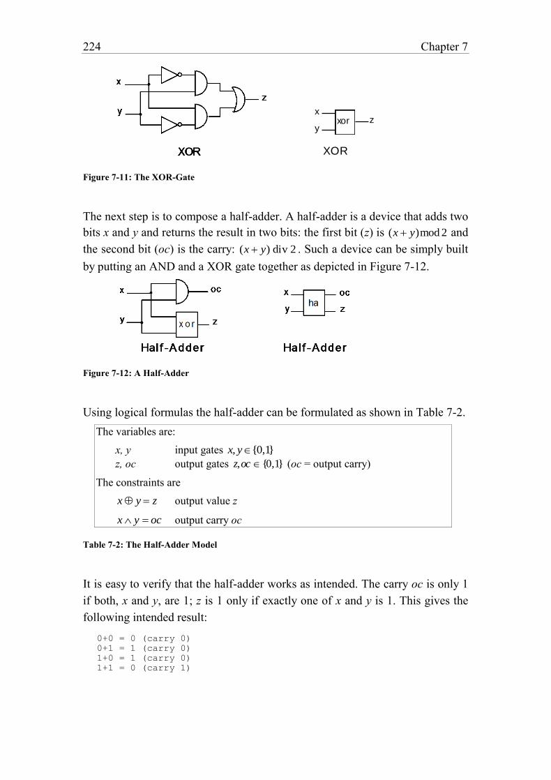
224 Chapter 7
x
yz
XOR
xor
Figure 7-11: The XOR-Gate
The next step is to compose a half-adder. A half-adder is a device that adds two
bits x and y and returns the result in two bits: the first bit (z) is (x y)mod 2 and
the second bit (oc) is the carry: (x y) div 2 . Such a device can be simply built
by putting an AND and a XOR gate together as depicted in Figure 7-12.
Figure 7-12: A Half-Adder
Using logical formulas the half-adder can be formulated as shown in Table 7-2.
The variables are:
x, y input gates x, y {0,1}
z, oc output gates z,oc {0,1} (oc = output carry)
The constraints are
x y z output value z
x y oc output carry oc
Table 7-2: The Half-Adder Model
It is easy to verify that the half-adder works as intended. The carry oc is only 1
if both, x and y, are 1; z is 1 only if exactly one of x and y is 1. This gives the
following intended result:
0+0 = 0 (carry 0)
0+1 = 1 (carry 0)
1+0 = 1 (carry 0)
1+1 = 0 (carry 1)
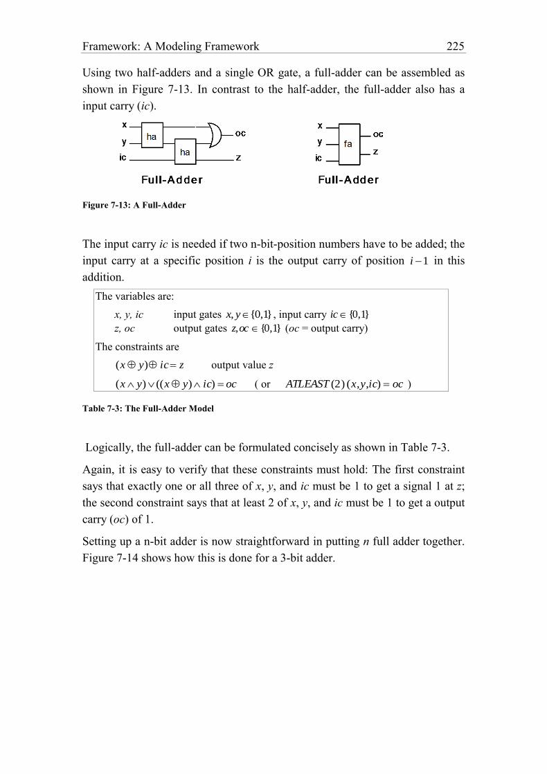
Framework: A Modeling Framework 225
Using two half-adders and a single OR gate, a full-adder can be assembled as
shown in Figure 7-13. In contrast to the half-adder, the full-adder also has a
input carry (ic).
Figure 7-13: A Full-Adder
The input carry ic is needed if two n-bit-position numbers have to be added; the
input carry at a specific position i is the output carry of position i 1 in this
addition.
The variables are:
x, y, ic input gates x, y {0,1} , input carry ic {0,1}
z, oc output gates z,oc {0,1} (oc = output carry)
The constraints are
(x y) ic z output value z
(x y) ((x y) ic) oc ( or ATLEAST (2) (x,y,ic) oc )
Table 7-3: The Full-Adder Model
Logically, the full-adder can be formulated concisely as shown in Table 7-3.
Again, it is easy to verify that these constraints must hold: The first constraint
says that exactly one or all three of x, y, and ic must be 1 to get a signal 1 at z;
the second constraint says that at least 2 of x, y, and ic must be 1 to get a output
carry (oc) of 1.
Setting up a n-bit adder is now straightforward in putting n full adder together.
Figure 7-14 shows how this is done for a 3-bit adder.
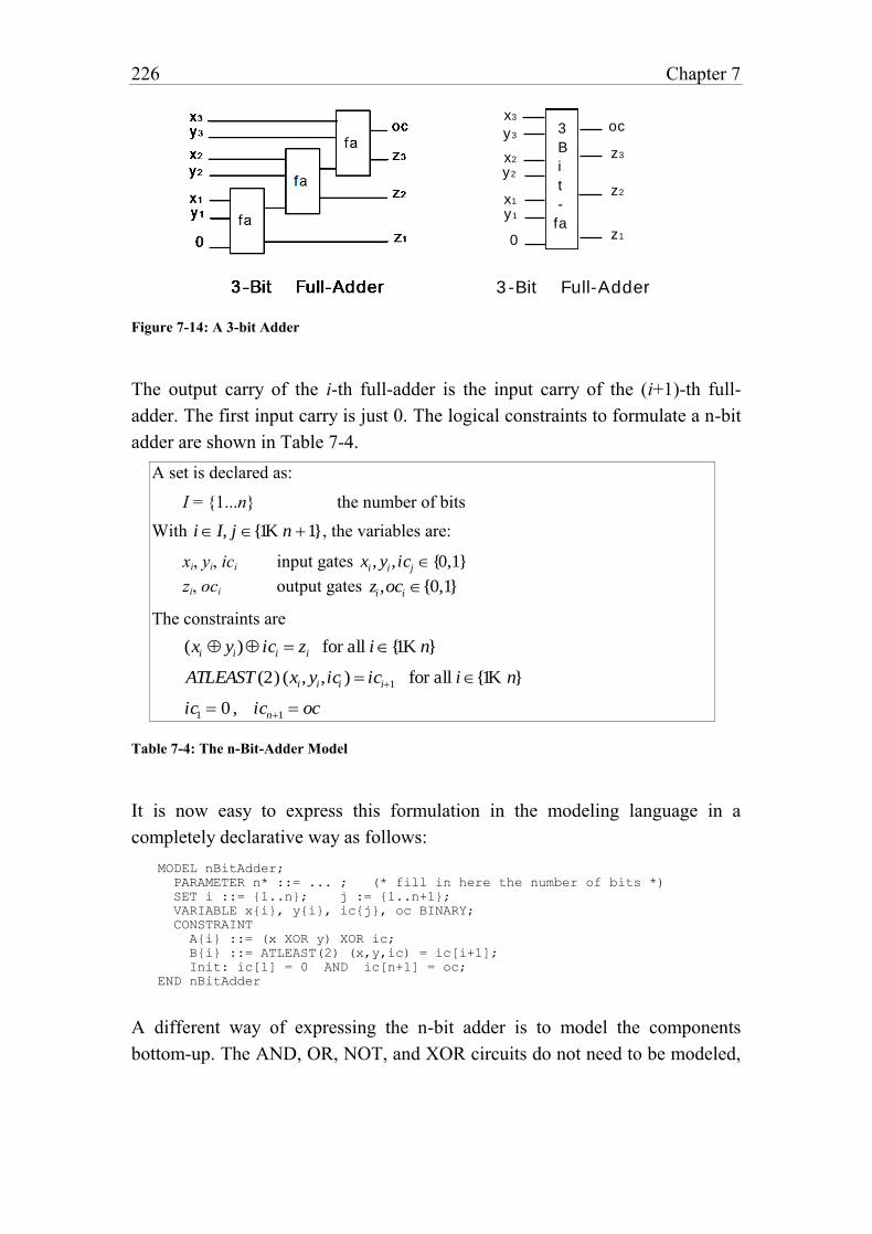
226 Chapter 7
x1
y1
0
z2
z1
fa
x2
y2
x3
y3
z3
oc
3 -Bit Full-Adder
3
B
i
t
-
Figure 7-14: A 3-bit Adder
The output carry of the i-th full-adder is the input carry of the (i+1)-th full-
adder. The first input carry is just 0. The logical constraints to formulate a n-bit
adder are shown in Table 7-4.
A set is declared as:
I = {1...n} the number of bits
With i I, j {1K n 1}, the variables are:
xi, yi, ici input gates xi , yi ,icj {0,1}
zi, oci output gates zi,oci {0,1}
The constraints are
(xi yi) ici zi for all i{1K n}
ATLEAST (2) (xi, yi,ici ) ici1 for all i{1K n}
ic1 0 , icn1 oc
Table 7-4: The n-Bit-Adder Model
It is now easy to express this formulation in the modeling language in a
completely declarative way as follows:
MODEL nBitAdder;
PARAMETER n* ::= ... ; (* fill in here the number of bits *)
SET i ::= {1..n}; j := {1..n+1};
VARIABLE x{i}, y{i}, ic{j}, oc BINARY;
CONSTRAINT
A{i} ::= (x XOR y) XOR ic;
B{i} ::= ATLEAST(2) (x,y,ic) = ic[i+1];
Init: ic[1] = 0 AND ic[n+1] = oc;
END nBitAdder
A different way of expressing the n-bit adder is to model the components
bottom-up. The AND, OR, NOT, and XOR circuits do not need to be modeled,
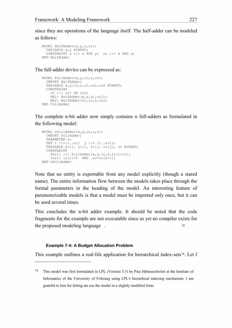
Framework: A Modeling Framework 227
since they are operations of the language itself. The half-adder can be modeled
as follows:
MODEL HalfAdder(x,y,z,oc);
VARIABLE x,y BINARY;
CONSTRAINT z ::= x XOR y; oc ::= x AND y;
END HalfAdder
The full-adder device can be expressed as:
MODEL FullAdder(x,y,ic,z,oc);
IMPORT HalfAdder;
VARIABLE x,y,ic,z,z1,oc1,oc2 BINARY;
CONSTRAINT
oc ::= oc1 OR oc2;
HA1: HalfAdder(x,y,z1,oc1);
HA2: HalfAdder(z1,ic,z,oc2;
END FullAdder
The complete n-bit adder now simply contains n full-adders as formulated in
the following model:
MODEL nFullAdder(x,y,oc,z,n);
IMPORT FullAdder;
PARAMETER n;
SET i ::={1..n}; j ::= {1..n+1};
VARIABLE x{i}, y{i}, z{i}, ic{j}, oc BINARY;
CONSTRAINT
FA{i} ::= FullAdder(x,y,ic,z,ic[i+1]);
Init: ic[1]=0 AND oc=ic[n+1];
END nFullAdder
Note that no entity is exportable from any model explicitly (though a stared
name). The entire information flow between the models takes place through the
formal parameters in the heading of the model. An interesting feature of
parameterizable models is that a model must be imported only once, but it can
be used several times.
This concludes the n-bit adder example. It should be noted that the code
fragments for the example are not executable since as yet no compiler exists for
the proposed modeling language . ¤
Example 7-4: A Budget Allocation Problem
This example outlines a real-life application for hierarchical index-sets74. Let I
74 This model was first formulated in LPL (Version 3.5) by Pius Hättenschwiler at the Institute of
Informatics of the University of Fribourg using LPL's hierachical indexing mechanism. I am
grateful to him for letting me use the model in a slightly modified form.
228 Chapter 7
be a hierarchical structure of accounts with final (not subtotalled) accounts,
aggregated accounts (subtotals), and an overall total account. Such accounting
structures are used in many contexts such as family budgets, company
accounting systems, or in social accounting matrices. An extract of a family
budget may be:
Total
Household
Bar
Telephone
Tel1
Tel2
Wine
Clothes
Dwelling
Rent
Electricity
Repair
Rest
Total, Household, Telephone, and Dwelling are subtotal accounts since their
amount is calculated as a summation of other accounts.
There are many applications which can be subsumed under the concept of
pattern matching problems: Often a subset of amounts in the accounting system
is given and the other accounts must be completed such that some measure of
deviation becomes minimal; or there exists a target value for each account (an
“ideal” budget) and a global amount must be distributed over the amounts in
such a way that the deviation from the target values is minimal. Our Budget
Allocation Problem is as follows:
Given an accounting system as described above. Five parameters are attached to each account: a target value, a relative target in percent, a lower and upper bound, and a weight. The target value is the value we ideally want to attribute to this account, the relative target is the percent we want to attribute to each account, lower and upper bounds are hard constraints on an account, the value of which cannot be under- or overshot; finally, the weight is a measure to control the deviation of the real value from the target value; the higher the weight, the closer the real value should be to the target value. The goal is to attribute an amount to each account such that the total absolute and relative deviations are minimized.
The formulation of this problem is given in Table 7–5.
We use one (hierarchical) index-set:
I the accounting structure
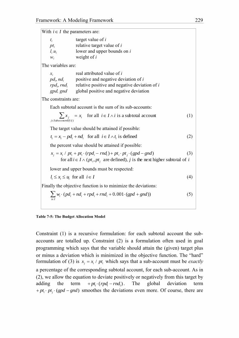
Framework: A Modeling Framework 229
With i I the parameters are:
ti target value of i
pti relative target value of i
li ui lower and upper bounds on i
wi weight of i
The variables are:
xi real attributed value of i
pdi, ndi positive and negative deviation of i
rpdi, rndi relative positive and negative deviation of i
gpd, gnd global positive and negative deviation
The constraints are:
Each subtotal account is the sum of its sub-accounts:
x j
jSubaccountOf (i )
xi for all i I i is a subtotal account (1)
The target value should be attained if possible:
ti xi pdi ndi for all iI ti is defined (2)
the percent value should be attained if possible:
xj xi / pti pti (rpdi rndi ) pt i pt j (gpd gnd) (3)
for all i I (pti , ptj are defined), j is the next higher subtotal of i
lower and upper bounds must be respected:
li xi ui for all iI (4)
Finally the objective function is to minimize the deviations:
wi (pdi ndi rpdi rndi 0.001 (gpd gnd))iI
(5)
Table 7-5: The Budget Allocation Model
Constraint (1) is a recursive formulation: for each subtotal account the sub-
accounts are totalled up. Constraint (2) is a formulation often used in goal
programming which says that the variable should attain the (given) target plus
or minus a deviation which is minimized in the objective function. The “hard”
formulation of (3) is x j xi / pti which says that a sub-account must be exactly
a percentage of the corresponding subtotal account, for each sub-account. As in
(2), we allow the equation to deviate positively or negatively from this target by
adding the term pti (rpdi rndi) . The global deviation term
pti pt j (gpd gnd) smoothes the deviations even more. Of course, there are
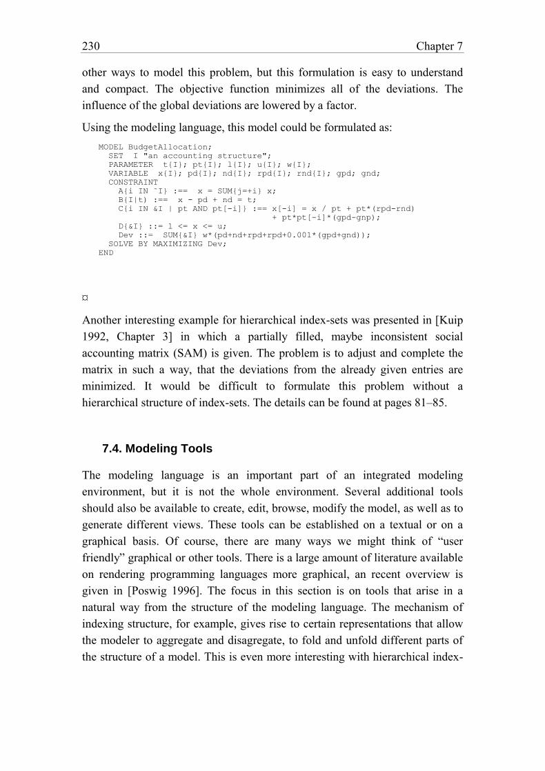
230 Chapter 7
other ways to model this problem, but this formulation is easy to understand
and compact. The objective function minimizes all of the deviations. The
influence of the global deviations are lowered by a factor.
Using the modeling language, this model could be formulated as:
MODEL BudgetAllocation;
SET I "an accounting structure";
PARAMETER t{I}; pt{I}; l{I}; u{I}; w{I};
VARIABLE x{I}; pd{I}; nd{I}; rpd{I}; rnd{I}; gpd; gnd;
CONSTRAINT
A{i IN ˜I} :== x = SUM{j=+i} x;
B{I|t) :== x - pd + nd = t;
C{i IN &I | pt AND pt[-i]} :== x[-i] = x / pt + pt*(rpd-rnd)
+ pt*pt[-i]*(gpd-gnp);
D{&I} ::= l <= x <= u;
Dev ::= SUM{&I} w*(pd+nd+rpd+rpd+0.001*(gpd+gnd));
SOLVE BY MAXIMIZING Dev;
END
¤
Another interesting example for hierarchical index-sets was presented in [Kuip
1992, Chapter 3] in which a partially filled, maybe inconsistent social
accounting matrix (SAM) is given. The problem is to adjust and complete the
matrix in such a way, that the deviations from the already given entries are
minimized. It would be difficult to formulate this problem without a
hierarchical structure of index-sets. The details can be found at pages 81–85.
7.4. Modeling Tools
The modeling language is an important part of an integrated modeling
environment, but it is not the whole environment. Several additional tools
should also be available to create, edit, browse, modify the model, as well as to
generate different views. These tools can be established on a textual or on a
graphical basis. Of course, there are many ways we might think of “user
friendly” graphical or other tools. There is a large amount of literature available
on rendering programming languages more graphical, an recent overview is
given in [Poswig 1996]. The focus in this section is on tools that arise in a
natural way from the structure of the modeling language. The mechanism of
indexing structure, for example, gives rise to certain representations that allow
the modeler to aggregate and disagregate, to fold and unfold different parts of
the structure of a model. This is even more interesting with hierarchical index-
Framework: A Modeling Framework 231
sets in which parts of the tree can be shrunk into a single node. Such
contracting and expanding operations might be extremely useful for selecting
and viewing, or for browsing and editing the model.
An interesting feature is that such representations are bijective to the
mathematical structure of the (declarative) modeling code. Therefore, the
modeler can use them as two-way tools, i.e. we can switch from view to view
and employ the one that seems most suitable to modify and edit the model. The
modifications can be directly reflected in the internal structure generated by
the compiler, hence avoiding the need to update several data structures what
might then become inconsistent. Two types of such tools are conceivable: tools
based on textual representation and tools based in graphs, although both
approaches can be integrated seamlessly into a single framework.
7.4.1. A Textual-Based Tool
[Mousavi al. 1995], as mentioned in Chapter 6.6.4, have suggested a browsing
and editing tool with a static and fixed number of pages which are connected by
hyperlinks. AIMMS (as outlined in Chapter 6.5.1.), on the other hand, contains
a completely open interface builder where the user can create and design her
own pages. Another general hypertext tool (WEBSs) with its own script-
language was developed by [Pasquier/Monnard 1995] and used to implement a
browsing and editing tool (gLP) for linear programs [Collaud/Pasquier 1996].
The proposition here is for a textual browsing and editing tool based entirely on
the entities defined in the modeling language, i.e. certain pages are created
automatically from the (declarative) specification of the model, and they reflect
the structure of the model. Such a device can be designed as a two-way
mechanism: it can be used to generate parts of the source code or, given the
code, it can be used to view and browse the model. Both tasks can be smoothly
integrated. The architecture can be schematically depicted as in Figure 7-15.
Each rectangle designates a page and the arrows represent hyper-links. Cross
links have been left out to make the figure easy to survey.
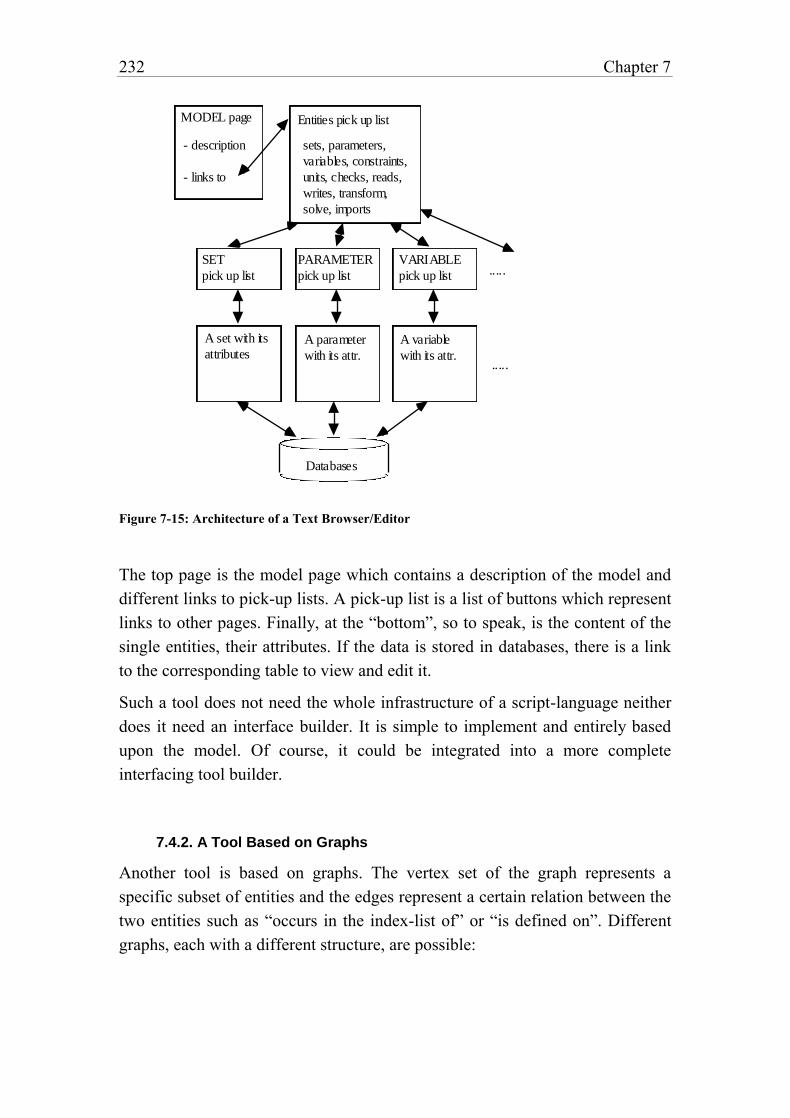
232 Chapter 7
MODEL page
- description
- links to
Entities pick up list
sets, parameters,
variables, constraints,
units, checks, reads,
writes, transform,
solve, imports
SET
pick up list
VARIABLE
pick up list
PARAMETER
pick up list .....
A set with its
attributesA parameter
with its attr.
A variable
with its attr......
Databases
Figure 7-15: Architecture of a Text Browser/Editor
The top page is the model page which contains a description of the model and
different links to pick-up lists. A pick-up list is a list of buttons which represent
links to other pages. Finally, at the “bottom”, so to speak, is the content of the
single entities, their attributes. If the data is stored in databases, there is a link
to the corresponding table to view and edit it.
Such a tool does not need the whole infrastructure of a script-language neither
does it need an interface builder. It is simple to implement and entirely based
upon the model. Of course, it could be integrated into a more complete
interfacing tool builder.
7.4.2. A Tool Based on Graphs
Another tool is based on graphs. The vertex set of the graph represents a
specific subset of entities and the edges represent a certain relation between the
two entities such as “occurs in the index-list of” or “is defined on”. Different
graphs, each with a different structure, are possible:
Framework: A Modeling Framework 233
– Modular structure [Geoffrion 1988]: The vertices are the model entities, an
arc is defined if a model is nested within another. The resulting graph is a
DAG (directed acyclic graph).
– Index-dependency graph: The vertices are all entities, an edge is defined
between an arbitrary entity E and a set entity I, if the index-set I occurs in
the index-list of E.
– Value-dependency graph: The vertices are all entities, an edge (or an arc) is
defined between an arbitrary entity E and another entity I, if I occurs in the
expression of E.
– Domain-dependency-graph: The vertices are all entities, an edge (or an arc)
is defined between an arbitrary entity E and another entity I, if I occurs in
the indexlist expression of E. [This graph was proposed by Marcel Roelofs
of Paragon Technology (AIMMS).]
– A-C graph (activity-constraint graph): The vertices are the variable and the
constraint entities, an edge (or an arc) is defined if a variable occurs in the
corresponding constraint. The graph is normally bipartite (see [Greenberg
1981]).
– A-A graph (activity-activity graph): The vertices are the variable entities, an
edge is defined if both variables occur in the same constraint (see
[Greenberg 1981]).
Many other graphs could be conceived by this general scheme. Note that all
graphs are generic; they can be unfolded partially or entirely by expanding an
indexed entity, represented by a single node, into several nodes. Of course, the
layout of the graph can quickly become large and difficult to survey, but
suitable switching to a microlevel where only few nodes are visible, could help
to alleviate this problem greatly.
At a single node (representing an entity) its attributes might be displayed; if the
node represent a variable or an parameter entity, for example, switching to a
suitable table (spreadsheet) form may show the values.
Such a graph is also a browsing and editing tool which allows a modeler to
quickly access a specific piece of data. A modeler, having built a large model
with thousands of variables and constraints, would certainly appreciate this,
because nothing is more time-consuming than checking whether a single
element is correct.
234 Chapter 7
7.5. Outlook
This concludes the specification of the modeling framework. The largest part of
this Chapter was allocated to the specification of the modeling language. This
demonstrates its importance. It also underlines my thinking that, almost
“everything follows in a natural way” from a well designed modeling language.
This is not only the case for the browsing and editing tools presented in Section
7.4, but it is also true for database and spreadsheet linking: the index
mechanism maps the entities to tables and spreadsheets in an clear way.
As already mentioned at the beginning of this Chapter, I do not consider this
specification as a final and definitive framework. A lot of work still remains to
be done. The most critical point, in my view, is the communication with solvers
and how it can be integrated (Transform and Solve instructions). Still, the
executable part allows the modeler to write any program. For this point of view,
every model for which we know a solution method could be implemented. On
the other hand, our approach was guided by an important maxim:
“If a model can be expressed in a declarative way, then one should
do so. If the model cannot be solved in this form, then one should
first look for a more appropriate declarative form (transforming
the model eventually). Only if this fails, should one recur to a more
procedural specification.”
I am, of course, fully aware that many problems have no easy declarative
formulation, or are best expressed as an algorithm. What is “best” in a concrete
situation, will in any case be decided by economical considerations. In this
sense, the maxim only expresses my belief that, “in the long run”, it might be
more advantageous to have a declarative formulation since it can be written
concisely. Furthermore, it is more readable for humans since the structure is
explicit and supports a better maintenance of the model.
This concludes Part II, in which I have tried to give an overview of different
modeling approaches. I have come to the conclusion that a modeling language
is needed which is able to express declarative and algorithmic knowledge
without intermingling them too much. A modeling language specification was
presented in this Chapter.
Part III offers a concrete implementation of a subset of this specification in

Framework: A Modeling Framework 235
order to show, at least partially, that the framework works.

Part III
LPL – AN IMPLEMENTED
FRAMEWORK
238
“In general, whatever you're trying to learn, if you can imagine trying to explain it to a computer, then you learn what you don't know about the subject. It helps you ask the right questions. It's the ultimate test of what you know.” — Knuth D.E., [1995] in: Dennis/Cathy p. 100.
This final Part contains a concrete implementation of the framework presented
in Chapter 7. Chapter 8 gives an overview of the modeling language LPL.
Features unique to LPL are reported more extensively than other more general
features. The environment in which LPL is embedded is outlined in Chapter 9.
A textual model browser and different graphical tools are also presented.
Concrete models and applications from different domains are outlined in the
last Chapter. The examples used in this chapter should convince the reader that
declarative modeling representation is a powerful means of describing
problems. They also show how logical and mathematical knowledge can be
mixed in a unified way.
239
8. THE DEFINITION OF THE LANGUAGE
“No official programming language document should ever be published unless all major components of the language have been successfully implemented...” — Meyer B., [1992], p. xi.
8.1. Introduction
LPL is not a commercial system which needs to compete with other systems.
The language is relatively simple and small. There are three reasons why LPL
has been developed. In the mid-eighties, when the LPL project began, there
were virtually no modeling tools available for personal computers. Yet, people
at our Institute of Informatics had to manage real-life, large models. LPL and
other tools have been developed and have been used since for this purpose. The
second reason was to have computer-based tools for teaching modeling in
operations research. I always found it to be an anachronism to teach modeling
in OR without a computer. After all, wasn't OR a child of the advent of
computers? Mathematically, it makes no difference whether we solve a problem
with 2 or with hundreds of variables. From the point of view of model
management, however, this is very different, and only larger models can teach
real-life applications. A third reason has become more important: LPL is
becoming a “playground” in which to illustrate new ideas in computer-based
modeling. It is easy, after all, to present ideas on what a modeling system
should look like, what functions it should fulfill, how it should work etc., tt is
however much harder to present realized ideas.
LPL is a subset of the specifications presented in Chapter 7 and is fully
240 Chapter 8
documented in [Hürlimann 1997a]. The following parts of the proposal in
Chapter 7 are not implemented in the LPL modeling language:
– user defined types,
– procedure declaration and call as well as procedural constructs,
– several model transformations,
– hierachical index-set in its generality,
– direct link to databases via ODBC or other,
– non-linear models, except quadratic programming (QP).
The least favorable aspect of LPL (version 4.20) is that it does not clearly
distinguish between the declarative and executable part of a model. Some
declarations are executed at parse time, which means that their sequence is
important. This is clearly not desirable.
LPL, on the other hand, has several unique features which are not shared by
other languages:
– unit declaration,
– symbolic translator of logical models into mathematical statements,
– unified import and report generator,
– sophisticated data table format,
– user definable nomenclature,
– goal programming.
In this chapter, a short overview of the LPL modeling language is given.
8.2. An Overview of the LPL-Language
There is no space here to present the entire language. It is fully documented in
[Hürlimann 1997a]. However, I would like to address the most interesting
aspects and to present them briefly. Version 4.20 as is used (available on the
Internet at the LPL-site).
8.2.1. The Entities and the Attributes
The entity-attribute philosophy is fully integrated in LPL. Every statement in
LPL is an entity declaration, and each entity consists of several attributes. An
LPL model is a sequence of entity declarations. 12 different entities (genus) are
possible:
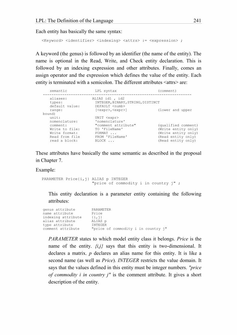
LPL: The Definition of the Language 241
Each entity has basically the same syntax:
<Keyword> <identifier> <indexing> <attrs> := <expression> ;
A keyword (the genus) is followed by an identifier (the name of the entity). The
name is optional in the Read, Write, and Check entity declaration. This is
followed by an indexing expression and other attributes. Finally, comes an
assign operator and the expression which defines the value of the entity. Each
entity is terminated with a semicolon. The different attributes <attrs> are:
semantic LPL syntax (comment)
---------------------------------------------------------------------
aliases: ALIAS id1 , id2
types: INTEGER,BINARY,STRING,DISTINCT
default value: DEFAULT <numb>
range: [<expr>,<expr>] (lower and upper
bound)
unit: UNIT <expr>
nomenclature: 'nomenclature'
comment: "comment attribute" (qualified comment)
Write to file: TO 'FileName' (Write entity only)
Write format: FORMAT ... (Write entity only)
Read from file FROM 'FileName' (Read entity only)
read a block: BLOCK ... (Read entity only)
These attributes have basically the same semantic as described in the proposal
in Chapter 7.
Example:
PARAMETER Price{i,j} ALIAS p INTEGER
"price of commodity i in country j" ;
This entity declaration is a parameter entity containing the following
attributes:
genus attribute PARAMETER
name attribute Price
indexing attribute {i,j}
alias attribute ALIAS p
type attribute INTEGER
comment attribute "price of commodity i in country j"
PARAMETER states to which model entity class it belongs. Price is the
name of the entity. {i,j} says that this entity is two-dimensional. It
declares a matrix. p declares an alias name for this entity. It is like a
second name (as well as Price). INTEGER restricts the value domain. It
says that the values defined in this entity must be integer numbers. "price
of commodity i in country j" is the comment attribute. It gives a short
description of the entity.
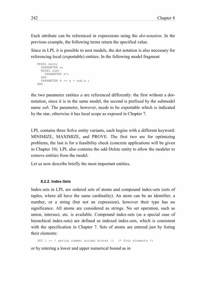
242 Chapter 8
Each attribute can be referenced in expressions using the dot-notation. In the
previous example, the following terms return the specified value.
Since in LPL it is possible to nest models, the dot notation is also necessary for
referencing local (exportable) entities. In the following model fragment
MODEL main;
PARAMETER a;
MODEL sub;
PARAMETER a*;
END
PARAMETER b := a + sub.a ;
END
the two parameter entities a are referenced differently: the first without a dot-
notation, since it is in the same model, the second is prefixed by the submodel
name sub. The parameter, however, needs to be exportable which is indicated
by the star, otherwise it has local scope as exposed in Chapter 7.
LPL contains three Solve entity variants, each begins with a different keyword:
MINIMIZE, MAXIMIZE, and PROVE. The first two are for optimizing
problems, the last is for a feasibility check (concrete applications will be given
in Chapter 10). LPL also contains the odd Delete entity to allow the modeler to
remove entities from the model.
Let us now describe briefly the most important entities.
8.2.2. Index-Sets
Index-sets in LPL are ordered sets of atoms and compound index-sets (sets of
tuples, where all have the same cardinality). An atom can be an identifier, a
number, or a string (but not an expression), however their type has no
significance. All atoms are considered as strings. No set operation, such as
union, intersect, etc. is available. Compound index-sets (as a special case of
hierachical index-sets) are defined as indexed index-sets, which is consistent
with the specification in Chapter 7. Sets of atoms are entered just by listing
their elements:
SET i := / spring summer autumn winter /; (* four elements *)
or by entering a lower and upper numerical bound as in
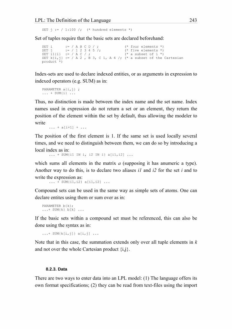
LPL: The Definition of the Language 243
SET j := / 1:100 /; (* hundred elements *)
Set of tuples require that the basic sets are declared beforehand:
SET i := / A B C D / ; (* four elements *)
SET j := / 1 2 3 4 5 /; (* five elements *)
SET i1{i} := / A C / ; (* a subset of i *)
SET k{i,j} := / A 2 , B 3, C 1, A 4 /; (* a subset of the Cartesian
product *)
Index-sets are used to declare indexed entities, or as arguments in expression to
indexed operators (e.g. SUM) as in:
PARAMETER a{i,j} ;
... + SUM{i} ...
Thus, no distinction is made between the index name and the set name. Index
names used in expression do not return a set or an element, they return the
position of the element within the set by default, thus allowing the modeler to
write ... + a[i+1] + ...
The position of the first element is 1. If the same set is used locally several
times, and we need to distinguish between them, we can do so by introducing a
local index as in: ... + SUM{i1 IN i, i2 IN i} a[i1,i2] ...
which sums all elements in the matrix a (supposing it has anumeric a type).
Another way to do this, is to declare two aliases i1 and i2 for the set i and to
write the expression as: ... + SUM{i1,i2} a[i1,i2] ...
Compound sets can be used in the same way as simple sets of atoms. One can
declare entites using them or sum over as in:
PARAMETER b{k};
...+ SUM{k} b[k] ...
If the basic sets within a compound set must be referenced, this can also be
done using the syntax as in:
...+ SUM{k[i,j]} a[i,j] ...
Note that in this case, the summation extends only over all tuple elements in k
and not over the whole Cartesian product {i,j}.
8.2.3. Data
There are two ways to enter data into an LPL model: (1) The language offers its
own format specifications; (2) they can be read from text-files using the import
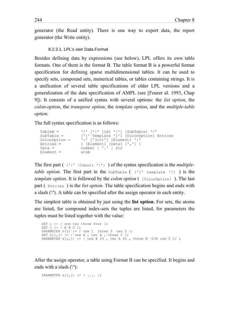
244 Chapter 8
generator (the Read entity). There is one way to export data, the report
generator (the Write entity).
8.2.3.1. LPL's own Data Format
Besides defining data by expressions (see below), LPL offers its own table
formats. One of them is the format B. The table format B is a powerful format
specification for defining sparse multidimensional tables. It can be used to
specify sets, compound sets, numerical tables, or tables containing strings. It is
a unification of several table specifications of older LPL versions and a
generalization of the data specification of AMPL (see [Fourer al. 1993, Chap
9]). It consists of a unified syntax with several options: the list option, the
colon-option, the transpose option, the template option, and the multiple-table
option.
The full syntax specification is as follows:
TableB = '/' ['|' {id} '|'] {SubTable} '/'
SubTable = ['[' Template ']'] [ColonOption] Entries
ColonOption = ':' ['(tr)'] {Element} ':'
Entries = { {Element} {Data} [','] }
Data = number | '.' | str
Element = atom
The first part ( ['|' {Ident} '|'] ) of the syntax specification is the multiple-
table option. The first part in the SubTable ( ['[' template ']] ) is the
template option. It is followed by the colon option ( [ColonOption] ). The last
part ( Entries ) is the list option. The table specification begins and ends with
a slash ('/'). A table can be specified after the assign operator in each entity.
The simplest table is obtained by just using the list option. For sets, the atoms
are listed, for compound index-sets the tuples are listed, for parameters the
tuples must be listed together with the value:
SET i := / one two three four /;
SET j := / A B C /;
PARAMETER v{i} := / one 1 three 3 two 2 /;
SET k{i,j} := / one A , two A , three C /;
PARAMETER w{i,j} := / one B 23 , two A 45 , three B -234 one C 1/ ;
After the assign operator, a table using Format B can be specified. It begins and
ends with a slash ('/'):
PARAMETER a{i,j} := / .... /;
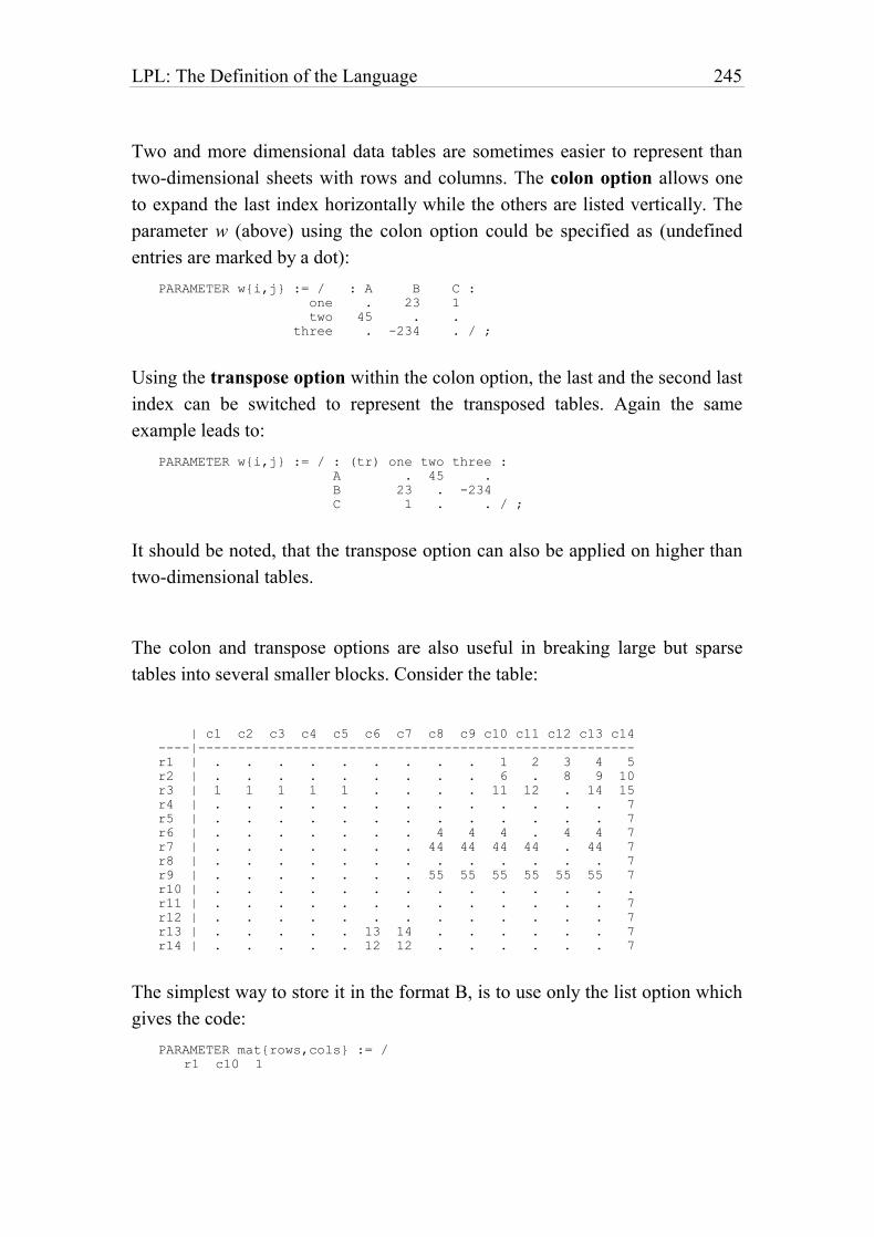
LPL: The Definition of the Language 245
Two and more dimensional data tables are sometimes easier to represent than
two-dimensional sheets with rows and columns. The colon option allows one
to expand the last index horizontally while the others are listed vertically. The
parameter w (above) using the colon option could be specified as (undefined
entries are marked by a dot):
PARAMETER w{i,j} := / : A B C :
one . 23 1
two 45 . .
three . -234 . / ;
Using the transpose option within the colon option, the last and the second last
index can be switched to represent the transposed tables. Again the same
example leads to:
PARAMETER w{i,j} := / : (tr) one two three :
A . 45 .
B 23 . -234
C 1 . . / ;
It should be noted, that the transpose option can also be applied on higher than
two-dimensional tables.
The colon and transpose options are also useful in breaking large but sparse
tables into several smaller blocks. Consider the table:
| c1 c2 c3 c4 c5 c6 c7 c8 c9 c10 c11 c12 c13 c14
----|-------------------------------------------------------
r1 | . . . . . . . . . 1 2 3 4 5
r2 | . . . . . . . . . 6 . 8 9 10
r3 | 1 1 1 1 1 . . . . 11 12 . 14 15
r4 | . . . . . . . . . . . . . 7
r5 | . . . . . . . . . . . . . 7
r6 | . . . . . . . 4 4 4 . 4 4 7
r7 | . . . . . . . 44 44 44 44 . 44 7
r8 | . . . . . . . . . . . . . 7
r9 | . . . . . . . 55 55 55 55 55 55 7
r10 | . . . . . . . . . . . . . .
r11 | . . . . . . . . . . . . . 7
r12 | . . . . . . . . . . . . . 7
r13 | . . . . . 13 14 . . . . . . 7
r14 | . . . . . 12 12 . . . . . . 7
The simplest way to store it in the format B, is to use only the list option which
gives the code:
PARAMETER mat{rows,cols} := /
r1 c10 1
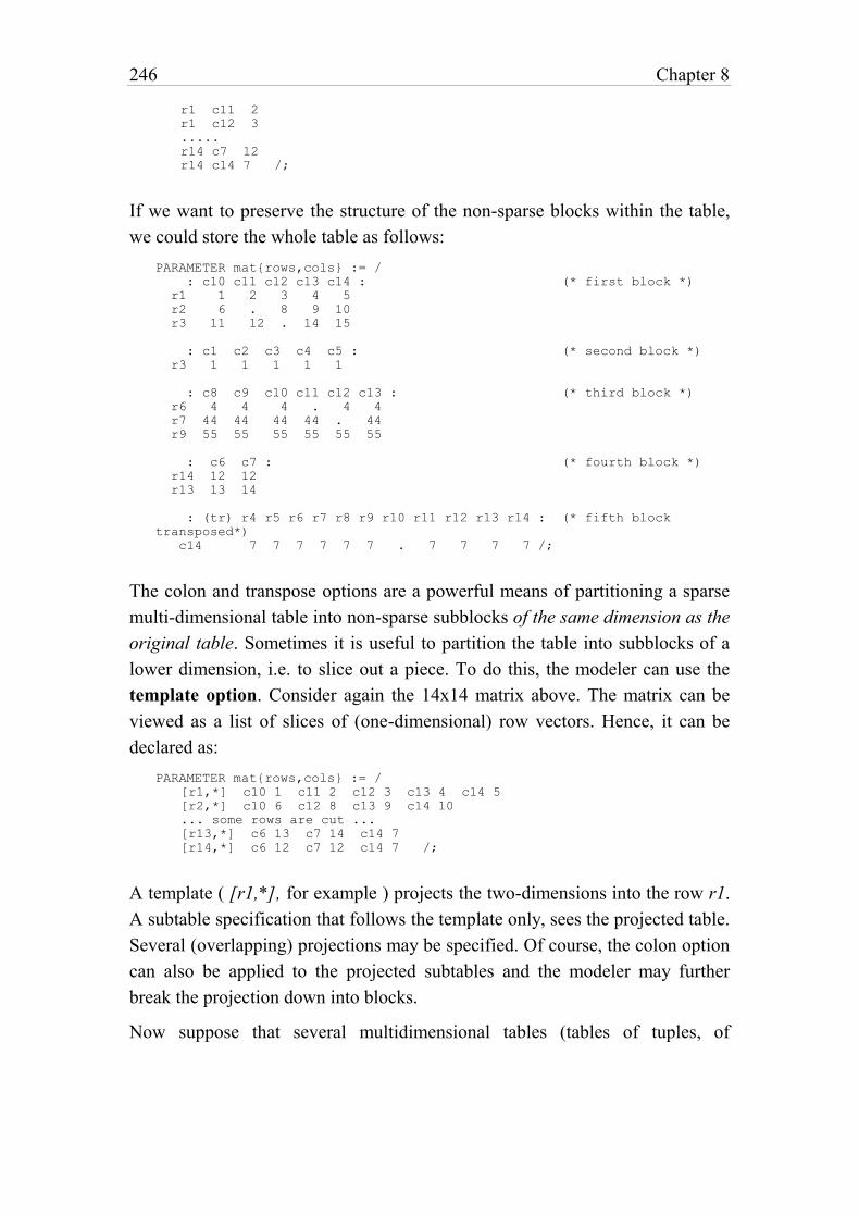
246 Chapter 8
r1 c11 2
r1 c12 3
.....
r14 c7 12
r14 c14 7 /;
If we want to preserve the structure of the non-sparse blocks within the table,
we could store the whole table as follows:
PARAMETER mat{rows,cols} := /
: c10 c11 c12 c13 c14 : (* first block *)
r1 1 2 3 4 5
r2 6 . 8 9 10
r3 11 12 . 14 15
: c1 c2 c3 c4 c5 : (* second block *)
r3 1 1 1 1 1
: c8 c9 c10 c11 c12 c13 : (* third block *)
r6 4 4 4 . 4 4
r7 44 44 44 44 . 44
r9 55 55 55 55 55 55
: c6 c7 : (* fourth block *)
r14 12 12
r13 13 14
: (tr) r4 r5 r6 r7 r8 r9 r10 r11 r12 r13 r14 : (* fifth block
transposed*)
c14 7 7 7 7 7 7 . 7 7 7 7 /;
The colon and transpose options are a powerful means of partitioning a sparse
multi-dimensional table into non-sparse subblocks of the same dimension as the
original table. Sometimes it is useful to partition the table into subblocks of a
lower dimension, i.e. to slice out a piece. To do this, the modeler can use the
template option. Consider again the 14x14 matrix above. The matrix can be
viewed as a list of slices of (one-dimensional) row vectors. Hence, it can be
declared as:
PARAMETER mat{rows,cols} := /
[r1,*] c10 1 c11 2 c12 3 c13 4 c14 5
[r2,*] c10 6 c12 8 c13 9 c14 10
... some rows are cut ...
[r13,*] c6 13 c7 14 c14 7
[r14,*] c6 12 c7 12 c14 7 /;
A template ( [r1,*], for example ) projects the two-dimensions into the row r1.
A subtable specification that follows the template only, sees the projected table.
Several (overlapping) projections may be specified. Of course, the colon option
can also be applied to the projected subtables and the modeler may further
break the projection down into blocks.
Now suppose that several multidimensional tables (tables of tuples, of
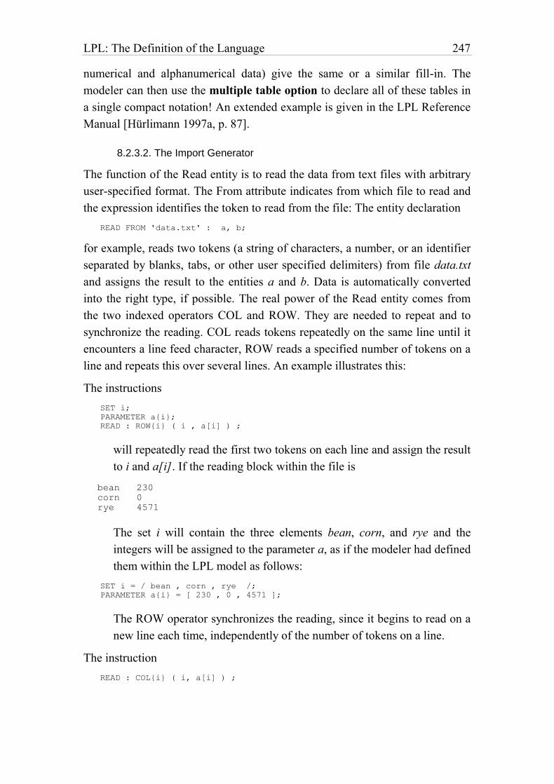
LPL: The Definition of the Language 247
numerical and alphanumerical data) give the same or a similar fill-in. The
modeler can then use the multiple table option to declare all of these tables in
a single compact notation! An extended example is given in the LPL Reference
Manual [Hürlimann 1997a, p. 87].
8.2.3.2. The Import Generator
The function of the Read entity is to read the data from text files with arbitrary
user-specified format. The From attribute indicates from which file to read and
the expression identifies the token to read from the file: The entity declaration
READ FROM 'data.txt' : a, b;
for example, reads two tokens (a string of characters, a number, or an identifier
separated by blanks, tabs, or other user specified delimiters) from file data.txt
and assigns the result to the entities a and b. Data is automatically converted
into the right type, if possible. The real power of the Read entity comes from
the two indexed operators COL and ROW. They are needed to repeat and to
synchronize the reading. COL reads tokens repeatedly on the same line until it
encounters a line feed character, ROW reads a specified number of tokens on a
line and repeats this over several lines. An example illustrates this:
The instructions
SET i;
PARAMETER a{i};
READ : ROW{i} ( i , a[i] ) ;
will repeatedly read the first two tokens on each line and assign the result
to i and a[i]. If the reading block within the file is
bean 230
corn 0
rye 4571
The set i will contain the three elements bean, corn, and rye and the
integers will be assigned to the parameter a, as if the modeler had defined
them within the LPL model as follows:
SET i = / bean , corn , rye /;
PARAMETER a{i} = [ 230 , 0 , 4571 ];
The ROW operator synchronizes the reading, since it begins to read on a
new line each time, independently of the number of tokens on a line.
The instruction
READ : COL{i} ( i, a[i] ) ;
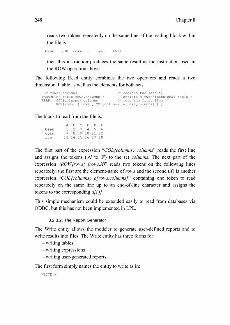
248 Chapter 8
reads two tokens repeatedly on the same line. If the reading block within
the file is
bean 230 corn 0 rye 4571
then this instruction produces the same result as the instruction used in
the ROW operation above.
The following Read entity combines the two operators and reads a two
dimensional table as well as the elements for both sets
SET rows; columns; (* declare two sets *)
PARAMETER table{rows,columns}; (* declare a two-dimensional table *)
READ : COL{columns} columns , (* read the first line *)
ROW{rows} ( rows , COL{columns} a[rows,columns] ) ;
The block to read from the file is:
A B C D E F
bean 1 2 3 4 5 6
corn 7 8 9 10 11 12
rye 13 14 15 16 17 18
The first part of the expression “COL{columns} columns” reads the first line
and assigns the tokens ('A' to 'F') to the set columns. The next part of the
expression “ROW{rows} (rows,X)” reads two tokens on the following lines
repeatedly, the first are the element-name of rows and the second (X) is another
expression “COL{columns} a[rows,columns]” containing one token to read
repeatedly on the same line up to an end-of-line character and assigns the
tokens to the corresponding a[i,j].
This simple mechanism could be extended easily to read from databases via
ODBC, but this has not been implemented in LPL.
8.2.3.2. The Report Generator
The Write entity allows the modeler to generate user-defined reports and to
write results into files. The Write entity has three forms for:
– writing tables
– writing expressions
– writing user-generated reports.
The first form simply names the entity to write as in:
WRITE a;
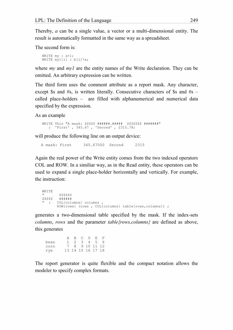
LPL: The Definition of the Language 249
Thereby, a can be a single value, a vector or a multi-dimensional entity. The
result is automatically formatted in the same way as a spreadsheet.
The second form is:
WRITE my : a+1;
WRITE my1{i} : b[i]*a;
where my and my1 are the entity names of the Write declaration. They can be
omitted. An arbitrary expression can be written.
The third form uses the comment attribute as a report mask. Any character,
except $s and #s, is written literally. Consecutive characters of $s and #s –
called place-holders – are filled with alphanumerical and numerical data
specified by the expression.
As an example
WRITE This "A mask: $$$$$ ######.##### $$$$$$$ #######"
: 'First' , 345.67 , 'Second' , 2315.78;
will produce the following line on an output device:
A mask: First 345.67000 Second 2315
Again the real power of the Write entity comes from the two indexed operators
COL and ROW. In a similiar way, as in the Read entity, these operators can be
used to expand a single place-holder horizontally and vertically. For example,
the instruction:
WRITE
" $$$$$$
$$$$$ ######
" : COL{columns} columns ,
ROW{rows} (rows , COL{columns} table[rows,columns]) ;
generates a two-dimensional table specified by the mask. If the index-sets
columns, rows and the parameter table{rows,columns} are defined as above,
this generates
A B C D E F
bean 1 2 3 4 5 6
corn 7 8 9 10 11 12
rye 13 14 15 16 17 18
The report generator is quite flexible and the compact notation allows the
modeler to specify complex formats.
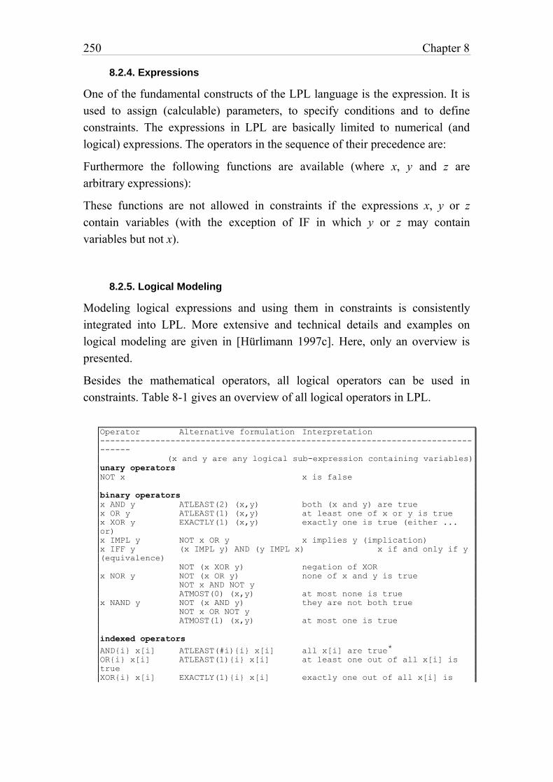
250 Chapter 8
8.2.4. Expressions
One of the fundamental constructs of the LPL language is the expression. It is
used to assign (calculable) parameters, to specify conditions and to define
constraints. The expressions in LPL are basically limited to numerical (and
logical) expressions. The operators in the sequence of their precedence are:
Furthermore the following functions are available (where x, y and z are
arbitrary expressions):
These functions are not allowed in constraints if the expressions x, y or z
contain variables (with the exception of IF in which y or z may contain
variables but not x).
8.2.5. Logical Modeling
Modeling logical expressions and using them in constraints is consistently
integrated into LPL. More extensive and technical details and examples on
logical modeling are given in [Hürlimann 1997c]. Here, only an overview is
presented.
Besides the mathematical operators, all logical operators can be used in
constraints. Table 8-1 gives an overview of all logical operators in LPL.
Operator Alternative formulation Interpretation
--------------------------------------------------------------------------
------
(x and y are any logical sub-expression containing variables)
unary operators
NOT x x is false
binary operators
x AND y ATLEAST(2) (x,y) both (x and y) are true
x OR y ATLEAST(1) (x,y) at least one of x or y is true
x XOR y EXACTLY(1) (x,y) exactly one is true (either ...
or)
x IMPL y NOT x OR y x implies y (implication)
x IFF y (x IMPL y) AND (y IMPL x) x if and only if y
(equivalence)
NOT (x XOR y) negation of XOR
x NOR y NOT (x OR y) none of x and y is true
NOT x AND NOT y
ATMOST(0) (x,y) at most none is true
x NAND y NOT (x AND y) they are not both true
NOT x OR NOT y
ATMOST(1) (x,y) at most one is true
indexed operators
AND{i} x[i] ATLEAST(#i){i} x[i] all x[i] are true*
OR{i} x[i] ATLEAST(1){i} x[i] at least one out of all x[i] is
true
XOR{i} x[i] EXACTLY(1){i} x[i] exactly one out of all x[i] is
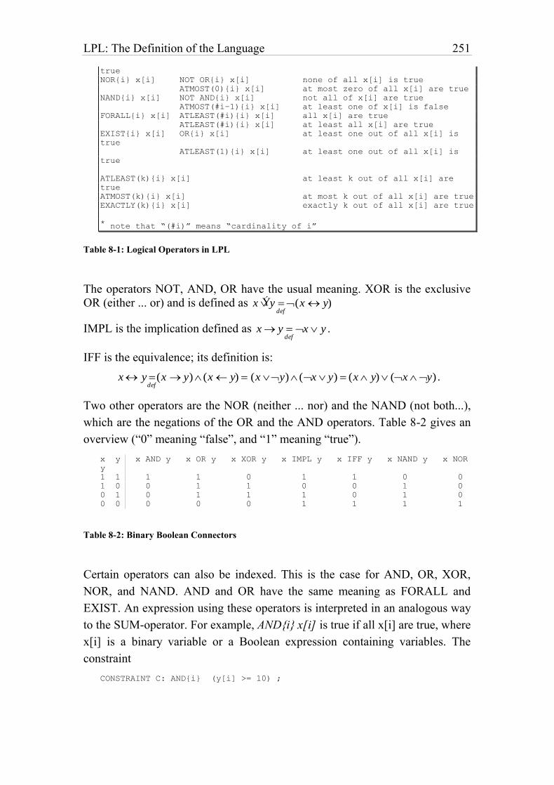
LPL: The Definition of the Language 251
true
NOR{i} x[i] NOT OR{i} x[i] none of all x[i] is true
ATMOST(0){i} x[i] at most zero of all x[i] are true
NAND{i} x[i] NOT AND{i} x[i] not all of x[i] are true
ATMOST(#i–1){i} x[i] at least one of x[i] is false
FORALL{i} x[i] ATLEAST(#i){i} x[i] all x[i] are true
ATLEAST(#i){i} x[i] at least all x[i] are true
EXIST{i} x[i] OR{i} x[i] at least one out of all x[i] is
true
ATLEAST(1){i} x[i] at least one out of all x[i] is
true
ATLEAST(k){i} x[i] at least k out of all x[i] are
true
ATMOST(k){i} x[i] at most k out of all x[i] are true
EXACTLY(k){i} x[i] exactly k out of all x[i] are true
* note that “(#i)” means “cardinality of i”
Table 8-1: Logical Operators in LPL
The operators NOT, AND, OR have the usual meaning. XOR is the exclusive
OR (either ... or) and is defined as x Ý y def(x y)
IMPL is the implication defined as x y defx y .
IFF is the equivalence; its definition is:
x y def
(x y) (x y) (x y) (x y) (x y) (x y) .
Two other operators are the NOR (neither ... nor) and the NAND (not both...),
which are the negations of the OR and the AND operators. Table 8-2 gives an
overview (“0” meaning “false”, and “1” meaning “true”).
x y x AND y x OR y x XOR y x IMPL y x IFF y x NAND y x NOR
y
1 1 1 1 0 1 1 0 0
1 0 0 1 1 0 0 1 0
0 1 0 1 1 1 0 1 0
0 0 0 0 0 1 1 1 1
Table 8-2: Binary Boolean Connectors
Certain operators can also be indexed. This is the case for AND, OR, XOR,
NOR, and NAND. AND and OR have the same meaning as FORALL and
EXIST. An expression using these operators is interpreted in an analogous way
to the SUM-operator. For example, AND{i} x[i] is true if all x[i] are true, where
x[i] is a binary variable or a Boolean expression containing variables. The
constraint
CONSTRAINT C: AND{i} (y[i] >= 10) ;
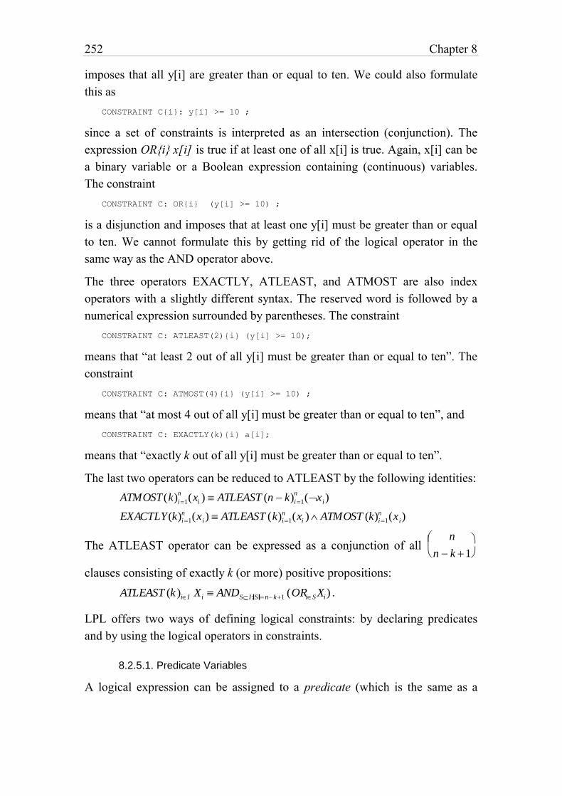
252 Chapter 8
imposes that all y[i] are greater than or equal to ten. We could also formulate
this as
CONSTRAINT C{i}: y[i] >= 10 ;
since a set of constraints is interpreted as an intersection (conjunction). The
expression OR{i} x[i] is true if at least one of all x[i] is true. Again, x[i] can be
a binary variable or a Boolean expression containing (continuous) variables.
The constraint
CONSTRAINT C: OR{i} (y[i] >= 10) ;
is a disjunction and imposes that at least one y[i] must be greater than or equal
to ten. We cannot formulate this by getting rid of the logical operator in the
same way as the AND operator above.
The three operators EXACTLY, ATLEAST, and ATMOST are also index
operators with a slightly different syntax. The reserved word is followed by a
numerical expression surrounded by parentheses. The constraint
CONSTRAINT C: ATLEAST(2){i} (y[i] >= 10);
means that “at least 2 out of all y[i] must be greater than or equal to ten”. The
constraint
CONSTRAINT C: ATMOST(4){i} (y[i] >= 10) ;
means that “at most 4 out of all y[i] must be greater than or equal to ten”, and
CONSTRAINT C: EXACTLY(k){i} a[i];
means that “exactly k out of all y[i] must be greater than or equal to ten”.
The last two operators can be reduced to ATLEAST by the following identities:
ATMOST(k)i1
n(xi ) ATLEAST (n k)i1
n(x i)
EXACTLY (k)i1
n (x i) ATLEAST (k)i1
n (xi ) ATMOST (k)i1
n (x i)
The ATLEAST operator can be expressed as a conjunction of all n
n k 1
clauses consisting of exactly k (or more) positive propositions:
ATLEAST (k )iI Xi ANDS I: S n k1 (ORiS Xi) .
LPL offers two ways of defining logical constraints: by declaring predicates
and by using the logical operators in constraints.
8.2.5.1. Predicate Variables
A logical expression can be assigned to a predicate (which is the same as a
LPL: The Definition of the Language 253
binary variable). Predicates, normally make the link between the logical and
mathematical part of a model. Suppose, we want to impose the constraint
(x 10) (y 5) where x and y are real variables. One way to do so, is simply to
state it as:
CONSTRAINT C: (x >=10) OR (y<=5); (1)
Another way is to introduce two predicates d and f and to impose the three
constraints:
d f , d (x 10), and f (y 5) . (2)
In LPL, this is equivalent to:
VARIABLE d BINARY := x >= 10 ;
VARIABLE f BINARY := y <= 5 ; (3)
CONSTRAINT C : d OR f ;
The two variable declarations define the implications as stated in (2). The
expression attached to the predicate name is called the predicate expression.
(So, “x ≥ 10” is the predicate expression of d, and “y ≤ 5” is the predicate
expression of f). By the way, LPL automatically translates (1) into (3)
symbolically.
The modeler can also impose the inverse implication. The constraint
(x 10) d (which is equivalent to d (x 10)) can also be defined by a
predicate as follows:
VARIABLE d BINARY NOT := x >= 10 ;
The keyword NOT imposes the inverse implication.
A third type of predicates is equivalence between the predicate and the
expression. For example, if the modeler wants to impose the constraint
d (x 10) , then this can be done as:
VARIABLE d BINARY IFF := x >= 10 ;
The keyword IFF imposes the equivalence. A reader, who is not familiar with
these different variants, may wonder why the equivalence is not always the best
way to model the connection between a predicate and a (mathematical or
logical) expression. The reason is that equivalence generates more constraints
than are really needed. Take the expression (2). Implication is sufficient. Why?
If d f holds (and it must hold, otherwise the whole constraint cannot be
satisfied) then at least one of the implications d (x 10), and f (y 5)
implies that either x ≥ 10 or y ≤ 5 must hold. But this is exactly what we want to
model with the constraint (x 10) (y 5).
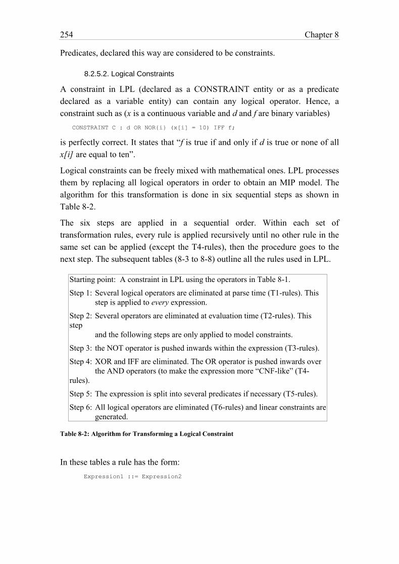
254 Chapter 8
Predicates, declared this way are considered to be constraints.
8.2.5.2. Logical Constraints
A constraint in LPL (declared as a CONSTRAINT entity or as a predicate
declared as a variable entity) can contain any logical operator. Hence, a
constraint such as (x is a continuous variable and d and f are binary variables)
CONSTRAINT C : d OR NOR{i} (x[i] = 10) IFF f;
is perfectly correct. It states that “f is true if and only if d is true or none of all
x[i] are equal to ten”.
Logical constraints can be freely mixed with mathematical ones. LPL processes
them by replacing all logical operators in order to obtain an MIP model. The
algorithm for this transformation is done in six sequential steps as shown in
Table 8-2.
The six steps are applied in a sequential order. Within each set of
transformation rules, every rule is applied recursively until no other rule in the
same set can be applied (except the T4-rules), then the procedure goes to the
next step. The subsequent tables (8-3 to 8-8) outline all the rules used in LPL.
Starting point: A constraint in LPL using the operators in Table 8-1.
Step 1: Several logical operators are eliminated at parse time (T1-rules). This
step is applied to every expression.
Step 2: Several operators are eliminated at evaluation time (T2-rules). This
step
and the following steps are only applied to model constraints.
Step 3: the NOT operator is pushed inwards within the expression (T3-rules).
Step 4: XOR and IFF are eliminated. The OR operator is pushed inwards over
the AND operators (to make the expression more “CNF-like” (T4-
rules).
Step 5: The expression is split into several predicates if necessary (T5-rules).
Step 6: All logical operators are eliminated (T6-rules) and linear constraints are
generated.
Table 8-2: Algorithm for Transforming a Logical Constraint
In these tables a rule has the form:
Expression1 ::= Expression2
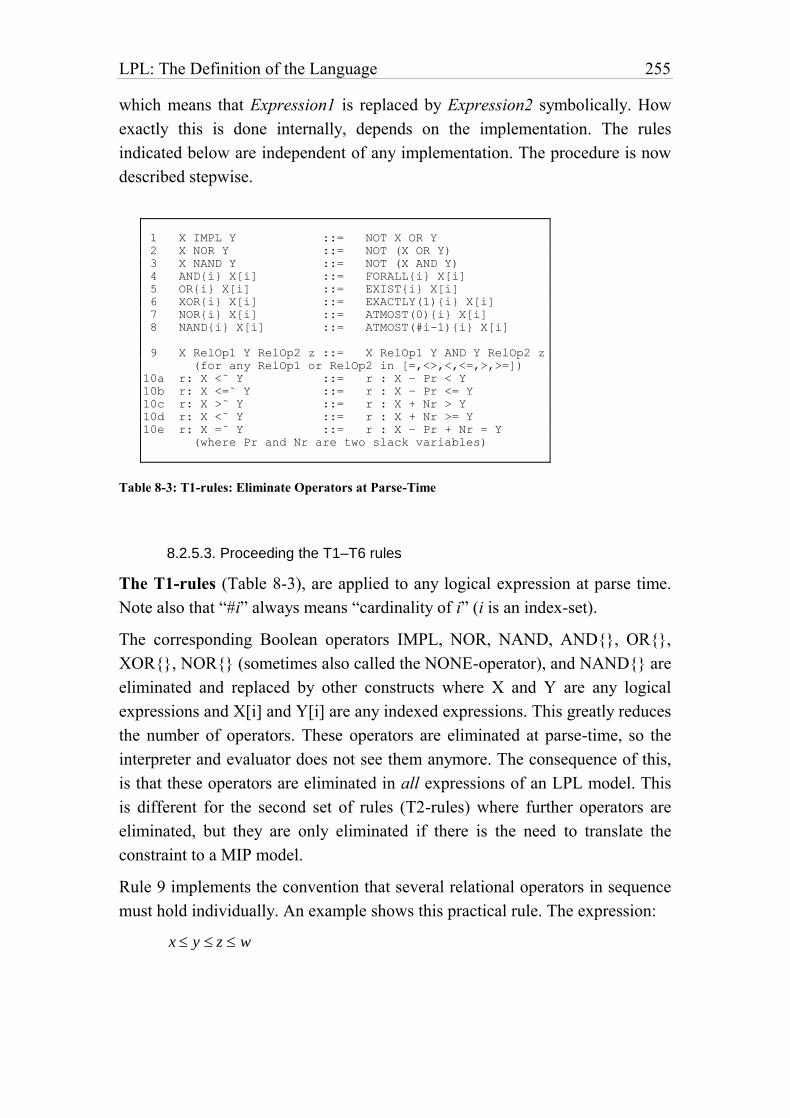
LPL: The Definition of the Language 255
which means that Expression1 is replaced by Expression2 symbolically. How
exactly this is done internally, depends on the implementation. The rules
indicated below are independent of any implementation. The procedure is now
described stepwise.
1 X IMPL Y ::= NOT X OR Y
2 X NOR Y ::= NOT (X OR Y)
3 X NAND Y ::= NOT (X AND Y)
4 AND{i} X[i] ::= FORALL{i} X[i]
5 OR{i} X[i] ::= EXIST{i} X[i]
6 XOR{i} X[i] ::= EXACTLY(1){i} X[i]
7 NOR{i} X[i] ::= ATMOST(0){i} X[i]
8 NAND{i} X[i] ::= ATMOST(#i-1){i} X[i]
9 X RelOp1 Y RelOp2 z ::= X RelOp1 Y AND Y RelOp2 z
(for any RelOp1 or RelOp2 in [=,<>,<,<=,>,>=])
10a r: X <˜ Y ::= r : X – Pr < Y
10b r: X <=˜ Y ::= r : X – Pr <= Y
10c r: X >˜ Y ::= r : X + Nr > Y
10d r: X <˜ Y ::= r : X + Nr >= Y
10e r: X =˜ Y ::= r : X – Pr + Nr = Y
(where Pr and Nr are two slack variables)
Table 8-3: T1-rules: Eliminate Operators at Parse-Time
8.2.5.3. Proceeding the T1–T6 rules
The T1-rules (Table 8-3), are applied to any logical expression at parse time.
Note also that “#i” always means “cardinality of i” (i is an index-set).
The corresponding Boolean operators IMPL, NOR, NAND, AND{}, OR{},
XOR{}, NOR{} (sometimes also called the NONE-operator), and NAND{} are
eliminated and replaced by other constructs where X and Y are any logical
expressions and X[i] and Y[i] are any indexed expressions. This greatly reduces
the number of operators. These operators are eliminated at parse-time, so the
interpreter and evaluator does not see them anymore. The consequence of this,
is that these operators are eliminated in all expressions of an LPL model. This
is different for the second set of rules (T2-rules) where further operators are
eliminated, but they are only eliminated if there is the need to translate the
constraint to a MIP model.
Rule 9 implements the convention that several relational operators in sequence
must hold individually. An example shows this practical rule. The expression:
x y z w
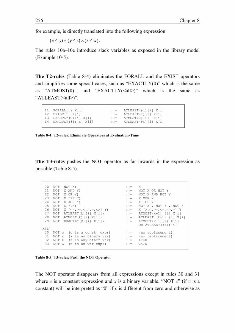
256 Chapter 8
for example, is directly translated into the following expression:
(x y) (y z) (z w) .
The rules 10a–10e introduce slack variables as exposed in the library model
(Example 10-5).
The T2-rules (Table 8-4) eliminates the FORALL and the EXIST operators
and simplifies some special cases, such as “EXACTLY(0)” which is the same
as “ATMOST(0)”, and ”EXACTLY(<all>)” which is the same as
“ATLEAST(<all>)”.
11 FORALL{i} X[i] ::= ATLEAST(#i){i} X[i]
12 EXIST{i} X[i] ::= ATLEAST(1){i} X[i]
13 EXACTLY(0){i} X[i] ::= ATMOST(0){i} X[i]
14 EXACTLY(#i){i} X[i] ::= ATLEAST(#i){i} X[i]
Table 8-4: T2-rules: Eliminate Operators at Evaluation-Time
The T3-rules pushes the NOT operator as far inwards in the expression as
possible (Table 8-5).
20 NOT (NOT X) ::= X
21 NOT (X AND Y) ::= NOT X OR NOT Y
22 NOT (X OR Y) ::= NOT X AND NOT Y
23 NOT (X IFF Y) ::= X XOR Y
24 NOT (X XOR Y) ::= X IFF Y
25 NOT (X,Y,Z) ::= NOT X , NOT Y , NOT Z
26 NOT (X [<=,>=,<,>,=,<>] Y) ::= X [>,<,>=,<=,<>,=] Y
27 NOT (ATLEAST(k){i} X[i]) ::= ATMOST(k-1) {i} X[i]
28 NOT (ATMOST(k){i} X[i]) ::= ATLEAST (k+1) {i} X[i]
29 NOT (EXACTLY(k){i} X[i]) ::= ATMOST(k-1){i} X[i]
OR ATLEAST(k+1){i}
X[i]
30 NOT c (c is a const. expr) ::= (no replacement)
31 NOT x (x is an binary var) ::= (no replacement)
32 NOT z (z is any other var) ::= z<=0
33 NOT Z (Z is an var expr) ::= Z<>0
Table 8-5: T3-rules: Push the NOT Operator
The NOT operator disappears from all expressions except in rules 30 and 31
where c is a constant expression and x is a binary variable. “NOT c” (if c is a
constant) will be interpreted as “0” if c is different from zero and otherwise as
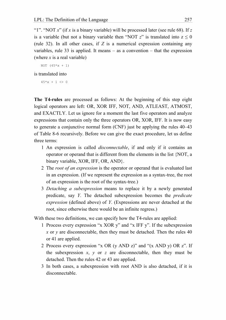
LPL: The Definition of the Language 257
“1”. “NOT x” (if x is a binary variable) will be processed later (see rule 68). If z
is a variable (but not a binary variable then “NOT z” is translated into z ≤ 0
(rule 32). In all other cases, if Z is a numerical expression containing any
variables, rule 33 is applied. It means – as a convention – that the expression
(where x is a real variable)
NOT (45*x + 1)
is translated into
45*x + 1 <> 0
The T4-rules are processed as follows: At the beginning of this step eight
logical operators are left: OR, XOR IFF, NOT, AND, ATLEAST, ATMOST,
and EXACTLY. Let us ignore for a moment the last five operators and analyze
expressions that contain only the three operators OR, XOR, IFF. It is now easy
to generate a conjunctive normal form (CNF) just be applying the rules 40–43
of Table 8-6 recursively. Before we can give the exact procedure, let us define
three terms:
1 An expression is called disconnectable, if and only if it contains an
operator or operand that is different from the elements in the list {NOT, a
binary variable, XOR, IFF, OR, AND}.
2 The root of an expression is the operator or operand that is evaluated last
in an expression. (If we represent the expression as a syntax-tree, the root
of an expression is the root of the syntax-tree.)
3 Detaching a subexpression means to replace it by a newly generated
predicate, say Y. The detached subexpression becomes the predicate
expression (defined above) of Y. (Expressions are never detached at the
root, since otherwise there would be an infinite regress.)
With these two definitions, we can specify how the T4-rules are applied:
1 Process every expression “x XOR y” and “x IFF y”. If the subexpression
x or y are disconnectable, then they must be detached. Then the rules 40
or 41 are applied.
2 Process every expression “x OR (y AND z)” and “(x AND y) OR z”. If
the subexpression x, y or z are disconnectable, then they must be
detached. Then the rules 42 or 43 are applied.
3 In both cases, a subexpression with root AND is also detached, if it is
disconnectable.
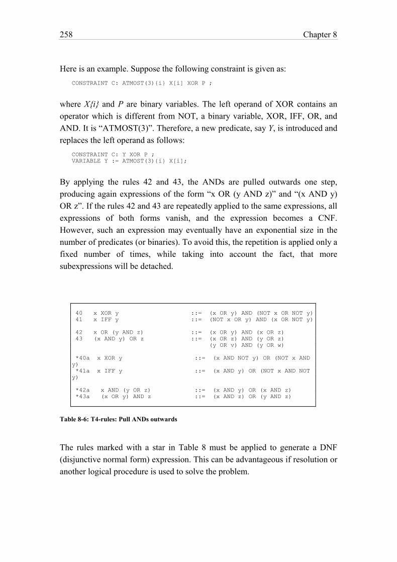
258 Chapter 8
Here is an example. Suppose the following constraint is given as:
CONSTRAINT C: ATMOST(3){i} X[i] XOR P ;
where X{i} and P are binary variables. The left operand of XOR contains an
operator which is different from NOT, a binary variable, XOR, IFF, OR, and
AND. It is “ATMOST(3)”. Therefore, a new predicate, say Y, is introduced and
replaces the left operand as follows:
CONSTRAINT C: Y XOR P ;
VARIABLE Y := ATMOST(3){i} X[i];
By applying the rules 42 and 43, the ANDs are pulled outwards one step,
producing again expressions of the form “x OR (y AND z)” and “(x AND y)
OR z”. If the rules 42 and 43 are repeatedly applied to the same expressions, all
expressions of both forms vanish, and the expression becomes a CNF.
However, such an expression may eventually have an exponential size in the
number of predicates (or binaries). To avoid this, the repetition is applied only a
fixed number of times, while taking into account the fact, that more
subexpressions will be detached.
40 x XOR y ::= (x OR y) AND (NOT x OR NOT y)
41 x IFF y ::= (NOT x OR y) AND (x OR NOT y)
42 x OR (y AND z) ::= (x OR y) AND (x OR z)
43 (x AND y) OR z ::= (x OR z) AND (y OR z)
(y OR v) AND (y OR w)
*40a x XOR y ::= (x AND NOT y) OR (NOT x AND
y)
*41a x IFF y ::= (x AND y) OR (NOT x AND NOT
y)
*42a x AND (y OR z) ::= (x AND y) OR (x AND z)
*43a (x OR y) AND z ::= (x AND z) OR (y AND z)
Table 8-6: T4-rules: Pull ANDs outwards
The rules marked with a star in Table 8 must be applied to generate a DNF
(disjunctive normal form) expression. This can be advantageous if resolution or
another logical procedure is used to solve the problem.
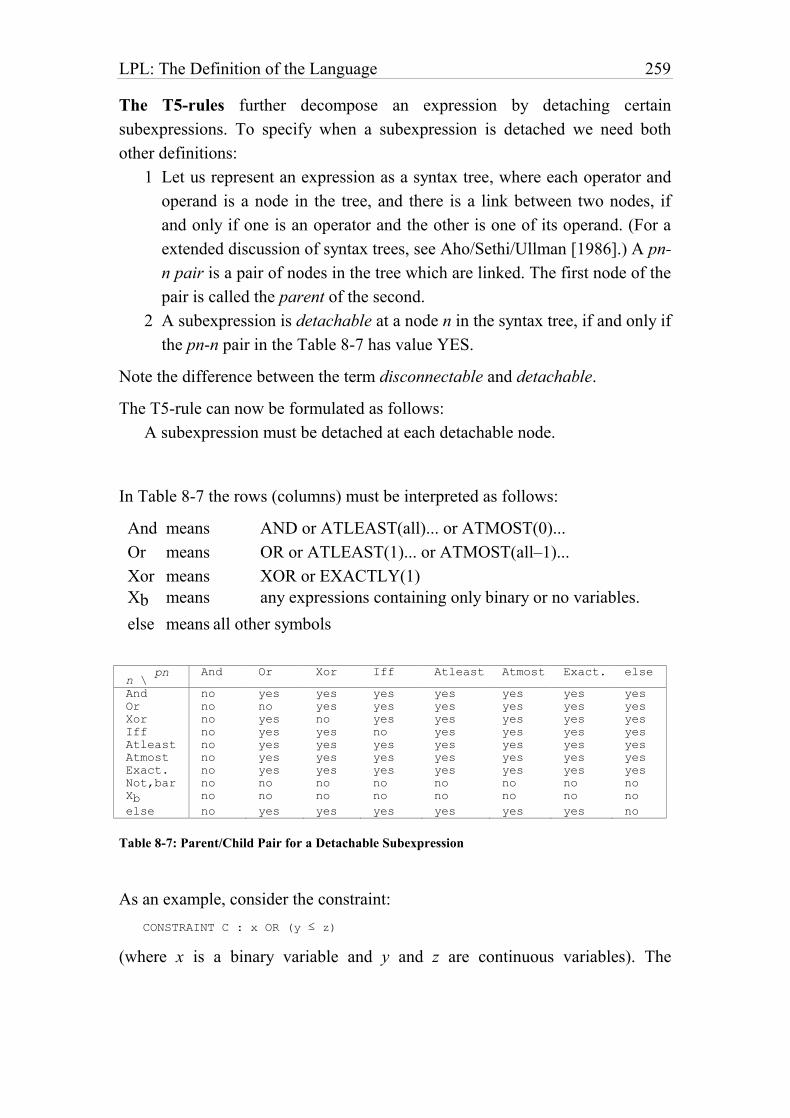
LPL: The Definition of the Language 259
The T5-rules further decompose an expression by detaching certain
subexpressions. To specify when a subexpression is detached we need both
other definitions:
1 Let us represent an expression as a syntax tree, where each operator and
operand is a node in the tree, and there is a link between two nodes, if
and only if one is an operator and the other is one of its operand. (For a
extended discussion of syntax trees, see Aho/Sethi/Ullman [1986].) A pn-
n pair is a pair of nodes in the tree which are linked. The first node of the
pair is called the parent of the second.
2 A subexpression is detachable at a node n in the syntax tree, if and only if
the pn-n pair in the Table 8-7 has value YES.
Note the difference between the term disconnectable and detachable.
The T5-rule can now be formulated as follows:
A subexpression must be detached at each detachable node.
In Table 8-7 the rows (columns) must be interpreted as follows:
And means AND or ATLEAST(all)... or ATMOST(0)...
Or means OR or ATLEAST(1)... or ATMOST(all–1)...
Xor means XOR or EXACTLY(1)
Xb means any expressions containing only binary or no variables.
else means all other symbols
n \ pn
And Or Xor Iff Atleast Atmost Exact. else
And no yes yes yes yes yes yes yes
Or no no yes yes yes yes yes yes
Xor no yes no yes yes yes yes yes
Iff no yes yes no yes yes yes yes
Atleast no yes yes yes yes yes yes yes
Atmost no yes yes yes yes yes yes yes
Exact. no yes yes yes yes yes yes yes
Not,bar no no no no no no no no
Xb no no no no no no no no
else no yes yes yes yes yes yes no
Table 8-7: Parent/Child Pair for a Detachable Subexpression
As an example, consider the constraint:
CONSTRAINT C : x OR (y ≤ z)
(where x is a binary variable and y and z are continuous variables). The
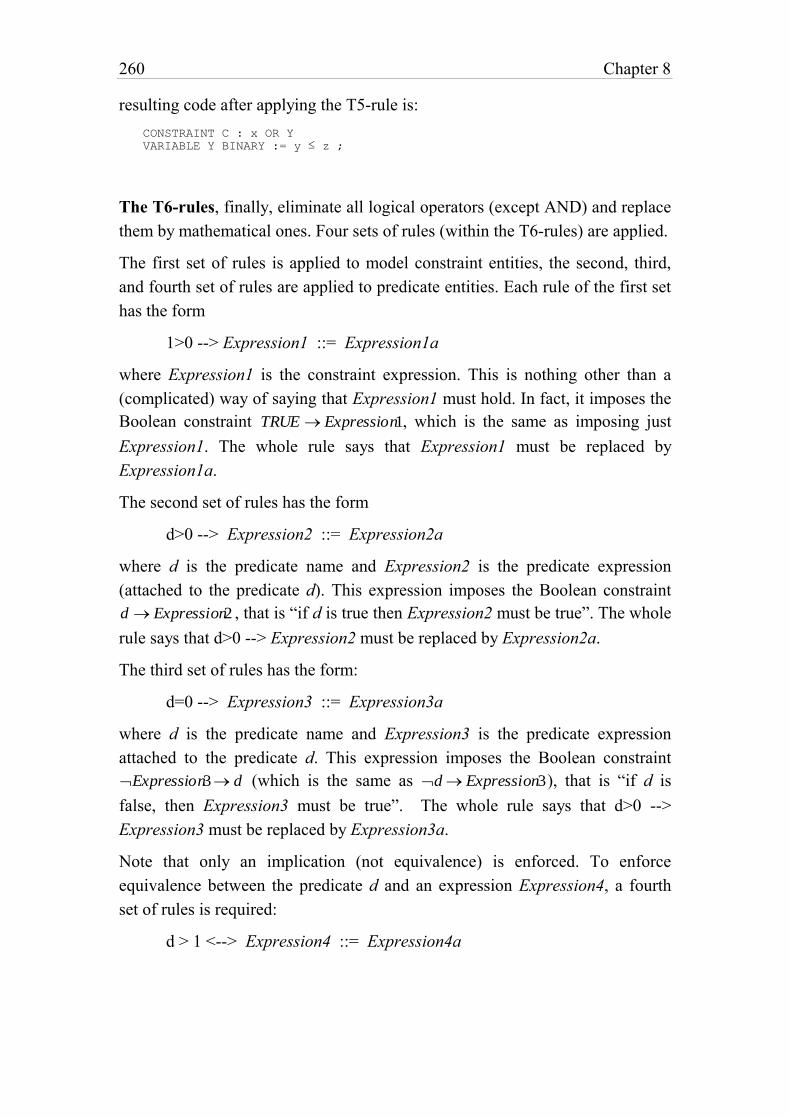
260 Chapter 8
resulting code after applying the T5-rule is:
CONSTRAINT C : x OR Y
VARIABLE Y BINARY := y ≤ z ;
The T6-rules, finally, eliminate all logical operators (except AND) and replace
them by mathematical ones. Four sets of rules (within the T6-rules) are applied.
The first set of rules is applied to model constraint entities, the second, third,
and fourth set of rules are applied to predicate entities. Each rule of the first set
has the form
1>0 --> Expression1 ::= Expression1a
where Expression1 is the constraint expression. This is nothing other than a
(complicated) way of saying that Expression1 must hold. In fact, it imposes the
Boolean constraint TRUE Expression1, which is the same as imposing just
Expression1. The whole rule says that Expression1 must be replaced by
Expression1a.
The second set of rules has the form
d>0 --> Expression2 ::= Expression2a
where d is the predicate name and Expression2 is the predicate expression
(attached to the predicate d). This expression imposes the Boolean constraint
d Expression2 , that is “if d is true then Expression2 must be true”. The whole
rule says that d>0 --> Expression2 must be replaced by Expression2a.
The third set of rules has the form:
d=0 --> Expression3 ::= Expression3a
where d is the predicate name and Expression3 is the predicate expression
attached to the predicate d. This expression imposes the Boolean constraint
Expression3 d (which is the same as d Expression3), that is “if d is
false, then Expression3 must be true”. The whole rule says that d>0 -->
Expression3 must be replaced by Expression3a.
Note that only an implication (not equivalence) is enforced. To enforce
equivalence between the predicate d and an expression Expression4, a fourth
set of rules is required:
d > 1 <--> Expression4 ::= Expression4a
LPL: The Definition of the Language 261
which is the same as the conjunction of both rules (from set 2 and 3) defined as:
d > 0 --> Expression4 ::= Expression4a
d = 0 --> NOT Expression4 ::= NOT Expression4a
All T6-rules are shown in Table 8-8.
Rule 50 just says that a conjunction of constraints is considered as a set of
constraints. Rule 51 replaces all ORs by the addition operator. The addition
must be greater than or equal one. This enforces at least one operand to be true.
Rule 57 is the starting rule for every constraint entity. Rule 58 is applied if
“NOT x” is a complete constraint while 58a is applied if “NOT x” is a
subexpression and belongs to a constraint.
(Rules 65 and 66 do not exactly enforce the intended implication. The correct
two rules would be as follows: 65a d>0 --> ATMOST(k){i} X[i] ::= SUM{i} x[i] <= n -(n-k)*d
66a d>0 --> EXACTLY(k){i} X[i] ::= d>0 --> ATLEAST(k){i} X[i]
AND
d>0 --> ATMOST(k){i} X[i]
The rule 65 and 66 enforce the implications supposing d is true. This can be
supposed most of the time. However the modeler should use EXACTLY and
ATMOST with care in an LPL model.)
50 1>0 --> X AND Y AND ... ::= x, y, ...
51 1>0 --> X OR Y OR ... ::= x + y + ... >= 1
54 1>0 --> ATLEAST(k){i} X[i] ::= SUM{i} x[i] >= k
55 1>0 --> ATMOST(k){i} X[i] ::= SUM{i} x[i] <= k
56 1>0 --> EXACTLY(k){i} X[i] ::= SUM{i} x[i] = k
57 1>0 --> X ::= X
58 NOT x (x is a binary var) ::= x<=0 (complete constraint)
58a NOT x (x is a binary var) ::= 1-x (in a subexpression)
59 x (x is a binary variable) ::= x>=1 (complete expression)
60 d>0 --> X AND Y AND ... ::= x >= d , y >= d , ...
61 d>0 --> X OR Y OR ... ::= x + y + ... >= d
64 d>0 --> ATLEAST(k){i} X[i] ::= SUM{i} x[i] >= k*d
65 d>0 --> ATMOST(k){i} X[i] ::= SUM{i} x[i] <= k*d
66 d>0 --> EXACTLY(k){i} X[i] ::= SUM{i} x[i] = k*d
67 d>0 --> X ::= X >= d
70 d>0 --> ∑ ax <= b ::= ∑ ax-b <= U(∑ ax-b)*(1-d)
71 d>0 --> ∑ ax >= b ::= ∑ ax-b >= L(∑ ax-b)*(1-d)
72 d>0 --> ∑ ax = b ::= d>0 --> ∑ax >= b AND d>0 --> ∑ax <=
b
80 d=0 --> ∑ ax <= b ::= ∑ ax-b <= U(∑ ax-b)*d
81 d=0 --> ∑ ax >= b ::= ∑ ax-b >= L(∑ ax-b)*d
82 d=0 --> ∑ ax = b ::= d=0 --> ∑ax >= b AND d=0 --> ∑ax <=
262 Chapter 8
b
90 x <> y ::= d>0 --> x < y ; d=0 --> x > y
91 x < y ::= x + e <= y
92 x > y ::= x >= y + e
Table 8-8: T6-rules
At this point, all logical operators are eliminated as can be verified by the T6-
rules. The rules 50–57 are straightforward and implement the first set of the T5-
rules. Rules 60–67 implements the second set of the T5-rules. Hence, rule 67,
for example, means that if d is true then X must also be true. The resulting
constraint “X >= d” reflects this fact: if d is 1, then X must be at least 1,
otherwise X can be true or not. Similar arguments hold for the other rules.
The rules 70–71 make the link between mathematical constraints and logical
proposition, where the expressions L(X) and U(X) are lower and upper bounds
on the expression X. Normally, they are applied on a linear constraints such as
L a jx jj1
n
b U
These bounds may be given by the modeler or they may be calculated
automatically from the lower and upper bounds lj and uj of the variables xj
involved in the linear expression. (In LPL both methods are possible.) In the
second case, they are calculated using the following formula
[Brearley/Mitra/Williams 1975]:
L aj l j
j{ j: a j 0}
a juj
j{ j:a j 0}
b
U a ju j
j{ j :a j 0}
a j lj
j{ j:a j 0}
b
where l j x j u j . (X)
In LPL, it is easy to bound variables as well as constraints. A range
specification [...,...] must be attached to the corresponding declaration entity, as
in
VARIABLE x [10,50]; (*lower and upper bounds of the variable x are 10
and 50*)
CONSTRAINT R [l,u]; (*lower and upper bounds of the constraint R are l
and u*)
These bounds are used by LPL to calculate U and L of a constraint according to
LPL: The Definition of the Language 263
the formula (X).
An extended application, on how these rules are applied will be given in
Example 10-9.
8.3. The Backus-Naur Specification of LPL (4.20)
The complete syntax of LPL version 4.20 is presented in the extended Backus-
Naur Form. The following symbols are metasymbols (are not part of the LPL
syntax), unless they are included in quotes (as '{' or '['):
= means “is defined as” (defines a production)
| means “or”
{ } enclosed items can be repeated zero or any number of times
[ ] enclosed items can be repeated zero or one times
... (in 'A' | ... | 'Z') means
All other symbols are part of LPL. Reserved words are written entirely in upper
case letters. Symbols starting with a lower character, reserved words and strings
between quotes are symbols recognized by the LPL scanner. The starting
production symbol of the language is Model.
Model = MODEL ModelAttr {Statement} END
ModelAttr = StaredId {Attrs} [assOp Expr] ';'
StaredId = id ['*']
Statement = Model | [Keyword] [StaredId] [IndexList] {Attrs}
[assOp Expr | assOp Table] ';'
Keyword = SET | UNIT | PARAMETER | VARIABLE | CONSTRAINT |
MAXIMIZE | MINIMIZE | PROVE | CHECK | WRITE |
READ | OPTION | DELETE
IndexList = '{' Index {',' Index} ['|' Expr] '}'
Index = [id '='|IN] id ['[' id {',' id} ']']
Attrs = ALIAS id [',' id] | INTEGER | BINARY | STRING |
INACTIVE | DISTINCT | DEFAULT [=] number | '['
Expr ']' | UNIT Expr | TO ['+'] str | FORMAT ':'
int [':' int] ['[' int ',' int [',' int] ']'] |
FROM ['*'] str | BLOCK [int] [FROM str TO str] |
comment | str
Expr = SimpleExpr {Relation SimpleExpr}
SimpleExpr = [Indexing] Term {MulOp Term}
Term = ['+' | '-' | '#' | NOT] Factor
Factor = number ['[' Expr ']'] | str | id IN id | id ['['
Expr ']'] | Funct '(' Expr ')' | '(' Expr ')'
Relation = ',' | IMPL | XOR | IFF | OR | NOR | AND | NAND |
'=' | '<>' | '<' | '<=' | '>' | '>=' | '=~' |
'<~' | '<=~' | '>~' | '>=~' | '+' | '-'
MulOp = '*' | '/' | '^' | '%'
Indexing = IndexOp [IndexList]
264 Chapter 8
IndexOp = OR | XOR | NOR | AND | NAND | EXIST | FORALL |
PROD | MAX | MIN | PMAX | PMIN | ROW | COL | SUM
| ATLEAST '(' int ')' | ATMOST '(' int ')' |
EXACTLY '(' int ')'
Funct = ABS | CEIL | COS | EXP | FLOOR | LOG | SIN | SQRT
| TRUNC | RND | RNDN | IF | ARCTAN
Table = TableA | TableB | TableC
TableA = '[' {Data} ']'
TableB = '/' ['|' {id} '|'] {SubTable} '/'
SubTable = ['[' Template ']'] [ColonOption] Entries
ColonOption = ':' ['(tr)'] {Element} ':'
Entries = { {Element} {Data} [','] }
Data = number | '.' | str
Element = {char1} | str
Template = EleOrStar {',' EleOrStar}
EleOrStar = Element | '*'
TableC = '/' int ':' int '/'
comment = '"' {char} '"'
str = '''' {char} ''''
id = letter {letter | digit}
number = int | real
int = digit {digit}
real = digit {digit} '.' {digit} [scaleFactor]
scaleFactor = 'E' ['+' | '-'] digit {digit}
assOp = ':=' | '=' | ':'
digit = '0' | ... | '9'
letter = 'A' | ... | 'Z' | 'a' | ... | 'z' | '_'
char = (any character)
char1 = any chars except blanks, and the 13 chars:
()*,:;/[|]'"=
This completes the brief overview of the LPL language. More detailed
information can be found in the official language document [Hürlimann 1997a],
which is updated at regular intervals. The next chapter gives a survey of the
environment in which LPL is embedded.
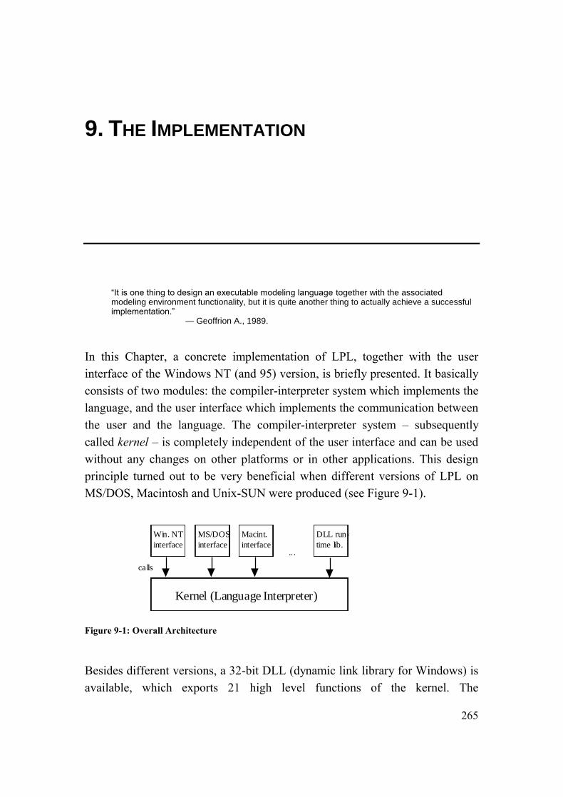
265
9. THE IMPLEMENTATION
“It is one thing to design an executable modeling language together with the associated modeling environment functionality, but it is quite another thing to actually achieve a successful implementation.” — Geoffrion A., 1989.
In this Chapter, a concrete implementation of LPL, together with the user
interface of the Windows NT (and 95) version, is briefly presented. It basically
consists of two modules: the compiler-interpreter system which implements the
language, and the user interface which implements the communication between
the user and the language. The compiler-interpreter system – subsequently
called kernel – is completely independent of the user interface and can be used
without any changes on other platforms or in other applications. This design
principle turned out to be very beneficial when different versions of LPL on
MS/DOS, Macintosh and Unix-SUN were produced (see Figure 9-1).
Kernel (Language Interpreter)
Win. NT
interface
MS/DOS
interface
Macint.
interface
DLL run-
time lib... .
ca lls
Figure 9-1: Overall Architecture
Besides different versions, a 32-bit DLL (dynamic link library for Windows) is
available, which exports 21 high level functions of the kernel. The
266 Chapter 9
specifications of this DLL are fully described in Hürlimann [1997d].
9.1. The Kernel
The kernel contains the complete implementation of the LPL language,
consisting of the parser, the data structures for the symbol table, an interpreter
and evaluator, a symbolic transformator, and different tools to generate the
input code to an MIP solver. Import and report generator are also parts of the
kernel. It is not necessary to describe the implementation in more detail here,
although some hints are given.
The implementation was written in highly portable Pascal and can easily be
translated automatically to C using a free Pascal-to-C translator. The source
code consists of about 10,000 lines. The executable is less than 120 kbytes.
Complex data structures have been used to make the execution reasonably fast,
although measures could be taken to make it faster. However, since LPL is a
prototype, I did not concentrate much on this issue.
The parser reads the LPL source code and translates it into an internal data
structure: the symbol table. It is implemented as a one-pass, recursive descent
parser as described in Wirth [1996].
The structure of the symbol table is critical. It must fulfil four goals: (1) the
source code must be easily reproducible from this structure, (2) it should not be
too hard to transform the model symbolically, (3) the evaluation of numerical
expression should be fast, and (4) the data should be stored as compactly as
possible. It is not easy to reconcile these often incompatible objectives. Goal 3
and 4 are especially hard to attain at the same time. The executable time is often
inversely correlated to the size of the data structure. Goal 1 is important in an
interactive modeling environment, in which the source code of the model could
be generated by other – maybe graphical – means (instead of a plain text
editor). Furthermore, symbolical transformations can easily be traced. Goal 2 is
presently used in logical modeling to apply the different transformation rules.
Using the wrong data structure, the implementation of such transformations
could be a virtual nightmare.
Of course, in a commercial product, machine code should be generated for the
execution. This is not the case in this implementation. Instead, an intermediate
LPL: The Implementation 267
code (not unlike the p-code of the first Pascal compilers/interpreters) is
generated which is independent of the machine instruction set of any specific
machine. The evaluator, which is also a part of the kernel, then interprets this
intermediate code. This is much slower than a compiled version which
generates direct machine code, but it is still reasonably fast in most situations.
The import and report generator (represented by the Read- and Write entity) are
also a part of the kernel. The input and output devices are plain text files to
make them independent from any database server. However, links to databases
are easy to build by means of generic protocols like the ODBC-standard. It is
not integrated in the actual version 4.20.
9.2. The Environment (User Interface)
Building a user-conform, interactive interface is easy today, if one uses the
right software development tools. To create a modeling environment on
Windows NT, Delphi 2 (from Borland) was used. It allows the programmer to
place the components into forms in an interactive way. In this way, it was not
very time consuming to create a modeling environment consisting of a text
editor, a text and graphical browser, as well as an interpreter.
The main windows of the environment are depicted in Figure 9-2. On the left
hand side is the LPL source code editor window and other editor windows. On
the right hand side are two smaller windows: the LOG-window at the top and
the interpreter-window at the bottom. Compiler error messages are sent to the
LOG-window. The interpreter window allows the user to add and to interpret
LPL code, this can be appended to the model in an incremental way.
The File menu contains the usual functions such as: create new, load, save
model etc. The Edit and Character menus comprise such standard functions as
copy, paste etc. The Run menu allows the user to compile and solve the model.
The result of a successful run is written into a newly created text window. The
Tools menu contains such functions as “show the statistics of the model,”
generate an equation listing, “show the MPS-file”, as well as “open the text and
graphical browsers” (see Section 9.3 and 9.4). The Window and Help menu are
also quite standard under any Windows application.
This completes the short overview of the LPL environment. We turn now our
attention to two model browsers also implemented as interactive tools into the
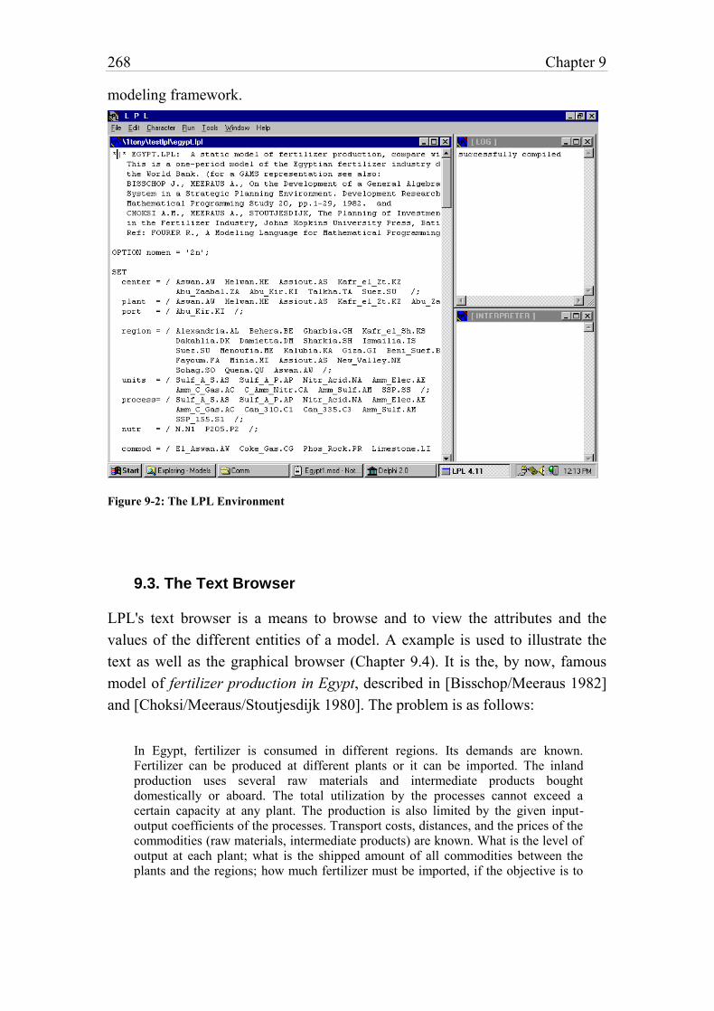
268 Chapter 9
modeling framework.
Figure 9-2: The LPL Environment
9.3. The Text Browser
LPL's text browser is a means to browse and to view the attributes and the
values of the different entities of a model. A example is used to illustrate the
text as well as the graphical browser (Chapter 9.4). It is the, by now, famous
model of fertilizer production in Egypt, described in [Bisschop/Meeraus 1982]
and [Choksi/Meeraus/Stoutjesdijk 1980]. The problem is as follows:
In Egypt, fertilizer is consumed in different regions. Its demands are known. Fertilizer can be produced at different plants or it can be imported. The inland production uses several raw materials and intermediate products bought domestically or aboard. The total utilization by the processes cannot exceed a certain capacity at any plant. The production is also limited by the given input-output coefficients of the processes. Transport costs, distances, and the prices of the commodities (raw materials, intermediate products) are known. What is the level of output at each plant; what is the shipped amount of all commodities between the plants and the regions; how much fertilizer must be imported, if the objective is to
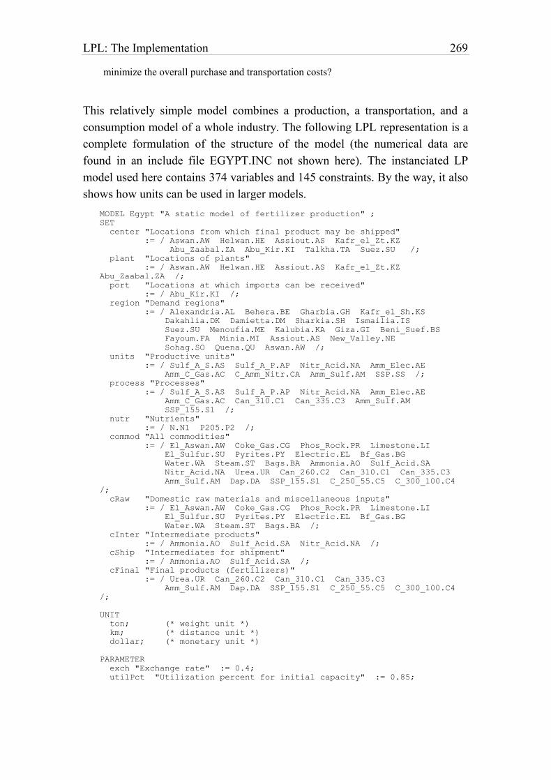
LPL: The Implementation 269
minimize the overall purchase and transportation costs?
This relatively simple model combines a production, a transportation, and a
consumption model of a whole industry. The following LPL representation is a
complete formulation of the structure of the model (the numerical data are
found in an include file EGYPT.INC not shown here). The instanciated LP
model used here contains 374 variables and 145 constraints. By the way, it also
shows how units can be used in larger models.
MODEL Egypt "A static model of fertilizer production" ;
SET
center "Locations from which final product may be shipped"
:= / Aswan.AW Helwan.HE Assiout.AS Kafr_el_Zt.KZ
Abu_Zaabal.ZA Abu_Kir.KI Talkha.TA Suez.SU /;
plant "Locations of plants"
:= / Aswan.AW Helwan.HE Assiout.AS Kafr_el_Zt.KZ
Abu_Zaabal.ZA /;
port "Locations at which imports can be received"
:= / Abu_Kir.KI /;
region "Demand regions"
:= / Alexandria.AL Behera.BE Gharbia.GH Kafr_el_Sh.KS
Dakahlia.DK Damietta.DM Sharkia.SH Ismailia.IS
Suez.SU Menoufia.ME Kalubia.KA Giza.GI Beni_Suef.BS
Fayoum.FA Minia.MI Assiout.AS New_Valley.NE
Sohag.SO Quena.QU Aswan.AW /;
units "Productive units"
:= / Sulf_A_S.AS Sulf_A_P.AP Nitr_Acid.NA Amm_Elec.AE
Amm_C_Gas.AC C_Amm_Nitr.CA Amm_Sulf.AM SSP.SS /;
process "Processes"
:= / Sulf_A_S.AS Sulf_A_P.AP Nitr_Acid.NA Amm_Elec.AE
Amm_C_Gas.AC Can_310.C1 Can_335.C3 Amm_Sulf.AM
SSP_155.S1 /;
nutr "Nutrients"
:= / N.N1 P205.P2 /;
commod "All commodities"
:= / El_Aswan.AW Coke_Gas.CG Phos_Rock.PR Limestone.LI
El_Sulfur.SU Pyrites.PY Electric.EL Bf_Gas.BG
Water.WA Steam.ST Bags.BA Ammonia.AO Sulf_Acid.SA
Nitr_Acid.NA Urea.UR Can_260.C2 Can_310.C1 Can_335.C3
Amm_Sulf.AM Dap.DA SSP_155.S1 C_250_55.C5 C_300_100.C4
/;
cRaw "Domestic raw materials and miscellaneous inputs"
:= / El_Aswan.AW Coke_Gas.CG Phos_Rock.PR Limestone.LI
El_Sulfur.SU Pyrites.PY Electric.EL Bf_Gas.BG
Water.WA Steam.ST Bags.BA /;
cInter "Intermediate products"
:= / Ammonia.AO Sulf_Acid.SA Nitr_Acid.NA /;
cShip "Intermediates for shipment"
:= / Ammonia.AO Sulf_Acid.SA /;
cFinal "Final products (fertilizers)"
:= / Urea.UR Can_260.C2 Can_310.C1 Can_335.C3
Amm_Sulf.AM Dap.DA SSP_155.S1 C_250_55.C5 C_300_100.C4
/;
UNIT
ton; (* weight unit *)
km; (* distance unit *)
dollar; (* monetary unit *)
PARAMETER
exch "Exchange rate" := 0.4;
utilPct "Utilization percent for initial capacity" := 0.85;
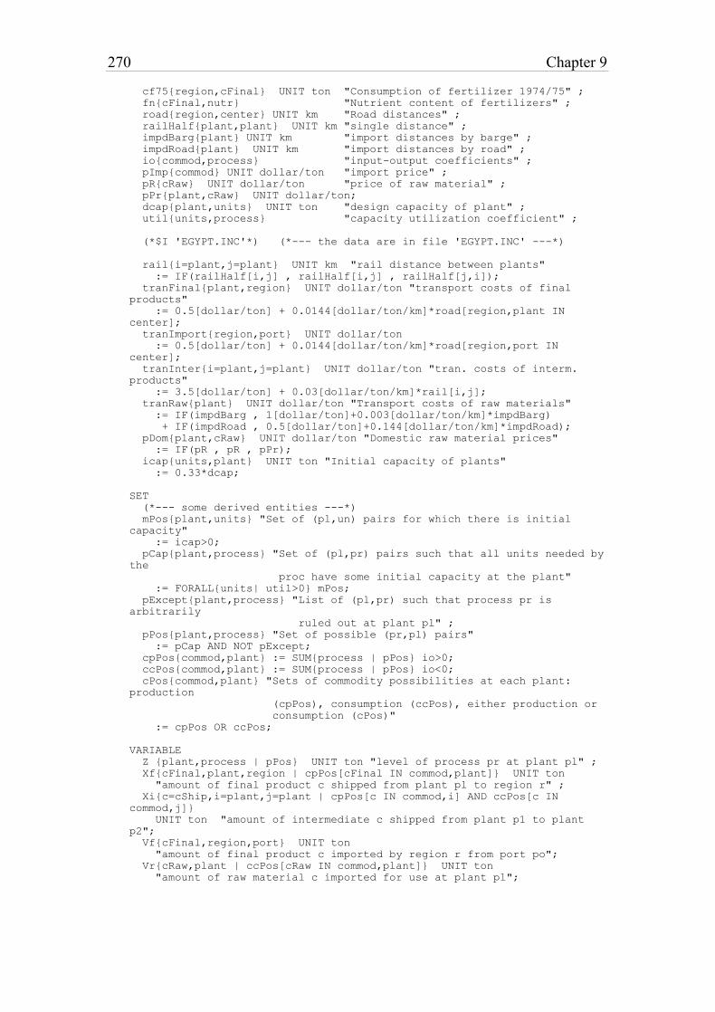
270 Chapter 9
cf75{region,cFinal} UNIT ton "Consumption of fertilizer 1974/75" ;
fn{cFinal,nutr} "Nutrient content of fertilizers" ;
road{region,center} UNIT km "Road distances" ;
railHalf{plant,plant} UNIT km "single distance" ;
impdBarg{plant} UNIT km "import distances by barge" ;
impdRoad{plant} UNIT km "import distances by road" ;
io{commod,process} "input-output coefficients" ;
pImp{commod} UNIT dollar/ton "import price" ;
pR{cRaw} UNIT dollar/ton "price of raw material" ;
pPr{plant,cRaw} UNIT dollar/ton;
dcap{plant,units} UNIT ton "design capacity of plant" ;
util{units,process} "capacity utilization coefficient" ;
(*$I 'EGYPT.INC'*) (*--- the data are in file 'EGYPT.INC' ---*)
rail{i=plant,j=plant} UNIT km "rail distance between plants"
:= IF(railHalf[i,j] , railHalf[i,j] , railHalf[j,i]);
tranFinal{plant,region} UNIT dollar/ton "transport costs of final
products"
:= 0.5[dollar/ton] + 0.0144[dollar/ton/km]*road[region,plant IN
center];
tranImport{region,port} UNIT dollar/ton
:= 0.5[dollar/ton] + 0.0144[dollar/ton/km]*road[region,port IN
center];
tranInter{i=plant,j=plant} UNIT dollar/ton "tran. costs of interm.
products"
:= 3.5[dollar/ton] + 0.03[dollar/ton/km]*rail[i,j];
tranRaw{plant} UNIT dollar/ton "Transport costs of raw materials"
:= IF(impdBarg , 1[dollar/ton]+0.003[dollar/ton/km]*impdBarg)
+ IF(impdRoad , 0.5[dollar/ton]+0.144[dollar/ton/km]*impdRoad);
pDom{plant,cRaw} UNIT dollar/ton "Domestic raw material prices"
:= IF(pR , pR , pPr);
icap{units,plant} UNIT ton "Initial capacity of plants"
:= 0.33*dcap;
SET
(*--- some derived entities ---*)
mPos{plant,units} "Set of (pl,un) pairs for which there is initial
capacity"
:= icap>0;
pCap{plant,process} "Set of (pl,pr) pairs such that all units needed by
the
proc have some initial capacity at the plant"
:= FORALL{units| util>0} mPos;
pExcept{plant,process} "List of (pl,pr) such that process pr is
arbitrarily
ruled out at plant pl" ;
pPos{plant,process} "Set of possible (pr,pl) pairs"
:= pCap AND NOT pExcept;
cpPos{commod,plant} := SUM{process | pPos} io>0;
ccPos{commod,plant} := SUM{process | pPos} io<0;
cPos{commod,plant} "Sets of commodity possibilities at each plant:
production
(cpPos), consumption (ccPos), either production or
consumption (cPos)"
:= cpPos OR ccPos;
VARIABLE
Z {plant,process | pPos} UNIT ton "level of process pr at plant pl" ;
Xf{cFinal,plant,region | cpPos[cFinal IN commod,plant]} UNIT ton
"amount of final product c shipped from plant pl to region r" ;
Xi{c=cShip,i=plant,j=plant | cpPos[c IN commod,i] AND ccPos[c IN
commod,j]}
UNIT ton "amount of intermediate c shipped from plant p1 to plant
p2";
Vf{cFinal,region,port} UNIT ton
"amount of final product c imported by region r from port po";
Vr{cRaw,plant | ccPos[cRaw IN commod,plant]} UNIT ton
"amount of raw material c imported for use at plant pl";
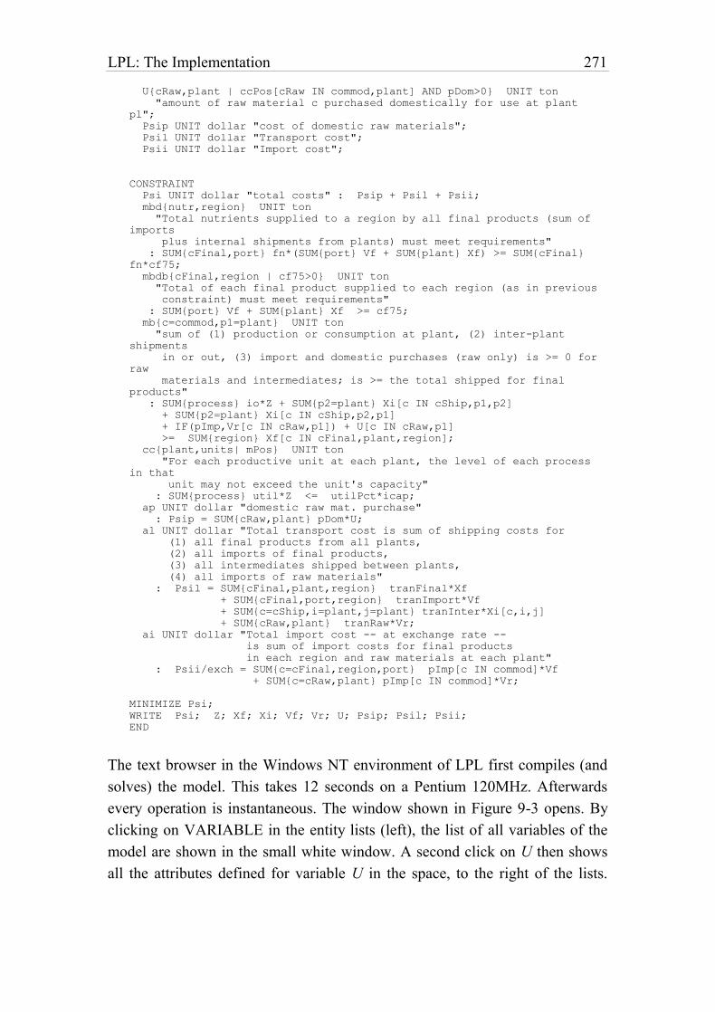
LPL: The Implementation 271
U{cRaw,plant | ccPos[cRaw IN commod,plant] AND pDom>0} UNIT ton
"amount of raw material c purchased domestically for use at plant
pl";
Psip UNIT dollar "cost of domestic raw materials";
Psil UNIT dollar "Transport cost";
Psii UNIT dollar "Import cost";
CONSTRAINT
Psi UNIT dollar "total costs" : Psip + Psil + Psii;
mbd{nutr,region} UNIT ton
"Total nutrients supplied to a region by all final products (sum of
imports
plus internal shipments from plants) must meet requirements"
: SUM{cFinal,port} fn*(SUM{port} Vf + SUM{plant} Xf) >= SUM{cFinal}
fn*cf75;
mbdb{cFinal,region | cf75>0} UNIT ton
"Total of each final product supplied to each region (as in previous
constraint) must meet requirements"
: SUM{port} Vf + SUM{plant} Xf >= cf75;
mb{c=commod,p1=plant} UNIT ton
"sum of (1) production or consumption at plant, (2) inter-plant
shipments
in or out, (3) import and domestic purchases (raw only) is >= 0 for
raw
materials and intermediates; is >= the total shipped for final
products"
: SUM{process} io*Z + SUM{p2=plant} Xi[c IN cShip,p1,p2]
+ SUM{p2=plant} Xi[c IN cShip,p2,p1]
+ IF(pImp,Vr[c IN cRaw,p1]) + U[c IN cRaw,p1]
>= SUM{region} Xf[c IN cFinal,plant,region];
cc{plant,units| mPos} UNIT ton
"For each productive unit at each plant, the level of each process
in that
unit may not exceed the unit's capacity"
: SUM{process} util*Z <= utilPct*icap;
ap UNIT dollar "domestic raw mat. purchase"
: Psip = SUM{cRaw,plant} pDom*U;
al UNIT dollar "Total transport cost is sum of shipping costs for
(1) all final products from all plants,
(2) all imports of final products,
(3) all intermediates shipped between plants,
(4) all imports of raw materials"
: Psil = SUM{cFinal,plant,region} tranFinal*Xf
+ SUM{cFinal,port,region} tranImport*Vf
+ SUM{c=cShip,i=plant,j=plant} tranInter*Xi[c,i,j]
+ SUM{cRaw,plant} tranRaw*Vr;
ai UNIT dollar "Total import cost -- at exchange rate --
is sum of import costs for final products
in each region and raw materials at each plant"
: Psii/exch = SUM{c=cFinal,region,port} pImp[c IN commod]*Vf
+ SUM{c=cRaw,plant} pImp[c IN commod]*Vr;
MINIMIZE Psi;
WRITE Psi; Z; Xf; Xi; Vf; Vr; U; Psip; Psil; Psii;
END
The text browser in the Windows NT environment of LPL first compiles (and
solves) the model. This takes 12 seconds on a Pentium 120MHz. Afterwards
every operation is instantaneous. The window shown in Figure 9-3 opens. By
clicking on VARIABLE in the entity lists (left), the list of all variables of the
model are shown in the small white window. A second click on U then shows
all the attributes defined for variable U in the space, to the right of the lists.

272 Chapter 9
Beneath the two lists, a spreadsheet-like matrix is opened and shows the values
of the two-indexed variable U. The representation is not limited to two-
dimensional entities, three- or higher-dimensional entities can be displayed.
Horizontal and vertical scrollbars automatically appear if the screen is too
small. Using the text browser, it is easy to look through all elements of the
model. Variables as well as parameters can be skimmed. For constraints, the
modeler can display the right hand side, the left hand side, their difference or
just whether the constraint is satisfied (1) or not (0).
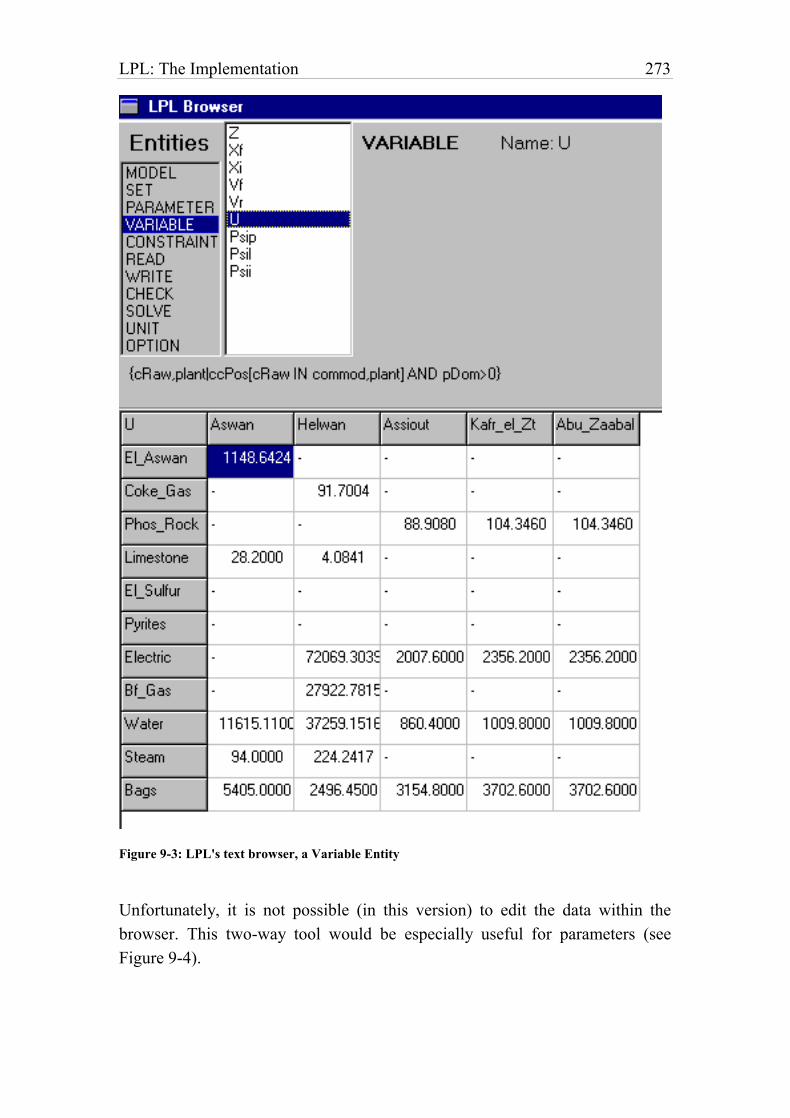
LPL: The Implementation 273
Figure 9-3: LPL's text browser, a Variable Entity
Unfortunately, it is not possible (in this version) to edit the data within the
browser. This two-way tool would be especially useful for parameters (see
Figure 9-4).
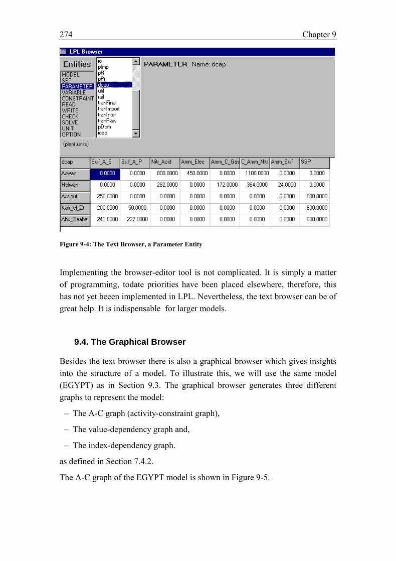
274 Chapter 9
Figure 9-4: The Text Browser, a Parameter Entity
Implementing the browser-editor tool is not complicated. It is simply a matter
of programming, todate priorities have been placed elsewhere, therefore, this
has not yet beeen implemented in LPL. Nevertheless, the text browser can be of
great help. It is indispensable for larger models.
9.4. The Graphical Browser
Besides the text browser there is also a graphical browser which gives insights
into the structure of a model. To illustrate this, we will use the same model
(EGYPT) as in Section 9.3. The graphical browser generates three different
graphs to represent the model:
– The A-C graph (activity-constraint graph),
– The value-dependency graph and,
– The index-dependency graph.
as defined in Section 7.4.2.
The A-C graph of the EGYPT model is shown in Figure 9-5.
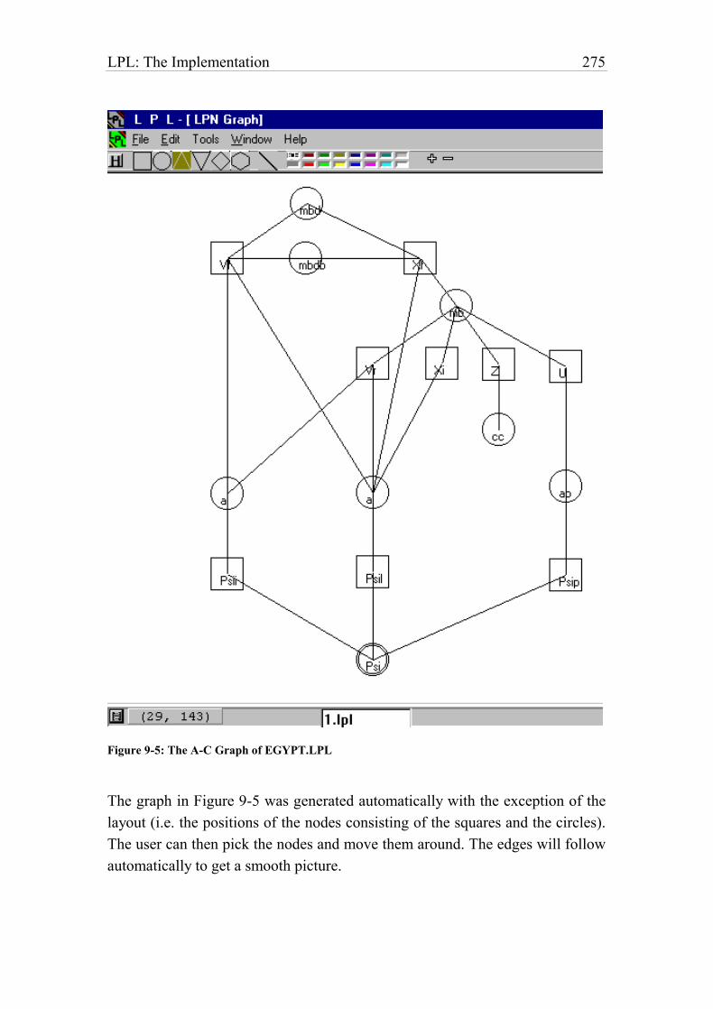
LPL: The Implementation 275
Figure 9-5: The A-C Graph of EGYPT.LPL
The graph in Figure 9-5 was generated automatically with the exception of the
layout (i.e. the positions of the nodes consisting of the squares and the circles).
The user can then pick the nodes and move them around. The edges will follow
automatically to get a smooth picture.
276 Chapter 9
The A-C graph is a bipartite graph where a square represents a variable entity
and a circle represents a constraint entity (a double circle represents the
optimizing function). If a variable occurs in a constraint then an edge links the
corresponding two nodes. The A-C graph often gives semantically useful
information about the model. In Figure 9-5, one can “see” how the model is
built. The bottom part contains the costs constraints. The overall cost Psi is split
into three components: Psii (import), Psil (transportation), and Psip (domestic
raw material purchase). The import costs are split between the imported raw
materials Vr and the imported final products Vf. The transportation costs are
divided into transportation of imported products (Vr and Vr), the transportation
of intermediary products between the plants (Xi), and the transportation of the
final (domestically produced) products (Xf). The domestic raw material costs
depend only upon their quantities (U). The reader should also note the change
in the units: while Psii, Psil, and Psip are all in dollar per tons, the other
variables Vf, Vr, Xi, Xf, and U are in tons. The constraints (ai, al, and ap) make
the corresponding unit transformation.
The whole of inland production is expressed by the constraint mb. The input to
this production are the domestic raw materials (U), the consumption of
different (final) products at a plant (Z), the intermediary products shipped from
other plants (Xi), and the imported raw materials (Vr). The output is the
quantity of final products (Xf). Different processes require a certain combustion
of final products, which is expressed by the constraint cc.
At the top of the graph, two demand constraints are imposed: mbdb expresses
the quantity of fertilizer (the final product) to be demanded, and mbd expresses
the quantity of their nutrient contents to be demanded. Of course, the total
quantity of imported (Vf) and domestically produced (Xf) fertilizer must meet
these requirements.
Is there a faster or easier way to explain the overall structure of the model? It
seems unlikely! However, not every model can be explained using an A-C
graph. Bat it is especially appealing if the model can be represented as a flow of
physical or virtual entities (not to be confused with network models). The Egypt
model can be represented in this way: The quantity of money (minimizing
costs) flows and split into different components measured in tons. They are
then combined into the quantities of final products. Finally, these quantities all
“flow” into the requested demand.
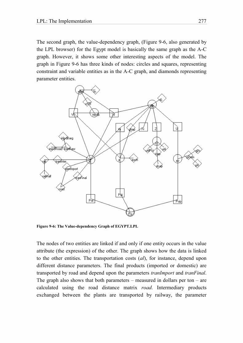
LPL: The Implementation 277
The second graph, the value-dependency graph, (Figure 9-6, also generated by
the LPL browser) for the Egypt model is basically the same graph as the A-C
graph. However, it shows some other interesting aspects of the model. The
graph in Figure 9-6 has three kinds of nodes: circles and squares, representing
constraint and variable entities as in the A-C graph, and diamonds representing
parameter entities.
Figure 9-6: The Value-dependency Graph of EGYPT.LPL
The nodes of two entities are linked if and only if one entity occurs in the value
attribute (the expression) of the other. The graph shows how the data is linked
to the other entities. The transportation costs (al), for instance, depend upon
different distance parameters. The final products (imported or domestic) are
transported by road and depend upon the parameters tranImport and tranFinal.
The graph also shows that both parameters – measured in dollars per ton – are
calculated using the road distance matrix road. Intermediary products
exchanged between the plants are transported by railway, the parameter
278 Chapter 9
tranInter giving the dollar per ton costs, which are calculated from the railway
distances rail. Finally, the raw materials are transported by barge or by road.
Their costs (tranRaw), are also measured in dollars per ton, and are calculated
from the distances impdBarg and impdRoad.
The value-dependency graph gives a first quick view of how the data enters the
model and it enables the modeler to verify their dependencies at a single glance.
The third graph, the index-dependency graph, is shown in (Figure 9-7). This
graph has five kinds of nodes: circles, squares and diamonds representing again
constraint, variable and parameter entities; and two types of triangles, the
pyramid and the inverse pyramid representing relations (indexed index-set) and
plain index-set (not indexed ones). Two nodes, where one must represent an
(indexed or not) index-set, are linked if the corresponding entity (an index-set)
occurs in the index list of the other entity. The graph can be used to show which
entities are indexed and over which index-sets. The graph in Figure 9-7, for
example, shows that the entity Z is indexed over two index-sets: plant and
process. It also shows that the entities exch, utilPct, Psip, etc. are not indexed.
Incidentally, the first entity (cInter) in the vertical list at the left indicates a
model error. It says that the index-set cInter is not used in any indexlist of the
other entities.75
The graph gives a hint about how a modification of index-set affects the model.
A change to the index-set center, for example, only influences the parameter
road, whereas a modification to plant requires one to update almost every data
table. The graph can also give some clues about its structure. Figure 9-7, for
example, shows how the submodel “demand of final products (the fertilizer)” is
grouped around the index-set region (the top-right hand part of the graph). The
submodel of “inland production”, on the other hand is clustered around the two
index-sets commod and process (bottom-right of the graph).
75 This “error” is due to the fact that cInter should be used to define cShip (which is a proper
subset of cInter), and commod (which is defined as the union of cFinal, cInter and cRaw). In the
LPL formulation above these relations are not explicitly enforced. The reason being that LPL
does not support set union of independent index-sets. One could do so by using compound
index-sets, but this would complicate the model formulation.
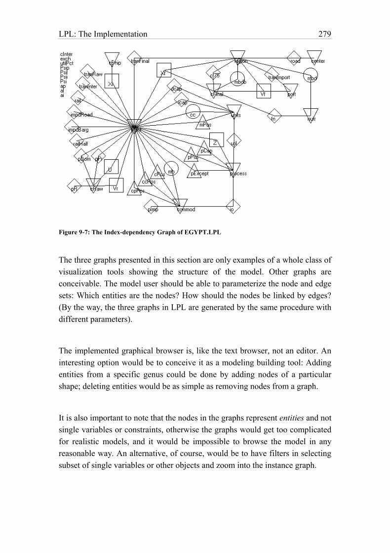
LPL: The Implementation 279
Figure 9-7: The Index-dependency Graph of EGYPT.LPL
The three graphs presented in this section are only examples of a whole class of
visualization tools showing the structure of the model. Other graphs are
conceivable. The model user should be able to parameterize the node and edge
sets: Which entities are the nodes? How should the nodes be linked by edges?
(By the way, the three graphs in LPL are generated by the same procedure with
different parameters).
The implemented graphical browser is, like the text browser, not an editor. An
interesting option would be to conceive it as a modeling building tool: Adding
entities from a specific genus could be done by adding nodes of a particular
shape; deleting entities would be as simple as removing nodes from a graph.
It is also important to note that the nodes in the graphs represent entities and not
single variables or constraints, otherwise the graphs would get too complicated
for realistic models, and it would be impossible to browse the model in any
reasonable way. An alternative, of course, would be to have filters in selecting
subset of single variables or other objects and zoom into the instance graph.

280 Chapter 9
281
10. SELECTED APPLICATIONS
In this Chapter several interesting models and their formulation in LPL are
presented. The examples have been chosen in order to give a “round-trip” of
LPL and to highlight several stimulating aspects not found in other languages,
especially in the field of modeling logical problems. Each problem is briefly
described in natural language followed by a formal statement of the model
structure. Comments are given on the model structure and the LPL code when
appropriate from the point of view of modeling language specification. All
problems can be found on the LPL-site (see Availability of the LPL System).
10.1. General LP-, MIP-, and QP-Models
Four models cover the most general aspects of the language. The first is an LP,
the second and third are IP models, and the last is a QP model (a quadratic
model, i.e. a linear model with a quadratic objective function).
Example 10-1: Determine Workforce Level
This model is a multiperiod production model from [Fourer al. 1990]. The
formulation was motivated by the experiences of a large producer in the United
States. There exists an AMPL formulation and the reader may compare both,
the LPL and the AMPL formulation. This model, with three products and 13
periods, consists of 235 variables, 190 constraints and 896 non-zero entries.
The problem is as follows:
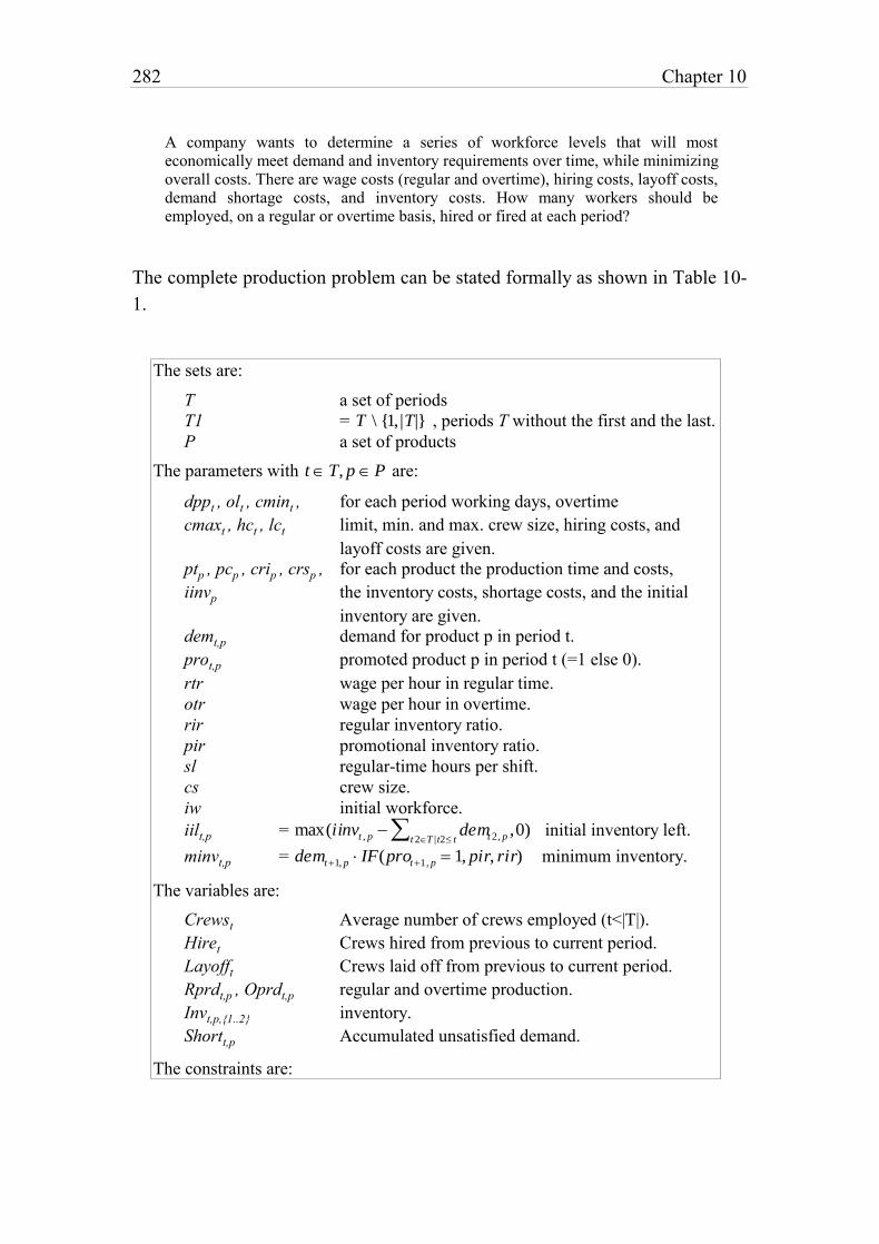
282 Chapter 10
A company wants to determine a series of workforce levels that will most economically meet demand and inventory requirements over time, while minimizing overall costs. There are wage costs (regular and overtime), hiring costs, layoff costs, demand shortage costs, and inventory costs. How many workers should be employed, on a regular or overtime basis, hired or fired at each period?
The complete production problem can be stated formally as shown in Table 10-
1.
The sets are:
T a set of periods
T1 = T \ {1,|T|} , periods T without the first and the last.
P a set of products
The parameters with t T, p P are:
dppt , olt , cmint , for each period working days, overtime
cmaxt , hct , lct limit, min. and max. crew size, hiring costs, and
layoff costs are given.
ptp , pcp , crip , crsp , for each product the production time and costs,
iinvp the inventory costs, shortage costs, and the initial
inventory are given.
demt,p demand for product p in period t.
prot,p promoted product p in period t (=1 else 0).
rtr wage per hour in regular time.
otr wage per hour in overtime.
rir regular inventory ratio.
pir promotional inventory ratio.
sl regular-time hours per shift.
cs crew size.
iw initial workforce.
iilt,p = max(iinvt , p demt 2, pt 2T |t2 t ,0) initial inventory left.
minvt,p = demt1, p IF(prot1, p 1, pir, rir) minimum inventory.
The variables are:
Crewst Average number of crews employed (t<|T|).
Hiret Crews hired from previous to current period.
Layofft Crews laid off from previous to current period.
Rprdt,p , Oprdt,p regular and overtime production.
Invt,p,{1..2} inventory.
Shortt,p Accumulated unsatisfied demand.
The constraints are:
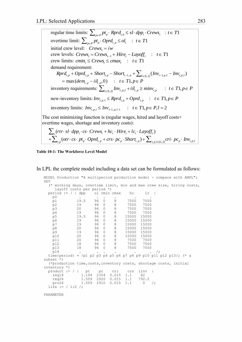
LPL: Selected Applications 283
regular time limits: ptp Rprdt, ppP sl dppt Crewst : tT1
overtime limit: ptp Oprdt , ppP olt : tT1
initial crew level: Crews1 iw
crew levels: Crewst Crewst1 Hiret Layofft : tT1
crew limits: cmint Crewst cmaxt : tT1
demand requirement:
Rprdt, p Oprd t, p Shortt, p Shortt1, p (Invt1, p,l Invt, p,l )l{1, 2}
max(demt , p iilt , p,0) : t T1, pP
inventory requirements: Invt , p,l iilt , pl{1,2} minvt, p : t T1, pP
new-inventory limits: Invt, p,1 Rprdt, p Oprd t, p : t T1, pP
inventory limits: Invt, p,l Inv t1, p, l1 : t T1, pP,l 2
The cost minimizing function is (regular wages, hired and layoff costs+
overtime wages, shortage and inventory costs):
(rtr sl dppt cs Crewst hct Hiret lct Layoff t )t
(otr cs ptp Oprdt , p crs pcp Shortt , p )t, p cri pcp Invt, p,lt, p,l{1, 2}
Table 10-1: The Workforce Level Model
In LPL the complete model including a data set can be formulated as follows:
MODEL Production "A multiperiod production model - compare with AMPL";
SET
(* working days, overtime limit, min and max crew size, hiring costs,
layoff costs per period *)
period := / | dpp ol cmin cmax hc lc |
p0 . . . . . .
p1 19.5 96 0 8 7500 7500
p2 19 96 0 8 7500 7500
p3 20 96 0 8 7500 7500
p4 19 96 0 8 7500 7500
p5 19.5 96 0 8 15000 15000
p6 19 96 0 8 15000 15000
p7 19 96 0 8 15000 15000
p8 20 96 0 8 15000 15000
p9 19 96 0 8 15000 15000
p10 20 96 0 8 15000 15000
p11 20 96 0 8 7500 7500
p12 18 96 0 8 7500 7500
p13 18 96 0 8 7500 7500
p14 . . . . . . /;
time{period} = /p1 p2 p3 p4 p5 p6 p7 p8 p9 p10 p11 p12 p13/; (* a
subset *)
(*production time,costs,inventory costs, shortage costs, initial
inventory *)
product := / | pt pc cri crs iinv |
reg18 1.194 2304 0.015 1.1 82
reg24 1.509 2920 0.015 1.1 792.2
pro24 1.509 2910 0.015 1.1 0 /;
life := / 1:2 /;
PARAMETER
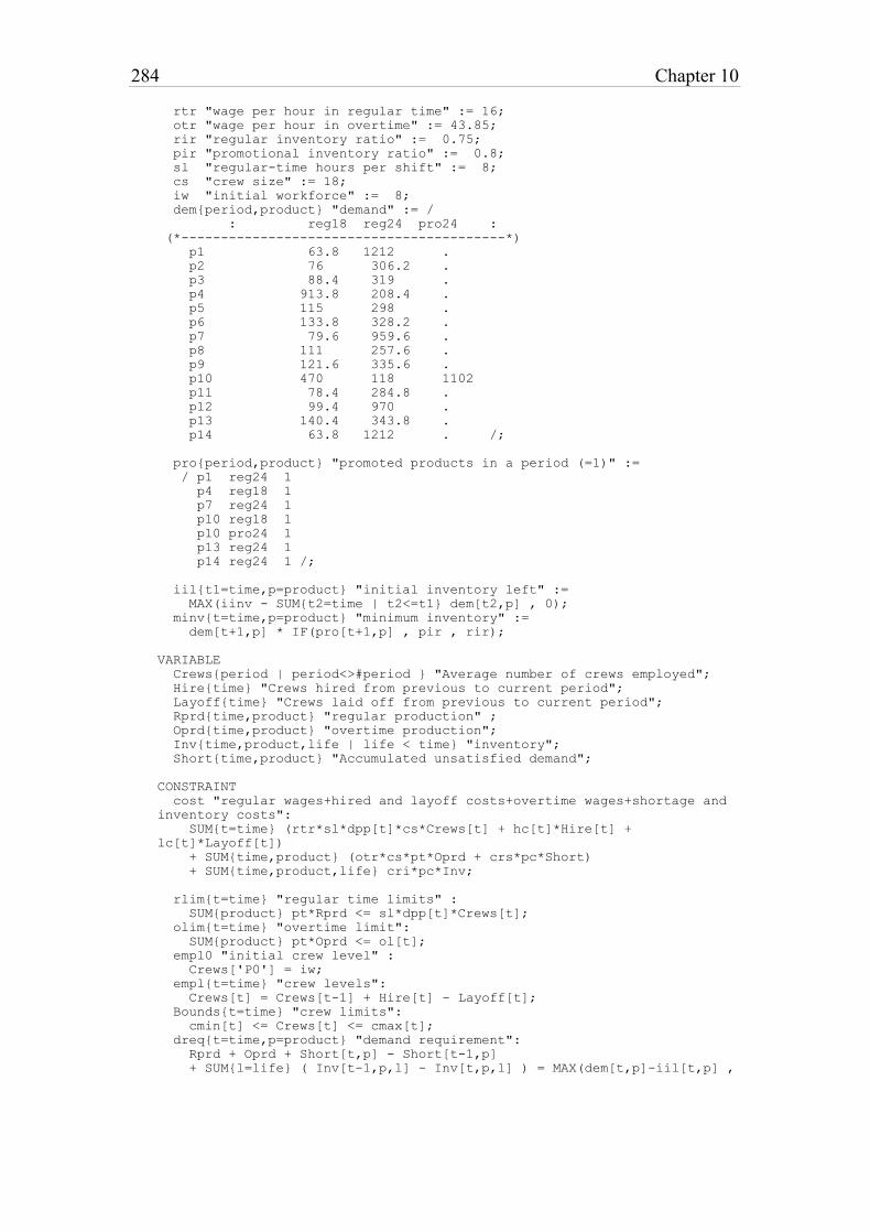
284 Chapter 10
rtr "wage per hour in regular time" := 16;
otr "wage per hour in overtime" := 43.85;
rir "regular inventory ratio" := 0.75;
pir "promotional inventory ratio" := 0.8;
sl "regular-time hours per shift" := 8;
cs "crew size" := 18;
iw "initial workforce" := 8;
dem{period,product} "demand" := /
: reg18 reg24 pro24 :
(*-----------------------------------------*)
p1 63.8 1212 .
p2 76 306.2 .
p3 88.4 319 .
p4 913.8 208.4 .
p5 115 298 .
p6 133.8 328.2 .
p7 79.6 959.6 .
p8 111 257.6 .
p9 121.6 335.6 .
p10 470 118 1102
p11 78.4 284.8 .
p12 99.4 970 .
p13 140.4 343.8 .
p14 63.8 1212 . /;
pro{period,product} "promoted products in a period (=1)" :=
/ p1 reg24 1
p4 reg18 1
p7 reg24 1
p10 reg18 1
p10 pro24 1
p13 reg24 1
p14 reg24 1 /;
iil{t1=time,p=product} "initial inventory left" :=
MAX(iinv - SUM{t2=time | t2<=t1} dem[t2,p] , 0);
minv{t=time,p=product} "minimum inventory" :=
dem[t+1,p] * IF(pro[t+1,p] , pir , rir);
VARIABLE
Crews{period | period<>#period } "Average number of crews employed";
Hire{time} "Crews hired from previous to current period";
Layoff{time} "Crews laid off from previous to current period";
Rprd{time,product} "regular production" ;
Oprd{time,product} "overtime production";
Inv{time,product,life | life < time} "inventory";
Short{time,product} "Accumulated unsatisfied demand";
CONSTRAINT
cost "regular wages+hired and layoff costs+overtime wages+shortage and
inventory costs":
SUM{t=time} (rtr*sl*dpp[t]*cs*Crews[t] + hc[t]*Hire[t] +
lc[t]*Layoff[t])
+ SUM{time,product} (otr*cs*pt*Oprd + crs*pc*Short)
+ SUM{time,product,life} cri*pc*Inv;
rlim{t=time} "regular time limits" :
SUM{product} pt*Rprd <= sl*dpp[t]*Crews[t];
olim{t=time} "overtime limit":
SUM{product} pt*Oprd <= ol[t];
empl0 "initial crew level" :
Crews['P0'] = iw;
empl{t=time} "crew levels":
Crews[t] = Crews[t-1] + Hire[t] - Layoff[t];
Bounds{t=time} "crew limits":
cmin[t] <= Crews[t] <= cmax[t];
dreq{t=time,p=product} "demand requirement":
Rprd + Oprd + Short[t,p] - Short[t-1,p]
+ SUM{l=life} ( Inv[t-1,p,l] - Inv[t,p,l] ) = MAX(dem[t,p]-iil[t,p] ,
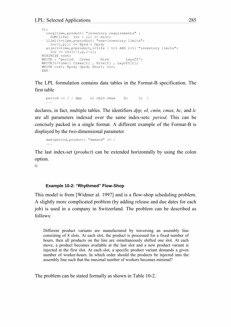
LPL: Selected Applications 285
0);
ireq{time,product} "inventory requirements" :
SUM{life} Inv + iil >= minv;
ilim1{t=time,p=product} "new-inventory limits":
Inv[t,p,1] <= Rprd + Oprd;
alim{t=time,p=product,l=life | t>1 AND l>1} "inventory limits":
Inv <= Inv[t-1,p,l-1];
MINIMIZE cost;
WRITE : 'period Crews Hire Layoff';
WRITE{t=time}: Crews[t] , Hire[t] , Layoff[t];
WRITE cost; Rprd; Oprd; Short; Inv;
END
The LPL formulation contains data tables in the Format-B specification. The
first table
period := / | dpp ol cmin cmax hc lc |
...
declares, in fact, multiple tables. The identifiers dpp, ol, cmin, cmax, hc, and lc
are all parameters indexed over the same index-sets: period. This can be
concisely packed in a single format. A different example of the Format-B is
displayed by the two-dimensional parameter
dem{period,product} "demand" := /
...
The last index-set (product) can be extended horizontally by using the colon
option.
¤
Example 10-2: “Rhythmed” Flow-Shop
This model is from [Widmer al. 1997] and is a flow-shop scheduling problem.
A slightly more complicated problem (by adding release and due dates for each
job) is used in a company in Switzerland. The problem can be described as
follows:
Different product variants are manufactured by traversing an assembly line consisting of 8 slots. At each slot, the product is processed for a fixed number of hours, then all products on the line are simultaneously shifted one slot. At each move, a product becomes available at the last slot and a new product variant is injected at the first slot. At each slot, a specific product variant demands a given number of worker-hours. In which order should the products be injected into the assembly line such that the maximal number of workers becomes minimal?
The problem can be stated formally as shown in Table 10-2.
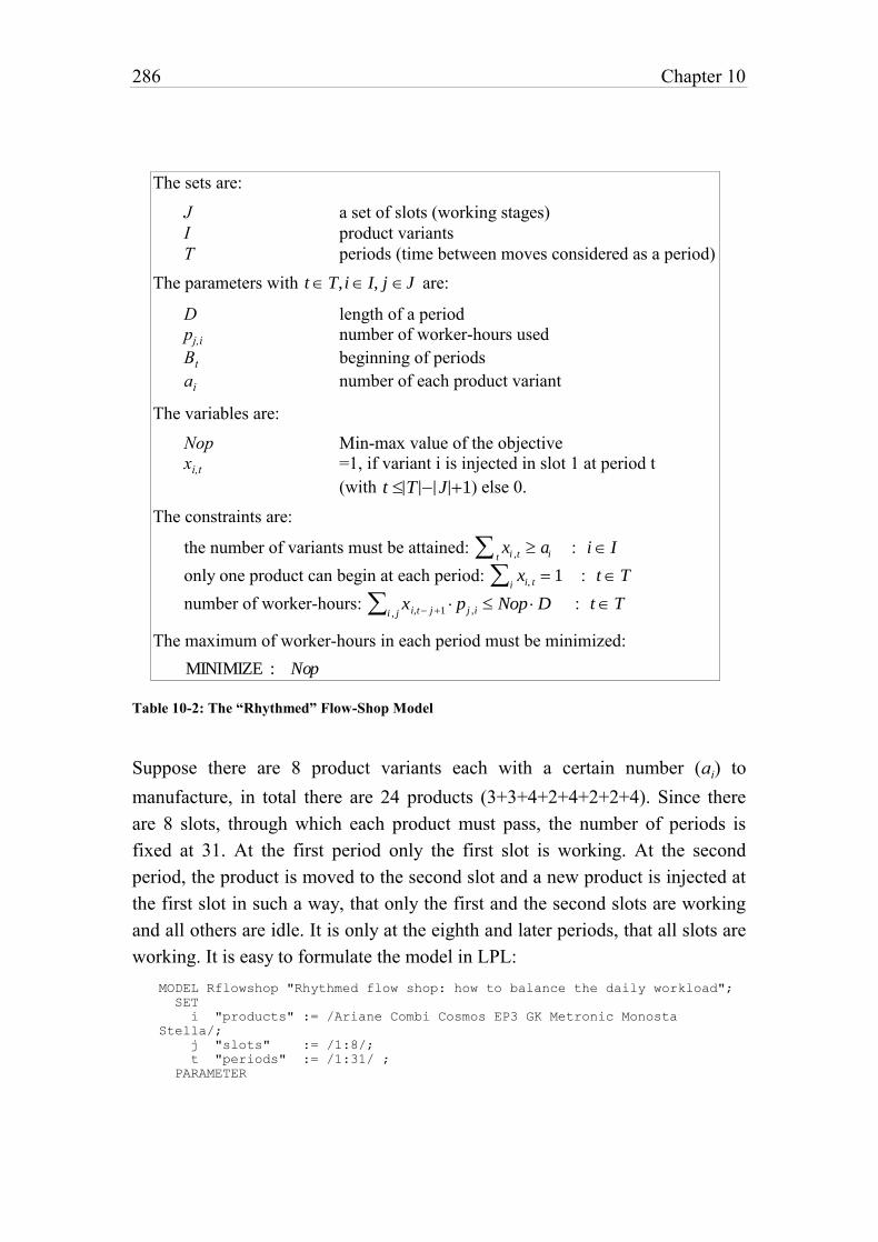
286 Chapter 10
The sets are:
J a set of slots (working stages)
I product variants
T periods (time between moves considered as a period)
The parameters with t T,i I, j J are:
D length of a period
pj,i number of worker-hours used
Bt beginning of periods
ai number of each product variant
The variables are:
Nop Min-max value of the objective
xi,t =1, if variant i is injected in slot 1 at period t
(with t |T ||J|1) else 0.
The constraints are:
the number of variants must be attained: xi ,tt ai : i I
only one product can begin at each period: xi, ti 1 : t T
number of worker-hours: xi,t j1 p j ,ii , j Nop D : t T
The maximum of worker-hours in each period must be minimized:
MINIMIZE : Nop
Table 10-2: The “Rhythmed” Flow-Shop Model
Suppose there are 8 product variants each with a certain number (ai) to
manufacture, in total there are 24 products (3+3+4+2+4+2+2+4). Since there
are 8 slots, through which each product must pass, the number of periods is
fixed at 31. At the first period only the first slot is working. At the second
period, the product is moved to the second slot and a new product is injected at
the first slot in such a way, that only the first and the second slots are working
and all others are idle. It is only at the eighth and later periods, that all slots are
working. It is easy to formulate the model in LPL:
MODEL Rflowshop "Rhythmed flow shop: how to balance the daily workload";
SET
i "products" := /Ariane Combi Cosmos EP3 GK Metronic Monosta
Stella/;
j "slots" := /1:8/;
t "periods" := /1:31/ ;
PARAMETER
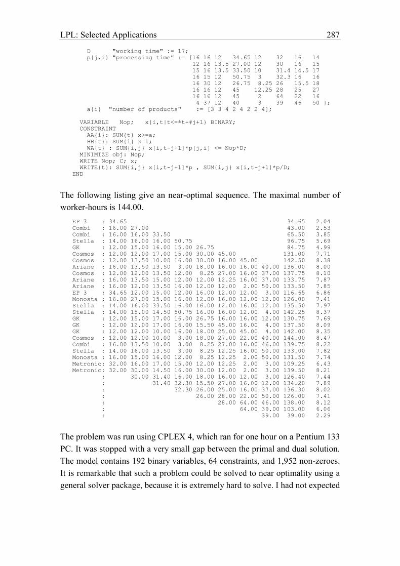
LPL: Selected Applications 287
D "working time" := 17;
p{j,i} "processing time" := [16 16 12 34.65 12 32 16 14
12 16 13.5 27.00 12 30 16 15
15 16 13.5 33.50 10 31.4 14.5 17
16 15 12 50.75 3 32.3 16 16
16 30 12 26.75 8.25 26 15.5 18
16 16 12 45 12.25 28 25 27
16 16 12 45 2 64 22 16
4 37 12 40 3 39 46 50 ];
a{i} "number of products" := [3 3 4 2 4 2 2 4];
VARIABLE Nop; x{i,t|t<=#t-#j+1} BINARY;
CONSTRAINT
AA{i}: SUM{t} x>=a;
BB{t}: SUM{i} x=1;
WA{t} : SUM{i,j} x[i,t-j+1]*p[j,i] <= Nop*D;
MINIMIZE obj: Nop;
WRITE Nop; C; x;
WRITE{t}: SUM{i,j} x[i,t-j+1]*p , SUM{i,j} x[i,t-j+1]*p/D;
END
The following listing give an near-optimal sequence. The maximal number of
worker-hours is 144.00.
EP 3 : 34.65 34.65 2.04
Combi : 16.00 27.00 43.00 2.53
Combi : 16.00 16.00 33.50 65.50 3.85
Stella : 14.00 16.00 16.00 50.75 96.75 5.69
GK : 12.00 15.00 16.00 15.00 26.75 84.75 4.99
Cosmos : 12.00 12.00 17.00 15.00 30.00 45.00 131.00 7.71
Cosmos : 12.00 13.50 10.00 16.00 30.00 16.00 45.00 142.50 8.38
Ariane : 16.00 13.50 13.50 3.00 18.00 16.00 16.00 40.00 136.00 8.00
Cosmos : 12.00 12.00 13.50 12.00 8.25 27.00 16.00 37.00 137.75 8.10
Ariane : 16.00 13.50 15.00 12.00 12.00 12.25 16.00 37.00 133.75 7.87
Ariane : 16.00 12.00 13.50 16.00 12.00 12.00 2.00 50.00 133.50 7.85
EP 3 : 34.65 12.00 15.00 12.00 16.00 12.00 12.00 3.00 116.65 6.86
Monosta : 16.00 27.00 15.00 16.00 12.00 16.00 12.00 12.00 126.00 7.41
Stella : 14.00 16.00 33.50 16.00 16.00 12.00 16.00 12.00 135.50 7.97
Stella : 14.00 15.00 14.50 50.75 16.00 16.00 12.00 4.00 142.25 8.37
GK : 12.00 15.00 17.00 16.00 26.75 16.00 16.00 12.00 130.75 7.69
GK : 12.00 12.00 17.00 16.00 15.50 45.00 16.00 4.00 137.50 8.09
GK : 12.00 12.00 10.00 16.00 18.00 25.00 45.00 4.00 142.00 8.35
Cosmos : 12.00 12.00 10.00 3.00 18.00 27.00 22.00 40.00 144.00 8.47
Combi : 16.00 13.50 10.00 3.00 8.25 27.00 16.00 46.00 139.75 8.22
Stella : 14.00 16.00 13.50 3.00 8.25 12.25 16.00 50.00 133.00 7.82
Monosta : 16.00 15.00 16.00 12.00 8.25 12.25 2.00 50.00 131.50 7.74
Metronic: 32.00 16.00 17.00 15.00 12.00 12.25 2.00 3.00 109.25 6.43
Metronic: 32.00 30.00 14.50 16.00 30.00 12.00 2.00 3.00 139.50 8.21
: 30.00 31.40 16.00 18.00 16.00 12.00 3.00 126.40 7.44
: 31.40 32.30 15.50 27.00 16.00 12.00 134.20 7.89
: 32.30 26.00 25.00 16.00 37.00 136.30 8.02
: 26.00 28.00 22.00 50.00 126.00 7.41
: 28.00 64.00 46.00 138.00 8.12
: 64.00 39.00 103.00 6.06
: 39.00 39.00 2.29
The problem was run using CPLEX 4, which ran for one hour on a Pentium 133
PC. It was stopped with a very small gap between the primal and dual solution.
The model contains 192 binary variables, 64 constraints, and 1,952 non-zeroes.
It is remarkable that such a problem could be solved to near optimality using a
general solver package, because it is extremely hard to solve. I had not expected
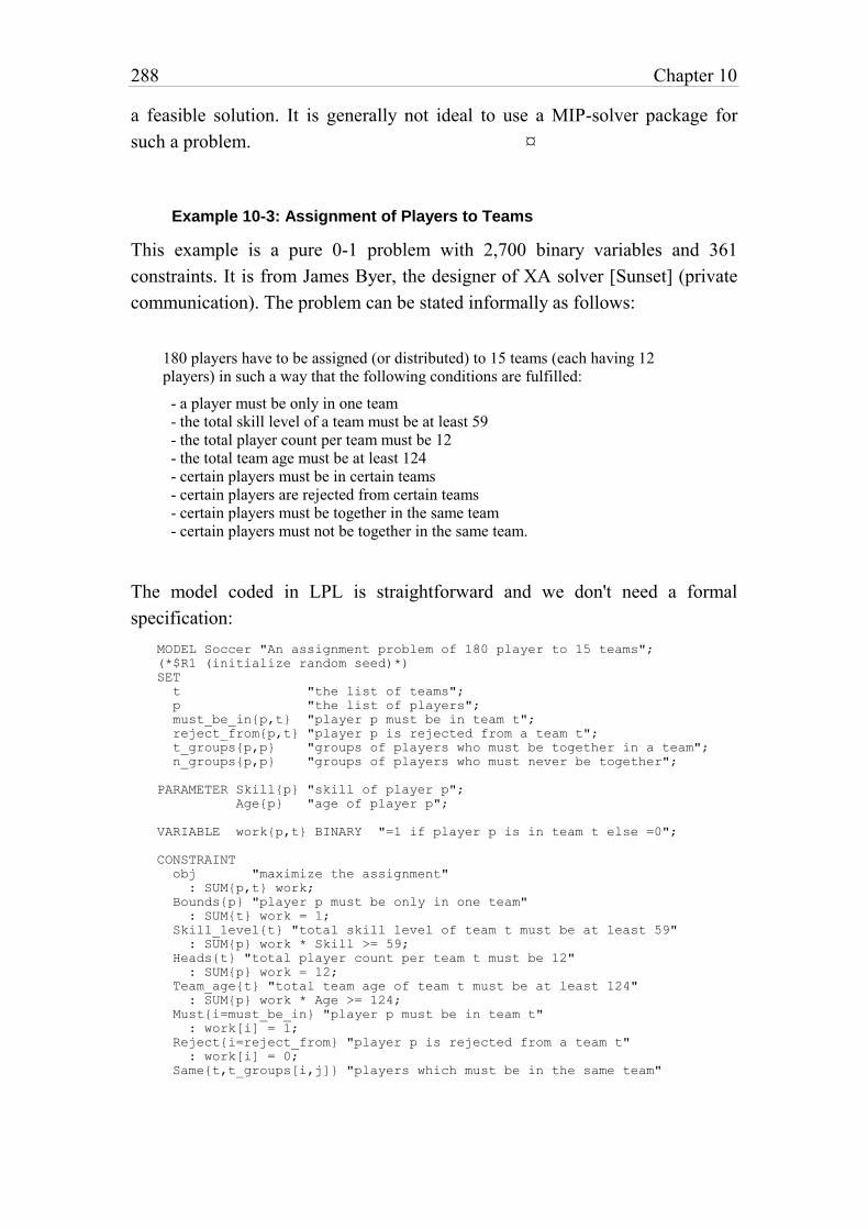
288 Chapter 10
a feasible solution. It is generally not ideal to use a MIP-solver package for
such a problem. ¤
Example 10-3: Assignment of Players to Teams
This example is a pure 0-1 problem with 2,700 binary variables and 361
constraints. It is from James Byer, the designer of XA solver [Sunset] (private
communication). The problem can be stated informally as follows:
180 players have to be assigned (or distributed) to 15 teams (each having 12 players) in such a way that the following conditions are fulfilled:
- a player must be only in one team - the total skill level of a team must be at least 59 - the total player count per team must be 12 - the total team age must be at least 124 - certain players must be in certain teams - certain players are rejected from certain teams - certain players must be together in the same team - certain players must not be together in the same team.
The model coded in LPL is straightforward and we don't need a formal
specification:
MODEL Soccer "An assignment problem of 180 player to 15 teams";
(*$R1 (initialize random seed)*)
SET
t "the list of teams";
p "the list of players";
must_be_in{p,t} "player p must be in team t";
reject_from{p,t} "player p is rejected from a team t";
t_groups{p,p} "groups of players who must be together in a team";
n_groups{p,p} "groups of players who must never be together";
PARAMETER Skill{p} "skill of player p";
Age{p} "age of player p";
VARIABLE work{p,t} BINARY "=1 if player p is in team t else =0";
CONSTRAINT
obj "maximize the assignment"
: SUM{p,t} work;
Bounds{p} "player p must be only in one team"
: SUM{t} work = 1;
Skill_level{t} "total skill level of team t must be at least 59"
: SUM{p} work * Skill >= 59;
Heads{t} "total player count per team t must be 12"
: SUM{p} work = 12;
Team_age{t} "total team age of team t must be at least 124"
: SUM{p} work * Age >= 124;
Must{i=must_be_in} "player p must be in team t"
: work[i] = 1;
Reject{i=reject_from} "player p is rejected from a team t"
: work[i] = 0;
Same{t,t_groups[i,j]} "players which must be in the same team"
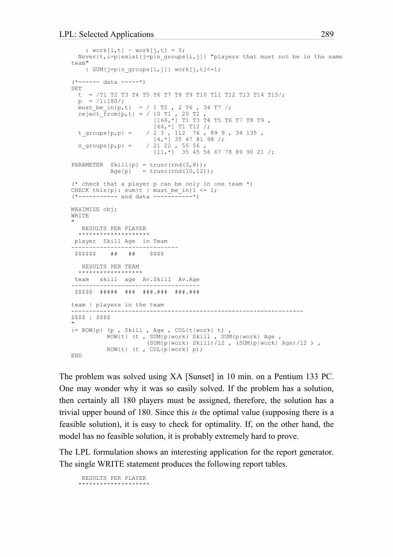
LPL: Selected Applications 289
: work[i,t] - work[j,t] = 0;
Never{t,i=p|exist{j=p}n_groups[i,j]} "players that must not be in the same
team"
: SUM{j=p|n_groups[i,j]} work[j,t]<=1;
(*------ data -----*)
SET
t = /T1 T2 T3 T4 T5 T6 T7 T8 T9 T10 T11 T12 T13 T14 T15/;
p = /1:180/;
must_be_in{p,t} = / 1 T2 , 2 T6 , 34 T7 /;
reject_from{p,t} = / 10 T1 , 20 T2 ,
[166,*] T1 T3 T4 T5 T6 T7 T8 T9 ,
[64,*] T1 T12 /;
t_groups{p,p} = / 2 3 , 112 76 , 89 9 , 34 135 ,
[4,*] 35 47 81 98 /;
n_groups{p,p} = / 21 22 , 55 56 ,
[11,*] 35 45 56 67 78 89 90 21 /;
PARAMETER Skill{p} = trunc(rnd(3,8));
Age{p} = trunc(rnd(10,12));
(* check that a player p can be only in one team *)
CHECK this{p}: sum{t | must_be_in}1 <= 1;
(*----------- end data -----------*)
MAXIMIZE obj;
WRITE
"
RESULTS PER PLAYER
********************
player Skill Age in Team
------------------------------
$$$$$$ ## ## $$$$
RESULTS PER TEAM
******************
team skill age Av.Skill Av.Age
------------------------------------
$$$$$ ##### ### ###.### ###.###
team | players in the team
-----------------------------------------------------------------
$$$$ | $$$$
"
:= ROW{p} (p , Skill , Age , COL{t|work} t) ,
ROW{t} (t , SUM{p|work} Skill , SUM{p|work} Age ,
(SUM{p|work} Skill)/12 , (SUM{p|work} Age)/12 ) ,
ROW{t} (t , COL{p|work} p);
END
The problem was solved using XA [Sunset] in 10 min. on a Pentium 133 PC.
One may wonder why it was so easily solved. If the problem has a solution,
then certainly all 180 players must be assigned, therefore, the solution has a
trivial upper bound of 180. Since this is the optimal value (supposing there is a
feasible solution), it is easy to check for optimality. If, on the other hand, the
model has no feasible solution, it is probably extremely hard to prove.
The LPL formulation shows an interesting application for the report generator.
The single WRITE statement produces the following report tables.
RESULTS PER PLAYER
********************
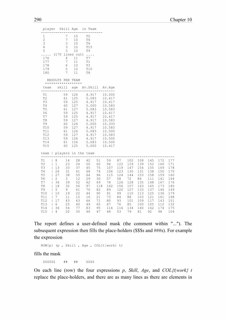
290 Chapter 10
player Skill Age in Team
------------------------------
1 7 10 T2
2 7 10 T6
3 3 10 T6
4 3 10 T15
5 3 10 T9
..... (170 lines cut) ....
176 4 11 T7
177 7 11 T1
178 6 10 T3
179 5 10 T10
180 7 11 T8
RESULTS PER TEAM
******************
team skill age Av.Skill Av.Age
------------------------------------
T1 59 126 4.917 10.500
T2 61 125 5.083 10.417
T3 59 125 4.917 10.417
T4 60 127 5.000 10.583
T5 61 127 5.083 10.583
T6 59 125 4.917 10.417
T7 59 125 4.917 10.417
T8 59 127 4.917 10.583
T9 60 124 5.000 10.333
T10 59 127 4.917 10.583
T11 61 126 5.083 10.500
T12 59 127 4.917 10.583
T13 59 126 4.917 10.500
T14 61 126 5.083 10.500
T15 60 125 5.000 10.417
team | players in the team
-----------------------------------------------------------------
T1 | 8 14 28 42 51 59 87 102 108 145 172 177
T2 | 1 23 24 50 60 94 122 129 139 152 166 171
T3 | 13 33 37 45 75 107 119 147 154 155 169 178
T4 | 26 31 41 68 74 106 123 130 131 138 150 170
T5 | 27 38 55 64 96 115 124 144 153 158 159 160
T6 | 2 3 12 29 30 57 58 72 86 111 141 164
T7 | 34 39 52 62 69 78 126 128 135 148 167 176
T8 | 18 32 56 97 118 142 156 157 163 165 173 180
T9 | 5 9 61 70 82 89 120 127 133 137 146 149
T10 | 10 19 22 44 90 91 99 110 113 125 136 179
T11 | 7 11 15 16 21 73 84 88 103 121 161 168
T12 | 17 43 63 66 71 80 93 101 109 117 143 151
T13 | 6 25 40 49 65 67 76 85 100 105 112 132
T14 | 36 54 77 83 95 114 116 134 140 162 174 175
T15 | 4 20 35 46 47 48 53 79 81 92 98 104
The report defines a user-defined mask (the comment within "..."). The
subsequent expression then fills the place-holders ($$$s and ###s). For example
the expression
ROW{p} (p , Skill , Age , COL{t|work} t)
fills the mask
$$$$$$ ## ## $$$$
On each line (row) the four expressions p, Skill, Age, and COL{t|work} t
replace the place-holders, and there are as many lines as there are elements in
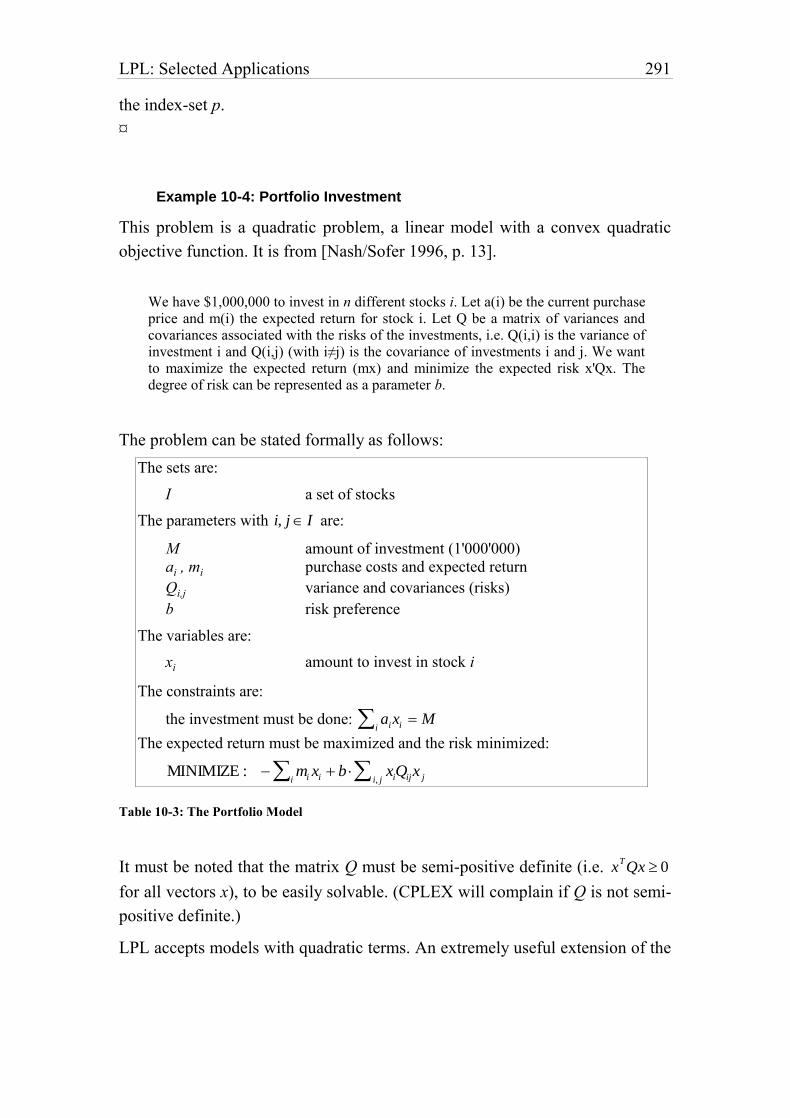
LPL: Selected Applications 291
the index-set p.
¤
Example 10-4: Portfolio Investment
This problem is a quadratic problem, a linear model with a convex quadratic
objective function. It is from [Nash/Sofer 1996, p. 13].
We have $1,000,000 to invest in n different stocks i. Let a(i) be the current purchase price and m(i) the expected return for stock i. Let Q be a matrix of variances and covariances associated with the risks of the investments, i.e. Q(i,i) is the variance of investment i and Q(i,j) (with i≠j) is the covariance of investments i and j. We want to maximize the expected return (mx) and minimize the expected risk x'Qx. The degree of risk can be represented as a parameter b.
The problem can be stated formally as follows:
The sets are:
I a set of stocks
The parameters with i, j I are:
M amount of investment (1'000'000)
ai , mi purchase costs and expected return
Qi,j variance and covariances (risks)
b risk preference
The variables are:
xi amount to invest in stock i
The constraints are:
the investment must be done: aixii M
The expected return must be maximized and the risk minimized:
MINIMIZE : mi xii b xiQijx ji, j
Table 10-3: The Portfolio Model
It must be noted that the matrix Q must be semi-positive definite (i.e. xTQx 0
for all vectors x), to be easily solvable. (CPLEX will complain if Q is not semi-
positive definite.)
LPL accepts models with quadratic terms. An extremely useful extension of the
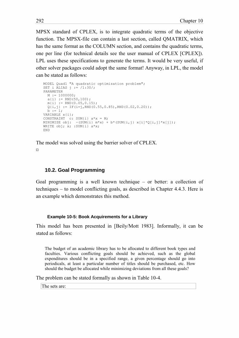
292 Chapter 10
MPSX standard of CPLEX, is to integrate quadratic terms of the objective
function. The MPSX-file can contain a last section, called QMATRIX, which
has the same format as the COLUMN section, and contains the quadratic terms,
one per line (for technical details see the user manual of CPLEX [CPLEX]).
LPL uses these specifications to generate the terms. It would be very useful, if
other solver packages could adopt the same format! Anyway, in LPL, the model
can be stated as follows:
MODEL Quad1 "A quadratic optimization problem";
SET i ALIAS j := /1:30/;
PARAMETER
M := 1000000;
a{i} := RND(50,100);
m{i} := RND(0.05,0.15);
Q{i,j} := IF(i=j,RND(0.55,0.85),RND(0.02,0.20));
b := 1;
VARIABLE x{i};
CONSTRAINT c: SUM{i} a*x = M;
MINIMIZE obj: -(SUM{i} m*x) + b*(SUM{i,j} x[i]*Q[i,j]*x[j]);
WRITE obj; x; :SUM{i} a*x;
END
The model was solved using the barrier solver of CPLEX.
¤
10.2. Goal Programming
Goal programming is a well known technique – or better: a collection of
techniques – to model conflicting goals, as described in Chapter 4.4.3. Here is
an example which demonstrates this method.
Example 10-5: Book Acquirements for a Library
This model has been presented in [Beily/Mott 1983]. Informally, it can be
stated as follows:
The budget of an academic library has to be allocated to different book types and faculties. Various conflicting goals should be achieved, such as the global expenditures should be in a specified range, a given percentage should go into periodicals, at least a particular number of titles should be purchased, etc. How should the budget be allocated while minimizing deviations from all these goals?
The problem can be stated formally as shown in Table 10-4.
The sets are:
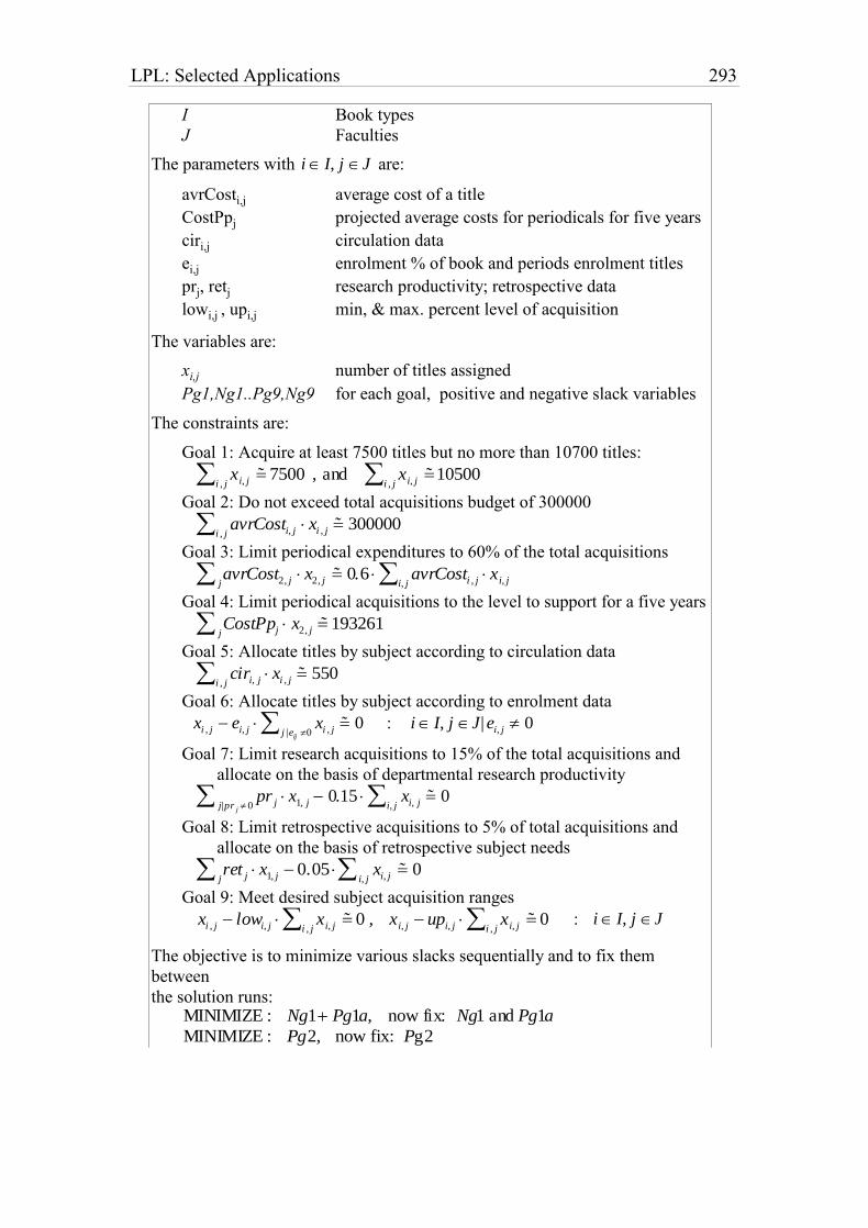
LPL: Selected Applications 293
I Book types
J Faculties
The parameters with i I, j J are:
avrCosti,j average cost of a title
CostPpj projected average costs for periodicals for five years
ciri,j circulation data
ei,j enrolment % of book and periods enrolment titles
prj, retj research productivity; retrospective data
lowi,j , upi,j min, & max. percent level of acquisition
The variables are:
xi,j number of titles assigned
Pg1,Ng1..Pg9,Ng9 for each goal, positive and negative slack variables
The constraints are:
Goal 1: Acquire at least 7500 titles but no more than 10700 titles:
xi, ji , j ˜ 7500 , and xi, ji , j ˜ 10500
Goal 2: Do not exceed total acquisitions budget of 300000
avrCosti, j xi , ji , j ˜ 300000
Goal 3: Limit periodical expenditures to 60% of the total acquisitions
avrCost2, j x2, jj ˜ 0.6 avrCosti , j xi, ji, j
Goal 4: Limit periodical acquisitions to the level to support for a five years
CostPpj x2, jj ˜ 193261
Goal 5: Allocate titles by subject according to circulation data
ciri, j xi , ji , j ˜ 550
Goal 6: Allocate titles by subject according to enrolment data
xi , j ei, j xi , jj |eij 0 ˜ 0 : i I, j J| ei, j 0
Goal 7: Limit research acquisitions to 15% of the total acquisitions and
allocate on the basis of departmental research productivity
pr j x1, jj|pr j 0 0.15 xi, ji, j ˜ 0
Goal 8: Limit retrospective acquisitions to 5% of total acquisitions and
allocate on the basis of retrospective subject needs
ret j x1, jj 0.05 xi, ji, j ˜ 0
Goal 9: Meet desired subject acquisition ranges
xi , j lowi, j xi, ji , j ˜ 0 , xi, j upi, j xi, ji , j ˜ 0 : i I, j J
The objective is to minimize various slacks sequentially and to fix them
between
the solution runs: MINIMIZE : Ng1 Pg1a, now fix: Ng1 and Pg1a
MINIMIZE : Pg2, now fix: Pg2
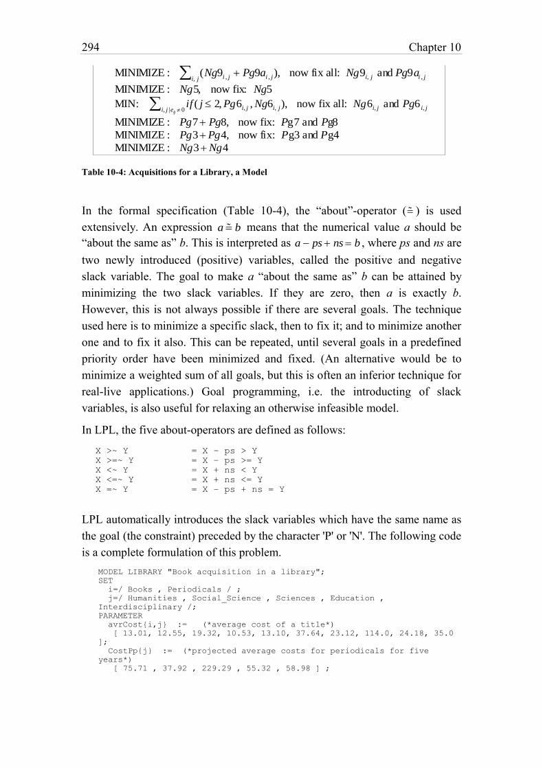
294 Chapter 10
MINIMIZE : (Ng9i , j Pg9ai , j)i, j , now fix all: Ng9i, j and Pg9ai , j
MINIMIZE : Ng5, now fix: Ng5
MIN: if ( j 2, Pg6i, j , Ng6i, j)i, j |eij 0 , now fix all: Ng6i, j and Pg6 i, j
MINIMIZE : Pg7 Pg8, now fix: Pg7 and Pg8
MINIMIZE : Pg3Pg4, now fix: Pg3 and Pg4
MINIMIZE : Ng3Ng4
Table 10-4: Acquisitions for a Library, a Model
In the formal specification (Table 10-4), the “about”-operator ( ˜ ) is used
extensively. An expression a ˜ b means that the numerical value a should be
“about the same as” b. This is interpreted as a ps ns b , where ps and ns are
two newly introduced (positive) variables, called the positive and negative
slack variable. The goal to make a “about the same as” b can be attained by
minimizing the two slack variables. If they are zero, then a is exactly b.
However, this is not always possible if there are several goals. The technique
used here is to minimize a specific slack, then to fix it; and to minimize another
one and to fix it also. This can be repeated, until several goals in a predefined
priority order have been minimized and fixed. (An alternative would be to
minimize a weighted sum of all goals, but this is often an inferior technique for
real-live applications.) Goal programming, i.e. the introducting of slack
variables, is also useful for relaxing an otherwise infeasible model.
In LPL, the five about-operators are defined as follows:
X >~ Y = X – ps > Y
X >=~ Y = X – ps >= Y
X <~ Y = X + ns < Y
X <=~ Y = X + ns <= Y
X =~ Y = X – ps + ns = Y
LPL automatically introduces the slack variables which have the same name as
the goal (the constraint) preceded by the character 'P' or 'N'. The following code
is a complete formulation of this problem.
MODEL LIBRARY "Book acquisition in a library";
SET
i=/ Books , Periodicals / ;
j=/ Humanities , Social_Science , Sciences , Education ,
Interdisciplinary /;
PARAMETER
avrCost{i,j} := (*average cost of a title*)
[ 13.01, 12.55, 19.32, 10.53, 13.10, 37.64, 23.12, 114.0, 24.18, 35.0
];
CostPp{j} := (*projected average costs for periodicals for five
years*)
[ 75.71 , 37.92 , 229.29 , 55.32 , 58.98 ] ;
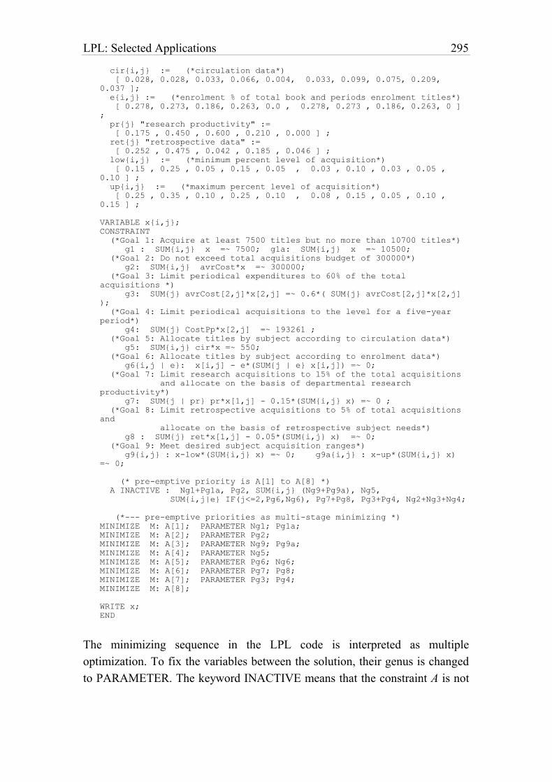
LPL: Selected Applications 295
cir{i,j} := (*circulation data*)
[ 0.028, 0.028, 0.033, 0.066, 0.004, 0.033, 0.099, 0.075, 0.209,
0.037 ];
e{i,j} := (*enrolment % of total book and periods enrolment titles*)
[ 0.278, 0.273, 0.186, 0.263, 0.0 , 0.278, 0.273 , 0.186, 0.263, 0 ]
;
pr{j} "research productivity" :=
[ 0.175 , 0.450 , 0.600 , 0.210 , 0.000 ] ;
ret{j} "retrospective data" :=
[ 0.252 , 0.475 , 0.042 , 0.185 , 0.046 ] ;
low{i,j} := (*minimum percent level of acquisition*)
[ 0.15 , 0.25 , 0.05 , 0.15 , 0.05 , 0.03 , 0.10 , 0.03 , 0.05 ,
0.10 ] ;
up{i,j} := (*maximum percent level of acquisition*)
[ 0.25 , 0.35 , 0.10 , 0.25 , 0.10 , 0.08 , 0.15 , 0.05 , 0.10 ,
0.15 ] ;
VARIABLE x{i,j};
CONSTRAINT
(*Goal 1: Acquire at least 7500 titles but no more than 10700 titles*)
g1 : SUM{i,j} x =~ 7500; g1a: SUM{i,j} x =~ 10500;
(*Goal 2: Do not exceed total acquisitions budget of 300000*)
g2: SUM{i,j} avrCost*x =~ 300000;
(*Goal 3: Limit periodical expenditures to 60% of the total
acquisitions *)
g3: SUM{j} avrCost[2,j]*x[2,j] =~ 0.6*( SUM{j} avrCost[2,j]*x[2,j]
);
(*Goal 4: Limit periodical acquisitions to the level for a five-year
period*)
g4: SUM{j} CostPp*x[2,j] =~ 193261 ;
(*Goal 5: Allocate titles by subject according to circulation data*)
g5: SUM{i,j} cir*x =~ 550;
(*Goal 6: Allocate titles by subject according to enrolment data*)
g6{i,j | e}: x[i,j] - e*(SUM{j | e} x[i,j]) =~ 0;
(*Goal 7: Limit research acquisitions to 15% of the total acquisitions
and allocate on the basis of departmental research
productivity*)
g7: SUM{j | pr} pr*x[1,j] - 0.15*(SUM{i,j} x) =~ 0 ;
(*Goal 8: Limit retrospective acquisitions to 5% of total acquisitions
and
allocate on the basis of retrospective subject needs*)
g8 : SUM{j} ret*x[1,j] - 0.05*(SUM{i,j} x) =~ 0;
(*Goal 9: Meet desired subject acquisition ranges*)
g9{i,j} : x-low*(SUM{i,j} x) =~ 0; g9a{i,j} : x-up*(SUM{i,j} x)
=~ 0;
(* pre-emptive priority is A[1] to A[8] *)
A INACTIVE : Ng1+Pg1a, Pg2, SUM{i,j} (Ng9+Pg9a), Ng5,
SUM{i,j|e} IF(j<=2,Pg6,Ng6), Pg7+Pg8, Pg3+Pg4, Ng2+Ng3+Ng4;
(*--- pre-emptive priorities as multi-stage minimizing *)
MINIMIZE M: A[1]; PARAMETER Ng1; Pg1a;
MINIMIZE M: A[2]; PARAMETER Pg2;
MINIMIZE M: A[3]; PARAMETER Ng9; Pg9a;
MINIMIZE M: A[4]; PARAMETER Ng5;
MINIMIZE M: A[5]; PARAMETER Pg6; Ng6;
MINIMIZE M: A[6]; PARAMETER Pg7; Pg8;
MINIMIZE M: A[7]; PARAMETER Pg3; Pg4;
MINIMIZE M: A[8];
WRITE x;
END
The minimizing sequence in the LPL code is interpreted as multiple
optimization. To fix the variables between the solution, their genus is changed
to PARAMETER. The keyword INACTIVE means that the constraint A is not
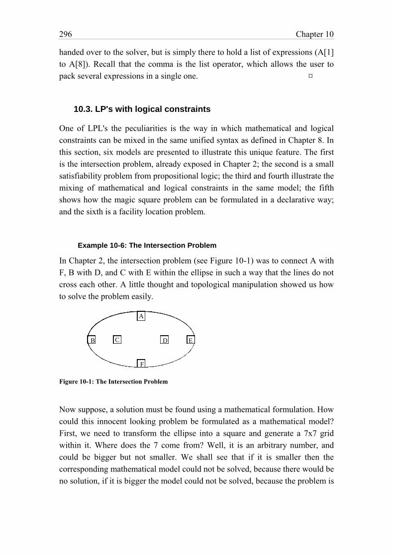
296 Chapter 10
handed over to the solver, but is simply there to hold a list of expressions (A[1]
to A[8]). Recall that the comma is the list operator, which allows the user to
pack several expressions in a single one. ¤
10.3. LP's with logical constraints
One of LPL's the peculiarities is the way in which mathematical and logical
constraints can be mixed in the same unified syntax as defined in Chapter 8. In
this section, six models are presented to illustrate this unique feature. The first
is the intersection problem, already exposed in Chapter 2; the second is a small
satisfiability problem from propositional logic; the third and fourth illustrate the
mixing of mathematical and logical constraints in the same model; the fifth
shows how the magic square problem can be formulated in a declarative way;
and the sixth is a facility location problem.
Example 10-6: The Intersection Problem
In Chapter 2, the intersection problem (see Figure 10-1) was to connect A with
F, B with D, and C with E within the ellipse in such a way that the lines do not
cross each other. A little thought and topological manipulation showed us how
to solve the problem easily.
A
F
D ECB
Figure 10-1: The Intersection Problem
Now suppose, a solution must be found using a mathematical formulation. How
could this innocent looking problem be formulated as a mathematical model?
First, we need to transform the ellipse into a square and generate a 7x7 grid
within it. Where does the 7 come from? Well, it is an arbitrary number, and
could be bigger but not smaller. We shall see that if it is smaller then the
corresponding mathematical model could not be solved, because there would be
no solution, if it is bigger the model could not be solved, because the problem is
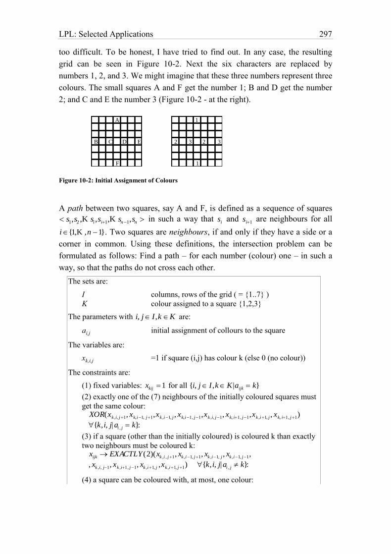
LPL: Selected Applications 297
too difficult. To be honest, I have tried to find out. In any case, the resulting
grid can be seen in Figure 10-2. Next the six characters are replaced by
numbers 1, 2, and 3. We might imagine that these three numbers represent three
colours. The small squares A and F get the number 1; B and D get the number
2; and C and E the number 3 (Figure 10-2 - at the right).
A
F
B DC E
1
1
2 23 3
Figure 10-2: Initial Assignment of Colours
A path between two squares, say A and F, is defined as a sequence of squares
s1,s2 ,K si,si1,K sn1,sn in such a way that si and si1 are neighbours for all
i {1,K ,n 1}. Two squares are neighbours, if and only if they have a side or a
corner in common. Using these definitions, the intersection problem can be
formulated as follows: Find a path – for each number (colour) one – in such a
way, so that the paths do not cross each other.
The sets are:
I columns, rows of the grid ( = {1..7} )
K colour assigned to a square {1,2,3}
The parameters with i, j I,k K are:
ai,j initial assignment of collours to the square
The variables are:
xk,i,j =1 if square (i,j) has colour k (else 0 (no colour))
The constraints are:
(1) fixed variables: xkij 1 for all {i, j I ,k K |aijk k}
(2) exactly one of the (7) neighbours of the initially coloured squares must
get the same colour: XOR(xk ,i, j1, xk,i1, j1,xk ,i1, j , xk,i1, j1,xk ,i, j1, xk, i1, j1,xk ,i1, j , xk, i1, j1)
{k,i, j| ai , j k}:
(3) if a square (other than the initially coloured) is coloured k than exactly
two neighbours must be coloured k: xijk EXACTLY (2)(xk ,i , j1, xk ,i1, j1, xk ,i1, j , xk ,i1, j1,
, xk ,i, j1, xk ,i1, j1, xk ,i1, j ,xk ,i1, j1) {k,i, j| ai , j k}:
(4) a square can be coloured with, at most, one colour:
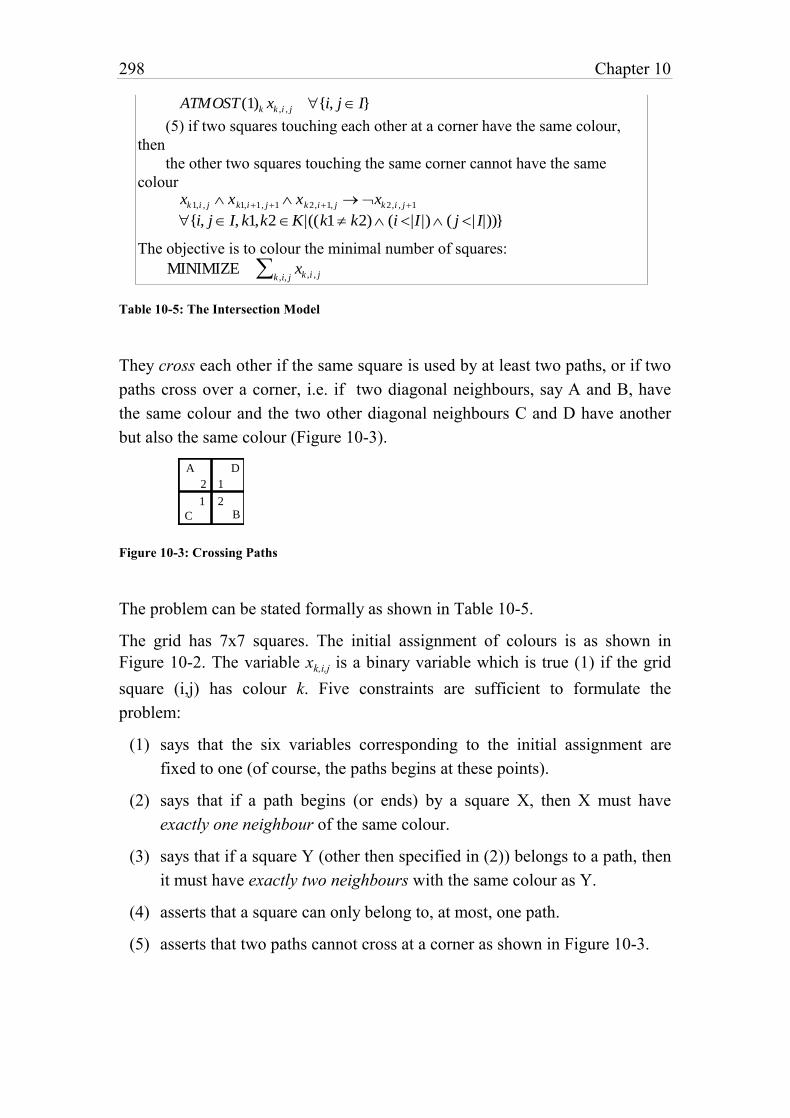
298 Chapter 10
ATMOST (1)k xk ,i , j {i, j I}
(5) if two squares touching each other at a corner have the same colour,
then
the other two squares touching the same corner cannot have the same
colour xk1,i , j xk1,i1, j1 xk2,i1, j xk2,i , j1
{i, j I, k1,k2 K|((k1 k2) (i |I |) ( j | I|))}
The objective is to colour the minimal number of squares:
MINIMIZE xk ,i , jk ,i, j
Table 10-5: The Intersection Model
They cross each other if the same square is used by at least two paths, or if two
paths cross over a corner, i.e. if two diagonal neighbours, say A and B, have
the same colour and the two other diagonal neighbours C and D have another
but also the same colour (Figure 10-3).
A
BC
D
1
12
2
Figure 10-3: Crossing Paths
The problem can be stated formally as shown in Table 10-5.
The grid has 7x7 squares. The initial assignment of colours is as shown in
Figure 10-2. The variable xk,i,j is a binary variable which is true (1) if the grid
square (i,j) has colour k. Five constraints are sufficient to formulate the
problem:
(1) says that the six variables corresponding to the initial assignment are
fixed to one (of course, the paths begins at these points).
(2) says that if a path begins (or ends) by a square X, then X must have
exactly one neighbour of the same colour.
(3) says that if a square Y (other then specified in (2)) belongs to a path, then
it must have exactly two neighbours with the same colour as Y.
(4) asserts that a square can only belong to, at most, one path.
(5) asserts that two paths cannot cross at a corner as shown in Figure 10-3.
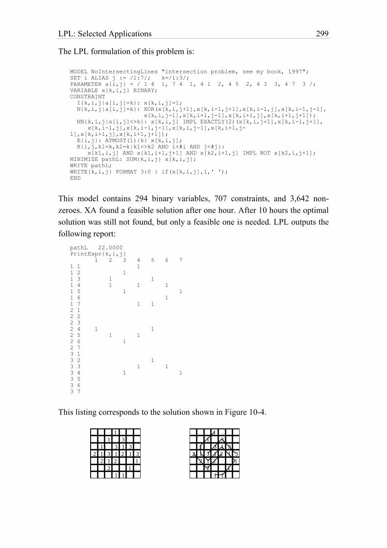
LPL: Selected Applications 299
The LPL formulation of this problem is:
MODEL NoIntersectingLines "intersection problem, see my book, 1997";
SET i ALIAS j := /1:7/; k=/1:3/;
PARAMETER a{i,j} = / 1 4 1, 7 4 1, 4 1 2, 4 5 2, 4 3 3, 4 7 3 /;
VARIABLE x{k,i,j} BINARY;
CONSTRAINT
I{k,i,j|a[i,j]=k}: x[k,i,j]=1;
N{k,i,j|a[i,j]=k}: XOR(x[k,i,j+1],x[k,i-1,j+1],x[k,i-1,j],x[k,i-1,j-1],
x[k,i,j-1],x[k,i+1,j-1],x[k,i+1,j],x[k,i+1,j+1]);
NN{k,i,j|a[i,j]<>k}: x[k,i,j] IMPL EXACTLY(2)(x[k,i,j+1],x[k,i-1,j+1],
x[k,i-1,j],x[k,i-1,j-1],x[k,i,j-1],x[k,i+1,j-
1],x[k,i+1,j],x[k,i+1,j+1]);
E{i,j}: ATMOST(1){k} x[k,i,j];
K{i,j,k1=k,k2=k|k1<>k2 AND i<#i AND j<#j}:
x[k1,i,j] AND x[k1,i+1,j+1] AND x[k2,i+1,j] IMPL NOT x[k2,i,j+1];
MINIMIZE pathL: SUM{k,i,j} x[k,i,j];
WRITE pathL;
WRITE{k,i,j} FORMAT 3:0 : if(x[k,i,j],1,' ');
END
This model contains 294 binary variables, 707 constraints, and 3,642 non-
zeroes. XA found a feasible solution after one hour. After 10 hours the optimal
solution was still not found, but only a feasible one is needed. LPL outputs the
following report:
pathL 22.0000
PrintExpr{k,i,j}
1 2 3 4 5 6 7
1 1 1
1 2 1
1 3 1 1
1 4 1 1 1
1 5 1 1
1 6 1
1 7 1 1
2 1
2 2
2 3
2 4 1 1
2 5 1 1
2 6 1
2 7
3 1
3 2 1
3 3 1 1
3 4 1 1
3 5
3 6
3 7
This listing corresponds to the solution shown in Figure 10-4.
1
1
2 23 3
2
2
2
3
3
3
1
1
1
1
1
1
1
1
1
1
1
1
2 23 3
2
2
2
3
3
3
1
1
1
1
1
1
1
1
1
1
300 Chapter 10
Figure 10-4: A Solution to the Intersection Problem
It is certainly not my claim here to replace mathematical thinking, which can
solve the problem in five, maybe ten minutes using some elegant theorems from
topology, by a mathematical model – which took longer than one hour simply to
formulate it, not to mention the frustrations involved in coding all of the
constraints correctly. Beware! I can only say in this context: Use your brains
before you hack the problem into the computer – the brain is a much smarter
computer than your desktop version. These remarks aside, the model is
interesting in several respects.
1 It was challenging to formulate it: If the modeling language is given, then
one can quickly decide whether and how it can be formulated. However,
if language has to be found to formulate it, then one has to switch
between language design and modeling all the time. This was the case
when I tried to formulate it. It was stimulating for the language design!
2 The mathematical model can be easily generalized to a whole class of
“discrete path” problems. (finding crossing, no-crossing, touching etc.
paths or trees between points). Whether such problems could be solved
afterwards is another question.76
3 Solving this problem is a challenging task for any solver. It came as a
surprise to me, that the model could be solved using general MIP-
techniques.
¤
Example 10-7: A Satisfiability Problem (SAT)
76 Generalizing sometimes means sacrificing complexity. The most pointless model in this respect
(from the economical point of view!) would be to formulate the decision problem whether a
graph is planar using these techniques. The planar graph problem is polynomial and can be
solved even in linear time, i.e. it is proportional to the size of the graph! The problem of how to
model in the best way, is the business of the modeler not the modeling language. In the same
way, a programmer could use a programming language to sort an array in exponential time by
trying all permutions instead of using quicksort or any other well known method. The point here
is, that we should not blame the language, if a problem cannot be solved, but the modeler.
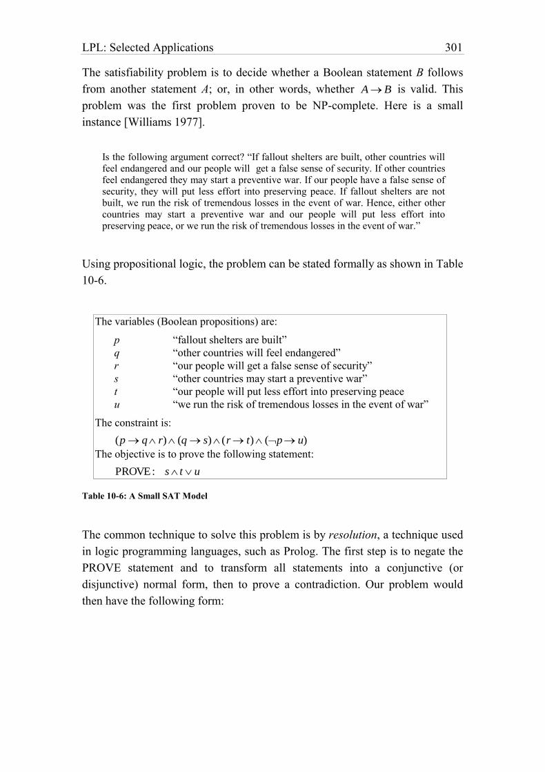
LPL: Selected Applications 301
The satisfiability problem is to decide whether a Boolean statement B follows
from another statement A; or, in other words, whether AB is valid. This
problem was the first problem proven to be NP-complete. Here is a small
instance [Williams 1977].
Is the following argument correct? “If fallout shelters are built, other countries will feel endangered and our people will get a false sense of security. If other countries feel endangered they may start a preventive war. If our people have a false sense of security, they will put less effort into preserving peace. If fallout shelters are not built, we run the risk of tremendous losses in the event of war. Hence, either other countries may start a preventive war and our people will put less effort into preserving peace, or we run the risk of tremendous losses in the event of war.”
Using propositional logic, the problem can be stated formally as shown in Table
10-6.
The variables (Boolean propositions) are:
p “fallout shelters are built”
q “other countries will feel endangered”
r “our people will get a false sense of security”
s “other countries may start a preventive war”
t “our people will put less effort into preserving peace
u “we run the risk of tremendous losses in the event of war”
The constraint is:
(p q r) (q s) (r t) (p u)
The objective is to prove the following statement:
PROVE: s t u
Table 10-6: A Small SAT Model
The common technique to solve this problem is by resolution, a technique used
in logic programming languages, such as Prolog. The first step is to negate the
PROVE statement and to transform all statements into a conjunctive (or
disjunctive) normal form, then to prove a contradiction. Our problem would
then have the following form:
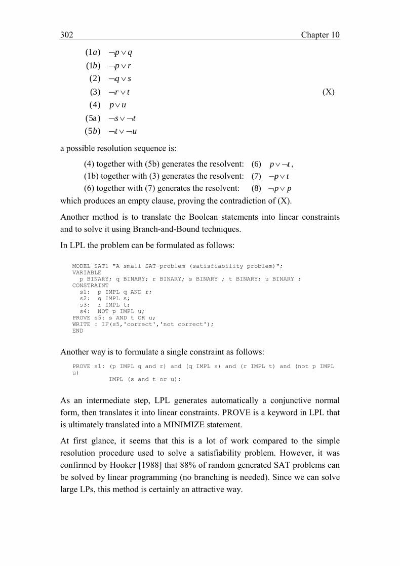
302 Chapter 10
(1a) p q
(1b) p r
(2) q s
(3) r t
(4) p u
(5a) s t
(5b) t u
(X)
a possible resolution sequence is:
(4) together with (5b) generates the resolvent: (6) p t ,
(1b) together with (3) generates the resolvent: (7) p t
(6) together with (7) generates the resolvent: (8) p p
which produces an empty clause, proving the contradiction of (X).
Another method is to translate the Boolean statements into linear constraints
and to solve it using Branch-and-Bound techniques.
In LPL the problem can be formulated as follows:
MODEL SAT1 "A small SAT-problem (satisfiability problem)";
VARIABLE
p BINARY; q BINARY; r BINARY; s BINARY ; t BINARY; u BINARY ;
CONSTRAINT
s1: p IMPL q AND r;
s2: q IMPL s;
s3: r IMPL t;
s4: NOT p IMPL u;
PROVE s5: s AND t OR u;
WRITE : IF(s5,'correct','not correct');
END
Another way is to formulate a single constraint as follows:
PROVE s1: (p IMPL q and r) and (q IMPL s) and (r IMPL t) and (not p IMPL
u)
IMPL (s and t or u);
As an intermediate step, LPL generates automatically a conjunctive normal
form, then translates it into linear constraints. PROVE is a keyword in LPL that
is ultimately translated into a MINIMIZE statement.
At first glance, it seems that this is a lot of work compared to the simple
resolution procedure used to solve a satisfiability problem. However, it was
confirmed by Hooker [1988] that 88% of random generated SAT problems can
be solved by linear programming (no branching is needed). Since we can solve
large LPs, this method is certainly an attractive way.
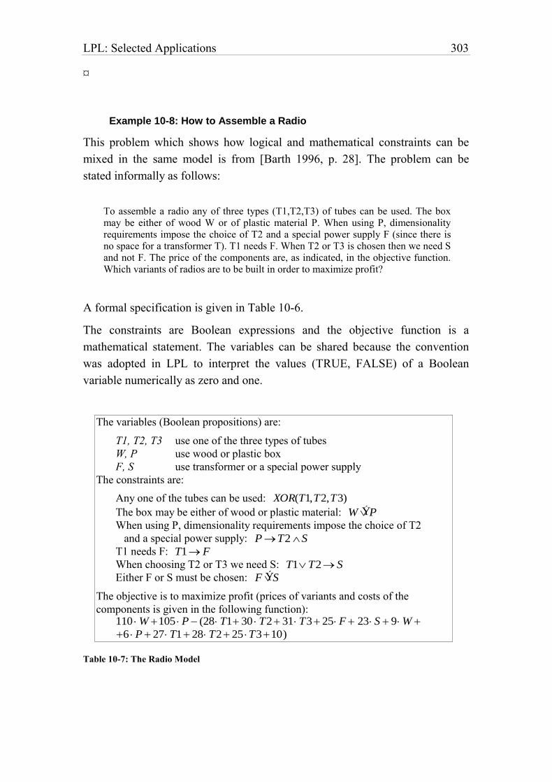
LPL: Selected Applications 303
¤
Example 10-8: How to Assemble a Radio
This problem which shows how logical and mathematical constraints can be
mixed in the same model is from [Barth 1996, p. 28]. The problem can be
stated informally as follows:
To assemble a radio any of three types (T1,T2,T3) of tubes can be used. The box may be either of wood W or of plastic material P. When using P, dimensionality requirements impose the choice of T2 and a special power supply F (since there is no space for a transformer T). T1 needs F. When T2 or T3 is chosen then we need S and not F. The price of the components are, as indicated, in the objective function. Which variants of radios are to be built in order to maximize profit?
A formal specification is given in Table 10-6.
The constraints are Boolean expressions and the objective function is a
mathematical statement. The variables can be shared because the convention
was adopted in LPL to interpret the values (TRUE, FALSE) of a Boolean
variable numerically as zero and one.
The variables (Boolean propositions) are:
T1, T2, T3 use one of the three types of tubes
W, P use wood or plastic box
F, S use transformer or a special power supply
The constraints are:
Any one of the tubes can be used: XOR(T1,T2,T3)
The box may be either of wood or plastic material: W Ý P
When using P, dimensionality requirements impose the choice of T2
and a special power supply: PT2 S
T1 needs F: T1 F
When choosing T2 or T3 we need S: T1 T2 S
Either F or S must be chosen: F Ý S
The objective is to maximize profit (prices of variants and costs of the
components is given in the following function): 110 W 105 P (28T1 30 T2 31T3 25F 23 S 9W
6 P 27T1 28T2 25 T310)
Table 10-7: The Radio Model
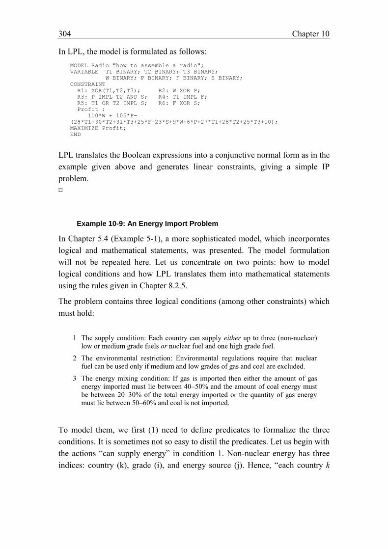
304 Chapter 10
In LPL, the model is formulated as follows:
MODEL Radio "how to assemble a radio";
VARIABLE T1 BINARY; T2 BINARY; T3 BINARY;
W BINARY; P BINARY; F BINARY; S BINARY;
CONSTRAINT
R1: XOR(T1,T2,T3); R2: W XOR P;
R3: P IMPL T2 AND S; R4: T1 IMPL F;
R5: T1 OR T2 IMPL S; R6: F XOR S;
Profit :
110*W + 105*P-
(28*T1+30*T2+31*T3+25*F+23*S+9*W+6*P+27*T1+28*T2+25*T3+10);
MAXIMIZE Profit;
END
LPL translates the Boolean expressions into a conjunctive normal form as in the
example given above and generates linear constraints, giving a simple IP
problem.
¤
Example 10-9: An Energy Import Problem
In Chapter 5.4 (Example 5-1), a more sophisticated model, which incorporates
logical and mathematical statements, was presented. The model formulation
will not be repeated here. Let us concentrate on two points: how to model
logical conditions and how LPL translates them into mathematical statements
using the rules given in Chapter 8.2.5.
The problem contains three logical conditions (among other constraints) which
must hold:
1 The supply condition: Each country can supply either up to three (non-nuclear) low or medium grade fuels or nuclear fuel and one high grade fuel.
2 The environmental restriction: Environmental regulations require that nuclear fuel can be used only if medium and low grades of gas and coal are excluded.
3 The energy mixing condition: If gas is imported then either the amount of gas energy imported must lie between 40–50% and the amount of coal energy must be between 20–30% of the total energy imported or the quantity of gas energy must lie between 50–60% and coal is not imported.
To model them, we first (1) need to define predicates to formalize the three
conditions. It is sometimes not so easy to distil the predicates. Let us begin with
the actions “can supply energy” in condition 1. Non-nuclear energy has three
indices: country (k), grade (i), and energy source (j). Hence, “each country k
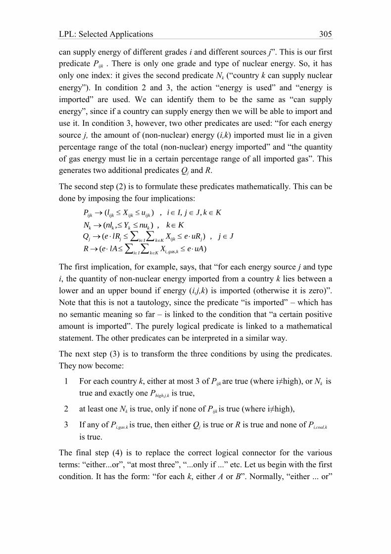
LPL: Selected Applications 305
can supply energy of different grades i and different sources j”. This is our first
predicate Pijk . There is only one grade and type of nuclear energy. So, it has
only one index: it gives the second predicate Nk (“country k can supply nuclear
energy”). In condition 2 and 3, the action “energy is used” and “energy is
imported” are used. We can identify them to be the same as “can supply
energy”, since if a country can supply energy then we will be able to import and
use it. In condition 3, however, two other predicates are used: “for each energy
source j, the amount of (non-nuclear) energy (i,k) imported must lie in a given
percentage range of the total (non-nuclear) energy imported” and “the quantity
of gas energy must lie in a certain percentage range of all imported gas”. This
generates two additional predicates Qj and R.
The second step (2) is to formulate these predicates mathematically. This can be
done by imposing the four implications:
Pijk (lijk Xijk uijk ) , i I, j J, k K
Nk (nlk ,Yk nuk ) , kK
Qj (e lRj XijkkKiI e uRj) , j J
R (e lA Xi, gas,kkKiI e uA)
The first implication, for example, says, that “for each energy source j and type
i, the quantity of non-nuclear energy imported from a country k lies between a
lower and an upper bound if energy (i,j,k) is imported (otherwise it is zero)”.
Note that this is not a tautology, since the predicate “is imported” – which has
no semantic meaning so far – is linked to the condition that “a certain positive
amount is imported”. The purely logical predicate is linked to a mathematical
statement. The other predicates can be interpreted in a similar way.
The next step (3) is to transform the three conditions by using the predicates.
They now become:
1 For each country k, either at most 3 of Pijk are true (where i≠high), or Nk is
true and exactly one Phigh,j,k is true,
2 at least one Nk is true, only if none of Pijk is true (where i≠high),
3 If any of Pi,gas.k is true, then either Qj is true or R is true and none of Pi,coal,k
is true.
The final step (4) is to replace the correct logical connector for the various
terms: “either...or”, “at most three”, “...only if ...” etc. Let us begin with the first
condition. It has the form: “for each k, either A or B”. Normally, “either ... or”
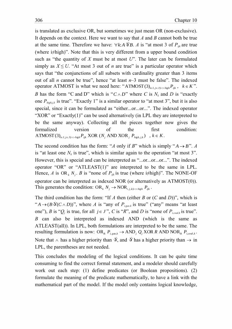
306 Chapter 10
is translated as exclusive OR, but sometimes we just mean OR (non-exclusive).
It depends on the context. Here we want to say that A and B cannot both be true
at the same time. Therefore we have: k:A Ý B. A is “at most 3 of Pijk are true
(where i≠high)”. Note that this is very different from a upper bound condition
such as “the quantity of X must be at most U”. The later can be formulated
simply as X ≤ U. “At most 3 out of n are true” is a particular operator which
says that “the conjunctions of all subsets with cardinality greater than 3 items
out of all n cannot be true”, hence “at least n–3 must be false”. The indexed
operator ATMOST is what we need here: “ATMOST (3)iI , jJ |i high Pijk , k K ”.
B has the form “C and D” which is “C D” where C is Nk and D is “exactly
one Phigh,j,k is true”. “Exactly 1” is a similar operator to “at most 3”, but it is also
special, since it can be formulated as “either...or...or...”. The indexed operator
“XOR” or “Exactly(1)” can be used alternatively (in LPL they are interpreted to
be the same anyway). Collecting all the pieces together now gives the
formalized version of the first condition:
ATMOST (3)iI , jJ |i high Pijk XOR (N j AND XOR j Phigh, j,k ) , k K .
The second condition has the form: “A only if B” which is simply “ AB”. A
is “at least one Nk is true”, which is similar again to the operation “at most 3”.
However, this is special and can be interpreted as “...or...or...or...”. The indexed
operator “OR” or “ATLEAST(1)” are interpreted to be the same in LPL.
Hence, A is OR k N j . B is “none of Pijk is true (where i≠high)”. The NONE-OF
operator can be interpreted as indexed NOR (or alternatively as ATMOST(0)).
This generates the condition: ORk N j NORi , j ,k |i high Pijk .
The third condition has the form: “If A then (either B or (C and D))”, which is
“ A (B Ý (C D))”, where A is “any of Pi,gas.k is true” (“any” means “at least
one”), B is “Qj is true, for all j J ”, C is “R”, and D is “none of Pi,coal,k is true”.
B can also be interpreted as indexed AND (which is the same as
ATLEAST(all)). In LPL, both formulations are interpreted to be the same. The
resulting formulation is now: ORik Pi, gas,k AND j Qj XOR R AND NORik Pi,coal ,k .
Note that has a higher priority than Ý , and Ý has a higher priority than in
LPL, the parentheses are not needed.
This concludes the modeling of the logical conditions. It can be quite time
consuming to find the correct formal statement, and a modeler should carefully
work out each step: (1) define predicates (or Boolean propositions). (2)
formulate the meaning of the predicate mathematically, to have a link with the
mathematical part of the model. If the model only contains logical knowledge,
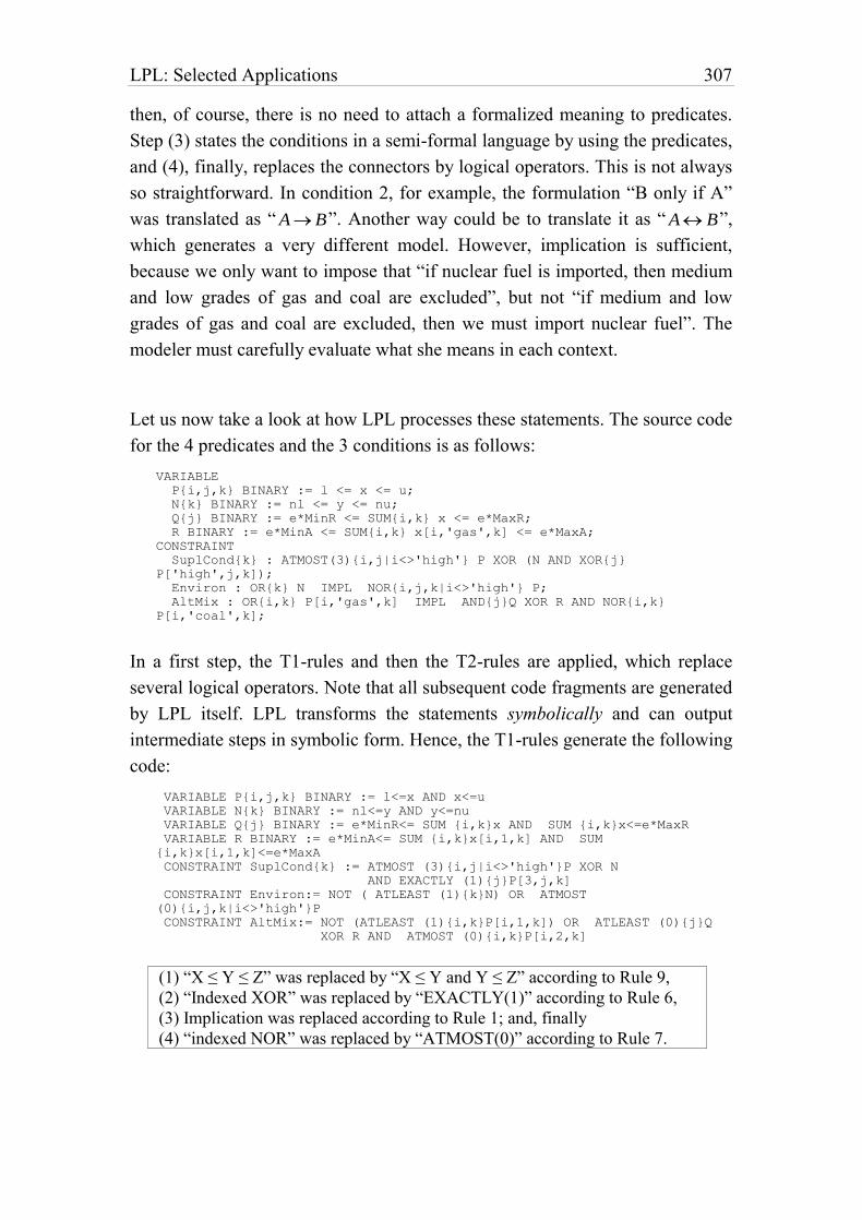
LPL: Selected Applications 307
then, of course, there is no need to attach a formalized meaning to predicates.
Step (3) states the conditions in a semi-formal language by using the predicates,
and (4), finally, replaces the connectors by logical operators. This is not always
so straightforward. In condition 2, for example, the formulation “B only if A”
was translated as “ AB”. Another way could be to translate it as “ A B”,
which generates a very different model. However, implication is sufficient,
because we only want to impose that “if nuclear fuel is imported, then medium
and low grades of gas and coal are excluded”, but not “if medium and low
grades of gas and coal are excluded, then we must import nuclear fuel”. The
modeler must carefully evaluate what she means in each context.
Let us now take a look at how LPL processes these statements. The source code
for the 4 predicates and the 3 conditions is as follows:
VARIABLE
P{i,j,k} BINARY := l <= x <= u;
N{k} BINARY := nl <= y <= nu;
Q{j} BINARY := e*MinR <= SUM{i,k} x <= e*MaxR;
R BINARY := e*MinA <= SUM{i,k} x[i,'gas',k] <= e*MaxA;
CONSTRAINT
SuplCond{k} : ATMOST(3){i,j|i<>'high'} P XOR (N AND XOR{j}
P['high',j,k]);
Environ : OR{k} N IMPL NOR{i,j,k|i<>'high'} P;
AltMix : OR{i,k} P[i,'gas',k] IMPL AND{j}Q XOR R AND NOR{i,k}
P[i,'coal',k];
In a first step, the T1-rules and then the T2-rules are applied, which replace
several logical operators. Note that all subsequent code fragments are generated
by LPL itself. LPL transforms the statements symbolically and can output
intermediate steps in symbolic form. Hence, the T1-rules generate the following
code:
VARIABLE P{i,j,k} BINARY := l<=x AND x<=u
VARIABLE N{k} BINARY := nl<=y AND y<=nu
VARIABLE Q{j} BINARY := e*MinR<= SUM {i,k}x AND SUM {i,k}x<=e*MaxR
VARIABLE R BINARY := e*MinA<= SUM {i,k}x[i,1,k] AND SUM
{i,k}x[i,1,k]<=e*MaxA
CONSTRAINT SuplCond{k} := ATMOST (3){i,j|i<>'high'}P XOR N
AND EXACTLY (1){j}P[3,j,k]
CONSTRAINT Environ:= NOT ( ATLEAST (1){k}N) OR ATMOST
(0){i,j,k|i<>'high'}P
CONSTRAINT AltMix:= NOT (ATLEAST (1){i,k}P[i,1,k]) OR ATLEAST (0){j}Q
XOR R AND ATMOST (0){i,k}P[i,2,k]
(1) “X ≤ Y ≤ Z” was replaced by “X ≤ Y and Y ≤ Z” according to Rule 9,
(2) “Indexed XOR” was replaced by “EXACTLY(1)” according to Rule 6,
(3) Implication was replaced according to Rule 1; and, finally
(4) “indexed NOR” was replaced by “ATMOST(0)” according to Rule 7.
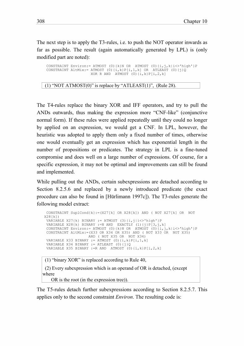
308 Chapter 10
The next step is to apply the T3-rules, i.e. to push the NOT operator inwards as
far as possible. The result (again automatically generated by LPL) is (only
modified part are noted):
CONSTRAINT Environ:= ATMOST (0){k}N OR ATMOST (0){i,j,k|i<>'high'}P
CONSTRAINT AltMix:= ATMOST (0){i,k}P[i,1,k] OR ATLEAST (0){j}Q
XOR R AND ATMOST (0){i,k}P[i,2,k]
(1) “NOT ATMOST(0)” is replace by “ATLEAST(1)”, (Rule 28).
The T4-rules replace the binary XOR and IFF operators, and try to pull the
ANDs outwards, thus making the expression more “CNF-like” (conjunctive
normal form). If these rules were applied repeatedly until they could no longer
by applied on an expression, we would get a CNF. In LPL, however, the
heuristic was adopted to apply them only a fixed number of times, otherwise
one would eventually get an expression which has exponential length in the
number of propositions or predicates. The strategy in LPL is a fine-tuned
compromise and does well on a large number of expressions. Of course, for a
specific expression, it may not be optimal and improvements can still be found
and implemented.
While pulling out the ANDs, certain subexpressions are detached according to
Section 8.2.5.6 and replaced by a newly introduced predicate (the exact
procedure can also be found in [Hürlimann 1997c]). The T3-rules generate the
following model extract:
CONSTRAINT SuplCond{k}:=(X27[k] OR X28[k]) AND ( NOT X27[k] OR NOT
X28[k])
VARIABLE X27{k} BINARY := ATMOST (3){i,j|i<>'high'}P
VARIABLE X28{k} BINARY :=N AND EXACTLY (1){j}P[3,j,k]
CONSTRAINT Environ:= ATMOST (0){k}N OR ATMOST (0){i,j,k|i<>'high'}P
CONSTRAINT AltMix:=(X33 OR X34 OR X35) AND ( NOT X33 OR NOT X35)
AND ( NOT X35 OR NOT X34)
VARIABLE X33 BINARY := ATMOST (0){i,k}P[i,1,k]
VARIABLE X34 BINARY := ATLEAST (0){j}Q
VARIABLE X35 BINARY :=R AND ATMOST (0){i,k}P[i,2,k]
(1) “binary XOR” is replaced according to Rule 40,
(2) Every subexpression which is an operand of OR is detached, (except
where
OR is the root (in the expression tree)).
The T5-rules detach further subexpressions according to Section 8.2.5.7. This
applies only to the second constraint Environ. The resulting code is:
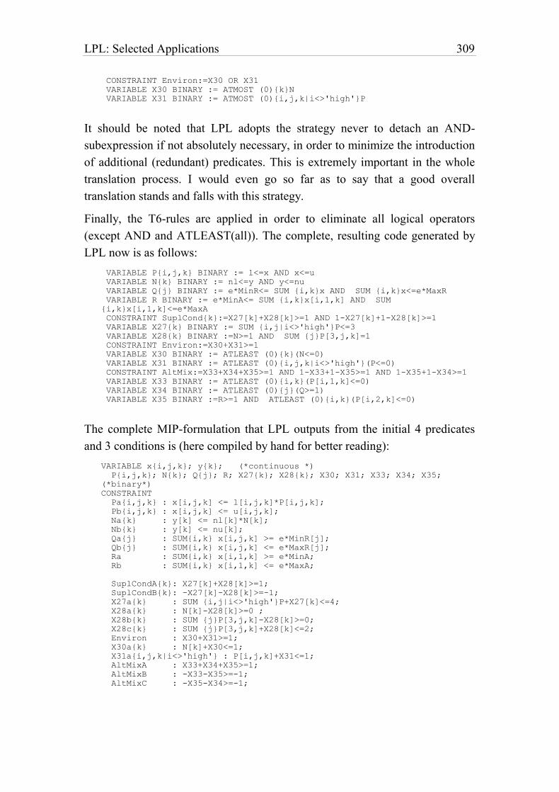
LPL: Selected Applications 309
CONSTRAINT Environ:=X30 OR X31
VARIABLE X30 BINARY := ATMOST (0){k}N
VARIABLE X31 BINARY := ATMOST (0){i,j,k|i<>'high'}P
It should be noted that LPL adopts the strategy never to detach an AND-
subexpression if not absolutely necessary, in order to minimize the introduction
of additional (redundant) predicates. This is extremely important in the whole
translation process. I would even go so far as to say that a good overall
translation stands and falls with this strategy.
Finally, the T6-rules are applied in order to eliminate all logical operators
(except AND and ATLEAST(all)). The complete, resulting code generated by
LPL now is as follows:
VARIABLE P{i,j,k} BINARY := l<=x AND x<=u
VARIABLE N{k} BINARY := nl<=y AND y<=nu
VARIABLE Q{j} BINARY := e*MinR<= SUM {i,k}x AND SUM {i,k}x<=e*MaxR
VARIABLE R BINARY := e*MinA<= SUM {i,k}x[i,1,k] AND SUM
{i,k}x[i,1,k]<=e*MaxA
CONSTRAINT SuplCond{k}:=X27[k]+X28[k]>=1 AND 1-X27[k]+1-X28[k]>=1
VARIABLE X27{k} BINARY := SUM {i,j|i<>'high'}P<=3
VARIABLE X28{k} BINARY :=N>=1 AND SUM {j}P[3,j,k]=1
CONSTRAINT Environ:=X30+X31>=1
VARIABLE X30 BINARY := ATLEAST (0){k}(N<=0)
VARIABLE X31 BINARY := ATLEAST (0){i,j,k|i<>'high'}(P<=0)
CONSTRAINT AltMix:=X33+X34+X35>=1 AND 1-X33+1-X35>=1 AND 1-X35+1-X34>=1
VARIABLE X33 BINARY := ATLEAST (0){i,k}(P[i,1,k]<=0)
VARIABLE X34 BINARY := ATLEAST (0){j}(Q>=1)
VARIABLE X35 BINARY :=R>=1 AND ATLEAST (0){i,k}(P[i,2,k]<=0)
The complete MIP-formulation that LPL outputs from the initial 4 predicates
and 3 conditions is (here compiled by hand for better reading):
VARIABLE x{i,j,k}; y{k}; (*continuous *)
P{i,j,k}; N{k}; Q{j}; R; X27{k}; X28{k}; X30; X31; X33; X34; X35;
(*binary*)
CONSTRAINT
Pa{i,j,k} : x[i,j,k] <= l[i,j,k]*P[i,j,k];
Pb{i,j,k} : x[i,j,k] <= u[i,j,k];
Na{k} : y[k] <= nl[k]*N[k];
Nb{k} : y[k] <= nu[k];
Qa{j} : SUM{i,k} x[i,j,k] >= e*MinR[j];
Qb{j} : SUM{i,k} x[i,j,k] <= e*MaxR[j];
Ra : SUM{i,k} x[i,1,k] >= e*MinA;
Rb : SUM{i,k} x[i,1,k] <= e*MaxA;
SuplCondA{k}: X27[k]+X28[k]>=1;
SuplCondB{k}: -X27[k]-X28[k]>=-1;
X27a{k} : SUM {i,j|i<>'high'}P+X27[k]<=4;
X28a{k} : N[k]-X28[k]>=0 ;
X28b{k} : SUM {j}P[3,j,k]-X28[k]>=0;
X28c{k} : SUM {j}P[3,j,k]+X28[k]<=2;
Environ : X30+X31>=1;
X30a{k} : N[k]+X30<=1;
X31a{i,j,k|i<>'high'} : P[i,j,k]+X31<=1;
AltMixA : X33+X34+X35>=1;
AltMixB : -X33-X35>=-1;
AltMixC : -X35-X34>=-1;
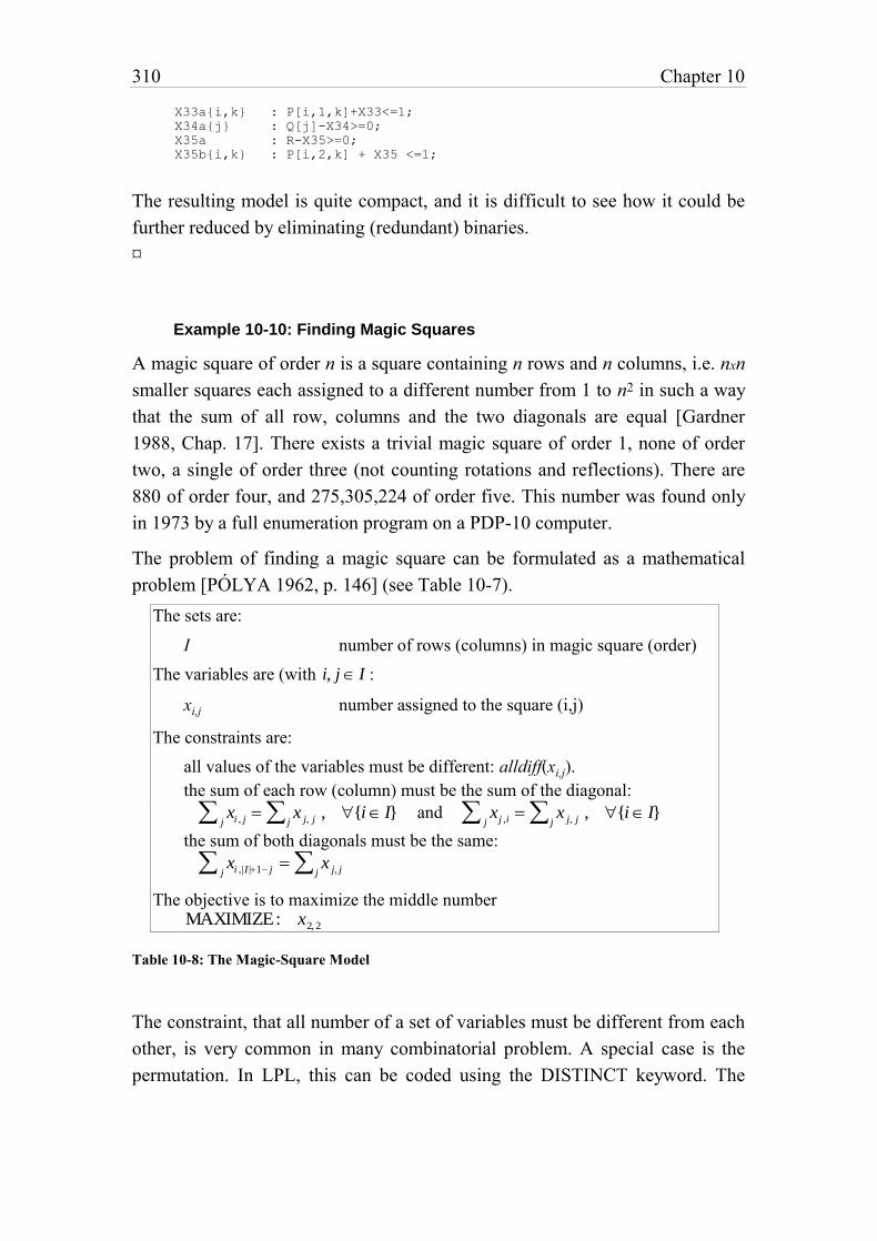
310 Chapter 10
X33a{i,k} : P[i,1,k]+X33<=1;
X34a{j} : Q[j]-X34>=0;
X35a : R-X35>=0;
X35b{i,k} : P[i,2,k] + X35 <=1;
The resulting model is quite compact, and it is difficult to see how it could be
further reduced by eliminating (redundant) binaries.
¤
Example 10-10: Finding Magic Squares
A magic square of order n is a square containing n rows and n columns, i.e. nxn
smaller squares each assigned to a different number from 1 to n2 in such a way
that the sum of all row, columns and the two diagonals are equal [Gardner
1988, Chap. 17]. There exists a trivial magic square of order 1, none of order
two, a single of order three (not counting rotations and reflections). There are
880 of order four, and 275,305,224 of order five. This number was found only
in 1973 by a full enumeration program on a PDP-10 computer.
The problem of finding a magic square can be formulated as a mathematical
problem [PÓLYA 1962, p. 146] (see Table 10-7).
The sets are:
I number of rows (columns) in magic square (order)
The variables are (with i, j I :
xi,j number assigned to the square (i,j)
The constraints are:
all values of the variables must be different: alldiff(xi,j).
the sum of each row (column) must be the sum of the diagonal:
xi , jj x j, jj , {i I} and xj ,ij x j, jj , {i I}
the sum of both diagonals must be the same:
xi ,|I |1 jj x j, jj
The objective is to maximize the middle number MAXIMIZE: x2, 2
Table 10-8: The Magic-Square Model
The constraint, that all number of a set of variables must be different from each
other, is very common in many combinatorial problem. A special case is the
permutation. In LPL, this can be coded using the DISTINCT keyword. The
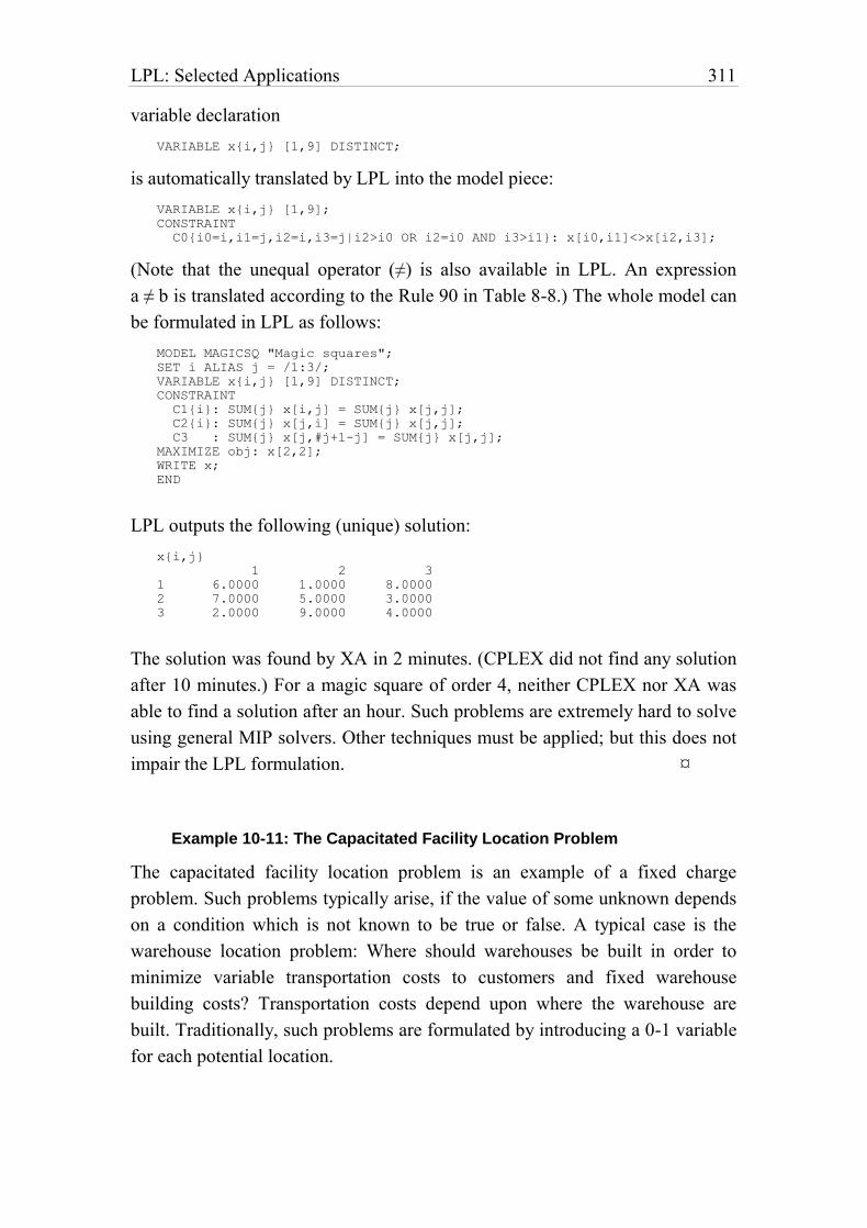
LPL: Selected Applications 311
variable declaration
VARIABLE x{i,j} [1,9] DISTINCT;
is automatically translated by LPL into the model piece:
VARIABLE x{i,j} [1,9];
CONSTRAINT
C0{i0=i,i1=j,i2=i,i3=j|i2>i0 OR i2=i0 AND i3>i1}: x[i0,i1]<>x[i2,i3];
(Note that the unequal operator (≠) is also available in LPL. An expression
a ≠ b is translated according to the Rule 90 in Table 8-8.) The whole model can
be formulated in LPL as follows:
MODEL MAGICSQ "Magic squares";
SET i ALIAS j = /1:3/;
VARIABLE x{i,j} [1,9] DISTINCT;
CONSTRAINT
C1{i}: SUM{j} x[i,j] = SUM{j} x[j,j];
C2{i}: SUM{j} x[j,i] = SUM{j} x[j,j];
C3 : SUM{j} x[j,#j+1-j] = SUM{j} x[j,j];
MAXIMIZE obj: x[2,2];
WRITE x;
END
LPL outputs the following (unique) solution:
x{i,j}
1 2 3
1 6.0000 1.0000 8.0000
2 7.0000 5.0000 3.0000
3 2.0000 9.0000 4.0000
The solution was found by XA in 2 minutes. (CPLEX did not find any solution
after 10 minutes.) For a magic square of order 4, neither CPLEX nor XA was
able to find a solution after an hour. Such problems are extremely hard to solve
using general MIP solvers. Other techniques must be applied; but this does not
impair the LPL formulation. ¤
Example 10-11: The Capacitated Facility Location Problem
The capacitated facility location problem is an example of a fixed charge
problem. Such problems typically arise, if the value of some unknown depends
on a condition which is not known to be true or false. A typical case is the
warehouse location problem: Where should warehouses be built in order to
minimize variable transportation costs to customers and fixed warehouse
building costs? Transportation costs depend upon where the warehouse are
built. Traditionally, such problems are formulated by introducing a 0-1 variable
for each potential location.
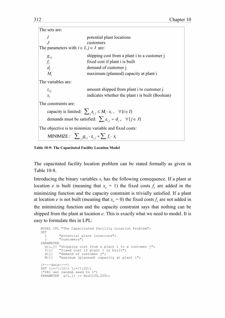
312 Chapter 10
The sets are:
I potential plant locations
J customers
The parameters with i I, j J are:
gi,j shipping cost from a plant i to a customer j
fi fixed cost if plant i is built
dj demand of customer j
Mi maximum (planned) capacity at plant i
The variables are:
zi,j amount shipped from plant i to customer j
xi indicates whether the plant i is built (Boolean)
The constraints are:
capacity is limited: zi, jj Mi xi , {i I}
demands must be satisfied: zi, ji d j , { j J}
The objective is to minimize variable and fixed costs:
MINIMIZE : gi. j zi , ji, j fi xii
Table 10-9: The Capacitated Facility Location Model
The capacitated facility location problem can be stated formally as given in
Table 10-8.
Introducing the binary variables xi has the following consequence. If a plant at
location e is built (meaning that xe = 1) the fixed costs fe are added in the
minimizing function and the capacity constraint is trivially satisfied. If a plant
at location e is not built (meaning that xe = 0) the fixed costs fe are not added in
the minimizing function and the capacity constraint says that nothing can be
shipped from the plant at location e. This is exactly what we need to model. It is
easy to formulate this in LPL:
MODEL CFL "The Capacitated Facility Location Problem";
SET
i "potential plant locations";
j "customers";
PARAMETER
g{i,j} "shipping cost from a plant i to a customer j";
f{i} "fixed cost if plant i is built";
d{j} "demand of customer j";
M{i} "maximum (planned) capacity at plant i";
(*---data---*)
SET i:=/1:10/; j:=/1:20/;
(*$R1 set random seed to 1*)
PARAMETER g{i,j} := Rnd(100,200);
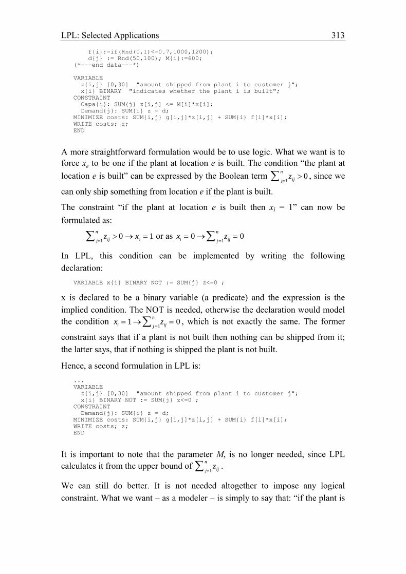
LPL: Selected Applications 313
f{i}:=if(Rnd(0,1)<=0.7,1000,1200);
d{j} := Rnd(50,100); M{i}:=600;
(*---end data---*)
VARIABLE
z{i,j} [0,30] "amount shipped from plant i to customer j";
x{i} BINARY "indicates whether the plant i is built";
CONSTRAINT
Capa{i}: SUM{j} z[i,j] <= M[i]*x[i];
Demand{j}: SUM{i} z = d;
MINIMIZE costs: SUM{i,j} g[i,j]*z[i,j] + SUM{i} f[i]*x[i];
WRITE costs; z;
END
A more straightforward formulation would be to use logic. What we want is to
force xe to be one if the plant at location e is built. The condition “the plant at
location e is built” can be expressed by the Boolean term zijj1
n
0 , since we
can only ship something from location e if the plant is built.
The constraint “if the plant at location e is built then xi = 1” can now be
formulated as:
zijj1
n
0 xi 1 or as xi 0 zijj1
n
0
In LPL, this condition can be implemented by writing the following
declaration:
VARIABLE x{i} BINARY NOT := SUM{j} z<=0 ;
x is declared to be a binary variable (a predicate) and the expression is the
implied condition. The NOT is needed, otherwise the declaration would model
the condition xi 1 zijj1
n
0 , which is not exactly the same. The former
constraint says that if a plant is not built then nothing can be shipped from it;
the latter says, that if nothing is shipped the plant is not built.
Hence, a second formulation in LPL is:
...
VARIABLE
z{i,j} [0,30] "amount shipped from plant i to customer j";
x{i} BINARY NOT := SUM{j} z<=0 ;
CONSTRAINT
Demand{j}: SUM{i} z = d;
MINIMIZE costs: SUM{i,j} g[i,j]*z[i,j] + SUM{i} f[i]*x[i];
WRITE costs; z;
END
It is important to note that the parameter M, is no longer needed, since LPL
calculates it from the upper bound of zijj1
n
.
We can still do better. It is not needed altogether to impose any logical
constraint. What we want – as a modeler – is simply to say that: “if the plant is
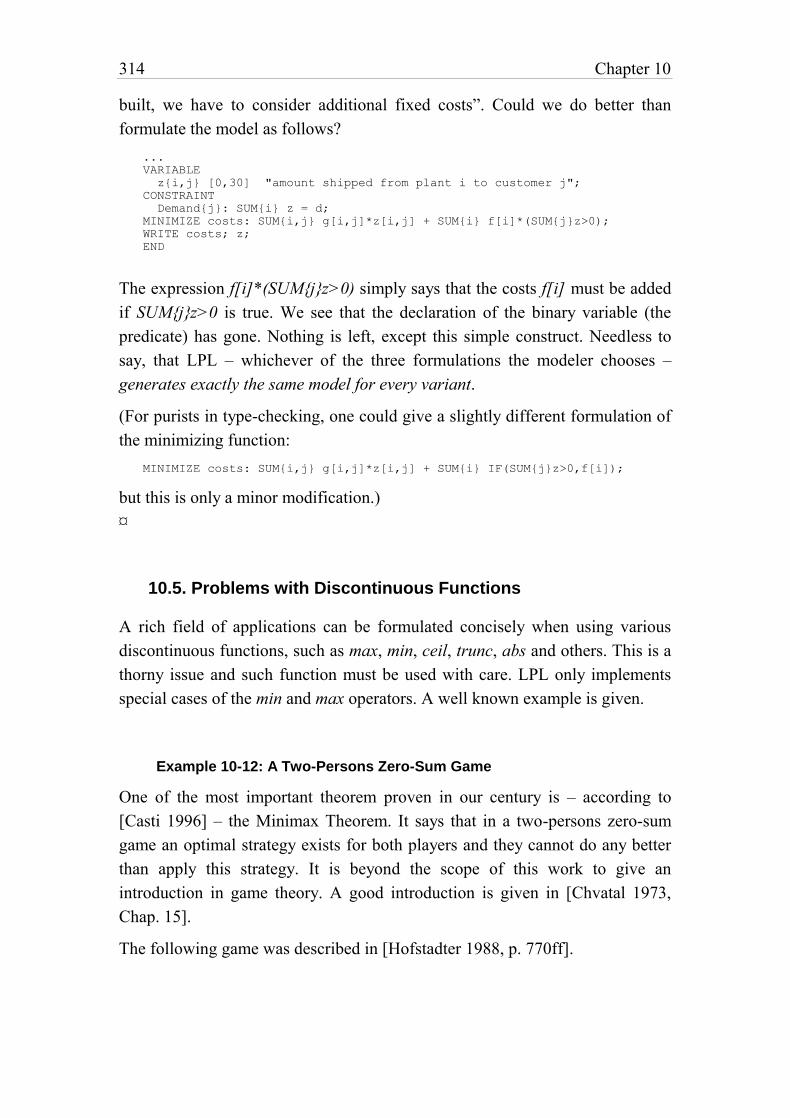
314 Chapter 10
built, we have to consider additional fixed costs”. Could we do better than
formulate the model as follows?
...
VARIABLE
z{i,j} [0,30] "amount shipped from plant i to customer j";
CONSTRAINT
Demand{j}: SUM{i} z = d;
MINIMIZE costs: SUM{i,j} g[i,j]*z[i,j] + SUM{i} f[i]*(SUM{j}z>0);
WRITE costs; z;
END
The expression f[i]*(SUM{j}z>0) simply says that the costs f[i] must be added
if SUM{j}z>0 is true. We see that the declaration of the binary variable (the
predicate) has gone. Nothing is left, except this simple construct. Needless to
say, that LPL – whichever of the three formulations the modeler chooses –
generates exactly the same model for every variant.
(For purists in type-checking, one could give a slightly different formulation of
the minimizing function:
MINIMIZE costs: SUM{i,j} g[i,j]*z[i,j] + SUM{i} IF(SUM{j}z>0,f[i]);
but this is only a minor modification.)
¤
10.5. Problems with Discontinuous Functions
A rich field of applications can be formulated concisely when using various
discontinuous functions, such as max, min, ceil, trunc, abs and others. This is a
thorny issue and such function must be used with care. LPL only implements
special cases of the min and max operators. A well known example is given.
Example 10-12: A Two-Persons Zero-Sum Game
One of the most important theorem proven in our century is – according to
[Casti 1996] – the Minimax Theorem. It says that in a two-persons zero-sum
game an optimal strategy exists for both players and they cannot do any better
than apply this strategy. It is beyond the scope of this work to give an
introduction in game theory. A good introduction is given in [Chvatal 1973,
Chap. 15].
The following game was described in [Hofstadter 1988, p. 770ff].
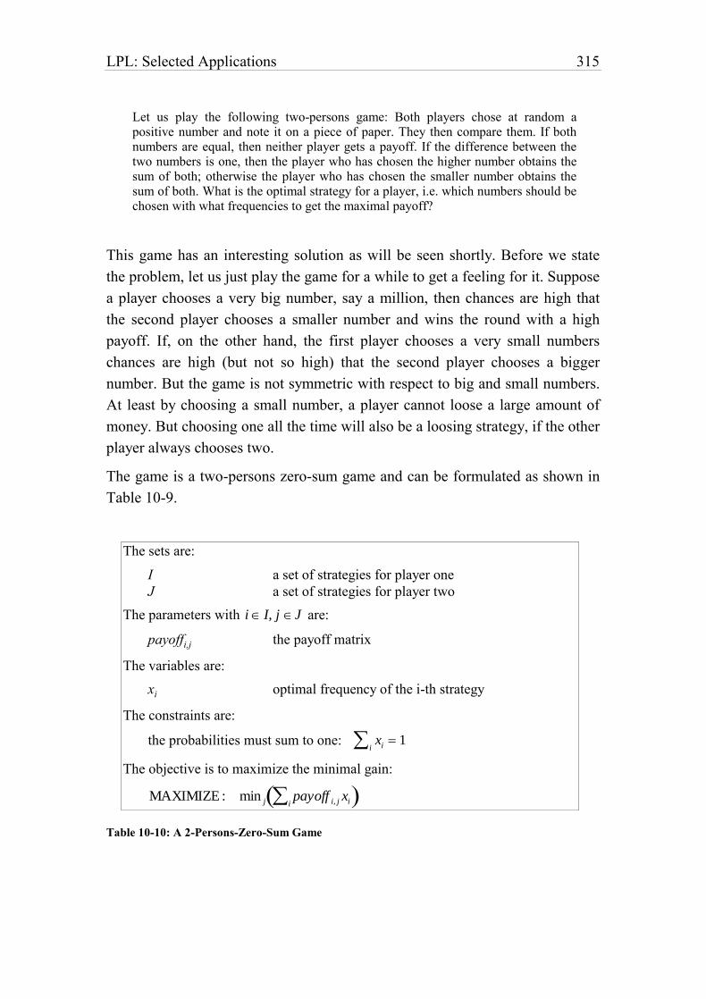
LPL: Selected Applications 315
Let us play the following two-persons game: Both players chose at random a positive number and note it on a piece of paper. They then compare them. If both numbers are equal, then neither player gets a payoff. If the difference between the two numbers is one, then the player who has chosen the higher number obtains the sum of both; otherwise the player who has chosen the smaller number obtains the sum of both. What is the optimal strategy for a player, i.e. which numbers should be chosen with what frequencies to get the maximal payoff?
This game has an interesting solution as will be seen shortly. Before we state
the problem, let us just play the game for a while to get a feeling for it. Suppose
a player chooses a very big number, say a million, then chances are high that
the second player chooses a smaller number and wins the round with a high
payoff. If, on the other hand, the first player chooses a very small numbers
chances are high (but not so high) that the second player chooses a bigger
number. But the game is not symmetric with respect to big and small numbers.
At least by choosing a small number, a player cannot loose a large amount of
money. But choosing one all the time will also be a loosing strategy, if the other
player always chooses two.
The game is a two-persons zero-sum game and can be formulated as shown in
Table 10-9.
The sets are:
I a set of strategies for player one
J a set of strategies for player two
The parameters with i I, j J are:
payoffi,j the payoff matrix
The variables are:
xi optimal frequency of the i-th strategy
The constraints are:
the probabilities must sum to one: xii 1
The objective is to maximize the minimal gain:
MAXIMIZE : min j payoff i, j xii
Table 10-10: A 2-Persons-Zero-Sum Game
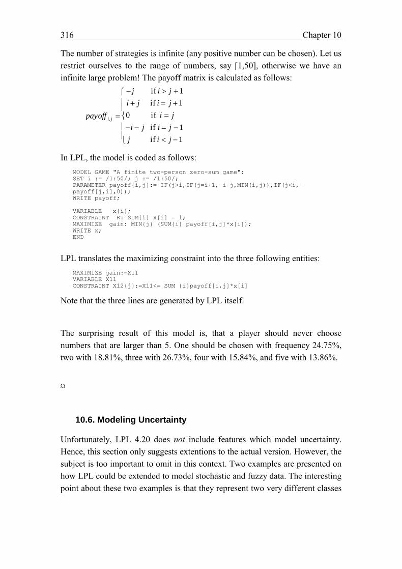
316 Chapter 10
The number of strategies is infinite (any positive number can be chosen). Let us
restrict ourselves to the range of numbers, say [1,50], otherwise we have an
infinite large problem! The payoff matrix is calculated as follows:
payoff i, j
j if i j 1
i j if i j 1
0 if i j
i j if i j 1
j if i j 1
In LPL, the model is coded as follows:
MODEL GAME "A finite two-person zero-sum game";
SET i := /1:50/; j := /1:50/;
PARAMETER payoff{i,j}:= IF(j>i,IF(j=i+1,-i-j,MIN(i,j)),IF(j<i,-
payoff[j,i],0));
WRITE payoff;
VARIABLE x{i};
CONSTRAINT R: SUM{i} x[i] = 1;
MAXIMIZE gain: MIN{j} (SUM{i} payoff[i,j]*x[i]);
WRITE x;
END
LPL translates the maximizing constraint into the three following entities:
MAXIMIZE gain:=X11
VARIABLE X11
CONSTRAINT X12{j}:=X11<= SUM {i}payoff[i,j]*x[i]
Note that the three lines are generated by LPL itself.
The surprising result of this model is, that a player should never choose
numbers that are larger than 5. One should be chosen with frequency 24.75%,
two with 18.81%, three with 26.73%, four with 15.84%, and five with 13.86%.
¤
10.6. Modeling Uncertainty
Unfortunately, LPL 4.20 does not include features which model uncertainty.
Hence, this section only suggests extentions to the actual version. However, the
subject is too important to omit in this context. Two examples are presented on
how LPL could be extended to model stochastic and fuzzy data. The interesting
point about these two examples is that they represent two very different classes
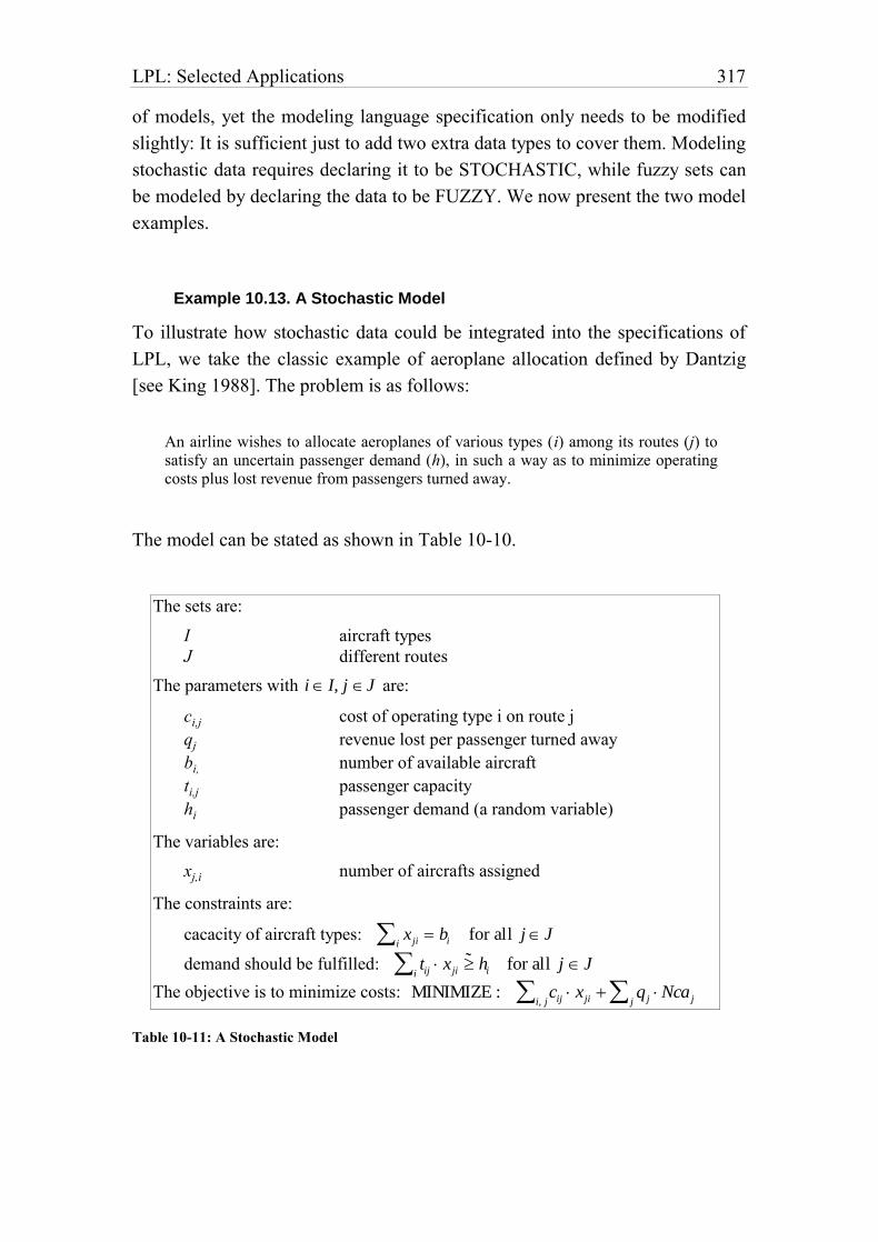
LPL: Selected Applications 317
of models, yet the modeling language specification only needs to be modified
slightly: It is sufficient just to add two extra data types to cover them. Modeling
stochastic data requires declaring it to be STOCHASTIC, while fuzzy sets can
be modeled by declaring the data to be FUZZY. We now present the two model
examples.
Example 10.13. A Stochastic Model
To illustrate how stochastic data could be integrated into the specifications of
LPL, we take the classic example of aeroplane allocation defined by Dantzig
[see King 1988]. The problem is as follows:
An airline wishes to allocate aeroplanes of various types (i) among its routes (j) to satisfy an uncertain passenger demand (h), in such a way as to minimize operating costs plus lost revenue from passengers turned away.
The model can be stated as shown in Table 10-10.
The sets are:
I aircraft types
J different routes
The parameters with i I, j J are:
ci,j cost of operating type i on route j
qj revenue lost per passenger turned away
bi, number of available aircraft
ti,j passenger capacity
hi passenger demand (a random variable)
The variables are:
xj,i number of aircrafts assigned
The constraints are:
cacacity of aircraft types: x jii bi for all j J
demand should be fulfilled: tij xjii ˜ hi for all j J
The objective is to minimize costs: MINIMIZE : cij xjii, j q j Nca jj
Table 10-11: A Stochastic Model
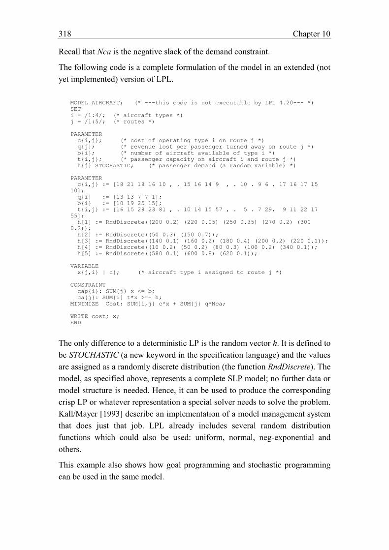
318 Chapter 10
Recall that Nca is the negative slack of the demand constraint.
The following code is a complete formulation of the model in an extended (not
yet implemented) version of LPL.
MODEL AIRCRAFT; (* ---this code is not executable by LPL 4.20--- *)
SET
i = /1:4/; (* aircraft types *)
j = /1:5/; (* routes *)
PARAMETER
c{i,j}; (* cost of operating type i on route j *)
q{j}; (* revenue lost per passenger turned away on route j *)
b{i}; (* number of aircraft available of type i *)
t{i,j}; (* passenger capacity on aircraft i and route j *)
h{j} STOCHASTIC; (* passenger demand (a random variable) *)
PARAMETER
c{i,j} := [18 21 18 16 10 , . 15 16 14 9 , . 10 . 9 6 , 17 16 17 15
10];
q{i} := [13 13 7 7 1];
b{i} := [10 19 25 15];
t{i,j} := [16 15 28 23 81 , . 10 14 15 57 , . 5 . 7 29, 9 11 22 17
55];
h[1] := RndDiscrete((200 0.2) (220 0.05) (250 0.35) (270 0.2) (300
0.2));
h[2] := RndDiscrete((50 0.3) (150 0.7));
h[3] := RndDiscrete((140 0.1) (160 0.2) (180 0.4) (200 0.2) (220 0.1));
h[4] := RndDiscrete((10 0.2) (50 0.2) (80 0.3) (100 0.2) (340 0.1));
h[5] := RndDiscrete((580 0.1) (600 0.8) (620 0.1));
VARIABLE
x{j,i} | c}; (* aircraft type i assigned to route j *)
CONSTRAINT
cap{i}: SUM{j} x <= b;
ca{j}: SUM{i} t*x >=~ h;
MINIMIZE Cost: SUM{i,j} c*x + SUM{j} q*Nca;
WRITE cost; x;
END
The only difference to a deterministic LP is the random vector h. It is defined to
be STOCHASTIC (a new keyword in the specification language) and the values
are assigned as a randomly discrete distribution (the function RndDiscrete). The
model, as specified above, represents a complete SLP model; no further data or
model structure is needed. Hence, it can be used to produce the corresponding
crisp LP or whatever representation a special solver needs to solve the problem.
Kall/Mayer [1993] describe an implementation of a model management system
that does just that job. LPL already includes several random distribution
functions which could also be used: uniform, normal, neg-exponential and
others.
This example also shows how goal programming and stochastic programming
can be used in the same model.
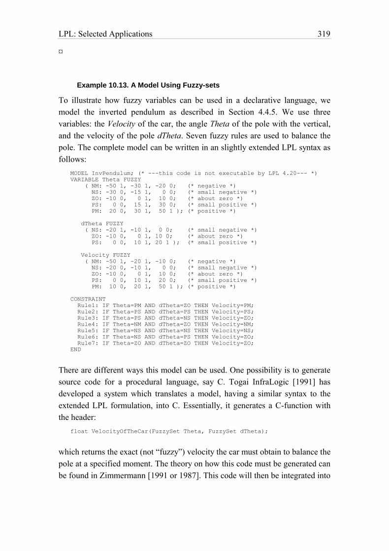
LPL: Selected Applications 319
¤
Example 10.13. A Model Using Fuzzy-sets
To illustrate how fuzzy variables can be used in a declarative language, we
model the inverted pendulum as described in Section 4.4.5. We use three
variables: the Velocity of the car, the angle Theta of the pole with the vertical,
and the velocity of the pole dTheta. Seven fuzzy rules are used to balance the
pole. The complete model can be written in an slightly extended LPL syntax as
follows:
MODEL InvPendulum; (* ---this code is not executable by LPL 4.20--- *)
VARIABLE Theta FUZZY
( NM: -50 1, -30 1, -20 0; (* negative *)
NS: -30 0, -15 1, 0 0; (* small negative *)
ZO: -10 0, 0 1, 10 0; (* about zero *)
PS: 0 0, 15 1, 30 0; (* small positive *)
PM: 20 0, 30 1, 50 1 ); (* positive *)
dTheta FUZZY
( NS: -20 1, -10 1, 0 0; (* small negative *)
ZO: -10 0, 0 1, 10 0; (* about zero *)
PS: 0 0, 10 1, 20 1 ); (* small positive *)
Velocity FUZZY
( NM: -50 1, -20 1, -10 0; (* negative *)
NS: -20 0, -10 1, 0 0; (* small negative *)
ZO: -10 0, 0 1, 10 0; (* about zero *)
PS: 0 0, 10 1, 20 0; (* small positive *)
PM: 10 0, 20 1, 50 1 ); (* positive *)
CONSTRAINT
Rule1: IF Theta=PM AND dTheta=ZO THEN Velocity=PM;
Rule2: IF Theta=PS AND dTheta=PS THEN Velocity=PS;
Rule3: IF Theta=PS AND dTheta=NS THEN Velocity=ZO;
Rule4: IF Theta=NM AND dTheta=ZO THEN Velocity=NM;
Rule5: IF Theta=NS AND dTheta=NS THEN Velocity=NS;
Rule6: IF Theta=NS AND dTheta=PS THEN Velocity=ZO;
Rule7: IF Theta=ZO AND dTheta=ZO THEN Velocity=ZO;
END
There are different ways this model can be used. One possibility is to generate
source code for a procedural language, say C. Togai InfraLogic [1991] has
developed a system which translates a model, having a similar syntax to the
extended LPL formulation, into C. Essentially, it generates a C-function with
the header:
float VelocityOfTheCar(FuzzySet Theta, FuzzySet dTheta);
which returns the exact (not “fuzzy”) velocity the car must obtain to balance the
pole at a specified moment. The theory on how this code must be generated can
be found in Zimmermann [1991 or 1987]. This code will then be integrated into
320 Chapter 10
a simualtion package.
Another possibility is that the model directly generates executable code and the
modeling language itself can be used as a simulation software tool. One does
not need to make the detour via another language.
Finally, I would like to mention that one of the first (declarative) fuzzy-set
languages was called L.P.L. and was developed at the end of the seventies
[Adamo 1980]. LPL is not related to L.P.L., but – who knows – in a future
version, L.P.L. might become a subset of LPL! ¤
This somewhat future vision (version) concludes this last chapter. The objective
of the examples was not to practice modeling, but to illustrate the wide range of
applications and the conciseness of the declarative modeling formulation. Used
together with procedural knowledge in the same language (which is not the case
in LPL), this gives a powerful means to formulate and solve complex problems
without the need for large scale programming.
321
11. CONCLUSION
“The best is yet to come. We've only scratched the surface...” — Shannon C.E.
Computer-based modeling is not an “ad hoc science” where we could apply the
slogan “everything goes”; on the contrary, it is, like software engineering, a
discipline which must follow certain criteria of quality. These criteria are
reliability to ensure correctness and robustness of models, and transparency to
enhance model extendibility, reusability and compatibility. Reliability can be
achieved by a unique notation, in which models are coded, by a formal
specification of its semantics, and by introducing types, units and other
checking mechanisms, in order to enforce domain consistencies. Transparency
can be obtained by flexible decomposition techniques which fractionates the
whole model into easily maintainable software modules and components.
Models are different from programs in the sense that models often contain
declarative and procedural elements of knowledge, while programs only
describe algorithms. The declarative part in a model represents the state space –
the “what-is”, while the procedural part covers how the model is to be
transformed and, ultimately, solved. This combination implies that the notation,
i.e. the computer-readable language, in which the model is expressed, must
embrace both paradigms, the declarative and the procedural one.
One of the main goal of this book was to propose a modeling language, which
allows the representation of both of these characteristics of models, and to
322 Conclusion
emphasize that modeling language design is submitted to the same criteria as
programming language design in general.
With respect to this goal, several new concepts have been introduced:
– the model specification as an encapsulated software module containing a
well defined interface (exports and imports) in order to communicate with
other modules,
– the coexistence (not the mixing) of declarative and procedural style within
the same language to allow the concise expression of a much broader
number of models, than would be possible otherwise,
– hierarchical index-sets to allow the presentation and manipulation of
hierarchical multi-dimensional data tables and sets in general.
– graphical and textual views which allow the modeler and user to switch in a
bi-directional manner between different visual representations of the model,
in order to browse, to edit, to modify, and to maintain it.
Specifying models as encapsulated modules or decomposing them into well
defined, encapsulated software components have the advantage to reuse and to
maintain the parts independently from the whole. Modifying a module is
confined to its boundary, since the communication to other modules is explicit
and transparent, and its inner working is hidden from the outside. Complexity
can only be controlled by breaking the whole into autonomous, self-contained
pieces. With this respect, no difference exists between models and programs,
between “model engineering” and “software engineering”; all techniques and
principles used in software engineering (information hiding, structured
programming, object orientation, modular design, etc.) are equally applicable
for model building.
Combining the declarative and procedural style, however, are necessary in
coding models. A striking example, of why declarative and procedural
knowledge must coexist for building models, was given in the cutting stock
problem (Example 7-2). This model consists of two purely declarative models
(an LP and a knapsack model) and a simple executable part, in which both
(sub)models are solved several times. Many other models have a similar
“solution structure”. The only two alternatives to approach such problems are
Conclusion 323
(1) to code them as very large (declarative) models or (2) to program the
column generation method – or whatever method is used – explicitly in a
procedural way. The first approach yields elegant and compact models which
are unsolvable because of their size. The second obscures the model structure
as well as the solution process. Combining the two paradigms not only makes
the code much more readable and transparent but also a lot shorter.
An important constituent of every modeling language is its indexing
mechanism in order to formulate large models. Like the mathematical notation
itself, the modeling language should use indexed notation which allows the
formulation of sparse tables and many indexed operations in a very convenient
way. The concept of hierarchical index-set, as proposed in this book, is a
generalization of this indexing mechanism and unifies different well-known
notions already used in existing modeling languages (such as “compound
index-sets”, “indexed index-sets”, “set of index-sets” and others). This
fundamental part of the language also allows the manipulation of hierarchically
organized data tables and other entities.
Of course, the modeling language is not the whole. It must be embedded in a
modeling framework with model browsers and editors. Viewing models from
different angles and through particular filters is an important ingredient to every
modeling management system. However, this presupposes a unique “kernel
form” in which a model is coded, otherwise it would not be possible to switch
between the views in a bi-directional way. Several views – graphical and
textual – have been presented and exemplified.
This book has taken a somewhat biased approach of declarative modeling,
since it favoured that part of model specification, and most model examples are
purely declarative. This bias is only natural in view of the overwhelming
literature about procedural and algorithmic languages. The declarative style has
received surprisingly little attention. I think, this is due to the prevailing opinion
that “real” modeling cannot be done (that is, solved) using a declarative style.
Only toy examples are possible. At best, a declarative representation can be
used for model documentation, so goes the argument. I recall here that solving
a model is only one aspect, documenting being another, and a model has many
other functions. Having a language to automatically pretty-print a model
specification and to compute the documentation is useful; in fact that's all what
324 Conclusion
TEX [Knuth 1986] is about for type-setting.
Furthermore, declarative modeling is powerful and generates compact models
which are easy to maintain. Therefore, the modeler should favour this
paradigm. On the other hand, many problems can easily be expressed as a
mathematical constraint which is unsolvable in any reasonable time – or worse,
of which we do not know when the solution is returned. If the model is to be
solved, it is important to find an efficient formulation. This is, in general, easier
said than done! Finding efficient formulation is a creative work. In any case,
the modeling language does not help in finding efficient formulations, it only
provides syntactical elements in order to code them. We do not expect from a
programming language to assist us in finding an efficient sorting algorithm, we
are already happy if we can code it without too much compromises to the
language syntax! Certainly, it is so simple to formulate a model declaratively
and then to blame the solver of not being able to solve it. In a world, where
most “real” problems are (at least) NP-complete, there is little hope for having
efficiency and beauty at the same time. Nevertheless, in declarative modeling –
sometimes– we get a maximum of both.
The opinion may be expressed that I have proposed but a different
programming language and that we do not need the term “modeling language”
in any way. I would not mind to renounce this term, but would then insist that
there are two particular elements in this new “programming language”, namely
mathematical variables and constraints, not present in any other language (with
exception of the logical programming languages). So, then my proposition is
simply another logical programming language? Not quite! The difference to
logical programming languages is that the proposal here clearly separates
declarative and procedural knowledge and that the search procedures are made
explicit which are coded in a procedural style or are encapsulated in an external
solver. In view of the many very different methods that we need for solving a
wide range of models, it is my impression that such an approach is more
powerful. The modeler has the most flexible way in formulating the model:
mathematically well-understood components can be done declaratively in a
straightforward way, while the other parts are coded in a procedural way. In the
logical programming paradigm the modeler is confined to the search and
solution procedures which are hard-coded in the engine machine itself.
Conclusion 325
Another powerful concept is integrated into the modeling language which
distinguish it from most programming languages: the indexing mechanism.
This introduces set manipulation which is often hard to code in other
languages, because they appear in so many forms, and dealing with them in an
efficient way is not straightforward. The indexing mechanism also predisposes
the modeling language to tackle with a mass of data and to communicate with
databases in a natural way.
The propositions suggested in this book are far from being a well-settled theory
about computer-based modeling. The research topic is simply too new. Many
modeling languages exist in a pre-prototypical stage, but only few are really
useful modeling languages in a general sense. Many syntax-concepts in existing
languages are ad hoc constructs and should be embedded in a more consistent
framework of language design. This does not mean, that I want to blame
existing languages – modeling is hard and modeling language design is even
harder – it only means that we should begin to look at modeling languages as
fully-fletched programming languages in which we code the models, in the
same way as we code algorithms as programs.
Using modeling languages is a new paradigm of mathematical modeling; and I
am convinced that they will have a bright future if they follow certain criteria in
language design coupled with simplicity and elegance.
“Language – notation – shapes thought and mind. Our languages, and how they are defined, have a tremendous influence on what we can express and how simple. Often, a concept becomes clear only when a suitable notation for it has been defined and when rules for manipulating the notation have been developed: a concept and its expression are inextricably intertwined.”
— Gries David in: [Hoare 1989, Preface].
In this sense, we would prefer to live with unsolved problems than accept a
model and its solution we cannot understand.


327
APPENDICES

329
REFERENCES
ADAMO J.M., [1980], L.P.L. – A Fuzzy Programming Language, 1. Sytactic
Aspects, 2. Semantic Aspects, in: Fuzzy Sets and Systems Vol. 3, p. 151–
179 and pp 261–289.
AGGOUN A. & BELDICEANU N., [1993], Extending CHIP in Order to Solve
Complex Scheduling and Placement Problems, in: Math. Comput.
Modelling, Vol. 17, No. 7, p. 57–73.
AHO A.V. & SETHI R. & ULLMAN J.D., [1986], Compilers, Principles,
Techniques, and Tools, Addison-Wesley Publ., Reading, Massachusetts.
AIBA A. & SAKAI K. & SATO Y. & HAWLEY D.J. & HASEGAWA R.,
[1988], Constraint Logic Programming Language CAL, in: FGCS'88, p.
263–276.
AIGNER M., [1988], Combinatorial Search, Wiley-Teubner Series in
Computer Science, Chichester/Stuttgart.
ANDERSEN K.A. & HOOKER J.N., [1994], Bayesian Logic, in: Decision
Support Systems 11, p 191–210.
ANGEHRN A.A. & LÜTHI H-J., [1990], Intelligent Decision Support
Systems: A Visual Interactive Approach, in. Interfaces, Vol. 20:6, pp. 17–
28.
BACKUS J., [1978], Can Programming be liberated from the von Neumann
style? in: Comm. of the ACM 21 (1978), pp. 613–641.
330 References
BAECKER R & DIGIANO C. & MARCUS A., [1997], Software Visualization
for Debugging, in: Comm of the ACM, Vol. 40, 4 (April), pp. 44–54.
BALCI O. & SHARDA R. & ZENIOS S.A. (eds), [1992], Computer Science
and Operations Research, New Developments in their Interfaces,
Pergamon Press, Oxford.
BALDWIN G., [1987], Implementation of Physical Units, Sigplan Notices,
Vol.22, No.8, August 87, pp. 45–50
BELDICEANU N. & CONTEJEAN E., [1994], Introducing Global Constraints
in CHIP, in: Math. Comput. Modelling, Vol. 20, No. 12, p. 97–123.
Bell Northern Research, [1988], BNR-Prolog, Reference Manual, Ottawa,
Ontario, Canada.
BELLOMO N. & PREZIOSI L., [1995], Modelling Mathematical Methods and
Scientific Computation, CRC Press, Boca Raton.
BENHAMOU F. & COLMERAUER A. (eds.), [1993], Constraint Logic
Programming, Selected Research, The MIT Press, Cambridge, Mass.
BERRY J.S. & BURGHES D.N. & HUNTLEY I.D. & JAMES D.J.G. &
MOSCARDINI A.O. (eds.), [1986], Mathematical Modelling
Metholology, Models and Micros, Ellis Horwood, Chichester.
BEILBY M.H. & MOTT T.H., [1983], Academic Library Acquisitions,
Allocation based on Multiple Collection Development Goals, in: Comput.
& Ops. Res. Vol. 10, No. 4, pp 335–343.
BHARGAVA H.K. & KIMBROUGH S.O., [1993], Model Management, An
embedded languages approach, in: Decision Support Systems, Vol. 10, pp.
277–299.
BHARGAVA H.K. & KIMBROUGH S.O., [1995], On Embedded Languages,
Meta-Level Reasoning, and Computer-Aided Modeling, in: [Nash al.
1995], pp. 27–44.
BIRGE J.R. & WETS R. J-B. (eds), [1991], Stochastic Programming – Part I,
Annals of Operations Research (ed-in-chief: Hammer P.L.), Vol 30, J.C.
Baltzer AG, Basel.
BIRGE J.R. & WETS R. J-B. (eds), [1991], Stochastic Programming – Part II,
Annals of Operations Research (ed-in-chief: Hammer P.L.), Vol 31, J.C.
Baltzer AG, Basel.
References 331
BISSCHOP J. & ENTRIKEN R., [1993], AIMMS, The Modeling System,
Paragon Decision Technology B.V.
BISSCHOP J.J., [1988], Language Requirements for a Priori Error Checking
and Model Reduction in Large-Scale Programming, in: Mathematical
Models for Decision Support, ed. G. Mitra, NATO ASI Series F. Vol:48,
pp. 170–181.
BISSCHOP J. & MEERAUS A., [1982], On the Development of a General
Algebraic Modeling System in a Strategic Planning Environment, in:
Math. Programming Studies, Vol. 20, pp. 1–29.
BLANNING R.W. & HOLSAPPLE C.W. & WHINSTON A.B. (eds.), [1993],
Special Issue on Model Management Systems, in: Decision Support
Systems, Vol. 9, No. 1 (Jan.).
BLUM W. & BERRY J.S. & BIELER R. & HUNTLEY D. & KAISER-
MESSMER G. & PROFKE L. (eds.), [1989], Applications and Modelling
in Learning and Teaching Mathematics, Ellis Horwood, Chichester.
BOOK R.V., [1991], Rewriting Techniques and Applications, 4th International
Conference, RTA–91, Como, Italy, April 1991, Proceedings, Springer,
Berlin.
BOWMAN J.S. & EMERSON S.L. & DARNOVSKY M., [1996], The
Practical SQL Handbook, 3th edition, Addison-Wesley Developers Press,
Reading, Massachusetts.
BOYCE W.E. (ed.), [1980], Case Studies in Mathematical Modeling, Pitman
Advanced Publ. Program, Boston.
BRADLEY G.H. & CLEMENCE R.D., [1987], A Type Calculus for
Executable Modeling Languages, IMA Journal of Mathematics in
Management, Vol 1(1987) pp. 177–191.
BRAMS S.J. & LUCAS W.F. & STRAFFIN P.D. Jr. (eds.), [1983], Political
and Related Models, (Modules in Applied Mathematics, Vol 2), Springer,
New York.
BRAUN M. & COLEMAN C.S. & DREW D.A. (eds.), [1983], Differential
Equation Models, (Modules in Applied Mathematics, Vol 1), Springer,
New York.
BROOKE A. & KENDRICK D. & MEERAUS A., [1988], GAMS, A User's
Guide, The Scientific Press.
332 References
BROWN R.G. & CHINNECK J.W. & KARAM G.M., [1989], Optimization
with Constraint Programming Systems, in: Sharda al. (eds), p. 463– 473.
BUCHBERGER B., [1985], Gröbner Bases: An Algorithmic Method in
Polynomial Ideal Theory, in: Bose N. (ed), Multidimensional Systems
Theory, D. Reidel Publ. Comp., Dordrecht, p. 184–232.
BUDD T.A., [1994], Multiparadigm Programming in LEDA, Addison-Wesley
Publ., Reading, Massachusetts.
CALVERT J.E. & VOXMAN W.L., [1989], Linear Programming, Harcourt
Brace Jovanovich, Publishers, Academic Press, San Diego.
CASTI J., [1996], Die grossen Fünf. Mathematische Theorien, die unser
Jahrhundert prägten, Birkhäuser, Basel.
CHANDRASEKHAR S., [1987], Truth and Beauty, Aesthetics and
Motivations in Science, The University of Chicago Press, Chicago.
CHAR B.W. et al., [1991], Maple V Language/Reference Manual, Springer
Verlag, New York (see also the WWW page: http://www.maplesoft.com/).
CHOKSI A.M. & MEERAUS A. & STOUTJESDIJK, The Planning of
Investment Programs in the Fertilizer Industry, Johns Hopkins University
Press, Batimore, 1980.
CHVATAL V., [1973], Linear Programming, W.H. Freeman Company, New
York.
CLEMENTS R.R., [1989], Mathematical Modelling, A case study approach,
Cambridge University Press, Cambridge.
CHINNECK J. & DRAVNIEKS E, [1991], Locating Minimal Infeasible
Constraint Sets in Linear Programs, in: ORSA Journal on Computing, Vol
3, Nr 2, pp 157–168.
COHEN J., [1994], Automatic Identification and Data Collection Systems,
McGraw-Hill, London.
COHEN J., [1990], Constraint logic programming languages, in:
Communications of the ACM, 33(7), pp 52–68.
COLMENAUER A., [1990], An Introduction to PROLOG-III, in:
Communications of the ACM, 33(7), pp 69–90.
References 333
COLLAUD G., [1993], Modélisation et optimation linéaire, un système
graphique de création et de gestion des modèles (gLPS), Thèse, Université
de Fribourg, Suisse.
COLLAUD G. & PASQUIER J., [1996], gW: un environnement hypertexte
programmable comme support de cours pour l'optimisation linéaire, in:
Revue Informatique et Statistique dans les Sciences Humaines, No. 4
(décembre), p. 225–241.
COLLAUD G. & PASQUIER J., [1994], gLPS: a Graphical Tool for the
Definition and Manipulation of Linear Problems, in: European Journal of
Operations Research, Vol. 72:2, p. 277–286.
COULLARD C. & FOURER R., [1995], Interdependence of Methods and
Representations in Design of Software for Combinatorial Optimization,
Technical Report 95-67, Industrial Engineering and Management
Sciences, Northwestern University.
CPLEX, CPLEX Optimization, Inc., (version 4, 1996), see at [email protected]
or http://www.cplex.com/.
CROSS M. & MOSCARDINI A.O., [1985], Learning the Art of Mathematical
Modelling, Ellis Horwood Lim., Chichester.
CUNNINGHAM K. & SCHRAGE L, [1989], The LINGO Modeling
Language, University of Chicago, Preliminary.
CZYZAK P. & SLOWINSKI R., [1989], Multiobjective Diet Optimization
Problem under Fuzziness, in: The Interface between Artificial Intelligence
and OR in Fuzzy Environment, Verdegay/Delgado (eds.), TÜV Rheinland,
Köln.
DAVIS M.D. & WEYUKER E. J., [1983], Computability, Complexity, and
Languages, Fundamentals of Theoretical Comptuer Science, Academic
Press, New York.
DAVIS L. (ed.), 1991], Handbook of Genetic Algorithms, Van Nostrand
Reinhold, New York.
De FINETTI B., [1981], Wahrscheinlichkeitstheorie, Oldenbourg, München.
De KLEER J., [1986], An Assumption-based TMS. in: Artificial Intelligence,
Elsevier Science Publ. B.V., Amsterdam, Vol. 28, pp. 127–162.
334 References
DENNIS S. & CATHY L., [1995], Out of their Minds, The Lives and
Discoveries of 15 Great Computer Scientists, Copernicus (Spinger), New
York.
DINCBAS M. & SIMONIS H. & Van HENTENRYCK P., [1990], Solving
Large Combinatorial Problems in Logic Programming, in: J. Logic
Programming, Vol. 8, p. 75–93.
DINCBAS M. & Van HENTENRYCK P. & SIMONIS H. & AGGOUN A. &
GRAF T. & BERTHIER F., [1988], The constraint programming language
CHIP, in FGCS'88, p. 693–710.
DOLK D., [1988], Model Management Systems for Operations Research: A
Prospectus, in: [Mitra 1988, pp. 347–373].
DOLK D.R. & KONSYNSKI B.R., [1984], Knbowledge Representation for
Model Management, in: IEEE Transaction Software Eng., SE-10.
DOUANYA NGUETSE G-B. & HANSEN P. & JAUMARD B., [1994],
Probabilistic Satisfiability and Decomposition, Working Paper no 94-26,
December, Institute of Informatics, University of Fribourg (Switzerland).
DREIHELLER A. & MOERSCHBACHER M. & MOHR B., [1986],
Programming Pascal with Physical Units, Sigplan Notices, Vol. 21, No.12,
December 1986, pp. 114–123.
DYM C.L. & IVEY E.S., [1980], Priciples of Mathematical Modeling,
Academic Press, New York.
ELLISON E.F.D. & MITRA G., [1982], UIMP: User Interface for
Mathematical Programming, ACM Transactions on Mathematical
Software, Vol.8, No.3, September 1982, pp. 229–255.
ERMOLIEV Y. & WETS R. J-B., [1988], Numerical Techniques for Stochastic
Optimization, Springer, Berlin.
ERSOY Y. & MOSCARDINI A.O. (eds.), [1994], Mathematical Modelling
Courses for Engineering Education, Springer, Berlin.
EVES H., [1992], An Introduction to the History of Mathematics, sixth edition,
The Saunders Series, Fort Worth.
FEIGENBAUM E.A., [1996], How the “What” Becomes the “How”, in:
Communications of the ACM, Vol. 39, No. 5, pp 97–104.
References 335
FORSTER M. & MEVERT P., [1994], A Tool for Network Modeling, in:
EJOR, Vol. 72(2), pp. 287–299.
FOURER R., [1995], What's new in standard AMPL?, in: Compass News,
Issue No. 1, Fall 1995, 1005 Terminal Way, Suite 100, Reno, NV 89502.
FOURER R., [1993], Database Structure for Mathematical Programming
Models, Technical Report 90-06, (revised November 1993), Industrial
Engineering and Management Sciences, Northwestern University.
FOURER R. & GAY D.M. & KERNIGHAN B.W., [1990], A Modeling
Language For Mathematical Programming, in: Management Science, Vol.
36, p. 519–554.
FOURER R. & GAY D.M. & KERNIGHAN B.W., [1993], AMPL, A
Modeling Language For Mathematical Programming, The Scientific Press,
San Francisco.
FOURER R., [1983], Modeling Languages Versus Matrix Generators for
Linear Programming, in: ACM Transactions on Mathematical Software,
Vol. 9, No. 2, June 1983, pp. 143–183.
FRÜHWIRTH T. & HEROLD A. & KÜCHENHOFF V. & LE PROVOST T.
& LIM P. & MONFROY E. & WALLACE M., [1992], Constraint Logic
Programming, An Informal Introduction, in: Comyn G., Fuchs N.E.,
Ratcliffe M.J., (eds), Logic Programming in Action, Proceedings of the
Second International Logic Programming Summer School, LPSS '92,
Zürich, Springer Lecture Notes in AI No 636, pp 3–35.
GARDNER M., [1991], The Unexpected Hanging and Other Mathematical
Diversions, The University of Chicago Press, Chicago.
GARDNER M., [1988], Time Travel and other Mathematical Bewilderments,
W.H. Freeman and Company, New York.
GEIGER K., [1995], Inside ODBC, Microsoft Press, Redmond.
GEOFFRION A.M., [1987], An Introduction to Structured Modeling, in:
Management Science, Vol. 33, No. 5 (May), pp. 547–588.
GEOFFRION A.M., [1988], The Formal Aspects of Structured Modeling, in:
Operations Research, Vol. 37, No. 1, pp. 30–51.
GEOFFRION A.M., [1989], Computer-based Modeling Environments, in:
European Journal of Operational Research, 41, pp. 33–45.
336 References
GEOFFRION A., [1989a], SML: A Model Definition Language for Structured
Modeling, Western Management Science Institute, University of
California, Los Angeles, Working Paper No.#360, revised Nov. 1989.
GEOFFRION A.M., [1994], Structured Modeling: Survey and Future Research
Directions, in: ORSA CSTS Newsletter, Vol. 15, No. 1, Spring 1994.
GEOFFRION A.M., [1995], An Informal Annotated Bibliography on
Structured Modeling, Working Paper No. 390, Western Management
Science Institute, University of California, LA, Revised October 1995.
GERTEN R. & JACOB U., [1989], Ein Report-Generator für eine Softwareent-
wicklungsumgebung, Interner Bericht 191, Fachbereich Informatik,
Universität Kaiserslautern.
GLASS R.L., [1996], The Relationship Between Theory and Practice in
Software Engineering, in: Communication of the ACM, Vol. 39,11,
November, 1996.
GLOVER F. & KLINGMAN D. & McMILLAN C., [1977], The NETFORM
concept: A More Effective Model Form and Solution Procedure for Large
Scale Nonlinear Problems, in: Annual Proceedings of the ACM, Oct. 16–
19, 1977, pp. 283–289.
GLOVER F., [1993], Tabu Search, Annals of Operations Research, Vol. 41,
Baltzer, Basel.
GOLDBERG D.E., [1989], Genetic Algorithms in Search, Optimization &
Machine Learning, Addison-Wesley Publ., Mass.
GÖRZ G. (Hrsg.), [1993], Einführung in die künstliche Intelligenz, Addison-
Wesley, Bonn.
GREGORY J. W., ([email protected]), Linear Programming FAQ, Usenet
sci.answers. Available via anonymous FTP from rtfm.mit.edu in
/pub/usenet/sci.answers/linear-programming-faq
GREENBERG H.J., [1981], Graph-Theoretic Foundations of Computer-
Assisted Analysis, in: Greenberg H.J. & Maybee J.S., (eds.), Computer
Assisted Analysis and Model Simplification, Academic Press, New York,
1981, p. 481–495.
References 337
GREENBERG H.J., [1995], A Bibliography for the Development of An
Intelligent Mathematical Programming System, Working Paper,
University of Colorado, Center for Computational Mathematics,
UCD/CCM Report No. 59, July 1995. (see latest version in url
http://www-math.cudenver.edu/~hgreenbe/impsbib.html).
GREENBERG H.J., [1995a], A Computer-Assisted Analysis System for
Mathematical Programming Models and Solutions: A User's Guide for
ANALYZE, November 1995, Mathematics Department, University of
Colorado at Denver.
GREENBERG H.J., [1994], Syntax-directed Report Writing in Linear
Programming using ANALYZE, in: EJOR Vol. 72(2), pp. 300–311.
GREENBERG H.J. & MURPHY F.H., [1995], Views of Mathematical
Programming Models and their Instances, in: Desicion Support Systems,
Vol. 3, No. 1, pp. 3–34.
HAILPERIN T., [1986], Boole's Logic and Probability, 2nd ed., North-Holland,
Amsterdam.
HAMMER M. & CHAMPY J., [1994], Reengineering the Corporation,
HarperBusiness.
HAMMER R. & HOCKS M. & KULISCH U. & RATZ D., [1993], Numerical
Toolbox for Verified Computing I, Basic Numerical Problems, Springer,
Berlin.
HANSEN P. & JAUMARD B. & POGGI M. de ARAGÃO P., [1991], Mixed-
Integer Column Generation Algorithms and the Probabilistic Maximum
Satisfiability Problem, Working Paper no G–91-53, December, GERAD,
École des Hautes Études Commerciales, École Polytechnique, Université
McGill, Montréal (Québec), Canada.
HANSEN P. & JAUMARD B. & DOUANYA NGUETSE G-B-. & de
ARAGÃO P., [1995], Models and Algorithms for Probabilistic and
Bayesian Logic, Working Paper no 95-01, January, Institute of
Informatics, University of Fribourg (Switzerland).
HÄTTENSCHWILER P., [1988], Goal Programming becomes most useful
using L1–smoothing functions, in: Computational Statistics & Data
Analysis 6, pp. 369–383.
338 References
HEIDEMAN M.T. & JOHNSON D.H. & BURRUS C.S., [1985], Gauss and
the History of the Fast Fourier Transform, in: Archive for History of Exact
Sciences, Vol 34, pp. 265–277.
HERFEL W.E. & KRAJEWSKI W. & NIINILUOTO I. & WOJCICKI R.
(eds.), [1995], Theories and Models in Scientific Processes, (Proceedings
of the AFOS ’94 Workshop, August 15–26, Madralin and IUHPS ’94
Conference, August 27–29, Warszawa), Rodopi, Amsterdam.
HOARE C.A.R., [1974], Hints on Programming Language Design, in: Bunyan
C.J., (ed.), State of the Art Reprt 20: Computer Systems Reliability,
Pergamon/Infotech, p. 505–534, reprinted also in: [Hoare/Jones 1989,
Chapter 13].
HOARE C.A.R. & Jones C.B., [1989], Essays in Computing Science, Prentice
Hall, New York.
HODGES J.S. & DEWAR J.A., [1992], Is it You or Your Model Talking? A
Framework for Model Validation, RAND Publication Series: R-4114-
AF/A/OSD, 1700 Main Street, P.O. Box 2138, Santa Monica, CA 90407-
2138.
HOFSTADTER D.R., [1988], Metamagicum, Fragen nach der Essenz von
Geist und Struktur, Klett-Cotta, Stuttgart.
HOOKER J.N., [1988], A Quantitative Approach to Logical Inference, in:
Workshop "Mathematics and AI", Vol II, FAW Ulm, 19th–22nd
December 1988, p.289–314. (reprinted in: DSS 4 (1988), p.45–69).
HOUSE R.T., [1983], A Proposal for an Extended Form of Type Checking of
Expressions, The Computer Journal, Vol. 26, No. 4, 1983, pp. 366–374.
HÜRLIMANN T., [1997a], Reference Manual for the LPL Modeling
Language, Working Paper, Version 4.01, December 1996, Institute of
Informatics, Universit of Fribourg, (newest version is always on: ftp://ftp-
iiuf.unifr.ch/pub/lpl/Manuals, file Manual.ps).
HÜRLIMANN T., [1997b], Index-sets in Modeling Languages, Working
Paper, forthcoming, April 1997, Institute of Informatics, University of
Fribourg, ftp://ftp-iiuf.unifr.ch/pub/lpl/Manuals, file Indexset.ps)
(forthcoming).
HÜRLIMANN T., [1997c], IP, MIP and Logical Modeling Using LPL,
Working Paper, April 1997, Institute of Informatics, University of
Fribourg, ftp://ftp-iiuf.unifr.ch/pub/lpl/Manuals, file Mip.ps).
References 339
HÜRLIMANN T., [1997d], LPL DLL Guide, Working Paper, January 1997,
Institute of Informatics, University of Fribourg, ftp://ftp-
iiuf.unifr.ch/pub/lpl/Manuals, file LPLDLL4.ps).
HÜRLIMANN T. (guest editor), [1994], Software Tools for Mathematical
Programming, EJOR, feature issue, Vol 72 (1994), No 2, North-Holland.
HÜRLIMANN T., [1991], Units in LPL, Institute of Informatics (formerly:
Institute for Automation and Operations Research), Working Paper
No. 182, April 1991, (last update August 95), Fribourg.
HÜRLIMANN T., [1987], LPL: A Structured Language for Modeling Linear
Programs, Disseration, Peter Lang, Bern.
IBM, [1988], Mathematical Programming System Extended/370 (MPSX/370),
Version 2, Program Reference Manual.
IGNIZIO J.P. & CAVALIER T.M., [1994], Linear Programming, Prentice
Hall, Englewood Cliffs, NJ.
IGNIZIO J.P., [1976], Goal Programming and Extensions, Lexington Bokks,
D.C. Health and Comp., Toronto.
JACOBY S.L.S. & KOWALIK J.S., [1980], Mathematical Modeling with
Computers, Prentice-Hall Inc., Englewood Cliffs, New Jersey.
JAFFAR J. & MAHER M.J., [1996], Constraint Logic Programming: A
Survey, (to appear), (a final draft can be downloaded from pop.cs.cmu.edu
in the directory: /usr/joxan/public).
JAFFAR J. & MICHAYLOV S. & STUCKEY P.J., [1992], The CLP(R)
Language and System, in: ACM Transactions on Programming Languages
and Systems, Vol. 14, No. 3, July, p. 339–395.
JENKS R.D. & SUTOR R.S., [1992], AXIOM, The Scientific Computation
System, NAG and Springer, New York.
JEROSLOW R. G. (ed.), [1987], Approaches to Intelligent Decision Support,
Annals of Operations Research Vol. 12, Baltzer; Basel.
JEROSLOW R.G., [1989], Logic-Based Decision Support, Mixed Integer
Model Formulation, Annals of Discrete Mathematics Vol 40, North-
Holland, Amsterdam.
340 References
JOHNSON E.L., [1989], Modeling and Strong Linear Programs for Mixed
Integer Programming, in: Algorithms and Model Formulations in
Mathematical Programming, ed. Stein W.W., NATO ASI Series F, Vol.
51, Springer, pp. 1–43.
JONES C.V., [1990], Anintroduction to Graph-Based Modeling Systems, Part
I: Overview, in: ORSA Journal of Computing, Vol. 2, No. 2, pp. 136–151.
JONES C.V., [1991], Anintroduction to Graph-Based Modeling Systems, Part
II: Graph-Grammars and the Implementation, in: ORSA Journal of
Computing, Vol. 3, No. 3, pp. 180–207.
JONES C.V., [1996], Visualization and Optimization, Kluwer Academic
Publishers, Boston.
KALL P., [1976], Stochastic Linear Programming, Springer, Berlin.
KALL P. & MAYER J., [1993], SLP-IOR: An Interactive Model Management
System for Stochastic Linear Programs, IOR, University of Zurich,
Switzerland, (submitted to Math Programming Ser. B).
KALL P., [1992], A Model Management System for Stochastic Linear
Programming, in: Kall P. (ed), System Modelling and Optimization,
Springer, 1992, pp 580–587.
KALL P. & WALLACE S.W., [1994], Stochastic Programming, John Wiley &
Sons, Chichster.
KAPUR J.N., [1979], Mathematical Modelling, Its Philosophy, Scope, Powers
and Limitations, in: Bulletin of the Mathematical Association of India,
Vol. XI, No 3, 1979, pp. 69–112.
KARR M. & LOVEMAN D.B., [1978], Incorporation of Units into
Programming Languages, Comm. of the ACM, May 1978, Vol. 21, No.5,
pp. 385–391.
KENDRICK D.A. & LASDON L.S. & RUEFLI T.W. (eds.), [1989], Integrated
Modeling Systems: AI in the Business and Economic Context, in:
Computer Science in Economics and Management, Vol. 2 No. 1, 1989,
KING A.J., [1988], Stochastic Programming Problems: Examples from the
Literature, in: Ermoliev/Wets, pp 543–567.
KNUTH D.E., [1996], Selected Papers on Computer Science, CSLI
Publications, Cambridge University Press.
References 341
KNUTH D.E., [1986], The Texbokk, Addison Wesley, Reading,
Massachusetts.
KNUTH D.E., [1984], Literate Programming, in: Computer Journal, Vol. 27, 2
(May), pp. 97–111.
KNUTH D.E., [1976], Ancient Babylonian Algorithms, in: [Knuth 1996,
Chapter 11].
KNUTH D.E. & LEVY S., [1994], The CWEB System of Structured
Documentation, Addison-Wesley Publ. Comp., Reading, Massachusetts.
KOHLAS J. & MONNEY P.-A., [1994], Theory of Evidence – A Survey of its
Mathematical Foundations, Applications and Computational Aspects, in:
ZOR – Mathematical Methods of Operational Research, (1994) Vol 39, p.
35–68.
KOHLAS J. & MONNEY J-P., [1995], A Mathematical Theory of Hints, An
Approach to the Dempster-Shafer Theory of Evidence, Springer, Lecture
Notes in Economics and Mathematical Systems, Vol. 425, Berlin.
KUHN T.S., [1962], The Structure of Scientific Revolutions, University of
Chigago Press, Chigago.
KUIP C.A.C., [1992], Index Sets in Mathematical Programming Modeling
Languages, Proefschrift, Universiteit Twente, Netherland.
KUMAR V., [1992], Algorithms for Constraint-Satisfaction Problems: A
Survey, in: AI Magazine, Spring 1992, p. 32–44.
LAHDELMA R. & RUUTH S., [1995], An Object-Oriented Mathematical
Modelling Language in C++ –– Proposal for a New Standard, Talk at:the
Applied Mathematical Programming and Modelling Conference, Brunel
University, 3–5 April 1995.
LELER W., [1988], Constraint Programming Languages: Their Specification
and Generation, Addison-Wesley, Readings, Mass.
LENARD M.L., [1988], Structured Model Management, in: [Mitra 1988, pp.
375–391].
Lindo Systems Inc., [1995], Solver Suite, Lindo, Lingo, What's Best!, 1415
North Dayton Street, Chicago, Illinois 60622, email: [email protected].
342 References
LOECKX J. & EHRLICH H.D. & WOLF M., [1996], Specification of Abstract
Data Types, Wiley/Teubner, Chichester.
LUCAS W.F. & ROBERTS F.S. & THRALL R.M. (eds.), [1983], Discrete and
System Models, (Modules in Applied Mathematics, Vol 3), Springer, New
York.
MANKIN R., [1987], (Letter), Sigplan Notices, Vol. 22, No. 3, March, p. 13.
MÄNNER R., [1986], Strong Typing and Physical Units, Sigplan Notices,
Vol. 21, No. 3, March 1986, pp. 11–20.
MANNA Z., [1974], Mathematical Theory of Computation, McGraw-Hill
Book Company, New York.
MARCUS-ROBERTS H. & THOMPSON M. (eds.), [1983], Life Science
Models, (Modules in Applied Mathematics, Vol 4), Springer, New York.
MatLab, [1993], User's Guide, The MathWorks, Inc., 24 Prime Park Way,
Natick, MA 01760. (see also the page: http://www.mathworks.com).
MAYOH B. & TYUGU E. & PENJAM J. (eds), [1994], Constraint
Programming, NATO ASI Series F: Computer and Systems Sciences, Vol.
131, Springer, Berlin.
McALOON K. & TRETKOFF C., [1995], 2LP: Linear Programming and Logic
Programming, in: Saraswat/van Hentenryck 1995, pp. 101–116.
MESTERTON-GIBBONS M., [1989], A Concrete Approach to Mathematical
Modelling, Addison-Wesley Publ., Redwood City.
MEYER B., [1997], Object-oriented Software Construction, 2nd edition,
Prentice Hall, New York.
MEYER B., [1992], Eiffel: The Language, Prentice Hall, Object-Oriented
Series, New York.
MITCHELL G., [1993], The Practice of Operational Research, John Wiley ]
Sons, Chichester.
MITRA G. (ed.), [1988], Mathematical Models for Decision Support, NATO
ASI Series, Series F: Computer and Systems Sciences, Vol. 48, Springer,
Berlin.
References 343
MITRA G. & LUCAS C. & MOODY S., [1995], Sets and Indices in Linear
Programming Modelling and their Integration with Relational Data
Models, in: Computational Optimization and Applications, Vol. 4, p. 263–
283.
MITRA G. & LUCAS C. & MOODY S., [1994], Tools for reformulation
logical forms into zero–one mixed integer programs, in: European Journal
of Operational Research, Vol. 72,2, North-Holland.
MÖSSENBÖCK H., [1994], Objektorientierte Programmierung in Oberon-2,
2. Auflage, Springer, Berlin.
MOUSAVI H. & MITRA G. & LUCAS C., [1995], Data and Optimisation
Modelling: A Tool for Elicitation and Browsing (DOME), Working Paper
TR/11/95, Brunel University, Uxbridge, Middlesex, UK, June, 1995.
MÜLLER-MERBACH H., [1990], Database-Oriented Design of Planning
Models, in: IMA Journal of Mathematics Applied in Business & Industry,
Vol. 2, pp. 141–155.
NAG library, [1996], see the WWW page: http://www.nag.co.uk/.
NASH S.G. & SOFER A., [1996], Linear and Nonlinear Programming, The
McGraw-Hill Companies, Inc., New York.
NASH S.G. & SOFER A. (eds.), [1995], The Impact of Emerging Technologies
on Computer Science and Operations Research, Kluwer Acad. Publ.,
Boston.
NAUR P., [1981], The European Side of the Last Phase of the Development of
ALGOL 60, in: History of Programming Languages, Wexelblat R.L. (ed.),
(from the ACM SIGPLAN History of Programming Languages
Conference, June 1–3, 1978), Academic Press.
NEELAMKAVIL F., [1987], Computer Simulation and Modelling, John Wiley
& Sons, Chichester.
NEMHAUSER G.L. & WOLSEY L.A., [1988], Integer and Combinatorial
Optimization, Wiley.
NEWELL A. & SIMON H.A., [1972], Human Problem Solving, Prentice-Hall
Inc., Englewood Cliffs.
NIELSEN S.S., [1995], A C++ Class Library for Mathematical Programming,
in: [Nash al. 1995], pp. 221–243.
344 References
NILSSON N.J., [1986], Probabilistic Logic, Artificial Intelligence, 28 (1986),
pp.71–87.
OLDER W.J. & BENHAMOU F., [1996], Programming in CLP(BNR), papar
available from [email protected].
OTTEN R.H.J.M. & Van GINNEKEN L.P.P.P., [1989], The Annealing
Algorithm, Kluwer Academic Publishers, Boston.
PALMER K.H., [1984], A Model-Management Framework for Mathematical
Programming, An Exxon Monograph, John Wiley & Sons, New York.
PARNAS D.L., [1972], On the Criteria to Be Used in Decomposing Systems
into Modules, in: Communications of the ACM, Vol. 15, 12, pp. 1059–
1062.
PARRELLO B.D. & KABAT W.C. & WOS L., [1986], Job-Shop Scheduling
Using Automated Reasoning: A Case Study of the Car-Sequencing
Problem, in: Journal of Automated Reasoning, Vol. 2, p. 1–42.
PASQUIER J. & MONNARD J., [1995], Livres électronique, de l'utopie à la
réalisation, Presses Polytechniques et Universitaires Romandes, Lausanne.
PASQUIER J. & HÄTTENSCHWILER P. & HÜRLIMANN T. & SUDAN B.,
[1986], A Convenient Technique for Constructing Your Own MPSX
Generator Using dBASEII, in: Angewandte Informatik, Vol. 7, pp. 295–
300.
PAWLAK Z., [1982], Rough Sets, in: International Journal of computer and
Information Sciences, 11 (1982), pp. 341–356.
PEARL J., [1988], Probabilistic Reasoning in Intelligent Systems: Networks of
Plausible Inference, Morgan Kaufmann, San Mateo, CA.
POLYA G., [1962], Mathematical Discovery, On understanding, learning, and
teaching problem solving, Vol I+II, John Wiley & Sons, New York.
POLYA G., [1954], Mathematics and Plausible Reasoning, Volume I:
Induction and Analogy in Mathematics, Princeton University Press, New
Jersey, 12th printing, 1990.
POLYA G., [1954a], Mathematics and Plausible Reasoning, Volume II:
Patterns of Plausible Inference, Princeton University Press, New Jersey,
12th printing, 1990.
References 345
POLYA G, [1945], How To Solve It, (new edition with a preface by I.
Stewart), Penguin Books 1990, London.
POLYA G. & TARJAN R.E. & WOODS D.R., [1983], Notes on Introductory
Combinatorics, Birkhäuser, Boston.
POPPER K., [1976], Logik der Forschung, sechste, verb. Auflage, J.C.B. Mohr
(Paul Siebeck) Tübingen.
POSWIG J., [1996], Visuelle Programmierung, Carl Hanser Verlag, München.
RABINOVICH L.M., [1992], Mathematical Modelling of Chemical Processes,
CRC Press, Boca Raton.
RAVINDRAN A. & PHILLIPS D.T. & SOLBERG J.J., [1987], Operations
Research, Principles and Practice, 2ed, John Wiley ] Sons, New York.
REEVES C.R. (ed), [1993], Modern Heuristic Techniques for Combinatorial
Problems, John Wiley & Sons, New York.
REISER M., [1992], Programming in Oberon, Steps Beyond Pascal and
Modula, Addison-Wesley, New York.
RICH E. & KNIGHT K., [1991], Artificial Intelligence (2nd edition),
International edition, McGraw-Hill, Inc., New York.
RIVETT P., [1980], Model Building for Decision Analysis, Wiley, Chichester.
ROBERTS F.S., [1976], Discrete Mathematical Models, With applications to
social, biological, and environmental problems, Prentice Hall, Englewood
Cliffs, New Jersey.
ROBINSON J.A., [1965], A Machine-Oriented Logic Based on the Resolution
Principle, in: Journal of the ACM, Vol 12 pp. 163–174.
ROMMELFANGER H., [1993], Fuzzy Decision Support-Systeme, Entscheiden
bei Unschärfe, (2. Auflage), Springer-Lehrbuch, Berlin.
ROZENBERG G. & SALOMAA A., [1994], Cornerstones of Undecidability,
Prentice Hall, New York.
SARASWAT V. & Van HENTENRYCK P. (eds.), [1995], Principles and
Practice of Constraint Programming, The MIT Press, Cambridge.
346 References
SHAFER G., [1976], A mathematical theory of evidence, Princeton University
Press, Princeton.
SHAFER G., [1978], Non-Additive Probabilities in the Work of Bernoulli and
Lambert, in: Archives for the History of Exact Sciences, 19, p309–370.
SCHIFFER M.M. & BOWDEN L., [1984], The Role of Mathematics in
Science, The Mathematical Association of America.
SCHNIEDERJANS M.J., [1995], Goal Programming, Metholology and
Applications, Kluwer Acad. Publ., Boston.
SENGUPTA J.K., [1972], Stochastic Programming, Methods and Applications,
North-Holland, Amsterdam.
SHARDA R. & GOLDEN B.L. & WASIL E. & BALCI O. & STEWART W.
(eds.), [1989], Impacts of Recent Computer Advances on Operations
Research, North-Holland, New York.
SHARDA R. & RAMPAL G., [1995], Algebraic Modeling Languages on PC's,
OR/MS Today, June 1995.
SHETTY B. & BHARAGAVA H.K. & KRISHNAN R. (eds.), [1992], Model
Management in Operations Research, in: Annals of Operations Research,
Vol. 38 (1992), No. 1–4, J.C. Baltzer AG, Basel.
SOBER E., [1975], Simplicity, Clarendon Press, Oxford.
STACHOWIAK H. (Hrsg.), 1983], Modelle – Konstruktion der Wirklichkeit,
Wilhelm Fink Verlag, München.
STEIGER D. & SHARDA R. & LeCLAIRE B., [1992], Functional Description
of a Graph-Based Interface for Network Modeling (GIN), in: Balci 1992
pp. 213–229.
STERLING L. & SHAPIRO E., [1986], The Art of Prolog: Advanced
Programming Techniques, The MIT Press, Cambridge, Mass.
STÖCKLE D. & POLSTER F.J., [1980], Die Report-Definitionssprache RDL
und ihre Implementierung im Report-Generator FAREG, KfK 2910,
Institut für Datenverarbeitung in der Technik, Kernforschungszentrum
Karlsruhe.
STRANG G., [1988], Linear Albegra and its Applications, Third Edition,
Harcourt Brace Jovanovich, Publ. San Diego.
References 347
SUNSET SOFTWARE, XA, A Professional Linear and Mixed 0/1 Integer
Programming System, 1613 Chelsea Road, Suite 153, San Marino,
California 91108, phone: 818-441-1565, fax: 818-441-1567.
TAMIZ M. & MARDLE S.J. & JONES D.F., [1995], Detecting IIS in
Infeasible Linear Programmes using Techniques from Goal Programming,
Talk presented at the APMOD 95 conference, 3–5 April 1995, at the
Brunel University, West London
TARSKI A., [1994], Introduction to Logic and to the Methodology of the
Deductive Sciences, 4rd edition, Oxford University Press.
THOMPSON J.R., [1989], Empirical Model Building, Wiley, New York.
TOGAI InfraLogic Inc., [1991], Fuzzy-C Development System, User's Manual,
30 Corporate Park, Suite 107, Irvine, CA 92714.
TSANG E., [1993], Foundations of Constraint Satisfaction, Academic Press,
London.
ULLMAN J.D., [1988], Principles of Database and Knowledge-Base Systems,
Volume I: Classical Database Systems, Computer Science Press,
Rockville.
Van HENTENRYCK P., [1989], Constraint satisfaction in logic programming,
Logic Programming Series, MIT Press.
Van LAARHOVEN P. J. M. & AARTS E. H. L., [1987], Simulated Annealing:
Theory and Applications, Dordrecht, Boston.
YAGLOM I.M., [1986], Mathematical Structures and Mathematical Modelling,
Gordon and Breach Science Publ., New York, (translated from the
Russian by D. Hance, original edition 1980).
YAMAKAWA T., [1989], Stabilization of an Inverted Pendulum by a High-
speed Fuzzy Logic Controller Hardware System, in: Fuzzy Sets and
Systems Vol 32, p.161ff.
WEGNER P., [1997], Why Interaction Is More Powerful Than Algorithms, in:
Communications of the ACM, Vol. 40, No. 5, p. 80–91.
WELSH J.S. Jr., [1987], PAM – a Practitionar's Approach to Modeling, in:
Management Science, Vol. 33, p. 610–625.
348 References
WETS R.J-B., [1991], Stochastic Programming, in: Handbooks in Operations
Research and Management Science, Vol 1, Optimization (eds. Nemhauser
G.L., Rinnooy Kan A.H.G., Todd M.J.), North-Holland, Amsterdam.
WIDMER M. & BUGNON B. & VARONE S. & HERTZ A., [1997],
Rhythmed Flow-Shop: How to Balance the Daily Workload, in: the
Proceedings of the IFAC/IFIP Conference on Management and Control of
Production and Logistics, 31 August – 3 September 1997, Campinas,
Brazil (to appear).
WIGNER E.P., [1960], The Unreasonable Effectiveness of Mathematics in the
Natural Sciences, in: Communications on Pure and Applied Mathematics,
Vol. XIII (1960), pp. 1–14.
WILLIAMS H.P., [1993], Model building in mathematical programming, 3rd
edition, Wiley, Chichester.
WILLIAMS H.P. [1977], Logical problems and integer programming, Bull.
Inst. Math. Appl., 13 (1977), pp.18–20.
WINSTON P.H., [1992], Artificial Intelligence (3rd edition), Addison-Wesley
Publ., Reading, Mass.
WIRTH N., [1996], Grundlagen und Techniken de Compilerbaus, Addison-
Wesley, Bonn.
WIRTH N, [1993], Recollactions about the Development of Pascal, in: ACM
SIGPlan Notices, Vol 28,3, March 1993, pp. 333–342.
WIRTH N. & GUTKNECHT J., [1992], Project OBERON, The Design of an
Operating System and Compiler, ACM Press, New York, Addison-Wesley
Publ., Workingham.
WIRTH N, [1984], Compilerbau, Teubner Studienbücher, Informatik, Stuttgart.
WIRTH N., [1977], Modula – A Programming Language for Modular
Multiprogramming, in: Software – Practice and Experience, Vol. 7(1977),
p. 3–35.
WOLFRAM S., [1991], Mathematica, A System for Doing Mathematics by
Computer, Second Edition, Addison-Wesley Publ. (see also in the WWW
page: http://www.mathematica.com/).
ZADEH L.A., [1965], Fuzzy Sets, in: Information and Control Vol 8 (1965),
pp. 338–353.

References 349
ZIMMERMANN H.J. & ZADEH L.A. & GAINES B.R. (eds.), [1984], Fuzzy
Sets and Decision Analysis, in: Studies in the Management Sciences, Vol
20, North Holland, Amsterdam.
ZIMMERMANN H.J., [1987], Fuzzy Sets, Decision Making, and Expert
Systems, Kluwer Acad. Press, Boston.
ZIMMERMANN H.J., [1991], Fuzzy Set Theory and its Applications, Second
Edition, Kluwer Academic Publ., Boston.
ZIONTS S., [1988], Multiple Criteria Mathematical Programming: An Updated
Overview and Several Approaches, in: Mathematical Models for Decision
Support, Mitra G. (ed.), NATO ASI Series F, Vol 48, Springer Verlag.

351
GLOSSARY
The objective of this glossary is to summarize the vocabulary used in this book.
It is confined to the “modeling language design community”. The standard
vocabulary of other scientific branches such as operations research, computer
science, discrete mathematics, etc. has not be considered here. However, certain
terms used also in computer science are so fundamental in the proposed
framework that they have been entered the following list (example algorithm).
Several terms collide with well known concepts in mathematics or computer
science. A prominent example is the term variable which is an unknown
quantity in mathematics, while it is a place-holder of a memory location in
computer science. (I use memory variable for the latter case.) Another example
is the term parameter, which is a symbolic name for a known quantity in
mathematics while in computer science it is a place-holder for passing values
from and to procedures and functions. (I use formal and actual parameter in the
latter cases.)
actual parameter
an argument in a calling procedure in a programming or modeling
language (see also formal parameter; do not confound with parameter)
algorithm
a process, a procedure, a method or a recipe that expresses how a problem
can be solved in a finite number of steps. Any algorithm can be
represented by a Turing Machine (Church/Turing thesis)
352 Glossary
algorithmic knowledge
the amount of information for a problem to represent its solution as an
algorithm (see also declarative knowledge)
algorithmic part
the coded part in a modeling language which expresses the algorithmic
knowledge of a model (see also declarative part )
alias (attribute)
an optional attribute defining additional name attributes for an entity
atom
an undecomposable item used as element which can be an identifier, a
number, a string (or an expression returning an identifier, a number or a
string)
attribute
a property of an entity. Each entity consists of a set of attributes; some are
mandatory others are optional
arity (of a tuple)
the number of components forming a tuple
browser (of a model)
a tool that allows the modeler or the model user to skim through a
particular view of the model (see also editor and view)
comment (attribute)
a text explaining a particular entity
component (in a tuple)
a part of a tuple representing an element
compound index-set
an index-set where all elements are tuples of the same arity
constraint
an Boolean expression containing variables that restricts the state space
for a problem
data
see model data
Glossary 353
declarative knowledge
the amount of information for a problem to represent it as a the subset of
the state space. The subset is normally expressed by a set of constraints
declarative part
the coded part in a modeling language which expresses the declarative
knowledge of a model (see also algorithmic or procedural part)
editor (of a model)
a tool that allows the modeler or the model user to skim through a
particular view of the model and to modify, update or extend the model
(see also browser and view)
element
an item in an index-set which can be an atom or a tuple
entity
an indivisible fragment of the declarative part of a model
formal parameter
an argument in the heading of a procedure that acts as a place-holder for
passing values to and from the procedure (see also actual parameter; do
not confound with parameter)
genus
the class to which an entity belongs (set, parameter, variable, etc.); it is a
mandatory attribute for every entity
index
a symbolic name (an identifier) in an expression referring to an arbitrary
element of an index-set
hierarchical index-set
a countable, normally finite collection of elements, where the elements are
atoms or tuples of arbitrary arity
index-set
a countable, normally finite collection of elements (see also simple,
compound and hierarchical index-set
index-tree
a graphical picture to represent a (hierarchical) index-set
354 Glossary
instruction entity
one of the five following entities: Check, Read, Write, Transform, and
Solve entity
label
the stamp (a tuple) of a node in the index-tree
memory variable
a symbolic place-holder for a memory location in a program (do not
confound with variable)
modeling management system (MMS)
a (computer based) framework which allows the modeler to create and the
model user to maintain and solve a model
modeling language
a machine readable language which allows a modeler to express
declarative as well as algorithmic knowledge (see also programming
language)
model (mathematical)
a formal representation expressing the declarative as well as the
algorithmic knowledge of a problem, (see also program). From a purely
mathematical point of view, a model only expresses the declarative
knowledge (Chapter 2). In logic and model theory, a model is an valid
interpretation (Chapter 2).
model data
the values (numerical or alphanumerical) assigned to parameters, index-
sets and eventually to variables
model instance
a model where all parameters and index-sets are assigned by concrete data
(see also model structure)
model structure
a model where the parameters and/or the index-sets have not yet assigned
data (see also model instance)
model user
the “end-user” who uses and maintains the model in order to solve
problems (do not confound with modeler)
Glossary 355
modeler
the creator of a model. The modeler is for modeling what the programmer
is for programming (do not confound with model user)
modeling
the process of creating a model which maps a certain problem
name (attribute)
an identifier naming an entity; it is an mandatory attribute
parameter
an entity representing a known quantity (see also variable; do not
confound with formal parameter and actual parameter)
procedural part
see algorithmic part
program
a formal representation expressing an algorithm (see also model)
programming language
a machine readable language which allows a programmer to express the
algorithmic knowledge of a problem (see also modeling language)
simple index-set
an index-set where the elements are atoms
solution (of a model)
an assignment of values to all variables such that the constraints are
fulfilled. Note that this term normally expresses both things: the process of
finding an assignment and the assignment itself.
solver
a program or an algorithm which finds a solution of a model
state space
the set of all values assignable to the variables
tag (of a component)
an identifier representing a component
356 Glossary
tuple
an ordered sequence of components which is used as elements in index-
sets
type (attribute)
an expression or an identifier specifying the domain of the value of an
entity
unit (attribute)
an expression or an identifier specifying the measurement of the value of
an entity
variable
an entity representing an unknown quantity (see also parameter; do not
confound with memory variable)
view
an appearance, a showing or a presentation of certain aspects of a model.
A model can have a multitude of views. They can be in textual, graphical,
pictorial or any other form (see also browser and editor)
357
INDEX
2LP 154 A*-algorithm 89 A-A graph 233 A-C graph 144, 233, 275 Aesthetics 21, 24 Agassi J. 25 Algorithm 39, 122, 126, 179 Alias 194 ATMS 105 Atom 203, 243 Attribute 187, 198
in LPL 240 Axiom 13 Backtracking 90 Backus 39 Backus-Naur Form 213, 264 Backus_naur Form 192 Bjerknes V. 9 BNR-Prolog 154 Boole G. 100 Browser 144, 176, 180 C++ 189 CAD 84 CAL 154 Carnap R. 32 Chandrasekhar S. 25 CHIP 151, 155, 202 Chvatal V. 316 Class 189 CLP 41, 92, 149
versus Modeling language 119 CLP(R) 154 Cobol 189 Comment (qualified) 182, 201 Compatibility 125 Component 204
software 188 Consistency techniques 151 Consistent 30 Constraint 29
logical 255 soft 98, 296
symbolic 151 Correctness 125 CPLEX 143, 289, 293, 313 Dantzig 79 Dantzig G. 7 Data 29
management 121, 137 de Finetti B. 102 Declarative 38, 126, 178, 191 Delaunay E. 8 Dempster-Shafer 96 Domain-dependency graph 233 Eiffel 189 Element 203, 243 ENIAC 9 Entity 186, 198
(in LPL) 240 Extendibility 125 Feigenbaum E. 39 Feyerabend P. 32, 58 FFT 8 Format B 244 Fractional programming 104 Fuzzy set 107 Gauss K. 8 Genetic algorithm 91 Genus 196 GIN 144 gLP 231 GNGEN 144 Goal programming 97 Hailperin T. 101 Hempel C. 32 Heuristics 91 Hofstadter D. 316 Ignorance 106 Ill-conditioned (see also Sensitivity) 62 Inconsistency 94 Inconsistent (see Infeasible ) Index-dependency graph 233, 275 Index-set 159, 181, 203
compound 204, 243

358 Index
hierarchical 204 indexed 204, 243
Infeasible 30, 59, 93, 97, 296 Information hiding 188 Instruction entity 188, 212 interaction 95 Interpretation 27, 31 IP 85, 283 IS-LM 2 Jones C. 144 Kant I. 1 Kepler J. 25, 66 Kernel form 122 Knuth D. 40, 171, 238 Kuhn 45 Kuhn T. 32 L.P.L. (not LPL) 321 Label 205 Lacatos I. 32 Lindo 133 Linguistic term 107, 109 Literate programming 171 Literature (versus science) 25 Lotka-Volterra 80 LP 86
solved exactly 158 LPL-site VII, 240 Maple 13, 119 Marx K. 4 Mathematica 13, 38, 68, 72, 119 MatLab 13, 38, 119 Michelson–Morley experiment 2 MIP 85, 213, 255, 268, 283, 311 Model
(versus theory) 33 Bohr's 19 definition 19, 26 documentation 124, 171 instance (see Model structure ) mathematical 29 physical and mental 21 refinement 44, 54 representation 148 representation (see also view) 122 structure 37, 78, 118 user 35
Modeler 35 Modeling
case study approach 12 data 36 geometric 36 language 15, 38, 179, 186 process of 36 structured 144, 172
Modular Structure 144, 233 Module 188, 190
versus class (see Eiffel ) MPSX 140, 269, 293 NAG 13 Name 199 Neighbourhood structure 88 Neptune (its discovery) 52 Netform 144 Neumann architecture 39 Nilsson N. 96 Normal form
conjunctive 258, 303, 309 disjunctive 260 third 137, 180
NP-completness 62, 86, 302 Oberon 188 Object 189 Ockham's Razor 23, 61 Parameter 29
actual 353 formal 194 template (in C++) 194
Pearl J. 96 Poincaré H. 25 Pólya G. 21, 47 Popper K. 32, 44 Probabilistic entailment (see PSAT ) Probability
conditional 101, 104 of an implication 101
Procedural 38, 178 Programming language (see Modeling
language ) Prolog 41, 89, 149, 154, 303 Propagation 150 PSAT 102 Pythagorean triples 39 QP 283 Report generator 67, 249 Resolution 92, 157 Reuseability 125

Index 359
Robustness 125 Runde-Kutta algorithm 8 Satisfiable (see Consistent ) Scoping 188 Sensitivity 63, 125 Shannon C. 325 Simplicity 21 Simulated anealing 91 Simulation 37 Solution 29, 51 Sorites paradox 107 SQL 137 State space 29 Sterling/Shapiro 41 Stewart I. 22 Stochastic programming 97, 318 Structuralist view 32 Syllogism 100 Tabu search 91 Tag (of a component) 204 Tarski A. 30 Term rewriting 151 Togai 110 Tree
index 205 search 90
Tuple 203, 243 arity 204 nested 207 notation 204
Turing machine 41, 94, 186 test 7
Tycho B. 66 Type 195, 200 Ulaw S. 37 Unit 60, 192, 195, 200 Unsatisfiable (see Infeasible ) Validation 50, 52, 180 Validity (see Correctness ) Value-dependency graph 233, 275 Variable 29, 157
fuzzy 109, 203, 320 memory 29, 39, 189, 196 predicate 254 slack 97, 296
Vieta F. 30 View 174, 175
von Neumann J. 10, 37 Wagner H. 1 WEBS 231 Weyl H. 25 What's Best 134 Wigner E. 28 Wittgenstein L. 19 XA 290, 291, 300, 313 Zadeh L. 81, 96 Zuse K. 40

360