arX

iv:0

802.

1957

v2 [

cs.G

T]

21 J

ul 2

008

To Broad-Match or Not to Broad-Match : An Auctioneer’sDilemma ?∗

Sudhir Kumar Singh† ‡ Vwani Roychowdhury§

February 22, 2013

Abstract

We initiate the study of an interesting aspect of sponsored search advertising, namely the conse-quences ofbroad match-a feature where an ad of an advertiser can be mapped to a broader range ofrelevant queries, and not necessarily to the particular keyword(s) that ad is associated with. In spite of itsunanimously believed importance, this aspect has not been formally studied yet, perhaps because of theinherent difficulty involved in formulating a tractable framework that can yield meaningful conclusions.In this paper, we provide a natural and reasonable frameworkthat allows us to make definite statementsabout the economic outcomes of broad match.

Starting with a very natural setting for strategies available to the advertisers, and via a careful lookthrough the algorithmic lens, we first propose solution concepts for the game originating from the strate-gic behavior of advertisers as they try to optimize their budget allocation across various keywords.

Next, we consider two broad match scenarios based on factorssuch as information asymmetry be-tween advertisers and the auctioneer (i.e. the search engine company), and the extent of auctioneer’scontrol on the budget splitting. In the first scenario, the advertisers have the full information about broadmatch and relevant parameters, and can reapportion their own budgets to utilize the extra information;in particular, the auctioneer has no direct control over budget splitting. We show that, the same broadmatch may lead to different equilibria, one leading to arevenue improvement, whereas another to arev-enue loss. This leaves the auctioneer in adilemma- whether to broad-match or not, and consequentlyleaves him with a computational problem of predicting whichbroad matches will provably lead to rev-enue improvement. This motivates us to consider another broad match scenario, where the advertisershave informationonly about the current scenario, i.e.,without any broad-match, and the allocation ofthe budgets unspent in the current scenario is in the controlof the auctioneer. Perhaps not surprisingly,we observe that if the quality of broad match is good, the auctioneer canalwaysimprove his revenue byjudiciously using broad match. Thus, information seems to be a double-edged sword for the auctioneer.Further, we also discuss the effect of both broad match scenarios on social welfare.

1 Introduction and Motivation

The importance of understanding the various aspects of sponsored search advertising(SSA) is now wellknown. Indeed, this advertising framework has been studiedextensively in recent years from algorithmic[12,6, 13, 18], game-theoretic[5, 22, 1, 9, 3, 4, 11], learning-theoretic[7, 24, 19] perspectives, as well as, fromthe viewpoint of emerging diversification in the internet economy[20, 21]. Specifically, among others, thesestudies include important aspects such as (i) the design of mechanisms for optimizing the revenue of the

∗A preliminary version of this paper was presented at Fourth Workshop on Ad Auctions.†Department of Electrical Engineering, University of California, Los Angeles, CA 90095, Email:suds@ee.ucla.edu‡Financially supported by NetSeer Inc., Los Angeles, duringcourse of this work.§Department of Electrical Engineering, University of California, Los Angeles, CA 90095, Email:vwani@ee.ucla.edu

1

auctioneer, (ii) budget optimization problem of an advertiser, (iii) analyzing the bidding behavior of adver-tisers in the auction of a keyword query, (iv) learning the Click-Through-Rates and (v) the role of for-profitmediators. In the present paper, our goal is to initiate the study of yet another interesting aspect of SSA,namely the consequences ofbroad match. Despite its unanimously believed importance, to the best of ourknowledge, this aspect has not been formally studied yet, probably because of the hardness in employing aproper framework for such an study. Our main aim in this paperis to attempt to provide such a framework.In the rest part of this section, we start by an informal introduction tobroad match, then while establishingthe need of a framework to studybroad matchwe provide a glimpse of the present work.

1.1 What is Broad Match?

In SSA format, each advertiser has a set of keywords relevantto her products and a daily budget that shewants to spend on these keywords. Further, for each of these keywords she has a true value associated withit that she derives when a user clicks on her ad correspondingto that keyword, and based on this true valueshe reports her bid to the search engine company (i.e. the auctioneer) to indicate the maximum amount sheis willing to pay for a click. When a user queries for a keyword, the auctioneer runs an auction among all theadvertisers interested in that keyword whose budget is not over yet. The advertisers winning in this auctionare allocated an ad slot each, determined according to the auction’s allocation rule and an advertiser ischarged, whenever the user clicks on her ad, an amount determined according to the auction’s payment rule.In this way, for each of the advertisers, each of her ads is matched to queries of the particular keyword(s)that ad is associated with.

Broad Matchis a feature where an ad of an advertiser can be mapped to a broader range of relevantqueries, and not necessarily to the particular keyword(s) that ad is associated with. Such relevant queriescould be possible variations of the associated keyword or could even correspond to a completely differentkeyword which isconceptually relatedto the associated keyword. For example, the variations of keyword“Scuba” could include “Scuba diving”, “Scuba gear”, “Scubashops in Los Angeles” etc and conceptuallyrelated keywords could include “Snorkeling”, “under waterphotography” etc. Similarly, for the keyword“internet advertising”, the variations could include “banner advertising”, “PPC advertising”, “advertisingon the internet”, “keyword advertising”, “online advertising” etc, and conceptually related keywords couldinclude “adword”, “adsense” etc; for the keyword “horse race”, the variations could include “horse rac-ing tickets”, “horse race betting”, “online horse racing” etc, and a conceptually related keyword could be“thoroughbred”.

1.2 The Need of a Framework to Study Broad Match

To study the effect of incorporatingbroad matchon macroscopic quantities such as revenue of the auctioneer,social value etc, compared to the scenario without broad match, we must consider the interaction amongvarious keywords. We must take into account the changes in the bidding behavior of advertisers for specifickeyword queries, as well as, the effect of changes in their budget allocation across various keywords. Aswe mentioned earlier, the incentive properties of query specific keyword auction is well analyzed in articlessuch as[5, 22, 1, 9, 3, 4, 11]. Further, the budget optimization problem of an advertiser, that is to spendthe budget across various keywords in an optimal manner given quantities such as keyword specific cost-per-clicks, expected number of clicks, and payoffs as a function of bid, has also been studied under variousmodels[6, 13, 18]. However, the incentive constraints originating from such budget optimizing strategicbehavior of advertisers has not been formally studied yet. In particular, there is no proposed solution conceptpertinent for predicting the stable behavior of advertisers in this game[2]. On the other hand, for the analysisof the effect of incorporatingbroad match, it becomes inevitable to have such a solution concept, thatis a notion of equilibrium behavior, under which we can compare the quantities such as revenue of the

2

auctioneer, social value etc, for the two scenarios one withthe broad match and the one without it at theirrespective equilibrium points.

1.3 Our Results

Our first goal in this paper is to attempt to provide a reasonable solution concept for the game originatingfrom the strategic behavior of advertisers as they try to optimize their budget allocation/splitting acrossvarious keywords. We realize that without some reasonable restrictions on the set of available strategies tothe advertisers, it is a much harder task to achieve[2]. To this end, we consider a very natural setting foravailable strategies- (i) first split/allocate the budget across various keywords and then (ii) play the keywordquery specific bidding/auction game as long as you have budget left over for that keyword when that queryarrives -thereby dividing the overall game in to two stages.In the spirit of [5, 22] wherein the query specifickeyword auction is modeled as a static one shot game of complete information despite its repeated nature inpractice, we model the budget splitting too as a static one shot game of complete information because if thebudget splitting and bidding process ever stabilize, advertisers will be playing static best responses to theircompetitors’ strategies.

Now, with this one shot complete information game modeling,the most natural solution concept to con-sider ispure Nash equilibrium. However, in our case, it seems to be a very strong notion of equilibriumbehavior if we look through our algorithmic glasses1 because, as we argue in the paper, an advertiser’sproblem of choosing her best response is computationally hard. Consequently, we first consider a weakersolution concept based onlocal Nash equilibrium. We show that there is a strongly polynomial time (poly-nomial in number of advertisers, keywords and ad slots and not the volume of queries or total daily budget)algorithm to compute an advertiser’slocally best response. This notion of equilibrium, which we callbroadmatch equilibrium(BME), is defined in terms ofmarginal payoff(or bang-per-buck) for various keywordscorresponding to a budget splitting, and looks similar to the definition ofuser equilibrium/Waldrop equilib-rium in routing and transportation science literature[17]. Further, there is a strongly poly-time algorithm tocompute an advertiser’sapproximatebest response as well. Therefore, theapproximateNash equilibrium(ǫ-NE) is also reasonable in our setting. Indeed, all the conclusions of our work hold true irrespective ofwhich of these two solution concepts we adopt, theBME or theǫ-NE.

In the full information setting, under the solution conceptof BME we obtain several observations byexplicitly constructing examples. In particular, even with this natural and reasonably restricted notion ofstable behavior, we observe that samebroad matchmight lead to differentBMEs where oneBME mightlead to an improvement in the revenue of the auctioneer over the scenario withoutbroad matchwhile theother to a loss in revenue, even when thequality of broad-matchis very good. This leaves the auctioneer ina dilemma about whether he should broad-match or not. If he could somehow predict which choice of broadmatch lead to a revenue improvement for him and which not, he could potentially choose the ones leading toa revenue improvement.Further, the same examples imply the same conclusions underthe solution conceptof ǫ-NE. This brings forth one of the big questions left open in this paper, that is of efficiently computing aBME / ǫ-NE, if one exists, given a choice ofbroad match.

Note that in the above scenario of broad match, the advertisers had all the relevant information about thebroad match, and the control of budget splitting is in the hands of respective advertisers. We also exploreanother broad match scenario where the advertisers have informationonlyabout the scenario without broad-match, and they allow the auctioneer to spend theirexcess budgets(i.e the budget unspent in the scenariowithout broad match), in whatever way the auctioneer wants,in the hope of potential improvements in theirpayoffs. Perhaps not surprisingly, we observe that if the quality of broad match is good, the auctioneer

1Efficient computability is an important modeling prerequisite for solution concepts. In the words of Kamal Jain, “If your laptopcannot find it, neither can the market”[14].

3

canalwaysimprove his revenue. Thus,information seems to be a double-edged sword for the auctioneer.Further, we also discuss the effect of both broad match scenarios on social welfare.

1.4 Organization of the Paper

Rest of the paper is organized as follows. In Section 2, we describe the formal setting of the query specifickeyword auctions. In Section 3, we defineBroad Match Graph, a weighted bipartite graph between the set ofadvertisers and the set of keywords, which serves as the basic back bone in terms of which we formulate allour notions and results. In Section 4, we present the definingcharacteristics of the two broad match scenariosstudied in this paper, in terms of factors such as information asymmetry and the extent of auctioneer’s controlon the budget splitting. The Section 5 is devoted to the studyof broad matchscenario in the full informationsetting where the auctioneer has no direct control on the budget splitting. This is essentially the mostcontributing part of this paper wherein first we appropriately model the game originating from the strategicbehavior of advertisers as they try to optimize their budgetallocation/splitting across various keywords,then we propose appropriate solution concepts for this game, and finally study the effect of broad matchunder this proposed framework. In Section 6, we study the other broad match scenario, where advertisersdo not have full information about the broad match being performed and the auctioneer partially controlsthe budget splitting. Finally, in Section 7, we conclude with potential directions for future work motivatedby the present paper.

2 Keyword Auctions

There areK slots to be allocated amongN (≥ K) bidders (i.e. the advertisers). A bidderi has a truevaluationvi (known only to the bidderi) for the specific keyword and she bidsbi. The expectedclickthrough rate(CTR) of an ad put by bidderi when allocated slotj has the formCTRi,j = γjei i.e. separablein to a position effect and an advertiser effect.γj ’s can be interpreted as the probability that an ad will benoticed when put in slotj and it is assumed thatγj > γj+1 for all 1 ≤ j ≤ K andγj = 0 for j > K. ei

can be interpreted as the probability that an ad put by bidderi will be clicked on if noticed and is referred toas therelevanceof bidderi. The payoff/utility of bidderi when given slotj at a price ofp per-click is givenby eiγj(vi − p) and they are assumed to be rational agents trying to maximizetheir payoffs.

As of now, Google as well as Yahoo! use schemes closely modeled as RBR(rank by revenue) withGSP(generalized second pricing). The bidders are ranked inthe decreasing order ofeibi and the slots areallocated as per this ranks. For simplicity of notation, assume that theith bidder is the one allocated slotiaccording to this ranking rule, theni is charged an amount equal toei+1bi+1

eiper-click. This mechanism has

been extensively studied in recent years[5, 9, 22, 11]. The solution concept that is widely adopted to studythis auction game is a refinement of Nash equilibrium independently proposed by Varian[22] and Edelman etal[5]. Under this refinement, the bidders have no incentive to change to another positions even at the currentprice paid by the bidders currently at that position. Edelmen et al [5] calls itlocally envy-free equilibriaandargue that such an equilibrium arises if agents are raising their bids to increase the payments of those abovethem, a practice which is believed to be common in actual keyword auctions. Varian[22] called itsymmetricNash equilibria(SNE)and provided some empirical evidence that the Google bid data agrees well with theSNE bid profile. In particular, anSNEbid profilebi’s satisfy

(γi − γi+1)vi+1ei+1 + γi+1ei+2bi+2 ≤ γiei+1bi+1

≤ (γi − γi+1)viei + γi+1ei+2bi+2 (1)

for all i = 1, 2, . . . , N . Now, recall that in the RBR with GSP mechanism, the bidderi pays an amountei+1bi+1

eiper-click, therefore the expected paymenti makes per-impression isγiei

ei+1bi+1

ei= γiei+1bi+1.

4

Thus the bestSNE bid profile for advertisers (worst for the auctioneer) is minimum bid profile possibleaccording to Equation 1 and is given by

γiei+1bi+1 =

K∑

j=i

(γj − γj+1)vj+1ej+1 (2)

and therefore, the revenue of the auctioneer at this minimumSNEis

K∑

i=1

γiei+1bi+1 =

K∑

i=1

K∑

j=i

(γj − γj+1)vj+1ej+1 (3)

=K∑

i=1

(γj − γj+1)jvj+1ej+1.

3 Broad Match Graph

In this section, we set up a basic backbone to study the dynamics of bidding across variousrelatedkeywords,in the sponsored search advertising, via a bipartite graph between the set of bidders (i.e. the advertisers) andthe set of keywords with the parameters(N,M,K,S = (si,j), B = (Bi), V = (Vj)) as follows.

• Keywords: M is the number of keywords in consideration. We will denote the set of keywords{1, 2, . . . ,M} byM. Further,Vj is the total (expected) volume of queries for the keywordj for a givenperiod of time which we call a “day”. These may not be all the keywords a particular advertiser maybe interested in bidding on but one of the sets of keywords which are related by some category/conceptthat the advertiser is interested in bidding on e.g. for selling the same product or service.

• Bidders/Advertisers: N is the total number of bidders interested in the aboveM keywords. We willdenote the set of bidders{1, 2, . . . , N} by N. Further,Bi is the total budget of the bidderi for a “day”that she wants to spend on these keywords.

• Slots: K is the maximum number of ad-slots available. LetL be the number of advertisers withsufficient budgets when a particular query of a keywordj arrives then for that query ofj, the slot-clickability (i.e. the position based CTRs) are defined to beγl corresponding to a slotl for l ≤min{K,L} and zero otherwise2.

• Valuation Matrix: Let vi,j be the true value of the bidderi for the keywordj andei,j be herrele-vance2 (quality score) forj. We call theN×M matrixS, with (i, j)th entries defined assi,j = vi,jei,j,as thevaluation matrix. For a keywordj for which a bidderi has no interest or is not allowed to bid,si,j := −∞. In the revenue/efficiency/payoffs calculations at SNE, itis enough to knowsi,j and notthevi,j andei,j separately, therefore, in this paper we will often refer only to si,j and notvi,j andei,j

individually.

• Broad Match Graph (BMG): Given instance parameters(N,M,K,S,B, V ), a bipartite graphG =(N,M,E), with vertex setsN and M and edge setE = {(i, j) : i ∈ N, j ∈ M, si,j > 0}, isconstructed. Further, each edge(i, j) ∈ E is associated with a weightsi,j. The weight of a nodei ∈ N is Bi and that of a nodej ∈ M is Vj. Furthermore, ani ∈ N will be called anad-nodeand anj ∈M will be referred to as akeyword-node.

2We assume that the clicks-through-rates(CTRs) are separable.

5

• Extension of a BMG: A BMG G′

= (N,M,E′) for the instance(N,M,K,S

′, B, V ) is called an

extensionof a BMGG = (N,M,E) for the instance(N,M,K,S,B, V ) if E ⊂ E′ands

′

i,j = si,j forall (i, j) ∈ E. Interpretation is that the instance represented by an extension is more broader in thesense that an advertiser has a choice to be and could be matched to a larger set of keywords. Indeed,we will formally refer anextensionG

′= (N,M,E

′) to be abroad-matchfor its baseG = (N,M,E).

Note that, without loss of generality, this definition of extension (broad-match) captures the possibilitythat new keywords are introduced. This is because we can always think that a new keyword to beincluded was already there as an isolated node and now we are creating only edges.

4 Information Asymmetry, Budget Splitting and Two Broad Mat ch Scenar-ios

Depending on how much information the auctioneer (i.e. the search engine company) provides to advertisersabout various parameters, such as CTRs, conversion rates, volume of queries etc, related to the keywordsand depending on who splits the daily budget across the various keywords, the auctioneer or the advertisers,we consider the following two scenarios for broad matching:

I) AdBM: Advertisers Controlled Broad Match, extra information to advertisers, advertisers split theirbudgets.

II) AcBM : Auctioneer Controlled Broad Match, no extra information toadvertisers, auctioneer splitsthe budget.

Formally, letG′= (N,M,E

′) be thebroad-matchfor G = (N,M,E), then we characterize these two

scenarios of broad-match based on the following factors(ref. Table 1):

• Information asymmetry:Of course, advertisers already have all the information about theBMG G.That is, they all know their CTRs, conversion rates, volume of queries, who participates how long,spends and bids how much on which keyword, across various keywords they are bidding currently.It is the knowledge about these quantities for the part of theextensionG

′which is not inG i.e.

along the edges inE′\ E that advertisers may or may not be aware of depending on whether the

auctioneer provides this information to them or not3. In AcBM scenario, advertisers do not have thisinformation. At most what they know is that there is some broad-match the auctioneer is performingand they can effect the dynamics on theextensionG

′only passively through their bidding behavior on

G4. In AdBM scenario, there is no such asymmetry in information. Advertisers know (or are ratherinformed by the auctioneer) all the information aboutE

′\ E.

• Extent of auctioneer’s control on the budget splitting:In AdBM scenario, the auctioneer has nocontrol over the budget splitting. It is upto the advertisers to decide which keywords they want toparticipate in and how much budget they want to spend on each of those keywords. Thus, the budgetsplitting of an advertiser, across various keywords she is connected to inG

′, is in her own control

and she can split her budget so as to maximize her total payoffacross those keywords. As discussedin section 1.2, this brings in another layer of incentive constraints from advertisers besides choosing

3Of course, to learn these relevance scores there might be a cost incurred by the auctioneer in the short run, neverthelessif thebroad-match quality is good, this cost will generally be minimal.

4As we know, in the sponsored search advertising, advertisers effectively derive their valuations from the rate of conversionwhich might very well change by broad match and accordingly bidders may adjust their true values (and consequently the bids)due to broad match. This might lead to another level of cost tothe auctioneer due to uncertainty in performing broad-match.Nevertheless, if the broad-match quality is good, this costwill generally be minimal.

6

AdBM AcBMInformation asymmetry No Yes

(advertisers know all info on new edges)(advertisers don’t know info on new edges)Extent of auctioneer’s control on the budget splitting No Control Limited Control

(only for the excess budgets)An advertiser’s starting time for a keyword Very First Query Any Query

(only for the part auctioneer controls)

Table 1: Two Broad-Match Scenarios

the bid values for individual queries. InAcBM scenario, the auctioneer does have some control overbudget splitting. At one extreme, an advertiser might give the complete control to the auctioneer forsplitting her budget across various keywords letting the auctioneer decide how much should be spenton which keyword. In this case, since the control will be completely in the hands of the auctioneer itcan perform the budget splitting so as to maximize his own total revenue without much concern to thewelfare of advertisers. Therefore, advertisers would hardly give such a full control to the auctioneer.However, it is reasonable that an advertiser allows the auctioneer to spend herexcessbudget i.e. thebudgetunspentin the case ofG, in whatever way the auctioneer wants to spend it inG

′, in hope of an

additional payoff. Note that there must be some advertiserswith excess budget for theAcBMto makesense. If every advertiser is already spending its all budget then why to take all the pain of doing abroad-match5. In our study ofAcBM in Section 6, we consider this limited control setting. Anotherissue the auctioneer faces inAcBM is that what bid profiles to use along the edges inE

′\ E. The

auctioneer must perform these calculations in a manner to maintain equilibrium across the keywordsmeaning that the advertisers should not be indirectly compelled to revise their true values along theedges inG4. This assumption is reasonable as at SNE the auctioneer can estimate the true values fromthe equilibrium bids onG and then along with the new information gathered forE

′\ E, can do the

proper SNE bids calculations on the behalf of the advertisers.

• An advertiser’s starting time for a keyword:In AdBM scenario, an advertisers participates in allkeywords she is interested instarting with its first queryuntil her budget allocated for that keyword isspent or there are no more queries for that keyword6. In AcBM scenario, however, since the auctioneeris controlling at least a part of the budget splitting, and unlike advertisers, since it can easily track whathappens at which query in an online manner, it can choose to bring in an advertiser’s budget along anedge starting with any particular query of that keyword. Forexample, it can bring advertiseri in theauction of keywordj starting at say1000th query ofj.

Now, let us illustrate the above two scenarios via an exampleby considering theBMGgiven in Figure 1(i.e. the graph without the edge(3, 1)) and itsextensiongiven in the same figure (i.e. the graph including theedge(3, 1)). Further, each query is sold via aGSPauction (ref. Section 2), and the revenues are calculatedat SNE(ref. Equations 2, 3 in Section 2). In the baseBMG, underGSPthe advertiser2 pays zero amountfor each query since there is no bidder ranked below her, therefore even with a very small budget she isable to participate in all the queries of keyword1. Thus, the total revenue extracted in the baseBMG is

5In case, doing a broad-match encourages advertisers to increase their budgets, for the purpose of analysis, this increase can beconsidered as an excess budget.

6In reality, Google/Yahoo! roughly allows the advertisers to specify which part of the day they want to spend most of theirbudgets, nevertheless this option does not give a finer control such as specifying a particular query number they can start with.Therefore, to simplify the incentive analysis we do not consider such option in this paper. Further, note that if the advertisers aregiven a chance to express their desire as to which part of the day they want to spend how much budget, and as long as the dayis divided in to few parts (say polynomially many in the size of the BMG), then this expressiveness can be easily captured in thepresent framework by replicating the role of relevant keyword nodes and dividing the total volume of queries for that keyword nodeamong these new nodes according to the size of the various parts of the day.

7

0.9V1 + 0.6V2, 0.9V1 from keyword1 and0.6V2 from the keyword2. Now in the extension, there is anew edge(3, 1). In the AdBM scenario, since the advertiser3 has the control of splitting the budget andwhether she wants to participate for keyword1, she participates along(3, 1) for all queries as she neverneeds to pay anything but certainly gets the second slot and positive payoffs for all the queries after theadvertiser2 spends its all budget and drops out i.e. for all the queries after the firstǫV1th query. Note thatadvertiser2 now pays a positive amount for each query and is forced to dropas its total budget gets spent.Therefore, the new revenue of the auctioneer is0.9V1 + 3.1V1

(

ǫ− 0.33.1

)

+ 0.6V2 which is smaller than therevenue generated in the baseBMG if ǫ < 0.3

3.1 . However, in theAcBMscenario, the control is in the hands ofauctioneer and he can choose not to spend the (excess) budgetof advertiser3 along(3, 1), thereby avoidinga potential revenue loss. Moreover, he has a finer control andcan choose to bring3 along(3, 1) after somequeries for1 has already arrived. In particular, if he brings3 along(3, 1) starting(1− ǫ)V1 + 1th query, thenew revenue generated is(1− ǫ)0.9V1 +2.3ǫV1 +1.4ǫV1 +0.6V2 which is more than the revenue generatedin the baseBMG.

s4,2= 2

4B4

2V2

s3,2 = 4

3B3 = 0.6V2 + 4

s2,1= 3

2B2 = 1.4ǫV1

1V1

s1,1 = 5

1B1 = 0.9V1 + 1.4ǫV1

Advertisers Keywords

s3,1= 2

Figure 1: ABMG (without the edge (3,1) ) and an extension (with the edge (3,1)), K = 2, γ1 = 1, γ2 = 0.7

5 Advertisers Controlled Broad Match (AdBM)

In this section, we start out with our first goal, that is to provide a reasonable solution concept for the gameoriginating from strategic behavior of advertisers as theytry to optimize their budget allocation/splittingacross various keywords. We realize that without some reasonable restrictions on the set of available strate-gies to the advertisers, it is a much harder task to achieve[2]. To this end, we consider a very natural settingfor available strategies- (i) first split/allocate the budget across various keywords and then (ii) play the key-word query specific bidding/auction game as long as you have budget left over for that keyword when thatquery arrives -thereby dividing the overall game in to two stages.

The second stage is exactly the query specific keyword auction and for that stage we can utilize the equi-librium behavior proposed in literature. Therefore, in thesecond stage, we are restricting the behavior ofadvertisers in that, given the availability of budget to participate in the auction of a particular query, an adver-tiser acts rationallybut being ignorantabout anddisregarding the fact that her bidding behavior might effect

8

her decision in the splitting/allocation of her budget across various keywords in the first stage. For example,in the second stage, for the auction mechanisms currently used by Google and Yahoo! i.e.GeneralizedSecond Price(GSP) Mechanism, we can adopt the solution concept ofSymmetric Nash Equilibrium(SNE)proposed in [5, 22]. That is, once the budget is split, for each query all advertisers, with available budgetsfor the corresponding keyword, bid according to a minimumSNEbid profile. Note that, even for the samekeyword, different queries may have differentSNEbid profiles because the set of advertisers with availablebudgets may be different when those queries arrive.

Now, for the first stage i.e. budget splitting, we do not put any restriction on how the advertisers splittheir budget across various keywords. Each advertiser,knowing the fact that all advertisers will behaveaccording to SNE for keyword queries, chooses her budget splitting so as to maximize her total payoffacross all queries of all keywords for the day. Thus, with therestriction on the bidding behavior in secondstage, we are left only to analyze the game of splitting the budget across various keywords.

In the spirit of [5, 22] wherein the query specific keyword auction is modeled as a static one shot gameof complete information despite its repeated nature in practice, we model the budget splitting too as a staticone shot game of complete information because if the budget splitting and bidding process ever stabilize,advertisers will be playing static best responses to their competitors’ strategies. Let us refer to this gameasBroad-Match Game. In the following, we search for a reasonable notion of stable budget splitting i.e. areasonable solution concept for the Broad-Match Game.

5.1 Advertisers’ Best Response Problem and Search for an Appropriate Solution Conceptfor Broad-Match Game

Let the budget of advertiseri decided for the keywordj beBi,j, then this budget allows her to participatefor the firstVi,j number of queries for someVi,j ≤ Vj. And given a number of queriesVi,j for j, there willbe a budget requirement fromi, depending on the bidding interests of the other bidders, their valuations etc,to participate in the firstVi,j queries ofj. Thus, there is a one-to-one correspondence between the budgetspent on a particular keyword by a bidder and the total numberof queries of that keyword starting the firstone, that the bidder participates in. Clearly, then the splitting of budget across various keywords can beequivalently considered as deciding on how many queries to participate in, starting their first queries, forthose keywords.

Now, with the one shot complete information game modeling, the most natural solution concept toconsider ispure Nash equilibrium which in our scenario (i.e. for the Broad-Match Game correspond-ing to the instance(N,M,K,S,B, V ) & BMG (N,M,E)) can be defined as the matrix of query values{Vi,j , (i, j) ∈ E} such that for eachi, given that these values are fixed for alll ∈ N − {i}, no other valuesof {Vi,j} gives a better total payoff to the bidderi. Equivalently, it is the matrix of values{Bi,j , (i, j) ∈ E}such that for eachi, given that the these values are fixed for alll ∈ N− {i}, no other values of{Bi,j} givesa better total payoff to the bidderi.

The solution concept of pure Nash equilibrium that we have proposed above requires that the players(i.e. the advertisers) are powerful enough to play the game rationally. In particular, they should be ableto compute the best responses to their competitors’ strategies. In the present case, for an advertiseri, itboils down to solving an optimization problem of finding the budget-splitting across various keywords withmaximum total payoff, given the budget- splitting of other advertisers. That is, given the values{Bn,j} forall n ∈ N − {i} and for allj ∈ M, to compute{Bi,j} yielding maximum payoff for the advertiseri. Ofcourse, the details ofBMG is known to every player. To justify this solution concept onalgorithmic grounds,it should be essential that this optimization problem of advertiseri, henceforth referred to asAdvertisers’Best Response Problem(AdBRP), should be solvable in time polynomial inN,M,K. Note that we arestrictly asking the time complexity to be polynomial inN,M,K and not inVj ’s andBi’s. This is becauseVj ’s andBi’s could in general be exponentially larger thanN,M,K. In fact, in practice this seem to be the

9

case as volume of queries could be much larger than the numberof advertisers and keywords. Therefore,let us first formulate this optimization problem for advertiser i. Let c(m, j, l) be the (expected) cost ofadvertiserm for thelth query of the keywordj if she participates in the queryl and all the previous queriesof the keywordj. Similarly, u(m, j, l) is the (expected) payoff of advertiserm for the lth query of thekeywordj if she participates in the queryl and all the previous queries of the keywordj. Also define themarginal payoffor bang-per-buckfor advertiserm for the lth query of keywordj asπ(m, j, l) = u(m,j,l)

c(m,j,l) .To be able to compute her best response, an advertiser must beable to efficiently compute these valuesfirst. For each(i, j) ∈ E there areO(Vj) such values and at first glance it seems that the advertiser mighttake a time polynomial inVj, i.e. not in strongly polynomial time, to compute these values. However, ifwe observe carefully there is a lot of redundancy in these values as noted in the following lemma. Theidea is that the cost and the payoff of an advertiser for a query of a keyword depends only on the set ofadvertisers participating in that query and the valuationstheir of. Therefore, as long as this set is the samethese quantities will remain the same.

Lemma 1 For eachi ∈ N, given theBMG G = (N,M,E) and the budget splitting of all advertisers inN−{i} (i.e. theBn,j values for alln ∈ N, j ∈M), there exist non-negative integersΛj, zj,0, zj,1, zj,2, . . . , zj,Λj

for all j ∈ {j ∈M : (i, j) ∈ E} such thatΛj = O(N) and for all0 ≤ λ ≤ Λj − 1,

c(i, j, l) = C(i, j, λ), u(i, j, l) = U(i, j, λ), π(i, j, l) = Π(i, j, λ) ∀zj,λ < l ≤ zj,λ+1,

whereC(i, j, λ) := c(i, j, zj,λ + 1), U(i, j, λ) := u(i, j, zj,λ + 1),Π(i, j, λ) := π(i, j, zj,λ + 1). Moreover,all theseΛ, z, c, u, π values can be computed together inO(MN2K) time.

Proof: The proof follows from Algorithm 5.1 described in the following. The idea in the Algorithm5.1 is that the cost and the payoff of an advertiser for a queryof a keyword depends only on the set ofadvertisers participating in that query and the valuationstheir of. Therefore, as long as this set is the samethese quantities will remain the same. Further, there can beat mostN choices of this set. For the very firstquery, this set consists of all the advertisers with positive budget for that keyword along with the advertiseri(recall that the budget splittings for other advertisers are given). This set changes when advertisers drop outas their budgets get spent and they no longer have enough amount to buy the next query. This change canoccur at mostN − 1 times. The Algorithm 5.1 tracks exactly when the advertisers drop out and computethec, u, π values accordingly.

The Algorithm 5.1 runs in timeO(N2K). Initialization requiresO(N) and thewhile loop requiresO(NK) in each iteration. There are at mostO(N) iteration of thewhile loop because for every two itera-tion at least one advertiser drops out. There is aNlogN term, subsumed byN2, that comes from the needto sort the valuationsi,j ’s before computing the SNE bid profile.

10

✓

✒

✏

✑

Algorithm 5.1: QUERY PARTITION (G, j,Bn,j∀n ∈ N − {i})

A← {n ∈ N − {i} : Bn,j > 0}λ← 0zj,0 ← 0

while A 6= φ

do

Compute C(n, j, λ) ∀n ∈ A ∪ {i}andU(i, j, λ)

Π(i, j, λ) ← U(i,j,λ)C(i,j,λ)

if C(i, j, λ) = 0then Π(i, j, λ) ←∞

y ← minn∈A{⌊Bn,j

C(n,j,λ)⌋}

if y > 0

then

A1 ← A− {n ∈ A :Bn,j

C(n,j,λ) = y}

Bn,j ← Bn,j − yC(n, j, λ) ∀n ∈ Azj,λ+1 ← min{zj,λ + y, Vj}A← A1

λ← λ + 1

if zj,λ = Vj

then exitcomment: Exiting thewhile LOOP

elseA← {n ∈ A : ⌊

Bn,j

C(n,j,λ)⌋ 6= 0}

if A = φ

then

C(i, j, λ)← 0U(i, j, λ)← γ1si,j

Π(i, j, λ)←∞λ← λ + 1zj,λ ← Vj

Λj ← λ

output (Λj , {zj,λ}, {C(i, j, λ)}, {U(i, j, λ)}, {Π(i, j, λ)})

.

11

Now, using the above lemma we are ready to formulate theAdBRPof advertiseri. Let us define,

U(i, j, l) = (l − zj,λ−1)U(i, j, λ− 1) +λ−1∑

m=1

(zj,m − zj,m−1)U(i, j, m− 1) if zj,λ−1 < l ≤ zj,λ. (4)

C(i, j, l) = (l − zj,λ−1)C(i, j, λ − 1) +λ−1∑

m=1

(zj,m − zj,m−1)C(i, j, m− 1) if zj,λ−1 < l ≤ zj,λ. (5)

then theAdBRPis the following optimization problem in non-negative integer variablesxi,j ’s.

Max∑

(i,j)∈E

U(i, j, xi,j)

s.t.∑

(i,j)∈E

C(i, j, xi,j) ≤ Bi (6)

0 ≤ xi,j ≤ Vj ∀ (i, j) ∈ E

xi,j ∈ Z ∀ (i, j) ∈ E

It is not hard to see that being a variant ofKnapsack Problem(decision version of)AdBRPis NP-hard.Its NP hardness follows from simple restrictions that makesit equivalent to 0-1 Knapsack Problem or Inte-ger Knapsack Problem(IKP) respectively. First, let us restrict all relevant quantities such as budget, utilitiesand costs to be integer values. Now, in AdBRP, choosingVj = 1 for all j ∈ M makes it equivalent to the0-1 Knapsack Problem. Also, in AdBRP, choosingΛj = 1 for all j ∈ M (i.e. a single partition for eachkeyword) makes it equivalent to the Integer Knapsack Problem.

Now being NP-hard,AdBRPis unlikely to have an efficient algorithm and thus the solution conceptbased on pure Nash equilibrium does not seem to be reasonableand we should consider weaker notions. Onesuch reasonable solution concept could be that based on local Nash equilibrium, where the advertisers arenot required to be so sophisticated and can deviate only locally i.e. by small amounts from the their currentstrategies. We show that an advertiser’slocally best responsecan be computed via a greedy algorithmin strongly polynomial time. Further, this equilibrium notion is similar to theuser equilibrium/Waldropequilibrium in routing and transportation science literature[17]. Another solution concept that we exploreis motivated by the fact that being a variant ofIKP and given thatIKP can be approximated well, it may bepossible to efficiently compute a pretty good approximationof the advertiser’s best response, and thereforean approximate Nash equilibrium may also make sense. In the following sub-sections we investigate thesetwo solution concepts.

5.2 Broad Match Equilibrium(BME)

Based on our discussion in section 5.1, let us first formally define the equilibrium notion based on localNash equilibrium and let us refer to it asBroad Match Equilibrium(BME).

Definition 2 Given aBMG G = (N,M,E), a BME for G is defined as the matrix of query values{Vi,j}and the budget splitting values{Bi,j} iff they satisfy the following conditions.

E1) For all i, if (i, j) ∈ E with Vi,j > 0, and(i, l) ∈ E which is not query-saturated meaningVi,j < Vj

thenMP−i,j :=

u(i,j,Vi,j)c(i,j,Vi,j)

≥ MP+i,l :=

u(i,l,Vi,l+1)c(i,l,Vi,l+1) i.e. the advertiseri does not have an incentive to

deviate locally from keywordj to keywordl.

12

E2) For all i, i spends her total budgetBi (on some keyword or the other) unless each(i, j) ∈ E is eitherquery-saturated (i.e.Vi,j = Vj) or budget-saturated meaning that the left over budget of advertiserifor keywordj is insufficient to buy the next query ofj.

Now given the{Vn,j} and{Bn,j} values for alln ∈ N − {i}, the locally best response problem (localAdBRP) for i is to compute a set of{Vi,j} and{Bi,j} values such that they satisfy all conditions in the abovedefinition of BME. We show in the following theorem that thelocal AdBRPcan be computed efficiently.Thus,BME is indeed a reasonable solution concept for the Broad-MatchGame.

The idea in the proof of Theorem 3 is to first partition the queries across various keywords via Lemma1 so that the payoff, cost, and marginal payoff ofi is the same for all queries in a given partition. Then, in aGREEDY ALLOCATION PHASE, to greedily distribute the budgets across various keywords moving fromone partition to another. Finally, in aGREEDY READJUSTMENT PHASE, if there is an edge(i, l) which isnot stable (i.e. the advertiseri could profitably deviate locally to this edge from another edge(s)), a reversegreedy approach would take budgets from edge with minimum marginal payoff and put it to(i, l) until(i, l) becomes stable, again via moving from partition to partition. Since we always move from partition topartition and a partition is visited at most once in each of the above two phases, and there are at mostO(N)partitions per keyword, this algorithm is efficient.

Theorem 3 There is a strongly polynomial time algorithm for local AdBRP.

Proof: The proof follows from the Algorithm 5.2 provided in the following. The Algorithm 5.2 first parti-tions the queries across various keywords so that the payoff, cost, and marginal payoff ofi is the same forall queries in a given partition. This is computed via Algorithm 5.1 which takesO(MN2K) time. Initial-ization takesO(M) time. In theGREEDY ALLOCATION PHASE, the algorithm greedily distributes thebudgets across various keywords moving from one partition to another. Each iteration of thewhile loopin this phase takesO(M) time and since there areO(MN) partitions the total time taken for this loop isO(M2N). GREEDY READJUSTMENT PHASEfirst checks if there is any edge(i, l) which is not stable i.e.the advertiseri could profitably deviate locally to this edge from another edge(s). It is not hard to see that atthe end ofGREEDY ALLOCATION PHASE, there can be at most one such edge (ref. Lemma 4). If there issuch an edge, this phase adjusts the budget to make this edge stable without making any other edge unstable.This is achieved via a reverse greedy approach taking budgets from edge with minimum marginal payoff andputting to(i, l) until (i, l) becomes stable, again via moving from partition to partition. Thus,Algorithm 5.2correctly computes a locally best response for advertiseri. Thewhile loop in this readjustment phase alsoterminates inO(MN) iterations and therefore this phase takes total ofO(M2N) time. Hence, the running

13

time of Algorithm 5.2 isO(MN2K + M2N) i.e. strongly polynomial time.

Algorithm 5.2: GREEDY BUDGET SPLITTING(G,Bn,j∀n ∈ N− {i}, j ∈M)

Ji = {j ∈M : (i, j) ∈ E}

comment:ComputingΛ, z, C,U,Π values for all relevantj’s

for each j ∈ Ji

do QUERY PARTITION(G, j,Bn,j∀n ∈ N − {i})

comment: Initialization

λj ← 0 ∀j ∈ Ji

yj ← zj,1 ∀j ∈ Ji

Ci,j ← 0, Bi,j ← 0, Vi,j ← 0 ∀j ∈ Ji

Ci ← 0

comment:GREEDY ALLOCATION PHASE

while Ji 6= φ

do

L← arg maxj∈JiΠ(i, j, λj)

if there are more than one such index take the minimum one

if Ci + yLC(i, L, λL) > Bi

then

y ← ⌊ Bi−Ci

C(i,L,λL)⌋

Vi,L ← Vi,L + yBi,L ← Bi,L + (Bi − Ci)Ci,L ← Ci,L + yC(i, L, λL)Ci ← Ci + yC(i, L, λL)exitcomment: Exiting thewhile LOOP

else

Bi,L ← Bi,L + yLC(i, L, λL)Ci,L ← Ci,L + yLC(i, L, λL)Ci ← Ci + yLC(i, L, λL)Vi,L ← Vi,L + yL

if λL = Λj − 1comment: i.e. no more queries forL is left

then{

Ji ← Ji − {L}λL ← λL + 1

else{

yL ← zL,λL+1 − zL,λL

λL ← λL + 1

comment:GREEDY READJUSTMENT PHASE

Ji ← {j : (i, j) ∈ E and Vi,j > 0}

l← {l ∈M : (i, l) ∈ E and ∃j ∈ Ji − {l} s.t. MP+i,l > MP−

i,j}

14

comment: there can be at most one suchl (ref. Lemma 4)

if such anl does not existthen return ({Vi,j}, {Bi,j})

comment:Readjustment not required

while λl < Λl and MP+i,l > minj∈Ji−{l} MP−

i,j

do

j ← arg minj∈Ji−{l} MP−i,j

y ←

⌊

(Vi,j−zj,λj−1)C(i,j,λj−1)+(Bi,j−Ci,j)+(Bi,l−Ci,l)

C(i,l,λl)

⌋

if y < zl,λl+1 − Vi,l

then

Bi,l ← Bi,l + (Vi,j − zj,λj−1)C(i, j, λj − 1)

+(Bi,j − Ci,j)Ci,j ← Ci,j − (Vi,j − zj,λj−1)C(i, j, λj − 1)Bi,j ← Ci,j

Ci,l ← Ci,l + yC(i, l, λl)λj ← λj − 1Vi,j ← zj,λj

if Vi,j = 0then Ji ← Ji − {j}

Vi,l ← Vi,l + y

else

y ←⌈

(zl,λl+1−Vi,l)C(i,l,λl)−(Bi,j−Ci,j)−(Bi,l−Ci,l)

C(i,j,λj−1)

⌉

Ci,j ← Ci,j − yC(i, j, λj − 1)Bi,j ← Bi,j + [(zl,λl+1 − Vi,l)C(i, l, λl)− (Bi,l − Ci,l)]Ci,l ← Ci,l + (zl,λl+1 − Vi,l)C(i, l, λl)Bi,l ← Ci,l

if y = Vi,j − zj,λj−1

then

λj ← λj − 1Vi,j ← zj,λj

if Vi,j = 0then Ji ← Ji − {j}

elseVi,j ← Vi,j − y

λl ← λl + 1Vi,l ← zl,λl

output ({Vi,j}, {Bi,j})

15

.

Lemma 4 At the end ofGREEDY ALLOCATION PHASE of Algorithm 5.2, there can be at most oneunstable edge, that is

|{

l ∈M : (i, l) ∈ E and ∃j s.t.(i, j) ∈ E, Vi,j > 0 & MP+i,l > MP−

i,j

}

| < 1.

Proof: We will provide a proof by contradiction. If possible, let there be two unstable edges namely(i, l)and(i,m), thus there exist an edge(i, j) ∈ E with Vi,j > 0 such thatMP+

i,l > MP−i,j andMP+

i,m > MP−i,j.

Note that there could be many such choices ofj, let us choose the one with the minimum value ofMP−i,j.

Thus, in the Figure 2, we are given thatπ1 < min {π3, π5}. Since the greedy allocation phase fills up ( orselects) the partitions with higher values first, starting the markers on the first partition of all the keywords,there must be partitions with valuesπ2 ≤ π1 andπ4 ≤ π1 as shown in Figure 2, otherwise all partitionsof (i, l) before and with the valueπ3 must have been filled/selected before the partition with valueπ1 andsimilarly for all partitions of(i,m) before and with the valueπ5. WLog let the partition with the valueπ2 isfilled before that withπ4. Therefore,π3 ≤ π4 otherwise the open partition ( i.e. the one not yet completelyfilled ) with valueπ3 would have been filled beforeπ4. Further, by usingπ2 ≤ π1 andπ1 < π3 we getπ2 < π3 and consequentlyπ2 < π4. As before we can again argue that there exist a partition with valueπ6 < π2 but we must also haveπ3 ≤ π6 otherwise the open partition with valueπ3 would have been filled

beforeπ6. But this impliesπ3 < π2 which is a contradiction..

. . .

MP−

i,j = π1 < min {π3, π5}

. . . . . .

. . .π2 π3

. . . . . .MP+

i,l = π3 > π2

. . .π4 π5

. . . . . .MP+

i,m = π5 > π4

Figure 2: There can not be two unstable edges at the end ofGREEDY ALLOCATION PHASEin Algorithm5.2. Theπ values shown in the figure are the marginal payoffs ofi in the respective partitions. “. . . ” shownbetween two partitions indicate that there could be severalor no partitions between these partitions.

One might also like to consider another natural strongly polynomial time greedy algorithm based onthe algorithm forfractional knapsack problem, considering each keyword as an item, total payoff (from allthe queries that can be bought within the budget constraint)as the value and the corresponding total cost

as the size, sorting the keywords byeffectivemarginal payoffs i.e.total payofftotal cost , and greedily selecting the

keywords until budget is exhausted. However, it can be shown(Figure 4) that this greedy approach does notalways lead to a locally best response of an advertiser i.e. there are examples where the solution given bythis algorithm is not stable and the advertiser can improve her payoff by local deviation. Further, it is notclear whether some readjustment procedure as in theGREEDY READJUSTMENT PHASEof the Algorithm

16

5.2 could be applied to make such solutions stable. In this paper, we have not explored this direction indetails and it might be interesting to make this algorithm work, if possible, by some suitable readjustment,and compare its performance with to that of Algorithm 5.2. For an initial insight, first note that, in theexample given in Figure 3, the marginal payoffs for a keywordare increasing with the partition number i.e.Π(i, 2, 1) > Π(i, 2, 0). The effective marginal payoff for keyword2 is 4.5V1−7.5

2V1−2 > 2 whenV1 > 7 andthis algorithms therefore spends all budget on keyword2, giving a payoff better than Algorithm 5.2. Also,it is a stable solution becauseMP−

i,2 = 3 > 2 = MP+i,1. In fact, in this particular example it is the global

optimum. In general, clearly when this algorithm returns a stable solution without a need for readjustment,it always chooses a better budget splitting than Algorithm 5.2, however as we give an example below in theFigure 4, it might not always return a stable solution.

z1,0 = 0 z1,1 = V1

U(i, 1, 0) = 4

C(i, 1, 0) = 2

Π(i, 1, 0) = 2

z2,0 = 0 z2,1 = V1 + 1

U(i, 2, 0) = 1.5

C(i, 2, 0) = 1

Π(i, 2, 0) = 1.5

z2,2 = V2

U(i, 2, 1) = 3

C(i, 2, 1) = 1

Π(i, 2, 1) = 3

Figure 3: LetBi = 2(V1 − 1) andV2 ≥ 2V1 − 2. Algorithm 5.2 outputs (Bi,1 = Bi, Bi,2 = 0, Vi,1 =V1 − 1, Vi,2 = 0) with total payoff of4V1 − 4 to the advertiser. However, the splitting (Bi,1 = 0, Bi,2 =Bi, Vi,1 = 0, Vi,2 = 2V1 − 2) gives a total payoff of4.5V1 − 7.5 > 4V1 − 4 whenV1 > 7.

17

0 20

U(i, 1, 0) = 3.36

C(i, 1, 0) = 0.8

Π(i, 1, 0) = 4.2

0 10

U(i, 2, 0) = 2

C(i, 2, 0) = 0.4

Π(i, 2, 0) = 5

30

U(i, 2, 1) = 3.2

C(i, 2, 1) = 0.8

Π(i, 2, 1) = 4

Figure 4: Greedy fractional knapsack algorithm may not return a stable solution.Bi = 12. This algorithmallocates all the budget to the keyword2 as the effective marginal payoffs is2×10+3.2×10

0.4×10+0.8×10 = 5212 which

is greater than that of keyword1 which is 3.36×150.8×15 = 50.4

12 . However, the edge(i, 1) is now unstable asMP+

i,1 = 4.2 > 4 = MP−i,2.

18

5.3 Approximate Nash Equilibrium(ǫ-NE)

Let us first define the approximate Nash equilibrium for our setting as follows.

Definition 5 Given aBMG G = (N,M,E), an ǫ-NE for G is defined as the matrix of query values{Vi,j}and the budget splitting values{Bi,j} such that for alli,

∑

(i,j)∈EU(i, j, Vi,j) ≥ (1−ǫ)

∑

(i,j)∈EU(i, j, Vi,j)

for all alternative strategy choices{Vi,j} of advertiseri that satisfies the constraints in Equation 6.

Now given the{Vn,j} and{Bn,j} values for alln ∈ N − {i}, the approximate best response problem (ǫ-AdBRP) for i is to compute a set of{Vi,j} and{Bi,j} values satisfying the conditions in the above defini-tion of ǫ-NE.

As we mentioned earlier, theAdBRPis a variant of knapsack problem and we also know that the latercan be approximated very well. Further, if we expect to get anFPTASfor AdBRP, we would expect thatit also admits a pseudo-polynomial time algorithm (i.e. polynomial inN , M , K, Vj ’s, andBi’s) as well[23, 16]. Furthermore, all known pseudo-polynomial time algorithms forNP-hard problems are based ondynamic programming [23, 16]. Therefore, naturally we try asimilar approach. Perhaps not surprisingly,we design a pseudo-polynomial time algorithm forAdBRP. However, unlike the case of standard knapsackproblems[8, 10, 23, 16], this algorithm does not immediately give aFPTASdue to difficulty in handlingthe volume of queries and because for a given keyword (i.e. the item) queries may have different costsand utilities (i.e. all units of an item are not equivalent incost and value) etc. Nevertheless, by judiciouslyutilizing the properties of the optimum and a double-layered approximation we will indeed present aFPTASfor AdBRP(Theorem 6). We will devote the Sections 5.3.1, 5.3.2, 5.3.3on developing a FPTAS for AdBRP.

Theorem 6 There is a FPTAS for AdBRP.

Thus,ǫ-NE is indeed another reasonable solution concept for the Broad-Match Game.

5.3.1 A Pseudo Polynomial Time Algorithm for AdBRP

Without loss of generality, first let us assume that all relevant parameters such as budget, utilities, and costsare integer valued. This can be achieved by suitable approximation to rational numbers and then by appro-priate multiplication factors, without significant increase in instance size.

Let P be the maximum total utility that the advertiseri can derive from asingle keyword i.e. fromany one of thej ∈ M while respecting her budget constraint. Therefore,MP is a trivial upperbound onthe total utility that can be achieved by any solution (i.e. any choice of feasiblexi,l’s). For j ∈ M andp = 1, 2, . . . ,MP let us define,

A(j, p) =

Min∑j

l=1 C(i, l, xi,l)

s.t.∑j

l=1 U(i, l, xi,l) ≥ p0 ≤ xi,l ≤ Vl for l = 1, 2, . . . , jxi,l ∈ Z for l = 1, 2, . . . , j

∞ if no solution to the above minimization problem exists

(7)

Clearly, the valuesA(1, p) for all p = 1, 2, . . . ,MP can each be efficiently computed ( inO(Nlog(V1))time) by utilizing the partition structure as per Lemma 1 andthe Equations 4 and 5. The termlog(V1)

19

instead ofV1 comes from the the fact that it is enough to perform a binary search inside a partition foran appropriatexi,1. Therefore, the valuesA(1, p) for all p = 1, 2, . . . ,MP can be together computed inO(Nlog(V1)MP ) time. LetV =

∑

j∈MVj . Now, A(j, p) for all j = 2, 3, . . . ,M andp = 1, 2, . . . ,MP

can be computed together inO(M2PNV ) using following recurrence relation. Further, for each choice ofj = 1, 2, 3, . . . ,M andp = 1, 2, . . . ,MP , we also compute and store the set ofxi,j ’s values that achievesthe value ofA(j, p), and this task can be performed in same order of time complexity.

A(j + 1, p) =

Min∑j

l=1 C(i, l, xi,l) + C(i, j + 1, xi,j+1)

s.t.∑j

l=1 U(i, l, xi,l) + U(i, j + 1, xi,j+1) ≥ p0 ≤ xi,l ≤ Vl for l = 1, 2, . . . , j + 1xi,l ∈ Z for l = 1, 2, . . . , j + 1

∞ if no solution to the above minimization problem exists

= minxi,j+1∈{0,1,2,...,Vj+1}:U(i,j+1,xi,j+1)≤p

{

C(i, j + 1, xi,j+1) + A(j, p − U(i, j + 1, xi,j+1))}

(8)

After computing theA(j, p)’s, we can obtain the solution of AdBRP and the optimum value via

OPT = maxp=1,2,...,MP

{p : A(M,p) ≤ Bi} . (9)

Thus, we have a pseudo-polynomial time algorithm forAdBRP.

5.3.2 A Pseudo Polynomial Time Approximation Scheme for AdBRP

Now, we will convert the pseudo polytime algorithm of Section 5.3.1 to an approximation scheme by appro-priately rounding the payoffs of the advertisers. Let us call this schemeAS1.

For a givenǫ > 0, let T = ǫPM

and let us round the utility functions fromU(i, l, xi,l) to U′(i, l, xi,l) =

⌊U(i,l,xi,l)

T⌋. Now, let us use the above dynamic programming algorithm by replacing the upper bound on

utility P to ⌊PT⌋ and utilitiesU(i, l, xi,l) to U

′(i, l, xi,l). Let us denote the solution returned asV

′

i,j i.e. the

optimum of the problem after above rounding is attained atxi,j = V′

i,j, j ∈ M. Correspondingly, let theoptimal solution without any rounding isVi,j, j ∈ M. Note that the values{Vi,j} are still feasible for therounded problem.

Now since{V′

i,j} is optimal for the rounded problem we have

∑

j∈M

U′

(i, j, V′

i,j) ≥∑

j∈M

U′

(i, j, Vi,j)

≥∑

j∈M

(

U(i, j, Vi,j)

T− 1

)

=∑

j∈M

U(i, j, Vi,j)

T−M (10)

20

Further, using the inequality 10, we can get

∑

j∈M

U(i, j, V′

i,j) ≥∑

j∈M

T U′

(i, j, V′

i,j)

≥∑

j∈M

U(i, j, Vi,j)− TM

=∑

j∈M

U(i, j, Vi,j)− ǫP

≥ (1− ǫ)∑

j∈M

U(i, j, Vi,j)

where the last inequality is implied by the fact that the optimal value without rounding will at least be themaximum derived from a single keyword i.e.

∑

j∈MU(i, j, Vi,j) ≥ P . Therefore, the{V

′

i,j} gives an(1− ǫ) approximation to the advertiseri’s best response. The time complexity of the dynamic programmingapplied to obtain the solution{V

′

i,j} is O(M2⌊PT⌋NV ) = O(M2N(⌊M

ǫ⌋)V ) which is polynomial inN ,

M , V and 1ǫ. Note that this scheme is still pseudo polynomial due to appearance ofV . This terms appears

because when we build up the dynamic programming table we need to use the Equation 8. Nevertheless,this algorithm will be helpful in designing our FPTAS.

5.3.3 FPTAS for AdBRP

Now using the approximation schemeAS1 and by judiciously truncating set of possible query values wewill present an FPTAS for AdBRP. Let us first note that for eachkeyword only the number of queries,starting the first one, that can be bought under budget constraint Bi are feasible. Therefore, for the ease ofnotation, without loss of generality, we can assume thatVj is infact the maximum number of queries thatcan be bought under budget constraint meaning all possible queries of a particular keyword are feasible ifiwanted to spend her total budget on this keyword. LetV =

∑

j∈M Vj. Also, without loss of generality wehaveU(i, j, λ) > 0 for all λ andj such that(i, j) ∈ E.

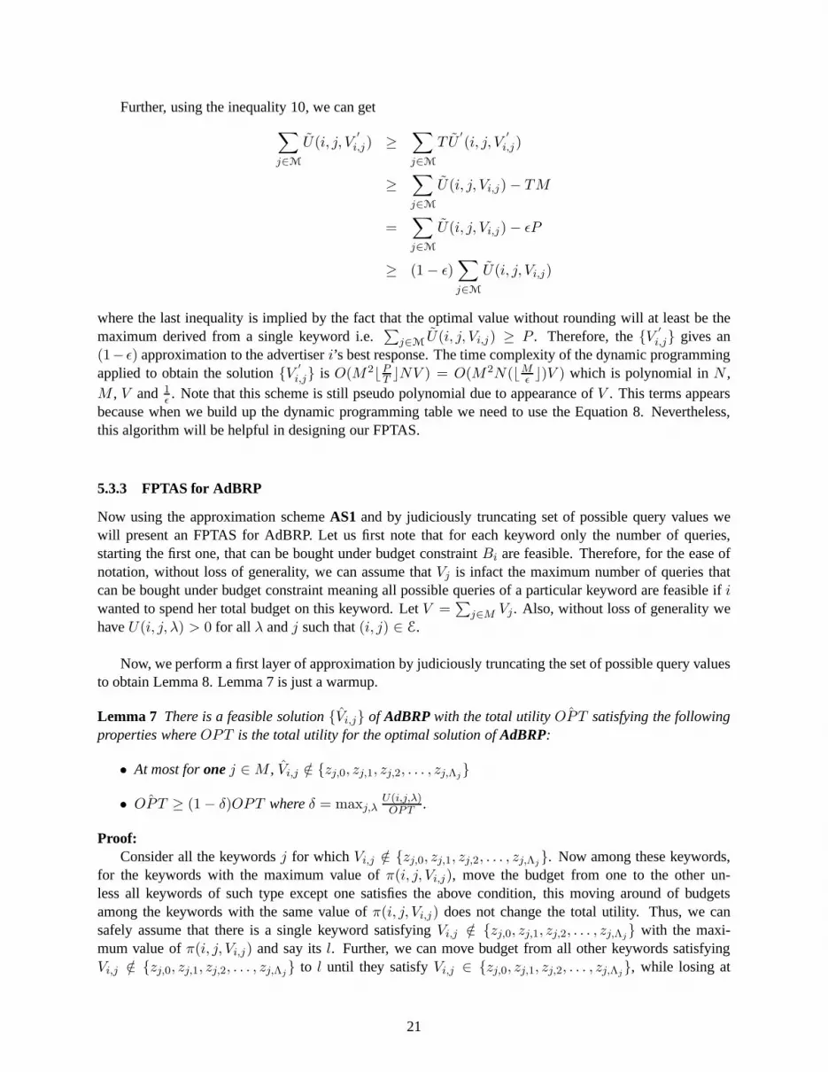
Now, we perform a first layer of approximation by judiciouslytruncating the set of possible query valuesto obtain Lemma 8. Lemma 7 is just a warmup.

Lemma 7 There is a feasible solution{Vi,j} of AdBRP with the total utility ˆOPT satisfying the followingproperties whereOPT is the total utility for the optimal solution ofAdBRP:

• At most forone j ∈M , Vi,j /∈ {zj,0, zj,1, zj,2, . . . , zj,Λj}

• ˆOPT ≥ (1− δ)OPT whereδ = maxj,λU(i,j,λ)OPT

.

Proof:Consider all the keywordsj for which Vi,j /∈ {zj,0, zj,1, zj,2, . . . , zj,Λj

}. Now among these keywords,for the keywords with the maximum value ofπ(i, j, Vi,j), move the budget from one to the other un-less all keywords of such type except one satisfies the above condition, this moving around of budgetsamong the keywords with the same value ofπ(i, j, Vi,j) does not change the total utility. Thus, we cansafely assume that there is a single keyword satisfyingVi,j /∈ {zj,0, zj,1, zj,2, . . . , zj,Λj

} with the maxi-mum value ofπ(i, j, Vi,j) and say itsl. Further, we can move budget from all other keywords satisfyingVi,j /∈ {zj,0, zj,1, zj,2, . . . , zj,Λj

} to l until they satisfyVi,j ∈ {zj,0, zj,1, zj,2, . . . , zj,Λj}, while losing at

21

mostu(i, l, Vi,l). This is because while doing this reallocation we lose only when we do not have enough

budget to move to buy the next query ofl. .

Lemma 8 For every given parameterǫ < 1, there is a feasible solution{Vi,j} of AdBRP with the totalutility ˆOPT satisfying the following properties whereOPT is the total utility for the optimal solution ofAdBRP:

• ˆOPT ≥ (1− ǫ2)OPT

• Vi,j ∈ {yj,0, yj,1, yj,2, . . . , yj,nj} for all j ∈M where theyj,. values are defined as follows:

for each partitionλ = 1, 2, . . . ,Λj of the keywordj let zj,λ − zj,λ−1 = a⌈Mǫ2⌉ + b wherea and

b are non-negative integers andb < ⌈Mǫ2⌉ (recall that zj,λ − zj,λ−1 is the size of partitionλ). Now

divide the partitionλ in to min{a, 1}.⌈Mǫ2⌉+b sub-partitions, the firstmin{a, 1}.⌈M

ǫ2⌉ sub-partitions

being of sizea queries each and the nextb partitions each of size1 query each. Defineyj,0 = 0 andyj,1, yj,2, . . . , yj,nj

as the end points of the sub-partitions created as above.

Proof: Clearly, each partition is divided in to at most2⌈Mǫ2⌉ sub-partitions and sinceΛj = O(N) we obtain

nj = O(NMǫ2

).

Let {Vi,j} be an optimal solution forAdBRP, then we find a solution{Vi,j} as follows:

• if Vi,j ∈ {yj,0, yj,1, yj,2, . . . , yj,nj} thenVi,j = Vi,j, therefore we do not lose anything in total utility

coming from keywordj by moving fromVi,j to Vi,j.

• if Vi,j /∈ {yj,0, yj,1, yj,2, . . . , yj,nj} then defineVi,j to be the maximum value among{yj,0, yj,1, yj,2, . . . , yj,nj

}which is smaller thanVi,j. Note that this case arises only whenVi,j comes from a sub-partition ofsizea > 1 and in that case there are at least⌈M

ǫ2⌉ sub-partitions of sizea with the same utility value

u(i, j, Vi,j) for each query in those sub-partitions. The maximum utilitythat we can lose by truncatingVi,j to Vi,j is≤ a u(i, j, Vi,j) ≤

1⌈M

ǫ2⌉

(

⌈Mǫ2⌉ a u(i, j, Vi,j)

)

≤ 1⌈M

ǫ2⌉OPT ≤ ǫ2

MOPT .

Note that the way we have constructed{Vi,j}, it satisfies the budget constraint of the advertiseribecauseVi,j ≤ Vi,j and hence{Vi,j} is a feasible solution ofAdBRP. Now, across all the keywordswe can lose at mostM ǫ2

MOPT i.e. ǫ2OPT by truncating the optimal solution{Vi,j} to the feasible

solution{Vi,j}. .

Now we perform a second layer of approximation by applyingAS1with truncated set of possible queryvalues as per Lemma 8. We present this approximation algorithm calledAS2 in the following.

1. Divide each partition of each keyword in to several sub-partitions as follows (same as in the proof ofLemma 8). For each partitionλ = 1, 2, . . . ,Λj of the keywordj let zj,λ−zj,λ−1 = a⌈M

ǫ2⌉+b wherea

andb are non-negative integers andb < ⌈Mǫ2⌉ (recall thatzj,λ− zj,λ−1 is the size of partitionλ). Now

divide the partitionλ in to min{a, 1}.⌈Mǫ2⌉+ b sub-partitions, the firstmin{a, 1}.⌈M

ǫ2⌉ sub-partitions

being of sizea queries each and the nextb partitions each of size1 query each. Defineyj,0 = 0 andyj,1, yj,2, . . . , yj,nj

as the end points of the sub-partitions created as above.

2. Apply AS1by restricting the query values to take values only from the set {yj,0, yj,1, yj,2, . . . , yj,nj}

i.e. by changing the recurrence relation 8 to

A(j+1, p) = minxi,j+1∈{yj,0,yj,1,yj,2,...,yj,nj

}:U(i,j+1,xi,j+1)≤p

{

C(i, j + 1, xi,j+1) + A(j, p − U(i, j + 1, xi,j+1))}

(11)

22

and with the error parameterǫ, where1ǫ

= 1ǫ

+ 1 ≤ 2ǫ.

The total utility of the solution returned by the algorithmAS2 is

≥ (1− ǫ)(1 − ǫ2)OPT = (1−ǫ

1 + ǫ)(1− ǫ2)OPT = (1− ǫ)OPT.

The time complexity in constructing the sub-partitions isO(NMǫ2

) and that of applyingAS1on the

truncated set of query values{yj,0, yj,1, yj,2, . . . , yj,nj} isO(M2N(⌊M

ǫ⌋)NM

ǫ2) = O(M4N2

ǫ3) as1

ǫ= 1

ǫ+1 ≤

2ǫ

= O(1ǫ). Therefore,AS2 is indeed aFPTAS for AdBRP.

5.4 To Broad-match or not to Broad-match

In this section, we start out with a very important observation in the following theorem.

Theorem 9 A BMG does not necessarily have a uniqueBME and the differentBMEs can yield differentrevenues to the auctioneer. Moreover, in one of them the auctioneer loses while in the other one it gains interms of revenue.

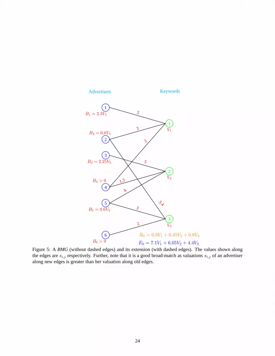
The Theorem 9 leaves the auctioneer in a dilemma about whether he should broad-match or not. If hecould somehow predict which choice of broad match lead to a revenue improvement for him and which not,he could potentially choose the ones leading to a revenue improvement. This brings forth one of the bigquestions left open in this paper, that is of efficiently computing aBME / ǫ-NE, if one exists, given a choiceof broad match. We plan to explore it in our future works. The proof of the above theorem follows fromexamples constructed in Figures 5, 6, 7. Further,in all the examples we takeK = 2, γ1 = 1, γ2 = 0.7.

We also note several other observations such as

• introducing an edge may or may not shift theBME ( See Figures 8,9)

• introducing an edge can shift theBME to one yielding less revenue to the auctioneer , as well as, toone with less efficiency i.e. social welfare ( See Figure 1, 9)

• introducing new edges can shift theBME to one yielding more revenue to the auctioneer (See Figures9, 5, 6, 7)

• unlike in Figure 9, an extension of aBMG may not have aBMEwhere for all nodes the degree is thesame as in theBME for the baseBMG. See Figures 1, 6, 7.

It is instructive to note that all the above observations (including Theorem 9) continue to holdunder the solution concept ofǫ-NE.

23

2

6B6 > 0

3V3

35

B5 = 0.6V3

1.5

4

B4 > 0

2V2

53

B3 = 2.25V2

3

2

B2 = 0.6V3

1V1

51

B1 = 2.3V1

R0 = 0.9V1 + 0.45V2 + 0.6V3

Advertisers Keywords

E0 = 7.1V1 + 6.05V2 + 4.4V3

3.4

2

4

Figure 5: ABMG (without dashed edges) and its extension (with dashed edges). The values shown alongthe edges aresi,j respectively. Further, note that it is a good broad-match asvaluationssi,j of an advertiseralong new edges is greater than her valuation along old edges.

24

V3

6

3

05

V2

4

2

V2

3

0

2

1

V1

1

R = R0 + 11.4V3

7 − 0.3V1

E = E0 + 1.4V3 − 0.7V1

V3

V 1

47V 3

MP+2,1 = 0.5

MP−

2,3 = 4.67

MP−

5,2 = 1.67

MP+

5,3 = 0.5

Figure 6: OneBME for the extension ofBMG in Figure 5 ( the valuesVi,j at thisBME are shown alongcorresponding edges).Not a pure Nash equilibrium but an ǫ-NE for ǫ ≥ 0.15.

25

V3

6

3

V3

5

V2

4

2

V2

3

37V3

2

1

V1

1

R = R0 + 9.3V3

7 − 0.3V1

E = E0 + 0.73V3

7 − 0.7V1

0

V 1

0

MP−

2,1 = 0.5

MP+

2,3 = 0.48

MP+

5,2 = 1.67

MP−

5,3 = 4

Figure 7: AnotherBME for the extension ofBMG in Figure 5.Also a pure Nash equilibrium, therefore anǫ-NE for ǫ ≥ 0.

26

2,V2

4B4

u4 = 1.4V2

2V2

R2 = 0.6V2

4,V2

3B3 = 0.6V2

u3 = 3.4V2

3,V1

2

B2 = 1.4ǫV1

u2 = 2.1V1

1V1

R1 = 0.9V1

5,V1

1B1 = 2.1V1

u1 = 4.1V1

R = 0.9V1 + 0.6V2

Advertisers Keywords

4, 0

E = 7.1V1 + 6.4V2

Figure 8: No Shift in Equilibrium due to the new edge (3,1). The values shown along edge(i, j) is (si,j, Vi,j).ui denote total payoff of advertiseri.

2,V2

4B4

u4 = 2V2

2V2

R2 = 0.0

4, 03

B3 = 0.6V2

u3 = 3.567V2

3,V1

2

B2 = 1.4ǫV1

u2 = 2.1(V1 −V2

6)

1V1

R1 = 0.8V2 + 0.9V1

5,V1

1B1 = 2.1V1

u1 = 1.4V2

6+ 4.1(V1 −

V2

6)

R = 0.8V2 + 0.9V1 > 0.9V1 + 0.6V2

Advertisers Keywords

25,V2

6

Assume:V1 > V2

6

E = 6.749V2 < 7.583V2 for V1 = V2

6

Figure 9: A Shift in Equilibrium due to the new edge (3,1). Thevalues shown along edge(i, j) is (si,j, Vi,j).ui denote total payoff of advertiseri.

27

6 Auctioneer Controlled Broad Match(AcBM)

In this section we study the second broad match scenario i.e.AcBMas described in section 4. First, we needa few definitions.

Definition 10 Excess Budget:LetG = (N,M,E) be aBMG andG′= (N,M,E

′) be an extension (broad-

match) ofG. For ani ∈ N, let Di denote the budget ofi unspent inG and letsi = maxj∈E si,j. We say thati has an excess budget inG iff si ≤ Di.

Intuitively, what we mean by an advertiser to have an excess budget is that she has enough amount currentlyleft unspent so that she can participate in at least one queryof any of the keywords she is currently biddingon, if given a chance, irrespective of the valuations of her competitors.

Definition 11 Revenue Improving Broad-Match: An extensionG′= (N,M,E

′) of BMG G = (N,M,E)

is called revenue improving if there exist an allocation of the excess budgets along new edges (i.e. edges inE

′\ E) so that the sum of total budget spent by all the advertisers is more inG

′than inG, as well as, there

is a strongly polynomial time algorithm to find such an allocation of the excess budgets.

Now, for a keywordj, let I(j, l) denote the set of advertisers having sufficient budget to participate inthe lth query of this keyword. The following lemma can be obtainedin a way similar to the Lemma 1 andagain utilizing the partition structure per this lemma, we obtain Observation 13 that as long as the qualityof broad-match isgoodin some sense, the auctioneer can guarantee a better revenuefor himself by suitablyexploiting the extension.

Lemma 12 Given the budget splitting of all the advertisers for theBMG G = (N,M,E) (i.e. the cur-rent budget splitting ), that is the valuesBi,j ’s for all (i, j) ∈ E, there exist non-negative integersΛj,zj,0, zj,1, zj,2, . . . , zj,Λj

, and setsIj,1, Ij,2, . . . , Ij,Λj, Ij for all j ∈ M} such thatΛj = O(N) and for

all 0 ≤ λ ≤ Λj − 1, c(i, j, l) = C(i, j, λ), I(j, l) = Ij,λ+1 ∀zj,λ < l ≤ zj,λ+1 whereC(i, j, λ) :=c(i, j, zj,λ + 1), Ij,λ+1 := I(j, zj,λ + 1) and Ij = {i ∈ N : (i, j) ∈ E, i has an excess budget inG}.Moreover, all theseΛ, z, C, I values can be computed together in time polynomial inN , M andK.

Observation 13 Let G′

= (N,M,E′) be an extension ofBMG G = (N,M,E), I = ∪j∈MIj , Ji =

{

j ∈M : (i, j) ∈ E′\ E

}

for i ∈ I, Γj ={

i ∈ N : (i, j) ∈ E′}

, and Φ ={

j ∈M : Ij,Λj= φ

}

. This

extension is revenue improving if there is ani ∈ I having one or more of the following properties/conditions:

a) ∃j ∈ Ji \ Φ such thatIj,Λj= Ij and |

{

m ∈ Ij,Λj: sm,j > si,j

}

| < K.

b) ∃j ∈ Ji ∩ Φ such that| {l ∈ I ∩ Γj : sl,j = si,j} ∪ {l ∈ Γj : sl,j < si,j} | > 1.

c) ∃j ∈ Ji \ Φ such thatIj,Λj6= Ij andsi,j > maxl∈Ij,Λj

\Ijsl,j .

Intuitively, the propertiesa) andc) says that there is an advertiseri with excess budget inG and a keywordj such thati has a good enough valuation forj in G

′so as to obtain a slot, and moreover ifi is brought in

for the last query, all advertisers already participating in that query have still enough budget to participatein that query. The conditionb) says that there is a keywordj with unsold queries inG and we can sellthese queries inG

′to at least two advertisers13. Thus, these conditions allow the auctioneer to bring addi-

tional advertiser(s) for the keywordj to j’s last query or equivalently the very first query in the last partition

13Note that just selling to one advertiser does not generate any money in GSP. In practice, however Google/Yahoo! charges aminimum amount i.e. a reserve price for the last slot. Nevertheless, all the results we present remains unchanged by introducingreserve prices for the last slot. In that case, the conditionb) will change to∃j ∈ Ji ∩ Φ.

28

((zj,Λj−1 + 1)th query) so that revenue extracted from this particular query is improved without changingthe revenue generated from any other query. Therefore, in terms of the existence of a revenue improvingextension we have the above observation. Nevertheless, in general the auctioneer can do much more thanthe above trivial way. In particular, there might be severali andj’s satisfying the properties in Observation13 and he could exploit this profitably. Recall that he has a finer control over which query to start withand whatever part of excess budget he can spend along edges inE

′\ E. So his task is to choose splitting

of excess budgets along new edges as well as to decide a starting query number. In general, there couldbeO(N) advertisers with excess budgets and there could beO(MN) new edges, finding the best splittingis a variant of Integer Knapsack problem again and thus computationally hard. Nevertheless, it is clearlypossible to design strongly polynomial time sub-optimal algorithm that does significantly better than thetrivial improvement possible by increasing competition for the last query. The problem with participatingstarting a query in other partitions is that it may change thepartition structure in a way that is not revenueimproving, but since there are onlyO(N) such partitions for each keyword, we could check for each parti-tion whether starting with its first query is revenue improving or not. Indeed, it is easy to think of a stronglypolynomial time algorithm that finds excess budget splittings which improves revenue, one that moves frompartition to partition, taking starting query as the first query in that partition and then doing a binary searchfor appropriate budget (as high as possible) to be allocatedand tracks which one of these possibilities leadto the highest revenue. Note that since we are doing a binary search on budget (and equivalently on thenumber of queries to participate in), we are still in strongly polynomial time regime. Finally, it should beinteresting to search for efficient algorithms generating better revenue and in particular a FPTAS, possiblyby efficiently searching for which query to start with along with efficiently searching for how many queriesto participate for.

Now, given that auctioneer’s goal is primarily to improve revenue, we should also analyze what happensto the efficiency (i.e. social welfare), if the auctioneer implements such revenue improving broad-match.First, it is clear that if auctioneer’s goal were to improve social welfare instead of revenue, he could cer-tainly do so in a way similar to the one discussed above for revenue improvement. Moreover, revenue andsocial welfare could infact be improved together if one of the conditions in Observation 13 holds and theproof is same as that for Observation 13 by bringing in appropriate advertiser(s) in the last query of an ap-propriate keyword. However, if auctioneer deviates from this trivial way of improving revenue, which infacthe will do if his goal is to maximize revenue, there can often be a tradeoff with social welfare. For an explicitexample of this tradeoff please refer to Figure 10. Furthermore,even when the conditions in Observation 13are NOT satisfied, there might still be a possibility of revenue improvement(ref. Figure 1).

29

1

4B4 = 20

2V2 = 100

1.53

B3 = 40

3

2B2 = 37

1V1 = 100

51

B1 = 45

2

z1,0 = 0 z1,1 = 50

I1,1 = {1, 2}

R0 = 50× (0.3× 3) = 45

E0 = 50× (5 + 0.7× 3) + 50× 3 = 505

z1,2 = 100

I1,2 = {2}

a)

0 19

{1, 2, 3}

36

{2, 3}

100

{3}

Ra = 19× (0.3× 3 + 2× 1.4× 2) + 17× (0.3× 2) = 80.5 > R0

Ea = 19× (5 + 0.7× 3) + 17× (3 + 0.7× 2) + 64× 2 = 337.7 < E0

b)

0

{1, 2}

50 100

{2, 3}

Rb = 50× (0.3× 3) + 50× (0.3× 2) = 75 > R0

Eb = 50× (5 + 0.7× 3) + 50× (3 + 0.7× 2) = 575 > E0

R0 < Rb < Ra butEa < E0 < Eb

c)

0

{1, 2} {1, 2, 3} {2, 3}

403 21 100

{3}

Rc = 3× (0.3× 3) + 18× (0.3× 3 + 2× 0.7× 2) + 19× (0.3× 2) = 80.7

Ec = 21× (5 + 0.7× 3) + 19× (3 + 0.7× 2) + 60× 2 = 352.7

Rc > Ra

Figure 10: Tradeoff in revenue and social welfare, the baseBMGdoes not include edge(3, 1), its extensiondoes. The revenue and efficiency value is just for keyword1, as these values do not change for keyword2 even in the extension. In a) and b) advertiser3 is brought in for keyword1 starting with first queryin partition 1 and2 respectively. Note that the choice of partition with betterrevenue is the one whereefficiency decreases.c) shows that just starting with the first query of a partition may not lead to optimalrevenue, for example if3 is started with4th query then the revenue improvement is even better thana) orb).

30

7 Future Directions

We have initiated a study of broad-match, an interesting aspect of sponsored search advertising, and as com-mon to papers that initiate a new direction of study, this paper leaves out several important open problemsthat deserve theoretical investigation and analysis. We discuss some of these interesting problems in thefollowing.

Budget Splitting Games(BSG): Abstracting the settings in Broad-Match Game can provide uswith a richclass of mutli-player games having compact representations. It should be interesting to study these gamesand to consider the budget splitting/allocation scenariosbeyond the currently prevailing models for spon-sored search advertising, as well as, other interesting applications. Herebelow we provide an abstraction.

An instance ofBSGis given by(N,M,E, B, V,O). N is the set of players,M is set of distinct type ofindivisible items and(N,M,E) is a bi-partite graph between the players and items wherein an (i, j) ∈ E iffthe playeri ∈ N is interested in buying the itemj ∈M (i.e. i have a positive valuation forj). B = {Bi}i∈N

is the budget vector,Bi being the total budget of playeri. V = {Vj}j∈M is the volume vector,Vj beingthe total number of units of the itemj for sale. Let|N| = N and |M| = M . O is an oracle that takesas input(i, j) ∈ E and a set of budget values{Bn,j}n∈N−{i} and output the set of valuesΛj = O(N),zj,0 = 0, zj,1, zj,2, . . . , zj,Λj

= Vj, andC(i, j, λ), U(i, j, λ) for all 0 ≤ λ ≤ Λj − 1, to be interpretedas follows: given that for alln ∈ N − {i}, the playern spends/allocates an amountBn,j on the itemj,C(i, j, λ) andU(i, j, λ) respectively are the cost and the utility for each unit of theitem if the playeridecides to buyzj,λ < Vi,j ≤ zj,λ+1 units of the itemj. Each player has access to the oracleO. The strategyof a playeri is to split her budget across various items that is to choose the values{Bi,j}j∈M:(i,j)∈E suchthat

∑

j∈M:(i,j)∈EBi,j ≤ Bi and correspondignly the number of units of the various items{Vi,j}j∈M:(i,j)∈E

with Vi,j ≤ Vj. The payoff of a player is the total utility it derives acrossall the items from their units shebought as per her chosen strategy.

Note that this abstraction nicely captures the Broad-MatchGame studied in the present paper whereinan item is a keyword and a query of a keyword corresponds to a unit. The oracleO corresponds to theLemma 1. Further, by varying the properties satisfied by the valuesC(i, j, λ), U(i, j, λ)’s we may obtainother interesting scenarios.

Complexity of Auctioneer’s Dilemma: The Theorem 9 leaves the auctioneer in a dilemma about whetherhe should broad-match or not. If he could somehow predict which choice of broad match lead to a revenueimprovement for him and which not, he could potentially choose the ones leading to a revenue improvement.This brings forth one of the big questions left open in this paper, that is of efficiently computing aBME /ǫ-NE, if one exists, given a choice ofbroad match, as well as, to efficiently decide whether a given broadmatch is revenue improving or not in theAdBMscenario.

Existence of pure NE/ǫ-NE/BME in Broad-Match Game: Despite some effort we have not been able toshow that a Broad-Match Game always admits pure NE or evenǫ-NE or BME. On the other hand we havealso not been able to construct examples where they do not exist. The problem arises from the fact that thepayoff funtions are discontinuous and not even quasi-concave. Therefore, the existing techniques or theirsimple extensions do not seem to work. This calls for developing new techniques for proving the existenceof pure Nash equilibria and the complexity of deciding the existence in general, and for the Broad-MatchGame and BSGs in particular.

Quantifying the Effect of Broad-Match: As per various observations including Theorem 9 obtained inthe Section 5.4 we know that the the revenue of the autioneer and the social welfare could very well degrade

31

by incorporating broad-match and it would be interesting tocharacterize the extent of such degradation.

Total Click-Through-Rates as Payoff: It would be interesting to analyze the effect of broad-matchin ascenario where the advertisers are interested in maximizing their total Click-Through-Rate across variouskeywords rather than their total utilities. Note that the budget splitting game arising in this sceneario indeedfits in our abtract model ofBSGdiscussed earlier in this section. With the intuition developed from this paper,we believe that similar conclusions hold true even in the case of total Click-Through-Rates as payoffs.

BME vs ǫ-NE: As we argued in the paper, both theBME and ǫ-NE are reasonable solution conceptsfor the Broad-Match Game. Further, we constructed exampleswhere the both solution concepts coincide.Nevertheless, it would be nice to study these two concept comparatively at a finer level. For example,BMEmay not provide good approximation guarantee to the advertisers but it demands less shophistication levelfrom them than that required for good approximation guarantee.

Network Level Competition via Broad-Match Game: The framework provided in the present paperis easily applicable to the scenario where advertisers are trying to optimally split budgets across variouskeywordscoming from several competing search engines.How does the revenue of one search engine getseffected by the fact that another competeting search engineoffers broad-match? For example consider theBMG in the Figure 9, without the dashed edge(3, 1), and suppose that the keyword1 is coming from thesearch engine1 and the keyword2 is coming from the serach engine2. Now if the search engine1 doesbroad-match and introduces the new edge(3, 1) then we can see that the revenue of the search engine1increases whereas that of search engine2 decreases. It should be interesting to further explore thisdirection.

Formalizing a Notion of “Good” Broad-Match: In the analysis we have presented, we have not con-sidered costs incurred by the auctioneer in the short run dueto uncertainty about the extended part of theBMG, although we can expect that as long as the quality of broad match being performed is good, such costsshould be minimal. Nevertheless, formalizing a notion ofgoodbroad match should be interesting. Featuressuch as the improvement in the relevance scores and conversion rates should be an essential ingredient ofa goodbroad match. Further, the conditions noted in the Observation 13 also provides some sense of whatshould be the features of a good broad-match from the viewpoint of the auctioneer.

Acknowledgements: We thank Gunes Ercal, Himawan Gunadhi, Adam Meyerson and Behnam Rezaeifor discussions and anonymous reviewers of an earlier version for valuable comments and suggestions. SKSthanks Zoe Abrams, Arpita Ghosh, Gagan Goel, Jason Hartline, Aranyak Mehta, Hamid Nazerzadeh, andZoya Svitkina for useful discussions during WINE 2007.

References

[1] G. Aggarwal, A. Goel, R. Motwani, Truthful Auctions for Pricing Search Keywords, EC 2006.

[2] C. Borgs, J. Chayes, N. Immorlica, K. Jain, O. Etesami, and M. Mahdian, Dynamics of bid optimiza-tion in online advertisement auctions, WWW 2007.

[3] M. Cary, A. Das, B. Edelman, I. Giotis, K. Heimerl, A. R. Karlin, C. Mathieu, and M. Schwarz,Greedy bidding strategies for keyword auctions, EC 2007.

[4] B. Edelman and M. Ostrovsky, Strategic bidder behavior in sponsored search auctions, Decis. SupportSyst., 43(1):192-198, 2007.

32

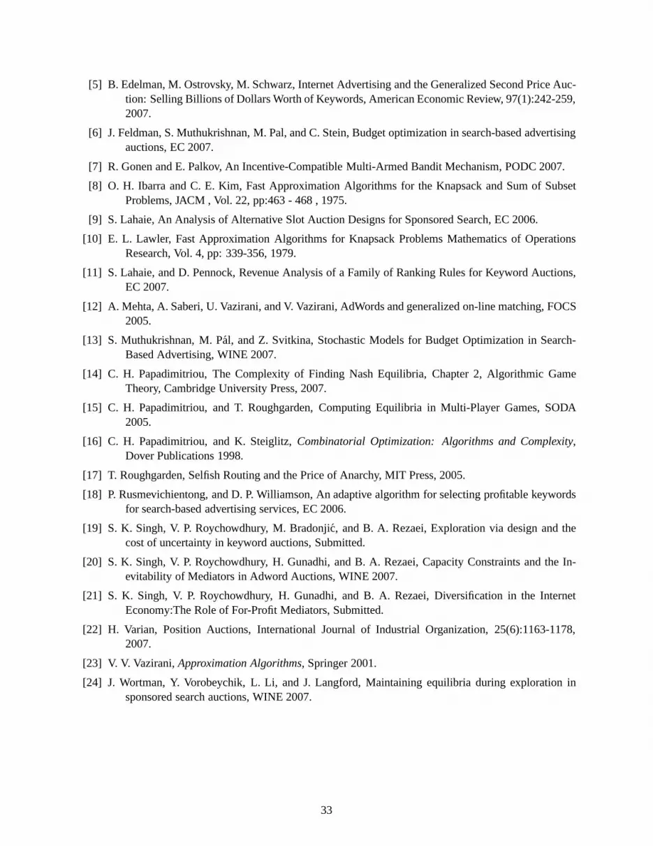
[5] B. Edelman, M. Ostrovsky, M. Schwarz, Internet Advertising and the Generalized Second Price Auc-tion: Selling Billions of Dollars Worth of Keywords, American Economic Review, 97(1):242-259,2007.

[6] J. Feldman, S. Muthukrishnan, M. Pal, and C. Stein, Budget optimization in search-based advertisingauctions, EC 2007.

[7] R. Gonen and E. Palkov, An Incentive-Compatible Multi-Armed Bandit Mechanism, PODC 2007.

[8] O. H. Ibarra and C. E. Kim, Fast Approximation Algorithmsfor the Knapsack and Sum of SubsetProblems, JACM , Vol. 22, pp:463 - 468 , 1975.

[9] S. Lahaie, An Analysis of Alternative Slot Auction Designs for Sponsored Search, EC 2006.

[10] E. L. Lawler, Fast Approximation Algorithms for Knapsack Problems Mathematics of OperationsResearch, Vol. 4, pp: 339-356, 1979.

[11] S. Lahaie, and D. Pennock, Revenue Analysis of a Family of Ranking Rules for Keyword Auctions,EC 2007.

[12] A. Mehta, A. Saberi, U. Vazirani, and V. Vazirani, AdWords and generalized on-line matching, FOCS2005.

[13] S. Muthukrishnan, M. Pal, and Z. Svitkina, StochasticModels for Budget Optimization in Search-Based Advertising, WINE 2007.

[14] C. H. Papadimitriou, The Complexity of Finding Nash Equilibria, Chapter 2, Algorithmic GameTheory, Cambridge University Press, 2007.

[15] C. H. Papadimitriou, and T. Roughgarden, Computing Equilibria in Multi-Player Games, SODA2005.

[16] C. H. Papadimitriou, and K. Steiglitz,Combinatorial Optimization: Algorithms and Complexity,Dover Publications 1998.

[17] T. Roughgarden, Selfish Routing and the Price of Anarchy, MIT Press, 2005.

[18] P. Rusmevichientong, and D. P. Williamson, An adaptivealgorithm for selecting profitable keywordsfor search-based advertising services, EC 2006.

[19] S. K. Singh, V. P. Roychowdhury, M. Bradonjic, and B. A.Rezaei, Exploration via design and thecost of uncertainty in keyword auctions, Submitted.

[20] S. K. Singh, V. P. Roychowdhury, H. Gunadhi, and B. A. Rezaei, Capacity Constraints and the In-evitability of Mediators in Adword Auctions, WINE 2007.

[21] S. K. Singh, V. P. Roychowdhury, H. Gunadhi, and B. A. Rezaei, Diversification in the InternetEconomy:The Role of For-Profit Mediators, Submitted.

[22] H. Varian, Position Auctions, International Journal of Industrial Organization, 25(6):1163-1178,2007.

[23] V. V. Vazirani,Approximation Algorithms, Springer 2001.

[24] J. Wortman, Y. Vorobeychik, L. Li, and J. Langford, Maintaining equilibria during exploration insponsored search auctions, WINE 2007.

33