How does the trans–cis photoisomerization ofazobenzene take place in organic solvents?

Giustiniano Tiberio, Luca Muccioli, Roberto Berardi and Claudio Zannoni∗

Dipartimento di Chimica Fisica e Inorganica and INSTM, Universita diBologna ,viale Risorgimento 4, IT-40136 Bologna, Italy

∗ Fax: +39 051 644 7012, E-mail: Claudio.Zannoni@unibo.it

Abstract

The trans–cis photoisomerization of azobenzene–containing ma-terials is key to a number of photomechanical applications, but theactual conversion mechanism in condensed phases is still largely un-known. Here we have studied the (n, π∗) isomerization in vacuumand in various solvents via a modified molecular dynamics simula-tion adopting an ab initio torsion–inversion force field in the groundand excited states while allowing for electronic transitions and for astochastic decay to the fundamental state. We have determined thetrans–cis photoisomerization quantum yield and decay times in var-ious solvents (n–hexane, anisole, toluene, ethanol and ethylene gly-col), obtaining results comparable with the experimental ones whereavailable. We find a profound difference between the isomerizationmechanism in vacuum and in solution, with the often neglected mixedtorsional–inversion pathway being the most important in solvents.

Keywords

Azo compounds*, Isomerization*, Molecular Dynamics*, Photoresponsive Ma-terials, Actuators, Atomistic Simulation(basic keywords* )

1 Introduction

It is well known that AB and its derivatives can undergo a major structuralchange upon irradiation with light, transforming from the longer trans–isomerto the shorter, bent, cis–isomer and vice versa. This variation, coupled withthe high stability of the cis form and the reversibility of the isomerization,

1

now published in ChemPhysChem, 11, 1018-1028(2009)

can be exploited in the design of materials with photo–switchable physicalproperties [1, 2, 3, 4] for photonic [5] and micro– and nano–scale device appli-cations [6, 7, 8, 9, 10, 11, 12]. Understanding the molecular mechanism of thetrans-cis conversion and how it can take place in the crowded environment ofa condensed phase is thus a task of great importance but also one of consider-able complexity that still awaits to be clarified. This is not surprising, sincethe simulation of photoisomerization, which includes excited states dynam-ics and nonadiabatic crossings between different electronic states has beenchallenging computational chemists and physicists [13, 14, 15, 16] since manyyears, even in the gas phase. In particular, notwithstanding the considerableprogress of quantum chemical excited state methods in the investigation ofpotential energy surfaces (PES) and of their intersections [17], in nonadi-abatic dynamics techniques [18, 19, 20, 21, 22], a fully quantum chemicalsimulation [23] of a photochemical process in a complex environment andat given thermodynamic conditions is still not feasible. In the search of asuitable approximation that reduces the computational burden to amenablelevels, a number of proposals for treating various contributions to the totalhamiltonian at different levels of theory have been put forward. For exam-ple in the QM/MM approach some atoms, usually belonging to the solvent[24, 25, 26] or to the non-active part of a large molecule[27, 28] are treatedclassically, while in the molecular-mechanics valence bond method [29] andin the tight binding density functional theory [30] the subdivision regardsthe electrons on each atom. Also more affordable semi-empirical hamiltoni-ans, suitably parametrized by means of higher level calculations, have beenemployed to describe the dynamics of a chromophore [31, 32, 33], with con-siderable advantages in terms of computational time, while the interactionwith the surrounding environment is again modeled with classical force fields.

However, a further drastic simplification is needed to be able to studythe photochemistry of complex systems with adequate sampling and timescales, and it would be desirable to extend to excited states the applicationof classical force fields, that have proved to be successful in describing andpredicting ground state physical properties. While is certainly becoming pos-sible for phenomena which are determined by the excited states equilibriumgeometries, such as steady emission spectra [34], since in principle they canbe described as accurately as the ground one with molecular mechanics, theclassical description of dynamics processes that take place upon photon ab-sorption is by far more complicate, given the large displacements from theexcited state equilibrium geometry that can follow a Franck-Condon transi-

2

tion from the ground state. It is also worth noting that the curvature of thepotential energy surface (PES) along these displacement coordinates is hardlyrepresentable with harmonic functions of normal modes. In this context, ithas proved helpful to select the vibronic channels relevant for the dynamics[35, 36] and treating them at quantum mechanical level, while adopting amore approximate descriptions for the less relevant ones.

On the positive side, the AB photophysics at the root of the conforma-tional change has been extensively studied for fifty years, and various essentialfeatures are now understood, at least in the gas phase. The process, thattypically occurs in the picosecond time scale, can involve a (n, π∗) or a (π, π∗)absorption, depending on the excitation wavelength [31, 37, 38, 39]. In themost common experimental conditions (a near UV excitation), a three–statemechanism seems to take place, with promotion from the fundamental stateS0 of the trans isomer to the second singlet excited state S2, followed by adecay to the first singlet state S1, and finally by a decay, either non–radiativevia conical intersection (S0/S1 CI) or radiative by weak fluorescence, to the S0

state. The process can be even more complex and some authors have recentlypointed out the importance of other singlet and triplet states [31, 40, 41, 42].By comparison, the photophysics of the process following the (n, π∗) absorp-tion from the ground state in the visible (λ = 440− 480 nm) is simpler as itinvolves only the first excited state S1 [39, 43, 44]. In addition to the photo-physical aspects, the intramolecular mechanism of the isomerization processinvolves two basic pathways: torsion (changing the dihedral angle Ph-N=N-Ph), that requires a reduction of the order of the nitrogen-nitrogen doublebond, and inversion, that implies a wide increase of the Ph-N=N bendingangles with an exchange of the position of the lone pair of one of the nitro-gens. The two mechanisms have often been considered in alternative, andtheir relative contributions to the isomerization is still controversial even inthe gas phase, although some precious clarification has been provided by re-cent works [31, 41]. In the more general case the photoactive molecule canbe considered to undergo a mixed mechanism that involves both processesand that reduces to pure torsion or inversion only in the limiting cases. Sur-prisingly enough the trans–cis quantum yield for the (n, π∗) is nearly doublethan that of the (π, π∗) in n–hexane [45], while according to the standardwisdom (Kasha rule) they should be the same. This violation seems to begeneralizable to other aromatic compounds containing the nitrogen-nitrogendouble bond, such as phenylazo imidazoles [46].

Given that in all practical applications the AB photoisomerization takes

3

place in solution or in a polymer, it is somehow disappointing that the vastmajority of the theoretical information available only refers to isomerizationin the gas phase, where the conformational change is not hindered by theenvironment and where we can expect that the mechanism can be different.As we have seen, part of the difficulty in studying the solvent environmenteffects on the trans–cis isomerization is due to the need of building a modelof the process that combines the essential photophysics with an atomisticdescription of the guest–host system.

Here we wish to contribute to this challenging task by following the pho-tophysically simpler (n, π∗) transition in various low molar mass organic sol-vents using non equilibrium molecular dynamics (MD) simulations, allowingalso for transitions from the ground to the excited state and back duringthe time evolution. The method we propose is in essence a simple QM/MDscheme and we aim at testing the methodology as well as getting new physi-cal insights on the mechanism of photoisomerization in organic solvents. Webelieve this investigation to be particularly timely, since significant experi-mental studies on AB photoisomerization in solution following a S1 excitationhave started to appear [39].

The paper is organized as follows: in the next section we introduce themodels adopted for the AB ground and excited states, then we describe ourprocedure for modelling with “virtual experiments” the transitions betweenthe two states, while parameterization details are given in Appendix. We alsodiscuss the modelling of the various solvents and the simulation conditions.In the latest sections we describe our simulations results, discussing the iso-merization mechanism, and its modifications when going from vacuum tosolvents and providing a comparison with experimental data when available.

2 Models and Simulation Details

2.1 Azobenzene ground and excited states

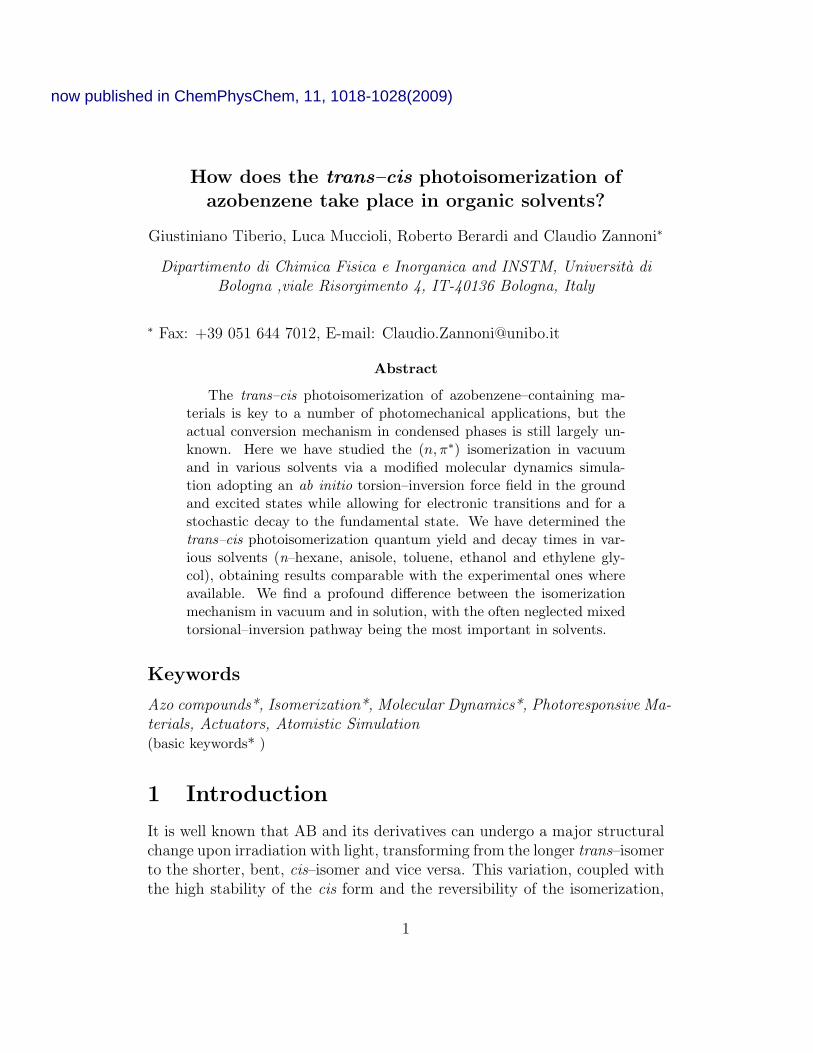
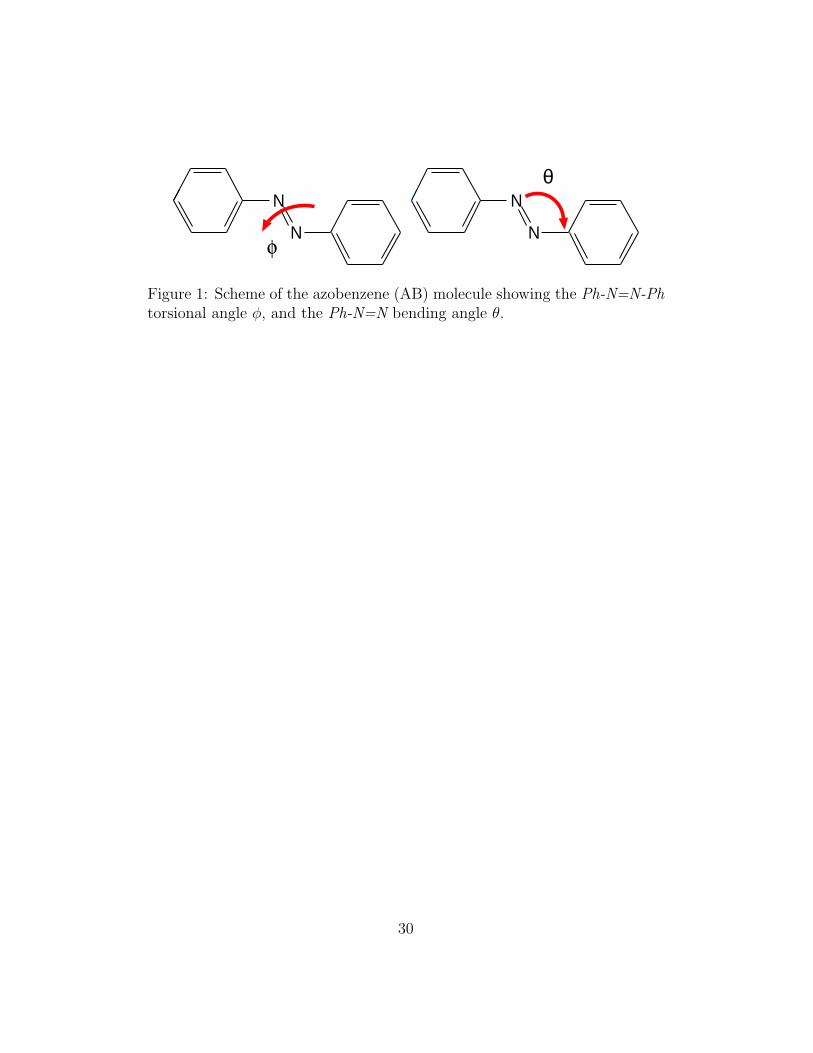
We have modeled the AB molecule at fully atomistic level starting from theAMBER molecular mechanics force field (FF) [47], similarly to other recentstudies of AB derivatives [48, 49] and modifying some terms in order toapproximate ab initio energy profiles. The trans–cis isomerization directlyinfluences at least five internal degrees of freedom [50], namely: the Ph-N=N-Ph torsional angle (φ), the two Ph-N=N bending angles (θ), and both N=N

4

and Ph-N bond lengths. Since the only QM complete PES for azobenzeneavailable in the literature is restricted only to the two most important internalcoordinates, the torsional angle φ and one of the bending angles θ [38], andalso because of the increasing computational complexity associated to the useof manifold PES, we limit here the QM-derived force field contributions onlyto these two degrees of freedom. The remaining ones instead are assumed tobe reasonably described, for the purpose of this study, by the AMBER FFfor the ground state. We note that this simplification may possibly lead toan incorrect description of the symmetric inversion channel, a decay pathwayproducing the trans isomer which is probably responsible for the quantumyield decrease upon S2 (ππ∗) excitation, but should be scarcely relevant forS1 excitation [44, 51].

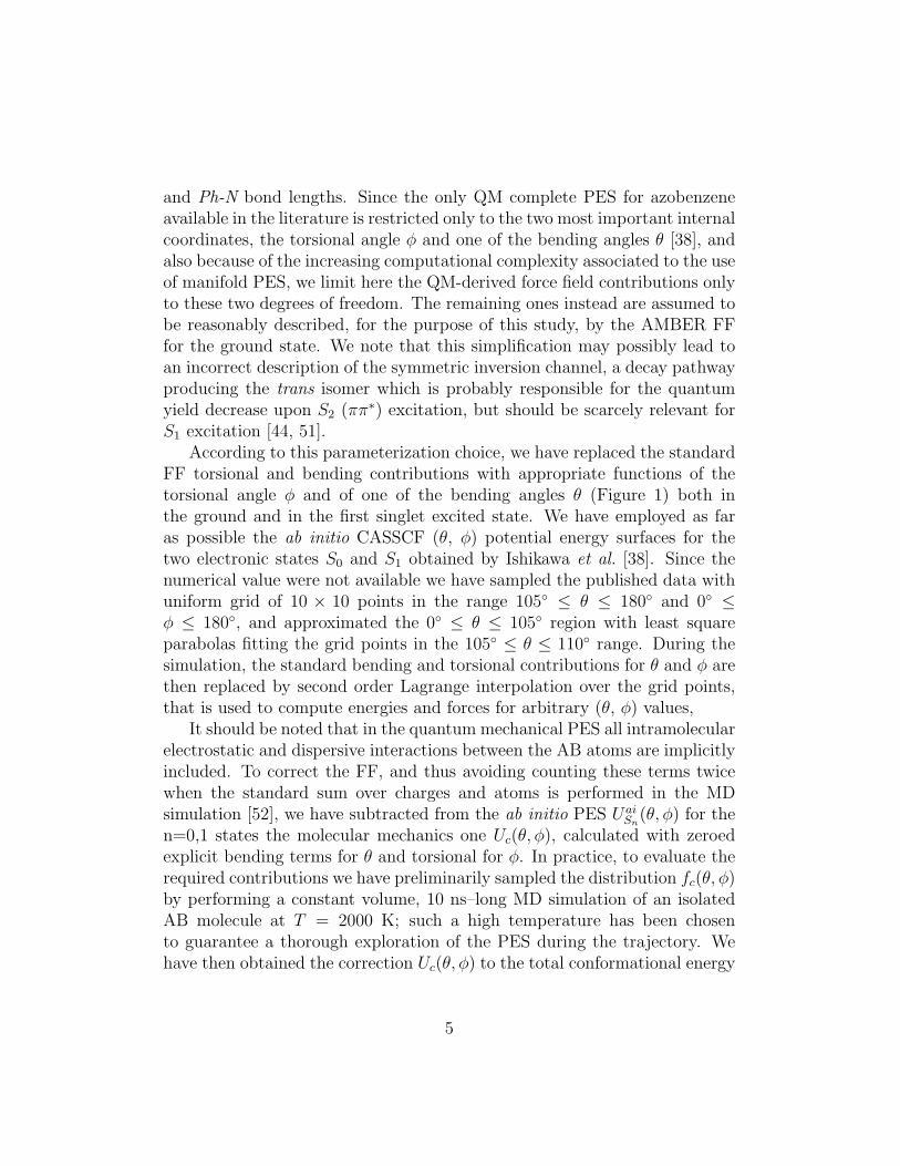
According to this parameterization choice, we have replaced the standardFF torsional and bending contributions with appropriate functions of thetorsional angle φ and of one of the bending angles θ (Figure 1) both inthe ground and in the first singlet excited state. We have employed as faras possible the ab initio CASSCF (θ, φ) potential energy surfaces for thetwo electronic states S0 and S1 obtained by Ishikawa et al. [38]. Since thenumerical value were not available we have sampled the published data withuniform grid of 10 × 10 points in the range 105◦ ≤ θ ≤ 180◦ and 0◦ ≤φ ≤ 180◦, and approximated the 0◦ ≤ θ ≤ 105◦ region with least squareparabolas fitting the grid points in the 105◦ ≤ θ ≤ 110◦ range. During thesimulation, the standard bending and torsional contributions for θ and φ arethen replaced by second order Lagrange interpolation over the grid points,that is used to compute energies and forces for arbitrary (θ, φ) values,

It should be noted that in the quantum mechanical PES all intramolecularelectrostatic and dispersive interactions between the AB atoms are implicitlyincluded. To correct the FF, and thus avoiding counting these terms twicewhen the standard sum over charges and atoms is performed in the MDsimulation [52], we have subtracted from the ab initio PES Uai

Sn(θ, φ) for the

n=0,1 states the molecular mechanics one Uc(θ, φ), calculated with zeroedexplicit bending terms for θ and torsional for φ. In practice, to evaluate therequired contributions we have preliminarily sampled the distribution fc(θ, φ)by performing a constant volume, 10 ns–long MD simulation of an isolatedAB molecule at T = 2000 K; such a high temperature has been chosento guarantee a thorough exploration of the PES during the trajectory. Wehave then obtained the correction Uc(θ, φ) to the total conformational energy

5

through an inversion of the distribution as in reference [53]

Uc(θ, φ) = −kBT ln fc(θ, φ)− U0, (1)

where kB is the Boltzmann constant and U0 shifts to zero the minimum of theenergy. The corrected force field contribution for the state Sn is therefore:

USn(θ, φ) = UaiSn

(θ, φ)− Uc(θ, φ) (2)

and replaces the torsional term for the Ph-N=N-Ph dihedral and the bendingterm for the Ph-N=N angle.

2.2 Azobenzene excitation and decay

To perform during the MD simulation the virtual excitation and decay ex-periments, we imagine the system to be exposed to radiation of the suitablewavelength. The transition between the electronic states has been modelledin a simplified way, by considering the S0 → S1 process to take place withinthe Franck–Condon regime, i.e. as a vertical transition occurring at fixednuclei positions. We have scheduled an excitation event (photon absorption)at regular time intervals of 10 ps along the ground state trajectory whichproceeds in the background. When this happens, the FF parameterizationfor the AB molecule is switched from that of the ground state S0 to thatof the first excited state S1 and a new and independent MD trajectory isspawned from the main one.This secondary trajectory is then followed while AB moves and changes itsconformation according to the S1 PES and under the influence of the solventenvironment and eventually decays back and relax in S0. The probability ofnonradiative decay to the ground state (S1 → S0) has been modeled statis-tically according to an energy gap law [54, 55]:

dP1→0(θ, φ, t)/dt = K exp {−χ[US1(θ, φ)− US0(θ, φ)]} , (3)

where US1(θ, φ) and US0(θ, φ) are respectively the energies for the excited andground state in the given (θ, φ) conformation (see Equation 2), P1→0(θ, φ, 0) =0, and χ (1.5 and 1.9 mol kcal−1 in vacuum and solvents), K (5 fs−1) are em-pirical constants whose estimation is described in the Appendix. The prob-ability of occurrence of the inverse process (“recrossing” from the S0 to theS1 surface) was instead neglected in the simulation.

6

This simple model for non-radiative decay, originally due to Jortner [55], isnow widely accepted and supported by many theoretical and experimentalstudies [54, 56, 57], even though it is not applicable to all systems [58]. Theenergy gap law approximation seems here somehow justified by the fact thatthe conical intersection lies very close to the minimum of the excited stateand to the maximum of the ground state PES, therefore it can be consideredas a “minimum energy” CI, i. e. the centre of a broad region where popula-tion transfer may occur [21]. Is is worth mentioning that at least other twoconical intersections with the ground state are present on the S1 PES, butonly the minimum energy one modelled here is likely to be accessible throughn, π∗ excitation, whilst the others become important when reaching the S1

state from higher excited states (“hot” isomerization) [40, 41, 44, 51, 42].In practice, during each trajectory in S1 a uniformly distributed randomnumber was generated every time step and the transition to the fundamentalstate was accepted or not using Equation 3 and applying von Neumann’srejection method [59].

2.3 Solvents and solutions

We have studied the trans–cis isomerization of AB either isolated (in vac-uum, VAC) or dissolved in five isotropic solvents: n–hexane (HEX), alsoemployed to parameterize the decay model of Equation 3, as well as anisole(ANI), ethanol (ETH), ethylene glycol (EGL), and toluene (TOL). The fivesolvents have a different density, viscosity and polarity (see Table 1) andlater on we shall try to connect these features to their effects on the isomer-ization process. For all the compounds studied (AB in S0 and solvents) wehave preliminarily performed a quantum mechanical DFT B3LYP/6–31G∗∗

geometry optimization, and determined the atomic point charges using theESP scheme with the additional constraint of reproducing the total dipolemoment [60]; their values were kept fixed during all simulations.

We have further assumed the AB intramolecular energy for torsion anxbending (Equation 2) to be unaffected by solute–solvent interactions. Thisnecessary, even if seemingly drastic, approximation is supported theoreticallyand experimentally at least in terms of the scant variation of vertical exci-tation energies registered in different solvents [61, 45, 62, 63]. On the otherhand the intermolecular (van der Waals and electrostatic) AB-solvent inter-actions are taken into account and greatly affect the trans–cis conversion as

7

shown later. In particular, the explicit consideration of atomic charges, al-beit in an approximate way, allows us to start to investigate solvent polarityeffects.

2.4 Simulation conditions

Each sample consisted of one trans–AB molecule surrounded by 99 solventmolecules, all modelled at atomistic level, and contained in a cubic volumewith three-dimensional periodic boundary conditions (PBC). We have foundthis relatively small sample size to be sufficient to describe about two sol-vation shells, and thus adequate for the short range solvent effects expectedin these isotropic systems. The simulations have been conducted with a in-house modified version of MD code ORAC [64], integrating the equations ofmotion with a multiple time step scheme[64] with longest time step ∆t = 5fs. Electrostatic long-range interactions were evaluated with the ParticleMesh Ewald method [65], with parameters α = 0.4 A−1, a cubic grid of size30 and 4th order splines. Simulations were kept in isothermal–isobaric con-ditions (NPT ) using a Nose–Hoover thermostat [66, 67], and an isotropicParrinello–Rahman barostat [68] at the pressure of 1 atm and T = 300 K.The simulations in vacuum were performed for AB in a cubic box with sidesof 100 A and canonical (NV T ) conditions at T = 300 K. The MD equilibra-tion was continued until specific thermodynamics observables (e.g. density,energy) were found to fluctuate around a constant average value for at least1 ns. In Table 1 we see that the equilibrium densities obtained for the fivesolutions compare rather well with the corresponding experimental values forthe pure solvents.

After this preliminary stage, we have used the equilibrated samples tofollow for 15 ns the main trajectories described earlier. The configurationsused as starting point for the virtual excitation-decay experiments wereextracted every 10 ps, for a total of 1500 independent measurements foreach system (vacuum and solvents). After the vertical electronic transitionS0 → S1, the ensuing relaxation dynamics was followed with NVT simu-lations for a time window (VAC 10 ps, EGL 150 ps, for other solvents 50ps) wide enough to span both the experimental isomerization time scale andthe solvent-dependent relaxation times. Figure 2 provides a graphical rep-resentation of a typical trajectory. As each experiment provides a differentestimate of the permanence time in the excited state, determined by the sta-tistical sampling of the hopping probability P1→0 (integrating equation 3 as

8

P1→0(θ, φ,∆t) = ∆t K exp{−χ[U1(θ, φ)−U0(θ, φ)]}, with ∆t = 5 fs), a largenumber of excitation events was necessary to compute the ensemble–averagedobservables which are presented in the following.

3 Results and discussion

3.1 Quantum yields and lifetimes

We start analysing the trans-cis AB quantum yields obtained from N = 1500independent experiments in vacuum and solvents; these values are directlycompared in Table 2 with the experimental ranges reported, following theclassification of polar, protic and viscous solvents introduced in [69]. Allcomputed yields in solvent are very similar; this is not surprising as it isexperimentally known the very weak dependence of Φ on solvent proper-ties, in particular from the work Fischer and coworkers [70, 71]. All yieldvalues fall in the experimental range except the one in EGL, which is alsosomehow at variance with Φ = 0.43 in glycerol registered by Fischer andcoworkers [71]. What is striking is the strong reduction of the yield in sol-vent with respect to vacuum: as we shall show later (and can be intuitivelydeduced from Figure 1), for a successful photoisomerization the specific shapeof PES determines that torsional angles lower than about 90 degrees haveto be reached, starting from the Frank-Condon point at 180 degrees. Thesolvent hindrance slows down the motion in the excited state (cf S1 lifetimesin Table 2) thus increasing the probability of decaying at higher torsionalangles, and consequently of going back to a ground state trans isomer. It isworth noting that a similar result was obtained by Creatini et al. in a sur-face hopping simulation in vacuum, where the solvent effect was mimickedwith a pulling force [72]. Their study, which makes use of a more sophisti-cated decay probability law than ours, shows that the quantum yield alwaysdecreases when the force is applied, and that the isomerization pathway re-mains predominantly torsional nonetheless. The excited state lifetimes τS1

are weakly affected by solvent properties and in all instances fall in the pi-cosecond time scale. However, in the case of EGL viscosity, which is one orderof magnitude larger than for the other solvents studied here, determines asignificantly longer lifetime. Such an effect has already been reported forthe π, π∗ isomerization of the azo dye Disperse Red 1, in which τS1 goesfrom 0.9 ps in ANI to 1.5 ps in EGL [73], but also for azobenzene n, π∗

9

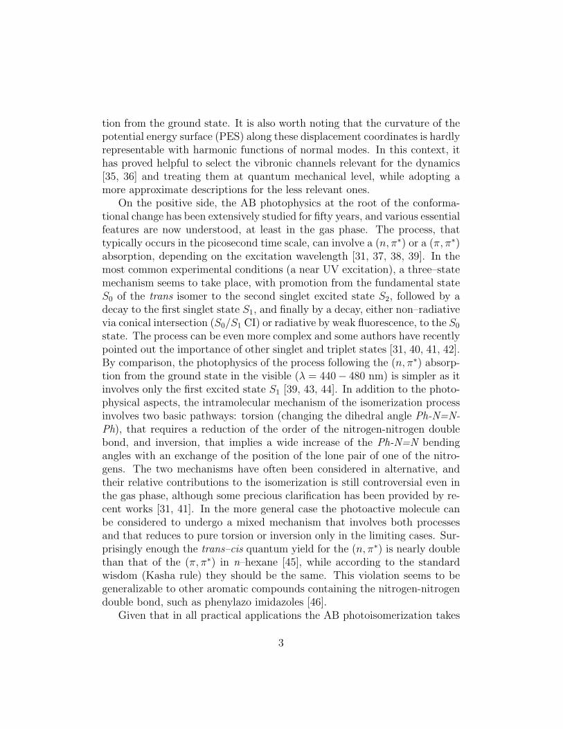
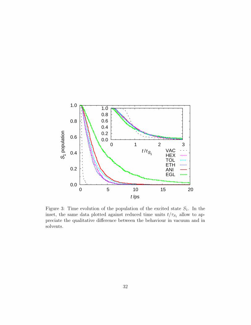
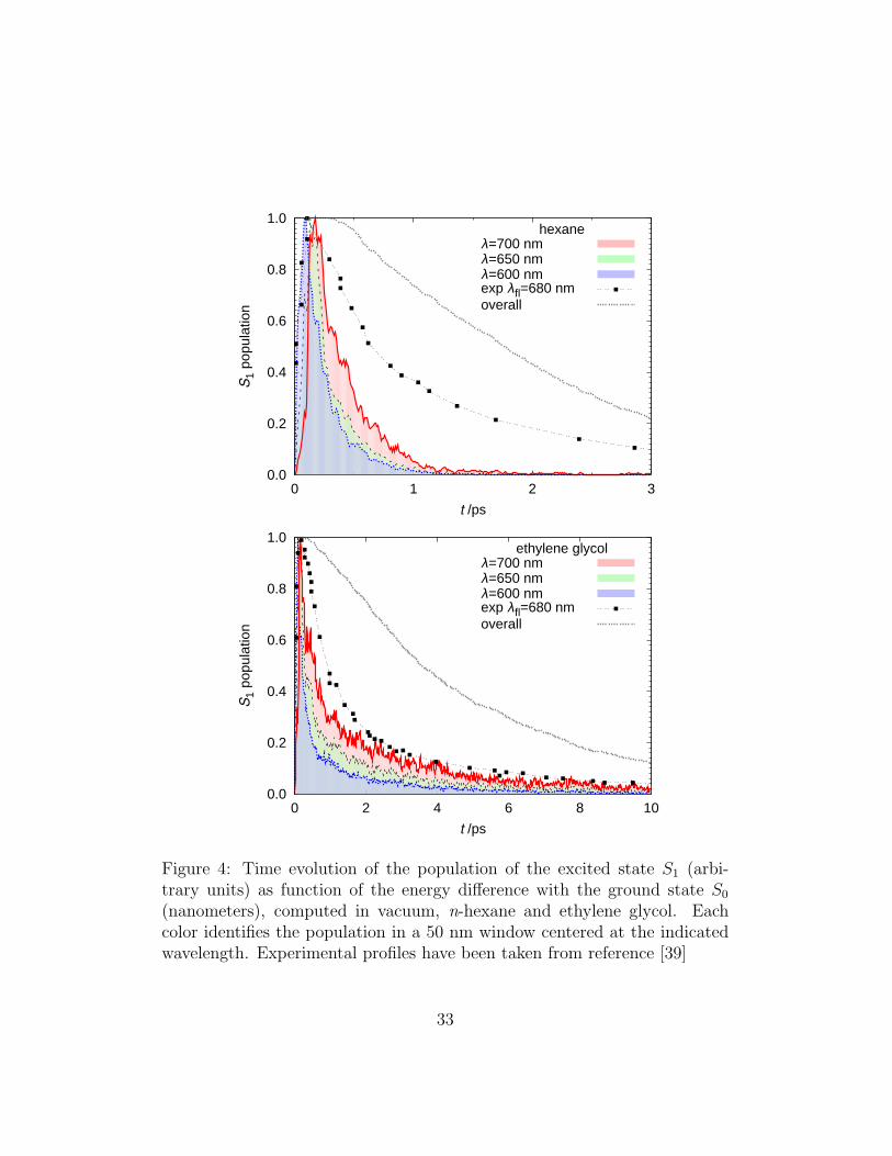
isomerization by Chang et al. (in HEX τ1 = 0.24 − 0.33, τ2 = 1.7 − 2.0ps; in EGL τ1 = 0.35 − 0.65, τ2 = 3.1 − 3.6 ps) [39]. Also the MD resultin ETH is in good agreement with time-resolved measurements for azoben-zene (τ1 = 0.32, τ2 = 2.1 ps) [74] and 4-aminoazobenzene (τ1 = 0.5 − 0.6,τ2 = 1.7−2 ps)[75]. The S1 population decay is clearly not mono-exponentialin vacuum, and to a lesser extent in solvents (Figure 3). For attempting acomparison with time-resolved experimental decays, and for sake of repro-ducibility, in Table 2 we report the results of a fit of a delayed biexponentialfunction PS1(t) = a1 exp(−(t− τ0)/τ1) + a2 exp(−(t− τ0)/τ2) to the excitedstate population; in all cases we obtained a higher coefficient for the slowestdecay component. Simulations also allow to compute separately excited statelifetimes for successful and unsuccessful isomerization outcome, however inTable 2 we show that they are not distinguishable, at least with the numberof experiments we performed, suggesting the possibility of a unique S1 path-way.Concluding the discussion on lifetimes, we would like to attempt a direct com-parison with fluorescence time-resolved experiments: in Figure 4 we show thetime evolution of emission at λ = 680 nm published in [39] for hexane andethylene glycol, together with the probability of the S1−S0 energy gaps cal-culated from our simulation for three different wavelengths, and finally theexcited state population. More than discussing the agreement between sim-ulation and experiment, which for many reasons is very difficult to judge (forexample in the simulation the fluorescence probability was assumed constantin time, and the pulse shape is a Dirac’s delta), the comparison betweenthe excited state population and the simulated emission is very interesting,as it clearly shows that they are very different, even if of course related; inparticular when increasing the sampling wavelength the intensity peak of theemission appears progressively delayed with respect to the time origin (ver-tical excitation); moreover sampling a single wavelength seems to cause adecrease of the long time component, and the decay time τS1 is consequentlyalways underestimated by the fluorescence experiment. As a side commentwe would like to underline that, besides the knowledge of AB transitiondipole as function of the molecular geometry [63], a good statistics is neededto simulate this type of observable (cf the noise in Figure 4), as at any timevalue only the small fraction of molecules which is still excited and lies in aspecific region of the PES contributes to the histogram.

10

3.2 Geometry modifications during the isomerizationprocess

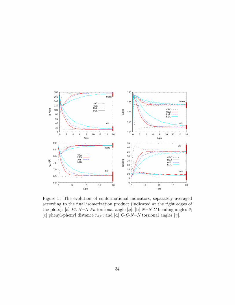
Having seen that our simulations can reproduce semi-quantitatively quan-tum yield and decay time data, we now wish to focus on the details of thetrans–cis transformation in solution as obtained from our computer simula-tion results. We have monitored the isomerization mechanism with variousgeometrical indicators, related to the structural reorganization of AB, includ-ing the absolute value of the Ph-N=N-Ph torsional angle (|φ|), the selectedPh-N=N bending angle (θ), the distance between the outmost 4, 4′ carbons ofthe phenyl rings (r4,4′), and the average module of the four Ph-N=N torsionalangles (|γ|) which monitors the rotation of the phenyl groups. The dynamicevolution of these indicators from the initial trans values is reported in Fig-ure 5, where for clarity we do not plot the curves in anisole and toluene sincethey are very similar to those in hexane. The averages have been computedconsidering all the experiments and separating the values for the trajectoriesleading to successful (cis final isomer) and unsuccessful (trans final isomer)photoisomerization outcomes, as indicated by the lateral bars on the rightedges of the plots of Figure 5. We first notice that the AB isomerization invacuum differs from the one in solution in that the trajectories are alreadywell separated at 0.5 ps in two branches leading to cis and trans. For allother cases we can observe, looking at Figures 5–[a], 5–[c] and 5–[d], thatthe geometrical indicators in the excited state (first few picoseconds) are stillcloser to those of the starting trans isomer than those of the cis. The ex-ception to this pattern is given by the bending angle (Figure 5–[b]), whichwithin the first 0.5 ps in the excited state has already attained values closerto the cis conformer ones.We can see that the trans–cis isomerization involves a large rotation of aphenyl group from |γ| = 4 − 10◦ to |γ| = 30 − 40◦ (and even larger in vac-uum) and thus if this rotation is hindered, e.g. by steric interactions with theneighboring solvent molecules, the isomerization dynamics is correspondinglyslowed down (Figure 5–[d]), and the quantum yield consequently decreases.The distance indicator r4,4′ is strictly related to the torsional angle φ (seeFigures 5–[a] and 5–[c]) and shows directly the overall shortening of the ABwhen going from the trans to cis conformer, that turns out to be about 2.25 Ain solution and 2.5 A in vacuum. Recalling the permanence times in the ex-cited state (Table 2), it can be safely concluded that most of the geometricalrearrangements take place (or continue for a long time) in the ground state,

11

while in the excited state both unsuccessful and successful trajectories arevery similar, indicating a unique pathway in the S1 PES like suggested byother studies [31].

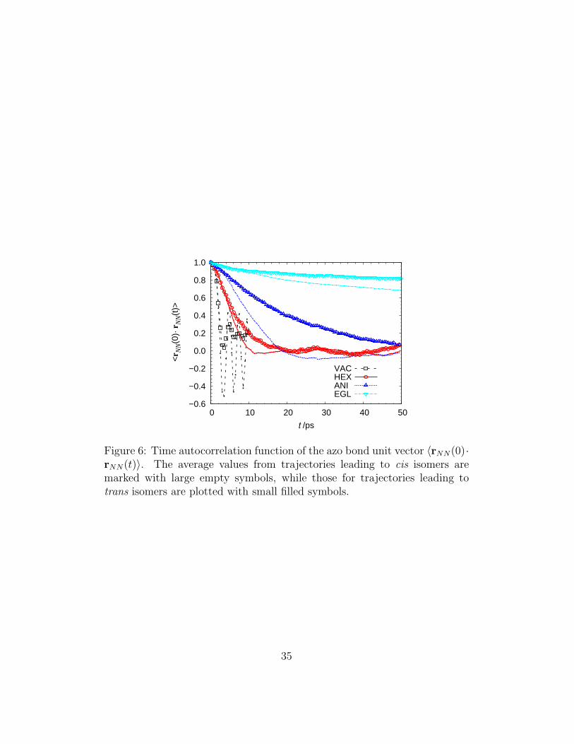
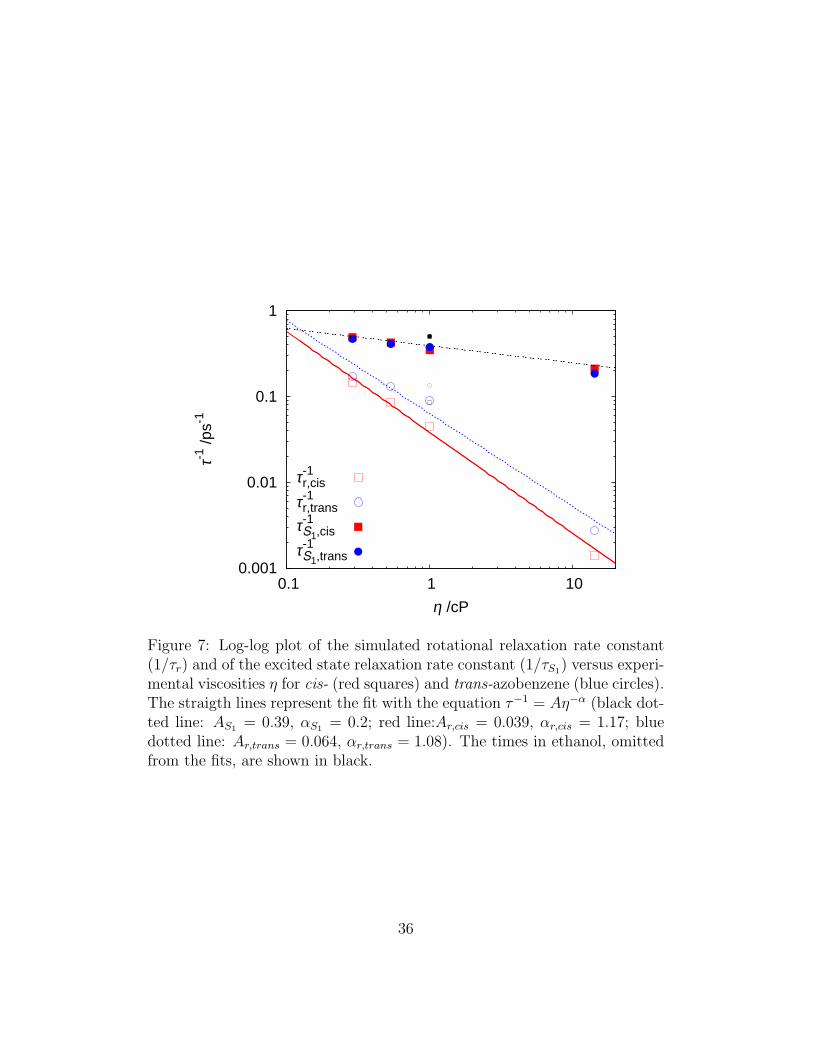
The rotational dynamics of AB, which has been sometimes brought intoplay in the interpretation of time–resolved experiments [39], can also be fol-lowed by MD simulations [76]; here we chose to monitor it through the timeautocorrelation function of the unit vector describing the orientation of the-N=N- bond, 〈rNN(0)·rNN(t)〉 in Figure 6. These functions clearly show thatthe rotation of the molecule takes place on a longer time scale than that ofthe isomerization process, with typical times depending on the solvent and onthe isomerization product. To better quantify these effects, we estimated therotational correlation times τr as the time at which 〈rNN(0) · rNN(τr)〉 = 1/e(Table 3) and displayed in a log-log plot versus experimental viscosities (Fig-ure 7). To investigate the dependence of rotational times τr and lifetimesτS1 on solvent experimental viscosities, we interpolated both data sets with apower law, commonly used in the analysis of time–resolved fluorescence data[77]:

τ−1r = Aη−α. (4)

All times were well fitted with this equation but the ones in ethanol, prob-ably because our simulations do not seem to reproduce correctly the actualviscosity value for this solvent. The rotational times of the N=N axis exhibita Stokes-Einstein like behaviour, i.e. they are roughly proportional to solventviscosity (α ≈ 1), but they are clearly separated in two groups, one for thetrans and one for the cis final isomer. As expected the shape of the moleculeaffects the rotational dynamics, but quite surprising is the outcome for ABisomers, in fact the trans rotates about the N=N vector approximately twotimes faster than the cis; we believe that this physical effect should be takeninto account in the interpretation of time-resolved measurements.The excited state lifetimes show a different behaviour: they are weakly af-fected by the viscosity (α = 0.2), in accord with experimental results of anAB acrylate derivative [78], and as previously observed, they do not appar-ently depend on the final isomerization product; consequently the data setsfor cis and trans AB can be fitted with the same set of parameters.

12

3.3 Isomerization mechanism

We now proceed to assess the likelihood of the torsion or inversion trans–cisisomerization channels by following the molecular geometry time evolution.To do this, we have first defined three main isomerization pathways in the (θ,φ) surfaces according to the upper limit, θmax, of the bending angle valuesexplored by the AB molecule during its trajectory in both electronic states:torsion (if θmax < 140◦); mixed (if 140◦ ≤ θmax < 160◦); and inversion (ifθmax ≥ 160◦); then, we have classified each experiment according to thisdefinition and evaluated the relative importance of each of the channels com-puting the ratios reported in Table 4.two most probable pathways for isomerization are the torsional (56%) andmixed ones (43%), with unlikely occurrence of pure inversion, in agreementwith other semiclassical studies [31, 79]. We also find that, even if the ratiosexhibit different values in the various solvents, the most probable pathwaysin condensed phase always correspond to a mixed mechanism [80]. Pure in-version and pure torsional pathways seem to be hindered by steric solventinteractions and are consequently less likely to occur. Even if we registeredthe highest occurrence of inversion pathways in the more viscous solvent(ethylene glycol), in agreement with reference [39], the isomerization mecha-nism seems relatively unaffected by solvent viscosity.

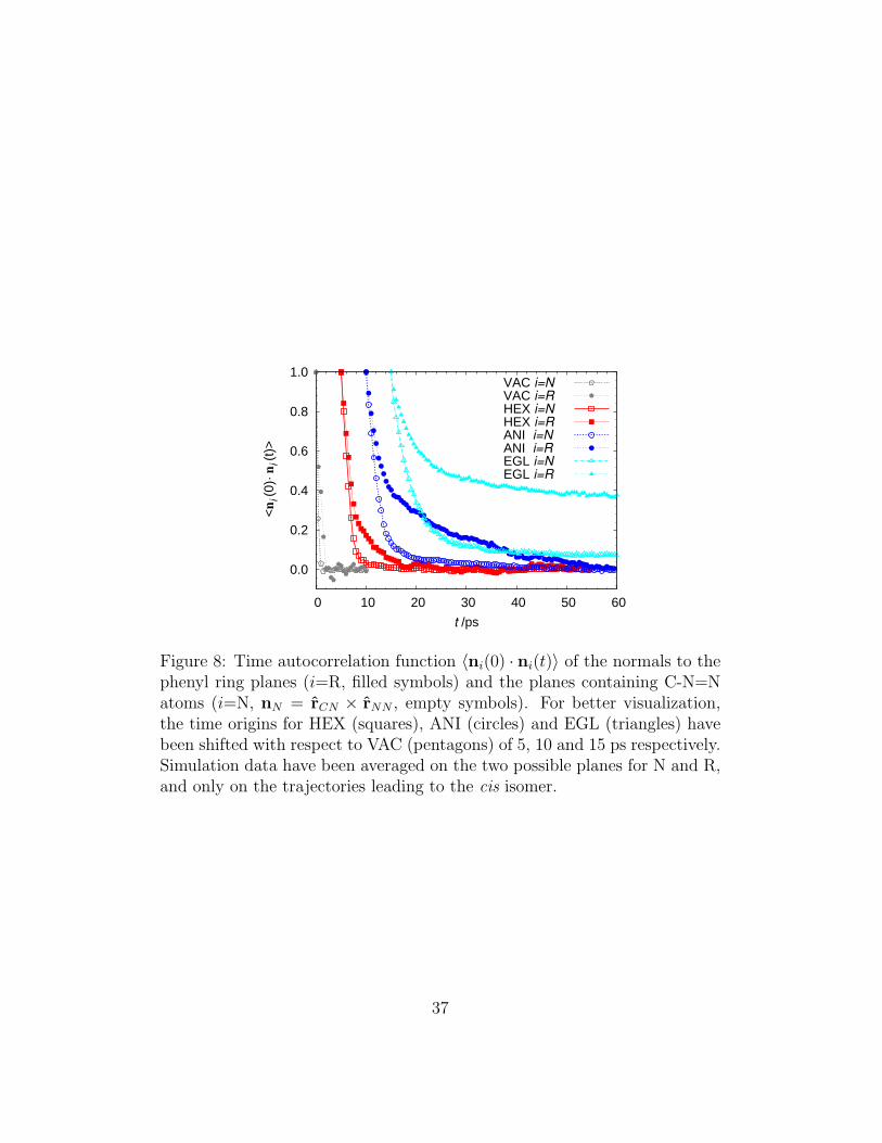
In their recent QM/MM study on cis-trans isomerization of AB, whereboth AB PES and excited state dynamics were treated at DFT level, Marxand coworkers [80] evidenced that the isomerization mechanism somehowdeparts from the standard torsional or inversion pathways, as it involves afaster rearrangement of nitrogen atoms with respect to the bulkier phenylrings. In order to compare our findings with this study, we have evaluatedspecific autocorrelation functions measuring the time change of orientation ofthe normal to each phenyl ring plane (nR), and of the orientation of the nor-mals to the planes containing C-N=N atoms (nN = rCN× rNN) for successfulisomerizations (Figure 8). We have found that, in line with the results in[80], a faster reorientation of nN with respect to nR during the isomerizationfor all the cases studied, as shown by the faster decay of the correspondingautocorrelation functions in Figure 8. Since our simulation are on one handbased on different (and more drastic) approximations on the photophysics,and on the other, they explore a time window up to one hundred times largerthan that studied in [80], we think that these two independent approachesprovide a cross-validation of the isomerization mechanism. In addition, the

13

availability of simulations for different solvent viscosities allows to identifythe marked effect this property has on the isomerization dynamics: as ex-pected, the bulky phenyl groups need more time to adapt their orientationto the change of PES occurring upon excitation. This effect gives rise to thepredominance of what we call “mixed” isomerization mechanism in the ex-cited state, even if the reorientation dynamics continues also after the decayto S0.The analysis of MD simulations trajectories also gives insights on the elec-tronic state dependence of the inversion and rotation processes. When themolecule is excited, it generally moves torsionally towards the S1 surface en-ergy minimum and conical intersection region, and only after it has decayedto the S0 state, the bending angle θ can reach values close to 180◦. As ev-idenced by the low fraction of trajectories reaching the maximum bendingangle in the excited state (Table 4), the inversion movement takes place pri-marily in the S0 state, at least in these excitation conditions. These resultssupport the “cold isomerization” model described by Diau and coworkers [81],that depicts a rotational pathway in the S1 state for an (n, π∗) excitation.The inversion mechanism in the excited state could become possible only ifthe molecule started from a higher vibrational state (“hot isomerization”)having enough energy to overcome the inversion energy barrier; this secondmechanism is expected to be important only after a decay from a higherexcited state [82], as it can happen in (π, π∗) isomerization.

4 Conclusions

In this work we have analyzed the mechanism for the trans–cis photoiso-merization of azobenzene in various organic solvents when excited in thevisible ((n, π∗) transition). For this purpose, we have introduced a methodfor the molecular dynamics simulation of photoresponsive molecules in so-lution which has the feature of allowing for their electronic excitation andstatistical decay while they move in the crowded solvent environment. Withthe help of two empirical parameters to model the decay probability of ABfrom S1 to ground state, tuned for reproducing experimental quantum yieldsand the excited state lifetimes in vacuum and hexane, we have been able tofollow the conformational changes of AB and to evaluate conversion efficiencyand decay dynamics in different solvation conditions.

The average decay times resulted fairly independent on the nature of the

14

photo product obtained after decay, thus indicating similar trajectories in theexcited state for both possible outcomes. The simulations also show that,while in vacuum the isomerization follows prevalently a torsional mechanism,as already found by other authors [31], the dominant isomerization mecha-nism in solution is a mixed torsional-inversion one, with a probability whichis double than the one for a pure torsion. Indeed the pure inversion seemsto occur only after the decay into the S0 state, while in the excited statethis pathway appears unlikely, as a high energy barrier must be overcome. Ahigher solvent viscosity seems to increase the pure inversion contribution, al-beit the principal mechanisms remain the mixed one and torsional ones (witha probability of about 65% and 30% respectively). Viscosity also clearly af-fects the rotational dynamics of AB, notably resulting in a faster dynamicsfor the trans isomer.

Addressing the interpretation of time-resolved absorption or emission ex-periments, we have predicted the intensity time profile to be a lower bound ofthe excited state population, and also suggested that the different rotationaltimes of the two isomers must be taken into account when evaluating thedepolarization of fluorescence.

Although a number of approximations have been introduced to make thestudy computationally feasible, we believe the present approach to be quitegeneral, easily improvable as soon as more accurate quantum mechanics de-scription of electronic states and transition probabilities become available,and applicable to other, even more complex, isotropic and anisotropic sur-roundings.

5 Acknowledgements

We acknowledge EU RT Network “Functional Liquid Crystalline Elastomers”(FULCE) for initially funding this research, and a CINECA-INSTM com-puter time co-funded grant. We also wish to thank Prof. Maurizio Persico(university of Pisa) and Prof. Giorgio Orlandi (university of Bologna) foruseful discussions.

15

Appendix: parameterization of the decay probabilitylaw in vacuum and hexane

In this appendix we discuss the technical details for derivation of the twoparameters K and χ appearing in the decay model described by Equation 3.At least in principle these parameters, or the probability rates themselves,could be calculated ab initio, but for simplicity here we followed an empiricalapproach, consisting in tuning K and χ on the basis of the comparison withavailable theoretical data in vacuum and experimental ones in hexane. Thetypical observable of a photoisomerization experiment is the quantum yield,Φ, expressing the ratio between the number of isomerized molecules and thenumber of absorbed photons. Richer dynamical information can be gath-ered with pico or femtosecond time–resolved experiments (e.g. absorbance,fluorescence, IR, Raman), which measure the time evolution of some tran-sient species characteristic spectral features; however these results are oftendifficult to interpret [69, 63], as they represent a weighted average of bothisomers dynamics, and they are to some extent also dependent on solventnature, on probing wavelength and, of course, on excitation wavelength, thatmay determine different excited state pathways. In the case of nπ∗ excita-tion, the intensity decay is usually well fitted with a tri-exponential function,with lifetimes τ1, τ2, and τ3 of the order of magnitude of 0.1 − 1, 1 − 5 and10− 30 ps respectively [81, 39, 83], and relative weight 2− 3 : 1 :< 0.1. Thefaster decay is reasonably ascribed to the relaxation from the Frank-Condonpoint to the minimum of S1, while for the other two the assignment is morecontroversial; here we base the parametrization on the interpretation of thesecond process as the relaxation in the flatter CI region, and the third oneto the rotational and vibrational cooling in S0 [84, 42]. Simulations allow tomeasure directly the time evolution of the population of S1, and its averagelifetime τS1 can be directly compared with the experimental time scale of thetwo fastest processes in a given solvent. The timescale of the rotational mo-tion of AB can be calculated from the autocorrelation function of a relevantmolecular axis, and again compared with τ3. Finally, we define the the quan-tum yield as Φ = Ncis/N , where Ncis is the number of virtual experimentsyielding a cis isomer out of the total number of experiments N , which is inturn equivalent to the number of absorbed photons. We start presenting thequantum yield and the decay kinetics of AB in vacuum and in n–hexane forvarious sets of MD experiments differing in the values of the parameters Kand χ, and comparing them with available theoretical data and with experi-

16

mental yields in n–hexane. Without attempting a perfect match that wouldbe inappropriate considering the various approximations made in our ap-proach, a comparison with these data can provide a reasonable estimate forχ and K. In particular Persico and coworkers performed several simulationsof azobenzene and derivatives in vacuum using prevalently surface hopping[31, 32, 69, 72] but also full multiple spawning (FMS) [85, 86]. As they referto this second method as the most accurate, we compare our results in vac-uum with the FMS ones. Luckily not only the quantum yield (0.46± 0.08 in[85]), but also the lifetime of the excited state tS1 (about 0.5 ps) and the S1

population in function of time can be calculated with these techniques anda thorough comparison with our simulations is possible.

From Table 5, where we report the estimated Φ and tS1 in vacuum forvarious values of K and χ, it is apparent that with small variations of theparameters any quantum yield ranging from 0.0 to 0.6 can be reproduced;moreover, some parameter choices can lead to reasonably correct yields andlifetimes. In the selection of the best K and χ, it would be desirable to usethe same set for vacuum and hexane; for this solvent n, π∗ quantum yieldmeasurements are available but due to large experimental uncertainties onlythe yield range is known (φ = 0.20−0.27) [45]. Also the data for the excited-state lifetime τS1 are relatively scattered, but always in the 1 − 3 ps range[87, 88, 81, 39, 83].

Analysing the the test results in Table 5, some trends emerge: i) asexpected, lifetime increases with increasing χ and decreasing K; ii) for anyK, χ pair the permanence time is roughly doubled in hexane with respectto vacuum; iii) with K fixed, the yield increases with χ for “small” χ untilreaching a maximum value of about 0.55 in vacuum and 0.24 in hexane;further increasing χ determines long lifetimes and an eventual falling of theyield (at least for K = 5).

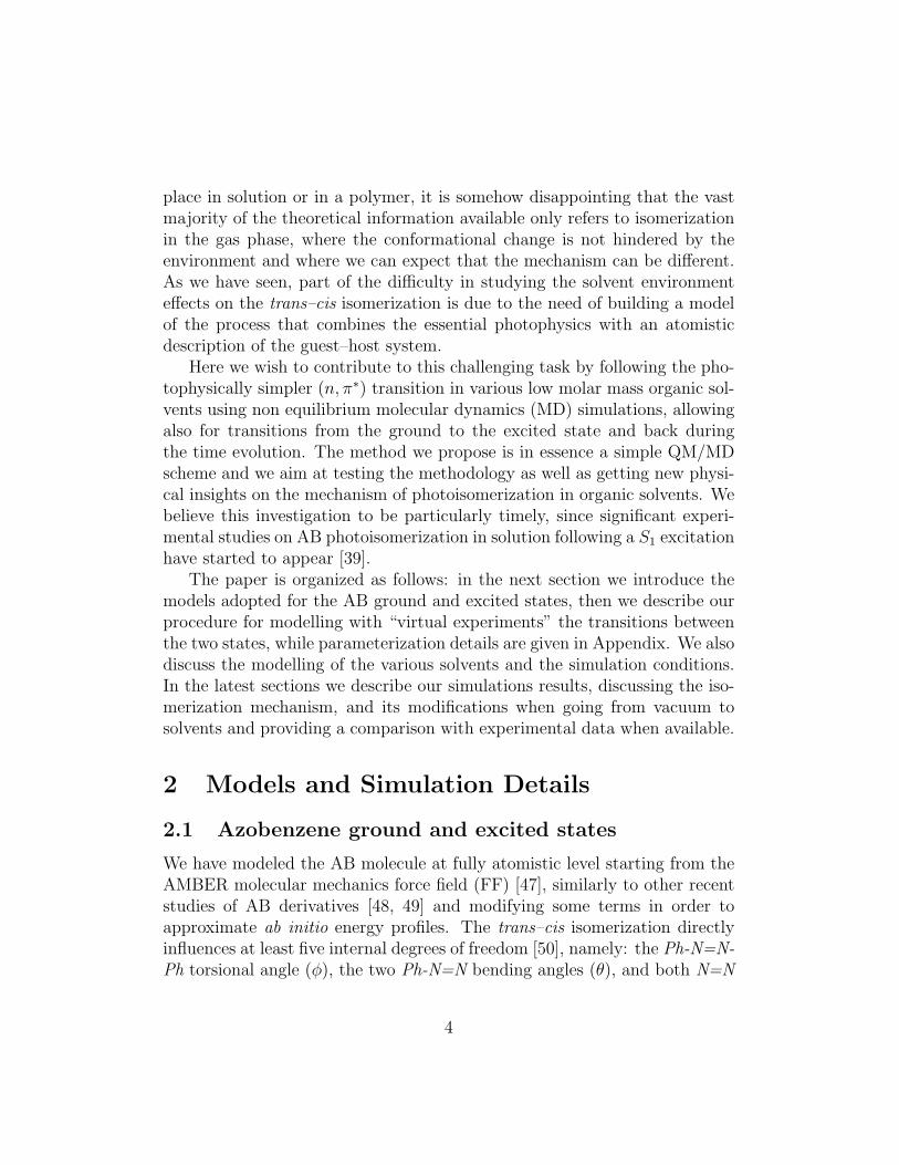
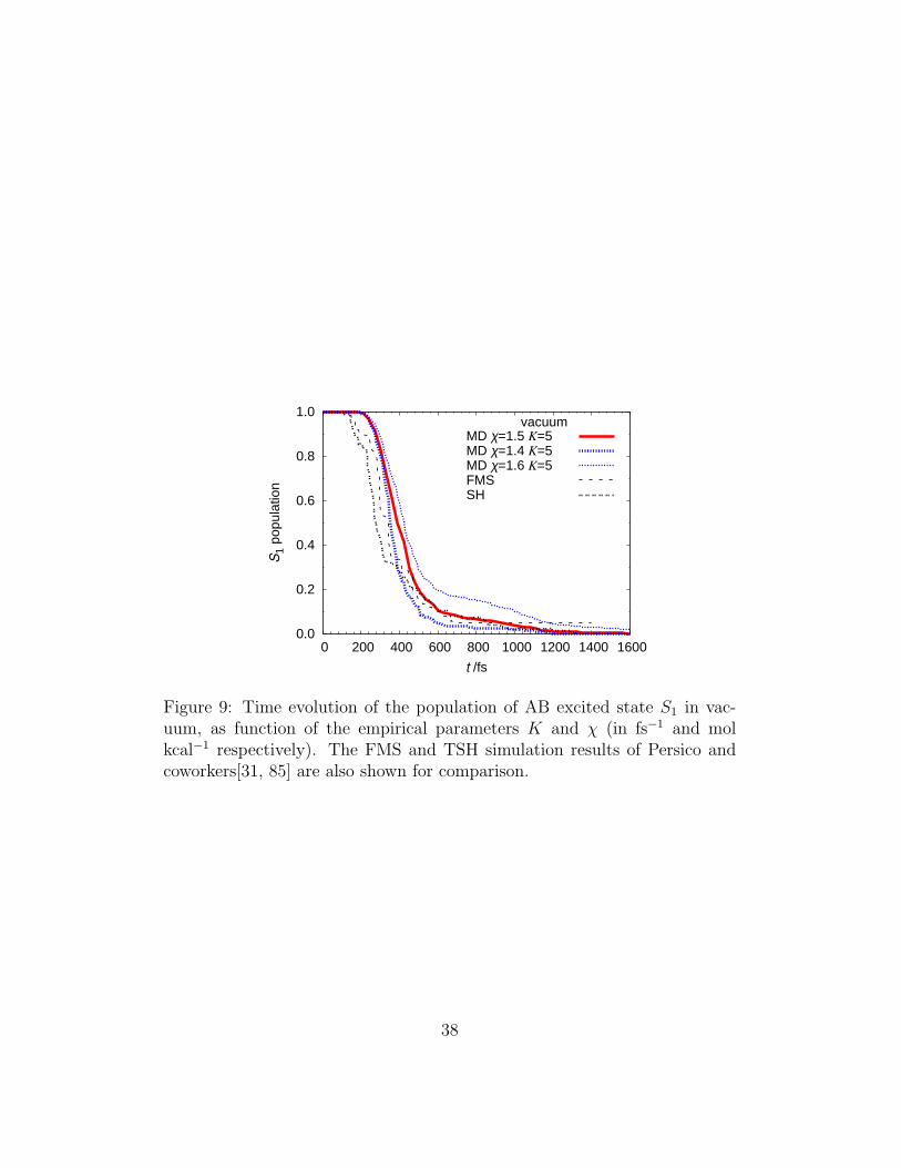
It is also clear that it is not possible to obtain yield and lifetimes inperfect agreement with experiment for vacuum and hexane with a uniqueparameterization; on the other hand it is easy to reproduce both yield andlifetime, with different combinations of K and χ. Actually it is not clearif the coupling between the two states should be solvent-independent (i. e.with the same K, χ), as calculation and experiments indicate only smallbathochromic shifts [62]; considering that the best results for hexane areobtained at high K, we have decided to keep constant K = 5 fs−1 for vacuumand solutions, but to use slightly different values of χ (1.5 in vacuum and1.9 mol kcal−1 in solvents). This choice gives an excellent agreement with

17

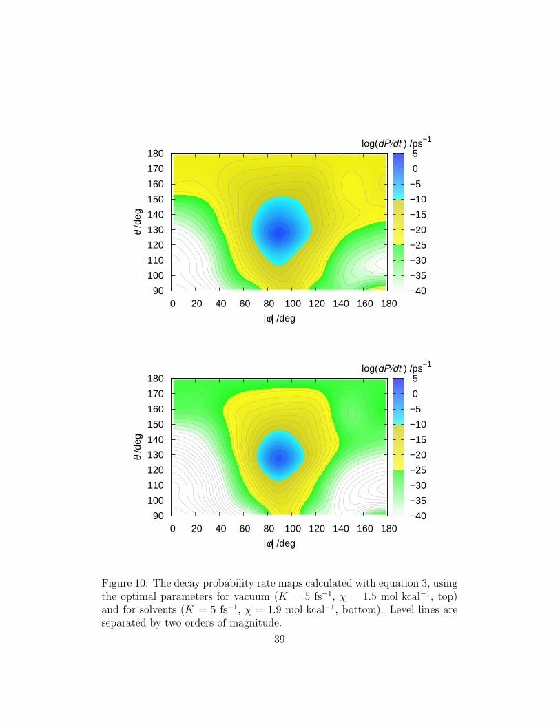
the S1 population calculated by Persico and coworkers (Figure 9) for AB invacuum, and determines the probability maps shown in Figure 10.

References

[1] H. Finkelmann, E. Nishikawa, G. G. Pereira, and M. Warner. A newopto-mechanical effect in solids. Phys. Rev. Lett., 87:15501, 2001.

[2] T. Ikeda and O. Tsutsumi. Optical switching and image storage bymeans of azobenzene liquid-crystal films. Science, 268:1873–1875, 1995.

[3] Y. Yu, M. Nakano, and T. Ikeda. Directed bending of a polymer filmby light. Nature, 425:145–145, 2003.

[4] M. Camacho-Lopez, H. Finkelmann, P. Palffy-Muhoray, and M. Shelley.Fast liquid crystal elastomer swims into the dark. Nat. Mater., 3:307–310, 2004.

[5] X. Tong, G. Wang, A. Yavrian, T. Galstian, and Y. Zhao. Dual-modeswitching of diffraction gratings based on azobenzene-polymer-stabilizedliquid crystals. Adv. Mater., 17:370–374, 2005.

[6] Y. Lansac, M. A. Glaser, N. A. Clark, and O. D. Lavrentovich. Pho-tocontrolled nanophase segregation in a liquid-crystal solvent. Nature,398:54–57, 1999.

[7] T. Hugel, N. B. Holland, A. Cattani, L. Moroder, M. Seitz, and H. E.Gaub. Single-molecule optomechanical cycle. Science, 296:1103–1106,2002.

[8] I. A. Banerjee, L. Yu, and H. Matsui. Application of host-guest chem-istry in nanotube-based device fabrication: Photochemically controlledimmobilization of azobenzene nanotubes on patterned α-cd mono-layer/au substrates via molecular recognition. J. Am. Chem. Soc.,125:9542–9543, 2003.

[9] A. Buguin, M. H. L. Silberzan, B. Ladoux, and P. Keller. Micro-actuators: When artificial muscles made of nematic liquid crystal elas-tomers meet soft lithography. J. Am. Chem. Soc., 128:1088–1089, 2006.

18

[10] T. Muraoka, K. Kinbara, and T. Aida. Mechanical twisting of a guestby a photoresponsive host. Nature, 440:512–515, 2006.

[11] M. Yamada, J.-I. Mamiya M. Kondo M, Y.-L. Yu, M. Kinoshita, C. Bar-rett, and T. Ikeda. Photomobile polymer materials: Towards light-driven plastic motors. Angew. Chem. Int. Ed. Engl., 47:4986–4988, 2008.

[12] J. M. Mativetsky, G. Pace, M. Elbing, M. A. Rampi, M. Mayor,and P. Samorı. Azobenzenes as light-controlled molecular electronicswitches in nanoscale metal-molecule-metal junctions. J. Am. Chem.Soc., 130:9192–9193, 2008.

[13] F. Bernardi, M. Olivucci, and M. A. Robb. Potential energy surfacecrossings in organic photochemistry. Chem. Soc. Rev., 25:321–328, 1996.

[14] D. R. Yarkony. Diabolical conical intersections. Rev. Mod. Phys.,68:985–1013, 1996.

[15] A. W. Jasper, C. Y. Zhu, S. Nangia, and D. G. Truhlar. Introductorylecture: Nonadiabatic effects in chemical dynamics. Faraday Discuss.,127:1–22, 2004.

[16] M. Garavelli. Computational organic photochemistry: strategy, achieve-ments and perspectives. Theor. Chem. Acc., 116:87–105, 2006.

[17] D. R. Yarkony. Conical intersections: The new conventional wisdom. J.Phys. Chem. A, 105:6277–6293, 2000.

[18] N. L. Doltsinis and D. Marx. Nonadiabatic Car-Parrinello moleculardynamics. Phys. Rev. Lett., 88:166402, 2002.

[19] G. A. Worth and L. S. Cederbaum. Beyond born-oppenheimer: molec-ular dynamics through a conical intersection. Annu. Rev. Phys. Chem.,55:127–158, 2004.

[20] X.S. Li, J. C. Tully, H. B. Schlegel, and M. J. Frisch. Ab initio Ehrenfestdynamics. J. Chem. Phys., 123:084106, 2005.

[21] B. G. Levine and T. J. Martinez. Isomerization through conical inter-sections. Annu. Rev. Phys. Chem., 58:613–634, 2007.

19

[22] A. W. Jasper, S. Nangia, C. Y. Zhu, and D. G. Truhlar. Non-Born-Oppenheimer molecular dynamics. Acc. Chem. Res., 39:101–108, 2007.

[23] B. Lasorne, M. J. Bearpark, M. A. Robb, and G. A. Worth. Controllings1/s0 decay and the balance between photochemistry and photostabil-ity in benzene: a direct quantum dynamics study. J. Phys. Chem. A,112:1301713027, 2008.

[24] J. Kongsted, A. Osted, and K. V. Mikkelsen. Solvent effects on then→ π∗ electronic transition in formaldehyde: a combined coupled clus-ter/molecular dynamics study. J. Phys. Chem, 121:8435–8445, 2004.

[25] M. Sulpizi, U. F. Rohrig, J. Hutter, and U. Rothlisberger. Opticalproperties of molecules in solution via hybrid TDDFT/MM simulations.Int. J. Quantum Chem., 101:671–682, 2005.

[26] A. M. Losa, I. F. Galvin, M. L. Sanchez, and M. E. Martin. Solventeffects on internal conversions and intersystem crossings: The radiation-less de-excitation of acrolein in water. J. Phys. Chem. B, 112:877–884,2008.

[27] L. M. Frutos, T. Andruniow, F. Santoro, N. Ferre, and M. Olivucci.Tracking the excited-state time evolution of the visual pigment withmulticonfigurational quantum chemistry. Proc. Natl. Acad. Sci. U.S.A.,104:7764–7769, 2007.

[28] M. Boggio-Pasqua, M. A. Robb, and G. Groenhof. Hydrogen bond-ing controls excited-state decay of the photoactive yellow protein chro-mophore. J. Am. Chem. Soc., 131:1358013581, 2009.

[29] M. J. Bearpark, M. Boggio-Pasqua, M. A. Robb, and F. Ogliaro. Ex-cited states of conjugated hydrocarbons using the molecular mechanics-valence bond (MMVB) method: conical intersections and dynamics.Theor. Chem. Acc., 116:670–682, 2006.

[30] T. Frauenheim, G. Seifert, M. Elstner, T. Niehaus, C. Kohler,M. Amkreutz, M. Sternberg, Z. Hajnal, A. Di Carlo, and S. Suhai.Atomistic simulations of complex materials: ground-state and excited-state properties. J. Phys.: Condens. Matter, 14:3015–3047, 2002.

20

[31] C. Ciminelli, G. Granucci, and M. Persico. The photoisomerizationmechanism of azobenzene: A semiclassical simulation of nonadiabaticdynamics. Chem.-Eur. J., 10:2327–2341, 2004.

[32] C. Ciminelli, G. Granucci, and M. Persico. Are azobenzenophanesrotation–restricted? J. Chem. Phys., 123:174317, 2005.

[33] M. Barbatti, G. Granucci, M. Persico, M. Ruckenbauer, M. Vazdar,M. Eckert-Maksic, and H. Lischka. The on-the-fly surface-hopping pro-gram system NEWTON-X: application to ab initio simulation of thenonadiabatic photodynamics of benchmark systems. J. Photochem. Pho-tobiol. A, 190:228–240, 2007.

[34] P. de Sainte Claire. Molecular simulation of excimer fluorescence inpolystyrene and poly(vinylcarbazole). J. Phys. Chem. B, 110:7334–7343,2006.

[35] F. Santoro, A. Lami, R. Improta, and V. Barone. Effective methodto compute vibrationally resolved optical spectra of large molecules atfinite temperature in the gas phase and in solution. J. Chem. Phys.,126:184102, 2007.

[36] E. Gindensperger, H. Koppel, and L. S. Cederbaum. Hierarchy of effec-tive modes for the dynamics through conical intersections in macrosys-tems. J. Chem. Phys., 126:034106, 2007.

[37] H. Satzger, C. Root, and M. Braun. Excited-state dynamics of trans-and cis-azobenzene after UV excitation in the ππ∗ band. J. Phys. Chem.A, 108:6265–6271, 2004.

[38] T. Ishikawa, T. Noro, and T. Shoda. Theoretical study of the photoiso-merization of azobenzene. J. Chem. Phys., 115:7503–7512, 2001.

[39] C-W. Chang, Y-C. Lu, T-T. Wang, and E. W-G. Diau. Photoisomeriza-tion dynamics of azobenzene in solution with s1 excitation: A femtosec-ond fluorescence anisotropy study. J. Am. Chem. Soc., 126:10109–10118,2004.

[40] L. Gagliardi, G. Orlandi, F. Bernardi, A. Cembran, and M. Garavelli. Atheoretical study of the lowest electronic states of azobenzene: the role

21

of torsion coordinate in the cis-trans isomerization. Theor. Chem. Acc.,111:363–372, 2004.

[41] A. Cembran, F. Bernardi, M. Garavelli, L. Gagliardi, and G. Orlandi.On the mechanism of the cis-trans isomerization in the lowest electronicstate of azobenzene: S0, S1, T1. J. Am. Chem. Soc., 126:3234–3243,2004.

[42] I. Conti, M. Garavelli, and G. Orlandi. The different photoisomeriationefficiency of azobenzene in the lowest nπ∗ and ππ∗ singlets: the role ofa phantom state. J. Am. Chem. Soc., 130:5216–5230, 2008.

[43] P. Cattaneo and M. Persico. An ab initio study of the photochemistryof azobenzene. Phys. Chem. Chem. Phys., 1:4739–4743, 1999.

[44] E. W.-G. Diau. A new trans-to-cis photoisomerization mechanism ofazobenzene on the s1(n,π∗) surface. J. Phys. Chem. A, 108:950–956,2004.

[45] H. Rau. Photochromism. Molecules and systems, chapter 4. Elsevier,Amsterdam, 1990.

[46] J. Otsuki, K. Suwa, K. Narutaki, C. Sinha, I. Yoshikawa, andK. Araki. Photochromism of 2-(phenylazo)imidazoles. J. Phys. Chem.A, 109:8064–8069, 2005.

[47] W. D. Cornell, P. Cieplak, C. I. Bayly, I. R. Gould, K. M. Merz Jr.,D. M. Ferguson, D. C. Spellmeyer, T. Fox, J. W. Caldwell, and P. A.Kollman. A second generation force field for the simulation of proteinsand nucleic acids. J. Am. Chem. Soc., 117:5179–5197, 1995.

[48] M. Bockmann, C. Peter, L. Delle Site, N. L. Doltsinis, K. Kremer, andD. Marx. Atomistic force field for azobenzene compounds adapted forqm/mm simulations with applications to liquids and liquid crystals. J.Chem. Theory Comput., 3:1789–1802, 2007.

[49] H. Heinz, R. A. Vaia, H. Koerner, and B. L. Farmer. Photoisomerizationof azobenzene grafted to layered silicates: simulation and experimentalchallenges. Chem. Mater., 20:6444–6456, 2008.

22

[50] S. A. Yuan, Y. S. Dou, W. F. Wu, Y. Hu, and J. S. Zhao. Why doestrans-azobenzene have a smaller isomerization yield for ππ∗ excitationthan for nπ∗ excitation? J. Phys. Chem. A, 112:13326–13334, 2008.

[51] L. Wang and X. Wang. Ab initio study of photoisomerization mecha-nisms of push-pull p, p′-disubstituted azobenzene derivatives on s1 ex-cited state. J. Mol. Struct.:THEOCHEM, 847:1–9, 2007.

[52] D. L. Cheung, S. J. Clark, and M. R. Wilson. Parametrization andvalidation of a force field for liquid-crystal forming molecules. Phys.Rev. E, 65:051709, 2002.

[53] R. Berardi, G. Cainelli, P. Galletti, D. Giacomini, A. Gualandi, L. Muc-cioli, and C. Zannoni. Can the π-facial selectivity of solvation be pre-dicted by atomistic simulation? J. Am. Chem. Soc., 127:10699–10706,2005.

[54] R. Englman and J. Jortner. The energy gap law for radiationless tran-sitions in large molecules. Molec. Phys., 18:145–164, 1970.

[55] J. Jortner and D. Levine. Photoselective Chemistry. Part I. Adv. Chem.Phys. Wiley, New York, 1981.

[56] N. Kitamura, N. Sakata, H.-B. Kim, and S. Habuchi. Energy gap depen-dence of the nonradiative decay rate constant of 1-anilino-8-naphthalenesulfonato in reverse micelles. Analytical Sciences, 15:413–419, 1999.

[57] F. Ehlers, D. A. Wild, T. Lenzer, and K. Oum. Investigation of the s1/ict→ s0 internal conversion lifetime of 4′-apo-β-caroten-4′-al and 8′-apo-β-caroten-8′-al: dependence on conjugation length and solvent polarity. J.Phys. Chem. A, 111:2257–2265, 2007.

[58] S. Velate, X. Liu, and R. P. Steer. Does the radiationless relaxationof Soret-excited metalloporphyrins follow the energy gap law? Chem.Phys. Lett., 427:295–299, 2006.

[59] J. von Neumann. Various techniques used in connection with randomdigits. Appl. Math. Ser., 12:36–38, 1951.

[60] B. H. Besler, K. M. Merz Jr., and P. A. Kollman. Atomic charges derivedfrom semiempirical methods. J. Comput. Chem., 11:431, 1990.

23

[61] S. Kobayashi, H. Yokoyama, and H. Kamei. Substituent and solventeffects on electronic absorption spectra and thermal isomerization ofpush–pull–substitued cis azobenzenes. Chem. Phys. Lett., 138:333–338,1987.

[62] L. Briquet, D. P. Vercauteren, E. A. Perpete, and D. Jacquemin. Is sol-vated trans-azobenzene twisted or planar? Chem. Phys. Lett., 417:190–195, 2006.

[63] T. Cusati, G. Granucci, M. Persico, and G. Spighi. Oscillator strengthand polarization of the forbidden n → π∗ band of trans-azobenzene: acomputational study. J. Chem. Phys., 128:194312, 2008.

[64] P. Procacci, E. Paci, T. Darden, and M. Marchi. Orac: a moleculardynamics program to simulate complex molecular systems with realisticelectrostatic interactions. J. Comput. Chem., 18:1848–1862, 1997.

[65] U. Essmann, L. Perera, M. L. Berkowitz, T. Darden, H. Lee, and L. G.Pedersen. A smooth particle mesh Ewald method. J. Chem. Phys.,101:8577–8593, 1995.

[66] S. Nose. A molecular dynamics method for simulations in the canonicalensemble. Molec. Phys., 52:255268, 1984.

[67] W. G. Hoover. Canonical dynamics: Equilibrium phase-space distribu-tions. Phys. Rev. A, 31:1695–1697, 1985.

[68] M. Parrinello and A. Rahman. Crystal structure and pair potentials: Amolecular-dynamics study. Phys. Rev. Letters, 45:1196–1199, 1980.

[69] G. Granucci and M. Persico. Excited state dynamics with the trajectorysurface hopping method: azobenzene and its derivatives as a case study.Theor. Chem. Acc., 117:1131–1143, 2007.

[70] S. Malkin and E. Fischer. Temperature dependence of photoisomer-ization. part II. quantum yields of cis⇀↽trans isomerizations in azo-compounds. J. Am. Chem. Soc., 66:2482–2486, 1962.

[71] D. Gegiou, K. A. Muszkat, and E. Fischer. Temperature dependence ofphotoisomerization. VI. viscosity effect. J. Am. Chem. Soc., 90:12–18,1968.

24

[72] L. Creatini, T. Cusati, Granucci, and M. Persico. Photodynamics ofazobenzene in a hindering environment. Chem. Phys., 347:492–502,2008.

[73] M. Poprawa-Smoluch M, J. Baggerman, H. Zhang, H. P. A. Maas, L. DeCola, and A. M. Brouwer. Photoisomerization of disperse red 1 studiedwith transient absorption spectroscopy and quantum chemical calcula-tions. J. Phys. Chem. A, 110:11926–11937, 2006.

[74] T. Nagele, R. Hoche, W. Zinth, and J. Wachtveit. Femtosecond photoi-somerization of cis-azobenzene. Chem. Phys. Lett., 272:489–495, 1997.

[75] Y. Hirose, H. Yui, and T. Sawada. Effect of potential energy gap betweenthe n–π∗ and the π–π∗ state on ultrafast photoisomerization dynamicsof an azobenzene derivative. J. Phys. Chem. A, 106:3067–3071, 2002.

[76] Y. Zhang, R. M. Venable, and R. W. Pastor. Molecular dynamics simula-tions of neat alkanes: The viscosity dependence of rotational relaxation.J. Chem. Phys., 100:2652–2660, 1996.

[77] R. E. Di Paolo, J. S. de Melo, J. Pina, H. D. Burrows, J. Morgado,and A. L. Macanita. Conformational relaxation of p-phenylene-vinylenetrimers in solution studied by picosecond time-resolved fluorescence.ChemPhysChem, 8:2657–2664, 2007.

[78] F. Serra and E. M. Terentjev. Effects of solvent viscosity and polarityon the isomerization of azobenzene. Macromolecules, 41:981–986, 2008.

[79] J. Shao, Y. Lei, Z. Wen, Y. Dou, and Z. Wang. Nonadiabatic simulationstudy of photoisomerization of azobenzene: detailed mechanism andload-resisting capacity. J. Chem. Phys., 129:164111, 2008.

[80] M. Bockmann, N. L. Doltsinis, and D. Marx. Azobenzene photoswitchesin bulk materials. Phys. Rev. E, 78:036101, 2008.

[81] Y.-C. Lu, C.-W. Chang, and E. W.-G. Diau. Femtosecond fluorescencedynamics of trans–azobenzene in hexane on excitation to the s1(n, π

∗)state. J. Chin. Chem. Soc., 49:693–701, 2002.

[82] T. Schultz, J. Quenneville, B. Levine, A. Toniolo, T. J. Martinez,S. Lochbrunner, M. Schmitt, J. P. Shaffer, M. Z. Zgierski, and A. Stolow.

25

Mechanism and dynamics of azobenzene photoisomerization. J. Am.Chem. Soc., 125:8098–8099, 2003.

[83] C. M. Stuart, R. R. Frontiera, and R. A. Mathies. Excited-state struc-ture and dynamics of cis- and trans-azobenzene from resonance Ramanintensity analysis. J. Phys. Chem. A, 111:12072–12080, 2007.

[84] P. Hamm, S. M. Ohline, and W. Zinth. Vibrational cooling after ultra-fast photoisomerization of azobenzene measured by femtosecond infraredspectroscopy. J. Phys. Chem, 106:519–529, 1997.

[85] A. Toniolo, C. Ciminelli, M. Persico, and T. J. Martinez. Simulation ofthe photodynamics of azobenzene on its first excited state: Comparisonof full multiple spawning and surface hopping treatments. J. Chem.Phys., 123:234308, 2005.

[86] G. Granucci and M. Persico. Critical appraisal of the fewest switchesalgorithm for surface hopping. J. Chem. Phys., 126:134114, 2007.

[87] I. K. Lednev, T.-Q. Ye, P. Matousek, M. Towrie, P. Foggi, F. V. R.Neuwahl, S. Umapathy, R. E. Hester, and J. N. Moore. Femtosecondtime-resolved uv-visible absorbtion spectroscopy of trans-azobenzene onexcitation wavelength. Chem. Phys. Lett., 290:68–74, 1998.

[88] T. Fujino and T. Tahara. Femtosecond time-resolved Raman study oftrans-azobenzene. J. Phys. Chem. A, 104:4203–4210, 2000.

[89] J. G. Baragi and M. I. Aralaguppi. Excess and deviation propertiesfor the binary mixtures of of methylcyclohexane with benzene, toluene,p-xylene, mesitylene, and anisole at T=(298.15, 303.15, and 308.15) K.J. Chem. Thermodynamics, 38:1717–1724, 2006.

26

Table 1: Selected physical properties of the solvents studied: experimen-tal viscosities (cP), densities (g cm−3), boiling temperatures (K), calculateddensities (g cm−3), and molecular dipoles (D).

solvent ρ(a) η(a) T(a)b ρ(b) µ(c)

n-hexane (HEX) 0.659 0.289 342 0.62 0.00toluene (TOL) 0.867 0.538 384 0.89 0.34ethanol (ETH) 0.789 1.005 352 0.75 1.53anisole (ANI) 0.989 1.008 427 1.02 1.06ethylene glycol (EGL) 1.114 14.38 470 1.06 0.00

(a) Experimental values. Data for ANI (at 298.15 K) have beeb taken from reference [89], while forETH, EGL, HEX, TOL (at 293 K) the source was the Korea Thermophysical Properties Data Bank(URL http://www.cheric.org/research/kdb/).(b) Calculated from a MD simulation of a model solution of 99 solvent molecules and 1 AB solute, atT = 300 K, and P = 1 bar.

(c) Computed in vacuum for an isolated molecule at B3LYP//6–31G∗∗ level.

Table 2: Simulated (ΦMD, this work) and experimental (Φexp, assigned usingthe solvent classification proposed in table 1 of reference [69]) nπ∗ quantumyields; average lifetimes of the excited state (overall τS1 , and specific for transand cis products only τS1,cis, τS1,trans); parameters obtained by fitting the S1

population with the decay model PS1(t) = a1 exp(−(t−τ0)/τ1)+a2 exp(−(t−τ0)/τ2) discussed in the text. All times are expressed in picoseconds.property VAC HEX TOL ETH ANI EGLΦexp 0.46 0.20-0.27 0.21-0.28 0.20-0.36 0.21-0.28 0.20-0.42ΦMD 0.52 0.24 0.23 0.24 0.20 0.16τS1 0.44 2.11 2.42 1.98 2.70 5.30τS1,cis 0.46 2.04 2.35 2.00 2.87 4.74τS1,trans 0.42 2.13 2.44 1.98 2.65 5.41τ0 0.18 0.28 0.28 0.26 0.27 0.31

τ(a1)1 0.26(1.0) 0.94(0.4) 0.45(0.2) 0.50(0.2) 0.83(0.3) 0.30(0.1)

τ(a2)2 - 1.17(0.6) 1.70(0.8) 1.38(0.8) 1.67(0.7) 4.50(0.9)

27

Table 3: Typical correlation times for the rotational dynamics of azobenzene(τr, ps) during the photoisomerization for cis and trans final products, esti-mated from the decay time of the autocorrelation function of the N=N bondorientation.

time /ps VAC HEX TOL ETH ANI EGLτrot,cis 2.3 6.9 11.8 11.8 22 720τrot,trans 2.1 5.8 7.6 7.4 11 364

Table 4: The isomerization pathway classification in vacuum and in the dif-ferent solvents. For each patway, the fraction of trajectories reaching themaximum value of θ in the excited state is reported between parentheses.

mechanism VAC HEX TOL ETH ANI EGL

torsion 0.56(0.32) 0.24(0.38) 0.27(0.40) 0.30(0.28) 0.28(0.36) 0.24(0.31)

mixed 0.43(0.01) 0.67(0.00) 0.66(0.01) 0.64(0.01) 0.65(0.01) 0.64(0.01)

inversion 0.01(0.00) 0.09(0.00) 0.07(0.00) 0.06(0.00) 0.07(0.00) 0.11(0.00)

28

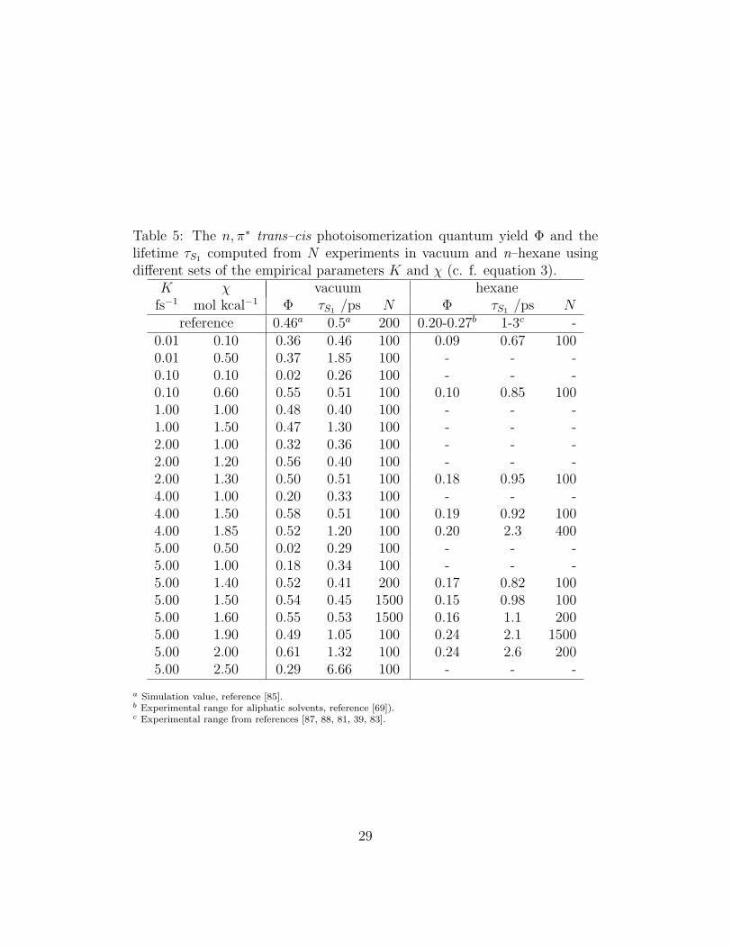
Table 5: The n, π∗ trans–cis photoisomerization quantum yield Φ and thelifetime τS1 computed from N experiments in vacuum and n–hexane usingdifferent sets of the empirical parameters K and χ (c. f. equation 3).

K χ vacuum hexanefs−1 mol kcal−1 Φ τS1 /ps N Φ τS1 /ps N

reference 0.46a 0.5a 200 0.20-0.27b 1-3c -0.01 0.10 0.36 0.46 100 0.09 0.67 1000.01 0.50 0.37 1.85 100 - - -0.10 0.10 0.02 0.26 100 - - -0.10 0.60 0.55 0.51 100 0.10 0.85 1001.00 1.00 0.48 0.40 100 - - -1.00 1.50 0.47 1.30 100 - - -2.00 1.00 0.32 0.36 100 - - -2.00 1.20 0.56 0.40 100 - - -2.00 1.30 0.50 0.51 100 0.18 0.95 1004.00 1.00 0.20 0.33 100 - - -4.00 1.50 0.58 0.51 100 0.19 0.92 1004.00 1.85 0.52 1.20 100 0.20 2.3 4005.00 0.50 0.02 0.29 100 - - -5.00 1.00 0.18 0.34 100 - - -5.00 1.40 0.52 0.41 200 0.17 0.82 1005.00 1.50 0.54 0.45 1500 0.15 0.98 1005.00 1.60 0.55 0.53 1500 0.16 1.1 2005.00 1.90 0.49 1.05 100 0.24 2.1 15005.00 2.00 0.61 1.32 100 0.24 2.6 2005.00 2.50 0.29 6.66 100 - - -

a Simulation value, reference [85].b Experimental range for aliphatic solvents, reference [69]).c Experimental range from references [87, 88, 81, 39, 83].

29

N

Nφ

N

N

θ

Figure 1: Scheme of the azobenzene (AB) molecule showing the Ph-N=N-Phtorsional angle φ, and the Ph-N=N bending angle θ.

30

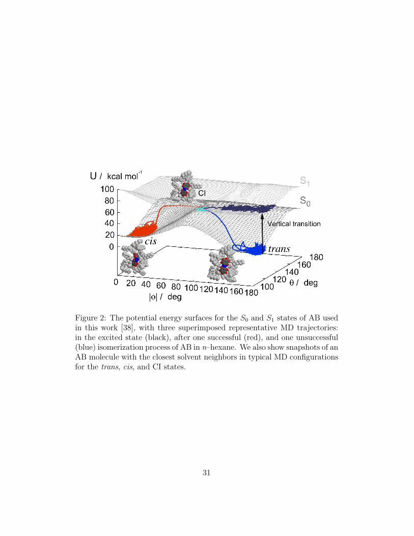
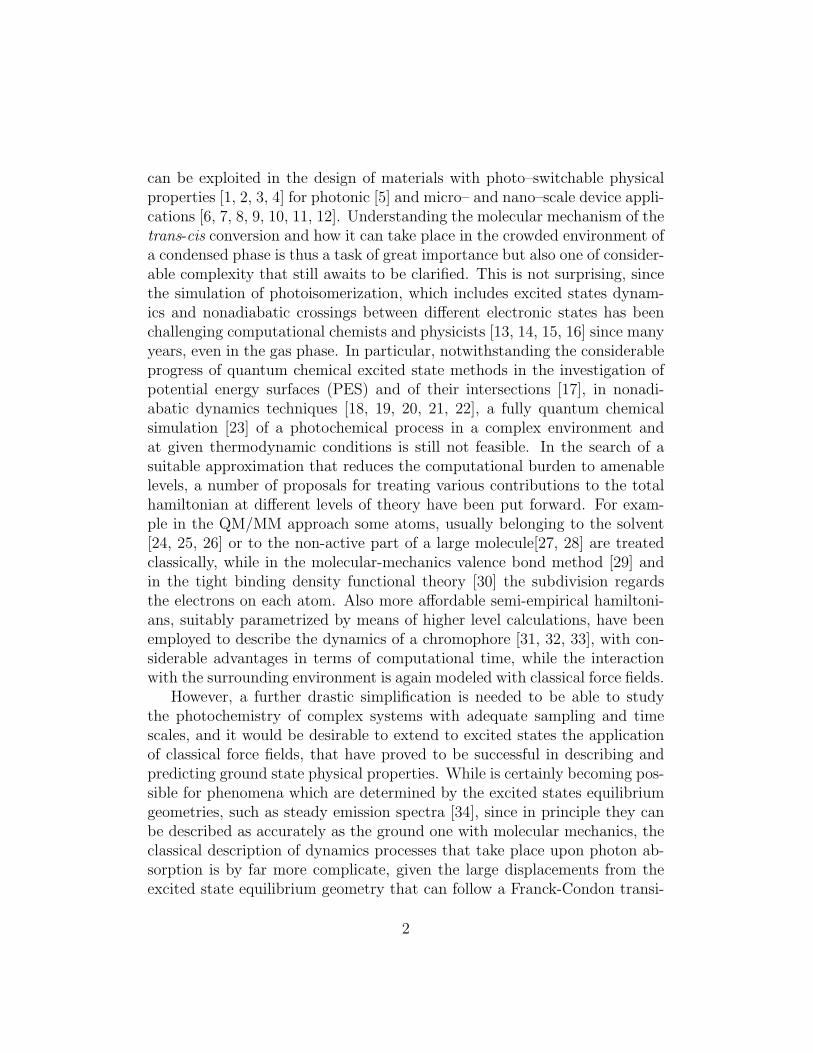
Figure 2: The potential energy surfaces for the S0 and S1 states of AB usedin this work [38], with three superimposed representative MD trajectories:in the excited state (black), after one successful (red), and one unsuccessful(blue) isomerization process of AB in n–hexane. We also show snapshots of anAB molecule with the closest solvent neighbors in typical MD configurationsfor the trans, cis, and CI states.

31

0.0

0.2

0.4

0.6

0.8

1.0

0 5 10 15 20

S1

popu

latio

n

t /ps

VACHEXTOLETHANIEGL

0.00.20.40.60.81.0

0 1 2 3t /τS1

Figure 3: Time evolution of the population of the excited state S1. In theinset, the same data plotted against reduced time units t/τS1 allow to ap-preciate the qualitative difference between the behaviour in vacuum and insolvents.

32

0.0

0.2

0.4

0.6

0.8

1.0

0 1 2 3

S1

popu

latio

n

t /ps

hexaneλ=700 nmλ=650 nmλ=600 nmexp λfl=680 nmoverall

0.0

0.2

0.4

0.6

0.8

1.0

0 2 4 6 8 10

S1

popu

latio

n

t /ps

ethylene glycolλ=700 nmλ=650 nmλ=600 nmexp λfl=680 nmoverall

Figure 4: Time evolution of the population of the excited state S1 (arbi-trary units) as function of the energy difference with the ground state S0

(nanometers), computed in vacuum, n-hexane and ethylene glycol. Eachcolor identifies the population in a 50 nm window centered at the indicatedwavelength. Experimental profiles have been taken from reference [39]

33

0

20

40

60

80

100

120

140

160

180

0 2 4 6 8 10 12 14 16

|φ| /

deg

t /ps

trans

cis

VACHEXANIEGL

110

115

120

125

130

0 2 4 6 8 10 12 14 16

θ /d

eg

t /ps

trans

cis

VACHEXANIEGL

6.0

6.5

7.0

7.5

8.0

8.5

9.0

0 5 10 15 20

r 4,4

’ /(Å

)

t /ps

trans

cis

VACHEXANIEGL

0

5

10

15

20

25

30

35

40

45

0 5 10 15 20

|γ| /

deg

t /ps

trans

cis

VACHEXANIEGL

Figure 5: The evolution of conformational indicators, separately averagedaccording to the final isomerization product (indicated at the right edges ofthe plots): [a] Ph-N=N-Ph torsional angle |φ|; [b] N=N-C bending angles θ;[c] phenyl-phenyl distance r4,4′ ; and [d] C-C-N=N torsional angles |γ|.

34

−0.6

−0.4

−0.2

0.0

0.2

0.4

0.6

0.8

1.0

0 10 20 30 40 50

<r

NN(0

)· r

NN(t

)>

t /ps

VACHEXANIEGL

Figure 6: Time autocorrelation function of the azo bond unit vector 〈rNN(0)·rNN(t)〉. The average values from trajectories leading to cis isomers aremarked with large empty symbols, while those for trajectories leading totrans isomers are plotted with small filled symbols.

35

0.001

0.01

0.1

1

0.1 1 10

τ-1 /p

s-1

η /cP

τ-1r,cis

τ-1r,trans

τ-1S1,cis

τ-1S1,trans

Figure 7: Log-log plot of the simulated rotational relaxation rate constant(1/τr) and of the excited state relaxation rate constant (1/τS1) versus experi-mental viscosities η for cis- (red squares) and trans-azobenzene (blue circles).The straigth lines represent the fit with the equation τ−1 = Aη−α (black dot-ted line: AS1 = 0.39, αS1 = 0.2; red line:Ar,cis = 0.039, αr,cis = 1.17; bluedotted line: Ar,trans = 0.064, αr,trans = 1.08). The times in ethanol, omittedfrom the fits, are shown in black.

36

0.0

0.2

0.4

0.6

0.8

1.0

0 10 20 30 40 50 60

<n

i (0

)· n

i (t

)>

t /ps

VAC i=N

VAC i=R

HEX i=N

HEX i=R

ANI i=N

ANI i=R

EGL i=N

EGL i=R

Figure 8: Time autocorrelation function 〈ni(0) · ni(t)〉 of the normals to thephenyl ring planes (i=R, filled symbols) and the planes containing C-N=Natoms (i=N, nN = rCN × rNN , empty symbols). For better visualization,the time origins for HEX (squares), ANI (circles) and EGL (triangles) havebeen shifted with respect to VAC (pentagons) of 5, 10 and 15 ps respectively.Simulation data have been averaged on the two possible planes for N and R,and only on the trajectories leading to the cis isomer.

37

0.0

0.2

0.4

0.6

0.8

1.0

0 200 400 600 800 1000 1200 1400 1600

S1

popu

latio

n

t /fs

vacuumMD χ=1.5 K=5MD χ=1.4 K=5MD χ=1.6 K=5FMSSH

Figure 9: Time evolution of the population of AB excited state S1 in vac-uum, as function of the empirical parameters K and χ (in fs−1 and molkcal−1 respectively). The FMS and TSH simulation results of Persico andcoworkers[31, 85] are also shown for comparison.

38

log(dP/dt ) /ps−1

0 20 40 60 80 100 120 140 160 180

|φ| /deg

90

100

110

120

130

140

150

160

170

180

θ /d

eg

−40

−35

−30

−25

−20

−15

−10

−5

0

5

log(dP/dt ) /ps−1

0 20 40 60 80 100 120 140 160 180

|φ| /deg

90

100

110

120

130

140

150

160

170

180

θ /d

eg

−40

−35

−30

−25

−20

−15

−10

−5

0

5

Figure 10: The decay probability rate maps calculated with equation 3, usingthe optimal parameters for vacuum (K = 5 fs−1, χ = 1.5 mol kcal−1, top)and for solvents (K = 5 fs−1, χ = 1.9 mol kcal−1, bottom). Level lines areseparated by two orders of magnitude.

39