time-varying demand for lottery
TRANSCRIPT
ARTICLE IN PRESS
JID: FINEC [m3Gdc; August 8, 2020;1:54 ]
Journal of Financial Economics xxx (xxxx) xxx
Contents lists available at ScienceDirect
Journal of Financial Economics
journal homepage: www.elsevier.com/locate/jfec
Time-varying demand for lottery: Speculation ahead of
earnings announcements
�
Bibo Liu
a , Huijun Wang
b , c , Jianfeng Yu
a , ∗, Shen Zhao
d
a PBCSF, Tsinghua University, 43 Chengfu Road, Haidian District, Beijing 10 0 083, China b Faculty of Business and Economics, University of Melbourne, Level 11, 198 Berkeley Street, Carlton, VIC 3053, Australia c Harbert College of Business, Auburn University, 405 W. Magnolia Ave. Auburn, AL 36849, United States d School of Management and Economics, Chinese University of Hong Kong (Shenzhen), 2001 Longxiang Blvd, Longgang District, Shenzhen,
China
a r t i c l e i n f o
Article history:
Received 16 January 2019
Revised 6 November 2019
Accepted 8 November 2019
Available online xxx
JEL classification:
G12
G14
Keywords:
Speculation
Lottery
Earnings announcements
Skewness
a b s t r a c t
Investor preferences for holding speculative assets are likely to be more pronounced ahead
of firms’ earnings announcements, probably because of lower inventory costs and imme-
diate payoffs or because of enhanced investor attention. We show that the demand for
lottery-like stocks is stronger ahead of earnings announcements, leading to a price run-
up for these stocks. In sharp contrast to the standard underperformance of lottery-like
stocks, lottery-like stocks outperform non-lottery stocks by about 52 basis points in the
5-day window ahead of earnings announcements. However, this return spread is reversed
by 80 basis points in the 5-day window after the announcements. Moreover, this inverted-
V-shaped pattern on cumulative return spreads is more pronounced among firms with a
greater retail order imbalance, among firms with low institutional ownership, and in re-
gions with a stronger gambling propensity, and it is also robust after controlling for past
12-month returns and various proxies for investor attention.
© 2020 Elsevier B.V. All rights reserved.
� We thank Zhuo Chen, Jay Coughenour, Zhiguo He, Shiyang Huang
(discussant), Peter Kelly (discussant), Xiaoxia Lou, Christopher Malloy,
Ron Masulis, Veronika Pool (discussant), Avanidhar Subrahmanyam (ref-
eree), and seminar participants at Auburn University, Federal Reserve
Bank of Richmond, Shanghai Advanced Institute of Finance, University
of Arkansas, University of Central Florida, University of Delaware, Uni-
versity of Melbourne, University of Missouri, University of New Mexico,
University of New South Wales, University of Technology Sydney, Univer-
sity of Tennessee, University of Texas at San Antonio, 2017 China Interna-
tional Conference in Finance, University of Oregon Summer Finance Con-
ference, and 2019 American Finance Association annual meeting for help-
ful comments and discussions. Yu acknowledges financial support from
the National Natural Science Foundation of China (Grant no. 71790591 ). ∗ Corresponding author.
E-mail addresses: [email protected] (B. Liu),
[email protected] (H. Wang), [email protected] (J. Yu),
[email protected] (S. Zhao).
https://doi.org/10.1016/j.jfineco.2020.06.016
0304-405X/© 2020 Elsevier B.V. All rights reserved.
Please cite this article as: B. Liu, H. Wang and J. Yu et al., Time-v
announcements, Journal of Financial Economics, https://doi.org/1
1. Introduction
Many studies find that investors exhibit a preference
for speculative assets, and thus these assets tend to be
overvalued on average, leading to underperformance of
these stocks relative to non-speculative assets. 1 In this pa-
per, we argue that investors’ preferences for speculative
stocks are time varying and are especially strong ahead
of firms’ earnings announcements. Because the positions
are held for only a short period of time, trading ahead
of earnings announcements reduces holding costs and in-
ventory risk. Thus, speculative trading tends to increase
prior to earnings announcements. Since lottery-like assets
1 A partial list includes Barberis and Huang (2008) ; Boyer et al. (2010) ;
Bali et al. (2011) ; Green and Hwang (2012) ; Bali et al. (2017) ;
Conrad et al. (2014) , and An et al. (2020) , among others.
arying demand for lottery: Speculation ahead of earnings
0.1016/j.jfineco.2020.06.016

2 B. Liu, H. Wang and J. Yu et al. / Journal of Financial Economics xxx (xxxx) xxx
ARTICLE IN PRESS
JID: FINEC [m3Gdc; August 8, 2020;1:54 ]
are especially good for speculation, the excess demand
for these stocks should be notably higher especially be-
fore earnings announcements. In addition, since earnings
announcement events tend to grab retail investors’ atten-
tion and lottery stocks are traded predominantly by retail
investors, the attention-driven demand for lottery stocks
could increase prior to earnings announcements. 2 More-
over, because of inventory and idiosyncratic volatility con-
cerns leading up to earnings announcements, arbitrageurs’
ability to act against excess demand from noisy traders is
weakened. 3 Taken together, during the days ahead of earn-
ings announcements, lottery-like assets should earn higher
returns than non-lottery assets, which is exactly the oppo-
site pattern of the usual underperformance of the lottery-
like assets documented in the existing literature. 4
By contrast, after earnings announcements, we should
expect the usual underperformance of lottery-like assets.
This is because there are again two reinforcing mecha-
nisms. First, investors might be surprised by negative earn-
ings news associated with lottery-like stocks. 5 Second, af-
ter the earnings announcements, uncertainty about earn-
ings news is resolved. Thus, potential concerns about in-
ventory and idiosyncratic volatility also subside. As a re-
sult, the arbitrage forces are restored, and thus price rever-
sal for lottery-like stocks is expected.
We empirically test this idea by using the following
procedure. We first choose a few popular proxies for the
speculative feature of a stock. Following Kumar (2009) , we
choose stock price level, idiosyncratic volatility, and ex-
pected idiosyncratic skewness as our measures for the de-
gree of speculativeness of a stock. In addition, the maxi-
mum daily return proposed by Bali et al. (2011) is also a
proxy for speculativeness. They show that this measure is
negatively associated with future stock returns in the cross
section. More recently, Conrad et al. (2014) show that jack-
pot probability is another good proxy for lottery features,
and that firms with a high predicted jackpot probability
tend to be overvalued on average and earn lower subse-
quent returns. Thus, we use these five popular proxies for
a stock’s speculative feature. In addition, based on these
five individual proxies, we construct a composite z -score
to proxy for the lottery feature.
2 For example, Aboody et al. (2010) provide evidence of the increase in
investor attention before earnings announcements that can lead to price
run-ups for stocks in the top percentile of past 12-month returns. 3 For example, Berkman et al. (2009) show that, on average, short sell-
ers decrease their positions prior to earnings announcements and in-
crease their positions shortly thereafter. 4 We use “speculative assets” and “lottery-like assets” interchangeably
in the paper. 5 Indeed, we find that earnings surprise is more negative for lottery-
like stocks (see Table A1 in the Online Appendix), suggesting that in-
vestors not only may overweight the small probability events but also
may overestimate the small probability for large return outcomes. This
is consistent with Fox (1999) , who argues that individuals tend to both
overweight and overestimate small probability outcomes. In addition,
Brunnermeier et al. (2007) show that investors’ optimal beliefs could be
overly optimistic about the probability of good states, leading to pref-
erences for skewness. Thus, the more pronounced underperformance on
and after announcement days could be partially due to the usual expec-
tation errors, corrected upon the announcements.
Please cite this article as: B. Liu, H. Wang and J. Yu et al., Time-v
announcements, Journal of Financial Economics, https://doi.org/1
Using these six measures, we find that the 5-day return
spread between lottery-like stocks and non-lottery stocks
is about 0.52% ahead of earnings announcements. In sharp
contrast, the spread is reversed by 0.80% in the 5-day win-
dow after earnings announcements. Fig. 1 plots the cumu-
lative lottery spread during the ( −5,+5) 11-day event win-
dow and presents the key result of our paper. This result
is consistent with the view that the stronger demand for
lottery-like assets ahead of earnings announcements drives
up their stock prices, and later on stock prices are re-
versed because of the diminished demand for lottery-like
stocks to gamble after the news announcements and earn-
ings surprises. Since most anomalies tend to be more pro-
nounced during the earnings announcements, 6 the strong
underperformance of the lottery-like stocks right after the
earnings announcements is expected. However, the novel
finding of our study is that ahead of the earnings an-
nouncements, we show a sharp price run-up for lottery-
like stocks relative to non-lottery stocks. Most prior stud-
ies argue that lottery-like stocks could be overvalued and
focus on the subsequent price reversal of these stocks. Our
focus on pre-announcement periods provides useful infor-
mation on the mechanism and timing of the overvaluation
in the first place and its subsequent corrections. In partic-
ular, we identify specific periods when the overvaluation
is exacerbated, whereas prior studies mostly focus on the
subsequent reversals.
One might argue that the more intense speculative
trading behavior may also hold for other anomaly charac-
teristics, and thus there is nothing special about our re-
sults on the inverted-V-shaped cumulative lottery return
spreads. For comparison, we also perform the same exer-
cise for a set of prominent anomaly-related characteristics,
in particular, value, momentum, profitability, and invest-
ment. We find that the cumulative return spreads based on
book-to-market, past returns, profitability, and the oppo-
site of investment over assets increase both before and af-
ter earnings announcements. Thus, the inverted-V shaped
cumulative return spread is unique to lottery-related char-
acteristics. This contrast in the shape of cumulative return
spreads highlights the unique role of speculation ahead of
earnings announcements for our lottery-related character-
istics. This result can also help us distinguish alternative
potential explanations for our documented pattern. In par-
ticular, a reasonable explanation should invoke the spe-
cial property of the lottery characteristic, rather than sim-
ply and exclusively relying on overall changes in short-
sale activities or investor attention around the earnings an-
nouncement periods.
In a closely related paper, Aboody et al. (2010) docu-
ment that stocks with the strongest prior 12month returns
experience a significant positive average marketadjusted
return before earnings announcements and a significant
negative average marketadjusted return afterward. They ar-
gue that stocks with sharp past run-ups tend to attract in-
vestors attention and thus lead to higher returns for past
6 For a recent comprehensive study on anomaly returns around earn-
ings announcements, see Engelberg et al. (2018) .
arying demand for lottery: Speculation ahead of earnings
0.1016/j.jfineco.2020.06.016

B. Liu, H. Wang and J. Yu et al. / Journal of Financial Economics xxx (xxxx) xxx 3
ARTICLE IN PRESS
JID: FINEC [m3Gdc; August 8, 2020;1:54 ]
Fig. 1. Event-time lottery portfolio excess returns over 11 trading days. This figure plots the cumulative buy-and-hold hedge portfolio returns (in percent-
ages) during the ( −5,+5) event window centered at the earnings announcement date. Each quarter, firms with earnings announcements are divided into
five portfolios based on each of six lottery proxies from the month prior to the announcements. If the earnings announcement date is in the first ten
trading days of a month, we lag one more month and use the lottery proxies from two months prior to the announcements. For each day during the
( −5,+5) event window for each portfolio, we calculate the equal-weighted average buy-and-hold excess returns (in excess of the value-weighted return
of the CRSP index) accumulated starting from day −5. We plot the difference in the average returns between the top and bottom quintile lottery port-
folios. We consider six lottery proxies: Maxret, Skewexp, Prc, Jackpotp, Ivol, and Z -score. Maxret is the maximum daily return; Skewexp is the expected
idiosyncratic skewness from Boyer et al. (2010) ; Prc is the negative log of one plus stock price (i.e., Prc = −log(1 + Price ) ); Jackpotp is the predicted jackpot
probability from Conrad et al. (2014) ; Ivol is idiosyncratic volatility from Ang et al. (2006) ; Z -score is a composite Z -score based on the previous five lottery
proxies. Detailed variable definitions are described in the Appendix. The sample includes NYSE/Amex/Nasdaq common stocks with a price of at least $1
per share at the end of the month prior to the earnings announcements. The sample period is from 1972 to 2014 except for Skewexp, which is from 1988
to 2014.
winners before earnings announcements. Thus, if lottery
stocks simply resemble extreme winner stocks, they could
also attract more attention than non-lottery stocks. This
heightened attention to lottery stocks could also lead to
higher buying pressure and thus higher returns for lottery
stocks than non-lottery stocks before earnings announce-
ments. Thus, this pure attention channel could potentially
produce our return pattern.
On the other hand, it is also possible that investors just
have intrinsic preference for lottery stocks, especially be-
fore earnings announcements. To differentiate the intrin-
sic preference channel from the pure attention channel, we
perform a double-sorting exercise to control for the effect
of past returns. We find that after controlling for past re-
turns, the average return spreads between lottery and non-
lottery stocks (using the composite lottery index) before
earning announcements is still 53.3 basis points, a mag-
nitude similar to our original unconditional spread of 52
basis points. In addition, we also exclude the top decile
winners from our sample and show that our results re-
main largely the same. More important, we use various di-
rect proxies for investor attention and find that for firms
with a similar level of attention before earnings announce-
ments, lottery stocks still tend to earn higher returns than
non-lottery stocks, suggesting that the intrinsic preference
channel plays a significant role.
To further investigate the underlying mechanisms for
our findings during the pre-event window, we use trans-
Please cite this article as: B. Liu, H. Wang and J. Yu et al., Time-v
announcements, Journal of Financial Economics, https://doi.org/1
action data to examine the change in the retail order
imbalance for lottery-like assets before the earnings an-
nouncements. The retail order imbalance captures the buy-
ing pressure from retail investors. We find that the retail
order imbalance increases significantly more for lottery-
like stocks than non-lottery stocks ahead of earnings an-
nouncements. Since there is stronger buying pressure from
retail investors before earnings announcements for lottery-
like stocks, we observe a positive lottery return spread dur-
ing this period. Thus, the pattern in retail order imbalance
before the earnings announcements is consistent with our
findings on the return behavior for lottery-like and non-
lottery stocks. Moveover, the above pattern on retail or-
der imbalance still holds after we control for various prox-
ies for investor attention, lending support for the intrinsic
preference channel.
In addition to the retail order imbalance in stocks, we
also use option data to gauge gambling behavior around
earnings announcements. In particular, we study the daily
adjusted volume of short-term out-of-the-money (OTM)
call options during the (-5,+5) event window centered at
the earnings announcement date. We find that the ad-
justed volume increases ahead of earnings announcements
and decreases after the announcements, consistent with
the notion that gambling behavior is more prominent
ahead of earnings announcements. In addition, the implied
volatility and retail order imbalance of OTM call options
also increase before earnings announcements and are
arying demand for lottery: Speculation ahead of earnings
0.1016/j.jfineco.2020.06.016

4 B. Liu, H. Wang and J. Yu et al. / Journal of Financial Economics xxx (xxxx) xxx
ARTICLE IN PRESS
JID: FINEC [m3Gdc; August 8, 2020;1:54 ]
8 In addition, several studies have employed options data to study
the relation between alternative skewness measures and future re-
turns. For instance, see Xing et al. (2010) , Bali and Murray (2013) , and
Conrad et al. (2013) . 9 There might be some exceptions though. For example,
Barber et al. (2013) argue that the earnings announcement premium
subdued afterward, suggesting a stronger demand for
these lottery-like assets ahead of earnings news.
Kumar et al. (2011) argue that gambling preferences
should be stronger in regions with a higher concentra-
tion of Catholics relative to Protestants since the Catholic
religion is more tolerant of gambling behavior. Indeed,
they show that investors located in regions with a higher
Catholic-Protestant ratio (CPRATIO) exhibit a stronger
propensity to hold stocks with lottery features. Thus, if our
positive lottery return spread ahead of earnings announce-
ments is driven by the excess demand from investors with
gambling preferences, we should expect that this positive
lottery spread is higher for firms located in high CPRA-
TIO regions where local speculative demand is expected to
be stronger because of local bias. Using Fama–MacBeth re-
gression analysis, we indeed confirm this hypothesis.
Using data from 38 countries, we also explore the
cross-country variation in the pre-announcement lottery
premium documented in this study. In particular, we in-
vestigate the pattern in our lottery return spreads around
earnings announcements for 38 countries. We find that
among countries with a stronger preference for lottery
(i.e., countries with high stock market turnover), the pre-
announcement lottery premium is much stronger than that
among countries with a weaker preference for lottery, con-
sistent with the intrinsic preference channel.
Since individuals tend to exhibit stronger preferences
for lottery-like stocks, we expect this inverted-V-shaped
pattern on cumulative lottery return spreads to be more
pronounced among firms with lower institutional own-
ership. In addition, lower institutional ownership more
severely impedes arbitrage forces, and thus the price run-
up for lottery-like stocks ahead of earnings announce-
ments is also expected to be stronger among this group of
stocks. Indeed, we find that the inverted-V-shaped pattern
is stronger among firms with lower institutional owner-
ship, although it is still significant among firms with higher
institutional ownership.
Lastly, since the lottery-like stocks can outperform non-
lottery stocks ahead of earnings announcements, by tak-
ing this fact into account, one could improve the tradi-
tional strategy that bets against lottery-like stocks. In par-
ticular, we should bet for lottery-like stocks ahead of earn-
ings news and revert to the traditional betting-against-
lottery strategy during other times. We show that this new
strategy improves substantially upon the standard betting-
against-lottery strategy. In particular, the monthly strategy
return is improved from 1.09% to 1.50% for the composite
lottery proxy.
In terms of related literature, our paper is related
to a long list of papers on lottery-related anomalies. A
large strand of literature documents that lottery-like as-
sets have low subsequent returns. Boyer et al. (2010) find
that expected idiosyncratic skewness and future returns
are negatively correlated. Bali et al. (2011) show that
maximum daily returns in the previous month are neg-
atively associated with future returns. 7 More recently,
7 Bali et al. (2011) and Bali et al. (2017) argue that preferences for
lottery-like stocks can also account for the puzzle that firms with low
volatility and low beta tend to earn higher risk-adjusted returns.
Please cite this article as: B. Liu, H. Wang and J. Yu et al., Time-v
announcements, Journal of Financial Economics, https://doi.org/1
Conrad et al. (2014) document that firms with a high prob-
ability of extremely large returns (i.e., jackpot) usually earn
abnormally low future returns. All of these empirical stud-
ies suggest that positively skewed stocks can be overpriced
and earn lower future returns. 8 In contrast to this litera-
ture, we show that lottery-like stocks actually outperform
non-lottery stocks ahead of earnings announcements. We
also show that by taking this pre-announcement pattern
into account, we can significantly improve the traditional
lottery strategy. Further, Doran et al. (2012) show that in-
vestors’ preferences for lottery features are stronger dur-
ing January because of the New Year gambling effect and
lottery-like stocks outperform in January. Our study differs
by investigating the news-driven time-variation in lottery
demand.
Our paper is closely related to Aboody et al. (2010) ,
who document that extreme winners, the attention-
grabbing stocks, experience a significant positive average
marketadjusted return during the five trading days be-
fore their earnings announcements and a significant nega-
tive average marketadjusted return in the five trading days
afterward, a pattern similar to ours using lottery stocks.
We show that after controlling for past returns and con-
trolling for many direct proxies for investor attention, the
pre-announcement lottery premium remains quantitatively
similar. Thus, our results are driven by neither the cor-
relation of lottery stocks with past winners nor the pure
attention-grabbing feature of the lottery stocks.
Prior studies find that most anomalies tend to be
more pronounced around earnings announcements. For
example, La Porta et al. (1997) find that the value
strategy performs much better around earnings an-
nouncements. Berkman and McKenzie (2009) find that
firms with high differences of opinion earn signifi-
cantly lower returns around earnings announcements than
firms with low differences of opinion. More recently,
Engelberg et al. (2018) use a large set of stock return
anomalies and find that anomaly returns are about six
times higher on earnings announcement dates. On the one
hand, the pattern of more pronounced anomaly returns
around earnings announcements is consistent with biased
expectations, which are at least partially corrected upon
news arrival. On the other hand, this pattern could also
be consistent with a disproportionally large risk associ-
ated with earnings news. However, our results are hard to
reconcile with a pure risk-based story since the sign on
the return spread switches before and after the event. It
is difficult to build a risk-based model in which lottery-
like stocks are more risky before earnings announcements
and less risky after earnings announcements. 9 Our paper is
could be due to the idiosyncratic risk that cannot be diversified away.
An elaborated model based on their argument could potentially generate
a higher price run-up for lottery stocks relative to non-lottery stocks
before earnings announcements. However, for a pure risk-based story
to convincingly explain our pattern, the model needs to produce lower
arying demand for lottery: Speculation ahead of earnings
0.1016/j.jfineco.2020.06.016

B. Liu, H. Wang and J. Yu et al. / Journal of Financial Economics xxx (xxxx) xxx 5
ARTICLE IN PRESS
JID: FINEC [m3Gdc; August 8, 2020;1:54 ]
also related to So and Wang (2014) who study the short-
term return reversal effect ahead of earnings announce-
ments. They argue that market makers demand higher ex-
pected returns for the liquidity provision prior to earn-
ings announcements because of the increased inventory
risk ahead of the anticipated earnings news. Indeed, they
document a strong increase in short-term return rever-
sals ahead of earnings announcements. We differ by fo-
cusing on the time-varying demand for lottery-like stocks
rather than the time-varying liquidity provision. Moreover,
whereas they show that the short-term reversal effect is
stronger ahead of earnings announcements, we show that
the lottery-return spread is reversed ahead of earnings an-
nouncements, compared with other periods.
Lastly, our paper is also related to a recent study by
Rosch et al. (2017) . They hypothesize that stock-specific in-
formation events (such as earnings announcements) may
affect price efficiency because inventory and idiosyncratic
volatility concerns leading up to the event could temporar-
ily challenge arbitrageurs’ ability to act against predictable
patterns in returns and price deviations from the efficient
market benchmark. Thus, the stock market is less efficient
ahead of earnings announcements. Our results are consis-
tent with their general view since lottery-like stocks are
indeed more overvalued ahead of earnings news. We differ
from them by focusing on one specific set of firm charac-
teristics, i.e., firm-level lottery features, and we provide an
in-depth study of investor demand for lottery around earn-
ings announcements.
2. Data and definitions of key variables
This section describes our data sources and empirical
measures. We also provide summary statistics for the key
variables used in our subsequent analysis.
2.1. Data
Our sample includes quarterly earnings announcements
made by firms listed on the NYSE, Amex, and Nasdaq
from January 1972 to December 2014. The sample includes
only common stocks, and to reduce the potential effects
of penny stocks, we delete stocks with a price of less
than $1 per share at the end of the month prior to the
earnings announcements. Our data come from several data
sources. Earnings announcement dates are from the Com-
pustat Quarterly files. Stock returns data are from Cen-
ter for Research in Security Prices (CRSP) and accounting
data are from Compustat. Analyst data are from the In-
stitutional Brokers’ Estimate System (IBES) from 1985 to
2014. 10 Institutional ownership data are from the Thom-
son Financial 13F file from 1980 to 2014. The transaction
data are from the Institute for the Study of Securities Mar-
kets (ISSM) from 1983 to 1992 and the Trade and Quote
returns for lottery stocks relative to non-lottery stocks after earnings
announcements and also needs to show the lack of an inverted V-
shape around earnings announcements for other anomalies such as the
profitability premium at the same time. 10 Following Berkman and Truong (2009) , our IBES data start in 1985
because of insufficient data prior to that year.
Please cite this article as: B. Liu, H. Wang and J. Yu et al., Time-v
announcements, Journal of Financial Economics, https://doi.org/1
(TAQ) data from 1993 to 20 0 0 for NYSE and Amex com-
mon stocks. 11 Population density data are from the US
Census Bureau. The Facebook Social Connectedness Index
(SCI) data are from Facebook. 12 Religious composition data
are from “Churches and Church Membership” files from
the American Religion Data Archive (ARDA). Options data
are from the OptionMetrics database. Option order flow
data are from the International Securities Exchange (ISE)
Open/Close Trade profile. Monthly mutual fund total net
assets and returns data come from the CRSP Survivor-Bias-
Free US Mutual Fund Database. Monthly hedge fund to-
tal net assets and returns data come from the Thomson
Reuters Lipper Hedge Fund (TASS) Database. Our firm-level
stock and accounting data for non-US companies come
from the Compustat Global database. The earnings an-
nouncement dates for non-US companies are from Bloom-
berg. The stock market turnover ratio of domestic shares
data for international countries are from the World Bank.
2.2. Lottery measures
For US stocks, we use six variables to proxy for the lot-
tery feature of stocks following prior studies. These mea-
sures include the maximum daily return (Maxret), ex-
pected idiosyncratic skewness (Skewexp), stock price (Prc),
the probability of jackpot returns (Jackpotp), idiosyncratic
volatility (Ivol), and a composite z -score ( Z -score) based
on these five variables. This section briefly describes how
these measures are calculated. More details on the con-
struction of these measures are provided in the Appendix.
Maxret : Bali et al. (2011) document a significant and
negative relation between the maximum daily return over
the previous month and the returns in the future. They
also show that firms with larger maximum daily returns
have higher return skewness. It is conjectured that the
negative relation between the maximum daily return and
future returns is due to investors’ preference for lottery-
like stocks. Following their study, we use each stock’s max-
imum daily return (Maxret) as our first measure of the lot-
tery feature.
Skewexp : Boyer et al. (2010) estimate a cross-sectional
model of expected idiosyncratic skewness and find that it
negatively predicts future returns. We use the expected id-
iosyncratic skewness estimated from their model (model 6
of Table 2 on page 179) as our second measure. Following
their estimation, this measure starts from 1988.
Prc : Stocks with low prices attract gamblers because
they create an illusion of more potential for future price
increases, so we use each stock’s closing price as our
third measure of the lottery feature. Low-price stocks are
lottery-like assets, so we take a nonessential transforma-
tion of stock prices in our empirical tests to be consistent
with other proxies, that is, P rc = −log(1 + Price ) .
11 We follow the previous literature (e.g., Barber et al., 2009 ) to restrict
our analysis to the sample period of 1983 to 20 0 0 for NYSE/Amex stocks
because it is not appropriate to distinguish institutional from retail trades
based on the order size after the decimalization since 20 0 0, and the trad-
ing mechanism is different in Nasdaq. 12 We thank Facebook for providing the SCI data. See
Bailey et al. (2018) for more details about the data.
arying demand for lottery: Speculation ahead of earnings
0.1016/j.jfineco.2020.06.016

6 B. Liu, H. Wang and J. Yu et al. / Journal of Financial Economics xxx (xxxx) xxx
ARTICLE IN PRESS
JID: FINEC [m3Gdc; August 8, 2020;1:54 ]
14 Following Aboody et al. (2010) , we use the average RIMB during a pe-
riod after the post-event window as the benchmark to normalize RIMB
in our definition of abnormal RIMB. In particular, we use the average
RIMB during the six five-day periods beginning 30 days after the earnings
announcement and ending 59 days after. The benchmark window ends
59 days after the event, rather than 89 days as in Aboody et al. (2010) ,
to ensure there is no overlap with the pre-event window in the next
earnings announcement. Our results are similar if we use the average
RIMB during the 12 five-day periods beginning 30 days after the earn-
ings announcement and ending 89 days after as the benchmark RIMB,
as in Aboody et al. (2010) . In untabulated tests, we also use an alterna-
Jackpotp : Conrad et al. (2014) show that stocks with a
high predicted probability of extremely large payoffs earn
abnormally low subsequent returns. Their finding suggests
that investors prefer lottery-like payoffs that are positively
skewed. Thus, we use the predicted probability of jackpot
(log returns greater than 100% over the next year), which is
estimated from their baseline model (Panel A of Table 3 on
page 461), as our fourth measure.
Ivol : Stocks with high idiosyncratic volatility are attrac-
tive to investors with gambling preferences because the
high volatility creates the misconception of a high proba-
bility of realizing high returns. Following Ang et al. (2006) ,
we compute idiosyncratic volatility (Ivol) as the standard
deviation of daily residual returns relative to the Fama and
French (1993) three-factor model and use it as our fifth
measure of the lottery feature.
Z -score : The Z -score is a monthly composite lottery
measure calculated as the average of the individual z -
scores of the previous five lottery measures: Maxret, Skew-
exp, Prc, Jackpotp, and Ivol. Each month for each stock,
each one of the five lottery measures is first converted into
its rank and then standardized to obtain its z -score. We re-
quire a minimum of three nonmissing lottery measures out
of five to compute this measure.
2.3. Attention measures
We use five measures to capture investor attention.
Our first proxy is a dummy for media coverage in the
Dow Jones edition of RavenPack news data. Barber and
Odean (2008) find that media coverage catches investor at-
tention, and individual investors are net buyers of stocks
in the news. Extreme events are likely to attract investor
attention, so following Bali et al. (2019) , we use the mag-
nitude of the most recent earnings surprise to proxy for
investor attention. Since more social interaction is more
likely to attract more attention, following Bali et al. (2019) ,
we also use population density (PD) and the social con-
nectedness (SCIH) of a firm’s headquarters as another
proxy for attention. Lastly, we construct a monthly com-
posite measure for attention (Attn) calculated as the aver-
age of the individual z -scores of these four attention mea-
sures. More details on the construction of these measures
are provided in the Appendix.
2.4. Retail order imbalance
To measure retail order imbalance (RIMB), we follow
Hvidkjaer (2006) and use the imbalance inferred from the
transaction data from ISSM and TAQ. We only include NYSE
and Amex common stocks from 1983 to 20 0 0. We apply
the standard filters and delete trades and quotes with ir-
regular terms and those with likely erroneous prices.
The RIMB is computed in two steps. 13 In the first step,
all eligible trades are classified as small, medium, or large
trades using a variation of the Lee (1992) firm-specific
dollar-based trade-size proxy. Each month, we form five
13 See Hvidkjaer (2006) for more details on the construction of this
measure.
Please cite this article as: B. Liu, H. Wang and J. Yu et al., Time-v
announcements, Journal of Financial Economics, https://doi.org/1
portfolios based on firm size at the end of the previous
month and then use the size-quintile-specific dollar value
in the following table as the breakpoints to identify small,
medium, or large trades.
Firm-size quintile Small 2 3 4 Large
Small trade cut-off, in $ 3400 4800 7300 10,300 16,400
Large trade cut-off, in $ 6800 9600 14,600 20,600 32,800
All trades are further classified as either buy-initiated
or sell-initiated based on the tick and trades rule accord-
ing to the Lee and Ready (1991) algorithm. A trade is sell-
initiated if it is executed at a price below the quote mid-
point and is buy-initiated if it is executed at a price above
the quote midpoint. If a trade is executed at the quote
midpoint, we use the tick rule: it is sell-initiated if the
trade price is below the last executed trade price; it is
buy-initiated if the trade price is above the last executed
trade price. This procedure classifies all eligible trades
into one of six categories: buy-initiated small trades, sell-
initiated small trades, buy-initiated medium trades, sell-
initiated medium trades, buy-initiated large trades, and
sell-initiated large trades. In the second step, for each
stock during each window period, we compute its retail or-
der imbalance as the difference between the buy-initiated
and sell-initiated small-trade volume divided by the sum
of the buy-initiated and sell-initiated small-trade volume:
RIMB = ( BUYVOL − SELLVOL ) / ( BUYVOL + SELLVOL ) , where
BUYVOL and SELLVOL are the sum of daily buy-initiated
and sell-initiated small-trade volume of this stock during
each window period, respectively. To capture the change in
the sentiment among retail investors, we use the average
RIMB of the six five-day windows starting from 30 days af-
ter the earnings announcements and ending 59 days after
as the benchmark RIMB and subtract it from the RIMB dur-
ing the ( −5, −1) pre-event or the (+1,+5) post-event win-
dow to get the abnormal RIMB during the corresponding
event window. 14
2.5. Option volume, implied volatility, and option retail order
imbalance
Our option volume and implied volatility data are
from OptionMetrics from 1996 to 2014. Out-of-the-money
(OTM) call options are particularly attractive to investors
with a gambling preference because the highly skewed
payoffs make them like lottery-like assets. If investors are
tive benchmark RIMB for the pre-event (post-event) window to be the
RIMB during the five-day period immediately before (after) the earnings
announcement and obtain similar results. In fact, our results are very sim-
ilar when using different definitions.
arying demand for lottery: Speculation ahead of earnings
0.1016/j.jfineco.2020.06.016

B. Liu, H. Wang and J. Yu et al. / Journal of Financial Economics xxx (xxxx) xxx 7
ARTICLE IN PRESS
JID: FINEC [m3Gdc; August 8, 2020;1:54 ]
16 These 38 countries are Argentina, Australia, Austria, Belgium, Brazil,
Canada, Switzerland, Chile, China, Germany, Denmark, Spain, Finland,
France, United Kingdom, Greece, Hong Kong, Indonesia, India, Israel,
Italy, Japan, South Korea, Mexico, Malaysia, Netherlands, Norway, New
more likely to gamble before earnings announcements,
then they might tend to trade more OTM calls than dur-
ing other periods as well. To capture this sentiment, we
examine the adjusted daily volume and implied volatility
for all short-term OTM call options expiring in the follow-
ing month. An option is defined as OTM if its strike price
to stock price ratio is greater than 1.05. We remove op-
tions with nonstandard settlement, options that violate ba-
sic arbitrage conditions, and options with zero open inter-
est, missing bid, or offer prices. After applying these fil-
ters, for each stock at each day, we aggregate the trading
volume for all of its valid short-term OTM calls. The ad-
justed volume is then computed as the percentage change
in daily volume from its past 3-month moving average
to remove the upward time trend of the trading volume.
Lastly, we average the adjusted volume across all stocks for
each event day. Similarly, we average the implied volatility
across all valid short-term OTM calls for each stock on each
day and then average across all stocks for each event day.
The option abnormal retail order imbalance measure is
computed using data from the ISE Open/Close Trade Pro-
file from 2008 to 2014. 15 The ISE data contain daily infor-
mation about buy and sell trading volumes for each option
traded at the ISE disaggregated by different customer types
(market maker, firm, customer, and professional customer),
different size brackets (small, medium, and large), whether
the trade is to open new positions or close existing posi-
tions (open buy, open sell, close buy, and close sell), along
with the basic characteristics of the option including expi-
ration date, strike price, option type (call or put), and mon-
eyness. We focus on the short-term OTM call options ex-
piring in the next month. To measure the trading volumes
at the stock level, we first convert the trading volume (in
terms of the number of option contracts) in the ISE to
the number of underlying shares. We then aggregate open
buy and open sell shares for all of their valid short-term
OTM calls for different customer types for each underlying
stock on each day. The buy-initiated and sell-initiated re-
tail trading volumes are the open buy and open sell shares
by the customer type identified as customers, respectively.
The retail order imbalance is computed by taking the dif-
ference between the daily buy-initiated and sell-initiated
retail trading volume divided by the sum of the daily buy-
initiated and sell-initiated retail trading volume. We fur-
ther normalize this retail order imbalance by subtracting
the benchmark retail order imbalance, which is the average
daily retail order imbalance starting from 30 days after the
earnings announcements and ending 59 days after. Lastly,
we average the abnormal retail order imbalance across all
stocks for each event day.
2.6. Religious characteristics
Our main religion proxy is the Catholic-Protestant ratio
(CPRATIO) as defined in Kumar et al. (2011) . The Glenmary
Research Center collects detailed county-level data on the
number of churches and the number of adherents to each
15 About 30% of the trading volume in individual equity options is in
the ISE Open/Close Trade Profile. The moneyness variable in the ISE data
starts in November 2007, so our sample starts in 2008.
Please cite this article as: B. Liu, H. Wang and J. Yu et al., Time-v
announcements, Journal of Financial Economics, https://doi.org/1
church for the years 1971, 1980, 1990, 20 0 0, and 2010, and
publishes the data in “Churches and Church Membership”
files in the American Religion Data Archive (ARDA). We fol-
low previous literature (e.g., Hilary and Hui, 2009, Kumar
et al., 2011 to linearly interpolate the data in the interme-
diate years. We further merge this religion variable with
the firm headquarters location data from Compustat and
use it as the firm-level CPRATIO.
2.7. International sample
Our international sample includes 38 countries. 16 For
each non-US country, we only include common stocks
traded on the major national stock exchanges following
Gao et al. (2018) . We convert all returns, prices, and ac-
counting variables from local currency to US dollars. We
further exclude micro-cap firms that have a market equity
or price below 5% in each quarter in a country. To avoid ex-
treme values, returns are set as missing if falling out of the
0.1 and 99.9 percentiles. The earnings announcement dates
for non-US countries come from Bloomberg. To avoid po-
tential bias from having portfolios with too few assets, we
require a minimum of eight quarters and a minimum of
30 stocks each quarter for each country. Our international
sample starts in 1999.
To measure the lottery feature of non-US stocks, we
use three proxies similar to our definitions for US stocks:
Maxret, Prc, and Ivol. 17 Maxret is the maximum daily re-
turn within a month, and Prc is the negative log of one
plus the month-end stock price, that is, P rc = −log(1 +Price ) ). To compute Ivol for each country, we first specify
a local version of the Fama-French three-factor model in-
cluding a local market excess return factor, a local size fac-
tor, and a local value factor, following Ang et al. (2009) and
Gao et al. (2018) . The market factor is the value-weighted
return of the local market portfolio minus the one-month
US T-bill rate. The country-specific size is the return spread
between the smallest and biggest local firms, and the
value factor is the spread between the local value and
growth firms. Idiosyncratic volatility (Ivol) is computed as
the standard idiosyncratic volatility measure, that is, the
standard deviation of residuals from the daily local fac-
tor model within a month with a minimum requirement
of ten nonmissing values. After we obtain Maxret, Prc, and
Ivol for each stock, we construct a composite z -score as the
average of these individual z -scores.
2.8. Summary statistics
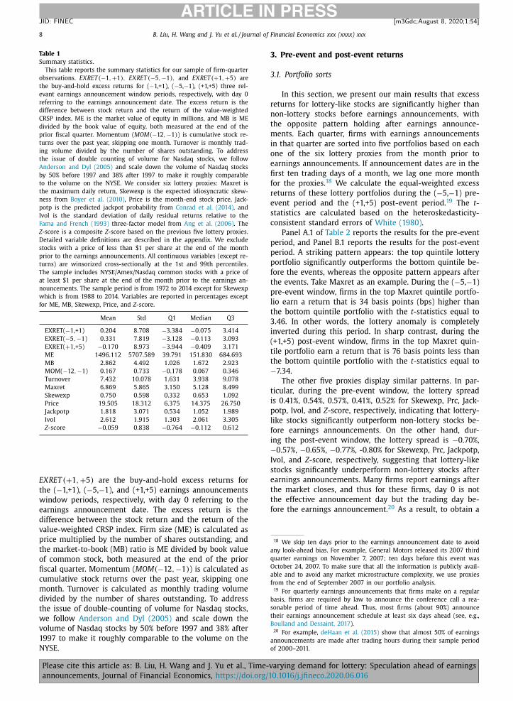
Table 1 presents the summary statistics. Our sam-
ple includes a total of 643,729 quarterly earnings an-
nouncements. E XRE T (−1 , +1) , E XRE T (−5 , −1) , and
Zealand, Pakistan, Philippines, Poland, Portugal, Singapore, Sweden, Thai-
land, Turkey, the United States, and South Africa. 17 The data to construct the other two lottery proxies are limited for
non-US stocks; thus, we only use these three easy-to-calculate proxies to
compute our lottery proxy.
arying demand for lottery: Speculation ahead of earnings
0.1016/j.jfineco.2020.06.016
8 B. Liu, H. Wang and J. Yu et al. / Journal of Financial Economics xxx (xxxx) xxx
ARTICLE IN PRESS
JID: FINEC [m3Gdc; August 8, 2020;1:54 ]
Table 1
Summary statistics.
This table reports the summary statistics for our sample of firm-quarter
observations. E XRE T (−1 , +1) , E XRE T (−5 , −1) , and E XRE T (+1 , +5) are
the buy-and-hold excess returns for ( −1,+1), ( −5, −1), (+1,+5) three rel-
evant earnings announcement window periods, respectively, with day 0
referring to the earnings announcement date. The excess return is the
difference between stock return and the return of the value-weighted
CRSP index. ME is the market value of equity in millions, and MB is ME
divided by the book value of equity, both measured at the end of the
prior fiscal quarter. Momentum ( M OM (−12 , −1) ) is cumulative stock re-
turns over the past year, skipping one month. Turnover is monthly trad-
ing volume divided by the number of shares outstanding. To address
the issue of double counting of volume for Nasdaq stocks, we follow
Anderson and Dyl (2005) and scale down the volume of Nasdaq stocks
by 50% before 1997 and 38% after 1997 to make it roughly comparable
to the volume on the NYSE. We consider six lottery proxies: Maxret is
the maximum daily return, Skewexp is the expected idiosyncratic skew-
ness from Boyer et al. (2010) , Price is the month-end stock price, Jack-
potp is the predicted jackpot probability from Conrad et al. (2014) , and
Ivol is the standard deviation of daily residual returns relative to the
Fama and French (1993) three-factor model from Ang et al. (2006) . The
Z -score is a composite Z -score based on the previous five lottery proxies.
Detailed variable definitions are described in the appendix. We exclude
stocks with a price of less than $1 per share at the end of the month
prior to the earnings announcements. All continuous variables (except re-
turns) are winsorized cross-sectionally at the 1st and 99th percentiles.
The sample includes NYSE/Amex/Nasdaq common stocks with a price of
at least $1 per share at the end of the month prior to the earnings an-
nouncements. The sample period is from 1972 to 2014 except for Skewexp
which is from 1988 to 2014. Variables are reported in percentages except
for ME, MB, Skewexp, Price, and Z -score.
Mean Std Q1 Median Q3
EXRET( −1,+1) 0.204 8.708 −3.384 −0.075 3.414
EXRET( −5 , −1) 0.331 7.819 −3.128 −0.113 3.093
EXRET( + 1,+5) −0.170 8.973 −3.944 −0.409 3.171
ME 1496.112 5707.589 39.791 151.830 684.693
MB 2.862 4.492 1.026 1.672 2.923
MOM( −12 , −1) 0.167 0.733 −0.178 0.067 0.346
Turnover 7.432 10.078 1.631 3.938 9.078
Maxret 6.869 5.865 3.150 5.128 8.499
Skewexp 0.750 0.598 0.332 0.653 1.092
Price 19.505 18.312 6.375 14.375 26.750
Jackpotp 1.818 3.071 0.534 1.052 1.989
Ivol 2.612 1.915 1.303 2.061 3.305
Z -score −0.059 0.838 −0.764 −0.112 0.612
18 We skip ten days prior to the earnings announcement date to avoid
any look-ahead bias. For example, General Motors released its 2007 third
quarter earnings on November 7, 2007; ten days before this event was
October 24, 2007. To make sure that all the information is publicly avail-
able and to avoid any market microstructure complexity, we use proxies
from the end of September 2007 in our portfolio analysis. 19 For quarterly earnings announcements that firms make on a regular
basis, firms are required by law to announce the conference call a rea-
sonable period of time ahead. Thus, most firms (about 90%) announce
their earnings announcement schedule at least six days ahead (see, e.g.,
Boulland and Dessaint, 2017 ). 20 For example, deHaan et al. (2015) show that almost 50% of earnings
announcements are made after trading hours during their sample period
of 20 0 0–2011.
E XRE T (+1 , +5) are the buy-and-hold excess returns for
the ( −1,+1), ( −5, −1), and (+1,+5) earnings announcements
window periods, respectively, with day 0 referring to the
earnings announcement date. The excess return is the
difference between the stock return and the return of the
value-weighted CRSP index. Firm size (ME) is calculated as
price multiplied by the number of shares outstanding, and
the market-to-book (MB) ratio is ME divided by book value
of common stock, both measured at the end of the prior
fiscal quarter. Momentum ( M OM (−12 , −1) ) is calculated as
cumulative stock returns over the past year, skipping one
month. Turnover is calculated as monthly trading volume
divided by the number of shares outstanding. To address
the issue of double-counting of volume for Nasdaq stocks,
we follow Anderson and Dyl (2005) and scale down the
volume of Nasdaq stocks by 50% before 1997 and 38% after
1997 to make it roughly comparable to the volume on the
NYSE.
Please cite this article as: B. Liu, H. Wang and J. Yu et al., Time-v
announcements, Journal of Financial Economics, https://doi.org/1
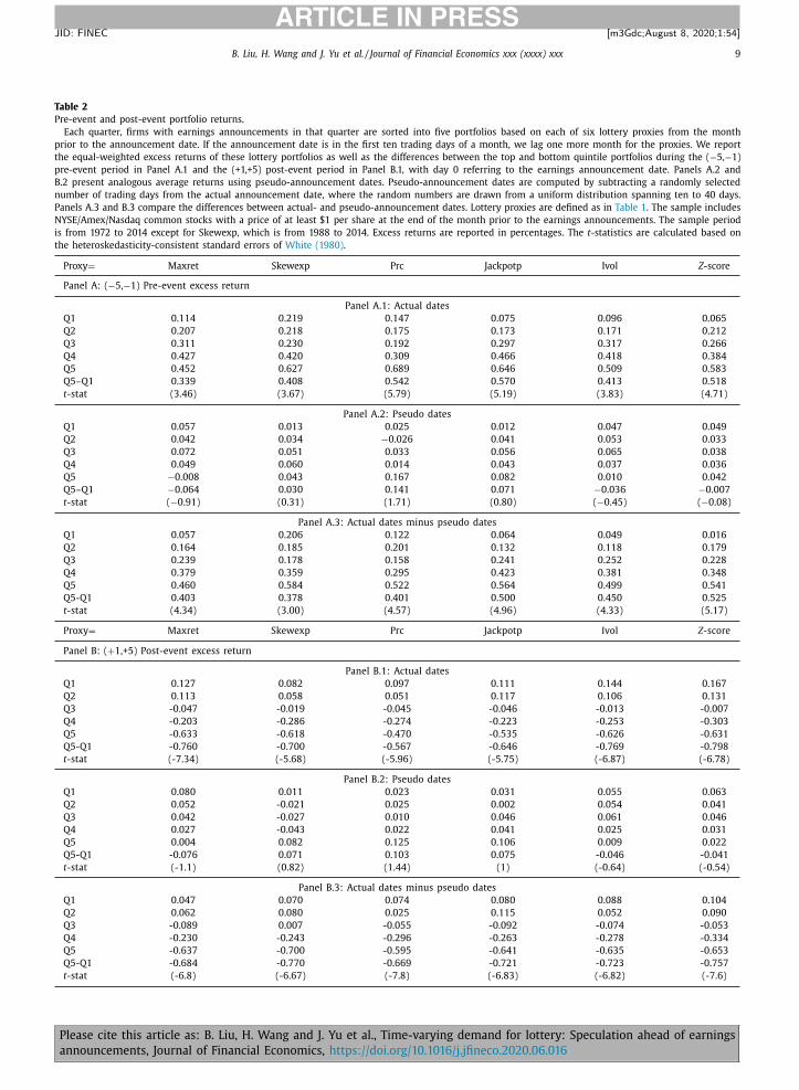
3. Pre-event and post-event returns
3.1. Portfolio sorts
In this section, we present our main results that excess
returns for lottery-like stocks are significantly higher than
non-lottery stocks before earnings announcements, with
the opposite pattern holding after earnings announce-
ments. Each quarter, firms with earnings announcements
in that quarter are sorted into five portfolios based on each
one of the six lottery proxies from the month prior to
earnings announcements. If announcement dates are in the
first ten trading days of a month, we lag one more month
for the proxies. 18 We calculate the equal-weighted excess
returns of these lottery portfolios during the ( −5, −1) pre-
event period and the (+1,+5) post-event period. 19 The t -
statistics are calculated based on the heteroskedasticity-
consistent standard errors of White (1980) .
Panel A.1 of Table 2 reports the results for the pre-event
period, and Panel B.1 reports the results for the post-event
period. A striking pattern appears: the top quintile lottery
portfolio significantly outperforms the bottom quintile be-
fore the events, whereas the opposite pattern appears after
the events. Take Maxret as an example. During the ( −5, −1)
pre-event window, firms in the top Maxret quintile portfo-
lio earn a return that is 34 basis points (bps) higher than
the bottom quintile portfolio with the t -statistics equal to
3.46. In other words, the lottery anomaly is completely
inverted during this period. In sharp contrast, during the
(+1,+5) post-event window, firms in the top Maxret quin-
tile portfolio earn a return that is 76 basis points less than
the bottom quintile portfolio with the t -statistics equal to
−7.34.
The other five proxies display similar patterns. In par-
ticular, during the pre-event window, the lottery spread
is 0.41%, 0.54%, 0.57%, 0.41%, 0.52% for Skewexp, Prc, Jack-
potp, Ivol, and Z -score, respectively, indicating that lottery-
like stocks significantly outperform non-lottery stocks be-
fore earnings announcements. On the other hand, dur-
ing the post-event window, the lottery spread is −0.70%,
−0.57%, −0.65%, −0.77%, -0.80% for Skewexp, Prc, Jackpotp,
Ivol, and Z -score, respectively, suggesting that lottery-like
stocks significantly underperform non-lottery stocks after
earnings announcements. Many firms report earnings after
the market closes, and thus for these firms, day 0 is not
the effective announcement day but the trading day be-
fore the earnings announcement. 20 As a result, to obtain a
arying demand for lottery: Speculation ahead of earnings
0.1016/j.jfineco.2020.06.016
B. Liu, H. Wang and J. Yu et al. / Journal of Financial Economics xxx (xxxx) xxx 9
ARTICLE IN PRESS
JID: FINEC [m3Gdc; August 8, 2020;1:54 ]
Table 2
Pre-event and post-event portfolio returns.
Each quarter, firms with earnings announcements in that quarter are sorted into five portfolios based on each of six lottery proxies from the month
prior to the announcement date. If the announcement date is in the first ten trading days of a month, we lag one more month for the proxies. We report
the equal-weighted excess returns of these lottery portfolios as well as the differences between the top and bottom quintile portfolios during the ( −5, −1)
pre-event period in Panel A.1 and the (+1,+5) post-event period in Panel B.1, with day 0 referring to the earnings announcement date. Panels A.2 and
B.2 present analogous average returns using pseudo-announcement dates. Pseudo-announcement dates are computed by subtracting a randomly selected
number of trading days from the actual announcement date, where the random numbers are drawn from a uniform distribution spanning ten to 40 days.
Panels A.3 and B.3 compare the differences between actual- and pseudo-announcement dates. Lottery proxies are defined as in Table 1 . The sample includes
NYSE/Amex/Nasdaq common stocks with a price of at least $1 per share at the end of the month prior to the earnings announcements. The sample period
is from 1972 to 2014 except for Skewexp, which is from 1988 to 2014. Excess returns are reported in percentages. The t -statistics are calculated based on
the heteroskedasticity-consistent standard errors of White (1980) .
Proxy = Maxret Skewexp Prc Jackpotp Ivol Z -score
Panel A: ( −5, −1) Pre-event excess return
Panel A.1: Actual dates
Q1 0.114 0.219 0.147 0.075 0.096 0.065
Q2 0.207 0.218 0.175 0.173 0.171 0.212
Q3 0.311 0.230 0.192 0.297 0.317 0.266
Q4 0.427 0.420 0.309 0.466 0.418 0.384
Q5 0.452 0.627 0.689 0.646 0.509 0.583
Q5–Q1 0.339 0.408 0.542 0.570 0.413 0.518
t -stat (3.46) (3.67) (5.79) (5.19) (3.83) (4.71)
Panel A.2: Pseudo dates
Q1 0.057 0.013 0.025 0.012 0.047 0.049
Q2 0.042 0.034 −0.026 0.041 0.053 0.033
Q3 0.072 0.051 0.033 0.056 0.065 0.038
Q4 0.049 0.060 0.014 0.043 0.037 0.036
Q5 −0.008 0.043 0.167 0.082 0.010 0.042
Q5–Q1 −0.064 0.030 0.141 0.071 −0.036 −0.007
t -stat ( −0.91) (0.31) (1.71) (0.80) ( −0.45) ( −0.08)
Panel A.3: Actual dates minus pseudo dates
Q1 0.057 0.206 0.122 0.064 0.049 0.016
Q2 0.164 0.185 0.201 0.132 0.118 0.179
Q3 0.239 0.178 0.158 0.241 0.252 0.228
Q4 0.379 0.359 0.295 0.423 0.381 0.348
Q5 0.460 0.584 0.522 0.564 0.499 0.541
Q5-Q1 0.403 0.378 0.401 0.500 0.450 0.525
t -stat (4.34) (3.00) (4.57) (4.96) (4.33) (5.17)
Proxy = Maxret Skewexp Prc Jackpotp Ivol Z -score
Panel B: ( + 1,+5) Post-event excess return
Panel B.1: Actual dates
Q1 0.127 0.082 0.097 0.111 0.144 0.167
Q2 0.113 0.058 0.051 0.117 0.106 0.131
Q3 -0.047 -0.019 -0.045 -0.046 -0.013 -0.007
Q4 -0.203 -0.286 -0.274 -0.223 -0.253 -0.303
Q5 -0.633 -0.618 -0.470 -0.535 -0.626 -0.631
Q5-Q1 -0.760 -0.700 -0.567 -0.646 -0.769 -0.798
t -stat (-7.34) (-5.68) (-5.96) (-5.75) (-6.87) (-6.78)
Panel B.2: Pseudo dates
Q1 0.080 0.011 0.023 0.031 0.055 0.063
Q2 0.052 -0.021 0.025 0.002 0.054 0.041
Q3 0.042 -0.027 0.010 0.046 0.061 0.046
Q4 0.027 -0.043 0.022 0.041 0.025 0.031
Q5 0.004 0.082 0.125 0.106 0.009 0.022
Q5-Q1 -0.076 0.071 0.103 0.075 -0.046 -0.041
t -stat (-1.1) (0.82) (1.44) (1) (-0.64) (-0.54)
Panel B.3: Actual dates minus pseudo dates
Q1 0.047 0.070 0.074 0.080 0.088 0.104
Q2 0.062 0.080 0.025 0.115 0.052 0.090
Q3 -0.089 0.007 -0.055 -0.092 -0.074 -0.053
Q4 -0.230 -0.243 -0.296 -0.263 -0.278 -0.334
Q5 -0.637 -0.700 -0.595 -0.641 -0.635 -0.653
Q5-Q1 -0.684 -0.770 -0.669 -0.721 -0.723 -0.757
t -stat (-6.8) (-6.67) (-7.8) (-6.83) (-6.82) (-7.6)
Please cite this article as: B. Liu, H. Wang and J. Yu et al., Time-varying demand for lottery: Speculation ahead of earnings
announcements, Journal of Financial Economics, https://doi.org/10.1016/j.jfineco.2020.06.016

10 B. Liu, H. Wang and J. Yu et al. / Journal of Financial Economics xxx (xxxx) xxx
ARTICLE IN PRESS
JID: FINEC [m3Gdc; August 8, 2020;1:54 ]
22 Thus, the overall five-day return for the momentum anomaly dur-
ing the post-event window in our sample is close to zero. However,
the overall five-day return during the post-event window is −42 bps in
Aboody et al. (2010) sample. There are at least three reasons that led
to the discrepancy with Aboody et al. (2010) . First, we skip one month
in forming the momentum portfolio, following the momentum tradition.
Second, we use quintile sorting, whereas Aboody et al. (2010) use decile
sorting. Third, our sample is different from theirs. We use common shares
clean measure of post-event performance, we focus on the
(+1,+5) post-event window. In the robustness checks sec-
tion, we use an alternative definition of the earnings an-
nouncement date based on the day of highest relative trad-
ing volume following Engelberg et al. (2018) and show that
our results remain quantitatively similar. 21 Further, in unt-
abulated tests, we find similar results if we use (0, +5) as
our post-event window or ( −5, 0) as our pre-event win-
dow.
Further, to make sure that the patterns we discov-
ered are specific to earnings announcements, rather than
a general phenomenon for any date, we compare the
announcement period returns to the non-announcement
period using a placebo test based on “pseudo-event”
dates. In particular, we repeat our portfolio analysis in
Panel A.1 and Panel B.1 using randomly selected non-
announcement dates. Following So and Wang (2014) ,
pseudo-announcement dates are chosen from a baseline
period relative to the actual announcement dates by sub-
tracting a randomly selected number of days that is drawn
from a uniform distribution from ten to 40 days. We skip
ten days from the actual announcement dates to avoid
the scenario that the post-event period of the pseudo-
announcement dates overlaps with the pre-event period
of the actual-announcement dates. Panel A.2 and Panel
B.2 report the results for these “pseudo-announcement”
portfolios. Lottery-like stocks generally earn similar re-
turns to non-lottery stocks. More importantly, Panel A.3
and Panel B.3 compare the “actual-announcement” and
“pseudo-announcement” portfolios and report their differ-
ences. All the difference-in-differences are significant with
the right sign during both pre-event and post-event peri-
ods, in both a statistical and economical sense.
Fig. 1 plots the difference in the cumulative buy-and-
hold excess returns between top and bottom quintile port-
folios based on lottery proxies over the (-5,+5) 11 trading
days centered around the earnings announcement dates. In
particular, we calculate equal-weighted average buy-and-
hold excess returns accumulated starting from day −5. We
plot the difference in the average returns between the top
and the bottom quintile lottery portfolios. For all six lottery
proxies, the returns of these hedge portfolios start to in-
crease five days prior to the event date and then decrease
immediately after the event, with the biggest drop hap-
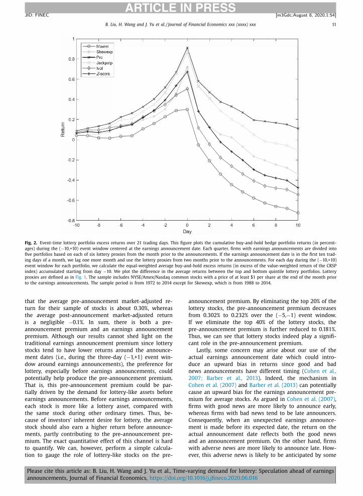
pening on the date right after the event. Further, a simi-
lar pattern holds if we use the ( −10,+10) 21 trading days
event window, as shown in Fig. 2 . In sum, we provide in-
formation on when the overvaluation of lottery-like stocks
occurs in the first place, whereas most prior studies focus
on the subsequent reversals for lottery-like stocks.
We have documented an inverted-V-shaped cumulative
return spread based on lottery proxies before and after
earnings announcements in Fig. 1 . One might think that
the more intense speculative trading behavior may also
hold for other anomaly characteristics, and thus there is
21 As another robustness check, in untabulated tests, we repeat the anal-
ysis using the earlier of the IBES earnings announcement and Compustat
earnings announcement dates as the definition of the earnings announce-
ment date, following DellaVigna and Pollet (2009) . Our results remain
similar and are available upon request.
Please cite this article as: B. Liu, H. Wang and J. Yu et al., Time-v
announcements, Journal of Financial Economics, https://doi.org/1
nothing special about our results for the inverted-V-shaped
cumulative lottery spreads. Thus, for comparison, we also
perform the same exercise for a set of other anomaly-
related characteristics. Probably the most well-known
anomalies are value and momentum. Recently, profitabil-
ity and investment have also attracted a lot of attention.
In particular, Novy-Marx (2013) , Fama and French (2015) ,
Fama and French (2018) , and Hou et al. (2015) show
that new factor models with additional factors related
to profitability and investment can account for a large
set of asset pricing anomalies. Thus, we repeat our ex-
ercise for value, momentum, profitability, and investment
and plot the cumulative anomaly return spreads around
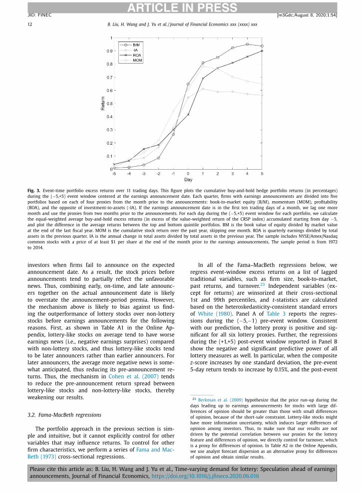
the earnings announcements in Fig. 3 . First, the return
spreads are more pronounced around the earnings an-
nouncements than in other periods, a finding consistent
with La Porta et al. (1997) and Engelberg et al. (2018) .
More importantly, the cumulative return spreads based on
book-to-market, profitability, and the opposite of invest-
ment over assets increase both before and after earnings
announcements. For the momentum effect, the post-event
return spread is positive in the first day after the an-
nouncement, and reversed to some degree starting from
day 2 after the event. 22 It is worth noting that the shape
for the cumulative return spread in Fig. 3 is monotonically
increasing for book-to-market, profitability, and the oppo-
site of investment over assets, whereas for lottery charac-
teristics, an inverted-V shape obtains. This contrast high-
lights the unique role of speculation ahead of earnings an-
nouncements for our lottery-related characteristics.
We would also like to link our previous result to the
well-known earnings announcement premium literature.
Indeed, many studies have documented an earnings an-
nouncement premium. For example, over the three days
surrounding the earnings announcement, Frazzini and La-
mont (2007) find that the average abnormal return is
0.21%. Ball and Kothari (1991) and Cohen et al. (2007) also
find average three-day announcement abnormal returns of
0.24% and 0.11%, respectively, over different sample peri-
ods. Moreover, Barber et al. (2013) find that stocks tend
to earn higher returns during the earnings announce-
ment month across 20 countries. In addition, Ball and
Kothari (1991) and Berkman et al. (2009) find average pre-
announcement abnormal returns of 0.17% and 0.34%, re-
spectively, and a negligible average abnormal return of
−0.01% post-announcement. Aboody et al. (2010) also find
listed on NYSE/Amex/Nasdaq from CRSP with all fiscal year-ends, and is-
suing earnings announcements on Compustat from January 1, 1972 to De-
cember 31, 2014, whereas the sample in Aboody et al. (2010) includes all
CRSP stocks with a December 31 fiscal year-end, and issuing earnings an-
nouncements on Compustat from January 1, 1971 to September 30, 2005.
If we use a similar sample, decile sorting, and the same definition of past
winners, we actually obtain the same 10-minus-1 portfolio spread of −42
bps as in Aboody et al. (2010) .
arying demand for lottery: Speculation ahead of earnings
0.1016/j.jfineco.2020.06.016
B. Liu, H. Wang and J. Yu et al. / Journal of Financial Economics xxx (xxxx) xxx 11
ARTICLE IN PRESS
JID: FINEC [m3Gdc; August 8, 2020;1:54 ]
Fig. 2. Event-time lottery portfolio excess returns over 21 trading days. This figure plots the cumulative buy-and-hold hedge portfolio returns (in percent-
ages) during the ( −10,+10) event window centered at the earnings announcement date. Each quarter, firms with earnings announcements are divided into
five portfolios based on each of six lottery proxies from the month prior to the announcements. If the earnings announcement date is in the first ten trad-
ing days of a month, we lag one more month and use the lottery proxies from two months prior to the announcements. For each day during the ( −10,+10)
event window for each portfolio, we calculate the equal-weighted average buy-and-hold excess returns (in excess of the value-weighted return of the CRSP
index) accumulated starting from day −10. We plot the difference in the average returns between the top and bottom quintile lottery portfolios. Lottery
proxies are defined as in Fig. 1 . The sample includes NYSE/Amex/Nasdaq common stocks with a price of at least $1 per share at the end of the month prior
to the earnings announcements. The sample period is from 1972 to 2014 except for Skewexp, which is from 1988 to 2014.
that the average pre-announcement market-adjusted re-
turn for their sample of stocks is about 0.30%, whereas
the average post-announcement market-adjusted return
is a negligible −0.1%. In sum, there is both a pre-
announcement premium and an earnings announcement
premium. Although our results cannot shed light on the
traditional earnings announcement premium since lottery
stocks tend to have lower returns around the announce-
ment dates (i.e., during the three-day ( −1,+1) event win-
dow around earnings announcements), the preference for
lottery, especially before earnings announcements, could
potentially help produce the pre-announcement premium.
That is, this pre-announcement premium could be par-
tially driven by the demand for lottery-like assets before
earnings announcements. Before earnings announcements,
each stock is more like a lottery asset, compared with
the same stock during other ordinary times. Thus, be-
cause of investors’ inherent desire for lottery, the average
stock should also earn a higher return before announce-
ments, partly contributing to the pre-announcement pre-
mium. The exact quantitative effect of this channel is hard
to quantify. We can, however, perform a simple calcula-
tion to gauge the role of lottery-like stocks on the pre-
Please cite this article as: B. Liu, H. Wang and J. Yu et al., Time-v
announcements, Journal of Financial Economics, https://doi.org/1
announcement premium. By eliminating the top 20% of the
lottery stocks, the pre-announcement premium decreases
from 0.302% to 0.232% over the ( −5, −1) event window.
If we eliminate the top 40% of the lottery stocks, the
pre-announcement premium is further reduced to 0.181%.
Thus, we can see that lottery stocks indeed play a signifi-
cant role in the pre-announcement premium.
Lastly, some concern may arise about our use of the
actual earnings announcement date which could intro-
duce an upward bias in returns since good and bad
news announcements have different timing ( Cohen et al.,
2007; Barber et al., 2013 ). Indeed, the mechanism in
Cohen et al. (2007) and Barber et al. (2013) can potentially
cause an upward bias for the earnings announcement pre-
mium for average stocks. As argued in Cohen et al. (2007) ,
firms with good news are more likely to announce early,
whereas firms with bad news tend to be late announcers.
Consequently, when an unexpected earnings announce-
ment is made before its expected date, the return on the
actual announcement date reflects both the good news
and an announcement premium. On the other hand, firms
with adverse news are more likely to announce late. How-
ever, this adverse news is likely to be anticipated by some
arying demand for lottery: Speculation ahead of earnings
0.1016/j.jfineco.2020.06.016
12 B. Liu, H. Wang and J. Yu et al. / Journal of Financial Economics xxx (xxxx) xxx
ARTICLE IN PRESS
JID: FINEC [m3Gdc; August 8, 2020;1:54 ]
Fig. 3. Event-time portfolio excess returns over 11 trading days. This figure plots the cumulative buy-and-hold hedge portfolio returns (in percentages)
during the ( −5,+5) event window centered at the earnings announcement date. Each quarter, firms with earnings announcements are divided into five
portfolios based on each of four proxies from the month prior to the announcements: book-to-market equity (B/M), momentum (MOM), profitability
(ROA), and the opposite of investment-to-assets (-IA). If the earnings announcement date is in the first ten trading days of a month, we lag one more
month and use the proxies from two months prior to the announcements. For each day during the ( −5,+5) event window for each portfolio, we calculate
the equal-weighted average buy-and-hold excess returns (in excess of the value-weighted return of the CRSP index) accumulated starting from day −5,
and plot the difference in the average returns between the top and bottom quintile portfolios. BM is the book value of equity divided by market value
at the end of the last fiscal year. MOM is the cumulative stock return over the past year, skipping one month. ROA is quarterly earnings divided by total
assets in the previous quarter. IA is the annual change in total assets divided by total assets in the previous year. The sample includes NYSE/Amex/Nasdaq
common stocks with a price of at least $1 per share at the end of the month prior to the earnings announcements. The sample period is from 1972
to 2014.
23 Berkman et al. (2009) hypothesize that the price run-up during the
days leading up to earnings announcements for stocks with large dif-
ferences of opinion should be greater than those with small differences
of opinion, because of the short-sale constraint. Lottery-like stocks might
have more information uncertainty, which induces larger differences of
opinion among investors. Thus, to make sure that our results are not
driven by the potential correlation between our proxies for the lottery
feature and differences of opinion, we directly control for turnover, which
is a proxy for differences of opinion. In Table A2 in the Online Appendix,
we use analyst forecast dispersion as an alternative proxy for differences
of opinion and obtain similar results.
investors when firms fail to announce on the expected
announcement date. As a result, the stock prices before
announcements tend to partially reflect the unfavorable
news. Thus, combining early, on-time, and late announc-
ers together on the actual announcement date is likely
to overstate the announcement-period premia. However,
the mechanism above is likely to bias against us find-
ing the outperformance of lottery stocks over non-lottery
stocks before earnings announcements for the following
reasons. First, as shown in Table A1 in the Online Ap-
pendix, lottery-like stocks on average tend to have worse
earnings news (i.e., negative earnings surprises) compared
with non-lottery stocks, and thus lottery-like stocks tend
to be later announcers rather than earlier announcers. For
later announcers, the average more negative news is some-
what anticipated, thus reducing its pre-announcement re-
turns. Thus, the mechanism in Cohen et al. (2007) tends
to reduce the pre-announcement return spread between
lottery-like stocks and non-lottery-like stocks, thereby
weakening our results.
3.2. Fama-MacBeth regressions
The portfolio approach in the previous section is sim-
ple and intuitive, but it cannot explicitly control for other
variables that may influence returns. To control for other
firm characteristics, we perform a series of Fama and Mac-
Beth (1973) cross-sectional regressions.
Please cite this article as: B. Liu, H. Wang and J. Yu et al., Time-v
announcements, Journal of Financial Economics, https://doi.org/1
In all of the Fama–MacBeth regressions below, we
regress event-window excess returns on a list of lagged
traditional variables, such as firm size, book-to-market,
past returns, and turnover. 23 Independent variables (ex-
cept for returns) are winsorized at their cross-sectional
1st and 99th percentiles, and t -statistics are calculated
based on the heteroskedasticity-consistent standard errors
of White (1980) . Panel A of Table 3 reports the regres-
sions during the ( −5, −1) pre-event window. Consistent
with our prediction, the lottery proxy is positive and sig-
nificant for all six lottery proxies. Further, the regressions
during the (+1,+5) post-event window reported in Panel B
show the negative and significant predictive power of all
lottery measures as well. In particular, when the composite
z -score increases by one standard deviation, the pre-event
5-day return tends to increase by 0.15%, and the post-event
arying demand for lottery: Speculation ahead of earnings
0.1016/j.jfineco.2020.06.016
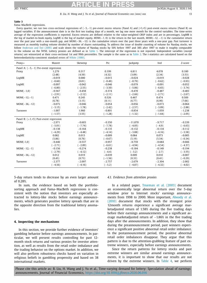
B. Liu, H. Wang and J. Yu et al. / Journal of Financial Economics xxx (xxxx) xxx 13
ARTICLE IN PRESS
JID: FINEC [m3Gdc; August 8, 2020;1:54 ]
Table 3
Fama–MacBeth regressions.
Every quarter, we run two cross-sectional regressions of ( −5, −1) pre-event excess returns (Panel A) and (+1,+5) post-event excess returns (Panel B) on
lagged variables. If the announcement date is in the first ten trading days of a month, we lag one more month for the control variables. The time-series
average of the regression coefficients is reported. Excess returns are defined relative to the value-weighted CRSP index and are in percentages. LogMB is
the log of market-to-book equity, LogME is the log of market equity, M OM (−1 , 0) is the return in the last month, M OM (−12 , −1) is the cumulative return
over the past year with a one-month gap, and M OM (−36 , −12) is the cumulative return over the past three years with a one-year gap. Past turnover is
measured as monthly trading volume divided by number of shares outstanding. To address the issue of double counting of volume for Nasdaq stocks, we
follow Anderson and Dyl (2005) and scale down the volume of Nasdaq stocks by 50% before 1997 and 38% after 1997 to make it roughly comparable
to the volume on the NYSE. Lottery proxies are defined as in Table 1 . The intercept of the regression is not reported. Independent variables (except
returns) are winsorized at their cross-sectional 1st and 99th percentiles. The sample is the same as in Table 2 . The t -statistics are calculated based on the
heteroskedasticity-consistent standard errors of White (1980) .
Proxy = Maxret Skewexp Prc Jackpotp Ivol Z -score
Panel A: ( −5, −1) Pre-event regression
Proxy 1.279 0.317 0.199 6.811 4.078 0.180
(2.48) (4.50) (4.32) (3.09) (2.34) (3.53)
LogMB −0.019 0.000 −0.015 −0.024 −0.019 −0.028
( −0.60) (0.01) ( −0.49) ( −0.79) ( −0.62) ( −0.93)
LogME −0.097 −0.042 −0.046 −0.079 −0.091 −0.052
( −6.80) ( −2.55) ( −3.50) ( −5.06) ( −6.65) ( −3.74)
MOM( −1,0) −0.567 −0.458 −0.374 −0.470 −0.487 −0.483
( −2.91) ( −2.12) ( −2.11) ( −2.66) ( −2.71) ( −2.67)
MOM( −12, −1) 0.471 0.245 0.526 0.467 0.474 0.509
(6.78) (3.15) (8.11) (6.77) (6.90) (7.66)
MOM( −36, −12) −0.075 −0.046 −0.054 −0.056 −0.073 −0.064
( −3.15) ( −1.78) ( −2.42) ( −2.57) ( −3.09) ( −2.88)
Turnover −1.007 1.960 −0.801 −0.854 −1.059 −1.238
( −1.57) (3.55) ( −1.28) ( −1.32) ( −1.64) ( −2.05)
Panel B: ( + 1,+5) Post-event regression
Proxy −2.971 −0.603 −0.350 −11.870 −9.717 −0.339
( −5.01) ( −7.74) ( −7.78) ( −4.05) ( −4.9) ( −6.63)
LogMB −0.138 −0.164 −0.135 −0.132 −0.134 −0.112
( −4.29) ( −4.48) ( −4.14) ( −3.88) ( −4.16) ( −3.58)
LogME 0.082 0.015 −0.009 0.084 0.073 −0.005
(5.86) (0.76) ( −0.67) (5.19) (5.54) ( −0.34)
MOM(-1,0) −0.446 −0.537 −0.957 −0.759 −0.684 −0.666
( −2.71) ( −2.89) ( −6.61) ( −4.94) ( −4.54) ( −4.37)
MOM( −12, −1) −0.156 −0.274 −0.238 −0.184 −0.149 −0.194
( −2.79) ( −4.12) ( −4.4) ( −3.2) ( −2.7) ( −3.55)
MOM( −36, −12) 0.012 0.019 −0.039 0.009 0.010 −0.007
(0.45) (0.73) ( −1.56) (0.33) (0.41) ( −0.29)
Turnover −2.377 −2.097 −2.757 −2.679 −2.304 −2.002
( −4.56) ( −4.16) ( −5.2) ( −4.87) ( −4.32) ( −4.02)
5-day return tends to decrease by an even larger amount
of 0.28%.
In sum, the evidence based on both the portfolio-
sorting approach and Fama–MacBeth regressions is con-
sistent with the notion that investors are especially at-
tracted to lottery-like stocks before earnings announce-
ments, which generates positive lottery spreads that are in
the opposite direction from the traditional lottery anoma-
lies.
4. Inspecting the mechanisms
In this section, we provide further evidence of investors’
gambling behavior before earnings announcements. In par-
ticular, we will present results controlling for past 12-
month stock returns and various proxies for investor atten-
tion, as well as results from the retail order imbalance and
the trading behavior on the options market. In addition, we
will also perform robustness checks based on variation in
religious beliefs in gambling propensity and based on 38
international markets.
Please cite this article as: B. Liu, H. Wang and J. Yu et al., Time-v
announcements, Journal of Financial Economics, https://doi.org/1
4.1. Evidence from attention proxies
In a related paper, Trueman et al. (2003) document
an economically large abnormal return over the 5-day
window prior to Internet stocks’ earnings announce-
ments from 1998 to 20 0 0. More important, Aboody et al.
(2010) document that stocks with the strongest prior
12month returns experience a significant average mar-
ketadjusted return of 1.58% during the five trading days
before their earnings announcements and a significant av-
erage marketadjusted return of −1.86% in the five trading
days after the announcements. In addition, they show that
during the preannouncement period, past winners experi-
ence a significant positive abnormal retail order imbalance.
In the postannouncement period, the positive abnormal
retail order imbalances disappear. They argue that this
pattern is due to the attention-grabbing feature of past ex-
treme winners, especially before earnings announcements.
Since the return patterns for lottery stocks and past
extreme winners are similar around earnings announce-
ments, it is important to show that our results are not
driven by the extreme winners. In Table 4 , we perform
arying demand for lottery: Speculation ahead of earnings
0.1016/j.jfineco.2020.06.016
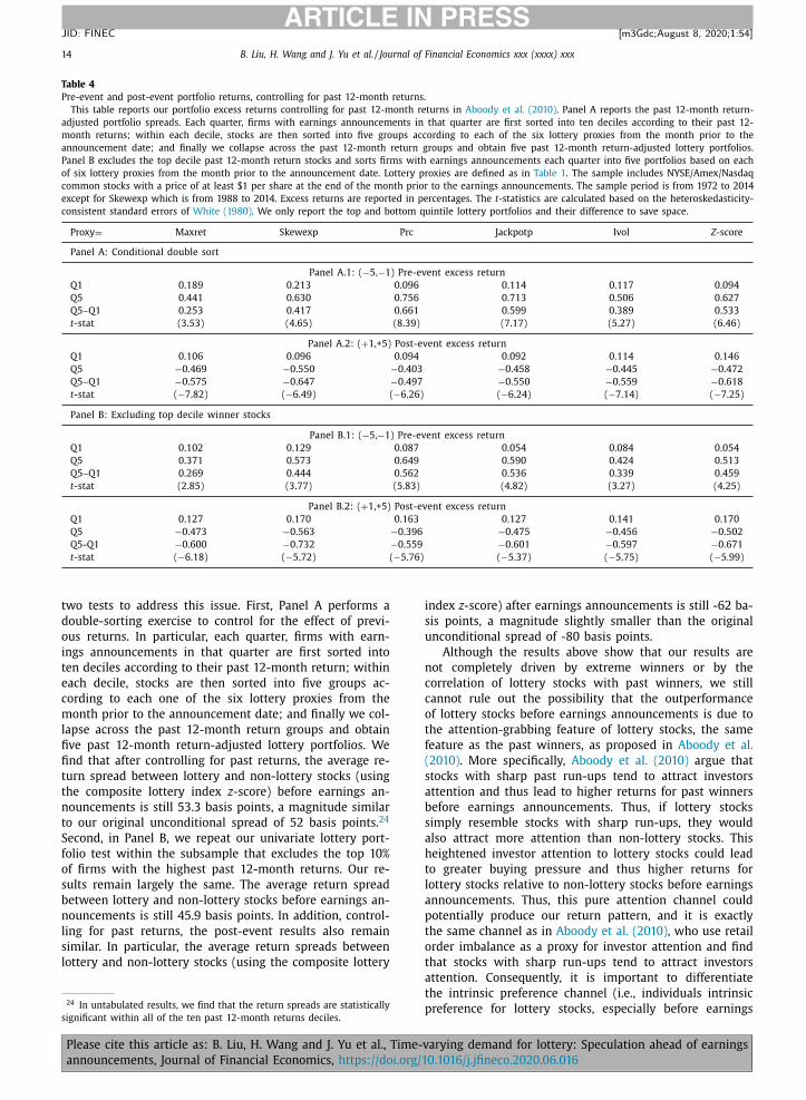
14 B. Liu, H. Wang and J. Yu et al. / Journal of Financial Economics xxx (xxxx) xxx
ARTICLE IN PRESS
JID: FINEC [m3Gdc; August 8, 2020;1:54 ]
Table 4
Pre-event and post-event portfolio returns, controlling for past 12-month returns.
This table reports our portfolio excess returns controlling for past 12-month returns in Aboody et al. (2010) . Panel A reports the past 12-month return-
adjusted portfolio spreads. Each quarter, firms with earnings announcements in that quarter are first sorted into ten deciles according to their past 12-
month returns; within each decile, stocks are then sorted into five groups according to each of the six lottery proxies from the month prior to the
announcement date; and finally we collapse across the past 12-month return groups and obtain five past 12-month return-adjusted lottery portfolios.
Panel B excludes the top decile past 12-month return stocks and sorts firms with earnings announcements each quarter into five portfolios based on each
of six lottery proxies from the month prior to the announcement date. Lottery proxies are defined as in Table 1 . The sample includes NYSE/Amex/Nasdaq
common stocks with a price of at least $1 per share at the end of the month prior to the earnings announcements. The sample period is from 1972 to 2014
except for Skewexp which is from 1988 to 2014. Excess returns are reported in percentages. The t -statistics are calculated based on the heteroskedasticity-
consistent standard errors of White (1980) . We only report the top and bottom quintile lottery portfolios and their difference to save space.
Proxy = Maxret Skewexp Prc Jackpotp Ivol Z -score
Panel A: Conditional double sort
Panel A.1: ( −5, −1) Pre-event excess return
Q1 0.189 0.213 0.096 0.114 0.117 0.094
Q5 0.441 0.630 0.756 0.713 0.506 0.627
Q5–Q1 0.253 0.417 0.661 0.599 0.389 0.533
t -stat (3.53) (4.65) (8.39) (7.17) (5.27) (6.46)
Panel A.2: ( + 1,+5) Post-event excess return
Q1 0.106 0.096 0.094 0.092 0.114 0.146
Q5 −0.469 −0.550 −0.403 −0.458 −0.445 −0.472
Q5–Q1 −0.575 −0.647 −0.497 −0.550 −0.559 −0.618
t -stat ( −7.82) ( −6.49) ( −6.26) ( −6.24) ( −7.14) ( −7.25)
Panel B: Excluding top decile winner stocks
Panel B.1: ( −5, −1) Pre-event excess return
Q1 0.102 0.129 0.087 0.054 0.084 0.054
Q5 0.371 0.573 0.649 0.590 0.424 0.513
Q5–Q1 0.269 0.444 0.562 0.536 0.339 0.459
t -stat (2.85) (3.77) (5.83) (4.82) (3.27) (4.25)
Panel B.2: ( + 1,+5) Post-event excess return
Q1 0.127 0.170 0.163 0.127 0.141 0.170
Q5 −0.473 −0.563 −0.396 −0.475 −0.456 −0.502
Q5-Q1 −0.600 −0.732 −0.559 −0.601 −0.597 −0.671
t -stat ( −6.18) ( −5.72) ( −5.76) ( −5.37) ( −5.75) ( −5.99)
two tests to address this issue. First, Panel A performs a
double-sorting exercise to control for the effect of previ-
ous returns. In particular, each quarter, firms with earn-
ings announcements in that quarter are first sorted into
ten deciles according to their past 12-month return; within
each decile, stocks are then sorted into five groups ac-
cording to each one of the six lottery proxies from the
month prior to the announcement date; and finally we col-
lapse across the past 12-month return groups and obtain
five past 12-month return-adjusted lottery portfolios. We
find that after controlling for past returns, the average re-
turn spread between lottery and non-lottery stocks (using
the composite lottery index z -score) before earnings an-
nouncements is still 53.3 basis points, a magnitude similar
to our original unconditional spread of 52 basis points. 24
Second, in Panel B, we repeat our univariate lottery port-
folio test within the subsample that excludes the top 10%
of firms with the highest past 12-month returns. Our re-
sults remain largely the same. The average return spread
between lottery and non-lottery stocks before earnings an-
nouncements is still 45.9 basis points. In addition, control-
ling for past returns, the post-event results also remain
similar. In particular, the average return spreads between
lottery and non-lottery stocks (using the composite lottery
24 In untabulated results, we find that the return spreads are statistically
significant within all of the ten past 12-month returns deciles.
Please cite this article as: B. Liu, H. Wang and J. Yu et al., Time-v
announcements, Journal of Financial Economics, https://doi.org/1
index z -score) after earnings announcements is still -62 ba-
sis points, a magnitude slightly smaller than the original
unconditional spread of -80 basis points.
Although the results above show that our results are
not completely driven by extreme winners or by the
correlation of lottery stocks with past winners, we still
cannot rule out the possibility that the outperformance
of lottery stocks before earnings announcements is due to
the attention-grabbing feature of lottery stocks, the same
feature as the past winners, as proposed in Aboody et al.
(2010) . More specifically, Aboody et al. (2010) argue that
stocks with sharp past run-ups tend to attract investors
attention and thus lead to higher returns for past winners
before earnings announcements. Thus, if lottery stocks
simply resemble stocks with sharp run-ups, they would
also attract more attention than non-lottery stocks. This
heightened investor attention to lottery stocks could lead
to greater buying pressure and thus higher returns for
lottery stocks relative to non-lottery stocks before earnings
announcements. Thus, this pure attention channel could
potentially produce our return pattern, and it is exactly
the same channel as in Aboody et al. (2010) , who use retail
order imbalance as a proxy for investor attention and find
that stocks with sharp run-ups tend to attract investors
attention. Consequently, it is important to differentiate
the intrinsic preference channel (i.e., individuals intrinsic
preference for lottery stocks, especially before earnings
arying demand for lottery: Speculation ahead of earnings
0.1016/j.jfineco.2020.06.016
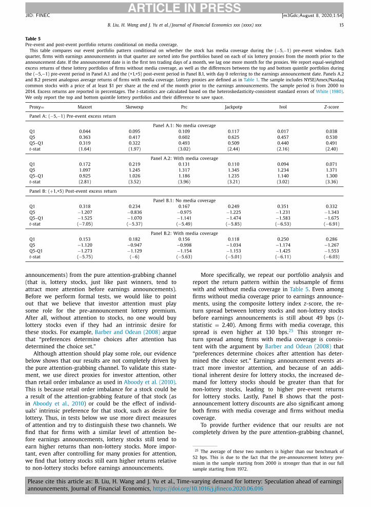
B. Liu, H. Wang and J. Yu et al. / Journal of Financial Economics xxx (xxxx) xxx 15
ARTICLE IN PRESS
JID: FINEC [m3Gdc; August 8, 2020;1:54 ]
Table 5
Pre-event and post-event portfolio returns conditional on media coverage.
This table compares our event portfolio pattern conditional on whether the stock has media coverage during the ( −5, −1) pre-event window. Each
quarter, firms with earnings announcements in that quarter are sorted into five portfolios based on each of six lottery proxies from the month prior to the
announcement date. If the announcement date is in the first ten trading days of a month, we lag one more month for the proxies. We report equal-weighted
excess returns of these lottery portfolios of firms without media coverage, as well as the differences between the top and bottom quintile portfolios during
the ( −5, −1) pre-event period in Panel A.1 and the (+1,+5) post-event period in Panel B.1, with day 0 referring to the earnings announcement date. Panels A.2
and B.2 present analogous average returns of firms with media coverage. Lottery proxies are defined as in Table 1 . The sample includes NYSE/Amex/Nasdaq
common stocks with a price of at least $1 per share at the end of the month prior to the earnings announcements. The sample period is from 20 0 0 to
2014. Excess returns are reported in percentages. The t -statistics are calculated based on the heteroskedasticity-consistent standard errors of White (1980) .
We only report the top and bottom quintile lottery portfolios and their difference to save space.
Proxy = Maxret Skewexp Prc Jackpotp Ivol Z -score
Panel A: ( −5, −1) Pre-event excess return
Panel A.1: No media coverage
Q1 0.044 0.095 0.109 0.117 0.017 0.038
Q5 0.363 0.417 0.602 0.625 0.457 0.530
Q5–Q1 0.319 0.322 0.493 0.509 0.440 0.491
t -stat (1.64) (1.97) (3.02) (2.44) (2.16) (2.40)
Panel A.2: With media coverage
Q1 0.172 0.219 0.131 0.110 0.094 0.071
Q5 1.097 1.245 1.317 1.345 1.234 1.371
Q5–Q1 0.925 1.026 1.186 1.235 1.140 1.300
t -stat (2.81) (3.52) (3.96) (3.21) (3.02) (3.36)
Panel B: ( + 1,+5) Post-event excess return
Panel B.1: No media coverage
Q1 0.318 0.234 0.167 0.249 0.351 0.332
Q5 −1.207 −0.836 −0.975 −1.225 −1.231 −1.343
Q5–Q1 −1.525 −1.070 −1.141 −1.474 −1.583 −1.675
t -stat ( −7.05) ( −5.37) ( −5.49) ( −5.85) ( −6.53) ( −6.91)
Panel B.2: With media coverage
Q1 0.153 0.182 0.156 0.118 0.250 0.286
Q5 −1.120 −0.947 −0.998 −1.034 −1.174 −1.267
Q5-Q1 −1.273 −1.129 −1.154 −1.153 −1.425 −1.553
t -stat ( −5.75) ( −6) ( −5.63) ( −5.01) ( −6.11) ( −6.03)
25 The average of these two numbers is higher than our benchmark of
52 bps. This is due to the fact that the pre-announcement lottery pre-
mium in the sample starting from 20 0 0 is stronger than that in our full
sample starting from 1972.
announcements) from the pure attention-grabbing channel
(that is, lottery stocks, just like past winners, tend to
attract more attention before earnings announcements).
Before we perform formal tests, we would like to point
out that we believe that investor attention must play
some role for the pre-announcement lottery premium.
After all, without attention to stocks, no one would buy
lottery stocks even if they had an intrinsic desire for
these stocks. For example, Barber and Odean (2008) argue
that “preferences determine choices after attention has
determined the choice set.”
Although attention should play some role, our evidence
below shows that our results are not completely driven by
the pure attention-grabbing channel. To validate this state-
ment, we use direct proxies for investor attention, other
than retail order imbalance as used in Aboody et al. (2010) .
This is because retail order imbalance for a stock could be
a result of the attention-grabbing feature of that stock (as
in Aboody et al., 2010 ) or could be the effect of individ-
uals’ intrinsic preference for that stock, such as desire for
lottery. Thus, in tests below we use more direct measures
of attention and try to distinguish these two channels. We
find that for firms with a similar level of attention be-
fore earnings announcements, lottery stocks still tend to
earn higher returns than non-lottery stocks. More impor-
tant, even after controlling for many proxies for attention,
we find that lottery stocks still earn higher returns relative
to non-lottery stocks before earnings announcements.
Please cite this article as: B. Liu, H. Wang and J. Yu et al., Time-v
announcements, Journal of Financial Economics, https://doi.org/1
More specifically, we repeat our portfolio analysis and
report the return pattern within the subsample of firms
with and without media coverage in Table 5 . Even among
firms without media coverage prior to earnings announce-
ments, using the composite lottery index z -score, the re-
turn spread between lottery stocks and non-lottery stocks
before earnings announcements is still about 49 bps ( t -
statistic = 2.40). Among firms with media coverage, this
spread is even higher at 130 bps. 25 This stronger re-
turn spread among firms with media coverage is consis-
tent with the argument by Barber and Odean (2008) that
“preferences determine choices after attention has deter-
mined the choice set.” Earnings announcement events at-
tract more investor attention, and because of an addi-
tional inherent desire for lottery stocks, the increased de-
mand for lottery stocks should be greater than that for
non-lottery stocks, leading to higher pre-event returns
for lottery stocks. Lastly, Panel B shows that the post-
announcement lottery discounts are also significant among
both firms with media coverage and firms without media
coverage.
To provide further evidence that our results are not
completely driven by the pure attention-grabbing channel,
arying demand for lottery: Speculation ahead of earnings
0.1016/j.jfineco.2020.06.016

16 B. Liu, H. Wang and J. Yu et al. / Journal of Financial Economics xxx (xxxx) xxx
ARTICLE IN PRESS
JID: FINEC [m3Gdc; August 8, 2020;1:54 ]
Table 6 conducts a double-sorting exercise using three ad-
ditional proxies for attention that have been used in pre-
vious studies including the magnitude of recent standard-
ized unexpected earnings, or SUE (|SUE|), the population
density of a firm’s headquarters (PD), and the social con-
nectedness of a firm’s headquarters (SCIH), as well as a
composite measure for attention (Attn) based on the av-
erage of the individual z -scores of media, |SUE|, PD, and
SICH. Each quarter, firms with earnings announcements in
that quarter are sequentially sorted into 25 5-by-5 port-
folios based first on each one of the four attention prox-
ies and then on each one of the six lottery proxies. To
save space, except for the double sort by the composite
attention measure and the composite lottery measure, we
only report the results of the five attention-adjusted lot-
tery portfolios from collapsing across the five attention
groups. Panel A reports the excess returns of the 25 portfo-
lios from the double sort by the composite attention score
and the lottery z -score, the difference between the bottom
and top quintile lottery portfolios within each attention
quintile, as well as the conditional returns average across
all five attention quintiles. The results show that within
each attention quintile, lottery stocks still earn significantly
higher (lower) returns than non-lottery stocks before (af-
ter) earnings announcements. Panel B reports the returns
of the attention-adjusted lottery portfolios from our dou-
ble sort when using different attention proxies. The results
show that for each of these four measures, after control-
ling for attention in a double-sorting exercise, the effect is
still there. More specifically, after controlling for each of
these 4 measures, the average outperformance of lottery
stocks over non-lottery stocks before earnings announce-
ments is still significant. For example, the outperformance
is 54 bps, 52 bps, 53 bps, and 51 bps after controlling
for each of these four measures, respectively. The average
value is 53 bps in the 5-day pre-event window. That is,
among firms with a similar level of pre-event attention,
the pre-event lottery effect is similar to that (i.e., 52 bps)
without controlling for the effect of attention. 26
In addition, in Table 7 , we add the composite atten-
tion score to the Fama-MacBeth regressions in Table 3 . The
results show that after controlling for investor attention
and other variables, the coefficients on lottery proxies are
still positive (negative) and significant during the pre-event
(post-event) window for all six lottery proxies. In particu-
lar, when the composite z -score (attention score, momen-
tum) increases by one standard deviation, the pre-event 5-
day return tends to increase by 0.13% (0.06%, 0.28%), and
the post-event 5-day return tends to decrease by 0.31%
(0.04%, 0.10%). Thus, although the attention proxy is statis-
tically more significant than the lottery proxy, the lottery
proxy is economically more significant than the attention
proxy. On the other hand, the lottery proxy has weaker
(stronger) power in predicting the pre-event (post-event)
return than the momentum variable.
26 In Table A4 in the Online Appendix, we show that our results are
robust to using alternative attention proxies including abnormal turnover,
abnormal trading volume ( Gervais et al., 2001; Barber and Odean, 2008 ),
and recency ( Bali et al., 2019 ).
Please cite this article as: B. Liu, H. Wang and J. Yu et al., Time-v
announcements, Journal of Financial Economics, https://doi.org/1
In sum, although the attention-grabbing feature of lot-
tery stocks could play some role in the pre-event run-up
for lottery stock prices, our evidence shows that investors’
inherent desire for lottery stocks should also play a signif-
icant role.
4.2. Evidence from retail order imbalance
Lottery preferences, like other behavioral biases, tend to
be more prominent among individual investors (see, e.g.,
Kumar, 2009 ). In addition, earnings announcement events
tend to grab retail investors attention. Thus, the attention-
driven demand for lotteries could increase ahead of earn-
ings announcements. Consequently, we expect to see more
trading initiated by retail investors before earnings an-
nouncements, especially among lottery-like stocks. Panel
A of Table 8 compares the change in retail order imbal-
ance between lottery-like and non-lottery stocks prior to
the announcements. As shown in Panel A.1, the increase
in retail order imbalance is generally significantly larger
among lottery-like stocks than among non-lottery stocks.
However, this pattern is subdued or even reversed after the
announcements for some lottery proxies, a pattern simi-
lar to top decile winners, as in Aboody et al. (2010) . In-
deed, none of the retail order imbalance increase during
the post-event window is significant. Thus, the return re-
versal effect for lottery stocks after the earnings announce-
ment is probably partially driven by the subdued abnormal
retail order imbalance. 27
Since Aboody et al. (2010) also find an increased re-
tail order imbalance for past winners before earnings an-
nouncements, it is important to investigate the possibility
that our results arise from the correlation between lottery
stocks and past returns. In Panel B of Table 8 , we control
directly for the past 12-month return in our test of retail
order imbalance by either doing a conditional double sort
or excluding the top 10% of past 12-month winner stocks.
More specifically, in Panel B.1, each quarter, firms with
earnings announcements in that quarter are first sorted
into ten deciles according to their past 12-month return;
within each decile, stocks are then sorted into five groups
according to each one of the six lottery proxies from the
month prior to the announcement date; and finally we
collapse across the past 12-month return groups and ob-
tain five past 12-month return-adjusted lottery portfolios.
The result shows that the retail order imbalance pattern
remains the same in a conditional double-sorting exercise
by controlling for past 12-month returns. Lastly, Panel B.2
shows that when we exclude the top 10% of firms with the
highest past 12-month returns, the abnormal retail order
imbalance pattern remains quantitatively similar. In sum,
we still find that the abnormal retail order imbalance in-
creases more for lottery stocks than for non-lottery stocks
before the earnings announcements after controlling for
past returns. Thus, our results are distinct from the results
in Aboody et al. (2010) .
27 In addition, the earnings announcement news for lottery stocks tends
to be worse than that for non-lottery stocks. This fact also partially con-
tributes to the underperformance of lottery stocks after earnings an-
nouncements.
arying demand for lottery: Speculation ahead of earnings
0.1016/j.jfineco.2020.06.016
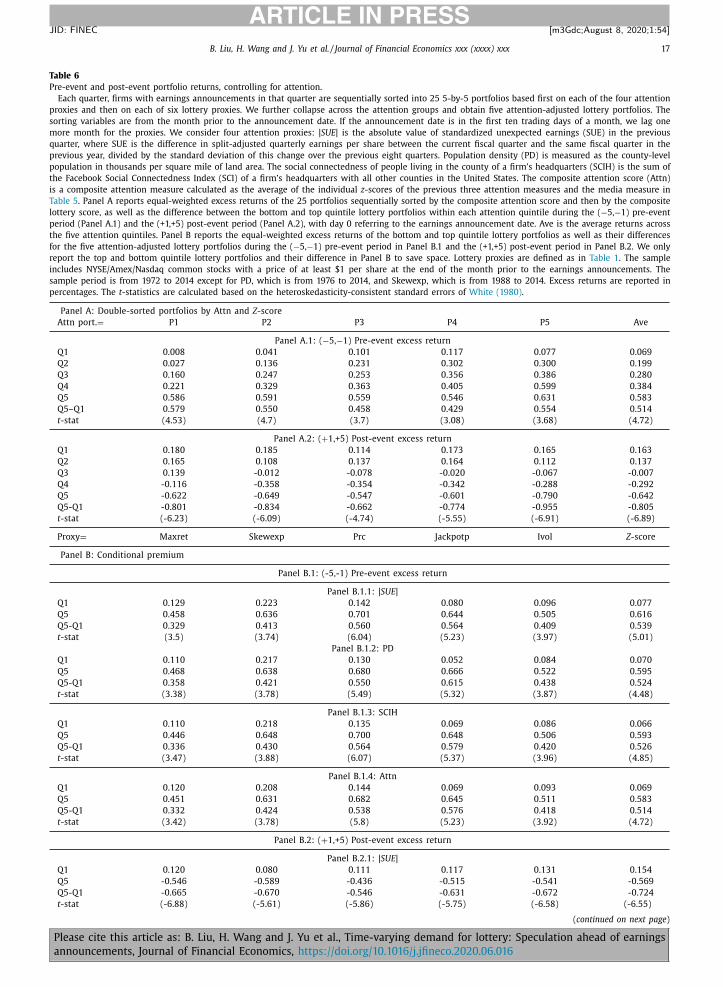
B. Liu, H. Wang and J. Yu et al. / Journal of Financial Economics xxx (xxxx) xxx 17
ARTICLE IN PRESS
JID: FINEC [m3Gdc; August 8, 2020;1:54 ]
Table 6
Pre-event and post-event portfolio returns, controlling for attention.
Each quarter, firms with earnings announcements in that quarter are sequentially sorted into 25 5-by-5 portfolios based first on each of the four attention
proxies and then on each of six lottery proxies. We further collapse across the attention groups and obtain five attention-adjusted lottery portfolios. The
sorting variables are from the month prior to the announcement date. If the announcement date is in the first ten trading days of a month, we lag one
more month for the proxies. We consider four attention proxies: | SUE | is the absolute value of standardized unexpected earnings (SUE) in the previous
quarter, where SUE is the difference in split-adjusted quarterly earnings per share between the current fiscal quarter and the same fiscal quarter in the
previous year, divided by the standard deviation of this change over the previous eight quarters. Population density (PD) is measured as the county-level
population in thousands per square mile of land area. The social connectedness of people living in the county of a firm’s headquarters (SCIH) is the sum of
the Facebook Social Connectedness Index (SCI) of a firm’s headquarters with all other counties in the United States. The composite attention score (Attn)
is a composite attention measure calculated as the average of the individual z -scores of the previous three attention measures and the media measure in
Table 5 . Panel A reports equal-weighted excess returns of the 25 portfolios sequentially sorted by the composite attention score and then by the composite
lottery score, as well as the difference between the bottom and top quintile lottery portfolios within each attention quintile during the ( −5, −1) pre-event
period (Panel A.1) and the (+1,+5) post-event period (Panel A.2), with day 0 referring to the earnings announcement date. Ave is the average returns across
the five attention quintiles. Panel B reports the equal-weighted excess returns of the bottom and top quintile lottery portfolios as well as their differences
for the five attention-adjusted lottery portfolios during the ( −5, −1) pre-event period in Panel B.1 and the (+1,+5) post-event period in Panel B.2. We only
report the top and bottom quintile lottery portfolios and their difference in Panel B to save space. Lottery proxies are defined as in Table 1 . The sample
includes NYSE/Amex/Nasdaq common stocks with a price of at least $1 per share at the end of the month prior to the earnings announcements. The
sample period is from 1972 to 2014 except for PD, which is from 1976 to 2014, and Skewexp, which is from 1988 to 2014. Excess returns are reported in
percentages. The t -statistics are calculated based on the heteroskedasticity-consistent standard errors of White (1980) .
Panel A: Double-sorted portfolios by Attn and Z -score
Attn port. = P1 P2 P3 P4 P5 Ave
Panel A.1: ( −5, −1) Pre-event excess return
Q1 0.008 0.041 0.101 0.117 0.077 0.069
Q2 0.027 0.136 0.231 0.302 0.300 0.199
Q3 0.160 0.247 0.253 0.356 0.386 0.280
Q4 0.221 0.329 0.363 0.405 0.599 0.384
Q5 0.586 0.591 0.559 0.546 0.631 0.583
Q5–Q1 0.579 0.550 0.458 0.429 0.554 0.514
t -stat (4.53) (4.7) (3.7) (3.08) (3.68) (4.72)
Panel A.2: ( + 1,+5) Post-event excess return
Q1 0.180 0.185 0.114 0.173 0.165 0.163
Q2 0.165 0.108 0.137 0.164 0.112 0.137
Q3 0.139 -0.012 -0.078 -0.020 -0.067 -0.007
Q4 -0.116 -0.358 -0.354 -0.342 -0.288 -0.292
Q5 -0.622 -0.649 -0.547 -0.601 -0.790 -0.642
Q5-Q1 -0.801 -0.834 -0.662 -0.774 -0.955 -0.805
t -stat (-6.23) (-6.09) (-4.74) (-5.55) (-6.91) (-6.89)
Proxy = Maxret Skewexp Prc Jackpotp Ivol Z -score
Panel B: Conditional premium
Panel B.1: (-5,-1) Pre-event excess return
Panel B.1.1: | SUE |
Q1 0.129 0.223 0.142 0.080 0.096 0.077
Q5 0.458 0.636 0.701 0.644 0.505 0.616
Q5-Q1 0.329 0.413 0.560 0.564 0.409 0.539
t -stat (3.5) (3.74) (6.04) (5.23) (3.97) (5.01)
Panel B.1.2: PD
Q1 0.110 0.217 0.130 0.052 0.084 0.070
Q5 0.468 0.638 0.680 0.666 0.522 0.595
Q5-Q1 0.358 0.421 0.550 0.615 0.438 0.524
t -stat (3.38) (3.78) (5.49) (5.32) (3.87) (4.48)
Panel B.1.3: SCIH
Q1 0.110 0.218 0.135 0.069 0.086 0.066
Q5 0.446 0.648 0.700 0.648 0.506 0.593
Q5-Q1 0.336 0.430 0.564 0.579 0.420 0.526
t -stat (3.47) (3.88) (6.07) (5.37) (3.96) (4.85)
Panel B.1.4: Attn
Q1 0.120 0.208 0.144 0.069 0.093 0.069
Q5 0.451 0.631 0.682 0.645 0.511 0.583
Q5-Q1 0.332 0.424 0.538 0.576 0.418 0.514
t -stat (3.42) (3.78) (5.8) (5.23) (3.92) (4.72)
Panel B.2: ( + 1,+5) Post-event excess return
Panel B.2.1: | SUE |
Q1 0.120 0.080 0.111 0.117 0.131 0.154
Q5 -0.546 -0.589 -0.436 -0.515 -0.541 -0.569
Q5-Q1 -0.665 -0.670 -0.546 -0.631 -0.672 -0.724
t -stat (-6.88) (-5.61) (-5.86) (-5.75) (-6.58) (-6.55)
( continued on next page )
Please cite this article as: B. Liu, H. Wang and J. Yu et al., Time-varying demand for lottery: Speculation ahead of earnings
announcements, Journal of Financial Economics, https://doi.org/10.1016/j.jfineco.2020.06.016
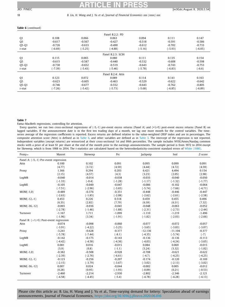
18 B. Liu, H. Wang and J. Yu et al. / Journal of Financial Economics xxx (xxxx) xxx
ARTICLE IN PRESS
JID: FINEC [m3Gdc; August 8, 2020;1:54 ]
Table 6 ( continued )
Panel B.2.2: PD
Q1 0.108 0.066 0.063 0.094 0.111 0.147
Q5 -0.617 -0.567 -0.427 -0.518 -0.591 -0.586
Q5-Q1 -0.726 -0.633 -0.490 -0.612 -0.702 -0.733
t -stat (-6.69) (-5.25) (-4.88) (-5.16) (-5.93) (-6.05)
Panel B.2.3: SCIH
Q1 0.115 0.065 0.080 0.111 0.135 0.154
Q5 -0.615 -0.587 -0.440 -0.532 -0.608 -0.598
Q5-Q1 -0.730 -0.652 -0.519 -0.643 -0.743 -0.753
t -stat (-7.39) (-5.43) (-5.46) (-5.78) (-6.83) (-6.6)
Panel B.2.4: Attn
Q1 0.123 0.072 0.089 0.114 0.141 0.163
Q5 -0.623 -0.605 -0.463 -0.529 -0.622 -0.642
Q5-Q1 -0.746 -0.677 -0.552 -0.643 -0.762 -0.805
t -stat (-7.26) (-5.42) (-5.73) (-5.68) (-6.85) (-6.89)
Table 7
Fama–MacBeth regressions, controlling for attention.
Every quarter, we run two cross-sectional regressions of (-5,-1) pre-event excess returns (Panel A) and (+1,+5) post-event excess returns (Panel B) on
lagged variables. If the announcement date is in the first ten trading days of a month, we lag one more month for the control variables. The time-
series average of the regression coefficients is reported. Excess returns are defined relative to the value-weighted CRSP index and are in percentages. The
composite attention score (Attn) is defined as in Table 6 , and other variables are defined as in Table 3 . The intercept of the regression is not reported.
Independent variables (except returns) are winsorized at their cross-sectional 1st and 99th percentiles. The sample includes NYSE/Amex/Nasdaq common
stocks with a price of at least $1 per share at the end of the month prior to the earnings announcements. The sample period is from 1972 to 2014 except
for Skewexp, which is from 1988 to 2014. The t -statistics are calculated based on the heteroskedasticity-consistent standard errors of White (1980) .
Proxy = Maxret Skewexp Prc Jackpotp Ivol Z -score
Panel A: (-5,-1) Pre-event regression
Attn 0.100 0.102 0.091 0.095 0.099 0.091
(4.77) (3.72) (4.59) (4.44) (4.72) (4.59)
Proxy 1.366 0.294 0.203 6.421 4.494 0.154
(2.15) (4.57) (4.3) (3.23) (2.05) (2.98)
LogMB -0.040 -0.014 -0.038 -0.035 -0.040 -0.050
(-1.33) (-0.4) (-1.28) (-1.17) (-1.32) (-1.77)
LogME -0.105 -0.049 -0.047 -0.086 -0.102 -0.064
(-7.51) (-2.96) (-3.65) (-5.74) (-7.66) (-4.71)
MOM(-1,0) -0.489 -0.376 -0.351 -0.448 -0.446 -0.447
(-2.63) (-1.85) (-2.08) (-2.62) (-2.61) (-2.58)
MOM(-12,-1) 0.453 0.226 0.518 0.459 0.455 0.496
(6.35) (2.82) (7.79) (6.59) (6.51) (7.32)
MOM(-36,-12) -0.065 -0.036 -0.041 -0.048 -0.063 -0.052
(-2.78) (-1.46) (-1.88) (-2.31) (-2.73) (-2.44)
Turnover -1.167 1.711 -1.099 -1.110 -1.219 -1.496
(-1.96) (3.34) (-1.91) (-1.82) (-2.03) (-2.66)
Panel B: ( + 1,+5) Post-event regression
Attn -0.074 -0.098 -0.060 -0.077 -0.072 -0.057
(-3.91) (-4.22) (-3.25) (-3.65) (-3.83) (-3.07)
Proxy -3.241 -0.628 -0.377 -12.136 -11.104 -0.377
(-5.78) (-7.44) (-8.1) (-4.35) (-5.74) (-7)
LogMB -0.142 -0.175 -0.143 -0.136 -0.136 -0.113
(-4.42) (-4.58) (-4.36) (-4.03) (-4.24) (-3.65)
LogME 0.081 0.016 -0.015 0.084 0.069 -0.015
(5.9) (0.8) (-1.1) (5.24) (5.32) (-1.02)
MOM(-1,0) -0.382 -0.508 -0.928 -0.708 -0.621 -0.622
(-2.39) (-2.76) (-6.61) (-4.7) (-4.25) (-4.25)
MOM(-12,-1) -0.123 -0.256 -0.207 -0.174 -0.120 -0.169
(-2.15) (-3.79) (-3.67) (-3.02) (-2.13) (-3.02)
MOM(-36,-12) 0.007 0.024 -0.044 -0.002 0.005 -0.012
(0.28) (0.95) (-1.93) (-0.09) (0.21) (-0.53)
Turnover -2.460 -2.214 -2.930 -2.802 -2.346 -2.121
(-4.58) (-4.45) (-5.4) (-4.78) (-4.28) (-4.13)
Please cite this article as: B. Liu, H. Wang and J. Yu et al., Time-varying demand for lottery: Speculation ahead of earnings
announcements, Journal of Financial Economics, https://doi.org/10.1016/j.jfineco.2020.06.016
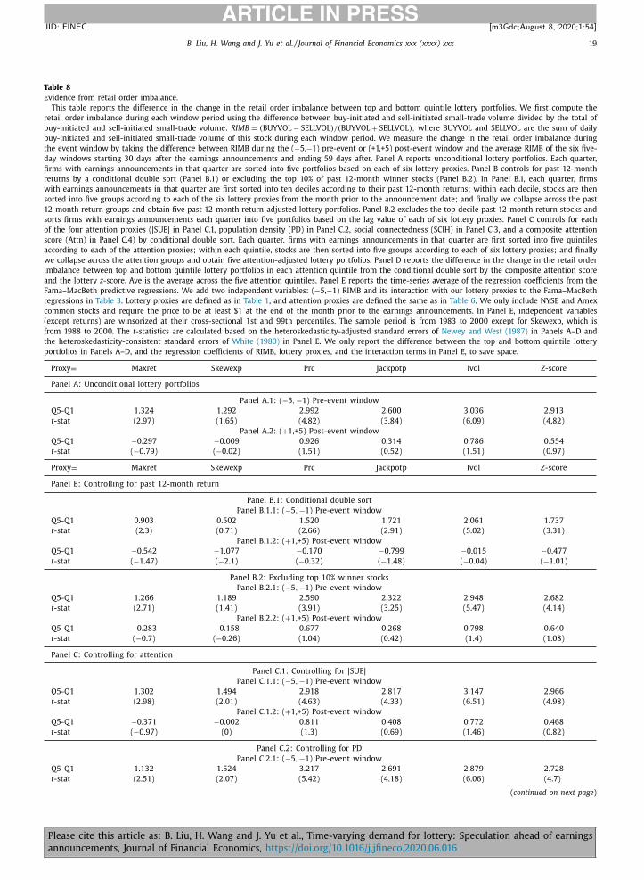
B. Liu, H. Wang and J. Yu et al. / Journal of Financial Economics xxx (xxxx) xxx 19
ARTICLE IN PRESS
JID: FINEC [m3Gdc; August 8, 2020;1:54 ]
Table 8
Evidence from retail order imbalance.
This table reports the difference in the change in the retail order imbalance between top and bottom quintile lottery portfolios. We first compute the
retail order imbalance during each window period using the difference between buy-initiated and sell-initiated small-trade volume divided by the total of
buy-initiated and sell-initiated small-trade volume: RIMB = ( BUYVOL − SELLVOL ) / ( BUYVOL + SELLVOL ) , where BUYVOL and SELLVOL are the sum of daily
buy-initiated and sell-initiated small-trade volume of this stock during each window period. We measure the change in the retail order imbalance during
the event window by taking the difference between RIMB during the ( −5, −1) pre-event or (+1,+5) post-event window and the average RIMB of the six five-
day windows starting 30 days after the earnings announcements and ending 59 days after. Panel A reports unconditional lottery portfolios. Each quarter,
firms with earnings announcements in that quarter are sorted into five portfolios based on each of six lottery proxies. Panel B controls for past 12-month
returns by a conditional double sort (Panel B.1) or excluding the top 10% of past 12-month winner stocks (Panel B.2). In Panel B.1, each quarter, firms
with earnings announcements in that quarter are first sorted into ten deciles according to their past 12-month returns; within each decile, stocks are then
sorted into five groups according to each of the six lottery proxies from the month prior to the announcement date; and finally we collapse across the past
12-month return groups and obtain five past 12-month return-adjusted lottery portfolios. Panel B.2 excludes the top decile past 12-month return stocks and
sorts firms with earnings announcements each quarter into five portfolios based on the lag value of each of six lottery proxies. Panel C controls for each
of the four attention proxies (|SUE| in Panel C.1, population density (PD) in Panel C.2, social connectedness (SCIH) in Panel C.3, and a composite attention
score (Attn) in Panel C.4) by conditional double sort. Each quarter, firms with earnings announcements in that quarter are first sorted into five quintiles
according to each of the attention proxies; within each quintile, stocks are then sorted into five groups according to each of six lottery proxies; and finally
we collapse across the attention groups and obtain five attention-adjusted lottery portfolios. Panel D reports the difference in the change in the retail order
imbalance between top and bottom quintile lottery portfolios in each attention quintile from the conditional double sort by the composite attention score
and the lottery z -score. Ave is the average across the five attention quintiles. Panel E reports the time-series average of the regression coefficients from the
Fama–MacBeth predictive regressions. We add two independent variables: ( −5, −1) RIMB and its interaction with our lottery proxies to the Fama–MacBeth
regressions in Table 3 . Lottery proxies are defined as in Table 1 , and attention proxies are defined the same as in Table 6 . We only include NYSE and Amex
common stocks and require the price to be at least $1 at the end of the month prior to the earnings announcements. In Panel E, independent variables
(except returns) are winsorized at their cross-sectional 1st and 99th percentiles. The sample period is from 1983 to 20 0 0 except for Skewexp, which is
from 1988 to 20 0 0. The t -statistics are calculated based on the heteroskedasticity-adjusted standard errors of Newey and West (1987) in Panels A–D and
the heteroskedasticity-consistent standard errors of White (1980) in Panel E. We only report the difference between the top and bottom quintile lottery
portfolios in Panels A–D, and the regression coefficients of RIMB, lottery proxies, and the interaction terms in Panel E, to save space.
Proxy = Maxret Skewexp Prc Jackpotp Ivol Z -score
Panel A: Unconditional lottery portfolios
Panel A.1: ( −5 , −1) Pre-event window
Q5-Q1 1.324 1.292 2.992 2.600 3.036 2.913
t -stat (2.97) (1.65) (4.82) (3.84) (6.09) (4.82)
Panel A.2: ( + 1,+5) Post-event window
Q5-Q1 −0.297 −0.009 0.926 0.314 0.786 0.554
t -stat ( −0.79) ( −0.02) (1.51) (0.52) (1.51) (0.97)
Proxy = Maxret Skewexp Prc Jackpotp Ivol Z -score
Panel B: Controlling for past 12-month return
Panel B.1: Conditional double sort
Panel B.1.1: ( −5 , −1) Pre-event window
Q5-Q1 0.903 0.502 1.520 1.721 2.061 1.737
t -stat (2.3) (0.71) (2.66) (2.91) (5.02) (3.31)
Panel B.1.2: ( + 1,+5) Post-event window
Q5-Q1 −0.542 −1.077 −0.170 −0.799 −0.015 −0.477
t -stat ( −1.47) ( −2.1) ( −0.32) ( −1.48) ( −0.04) ( −1.01)
Panel B.2: Excluding top 10% winner stocks
Panel B.2.1: ( −5 , −1) Pre-event window
Q5-Q1 1.266 1.189 2.590 2.322 2.948 2.682
t -stat (2.71) (1.41) (3.91) (3.25) (5.47) (4.14)
Panel B.2.2: ( + 1,+5) Post-event window
Q5-Q1 −0.283 −0.158 0.677 0.268 0.798 0.640
t -stat ( −0.7) ( −0.26) (1.04) (0.42) (1.4) (1.08)
Panel C: Controlling for attention
Panel C.1: Controlling for |SUE|
Panel C.1.1: ( −5 , −1) Pre-event window
Q5-Q1 1.302 1.494 2.918 2.817 3.147 2.966
t -stat (2.98) (2.01) (4.63) (4.33) (6.51) (4.98)
Panel C.1.2: ( + 1,+5) Post-event window
Q5-Q1 −0.371 −0.002 0.811 0.408 0.772 0.468
t -stat ( −0.97) (0) (1.3) (0.69) (1.46) (0.82)
Panel C.2: Controlling for PD
Panel C.2.1: ( −5 , −1) Pre-event window
Q5-Q1 1.132 1.524 3.217 2.691 2.879 2.728
t -stat (2.51) (2.07) (5.42) (4.18) (6.06) (4.7)
( continued on next page )
Please cite this article as: B. Liu, H. Wang and J. Yu et al., Time-varying demand for lottery: Speculation ahead of earnings
announcements, Journal of Financial Economics, https://doi.org/10.1016/j.jfineco.2020.06.016
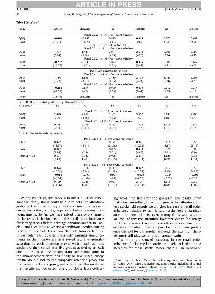
20 B. Liu, H. Wang and J. Yu et al. / Journal of Financial Economics xxx (xxxx) xxx
ARTICLE IN PRESS
JID: FINEC [m3Gdc; August 8, 2020;1:54 ]
Table 8 ( continued )
Proxy = Maxret Skewexp Prc Jackpotp Ivol Z -score
Panel C.2.2: ( + 1,+5) Post-event window
Q5-Q1 −0.440 −0.269 0.825 0.415 0.679 0.462
t -stat ( −1.18) ( −0.44) (1.31) (0.67) (1.3) (0.83)
Panel C.3: Controlling for SCIH
Panel C.3.1: ( −5 , −1) Pre-event window
Q5-Q1 1.337 1.445 2.981 2.694 2.909 2.805
t -stat (3.04) (1.98) (4.68) (4.26) (5.76) (4.67)
Panel C.3.2: ( + 1,+5) Post-event window
Q5-Q1 −0.292 −0.009 1.023 0.305 0.789 0.442
t -stat ( −0.77) ( −0.01) (1.62) (0.48) (1.51) (0.76)
Panel C.4: Controlling for Attn
Panel C.4.1: ( −5 , −1) Pre-event window
Q5-Q1 1.384 1.391 2.880 2.775 3.143 2.906
t -stat (3.27) (1.81) (4.65) (4.24) (6.36) (4.79)
Panel C.4.2: ( + 1,+5) Post-event window
Q5-Q1 −0.214 0.114 0.950 0.290 0.912 0.674
t -stat ( −0.58) (0.2) (1.53) (0.47) (1.85) (1.18)
Proxy = Maxret Skewexp Prc Jackpotp Ivol Z -score
Panel D: Double-sorted portfolios by Attn and Z -score
Attn port. = P1 P2 P3 P4 P5 Ave
Panel D.1: ( −5 , −1) Pre-event window
Q5-Q1 2.699 2.754 2.541 3.457 3.081 2.906
t -stat (2.95) (3.46) (3.16) (4.2) (3.9) (4.79)
Panel D.2: ( + 1,+5) Post-event window
Q5-Q1 0.165 0.236 0.752 1.204 1.014 0.674
t -stat (0.18) (0.33) (1.01) (1.44) (1.1) (1.18)
Panel E: Fama–MacBeth regressions
Panel E.1: ( −5 , −1) Pre-event regression
RIMB 0.022 0.013 0.121 0.021 0.010 0.056
(13.67) (6.01) (24.76) (12.94) (5.37) (25.15)
Proxy 0.042 0.010 0.005 0.430 0.176 0.005
(3.94) (7.2) (6.21) (6.45) (4.41) (5.9)
Proxy x RIMB 0.421 0.047 0.028 2.217 1.629 0.033
(14.9) (15.00) (19.95) (15.39) (16.95) (17.31)
Panel E.2: ( + 1,+5) Post-event regression
RIMB 0.024 0.014 0.117 0.022 0.012 0.055
(12.78) (6.64) (24.28) (12.56) (6.15) (24.89)
Proxy −0.014 −0.002 −0.001 −0.020 −0.034 −0.001
( −1.34) ( −1.48) ( −1.4) ( −0.28) ( −0.97) ( −2.12)
Proxy x RIMB 0.379 0.046 0.027 2.107 1.519 0.030
(14.56) (15.85) (19.61) (14.54) (16.89) (17.05)
increases for those stocks. When there is an imbalance
28 As shown in Table A5 in the Online Appendix, we obtain simi-
lar results when using alternative attention proxies including abnormal
turnover, abnormal trading volume ( Gervais et al., 2001; Barber and
As argued earlier, the increase in the retail order imbal-
ance for lottery stocks could be due to both the attention-
grabbing feature of lottery stocks and investors intrinsic
desire for lottery stocks, especially before earnings an-
nouncements. So far, we have mixed these two channels
in the tests of the increase in the retail order imbalance
for lottery stocks before earnings announcements. In Pan-
els C and D of Table 8 , we use a conditional double-sorting
procedure to isolate these two channels from each other.
In particular, each quarter, firms with earnings announce-
ments in that quarter are first sorted into five quintiles
according to each attention proxy; within each quintile,
stocks are then sorted into five groups according to each
one of the six lottery proxies from the month prior to
the announcement date; and finally to save space, except
for the double sort by the composite attention proxy and
the composite lottery proxy, we only report the results of
the five attention-adjusted lottery portfolios from collaps-
Please cite this article as: B. Liu, H. Wang and J. Yu et al., Time-v
announcements, Journal of Financial Economics, https://doi.org/1
ing across the five attention groups. 28 The results show
that after controlling for various proxies for attention, lot-
tery stocks still experience a higher increase in retail order
imbalance relative to non-lottery stocks before earnings
announcements. That is, even among firms with a simi-
lar level of investor attention, investors’ desire for lottery
stocks is stronger than for non-lottery stocks. Thus, our
evidence provides further support for the intrinsic prefer-
ence channel for our results, although the attention chan-
nel must still play some role, as argued earlier.
The more pronounced increases in the retail order
imbalance for lottery-like stocks are likely to lead to price
Odean, 2008 ), and recency ( Bali et al., 2019 ).
arying demand for lottery: Speculation ahead of earnings
0.1016/j.jfineco.2020.06.016

B. Liu, H. Wang and J. Yu et al. / Journal of Financial Economics xxx (xxxx) xxx 21
ARTICLE IN PRESS
JID: FINEC [m3Gdc; August 8, 2020;1:54 ]
between buy and sell orders, market markers may absorb
the order imbalance by serving as the trade counterparty.
However, market makers may demand greater compensa-
tion for incurring inventory risks because of the greater
anticipated volatility associated with the information event
(see, e.g., Nagel, 2012; So and Wang, 2014 ). In addition,
as discussed in the introduction, arbitrage forces should
also be more limited ahead of earnings announcements
because of greater uncertainty. Taken together, this im-
plies a greater price run-up for lottery-like stocks ahead
of earnings announcements, consistent with our main
findings in Table 2 .
In light of the above discussion, we also study how
the retail order imbalance affects returns ahead of earn-
ings announcements. In Panel E of Table 8 , we use the re-
gression approach and include the ( −5, −1) RIMB and its
interaction with lottery proxies along with all other con-
trols in the Fama–MacBeth regressions framework used
in the previous section (i.e., Table 3 ). All the interaction
terms between the retail order imbalance and lottery prox-
ies appear to be positive and significant, indicating that
an increase in retail investor interest before the announce-
ments tends to amplify the positive lottery spread be-
fore the announcements. Lastly, in untabulated tests, we
use a short sample of detailed individual transaction data
from Barber and Odean (20 0 0) , Barber and Odean (2001) ,
Barber and Odean (2002) 29 and also find some preliminary
evidence that individual investors are more likely to buy
lottery-like stocks before earnings announcements.
4.3. Evidence from the option markets
In addition to the direct evidence from investors’
trading behavior on the stock market, we also examine
whether the gambling preference exists in the options
market and whether it is intensified ahead of earnings an-
nouncements. OTM calls are a natural candidate for gam-
bling because they are cheap and have highly skewed pay-
offs. 30 Therefore, if investors have a stronger demand for
lottery stocks before earnings announcements, they would
be more likely to buy short-term OTM calls prior to the
event. We plot the dynamics of the adjusted trading vol-
ume of short-term OTM calls during the ( −5,+5) event
window in Fig. 4 . As expected, trading volume starts to in-
crease from five days prior to the event, peaks at the event
date, and then sharply drops immediately after the event.
This pre-event increase pattern echoes that of the retail or-
der imbalance of the lottery-like stocks in the stock mar-
ket. We also study the pattern of implied volatilities of the
OTM call options around the announcement dates. Because
of the stronger demand for lottery-like assets before earn-
ings announcements, the implied volatility of these call op-
tions spikes before the announcement and then declines
after the earnings announcement, as shown in Fig. 4 .
29 We thank Terrance Odean for sharing the data with us. 30 We focus on the behavior of the OTM call options near the announce-
ment dates as individual investors like to trade call options more than
put options. Indeed, Doran et al. (2013) show that individual investors
demand for call options is about 16.4 contracts per day, and the demand
for put options is about 10.5 contracts per day.
Please cite this article as: B. Liu, H. Wang and J. Yu et al., Time-v
announcements, Journal of Financial Economics, https://doi.org/1
Lastly, we also examine the order flow pattern for OTM
call options around earnings announcements. On average,
prior to earnings announcements, the retail order imbal-
ance increases for average OTM call options, a pattern also
seen in lottery stocks. This imbalance is subdued or even
reversed after the announcements, a pattern similar to that
in the stock market. 31 One might expect weaker results
in the options market since that market has more insti-
tutional investors relative to the stock market. However,
Doran et al. (2013) show that OTM options, which have a
strong resemblance to lotteries, have more individual in-
vestors than institutional investors [about 8:1 according to
Table 6 in Doran et al. (2013) ], and thus we also see a sim-
ilar order flow pattern in the options market as we do in
the stock market.
In sum, the results from investors’ trading behavior on
the stock market as well as the options market provide fur-
ther support for our hypothesis on investors’ amplified de-
mand for lottery ahead of earnings announcements.
4.4. Evidence from religious beliefs in gambling propensity
In this subsection, we examine the role of religious be-
liefs in gambling propensity. Kumar et al. (2011) find that
religion-induced gambling preference exhibits geographic
variation, and that the lottery-stock premium is larger
when a firm is located in a region with high concentra-
tions of Catholics relative to Protestants. Compared with
the more tolerant gambling views of Catholic churches,
many Protestant churches maintain a strong moral oppo-
sition to gambling and consider it as a sinful activity.
Following the logic in Kumar et al. (2011) , if the specu-
lative trading is due to lottery-like preferences, we expect
the effect to be stronger for firms in high CPRATIO regions
as well. To test this conjecture, we add the log of CPRATIO
and its interaction with our lottery proxies to the Fama–
MacBeth regressions in Table 3 . Table 9 reports the results.
Consistent with our prediction, the interaction terms are
all positive in the pre-event regressions, and the sign flips
for four out of six proxies in the post-event regressions.
That is, the inverted-V-shaped pattern in the cumulative
return spreads is more pronounced among firms in the re-
gions with a stronger gambling propensity.
4.5. Evidence from international markets
In this subsection, we examine the international data
to see whether the results we documented are an interna-
tional phenomenon. We use aggregate turnover as a proxy
for gambling preference in each country. 32 The country-
level aggregate turnover is the average annual turnover
across all the years we have data for the country. In Panel
A of Table 10 , we rank countries by aggregate turnover
into three groups and then examine the portfolio pattern
31 In untabulated tests, we also find that the retail order imbalance for
OTM calls on lottery stocks increases more than it does for non-lottery
stocks before earnings announcements. 32 We thank the referee for making this suggestion. Gao and
Lin (2015) also present evidence that investors treat trading as an exciting
gambling activity.
arying demand for lottery: Speculation ahead of earnings
0.1016/j.jfineco.2020.06.016
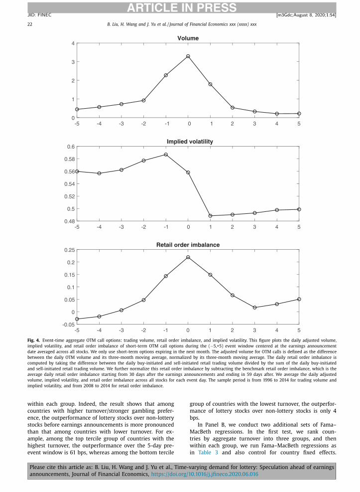
22 B. Liu, H. Wang and J. Yu et al. / Journal of Financial Economics xxx (xxxx) xxx
ARTICLE IN PRESS
JID: FINEC [m3Gdc; August 8, 2020;1:54 ]
Fig. 4. Event-time aggregate OTM call options: trading volume, retail order imbalance, and implied volatility. This figure plots the daily adjusted volume,
implied volatility, and retail order imbalance of short-term OTM call options during the ( −5,+5) event window centered at the earnings announcement
date averaged across all stocks. We only use short-term options expiring in the next month. The adjusted volume for OTM calls is defined as the difference
between the daily OTM volume and its three-month moving average, normalized by its three-month moving average. The daily retail order imbalance is
computed by taking the difference between the daily buy-initiated and sell-initiated retail trading volume divided by the sum of the daily buy-initiated
and sell-initiated retail trading volume. We further normalize this retail order imbalance by subtracting the benchmark retail order imbalance, which is the
average daily retail order imbalance starting from 30 days after the earnings announcements and ending in 59 days after. We average the daily adjusted
volume, implied volatility, and retail order imbalance across all stocks for each event day. The sample period is from 1996 to 2014 for trading volume and
implied volatility, and from 2008 to 2014 for retail order imbalance.
within each group. Indeed, the result shows that among
countries with higher turnover/stronger gambling prefer-
ence, the outperformance of lottery stocks over non-lottery
stocks before earnings announcements is more pronounced
than that among countries with lower turnover. For ex-
ample, among the top tercile group of countries with the
highest turnover, the outperformance over the 5-day pre-
event window is 61 bps, whereas among the bottom tercile
Please cite this article as: B. Liu, H. Wang and J. Yu et al., Time-v
announcements, Journal of Financial Economics, https://doi.org/1
group of countries with the lowest turnover, the outperfor-
mance of lottery stocks over non-lottery stocks is only 4
bps.
In Panel B, we conduct two additional sets of Fama–
MacBeth regressions. In the first test, we rank coun-
tries by aggregate turnover into three groups, and then
within each group, we run Fama–MacBeth regressions as
in Table 3 and also control for country fixed effects.
arying demand for lottery: Speculation ahead of earnings
0.1016/j.jfineco.2020.06.016
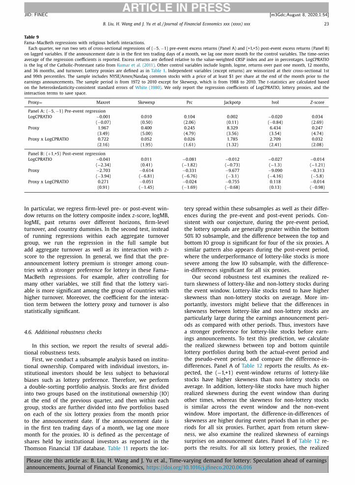
B. Liu, H. Wang and J. Yu et al. / Journal of Financial Economics xxx (xxxx) xxx 23
ARTICLE IN PRESS
JID: FINEC [m3Gdc; August 8, 2020;1:54 ]
Table 9
Fama–MacBeth regressions with religious beliefs interactions.
Each quarter, we run two sets of cross-sectional regressions of ( −5 , −1) pre-event excess returns (Panel A) and (+1,+5) post-event excess returns (Panel B)
on lagged variables. If the announcement date is in the first ten trading days of a month, we lag one more month for the control variables. The time-series
average of the regression coefficients is reported. Excess returns are defined relative to the value-weighted CRSP index and are in percentages. LogCPRATIO
is the log of the Catholic-Protestant ratio from Kumar et al. (2011) . Other control variables include logmb, logme, returns over past one month, 12 months,
and 36 months, and turnover. Lottery proxies are defined as in Table 1 . Independent variables (except returns) are winsorized at their cross-sectional 1st
and 99th percentiles. The sample includes NYSE/Amex/Nasdaq common stocks with a price of at least $1 per share at the end of the month prior to the
earnings announcements. The sample period is from 1972 to 2010 except for Skewexp, which is from 1988 to 2010. The t -statistics are calculated based
on the heteroskedasticity-consistent standard errors of White (1980) . We only report the regression coefficients of LogCPRATIO, lottery proxies, and the
interaction terms to save space.
Proxy = Maxret Skewexp Prc Jackpotp Ivol Z -score
Panel A: ( −5 , −1) Pre-event regression
LogCPRATIO −0.001 0.010 0.104 0.002 −0.020 0.034
( −0.07) (0.50) (2.06) (0.11) ( −0.84) (2.69)
Proxy 1.967 0.400 0.245 8.329 6.434 0.247
(3.49) (5.00) (4.79) (3.56) (3.54) (4.74)
Proxy x LogCPRATIO 0.722 0.052 0.026 1.785 2.709 0.032
(2.16) (1.95) (1.61) (1.32) (2.41) (2.08)
Panel B: ( + 1,+5) Post-event regression
LogCPRATIO −0.041 0.011 −0.081 −0.012 −0.027 −0.014
( −2.34) (0.41) ( −1.82) ( −0.73) ( −1.3) ( −1.21)
Proxy −2.703 −0.614 −0.331 −9.677 −9.090 −0.313
( −3.94) ( −6.81) ( −6.76) ( −3.1) ( −4.16) ( −5.8)
Proxy x LogCPRATIO 0.271 −0.051 −0.024 −0.755 0.118 −0.014
(0.91) ( −1.45) ( −1.69) ( −0.68) (0.13) ( −0.98)
In particular, we regress firm-level pre- or post-event win-
dow returns on the lottery composite index z -score, logMB,
logME, past returns over different horizons, firm-level
turnover, and country dummies. In the second test, instead
of running regressions within each aggregate turnover
group, we run the regression in the full sample but
add aggregate turnover as well as its interaction with z -
score to the regression. In general, we find that the pre-
announcement lottery premium is stronger among coun-
tries with a stronger preference for lottery in these Fama–
MacBeth regressions. For example, after controlling for
many other variables, we still find that the lottery vari-
able is more significant among the group of countries with
higher turnover. Moreover, the coefficient for the interac-
tion term between the lottery proxy and turnover is also
statistically significant.
4.6. Additional robustness checks
In this section, we report the results of several addi-
tional robustness tests.
First, we conduct a subsample analysis based on institu-
tional ownership. Compared with individual investors, in-
stitutional investors should be less subject to behavioral
biases such as lottery preference. Therefore, we perform
a double-sorting portfolio analysis. Stocks are first divided
into two groups based on the institutional ownership (IO)
at the end of the previous quarter, and then within each
group, stocks are further divided into five portfolios based
on each of the six lottery proxies from the month prior
to the announcement date. If the announcement date is
in the first ten trading days of a month, we lag one more
month for the proxies. IO is defined as the percentage of
shares held by institutional investors as reported in the
Thomson Financial 13F database. Table 11 reports the lot-
Please cite this article as: B. Liu, H. Wang and J. Yu et al., Time-v
announcements, Journal of Financial Economics, https://doi.org/1
tery spread within these subsamples as well as their differ-
ences during the pre-event and post-event periods. Con-
sistent with our conjecture, during the pre-event period,
the lottery spreads are generally greater within the bottom
50% IO subsample, and the difference between the top and
bottom IO group is significant for four of the six proxies. A
similar pattern also appears during the post-event period,
where the underperformance of lottery-like stocks is more
severe among the low IO subsample, with the difference-
in-differences significant for all six proxies.
Our second robustness test examines the realized re-
turn skewness of lottery-like and non-lottery stocks during
the event window. Lottery-like stocks tend to have higher
skewness than non-lottery stocks on average. More im-
portantly, investors might believe that the differences in
skewness between lottery-like and non-lottery stocks are
particularly large during the earnings announcement peri-
ods as compared with other periods. Thus, investors have
a stronger preference for lottery-like stocks before earn-
ings announcements. To test this prediction, we calculate
the realized skewness between top and bottom quintile
lottery portfolios during both the actual-event period and
the pseudo-event period, and compare the difference-in-
differences. Panel A of Table 12 reports the results. As ex-
pected, the ( −1,+1) event-window returns of lottery-like
stocks have higher skewness than non-lottery stocks on
average. In addition, lottery-like stocks have much higher
realized skewness during the event window than during
other times, whereas the skewness for non-lottery stocks
is similar across the event window and the non-event
window. More important, the difference-in-differences of
skewness are higher during event periods than in other pe-
riods for all six proxies. Further, apart from return skew-
ness, we also examine the realized skewness of earnings
surprises on announcement dates. Panel B of Table 12 re-
ports the results. For all six lottery proxies, the realized
arying demand for lottery: Speculation ahead of earnings
0.1016/j.jfineco.2020.06.016
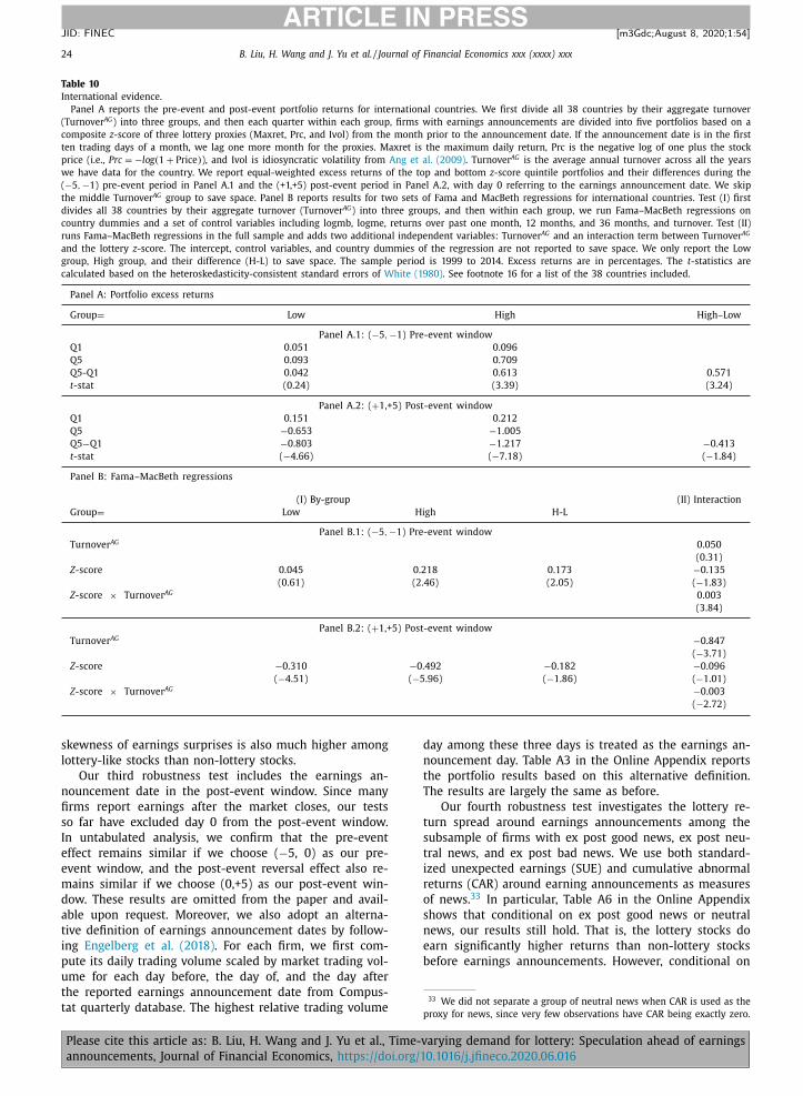
24 B. Liu, H. Wang and J. Yu et al. / Journal of Financial Economics xxx (xxxx) xxx
ARTICLE IN PRESS
JID: FINEC [m3Gdc; August 8, 2020;1:54 ]
Table 10
International evidence.
Panel A reports the pre-event and post-event portfolio returns for international countries. We first divide all 38 countries by their aggregate turnover
(Turnover AG ) into three groups, and then each quarter within each group, firms with earnings announcements are divided into five portfolios based on a
composite z -score of three lottery proxies (Maxret, Prc, and Ivol) from the month prior to the announcement date. If the announcement date is in the first
ten trading days of a month, we lag one more month for the proxies. Maxret is the maximum daily return, Prc is the negative log of one plus the stock
price (i.e., Prc = −log(1 + Price ) ), and Ivol is idiosyncratic volatility from Ang et al. (2009) . Turnover AG is the average annual turnover across all the years
we have data for the country. We report equal-weighted excess returns of the top and bottom z -score quintile portfolios and their differences during the
( −5 , −1) pre-event period in Panel A.1 and the (+1,+5) post-event period in Panel A.2, with day 0 referring to the earnings announcement date. We skip
the middle Turnover AG group to save space. Panel B reports results for two sets of Fama and MacBeth regressions for international countries. Test (I) first
divides all 38 countries by their aggregate turnover (Turnover AG ) into three groups, and then within each group, we run Fama–MacBeth regressions on
country dummies and a set of control variables including logmb, logme, returns over past one month, 12 months, and 36 months, and turnover. Test (II)
runs Fama–MacBeth regressions in the full sample and adds two additional independent variables: Turnover AG and an interaction term between Turnover AG
and the lottery z -score. The intercept, control variables, and country dummies of the regression are not reported to save space. We only report the Low
group, High group, and their difference (H-L) to save space. The sample period is 1999 to 2014. Excess returns are in percentages. The t -statistics are
calculated based on the heteroskedasticity-consistent standard errors of White (1980) . See footnote 16 for a list of the 38 countries included.
Panel A: Portfolio excess returns
Group = Low High High–Low
Panel A.1: ( −5 , −1) Pre-event window
Q1 0.051 0.096
Q5 0.093 0.709
Q5-Q1 0.042 0.613 0.571
t -stat (0.24) (3.39) (3.24)
Panel A.2: ( + 1,+5) Post-event window
Q1 0.151 0.212
Q5 −0.653 −1.005
Q5 −Q1 −0.803 −1.217 −0.413
t -stat ( −4.66) ( −7.18) ( −1.84)
Panel B: Fama–MacBeth regressions
(I) By-group (II) Interaction
Group = Low High H-L
Panel B.1: ( −5 , −1) Pre-event window
Turnover AG 0.050
(0.31)
Z -score 0.045 0.218 0.173 −0.135
(0.61) (2.46) (2.05) ( −1.83)
Z -score × Turnover AG 0.003
(3.84)
Panel B.2: ( + 1,+5) Post-event window
Turnover AG −0.847
( −3.71)
Z -score −0.310 −0.492 −0.182 −0.096
( −4.51) ( −5.96) ( −1.86) ( −1.01)
Z -score × Turnover AG −0.003
( −2.72)
33 We did not separate a group of neutral news when CAR is used as the
skewness of earnings surprises is also much higher among
lottery-like stocks than non-lottery stocks.
Our third robustness test includes the earnings an-
nouncement date in the post-event window. Since many
firms report earnings after the market closes, our tests
so far have excluded day 0 from the post-event window.
In untabulated analysis, we confirm that the pre-event
effect remains similar if we choose ( −5, 0) as our pre-
event window, and the post-event reversal effect also re-
mains similar if we choose (0,+5) as our post-event win-
dow. These results are omitted from the paper and avail-
able upon request. Moreover, we also adopt an alterna-
tive definition of earnings announcement dates by follow-
ing Engelberg et al. (2018) . For each firm, we first com-
pute its daily trading volume scaled by market trading vol-
ume for each day before, the day of, and the day after
the reported earnings announcement date from Compus-
tat quarterly database. The highest relative trading volume
Please cite this article as: B. Liu, H. Wang and J. Yu et al., Time-v
announcements, Journal of Financial Economics, https://doi.org/1
day among these three days is treated as the earnings an-
nouncement day. Table A3 in the Online Appendix reports
the portfolio results based on this alternative definition.
The results are largely the same as before.
Our fourth robustness test investigates the lottery re-
turn spread around earnings announcements among the
subsample of firms with ex post good news, ex post neu-
tral news, and ex post bad news. We use both standard-
ized unexpected earnings (SUE) and cumulative abnormal
returns (CAR) around earning announcements as measures
of news. 33 In particular, Table A6 in the Online Appendix
shows that conditional on ex post good news or neutral
news, our results still hold. That is, the lottery stocks do
earn significantly higher returns than non-lottery stocks
before earnings announcements. However, conditional on
proxy for news, since very few observations have CAR being exactly zero.
arying demand for lottery: Speculation ahead of earnings
0.1016/j.jfineco.2020.06.016
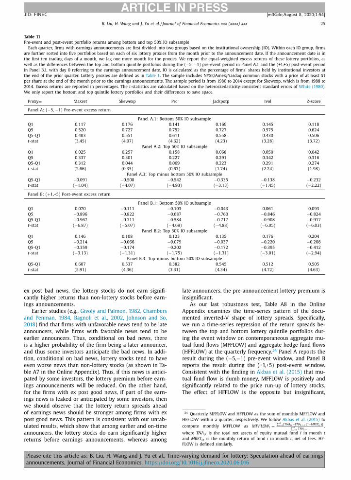
B. Liu, H. Wang and J. Yu et al. / Journal of Financial Economics xxx (xxxx) xxx 25
ARTICLE IN PRESS
JID: FINEC [m3Gdc; August 8, 2020;1:54 ]
Table 11
Pre-event and post-event portfolio returns among bottom and top 50% IO subsample
Each quarter, firms with earnings announcements are first divided into two groups based on the institutional ownership (IO). Within each IO group, firms
are further sorted into five portfolios based on each of six lottery proxies from the month prior to the announcement date. If the announcement date is in
the first ten trading days of a month, we lag one more month for the proxies. We report the equal-weighted excess returns of these lottery portfolios, as
well as the differences between the top and bottom quintile portfolios during the ( −5 , −1) pre-event period in Panel A.1 and the (+1,+5) post-event period
in Panel B.1, with day 0 referring to the earnings announcement date. IO is calculated as the percentage of firms’ shares held by institutional investors at
the end of the prior quarter. Lottery proxies are defined as in Table 1 . The sample includes NYSE/Amex/Nasdaq common stocks with a price of at least $1
per share at the end of the month prior to the earnings announcements. The sample period is from 1980 to 2014 except for Skewexp, which is from 1988 to
2014. Excess returns are reported in percentages. The t -statistics are calculated based on the heteroskedasticity-consistent standard errors of White (1980) .
We only report the bottom and top quintile lottery portfolios and their differences to save space.
Proxy = Maxret Skewexp Prc Jackpotp Ivol Z -score
Panel A: ( −5 , −1) Pre-event excess return
Panel A.1: Bottom 50% IO subsample
Q1 0.117 0.176 0.141 0.169 0.145 0.118
Q5 0.520 0.727 0.752 0.727 0.575 0.624
Q5-Q1 0.403 0.551 0.611 0.558 0.430 0.506
t -stat (3.45) (4.07) (4.62) (4.23) (3.28) (3.72)
Panel A.2: Top 50% IO subsample
Q1 0.025 0.257 0.158 0.068 0.050 0.042
Q5 0.337 0.301 0.227 0.291 0.342 0.316
Q5-Q1 0.312 0.044 0.069 0.223 0.291 0.274
t -stat (2.66) (0.35) (0.67) (1.74) (2.24) (1.98)
Panel A.3: Top minus bottom 50% IO subsample
Q5-Q1 −0.091 −0.508 −0.542 −0.335 −0.138 −0.232
t -stat ( −1.04) ( −4.07) ( −4.93) ( −3.13) ( −1.45) ( −2.22)
Panel B: ( + 1,+5) Post-event excess return
Panel B.1: Bottom 50% IO subsample
Q1 0.070 −0.111 −0.103 −0.043 0.061 0.093
Q5 −0.896 −0.822 −0.687 −0.760 −0.846 −0.824
Q5-Q1 −0.967 −0.711 −0.584 −0.717 −0.908 −0.917
t -stat ( −6.87) ( −5.07) ( −4.69) ( −4.88) ( −6.05) ( −6.03)
Panel B.2: Top 50% IO subsample
Q1 0.146 0.108 0.123 0.135 0.176 0.204
Q5 −0.214 −0.066 −0.079 −0.037 −0.220 −0.208
Q5-Q1 −0.359 −0.174 −0.202 −0.172 −0.395 −0.412
t -stat ( −3.13) ( −1.31) ( −1.75) ( −1.31) ( −3.01) ( −2.94)
Panel B.3: Top minus bottom 50% IO subsample
Q5-Q1 0.607 0.537 0.382 0.545 0.512 0.505
t -stat (5.91) (4.36) (3.31) (4.34) (4.72) (4.63)
34 Quarterly MFFLOW and HFFLOW as the sum of monthly MFFLOW and
HFFLOW within a quarter, respectively. We follow Akbas et al. (2015) to
compute monthly MFFLOW as MF F LOW t =
∑ N i =1 [ T NA i,t −T NA i,t−1 (1+ MRET i,t )]
∑ N i =1 TNA i,t−1
,
where TNA i,t is the total net assets of equity mutual fund i in month t
and MRET i,t is the monthly return of fund i in month t , net of fees. HF-
ex post bad news, the lottery stocks do not earn signifi-
cantly higher returns than non-lottery stocks before earn-
ings announcements.
Earlier studies (e.g., Givoly and Palmon, 1982, Chambers
and Penman, 1984, Bagnoli et al., 2002, Johnson and So,
2018 ) find that firms with unfavorable news tend to be late
announcers, while firms with favorable news tend to be
earlier announcers. Thus, conditional on bad news, there
is a higher probability of the firm being a later announcer,
and thus some investors anticipate the bad news. In addi-
tion, conditional on bad news, lottery stocks tend to have
even worse news than non-lottery stocks (as shown in Ta-
ble A7 in the Online Appendix). Thus, if this news is antici-
pated by some investors, the lottery premium before earn-
ings announcements will be reduced. On the other hand,
for the firms with ex post good news, if part of the earn-
ings news is leaked or anticipated by some investors, then
we should observe that the lottery return spreads ahead
of earnings news should be stronger among firms with ex
post good news. This pattern is consistent with our untab-
ulated results, which show that among earlier and on-time
announcers, the lottery stocks do earn significantly higher
returns before earnings announcements, whereas among
Please cite this article as: B. Liu, H. Wang and J. Yu et al., Time-v
announcements, Journal of Financial Economics, https://doi.org/1
late announcers, the pre-announcement lottery premium is
insignificant.
As our last robustness test, Table A8 in the Online
Appendix examines the time-series pattern of the docu-
mented inverted-V shape of lottery spreads. Specifically,
we run a time-series regression of the return spreads be-
tween the top and bottom lottery quintile portfolios dur-
ing the event window on contemporaneous aggregate mu-
tual fund flows (MFFLOW) and aggregate hedge fund flows
(HFFLOW) at the quarterly frequency. 34 Panel A reports the
result during the ( −5, −1) pre-event window, and Panel B
reports the result during the (+1,+5) post-event window.
Consistent with the finding in Akbas et al. (2015) that mu-
tual fund flow is dumb money, MFFLOW is positively and
significantly related to the price run-up of lottery stocks.
The effect of HFFLOW is the opposite but insignificant,
FLOW is defined similarly.
arying demand for lottery: Speculation ahead of earnings
0.1016/j.jfineco.2020.06.016
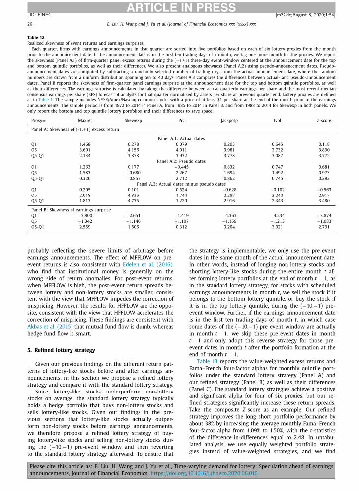
26 B. Liu, H. Wang and J. Yu et al. / Journal of Financial Economics xxx (xxxx) xxx
ARTICLE IN PRESS
JID: FINEC [m3Gdc; August 8, 2020;1:54 ]
Table 12
Realized skewness of event returns and earnings surprises.
Each quarter, firms with earnings announcements in that quarter are sorted into five portfolios based on each of six lottery proxies from the month
prior to the announcement date. If the announcement date is in the first ten trading days of a month, we lag one more month for the proxies. We report
the skewness (Panel A.1) of firm-quarter panel excess returns during the ( −1,+1) three-day event-window centered at the announcement date for the top
and bottom quintile portfolios, as well as their differences. We also present analogous skewness (Panel A.2) using pseudo-announcement dates. Pseudo-
announcement dates are computed by subtracting a randomly selected number of trading days from the actual announcement date, where the random
numbers are drawn from a uniform distribution spanning ten to 40 days. Panel A.3 compares the differences between actual- and pseudo-announcement
dates. Panel B reports the skewness of firm-quarter panel earnings surprise at the announcement date for the top and bottom quintile portfolios, as well
as their differences. The earnings surprise is calculated by taking the difference between actual quarterly earnings per share and the most recent median
consensus earnings per share (EPS) forecast of analysts for that quarter normalized by assets per share at previous quarter end. Lottery proxies are defined
as in Table 1 . The sample includes NYSE/Amex/Nasdaq common stocks with a price of at least $1 per share at the end of the month prior to the earnings
announcements. The sample period is from 1972 to 2014 in Panel A, from 1985 to 2014 in Panel B, and from 1988 to 2014 for Skewexp in both panels. We
only report the bottom and top quintile lottery portfolios and their differences to save space.
Proxy = Maxret Skewexp Prc Jackpotp Ivol Z -score
Panel A: Skewness of (-1, + 1) excess return
Panel A.1: Actual dates
Q1 1.468 0.278 0.079 0.203 0.645 0.118
Q5 3.601 4.156 4.011 3.981 3.732 3.890
Q5-Q1 2.134 3.878 3.932 3.778 3.087 3.772
Panel A.2: Pseudo dates
Q1 1.263 0.177 −0.445 0.832 0.747 0.681
Q5 1.583 −0.680 2.267 1.694 1.492 0.973
Q5-Q1 0.320 −0.857 2.712 0.862 0.745 0.292
Panel A.3: Actual dates minus pseudo dates
Q1 0.205 0.101 0.524 −0.628 −0.102 −0.563
Q5 2.018 4.836 1.744 2.287 2.240 2.917
Q5-Q1 1.813 4.735 1.220 2.916 2.343 3.480
Panel B: Skewness of earnings surprise
Q1 −3.900 −2.651 −1.419 −4.363 −4.234 −3.874
Q5 −1.342 −1.146 −1.107 −1.159 −1.213 −1.083
Q5-Q1 2.559 1.506 0.312 3.204 3.021 2.791
probably reflecting the severe limits of arbitrage before
earnings announcements. The effect of MFFLOW on pre-
event returns is also consistent with Edelen et al. (2016) ,
who find that institutional money is generally on the
wrong side of return anomalies. For post-event returns,
when MFFLOW is high, the post-event return spreads be-
tween lottery and non-lottery stocks are smaller, consis-
tent with the view that MFFLOW impedes the correction of
mispricing. However, the results for HFFLOW are the oppo-
site, consistent with the view that HFFLOW accelerates the
correction of mispricing. These findings are consistent with
Akbas et al. (2015) that mutual fund flow is dumb, whereas
hedge fund flow is smart.
5. Refined lottery strategy
Given our previous findings on the different return pat-
terns of lottery-like stocks before and after earnings an-
nouncements, in this section we propose a refined lottery
strategy and compare it with the standard lottery strategy.
Since lottery-like stocks underperform non-lottery
stocks on average, the standard lottery strategy typically
holds a hedge portfolio that buys non-lottery stocks and
sells lottery-like stocks. Given our findings in the pre-
vious sections that lottery-like stocks actually outper-
form non-lottery stocks before earnings announcements,
we therefore propose a refined lottery strategy of buy-
ing lottery-like stocks and selling non-lottery stocks dur-
ing the ( −10, −1) pre-event window and then reverting
to the standard lottery strategy afterward. To ensure that
Please cite this article as: B. Liu, H. Wang and J. Yu et al., Time-v
announcements, Journal of Financial Economics, https://doi.org/1
the strategy is implementable, we only use the pre-event
dates in the same month of the actual announcement date.
In other words, instead of longing non-lottery stocks and
shorting lottery-like stocks during the entire month t af-
ter forming lottery portfolios at the end of month t − 1 , as
in the standard lottery strategy, for stocks with scheduled
earnings announcements in month t , we sell the stock if it
belongs to the bottom lottery quintile, or buy the stock if
it is in the top lottery quintile, during the ( −10, −1) pre-
event window. Further, if the earnings announcement date
is in the first ten trading days of month t , in which case
some dates of the ( −10, −1) pre-event window are actually
in month t − 1 , we skip these pre-event dates in month
t − 1 and only adopt this reverse strategy for those pre-
event dates in month t after the portfolio formation at the
end of month t − 1 .
Table 13 reports the value-weighted excess returns and
Fama–French four-factor alphas for monthly quintile port-
folios under the standard lottery strategy (Panel A) and
our refined strategy (Panel B) as well as their differences
(Panel C). The standard lottery strategies achieve a positive
and significant alpha for four of six proxies, but our re-
fined strategies significantly increase these return spreads.
Take the composite Z -score as an example. Our refined
strategy improves the long-short portfolio performance by
about 38% by increasing the average monthly Fama–French
four-factor alpha from 1.09% to 1.50%, with the t -statistics
of the difference-in-differences equal to 2.48. In untabu-
lated analysis, we use equally weighted portfolio strate-
gies instead of value-weighted strategies, and we find
arying demand for lottery: Speculation ahead of earnings
0.1016/j.jfineco.2020.06.016
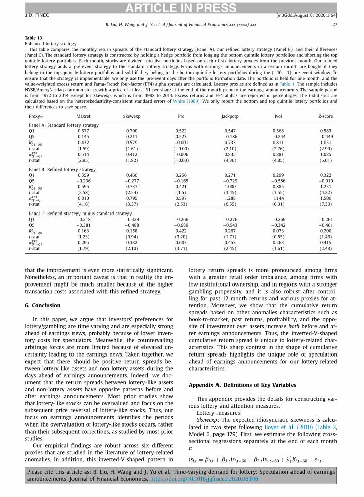
B. Liu, H. Wang and J. Yu et al. / Journal of Financial Economics xxx (xxxx) xxx 27
ARTICLE IN PRESS
JID: FINEC [m3Gdc; August 8, 2020;1:54 ]
Table 13
Enhanced lottery strategy.
This table compares the monthly return spreads of the standard lottery strategy (Panel A), our refined lottery strategy (Panel B), and their differences
(Panel C). The standard lottery strategy is constructed by holding a hedge portfolio from longing the bottom quintile lottery portfolios and shorting the top
quintile lottery portfolios. Each month, stocks are divided into five portfolios based on each of six lottery proxies from the previous month. Our refined
lottery strategy adds a pre-event strategy to the standard lottery strategy. Firms with earnings announcements in a certain month are bought if they
belong to the top quintile lottery portfolios and sold if they belong to the bottom quintile lottery portfolios during the ( −10 , −1) pre-event window. To
ensure that the strategy is implementable, we only use the pre-event days after the portfolio formation date. The portfolio is held for one month, and the
value-weighted excess return and Fama–French four-factor (FF4) alpha spreads are calculated. Lottery proxies are defined as in Table 1 . The sample includes
NYSE/Amex/Nasdaq common stocks with a price of at least $1 per share at the end of the month prior to the earnings announcements. The sample period
is from 1972 to 2014 except for Skewexp, which is from 1988 to 2014. Excess returns and FF4 alphas are reported in percentages. The t -statistics are
calculated based on the heteroskedasticity-consistent standard errors of White (1980) . We only report the bottom and top quintile lottery portfolios and
their differences to save space.
Proxy = Maxret Skewexp Prc Jackpotp Ivol Z -score
Panel A: Standard lottery strategy
Q1 0.577 0.790 0.522 0.547 0.568 0.583
Q5 0.145 0.211 0.523 −0.186 −0.244 −0.449
R e Q 1 −Q 5 0.432 0.579 −0.001 0.733 0.811 1.031
t -stat (1.59) (1.61) ( −0.00) (2.10) (2.76) (2.99)
αF F 4 Q 1 −Q 5 0.514 0.412 −0.006 0.835 0.881 1.085
t -stat (2.95) (1.82) ( −0.03) (4.36) (4.85) (5.01)
Panel B: Refined lottery strategy
Q1 0.359 0.460 0.256 0.271 0.299 0.322
Q5 −0.236 −0.277 −0.165 −0.729 −0.586 −0.910
R e Q 1 −Q 5 0.595 0.737 0.421 1.000 0.885 1.231
t -stat (2.58) (2.54) (1.5) (3.45) (3.55) (4.22)
αF F 4 Q 1 −Q 5 0.810 0.795 0.597 1.288 1.144 1.500
t -stat (4.16) (3.37) (2.53) (6.55) (6.31) (7.30)
Panel C: Refined strategy minus standard strategy
Q1 −0.218 −0.329 −0.266 −0.276 −0.269 −0.261
Q5 −0.381 −0.488 −0.689 −0.543 −0.342 −0.461
R e Q 1 −Q 5 0.163 0.158 0.422 0.267 0.073 0.200
t -stat (1.23) (0.94) (3.20) (1.71) (0.55) (1.46)
αF F 4 Q 1 −Q 5 0.295 0.382 0.603 0.453 0.263 0.415
t -stat (1.79) (2.10) (3.71) (2.45) (1.61) (2.48)
that the improvement is even more statistically significant.
Nonetheless, an important caveat is that in reality the im-
provement might be much smaller because of the higher
transaction costs associated with this refined strategy.
6. Conclusion
In this paper, we argue that investors’ preferences for
lottery/gambling are time varying and are especially strong
ahead of earnings news, probably because of lower inven-
tory costs for speculators. Meanwhile, the countervailing
arbitrage forces are more limited because of elevated un-
certainty leading to the earnings news. Taken together, we
expect that there should be positive return spreads be-
tween lottery-like assets and non-lottery assets during the
days ahead of earnings announcements. Indeed, we doc-
ument that the return spreads between lottery-like assets
and non-lottery assets have opposite patterns before and
after earnings announcements. Most prior studies show
that lottery-like stocks can be overvalued and focus on the
subsequent price reversal of lottery-like stocks. Thus, our
focus on earnings announcements identifies the periods
when the overvaluation of lottery-like stocks occurs, rather
than their subsequent corrections, as studied by most prior
studies.
Our empirical findings are robust across six different
proxies that are studied in the literature of lottery-related
anomalies. In addition, this inverted-V-shaped pattern in
Please cite this article as: B. Liu, H. Wang and J. Yu et al., Time-v
announcements, Journal of Financial Economics, https://doi.org/1
lottery return spreads is more pronounced among firms
with a greater retail order imbalance, among firms with
low institutional ownership, and in regions with a stronger
gambling propensity, and it is also robust after control-
ling for past 12-month returns and various proxies for at-
tention. Moreover, we show that the cumulative return
spreads based on other anomalies characteristics such as
book-to-market, past returns, profitability, and the oppo-
site of investment over assets increase both before and af-
ter earnings announcements. Thus, the inverted-V-shaped
cumulative return spread is unique to lottery-related char-
acteristics. This sharp contrast in the shape of cumulative
return spreads highlights the unique role of speculation
ahead of earnings announcements for our lottery-related
characteristics.
Appendix A. Definitions of Key Variables
This appendix provides the details for constructing var-
ious lottery and attention measures.
Lottery measures:
Skewexp : The expected idiosyncratic skewness is calcu-
lated in two steps following Boyer et al. (2010) ( Table 2 ,
Model 6, page 179). First, we estimate the following cross-
sectional regressions separately at the end of each month
t :
is i,t = β0 ,t + β1 ,t is i,t−60 + β2 ,t i v i,t−60 + λ′ t X i,t−60 + ε i,t ,
arying demand for lottery: Speculation ahead of earnings
0.1016/j.jfineco.2020.06.016

28 B. Liu, H. Wang and J. Yu et al. / Journal of Financial Economics xxx (xxxx) xxx
ARTICLE IN PRESS
JID: FINEC [m3Gdc; August 8, 2020;1:54 ]
where is i,t and iv i, t denote the historical estimates of id-
iosyncratic volatility and skewness relative to the Fama
and French three-factor model, respectively, for firm i using
daily stock data over the past 60 months to month t. X i,t
is a set of firm-specific variables including momentum as
the cumulative returns over months t − 72 through t − 61 ,
turnover as the average daily turnover in month t − 60 , the
small-size market capitalization dummy, the medium-size
market capitalization dummy, the industry dummy based
on the Fama–French 17-industries definition, and the NAS-
DAQ dummy. After we have these regression parameters,
the expected idiosyncratic skewness for each firm i at the
end of each month t is then computed in the second step:
Skewexp t ≡ E t [ is i,t+60 ] = β0 ,t + β1 ,t is i,t + β2 ,t i v i,t + λ′ t X i,t .
Similar to Boyer et al. (2010) baseline database, our ex-
pected idiosyncratic skewness measure dates back to Jan-
uary 1988.
Jackpotp : The predicted jackpot probability is con-
structed from the baseline model in Conrad et al.
(2014) ( Table 3 , Panel A, page 461). In particular, for each
firm, we first estimate the baseline logit model using data
from the past 20 years at the end of June every year:
P rob t−1 (Jackpot i,t = 1) =
exp(a + b × X i,t−1 )
1 + exp(a + b × X i,t−1 ) ,
where Jackpot i,t is a dummy that equals 1 if firm i ’s log
return in the next 12-month period is greater than 100%.
The vector X i,t−1 is a set of firm-specific variables known
at time t − 1 , including skewness of log daily returns (cen-
tered around 0) over the last three months, log stock re-
turn over the past year, firm age as the number of years
since appearance on CRSP, asset tangibility as the ratio of
gross PPE (property plant and equipment) to total assets,
the log of sales growth over the prior year, detrended stock
turnover as the difference between the average past 6-
month turnover and the average past 18-month turnover,
volatility as the standard deviation of daily returns (cen-
tered around 0) over the past 3 months, and the log of
market equity in thousands. Next, we use these estimated
parameters to construct the out-of-sample predicted jack-
pot probability (Jackpotp). We reestimate this model for
each firm every year from 1951, so our first set of out-
of-sample predicted jackpot probabilities is from January
1972.
Ivol : The idiosyncratic stock return volatility is con-
structed following Ang et al. (2006) . In particular, we mea-
sure IVOL by the standard deviation of the residual values
from the following time-series model:
R i,t = b 0 + b 1 R M,t + b 2 SMB t + b 3 HML t + ε i,t , (A.1)
where R i,t is stock i ’s daily excess return on date t , and
R M,t , SMB t , and HML t are the market factor, size factor,
and value factor on date t , respectively. 35 We estimate the
above equation for each stock each month in the data set
using the daily return from the previous month with a
minimum requirement of 10 nonmissing values. 36
35 We thank Ken French for providing updated series for these factors. 36 Our results are not sensitive to this cutoff.
Please cite this article as: B. Liu, H. Wang and J. Yu et al., Time-v
announcements, Journal of Financial Economics, https://doi.org/1
Z-score: Z -score is a monthly composite lottery mea-
sure calculated as the average of the individual z -scores of
the following five lottery measures: Maxret, Skewexp, Prc,
Jackpotp, and Ivol. Each month for each stock, each of the
five lottery measures is first converted into its rank and
then standardized to obtain its z -score: z = (r − μr ) /σr ,
where r is the rank of this measure, and μr and σ r are
the cross-sectional mean and standard deviation of r . The
composite z -score is the average of these five z -scores. We
require a minimum of three nonmissing z -scores to com-
pute this measure.
Attention measures:
Media : A firm with more discussions in the media tends
to draw investor attention because of its high public profile
( Barber and Odean, 2008 ). Media coverage is a dummy be-
ing 1 if it has news coverage during the ( −5 , −1) window.
Following Gao et al. (2018) , we use the Dow Jones edi-
tion of RavenPack news data and include only news stories
with an Event Novelty Score (ENS) of 100 to avoid double-
counting the same event of a company. We further require
news to have a relevance score of at least 20 to filter out
nonessential news. The sample starts in 20 0 0.
| SUE | : Extreme earnings news tend to be salient and
easily draw investor attention. Following Bali et al. (2019) ,
the magnitude of earnings surprise is computed as the ab-
solute value of standardized unexpected earnings (SUE) in
the previous quarter. SUE is the difference in split-adjusted
quarterly earnings per share between the current fiscal
quarter and the same fiscal quarter in the previous year,
divided by the standard deviation of this change over the
previous eight quarters.
PD : Social interaction tends to stimulate investor atten-
tion. Following Bali et al. (2019) , we use the population
density (PD) of a firm’s headquarters to proxy for atten-
tion measured as the county-level population in thousands
per square mile of land area from the US Census Bureau in
1980, 1990, 20 0 0, and 2010.
SCIH : The social connectedness of people living in the
county of a firm’s headquarters (SCIH) is based on the
Facebook Social Connectedness Index (SCI) introduced by
Bailey, Cao, Kuchler, Stroebel, and Wong (2018). The Face-
book SCI is a county-pair level measure based on friend-
ship networks among all Facebook users as of April 2016.
Following Bali et al. (2019) , we compute SCIH as the sum
of the SCI of a firm’s headquarters with all other counties
in the United States.
Attn : Attn is a monthly composite measure for attention
calculated as the average of the individual z -scores of the
previous four attention measures.
References
Aboody, D. , Lehavy, R. , Trueman, B. , 2010. Limited attention and the earn-
ings announcement returns of past stock market winners. Rev. Ac- count. Stud. 15, 317–344 .
Akbas, F. , Armstrong, W. , Sorescu, S. , Subrahmanyam, A. , 2015. Smartmoney, dumb money, and capital market anomalies. J. Financ. Econ.
118, 355–382 .
An, L. , Wang, H. , Wang, J. , Yu, J. , 2020. Lottery-related anomalies: the roleof reference-dependent preferences. Manag. Sci. 66, 473–501 .
Anderson, A. , Dyl, E. , 2005. Market structure and trading volume. J. Financ. Res. 28, 115–131 .
Ang, A. , Hodrick, R. , Xing, Y. , Zhang, X. , 2006. The cross-section of volatil-ity and expected returns. J. Finance 61, 259–299 .
arying demand for lottery: Speculation ahead of earnings
0.1016/j.jfineco.2020.06.016

B. Liu, H. Wang and J. Yu et al. / Journal of Financial Economics xxx (xxxx) xxx 29
ARTICLE IN PRESS
JID: FINEC [m3Gdc; August 8, 2020;1:54 ]
Ang, A. , Hodrick, R. , Xing, Y. , Zhang, X. , 2009. High idiosyncratic volatil-ity and low returns: international and further u.s. evidence. J. Financ.
Econ. 91, 1–23 . Bagnoli, M. , Kross, W. , Watts, S. , 2002. The information in management’s
expected earnings report date: a day late, a penny short. J. Account.Res. 40, 1275–1296 .
Bailey, M. , Cao, R. , Kuchler, T. , Stroebel, J. , Wong, A. , 2018. Social connect-
edness: measurement, determinants, and effects. J. Econ. Perspect. 32,259–280 .
Bali, T. , Brown, S. , Murray, S. , Yang, Y. , 2017. A lottery-demand-based ex-planation of the beta anomaly. J. Financ. Quant. Anal. 52, 2369–2397 .
Bali, T. , Cakici, N. , Whitelaw, R. , 2011. Maxing out: stocks as lotteries andthe cross-section of expected returns. J. Financ. Econ. 99, 427–446 .
Bali, T. , Hirshleifer, D. , Peng, L. , Tang, Y. , 2019. Attention, social interaction,and investor attraction to lottery stocks. Unpublished working paper.
Georgetown University, University of California, Irvine, Baruch College
CUNY, and Fordham University . Bali, T. , Murray, S. , 2013. Does risk-neutral skewness predict the cross–
section of equity option portfolio returns? J. Financ. Quant. Anal. 48,1145–1171 .
Ball, R. , Kothari, S. , 1991. Security returns around earnings announce-ments. Account. Rev. 66, 718–738 .
Barber, B. , De George, E. , Lehavy, R. , Trueman, B. , 2013. The earnings an-
nouncement premium around the globe. J. Financ. Econ. 108, 118–138 .Barber, B. , Odean, T. , 20 0 0. Trading is hazardous to your wealth: the com-
mon stock investment performance of individual investors. J. Finance56, 773–806 .
Barber, B. , Odean, T. , 2001. Boys will be boys: gender, overconfidence, andcommon stock investment. Q. J. Econ. 116, 261–292 .
Barber, B. , Odean, T. , 2002. Online investors: do the slow die first? Rev.
Financ. Stud. 15, 455–488 . Barber, B. , Odean, T. , 2008. All that glitters: the effect of attention and
news on the buying behavior of individual and institutional investors.Rev. Financ. Stud. 21, 785–818 .
Barber, B. , Odean, T. , Zhu, N. , 2009. Do retail trades move markets? Rev.Financ. Stud. 22, 151–186 .
Barberis, N. , Huang, M. , 2008. Stocks as lotteries: the implications of prob-
ability weighting for security prices. Am. Econ. Rev. 98, 2066–2100 . Berkman, H. , Dimitrov, V. , Jain, P. , Koch, P. , Tice, S. , 2009. Sell on the news:
differences of opinion, short-sales constraints, and returns aroundearnings announcements. J. Financ. Econ. 92, 376–399 .
Berkman, H. , McKenzie, M. , 2009. The Trading Behaviour of InstitutionalOwners and Short Sellers Around Earnings Announcements. Unpub-
lished working paper. University of Auckland and University of Syd-
ney . Berkman, H. , Truong, C. , 2009. Event day 0? After-a hours earnings an-
nouncements. J. Account. Res. 47, 71–103 . Boulland, R. , Dessaint, O. , 2017. Announcing the announcement. J. Bank.
Finance 82, 59–79 . Boyer, B. , Mitton, T. , Vorkink, K. , 2010. Expected idiosyncratic skewness.
Rev. Financ. Stud. 23, 169–202 .
Brunnermeier, M. , Gollier, C. , Parker, J. , 2007. Optimal beliefs, asset prices,and the preference for skewed returns. Am. Econ. Rev. 97, 159–165 .
Chambers, A. , Penman, S. , 1984. Timeliness of reporting and the stockprice reaction to earnings announcements. J. Account. Res. 22, 21–47 .
Cohen, D. , Dey, A. , Lys, T. , Sunder, S. , 2007. Earnings announcement premiaand the limits to arbitrage. J. Account. Econ. 43, 153–180 .
Conrad, J. , Dittmar, R. , Ghysels, E. , 2013. Ex ante skewness and expectedstock returns. J. Finance 68, 85–124 .
Conrad, J. , Kapadia, N. , Xing, Y. , 2014. Death and jackpot: why do individ-
ual investors hold overpriced stocks? J. Financ. Econ. 113, 455–475 . deHaan, E. , Shevlin, T. , Thornock, J. , 2015. Market (in)attention and the
strategic scheduling and timing of earnings announcements. J. Ac-count. Econ. 60, 36–55 .
DellaVigna, S. , Pollet, J. , 2009. Investor inattention and friday earnings an-nouncements. J. Finance 64, 709–749 .
Doran, J. , Fodor, A. , Jiang, D. , 2013. Call-put implied volatility spreads and
option returns. Rev. Asset Pricing Stud. 3, 258–290 .
Please cite this article as: B. Liu, H. Wang and J. Yu et al., Time-v
announcements, Journal of Financial Economics, https://doi.org/1
Doran, J. , Jiang, D. , Peterson, D. , 2012. Gambling preference and the newyear effect of assets with lottery features. Rev. Finance 16, 685–731 .
Edelen, R. , Ince, O. , Kadlec, G. , 2016. Institutional investors and stock re-turn anomalies. J. Financ. Econ. 119, 472–488 .
Engelberg, J. , McLean, D. , Pontiff, J. , 2018. Anomalies and news. J. Finance73, 1971–2001 .
Fama, E. , French, K. , 1993. Common risk factors in the returns on stocks
and bonds. J. Financ. Econ. 33, 3–56 . Fama, E. , French, K. , 2015. A five-factor asset pricing model. J. Financ.
Econ. 116, 1–22 . Fama, E. , French, K. , 2018. Choosing factors. J. Financ. Econ. 128, 234–252 .
Fama, E. , MacBeth, J. , 1973. Risk, return, and equilibrium: empirical tests.J. Polit. Econ. 81, 607–636 .
Fox, C. , 1999. Strength of evidence, judged probability, and choice underuncertainty. Cogn. Psychol. 38, 167–189 .
Frazzini, A., Lamont, O., 2007. The earnings announcement premium and
trading volume. Working paper, NBER. Gao, P. , Parsons, C. , Shen, J. , 2018. Global relation between financial dis-
tress and equity returns. Rev. Financ. Stud. 31, 239–277 . Gao, X. , Lin, T. , 2015. Do individual investors treat trading as a fun and ex-
citing gambling activity? Evidence from repeated natural experiments.Rev. Financ. Stud. 28, 2128–2166 .
Gervais, S. , Kaniel, R. , Mingelgrin, D. , 2001. The high-volume return pre-
mium. J. Finance 56, 877–919 . Givoly, D. , Palmon, D. , 1982. Timeliness of annual earnings announce-
ments: some empirical evidence. Account. Rev. 57, 486–508 . Green, C. , Hwang, B. , 2012. Initial public offerings as lotteries: skewness
preference and first-day returns. Manag. Sci. 58, 432–4 4 4 . Hilary, G. , Hui, K. , 2009. Does religion matter in corporate decision mak-
ing in America? J. Financ. Econ. 93, 455–473 .
Hou, K. , Xue, C. , Zhang, L. , 2015. Digesting anomalies: an investment ap-proach. Rev. Financ. Stud. 28, 650–705 .
Hvidkjaer, S. , 2006. A trade-based analysis of momentum. Rev. Financ.Stud. 19, 457–491 .
Johnson, T. , So, E. , 2018. Time will tell: information in the timing of sched-uled earnings news. J. Financ. Quant. Anal. 53, 2431–2464 .
Kumar, A. , 2009. Who gambles in the stock market? J. Finance 64,
1889–1933 . Kumar, A. , Page, J. , Spalt, O. , 2011. Religious beliefs, gambling attitudes,
and financial market outcomes. J. Financ. Econ. 102, 671–708 . La Porta, R. , Lakonishok, J. , Shleifer, A. , Vishny, R. , 1997. Good news for
value stocks: further evidence on market efficiency. J. Finance 52,859–874 .
Lee, C. , 1992. Earnings news and small traders. J. Account. Econ. 15,
265–302 . Lee, C. , Ready, M. , 1991. Inferring trade direction from intraday data. J.
Finance 46, 733–746 . Nagel, S. , 2012. Evaporating liquidity. Rev. Financ. Stud. 25, 2005–2039 .
Newey, W. , West, K. , 1987. A simple, positive semi-definite, heteroskedas-ticity and autocorrelation consistent covariance matrix. Econometrica
55, 703–708 .
Novy-Marx, R. , 2013. The other side of value: the gross profitability pre-mium. J. Financ. Econ. 108, 1–28 .
Rosch, D. , Subrahmanyam, A. , van Dijk, M. , 2017. The dynamics of marketefficiency. Rev. Financ. Stud. 30, 1151–1187 .
So, E. , Wang, S. , 2014. News-driven return reversals: liquidity provisionahead of earnings announcements. J. Financ. Econ. 114, 20–35 .
Trueman, B. , Wong, M. , Zhang, X. , 2003. Anomalous stock returnsaround internet firms’ earnings announcements. J. Account. Econ. 34,
249–271 .
White, H. , 1980. A heteroskedasticity-consistent covariance matrix estima-tor and a direct test for heteroskedasticity. Econometrica 48, 817–838 .
Xing, Y. , Zhang, X. , Zhao, R. , 2010. What does the individual option volatil-ity smirk tell us about future equity returns? J. Financ. Quant. Anal.
45, 641–662 .
arying demand for lottery: Speculation ahead of earnings
0.1016/j.jfineco.2020.06.016