‘Til Dowry Do Us Part:

Bargaining and Violence in Indian Families

Rossella Calvi∗

Ajinkya Keskar†

November 2020

Abstract

Dowries are wealth transfers at the time of marriage from the bride’s family to the groom’s family. In India,

such transfers are widespread, sizable, and often associated with extreme forms of gender inequality. To

better understand this issue, we develop a non-cooperative bargaining model with incomplete information

linking dowry payments, domestic violence, the allocation of resources between a husband and a wife, and

separation. Our model generates several predictions, which we test empirically using amendments to the

Indian anti-dowry law as a natural experiment. We first confirm that the amendments were successful in

decreasing dowry payments. In line with the model predictions, we document a sharp decline in women’s

decision-making power and separations, and a surge in domestic violence following the reforms. These

unintended consequences are attenuated when social stigma against separation is low and, in some circum-

stances, when gains from marriage are high. Whenever possible, parents increase their investment in the

human capital of their daughters to compensate for lower dowries.

Keywords: Domestic violence, dowry, non-cooperative bargaining, India, marital surplus, women’s empow-

erment.

JEL codes: D13, I31, J12, O15.

∗Corresponding author: Rice University, Department of Economics, Houston, TX. E-mail: rossella.calvi@rice.edu.†Rice University, Department of Economics, Houston, TX. E-mail: ajinkya.keskar@rice.edu.

This paper has benefited from helpful comments from Abi Adams, Samson Alva, Dan Anderberg, Prashant Bharadwaj, Girija Borker, Nathan Canen,Flavio Cunha, Gaurav Chiplunkar, Willa Friedman, Yinghua He, Gaurav Khanna, Yunmi Kong, Bolun Li, Karthik Muralidharan, Jacob Penglase, IsabellePerrigne, Vijayendra Rao, Tom Vogl, Fan Wang, and from seminar and conference participants at Royal Holloway University of London, University ofCalifornia San Diego, Clemson University, NEUDC Conference at Dartmouth College, and SEA Annual Meeting. All errors are our own.

1 Introduction

Transfers of wealth between families at the time of marriage existed historically in many parts of the

world, from the Babylonian civilization to Renaissance Europe, from the Roman and Byzantine empires

to the Song Period in China. In current times, marriage payments remain pervasive in many areas of the

developing world. While the practice of bride-price (a transfer from the groom’s side to the bride’s) is

widespread in parts of East Asia and some African countries, dowries (wealth transfers from the bride’s

family to the groom or his family) are most common in South Asia. In India, Pakistan, and Bangladesh,

dowry payments are nearly universal and quite sizable, often amounting to several times more than a

household’s annual income (Goody, 1973; Anderson, 2007).1

The custom of dowry in India has been linked to extreme forms of gender inequality, such as sex-

selective abortion related to parental preferences for sons (Alfano, 2017; Bhalotra et al., 2020a), and the

occurrence of bride-burning, dowry-deaths, and other forms of domestic violence (Bloch and Rao, 2002;

Srinivasan and Bedi, 2007). It has also been shown that higher dowries can increase women’s status

and decision power in their marital families (Zhang and Chan, 1999; Brown, 2009; Calvi and Keskar,

2020). Since more than one-third of women in India report being physically abused by their husbands

and about half are excluded from consequential household decisions,2 understanding the connections

between marriage transfers and women’s status in their marital family is of primary importance.

In this paper, we develop a non-cooperative bargaining model that links marriage payments, domes-

tic violence, the allocation of marital gains between a husband and a wife, and separation. The model

includes some features that are typical of the Indian context, such as the practice of arranged marriage

and a strong social stigma against marital dissolution. Popular models of intra-household bargaining

(see, e.g., Chiappori (1988, 1992)) assume complete information and generally predict that the house-

hold allocation is efficient. However, this assumption conflicts with the occurrence of domestic violence,

a prominent form of inefficient household behavior. Instead, we consider a bargaining model with incom-

plete information, where domestic violence is used by the husband to signal his private type (Bloch and

Rao, 2002). Our model generates several predictions, which we test empirically using amendments to

the Indian anti-dowry law as a natural experiment. We estimate a fall in dowry payments following the

amendments, along with a sharp decline in women’s decision-making power, a surge in domestic violence,

and a decrease in separations. These effects are attenuated when social stigma against separation is low

and, in some circumstances, when gains from marriage are high.

We begin by modeling the relationship between dowries and women’s status in their marital family.

In our model, at the time of marriage a dowry is paid, the spouses learn about observable marriage

characteristics, and the husband learns his private type, which we interpret as his level of satisfaction

with the match. This timeline of events is consistent with the widespread custom of arranged marriage,

whereby the spouses are selected for each other by their parents, and the bride and the groom often

1The literature on the origins of dowries and their role in the marriage market is extensive. A series of papers studies the role of population growth incombination with the existence of an age gap between the bride and the groom as a cause of rising of dowries in India (the so-called "marriage squeeze;"see, e.g., Caldwell et al. (1983); Rao (1993a,b, 2000); Edlund (2000); Bhaskar (2019)). Anderson (2003) proposes a matching model in which dowryinflation emerges naturally during the process of modernization in a caste-based society. In Botticini and Siow (2003), altruistic parents in patrilocalsocieties use dowries and bequests to mitigate a free-riding problem between siblings. Anderson and Bidner (2015) construct an equilibrium model ofthe marriage market with intra-household bargaining to study shifts in women’s property rights over marital transfers. Their model formalizes the dualrole of dowry as a premortem bequest and a market-clearing price, and predicts that women’s property rights over dowry deteriorate with development.One exception to this primarily theoretical literature is Chiplunkar and Weaver (2019), who document the evolution of dowry payments in India overthe past century. They also find that a competitive search model best rationalizes the empirical trends in dowry payments.

2These figures are based on women’s responses to the National Family Health Survey (see Section 2 for more details).

1

meet on or shortly before their wedding day. After the marriage, the husband and the wife bargain over

the allocation of marital gains, which may arise from joint consumption and joint production (Becker,

1973, 1991). The post-marital bargaining game consists of three stages. In the first stage, the husband

chooses whether to exercise violence. If violence occurs, then both the husband and the wife incur a

utility cost. While the cost for women is fixed, the cost faced by husbands varies with their private type.

At this time, the husband may demand a reallocation of household resources to receive a higher fraction

of the marital surplus. In the second stage, the wife chooses whether to accept the husband’s demand.

In the last stage of the game, the husband decides whether to separate from his wife.3 There exists

a unique perfect bayesian equilibrium of the game that satisfies the intuitive criterion. It is a separating

equilibrium, whereby only dissatisfied husbands facing a low cost of violence engage in domestic violence,

only dissatisfied husbands with a high cost of violence separate from their wives, and wives accept their

husband’s request of intra-household reallocation of the marital surplus only if violence occurs.

Our model yields five testable predictions linking changes in dowries to changes in women’s post-

marital outcomes. First, the share of marital gains commanded by the husband and the occurrence of

domestic violence increase following a decrease in dowry. Second, these effects are stronger when the

social stigma associated with separation is high. Third, the impact of a reduction in dowry on the hus-

band’s share of marital gains tends to zero as marital gains increase. Fourth, the impact of a reduction in

dowry on the probability of wife-abuse is larger when marital gains are high. Fifth, since in equilibrium

only dissatisfied husbands with a high cost of violence separate, the probability of separation decreases

following a decrease in dowry.

Next, we consider an extension of the model to a pre-marital game between the bride’s family and the

groom or his family. In this stage, parents make decisions about how much to invest in the human capital

of their daughter and how much to save for the dowry (Anukriti et al., 2019). Such decisions culminate

in a marriage offer by the bride’s parents that the groom can accept or reject. Under the assumptions

that parents strictly prefer their daughters to be married relative to them remaining unmarried and that

grooms value brides’ education (Borker et al., 2017; Adams and Andrew, 2019), the extended model

yields an additional prediction: parents invest more in their daughter’s human capital in response to a

decrease in expected dowry payments.

Our empirical analysis exploits the introduction of amendments to the Dowry Prohibition Act between

1985 and 1986 as a natural experiment, and consists of two main parts. Using data from the Rural

Economic and Demographic Survey, we first confirm that the amendments were successful at reducing

dowry payments (Alfano, 2017). Next, we test the predictions of our model using data from the National

Family Health Survey. Since the Dowry Prohibition Act (initially introduced in 1961) and its amendments

do not apply to Muslims,4 we exploit variation in religion as well as in the year of marriage to identify the

effect of the reforms in a difference-in-difference framework.

We find that the Dowry Prohibition Act amendments significantly reduced dowry payments. Women

exposed to the amendments paid 0.1 standard deviations lower dowries, on average. This corresponds

to a 10,000 Rupees decline in dowry payments (in 1999 Rupees). Such reductions result from changes

occurring both at the intensive and extensive margins. We carefully rule out that these findings are driven

by changes in reporting, which would be relevant if survey respondents were less keen to answer dowry-

3As divorce is rare in India (Jacob and Chattopadhyay, 2016), separation in our model can capture an unproductive marriage (with gains equal tozero) as well as a situation where the husband and the wife stop living together while staying married.

4The Shariat governs marriage and family matters for Muslims.

2

related questions after the reforms. We also assess the potential endogeneity of the time of marriage,

which could matter if parents anticipated the introduction of the amendments and scheduled the wedding

date of their sons and daughters accordingly. Finally, we analyze the interaction between the Dowry

Prohibition Act amendments and other reforms that may have had differential impacts by religion, and

do not find it critical for our findings.

In line with the model predictions, we estimate a decline in women’s involvement in household

decision-making (which we use to measure her share of marital gains; Browning et al. (2013)), and

an increase in domestic violence following the introduction of the amendments. For instance, we find

that women exposed to the reforms (and the subsequent decline in dowry payments) are 2.6 percentage

points less likely to be involved in household decisions, on average. The decline in women’s decision-

making power is particularly pronounced for infrequent, possibly more consequential decisions, such as

large household purchases and women’s health care decisions. We also find that the introduction of the

amendments resulted in a 1.9 percentage points increase in the probability of domestic violence. Con-

ditional on ever experiencing violence by their husbands, treated women suffer a much wider array of

injuries, such as cuts, bruises, burns, sprains, dislocations, broken bones or teeth. Finally, we document

a decrease in separation after the reforms. These findings are robust to various specifications and appro-

priate restrictions of the estimation sample, and are not driven by changes in marital sorting.

We uncover substantial heterogeneity in the impact of the anti-dowry reforms on women’s status in

their marital families. The effects of the reforms are mitigated in more progressive areas, such as North-

East and South India, urban areas, and villages with relatively higher rates of separation. Moreover, we

provide suggestive evidence of differential effects by a couple’s gains from marriage. We follow Becker

(1973) and measure gains from marriage with fertility outcomes. Consistent with the model, we show

that the impact of the reforms on women’s decision making power is alleviated when gains from marriage

are high. By contrast, the impact on domestic violence and separation is exacerbated when marital gains

are large. We also show that women exposed to the amendments have better human capital outcomes

(e.g., years of education and height), suggesting that parents increased investment in the human capital of

their daughters to compensate for lower expected dowries. Unsurprisingly, these human capital responses

are particularly effective for girls who were young enough at the time of the reforms.

Related Literature. Previous work has shown that insufficient dowry payments may increase

women’s likelihood of being abused in their marital families. Bloch and Rao (2002) build a non-cooperative

bargaining model between two families with incomplete information, where violence is used by the

groom’s family to extract resources from the bride’s family after marriage. Based on an original data from

three villages in the state of Karnataka, they show that lower dowries are associated with an increase

in domestic violence and that women are more likely to be abused when their natal family is wealthier.

Using data from a village in South India, Srinivasan and Bedi (2007) also show that larger dowries reduce

post-marital violence by increasing the economic resources of the marital household and enhancing the

social status of the groom and his family. We modify and expand the Bloch and Rao (2002) framework to

include gains from marriage, the intra-household allocation of resources between a husband and a wife,

social stigma against separation, and parental investment in the human capital of future brides. We then

test our model predictions using plausibly exogenous changes in dowry payments and data from a large,

nationally representative survey. The broad coverage of the survey allows us to explore heterogeneity

along several dimensions.

3

Several studies have analyzed the consequences of dowries on economic and social outcomes, focus-

ing on women’s well-being. Borker et al. (2017), for instance, develop a model of assortative matching

with caste-endogamous marriage markets, in which sex selection and dowry payments arise endoge-

nously. Studying parental responses to shocks in the world gold price, Bhalotra et al. (2020a) establish

a link between dowry payments and sex-selective abortion, female infanticide, and parental underinvest-

ment in daughters, while Menon (2020) finds that a higher price of gold at the time of marriage increases

the likelihood of domestic violence. Closest to our empirical application is Alfano (2017), who exploits

the introduction of the 1985-1986 amendments to the Dowry Prohibition Act to document a positive

association between dowry payments and son preference.5

The literature studying the causes of domestic violence and its impact on women’s well-being is

rich. A series of papers document the existence of a "backlash effect," whereby an increase in women’s

bargaining power leads to an increase in domestic violence (Angelucci, 2008; Luke and Munshi, 2011;

Bobonis et al., 2013; Hidrobo and Fernald, 2013; Anderson and Genicot, 2015; Kagy, 2014). By contrast,

Haushofer et al. (2019) find that unconditional cash transfers in Kenya reduce the occurrence of domestic

violence independently on whether the husband or the wife receives the transfer. Studying families in

Brazil and leveraging data from mass layoffs, Bhalotra et al. (2020b) estimate that both male and female

job loss lead to a large and persistent increase in domestic violence. Ramos (2018) uses data from Ecuador

to show that domestic violence destroys female labor productivity, while Lewbel and Pendakur (2019)

find that domestic violence in Bangladeshi families reduces consumption efficiency and shifts household

resources towards men. In the Indian context, Eswaran and Malhotra (2011) show that domestic violence

can drastically reduce women’s autonomy, which is consistent with a non-cooperative model in which

husbands use domestic violence to undermine their wives’ bargaining position.6

The effect of dowry payments on women’s intra-household bargaining power and resource allocation

has also received attention. Zhang and Chan (1999), e.g., include marital transfers into a Nash bargain-

ing model, showing both theoretically and empirically using data from Taiwan that higher dowries lead

to improved welfare for women. Studying China, Brown (2009) shows that the payment of a dowry pos-

itively impacts numerous measures of a woman’s well-being and life satisfaction, while Makino (2019)

estimates that higher dowries improve women’s autonomy and decision power in the marital household

in the Pakistan Punjab. In related work (Calvi and Keskar, 2020), we find that higher dowry payments are

associated with larger shares of household resources allocated to Indian women and lower poverty rates

of women relative to men. We contribute to this extensive body of work by developing a comprehensive

framework to understand the interconnections between dowry payments, domestic violence, women’s

empowerment, and the likelihood of separation.

The rest of the paper is organized as follows. In Section 2, we provide an overview of the custom

of dowry, discuss the issues of domestic violence and women’s limited power in India, and illustrate the

legal framework governing marital transfers. In Section 3, we set out our theoretical model and derive six

5An extensive literature documents the consequences of marital transfers from the groom to the bride’s family (bride-price). Lowes and Nunn(2017), for instance, show that larger bride-price payments are associated with better-quality marriages as measured by beliefs about the acceptabilityof domestic violence, the frequency of engaging in positive activities as a couple, and the self-reported happiness of the wife. Using data from Indonesiaand Zambia, Ashraf et al. (2020) find that the probability of a girl being educated is higher among ethnic groups practicing bride-price and that familiesfrom bride price groups are the most responsive to policies, like school construction, that aim at increasing female education. Focusing on transfer thatare typical in Muslim marriages, Anderson et al. (2020) studies the interaction between gender norms outside and inside the marriage and the paymentof a dower (a transfer from the groom to the bride either at marriage or after marriage) in Egypt.

6A number of papers have analyzed the issue of domestic violence in developed countries. Examples include Tauchen et al. (1991), Bowlus and Seitz(2006), Aizer (2010), Anderberg and Rainer (2013), and Anderberg et al. (2018).

4

testable predictions. In Section 4, we discuss the identification strategy and data sources. In Section 5,

we present our main empirical results, while in Section 6 we investigate alternative mechanisms. Section

7 concludes. Proofs and additional material are in an online Appendix.

2 Dowries, Violence, and Women’s Power in Indian Families

Dowry payments are wealth transfers from the bride’s family at the time of marriage. Historically, dowries

served as a premortem bequest to a daughter, especially in patrilocal and patrilineal societies, where the

family wealth is inherited by male children and a couple typically resides with or near the husband’s

parents (Zhang and Chan, 1999; Botticini and Siow, 2003; Anderson, 2007).7 Substantial variation,

however, exists in property rights over these transfers. Over time the institution of dowry has departed

from its original purpose of endowing daughters with financial security into a groom-price (i.e., a wealth

transfer from the bride’s parents directly to the groom and his family, with the bride having little to no

ownership rights over it; Anderson and Bidner (2015)).

In India, too, the traditional custom of stridhan (a parental gift to the bride) has evolved into a

groom-price. Srinivas (1984) links the emergence of groom-price to the creation of white-collar jobs in

the British bureaucracy during the 1930s and 1940s. High-quality grooms in these positions were very

attractive and able to command substantial dowry payments from potential brides who wanted to pursue

them. In contemporary India, dowry payments are nearly universal, and a woman is typically unable

to marry without such transfers. In an insightful paper, Chiplunkar and Weaver (2019) investigate the

evolution of dowries in India over the past century. They document a rapid increase in the prevalence of

dowry between 1935 and 1975. Since then, more than 80 percent of Indian marriages have involved the

payment of a dowry. Dowry amounts increased substantially between 1945 and 1975 but then declined

in real terms (and as a fraction of household income) after 1975. Despite this decline, dowries remain

strikingly sizable, amounting to one to several times the average annual income of Indian households

(Rao, 1993a,b, 2000). The total value of dowry payments is estimated to be roughly 5 billion dollars

annually, approximately equal to the annual spending of the Indian national government on health.

The dowry system places a tremendous financial burden on the bride’s family. So, the prospect of

paying a dowry is often listed as a critical factor in parents’ desire to have sons rather than daughters and

has been linked to female infanticide, sex-selective abortion, and the missing-women phenomenon (Sen,

1990, 1992; Anderson and Ray, 2010, 2012; Jayachandran, 2015; Borker et al., 2017). Dowries have

also been associated with the dreadful occurrence of bride-burning and dowry-deaths (Bloch and Rao,

2002; Srinivasan and Bedi, 2007; Sekhri and Storeygard, 2014).8 These are extreme forms of domestic

violence, which is pervasive in India as well as in other developing countries. The following figures

may help gauge the gravity of the phenomenon. According to the latest National Family and Health

Survey (hereafter NFHS), 36 percent of ever-married Indian women have experienced physical or sexual

7Dowries were widespread practice in medieval western Europe. Since they were required under Roman law, dowries also became prevalent in manyparts of the Byzantine Empire up until the fifteenth century. In the seventeenth and eighteenth century, dowry payments were prevalent in Mexico andBrazil, as a result of Spanish and Portuguese colonial laws. Goody (1973) and Anderson (2007) provide insightful surveys on the history and evolutionof dowries over time and around the world; Srinivas (1984) and Arunachalam and Logan (2016) carefully document how dowries have graduallytransformed from their original role of premortem bequest into a groom-price.

8The offense "dowry death" was introduced into India’s Penal Code in 1986, as section 304-B by an amendment to the Dowry Prohibition Act. Section498-A of India’s Penal Code penalizes any harassment by a husband’s family; the penal provisions of section 304-B may apply in any unnatural deathof a woman within seven years of marriage. In cases where a woman commits suicide as a result of harassment by her husband or his family, section306 is applicable. In cases of dowry-related suicide, both sections 304-B and 306 are applicable (UNODC, 2018).

5

violence by their husbands. The most common type of domestic violence is less severe physical violence

(28 percent), followed by severe physical violence (8 percent), and sexual violence (7 percent). Many

of these women consider wife-beating justified in several circumstances: e.g., if the wife goes outside

without telling her husband (24 percent), neglects the children (30 percent), argues with her husband

(27 percent), refuses to have sex with him (13 percent), or burns the food (18 percent).9 One out of

three female respondents in the India Human Development Survey (IHDS) answers affirmatively when

asked whether in their community it is usual for a husband to beat his wife when her natal family does

not provide enough money or gifts. According to data from the National Crime Records Bureau (NCRB),

out of the almost 330,000 crimes against women committed in 2015,10 19 percent consisted of acts of

"cruelty by husband or his relatives," and 1 percent were dowry deaths.

Domestic violence is a dramatic form of gender inequality, but the limited decision-making power

of women inside their families is another widespread example. Due to growing attention regarding the

status of women in developing countries, in many household surveys, a common type of question to ask is,

"Who usually makes decisions about [X] in your household?" The NFHS asks this question to ever-married

women aged 15 to 49, with [X] referring to decisions regarding, e.g., own health care, contraceptive use,

household purchases and finances, visits to relatives, or even what to cook. According to the most recent

wave of the survey, less than two-thirds of currently married women participate in decision making about

their health, major household purchases, or visits to their own family or relatives. One in six women

reports being involved in no decision at all.

The Dowry Prohibition Act and its amendments. In 1961, the government of India enacted the

Dowry Prohibition Act, prohibiting both the giving or receiving of a dowry. The law defined a dowry as

"any property or valuable security given or agreed to be given either directly or indirectly (a) by one party

to a marriage to the other party to the marriage; or (b) by the parents of either party to a marriage or

by any other person, to either party to the marriage or any other person [...]." The act explicitly excluded

from the definition of dowry (and hence from the law itself) any marital transfers "in the case or persons

to whom the Muslim Personal Law (Shariat) applied." It also stipulated that dowries could be punished

either by imprisonment up to six months, or with a fine up to 5,000 Rupees.

However, the provisions of the act were not strong enough, and its attempt to reduce dowries proved

mostly unsuccessful (Chiplunkar and Weaver, 2019). Between 1985 and 1986, the Indian government

took a series of steps towards tightening the existing anti-dowry legislation. The Dowry Prohibition Rules

(introduced in October 1985) established a set of rules according to which a list of wedding gifts must

be maintained. The list must include a brief description of each gift, the approximate value of the gift,

the name of the person who has given the gift, and, when the person giving the present is related to

the bride or groom, a description of such a relationship. Another amendment followed closely in 1986,

increasing the minimum punishment for taking or abetting dowry to five years of imprisonment and to a

fine of not less than 15,000 Rupees (or the amount of the value of the dowry, whichever is higher). The

9The NFHS figures are mostly consistent with women’s responses to the Survey of Status of Women and Fertility (SWAF), a focused survey coveringtwo districts in Tamil Nadu and two districts in Uttar Pradesh collected between 1993 and 1994. A significant fraction of SWAF respondents believethat wife-beating is justified if the wife is disobedient (65 percent), neglects household chores (51 percent), or disrespects the husband’s parents (41percent).

10The NCRB classifies as crimes against women: rape, attempt to commit rape, kidnapping and abduction of women, dowry deaths, assault onwomen with intent to outrage her modesty, insult to the modesty of women, cruelty by husband or his relatives, importation of girls from foreigncountry, abetment of suicides of women, and violations of the Dowry Prohibition Act (1961), the Indecent Representation of Women (Prohibition)Act (1986), the Commission of Sati Prevention Act (1987), the Protection of Women from Domestic Violence Act (2005), and the Immoral Traffic(Prevention) Act (1956).

6

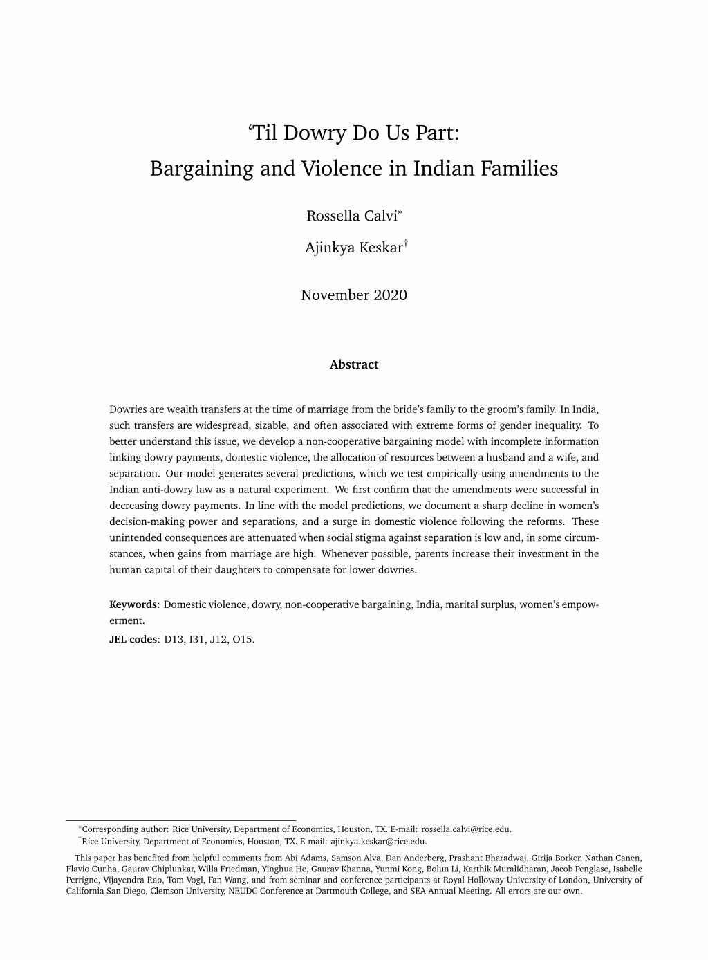
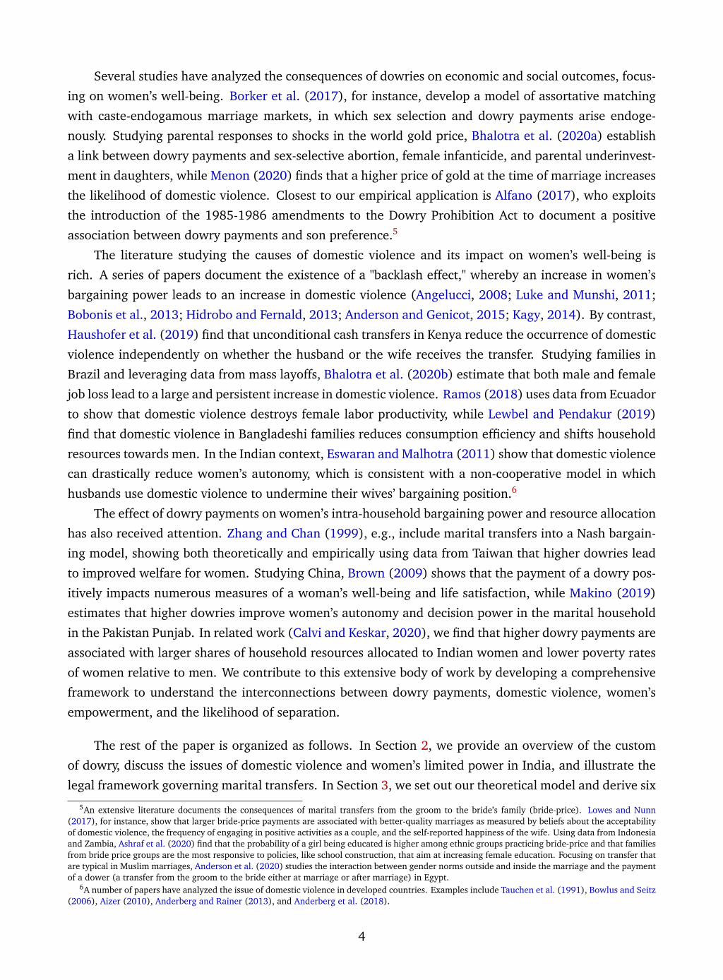
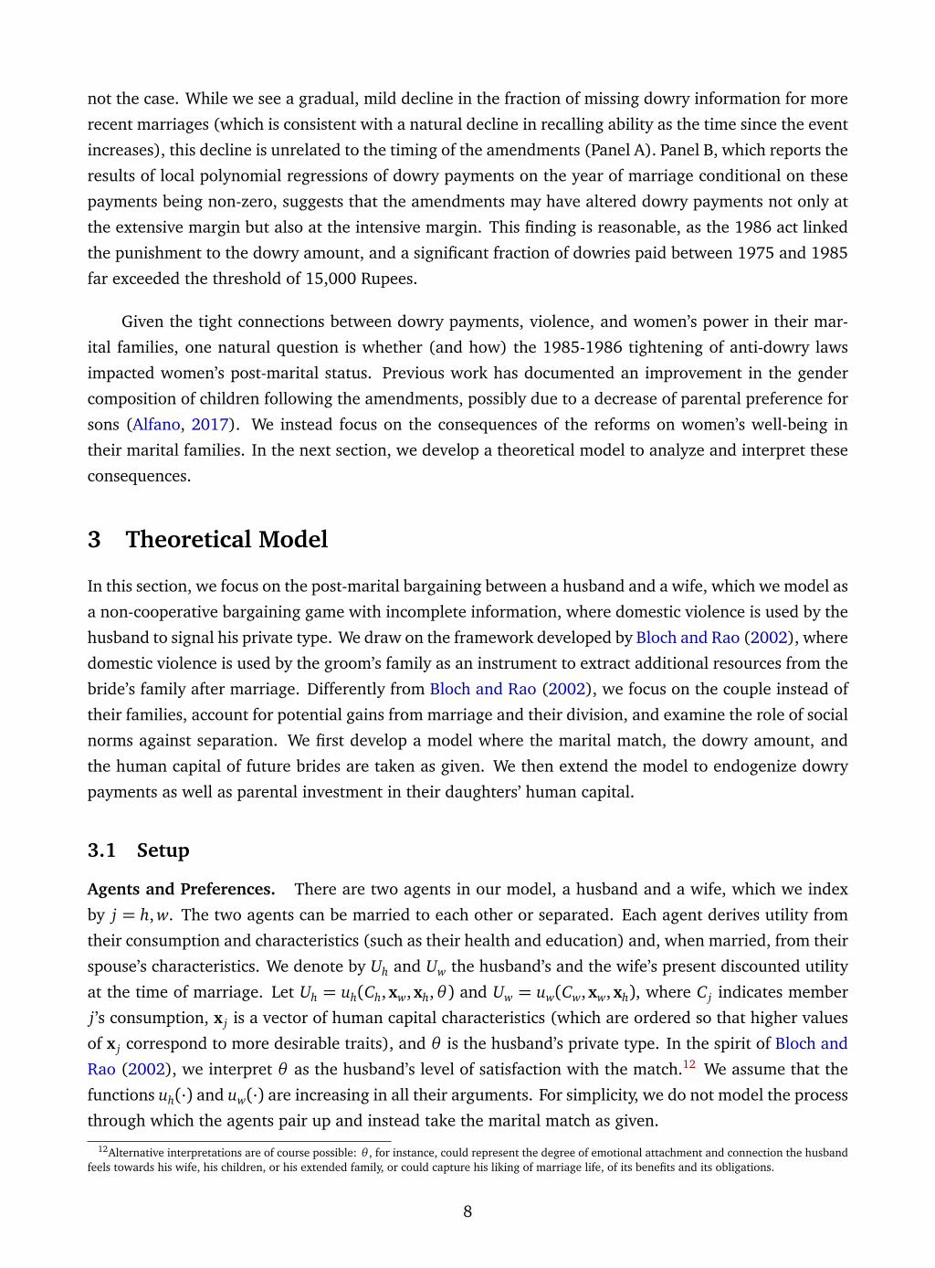
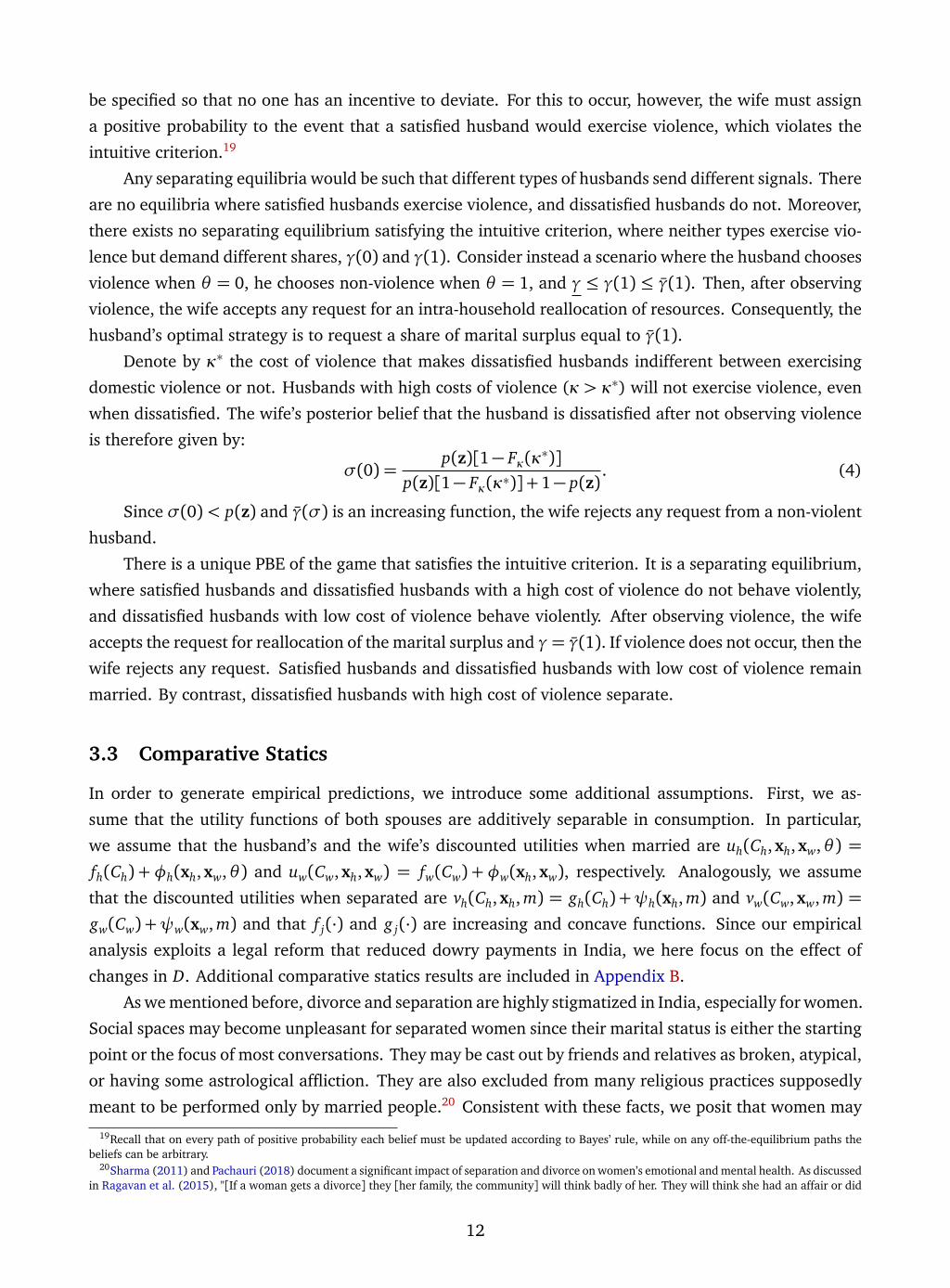
Figure 1: Dowries in India

NOTES: The figure shows local polynomial regressions of real dowry payments on the year of marriage. Gross dowries represent the value of transfersmade to the groom’s family at the time of marriage. Net dowries are defined as gross dowries minus the value of transfers made from the groom’s familyto the bride’s family. All dowry amounts are converted to 1999 Rupees.

1986 amendment also shifted the burden of proving that no funds were exchanged to the person who

receives or requests the dowry, and prescribed that any offense under the act be non-bailable.11 Finally,

the amendment gave power to any state government to appoint "as many Dowry Prohibition Officers as

it thinks fit," to prevent the taking or demanding of dowry and to collect the necessary evidence for the

prosecution of violators of the Dowry Prohibition Act.

Figure 1 plots the results of local polynomial regressions of real dowry payments on the year of

marriage. We obtain information about dowry payments from the 1999 round of the Rural Economic

and Demographic Survey (we provide details about this survey in Section 4.1), and convert all dowries

in 1999 Rupees. Gross dowries represent the value of transfers made to the groom’s family at the time

of marriage, while net dowries are defined as gross dowries minus the value of transfers made from the

groom’s family to the bride’s family. Before 1985, the average gross dowry ranged between 40,000 and

55,000 Rupees, and net dowries varied between approximately 23,000 and 34,000 Rupees. Between 1985

and 1990, both gross and net dowries declined by more than 20 percent. Dowry transfers kept declining

in subsequent years, but at a slower pace.

In Section 4, we extensively investigate the impact of the 1985-1986 amendments on dowry pay-

ments, both at the intensive and extensive margins. A first-order concern, however, is that changes in

reporting may drive the declines shown in Figure 1. This concern would be especially relevant if respon-

dents feared legal consequences from admitting to having paid or received a dowry in the survey. If this

were the case, we would expect the number of respondents refusing to answer dowry-related questions

to increase after the amendments. Moreover, we would expect the average dowry conditional on admit-

ting that a dowry payment was made to be stable over time, with lower average dowries driven by an

increased number of respondents reporting zero dowries. Figure A1 in the Appendix shows that this is

11Between 1975 and 1976, the states of Bihar, Punjab, Haryana, Himachal Pradesh, West Bengal, and Orissa implemented state-level amendments tothe 1961 act. The changes introduced by these early amendments, however, were moderate. In the states of Bihar and Punjab, for instance, the takingof dowry was made punishable by a prison sentence of six months and a fine of 5,000 rupees. In Himachal Pradesh, the punishment was changed to1-year imprisonment and a 5,000 rupee fine (Alfano, 2017).

7

not the case. While we see a gradual, mild decline in the fraction of missing dowry information for more

recent marriages (which is consistent with a natural decline in recalling ability as the time since the event

increases), this decline is unrelated to the timing of the amendments (Panel A). Panel B, which reports the

results of local polynomial regressions of dowry payments on the year of marriage conditional on these

payments being non-zero, suggests that the amendments may have altered dowry payments not only at

the extensive margin but also at the intensive margin. This finding is reasonable, as the 1986 act linked

the punishment to the dowry amount, and a significant fraction of dowries paid between 1975 and 1985

far exceeded the threshold of 15,000 Rupees.

Given the tight connections between dowry payments, violence, and women’s power in their mar-

ital families, one natural question is whether (and how) the 1985-1986 tightening of anti-dowry laws

impacted women’s post-marital status. Previous work has documented an improvement in the gender

composition of children following the amendments, possibly due to a decrease of parental preference for

sons (Alfano, 2017). We instead focus on the consequences of the reforms on women’s well-being in

their marital families. In the next section, we develop a theoretical model to analyze and interpret these

consequences.

3 Theoretical Model

In this section, we focus on the post-marital bargaining between a husband and a wife, which we model as

a non-cooperative bargaining game with incomplete information, where domestic violence is used by the

husband to signal his private type. We draw on the framework developed by Bloch and Rao (2002), where

domestic violence is used by the groom’s family as an instrument to extract additional resources from the

bride’s family after marriage. Differently from Bloch and Rao (2002), we focus on the couple instead of

their families, account for potential gains from marriage and their division, and examine the role of social

norms against separation. We first develop a model where the marital match, the dowry amount, and

the human capital of future brides are taken as given. We then extend the model to endogenize dowry

payments as well as parental investment in their daughters’ human capital.

3.1 Setup

Agents and Preferences. There are two agents in our model, a husband and a wife, which we index

by j = h, w. The two agents can be married to each other or separated. Each agent derives utility from

their consumption and characteristics (such as their health and education) and, when married, from their

spouse’s characteristics. We denote by Uh and Uw the husband’s and the wife’s present discounted utility

at the time of marriage. Let Uh = uh(Ch,xw,xh,θ ) and Uw = uw(Cw,xw,xh), where C j indicates member

j’s consumption, x j is a vector of human capital characteristics (which are ordered so that higher values

of x j correspond to more desirable traits), and θ is the husband’s private type. In the spirit of Bloch and

Rao (2002), we interpret θ as the husband’s level of satisfaction with the match.12 We assume that the

functions uh(·) and uw(·) are increasing in all their arguments. For simplicity, we do not model the process

through which the agents pair up and instead take the marital match as given.

12Alternative interpretations are of course possible: θ , for instance, could represent the degree of emotional attachment and connection the husbandfeels towards his wife, his children, or his extended family, or could capture his liking of marriage life, of its benefits and its obligations.

8

When married, the agents partake in marital gains, which may arise from joint consumption and

production. For instance, both spouses can equally enjoy their children (which we model as public goods)

and live in the same home. They could also partially share some goods, such as fuel for transportation,

and save on food waste and spoilage (Barten, 1964; Gorman, 1976; Browning et al., 2013). The couple

can also benefit from specialization in production, comparative advantage, and increasing returns to scale

(Becker, 1973, 1991). We denote by M the material gains from marriage and define them as follows:

M = Yhw− Yh− Yw ≥ 0,

where the Yh is how much the husband can produce if unmarried, Yw is how much the wife can produce

if unmarried, and Yhw is the sum of husband’s and wife’s production when married (Chiappori et al.,

2009).13 In our model, we focus on the allocation of M between the husband and the wife, and denote

by γ the share of marital gains commanded by the husband. Note that the insights and implications of

our model are invariant to interpreting γ as the share of Yhw (and not only M) allocated to the husband.

Let Vh = vh(Ch,xh, m) and Vw = vw(Cw,xw, m) be the husband’s and the wife’s discounted utility

flows when separated, where m denotes the marriage market conditions at the time of separation. Since

divorce is rare and often stigmatized in India,14 we can interpret separation as a situation where the

husband and the wife stop living together while staying married. Alternatively, separation can represent

an unproductive marriage, where the marital surplus is null (Lundberg and Pollak, 1993) and the spouses

stop deriving utility from each others’ traits. As above, we require the functions vh(·) and vw(·) to be

increasing in all their arguments.

At the time of marriage, the bride’s family pays a dowry D to the husband’s family, which we take

as given for now. The consumption levels of the husband and the wife can be summarized as follows:

if the marriage is intact, then Ch = Yh+ D+ γM and Cw = Yw− D+ (1− γ)M ; if separation occurs, then

Ch = Yh+ D and Cw = Yw− D. Importantly, in our primary model, any dowry payment impacts the utility

of the spouses only through consumption, while the husband’s private type (or degree of satisfaction with

the marriage) is not directly affected by D. Similarly, we take M as given and do not treat gains from

marriage as a strategic lever of the spouses. We also assume that dowries do not serve as an early bequest

for daughters (that is, wives do not have access to or property rights over any fraction of D) and that

dowries are not returned to the bride’s family in case of separation.15

The Bargaining Game. We model the interaction between the husband and the wife as a non-

cooperative bargaining game with incomplete information. When the marriage takes place, the newly-

weds learn about observable marriage characteristics. We denote such characteristics by z. These include

(but are not limited to) the initial division of the gains from marriage, γ0, which we assume to be fully

determined by marriage market conditions for brides and grooms at the time of the match (Chiappori

et al., 2009). Right after marriage, the husband learns his private type θ , that is, his level of satisfaction

13There may be emotional gains from marriage, such as love and companionship, but we abstract from them for simplicity.14According to the 2011 Census of India, 1.36 million individuals in India are divorced, amounting to 0.24 percent of the married population and

0.11 percent of the total population (Jacob and Chattopadhyay, 2016).15In Section D in the Appendix, we consider a few extensions to our baseline model. First, we consider a model where the occurrence of domestic

violence decreases gains from marriage. This extension is consistent with domestic violence potentially destroying female labor productivity (as inRamos (2018)) or reducing household’s ability to cooperate and share goods (as in Lewbel and Pendakur (2019)). We also extend our model to aframework where the husband (or his family) receives a transfer equal to αD, while the wife retains control over (1−α)D. Such a model, which leadsto qualitatively similar predictions, accommodates situations in which dowries serve as early bequests for daughters.

9

with the match.16 This new information may trigger a post-marital renegotiation over the division of the

marital surplus. For simplicity, we define θ to be binary, with satisfied husbands having θ equal to 1 and

dissatisfied husbands having θ equal to 0. We denote by p(z) the prior probability that the husband is

not satisfied with the marriage.

The model consists of three stages. In the first stage, the husband decides whether to exercise vio-

lence. If violence occurs, then the husband and the wife incur in a utility cost, which we denote by Kh

and Kw, respectively. For tractability, we assume that satisfied husbands face an infinite cost of violence

(i.e., Kh(1) =∞). For dissatisfied husbands, the cost of violence is a random variable with cumulative

distribution function Fκ on [0,∞). At this time, the husband also demands a renegotiation of the division

of gains from marriage and makes a take-it-or-leave-it demand for a higher share γ > γ0.17 In the second

stage, the wife decides whether to accept the husband’s demand for a higher share of the marital surplus.

In the third stage, the husband chooses whether to separate. To avoid issues related to limited commit-

ment, we assume that any intra-household reallocation of marital gains occurs after the husband makes

the separation decision. Figure A2 in the Appendix shows the model timeline and the game in extensive

form.

Context-driven Assumptions. Divorce and separation are riddled with stigma in India, especially

for women. The majority of women are financially dependent on their husbands and do not view divorce

as a viable option, even when they are in an abusive marriage. The dissolution of a marriage is also often

seen as damaging to a woman’s reputation (Ragavan et al., 2015).18 According to the Survey of Status

of Women and Fertility (SWAF), e.g., 83 percent of interviewed women believe that it is justified for a

husband to leave his wife if she is unfaithful to him, while only 40 percent think it is okay for the wife

to leave her husband if he is unfaithful. The vast majority (approximately 90 percent) of women would

not consider leaving their husbands even if he abuses her or if he is a drunk or drug addict. Also, only

one out of five women believes that she could leave her husband if he were unable to provide for the

family financially, suggesting that financial motives are not the only reason behind a woman’s aversion to

separating.

In summary, while separation is undesirable for all, women disproportionately bear the cost of marital

dissolution. This is an essential feature of the Indian context that we embed in our model as follows. For

any level of consumption, human capital characteristics, and marriage market conditions, women strictly

prefer to be in a marriage than to separate, even when the husband exercises domestic violence:

uw(Yw− D+(1−γ)M ,xh,xw)− Kw > vw(Yw− D,xw, m).

Moreover, satisfied husbands strictly prefer to stay married:

uh(Yh+ D+γM ,xh,xw, 1)> vh(Yh+ D,xh, m),16These modeling assumptions are reasonable in the Indian context, where the majority of marriages is arranged by the bride’s and the groom’s family

(Anukriti and Dasgupta, 2017; Vogl, 2013) and the spouses only meet on the day of the wedding (or shortly before then). According to the latest IndiaHuman Development Survey, 65 percent of ever-married Indian women aged 15 to 49 met their husband on their wedding day and 14 percent met himless than one month before the wedding. Moreover, 58 percent of women report having no say in the choice of their husbands.

17In our model, the husband would never ask for γ < γ0, since he will be worse off if he does. Note, however, that this would be possible in a modelthat allowed for altruistic preferences, where the husband cares substantially about the wife’s well-being. Since γ and γ0 are shares, they range between0 and 1.

18The likelihood of remarriage is low overall in India, but somewhat higher for men. According to the India Human Development Survey, for instance,less than 1 percent of ever-married Indian women remarry, while about 3.5 percent of them report their husband being married more than once. Thisfigures exclude polygamous families and include remarriage after the death of the spouse.

10

while dissatisfied husbands strictly prefer to separate:

uh(Yh+ D+γ0M ,xh,xw, 0)< vh(Yh+ D,xh, m).

3.2 Solving for Equilibrium

To solve the game, we proceed by backward induction. In the last stage of the game, only dissatisfied

husbands whose demand for a higher share of marital gains is not met decide to end their marriage. In

particular, dissatisfied husbands choose not to separate if the following inequality holds:

uh(Yh+ D+γM ,xh,xw, 0)≥ vh(Yh+ D,xh, m) (1)

Denote γ the minimal transfer that keeps the marriage intact. Then, for γ = γ equation (1) holds

with equality.

In the second stage, the wife decides whether to accept or reject the husband’s request for a reallo-

cation of resources. The wife rejects any request for γ < γ, since it would not dissuade the husband from

separating. Denote by σ the wife’s belief that the husband is dissatisfied after observing the occurrence

of violence and the request for resource reallocation. Then, if γ ≥ γ, the wife accepts any request that

satisfies the following condition:

uw(Yw− D+(1−γ)M ,xh,xw)≥ σvw(Yw− D,xw, m)+ (1−σ)uw(Yw− D+(1−γ0)M ,xh,xw) (2)

When the wife is indifferent between accepting or rejecting her husband’s request, then equation (2)

holds with equality and γ = γ̄(σ). So, γ̄(σ) is the maximal share of marital gains that the husband can

extract. Note that this maximal share is an increasing function of the wife’s beliefs. In other words, the

wife is willing to forgo a higher share of the marital gains when she is more likely to believe that her

husband is dissatisfied. The wife’s optimal decision is to accept any request for γ̄(σ)≥ γ≥ γ and to reject

it otherwise.

In the first stage, the husband decides whether to exercise violence. Recall that, in our model, domes-

tic violence is a signal from the husband to the wife about his degree of dissatisfaction with the marriage.

To calculate the perfect bayesian equilibria (PBE) of the game, we consider both pooling equilibria

and separating equilibria. In what follows, we assume that the wife rejects any request for reallocation

if she does not update her beliefs about the husband’s degree of satisfaction. We also assume that she is

willing to increase her husband’s share of gains from marriage and keep the marriage intact when she

believes that her husband is dissatisfied. More formally, we assume that

γ̄(1)> γ > γ(p(z)). (3)

Any pooling equilibria would be such that both satisfied and dissatisfied husbands send the same

signal with probability one. Given that the cost of violence for satisfied husbands is infinite, there are no

equilibria where both satisfied and dissatisfied husbands behave violently. Consider instead a situation

where both satisfied and dissatisfied husbands do not exercise violence. Then, the husband’s signal would

be uninformative, the wife’s prior and posterior beliefs would coincide, and, given equation (3), the wife

would reject any request for reallocation. For such equilibrium to exist, off-the-equilibrium beliefs must

11

be specified so that no one has an incentive to deviate. For this to occur, however, the wife must assign

a positive probability to the event that a satisfied husband would exercise violence, which violates the

intuitive criterion.19

Any separating equilibria would be such that different types of husbands send different signals. There

are no equilibria where satisfied husbands exercise violence, and dissatisfied husbands do not. Moreover,

there exists no separating equilibrium satisfying the intuitive criterion, where neither types exercise vio-

lence but demand different shares, γ(0) and γ(1). Consider instead a scenario where the husband chooses

violence when θ = 0, he chooses non-violence when θ = 1, and γ ≤ γ(1) ≤ γ̄(1). Then, after observing

violence, the wife accepts any request for an intra-household reallocation of resources. Consequently, the

husband’s optimal strategy is to request a share of marital surplus equal to γ̄(1).Denote by κ∗ the cost of violence that makes dissatisfied husbands indifferent between exercising

domestic violence or not. Husbands with high costs of violence (κ > κ∗) will not exercise violence, even

when dissatisfied. The wife’s posterior belief that the husband is dissatisfied after not observing violence

is therefore given by:

σ(0) =p(z)[1− Fκ(κ∗)]

p(z)[1− Fκ(κ∗)]+1− p(z). (4)

Since σ(0)< p(z) and γ̄(σ) is an increasing function, the wife rejects any request from a non-violent

husband.

There is a unique PBE of the game that satisfies the intuitive criterion. It is a separating equilibrium,

where satisfied husbands and dissatisfied husbands with a high cost of violence do not behave violently,

and dissatisfied husbands with low cost of violence behave violently. After observing violence, the wife

accepts the request for reallocation of the marital surplus and γ= γ̄(1). If violence does not occur, then the

wife rejects any request. Satisfied husbands and dissatisfied husbands with low cost of violence remain

married. By contrast, dissatisfied husbands with high cost of violence separate.

3.3 Comparative Statics

In order to generate empirical predictions, we introduce some additional assumptions. First, we as-

sume that the utility functions of both spouses are additively separable in consumption. In particular,

we assume that the husband’s and the wife’s discounted utilities when married are uh(Ch,xh,xw,θ ) =fh(Ch) +φh(xh,xw,θ ) and uw(Cw,xh,xw) = fw(Cw) +φw(xh,xw), respectively. Analogously, we assume

that the discounted utilities when separated are vh(Ch,xh, m) = gh(Ch) +ψh(xh, m) and vw(Cw,xw, m) =gw(Cw) +ψw(xw, m) and that f j(·) and g j(·) are increasing and concave functions. Since our empirical

analysis exploits a legal reform that reduced dowry payments in India, we here focus on the effect of

changes in D. Additional comparative statics results are included in Appendix B.

As we mentioned before, divorce and separation are highly stigmatized in India, especially for women.

Social spaces may become unpleasant for separated women since their marital status is either the starting

point or the focus of most conversations. They may be cast out by friends and relatives as broken, atypical,

or having some astrological affliction. They are also excluded from many religious practices supposedly

meant to be performed only by married people.20 Consistent with these facts, we posit that women may

19Recall that on every path of positive probability each belief must be updated according to Bayes’ rule, while on any off-the-equilibrium paths thebeliefs can be arbitrary.

20Sharma (2011) and Pachauri (2018) document a significant impact of separation and divorce on women’s emotional and mental health. As discussedin Ragavan et al. (2015), "[If a woman gets a divorce] they [her family, the community] will think badly of her. They will think she had an affair or did

12

have different preferences over consumption inside and outside of marriage, and that, for a given level of

consumption, their marginal utility of consumption when married may be higher than when separated.

This assumption is critical for our comparative statics results, but realistic in the Indian context. Specifi-

cally, we assume that, for a given level of consumption c, f ′w(c)≥ g ′w(c). By contrast, we set f ′h(c) = g ′h(c),i.e., the husband’s marginal utility of consumption is independent of his marital status.21

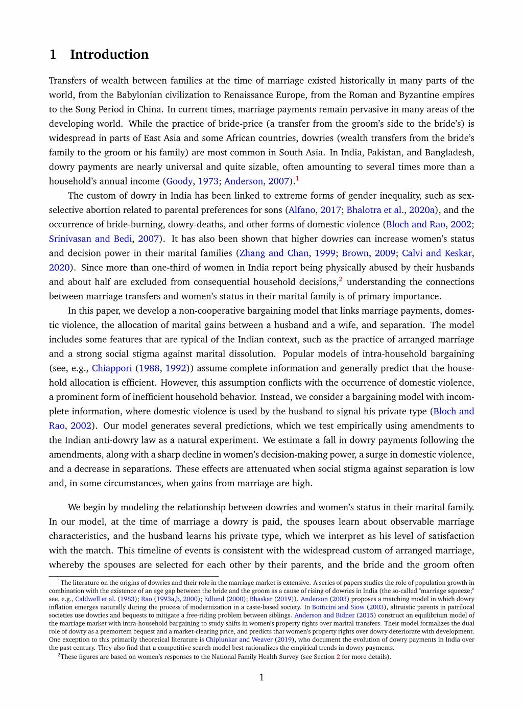
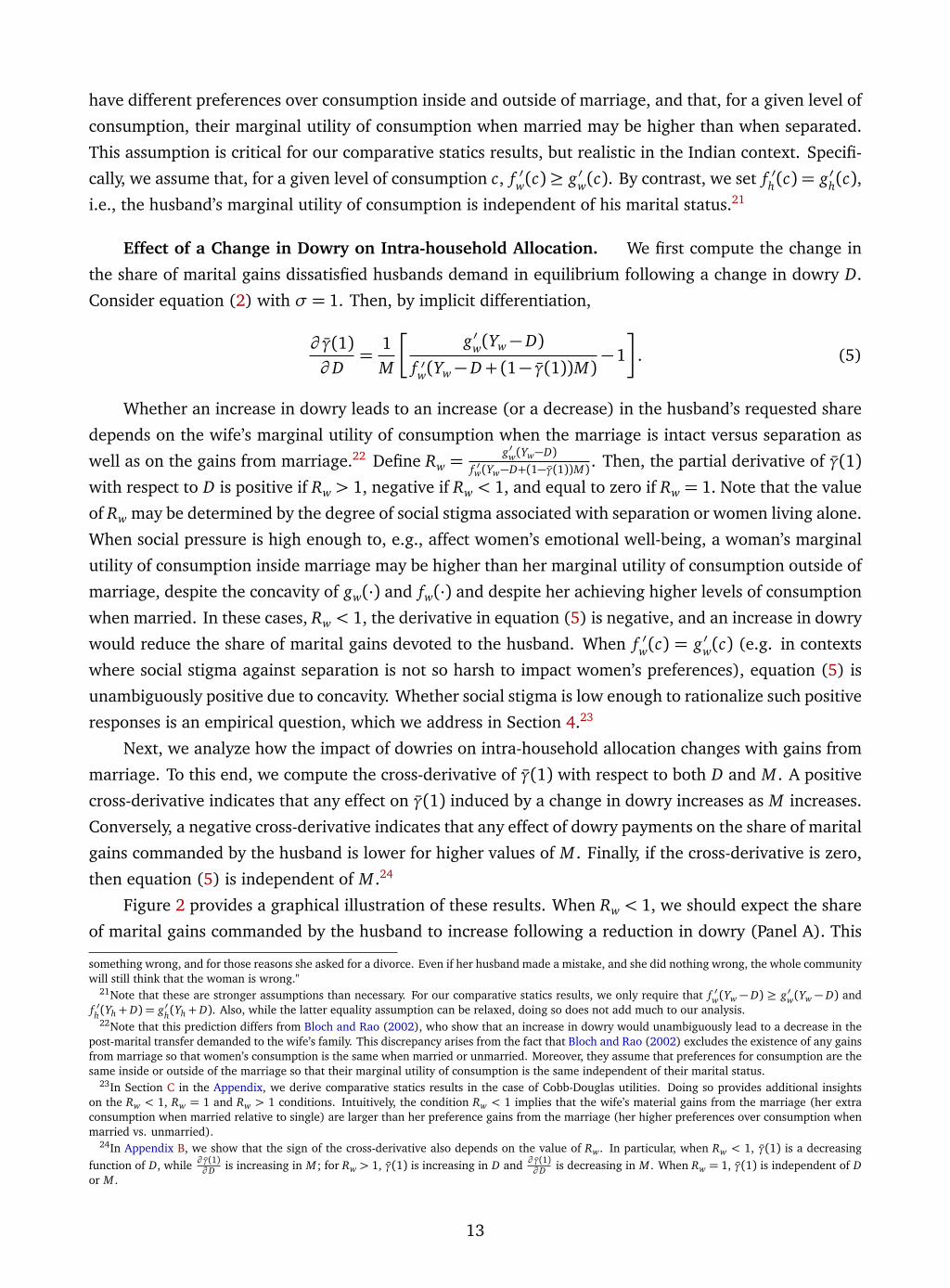
Effect of a Change in Dowry on Intra-household Allocation. We first compute the change in

the share of marital gains dissatisfied husbands demand in equilibrium following a change in dowry D.

Consider equation (2) with σ = 1. Then, by implicit differentiation,

∂ γ̄(1)∂ D

=1M

�

g ′w(Yw− D)

f ′w(Yw− D+(1− γ̄(1))M)−1

�

. (5)

Whether an increase in dowry leads to an increase (or a decrease) in the husband’s requested share

depends on the wife’s marginal utility of consumption when the marriage is intact versus separation as

well as on the gains from marriage.22 Define Rw =g′w(Yw−D)

f ′w(Yw−D+(1−γ̄(1))M) . Then, the partial derivative of γ̄(1)with respect to D is positive if Rw > 1, negative if Rw < 1, and equal to zero if Rw = 1. Note that the value

of Rw may be determined by the degree of social stigma associated with separation or women living alone.

When social pressure is high enough to, e.g., affect women’s emotional well-being, a woman’s marginal

utility of consumption inside marriage may be higher than her marginal utility of consumption outside of

marriage, despite the concavity of gw(·) and fw(·) and despite her achieving higher levels of consumption

when married. In these cases, Rw < 1, the derivative in equation (5) is negative, and an increase in dowry

would reduce the share of marital gains devoted to the husband. When f ′w(c) = g ′w(c) (e.g. in contexts

where social stigma against separation is not so harsh to impact women’s preferences), equation (5) is

unambiguously positive due to concavity. Whether social stigma is low enough to rationalize such positive

responses is an empirical question, which we address in Section 4.23

Next, we analyze how the impact of dowries on intra-household allocation changes with gains from

marriage. To this end, we compute the cross-derivative of γ̄(1) with respect to both D and M . A positive

cross-derivative indicates that any effect on γ̄(1) induced by a change in dowry increases as M increases.

Conversely, a negative cross-derivative indicates that any effect of dowry payments on the share of marital

gains commanded by the husband is lower for higher values of M . Finally, if the cross-derivative is zero,

then equation (5) is independent of M .24

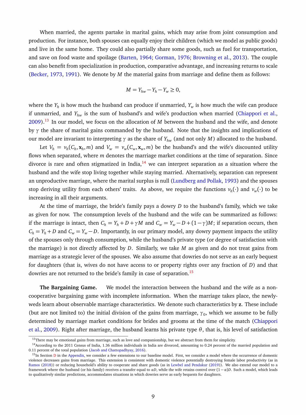
Figure 2 provides a graphical illustration of these results. When Rw < 1, we should expect the share

of marital gains commanded by the husband to increase following a reduction in dowry (Panel A). This

something wrong, and for those reasons she asked for a divorce. Even if her husband made a mistake, and she did nothing wrong, the whole communitywill still think that the woman is wrong."

21Note that these are stronger assumptions than necessary. For our comparative statics results, we only require that f ′w(Yw − D) ≥ g′w(Yw − D) andf ′h(Yh+ D) = g′h(Yh+ D). Also, while the latter equality assumption can be relaxed, doing so does not add much to our analysis.

22Note that this prediction differs from Bloch and Rao (2002), who show that an increase in dowry would unambiguously lead to a decrease in thepost-marital transfer demanded to the wife’s family. This discrepancy arises from the fact that Bloch and Rao (2002) excludes the existence of any gainsfrom marriage so that women’s consumption is the same when married or unmarried. Moreover, they assume that preferences for consumption are thesame inside or outside of the marriage so that their marginal utility of consumption is the same independent of their marital status.

23In Section C in the Appendix, we derive comparative statics results in the case of Cobb-Douglas utilities. Doing so provides additional insightson the Rw < 1, Rw = 1 and Rw > 1 conditions. Intuitively, the condition Rw < 1 implies that the wife’s material gains from the marriage (her extraconsumption when married relative to single) are larger than her preference gains from the marriage (her higher preferences over consumption whenmarried vs. unmarried).

24In Appendix B, we show that the sign of the cross-derivative also depends on the value of Rw. In particular, when Rw < 1, γ̄(1) is a decreasingfunction of D, while ∂ γ̄(1)

∂ D is increasing in M ; for Rw > 1, γ̄(1) is increasing in D and ∂ γ̄(1)∂ D is decreasing in M . When Rw = 1, γ̄(1) is independent of D

or M .

13

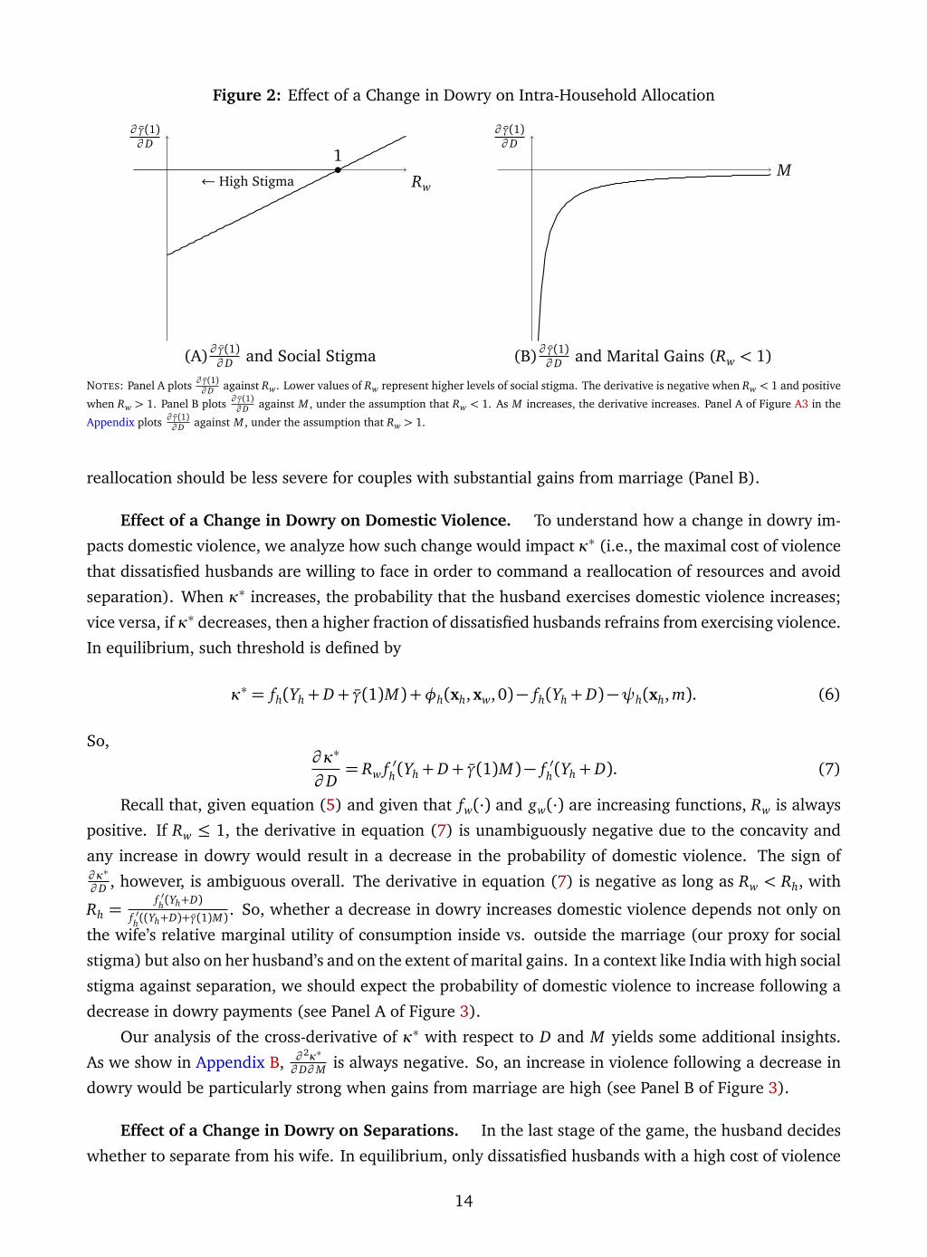
Figure 2: Effect of a Change in Dowry on Intra-Household Allocation

← High Stigma Rw

∂ γ̄(1)∂ D

1

(A)∂ γ̄(1)∂ D and Social Stigma

M

∂ γ̄(1)∂ D

(B)∂ γ̄(1)∂ D and Marital Gains (Rw < 1)

NOTES: Panel A plots ∂ γ̄(1)∂ D against Rw. Lower values of Rw represent higher levels of social stigma. The derivative is negative when Rw < 1 and positive

when Rw > 1. Panel B plots ∂ γ̄(1)∂ D against M , under the assumption that Rw < 1. As M increases, the derivative increases. Panel A of Figure A3 in the

Appendix plots ∂ γ̄(1)∂ D against M , under the assumption that Rw > 1.

reallocation should be less severe for couples with substantial gains from marriage (Panel B).

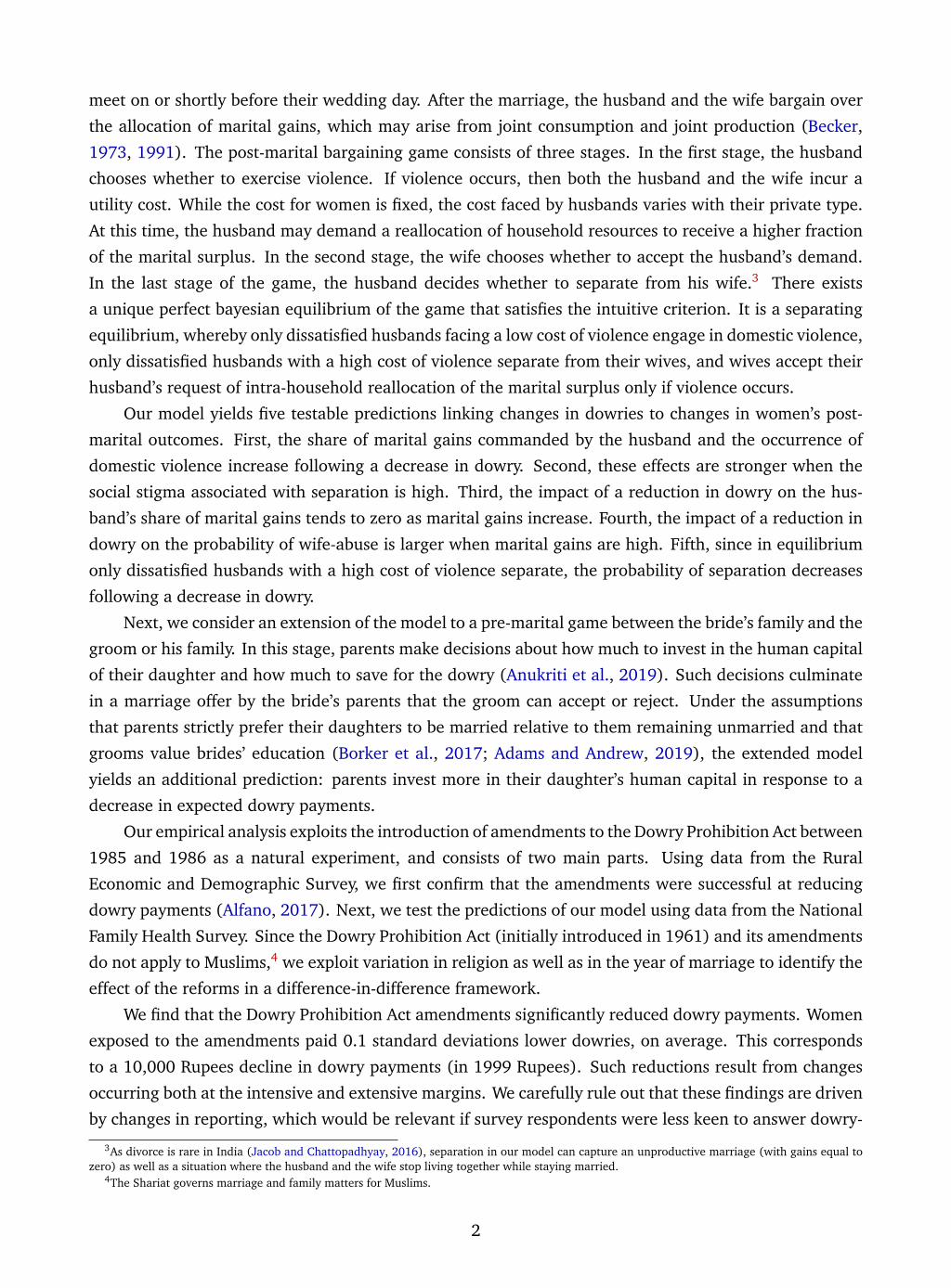
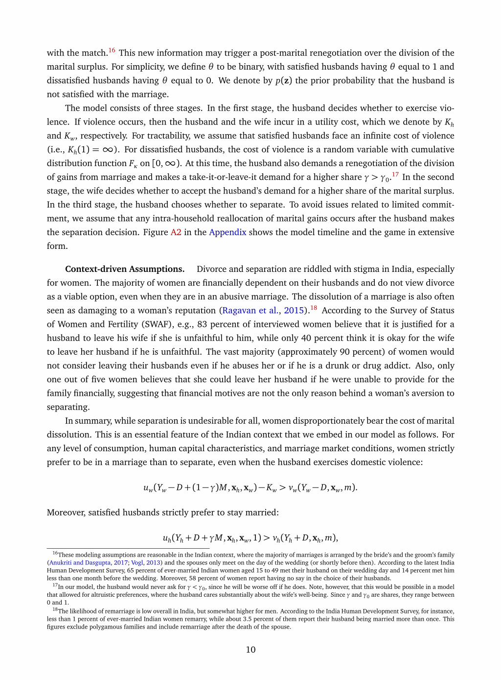
Effect of a Change in Dowry on Domestic Violence. To understand how a change in dowry im-

pacts domestic violence, we analyze how such change would impact κ∗ (i.e., the maximal cost of violence

that dissatisfied husbands are willing to face in order to command a reallocation of resources and avoid

separation). When κ∗ increases, the probability that the husband exercises domestic violence increases;

vice versa, if κ∗ decreases, then a higher fraction of dissatisfied husbands refrains from exercising violence.

In equilibrium, such threshold is defined by

κ∗ = fh(Yh+ D+ γ̄(1)M)+φh(xh,xw, 0)− fh(Yh+ D)−ψh(xh, m). (6)

So,∂ κ∗

∂ D= Rw f ′h(Yh+ D+ γ̄(1)M)− f ′h(Yh+ D). (7)

Recall that, given equation (5) and given that fw(·) and gw(·) are increasing functions, Rw is always

positive. If Rw ≤ 1, the derivative in equation (7) is unambiguously negative due to the concavity and

any increase in dowry would result in a decrease in the probability of domestic violence. The sign of∂ κ∗

∂ D , however, is ambiguous overall. The derivative in equation (7) is negative as long as Rw < Rh, with

Rh =f ′h(Yh+D)

f ′h((Yh+D)+γ̄(1)M) . So, whether a decrease in dowry increases domestic violence depends not only on

the wife’s relative marginal utility of consumption inside vs. outside the marriage (our proxy for social

stigma) but also on her husband’s and on the extent of marital gains. In a context like India with high social

stigma against separation, we should expect the probability of domestic violence to increase following a

decrease in dowry payments (see Panel A of Figure 3).

Our analysis of the cross-derivative of κ∗ with respect to D and M yields some additional insights.

As we show in Appendix B, ∂ 2κ∗

∂ D∂M is always negative. So, an increase in violence following a decrease in

dowry would be particularly strong when gains from marriage are high (see Panel B of Figure 3).

Effect of a Change in Dowry on Separations. In the last stage of the game, the husband decides

whether to separate from his wife. In equilibrium, only dissatisfied husbands with a high cost of violence

14

Figure 3: Effect of a Change in Dowry on Domestic Violence

Rw

∂ κ∗

∂ D

← High Stigma

1

Rh

(A)∂ κ∗

∂ D and Social Stigma

M

∂ κ∗

∂ D

(B)∂ κ∗

∂ D and Marital Gains (Rw < 1)

NOTES: Panel A plots ∂ κ∗

∂ D against Rw. Lower values of Rw represent higher levels of social stigma. The derivative is negative when Rw < Rh and positive

when Rw > Rh. Panel B plots ∂ κ∗

∂ D against marital gains (M), under the assumption that Rw < 1. As M increases, the derivative decreases. Panel B of

Figure A3 in the Appendix plots ∂ κ∗

∂ D against M , under the assumption that Rw ≥ 1.

separate, while husbands with a low cost of violence remain married. Thus, any increase in dowry pay-

ments would have an impact on separations that is the reverse of its impact on domestic violence (that is,

it would have a positive effect when social stigma is high and a possibly negative impact for low levels of

social stigma). It is important to note that dowry payments do not affect the husband’s level of satisfaction

with the marriage, which we model as his private type drawn by nature at the time of marriage. Instead,

a dowry increases the husband’s consumption level both within and outside of the marriage (in line with

marriage practices, dowries are not returned to the bride or her family in case of separation). This feature

of the model is critical to make sense of the predicted relationship between dowry and separations.

3.4 Endogenous Dowry and Human Capital

So far, we have taken dowry payments and the bride’s characteristics as given. In Section D.3 in Appendix,

we provide an extension to our model that includes a pre-marital bargaining game between the bride’s

family and the groom (or his family). We interpret this first stage, which we briefly summarize below, as

one in which parents make decisions about how much to invest in the human capital of their daughter

and about how much to save for a future dowry (Anukriti et al., 2019). For simplicity, we abstract from

the specific process through which potential grooms match with brides.

In line with the social norms in the Indian context, we assume a very high social cost of a daughter

remaining unmarried (as in Borker et al. (2017)). So, parents strictly prefer their daughters to be mar-

ried relative to them remaining unmarried. Before the marriage takes place, the bride’s parents make a

take-it-or-leave-it offer to the groom. This offer consists of the dowry payment and a set of bridal charac-

teristics, including her human capital.25 At this stage, the marriage characteristics, the cost of domestic

violence, and the future marriage market conditions are unknown to the potential groom and the bride’s

parents (although their distributions are known). The groom decides to accept or reject the offer based

on how his expected utility from marriage fares relative to his reservation utility. His expected utility from

marriage takes into account the three possible post-marital scenarios discussed before (that he is satis-

25We can interpret these characteristics as increasing a bride’s overall attractiveness. As in Bloch and Rao (2002), we also assume that the bride’sfamily has all the bargaining power in this stage. Differently from Bloch and Rao (2002), we consider pre-marital decisions not only about D, but alsoabout xw.

15

fied, dissatisfied but non-violent, or dissatisfied and violent), while his reservation utility depends on his

income, human capital, and the current marriage market conditions. In equilibrium, the bride’s parents’

offer makes the potential groom indifferent between accepting and rejecting the marriage proposal. Since

the groom values consumption as well as his future wife’s human capital, and parents strictly prefer to

have their daughter married over remaining unmarried, a decrease in dowry leads to an increase in the

human capital of future brides.26

3.5 Summary of the Model Predictions

In summary, our theoretical framework illustrates the relationship between dowry payments, the allo-

cation of marital gains between a husband and a wife, and the occurrence of domestic violence and

separation. It also describes the link between parental investment in the human capital investment of fu-

ture brides and dowry payments. Our model incorporates many features of the Indian cultural and social

norms associated with marriage, including the widespread social stigma associated with separation. This

stigma can have significant consequences not only for the material but also for the spouses’ emotional

well-being, especially for women. The main predictions of the model can be summarized as follows.

Prediction 1. If social stigma against separation is high, the share of marital gains commanded by the

husband increases following a decrease in dowry.

Prediction 2. If social stigma against separation is high, the probability of domestic violence increases

following a decrease in dowry.

Prediction 3. The effect of a decrease in dowry on the share of marital gains commanded by the husband

and on the probability of domestic violence decreases as social stigma against separation decreases. If

social stigma against separation is low enough, the husband’s share of marital gains and the probability

of domestic violence decrease following a decrease in dowry.

Prediction 4. The effect of a decrease in dowry on the share of marital gains commanded by the husband

decreases as marital gains increase. The effect of a decrease in dowry on the probability the husband

would engage in domestic violence increases as marital gains increase.

Prediction 5. In equilibrium, only dissatisfied husbands with a high cost of violence choose to separate.

So, for high enough levels of social stigma against separation, the probability of separation decreases

following a decrease in dowry. The effect of a decrease in dowry on separations increases as marital gains

increase.

Prediction 6. Parental investments in the human capital of future brides increase following a decrease in

(expected) dowry payments.

26It is important to note, however, that the impact of a change in the human capital of future brides on domestic violence, intra-household resourceallocation, and marital dissolution is ambiguous (see Section B in the Appendix for more details). As the cost of not marrying off a daughter is high,parents may still increase investment in her human capital, even though doing so may worsen her status after marriage.

16

4 Empirical Strategy

4.1 Data and Measurement

To our knowledge, no dataset exists for India recording dowry payments, women’s decision power and

living arrangements, and information about domestic violence against women. So, for our empirical

application, we rely on two separate data sources: data on dowry payments are from the 1999 Rural

Economic and Demographic Survey; data on intra-household decision-making power, domestic violence,

and separations are from the 2005-2006 National Family Health Survey.

Dowries. The Rural Economic and Demographic Survey (hereafter REDS) is a detailed panel

survey of rural households conducted by the National Council of Applied Economic Research. The survey

covers sixteen of the most populous states in India and contains detailed retrospective information on

year of marriage and marital transfers for the household head, their parents, their sisters and brothers,

and their daughters and sons. It also includes socio-economic and demographic traits.

Note that information on dowries is rare as dowries are illegal. Thus, a typical approach is to ask

indirect questions about dowry payments. The India Human Development Survey, for instance, asks

questions about total marriage expenditure by families that are similar to the respondent’s family, but

not actual payments by brides and grooms in the surveyed households. Such questions are of limited use

for analysis like ours. The REDS dataset instead reports the monetary value of marital transfers made

from the family of the bride to that of the groom in each marriage as well as transfers from the family of

the groom to that of the bride (though this information is missing for 40 percent of marriages).27 Since

marriage-related events are particularly salient to households and dowry payments are conspicuous, we

can expect respondents to remember them accurately (Chiplunkar and Weaver, 2019). Based on these

data, we construct our outcomes of interest: gross dowry (the value of transfers made to the groom’s

family at the time of marriage), net dowry (defined as gross dowries minus the value of transfers made

from the groom’s family to the bride’s family), and an indicator variable for whether the marriage involved

a positive transfer from the bride’s family to the groom’s family. We use the national consumer price index

to convert all nominal payments to 1999 Rupees.

From the 1999 REDS round, we select a sample of 15,715 marriages that took place between 1975

and 1999.28 Figure A4 in the Appendix shows the distribution of gross and net dowries in our sample. The

average gross dowry is about 38,000 Rupees ($4,104 in 1999 PPP), the average net dowry approaches

27,000 Rupees ($2,916 in 1999 PPP), and respondents reported that dowries were paid in 91 percent of

marriages (see Table A1 in the Appendix). The average year of marriage in the sample is 1986, while the

median is 1985. All respondents live in rural areas, and they are primarily Hindu (though Muslims account

for 7 percent of the sample). More than half of the sample belongs to Scheduled Castes, Scheduled Tribes

or other backward castes. Educational attainment is low, with average years of schooling being four and

five for women and their spouses, respectively.

27Missing information may indicate that there was no transfer from the groom’s family to the bride’s family. In this case, gross and net dowries wouldcoincide. We err on the side of caution and treat these observations as having missing net dowries.

28Compared to the most recent round of REDS (which was collected in 2006), the 1999 round has two advantages. First, while in the 1999 roundsurveyors directly asked questions about “dowry" payments, the 2006 round reports the total value of “gifts given or received" at the time of marriage.Such gifts may include gifts from her family to the bride herself, which would not be subject to the Dowry Prohibition Act and its amendments. Second,the 1999 round includes a larger number of marriages (approximately 3000 more marriages) that took place in the decades before and after the1985-1986 reforms, therefore ensuring more balanced treatment and control groups.

17

Intra-household Allocation, Domestic Violence, and Separation. One well-known issue in em-

pirical applications of household economics is that the allocation of gains from marriage (or of household

resources in general) is not directly observable.29 We overcome this data limitation by using self-reported

measures of women’s decision-making power to construct proxies for the share of gains from marriages

commanded by the wife (i.e., 1−γ).30 The National Family Health Survey (NFHS) contains information

about both a woman’s involvement in household decisions and domestic violence. The survey also pro-

vides information on year of marriage and religion as well as women’s current marital status, educational

attainment, anthropometric indicators, and other demographic and socioeconomic traits. To ensure an

adequate number of marriages before and after the 1985-1986 anti-dowry law amendments, we use data

from the 2005-2006 round. To ensure comparability with our analysis of dowry payments, we select a

sample of more than 65,000 married women whose marriage took place between 1975 and 1999.

As we report in Table A2 in the Appendix, slightly more than half of the women in our sample reside

in rural areas, 75 percent are Hindu, and 13 percent are Muslim; two-thirds married after 1985. For

women, the average age is 34, and the average schooling is five years. For their husbands, the average

age is 40, and the average schooling is seven years. The descriptive statistics for domestic violence in

our sample are in line with those discussed in Section 2. More than 10 percent of women report having

experienced injuries caused by the husband or severe physical violence, and one-third of women report

ever experiencing less severe physical violence. Questions about injuries caused by the husband are

quite detailed: 33 percent of women report cuts, bruises, or aches, 8 percent report eye injuries, sprains,

dislocations, or burns (2 percent report severe burns), and 6 percent report deep wounds, broken bones,

broken teeth, or any other serious injury. Based on these reports, as well as on general questions about

experiences of different types of domestic violence, we construct an ordinal measure of violence, which

ranges between 1 and 6. Conditional on ever experiencing any injuries or violence, a woman experiences

two types of injuries, on average.31

For a number of household decisions, the survey asks respondents about their degree of involvement

in the decision-making process. We construct several indicator variables for whether the respondent

reports participating in the decision-making process and zero otherwise. One in three women in our

sample has no say in decisions about household purchases; in one out of six families, the husband is

in charge of all decisions regarding contraception and his wife’s health care. To capture the scope of

women’s decision-making power, we also consider the number of decisions she reports being involved

in (conditional on being involved in at least one). This variable ranges between 1 and 6 and is based

on women’s answers to questions regarding decisions over large and small household purchases, how to

spend their husband’s money, health and contraception decisions, and decisions about what to cook.

29Recent papers have developed and applied methodologies to structurally estimate the share of resources allocated to husbands and wives. See e.g.Calvi (2019), Calvi et al. (2017) and Calvi and Keskar (2020) for applications using Indian data, based on methodologies developed by Browning et al.(2013) and Dunbar et al. (2013). These approaches, however, require detailed expenditure data and cannot be applied in our context.

30While these measures have been widely used in the literature, we acknowledge some important limitations. First, having a say in decisions atall may not always be empowering to women. Moreover, some areas of decision-making may be more desirable than others and therefore reflecthigher decision-making power (Heath and Tan, 2019). Browning et al. (2013) provide theoretical foundations of a monotonic correspondence betweenwomen’s bargaining power and the share of resources they control. Calvi et al. (2017) shows, using Indian data, that self-reported measures of decision-making power are positively correlated with structurally-estimated shares of household consumption.

31Clearly, one concern about using self-reported occurrences of domestic violence is misreporting. Looking at a sample of women in Peru, Agüero andFrisancho (2017) employ indirect questioning techniques to measure the misreporting of intimate partner violence when using direct questions (suchas those included in the NFHS). They find that, on average, there are no significant differences in direct versus indirect questions. However, they findsignificant underreporting of violence for highly educated women. Since education levels are quite low in our context, concerns about misreportingmay be less critical. Moreover, we are not using these reports as explanatory variables, which reduces our concern about measurement error biasingour estimates.

18

4.2 Identification Strategy

The Dowry Prohibition Act and its amendments explicitly exclude marital transfers governed by the Mus-

lim Personal Law. Consistently with the scope of the law, dowry payments for non-Muslim declined sub-

stantially after the introduction of the 1985-1986 reforms, while marital transfers for Muslims were virtu-

ally unaffected (see Figure A5 in the Appendix).32 For our identification strategy, we exploit this difference

by religion as well as the timing of the marriages. We consider the following specification:

yi = β1Posti ×Non-Muslimi +β2Posti +β3Non-Muslimi + X ′iγ+αc +αs+ εi, (8)

where yi is the outcome of interest for woman i and Posti is an indicator variable equal to one if woman

i got married in or after 1986; X i is a vector of individual and household level exogenous covariates,

including indicator variables for religion, for living in rural areas, and for being part of disadvantaged

social groups such as Scheduled Castes, Scheduled Tribes or other backward castes. As a robustness

check, we include covariates that may be impacted directly by the amendments, such as women’s educa-

tion, household size and wealth, as well as husband’s characteristics. Our empirical model also includes

women’s birth cohort fixed effects (αc) and state fixed effects (αs). In alternative specifications, we include

district-level fixed effects and religion-specific time trends. β1 is the parameter of interest and represents

the treatment effect of being exposed to the 1985-1986 tightening of anti-dowry laws in India.

Unless otherwise noted, we estimate equation (8) with OLS, using a sample of married women, who

got married between 1975 and 1999. Standard errors are clustered at the state level. Whenever appro-

priate, we account for multiple hypothesis testing and apply the Romano-Wolf step-down procedure to

compute adjusted p-values (Romano and Wolf, 2005a,b, 2016). This procedure uses resampling methods

to control for the family-wise error rate (or FWER, i.e., the probability of rejecting at least one true null

hypothesis in a family of hypotheses under test).

We start by establishing that the amendments were successful at reducing dowries. To this aim, we

estimate equation (8) with measures of dowry payments (both at the intensive and extensive margins)

as outcomes. A threat to the identification of β1 is that a woman’s exposure to the reforms is determined

by her year of marriage, which is an endogenous choice. If the timing of marriage responded to the

amendments, our estimates of treatment effects would be biased due to selection. To address this concern,

we pursue several strategies. First, we exclude from the analysis women who got married right around

the reforms, whose marriage could be more easily scheduled before or after the amendments according

to their family’s or their husbands’ family’s preferences. Second, we estimate an intent-to-treat effect and

compare older women to women who were young enough at the time of the amendments and, therefore,

likely to be unmarried. Third, we apply an instrumental variable approach and use women’s eligibility to

the amendments as an instrument for their actual exposure.

Next, we test the model predictions we outlined in Section 3.3. We test Predictions 1 and 2 by es-

timating the regression model in equation (8) using NFHS responses to questions on domestic violence

and intra-household decision-making as outcomes of interest. To test whether the impact of an exogenous

decrease in dowry on the women’s decision power varies with societal norms about divorce and separa-

tion (Prediction 3), we check whether β1 is lower in villages with higher rates of divorced or separated

women or in urban, possibly more progressive, areas. We also check whether the Dowry Protection Act

32According to the 2011 Census, 79.8 percent of the population is Hindu, 14.2 percent is Muslim, 2.3 percent is Christian. Among the other religiousminorities, 1.7 percent adhere to Sikhism, 0.7 percent to Buddhism, and 0.37 percent to Jainism.

19

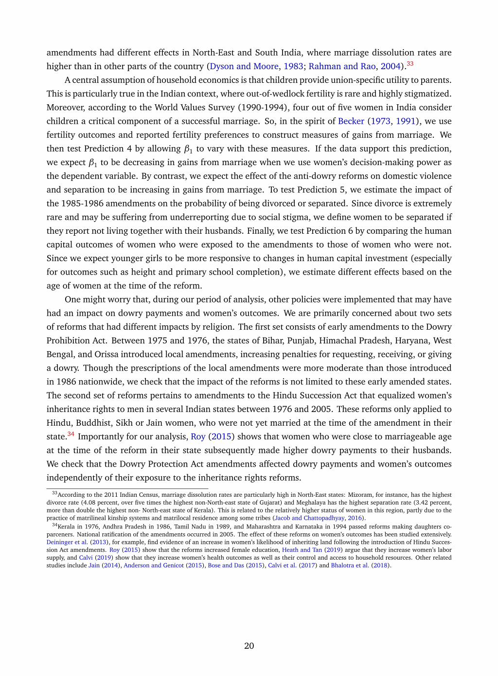
amendments had different effects in North-East and South India, where marriage dissolution rates are

higher than in other parts of the country (Dyson and Moore, 1983; Rahman and Rao, 2004).33

A central assumption of household economics is that children provide union-specific utility to parents.

This is particularly true in the Indian context, where out-of-wedlock fertility is rare and highly stigmatized.

Moreover, according to the World Values Survey (1990-1994), four out of five women in India consider

children a critical component of a successful marriage. So, in the spirit of Becker (1973, 1991), we use

fertility outcomes and reported fertility preferences to construct measures of gains from marriage. We

then test Prediction 4 by allowing β1 to vary with these measures. If the data support this prediction,

we expect β1 to be decreasing in gains from marriage when we use women’s decision-making power as

the dependent variable. By contrast, we expect the effect of the anti-dowry reforms on domestic violence

and separation to be increasing in gains from marriage. To test Prediction 5, we estimate the impact of

the 1985-1986 amendments on the probability of being divorced or separated. Since divorce is extremely

rare and may be suffering from underreporting due to social stigma, we define women to be separated if

they report not living together with their husbands. Finally, we test Prediction 6 by comparing the human

capital outcomes of women who were exposed to the amendments to those of women who were not.

Since we expect younger girls to be more responsive to changes in human capital investment (especially

for outcomes such as height and primary school completion), we estimate different effects based on the

age of women at the time of the reform.

One might worry that, during our period of analysis, other policies were implemented that may have

had an impact on dowry payments and women’s outcomes. We are primarily concerned about two sets

of reforms that had different impacts by religion. The first set consists of early amendments to the Dowry

Prohibition Act. Between 1975 and 1976, the states of Bihar, Punjab, Himachal Pradesh, Haryana, West

Bengal, and Orissa introduced local amendments, increasing penalties for requesting, receiving, or giving

a dowry. Though the prescriptions of the local amendments were more moderate than those introduced

in 1986 nationwide, we check that the impact of the reforms is not limited to these early amended states.

The second set of reforms pertains to amendments to the Hindu Succession Act that equalized women’s

inheritance rights to men in several Indian states between 1976 and 2005. These reforms only applied to

Hindu, Buddhist, Sikh or Jain women, who were not yet married at the time of the amendment in their

state.34 Importantly for our analysis, Roy (2015) shows that women who were close to marriageable age

at the time of the reform in their state subsequently made higher dowry payments to their husbands.

We check that the Dowry Protection Act amendments affected dowry payments and women’s outcomes

independently of their exposure to the inheritance rights reforms.

33According to the 2011 Indian Census, marriage dissolution rates are particularly high in North-East states: Mizoram, for instance, has the highestdivorce rate (4.08 percent, over five times the highest non-North-east state of Gujarat) and Meghalaya has the highest separation rate (3.42 percent,more than double the highest non- North-east state of Kerala). This is related to the relatively higher status of women in this region, partly due to thepractice of matrilineal kinship systems and matrilocal residence among some tribes (Jacob and Chattopadhyay, 2016).

34Kerala in 1976, Andhra Pradesh in 1986, Tamil Nadu in 1989, and Maharashtra and Karnataka in 1994 passed reforms making daughters co-parceners. National ratification of the amendments occurred in 2005. The effect of these reforms on women’s outcomes has been studied extensively.Deininger et al. (2013), for example, find evidence of an increase in women’s likelihood of inheriting land following the introduction of Hindu Succes-sion Act amendments. Roy (2015) show that the reforms increased female education, Heath and Tan (2019) argue that they increase women’s laborsupply, and Calvi (2019) show that they increase women’s health outcomes as well as their control and access to household resources. Other relatedstudies include Jain (2014), Anderson and Genicot (2015), Bose and Das (2015), Calvi et al. (2017) and Bhalotra et al. (2018).

20

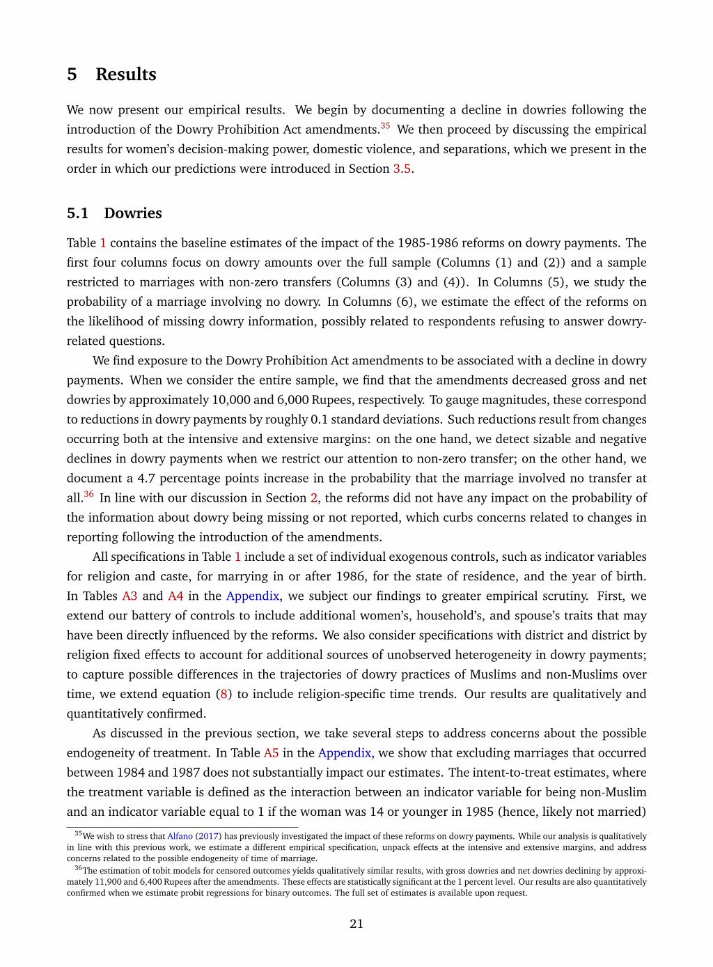
5 Results

We now present our empirical results. We begin by documenting a decline in dowries following the

introduction of the Dowry Prohibition Act amendments.35 We then proceed by discussing the empirical

results for women’s decision-making power, domestic violence, and separations, which we present in the

order in which our predictions were introduced in Section 3.5.

5.1 Dowries

Table 1 contains the baseline estimates of the impact of the 1985-1986 reforms on dowry payments. The

first four columns focus on dowry amounts over the full sample (Columns (1) and (2)) and a sample

restricted to marriages with non-zero transfers (Columns (3) and (4)). In Columns (5), we study the

probability of a marriage involving no dowry. In Columns (6), we estimate the effect of the reforms on

the likelihood of missing dowry information, possibly related to respondents refusing to answer dowry-

related questions.

We find exposure to the Dowry Prohibition Act amendments to be associated with a decline in dowry

payments. When we consider the entire sample, we find that the amendments decreased gross and net

dowries by approximately 10,000 and 6,000 Rupees, respectively. To gauge magnitudes, these correspond

to reductions in dowry payments by roughly 0.1 standard deviations. Such reductions result from changes

occurring both at the intensive and extensive margins: on the one hand, we detect sizable and negative

declines in dowry payments when we restrict our attention to non-zero transfer; on the other hand, we

document a 4.7 percentage points increase in the probability that the marriage involved no transfer at

all.36 In line with our discussion in Section 2, the reforms did not have any impact on the probability of

the information about dowry being missing or not reported, which curbs concerns related to changes in

reporting following the introduction of the amendments.

All specifications in Table 1 include a set of individual exogenous controls, such as indicator variables

for religion and caste, for marrying in or after 1986, for the state of residence, and the year of birth.

In Tables A3 and A4 in the Appendix, we subject our findings to greater empirical scrutiny. First, we

extend our battery of controls to include additional women’s, household’s, and spouse’s traits that may

have been directly influenced by the reforms. We also consider specifications with district and district by

religion fixed effects to account for additional sources of unobserved heterogeneity in dowry payments;

to capture possible differences in the trajectories of dowry practices of Muslims and non-Muslims over

time, we extend equation (8) to include religion-specific time trends. Our results are qualitatively and

quantitatively confirmed.

As discussed in the previous section, we take several steps to address concerns about the possible

endogeneity of treatment. In Table A5 in the Appendix, we show that excluding marriages that occurred

between 1984 and 1987 does not substantially impact our estimates. The intent-to-treat estimates, where

the treatment variable is defined as the interaction between an indicator variable for being non-Muslim

and an indicator variable equal to 1 if the woman was 14 or younger in 1985 (hence, likely not married)

35We wish to stress that Alfano (2017) has previously investigated the impact of these reforms on dowry payments. While our analysis is qualitativelyin line with this previous work, we estimate a different empirical specification, unpack effects at the intensive and extensive margins, and addressconcerns related to the possible endogeneity of time of marriage.

36The estimation of tobit models for censored outcomes yields qualitatively similar results, with gross dowries and net dowries declining by approxi-mately 11,900 and 6,400 Rupees after the amendments. These effects are statistically significant at the 1 percent level. Our results are also quantitativelyconfirmed when we estimate probit regressions for binary outcomes. The full set of estimates is available upon request.

21

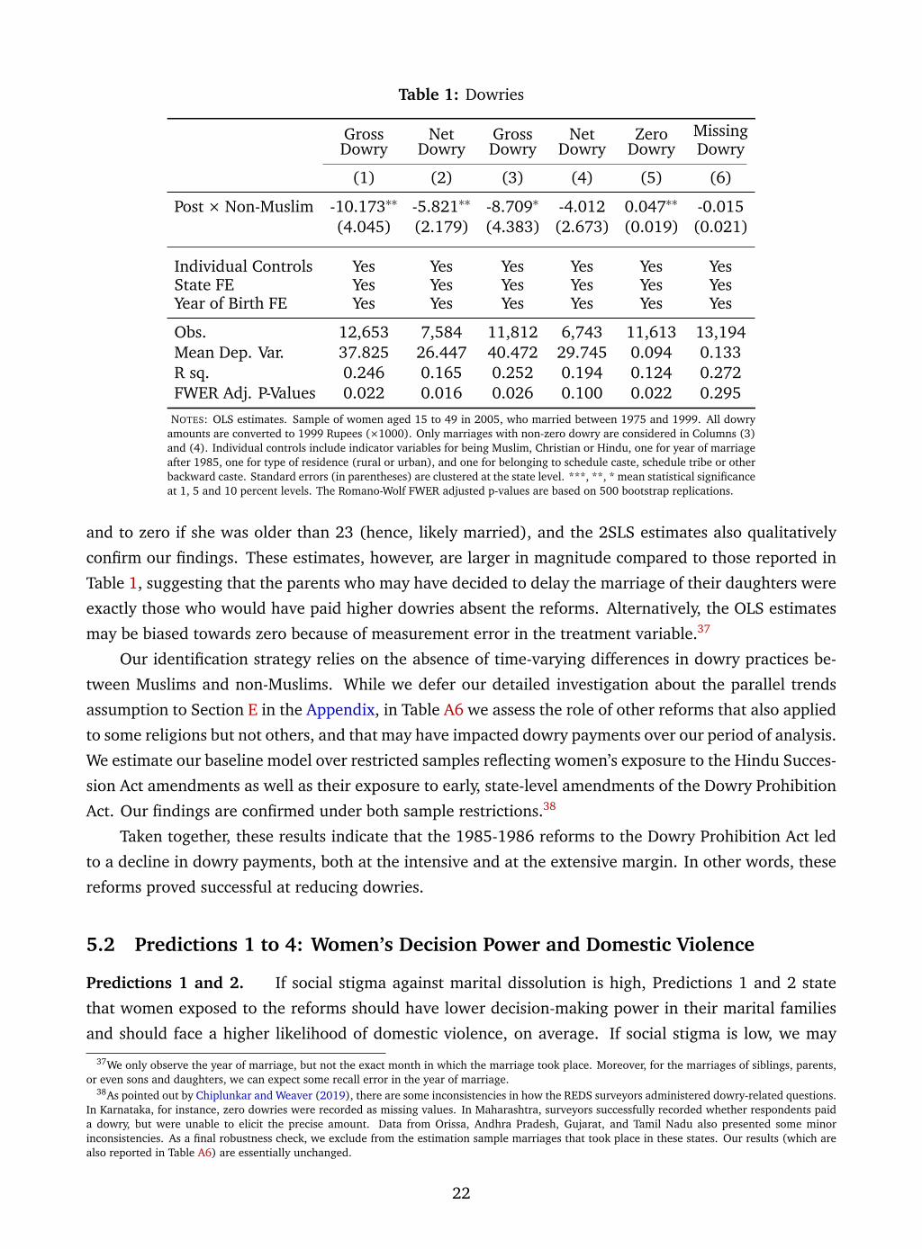
Table 1: Dowries

GrossDowry

NetDowry

GrossDowry

NetDowry

ZeroDowry

MissingDowry

(1) (2) (3) (4) (5) (6)

Post × Non-Muslim -10.173∗∗ -5.821∗∗ -8.709∗ -4.012 0.047∗∗ -0.015(4.045) (2.179) (4.383) (2.673) (0.019) (0.021)

Individual Controls Yes Yes Yes Yes Yes YesState FE Yes Yes Yes Yes Yes YesYear of Birth FE Yes Yes Yes Yes Yes Yes

Obs. 12,653 7,584 11,812 6,743 11,613 13,194Mean Dep. Var. 37.825 26.447 40.472 29.745 0.094 0.133R sq. 0.246 0.165 0.252 0.194 0.124 0.272FWER Adj. P-Values 0.022 0.016 0.026 0.100 0.022 0.295

NOTES: OLS estimates. Sample of women aged 15 to 49 in 2005, who married between 1975 and 1999. All dowryamounts are converted to 1999 Rupees (×1000). Only marriages with non-zero dowry are considered in Columns (3)and (4). Individual controls include indicator variables for being Muslim, Christian or Hindu, one for year of marriageafter 1985, one for type of residence (rural or urban), and one for belonging to schedule caste, schedule tribe or otherbackward caste. Standard errors (in parentheses) are clustered at the state level. ***, **, * mean statistical significanceat 1, 5 and 10 percent levels. The Romano-Wolf FWER adjusted p-values are based on 500 bootstrap replications.

and to zero if she was older than 23 (hence, likely married), and the 2SLS estimates also qualitatively

confirm our findings. These estimates, however, are larger in magnitude compared to those reported in

Table 1, suggesting that the parents who may have decided to delay the marriage of their daughters were

exactly those who would have paid higher dowries absent the reforms. Alternatively, the OLS estimates

may be biased towards zero because of measurement error in the treatment variable.37

Our identification strategy relies on the absence of time-varying differences in dowry practices be-

tween Muslims and non-Muslims. While we defer our detailed investigation about the parallel trends

assumption to Section E in the Appendix, in Table A6 we assess the role of other reforms that also applied

to some religions but not others, and that may have impacted dowry payments over our period of analysis.

We estimate our baseline model over restricted samples reflecting women’s exposure to the Hindu Succes-

sion Act amendments as well as their exposure to early, state-level amendments of the Dowry Prohibition

Act. Our findings are confirmed under both sample restrictions.38

Taken together, these results indicate that the 1985-1986 reforms to the Dowry Prohibition Act led

to a decline in dowry payments, both at the intensive and at the extensive margin. In other words, these

reforms proved successful at reducing dowries.

5.2 Predictions 1 to 4: Women’s Decision Power and Domestic Violence

Predictions 1 and 2. If social stigma against marital dissolution is high, Predictions 1 and 2 state

that women exposed to the reforms should have lower decision-making power in their marital families

and should face a higher likelihood of domestic violence, on average. If social stigma is low, we may

37We only observe the year of marriage, but not the exact month in which the marriage took place. Moreover, for the marriages of siblings, parents,or even sons and daughters, we can expect some recall error in the year of marriage.

38As pointed out by Chiplunkar and Weaver (2019), there are some inconsistencies in how the REDS surveyors administered dowry-related questions.In Karnataka, for instance, zero dowries were recorded as missing values. In Maharashtra, surveyors successfully recorded whether respondents paida dowry, but were unable to elicit the precise amount. Data from Orissa, Andhra Pradesh, Gujarat, and Tamil Nadu also presented some minorinconsistencies. As a final robustness check, we exclude from the estimation sample marriages that took place in these states. Our results (which arealso reported in Table A6) are essentially unchanged.

22

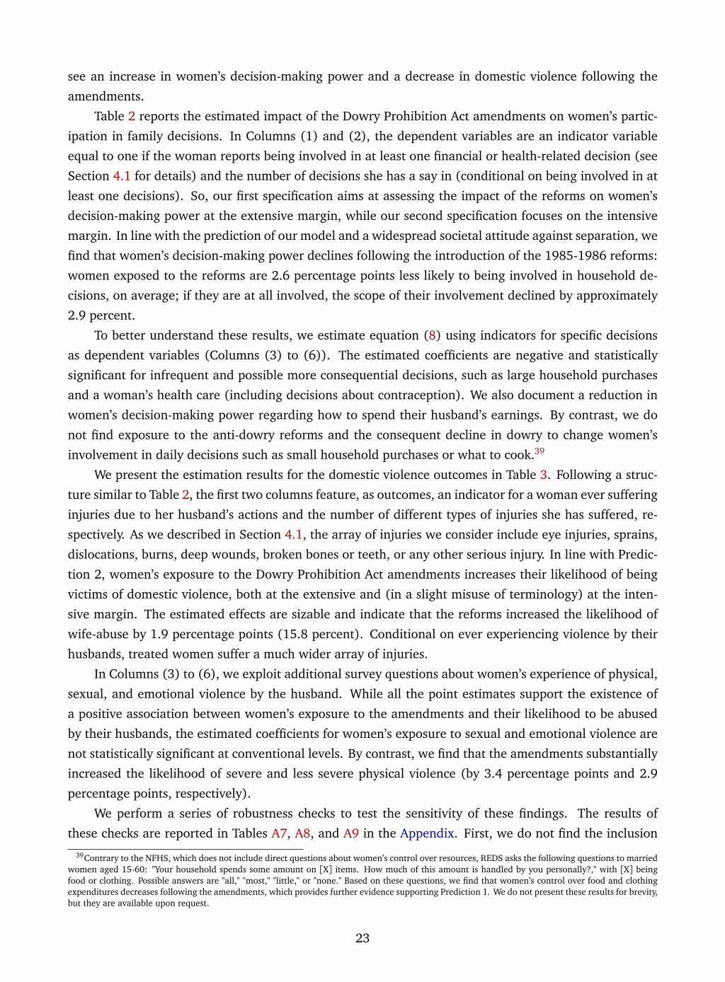
see an increase in women’s decision-making power and a decrease in domestic violence following the

amendments.

Table 2 reports the estimated impact of the Dowry Prohibition Act amendments on women’s partic-

ipation in family decisions. In Columns (1) and (2), the dependent variables are an indicator variable

equal to one if the woman reports being involved in at least one financial or health-related decision (see

Section 4.1 for details) and the number of decisions she has a say in (conditional on being involved in at

least one decisions). So, our first specification aims at assessing the impact of the reforms on women’s

decision-making power at the extensive margin, while our second specification focuses on the intensive

margin. In line with the prediction of our model and a widespread societal attitude against separation, we

find that women’s decision-making power declines following the introduction of the 1985-1986 reforms:

women exposed to the reforms are 2.6 percentage points less likely to being involved in household de-

cisions, on average; if they are at all involved, the scope of their involvement declined by approximately

2.9 percent.

To better understand these results, we estimate equation (8) using indicators for specific decisions

as dependent variables (Columns (3) to (6)). The estimated coefficients are negative and statistically

significant for infrequent and possible more consequential decisions, such as large household purchases

and a woman’s health care (including decisions about contraception). We also document a reduction in

women’s decision-making power regarding how to spend their husband’s earnings. By contrast, we do

not find exposure to the anti-dowry reforms and the consequent decline in dowry to change women’s

involvement in daily decisions such as small household purchases or what to cook.39

We present the estimation results for the domestic violence outcomes in Table 3. Following a struc-

ture similar to Table 2, the first two columns feature, as outcomes, an indicator for a woman ever suffering

injuries due to her husband’s actions and the number of different types of injuries she has suffered, re-

spectively. As we described in Section 4.1, the array of injuries we consider include eye injuries, sprains,

dislocations, burns, deep wounds, broken bones or teeth, or any other serious injury. In line with Predic-

tion 2, women’s exposure to the Dowry Prohibition Act amendments increases their likelihood of being

victims of domestic violence, both at the extensive and (in a slight misuse of terminology) at the inten-

sive margin. The estimated effects are sizable and indicate that the reforms increased the likelihood of

wife-abuse by 1.9 percentage points (15.8 percent). Conditional on ever experiencing violence by their

husbands, treated women suffer a much wider array of injuries.

In Columns (3) to (6), we exploit additional survey questions about women’s experience of physical,

sexual, and emotional violence by the husband. While all the point estimates support the existence of

a positive association between women’s exposure to the amendments and their likelihood to be abused

by their husbands, the estimated coefficients for women’s exposure to sexual and emotional violence are

not statistically significant at conventional levels. By contrast, we find that the amendments substantially

increased the likelihood of severe and less severe physical violence (by 3.4 percentage points and 2.9

percentage points, respectively).

We perform a series of robustness checks to test the sensitivity of these findings. The results of

these checks are reported in Tables A7, A8, and A9 in the Appendix. First, we do not find the inclusion

39Contrary to the NFHS, which does not include direct questions about women’s control over resources, REDS asks the following questions to marriedwomen aged 15-60: "Your household spends some amount on [X] items. How much of this amount is handled by you personally?," with [X] beingfood or clothing. Possible answers are "all," "most," "little," or "none." Based on these questions, we find that women’s control over food and clothingexpenditures decreases following the amendments, which provides further evidence supporting Prediction 1. We do not present these results for brevity,but they are available upon request.

23

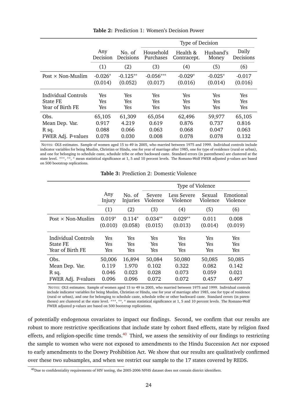
Table 2: Prediction 1: Women’s Decision Power

Type of Decision

AnyDecision

No. ofDecisions

HouseholdPurchases

Health &Contracept.

Husband’sMoney

DailyDecisions

(1) (2) (3) (4) (5) (6)

Post × Non-Muslim -0.026∗ -0.125∗∗ -0.056∗∗∗ -0.029∗ -0.025∗ -0.017(0.014) (0.052) (0.017) (0.016) (0.014) (0.016)

Individual Controls Yes Yes Yes Yes Yes YesState FE Yes Yes Yes Yes Yes YesYear of Birth FE Yes Yes Yes Yes Yes Yes

Obs. 65,105 61,309 65,054 62,496 59,977 65,105Mean Dep. Var. 0.917 4.219 0.619 0.876 0.737 0.816R sq. 0.088 0.066 0.063 0.068 0.047 0.063FWER Adj. P-values 0.078 0.030 0.008 0.078 0.078 0.132

NOTES: OLS estimates. Sample of women aged 15 to 49 in 2005, who married between 1975 and 1999. Individual controls includeindicator variables for being Muslim, Christian or Hindu, one for year of marriage after 1985, one for type of residence (rural or urban),and one for belonging to schedule caste, schedule tribe or other backward caste. Standard errors (in parentheses) are clustered at thestate level. ***, **, * mean statistical significance at 1, 5 and 10 percent levels. The Romano-Wolf FWER adjusted p-values are basedon 500 bootstrap replications.

Table 3: Prediction 2: Domestic Violence

Type of Violence

AnyInjury

No. ofInjuries

SevereViolence

Less SevereViolence

SexualViolence

EmotionalViolence

(1) (2) (3) (4) (5) (6)

Post × Non-Muslim 0.019∗ 0.114∗ 0.034∗∗ 0.029∗∗ 0.011 0.008(0.010) (0.058) (0.015) (0.013) (0.014) (0.019)

Individual Controls Yes Yes Yes Yes Yes YesState FE Yes Yes Yes Yes Yes YesYear of Birth FE Yes Yes Yes Yes Yes Yes

Obs. 50,006 16,894 50,084 50,080 50,085 50,085Mean Dep. Var. 0.119 1.970 0.102 0.322 0.082 0.142R sq. 0.046 0.023 0.028 0.073 0.059 0.021FWER Adj. P-values 0.096 0.096 0.072 0.072 0.457 0.497

NOTES: OLS estimates. Sample of women aged 15 to 49 in 2005, who married between 1975 and 1999. Individual controlsinclude indicator variables for being Muslim, Christian or Hindu, one for year of marriage after 1985, one for type of residence(rural or urban), and one for belonging to schedule caste, schedule tribe or other backward caste. Standard errors (in paren-theses) are clustered at the state level. ***, **, * mean statistical significance at 1, 5 and 10 percent levels. The Romano-WolfFWER adjusted p-values are based on 500 bootstrap replications.

of potentially endogenous covariates to impact our findings. Second, we confirm that our results are

robust to more restrictive specifications that include state by cohort fixed effects, state by religion fixed

effects, and religion-specific time trends.40 Third, we assess the sensitivity of our findings to restricting

the sample to women who were not exposed to amendments to the Hindu Succession Act nor exposed

to early amendments to the Dowry Prohibition Act. We show that our results are qualitatively confirmed

over these two subsamples, and when we restrict our sample to the 17 states covered by REDS.

40Due to confidentiality requirements of HIV testing, the 2005-2006 NFHS dataset does not contain district identifiers.

24

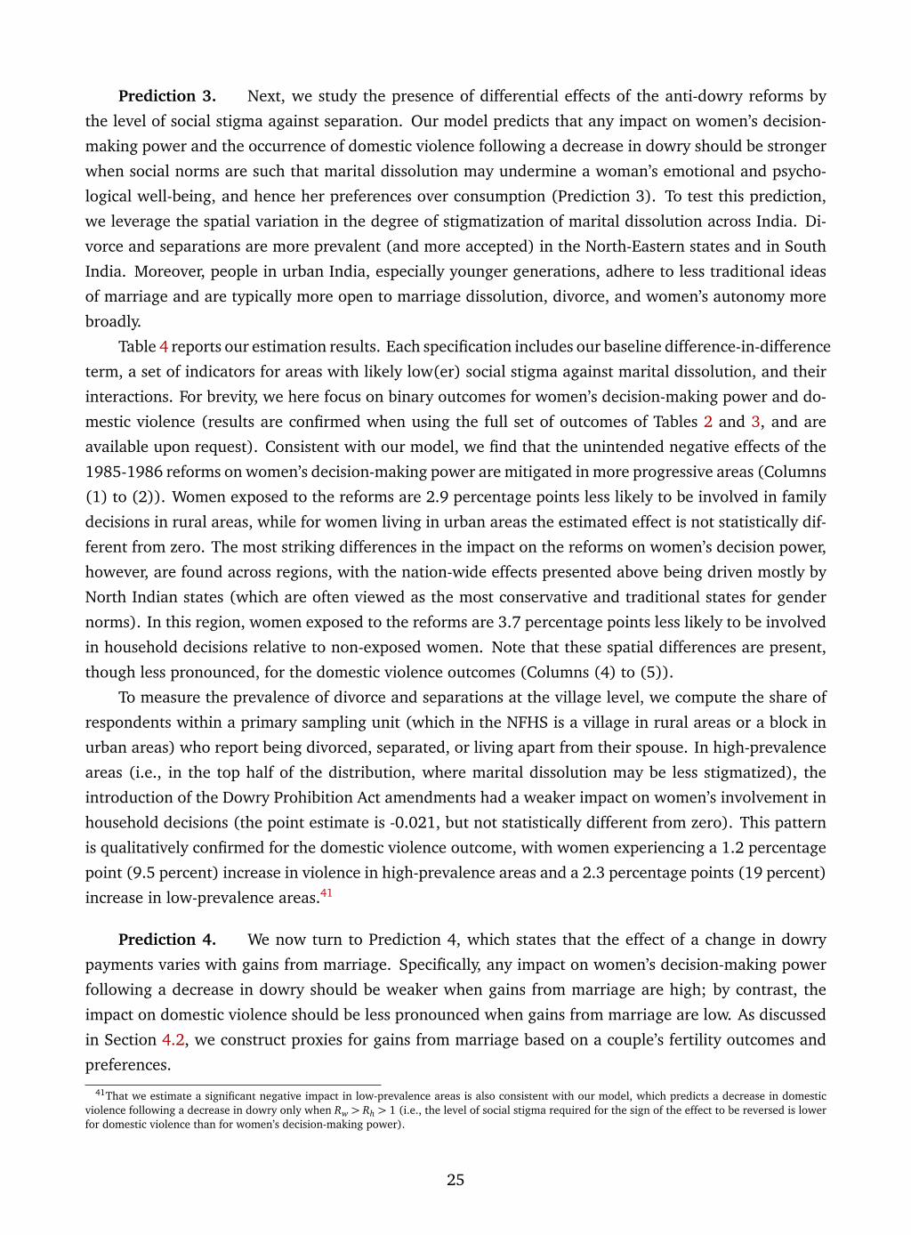
Prediction 3. Next, we study the presence of differential effects of the anti-dowry reforms by

the level of social stigma against separation. Our model predicts that any impact on women’s decision-

making power and the occurrence of domestic violence following a decrease in dowry should be stronger

when social norms are such that marital dissolution may undermine a woman’s emotional and psycho-

logical well-being, and hence her preferences over consumption (Prediction 3). To test this prediction,

we leverage the spatial variation in the degree of stigmatization of marital dissolution across India. Di-

vorce and separations are more prevalent (and more accepted) in the North-Eastern states and in South

India. Moreover, people in urban India, especially younger generations, adhere to less traditional ideas

of marriage and are typically more open to marriage dissolution, divorce, and women’s autonomy more

broadly.

Table 4 reports our estimation results. Each specification includes our baseline difference-in-difference

term, a set of indicators for areas with likely low(er) social stigma against marital dissolution, and their

interactions. For brevity, we here focus on binary outcomes for women’s decision-making power and do-

mestic violence (results are confirmed when using the full set of outcomes of Tables 2 and 3, and are

available upon request). Consistent with our model, we find that the unintended negative effects of the

1985-1986 reforms on women’s decision-making power are mitigated in more progressive areas (Columns

(1) to (2)). Women exposed to the reforms are 2.9 percentage points less likely to be involved in family

decisions in rural areas, while for women living in urban areas the estimated effect is not statistically dif-

ferent from zero. The most striking differences in the impact on the reforms on women’s decision power,

however, are found across regions, with the nation-wide effects presented above being driven mostly by

North Indian states (which are often viewed as the most conservative and traditional states for gender

norms). In this region, women exposed to the reforms are 3.7 percentage points less likely to be involved

in household decisions relative to non-exposed women. Note that these spatial differences are present,

though less pronounced, for the domestic violence outcomes (Columns (4) to (5)).

To measure the prevalence of divorce and separations at the village level, we compute the share of

respondents within a primary sampling unit (which in the NFHS is a village in rural areas or a block in

urban areas) who report being divorced, separated, or living apart from their spouse. In high-prevalence

areas (i.e., in the top half of the distribution, where marital dissolution may be less stigmatized), the

introduction of the Dowry Prohibition Act amendments had a weaker impact on women’s involvement in

household decisions (the point estimate is -0.021, but not statistically different from zero). This pattern

is qualitatively confirmed for the domestic violence outcome, with women experiencing a 1.2 percentage

point (9.5 percent) increase in violence in high-prevalence areas and a 2.3 percentage points (19 percent)

increase in low-prevalence areas.41

Prediction 4. We now turn to Prediction 4, which states that the effect of a change in dowry

payments varies with gains from marriage. Specifically, any impact on women’s decision-making power

following a decrease in dowry should be weaker when gains from marriage are high; by contrast, the

impact on domestic violence should be less pronounced when gains from marriage are low. As discussed

in Section 4.2, we construct proxies for gains from marriage based on a couple’s fertility outcomes and

preferences.

41That we estimate a significant negative impact in low-prevalence areas is also consistent with our model, which predicts a decrease in domesticviolence following a decrease in dowry only when Rw > Rh > 1 (i.e., the level of social stigma required for the sign of the effect to be reversed is lowerfor domestic violence than for women’s decision-making power).

25

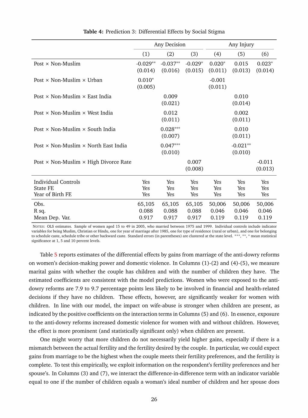
Table 4: Prediction 3: Differential Effects by Social Stigma

Any Decision Any Injury

(1) (2) (3) (4) (5) (6)

Post × Non-Muslim -0.029∗∗ -0.037∗∗ -0.029∗ 0.020∗ 0.015 0.023∗

(0.014) (0.016) (0.015) (0.011) (0.013) (0.014)

Post × Non-Muslim × Urban 0.010∗ -0.001(0.005) (0.011)

Post × Non-Muslim × East India 0.009 0.010(0.021) (0.014)

Post × Non-Muslim × West India 0.012 0.002(0.011) (0.011)

Post × Non-Muslim × South India 0.028∗∗∗ 0.010(0.007) (0.011)

Post × Non-Muslim × North East India 0.047∗∗∗ -0.021∗∗

(0.010) (0.010)

Post × Non-Muslim × High Divorce Rate 0.007 -0.011(0.008) (0.013)

Individual Controls Yes Yes Yes Yes Yes YesState FE Yes Yes Yes Yes Yes YesYear of Birth FE Yes Yes Yes Yes Yes Yes

Obs. 65,105 65,105 65,105 50,006 50,006 50,006R sq. 0.088 0.088 0.088 0.046 0.046 0.046Mean Dep. Var. 0.917 0.917 0.917 0.119 0.119 0.119

NOTES: OLS estimates. Sample of women aged 15 to 49 in 2005, who married between 1975 and 1999. Individual controls include indicatorvariables for being Muslim, Christian or Hindu, one for year of marriage after 1985, one for type of residence (rural or urban), and one for belongingto schedule caste, schedule tribe or other backward caste. Standard errors (in parentheses) are clustered at the state level. ***, **, * mean statisticalsignificance at 1, 5 and 10 percent levels.

Table 5 reports estimates of the differential effects by gains from marriage of the anti-dowry reforms

on women’s decision-making power and domestic violence. In Columns (1)-(2) and (4)-(5), we measure

marital gains with whether the couple has children and with the number of children they have. The

estimated coefficients are consistent with the model predictions. Women who were exposed to the anti-

dowry reforms are 7.9 to 9.7 percentage points less likely to be involved in financial and health-related

decisions if they have no children. These effects, however, are significantly weaker for women with

children. In line with our model, the impact on wife-abuse is stronger when children are present, as

indicated by the positive coefficients on the interaction terms in Columns (5) and (6). In essence, exposure

to the anti-dowry reforms increased domestic violence for women with and without children. However,

the effect is more prominent (and statistically significant only) when children are present.

One might worry that more children do not necessarily yield higher gains, especially if there is a

mismatch between the actual fertility and the fertility desired by the couple. In particular, we could expect

gains from marriage to be the highest when the couple meets their fertility preferences, and the fertility is

complete. To test this empirically, we exploit information on the respondent’s fertility preferences and her

spouse’s. In Columns (3) and (7), we interact the difference-in-difference term with an indicator variable

equal to one if the number of children equals a woman’s ideal number of children and her spouse does

26

Table 5: Prediction 4: Differential Effects by Gains from Marriage

Any Decision Any Injury

(1) (2) (3) (4) (5) (6) (7) (8)

Post × Non-Muslim -0.079∗∗∗ -0.097∗∗∗ -0.028∗ -0.036∗∗∗ 0.014 0.022 0.024 0.023(0.017) (0.019) (0.014) (0.010) (0.019) (0.014) (0.016) (0.015)

Post × Non-Muslim × No. Kids 0.022∗∗∗ 0.004(0.003) (0.003)

Post × Non-Muslim × Any Kid 0.074∗∗∗ 0.005(0.015) (0.013)

Post × Non-Muslim × Completed Fertility 0.008 0.009(0.007) (0.009)

Post × Non-Muslim × First Born Boy 0.022∗∗ 0.007(0.010) (0.010)

Individual Controls Yes Yes Yes Yes Yes Yes Yes YesState FE Yes Yes Yes Yes Yes Yes Yes YesYear of Birth FE Yes Yes Yes Yes Yes Yes Yes Yes

Obs. 65,105 65,105 65,105 65,105 50,021 50,021 50,021 50,021R sq. 0.094 0.093 0.089 0.089 0.048 0.047 0.049 0.047Mean Dep. Var. 0.917 0.917 0.917 0.917 0.153 0.153 0.153 0.153

NOTES: OLS estimates. Sample of women aged 15 to 49 in 2005, who married between 1975 and 1999. Individual controls include indicator variables for being Muslim, Christianor Hindu, one for year of marriage after 1985, one for type of residence (rural or urban), and one for belonging to schedule caste, schedule tribe or other backward caste. Standarderrors (in parentheses) are clustered at the state level. ***, **, * mean statistical significance at 1, 5 and 10 percent levels.

not want any more (or any less) children. While the estimated coefficients are not statistically significant,

their sign is as expected.

Finally, we use the gender of the first born child as an alternative measure of marital gains. Note that,

while parental preferences for sons are widespread in India, the sex of the firstborn child is quasi-random

(Bhalotra and Cochrane, 2010; Anukriti et al., 2016). We find that the impact of the policy on women’s

decision power (domestic violence) is mitigated (strengthen) when gains from marriage are high (i.e.,

when the first born child is male).

Discussion. Taken together, the results presented so far are mostly consistent with Predictions

1 to 4 of our model. They also imply that the tightening of anti-dowry laws introduced by the Indian

government between 1985 and 1986 had some unintended negative consequences for women’s welfare.42

The overall decline in women’s involvement in household decisions and the increase in domestic violence

increases following the amendments (and the consequent decreases in dowry payments documented in

Section 5.1) indicate that social stigma against separation in India is high, on average (that is, Rw < 1).

There is, however, substantial variation in the stigmatization and social cost of marital dissolution across

regions, which results in markedly differential impacts of the anti-dowry reforms on women’s outcomes

(Prediction 3). The unintended consequences of the reforms appear to be mitigated in more progressive

areas and exacerbated in more conservative regions, suggesting that one-size-fits-all policies may not be

optimal, and that the social and cultural context may matter a great deal when designing policies (an

important point also raised by Rao and Walton (2004) and Ashraf et al. (2020)).

Our heterogeneity analysis by gains from marriage hinges on the assumption that any changes in

42Other well-intended policies have been recently found to generate unintended consequences in India. Anukriti (2018), e.g., shows that a programintroduced in the state of Haryana to fertility-sex ratio trade-off, in fact exacerbated the problem and increased the sex-ratio through differential stoppingbehavior and sex selection at first and second parities. Studying the impact of the Child Labor (Prohibition and Regulation) Act, Bharadwaj et al. (2020)show that child wages decrease and child labor increases after the ban.

27

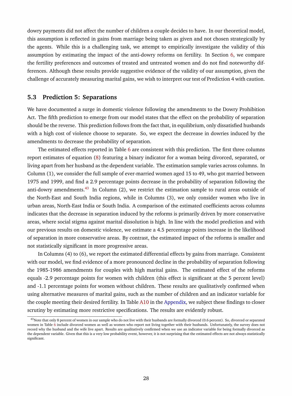
dowry payments did not affect the number of children a couple decides to have. In our theoretical model,

this assumption is reflected in gains from marriage being taken as given and not chosen strategically by

the agents. While this is a challenging task, we attempt to empirically investigate the validity of this

assumption by estimating the impact of the anti-dowry reforms on fertility. In Section 6, we compare

the fertility preferences and outcomes of treated and untreated women and do not find noteworthy dif-

ferences. Although these results provide suggestive evidence of the validity of our assumption, given the

challenge of accurately measuring marital gains, we wish to interpret our test of Prediction 4 with caution.

5.3 Prediction 5: Separations

We have documented a surge in domestic violence following the amendments to the Dowry Prohibition

Act. The fifth prediction to emerge from our model states that the effect on the probability of separation

should be the reverse. This prediction follows from the fact that, in equilibrium, only dissatisfied husbands

with a high cost of violence choose to separate. So, we expect the decrease in dowries induced by the

amendments to decrease the probability of separation.

The estimated effects reported in Table 6 are consistent with this prediction. The first three columns

report estimates of equation (8) featuring a binary indicator for a woman being divorced, separated, or

living apart from her husband as the dependent variable. The estimation sample varies across columns. In

Column (1), we consider the full sample of ever-married women aged 15 to 49, who got married between

1975 and 1999, and find a 2.9 percentage points decrease in the probability of separation following the

anti-dowry amendments.43 In Column (2), we restrict the estimation sample to rural areas outside of

the North-East and South India regions, while in Columns (3), we only consider women who live in

urban areas, North-East India or South India. A comparison of the estimated coefficients across columns

indicates that the decrease in separation induced by the reforms is primarily driven by more conservative

areas, where social stigma against marital dissolution is high. In line with the model prediction and with

our previous results on domestic violence, we estimate a 4.5 percentage points increase in the likelihood

of separation in more conservative areas. By contrast, the estimated impact of the reforms is smaller and

not statistically significant in more progressive areas.

In Columns (4) to (6), we report the estimated differential effects by gains from marriage. Consistent

with our model, we find evidence of a more pronounced decline in the probability of separation following

the 1985-1986 amendments for couples with high marital gains. The estimated effect of the reforms

equals -2.9 percentage points for women with children (this effect is significant at the 5 percent level)

and -1.1 percentage points for women without children. These results are qualitatively confirmed when

using alternative measures of marital gains, such as the number of children and an indicator variable for

the couple meeting their desired fertility. In Table A10 in the Appendix, we subject these findings to closer

scrutiny by estimating more restrictive specifications. The results are evidently robust.

43Note that only 8 percent of women in our sample who do not live with their husbands are formally divorced (0.6 percent). So, divorced or separatedwomen in Table 6 include divorced women as well as women who report not living together with their husbands. Unfortunately, the survey does notrecord why the husband and the wife live apart. Results are qualitatively confirmed when we use an indicator variable for being formally divorced asthe dependent variable. Given that this is a very low probability event, however, it is not surprising that the estimated effects are not always statisticallysignificant.

28

Table 6: Prediction 5: Separations

Divorced or Separated

(1) (2) (3) (4) (5) (6)

Post × Non-Muslim -0.029∗∗ -0.045∗ -0.017 -0.004 -0.011 -0.025∗∗

(0.011) (0.022) (0.012) (0.011) (0.027) (0.012)

Post × Non-Muslim × Number of Kids -0.006∗∗∗

(0.002)

Post × Non-Muslim × Any Kid -0.018(0.023)

Post × Non-Muslim × Desired Fertility Met -0.010(0.006)

Individual Controls Yes Yes Yes Yes Yes YesState FE Yes Yes Yes Yes Yes YesYear of Birth FE Yes Yes Yes Yes Yes Yes

Obs. 69,837 26,437 43,400 69,837 69,837 69,837R sq. 0.046 0.062 0.028 0.063 0.057 0.046Mean Dep. Var. 0.134 0.154 0.121 0.134 0.134 0.134

NOTES: OLS estimates. Sample of women aged 15 to 49 in 2005, who married between 1975 and 1999. In Columns (2), the estimation sampleexcludes women living in urban areas, North-India, or South India; in Columns (3), the estimation sample includes only women living in urban areas inNorth-India or South India. Individual controls include indicator variables for being Muslim, Christian or Hindu, one for year of marriage after 1985, onefor type of residence (rural or urban), and one for belonging to schedule caste, schedule tribe or other backward caste. Standard errors (in parentheses)are clustered at the state level. ***, **, * mean statistical significance at 1, 5 and 10 percent levels.

5.4 Prediction 6: Women’s Human Capital

We now turn to our last prediction, which states that parental investment in the human capital of future

brides should increase following a tightening of anti-dowry laws. The expectation of a lower dowry

payment in the future may incentivize parents to invest in their daughters’ human capital to maintain their

attractiveness in the marriage market and ensure that they would find a husband (Adams and Andrew,

2019). Also, parents may decide to reallocate resources that they would have otherwise saved for their

daughters’ dowry to alternative expenses that may benefit them (Anukriti et al., 2019). The NFHS does

not include information on past expenditure or saving patterns of a woman’s natal family. So, we rely

on women’s outcomes in adulthood to inform us of any changes in parental investment induced by the

reforms.

We focus on two sets of human capital outcomes: outcomes related to education, such as years of

schooling and the probability of having completed primary school; and long-run health outcomes, such as

height and the probability of being in the bottom half of the height distribution in our sample.44 Naturally,

parents’ ability to shape their daughters’ human capital in response to the 1985-1986 amendments would

be limited if their daughters were too old at the time of the reforms. Height, for instance, is mostly

determined by early childhood inputs. So, any response from parents whose daughters were, e.g., five or

older in 1985, may not be reflected in their daughter’s outcomes in adulthood. Similarly, the effect of the

amendments on primary school completion may be strongest for those women who were not too old to

attend primary school in 1985. We test for this by estimating equation (8) using measures of women’s

44Contrary to weight-based anthropometric indicators such as the body mass index (which respond to shorter-run variations in access to food andexposure to diseases), height captures the long-run effect of fetal and childhood nutritional limitations and has often been used as a proxy of parentalcare and allocation of resources to children (see, e.g., Jayachandran and Pande (2017)).

29

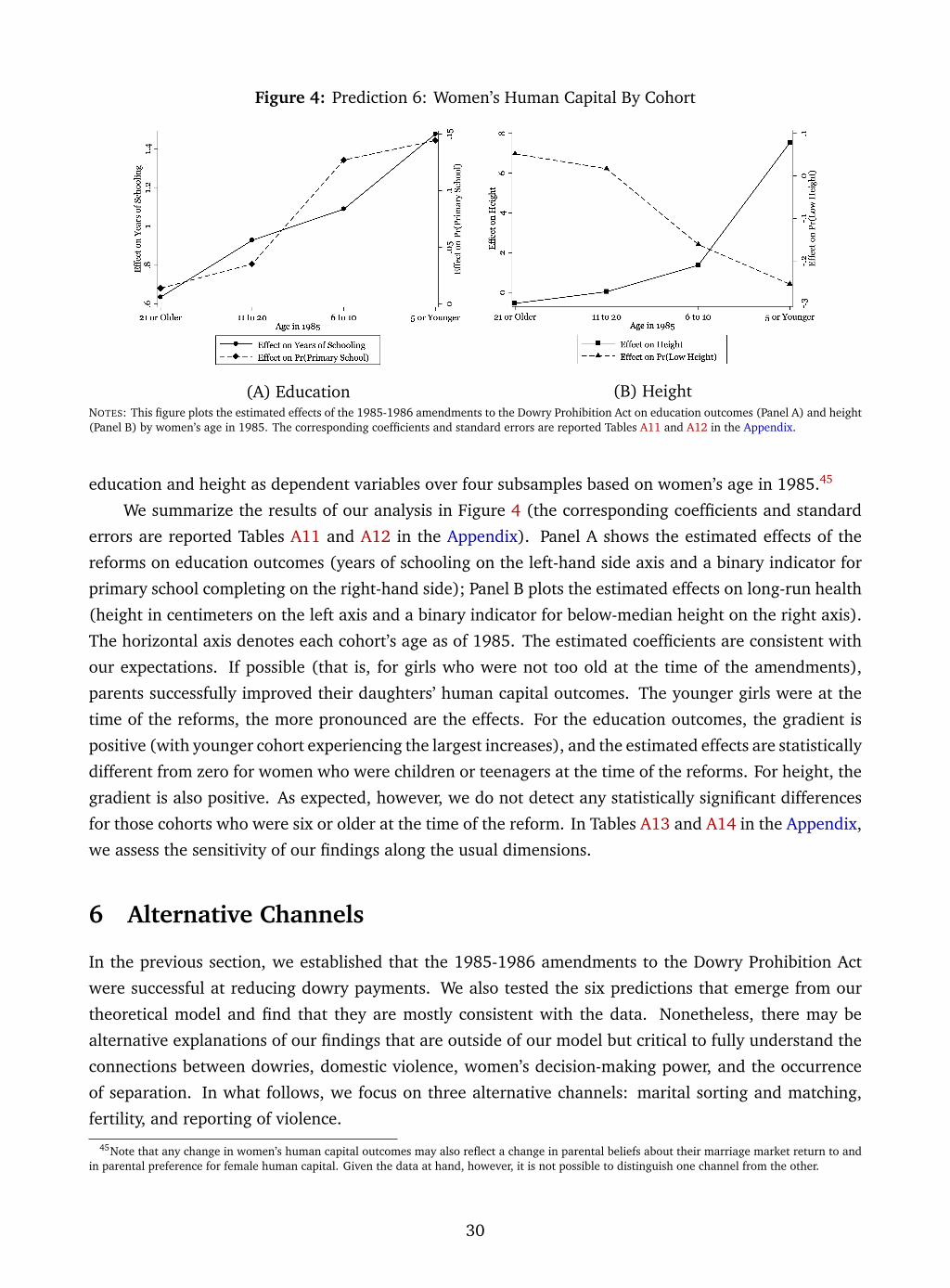
Figure 4: Prediction 6: Women’s Human Capital By Cohort

(A) Education (B) HeightNOTES: This figure plots the estimated effects of the 1985-1986 amendments to the Dowry Prohibition Act on education outcomes (Panel A) and height(Panel B) by women’s age in 1985. The corresponding coefficients and standard errors are reported Tables A11 and A12 in the Appendix.

education and height as dependent variables over four subsamples based on women’s age in 1985.45

We summarize the results of our analysis in Figure 4 (the corresponding coefficients and standard

errors are reported Tables A11 and A12 in the Appendix). Panel A shows the estimated effects of the

reforms on education outcomes (years of schooling on the left-hand side axis and a binary indicator for

primary school completing on the right-hand side); Panel B plots the estimated effects on long-run health

(height in centimeters on the left axis and a binary indicator for below-median height on the right axis).

The horizontal axis denotes each cohort’s age as of 1985. The estimated coefficients are consistent with

our expectations. If possible (that is, for girls who were not too old at the time of the amendments),

parents successfully improved their daughters’ human capital outcomes. The younger girls were at the

time of the reforms, the more pronounced are the effects. For the education outcomes, the gradient is

positive (with younger cohort experiencing the largest increases), and the estimated effects are statistically

different from zero for women who were children or teenagers at the time of the reforms. For height, the

gradient is also positive. As expected, however, we do not detect any statistically significant differences

for those cohorts who were six or older at the time of the reform. In Tables A13 and A14 in the Appendix,

we assess the sensitivity of our findings along the usual dimensions.

6 Alternative Channels

In the previous section, we established that the 1985-1986 amendments to the Dowry Prohibition Act

were successful at reducing dowry payments. We also tested the six predictions that emerge from our

theoretical model and find that they are mostly consistent with the data. Nonetheless, there may be

alternative explanations of our findings that are outside of our model but critical to fully understand the

connections between dowries, domestic violence, women’s decision-making power, and the occurrence

of separation. In what follows, we focus on three alternative channels: marital sorting and matching,

fertility, and reporting of violence.

45Note that any change in women’s human capital outcomes may also reflect a change in parental beliefs about their marriage market return to andin parental preference for female human capital. Given the data at hand, however, it is not possible to distinguish one channel from the other.

30

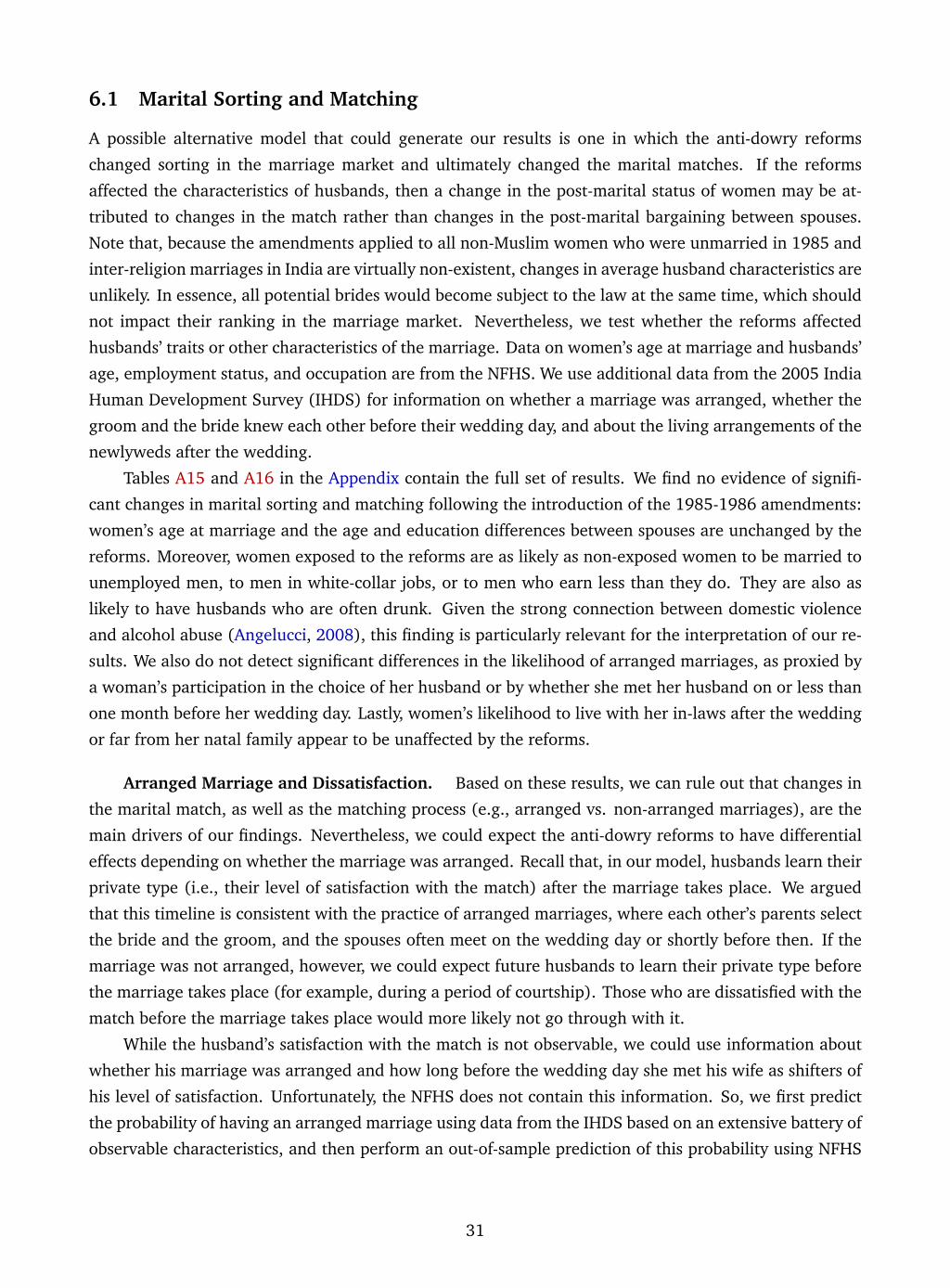
6.1 Marital Sorting and Matching

A possible alternative model that could generate our results is one in which the anti-dowry reforms

changed sorting in the marriage market and ultimately changed the marital matches. If the reforms

affected the characteristics of husbands, then a change in the post-marital status of women may be at-

tributed to changes in the match rather than changes in the post-marital bargaining between spouses.

Note that, because the amendments applied to all non-Muslim women who were unmarried in 1985 and

inter-religion marriages in India are virtually non-existent, changes in average husband characteristics are

unlikely. In essence, all potential brides would become subject to the law at the same time, which should

not impact their ranking in the marriage market. Nevertheless, we test whether the reforms affected

husbands’ traits or other characteristics of the marriage. Data on women’s age at marriage and husbands’

age, employment status, and occupation are from the NFHS. We use additional data from the 2005 India

Human Development Survey (IHDS) for information on whether a marriage was arranged, whether the

groom and the bride knew each other before their wedding day, and about the living arrangements of the

newlyweds after the wedding.

Tables A15 and A16 in the Appendix contain the full set of results. We find no evidence of signifi-

cant changes in marital sorting and matching following the introduction of the 1985-1986 amendments:

women’s age at marriage and the age and education differences between spouses are unchanged by the

reforms. Moreover, women exposed to the reforms are as likely as non-exposed women to be married to

unemployed men, to men in white-collar jobs, or to men who earn less than they do. They are also as

likely to have husbands who are often drunk. Given the strong connection between domestic violence

and alcohol abuse (Angelucci, 2008), this finding is particularly relevant for the interpretation of our re-

sults. We also do not detect significant differences in the likelihood of arranged marriages, as proxied by

a woman’s participation in the choice of her husband or by whether she met her husband on or less than

one month before her wedding day. Lastly, women’s likelihood to live with her in-laws after the wedding

or far from her natal family appear to be unaffected by the reforms.

Arranged Marriage and Dissatisfaction. Based on these results, we can rule out that changes in

the marital match, as well as the matching process (e.g., arranged vs. non-arranged marriages), are the

main drivers of our findings. Nevertheless, we could expect the anti-dowry reforms to have differential

effects depending on whether the marriage was arranged. Recall that, in our model, husbands learn their

private type (i.e., their level of satisfaction with the match) after the marriage takes place. We argued

that this timeline is consistent with the practice of arranged marriages, where each other’s parents select

the bride and the groom, and the spouses often meet on the wedding day or shortly before then. If the

marriage was not arranged, however, we could expect future husbands to learn their private type before

the marriage takes place (for example, during a period of courtship). Those who are dissatisfied with the

match before the marriage takes place would more likely not go through with it.

While the husband’s satisfaction with the match is not observable, we could use information about

whether his marriage was arranged and how long before the wedding day she met his wife as shifters of

his level of satisfaction. Unfortunately, the NFHS does not contain this information. So, we first predict

the probability of having an arranged marriage using data from the IHDS based on an extensive battery of

observable characteristics, and then perform an out-of-sample prediction of this probability using NFHS

31

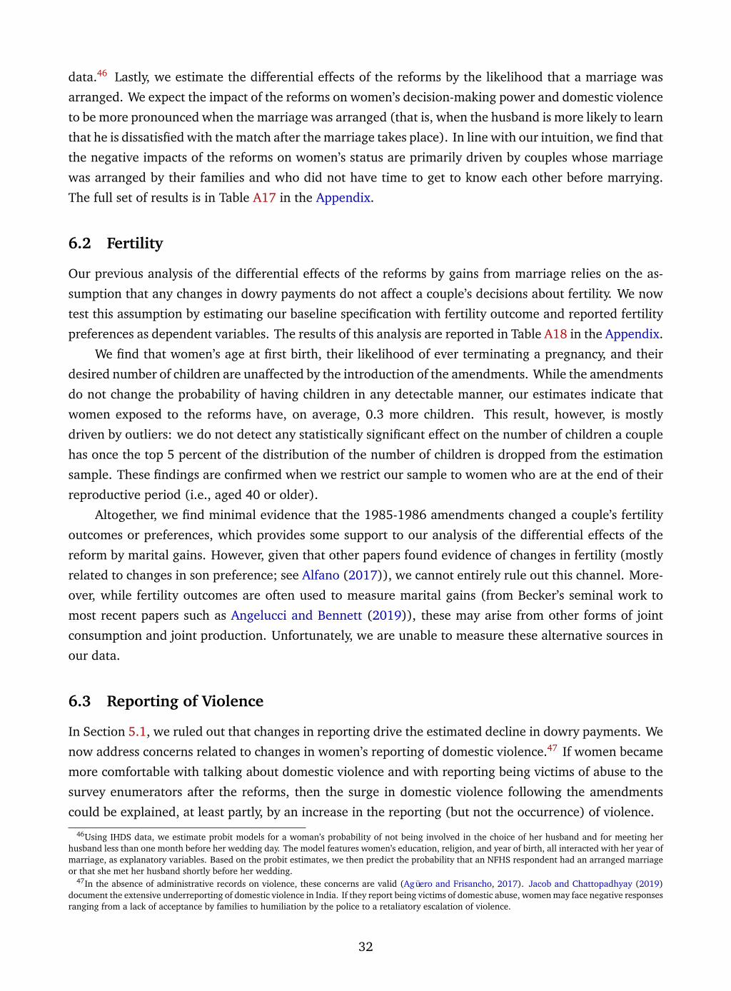
data.46 Lastly, we estimate the differential effects of the reforms by the likelihood that a marriage was

arranged. We expect the impact of the reforms on women’s decision-making power and domestic violence

to be more pronounced when the marriage was arranged (that is, when the husband is more likely to learn

that he is dissatisfied with the match after the marriage takes place). In line with our intuition, we find that

the negative impacts of the reforms on women’s status are primarily driven by couples whose marriage

was arranged by their families and who did not have time to get to know each other before marrying.

The full set of results is in Table A17 in the Appendix.

6.2 Fertility

Our previous analysis of the differential effects of the reforms by gains from marriage relies on the as-

sumption that any changes in dowry payments do not affect a couple’s decisions about fertility. We now

test this assumption by estimating our baseline specification with fertility outcome and reported fertility

preferences as dependent variables. The results of this analysis are reported in Table A18 in the Appendix.

We find that women’s age at first birth, their likelihood of ever terminating a pregnancy, and their

desired number of children are unaffected by the introduction of the amendments. While the amendments

do not change the probability of having children in any detectable manner, our estimates indicate that

women exposed to the reforms have, on average, 0.3 more children. This result, however, is mostly

driven by outliers: we do not detect any statistically significant effect on the number of children a couple

has once the top 5 percent of the distribution of the number of children is dropped from the estimation

sample. These findings are confirmed when we restrict our sample to women who are at the end of their

reproductive period (i.e., aged 40 or older).

Altogether, we find minimal evidence that the 1985-1986 amendments changed a couple’s fertility

outcomes or preferences, which provides some support to our analysis of the differential effects of the

reform by marital gains. However, given that other papers found evidence of changes in fertility (mostly

related to changes in son preference; see Alfano (2017)), we cannot entirely rule out this channel. More-

over, while fertility outcomes are often used to measure marital gains (from Becker’s seminal work to

most recent papers such as Angelucci and Bennett (2019)), these may arise from other forms of joint

consumption and joint production. Unfortunately, we are unable to measure these alternative sources in

our data.

6.3 Reporting of Violence

In Section 5.1, we ruled out that changes in reporting drive the estimated decline in dowry payments. We

now address concerns related to changes in women’s reporting of domestic violence.47 If women became

more comfortable with talking about domestic violence and with reporting being victims of abuse to the

survey enumerators after the reforms, then the surge in domestic violence following the amendments

could be explained, at least partly, by an increase in the reporting (but not the occurrence) of violence.

46Using IHDS data, we estimate probit models for a woman’s probability of not being involved in the choice of her husband and for meeting herhusband less than one month before her wedding day. The model features women’s education, religion, and year of birth, all interacted with her year ofmarriage, as explanatory variables. Based on the probit estimates, we then predict the probability that an NFHS respondent had an arranged marriageor that she met her husband shortly before her wedding.

47In the absence of administrative records on violence, these concerns are valid (Agüero and Frisancho, 2017). Jacob and Chattopadhyay (2019)document the extensive underreporting of domestic violence in India. If they report being victims of domestic abuse, women may face negative responsesranging from a lack of acceptance by families to humiliation by the police to a retaliatory escalation of violence.

32

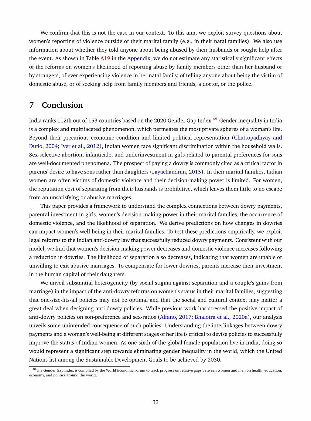
We confirm that this is not the case in our context. To this aim, we exploit survey questions about

women’s reporting of violence outside of their marital family (e.g., in their natal families). We also use

information about whether they told anyone about being abused by their husbands or sought help after

the event. As shown in Table A19 in the Appendix, we do not estimate any statistically significant effects

of the reforms on women’s likelihood of reporting abuse by family members other than her husband or

by strangers, of ever experiencing violence in her natal family, of telling anyone about being the victim of

domestic abuse, or of seeking help from family members and friends, a doctor, or the police.

7 Conclusion

India ranks 112th out of 153 countries based on the 2020 Gender Gap Index.48 Gender inequality in India

is a complex and multifaceted phenomenon, which permeates the most private spheres of a woman’s life.

Beyond their precarious economic condition and limited political representation (Chattopadhyay and

Duflo, 2004; Iyer et al., 2012), Indian women face significant discrimination within the household walls.

Sex-selective abortion, infanticide, and underinvestment in girls related to parental preferences for sons

are well-documented phenomena. The prospect of paying a dowry is commonly cited as a critical factor in

parents’ desire to have sons rather than daughters (Jayachandran, 2015). In their marital families, Indian

women are often victims of domestic violence and their decision-making power is limited. For women,

the reputation cost of separating from their husbands is prohibitive, which leaves them little to no escape

from an unsatisfying or abusive marriages.

This paper provides a framework to understand the complex connections between dowry payments,

parental investment in girls, women’s decision-making power in their marital families, the occurrence of

domestic violence, and the likelihood of separation. We derive predictions on how changes in dowries

can impact women’s well-being in their marital families. To test these predictions empirically, we exploit

legal reforms to the Indian anti-dowry law that successfully reduced dowry payments. Consistent with our

model, we find that women’s decision-making power decreases and domestic violence increases following

a reduction in dowries. The likelihood of separation also decreases, indicating that women are unable or

unwilling to exit abusive marriages. To compensate for lower dowries, parents increase their investment

in the human capital of their daughters.

We unveil substantial heterogeneity (by social stigma against separation and a couple’s gains from

marriage) in the impact of the anti-dowry reforms on women’s status in their marital families, suggesting

that one-size-fits-all policies may not be optimal and that the social and cultural context may matter a

great deal when designing anti-dowry policies. While previous work has stressed the positive impact of

anti-dowry policies on son-preference and sex-ratios (Alfano, 2017; Bhalotra et al., 2020a), our analysis

unveils some unintended consequence of such policies. Understanding the interlinkages between dowry

payments and a woman’s well-being at different stages of her life is critical to devise policies to successfully

improve the status of Indian women. As one-sixth of the global female population live in India, doing so

would represent a significant step towards eliminating gender inequality in the world, which the United

Nations list among the Sustainable Development Goals to be achieved by 2030.

48The Gender Gap Index is compiled by the World Economic Forum to track progress on relative gaps between women and men on health, education,economy, and politics around the world.

33

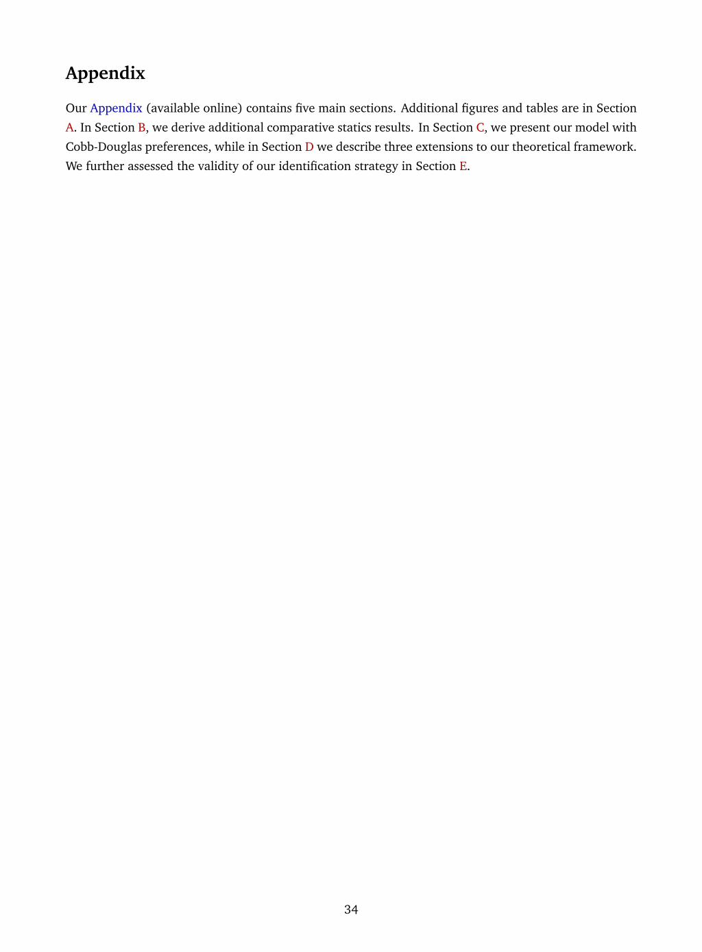
Appendix

Our Appendix (available online) contains five main sections. Additional figures and tables are in Section

A. In Section B, we derive additional comparative statics results. In Section C, we present our model with

Cobb-Douglas preferences, while in Section D we describe three extensions to our theoretical framework.

We further assessed the validity of our identification strategy in Section E.

34

References

ADAMS, A. AND A. ANDREW (2019): “Preferences and beliefs in the marriage market for young brides,”Tech. rep., IFS Working Papers. [2], [29]

AGÜERO, J. AND V. FRISANCHO (2017): “Misreporting in Sensitive Health Behaviors and Its Impact onTreatment Effects: An Application to Intimate Partner Violence,” . [18], [32]

AIZER, A. (2010): “The gender wage gap and domestic violence,” American Economic Review, 100, 1847–59. [4]

ALFANO, M. (2017): “Daughters, dowries, deliveries: The effect of marital payments on fertility choicesin India,” Journal of Development Economics, 125, 89–104. [1], [2], [4], [7], [8], [21], [32], [33]

ANDERBERG, D., N. MANTOVAN, AND R. M. SAUER (2018): “The dynamics of domestic violence: learningabout the match,” . [4]

ANDERBERG, D. AND H. RAINER (2013): “Economic abuse: A theory of intrahousehold sabotage,” Journalof Public Economics, 97, 282–295. [4]

ANDERSON, S. (2003): “Why dowry payments declined with modernization in Europe but are rising inIndia,” Journal of Political Economy, 111, 269–310. [1]

——— (2007): “The economics of dowry and brideprice,” Journal of Economic Perspectives, 21, 151–174.[1], [5]

ANDERSON, S. AND C. BIDNER (2015): “Property Rights Over Marital Transfers,” The Quarterly Journal ofEconomics, 130, 1421–1484. [1], [5]

ANDERSON, S., C. BIDNER, AND C. SADANIA (2020): “Marriage, Commitment and Unbundling GenderedNorms,” Unpublished Manuscript. [4]

ANDERSON, S. AND G. GENICOT (2015): “Suicide and Property Rights in India,” Journal of DevelopmentEconomics, 114, 64 – 78. [4], [20]

ANDERSON, S. AND D. RAY (2010): “Missing women: age and disease,” The Review of Economic Studies,77, 1262–1300. [5]

——— (2012): “The age distribution of missing women in India,” Economic and Political Weekly, 87–95.[5]

ANGELUCCI, M. (2008): “Love on the rocks: Domestic violence and alcohol abuse in rural Mexico,” TheBE Journal of Economic Analysis & Policy, 8. [4], [31]

ANGELUCCI, M. AND D. BENNETT (2019): “The Marriage Market for Lemons: HIV Testing and Marriagein Rural Malawi,” Unpublished Manuscript. [32]

ANUKRITI, S. (2018): “Financial incentives and the fertility-sex ratio trade-off,” American Economic Jour-nal: Applied Economics, 10, 27–57. [27]

ANUKRITI, S., S. R. BHALOTRA, AND E. H. F. TAM (2016): “On the quantity and quality of girls: Newevidence on abortion, fertility, and parental investments,” . [27]

ANUKRITI, S. AND S. DASGUPTA (2017): “Marriage markets in developing countries,” in The Oxford Hand-book of Women and the Economy. [10]

ANUKRITI, S., S. KWON, AND N. PRAKASH (2019): “Saving for Dowry: Evidence from Rural India,” Unpub-lished Manuscript. [2], [15], [29]

35

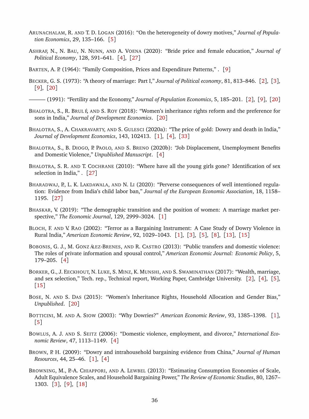
ARUNACHALAM, R. AND T. D. LOGAN (2016): “On the heterogeneity of dowry motives,” Journal of Popula-tion Economics, 29, 135–166. [5]

ASHRAF, N., N. BAU, N. NUNN, AND A. VOENA (2020): “Bride price and female education,” Journal ofPolitical Economy, 128, 591–641. [4], [27]

BARTEN, A. P. (1964): “Family Composition, Prices and Expenditure Patterns,” . [9]

BECKER, G. S. (1973): “A theory of marriage: Part I,” Journal of Political economy, 81, 813–846. [2], [3],[9], [20]

——— (1991): “Fertility and the Economy,” Journal of Population Economics, 5, 185–201. [2], [9], [20]

BHALOTRA, S., R. BRULÉ, AND S. ROY (2018): “Women’s inheritance rights reform and the preference forsons in India,” Journal of Development Economics. [20]

BHALOTRA, S., A. CHAKRAVARTY, AND S. GULESCI (2020a): “The price of gold: Dowry and death in India,”Journal of Development Economics, 143, 102413. [1], [4], [33]

BHALOTRA, S., B. DIOGO, P. PAOLO, AND S. BRENO (2020b): “Job Displacement, Unemployment Benefitsand Domestic Violence,” Unpublished Manuscript. [4]

BHALOTRA, S. R. AND T. COCHRANE (2010): “Where have all the young girls gone? Identification of sexselection in India,” . [27]

BHARADWAJ, P., L. K. LAKDAWALA, AND N. LI (2020): “Perverse consequences of well intentioned regula-tion: Evidence from India’s child labor ban,” Journal of the European Economic Association, 18, 1158–1195. [27]

BHASKAR, V. (2019): “The demographic transition and the position of women: A marriage market per-spective,” The Economic Journal, 129, 2999–3024. [1]

BLOCH, F. AND V. RAO (2002): “Terror as a Bargaining Instrument: A Case Study of Dowry Violence inRural India,” American Economic Review, 92, 1029–1043. [1], [3], [5], [8], [13], [15]

BOBONIS, G. J., M. GONZÁLEZ-BRENES, AND R. CASTRO (2013): “Public transfers and domestic violence:The roles of private information and spousal control,” American Economic Journal: Economic Policy, 5,179–205. [4]

BORKER, G., J. EECKHOUT, N. LUKE, S. MINZ, K. MUNSHI, AND S. SWAMINATHAN (2017): “Wealth, marriage,and sex selection,” Tech. rep., Technical report, Working Paper, Cambridge University. [2], [4], [5],[15]

BOSE, N. AND S. DAS (2015): “Women’s Inheritance Rights, Household Allocation and Gender Bias,”Unpublished. [20]

BOTTICINI, M. AND A. SIOW (2003): “Why Dowries?” American Economic Review, 93, 1385–1398. [1],[5]

BOWLUS, A. J. AND S. SEITZ (2006): “Domestic violence, employment, and divorce,” International Eco-nomic Review, 47, 1113–1149. [4]

BROWN, P. H. (2009): “Dowry and intrahousehold bargaining evidence from China,” Journal of HumanResources, 44, 25–46. [1], [4]

BROWNING, M., P.-A. CHIAPPORI, AND A. LEWBEL (2013): “Estimating Consumption Economies of Scale,Adult Equivalence Scales, and Household Bargaining Power,” The Review of Economic Studies, 80, 1267–1303. [3], [9], [18]

36

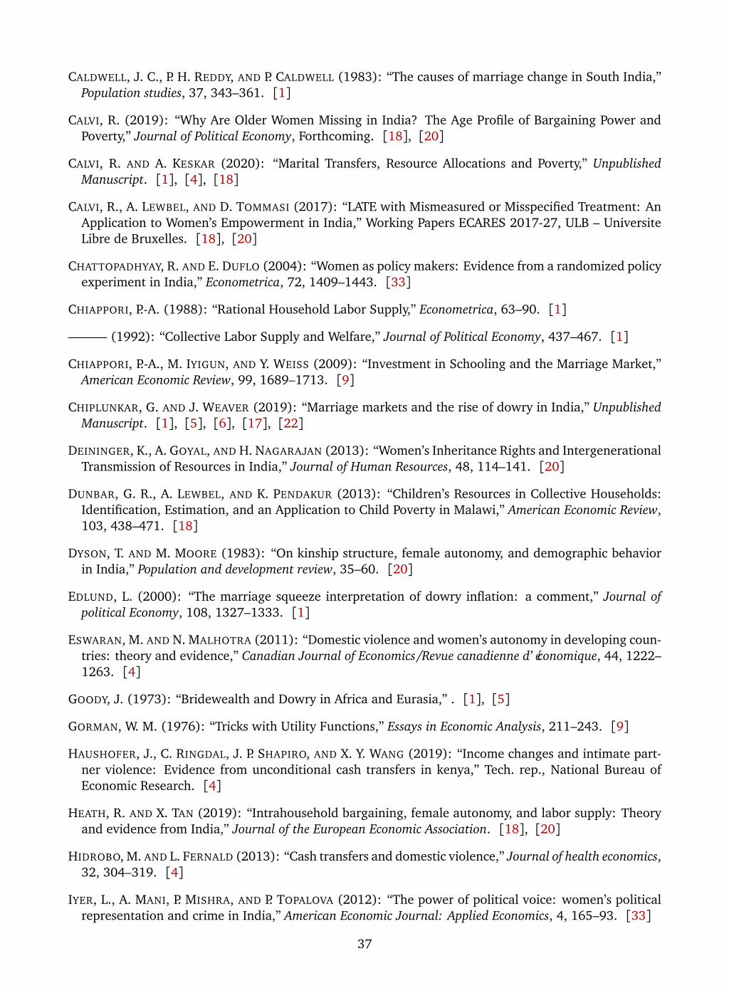
CALDWELL, J. C., P. H. REDDY, AND P. CALDWELL (1983): “The causes of marriage change in South India,”Population studies, 37, 343–361. [1]

CALVI, R. (2019): “Why Are Older Women Missing in India? The Age Profile of Bargaining Power andPoverty,” Journal of Political Economy, Forthcoming. [18], [20]

CALVI, R. AND A. KESKAR (2020): “Marital Transfers, Resource Allocations and Poverty,” UnpublishedManuscript. [1], [4], [18]

CALVI, R., A. LEWBEL, AND D. TOMMASI (2017): “LATE with Mismeasured or Misspecified Treatment: AnApplication to Women’s Empowerment in India,” Working Papers ECARES 2017-27, ULB – UniversiteLibre de Bruxelles. [18], [20]

CHATTOPADHYAY, R. AND E. DUFLO (2004): “Women as policy makers: Evidence from a randomized policyexperiment in India,” Econometrica, 72, 1409–1443. [33]

CHIAPPORI, P.-A. (1988): “Rational Household Labor Supply,” Econometrica, 63–90. [1]

——— (1992): “Collective Labor Supply and Welfare,” Journal of Political Economy, 437–467. [1]

CHIAPPORI, P.-A., M. IYIGUN, AND Y. WEISS (2009): “Investment in Schooling and the Marriage Market,”American Economic Review, 99, 1689–1713. [9]

CHIPLUNKAR, G. AND J. WEAVER (2019): “Marriage markets and the rise of dowry in India,” UnpublishedManuscript. [1], [5], [6], [17], [22]

DEININGER, K., A. GOYAL, AND H. NAGARAJAN (2013): “Women’s Inheritance Rights and IntergenerationalTransmission of Resources in India,” Journal of Human Resources, 48, 114–141. [20]

DUNBAR, G. R., A. LEWBEL, AND K. PENDAKUR (2013): “Children’s Resources in Collective Households:Identification, Estimation, and an Application to Child Poverty in Malawi,” American Economic Review,103, 438–471. [18]

DYSON, T. AND M. MOORE (1983): “On kinship structure, female autonomy, and demographic behaviorin India,” Population and development review, 35–60. [20]

EDLUND, L. (2000): “The marriage squeeze interpretation of dowry inflation: a comment,” Journal ofpolitical Economy, 108, 1327–1333. [1]

ESWARAN, M. AND N. MALHOTRA (2011): “Domestic violence and women’s autonomy in developing coun-tries: theory and evidence,” Canadian Journal of Economics/Revue canadienne d’économique, 44, 1222–1263. [4]

GOODY, J. (1973): “Bridewealth and Dowry in Africa and Eurasia,” . [1], [5]

GORMAN, W. M. (1976): “Tricks with Utility Functions,” Essays in Economic Analysis, 211–243. [9]

HAUSHOFER, J., C. RINGDAL, J. P. SHAPIRO, AND X. Y. WANG (2019): “Income changes and intimate part-ner violence: Evidence from unconditional cash transfers in kenya,” Tech. rep., National Bureau ofEconomic Research. [4]

HEATH, R. AND X. TAN (2019): “Intrahousehold bargaining, female autonomy, and labor supply: Theoryand evidence from India,” Journal of the European Economic Association. [18], [20]

HIDROBO, M. AND L. FERNALD (2013): “Cash transfers and domestic violence,” Journal of health economics,32, 304–319. [4]

IYER, L., A. MANI, P. MISHRA, AND P. TOPALOVA (2012): “The power of political voice: women’s politicalrepresentation and crime in India,” American Economic Journal: Applied Economics, 4, 165–93. [33]

37

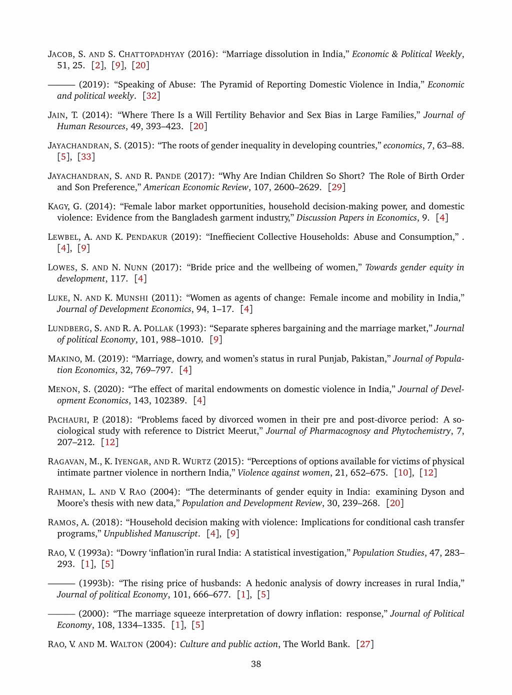
JACOB, S. AND S. CHATTOPADHYAY (2016): “Marriage dissolution in India,” Economic & Political Weekly,51, 25. [2], [9], [20]

——— (2019): “Speaking of Abuse: The Pyramid of Reporting Domestic Violence in India,” Economicand political weekly. [32]

JAIN, T. (2014): “Where There Is a Will Fertility Behavior and Sex Bias in Large Families,” Journal ofHuman Resources, 49, 393–423. [20]

JAYACHANDRAN, S. (2015): “The roots of gender inequality in developing countries,” economics, 7, 63–88.[5], [33]

JAYACHANDRAN, S. AND R. PANDE (2017): “Why Are Indian Children So Short? The Role of Birth Orderand Son Preference,” American Economic Review, 107, 2600–2629. [29]

KAGY, G. (2014): “Female labor market opportunities, household decision-making power, and domesticviolence: Evidence from the Bangladesh garment industry,” Discussion Papers in Economics, 9. [4]

LEWBEL, A. AND K. PENDAKUR (2019): “Ineffiecient Collective Households: Abuse and Consumption,” .[4], [9]

LOWES, S. AND N. NUNN (2017): “Bride price and the wellbeing of women,” Towards gender equity indevelopment, 117. [4]

LUKE, N. AND K. MUNSHI (2011): “Women as agents of change: Female income and mobility in India,”Journal of Development Economics, 94, 1–17. [4]

LUNDBERG, S. AND R. A. POLLAK (1993): “Separate spheres bargaining and the marriage market,” Journalof political Economy, 101, 988–1010. [9]

MAKINO, M. (2019): “Marriage, dowry, and women’s status in rural Punjab, Pakistan,” Journal of Popula-tion Economics, 32, 769–797. [4]

MENON, S. (2020): “The effect of marital endowments on domestic violence in India,” Journal of Devel-opment Economics, 143, 102389. [4]

PACHAURI, P. (2018): “Problems faced by divorced women in their pre and post-divorce period: A so-ciological study with reference to District Meerut,” Journal of Pharmacognosy and Phytochemistry, 7,207–212. [12]

RAGAVAN, M., K. IYENGAR, AND R. WURTZ (2015): “Perceptions of options available for victims of physicalintimate partner violence in northern India,” Violence against women, 21, 652–675. [10], [12]

RAHMAN, L. AND V. RAO (2004): “The determinants of gender equity in India: examining Dyson andMoore’s thesis with new data,” Population and Development Review, 30, 239–268. [20]

RAMOS, A. (2018): “Household decision making with violence: Implications for conditional cash transferprograms,” Unpublished Manuscript. [4], [9]

RAO, V. (1993a): “Dowry ‘inflation’in rural India: A statistical investigation,” Population Studies, 47, 283–293. [1], [5]

——— (1993b): “The rising price of husbands: A hedonic analysis of dowry increases in rural India,”Journal of political Economy, 101, 666–677. [1], [5]

——— (2000): “The marriage squeeze interpretation of dowry inflation: response,” Journal of PoliticalEconomy, 108, 1334–1335. [1], [5]

RAO, V. AND M. WALTON (2004): Culture and public action, The World Bank. [27]

38

ROMANO, J. P. AND M. WOLF (2005a): “Exact and approximate stepdown methods for multiple hypothesistesting,” Journal of the American Statistical Association, 100, 94–108. [19]

——— (2005b): “Stepwise multiple testing as formalized data snooping,” Econometrica, 73, 1237–1282.[19]

——— (2016): “Efficient computation of adjusted p-values for resampling-based stepdown multiple test-ing,” Statistics & Probability Letters, 113, 38–40. [19]

ROY, S. (2015): “Empowering women? Inheritance rights, female education and dowry payments inIndia,” Journal of Development Economics, 114, 233–251. [20]

SEKHRI, S. AND A. STOREYGARD (2014): “Dowry deaths: Response to weather variability in India,” Journalof development economics, 111, 212–223. [5]

SEN, A. (1990): “More than 100 million women are missing,” The New York Review of Books, 37, 61–66.[5]

——— (1992): “Missing Women,” BMJ: British Medical Journal, 304, 587. [5]

SHARMA, B. (2011): “Mental and Emotional Impact of Divorce on Women,” Journal of the Indian Academyof Applied Psychology, 37, 125–31. [12]

SRINIVAS, M. N. (1984): Some Reflections on Dowry, 1983, Centre for Women’s Development Studies, NewDelhi. [5]

SRINIVASAN, S. AND A. S. BEDI (2007): “Domestic violence and dowry: Evidence from a South Indianvillage,” World Development, 35, 857–880. [1], [3], [5]

TAUCHEN, H. V., A. D. WITTE, AND S. K. LONG (1991): “Domestic violence: A nonrandom affair,” Interna-tional Economic Review, 491–511. [4]

UNODC (2018): Global Study on Homicide 2018, United Nations Office on Drugs and Crime (UNODC).[5]

VOGL, T. S. (2013): “Marriage institutions and sibling competition: Evidence from South Asia,” The Quar-terly journal of economics, 128, 1017–1072. [10]

ZHANG, J. AND W. CHAN (1999): “Dowry and Wife’s Welfare: A Theotrical and Empirical Analysis,” Journalof Political Economy, 107, 786–808. [1], [4], [5]

39