Prepared for submission to JHEP

Three Avatars of Mock Modularity

Atish Dabholkar and Pavel Putrov

International Centre for Theoretical PhysicsStrada Costiera 11, Trieste 34151 Italy

Abstract: Mock theta functions were introduced by Ramanujan in 1920 but a proper under-standing of mock modularity has emerged only recently with the work of Zwegers in 2002. Inthese lectures we describe three manifestations of this apparently exotic mathematics in threeimportant physical contexts of holography, topology and duality where mock modularity hascome to play an important role.

Lectures delivered at 2020 ICTP Online Summer School on String Theory and Related Topics

arX

iv:2

110.

0979

0v1

[he

p-th

] 1

9 O

ct 2

021

Contents

1 Introduction 1

2 Modular Forms 22.1 Definitions 22.2 The Ring of Modular Forms 3

3 Jacobi Forms 43.1 Definitions 53.2 Theta Expansion 63.3 The Ring of Jacobi Forms 6

4 Modularity in Physics 74.1 Topology 74.2 Duality 84.3 Holography 9

5 Mock Modular Forms 105.1 Definitions 105.2 Examples 11

6 Mock Jacobi Forms 116.1 Definitions 126.2 Example 12

7 Black Holes and Mock Modularity 137.1 Black Holes, Poles, and Walls 147.2 Multi-Centered Black Holes and the Appel-Lerch Sum 147.3 The Decomposition Theorem 15

8 Topology and Mock Modularity 168.1 Witten Index 168.2 Noncompact Witten Index 17

9 Holomorphic Anomaly in Gauge Theories 199.1 Vafa-Witten Partition Function 199.2 M-theory Realization 219.3 The su(2) theory on the tensor branch 23

– i –

10 Path integral derivation of holomorphic anomaly 2410.1 Reversing the order of compactification 2410.2 Review of 2d N = (0, 1) sigma-models 2710.3 Holomorphic anomaly for CP2 29

A Solutions 31

1 Introduction

In Ramanujan’s famous last letter to Hardy in 1920, he gave 17 examples (without any defini-tion) of mock theta functions that he found very interesting [1]. For example,

f(τ) = −q−25/168

∞∑n=1

qn2

(1− qn) . . . (1− q2n−1)(q := e2πiτ ) . (1.1)

This function may seem unremarkable to the uninitiated, but Ramanujan had reasons to believethat it was very similar to an ordinary theta function with hints of a ‘mock’ or ‘hidden’ symmetryunder the modular group SL(2,Z).

Despite much work by many eminent mathematicians, this fascinating mock modular sym-metry remained mysterious for a century until the thesis of Zwegers in 2002 [2, 3]. As we willsee, the essence of mock modularity is an incompatibility between holomorphy and modular-ity. For example, the function f(τ) above, which is holomorphic in τ , has no obvious modularproperties. However, it is possible to add to it a non-holomorphic ‘correction’ term such thatthe sum is indeed modular but at the expense of being nonholomorphic. One can either havemodularity or holomorphy but not both.

It is useful to keep a geometric analogy in mind. The property of being modular can belikened to being circular. A modular form is a function with high degree of symmetry underthe modular group SL(2,Z) much like a circle which is a geometric figure with a high degreeof symmetry under the rotation group O(2). Similarly, the property of being holomorphic canbe likened to the property of being blue. In this analogy, a holomorphic mock modular form islike a blue geometric figure which is not circular but can be made circular by adding a non-bluepiece to it. One can either have circularity or blueness but not both.

Even though mock modular forms have a rich and interesting mathematical history, it wasnot clear if this exotic mathematics has any relevance to physics. A marvelous essay titled ‘Awalk through Ramanujan’s Garden’ by Freeman Dyson [4] on the occasion of the RamanujanCentenary Conference in 1987 gives a glimpse of the history of these intriguing functions andends with a prescient remark about possible physics applications:

“My dream is that I will live to see the day when our young physicists, struggling to bringthe predictions of superstring theory into correspondence with the facts of nature, will be led toenlarge their analytic machinery to include not only theta-functions but mock theta-functions . . .

– 1 –

But before this can happen, the purely mathematical exploration of the mock-modular forms andtheir mock-symmetries must be carried a great deal further.”

True to the hope expressed by Dyson, over the past decade, mock modular forms havemade their appearance in diverse physical contexts connecting to deep and important physicalconcepts such as holography and duality even if not directly to facts of nature. The purposeof these lectures is to introduce the basic notions about mock modular forms and then outlinetheir applications in three physical contexts: supersymmetric sigma models with non-compacttarget, counting of black hole degeneracies, and 4-dimensional Vafa-Witten topological gaugetheory. We leave uncovered some other topics where mock modularity plays an important role,in particular, umbral moonshine [5] and quantum 3-manifold invariants [6–8]. For other reviewsof applications of (mock) modularity see for example [9, 10].

2 Modular Forms

We first review modular and Jacobi forms and their appearance in the context of black holephysics and holography, topology, and duality. For more details see [11]

2.1 Definitions

Let IH be the upper half plane, i.e., the set of complex numbers τ whose imaginary part

satisfies Im(τ) > 0. Let SL(2,Z) be the group of matrices(a b

c d

)with integer entries such that

ad− bc = 1.A modular form f(τ) of weight k on SL(2,Z) is a holomorphic function on IH that trans-

forms as

(cτ + d)−kf(aτ + b

cτ + d) = f(τ) ∀

(a b

c d

)∈ SL(2,Z) (2.1)

for an integer k (necessarily even if f 6≡ 0) and is bounded as Im(τ)→∞. It follows from thedefinition that f(τ) is periodic under τ → τ + 1 and can be written as a Fourier series

f(τ) =∞∑n=0

a(n) qn(q := e2πiτ

). (2.2)

A holomorphic modular form must have non-negative weight (strictly positive weight if theform is not a constant).

If a(0) = 0, then the modular form vanishes at infinity and is called a cusp form. Inthe other direction, one may weaken the growth condition as Im(τ) → ∞ from f(τ) = O(1)

to f(τ) = O(q−N) for some N ≥ 0; then f has a Fourier expansion containing finitely manynegative powers of q. Such a function is called a weakly holomorphic modular form. The weightof weakly holomorphic modular forms can be negative.

We denote the vector space over C of holomorphic modular forms of weight k on SL(2,Z)

by Mk, while the space of cusp forms of weight k and the space of weakly holomorphic modular

– 2 –

forms of weight k are denoted by Sk and M !k respectively. We thus have the inclusions

Sk ⊆Mk ⊂ M !k , (2.3)

The growth condition at Im(τ) → ∞ is related to the growth properties of the Fourier coeffi-cients a(n) as n→∞:

f ∈ Sk ⇒ an = O(nk/2) as n→∞ ; (2.4)

f ∈Mk ⇒ an = O(nk−1) as n→∞ ; (2.5)

f ∈M !k ⇒ an = O(eC

√n) as n→∞ (2.6)

The exponential growth of a(n) for f ∈M !k can be recognized as the Cardy formula in conformal

field theory as we explain below in an example.

2.2 The Ring of Modular Forms

It is clear from the definition that the product f1(τ)f2(τ) of two modular forms f1(τ) and f2(τ)

of weights k1 and k2 respectively is also a modular form of weight k1 +k2. With these operationof usual pointwise addition and multiplication, modular forms form a ring. An importanttheorem in the theory of modular forms states that the ring of (holomorphic) modular forms isgenerated by the two Eisenstein series E4(τ) and E6(τ) defined by

E4(τ) = 1 + 240∞∑n=1

n3qn

1− qn= 1 + 240q + 2160q2 + · · · , (2.7)

E6(τ) = 1 − 504∞∑n=1

n5qn

1− qn= 1− 504q − 16632q2 − · · · . (2.8)

In other words, any holomorphic modular form can be expressed as a linear combination ofproducts of E4 and E6 of appropriate weight.

This important theorem reveals the power of modularity. A priori, to determine an arbitrarytranslation invariant function, one needs to know all its infinite Fourier coefficients a(n) inthe q-expansion (2.2). Thanks to the theorem stated above, for a modular form, it suffices toknow just the first few Fourier coefficients which can be determined by comparison with (2.7).For example, a weight 12 modular form must be a linear combination of the form

f12(τ) = aE34(τ) + bE2

6(τ) , (2.9)

for some numerical complex coefficients a and b which can be readily determined knowing thefirst two Fourier coefficients.

Exercise 1. Show that (up to normalization) there is a unique cusp form of weight 12 andexpress it in terms of E4 and E6. This is an important example of a cusp form known as thediscriminant function and denoted by ∆(τ).

– 3 –

The cusp form ∆(τ) admits a product representation:

∆(τ) := q∞∏n=1

(1− qn)24 = q − 24q2 + 252q3 + · · · (2.10)

The Fourier coefficients of the discriminant function, usually denoted by τ(n), play an importantin number theory. Because ∆(τ) is a cusp form, τ(n) grow very slowly as n→∞.

In physics applications, one encounters not the cusp form but rather its inverse

1

∆(τ)=

1

η(τ)24:=

∞∑n=−1

d(n)qn (2.11)

where

η(τ) = q124

∞∏n=1

(1− qn) (2.12)

is the Dedekind η function. This inverse of the cusp form is clearly a weakly holomorphicmodular form, and arises, for example, as the partition function of 24 left-moving bosons of thelight-cone bosonic string. In number theory, the partition function above is well-known in thecontext of the problem of partitions of integers. One can identify

d(n) = p24(n+ 1) (n ≥ 0) . (2.13)

where p24(I) is the number of colored partitions of a positive integer I using integers of 24 dif-ferent colors, which is the same combinatoric problem of dividing energy I among 24 transverseoscillators. Now, the Fourier coefficients grow exponentially in accordance with (2.4)

d(n) ∼ exp[4π√n] , (2.14)

and is related to the Cardy formula

d(n) ∼ exp

[2π

√nc

6

](2.15)

with c = 24 which the central charge of 24 left-moving bosons.

3 Jacobi Forms

Jacobi forms are functions of two variables τ and z that transform nicely under the Jacobitransformations as defined below. One can regard τ as the complex-structure parameter ofa 2-torus obtained by modding a complex plane with coordinate z by the lattice of pointsz = λτ + µ for all λ, µ ∈ Z. The Jacobi group is the group of Jacobi transformations as belowgenerated by the modular transformations as well as the translations of z by lattice shifts.

– 4 –

3.1 Definitions

Consider a holomorphic function ϕ(τ, z) from IH×C to C which is “modular in τ and elliptic inz” in the sense that it transforms under the modular group as

ϕ(aτ + b

cτ + d,

z

cτ + d

)= (cτ + d)k e

2πimcz2

cτ+d ϕ(τ, z) ∀( a bc d

)∈ SL(2,Z) (3.1)

and under the translations of z by Zτ + Z as

ϕ(τ, z + λτ + µ) = e−2πim(λ2τ+2λz)ϕ(τ, z) ∀ λ, µ ∈ Z , (3.2)

where k is an integer and m is a positive integer.These equations include the periodicities ϕ(τ + 1, z) = ϕ(τ, z) and ϕ(τ, z + 1) = ϕ(τ, z), so

ϕ has a Fourier expansion

ϕ(τ, z) =∑n,r

c(n, r) qn yr , (q := e2πiτ , y := e2πiz) . (3.3)

Equation (3.2) is then equivalent to the periodicity property

c(n, r) = C(4nm− r2, r) , where C(∆, r) depends only on r mod 2m . (3.4)

The function ϕ(τ, z) is called a holomorphic Jacobi form (or simply a Jacobi form) of weightk and index m if the coefficients C(∆, r) vanish for ∆ < 0, i.e. if

c(n, r) = 0 unless 4mn ≥ r2 . (3.5)

It is called a Jacobi cusp form if it satisfies the stronger condition that C(∆, r) vanishes unless∆ is strictly positive, i.e.

c(n, r) = 0 unless 4mn > r2 , (3.6)

and it is called a weak Jacobi form if it satisfies the weaker condition

c(n, r) = 0 unless n ≥ 0 (3.7)

rather than (3.5), whereas a merely weakly holomorphic Jacobi form satisfies only the yet weakercondition that c(n, r) = 0 unless n ≥ n0 for some possibly negative integer n0 (or equivalentlyC(∆, r) = 0 unless ∆ ≥ ∆0 for some possibly negative integer ∆0).

Finally, the quantity ∆ = 4mn− r2, which by virtue of the above discussion is the crucialinvariant of a monomial qnyr occurring in the Fourier expansion of ϕ, will be referred to as itsdiscriminant (not to be confused with the discriminant function (2.10) introduced earlier).

– 5 –

3.2 Theta Expansion

If ϕ(τ, z) is a Jacobi form, then the transformation property (3.2) implies its Fourier expansionwith respect to z has the form

ϕ(τ, z) =∑`∈Z

q`2/4m h`(τ) e2πi`z (3.8)

where h`(τ) is periodic in ` with period 2m. In terms of the coefficients (3.4) we have

h`(τ) =∑

∆

C(∆, `) q∆/4m (`∈Z/2mZ) . (3.9)

Because of the periodicity property, equation (3.8) can be rewritten in the form

ϕ(τ, z) =∑

`∈Z/2mZ

h`(τ)ϑm,`(τ, z) , (3.10)

where ϑm,`(τ, z) denotes the standard index m theta function

ϑm,`(τ, z) :=∑n∈Z

q(`+2mn)2/4m y`+2mn (3.11)

(which is a Jacobi form of weight 12and index m on some subgroup of SL(2,Z)). This is called

the theta expansion of ϕ. The coefficiens h`(τ) are modular forms of weight k− 12and are weakly

holomorphic, holomorphic or cuspidal if ϕ is a weak Jacobi form, a Jacobi form or a Jacobi cuspform, respectively. More precisely, the vector h := (h1, . . . , h2m) transforms like a modular formof weight k− 1

2under SL(2,Z). Jacobi forms, which are functions are two complex variables τ

and z are thus equivalent to vector valued modular forms of a single complex variable τ .

3.3 The Ring of Jacobi Forms

Consider the two Jacobi forms defined below

A(τ, z) =ϑ21(τ,z)

η6(τ)(k = −2 , m = 1) (3.12)

B(τ, z) = 8(ϑ22(τ,z)

ϑ22(τ)+

ϑ22(τ,z)

ϑ22(τ)+

ϑ22(τ,z)

ϑ22(τ)

)(k = 0 , m = 1) (3.13)

where ϑi(τ, z) are the Jacobi theta functions. The ring of Jacobi forms of weight k and indexm is generated by these two Jacobi forms with ordinary modular forms as coefficients. Indexand weight both add when you multiply Jacobi forms and modular forms. Thus, as in the caseof modular forms, a Jacobi form can be determined by knowing its weight and index and firstfew Fourier coefficients. For example, the most general holomorphic Jacobi form of weight 4

and index 2 must be of the form

aE24(τ)A2(τ, z) + bE6(τ)A(τ, z)B(τ, z) + cE4(τ)B2(τ, z) (3.14)

and hence is completely fixed by determining the three constants a, b, c.

– 6 –

4 Modularity in Physics

The modular group SL(2,Z) appears in physics in many different contexts as a physical symme-try. The most familiar occurrence is in conformal field theory. The modular group of a two-torusis the group of global diffeomorphisms of the 2-torus modulo the Weyl group. If one uses acoordinate invariant regulator then the path integral for the sigma model on a two-dimensionaltorus is diffeomorphism invariant. For a conformal sigma model it also Weyl invariant. Hencethe path integral of a conformal field theory on a 2-torus is expected to be SL(2,Z)-invariant.It is thus natural that modular forms, which transform nicely under this symmetry, have cometo play an important role in physics. We focus on the following three contexts.

4.1 Topology

In general, the partition function of a conformal field theory will be a function of both τ andτ . However, certain indexed partition functions, which capture a topological subsector of thetheory are functions of τ alone and are thus holomorphic by an argument due to Witten thatwe outline in §8.1.

Consider a conformally invariant nonlinear sigma model with target space M with (2, 2)

superconformal symmetry with left and right super Virasoro algebra and central charge 6m

both for the left-movers and the right-movers. There is a U(1)L × U(1)R R-symmetry ofthe superconformal algebra. The U(1)L symmetry (and similarly the U(1)R symmetry ) isanomalous with anomaly coefficient m which by supersymmetry is related to the conformalanomaly governed by the central charge 6m. Let FR and FL be the charges associated with thissymmetry. One can then define the elliptic genus as the following indexed partition function:

χ(τ, z|M) = Tr (−1)FR+FL e2πiτHL e−2πiτHR e2πizFL . (4.1)

Elliptic genus thus defined is a Jacobi form weight 0 and index m. As argued above, it ismodular invariant and hence has modular weight zero. The (2, 2) superconformal algebra has anadditional symmetry called the spectral flow symmetry. If one bosonizes the left-moving U(1)Lcurrent, then the spectral flow symmetry corresponds to the shifts of this boson. Consequently,the path integral is elliptic with index m related to the anomaly in the U(1)L symmetry.Because, the R-symmetry acts on fermions alone, (−1)FR can be identified with the right-moving fermion number. The indexed partition function defined above can thus be thought ofas the Witten index for the right-moving sector that counts right-moving ground states whichis a topological quantity called the elliptic genus.

The Fourier coefficients of the elliptic genus correspond the Dirac indices of an infinityfamily of Dirac-like (elliptic) operators. Jacobi forms thus appear naturally in topology in thecontext of elliptic genera of manifolds.

Exercise 2. Show that the modified elliptic genus of T 4 equals A(τ, z).

Exercise 3. Show that the elliptic genus of K3 equals B(τ, z).

– 7 –

4.2 Duality

The hypothesis of S-duality asserts that N = 4 super Yang-Mills theory is invariant under theaction of a large duality group (SL(2,Z) or a close relative, depending on the four-dimensionalgauge group G) acting on τ ≡ τ1 + iτ2 = θ/2π+4πi/g2; here g and θ are the gauge coupling andtheta angle; τ1 and τ2 denote the real and imaginary parts of τ . But S-duality is hard to test,because computations for strong coupling are difficult. One way to circumvent this difficultyis to consider a topologically twisted version of the theory in which localization can be used toperform computations for strong coupling.

A twist of particular interest is the Vafa-Witten twist introduced in [12]. With this twist-ing, a formal argument shows that the partition function on a compact four-manifold M4 isholomorphic in τ or equivalently in q = exp(2πiτ). Furthermore, if a certain curvature condi-tion (eqn. (2.58) in [12]) is satisfied, the evaluation of the path integral can formally be arguedto localize on the contribution of ordinary Yang-Mills instantons. The contribution to the pathintegral from the component of field space with instanton number1 n is then anq

n, where anis the Euler characteristic of the instanton number n moduli space Mn. Thus the partitionfunction after summing over bundles of all values of the instanton number is expected to be

Z =∑n

anqn. (4.2)

The relevant curvature condition is highly restrictive, but there are a number of four-manifolds that satisfy this condition and for which computations of the an were available in themathematical literature [13, 14]. In particular, two important examples that we consider hereare a K3 surface and CP2.

A four-dimensional gauge theory arises naturally as the low-energy worldvolume theoryof N conincident D3-branes. In the Euclidean version one can consider Euclidean D3-braneswrapping a four-manifold M4. In the D-brane picture, instantons in the gauge theory corre-spond to D-instantons bound to the D3-branes. The Vafa-Witten partition function counts thenumber of such bound states. By T-duality in directions transverse to the branes, this is thesame the number of D0-D4 or D1-D5 bound states which we will encounter in the context ofblack hole microstates.

In the simplest context of a single Euclidean D3 brane wrapping a K3 with m+1 point-likeinstantons2, one can heuristically think of them as m + 1 point particles moving on K3. Theindexed partition function for each particle gives simply the ground states of the supersymmetricquantum mechanics of a super particle with K3 as the target, which is nothing but Euler

1Here n is an integer for a simply-connected gauge group such as G = SU(2), but may have a fractionalpart if G is not simply-connected. The fractional part is determined by a two-dimensional cohomology class(for example, by the second Stieffel-Whitney class w2 if G = SO(3)), and in the partition function

∑n anq

n, itis natural to sum over all bundles keeping this class fixed. The values of n in the sum are then congruent toeach other mod Z. A restriction on w2 (and its analog for other groups) is assumed in eqn. (4.2).

2In a U(1) gauge theory the instantons are singular but one can turn on a noncommmutativy parameter tomake the problem better defined

– 8 –

characteristic of K3 which is 24. The (m+ 1) superparticles on K3 can be treated as identicalbosonic particles and thus have as the target space symmetrized product of (m + 1) copies ofK3. The indexed partition function which gives the coefficients am+1 thus equal the orbifoldEuler character χ(Symm+1(K3)) of the symmetric product of (m+ 1) copies of K3-surface [12].The generating function for the orbifold Euler character

Z(σ) =∞∑

m=−1

χ(Symm+1(K3)) pm(p := e2πiσ

)(4.3)

can be thought of the grand-canonical partition function for this quantum mechanical systemof m + 1 identical bosons with fugacity p. This can be readily evaluated using Bose-Einsteindistribution knowing the single-particle degenercies to obtain to obtain

Z(σ) =1

p

∞∏n=1

1

(1− pn)24. (4.4)

This is a modular form of weight −12, in fact the inverse of the cusp form that we haveencountered earlier. Its modular properties are a consequence of S-duality of the gauge theoryliving on the D-brane worldvolume.

Note that this partition function is the same as the one we encountered for 24 left-movingbosons of the heterotic string. This is not an accident. The heterotic string on a 4-torus T 4 isdual to Type-IIA string on K3 Duality requires that the number of BPS-states of a given chargemust equal the number of BPS-states with the dual charge. The equality of the two partitionfunctions (2.11) and (4.4) coming from two very different counting problems is consistent withthis expectation. This fact was indeed one of the early indications of a possible duality betweenheterotic and Type-II strings [12].

4.3 Holography

In AdS3 quantum gravity, the modular group SL(2,Z) is the group of global diffeomorphismsof the boundary. Quantum string theory in AdS3 background is expected to be dual to a sigmamodel living on the boundary.

A well-studied special case of this duality is in the context of Type-IIB string theory com-pactified on K3× S1. Consider Q5 D5-branes wrapping K3× S1 and Q1 D1-branes wrappingS1 with Q1Q5 ≡ m. The near horizon geometry of this brane system is AdS3 × S3 ×K3. Thesigma model dual to this theory has as target space symmetric product of m+ 1 copies of K3

defines a (2, 2) superconformal symmetry (actually it has a larger (4, 4) symmetry but that isnot relevant to our discussion) with left and right moving central charges 6(m+ 1). The ellipticgenus defined as above

χ(τ, z|Symm+1 K3) , (4.5)

gives the indexed partition function of this boundary theory is a generalization of the Eulercharacteristic of symmetrized product that we encountered earlier. By general arguments re-viewed earlier, this elliptic genus is a weak Jacobi form of weight 0 and index m+1. Henceforth

– 9 –

we will denote it simply by χm+1(τ, z). We thus see that Jacobi forms appear naturally in thecontext of AdS3/CFT2 holographic duality.

5 Mock Modular Forms

We now review mock modular and mock Jacobi forms.

5.1 Definitions

We define a (weakly holomorphic) pure mock modular form of weight k ∈ 12Z as the first member

of a pair (h, g), where

1. h is a holomorphic function in IH with at most exponential growth at all cusps,

2. the function g(τ), called the shadow of f , is a holomorphic3 modular form of weight 2−k ,and

3. the sum h := h+ g∗, called the completion of f , transforms like a holomorphic modularform of weight k, i.e. h(τ)/θ(τ)2k is invariant under τ → γτ for all τ ∈ IH and for all γin some congruence subgroup of SL(2,Z).

Here g∗(τ), called the non-holomorphic Eichler integral, is a solution of the differential equation

(4πτ2)k∂g∗(τ)

∂τ= −2πi g(τ) . (5.1)

If g has the Fourier expansion g(τ) =∑

n≥0 bn qn, we fix the choice of g∗ by setting

g∗(τ) = b0(4πτ2)−k+1

k − 1+∑n>0

nk−1 bn Γ(1− k, 4πnτ2) q−n , (5.2)

where τ2 = Im(τ) and

Γ(1− k, x) =

∫ ∞x

t−k e−t dt (5.3)

denotes the incomplete gamma function.Note that the series in (5.2) converges despite the exponentially large factor q−n because

Γ(1− k, x) = O(x−ke−x) . If we assume either that k > 1 or that b0 = 0, then we can define g∗

alternatively by the integral

g∗(τ) =

(i

2π

)k−1∫ ∞−τ

(z + τ)−k g(−z) dz . (5.4)

3One can also consider the case where the shadow is allowed to be a weakly holomorphic modular form, butwe do not do this since none of our examples will be of this type.

– 10 –

(The integral is independent of the path chosen because the integrand is holomorphic in z.)Since h is holomorphic, (5.1) implies that the completion of h is related to its shadow by

(4πτ2)k∂h(τ)

∂τ= −2πi g(τ) . (5.5)

This ‘holomorphic anomaly equation’ captures the failure of holomorphy of the completion ofthe mock modular form, which is modular but not holomorphic.

If one multiplies the mock modular form by a holomorphic modular form f(τ) of weight k′

the holomorphic anomaly equation above simply gets multiplied by f(τ) on both sides. Onethus gets a mixed mock modular form f(τ)h(τ) of weight k+ k′ with completion f(τ)h(τ) anda mixed shadow f(τ)g(τ) that is a product of a holomorphic and anti-holomorphic piece.

5.2 Examples

Apart from the examples introduced by Ramanujan, a particularly interesting example is theZagier mock modular form which will play a role in our later discussions. The Fourier coefficientsof this mock modular form give the Hurwitz-Kronecker class numbers, denoted by H(N) forN ∈ Z.

These class numbers are defined for N > 0 as the number of PSL(2,Z)-equivalence classesof integral binary quadratic forms of discriminant −N , weighted by the reciprocal of the numberof their automorphisms (if −N is the discriminant of an imaginary quadratic field K other thanQ(i) or Q(

√−3), this is just the class number ofK), and for other values of N by H(0) = −1/12

and H(N) = 0 for N < 0. These numbers vanish unless N is 0 or −1 modulo 4.The Zagier mock modular form [15] is the generating function for these class numbers:

H(τ) :=∞∑N=0

H(N) qN = − 1

12+

1

3q3 +

1

2q4 + q7 + q8 + q11 + · · · (5.6)

It is a ‘pure mock modular form’ of weight 3/2 on Γ0(4) and shadow the classical theta functionϑ(τ) =

∑qn

2 . See [3, 16] for the definition and further discussion. We see from the q-expansionof H(τ) that it has no poles at q = 0 and hence is strongly holomorphic. Consequently, itsFourier coefficients grow very slowly. This is exceptional. In fact, up to minor variationsthe Zagier mock modular form is essentially the only known non-trivial example of a stronglyholomorphic pure mock modular form.

6 Mock Jacobi Forms

A mock Jacobi form is a new mathematical object defined in [16] as a mock generalizationof a Jacobi form. It has the same elliptic symmetry properties as a Jacobi form and hencedoes admit a theta expansion using this symmetry. However, the theta-coefficients are notvector-valued modular forms but rather vector-valued mock modular forms.

– 11 –

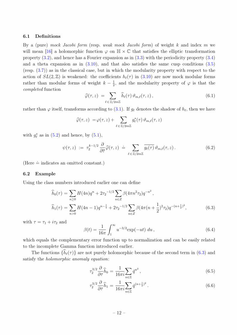
6.1 Definitions

By a (pure) mock Jacobi form (resp. weak mock Jacobi form) of weight k and index m wewill mean [16] a holomorphic function ϕ on H × C that satisfies the elliptic transformationproperty (3.2), and hence has a Fourier expansion as in (3.3) with the periodicity property (3.4)and a theta expansion as in (3.10), and that also satisfies the same cusp conditions (3.5)(resp. (3.7)) as in the classical case, but in which the modularity property with respect to theaction of SL(2,Z) is weakened: the coefficients h`(τ) in (3.10) are now mock modular formsrather than modular forms of weight k − 1

2, and the modularity property of ϕ is that the

completed functionϕ(τ, z) =

∑`∈Z/2mZ

h`(τ)ϑm,`(τ, z) , (6.1)

rather than ϕ itself, transforms according to (3.1). If g` denotes the shadow of h`, then we have

ϕ(τ, z) =ϕ(τ, z) +∑

`∈Z/2mZ

g∗` (τ)ϑm,`(τ, z)

with g∗` as in (5.2) and hence, by (5.1),

ψ(τ, z) := τk−1/22

∂

∂τϕ(τ, z)

.=

∑`∈Z/2mZ

g`(τ)ϑm,`(τ, z) . (6.2)

(Here .= indicates an omitted constant.)

6.2 Example

Using the class numbers introduced earlier one can define

h0(τ) =∑n≥0

H(4n)qn + 2τ2−1/2

∑n∈Z

β(4πn2τ2)q−n2

,

h1(τ) =∑n>0

H(4n− 1)qn−14 + 2τ2

−1/2∑n∈Z

β(4π(n+1

2)2τ2)q−(n+ 1

2)2 , (6.3)

with τ = τ1 + iτ2 and

β(t) =1

16π

∫ ∞1

u−3/2exp(−ut) du , (6.4)

which equals the complementary error function up to normalization and can be easily relatedto the incomplete Gamma function introduced earlier.

The functions h`(τ) are not purely holomorphic because of the second term in (6.3) andsatisfy the holomorphic anomaly equation:

τ3/22

∂

∂τh0 =

1

16πi

∑n∈Z

qn2

, (6.5)

τ3/22

∂

∂τh1 =

1

16πi

∑n∈Z

q(n+ 12

)2 . (6.6)

– 12 –

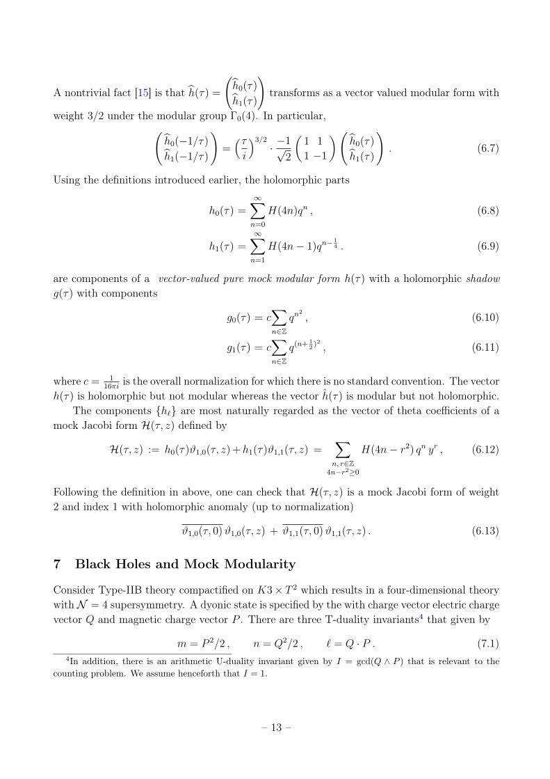
A nontrivial fact [15] is that h(τ) =

(h0(τ)

h1(τ)

)transforms as a vector valued modular form with

weight 3/2 under the modular group Γ0(4). In particular,(h0(−1/τ)

h1(−1/τ)

)=(τi

)3/2

· −1√2

(1 1

1 −1

)(h0(τ)

h1(τ)

). (6.7)

Using the definitions introduced earlier, the holomorphic parts

h0(τ) =∞∑n=0

H(4n)qn , (6.8)

h1(τ) =∞∑n=1

H(4n− 1)qn−14 . (6.9)

are components of a vector-valued pure mock modular form h(τ) with a holomorphic shadowg(τ) with components

g0(τ) = c∑n∈Z

qn2

, (6.10)

g1(τ) = c∑n∈Z

q(n+ 12

)2 , (6.11)

where c = 116πi

is the overall normalization for which there is no standard convention. The vectorh(τ) is holomorphic but not modular whereas the vector h(τ) is modular but not holomorphic.

The components h` are most naturally regarded as the vector of theta coefficients of amock Jacobi form H(τ, z) defined by

H(τ, z) := h0(τ)ϑ1,0(τ, z) +h1(τ)ϑ1,1(τ, z) =∑n, r∈Z

4n−r2≥0

H(4n− r2) qn yr , (6.12)

Following the definition in above, one can check that H(τ, z) is a mock Jacobi form of weight2 and index 1 with holomorphic anomaly (up to normalization)

ϑ1,0(τ, 0)ϑ1,0(τ, z) + ϑ1,1(τ, 0)ϑ1,1(τ, z) . (6.13)

7 Black Holes and Mock Modularity

Consider Type-IIB theory compactified on K3× T 2 which results in a four-dimensional theorywith N = 4 supersymmetry. A dyonic state is specified by the with charge vector electric chargevector Q and magnetic charge vector P . There are three T-duality invariants4 that given by

m = P 2/2 , n = Q2/2 , ` = Q · P . (7.1)4In addition, there is an arithmetic U-duality invariant given by I = gcd(Q ∧ P ) that is relevant to the

counting problem. We assume henceforth that I = 1.

– 13 –

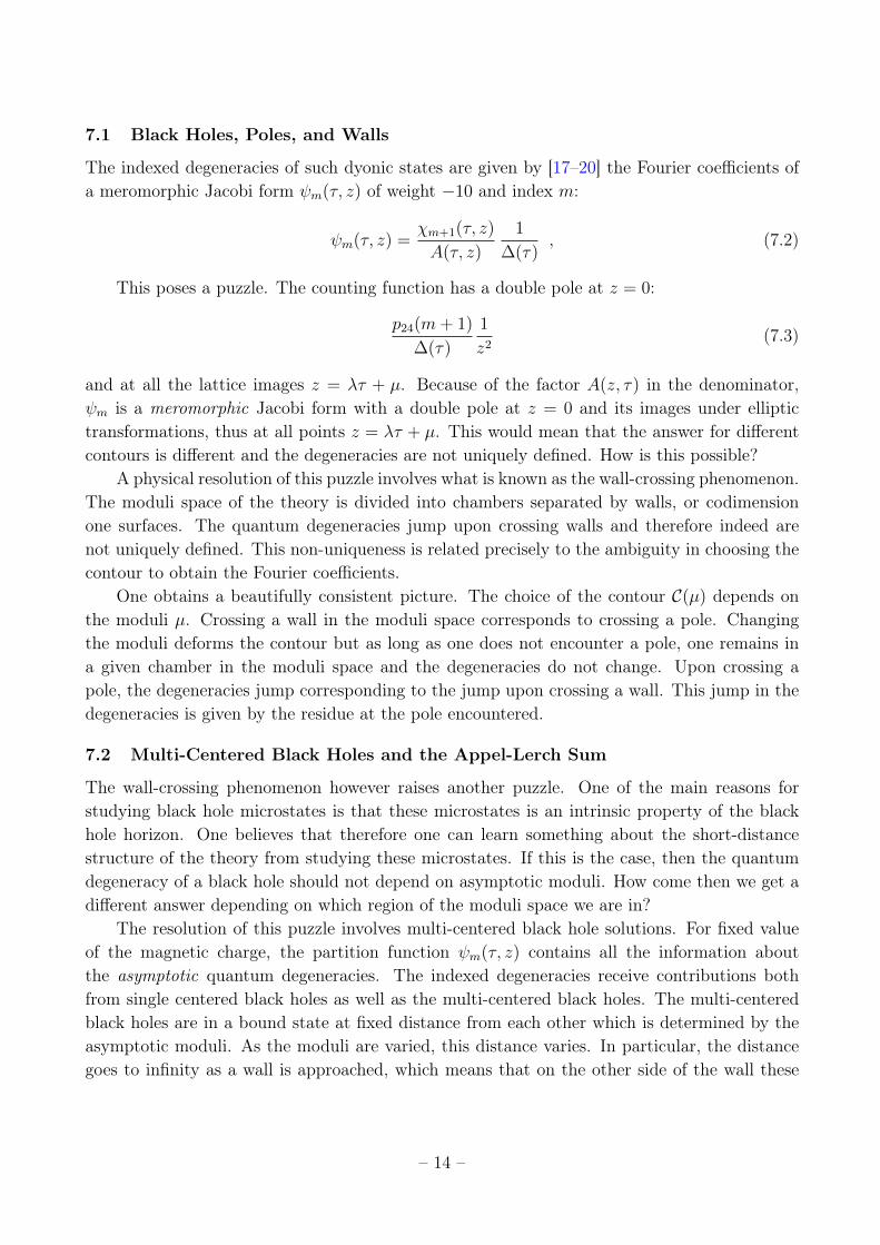
7.1 Black Holes, Poles, and Walls

The indexed degeneracies of such dyonic states are given by [17–20] the Fourier coefficients ofa meromorphic Jacobi form ψm(τ, z) of weight −10 and index m:

ψm(τ, z) =χm+1(τ, z)

A(τ, z)

1

∆(τ), (7.2)

This poses a puzzle. The counting function has a double pole at z = 0:

p24(m+ 1)

∆(τ)

1

z2(7.3)

and at all the lattice images z = λτ + µ. Because of the factor A(z, τ) in the denominator,ψm is a meromorphic Jacobi form with a double pole at z = 0 and its images under elliptictransformations, thus at all points z = λτ + µ. This would mean that the answer for differentcontours is different and the degeneracies are not uniquely defined. How is this possible?

A physical resolution of this puzzle involves what is known as the wall-crossing phenomenon.The moduli space of the theory is divided into chambers separated by walls, or codimensionone surfaces. The quantum degeneracies jump upon crossing walls and therefore indeed arenot uniquely defined. This non-uniqueness is related precisely to the ambiguity in choosing thecontour to obtain the Fourier coefficients.

One obtains a beautifully consistent picture. The choice of the contour C(µ) depends onthe moduli µ. Crossing a wall in the moduli space corresponds to crossing a pole. Changingthe moduli deforms the contour but as long as one does not encounter a pole, one remains ina given chamber in the moduli space and the degeneracies do not change. Upon crossing apole, the degeneracies jump corresponding to the jump upon crossing a wall. This jump in thedegeneracies is given by the residue at the pole encountered.

7.2 Multi-Centered Black Holes and the Appel-Lerch Sum

The wall-crossing phenomenon however raises another puzzle. One of the main reasons forstudying black hole microstates is that these microstates is an intrinsic property of the blackhole horizon. One believes that therefore one can learn something about the short-distancestructure of the theory from studying these microstates. If this is the case, then the quantumdegeneracy of a black hole should not depend on asymptotic moduli. How come then we get adifferent answer depending on which region of the moduli space we are in?

The resolution of this puzzle involves multi-centered black hole solutions. For fixed valueof the magnetic charge, the partition function ψm(τ, z) contains all the information aboutthe asymptotic quantum degeneracies. The indexed degeneracies receive contributions bothfrom single centered black holes as well as the multi-centered black holes. The multi-centeredblack holes are in a bound state at fixed distance from each other which is determined by theasymptotic moduli. As the moduli are varied, this distance varies. In particular, the distancegoes to infinity as a wall is approached, which means that on the other side of the wall these

– 14 –

bound states no longer exit and hence these multi-centered black holes no longer contribute tothe indexed degeneracies. Thus, even though the degeneracy of a black hole is indeed a propertyof its horizon, the degeneracies of multi-centered black holes which are bound states can jumpupon crossing walls in moduli space depending on whether a stable bound state exists or not.

This poses an interesting question whether one can define a counting function whose Fouriercoefficients give directly the degeneracies of the horizons of the single-centered black holeswithout the polluting contributions from the multi-centered black holes. After all, the degreesof freedom of the horizon is the quantity of real interest in the explorations of quantum gravity.It turns out that one can in fact remove this ambiguity in Fourier expansion by subtracting thecontribution of the various multi-centered black holes which is captured by the function

ψPm :=p24(m+ 1)

η24(τ)

∑s∈Z

qms2+sy2ms+1

(1− qsy)2, (7.4)

which is simply the ‘elliptic average’ over the lattice Zτ + Z of the simplest wall-crossing atz = 0 given by

p24(m+ 1)

η24(τ)

y

(1− y)2. (7.5)

The function ψPm is called the polar part of ψm because it has identical poles in the complex zplane. It is convenient to define

ψPm(τ, z) :=p24(m+ 1)

η24(τ)A2,m(τ, z) (7.6)

where A2,m(τ, z) is known as the Appel-Lerch sum which is simply the elliptic average of 1/z2

defined by

A2,m(τ, z) =∑s∈Z

qms2+sy2ms+1

(1− qsy)2, (7.7)

One can now obtain the horizon degeneracies of single-centered black holes simply by subtract-ing this contribution from the partition function ψm(τ, z) which counts all degeneracies. Thisphysical observation corresponds to the following decomposition theorem which also connectsthis problem with mock modularity.

7.3 The Decomposition Theorem

The decomposition theorem [16] states that subtracting ψPm leaves us with the finite part ψFm,which, as we saw above is exactly the attractor partition function:

ψFm(τ, z) ≡ ψm(τ, z)− ψPm(τ, z) . (7.8)

By separating part of the function ψm, we have of course broken modularity, and ψFm(τ, z) isnot a Jacobi form any more. However, ψFm still has a very special modular behavior, in that itis a mock Jacobi form. It is convenient to define as in (7.6) a function ϕFm(τ) by

ψFm(τ, z) :=p24(m+ 1)

η24(τ)ϕFm(τ) . (7.9)

– 15 –

The nontrivial part of the decomposition theorem is that ϕFm is a mock Jacobi form andhence admits a completion ϕFm. The mock behavior can be summarized by the following partialdifferential equation which is obeyed by its completion:

τ3/22

∂

∂τϕFm(τ) =

√m

8πi

∑` mod (2m)

ϑm,`(τ)ϑm,`(τ, z) . (7.10)

Thus, puzzles concerning the degeneracies of supersymmetric quantum black holes in stringtheory naturally lead to the mathematics of mock Jacobi forms.

8 Topology and Mock Modularity

As we explained earlier, the elliptic genus can be thought of as the right-moving Witten index,formally treating τ as the right-moving inverse temperature. As a result, naively, this quantityis expected to be independent of τ and is indeed so for a compact theory. The naive argumentfails in a non-compact conformal field theory, see e.g. [21–26]. The holomorphic anomalycaptures this ‘anomalous τ dependence’ of the elliptic genus. To understand the physical originof mock modularity, one would like to understand how precisely the holomorphic anomaly isrelated to the noncompactness of the underlying conformal field theory.

To appreciate the essence of this phenomenon, one can consider a simpler problem aboutthe Witten index of a noncompact quantum mechanical system. In this context, the anomalousτ dependence that we are interested in can be related to the anomalous β dependence of theWitten index where β is the inverse temperature.

8.1 Witten Index

For a supersymmetric quantum field theory in a d-dimensional spacetime, the Witten index[27] is defined by

W (β) := TrH[(−1)F e−βH

](8.1)

where H is the Hamiltonian, F is the fermion number and H is the Hilbert space of the the-ory. As usual, this trace can be related to a supersymmetric Euclidean path integral over ad-dimensional Euclidean base space Σ with periodic boundary conditions for all fields schemat-ically denoted by φ in the Euclidean time direction

W (β) =

∫dφ 〈φ|(−1)F e−βH |φ〉

=

∫[dφ] exp (−S[φ, β]) , (8.2)

where the path integral is over superfield configurations that are periodic in Euclidean timewith period β, so the Euclidean base space Σ is a circle of radius β times the spatical manifold.

– 16 –

If the quantum field theory is compact in the sense that the spectrum of the Hamiltonianis discrete, then the Witten index is independent of the inverse temperature β:

dW (β)

dβ= 0 . (8.3)

This follows from the observation that the states with nonzero energy come in Bose-Fermi pairsand do not contribute to the Witten index [27]. Only the zero energy states graded by (−1)F

contribute and consequently, the Witten index is a topological invariant. This is the case, forexample, for a supersymmetric sigma model with a compact target space.

By an appropriate choice of the sigma model, the Witten index in the zero temperature(β → ∞) limit can be related to some of the classic topological invariants such as the Eulercharacter or the Dirac index of the target manifold. Using temperature independence of theindex, one can evaluate it in the much simpler high temperature (β → 0) limit using the heatkernel expansion to prove the Atiyah-Singer index theorem [28]. Evaluating the path integralcorresponding to the Witten index in this high-temperature semiclassical limit gives anotherderivation of the index theorem [29, 30].

8.2 Noncompact Witten Index

If the field space is noncompact and the spectrum is continuous, then the above argument canfail because now instead of a discrete indexed sum, one has an integral over a continuum ofscattering states. To define the noncompact Witten index properly, one needs a framework toincorporate the non-normalizable scattering states into the trace. One can address this issueand give a suitable definition using the formalism of Gel’fand triplet [31].

In general, the bosonic density of states in this continuum may not precisely cancel thefermionic density of states, and the noncompact Witten index can be temperature dependent.In other words, the equation (8.3) above can have an ‘anomaly’ in that the naive expectationexpressed by (8.3) can fail. It is possible to compute the temperature dependence using lo-calization of the supersymmetric path integral. The temperature dependent piece is no longertopological but is nevertheless ‘semi-topological’ in that it is independent of any deformationsthat do not change the asymptotics.

Some of the essential points about a noncompact path integral can be illustrated by a‘worldpoint’ path integral where the base space Σ is a point and the target space X is a thereal line −∞ < u < ∞. We discuss this example first before proceeding to localization. Thesupersymmetric worldpoint action is given by

S(u, F, ψ−, ψ+) =1

2F 2 + iF h′(u) + ih

′′(u)ψ−ψ+ (8.4)

whereh′(u) :=

dh

du, h

′′(u) :=

d2h

du2. (8.5)

– 17 –

The path integral is now just an ordinary superintegral with flat measure5

W (β) = −i∫ ∞−∞

du

∫ ∞−∞

dF

∫dψ− dψ+ exp [−βS(U)] . (8.6)

A particularly interesting special case is

h′(u) = λ tanh(au) , (8.7)

for real λ. Integrating out the fermions and the auxiliary field F gives

W (β) = −√

β

2π

∫ ∞−∞

du h′′(u) exp

[−β

2(h′(u))2

](8.8)

One can change variables

y =

√β

2h′(u) , dy =

√β

2h′′(u)du (8.9)

As u goes from −∞ to ∞, y(u) is monotonically increasing or decreasing depending on if λ ispositive or negative; the inverse function u(y) is single-valued, and the integral reduces to

W (β) = − 1√π

∫ √β2λ

−√

β2λ

dy e−y2

= −sgn(λ) erf

(√β

2|λ|

)(8.10)

The error function which appears naturally in this integral, has already made its appearancein the definition of the completion (5.2) of a mock modular form in the guise of an incompleteGamma function. Note that with a change of variable y2 = t, the integral∫ √β

2λ

−√

β2λ

dy e−y2

(8.11)

can be written as ∫ β2λ2

0

t−12 e−t dt (8.12)

5The normalization factor −i can be understood as follows. Consider quantum mechanics of 2n real fermions.Denoting their zero-modes by ψi

0, i = 1, . . . , 2n we have:

γ = inγ1 . . . γ2n = (−2i)nψ10 . . . ψ

2n0 .

Moreover, Tr γ2 = 2n which is the dimension of the spinor representation

Tr γ2 = N

∫(−2i)nψ1

0 . . . ψ2n0 dψ1

0 . . . dψ2n0

which implies N = (−i)n. For two real fermions n = 1 and N = −i.

– 18 –

which we recognize as the lower incomplete gamma function γ(12, β

2λ2) related to the upper

incomplete gamma function (5.3) by γ(s, x) + Γ(s, x) = Γ(s).The noncompact Witten index is thus not temperature independent. The anomalous tem-

perature dependence is captured by the equation

β12d

dβW (β)

.= λ sgn(λ) e−

βλ2

2 (8.13)

which is a close analog of the holomorphic anomaly equation (5.5). Similar expressions appearin the path integral derivation of the holomorphic anomaly equation of mock modular formsencountered in gauge theory [32].

The worldpoint integral illustrates a number of important points.

1. Without the fermionic integrations, the integral has a volume divergence because h′(u) isbounded above for large |u|. Inclusion of fermions effectively limits the integrand to theregion close to the origin where h′(u) varies, and makes the integral finite.

2. The answer depends only the asymptotic behavior of h′(u) at ±∞ and is independent ofany deformations that do not change the asymptotics. In particular, one would obtainthe same result in the limit a→∞ in (8.7), when h′(u) can be expressed in terms of theHeaviside step function:

h′(u) = λ[θ(u)− θ(−u)

]. (8.14)

3. The appearance of the incomplete Gamma function in this context is not a coincidence.The two turn out to be related through a path integral which localizes precisely onto theordinary superintegral considered above. For this reason, this example is particularly im-portant for understanding the connection between noncompactness and mock modularity.

9 Holomorphic Anomaly in Gauge Theories

In [12] Vafa and Witten considered a topologically twisted version of maximally supersymmetric(N = 4) Yang-Mills theory in four dimensions. The partition function is naively expected tobe a holomorphic function of the coupling constant τ and S-duality invariant. However, thenaive holomorphic partition function by itself is not S-duality invariant and there is in fact aholomorphic anomaly as we describe below.

9.1 Vafa-Witten Partition Function

The topological twist is defined by identifying the SU(2) = Spin(3) subgroup of R-symmetrySU(4) = Spin(6) (with the standard embedding Spin(3) ⊂ Spin(6)) with the chiral SU(2)

subgroup of the Spin(4) ∼= SU(2) × SU(2) group of Euclidean rotations. The details of thetwist are reviewed in the Section 9.2 from the point of view of the parent 6d N = (2, 0) theory.We will denote by ZG[M4, τ ] the partition function of the twisted theory with gauge group Gand complexified gauge coupling τ = 4πi

g2+ θ

2πon 4-manifold M4. It has the following expected

properties:

– 19 –

(i) ZG[M4, τ ] 6= 0 (generically, due to vanishing ghost number anomaly)

(ii) ZG[M4,−1/τ ] = ZG[M4, τ ] (up to a simple phase determined by ’t Hooft anomalies)where G is the Langlands dual of G. E.g. G = SU(2), G = PSU(2) = SO(3).

(iii) (naively) ∂∂τZG[M4, τ ] = 0

(iv) (naively) ∂∂gM4

ZG[M4, τ ] = 0 where gM4 is the metric onM4, that is the partition functionis a topological invariant (only depends on the diffeomorphism class of the 4-manifold).

The (naive) argument for both (iii) and (iv) is based on the fact that one can write theaction of the twisted 4d SYM in the form

S4d = −i τ8π2

∫M4

TrF ∧ F +Q(Λ) (9.1)

for some Λ, where Q is one of the unbroken supercharges. The first term in the right-hand sideis holomorphic in τ and independent of metric. Then, denoting by Φ the collection of all fields,we have in particular

∂

∂τZG[M4, τ ] =

∫DΦ

∂

∂τe−S4d[Φ] =

∫DΦQ

(e−S4d[Φ]∂Λ

∂τ

)= 0. (9.2)

The last equality follows from the fact that Q is a derivation on the space of fields, assumingthere is no contribution from the boundary at infinity. Explicitly, if one introduces somecoordinates Φi on the space of fields (e.g. harmonics on M4) and Q(Φi) = αi[Φ], then Q =∑

i αi[Φ] ∂

∂Φiand one can apply Stokes theorem. However the assumption about vanishing

contribution from infinity can in principle fail (and does in certain cases).Moreover, under certain additional conditions (e.g. M4 is Kähler with c1 ≥ 0) the partition

function can be localized on instanton solutions:

ZG[M4, τ ] =∑n

qnχ(MGn [M4]) (q := e2πiτ ) (9.3)

where χ is the Euler characteristic andMGn [M4] is the moduli space of n G-instantons on M4

(that is space of solutions to the equations ∗F = −F with fixed n = 18π2

∫TrF ∧ F , modulo

gauge transformations).In one applies naively the formula (9.3) for M4 = CP2 [12–14, 33, 34]:

ZSU(2)naive [CP2, τ ] =

1

2f0(τ) (9.4)

ZSO(3)naive [CP2, τ ] = f0(τ) + f1(τ) (9.5)

where6 fv(τ), up to simple factors, are given by generating functions for Hurwitz class numbersH(n) that have already appeared in Section 6.2:

fv(τ) =∑n

3H(4n− v)qn−v/4

η(τ)3≡ 3hv(τ)

η(τ)3, v = 0, 1 (9.6)

6Individual fv is the contribution from SO(3) bundles with fixed Z2 flux v =∫CP1 w2 through CP1 ⊂ CP2.

– 20 –

It turns out, that unlike in the case M4 = K3, the the property (ii) is not respected:

ZSU(2)naive [CP2,−1/τ ] 6= Z

SO(3)naive [CP2, τ ] (9.7)

but “almost”. Namely, fv(τ) transform as a vector valued modular form that has a non-holomorphic modular completion:

fv(τ) fv(τ) + gv(τ, τ) (9.8)

where gv(τ, τ)→ 0 at τ →∞ and, as follows from (6.5)-(6.6),

∂gv(τ, τ)

∂τ=

3

τ3/22 16πiη(τ)3

∑n∈Z

q(n+v/2)2 . (9.9)

Since the property (ii) is more fundamental than the property (iii), it is natural to guess that themodular completion above gives the full physical partition function. Its holomorphic anomalyis then determined by (9.9). In particular

∂ZSU(2)[M4, τ ]

∂τ=

3

τ3/22 32πiη(τ)3

∑n∈Z

qn2

. (9.10)

By now the appearance of mock-modular forms in instanton counting problems has already along history: [35–39].

9.2 M-theory Realization

In this section we briefly review some prerequisite facts about 6d maximally supersymmetricconformal field theories and their topologically twisted compactification on 4-manifolds. Six-dimensionalN = (2, 0) superconformal quantum field theories (QFTs) are known to be classifiedby Lie algebras of the form g = ⊕igi, where each gi = u(1) or simply-laced (i.e. of ADEtype). In these lectures by defult we assume Euclidean signature of space-time metric. The6d N = (2, 0) extension of spin-Poincare symmetry (non-including conformal transformations)has Spin(6)E ×Z2 Spin(5)R even subgroup, where Spin(6)E is the symmetry of the spacetimerotations and Spin(5)R is the R-symmetry. The extension has 16 supecharges transforming inthe representation (4+,4).

Recall that Spin(n) group is the nontrival central extension of SO(n) by Z2:

1 −→ Z2 −→ Spin(n) −→ SO(n) −→ 1. (9.11)

Useful isomorphisms in low dimensions:

Spin(3) ∼= SU(2), (9.12)

Spin(4) ∼= Spin(3)` × Spin(3)r ∼= SU(2)` × SU(2)r, (9.13)

Spin(6) ∼= SU(4). (9.14)

– 21 –

Note that when g = u(N) or su(N) the theory describes the worldwolume theory of NM5-branes (respectively with or without center of mass degrees of freedom included) in 11-dimensional M-theory. The R-symmetry Spin(5)R then can be understood as the group ofrotations of the 5 normal directions.

The 6d N = (0, 2) theories do not have a Lagrangian description, however their compactifi-cation on a circle or a torus can be described in terms of maximally supersymmetric Yang-Millsgauge theory. In particular, 6d N = (2, 0) theory corresponding to a Lie algebra g, compactifiedon a 2-torus T 2 = C/(Z + τZ) is equivalent to a 4d N = 4 super-Yang-Mills (SYM) theorywith gauge group G such that Lie(G) = g and the complexified coupling τ = 4πi

g2+ θ

2πequal to

the complex structure of the torus.Note that the choice of global structure of the gauge group G is determined by the finite

choice of “sector” of the 6d theory, which is a relative QFT. It is similar to a 2d chiral Wess-Zumino-Witten conformal field theory (CFT), where one has to choose a conformal block. Inthe case of g = su(N) there are two distinguished choices: G = SU(N) and G = PSU(N) =

SU(N)/ZN . They are related to each other by gauging a certain 1-form ZN global symmetries.Consider now a 6d N = (2, 0) theory on a spacetime of the form M4 × Σ2, where M4 is

a closed oriented 4-manifold and Σ2 is a 2d spacetime. The group of local spacetime rotationsthen has a natural subgroup Spin(4)E × Spin(2)E ⊂ Spin(6)E where Spin(4)E and Spin(2)Eare local rotations along M4 and Σ2 respectively. We will consider the theory topologicaltwisted along M4. In principle there are various ways to topologically twist the theory. Thetwist that we are interested in can be understood as identification of Spin(3) ⊂ Spin(5)R(embedded as the subgruop of rotations of 3 out 5 directions) with SU(2)` ⊂ Spin(4)E ∼=SU(2)` × SU(2)r. Equivalently, this means turning on a background gauge field for Spin(3)

subgroup of R-symmetry equal to SU(2)` component of the spin-connection on M4.When Σ = T 2, from the point of view of the 4d N = 4 SYM on M4 this twist is known as

Vafa-Witten topological twist. The effective 4d theory is the Vafa-Witten theory [12] so thatits partition function ZG[M4, τ ] considered in Section 9.1 can be interpreted as the partitionfunction of the 6d theory on M4 × T 2.

Exercise 4. Consider the homomorphism

t : Spin(4)′E × Spin(2)E −→ Spin(6)E × Spin(5)R (9.15)

correposning to the topological twist defined above. Namely, the component of the map inSpin(6)E is given by the standard ebedding, while the component of the map in Spin(5)R is givenby the projection onto SU(2)′` ⊂ Spin(4)′E composed with the standard embedding Spin(3) →Spin(5)R. Show that the representations decompose as follows:

t∗(4+,4) = 2(1,1)+ 12

+ 2(3,1)+ 12

+ 2(2,2)− 12

(9.16)

t∗(1,5) = 2(1,1)0 + (3,1)0 (9.17)

where in the right hand side the pair of numbers denote the dimensions of the representationsof SU(2)′` × SU(2)′r and the index denotes the spin with respect to Spin(2)E.

– 22 –

Note that in the case when g = su(N) and the 6d theory is the worldwolume theory ofthe stack of N fivebranes in M-theory the twist can be realized geometrically in the followingsetup:

M-theory Λ2+TM4 × R2 × T 2

N M5’s M4 × 0 × T 2 (9.18)

where Λ2+TM4 is the rank 3 bundle of self-dual 2-forms over M4. This follows from (9.17) asthe represenation (3,1) can be realized by self-dual antisymmetric rank 2 tensors.

From the result of the Exercise 4 it follows that the 6d theory twisted on M4 has ingeneral 2 unbroken supercharges. They both transform as right-moving spinors in the residual2 dimensions.

9.3 The su(2) theory on the tensor branch

For g = su(2) the 6d theory is interacting and non-Lagrangian. However on the tensor branchit can be effectively decribed in term of a single tensor multiplet corresponding to the Cartansubalgebra u(1) ⊂ su(2) with extra interaction terms.

The tensor branch of the theory can be roughly understood as the phase where the scalarfields fluctuate over non-zero values. The non-compactness of the 6d theory can only arise inthe directions corresponding to the large values of the scalar fields. Therefore to determine theholomorphic anomaly it should be enough to use the effective description of the theory on thetensor branch, which becomes asymptoticlly exact when the values of the scalar fields tend toinfinity. In the M-theory setup the tensor branch corresponds to the phase when 2 fivebranesare separated in a normal direction.

The quantization conditions on the gauge transformations on the field B are rescaled com-pared to the previous case7:

B ∼ B + β, dβ = 0 ,

∫∀ 2-cycle

β ∈ 2π√

2Z. (9.19)

where the extra√

2 factor is the length of the root in su(2) algebra. Consequently, the fields ofthe effective 2d theory will be the same as in the g = u(1) case, but with modified periodicityof the chiral scalars:

X i± ∼ X i

± + 2√

2πni± (9.20)

where ni± are quantized as before. In the description in terms of a lattice CFT, this means thatthe lattice is now

√2H2(M4,Z).

The 6d interaction term that will be relevant for us is [40, 41]:

i√2

∫B ∧ η4 (9.21)

Where η4 is a 4-form that can be defined as follows. Let

ϕa :=ϕa√∑a(ϕ

a)2, (Dϕ)a := dϕa − AabRϕb, a, b = 1, . . . , 5. (9.22)

7The normalization conventions are slighlty different from that of [32].

– 23 –

where ϕa are the scalars of the tensor multiplet and Aab are the components of the backgroundSpin(5)R connection 1-form valued in the so(5) algebra. Then

η4 :=1

64π2εa1a2a3a4a5 [(Dϕ)a1(Dϕ)a2(Dϕ)a3(Dϕ)a4

− 2F a1a2R (Dϕ)a3(Dϕ)a4 + F a1a2

R F a3a4R ]ϕa5 . (9.23)

where FR is the curvature of the R-symmetry connection AR. The interaction term above iswritten in the untwisted theory, on a flat spacetime, but with non-trivial background SO(5)

R-symmetry gauge field.Note that the term (9.21) corresponds to the fact that skyrmionic strings are electrically

charged with respect to the B field. In the dimensional reduction to 5d/4d gauge theory thecorresponding term arises in 1-loop effective action on the Coulomb branch.

10 Path integral derivation of holomorphic anomaly

Our goal is to derive this holomorphic anomaly equation from the path integral. It is possibleto do this from the path integral of the 4d SYM by calculating the non-vanishing boundarycontribution in (9.2) [32]. However in these lectures we will use an alternative (but in manyways analogous) approach, also from [32].

10.1 Reversing the order of compactification

Instead of considering the 4d theory on M4 obtained by compactification of the 6d theory onT 2 one can reverse the order of compactification and work with the 2d theory, usually denotedas Tg[M4] obtained by compactification of the 6d theory on M4. The partition function of theVafa-Witen theory on M4 is equal to the partition function of this 2d theory on the torus T 2

with complex structure τ (with periodic-periodic boundary conditions on fermions). The lattercan be also understood as a trace over the Hilbert space H of the 2d theory on a circle:

ZG[M4, τ ] = ZT [M4][T2] = TrH(−1)F qL0 qL0 . (10.1)

As usual, L0 = H+P , L0 = H−P where H, P are the Hamiltonian and momentum. The resultof the Exercise 4 tells us that the 2d theory Tg[M4] has at least N = (0, 2) supersymmetry. As-suming the spectrum of the theory is discrete, the usual argument can be applied to show thatthe dependence on q in the trace above should drop out due to cancellation between femrionicand bosonic states with L0 ≡ Q2 6= 0 (where Q is one of the right-moving supercharges). How-ever, if the theory suffers from some sort of “non-compactness” and the spectrum is continuous,the canecellation can fail and the partition function can have an anomalous dependence on q.As we will see, this is indeed the case for Tsu(2)[CP2].

To summarize, the computations of the holomorphic anomaly both in the 2d sigma modeldescription and directly in the 4d gauge theory description give the same result on the righthand side of (9.9), but the various factors have different origins in the two regions.

– 24 –

• The factor of 3 is related to the to the quantum of H-flux in the sigma-model descriptionand to the first Chern class of the canonical line bundle of CP2 in the gauge theorydescription.

• The factor of τ−3/22 comes from the integral over three non-compact bosonic zero-modes in

the sigma model description and from the integral over the constant mode of the auxiliaryfield in the gauge theory description.

• The factor of η(τ)−3 = η(τ)−χ(CP2) is the contribution of the left-moving oscillators in thesigma model description and of point-like instantons in the gauge theory description.

• Finally, the anti-holomorphic theta-function∑

n∈Z qn2 is a contribution of right-moving

momenta of a compact chiral boson in the sigma model description and of abelian anti-instantons in the gauge theory decsription.

We now comment on the relation between the holomorphic anomaly and mock modularity.The naive holomorphic partition function of the twisted SO(3) super Yang-Mills theory on CP2

is the holomorphic kernel of the anomaly equation (9.9) which receives contributions only fromthe instantons. It is holomorphic but not modular. The presence of the holomorphic anomalyimplies that the physical partition function necessarily contains a nonholomorphic piece givenby an Eichler integral of the anomaly [15] which receives contributions from the anti-instantons.In the modern terminology [2, 3, 16] discussed earlier, the holomorphic piece is a (vector valued)‘mixed mock modular form’ whereas the anomaly is governed by its ‘shadow’. The physicalpartition function satisfying the anomaly equation is the ‘modular completion’ and has goodmodular properties, as expected from duality.

These considerations extend naturally to other Kähler 4-manifolds with b+2 = 1, b1 = 0 and

to other groups [32]. In general, when the configuration space of the twisted theory is non-compact, the partition function is modular but not holomorphic, and satisfies a holomorphicanomaly equation similar to (9.9). As we have seen, this incompatibility between holomor-phy and modularity is the essence of mock modularity. The physical requirement of dualityinvariance of the path integral thus leads naturally to the mathematical formalism of mockmodularity whenever the relevant configuration space is noncompact.

Before we proceed with the derivation of the holomorphic anomaly equation from the pointof view of the effective 2d theory for g = su(2), consider first the case of g = u(1). Thecorresponding 6d theory is the free theory of N = (2, 0) tensor multiplet. It consists of thefields forming the following rerpresentations of Spin(6)E × Spin(5)R:

(a) scalars ϕ in (1,5)

(b) fermions in (4+,4)

(c) a self-dual 2-form field B in (15,1) (dB = ∗dB). In general it is only locally well-definedand is subject to 1-form gauge transformations:

B ∼ B + β, dβ = 0 (β = dα locally),

∫∀ 2-cycle

β ∈ 2πZ. (10.2)

– 25 –

In what follows we will assume that M4 is simply-connected (in particular b1 = 0). ThenH2(M4,Z) can be identified with subgroup of de Rham cohomology H2(M4,R) representedby 2-forms h such that

∫a 2-cycle h ∈ Z. As usual, we will denote by b±2 the number of posi-

tive/negative eigenvalues of the bilinear form on H2(M4,Z) given by∫M4 · ∧ ·.

The effictive 3d theory Tu(1)[M4] can be obtained by the standard Kaluza-Klein (KK)

reduction, by counting harmonic forms onM4 and taking into account the results of the Exercise4 (cf. [42, 43]):

(a) 2 + b+2 real scalars φi

(b) 2 + 2b+2 Majorana-Weyl right-moving fermions

(c) b±2 right/left-moving chiral compact scalars X i±.

The result (c) can be seen as follows. The (massless) KK reduction of the field B is given bythe following decomposition:

B =

b+2∑i=1

X i+ h

+i +

b−2∑i=1

X i− h−i (10.3)

where h±i are the basis in the space of harmonic 2-forms on M4 chosen such that

∗4dh±i = ±h±i , (10.4)∫

M4

h+i h−j = 0, (10.5)∫

M4

h±i h±j = ±δij. (10.6)

From the self-duality dB = ∗6ddB it then follows that ∗2ddXi± = ±dX i

±. Equivalently, usinga complex coordinate z to parametrize the 2d spacetime, ∂X i

+ = 0, ∂X i− = 0. From the large

gauge transformations (10.2) it follows that X i± are compact:

X i± ∼ X i

± + 2πni± (10.7)

where ni± are quantized such that∑

i,± ni±h±i ∈ H2(M4,Z). That is X i

± can be understood ascomponents of a field valued in the b2-torus H2(M4,R)/2πH2(M4,Z).

The collection of field X i± form what is usually called Narain’s lattice CFT corresponding

to the indefinite lattice H2(M4,Z) ∼= H2(M4,Z) (for closed M4, as we assume, the lattice isself-dual) with the bilinear form

∫M4 · ∧ ·.

Exercise 5. Show that whenM4 is (hyper-)Kähler, that is the holonomy is reduced to (SU(2)) U(2) ⊂SO(4)E, there are (8) 4 unbroken supercharges, all right-moving in 2d.

– 26 –

10.2 Review of 2d N = (0, 1) sigma-models

For our purposes it is enough to considerN = (0, 1) sigma-models without left-moving fermions.The theories from such class are defined by the choice of a target manifold X equipped withRiemannian metric and a closed 3-form h ∈ Ω3(X ). The target manifold should satisfy cer-tain topological constraints for theory to be well defined on the quantum level (w1(TX ) = 0,w2(TX ) = 0, 1

2p1(TX ) = 0). Let Σ be the 2-dimensional spacetime (also known as source or

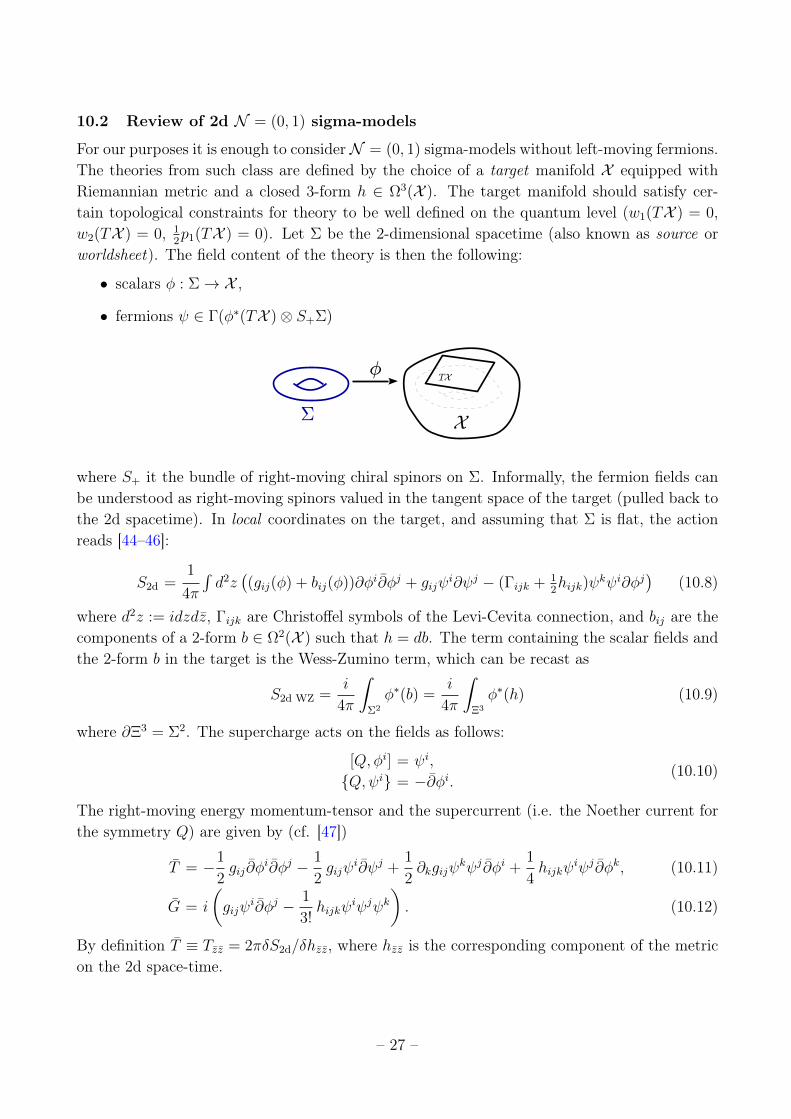
worldsheet). The field content of the theory is then the following:

• scalars φ : Σ→ X ,

• fermions ψ ∈ Γ(φ∗(TX )⊗ S+Σ)

X

TX

§

Á

where S+ it the bundle of right-moving chiral spinors on Σ. Informally, the fermion fields canbe understood as right-moving spinors valued in the tangent space of the target (pulled back tothe 2d spacetime). In local coordinates on the target, and assuming that Σ is flat, the actionreads [44–46]:

S2d =1

4π

∫d2z((gij(φ) + bij(φ))∂φi∂φj + gijψ

i∂ψj − (Γijk + 12hijk)ψ

kψi∂φj)

(10.8)

where d2z := idzdz, Γijk are Christoffel symbols of the Levi-Cevita connection, and bij are thecomponents of a 2-form b ∈ Ω2(X ) such that h = db. The term containing the scalar fields andthe 2-form b in the target is the Wess-Zumino term, which can be recast as

S2d WZ =i

4π

∫Σ2

φ∗(b) =i

4π

∫Ξ3

φ∗(h) (10.9)

where ∂Ξ3 = Σ2. The supercharge acts on the fields as follows:

[Q, φi] = ψi,

Q,ψi = −∂φi. (10.10)

The right-moving energy momentum-tensor and the supercurrent (i.e. the Noether current forthe symmetry Q) are given by (cf. [47])

T = −1

2gij ∂φ

i∂φj − 1

2gijψ

i∂ψj +1

2∂kgijψ

kψj ∂φi +1

4hijkψ

iψj ∂φk, (10.11)

G = i

(gijψ

i∂φj − 1

3!hijkψ

iψjψk). (10.12)

By definition T ≡ Tzz = 2πδS2d/δhzz, where hzz is the corresponding component of the metricon the 2d space-time.

– 27 –

Exercise 6. Check that the supercurrent G above satisfies

Q, G = 2i T . (10.13)

The path integral for partition function of the 2d theory (which we will denote as σ(X )) ona 2-torus with periodic-periodic boundary conditions on fermions localizes on constant mapsto the target. If the target X is a closed manifold (∂X = 0) the result has an explicit formula8

[48]:

Zσ(X )[T2] = TrH(−1)F qL0 qL0 =

∫X

√det

R/2πiθ(R/2πi; τ)

(10.14)

where R ∈ Ω2 ⊗ so(dimX ) is the curvature 2-form on X and

θ(u; τ) := q112 (eu/2 − e−u/2)

∏n≥1

(1− qneu)(1− qne−u) ≡iθ1(τ, u

2πi)

η(τ). (10.15)

The characteristic class of X in the right-hand side of (10.14) is known as elliptic genus.

Exercise 7. Show that∫X

√det

R/2πiθ(R/2πi; τ)

=1

η(τ)dimX

∫X

1 + E2(τ)p1 +

(E2(τ)2

2p2

1 +E4(τ)

12(p2

1 − 2p2)

)+ . . .

,

(10.16)where pi are Pontryagin classes of X and find the next term. The n-th term in the expansionis a characteristic class of degree 4n with coefficients in being quasi-modular forms of SL(2,Z)

(i.e. polynomials in the Eisenstein series E2k) of weight 2n. Argue that when p1 = 0 thedependence on E2 drops out.

If X is non-compact, however, ∂Zσ(X )

∂τ6= 0 in general. Assuming that X asymptotically is of

the form Y×R (informally ∂X = Y), it was argued in [49] that the anti-holomorphic derivativecan be expressed in terms of a 1-point function of the supercurrent of in the sigma model withtarget Y . Namely

∂Zσ(X )[T2]

∂τ=−eπi/4√8τ2η(τ)

〈G〉σ(Y) (10.17)

where 〈. . .〉T denotes a 1-point function in a theory T on T 2.Below we present a sketch of the proof of this formula and address to [32, 49] for details.

Omitting numerical factors we have

∂Zσ(X )[T2]

∂τ∝∫DφDψ

∂

∂hzze−S2d[φ,ψ] ∝ 〈T 〉σ(X ) ∝ 〈Q, G〉σ(X ) ∝

1√τ2η(τ)

〈G〉σ(Y) (10.18)

8As usual, it is assumed that∫X f ≡ 0 for f ∈ Ωn(X ), n 6= dimX .

– 28 –

The last equality is the most non-trivial and can be argued as follows. A correlator of a Q-invariant observable on the torus localizes on the space of zero-modes, that is space of constantfunctions φ and ψ on T 2:

〈Q, G〉σ(X ) =

∫zero modes

dφ0dψ0f(φ0, ψ0) (10.19)

where f(φ0, ψ0) is result of the integration over nonzero bosonic and fermions modes. Thefunctions on the space of bosonic and femrmionic zero-modes are in 1-to-1 correspondence withforms on the target X . Namely, the components of the bosonic zero-modes can be identifiedwith local coordinates φi0 on X and the components of the fermionic zero-modes can be identifiedwith their differentials: ψi0 ≡ dφi0. Under this correpondence∫

zero modesdφ0dψ0f(φ0, ψ0) =

∫Xf (10.20)

where in the right-hand side f is understood as the corresponding element of Ω∗(X ). Moreover,the supercharge (10.10) restricted to the space of zero modes can be indentified with the exteriorderivative under this correspondence:

Q|zm =∑i

ψi0∂

∂φi0≡ d (acting on Ω∗(X )) (10.21)

Therefore f = dg where g corresponds to G in the way f corresponds to T and∫Xf =

∫Yg (10.22)

from Stokes theorem. The extra factor in (10.18) is the contribution of bosonic and fermionicnonzero modes corresponding to the extra direction R in X :

1√τ2|η(τ)|2

· η(τ) =1

√τ2η(τ)

(10.23)

10.3 Holomorphic anomaly for CP2

Consider now the particular case of M4 = CP2. Although the final result is independent on thechoice of metric, assume the standard Fubini-Studi metric (which is Kähler) for concreteness.The group H2(CP2,Z) has a single generator represented by the self-dual form h1

+ = ω equalto the Kähler form, satisfying

∫CP2 ω2 = 1 (also

∫CP1 ω = 1). In particular b+

2 = 1 and b−2 = 0.According to the general result, the field content of the effective 2d theory Tsu(2)[CP2] on thetensor branch is then the following:

(a) 3 scalars φi, i = 1, 2, 3,

(b) 4 fermions ψi, i = 1, 2, 3, 4,

(c) 1 right-moving compact chiral boson X+ of radius√

2.

– 29 –

This theory is a sigma-model with target X = R3 × S1 with the exception that the scalarfield valued in S1 is chiral right-moving. The missing left-moving component, however is notparticipating in supersymmetry tranformations anyway. Topologically this target space lookslike S2 × S1 × R near infinity, where R is the radial direction of R3.

Exercise 8. Show that the 6d skyrmionic string term (9.21) reduces to a 2d Wess-Zumino term(10.9) with

h = 3 · 8π2 · volS2 ∧ volS1 (10.24)

where volS2 and volS1 are the standard volume forms on S2 and S1 normalized so that the totalvolume is 1. Use the fact that one can always choose SO(5)R indices so that the 2d fieldsφi, i = 1, 2, 3 arise as constant modes of ϕa, a = 1, 2, 3. Then in the twisted theory F ab

R = 0

unless (a, b) is a permutation of (4, 5), while F 45R /(2π) is equal to (up to a sign) to the Ricci

form, which is 3ω for CP2.

To calculate the holomorphic anomaly it is then enough to calculat the 1-point function ofthe supercurrent given by (10.12) in the sigma-model with target Y = S2 × S1:

〈G〉σ(X ) = 〈igijψi∂φj −i

3!hijkψ

iψjψk〉σ(X ) (10.25)

One can argue that the first term in the correlator does not contribute, as it cannot saturatethe integral over 3 fermionic zero-modes. The correlator of the second term, as before, localizesto the integral over zero-modes with an overall factor from the contribution of non-zero modes.Ommitting non-essential numerical factors (for a careful calculation see [32]), the integral overzero-modes reads ∫

S2×S1

h = 3 · 8π2 (10.26)

where we used again the correspondence between functions of zero-modes and forms on thetarget. The contribution from nonzero modes is

η(τ)3 · 1

τ2η(τ)2η(τ)2·∑

n qn2

η(τ)(10.27)

where the first factor is the contribution of nonzero modes of 3 right-moving fermions, thesecond factor is the contribution of nonzero modes of 2 scalars valued in S2, and the final factoris the contribution of the chiral right-moving bosons of radius

√2 (in the vacuum sector).

Combining the contributions from zero- and nonzero modes together we arive at the desiredformula for the holomorphic anomaly:

∂ZSU(2)[M4, τ ]

∂τ=

3

τ3/22 32πiη(τ)3

∑n∈Z

qn2

. (10.28)

The choice of the vacuum sector in the theory of chiral compact boson of radius√

2 corre-ponds to the choice of the gauge group G = SU(2) (equivalently, up to a factor, the sector ofSO(3) gauge theory with

∫CP1 w2 = 0). The other sector (out of 2 in total) of the chiral boson

corresponds to the sector of SO(3) gauge theory with∫CP1 w2 = 1 and gives the result for the

right-hand side of (9.9) for v = 1.

– 30 –

A Solutions

Exercise 1. A weight 12 modular form must be a linear combination of the form (2.9). Fora cusp form, the q-expansion has no constant term. Hence we determine a = −b to prove that

∆(τ) =1

1728

(E3

4(τ)− E26(τ)

)(A.1)

is the unique weight 12 cusp form, normalized so that the q-expansion starts with q.

Exercise 2. The SCFT with target space T 4 has four free bosons and four free fermions;hence the total central charge is 6. The path integral for the elliptic genus vanishes because theright-moving fermions with the periodic boundary condition in the Ramond sector have zeromodes. To get a nonzero answer one can define a modified elliptic genus χmod(τ, z|X ) with twoinsertions of the current JR in the trace (4.1) to soak up the four fermion zero modes. Sincethe current operator has conformal weight 1, now the path integral transforms with weight −2

rather than with weight 0. This implies that the elliptic genus should be a Jacobi form of index1 and weight −2 and hence must be proportional to A(τ, z). It is easy to confirm this by anexplicit computation for the free bosons and fermions using the product representation of thetheta function which also fixes the overall normalization.

Exercise 3. The SCFT with target space K3 also has central charge 6. This is easy to see inthe large volume limit where the curvarture can be ignored and one has four free bosons andfour free fermions. This implies that the elliptic genus of K3 must be a Jacobi form of index1 and weight 0; and hence must be proportional to B(τ, z). To fix the normalization, we usethe fact that when z = 0 the elliptic genus reduces to the Witten index which gives the Eulernumber of K3 which is 24. Hence, the elliptic genus of K3 equals B(τ, z).

This general conclusion can be verified by an explicit computation at a point in the modulispace where the SCFT is exactly solvable. For example, one can consider the point where theK3 is represented as an orbifold of a 4-torus T 4/Z2 where the Z2 symmetry with generatorR reflects the bosonic coordinates of the torus and their fermionic partners (see, for example,[50]). The elliptic genus (4.1) can then be written as a projected trace over untwisted (U) andtwisted (T) sectors as

χ(τ, z|K3) =1

2TrU(1 +R) +

1

2TrT (1 +R) , (A.2)

(with all other operators implicitly in the trace as in (4.1)). The first term vanishes because ofthe fermionic zero modes as explained above. The second term gives the first term in (3.13).There are 16 fixed points of the orbifolding symmetry and in the twisted sector the fields arehalf-integer moded. Summing over the contributions from all fixed points, the third term givesthe second term in (3.13) whereas the fourth term gives the third term in (3.13) as can be seenfrom the product representation of the theta functions.

– 31 –

Exercise 4. First we decompose the chiral spinor representation of Spin(6)E into a sum oftersor products of chiral spinor represntations of Spin(4)E = SU(2)` × SU(2)r and Spin(2)Ewith respect to the standard emebedding Spin(4)E × Spin(2)E ⊂ Spin(6)E (with two chiralitiescorrelated):

4+ = (2,1)+ 12

+ (1,2)− 12. (A.3)

The non-chiral spinor representation of Spin(5)R splits into two copies of non-chiral spinorrepresentation of Spin(3)R ⊂ Spin(5)R:

4 = 2 · 2. (A.4)

Taking their product and identifying SU(2)` with Spin(3)R we have:

4+ ⊗ 4 = 2 · (2⊗ 2,1)+ 12

+ 2 · (2⊗ 1,2)− 12

= 2 · (3,1)+ 12

+ 2 · (1,1)+ 12

+ 2 · (2,2)− 12. (A.5)

Similarly, the vector representation of Spin(5)R splits into the vector two scalar representationsof Spin(3)R:

5 = 3 + 2 · 1 (A.6)

so that1⊗ 5 = (3,1)0 + 2 · (1,1)0. (A.7)

Exercise 5. In the Kähler case the holonomy is reduced down to the subgroup U(1)′` ×SU(2)′r ⊂ Spin(4)′E. The right-hand side of the first equation in (9.17) then decomposes asfollows:

4 · 10,+ 12

+ 2 · 1+1,+ 12

+ 2 · 1−1,+ 12

+ 2 · 2+ 12,− 1

2+ 2 · 2− 1

2,− 1

2. (A.8)

where the bold numbers denote irreducible representations of SU(2)′r of the correspondingdimensions and the subscripts denote the charges of U(1)′` × Spin(2)E. This indeed containsfour scalars on M4 (the first term in the decomposition), all of which are right-moving on Σ.

On a hyper-Kähler M4 the group U(1)′` is reduced further to the trivial one, so that wehave the following decomposition into representations of SU(2)′r × Spin(2)E:

8 · 1+ 12

+ 4 · 2− 12. (A.9)

This indeed has 8 scalars on M4, all of which are right-moving on Σ.

Exercise 6. Acting by Q on the first term of G and using (10.10) we have

Q, igijψi∂φj = i[Q, gij]ψi∂φj + igijQ,ψi∂φj − igijψ∂[Q, φj] =

i∂kgijψkψi∂φj − igij ∂φi∂φj − igijψ∂ψj. (A.10)

Similarly, action on the second term gives

Q,− i

3!hijkψ

iψjψk = − i

3![Q, hijk]ψ

iψjψk − i

2hijkψ

iψjQ,ψk =

− i

3!

∂hijk∂φr

ψrψiψjψk +i

2hijkψ

iψj ∂φk = 0 +i

2hijkψ

iψj ∂φk (A.11)

where we used closedness of the 3-form h. Combining these together we indeed arrive at (10.13).

– 32 –

Exercise 7. Recall the following identity:

θ(u; τ)

η(τ)2= u exp

(−2∑k≥1

u2k

(2k)!E2k(τ)

)(A.12)

and the definitions of the Pontryagin classes in terms of the eigenvalues±2πiλi, i = 1, . . . , dimX/2(when dimX is odd, one of the eigenvalues is zero and the elliptic genus vanishes identically)of the curvature 2-form R:

p1 =∑i

λ2i , (A.13)

p2 =∑i<j

λ2iλ

2j , (A.14)

p3 =∑i<j<k

λ2iλ

2jλ

2k, (A.15)

. . . (A.16)

We then have∫X

√det

Rθ(R; τ)

=1

η(τ)dimX

∫X

exp

2∑i

∑k≥1

λ2ki

(2k)!E2k(τ)

=

1

η(τ)dimX

∫X

exp

p1E2(τ) +

p21 − 2p2

12E4(τ) +

p31 − 3p1p2 + 3p3

360E6(τ) + . . .

=

1

η(τ)dimX

∫X

1 + E2(τ)p1 +

(E2(τ)2

2p2

1 +E4(τ)

12(p2

1 − 2p2)

)+

+

(E2(τ)3

6p3

1 +E2(τ)E4(τ)

14(p3

1 + 2p1p2) +E6(τ)

360(p3

1 − 3p1p2 + 4p3) + . . .

)(A.17)

When p1 = 0 the dependence on E2(τ) drops out because it always comes multiplied with p1,as it is clear from the second line of (A.17).

Exercise 8. See Section 4.2 of [32].

References

[1] S. Ramanujan, The Lost Notebook and other unpublished papers. With an introduction by GeorgeE. Andrews. New Delhi: Narosa Publishing House; Berlin (FRG): Springer-Verlag, 1988.

[2] S. Zwegers, Mock Theta Functions, Ph.D. thesis, 2008. 0807.4834.

[3] D. Zagier, Ramanujan’s mock theta functions and their applications (after Zwegers andOno-Bringmann), Astérisque (2009) Exp. No. 986, vii.

[4] F. Dyson, A walk through Ramanujan’s garden, 2001.

– 33 –

[5] M. C. N. Cheng, J. F. R. Duncan and J. A. Harvey, Umbral Moonshine, Commun. Num. Theor.Phys. 08 (2014) 101 [1204.2779].

[6] R. Lawrence and D. Zagier, Modular forms and quantum invariants of 3-manifolds, Asian J.Math. 3 (1999) 93.

[7] S. Gukov, P. Putrov and C. Vafa, Fivebranes and 3-manifold homology, JHEP 07 (2017) 071[1602.05302].

[8] M. C. N. Cheng, S. Chun, F. Ferrari, S. Gukov and S. M. Harrison, 3d Modularity, 1809.10148.

[9] D. Zagier, Elliptic modular forms and their applications, in The 1-2-3 of modular forms. Lecturesat a summer school in Nordfjordeid, Norway, June 2004, pp. 1–103, Berlin: Springer, (2008),DOI.

[10] D. Zagier, Ramanujan’s mock theta functions and their applications (after Zwegers andOno-Bringmann), in Séminaire Bourbaki. Volume 2007/2008. Exposés 982–996, pp. 143–164, ex,Paris: Société Mathématique de France (SMF), (2009).

[11] A. Dabholkar and S. Nampuri, Quantum black holes, Lect. Notes Phys. 851 (2012) 165[1208.4814].

[12] C. Vafa and E. Witten, A Strong coupling test of S duality, Nucl. Phys. B431 (1994) 3[hep-th/9408074].

[13] A. A. Klyachko, Moduli of vector bundles and numbers of classes, Funct. Anal. and Appl. 25(1991) 67.

[14] K. Yoshioka, The Betti numbers of the moduli space of stable sheaves of rank 2 on P2, J. ReineAngew. Math. 453 (1994) 193.

[15] D. Zagier, Nombres de classes et formes modulaires de poids 3/2., Séminaire de Théorie desNombres de Bordeaux 4 (1975) 1.

[16] A. Dabholkar, S. Murthy and D. Zagier, Quantum Black Holes, Wall Crossing, and MockModular Forms, 1208.4074.

[17] R. Dijkgraaf, E. P. Verlinde and H. L. Verlinde, Counting dyons in N=4 string theory, Nucl.Phys. B484 (1997) 543 [hep-th/9607026].

[18] R. Dijkgraaf, E. P. Verlinde and M. Vonk, On the partition sum of the NS five-brane,hep-th/0205281.

[19] D. Gaiotto, A. Strominger and X. Yin, New connections between 4-D and 5-D black holes, JHEP02 (2006) 024 [hep-th/0503217].

[20] J. R. David and A. Sen, CHL Dyons and Statistical Entropy Function from D1-D5 System,JHEP 11 (2006) 072 [hep-th/0605210].

[21] T. Eguchi and Y. Sugawara, Non-holomorphic Modular Forms and SL(2,R)/U(1)Superconformal Field Theory, JHEP 03 (2011) 107 [1012.5721].

[22] J. Troost, The non-compact elliptic genus: mock or modular, JHEP 06 (2010) 104 [1004.3649].

– 34 –

[23] T. Creutzig and D. Ridout, Logarithmic Conformal Field Theory: Beyond an Introduction, J.Phys. A 46 (2013) 4006 [1303.0847].

[24] S. Murthy, A holomorphic anomaly in the elliptic genus, JHEP 06 (2014) 165 [1311.0918].

[25] J. A. Harvey, S. Lee and S. Murthy, Elliptic genera of ALE and ALF manifolds from gaugedlinear sigma models, JHEP 02 (2015) 110 [1406.6342].

[26] A. Dabholkar, D. Jain and A. Rudra, APS η-invariant, path integrals, and mock modularity,JHEP 11 (2019) 080 [1905.05207].

[27] E. Witten, Supersymmetry and Morse theory, J. Diff. Geom. 17 (1982) 661.

[28] M. F. Atiyah and I. M. Singer, The index of elliptic operators on compact manifolds, Bull. Am.Math. Soc. 69 (1969) 422.

[29] L. Alvarez-Gaume, Supersymmetry and the Atiyah-Singer Index Theorem, in MathematicalPhysics VII. Proceedings, 7th International Congress, Boulder, USA, August 1-10, 1983,pp. 559–571, 1983.

[30] D. Friedan and P. Windey, Supersymmetric Derivation of the Atiyah-Singer Index and theChiral Anomaly, Nucl. Phys. B235 (1984) 395.

[31] I. M. Gelfand, N. J. Vilenkin, G. E. Silov and A. Feinstein, Generalized functions. AMS ChelseaPublishing, 2016.

[32] A. Dabholkar, P. Putrov and E. Witten, Duality and Mock Modularity, SciPost Phys. 9 (2020)072 [2004.14387].

[33] K. Yoshioka, The Betti numbers of the moduli space of stable sheaves of rank 2 on a ruledsurface, Math. Ann. 302 (1995) 519.

[34] K. Yoshioka, Betti numbers of moduli of stable sheaves on some surfaces, Nuclear Phys. B Proc.Suppl. 46 (1996) 263.

[35] L. Göttsche and D. Zagier, Jacobi forms and the structure of Donaldson invariants for4-manifolds with b_+=1, arXiv e-prints (1996) alg [alg-geom/9612020].

[36] S. Alexandrov, S. Banerjee, J. Manschot and B. Pioline, Multiple D3-instantons and mockmodular forms I, Commun. Math. Phys. 353 (2017) 379 [1605.05945].

[37] S. Alexandrov, S. Banerjee, J. Manschot and B. Pioline, Multiple D3-instantons and mockmodular forms II, Commun. Math. Phys. 359 (2018) 297 [1702.05497].

[38] J. Manschot, Vafa–Witten Theory and Iterated Integrals of Modular Forms, Commun. Math.Phys. 371 (2019) 787 [1709.10098].

[39] G. Korpas, J. Manschot, G. W. Moore and I. Nidaiev, Mocking the u-plane integral, 1910.13410.

[40] K. A. Intriligator, Anomaly matching and a Hopf-Wess-Zumino term in 6d, N=(2,0) fieldtheories, Nucl. Phys. B581 (2000) 257 [hep-th/0001205].

[41] O. Ganor and L. Motl, Equations of the (2,0) theory and knitted five-branes, JHEP 05 (1998)009 [hep-th/9803108].

– 35 –

[42] M. Dedushenko, S. Gukov and P. Putrov, Vertex algebras and 4-manifold invariants, inProceedings, Nigel Hitchin’s 70th Birthday Conference : Geometry and Physics : A Festschrift inhonour of Nigel Hitchin : 2 volumes: Aarhus, Denmark, Oxford, UK, Madrid, Spain, September5-16, 2016, vol. 1, pp. 249–318, 2018, 1705.01645, DOI.

[43] A. Gadde, S. Gukov and P. Putrov, Fivebranes and 4-manifolds, Prog. Math. 319 (2016) 155[1306.4320].

[44] C. M. Hull and E. Witten, Supersymmetric Sigma Models and the Heterotic String, Phys. Lett.160B (1985) 398.

[45] R. Brooks, F. Muhammad and S. Gates, Unidexterous D=2 Supersymmetry in Superspace, Nucl.Phys. B 268 (1986) 599.

[46] I. V. Melnikov, An introduction to two-dimensional quantum field theory with (0, 2)supersymmetry. Springer, 2019.

[47] X. de La Ossa and M.-A. Fiset, G-structure symmetries and anomalies in (1, 0) non-linearσ-models, JHEP 01 (2019) 062 [1809.01138].

[48] E. Witten, Elliptic Genera and Quantum Field Theory, Commun. Math. Phys. 109 (1987) 525.

[49] D. Gaiotto and T. Johnson-Freyd, Mock modularity and a secondary elliptic genus, 1904.05788.

[50] A. Dabholkar, Lectures on orientifolds and duality, in ICTP Summer School in High-EnergyPhysics and Cosmology, pp. 128–191, 6, 1997, hep-th/9804208.

– 36 –