thin-trading effects in beta : bias v. estimator error
TRANSCRIPT

Thin-Trading Effects in Beta:
Bias v. Estimation Error∗
Piet Sercu†, Martina Vandebroek‡ and Tom Vinaimont§
First draft: July 2004. This draft: July 2007.Preliminary — comments very welcome
∗The authors thank Geert Bekaert and Geert Dhaene for useful suggestions, but accept full respon-sability for any remaining errors.†KU Leuven, Graduate School of Business Studies, Naamsestraat 69, B- 3000 Leuven; Tel: +32 16
326 756; [email protected].‡KU Leuven, Graduate School of Business Studies, Naamsestraat 69, B- 3000 Leuven; Tel: +32 16
326 975; [email protected].§Department of Economics & Finance, City University of Hong Kong, 83 Tat Chee Avenue, Kowloon,
Hong Kong; email: [email protected]

Abstract
Two regression coefficients often used in Finance, the Scholes-Williams (1977) quasi-multiperiod”thin-trading” beta and the Hansen-Hodrick (1980) overlapping-periods regression coefficient,can both be written as instrumental-variables estimators. Competitors are Dimson’s beta andthe Hansen-Hodrick original OLS beta. We check the performance of all these estimators andthe validity of the t-tests in small and medium samples, in and outside their stated assumptions,and we report their performances in a hedge-fund style portfolio-management application. Inall experiments as well as in the real-data estimates, less bias comes at the cost of a higherstandard error. Our hedge-portfolio experiment shows that the safest procedure even is tosimply match by size and industry; any estimation just adds noise. There is a clear relationbetween portfolio variance and the variance of the beta estimator used in market-neutralizingthe portfolio, dwarfing the beneficial effect of bias.
Keywords: Market Model, thin trading.JEL-codes: C13, C22, G11.

Thin-Trading Effects in Beta:Bias v. Estimation Error
Introduction
The ”beta” coefficient of the market model—the slope in the regression of an asset’s return
onto the market return—is crucial in tests or applications of the CAPM or in event studies
since Fama, Fisher, Jensen and Roll (1973). The standard, in much of the literature, is an
OLS beta, which assumes IID idiosyncratic returns. If, in addition, also market returns are IID
and if n-period returns are sums of n one-period returns—a feature that strictly holds only for
log-change returns—the population beta is also independent of the observation interval used in
the returns.1 In the rest of the paper we refer to the model with IID and time-additive returns
as the standard model.
This standard model has also been at the basis of beta variants that were proposed to
handle measurement errors in returns, caused by thin trading, bid-ask bounce, differential
reaction speeds to news, and so on. Its no-autocorrelation assumption echoes the stylized view
of the early efficient-markets literature as popularised by e.g. Fama (1965). True, observed
returns do not fully meet these early efficient-markets assumptions, but the violations are not
massive, and many apparent infractions are potentially explained by thin trading.2 The main
effect of thin trading is that the purely contemporaneous correlation between asset and market
return seems to get smeared out forward and backward when reported returns are used instead
of true returns. The measured return on stock j becomes linked to the past L true market
returns because j’s period-t return may contain its bottled-up true returns over the past L
1Under these assumptions, indeed, also the total stock returns are IID whatever the holding period, and anycorrelation between asset return and market return is purely contemporaneous; as a result, the covariance inthe beta’s numerator and the variance in its denominator simply go up by the same multiple, the number ofperiods, leaving the ratio unaffected.
2For instance, autocorrelation in market-index returns is exactly what one would expect when not all stocksget quoted every day: the day t+ 1 reported return for stocks that did not trade on day t contains the stock’strue day-t return and, therefore, introduces a spurious echo of the day-t market evolution into the reported indexreturn for the next day. For the same reason, actively traded stocks seem to lead the market return by one day,and reported returns on thinly traded stock seem to be related to the once-lagged market. The residual for athinly traded stock is negatively autocorrelated, when the stock seems to belatedly catch up with the market.And, lastly, the market-model residuals for actively traded stocks are positively autocorrelated, if only becausethe cross-sectional average autocorrelation is positive.

Thin Trading: Bias v. Estimation Error 2
periods, which are logically linked to the past L true market returns. But also the leading
market returns must be included, because the true market return for a period t can be smeared
out over all periods t, ..., t+ L if the market index contains thinly-traded stocks.
The standard model is adopted by Scholes and Williams (1977), whose beta estimator
accounts for non-trading that lasts at most one period. Fowler and Rorke (1983) generalize
this to longer no-trading intervals. The Scholes-Williams-Fowler-Rorke (SWFR) solution is an
instrumental-variable estimator with, as the instrument, a moving sum of the contemporaneous
market return plus L leading and L lagging market returns, L being the longest period of non-
trading.
The SWFR estimator has been used also in different contexts. Apte, Kane and Sercu (1993)
consider a setting where Purchasing Power Parity holds for traded-goods prices and where CPI
inflation sluggishly reacts to traded-goods prices. They show that a SWFR-like estimator is
needed to extract the full impact of inflation on the exchange rate. In optimal-hedge problems,
the variance-minimizing hedge ratio is likewise found by regressing price changes of the exposed
asset on price changes of the hedge instrument (Johnson, 1960, and Stein, 1961). Sercu and
Wu (2000) obtain good results from the SWFR estimator when some currencies partly follow
others with a lag, as was the case in the Exchange Rate Mechanism.
There are two or three alternative estimators that are not strictly consistent but still reduce
the thin-trading bias and might be useful in reducing other errors-in-data biases too. Dimson
(1979) proposes a multiple regression with leading and lagging market returns as additional
regressors. Dimson’s beta is the sum of all these multiple coefficients. Another alternative
is to measure returns at lower frequencies, using e.g. weekly holding-period returns rather
than daily ones. The advantage of working with returns from longer holding periods is that
while the amount of noise generated by thin trading is not affected, the true returns become
larger, implying a better signal-to-noise ratio (see e.g. Stoll and Whaley, 1990). Similar
possible motivators for lower observation frequencies are data problems like bid-ask bounce,
reporting lags, or differential adjustment speeds due to differences in trading costs or liquidity:
with longer holding periods, the signal-to-noise ratio improves. The cost is that extracting
non-overlapping longer holding periods from a data base substantially reduces the number of
observations. Hansen and Hodrick (1980), discussing a different econometric issue, point out
that the use of overlapping multi-period returns mitigates the problem. They further show
that, in such overlapping-return regressions, GLS is not the way to deal with the induced auto-
correlation in the errors; OLS, in contrast, remains unbiased (in the absence of data problems,
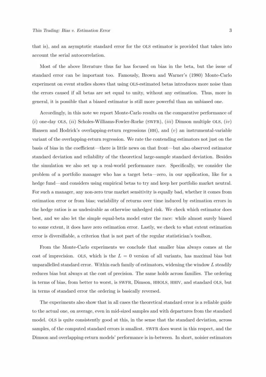
Thin Trading: Bias v. Estimation Error 3
that is), and an asymptotic standard error for the OLS estimator is provided that takes into
account the serial autocorrelation.
Most of the above literature thus far has focused on bias in the beta, but the issue of
standard error can be important too. Famously, Brown and Warner’s (1980) Monte-Carlo
experiment on event studies shows that using OLS-estimated betas introduces more noise than
the errors caused if all betas are set equal to unity, without any estimation. Thus, more in
general, it is possible that a biased estimator is still more powerful than an unbiased one.
Accordingly, in this note we report Monte-Carlo results on the comparative performance of
(i) one-day OLS, (ii) Scholes-Williams-Fowler-Rorke (SWFR), (iii) Dimson multiple OLS, (iv)
Hansen and Hodrick’s overlapping-return regressions (HH), and (v) an instrumental-variable
variant of the overlapping-return regression. We rate the contending estimators not just on the
basis of bias in the coefficient—there is little news on that front—but also observed estimator
standard deviation and reliability of the theoretical large-sample standard deviation. Besides
the simulation we also set up a real-world performance race. Specifically, we consider the
problem of a portfolio manager who has a target beta—zero, in our application, like for a
hedge fund—and considers using empirical betas to try and keep her portfolio market neutral.
For such a manager, any non-zero true market sensitivity is equally bad, whether it comes from
estimation error or from bias; variability of returns over time induced by estimation errors in
the hedge ratios is as undesirable as otherwise unhedged risk. We check which estimator does
best, and we also let the simple equal-beta model enter the race: while almost surely biased
to some extent, it does have zero estimation error. Lastly, we check to what extent estimation
error is diversifiable, a criterion that is not part of the regular statistician’s toolbox.
From the Monte-Carlo experiments we conclude that smaller bias always comes at the
cost of imprecision. OLS, which is the L = 0 version of all variants, has maximal bias but
unparallelled standard error. Within each family of estimators, widening the window L steadily
reduces bias but always at the cost of precision. The same holds across families. The ordering
in terms of bias, from better to worst, is SWFR, Dimson, HHOLS, HHIV, and standard OLS, but
in terms of standard error the ordering is basically reversed.
The experiments also show that in all cases the theoretical standard error is a reliable guide
to the actual one, on average, even in mid-sized samples and with departures from the standard
model. OLS is quite consistently good at this, in the sense that the standard deviation, across
samples, of the computed standard errors is smallest. SWFR does worst in this respect, and the
Dimson and overlapping-return models’ performance is in-between. In short, noisier estimators

Thin Trading: Bias v. Estimation Error 4
also have noisier estimated standard errors.
All this bears on Monte-Carlo sampling. The real-world results similarly confirm that,
within and across estimator families, bias disappears only at the cost of precision. This is found
directly in the betas, and confirmed by variances of portfolios that, in hedge-fund style, are
market-neutralized using beta estimates. The overwhelming winner of the portfolio experiment
however is the equal-beta model: just match by industry and size, and assume without any
estimation that matched stocks have identical market sensitivities. There may be bias here,
but the standard error equals an unparalleled zero, and this seems to be the more important
aspect.
1 The contenders
The familiar market-model regression is
Rj,t = α+ βjRm,t + εj,t, (1)
where Rj,t is the simple percentage change, cum dividend, in the j-th stock price over period
t and Rm,t is the return on the market portfolio. The stylized assumptions are that the only
correlation among these variables is the contemporaneous one between Rj,t and Rm,t, without
any auto- or cross-correlation anywhere.
1.1 Scholes-Williams-Fowler-Rorke (SWFR)
As illustrated in e.g. Dimson (1979), thin trading induces bias in the OLS beta because it
leads to errors in both the regressand and in the regressor.3 The interactions of these errors
mean that for active stocks the beta is biased upward, while for thinly traded stocks the bias is
negative, as Scholes and Williams show. Assuming that the duration of inaction never exceeds
one period, they then derive a consistent instrumental-variable estimator for the market-model
beta, where the instrument is a moving sum of the market returns for days t− 1, t, and t+ 1.
3On the regressand side, a stock that is not traded on day t reports a return of zero, apparently withoutrelation with the market’s movement. Actually, the unobserved true day-t return shows up on day t+1 (as partof the return reported for that day), but again seemingly without relation with the true day-t market return.Thus, at least two returns are mis-measured. On the regressor side, thin trading likewise induces two types oferror, each induced by the errors in the regressands. First, as yesterday’s non-traded stocks catch up today,an echo of yesterday’s market return is added into today’s reported market return; this error is assumed to beuncorrelated with today’s true return. Second, due to non-trading today, part of today’s true market returnis missing, an error that is negatively correlated with the true market return. It will also be obvious that thethin-trading error in the regressand is positively correlated with the one in the regressor.

Thin Trading: Bias v. Estimation Error 5
Fowler and Rorke (1983) generalize this solution to longer no-trading intervals by extending
the moving-sum window. So Scholes and Williams (1977) and Fowler and Rorke (1983) show
that, when reported prices may really date from up to L periods ago, the downward bias is
avoided if beta is estimated as
βSWj,H =
cov(Rj , ZSWH )
cov(Rm, ZSWH )
with ZSWH,t =
L∑l=−L
Rm,t+l. (2)
The reason why this IV solution works here is that (i) any auto- and cross-correlations
present in actually observed returns are, by assumption, induced by thin trading, and (ii) the
(2L + 1)-period moving sum of market returns does pick up all correlations induced by thin
trading. Since the mis-timing of the true day-t return does not affect the moving sum of market
returns, the instrument is uncorrelated with the error in the reported market return, the key
requirement for a proper instrument.
The consistency of the SWFR estimator is not the issue, so our Monte-Carlo tests are
intended as checks for small-sample unbiasedness and especially for the validity of the standard
error, whose consistent estimator is:4
asymptotic stdev(βSWj,H) =
√√√√ σ2ε (1 + 2
∑Ll=1,L ρl,jρl,Z)∑N−L
1+L (Rm,t −Rm)2R2RM ,Z
(3)
where σ2ε is the residual variance, ρl,X the lth-order autocorrelation of the returns from asset
X = j,m and R2RM ,Z the squared correlation between the market return and the instrument.
1.2 The Hansen-Hodrick overlapping-observation regression
Under standard assumptions, in the absence of thin trading the true one- and multi-period
betas are the same. For reasons outlined in the introduction, an overlapping-return regression
may be preferred, (H−1∑l=0
Rj,t+l
)= α+ βHH
j,H
(H−1∑l=0
Rm,t+l
)+ εj,t,H . (4)
The overlapping returns obviously generate autocorrelation in the error terms. Hansen and
Hodrick (1980) reject GLS as biased, in the case of overlapping returns, and propose OLS with
an autocorrelation-consistent standard deviation which is consistently estimated as
Θ = (X ′X)−1X ′Ω−1X(X ′X)−1, (5)
4The autocorrelations are new relative to the textbook IV case. See Scholes and Williams for the derivationsfor L = 1. The generalisation to L ≥ 2 follows easily.

Thin Trading: Bias v. Estimation Error 6
where X is the N × 2 matrix of observations 1, Rm,t and Ω is a band matrix with the
estimated variances and autocovariances of the regression errors u:
Ω = σ2ε
1 ρ1 ... ρH−1 0 ... ... ... 0ρ1 1 ρ1 ... ρH−1 0 ... ... 0... ρ1 1 ρ1 ... ρH−1 0 ... 0
ρH−1 ... ρ1 1 ρ1 ... ρH−1 0 00 00 0 ρH−1 ... ρ1 1 ρ1 ... ρH−1
0 ... 0 ρH−1 ... ρ1 1 ρ1 ...0 ... ... 0 ρH−1 ... ρ1 1 ρ1
0 ... ... ... 0 ρH−1 ... ρ1 1
. (6)
1.3 An Instrumental-Variable Overlapping-Return Estimator
We easily derive a consistent IV estimator of the overlapping-return model. We start from
the explicit objective that we want to estimate the beta over a horizon of H periods, and
accordingly write the H-period price change as the sum of H one-period changes. Next, we
use equalities like cov(X(+1), Y (+3)) = cov(X,Y (+2)); and lastly we regroup and interpret
the estimator as an IV one:
βIVj,H =
cov(Rj +Rj(+1) + ...+Rj(+H − 1), Rm +Rm(+1) + ...Rm(+H − 1))var(Rm +Rm(+1) + ...Rm(+H − 1))
=∑H−1k=0
∑H−1l=0 cov(Rj(+k), Rm(+l))∑H−1
k=0
∑H−1l=0 cov(Rm(+k), Rm(+l))
=∑H−1k=−H+1(H − |k|)cov(Rj , Rm(+k))∑H−1k=−H+1(H − |k|)cov(Rj , Rm(+k))
=cov(Rj , ZIV
H )cov(Rm, ZIV
H )), (7)
where the instrument is a pyramid-weighted moving sum rather than the SWFR equally weighted
one:
ZIVH =
H−1∑k=−H+1
(H − |k|)Rm(+k). (8)
The asymptotic standard error is the same as for SWFR.
In the next section we compare the performance of these contenders as far as bias is
concerned, true standard error, and reliability of the standard error produced by standard
software. This last issue is especially relevant when the method is applied to data where the
standard model does not hold.

Thin Trading: Bias v. Estimation Error 7
2 Simulation results
2.1 Monte Carlo results for the standard model
Each complete simulation contains 10,000 experiments, and one such experiment consists of
the following steps. First, an IID market factor f is generated with zero mean and constant
volatility equal to 0.01 per diem, i.e. about 0.15 per annum (p.a.). This market factor has a
fat-tailed Student’s distribution with seven df, which produces a realistic level for the kurtosis
and tail coefficient (Bauwens et al., 2006). From this, returns for 2,000 assets are generated,
all with a unit beta and idiosyncratic noise with 1.5 times the market standard deviation,
generating the typical p.a volatility of about 0.30 for an individual stock. There are three
classes of trading thinness: 1000 of the stocks trade every day, 500 trade with a probability of
0.9, and 500 trade with probability 0.75. If a stock is not traded, the recorded return is zero;
simultaneously, its true return is added to a buffer until the stock does trade, at which time
the cumulative return is recorded. Starting from 2000 initial value weights taken from NYSE
in 1992, we then update the value weights. The initial market caps are ranked in descending
order, so that large stocks tend to be active ones, and the smallest firms most prone to missing
prices. The market return is computed as a value-weighted average of asset returns. For the
market-model regressions we generate 250 such “daily” observations for all 2000 stocks, and
pick three stock files out of these, one per thinness class, to run the regressions. We then
start a new experiment, until we have gone through 10,000 of them. For SWFR and Dimson,
L is set at 1, 2, 3, 4 and 19 each side,5 while for the overlapping-observation regressions H
is likewise set at 2, 3, 4, 5 (one week) and 20 (monthly holding periods). For each regression
we compute the slopes and theoretical asymptotic standard error. For each set of 10,000 such
computations (one per type of regression and thinness class) we then produce the mean and
standard deviation. Table 1 summarizes the results.
Predictably, OLS does worst in terms of bias, with beta approximating unity minus the
probability of no trade. There is no evidence of any upward bias for the active stocks. Scholes
and Williams demonstrate the theoretical possibility: since the weighted average beta estimate
tautologically equals unity, downward bias for sleepy stocks must come with upward bias for
active stocks. The fact that our unweighted average beta is below unity, in this table, is still
5The chance that a stock with no-trade probabilty 0.25 would not trade for 3 (4) periods is 0.7520.253 = 0.0088(0.7520.254 = 0.0022), so L = 3 looks reasonable. We add 19 for comparability with the overlapping-returntechniques, where monthly returns (approximately 20 trading days) are quite popular.

Thin Trading: Bias v. Estimation Error 8
Table 1: Simulation results: base case
Mean β mean SE (β)s stdev across β stdev of SE (β)sprob no trade .00 .10 .25 .00 .10 .25 .00 .10 .25 .00 .10 .25
One-period regression
OLS .99 .89 .74 .10 .10 .10 .09 .11 .12 .008 .008 .009
SWFR ±1 .99 .98 .92 .17 .18 .18 .17 .17 .18 .020 .021 .023SWFR ±2 .99 .98 .97 .22 .23 .25 .22 .23 .23 .036 .037 .040SWFR ±3 .99 .99 .98 .27 .28 .30 .27 .28 .28 .055 .058 .062SWFR ±4 .99 .98 .98 .32 .33 .35 .32 .32 .32 .078 .082 .087
Dimson±1 .99 .98 .92 .14 .14 .15 .14 .14 .15 .012 .012 .013Dimson±2 .99 .98 .97 .17 .17 .18 .17 .17 .17 .016 .016 .017Dimson±3 .99 .99 .98 .19 .20 .21 .19 .20 .20 .019 .020 .021Dimson±4 .98 .99 .98 .22 .23 .24 .22 .22 .22 .023 .024 .026Dimson±19 .99 .99 .99 .51 .53 .55 .52 .51 .52 .100 .105 .110
H-period overlapping-returns regression
IV 2 .99 .93 .83 .12 .12 .13 .12 .12 .13 .010 .010 .011IV 3 .99 .95 .87 .14 .15 .15 .14 .15 .15 .012 .013 .014IV 4 .99 .96 .90 .16 .17 .18 .16 .17 .17 .015 .016 .017IV 5 .99 .96 .92 .18 .19 .20 .18 .18 .18 .018 .018 .020IV 20 .99 .98 .96 .41 .42 .44 .39 .40 .41 .074 .077 .084
OLSHH 2 .99 .95 .88 .13 .13 .13 .14 .14 .15 .014 .014 .014OLSHH 3 .99 .96 .90 .15 .15 .16 .16 .16 .16 .018 .018 .019OLSHH 4 .99 .96 .92 .17 .17 .17 .18 .18 .18 .023 .023 .023OLSHH 5 .99 .97 .93 .19 .19 .19 .20 .20 .20 .027 .027 .027OLSHH 20 .99 .98 .96 .33 .33 .33 .38 .39 .39 .089 .091 .089
Key. 250 ”daily” returns for 2000 stocks are generated by a unit-beta market model with a thick-tailed IIDmarket factor with stdev 0.01/day plus idiosyncratic noise (R2=0.3). 1000 of the 2000 stocks trade daily, 500nine days out of ten, and 500 three days out of four. On no-trade days a zero return is reported, and the invisibleprice change is cumulated until the first trade. Value-weighted market returns are computed from these 2000returns, and three individual-stock return series are stored, one for each thinness class. This experiment isrepeated 10,000 times. OLS uses daily data. SWFR uses as the instrument a moving-window sum of marketreturns with ±L leads/lags. Dimson uses a multiple regresion with ±L leading/lagging market returns asadditional regressors; the beta is the sum of these 2L + 1 coefficients. The overlapping-return IV regressionuses H − 1 proximity-weighted leading and lagging market returns as the instrument. OLSHH runs OLS withautocorrelation-adjusted SE’s. The IVSE’s also account for thin-trading-induced autocorrelation in regressandand regressor.
compatible with a value-weighted average beta equal to unity because of the positive covariance
between weights and estimated beta:
1 =∑j
wj βj = (∑j
wj)β +∑j
(wj − w)(βj − β) = β +∑j
(wj − w)(βj − β) > β. (9)
Equally predictably, SWFR does a good job in eliminating even severe thin-trading biases like
p = .25 with modest values like L = 3. But Dimson’s beta does as well in terms of bias. For
both estimators, the reduction in bias upon increasing the window size 2L + 1 comes quite
rapidly: with no-trading probabilities not exceeding 0.25, there seems to be no point in going
beyond L = 4. The overlapping-return regressions, whether OLS or IV, are good at handling
Thin Trading: Bias v. Estimation Error 9
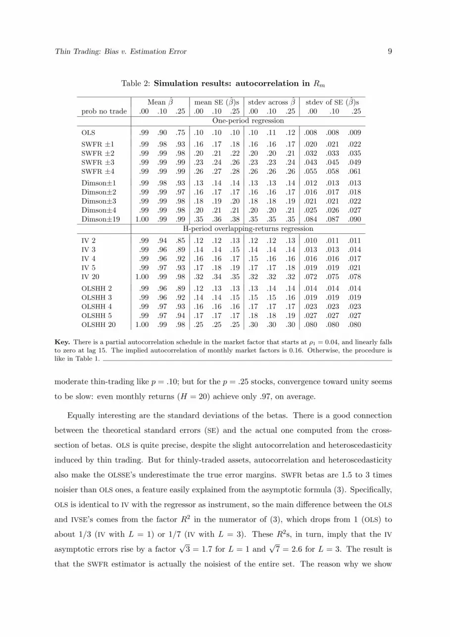
Table 2: Simulation results: autocorrelation in Rm
Mean β mean SE (β)s stdev across β stdev of SE (β)sprob no trade .00 .10 .25 .00 .10 .25 .00 .10 .25 .00 .10 .25
One-period regression
OLS .99 .90 .75 .10 .10 .10 .10 .11 .12 .008 .008 .009
SWFR ±1 .99 .98 .93 .16 .17 .18 .16 .16 .17 .020 .021 .022SWFR ±2 .99 .99 .98 .20 .21 .22 .20 .20 .21 .032 .033 .035SWFR ±3 .99 .99 .99 .23 .24 .26 .23 .23 .24 .043 .045 .049SWFR ±4 .99 .99 .99 .26 .27 .28 .26 .26 .26 .055 .058 .061
Dimson±1 .99 .98 .93 .13 .14 .14 .13 .13 .14 .012 .013 .013Dimson±2 .99 .99 .97 .16 .17 .17 .16 .16 .17 .016 .017 .018Dimson±3 .99 .99 .98 .18 .19 .20 .18 .18 .19 .021 .021 .022Dimson±4 .99 .99 .98 .20 .21 .21 .20 .20 .21 .025 .026 .027Dimson±19 1.00 .99 .99 .35 .36 .38 .35 .35 .35 .084 .087 .090
H-period overlapping-returns regression
IV 2 .99 .94 .85 .12 .12 .13 .12 .12 .13 .010 .011 .011IV 3 .99 .96 .89 .14 .14 .15 .14 .14 .14 .013 .013 .014IV 4 .99 .96 .92 .16 .16 .17 .15 .16 .16 .016 .016 .017IV 5 .99 .97 .93 .17 .18 .19 .17 .17 .18 .019 .019 .021IV 20 1.00 .99 .98 .32 .34 .35 .32 .32 .32 .072 .075 .078
OLSHH 2 .99 .96 .89 .12 .13 .13 .13 .14 .14 .014 .014 .014OLSHH 3 .99 .96 .92 .14 .14 .15 .15 .15 .16 .019 .019 .019OLSHH 4 .99 .97 .93 .16 .16 .16 .17 .17 .17 .023 .023 .023OLSHH 5 .99 .97 .94 .17 .17 .17 .18 .18 .19 .027 .027 .027OLSHH 20 1.00 .99 .98 .25 .25 .25 .30 .30 .30 .080 .080 .080
Key. There is a partial autocorrelation schedule in the market factor that starts at ρ1 = 0.04, and linearly fallsto zero at lag 15. The implied autocorrelation of monthly market factors is 0.16. Otherwise, the procedure islike in Table 1.
moderate thin-trading like p = .10; but for the p = .25 stocks, convergence toward unity seems
to be slow: even monthly returns (H = 20) achieve only .97, on average.
Equally interesting are the standard deviations of the betas. There is a good connection
between the theoretical standard errors (SE) and the actual one computed from the cross-
section of betas. OLS is quite precise, despite the slight autocorrelation and heteroscedasticity
induced by thin trading. But for thinly-traded assets, autocorrelation and heteroscedasticity
also make the OLSSE’s underestimate the true error margins. SWFR betas are 1.5 to 3 times
noisier than OLS ones, a feature easily explained from the asymptotic formula (3). Specifically,
OLS is identical to IV with the regressor as instrument, so the main difference between the OLS
and IVSE’s comes from the factor R2 in the numerator of (3), which drops from 1 (OLS) to
about 1/3 (IV with L = 1) or 1/7 (IV with L = 3). These R2s, in turn, imply that the IV
asymptotic errors rise by a factor√
3 = 1.7 for L = 1 and√
7 = 2.6 for L = 3. The result is
that the SWFR estimator is actually the noisiest of the entire set. The reason why we show
Thin Trading: Bias v. Estimation Error 10
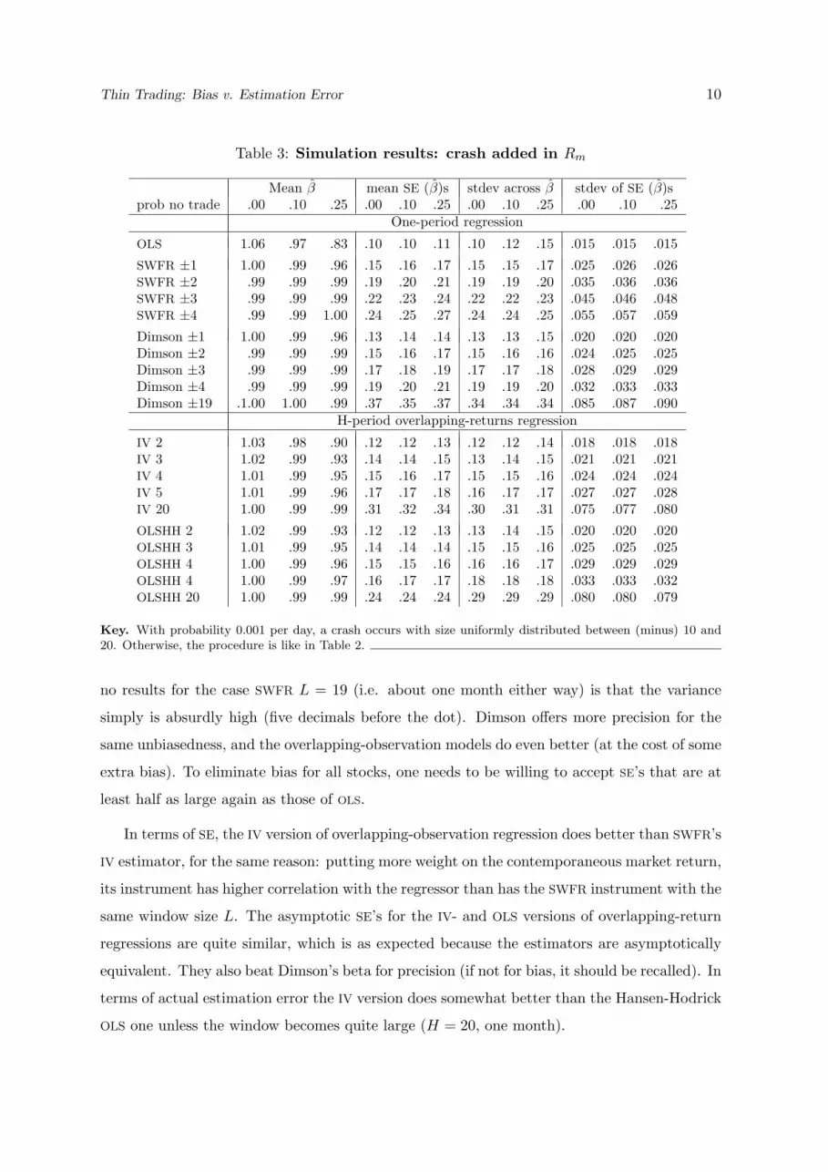
Table 3: Simulation results: crash added in Rm
Mean β mean SE (β)s stdev across β stdev of SE (β)sprob no trade .00 .10 .25 .00 .10 .25 .00 .10 .25 .00 .10 .25
One-period regression
OLS 1.06 .97 .83 .10 .10 .11 .10 .12 .15 .015 .015 .015
SWFR ±1 1.00 .99 .96 .15 .16 .17 .15 .15 .17 .025 .026 .026SWFR ±2 .99 .99 .99 .19 .20 .21 .19 .19 .20 .035 .036 .036SWFR ±3 .99 .99 .99 .22 .23 .24 .22 .22 .23 .045 .046 .048SWFR ±4 .99 .99 1.00 .24 .25 .27 .24 .24 .25 .055 .057 .059
Dimson ±1 1.00 .99 .96 .13 .14 .14 .13 .13 .15 .020 .020 .020Dimson ±2 .99 .99 .99 .15 .16 .17 .15 .16 .16 .024 .025 .025Dimson ±3 .99 .99 .99 .17 .18 .19 .17 .17 .18 .028 .029 .029Dimson ±4 .99 .99 .99 .19 .20 .21 .19 .19 .20 .032 .033 .033Dimson ±19 .1.00 1.00 .99 .37 .35 .37 .34 .34 .34 .085 .087 .090
H-period overlapping-returns regression
IV 2 1.03 .98 .90 .12 .12 .13 .12 .12 .14 .018 .018 .018IV 3 1.02 .99 .93 .14 .14 .15 .13 .14 .15 .021 .021 .021IV 4 1.01 .99 .95 .15 .16 .17 .15 .15 .16 .024 .024 .024IV 5 1.01 .99 .96 .17 .17 .18 .16 .17 .17 .027 .027 .028IV 20 1.00 .99 .99 .31 .32 .34 .30 .31 .31 .075 .077 .080
OLSHH 2 1.02 .99 .93 .12 .12 .13 .13 .14 .15 .020 .020 .020OLSHH 3 1.01 .99 .95 .14 .14 .14 .15 .15 .16 .025 .025 .025OLSHH 4 1.00 .99 .96 .15 .15 .16 .16 .16 .17 .029 .029 .029OLSHH 4 1.00 .99 .97 .16 .17 .17 .18 .18 .18 .033 .033 .032OLSHH 20 1.00 .99 .99 .24 .24 .24 .29 .29 .29 .080 .080 .079
Key. With probability 0.001 per day, a crash occurs with size uniformly distributed between (minus) 10 and20. Otherwise, the procedure is like in Table 2.
no results for the case SWFR L = 19 (i.e. about one month either way) is that the variance
simply is absurdly high (five decimals before the dot). Dimson offers more precision for the
same unbiasedness, and the overlapping-observation models do even better (at the cost of some
extra bias). To eliminate bias for all stocks, one needs to be willing to accept SE’s that are at
least half as large again as those of OLS.
In terms of SE, the IV version of overlapping-observation regression does better than SWFR’s
IV estimator, for the same reason: putting more weight on the contemporaneous market return,
its instrument has higher correlation with the regressor than has the SWFR instrument with the
same window size L. The asymptotic SE’s for the IV- and OLS versions of overlapping-return
regressions are quite similar, which is as expected because the estimators are asymptotically
equivalent. They also beat Dimson’s beta for precision (if not for bias, it should be recalled). In
terms of actual estimation error the IV version does somewhat better than the Hansen-Hodrick
OLS one unless the window becomes quite large (H = 20, one month).
Thin Trading: Bias v. Estimation Error 11
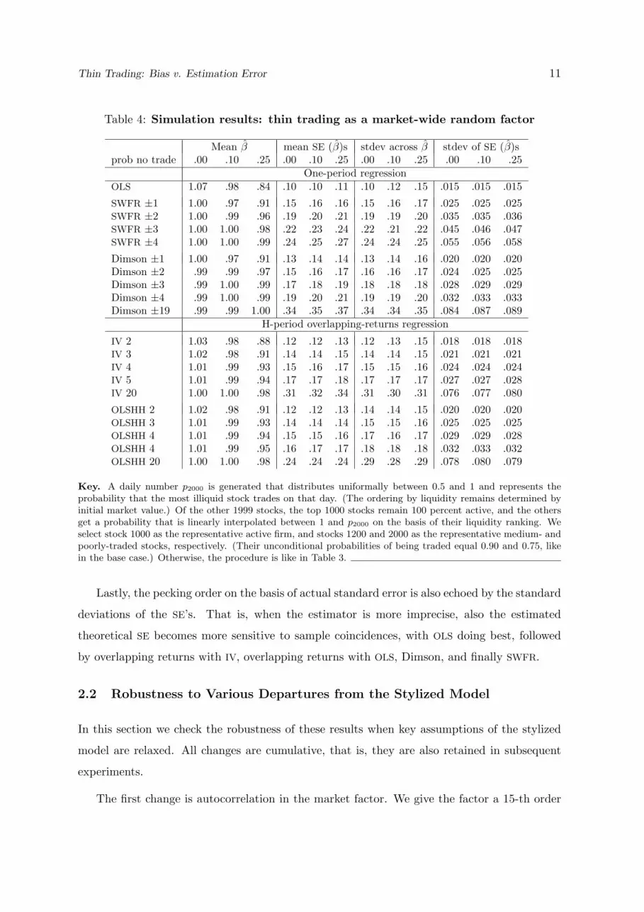
Table 4: Simulation results: thin trading as a market-wide random factor
Mean β mean SE (β)s stdev across β stdev of SE (β)sprob no trade .00 .10 .25 .00 .10 .25 .00 .10 .25 .00 .10 .25
One-period regressionOLS 1.07 .98 .84 .10 .10 .11 .10 .12 .15 .015 .015 .015
SWFR ±1 1.00 .97 .91 .15 .16 .16 .15 .16 .17 .025 .025 .025SWFR ±2 1.00 .99 .96 .19 .20 .21 .19 .19 .20 .035 .035 .036SWFR ±3 1.00 1.00 .98 .22 .23 .24 .22 .21 .22 .045 .046 .047SWFR ±4 1.00 1.00 .99 .24 .25 .27 .24 .24 .25 .055 .056 .058
Dimson ±1 1.00 .97 .91 .13 .14 .14 .13 .14 .16 .020 .020 .020Dimson ±2 .99 .99 .97 .15 .16 .17 .16 .16 .17 .024 .025 .025Dimson ±3 .99 1.00 .99 .17 .18 .19 .18 .18 .18 .028 .029 .029Dimson ±4 .99 1.00 .99 .19 .20 .21 .19 .19 .20 .032 .033 .033Dimson ±19 .99 .99 1.00 .34 .35 .37 .34 .34 .35 .084 .087 .089
H-period overlapping-returns regression
IV 2 1.03 .98 .88 .12 .12 .13 .12 .13 .15 .018 .018 .018IV 3 1.02 .98 .91 .14 .14 .15 .14 .14 .15 .021 .021 .021IV 4 1.01 .99 .93 .15 .16 .17 .15 .15 .16 .024 .024 .024IV 5 1.01 .99 .94 .17 .17 .18 .17 .17 .17 .027 .027 .028IV 20 1.00 1.00 .98 .31 .32 .34 .31 .30 .31 .076 .077 .080
OLSHH 2 1.02 .98 .91 .12 .12 .13 .14 .14 .15 .020 .020 .020OLSHH 3 1.01 .99 .93 .14 .14 .14 .15 .15 .16 .025 .025 .025OLSHH 4 1.01 .99 .94 .15 .15 .16 .17 .16 .17 .029 .029 .028OLSHH 4 1.01 .99 .95 .16 .17 .17 .18 .18 .18 .032 .033 .032OLSHH 20 1.00 1.00 .98 .24 .24 .24 .29 .28 .29 .078 .080 .079
Key. A daily number p2000 is generated that distributes uniformally between 0.5 and 1 and represents theprobability that the most illiquid stock trades on that day. (The ordering by liquidity remains determined byinitial market value.) Of the other 1999 stocks, the top 1000 stocks remain 100 percent active, and the othersget a probability that is linearly interpolated between 1 and p2000 on the basis of their liquidity ranking. Weselect stock 1000 as the representative active firm, and stocks 1200 and 2000 as the representative medium- andpoorly-traded stocks, respectively. (Their unconditional probabilities of being traded equal 0.90 and 0.75, likein the base case.) Otherwise, the procedure is like in Table 3.
Lastly, the pecking order on the basis of actual standard error is also echoed by the standard
deviations of the SE’s. That is, when the estimator is more imprecise, also the estimated
theoretical SE becomes more sensitive to sample coincidences, with OLS doing best, followed
by overlapping returns with IV, overlapping returns with OLS, Dimson, and finally SWFR.
2.2 Robustness to Various Departures from the Stylized Model
In this section we check the robustness of these results when key assumptions of the stylized
model are relaxed. All changes are cumulative, that is, they are also retained in subsequent
experiments.
The first change is autocorrelation in the market factor. We give the factor a 15-th order

Thin Trading: Bias v. Estimation Error 12
Table 5: Simulation results: magnified thin-trading problem
Mean β mean SE (β)s stdev across β stdev of SE (β)sprob no trade .00 .25 .50 .00 .25 .50 .00 .25 .50 .00 .25 .50
One-period regression
OLS 1.23 .99 .75 .12 .13 .13 .12 .16 .19 .017 .016 .017
SWFR ±1 1.06 1.07 .87 .16 .17 .18 .16 .16 .20 .025 .025 .025SWFR ±2 1.02 1.02 .98 .19 .21 .22 .19 .19 .21 .033 .033 .034SWFR ±3 1.01 1.01 1.02 .22 .24 .25 .22 .22 .23 .043 .043 .045SWFR ±4 1.01 1.01 1.02 .25 .26 .28 .24 .25 .25 .052 .053 .055
Dimson ±1 1.03 1.08 .88 .15 .16 .17 .15 .15 .19 .022 .022 .022Dimson ±2 1.01 1.01 1.02 .17 .18 .19 .17 .17 .19 .026 .026 .027Dimson ±3 1.01 1.01 1.04 .19 .20 .21 .19 .19 .20 .030 .031 .031Dimson ±4 1.00 1.00 1.02 .20 .22 .23 .20 .20 .21 .034 .035 .035Dimson ±19 1.00 .99 1.00 .34 .37 .40 .35 .35 .35 .087 .092 .095
H-period overlapping-returns regression
IV 2 1.12 1.04 .82 .13 .14 .15 .13 .14 .18 .019 .019 .020IV 3 1.08 1.03 .88 .15 .16 .17 .15 .15 .18 .022 .022 .023IV 4 1.06 1.03 .92 .17 .18 .19 .16 .17 .18 .026 .025 .026IV 5 1.05 1.02 .95 .18 .20 .21 .18 .18 .19 .029 .029 .029IV 20 1.01 1.00 .99 .32 .35 .37 .31 .31 .32 .078 .080 .084
OLSHH 2 1.08 1.03 .89 .13 .14 .14 .15 .15 .17 .022 .022 .022OLSHH 3 1.06 1.03 .93 .15 .15 .16 .16 .16 .18 .027 .027 .027OLSHH 4 1.05 1.02 .95 .17 .17 .17 .18 .18 .19 .031 .031 .031OLSHH 4 1.04 1.02 .96 .18 .18 .18 .19 .19 .20 .035 .035 .034OLSHH 20 1.01 1.01 .99 .24 .24 .24 .30 .30 .30 .083 .082 .082
Key. There are 666 active stocks, 667 stocks that trade 3 days out of 4, and 667 stocks that trade one day outof two. Otherwise, the procedure is like in Table 3.
autocorrelation (prior to the autocorrelation induced by thin trading), starting at ρ1 = 0.04
and linearly falling to 0 at lag 16. This, it can be checked, induces an autocorrelation of
monthly returns of 0.16. Adding thin trading, we get a total autocorrelation in the index of
about 0.20, which is realistic for monthly intervals. As can be verified in Table 2, the results
do not differ in any meaningful way from the base-case output.
The second change is skewness in the returns. From Bauwens et al. (2006), active stocks
exhibit no skewness at the daily level as long as there is no crash; so we generate skewness via a
crash factor in the market. In the experiment we report the crash occurs with a quite generous
daily probability of 0.001 (about once every 4 years), and when it does take place the fall is
uniformly distributed between –10 and –20 percent. Unlike the regular market factor f , which
retains its 15th-order autocorrelation, the crash factor is not autocorrelated. Table 3 has the
results. The relevant conclusions are unaffected; in fact, there is but one pervasive change: all
betas are higher. This reflects the fact that there is an extra common factor that affects all

Thin Trading: Bias v. Estimation Error 13
stocks in the same way without increase in the errors-in-variables problems. As a result, there
now is a noticeable upward bias in the active stocks, as predicted theoretically. The reason
why it shows up now and not in the earlier experiments is that the the covariance between beta
error and asset weight is weakened if a common crash factor affects all stocks alike, whether
big or small. The OLS beta is still below unity on average, but the active subgroup no longer
is.6
The above modifications were cumulative, and also show up in the next two experiments,
which have to do with the way we modeled the thin-trading problem. In the first robustness
check we let the probabilities of no trade vary randomly over time, while creating correlation
between the no-trading events across stocks. Specifically, a daily number p2000 is generated that
distributes uniformally between 0.5 and 1 and represents the probability that the most illiquid
stock gets traded on that day. (The ordering by liquidity remains determined by initial market
value.) Of the other 1999 stocks, the top 1000 stocks remain 100 percent active as before, but
the others get a probability that is linearly interpolated between 1 and p2000 on the basis of their
liquidity ranking. We select stock 1000 as the representative active firm, and stocks 1200 and
2000 as the representative medium- and poorly-traded stocks, respectively. Thus, comparable
with the base case, the three stocks we study still have unconditional probabilities of being
traded equal to 1.00, 0.90 and 0.75, but now the non-trading problem is correlated across stocks,
and assets’ errors-in-variables are more strongly correlated with the measurement errors in the
market. Despite this, the only remarkable effect in Table 4 is how small and unsystematic the
changes are relative to the previous case.
In our second robustness check w.r.t. the details of the thin-trading mechanism we return
to the original setup except that we worsen the thin-trading problem substantially. Instead
of 1000 active stocks, 500 moderately traded, and 500 thinly traded ones we make the groups
equally large, and we increase the probability of no trade from 0.10 to 0.25 for the middle group
and from 0.25 to 0.50 for the worst affected stocks. In Table 5, summarizing the results, we see
many effects magnified. The gap between the active and sleepy stocks’ OLS betas is still equal
to the (now larger) probability of no trade, but the active betas are substantially overestimated.
This upward bias for the active stocks gets weakened quite quickly when we use any of the other
estimators, and is no longer a major problem when L = 4; for monthly windows it is entirely
6Results for lower crash probabilities are, not surprisingly, in-between those of Tables 3 and 1 and areavailable on request. The same holds for experiments that are identical to those already summarized except forthicker tails in the market and idiosyncratic returns (five df instead of seven): the changes are minute.

Thin Trading: Bias v. Estimation Error 14
Table 6: Simulation results: stochastic liquidity, big market variance
Mean β mean SE (β)s stdev across β stdev of SE (β)sprob no trade .00 .25 .50 .00 .25 .50 .00 .25 .50 .00 .25 .50
One-period regression
OLS 1.07 .99 .85 .07 .07 .08 .07 .09 .11 .007 .008 .008
SWFR ±1 1.01 .98 .92 .10 .11 .12 .10 .11 .13 .014 .015 .015SWFR ±2 1.00 1.00 .97 .13 .14 .16 .13 .13 .14 .021 .022 .023SWFR ±3 1.00 1.00 .99 .15 .16 .18 .15 .15 .15 .028 .030 .032SWFR ±4 1.00 1.00 .99 .17 .18 .20 .17 .17 .17 .035 .037 .040
Dimson±1 1.00 .97 .92 .09 .10 .11 .09 .10 .12 .010 .011 .011Dimson±2 1.00 .99 .97 .11 .12 .13 .11 .11 .12 .013 .014 .014Dimson±3 1.00 1.00 .99 .12 .13 .14 .12 .12 .13 .016 .017 .017Dimson±4 1.00 1.00 1.00 .13 .14 .16 .13 .13 .14 .018 .020 .020Dimson±19 .99 1.00 1.00 .23 .25 .27 .23 .23 .24 .056 .059 .063
H-period overlapping-returns regression
IV 2 1.04 .98 .89 .08 .09 .10 .08 .09 .11 .009 .010 .010IV 3 1.02 .99 .92 .09 .10 .11 .09 .10 .11 .011 .012 .012IV 4 1.02 .99 .94 .11 .11 .13 .11 .11 .11 .013 .014 .014IV 5 1.01 .99 .95 .12 .12 .14 .12 .11 .12 .015 .016 .017IV 20 1.00 1.00 .99 .21 .23 .25 .21 .21 .21 .049 .051 .056
OLSHH 2 1.02 .99 .92 .08 .09 .09 .09 .10 .11 .011 .011 .012OLSHH 3 1.02 .99 .94 .10 .10 .10 .10 .11 .11 .014 .014 .014OLSHH 4 1.01 .99 .95 .11 .11 .11 .11 .11 .12 .017 .017 .017OLSHH 5 1.01 .99 .96 .11 .11 .12 .12 .12 .13 .019 .020 .019OLSHH 20 1.00 1.00 .99 .16 .16 .16 .20 .19 .20 .052 .053 .053
Key. The market-factor volatility is increased by one-half to 1.5% per diem. Otherwise, the procedure is likein Table 4.
gone. The other effects that we observed in the base case remain unaffected: Scholes-Williams,
Dimson, and Hansen-Hodrick handle the bias well (in that order), and the IV version of the
overlapping-return regression rather well. Actual precision of OLS now substantially overstates
the calculated one, but still does not do badly relative to the other estimators; the OLS and
IV overlapping-observations models still come next, followed by Dimson and, lastly, SWFR.
We conclude that in all experiments, lower bias comes at the cost of higher SE’s and noisier
estimates of these SE’s.
We end with three encores. In all of these, we return to the stochastic-liquidity setup of
Table 4. First, we increase the market factor volatility from 1% per day to 1.5%, i.e from about
16% per annum to 24%, at constant idiosyncratic noise. Predictably, with a clearer signal and
unmodified residual risk, the precision is higher, but otherwise the outcomes are similar to
those Table 4, as can be seen from Table 6. For the remaining two variants we again return to
the scenario of Table 4, with base-case market variance (and stochastic liquidity and a crash),
but now we add standard negative skewness in both the market and the idiosyncratic factor.
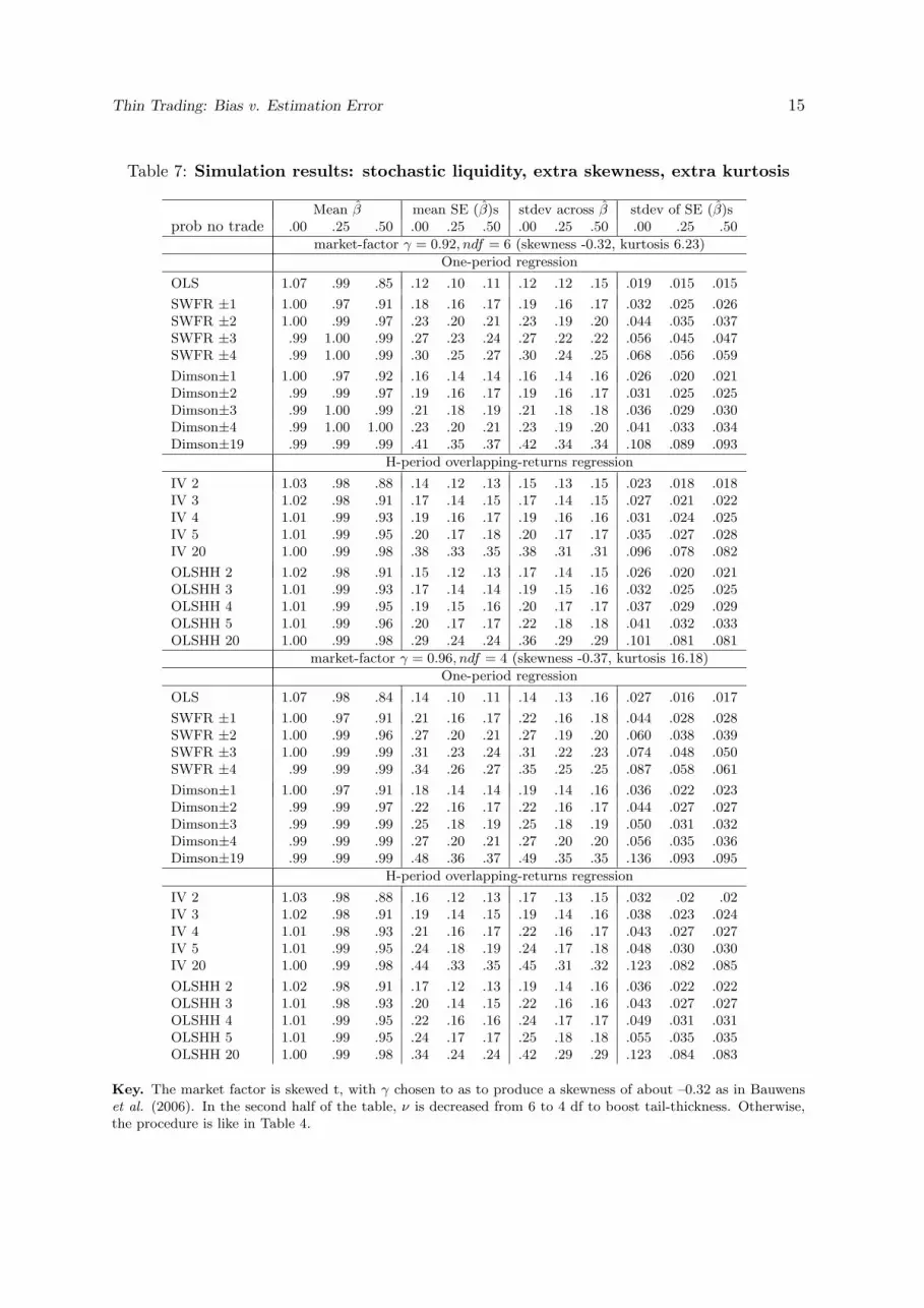
Thin Trading: Bias v. Estimation Error 15
Table 7: Simulation results: stochastic liquidity, extra skewness, extra kurtosis
Mean β mean SE (β)s stdev across β stdev of SE (β)sprob no trade .00 .25 .50 .00 .25 .50 .00 .25 .50 .00 .25 .50
market-factor γ = 0.92, ndf = 6 (skewness -0.32, kurtosis 6.23)
One-period regression
OLS 1.07 .99 .85 .12 .10 .11 .12 .12 .15 .019 .015 .015
SWFR ±1 1.00 .97 .91 .18 .16 .17 .19 .16 .17 .032 .025 .026SWFR ±2 1.00 .99 .97 .23 .20 .21 .23 .19 .20 .044 .035 .037SWFR ±3 .99 1.00 .99 .27 .23 .24 .27 .22 .22 .056 .045 .047SWFR ±4 .99 1.00 .99 .30 .25 .27 .30 .24 .25 .068 .056 .059
Dimson±1 1.00 .97 .92 .16 .14 .14 .16 .14 .16 .026 .020 .021Dimson±2 .99 .99 .97 .19 .16 .17 .19 .16 .17 .031 .025 .025Dimson±3 .99 1.00 .99 .21 .18 .19 .21 .18 .18 .036 .029 .030Dimson±4 .99 1.00 1.00 .23 .20 .21 .23 .19 .20 .041 .033 .034Dimson±19 .99 .99 .99 .41 .35 .37 .42 .34 .34 .108 .089 .093
H-period overlapping-returns regression
IV 2 1.03 .98 .88 .14 .12 .13 .15 .13 .15 .023 .018 .018IV 3 1.02 .98 .91 .17 .14 .15 .17 .14 .15 .027 .021 .022IV 4 1.01 .99 .93 .19 .16 .17 .19 .16 .16 .031 .024 .025IV 5 1.01 .99 .95 .20 .17 .18 .20 .17 .17 .035 .027 .028IV 20 1.00 .99 .98 .38 .33 .35 .38 .31 .31 .096 .078 .082
OLSHH 2 1.02 .98 .91 .15 .12 .13 .17 .14 .15 .026 .020 .021OLSHH 3 1.01 .99 .93 .17 .14 .14 .19 .15 .16 .032 .025 .025OLSHH 4 1.01 .99 .95 .19 .15 .16 .20 .17 .17 .037 .029 .029OLSHH 5 1.01 .99 .96 .20 .17 .17 .22 .18 .18 .041 .032 .033OLSHH 20 1.00 .99 .98 .29 .24 .24 .36 .29 .29 .101 .081 .081
market-factor γ = 0.96, ndf = 4 (skewness -0.37, kurtosis 16.18)
One-period regression
OLS 1.07 .98 .84 .14 .10 .11 .14 .13 .16 .027 .016 .017
SWFR ±1 1.00 .97 .91 .21 .16 .17 .22 .16 .18 .044 .028 .028SWFR ±2 1.00 .99 .96 .27 .20 .21 .27 .19 .20 .060 .038 .039SWFR ±3 1.00 .99 .99 .31 .23 .24 .31 .22 .23 .074 .048 .050SWFR ±4 .99 .99 .99 .34 .26 .27 .35 .25 .25 .087 .058 .061
Dimson±1 1.00 .97 .91 .18 .14 .14 .19 .14 .16 .036 .022 .023Dimson±2 .99 .99 .97 .22 .16 .17 .22 .16 .17 .044 .027 .027Dimson±3 .99 .99 .99 .25 .18 .19 .25 .18 .19 .050 .031 .032Dimson±4 .99 .99 .99 .27 .20 .21 .27 .20 .20 .056 .035 .036Dimson±19 .99 .99 .99 .48 .36 .37 .49 .35 .35 .136 .093 .095
H-period overlapping-returns regression
IV 2 1.03 .98 .88 .16 .12 .13 .17 .13 .15 .032 .02 .02IV 3 1.02 .98 .91 .19 .14 .15 .19 .14 .16 .038 .023 .024IV 4 1.01 .98 .93 .21 .16 .17 .22 .16 .17 .043 .027 .027IV 5 1.01 .99 .95 .24 .18 .19 .24 .17 .18 .048 .030 .030IV 20 1.00 .99 .98 .44 .33 .35 .45 .31 .32 .123 .082 .085
OLSHH 2 1.02 .98 .91 .17 .12 .13 .19 .14 .16 .036 .022 .022OLSHH 3 1.01 .98 .93 .20 .14 .15 .22 .16 .16 .043 .027 .027OLSHH 4 1.01 .99 .95 .22 .16 .16 .24 .17 .17 .049 .031 .031OLSHH 5 1.01 .99 .95 .24 .17 .17 .25 .18 .18 .055 .035 .035OLSHH 20 1.00 .99 .98 .34 .24 .24 .42 .29 .29 .123 .084 .083
Key. The market factor is skewed t, with γ chosen to as to produce a skewness of about –0.32 as in Bauwenset al. (2006). In the second half of the table, ν is decreased from 6 to 4 df to boost tail-thickness. Otherwise,the procedure is like in Table 4.
Thin Trading: Bias v. Estimation Error 16
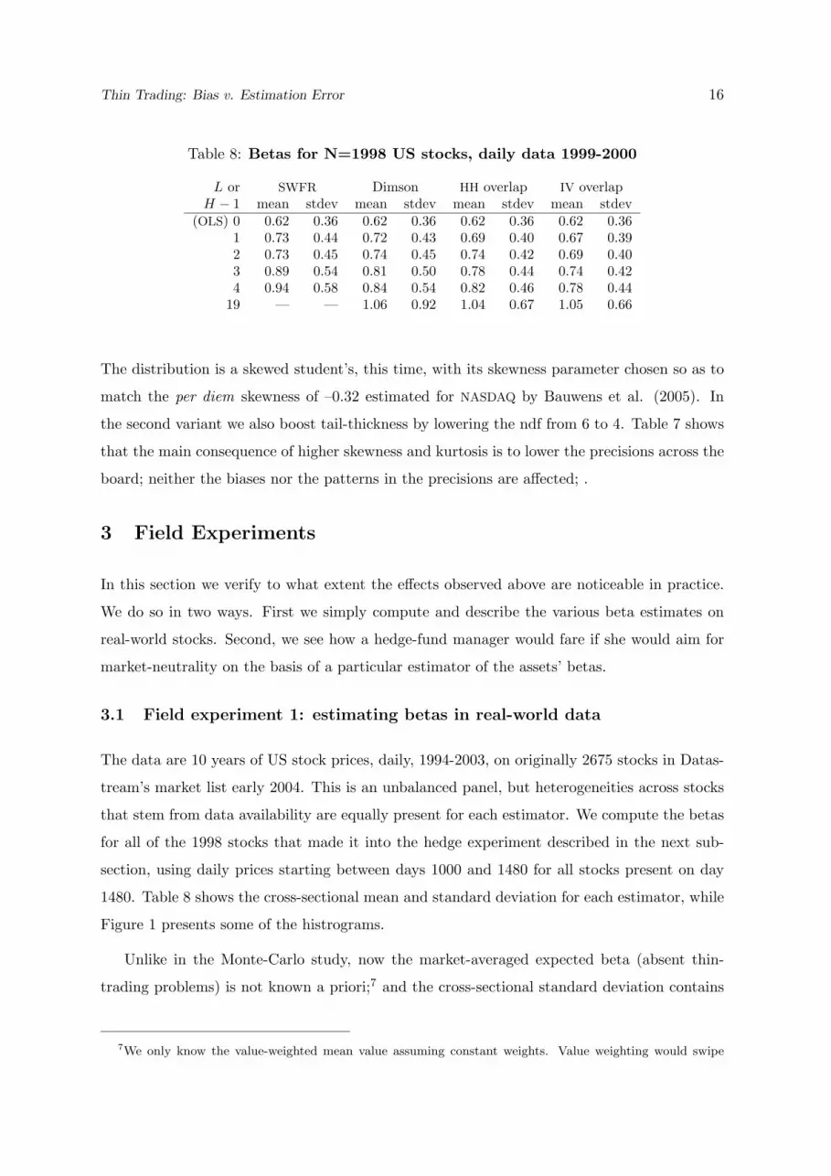
Table 8: Betas for N=1998 US stocks, daily data 1999-2000
L or SWFR Dimson HH overlap IV overlapH − 1 mean stdev mean stdev mean stdev mean stdev
(OLS) 0 0.62 0.36 0.62 0.36 0.62 0.36 0.62 0.361 0.73 0.44 0.72 0.43 0.69 0.40 0.67 0.392 0.73 0.45 0.74 0.45 0.74 0.42 0.69 0.403 0.89 0.54 0.81 0.50 0.78 0.44 0.74 0.424 0.94 0.58 0.84 0.54 0.82 0.46 0.78 0.44
19 — — 1.06 0.92 1.04 0.67 1.05 0.66
The distribution is a skewed student’s, this time, with its skewness parameter chosen so as to
match the per diem skewness of –0.32 estimated for NASDAQ by Bauwens et al. (2005). In
the second variant we also boost tail-thickness by lowering the ndf from 6 to 4. Table 7 shows
that the main consequence of higher skewness and kurtosis is to lower the precisions across the
board; neither the biases nor the patterns in the precisions are affected; .
3 Field Experiments
In this section we verify to what extent the effects observed above are noticeable in practice.
We do so in two ways. First we simply compute and describe the various beta estimates on
real-world stocks. Second, we see how a hedge-fund manager would fare if she would aim for
market-neutrality on the basis of a particular estimator of the assets’ betas.
3.1 Field experiment 1: estimating betas in real-world data
The data are 10 years of US stock prices, daily, 1994-2003, on originally 2675 stocks in Datas-
tream’s market list early 2004. This is an unbalanced panel, but heterogeneities across stocks
that stem from data availability are equally present for each estimator. We compute the betas
for all of the 1998 stocks that made it into the hedge experiment described in the next sub-
section, using daily prices starting between days 1000 and 1480 for all stocks present on day
1480. Table 8 shows the cross-sectional mean and standard deviation for each estimator, while
Figure 1 presents some of the histrograms.
Unlike in the Monte-Carlo study, now the market-averaged expected beta (absent thin-
trading problems) is not known a priori;7 and the cross-sectional standard deviation contains
7We only know the value-weighted mean value assuming constant weights. Value weighting would swipe

Thin Trading: Bias v. Estimation Error 17
Figure 1:
Thin-Trading Bias in Beta v. Estimation Error 22
His
togr
ams
ofbet
aes
tim
ates
,N
=19
98U
Sst
ock
s,dai
ly,19
99-2
000
.L=
0(O
LS)
L=
1or
H=
2L=
4or
H=
5L=
19or
H=
20
SW
FR
0
50
100
150
200
250
-2-1
01
23
45
Beta
Frequency
0
50
100
150
200
250
-2-1
01
23
45
Beta
Frequency
0
50
100
150
200
250
-2-1
01
23
45
Beta
Frequency
Dm
sn0
50
100
150
200
250
-2-1
01
23
45
Beta
Frequency
0
50
100
150
200
250
-2-1
01
23
45
Beta
Frequency
0
50
100
150
200
250
-2-1
01
23
45
Beta
Frequency
0
50
100
150
200
250
-2-1
01
23
45
Beta
Frequency
HH
0
50
100
150
200
250
-2-1
01
23
45
Beta
Frequency
0
50
100
150
200
250
-2-1
01
23
45
Beta
Frequency
0
50
100
150
200
250
-2-1
01
23
45
Beta
Frequency
0
50
100
150
200
250
-2-1
01
23
45
Beta
Frequency
IV0
50
100
150
200
250
-2-1
01
23
45
Beta
Frequency
0
50
100
150
200
250
-2-1
01
23
45
Beta
Frequency
0
50
100
150
200
250
-2-1
01
23
45
Beta
Frequency
0
50
100
150
200
250
-2-1
01
23
45
Beta
Frequency
much of the thin-trading problem under the carpet.

Thin Trading: Bias v. Estimation Error 18
the unknown variability of true betas across stocks and must be affected by heterogeneity of
SE’s too. Despite these complicating factors, the similarities with the simulation results are
striking. Within each and every class we see increasing average betas, indicating a falling bias,
but at the cost of a rising standard deviation. We again note that the two estimators that are
explicitly set up to cope with thin trading do best re bias, but again at the cost of precision.
Even within each class (SWFR versus Dimson; and OLS overlapping versus IV overlapping)
we see the same effect. In sum, like in our Monte-carlo experiments the bias-versus-precision
trade-off also holds across estimators.
Whether bias should be the overwhelming consideration rather than precision depends on
the application. We consider one such application in the remainder of this section.
3.2 Field experiment 2: setting up market-neutral portfolios
We consider the problem of a hedge-fund manager who has selected an underpriced stock and
now wants to add a position in another stock so as to make the combination market-neutral.
Common sense would already suggest we match by industry and size. The question is whether
this suffices: can one just invest equal amounts (up to the sign), implicitly assuming the two
stocks have the same beta, or is it helpful to look at estimated betas and come up with a non-
unit hedge ratio? In this problem, bias and estimation variance are equally bad as they enter
into the portfolio-return as a sum. This can be seen as follows. Regard, in Bayesian style, the
portfolio’s true beta as a random variable. For simplicity and without loss of generality, let all
returns be mean-centered. The portfolio return then equals rp = βprm+ ep. In line 3 of the set
of equations below, we use the fact that, rm being centered, the expected cross product equals
the covariance, which in turn equals zero as the portfolio beta is fixed at the beginning of the
period.8 In line 4 we work out the expectation of a product and set the resulting covariance
zero, for the same reason. Line 5 again uses the zero-mean property of rm.
var(rp) = var(βprm) + var(ep),
= [E(β2p r
2m)− E(βprm)2] + var(ep),
= [E(β2p r
2m)− cov(βp, rm)2︸ ︷︷ ︸
=0
] + var(ep),
8In the empirical work, another argument is relevant, but the conclusion is similar: the beta is determinedby decisions based on realized returns prior to t, while the market return is subsequent to t. This rules outstrong links.

Thin Trading: Bias v. Estimation Error 19
= [E(β2p)E(r2m)− cov(β2
p , r2m)︸ ︷︷ ︸
=0
] + var(ep),
= [var(βp) + E(βp)2]var(rm) + var(ep). (10)
The square-bracketed factor collapses to the familiar β2p if there is no uncertainty about beta,
the standard textbook case. In the presence of estimation error, however, what matters is the
sum of uncertainty about beta (estimation variance) and bias, the squared deviation from the
target beta of zero.
3.2.1 Procedure
There are four sets of computations, of which we show three. In the first variant, every month
we take all US stocks of a given industry, and rank them by size (market cap). For the long
positions (subscript l) we pick, sequentially, assets ranked 1, 4, 5, 8, 9, 12, ..., and match each
of them with a short positions (subscript s) in a size-wise close stock of the same industry,
notably those ranked 2, 3, 6, 7, 10, 11, etc. Each pair’s hedge ratio must then be set so as to
produce a market-neutral position for each such pair. For the portfolio to have a zero beta,
the weights of the two risky assets have to satisfy
wlws
= −βsβl. (11)
In a first round of experiments we have one asset that is deemed underpriced, which we then
hedge; so we set wl = 1, implying ws = −βl/βs and a risk-free position w0 = 1−wl−ws = βl/βs.
The data are again our 10 years of US stock prices, daily, 1994-2003, on the 2004 Datastream
market list. Of these 2675 stocks, 2×999 have at least one period of 480 days of data and
could be well matched by size and industry. We divide the time line into 123 20-trading-day
periods which we somewhat inaccurately refer to, below, as “months”. Betas are estimated
using the first 480 daily data (24 months). Given the portfolio weights we then hold the two
stocks and a risk-free deposit for one month, and note the portfolio returns per estimator. We
next re-estimate the betas using a one-month-updated 24-month sample, re-rank the stocks
by value, and form new pairs, etc. This produces 99 non-overlapping out-of-sample tests per
pair; and since we have 999 US matched pairs with a 10-year history, there are, for each of the
99 test months, 999 such two-asset-portfolio returns available for performance analysis.
We see three problems with this approach. First, it studies pairs of assets in isolation,
as standard in the optimal-hedge-ratio literature; but a portfolio manager may reckon that
much of this risk must be diversifiable. Second, some estimated beta pairs are occasionally

Thin Trading: Bias v. Estimation Error 20
so egregious, say 2 and 0.1, that hedge ratios of 20 would be implied, generating absurd
variances for the “hedged” portfolios. It is hard to believe a manager would adopt such
positions. Third, the result of an individual hedge depends very much on which stock happens
to be stock l or stock s. If, for instance, the betas are 2 for l and 0.5 for s, the weights
would be (wl = 1, ws = 4), producing on average a sixteen-times higher portfolio variance
than if the betas had been the other way around and the weights, accordingly, had been
(wl = 1, ws = 0.25). This random element in the portfolio strategy would add noise to the
variance of the investment strategy. In the standard hedging literature the position to be
covered is given exogenously, but in the current portfolio-management setting this position is
a decision variable. If the manager actually believed a hedge ratio of 4 is needed, then she
would probably scale down both sides.
The last two of the above problems turned out to be quite large: portfolio-return variances
were quite absurd, thus demonstrating that the naive procedure does not make a lot of sense.
We show, instead, the results for three variants. In one amended version of the experiment we
make two adjustments. First, we truncate the estimated betas at 0.25 and 4, reckoning that no
real-world manager worth her salt would believe estimates outside this range. This provision
was rarely needed in the actual computations. To weaken the effect on the portfolio weights of
switching the betas, we rescale the first-pass weights by their geometric average. Elementary
algebra show that this gives us the following weights (with βtr denoting a truncated beta):
wl =
√√√√ βtrs
βtrl; ws = −
√√√√ βtrlβtrs
; w0 = 1− wl − ws, (12)
With this rule it hardly matters whether the stock held long happens to be the smaller-beta
one or not. With estimated betas equal to 2 and 0.5, for example, the weights could now be
either 2 and 0.5 or 0.5 and 2 (depending on whether the high-beta stock acts as stock l or not),
but this has no predictable impact on the portfolio variance.
In the third variant we want to obtain an impression of to what extent estimation risk is
diversifiable. We proceed as in version 2, except that we now work with portfolios of ten stocks
held long and ten held short. For instance, in the first portfolio the stocks with size rank 1,
4, 5, 8, ... , 17, 20 of industry 1 are held long, and assets with ranks 2, 3, 6, 7, . ... , 18, 19
short. The second portfolio proceeds similarly with the next 20 stocks in the industry’s size
ranking, and so on. Betas are computed for the entire long side of the portfolio, and for the
entire short side, and then handled as before: truncated, and converted in balanced weights.
There are 88 such portfolios per month.
Thin Trading: Bias v. Estimation Error 21
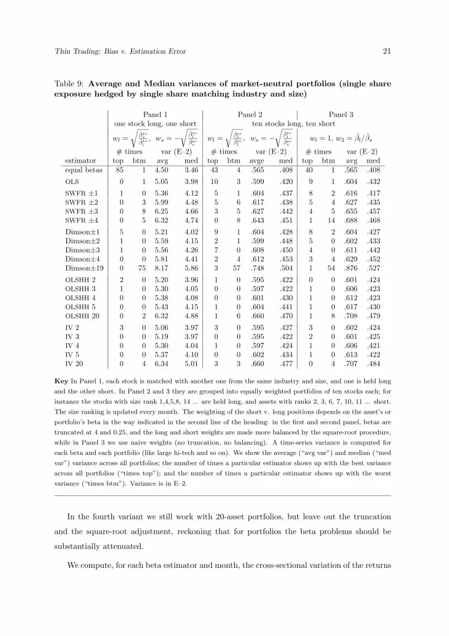
Table 9: Average and Median variances of market-neutral portfolios (single shareexposure hedged by single share matching industry and size)
Panel 1 Panel 2 Panel 3one stock long, one short ten stocks long, ten short
wl =√
βtrs
βtrl
, ws = −√
βtrl
βtrs
wl =√
βtrs
βtrl
, ws = −√
βtrl
βtrs
wl = 1, w2 = βl/βs
# times var (E–2) # times var (E–2) # times var (E–2)estimator top btm avg med top btm avge med top btm avg medequal betas 85 1 4.50 3.46 43 4 .565 .408 40 1 .565 .408
OLS 0 1 5.05 3.98 10 3 .599 .420 9 1 .604 .432
SWFR ±1 1 0 5.36 4.12 5 1 .604 .437 8 2 .616 .417SWFR ±2 0 3 5.99 4.48 5 6 .617 .438 5 4 .627 .435SWFR ±3 0 8 6.25 4.66 3 5 .627 .442 4 5 .655 .457SWFR ±4 0 5 6.32 4.74 0 8 .643 .451 1 14 .688 .468
Dimson±1 5 0 5.21 4.02 9 1 .604 .428 8 2 .604 .427Dimson±2 1 0 5.59 4.15 2 1 .599 .448 5 0 .602 .433Dimson±3 1 0 5.56 4.26 7 0 .608 .450 4 0 .611 .442Dimson±4 0 0 5.81 4.41 2 4 .612 .453 3 4 .629 .452Dimson±19 0 75 8.17 5.86 3 57 .748 .504 1 54 .876 .527
OLSHH 2 2 0 5.20 3.96 1 0 .595 .422 0 0 .601 .424OLSHH 3 1 0 5.30 4.05 0 0 .597 .422 1 0 .606 .423OLSHH 4 0 0 5.38 4.08 0 0 .601 .430 1 0 .612 .423OLSHH 5 0 0 5.43 4.15 1 0 .604 .441 1 0 .617 .430OLSHH 20 0 2 6.32 4.88 1 6 .660 .470 1 8 .708 .479
IV 2 3 0 5.06 3.97 3 0 .595 .427 3 0 .602 .424IV 3 0 0 5.19 3.97 0 0 .595 .422 2 0 .601 .425IV 4 0 0 5.30 4.04 1 0 .597 .424 1 0 .606 .421IV 5 0 0 5.37 4.10 0 0 .602 .434 1 0 .613 .422IV 20 0 4 6.34 5.01 3 3 .660 .477 0 4 .707 .484
Key In Panel 1, each stock is matched with another one from the same industry and size, and one is held long
and the other short. In Panel 2 and 3 they are grouped into equally weighted portfolios of ten stocks each; for
instance the stocks with size rank 1,4,5,8, 14 ... are held long, and assets with ranks 2, 3, 6, 7, 10, 11 ... short.
The size ranking is updated every month. The weighting of the short v. long positions depends on the asset’s or
portfolio’s beta in the way indicated in the second line of the heading: in the first and second panel, betas are
truncated at 4 and 0.25, and the long and short weights are made more balanced by the square-root procedure,
while in Panel 3 we use naive weights (no truncation, no balancing). A time-series variance is computed for
each beta and each portfolio (like large hi-tech and so on). We show the average (“avg var”) and median (“med
var”) variance across all portfolios; the number of times a particular estimator shows up with the best variance
across all portfolios (“times top”); and the number of times a particular estimator shows up with the worst
variance (“times btm”). Variance is in E–2.
In the fourth variant we still work with 20-asset portfolios, but leave out the truncation
and the square-root adjustment, reckoning that for portfolios the beta problems should be
substantially attenuated.
We compute, for each beta estimator and month, the cross-sectional variation of the returns
Thin Trading: Bias v. Estimation Error 22
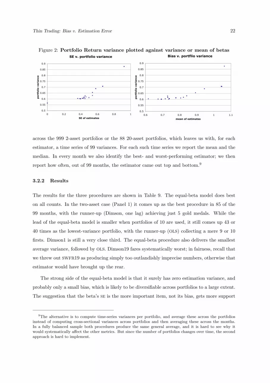
Figure 2: Portfolio Return variance plotted against variance or mean of betasSE v. portfolio variance
0.5
0.55
0.6
0.65
0.7
0.75
0.8
0.85
0.9
0 0.2 0.4 0.6 0.8 1
SE of estimates
po
rtf
oli
o v
aria
nce
Series1
Bias v. portflio variance
0.5
0.55
0.6
0.65
0.7
0.75
0.8
0.85
0.9
0.6 0.7 0.8 0.9 1 1.1
mean of estimates
po
rtf
olio
varia
nce
Series1
across the 999 2-asset portfolios or the 88 20-asset portfolios, which leaves us with, for each
estimator, a time series of 99 variances. For each such time series we report the mean and the
median. In every month we also identify the best- and worst-performing estimator; we then
report how often, out of 99 months, the estimator came out top and bottom.9
3.2.2 Results
The results for the three procedures are shown in Table 9. The equal-beta model does best
on all counts. In the two-asset case (Panel 1) it comes up as the best procedure in 85 of the
99 months, with the runner-up (Dimson, one lag) achieving just 5 gold medals. While the
lead of the equal-beta model is smaller when portfolios of 10 are used, it still comes up 43 or
40 times as the lowest-variance portfolio, with the runner-up (OLS) collecting a mere 9 or 10
firsts. Dimson1 is still a very close third. The equal-beta procedure also delivers the smallest
average variance, followed by OLS. Dimson19 fares systematically worst; in fairness, recall that
we threw out SWFR19 as producing simply too outlandishly imprecise numbers, otherwise that
estimator would have brought up the rear.
The strong side of the equal-beta model is that it surely has zero estimation variance, and
probably only a small bias, which is likely to be diversifiable across portfolios to a large extent.
The suggestion that the beta’s SE is the more important item, not its bias, gets more support
9The alternative is to compute time-series variances per portfolio, and average these across the portfoliosinstead of computing cross-sectional variances across portfolios and then averaging these across the months.In a fully balanced sample both procedures produce the same general average, and it is hard to see why itwould systematically affect the other metrics. But since the number of portfolios changes over time, the secondapproach is hard to implement.

Thin Trading: Bias v. Estimation Error 23
Figure 3: Mean and median portfolio-return variances: 20- v 2-asset portfolios
0.4
0.5
0.6
0.7
0.8
3 3.5 4 4.5 5 5.5 6
mean variance, 2 assets
mean v
ariance,
20 a
ssets
0.4
0.5
0.6
0.7
0.8
3 3.5 4 4.5 5 5.5 6
median variance 2 assets
media
n v
aria
nce 2
0 a
ssets
if we recall that OLS, our runner-up, has the worst bias but the highest precision, while last-
comer Dimson19 combines zero bias with the highest SE’s. The same picture emerges when we
compare the average variances of within each family. Recall that, for Dimson, SWFR, HH and
IV, the bias disappears as one increases the window L or H, but at the cost of less precision.
We now see that the cost of imprecision outweighs the benefit of a lower bias: within each
family of estimators, the portfolio-return variance steadily increases as the H- or L-window
widens, with only two exceptions out of 57 comparisons of adjacent pairs of variances. Figure
2 plots, for each given beta estimator, the average portfolio-return variance obtained in Table
9 Panel 3 against either the cross-asset standard deviation or the mean as taken from Table
8. We see that returns become more volatile when betas are noisier, but also when the mean
beta rises, that is, when the bias becomes smaller. The last result makes no sense except if
bias comes along with lower precision and if the latter effect dominates. We conclude that the
niceties about bias are dwarfed by issues of standard error when the problem is one of building
market-neutral portfolios.
Predictably, the variances for 20-asset portfolios are substantially lower than those of 2-
asset ones. But the ratio is not a constant ten-to-one, as one would expect if pairwise matching
on size and industry left only purely idiosyncratic noise. In Figure 3 we plot the means or
medians of the 20-asset portfolio variances against those of 2-asset ones. While there is a good
preservation of order, the portfolio variances clearly do not plot on a ray from the origin with
slope 1/10. There is, first, some randomness and, second, a large dose of attenuation: the
slope is 0.04 or 0.07 rather than 0.10, and there is an intercept. The attenuation must be to
some extent explained by the randomness. The reason is that if the 2-asset variances are noisy
estimates of large-sample values, there is an errors-in-variables bias towards zero in the slope
of the trendline. The observation that the more imprecise estimators seem to benefit relatively

Thin Trading: Bias v. Estimation Error 24
more from attenuation than the precise ones is consistent with this: noisiness in the estimates
goes together with noisiness in the variance. But ascribing all of the attenuation to noisiness
in the 2-asset return variances would be going too far: to shrink a slope from 0.10 to 0.04, the
error variance for the variable on the horizontal axis would have to be 1.5 times larger than the
true variance, which seems hard to reconcile with the strength of the observed relation. If part
of the flattening out is real, then high-variance estimators benefit more from diversification
than low- variance ones. There is another piece of evidence in that direction: the lead of the
equal-beta rule of thumb shrinks when the portfolios are larger, suggesting the estimators do
become less bad. While we do not have enough data to work with 100- or 1000-asset portfolios,
our exploratory evidence on diversification raises the possibility that, with a great many assets,
a regression may actually not do much harm relative to the equal-beta rule of thumb. Still, at
this point there is no evidence that estimation would ever positively help.
4 Conclusion
Two regression coefficients often used in Finance, the Scholes-Williams (1977) quasi-multiperiod
”thin-trading” beta and the Hansen-Hodrick (1980) overlapping-periods regression coefficient,
can both be written as instrumental-variables estimators. We check the performance of these
IV-estimators and the validity of the theoretical standard errors in small and medium samples,
gauge the robustness of the Scholes-Williams estimator outside its stated assumptions, and
report performances relative to the Dimson beta, standard OLS, and the equal-beta model in
a hedge-fund style application. We learn that, across and within “families” of estimators, less
bias comes at the cost of a higher standard error. The hedge-portfolio experiment shows that
the safest procedure is to simply match by size and industry; any estimation just adds noise.
There is a clear relation between portfolio variance and the variance of the beta estimator,
dwarfing the effect of bias.

Thin Trading: Bias v. Estimation Error 25
References
[1] Apte, P., M. Kane, and P. Sercu, 1994: Evidence of PPP in the medium run, Journal of
International Money and Finance, 601-622
[2] Bauwens, L., , S. Laurent, and J. Rombouts, 2006: Multivariate GARCH models: a
survey, Journal of Applied Econometrics, 21/1, 79-109
[3] Brown, S. and J. Warner, 1980: Measuring security price performance, Journal of Finan-
cial Economics 8, 205-258
[4] Dimson, E., 1979, Risk measurement when shares are subject to infrequent trading, Jour-
nal of Financial Economics 7, 197-226
[5] Fama, E.F., 1965, Tomorrow in the New York Stock Exchange, Journal of Business Studies
38, 191-225
[6] Fama, E. F., L. Fisher, M. Jensen, and R. Roll, 1969, The Adjustment of Stock Prices to
New Information, International Economic Review, 10, 1-21
[7] Fowler, D.J., and H.C. Rorke, 1983, Risk Measurement when shares are subject to infre-
quent trading: Comment, Journal of Financial Economics 12, 297-283
[8] Hansen, L. P. and R. J. Hodrick, 1980, Forward Exchange Rates as Optimal Predictors
of Future Spot Rates: An Econometric Analysis, Journal of Political Economy 88(5),
829-853
[9] Johnson, L.L., 1960: The theory of hedging and speculation in commodity futures, Review
of Economic Studies 27, 139-151
[10] Sercu, P. and X. Wu, 2000, Cross- and delta-hedges: Regression- versus price-based hedge
ratios, Journal of Banking and Finance, vol. 24 (May), no. 5, pp. 735 - 757.
[11] Scholes, M. AND J. Williams, 1977: Estimating betas from non-synchronous data, Journal
of Financial Economics 5, 308-328
[12] Sterin, J.L. 1961, The simultaneous determination of spot and futures prices, American
Economic Review 51, 1012-1025
[13] Stoll, H. and R. Whaley, 1990: The dynamics of stock index and stock index futures
returns, Journal of Financial and Quantitative Analysis 25, 441-368