th`ese de doctorat distributed edge partitioning
TRANSCRIPT
Ecole doctorale STIC
Unite de recherche: Inria/I3S
These de doctoratPresentee en vue de l’obtention du
grade de docteur en Science
mention Informatique
de
UNIVERSITE COTE D’AZUR
par
Hlib Mykhailenko
Distributed edge partitioning
Dirigee par Fabrice Huet et Philippe Nain
Soutenue le 14 Juin 2017
Devant le jury compose de :
Damiano Carra Maıtre de conferences, University of Verona Examinateur
Fabrice Huet Maıtre de conferences, Laboratoire I3S Co-directeur de these
Pietro Michardi Professeur, Eurecom Rapporteur
Giovanni Neglia Charge de recherche, Inria, Universite Cote d’Azur Invite
Matteo Sereno Professeur, Universita degli Studi di Torino Rapporteur
Guillaume Urvoy-Keller Professeur, Laboratoire I3S Examinateur

ii

iii
Resume
Pour traiter un graphe de maniere repartie, le partitionnement est une etape
preliminaire importante car elle influence de maniere significative le temps final
d’executions. Dans cette these nous etudions le probleme du partitionnement
reparti de graphe. Des travaux recents ont montre qu’une approche basee sur
le partitionnement des sommets plutot que des aretes offre de meilleures perfor-
mances pour les graphes de type power-laws qui sont courant dans les donnees
reelles. Dans un premier temps nous avons etudie les differentes metriques utilisees
pour evaluer la qualite d’un partitionnement. Ensuite nous avons analyse et com-
pare plusieurs logiciels d’analyse de grands graphes (Hadoop, Giraph, Giraph++,
Distributed GrahpLab et PowerGraph), les comparant a une solution tres pop-
ulaire actuellement, Spark et son API de traitement de graphe appelee GraphX.
Nous presentons les algorithmes de partitionnement les plus recents et introduisons
une classification. En etudiant les differentes publications, nous arrivons a la
conclusion qu’il n’est pas possible de comparer la performance relative de tout
ces algorithmes. Nous avons donc decide de les implementer afin de les com-
parer experimentalement. Les resultats obtenus montrent qu’un partitionneur de
type Hybrid-Cut offre les meilleures performances. Dans un deuxieme temps,
nous etudions comment il est possible de predire la qualite d’un partitionnement
avant d’effectivement traiter le graphe. Pour cela, nous avons effectue de nom-
breuses experimentations avec GraphX et effectue une analyse statistique precise
des resultats en utilisation un modele de regression lineaire. Nos experimentations
montrent que les metriques de communication sont de bons indicateurs de la per-
formance. Enfin, nous proposons un environnement de partitionnement reparti
base sur du recuit simule qui peut etre utilise pour optimiser une large parte des
metriques de partitionnement. Nous fournissons des conditions suffisantes pour
assurer la convergence vers l’optimum et discutons des metriques pouvant etre ef-
fectivement optimisees de maniere repartie. Nous avons implemente cet algorithme
dans GraphX et compare ses performances avec JA-BE-JA-VC. Nous montrons
que notre strategie amene a des ameliorations significatives.
iv
Abstract
In distributed graph computation, graph partitioning is an important prelimi-
nary step because the computation time can significantly depend on how the graph
has been split among the different executors. In this thesis we explore the graph
partitioning problem. Recently, edge partitioning approach has been advocated as
a better approach to process graphs with a power-law degree distribution, which
are very common in real-world datasets. That is why we focus on edge partition-
ing approach. We start by an overview of existing metrics, to evaluate the quality
of the graph partitioning. We briefly study existing graph processing systems:
Hadoop, Giraph, Giraph++, Distributed GrahpLab, and PowerGraph with their
key features. Next, we compare them to Spark, a popular big-data processing
framework with its graph processing APIs — GraphX. We provide an overview of
existing edge partitioning algorithms and introduce partitioner classification. We
conclude that, based only on published work, it is not possible to draw a clear
conclusion about the relative performances of these partitioners. For this reason,
we have experimentally compared all the edge partitioners currently available for
GraphX. Results suggest that Hybrid-Cut partitioner provides the best perfor-
mance with respect to the execution time of the graph processing algorithm. We
then study how it is possible to evaluate the quality of a partition before running a
computation. To this purpose, we carry experiments with GraphX and we perform
an accurate statistical analysis using a linear regression model. Our experimen-
tal results show that communication metrics like vertex-cut and communication
cost are effective predictors in most of the cases. Finally, we propose a frame-
work for distributed edge partitioning based on distributed simulated annealing
which can be used to optimize a large family of partitioning metrics. We provide
sufficient conditions for convergence to the optimum and discuss which metrics
can be efficiently optimized in a distributed way. We implemented our framework
with GraphX and performed a comparison with JA-BE-JA-VC, a state-of-the-art
partitioner that inspired our approach. We show that our approach can provide
significant improvements.

Table of Contents
List of Figures ix
List of Tables xv
1 Introduction 1
1.1 Motivation and Objectives . . . . . . . . . . . . . . . . . . . . . . . 1
1.2 Contributions . . . . . . . . . . . . . . . . . . . . . . . . . . . . . . 2
1.3 Outline . . . . . . . . . . . . . . . . . . . . . . . . . . . . . . . . . . 3
2 Context 5
2.1 Problem definition . . . . . . . . . . . . . . . . . . . . . . . . . . . 6
2.2 Notations . . . . . . . . . . . . . . . . . . . . . . . . . . . . . . . . 8
2.3 Partition quality . . . . . . . . . . . . . . . . . . . . . . . . . . . . 9
2.3.1 Execution metrics . . . . . . . . . . . . . . . . . . . . . . . . 10
2.3.2 Partition metrics . . . . . . . . . . . . . . . . . . . . . . . . 10
2.4 Pregel model . . . . . . . . . . . . . . . . . . . . . . . . . . . . . . 12
2.5 Apache Spark . . . . . . . . . . . . . . . . . . . . . . . . . . . . . . 14
2.5.1 Resilient Distributed Dataset . . . . . . . . . . . . . . . . . 15
2.5.2 Bulk Synchronous Parallel model . . . . . . . . . . . . . . . 18
2.5.3 GraphX . . . . . . . . . . . . . . . . . . . . . . . . . . . . . 19
2.6 Other graph processing systems . . . . . . . . . . . . . . . . . . . . 21
2.6.1 Apache Hadoop . . . . . . . . . . . . . . . . . . . . . . . . . 21
2.6.2 Giraph . . . . . . . . . . . . . . . . . . . . . . . . . . . . . . 23
2.6.3 Giraph++ . . . . . . . . . . . . . . . . . . . . . . . . . . . . 24
2.6.4 Distributed GraphLab . . . . . . . . . . . . . . . . . . . . . 25
v

vi TABLE OF CONTENTS
2.6.5 PowerGraph . . . . . . . . . . . . . . . . . . . . . . . . . . . 26
2.7 Computational clusters . . . . . . . . . . . . . . . . . . . . . . . . . 27
2.8 Conclusion . . . . . . . . . . . . . . . . . . . . . . . . . . . . . . . . 27
3 Comparison of GraphX partitioners 29
3.1 Introduction . . . . . . . . . . . . . . . . . . . . . . . . . . . . . . . 30
3.2 Classification of the partitioners . . . . . . . . . . . . . . . . . . . . 30
3.2.1 Random assignment . . . . . . . . . . . . . . . . . . . . . . 31
3.2.2 Segmenting the hash space . . . . . . . . . . . . . . . . . . . 33
3.2.3 Greedy approach . . . . . . . . . . . . . . . . . . . . . . . . 36
3.2.4 Hubs Cutting . . . . . . . . . . . . . . . . . . . . . . . . . . 38
3.2.5 Iterative approach . . . . . . . . . . . . . . . . . . . . . . . 39
3.3 Discussion . . . . . . . . . . . . . . . . . . . . . . . . . . . . . . . . 40
3.4 Experiments . . . . . . . . . . . . . . . . . . . . . . . . . . . . . . . 42
3.4.1 Partitioning matters . . . . . . . . . . . . . . . . . . . . . . 42
3.4.2 Comparison of different partitioners . . . . . . . . . . . . . . 43
3.5 Conclusion . . . . . . . . . . . . . . . . . . . . . . . . . . . . . . . . 45
4 Predictive power of partition metrics 47
4.1 Statistical analysis methodology . . . . . . . . . . . . . . . . . . . . 48
4.2 Experiments . . . . . . . . . . . . . . . . . . . . . . . . . . . . . . . 50
4.3 Conclusion . . . . . . . . . . . . . . . . . . . . . . . . . . . . . . . . 56
5 A simulated annealing partitioning framework 59
5.1 Introduction . . . . . . . . . . . . . . . . . . . . . . . . . . . . . . . 60
5.2 Background and notations . . . . . . . . . . . . . . . . . . . . . . . 61
5.3 Reverse Engineering JA-BE-JA-VC . . . . . . . . . . . . . . . . . . 63
5.4 A general SA framework for edge partitioning . . . . . . . . . . . . 66
5.5 The SA framework . . . . . . . . . . . . . . . . . . . . . . . . . . . 70
5.6 Evaluation of the SA framework . . . . . . . . . . . . . . . . . . . . 72
5.7 The multi-opinion SA framework . . . . . . . . . . . . . . . . . . . 79
5.7.1 Distributed implementation . . . . . . . . . . . . . . . . . . 81
5.8 Evaluation of the multi-opinion SA framework . . . . . . . . . . . . 84
5.9 Conclusion . . . . . . . . . . . . . . . . . . . . . . . . . . . . . . . . 87

TABLE OF CONTENTS vii
6 Conclusion 91
6.1 Perspectives . . . . . . . . . . . . . . . . . . . . . . . . . . . . . . . 93
Appendix A Extended Abstract in French 95
A.1 Introduction . . . . . . . . . . . . . . . . . . . . . . . . . . . . . . . 95
A.2 Resume des developpements . . . . . . . . . . . . . . . . . . . . . . 96
A.3 Conclusion . . . . . . . . . . . . . . . . . . . . . . . . . . . . . . . . 99
A.3.1 Perspectives . . . . . . . . . . . . . . . . . . . . . . . . . . . 101
Acronyms 113

viii TABLE OF CONTENTS
List of Figures
2.1 Edge Cut (vertex partitioning) and Verex Cut (edge partitioning) [8] 9
2.2 Pregel model [12] . . . . . . . . . . . . . . . . . . . . . . . . . . . . 13
2.3 Spark standalone cluster architecture [21] . . . . . . . . . . . . . . . 15
2.4 Narrow and wide transformations [23] . . . . . . . . . . . . . . . . . 17
2.5 Under The Hood: DAG Scheduler [26], where from A, B, C, D, E,
F RDDs created G RDD. . . . . . . . . . . . . . . . . . . . . . . . 19
2.6 Bulk synchronous parallel model [29] . . . . . . . . . . . . . . . . . 20
2.7 YARN and HDFS nodes [35] . . . . . . . . . . . . . . . . . . . . . . 23
2.8 Different consistency models [39] when algorithm tries to update
value associated with vertex 3. . . . . . . . . . . . . . . . . . . . . . 26
3.1 Partition of bipaprtite graph into 3 components. First component
has 3 blue edges. Second component has 4 red edges. Third com-
ponent has 6 violet edges. . . . . . . . . . . . . . . . . . . . . . . . 34
3.2 Gird partitioning. Source vertex corresponds to row 2 and destina-
tion vertex corresponds to column 3. . . . . . . . . . . . . . . . . . 35
3.3 Torus partitioner. Source vertex corresponds to row 3 and column
0, destination vertex corresponds to row 0 and column 7. These
cells intersect in cell (0, 0). . . . . . . . . . . . . . . . . . . . . . . . 36
3.4 Number of experiments finished with particular time (grouped by
10 seconds), where time is the sum of partitioning and execution
time of PageRank algorithm executed on 1% snapshot of twitter
graph . . . . . . . . . . . . . . . . . . . . . . . . . . . . . . . . . . . 42
ix
x LIST OF FIGURES
3.5 Number of experiments finished with particular time (grouped by
10 seconds), where time is the sum of partitioning and execution
time of PageRank algorithm executed on 2.5% snapshot of twitter
graph . . . . . . . . . . . . . . . . . . . . . . . . . . . . . . . . . . . 43
3.6 Communication metrics (lower is better) . . . . . . . . . . . . . . . 44
3.7 Execution time of algorithms. . . . . . . . . . . . . . . . . . . . . . 45
4.1 Execution time for PageRank algorithm on com-Youtube graph: ex-
perimental results vs best LRM predictions . . . . . . . . . . . . . . 52
4.2 Execution time for Connected Components algorithm on com-Youtube
graph: experimental results vs best LRM predictions . . . . . . . . 53
4.3 Execution time for PageRank algorithm on com-Orkut graph: ex-
perimental results vs best LRM predictions . . . . . . . . . . . . . . 55
4.4 Execution time for PageRank algorithm on com-Youtube graph: ex-
perimental results vs LRM predictions using a single communication
metrics . . . . . . . . . . . . . . . . . . . . . . . . . . . . . . . . . . 55
4.5 Execution time for PageRank algorithm on com-Youtube graph: ex-
perimental results vs LRM predictions using a single balance metrics 56
4.6 Prediction for HC partitioner (using com-Youtube graph, and PageRank
algorithm) . . . . . . . . . . . . . . . . . . . . . . . . . . . . . . . . 56
4.7 Prediction for HC and HCP parititioners (using com-Youtube graph,
and PageRank algorithm) . . . . . . . . . . . . . . . . . . . . . . . . 57
5.1 Ecomm value for JA-BE-JA-VC and E value for SA using email-
Enron graph (1000 iterations were performed) . . . . . . . . . . . . 76
5.2 Vertex-cut metric for JA-BE-JA-VC and SA using email-Enron
graph (1000 iterations were performed) . . . . . . . . . . . . . . . . 77
5.3 Communication cost metric for JA-BE-JA-VC and SA using email-
Enron graph (1000 iterations were performed) . . . . . . . . . . . . 78
5.4 Vertex-cut metric value for JA-BE-JA-VC and SA using com-Amazon
graph (1000 iterations were performed) . . . . . . . . . . . . . . . . 78
5.5 Balance metric value for JA-BE-JA-VC and SA using com-Amazon
graph (1000 iterations were performed) . . . . . . . . . . . . . . . . 79

LIST OF FIGURES xi
5.6 Energy value for Ecc function for original and pre-processed email-
Enron graphs . . . . . . . . . . . . . . . . . . . . . . . . . . . . . . 87
5.7 Energy value for Ecc function for pre-processed email-Enron graph
(HybridCut is initial partitioner, L equals to 105). . . . . . . . . . 88
5.8 Energy value for Ecc function for pre-processed email-Enron graph
(HybridCut is initial partitioner, L equals to 105, initial temperature
is 10−7). . . . . . . . . . . . . . . . . . . . . . . . . . . . . . . . . . 88

xii LIST OF FIGURES

List of Algorithms
1 Execution model of Distributed GraphLab . . . . . . . . . . . . . . 25
2 Implementation of SA for GraphX . . . . . . . . . . . . . . . . . . . 73
3 Asynchronous SA for GraphX . . . . . . . . . . . . . . . . . . . . . 85
xiii

xiv LIST OF ALGORITHMS

List of Tables
3.1 Metrics used to evaluate partitioners grouped by papers (ET - ex-
ecution time, PT - partitioning time, RF - replication factor, CC -
communication cost, VC - vertex-cut) . . . . . . . . . . . . . . . . . 32
3.2 Spark configuration . . . . . . . . . . . . . . . . . . . . . . . . . . . 41
3.3 Partitioners pairwise comparisons, considering execution metrics
(E) or partitioning metrics (P).
Bold fonts indicate experiments we conducted. . . . . . . . . . . . 46
4.1 Spark configuration . . . . . . . . . . . . . . . . . . . . . . . . . . . 50
4.2 Correlation matrix for partition metrics com-Youtube . . . . . . . . 51
4.3 Metrics and execution time of PageRank for HC and CRVC . . . . . 57
4.4 The best linear regression models for PageRank algorithm . . . . . . 58
4.5 The best linear regression models for Connected Components algo-
rithm . . . . . . . . . . . . . . . . . . . . . . . . . . . . . . . . . . . 58
5.1 Spark configuration . . . . . . . . . . . . . . . . . . . . . . . . . . . 72
5.2 Final partitioning metrics obtained by JA-BE-JA-VC partitioner.
Temperature decreases linearly from T0 till 0.0 by given number of
iterations. . . . . . . . . . . . . . . . . . . . . . . . . . . . . . . . . 75
5.3 Final partitioning metrics obtained by SA using only Ecomm as en-
ergy function. Temperature decreases linearly from T0 till 0.0 by
given number of iterations. . . . . . . . . . . . . . . . . . . . . . . . 75
5.4 Final partitioning metrics obtained by SA using Ecomm + 0.5Ebal as
energy function). Temperature decreases linearly from T0 till 0.0 by
given number of iterations. . . . . . . . . . . . . . . . . . . . . . . . 76
xv
xvi LIST OF TABLES
5.5 Spark configuration . . . . . . . . . . . . . . . . . . . . . . . . . . . 86
Chapter 1
Introduction
Contents
1.1 Motivation and Objectives . . . . . . . . . . . . . . . . . 1
1.2 Contributions . . . . . . . . . . . . . . . . . . . . . . . . . 2
1.3 Outline . . . . . . . . . . . . . . . . . . . . . . . . . . . . . 3
1.1 Motivation and Objectives
The size of read-world graphs obligates to process them in a distributed way.
That is why, graph partitioning is the indispensable preliminary step performed
before graph processing. In addition to the fact that graph partitioning is an NP
hard problem, there is clearly, lack of research dedicated to graph partitioning,
e.g., it is not clear how to evaluate the quality of a graph partition, how different
partitioners compare to each other, and what is the final effect of partitioning on
the computational time. Moreover, there is always a trade-off between simple and
complex partitioners: complex partitioners may require a partitioning time too
long to nullify the execution time savings.
In this work we tried to tackle these issues. In particular our objectives were: to
find a correct way to compare partitioners (especially, before running actual graph
processing algorithms), to identify an objective function the partitioner should
optimize, and to design a partitioner which can optimize this function.
1

2 CHAPTER 1. INTRODUCTION
1.2 Contributions
We present below the main contributions of this thesis.
We have considered all the edge partitioners in the literature and provided
new classification for them. From the literature it was not possible to compare
all partitioners. That is why we compared them by ourselves on GraphX. Results
suggest that Hybrid-Cut partitioner provides the best performance.
To evaluate the quality of a partition before running the computation we
have performed a correct statistical analysis using a linear regression model which
showed us that communication metrics are more effective predictors than balance
metrics.
In order to optimize a given objective function (e.g., a communication metric)
we have developed and implemented a new graph partitioner framework based on
simulated annealing and new distributed asynchronous Gibbs sampling techniques.
The contributions presented in this thesis are included in the following publi-
cations:
– H. Mykhailenko, F. Huet and G. Neglia, “Comparison of Edge Partition-
ers for Graph Processing” 2016 International Conference on Computational
Science and Computational Intelligence (CSCI): December 15-17, 2016, Las
Vegas. This paper provides an overview of existing edge partitioning algo-
rithms.
– H. Mykhailenko, G. Neglia and F. Huet, “Which metrics for vertex-cut par-
titioning?,” 2016 11th International Conference for Internet Technology and
Secured Transactions (ICITST), Barcelona, 2016, pp. 74-79. This paper
focuses on edge partitioning and investigates how it is possible to evaluate
the quality of a partition before running the computation.
– H. Mykhailenko, G. Neglia and F. Huet, “Simulated Annealing for Edge
Partitioning” DCPerf 2017: Big Data and Cloud Performance Workshop at
INFOCOM 2017, Atlanta. This paper proposes a framework for distributed
edge partitioning based on simulated annealing.

1.3. OUTLINE 3
1.3 Outline
In Chapter 2 we provide background overview, we define the graph partitioning
problem, the notations we used in this thesis, the existing partitioning metrics,
and the existing graph processing frameworks.
Next, in Chapter 3 we overview existing edge partitioning algorithms and in-
troduce a classification of the partitioners.
After, Chapter 4 shows that a linear model can explain significant part of the
dependency between partitioning metrics and execution time of graph processing
algorithms. We suggest that communication metrics are the most important ones.
Chapter 5 presents a new distributed approach for graph partitioning based
on simulated annealing and asynchronous Gibbs sampling techniques. We have
implemented our approach in GraphX
Finally, we conclude and discuss the perspectives in Chapter 6.

4 CHAPTER 1. INTRODUCTION

Chapter 2
Context
Contents
2.1 Problem definition . . . . . . . . . . . . . . . . . . . . . . 6
2.2 Notations . . . . . . . . . . . . . . . . . . . . . . . . . . . 8
2.3 Partition quality . . . . . . . . . . . . . . . . . . . . . . . 9
2.3.1 Execution metrics . . . . . . . . . . . . . . . . . . . . . 10
2.3.2 Partition metrics . . . . . . . . . . . . . . . . . . . . . . 10
2.4 Pregel model . . . . . . . . . . . . . . . . . . . . . . . . . 12
2.5 Apache Spark . . . . . . . . . . . . . . . . . . . . . . . . . 14
2.5.1 Resilient Distributed Dataset . . . . . . . . . . . . . . . 15
2.5.2 Bulk Synchronous Parallel model . . . . . . . . . . . . . 18
2.5.3 GraphX . . . . . . . . . . . . . . . . . . . . . . . . . . . 19
2.6 Other graph processing systems . . . . . . . . . . . . . . 21
2.6.1 Apache Hadoop . . . . . . . . . . . . . . . . . . . . . . . 21
2.6.2 Giraph . . . . . . . . . . . . . . . . . . . . . . . . . . . . 23
2.6.3 Giraph++ . . . . . . . . . . . . . . . . . . . . . . . . . . 24
2.6.4 Distributed GraphLab . . . . . . . . . . . . . . . . . . . 25
2.6.5 PowerGraph . . . . . . . . . . . . . . . . . . . . . . . . . 26
2.7 Computational clusters . . . . . . . . . . . . . . . . . . . 27
2.8 Conclusion . . . . . . . . . . . . . . . . . . . . . . . . . . 27
5

6 CHAPTER 2. CONTEXT
In this chapter we introduce the graph partitioning problem and the notation
we used. We describe existing metrics which evaluate the quality of a partition. We
explain what is GraphX, and why we have selected it to perform experiments on
graphs. We make a brief overview of other existing graph processing systems (such
as Apache Hadoop, Apache Giraph, etc) and show their key features. Finally, we
describe the computational resources we used in our experiments.
2.1 Problem definition
Analyzing large graphs is a space intensive operation which usually cannot be
performed on a single machine. There are two reasons why a graph has to be
distributed: memory and computation issues. Memory issue occurs when the
whole graph should be loaded in RAM. For example, a graph with one billion
of edges would require at least 8|E| bytes of space to store information about
the edges, where E is the set of edges, and this does not include computational
overhead — in practice, graph processing would require several times more space.
Even if a machine has enough RAM to store and process a graph, it can take an
unacceptably long time if a graph is not-partitioned, but is instead processed using
a single computational thread.
In order to overcome memory and computational issues, we need to partition
a graph into several components. Then, a partitioned graph can be processed in
parallel on multiple cores independently of whether they are on the same machine
or not. Naturally, the size of each component is smaller than the original graph,
which leads to smaller memory requirements.
There has been a lot of work dedicated to designing programming models
and building distributed middleware graph processing systems to perform such
a computation on a set of machines. A partitioned graph is distributed over a
set of machines. Each machine then processes only one subset of the graph — a
component — although it needs to periodically share intermediate-computation
results with the other machines.
Naturally, to find an optimal partition, graph partitioning problems arise.
2.1. PROBLEM DEFINITION 7
Graph partitioning splits a graph into several sub-graphs so that achieve better
computational time of a graph processing algorithm under two conflicting aspects.
The first aspect — balance — says that the size of each component should be
almost the same. It comes from the fact that graphs are processed by clusters of
machines and if one machine has too big component then it will slow down the
whole execution. The second aspect — communication — says that partitioning
should reduce how much components overlap with each other. As a trivial ex-
ample, if a graph has different disconnected components and each executor gets
assigned one of them, executors can in many cases work almost independently.
Graph partitioning is different from graph clustering and community detection
problems. The number of clusters is not given in clustering problems whether in
graph partitioning the number of components is given and it is multiple to some
specific computational resource such as number of the threads available. Compar-
ing to community detection, graph partitioning has an additional constraint which
is balance, i.e., size of all the partitions should be relatively the same.
Partitioning algorithms (partitioners) take as an input a graph, and split it
into N components. In particular, we are interested in partitioners that can be
executed in a distributed way. A distributed partitioner is an algorithm which
is composed of several instances, where each instance performs partitioning us-
ing the same algorithm but on a different components of graph. Each instance
represents a copy of algorithm with the unique component of the graph and some
resources assigned to it, such as computational threads and RAM. Instances of the
distributed partitioner may or may not communicate among themselves. In what
follows, we assume the number of instances of a distributed partitioner equals N ,
the number of components of the graph.
While partitioning can significantly affect the total execution time of graph
processing algorithms executed on a partitioned graph, finding a relatively good
partition is intrinsically an NP hard problem, whose state space is N |E|, i.e., we
can place each of |E| edges in N components.
Moreover, before finding an appropriate partitioning, tuning the cluster and
the different application parameters can be itself a hard problem [1].
In practice, existing partitioners rely on heuristics to find good enough trade-
offs between balance and communication properties. It is always possible to sacri-
8 CHAPTER 2. CONTEXT
fice balance in favor of communication and vice versa, e.g., we can achieve perfect
balance by partitioning edges or vertices in a round robin fashion or we can keep
the whole graph in a single component and get the worst balance with the best
communication property.
Two approaches were developed to tackle graph partitioning problem: vertex
and edge partitioning (see Figure 2.1). A classic way to distribute a graph is the
vertex partitioning approach (also called edge-cut partitioning) where vertices are
assigned to different components. An edge is cut, if its vertices belong to two
different components. Vertex partioners try then to minimize the number of edges
cut. More recently, edge partitioning (so-called vertex-cut partitioning) has been
proposed and advocated [2] as a better approach to process graphs with a power-
law degree distribution [3] (power-law graphs are common in real-world datasets [4,
5]). In this case, edges are mapped to components and vertices are cut if their
edges happen to be assigned to different components. The improvement can be
qualitatively explained with the presence, in a power-law graph, of hubs, i.e., nodes
with degree much larger than the average. In a vertex partitioning, attributing a
hub to a given partition easily leads to i) computation unbalance, if its neighbors
are also assigned to the same component, or ii) to a large number of edges cut
and then strong communication requirements. An edge partitioning partitioner
may instead achieve a better trade-off, by cutting only a limited number of hubs.
Analytical support to these findings is presented in [6]. For this reason many new
graph computation frameworks, like GraphX [7] and PowerGraph [2], rely on edge
partitioning.
2.2 Notations
Let us denote the input directed graph as G = (V,E), where V is a set of vertices
and E is a set of edges. Edge partitioning process splits a set of edges into N
disjoint subsets, E1, E2, . . . , EN . We call E1, E2, . . . , EN a partition of G and Ei
an edge-component (or simply component in what follows). We say that a vertex
v belongs to component Ei if at least one of its edges belongs to Ei.
Note that an edge can only belong to one component, but a vertex is at least in
one component and at most in N . Let V (Ei) denote the set of vertices that belong

2.3. PARTITION QUALITY 9
Figure 2.1 – Edge Cut (vertex partitioning) and Verex Cut (edge partitioning) [8]
to component Ei. Let src(e) and dst(e) denote the source and destination vertices
of an edge e respectively. E(V (Ei)) , {e ∈ Ei : src(e) ∈ V (Ei) ∨ dst(e) ∈ V (Ei)}denotes the set of edge which are attached to vertices attached to the set of edge Ei.
The vertices that appear in more than one component are called frontier vertices.
Each frontier vertex has then been cut at least once. F (Ei) denotes the set of
frontier vertices that are inside component Ei, and F (Ei) , V (Ei)\F (Ei) denotes
the set of vertices in component Ei that were not cut.
2.3 Partition quality
Different partitioners provide different partitions, however it is not obvious which
partition is better. Partition quality can be evaluated in two ways. One way is
to evaluate the effect of the partition on the algorithm we want to execute on the
graph, e.g., in terms of the total execution time or total communication overhead.
While this analysis provides the definitive answer, it is clear that we would like
to choose the best partition before running an algorithm. The second way uses
metrics which can be computed directly from the partition without the need to
run the target algorithm. We call the first set of metrics execution metrics and
the second one partition metrics.

10 CHAPTER 2. CONTEXT
2.3.1 Execution metrics
A partition is better than another if it reduces the execution time of the specific
algorithm we want to run on the graph. In some cases the partitioning time itself
may not be negligible and then we want to take it into account while comparing
the total execution times.
Partitioning time: it is time spent to partition a graph using a particular
computing resources. This metric shows how fast a partitioner works and not the
final effect on the partitioned graph.
Execution time: this metric measures the execution time of a graph processing
algorithm (such as Connected Components, PageRank, Single Source Shortest
Path, etc. ) on a partitioned graph using some specific computing resources.
Some other metrics may be used as proxies for these quantities.
Network communication: it measures in bytes of traffic or in number of logical
messages, how much information has been exchanged during the partitioning or
the execution of graph processing algorithms.
Rounds : this metric indicates the number of rounds (iterations) performed by
the partitioner. It can only be applied to iterative partitioners. This metric is
useful to compare the impact of a modification of a partitioner and to evaluate its
convergence speed. This metric can provide an indication of the total partitioning
time.
2.3.2 Partition metrics
Partition metrics can be split into two groups. In the first group there are the
metrics that quantify balance, i.e., how homogeneous the partitions’ sizes are.
The underlying idea is that if one component is much larger that the others, the
computational load on the corresponding machine is higher and then this machine
can slow down the whole execution. The metrics in the second group quantify
communication, i.e., how much overlap there is among the different components,
i.e., how many vertices appear in multiple components. This overlap is a reasonable
proxy for the amount of inter-machine communication that will be required to
merge the results of the local computations. The first two metrics below are
balance metrics, all the other ones are communication metrics.

2.3. PARTITION QUALITY 11
Balance (denoted as BAL): it is the ratio of the maximum number of edges in
a component to the average number of edges across all the components:
BAL =max
i=1,...N|Ei|
|E|/N.
Standard deviation of partition size (denoted as STD): it is the normalized stan-
dard deviation of the number of edges in each component:
STD =
√√√√ 1
N
N∑i=1
(|Ei||E|/N
− 1
)2
Replication factor (denoted as RF): it is the ratio of the number of vertices in all
the components to the number of vertices in the original graph. It measures the
overhead, in terms of vertices, induced by the partitioning. The overhead appears
due to the fact that some vertices get cut by graph partitioning algorithm.
RF =N∑i=1
|V (Ei)|1
|V |
Communication cost (denoted as CC): it is defined as the total number of frontier
vertices and measures communication overhead due to the fact that framework
will synchronize states of vertices that were cut:
CC =N∑i=1
|F (Ei)|
Vertex-cut (denoted as VC): this metric measures how many times vertices were
cut. For example, if a vertex is cut in 5 pieces, then its contribution to this metric
is 4.
VC =N∑i=1
F (Ei) +N∑i=1
F (Ei)− |V |
Normalized vertex-cut : it is a ratio of the vertex-cut metric of the partitioned
graph to the expected vertex-cut of a randomly partitioned graph.
Expansion: it was originally introduced in [9, 10] in the context of vertex
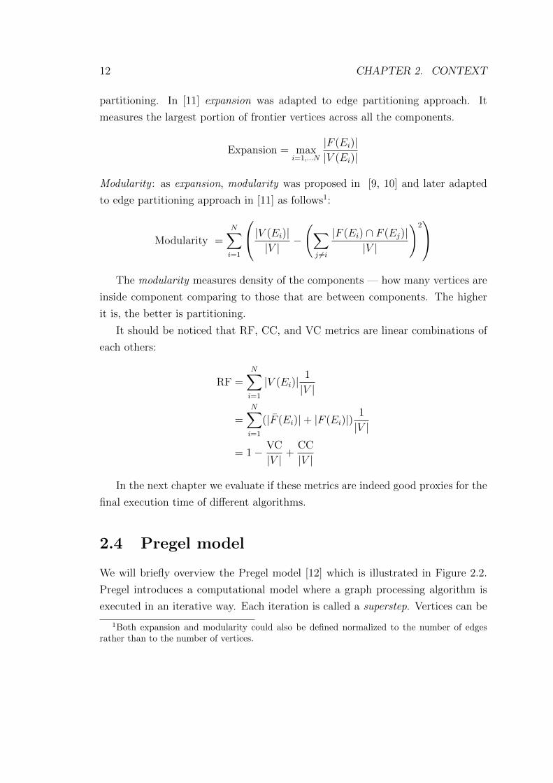
12 CHAPTER 2. CONTEXT
partitioning. In [11] expansion was adapted to edge partitioning approach. It
measures the largest portion of frontier vertices across all the components.
Expansion = maxi=1,...N
|F (Ei)||V (Ei)|
Modularity : as expansion, modularity was proposed in [9, 10] and later adapted
to edge partitioning approach in [11] as follows1:
Modularity =N∑i=1
|V (Ei)||V |
−
(∑j 6=i
|F (Ei) ∩ F (Ej)||V |
)2
The modularity measures density of the components — how many vertices are
inside component comparing to those that are between components. The higher
it is, the better is partitioning.
It should be noticed that RF, CC, and VC metrics are linear combinations of
each others:
RF =N∑i=1
|V (Ei)|1
|V |
=N∑i=1
(|F (Ei)|+ |F (Ei)|)1
|V |
= 1− VC
|V |+
CC
|V |
In the next chapter we evaluate if these metrics are indeed good proxies for the
final execution time of different algorithms.
2.4 Pregel model
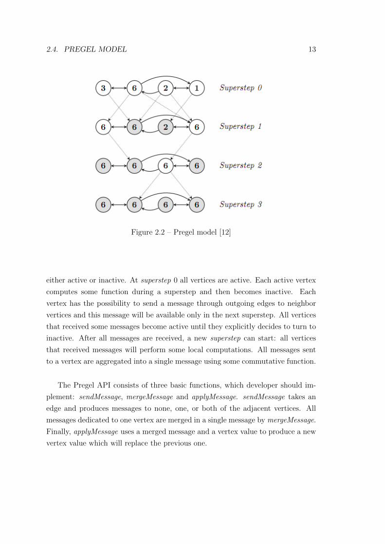
We will briefly overview the Pregel model [12] which is illustrated in Figure 2.2.
Pregel introduces a computational model where a graph processing algorithm is
executed in an iterative way. Each iteration is called a superstep. Vertices can be
1Both expansion and modularity could also be defined normalized to the number of edgesrather than to the number of vertices.
2.4. PREGEL MODEL 13
Figure 2.2 – Pregel model [12]
either active or inactive. At superstep 0 all vertices are active. Each active vertex
computes some function during a superstep and then becomes inactive. Each
vertex has the possibility to send a message through outgoing edges to neighbor
vertices and this message will be available only in the next superstep. All vertices
that received some messages become active until they explicitly decides to turn to
inactive. After all messages are received, a new superstep can start: all vertices
that received messages will perform some local computations. All messages sent
to a vertex are aggregated into a single message using some commutative function.
The Pregel API consists of three basic functions, which developer should im-
plement: sendMessage, mergeMessage and applyMessage. sendMessage takes an
edge and produces messages to none, one, or both of the adjacent vertices. All
messages dedicated to one vertex are merged in a single message by mergeMessage.
Finally, applyMessage uses a merged message and a vertex value to produce a new
vertex value which will replace the previous one.

14 CHAPTER 2. CONTEXT
2.5 Apache Spark
Apache Spark [13] is a large-scale distributed framework for general purpose data
processing. It relies on the concept of Resilient Distributed Dataset [14] (see
Section 2.5.1) and Bulk Synchronous Parallel (see Section 2.5.2) model. Spark
basic functionality (Spark Core) covers: scheduling, distributing, and monitoring
jobs, memory management, cache management, fault recovery, and communication
with data source.
Spark itself is implemented on a JVM [15] program, using the Scala [16] pro-
gramming language.
Spark can use three cluster managers: Standalone (a native part of Spark),
Apache Mesos, [17] and Hadoop YARN [18]. All these cluster managers consist
of one master program and several worker programs. Several Spark applications
can be executed by one cluster manager simultaneously. A Spark application
launched, using one of the scripts provided by Spark, on the driver machine, is
called a driver program (see Figure 2.3). The driver program connects to a mas-
ter program, which allocates resources on worker machines and instantiates one
executor program on each worker machine. Each executor may operate several
components using several cores. Driver, master, and worker programs are imple-
mented as Akka actors [19].
Fault tolerance in Spark is implemented in the following manner. In case a task
failed during execution but the executor is still work, then this task is rescheduled
on the same executor. Spark limits (by the property spark.task.maxFailures) how
many times a task can be rescheduled before finally giving up on the whole job. In
case the cluster manager loses a worker (basically the machine stops responding)
then the cluster manager reschedules tasks previously assigned to the working
machine. It is easy to reschedule a failed task thanks to the fact that all RDDs (see
next section) are computed as ancestor of other RDDs, according to the principle
of RDD lineage [20].

2.5. APACHE SPARK 15
Figure 2.3 – Spark standalone cluster architecture [21]
2.5.1 Resilient Distributed Dataset
A Resilient Distributed Dataset ( RDD) is an immutable, distributed, lazy-evaluated
collection with predefined set of operations. An RDD can be created from either
raw data or another RDD (called parent RDD). An RDD is partitioned collection,
and its components are distributed among the machines of the computational clus-
ter. Remember that both an RDD and a partitioned graph are distributed data
structures, which are partitioned into components. Note that the number of com-
ponents N can be different from the number Nm of machines, i.e multiple compo-
nents can be assigned to one machine . The set of operations which can be applied
to an RDD came from the functional programming paradigm. The advantage is
that the developer should only correctly utilize RDD operations but should not
take care of synchronization and information distribution over the cluster, which
come out-of-the-box. This advantage comes at the price of a more restricted set
of operations available.
One of the main ideas behind RDD is to reduce slow2 interaction with hard-disk
by keeping as much as possible in RAM memory. Usually, the whole sequence of
RDDs is stored in RAM memory without saving it to the file system. Nevertheless,
it can be impossible to avoid using hard-disk, despite of the fact that Spark uses
2Approximately, sequential access to a hard-disk is about 6 times slower and random access100,000 slower, than access to RAM, according to [22].

16 CHAPTER 2. CONTEXT
memory serialization (to reduce memory occupation) and lazy-evaluation.
There are two kinds of operations that can be executed on RDDs: transforma-
tions and actions. All transformations are lazy evaluated operations which create a
new RDD from an existing RDD. There are two types of transformations: narrow
and wide (see Figure 2.4).
Narrow transformations preserve partitioning between parent and child RDD
and do not require inter-node communication/synchronization. Filter, map, flatMap
are the examples of narrow transformations (all of them are related to functions
in functional programming). Let us consider the filter transformation: it is a
higher-order function, which requires a function that takes an item of an RDD
and returns a boolean value (basically it is a predicate). After we apply a filter
transformation to an RDD r1, we get a new RDD r2, which contains only those
items from r1, on which the predicate given to filter returned the true value.
A wide transformation requires inter-node communication (so-called shuffles).
Examples of wide transformations are groupByKey, reduceByKey, sortByKey, join
and so on. Let us consider the groupByKey transformation. It requires that items
of the RDD (on which it will be applied) are represented as key-value pairs. For
example, we have the following component:
component = [(k1, v1), (k2, v2), (k2, v3), (k1, v4), (k1, v5), (k3, v6), (k3, v7), . . . ]
Initially, each component contains some part of the RDD, groupByKey first groups
key-value pairs with similar ids in each component independently (this preparation
require inter-node communication):
k1⇒ [v1, v4, v5]
k2⇒ [v2, v3]
k3⇒ [v6, v7]
. . .
Then each component sends all its groups to the dedicated components according
to the key of the group. Each key is related to one component by using Hash-

2.5. APACHE SPARK 17
Figure 2.4 – Narrow and wide transformations [23]
Partitioner.3 In this way, a groupByKey transformation can compute to which
component each key belongs. After it has computed all N − 1 (remember that N
is number of components) messages to others components (all groups dedicated to
one component form single message), it can start to send them as following:
messageForComponent0⇒ [k3⇒ [v6, v7], k2⇒ [v2, v3]]
messageForComponent1⇒ [k1⇒ [v1, v4, v5]]
. . .
After a component has received all messages dedicated to it, it can finally merge
all the groups of key-values.
An action returns some value from an existing RDD, e.g., first, collect, re-
duce and so on. Only when an action is called on an RDD, it is actually evalu-
3It partitions based on key by using hash funciton.
18 CHAPTER 2. CONTEXT
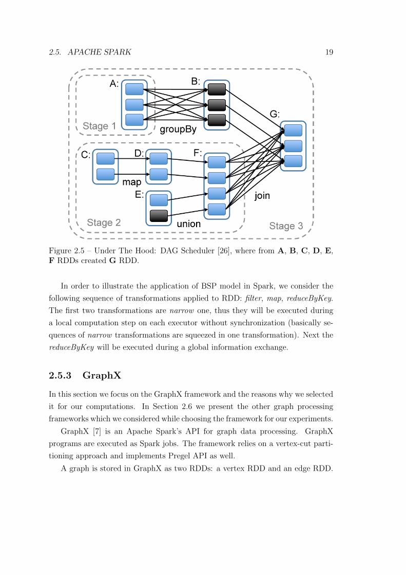
ated. An invoked action submits a job to the DAGScheduler, the class responsible
for scheduling in Spark. A submitted job represents a logical computation plan
made from a sequence of RDD transformations with an action at the end. The
DAGScheduler creates a physical computation plan which is represented as a di-
rected acyclic graph (DAG) of stages (see Figure 2.5). There are two types of
stages: ResultStage and ShuffleMapStage. The DAG is ended with a ResultStage.
Each ShuffleMapStage stage consists of sequence of narrow transformations fol-
lowed by a wide transformation. Each stage is split in N tasks.
In-memory caching in Spark follows Least Recently Used (LRU) policy [24].
Spark does not support automatic caching. Instead, the Spark user has to explicitly
specify which RDD he/she would like to cache, and then the framework may cache
it. If there is not enough space to cache, Spark applies LRU policy and removes
some other RDDs from the cache. The user also can directly request to uncache
an RDD.
To recap, Spark is based on several trending ideas:
– immutable collections (RDD), which simplify coding process;
– limited number of operations (transformations and actions) — users are re-
stricted to use pure functions [25];
– use of RAM instead of disk, which accelerate computations.
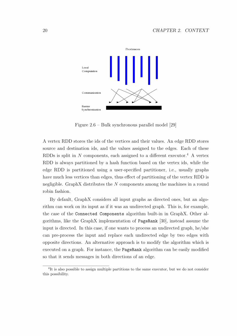
2.5.2 Bulk Synchronous Parallel model
The Bulk Synchronous Parallel model( BSP) [27] is an abstract model, which
is built on iterations. Each iteration consists of two parts: a local computation
and a global information exchange. Each executor computes its own component
of distributed data structure independently and after sends messages to other
executors. A new iteration does not start until all components have received all
messages dedicated to them (see Figure 2.6). This way, BSP implements a barrier
synchronization mechanism [28, Chapter 17].
The total time of an iteration consist of three parts: the time to perform local
computation by the slowest machine, the time to exchange messages, and, finally,
the time to process barrier synchronization.
2.5. APACHE SPARK 19
Figure 2.5 – Under The Hood: DAG Scheduler [26], where from A, B, C, D, E,F RDDs created G RDD.
In order to illustrate the application of BSP model in Spark, we consider the
following sequence of transformations applied to RDD: filter, map, reduceByKey.
The first two transformations are narrow one, thus they will be executed during
a local computation step on each executor without synchronization (basically se-
quences of narrow transformations are squeezed in one transformation). Next the
reduceByKey will be executed during a global information exchange.
2.5.3 GraphX
In this section we focus on the GraphX framework and the reasons why we selected
it for our computations. In Section 2.6 we present the other graph processing
frameworks which we considered while choosing the framework for our experiments.
GraphX [7] is an Apache Spark’s API for graph data processing. GraphX
programs are executed as Spark jobs. The framework relies on a vertex-cut parti-
tioning approach and implements Pregel API as well.
A graph is stored in GraphX as two RDDs: a vertex RDD and an edge RDD.
20 CHAPTER 2. CONTEXT
Figure 2.6 – Bulk synchronous parallel model [29]
A vertex RDD stores the ids of the vertices and their values. An edge RDD stores
source and destination ids, and the values assigned to the edges. Each of these
RDDs is split in N components, each assigned to a different executor.4 A vertex
RDD is always partitioned by a hash function based on the vertex ids, while the
edge RDD is partitioned using a user-specified partitioner, i.e., usually graphs
have much less vertices than edges, thus effect of partitioning of the vertex RDD is
negligible. GraphX distributes the N components among the machines in a round
robin fashion.
By default, GraphX considers all input graphs as directed ones, but an algo-
rithm can work on its input as if it was an undirected graph. This is, for example,
the case of the Connected Components algorithm built-in in GraphX. Other al-
gorithms, like the GraphX implementation of PageRank [30], instead assume the
input is directed. In this case, if one wants to process an undirected graph, he/she
can pre-process the input and replace each undirected edge by two edges with
opposite directions. An alternative approach is to modify the algorithm which is
executed on a graph. For instance, the PageRank algorithm can be easily modified
so that it sends messages in both directions of an edge.
4It is also possible to assign multiple partitions to the same executor, but we do not considerthis possibility.

2.6. OTHER GRAPH PROCESSING SYSTEMS 21
We have selected GraphX as a system on which we perform our experiments
due to multiple reasons:
– GraphX is free to use;
– it supports edge partitioning;
– it is still under development and maintenance;
– it is built on top of Spark. Most of the effective solutions are based on
Hadoop or Spark. As we discuss in the following section, we believe that
Spark is more promising than Hadoop.
2.6 Other graph processing systems
In addition to GraphX, there are many frameworks for distributed graph process-
ing, such as PowerGraph [2], Distributed GraphLab [31], Giraph [32], Giraph+ [33],
etc.
According to the survey [34] parallel graph processing frameworks may be
classified by programming model, by communication model, by execution model,
by the platform on which their run.
There are few frameworks that support edge partitioning approach. We con-
sider below those that are the most popular according to the number of citations.
2.6.1 Apache Hadoop
Apache Hadoop [35] is a distributed engine for general data processing and is
probably one of the most popular ones. It is an open source implementation of
the MapReduce framework [36]. Hadoop splits the original data-set into a num-
ber of chunks. A chunk is a sorted sequence of key-value pairs. Each chunk is
independently processed in parallel by the map function. Map is a higher-order
function [37], which requires, as an input, an argument function that takes a key-
value pair and returns a sequence of key-values pairs: < k1, v1 >⇒ [< k2, v2 >]∗.The output of the map function is sorted and after, is processed by the reduce
function. The reduce function requires as input argument function which takes
22 CHAPTER 2. CONTEXT
as input a sequence of values with the same key and returns a single value:
< k2, [v2] > ⇒ < k2, v3 >.
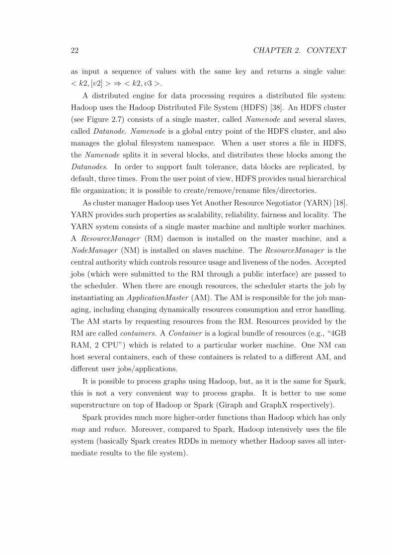
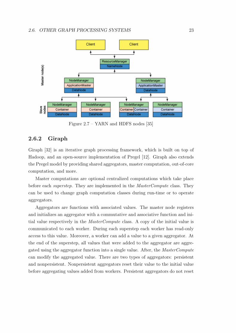
A distributed engine for data processing requires a distributed file system:
Hadoop uses the Hadoop Distributed File System (HDFS) [38]. An HDFS cluster
(see Figure 2.7) consists of a single master, called Namenode and several slaves,
called Datanode. Namenode is a global entry point of the HDFS cluster, and also
manages the global filesystem namespace. When a user stores a file in HDFS,
the Namenode splits it in several blocks, and distributes these blocks among the
Datanodes. In order to support fault tolerance, data blocks are replicated, by
default, three times. From the user point of view, HDFS provides usual hierarchical
file organization; it is possible to create/remove/rename files/directories.
As cluster manager Hadoop uses Yet Another Resource Negotiator (YARN) [18].
YARN provides such properties as scalability, reliability, fairness and locality. The
YARN system consists of a single master machine and multiple worker machines.
A ResourceManager (RM) daemon is installed on the master machine, and a
NodeManager (NM) is installed on slaves machine. The ResourceManager is the
central authority which controls resource usage and liveness of the nodes. Accepted
jobs (which were submitted to the RM through a public interface) are passed to
the scheduler. When there are enough resources, the scheduler starts the job by
instantiating an ApplicationMaster (AM). The AM is responsible for the job man-
aging, including changing dynamically resources consumption and error handling.
The AM starts by requesting resources from the RM. Resources provided by the
RM are called containers. A Container is a logical bundle of resources (e.g., “4GB
RAM, 2 CPU”) which is related to a particular worker machine. One NM can
host several containers, each of these containers is related to a different AM, and
different user jobs/applications.
It is possible to process graphs using Hadoop, but, as it is the same for Spark,
this is not a very convenient way to process graphs. It is better to use some
superstructure on top of Hadoop or Spark (Giraph and GraphX respectively).
Spark provides much more higher-order functions than Hadoop which has only
map and reduce. Moreover, compared to Spark, Hadoop intensively uses the file
system (basically Spark creates RDDs in memory whether Hadoop saves all inter-
mediate results to the file system).
2.6. OTHER GRAPH PROCESSING SYSTEMS 23
Figure 2.7 – YARN and HDFS nodes [35]
2.6.2 Giraph
Giraph [32] is an iterative graph processing framework, which is built on top of
Hadoop, and an open-source implementation of Pregel [12]. Giraph also extends
the Pregel model by providing shared aggregators, master computation, out-of-core
computation, and more.
Master computations are optional centralized computations which take place
before each superstep. They are implemented in the MasterCompute class. They
can be used to change graph computation classes during run-time or to operate
aggregators.
Aggregators are functions with associated values. The master node registers
and initializes an aggregator with a commutative and associative function and ini-
tial value respectively in the MasterCompute class. A copy of the initial value is
communicated to each worker. During each superstep each worker has read-only
access to this value. Moreover, a worker can add a value to a given aggregator. At
the end of the superstep, all values that were added to the aggregator are aggre-
gated using the aggregator function into a single value. After, the MasterCompute
can modify the aggregated value. There are two types of aggregators: persistent
and nonpersistent. Nonpersistent aggregators reset their value to the initial value
before aggregating values added from workers. Persistent aggregators do not reset
24 CHAPTER 2. CONTEXT
their values.
Giraph was designed to perform all computation in RAM. Unfortunately, it is
not always possible, that is why Giraph can spill some data to hard disk. In order to
reduce random swapping, user can use the out-of-core feature which allows explicit
swapping. Developer can specify how many graph components or messages should
be stored in-memory, while all rest will be spilled on disk using LRU policy [24].
Some application may intensively use messages which can exceed the memory
limit. Usually, this issue can be easily solved by aggregating messages, but it
can work only if messages are aggregatable, i.e., there should be an operation,
which can merge two messages in one. This operation should be commutative
and associative. Unfortunately, this is not always the case. For this reason, a
superstep splitting technique was developed. It allows splitting a superstep into
several iterations. During each iteration, each vertex sends messages only to some
subset of its neighbors, so that, after all iterations of the superstep each vertex
has sent messages to all its neighbors. Of course, there are some limitations:
– the function which updates vertex values after receiving fragments of all
messages dedicated to this vertex should be aggregatable;
– the maximum amount of messages between two machines should fit in mem-
ory.
2.6.3 Giraph++
Giraph++ [33] is an extension of Giraph. This framework is based on a different
conceptual model. It supports a graph-centric model instead of a vertex-centric,
which means that instead of processing in parallel each set of vertices or edges, it
processes some sub-graphs. The vertex-centric model is much easier to use. How-
ever, in Pregel (implemented in Giraph), a vertex has access only to the immediate
neighbors and message from a vertex can only be sent to the direct neighbors. That
is why, it takes a lot of supersteps to propagate some information from the source
and destination vertices which appear in the same component.
In the graph-centric models the user operates on the whole component. There
are two kinds of vertices: internal and boundary ones. An internal vertex appears

2.6. OTHER GRAPH PROCESSING SYSTEMS 25
only in one component, a boundary one in multiple ones.
Giraph++ also performs a sequence of supersteps, and in each superstep, a
user function is executed on each component. After this computation, the system
synchronizes states of boundary vertices, because they connect components with
each others.
2.6.4 Distributed GraphLab
The Distributed GraphLab [31] framework introduces a new asynchronous, dy-
namic, graph-parallel computation abstraction. It does not require iterative com-
putation, but parallel asynchronous computations. Distributed GraphLab is based
on three abstractions: the data graph, the update function, and the sync oper-
ation. The data graph is a directed graph which can store an arbitrary value
associated with any vertex or edge. The update is a pure function which takes as
input a vertex v and its scope Sv, and returns the new version of the scope and
a set of vertices T . The scope of vertex v is the data associated with vertex v,
and with adjacent edges and vertices. The update function has mutual exclusion
access to the scope Sv. After the update function is computed, a new version of the
scope replaces the older one and releases the lock. Eventually the set of vertices T
will be processed in an update function (see Algorithm 1), that schedules future
execution of itself on other vertices.
1: T ← v1, v2, ... . initial set of vertices2: while |T | > 0 do3: u← removeV ertex(T )4: (T ′, Sv)← updateFunction(v, Sv)5: T ← T ∪ T ′6: end while
Algorithm 1 Execution model of Distributed GraphLab
Moreover, Distributed GraphLab supports serializable execution [28, Chap-
ter 3]. In order to implement the chosen consistency level, Distributed GraphLab
implements edge consistency and even vertex consistency. Edge consistency make
sure that each update function has exclusive rights to read and write to its vertex

26 CHAPTER 2. CONTEXT
Figure 2.8 – Different consistency models [39] when algorithm tries to update valueassociated with vertex 3.
and adjacent edges, but read-only access to adjacent vertices. Vertex consistency
provides exclusive read-write access to the vertex, and read-only to adjacent edges
(see Figure 2.8).
2.6.5 PowerGraph
PowerGraph [2] relies on the GAS model (stands for Gather, Apply and Scat-
ter). The GAS model is a mix of Pregel and Distributed GraphLab models.
The GAS model took from Pregel commutative associative combiners. From Dis-
tributed GraphLab, the GAS model borrowed data graph and shared-memory view
of computation. Gather, Apply and Scatter (GAS API) correspond to Pregel’s
mergeMessage, applyMessage and sendMessage.
Every Pregel or Distributed GraphLab program can be translated in a GAS
model program. Moreover, this framework allows both synchronous (BSP), and
asynchronous execution. It looks like asynchronous Pregel execution.

2.7. COMPUTATIONAL CLUSTERS 27
2.7 Computational clusters
In our experiments we used two computational clusters: Nef cluster sophia [40]
and Grid5000 [41].
Nef cluster sophia possesses multiple high performance servers, that are com-
bined into a heterogeneous parallel architecture. It currently has 148 machines
with more than 1000 cores. The cluster allows direct access to machines with
an installed Linux (through ssh [42]) and to an already mounted distributed file
system.
Grid5000 is a set of sites (each in a different French city), where each site has
several clusters. Each cluster has a star network topology. Overall, Grid5000 has
more than 1000 machines with 8000 cores. Grid5000 provides bare-metal deploy-
ment feature [43]. Thus working with Spark on Grid5000 requires the following
preliminary routine steps:
– prepare an image of the linux system with a pre-installed version of Spark
– book cluster resources using OAR2 [44]
– deploy the prepared image on a cluster using Kadeploy 3 [45]
– mount the distributed file system
– access cluster machines through oarsh [46]
– configure the master machine of the cluster
– launch the experiment
2.8 Conclusion
In this chapter we presented the graph partitioning problem along with metrics
for partitioning quality. We have considered GraphX and other graph processing
systems. We advocated selection GraphX as system on which we conduct ex-
periments. Moreover, we mentioned computation clusters which are used in our
experiments.

28 CHAPTER 2. CONTEXT
Chapter 3
Comparison of GraphX
partitioners
Contents
3.1 Introduction . . . . . . . . . . . . . . . . . . . . . . . . . 30
3.2 Classification of the partitioners . . . . . . . . . . . . . 30
3.2.1 Random assignment . . . . . . . . . . . . . . . . . . . . 31
3.2.2 Segmenting the hash space . . . . . . . . . . . . . . . . 33
3.2.3 Greedy approach . . . . . . . . . . . . . . . . . . . . . . 36
3.2.4 Hubs Cutting . . . . . . . . . . . . . . . . . . . . . . . . 38
3.2.5 Iterative approach . . . . . . . . . . . . . . . . . . . . . 39
3.3 Discussion . . . . . . . . . . . . . . . . . . . . . . . . . . . 40
3.4 Experiments . . . . . . . . . . . . . . . . . . . . . . . . . 42
3.4.1 Partitioning matters . . . . . . . . . . . . . . . . . . . . 42
3.4.2 Comparison of different partitioners . . . . . . . . . . . 43
3.5 Conclusion . . . . . . . . . . . . . . . . . . . . . . . . . . 45
We start our study of edge partitioning by an overview of existing partitioners,
for which we provide a taxonomy. We survey published work, comparing these
partitioners. Our study suggests that it is not possible to draw a clear conclusion
29

30 CHAPTER 3. COMPARISON OF GRAPHX PARTITIONERS
about their relative performance. For this reason, we performed an experimental
comparison of all the edge partitioners currently available for GraphX. Our results
suggest that Hybrid-Cut partitioner provides the best performance.
3.1 Introduction
The first contribution of this chapter is to provide an overview of all edge par-
titioners which, to the best of our knowledge, have been published in the past
years. Beside describing the specific algorithms proposed, we focus on existing
comparisons of their relative performance. It is not easy to draw conclusions
about which are the best partitioners, because research papers often consider a
limited subset of partitioners, different performance metrics and different compu-
tational frameworks. For this reason a second contribution in this chapter is an
evaluation of all the edge partitioners currently implemented for GraphX [7], one
of the most promising graph processing frameworks. Our current results suggest
that Hybrid-Cut [47] is probably the best choice, achieving significant reduction
of the execution time with limited time required to partition the graph. Due to
the fact that GraphX does not have a built-in function which provides values for
partitioning metrics, we have implemented a new GraphX functions to compute
them [48].
This chapter is organized as follows. Section 3.2 presents all existing edge
partitioning algorithms and is followed by a discussion in Section 3.3 about what
can be concluded from the literature. Our experiments with GraphX partitioners
are described in Section 3.4. Finally, Section 3.5 presents our conclusions.
3.2 Classification of the partitioners
In this section we will first provide a classification of the partitioners. We al-
ready mentioned the main distinction between vertex partitioning and edge
partitioning, and the focus of this work is on the second one.
We can classify partitioners by the amount of information they require; they
can be online or offline [49]. Online partitioners decide where to assign an edge
3.2. CLASSIFICATION OF THE PARTITIONERS 31
on the basis of local information (e.g., about its vertices, and their degrees). For
this reason they can easily be distributed. On the contrary, in offline partitioners
(like METIS [50]) the choice depends in general on the whole graph and multiple
iterations may be needed to produce the final partitioning.
Some partitioner can refine the partitioning during the execution of a graph
processing algorithm (e.g., those in Giraph [32]). For example, after several iter-
ations of the PageRank algorithm, the graph can be re-partitioned, based on the
current execution time of the algorithm itself.
Most of the non-iterative algorithms have a time complexity O(|E|), thus itera-
tive algorithms have O(k|E|) time complexity, where k is the number of iterations
of the partitioner.
In the rest of the section we introduce our own classification of partitioners,
and we classify 16 partitioners according to our taxonomy. Table 3.1 provides a list
of references where the following algorithms were first described or implemented.
3.2.1 Random assignment
The random assignment approach includes partitioners that randomly assign edges
using a hash function based on some value of the edge or of its vertices. Sometimes,
the input value of the hash function is not specified (e.g., [52]). Because of the
law of large numbers, the random partitions will have similar sizes, thus these
partitioners achieve good balance. The following partitioners adopt this approach.
RandomVertexCut
RandomVertexCut (denoted as RVC) partitioner randomly assigns edges to compo-
nents to achieve good balance (with high probability) using a hash value computed
for each source vertex id and destination vertex id pair. The hash space is parti-
tioned in N sets with the same size. As a result, in a multigraph all edges with the
same source and destination vertices are assigned to the same component. On the
contrary, two edges among the same nodes but with opposite directions belong in
general to different components.

32 CHAPTER 3. COMPARISON OF GRAPHX PARTITIONERS
Table 3.1 – Metrics used to evaluate partitioners grouped by papers (ET - executiontime, PT - partitioning time, RF - replication factor, CC - communication cost,VC - vertex-cut)
Ref.Partitioners Execution metrics Partitioning metrics
[2]CanonicalRandomVertexCut
PT andET (PowerGraph)
RFGreedy-CoordinatedGreedy-Oblivious
[49]
RandomVertexCut
ET (GraphBuilder)RF
Greedy-CoordinatedGrid GreedyTorus GreedyGrid -Torus -
[51]
DFEP ET and rounds(Hadoop and GraphX) Balance, CC, STDDFEPC
JA-BE-JA RoundsGreedy-Coordinated
- Balance and CCGreedy-Oblivious
[52]
Random
- VC, normalized VC, STDDFEPDFEPCJA-BE-JAJA-BE-JA-VC
[47]
Hybrid-Cut
ET(PowerLyra) RFGingerGreedy-CoordinatedGreedy-ObliviousGrid
[53]BiCut ET and normalized
network traffic(GraphLab)
RFAwetoGrid
[7]
RandomVertexCut
- -CanonicalRandomVertexCutEdgePartition1DGrid
3.2. CLASSIFICATION OF THE PARTITIONERS 33
CanonicalRandomVertexCut
CanonicalRandomVertexCut (denoted CRVC) works similar to RVC but first it
orders two values of each edge: source vertex id and destination vertex id of this
edge. Then, it applies the previous hash function and a modulo operation to obtain
a hash value. Ordering values allows placing opposite directed edges that connect
the same vertices into the same partition.
EdgePartition1D
EdgePartition1D is similar to RandomVertexCut but uses only the source vertex
id of the edge in the hash function. Hence, all outgoing edges of the vertex will be
placed in the same component. If the graph has nodes with very large out degree,
this partitions will lead to poor balance.
Randomized Bipartite-cut (BiCut)
This partitioner is applicable only for bipartite-oriented graphs.1 This partitioner
relies on the idea that random assigning the vertices of one of the two independent
sets of a bipartite graph may not introduce any replica. In particular, BiCut selects
the largest set of independent vertices (vertices that are not connected by edges),
and then splits it randomly into N subsets. Then, a component is created from
all the edges connected to the corresponding subset (see Figure 3.1).
3.2.2 Segmenting the hash space
This approach complements random assignment with a segmentation of the hash
space using some geometrical forms such as grids, torus, etc. It maintains the good
balance of the previous partitioners, while trying to limit communication cost. For
graph these partitioners can generate some upper bounds for the replication factor
metric.
1Graph whose set of vertices can be split into two disjoint sets U and V , and every edgeconnects vertex from U and V

34 CHAPTER 3. COMPARISON OF GRAPHX PARTITIONERS
Figure 3.1 – Partition of bipaprtite graph into 3 components. First component has3 blue edges. Second component has 4 red edges. Third component has 6 violetedges.
Grid-based Constrained Random Vertex-cuts (Grid)
It partitions edges in some logical grid G (see Figure 3.2) by using a simple hash
function. G consists of M rows and columns, where M , d√Ne (N is number
of components). For example the EdgePartition2D partitioner in [7] maps the
source vertex to a column of G and the destination vertex to a row of G. The edge
is then placed in the cell at the column-row intersection. All cells are assigned to
components in a round robin fashion.
If M =√N then one cell is assigned to one component, otherwise, if N is not
a square number, then components will have either one or two cells. In the last
case, we can roughly calculate balance metric (ratio between biggest component
and average component size). Biggest component would have 2 |E|M2 edges, because
two cells were assigned to it. Average number of edges in a component is still |E|N
.
Hence, balance equals 2NM2 .
This partitioner guarantees that the RF is upper-bounded by 2d√n e−1, which
is usually never reached.
A variant of this algorithm is proposed in [49], where two different column-row
pairs are selected for the source and the destination and then the edge is randomly

3.2. CLASSIFICATION OF THE PARTITIONERS 35
Figure 3.2 – Gird partitioning. Source vertex corresponds to row 2 and destinationvertex corresponds to column 3.
assigned to one of the cell belonging to both pairs.
Torus-based Constrained Random Vertex-cuts (Torus)
It is similar to the Grid partitioner considered in [49] but relies on a logical 2D
torus T (see Figure 3.3). Each vertex is mapped to one column and to 12R + 1
cells of a given row of T , where R is the number of cells in a row. The rational
behind 12R + 1 is that, we do not want to use all the cells in the row to decrease
an upper bound for replication factor. Thus, we use only half of cells in a row,
plus one more — to be sure that two sets of cells (for source and for destination
vertex) will overlap.
Then, as the previous partitioner, this consider the cells at the intersection
of the two sets identified for the two vertices, and randomly selects one of them
(again, cells are assigned to components in round robin fashion). In this way, the
replication factor has an upper bound equal to 1.5√N + 1.
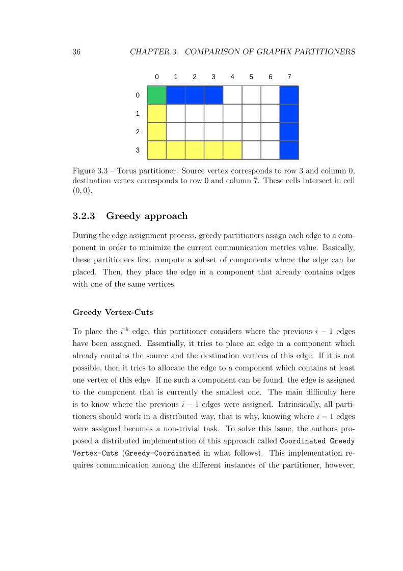
36 CHAPTER 3. COMPARISON OF GRAPHX PARTITIONERS
Figure 3.3 – Torus partitioner. Source vertex corresponds to row 3 and column 0,destination vertex corresponds to row 0 and column 7. These cells intersect in cell(0, 0).
3.2.3 Greedy approach
During the edge assignment process, greedy partitioners assign each edge to a com-
ponent in order to minimize the current communication metrics value. Basically,
these partitioners first compute a subset of components where the edge can be
placed. Then, they place the edge in a component that already contains edges
with one of the same vertices.
Greedy Vertex-Cuts
To place the ith edge, this partitioner considers where the previous i − 1 edges
have been assigned. Essentially, it tries to place an edge in a component which
already contains the source and the destination vertices of this edge. If it is not
possible, then it tries to allocate the edge to a component which contains at least
one vertex of this edge. If no such a component can be found, the edge is assigned
to the component that is currently the smallest one. The main difficulty here
is to know where the previous i − 1 edges were assigned. Intrinsically, all parti-
tioners should work in a distributed way, that is why, knowing where i − 1 edges
were assigned becomes a non-trivial task. To solve this issue, the authors pro-
posed a distributed implementation of this approach called Coordinated Greedy
Vertex-Cuts (Greedy-Coordinated in what follows). This implementation re-
quires communication among the different instances of the partitioner, however,

3.2. CLASSIFICATION OF THE PARTITIONERS 37
it can be too costly. Hence, the authors also introduced a relaxed version called
Oblivious Greedy Vertex-Cuts (Greedy-Oblivious in what follows), where no
communication is required among the different instances of the partitioner, but
each instance remembers its own assignments. Each instance of the partitioner
greedily assigns an edge as described above but only considering its own previous
choices.
Grid-based Constrained Greedy Vertex-cuts (Grid Greedy)
As the Grid partitioner proposed in [49], it relies on a logical grid. Instead of
randomly selecting one cell from the intersection of cells, it selects a cell using the
same greedy criterium as in Section 3.2.3.
The issue here is to remember previous assignments. As in previous case, there
can be correct expensive solution, where after each assignment of N edges (because
we have N instances of the partitioner) we have to propagate all the information
between all the instances, even though it does not support serializability.2 Again,
this partitioner can be implemented as the Greedy-Oblivious partitioner: each
instance remembers only its own assignments.
Torus-based Constrained Greedy Vertex-cuts (Torus Greedy)
It is a greedy version of the Torus algorithm. First, like Torus, it computes two
pairs of row-column in 2D torus T , which correspond to source and destination
vertices. Second, it finds an intersection of cells of these two pairs of row-column.
Finally, it selects one cell from the intersection according to the greedy heuristic
as in Section 3.2.3.
Distributed Funding-based Edge Partitioning (DFEP)
This partitioner was proposed in [51] and implemented for both Hadoop [35] and
Spark [13]. In the DFEP algorithm each component initially receives a randomly
assigned vertex and then tries to progressively grow by including all the edges of
the vertices currently in the component that are not yet assigned. In order to avoid
2Serializability property says that concurrent operations applied to a shared object appear assome serial execution of these operations.
38 CHAPTER 3. COMPARISON OF GRAPHX PARTITIONERS
a dishomogeneous growth of the components, a virtual currency is introduced and
each component receives an initial funding that can be used to bid on the edges.
Periodically, each component receives additional funding inversely proportional to
the number of edges it has.
3.2.4 Hubs Cutting
Most of the real-world graphs are power-law graphs, where a relatively small per-
centage of nodes (hubs) concentrate most of the edges [54]. This approach moves
then from the observation that most probably hubs will need to be cut into N
pieces to maintain balance among the components.These partitioners prefer then
to cut hubs, trying to spare the large share of nodes that have a small degree
Hybrid-Cut
The Hybrid-cut [47] partitioner considers that a vertex is not a hub if its in-degree
is below a given threshold. In such case all the incoming edges are partitioned based
on the hash value of this vertex and are placed in the same component. Otherwise
the algorithm partitions based on their source vertices (assuming that the source
vertices are not hubs). The algorithm was implemented for GraphX [55]. It is
important to notice that this partitioner starts by calculating the degree of each
vertex, which itself can be a time consuming operation.
Ginger
As Hybrid-cut this partitioner [47] allocates the incoming edges to a non-hub
vertex (v) to the same component. It partitions edges based on destination vertices
if the destination vertices are not hubs (otherwise is not specified).
The difference between Hybrid-Cut and Ginger is that the component Ei is
selected based on the following greedy heuristic:
i = argmaxi=1,...N
{|Nin(v) ∩ V (Ei)| −
1
2
(|V (Ei)|+
|V ||E||Ei|)}
(3.1)
The underlying idea is that the partitioner selects the component where there
are already neighbors of node v, as far as this component is not too large.
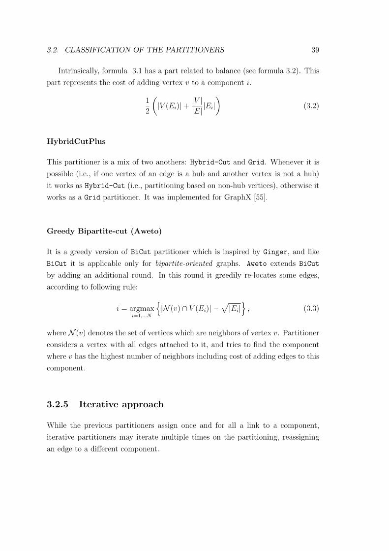
3.2. CLASSIFICATION OF THE PARTITIONERS 39
Intrinsically, formula 3.1 has a part related to balance (see formula 3.2). This
part represents the cost of adding vertex v to a component i.
1
2
(|V (Ei)|+
|V ||E||Ei|)
(3.2)
HybridCutPlus
This partitioner is a mix of two anothers: Hybrid-Cut and Grid. Whenever it is
possible (i.e., if one vertex of an edge is a hub and another vertex is not a hub)
it works as Hybrid-Cut (i.e., partitioning based on non-hub vertices), otherwise it
works as a Grid partitioner. It was implemented for GraphX [55].
Greedy Bipartite-cut (Aweto)
It is a greedy version of BiCut partitioner which is inspired by Ginger, and like
BiCut it is applicable only for bipartite-oriented graphs. Aweto extends BiCut
by adding an additional round. In this round it greedily re-locates some edges,
according to following rule:
i = argmaxi=1,...N
{|N (v) ∩ V (Ei)| −
√|Ei|}, (3.3)
where N (v) denotes the set of vertices which are neighbors of vertex v. Partitioner
considers a vertex with all edges attached to it, and tries to find the component
where v has the highest number of neighbors including cost of adding edges to this
component.
3.2.5 Iterative approach
While the previous partitioners assign once and for all a link to a component,
iterative partitioners may iterate multiple times on the partitioning, reassigning
an edge to a different component.
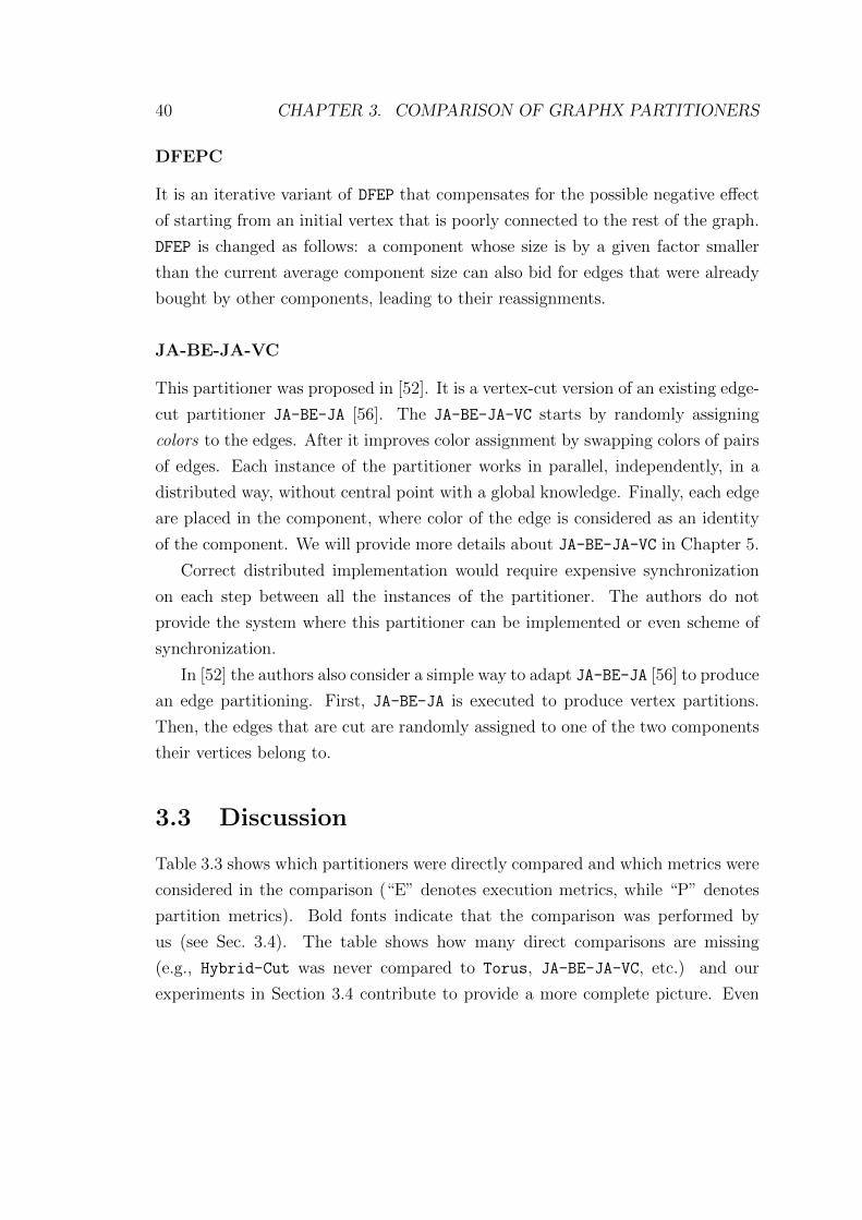
40 CHAPTER 3. COMPARISON OF GRAPHX PARTITIONERS
DFEPC
It is an iterative variant of DFEP that compensates for the possible negative effect
of starting from an initial vertex that is poorly connected to the rest of the graph.
DFEP is changed as follows: a component whose size is by a given factor smaller
than the current average component size can also bid for edges that were already
bought by other components, leading to their reassignments.
JA-BE-JA-VC
This partitioner was proposed in [52]. It is a vertex-cut version of an existing edge-
cut partitioner JA-BE-JA [56]. The JA-BE-JA-VC starts by randomly assigning
colors to the edges. After it improves color assignment by swapping colors of pairs
of edges. Each instance of the partitioner works in parallel, independently, in a
distributed way, without central point with a global knowledge. Finally, each edge
are placed in the component, where color of the edge is considered as an identity
of the component. We will provide more details about JA-BE-JA-VC in Chapter 5.
Correct distributed implementation would require expensive synchronization
on each step between all the instances of the partitioner. The authors do not
provide the system where this partitioner can be implemented or even scheme of
synchronization.
In [52] the authors also consider a simple way to adapt JA-BE-JA [56] to produce
an edge partitioning. First, JA-BE-JA is executed to produce vertex partitions.
Then, the edges that are cut are randomly assigned to one of the two components
their vertices belong to.
3.3 Discussion
Table 3.3 shows which partitioners were directly compared and which metrics were
considered in the comparison (“E” denotes execution metrics, while “P” denotes
partition metrics). Bold fonts indicate that the comparison was performed by
us (see Sec. 3.4). The table shows how many direct comparisons are missing
(e.g., Hybrid-Cut was never compared to Torus, JA-BE-JA-VC, etc.) and our
experiments in Section 3.4 contribute to provide a more complete picture. Even

3.3. DISCUSSION 41
Table 3.2 – Spark configuration
Property name Property valuespark.executor.memory 4GB
spark.driver.memory 10GBspark.cores.max 10spark.local.dir “tmp”
when a direct comparison is available, results are not necessarily conclusive. For
example, in [52] the authors show that JA-BE-JA-VC outperforms DEFP, DFEPC,
and JA-BE-JA3 in terms of STD. However in terms of normalized vertex-cut, the
modified version of JA-BE-JA is the best.
Table 3.1 indicates which specific metrics were considered in each paper. We
can observe that in many cases execution metrics have not been considered, e.g.,
in [52] authors do not provide any experiments which shows change in execution
time. It happens because they are expensive in terms of computation time. In
particular, the lack of information about the partitioning time is problematic be-
cause in our experiments we have observed that it can vary by more than one order
of magnitude across partitioners and contribute the most to the total execution
time. The table also shows that it is difficult to perform an indirect comparison
among partitioners using results from different papers, because there is often no
common set of metrics considered across them.
In conclusion, it is hard to reach any conclusion regarding the benefits of ex-
isting partitioners for multiple reasons. First, not all partitioners have been com-
pared. Second, execution metrics are not always provided and are tied to a specific
computing environment. Finally, there is no study which links partitioning metrics
to execution metrics, but for [57]. Motivated by these considerations, we decided to
conduct experiments using the GraphX framework. Our results partially complete
the pairwise comparison in Table 3.3 and are presented in the next section.
3Actually, they have used modified version of partitioner (original JA-BE-JA performs vertexpartitioning), where each cut edge replaced with one cut vertex (randomly selected from sourceor destination vertices of cut edge)
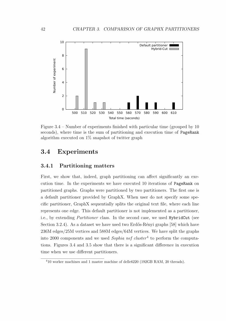
42 CHAPTER 3. COMPARISON OF GRAPHX PARTITIONERS
0
2
4
6
8
10
500 510 520 530 540 550 560 570 580 590 600 610
Num
ber
of
exp
eri
ment
Total time (seconds)
Default partitionerHybrid-Cut
Figure 3.4 – Number of experiments finished with particular time (grouped by 10seconds), where time is the sum of partitioning and execution time of PageRank
algorithm executed on 1% snapshot of twitter graph
3.4 Experiments
3.4.1 Partitioning matters
First, we show that, indeed, graph partitioning can affect significantly an exe-
cution time. In the experiments we have executed 10 iterations of PageRank on
partitioned graphs. Graphs were partitioned by two partitioners. The first one is
a default partitioner provided by GraphX. When user do not specify some spe-
cific partitioner, GraphX sequentially splits the original text file, where each line
represents one edge. This default partitioner is not implemented as a partitioner,
i.e., by extending Partitioner class. In the second case, we used HybridCut (see
Section 3.2.4). As a dataset we have used two Erdos-Renyi graphs [58] which have
236M edges/25M vertices and 588M edges/64M vertices. We have split the graphs
into 2000 components and we used Sophia nef cluster 4 to perform the computa-
tions. Figures 3.4 and 3.5 show that there is a significant difference in execution
time when we use different partitioners.
410 worker machines and 1 master machine of dellc6220 (192GB RAM, 20 threads).

3.4. EXPERIMENTS 43
0
5
10
15
20
25
30
35
40
640 680 720 760 800 840 880 920 960
Num
ber
of
exp
eri
ment
Total time (seconds)
Default partitionerHybrid-Cut
Figure 3.5 – Number of experiments finished with particular time (grouped by 10seconds), where time is the sum of partitioning and execution time of PageRank
algorithm executed on 2.5% snapshot of twitter graph
3.4.2 Comparison of different partitioners
We measured replication factor, communication cost, balance, STD as partitioning
metrics, and the partitioning time and the execution time of Connected Components and
PageRank (10 iterations) algorithms as execution metrics.
We conducted our experiments on Nef cluster sophia by using nodes with dual-
Xeon [email protected], 192GB RAM and 20 cores. We used Spark version 1.4.0
in standalone cluster mode. Our cluster configuration had eleven machines, one
for master and ten for executors. We configured 4 Spark properties as in Table 3.2.
As input we used the undirected com-Youtube graph (1,134,890 vertices/2,987,624
edges) from the SNAP project [59].
As a set of partitioners, we used all the GraphX built-in partitioners, i.e.,
RandomVertexCut, CanonicalRandomVertexCut, EdgePartition1D, Grid, the par-
titioner DFEP (whose code was kindly made available by the authors of [51]),
Greedy-Oblivious (implemented by us), Hybrid-Cut and HybridCutPlus (both
implemented by Larry Xiao [55]).
In each experiment we first randomly selected a partitioner and a graph pro-

44 CHAPTER 3. COMPARISON OF GRAPHX PARTITIONERS
0
0.5
1
1.5
2
2.5
3
CRVCDFEP
EP1DGrid
Greedy
HybridCut
HCPRVC
Metr
ics
valu
es
Communication costReplication factor
Figure 3.6 – Communication metrics (lower is better) .
cessing algorithm. Then, we applied the selected partitioner to the input graph.
Finally, we executed the selected graph processing algorithm. We repeated every
combination at least 30 times to obtain 95% confidence intervals for the execution
time whose relative amplitude is always less than 10%.
Our experiments confirm that, as expected, the best balance, and STD metrics
are obtained by random partitioners like RVC and CRVC. In terms of communica-
tion metrics, Fig. 3.6 shows that DFEP outperforms the other partitioners. This
improvement comes at the cost of a much larger partitioning time, indeed in our
setting DFEP partitions the graph in a few minutes, while the other partitioners are
at least 20 times faster. Moreover, these partitioning metrics are not necessarily
good predictors for the final execution time. Indeed, Fig. 3.7 shows that while
PageRank achieves the shortest execution time when the graph is partitioned by
DFEP, Hybrid-Cut provides the best partitioning for Connected Components and
HybridCutPlus performs almost as DFEP. This result questions the extent to which
partitioning metrics can be used to predict the actual quality of a partition (this
aspect are investigated in the next chapter). From the practical point of view,
Hybrid-Cut appears to achieve the best trade-off between partitioning time and
reduction of the execution time.
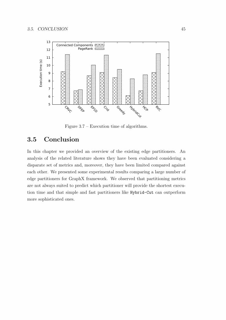
3.5. CONCLUSION 45
5
6
7
8
9
10
11
12
13
CRVCDFEP
EP1DCrid
Greedy
HybridCut
HCPRVC
Exe
cuti
on t
ime (
s)
Connected ComponentsPageRank
Figure 3.7 – Execution time of algorithms.
3.5 Conclusion
In this chapter we provided an overview of the existing edge partitioners. An
analysis of the related literature shows they have been evaluated considering a
disparate set of metrics and, moreover, they have been limited compared against
each other. We presented some experimental results comparing a large number of
edge partitioners for GraphX framework. We observed that partitioning metrics
are not always suited to predict which partitioner will provide the shortest execu-
tion time and that simple and fast partitioners like Hybrid-Cut can outperform
more sophisticated ones.

46 CHAPTER 3. COMPARISON OF GRAPHX PARTITIONERST
able
3.3–
Partition
erspairw
isecom
parison
s,con
siderin
gex
ecution
metrics
(E)
orpartition
ing
metrics
(P).
Bold
fonts
indicate
exp
erimen
tsw
econ
ducted
.
RandomVertexCut
CRVC
EdgePartition1D
Greedy-Coordinated
Greedy-Oblivious
Grid
GridGreedy
Torus
TorusGreedy
DFEP
DFEPC
JA-BE-JA-VC
Hybrid-Cut
Ginger
HybridCutPlus
BiCut
Aweto
JA-BE-JA
Ran
dom
Vertex
Cut
-E
PE
PE
PE
PE
PE
PP
EP
EP
EP
EP
CR
VC
-E
PE
PE
PE
PE
PE
PE
PE
dgeP
artition1D
-E
PE
PE
PE
PE
PG
reedy-
Coord
inated
-E
PE
PE
PP
EP
PP
EP
EP
P
Greed
y-O
bliv
ious
-E
PE
PP
EP
EP
EP
PG
rid-
PP
PE
PE
PE
PE
PE
PE
PG
ridG
reedy
-P
EP
Toru
s-
PT
orus
Greed
y-
DF
EP
-E
PP
EP
EP
EP
DF
EP
C-
PE
PJA
-BE
-JA
-VC
-P
Hybrid
-Cut
-E
PE
PG
inger
-H
ybrid
CutP
lus
-B
iCut
-E
PA
weto
-JA
-BE
-JA
-
Chapter 4
Predictive power of partition
metrics
Contents
4.1 Statistical analysis methodology . . . . . . . . . . . . . 48
4.2 Experiments . . . . . . . . . . . . . . . . . . . . . . . . . 50
4.3 Conclusion . . . . . . . . . . . . . . . . . . . . . . . . . . 56
In this chapter we investigate how it is possible to evaluate the quality of a
partitioning before running the computation. Answering this question would be
useful both for the data analysts who need to choose the partitioner appropriate for
their graphs and for developers who aim at proposing more efficient partitioners.
As discussed in Chapter 2, some metrics have been proposed to this purpose.
The survey of the related literature in the previous chapter shows that there is
no common agreement about which metrics should be used for a comparison. In
this chapter we make a step towards providing an answer by carrying experiments
with the widely-used framework for graph processing GraphX and performing an
accurate statistical analysis.
The chapter is organized as follows. In Section 4.1 we discuss our statistical
methodology to study the dependency between the execution time of different
graph-processing algorithms and partitioning metrics. We discuss the experimental
setup and illustrate the results in Section 4.2. Finally, we conclude in Section 4.3.
47

48 CHAPTER 4. PREDICTIVE POWER OF PARTITION METRICS
The source code for all experiments is available here [48].
4.1 Statistical analysis methodology
Six partitioning algorithms are considered in this chapter, the GraphX built-in ones
(RandomVertexCut, CanonicalRandomVertexCut, EdgePartition1D, EdgePartition2D)
and two external(HybridCut, HybridCutPlus). We want to study if the partition-
ing metrics considered in the literature and described in Section 2.3.2 are good
predictors for the final execution time. Remember that an execution time does
not include partitioning time. We do not consider partitioning time because it
does not depend on the partitions but on how partitioner was implemented.
To this purpose, we would like ideally to design experiments where we could
randomly and independently select the five different metrics, generate an input
graph with these quintuple of characteristics, evaluate the execution time of the
application of interest and finally use some statistical tool like a regression models
to identify the contribution of each metric to the execution time. Unfortunately, it
is not possible to select first the partitioning metrics and then produce a graph with
such characteristics. We can only use a partitioner on a given graph to produce
a partition and then compute the metrics. As a consequence, their values will be
far from independent and in particular the structure of their correlation can be a
function of the specific partitioner used.
For this reason, in order to obtain a variety of different configurations, we used
all the six partitioners on the same set of graphs. For each graph this leads to
six different quintuples. A statistical model based on 6 points in a five-dimension
space would very likely overfit the data. Considering other graphs allow us to
obtain other samples. The drawback is that if we use real datasets, they are
going to differ for the number of nodes and of edges. Now, these two metrics are
very likely to have an effect much more important on the execution time than the
partitioning metrics, which are the focus of our study. Remember that our goal
is choosing the best partitioner for a given input graph of interest, whose size in
terms of number of nodes and edges is out of our control. The contribution of the
partition metrics would be dwarfed by the size change.
In order to overcome this difficulty, we generated 10 input graphs with the same

4.1. STATISTICAL ANALYSIS METHODOLOGY 49
size by simply randomly permutating the ids of the vertices, by replacing vertices
ids with the random unique numbers. Even if the different graphs are homeomor-
phic, components are calculated using the ids, and then each partitioner produces
different subsets with different values for the metrics of interest. This approach
allowed us to have 60 different quintuples for each graph: the ten permutations
of the original graph multiplied by the six partitioners. In this way the risk of an
overfitting model is significantly reduced.
To identify the most important metrics, we then used a linear regression model
(denoted as LRM) with the five partition metrics as input variables (or predictors)
and the execution time as the output variable (or response):
β1BAL+ β2LP + β3NSD + β4V C + β5CC + ε = execution time
where βi are regression coefficients, and ε is error term. We want to find the
most important predictors, but also rank these predictors by their importance.
Obviously the more predictors we have in a LRM the smaller is the residual error,
but which ones are really important? For this purpose we used the best subset
selection method [60, Chapter 6]. According best subset selection method we have
to first compare models with the same number of predictors, in order to find the
best one for each number of predictors. And then, compare these best models
by using, for example Akaike information criterion [61]. In particular, given the
small number of predictors (5), we were able to consider all the possible 5! linear
models for each original graph. Models with the same number of predictors were
compared through their R2 value. In this way 5 models were selected, respectively
with 1,2,3,4 and 5 predictors. The best model was finally identified as the one with
the smallest Akaike information criterion. We have considered another indices as
well, such as Bayesian Information Criteria, sample-size corrected AIC, or R2
adjusted. However, in the most cases the results did not differ. Once the best
model was selected, we ordered its predictors by considering those that lead to the
largest increase of the R2 value when added as predictors.
50 CHAPTER 4. PREDICTIVE POWER OF PARTITION METRICS
Table 4.1 – Spark configuration
Property name Property valuespark.executor.memory 4GB (for 10 executors)/ 40GB (for 1 executor)
spark.driver.memory 10GBspark.cores.max 10spark.local.dir “tmp”
4.2 Experiments
Our experiments were performed on the Nef sophia cluster. Each machine had
nodes two Xeon E5-2680 v2 @2.80GHz with 192GB RAM and 10 cores (20 threads).
We used Spark version 1.4.0 and Spark standalone cluster [62] as a resource man-
ager. We used two different cluster configurations. In the first configuration, a
master and an executor share the same machine. In the second case, one machine
is dedicated to the master and one to each of the ten executors. We configured
Spark properties as shown in the Table 4.1.
Two different processing algorithms were evaluated: Connected Components
and PageRank with 10 iterations. PageRank exhibits the same computation and
communication pattern at each stage (the PageRank of each vertex value is up-
dated according to the same formula and then propagated to the neighbors), while
Connected Components implements a label propagation mechanism, where as time
goes on, less updates are required.
As datasets, we used two undirected graphs: the com-Youtube graph (1,134,890
vertices/2,987,624 edges) and the com-Orkut graph (3,072,441 vertices/117,185,083
edges) from the SNAP project [59].
For each experiment, first we randomly selected a partitioner, a graph pro-
cessing algorithm, and a permutation of an input graph. Second, we applied the
selected partitioner to the input graph. Finally, we executed the selected graph
processing algorithm. To overcome execution time variability (due to a shared
network, shared distributed file system, operating system layer, etc.), every com-
bination has been tested at least 30 times, obtaining 95% confidence intervals for
the execution time whose relative amplitude is always less than 10%.
As we mentioned earlier, for each graph we obtained 60 different quintuples for

4.2. EXPERIMENTS 51
Table 4.2 – Correlation matrix for partition metrics com-Youtube
BAL LP NSD VC CCBAL 1 0.9332 0.9445 0.2070 -0.2448LP 1 0.9799 0.0993 -0.3177
NSD 1 0.1275 -0.2667VC 1 0.8737CC 1
the partition metrics. Table 4.2 shows their correlation matrix for com-Youtube
graph.1 Let us consider all values of the Table 4.2 which are more than 0.8. We
can clearly identify the two groups of metrics: those relative to partition balance
(BAL, LP NSTDEV) and those related to communication (VC, CC). The high
level of collinearity also explains why in the LRM some coefficients are negative [60,
Chapter 3].
We computed and selected linear regression models for com-Youtube, com-
Youtube doubled, and com-Orkut graph, as it was discussed in Section 4.1. Table 4.4
and Table 4.5 summarize our experimental results respectively for PageRank and
Connected Components. For each input graph and number of machines, they show
the best LRM with the factors listed in decreasing order of importance. We note
that, although a single node has enough resources to perform all the computation,
the results in Table 4.4 and Table 4.5 show that the average execution time de-
creases as the number of machines increases. A similar result was observed in [63]
where it was due to the higher memory contention in case of a single machine. It
is possible that the effect has the same cause here.
Below we illustrate our main findings about the partition metrics.
The execution time depends on the partition metrics
For PageRank (see Table 4.4) the R2 value is very high (always above 0.98) while
the Root Mean Square Error ( RMSE) is less than 5% of mean execution time.
This leads to conclude that indeed the execution time depends on these metrics.
The dependency is less stronger for Connected Components. This can be explained
1Correlation matrix shows how much partition metrics correlate with each other. 0 means -no correlation, 1 means - maximum correlation.
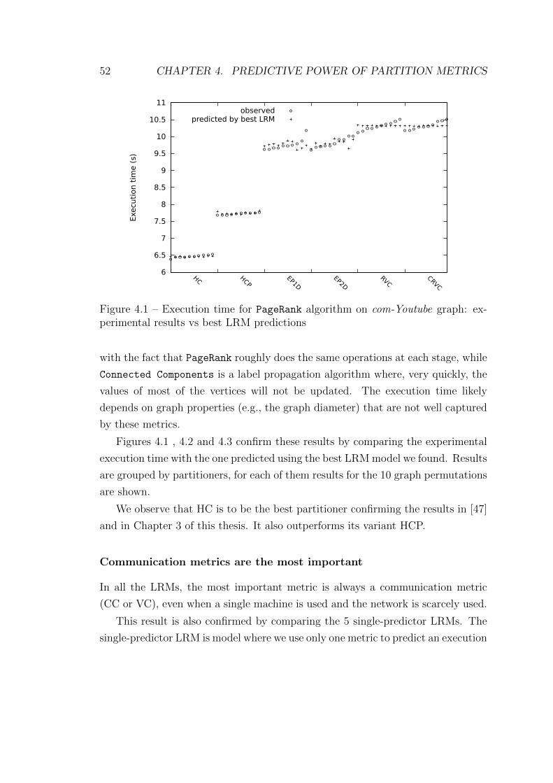
52 CHAPTER 4. PREDICTIVE POWER OF PARTITION METRICS
6
6.5
7
7.5
8
8.5
9
9.5
10
10.5
11
HC HCPEP1D
EP2DRVC
CRVC
Exe
cuti
on t
ime (
s)
observedpredicted by best LRM
Figure 4.1 – Execution time for PageRank algorithm on com-Youtube graph: ex-perimental results vs best LRM predictions
with the fact that PageRank roughly does the same operations at each stage, while
Connected Components is a label propagation algorithm where, very quickly, the
values of most of the vertices will not be updated. The execution time likely
depends on graph properties (e.g., the graph diameter) that are not well captured
by these metrics.
Figures 4.1 , 4.2 and 4.3 confirm these results by comparing the experimental
execution time with the one predicted using the best LRM model we found. Results
are grouped by partitioners, for each of them results for the 10 graph permutations
are shown.
We observe that HC is to be the best partitioner confirming the results in [47]
and in Chapter 3 of this thesis. It also outperforms its variant HCP.
Communication metrics are the most important
In all the LRMs, the most important metric is always a communication metric
(CC or VC), even when a single machine is used and the network is scarcely used.
This result is also confirmed by comparing the 5 single-predictor LRMs. The
single-predictor LRM is model where we use only one metric to predict an execution

4.2. EXPERIMENTS 53
6
7
8
9
10
11
12
13
HC HCPEP1D
EP2DRVC
CRVC
Exe
cuti
on t
ime (
s)
observedpredicted by best LRM
Figure 4.2 – Execution time for Connected Components algorithm on com-Youtubegraph: experimental results vs best LRM predictions
time of the algorithm. The LRMs using VC or CC have larger R2 value. Figure 4.4
shows how LRM models using only VC or CC are able to produce quite good
predictions at least of the relative performance of the different partitioners. On
the contrary, the corresponding plot for balance metrics (BAL, LP, NSTDEV)
shows an almost horizontal line (see Figure 4.5).
As a side note, we tried to find a setting where balance metrics would have
become the most important ones. In particular we considered i) a single machine,
ii) very limited memory for each partitioner (70MB), iii) a modified version of
PageRank where each computation is performed 1000 more times. The purpose
was to make communication among executors as fast as possible, while increasing
the computational burden on each executor. Even in this settings, communication
metrics appeared to be the most important ones.
Results are robust to the partitioners considered
One of the purposes of our analysis is to be able to rank a priori different partition-
ers before carrying on the experiments. We evaluated how much our results are
sensitive to the specific set of partitioners used to tune the LRM. To this purpose,

54 CHAPTER 4. PREDICTIVE POWER OF PARTITION METRICS
we carried on the same analysis using only 5 partitioners (we did not use HC). We
then used the new LRM model to predict the execution time for the HC parti-
tioner. Figure 4.6 shows that predicted execution time for HC is underestimated.
However, the order of the partitioners in terms of execution time is the correct one.
Then the LRM model correctly predicts that HC partitioning will lead to a shorter
execution time. One could argue that the LRM has been trained using HCP that
is a variant of HC. We then performed the same set of experiments removing both
HC and HCP (see Figure 4.7). In this case the predicted executed time is really
off, but the LRM still correctly predicts the ranking of the different partitioners.
There is space for better partition metrics
While the results above are encouraging, the following experiment suggests that
these partition metrics do not capture all the relevant features.
We considered a version of com-Youtube graph where we doubled each edge
so that both directions are present in the input graph and PageRank correctly
computes the PageRank of the original undirected graph. We denote the doubled
graph as com-Youtube doubled.
The execution time of both algorithms on com-Youtube doubled is larger, roughly
30% (see Table 4.3). Nevertheless, the communication metrics that we identified
as the most important ones may fail to detect the change. This is evident if we
compare the CRVC partitioner with the other ones. As shown in Table 4.3 for a
specific input graph, the CRVC partitioner provides the same values for all the
partition metrics, and in particular for VC and CC metrics, both for com-Youtube
doubled and com-Youtube, since it partitions edges based on the vertex (either
source or destination) with the smallest id. For the other partitioners instead, the
metrics VC and CC are different. The difference is evident if we compute the LRM
including or not CRVC. In the first case the R2 value of the LRM for PageRank
significantly decreases from 0.99 for com-Youtube (see Table 4.4) to 0.82. In the
second case the LRMs are equally good.
We think a more meaningful communication metric could be defined that would
permit to identify the difference between CRVC and the other partitioners. We
plan to investigate this aspect in the future.

4.2. EXPERIMENTS 55
60
70
80
90
100
110
120
HC HCPEP2D
EP1DCRVC
RVC
Exe
cuti
on t
ime (
s)
observedpredicted by best LRM
Figure 4.3 – Execution time for PageRank algorithm on com-Orkut graph: exper-imental results vs best LRM predictions
6
6.5
7
7.5
8
8.5
9
9.5
10
10.5
11
HC HCPEP1D
EP2DRVC
CRVC
Exe
cuti
on t
ime (
s)
observedpredicted by VCpredicted by CC
Figure 4.4 – Execution time for PageRank algorithm on com-Youtube graph: ex-perimental results vs LRM predictions using a single communication metrics

56 CHAPTER 4. PREDICTIVE POWER OF PARTITION METRICS
6
6.5
7
7.5
8
8.5
9
9.5
10
10.5
11
HC HCP EP1D EP2D RVC CRVC
Exe
cuti
on t
ime (
s)
observedpredicted by BAL
predicted by LPpredicted by NSTDEV
Figure 4.5 – Execution time for PageRank algorithm on com-Youtube graph: ex-perimental results vs LRM predictions using a single balance metrics
4
5
6
7
8
9
10
11
HC HCPEP1D
EP2DRVC
CRVC
Exe
cuti
on t
ime (
s)
observedpredicted by LRM
Figure 4.6 – Prediction for HC partitioner (using com-Youtube graph, andPageRank algorithm)
4.3 Conclusion
We used linear regression models with partitioning metrics as predictors and the
average execution time for different graph processing algorithms as the observed

4.3. CONCLUSION 57
-20
-15
-10
-5
0
5
10
15
HC HCPEP1D
EP2DRVC
CRVC
Exe
cuti
on t
ime (
s)
observedpredicted by best LRM
Figure 4.7 – Prediction for HC and HCP parititioners (using com-Youtube graph,and PageRank algorithm)
Table 4.3 – Metrics and execution time of PageRank for HC and CRVC
Graph nameHC CRVC
Averagetime (ms)
VC CCAverage
time (ms)VC CC
com-Youtube 6468 0.304 1.091 10327 0.452 1.831com-Youtube
doubled8121 0.702 2.204 13404 0.452 1.831
values. The obtained models confirmed that there is an actual dependency between
these quantities. More importantly, the most important metrics are CC and VC.
Both are an indicator of the amount of communication among the executors. On
the contrary, the metrics that quantify load unbalance across the executors are
less important. This conclusion holds whether communication is inter-machine or
intra-machine, i.e., both if the network is used or not. Our results are robust to the
original set of partitioners used to train the model, and the model can correctly
rank other partitioners. Moreover, we show that current metrics are not sufficient
to evaluate partitions.

58 CHAPTER 4. PREDICTIVE POWER OF PARTITION METRICS
Tab
le4.4
–T
he
best
linear
regressionm
odels
forPageRank
algorithm
Grap
hnam
eC
luster
con-
figu
ration
Mean
time
(ms)
Metrics
(ordered
by
imp
ortance)
RM
SE
R2
com-Y
outu
be
single
mach
ine
12,343m
etr.V
CC
CB
AL
LP
NSD
111.830.996
coeff
.1.5507
0.31560.42743
-0.495040.33548
1m
aster+
10ex
ecutors
9,068m
etr.V
CC
CB
AL
LP
NSD
125.470.993
coeff
.1.2816
0.272610.50989
-0.648570.49891
com-O
rkut
single
mach
ine
122,929m
etr.C
CL
PV
C1199.4
0.998co
eff.
2.3125.039
12.9421
master
+10
execu
tors94,738
metr.
CC
LP
NSD
VC
2222.80.989
coeff
.1.3285
8.3243-11.486
12.881
Tab
le4.5
–T
he
best
linear
regressionm
odels
forConnected
Components
algorithm
Grap
hnam
eC
luster
configu
rationM
eantim
e(m
s)M
etrics(ord
eredby
imp
ortance)
RM
SE
R2
com-Y
outu
be
single
mach
ine
12,429m
etricsV
CL
PN
SD
1119.20.499
coeffi
cients
1.7884-1.3177
1.38611
master
+10
execu
tors9,635
metrics
VC
LP
NSD
922.270.681
coeffi
cients
2.1131-1.7528
2.1043
com-O
rkut
single
mach
ine
86,253m
etricsC
CL
PN
SD
2628.20.959
coeffi
cients
1.20399.771
-8.26341
master
+10
execu
tors71,952
metrics
CC
LP
NSD
2235,60.973
coeffi
cients
1.085415.484
-17.96
Chapter 5
A simulated annealing
partitioning framework
Contents
5.1 Introduction . . . . . . . . . . . . . . . . . . . . . . . . . 60
5.2 Background and notations . . . . . . . . . . . . . . . . . 61
5.3 Reverse Engineering JA-BE-JA-VC . . . . . . . . . . . 63
5.4 A general SA framework for edge partitioning . . . . . 66
5.5 The SA framework . . . . . . . . . . . . . . . . . . . . . 70
5.6 Evaluation of the SA framework . . . . . . . . . . . . . 72
5.7 The multi-opinion SA framework . . . . . . . . . . . . . 79
5.7.1 Distributed implementation . . . . . . . . . . . . . . . . 81
5.8 Evaluation of the multi-opinion SA framework . . . . . 84
5.9 Conclusion . . . . . . . . . . . . . . . . . . . . . . . . . . 87
This chapter describes how simulated annealing (SA) technique can be used in
order to partition a graph with a purpose to minimize a specific partition metric.
We propose a general SA framework for distributed edge partitioning based
on simulated annealing [64]. The framework can be used to optimize a large
family of partitioning metrics. We provide sufficient conditions for convergence
59

60CHAPTER 5. A SIMULATED ANNEALING PARTITIONING FRAMEWORK
to the optimum as well as discuss which metrics can be efficiently optimized in a
distributed way. We have implemented our partitioners in GraphX and performed
a comparison with JA-BE-JA-VC [52], a state-of-the-art partitioner that inspired
our approach. We show that our approach can provide improvements. We have
also developed two version of the proposed framework. The first version — the SA
framework — is faster but may not converge to the optimum. The second version
— the multiopinion SA framework — is guaranteed to converge, thanks to some
new theoretical results in [65]. Part of the results in this chapter appeared in [66].
5.1 Introduction
A new edge partitioning algorithm, called JA-BE-JA-VC , has been proposed in
[52] and shown to significantly outperform existing algorithms. The algorithm
starts by assigning an initial (arbitrary) color to each edge.1 Each color represents
a component where the edge will be placed after the partitioner has finished. The
partitioner iteratively improves on the initial edge colors assignment, by allowing
two edges to swap their color if this seems to be beneficial to reduce the number
of cuts of the corresponding vertices. In order to avoid getting stuck at local
minima, JA-BE-JA-VC borrows from simulated annealing (SA) the idea to permit
apparently detrimentals swaps at early stages of the partitioning.
In this chapter, we develop this initial inspiration and propose two version of
graph partitioners based on SA for Spark.
To this purpose, we start by reverse engineering JA-BE-JA-VC to show which
metric it is targeting. After, we propose the first version of our general SA frame-
work that can optimize a large spectrum of objective functions, and for which
convergence results can be proven. The naive implementation of this approach (as
well as of JA-BE-JA-VC ), requires a significant number of costly synchronization
operations during the partitioning. Then we explain how these algorithms can be
efficiently implemented in a distributed architecture as Spark. However, in this
case, instances can operate on stale values, which can prevent convergence to the
optimum. As a proof of concept, we perform some preliminary experiments con-
1In this chapter, we refer to edge assignment to components as edge coloring to maintain theoriginal terminology in [52].

5.2. BACKGROUND AND NOTATIONS 61
sidering an objective function that takes into account both communication cost
and computational balance. We show that this objective function may obtain bet-
ter partitions than JA-BE-JA-VC , but this does not happen consistently. Finally,
we propose and evaluate a second version of our SA framework, relying on new
theoretical results about asynchronous Gibbs sampler [65]. In this version, each
instance maintains a different opinion about how the edge should be colored.
The rest of the chapter is organized as follows. We start by introducing the
notation and tools used in this work (Section 5.2). Next, we reverse-engineer the
JA-BE-JA-VC algorithm in Section 5.3. Then, we present the general SA frame-
work for edge partitioning in Section 5.4. After, we introduce our first implemen-
tation of it — the SA framework, in Section 5.5. We compare JA-BE-JA-VC and
the SA framework in Section 5.6. In Section 5.7 we present a second version of our
framework — the multi-opinion SA framework and we evaluate its performance in
Section 5.8. Finally, we conclude in Section 5.9.
5.2 Background and notations
We have to introduce some additional notations. As we have already mentioned in
Section 2, we have an undirected graph G = (V,E). This graph will be partitioned
in N distinct components, each of the N component is identified with one of the
N colors from the set C. Let E(c) denote the set of edges with color c ∈ C, then
E =⋃c∈C
E(c). Given a vertex v ∈ V , its degree is denoted by dv and the number
of its edges with color c is denoted by nv(c).
JA-BE-JA-VC [52] is a recently proposed edge partitioner. Given an initial
color assignment to edges (e.g., a random one), the algorithm iteratively improves
this color assignment. At the end of the partitioning, JA-BE-JA-VC distributes
all edges to the components by considering the color of the edge as the component
identifier. During an algorithm iteration, JA-BE-JA-VC selects two vertices u and
u′. For each of these two vertices, it then selects an edge among those whose color
is less represented in their neighborhood. For example, considering u, it will select
an edge of color c ∈ argmin{nu(c)}. Let us denote these two edges as (u, v) and
(u′, v′) with color respectively c and c′. The algorithm always swaps the colors of

62CHAPTER 5. A SIMULATED ANNEALING PARTITIONING FRAMEWORK
the two edges if
g(u, v, c) + g(u′, v′, c′) < g(u, v, c′) + g(u′, v′, c)
+1
du+
1
dv+
1
du′+
1
dv′, (5.1)
where g(u, v, c) , nu(c)du
+ nv(c)dv
. The more links of color c the two nodes u and v
have, the larger g(u, v, c) is, and then the two nodes are potentially cut in a smaller
number of pieces. In particular, if all edges of u and v have color c, g(u, v, c)
attains its maximum value is equal to 2. If we consider that g(u, v, c) is a measure
of the quality of the current assignment, (5.1) compares the current quality of
the assignment with the quality of an assignment were colors are swapped. The
additional terms on the right hand side correspond to the fact that after swapping
there is one link more of color c′ (resp. c) for u and v (resp. u′ and v′). While
we have provided an interpretation of g(u, v, c), one may wonder which objective
function (if any) JA-BE-JA-VC is optimizing by swapping color according to
the criterium in (5.1) and if it is related to one of the usual partitioning quality
metrics like VC or CC defined above. In Section 5.3 we provide an answer to such
questions.
The authors of [52] state that, in order to avoid getting stuck in local optima (of
this still unknown objective function), one can introduce the possibility to accept
changes that do not satisfy (5.1), especially during the first iterations. To this
purpose, inspired by simulated annealing (SA) [67, Chapter 7] they introduce a
positive parameter T (the temperature) and change condition (5.1) as follows:
g(u, v, c) + g(u′, v′, c′) <(1 + T )
[g(u, v, c′) + g(u′, v′, c)
+1
du+
1
dv+
1
du′+
1
dv′
], (5.2)
where T decreases linearly from some initial value to zero. Condition (5.2) accepts
all changes that increase the quality of the current assignment, or decrease it no
more than a factor 1 + T . However, it does not accept any changes that decreases
the quality of the current assignment by a larger factor. Thus, this condition does
not consider a lot of exploration possibilities.

5.3. REVERSE ENGINEERING JA-BE-JA-VC 63
JA-BE-JA-VC is presented in [52] as a distributed algorithm, because an edge
swap requires only information available to the nodes involved, i.e., u, v, u′ and
v′. We observe that this property is not necessarily helpful for performing the
partitioning operation on distributed computation frameworks like Spark, because
this information is not necessarily local to the instance that processes the two
edges. Indeed, while the instance may have access to both the edges (u, v) and
(u′, v′), it may not know the current value of edges of a given color that each vertex
has (e.g., it may not know nu(c)), because these other edges might be assigned to
other partitioners. Moreover, the color of these remote edges might be changed
concurrently. Hence, expensive communication exchange among instances could
be required to implement JA-BE-JA-VC . In Section 5.4 we discuss how to modify
JA-BE-JA-VC in order to significantly reduce communication exchange.
5.3 Reverse Engineering JA-BE-JA-VC
The first contribution of this chapter is to identify the global objective function
(energy function in what follows) JA-BE-JA-VC is optimizing when links are
swapped according to (5.1). Let mc be the initial number of edges with color c.
Condition (5.1) corresponds to greedily minimizing the function
Ecomm ,1
2|E|(1− 1N
)
(2|E| −
∑v∈V
∑c∈C
nv(c)2
dv
), (5.3)
under the constraint that at each step |E(c)| = mc for any color c, where mc is
some constant value and∑
c∈C mc = |E|. The constraint is easy to understand,
because JA-BE-JA-VC simply swaps colors of two edges so that number of edges
of a given color is always equal to the initial value. In what follows we show that
a swap makes Ecomm decrease if and only if condition (5.1) is satisfied.
We have two edges (u, v) and (u′, v′) with colors respectively c and c′. If we
accept to swap them, then the number of colors of the vertices will change as
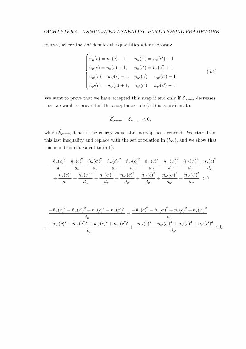
64CHAPTER 5. A SIMULATED ANNEALING PARTITIONING FRAMEWORK
follows, where the hat denotes the quantities after the swap:
nu(c) = nu(c)− 1, nu(c′) = nu(c′) + 1
nv(c) = nv(c)− 1, nv(c′) = nv(c
′) + 1
nu′(c) = nu′(c) + 1, nu′(c′) = nu′(c
′)− 1
nv′(c) = nv′(c) + 1, nv′(c′) = nv′(c
′)− 1
(5.4)
We want to prove that we have accepted this swap if and only if Ecomm decreases,
then we want to prove that the acceptance rule (5.1) is equivalent to:
Ecomm − Ecomm < 0,
where Ecomm denotes the energy value after a swap has occurred. We start from
this last inequality and replace with the set of relation in (5.4), and we show that
this is indeed equivalent to (5.1).
− nu(c)2
du− nv(c)
2
dv− nu(c′)2
du− nv(c
′)2
dv− nu′(c)
2
du′− nv′(c)
2
dv′− nu′(c
′)2
du′− nv′(c
′)2
du′+nu(c)2
du
+nv(c)
2
dv+nu(c′)2
du+nv(c
′)2
dv+nu′(c)
2
du′+nv′(c)
2
dv′+nu′(c
′)2
du′+nv′(c
′)2
dv′< 0
−nu(c)2 − nu(c′)2 + nu(c)2 + nu(c′)2
du+−nv(c)
2 − nv(c′)2 + nv(c)
2 + nv(c′)2
dv
+−nu′(c)
2 − nu′(c′)2 + nu′(c)
2 + nu′(c′)2
du′+−nv′(c)
2 − nv′(c′)2 + nv′(c)
2 + nv′(c′)2
dv′< 0

5.3. REVERSE ENGINEERING JA-BE-JA-VC 65
nu(c)2 −(nu(c)− 1
)2+ nu(c′)2 −
(nu(c′) + 1
)2
du
+nv(c)
2 −(nv(c)− 1
)2+ nv(c
′)2 −(nv(c
′) + 1)2
dv
+nu′(c)
2 −(nu′(c) + 1
)2+ nu′(c
′)2 −(nu′(c
′)− 1)2
du′
+nv′(c)
2 −(nv′(c) + 1
)2+ nv′(c
′)2 −(nv′(c
′)− 1)2
dv′< 0
2nu(c)− 2nu(c′)− 2
du+
2nv(c)− 2nv(c′)− 2
dv
+2nu′(c
′)− 2nu′(c)− 2
du′+
2nv′(c′)− 2nv′(c)− 2
dv′< 0
2
(nu(c)
du+nv(c)
dv− nu(c′)
du− nv(c
′)
dv+nu′(c
′)
du′+nv′(c
′)
dv′
−nu′(c)
du′− nv′(c)
dv′− 1
du− 1
dv− 1
du′− 1
dv′
)< 0
2
(g(u, v, c)− g(u, v, c′) + g(u′, v′, c′)− g(u′, v′, c)− 1
du− 1
dv− 1
du′− 1
dv′
)< 0
g(u, v, c) + g(u′, v′, c′) < g(u, v, c′) + g(u′, v′, c) +1
du+
1
dv+
1
du′+
1
dv′
We could equivalently, and more succinctly, state that JA-BE-JA-VC is maximiz-
ing∑
v∈V∑
c∈Cnv(c)2
dv. The advantage of (5.3) is that Ecomm belongs to [0, 1] and
SA algorithms are usually presented as minimizing an energy function.
Because of the above considerations, JA-BE-JA-VC can be thought as a heuris-
tic to solve the following problem:
minimizec∈C|E|
Ecomm(c)
subject to |E(c)| = mc

66CHAPTER 5. A SIMULATED ANNEALING PARTITIONING FRAMEWORK
where c denotes the vectors of colors chosen for all the edges in the network.
While the greedy rule (5.1) would lead, in general, to a local minimum of Ecomm,
one may wonder if rule (5.2), together with the specific criterium to choose the
edges to swap in JA-BE-JA-VC and to change the temperature, can lead to a
solution of the problem stated above. Unfortunately, it is possible to show that
this is not the case in general.
A second remark is that (5.3) appears to be a quite arbitrary metric, and is
not directly related to metrics like VC or CC. Our experiments show indeed that
Ecomm can decrease while both VC and CC increase, even if the evaluation in [52]
indicates that this is not usually the case.
In the next section we address these two remarks.
5.4 A general SA framework for edge partition-
ing
Let us consider a general optimization problem
minimizec∈C|E|
E(c)
subject to c ∈ D,(5.5)
where D is a generic set of constraints. We can solve this problem with SA as
follows.
– given the current solution c, select a possible alternative c′ ∈ D with prob-
ability qc,c′
– if E(c′) ≤ E(c) accept the change, otherwise accept it with probability
exp(E(c)−E(c′)
T
)< 1. The probability to accept the change can be also ex-
pressed as βc,c′ = min(
1, exp(E(c)−E(c′)
T
))If the selection probabilities qc,c′ are symmetric (qc,c′ = qc′,c) and if the temperature
decreases as T0/ log(1 + k), where k ≥ 0 is the iteration number and the initial
temperature T0 is large enough, then this algorithm is guaranteed to converge to
the optimal solution of the above problem [67, Chapter 7]. JA-BE-JA-VC does
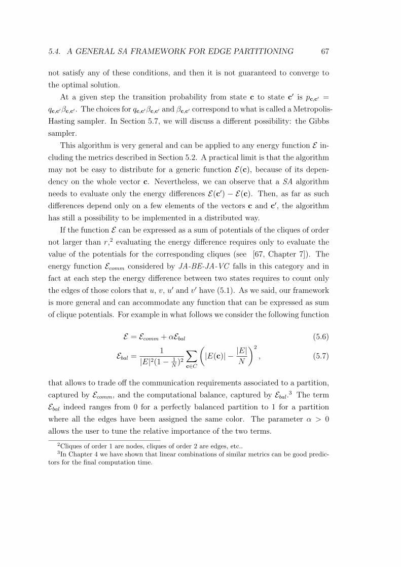
5.4. A GENERAL SA FRAMEWORK FOR EDGE PARTITIONING 67
not satisfy any of these conditions, and then it is not guaranteed to converge to
the optimal solution.
At a given step the transition probability from state c to state c′ is pc,c′ =
qc,c′βc,c′ . The choices for qc,c′βc,c′ and βc,c′ correspond to what is called a Metropolis-
Hasting sampler. In Section 5.7, we will discuss a different possibility: the Gibbs
sampler.
This algorithm is very general and can be applied to any energy function E in-
cluding the metrics described in Section 5.2. A practical limit is that the algorithm
may not be easy to distribute for a generic function E(c), because of its depen-
dency on the whole vector c. Nevertheless, we can observe that a SA algorithm
needs to evaluate only the energy differences E(c′) − E(c). Then, as far as such
differences depend only on a few elements of the vectors c and c′, the algorithm
has still a possibility to be implemented in a distributed way.
If the function E can be expressed as a sum of potentials of the cliques of order
not larger than r,2 evaluating the energy difference requires only to evaluate the
value of the potentials for the corresponding cliques (see [67, Chapter 7]). The
energy function Ecomm considered by JA-BE-JA-VC falls in this category and in
fact at each step the energy difference between two states requires to count only
the edges of those colors that u, v, u′ and v′ have (5.1). As we said, our framework
is more general and can accommodate any function that can be expressed as sum
of clique potentials. For example in what follows we consider the following function
E = Ecomm + αEbal (5.6)
Ebal =1
|E|2(1− 1N
)2
∑c∈C
(|E(c)| − |E|
N
)2
, (5.7)
that allows to trade off the communication requirements associated to a partition,
captured by Ecomm, and the computational balance, captured by Ebal.3 The term
Ebal indeed ranges from 0 for a perfectly balanced partition to 1 for a partition
where all the edges have been assigned the same color. The parameter α > 0
allows the user to tune the relative importance of the two terms.
2Cliques of order 1 are nodes, cliques of order 2 are edges, etc..3In Chapter 4 we have shown that linear combinations of similar metrics can be good predic-
tors for the final computation time.
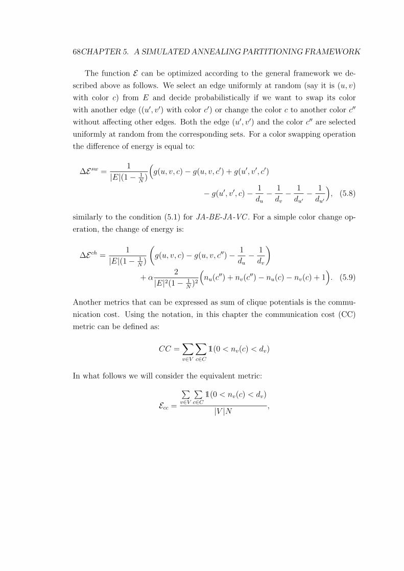
68CHAPTER 5. A SIMULATED ANNEALING PARTITIONING FRAMEWORK
The function E can be optimized according to the general framework we de-
scribed above as follows. We select an edge uniformly at random (say it is (u, v)
with color c) from E and decide probabilistically if we want to swap its color
with another edge ((u′, v′) with color c′) or change the color c to another color c′′
without affecting other edges. Both the edge (u′, v′) and the color c′′ are selected
uniformly at random from the corresponding sets. For a color swapping operation
the difference of energy is equal to:
∆Esw =1
|E|(1− 1N
)
(g(u, v, c)− g(u, v, c′) + g(u′, v′, c′)
− g(u′, v′, c)− 1
du− 1
dv− 1
du′− 1
du′
), (5.8)
similarly to the condition (5.1) for JA-BE-JA-VC . For a simple color change op-
eration, the change of energy is:
∆Ech =1
|E|(1− 1N
)
(g(u, v, c)− g(u, v, c′′)− 1
du− 1
dv
)+ α
2
|E|2(1− 1N
)2
(nu(c′′) + nv(c
′′)− nu(c)− nv(c) + 1). (5.9)
Another metrics that can be expressed as sum of clique potentials is the commu-
nication cost. Using the notation, in this chapter the communication cost (CC)
metric can be defined as:
CC =∑v∈V
∑c∈C
1(0 < nv(c) < dv)
In what follows we will consider the equivalent metric:
Ecc =
∑v∈V
∑c∈C
1(0 < nv(c) < dv)
|V |N,

5.4. A GENERAL SA FRAMEWORK FOR EDGE PARTITIONING 69
that has the advantage of being between 0 and 1. Let us consider the color change
from c to c′ for edge (u, v). The number of colors change as follows:
nu(c) = nu(c)− 1 nv(c) = nv(c)− 1
nu(c′) = nu(c′) + 1 nv(c′) = nv(c
′) + 1
The change of the energy of the graph is then equal to:
∆Echcc (u, v) = εchcc − εchcc ,
where εchcc and εchcc denote the contribution from the vertices u and v to the to-
tal energy of the graph, before and after we have changed the color of the edge
respectively. εchcc and εchcc are defined as follows:
εchcc =1
|V |N(1(0 < nu(c) < du) + 1(0 < nv(c) < dv)
+ 1(0 < nu(c′) < du) + 1(0 < nv(c′) < dv))
=1
|V |N(1(0 < nu(c)− 1 < du) + 1(0 < nv(c)− 1 < dv)
+ 1(0 < nu(c′) + 1 < du) + 1(0 < nv(c′) + 1 < dv))
εchcc =1
|V |N(1(0 < nu(c) < du) + 1(0 < nv(c) < dv)
+ 1(0 < nu(c′) < du) + 1(0 < nv(c′) < dv))
Then ∆Echcc takes values −2|V |N ,
−1|V |N , 0,
1|V |N ,
2|V |N . In case of color swapping opera-
tion, we swaps the colors c and c′ of edges (u, v) and (u′, v′) respectively. Then
the energy change is equal to:
∆Eswcc (u, v, u′, v′) = εswcc − εswcc
where εswcc and εswcc denote contribution from the vertices u, v, u′, and v′ to the
total energy of the graph, before and after we have swapped the color of the edge
70CHAPTER 5. A SIMULATED ANNEALING PARTITIONING FRAMEWORK
respectively.
εswcc =1
|V |N(1(0 < nu(c) < du) + 1(0 < nv(c) < dv) + 1(0 < nu(c′) < du)
+ 1(0 < nv(c′) < dv) + 1(0 < nu′(c) < du′) + 1(0 < nv′(c) < dv′)
+ 1(0 < nu′(c′) < du′) + 1(0 < nv′(c
′) < dv′))
=1
|V |N(1(0 < nu(c)− 1 < du) + 1(0 < nv(c)− 1 < dv) + 1(0 < nu(c′) + 1 < du)
+ 1(0 < nv(c′) + 1 < dv) + 1(0 < nu′(c) + 1 < du′) + 1(0 < nv′(c) + 1 < dv′)
+ 1(0 < nu′(c′)− 1 < du′) + 1(0 < nv′(c
′)− 1 < dv′))
εswcc =1
|V |N(1(0 < nu(c) < du) + 1(0 < nv(c) < dv) + 1(0 < nu(c′) < du)
+ 1(0 < nv(c′) < dv) + 1(0 < nu′(c) < du′) + 1(0 < nv′(c) < dv′)
+ 1(0 < nu′(c′) < du′) + 1(0 < nv′(c
′) < dv′))
To calculate energy change (due to the change of color of the edge or to the
swap of colors of edges) of functions E and Ecc , only information about the nodes
involved and their neighborhood is required as it was the case for JA-BE-JA-VC .
At the same time, the same difficulty noted in Section 5.2 holds. In an edge-centric
distributed framework, in general the edges for a node are processed by different
instances. First, we have implemented a naive version of our SA algorithm of
JA-BE-JA-VC which requires each instance to propagate color updates (e.g., the
new values of nu(c), nv(c), etc.) to other instances at each iteration, however it
leads to an unacceptable partitioning time. We have thus developed two versions
of SA framework which overcome this issue.
5.5 The SA framework
In order to reduce partitioning time, we implemented the following distributed ver-
sion of the algorithm. First, edges are randomly distributed among the instances,
and each of them executes the general SA algorithm described above on the local

5.5. THE SA FRAMEWORK 71
set of edges for L swaps. No communication can take place among instances dur-
ing this phase. After this phase is finished, communication is allowed, the correct
values are computed and all the edges are again distributed at random among the
instances. This reshuffle guarantees that any pair of edges has a probability to be
considered for color swapping.
The larger L, the larger risk that workers operate with stale information. We
want then to fix L, so that it is very unlikely that two workers change the color
of two different edges of the same vertex. To calculate the upper-bound for L
we considered the following situation. When we change the color of an edge in
component j (Pj), in average there are 2d (where d is the average degree in the
graph) edges attached to this edge. Hence, the probability that all these 2d edges
will not be situated in Pi is the following:(1− 1
N
)2d
Then, the probability that at least one edge from these 2d edges will be in Pi is:
1−(
1− 1
N
)2d
The maximum number of vertices in Pi affected by performing swaps in all other
N − 1 components is the following:
4d(N − 1)
(1−
(1− 1
N
)2d)
(5.10)
In case we perform L swaps during a local step, then in Pi we have two sets of
vertices: Sdirect, Sindirect. Sdirect consists of vertices that are directly affected by
the L swaps performed in current component, |Sdirect| <= 4L. Sindirect is the set
of vertices that are affected by the swaps in other components; its size is at most
the value in (5.10).
Hence, we need to be sure that these two sets (Sdirect, Sindirect) are significantly

72CHAPTER 5. A SIMULATED ANNEALING PARTITIONING FRAMEWORK
Table 5.1 – Spark configuration
Property name Property valuespark.executor.memory 20GB
spark.driver.memory 40GBspark.cores.max 10spark.local.dir “tmp”
spark.cleaner.ttl 20
smaller than |V |N
:
max
(4L, 4Ld(N − 1)
(1−
(1− 1
N
)2d))
< 4L(
1 + 4dNe−2d)<<|V |N
(5.11)
L <<|V |
4N(1 + 4dNe−2d
) (5.12)
Given the same number of potential changes considered, this implementation
requires L times less synchronization phases among the instances. Due to the large
time required for the synchronization phase in comparison to the time required for
the local step, one can expect the total partitioning time to be reduced by roughly
the same factor. Our experiments show that this is the case. In the setting
described in the following section, with L = 200, there is no difference between
the final components produced by the two implementations, but the partitioning
time for the naive one is 100 times larger.
The detailed steps are described in Algorithm 2.
5.6 Evaluation of the SA framework
All our experiments were performed on a cluster of 2 nodes (1 master and 1 slave)
with dual-Xeon E5-2680 v2 @2.80GHz with 192GB RAM and 10 cores (20 threads).
We used Spark version 1.4.0 and Spark standalone cluster as a resource manager.
We configured Spark properties as in the Table 5.1.
We used two undirected graphs: the email-Enron graph (36,692 vertices/
367,662 edges) and the com-Amazon graph (334,863 vertices/ 925,863 edges) pro-
vided by SNAP project [59].

5.6. EVALUATION OF THE SA FRAMEWORK 73
1: procedure SimulatedAnnealing2: G← randomlyAssignColors(G)3: round← 04: while T > 0 do5: G← partitionRandomly(G)6: G← propagateV alues(G)7: for component← components do . Executes locally on each
component8: for i < L do9: if tossCoin(2/3) == ”head” then . swapping with probability
2/3...10: e← randomEdge(component)11: e′ ← randomEdge(component)12: ∆E ← computeDelta(e, e′)13: if ∆E < 0 then14: swapColors(e, e′)15: else16: swapColorsWithProb(e, e′, e−
∆ET )
17: end if18: else . changing...19: e← randomEdge(component)20: c′ ← anotherColor(c)21: ∆E ← computeDelta(e, c′)22: if ∆E < 0 then23: changeColor(e, c′)24: else25: changeColorWithProb(e, c′, e−
∆ET )
26: end if27: end if28: i+ +29: end for30: end for31: round+ +32: T ← Tinit − round ∗∆T33: end while34: G = partitionBasedOnColor(G)35: end procedure
Algorithm 2 Implementation of SA for GraphX
74CHAPTER 5. A SIMULATED ANNEALING PARTITIONING FRAMEWORK
We implemented JA-BE-JA-VC and SA (Algorithm 2) for GraphX. In both
cases we considered the distributed operation described at the end of the previous
section: L(= 200) steps are performed locally at each instance before performing
a synchronization phase. For a fair comparison between the two algorithms, L
corresponds in both cases to the number of alternative configurations considered
(i.e., those for which the energy variation is computed). The source code of both
versions of our SA framework is available online [68].
Each experiment consists of the following steps: i) launch the computational
cluster; ii) load the given graph; iii) color the graph according to a random par-
titioner (CanonicalRandomVertexCut); iv) re-color it with JA-BE-JA-VC or SA;
v) compute the partition metrics.
While SA is guaranteed to converge to an optimal solution of problem (5.5)
if T decreases as the inverse of the logarithm of the number of iterations, the
convergence would be too slow for practical purposes. For this reason and to
permit a simpler comparison of SA and JA-BE-JA-VC , in both cases the initial
temperature decreases linearly from T0 till 0 in 100 or 1000 iterations.
As we said our SA partitioner can be used to optimize different functions. We
start by comparing JA-BE-JA-VC and SA when they have the same target Ecomm
in (5.3). When the objective function is the same, the two main differences between
the algorithms are i) the way to choose the edges to swap, and ii) the rule to accept
a change. In particular, JA-BE-JA-VC chooses edges whose color is the rarest in
a neighborhood, while SA selects them uniformly at random. JA-BE-JA-VC then
decides to swap or not the colors according to the deterministic rule (5.2), while
SA adopts the probabilistic rule (see Section 5.4)
The corresponding results are in Tables 5.2, 5.3, row I and II, for different
values of the initial temperature for email-Enron. Both the algorithms reduce the
value of Ecomm, but the decrease is larger for JA-BE-JA-VC . This is essentially due
to the fact that JA-BE-JA-VC performs more swaps, although the number of pairs
of links to swap considered is the same (equal to L times the number of iterations).
For example for the initial temperature 5∗10−11 SA swaps the color of 8808 edges,
while JA-BE-JA-VC swaps the color of 37057 edges. In fact, SA random edge
selection leads to consider a large number of pairs that is not useful to swap, while
JA-BE-JA-VC only considers candidates that are more likely to be advantageous

5.6. EVALUATION OF THE SA FRAMEWORK 75
Table 5.2 – Final partitioning metrics obtained by JA-BE-JA-VC partitioner.Temperature decreases linearly from T0 till 0.0 by given number of iterations.
# iterations T0 Final Ecomm Vertex-cut Comm. cost Balance STD
1005.00E-11 0.888788 25091 122477 1.0091 0.00551.00E-10 0.888638 25096 122572 1.0091 0.00555.00E-10 0.888634 25085 122350 1.0091 0.0055
10005.00E-11 0.8197 25685 118453 1.0091 0.00551.00E-10 0.8202 25656 118588 1.0091 0.00555.00E-10 0.8193 25603 118455 1.0091 0.0055
Table 5.3 – Final partitioning metrics obtained by SA using only Ecomm as energyfunction. Temperature decreases linearly from T0 till 0.0 by given number ofiterations.
# iterations T0 Final Ecomm Vertex-cut Comm. cost Balance STD
1005.00E-11 0.900026 25046 120083 1.0091 0.00551.00E-10 0.900027 25046 120087 1.0091 0.00555.00E-10 0.900006 25046 120080 1.0091 0.0055
10005.00E-11 0.8989 25048 120648 1.0091 0.00551.00E-10 0.8990 25049 120634 1.0091 0.00555.00E-10 0.8989 25046 120664 1.0091 0.0055
to swap. In this sense JA-BE-JA-VC is greedier than SA: JA-BE-JA-VC exploits
more, while SA explores more. Adopting the same choice for SA would lead to
lose the condition qc,c′ = qc′,c, that is required to guarantee convergence to the
global minimum of the function. We plan to investigate in the future how to bias
the selection process so that edges whose color is less represented are more likely
to be selected, but still the condition qc,c′ = qc′,c is satisfied.
Although SA seems to be less effective to reduce the energy, the results in
Tables 5.2, 5.3 also show that the function Ecomm is not necessarily a good proxy
for the usual partition metrics like VC or CC. In fact, we see that for 100 iterations
SA slightly outperforms JA-BE-JA-VC both in terms of VC and CC for the initial
temperature values, even if its final energy is always larger. For 1000 iterations
JA-BE-JA-VC performs better in terms of VC and worse in terms of CC. What
is even more striking is that the increase in the number of iterations leads to a
decrease of the energy value (as expected), but not necessarily to a decrease of

76CHAPTER 5. A SIMULATED ANNEALING PARTITIONING FRAMEWORK
Table 5.4 – Final partitioning metrics obtained by SA using Ecomm + 0.5Ebal asenergy function). Temperature decreases linearly from T0 till 0.0 by given numberof iterations.
# iterations T0 Final Ecomm Vertex-cut Comm. cost Balance STD
1005.00E-11 0.894742 25044 120768 1.0088 0.00581.00E-10 0.894692 25043 120751 1.0079 0.00585.00E-10 0.894617 25043 120782 1.0084 0.0061
10005.00E-11 0.8466 24795 113008 1.0144 0.01141.00E-10 0.8467 24794 112951 1.0178 0.00995.00E-10 0.8466 24771 112946 1.0332 0.0211
0.81
0.82
0.83
0.84
0.85
0.86
0.87
0.88
0.89
0.9
0.91
0 200 400 600 800 1000
Energ
y
Iterations
JABEJAVC 10e-11JABEJAVC 10e-10
JABEJAVC 10e-9JABEJAVC 10e-8
SA 10e-11SA 10e-10
SA 10e-9SA 10e-8
Figure 5.1 – Ecomm value for JA-BE-JA-VC and E value for SA using email-Enrongraph (1000 iterations were performed)
VC and CC. These results suggest that more meaningful energy functions should
probably be considered and our framework has the advantage to work for a large
family of different objectives.
We now move to compare JA-BE-JA-VC with SA when the function E =
Ecomm + αEbal is considered. Figure 5.1 shows the evolution of the energy after
each local phase and then every L = 200 local iterations. Note that after a
given iteration the energy can increase both for JA-BE-JA-VC and SA, but the
figure shows that every L iterations, the energy always decrease. While the two

5.6. EVALUATION OF THE SA FRAMEWORK 77
20000
21000
22000
23000
24000
25000
26000
27000
1.00E-11 1.00E-10 1.00E-09 1.00E-08
Vert
ex-c
ut
metr
ic
Initial temperature
JA-BE-JA-VCSA
Figure 5.2 – Vertex-cut metric for JA-BE-JA-VC and SA using email-Enron graph(1000 iterations were performed)
energies have different expressions, the initial energy values are indistinguishable,
because the starting point is an almost balanced partition and then Ebal << Ecomm
and E ≈ Ebal. As in the previous case, JA-BE-JA-VC appears to be greedier
in reducing the energy function. Tables 5.2, 5.4 show that this does not lead
necessarily to a better partitioning. Indeed, after 100 iterations, SA minimizing
E provides the best partition in terms of VC, CC and BAL, while STD is slightly
worse. After 1000 iterations, SA has further improved VC and CC at the expenses
of the balance metrics like BAL and STD.
Figures 5.2 and 5.3 show similar results comparing the final metrics VC and
CC for an even larger range of initial temperatures.
While for email-Enron we have shown how SA can improve communication
metrics at the expenses of balance metrics, we show that the opposite result can
be obtained on a different graph (com-Amazon) in Figures 5.4 and 5.5. Remember
that in any case, for a given graph, it is possible to tune the relative importance
of the different metrics by varying the parameter α.
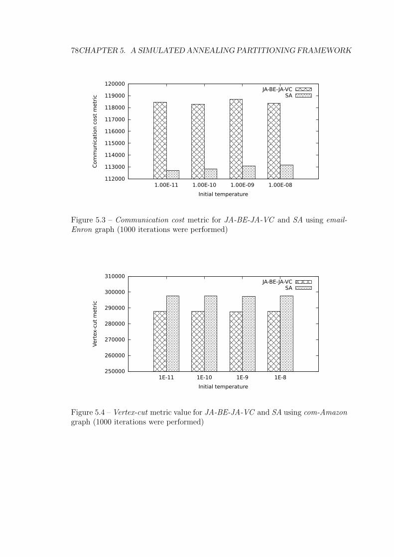
78CHAPTER 5. A SIMULATED ANNEALING PARTITIONING FRAMEWORK
112000
113000
114000
115000
116000
117000
118000
119000
120000
1.00E-11 1.00E-10 1.00E-09 1.00E-08
Com
munic
ati
on c
ost
metr
ic
Initial temperature
JA-BE-JA-VCSA
Figure 5.3 – Communication cost metric for JA-BE-JA-VC and SA using email-Enron graph (1000 iterations were performed)
250000
260000
270000
280000
290000
300000
310000
1E-11 1E-10 1E-9 1E-8
Vert
ex-c
ut
metr
ic
Initial temperature
JA-BE-JA-VCSA
Figure 5.4 – Vertex-cut metric value for JA-BE-JA-VC and SA using com-Amazongraph (1000 iterations were performed)

5.7. THE MULTI-OPINION SA FRAMEWORK 79
1
1.001
1.002
1.003
1.004
1.005
1.006
1.007
1E-11 1E-10 1E-9 1E-8
Bala
nce
metr
ic
Initial temperature
JA-BE-JA-VCSA
Figure 5.5 – Balance metric value for JA-BE-JA-VC and SA using com-Amazongraph (1000 iterations were performed)
5.7 The multi-opinion SA framework
In this section, we provide an enhanced version of our framework — the multi-
opinion SA framework, which relies on some ideas from the asynchronous Gibbs
sampler proposed in [65].
A Gibbs sampler is another possible set of rules to determine the next state,
i.e., the next color assignment in our case. Under Gibbs sampler, a subvector cs
of c4 is selected with probability qcs . Let c−s denote the other elements of c, so
that c = (cs, c−s). A new random subvector c′s is randomly generated so that the
probability to move to c′ = (c′s, c−s) is:
e−E(c′s,c−s)
T∑ds∈C|cs| e
−E(ds,c−s)
T
. (5.13)
Gibbs samplers can be considered as a special case of Metropolis-Hasting sam-
plers where the new candidate states are selected with probabilities qc,c′ as in (5.13)
and the acceptance probabilities βc,c′ are all equal to one. Practically speaking
4c is the solution for (5.5)

80CHAPTER 5. A SIMULATED ANNEALING PARTITIONING FRAMEWORK
one talks about a Metropolis-Hasting sampler, if the probabilities qc,c′ are fixed
(independently from the energy function) and the acceptance probabilities βc,c′
can be smaller than 1. The Gibbs sampler has the advantage that no change is
refused (but it may be c′s = c) but it requires to be able to sample according to
(5.13), that corresponds, in general, to knowing the full conditional distribution.
This may limit the size of the state vector that can be modified at a given time.
Often, a single vector element (the color of a single edge in our case) is modified
by a Gibbs sampler.
Also for the Gibbs sampler, if the temperature decreases logarithmically to
0, the state will converge almost surely to a global minimizer of the function E .
Sometimes the expression annealed Gibbs sampler is used for this specific SA
algorithm.
In a distributed setting, one would split the vector c among the N workers:
c = (c1, c2, . . . cN). While every instance, say it i, could independently modify its
subvector ci (i.e., the colors of its component), it would need to know the current
value of all the other variables c−i. The same difficulties we exposed above hold
then. Recently, the authors of [65] have shown that it is possible to circumvent this
problem. Their asynchronous Gibbs sampler allow workers to proceed in parallel
without synchronization or locking. We briefly describe the algorithm using our
notation.
The algorithm requires each instance to maintain an opinion about the color
assignment for all the edges. We use the superscript i to denote the opinion
of instance i, that we can write as (ci1, c
i2, . . . c
iN). Each iteration of the proposed
algorithm consists of two steps: local and global. During a local step each instance
of the algorithm improves its own component of the graph. Instance i selects a
subset cii,s of its subvector ci
i and generate cii,s with probability
e−E(cii,s,c
i−i)
T∑di,s∈C
|cii,s| e−E(di,s,c
i−s)
T
, (5.14)
that depends only on the current opinion of instance i. Then, during the global
step, each instance, decides whether to update its opinion according to what other

5.7. THE MULTI-OPINION SA FRAMEWORK 81
instances think about their components or not. In particular an instance j updates
its opinion about component i, according to what i thinks about it with probability
αi,j:
αi,j = min
(1, exp
(− 1
T(E(ci
i, cj−i)− E(cj
i , cj−i) + E(cj
i , ci−i)− E(ci
i, ci−i))
))(5.15)
In [65] it is proven that the probability distribution of each opinion ci converges
to the same distribution the centralized Gibbs sampler would converge. It follows
then that if we gradually decrease the temperature according to the usual law, each
opinion will converge almost surely to a global minimizer of the energy function.
The next section describes how we have modified our original simulated algo-
rithm according to the results in [65] and how we have implemented it in GraphX.
5.7.1 Distributed implementation
Our new algorithm borrows from [65] the idea to maintain potentially different
opinions at each instance, and to use the probabilities in (5.15) to accept the
opinions of other instances. At the same time, instance i updates its subvector
cii according to Metropolis-Hasting sampling described in Section 5.4, because it
is computationally simpler than Gibbs sampling. Moreover, the stationary dis-
tribution corresponding to the local Metropolis-Hasting sampling steps is (5.14).
Hence a “large” number of Metropolist-Hasting steps correspond to draw a single
Gibbs sample. We suspect that the results in [65] hold also when a finite number
of Metropolis-Hasting sampling steps are performed, but we do not have yet a
formal proof. At the same time, implementing a simulated annealing algorithm
based on the asynchronous Gibbs sampler in [65] requires minor changes to the
Spark implementation of our algorithm described in what follows, as far as Gibbs
samples can be drawn efficiently.
We assume that the energy can be decomposed as sum of vertex energies that
depend only on the number of edges of each color the vertex has:
E(c) =∑v∈V
εv(c) =∑v∈V
εv({nv(c), c ∈ C}).

82CHAPTER 5. A SIMULATED ANNEALING PARTITIONING FRAMEWORK
This is for example the case of both Ecomm and Ecc. This assumption allows us to
simplify the computational requirement of the algorithm, but it is not necessary.
It will be convenient to define the energy associated to a subset A of the vertices:
EA(c) ,∑v∈A
εv(c).
Remember that we have N instances of the partitioner algorithm, where each
instance has its own subset of edges Ei, whose set of vertices is V (Ei). Let E−i
denote all the edges except those in Ei Each edge has two values attached to it:
the index of the instance to whom this edges belongs, and an array of colors of
length N : c0k, c
1k, ..., c
Nk which represents the colors of edge k according to the N
different instances. The different opinions the instances have about what the color
of edges k should be. When an instance i changes the color of edge k, it changes
cik. A value attached to a vertex is an array which contains N different maps. Each
of these maps contains an information about the colors of the edges attached to
this vertex according to some instance opinion, e.g., a map says there are n0 edges
of color c0, n1 edges of color c1, etc.
Each iteration of this distributed algorithm consists of two steps: a local step
and global step. Each instance updates its opinion during the local step performing
L attempts to swap/change colors as in the first version. No communication
between instances is required. Then during a global step, it performs a shuffle,
which propagates vertex values to all the instances, and after it computes the
N(N−1) values of αi,j, which are used to accept the opinions of the other instances.
A naive computation of the probabilities αi,j requires computing four times the
energy of the whole graph in our case. Computing the energy of the whole graph
in GraphX, requires using all N instances, because each instance has only a subset
of the graph. Thus, each instance i needs to compute the N − 1 acceptance
probabilities αk,i for k different from i. To compute all α for each instance, we will
need to compute sequentially 4N(N − 1) times energy of different graphs.
In order to speed up the computation of the probabilities αi,j, we propose the
following procedure that makes possible to calculate the four energies appearing
in (5.15) as sum of two differences, where each difference can be computed locally
by instance i, thanks to our assumption on the energy function.

5.7. THE MULTI-OPINION SA FRAMEWORK 83
First we consider the difference between the third and forth energy terms
in (5.15):
E(cji , c
i−i)− E(ci
i, ci−i).
Both these energies are computed as function of the vertices of the whole graph,
but these graphs are different. The two energies are different because i and j have
in general different opinions about what colors assign to the edges Ei: cii 6= cj
i . It
is important to notice that cji did not change during the local step: instance j may
only have changed cjj. Instance i has then all the information required to compute
this difference. Moreover, because of our assumption on the energy function, the
difference of the two energies can be reduced to computing the difference between
energies attached to V (Ei) according to j and i opinions:
E(cji , c
i−i)− E(ci
i, ci−i) = EV (Ei)(c
ji , c
i−i)− EV (Ei)(c
ii, c
i−i). (5.16)
As we said above, this difference can be computed immediately after the local step,
without any need for the nodes to communicate.
Now, we consider the difference between the first two energies appearing in the
formula (5.15):
E(cii, c
j−i)− E(cj
i , cj−i)
However, cjj ⊂ cj
−i and the updated values of cjj are located on instance j. That it
why, it is necessary to perform a shuffle first to propate the new set of opinions.
We observe that, because of our assumption on the energy function:
E(cii, c
j−i)− E(cj
i , cj−i) = EV (Ei)(c
ii, c
j−i)− EV (Ei)(c
ji , c
j−i). (5.17)
Moreover, we need to know only the colors of E(V (Ei)) (all neighbors edges of
V (Ei))). We calculate EV (Ei)(cii, c
j−i) in the following manner. First, instance i
collects all the triplets (edges with their vertices) that correspond to Ei. Next,
it takes all vertices attached to these triplets and reduce it to a set of vertices
(because some vertices may be repeated). After, instance i takes vertex values
(mapping from color to the number of times edges of this color are connected to
this vertex) according to j opinion. Then, it traverses all triplets and compare

84CHAPTER 5. A SIMULATED ANNEALING PARTITIONING FRAMEWORK
color of the edges according to i and j. In case the colors of edge e = (u, v) are
different for i and j we modify vertex values of u and v (by removing from both
vertex data one appearance of color cje and adding one appearance of color cie).
Formulas (5.17) and (5.16) simplify the computation of αi,j: instead of com-
puting four times an energy of the four different graphs (which cannot be done in
local way), it is necessary to compute locally difference in energy related to the
local vertices between what the owner instance thinks and remote instance thinks.
Finally, computing αi,j is reduced to (5.18):
αi,j = min
(1, exp
(− 1
T(EV (Ei)(c
ii, c
j−i)− EV (Ei)(c
ji , c
j−i)
+EV (Ei)(cji , c
i−i)− EV (Ei)(c
ii, c
i−i))
)) (5.18)
The probability αi,j (the probability to assign cji := ci
i) can be computed then by
instance i in two phases requiring only one shuffle. Once αi,j has been computed for
all j different from i, instance i can generate the corresponding Bernoulli random
variable and decide if cji should be updated to ci
i. Note that the values cji are
associated the links Ei and are then stored at instance i. Hence, no communication
is required for this update. Finally, instance i computes for each vertex in V (Ei)
how many edges in Ei of a given color it has according to the different N opinion.
A second shuffle is needed to aggregate this information and update the array of
maps associated to each vertex.
Algorithm 3 shows the pseudo-code of the distributed implementation of our
algorithm.
5.8 Evaluation of the multi-opinion SA frame-
work
As a cluster we used 2 machines of Nef Sophia cluster (1 master and 1 slave) with
dual-Xeon E5-2680 v2 @2.80GHz with 192GB RAM and 10 core (20 threads). We
used Spark version 1.4.0 and Spark standalone cluster as a resource manager. We
have configured Spark properties as in the Table 5.5. We used the undirected graph

5.8. EVALUATION OF THE MULTI-OPINION SA FRAMEWORK 85
1: procedure SimulatedAnnealing2: G← randomlyAssignColors(G)3: G← partitionRandomly(G)4: round← 05: while T > 0 do6: G← propagateV alues(G)7: for component← components do . Executes locally on each
component8: for i < L do9: if tossCoin(probabillityToSwap) == ”head” then . swap
10: e← randomEdge(component)11: e′ ← randomEdge(component)12: ∆E ← computeDelta(e, e′)13: if ∆E < 0 then14: swapColors(e, e′)15: else16: swapColorsWithProb(e, e′, e−
∆ET )
17: end if18: else . change19: e← randomEdge(component)20: c′ ← anotherColor(c)21: ∆E ← computeDelta(e, c′)22: if ∆E < 0 then23: changeColor(e, c′)24: else25: changeColorWithProb(e, c′, e−
∆ET )
26: end if27: end if28: i+ +29: end for30: D2 = computeDifferenceD2(component) . See 5.1631: end for32: G← propagateV alues(G)33: for component← components do . Executes locally on each
component34: D1 = computeDifferenceD1(component) . See 5.1735: αi,j = computeAlpha(D1, D2)36: propagateWithPtob(i, j, αi,j)37: end for38: round+ +39: T ← Tinit − round ∗∆T40: end while41: G = partitionBasedOnColor(G)42: end procedure
Algorithm 3 Asynchronous SA for GraphX
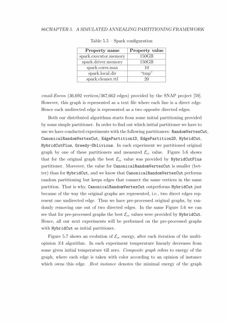
86CHAPTER 5. A SIMULATED ANNEALING PARTITIONING FRAMEWORK
Table 5.5 – Spark configuration
Property name Property valuespark.executor.memory 150GB
spark.driver.memory 150GBspark.cores.max 10spark.local.dir “tmp”
spark.cleaner.ttl 20
email-Enron (36,692 vertices/367,662 edges) provided by the SNAP project [59].
However, this graph is represented as a text file where each line is a direct edge.
Hence each undirected edge is represented as a two opposite directed edges.
Both our distributed algorithms starts from some initial partitioning provided
by some simple partitioner. In order to find out which initial partitioner we have to
use we have conducted experiments with the following partitioners: RandomVertexCut,
CanonicalRandomVertexCut, EdgePartition1D, EdgePartition2D, HybridCut,
HybridCutPlus, Greedy-Oblivious. In each experiment we partitioned original
graph by one of these partitioners and measured Ecc value. Figure 5.6 shows
that for the original graph the best Ecc value was provided by HybridCutPlus
partitioner. Moreover, the value for CanonicalRandomVertexCut is smaller (bet-
ter) than for HybridCut, and we know that CanonicalRandomVertexCut performs
random partitioning but keeps edges that connect the same vertices in the same
partition. That is why, CanonicalRandomVertexCut outperforms HybridCut just
because of the way the original graphs are represented, i.e., two direct edges rep-
resent one undirected edge. Thus we have pre-processed original graphs, by ran-
domly removing one out of two directed edges. In the same Figure 5.6 we can
see that for pre-processed graphs the best Ecc values were provided by HybridCut.
Hence, all our next experiments will be performed on the pre-processed graphs
with HybridCut as initial partitioner.
Figure 5.7 shows an evolution of Ecc energy, after each iteration of the multi-
opinion SA algorithm. In each experiment temperature linearly decreases from
some given initial temperature till zero. Composite graph refers to energy of the
graph, where each edge is taken with color according to an opinion of instance
which owns this edge. Best instance denotes the minimal energy of the graph
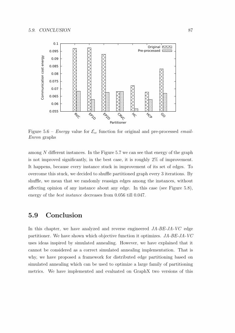
5.9. CONCLUSION 87
0.055
0.06
0.065
0.07
0.075
0.08
0.085
0.09
0.095
0.1
RVCEP1D
EP2DCRVC
HC HCPGO
Com
munic
ati
on c
ost
energ
y
Partitioner
OriginalPre-processed
Figure 5.6 – Energy value for Ecc function for original and pre-processed email-Enron graphs
among N different instances. In the Figure 5.7 we can see that energy of the graph
is not improved significantly, in the best case, it is roughly 2% of improvement.
It happens, because every instance stuck in improvement of its set of edges. To
overcome this stuck, we decided to shuffle partitioned graph every 3 iterations. By
shuffle, we mean that we randomly reassign edges among the instances, without
affecting opinion of any instance about any edge. In this case (see Figure 5.8),
energy of the best instance decreases from 0.056 till 0.047.
5.9 Conclusion
In this chapter, we have analyzed and reverse engineered JA-BE-JA-VC edge
partitioner. We have shown which objective function it optimizes. JA-BE-JA-VC
uses ideas inspired by simulated annealing. However, we have explained that it
cannot be considered as a correct simulated annealing implementation. That is
why, we have proposed a framework for distributed edge partitioning based on
simulated annealing which can be used to optimize a large family of partitioning
metrics. We have implemented and evaluated on GraphX two versions of this
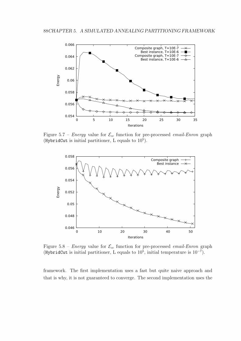
88CHAPTER 5. A SIMULATED ANNEALING PARTITIONING FRAMEWORK
0.054
0.056
0.058
0.06
0.062
0.064
0.066
0 5 10 15 20 25 30 35
Energ
y
Iterations
Composite graph, T=10E-7Best instance, T=10E-6
Composite graph, T=10E-7Best instance, T=10E-6
Figure 5.7 – Energy value for Ecc function for pre-processed email-Enron graph(HybridCut is initial partitioner, L equals to 105).
0.046
0.048
0.05
0.052
0.054
0.056
0.058
0 10 20 30 40 50
Energ
y
Iterations
Composite graphBest instance
Figure 5.8 – Energy value for Ecc function for pre-processed email-Enron graph(HybridCut is initial partitioner, L equals to 105, initial temperature is 10−7).
framework. The first implementation uses a fast but quite naive approach and
that is why, it is not guaranteed to converge. The second implementation uses the

5.9. CONCLUSION 89
same multi-opinion approach for which [65] proves that a Gibbs-sampler would
converge. We believe convergence holds also in our case, even if we have not
proved yet. Our experimental results show that our framework is quite flexible,
but at the same time it is difficult to provide rules for parameter tuning and
greedier algorithms (as JA-BE-JA-VC ) can provide a better partitioning when
the number of iterations is limited.

90CHAPTER 5. A SIMULATED ANNEALING PARTITIONING FRAMEWORK

Chapter 6
Conclusion
In this thesis we addressed the problem of how to partition a graph in order to
speed up distributed algorithms to be run on the partitioned graph. This is a
difficult problem. First, from a computational point of view, the problem to find
the optimal partition is NP-hard for most of the natural objective functions one
can think about. Moreover, it is not even clean which objective function should
be considered to reduce the final computational time. We have dug in graph
partitioning by overviewing the common approaches, solutions, and frameworks
that have been proposed in literature, with a special attention to those for which
running code is available. All partitioners can be classified into two approaches:
edge and vertex partitioners. Based on the current study, we decided to work with
the edge partitioning approach as more suitable for real-world graphs. Among
the different graph processing frameworks available, we selected GraphX for our
experiments.
In order to better understand what is the current progress in the area of dis-
tributed edge-partitioning and what are the commonly accepted solutions, we made
a survey of all the existing algorithms. Moreover, we provided a new taxonomy for
partitioners. It was important for us to see how partitioners are compared. How-
ever, during this process we have noticed that i) there is no commonly accepted
solution for graph partitioning, ii) different partitioners are rarely compared to
each other, iii) it is not even clear how to compare them the best. To fulfill
this lack of comparison we conducted series of experiments on GraphX with all
91

92 CHAPTER 6. CONCLUSION
existing partitioners available for GraphX plus some other ones which we have im-
plemented. In these experiments we compared partitioners using existing metrics.
Our results suggest that the Hybrid-Cut partitioner provides a partition on which
graph algorithms perform the fastest.
This analysis was carried out by directly comparing the final execution time of
different typical graph algorithms like Connected Components or PageRank. This
approach provides the definitive comparison among different partitioners, but we
would like to be able to compare two partitions and choose the best one for the
purposes of our computation without running actual the computation itself. For
this reason, we are interested in partition metrics, i.e., metrics that can be easily
evaluated considering the partitioned graph. That is why we decided to conduct
a deeper study of existing partition metrics which would allow us to argue about
their importance. For this reason, we have conducted another series of experiments
and used a sound statistical methodology. One of the difficulties was to handle
huge variability of execution time which came from multiple sources,1 and still get
statisically significant conclusions. Finally, we have shown that there is a linear
dependency between partition metrics and the execution time of graph processing
algorithms. Our results show that communication metrics are more important than
balance metrics. This important finding as well as JA-BE-JA-VC [52] partitioner
inspired us for the next step.
We have decided to develop a new approach for distributed edge partitioning,
based on simulated annealing that can be used to optimize a large family of parti-
tion metrics, including the communication ones. The challenge was to implement
distributed simulated annealing in GraphX. The naive implementation of the al-
gorithm would perform only one swap during an iteration and would then require
an unacceptable computation time, because of the frequent data shuffles. After,
we enhanced it by showing that each instance can perform up to L swaps during
iteration without significantly affecting other instances. The recent results [65]
allowed us to implement a second version of the partitioner based on Gibbs sam-
pler. Nevertheless, also in this case the most natural implementation would lead to
enormous amount of communication between iteration of the algorithm. We found
out how to reduce this amount of communication from 4N(N − 1) to 2 shuffles.
1Variability comes from operation system, newtwork, and distributed file system layers.

6.1. PERSPECTIVES 93
We conducted experiments to show the efficiency as well as the flexibility of our
approach compared to state-of-the-art JA-BE-JA-VC .
6.1 Perspectives
In our experiments we have used relatively small graphs, for the reason that it is
not be possible to conduct thousands of experiments with larger graphs due to the
unacceptable execution time, but also because GraphX has implicit limitation to
the graph size it can process. It is easy to observe failure while loading graph in
GraphX with no apparent explanation. Thus, one of the perspectives is to perform
on the short term some limited experiments on larger graphs.
Naturally the more time is allocated to partitioning the better the partitions
are. However, sophisticated partitioners may require 100 times longer partitioning
time while providing 1 − 2% of improvement in terms of metrics. Thus, another
perspective is to provide partitioning service, where user of this service provides
a graph, graph processing algorithm (such as PageRank), number of time this
algorithm will be executed (with different initial settings), and desired number of
components N . Partitioning service selects and runs appropriate partitioner (if
any partitioner is required) itself.
Partitioning service may be implemented using GraphX, however, it can be
implemented also on other frameworks, including implementing it without using
any framework.
The development of our simulated-annealing partitioning framework is illus-
trative of the general difficulty of adapting distributed algorithms, which require
some form of shared state, to the bulk synchronous parallel model. Indeed, the
communication cost of the synchronization phase and the need to wait for the
slowest instances can significantly slow down computation. This problem is nowa-
days particularly evident in machine learning. Indeed, a basic step in machine
learning is to compute parameter models using some stochastic gradient method
in a distributed way. The dataset is split among different executors, each using
its data subset to compute a noisy estimation of the gradient of the loss func-
tion. The gradient estimates are then averaged during a synchronization phase
and this improved estimate is used to update the parameter models. The synchro-

94 CHAPTER 6. CONCLUSION
nization phase is time consuming because of the reasons provided above, so that
asynchronous solutions have been proposed, where nodes may work on stale data
and read-write race conditions may arise. Empirically, on single-node systems,
these asynchronous algorithms have yielded order-of-magnitude improvements in
performance (see e.g., [69]).
Our goal in the future is to investigate how these algorithms can be adapted
to Spark, for example averaging the intrinsically low time requirement of local
operations. As in our implementations of the SA partitioner framework, we can
perform many local operations on the basis of potentially “wrong” local data as
far as we keep the number of inconsistencies bounded (as in our single-opinion im-
plementation) or we can embrace inconsistencies maintaining potentially different
coupled versions of the shared state (as in our multi-opinion implementation).
ACKNOWLEDGMENT: This work was partly funded by the French Govern-
ment (National Research Agency, ANR) through the ”Investments for the Future”
Program reference #ANR-11-LABX-0031-01.

Appendix A
Extended Abstract in French
Partitionnement reparti base surles sommets
A.1 Introduction
La taille des graphes du monde reel obligent de les traiter d’une maniere distribuee.
C’est pourquoi, le partitionnement de graphe est la premiere etape indispensable
avant le traitement des graphes. En plus, car le partitionnement de graphe est
un probleme NP-difficile, il y a clairement un manque de recherche consacre au
partitionnement de graphe, par ex. Il n’est pas clair comment evaluer la qualite
des methodes de partitionnement (partitionneurs) de graphe, comment comparer
des methodes de partitionnement differentes et comment le partitionnement af-
fecte le temps final de calcul. En outre, il existe toujours un compromis entre
les partitionneurs simples et complexes: partitionneurs complexes peuvent avoir
besoin d’un temps de partitionnement trop long pour annuler les economies de
temps d’execution.
Dans ce travail, nous avons essaye de resoudre ces problemes. En particulier,
nos objectifs etaient: trouver un moyen correct de comparer les partitionneurs
(en particulier, avant d’executer les algorithmes de traitement de graphe actuel),
identifier une fonction objective que le partitionneur devrait optimiser et concevoir
un partitionneur capable d’optimiser cette fonction.
95

96 APPENDIX A. EXTENDED ABSTRACT IN FRENCH
A.2 Resume des developpements
L’analyse des grands graphes est une operation qui demande beaucoup d’espace,
qui ne peut normalement pas etre effectue sur une seule machine. Il y a deux
raisons pour lesquelles un graphe doit etre distribue: des problemes de la memoire
et de calcul. Le probleme de la memoire se produit lorsque tout le graphe doit
etre charge dans la RAM. Par exemple, un graphe avec un milliard des aretes
necessiteraient au moins 8|E| octets d’espace pour stocker des informations sur
les bords, ou E est l’ensemble des aretes, et cela ne comprend pas le calcul frais
generaux - en pratique, le traitement du graphe necessiterait plusieurs fois plus
d’espace. Meme si une machine a suffisamment de RAM pour stocker et traiter un
graphe, elle peut prendre un inacceptablement longtemps si un graphe n’est pas
partitionne, mais est plutot traite en utilisant un seul thread d’execution.
Afin de surmonter les problemes de memoire et de calcul, nous devons parti-
tionner un graphe en plusieurs composants. Ensuite, un graphe partitionne peut
etre traite en parallele sur plusieurs coeurs independamment du fait qu’ils soient
sur la meme machine ou pas. Naturellement, la taille de chaque composant est
plus petite que le graphe original, ce qui conduit a des exigences de memoire plus
petites.
Naturellement, pour trouver une partition optimale, des problemes de par-
titionnement de graphe apparaissent. Le partitionnement divise un graphe en
plusieurs sous-graphes afin d’obtenir le meilleur temps de calcul d’un algorithme de
traitement de graphe sous deux aspects conflictuels. Le premier aspect - equilibre
- dit que la taille de chaque composant devrait etre presque la meme. Il provient
du fait que les graphes sont traites par des clusters de machines et si une machine a
aussi grande composante, cela ralentira l’execution complete. Le deuxieme aspect
- communication - indique que le partitionnement devrait reduire la quantite de
composants en commune. Comme un exemple trivial, si un graphe a composants
non connexe et chaque executeur testamentaire recoit un composant, les executeurs
peuvent, dans de nombreux cas, fonctionner de maniere presque independante.
Les algorithmes de partitionnement (partitionneurs) prennent divisent un graphe
dans les N composants. En particulier, nous sommes interesses par les divisions
qui peuvent etre execute de facon distribuee. Un partitionneur distribue est un

A.2. RESUME DES DEVELOPPEMENTS 97
algorithme qui se compose de plusieurs instances, ou chaque instance effectue le
partitionnement en utilisant le meme algorithme mais sur des composants differents
du graphe. Chaque instance represente une copie de l’algorithme avec le composant
unique du graphe et certains ressources qui lui sont affectees, comme les threads
informatiques et la RAM. Instances de la partitionneur distribue peut communi-
quer entre eux ou pas. Dans ce qui suit, nous supposons que le nombre d’instances
d’un partitionneur distribue est egal a N, le nombre de composants du graphe.
Deux approches ont ete developpees pour resoudre le probleme de partition-
nement de graphe: le partitionnement des sommets et le partitionnement des
aretes. Une facon classique de distribuer un graphe est le partitionnement des som-
mets ou les sommets sont affectes aux composants differents. Un arete est coupe,
si ses sommets appartiennent a deux composants differents. Les partitionneurs des
sommets essaient alors de minimiser le nombre d’aretes coupees. Plus recemment,
le partitionnement des aretes a ete propose et preconise [2] comme une meilleure
approche pour traiter les graphes avec la distribution d’une loi de puissance [3] (les
graphes de loi de puissance sont communs dans des donnees du monde reel plaw,
plaw2). Dans ce cas, les aretes sont mappes aux composants et les sommets sont
coupes si leurs aretes sont attribues aux composants differents. L’amelioration
peut etre explique qualitativement avec la presence, dans un graphe de loi de
puissance, de centres, c.a.d. des sommets de degre beaucoup plus grand que la
moyenne. Dans un partitionnement de sommet, l’attribution d’un concentrateur
a une partition donnee conduit facilement a i) desequilibre de calcul, si ses voisins
sont egalement affectes au meme composant, ou ii) a un grand nombre d’aretes
coupees et a des exigences de communication fortes. Un partitionneur des aretes
peut plutot obtenir un meilleur compromis, en coupant uniquement un nombre
limite de hubs. Le support analytique de ces resultats est presente dans [6]. Pour
cette raison, de nombreux nouveaux cadres de calcul graphe, comme GraphX [7]
et PowerGraph [2], reposent sur le partage des aretes.
Les partitionneurs differents fournissent des partitions differentes, mais il n’est
pas evident quelle partition est meilleure. La qualite de la partition peut etre
evaluee de deux facons. Une facon est pour evaluer l’effet de la partition sur
l’algorithme que nous voulons executer sur le graphe, par ex. en termes de temps
total d’execution ou de frais generaux de communication. Bien que cette analyse
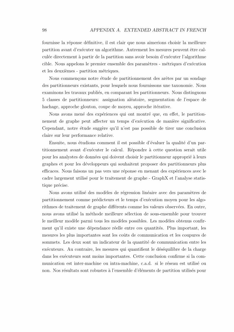
98 APPENDIX A. EXTENDED ABSTRACT IN FRENCH
fournisse la reponse definitive, il est clair que nous aimerions choisir la meilleure
partition avant d’executer un algorithme. Autrement les mesures peuvent etre cal-
culee directement a partir de la partition sans avoir besoin d’executer l’algorithme
cible. Nous appelons le premier ensemble des parametres - metriques d’execution
et les deuxiemes - partition metriques.
Nous commencons notre etude de partitionnement des aretes par un sondage
des partitionneurs existants, pour lesquels nous fournissons une taxonomie. Nous
examinons les travaux publies, en comparant les partitionneurs. Nous distinguons
5 classes de partitionneurs: assignation aleatoire, segmentation de l’espace de
hachage, approche glouton, coupe de moyeu, approche iterative.
Nous avons mene des experiences qui ont montre que, en effet, le partition-
nement de graphe peut affecter un temps d’execution de maniere significative.
Cependant, notre etude suggere qu’il n’est pas possible de tirer une conclusion
claire sur leur performance relative.
Ensuite, nous etudions comment il est possible d’evaluer la qualite d’un par-
titionnement avant d’executer le calcul. Repondre a cette question serait utile
pour les analystes de donnees qui doivent choisir le partitionneur approprie a leurs
graphes et pour les developpeurs qui souhaitent proposer des partitionneurs plus
efficaces. Nous faisons un pas vers une reponse en menant des experiences avec le
cadre largement utilise pour le traitement de graphe - GraphX et l’analyse statis-
tique precise.
Nous avons utilise des modeles de regression lineaire avec des parametres de
partitionnement comme predicteurs et le temps d’execution moyen pour les algo-
rithmes de traitement de graphe differents comme les valeurs observees. En outre,
nous avons utilise la methode meilleure selection de sous-ensemble pour trouver
le meilleur modele parmi tous les modeles possibles. Les modeles obtenus confir-
ment qu’il existe une dependance reelle entre ces quantites. Plus important, les
mesures les plus importantes sont les couts de communication et les coupures de
sommets. Les deux sont un indicateur de la quantite de communication entre les
executeurs. Au contraire, les mesures qui quantifient le desequilibre de la charge
dans les executeurs sont moins importantes. Cette conclusion confirme si la com-
munication est inter-machine ou intra-machine, c.a.d. si le reseau est utilise ou
non. Nos resultats sont robustes a l’ensemble d’elements de partition utilises pour

A.3. CONCLUSION 99
former le modele, et le modele peut classer correctement d’autres partitionneurs.
Un nouveau algorithme de partitionnement des aretes, appele JA-BE-JA-VC ,
a ete propose dans [52] et a montre qu’il depassait considerablement les algorithmes
existants. L’algorithme commence par attribuer une couleur initiale (arbitraire) a
chaque arete. Chaque couleur represente un composant ou l’arete sera place apres
la partitionnement. Le partitionneur s’ameliore iterativement sur l’affectation des
couleurs des aretes initial, en permettant a deux aretes d’echanger leur couleur
si cela semble etre benefique pour reduire le nombre de coupures des sommets
correspondants. Afin d’eviter de se coincer a des minima locaux, JA-BE-JA-VC
emprunt d’un recuit simule (SA) l’idee de permettre apparemment des compromis
swaps aux premiers stades du partitionnement.
Nous developpons cette inspiration initiale et proposons deux versions de par-
tition de graphe basees sur SA for Spark.
A cet effet, nous commencons par l’ingenierie inverse de JA-BE-JA-VC pour
montrer la metrique ciblee. Ensuite, nous proposons la premiere version de notre
cadre general de SA qui peut optimiser un large eventail de fonctions objectives
et pour lesquelles les resultats de convergence peuvent etre prouves. La mise en
oeuvre naıve de cette approche (ainsi que de JA-BE-JA-VC ) necessite un nombre
important d’operations de synchronisation couteuses pendant le partitionnement.
Ensuite, nous expliquons comment ces algorithmes peuvent etre mis en oeuvre
efficacement dans une architecture distribuee comme Spark. Cependant, dans
ce cas, les instances peuvent fonctionner sur des valeurs perimees, ce qui peut
empecher la convergence a l’optimum.
Ensuite, nous avons fourni une version amelioree de notre cadre - le cadre
multi-opinion SA, qui repose sur certaines idees de l’echantillonneur asynchrone
de Gibbs propose dans [65].
A.3 Conclusion
Dans cette these, nous avons aborde le probleme de la partition d’un graphe afin
d’accelerer les algorithmes distribues a executer sur le graphe partitionne. C’est
un probleme difficile. Tout d’abord, d’un point de vue informatique, le probleme
pour trouver la partition optimale est NP-difficile pour la plupart des fonctions ob-

100 APPENDIX A. EXTENDED ABSTRACT IN FRENCH
jectives naturelles auxquelles on peut penser. En outre, il n’est meme pas evident
quelle fonction objective doit etre consideree comme reduisant le temps de cal-
cul final. Nous avons creuse dans le partitionnement de graphe en abordant les
approches, solutions et cadres communs qui ont ete proposes dans la litterature,
en accordant une attention particuliere a ceux pour lesquels le code d’execution
est disponible. Tous les partitionneurs peuvent etre classes en deux approches:le
partitionnement des sommets et le partitionnement des aretes. Sur la base de
l’etude actuelle, nous avons decide de travailler avec l’approche de partitionnement
des aretes comme plus adapte aux graphes du monde reel. Parmi les differents
cadres de traitement graphe disponibles, nous avons selectionne GraphX pour nos
experiences.
Afin de mieux comprendre quel est le progres actuel dans le domaine du parti-
tionnement des aretes distribue et quelles sont les solutions couramment acceptees,
nous avons mener un sondage sur tous les algorithmes existants. En outre, nous
avons fourni une nouvelle taxonomie pour les partitionneurs. Il etait important
pour nous de voir comment les partitionneurs sont compares. Cependant, au
cours de ce processus, nous avons remarque que i) il n’existe pas de solution
generalement acceptee pour le partitionnement de graphe, ii) des partitionneurs
differents sont rarement compares les uns aux autres, iii) il n’est meme pas clair
comment les comparer au mieux. Pour realiser ce manque de comparaison, nous
avons mene des series d’experiences sur GraphX avec tous les partitionneurs ex-
istants et disponibles pour GraphX plus d’autres que nous avons mis en oeuvre.
Dans ces experiences, nous avons compare les partitionneurs a l’aide de metriques
existantes. Nos resultats suggerent que le partitionneur Hybrid-Cut fournit une
partition sur laquelle les algorithmes graphes executent le plus rapidement.
Cette analyse a ete effectuee en comparant directement le temps d’execution fi-
nal des algorithmes de graphe differents comme Connected Components ou PageRank.
Cette approche fournit une comparaison definitive entre les partitionneurs differents,
mais nous aimerions pouvoir comparer deux partitions et choisir la meilleure pour
les besoins de notre calcul sans executer le calcul. Pour cette raison, nous sommes
interesses par les parametres de partition, c’est-a-dire des mesures qui peuvent etre
facilement evaluees compte tenu du graphe partitionne. C’est pourquoi nous avons
decide de mener une etude plus approfondie des parametres de partition existants

A.3. CONCLUSION 101
qui nous permettrait de discuter de leur importance. Pour cette raison, nous avons
effectue une autre serie d’experiences et utilise une methodologie statistique solide.
L’une des difficultes etait de gerer une grande variabilite du temps d’execution
provenant de sources multiples, et obtient toujours des conclusions statistiquement
significatives. Enfin, nous avons montre qu’il existe une dependance lineaire entre
les parametres de partition et le temps d’execution des algorithmes de traitement
de graphe. Nos resultats montrent que les metriques communication sont plus im-
portantes que les metriques d’equilibre. Cette constatation importante ainsi que
le partitionneur JA-BE-JA-VC [52] nous ont inspire pour la prochaine etape.
Nous avons decide de developper une nouvelle approche pour le partitionnement
des aretes distribue, base sur un recuit simule qui peut etre utilise pour optimiser
une grande famille de parametres de partition, y compris la communication. Le
defi etait de mettre en place un recuit simule distribue dans GraphX. La mise
en oeuvre naıve de l’algorithme effectuera un seul echange lors d’une iteration
et necessiterait alors un temps de calcul inacceptable, en raison des melanges
de donnees frequents. Ensuite, nous l’avons ameliore en montrant que chaque
instance peut effectuer jusqu’a L swaps pendant l’iteration sans affecter de maniere
significative d’autres instances. Les resultats recents [65] nous ont permis de mettre
en oeuvre une deuxieme version du partitionneur base sur l’echantillonneur de
Gibbs. Neanmoins, dans ce cas, la mise en oeuvre la plus naturelle entraınerait
une enorme quantite de communication entre l’iteration de l’algorithme. Nous
avons decouvert comment reduire cette quantite de communication de 4N(N − 1)
a 2 melanges. Nous avons mene des experiences pour montrer l’efficacite ainsi que
la flexibilite de notre approche par rapport a l’etat de l’art JA-BE-JA-VC .
A.3.1 Perspectives
Dans nos experiences, nous avons utilise des graphes relativement petits, car il
n’est pas possible de mener des experiences avec des graphes plus grands parce
que le temps d’execution est inacceptable, mais aussi parce que GraphX a une
limitation implicite a la taille du graphe qu’il peut traiter. Il est facile d’observer
les erreurs lors du chargement du graphe dans GraphX sans explication evident.
Ainsi, l’une des perspectives est d’effectuer a court terme des experiences sur des
102 APPENDIX A. EXTENDED ABSTRACT IN FRENCH
graphes plus grands.
Naturellement, les partitions sont mieux si plus du temps est alloue au par-
titionner. Cependant, les partitionneurs sophistiques peuvent necessiter 100 fois
plus de temps de partitionnement, tout en offrant une amelioration de 1− 2% par
rapport a la valeur mesuree. Ainsi, une autre perspective est de creer un service de
partitionnement, ou l’utilisateur de ce service fournit un graphe, un algorithme de
traitement de graphe (tel que PageRank), le quantite de temps que cet algorithme
sera etre execute (avec parametres initiaux differents) et souhaite Nombre de com-
posants N . Le service de partitionnement selectionne et execute le partitionneur
approprie (si un partitionneur est requis) lui-meme.
Le service de partitionnement peut etre implemente a l’aide de GraphX, mais
il peut etre implemente egalement sur des autres frameworks.
Le developpement de notre cadre de partitionnement de recuit simule illustre la
difficulte generale d’adaptation d’algorithmes distribues, qui necessitent une forme
d’etat partage, au modele en parallele synchrone en vrac (BSP model). En effet, le
cout de communication de la phase de synchronisation et la necessite d’attendre les
instances les plus lentes peuvent considerablement ralentir le calcul. Ce probleme
est aujourd’hui particulierement evident a l’apprentissage automatique. En effet,
une etape de base a l’apprentissage automatique consiste a calculer des modeles de
parametres utilisant une methode de gradient stochastique de maniere distribuee.
Les donnees sont divise entre executeurs differents, chaque executeur utilise son
partie de donnees pour calculer une estimation bruyante du degrade de la fonction
de perte. Les estimations de gradient sont calculees en moyenne au cours d’une
phase de synchronisation et cette estimation amelioree est utilisee pour mettre a
jour les modeles de parametres. La phase de synchronisation prend du temps en
raison expliquee ci-dessus, de sorte que des solutions asynchrones ont ete proposees,
ou les sommets peuvent fonctionner sur des donnees perimees et des conditions de
course de lecture et d’ecriture peuvent survenir. Empiriquement, sur les systemes
a un seul noeud, ces algorithmes asynchrones ont donne des ameliorations de per-
formance de l’ordre de la grandeur (voir par exemple [69]).
Notre objectif est d’etudier comment ces algorithmes peuvent etre adaptes a
Spark, par exemple en moyenne des exigences de temps intrinsequement bas des
operations locales. Comme dans nos implementations du framework de partition-

A.3. CONCLUSION 103
nement SA, nous pouvons effectuer de nombreuses operations locales sur la base
de donnees locales potentiellement ”incorrectes” dans la mesure ou nous gardons
le nombre d’incoherences limitees (comme dans notre implementation d’opinion
unique) ou nous peuvent adopter des incoherences en maintenant des versions
couplees potentiellement differentes de l’etat partage (comme dans notre mise en
oeuvre multi-opinion).
LA RECONNAISANCE: Ce travail a beneficie d’une aide de l’Etat geree
par l’Agence Nationale de la Recherche au titre du programme ”Investissements
d’Avenir” portant la reference : ANR-11-LABX-0031-01.

104 APPENDIX A. EXTENDED ABSTRACT IN FRENCH

Bibliography
[1] Jesun Sahariar Firoz, Thejaka Amila Kanewala, Marcin Zalewski, Martina
Barnas, and Andrew Lumsdaine. “The anatomy of large-scale distributed
graph algorithms”. In: arXiv preprint arXiv:1507.06702 (2015) (cit. on p. 7).
[2] Joseph E Gonzalez, Yucheng Low, Haijie Gu, Danny Bickson, and Carlos
Guestrin. “Powergraph: Distributed graph-parallel computation on natural
graphs”. In: Presented as part of the 10th USENIX Symposium on Operating
Systems Design and Implementation (OSDI 12). 2012, pp. 17–30 (cit. on
pp. 8, 21, 26, 32, 97).
[3] Power Law. http://www.necsi.edu/guide/concepts/powerlaw.html
(cit. on pp. 8, 97).
[4] Lada A Adamic, Rajan M Lukose, Amit R Puniyani, and Bernardo A Hu-
berman. “Search in power-law networks”. In: Physical review E 64.4 (2001),
p. 046135 (cit. on p. 8).
[5] Michalis Faloutsos, Petros Faloutsos, and Christos Faloutsos. “On power-
law relationships of the internet topology”. In: ACM SIGCOMM computer
communication review. Vol. 29. 4. ACM. 1999, pp. 251–262 (cit. on p. 8).
[6] Florian Bourse, Marc Lelarge, and Milan Vojnovic. “Balanced graph edge
partition”. In: Proceedings of the 20th ACM SIGKDD international confer-
ence on Knowledge discovery and data mining. ACM. 2014, pp. 1456–1465
(cit. on pp. 8, 97).
[7] Reynold S. Xin, Joseph E. Gonzalez, Michael J. Franklin, and Ion Stoica.
“GraphX: A Resilient Distributed Graph System on Spark”. In: First Inter-
national Workshop on Graph Data Management Experiences and Systems.
105
106 BIBLIOGRAPHY
GRADES ’13. New York, New York: ACM, 2013, 2:1–2:6 (cit. on pp. 8, 19,
30, 32, 34, 97).
[8] GraphX programming guide. http://spark.apache.org/docs/latest/
graphx-programming-guide.html (cit. on p. 9).
[9] Ravi Kannan, Santosh Vempala, and Adrian Vetta. “On clusterings: Good,
bad and spectral”. In: Journal of the ACM (JACM) 51.3 (2004), pp. 497–515
(cit. on pp. 11, 12).
[10] Gary William Flake, Robert E Tarjan, and Kostas Tsioutsiouliklis. “Graph
clustering and minimum cut trees”. In: Internet Mathematics 1.4 (2004),
pp. 385–408 (cit. on pp. 11, 12).
[11] Mijung Kim and K Selcuk Candan. “SBV-Cut: Vertex-cut based graph parti-
tioning using structural balance vertices”. In: Data & Knowledge Engineering
72 (2012), pp. 285–303 (cit. on p. 12).
[12] Grzegorz Malewicz, Matthew H Austern, Aart JC Bik, James C Dehnert,
Ilan Horn, Naty Leiser, and Grzegorz Czajkowski. “Pregel: a system for
large-scale graph processing”. In: Proceedings of the 2010 ACM SIGMOD
International Conference on Management of data. ACM. 2010, pp. 135–146
(cit. on pp. 12, 13, 23).
[13] Matei Zaharia, Mosharaf Chowdhury, Michael J Franklin, Scott Shenker,
and Ion Stoica. “Spark: cluster computing with working sets.” In: HotCloud
10 (2010), pp. 10–10 (cit. on pp. 14, 37).
[14] Matei Zaharia, Mosharaf Chowdhury, Tathagata Das, Ankur Dave, Justin
Ma, Murphy McCauley, Michael J Franklin, Scott Shenker, and Ion Stoica.
“Resilient distributed datasets: A fault-tolerant abstraction for in-memory
cluster computing”. In: Proceedings of the 9th USENIX conference on Net-
worked Systems Design and Implementation. 2012 (cit. on p. 14).
[15] Java Vitrual Machine. http://docs.oracle.com/javase/specs/ (cit. on
p. 14).
[16] Scala programming language. http://www.scala-lang.org/ (cit. on p. 14).
[17] Apache Mesos. http://mesos.apache.org/ (cit. on p. 14).

BIBLIOGRAPHY 107
[18] Vinod Kumar Vavilapalli, Arun C Murthy, Chris Douglas, Sharad Agarwal,
Mahadev Konar, Robert Evans, Thomas Graves, Jason Lowe, Hitesh Shah,
Siddharth Seth, et al. “Apache hadoop yarn: Yet another resource nego-
tiator”. In: Proceedings of the 4th annual Symposium on Cloud Computing.
ACM. 2013, p. 5 (cit. on pp. 14, 22).
[19] Akka toolkit. http://akka.io/ (cit. on p. 14).
[20] RDD Lineage. https://jaceklaskowski.gitbooks.io/mastering-apache-
spark/content/spark-rdd-lineage.html (cit. on p. 14).
[21] Spark cluster mode overview. http://spark.apache.org/docs/latest/
cluster-overview.html (cit. on p. 15).
[22] The Pathologies of Big Data. http://queue.acm.org/detail.cfm?id=
1563874 (cit. on p. 15).
[23] Narrow and wide transformations. http://horicky.blogspot.fr/2015/
02/big-data-processing-in-spark.html (cit. on p. 17).
[24] LRU policy. https://en.wikipedia.org/wiki/Cache_replacement_
policies#LRU (cit. on pp. 18, 24).
[25] Pure function. https://en.wikipedia.org/wiki/Pure_function (cit. on
p. 18).
[26] Under The Hood: DAS Scheduler. http : / / slideplayer . com / slide /
5892719/ (cit. on p. 19).
[27] Leslie G Valiant. “A bridging model for parallel computation”. In: Commu-
nications of the ACM 33.8 (1990), pp. 103–111 (cit. on p. 18).
[28] Maurice Herlihy and Nir Shavit. The art of multiprocessor programming.
Morgan Kaufmann, 2011 (cit. on pp. 18, 25).
[29] Bulk synchronous parallel model. https://en.wikipedia.org/wiki/Bulk_
synchronous_parallel (cit. on p. 20).
[30] Lawrence Page, Sergey Brin, Rajeev Motwani, and Terry Winograd. “The
PageRank citation ranking: bringing order to the web.” In: Technical report,
Stanford InfoLab, Stanford, CA (1999) (cit. on p. 20).

108 BIBLIOGRAPHY
[31] Yucheng Low, Danny Bickson, Joseph Gonzalez, Carlos Guestrin, Aapo Ky-
rola, and Joseph M Hellerstein. “Distributed GraphLab: a framework for ma-
chine learning and data mining in the cloud”. In: Proceedings of the VLDB
Endowment 5.8 (2012), pp. 716–727 (cit. on pp. 21, 25).
[32] Ching Avery. “Giraph: Large-scale graph processing infrastructure on hadoop”.
In: Proceedings of the Hadoop Summit. Santa Clara 11 (2011) (cit. on pp. 21,
23, 31).
[33] Yuanyuan Tian, Andrey Balmin, Severin Andreas Corsten, Shirish Tatikonda,
and John McPherson. “From think like a vertex to think like a graph”. In:
Proceedings of the VLDB Endowment 7.3 (2013), pp. 193–204 (cit. on pp. 21,
24).
[34] Niels Doekemeijer and Ana Lucia Varbanescu. “A survey of parallel graph
processing frameworks”. In: Delft University of Technology (2014) (cit. on
p. 21).
[35] Andrzej Bialecki, Michael Cafarella, Doug Cutting, and Owen O’Malley.
“Hadoop: a framework for running applications on large clusters built of com-
modity hardware”. In: Wiki at http://lucene. apache. org/hadoop 11 (2005)
(cit. on pp. 21, 23, 37).
[36] Jeffrey Dean and Sanjay Ghemawat. “MapReduce: simplified data processing
on large clusters”. In: Communications of the ACM 51.1 (2008), pp. 107–113
(cit. on p. 21).
[37] Higher-order function. https://en.wikipedia.org/wiki/Higher-order_
function (cit. on p. 21).
[38] Konstantin Shvachko, Hairong Kuang, Sanjay Radia, and Robert Chansler.
“The hadoop distributed file system”. In: Mass storage systems and technolo-
gies (MSST), 2010 IEEE 26th symposium on. IEEE. 2010, pp. 1–10 (cit. on
p. 22).
[39] Different consistencu model in Distributed GraphLab. http://slideplayer.
com/slide/8912832/ (cit. on p. 26).
[40] Nef Inria Cluster. http://nef.inria.fr/ (cit. on p. 27).
BIBLIOGRAPHY 109
[41] Raphael Bolze, Franck Cappello, Eddy Caron, Michel Dayde, Frederic De-
sprez, Emmanuel Jeannot, Yvon Jegou, Stephane Lanteri, Julien Leduc,
Noredine Melab, et al. “Grid’5000: A large scale and highly reconfigurable
experimental grid testbed”. In: International Journal of High Performance
Computing Applications 20.4 (2006), pp. 481–494 (cit. on p. 27).
[42] Secure Shell. https://en.wikipedia.org/wiki/Secure_Shell (cit. on
p. 27).
[43] Bare Metal environment. http://searchservervirtualization.techtarget.
com/definition/bare-metal-environment (cit. on p. 27).
[44] OAR2. http://oar.imag.fr (cit. on p. 27).
[45] Kadeploy 3. https://gforge.inria.fr/projects/kadeploy3/ (cit. on
p. 27).
[46] oarsh. http://manpages.ubuntu.com/manpages/wily/man1/oarsh.1.
html (cit. on p. 27).
[47] Rong Chen, Jiaxin Shi, Yanzhe Chen, and Haibo Chen. “Powerlyra: Differen-
tiated graph computation and partitioning on skewed graphs”. In: Proceed-
ings of the Tenth European Conference on Computer Systems. ACM. 2015,
p. 1 (cit. on pp. 30, 32, 38, 52).
[48] Source code. https://github.com/Mykhailenko/scala-graphx-tw-g5k
(cit. on pp. 30, 48).
[49] Nilesh Jain, Guangdeng Liao, and Theodore L Willke. “Graphbuilder: scal-
able graph ETL framework”. In: First International Workshop on Graph
Data Management Experiences and Systems. ACM. 2013, p. 4 (cit. on pp. 30,
32, 34, 35, 37).
[50] George Karypis and Vipin Kumar. “METIS–unstructured graph partitioning
and sparse matrix ordering system, version 2.0”. In: (1995) (cit. on p. 31).
[51] Alessio Guerrieri and Alberto Montresor. “DFEP: Distributed funding-based
edge partitioning”. In: European Conference on Parallel Processing. Springer.
2015, pp. 346–358 (cit. on pp. 32, 37, 43).

110 BIBLIOGRAPHY
[52] Fatemeh Rahimian, Amir H. Payberah, Sarunas Girdzijauskas, and Seif
Haridi. “Distributed Vertex-Cut Partitioning”. In: 4th International Confer-
ence on Distributed Applications and Interoperable Systems (DAIS). Vol. LNCS-
8460. Berlin, Germany, 2014, pp. 186–200 (cit. on pp. 31, 32, 40, 41, 60–63,
66, 92, 99, 101).
[53] Rong Chen, Jia-Xin Shi, Hai-Bo Chen, and Bin-Yu Zang. “Bipartite-oriented
distributed graph partitioning for big learning”. In: Journal of Computer
Science and Technology 30.1 (2015), pp. 20–29 (cit. on p. 32).
[54] Aaron Clauset, Cosma Rohilla Shalizi, and Mark EJ Newman. “Power-law
distributions in empirical data”. In: SIAM review 51.4 (2009), pp. 661–703
(cit. on p. 38).
[55] Hybrid-Cut and HybridCutPlus partitioners. https://github.com/larryxiao/
spark/ (cit. on pp. 38, 39, 43).
[56] Fatemeh Rahimian, Amir H Payberah, Sarunas Girdzijauskas, Mark Jela-
sity, and Seif Haridi. “Ja-be-ja: A distributed algorithm for balanced graph
partitioning”. In: (2013) (cit. on p. 40).
[57] Hlib Mykhailenko, Giovanni Neglia, and Fabrice Huet. “Which Metrics for
Vertex-Cut Partitioning?” In: Proceedings of the 11th International Confer-
ence for Internet Technology and Secured Transactions. 2016 (cit. on p. 41).
[58] Paul Erdos and Alfred Renyi. “On random graphs, I”. In: Publicationes
Mathematicae (Debrecen) 6 (1959), pp. 290–297 (cit. on p. 42).
[59] Stanford Large Network Dataset Collection. https://snap.stanford.edu/
data/ (cit. on pp. 43, 50, 72, 86).
[60] Gareth James, Daniela Witten, Trevor Hastie, and Robert Tibshirani. An
introduction to statistical learning. Vol. 6. Springer, 2013 (cit. on pp. 49, 51).
[61] Hirotugu Akaike. “Akaike’s Information Criterion”. In: International Ency-
clopedia of Statistical Science. Springer, 2011, pp. 25–25 (cit. on p. 49).
[62] Spark standalone cluster. http://spark.apache.org/docs/latest/spark-
standalone.html (cit. on p. 50).

BIBLIOGRAPHY 111
[63] Robert Hood, Haoqiang Jin, Piyush Mehrotra, Johnny Chang, Jahed Djomehri,
Sharad Gavali, Dennis Jespersen, Kenichi Taylor, and Rupak Biswas. “Per-
formance impact of resource contention in multicore systems”. In: Parallel
& Distributed Processing (IPDPS), IEEE International Symposium on. 2010
(cit. on p. 51).
[64] Scott Kirkpatrick, C Daniel Gelatt, Mario P Vecchi, et al. “Optimization
by simulated annealing”. In: science 220.4598 (1983), pp. 671–680 (cit. on
p. 59).
[65] Alexander Terenin, Daniel Simpson, and David Draper. “Asynchronous Gibbs
Sampling”. In: arXiv preprint arXiv:1509.08999 (2015) (cit. on pp. 60, 61,
79–81, 89, 92, 99, 101).
[66] Hlib Mykhailenko, Giovanni Neglia, and Fabrice Huet. “Simulated Annealing
for Edge Partitioning”. In: DCPerf 2017: Big Data and Cloud Performance
Workshop at INFOCOM 2017. 2017 (cit. on p. 60).
[67] Pierre Bremaud. Markov chains: Gibbs fields, Monte Carlo simulation, and
queues. Vol. 31. Springer Science & Business Media, 2013 (cit. on pp. 62, 66,
67).
[68] Source code of JA-BE-JA-VC and SA. https://bitbucket.org/hlibmykhailenko/
jabejavc/ (cit. on p. 74).
[69] Xixuan Feng, Arun Kumar, Benjamin Recht, and Christopher Re. “Towards
a unified architecture for in-RDBMS analytics”. In: Proceedings of the 2012
ACM SIGMOD International Conference on Management of Data. ACM.
2012, pp. 325–336 (cit. on pp. 94, 102).

112 BIBLIOGRAPHY
Acronyms
BAL Balance.
BSP Bulk Synchronous Parallel.
CC Communication cost.
CRVC CanonicalRandomVertexCut.
DAG Directed acyclic graph.
LRM Linear regression model.
LRU Least Recently Used.
RAM Random Access Memory.
RDD Resilient Distributed Dataset.
RF Replication factor.
RMSE Root mean square error.
RVC RandomVertexCut.
STD Standard deviation of partition size.
VC Vertex-cut.
113