Thermal Degradation of ligno-cellulosic fuels: DSC and TGA studies

V. Leroy, D. Cancellieri and E. Leoni*

SPE-CNRS UMR 6134 University of Corsica

Campus Grossetti B.P 52

20250 Corti (FRANCE).

* : corresponding author

Mail : eleoni@univ-corse.fr

Tel : +33-495-450-649

Fax : +33-495-450-162

Abstract

The scope of this work was to show the utility of thermal analysis and calorimetric

experiments to study the thermal oxidative degradation of Mediterranean scrubs. We

investigated the thermal degradation of four species; DSC and TGA were used under air

sweeping to record oxidative reactions in dynamic conditions. Heat released and mass loss are

important data to be measured for wildland fires modelling purpose and fire hazard studies on

ligno-cellulosic fuels. Around 638 K and 778 K, two dominating and overlapped exothermic

peaks were recorded in DSC and individualized using a experimental and numerical

separation. This stage allowed obtaining the enthalpy variation of each exothermic

phenomenon. As an application, we propose to classify the fuels according to the heat

released and the rate constant of each reaction. TGA experiments showed under air two

successive mass loss around 638 K and 778 K. Both techniques are useful in order to measure

ignitability, combustibility and sustainability of forest fuels.

Keywords: wildland fire; thermal degradation; oxidation; forest fuels; ignitability,

combustibility.

Abbreviations:

T: temperature (K)

ΔH: enthalpy of the reaction (endo up) (kJ g-1)

β: heating rate (K min-1)

Δm: variation of mass loss (%)

Ign: ignitability

r: correlation coefficient

F: virgin fuel

[o]: oxidation

G: evolved gases

k: rate constant

P: oxidation products

C: chars

A: ashes

Ea: activation energy (kJ mol-1)

K0: preexponential factor (s-1)

n: reaction order

α: conversion degree

t: time (min)

R: gas constant 8.314 J mol-1

f(α): kinetic model reaction

Comb: Combustibility

Subscripts:

melt: melting point

exp: experimental value

Cur: Curie point

p1: peak 1

p2: peak 2

1: refers to exotherm 1

2: refers to exotherm 2

1. Introduction

The effect of fire on ecosystems has been a research priority in ecological studies for several

years. Nevertheless, in spite of considerable efforts in fire research, our ability to predict the

impact of a fire is still limited, and this is partly due to the great variability of fire behaviour

in different plant communities [1,2]. Flaming combustion of ligno-cellulosic fuels occurs

when the volatile gaseous products from the thermal degradation ignite in the surrounding air.

The heat released from combustion causes the ignition of adjacent unburned fuel. Therefore,

the analysis of the thermal degradation of ligno-cellulosic fuels is decisive for wildland fire

modelling and fuel hazard studies [3-5]. Thermal analysis is widely used in combustion

research for both fundamental and practical investigation. Physical fire spread models are

based on a detailed description of physical and chemical mechanisms involved in fires.

However, thermal degradation models need to be improved. Also, ignitability, combustibility

and sustainability of forest fuels are important properties to be determined when talking to

efficient wildland fire management. The ignitability determines how easily the fuel ignites,

combustibility is the rate of burn after ignition and sustainability counts how well the fuel

continues to burn. These properties can be measured by thermal analysis and calorimetric

studies of fuels.

Thermal degradation of ligno-cellulosic fuels can be considered according to Figure 1:

GRAPHIC1.

There are only a few DSC studies in the literature concerning the thermal decomposition of

ligno-cellulosic materials which is preferably followed by TGA [7-10]. It is also important to

notice that the literature is very poor in studies concerning the thermal degradation

characteristics and kinetics of forest fuels under oxidizing environment. We adapted the DSC

in order to measure the heat flow released by natural fuels undergoing thermal decomposition

and we used a classical TGA to measure the mass loss of the fuel. Both techniques are useful

for the study of thermal degradation since in fire modelling the exchanged energy and the

mass loss are fundamental data. Even if the experimental conditions are far from reality,

thermal analysis and calorimetric studies can be very helpful in order to compare different

fuels behaviour and the combination of those two techniques allows us to improve the

knowledge on the thermal degradation of ligno-cellulosic fuels.

We present hereafter the results obtained on different flammable species encountered in the

Mediterrannean area.

2. Experimental

2.1. Samples preparation

Plant material was collected from a natural mediterranean ecosystem located at 450 meters

height above sea level and situated far away from urban areas (near the little town of Corte in

Corsica) in order to prevent any pollution on the samples. We chose to study the thermal

degradation of rockrose (Cistus monspeliensis: CM), heather (Erica arborea: EA), strawberry

tree (Arbutus unedo: AU) and pine (Pinus pinaster: PP) which are representative species of

the Corsican vegetation concerned by wildland fires. Naturally, the methodology developed

hereafter is applicable to every ligno-cellulosic fuel. Aerial parts of each plant were collected

in the beginning of April. For each species, a bulk sample from 6 individual plants was

collected in order to minimize interspecies differences. Current year, mature leaves were

selected, excluding newly developed tissues at the top of the twigs. About 500 g of each

species were brought to the laboratory and were sun dried. These materials were stored in

Teflon bags and kept at – 18°C. Only small particles (< 5 mm) are considered in fire spread.

Also, leaves and twigs were mixed, sampled and oven-dried for 24 hours at 333 K [11]. Dry

samples were then grounded and sieved to pass through a 600 µm mesh, then kept to the

desiccator. The moisture content coming from self-rehydration was about 4 percent for all the

samples. In order to characterize our fuels we decided to perform the elemental analysis on

these powders before the thermal analysis. Table 1 shows the results of the elemental analysis

performed at the laboratory of the Service Central d’Analyse du CNRS, Lyon, France.

Table 1

2.2. Thermogravimetric and calorimetric experiments

We recorded the Heat Flow vs. temperature (emitted or absorbed) thanks to a power

compensated DSC ( Perkin Elmer®, Pyris® 1) and the mass loss vs. temperature thanks to a

TGA 6 (Perkin Elmer®).

The DSC calibration was performed out using the melting point reference temperature and

enthalpy reference of pure indium and zinc (Tmelt (In) = 429.8 K, ΔHmelt(In) = 28.5 J g-1, Tmelt

(Zn) = 692.8 K, ΔHmelt(Zn) = 107.5 J g-1). Thermal degradation was investigated in the range

473 – 923 K under dry air or nitrogen with a gas flow of 20 mL min-1. Samples around 5.0 mg

± 0.1 mg were placed in an open aluminium crucible and an empty crucible was used as a

reference. The error caused by weighting gives an error of 1.9 % to 3 % on ΔHexp.

We adapted the DSC for thermal degradation studies by adding an exhaust cover disposed on

the measuring cell (degradation gases escape and pressure do not increase in the furnaces).

Several experiments were performed with different high heating rates.

The TGA calibration was performed using the Curie point of magnetic standards: perkalloy®

and alumel (TCur (alumel) = 427.4 K, TCur (perkalloy®) = 669.2 K). Samples around 10.000

mg ± 0.005 mg were placed in an open platinum crucible and the degradation was monitored

in the same range of temperature and heating rates as in DSC experiments.

The principal experimental variables which could affect the thermal degradation

characteristics in thermal and calorimetric analysis are the pressure, the purge gas flow rate,

the heating rate, the weight of the sample and the sample size fraction. In the present study,

the operating pressure was kept slightly positive, the purge gas (air or nitrogen) flow rate was

maintained at a constant value and the heating rate was varied from β = 10 to 30 K min-1. The

uniformity of the sample was maintained by spreading it uniformly over the crucible base in

all the experiments.

2.3. Thermal separation of DSC records

As it is presented in the results section, the thermal degradation under air of the fuels studied

exhibit partially overlapped processes: two exothermic phenomena are recorded in DSC.

Thanks to the switching of the surrounding atmosphere in the DSC furnaces we were able to

define two independent and successive reactional schemes. The experimental conditions have

been modified in order to hide the first exothermic phenomenon. Figure 2 presents the

schematic procedure we used to isolate the two phenomena with two experimental steps. The

samples were thermally degraded under nitrogen atmosphere (step 1) at different heating rates

from 473 K to 923 K. During this step the DSC plots were flats indicating a globally non-

exothermic and non-endothermic process. Then the residual charcoal formed during the step 1

was used as a sample to be analyzed by DSC under air sweeping (step 2) with the same

temperature range and heating rates as in step 1. Step 1 allowed to pyrolyze the fuels

generating a char residue and volatiles which escaped in the surrounding non-oxidizing

atmosphere.

GRAPHIC2

3. Results and discussion

3.1. Thermogravimetric and calorimetric data

Figure 3 shows the experimental DSC/TGA thermograms for an experiment performed at β =

30 K min-1. In this section, figures present only plots obtained for one heating rate to but two

exotherms are clearly visualized and associated with two mass losses for all the heating rates.

GRAPHIC3.

During the first exothermic process (around 638 K), gases are emitted and oxidized and the

rising temperature contributes to the formation of char. Gases emission are visualized in TGA

by a mass loss: 51.3 % < Δm1 < 73.2 %. An oxidation of these gases is possible when the

surrounding atmosphere selected is air; this phenomenon is represented in DSC by the first

exothermic peak. The second exothermic process can be considered like a burning process

and it is known as glowing combustion. The char forms ashes in the temperature range of 623

– 823 K, TGA plots show a mass loss 23.1 % < Δm2 < 42.8 % and the second exothermic

peak is recorded in DSC.

Other authors gave the same ascription for exotherm 1 and exotherm 2 [12,13].

Orfao et al. [14] studied the thermal degradation of pine wood, eucalyptus and pine bark by

TGA under air with a linear heating rate of 5 K min-1 and they found two successive steps

located around 560 K and 685 K. Bilbao et al. [15] recorded two successive mass losses

around 590 K and 720 K for pine sawdust studied by TGA with a heating rate of 12 K min-1

with different mixtures of Nitrogen/Oxygen as flowing gas. This behaviour has been also

reported by Bilbao et al. [16] on cellulose which is the principal component of ligno-

cellulosic fuels.

Safi et al. [17] reported two mass loss for the thermal degradation of pine needles under air

with a heating rate of 15 K min-1. The first one was recorded around 563 – 587 K and the

second one was recorded around 701 – 757 K. They also indicated the onset temperature

around 521 – 544 K. They also recorded two exothermic peaks in DTA measurements and

they ascribed the first (604 – 682 K) to the oxidation of volatiles, while the second peak (739

– 763 K) represents the oxidation of charred residue.

Table 2 presents the DSC records in the range 473 – 923 K, values of enthalpy were obtained

by numeric integration on the whole time domain and peak top temperatures were determined

thanks to the values of the derivative experimental curve. All the enthalpy values are

expressed in kilojoules per gram of the original fuel. The peak top temperatures correspond to

the value of temperature at the maximum of the peak. The onset temperatures correspond to

the start of oxidation reactions it was automatically determined by the first detected deviation

from the baseline curve (tangents plots).

Table 3 presents the results from TGA measurement for the considered heating rates. Mass

loss 1 and mass loss 2 refers to the successive thermal events recorded under air. The first

mass loss is clearly higher than the second for all the species considered herein. Offset 1 and 2

are the values of temperature corresponding to the end of mass loss 1 and mass loss 2.

Table 2

Table 3

As expected in classical Thermal Analysis, increasing the heating rate shifts the onset

temperature to higher values. However, the results presented in table 2 show that for the

heating rates considered in this work, EA fuel has the lower onset temperature, followed by

PP, CM and in fine, AU. This criterion is very helpful as it can be used as an ignition criterion

since onset temperature measure the starting of oxidation reactions. The fuels with low onset

temperature are the most ignitable and they burn easily. Our results show that the ignitability

is ranked as follows: Ign(AU) < Ign(CM) < Ign(PP) < Ign(EA). In DSC, ignition is measured

by the onset temperature of the first exothermic peak (i.e. the first detected deviation from the

baseline curve).

Table 3 shows that for the heating rates considered in this work, two groups are identified

according to the values of mass losses. We named GroupA: EA and PP fuels and GroupB:

CM and AU fuels. For the GroupA we found %3.721 =Δm and for the GroupB we found:

%7.531 =Δm . TGA measurements can be used in order to classify the fuels according to

their capacity to form combustible gases (i.e. ignitability), our results show that GroupA

forms more combustible gases than GroupB. Ignitability is directly linked to the quantity of

combustible gases emitted by the fuels. So, these results agree with the previous ones

(Ign(AU) < Ign(CM) < Ign(PP) < Ign(EA)), since the ignitability of fuels from GroupA is

greater than the ignitability of fuels from GroupB.

As shown in Table 2, for the heating rates considered in this work, two groups are identified

according to the values of enthalpy and peaks top temperature. We named GroupA’: AU and

EA fuels and GroupB’: CM and PP fuels. For the GroupA’ we found %385.12exp ±−=Δ oH

kJ/g, KTp 6411 = , KTp 7862 = and for the GroupB’, we found: %360.10exp ±−=Δo

H kJ/g,

KTp 6331 = , KTp 7642 = . DSC studies seem to be useful in order to classify the fuels

according to their evolved energy when subjected to an external heat flow. Our results show

that GroupA’ is more energetic than GroupB’ so, the sustainability of fuels from GroupA’ is

greater than the sustainability of fuels from GroupB’.

3.2. Thermal separation of DSC records

The thermal separation of DSC curves in order to isolate each exothermic reaction was

performed for all the fuels. During step 1 (see. section 2.3.) we did not observe any thermal

effect on the DSC records but TGA plots showed a mass loss during the pyrolysis of the fuels.

We attributed this mass loss to the generation of pyrolysis gases.

During step 2, we recorded only one exotherm located in the same temperature range of

exotherm 2 which was recorded under air atmosphere. We attributed this exotherm to the

oxidation of chars formed during step 1.

Thanks to this thermal separation we can assert that exotherm 1 refers to the oxidation of

evolved gases. This oxidation can be recorded as we used a power compensation DSC with

micro furnaces and platinum resistance sensors allowing the detection of thermal events in the

vicinity of the solid material in the crucible.

Table 4 shows the results of the numerical integration of the second oxidation which where

obtained by thermal separation. Enthalpy values for the first oxidation were calculated by

substraction from the global enthalpy values.

Table 4

3.3. Numerical separation of DSC records

The mathematical interpolation performed with Mathematica® [18] gave equations describing

the DSC curves. We fitted the global curves obtained under air with two equations [19], this

step have been detailed in a previous work [20].

Thanks to interpolation functions, experimental DSC curves were reconstructed (exotherm 1

and exotherm 2) for all the heating rates considered. Once the exotherms were plotted,

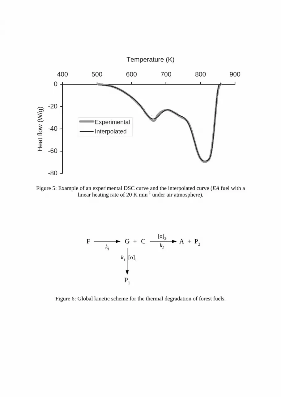
enthalpies of each reaction were calculated by numerical integration of the signal and the

results are shown in Table 5.

Table 5

Since Tab. 4 and Tab. 5 present mean values of three replicate measurements we can

conclude that the enthalpy values are constant for each reaction of each plant. We were able

to give a mean value for the enthalpy of the gases oxidation (exotherm 1) and for the

oxidation of char (exotherm 2) for each species. The obtained values are close whatever the

heating rate is.

It is important to notice that the values obtained from the numerical treatment were found to

be very close to those obtained by the thermal separation (cf. Tab. 4 and Tab 5.).

For every fuels the energy released by the reaction referred to exotherm 2 is more important

than the energy released by the reaction referred to exotherm 1. Actually, we found: 4.00 kJ g-

1 < oH1Δ < 4.84 kJ g-1 for the enthalpy of reaction referred to exotherm 1 whereas we found:

5.93 kJ g-1 < oH 2Δ < 8.74 kJ g-1 for the enthalpy of reaction referred to exotherm 2.

Figure 4 is an example of experimental data compared to isolated peaks, thanks to the thermal

and numerical separation we were able to interpolate with a very good fit the beginning and

the end of the global exotherm as it can be seen on figure 4. Figure 5 shows an example of

experimental data compared to the interpolated curve which is the sum of peak 1 and peak 2

isolated for each species and each heating rate. For this experiment we obtained a value of r =

0.9946. For all the species investigated and heating rates used the Pearson’s correlation

coefficient was about this value which indicates a very good fit.

GRAPHIC 4.

GRAPHIC 5.

Thermal and numerical separation is an indispensable step prior to the kinetic study of each

reaction.

3.4. Kinetic study

In our previous work we presented a hybrid kinetic method allowing studying complex and

multi-step reactional mechanisms [20]. Here are the results obtained on four species.

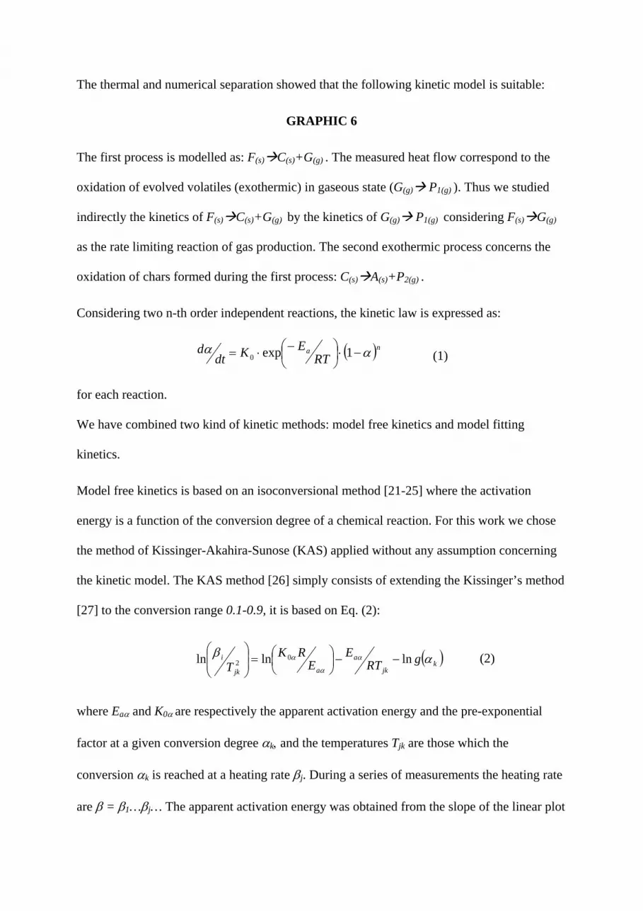
The thermal and numerical separation showed that the following kinetic model is suitable:

GRAPHIC 6

The first process is modelled as: F(s) C(s)+G(g) . The measured heat flow correspond to the

oxidation of evolved volatiles (exothermic) in gaseous state (G(g) P1(g) ). Thus we studied

indirectly the kinetics of F(s) C(s)+G(g) by the kinetics of G(g) P1(g) considering F(s) G(g)

as the rate limiting reaction of gas production. The second exothermic process concerns the

oxidation of chars formed during the first process: C(s) A(s)+P2(g) .

Considering two n-th order independent reactions, the kinetic law is expressed as:

( )naRT

EKdtd αα −⋅⎟

⎠⎞

⎜⎝⎛−⋅= 1exp0 (1)

for each reaction.

We have combined two kind of kinetic methods: model free kinetics and model fitting

kinetics.

Model free kinetics is based on an isoconversional method [21-25] where the activation

energy is a function of the conversion degree of a chemical reaction. For this work we chose

the method of Kissinger-Akahira-Sunose (KAS) applied without any assumption concerning

the kinetic model. The KAS method [26] simply consists of extending the Kissinger’s method

[27] to the conversion range 0.1-0.9, it is based on Eq. (2):

( )kjk

a

ajk

i gRTE

ERK

T αβ α

α

α lnlnln 02 −−⎟

⎠⎞

⎜⎝⎛=⎟⎟

⎠

⎞⎜⎜⎝

⎛ (2)

where Eaα and K0α are respectively the apparent activation energy and the pre-exponential

factor at a given conversion degree αk, and the temperatures Tjk are those which the

conversion αk is reached at a heating rate βj. During a series of measurements the heating rate

are β = β1…βj… The apparent activation energy was obtained from the slope of the linear plot

of ⎟⎟⎠

⎞⎜⎜⎝

⎛2lnjk

iT

β vs. jkT

1 performed thanks to a Microsoft® Excel® spreadsheet developed for

this purpose.

Model fitting kinetics is based on the fitting of Eq. 1 to the experimental values of dα/dt. We

used Fork® (CISP Ltd.) software which is provided for model fitting in isothermal or non-

isothermal conditions. The resolution of ordinary differential equations was automatically

performed by Fork® according to a powerful solver (Runge Kutta order 4 or Livermore

Solver of Ordinary Differential Equation). The reaction model f(α) = (1-α)n was determined

among six models specified in the literature [28]. Three heating rates (10, 20, 30 K min-1)

were used at the same time for each species; the software fit one kinetic triplet and one

reaction model valid for all the heating rates. Once the determination of the best kinetic

models and optimization of the parameters were achieved, the Residual Sum of Squares

between experimental and calculated values indicated the acceptable “goodness of fit” from a

statistical point of view.

In order to classify the fuels we chose to use the value of the rate constant at the temperature

of the maximum of each exotherm for each fuel. Figures 7 and 8 present the values of rate

constants of reaction 1 and reaction 2 calculated at the peak top temperatures with the

corresponding mean value of enthalpy reaction. These rate constants were calculated for each

species with the best set of kinetic parameters for the three heating rates considered herein.

GRAPHIC 7

GRAPHIC 8

These results show that the rate constant of gases oxidation is ranked as follow: k1(PP) <

k1(AU) < k1(CM) < k1(EA) and the rate constant of chars oxidation is ranked as follows:

k2(CM) < k2(EA) < k2(AU) < k2(PP)

Excepted for CM fuel which contain a higher quantity of mineral matter (cf. Tab. 1), the

limiting step of the thermal degradation is the gases oxidation since k1 < k2. Then we logically

compare the combustibility (the rate of burn after ignition) of the fuels by comparing the

constant rate of the gases oxidation, the result is the following: Comb(PP) < Comb(AU) <

Comb(CM) < Comb(EA).

4. Conclusion

Reactions of thermal degradation show multi-step characteristics. We showed that thermal

analysis and calorimetric investigations are useful tools in order to get information on the

ignitability, combustibility and sustainability of ligno-cellulosic fuels encountered in wildland

fires. The data derived from DSC and TGA analysis were: onset temperature and peak top

temperature of exothermic peak, global enthalpy of reaction, onset and offset temperatures of

successive mass loss. Our results showed that Erica arborea and Pinus pinaster fuels are the

most ignitable species whereas Arbutus unedo and Cistus monspeliensis are the less ignitable

species according to DSC and TGA data. We also found that Arbutus unedo and Erica

arborea are the most energetic species whereas Pinus pinaster and Cistus monspeliensis are

the less energetic species according to DSC data. DSC experiments on such fuels showed two

superposed exothermic phenomena. We individualized these phenomena in two oxidative

sub-reactions and the enthalpy reaction of each sub-reaction was calculated. We proposed a

kinetic scheme for the thermal degradation of ligno-cellulosic fuels under air with nth-order

model for the oxidative subreactions observed in DSC. Thanks to an hybrid kinetic method

[20] we calculated the rate constant at the peak top temperatures for each species considering

two n-th order reactions. Our results showed that Erica arborea is the most combustible fuel

whereas Pinus pinaster is the less combustible fuel, Cistus monspeliensis and Arbutus unedo

being intermediate combustible fuels. Even if the experimental conditions of thermal analysis

and calorimetry are far from actual conditions of wildland fires we think these tools are useful

in order to study the flammability of forest fuels. TGA and DSC experiments allow the

determination of combustibility, sustainability and ignitability of fuels and these data should

be complimentary to a global flammability parameter obtained thanks to lab-scale

flammability test [29,30].

References

[1] F.A. Albini, Comb. Sci. Tech 42 (1985) 229.

[2] M. De Luis, M.J. Baeza, J. Raventos, Int. J. Wildland Fire 13 (2004) 79.

[3] A.P. Dimitrakopoulos, J. Anal. Appl. Pyrolysis 60 (2001) 123.

[4] R. Alèn, E. Kuoppala, P.J. Oesch, Anal. Appl. Pyrolysis 36 (1996) 137.

[5] J.H. Balbi, P.A. Santoni, J.L. Dupuy, Int. J. Wildland Fire 9 (2000) 275.

[7] J. Kaloustian, A.M. Pauli, J. Pastor, J. Thermal Anal. 46 (1996) 1349.

[8] C.A. Koufopanos, G. Maschio, A. Lucchesi, Can. J. Chem. Eng. 67 (1989) 75.

[9] S. Liodakis, D. Barkirtzis, A.P. Dimitrakopoulos, Thermochim. Acta 390 (2002) 83.

[10] S. Liodakis, G. Katsigiannis and G. Kakali, Thermochim. Acta 437 (2005) 158.

[11] E. Leoni, D. Cancellieri, N. Balbi, P. Tomi, A.F. Bernardini, J. Kaloustian, T. Marcelli, J.

Fire Sci. 21 (2003) 117.

[12] J. Kaloustian, T.F. El-Moselhy, H. Portugal, Thermochim. Acta 401 (2003) 77.

[13] C. Branca, C. Di Blasi, J. Anal. Appl. Pyrolysis 67 (2003) 207.

[14] J.J.M. Orfao, F.J.A. Antunes, J.L. Figueiredo, Fuel 78 (1999) 349.

[15] R. Bilbao, J.F. Mastral, M.E. Aldea, J. Ceamanos, J. Anal. Appl. Pyrolysis 42 (1997)

189.

[16] R. Bilbao, J.F. Mastral, M.E. Aldea, J. Ceamanos, J. Anal. Appl. Pyrolysis 39 (1997) 53.

[17] M.J. Safi, I.M. Mishra, B. Prasad, Thermochim. Acta 412 (2004) 155.

[18] T.B. Bahder, Mathematica for scientists and Engineers, Addison-Wesley, Reading, 1995.

[19] M. Abramowitz, I.A. Stegun, Handbook of mathematical functions, Dover, New York,

1965.

[20] D. Cancellieri, E. Leoni, J.L. Rossi, Thermochim. Acta 438 (2005) 41.

[21] S. Vyazovkin, C.A. Wight, Thermochim. Acta 340 (1999) 53.

[22] N. Sbirrazzuoli, S. Vyazovkin, Thermochim. Acta 388 (2002) 289.

[23] S. Vyazovkin, V. Goryachko, Thermochim. Acta 197 (1992) 41.

[24] S. Vyazovkin, Thermochim. Acta 236 (1994) 1.

[25] S. Vyazovkin, C.A. Wight, Thermochim. Acta 340 (1999) 53.

[26] T. Akahira and T. Sunose, Res. Report. CHIBA Inst. Technol. 16 (1971) 22.

[27] H.E. Kissinger, Anal. Chem. 29 (1957) 1702.

[28] S. Vyazovkin, C.A. Wight, Int. Rev. Phys. Chem. 48 (1997) 125.

[29] A.P. Dimitrakopoulos, K. Kyriakos Papaioannou, Fire Technology 37 (2001) 143.

[30] S. Liodakis, D. Vorisis and I.P. Agiovlasitis, Thermochim. Acta 437 (2005) 150.

Acknowledgements

The authors express their gratitude to the autonomous region of Corsica for sponsoring the

present work. This research was also supported by the European Economic Community.

TABLES

Table 1: Elemental analysis of the fuels.

C (%) H (%) O (%) Total (%)

CM 46.58 6.22 37.68 90.48

EA 52.43 6.98 35.92 95.33

AU 48.24 6.15 40.33 94.72

PP 50.64 6.76 41.53 98.93

Table 2: Onset temperature, peaks top temperature and global enthalpy measured by DSC.

Temperature values are the mean values of three replicate measurements and in parenthesis are given the

corresponding RSD values

Species β = 10 K min-1 β = 20 K min-1 β = 30 K min-1

Onset

(K)

AU 563 (1.2) 567 (1.1) 572 (1.1) EA 529 (1.4) 534 (1.8) 538 (1.5) CM 556 (0.7) 560 (1.3) 563 (1.2) PP 540 (2.0) 546 (0.9) 549 (1.7)

Peak 1 top

Temperature

(K)

AU 634 (0.9) 638 (2.0) 643 (1.5) EA 639 (1.2) 644 (1.0) 649 (1.6) CM 624 (1.3) 628 (1.6) 632 (2.3) PP 632 (1.5) 638 (1.3) 644 (1.1)

Peak 2 top

Temperature

(K)

AU 784 (2.0) 788 (1.2) 792 (3.0) EA 779 (1.5) 784 (1.8) 790 (1.6) CM 772 (1.1) 776 (2.1) 780 (1.8) PP 747 (1.1) 753 (2.2) 760 (1.3)

ΔHo

(kJ g-1)

AU -13.01 -12.88 -12.79 EA -13.02 -12.96 -12.46 CM -10.63 -10.52 -10.75 PP -10.55 -10.44 -10.71

Table 3: Onset temperature, offset temperature and mass loss measured by TGA.

Species β = 10 K min-1 β = 20 K min-1 β = 30 K min-1

Onset

(K)

AU 563 (1.2) 567 (1.1) 572 (1.1) EA 529 (1.4) 534 (1.8) 538 (1.5) CM 556 (0.7) 560 (1.3) 563 (1.2) PP 540 (2.0) 546 (0.9) 549 (1.7)

Mass loss 1

(%)

AU 51.3 52.7 53.4 EA 72.0 71.0 72.3 CM 54.4 54.5 56.0 PP 73.2 72.2 73.0

Offset 1

(K)

AU 675 (2.3) 680 (1.0) 684 (0.6) EA 622 (1.9) 626 (1.7) 631 (1.3) CM 638 (1.4) 642 (1.1) 648 (1.0) PP 634 (1.3) 639 (1.3) 643 (0.5)

Mass loss 2

(%)

AU 42.8 41.6 42.0 EA 26.0 26.6 25.7 CM 34.4 35.6 35.9 PP 23.9 23.6 23.1

Offset 2

(K)

AU 803 (1.0) 807 (1.9) 812 (1.3) EA 818 (2.0) 823 (2.1) 827 (1.9) CM 825 (1.1) 829 (1.0) 834 (1.4) PP 809 (1.8) 813 (1.5) 818 (1.1)

Temperature values are the mean values of three replicate measurements and in parenthesis are given the

corresponding RSD values

Table 4: Enthalpy values obtained by the thermal separation.

Species β = 10 K min-1 β = 20 K min-1 β = 30 K min-1 °ΔH

ΔH°1 deducted

(kJ g-1)

AU -4.04 -4.01 -3.96 -4.00 (0.04) EA -4.84 -4.87 -4.82 -4.84 (0.07)CM -4.63 -4.61 -4.69 -4.64 (0.05)PP -4.18 -4.17 -4.22 -4.19 (0.03)

ΔH°2 isolated

(kJ g-1)

AU -8.87 -8.64 -8.71 -8.74 (0.10) EA -8.18 -8.09 -8.04 -8.10 (0.08)CM -6.00 -5.91 -6.06 -5.99 (0.08)PP -6.37 -6.27 -6.53 -6.39 (0.14)

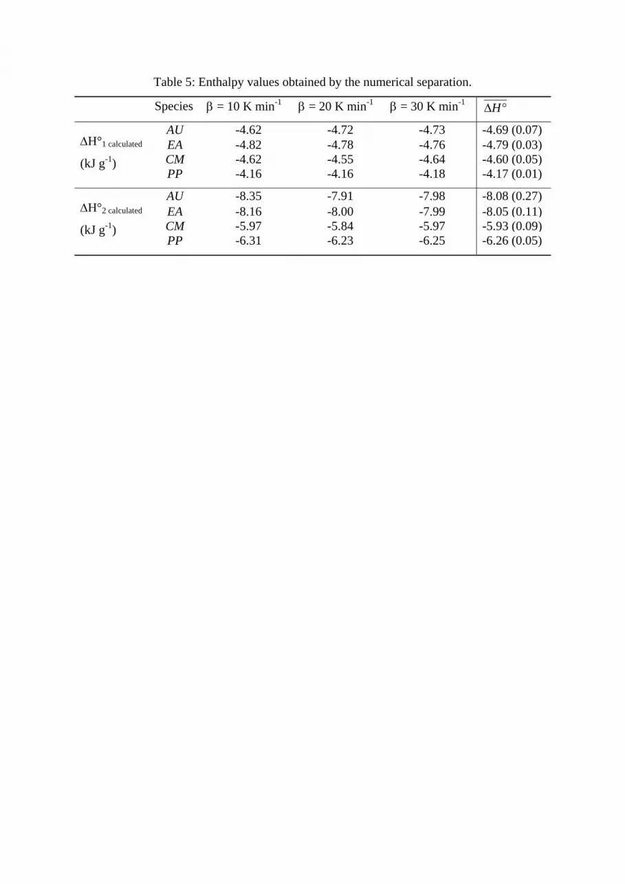
Table 5: Enthalpy values obtained by the numerical separation.

Species β = 10 K min-1 β = 20 K min-1 β = 30 K min-1 °ΔH

ΔH°1 calculated

(kJ g-1)

AU -4.62 -4.72 -4.73 -4.69 (0.07) EA -4.82 -4.78 -4.76 -4.79 (0.03)CM -4.62 -4.55 -4.64 -4.60 (0.05)PP -4.16 -4.16 -4.18 -4.17 (0.01)

ΔH°2 calculated

(kJ g-1)

AU -8.35 -7.91 -7.98 -8.08 (0.27) EA -8.16 -8.00 -7.99 -8.05 (0.11)CM -5.97 -5.84 -5.97 -5.93 (0.09)PP -6.31 -6.23 -6.25 -6.26 (0.05)

FIGURES

Figure 1: Thermal degradation of a ligno-cellulosic fuel.

Figure 2: Schematic representation of the thermal separation.

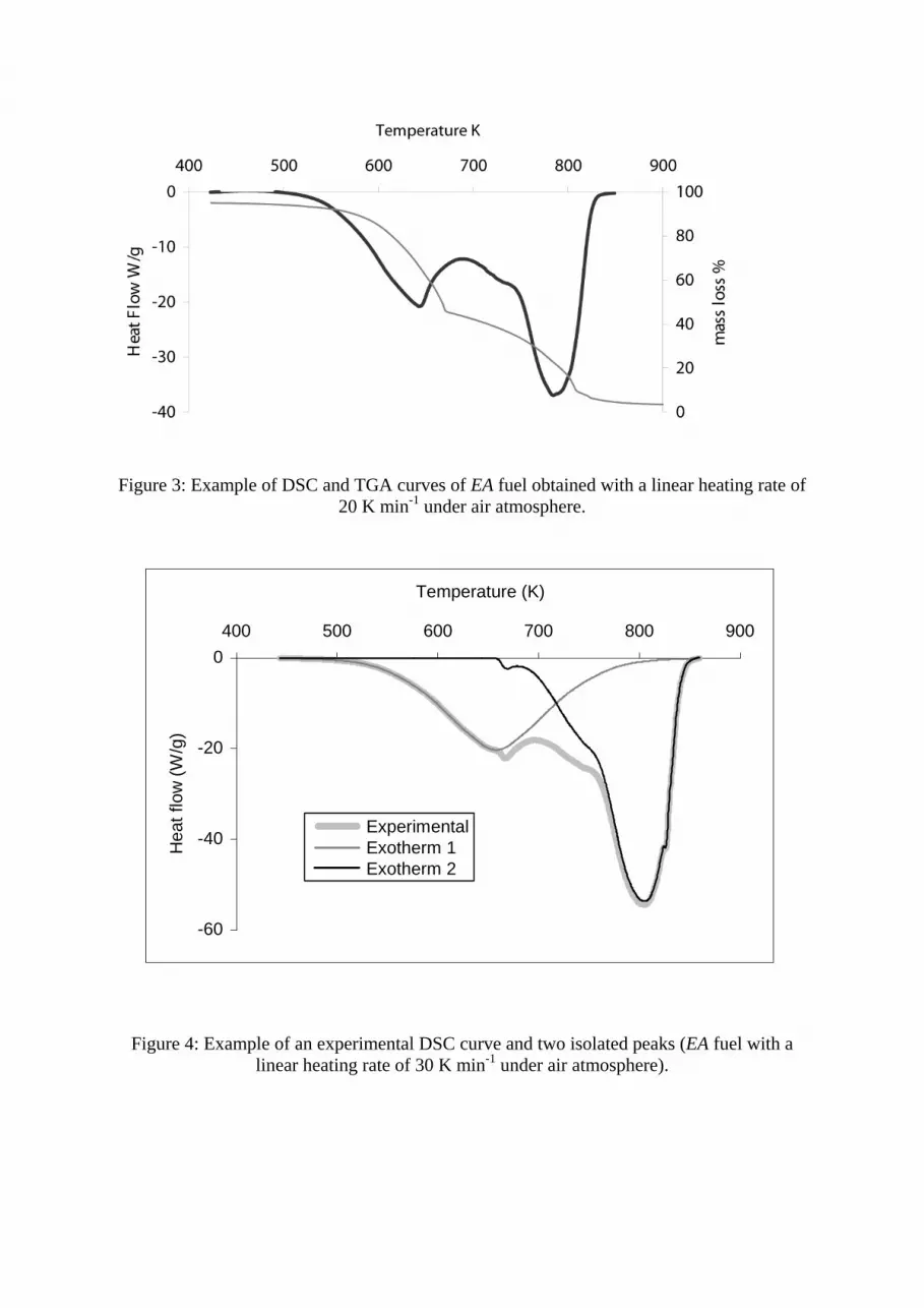
Figure 3: Example of DSC and TGA curves of EA fuel obtained with a linear heating rate of 20 K min-1 under air atmosphere.

-60

-40

-20

0 400 500 600 700 800 900

Temperature (K)

Hea

t flo

w (W

/g)

ExperimentalExotherm 1Exotherm 2

Figure 4: Example of an experimental DSC curve and two isolated peaks (EA fuel with a linear heating rate of 30 K min-1 under air atmosphere).

-80

-60

-40

-20

0

400 500 600 700 800 900

Temperature (K)

Hea

t flo

w (

W/g

)

Experimental

Interpolated

Figure 5: Example of an experimental DSC curve and the interpolated curve (EA fuel with a linear heating rate of 20 K min-1 under air atmosphere).

F G C A + P2

P1

+[o]2

[o]1

k2

k1

kl

Figure 6: Global kinetic scheme for the thermal degradation of forest fuels.

0

1

2

3

4

5

PP AU CM EA

Species

Rate

con

stan

t at T

max

*10-3

Figure 7: Rate constant for the first step oxidation ( RT

Ea

eKk−

⋅= 0 ) calculated at Tp1 for each species.

0

3

6

9

12

15

18

21

PP AU CM EA

Species

Rate

con

stan

t at T

max

*10-3

Figure 8: Rate constant for the second step oxidation ( RT

Ea

eKk−

⋅= 0 ) calculated at T = Tp2 for each species.