Ti

SDa

b

a

ARRAA

KCDHISW

1

bcptsb1Dlldydtpicm

G

0d

Ecological Modelling 224 (2012) 54– 64

Contents lists available at SciVerse ScienceDirect

Ecological Modelling

journa l h o me pa g e: www.elsev ier .com/ locate /eco lmodel

he response of the woodpigeon (Columba palumbus) to relaxation ofntraspecific competition: A hybrid modelling approach

uzanne M. O’Regana,∗, Denis Flynna, Thomas C. Kellyb, Michael J.A. O’Callaghana, Alexei V. Pokrovskii a,mitrii Rachinskii a

School of Mathematical Sciences, Western Gateway Building, Western Road, University College Cork, Cork, IrelandDepartment of Zoology, Ecology and Plant Science, Distillery Fields, North Mall, University College Cork, Cork, Ireland

r t i c l e i n f o

rticle history:eceived 9 June 2011eceived in revised form 1 October 2011ccepted 19 October 2011vailable online 25 November 2011

a b s t r a c t

The recent rapid growth of the woodpigeon population in the British Isles is a cause for concern forenvironmental managers. It is unclear what has driven their increase in abundance. Using a mathe-matical model, we explored two possible mechanisms, reduced intraspecific competition for food andincreased reproductive success. We developed an age-structured hybrid model consisting of a system ofordinary differential equations that describes density-dependent mortality and a discrete component,which represents the birth-pulse. We investigated equilibrium population dynamics using our model.

eywords:limate changeensity-dependenceybrid model

ntraspecific competitionemi-discrete model

The two hypotheses predict contrasting population age profiles at equilibrium. We adapted the model toexamine the impacts of control measures. We showed that an annual shooting season that follows theperiod of density-dependent mortality is the most effective control strategy because it simultaneouslyremoves adult and juvenile woodpigeons. The model is a first step towards understanding the processesthat influence the dynamics of woodpigeon populations.

oodpigeon

. Introduction

The woodpigeon, Columba palumbus, is a multi-brooded her-ivore and therefore likely to benefit from global warming andlimate change (Jiguet et al., 2007). It is a well-known agriculturalest, which has appeared to have benefitted from changing agricul-ural practices, particularly in Britain (Inglis et al., 1990). The pesttatus of woodpigeon led to a detailed research programme into itsiology and management in the 1960s (Murton, 1958, 1961, 1965,971; Murton et al., 1964, 1966, 1974; Murton and Isaacson, 1964).uring this period, the population was reasonably stable, although

arge fluctuations in numbers occurred within years, i.e., the popu-ation increased rapidly over the breeding season and then declinedrastically during the winter months so that the total observed eachear remained relatively constant. The amount of grain availableetermined numbers that survived after the breeding season untilhe period when woodpigeons switched to their clover food sup-ly in December. Juveniles required grain to aid their development

n the months after fledging whereas adults could more readilyonsume less nutritious clover leaves. The timing of the mini-um in woodpigeon numbers occurred in February and March,

∗ Corresponding author. Present address: Odum School of Ecology, University ofeorgia, Athens, GA 30602-2202, USA. Tel.: +1 706 583 5538.

E-mail addresses: smoregan@uga.edu, s.m.oregan@gmail.com (S.M. O’Regan).

304-3800/$ – see front matter © 2011 Elsevier B.V. All rights reserved.oi:10.1016/j.ecolmodel.2011.10.018

© 2011 Elsevier B.V. All rights reserved.

i.e., the period of least plentiful clover stocks. When food suppliesbecame depleted, the effects of intraspecific competition inten-sified and were density-dependent (Murton et al., 1966, 1971),i.e., if the size of a flock was high relative to the quantity of foodavailable, then mortality was higher. Mortality principally affectedsubordinate individuals and juveniles. It is important to note thatduring the period of Murton’s studies, winters were noticeablylonger and colder than in the period 1976–2000 (Houghton et al.,2001).

The recent increase in the woodpigeon population of the BritishIsles (Baillie et al., 2009; Crowe et al., 2010) has become a cause forconcern for agriculture (Tayleur, 2008), but also for aviation safety,because the species is increasingly involved in birdstrikes (Kellyet al., unpublished data). The exact reasons for this increase areunknown (Saari, 1997). One hypothesis is that climate change hasinduced the earlier onset of the growing season (Carroll et al., 2009;Donnelly et al., 2009; Menzel et al., 2006; Møller et al., 2010). Sincethe food supply does not fluctuate to the same extent as it did inthe 1960s, food is more readily available to woodpigeons through-out the year. Consequently, woodpigeon numbers are no longerregulated by natural fluctuations of the food supply, as they werebefore the onset of climate change. Therefore, decreased intraspe-

cific competition for food during winter may be the mechanismbehind the sustained increase. Alternatively, woodpigeons may beparticularly adapted to benefit from climate change because theyare multi-brooded; the ability to produce multiple broods per year,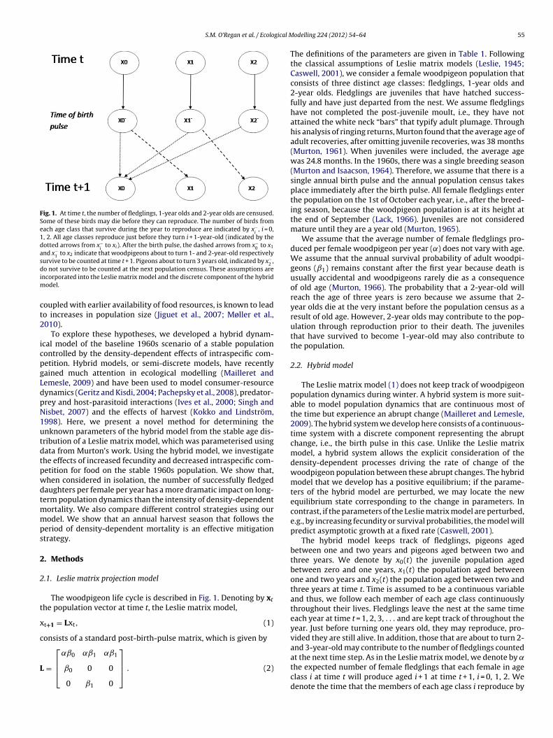

S.M. O’Regan et al. / Ecological M

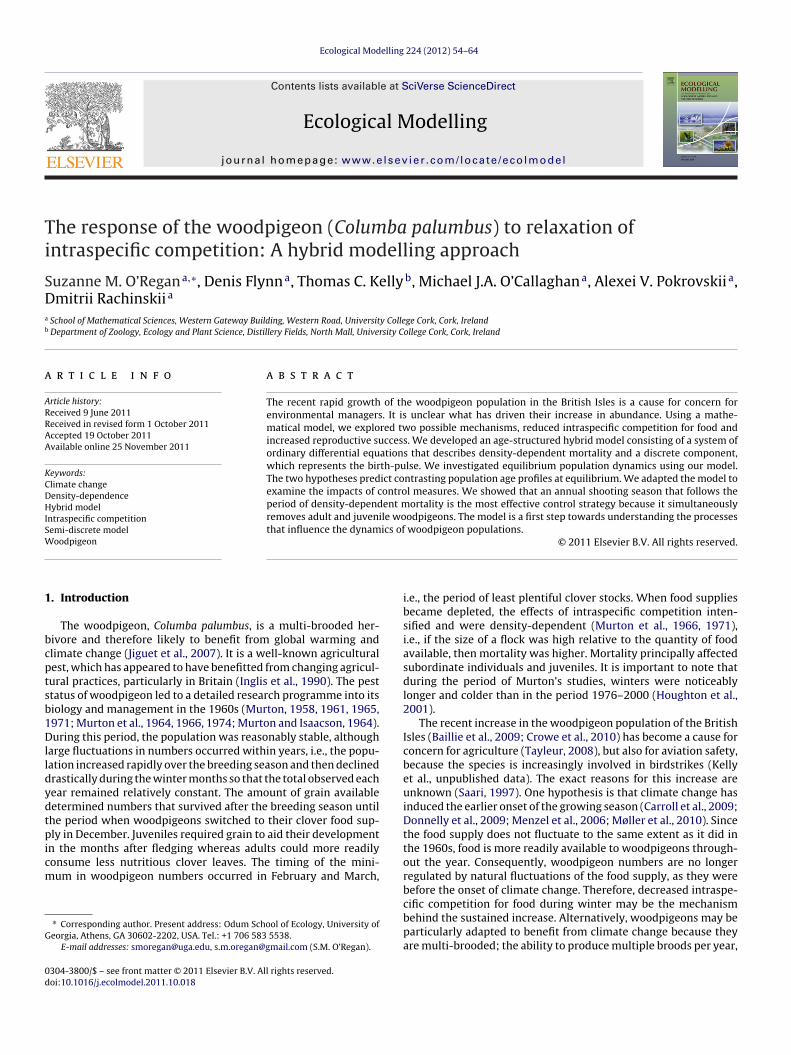
Fig. 1. At time t, the number of fledglings, 1-year olds and 2-year olds are censused.Some of these birds may die before they can reproduce. The number of birds fromeach age class that survive during the year to reproduce are indicated by x−

i, i = 0,

1, 2. All age classes reproduce just before they turn i + 1-year-old (indicated by thedotted arrows from x−

ito xi). After the birth pulse, the dashed arrows from x−

0 to x1

and x−1 to x2 indicate that woodpigeons about to turn 1- and 2-year-old respectively

survive to be counted at time t + 1. Pigeons about to turn 3 years old, indicated by x−2 ,

dim

ct2

icpgLdpN1utdtpwdtmmps

2

2

t

x

c

L

o not survive to be counted at the next population census. These assumptions arencorporated into the Leslie matrix model and the discrete component of the hybrid

odel.

oupled with earlier availability of food resources, is known to leado increases in population size (Jiguet et al., 2007; Møller et al.,010).

To explore these hypotheses, we developed a hybrid dynam-cal model of the baseline 1960s scenario of a stable populationontrolled by the density-dependent effects of intraspecific com-etition. Hybrid models, or semi-discrete models, have recentlyained much attention in ecological modelling (Mailleret andemesle, 2009) and have been used to model consumer-resourceynamics (Geritz and Kisdi, 2004; Pachepsky et al., 2008), predator-rey and host-parasitoid interactions (Ives et al., 2000; Singh andisbet, 2007) and the effects of harvest (Kokko and Lindström,998). Here, we present a novel method for determining thenknown parameters of the hybrid model from the stable age dis-ribution of a Leslie matrix model, which was parameterised usingata from Murton’s work. Using the hybrid model, we investigatehe effects of increased fecundity and decreased intraspecific com-etition for food on the stable 1960s population. We show that,hen considered in isolation, the number of successfully fledgedaughters per female per year has a more dramatic impact on long-erm population dynamics than the intensity of density-dependent

ortality. We also compare different control strategies using ourodel. We show that an annual harvest season that follows the

eriod of density-dependent mortality is an effective mitigationtrategy.

. Methods

.1. Leslie matrix projection model

The woodpigeon life cycle is described in Fig. 1. Denoting by xt

he population vector at time t, the Leslie matrix model,

t+1 = Lxt, (1)

onsists of a standard post-birth-pulse matrix, which is given by⎡ ⎤

= ⎢⎣

˛ˇ0 ˛ˇ1 ˛ˇ1

ˇ0 0 0

0 ˇ1 0

⎥⎦ . (2)

odelling 224 (2012) 54– 64 55

The definitions of the parameters are given in Table 1. Followingthe classical assumptions of Leslie matrix models (Leslie, 1945;Caswell, 2001), we consider a female woodpigeon population thatconsists of three distinct age classes: fledglings, 1-year olds and2-year olds. Fledglings are juveniles that have hatched success-fully and have just departed from the nest. We assume fledglingshave not completed the post-juvenile moult, i.e., they have notattained the white neck “bars” that typify adult plumage. Throughhis analysis of ringing returns, Murton found that the average age ofadult recoveries, after omitting juvenile recoveries, was 38 months(Murton, 1961). When juveniles were included, the average agewas 24.8 months. In the 1960s, there was a single breeding season(Murton and Isaacson, 1964). Therefore, we assume that there is asingle annual birth pulse and the annual population census takesplace immediately after the birth pulse. All female fledglings enterthe population on the 1st of October each year, i.e., after the breed-ing season, because the woodpigeon population is at its height atthe end of September (Lack, 1966). Juveniles are not consideredmature until they are a year old (Murton, 1965).

We assume that the average number of female fledglings pro-duced per female woodpigeon per year (˛) does not vary with age.We assume that the annual survival probability of adult woodpi-geons (ˇ1) remains constant after the first year because death isusually accidental and woodpigeons rarely die as a consequenceof old age (Murton, 1966). The probability that a 2-year-old willreach the age of three years is zero because we assume that 2-year olds die at the very instant before the population census as aresult of old age. However, 2-year olds may contribute to the pop-ulation through reproduction prior to their death. The juvenilesthat have survived to become 1-year-old may also contribute tothe population.

2.2. Hybrid model

The Leslie matrix model (1) does not keep track of woodpigeonpopulation dynamics during winter. A hybrid system is more suit-able to model population dynamics that are continuous most ofthe time but experience an abrupt change (Mailleret and Lemesle,2009). The hybrid system we develop here consists of a continuous-time system with a discrete component representing the abruptchange, i.e., the birth pulse in this case. Unlike the Leslie matrixmodel, a hybrid system allows the explicit consideration of thedensity-dependent processes driving the rate of change of thewoodpigeon population between these abrupt changes. The hybridmodel that we develop has a positive equilibrium; if the parame-ters of the hybrid model are perturbed, we may locate the newequilibrium state corresponding to the change in parameters. Incontrast, if the parameters of the Leslie matrix model are perturbed,e.g., by increasing fecundity or survival probabilities, the model willpredict asymptotic growth at a fixed rate (Caswell, 2001).

The hybrid model keeps track of fledglings, pigeons agedbetween one and two years and pigeons aged between two andthree years. We denote by x0(t) the juvenile population agedbetween zero and one years, x1(t) the population aged betweenone and two years and x2(t) the population aged between two andthree years at time t. Time is assumed to be a continuous variableand thus, we follow each member of each age class continuouslythroughout their lives. Fledglings leave the nest at the same timeeach year at time t = 1, 2, 3, . . . and are kept track of throughout theyear. Just before turning one years old, they may reproduce, pro-vided they are still alive. In addition, those that are about to turn 2-and 3-year-old may contribute to the number of fledglings counted

at the next time step. As in the Leslie matrix model, we denote by ˛the expected number of female fledglings that each female in ageclass i at time t will produce aged i + 1 at time t + 1, i = 0, 1, 2. Wedenote the time that the members of each age class i reproduce by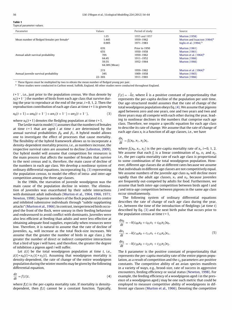

56 S.M. O’Regan et al. / Ecological Modelling 224 (2012) 54– 64

Table 1Typical parameter values.

Parameter Values Period of study Source

1.05 1955 and 1957 Murton (1958)Mean number of fledged females per femalea 1.445 1959–1962 Murton and Isaacson (1964)b

0.905 1971–1983 Inglis et al. (1994) b

63% Prior to 1950 Murton (1961)65% 1950–1958 Murton (1961)

Annual adult survival probability 70% 1959–1962 Murton et al. (1964)b

64.4% 1911–1952 Murton (1966)59.5% 1952–1964 Murton (1966)64.38% (Mean)

21% 1959–1962 Murton et al. (1964)b

Annual juvenile survival probability 34% 1909–1958 Murton (1965)22–36% 1911–1965 Murton (1966)

youngies we

txir

x

w

aaoTdrOtttotc

mtwNaapaaoljagto

zdpd

wd

a These figures must be multiplied by two to obtain the mean number of fledgedb These studies were conducted in Carlton wood, Suffolk, England. All other stud

+ 1−, i.e., just prior to the population census. We thus denote byi(t + 1−) the number of birds from each age class that survive dur-ng the year to reproduce at the end of the year, i = 0, 1, 2. Then theeproduction contribution of each age class at time t + 1 is given by

0(t + 1) = ˛x0(t + 1−) + ˛x1(t + 1−) + ˛x2(t + 1−), (3)

here x0(t + 1) denotes the fledgling population at time t + 1.The Leslie matrix model (1) assumes that the numbers of females

t time t + 1 that are aged i at time t are determined by thennual survival probabilities ˇ0 and ˇ1. A hybrid model allowsne to investigate the effect of processes that cause mortality.he flexibility of the hybrid framework allows us to incorporate aensity-dependent mortality process, i.e., as numbers increase, theespective survival rates are assumed to decline (Lebreton, 2009).ur hybrid model will assume that competition for resources is

he main process that affects the number of females that surviveo the next census and is, therefore, the main cause of decline ofhe numbers in each age class. We develop a nonlinear system ofrdinary differential equations, incorporating Eq. (3) representinghe population census, to model the effect of intra- and inter-ageompetition among the three age classes.

In the 1960s, the starvation of juvenile woodpigeon was theain cause of the population decline in winter. The elimina-

ion of juveniles was exacerbated by their subtle interactionsith dominant adult individuals (Murton et al., 1964, 1966, 1971;ewton, 1998). Superior members of the flock populated its centrend inhibited submissive individuals through “subtle supplantingttacks” (Murton et al., 1966). In contrast, inexperienced birds occu-ied the front of the flock, were uneasy in their feeding behaviournd endeavoured to avoid conflict with dominants. Juveniles werelso less efficient at feeding than adults and were less effective atbtaining adequate food supplies, especially when resources wereow. Therefore, it is natural to assume that the rate of decline ofuveniles, x0, will increase as the total flock-size increases. Wessume that the greater the number of birds in age class j, thereater the number of direct or indirect competitive interactionshat a bird of type i will have, and therefore, the greater the degreef inhibition a pigeon aged i will suffer.

Let z(t) be the total woodpigeon population at time t, i.e.,(t) = x0(t) + x1(t) + x2(t). Assuming that woodpigeon mortality isensity-dependent, the rate of change of the entire woodpigeonopulation during the winter months may be given by the followingifferential equation,

dz

dt= f (z)z, (4)

here f(z) is the per-capita mortality rate. If mortality is density-ependent, then f(z) cannot be a constant function. Typically,

per pair.re conducted throughout England.

f (z) = −kz, where k is a positive constant of proportionality thatrepresents the per-capita decline of the population per unit time.Our age-structured model assumes that the rate of change of thetotal woodpigeon population obeys Eq. (4). We assume that pigeonsaged between zero and one years, one and two years and two andthree years may all compete with each other during the year, lead-ing to nonlinear declines in the numbers that comprise each ageclass. Therefore, we require a specific equation for each age classto describe its rate of change. We assume that the rate of change ofeach age class xi is a function of all age classes, i.e., we have

dxi

dt= fi(x0, x1, x2)xi,

where fi(x0, x1, x2) is the per-capita mortality rate of xi, i = 0, 1, 2.We assume that each fi is a linear combination of x0, x1 and x2,i.e., the per-capita mortality rate of each age class is proportionalto some combination of the total woodpigeon population. How-ever, different age classes die at different rates because we assumethat individuals in different age classes are not competitively equal.We assume numbers of the juvenile age class x0 will decline morerapidly than the adult age classes, x1 and x2, because juvenilesare frequently out-competed by adults for food. Furthermore, weassume that both inter-age competition between birds aged i andj and intra-age competition between pigeons in the same age classoccur simultaneously.

The following system of ordinary differential equationsdescribes the rate of change of each age class during the year,i.e., between the time of the introduction of fledglings (at time t)described by Eq. (3) and the next birth pulse that occurs prior tothe population census at time t + 1,

dx0

dt= −k(c00x0 + c01x1 + c02x2)x0,

dx1

dt= −k(c10x0 + c11x1 + c12x2)x1,

dx2

dt= −k(c20x0 + c21x1 + c22x2)x2.

(5)

The k parameter is the positive constant of proportionality thatrepresents the per-capita mortality rate of the entire pigeon popu-lation, as a result of competition and the cij parameters are positiveconstants. The competitive ability of an avian species manifestsin a variety of ways, e.g., brood-size, rate of success in aggressiveencounters, feeding efficiency or social status (Newton, 1998). For

example, the feeding efficiency of a woodpigeon aged i in the pres-ence of a woodpigeon aged j may be one such metric that could beemployed to measure competitive ability of woodpigeons in dif-ferent age classes (Murton et al., 1966). Denoting the competitive

gical Modelling 224 (2012) 54– 64 57

alc

c

bjttyjwootTsHttn

s

imo

c2tcebs

Bdtt(F

2

rntood

c

ioa

Table 2The inter-age competition coefficients cij , i /= j, are expressed in terms of the relativecompetitive ability of 1-year olds to fledglings, A = c1/c0 and 2-year olds to fledglings,B = c2/c0. The numerical values for the relative competitive ability and competitioncoefficients were found using the optimization routine in Mathematica. These valueswere used to compute the stable one-periodic solution corresponding to the post-birth-pulse population at equilibrium.

Parameter Symbol Value

Fecundity 1.435Relative competitive ability of 1-year-old

to juvenilec1/c0 (A) 8.37378

Relative competitive ability of 2-year-oldto juvenile

c2/c0 (B) 8.37182

Inter-age competition coefficients c01 = A/(A + 1) 0.893319c02 = B/(B + 1) 0.893297c10 = 1/(A + 1) 0.106681c12 = B/(A + B) 0.499941c20 = 1/(B + 1) 0.106703c21 = A/(A + B) 0.500059

Intra-age competition coefficients cii , i = 0, 1, 2 0.5

S.M. O’Regan et al. / Ecolo

bility of a bird in age class i by ci, i = 0, 1, 2, we define the fol-owing nondimensional parameters, which we call the competitionoefficients,

ij = Competitive ability of bird j

Combined competitive abilities of birds i and j= cj

ci + cj.

(6)

The competition coefficients may be interpreted as the proba-ility of an interaction between a pigeon aged i and a pigeon aged

not leading to a ‘successful’ outcome for the pigeon aged i, i.e.,he probability of interactions with the xj population contributingo the decline of the xi population. A negative interaction for an i-ear-old might include starvation as a result of the presence of a-year-old. We assume that the probability of a negative encounter

ith a pigeon in age class j for a bird in age class i depends onlyn age and not on size, social status, genetics, etc. By definitionf the competition coefficients (6), cij + cji = 1, i.e., the probabilityhat either pigeon will succeed in a competitive encounter is one.herefore, we assume cji = 1 − cij. Note that we assume when food iscarce, there may be only one ‘winner’ of a competitive interaction.owever, if there is plenty of food available, it is easy to imagine

hat this condition may be relaxed, i.e., there is a probability thathe interaction of two birds in different age classes will not impactegatively on their respective population sizes.

Moreover, since cij + cji = 1 and choosing k = k/2, we may writeystem (5) as,

dz

dt= − k

2z2, (7)

.e., the rate of change of the woodpigeon population z = x0 + x1 + x2ay be described in terms of one differential equation. The solution

f Eq. (7) may be found explicitly, see Appendix A.To ensure that the hybrid model and the Leslie matrix model

orrespond exactly, we cannot assume that pigeons aged between and 3 can survive to be counted at the population census. In addi-ion, juvenile and 1-year-old pigeons must move into the next agelass at time t + 1. Therefore, denoting the pigeons that survive theffects of competition exactly prior to the next population censusy xi(t + 1−), i = 0, 1, the discrete survival component of the hybridystem is

x1(t + 1) = x0(t + 1−),

x2(t + 1) = x1(t + 1−).(8)

y solving the hybrid system numerically, we may explore theynamics of the age-structured woodpigeon population, using sys-em (5) to track continuous-time dynamics during the year andhen updating the populations each year according to Eqs. (3) and8). Note that the hybrid model processes are also described byig. 1.

.3. The hybrid system in terms of two parameters

Using the definition of the competition coefficients (6), we mayeduce the number of unknown parameters of the system (5) fromine to two. It is convenient that cij + cji = 1 because we wish to keephe number of unknown parameters of the hybrid system small inrder to identify them from the stationary age distribution vectorf the Leslie matrix model (1). We will describe this procedure inetail in Section 4.2. Note that

ii = ci = 1,

ci + ci 2

.e., we assume that there is an equal probability of a successfulutcome in a competitive encounter for pigeons that are in the samege class i.

Secondly, we may define the hybrid system in terms of c1/c0and c2/c0, i.e., the ratios of the competitive ability of pigeonsaged between one- and 2-year olds and the competitive abilityof pigeons aged between 2- and 3-year olds to juveniles’ com-petitive ability, respectively. We will refer to these parameters asthe relative competitive ability of 1-year olds and 2-year olds tojuveniles, respectively. All the inter-age competition coefficientscij may be described in terms of the relative competitive abil-ity parameters, see Table 2. Therefore, the relative competitiveability parameters are the only unknown quantities to be deter-mined from the stationary age distribution of the Leslie matrixmodel. In addition, we assume that adults have inherently morecompetitive ability compared to juveniles, i.e., c1/c0, c2/c0 > 1. It isreasonable for juveniles to have less ability to compete effectivelythan adults because inexperienced birds have been observed to benotably uneasy while feeding compared to adults and tended toavoid potential conflict situations (Murton et al., 1966). Further-more, adults have been observed to have a greater feeding ratethan juveniles during periods of low food supply (Murton et al.,1966; Newton, 1998). These factors may have led to the elimina-tion of juveniles through starvation or emigration (Murton et al.,1964).

3. Theory

3.1. Relationship arising from the stationary age distribution

The population determined by the Leslie matrix model (1) willgrow or decay at a rate � (the dominant eigenvalue of the matrix L).Furthermore, the population vector asymptotically becomes pro-portional to the associated eigenvector v, which is known as thestable age distribution. If � = 1, the population will stabilize to anequilibrium, depending on the initial condition. There are multipleequilibria, which form a straight line in the phase space. We referto the line of equilibria corresponding to � = 1 as the stationary agedistribution.

If L is a Leslie matrix, then Lv = �v. If v = (v0, v1, v2) and � = 1, thefollowing relationships must hold for the Leslie matrix (2),

˛(ˇ0v0 + ˇ1(v1 + v2)) = v0,

ˇ v = v , (9)

0 0 1

ˇ1v1 = v2.

58 S.M. O’Regan et al. / Ecological M

5 10 15 20Time (in years)

280

290

300

310

320

330

340To

talA

bund

ance

Hybrid

Leslie

Fig. 2. A typical solution of the hybrid system computed from the parameter valuesdescribed in Table 2 and a solution of the Leslie matrix model, = 1.435, ˇ0 = 0.34,ˇ1 = 0.64, starting from the initial condition (100, 100, 100). The short-term dynam-ics are somewhat different but the solutions tend to the same equilibrium in thelp

Tl

Fn

˛

Nbfp

3

actuaseeomiTtrioi

mtLS

ddb

reasonable parameters such that the dominant eigenvalue of the

ong-term, provided k is chosen according to Eq. (A.5). Here, k = 0.00793 per pigeoner year ensures coalescence of the two solutions.

he stationary age distribution may thus be described by the fol-owing relations (Caswell, 2001),

v0ˇ0 = v1,

v0ˇ0ˇ1 = v2.(10)

urthermore, from Eq. (9), we obtain an expression for the expectedumber of fledglings per female ˛,

= 1

ˇ0(1 + ˇ1 + ˇ21)

. (11)

ote that if > 1/ˇ0(1 + ˇ1 + ˇ21) then the population will grow

ut if < 1/ˇ0(1 + ˇ1 + ˇ21), the population will decay. Under this

ormulation, is bounded below by 1/3 since ˇ0 and ˇ1 are survivalrobabilities and cannot be greater than one.

.2. Scaling of the hybrid system

We multiplied the competition coefficients of the system (5) by positive constant k to scale the hybrid system appropriately. Theonstant k is an additional parameter that we may use to adjust theotal population of pigeons to a given number, for example, a pop-lation with an age structure that is proportional to the stationaryge distribution of the Leslie matrix model (1), given a particularet of parameters and an initial condition. For a given set of param-ters ˛, ˇ0 and ˇ1, the Leslie matrix model converges to a line ofquilibria corresponding to different initial conditions and the linef equilibria is spanned by the positive eigenvector v of the Leslieatrix. In contrast, the hybrid model converges to an isolated pos-

tive equilibrium for a given set of parameters ˛, c1/c0 and c2/c0.herefore, the parameter k enables us to adjust the equilibrium ofhe hybrid model such that it will coincide with a specific equilib-ium of the Leslie matrix model that corresponds to a particularnitial condition. This may be done very simply as the equilibriumf the hybrid system, which we denote by z0, scales linearly with k,.e., z0 = (x∗

0, x∗1, x∗

2) = (x0∗/k, x1

∗/k, x2∗/k).

Using the parameters in Table 2 and an appropriate k deter-ined using the procedure described in Appendix A, it is possible

o obtain complete agreement between a given equilibrium of theeslie matrix model and the equilibrium of the hybrid model (Fig. 2).ection 4 describes how the parameters in Table 2 were obtained.

Finally, it is useful to obtain the characteristic time for the

ensity-dependent mortality process, e.g., one may ask, how longoes it take for the population to half in size in the time betweenirth pulses? If we replace z(t) with z(0)/2 in Eq. (A.1), we obtain

odelling 224 (2012) 54– 64

t = 2/kz0. The characteristic time for system (5) is given in terms ofk and a characteristic population size z(0),

Tc = 1kz(0)

, (12)

and we would expect it to be of the order of one year. At equilibrium,Tc may be calculated using expression (A.4) for k. Assuming that thepopulation was at equilibrium in the 1960s and setting ˇ0 = 0.34and ˇ1 = 0.64, which are reasonable values for the annual survivalprobabilities in the 1960s (see Table 1), we obtain a characteristictime of approximately 0.405 years. Indeed, the 1960s populationwould half in size in 0.81 years, which is reasonable becausethe population experienced dramatic crashes from September toMarch, i.e., within the first six months following the birth pulse(Murton et al., 1964).

3.3. Asymptotic behaviour of the hybrid system for large ˛

We establish the asymptotic behaviour of the equilibrium of thehybrid model (i.e., the post-birth-pulse equilibrium population z0)for large values of the fecundity parameter ˛, e.g., > 3. Eq. (A.2)gives the total population before the birth pulse, i.e., Eq. (7) bringsthe equilibrium z0 population to the equilibrium pre-birth-pulsepopulation z1 at the end of one year. Eq. (A.2) implies

limz0→∞

z1 = 2k

, (13)

hence, z1 = x0(t + 1−) + x1(t + 1−) + x2(t + 1−) < 2/k and thus, after thebirth pulse,

x0(t + 1−) + x1(t + 1−) = x∗1 + x∗

2 <2k

. (14)

Therefore, the sum of the equilibrium populations of 1- and 2-yearolds are uniformly bounded for all ˛. Furthermore,

˛z1 < ˛z1 + x∗1 + x∗

2 = z0 < ˛z1 + z1, (15)

since x∗1 + x∗

2 < z1. Substituting Eq. (A.2) for z1 in expression (15),we obtain

2( − 1)k

< z0 <2˛

k, (16)

for all > 0. Therefore, the total population at equilibrium afterthe birth pulse grows linearly with between the lines 2(˛ − 1)/kand 2˛/k. The equilibrium fledgling population x∗

0 = z0 − (x∗1 + x∗

2)eventually grows linearly as the fecundity parameter increasesbecause for large values of ˛, the vast majority of the popula-tion consists of fledglings (see inequality (14)). Following the birthpulse, density-dependence causes the large fledgling population todecrease sharply to a very small number given by x0(t + 1−). At thenext birth pulse, the small number of fledglings that have survivedthe effects of intraspecific competition turn 1 year olds. Therefore,as ˛→ ∞, the 1- and 2-year-old populations will always be verysmall after the birth pulse whereas the fledgling population willalways be very large.

4. Calculation

4.1. Numerical values for the Leslie matrix model

In the 1960s, the woodpigeon population was stable. If wood-pigeon population dynamics can be described by a Leslie matrix,then this scenario corresponds to the matrix (2) having a domi-nant eigenvalue of one. Therefore, we need to choose biologically

matrix (2), is approximately equal to one.Using Haldane’s technique, Murton (1966) calculated an annual

adult survival probability of 64% and inferred from this that an

gical Modelling 224 (2012) 54– 64 59

amh6tˇffi

4h

deeo(srwrt

dittcimtt(

Tfmac

5

5

tnerzeb(ataz1tip

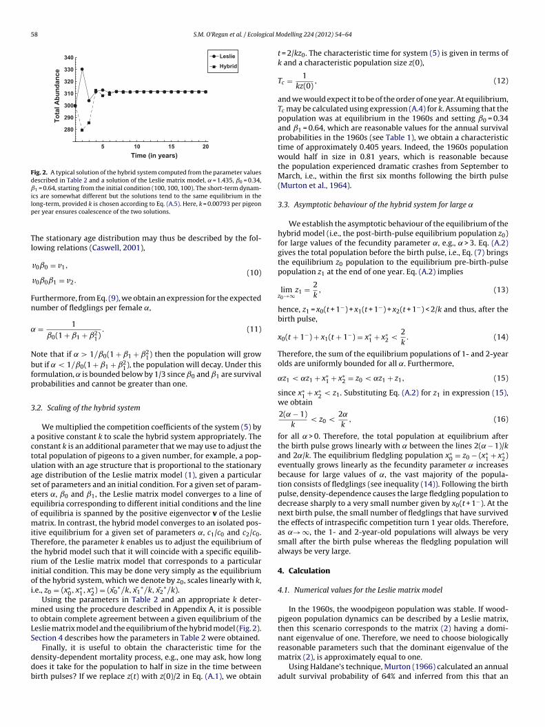
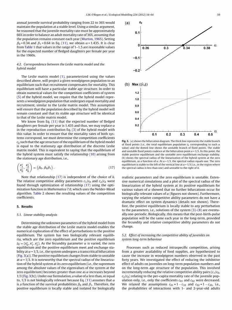
Fig. 3. (a) shows the bifurcation diagram. The thick line represents the stable branchof fixed points (i.e., the total equilibrium population z0 corresponding to each ˛value) and the dotted line shows the unstable branch of fixed points. The stableand unstable fixed points coalesce at the bifurcation point = 1/3. As this point, thestable positive equilibrium and the unstable zero equilibrium exchange stability.(b) shows the spectral radius of the linearization of the hybrid system at the zero

S.M. O’Regan et al. / Ecolo

nnual juvenile survival probability ranging from 22 to 36% wouldaintain the population at a stable level. Using a similar argument,

e reasoned that the juvenile mortality rate must be approximately6% in order to balance an adult mortality rate of 36%, assuming thathe population remains constant each year (Murton, 1965). Setting0 = 0.34 and ˇ1 = 0.64 in Eq. (11), we obtain = 1.435. It is clear

rom Table 1 that values in the range of 1–1.5 are reasonable valuesor the expected number of fledged daughters per female per yearn the 1960s.

.2. Correspondence between the Leslie matrix model and theybrid model

The Leslie matrix model (1), parameterized using the valuesescribed above, will project a given woodpigeon population to anquilibrium such that recruitment compensates for mortality. Thisquilibrium will have a particular stable age structure. In order tobtain numerical values for the competition coefficients of system5) of the hybrid model, we require that the hybrid model repre-ents a woodpigeon population that undergoes equal mortality andecruitment, similar to the Leslie matrix model. This assumptionill ensure that the population described by the hybrid model will

emain constant and that its stable age structure will be identicalo that of the Leslie matrix model.

We know from Eq. (11) that the expected number of fledgedaughters per female per year is 1.435 and thus, we may replace ˛

n the reproduction contribution Eq. (3) of the hybrid model withhis value. In order to ensure that the mortality rates of both sys-ems correspond, we must determine the competition coefficientsij such that the age structure of the equilibrium of the hybrid models equal to the stationary age distribution of the discrete Leslie

atrix model. This is equivalent to saying that the equilibrium ofhe hybrid system must satisfy the relationship (10) arising fromhe stationary age distribution, i.e.,

x∗1

x∗0

,x∗

2x∗

0

)=

(ˇ0, ˇ0ˇ1

). (17)

Note that relationship (17) is independent of the choice of k.he relative competitive ability parameters c1/c0 and c2/c0 wereound through optimization of relationship (17) using the opti-

ization function in Mathematica 7.0, which uses the Nelder-Meadlgorithm. Table 2 shows the resulting values of the competitionoefficients.

. Results

.1. Linear stability analysis

Determining the unknown parameters of the hybrid model fromhe stable age distribution of the Leslie matrix model enables theumerical exploration of the effect of perturbations to the positivequilibrium. The system has two biologically relevant equilib-ia, which are the zero equilibrium and the positive equilibrium0 = (x∗

0, x∗1, x∗

2). As the fecundity parameter is varied, the zeroquilibrium and the positive equilibrium meet and exchange sta-ility at = 1/3, i.e., the system undergoes a transcritical bifurcationFig. 3(a)). The positive equilibrium changes from stable to unstablet = 1/3. It is noteworthy that the spectral radius of the lineariza-ion of the hybrid system at its zero equilibrium (i.e., the supremummong the absolute values of the eigenvalues of the system at theero equilibrium) becomes greater than one as increases beyond

/3 (Fig. 3(b)). Under our formulation, a value of less than, or equalo, 1/3 is not biologically relevant because Eq. (11) assumes that ˛s a function of the survival probabilities ˇ0 and ˇ1. Therefore, theositive equilibrium is locally stable and isolated for biologically

equilibrium, as a function of ˛. At = 1/3, the spectral radius equals one. The zeroequilibrium is stable to the left of the vertical line at = 1/3 (i.e., in the region wherethe spectral radius is less than one) and unstable to the right of it.

realistic parameters and the zero equilibrium is unstable. Exten-sive numerical simulations and a plot of the spectral radius of thelinearization of the hybrid system at its positive equilibrium forvarious values of showed that no further bifurcations occur forbiologically relevant values of (figures not shown). Furthermore,varying the relative competitive ability parameters do not have adramatic effect on system dynamics (details not shown). There-fore, the positive equilibrium is locally stable to any perturbationto the parameters, i.e., solutions of the system (3)–(8) are eventu-ally one-periodic. Biologically, this means that the post-birth-pulsepopulation will be the same each year in the long-term, providedthe fecundity and relative competitive ability parameters do notchange.

5.2. Effect of increasing the competitive ability of juveniles onsystem long-term behaviour

Processes such as reduced intraspecific competition, arisingfrom a greater availability of food supplies, are hypothesised tocause the increase in woodpigeon numbers observed in the pastforty years. We investigated the effect of reducing the inhibitiveeffect of adults on juveniles on long-term population numbers andon the long-term age structure of the population. This involvedincrementally reducing the relative competitive ability pairs (c1/c0,

c2/c0) relating to the per-capita mortality rate of the juvenile pop-ulation only, i.e., only the coefficients c01 and c02 were decreased.We relaxed the assumptions c01 = 1 − c10 and c02 = 1 − c20, i.e.,the probabilities of interactions with 1- and 2-year-old adults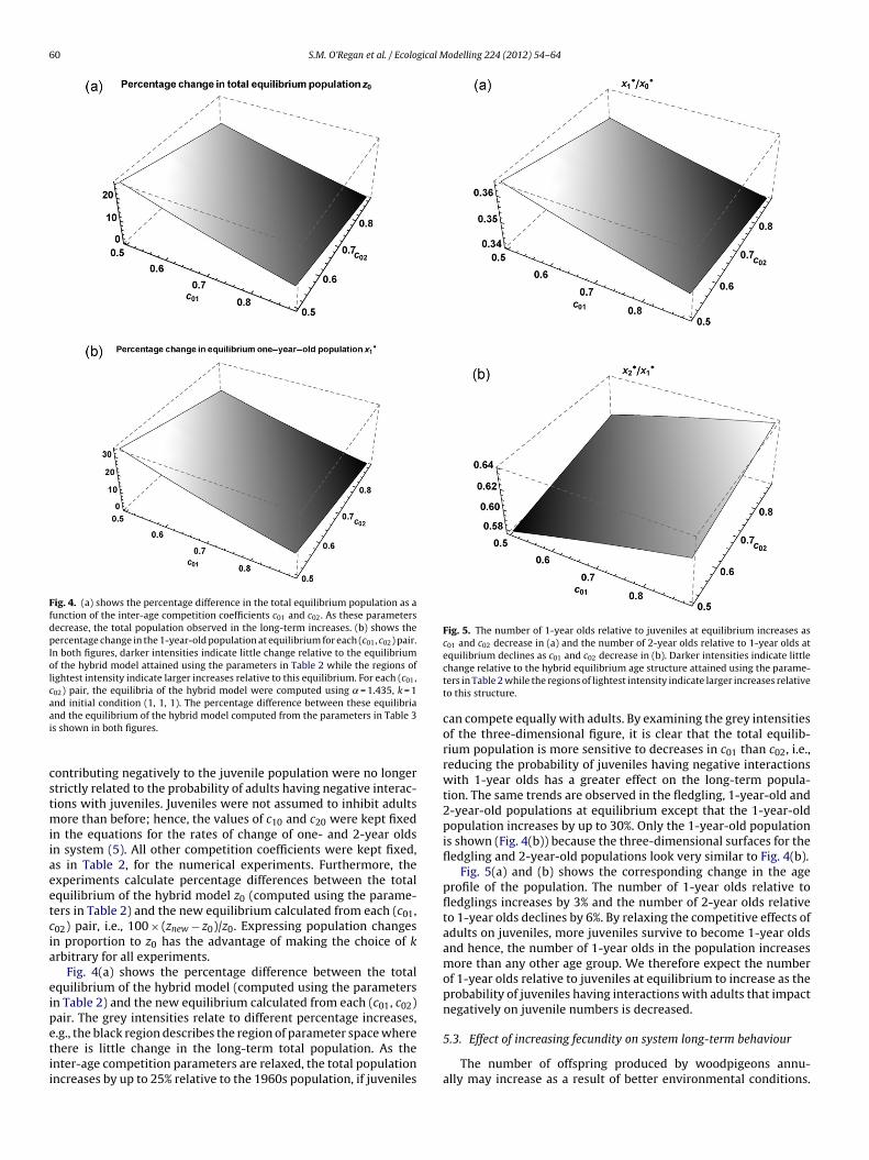

60 S.M. O’Regan et al. / Ecological Modelling 224 (2012) 54– 64

Fig. 4. (a) shows the percentage difference in the total equilibrium population as afunction of the inter-age competition coefficients c01 and c02. As these parametersdecrease, the total population observed in the long-term increases. (b) shows thepercentage change in the 1-year-old population at equilibrium for each (c01, c02) pair.In both figures, darker intensities indicate little change relative to the equilibriumof the hybrid model attained using the parameters in Table 2 while the regions oflightest intensity indicate larger increases relative to this equilibrium. For each (c01,c02) pair, the equilibria of the hybrid model were computed using = 1.435, k = 1and initial condition (1, 1, 1). The percentage difference between these equilibriaai

cstmiiaeetcia

eipetii

Fig. 5. The number of 1-year olds relative to juveniles at equilibrium increases asc01 and c02 decrease in (a) and the number of 2-year olds relative to 1-year olds at

nd the equilibrium of the hybrid model computed from the parameters in Table 3s shown in both figures.

ontributing negatively to the juvenile population were no longertrictly related to the probability of adults having negative interac-ions with juveniles. Juveniles were not assumed to inhibit adults

ore than before; hence, the values of c10 and c20 were kept fixedn the equations for the rates of change of one- and 2-year oldsn system (5). All other competition coefficients were kept fixed,s in Table 2, for the numerical experiments. Furthermore, thexperiments calculate percentage differences between the totalquilibrium of the hybrid model z0 (computed using the parame-ers in Table 2) and the new equilibrium calculated from each (c01,02) pair, i.e., 100 × (znew − z0)/z0. Expressing population changesn proportion to z0 has the advantage of making the choice of krbitrary for all experiments.

Fig. 4(a) shows the percentage difference between the totalquilibrium of the hybrid model (computed using the parametersn Table 2) and the new equilibrium calculated from each (c01, c02)air. The grey intensities relate to different percentage increases,.g., the black region describes the region of parameter space where

here is little change in the long-term total population. As thenter-age competition parameters are relaxed, the total populationncreases by up to 25% relative to the 1960s population, if juveniles

equilibrium declines as c01 and c02 decrease in (b). Darker intensities indicate littlechange relative to the hybrid equilibrium age structure attained using the parame-ters in Table 2 while the regions of lightest intensity indicate larger increases relativeto this structure.

can compete equally with adults. By examining the grey intensitiesof the three-dimensional figure, it is clear that the total equilib-rium population is more sensitive to decreases in c01 than c02, i.e.,reducing the probability of juveniles having negative interactionswith 1-year olds has a greater effect on the long-term popula-tion. The same trends are observed in the fledgling, 1-year-old and2-year-old populations at equilibrium except that the 1-year-oldpopulation increases by up to 30%. Only the 1-year-old populationis shown (Fig. 4(b)) because the three-dimensional surfaces for thefledgling and 2-year-old populations look very similar to Fig. 4(b).

Fig. 5(a) and (b) shows the corresponding change in the ageprofile of the population. The number of 1-year olds relative tofledglings increases by 3% and the number of 2-year olds relativeto 1-year olds declines by 6%. By relaxing the competitive effects ofadults on juveniles, more juveniles survive to become 1-year oldsand hence, the number of 1-year olds in the population increasesmore than any other age group. We therefore expect the numberof 1-year olds relative to juveniles at equilibrium to increase as theprobability of juveniles having interactions with adults that impactnegatively on juvenile numbers is decreased.

5.3. Effect of increasing fecundity on system long-term behaviour

The number of offspring produced by woodpigeons annu-ally may increase as a result of better environmental conditions.

S.M. O’Regan et al. / Ecological Modelling 224 (2012) 54– 64 61

1.5 2.0 2.5 3.0 3.5 4.0 4.5 5.00

100

200

300

400

Fecundity α

Incr

ease

z0

x2

x1

x0

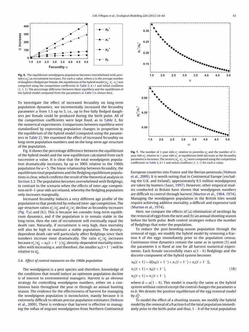
Fig. 6. The equilibrium woodpigeon population becomes overwhelmed with juve-niles (x∗

0) as recruitment increases. For each value, where is the average numberof daughters fledged per female, the equilibrium of the hybrid model (x∗

0, x∗1, x∗

2) wasc(t

Tpptttsttlo

ostpetSito

pa(rldwdnbsr

5

tiststeei

1.5 2.0 2.5 3.0 3.5 4.0 4.5 5.0

0.15

0.20

0.25

0.30

α

x 1x 0

1.5 2.0 2.5 3.0 3.5 4.0 4.5 5.0

0.50

0.55

0.60

α

x 2x 1

Fig. 7. The number of 1-year olds x∗1 relative to juveniles x∗

0 and the number of 2-

omputed using the competition coefficients in Table 2, k = 1 and initial condition1, 1, 1). The percentage difference between these equilibria and the equilibrium ofhe hybrid model computed from the parameters in Table 2 is shown here.

o investigate the effect of increased fecundity on long-termopulation dynamics, we incrementally increased the fecundityarameter from 1.5 up to 5, i.e., up to five fully fledged daugh-ers per female could be produced during the birth pulse. All ofhe competition coefficients were kept fixed, as in Table 2, forhe numerical experiments. Comparisons between equilibria weretandardised by expressing population changes in proportion tohe equilibrium of the hybrid model (computed using the parame-ers in Table 2). We examined the effect of increased fecundity onong-term population numbers and on the long-term age structuref the population.

Fig. 6 shows the percentage difference between the equilibriumf the hybrid model and the new equilibrium calculated from eachuccessive value. It is clear that the total woodpigeon popula-ion dramatically increases, by up to 300% relative to the 1960sopulation for = 5. The linear relationship between fecundity, thequilibrium total populations and the fledgling equilibrium popula-ions is clear, which confirms the result of the theoretical analysis inection 3.3. The population becomes overwhelmed with fledglings,n contrast to the scenario when the effects of inter-age competi-ion on 0–1-year olds are relaxed, whereby the fledgling populationnly increases marginally.

Increased fecundity induces a very different age profile of theopulation to that predicted by reduced inter-age competition. Thege structure ratios x∗

1/x∗0 and x∗

2/x∗1 decline as fecundity increases

Fig. 7(a) and (b)). This is because we consider long-term equilib-ium dynamics, and if the population is to remain stable in theong-term, then the rate of recruitment will eventually equal theeath rate. Naturally, if recruitment is very high, then mortalityill also be high to maintain a stable population. The density-ependent death rate will particularly affect fledglings since theirumbers increase most dramatically. The ratio x∗

1/x∗0 increases

ecause x∗1/x∗

0 = x0(t + 1−)/x∗0; density-dependent mortality inten-

ifies with increasing ˛, and therefore, the smaller x0(t + 1−) will beelative to x∗

0.

.4. Effect of control measures on the 1960s population

The woodpigeon is a pest species and therefore, knowledge ofhe conditions that would induce an optimum population declines of interest to environmental managers. Harvest is an obvioustrategy for controlling woodpigeon numbers, either on a con-inuous basis throughout the year or through an annual huntingeason. The evidence for the effectiveness of harvest for managing

he woodpigeon population is inconclusive, mainly because it isxtremely difficult to obtain precise population estimates (Hobsont al., 2009). There is evidence that harvest is effective in manag-ng the influx of migrant woodpigeons from Northern Continental

year olds x∗2 relative to 1-year olds x∗

1 at equilibrium both decrease as the fecundityparameter increases. The vectors (x∗

0, x∗1, x∗

2) were computed using the competitioncoefficients in Table 2, k = 1 and initial condition (1, 1, 1) for each value.

European countries into France and the Iberian peninsula (Hobsonet al., 2009). It is worth noting that in Continental Europe (exclud-ing the U.K. and Ireland), approximately 9.5 million woodpigeonsare taken by hunters (Saari, 1997). However, other empirical stud-ies conducted in Britain have shown that woodpigeon numbersare difficult to control through harvest (Murton et al., 1964, 1974).Managing the woodpigeon population in the British Isles wouldrequire achieving additive mortality, a difficult and expensive task(Murton et al., 1974).

Here, we compare the effects of (a) elimination of nestlings bythe removal of eggs from the nest and (b) an annual shooting seasonbefore the birth pulse. Both control strategies reduce the numberof fledglings that enter the population.

To reduce the post-breeding-season population through theremoval of eggs, we modify the hybrid model by removing a frac-tion h of the eggs immediately prior to the population census.Continuous-time dynamics remain the same as in system (5) andthe parameter k is fixed at one for all harvest numerical experi-ments. Each female successfully rears ˛(1 − h) fledglings and thediscrete component of the hybrid system becomes

x0(t + 1) = ˜ [x0(t + 1−) + x1(t + 1−) + x2(t + 1−)],

x1(t + 1) = x0(t + 1−),

x2(t + 1) = x1(t + 1−),

(18)

where ˜ = ˛(1 − h). This model is exactly the same as the hybridsystem without control except the control changes the parameter ˛to ˜ . We denote the positive equilibrium of the egg removal model

by zh1

0 .To model the effect of a shooting season, we modify the hybrid

model by the removal of a fraction h of the total population immedi-ately prior to the birth-pulse and thus, 1 − h of the total population

62 S.M. O’Regan et al. / Ecological Modelling 224 (2012) 54– 64

0.2 0.4 0.6 0.8h

20

40

60

80

100

Diff

eren

ce

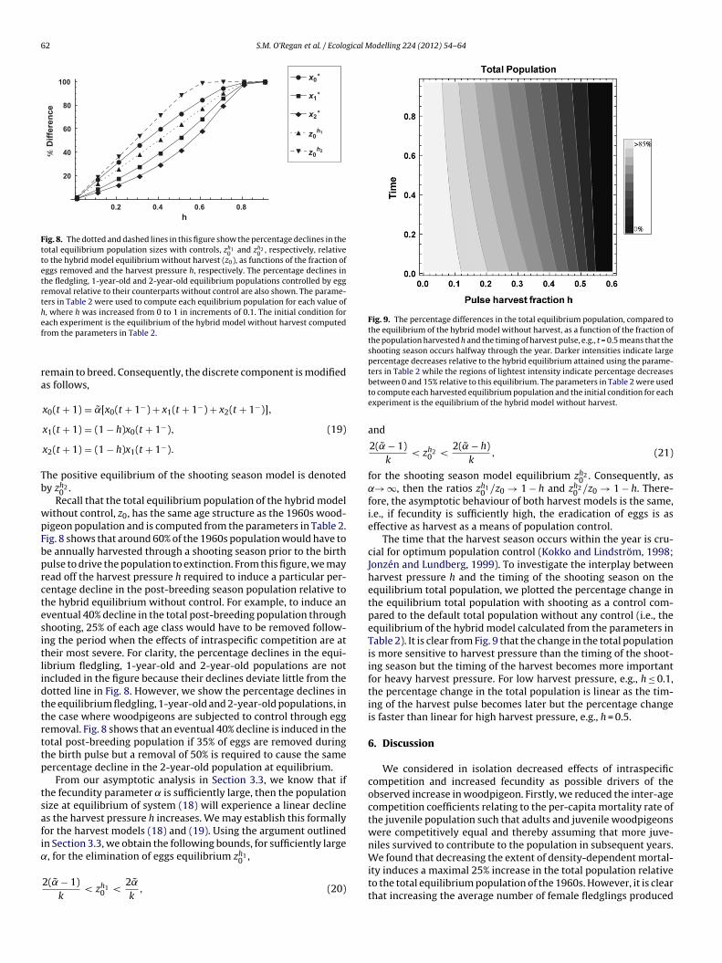
Fig. 8. The dotted and dashed lines in this figure show the percentage declines in thetotal equilibrium population sizes with controls, zh1

0 and zh20 , respectively, relative

to the hybrid model equilibrium without harvest (z0), as functions of the fraction ofeggs removed and the harvest pressure h, respectively. The percentage declines inthe fledgling, 1-year-old and 2-year-old equilibrium populations controlled by eggremoval relative to their counterparts without control are also shown. The parame-ters in Table 2 were used to compute each equilibrium population for each value ofh, where h was increased from 0 to 1 in increments of 0.1. The initial condition foref

ra

Tb

wpFbprctesitlidttrttp

tsafi˛

Fig. 9. The percentage differences in the total equilibrium population, compared tothe equilibrium of the hybrid model without harvest, as a function of the fraction ofthe population harvested h and the timing of harvest pulse, e.g., t = 0.5 means that theshooting season occurs halfway through the year. Darker intensities indicate largepercentage decreases relative to the hybrid equilibrium attained using the parame-ters in Table 2 while the regions of lightest intensity indicate percentage decreases

We found that decreasing the extent of density-dependent mortal-

ach experiment is the equilibrium of the hybrid model without harvest computedrom the parameters in Table 2.

emain to breed. Consequently, the discrete component is modifieds follows,

x0(t + 1) = ˜ [x0(t + 1−) + x1(t + 1−) + x2(t + 1−)],

x1(t + 1) = (1 − h)x0(t + 1−),

x2(t + 1) = (1 − h)x1(t + 1−).

(19)

he positive equilibrium of the shooting season model is denotedy zh2

0 .Recall that the total equilibrium population of the hybrid model

ithout control, z0, has the same age structure as the 1960s wood-igeon population and is computed from the parameters in Table 2.ig. 8 shows that around 60% of the 1960s population would have toe annually harvested through a shooting season prior to the birthulse to drive the population to extinction. From this figure, we mayead off the harvest pressure h required to induce a particular per-entage decline in the post-breeding season population relative tohe hybrid equilibrium without control. For example, to induce anventual 40% decline in the total post-breeding population throughhooting, 25% of each age class would have to be removed follow-ng the period when the effects of intraspecific competition are atheir most severe. For clarity, the percentage declines in the equi-ibrium fledgling, 1-year-old and 2-year-old populations are notncluded in the figure because their declines deviate little from theotted line in Fig. 8. However, we show the percentage declines inhe equilibrium fledgling, 1-year-old and 2-year-old populations, inhe case where woodpigeons are subjected to control through eggemoval. Fig. 8 shows that an eventual 40% decline is induced in theotal post-breeding population if 35% of eggs are removed duringhe birth pulse but a removal of 50% is required to cause the sameercentage decline in the 2-year-old population at equilibrium.

From our asymptotic analysis in Section 3.3, we know that ifhe fecundity parameter is sufficiently large, then the populationize at equilibrium of system (18) will experience a linear declines the harvest pressure h increases. We may establish this formallyor the harvest models (18) and (19). Using the argument outlinedn Section 3.3, we obtain the following bounds, for sufficiently large, for the elimination of eggs equilibrium zh1

0 ,

2( ˜ − 1)k

< zh10 <

2 ˜k

, (20)

between 0 and 15% relative to this equilibrium. The parameters in Table 2 were usedto compute each harvested equilibrium population and the initial condition for eachexperiment is the equilibrium of the hybrid model without harvest.

and

2( ˜ − 1)k

< zh20 <

2( ˜ − h)k

, (21)

for the shooting season model equilibrium zh20 . Consequently, as

˛→ ∞, then the ratios zh10 /z0 → 1 − h and zh2

0 /z0 → 1 − h. There-fore, the asymptotic behaviour of both harvest models is the same,i.e., if fecundity is sufficiently high, the eradication of eggs is aseffective as harvest as a means of population control.

The time that the harvest season occurs within the year is cru-cial for optimum population control (Kokko and Lindström, 1998;Jonzén and Lundberg, 1999). To investigate the interplay betweenharvest pressure h and the timing of the shooting season on theequilibrium total population, we plotted the percentage change inthe equilibrium total population with shooting as a control com-pared to the default total population without any control (i.e., theequilibrium of the hybrid model calculated from the parameters inTable 2). It is clear from Fig. 9 that the change in the total populationis more sensitive to harvest pressure than the timing of the shoot-ing season but the timing of the harvest becomes more importantfor heavy harvest pressure. For low harvest pressure, e.g., h ≤ 0.1,the percentage change in the total population is linear as the tim-ing of the harvest pulse becomes later but the percentage changeis faster than linear for high harvest pressure, e.g., h = 0.5.

6. Discussion

We considered in isolation decreased effects of intraspecificcompetition and increased fecundity as possible drivers of theobserved increase in woodpigeon. Firstly, we reduced the inter-agecompetition coefficients relating to the per-capita mortality rate ofthe juvenile population such that adults and juvenile woodpigeonswere competitively equal and thereby assuming that more juve-niles survived to contribute to the population in subsequent years.

ity induces a maximal 25% increase in the total population relativeto the total equilibrium population of the 1960s. However, it is clearthat increasing the average number of female fledglings produced

gical M

pts(oicwyiItd

mistutegewa

tldsW1ttpW

WitsnibiewiaHmfop

6

sshtpeil

S.M. O’Regan et al. / Ecolo

er female per birth-pulse has a much more dramatic effect onhe equilibrium population size than increasing the numbers thaturvive the density-dependent process of intraspecific competitioncf. Figs. 4(a) and 6). When we increase the reproductive outputf females, the post-birth-pulse equilibrium fledgling populationncreases by 400%. The increase in fledglings is much more dramaticompared to those of the 1- and 2-year-old age classes. In contrast,hen we relax the inhibitive effects of adults on juveniles, the 1-

ear-old population at equilibrium undergoes a larger percentagencrease (up to 30%) than the juvenile and 2-year-old age classes.t is useful to note that x∗

1/x∗0 declines as recruitment increases but

he ratio increases if competition is relaxed. Such contrasting ageistributions offer predictions that may be tested in the field.

If increased fecundity is driving the population increase, ourodel predicts that density-dependent mortality should also

ncrease to retain equilibrium population dynamics. However,ince woodpigeon numbers have been increasing consistently sincehe mid 1970s (Baillie et al., 2009), it appears that the current pop-lation has not yet reached its carrying capacity determined byhe environment. Future empirical investigations should focus onxploring the hypothesis that as a result of the lengthening of therowing season, the maximum number of woodpigeons that thenvironment can hold is increasing slowly year on year, i.e., theoodpigeon population is no longer regulated by seasonal fluctu-

tions in its food supply.The competition coefficients of system (5) are defined in terms of

he relative competitive ability parameters, which are dimension-ess. It is difficult to establish empirically how different mechanismsetermine the values of the coefficients (Tilman, 1982), or thetrengths of interactions in food webs in general (Laska and

ootton, 1998); a variety of approaches may be used (MacArthur,970; Case and Gilpin, 1974; Berlow et al., 2004). To estimatehe strengths of interaction empirically, explicit modeling assump-ions for the competition coefficients, which we have made in thisaper, can clarify the most important data for collection (Laska andootton, 1998).However, there are some limitations to our modeling approach.

e assume that all fledglings are produced in a single pulse, result-ng in a sudden increase in fledglings each year. In the 1960s,here was strong evidence that there was a single breeding sea-on each year (Murton and Isaacson, 1964). Although this mayot currently be the case, a single breeding season is reasonable

f we assume that a pair may successfully fledge more than onerood during this period (i.e., the fecundity parameter increases

n our model). Furthermore, the survival probability and fecunditystimates that we used to parameterize the Leslie matrix modelere annual estimates. If reproductive output has indeed increased,

t may be appropriate to model the creation of new fledglingss a series of equally-spaced birth pulses throughout the year.owever, an intensive data collection campaign using capture-ark-recapture methods would be required to obtain survival and

ecundity estimates over a shorter time frame, e.g., three monthsr six months, to parameterize a hybrid model with multiple birthulses.

.1. The effect of control

We examined the effect of two harvest strategies, a hunting sea-on and removal of eggs, on long-term population dynamics. Bothtrategies were implemented after density-dependent mortalityad taken place. We found that an annual shooting season, whichargets all age groups, is more effective than annually removing a

roportion of eggs laid during the birth-pulse. Harvest induces a lin-ar decline in all age groups but egg removal causes a slower declinen the 1- and 2-year-old populations at equilibrium, particularly forow values of fecundity (Fig. 8). If fecundity is sufficiently large, the

odelling 224 (2012) 54– 64 63

asymptotic analysis in Section 5.4 shows that the effects of bothcontrol measures on the total equilibrium population sizes zh1

0 andzh2

0 are similar. However, the corresponding age structures of theequilibrium populations are different. The population controlledby the eradication of eggs will contain more 1- and 2-year oldsat equilibrium than the population controlled by shooting. Clearlyadult woodpigeons have higher reproductive value than woodpi-geons in their first calendar year, which suggests that an annualharvest season would be a more effective control strategy than theremoval of eggs from nests.

We found that intense harvest pressure, coupled with a shoot-ing season that follows the period of density-dependent mortality,leads to the most dramatic decline in the woodpigeon population.Fig. 9 confirms that there is a synergistic effect between late timingof the harvest pulse and heavy harvest pressure. This synergisticeffect is not observed for low harvest pressure values, as the timingof the harvest pulse occurs at later intervals. The correct timingof the hunting season is very important to avoid compensationfor harvest mortality through other means (Kokko and Lindström,1998; Choisy and Rohani, 2006). If a sequence of density-dependentprocesses occur after the harvest season, then compensation mayoccur but it depends on the order of occurrence of these pro-cesses (Aström et al., 1996; Boyce et al., 1999; Jonzén and Lundberg,1999; Ratikainen et al., 2008). The harvest models (18) and (19) donot exhibit compensation; the equilibrium population size alwaysdeclines as a result of control because the harvest and reproductionprocesses are linear mappings.

6.2. Conclusions

Although the growth of the woodpigeon population is a seri-ous problem, to our knowledge, no mathematical models havebeen constructed to clarify the drivers of woodpigeon populationdynamics. Using a hybrid model, we showed that increased repro-ductive output of all age groups during the breeding season is amore likely mechanism behind the sustained increase in the wood-pigeon population than a decline in density-dependent mortality.This conclusion is consistent with the empirical findings of Ingliset al. (1994), who conducted a long-term study of the breeding biol-ogy of the woodpigeon in Carlton, England. Moreover, our resultsoffer two different predictions for the age structure of the wood-pigeon population (cf. Figs. 5(a), (b) and 7(a) and (b)), which couldbe tested experimentally. Finally, the hybrid model may be readilyadapted to describe the population dynamics of other Columbidaespecies such as the collared dove (Streptopelia decaocto), which hasrapidly increased in abundance in North America since the 1970s(Hengeveld, 1993).

Acknowledgements

S.M. O’Regan was supported by the Irish Research Council forScience, Engineering and Technology (IRCSET), under the EmbarkInitiative Postgraduate Funding Scheme. A. Pokrovskii and D.Rachinskii were supported by Federal Programme ‘Scientists ofInnovative Russia’, grant 2009-1.5-507-007 and Russian Founda-tion of Basic Research, grant 10-01-93112. The authors wish tothank L. Kalachev, M. Wilson and three anonymous reviewers forvaluable comments on the manuscript. This paper is dedicated tothe memory of Alexei Pokrovskii.

Appendix A.

The explicit solution of Eq. (7) at time t is

z(t) = 2z(0)2 + kz(0)t

. (A.1)

6 gical M

Hj

z

Ubt

z

Ee

k

EFtzs

k

R

A

B

B

B

C

C

C

C

C

D

G

H

H

H

4 S.M. O’Regan et al. / Ecolo

ence, at equilibrium, the total population at the end of one yearust before the birth pulse, which we denote by z1, is given by

1 = 2z0

2 + kz0. (A.2)

sing relationship (10), which describes the stationary age distri-ution, we may determine the total population at equilibrium prioro the birth pulse,

1 = ˇ0(1 + ˇ1 + ˇ21)z0

1 + ˇ0 + ˇ0ˇ1. (A.3)

quating expressions (A.2) and (A.3), we obtain the followingxpression for k in terms of the total population z0:

= 2(1 − ˇ0ˇ21)

ˇ0(1 + ˇ1 + ˇ21)z0

. (A.4)

q. (A.4) is used to compute the characteristic time of system (5).inally, recall that at equilibrium, the age structure of the popula-ion is given by the stationary age distribution (10) and therefore,0 = x∗

0 + ˇ0x∗0 + ˇ0ˇ1x∗

0. Hence, we obtain the following expres-ion for k in terms of a given fledgling population x∗

0,

= 2(1 − ˇ0ˇ21)

x∗0ˇ0(1 + ˇ0 + ˇ0ˇ1)(1 + ˇ1 + ˇ2

1). (A.5)

eferences

˚ ström, M., Lundberg, P., Lundberg, S., 1996. Population dynamics with sequentialdensity-dependence. Oikos 75, 174–181.

aillie, S.R., Marchant, J.H., Leech, D.I., Joys, A.C., Noble, D.G., Barimore, C.,et al., 2010. Breeding Birds in the Wider Countryside: Their ConservationStatus 2009. BTO, Thetford. BTO Research Report No. 541. Available from:http://www.bto.org/birdtrends.

erlow, E.L., Neutel, A.-M., Cohen, J.E., De Ruiter, P.C., Ebenman, B., Emmerson, M.,et al., 2004. Interaction strengths in food webs: issues and opportunities. J. Anim.Ecol. 73, 585–598.

oyce, M.S., Sinclair, A.R.E., White, G.C., 1999. Seasonal compensation of predationand harvesting. Oikos 87, 419–426.

arroll, E., Sparks, A., Donnelly, A., Cooney, T., 2009. Irish phenological observa-tions from the early 20th century reveal a strong response to temperature. Biol.Environ. 109B, 115–126.

ase, T.J., Gilpin, M.E., 1974. Interference competition and niche theory. Proc. Natl.Acad. Sci. U.S.A. 71, 3073–3077.

aswell, H., 2001. Matrix Population Models: Construction, Analysis and Interpre-tation, 2nd ed. Sinauer Associates Inc., Sunderland, MA.

hoisy, M., Rohani, P., 2006. Harvesting can increase severity of wildlife diseaseepidemics. Proc. Biol. Sci. 273, 2025–2034.

rowe, O., Coombs, R.H., Lysaght, L., O’Brien, C., Choudhury, K.R., Walsh, A.J., et al.,2010. Population trends of widespread breeding birds in the Republic of Ireland1998–2008. Bird Study 57, 267–280.

onnelly, A., Cooney, T., Jennings, E., Buscardo, E., Jones, M., 2009. Response ofbirds to climatic variability; evidence from the western fringe of Europe. Int.J. Biometeorol. 53, 211–220.

eritz, S.A.H., Kisdi, É., 2004. On the mechanistic underpinning of discrete-timepopulation models with complex dynamics. J. Theor. Biol. 228, 261–269.

engeveld, R., 1993. What to do about the North American invasion by the CollaredDove? J. Field Ornithol. 64, 477–489.

obson, K.A., Lormee, H., Van Wilgenburg, S.L., Wassenaar, L.I., Boutin, J.M., 2009.Stable isotopes (dD) delineate the origins and migratory connectivity of har-

vested animals: the case of European woodpigeons. J. Appl. Ecol. 46, 572–582.

oughton, J.T., Ding, Y., Griggs, D.J., Noguer, M., Van der Linden, P.J., Dai, X., et al.(Eds.), 2001. Climate Change 2001: The Scientific Basis: Contribution of Work-ing Group I to the Third Assessment Report of the Intergovernmental Panel onClimate Change. Cambridge University Press, Cambridge.

odelling 224 (2012) 54– 64

Inglis, I.R., Issacson, A.J., Thearle, R.J.P., Westwood, N.J., 1990. The effects of changingagricultural practice upon woodpigeon Columba palumbus numbers. Ibis 132,262–272.

Inglis, I.R., Issacson, A.J., Thearle, R.J.P., 1994. Long term changes in the breedingbiology of the woodpigeon Columba palumbus in eastern England. Ecography17, 182–188.

Ives, A.R., Gross, K., Jansen, V.A.A., 2000. Periodic mortality events in predator–preysystems. Ecology 81, 3330–3340.

Jiguet, F., Gadot, A-S., Julliard, R., Newson, S.E., Couvet, D., 2007. Climate envelope,life history traits and the resilience of birds facing global change. Glob. ChangeBiol. 13, 1672–1684.

Kokko, H., Lindström, J., 1998. Seasonal density dependence, timing of mortality andsustainable harvesting. Ecol. Modell. 110, 293–304.

Jonzén, N., Lundberg, P., 1999. Temporally structured density-dependence and pop-ulation management. Ann. Zool. Fenn. 36, 39–44.

Lack, D., 1966. Population Studies of Birds, 1st ed. Oxford University Press, London.Laska, M.S., Wootton, J.T., 1998. Theoretical concepts and empirical approaches to

measuring interaction strength. Ecology 79, 461–476.Leslie, P.H., 1945. On the use of matrices in certain population mathematics.

Biometrika 33, 183–212.Lebreton, J.-D., 2009. Assessing density-dependence: where are we left? In: Thom-

son, D.L., Cooch, E.G., Conroy, M.J. (Eds.), Modeling Demographic Processes inMarked Populations. Springer, New York, pp. 19–32.

MacArthur, R.H., 1970. Species packing and competitive equilibria for many species.Theor. Popul. Biol. 1, 1–11.

Mailleret, L., Lemesle, V., 2009. A note on semi-discrete modelling in the life sciences.Phil. Trans. Math Phys. Eng. Sci. 367, 4779–4799.

Menzel, A., Sparks, T.H., Estrella, N., Koch, E., Aasa, A., Ahas, R., et al., 2006. Europeanphenological response to climate change matches the warming pattern. Glob.Change Biol. 12, 1969–1976.

Møller, A.P., Flensted-Jensen, E., Klarborg, K., Mardal, W., Nielsen, J.T., 2010. Climatechange affects the duration of the reproductive season in birds. J. Anim. Ecol. 79,777–784.

Murton, R.K., 1958. The breeding of wood-pigeon populations. Bird Study 5,177–183.

Murton, R.K., 1961. Some survival estimates for the wood-pigeon. Bird Study 8,165–173.

Murton, R.K., 1965. The Wood-pigeon, 1st ed. Collins Clear-Type Press, London.Murton, R.K., 1966. A statistical evaluation of the effect of wood-pigeon shoot-

ing as evidenced by the recoveries of ringed birds. Statistician 16, 183–202.

Murton, R.K., 1971. The significance of a specific search image in the feedingbehaviour of the wood-pigeon. Behaviour 40, 10–42.

Murton, R.K., Isaacson, A.J., 1964. Productivity and egg predation in the woodpigeon.Ardea 52, 30–47.

Murton, R.K., Isaacson, A.J., Westwood, N.J., 1966. The relationships between wood-pigeons and their clover food supply and the mechanism of population control.J. Appl. Ecol. 3, 55–96.

Murton, R.K., Isaacson, A.J., Westwood, N.J., 1971. The significance of gregariousfeeding behaviour and adrenal stress in a population of Wood-pigeons Columbapalumbus. J. Zool. Lond. 165, 53–84.

Murton, R.K., Westwood, N.J., Isaacson, A.J., 1964. A preliminary investigation of thefactors regulating population size in the woodpigeon Columba palumbus. Ibis106, 482–507.

Murton, R.K., Westwood, N.J., Isaacson, A.J., 1974. A study of woodpigeon shooting:the exploitation of a natural animal population. J. Appl. Ecol. 11, 61–81.

Newton, I., 1998. Population Limitation in Birds, 1st ed. Academic Press, San Diego.Pachepsky, E., Nisbet, R.M., Murdoch, W.W., 2008. Between discrete and contin-

uous: consumer-resource dynamics with synchronized reproduction. Ecology89, 280–288.

Ratikainen, I.I., Gill, J.A., Gunnarsson, T.G., Sutherland, W.J., Kokko, H., 2008. Whendensity dependence is not instantaneous: theoretical developments and man-agement implications. Ecol. Lett. 11, 184–198.

Saari, L., 1997. Woodpigeon. In: Hagemeijer, E.J.M., Blair, M.J. (Eds.), The EBCC Atlasof European Breeding Birds. Their Distribution and Abundance. T & A.D. Poyser,London, pp. 384–385.

Singh, A., Nisbet, R.M., 2007. Semi-discrete host–parasitoid models. J. Theor. Biol.

247, 733–742.

Tayleur, J., 2008. Controlling woodpigeon damage to brassica crops. BTO News,March–April, 19–20.

Tilman, D., 1982. Resource Competition and Community Structure, 1st ed. PrincetonUniversity Press, Princeton, NJ.