the long-lasting momentum in weekly returns
TRANSCRIPT
THE JOURNAL OF FINANCE • VOL. LXIII, NO. 1 • FEBRUARY 2008
The Long-Lasting Momentum in Weekly Returns
ROBERTO C. GUTIERREZ JR. and ERIC K. KELLEY∗
ABSTRACT
Reversal is the current stylized fact of weekly returns. However, we find that anopposing and long-lasting continuation in returns follows the well-documented briefreversal. These subsequent momentum profits are strong enough to offset the initialreversal and to produce a significant momentum effect over the full year followingportfolio formation. Thus, ex post, extreme weekly returns are not too extreme. Ourfindings extend to weekly price movements with and without public news. In addi-tion, there is no relation between news uncertainty and the momentum in 1-weekreturns.
RETURNS OF INDIVIDUAL STOCKS reverse in the short run. Lehmann (1990) andJegadeesh (1990) find that stocks with the lowest returns over the prior week ormonth outperform stocks with the highest returns over the prior period. Giventhese findings, the literature currently views extreme weekly returns as largerthan those warranted by a stock’s fundamentals, due to overreaction and/orto microstructural issues. However, we find evidence suggesting that extremeweekly returns are not extreme enough: Despite the brief reversal documentedby prior research, abnormal returns over the 52 weeks following an extremeweekly return are actually in the same direction as those in the extreme week.In other words, we find return momentum in a new and seemingly unexpectedplace—weekly returns.
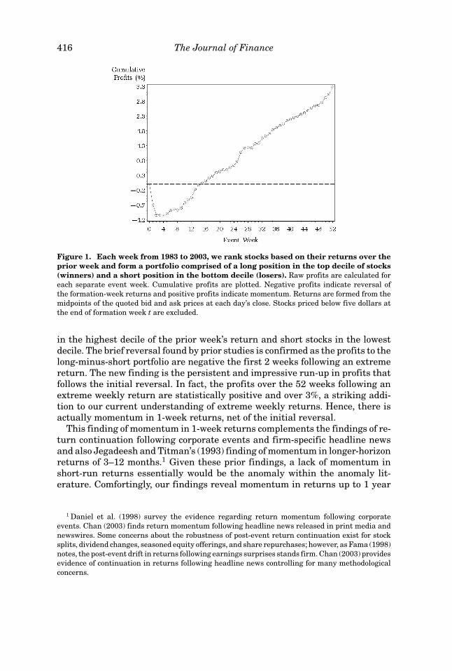
While prior studies examine the performance of stocks with extreme weeklyreturns for only a few weeks, which is the duration of the reversal, momentumprofits emerge several weeks after an extreme return and persist over the re-mainder of the year. The momentum that we document easily offsets the briefand initial reversal in returns. Figure 1 depicts this result (the figure is illus-trative only; our statistical methods are based on calendar time, not the eventtime shown in the figure). Each week we construct a portfolio that is long stocks
∗Gutierrez is at the Lundquist College of Business, University of Oregon. Kelley is at the EllerCollege of Management, University of Arizona. We thank two anonymous referees, Rob Stambaugh,Wayne Ferson, Christo Pirinsky, and seminar participants at Auburn University, Indiana Univer-sity at South Bend, Rutgers University at Camden, Texas A&M University, Texas Tech University,University of Arizona, University of Oregon, University of Utah, Washington State University, andthe 2004 Financial Management Association Meetings for their comments. Special thanks go toWes Chan for graciously providing his data on headline news and to Ekkehart Boehmer and JerryMartin for data assistance. Kelley acknowledges financial support from the Mays Post-DoctoralFellowship at Mays Business School, Texas A&M University. Kelley also completed a portion of thiswork while on the faculty at the College of Business and Economics, Washington State University.Any errors are ours.
415
416 The Journal of Finance
Figure 1. Each week from 1983 to 2003, we rank stocks based on their returns over theprior week and form a portfolio comprised of a long position in the top decile of stocks(winners) and a short position in the bottom decile (losers). Raw profits are calculated foreach separate event week. Cumulative profits are plotted. Negative profits indicate reversal ofthe formation-week returns and positive profits indicate momentum. Returns are formed from themidpoints of the quoted bid and ask prices at each day’s close. Stocks priced below five dollars atthe end of formation week t are excluded.
in the highest decile of the prior week’s return and short stocks in the lowestdecile. The brief reversal found by prior studies is confirmed as the profits to thelong-minus-short portfolio are negative the first 2 weeks following an extremereturn. The new finding is the persistent and impressive run-up in profits thatfollows the initial reversal. In fact, the profits over the 52 weeks following anextreme weekly return are statistically positive and over 3%, a striking addi-tion to our current understanding of extreme weekly returns. Hence, there isactually momentum in 1-week returns, net of the initial reversal.
This finding of momentum in 1-week returns complements the findings of re-turn continuation following corporate events and firm-specific headline newsand also Jegadeesh and Titman’s (1993) finding of momentum in longer-horizonreturns of 3–12 months.1 Given these prior findings, a lack of momentum inshort-run returns essentially would be the anomaly within the anomaly lit-erature. Comfortingly, our findings reveal momentum in returns up to 1 year
1 Daniel et al. (1998) survey the evidence regarding return momentum following corporateevents. Chan (2003) finds return momentum following headline news released in print media andnewswires. Some concerns about the robustness of post-event return continuation exist for stocksplits, dividend changes, seasoned equity offerings, and share repurchases; however, as Fama (1998)notes, the post-event drift in returns following earnings surprises stands firm. Chan (2003) providesevidence of continuation in returns following headline news controlling for many methodologicalconcerns.
The Long-Lasting Momentum in Weekly Returns 417
to be a remarkably pervasive phenomenon. This observation should benefitresearchers attempting to understand the momentum anomaly.2
Our results also provide researchers of the momentum phenomenon a new,and arguably superior, testing ground for their theories. Using weekly returnsto assess potential explanations of momentum affords researchers greater con-fidence in identifying the news that underlies the return. The 6- or 12-monthreturns commonly used to examine momentum theories preclude such identi-fication. We exploit this advantage to revisit two recent studies of the potentialsources of momentum in returns. Neither Chan’s (2003) finding regarding ex-plicit and implicit news nor Zhang’s (2006) finding regarding the uncertaintyof news extends to the momentum in 1-week returns.
Chan (2003) provides evidence that the market underreacts to explicit news,which is firm-specific news that is publicly released, yet overreacts to implicitnews, which is news implied by price changes not accompanied by any publiclyreleased news. In contrast, we find that extreme-return stocks with explicitnews and extreme-return stocks with implicit news behave similarly, both dis-playing short-run reversal and longer-run momentum (as in Figure 1). Thisfinding impedes concluding that the market categorically underreacts to onetype of news and overreacts to another type. Caution should therefore be ex-ercised in modeling traders as strictly overreacting to implicit news, which isthe general notion in the theories of Daniel, Hirshleifer, and Subrahmanyam(1998), Hong and Stein (1999), and Daniel and Titman (2006).
Zhang (2006) considers another potential determinant of momentum. If mo-mentum is a consequence of psychological biases inducing traders to misreactto news, then momentum should increase with the uncertainty in the valua-tion impact of news. This follows from the observation that psychological biasesworsen as the precision of news decreases. However, we find that the momen-tum in 1-week returns is not reliably related to measures of uncertainty.
Regarding the short-run reversal in returns, Jegadeesh and Titman (1995a),Cooper (1999), Subrahmanyam (2005), and others find that bid-ask bounce andother microstructural issues do not fully explain the return reversal.3 Theseresearchers interpret the remaining reversal in returns as evidence of the mar-ket’s overreaction to firm-specific news. On the other hand, Avramov, Chordia,and Goyal (2006) show that weekly reversals are strongest for stocks in whichliquidity is low and turnover is high. They attribute reversal in weekly returnsto price pressure caused by noninformational demand for immediacy.4 Our mo-mentum finding does not discriminate between these two interpretations ofthe brief reversal. For example, it is possible that short-run traders overreact
2 DeBondt and Thaler (1985) and others show that long-horizon returns of 3–5 years reverse.3 Kaul and Nimalendran (1990) and Conrad, Kaul, and Nimalendran (1991) show that part of the
return reversal is due to bid-ask bounce. Lo and MacKinlay (1990) and Boudoukh, Richardson, andWhitelaw (1994) note that nonsynchronous trading contributes to contrarian profits. Jegadeeshand Titman (1995b) observe that market makers set prices in part to control their inventories,which induces a return reversal.
4 Precisely measuring illiquidity is a difficult task, as Avramov et al. (2006) acknowledge. Theyemploy Amihud’s (2002) measure in their study.
418 The Journal of Finance
to news while longer-term traders underreact. Alternatively, the market mightgenerally respond incompletely to all news while sometimes simultaneouslygenerating sufficient price pressure to warrant a brief reversal. Understand-ing the precise sources of short-term reversal in returns remains a task forfuture research.
Regardless of the source of the reversal, our findings speak to the extant viewthat extreme weekly returns are too extreme. The emergence of strong and ul-timately dominant momentum profits a few weeks after an extreme weekly re-turn suggests that on average extreme weekly returns are not extreme enough.Moreover, after eliminating the spurious reversal induced by bid-ask bounce,we find that next-week reversal is largely confined to extreme-return stocks.Thus, our results show that momentum is the larger and more pervasive forcein 1-week returns.
The remainder of the paper is organized as follows. Section I details our dataand testing methods. Section II discusses the performance of weekly portfoliosthat are long winner stocks and short loser stocks, identifying momentum in1-week returns. Section III shows that 1-week momentum is a new finding,independent of the longer-run momentum documented by Jegadeesh and Tit-man (1993). Section IV revisits Chan’s (2003) and Zhang’s (2006) studies usingweekly returns and provides an overview of potential explanations of 1-weekmomentum. Section V further examines the robustness of momentum in short-run returns. Section VI examines the relation between return consistency andthe momentum in short-run returns. Section VII discusses the implications ofour findings for the literature on short-run reversal. Section VIII concludes.
I. Data and Methods
Prior research finds reversal in the weekly returns of individual stocks. Whenusing returns formed with transaction prices, part of this reversal is certainlydue to the spurious negative correlation induced by bid-ask bounce (Roll (1984)).We eliminate this spurious reversal, as Kaul and Nimalendran (1990) andothers do, by using quote data instead of transactions prices. Weekly returnsare based on the midpoint of the final bid and ask quotes from Wednesday toWednesday from 1983 through 2003. Quote data for stocks listed on NYSE andAMEX come from the Institute for the Study of Securities Markets (ISSM) for1983 to 1992 and from the New York Stock Exchange Trades and AutomatedQuotations databases (TAQ) for 1993 to 2003. Closing-quote data for NASDAQstocks come from CRSP. For ISSM and TAQ data, if the final quote of the day isbeyond 10 minutes after the market’s close, we exclude the quote.5 For all stocks,
5 The vast majority of final quotes are recorded within a few minutes of 4:00 p.m.; however,cursory examination of the data reveals some cases in which the final quote appears up to severalhours after the market closes. We use the last quote before 4:10 p.m. to avoid any issues associatedwith late quotes. If a Wednesday price is missing due to a holiday, we use Tuesday’s closing price.Also, price data are missing for NYSE-AMEX stocks on 43 Wednesdays across 1983–1991 and forNASDAQ stocks in February 1986. In later sections when we use multiweek returns, we avoidthe loss of observations surrounding these missing data by computing multiweek returns withWednesday prices adjacent to the missing week(s), adjusting these prices for dividends and splits.
The Long-Lasting Momentum in Weekly Returns 419
we obtain dividend and split data from CRSP and account for these events inour return calculations. We exclude all stocks priced below five dollars at theend of formation week t (to avoid extremely illiquid stocks).
With midpoint returns in hand, we rank all stocks in week t based on thatweek’s return. The stocks in the highest decile are labeled “winners,” and thestocks in the lowest decile are labeled “losers.” Winner and loser portfolios areequally weighted across all component stocks. We then form a portfolio that islong the winner portfolio and short the loser portfolio. In all reported results,negative profits reflect reversal in returns and positive profits reflect momen-tum. To evaluate the performance of the winner-minus-loser portfolio over hold-ing periods longer than 1 week, we employ the calendar-time method advocatedby Fama (1998) and Mitchell and Stafford (2000) and used by Jegadeesh andTitman (1993). The calendar-time method avoids overlapping returns and theaccompanying strongly positive serial correlation in returns while allowing allpossible formation periods to be considered.
Essentially, the calendar-time method overlaps portfolios instead of returns.For example, suppose we wish to evaluate the performance of the portfolios inevent weeks t + 1 to t + 52. In a given calendar week τ , there are 52 strategiesthat week—one formed in week τ − 1, one formed in week τ − 2, and so on. Theprofit in calendar week τ is the equally weighted average of the 52 overlappingcohort portfolios’ profits in that calendar week. Rolling forward to the next week,we drop the oldest portfolio and add the newest portfolio. After computing theequally weighted profit for each calendar week of the sample period, we havea single weekly calendar-time series of profits representing the event windowt + 1 through t + 52. Other event windows are examined similarly.
We consider several metrics for evaluating the performance of the winner-minus-loser portfolio in any given holding-period window. The strategy’s rawprofit for a particular holding period window is simply the mean of the calendar-time series of profits. We also calculate weekly CAPM and Fama-French three-factor alphas by regressing the calendar-time series of winner-minus-loser prof-its on the appropriate factor premia.6
Since we detect positive serial autocorrelation in the profit series, we calcu-late all test statistics using the consistent variance estimator of Gallant (1987).Following Andrews (1991), the bandwidth employed by the estimator is de-termined assuming an AR(1) process and using Andrews’ equations (6.2) and(6.4). Also following Andrews’ recommendation, we examine several alterna-tive bandwidths by adding ±1 and ±2 standard deviations to the autoregres-sive parameter. The number of lags used in estimating the standard errors ofthe portfolio’s profits ranges from 0 to 13. Our findings are robust across thevarious bandwidths.
Two concerns surrounding the use of a calendar-time procedure are the po-tential heteroskedasticity in the portfolio’s profit series and the potential timevariation in the portfolio’s factor loadings. Both of these effects might ariseas the composition of the portfolio changes week by week. However, because
6 We thank Kenneth French for providing daily data on the Fama-French factors and the risk-freerate via his website.
420 The Journal of Finance
Table IProfits to Weekly Extreme Portfolios (Winners minus Losers)
Each week from 1983 to 2003, we rank stocks based on their returns over the week and form aportfolio comprised of a long position in the top decile of stocks (winners) and a short position inthe bottom decile (losers). Returns are formed from the midpoints of the quoted bid and ask pricesat each day’s close. Stocks priced below five dollars at the end of formation week t are excluded.Calendar-time alphas are estimated over various holding periods using raw returns, the CAPM,and the Fama-French three-factor model. The t-statistics are in parentheses and are robust toheteroskedasticity and autocorrelation. Profits are in basis points.
Holding Period
Week Week Week Weeks Weeks1 2 3 4–52 1–52
Raw −70.61 −37.41 0.94 8.11 5.10(−8.10) (−5.67) (0.18) (4.59) (2.85)
CAPM −66.96 −33.30 3.42 8.51 5.67(−7.86) (−5.24) (0.63) (5.21) (3.49)
Fama-French −68.56 −34.27 0.97 8.56 5.60(−8.17) (−5.29) (0.18) (4.75) (3.08)
the winner-minus-loser portfolios select 20% of available stocks each month bydesign, these concerns are mitigated. Additionally, the standard errors in allthe tests are robust to heteroskedasticity as just discussed. Nevertheless, as arobustness check of our findings, we employ a standardization procedure thatcan account for both heteroskedasticity in the profit series and time variationin the factor loadings. The procedure is detailed in Section V.A. Our conclusionsare unaffected by the use of this procedure.
II. Performance of Extreme Weekly Portfolios
We begin by evaluating the performance of stocks with extreme weekly re-turns over a longer horizon than just a few weeks. Table I provides the meanweekly profits to the portfolio of last week’s winner stocks minus last week’sloser stocks over various holding periods. We see that extreme weekly returnsreverse. Reversal in the first week after portfolio formation is strong, averagingaround 69 basis points per week across raw and risk-adjusted metrics. Sincewe are using midpoint returns, bid-ask bounce is clearly not the sole source ofreturn reversal.7 Lo and MacKinlay (1990) and Jegadeesh and Titman (1995a,1995b) identify nonsynchronous trading, inventory management by dealers,
7 Using midpoint returns of NASDAQ stocks from 1983–1990 and using a weighting schemesimilar to Lehmann’s (1990), Conrad, Hameed, and Niden (1994) do not find statistically significantweekly reversal in returns (t = −1.60). We also find no reversal for our winner-minus-loser portfoliousing only NASDAQ stocks over their time period. However, midpoint returns of NASDAQ stocksdo reverse strongly after 1990 and over the full period 1983–2003. So their no-reversal finding isconfined to their sample period. Also, NYSE/AMEX stocks reverse during the 1983 to 1990 periodand over the full period.
The Long-Lasting Momentum in Weekly Returns 421
and investor overreaction to firm-specific news as possible sources of the rever-sal found in Table I.8
Consistent with all three of these hypotheses, and with the empirical evidenceof prior studies, the reversal in returns diminishes quickly and is gone by week3. However, the profit to the portfolio of winners minus losers across [t + 4, t +52] is positive and at least 8.11 basis points per week. This is the central findingof this study. Figure 1 plots the cumulative raw profits to the weekly portfo-lios across the 52 weeks following portfolio formation, estimating the profits ineach event week separately. The figure shows a dramatic run-up in the cumu-lative profits after week 3. In fact, the run-up is strong enough to overcome theinitial reversal, with cumulative profits exceeding 3% one year after portfolioformation. Table I shows that the profits in weeks [t + 1, t + 52] are statisticallypositive across all performance metrics, and are at least 5.10 basis points onaverage per week across 52 weeks. In short, we find that the extreme returns inthe formation week continue over the next year, suggesting ex post that extremeweekly returns are actually not extreme enough.9
This new result is a turnaround for the literature on the short-run predictabil-ity of individual stock returns. For almost two decades, reversal has been thelone stylized fact of weekly returns. The potential underlying sources of rever-sal have therefore been extensively examined and debated. We find, however,that reversals are accompanied by and eventually dominated by a momentumeffect. Our finding complements the evidence of momentum in firm-specificevents and headline news as well as in 3- to 12-month returns, as noted in theintroduction. We find this comforting, as short-run reversal in weekly returnsseems inconsistent with these other findings.10
To provide further evidence that momentum is a salient feature of weeklyreturns, we examine the profits of the less-extreme winner-minus-loser portfo-lios. Table II shows that reversal of raw returns is evident in week t + 1 onlyin the extreme (decile 10–decile 1) portfolio. All other portfolios generate sig-nificant momentum profits in week 1. (These results are similar when CAPMor Fama-French alphas are used.) We should note that for the less-extremeportfolios, the momentum in week t + 1 returns is attributable to NASDAQ
8 Madhavan and Smidt (1993), Hasbrouck and Sofianos (1993), Hansch, Naik, and Viswanathan(1998), and Hendershott and Seasholes (2006) find that prices quoted by dealers are inverselyrelated to their inventory and that inventory is mean reverting. These findings indicate that dealersactively manage their inventories.
9 Note that the magnitudes of the weekly profits in Table I might not be realizable after tradingcosts are imposed. Regardless, this should not discredit the importance of our finding of momentumin weekly returns. Whether profits are realizable or not is an interesting (and difficult) issue toconsider, but it does not affect the reality that momentum exists in weekly returns.
10 We also decompose the formation-week returns into firm-specific and factor-based price move-ments using the CAPM and the Fama-French three-factor models, respectively, where the factorloadings of each stock are estimated over weeks [t − 52, t − 1], requiring at least 26 nonmissingweeks. Longing the top decile and shorting the bottom decile of stocks according to the firm-specificand factor-based price changes reveals that both the week-1 reversal and the longer-run momen-tum are solely due to the firm-specific portion of return. Grundy and Martin (2001) reach the sameconclusion for 6-month momentum.
422 The Journal of Finance
Table IIProfits to Less-Extreme Portfolios (Winners minus Losers)
Each week from 1983 to 2003, we sort stocks into deciles based on their returns over the week.Returns are formed from the midpoints of the quoted bid and ask prices at each day’s close. Stockspriced below five dollars at the end of formation week t are excluded. We form a (10 − 1) portfoliocomprised of a long position in the top decile of stocks (winners) and a short position in the bottomdecile (losers), a (9 − 2) portfolio comprised of a long position in the second-highest decile and a shortposition in the second-lowest decile, and a (8 − 3), a (7 − 4), and a (6 − 5) portfolio correspondingly.The raw profits of these various winner-minus-loser portfolios are reported over different holdingperiods. The t-statistics are in parentheses and are robust to heteroskedasticity and autocorrelation.CAPM and Fama-French risk-adjusted profits produce similar findings. Profits are in basis points.
Holding Period
Week Week WeeksWinner-Loser 1 2 1–52
10 − 1 −70.61 −37.41 5.10(−8.10) (−5.67) (2.85)
9 − 2 24.17 −14.70 3.36(5.19) (−3.30) (3.06)
8 − 3 34.20 −3.44 2.19(10.81) (−1.10) (3.18)
7 − 4 24.24 −4.55 0.75(9.53) (−1.60) (1.73)
6 − 5 8.18 0.64 −0.24(4.44) (0.34) (−0.79)
stocks.11 However, additional untabulated results find that when using justNYSE stocks, only portfolios (10 − 1) and (9 − 2) reverse; the less-extremeportfolios do not. In short, Table II shows that, after eliminating bid-ask bounceby using midpoint returns, reversal in weekly returns does not always occur,whereas momentum is pervasive. The profits in the less-extreme portfolios inTable II are statistically positive across weeks 1–52 (except in portfolio (6–5),where the formation-week return spread is only roughly 80 basis points). Thus,momentum, not reversal, is the strong and consistent effect in weekly returns.12
We should note for completeness that we also examine the winner and losersubportfolios separately to ascertain if one side of the portfolio or the otheraccounts for a large portion of the momentum profits. There is some evidencethat losers contribute more to the profits of the winner-minus-loser portfolioover [t + 1, t + 52], similar to Hong, Lim, and Stein’s (2000) and Chan’s (2003)momentum results, but this finding is sensitive across our robustness checks.Some specifications find that winners contribute more. Further, when the losersare found to provide the bulk of the profits, their performance is often not
11 Ball, Kothari, and Wasley (1995) examine bid-to-bid returns on NASDAQ stocks from 1983–1990 and also detect momentum in the less-extreme portfolios. We pursue the notion of an exchangeeffect in short-run return reversal, but the additional test indicates that the exchange effect issubsumed by the size and return-volatility effects noted in Section IV.C.
12 These findings are unchanged if we skip a day between the formation and testing periods.
The Long-Lasting Momentum in Weekly Returns 423
statistically different from zero. Therefore, we focus our analyses in the rest ofthe paper on the return spreads between winners and losers, as prior studies do,since this is the more powerful and reliable test. The spread between winnersand losers is robustly anomalous.
III. Are These Findings New?
Before we discuss the implications of momentum in 1-week returns, we ad-dress potential concerns that our results are manifestations of Jegadeesh andTitman’s (1993) finding of momentum in longer-horizon returns. That is, wetest whether the momentum in Table I really is due to returns in week t or toreturns over other horizons. To do so, we first examine if the explanatory powerof rt for future returns remains after controlling for returns over the prior 13or 26 weeks. Second, we examine if the momentum in Table I is partly due toreturns after week t. Specifically, we examine if momentum in the latter partof the 1-year holding period is due to returns over [t + 1, t + 13] or [t + 1, t +26]. The potential concern addressed in this second test is that the persistentrun-up of profits in the first few months of the holding period might trigger afurther run-up, or in other words, momentum profits over weeks [t + 1, t + 52]might not be due to rt per se but to momentum arising after week t.
Both portfolio and regression evidence indicate that momentum followingweek t is due to returns in week t and not to pre- or post-formation returns.We also use the regression tests to examine other control variables, such asbook-to-market equity, size, and other stock characteristics. In short, we findthat momentum exists in 1-week returns.
A. Portfolio Evidence
We control for pre- and post-formation returns using two-way sorting pro-cedures. First, each week t we sort stocks into five portfolios based on theprior 26-week return, r[t−26,t−1]. We then sort each of these quintile portfoliosinto five portfolios based on rt. The 1-week winner-minus-loser portfolios areidentified within each prior-26-week return quintile, and the performancesof the five winner-minus-loser portfolios over various holding periods areexamined.
The results of this test are provided in Panel A of Table III. Momentum in1-week returns remains evident in each of the 26-week quintiles except the onewith the lowest returns. The last column labeled “All” provides the mean profitacross the five quintiles by equally weighting the five winner portfolios and thefive loser portfolios each week. These results indicate that controlling for prior26-week returns has little effect on momentum in 1-week returns.
Panel B of Table III examines 1-week momentum controlling for returns overthe post-formation period [t + 1, t + 26]. The two-way sorting procedure isanalogous to the one just discussed, and the findings are similar. In sum, theresults in Table III indicate that profits over [t + 1, t + 52] from a strategy ofbuying winners in week t and selling losers are attributable to returns in week
424 The Journal of Finance
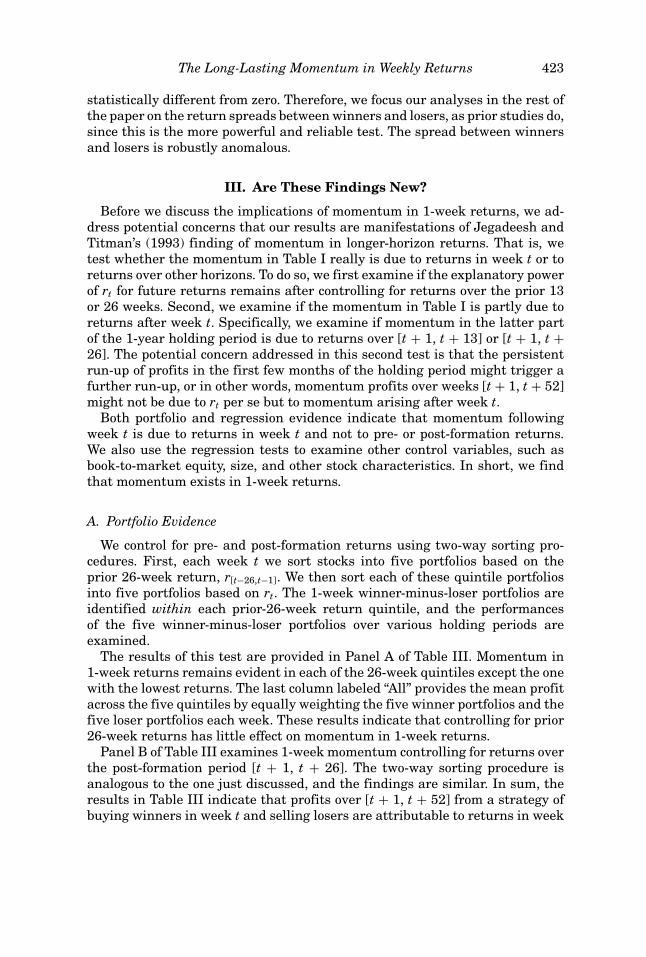
Table IIIProfits to Weekly Extreme Portfolios Controlling for 26-Week
Momentum (Winners minus Losers)Each week from 1983 to 2003, we rank stocks into quintiles based on 26-week returns. Withineach 26-week return quintile, we rank stocks into further quintiles based on 1-week returns andform portfolios comprised of long positions in the top 1-week quintile of stocks (winners) and shortpositions in the bottom quintile (losers). Panel A first sorts on returns over weeks [t − 26, t − 1] andthen sorts on returns over week t; portfolios are examined over [t + 1, t + 52]. Panel B first sortson returns over weeks [t + 1, t + 26] and then sorts returns over week t; portfolios are examinedover [t + 27, t + 52]. In both panels, the column labeled “All” represents a portfolio that is weightedequally across the 26-week-return quintiles. Returns are formed from the midpoints of the quotedbid and ask prices at each day’s close. Stocks priced below five dollars at the end of formation week tare excluded. Calendar-time alphas are estimated over various holding periods using raw returns.The t-statistics are in parentheses and are robust to heteroskedasticity and autocorrelation. CAPMand Fama-French risk-adjusted profits produce similar findings. Profits are in basis points.
Low 2 3 4 High All
Panel A: Sorting First on r[t−26,t−1] and Evaluating over Weeks 1–52
1.47 3.65 3.78 4.53 5.36 3.60(0.71) (2.69) (3.11) (3.64) (3.66) (2.81)
Panel B: Sorting First on r[t+1,t+26] and Evaluating over Weeks 27–52
6.30 6.25 6.45 6.53 8.04 6.69(4.57) (6.09) (6.25) (6.06) (6.39) (7.17)
t and not to returns over other horizons. The use of CAPM and Fama-Frenchalphas to evaluate performance does not alter this conclusion.
B. Regression Evidence
We continue examining the robustness of 1-week momentum using weeklycross-sectional regressions. The regression setting allows us to easily control formultiple characteristics (as opposed to using three-way or higher-order sortingsin the portfolio tests). Each week t, we regress the cross-section of return over[t + 1, t + 52] on the return in week t, the return over [t − 1, t − 26], size, andthe book-to-market-equity ratio ( B
M ). We measure size as the market value ofthe stock in the last available week of the prior June, and we measure B
M asthe book value of equity at fiscal year-end (Compustat item 60) divided by themarket value of equity in the last available week of the prior December. Bothsize and B
M are sampled in week t, along with the 1-week return, and naturallogarithms of both size and B
M are used in the regressions.Once the weekly regressions are estimated, the respective time series of each
coefficient is used to separately test the hypothesis that its mean is zero. Theoverlapping of the left-hand variable and some of the right-hand variables in-duces positive serial correlation in the time series of coefficient estimates. Thisneeds to be accounted for in the test statistics. We rely on the variance estimator
The Long-Lasting Momentum in Weekly Returns 425
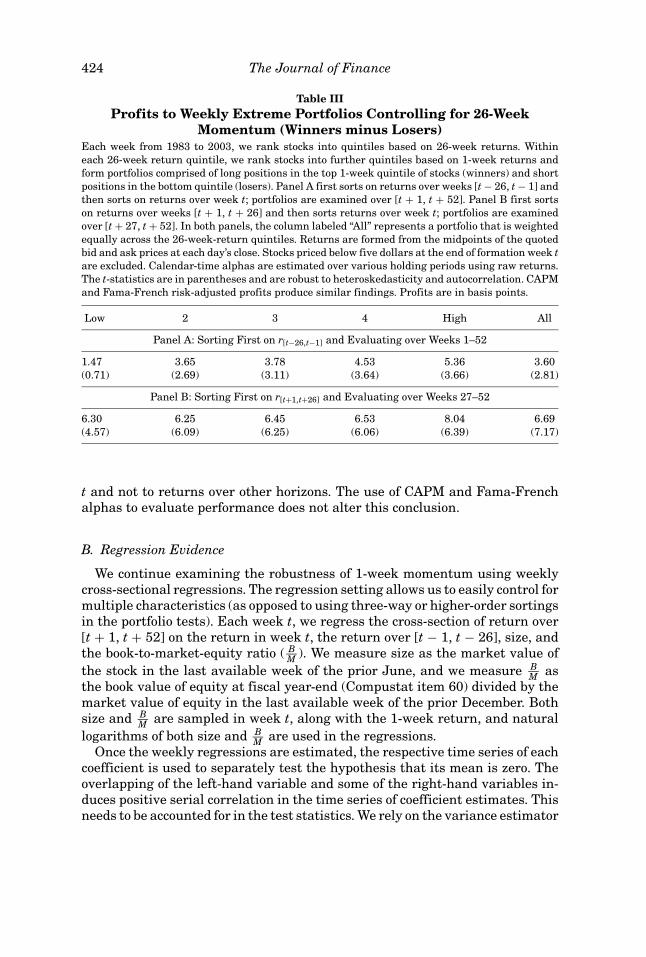
Table IVWeekly Cross-sectional Regressions
Each week from 1984 to 2002, we regress the cross-section of future holding-period return on the1-week return, 26-week return, and 13-week return, sampled at various horizons. The mean of theweekly time series of each coefficient is reported below and is tested to be zero. The t-statisticsare in parentheses and are robust to heteroskedasticity and autocorrelation. The mean coefficientson the 1-week return are given in column 1. The mean coefficients of the 26-week and 13-weekreturns, sampled at various points, are given in columns 2 and 3, respectively. The log of the book-to-market ratio (column 4) and size (column 5) are included as controls and are updated the firstweek in January and the first week in July respectively, and are sampled at week t. Returns areformed from the quoted bid and ask prices at each day’s close. Stocks priced below five dollars atthe end of the week from which the 1-week return is sampled are excluded. Reported coefficientestimates are multiplied by 100.
1 2 3 4 5
Future Return Explanatory Variables
A. r[t+1,t+52] rt r[t−26,t−1] ln( B
M
)ln(size)
9.20 12.56 8.88 0.74(4.14) (4.55) (6.24) (1.20)
B. r[t+14,t+52] rt r[t−26,t−1] r[t+1,t+13] ln( B
M
)ln(size)
12.19 7.26 11.01 5.12 0.32(6.85) (3.83) (4.19) (4.43) (0.70)
C. r[t+27,t+52] rt r[t+1,t+26] r[t−13,t−1] ln( B
M
)ln(size)
7.05 5.22 6.07 2.49 0.13(5.34) (3.06) (3.78) (3.30) (0.41)
of Gallant (1987), which is robust to heteroskedasticity and to serial correlation.Once again, we follow the advice of Andrews (1991) and model each time seriesas an AR(1) process to determine the bandwidth parameter of the kernel esti-mator (using equations (6.2) and (6.4) of Andrews). We then examine robustnessacross alternative bandwidths, again following Andrews’s recommendation, bychanging the autoregressive parameter by ±1 and ±2 standard deviations. Thenumber of lags used in testing the coefficient on rt ranges from 6 to 10 acrossthe various bandwidths and the various models considered. The findings to bediscussed next are robust across bandwidths and across models.13
The results of the regression-based tests are provided in Table IV. PanelA confirms the portfolio results of Table III. The explanatory power of rt forr[t+1,t+52] remains strong after controlling for r[t−26,t−1]; the t-statistic for rt is
13 The other right-hand variables, which are the longer-horizon returns, size, and BM , overlap
sizably in the weekly regressions so their AR(1) parameters notably increase. As such, the numberof lags employed to test these respective coefficients increases. For example, the number of lagsused to test the coefficient on r[t−1,t−26] ranges from 65 to 201. With a time series of roughly 950observations, readers might be justifiably concerned about the reliability of the estimates of thestandard errors when the number of lags is so large. However, the focus of this study is on theexplanatory power of rt, not the control variables. Since all coefficient estimates are consistent, wecan be confident in the test statistics for rt.
426 The Journal of Finance
4.14. In addition, controlling also for BM and size does not affect the finding
of momentum in 1-week returns. Although the results are not tabulated, wealso confirm that none of the findings in Table IV are affected by the inclusionof a stock’s return volatility, analyst coverage, and institutional ownership asadditional control variables (defined in Section IV.C).
Panel B of Table IV adds r[t+1,t+13] as an additional control. The explanatorypower of rt for future returns, in this case for r[t+14,t+52], continues to hold. PanelC switches the horizons of the pre-formation and post-formation controls. Thatis, in Panel C we explain r[t+27,t+52] using rt, lagged 13-week returns, and leading26-week returns. Again, the findings in Table I are not driven by longer-horizoneffects. In short, long-lasting momentum exists in 1-week returns.
The regression setting also allows us to directly compare the informationabout future returns found in 1-week returns to that found in longer-horizonreturns. We see in Table IV that the coefficients on the different return horizonsare of the same magnitude, indicating that the information contained in allreturn horizons is roughly comparable. Importantly then, the ability of pastreturns to predict future returns (i.e., momentum) is more related to the size ofthe past return than to its horizon. Of course, each horizon does have distinctexplanatory power for future returns, as shown in Tables III and IV, becauseeach horizon embodies a separate piece of information.
IV. New Testing Ground for Momentum Theories
Perhaps the most important contribution of the finding of momentum in1-week returns is the recognition that momentum is not exclusive to returnsfrom 3 to 12 months, as the literature currently suggests. Our findings providefinancial economists a simpler, clearer picture of the anomaly landscape: Returnmomentum is the dominant feature of returns of all horizons up to 12 months.Given this observation, potential explanations of momentum should be easierto develop.14
An outgrowth of the finding of momentum in weekly returns is thateconomists now have a new testing ground for momentum theories. Weeklyreturns can potentially reveal new information about the underlying process ofprice formation that produces momentum. Moreover, weekly returns can allowresearchers to link returns to specific news events, an opportunity that doesnot exist at the 6- or 12-month horizons commonly used in momentum stud-ies. Therefore, theories investigating how specific types of news might drivemomentum should be better tested using momentum in 1-week returns thanmomentum in longer-horizon returns.
In the next subsections, using weekly returns, we revisit Chan’s (2003) in-vestigation of the relation between momentum and public news and Zhang’s(2006) investigation of the relation between momentum and information un-
14 Interestingly, the most prominent theories of return momentum developed by Daniel et al.(1998), Hong and Stein (1999), and Barberis, Shleifer, and Vishny (1998) all ignore the short-runreversal. Our findings justify this omission.
The Long-Lasting Momentum in Weekly Returns 427
certainty. In particular, we consider whether the theories of momentum thatthey examine are potential contributors to the momentum in 1-week returns.
A. Explicit versus Implicit News
As Chan (2003) and many others note, we can think of price movements asreflecting private or intangible news, not just publicly available news. Severalcurrent and prominent behavioral theories of stock return anomalies predictthat the market overreacts to price movements not associated with public firm-specific news. Daniel et al. (1998) assume that investors’ overconfidence in theirprivate information yields an overreaction to private information and an un-derreaction to public information. Hong and Stein (1999) assume that there aretwo types of investors, one type that observes only public fundamental newsabout firms and a second type that observes only price movements. With theadditional assumption that information about fundamentals diffuses gradu-ally across the marketplace, Hong and Stein predict that public news will beunderreacted to and that price movements will be overreacted to. Daniel andTitman (2006) suggest that investors overreact to intangible news, which theyspecify as price movements unrelated to accounting measures of performance.The central assertion of these theories is that the market overreacts to returnsthat are unassociated with public news. We label such news “implicit” since noexplicit news is released.
Chan (2003) separates monthly stock returns into price movements that areand are not associated with media headline news, that is, into explicit andimplicit news respectively. He finds that implicit news generates reversal insubsequent returns and explicit news generates momentum. Chan concludesthat indeed the market might be overreacting to implicit news and underreact-ing to explicit news.
Using Chan’s (2003) data on headline news, we reexamine the performancesof implicit-news and explicit-news portfolios. We link headline news to 1-weekreturns, instead of 1-month returns, to provide a cleaner identification of thetype of news underlying price movements. Chan’s headline data are collectedfrom the Dow Jones Interactive Publications Library from 1980 to 2000. Eachday he identifies if a given stock is mentioned in a headline or lead paragraphfrom a newspaper or newswire article. To render the data collection feasible,he selects a random subset of roughly 25% of CRSP stocks, varying from 766 inJanuary 1980 to over 1,500 in December 2000.15
We rank the superset of all available stocks using CRSP and ISSM/TAQ (asin Table I) into deciles each week from 1983 to 2000 based on midpoint returnsfrom the prior week (the midpoint data begin in 1983). Using the breakpointsfrom the superset allows us to compare profits across implicit and explicit stocks
15 See Chan’s (2003) description of the data for more details. We collect announcement data onearnings, seasoned equity offerings, stock splits, dividend initiations, and share repurchases andcompare these with Chan’s headline-news data. This exercise suggests that his data are compre-hensive.
428 The Journal of Finance
Table VProfits to Explicit-News and Implicit-News Portfolios
(Winners minus Losers)Each week from 1983 to 2000, we rank stocks based on their returns over the week. Within thehighest decile of stocks (winners) and the lowest decile (losers), we then identify the stocks inChan’s (2003) random sample and separate these stocks into those with headline news in the week(explicit news) and those without headline news (implicit news). We form an implicit-news portfolioby taking a long position in the winner stocks with implicit news over the week and a short positionin loser stocks with implicit news. An explicit-news portfolio is formed analogously. Calendar-timeraw profits are estimated over various holding periods. Panel A reports the profits to the implicit-news portfolio, and Panel B reports the profits to the explicit-news portfolio. The t-statistics arein parentheses and are robust to heteroskedasticity and autocorrelation. Returns are formed fromthe midpoints of the quoted bid and ask prices at each day’s close. Stocks priced below five dollarsat the end of formation week t are excluded. CAPM and Fama-French risk-adjusted profits producesimilar findings. Profits are in basis points.
Holding Period
Week Week Week Weeks Weeks1 2 3 4–52 1–52
Panel A: Implicit News (no headline news)
−81.11 −45.76 −6.13 8.79 5.21(−6.93) (5.32) (−0.81) (5.41) (3.13)
Panel B: Explicit News (headline news)
−60.33 −8.96 20.03 12.49 9.85(−4.29) (−0.88) (2.53) (6.04) (4.25)
Panel C: t-test of (Explicit-Implicit) = 0
(2.19) (4.14) (3.06) (2.06) (2.41)
as the formation-period returns are similar. Stocks in the extreme deciles thatare in Chan’s (2003) data are identified and separated into implicit-news andexplicit-news stocks depending on whether a given stock has at least one head-line news release during the formation week. We impose a 10-stock requirementon each winner and loser portfolio in week t to mitigate potential consequencesof heteroskedasticity and of variations in factor loadings that may result fromthe portfolio’s composition changing from one calendar week to the next.
Table V provides the raw profits to implicit-news and explicit-news portfolioscomprised of implicit-news winners minus implicit-news losers and explicit-news winners minus explicit-news losers, respectively. For brevity, we do nottabulate the CAPM and Fama-French alphas since these metrics produce simi-lar results. In Panel A, we find, as Chan (2003) does, that implicit news reversesimmediately after portfolio formation. However, information from the longerevaluation windows suggests that implicit news in week t is not categoricallyoverreacted to. As before, there is a robust stream of momentum profits follow-ing the brief reversal that is strong enough to offset the initial reversal. Thelast column in Table V shows that the profit to the implicit-news portfolio is
The Long-Lasting Momentum in Weekly Returns 429
statistically positive in the 52 weeks following portfolio formation. So, just asin the general case of Table I, extreme price movements not associated withheadline news are found ex post to be not extreme enough.
Moreover, implicit-news stocks and explicit-news stocks display the samegeneral behaviors, namely, short-run reversal and longer-run momentum.Panel B provides the profits to the explicit-news portfolio. Panel C pro-vides the t-statistics comparing the mean profits of the explicit-news port-folio to those of the implicit-news portfolio. Interestingly, the profits to ex-plicit news are statistically greater than the profits to implicit news overevery holding period examined in Table V. Given that the formation-periodreturns are similar, we have evidence that the market does react differ-ently to implicit versus explicit news. However, the difference between im-plicit and explicit news is not as the aforementioned theories predict. Sinceboth groups display the same qualitative pattern of short-run reversal andlonger-run (stronger) momentum, we are unable to characterize one reac-tion as overreaction and the other as underreaction. The only difference isin the magnitudes of the profits, not in the patterns of the profits. Why thisdifference in magnitudes exists is an interesting topic for future studies topursue.
It is worth noting that earnings announcements do not drive the strongermomentum in explicit news. Removing stocks that announce earnings in weekt from the explicit-news portfolio diminishes momentum profits over weeks [t +1, t + 52], but explicit-news profits are still significantly greater than implicit-news profits.16
In sum, our findings impede concluding that the market categorically over-reacts to implicit news. Moreover, firm-specific news of all sorts, explicit andimplicit, appears to robustly generate momentum in returns.
B. Uncertainty and Momentum
As just noted, explicit news displays greater return momentum than implicitnews. One possible explanation is that explicit news is more precise than im-plicit news (in the sense of a less noisy signal), and greater precision inducesgreater momentum.17 However, in his examination of the relation between mo-mentum and several measures of the uncertainty (or ambiguity) of the valuationimpact of a given piece of firm-specific news, Zhang (2006) finds the seeminglyopposite result that momentum increases with uncertainty. Zhang’s hypothesisis that if psychological biases play a role in return momentum, then momentumshould increase as uncertainty increases. This prediction follows from evidencethat uncertainty intensifies psychological biases.18
16 Earnings announcements are from I/B/E/S.17 Readers may find it difficult to envision how greater precision, that is, less uncertainty, might
lead to greater momentum. Veronesi (2000) and Johnson (2004) identify mechanisms that canrationally produce higher expected returns for stocks with greater precision.
18 See Hirshleifer’s (2001) review for a detailed discussion.
430 The Journal of Finance
Zhang (2006) studies the relation between momentum in 11-month returnsand the general uncertainty regarding a stock’s valuation using such measuresas size, analyst coverage, return volatility, and the dispersion of analysts’ earn-ings forecasts. We extend his analyses to momentum in 1-week returns. Byusing such a short horizon, we can link momentum to specific news releases.Moreover, for earnings announcements in particular, we have a measure of theex ante uncertainty of the given news, namely, the dispersion of analysts’ earn-ings forecasts. Therefore, we have a seemingly more reliable and direct test ofthe relation between return momentum and the uncertainty of news.19
We define dispersion of the earnings forecasts to be the standard deviationof forecasts scaled by the stock’s price at the end of week t − 1. We excludeobservations with fewer than four forecasts to increase our confidence in themeasure of dispersion. Similar results obtain when stocks with less than fourearnings forecasts are included or when the standard deviation is scaled by theabsolute value of the mean earnings forecast. The forecast data are unadjustedfor splits and are provided by I/B/E/S. Diether, Malloy, and Scherbina (2002) andPayne and Thomas (2003) note that using standard deviations of forecasts thatare historically adjusted for splits can falsely classify high-dispersion stocksas low-dispersion stocks. Earnings announcement and forecast data begin May1984.
Each week t, stocks are sorted into deciles based on returns in week t (as inTable I). Winner (top-decile) stocks that announce earnings in week t are sortedbased on the dispersion of earnings forecasts. Stocks with dispersion above themedian value for that winner portfolio are classified as the high-dispersionwinner stocks; stocks with below-median dispersion are classified as the low-dispersion winner stocks. The low-dispersion and high-dispersion portfolios ofloser (bottom-decile) stocks are formed analogously.
One last detail to note is that we alter the weighting scheme within thecalendar-time portfolios when examining holding periods greater than 1 week.In other tests, we equally weight across all cohort portfolios held that week.For example, for the performance analysis across weeks [t + 1, t + 52], weequally weight the returns of the 52 portfolios in calendar week τ to estimate theportfolio’s return. Since we are faced in some calendar weeks of these dispersiontests with very few stocks being held in specific cohort portfolios, we equallyweight across all stocks held that week, instead of across cohort portfolios.Finally, we require at least 10 stocks in the winner and loser portfolios eachcalendar week for that week to be included in the analyses. In testing over[t + 1, t + 52] for whether momentum differs across forecast dispersion, eachweek we average roughly 300 stocks on the portfolio’s long side and 300 stockson the short side and lose only 46 out of 1,022 weeks (and these dispersionportfolios have on average the least number of stocks per week among the52-week portfolios examined in this study).
19 The measure of uncertainty remains indirect in our test as well because we are measuring theuncertainty of future earnings instead of the uncertainty of the valuation impact of the earnings.

The Long-Lasting Momentum in Weekly Returns 431
Table VIProfits to Weekly Extreme Portfolios across High and Low Dispersion
in Earnings Forecasts (Winners minus Losers)Each week from May 1984 to 2003, we rank stocks based on their returns over the week. Withinthe highest decile of stocks (winners) and the lowest decile (losers), we retain the stocks with (1) aquarterly earnings announcement occurring in the week and (2) earnings forecasts provided by atleast four analysts. We separate the remaining winner stocks into those with high (above-median)and low (below-median) dispersion in earnings forecasts. We form a high-dispersion portfolio bytaking a long position in winner stocks with high forecast dispersion and a short position in loserstocks with high forecast dispersion. A low-dispersion portfolio is formed analogously. Raw profitsare estimated over various holding periods. Panel A reports the profits to the high-dispersionportfolio, and Panel B reports the profits to the low-dispersion portfolio. The t-statistics are inparentheses and are robust to heteroskedasticity and autocorrelation. Returns are formed fromthe midpoints of the quoted bid and ask prices at each day’s close. Stocks priced below five dollarsat the end of formation week t are excluded. CAPM and Fama-French risk-adjusted profits producesimilar findings. Profits are in basis points.
Holding Period
Week Week Week Weeks Weeks1 2 3 4–52 1–52
Panel A: High Dispersion in Earnings Forecasts(and earnings released in week t)
23.76 13.81 29.71 10.15 10.50(0.99) (0.59) (1.46) (3.05) (3.25)
Panel B: Low Dispersion in Earnings Forecasts(and earnings released in week t)
0.67 17.12 −5.51 13.10 12.01(0.03) (0.79) (−0.28) (4.02) (3.85)
Panel C: t-test of (High-Low) = 0
(0.67) (−0.15) (1.38) (−0.94) (−0.51)
Table VI provides the raw profits to the high-dispersion and low-dispersionportfolios of winner-minus-loser stocks announcing earnings. In contrast toZhang’s (2006) findings, we see no evidence that the profits to the high-dispersion portfolios are different from the profits to the low-dispersion portfo-lios over any of the horizons considered. Panel C of Table VI gives the t-statisticsfor testing that the profits across high-dispersion and low-dispersion portfoliosare equal. The null hypothesis of equality cannot be rejected. In short, we findno relation between uncertainty and momentum in 1-week return. The CAPMand Fama-French alphas depict the same finding and are not tabulated.
In the next section, we consider how other characteristics relate to momen-tum. Some of these results echo Zhang’s (2006) findings; some do not. Ourmessage here is that the relation between uncertainty and momentum thatZhang detects using 11-month returns does not transfer to momentum at the1-week horizon.
432 The Journal of Finance
C. Relations between Momentum and Stock Characteristics
In this section, we examine how momentum in 1-week returns varies acrossstock size, return volatility, analyst coverage, and institutional ownership.These measures are typically used to probe how anomalies are affected by vari-ation in information environments, trading costs, and investor sophistication.Of course, the interpretations of these characteristics are not mutually exclu-sive. Though we focus more on the momentum phenomenon, for completenesswe continue to provide the profits for the winner-minus-loser portfolios overweeks 1, 2, and 3.
We begin with stock size. After sorting all stocks into deciles each week basedon returns over week t (as in Table I), we further sort the stocks in the highestand lowest decile portfolios based on their market values at the end of the priorJune. We use the median size of NYSE stocks from the prior June to classifylarge and small stocks. Stocks below the median value of size are grouped toform the small-stock portfolio; stocks above the median value of size are groupedto form the large-stock portfolio.
Panel A of Table VII provides the raw profits to small-stock and large-stockwinner-minus-loser portfolios. (All findings in Table VII are similar when usingCAPM and Fama-French alphas.) Extreme-return portfolios comprised of smallstocks only and of large stocks only behave similarly, both displaying short-run reversal and both displaying longer-run momentum after week 4. The t-statistics testing whether the profits across the small-stock and large-stockportfolios are different over weeks [t + 1, t + 52] exceed 2.90 across the threeperformance metrics (raw, CAPM, and Fama-French), and are not tabulated.Hence, small stocks display greater longer-run momentum, consistent with theresults of Hong et al. (2000) and others. This is possibly attributable to smallerstocks being more difficult to value, having less sophisticated traders, beingmore costly to arbitrage, and/or having a poorer information environment.
For the large-stock extreme portfolio, although the mean profit of 1.26 basispoints per week is not statistically significant over the [t + 1, t + 52] period, itis statistically positive over the [t + 4, t + 52] period. Hence, 1-week returns oflarge stocks do generate a momentum in returns.
We turn our attention now to the other characteristics. Given that return mo-mentum is stronger in small stocks, we control for size going forward to ensurethat we are not confounding the effects of the other characteristics with thesize effect. For each of the remaining characteristics examined in Table VII, weemploy the following sorting procedures to create size-neutral portfolios. Afteridentifying the winner stocks in week t, we sort the winners based on size mea-sured at the end of the prior June. Using the 70th and 30th size percentiles forNYSE stocks from the prior June, the winner portfolio is subdivided into threeportfolios: large, medium, and small. Each of these three size-based winnerportfolios is further sorted into two subportfolios based on the characteristicwe are examining, for example, institutional ownership (IO). Stocks with IObelow the median level for stocks in their respective winner/size portfoliosare grouped together as low-IO stocks; stocks with IO above the median level for

The Long-Lasting Momentum in Weekly Returns 433
Table VIIProfits to Weekly Extreme Portfolios across Stock Characteristics
(Winners minus Losers)Each week from 1983 to 2003, we rank stocks based on their returns over the week. We further dividethe top-decile (winner) stocks and the bottom-decile loser stocks based on the various characteristicsbelow. For Panel A, we divide winners into those with market values above the median NYSE valueand those below the median NYSE value. Market values are always sampled at the end of the priorJune. Losers are divided similarly. We form the small-stock portfolio by taking a long position inabove-median winners and a short position in below-median losers. The large-stock portfolio isformed analogously using above-median stocks. For Panel B, we divide winners and losers eachweek into two groups based on institutional ownership (IO) as of the prior quarter, sorting first onsize to create size-neutral IO portfolios as follows. After sorting on rt, winners are further sortedinto three size groups based on the 30th and 70th NYSE percentiles. We form a high-IO portfolio bytaking a long position in the winners with above-median IO for their respective winner-size groupsand a short position in the losers with above-median IO for their respective winner-size groups.A low-IO portfolio is formed analogously. For Panels C and D, we form size-neutral portfolios asjust described. Panel C forms portfolios of stocks with high (above-median) and low (below-median)weekly return volatility measured over [t − 52, t − 1]. Panel D forms portfolios of stocks withhigh (above-median) analyst coverage and low (below-median) analyst coverage, where coverageis defined as the number of analysts providing forecasts of future annual earnings and is sampledat the end of the prior month. Stocks with no coverage are excluded. Calendar-time alphas forthe portfolios are estimated over various holding periods using raw returns. The t-statistics arein parentheses and are robust to heteroskedasticity and autocorrelation. Returns are formed fromthe midpoints of the quoted bid and ask prices at each day’s close. Stocks priced below five dollarsat the end of formation week t are excluded. CAPM and Fama-French risk-adjusted profits producesimilar findings. Profits are in basis points.
Holding Period
Week Week Week Weeks Weeks1 2 3 4–52 1–52
Panel A: Size
Small −74.48 −39.57 0.55 8.80 5.45(−8.13) (−8.22) (0.11) (5.38) (3.26)
Large −115.78 −8.00 18.33 4.56 1.26(−8.22) (−0.77) (1.88) (2.60) (0.57)
Panel B: Institutional Ownership
High −86.34 −40.81 −1.17 6.85 3.27(−9.40) (−5.77) (−0.19) (3.89) (1.79)
Low −67.94 −30.88 −2.69 9.06 6.04(−7.19) (−4.35) (−0.44) (4.56) (3.02)
Panel C: Volatility
High −102.24 −46.99 6.47 6.78 2.81(−9.89) (−5.80) (0.97) (3.24) (1.30)
Low −45.76 −26.40 −4.26 8.47 6.29(−5.31) (−4.24) (−0.75) (4.79) (3.49)
Panel D: Analyst Coverage
High −93.38 −38.00 6.10 7.15 3.85(−9.76) (−4.97) (0.90) (3.71) (1.98)
Low −73.58 −38.41 −4.06 8.27 4.76(−7.59) (−5.35) (−0.70) (4.50) (2.54)
434 The Journal of Finance
stocks in their respective winner/size portfolios are grouped together as high-IO stocks. Loser portfolios comprised of high-IO stocks and of low-IO stocks areformed analogously. Winner-minus-loser portfolios for high-IO stocks and forlow-IO stocks can then be created, and are size-neutral.
Data on institutional ownership over 1983 to 2003 are from 13F filings andcome from Thomson Financial (CDA/Spectrum). Institutional ownership is de-fined as the percentage of each stock’s outstanding shares that is held byinstitutional investors at the end of the quarter prior to week t. Using size-neutral portfolios as described above, Panel B shows that stocks with lowerinstitutional ownership produce greater momentum over weeks [t + 1, t +52], with untabulated t-statistics exceeding 2.36 across the raw, CAPM, andFama-French metrics. The finding that momentum is decreasing in institu-tional ownership is consistent with the joint hypothesis that momentum isdue to mispricing and institutions are the more sophisticated, better-informedtraders.
In Panel C, we measure return volatility as the standard deviation of returnsover weeks [t − 52, t − 1], where returns are again formed using the midpointsof the quoted bid and ask prices so that price movements due to bid-ask spreadsare removed. Momentum is greater for low-volatility stocks (t-statistics testingthe difference are at least 3.16 across the raw, CAPM, and Fama-French perfor-mance metrics and are not tabulated). This finding is the opposite of Zhang’s(2006) 11-month finding that high-volatility stocks display greater momentum.To the extent that volatility captures uncertainty, 1-week momentum increasesas uncertainty decreases.
Panel D of Table VII provides the profits of winner-minus-loser portfoliosacross high and low analyst coverage, using size-neutral portfolios as above.For each stock from 1983 to 2003, we obtain the number of analysts providingforecasts of future annual earnings from I/B/E/S in the month prior to portfo-lio formation. Stocks with no coverage are excluded from this analysis, but thefindings are unaffected when we include them. We find that stocks with low an-alyst coverage produce slightly higher mean profits over the 52-week window,the same direction as Zhang’s (2006) finding using 11-month returns and Honget al.’s (2000) finding using 6-month returns. However, the momentum differ-ences across coverage are not statistically significant. The t-statistics testingthe difference do not exceed 1.23 and are not shown. Thus, the prior findingsthat momentum is negatively related to analyst coverage are not robust acrossreturn horizons.
The characteristics examined in Table VII are not independent. For exam-ple, Gompers and Metrick (2001) and others provide evidence that institutionsprefer to hold large stocks, Bhushan (1989) finds that stocks with greater an-alyst coverage are larger and have higher institutional ownership, and it iscommon knowledge that small stocks have greater return volatility. Therefore,to determine which of these effects if any dominates, we examine weekly cross-sectional regressions, as in Table IV. Each week, we regress r[t+1,t+52] on rt,the log of size, IO, return volatility, analyst coverage, and interactions of thesefour characteristics with rt. The log of B
M is also included as a control. Stockswith no analyst coverage are included in the regressions. The mean of the time
The Long-Lasting Momentum in Weekly Returns 435
series of coefficients on the interactions (multiplied by 100) and their associatedt-statistics are as follows:
Size × rt IO × rt Volatility × rt Coverage × rt
−4.95 0.65 −162.11 0.43(−4.73) (0.13) (−3.50) (1.78)
The regressions indicate that size, return volatility, and to a lesser extent,analyst coverage have separate effects on return momentum, whereas the effectof institutional ownership is subsumed by the other measures.20 Note that thepositive coefficient on the analyst-coverage interaction differs slightly from theportfolio evidence in Table VII. This seems attributable to the omitted variablesin the portfolio tests.
In sum, momentum in 1-week returns decreases with stock size and withreturn volatility. The effects of institutional ownership and analyst coverage onmomentum are less clear. More importantly, these findings are mixed in theirsupport for a positive relation between uncertainty and weekly momentum,and in the case of return volatility, are contradictory to the supposed relation.
There are also interesting results in Table VII with respect to short-runreversal. The week-1 reversal is statistically greater in large stocks, in high-institutional-ownership stocks, in high-volatility stocks, and in high-analyst-coverage stocks. Lehmann (1990) also identifies this large-firm effect in short-run reversals. The finding that large, high-institutional-ownership, and high-coverage stocks experience greater short-run reversal might seem counterintu-itive. Given that such stocks are typically associated with lower trading costsand illiquidity, with presumably a greater number of sophisticated traders, andwith a better information environment, both the microstructure and overreac-tion explanations of short-run reversal seem less likely for such stocks.
As in the longer-run momentum case, we also estimate weekly cross-sectionalregressions to examine the four short-run effects jointly. We regress rt+1 on rt,the log of size, IO, return volatility, analyst coverage, and interactions of thesefour characteristics with rt, and we include the log of B
M as a control. The meanof the time series of coefficients on the interactions (multiplied by 100) andtheir associated t-statistics are as follows:
Size × rt IO × rt Volatility × rt Coverage × rt
−0.82 −3.70 −78.50 −0.08(−4.09) (−4.78) (−8.85) (−1.92)
20 Serial correlation in the time series of coefficients on the interactions is not large in any case.The data-dependent number of lags used to estimate Gallant’s (1987) robust standard errors, asdiscussed in Section III.B, vary only from two to five across these interaction coefficients. Despitethe raw characteristics displaying strong persistence, the interactions do not; and consequentlythe test statistics on the interactions are reliable.
436 The Journal of Finance
The regressions show that the four effects on short-run reversal noted in theportfolio tests of Table VII are distinct. To not distract from the main focus of thisstudy, which is the momentum in 1-week returns, we defer further discussionof short-run reversal to Section VII, where we provide additional short-runresults as well as an overview of how our findings throughout this study affectthe literature’s view of short-run reversal.
D. Discussion of the Possible Sources of Momentum
What can possibly explain our finding of momentum in 1-week returns? Inthe preceding sections, we address several possibilities. The first is that mo-mentum is attributable to the market’s underreaction to explicit (public) news,which might be due to a combination of overconfidence and self-attribution biasor to a slow diffusion of information throughout the marketplace as Daniel etal. (1998) and Hong and Stein (1999), respectively, suggest. These two modelsalso jointly predict an overreaction to implicit news. However, Table V is in-consistent with the notion that the market’s reactions to explicit and implicitnews are categorically different. Table V does find though that explicit newssparks greater momentum than implicit news, and implicit news generatesgreater short-run reversal. These differences in future returns suggest thatfurther consideration of theories characterizing types of news and the market’spotentially differing reactions to each type is warranted.
The second possibility we examine is a more general notion that psychologicalbiases of some traders might be resulting in momentum. Zhang (2006) arguesthat if any psychological biases induce momentum, then uncertainty regardinga stock’s valuation should intensify these biases and amplify the momentumin returns. The results presented in Sections IV.B and IV.C do not support thistheory as a potential explanation of 1-week momentum.
In addition, Table VII and the regression results noted in Section IV.C do notfind that momentum in weekly returns increases as analyst coverage decreases.This seems inconsistent with Hong and Stein’s (1999) proposition that slowdiffusion of information contributes to momentum in returns.
On quite a different note, Grinblatt and Han (2005) argue that a dispositioneffect contributes to momentum, whereby traders hold loser stocks too long andsell winner stocks too soon, inducing underreaction to good and to bad news.This well-known disposition effect is motivated by a combination of prospecttheory and mental accounting. Grinblatt and Han find that stocks with largercapital-gains overhang experience greater momentum. Moreover, they find thattheir capital-gains measure dominates 1-year return as a predictor of futurereturns. Frazzini (2006) extends the evidence for this theory to return momen-tum following earnings announcements. However, it seems unlikely that sucha disposition effect is contributing to momentum in 1-week returns; we con-trol for prior 6-month returns in Tables III and IV, and prior returns over suchhorizons should be a (noisy) proxy for capital-gains overhang.
Recently, Grinblatt and Moskowitz (2004) and Watkins (2003) documentthat return consistency contributes to momentum in 6- to 12-month returns.Specifically, stocks with a high frequency of positive returns over the prior 6
The Long-Lasting Momentum in Weekly Returns 437
or 12 months have higher future returns, and stocks with a high frequency ofnegative returns have lower future returns. Grinblatt and Moskowitz cite sev-eral possible interpretations of these consistency effects, including informationdiffusion and the capital-gains-overhang (disposition) effect. Later in SectionVI, we examine short-run consistency in returns. For now, we note that we findno evidence that return consistency contributes to momentum in 1-week (or4-week) returns.
Lastly, we wish to highlight that rational theories of momentum (not involv-ing misspecified factor risks) also exist. Lewellen and Shanken (2002), Bravand Heaton (2002), and Veronesi (1999) show how rational learning can inducemomentum and reversal in returns. While these and other theoretical papersprovide intriguing, and to our view, reasonable possibilities, we are aware ofno empirical test of these rational learning theories. In fact, Brav and Heatonpoint out how difficult it is for current empirics to distinguish between behav-ioral and rational explanations, as they both predict similar patterns in returns.Further consideration of such rational theories is warranted as well.
V. Robustness Considerations
We now turn our attention to robustness checks regarding the evidence ofmomentum in 1-week returns. First, we consider an alternative specification ofthe calendar-time method that allows for heteroskedasticity in the time seriesof portfolio profits and for variations in portfolio factor loadings. Second, weexamine transaction prices to estimate returns instead of the midpoint of thebid and ask quotes. The transaction data go back to 1963 and greatly extendour testing period, which begins in 1983 using the quote data. Third, we providethe pre-formation profits to the extreme-return winner-minus-loser portfoliosand show that positive profits are not present before week t. This finding al-lays potentially lingering concerns that we are identifying momentum profits inthe post-formation period due to misspecification of the model of expected re-turns for these portfolios. Last, we show that momentum is detected in 1-month(4-week) returns as well.
A. Alternative Method to Accommodate Possible Heteroskedasticityand Varying Factor Loadings
When employing the calendar-time methods of the preceding sections, twopotential concerns arise from the weekly changes in the composition of the port-folios. The first is that the variance in a portfolio’s profits can change over time.The second is that the loadings on the factors in the CAPM and Fama-Frenchmodels can change over time. Readers might wonder if the procedures employedabove fully accommodate these potential issues. To address this question, weexamine an alternative testing procedure advocated by Mitchell and Stafford(2000) and others. Our findings are similar whether we use the methods aboveor the alternative we detail here.
Taking advantage of the data available on the individual stocks that comprisea portfolio in a given week, we accommodate potential time-series dynamics
438 The Journal of Finance
in the variance of the portfolio’s profits and in the portfolio’s factor loadings.Each calendar week τ , we identify the stocks in the winner and loser portfolios.Then, using only those specific stocks, we estimate the given winner-minus-loser portfolio’s abnormal returns over the [τ + 1, τ + 52] period. In the CAPMand Fama-French specifications, the abnormal return for week τ is calculatedusing the estimated portfolio loadings over [τ + 1, τ + 52] and the factor real-izations in week τ . Re-estimating the factor loadings for each week’s portfolioallows loadings to change each calendar week as the composition of the portfoliochanges.
To control for possible heteroskedasticity, the standard deviation of the prof-its to each week’s portfolio is estimated using the profits over [τ + 1, τ +52]. The abnormal return of the portfolio in week τ is divided by its stan-dard deviation. This procedure is repeated each calendar week to obtain a timeseries of standardized abnormal returns whose variance should be constant(one).
The outcome of this procedure is a time series of profits that accommodatesheteroskedasticity and variations in factor loadings. Our findings that momen-tum exists in 1-week returns as well as the various findings on interactionswith momentum are robust when using this alternative procedure, and are nottabulated.
B. Transaction Returns and Extended Time Period
We replace our initial sample of midpoint returns from 1983 to 2003 withtransaction returns formed using Wednesdays’ closing transaction prices fromCRSP for all stocks from 1963 to 2003. The advantage of using midpoint re-turns is that we eliminate the spurious reversal due to bid-ask bounce. Usingtransaction returns allows us to examine the robustness of our findings. Specif-ically, we examine whether the momentum discovered after week t + 3 is strongenough to offset the early reversal even when bid-ask bounce is included.
Table VIII reports the performances of the extreme winner-minus-loser port-folio using transaction returns from 1963 to 2003 over various holding periods.The procedure in Table VIII is the same as that in Table I save that transaction-based returns are used. As expected, the reversal in week t + 1 is much strongerusing transaction returns with profits roughly twice as large as those formedusing midpoint returns in Table I. Nevertheless, the last column of Table VIIIshows that the finding of momentum in weekly returns is robust when usingtransaction returns and when extending the sample period back to 1963. Profitsremain significantly positive over [t + 1, t + 52].
C. Pre-formation Performance
We examine the pre-formation performance of extreme-return stocks to ad-dress the concern that our modeling of expected stock returns is misspecified,that is, the concern that the results in Table I are due not to momentum in
The Long-Lasting Momentum in Weekly Returns 439
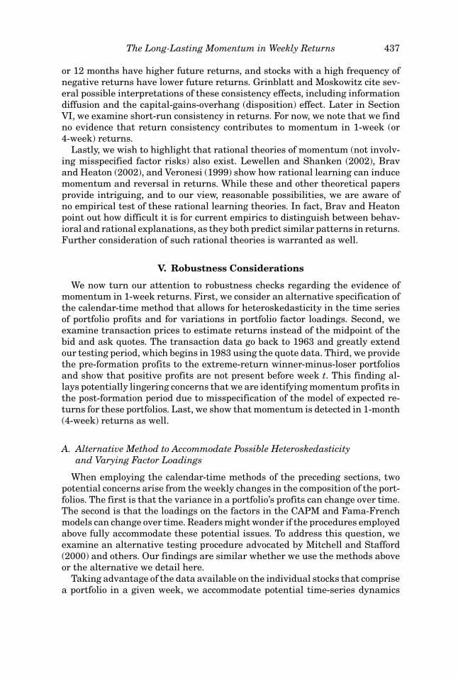
Table VIIIProfits to Weekly Portfolios Using Transaction Returns
(Winners minus Losers)Each week from July 1963 to 2003, we rank stocks based on their returns over the week and forma portfolio comprised of a long position in the top decile of stocks (winners) and a short position inthe bottom decile (losers). Returns are formed from closing transaction prices. Stocks priced belowfive dollars at the end of formation week t are excluded. Calendar-time alphas are estimated overvarious holding periods using raw returns, the CAPM, and the Fama-French three-factor model.The t-statistics are in parentheses and are robust to heteroskedasticity and autocorrelation. Profitsare in basis points.
Holding Period
Week Week Week Weeks Weeks1 2 3 4–52 1–52
Raw −132.13 −42.92 −8.00 6.48 2.49(−30.98) (−11.32) (−2.55) (6.55) (2.47)
CAPM −129.77 −40.68 −6.71 6.79 2.89(−31.59) (−11.06) (−2.15) (7.37) (3.14)
Fama-French −130.21 −40.33 −7.07 6.89 2.96(−30.32) (−10.83) (−2.25) (6.84) (2.92)
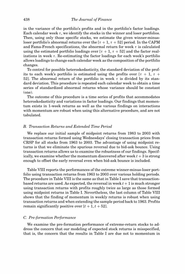
Table IXPre-formation Profits to Weekly Extreme Portfolios
(Winners minus Losers)Each week from 1983 to 2003, we rank stocks based on their returns over the week and form aportfolio comprised of a long position in the top decile of stocks (winners) and a short position inthe bottom decile (losers). Returns are formed from the midpoints of the quoted bid and ask pricesat each day’s close. Stocks priced below five dollars at the end of formation week t are excluded.Calendar-time alphas are estimated over various pre-formation windows from week t − 52 to weekt − 1 using raw returns, the CAPM, and the Fama-French three-factor model. The t-statistics are inparentheses and are robust to heteroskedasticity and autocorrelation. Profits are in basis points.
Holding Period
Weeks Week Week Week−52 to −4 −3 −2 −1
Raw 0.07 −6.29 −50.08 −94.53(0.05) (−1.15) (−7.72) (−10.56)
CAPM 1.03 −5.60 −50.45 −93.67(0.84) (−1.02) (−7.47) (−10.45)
Fama-French −0.81 −6.75 −50.21 −93.18(−0.65) (−1.19) (−7.79) (−10.88)
returns in week t but to an inherent (priced) characteristic of the selected stocksthat we fail to capture. Table IX reports the performances of the extreme-returnwinner-minus-loser portfolio (as in Table I) over various pre-formation windows.None of the windows from week t − 52 to week t − 1 display momentum profits.Hence, momentum profits in the 52-week post-formation window are not dueto a persistent misspecification of expected returns.
440 The Journal of Finance
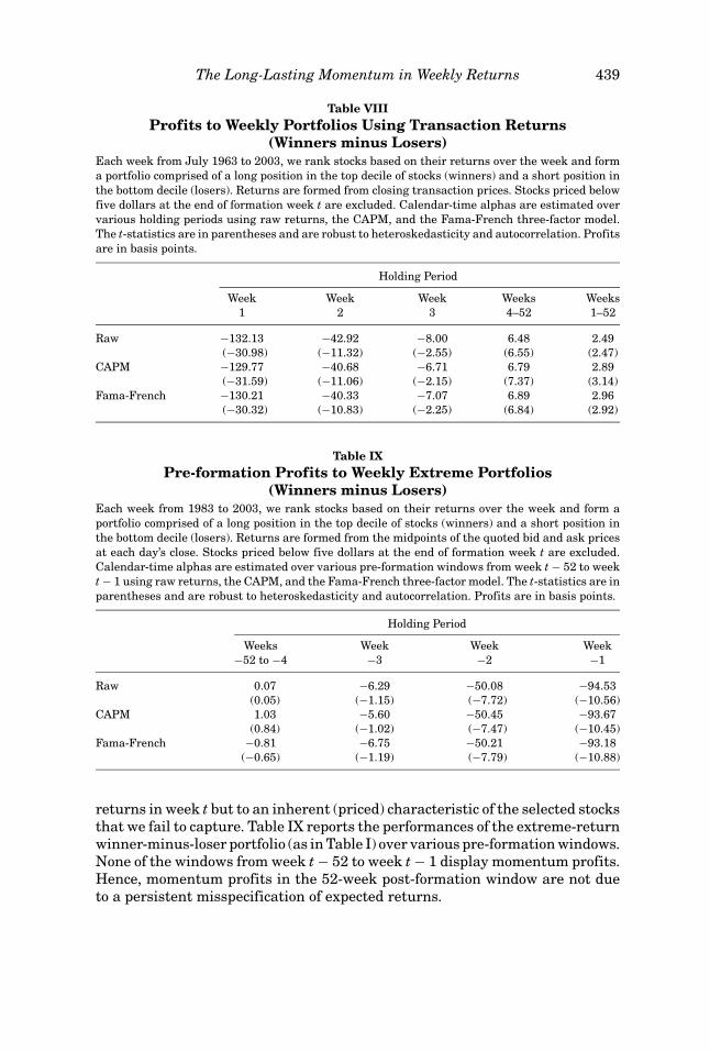
Table XProfits to Monthly Extreme Portfolios
(Winners minus Losers)Each week from 1983 to 2003, we rank stocks based on their returns over weeks [t − 3, t] and forma portfolio comprised of a long position in the top decile of stocks (winners) and a short positionin the bottom decile (losers). Returns are formed from the midpoints of the quoted bid and askprices at each day’s close. Stocks priced below five dollars at the end of the formation week t areexcluded. Calendar-time alphas are estimated over various holding periods using raw returns, theCAPM, and the Fama-French three-factor model. The t-statistics are in parentheses and are robustto heteroskedasticity and autocorrelation. Profits are in basis points.
Holding Period
Week Week Week Weeks Weeks1 2 3 4–52 1–52
Raw −61.41 −16.51 8.12 15.65 13.18(−6.15) (−2.01) (1.17) (4.55) (3.78)
CAPM −54.50 −11.41 11.82 15.79 13.63(−5.90) (−1.46) (1.65) (4.75) (4.08)
Fama-French −58.94 −15.63 8.00 16.54 14.10(−5.94) (−1.83) (1.05) (4.69) (3.91)
Interestingly, Table IX does show negative profits in weeks t − 1 and t − 2.This pre-formation reversal in returns is the mirror image of the post-formationreversal.21 This finding suggests that the forces that induce reversal in returnsacross weeks t to t + 1 also induce reversal across weeks t − 1 to t. As notedearlier, two potential explanations of the reversal are microstructure issues andtraders’ overreaction to news. In Section VII we discuss what our findings as awhole can and cannot say about the short-run reversal.
D. Momentum in 1-Month Returns
For completeness, we also examine whether momentum exists in 1-monthreturns. Jegadeesh (1990) finds that short-run reversal in returns occurs at the1-month horizon, not just the 1-week horizon documented by Lehmann (1990).We rank stocks each week based on returns over [t − 3, t] and define winnerstocks to be those in the top decile of returns over that 4-week period and loserstocks to be those in the bottom decile over that 4-week period.
Table X provides the profits to the winner-minus-loser portfolio over variousholding periods. Consistent with Jegadeesh’s (1990) results, we see that 4-weekreturns reverse strongly in week t + 1. As with 1-week returns (in Table I), thereversal dies out quickly and is completely gone by week t + 3. The 4-week ex-treme portfolio then displays a run-up in profits over weeks [t + 4, t + 52], andthis run-up is once again strong enough to offset the initial reversal and gener-ate statistically significant momentum profits over weeks [t + 1, t + 52], witht-statistics greater than 3.7 across raw, CAPM, and Fama-French performance
21 Ball et al. (1995) find similar results using bid-to-bid returns on NASDAQ stocks from 1983to 1990.
The Long-Lasting Momentum in Weekly Returns 441
metrics. In short, portfolios based on 4-week returns behave qualitatively thesame as portfolios based on 1-week returns.
VI. Return Consistency
Grinblatt and Moskowitz (2004) and Watkins (2003) find that stocks with ahigh frequency of positive returns over the past 6 to 36 months have higherreturns than other stocks, and Watkins finds that stocks with a high fre-quency of negative returns over these long horizons have lower returns thanother stocks.22 These researchers also show that a portion of the momentum in6- and 12-month returns is related to these return-consistency effects. In addi-tion, Watkins (2006) examines short-run consistency over 2 and 4 weeks andfinds that positive consistency leads to lower returns the next week and nega-tive consistency leads to higher returns the next week.
We extend this related literature and examine whether return consistencyover 1 and 4 weeks contributes to the momentum in returns that we documentin prior sections. We define a stock to be positively consistent in week t if ithas 5 days of raw returns greater than zero and negatively consistent in weekt if it has 5 days of raw returns less than zero. Our choice of 5 out of 5 daysto define consistency reflects our belief that 4 out of 5 might not be restrictiveenough. Grinblatt and Moskowitz (2004) select proportions of periods that haveroughly 10% probability under a binomial distribution assuming 0.5 probabilityof positive and nonpositive returns (or negative and nonnegative) each period.The probability of 5 out of 5 is roughly 3%, while the probability of at least 4out of 5 is roughly 19%.
For the 4-week formation period over weeks [t − 3, t], we define positiveconsistency to be at least 70% of the available days. For nonholiday periods,this requires at least 14 of the 20 days to be consistently positive or negative,which occurs under the binomial distribution with probability 6% and is thespecification used by Watkins (2006).
In this section we rely exclusively on cross-sectional regressions to examinethe ability of return consistency over weekly and monthly horizons to predictfuture returns. Portfolio methods, as it turns out, do not adequately controlfor prior returns when conditioning on return consistency. For example, afteridentifying winner and loser stocks in week t based on sorting raw returnsinto deciles, we find that the mean return spread between 1-week consistentwinners and losers in formation week t is 27% over 1983–2003; the spreadbetween nonconsistent winners and losers is only 22%. The 5% difference inreturns in the formation week should generate a significant momentum effectthat spuriously would be attributed to a consistency effect. As evidence of this,the less-extreme portfolio (8−3) in Table II has a 5.2% return spread in theformation week, and we detect momentum profits over weeks [t + 1, t + 52]
22 The source of the divergence in Grinblatt and Moskowitz’s (2004) and Watkins’s (2003) findingsregarding loser consistency is unclear, but is possibly due to the different methods used by each tocontrol for other known effects on stock returns.
442 The Journal of Finance
for that portfolio. We therefore conclude that the portfolio method does not ad-equately control for formation-week returns when conditioning on consistency.Hence, we use regressions.
Each week t, we regress the cross-section of return over [t + 1, t + 52] ona consistency dummy variable defined over either week t or weeks [t − 3, t],the corresponding return over either week t or weeks [t − 3, t], and the logsof size and B
M . The weekly time series of coefficients is then used to test thenull hypothesis that each coefficient is zero. See Section III.B for details on therobust standard errors. We define the consistency dummy variable (CONS) as
CONSith =
1 if stock i is positively consistent over horizon h−1 if stock i is negatively consistent over horizon h
0 otherwise,(1)
where h = (Week, Mth), which indicates whether consistency is determinedover week t or over weeks [t − 3, t]. We choose to combine the potential effectsof positive and negative consistency into a single dummy variable for brevity,since we find that little information is lost by reporting the single measure. Wealso examine the return over t + 1 as the dependent variable for completeness.In addition, for a given calendar week to be included in the analysis, we requireat least 10 stocks that week to be labeled positively consistent and 10 stocks tobe labeled negatively consistent.23
Table XI reports the results of the cross-sectional regression analyses. PanelsA and B respectively show that ConsWeek
t is not related to either the return overweek t + 1 or the return over weeks [t + 1, t + 52], controlling for B
M , size,and the formation-period return. Thus, consistency measured over the shortestwindow of 5 days does not display an ability to predict future returns.24 PanelC shows that ConsMth
t is negatively related to returns in week t, consistent withWatkins’s (2006) short-run finding. Specifically, the mean profit in week t +1 to buying stocks that were positively consistent over the past 4 weeks andshorting the stocks that were negatively consistent is −0.42% (= −0.21% × 2).However, Panel D shows that ConsMth
t is not related to longer-run performanceover weeks [t + 1, t + 52].
In short, while 4-week consistency is related to return reversal in the sub-sequent week, we find that consistency in returns does not contribute to ourfindings of longer-run momentum in 1- and 4-week returns.
VII. Short-Run Reversal
In addition to finding return momentum in a seemingly unexpected place–weekly returns—our results shed new light on short-run reversal. First, rever-sal in returns is less prevalent than prior studies indicate. After eliminating
23 The minimum number of weeks available for analysis across the various specifications ofregressions is 580.
24 Separating the consistency dummy variable into its positive and negative components finds anegative relation between negative consistency in week t and return in week t + 1.
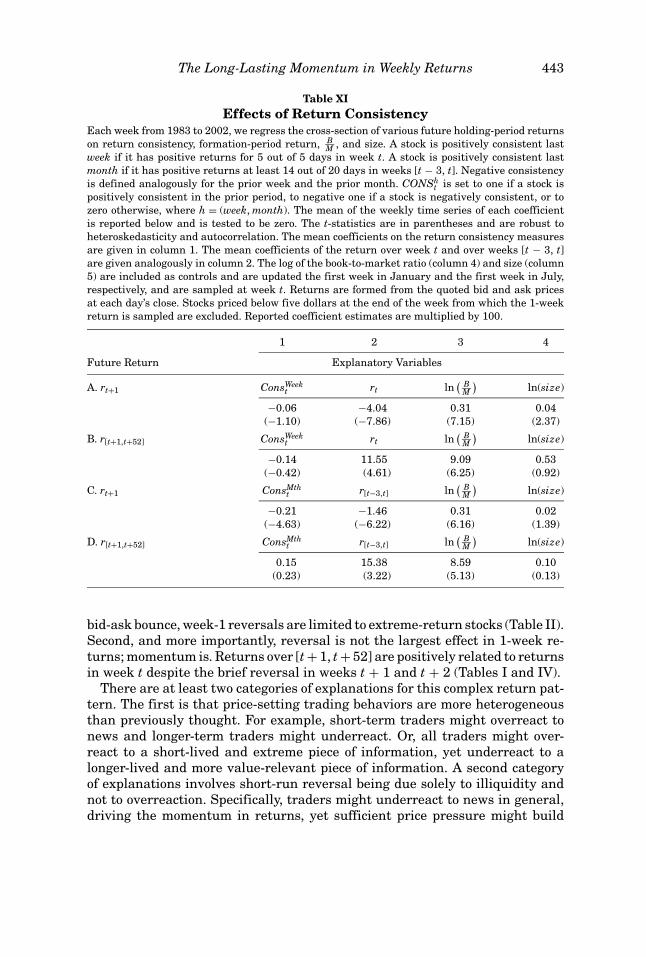
The Long-Lasting Momentum in Weekly Returns 443
Table XIEffects of Return Consistency
Each week from 1983 to 2002, we regress the cross-section of various future holding-period returnson return consistency, formation-period return, B
M , and size. A stock is positively consistent lastweek if it has positive returns for 5 out of 5 days in week t. A stock is positively consistent lastmonth if it has positive returns at least 14 out of 20 days in weeks [t − 3, t]. Negative consistencyis defined analogously for the prior week and the prior month. CONSh
t is set to one if a stock ispositively consistent in the prior period, to negative one if a stock is negatively consistent, or tozero otherwise, where h = (week, month). The mean of the weekly time series of each coefficientis reported below and is tested to be zero. The t-statistics are in parentheses and are robust toheteroskedasticity and autocorrelation. The mean coefficients on the return consistency measuresare given in column 1. The mean coefficients of the return over week t and over weeks [t − 3, t]are given analogously in column 2. The log of the book-to-market ratio (column 4) and size (column5) are included as controls and are updated the first week in January and the first week in July,respectively, and are sampled at week t. Returns are formed from the quoted bid and ask pricesat each day’s close. Stocks priced below five dollars at the end of the week from which the 1-weekreturn is sampled are excluded. Reported coefficient estimates are multiplied by 100.
1 2 3 4
Future Return Explanatory Variables
A. rt+1 ConsWeekt rt ln
( BM
)ln(size)
−0.06 −4.04 0.31 0.04(−1.10) (−7.86) (7.15) (2.37)
B. r[t+1,t+52] ConsWeekt rt ln
( BM
)ln(size)
−0.14 11.55 9.09 0.53(−0.42) (4.61) (6.25) (0.92)
C. rt+1 ConsMtht r[t−3,t] ln
( BM
)ln(size)
−0.21 −1.46 0.31 0.02(−4.63) (−6.22) (6.16) (1.39)
D. r[t+1,t+52] ConsMtht r[t−3,t] ln
( BM
)ln(size)
0.15 15.38 8.59 0.10(0.23) (3.22) (5.13) (0.13)
bid-ask bounce, week-1 reversals are limited to extreme-return stocks (Table II).Second, and more importantly, reversal is not the largest effect in 1-week re-turns; momentum is. Returns over [t + 1, t + 52] are positively related to returnsin week t despite the brief reversal in weeks t + 1 and t + 2 (Tables I and IV).
There are at least two categories of explanations for this complex return pat-tern. The first is that price-setting trading behaviors are more heterogeneousthan previously thought. For example, short-term traders might overreact tonews and longer-term traders might underreact. Or, all traders might over-react to a short-lived and extreme piece of information, yet underreact to alonger-lived and more value-relevant piece of information. A second categoryof explanations involves short-run reversal being due solely to illiquidity andnot to overreaction. Specifically, traders might underreact to news in general,driving the momentum in returns, yet sufficient price pressure might build
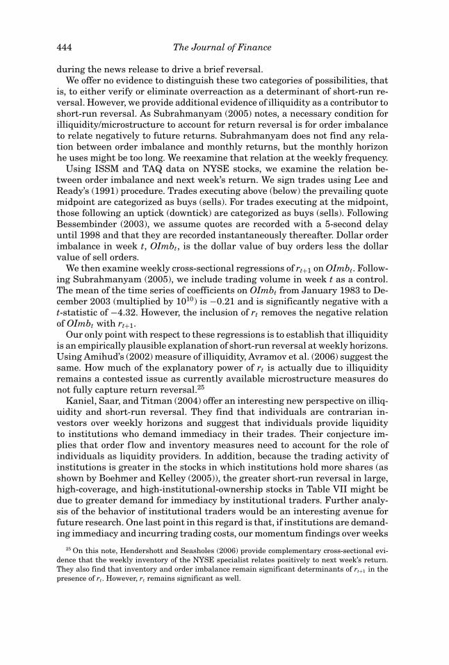
444 The Journal of Finance
during the news release to drive a brief reversal.We offer no evidence to distinguish these two categories of possibilities, that
is, to either verify or eliminate overreaction as a determinant of short-run re-versal. However, we provide additional evidence of illiquidity as a contributor toshort-run reversal. As Subrahmanyam (2005) notes, a necessary condition forilliquidity/microstructure to account for return reversal is for order imbalanceto relate negatively to future returns. Subrahmanyam does not find any rela-tion between order imbalance and monthly returns, but the monthly horizonhe uses might be too long. We reexamine that relation at the weekly frequency.
Using ISSM and TAQ data on NYSE stocks, we examine the relation be-tween order imbalance and next week’s return. We sign trades using Lee andReady’s (1991) procedure. Trades executing above (below) the prevailing quotemidpoint are categorized as buys (sells). For trades executing at the midpoint,those following an uptick (downtick) are categorized as buys (sells). FollowingBessembinder (2003), we assume quotes are recorded with a 5-second delayuntil 1998 and that they are recorded instantaneously thereafter. Dollar orderimbalance in week t, OImbt, is the dollar value of buy orders less the dollarvalue of sell orders.
We then examine weekly cross-sectional regressions of rt+1 on OImbt. Follow-ing Subrahmanyam (2005), we include trading volume in week t as a control.The mean of the time series of coefficients on OImbt from January 1983 to De-cember 2003 (multiplied by 1010) is −0.21 and is significantly negative with at-statistic of −4.32. However, the inclusion of rt removes the negative relationof OImbt with rt+1.
Our only point with respect to these regressions is to establish that illiquidityis an empirically plausible explanation of short-run reversal at weekly horizons.Using Amihud’s (2002) measure of illiquidity, Avramov et al. (2006) suggest thesame. How much of the explanatory power of rt is actually due to illiquidityremains a contested issue as currently available microstructure measures donot fully capture return reversal.25
Kaniel, Saar, and Titman (2004) offer an interesting new perspective on illiq-uidity and short-run reversal. They find that individuals are contrarian in-vestors over weekly horizons and suggest that individuals provide liquidityto institutions who demand immediacy in their trades. Their conjecture im-plies that order flow and inventory measures need to account for the role ofindividuals as liquidity providers. In addition, because the trading activity ofinstitutions is greater in the stocks in which institutions hold more shares (asshown by Boehmer and Kelley (2005)), the greater short-run reversal in large,high-coverage, and high-institutional-ownership stocks in Table VII might bedue to greater demand for immediacy by institutional traders. Further analy-sis of the behavior of institutional traders would be an interesting avenue forfuture research. One last point in this regard is that, if institutions are demand-ing immediacy and incurring trading costs, our momentum findings over weeks
25 On this note, Hendershott and Seasholes (2006) provide complementary cross-sectional evi-dence that the weekly inventory of the NYSE specialist relates positively to next week’s return.They also find that inventory and order imbalance remain significant determinants of rt+1 in thepresence of rt. However, rt remains significant as well.
The Long-Lasting Momentum in Weekly Returns 445
[t + 1, t + 52] suggest that on net institutions do not suffer if stocks are held forthe entire year, as the benefit of return momentum offsets the presumed costsof immediacy.
In short, neither the reversal nor the momentum that follows extreme weeklyreturns is fully understood. To the extent that weekly returns contain traders’misreactions to news, we can conclude that overreaction is not the largest mis-reaction; rather, underreaction is.26
VIII. Conclusion
A portfolio that buys last week’s winner stocks and shorts last week’s loserstocks earns positive profits over the next 52 weeks. This is striking given thewell-known presence of negative (contrarian) profits in the first weeks followingan extreme weekly return. Thus, a literature that once portrayed weekly re-turns only as reversing must now recognize a second effect, momentum, whichoffsets and indeed dominates the reversal.
The finding of momentum in 1-week returns, which complements the findingsof momentum in corporate events, firm-specific headline news, and longer-runreturns up to 12 months, simplifies the anomaly picture, as return continua-tion is a pervasive phenomenon. Moreover, weekly returns provide researchersa new and more stringent testing ground of momentum theories. For exam-ple, revisiting the studies by Chan (2003) and Zhang (2006), we find that theirlonger-run momentum results do not extend to 1-week momentum. Specifically,we find that the market’s reactions to explicit news (price movements associ-ated with public news) and to implicit news (price movements without publicnews) are not categorically different, and that uncertainty is not related tomomentum in 1-week returns. Interestingly though, return momentum follow-ing explicit news is stronger than return momentum following implicit news.Further examinations of this finding might be fruitful.
In addition to the finding of longer-run momentum following weekly returns,we find that winner and loser stocks outside the extreme deciles of weeklyreturns generate momentum profits in the subsequent week. In short, momen-tum is the dominant effect in weekly returns. If abnormal profits are due tothe market’s misreactions to news, then on net, weekly returns seem bettercharacterized as underreactions, not overreactions.
REFERENCESAmihud, Yakov, 2002, Illiquidity and stock returns: Cross-section and time-series effects, Journal
of Financial Markets 5, 31–56.Andrews, Donald W. K., 1991, Heteroskedastic and autocorrelation consistent covariance matrix
estimation, Econometrica 59, 817–858.Avramov, Doron, Tarun Chordia, and Amit Goyal, 2006, Liquidity and autocorrelations in individ-
ual stock returns, Journal of Finance 61, 2365–2394.
26 When we extend the holding-period window in Table I to 3 years following extreme weeklyreturns, profits are no longer statistically different from zero. The interpretation that extremeweekly returns are better viewed as underreactions is then tempered, but the evidence that extremeweekly returns are not too extreme remains, which is still a notable departure from prior studies.
446 The Journal of Finance
Ball, Ray, S.P. Kothari, and Charles E. Wasley, 1995, Can we implement research on stock tradingrules? Journal of Portfolio Management 21, 54–63.
Barberis, Nicholas, Andrei Shleifer, and Robert Vishny, 1998, A model of investor sentiment, Jour-nal of Financial Economics 49, 307–343.
Bessembinder, Hendrick, 2003, Issues in assessing trade execution costs, Journal of FinancialMarkets 6, 233–257.
Bhushan, Ravi, 1989, Firm characteristics and analyst following, Journal of Accounting and Eco-nomics 11, 255–274.
Boehmer, Ekkehart, and Eric Kelley, 2005, Institutional investors and the informational efficiencyof prices, Working paper, Texas A&M University.
Boudoukh, Jacob, Matthew P. Richardson, and Robert F. Whitelaw, 1994, Tale of three schools:Insights on autocorrelations of short-horizon stock returns, Review of Financial Studies 7,539–573.
Brav, Alon, and J. B. Heaton, 2002, Competing theories of financial anomalies, Review of FinancialStudies 15, 575–606.
Chan, Wesley S., 2003, Stock price reaction to news and no-news: Drift and reversal after headlines,Journal of Financial Economics 70, 223–260.
Conrad, Jennifer S., Allaudeen Hameed, and Cathy Niden, 1994, Volume and autocovariances inshort-horizon individual security returns, Journal of Finance 49, 1305–1329.
Conrad, Jennifer, Gautam Kaul, and M. Nimalendran, 1991, Components of short-horizon individ-ual security returns, Journal of Financial Economics 29, 365–384.
Cooper, Michael, 1999, Filter rules based on price and volume in individual security overreaction,Review of Financial Studies 12, 901–935.
Daniel, Kent, David Hirshleifer, and Avanidhar Subrahmanyam, 1998, Investor psychology andinvestor security market under- and overreactions, Journal of Finance 53, 1839–1886.
Daniel, Kent, and Sheridan Titman, 2006, Market reactions to tangible and intangible information,Journal of Finance 61, 1605–1643.
DeBondt, Werner F.M., and Richard Thaler, 1985, Does the stock market overreact? Journal ofFinance 40, 793–808.
Diether, Karl B., Christopher J. Malloy, and Anna Scherbina, 2002, Differences of opinion and thecross-section of stock returns, Journal of Finance 57, 2113–2141.
Fama, Eugene F., 1998, Market efficiency, long-term returns, and behavioral finance, Journal ofFinancial Economics 49, 283–306.
Frazzini, Andrea, 2006, The disposition effect and underreaction to news, Journal of Finance 61,2017–2046.
Gallant, A. Ronald, 1987, Nonlinear Statistical Models (John Wiley and Sons, New York).Gompers, Paul A., and Andrew Metrick, 2001, Institutional investors and equity prices, Quarterly
Journal of Economics 116, 229–259.Grinblatt, Mark, and Bing Han, 2005, Prospect theory, mental accounting and momentum, Journal
of Financial Economics 78, 311–333.Grinblatt, Mark, and Tobias J. Moskowitz, 2004, Predicting stock price movements from past re-
turns: The role of consistency and tax-loss selling, Journal of Financial Economics 71, 541–579.Grundy, Bruce D., and Spencer J. Martin, 2001, Understanding the nature of the risks and the
sources of the rewards to momentum investing, Review of Financial Studies 14, 29–78.Hansch, Oliver, Narayan Y. Naik, and S. Viswanathan, 1998, Do inventories matter in dealership
markets? Evidence from the London Stock Exchange, Journal of Finance 53, 1623–1656.Hasbrouck, Joel, and George Sofianos, 1993, The trades of market makers: An empirical analysis
of NYSE specialists, Journal of Finance 48, 1565–1593.Hendershott, Terrence, and Mark S. Seasholes, 2006, Specialist inventories and stock prices, Work-
ing paper, University of California, Berkeley.Hirshleifer, David, 2001, Investor psychology and asset pricing, Journal of Finance 56, 1533–1597.Hong, Harrison, Terence Lim, and Jeremy C. Stein, 2000, Bad news travels slowly: Size, analyst
coverage, and the profitability of momentum strategies, Journal of Finance 55, 265–295.Hong, Harrison, and Jeremy C. Stein, 1999, A unified theory of underreaction, momentum trading,
and overreaction in asset markets, Journal of Finance 54, 2143–2184.
The Long-Lasting Momentum in Weekly Returns 447
Jegadeesh, Narasimhan, 1990, Evidence of predictable behavior of security returns, Journal ofFinance 45, 881–898.
Jegadeesh, Narasimhan, and Sheridan Titman, 1993, Returns to buying winners and selling losers:Implications for market efficiency, Journal of Finance 48, 65–92.
Jegadeesh, Narasimhan, and Sheridan Titman, 1995a, Overreaction, delayed reaction, and con-trarian profits, Review of Financial Studies 8, 973–993.
Jegadeesh, Narasimhan, and Sheridan Titman, 1995b, Short-horizon return reversals and thebid-ask spread, Journal of Financial Intermediation 4, 116–132.
Johnson, Timothy C., 2004, Forecast dispersion and the cross-section of expected returns, Journalof Finance 59, 1957–1978.
Kaniel, Ron, Gideon Saar, and Sheridan Titman, 2004, Individual investor sentiment and stockreturns, Working paper, Duke University.
Kaul, Gautam, and M. Nimalendran, 1990, Price reversals: Bid-ask errors or market overreaction?Journal of Financial Economics 28, 67–93.
Lee, Charles M.C., and Mark Ready, 1991, Inferring trade direction from inter-day data, Journalof Finance 46, 733–746.
Lehmann, Bruce N., 1990, Fads, martingales, and market efficiency, Quarterly Journal of Eco-nomics 105, 1–28.
Lewellen, Jonathan, and Jay Shanken, 2002, Learning, asset-pricing tests, and market efficiency,Journal of Finance 57, 1113–1145.
Lo, Andrew W., and A. Craig MacKinlay, 1990, When are contrarian profits due to stock marketoverreaction? Review of Financial Studies 3, 175–205.
Madhavan, Ananth, and Seymour Smidt, 1993, An analysis of changes in specialists inventoriesand quotations, Journal of Finance 48, 1595–1628.
Mitchell, Mark L., and Erik Stafford, 2000, Managerial decisions and long-term stock price perfor-mance, Journal of Business 73, 287–329.
Payne, Jeff L., and Wayne B. Thomas, 2003, The implications of using stock-split adjusted I/B/E/Sdata in empirical research, Accounting Review 78, 1049–1067.
Roll, Richard, 1984, A simple implicit measure of the effective bid-ask spread in an efficient market,Journal of Finance 39, 1127–1139.
Subrahmanyam, Avanidhar, 2005, Distinguishing between rationales for short-horizon predictabil-ity in stock returns, Financial Review 40, 11–35.
Veronesi, Pietro, 1999, Stock market overreaction to bad news in good times: A rational expectationsequilibrium model, Review of Financial Studies 12, 975–1007.
Veronesi, Pietro, 2000, How does information quality affect stock returns? Journal of Finance 50,807–837.
Watkins, Boyce, 2003, Riding the wave of sentiment: An analysis of consistency as a predictor offuture returns, Journal of Behavioral Finance 4, 191–200.
Watkins, Boyce, 2006, Institutional ownership and return reversals following short-term returnconsistency, Financial Review 41, 435–448.
Zhang, X. Frank, 2006, Information uncertainty and stock returns, Journal of Finance 61, 105–137.