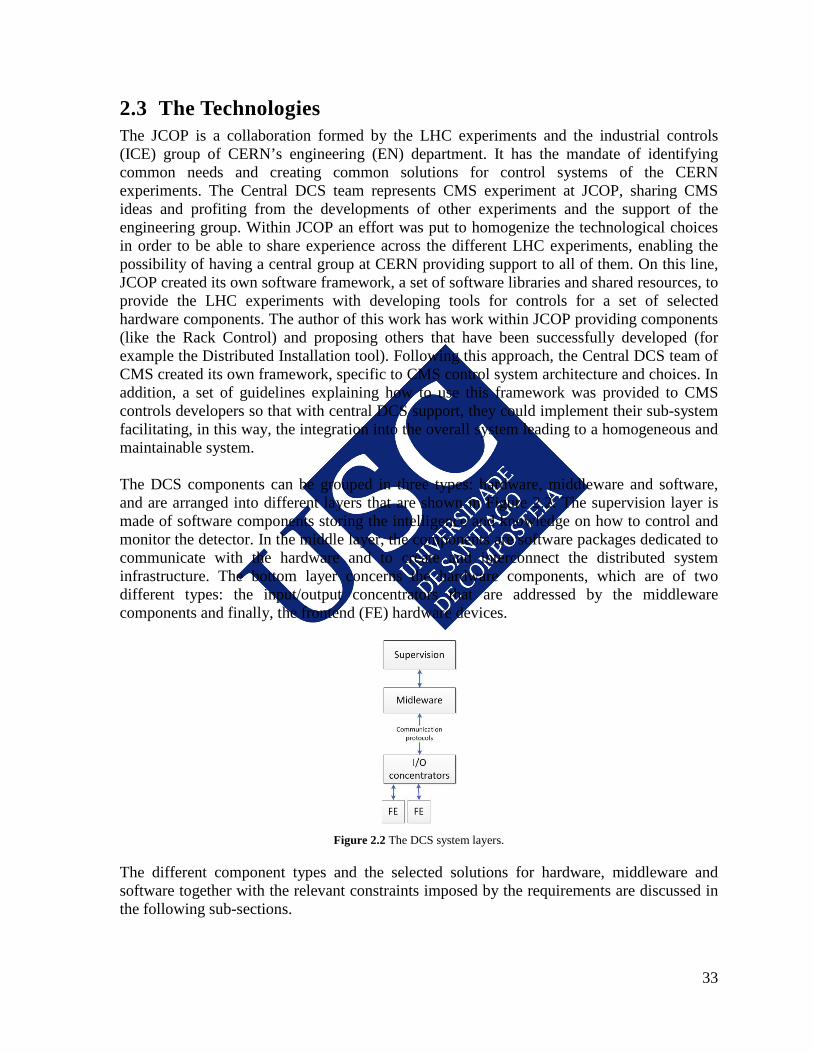
the distributed control system of lhc - cms - core
TRANSCRIPT
UNIVERSIDAD DE SANTIAGO
DE COMPOSTELA
FACULTAD DE FISICA Departamento de Física de Partículas
The distributed control system of LHC - CMS: study of the stability and dynamic range of the new SiPM detector
for the HCAL.
Robert Gómez-Reino Garrido
Memoria presentada para optar al Grado de Doctor en Física
Santiago de Compostela, 3 de Octubre de 2013

UNIVERSIDAD DE SANTIAGO
DE COMPOSTELA
El Dr. Fernando Varela Rodríguez, Funcionario investigador del CERN (European Organization for Nuclear Research) y El Prof. Ignacio Durán Escribano, Catedrático de la USC, CERTIFICAN: que la memoria titulada “The distributed control system of LHC - CMS: study of the stability and dynamic range of the new SiPM detector for the HCAL” ha sido realizada por Roberto Gomez-Reino Garrido en el Departamento de Física de Partículas de esta Universidad, bajo su dirección y tutela, constituyendo el trabajo de tesis que presenta para optar al grado de Doctor en Física. Santiago de Compostela, 3 de octubre de 2013.
Fdo: Fernando Varela Rodríguez Fdo: Ignacio Durán Escribano
Fdo: Roberto Gomez-Reino Garrido

Acknowledgments The PhD work presented here was carried out in the framework of a collaboration between the USC and CERN. It was supported by CERN´s Doctoral and Fellowship student programmes, under the supervision of Dr. F. Varela Rodriguez (CERN) and Prof. I. Durán Escribano (USC). I would like to thank both of my supervisors for their support and guidance. I would also like to thank HCAL collaboration, especially Dr. B. Lutz, for the opportunity of working and learning with them.

TABLE OF CONTENTS
SUMMARY ............................................................................................................................. 1
INTRODUCTION AND OBJECTIVES .............................................................................. 3 PART I 1. THE CMS EXPERIMENT ............................................................................................. 9
1.1 THE LARGE HADRON COLLIDER .......................................................................... 9 1.2 THE CMS DETECTOR .............................................................................................. 13
1.2.1 PHYSICS GOALS ............................................................................................ 13 1.2.2 DETECTOR PHYSICS REQUIREMENTS .................................................... 15
1.3 DETECTOR OVERALL DESIGN ............................................................................. 15 1.3.1 THE MAGNET ................................................................................................. 16 1.3.2 THE TRACKING SYSTEM ............................................................................ 17 1.3.3 THE MUON SYSTEM ..................................................................................... 19 1.3.4 THE CALORIMETER SYSTEM..................................................................... 22 1.3.5 THE ALIGNMENT, TRIGGER AND DATA ACQUISITION SYSTEMS ... 27
2. THE CMS DETECTOR CONTROL SYSTEM ......................................................... 29 2.1 REQUIREMENTS ...................................................................................................... 29 2.2 THE PROJECT ORGANIZATION ............................................................................ 30 2.3 THE TECHNOLOGIES.............................................................................................. 33
2.3.1 THE HARDWARE COMPONENTS............................................................... 34 2.3.2 THE INFRASTRUCTURE LAYER SOFTWARE.......................................... 36 2.3.3 THE CONTROLS RELATED SOFTWARE ................................................... 38
PART II 3. THE DCS IMPLEMENTATION................................................................................. 43
3.1 ARCHITECTURE OVERVIEW ................................................................................ 43 3.2 CMS DCS MIDDLEWARE ....................................................................................... 45 3.3 THE CMS DCS FRAMEWORK ................................................................................ 47
3.3.1 THE CMS CORE AND FUNCTIONAL COMPONENTS ............................. 47 3.3.2 DEVELOPMENT AND DEPLOYMENT STRATEGY ................................. 49
4. THE DCS OPERATION............................................................................................... 53 4.1 OPERATION OVERVIEW ........................................................................................ 53 4.2 THE CENTRAL DCS CONTROL STATION ........................................................... 55 4.3 COMMUNICATION WITH EXTERNAL SYSTEMS .............................................. 58
4.3.1 COMMUNICATION WITH THE LHC .......................................................... 58 4.3.2 COMMUNICATION WITH RUN CONTROL AND DAQ............................ 60 4.3.3 COMMUNICATION WITH THE CAVERN SERVICES .............................. 60
4.4 THE DCS FSM TREE ................................................................................................. 61 4.5 THE DCS AUTOMATION AND PROTECTION MECHANISMS .......................... 63
5. THE ECAL DCS ............................................................................................................ 67 5.1 THE COOLING SYSTEM ......................................................................................... 68 5.2 HIGH VOLTAGE AND LOW VOLTAGE SYSTEMS ............................................. 68 5.3 THE PRECISION TEMPERATURE (PTM) AND HUMIDITY (HM) SYSTEMS ... 69 5.4 THE ECAL SAFETY SYSTEM (ESS) ....................................................................... 71 5.5 THE DCS SOFTWARE .............................................................................................. 74
5.5.1 THE ECAL FSM ANALYSIS.......................................................................... 77 5.6 THE ECAL OPERATION .......................................................................................... 78
PART III 6. A NEW TECHNOLOGY FOR THE HCAL BARREL UPGRADE ........................ 81
6.1 THE HCAL HPDS ...................................................................................................... 81 6.1.1 OPERATIONAL EXPERIENCE WITH HPDS .............................................. 83
6.2 SILICON PHOTOMULTIPLIERS ............................................................................. 84 6.3 HO SIPM READOUT ................................................................................................. 85 6.4 THE TEST-STAND SETUP ....................................................................................... 86 6.5 THE SIPM CONTROL SYSTEM .............................................................................. 87 6.6 SIPM CURRENT STABILITY ANALYSIS .............................................................. 90
6.6.1 THE ANALYSIS METHODOLOGY .............................................................. 90 6.6.2 CURRENT AND TEMPERATURE STABILITY STUDIES ......................... 91
7. SIPM TEST BEAM ....................................................................................................... 97 7.1 TEST BEAM OVERVIEW AND SETUP .................................................................. 97 7.2 TEST BEAM OBJECTIVES ...................................................................................... 99 7.3 DYNAMIC RANGE ANALYSIS ............................................................................ 100 7.4 SIPM DYNAMIC RANGE ANALYSIS RESULT .................................................. 107
CONCLUSIONS ................................................................................................................. 109
RESUMEN EN ESPAÑOL ................................................................................................ 111 R.1 INTRODUCCIÓN ................................................................................................. 111 R.2 EL SISTEMA DE CONTROL DEL DETECTOR DE CMS .................................. 113 R.3 EL SISTEMA DE CONTROL DEL ECAL ........................................................... 116 R.4 EL CALORÍMETRO EXTERIOR DEL HCAL .................................................... 117 R.5 UNA TECNOLOGÍA DE DETECCIÓN BASADA EN SILICIO PARA EL BARRIL DEL HCAL ........................................................................................................ 120 R.6 PRUEBAS DE ESTABILIDAD DE LOS SIPM .................................................... 123 R.7 ESTUDIO DEL RANGO DINÁMICO DE LOS SIPM EN UN TEST-BEAM ..... 124 R.8 CONCLUSIÓN ...................................................................................................... 127
APPENDIX A. JCOP COMPONENTS IN CMS............................................................. 129
APPENDIX B. HADRONIC CALORIMETRY .............................................................. 131
APPENDIX C. TTREE GENERATION SCRIPT FOR THE HCAL SIPM STABILITY ANALYSIS ......................................................................................................................... 133
APPENDIX D. THE ROOT SCRIPT FOR THE SIPM STABILITY ANALYSIS IN 904 ......................................................................................................................... 139
REFERENCES .................................................................................................................... 147

1
Summary This dissertation concerns part of the work done by the author within the CMS collaboration. It consists of seven chapters that are conceptually divided into three Parts. The first Part includes the Introduction and the first two chapters. Firstly the CERN Large Hadron Collider where this work has been performed is described. The overall CMS detector is then presented: the sub-detectors and main systems are described, providing also an overview of the collaboration organization, as well as the experimental infrastructure. Finishing Part I, the main purpose of the CMS Detector Control System (DCS) is summarized together with the technologies chosen to cope with its operational, functional, environmental and organizational requirements. The main contributions of the author of this thesis to this first part consisted in the selection, validation and development of technologies and tools for the implementation of the CMS DCS. Part II includes Chapters 3, 4 and 5, and focuses on the developments performed in several sub-systems of the CMS DCS. The development challenges of the DCS and its unique infrastructure are brought to light. The overall design and architecture, with its different layers, is presented. Chapter 4 is dedicated to the operational aspects. The detector protection and the automation mechanisms are presented. Then, a practical example of a sub-detector control system is presented in Chapter 5. The architecture and development details of the CMS Electromagnetic Calorimeter (ECAL) supervisory control and its different control subsystems are explained. The author of this thesis participated in the design of the overall architecture of the DCS and in the definition of the operational model of the detector. Furthermore, the author of this thesis closely worked with the different CMS sub-detectors to assist them during the implementation of their local control system. An example of this is the implementation of the ECAL DCS where the author was a key developer of the system. The author also proposed and implemented various protection mechanisms that are currently in use at CMS. Finally, in Part III, Chapters 6 and 7 describe the studies performed by the author for the upgrade of the CMS Hadron Calorimeter (HCAL). An overview of the current detecting technology, the Hybrid Photo Diodes (HPD), used in the Hadron Outer Calorimeter (HO) is provided. The problems with these devices, motivating their replacement, are presented. Chapter 6 presents a photo detection technology based on Silicon Photomultipliers (SiPM), intended to replace the HPD in the HO calorimeter, and it summarizes the work done to validate and characterize these devices. The test bench in an integration area at CERN is described, and the stability studies performed are discussed. Chapter 7 presents the analysis of the data acquired during a test beam devoted to validate the use of the SiPM in the HO sub-detector. The author of this thesis developed the control system to perform these studies. Moreover, he participated in the data-taking and in the analysis for both the characterization of the SiMP detectors at the test-bench and various experimental setups to study the detector response to particles. The results of the SiPMs dynamic range studies are compared to the results with HPDs. In addition, the effects of using light mixers in front of the photo-detector devices are also presented. The chapter concludes providing a suggestion for a configuration

2
valid for the operation of the SiPMs in HO and discussing the impact of the DCS controlled parameters on the performance of the calorimeter to the physics processes of interest at the LHC. The overall conclusions are discussed after Chapter 7.

3
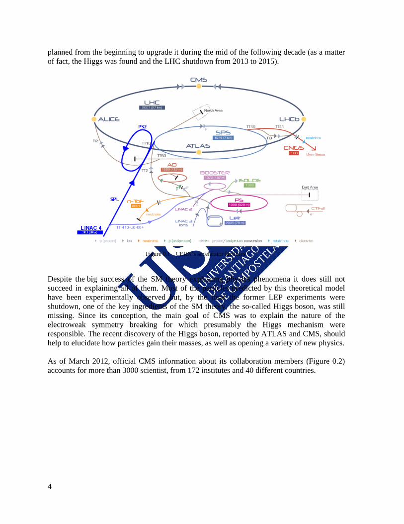
Introduction and objectives The Compact Muon Solenoid (CMS) [1] was built as a part of the big facilities of the European Centre for Nuclear Research (CERN). This laboratory has devoted most of it resources during the last two decades to the construction of the Large Hadron Collider (LHC) [2] and its experimental areas. The LHC experiments have being designed to operate in a ultra-high range of energy, where today’s main particle physics challenges can be addressed, being CMS one of the two LHC general purpose particle detectors, with the aim of exploring the full range of potentially interesting physics produced at this unique accelerator complex. CERN is nowadays the world's largest particle physics research laboratory. It was founded in September 1954, during the beginning of the Cold War, as an attempt to seduce European researchers that were emigrating, mostly to the United States of America, bringing all their knowledge and expertise overseas with them. With its first General Director, Felix Bloch, CERN confronted the challenge of restoring the prestige of the European physics. More than 50 years later, CERN has been recognized to have accomplished its initial goals. Today many not European researchers and institutions collaborate actively with CERN on its leading fundamental research. The laboratory hosts thousands of scientists and engineers that come mainly from Europe, but also from the other continents, with the purpose of breaking through the Standard Model wall and finding a new physics world beyond it. Since its foundation many thousands of physicists, including prestigious Nobel laureates and prize awarded ones (Felix Bloch, Edward Mills Purcell, Sam Ting, Burt Richter, Jack Steinberger, Carlo Rubbia, Georges Charpak, Gerard't Hooft and Simon Van der Meer) have collaborated with and managed several experiments. Together with physicists a large community of information technology experts and engineers come to CERN looking for challenging projects, experience and education in an environment well known for its high technology aspects; it is enough to mention that the WWW was born there. CERN’s facility complex (Figure 0.1) is a succession of particle accelerators that can reach increasingly higher energies. Each accelerator boosts the speed of a beam of particles, before injecting it into the next one in the sequence. It also includes the Antiproton Decelerator and the On-Line Isotope Mass Separator (ISOLDE) facility and feeds the CERN Neutrino to Gran Sasso (CNGS) project and the Compact Linear Collider (CLIC) test area called CLIC Test Facility 3 (CTF3). CERN’s flagship project, the LHC, is a particle accelerator that is probing deeper into matter than ever before. The accelerator collides two counter rotating beams of protons or heavy ions. For proton-proton collisions, LHC was designed to produce collisions at a maximum energy of 14 𝑇𝑒𝑉 in the center of masses (7 𝑇𝑒𝑉 per beam), that is expected to happen on 2015. Research projects at CERN are dictated by a restless search for scientific answers. But physics projects take decades to get prepared and, for this reason, the long-term programs at CERN are always overlapping with previous ones. The LHC started to be planned while its predecessor, the Large Electron–Positron collider, LEP, was still running; and the LHC upgrades were under study already before it get started. CERN’s future research programs depend on what LHC experiments bring to light and therefore, the CERN management
4
planned from the beginning to upgrade it during the mid of the following decade (as a matter of fact, the Higgs was found and the LHC shutdown from 2013 to 2015).
CERN’s accelerator facilities. Figure 0.1
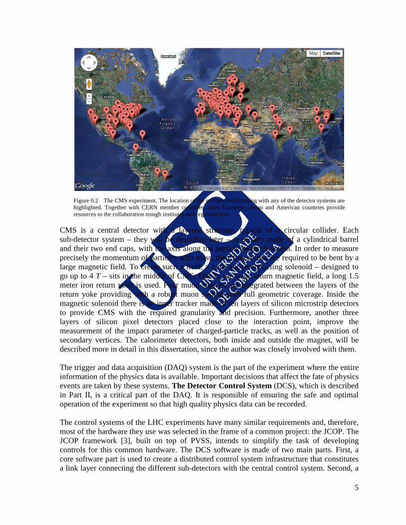
Despite the big success of the SM theory explaining physics phenomena it does still not succeed in explaining all of them. Most of the particles predicted by this theoretical model have been experimentally observed but, by the time the former LEP experiments were shutdown, one of the key ingredients of the SM theory, the so-called Higgs boson, was still missing. Since its conception, the main goal of CMS was to explain the nature of the electroweak symmetry breaking for which presumably the Higgs mechanism were responsible. The recent discovery of the Higgs boson, reported by ATLAS and CMS, should help to elucidate how particles gain their masses, as well as opening a variety of new physics. As of March 2012, official CMS information about its collaboration members (Figure 0.2) accounts for more than 3000 scientist, from 172 institutes and 40 different countries.
5
The CMS experiment. The location of the institute participating with any of the detector systems are Figure 0.2
highlighted. Together with CERN member countries, other European, Asian and American countries provide resources to the collaboration trough institutes and organizations.
CMS is a central detector with a layered structure, typical of a circular collider. Each sub-detector system – they will be described later – is usually made of a cylindrical barrel and their two end caps, with the axis along the particle beam direction. In order to measure precisely the momentum of particles with mass, their trajectories are required to be bent by a large magnetic field. To create such a field, a huge superconducting solenoid – designed to go up to 4 T – sits in the middle of CMS. Due to the large return magnetic field, a long 1.5 meter iron return yoke is used. Four muon stations are integrated between the layers of the return yoke providing with a robust muon system with full geometric coverage. Inside the magnetic solenoid there is an inner tracker made of ten layers of silicon microstrip detectors to provide CMS with the required granularity and precision. Furthermore, another three layers of silicon pixel detectors placed close to the interaction point, improve the measurement of the impact parameter of charged-particle tracks, as well as the position of secondary vertices. The calorimeter detectors, both inside and outside the magnet, will be described more in detail in this dissertation, since the author was closely involved with them. The trigger and data acquisition (DAQ) system is the part of the experiment where the entire information of the physics data is available. Important decisions that affect the fate of physics events are taken by these systems. The Detector Control System (DCS), which is described in Part II, is a critical part of the DAQ. It is responsible of ensuring the safe and optimal operation of the experiment so that high quality physics data can be recorded. The control systems of the LHC experiments have many similar requirements and, therefore, most of the hardware they use was selected in the frame of a common project: the JCOP. The JCOP framework [3], built on top of PVSS, intends to simplify the task of developing controls for this common hardware. The DCS software is made of two main parts. First, a core software part is used to create a distributed control system infrastructure that constitutes a link layer connecting the different sub-detectors with the central control system. Second, a
6
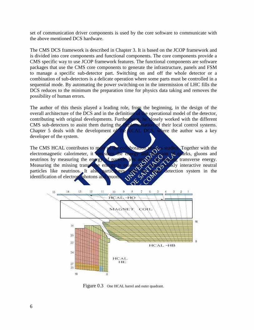
set of communication driver components is used by the core software to communicate with the above mentioned DCS hardware. The CMS DCS framework is described in Chapter 3. It is based on the JCOP framework and is divided into core components and functional components. The core components provide a CMS specific way to use JCOP framework features. The functional components are software packages that use the CMS core components to generate the infrastructure, panels and FSM to manage a specific sub-detector part. Switching on and off the whole detector or a combination of sub-detectors is a delicate operation where some parts must be controlled in a sequential mode. By automating the power switching-on in the intermission of LHC fills the DCS reduces to the minimum the preparation time for physics data taking and removes the possibility of human errors. The author of this thesis played a leading role, from the beginning, in the design of the overall architecture of the DCS and in the definition of the operational model of the detector, contributing with original developments. Furthermore, he closely worked with the different CMS sub-detectors to assist them during the implementation of their local control systems. Chapter 5 deals with the development of the ECAL DCS, where the author was a key developer of the system. The CMS HCAL contributes to most of the collaboration physics studies. Together with the electromagnetic calorimeter, it measures the energy and direction of quarks, gluons and neutrinos by measuring the energy of particle jets and of the missing transverse energy. Measuring the missing transverse energy is essential to detect weakly interactive neutral particles like neutrinos. It also participates with the muon detection system in the identification of electron, photons and muons.
One HCAL barrel and outer quadrant. Figure 0.3
7
It was found that the Hadronic Barrel calorimeter, HB, together with the tracker and the ECAL, give a large fluctuation of the energy leakage for the higher energy events [4], because HB is not able to completely stop the last part of the hadronic shower development. The (HB) inner radius is limited by the electromagnetic calorimeter (EB), and the outer radius by the magnetic coil (see Figure 0.3). For this reason an outer calorimeter, HO, is used to sample the energy leakage outside of the magnetic coil, detecting many particles not being completely stopped by the inner detector. The magnetic field is returned using an iron yoke structured in five ~2.5 𝑚 wide wheels. Matching this distribution and covering |𝜂| < 1.4 there are the HO layers (for a detailed description on the HO design see [5]), that are the first active material outside the magnet coil. At |𝜂| = 0 HB provides its minimum interaction length for hadrons coming from the 𝑝𝑝 collisions, therefore, in this region there are two HO layers. The tile geometry was made to approximately match the HCAL barrel reading towers. The light is collected using wave length shifting (WLS) fibers and transported through coupled clear optical links to readout boxes, where the hybrid photo diodes (HPDs) are installed. Precise magnetic field measurements were only done in 2009, using cosmic rays [6] to provide a precise mapping of the magnetic field. This mapping helped to better understand the CMS magnetic field configuration, satisfying the physics analysis requirements for the event reconstruction. However, it also showed that HPDs were not always correctly aligned with the magnetic field direction. The effect was especially visible outside the magnetic coil where the field was found to be far from the idealized, explaining the electrical discharges that were produced, generating fake events and, in some cases, damaging the photodiodes. Moreover, in the external muon wheel, where the magnetic field differed from what expected even more than in the central wheel, the discharge effects were bigger. Therefore, the HPDs must be actually operated at lower voltages than foreseen, having this way a lower gain and less sensitivity. For this reason, an HCAL barrel upgrade has been programmed, and studies were carried out carried to find new candidates for the HCAL optical readout. Part III is dedicated to the work performed by the author for the definition of the new solution chosen for the HCAL barrel upgrade. Performance studies of silicon-based photosensors [7] concluded that Silicon Photomultipliers (SiPMs) provide an excellent photoelectron resolution. In addition, due to the very high gain, the electronic noise is negligible, so that the main source of noise is the dark current (current that flows with or without incident photons due to the random generation of electrons and holes within the depletion region of the device). SiPMs have in addition large quantum efficiency ≈ 30% and work well in magnetic fields. CMS tests with SiPMs [8] showed that, when compared with the production HPDs, SiPMs provide an order of magnitude of improvement in the signal to noise ratio for single minimum ionizing particles (MIPs). Concerning the upgrade of the HCAL calorimeter, the objectives of the author's work were two, as it is presented in the Part III of this document. The first objective was to find an efficient mechanism to pull out defective SiPM sensors, from the large amount of devices to

8
be tested, by using LEDs to illuminate the SiPMs sensors, recording and analyzing their current and temperature stability. The second one was to verify in a test-beam that the selected SiPM can cover the needed dynamic range of energies expected at HO, suggesting also a possible configuration option to achieve this.

9
1. The CMS experiment 1.1 The Large Hadron Collider The LHC is a particle accelerator that is probing deeper into matter than ever before. It was built in the tunnel, 3.8 𝑚 in diameter and 27 𝑘𝑚 long, that was excavated - from 50 to 175 𝑚 below ground - to build the former LEP accelerator. Particle beams travel along two pipes, in a continuous vacuum comparable to outer space, being guided by powerful magnets. The LHC makes the two counter rotating beams collide at points were protons or heavy ions beams are squeezed down to get a never before attained luminosity. The LHC was designed to produce proton-proton collisions at a maximum energy of 14 𝑇𝑒𝑉 in the center of masses (7 𝑇𝑒𝑉 per beam). The recently stopped Tevatron at Fermilab could reach 1 𝑇𝑒𝑉, and the still running Relativistic Heavy Ion Collider (RHIC) is limited to 250 𝐺𝑒𝑉. The LHC went live on September 10𝑡ℎ 2008, with proton beams successfully circulating in the main ring of the LHC for the first time, but nine days later a faulty electrical connection led to an accident that forced the accelerator to be shutdown. The LHC resumed circulating the beams at relatively low energy on November 20𝑡ℎ 2009 with the first recorded proton–proton collisions occurring three days later at the injection energy of 450 𝐺𝑒𝑉 per beam. First high energy collisions were produced on March 30𝑡ℎ 2010. The LHC operated at 3.5 𝑇𝑒𝑉 per beam in 2010 and 2011 and at 4 𝑇𝑒𝑉 in 2012. It operated for two months in 2013 colliding protons with lead nuclei, and went into shutdown for upgrades in order to increase energy to 6.5 𝑇𝑒𝑉 per beam, with reopening planned for early 2015. Figure 1.1 shows a snapshot of one of the first physics event registered in the CMS experiment during those collisions.
Figure 1.1 The CMS event display during the first LHC collisions. The event displayed released energy in different barrel calorimeter regions and produced hits in three of the muon endcap detector chambers.
10
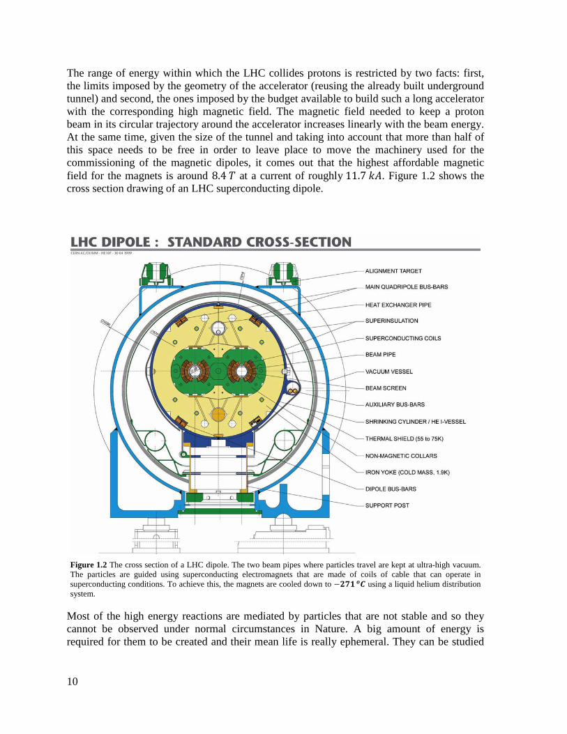
The range of energy within which the LHC collides protons is restricted by two facts: first, the limits imposed by the geometry of the accelerator (reusing the already built underground tunnel) and second, the ones imposed by the budget available to build such a long accelerator with the corresponding high magnetic field. The magnetic field needed to keep a proton beam in its circular trajectory around the accelerator increases linearly with the beam energy. At the same time, given the size of the tunnel and taking into account that more than half of this space needs to be free in order to leave place to move the machinery used for the commissioning of the magnetic dipoles, it comes out that the highest affordable magnetic field for the magnets is around 8.4 𝑇 at a current of roughly 11.7 𝑘𝐴. Figure 1.2 shows the cross section drawing of an LHC superconducting dipole.
Figure 1.2 The cross section of a LHC dipole. The two beam pipes where particles travel are kept at ultra-high vacuum. The particles are guided using superconducting electromagnets that are made of coils of cable that can operate in superconducting conditions. To achieve this, the magnets are cooled down to −𝟐𝟕𝟏 𝒐𝑪 using a liquid helium distribution system.
Most of the high energy reactions are mediated by particles that are not stable and so they cannot be observed under normal circumstances in Nature. A big amount of energy is required for them to be created and their mean life is really ephemeral. They can be studied

11
by colliding particles at high enough energies but the intensity of the beams need to increase more and more the rarer the events of interest become. Every reaction channel has a different probability of occurring, being a function of the scattering angle (𝜃).For a defined energy range, the probability of these reactions is measured in terms of the differential cross section:
𝑑𝜎(𝜃) =𝑁(𝜃)𝑑Ω𝑁0
Eq. 1-1
were N(𝜃) is the number of particles per second that goes trough the element of solid angle at 𝜃. The cross section is obtained integrating over all scattering angles (S is the surface of the unit sphere):
𝜎𝑒𝑙 =1𝑁0
� 𝑁(𝜃)𝑆
𝑑Ω Eq. 1-2
The total cross section is the sum of the elastic cross section plus these of as many as inelastic channels exist:
𝜎 = 𝜎𝑒𝑙 + �𝜎𝑖𝑖
Eq. 1-3
Cross sections of any scattering process, in all fields of Nuclear and HE Physics, are customarily expressed in barns. A barn (symbol 𝑏) is a unit of area, and is best understood as a measure of the probability of interaction between colliding particles. It was defined as 10−28 𝑚2 (100 𝑓𝑚2), approximately the cross sectional area of a uranium nucleus. While the barn is not an SI unit, it is one of the very few units being accepted for use with SI units, when working at nuclear scale. In the LHC, the energy in the collisions of the proton constituents (quarks and gluons) reaches the 𝑇𝑒𝑉 range. This is about 10 times what the LEP could achieve. However, increasing the energy of an accelerator and at the same time keeping an effective physics programme requires increasing also the Luminosity. The Luminosity (Eq. 1-4) is the quantity that characterizes the number of collisions in a collider. It is the proportional constant between the event rate 𝑛𝑥 and the total cross section 𝜎𝑥 .
𝑛𝑥 = 𝜎𝑥𝐿 Eq. 1-4
To see the less explored physics events, the ones with less probability of occurring and therefore with smaller cross section, the number of collision has to be sufficiently large in a small time. This means that the higher the Luminosity, the more probability of seen them. According to Eq. 1-4, the event rate depends linearly on the Luminosity.
12
The Luminosity of a proton beam is defined by Eq. 1-5. Where 𝑁 is the number of protons in each bunch, 𝑓 the fraction of bunch positions containing particles, 𝑡 the time between bunches and 𝐴𝑡 the transverse dimension of bunches at the interaction point.
𝐿 =1
4𝜋𝑁2𝑓𝑡𝐴𝑡
Eq. 1-5
The LHC was designed to reach a Luminosity of 10−34𝑐𝑚−1𝑠−1 that is two orders of magnitude bigger than what any accelerator reached until now. To achieve this Luminosity, both accelerator rings need to be filled with 2835 bunches of 1011 protons each, resulting in a large beam current 𝐼𝑏 = 0.53 𝐴. A major constrain for the engineering activities imposed by both the high energy and the huge luminosity of the LHC beams is related to the very high radiation levels at the LHC experimental halls. The radiation levels inside the cavern during the LHC operation are well over what a person can safely stand. On the other hand, the detector components age with the absorbed dose of radiation and, moreover, they can become activated. As it is described in Chapter 2, this environmental constraint must be taken into account for the design, the construction and the controls of CMS. The SI unit of absorbed dose associated with ionizing radiation is the Gray (symbol Gy). It is defined as the absorption of one Joule of energy in a kg of material, always independently of the target material. For electronic material, the Total Ionizing Dose (TID) represents the maximum energy that can be deposited in the material per kg without producing a failure on it. The energy deposited inside CMS in a year (3.1 ∙ 107 𝑠) of uninterrupted operation at the nominal LHC collision energy and luminosity (1.4 ∙ 1013 𝑒𝑉 and 108 collisions per second) could be roughly estimate as:
4.3 ∙ 1028 𝑒𝑉 = 6.9 ∙ 109 𝐽 Eq. 1-6
Assuming that approximately half of the mass of the detector (5 ∙ 106 𝑘𝑔) would absorb all this energy then the radiation dose would be 1.4 ∙ 103 𝐺𝑦/𝑦𝑒𝑎𝑟. The reality is that the largest part of the energy is deposited in the central most part of the detector barrel where, in some regions, the dose can be as much as five times this value. The hardware used in the detector hall (in Figure 2.3) had to be therefore chosen aiming for it to survive in such a hostile radiation environment for the whole experiment live. For human beings, the Sievert is used instead of the Gray. The Sievert is equivalent to a Gray corrected by a factor Q that takes into account the radiation type and energy and its biological effects. There are different controlled areas exposed to different radiation doses at the CMS experiment facilities but the legal top limit that a worker can be exposed to is 15 𝑚𝑆𝑣/𝑦𝑒𝑎𝑟. For remnant energy, electron and photons, the factor Q is 1, so 15 𝑚𝑆𝑣 = 15 𝑚𝐺𝑦 for this type of radiation. People working in controlled areas are obliged to carry personal dosimeters to keep a history of their radiation exposure. Looking at the radiation absorbed by the

13
detector and the limited radiation that a worker is allowed to be exposed to, the experiment cavern becomes an inaccessible place for engineers and technicians. The access is completely forbidden during LHC operation and very limited when it doesn’t operate.
1.2 The CMS detector The CMS detector is a general purpose detector designed to exploit the physics of proton-proton collisions at a center of mass energy up to 14 𝑇𝑒𝑉 over the full range of luminosities expected at the LHC. This detector is designed to measure the energy and momentum of photons, electrons, muons, and other charged particles with high precision, resulting in an excellent mass resolution for many new particles ranging from the Higgs boson up to a possible heavy 𝑍′ boson in the multi 𝑇𝑒𝑉 mass range.
1.2.1 Physics goals During the last century there was a remarkable work on the understandings on the fundamental structure of matter. It has been found that everything in the universe is made of twelve basic building blocks, the fundamental particles, and four types of forces explaining the interactions between them. The most complete physics theory explaining the fundamental matter to our days is the Standard Model (SM), concerning the electromagnetic, weak, and strong nuclear interactions, which mediate the reaction dynamics of the known subatomic particles (Figure 1.3). The fundamental particles were reduced to six quarks and six leptons, assigned to different generations. The first generation is for the lightest and more stable particles and the third one for the heavier and less stable ones. Three of their interactive forces we know that are quantified by its carriers (the Gauge bosons). The photon 𝛾 is the electromagnetic boson, gluons are the strong force carriers, and 𝑊± and 𝑍 bosons are the ones for the weak force. The graviton, although not yet experimentally observed, should be the gravitational force carrier. The SM is believed to be theoretically self-consistent, but it falls short of being a complete theory of fundamental interactions because it assumes certain simplifications: it does not incorporate the full theory of general relativity, failing in describing the graviton, or predicting the accelerating expansion of the universe (like possibly described by the existence of dark energy); it does not include a dark matter particle that possesses all of the required properties deduced from observational cosmology; and it also does not correctly account for neutrino oscillations. There is room for new physics beyond the SM and the LHC experiments must cope with the challenge. Most of the particles predicted by the SM have been experimentally observed and their interaction mechanisms are quite well understood. Nevertheless, one of the remaining open questions is to explain how particles gain the mass and—linked to this—why the weak force has a much shorter range than the e.m. force. This is supposed to be due to the existence of the Higgs field, initially theorized in 1964, that required the existence of the long time awaited Higgs boson. On 4 July 2012, it was announced that a previously unknown particle with a mass between 125 and 127 𝐺𝑒𝑉/𝑐2 (134.2 and 136.3 𝑎𝑚𝑢) had been detected at LHC; finally it was reported as being discovered by ATLAS and CMS experiments on 14 March 2013. Its existence and knowledge of its exact properties should allow physicists to
14
finally validate the last untested area of the Standard Model's approach to fundamental particles and forces, and guide other theories predicting new discoveries in particle physics.
Figure 1.3 The Standard Model fundamental particles and force carriers.
CMS design target was to elucidate the nature of the electroweak symmetry breaking for which the Higgs mechanism is responsible, as well as to explore new physics at the 𝑇𝑒𝑉 scale. At the CMS design time, the different Higgs boson scenarios, depending on their mass, dictated what predicted decays would be more probable than others. The former LEP experiments set the SM Higgs boson lower mass limit at about 100 𝐺𝑒𝑉. For different energy ranges, there were different Higgs signatures likely to happen:
𝑝𝑝 → 𝐻 → 𝛾𝛾 𝑚𝐻 < 140𝐺𝑒𝑉 Eq. 1-7
𝑝𝑝 → 𝐻 → 𝑊𝑊 → 𝑙𝑙𝑣𝑣 150𝐺𝑒𝑣 < 𝑚𝐻 < 180𝐺𝑒𝑉 Eq. 1-8
𝑝𝑝 → 𝐻 → 𝑍𝑍 → 𝑙𝑙𝑙𝑙 140𝐺𝑒𝑣 < 𝑚𝐻 < 600𝐺𝑒𝑉 Eq. 1-9
𝑝𝑝 → 𝐻 → 𝑍𝑍 → 𝑙𝑙𝑞𝑞 → 𝑙𝑙𝑗𝑗 𝑚𝐻 > 500𝐺𝑒𝑉 Eq. 1-10
𝑝:𝑝𝑟𝑜𝑡𝑜𝑛 𝐻:𝐻𝑖𝑔𝑔𝑠 𝑏𝑜𝑠𝑜𝑛 𝛾: 𝑝ℎ𝑜𝑡𝑜𝑛 𝑊,𝑍: 𝑤𝑒𝑎𝑘 𝑏𝑜𝑠𝑜𝑛𝑠 𝑙: 𝑙𝑒𝑝𝑡𝑜𝑛 𝑞: 𝑞𝑢𝑎𝑟𝑘 𝑗: 𝑗𝑒𝑡 𝑚𝐻:𝐻𝑖𝑔𝑔𝑠 𝑏𝑜𝑠𝑜𝑛 𝑚𝑎𝑠𝑠 Eq. 1-6 shows the predicted decay of the Higgs boson into two photons for 𝑚𝐻 below 140 𝐺𝑒𝑉. This was an important channel for CMS and it was used as benchmark for the detector design. Equations Eq. 1-7, Eq. 1-8 and Eq. 1-9 show different predicted channels, where the Higgs boson decays in heavy bosons (W or Z, the weak interaction carriers). Supersymetry theory extends the SM theory introducing supersymmetric partners for each SM particle, and predicting the existence of five or more Higgs bosons that introduce the possibility of many other signatures like decays into quarks. String Theory with its extra dimensions is also being investigated by the experiment. The signatures predicted by this theory involve the graviton particle and the production of mini black holes that would be followed by high energy multi-particle decays.
15
1.2.2 Detector physics requirements This challenging physics program together with the LHC luminosity and radiation levels introduces a very exigent set of detector performance and design requirements. The experiment physics goals had a direct impact in the design of the detector and introduced a set of requirements to be fulfilled. In particular, the CMS detector was designed to be able to provide:
i. Good muon identification and momentum resolution over a wide range of momenta in the regio𝑛 |𝜂| < 2.5, good dimuon mass resolution (∼ 1% 𝑎𝑡 100 𝐺𝑒𝑉/𝑐2), and the ability to determine unambiguously the charge of muons witℎ 𝑝 < 1 𝑇𝑒𝑉/𝑐. At the proton colliding energy at LHC lots of 𝑍 particles are produced. To reconstruct 𝑍 pairs, eventually produced from the Higgs channel Eq. 1-8, that fall into 𝜇+𝜇− pairs, it is necessary to be able to identify the charge of the muons with high momentum and practically not curved trajectories.
ii. Good charged particle momentum resolution and reconstruction efficiency in the inner tracker. Efficient triggering and offline tagging of 𝜏’s and b-jets, require pixel detectors close to the interaction region to detect 𝜏’s and b-jets and the decay products of heavy particles that could come from any of the Higgs channels Eq. 1-7, Eq. 1-8 and Eq. 1-9.
iii. Good electromagnetic energy resolution, good diphoton and dielectron mass resolution (≈ 1% 𝑎𝑡 100 𝐺𝑒𝑉/𝑐2), wide geometric coverage (|𝜂| < 2.5), measurement of the direction of photons and/or correct localization of the primary interaction vertex, 𝜋0 rejection and efficient photon and lepton isolation at high luminosities. The good diphoton resolution should help to explore the Higgs channel Eq. 1-6. The QCD decay 𝜋0 → 𝛾𝛾 creates a big background for this channel that needs to be rejected. These photons with high momentum create close hits in the detector and they need to be isolated.
iv. Good 𝐸𝑇𝑚𝑖𝑠𝑠 and dijet mass resolution, requiring hadron calorimeters with a large hermetic geometric coverage (|𝜂| < 5) and with fine lateral segmentation Δ𝜂 × Δ𝜙 <0.1 × 0.1). The energy missing is important in order to reconstruct neutrinos (𝜈) that might come from electroweak decays like (9) but also are involved in other Supersymetry (SUSY) processes. The study of dijets could lead to the discovery of theorized superheavy particles.
1.3 Detector overall design The CMS experiment (Figure 1.4) is located at the Large Hadron Collider Point 5, in the commune of Cessy, a French village only a few kilometers away from the Swiss border and Geneva city. Its detector is buried at about 100m below ground in a cavern (50 𝑚 long x 27 𝑚 wide x 24 𝑚 high) that took several years to excavate and involved great engineering challenges due to the local geological characteristics.
16
Figure 1.4 Overall layer design of the CMS detector.
The CMS layout corresponds to the typical circular collider detector layered structure. Each detector system is usually made of a cylindrical barrel with the axis along the particle beam direction and two end caps enclosing those barrels. In order to measure precisely the momentum of particles, a large magnetic bending field is required. To create such a field, a superconducting solenoid sits in the middle of CMS. This solenoid is designed to produce a 4 𝑇 field. Due to the large return magnetic field, a long 1.5 meter iron return yoke is used. Four muon stations are integrated between the layers of the return yoke. Those muon stations are made of several layers of aluminum Drift Tubes (DTs) [9] in the barrel part of the detector, Cathode Strip Chambers (CSCs) [10] in the detector end cap regions and Resistive Plate Chambers (RPCs) [11]. All these stations result is a robust muon system with full geometric coverage. Inside the magnetic solenoid there is an inner tracker [12] and a calorimeter [13] [14]. Ten layers of silicon microstrip detectors provide CMS with the required granularity and precision. Furthermore, another three layers of silicon pixel detectors placed close to the interaction point improve the measurement of the impact parameter of charged-particle tracks, as well as the position of secondary vertices. An electromagnetic calorimeter (ECAL) [13] surrounds the tracker system. ECAL uses lead tungstate crystals with coverage in pseudorapidity for |𝜂| < 3. In front of the ECAL end caps, a preshower system is installed to be used for 𝜋0rejections. Between the magnetic solenoid and the electromagnetic calorimeter the hadronic calorimeter (HCAL) [14] is placed. The combined response of the two calorimeters provides the raw data for reconstruction of particle jets and missing traverse energy.
1.3.1 The Magnet To produce a 4 𝑇 magnetic field [15], a superconducting solenoid circulates a ~20 𝑘𝐴 current. At 4 𝑇, the magnet stores an energy of 2.6 𝐺𝐽. The magnet flux returns through a 107 𝑘𝑔 yoke made out of 5 wheels and two end caps, each of them containing three disks.
17
With this magnet system the detector is able to achieve the required bending power to unambiguously determine the charge sign of muons with momentum up to ~1 𝑇𝑒𝑉/𝑐.
1.3.2 The Tracking System CMS Tracker’s active region extends to 115 𝑐𝑚 with a length of 540 𝑐𝑚, 270 𝑐𝑚 on each direction from the interaction point. Two technologies were chosen for the tracker detector fulfilling the requirements and constrains for the high, medium and lower particle density regions. Figure 1.5 shows the two tracker sub-detectors: the Pixel detector [16] and the Silicon Strip detector (SST) [17]. Single-sided silicon strip module positions are indicated as solid light (purple) lines, double-sided strip modules as open (blue) lines, and pixel modules as solid dark (blue) lines. Also shown are the paths of the laser rays (R), the beam splitters (B), and the alignment tubes (A) of the Laser Alignment System.
Figure 1.5 A quarter of the CMS silicon tracker in an rz view.
The tracker mainly reconstructs the paths of high-energy muons, electrons and hadrons but it can also see the tracks of particles coming from the decay of very short live particles such as b quarks. The Pixel detector is made of n-type silicon pixels on n-type silicon bulk. Its purpose is to verify the track segments proposed by the outer Tracker layers. Over the full acceptance of the CMS detector, the pixel system provides at least two hits per particle track. When charged particles pass through n-type silicon sensor sensors they knock out electrons from the silicon atoms. This creates electron-hole pairs. The electrical charge is collected and amplified by silicon strips connected to each of the sensors. A square pixel shape is used (Figure 1.6) measuring 150 𝜇𝑚 × 150 𝜇𝑚. The pixel barrel is deliberately arranged so that there is significant charge sharing in that region. The resolution hit on barrel region is 10 − 15𝜇𝑚. The end-caps are rotated 20° around their radial axis obtaining a resolution of 15 − 20 𝜇𝑚. These small sensors placed one next to the other one provide a high position resolution. Furthermore the use of an analog readout allows interpolating positions. For particles producing hits in more than one neighboring sensor there is some charge sharing in the readout strips. The charge sharing gives still a higher tracking precision.
18
Figure 1.6 Detail of CMS Pixel detectors.
From 4 𝑐𝑚 to 7 𝑐𝑚 two barrel layers of silicon pixel surround the interaction region. Two end-cap disks cover radii from 6 𝑐𝑚 to 15 𝑐𝑚. To accomplish the requirements of the tracker system, tracking extends as closely as possible to the vertex of interaction. Pattern recognition of high particle flux (10 million particles per square centimeter per second) at these small distances requires the use of pixel devices providing true space point information with very high resolution. Pixel detector materials were chosen such that could resist hard radiation environment during several years without an unacceptable degradation. The Silicon Strip Tracker (STT) detector is made of 𝑝-type silicon microstrips in 𝑛-type silicon bulk. Its purpose is to perform pattern recognition, track reconstruction and precise momentum measurement for all tracks above 2 𝐺𝑒𝑉 𝑐⁄ transverse momentum originating at interaction at maximum nominal LHC luminosity. When a charged particle passes through the detector it produces ionization of the 𝑛-type silicon bulk. This frees electrons leaving silicon atoms with electron vacancies (called holes). The holes then drift in the electrical field existing between the bulk backplane aluminum and the aluminum strips toward the negatively charged 𝑝-type strips. The electrons drift towards the backplane. The holes arriving to the 𝑝-type induce a measurable charge on the aluminum. The aluminum strips are connected to an analog readout system that can record the electronic channel fired by the particles. The SST covers the medium radial region from 22 𝑡𝑜 60 𝑐𝑚 (Figure 1.5). It consists on about 70 𝑚2 of instrumented silicon micro-strips detectors arranged in a barrel (Figure 1.7) and two end caps (Figure 1.8) extending longitudinally for about 5.6 𝑚 and covering the pseudorapidity region up to |𝜂| = 2.5. The design of the micro-strip devices is based on the use of single-sided 𝑝+segmented implants in an initially 𝑛-type bulk silicon. This option is the simplest that can be manufactured, providing a perfect solution in terms of production and cost. In order to equip the double-sided detector layers, two detectors back-to-back have to be coupled. The weakness of this approach comes after the type inversion of the bulk material induced by the radiation. The depletion voltage of a silicon detector depends upon the effective doping concentration of the substrate material. Irradiation results in an accumulation of negative space charge in the depletion region due to the introduction of acceptor defects which have energy levels deep within the forbidden gap. 𝑛-type detectors therefore become progressively less 𝑛-type with increasing hadron flux until they invert to effectively 𝑝-type and then continue to become more 𝑝-type beyond this point [18].The detector has to be substantially over-depleted to maintain a good performance.
19
Hence, the devices and the whole system itself have to be designed in a way that allows for high voltage operation.
Figure 1.7 Barrel SST detector image during the installation Figure 1.8 A tracker disk
Since the rate at which the type reversing proceeds is temperature highly dependent [12], the SST detector will be continuously kept below −10 ℃ during operation. Both, the Pixel and SST detector are kept inside a thermal shield isolating them from the calorimeter operating at much higher temperatures.
1.3.3 The Muon System The CMS muon system (Figure 1.9) consists of three different types of gaseous detectors. The materials were chosen considering the different radiation regions and the large area of detector to be covered. In the barrel region for |𝜂| < 1.2 where the neutron induced background is small and the residual magnetic field is low, drift tube (DT) chambers are used. On the other hand, cathode strip chambers (CSC) are used in the endcap parts where both the muon rate and the neutron induced background are high. CSC covers the region |𝜂| < 2.4. Resistive plate chambers (RPC) are used both in the end caps and in the barrel.
20
Figure 1.9 A quarter of the CMS longitudinal view showing the three muon sub-detectors and their different coverage. The muon system contains the order of 𝟐𝟓𝟎𝟎𝟎 𝒎𝟐 of active region and about 𝟏𝟎𝟔 readout channels.
The Drift Tubes (DT) purpose is to detect the coordinates of the trajectory of muons in the low rapidity region. Charged particles arriving to the detector chambers ionize the gas there-in contained. The electron swarm resulting from this ionization drifts through the gas mixture, being amplified just in the proximity of the wires. By identifying where in those wires the electrons hit (Figure 1.11) and the drift time (the time the electron takes to arrive to the wire is proportional to the distance they travel) the trajectory of the particle can be estimated. A drift tube chamber [9] is made of three Super Layers (SL). Each of this SL is made of four layers of rectangular drift cells. The wires in the two outer quadruplets are parallel to the beam line providing track information in the magnetic bending plane. On the other hand, in the inner quadruplet the wires are orthogonal to the beam line and measure the track position along the beam. The whole muon barrel detector is made of four stations (Figure 1.10) forming concentric cylinders around the beam like. The three inner ones consist of 60 chambers each while the most outer one has 70 chambers. The muon DT detector accounts for a total number of about 195000 sensitive wires.
Figure 1.10 Picture of one of the five CMS DT wheels. DT chambers are inserted in the red steel structure used for support and to return the magnetic coil field.
Figure 1.11 A track of a muon hitting in four of the DT detector chambers.
21
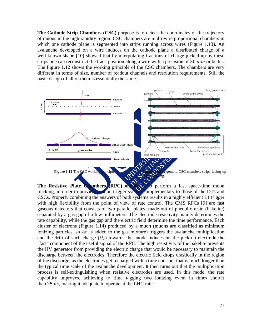
The Cathode Strip Chambers (CSC) purpose is to detect the coordinates of the trajectory of muons in the high rapidity region. CSC chambers are multi-wire proportional chambers in which one cathode plane is segmented into strips running across wires (Figure 1.13). An avalanche developed on a wire induces on the cathode plane a distributed charge of a well-known shape [10] showed that by interpolating fractions of charge picked up by these strips one can reconstruct the track position along a wire with a precision of 50 𝑚𝑚 or better. The Figure 1.12 shows the working principle of the CSC chambers. The chambers are very different in terms of size, number of readout channels and resolution requirements. Still the basic design of all of them is essentially the same.
Figure 1.12 The CSC working principle. Figure 1.13 A generic CSC chamber, strips facing up in the drawing.
The Resistive Plate Chambers (RPC) purpose is to perform a fast space-time muon tracking, in order to provide a muon trigger system complementary to those of the DTs and CSCs. Properly combining the answers of both systems results in a highly efficient L1 trigger with high flexibility from the point of view of rate control. The CMS RPCs [9] are fast gaseous detectors that consists of two parallel plates, made out of phenolic resin (bakelite) separated by a gas gap of a few millimeters. The electrode resistivity mainly determines the rate capability, while the gas gap and the electric field determine the time performance. Each cluster of electrons (Figure 1.14) produced by a muon (muons are classified as minimum ionizing particles, so 𝐴𝑟 is added to the gas mixture) triggers the avalanche multiplication and the drift of such charge (𝑄𝑒) towards the anode induces on the pick-up electrode the "fast" component of the useful signal of the RPC. The high resistivity of the bakelite prevents the HV generator from providing the electric charge that would be necessary to maintain the discharge between the electrodes. Therefore the electric field drops drastically in the region of the discharge, as the electrodes get recharged with a time constant that is much longer than the typical time scale of the avalanche development. It then turns out that the multiplication process is self-extinguishing when resistive electrodes are used. In this mode, the rate capability improves, achieving to time tagging two ionizing event in times shorter than 25 𝑛𝑠, making it adequate to operate at the LHC rates.
22
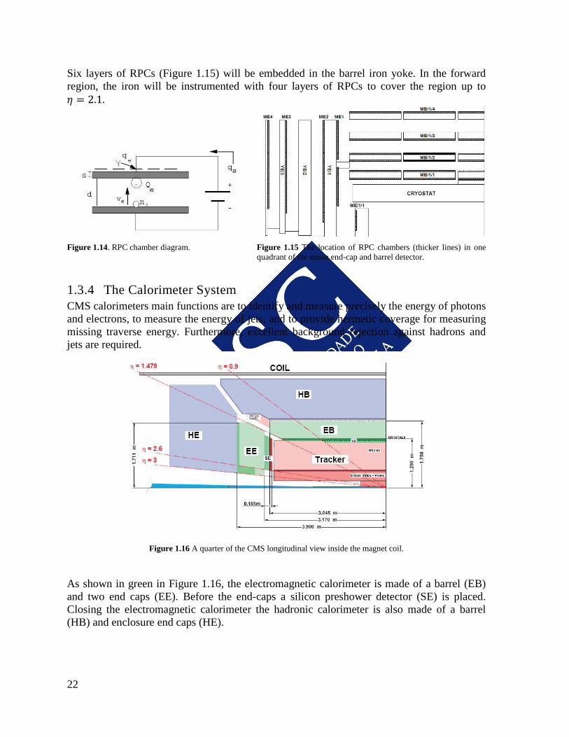
Six layers of RPCs (Figure 1.15) will be embedded in the barrel iron yoke. In the forward region, the iron will be instrumented with four layers of RPCs to cover the region up to 𝜂 = 2.1.
1.3.4 The Calorimeter System CMS calorimeters main functions are to identify and measure precisely the energy of photons and electrons, to measure the energy of jets, and to provide hermetic coverage for measuring missing traverse energy. Furthermore, excellent background rejection against hadrons and jets are required.
Figure 1.16 A quarter of the CMS longitudinal view inside the magnet coil.
As shown in green in Figure 1.16, the electromagnetic calorimeter is made of a barrel (EB) and two end caps (EE). Before the end-caps a silicon preshower detector (SE) is placed. Closing the electromagnetic calorimeter the hadronic calorimeter is also made of a barrel (HB) and enclosure end caps (HE).
Figure 1.14. RPC chamber diagram. Figure 1.15 The location of RPC chambers (thicker lines) in one
quadrant of the muon end-cap and barrel detector.

23
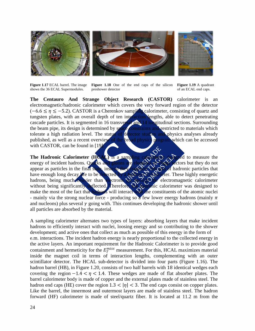
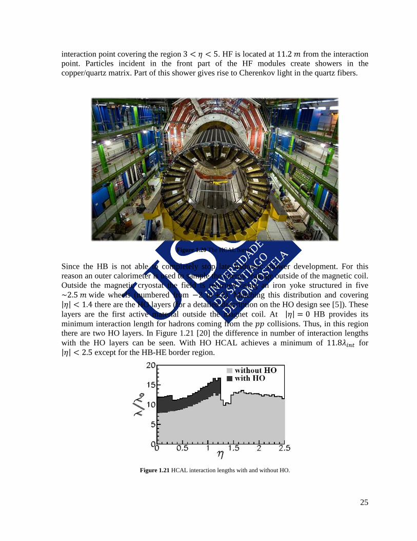
The Electromagnetic Calorimeter is a huge, very high performance, homogeneous calorimeter, made of a high-density inorganic scintillator, to measure the energy of electrons and photons. The Electromagnetic Calorimeter (ECAL) should play an essential role in the study of the physics of electroweak symmetry breaking, becoming an important detector for a large variety of SM and other new physics processes. Having the task of measuring the predicted decay 𝐻 → 𝛾𝛾 for low H boson mass, the ECAL has been crucial for finding the Higgs boson. When a high-energy electron enters the calorimeter it will likely interact with its material by emitting a few subsequent photons via bremsstrahlung, before starting to dissipate its remaining energy by ionization and excitation. These photons, carrying away part of the initial energy of the electron, will most probably convert into energetic electron-positron pairs, giving rise to a cascade whose longitudinal development is governed by their higher-energy part. The sum of all the created particles from the initial electrons is called a shower of secondary particles. The transverse dimension of the fully contained electromagnetic showers initiated by an incident high energy electron or photon is characterized by the Moliere radius that is dependent on the detection material. The total scintillating light created in the detector material is proportional to the energy of the initial incident particle. This light is efficiently collected by photodetectors and the very-front-end amplifiers produce the signal to be transmitted to the readout system. Scintillating crystal calorimeters offer the best performance for energy resolution. However, previous high energy experiments did not have to face as challenging conditions as the ones at the LHC, with a high radiation environment and about 20 events every 25 𝑛𝑠, with thousands of charged tracks created per event. After an intensive research program [13], lead tungstate (𝑃𝑏𝑊𝑂4) was chosen as the baseline detector material. It is a fast scintillator, having a high density and a short radiation length, with a small Moliere radius. Moreover, it is resistant to hard radiation environment and is technically easy to produce in big quantities. Nevertheless, their relative low light-yield, together with the high magnetic field, strongly limited the choice of suitable photodetectors. The final photodetectors chosen were Silicon Avalanche Photodiodes (APD) for the Barrel and Vacuum Phototriodes (VPT) for the Encaps. ECAL detector is placed between the Hadron Calorimeter and the Tracking System (Figure 1.16) covering from a radius of 1.290 𝑚 to 1.750 𝑚 and with a length of about 6 𝑚. The EB section, see photograph in Figure 1.17, is made out of 36 identical Supermodules summing up to 61200 lead tungstate crystals. The Supermodules are covering the interval of pseudorapidity 0 ≤ |𝜂| ≤ 1.479. The EE (Figure 1.19) covers a pseudorapidity range of 1.479 ≤ |𝜂| ≤ 3.0 and is structured in two halves made of structures called Supercrystals (arranged in structures of 5 by 5 crystals). Covering most of the pseudorapidity of the end caps, there is the SE (Figure 1.18) made of silicon strip detectors.
24
Figure 1.17 ECAL barrel. The image shows the 36 ECAL Supermodules.
Figure 1.18 One of the end caps of the silicon preshower detector
Figure 1.19 A quadrant of an ECAL end caps.
The Centauro And Strange Object Research (CASTOR) calorimeter is an electromagnetic/hadronic calorimeter which covers the very forward region of the detector (−6.6 ≤ 𝜂 ≤ −5.2). CASTOR is a Cherenkov sampling calorimeter, consisting of quartz and tungsten plates, with an overall depth of ten interaction lengths, able to detect penetrating cascade particles. It is segmented in 16 transversal and 14 longitudinal sections. Surrounding the beam pipe, its design is determined by space constraints and restricted to materials which tolerate a high radiation level. The status of detector studies and physics analyses already published, as well as a recent overview of the broad physics program which can be accessed with CASTOR, can be found in [19]. The Hadronic Calorimeter (HCAL) is a sampling calorimeter designed to measure the energy of incident hadrons. Quarks and gluons are elements of Higgs sectors but they do not appear as particles in the final state, instead they fragment into jets of hadronic particles that have enough long decay life to be detected by a hadronic calorimeter. These highly energetic hadrons, being much heavier than electrons go through the electromagnetic calorimeter without being significantly deflected. Therefore, the hadronic calorimeter was designed to make the most of the fact that hadrons will interact with the constituents of the atomic nuclei - mainly via the strong nuclear force - producing so a few lower energy hadrons (mainly 𝜋 and nucleons) plus several 𝛾 going with. This continues developing the hadronic shower until all particles are absorbed by the material. A sampling calorimeter alternates two types of layers: absorbing layers that make incident hadrons to efficiently interact with nuclei, loosing energy and so contributing to the shower development; and active ones that collect as much as possible of this energy in the form of e.m. interactions. The incident hadron energy is nearly proportional to the collected energy in the active layers. An important requirement for the Hadronic Calorimeter is to provide good containment and hermeticity for the 𝐸𝑇𝑚𝑖𝑠𝑠 measurement. For this, HCAL maximizes material inside the magnet coil in terms of interaction lengths, complementing with an outer scintillator detector. The HCAL sub-detector is divided into four parts (Figure 1.16). The hadron barrel (HB), in Figure 1.20, consists of two half barrels with 18 identical wedges each covering the region −1.4 < 𝜂 < 1.4. These wedges are made of flat absorber plates. The barrel calorimeter body is made of copper and the external plates made of stainless steel. The hadron end caps (HE) cover the region 1.3 < |𝜂| < 3. The end caps consist on copper plates. Like the barrel, the innermost and outermost layers are made of stainless steel. The hadron forward (HF) calorimeter is made of steel/quartz fiber. It is located at 11.2 m from the
25
interaction point covering the region 3 < 𝜂 < 5. HF is located at 11.2 𝑚 from the interaction point. Particles incident in the front part of the HF modules create showers in the copper/quartz matrix. Part of this shower gives rise to Cherenkov light in the quartz fibers.
Figure 1.20 The HCAL barrel.
Since the HB is not able to completely stop late hadronic shower development. For this reason an outer calorimeter is used to sample the energy leakage outside of the magnetic coil. Outside the magnetic cryostat the field is returned using an iron yoke structured in five ~2.5 𝑚 wide wheels (numbered from −2 to +2). Matching this distribution and covering |𝜂| < 1.4 there are the HO layers (for a detailed description on the HO design see [5]). These layers are the first active material outside the magnet coil. At |𝜂| = 0 HB provides its minimum interaction length for hadrons coming from the 𝑝𝑝 collisions. Thus, in this region there are two HO layers. In Figure 1.21 [20] the difference in number of interaction lengths with the HO layers can be seen. With HO HCAL achieves a minimum of 11.8𝜆𝑖𝑛𝑡 for |𝜂| < 2.5 except for the HB-HE border region.
Figure 1.21 HCAL interaction lengths with and without HO.
26
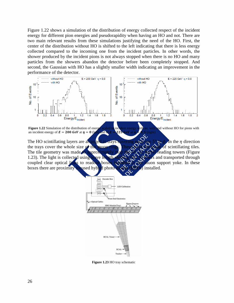
Figure 1.22 shows a simulation of the distribution of energy collected respect of the incident energy for different pion energies and pseudorapidity when having an HO and not. There are two main relevant results from these simulations justifying the need of the HO. First, the center of the distribution without HO is shifted to the left indicating that there is less energy collected compared to the incoming one from the incident particles. In other words, the shower produced by the incident pions is not always stopped when there is no HO and many particles from the showers abandon the detector before been completely stopped. And second, the Gaussian with HO has a slightly smaller width indicating an improvement in the performance of the detector.
Figure 1.22 Simulation of the distribution of energy scaled to incident energy with an with and without HO for pions with an incident energy of 𝑬 = 𝟐𝟎𝟎 𝑮𝒆𝑽 at 𝜼 = 𝟎 (left) and of 𝑬 = 𝟐𝟐𝟓 𝑮𝒆𝑽 at 𝜼 = 𝟎.𝟓 (right)
The HO scintillating layers are arranged in trays covering each one 5° in 𝜙. In the 𝜂 direction the trays cover the whole size of the muon rings. These trays are made of scintillating tiles. The tile geometry was made to approximately map the HCAL barrel reading towers (Figure 1.23). The light is collected using wave length shifting (WLS) fibers and transported through coupled clear optical links to readout boxes installed in the muon support yoke. In these boxes there are proximity focused hybrid photo diodes (HPDs) installed.
Figure 1.23 HO tray schematic

27
1.3.5 The Alignment, Trigger and Data Acquisition systems The detector alignment system’s [21] objective is to reduce the degradation of the track reconstruction due to alignment uncertainties that are in the range of 100 − 500 𝜇𝑚 after the detector installation. The goal of the alignment system is to reduce this range below the intrinsic detector sensors resolution. Together with the installation uncertainties, other time effects are to be covered by the alignment system like the environment changes effects like humidity and temperature or the effect of the 4 𝑇 magnetic field in many of the detector materials [22]. The CMS alignment strategy has a 3 step approach [23]. First, there is a measurement of the installation precision of tracking devices using photogrammetry (a technique to determine the geometric properties of objects from photographic images). Second, relative positions of sub-detectors are measured with lasers and TV-cameras. Finally there is a tracker-based alignment by means of pattern recognition. The Trigger [24] and Data Acquisition (DAQ) [25] system is the part of the experiment where the entire information of the physics data is available. Important decisions that affect the fate of physics events are taken by these systems. Besides the hardware system requirements (in term of computing power, high speed networks, etc.) these systems are flexible enough to adapt to unknown requirements derived from studies of first years of collisions. Also, it provides a way to monitor the data been rejected by the filtering system for eventual modifications. At the LHC the beams are colliding at a frequency of 40 MHz, resulting, at the design luminosity, in ~8 ∙ 108 inelastic 𝑝𝑝 collisions per second. Each ~20 𝑝𝑝 collisions (a bunch crossing) generates around 1 𝑀𝐵 of zero-suppressed data. This brings up to a total of ~107 𝑀𝐵 𝑠⁄ , out of which only 102 𝑀𝐵 𝑠⁄ are technically possible to save in a storage service. Therefore the CMS selection trigger and the data acquisition system must have a rejection power of 105 . The CMS experiment uses a two-stage trigger system, with events flowing from the first level trigger at a rate of 100 𝑘𝐻𝑧. These events are read out by the Data Acquisition system (DAQ), assembled in memory in a farm of computers, and finally fed into the high-level trigger (HLT) software that is running on the farm. The CMS DAQ assembles events at a rate of 100 𝑘𝐻𝑧, transporting event data at an aggregate throughput of 100 𝐺𝐵/𝑠. The trigger and data acquisition system (Figure 1.24) consist of four parts: the detector frontend electronics, the global trigger processor (Level-1 trigger [26]), a readout building network [27] and an online filter farm [28]. The CMS experiment's online cluster consists of 2300 computers and 170 switches or routers operating on a 24-hour basis. This huge infrastructure must be monitored in a way that the administrators are pro-actively warned of any failures or degradation in the system, in order to avoid or minimize downtime of the system which can lead to loss of data taking. The detector frontend electronics collect the information from physics events and store it in ~700 frontend modules waiting for Level-1 accept trigger signal. This Level-1 trigger uses custom hardware processors to generate the decision trigger. The data accepted after the decision trigger is generated (< 3.2𝜇𝑠) is stored in ~500 readout buffers in what are called readout columns. Each readout columns consist of a series of frontend drivers and a readout unit that
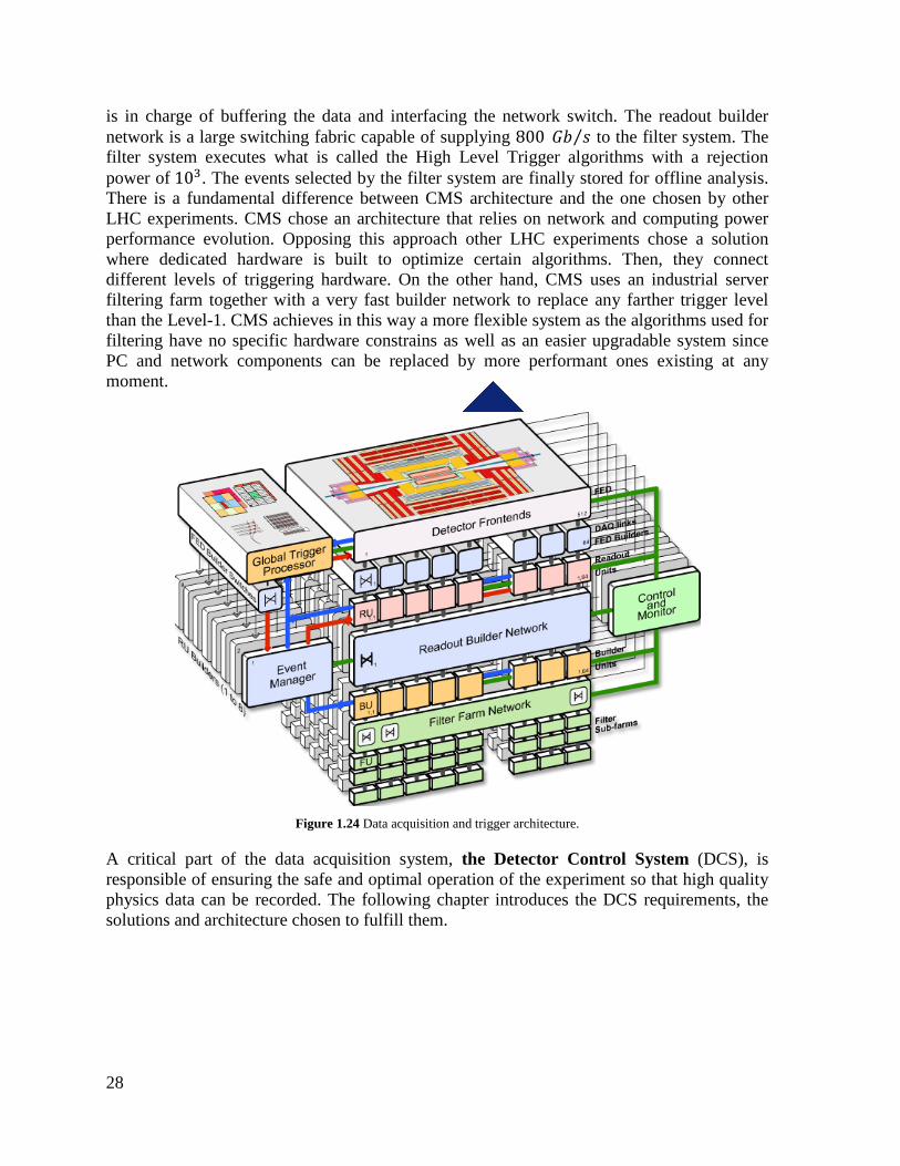
28
is in charge of buffering the data and interfacing the network switch. The readout builder network is a large switching fabric capable of supplying 800 𝐺𝑏 𝑠⁄ to the filter system. The filter system executes what is called the High Level Trigger algorithms with a rejection power of 103. The events selected by the filter system are finally stored for offline analysis. There is a fundamental difference between CMS architecture and the one chosen by other LHC experiments. CMS chose an architecture that relies on network and computing power performance evolution. Opposing this approach other LHC experiments chose a solution where dedicated hardware is built to optimize certain algorithms. Then, they connect different levels of triggering hardware. On the other hand, CMS uses an industrial server filtering farm together with a very fast builder network to replace any farther trigger level than the Level-1. CMS achieves in this way a more flexible system as the algorithms used for filtering have no specific hardware constrains as well as an easier upgradable system since PC and network components can be replaced by more performant ones existing at any moment.
Figure 1.24 Data acquisition and trigger architecture.
A critical part of the data acquisition system, the Detector Control System (DCS), is responsible of ensuring the safe and optimal operation of the experiment so that high quality physics data can be recorded. The following chapter introduces the DCS requirements, the solutions and architecture chosen to fulfill them.

29
2. The CMS Detector Control System This chapter provides an overview of the DCS challenges and the technologies used to face them. Section 2.1 introduces the various types of requirements given by the nature, size and complexity of the experiment. The project organization is presented in Section 2.2, and finally, in the last section, the different technologies that were chosen for the DCS implementation are presented.
2.1 Requirements The requirements of the CMS control system had no precedent in High Energy Physics experiments, surpassing by far the systems found in the industrial market. They can be classified into four types: operational, functional, environment related and organizational. The DCS operational requirements must be fulfilled whenever the CMS detector is not in complete shutdown mode and the DCS full functionality has to be assured. Moreover, a set of stringent environment requirements are imposed by the size, the geographical characteristics and the nature of the experiment. On the other hand, it is important to stress the fact that the LHC experiments took more than a decade from their design to their final commissioning. During that time, many people participated in different management, engineering and software development fields. Consequently, some structures needed to be created in order to coordinate the work of all the people involved and to guarantee that the operational requirements are achieved. The here mentioned requirements impose some constraints in the selection of the technologies used for the control system implementation, involving different groups at CERN. The project organization and its structure are introduced in the following sections, as well as the technologies chosen and their motivations. Operational requirements:
• Ensure a safe operation by preventing that the detector operates under potentially dangerous conditions and by anticipating the Detector Safety System (DSS) [29], which is the last resort experiment protection system. It should in addition provide uninterrupted operation regardless of the LHC machine state.
• Provide a coherent, centralized and automated system operation of the sub-detectors in synchronization with the LHC operation modes and in coordination also with the experiment Data Acquisition and Run Control system.
• Maximize the detector efficiency by minimizing the required time to execute any command and achieve any required target state.
• Provide a partitioning mechanism allowing for the operation of different parts of the detector independently.

30
Functional requirements: • Provide with a readout infrastructure to monitor and control the front-end
electronic devices summing up a number of parameters in the million range. • Provide analyzing means to process the readout data allowing the system to take
automatic decisions. • Provide an alert system that can raise an alarm for any abnormal device condition
and guide the operators during the problem resolution. • Archive the necessary data to provide offline analysis capabilities in order to debug
the system or to validate the quality of the recorded data. • Allow for current and historical data plotting. • Log the control system events for analysis and debug purposes. • Monitor the experiment site environmental conditions and the electrical power
distribution feeding the experiment electronics racks. Environment requirements:
• Adequate the use of DCS hardware to the areas exposed to high radiation doses and to a high magnetic field.
• Manage a big amount of hardware distributed in different large areas (see Figure 2.3) including surface buildings and underground zones, as well as hardware installed in locations with very difficult or practically impossible access.
• Monitor a number of parameters in the range of a few millions.
Organizational requirements: • Create a working structure allowing the DCS workers to participate locally (from
CERN) or remotely from their home institute. • Coordinate the work of the different involved institutes (see Error! Reference
source not found.) avoiding work replication and promoting the creation of reusable generic developments.
• Integrate the control sub-systems into a common infrastructure allowing for an easy maintenance.
• Create the communication channels to interact with other groups providing services to the DCS like the LHC machine, the CERN IT services groups (databases, networking, etc.) or the CERN engineering controls groups (cooling, ventilation, electricity, gas control, etc.).
2.2 The project organization A challenge that was faced by the experiment DCS was the big number of people and groups participating in the project, all along the more than a decade that took from the design to the final commissioning of CMS. During that time, many people participated in different management, engineering and software development fields. To guarantee that the operational requirements were achieved some structures needed to be created to coordinate the work of all the people involved. Table 2.1 shows the affiliation of people working for each of the sub-detectors and the average man-power during the last 10 years. To coordinate the project, a Central DCS team was created in CMS in 2003. Figure 2.1 shows the central DCS project human resources structure. The Central DCS team defined the design line of the whole CMS
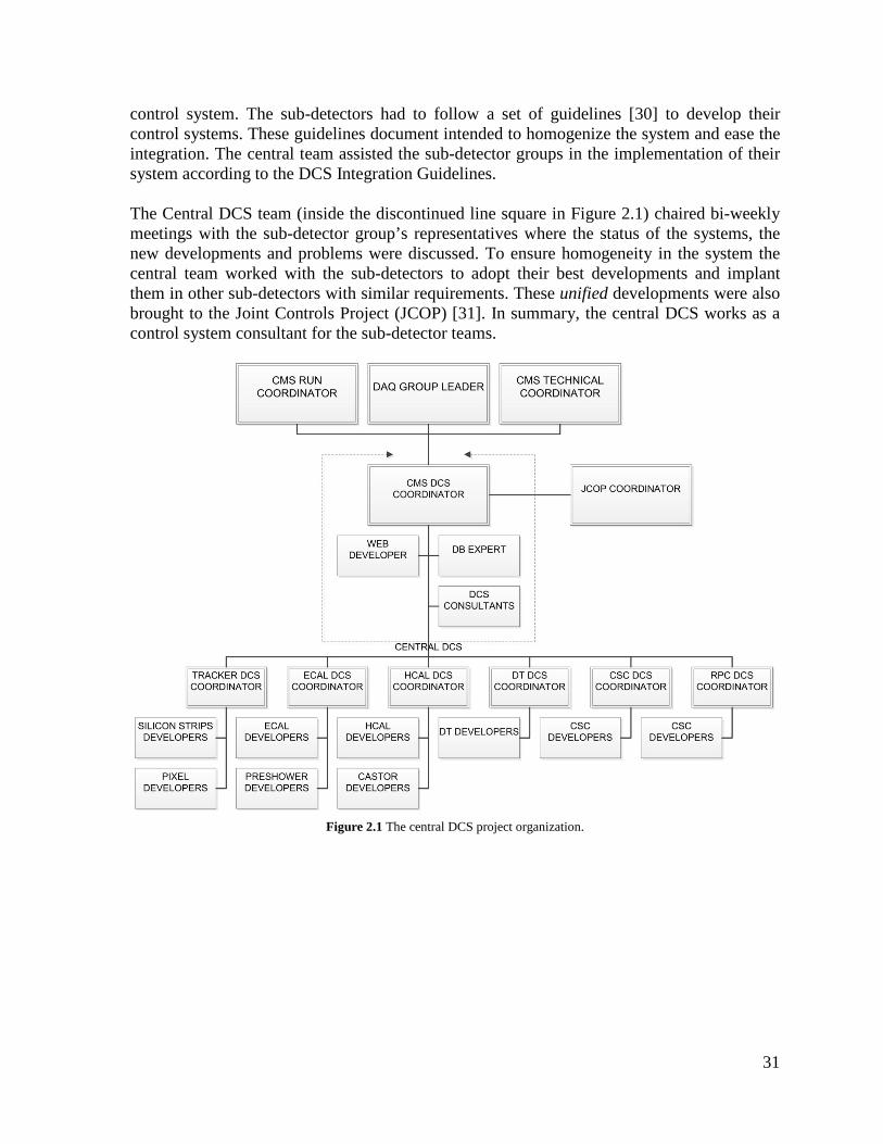
31
control system. The sub-detectors had to follow a set of guidelines [30] to develop their control systems. These guidelines document intended to homogenize the system and ease the integration. The central team assisted the sub-detector groups in the implementation of their system according to the DCS Integration Guidelines. The Central DCS team (inside the discontinued line square in Figure 2.1) chaired bi-weekly meetings with the sub-detector group’s representatives where the status of the systems, the new developments and problems were discussed. To ensure homogeneity in the system the central team worked with the sub-detectors to adopt their best developments and implant them in other sub-detectors with similar requirements. These unified developments were also brought to the Joint Controls Project (JCOP) [31]. In summary, the central DCS works as a control system consultant for the sub-detector teams.
Figure 2.1 The central DCS project organization.

32
Inside the CMS collaboration, the Central DCS team represents the DCS project in weekly data acquisition meetings, in daily Run Coordination meetings where everything related with the experiment operation is discussed, and twice a week in Technical Coordination meetings where all technical and safety aspects are discussed.
Detector or system Institute Manpower
Tracker Strips Karlsruhe university, Germany University of California, USA
CERN, Switzerland 2-3
Tracker Pixels
Purdue University, USA The University of Iowa, USA Vanderbilt University, USA
CERN, Switzerland
2-3
ECAL Swiss Federal Institute of Technology, Switzerland 5-6
Preshower Swiss Federal Institute of Technology, Switzerland National Central University, Taiwan 1-2
HCAL Fermi National Accelerator Laboratory, USA 2-3
CASTOR Deutsches Elektronen-Synchrotron, Germany Fermi National Accelerator Laboratory, USA 1-2
DT Istituto Nazionale di Fisica Nucleare, Italy, CERN, Switzerland 2
RPC Istituto Nazionale di Fisica Nucleare, Italy CERN, Switzerland 1-2
CSC Massachusetts Institute of Technology, USA
University of California, USA Fermi National Accelerator Laboratory, USA
3
Alignment Instituto de Física de Cantabria, Spain
University of California, USA Kossuth University, Hungary
4-5
Trigger MIT 1
Central DCS CERN, Switzerland
Vilnius University, Lithuania Santiago de Compostela, Spain
2-6
Table 2.1 The DCS manpower
The Central DCS team with the other JCOP members participated in an exhaustive selection of technologies that are introduced in the following section. The author actively participated in this selection from 2003 to 2005.
33
2.3 The Technologies The JCOP is a collaboration formed by the LHC experiments and the industrial controls (ICE) group of CERN’s engineering (EN) department. It has the mandate of identifying common needs and creating common solutions for control systems of the CERN experiments. The Central DCS team represents CMS experiment at JCOP, sharing CMS ideas and profiting from the developments of other experiments and the support of the engineering group. Within JCOP an effort was put to homogenize the technological choices in order to be able to share experience across the different LHC experiments, enabling the possibility of having a central group at CERN providing support to all of them. On this line, JCOP created its own software framework, a set of software libraries and shared resources, to provide the LHC experiments with developing tools for controls for a set of selected hardware components. The author of this work has work within JCOP providing components (like the Rack Control) and proposing others that have been successfully developed (for example the Distributed Installation tool). Following this approach, the Central DCS team of CMS created its own framework, specific to CMS control system architecture and choices. In addition, a set of guidelines explaining how to use this framework was provided to CMS controls developers so that with central DCS support, they could implement their sub-system facilitating, in this way, the integration into the overall system leading to a homogeneous and maintainable system. The DCS components can be grouped in three types: hardware, middleware and software, and are arranged into different layers that are shown in Figure 2.2. The supervision layer is made of software components storing the intelligence and knowledge on how to control and monitor the detector. In the middle layer, the components are software packages dedicated to communicate with the hardware and to create and interconnect the distributed system infrastructure. The bottom layer concerns the hardware components, which are of two different types: the input/output concentrators that are addressed by the middleware components and finally, the frontend (FE) hardware devices.
Figure 2.2 The DCS system layers.
The different component types and the selected solutions for hardware, middleware and software together with the relevant constraints imposed by the requirements are discussed in the following sub-sections.

34
2.3.1 The hardware components The DCS hardware was chosen taking into account the environment constraints: radiation, magnetic field, the difficult accessibility and the cost. As it was stated in Section 1.1, the radiation levels inside the cavern during the LHC operation are well over what a person can safely withstand. Looking at the radiation absorbed by the detector and the limited radiation that a worker is allowed to be exposed to, the experiment cavern becomes an inaccessible place for engineers and technicians. The access is completely forbidden during LHC operation and very limited and well controlled human interventions are allowed when it doesn’t operate. Industrial robust hardware was chosen wherever it was possible. Table 2.2 presents a summary of the most commonly used hardware in the CMS DCS. One of the main sources of the large amount of parameters is the power supplies. The CAEN [32] company was selected by JCOP as the provider of most of the LHC experiments’ power supplies. CAEN provides low and high voltage power supply crates and boards [33] appropriated for the balcony electronic racks installed in the detector hall. The W-IE-NE-R [34] company was also selected as a provider of low-voltage supplies, specially its MARATON radiation resistant systems.
Device type Usage Brand Parameters
Power supply Front end electronics and detector bias CAEN
W-IE-NE-R CMS-made
~2.5 M
Embedded Local Monitoring Board
(ELMB)
Temperature, humidity and pressure monitoring
Water leak detection Laser monitoring
CERN-made ~24 K
DCU, RBX Detector monitoring CMS-made ~0.5 M
PLC Safety, Cooling Rack electrical distribution
Siemens Schneider ~12 K
Table 2.2 Summary of the most commonly used hardware in the CMS DCS.
For the on-detector monitoring mainly 3 different devices are used: the first two, the RBX [35] (Readout BoX) and the DCU [36] (Detector Control Unit), are custom CMS radiation resistant solutions. The RBXs are made of a Clock and Control Module, a Calibration Module and 4 Readout Modules. Each RM is made of a sensor called Hybrid Photodiode (HPD), with 18 channels and 3 electronic cards measuring charge, QIE (for Charge Integrated Encoder). The HPD receive light from the detector scintillators and transform the signal into an electrical ones measured by the QIEs. The third device, the ELMB (Embedded Local Monitoring Board) [37] [38], is an ATLAS [39] radiation resistant data acquisition board, used for a range of frontend control and monitoring tasks. Various PLCs are used as part of the sub-detectors safety systems and they are interfaced from DCS for monitoring and configuration purposes.
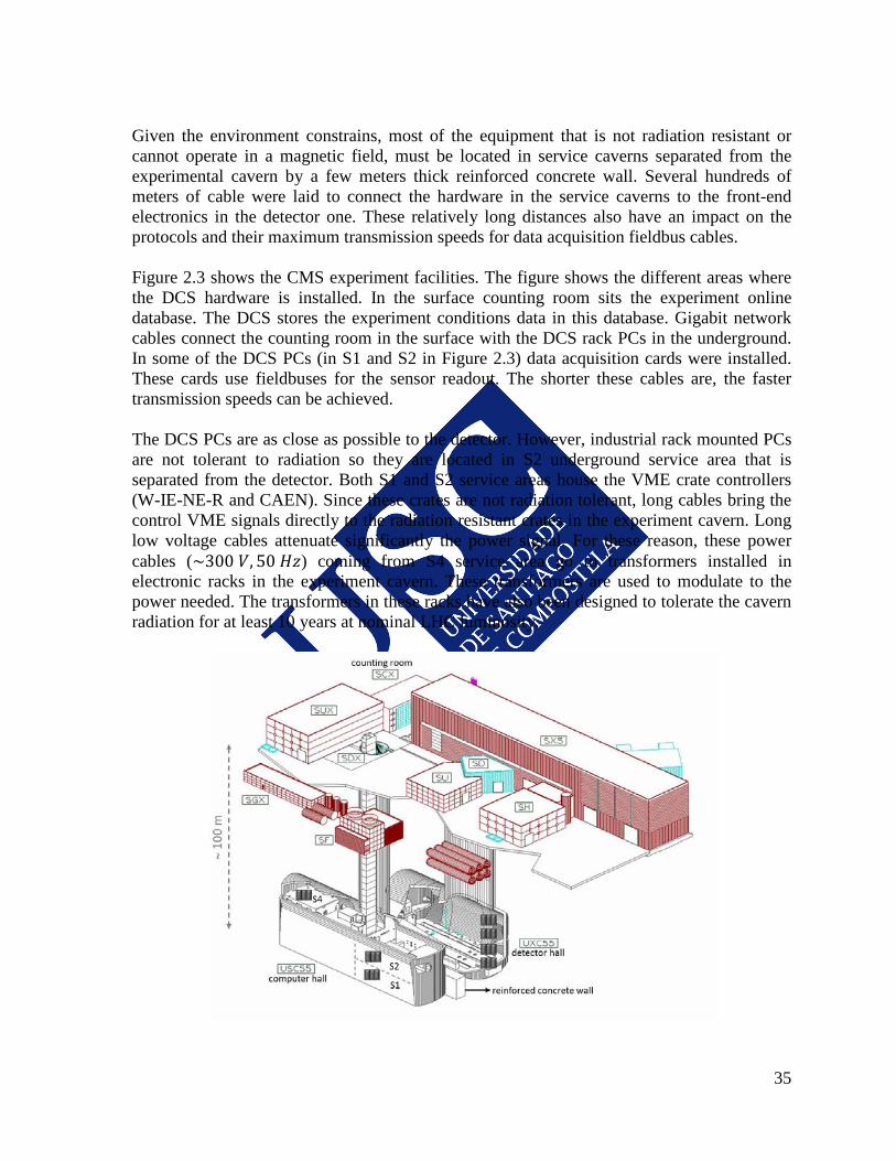
35
Given the environment constrains, most of the equipment that is not radiation resistant or cannot operate in a magnetic field, must be located in service caverns separated from the experimental cavern by a few meters thick reinforced concrete wall. Several hundreds of meters of cable were laid to connect the hardware in the service caverns to the front-end electronics in the detector one. These relatively long distances also have an impact on the protocols and their maximum transmission speeds for data acquisition fieldbus cables. Figure 2.3 shows the CMS experiment facilities. The figure shows the different areas where the DCS hardware is installed. In the surface counting room sits the experiment online database. The DCS stores the experiment conditions data in this database. Gigabit network cables connect the counting room in the surface with the DCS rack PCs in the underground. In some of the DCS PCs (in S1 and S2 in Figure 2.3) data acquisition cards were installed. These cards use fieldbuses for the sensor readout. The shorter these cables are, the faster transmission speeds can be achieved. The DCS PCs are as close as possible to the detector. However, industrial rack mounted PCs are not tolerant to radiation so they are located in S2 underground service area that is separated from the detector. Both S1 and S2 service areas house the VME crate controllers (W-IE-NE-R and CAEN). Since these crates are not radiation tolerant, long cables bring the control VME signals directly to the radiation resistant crates in the experiment cavern. Long low voltage cables attenuate significantly the power signal. For these reason, these power cables (~300 𝑉, 50 𝐻𝑧) coming from S4 service area go to transformers installed in electronic racks in the experiment cavern. These transformers are used to modulate to the power needed. The transformers in these racks have also been designed to tolerate the cavern radiation for at least 10 years at nominal LHC luminosity.
36
Figure 2.3 The CMS experiment facilities.
2.3.2 The infrastructure layer software The DCS infrastructure layer software is made of two main parts. First, a core software part is used to create a distributed control system software infrastructure that constitutes a link layer connecting the different sub-detectors with the central control system. Second, a set of communication driver components is used by the core software to communicate with the above mentioned DCS hardware. PVSS from the ETM Company (a Siemens satellite company) was selected [40] by JCOP as the supported official Supervisory Control and Data Acquisition (SCADA) package. It was chosen, after been compared with other ~40 SCADA packages, due to a list of features making its use suitable for the controls of the LHC experiments. The main features influencing the SCADA selection were:
• Event-driven architecture (EDA) [41]: events are a better means of managing I/O
concurrency than systems based on polling. Additionally event-based applications tend to have more stable performance under heavy load favoring the performance and scalability.
• Openness: it provides the possibility of extending the package by using a powerful Application Program Interface (API), allowing creating drivers to interface devices using non industry-standard CERN communication protocols, as well as to communicate with other systems like for example the experiment run control system.
• Modularity: unlike other commercial SCADA products, PVSS can be spread out into multiple computers where each of the sub-systems can be updated, maintained and operated independently. This is important for the LHC experiments, especially during commissioning periods where some sub-systems need to be reinstalled while others performed calibrations or combined tests.
• Programming easiness: a C-like language provides the programming easiness desired and reduces the learning time for new control system developers.
• Platform independence: a real multi-platform capability was mandatory for JCOP. PVSS offers the possibility to create distributed systems using Windows, Linux and Solaris operating systems. This was important for LHC experiments since most of industrial hardware selected communicates via drivers only available for Windows platform while other experiment systems required Linux. The LHC experiments have a mixture of Windows and Linux control system PCs.
In addition to the previous main features, PVSS shares the following ones with other SCADA packages:
• An event-driven QT based user interface with a visual editor. • Archiving capabilities either to files or to an Oracle relational database. • Basic trending tools. • An alarm handling infrastructure.
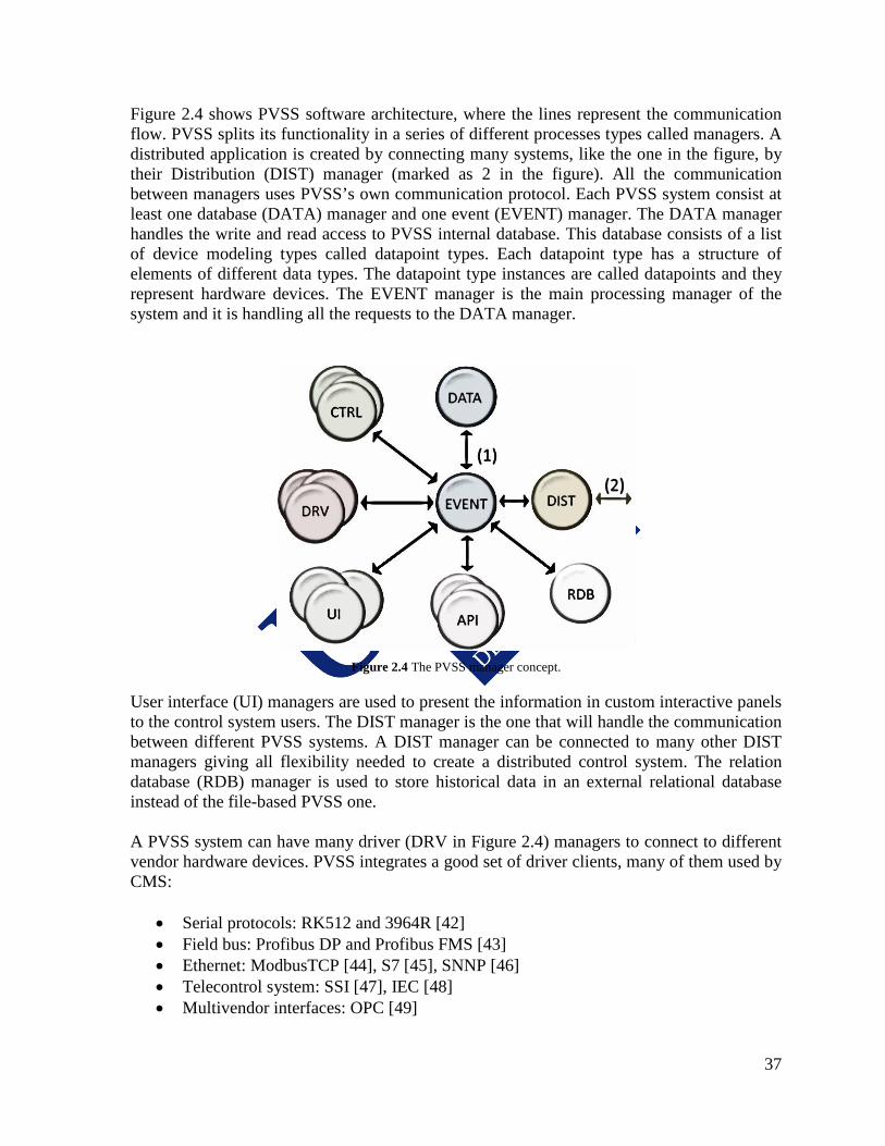
37
Figure 2.4 shows PVSS software architecture, where the lines represent the communication flow. PVSS splits its functionality in a series of different processes types called managers. A distributed application is created by connecting many systems, like the one in the figure, by their Distribution (DIST) manager (marked as 2 in the figure). All the communication between managers uses PVSS’s own communication protocol. Each PVSS system consist at least one database (DATA) manager and one event (EVENT) manager. The DATA manager handles the write and read access to PVSS internal database. This database consists of a list of device modeling types called datapoint types. Each datapoint type has a structure of elements of different data types. The datapoint type instances are called datapoints and they represent hardware devices. The EVENT manager is the main processing manager of the system and it is handling all the requests to the DATA manager.
Figure 2.4 The PVSS manager concept.
User interface (UI) managers are used to present the information in custom interactive panels to the control system users. The DIST manager is the one that will handle the communication between different PVSS systems. A DIST manager can be connected to many other DIST managers giving all flexibility needed to create a distributed control system. The relation database (RDB) manager is used to store historical data in an external relational database instead of the file-based PVSS one. A PVSS system can have many driver (DRV in Figure 2.4) managers to connect to different vendor hardware devices. PVSS integrates a good set of driver clients, many of them used by CMS:
• Serial protocols: RK512 and 3964R [42] • Field bus: Profibus DP and Profibus FMS [43] • Ethernet: ModbusTCP [44], S7 [45], SNNP [46] • Telecontrol system: SSI [47], IEC [48] • Multivendor interfaces: OPC [49]

38
Additionally, API managers, written in C++ programming language, can be developed to create drivers interfacing custom hardware. API managers, and also control managers (CTRL) can be used for data processing. CTRL managers are written in a C-like language that the SCADA interprets at run time.
2.3.3 The controls related software A framework was created, in the JCOP context, to help developers with their DCS implementation. CMS has designed and developed as well, its own software infrastructure to manage the DCS developments. In the next sub-sections the JCOP framework and the CMS guidelines and framework concepts are introduced. The JCOP framework The control systems of the LHC experiments have many similar requirements. Most of the hardware they use was selected in the frame of the JCOP. The JCOP framework [3], built on top of PVSS, intends to simplify the task of developing controls for this common hardware. It is divided in three main types of components:
• Core components: a set of general libraries defining the way to create hardware devices and define hardware and logical hierarchies with them. It also includes a powerful Finite State Machine (FSM) component that allows to create a tree-like structure of logical and hardware nodes modeling the state of a system.
• Device components: a set of user interface panel wizards and libraries that assists on the creation of controls for specific hardware (CAEN component, W-IE-NE-R component, ELMB component, etc.). These components hide from the developers the technicalities of the internal driver configuration and specific device channel hardware addressing.
• Functional application components: applications ready to use that with no need to provide any information connect to the experiment services automatically, create the necessary datapoints, install and configure the needed drivers, create alerts and provide user interface for the motoring.
JCOP chose the FSM component for the controls modeling since it was previously used in LEP DELPHI experiment with success and it did fulfill the functional and scalability requirements of LHC experiments.

39
The Finite State Machine PVSS toolkit The JCOP FSM toolkit [50] is a component developed and supported by the LHCb experiment. It allows for modeling complex systems by breaking them into smaller units characterized by a well-defined set of states and possible transitions among them. These units are arranged in a tree-like hierarchical structure that can be used to operate the system. Expert knowledge can be embedded in the tree hierarchy automating control actions. The FSM toolkit tree units can be of two types:
• Control units (CU): these are logical decision units. They are abstract entities used for grouping (ex: ECAL high voltage system)
• Devices units (DU): these represent the real hardware devices (ex: a high voltage channel or crate)
The control units are arranged in tree structures and can be partitioned out into sub-trees that run in standalone mode allowing for concurrent independent operation of parts of the system (for example for calibration and debugging purposes). Device units are always leaf units in the tree. The toolkit allows for sequencing and automating operations. Figure 2.5 shows a generic FSM tree where the states are summarized upwards and the commands are propagated downwards. The tree can have any number of levels and nodes.
Figure 2.5 Generic FSM tree. Control Units are represented in green. Device units are orange. Commands flow down the tree. Alerts and status flow up. Picture extracted from the FSM toolkit documentation.
The Figure 2.6 shows the possible transitions of a Sub-system node from 𝐸𝑅𝑅𝑂𝑅 to 𝑂𝑁 state and from 𝑂𝑁 to 𝐸𝑅𝑅𝑂𝑅.
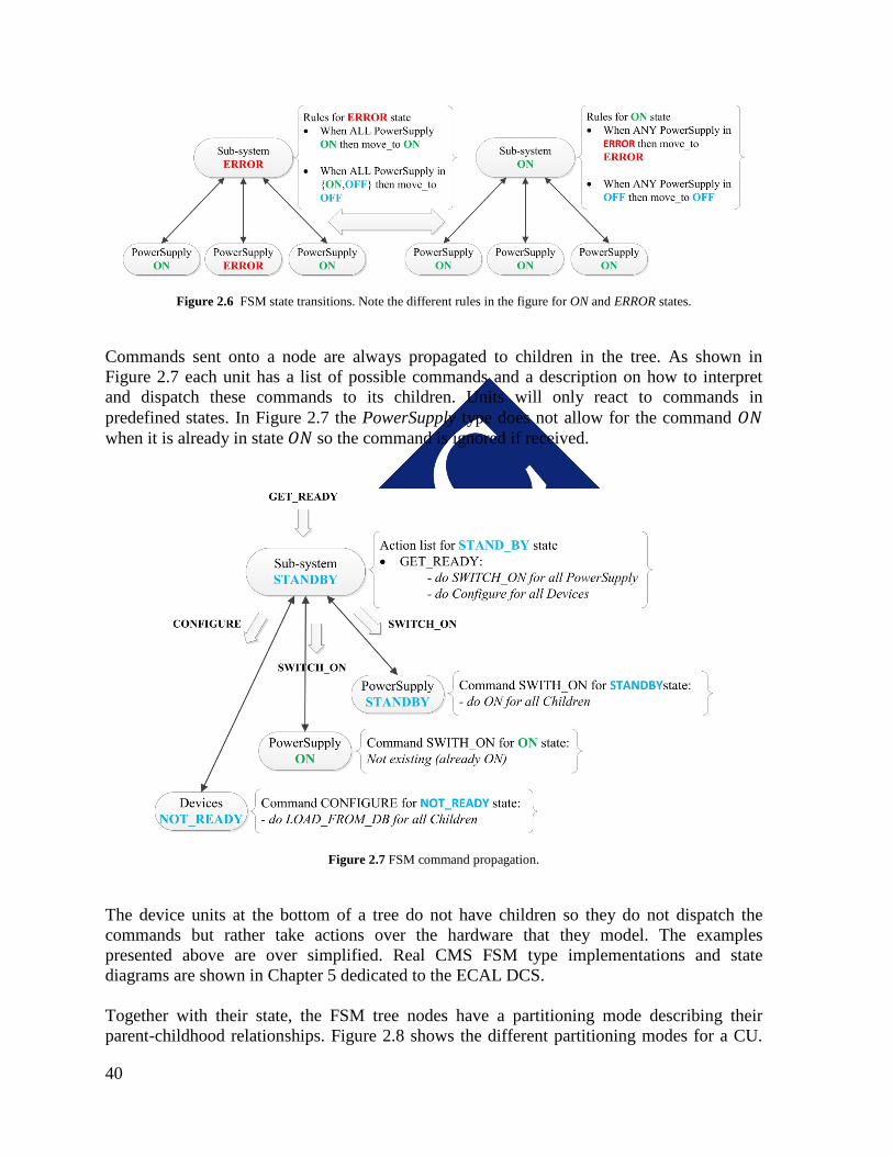
40
Figure 2.6 FSM state transitions. Note the different rules in the figure for ON and ERROR states.
Commands sent onto a node are always propagated to children in the tree. As shown in Figure 2.7 each unit has a list of possible commands and a description on how to interpret and dispatch these commands to its children. Units will only react to commands in predefined states. In Figure 2.7 the PowerSupply type does not allow for the command 𝑂𝑁 when it is already in state 𝑂𝑁 so the command is ignored if received.
Figure 2.7 FSM command propagation.
The device units at the bottom of a tree do not have children so they do not dispatch the commands but rather take actions over the hardware that they model. The examples presented above are over simplified. Real CMS FSM type implementations and state diagrams are shown in Chapter 5 dedicated to the ECAL DCS. Together with their state, the FSM tree nodes have a partitioning mode describing their parent-childhood relationships. Figure 2.8 shows the different partitioning modes for a CU.

41
For physics data-taking these units are included in the overall tree. However, they can be excluded and their state, and consequently all its children states, are ignored by its parent. Also, the excluded node will not receive commands from its parent. A node excluded, and its children bellow, can be taken by a second operator and run in a standalone partition. DUs have a simpler partitioning mode space as they can only be enabled or disabled. The JCOP FSM toolkit is based on the State Modeling Interface (SMI++) [51] package. SMI++ was originally developed by the DELPHI [52] experiment during the LEP era. It uses its own language, the State Manager Language (SML), to model objects. The JCOP framework translates the FSM rules into SML language. PVSS connects at run time with SMI++ binaries where the FSM node state evaluations are done.
Figure 2.8 JCOP FSM toolkit Control Unit partitioning modes. Picture extracted from the FSM toolkit documentation.
The CMS framework On top of the JCOP framework, CMS built its own set of tools. Like the JCOP framework, the CMS one is made of components. These components contain the functionality to control some part of the CMS system and they are usually refer to as functional components. An example of a JCOP component would be the 𝑓𝑤𝐶𝑎𝑒𝑛 providing the libraries and panels to create controls for CAEN hardware. An example of a CMS component would be the 𝐶𝑀𝑆𝑓𝑤𝐸𝑐𝑎𝑙𝐵𝑎𝑟𝑟𝑒𝑙𝐻𝑉 that uses the 𝑓𝑤𝐶𝑎𝑒𝑛 component and contains the functionality to control and model the ECAL barrel high voltage power supplies. The use of sub-detector components is one of the main differences between CMS and the rest of the LHC experiments. The CMS design approach provides the control system with more flexibility to re-distribute functional software components across the computing resources nodes. In addition it provides with a factorized mechanism to quickly rollback any changes when needed. Along this chapter the requirements of the Control System have been brought into light. The project human infrastructure and the technologies chosen were described, as well as the way these tools were used to satisfy the requirements. The author of this work was deeply involved in the conceptual design and development of the overall DCS, starting from the beginning, as a founding member of the CMS Central

42
DCS team. As such, he had a representing role of the experiment DCS in various CMS and external coordination and working-group meetings. He was the lead architect of the experiment control system and his original contributions have been incorporated repeatedly to the JCOP framework used by all LHC experiments.

43
3. The DCS Implementation In the last chapter of Part I, the technologies chosen to implement the DCS were described. During this second part, many of the author’s contributions to the architecture design, the development and the deployment strategy choice for the CMS DCS are presented. A distributed component-based model approach was selected and developed by the author for CMS, being later adopted and maintained by the CERN controls engineering support group (EN-ICE). This chapter describes how the selected building components are combined to satisfy the requirements stated in Section 2.1. Section 3.1 provides an overview of the control system layered-architecture. The later Sections present each of the architecture´s layers, starting from the bottom middleware layer, following with the JCOP framework and the way CMS makes use of it, and concluding with the CMS framework built on top of the JCOP one, which follows the same component approach.
3.1 Architecture Overview The DCS architecture is represented in Figure 3.1. The front-end hardware connects to the readout either via Ethernet or CAN field buses. The hardware pool of this layer was chosen trying to maximize the homogeneity. CAEN and WIENER vendors provide most of the hardware for power management.
The next layer consists of the computing infrastructure. CMS went a step ahead than the other LHC experiments by creating a fully centrally managed computing infrastructure making use of the CERN Computing Management Framework and, in addition, creating web applications to configure and monitor each to the computing nodes.
A middleware layer, containing the core of PVSS, provides clients for the used industrial drivers (OPC, SNMP, S7, etc.). For custom drivers, the PVSS clients had to be developed at CERN. Section (3.2) provides details on the driver and clients used by CMS in its production system. This layer also provides the interconnection tools between the different distributed PVSS projects.
The next layer, the application one, is made of the different control system component implementing the functionality of the control system. The JCOP framework created software components to ease the task of configuring PVSS driver clients to address specific hardware channels, setting automatically alerts and parameterizing the archiving of the monitored parameters into the experiment online Oracle database. In addition the JCOP framework provides functionality for mass configuration (this is, for configuring many channels using simple user interface forms), as well as storing and retrieving these configurations to (and from) a database. Section 3.3 gives details on the use of the JCOP framework in the CMS environment introducing the CMS particular deployment strategy. A supervision layer includes the control tree structure that integrates the distributed control system and automates the experiment operation by sequencing the commands to the
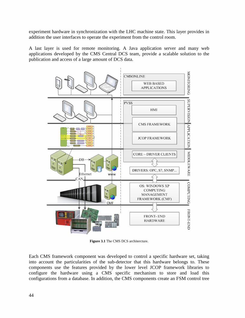
44
experiment hardware in synchronization with the LHC machine state. This layer provides in addition the user interfaces to operate the experiment from the control room. A last layer is used for remote monitoring. A Java application server and many web applications developed by the CMS Central DCS team, provide a scalable solution to the publication and access of a large amount of DCS data.
Figure 3.1 The CMS DCS architercture.
Each CMS framework component was developed to control a specific hardware set, taking into account the particularities of the sub-detector that this hardware belongs to. These components use the features provided by the lower level JCOP framework libraries to configure the hardware using a CMS specific mechanism to store and load this configurations from a database. In addition, the CMS components create an FSM control tree
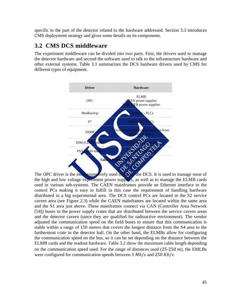
45
specific to the part of the detector related to the hardware addressed. Section 3.3 introduces CMS deployment strategy and gives some details on its components.
3.2 CMS DCS middleware The experiment middleware can be divided into two parts. First, the drivers used to manage the detector hardware and second the software used to talk to the infrastructure hardware and other external systems. Table 3.1 summarizes the DCS hardware drivers used by CMS for different types of equipment.
Driver Hardware
OPC ELMB
CAEN power supplies W-IE-NER power supplies
Modbus/tcp Schneider - PLCs
S7 SIEMENS - PLCs
SNMP Environment monitoring hardware from different vendors
DIM (CERN-made) HCAL readout boxes
PSX (CMS-made) Detector control units
Table 3.1 CMS DCS drivers
The OPC driver is the most extensively used driver in the DCS. It is used to manage most of the high and low voltage experiment power supplies, as well as to manage the ELMB cards used in various sub-systems. The CAEN mainframes provide an Ethernet interface to the control PCs making it easy to fulfill in this case the requirement of handling hardware distributed in a big experimental area. The DCS control PCs are located in the S2 service cavern area (see Figure 2.3) while the CAEN mainframes are located within the same area and the S1 area just above. These mainframes connect via CAN (Controller Area Network [54]) buses to the power supply crates that are distributed between the service cavern areas and the detector cavern (since they are qualified for radioactive environment). The vendor adjusted the communication speed on the field buses to ensure that this communication is stable within a range of 150 meters that covers the longest distance from the S4 area to the furthermost crate in the detector hall. On the other hand, the ELMBs allow for configuring the communication speed on the bus, so it can be set depending on the distance between the ELMB cards and the readout hardware. Table 3.2 show the maximum cable length depending on the communication speed used. For the range of distances used (25-250 𝑚), the EMLBs were configured for communication speeds between 1 𝑀𝑏/𝑠 and 250 𝐾𝑏/𝑠.
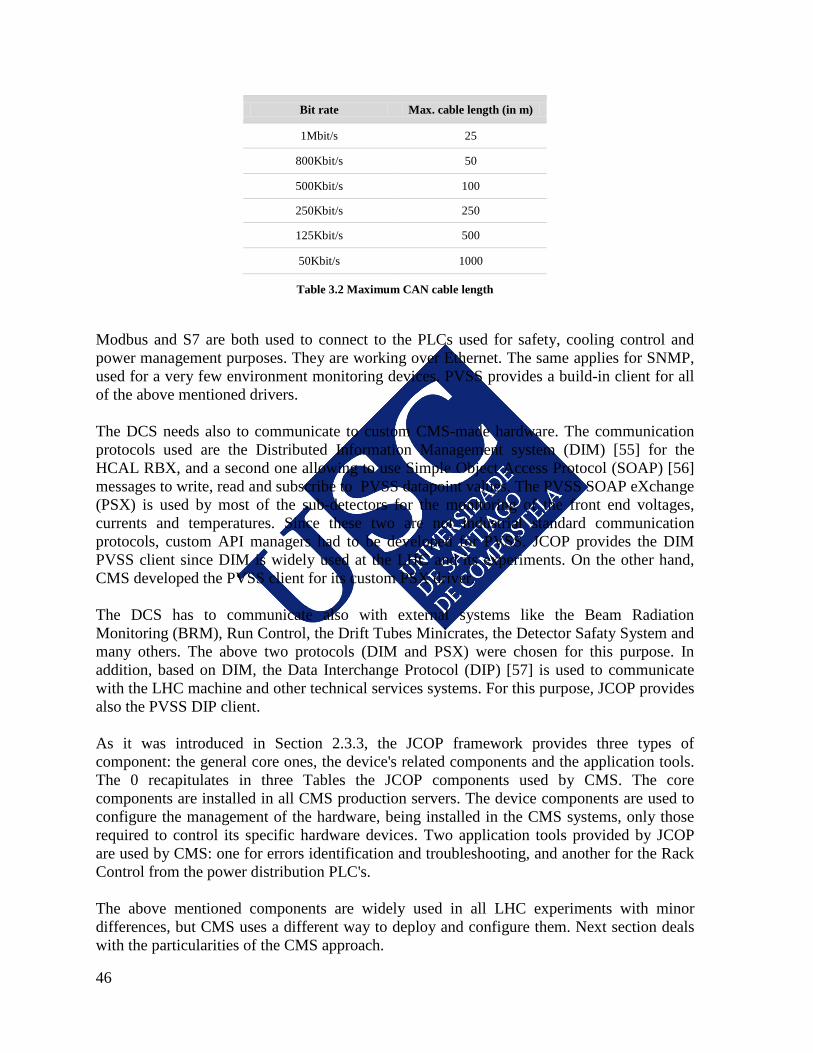
46
Bit rate Max. cable length (in m)
1Mbit/s 25
800Kbit/s 50
500Kbit/s 100
250Kbit/s 250
125Kbit/s 500
50Kbit/s 1000
Table 3.2 Maximum CAN cable length
Modbus and S7 are both used to connect to the PLCs used for safety, cooling control and power management purposes. They are working over Ethernet. The same applies for SNMP, used for a very few environment monitoring devices. PVSS provides a build-in client for all of the above mentioned drivers. The DCS needs also to communicate to custom CMS-made hardware. The communication protocols used are the Distributed Information Management system (DIM) [55] for the HCAL RBX, and a second one allowing to use Simple Object Access Protocol (SOAP) [56] messages to write, read and subscribe to PVSS datapoint values. The PVSS SOAP eXchange (PSX) is used by most of the sub-detectors for the monitoring of the front end voltages, currents and temperatures. Since these two are not industrial standard communication protocols, custom API managers had to be developed for PVSS. JCOP provides the DIM PVSS client since DIM is widely used at the LHC and its experiments. On the other hand, CMS developed the PVSS client for its custom PSX driver. The DCS has to communicate also with external systems like the Beam Radiation Monitoring (BRM), Run Control, the Drift Tubes Minicrates, the Detector Safaty System and many others. The above two protocols (DIM and PSX) were chosen for this purpose. In addition, based on DIM, the Data Interchange Protocol (DIP) [57] is used to communicate with the LHC machine and other technical services systems. For this purpose, JCOP provides also the PVSS DIP client. As it was introduced in Section 2.3.3, the JCOP framework provides three types of component: the general core ones, the device's related components and the application tools. The 0 recapitulates in three Tables the JCOP components used by CMS. The core components are installed in all CMS production servers. The device components are used to configure the management of the hardware, being installed in the CMS systems, only those required to control its specific hardware devices. Two application tools provided by JCOP are used by CMS: one for errors identification and troubleshooting, and another for the Rack Control from the power distribution PLC's. The above mentioned components are widely used in all LHC experiments with minor differences, but CMS uses a different way to deploy and configure them. Next section deals with the particularities of the CMS approach.
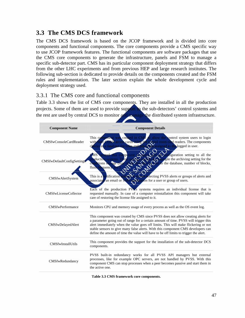
47
3.3 The CMS DCS framework The CMS DCS framework is based on the JCOP framework and is divided into core components and functional components. The core components provide a CMS specific way to use JCOP framework features. The functional components are software packages that use the CMS core components to generate the infrastructure, panels and FSM to manage a specific sub-detector part. CMS has its particular component deployment strategy that differs from the other LHC experiments and from previous HEP and large research institutes. The following sub-section is dedicated to provide details on the components created and the FSM rules and implementation. The later section explain the whole development cycle and deployment strategy used.
3.3.1 The CMS core and functional components Table 3.3 shows the list of CMS core components. They are installed in all the production projects. Some of them are used to provide support to the sub-detectors’ control systems and the rest are used by central DCS to monitor and manage the distributed system infrastructure.
Component Name Component Details
CMSfwConsoleCardReader This component was created in CMS to allow the control system users to login with their CERN access cards using the control room card readers. The components checks in a database the roles and privileges assigned to the logged in user.
CMSfwDefaultConfigSettings
CMS created this component to apply general configuration setting to all the production systems. These settings include for example the archiving setting for the conditions storage (size of the data blocks sent to the database, number of blocks, flush frequency, etc.)
CMSfwAlertSystem This is a notification system. It allows selecting PVSS alerts or groups of alerts and associated an email or SMS notification for a user or group of users.
CMSfwLicenseCollector Each of the production PVSS systems requires an individual license that is requested manually. In case of a computer reinstallation this component will take care of restoring the license file assigned to it.
CMSfwPerformance Monitors CPU and memory usage of every process as well as the OS event log.
CMSfwDelayedAlert
This component was created by CMS since PVSS does not allow creating alerts for a parameter going out of range for a certain amount of time. PVSS will trigger this alert immediately when the value goes off limits. This will make flickering or not stable sensors to give many false alerts. With this component CMS developers can define the amount of time the value will have to be off limits to trigger the alert.
CMSfwInstallUtils This component provides the support for the installation of the sub-detector DCS components.
CMSfwRedundancy
PVSS built-in redundancy works for all PVSS API managers but external processes, like for example OPC servers, are not handled by PVSS. With this component CMS can stop processes when a peer becomes passive and start them in the active one.
Table 3.3 CMS framework core components.
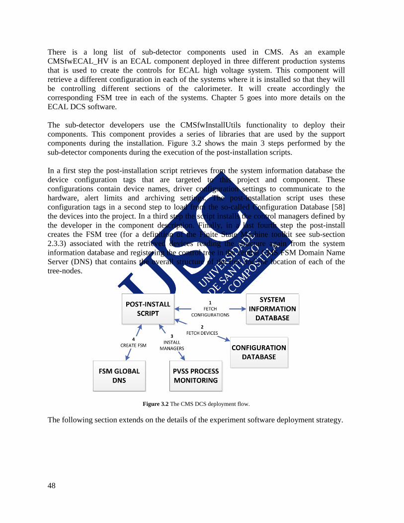
48
There is a long list of sub-detector components used in CMS. As an example CMSfwECAL_HV is an ECAL component deployed in three different production systems that is used to create the controls for ECAL high voltage system. This component will retrieve a different configuration in each of the systems where it is installed so that they will be controlling different sections of the calorimeter. It will create accordingly the corresponding FSM tree in each of the systems. Chapter 5 goes into more details on the ECAL DCS software. The sub-detector developers use the CMSfwInstallUtils functionality to deploy their components. This component provides a series of libraries that are used by the support components during the installation. Figure 3.2 shows the main 3 steps performed by the sub-detector components during the execution of the post-installation scripts. In a first step the post-installation script retrieves from the system information database the device configuration tags that are targeted to this project and component. These configurations contain device names, driver configuration settings to communicate to the hardware, alert limits and archiving settings. The post-installation script uses these configuration tags in a second step to load from the so-called Configuration Database [58] the devices into the project. In a third step the script installs the control managers defined by the developer in the component description. Finally, in a last fourth step the post-install creates the FSM tree (for a definition of the Finite State Machine toolkit see sub-section 2.3.3) associated with the retrieved devices reading the structure again from the system information database and registering the control tree in the central CMS FSM Domain Name Server (DNS) that contains the overall structure of the tree and the location of each of the tree-nodes.
Figure 3.2 The CMS DCS deployment flow.
The following section extends on the details of the experiment software deployment strategy.
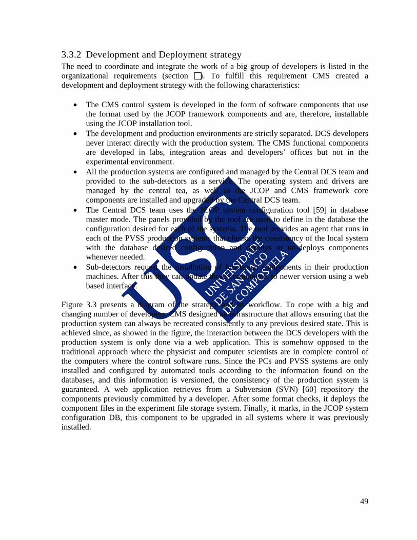
49
3.3.2 Development and Deployment strategy The need to coordinate and integrate the work of a big group of developers is listed in the organizational requirements (section ). To fulfill this requirement CMS created a development and deployment strategy with the following characteristics:
• The CMS control system is developed in the form of software components that use the format used by the JCOP framework components and are, therefore, installable using the JCOP installation tool.
• The development and production environments are strictly separated. DCS developers never interact directly with the production system. The CMS functional components are developed in labs, integration areas and developers’ offices but not in the experimental environment.
• All the production systems are configured and managed by the Central DCS team and provided to the sub-detectors as a service. The operating system and drivers are managed by the central tea, as well as the JCOP and CMS framework core components are installed and upgraded by the Central DCS team.
• The Central DCS team uses the JCOP system configuration tool [59] in database master mode. The panels provided by the tool are used to define in the database the configuration desired for each of the systems. The tool provides an agent that runs in each of the PVSS production systems that checks the consistency of the local system with the database desired configuration and deploys or un-deploys components whenever needed.
• Sub-detectors request the installation of functional components in their production machines. After this they can update those components to newer version using a web based interface.
Figure 3.3 presents a diagram of the strategy and its workflow. To cope with a big and changing number of developers, CMS designed an infrastructure that allows ensuring that the production system can always be recreated consistently to any previous desired state. This is achieved since, as showed in the figure, the interaction between the DCS developers with the production system is only done via a web application. This is somehow opposed to the traditional approach where the physicist and computer scientists are in complete control of the computers where the control software runs. Since the PCs and PVSS systems are only installed and configured by automated tools according to the information found on the databases, and this information is versioned, the consistency of the production system is guaranteed. A web application retrieves from a Subversion (SVN) [60] repository the components previously committed by a developer. After some format checks, it deploys the component files in the experiment file storage system. Finally, it marks, in the JCOP system configuration DB, this component to be upgraded in all systems where it was previously installed.
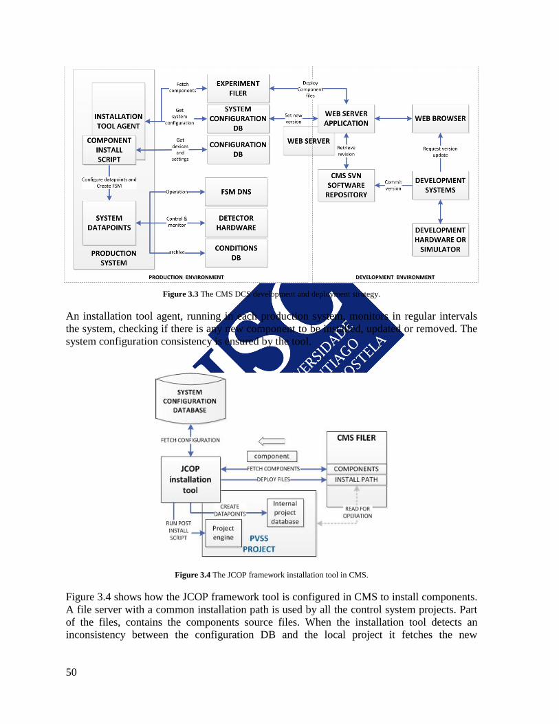
50
Figure 3.3 The CMS DCS development and deployment strategy.
An installation tool agent, running in each production system, monitors in regular intervals the system, checking if there is any new component to be installed, updated or removed. The system configuration consistency is ensured by the tool.
Figure 3.4 The JCOP framework installation tool in CMS.
Figure 3.4 shows how the JCOP framework tool is configured in CMS to install components. A file server with a common installation path is used by all the control system projects. Part of the files, contains the components source files. When the installation tool detects an inconsistency between the configuration DB and the local project it fetches the new
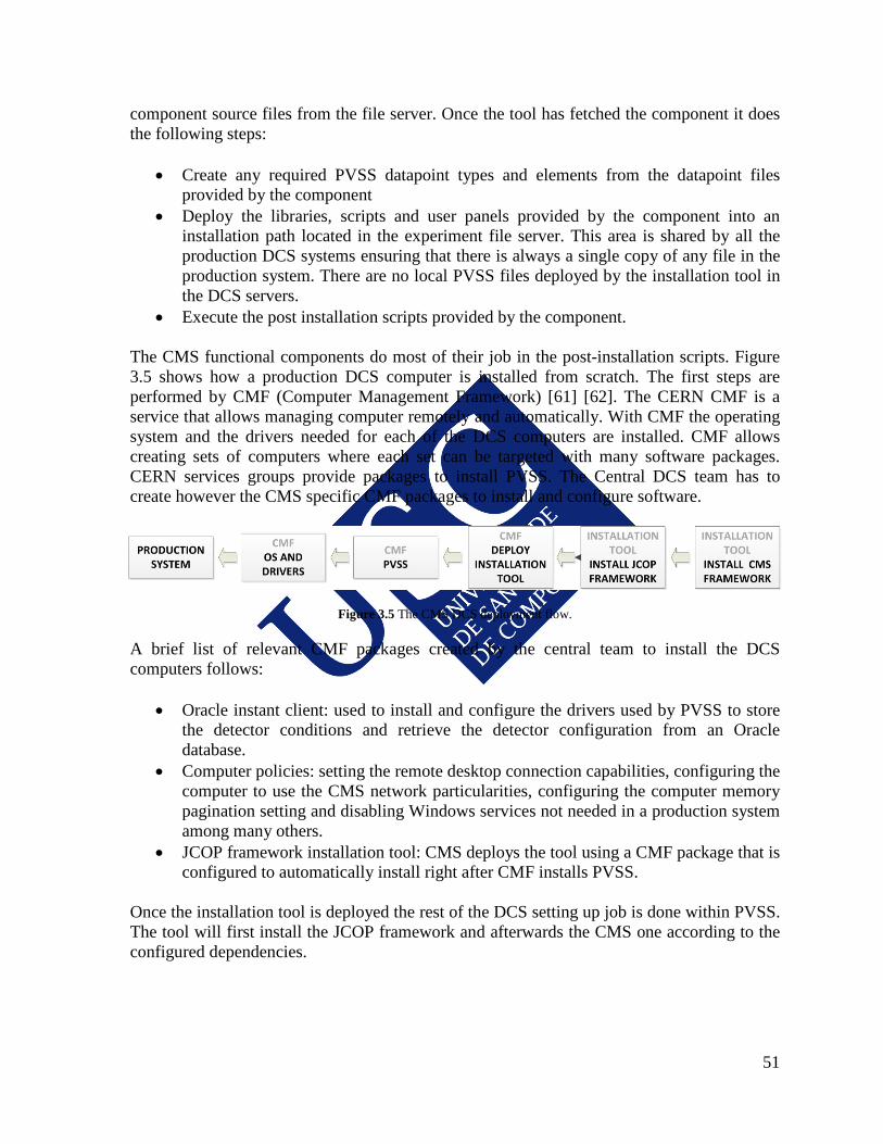
51
component source files from the file server. Once the tool has fetched the component it does the following steps:
• Create any required PVSS datapoint types and elements from the datapoint files provided by the component
• Deploy the libraries, scripts and user panels provided by the component into an installation path located in the experiment file server. This area is shared by all the production DCS systems ensuring that there is always a single copy of any file in the production system. There are no local PVSS files deployed by the installation tool in the DCS servers.
• Execute the post installation scripts provided by the component. The CMS functional components do most of their job in the post-installation scripts. Figure 3.5 shows how a production DCS computer is installed from scratch. The first steps are performed by CMF (Computer Management Framework) [61] [62]. The CERN CMF is a service that allows managing computer remotely and automatically. With CMF the operating system and the drivers needed for each of the DCS computers are installed. CMF allows creating sets of computers where each set can be targeted with many software packages. CERN services groups provide packages to install PVSS. The Central DCS team has to create however the CMS specific CMF packages to install and configure software.
Figure 3.5 The CMS DCS deployment flow.
A brief list of relevant CMF packages created by the central team to install the DCS computers follows:
• Oracle instant client: used to install and configure the drivers used by PVSS to store the detector conditions and retrieve the detector configuration from an Oracle database.
• Computer policies: setting the remote desktop connection capabilities, configuring the computer to use the CMS network particularities, configuring the computer memory pagination setting and disabling Windows services not needed in a production system among many others.
• JCOP framework installation tool: CMS deploys the tool using a CMF package that is configured to automatically install right after CMF installs PVSS.
Once the installation tool is deployed the rest of the DCS setting up job is done within PVSS. The tool will first install the JCOP framework and afterwards the CMS one according to the configured dependencies.

52
This Chapter showed the characteristics of the architecture of the CMS DCS. A DCS development and deployment strategy was proposed and developed for CMS by the author [53]. This innovative distributed component-based model was adopted by the CERN controls support engineering group (EN-ICE). In addition, the author participated in the design and development of most of the CMS framework components. Furthermore, he assisted the sub-detector DCS groups in the development of their own components. The next chapter focuses on the operational aspects and the implementation of the FSM control tree.

53
4. The DCS Operation The CMS DCS is operated by a single operator by means of a Finite State Machine control tree with well-defined states and transitions among them. The first section provides an overview of the experiment operation and the elements involved. Section 4.2 shows the main operation graphical interface for the DCS operator in the control room and the hierarchical alert help system that guarantees an efficient dynamic help for any possible alarm. In Section 4.3, the communication of the DCS with other experiment and accelerator systems is introduced, including the application created by the author to monitor and control the power distribution of all the experiment racks. This application was developed in the frame of the JCOP and is used by all LHC experiments to control the power on their racks. Section 4.4 is dedicated to present the top CMS FSM tree and its operation. Due to its complexity the author collaborated with an Eindhoven Technical University group in order to develop tools to automatically detect potential loops in the tree logic that could not be computed by traditional means due to the extremely large state space. The last section of the chapter, section 4.5, explains the detector automation and protections mechanism. The author participated in the design of both of these two crucial systems that improve the detector efficiency and ensure its safeness [63].
4.1 Operation overview Figure 4.1 shows a summary of the main CMS DCS operation elements. The whole detector is controlled form a single operator station. A user interface (1 in Figure 4.1) remotely connects to the central DCS PVSS system providing the operator with the control of the central FSM based tree (3 in Figure 4.1). This central tree has a parent node for each of the experiment sub-detectors. This way, the central tree takes control of each of the sub-detector trees (8 in Figure 4.1). The central DCS operator can yield however the control of a sub-detector tree and allow that sub-tree to be controlled in an independent partition from the sub-detector control stations (9 in Figure 4.1). In addition to the sub-detectors, the central DCS also connects to other services (5 in Figure 4.1) and models these in the control sub-tree. In particular, the power distribution of the ~500 experiment racks is modeled in a sub-tree, as well as the experiment cooling network. The communication to the LHC machine (4 in Figure 4.1) is modeled in another sub-tree that interprets the different handshake protocols defined. The sub-detectors are modeled (10 in Figure 4.1) following the central DCS guidelines document. In this way, the interface between the central DCS control tree and the sub-detectors is homogenous, simplifying the FSM tree logic. The particularities of each sub-detector are hidden down on their control tree. At the bottom of the tree there are the device type nodes. These nodes, called device units, model real devices or sets of hardware devices. A direct line connects CMS protection mechanism to the hardware (11 in Figure 4.1). This direct connection goes in parallel to the control tree so it ignores any possible created partition, addressing directly the devices’ datapoints in order to set the hardware to a desired safe state when required. The Central DCS has automated most of the detector control commands and uses the central control tree to dispatch them to the sub-detectors (6 in Figure 4.1).
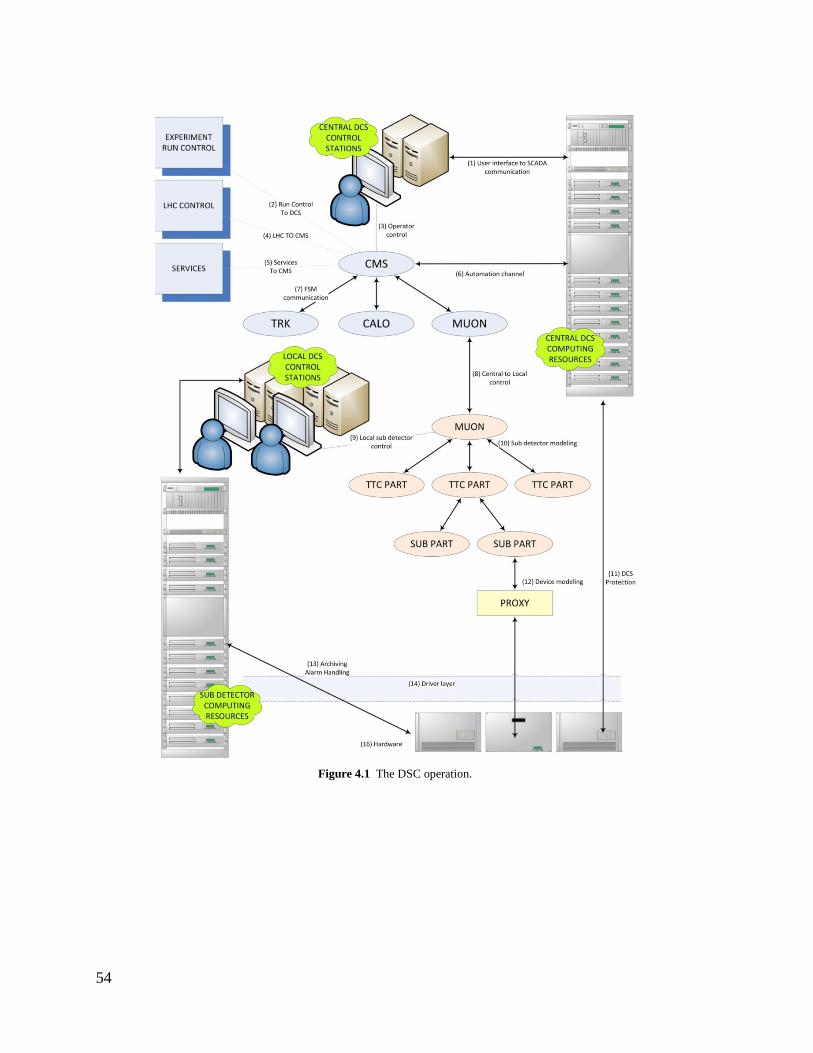
54
Figure 4.1 The DSC operation.
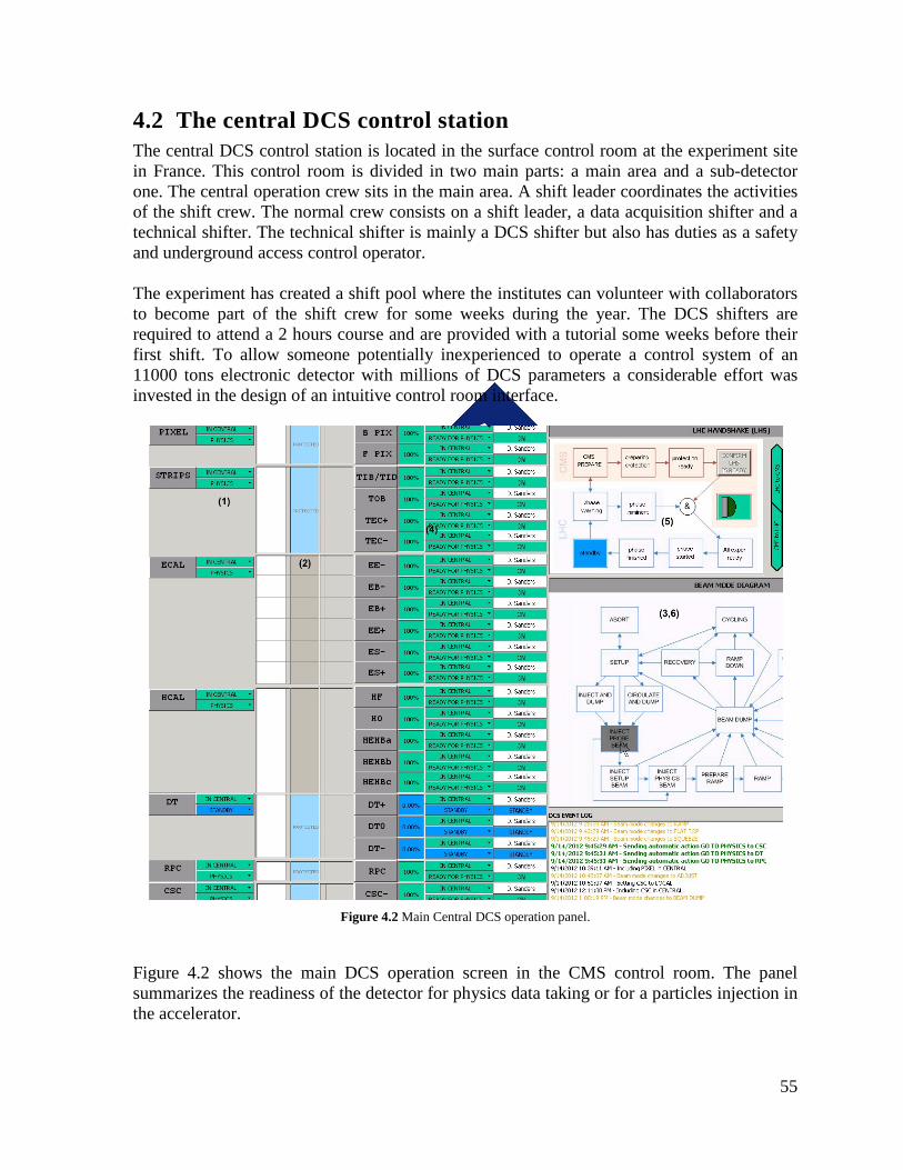
55
4.2 The central DCS control station The central DCS control station is located in the surface control room at the experiment site in France. This control room is divided in two main parts: a main area and a sub-detector one. The central operation crew sits in the main area. A shift leader coordinates the activities of the shift crew. The normal crew consists on a shift leader, a data acquisition shifter and a technical shifter. The technical shifter is mainly a DCS shifter but also has duties as a safety and underground access control operator. The experiment has created a shift pool where the institutes can volunteer with collaborators to become part of the shift crew for some weeks during the year. The DCS shifters are required to attend a 2 hours course and are provided with a tutorial some weeks before their first shift. To allow someone potentially inexperienced to operate a control system of an 11000 tons electronic detector with millions of DCS parameters a considerable effort was invested in the design of an intuitive control room interface.
Figure 4.2 Main Central DCS operation panel.
Figure 4.2 shows the main DCS operation screen in the CMS control room. The panel summarizes the readiness of the detector for physics data taking or for a particles injection in the accelerator.
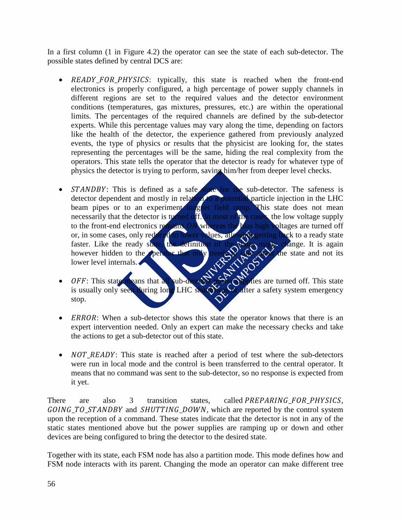
56
In a first column (1 in Figure 4.2) the operator can see the state of each sub-detector. The possible states defined by central DCS are:
• 𝑅𝐸𝐴𝐷𝑌_𝐹𝑂𝑅_𝑃𝐻𝑌𝑆𝐼𝐶𝑆: typically, this state is reached when the front-end
electronics is properly configured, a high percentage of power supply channels in different regions are set to the required values and the detector environment conditions (temperatures, gas mixtures, pressures, etc.) are within the operational limits. The percentages of the required channels are defined by the sub-detector experts. While this percentage values may vary along the time, depending on factors like the health of the detector, the experience gathered from previously analyzed events, the type of physics or results that the physicist are looking for, the states representing the percentages will be the same, hiding the real complexity from the operators. This state tells the operator that the detector is ready for whatever type of physics the detector is trying to perform, saving him/her from deeper level checks.
• 𝑆𝑇𝐴𝑁𝐷𝐵𝑌: This is defined as a safe state for the sub-detector. The safeness is detector dependent and mostly in relation to a potential particle injection in the LHC beam pipes or to an experiment magnet field ramp. This state does not mean necessarily that the detector is turned off. In most of the cases, the low voltage supply to the front-end electronics remains 𝑂𝑁 whereas the bias high voltages are turned off or, in some cases, only reduced to lower values, allowing getting back to a ready state faster. Like the ready state, the definition of the states might change. It is again however hidden to the operator that only needs to care about the state and not its lower level internals.
• 𝑂𝐹𝐹: This state means that all sub-detector power supplies are turned off. This state is usually only seen during long LHC shutdowns or after a safety system emergency stop.
• 𝐸𝑅𝑅𝑂𝑅: When a sub-detector shows this state the operator knows that there is an expert intervention needed. Only an expert can make the necessary checks and take the actions to get a sub-detector out of this state.
• 𝑁𝑂𝑇_𝑅𝐸𝐴𝐷𝑌: This state is reached after a period of test where the sub-detectors were run in local mode and the control is been transferred to the central operator. It means that no command was sent to the sub-detector, so no response is expected from it yet.
There are also 3 transition states, called 𝑃𝑅𝐸𝑃𝐴𝑅𝐼𝑁𝐺_𝐹𝑂𝑅_𝑃𝐻𝑌𝑆𝐼𝐶𝑆, 𝐺𝑂𝐼𝑁𝐺_𝑇𝑂_𝑆𝑇𝐴𝑁𝐷𝐵𝑌 and 𝑆𝐻𝑈𝑇𝑇𝐼𝑁𝐺_𝐷𝑂𝑊𝑁, which are reported by the control system upon the reception of a command. These states indicate that the detector is not in any of the static states mentioned above but the power supplies are ramping up or down and other devices are being configured to bring the detector to the desired state. Together with its state, each FSM node has also a partition mode. This mode defines how and FSM node interacts with its parent. Changing the mode an operator can make different tree

57
partitions by removing trees from its parent. A sub-detector tree that is included in the global tree is known to be in central mode. If it is excluded from the global tree is known to be in local mode. In central mode the detector is controlled by the central operator. In local mode, the detector is excluded from central operation. It may at this point be controlled independently from sub-detector control stations. The states of sub-detectors in local mode are ignored when calculating the global CMS readiness such as if a sub-detector is not participating in a physics run then it can be turned off or performing calibrations without affecting the global DCS state. The dynamic table, 2 in Figure 4.2, shows the expected experiment state for the current LHC beam mode and the expected state for the expected following beam modes. The current LHC machine mode is showed also in the user interface (3 in Figure 4.2). For each of the three beams modes shown in the picture, the table displays the programmed automatic commands, if any, that the sub-detector will receive from the central DCS. This gives the operator the information of whether the sub-detectors are in the correct state for the current LHC state and what to expect for the next modes. The possible LHC modes and their functional specification are documented in [64]. The third column, 4 in Figure 4.2, provides the information for each sub-detector in terms of its main sub-partitions. CMS has decided to map these to the detector Timing, Trigger and Control (TTC) partitions. The TTC distribution system must ensure high-quality clocking of the CMS experiment to allow the physics potential of the LHC machine to be fully exploited. The TTC partitions represent the different part of the detector that can have an independent clocking and trigger and therefore where physics operation can be performed independently. For this reason, the Central DCS team selected this granularity to homogenize the first level of sub-detector tree branching. In addition to its states (that can be the same as for the sub-detector nodes mentioned above) the panel provides a percentage of the number of bias high voltage channels in the nominal state. These primary partitions can also be operated in standalone mode. In this way, the central operator might control a sub-detector with the exception of one or more of its partitions that could be in local mode and controlled from the sub-detector workstations. Also, this column provides information about the hardware state for the partitions below the main sub-detector tree-nodes. The main partitions expect the hardware to be in 𝑂𝑁, 𝑂𝐹𝐹 or 𝐸𝑅𝑅𝑂𝑅 state. However sub-detectors can define other mixed states for their hardware (like for example 𝑃𝐴𝑅𝑇𝐿𝑌_𝑂𝑁) that are interpreted by the partition nodes as transitional states. Finally, this column provides also information on the operator name on control of each partition. If the partition is in central mode it shows his/her name, otherwise it will show the name of the sub-detector control station operator or expert. It will also show if the partition is just excluded from operations (see Figure 2.8) so that there is no one controlling it. On the right top and middle part of the screen (5 and 6 in Figure 4.2) the operator has the information related to the communication to the LHC machine. The LHC and its experiments communicate to keep each other updated about their status. Next section describes this communication and the reasons for it.

58
To complete the panel, in the bottom right part (7 in Figure 4.2), there is a widget containing an operations log. The log shows the automatic commands sent by the central DCS, the manual commands sent by the operator, the LHC beam and machine mode changes and the transitions of control nodes from central to local control. This log can help to make a first and quick reconstruction of the last events that took place in case of a problem. The main user interface provides the DCS readiness for physics related information. There is a second user interface panel complementing this information that is called the DCS Alert Screen panel. Any of the about 6 million DCS parameters can be configured to trigger an alert in the operator’s screen, when crossing predefined thresholds. Alerts do not imply that the sub-detectors are not in a ready for physics state. As previously stated, due to the large amount of bias voltages, the states are defined statically. Therefore a sub-detector can be in 𝑅𝐸𝐴𝐷𝑌_𝐹𝑂𝑅_𝑃𝐻𝑌𝑆𝐼𝐶𝑆 state while issuing some bias voltage trip alerts to the operator’s screen. Even when not necessarily compromising the physics run, alerts are required to be attended immediately by the operators. An accumulation of alerts in different parts of the detector would normally imply a statistical change in the amount of channels needed to keep a partition in a ready for physics state triggering, consequently, a state change. Alerts can also be a warning for abnormal conditions that can damage or accelerate the aging of the experiment electronics. An alert help system provides instructions for each of the possible alerts. The help is generated dynamically from a tree like structure that looks from the most concise possible help for a specific channel to a more generic help for the type of device or system.
4.3 Communication with external systems The DCS is an autonomous system required to run 24/7. Still, it needs to communicate with other systems for a correct operation of the experiment. DIP (introduced in section 3.2) is a protocol based on the client/server paradigm. Servers provide services to clients. The services are a set of data and are listed in a central name server. A client looking for some information requests from the name server its location address. With this address it then subscribes to the information publisher and from then on, it gets updates on the data values. Data is always made of a value, a timestamp and a quality bit assessing the validity of the value published.
4.3.1 Communication with the LHC During operation, the LHC works in an endless cycle of beam injection, beam collisions, beam dump and back to beam injection. Figure 4.3 shows the diagram of the possible beam states. When the LHC is in operation and providing the experiments with colliding particle beams it will follow the sequence: INJECT PREPARE_RAMP RAMP FLAT_TOP SQUEEZE ADJUST STABLE BEAMS BEAM_DUMP INJECT The particle beams might however become unstable or get dumped by any of the accelerator or experiments’ safety systems so the beam mode can switch to 𝑈𝑁𝑆𝑇𝐴𝐵𝐿𝐸_𝐵𝐸𝐴𝑀𝑆 or 𝐵𝐸𝐴𝑀_𝐷𝑈𝑀𝑃 at any moment. Other beam modes are used during machine setup after a
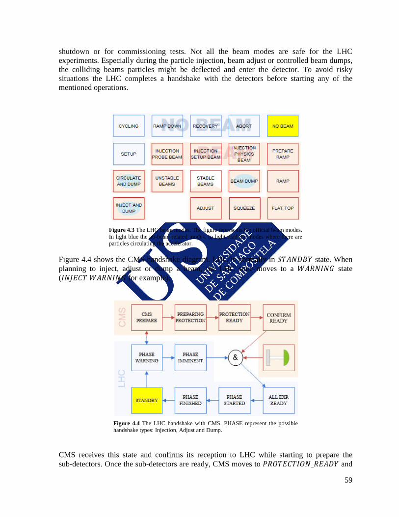
59
shutdown or for commissioning tests. Not all the beam modes are safe for the LHC experiments. Especially during the particle injection, beam adjust or controlled beam dumps, the colliding beams particles might be deflected and enter the detector. To avoid risky situations the LHC completes a handshake with the detectors before starting any of the mentioned operations.
Figure 4.3 The LHC beam modes. The figure represents the official beam modes. In light blue the no-beam related modes. In light read the modes where there are particles circulating the accelerator.
Figure 4.4 shows the CMS handshake diagram. LHC is normally in 𝑆𝑇𝐴𝑁𝐷𝐵𝑌 state. When planning to inject, adjust or dump a beam, the LHC state moves to a 𝑊𝐴𝑅𝑁𝐼𝑁𝐺 state (𝐼𝑁𝐽𝐸𝐶𝑇 𝑊𝐴𝑅𝑁𝐼𝑁𝐺 for example).
Figure 4.4 The LHC handshake with CMS. PHASE represent the possible handshake types: Injection, Adjust and Dump.
CMS receives this state and confirms its reception to LHC while starting to prepare the sub-detectors. Once the sub-detectors are ready, CMS moves to 𝑃𝑅𝑂𝑇𝐸𝐶𝑇𝐼𝑂𝑁_𝑅𝐸𝐴𝐷𝑌 and
60
at this point CMS is ready to send the ready signal to the LHC. There is still a hardware protection in the control room. This protection consists of a button that should be released to allow the injection. This button is also monitored by DCS and represented in the diagram. Both the software and hardware signals are necessary for the LHC to complete the handshake. When the LHC receives the ready confirmation from all the experiments then it starts an injection (or starts a beam adjust or beam dump). Only when finished it moves back to 𝑆𝑇𝐴𝑁𝐷𝐵𝑌 state.
4.3.2 Communication with Run Control and DAQ CMS Run Control [65] uses the DCS information to know when to start or stop recording physics data by sending synchronization signals to the front-end electronics. To interface the DCS, CMS developed its own communication interface that is called the PVSS SOAP eXchange (PSX) [66]. PSX clients can write, read or subscribe to PVSS datapoint values. In addition, they can subscribe to the FSM states of the sub-detector nodes or any of their children. Other consumers of the PSX service are the data acquisition systems of some sub-detectors, which use PSX to check the bias voltage status of its channels in order to synchronize the front-end electronics configuration.
4.3.3 Communication with the cavern services There are some services that are provided to the LHC experiments centrally by the engineering division. There are 4 main services that DCS communicates with:
• The Magnet control service uses DIP to provide DCS with the information about CMS magnet state. This information includes the circulating current and temperature. Also, there are a few flags indicating mostly if the magnet is in a stable regime or ramping. The information is used by the DCS to bring some sub-detectors that are sensitive to the magnetic field changes to a safe state. The Magnet system information is in addition recorded by DCS and used later on for analysis corrections.
• The cooling network service also uses DIP to forward to DCS information on the primary cooling circuits and the sub-circuits feeding each of the sub-detectors. The information includes water flows and temperatures, as well as the buffer tank weights for water leak detection. With the cooling information the DCS can anticipate incoming problems. CMS cooling network needs to account for approximately 7000 𝑘𝑤 so the stop of one of the network chillers or pumps increases the temperature of the cooled electronics in a short time. The DCS has the information about the state of the cooling network chillers and pumps and uses it to selectively turn off not indispensable hardware in order to relax the requirements on the cooling circuits in case of an incident.
• The Gas system service sends to the DCS information on the gas mixtures, temperatures and pressures. CMS gaseous sub-detectors consume this information and include it in the computations of its partition states.
• The Power Distribution system doesn’t communicate via DIP with DCS. In this case, the PVSS Modbus TCP/IP driver is used to communicate directly to the PLCs monitoring and controlling the power of the electronic racks.
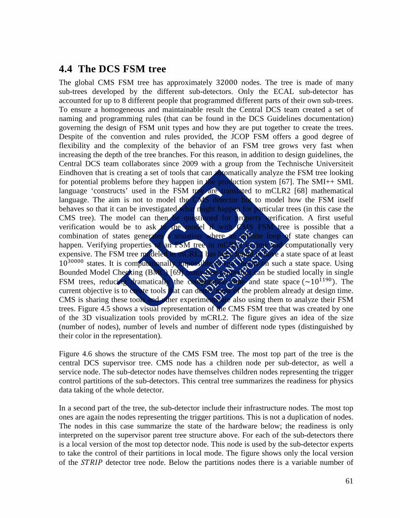
61
4.4 The DCS FSM tree The global CMS FSM tree has approximately 32000 nodes. The tree is made of many sub-trees developed by the different sub-detectors. Only the ECAL sub-detector has accounted for up to 8 different people that programmed different parts of their own sub-trees. To ensure a homogeneous and maintainable result the Central DCS team created a set of naming and programming rules (that can be found in the DCS Guidelines documentation) governing the design of FSM unit types and how they are put together to create the trees. Despite of the convention and rules provided, the JCOP FSM offers a good degree of flexibility and the complexity of the behavior of an FSM tree grows very fast when increasing the depth of the tree branches. For this reason, in addition to design guidelines, the Central DCS team collaborates since 2009 with a group from the Technische Universiteit Eindhoven that is creating a set of tools that can automatically analyze the FSM tree looking for potential problems before they happen in the production system [67]. The SMI++ SML language ‘constructs’ used in the FSM tree are translated to mCLR2 [68] mathematical language. The aim is not to model the CMS detector but to model how the FSM itself behaves so that it can be investigated what might happen for particular trees (in this case the CMS tree). The model can then be questioned for property verification. A first useful verification would be to ask to the model if with CMS FSM tree is possible that a combination of states generates a situation where an infinite loop of state changes can happen. Verifying properties of an FSM tree in mCRL2 is time and computationally very expensive. The FSM tree modeled in mCRL2 has been found to have a state space of at least 1030000 states. It is computationally impossible to run checks on such a state space. Using Bounded Model Checking (BMC) [69] many tree properties can be studied locally in single FSM trees, reducing dramatically the computation time and state space (~101190). The current objective is to create tools that can detect most of the problem already at design time. CMS is sharing these tools and other experiments are also using them to analyze their FSM trees. Figure 4.5 shows a visual representation of the CMS FSM tree that was created by one of the 3D visualization tools provided by mCRL2. The figure gives an idea of the size (number of nodes), number of levels and number of different node types (distinguished by their color in the representation). Figure 4.6 shows the structure of the CMS FSM tree. The most top part of the tree is the central DCS supervisor tree. CMS node has a children node per sub-detector, as well a service node. The sub-detector nodes have themselves children nodes representing the trigger control partitions of the sub-detectors. This central tree summarizes the readiness for physics data taking of the whole detector. In a second part of the tree, the sub-detector include their infrastructure nodes. The most top ones are again the nodes representing the trigger partitions. This is not a duplication of nodes. The nodes in this case summarize the state of the hardware below; the readiness is only interpreted on the supervisor parent tree structure above. For each of the sub-detectors there is a local version of the most top detector node. This node is used by the sub-detector experts to take the control of their partitions in local mode. The figure shows only the local version of the 𝑆𝑇𝑅𝐼𝑃 detector tree node. Below the partitions nodes there is a variable number of
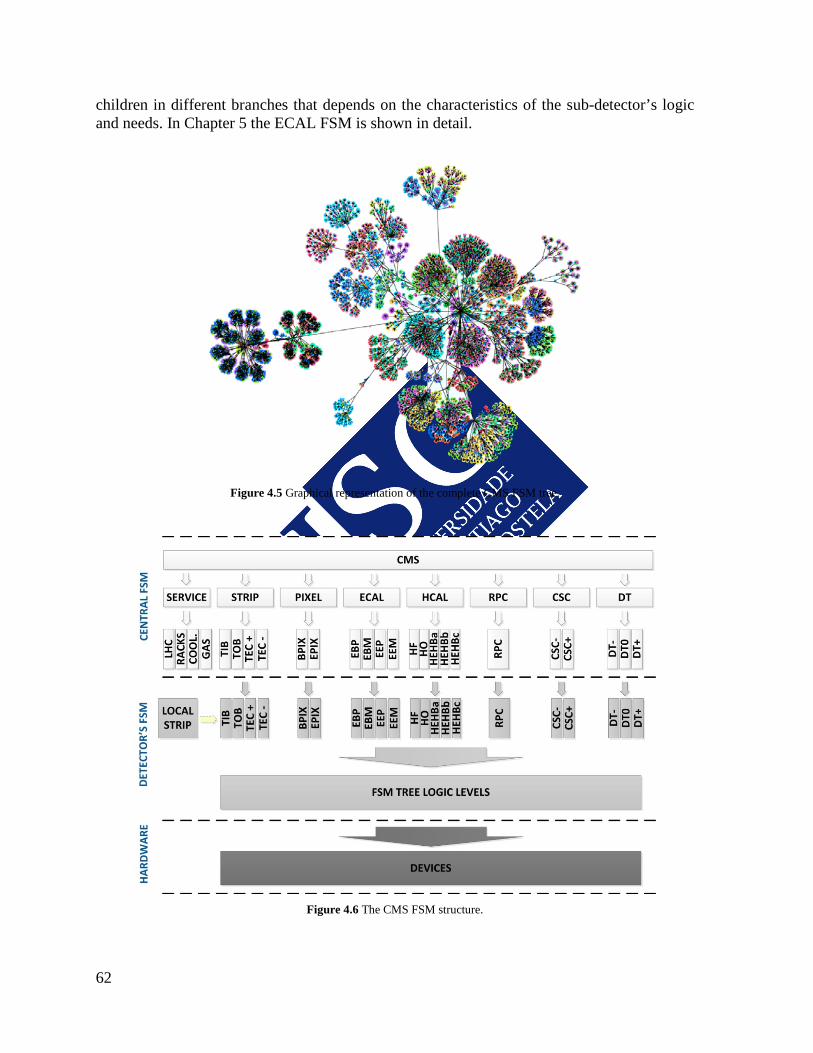
62
children in different branches that depends on the characteristics of the sub-detector’s logic and needs. In Chapter 5 the ECAL FSM is shown in detail.
Figure 4.5 Graphical representation of the complete CMS FSM tree.
Figure 4.6 The CMS FSM structure.
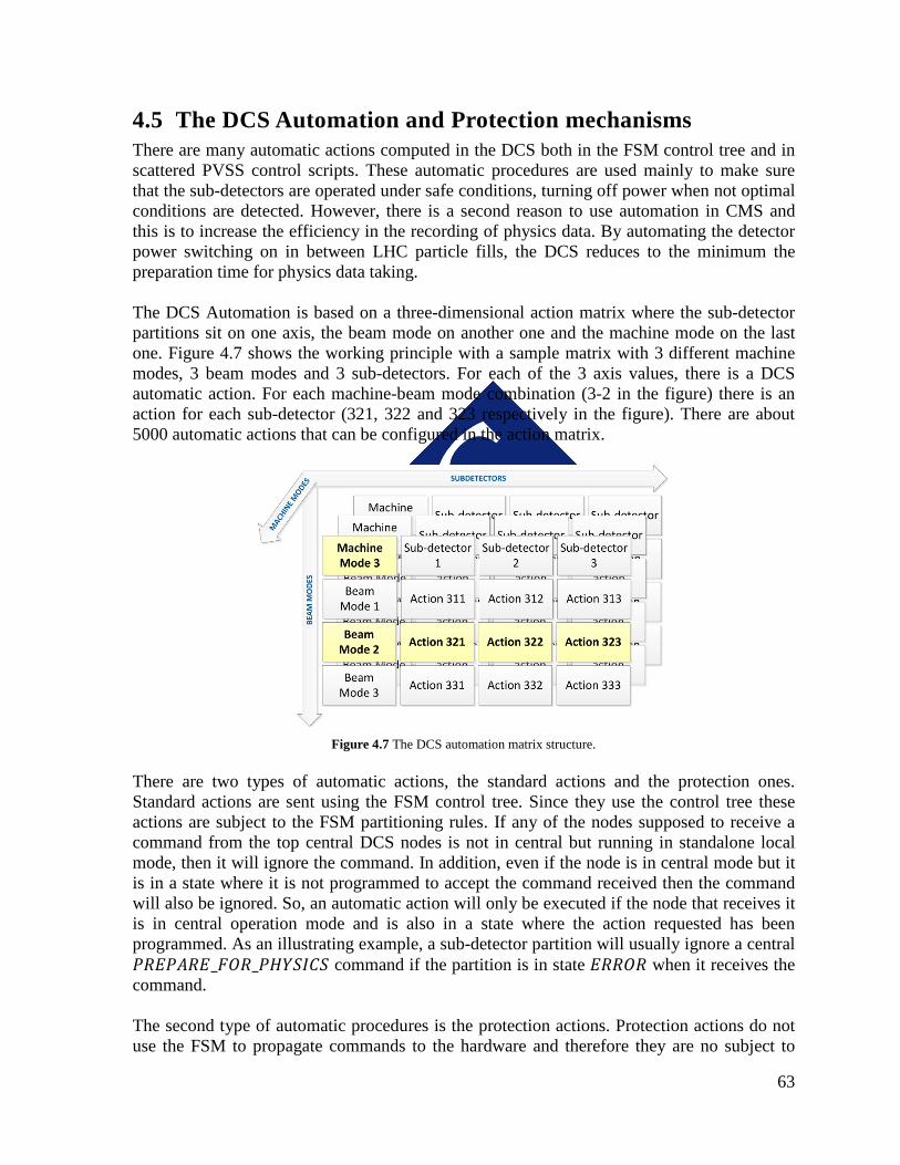
63
4.5 The DCS Automation and Protection mechanisms There are many automatic actions computed in the DCS both in the FSM control tree and in scattered PVSS control scripts. These automatic procedures are used mainly to make sure that the sub-detectors are operated under safe conditions, turning off power when not optimal conditions are detected. However, there is a second reason to use automation in CMS and this is to increase the efficiency in the recording of physics data. By automating the detector power switching on in between LHC particle fills, the DCS reduces to the minimum the preparation time for physics data taking. The DCS Automation is based on a three-dimensional action matrix where the sub-detector partitions sit on one axis, the beam mode on another one and the machine mode on the last one. Figure 4.7 shows the working principle with a sample matrix with 3 different machine modes, 3 beam modes and 3 sub-detectors. For each of the 3 axis values, there is a DCS automatic action. For each machine-beam mode combination (3-2 in the figure) there is an action for each sub-detector (321, 322 and 323 respectively in the figure). There are about 5000 automatic actions that can be configured in the action matrix.
Figure 4.7 The DCS automation matrix structure.
There are two types of automatic actions, the standard actions and the protection ones. Standard actions are sent using the FSM control tree. Since they use the control tree these actions are subject to the FSM partitioning rules. If any of the nodes supposed to receive a command from the top central DCS nodes is not in central but running in standalone local mode, then it will ignore the command. In addition, even if the node is in central mode but it is in a state where it is not programmed to accept the command received then the command will also be ignored. So, an automatic action will only be executed if the node that receives it is in central operation mode and is also in a state where the action requested has been programmed. As an illustrating example, a sub-detector partition will usually ignore a central 𝑃𝑅𝐸𝑃𝐴𝑅𝐸_𝐹𝑂𝑅_𝑃𝐻𝑌𝑆𝐼𝐶𝑆 command if the partition is in state 𝐸𝑅𝑅𝑂𝑅 when it receives the command. The second type of automatic procedures is the protection actions. Protection actions do not use the FSM to propagate commands to the hardware and therefore they are no subject to

64
FSM partitioning rules. The Central DCS team designed this protection mechanism to ensure the maximum software protection that was possible to achieve within the JCOP framework. The principle is the following: the protection mechanism clients subscribe the beam-machine mode matrix combinations. They also predefine a set of hardware channels and the desired protection settings. When the triggering machine-beam mode arrives then the channels are directly set at the lowest PVSS datapoint level to the previously defined protection settings. At the same time, these datapoints are locked by the protection mechanism using a blocking PVSS datapoint functionality. This lock basically means that the datapoint values cannot be changed by any other process. Like this, any manual or automatic FSM command aiming to change these settings, any control script or remote expert command will fail. The mechanism will only release the lock when the beam-machine mode changes. Figure 4.8 shows the action matrix for the machine mode 𝑃𝑅𝑂𝑇𝑂𝑁_𝑃𝐻𝑌𝑆𝐼𝐶𝑆. There is a similar table for each of the LHC machine modes (see Appendix A). According to a DCS naming convention, the actions starting by 𝑃𝑅𝑂𝑇𝐸𝐶𝑇 prefix are protection type commands that are sent directly to the hardware, and the actions starting by 𝐺𝑂_𝑇𝑂 are FSM control tree commands.
Figure 4.8 The DCS Automation matrix for the Proton Physics LHC machine mode.
During the injection and adjust of the beams, the sub-detectors subjected to have their components damaged due to beam deflection related incidents are forced into the 𝑆𝑇𝐴𝑁𝐷𝐵𝑌 state by the protection mechanism. However, other sub-detectors have chosen not to be forced by the protection system but just to receive a standard FSM command to move to 𝑆𝑇𝐴𝑁𝐷𝐵𝑌 state. For this sub-detectors (that in the current configuration are CSC and ECAL preshower partitions) moving to a standby safe state is not critical and they are not expected to be damaged if their partitions would not receive the command from the top nodes (for example if their FSM tree partitions are in local mode). When the LHC beam mode moves towards colliding stable beams (𝑆𝑇𝐴𝐵𝐿𝐸_𝐵𝐸𝐴𝑀𝑆) the detector partitions start to receive the 𝐺𝑂_𝑇𝑂_𝑃𝐻𝑌𝑆𝐼𝐶𝑆 command. The ECAL preshower partitions switch on during 𝐹𝐿𝐴𝑇_𝑇𝑂𝑃 beam mode while the muon sub-detectors and the ZDC do it during the 𝑆𝑄𝑈𝐸𝐸𝑍𝐸 mode.
65
The HCAL sub-detector does not receive the command to prepare for physics until the machine declares stable beams though nothing prevent HCAL to be already prepared manually before (as there is no protection command preventing that). The same applies for ECAL barrel and end-cap partitions that never receive a command from the automation matrix but the detector usually stays on between accelerator particle fills. The Tracker sub-detector stays in a protected state until the stable beams are declared. Once the beams are declared stable the automation mechanism still does some checks to decide whether to send automatic command to switch on or not. These sub-detectors, been the closest to the beam pipes, are the more susceptible to be damaged because of beam related problems, require extra verifications with the Beam Conditions Monitor (BCM) system before receiving an automatic command. The automation matrix can also be used to configure differently the front-end electronics depending on the machine and beam mode. For example, the CASTOR detector, as shown in Figure 4.8, receives the command 𝐺𝑂_𝑇𝑂_𝑃𝐻𝑌𝑆𝐼𝐶𝑆 in two different modes but sets different bias voltages in the detector.

66
67
5. The ECAL DCS A general description of the CMS high precision electromagnetic calorimeter, ECAL, was provided in Chapter 1 (section 1.3.4). This chapter includes the contribution of the author to the ECAL sub-detector control system. The system details for the ECAL () are provided. The author of this thesis work worked closely with the ECAL DCS development team in the design and implementation of their control system, co-authoring as well various journal articles and conference proceedings ( [70], [71], [72] and [73] ). The information in these papers is summarized and presented in the following sections. The chapter is extended with two more sections providing additional details on the ECAL FSM tree and ECAL operation. One of the most accurate, distinctive and important detector systems of the CMS experiment is the high precision Electromagnetic Calorimeter (ECAL). It provides measurements of electrons and photons with an excellent energy resolution (better than 0.5% at energies above 100 𝐺𝑒𝑉), and thus is essential in the search for new physics, in particular for the Higgs boson. In order to successfully achieve these physics goals the ECAL collaboration designed the calorimeter as a homogeneous hermetic detector based on 75848 Lead-tungstate (𝑃𝑏𝑊𝑂4) scintillating crystals. Avalanche Photo Diodes (APD) [74] and vacuum phototriodes (VPT) [75] are used as photodetectors in the barrel part and in the end-cap parts of the detector, respectively. All these components and frontend readout electronics inside the ECAL satisfy rigorous design requirements in terms of their response time, signal-to-noise ratio, immunity to high values of the magnetic field (up to 4T in the barrel part of the ECAL) as well as in terms of radiation tolerance (expected equivalent doses of up to 50 𝑘𝐺𝑦 and neutron fluence of up to 1014 𝑛𝑒𝑢𝑡𝑟𝑜𝑛𝑠/𝑐𝑚2). However, the light yield of PbWO4 crystals and the amplification of the APDs is rather sensitive to temperature and bias voltage fluctuations [76] [77]. Therefore, the use of these components imposed challenging constraints on the design of the ECAL, such as the need for rigorous temperature and high voltage stability. At the same time, mechanisms that allow radiation to induce changes in crystal transparency (and hence in its response), imposed additional requirements for “in situ” monitoring of the crystal transparency. For all these reasons specific ECAL subsystems that provide the necessary services had to be designed. These include: Cooling system [78], High Voltage (HV) and Low Voltage (LV) systems [79], as well as Laser Monitoring system [80]. In addition, a sophisticated ECAL Detector Control System (DCS) that could provide the necessary control and monitoring of the proper functioning of all these ECAL sub-systems, as well as the control and monitoring of important ECAL working parameters, had to be carefully designed.
68
Figure 5.1 shows a diagram with the different parts of the DCS systems and their connections. The following sections provide detailed information on each of the represented sub-systems.
Figure 5.1 CMS ECAL DCS block diagram
5.1 The Cooling system The ECAL Cooling system employs a water flow to stabilize the detector to 18 °𝐶 within 0.05 °𝐶. Each Supermodule and each End-cap is independently supplied with water at 18 °𝐶. The water runs through a thermal screen placed in front of the crystals which thermally decouples them from the silicon tracker, and through pipes embedded in the aluminum grid in front of the electronics compartments. Regulation of the water temperature and the water flow, as well as the opening of valves is performed by a dedicated 100 Siemens PLC system. This system is operated by a rack mounted PC via S7 connection.
5.2 High voltage and low voltage systems The APDs require a power supply system with a stability of the bias voltage of the order of few tens of mV. For this reason, a custom HV power supply system was designed for the CMS ECAL in collaboration with the CAEN Company. The system is based on a standard control crate (SY1527) hosting eight boards especially designed for this application (A1520PE). Up to nine channels can be hosted on a single A1520PE board and each channel can give a bias voltage of up to 500 𝑉 with a maximum current of 15 𝑚𝐴. The operating APD gain of 50 requires a voltage between 340 and 430 𝑉. In total, there are 18 crates and 144 boards for the barrel. The SY1527 crate communicates with a board controller via an internal bus and is operated by the ECAL DCS via an OPC server.

69
In the end-caps, by default all VPTs are operated at anode and dynode voltages of 800 and 600 𝑉 respectively. The VPTs require a stability of the bias voltages of about 10 𝑉. The HV system is based on standard CAEN control crates (SY1527) each hosting two off-the-shelf HV boards (A1735P). Up to six pairs of channels can be hosted on a single A1735P board and each channel can give a bias voltage of up to 1500 V with a maximum current of 7 mA. There is 1 crate for each of the 2 end-caps. The power supplies are complemented by a custom-designed 84-way distribution system which incorporates additional protection circuitry and a clean method to operate each of the 84 channels at one of three different pairs of bias voltages. The ECAL digitization electronics located on the very front-end (VFE) electronics cards require also a very stable low voltage to maintain constant signal amplification. The system uses low voltage regulators that guarantee this stability. The power is supplied by the LV system that is based on multichannel MARATON LV power supplies (PS) from Wiener. Two types of LV PS are used: a type with six channels of 8 𝑉/110𝐴 (660 𝑊) and a type with five channels of 8 𝑉/110𝐴 (660 𝑊) and two channels of 8 𝑉/55𝐴 (330 𝑊). In total there are 108 PS for the ECAL barrel and 28 PS for the ECAL end-cap. All the LV PS are water-cooled and operated by three ECAL DCS rack mounted PCs via CAN-bus and an OPC server.
5.3 The Precision Temperature (PTM) and Humidity (HM) systems
The purpose of the PTM system is to provide precision measurements to monitor the stability of the temperature distribution in the environment of the ECAL crystals and photo-detectors. In addition, it provides archiving of the temperature distribution history for use in the ECAL data processing. In order to provide this functionality, 360 high quality NTC thermistors [81] with very good long-term stability are installed in the ECAL Supermodules and 80 more are installed in the ECAL end-cap. Sensors are individually pre-calibrated by the manufacturer and then tested and sorted in the lab to ensure a relative precision better than 0.01 °𝐶. The purpose of the HM system is to monitor the relative humidity (RH) of the air inside the ECAL electronics compartments and to provide early warnings about high humidity conditions that may potentially lead to water condensation inside the detector. There are 176 HM sensors with 5 − 7% RH precision [82] placed inside the ECAL. Both PTM and HM sensor samples were tested for their capability to work in an environment with high radiation levels and strong magnetic field that is present in the ECAL region of CMS. Sensors have shown the ability to maintain their operational parameters unchanged during the expected running life time of the ECAL. All PTM/HM sensor probes are connected to readout electronics with shielded twisted-pair cables, which are routed through the CMS detector to ECAL patch panels. The cable lengths vary from 80 to 100 m. The readout systems of both PTM and HM systems are based on ELMBs. Each ELMB module is plugged on a specific PTM/HM electronic board that provides signal mapping/routing for 64 channels (Figure 5.2). In addition, the PTM uses specifically
70
designed circuit boards for thermistor excitation, while the HM uses transmitters from the sensor manufacturer to excite the RH sensors and provide the conditioning of their signals.
Figure 5.2 PTM/HM electronic boards with ELMB.
The PTM/HM readout electronics is implemented on 6 𝑈 size boards that are installed in PTM/HM standard 6 𝑈 Euro-crates. The complete configuration comprises four crates installed into two electronic racks on each side of the calorimeter. This configuration provides a readout system for 512 channels of the PTM and 192 channels of the HM system. All PTM/HM readout electronics is located on the balcony in the CMS experimental cavern (UXC), outside the CMS detector. The position of the PTM/HM outside CMS offers an additional advantage allowing easy access to the readout system for its maintenance and module replacement during CMS shut-down periods. After the raw sensor signals are digitized with the ELMB's ADC, the data are sent by the ELMB's microcontroller via a CAN bus to the DCS PC hosting the PTM/HM application, which is located in the CMS service cavern (USC). All ELMBs located in the crates inside one rack are connected to a single CAN bus. Low voltage DC power for the readout electronics at the PTM/HM crates (12 𝑉, 5 𝑉) is delivered from the USC. It is provided from a PTM/HM dedicated power supply unit in a way which provides galvanic isolation of all PTM/HM readout electronics from the ECAL detector. The performance of the PTM readout system in terms of resolution and noise levels has proved to be outstanding. Temperature fluctuations from the noise introduced in the system are of the order of 0.001 °𝐶 in the range of 18 − 22 °𝐶. Figure 5.3 shows an example of the stability of the cooling and performance of PTM readout system.

71
Figure 5.3 The PTM readout performance (SM-15).
5.4 The ECAL Safety System (ESS) The purposes of the ESS are:
• to monitor the air temperature of the ECAL VFE and FE environment (in range the of 25 − 30 °𝐶)
• to monitor water leakage sensors routed inside the electronics compartments • to control the proper functioning of the ECAL Cooling and LV Cooling systems • to automatically perform pre-defined safety actions and generate interlocks in case of
any alarm situation.
In order to achieve these goals 352 EPCOS NTC thermistors [83] are positioned in redundant pairs at the center of each module of the ECAL barrel SMs and at four locations inside each quadrant of the ECAL End-cap Dees. In accordance with the design objectives, the ESS temperature sensors are calibrated to a relative precision of 0.1°𝐶. The functionality of the water leakage detection has been based on commercial water leakage sensor-cables provided by RLE Technology [84]. Sensors are used in “2-wires connection” mode and terminated with an appropriate resistor. This configuration provides only information about the presence of a water leak inside the system, but no information about the exact location. The temperature and water leakage sensors of the ESS are read out by the front-end part of the ESS readout system, which comprises 12 ESS Readout Units (ESS RU) located in the CMS experimental cavern. Each ESS RU represents an electrically and logically independent entity that can support up to four ECAL SMs or up to two ECAL end-caps.
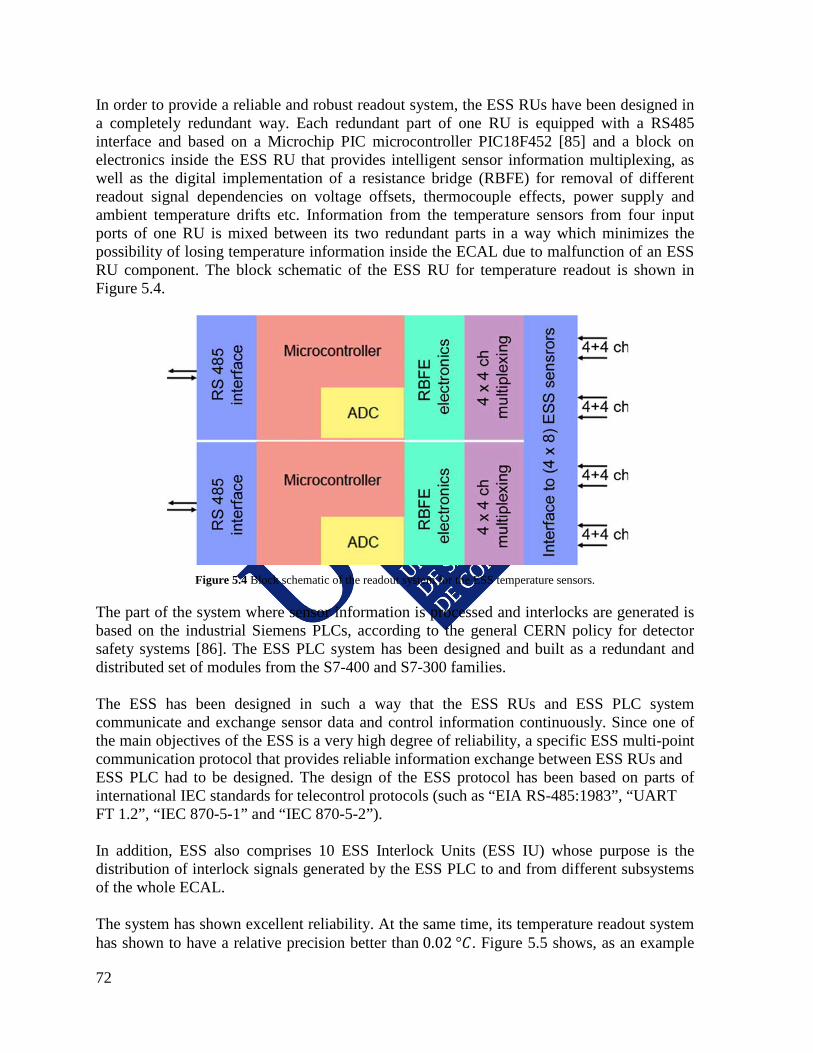
72
In order to provide a reliable and robust readout system, the ESS RUs have been designed in a completely redundant way. Each redundant part of one RU is equipped with a RS485 interface and based on a Microchip PIC microcontroller PIC18F452 [85] and a block on electronics inside the ESS RU that provides intelligent sensor information multiplexing, as well as the digital implementation of a resistance bridge (RBFE) for removal of different readout signal dependencies on voltage offsets, thermocouple effects, power supply and ambient temperature drifts etc. Information from the temperature sensors from four input ports of one RU is mixed between its two redundant parts in a way which minimizes the possibility of losing temperature information inside the ECAL due to malfunction of an ESS RU component. The block schematic of the ESS RU for temperature readout is shown in Figure 5.4.
Figure 5.4 Block schematic of the readout system for the ESS temperature sensors.
The part of the system where sensor information is processed and interlocks are generated is based on the industrial Siemens PLCs, according to the general CERN policy for detector safety systems [86]. The ESS PLC system has been designed and built as a redundant and distributed set of modules from the S7-400 and S7-300 families. The ESS has been designed in such a way that the ESS RUs and ESS PLC system communicate and exchange sensor data and control information continuously. Since one of the main objectives of the ESS is a very high degree of reliability, a specific ESS multi-point communication protocol that provides reliable information exchange between ESS RUs and ESS PLC had to be designed. The design of the ESS protocol has been based on parts of international IEC standards for telecontrol protocols (such as “EIA RS-485:1983”, “UART FT 1.2”, “IEC 870-5-1” and “IEC 870-5-2”). In addition, ESS also comprises 10 ESS Interlock Units (ESS IU) whose purpose is the distribution of interlock signals generated by the ESS PLC to and from different subsystems of the whole ECAL. The system has shown excellent reliability. At the same time, its temperature readout system has shown to have a relative precision better than 0.02 °𝐶. Figure 5.5 shows, as an example
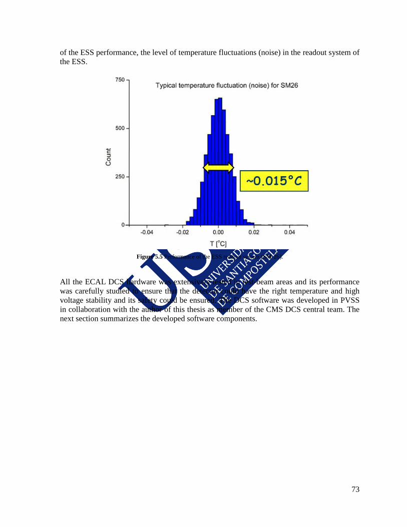
73
of the ESS performance, the level of temperature fluctuations (noise) in the readout system of the ESS.
All the ECAL DCS hardware was extensively tested in test-beam areas and its performance was carefully studied to ensure that the detector could have the right temperature and high voltage stability and its safety could be ensured. The DCS software was developed in PVSS in collaboration with the author of this thesis as member of the CMS DCS central team. The next section summarizes the developed software components.
Figure 5.5 Performance of the ESS readout system (SM-26).
74
5.5 The DCS software This section describes the developed software components and the integration of the ECAL subsystems under the ECAL DCS supervisor control tree. All the ECAL DCS applications were developed using PVSS, the JCOP and CMS frameworks and following the central DCS guidelines. The following components containing the ECAL applications where created as part of CMS DCS framework:
Component Name Component Details
CMSfwECAL_LV
This component retrieves the logical and hardware structure of the low voltage system from the ECAL configuration database and creates the corresponding distributed datapoint structure. The driver configuration, datapoint hardware addresses, alerts and archiving settings are loaded from the database as well. An FSM control tree is created for each of the supermodules allowing for the individual control of each of them.
CMSfwECAL_HV CMSfwECAL_EE_HVM
These components retrieve the logical and hardware structure of the high voltage system from the ECAL configuration database and create the corresponding distributed datapoint structure for the barrel (ECAL_HV) and end-caps (ECAL_EE). The driver configuration, datapoint hardware addresses, alerts and archiving settings are loaded from the database as well. In addition, these components load different voltage settings configurations allowing for diverse detector operation modes (different calibrations, proton physics…). The HV FSM control tree provides a tree for each supermodule allowing for the individual control of each of the 4 modules inside of each supermodule.
CMSfwECAL_Laser This component downloads from the configuration database the PVSS DIP infrastructure to monitor the status of ECAL laser system.
CMSfwECAL_Cooling
The ECAL application is a standalone application not developed by CMS but by CERN engineering group. The parameters that this application is monitoring are published via DIP. The CMSfw component loads from the configuration database the PVSS infrastructure to connect to these DIP publications. A FSM tree node is created for each of the supermodules/supercrystals.
CMSfwECAL_ESS The ESS component creates the support for the S7 address communication to the safety PLCs. It includes also an FSM tree reflecting the state of each of the supermodules or end-caps.
CMSfwECAL_HealtCheks CMSfwECAL_Instrastructure
CMSfwECAL_ENV CMSfwECAL_FrontEnd
A set of other components are used to monitor the status of the infrastructure hardware (electronic racks power and ventilation turbines, environment temperature and humidity reading, PC CPU and memory usage…) and software (driver client and server side status, running processes…)
CMSfwECAL_Supervisor
The supervisor component deploys a FSM tree that connects to all the sub-systems FSM trees. This supervisor tree contains the intelligence to perform automatic actions switching OFF or ON different parts of the detector when needed or locking the possibility of sending commands for non-experts for certain safety related situations.
The components are installed in 12 rack mounted PCs that are supervised by the central DCS management tools. The ECAL DCS team developed their software components in a dedicated lab and they upload them to production using their SVN and a provided central
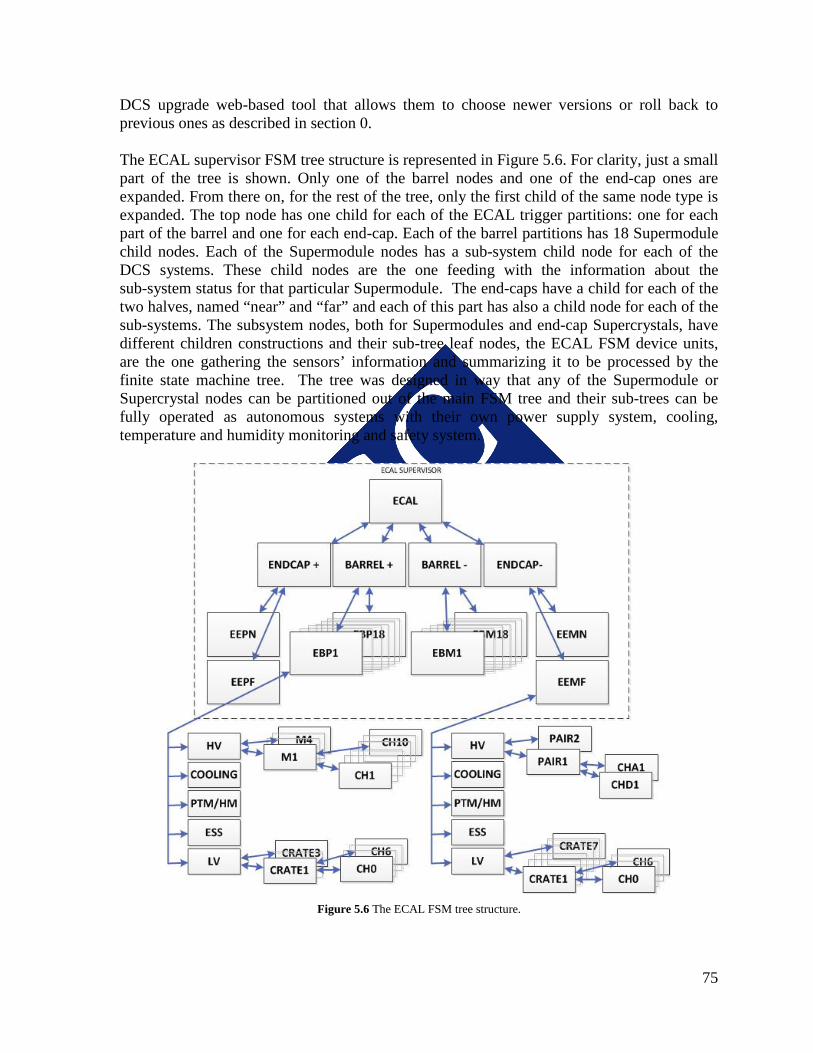
75
DCS upgrade web-based tool that allows them to choose newer versions or roll back to previous ones as described in section 0. The ECAL supervisor FSM tree structure is represented in Figure 5.6. For clarity, just a small part of the tree is shown. Only one of the barrel nodes and one of the end-cap ones are expanded. From there on, for the rest of the tree, only the first child of the same node type is expanded. The top node has one child for each of the ECAL trigger partitions: one for each part of the barrel and one for each end-cap. Each of the barrel partitions has 18 Supermodule child nodes. Each of the Supermodule nodes has a sub-system child node for each of the DCS systems. These child nodes are the one feeding with the information about the sub-system status for that particular Supermodule. The end-caps have a child for each of the two halves, named “near” and “far” and each of this part has also a child node for each of the sub-systems. The subsystem nodes, both for Supermodules and end-cap Supercrystals, have different children constructions and their sub-tree leaf nodes, the ECAL FSM device units, are the one gathering the sensors’ information and summarizing it to be processed by the finite state machine tree. The tree was designed in way that any of the Supermodule or Supercrystal nodes can be partitioned out of the main FSM tree and their sub-trees can be fully operated as autonomous systems with their own power supply system, cooling, temperature and humidity monitoring and safety system.
Figure 5.6 The ECAL FSM tree structure.
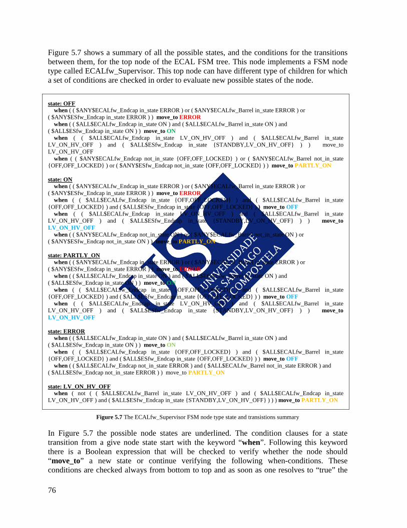
76
Figure 5.7 shows a summary of all the possible states, and the conditions for the transitions between them, for the top node of the ECAL FSM tree. This node implements a FSM node type called ECALfw_Supervisor. This top node can have different type of children for which a set of conditions are checked in order to evaluate new possible states of the node.
state: OFF when ( ( $ANY$ECALfw_Endcap in_state ERROR ) or ( $ANY$ECALfw_Barrel in_state ERROR ) or ( $ANY$ESfw_Endcap in_state ERROR ) ) move_to ERROR when ( ( $ALL$ECALfw_Endcap in_state ON ) and ( $ALL$ECALfw_Barrel in_state ON ) and ( $ALL$ESfw_Endcap in_state ON ) ) move_to ON when ( ( $ALL$ECALfw_Endcap in_state LV_ON_HV_OFF ) and ( $ALL$ECALfw_Barrel in_state LV_ON_HV_OFF ) and ( $ALL$ESfw_Endcap in_state {STANDBY,LV_ON_HV_OFF} ) ) move_to LV_ON_HV_OFF when ( ( $ANY$ECALfw_Endcap not_in_state {OFF,OFF_LOCKED} ) or ( $ANY$ECALfw_Barrel not_in_state {OFF,OFF_LOCKED} ) or ( $ANY$ESfw_Endcap not_in_state {OFF,OFF_LOCKED} ) ) move_to PARTLY_ON state: ON when ( ( $ANY$ECALfw_Endcap in_state ERROR ) or ( $ANY$ECALfw_Barrel in_state ERROR ) or ( $ANY$ESfw_Endcap in_state ERROR ) ) move_to ERROR when ( ( $ALL$ECALfw_Endcap in_state {OFF,OFF_LOCKED} ) and ( $ALL$ECALfw_Barrel in_state {OFF,OFF_LOCKED} ) and ( $ALL$ESfw_Endcap in_state {OFF,OFF_LOCKED} ) ) move_to OFF when ( ( $ALL$ECALfw_Endcap in_state LV_ON_HV_OFF ) and ( $ALL$ECALfw_Barrel in_state LV_ON_HV_OFF ) and ( $ALL$ESfw_Endcap in_state {STANDBY,LV_ON_HV_OFF} ) ) move_to LV_ON_HV_OFF when ( ( $ANY$ECALfw_Endcap not_in_state ON ) or ( $ANY$ECALfw_Barrel not_in_state ON ) or ( $ANY$ESfw_Endcap not_in_state ON ) ) move_to PARTLY_ON state: PARTLY_ON when ( ( $ANY$ECALfw_Endcap in_state ERROR ) or ( $ANY$ECALfw_Barrel in_state ERROR ) or ( $ANY$ESfw_Endcap in_state ERROR ) ) move_to ERROR when ( ( $ALL$ECALfw_Endcap in_state ON ) and ( $ALL$ECALfw_Barrel in_state ON ) and ( $ALL$ESfw_Endcap in_state ON ) ) move_to ON when ( ( $ALL$ECALfw_Endcap in_state {OFF,OFF_LOCKED} ) and ( $ALL$ECALfw_Barrel in_state {OFF,OFF_LOCKED} ) and ( $ALL$ESfw_Endcap in_state {OFF,OFF_LOCKED} ) ) move_to OFF when ( ( $ALL$ECALfw_Endcap in_state LV_ON_HV_OFF ) and ( $ALL$ECALfw_Barrel in_state LV_ON_HV_OFF ) and ( $ALL$ESfw_Endcap in_state {STANDBY,LV_ON_HV_OFF} ) ) move_to LV_ON_HV_OFF state: ERROR when ( ( $ALL$ECALfw_Endcap in_state ON ) and ( $ALL$ECALfw_Barrel in_state ON ) and ( $ALL$ESfw_Endcap in_state ON ) ) move_to ON when ( ( $ALL$ECALfw_Endcap in_state {OFF,OFF_LOCKED} ) and ( $ALL$ECALfw_Barrel in_state {OFF,OFF_LOCKED} ) and ( $ALL$ESfw_Endcap in_state {OFF,OFF_LOCKED} ) ) move_to OFF when ( ( $ALL$ECALfw_Endcap not_in_state ERROR ) and ( $ALL$ECALfw_Barrel not_in_state ERROR ) and ( $ALL$ESfw_Endcap not_in_state ERROR ) ) move_to PARTLY_ON state: LV_ON_HV_OFF when ( not ( ( $ALL$ECALfw_Barrel in_state LV_ON_HV_OFF ) and ( $ALL$ECALfw_Endcap in_state LV_ON_HV_OFF ) and ( $ALL$ESfw_Endcap in_state {STANDBY,LV_ON_HV_OFF} ) ) ) move_to PARTLY_ON
Figure 5.7 The ECALfw_Supervisor FSM node type state and transistions summary
In Figure 5.7 the possible node states are underlined. The condition clauses for a state transition from a give node state start with the keyword “when”. Following this keyword there is a Boolean expression that will be checked to verify whether the node should “move_to” a new state or continue verifying the following when-conditions. These conditions are checked always from bottom to top and as soon as one resolves to “true” the
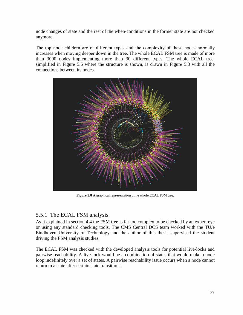
77
node changes of state and the rest of the when-conditions in the former state are not checked anymore. The top node children are of different types and the complexity of these nodes normally increases when moving deeper down in the tree. The whole ECAL FSM tree is made of more than 3000 nodes implementing more than 30 different types. The whole ECAL tree, simplified in Figure 5.6 where the structure is shown, is drawn in Figure 5.8 with all the connections between its nodes.
Figure 5.8 A graphical representation of he whole ECAL FSM tree.
5.5.1 The ECAL FSM analysis As it explained in section 4.4 the FSM tree is far too complex to be checked by an expert eye or using any standard checking tools. The CMS Central DCS team worked with the TU/e Eindhoven University of Technology and the author of this thesis supervised the student driving the FSM analysis studies. The ECAL FSM was checked with the developed analysis tools for potential live-locks and pairwise reachability. A live-lock would be a combination of states that would make a node loop indefinitely over a set of states. A pairwise reachability issue occurs when a node cannot return to a state after certain state transitions.
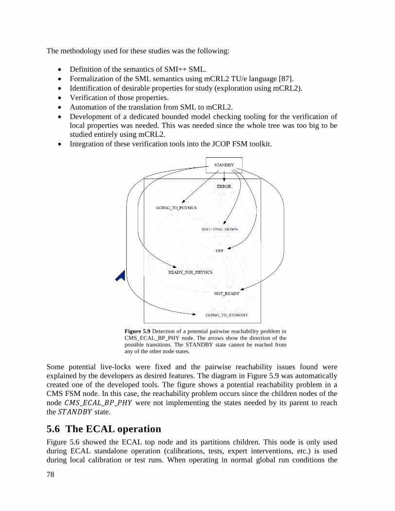
78
The methodology used for these studies was the following:
• Definition of the semantics of SMI++ SML. • Formalization of the SML semantics using mCRL2 TU/e language [87]. • Identification of desirable properties for study (exploration using mCRL2). • Verification of those properties. • Automation of the translation from SML to mCRL2. • Development of a dedicated bounded model checking tooling for the verification of
local properties was needed. This was needed since the whole tree was too big to be studied entirely using mCRL2.
• Integration of these verification tools into the JCOP FSM toolkit.
Some potential live-locks were fixed and the pairwise reachability issues found were explained by the developers as desired features. The diagram in Figure 5.9 was automatically created one of the developed tools. The figure shows a potential reachability problem in a CMS FSM node. In this case, the reachability problem occurs since the children nodes of the node 𝐶𝑀𝑆_𝐸𝐶𝐴𝐿_𝐵𝑃_𝑃𝐻𝑌 were not implementing the states needed by its parent to reach the 𝑆𝑇𝐴𝑁𝐷𝐵𝑌 state.
5.6 The ECAL operation Figure 5.6 showed the ECAL top node and its partitions children. This node is only used during ECAL standalone operation (calibrations, tests, expert interventions, etc.) is used during local calibration or test runs. When operating in normal global run conditions the
Figure 5.9 Detection of a potential pairwise reachability problem in CMS_ECAL_BP_PHY node. The arrows show the direction of the possible transitions. The STANDBY state cannot be reached from any of the other node states.
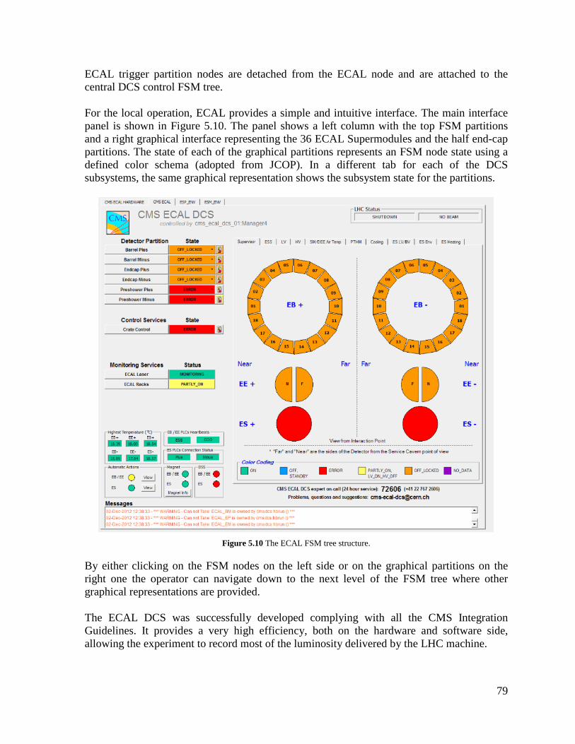
79
ECAL trigger partition nodes are detached from the ECAL node and are attached to the central DCS control FSM tree. For the local operation, ECAL provides a simple and intuitive interface. The main interface panel is shown in Figure 5.10. The panel shows a left column with the top FSM partitions and a right graphical interface representing the 36 ECAL Supermodules and the half end-cap partitions. The state of each of the graphical partitions represents an FSM node state using a defined color schema (adopted from JCOP). In a different tab for each of the DCS subsystems, the same graphical representation shows the subsystem state for the partitions.
Figure 5.10 The ECAL FSM tree structure.
By either clicking on the FSM nodes on the left side or on the graphical partitions on the right one the operator can navigate down to the next level of the FSM tree where other graphical representations are provided. The ECAL DCS was successfully developed complying with all the CMS Integration Guidelines. It provides a very high efficiency, both on the hardware and software side, allowing the experiment to record most of the luminosity delivered by the LHC machine.

80
Chapters 2, 3 and 4 were dedicated to describe the experiment control system. This chapter provided a complete example of a sub-detector implementation. The author participated in all the activities involved in the development, from the applications design, the low level code writing, to the deployment implementation to the FSM implementation and analysis. The following chapter introduces the CMS HCAL Outer (HO) calorimeter, a detector that is in the process of upgrading its detection sensors. The focus of this thesis work shifts from now on towards the particle detection sensor related world while keeping always an insight on the DCS.

81
6. A new technology for the HCAL Barrel upgrade As it was mentioned in Chapter 1, the HCAL is a sampling calorimeter with a brass (70% copper and 30% zinc) absorber and plastic scintillating detectors tiles. Their blue-violet light is trapped by wave-length-shifting (WLS) fibers, having a diameter of about 1 𝑚𝑚, that are coupled to optical fiber cables that carry the green light away to Readout BoXes (RBX) installed in the muon support yoke. The HCAL has good hermeticity to detect every particle emerging from the collisions. Even though it provides moderate energy resolution, its good transverse granularity makes it useful for most of the collaboration physics studies. Together with the electromagnetic calorimeter, it measures the energy and direction of quarks, gluons and neutrinos, by measuring the energy of particle jets and of the missing transverse energy. It also participates, with the muon detection system, in the identification of electron, photons and muons. The inner radius of the Barrel of this hadronic calorimeter (HB) is limited by the electromagnetic calorimeter (EB) and the outer radius by the magnetic coil (see Figure 1.16). Because of this physical limitation, the HB is not able to completely stop the late hadronic shower developments. For this reason, the outer calorimeter (HO) is used to sample the energy leakage outside of the magnetic coil. The HO scintillating tiles are arranged in trays, covering each one 5 grad in Φ, to approximately match the HCAL Barrel reading towers (Figure 1.23). The RBX were designed to use HPDs (see Sec 1.3.4) but, for the reasons that are discussed in the next sections, a new silicon-based solution was chosen for the HCAL barrel upgrade. The author of this thesis worked with the HCAL community in the burn-in test studies carried out at CERN, in the integration area called 904. The author's contribution was twofold: on one hand, collaborating in the development and set-up of the test area control system, and, on the other one, participating in the data analysis to study the stability of the new devices selected.
6.1 The HCAL HPDs An HPD (Figure 6.1) is made of a photocathode facing a silicon detector in a vacuum box. When photons hit the photocathode, this emits electrons. These electrons are accelerated by a 10 − 15 𝑘𝑉 voltage difference. The electrons deposit most of their energy in the depleted silicon diode region generating the signal.
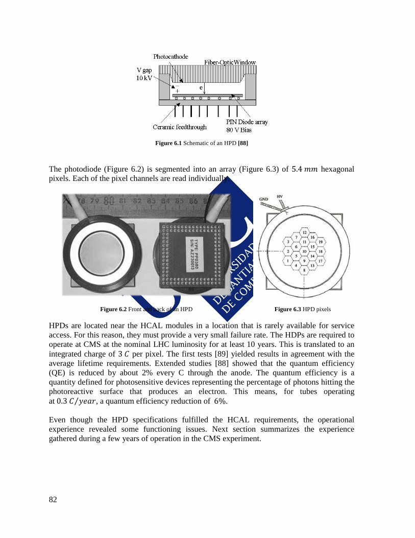
82
Figure 6.1 Schematic of an HPD [88]
The photodiode (Figure 6.2) is segmented into an array (Figure 6.3) of 5.4 𝑚𝑚 hexagonal pixels. Each of the pixel channels are read individually.
Figure 6.2 Front and back of an HPD Figure 6.3 HPD pixels
HPDs are located near the HCAL modules in a location that is rarely available for service access. For this reason, they must provide a very small failure rate. The HDPs are required to operate at CMS at the nominal LHC luminosity for at least 10 years. This is translated to an integrated charge of 3 𝐶 per pixel. The first tests [89] yielded results in agreement with the average lifetime requirements. Extended studies [88] showed that the quantum efficiency (QE) is reduced by about 2% every C through the anode. The quantum efficiency is a quantity defined for photosensitive devices representing the percentage of photons hitting the photoreactive surface that produces an electron. This means, for tubes operating at 0.3 𝐶 𝑦𝑒𝑎𝑟⁄ , a quantum efficiency reduction of 6%. Even though the HPD specifications fulfilled the HCAL requirements, the operational experience revealed some functioning issues. Next section summarizes the experience gathered during a few years of operation in the CMS experiment.
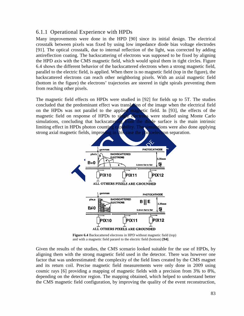
83
6.1.1 Operational Experience with HPDs Many improvements were done in the HPD [90] since its initial design. The electrical crosstalk between pixels was fixed by using low impedance diode bias voltage electrodes [91]. The optical crosstalk, due to internal reflection of the light, was corrected by adding antireflection coating. The backscattering of electrons was supposed to be fixed by aligning the HPD axis with the CMS magnetic field, which would spiral them in tight circles. Figure 6.4 shows the different behavior of the backscattered electrons when a strong magnetic field, parallel to the electric field, is applied. When there is no magnetic field (top in the figure), the backscattered electrons can reach other neighboring pixels. With an axial magnetic field (bottom in the figure) the electrons’ trajectories are steered in tight spirals preventing them from reaching other pixels. The magnetic field effects on HPDs were studied in [92] for fields up to 5T. The studies concluded that the predominant effect was translation of the image when the electrical field on the HPDs was not parallel to the applied magnetic field. In [93], the effects of the magnetic field on response of HPDs to single electrons were studied using Monte Carlo simulations, concluding that backscattering from the diode surface is the main intrinsic limiting effect in HPDs photon counting capability. The simulations were also done applying strong axial magnetic fields, improving in this case the photoelectron separation.
Figure 6.4 Backscattered electrons in HPD without magnetic field (top) and with a magnetic field pararel to the electric field (bottom) [94].
Given the results of the studies, the CMS scenario looked suitable for the use of HPDs, by aligning them with the strong magnetic field used in the detector. There was however one factor that was underestimated: the complexity of the field lines created by the CMS magnet and its return coil. Precise magnetic field measurements were only done in 2009 using cosmic rays [6] providing a mapping of magnetic fields with a precision from 3% to 8%, depending on the detector region. The mapping obtained, which helped to understand better the CMS magnetic field configuration, by improving the quality of the event reconstruction,
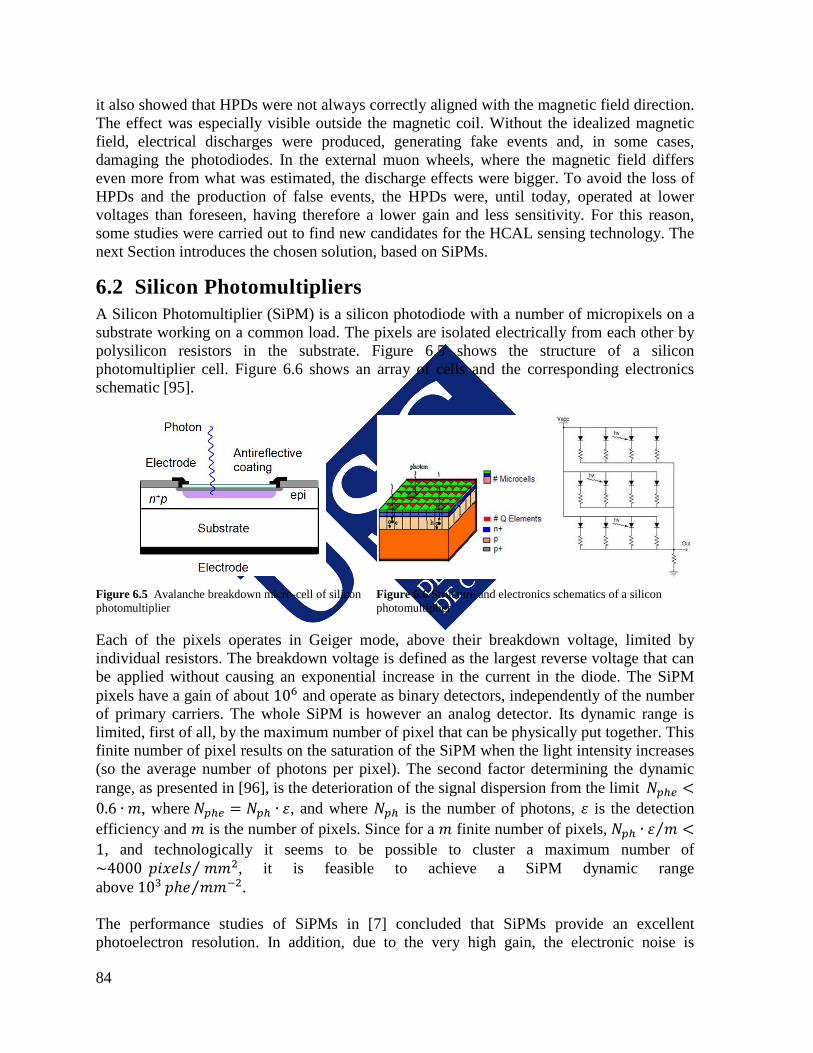
84
it also showed that HPDs were not always correctly aligned with the magnetic field direction. The effect was especially visible outside the magnetic coil. Without the idealized magnetic field, electrical discharges were produced, generating fake events and, in some cases, damaging the photodiodes. In the external muon wheels, where the magnetic field differs even more from what was estimated, the discharge effects were bigger. To avoid the loss of HPDs and the production of false events, the HPDs were, until today, operated at lower voltages than foreseen, having therefore a lower gain and less sensitivity. For this reason, some studies were carried out to find new candidates for the HCAL sensing technology. The next Section introduces the chosen solution, based on SiPMs.
6.2 Silicon Photomultipliers A Silicon Photomultiplier (SiPM) is a silicon photodiode with a number of micropixels on a substrate working on a common load. The pixels are isolated electrically from each other by polysilicon resistors in the substrate. Figure 6.5 shows the structure of a silicon photomultiplier cell. Figure 6.6 shows an array of cells and the corresponding electronics schematic [95].
Figure 6.5 Avalanche breakdown micro-cell of silicon photomultiplier
Figure 6.6 Structure and electronics schematics of a silicon photomultiplier
Each of the pixels operates in Geiger mode, above their breakdown voltage, limited by individual resistors. The breakdown voltage is defined as the largest reverse voltage that can be applied without causing an exponential increase in the current in the diode. The SiPM pixels have a gain of about 106 and operate as binary detectors, independently of the number of primary carriers. The whole SiPM is however an analog detector. Its dynamic range is limited, first of all, by the maximum number of pixel that can be physically put together. This finite number of pixel results on the saturation of the SiPM when the light intensity increases (so the average number of photons per pixel). The second factor determining the dynamic range, as presented in [96], is the deterioration of the signal dispersion from the limit 𝑁𝑝ℎ𝑒 <0.6 ∙ 𝑚, where 𝑁𝑝ℎ𝑒 = 𝑁𝑝ℎ ∙ 𝜀, and where 𝑁𝑝ℎ is the number of photons, 𝜀 is the detection efficiency and 𝑚 is the number of pixels. Since for a 𝑚 finite number of pixels, 𝑁𝑝ℎ ∙ 𝜀 𝑚⁄ <1, and technologically it seems to be possible to cluster a maximum number of ~4000 𝑝𝑖𝑥𝑒𝑙𝑠 𝑚𝑚2⁄ , it is feasible to achieve a SiPM dynamic range above 103 𝑝ℎ𝑒 𝑚𝑚−2⁄ . The performance studies of SiPMs in [7] concluded that SiPMs provide an excellent photoelectron resolution. In addition, due to the very high gain, the electronic noise is
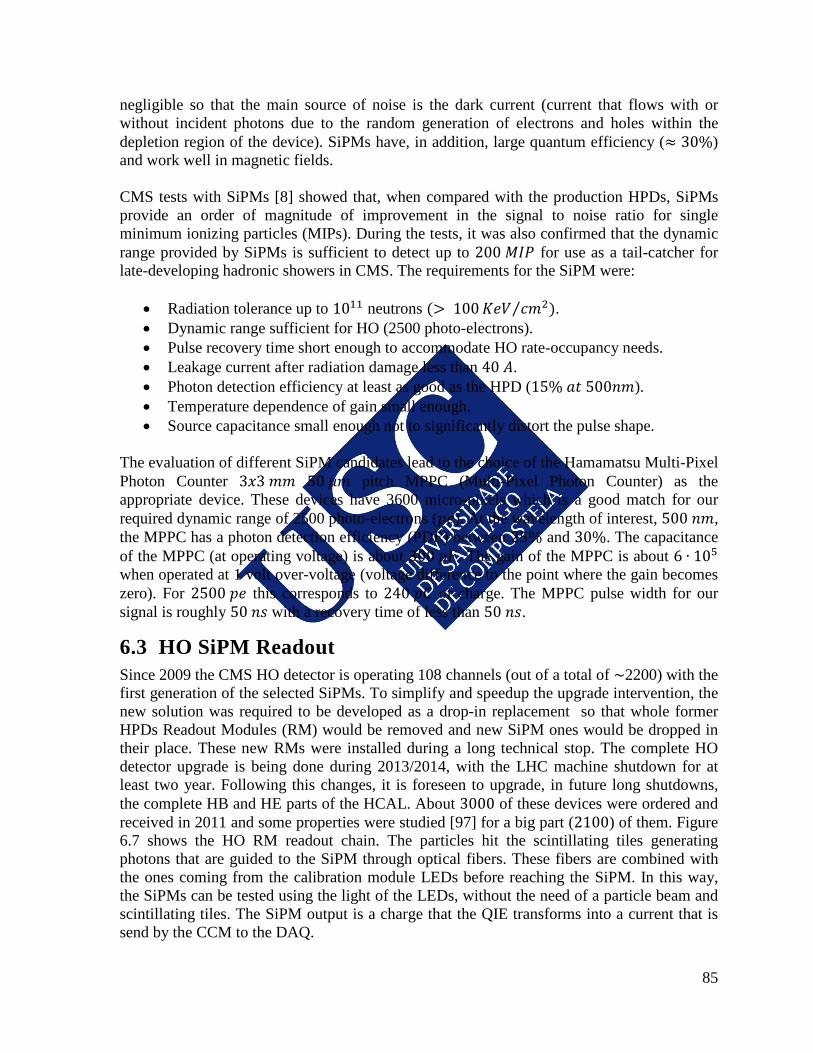
85
negligible so that the main source of noise is the dark current (current that flows with or without incident photons due to the random generation of electrons and holes within the depletion region of the device). SiPMs have, in addition, large quantum efficiency (≈ 30%) and work well in magnetic fields. CMS tests with SiPMs [8] showed that, when compared with the production HPDs, SiPMs provide an order of magnitude of improvement in the signal to noise ratio for single minimum ionizing particles (MIPs). During the tests, it was also confirmed that the dynamic range provided by SiPMs is sufficient to detect up to 200 𝑀𝐼𝑃 for use as a tail-catcher for late-developing hadronic showers in CMS. The requirements for the SiPM were:
• Radiation tolerance up to 1011 neutrons (> 100𝐾𝑒𝑉 𝑐𝑚2⁄ ). • Dynamic range sufficient for HO (2500 photo-electrons). • Pulse recovery time short enough to accommodate HO rate-occupancy needs. • Leakage current after radiation damage less than 40 𝐴. • Photon detection efficiency at least as good as the HPD (15% 𝑎𝑡 500𝑛𝑚). • Temperature dependence of gain small enough. • Source capacitance small enough not to significantly distort the pulse shape.
The evaluation of different SiPM candidates lead to the choice of the Hamamatsu Multi-Pixel Photon Counter 3𝑥3 𝑚𝑚 50 𝜇𝑚 pitch MPPC (Multi-Pixel Photon Counter) as the appropriate device. These devices have 3600 micro-pixels which is a good match for our required dynamic range of 2500 photo-electrons (𝑝𝑒). At the wavelength of interest, 500 𝑛𝑚, the MPPC has a photon detection efficiency (PDE) between 25% and 30%. The capacitance of the MPPC (at operating voltage) is about 300 𝑝𝐹. The gain of the MPPC is about 6 ∙ 105 when operated at 1 volt over-voltage (voltage difference to the point where the gain becomes zero). For 2500 𝑝𝑒 this corresponds to 240 𝑝𝐶 of charge. The MPPC pulse width for our signal is roughly 50 𝑛𝑠 with a recovery time of less than 50 𝑛𝑠.
6.3 HO SiPM Readout Since 2009 the CMS HO detector is operating 108 channels (out of a total of ~2200) with the first generation of the selected SiPMs. To simplify and speedup the upgrade intervention, the new solution was required to be developed as a drop-in replacement so that whole former HPDs Readout Modules (RM) would be removed and new SiPM ones would be dropped in their place. These new RMs were installed during a long technical stop. The complete HO detector upgrade is being done during 2013/2014, with the LHC machine shutdown for at least two year. Following this changes, it is foreseen to upgrade, in future long shutdowns, the complete HB and HE parts of the HCAL. About 3000 of these devices were ordered and received in 2011 and some properties were studied [97] for a big part (2100) of them. Figure 6.7 shows the HO RM readout chain. The particles hit the scintillating tiles generating photons that are guided to the SiPM through optical fibers. These fibers are combined with the ones coming from the calibration module LEDs before reaching the SiPM. In this way, the SiPMs can be tested using the light of the LEDs, without the need of a particle beam and scintillating tiles. The SiPM output is a charge that the QIE transforms into a current that is send by the CCM to the DAQ.
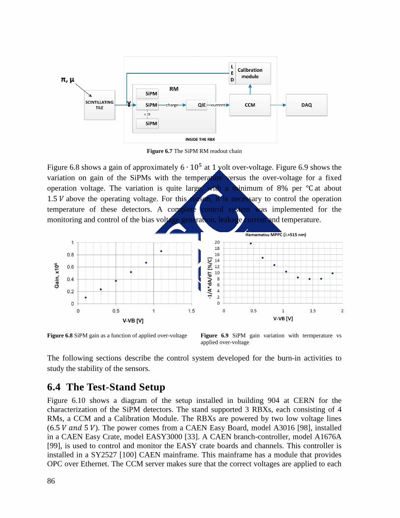
86
Figure 6.7 The SiPM RM readout chain
Figure 6.8 shows a gain of approximately 6 ∙ 105 at 1 volt over-voltage. Figure 6.9 shows the variation on gain of the SiPMs with the temperature versus the over-voltage for a fixed operation voltage. The variation is quite large, with a minimum of 8% per ℃ at about 1.5 𝑉 above the operating voltage. For this reason, it is necessary to control the operation temperature of these detectors. A complete control system was implemented for the monitoring and control of the bias voltage generation, leakage current and temperature.
Figure 6.8 SiPM gain as a function of applied over-voltage Figure 6.9 SiPM gain variation with termperature vs applied over-voltage
The following sections describe the control system developed for the burn-in activities to study the stability of the sensors.
6.4 The Test-Stand Setup Figure 6.10 shows a diagram of the setup installed in building 904 at CERN for the characterization of the SiPM detectors. The stand supported 3 RBXs, each consisting of 4 RMs, a CCM and a Calibration Module. The RBXs are powered by two low voltage lines (6.5 𝑉 𝑎𝑛𝑑 5 𝑉). The power comes from a CAEN Easy Board, model A3016 [98], installed in a CAEN Easy Crate, model EASY3000 [33]. A CAEN branch-controller, model A1676A [99], is used to control and monitor the EASY crate boards and channels. This controller is installed in a SY2527 [100] CAEN mainframe. This mainframe has a module that provides OPC over Ethernet. The CCM server makes sure that the correct voltages are applied to each
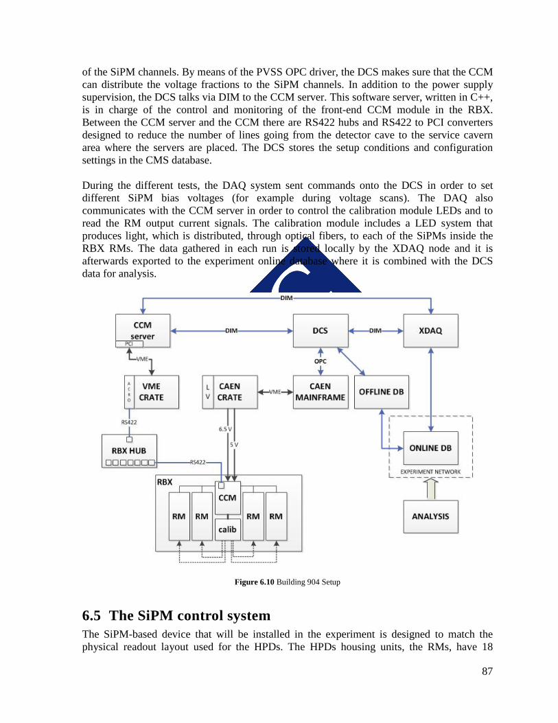
87
of the SiPM channels. By means of the PVSS OPC driver, the DCS makes sure that the CCM can distribute the voltage fractions to the SiPM channels. In addition to the power supply supervision, the DCS talks via DIM to the CCM server. This software server, written in C++, is in charge of the control and monitoring of the front-end CCM module in the RBX. Between the CCM server and the CCM there are RS422 hubs and RS422 to PCI converters designed to reduce the number of lines going from the detector cave to the service cavern area where the servers are placed. The DCS stores the setup conditions and configuration settings in the CMS database. During the different tests, the DAQ system sent commands onto the DCS in order to set different SiPM bias voltages (for example during voltage scans). The DAQ also communicates with the CCM server in order to control the calibration module LEDs and to read the RM output current signals. The calibration module includes a LED system that produces light, which is distributed, through optical fibers, to each of the SiPMs inside the RBX RMs. The data gathered in each run is stored locally by the XDAQ node and it is afterwards exported to the experiment online database where it is combined with the DCS data for analysis.
Figure 6.10 Building 904 Setup
6.5 The SiPM control system The SiPM-based device that will be installed in the experiment is designed to match the physical readout layout used for the HPDs. The HPDs housing units, the RMs, have 18
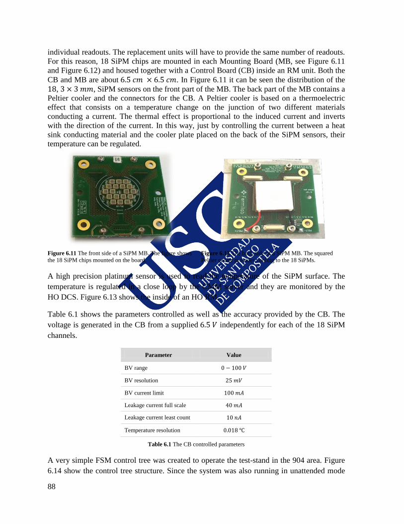
88
individual readouts. The replacement units will have to provide the same number of readouts. For this reason, 18 SiPM chips are mounted in each Mounting Board (MB, see Figure 6.11 and Figure 6.12) and housed together with a Control Board (CB) inside an RM unit. Both the CB and MB are about 6.5 𝑐𝑚 × 6.5 𝑐𝑚. In Figure 6.11 it can be seen the distribution of the 18, 3 × 3 𝑚𝑚, SiPM sensors on the front part of the MB. The back part of the MB contains a Peltier cooler and the connectors for the CB. A Peltier cooler is based on a thermoelectric effect that consists on a temperature change on the junction of two different materials conducting a current. The thermal effect is proportional to the induced current and inverts with the direction of the current. In this way, just by controlling the current between a heat sink conducting material and the cooler plate placed on the back of the SiPM sensors, their temperature can be regulated.
Figure 6.11 The front side of a SiPM MB. The figure shows the 18 SiPM chips mounted on the board.
Figure 6.12 The back side of a SiPM MB. The squared Peltier cooler provides cooling to the 18 SiPMs.
A high precision platinum sensor is used to read the temperature of the SiPM surface. The temperature is regulated in a close loop by the CMM server and they are monitored by the HO DCS. Figure 6.13 shows the inside of an HO RM.
Table 6.1 shows the parameters controlled as well as the accuracy provided by the CB. The voltage is generated in the CB from a supplied 6.5 𝑉 independently for each of the 18 SiPM channels.
Parameter Value
BV range 0 − 100 𝑉
BV resolution 25 𝑚𝑉
BV current limit 100 𝑚𝐴
Leakage current full scale 40 𝑚𝐴
Leakage current least count 10 𝑛𝐴
Temperature resolution 0.018 ℃
Table 6.1 The CB controlled parameters
A very simple FSM control tree was created to operate the test-stand in the 904 area. Figure 6.14 show the control tree structure. Since the system was also running in unattended mode
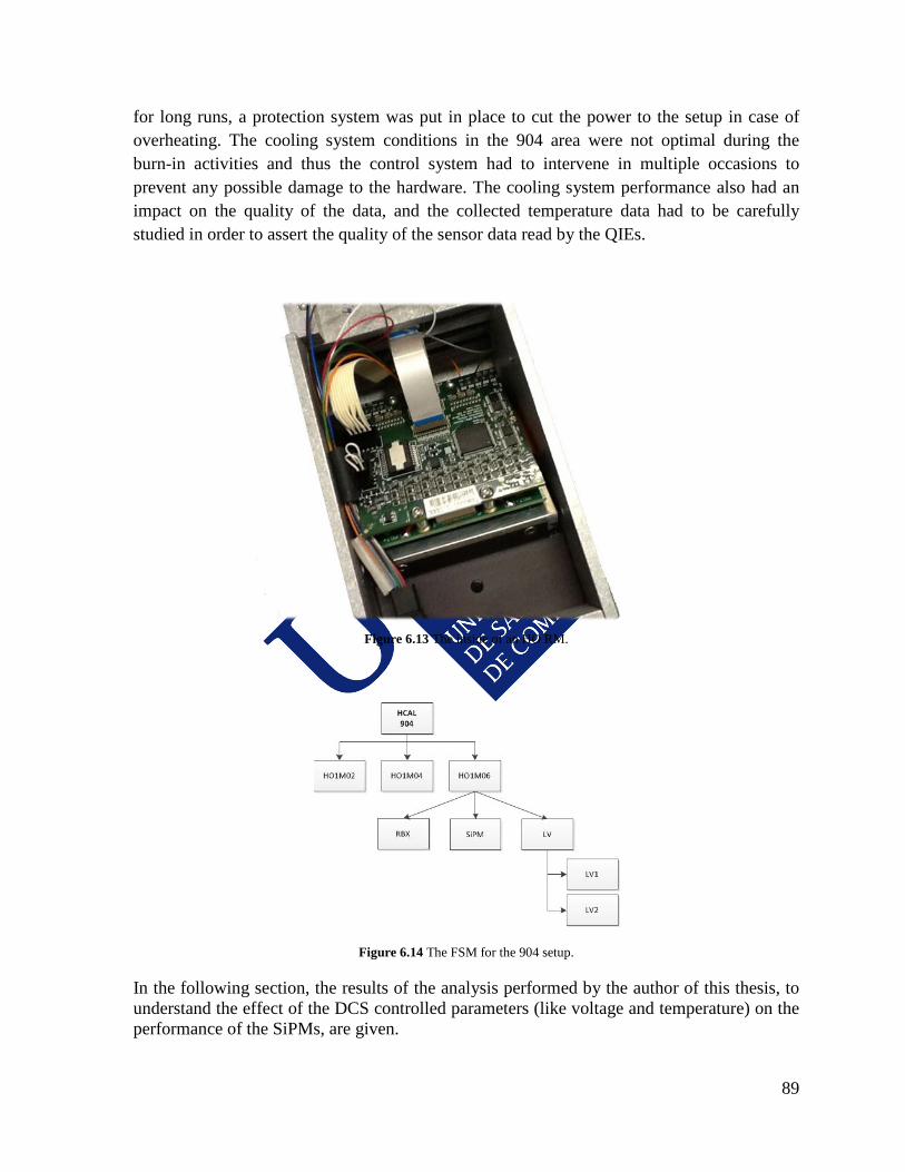
89
for long runs, a protection system was put in place to cut the power to the setup in case of overheating. The cooling system conditions in the 904 area were not optimal during the burn-in activities and thus the control system had to intervene in multiple occasions to prevent any possible damage to the hardware. The cooling system performance also had an impact on the quality of the data, and the collected temperature data had to be carefully studied in order to assert the quality of the sensor data read by the QIEs.
Figure 6.13 The inside of an HO RM.
Figure 6.14 The FSM for the 904 setup.
In the following section, the results of the analysis performed by the author of this thesis, to understand the effect of the DCS controlled parameters (like voltage and temperature) on the performance of the SiPMs, are given.
90
6.6 SiPM current stability analysis As it was shown in Figure 6.8 and Figure 6.9, the SiPM sensors are very sensitive to the variations of voltage and temperature. The scope of the stability study activities is to discover how stably these parameters can be operated and what gain stability can be achieved.
6.6.1 The analysis methodology The analysis scripts were written using CERN’s ROOT framework [101]. ROOT is an advanced object-oriented data analysis framework developed in C++. The author decided for a two-step solution. In a first step the data of interest are retrieved from the relational database where the test-stand control system stores them and they are processed and stored in a ROOT TTree file. The relevant data includes bias voltage fractions and currents for each of the SiPM channels, the measured and targeted RM temperatures, the card-pack (combination of a MB and a CB) IDs identifying each of the boards tested and the timestamp of each of the data entries. During the analysis, the data are organized in a ROOT TTree. A TTree is made of different branches representing different observables. In a TTree there is always the same amount of entries in each of the branches. The generated file contains ~ 7.5 million for each of the variables, including the 18-element array ones. The script used to create this file can be found in Appendix C, its workflow, described above, is shown in Figure 6.15.
Figure 6.15 SiPM current and temperature stability analysis data file creation script generator workflow
91
The script used in the second step can be found in Appendix D. The workflow of this second script is in Figure 6.16.
Figure 6.16 SiPM current and temperature stability analysis result plots script generator workflow
One of the most relevant parts of the script is the data buffer and the filters used in order to study only the current during stable periods, where no tests were carried on, where there was no cooling or temperature problems and where the nominal settings were configured in the electronics. The script also filters to allow only for periods when the LEDs were operating.
6.6.2 Current and Temperature stability studies After refining the scripts to properly filter out the uninteresting data, electrical current stability plots were generated for all of the SiPM card-packs. Figure 6.17 shows the recorded data over a week (10th -16th July) of the normalized current, induced by the LED calibration modules, for each of the 18 SiPMs (mapped to 18 RM channels) in a typical card-pack (in this case with ID 0905_0907). The first 4 digits of the ID (0905) are linked to a unique CB and the second four (0907) identify a unique MB. Figure 6.18 shows the histogram of the normalized current for the same card-pack. An excellent current stability of 1% 𝑅𝑀𝑆 for the whole series was achieved. This result is within the digital counting precision of the readout electronics (10 𝑛𝐴).
92
Figure 6.17 Normalized RM currents (18 SiPMs), induced by the calibration LED, for card-pack 0905_0907, over a period of 7 days.
Figure 6.18 Histogram of the normalized RM currents (18 SiPMs), induced by the calibration LED, for card-pack 0905_0907, over a period of 7 days.
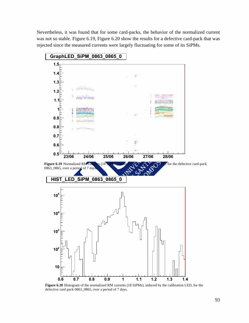
93
Nevertheless, it was found that for some card-packs, the behavior of the normalized current was not so stable. Figure 6.19, Figure 6.20 show the results for a defective card-pack that was rejected since the measured currents were largely fluctuating for some of its SiPMs.
Figure 6.19 Normalized RM currents (18 SiPMs), induced by the calibration LED, for the defective card-pack 0863_0865, over a period of 7 days.
Figure 6.20 Histogram of the normalized RM currents (18 SiPMs), induced by the calibration LED, for the defective card pack 0863_0865, over a period of 7 days.
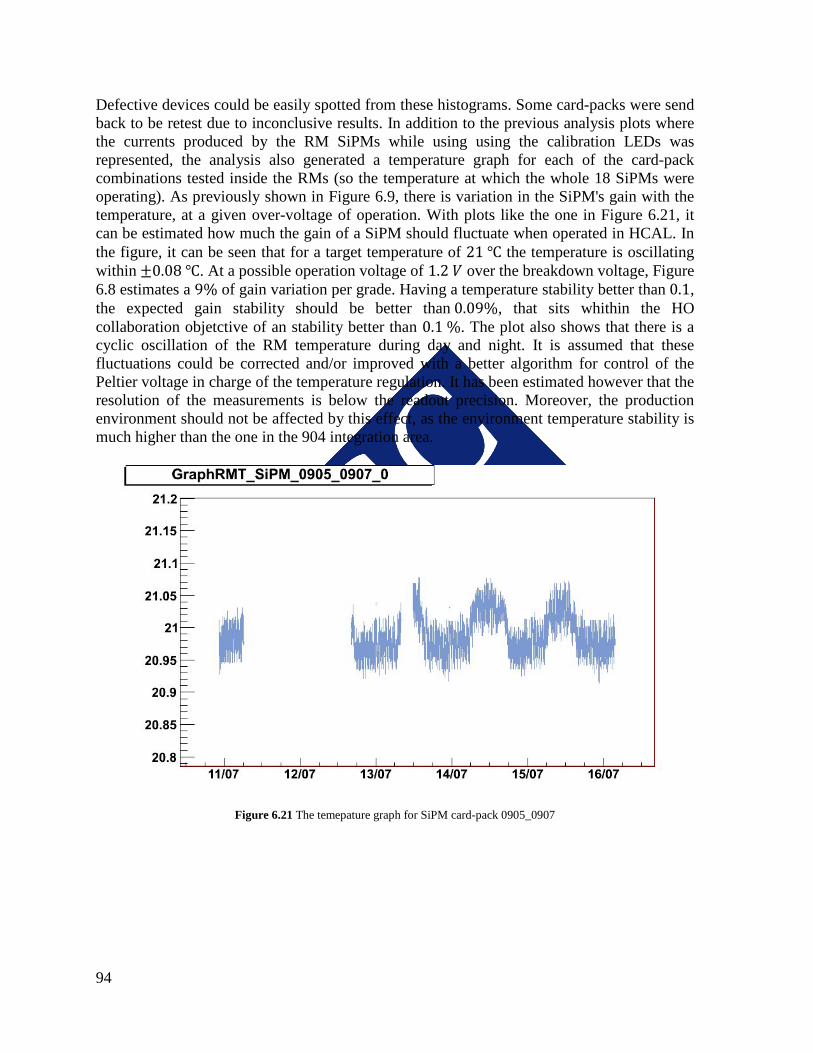
94
Defective devices could be easily spotted from these histograms. Some card-packs were send back to be retest due to inconclusive results. In addition to the previous analysis plots where the currents produced by the RM SiPMs while using using the calibration LEDs was represented, the analysis also generated a temperature graph for each of the card-pack combinations tested inside the RMs (so the temperature at which the whole 18 SiPMs were operating). As previously shown in Figure 6.9, there is variation in the SiPM's gain with the temperature, at a given over-voltage of operation. With plots like the one in Figure 6.21, it can be estimated how much the gain of a SiPM should fluctuate when operated in HCAL. In the figure, it can be seen that for a target temperature of 21 ℃ the temperature is oscillating within ±0.08 ℃. At a possible operation voltage of 1.2 𝑉 over the breakdown voltage, Figure 6.8 estimates a 9% of gain variation per grade. Having a temperature stability better than 0.1, the expected gain stability should be better than 0.09%, that sits whithin the HO collaboration objetctive of an stability better than 0.1 %. The plot also shows that there is a cyclic oscillation of the RM temperature during day and night. It is assumed that these fluctuations could be corrected and/or improved with a better algorithm for control of the Peltier voltage in charge of the temperature regulation. It has been estimated however that the resolution of the measurements is below the readout precision. Moreover, the production environment should not be affected by this effect, as the environment temperature stability is much higher than the one in the 904 integration area.
Figure 6.21 The temepature graph for SiPM card-pack 0905_0907

95
In conclusion, the tools developed by the author of this thesis, for the stability analysis, are being successfully used by the collaboration to identify and discard boards with big temperature and/or current fluctuations. In addition, the results of the temperature stability analysis provide an important parameter to calculate appropriate operation points with gain stability better than the 1% goal. In the following chapter, the results of the analysis of the response of the SiPM devices to particles are presented.

96
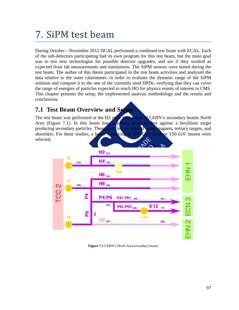
97
7. SiPM test beam During October - November 2012 HCAL performed a combined test beam with ECAL. Each of the sub-detectors participating had its own program for this test beam, but the main goal was to test new technologies for possible detector upgrades, and see if they worked as expected from lab measurements and simulations. The SiPM sensors were tested during the test beam. The author of this thesis participated in the test beam activities and analyzed the data relative to the outer calorimeter, in order to evaluate the dynamic range of the SiPM solution and compare it to the one of the currently used HPDs, verifying that they can cover the range of energies of particles expected to reach HO for physics events of interest in CMS. This chapter presents the setup, the implemented analysis methodology and the results and conclusions.
7.1 Test Beam Overview and Setup The test beam was performed at the H2 zone that is part of CERN’s secondary beams North Area (Figure 7.1). In this beam line, a proton beam is shot against a beryllium target producing secondary particles. These particles are filtered using magnets, tertiary targets, and absorbers. For these studies, a beam consisting of 300 𝐺𝑒𝑉 pions or 150 𝐺𝑒𝑉 muons were selected.
Figure 7.1 CERN’s North Area secondary beams
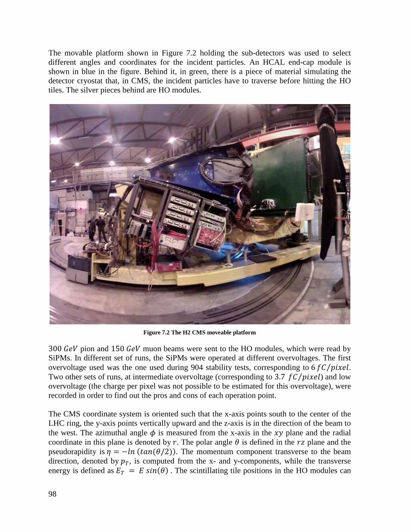
98
The movable platform shown in Figure 7.2 holding the sub-detectors was used to select different angles and coordinates for the incident particles. An HCAL end-cap module is shown in blue in the figure. Behind it, in green, there is a piece of material simulating the detector cryostat that, in CMS, the incident particles have to traverse before hitting the HO tiles. The silver pieces behind are HO modules.
Figure 7.2 The H2 CMS moveable platform
300 𝐺𝑒𝑉 pion and 150 𝐺𝑒𝑉 muon beams were sent to the HO modules, which were read by SiPMs. In different set of runs, the SiPMs were operated at different overvoltages. The first overvoltage used was the one used during 904 stability tests, corresponding to 6 𝑓𝐶 𝑝𝑖𝑥𝑒𝑙⁄ . Two other sets of runs, at intermediate overvoltage (corresponding to 3.7 𝑓𝐶 𝑝𝑖𝑥𝑒𝑙⁄ ) and low overvoltage (the charge per pixel was not possible to be estimated for this overvoltage), were recorded in order to find out the pros and cons of each operation point. The CMS coordinate system is oriented such that the x-axis points south to the center of the LHC ring, the y-axis points vertically upward and the z-axis is in the direction of the beam to the west. The azimuthal angle 𝜙 is measured from the x-axis in the 𝑥𝑦 plane and the radial coordinate in this plane is denoted by 𝑟. The polar angle 𝜃 is defined in the 𝑟𝑧 plane and the pseudorapidity is 𝜂 = −𝑙𝑛 (𝑡𝑎𝑛(𝜃/2)). The momentum component transverse to the beam direction, denoted by 𝑝𝑇, is computed from the x- and y-components, while the transverse energy is defined as 𝐸𝑇 = 𝐸 𝑠𝑖𝑛(𝜃) . The scintillating tile positions in the HO modules can
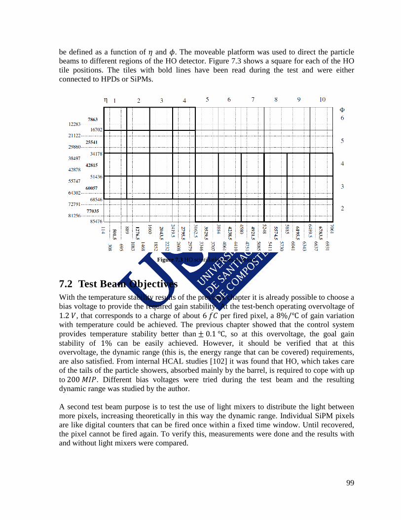
99
be defined as a function of 𝜂 and 𝜙. The moveable platform was used to direct the particle beams to different regions of the HO detector. Figure 7.3 shows a square for each of the HO tile positions. The tiles with bold lines have been read during the test and were either connected to HPDs or SiPMs.
Figure 7.3 HO scintillating tiles positions
7.2 Test Beam Objectives With the temperature stability results of the previous chapter it is already possible to choose a bias voltage to provide the required gain stability. At the test-bench operating overvoltage of 1.2 𝑉, that corresponds to a charge of about 6 𝑓𝐶 per fired pixel, a 8%/℃ of gain variation with temperature could be achieved. The previous chapter showed that the control system provides temperature stability better than ± 0.1 ℃, so at this overvoltage, the goal gain stability of 1% can be easily achieved. However, it should be verified that at this overvoltage, the dynamic range (this is, the energy range that can be covered) requirements, are also satisfied. From internal HCAL studies [102] it was found that HO, which takes care of the tails of the particle showers, absorbed mainly by the barrel, is required to cope with up to 200 𝑀𝐼𝑃. Different bias voltages were tried during the test beam and the resulting dynamic range was studied by the author. A second test beam purpose is to test the use of light mixers to distribute the light between more pixels, increasing theoretically in this way the dynamic range. Individual SiPM pixels are like digital counters that can be fired once within a fixed time window. Until recovered, the pixel cannot be fired again. To verify this, measurements were done and the results with and without light mixers were compared.

100
7.3 Dynamic Range Analysis The following tables summarize the test beam runs at the gain corresponding to 6 𝑓𝐶 that were studied:
𝜼 𝝓 run numbers
2(1466) 5(25541) 4989-4999
2(1466) 4(42814) 5000-5009
2(1277) 4(42814) 5010-5018
Table 7.1 Run Numbers for the 300 GeV pion runs at high SiPM gain.
The run numbers in the tables show sequences of 300 𝐺𝑒𝑉 runs. Each of the runs contains 5 ∙ 104 events. So for each of the 𝜂 − 𝜙 combinations above there is approximately half a million events for the analysis. Reducing to 3.7 𝑓𝐶, at an intermediate gain, two different types of runs were performed: one type with the light mixers installed and a second one without them:
𝜼 𝝓 Runs
2(1466) 5(25541) 5152-5154, 5179-5180, 5182-5183, 5184-5186, 5190-5191, 5193- 5197
2(1466) 4(42814) 5141-5150
Table 7.2 Run Numbers for the 300 GeV pion runs at the intermediate SiPM gain with light mixers.
𝜼 𝝓 Runs
2(1466) 5(25541) 5343-5247, 5349, 5351-5356
2(1466) 4(42814) 5357-5361, 5363-5365, 5432-5433
Table 7.3 Run Numbers for the 300 GeV pion runs at the intermediate SiPM gain without light mixers.
In addition to high and the intermediate gain runs, a series of low gain runs, where the equivalent charge per pixel could not be estimated, were also recorded:
𝜼 𝝓 Runs
2(1466) 4(1466) 5450-5451, 5453-5456, 5458-5461
Table 7.4 Run Numbers for the 300 GeV pion runs at low SiPM gain.
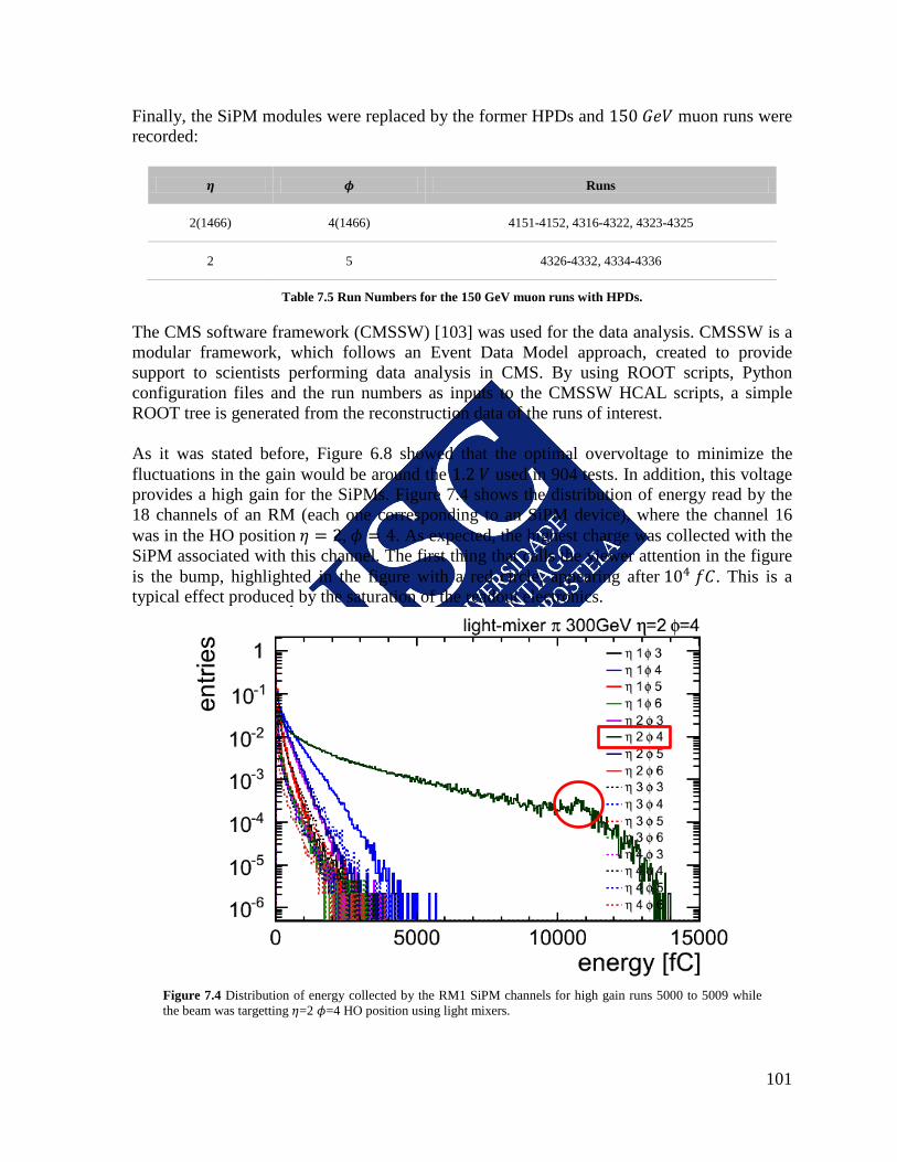
101
Finally, the SiPM modules were replaced by the former HPDs and 150 𝐺𝑒𝑉 muon runs were recorded:
𝜼 𝝓 Runs
2(1466) 4(1466) 4151-4152, 4316-4322, 4323-4325
2 5 4326-4332, 4334-4336
Table 7.5 Run Numbers for the 150 GeV muon runs with HPDs.
The CMS software framework (CMSSW) [103] was used for the data analysis. CMSSW is a modular framework, which follows an Event Data Model approach, created to provide support to scientists performing data analysis in CMS. By using ROOT scripts, Python configuration files and the run numbers as inputs to the CMSSW HCAL scripts, a simple ROOT tree is generated from the reconstruction data of the runs of interest. As it was stated before, Figure 6.8 showed that the optimal overvoltage to minimize the fluctuations in the gain would be around the 1.2 𝑉 used in 904 tests. In addition, this voltage provides a high gain for the SiPMs. Figure 7.4 shows the distribution of energy read by the 18 channels of an RM (each one corresponding to an SiPM device), where the channel 16 was in the HO position 𝜂 = 2, 𝜙 = 4. As expected, the highest charge was collected with the SiPM associated with this channel. The first thing that calls the viewer attention in the figure is the bump, highlighted in the figure with a red circle, appearing after 104 𝑓𝐶. This is a typical effect produced by the saturation of the readout electronics.
Figure 7.4 Distribution of energy collected by the RM1 SiPM channels for high gain runs 5000 to 5009 while the beam was targetting 𝜂=2 𝜙=4 HO position using light mixers.
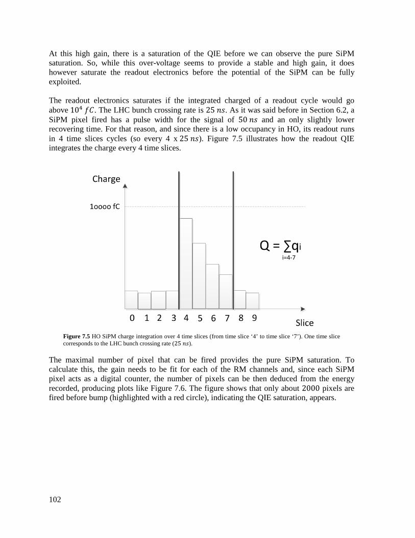
102
At this high gain, there is a saturation of the QIE before we can observe the pure SiPM saturation. So, while this over-voltage seems to provide a stable and high gain, it does however saturate the readout electronics before the potential of the SiPM can be fully exploited. The readout electronics saturates if the integrated charged of a readout cycle would go above 104 𝑓𝐶. The LHC bunch crossing rate is 25 𝑛𝑠. As it was said before in Section 6.2, a SiPM pixel fired has a pulse width for the signal of 50 𝑛𝑠 and an only slightly lower recovering time. For that reason, and since there is a low occupancy in HO, its readout runs in 4 time slices cycles (so every 4 x 25 𝑛𝑠). Figure 7.5 illustrates how the readout QIE integrates the charge every 4 time slices.
Figure 7.5 HO SiPM charge integration over 4 time slices (from time slice ‘4’ to time slice ‘7’). One time slice corresponds to the LHC bunch crossing rate (25 𝑛𝑠).
The maximal number of pixel that can be fired provides the pure SiPM saturation. To calculate this, the gain needs to be fit for each of the RM channels and, since each SiPM pixel acts as a digital counter, the number of pixels can be then deduced from the energy recorded, producing plots like Figure 7.6. The figure shows that only about 2000 pixels are fired before bump (highlighted with a red circle), indicating the QIE saturation, appears.
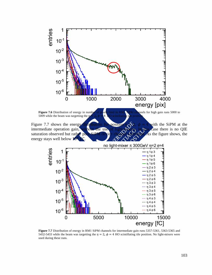
103
Figure 7.6 Distribution of energy in number of pixels fired in RM1 SiPM channels for high gain runs 5000 to 5009 while the beam was targetting the 𝜂 = 2, 𝜙 = 4 HO scintillating tile position.
Figure 7.7 shows the energy distribution for position 𝜂 = 2, 𝜙 = 4 with the SiPM at the intermediate operation gain, without the use of light-mixers. In this case there is no QIE saturation observed but rather pure SiPM device channel saturation. As the figure shows, the energy stays well below 104 𝑓𝐶.
Figure 7.7 Distribution of energy in RM1 SiPM channels for intermediate gain runs 5357-5361, 5363-5365 and 5432-5433 while the beam was targetting the 𝜂 = 2, 𝜙 = 4 HO scintillating tile position. No light-mixers were used during these runs.
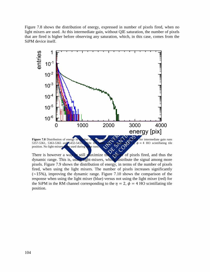
104
Figure 7.8 shows the distribution of energy, expressed in number of pixels fired, when no light mixers are used. At this intermediate gain, without QIE saturation, the number of pixels that are fired is higher before observing any saturation, which, in this case, comes from the SiPM device itself.
Figure 7.8 Distribution of energy in number of pixels fired in RM1 SiPM channels for intermediate gain runs 5357-5361, 5363-5365 and 5432-5433, while the beam was targetting 𝜂 = 2, 𝜙 = 4 HO scintillating tile position. No light-mixers were used during these runs.
There is however a way to still maximize the number of pixels fired, and thus the dynamic range. This is, using light-mixers, which distribute the signal among more pixels. Figure 7.9 shows the distribution of energy, in terms of the number of pixels fired, when using the light mixers. The number of pixels increases significantly (~15%), improving the dynamic range. Figure 7.10 shows the comparison of the response when using the light mixer (blue) versus not using the light mixer (red) for the SiPM in the RM channel corresponding to the 𝜂 = 2, 𝜙 = 4 HO scintillating tile position.
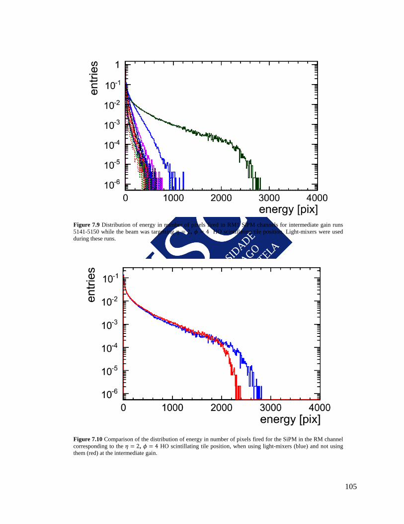
105
Figure 7.9 Distribution of energy in number of pixels fired in RM1 SiPM channels for intermediate gain runs 5141-5150 while the beam was targetting 𝜂 = 2, 𝜙 = 4 HO scintillating tile position. Light-mixers were used during these runs.
Figure 7.10 Comparison of the distribution of energy in number of pixels fired for the SiPM in the RM channel corresponding to the 𝜂 = 2, 𝜙 = 4 HO scintillating tile position, when using light-mixers (blue) and not using them (red) at the intermediate gain.
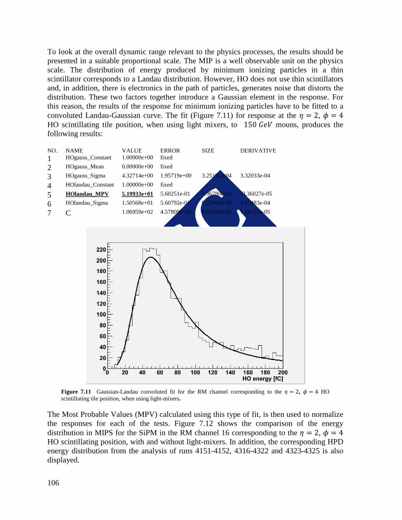
106
To look at the overall dynamic range relevant to the physics processes, the results should be presented in a suitable proportional scale. The MIP is a well observable unit on the physics scale. The distribution of energy produced by minimum ionizing particles in a thin scintillator corresponds to a Landau distribution. However, HO does not use thin scintillators and, in addition, there is electronics in the path of particles, generates noise that distorts the distribution. These two factors together introduce a Gaussian element in the response. For this reason, the results of the response for minimum ionizing particles have to be fitted to a convoluted Landau-Gaussian curve. The fit (Figure 7.11) for response at the 𝜂 = 2, 𝜙 = 4 HO scintillating tile position, when using light mixers, to 150 𝐺𝑒𝑉 mouns, produces the following results: NO. NAME VALUE ERROR SIZE DERIVATIVE 1 HOgauss_Constant 1.00000e+00 fixed 2 HOgauss_Mean 0.00000e+00 fixed 3 HOgauss_Sigma 4.32714e+00 1.95719e+00 3.25192e-04 3.32033e-04 4 HOlandau_Constant 1.00000e+00 fixed 5 HOlandau_MPV 5.19933e+01 5.60251e-01 1.96780e-03 -3.36027e-05 6 HOlandau_Sigma 1.50568e+01 5.60792e-01 9.23409e-04 1.02483e-04 7 C 1.06959e+02 4.57809e+01 8.04298e-03 1.28131e-05
Figure 7.11 Gaussian-Landau convoluted fit for the RM channel corresponding to the 𝜂 = 2, 𝜙 = 4 HO scintillating tile position, when using light-mixers.
The Most Probable Values (MPV) calculated using this type of fit, is then used to normalize the responses for each of the tests. Figure 7.12 shows the comparison of the energy distribution in MIPS for the SiPM in the RM channel 16 corresponding to the 𝜂 = 2, 𝜙 = 4 HO scintillating position, with and without light-mixers. In addition, the corresponding HPD energy distribution from the analysis of runs 4151-4152, 4316-4322 and 4323-4325 is also displayed.
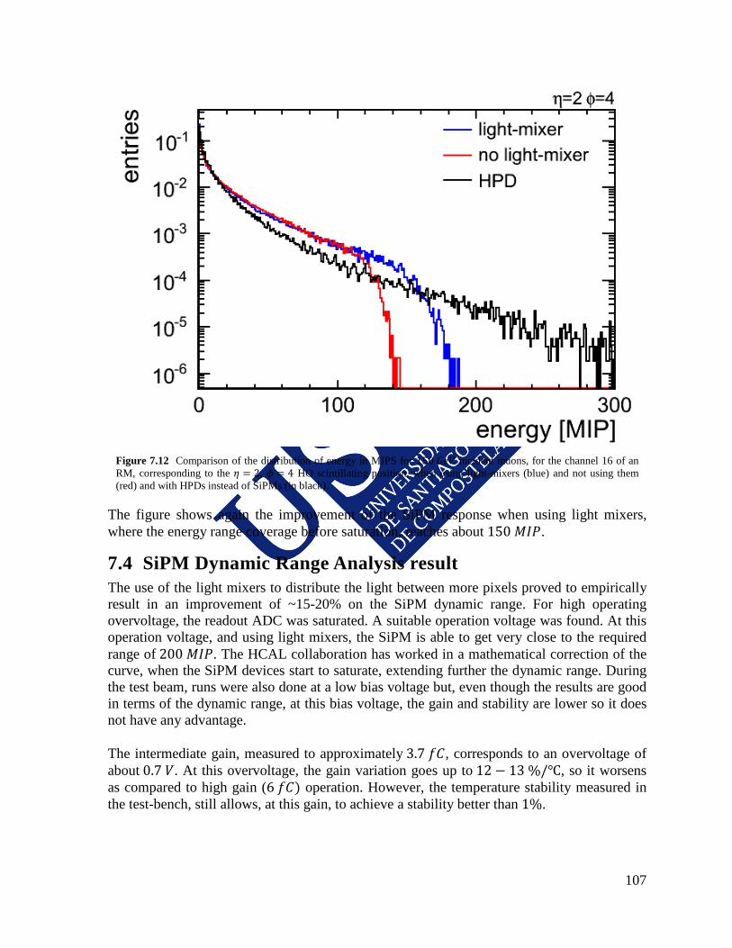
107
Figure 7.12 Comparison of the distribution of energy in MIPS for 150 𝐺𝑒𝑉 incident muons, for the channel 16 of an RM, corresponding to the 𝜂 = 2, 𝜙 = 4 HO scintillating position, when using light-mixers (blue) and not using them (red) and with HPDs instead of SiPMs (in black).
The figure shows again the improvement of the SiPM response when using light mixers, where the energy range coverage before saturation, reaches about 150 𝑀𝐼𝑃.
7.4 SiPM Dynamic Range Analysis result The use of the light mixers to distribute the light between more pixels proved to empirically result in an improvement of ~15-20% on the SiPM dynamic range. For high operating overvoltage, the readout ADC was saturated. A suitable operation voltage was found. At this operation voltage, and using light mixers, the SiPM is able to get very close to the required range of 200 𝑀𝐼𝑃. The HCAL collaboration has worked in a mathematical correction of the curve, when the SiPM devices start to saturate, extending further the dynamic range. During the test beam, runs were also done at a low bias voltage but, even though the results are good in terms of the dynamic range, at this bias voltage, the gain and stability are lower so it does not have any advantage. The intermediate gain, measured to approximately 3.7 𝑓𝐶, corresponds to an overvoltage of about 0.7 𝑉. At this overvoltage, the gain variation goes up to 12 − 13 %/℃, so it worsens as compared to high gain (6 𝑓𝐶) operation. However, the temperature stability measured in the test-bench, still allows, at this gain, to achieve a stability better than 1%.

108
The results of this analysis determine therefore that it is possible to find an operating overvoltage for the SiPM that can cover the required dynamic range, as the HPDs did, with the addition that the SiPM operates at a much higher gain, having therefore, a better signal to noise ratio and are insensitive to magnetic fields.
109
Conclusions This work is divided in three parts. The first one shows the importance of the control systems for the correct and efficient operation of the LHC experiments. It highlights the complexity of these systems that, years after their commissioning and more than a decade since their conceptual design, have no match in the industrial control world. The control system context, the unprecedented challenges and the technologies chosen for the development are analyzed. In a second part, the leading work performed by the author within the groups specialized in the design and development of system architecture is presented. The author was presenter in various international conferences and published, during different phases of the project, the advances achieved [53] [63] [104] [105]. The author also contributed to the publication of other articles, related with the high availability system architecture [106], helping the experiment data acquisition system to make the most of the collisions provided by the LHC, as well as related to the analysis and mathematic modeling of the DCS [67], that allows for finding errors in the system automatically. This second part gives also details about the concrete implementation of ECAL´s control system, of great importance for the performance of this detector that played an essential role in the Higgs Boson discovery [107]. The author contributed to diverse publications related with this development [70] [71] [72] [73]. The last part of this work is focused in the technical analysis of detectors proposed to improve the CMS calorimeters. The new SiPMs that will be used in the outer hadron calorimeter after the current technical stop are presented. Concrete examples of control parameters, like the bias voltage or the temperature, that are very important to guarantee the precise and stable operation of the SiPMs, are provided. The test-bench and the SiPM control system were presented in a calorimetry conference [108] and the results of the analysis performed by the author, together with the results of other analysis performed by HCAL collaboration members, were presented to the collaboration in a joint report in [109]. Those studies point out that the noise is dominated by the electronics, and not by the SiPM, and that with the developed instrumentation an excellent temperature stability is reached (𝑅𝑀𝑆 ± 0.025 𝐾, equivalent to 1 𝐿𝑆𝐵). Finally, the results of the test-beam demonstrated three things. First, that at 6 𝑓𝐶 gain, where the maximum stability of the gain could be achieved, there is a saturation of the readout electronics. Second, that at a lower gain, 3.7 𝑓𝐶, and in combination with light mixers, the SiPM can cover the required dynamic range of 200 𝑀𝐼𝑃 without saturating the readout electronics. And third, that further reducing the gain does not provide any significant improvement in the dynamic range, while worsening the stability.

110
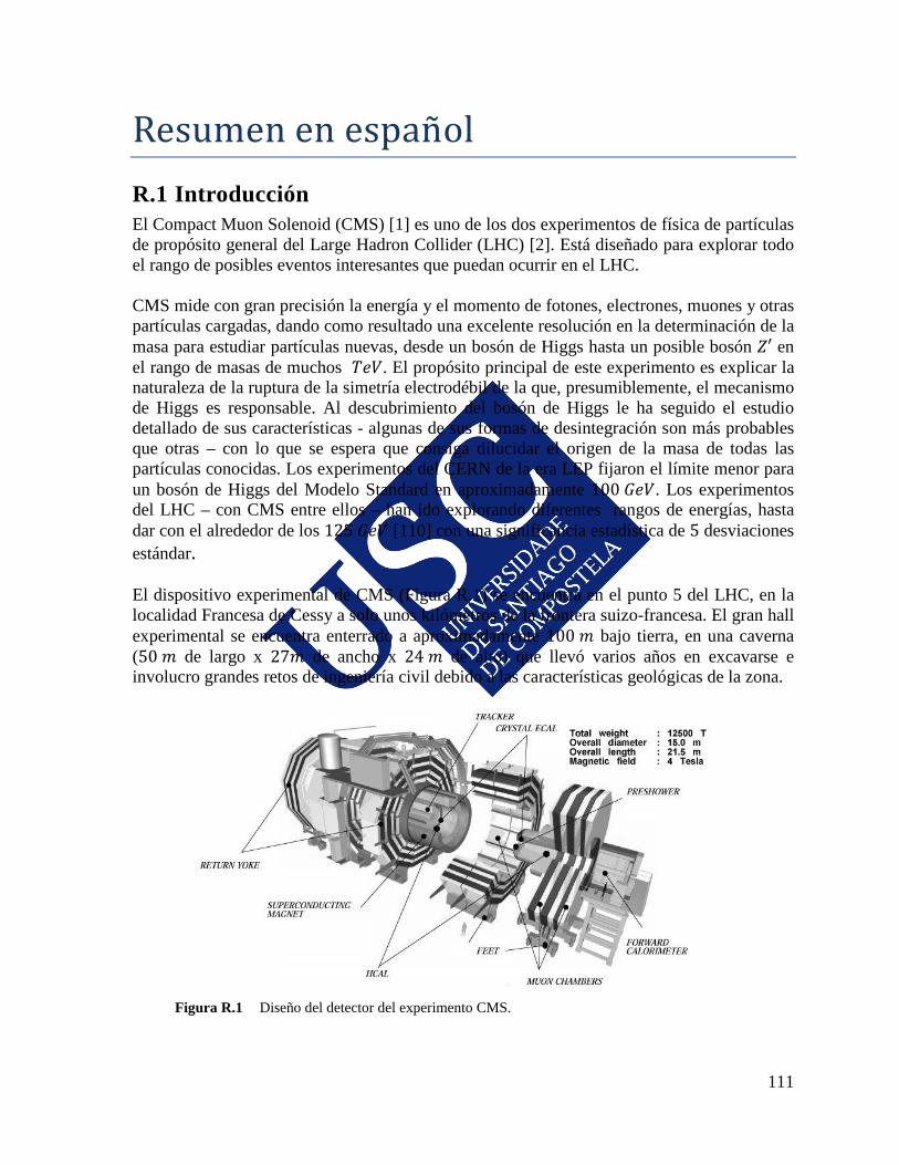
111
Resumen en espanol R.1 Introducción El Compact Muon Solenoid (CMS) [1] es uno de los dos experimentos de física de partículas de propósito general del Large Hadron Collider (LHC) [2]. Está diseñado para explorar todo el rango de posibles eventos interesantes que puedan ocurrir en el LHC. CMS mide con gran precisión la energía y el momento de fotones, electrones, muones y otras partículas cargadas, dando como resultado una excelente resolución en la determinación de la masa para estudiar partículas nuevas, desde un bosón de Higgs hasta un posible bosón 𝑍′ en el rango de masas de muchos 𝑇𝑒𝑉. El propósito principal de este experimento es explicar la naturaleza de la ruptura de la simetría electrodébil de la que, presumiblemente, el mecanismo de Higgs es responsable. Al descubrimiento del bosón de Higgs le ha seguido el estudio detallado de sus características - algunas de sus formas de desintegración son más probables que otras – con lo que se espera que consiga dilucidar el origen de la masa de todas las partículas conocidas. Los experimentos del CERN de la era LEP fijaron el límite menor para un bosón de Higgs del Modelo Standard en aproximadamente 100 𝐺𝑒𝑉. Los experimentos del LHC – con CMS entre ellos – han ido explorando diferentes rangos de energías, hasta dar con el alrededor de los 125 𝐺𝑒𝑉 [110] con una significancia estadística de 5 desviaciones estándar. El dispositivo experimental de CMS (Figura R.1) se encuentra en el punto 5 del LHC, en la localidad Francesa de Cessy a solo unos kilómetros de la frontera suizo-francesa. El gran hall experimental se encuentra enterrado a aproximadamente 100 𝑚 bajo tierra, en una caverna (50 𝑚 de largo x 27𝑚 de ancho x 24 𝑚 de alto) que llevó varios años en excavarse e involucro grandes retos de ingeniería civil debido a las características geológicas de la zona.
Diseño del detector del experimento CMS. Figura R.1
112
La organización de los distintos detectores se corresponde con una distribución cilíndrica de diferentes capas, típica de los colisionadores frontales en aceleradores circulares. Cada sub-detector consta normalmente de un cilindro hueco con su eje a lo largo de la dirección del haz de partículas y dos tapas cerrando el cilindro. Para poder medir con precisión el momento de las partículas cargadas, es necesario un campo magnético muy fuerte - 4 𝑇 en este caso - lo que se consigue con un solenoide superconductor colocado en el centro del detector. Debido a la magnitud de este campo magnético, el retorno necesita una estructura de hierro con un radio de mas de 1.5 𝑚. Integradas entre las capas de la estructura de hierro se han dispuesto cuatro capas de detectores de muones, formadas por multitud de Tubos de Deriva (DT, del inglés Drift Tubes) [9] en la parte del Barrel (barril del detector), Cathode Strip Chambers (CSC) [10] en las tapas y Cámaras de Placas Resistivas (RPC) [11]. De esta forma, CMS tiene un excepcional sistema de detección de muones con muy alta eficiencia y cobertura geométrica total. Dentro del solenoide magnético se encuentran el Tracker (un sistema de detección de trazas [12]) y los detectores calorimétricos [13] y [14]. Diez capas de detectores de micropistas de silicio dan a CMS la granularidad y precisión requerida por el programa físico. Por otra parte, tres capas suplementarias con detectores de pixeles de silicio, situadas en la parte más cercana al punto de colisión, mejoran las medidas de los parámetros de impacto de las trazas de las partículas cargadas, así como la posición de los vértices secundarios. En calorímetro electromagnético (ECAL) [13] rodéa el Tracker. ECAL utiliza cristales de tungstenato de plomo (𝑃𝑏𝑊𝑂4) con una cobertura en pseudorapidez de |𝜂| < 3. En la región del barril se utilizan fotodiodos de avalancha de silicio (APD) para detectar la luz, mientras que en las tapas se utilizan fototriodos de vacío. Delante de las tapas del ECAL, se encuentra un sistema de pre-detección de cascada que se utiliza para el filtrado de 𝜋0. Finalmente, entre el solenoide magnético y el ECAL, se encuentra el calorímetro hadrónico (HCAL) y la respuesta combinada de los dos calorímetros genera la información necesaria para la reconstrucción de jets de partículas y la deposición de energía transversal. HCAL es un detector de muestreo que consiste en material activo intercalado con placas de absorbente de cobre. El material activo está formado por placas gruesas de centelladores de plástico que se leen a través de fibras de plástico WLS (wavelength-shifting). El sistema de disparo (Trigger [24]) y el sistema de adquisición de datos (DAQ) [25]) son la parte del experimento donde todos datos brutos están físicamente disponibles y las decisiones importantes, que afectan al destino de la información relativa a los sucesos de interés físico, se toman en estos sistemas. Además de los requisitos en términos de hardware (capacidad de procesamiento, velocidad de las redes, etc.), estos sistemas se crearon de manera que son lo suficientemente flexibles como para adaptarse a las necesidades que se deriven de los estudios de las colisiones durante los primero años. Proporciona también una manera de monitorizar los datos que se desechan para poder efectuar modificaciones, eventualmente. En el LHC los haces de partículas colisionan a una frecuencia de 40 𝑀𝐻𝑧. Esto, a la luminosidad para la que está diseñado, resulta en ~8 ∙ 108 colisiones inelásticas 𝑝𝑝 por
113
segundo. Cada ~20 colisiones 𝑝𝑝 (un cruce de partículas) genera ~1 𝑀𝐵 de información. Esto significa un total de hasta ~107 𝑀𝐵 𝑠⁄ de los cuales, solo 102 es técnicamente posible guardar en un servicio de almacenamiento. De este modo, el sistema de selección y adquisición de datos de CMS necesita tener una capacidad de rechazo de 105. Una parte imprescindible del sistema de adquisición de datos es el sistema de control del detector (DCS), que es responsable de asegurar la operación óptima y segura del experimento, de manera que se puedan tomar datos de la mayor calidad posible. Este trabajo de Tesis Doctoral refleja el trabajo que en los últimos once años ha dedicado su autor al diseño, desarrollo, integración y puesta en marcha de un sistema sin precedentes para el control, tanto del detector como de la infraestructura del experimento.
R.2 El sistema de control del detector de CMS En este trabajo se analizan profundamente los principales requisitos del diseño original y se describe el diseño e implementación de la jerarquía global de control. Como miembro fundador del grupo central de controles de CMS, el autor ha jugado un rol importante como representante del DCS (sistema de control del experimento) en diferentes grupos de trabajo, tanto dentro de la colaboración que ha desarrollado el experimento como fuera de esta. Los requisitos del DCS se pueden clasificar en cuatro tipos: operacionales, funcionales, de entorno y los relacionados con la organización. Los requisitos operacionales son los relacionados con la operación segura, coherente, automática e ininterrumpida del detector. De estos, se derivan los requisitos funcionales más específicos, referidos a la frecuencia de lectura y almacenamiento de datos - que necesita poder trabajar con un número de variables de control en el orden del millón - las alarmas para esta gran cantidad de variables, el procesado de la información contenida en estas variables y la toma de decisiones automática correspondiente. Los requisitos de entorno son los específicos del lugar de operación de detector y de su tamaño, entre los que se encuentran la gran dispersión geográfica del hardware de control, la necesidad de utilizar dispositivos capaces de operar en grandes campos magnéticos y la de sobrevivir a un entorno con dosis de radiación importantes. Por último, los requisitos relacionados con la organización imponen la creación de estructuras de trabajo capaces de ser lo suficientemente flexibles para adaptarse a equipos de trabajo locales y otros remotos, además de una rotación importante de personal. Dentro del proyecto conjunto de control del CERN (JCOP, del inglés Joint COntrols Project), se puso mucho esfuerzo para homogenizar la selección de tecnologías para poder compartir experiencia entre los experimentos y para poder tener un grupo central en el CERN dando soporte a todos ellos. En esta misma línea, JCOP creó su propia infraestructura software, un conjunto de librerías de software y recursos compartidos, para proporcionar a los experimentos del LHC las herramientas para el control de una seria de hardware preseleccionado. El autor de esta tesis ha trabajado en el marco de JCOP creando componentes (como el Rack Control) y proponiendo otros que fueron desarrollados con éxito (como por ejemplo la herramienta de instalación distribuida de JCOP). Siguiendo este enfoque, el equipo central de DCS creó su propio marco de trabajo (DCS framework), adecuado a la arquitectura de CMS y a sus desarrollos específicos. Además, el equipo central
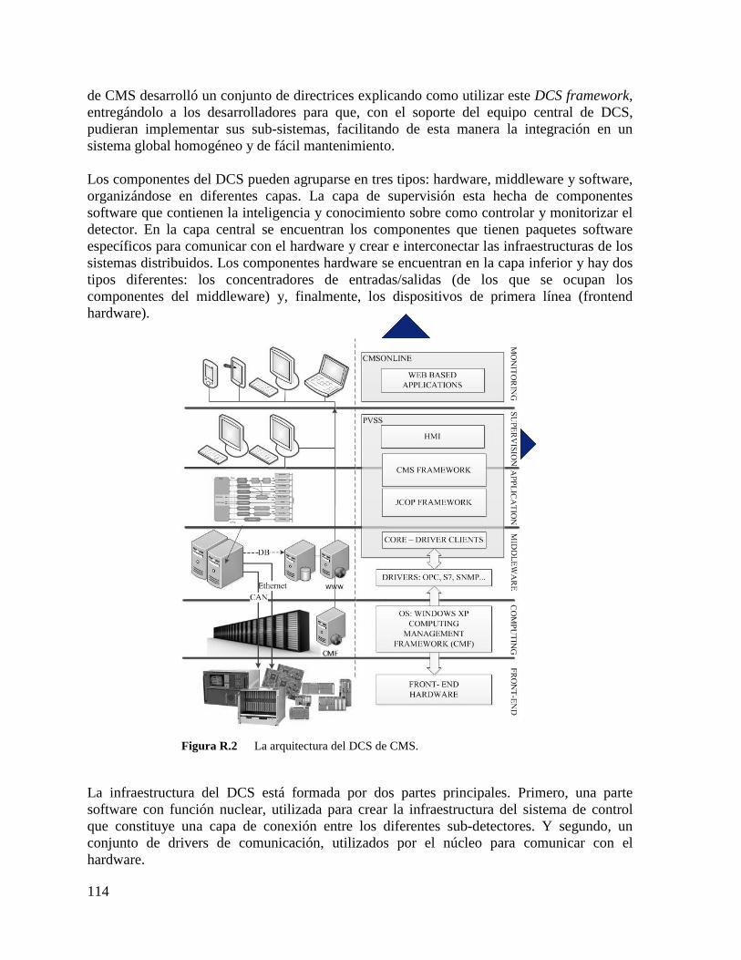
114
de CMS desarrolló un conjunto de directrices explicando como utilizar este DCS framework, entregándolo a los desarrolladores para que, con el soporte del equipo central de DCS, pudieran implementar sus sub-sistemas, facilitando de esta manera la integración en un sistema global homogéneo y de fácil mantenimiento. Los componentes del DCS pueden agruparse en tres tipos: hardware, middleware y software, organizándose en diferentes capas. La capa de supervisión esta hecha de componentes software que contienen la inteligencia y conocimiento sobre como controlar y monitorizar el detector. En la capa central se encuentran los componentes que tienen paquetes software específicos para comunicar con el hardware y crear e interconectar las infraestructuras de los sistemas distribuidos. Los componentes hardware se encuentran en la capa inferior y hay dos tipos diferentes: los concentradores de entradas/salidas (de los que se ocupan los componentes del middleware) y, finalmente, los dispositivos de primera línea (frontend hardware).
La arquitectura del DCS de CMS. Figura R.2
La infraestructura del DCS está formada por dos partes principales. Primero, una parte software con función nuclear, utilizada para crear la infraestructura del sistema de control que constituye una capa de conexión entre los diferentes sub-detectores. Y segundo, un conjunto de drivers de comunicación, utilizados por el núcleo para comunicar con el hardware.

115
PVSS de la compañía austriaca ETM (empresa satélite de Siemens) fue seleccionado [40] por JCOP como el sistema SCADA (del inglés Supervisory Control and Data Acquisition) para el desarrollo de los sistemas de control de los experimentos. La selección se hizo después de ser comparado con otros ~40 sistemas SCADA, fijándose en una serie de características que lo hiciesen ajustarse a las necesidades de los experimentos del LHC, como su modularidad, su capacidad para aceptar extensiones, su simplicidad de programación o el hecho de funcionar en diferentes sistemas operativos. La arquitectura del sistema de DCS está representada en la Figura R.2. El frontend hardware conecta al sistema de lectura a través de cables de red o buses de campo CAN. El conjunto del hardware que forma esta capa se eligió con el propósito de maximizar la homogeneidad y la compatibilidad con los fabricantes CAEN y WIENER, que proporcionan al experimento la mayoría del hardware de gestión de fuentes de alimentación. La siguiente capa consiste en la infraestructura de computación. CMS fue un paso más lejos que los demás experimentos del LHC, creando desde el principio una infraestructura completamente gestionada de manera centralizada, mediante el uso del framework de gestión de ordenadores del CERN, creando, además, aplicaciones web para configurar y monitorizar cada uno de los nodos de la infraestructura. Una capa de middleware, que contiene el núcleo de PVSS, proporciona clientes para los drivers industriales utilizados (OPC, SNMP, S7, etc.). Para los drivers creados en el CERN o CMS, los clientes tuvieron que ser específicamente desarrollados. Esta capa también proporciona las herramientas para conectar los diferentes sistemas de PVSS. La siguiente capa, la capa de aplicación, está formada por los diferentes componentes que implementan la funcionalidad del DCS. Una capa de supervisión incluye una estructura de árbol de control que integra el sistema distribuido y que automatiza la operación del experimento, mediante el envío secuenciado de comandos al hardware, en sincronización con los diferentes estados del LHC. Esta capa proporciona también las interfaces de usuario, que son utilizadas en la sala de control para operar el experimento. Una última capa es la que se utiliza para la monitorización remota. Un servidor de aplicaciones Java y varias aplicación web, que fueron desarrolladas por el equipo central de DCS, proporcionan una solución escalable para la publicación y acceso de grandes cantidades de información del sistema. El DCS se gestiona por un solo operador, mediante el uso de un árbol de control basado en máquinas de estados finitos, con estados y transiciones entre estos estados claramente definidos. La complejidad de esta tarea queda reflejada en el hecho de que el árbol completo tiene aproximadamente 32000 nodos. El árbol está formado por muchos sub-árboles, desarrollados por diferentes equipos en diferentes sub-detectores. Hay una serie de reglas de nomenclatura y programación que gobiernan el diseño de las clases de nodo del árbol y la forma como conectan entre ellas, que fueron desarrolladas para asegurar la homogeneidad y el sencillo mantenimiento del resultado final.
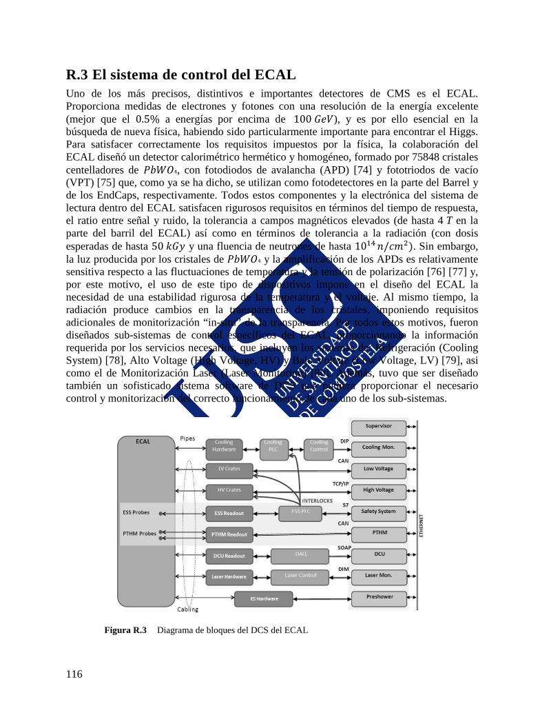
116
R.3 El sistema de control del ECAL Uno de los más precisos, distintivos e importantes detectores de CMS es el ECAL. Proporciona medidas de electrones y fotones con una resolución de la energía excelente (mejor que el 0.5% a energías por encima de 100 𝐺𝑒𝑉), y es por ello esencial en la búsqueda de nueva física, habiendo sido particularmente importante para encontrar el Higgs. Para satisfacer correctamente los requisitos impuestos por la física, la colaboración del ECAL diseñó un detector calorimétrico hermético y homogéneo, formado por 75848 cristales centelladores de 𝑃𝑏𝑊𝑂4, con fotodiodos de avalancha (APD) [74] y fototriodos de vacío (VPT) [75] que, como ya se ha dicho, se utilizan como fotodetectores en la parte del Barrel y de los EndCaps, respectivamente. Todos estos componentes y la electrónica del sistema de lectura dentro del ECAL satisfacen rigurosos requisitos en términos del tiempo de respuesta, el ratio entre señal y ruido, la tolerancia a campos magnéticos elevados (de hasta 4 T en la parte del barril del ECAL) así como en términos de tolerancia a la radiación (con dosis esperadas de hasta 50 𝑘𝐺𝑦 y una fluencia de neutrones de hasta 1014 𝑛/𝑐𝑚2). Sin embargo, la luz producida por los cristales de 𝑃𝑏𝑊𝑂4 y la amplificación de los APDs es relativamente sensitiva respecto a las fluctuaciones de temperatura y la tensión de polarización [76] [77] y, por este motivo, el uso de este tipo de dispositivos impone en el diseño del ECAL la necesidad de una estabilidad rigurosa de la temperatura y el voltaje. Al mismo tiempo, la radiación produce cambios en la transparencia de los cristales, imponiendo requisitos adicionales de monitorización “in-situ” de la transparencia. Por todos estos motivos, fueron diseñados sub-sistemas de control específicos del ECAL, proporcionando la información requerida por los servicios necesarios, que incluyen los sistemas de: Refrigeración (Cooling System) [78], Alto Voltage (High Voltage, HV) y Bajo Voltaje (Low Voltage, LV) [79], asi como el de Monitorización Laser (Laser Monitoring) [80]. Además, tuvo que ser diseñado también un sofisticado sistema software de DCS que pudiera proporcionar el necesario control y monitorización del correcto funcionamiento de cada uno de los sub-sistemas.
Diagrama de bloques del DCS del ECAL Figura R.3
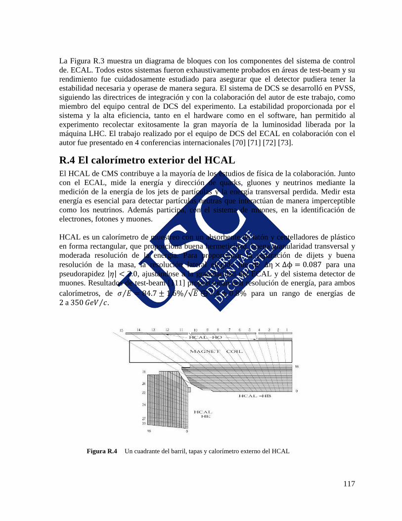
117
La Figura R.3 muestra un diagrama de bloques con los componentes del sistema de control de. ECAL. Todos estos sistemas fueron exhaustivamente probados en áreas de test-beam y su rendimiento fue cuidadosamente estudiado para asegurar que el detector pudiera tener la estabilidad necesaria y operase de manera segura. El sistema de DCS se desarrolló en PVSS, siguiendo las directrices de integración y con la colaboración del autor de este trabajo, como miembro del equipo central de DCS del experimento. La estabilidad proporcionada por el sistema y la alta eficiencia, tanto en el hardware como en el software, han permitido al experimento recolectar exitosamente la gran mayoría de la luminosidad liberada por la máquina LHC. El trabajo realizado por el equipo de DCS del ECAL en colaboración con el autor fue presentado en 4 conferencias internacionales [70] [71] [72] [73].
R.4 El calorímetro exterior del HCAL El HCAL de CMS contribuye a la mayoría de los estudios de física de la colaboración. Junto con el ECAL, mide la energía y dirección de quarks, gluones y neutrinos mediante la medición de la energía de los jets de partículas y la energía transversal perdida. Medir esta energía es esencial para detectar partículas neutras que interactúan de manera imperceptible como los neutrinos. Además participa, con el sistema de muones, en la identificación de electrones, fotones y muones. HCAL es un calorímetro de muestreo con un absorbente de latón y centelladores de plástico en forma rectangular, que proporciona buena hermeticidad, buena granularidad transversal y moderada resolución de la energía. Para proporcionar la separación de dijets y buena resolución de la masa, la resolución lateral elegida fue de Δη × Δϕ = 0.087 para una pseudorapidez |𝜂| < 2.0, ajustándose a la granularidad del ECAL y del sistema detector de muones. Resultados de test-beam [111] proporcionan una resolución de energía, para ambos calorímetros, de 𝜎 𝐸 = 84.7 ± 1.6% √𝐸 ⊕⁄⁄ 7.4 ± 0.8% para un rango de energías de 2 a 350𝐺𝑒𝑉 𝑐⁄ .
Un cuadrante del barril, tapas y calorímetro externo del HCAL Figura R.4
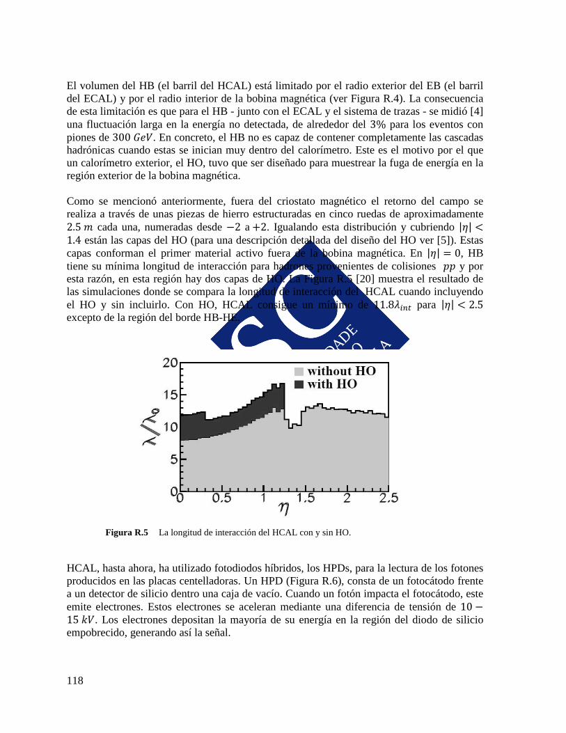
118
El volumen del HB (el barril del HCAL) está limitado por el radio exterior del EB (el barril del ECAL) y por el radio interior de la bobina magnética (ver Figura R.4). La consecuencia de esta limitación es que para el HB - junto con el ECAL y el sistema de trazas - se midió [4] una fluctuación larga en la energía no detectada, de alrededor del 3% para los eventos con piones de 300 𝐺𝑒𝑉. En concreto, el HB no es capaz de contener completamente las cascadas hadrónicas cuando estas se inician muy dentro del calorímetro. Este es el motivo por el que un calorímetro exterior, el HO, tuvo que ser diseñado para muestrear la fuga de energía en la región exterior de la bobina magnética. Como se mencionó anteriormente, fuera del criostato magnético el retorno del campo se realiza a través de unas piezas de hierro estructuradas en cinco ruedas de aproximadamente 2.5 𝑚 cada una, numeradas desde −2 a +2. Igualando esta distribución y cubriendo |𝜂| <1.4 están las capas del HO (para una descripción detallada del diseño del HO ver [5]). Estas capas conforman el primer material activo fuera de la bobina magnética. En |𝜂| = 0, HB tiene su mínima longitud de interacción para hadrones provenientes de colisiones 𝑝𝑝 y por esta razón, en esta región hay dos capas de HO. La Figura R.5 [20] muestra el resultado de las simulaciones donde se compara la longitud de interacción del HCAL cuando incluyendo el HO y sin incluirlo. Con HO, HCAL consigue un mínimo de 11.8𝜆𝑖𝑛𝑡 para |𝜂| < 2.5 excepto de la región del borde HB-HE.
La longitud de interacción del HCAL con y sin HO. Figura R.5
HCAL, hasta ahora, ha utilizado fotodiodos híbridos, los HPDs, para la lectura de los fotones producidos en las placas centelladoras. Un HPD (Figura R.6), consta de un fotocátodo frente a un detector de silicio dentro una caja de vacío. Cuando un fotón impacta el fotocátodo, este emite electrones. Estos electrones se aceleran mediante una diferencia de tensión de 10 −15 𝑘𝑉. Los electrones depositan la mayoría de su energía en la región del diodo de silicio empobrecido, generando así la señal.
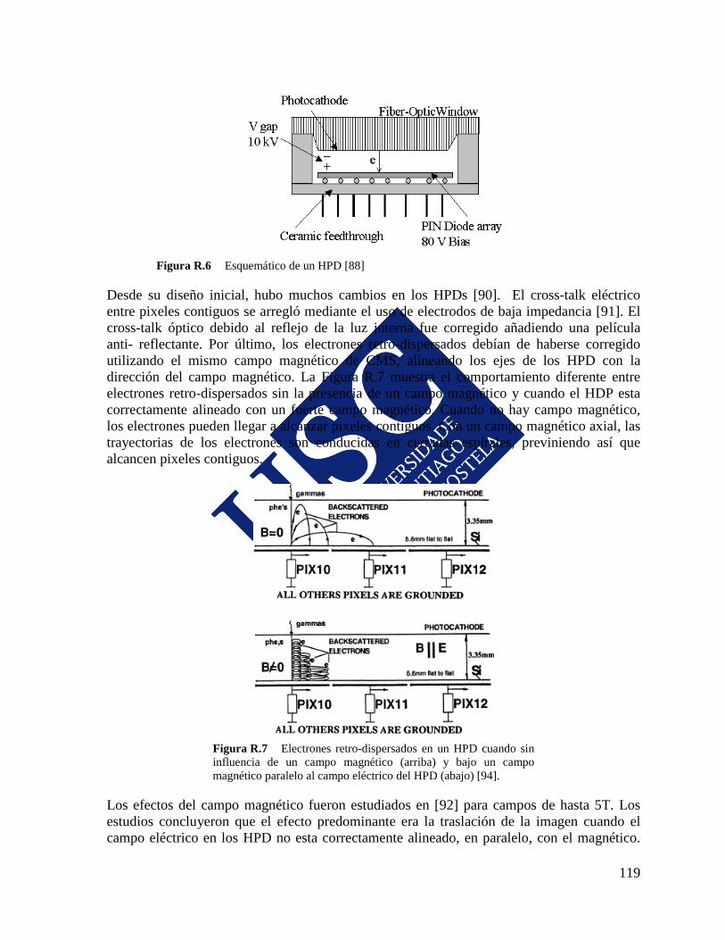
119
Esquemático de un HPD [88] Figura R.6
Desde su diseño inicial, hubo muchos cambios en los HPDs [90]. El cross-talk eléctrico entre pixeles contiguos se arregló mediante el uso de electrodos de baja impedancia [91]. El cross-talk óptico debido al reflejo de la luz interna fue corregido añadiendo una película anti- reflectante. Por último, los electrones retro-dispersados debían de haberse corregido utilizando el mismo campo magnético de CMS, alineando los ejes de los HPD con la dirección del campo magnético. La Figura R.7 muestra el comportamiento diferente entre electrones retro-dispersados sin la presencia de un campo magnético y cuando el HDP esta correctamente alineado con un fuerte campo magnético. Cuando no hay campo magnético, los electrones pueden llegar a alcanzar pixeles contiguos. Con un campo magnético axial, las trayectorias de los electrones son conducidas en cerradas espirales, previniendo así que alcancen pixeles contiguos.
Electrones retro-dispersados en un HPD cuando sin Figura R.7
influencia de un campo magnético (arriba) y bajo un campo magnético paralelo al campo eléctrico del HPD (abajo) [94].
Los efectos del campo magnético fueron estudiados en [92] para campos de hasta 5T. Los estudios concluyeron que el efecto predominante era la traslación de la imagen cuando el campo eléctrico en los HPD no esta correctamente alineado, en paralelo, con el magnético.
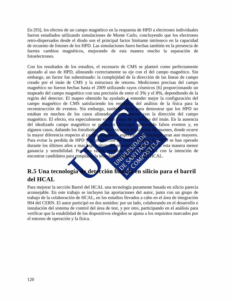
120
En [93], los efectos de un campo magnético en la respuesta de HPD a electrones individuales fueron estudiados utilizando simulaciones de Monte Carlo, concluyendo que los electrones retro-dispersados desde el diodo son el principal factor limitante intrínseco en la capacidad de recuento de fotones de los HPD. Las simulaciones fuero hechas también en la presencia de fuertes cambios magnéticos, mejorando de esta manera mucho la separación de fotoelectrones. Con los resultados de los estudios, el escenario de CMS se planteó como perfectamente ajustado al uso de HPD, alineando correctamente su eje con el del campo magnético. Sin embargo, un factor fue subestimado: la complejidad de la dirección de las líneas de campo creado por el imán de CMS y la estructura de retorno. Mediciones precisas del campo magnético no fueron hechas hasta el 2009 utilizando rayos cósmicos [6] proporcionando un mapeado del campo magnético con una precisión de entre el 3% y el 8%, dependiendo de la región del detector. El mapeo obtenido ha ayudado a entender mejor la configuración del campo magnético de CMS satisfaciendo los requisitos del análisis de la física para la reconstrucción de eventos. Sin embargo, también sirvió para demostrar que los HPD no estaban en muchos de los casos alineados correctamente con la dirección del campo magnético. El efecto, era especialmente visible fuera de la bobina del imán. En la ausencia del idealizado campo magnético se producen descargas generando falsos eventos y, en algunos casos, dañando los fotodiodos. En los extremos del sistema de muones, donde ocurre la mayor diferencia respecto al campo magnético esperado, las descargas eran aun mayores. Para evitar la perdida de HPD y la producción de falsos eventos, los HPD se han operado durante los últimos años a mas bajo voltaje del planeado, alcanzando de esta manera menor ganancia y sensibilidad. Por esta razón, estudios fueron realizados con la intención de encontrar candidatos para remplazar la tecnología de detección del HCAL.
R.5 Una tecnología de detección basada en silicio para el barril del HCAL Para mejorar la sección Barrel del HCAL una tecnología puramente basada en silicio parecía aconsejable. En este trabajo se incluyen las aportaciones del autor, junto con un grupo de trabajo de la colaboración de HCAL, en los estudios llevados a cabo en el área de integración 904 del CERN. El autor participó en dos sentidos: por un lado, colaborando en el desarrollo e instalación del sistema de control del área de test, y por otro, participando en el análisis para verificar que la estabilidad de los dispositivos elegidos se ajusta a los requisitos marcados por el entorno de operación y la física.
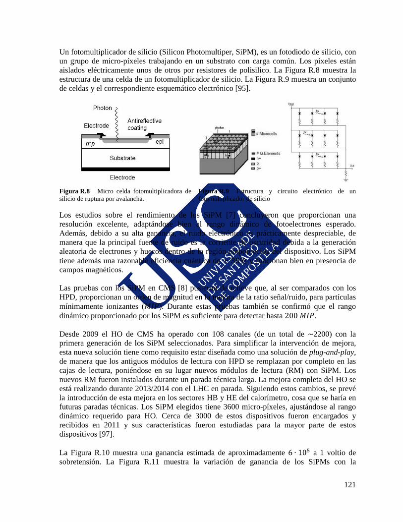
121
Un fotomultiplicador de silicio (Silicon Photomultiper, SiPM), es un fotodiodo de silicio, con un grupo de micro-píxeles trabajando en un substrato con carga común. Los píxeles están aislados eléctricamente unos de otros por resistores de polisilico. La Figura R.8 muestra la estructura de una celda de un fotomultiplicador de silicio. La Figura R.9 muestra un conjunto de celdas y el correspondiente esquemático electrónico [95].
Micro celda fotomultiplicadora de Figura R.8
silicio de ruptura por avalancha. Estructura y circuito electrónico de un Figura R.9
fotomultiplicador de silicio
Los estudios sobre el rendimiento de los SiPM [7] concluyeron que proporcionan una resolución excelente, adaptándose bien al rango dinámico de fotoelectrones esperado. Además, debido a su alta ganancia, el ruido electrónico es prácticamente despreciable, de manera que la principal fuente de ruido es la corriente de oscuridad debida a la generación aleatoria de electrones y huecos dentro de la región empobrecida del dispositivo. Los SiPM tiene además una razonable eficiencia cuántica de ≈ 30% y funcionan bien en presencia de campos magnéticos. Las pruebas con los SiPM en CMS [8] pusieron de relieve que, al ser comparados con los HPD, proporcionan un orden de magnitud en la mejora de la ratio señal/ruido, para partículas mínimamente ionizantes (𝑀𝐼𝑃). Durante estas pruebas también se confirmó que el rango dinámico proporcionado por los SiPM es suficiente para detectar hasta 200 𝑀𝐼𝑃. Desde 2009 el HO de CMS ha operado con 108 canales (de un total de ~2200) con la primera generación de los SiPM seleccionados. Para simplificar la intervención de mejora, esta nueva solución tiene como requisito estar diseñada como una solución de plug-and-play, de manera que los antiguos módulos de lectura con HPD se remplazan por completo en las cajas de lectura, poniéndose en su lugar nuevos módulos de lectura (RM) con SiPM. Los nuevos RM fueron instalados durante un parada técnica larga. La mejora completa del HO se está realizando durante 2013/2014 con el LHC en parada. Siguiendo estos cambios, se prevé la introducción de esta mejora en los sectores HB y HE del calorímetro, cosa que se haría en futuras paradas técnicas. Los SiPM elegidos tiene 3600 micro-píxeles, ajustándose al rango dinámico requerido para HO. Cerca de 3000 de estos dispositivos fueron encargados y recibidos en 2011 y sus características fueron estudiadas para la mayor parte de estos dispositivos [97]. La Figura R.10 muestra una ganancia estimada de aproximadamente 6 ∙ 105 a 1 voltio de sobretensión. La Figura R.11 muestra la variación de ganancia de los SiPMs con la
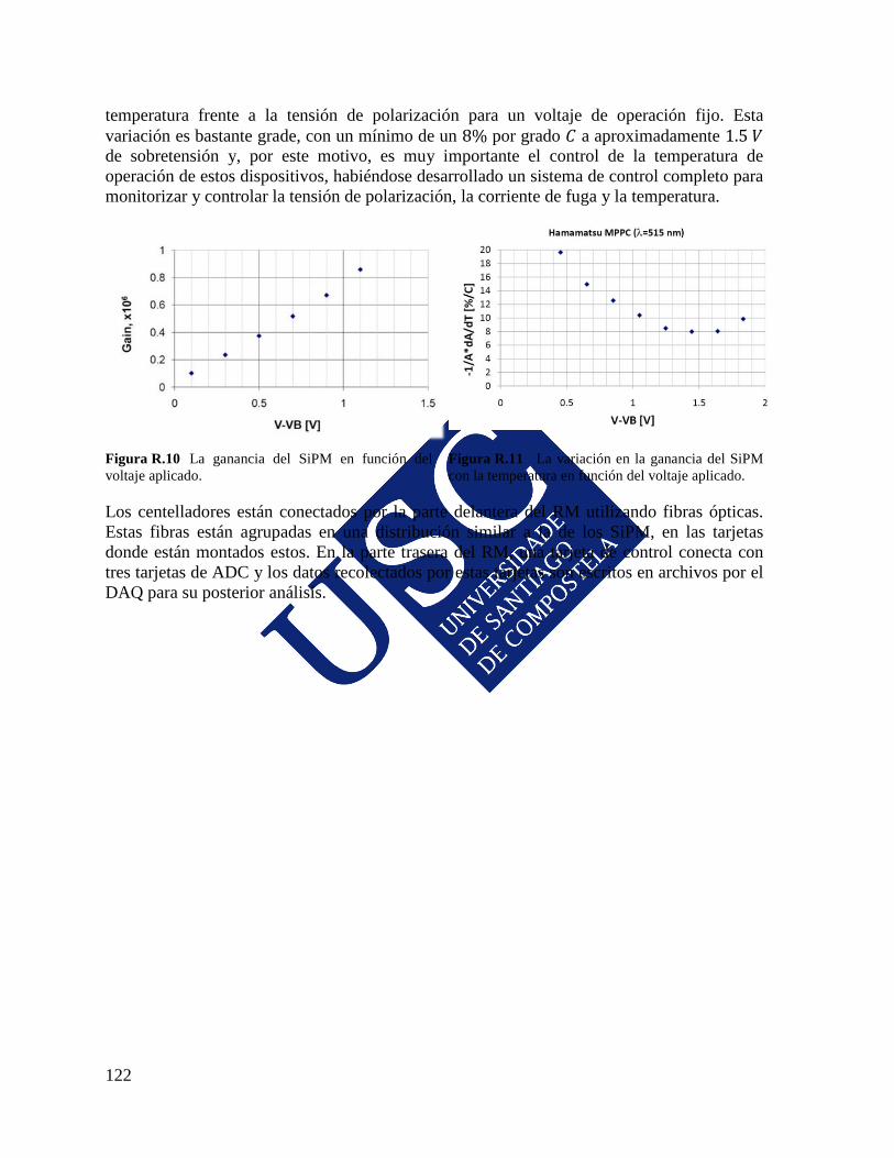
122
temperatura frente a la tensión de polarización para un voltaje de operación fijo. Esta variación es bastante grade, con un mínimo de un 8% por grado 𝐶 a aproximadamente 1.5 𝑉 de sobretensión y, por este motivo, es muy importante el control de la temperatura de operación de estos dispositivos, habiéndose desarrollado un sistema de control completo para monitorizar y controlar la tensión de polarización, la corriente de fuga y la temperatura.
La ganancia del SiPM en función del Figura R.10voltaje aplicado.
La variación en la ganancia del SiPM Figura R.11con la temperatura en función del voltaje aplicado.
Los centelladores están conectados por la parte delantera del RM utilizando fibras ópticas. Estas fibras están agrupadas en una distribución similar a la de los SiPM, en las tarjetas donde están montados estos. En la parte trasera del RM, una tarjeta de control conecta con tres tarjetas de ADC y los datos recolectados por estas tarjetas son escritos en archivos por el DAQ para su posterior análisis.
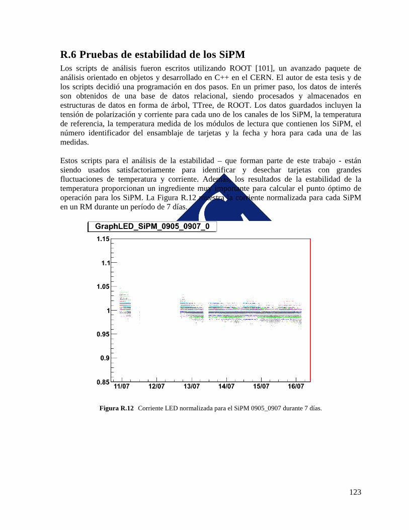
123
R.6 Pruebas de estabilidad de los SiPM Los scripts de análisis fueron escritos utilizando ROOT [101], un avanzado paquete de análisis orientado en objetos y desarrollado en C++ en el CERN. El autor de esta tesis y de los scripts decidió una programación en dos pasos. En un primer paso, los datos de interés son obtenidos de una base de datos relacional, siendo procesados y almacenados en estructuras de datos en forma de árbol, TTree, de ROOT. Los datos guardados incluyen la tensión de polarización y corriente para cada uno de los canales de los SiPM, la temperatura de referencia, la temperatura medida de los módulos de lectura que contienen los SiPM, el número identificador del ensamblaje de tarjetas y la fecha y hora para cada una de las medidas. Estos scripts para el análisis de la estabilidad – que forman parte de este trabajo - están siendo usados satisfactoriamente para identificar y desechar tarjetas con grandes fluctuaciones de temperatura y corriente. Además, los resultados de la estabilidad de la temperatura proporcionan un ingrediente muy importante para calcular el punto óptimo de operación para los SiPM. La Figura R.12 muestra la corriente normalizada para cada SiPM en un RM durante un período de 7 días.
Corriente LED normalizada para el SiPM 0905_0907 durante 7 días. Figura R.12

124
R.7 Estudio del Rango Dinámico de los SiPM en un test-beam Se incluye en este trabajo los resultados del test-beam que fue realizado en el área H2, que es parte de la Infraestructura Norte (Figura R.13) de haces secundarios del CERN. Un haz de protones disparado contra un objetivo de berilio produjo partículas secundarias que, debidamente separadas utilizando imanes, se condujo hacia objetivos terciarios y absorbentes, para conseguir los haces deseados. Para los estudios que forman parte de esta tesis, fueron seleccionados haces consistentes en piones de 300 𝐺𝑒𝑉 o muones de 150 𝐺𝑒𝑉.
Sistema de haces secundarios del Área Norte del CERN Figura R.13
Como se vio durante los estudios de la estabilidad, para alcanzar la deseada estabilidad de la ganancia es posible actuar sobre la tensión de polarización para elegir un punto de operación donde la variación de temperatura tenga el mínimo impacto en la estabilidad de la ganancia. Sin embargo, cambiar la tensión de polarización también tiene un impacto en otros parámetros de operación, como por ejemplo el rango dinámico de energías del detector. A partir de estudios internos en HCAL [102] se encontró que HO, que tiene como tarea asignada la detección de las partículas asociadas con cascadas de partículas que son en su mayoría absorbidas por el barril del HCAL, necesita poder trabajar con energías de hasta 200 𝑀𝐼𝑃. Diferentes voltajes de polarización fueron probados durante el test-beam de forma que en esta tesis se incluyen los resultados analizados por el autor. Los píxeles individuales de un SiPM son como un contador digital que pueden dispararse una sola vez durante un periodo limitado de tiempo. Hasta que se recuperan, un pixel no puede dispararse de nuevo. El segundo propósito del test-beam fue probar el uso de difusores de luz para distribuir la luz entre más píxeles, incrementando teóricamente de esta manera el rango dinámico del dispositivo. Para verificar esto, el autor comparó los resultados obtenidos con el uso y sin el uso de los difusores.
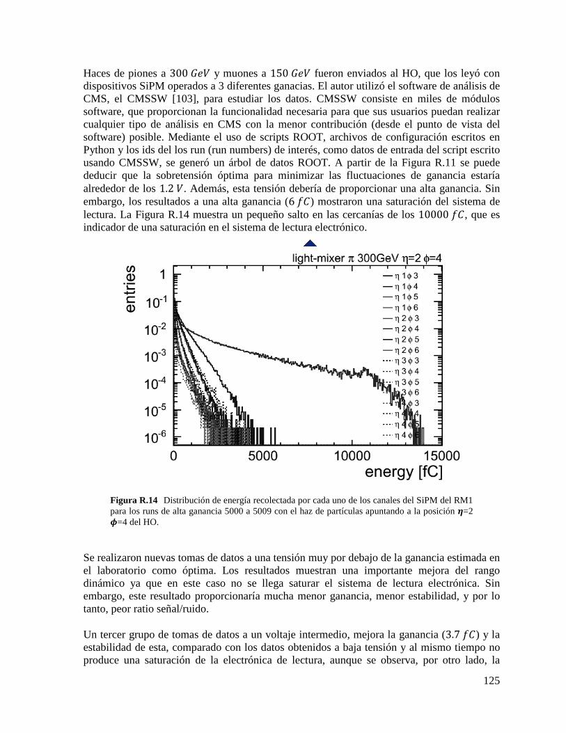
125
Haces de piones a 300 𝐺𝑒𝑉 y muones a 150 𝐺𝑒𝑉 fueron enviados al HO, que los leyó con dispositivos SiPM operados a 3 diferentes ganacias. El autor utilizó el software de análisis de CMS, el CMSSW [103], para estudiar los datos. CMSSW consiste en miles de módulos software, que proporcionan la funcionalidad necesaria para que sus usuarios puedan realizar cualquier tipo de análisis en CMS con la menor contribución (desde el punto de vista del software) posible. Mediante el uso de scripts ROOT, archivos de configuración escritos en Python y los ids del los run (run numbers) de interés, como datos de entrada del script escrito usando CMSSW, se generó un árbol de datos ROOT. A partir de la Figura R.11 se puede deducir que la sobretensión óptima para minimizar las fluctuaciones de ganancia estaría alrededor de los 1.2 𝑉. Además, esta tensión debería de proporcionar una alta ganancia. Sin embargo, los resultados a una alta ganancia (6 𝑓𝐶) mostraron una saturación del sistema de lectura. La Figura R.14 muestra un pequeño salto en las cercanías de los 10000 𝑓𝐶, que es indicador de una saturación en el sistema de lectura electrónico.
Distribución de energía recolectada por cada uno de los canales del SiPM del RM1 Figura R.14
para los runs de alta ganancia 5000 a 5009 con el haz de partículas apuntando a la posición 𝜼=2 𝝓=4 del HO.
Se realizaron nuevas tomas de datos a una tensión muy por debajo de la ganancia estimada en el laboratorio como óptima. Los resultados muestran una importante mejora del rango dinámico ya que en este caso no se llega saturar el sistema de lectura electrónica. Sin embargo, este resultado proporcionaría mucha menor ganancia, menor estabilidad, y por lo tanto, peor ratio señal/ruido. Un tercer grupo de tomas de datos a un voltaje intermedio, mejora la ganancia (3.7 𝑓𝐶) y la estabilidad de esta, comparado con los datos obtenidos a baja tensión y al mismo tiempo no produce una saturación de la electrónica de lectura, aunque se observa, por otro lado, la

126
saturación del dispositivo SiPM debido a su número finito de píxeles. Ahora bien, con el uso de los difusores de luz se incrementa significativamente (~15%) el rango dinámico del dispositivo. La Figura R.15 muestra una comparación entre la respuesta cuando se usan difusores de luz (curva inferior) y la respuesta sin usar difusores de luz (curva superior).
Comparación de la distribución de energía, expresada en el número de píxieles Figura R.15
disparados para el canal 16 del SiPM en el RM1 cuando se usan difusores de luz (curva ligeramente superior) y al no usar difusores de luz (curva inferior) a ganancia intermedia.
Para mirar al rango dinámico relevante a la física, los resultados necesitan ser presentados en una escala proporcional a los procesos físicos. El MIP (efecto producido por una Minimum Ionizing Particle) constituye una unidad muy útil en la escala de estos experimentos de física de partículas. La distribución de energía producida por partículas con ionización mínima en un centellador fino corresponde con una distribución de Landau. Sin embargo, HO no utiliza realmente centelladores finos, sino más bien gruesos. Esto, junto con el ruido introducido por la electrónica de lectura en la trayectoria de las partículas, introduce un factor en forma de distribución gaussiana. Por este motivo, la respuesta para partículas de ionización mínima se ajusta a una curva de convolución Landau-Gaussiana. La Figura R.16 muestra que utilizando los SiPM al voltaje intermedio seleccionado y con difusores de luz, se consigue cubrir prácticamente hasta 200 𝑀𝐼𝑃, alcanzándose así el máximo rango requerido. Además miembros de la colaboración de HCAL han desarrollado una corrección matemática de la curva con la que extienden el rango dinámico cuando comienza la saturación del dispositivo, si bien con la limitación de introducir un error que incrementa al acercarse a la saturación del dispositivo. Los resultados de este análisis concluyen que el dispositivo SiPM puede cubrir el rango dinámico necesario, tal como podían los HPD, con la adición de que los SiPM obtienen
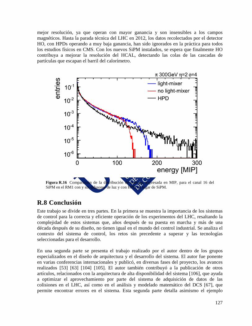
127
mejor resolución, ya que operan con mayor ganancia y son insensibles a los campos magnéticos. Hasta la parada técnica del LHC en 2012, los datos recolectados por el detector HO, con HPDs operando a muy baja ganancia, han sido ignorados en la práctica para todos los estudios físicos en CMS. Con los nuevos SiPM instalados, se espera que finalmente HO contribuya a mejorar la resolución del HCAL, detectando las colas de las cascadas de partículas que escapan el barril del calorímetro.
Comparación de la distribución de energía, expresada en MIP, para el canal 16 del Figura R.16
SiPM en el RM1 con y sin difusores de luz y con HPD en lugar de SiPM.
R.8 Conclusión Este trabajo se divide en tres partes. En la primera se muestra la importancia de los sistemas de control para la correcta y eficiente operación de los experimentos del LHC, resaltando la complejidad de estos sistemas que, años después de su puesta en marcha y más de una década después de su diseño, no tienen igual en el mundo del control industrial. Se analiza el contexto del sistema de control, los retos sin precedente a superar y las tecnologías seleccionadas para el desarrollo. En una segunda parte se presenta el trabajo realizado por el autor dentro de los grupos especializados en el diseño de arquitectura y el desarrollo del sistema. El autor fue ponente en varias conferencias internacionales y publicó, en diversas fases del proyecto, los avances realizados [53] [63] [104] [105]. El autor también contribuyó a la publicación de otros artículos, relacionados con la arquitectura de alta disponibilidad del sistema [106], que ayuda a optimizar el aprovechamiento por parte del sistema de adquisición de datos de las colisiones en el LHC, así como en el análisis y modelado matemático del DCS [67], que permite encontrar errores en el sistema. Esta segunda parte detalla asimismo el ejemplo
128
concreto de implementación del sistema de control del ECAL, de vital importancia para el rendimiento de este detector, que ha jugado un papel muy importante en el descubrimiento del Bosón de Higgs [107]. El autor colaboró en diversas publicaciones relacionadas con este desarrollo [70] [71] [72] [73]. La última parte del trabajo se centra en el análisis técnico de detectores propuestos para mejorar los calorímetros de CMS. Se proporcionan ejemplos concretos de parámetros de control, como la tensión de polarización o la temperatura de operación, muy importantes para garantizar el funcionamiento preciso y estable de los nuevos SiPMs, que serán usados en el calorímetro hadrónico externo de CMS cuando concluya la actual parada técnica. El entorno de pruebas y el sistema de control de los SiPM fueron presentados en una conferencia de calorimetría [108] y los resultados del análisis realizado por el autor, junto con los resultados de otros test realizados por miembros de HCAL, fueron presentado a la colaboración en un informe conjunto en [109]. De estos estudios se resalta que el ruido está dominado por la electrónica, y no por el SiPM, y que con la instrumentación desarrollada se alcanza una excelente estabilidad en la temperatura (𝑅𝑀𝑆 ± 0.025 𝐾, equivalente a 1 𝐿𝑆𝐵). Finalmente, los resultados de un test-beam han servido para demostrar tres cosas. Primera, que a una ganancia de 6 fC, considerada óptima para la estabilidad, se produce una saturación de la electrónica de lectura. Segunda, que a una ganancia menor, de 3.7 fC, y en combinación con el uso de difusores de luz, se consigue alcanzar el rango dinámico de energías requerido por el programa físico de CMS para HO, sin saturar la electrónica de lectura y proporcionando la estabilidad requerida.

129
Appendix A. JCOP components in CMS As it was introduced in section 2.3.3, the JCOP framework provides three types of component: the general core ones, device components and tools. Table A.1 shows the JCOP components used by CMS. These core components are installed in all CMS production servers.
Component Name Component Details
fwCore
This component is a set of libraries that hide the datapoint level layer complexity providing other JCOP components with the functionality to create alerts, to configure the archive and to set the hardware address of datapoints. CMS framework uses also many functions provided by this component.
fwAccesControl Contains the libraries and panels to configure a role-based access control mechanism in the DCS. In addition it offers the possibility of creating an access control server centralizing the access control of the whole distributed system.
fwLogErrHandler Collects the system event log and publishes it via DIM.
fwInstallation fwSystemConfiguration
These components are used to deploy all the rest of JCOP components. It allows creating a central database where the information about the projects and the components deployed in each one can be stored and retrieved. They allow for two different operational modes. An inventory mode where the systems’ configurations are dumped to the database whenever they change and a second one where the database contains the master configuration and everything configured in the database is applied automatically to the corresponding systems.
fwConfigurationDB It allows storing and retrieving from a database the devices created in a system. Furthermore, it provides a way to create configuration “recipes” with the hardware settings used for different experiment operation physics modes.
fwDIP Provides the communication support to allow for datapoint value publishing to DIP clients and for datapoint subscription from DIP values published from other systems.
Table A.1 The core JCOP framework components used in CMS
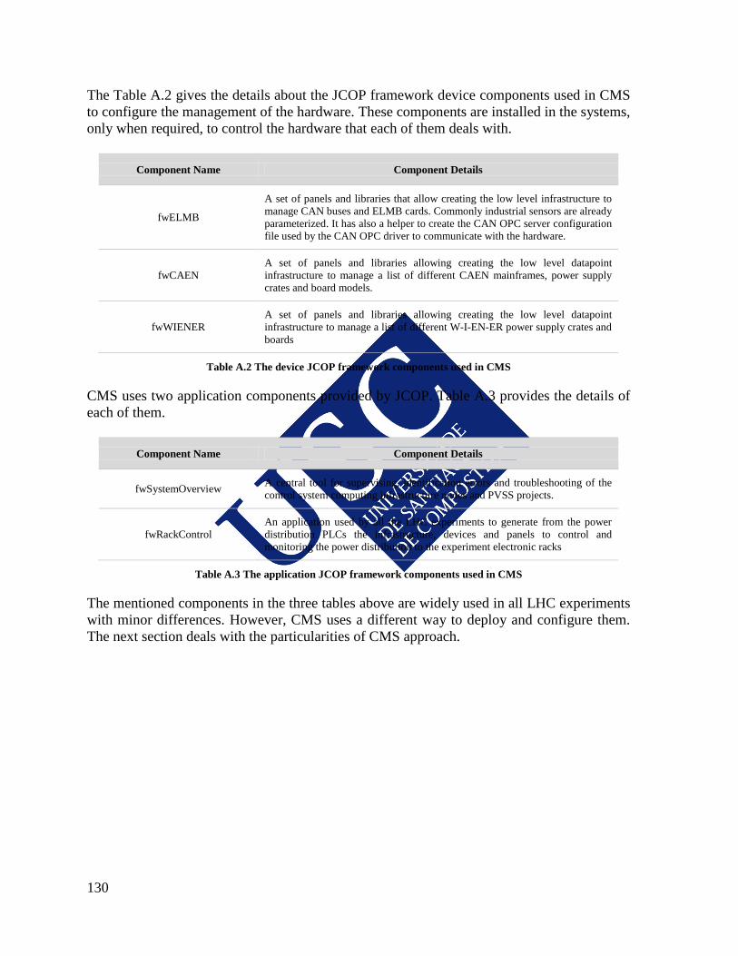
130
The Table A.2 gives the details about the JCOP framework device components used in CMS to configure the management of the hardware. These components are installed in the systems, only when required, to control the hardware that each of them deals with.
Component Name Component Details
fwELMB
A set of panels and libraries that allow creating the low level infrastructure to manage CAN buses and ELMB cards. Commonly industrial sensors are already parameterized. It has also a helper to create the CAN OPC server configuration file used by the CAN OPC driver to communicate with the hardware.
fwCAEN A set of panels and libraries allowing creating the low level datapoint infrastructure to manage a list of different CAEN mainframes, power supply crates and board models.
fwWIENER A set of panels and libraries allowing creating the low level datapoint infrastructure to manage a list of different W-I-EN-ER power supply crates and boards
Table A.2 The device JCOP framework components used in CMS
CMS uses two application components provided by JCOP. Table A.3 provides the details of each of them.
Component Name Component Details
fwSystemOverview A central tool for supervising, identification errors and troubleshooting of the control system computing infrastructure nodes and PVSS projects.
fwRackControl An application used by all the LHC experiments to generate from the power distribution PLCs the infrastructure, devices and panels to control and monitoring the power distribution to the experiment electronic racks
Table A.3 The application JCOP framework components used in CMS
The mentioned components in the three tables above are widely used in all LHC experiments with minor differences. However, CMS uses a different way to deploy and configure them. The next section deals with the particularities of CMS approach.

131
Appendix B. Hadronic calorimetry In Particle Physics, a calorimeter [112] is conceptually a block of matter that is sufficiently thick to stop an incident particle and make it deposit all of its energy within the material. In order to deposit its energy, the incident primary particle interacts with the material producing a shower of secondary ones with increasingly lower energy. In order to measure the energy, a fraction of the deposited energy produces a measurable signal (e.g. a scintillating light). This measurable signal is proportional to the energy of the initial particle. However, the same incident particle will not always develop the same particle shower in the calorimeter material. There is an uncertainty in the measured energy driven by the statistical fluctuation of this shower development and the calorimeter resolution 𝜎 𝐸⁄ , improves with increasing energy 𝐸 like 1 √𝐸⁄ . Calorimeters have the advantage of being sensitive not only to charged particles but also to neutral ones. The segmentation of calorimeters allow for precise measurement of position and angle of the incident particles. In addition, due to the different response to electrons, muons and hadrons, calorimeters can also be used to help on particle identification. Finally, their fast response makes them suitable to operate in experiments with high particle rates. The granularity of a calorimeter characterizes the spatial separation between two particles in an event. The desired granularity is defined by the physics studies performed and depends on the minimum angle 𝜃 at which two particles have to be distinguished. On the other hand, the energy at which the incident particles are expected determines the thickness of the calorimeter necessary for full shower containment. The needed thickness increases logarithmically with energy. In contrast with electromagnetic calorimeter showers, dominated mainly by bremsstrahlung and pair production, the hadronic showers are considerably more complex. First of all, there is a wide spectrum of secondary produced particles. Second, the nuclear effects related with the excitation of the absorber material nuclei can become dominant. One of the main characteristic properties of hadronic calorimeters, defining the scale of the shower, is the nuclear absorption length:
𝜆 = 𝐴 𝑁𝐴⁄ 𝜎𝐴𝑏𝑠 Eq. d.1
where 𝐴 is the mass number of the absorber, 𝑁𝐴 is Avogadro’s number and 𝜎𝐴𝑏𝑠 is the cross section of the absorber material. The average shower dimensions are proportional to 𝜆. In the hadronic interactions there is usually multiple particle production with limited transverse momentum for which about half of the energy is consumed. The secondaries are mainly nucleons and pions. The remaining half of the shower energy goes into fast forward-going particles. The understanding of the shower developments and the dependency on the material and energy are essential in order to design a calorimeter. Monte Carlo simulations can be used in order to understand the shower developments for different detector geometries and materials. The depth, radius and lateral granularity of the calorimeter are defined by the physics

132
requirements. The limit on the energy resolution on a calorimeter is dictated by the intrinsic shower fluctuations and the electronic instrumental limits. For electromagnetic showers the limit set by the shower fluctuations is really small (𝜎 𝐸⁄ ≅ 0.005𝐸−1 2⁄ [𝐺𝑒𝑉]), however, in hadronic calorimeters this is not the case and the inherent shower fluctuations are the major factor determining the performance (𝜎 𝐸⁄ ≅ 0.25𝐸−1 2⁄ [𝐺𝑒𝑉] with compensation for nuclear effects). There is therefore no incentive on using hadronic homogenous detectors since the scintillating material is much more expensive than the absorber one used in sampling calorimeters. In a sample calorimeter thick layers of absorber inert material where the showers are developed are interleaved with active scintillator layers where the energy loss is measured at fixed intervals. The energy loss in the sampling material is only a small proportion of the total shower energy but it is a fixed fraction of it. The energy resolution of a calorimeter is expressed like this:
𝜎𝐸
=𝑎√𝐸
⨁𝑏𝐸⨁ 𝑐 Eq. d.2
where the first term 𝑎 √𝐸⁄ accounts for the contribution of the sampling fluctuations that is ≃ 0.09�Δ𝐸 𝐸⁄ for hadronic showers [113], the second term 𝑏 𝐸⁄ represents the contributions of the readout electronics noise and background processes and the third one is the contribution due to calibration errors, non-uniformities and non-linearities in photomultipliers, proportional counters, ADC's, etc.
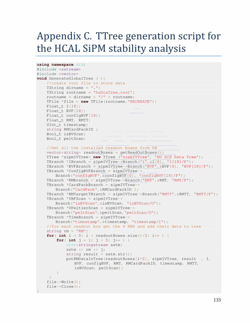
133
Appendix C. TTree generation script for the HCAL SiPM stability analysis using namespace std; #include <sstream> #include <vector> void GenerateGlobalTree ( ){ //create root file to store data TString dirname = "."; TString rootname = "hoDcsTree.root"; rootname = dirname + "/" + rootname; TFile *file = new TFile(rootname,"RECREATE"); Float_t I[18]; Float_t BVF[18]; Float_t configBVF[18]; Float_t RMT, RMTT; UInt_t timestamp; string RMCardPackID ; Bool_t isBVScan; Bool_t peltScan; //Get all the installed readout boxes from DB vector<string> readoutBoxes = getReadOutBoxes(); TTree *sipmIVTree= new TTree ("sipmIVTree", "HO DCS Data Tree"); TBranch *IBranch = sipmIVTree->Branch("I",&I[0], "I[18]/F"); TBranch *BVFBranch = sipmIVTree->Branch("BVF",&BVF[0], "BVF[18]/F"); TBranch *ConfigBVFBranch = sipmIVTree-> Branch("configBVF",&configBVF[0], "configBVF[18]/F"); TBranch *RMBranch = sipmIVTree->Branch("RMT",&RMT, "RMT/F"); TBranch *CardPackBranch = sipmIVTree-> Branch("CardPack",&RMCardPackID ); TBranch *RMTargetTBranch = sipmIVTree->Branch("RMTT",&RMTT, "RMTT/F"); TBranch *VBFScan = sipmIVTree-> Branch("isBVScan",&isBVScan, "isBVScan/O"); TBranch *VPeltierScan = sipmIVTree-> Branch("peltScan",&peltScan,"peltScan/O"); TBranch *TimeBranch = sipmIVTree-> Branch("timestamp",×tamp, "timestamp/i"); //for each readout box get the 4 RMS and add their data to tree string rm = "RM"; for( int i = 0; i < readoutBoxes.size()/2; i++ ) { for( int j = 1; j < 5; j++ ) { std::stringstream sstm; sstm << rm << j; string result = sstm.str(); putRMDataInTree(readoutBoxes[i*2], sipmIVTree, result , I, BVF, configBVF, RMT, RMCardPackID, timestamp, RMTT, isBVScan, peltScan); } } file->Write(); file->Close(); }
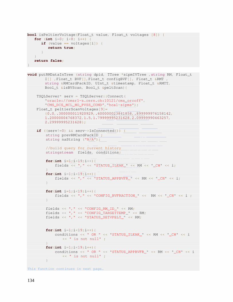
134
bool isPeltierVoltage(Float_t value, Float_t voltages [8]) { for (int i=0; i<8; i++) { if (value == voltages[i]) { return true; } } return false; } void putRMDataInTree (string dpid, TTree *sipmIVTree ,string RM, Float_t I[] ,Float_t BVF[],Float_t configBVF[], Float_t &RMT , string &RMCardPackID, UInt_t ×tamp, Float_t &RMTT, Bool_t &isBVScan, Bool_t &peltScan){ TSQLServer* serv = TSQLServer::Connect( "oracle://cmsr1-s.cern.ch:10121/cms_orcoff", "CMS_DCS_HCL_HO_PVSS_COND","hcal-sipms"); Float_t peltierScanVoltages[9]= {0.0,.300000011920929,.600000023841858,.899999976158142, 1.20000004768372,1.5,1.79999995231628,2.09999990463257, 2.29999995231628}; if ((serv!=0) && serv->IsConnected()) { string prevRMCardPackID ; string naString ("N/A"); //build query for current history stringstream fields, conditions; for(int i=1;i<19;i++){ fields << "," << "STATUS_ILEAK_" << RM << "_CH" << i; } for(int i=1;i<19;i++){ fields << "," << "STATUS_APPBVFR_" << RM << "_CH" << i; } for(int i=1;i<19;i++){ fields << "," << "CONFIG_BVFRACTION_" << RM << "_CH" << i ; } fields << "," << "CONFIG_RM_ID_" << RM; fields << "," << "CONFIG_TARGETTEMP_" << RM; fields << "," << "STATUS_SETVPELT_" << RM; for(int i=1;i<19;i++){ conditions << " OR " << "STATUS_ILEAK_" << RM << "_CH" << i << " is not null" ; } for(int i=1;i<19;i++){ conditions << " OR " << "STATUS_APPBVFR_" << RM << "_CH" << i << " is not null" ; } This function continues in next page…
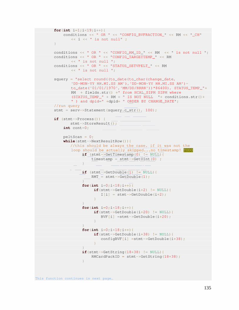
135
for(int i=1;i<19;i++){ conditions << " OR " << "CONFIG_BVFRACTION_" << RM << "_CH" << i << " is not null" ; } conditions << " OR " << "CONFIG_RM_ID_" << RM << " is not null "; conditions << " OR " << "CONFIG_TARGETTEMP_" << RM << " is not null "; conditions << " OR " << "STATUS_SETVPELT_" << RM << " is not null "; squery = "select round((to_date(to_char(change_date, 'DD-MON-YY HH.MI.SS AM'),'DD-MON-YY HH.MI.SS AM')- to_date('01/01/1970','MM/DD/RRRR'))*86400), STATUS_TEMP_"+ RM + fields.str() +" from HCAL_SIPM SIPM where (STATUS_TEMP_" + RM + " IS NOT NULL "+ conditions.str()+ " ) and dpid=" +dpid+ " ORDER BY CHANGE_DATE"; //run query stmt = serv->Statement(squery.c_str(), 100); if (stmt->Process()) { stmt->StoreResult(); int cont=0; peltScan = 0; while(stmt->NextResultRow()){ //this should be always the case. if it was not the loop should be actually skipped...no timestamp! TODO if (stmt->GetTimestamp(0) != NULL){ timestamp = stmt->GetUInt(0) ; } if (stmt->GetDouble(1) != NULL){ RMT = stmt->GetDouble(1); } for(int i=0;i<18;i++){ if(stmt->GetDouble(i+2) != NULL){ I[i] = stmt->GetDouble(i+2); } } for(int i=0;i<18;i++){ if(stmt->GetDouble(i+20) != NULL){ BVF[i] =stmt->GetDouble(i+20); } } for(int i=0;i<18;i++){ if(stmt->GetDouble(i+38) != NULL){ configBVF[i] =stmt->GetDouble(i+38); } } if(stmt->GetString(18+38) != NULL){ RMCardPackID = stmt->GetString(18+38); } This function continues in next page…
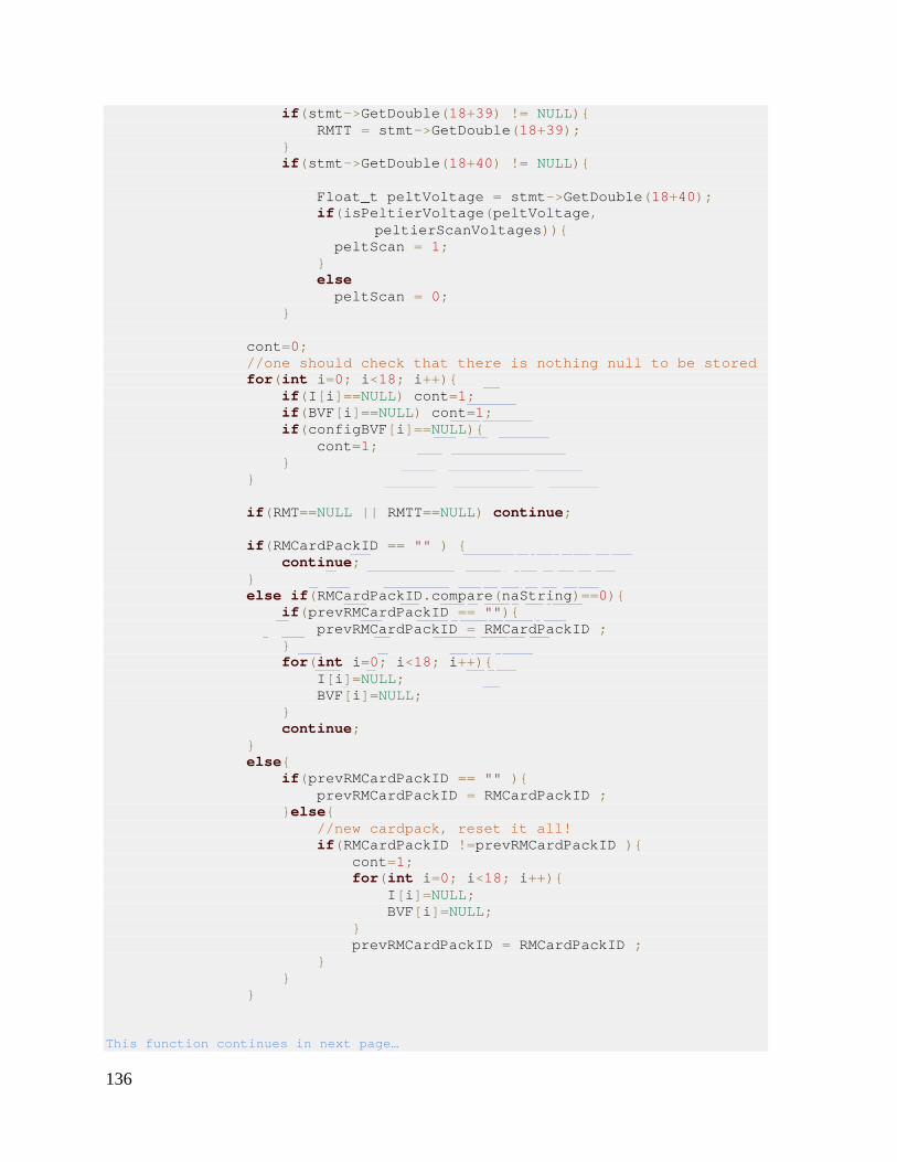
136
if(stmt->GetDouble(18+39) != NULL){ RMTT = stmt->GetDouble(18+39); } if(stmt->GetDouble(18+40) != NULL){ Float_t peltVoltage = stmt->GetDouble(18+40); if(isPeltierVoltage(peltVoltage, peltierScanVoltages)){ peltScan = 1; } else peltScan = 0; } cont=0; //one should check that there is nothing null to be stored for(int i=0; i<18; i++){ if(I[i]==NULL) cont=1; if(BVF[i]==NULL) cont=1; if(configBVF[i]==NULL){ cont=1; } } if(RMT==NULL || RMTT==NULL) continue; if(RMCardPackID == "" ) { continue; } else if(RMCardPackID.compare(naString)==0){ if(prevRMCardPackID == ""){ prevRMCardPackID = RMCardPackID ; } for(int i=0; i<18; i++){ I[i]=NULL; BVF[i]=NULL; } continue; } else{ if(prevRMCardPackID == "" ){ prevRMCardPackID = RMCardPackID ; }else{ //new cardpack, reset it all! if(RMCardPackID !=prevRMCardPackID ){ cont=1; for(int i=0; i<18; i++){ I[i]=NULL; BVF[i]=NULL; } prevRMCardPackID = RMCardPackID ; } } } This function continues in next page…
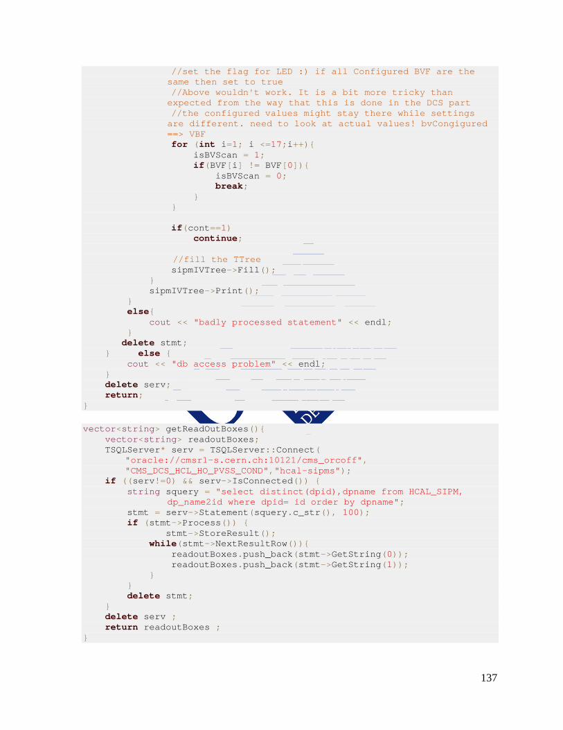
137
//set the flag for LED :) if all Configured BVF are the same then set to true //Above wouldn't work. It is a bit more tricky than expected from the way that this is done in the DCS part //the configured values might stay there while settings are different. need to look at actual values! bvCongigured ==> VBF for (int i=1; i <=17;i++){ isBVScan = 1; if(BVF[i] != BVF[0]){ isBVScan = 0; break; } } if(cont==1) continue; //fill the TTree sipmIVTree->Fill(); } sipmIVTree->Print(); } else{ cout << "badly processed statement" << endl; } delete stmt; } else { cout << "db access problem" << endl; } delete serv; return; } vector<string> getReadOutBoxes(){ vector<string> readoutBoxes; TSQLServer* serv = TSQLServer::Connect( "oracle://cmsr1-s.cern.ch:10121/cms_orcoff", "CMS_DCS_HCL_HO_PVSS_COND","hcal-sipms"); if ((serv!=0) && serv->IsConnected()) { string squery = "select distinct(dpid),dpname from HCAL_SIPM, dp_name2id where dpid= id order by dpname"; stmt = serv->Statement(squery.c_str(), 100); if (stmt->Process()) { stmt->StoreResult(); while(stmt->NextResultRow()){ readoutBoxes.push_back(stmt->GetString(0)); readoutBoxes.push_back(stmt->GetString(1)); } } delete stmt; } delete serv ; return readoutBoxes ; }

138
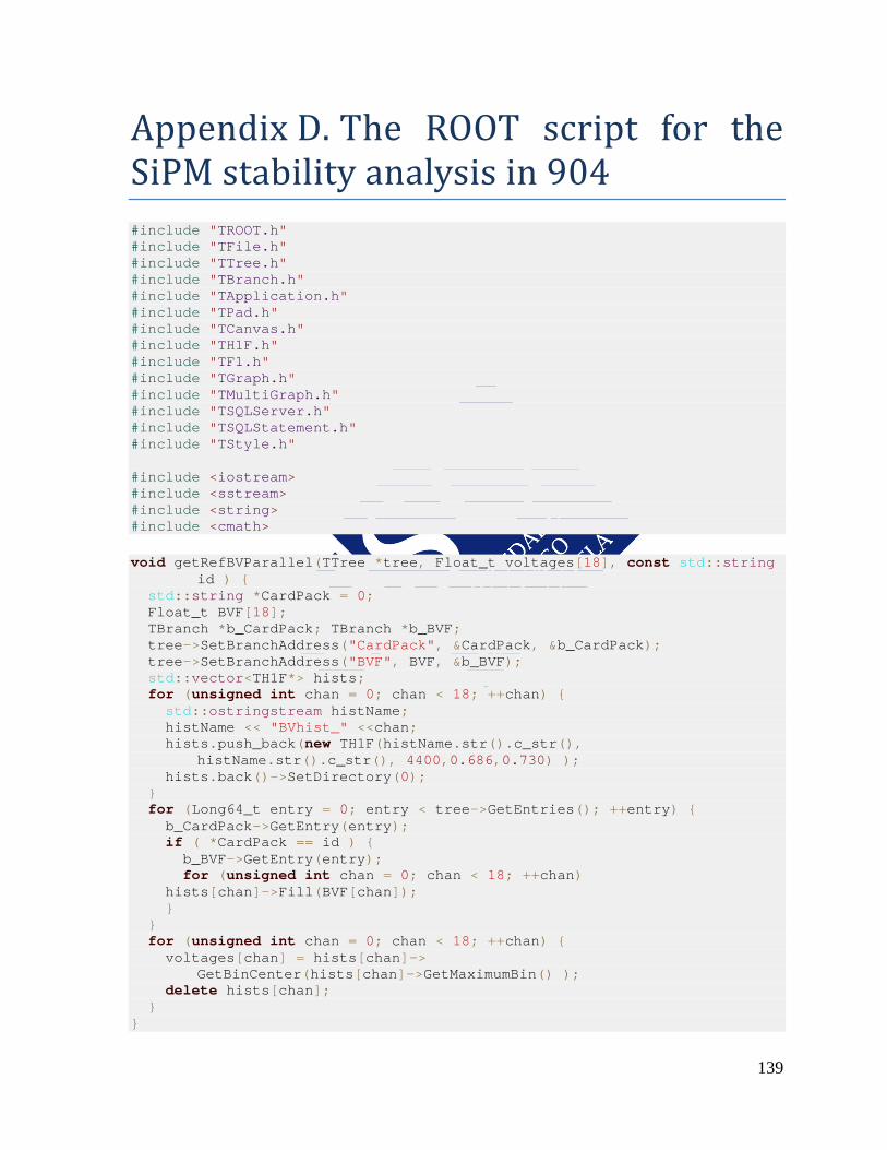
139
Appendix D. The ROOT script for the SiPM stability analysis in 904 #include "TROOT.h" #include "TFile.h" #include "TTree.h" #include "TBranch.h" #include "TApplication.h" #include "TPad.h" #include "TCanvas.h" #include "TH1F.h" #include "TF1.h" #include "TGraph.h" #include "TMultiGraph.h" #include "TSQLServer.h" #include "TSQLStatement.h" #include "TStyle.h" #include <iostream> #include <sstream> #include <string> #include <cmath> void getRefBVParallel(TTree *tree, Float_t voltages[18], const std::string id ) { std::string *CardPack = 0; Float_t BVF[18]; TBranch *b_CardPack; TBranch *b_BVF; tree->SetBranchAddress("CardPack", &CardPack, &b_CardPack); tree->SetBranchAddress("BVF", BVF, &b_BVF); std::vector<TH1F*> hists; for (unsigned int chan = 0; chan < 18; ++chan) { std::ostringstream histName; histName << "BVhist_" <<chan; hists.push_back(new TH1F(histName.str().c_str(), histName.str().c_str(), 4400,0.686,0.730) ); hists.back()->SetDirectory(0); } for (Long64_t entry = 0; entry < tree->GetEntries(); ++entry) { b_CardPack->GetEntry(entry); if ( *CardPack == id ) { b_BVF->GetEntry(entry); for (unsigned int chan = 0; chan < 18; ++chan) hists[chan]->Fill(BVF[chan]); } } for (unsigned int chan = 0; chan < 18; ++chan) { voltages[chan] = hists[chan]-> GetBinCenter(hists[chan]->GetMaximumBin() ); delete hists[chan]; } }
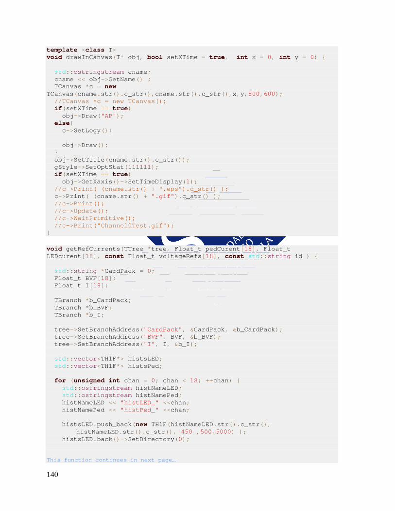
140
template <class T> void drawInCanvas(T* obj, bool setXTime = true, int x = 0, int y = 0) { std::ostringstream cname; cname << obj->GetName() ; TCanvas *c = new TCanvas(cname.str().c_str(),cname.str().c_str(),x,y,800,600); //TCanvas *c = new TCanvas(); if(setXTime == true) obj->Draw("AP"); else{ c->SetLogy(); obj->Draw(); } obj->SetTitle(cname.str().c_str()); gStyle->SetOptStat(111111); if(setXTime == true) obj->GetXaxis()->SetTimeDisplay(1); //c->Print( (cname.str() + ".eps").c_str() ); c->Print( (cname.str() + ".gif").c_str() ); //c->Print(); //c->Update(); //c->WaitPrimitive(); //c->Print("Channel0Test.gif"); } void getRefCurrents(TTree *tree, Float_t pedCurent[18], Float_t LEDcurent[18], const Float_t voltageRefs[18], const std::string id ) { std::string *CardPack = 0; Float_t BVF[18]; Float_t I[18]; TBranch *b_CardPack; TBranch *b_BVF; TBranch *b_I; tree->SetBranchAddress("CardPack", &CardPack, &b_CardPack); tree->SetBranchAddress("BVF", BVF, &b_BVF); tree->SetBranchAddress("I", I, &b_I); std::vector<TH1F*> histsLED; std::vector<TH1F*> histsPed; for (unsigned int chan = 0; chan < 18; ++chan) { std::ostringstream histNameLED; std::ostringstream histNamePed; histNameLED << "histLED_" <<chan; histNamePed << "histPed_" <<chan; histsLED.push_back(new TH1F(histNameLED.str().c_str(), histNameLED.str().c_str(), 450 ,500,5000) ); histsLED.back()->SetDirectory(0); This function continues in next page…
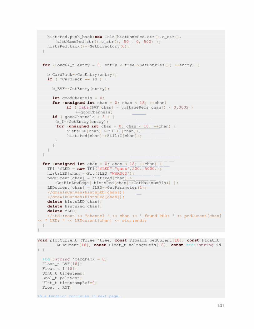
141
histsPed.push_back(new TH1F(histNamePed.str().c_str(), histNamePed.str().c_str(), 50 , 0, 500) ); histsPed.back()->SetDirectory(0); } for (Long64_t entry = 0; entry < tree->GetEntries(); ++entry) { b_CardPack->GetEntry(entry); if ( *CardPack == id ) { b_BVF->GetEntry(entry); int goodChannels = 0; for (unsigned int chan = 0; chan < 18; ++chan) if ( fabs(BVF[chan] - voltageRefs[chan]) < 0.0002 ) ++goodChannels; if ( goodChannels > 8 ) { b_I->GetEntry(entry); for (unsigned int chan = 0; chan < 18; ++chan) { histsLED[chan]->Fill(I[chan]); histsPed[chan]->Fill(I[chan]); } } } } for (unsigned int chan = 0; chan < 18; ++chan) { TF1 *fLED = new TF1("fLED","gaus",500.,5000.); histsLED[chan]->Fit(fLED,"WWRN0Q"); pedCurent[chan] = histsPed[chan]-> GetBinLowEdge( histsPed[chan]->GetMaximumBin() ); LEDcurent[chan] = fLED->GetParameter(1); //drawInCanvas(histsLED[chan]); //drawInCanvas(histsPed[chan]); delete histsLED[chan]; delete histsPed[chan]; delete fLED; //std::cout << "channel " << chan << " found PED: " << pedCurent[chan] << " LED: " << LEDcurent[chan] << std::endl; } } void plotCurrent (TTree *tree, const Float_t pedCurent[18], const Float_t LEDcurent[18], const Float_t voltageRefs[18], const std::string id ) { std::string *CardPack = 0; Float_t BVF[18]; Float_t I[18]; UInt_t timestamp; Bool_t peltScan; UInt_t timestampRef=0; Float_t RMT; This function continues in next page…

142
std::vector< std::vector<Float_t> > currents; std::vector<Float_t> timestamps; currents.resize(18); std::vector<Float_t> RMTs; std::vector< std::vector<Float_t> > currentsCache; std::vector<Float_t> timestampsCache; std::vector<Float_t> RMTCache; currentsCache.resize(18); Bool_t dropBlock=false; TBranch *b_CardPack; TBranch *b_BVF; TBranch *b_I; TBranch *b_timstamp; TBranch *b_peltScan; TBranch *b_RMT; tree->SetBranchAddress("CardPack", &CardPack, &b_CardPack); tree->SetBranchAddress("BVF", BVF, &b_BVF); tree->SetBranchAddress("I", I, &b_I); tree->SetBranchAddress("timestamp",×tamp, &b_timstamp); tree->SetBranchAddress("peltScan",&peltScan, &b_peltScan); tree->SetBranchAddress("RMT",&RMT,&b_RMT); std::ostringstream histNameLED; histNameLED << "HIST_LED_" << id; TH1F* ledHist = new TH1F(histNameLED.str().c_str(), histNameLED.str().c_str(), 80 ,0.6,1.4); for (Long64_t entry = 0; entry < tree->GetEntries(); ++entry) { b_CardPack->GetEntry(entry); if ( *CardPack == id ) { b_BVF->GetEntry(entry); b_peltScan->GetEntry(entry); int goodChannels = 0; Bool_t badReadings = false; for (unsigned int chan = 0; chan < 18; ++chan) if ( fabs(BVF[chan] - voltageRefs[chan]) < 0.0002 ) ++goodChannels; if(peltScan==1) dropBlock = true; if ( goodChannels > 8) { b_I->GetEntry(entry); b_timstamp->GetEntry(entry); b_RMT->GetEntry(entry); goodChannels = 0; for (unsigned int i=0; i < 18; ++i) if (I[i]>500) ++ goodChannels; badReadings = false; This function continues in next page…
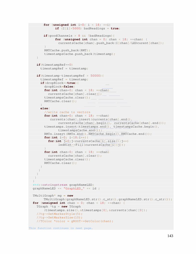
143
for (unsigned int i=0; i < 18; ++i) if (I[i]>5000) badReadings = true; if(goodChannels > 8 && !badReadings){ for (unsigned int chan = 0; chan < 18; ++chan) { currentsCache[chan].push_back(I[chan]/LEDcurent[chan]); } RMTCache.push_back(RMT); timestampsCache.push_back(timestamp); } if(timestampRef==0) timestampRef = timestamp; if(timestamp-timestampRef > 50000){ timestampRef = timestamp; if(dropBlock==true){ dropBlock=false; for(int chan=0; chan < 18; ++chan) currentsCache[chan].clear(); timestampsCache.clear(); RMTCache.clear(); } else{ //write cache to vectors for(int chan=0; chan < 18; ++chan) currents[chan].insert(currents[chan].end(), currentsCache[chan].begin(), currentsCache[chan].end()); timestamps.insert(timestamps.end(), timestampsCache.begin(), timestampsCache.end()); RMTs.insert(RMTs.end(),RMTCache.begin(),RMTCache.end()); for(int i=0; i<18;i++){ for(int j=0;j<currentsCache[i].size();j++) ledHist->Fill(currentsCache[i][j]); } for(int chan=0; chan < 18; ++chan) currentsCache[chan].clear(); timestampsCache.clear(); RMTCache.clear(); } } } } } std::ostringstream graphNameLED; graphNameLED << "GraphLED_" << id ; TMultiGraph* mg = new TMultiGraph(graphNameLED.str().c_str(),graphNameLED.str().c_str()); for (unsigned int chan = 0; chan < 18; ++chan) { TGraph *tg = new TGraph (timestamps.size(),×tamps[0],¤ts[chan][0]); //tg->SetMarkerStyle(5); //tg->SetMarkerSize(10); //TColor *color = gROOT->GetColor(chan); This function continues in next page…

144
tg->SetMarkerColor(1+chan);//->SetLineColor(color[i%9]) mg->Add(tg); } mg->SetMaximum(1.15); mg->SetMinimum(0.85); TGraph* RMTtg = new TGraph (timestamps.size(),×tamps[0],&RMTs[0]); RMTtg->SetName(id.c_str()); drawInCanvas(ledHist,false); drawInCanvas(mg); drawInCanvas(RMTtg); } std::vector< std::string > getReadOutBoxes(){ std::vector< std::string> readoutBoxes; TSQLServer* serv = TSQLServer::Connect( "oracle://cmsr1-s.cern.ch:10121/cms_orcoff", "CMS_DCS_HCL_HO_PVSS_COND","hcal-sipms"); if ((serv!=0) && serv->IsConnected()) { std::string squery = "select decode(CONFIG_RM_ID_RM1,null, " "decode(CONFIG_RM_ID_RM2, null, " "decode(CONFIG_RM_ID_RM3, null, " "CONFIG_RM_ID_RM4,CONFIG_RM_ID_RM3), CONFIG_RM_ID_RM2),CONFIG_RM_ID_RM1) " "From hcal_sipm " "where (CONFIG_RM_ID_RM1 is not null and CONFIG_RM_ID_RM1 <> 'N/A' and CONFIG_RM_ID_RM1 <> 'New SiPM') or " "(CONFIG_RM_ID_RM2 is not null and CONFIG_RM_ID_RM2 <> 'N/A' and CONFIG_RM_ID_RM2 <> 'New SiPM') or " "(CONFIG_RM_ID_RM3 is not null and CONFIG_RM_ID_RM3 <> 'N/A' and CONFIG_RM_ID_RM3 <> 'New SiPM') or " "(CONFIG_RM_ID_RM4 is not null and CONFIG_RM_ID_RM4 <> 'N/A' and CONFIG_RM_ID_RM4 <> 'New SiPM') order by change_date "; TSQLStatement* stmt = serv->Statement(squery.c_str(), 100); if (stmt->Process()) { stmt->StoreResult(); while(stmt->NextResultRow()){ readoutBoxes.push_back(stmt->GetString(0)); } } delete stmt; } delete serv ; return readoutBoxes ; }
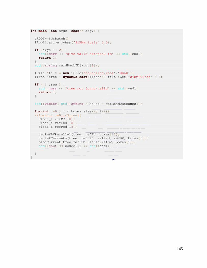
145
int main (int argc, char** argv) { gROOT->SetBatch(); TApplication myApp("SiPManlysis",0,0); if (argc != 2) { std::cerr << "give valid cardpack id" << std::endl; return 1; } std::string cardPackID(argv[1]); TFile *file = new TFile("hoDcsTree.root","READ"); TTree *tree = dynamic_cast<TTree*>( file->Get("sipmIVTree" ) ); if ( ! tree ) { std::cerr << "tree not found/valid" << std::endl; return 1; } std::vector< std::string > boxes = getReadOutBoxes(); for(int i=0 ; i < boxes.size(); i++){ //for(int i=0;i<3;i++){ Float_t refBV[18]; Float_t refLED[18]; Float_t refPed[18]; getRefBVParallel(tree, refBV, boxes[i]); getRefCurrents(tree, refLED, refPed, refBV, boxes[i]); plotCurrent(tree,refLED,refPed,refBV, boxes[i]); std::cout << boxes[i] << std::endl; } }

146
147
References [1] CERN, "CERN's public web site home," [Online]. Available:
http://public.web.cern.ch/public/. [2] CERN, "LHC's public website," [Online]. Available:
http://public.web.cern.ch/public/en/LHC/LHC-en.html. [3] O Holme et al., The JCOP Framework, in ICALEPCS (Geneva, Switzerland, 2005). [4] VV Abramov et al., Studies of the response of the prototype CMS hadron
calorimeter, including magnetic field effects, to pion, electron, and muon beams, Nuclear Instruments and Methods, vol. A457, p. 75 (2001).
[5] The CMS Collaboration, Outer Calorimeter Desing in Hadron Calorimeter Project Technical Design Report (Geneve, CERN, 1997), pp. 185-187.
[6] S Bolognesi, Calibration of the CMS magnetic field using cosmic muon tracks, in 24th international symposium on lepton photon interactions at high energies, Hamburg, Germany (2009).
[7] P Buzhana et al., Silicon photomultiplier and its possible applications, Nuclear Instruments & Methods in Physics Research Section A, pp. 48-52 (2003).
[8] A Heering et al., Large-area SiPMs for the CMS hadron outer calorimeter, Nuclear Science Symposium, pp. 1545 - 1550 (2007).
[9] The CMS Collaboration, The Barrel Muon Detector in The CMS Muon Technical Design Report (CERN, Geneva, 1997), pp. 47-139.
[10] The CMS Collaboration, "Encap Chambers - Cathode Strip Chambers" in The CMS Muon Technical Design Report (CERN, Geneva, 1997), pp. 141-244.
[11] The CMS Collaboration, "Resistive Plate Chambers" in The CMS Muon Technical Design Report (CERN, Geneva, 1997), pp. 249-308.
[12] The CMS Collaboration, The CMS Tracker Technical Design Report (CERN, Geneva, 1998).
[13] The CMS Collaboration, The CMS ECAL Technical Design Report (CERN, Geneva, 1997).
[14] The CMS Collaboration, The Hadron Calorimeter Project Technical Design Report (Geneva, CERN, 1997).
[15] The CMS Collaboration, The Magnet Project Technical Design Report (Geneve, CERN, 1997).
[16] The CMS Collaboration, The Pixel Detector System, in The CMS Tracker Technical Design Report (Geneve, CERN, 1998), pp. 13-79.
[17] The CMS Collaboration, The Silicon Strip Tracker, in The CMS Tracker Technical Design Report, (Geneve, CERN, 1998), pp. 81-168.

148
[18] K Gill et al., Radiation damage by neutrons and photons to silicon detectors, Nuclear Instruments and Methods in Physics, vol. A322, no. 177 (1992).
[19] P Gunnellini et al., 41st ITEP Physics School, Moscow 2013 arXiv:1304.2943v1 [physics.ins-det] 10 Apr 2013
[20] BS Acharya et al., The CMS Outer Hadron Calorimeter, CMS note (Geneve, CERN, 2006).
[21] P Arce, The CMS alignment system, Nuclear Instruments and Methods in Physics Research Section A: Accelerators, Spectrometers, Detectors and Associated Equipment, vol. 461, no. 1-3, pp. 172-173 (2001).
[22] N Hadengue, Alignment of the Silicon tracker of the CMS experiment using cosmic muons, Diploma Thesis (CERN - EPFL, 2007).
[23] M Weber et al., The CMS alignment challenge, in 1st LHC Detection Alignment Workshop (Geneva, CERN, 2006).
[24] CJ Seez et al., The CMS trigger system, 4th International Symposium on LHC : Physics and Detectors (Batavia, USA, 2003).
[25] R Mommsen, R Gomez-Reino et al., The Data Acquisition System of the CMS Experiment at LHC, Internation Conference on Computing in High Energy and Nuclear Physics (Taipei, Taiwan, 2010).
[26] M Jeitler et al., The level-1 global trigger for the CMS experiment at LHC, in 12th Workshop on Electronics For LHC and Future Experiments, (Valencia, Spain, 2006).
[27] V Brigljevic et al., The CMS Event Builder, in Conference for Computing in High-Energy and Nuclear Physics (La Jolla, USA, 2003).
[28] G Bauer, R Gomez-Reino et al., High Level Trigger Configuration and Handling of Trigger Tables in the CMS Filter Farm, in International Conference on Computing in High Energy and Nuclear Physics (Victoria, Canada, 2007).
[29] SM Schmeling et al, The detector safety system for LHC experiments, IEEE Trans. Nucl. Sci., vol. 51, pp. 521-525 (2004).
[30] R Gomez-Reino, CMS DCS Integration Guidelines, 2007. [Online]. Available: https://twiki.cern.ch/twiki/bin/view/CMS/DCSIntegrationGuidelines.
[31] DR Myers et al., The LHC Experiment’ Joint Controls Project - JCOP, in International Conference on Accelerator and Large Experimental Physics Control Systems (Trieste, Italy, 1999).
[32] CAEN, CAEN website, [Online]. Available: http://www.caen.it (2013). [33] CAEN Crate for EASY3000 Power Supply System for Hostile Area, CAEN,
[Online]. Available: http://www.caen.it/csite/CaenProd.jsp?parent=19&idmod=493 (2013).
[34] W-IE-NE-R, W-IE-NE-R Web site, [Online]. Available: http://www.wiener-d.com . W-IE-NE-R, W-IE-NE-R MARATON systems, [Online]. Available:
http://www.wiener-d.com/M/22/51.html .

149
[35] R Ruchti, HCAL RBX readiness review, [Online tech report]. Available: http://www.docstoc.com/docs/75916774/HCAL-RBX-Production-Readiness-Review (2013).
[36] G Magazzu et al., The Detector Control Unit: An ASIC for the Monitoring of the CMS Silicon Tracker, IEEE Transactions on Nuclear Science, vol. 51, no. 4, pp. 1333-1336 (2004).
[37] B Hallgren et al., The Embedded Local Monitor Board (ELMB) in the LHC Front-end I/O Control System, in 7th Workshop on Electronics for LHC Experiments (Stockholm, Sweden, 2001).
[38] F Varela, PhD Thesis: " The Detector Control System of the ATLAS experiment at CERN: An application to the calibration of the modules of the Tile Hadron Calorimeter.", Santiago de Compostela 2002.
[39] CERN, ATLAS collaboration website, [Online]. Available: http://atlas.web.cern.ch/Atlas/Collaboration/ (2013).
[40] Daneels and Salter, Selection and Evaluation of Commercial SCADA Systems for the Controls of the CERN LHC Experiments, International Conference on Accelerator & Large Experimental Physics Control Systems (Trieste, Italy, 1999).
[41] F Dabek et al., Event-driven programming for robust software, in EW 10 Proceedings of the 10th workshop on ACM SIGOPS European workshop (New York, 2002).
[42] SIEMENS, RK512 Protocol, [Online]. Available: http://www.kdtsys.com/UserFiles/bbs/Siemens%20RK512-3964R%20%28Eng%29.pdf (2013).
[43] Wikipedia, Profibus, [Online]. Available: http://en.wikipedia.org/wiki/Profibus (2013).
[44] Wikipedia, Modbus, [Online]. Available: http://en.wikipedia.org/wiki/Modbus (2013).
[45] Wikipedia, SIEMENS S7, [Online]. Available: https://support.automation.siemens.com/WW/llisapi.dll/csfetch/45531551/S7gs___b.pdf?func=cslib.csFetch&nodeid=45531552 (2013).
[46] Wikipedia, SNMP, [Online]. Available: http://en.wikipedia.org/wiki/Simple_Network_Management_Protocol (2013).
[47] Wikipedia, SSI, [Online]. Available: http://en.wikipedia.org/wiki/Simple_Sensor_Interface_protocol (2013).
[48] Wikipedia, IEC, [Online]. Available: http://en.wikipedia.org/wiki/IEC_60870 (2013). [49] Wikipedia, OPC, [Online]. Available:
http://en.wikipedia.org/wiki/OLE_for_process_control (2013). [50] C Gaspar, Control Hierarchy, [Online tech report]. Available: http://lhcb-
online.web.cern.ch/lhcb-online/ecs/fw/FSMConfig.pdf (2013). [51] B Franek & C Gaspar, SMI++ - Object Oriented Framework for Designing Control
Systems for HEP Experiments, in International Conference on Computing in High Energy and Nuclear Physics (Berlin, Germany, 1997).
[52] CERN, DELPHI, [Online]. Available: http://delphiwww.cern.ch/ (2013).

150
[53] R Gomez-Reino et al, the LHC Compact Muon Solenoid experiment detector control system, J. Phys.: Conf. Ser. 331(2011) 022009.
[54] Iterfacebus.com, CAN Bus, [Online]. Available: http://www.interfacebus.com/CAN-Bus-Description-Vendors-Canbus-Protocol.html (2013).
[55] C Gaspar et al., DIM, a Portable, Light Weight Package for Information Publishing, Data Transfer and Inter-process Communication, in International Conference on Computing in High Energy and Nuclear Physics (Padova, Italy, 2000).
[56] W3 org, Latest SOAP versions, [Online]. Available: http://www.w3.org/TR/soap/ (2013).
[57] W Salter, LHC Data Interchange Protocol (DIP), [Online tech. report]. Available: https://edms.cern.ch/file/457113/2/DIPDescription.doc (2013).
[58] P Golonka, JCOP Configuration Database, [Online]. Available: https://j2eeps.cern.ch/wikis/display/EN/JCOP+Framework+Configuration+Database (2013).
[59] CERN EN-ICE, JCOP Framework Configuration DB System Information, [Online]. Available: https://j2eeps.cern.ch/wikis/display/EN/JCOP+Framework+Configuration+DB+System+Information (2013).
[60] Tigris org., Subversion home page, [Online]. Available: http://subversion.tigris.org/ (2013).
[61] I Deloose, The Evolution of Managing Windows, in HEPix, (Rome, Italy, 2006). [62] CERN IT, Computer Management Framework, [Online]. Available:
https://espace.cern.ch/winservices-help/ComputerManagementFramework/Pages/InstallingApplicationsWithCMF.aspx (2013).
[63] R Gomez-Reino et al, Status of the CMS Detector Control System, Journal of Physics: Conference Series, Volume 396, Issue 1, article id. 012023 (2012)
[64] CENR AB/OP group, LHC modes, [Online tech. report]. Available: http://lhc-commissioning.web.cern.ch/lhc-commissioning/systems/data-exchange/doc/LHC-OP-ES-0005-10-00.pdf (2013).
[65] G Bauer, R Gomez-Reino et al., The run control system of the CMS experiment, in International Conference on Computing in High Energy and Nuclear Physics (Victoria, Canada, 2007).
[66] CERN CMS DAQ group, TwikiPSX XDAQ WIKI, [Online]. Available: https://twiki.cern.ch/twiki/bin/view/XdaqWiki/PSX#The_PSX_PVSS_SOAP_eXchange_packa (2013).
[67] YL Hwong, R Gomez-Reino et al., An Analysis of the Control Hierarchy Modelling of the CMS Detector Control System, in International Conference on Accelerator and Large Experimental Physics Control Systems (Taipei, Taiwan, 2010).
[68] J Groote, Analysis of distributed systems with mCRL2, in Process Algebra for Parallel and Distributed Processing , ed. CRC Press LCC (2001).

151
[69] A Biere, Bounded Model Checking, in Advances in Computers, vol. 58 (2003). [70] P Adzic, R Gomez-Reino et al., The detector control system for the electromagnetic
calorimeter of the CMS experiment at the LHC, in 10th International Conference on Accelerator and Large Experimental Physics Control Systems (Geneva, 2005).
[71] P Adzic, R Gomez-Reino et al., Detector Control System for the Electromagnetic Calorimeter in the CMS Experiment Summary of the first operational experience, in Topical Workshop on Electronics for Particle Physics (Naxos, Greece, 2008).
[72] P Adzic, R Gomez-Reino et al., Implementation and performance of the Detector Control System for the electromagnetic calorimeter of the CMS experiment, in Topical Workshop on Electronics for Particle Physics (Prague, Czech Republic, 2007).
[73] P Adzic, R Gomez-Reino et al., Detector Control System for the Electromagnetic Calorimeter of the CMS experiment, in Topical Workshop on Electronics for Particle Physics (Paris, France, 2009).
[74] The CMS ECAL, CMS ECAL APD information site, [Online]. Available: http://cms-ecal-apd.web.cern.ch/cms-ecal-apd (2013).
[75] K Bell et al., Vacuum phototriodes for the CMS electromagnetic calorimeter endcap, IEEE Trans. Nucl. Sci. 51 (2004) 2284-2287.
[76] A Annenkov et al., Lead Tungstate scintillation material, Nuclear Instruments and Methods in Physics Research Section A: Accelerators, Spectrometers, Detectors and Associated Equipment, vol. A, no. 490 (2002).
[77] Z Antunovic et al., Radiation hard avalanche photodiodes for the CMS detector, Nuclear Instruments and Methods in Physics Research Section A: Accelerators, Spectrometers, Detectors and Associated Equipment, vol. A, no. 537 (2002).
[78] P Baillon et al., Design and performance of the cooling system for the electromagnetic calorimeter of CMS, in IEEE Instrumentation and Measurement (Como, Italy, 2004).
[79] A Bartoloni, The power supply system for the CMS ECAL APDs, in 7th Workshop on Electronics for LHC Experiments (Stockholm, Sweden, 2001).
[80] L Zhang et al., Performance of the Monitoring Light Source for the CMS Lead Tungstate Crystal Calorimeter, in CMS-CR 2005/001 (Geneva, Switzerland, 2005).
[81] Betatherm , NTC thermistors 100K61A from Betatherm, [Online]. Available: http://www.betatherm.com (2013).
[82] cweb5.com, RH sensors UPS-600 from Ohmic instruments, [Online]. Available: http://www.cweb5.com/ohmic/ (2013).
[83] "EPCOS AG, NTC thermistor 470Ω@25°C," [Online]. Available: http://www.epcos.com/.
[84] Rlectech, RLE's patented Water Leak Detection Cable (SC), [Online]. Available: http://www.rletech.com/products/cable.html (2013).
[85] Microchip, PIC18F452, [Online]. Available: http://www.microchip.com/wwwproducts/Devices.aspx?dDocName=en010296 (2013).
152
[86] S Schmeling, A Detector Safety System for Experiments at the LHC - Scope & Architecture Overview, 2002. [Online tech. report]. Available: http://itco.web.cern.ch/itco/Projects-Services/JCOP/SubProjects/DSS/SteeringGroup/Minutes/10-01-02/DSS%20Scope%20Note%20Release%2010.01.2002.pdf (2013).
[87] J Groote, The Formal Specification Language mCRL2, [Online]. Available: http://www.win.tue.nl/~mweerden/docs/The_Formal_Specification_Language_mCRL2.pdf (2013).
[88] B Sherwood et al., Lifetime Studies of the 19-channel Hybrid Photodiode for the CMS Hadronic Calorimeter, Nuclear Instrumentation and Methods in Physics Research, vol. 587, no. 2-3, pp. 250-258 (2008).
[89] P Cushman et al., Status of the Lifetime Monitoring for the HCAL HPD's, tech. report, (CERN, Geneve, 1999).
[90] V Hagopian, What's new with the CMS hadron calorimeter, Advancer Technology & Particle Physics, pp. 429-434 (2002.)
[91] PB Cushman et al., Crosstalk properties of the CMS HCAL hybid photodiode, Nuclear Instruments & Methods in Physics Research, vol. A, no. 504, pp. 62-69 (2003).
[92] PB Cushman at al., Studies of hybrid photomultiplier tubes in magnetic fields up to 5 Tesla, Nuclear Instruments and Methods in Physics Research Section A, vol. 418, no. 2-3, pp. 300-305 (1998.)
[93] C Damiani et al., Magnetic field effects on Hybrid PhotoDiode single electron response, Nuclear Instruments & Methods In Physics Research Section A, vol. 442, pp. 136-139 (2000).
[94] J Freeman et al., Hybrid photodiode crosstalk due to backscattered electrons, Nuclear Instruments and Methods in Physics Research Section A: Accelerators, Spectrometers, Detectors and Associated Equipment, vol. 474, no. 2, p. 143–150 (2001).
[95] V Saveliev, Advances in Optical and Photonic Devices in Silicon Photomultiplier - New Era of Photon Detection, ed. InTech, ISBN 978-953-7619-76-3 (2010).
[96] P Buzhan et al., The Advanced Study of Silicon Photomultiplier, in Proceedings of the 7th International Conference on ICATPP-7 (Italy, 2001).
[97] B Lutz, Upgrade of the CMS Hadron Outer Calorimeter with SiPM sensors, in 15th International Conference on Calorimetry in High Energy Physics (Santa Fe, New Mexico, USA, 2012)
[98] CAEN , Easy Board A3016, [Online]. Available: http://www.caen.it/csite/CaenProd.jsp?parent=19&idmod=425 (2013).
[99] CAEN, EASY Branch Controller, [Online]. Available: http://www.caen.it/csite/CaenProd.jsp?idmod=467&parent=20 (2013).
[100] CAEN, Universal Multichannel Power Supply System, [Online]. Available: http://www.caen.it/csite/CaenProd.jsp?idmod=123&parent=20 (2013).
[101] R Brun et al., ROOT - an object oriented data analysis framework, Nuclear Instruments & Methods In Physics Research Section A, vol 389, p. 81-86 (1997).

153
[102] B Lutz et al., Upgrade of the CMS Hadron Outer Calorimeter with SiPM sensors, J. Phys., Conf. Ser. 404 012018 (2012).
[103] The CMS Collaboration, The CMSSW Documentation Suite, [Online]. Available: https://twiki.cern.ch/twiki/bin/view/CMSPublic/WorkBook.
[104] R Gomez-Reino et al., CMS DCS Design Concepts, in ICALEPCS, (Geneva, Switzerland, 2005).
[105] R Gomez.-Reino et al., The CMS Detector Control System, in ICALEPCS (Kobe, Japan, 2009)
[106] L Masetti, R Gomez-Reino et al., High availability through full redundancy of the CMS detector controls system, J. Phys.: Conf. Ser. 396 (2012) 012041
[107] The CMS Collaboration, A New Boson with a Mass of 125 GeV Observed with the CMS Experiment at the Large Hadron Collider, Science 338 , 6114 (2012) 1569-1575 (CERN, 2012)
[108] B Lutz, Upgrade of the CMS Hadron Outer Calorimeter with SiPM sensors, in 15th International Conference on Calorimetry in High Energy Physics (Santa Fe, New Mexico, USA, 2012)
[109] B Lutz, R Gomez-Reino et al., "HO Burn-In at Bld. 904 and QC at P5: Status and Perspective of the HO Test-Stand", [Online]. Available: http://indico.cern.ch/getFile.py/access?subContId=2&contribId=5&resId=0&materialId=slides&confId=218179 (2013)
[110] ATLAS collaboration, Observation of a new particle in the search for the Standard Model Higgs boson with the ATLAS detector at the LHC, Phys.Lett. B716 (2012) 1-29
[111] E Yazgan et al., The CMS barrel calorimeter response to particle beams from 2 to 350 GeV/c, The European Physics Journal C, vol. 60, pp. 359-373 (2009).
[112] CW Fabajn, Calorimetry in High Energy Physics, in Annu. Rev. Nucl. Part. Sci., (Geneva, CERN, 1982), pp. 335-388.
[113] T Ferbel, Calorimetry in High Energy Physics, in Experiemental Techniques in High-energy Nuclear and Particle Physics, (1991), p. 287.

154