arX

iv:0

802.

3726

v1 [

astr

o-ph

] 26

Feb

200

8

The Color Bimodality in Galaxy Clusters since z ∼ 0.9 1,2

Yeong-Shang Loh

Department of Physics and Astronomy, University of California, Los Angeles, CA 90095, USA

yeongloh@astro.ucla.edu

E. Ellingson

Center for Astrophysics and Space Astronomy, University ofColorado, Boulder, CO 80309, USA

H.K.C. Yee and D.G. Gilbank

Department of Astronomy and Astrophysics, University of Toronto, Toronto, ON M5S 3H4,Canada

M.D. Gladders

Department of Astronomy and Astrophysics, University of Chicago, Chicago, IL 60637, USA

and

L.F. Barrientos

Departamento de Astronomıa y Astrofısica, Universidad Catolica de Chile, Avenida VicunaMackenna 4860, Casilla 306, Santiago 22, Chile

ABSTRACT

We present the evolution of the color-magnitude distribution of galaxy clustersfrom z = 0.45 to z = 0.9 using a homogeneously selected sample of∼ 1000 clus-ters drawn from the Red-Sequence Cluster Survey (RCS). The red fraction of galaxiesdecreases as a function of increasing redshift for all cluster-centric radii, consistentwith the Butcher-Oemler effect, and suggesting that the cluster blue population maybe identified with newly infalling galaxies. We also find thatthe red fraction at thecore has a shallower evolution compared with that at the cluster outskirts. Detailedexamination of the color distribution of blue galaxies suggests that they have colorsconsistent with normal spirals and may redden slightly withtime. Galaxies of starburstspectral type contribute less than5% of the increase in the blue population at high red-shift, implying that the observed Butcher-Oemler effect isnot caused by a unobscuredstarbursts, but is more consistent with a normal coeval fieldpopulation.

– 2 –

Subject headings:methods: statistical – galaxies: elliptical and lenticular – galaxies:evolution – galaxies: clusters: general

1. Introduction

The comparison of local and high redshift clusters of galaxies is a powerful tool for constrain-ing theories of structure formation and cosmological worldmodels. The discovery that galaxy clus-ters atz ∼ 0.5 have a larger fraction of blue galaxies compared with similar clusters found in the lo-cal universe (Butcher & Oemler 1978, 1984) provided the firstdirect evidence of galaxy evolutionin dense environments. Since these early studies, the Butcher-Oemler effect has been confirmedphotometrically (Rakos & Schombert 1995; Margoniner & de Carvalho 2000; Margoniner et al.2001; Kodama & Bower 2001; Goto et al. 2003) and spectroscopically (Dressler & Gunn 1982;Lavery & Henry 1988; Fabricant, McClintock & Bautz 1991; Dressler & Gunn 1992; Poggianti et al.1999; Ellingson et al. 2001; Poggianti et al. 2006). This observed evolution has been interpretedvariously as evidence for a rapid change in galaxy populations driven by ram-pressure stripping(Gunn & Gott 1972), galaxy-merging or other physical processes in clusters (Lavery & Henry1988; Moore et al. 1996), as well as the effect of infalling galaxies from the field or near-fieldregions (Kauffmann 1995; Abraham et al. 1996; Ellingson et al. 2001).

However, the Butcher-Oemler phenomenon has been challenged from the start (e.g., Koo1981) and more recently by a host of new analyses, drawn primarily from X-ray selected sam-ples of clusters and near-infrared observation of galaxies(Andreon 1998; Andreon & Ettori 1999;Smail et al. 1998; De Propris et al. 2003). In these, the evolutionary trend with redshift was foundto be either weaker, or non-existent. The non-uniformity ofthe original Butcher-Oemler clusters,especially in physically related properties like galaxy surface number density (Newberry, Kirshner & Boroson1988) and X-ray luminosity (Andreon & Ettori 1999) may present selection biases that lead to astrong redshift evolutionary trend. Indeed, the original Butcher-Oemler clusters were selectedfrom photographic plates and may include lower mass and unvirialized merging systems. Thestrongk-correction pushes the sample to bluer rest bands. These optically-selected galaxy sam-ples may also preferentially select systems with strong star-formation (e.g., Gunn, Hoessel & Oke1986; Andreon 2005).

Earlier studies also suffered from low number statistics. While the analyses were usually done

1based on observations carried out at the Canada-France-Hawaii Telescope (CFHT), operated by the NationalResearch Council of Canada, the Centre National de la Recherche Scientifique of France and the University of Hawaii.

2based on observations taken at the Cerro Tololo Inter-American Observatory

– 3 –

with fewer than50 clusters over a large lookback time (e.g., fromz = 0 to z = 0.5), general claimswere often made about the cluster population as a whole. Partof the reason is that investigatorsnecessarily analysed whatever systems that were available. Uniformly selected cluster samples thatspan a large redshift range and have constant physical attributes (e.g., similar masses) are sparseand the variation of blue fraction within a fixed epoch is often considerable (e.g., Margoniner et al.2001). It is unclear to what extent this variation is due to actual cosmic variance or the perculiaritiesof the sample selection itself, since the number of clustersinvolved is at most a few tens.

With the advent of wide area photometric and spectroscopic redshift surveys like the SloanDigital Sky Survey (York et al. 2000, SDSS) and the Two-Degree Field Galaxy Redshift Survey(Colless et al. 2001, 2dFGRS), large catalogs of uniformly selected clusters are now availableat low (z ∼ 0.1) to intermediate (z ∼ 0.3) redshift (e.g., Annis et al. 1999; Goto et al. 2002;Kim et al. 2002; Merchan & Zandivarez 2002; Eke et al. 2004; Yang et al. 2005; Merchan & Zandivarez2005; Weinmann et al. 2006; Miller et al. 2005; Berlind et al.2006). However, in order to under-stand what processes are dominant in explaining the Butcher-Oemler effect, a large redshift rangeis desirable to provide maximal leverage to evolutionary studies as various theoretical models mayhave different redshift dependences.

In this work, we revisit the Butcher-Oemler phenomenon using the currently largest sam-ple of uniformly selected clusters of galaxies available, out to z ≈ 0.9. The galaxy clusters aredrawn from the complete and well-calibrated Red-Sequence Cluster Survey (RCS; Gladders & Yee2005). The RCS method searches for galaxy overdensities along a color-magnitude sequence cor-responding to cluster early-type galaxies, the cluster ”red sequence”. The apparent color of thissequence reddens with redshift, allowing us to separate overlapping structures and effectively re-move most of the contamination that has plagued monochromatic cluster surveys. All massiveclusters discovered by any methodology to date show a detectable red sequence, so that, while itis slightly less effective for very blue systems, this methodology is not expected to introduce astrong bias to the study of the cluster populations. To the extent that galaxies on the early-typered sequence have the largest fraction of stellar mass at a fixed luminosities (e.g., Bell et al. 2004),our cluster sample can be considered stellar mass dependent. Our sample may exhibit selectiondifferences when compared, for example, with dark mass dependent weak lensing detected clustersamples such as the Deep Lens Survey (DLS; Wittman et al. 2002), intracluster medium (ICM)density dependent X-ray selected samples (e.g.,; Rosati etal. 1998), or star-forming galaxy bi-ased blue overdensities for Lyman break selected samples. However, galaxy density maps derivedfrom red sequence galaxies have been shown to correlate withweak lensing shear maps with highsignificance (Wilson, Kaiser & Luppino 2001).

In this paper we study the evolutionary trend of the red fraction for cluster galaxies with red-shift within a range of radii, scaled byr/r200 – the radius at which the galaxy overdensity is200

– 4 –

times the mean density. Scaling the radii tor/r200 allows a statistical combination of many systemsand minimizes many problems arising from the foreground/background subtraction in photometricsurveys. Our approach is cluster-centric (e.g., Melnick & Sargent 1977; Whitmore, Gilmore & Jones1993; Ellingson et al. 2001), where we use a characteristic radiusr200 to normalize the clustersacross the richness range of the clusters. This approach is complementary to many more recentstudies of the Color (Star Formation Rate)-Density relation (Hogg et al. 2003; Balogh et al. 2004;Yee et al. 2005) which use local galaxy densities (Dressler 1980; Smith et al. 2005; Postman et al.2005; Cucciati et al. 2006; Cooper et al. 2007a).

The outline of this paper is as follows. In the next section, we describe the sample used in ouranalysis. The procedure for the statistical background correction of composite clusters is describedin section 3. In section 4, we discuss our results and give caveats that need to be taken into accountfor robust interpretation. In section 5, we summarize our conclusions. Throughout this paper,h = H0/100 km s−1 Mpc−1 and we adopt the concordanceΩm = 0.3, ΩΛ = 0.7 cosmology.

2. Sample

2.1. The RCS Survey

The Red-Sequence Cluster Survey (RCS; Gladders & Yee 2005) is a∼ 100 deg2 imagingsurvey in thez′ and Rc bandpasses conducted with the CFHT 3.6 m and CTIO 4 m with theprimary goal of searching for clusters of galaxies up toz ≈ 1.4. There are22 RCS patches(each of≈ 2.5 deg2) distributed over the northern and southern sky. Some of thepatches werechosen to overlap with other widely studied fields, such as XMM-LSS (Pierre et al. 2004), CDF-S (Giacconi et al. 2001), CNOC2 (Yee et al. 2001), SWIRE (Lonsdale et al. 2003) and PDCS(Postman et al. 1996).

2.2. Photometry, Calibration, Extinction

The primary RCS photometric reduction of object detection,source deblending, star-galaxyseparation and aperture photometry was performed using thePicture Processing Package (PPP;Yee 1991; Yee, Ellingson & Carlberg 1996). The detailed implementation of the RCS photometricpipeline is described in Gladders & Yee (2005). The average5σ limiting magnitudes for pointsources arez′ = 23.9 andRc = 25.0 (AB system). Analysis of log(N)-log(S) galaxy countssuggests that the photometry for extended sources is complete to∼ 0.8 mag brighter, althoughthere are variations from pointing to pointing. There are over 3 million point sources and11

– 5 –

million galaxies in the RCS database. The relative photometry between patches is better than0.1

magnitudes (Hsieh et al. 2005). Each detected extended source is further corrected for Galacticextinction, interpolating the dust map of Schlegel, Finkbeiner & Davis (1998) and assumingRRc

=

2.634 andRz′ = 1.479. For the present analysis, we use72 deg2 of the RCS survey with the bestphotometry (Gladders et al. 2007). Throughout this paper, our Rc andz′ photometry is presentedon the AB system.

2.3. The Cluster Sample

About 8000 groups and clusters of galaxies were detected with high significance by search-ing for source overdensities in color slices along the red-sequence of early-type galaxies. De-tails of the cluster detection method are outlined in Gladders & Yee (2000). The release of thefirst catalog, as well as improvements over the cluster detection methodology, are described inGladders & Yee (2005). A useful by-product of the red-sequence method is an estimated photo-metric redshift for each detected cluster. RCS uses only twobandpasses strategically chosen tostraddle the4000A break of the target redshift coverage, and photometric redshifts of the detectedclusters are quite well constrained, to∆z/z ≈ 0.1 (Gilbank et al. 2007). The dense collectionof red galaxies along the red-sequence effectively diminishes the Poisson noise from photometricuncertainties of individual sources (Lopez-Cruz, Barkhouse & Yee 2004).

In addition to an estimated photometric redshift (hereafter zph), an optical richness parametrizedby the amplitude of the galaxy-cluster cross-correlation functionBgc (Longair & Seldner 1979;Yee & Green 1987; Yee & Lopez-Cruz 1999) is measured.Bgc is found to correlate well withcluster properties such as X-ray temperature and galaxy velocity dispersion at intermediate red-shift, and it is relatively well calibrated for X-ray selected clusters atz ∼ 0.35 (Yee & Ellingson2003). Note that here we use red sequence galaxies for the measurement ofBgc (Gladders & Yee2005), which gives a tighter relation with respect to X-ray properties, especially at higher redshift(Hicks et al. 2007). ROSAT observations have also found thatmost groups and lower mass sys-tems with extended X-ray halos are dominated by early-type galaxies (Osmond & Ponman 2004;Mulchaey et al. 2003).Bgc computed from the red sequence will down-weight unvirialized poorsystems without a hot ICM.

For the present analysis, we use∼ 1000 clusters withBgc > 300 (h−150 Mpc)1.77 and0.45 <

zph < 0.90. Mass calibration using low to intermediate redshift clusters suggests these sys-tems have richnesses corresponding to Abell Richness Class(ARC) & 0, σv > 450 km s−1 andTX > 3 keV (Yee & Lopez-Cruz 1999; Yee & Ellingson 2003). The sample is divided into fiveredshift slices with171 to 263 systems in each slice (Table 1). While the mass of each clusteris uncertain due to the rather large uncertainty in the measured Bgc and the intrinsic scatter in

– 6 –

mass-Bgc relation, the overall distribution of cluster counts as a function of redshift is robust. Fig-ure 1 shows the redshift histogram of clusters used in our analysis. Analysis of the RCS clustercounts to constrain cosmological parameters yields results consistent with the concordance values(Gladders et al. 2007), indicating that large systematic errors in our mass estimates are unlikely.From abundance matching, clusters withBgc > 300 (h−1

50 Mpc)1.77 used in this paper are rare, withcomoving densities< 10−5h3 Mpc−3, consistent with dark matter halos with mass& 1014h−1 M⊙.

3. Methodology

3.1. Foreground and Background Subtraction

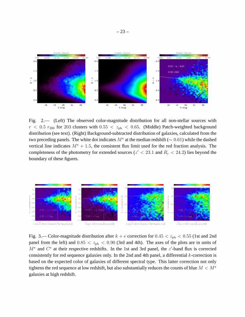
To obtain the composite color-magnitude distribution of our cluster galaxies, we have to sub-tract the contribution from foreground and background galaxies statistically. The two-dimensionalobserved background counts for non-stellar sources inRc − z′ color andz′ magnitude are con-structed for each of the22 RCS patches. Depending on the relative number of clusters from eachpatch used for the composite cluster analysis at each redshift slice, a weighted background basedon the effective area contributed by the clusters is created(Figure 2). This semi-global backgroundapproach allows us to model the background more accurately using a large area, but still mimicssome inherent patch to patch variations such as observing depth and seeing. This approach wassimilarly employed by Hansen et al. (2005) but performed in two dimensions (in color and magni-tude space) as in Loh & Strauss (2006). Our approach is in contrast with Valotto, Moore & Lambas(2001) who advocate a local background subtraction methodology. Goto et al. (2003) find littledifference with the two approaches if a large enough area is used. The global approach has theadvantage that it uses all available data to constrain a smooth background with high precision. Fora given patch of survey area, the region occupied by the clusters, after aggregating in redshift, takesup 2 − 5% of the entire patch area. We rescaled the background to matchthis total cluster areabefore the background subtraction.

We are interested in the average properties of clusters at a given redshift. If we assumethat clusters are self-similar systems with a universal galaxy density profile, then clusters of dif-ferent physical sizes can be scaled to some normalized cluster radius. However, without X-ray information or spectroscopy, it is difficult to measure the virial radius of each of the clus-ters. We use the measuredBgc for each cluster to estimate a virial radiusr200 using the relationlog r200 = 0.48 log Bgc − 1.10. This relation is empirically calibrated from intermediate redshiftclusters (Yee & Ellingson 2003; Blindert 2006). We stack allclusters in a given redshift slice,but scale each cluster by itsr200 for an effective normalizing scale. We emphasize here thatBgc

is measured at the core, within0.25 h−1 Mpc, and that the self-similar assumption is implicit in

– 7 –

Yee & Ellingson (2003). We note here that the spherical halo assumption inherent in theBgc mea-surements is not perfect, as in addition to spherical distribution of red galaxies, the RCS methodmay systematically include physically associated filamentary galaxy structure along the line-of-sight. However, because of the overdensities implied atBgc > 300 (h−1

50 Mpc)1.77, most structureswill be dynamically collapsed, if not completely virialized. We are exploring secondary measure-ments such as the concentration of the cluster galaxy distribution or the dominance of the BCG asa possible second parameter to further refine the mass measurements.

Figure 2 shows the color-magnitude distributions of galaxies withr/r200 < 0.5 at z ≈ 0.6.We have stacked203 clusters with0.55 < zph < 0.65 to obtain the observed distribution (leftpanel). The red sequence is clearly visible. The patch-weighted background distribution is shownnext in the middle panel. The distribution after backgroundsubtraction is shown in the right panel.A prominent red sequence appears after the subtraction. Thesolid line is the fitted red sequence atthe effective redshift. The solid dots indicate the modelM⋆ at this redshift and the dashed verticalline indicates1.5 magnitude fainter thanM⋆.

3.2. Semi-Empirical k + e corrections

3.2.1. Red Sequencek + e models

When computing statistics like red (or blue) fractions across a range of redshifts, the use ofan evolving luminosity limit is crucial since the absolute luminosity of galaxies changes by aboutone magnitude fromz = 0 to z ∼ 1. The original Butcher & Oemler (1984) prescription of usinga fixed rest-frameMV = −20 does not produce a consistent galaxy population across a rangeof redshifts. This bias is especially severe for studies which span a large redshift range. Theknown correlation between luminosity and color can also mimic the evolution of the blue fraction.However, there is considerable uncertainty in the measurement of luminosity evolution beyondz = 0.6. Work by Faber et al. (2005) and Bell et al. (2004) showed thatDEEP2 and COMBO-17surveys yielded very similar results out toz ∼ 1 with respect to theB-band luminosity density forred galaxies. However, Brown et al. (2007) and Scarlata et al. (2007) found a milder luminositydensity evolution in the NOAO Deep Wide-Field and COSMOS surveys.

The luminosity function was determined empirically from background-subtracted galaxy countsin the red sequence of the clusters. A more detailed study of the RCS cluster luminosity functioncan be found in Gilbank et al. (2008); our assumed luminosityfunction is within0.1 mag of thevalues listed in their Table I. These values ofM⋆ (in the z′ bandpass) as a function of redshiftare consistent with the combination ofk-correction for an early-type galaxy spectrum along withpassive evolution from az ∼ 3 single starburst population (see Gilbank et al. for details).

– 8 –

While our exact value ofM⋆ may differ slightly from that measured by others, the evolutionin M⋆ within our own sample is robust and will not influence trends with redshift. We explored thepossible effects of uncertainty in the cluster galaxy luminosity function. A systematic change of±0.25 mag per redshift inM⋆ for the cluster galaxies produced a change in red fraction less than1σ.

Our goal is to obtain a consistent rest-frame flux for the cluster galaxies across the redshiftrange we are probing. We first use our modelM⋆ to convert the apparentz′ magnitudes of redsequence galaxies to evolution-corrected luminosities atthe redshift of the cluster. The existenceof the red sequence then allows us to match the color-luminosity distribution across redshift. Theobserved slope can be used to change the apparentR − z′ color into units ofC⋆ (R − z′ color atM⋆), without appealing to model dependent color evolution (e.g., Bell et al. 2004; Loh & Strauss2006). Figure 3 shows the color-luminosity distribution for two redshift slices:0.45 < zph < 0.55

(first panel from the left) and0.85 < zph < 0.90 (3rd panel). The axes are in units ofM⋆ andC⋆,the color relative to the red sequence.

3.2.2. Differentialk-correction

While model independent, the approach from the above section does not take into accountthe differentialk-corrections between galaxies of different spectral typesfor a fixed observedz′

magnitude. To this end, we use the observed color blue-ward of the red-sequence to infer therelativek-correction beyond the flux relative to aM⋆ at that epoch, which gives a comparablek + e-correction to more traditional approaches (e.g.,; Yee et al. 2005)

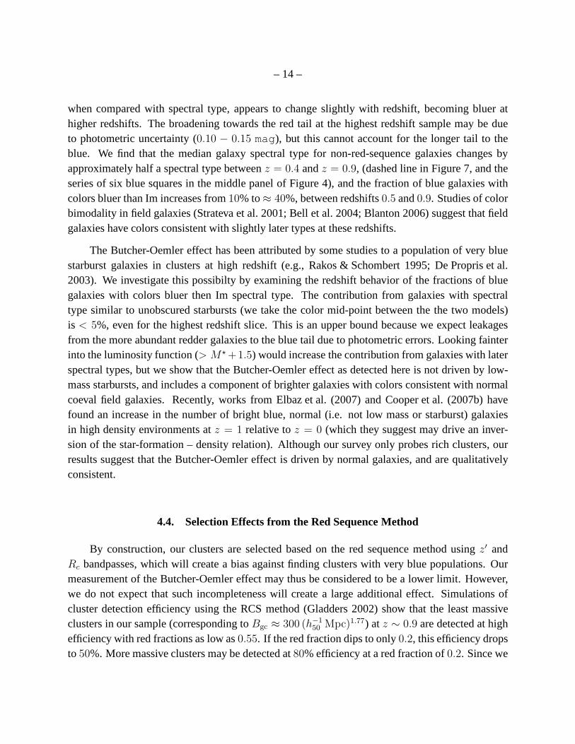
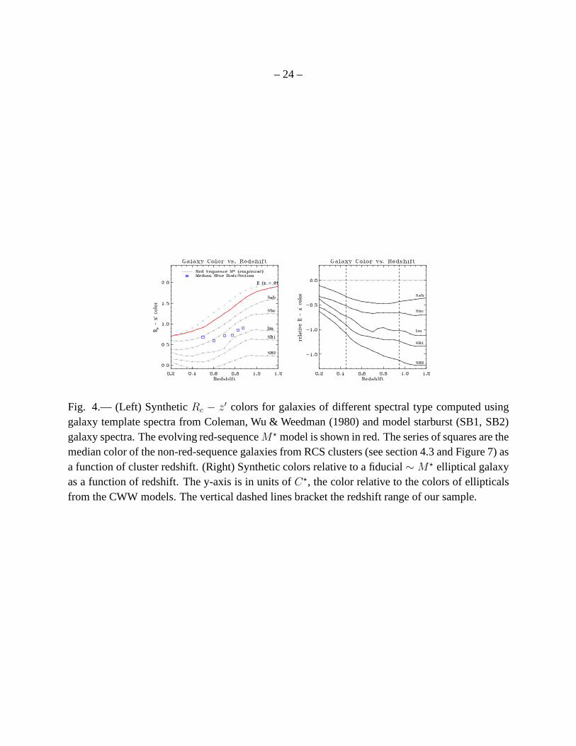
The left panel of Figure 4 shows the syntheticRc − z′ color for galaxies of different spectraltypes computed usingreal galaxy template spectra from Coleman, Wu & Weedman (1980) aug-mented with two starburst models. The empirically determined red-sequence color as a function ofredshift is shown in red. Since the red sequence includes passive evolution of the stellar population,it does not match the non-evolving colors derived from localellipticals at high redshift. Plottedon the right panel of Figure 4 are the synthetic colors, relative to the local ellipticals, for galaxiesof different spectral type as a function of redshift. The y-axis can be compared directly with they-axis of the red-sequence corrected color-magnitude distribution of Figure 3. From the relativecolor of each galaxy, we assign a spectral type to each, interpolating if the color is in betweentypes. The relativek-correction inz′-band, used to shift a given galaxy to a lower intrinsic lumi-nosity, is inferred from the differentialk-correction relative to the fiducial red sequence templateat each reshift.

Figure 3 shows the changes in the color-magnitude distributions before (1st and 3rd panels)

– 9 –

and after (2nd and 4th panels) applying the relativek-correction to thez′-band flux. This additionalrelativek-correction corrects blue galaxies for on-going star-formation by pushing them to faintermagnitudes, such that the bluest faint galaxies, which would otherwise just make our luminositycut, are pushed below the magnitude limit and are so removed from our sample. This effect isclearly visible at higher redshift by examining blue galaxies in the 3rd and 4th panels of Figure3 (0.85 < zph < 0.90). The numerous blue galaxies brighter thanM⋆ are corrected to faintermagnitudes but are still bright enough to be included in the sample. If we neglect the differentialevolution between red sequence and blue galaxies, the derived red fraction atr200 is reduced by2% atz ∼ 0.5 and by14% atz ∼ 0.8.

3.3. Cluster Red Fractions

There are a number of different ways in which red or blue galaxy fractions are defined in theliterature. Some use a fixed rest-frame color cut, say rest-frameB−V < 0.8 mag for blue galaxies(e.g., Rakos & Schombert 1995). Definitions like these usually yield a large number density evo-lution of early-type galaxies that are grossly inconsistent with the hiearchical model of structureformation (e.g., Wolf et al. 2003). Others, such as the original Butcher & Oemler (1984) studies,use a fixed color width∆ from the observed red sequence, say,∆(B − V ) = 0.2 mag for redgalaxies (e.g., Bell et al. 2004). As reviewed by Andreon (2005), a constant width bracketing thered sequence is not optimal because galaxies of different spectral types drift in and out of the fixedregion∆ for even the most generic models of stellar population. Claims of the evolution the blue(or red) fraction may just be a consequence of systematic spectral types drifting in and out of thewidth at different redshifts.

Here, we use an empirical approach that attempts to separatethe red sequence galaxies fromthe rest of the population, and divide the remaining galaxies amongst different fixed spectral types.We first construct thek + e correctedRc − z′ color distribution by summing over the counts fromall galaxies brighter thanM⋆ + 1.5. The distribution for redshifts slices of0.45 < zph < 0.55,0.65 < zph < 0.75 and0.85 < zph < 0.90 are shown on the bottom panels of Figure 5. Wethen fit the red side (split by the red sequence peak) of the distribution with a double Gaussianof a single mean, including a narrow peak and a broader wing. Because the intrinsic spreadof the red sequence is small (. 0.05 mag; Bower, Lucey & Ellis 1992; Blakeslee et al. 2003;Lopez-Cruz, Barkhouse & Yee 2004; Cool et al. 2006; Mei et al. 2006) and there should be on av-erage no excess of galaxies with redder colors associated with these clusters, this half of the colorprofile should be characteristic of the color uncertainty inour observations and should be symmet-ric about the red sequence peak. This peak is prominent enough at all observed redshifts that redsequence galaxies are thus robustly isolated. The red fraction,fR = 1−fB, the complement of the

– 10 –

traditionally measured blue fraction,fB, is estimated by mirroring the double Gaussian about themean model distribution, and normalizing by the total galaxy counts (red and blue, smoothed witha spline curve). We note here that our approach is in spirit similar to the original Butcher & Oemler(1984) studies where the color width of their red sequence galaxies was indeed≈ 0.2 mag. Thisapproach is also similar to the one suggested by Andreon (2005) of using the valley between thetwo distributions as a divider (e.g., Strateva et al. 2001) and more recent bi-gaussian fitting to thelocal field color distribution (at fixed luminosity) by Baldry et al. (2004). Our approach has theadded advantage of estimating a more robust red fraction in the absence of a well-defined valley(e.g., the first distribution shown in Figure 5), and when there is a departure from bi-gaussianity.Furthermore, the observed red distribution seems to broaden at increasing redshift. Our approachautomatically captures this broadening, presumably due tothe larger photometric uncertaintiesof the individual sources at fainter apparent magnitudes. Both the valley division and the fixedwidth approach will not take this into account, creating a susceptibility to an Eddington-like bias(Eddington 1913) which might mimic the redshift evolutionary trend we are trying to detect.

3.4. Cluster-to-Cluster Variation

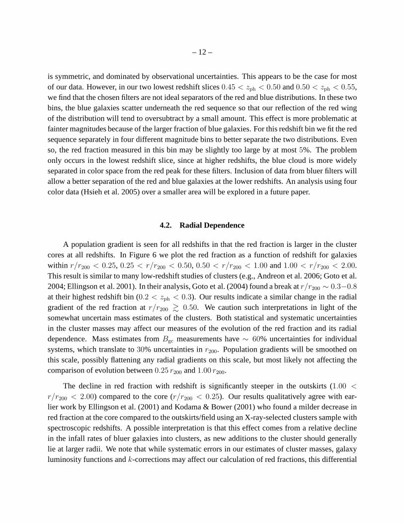
It has been noted from many previous studies of the Butcher-Oemler effect that even at fixedredshift, there is considerable variation in blue fraction. Some of this variation is due to the het-erogeneous manner in which the clusters were selected, while others are intrinsic in the sense thateven at a given epoch, clusters have various physical morphologies (e.g., Bautz-Morgan Class)and states of evolution. We try to capture this variation between clusters by performing a jackknifeanalysis on our stacked clusters at a given redshift slice. This is done by dividing the cluster samplefurther into 15 to 20 subsamples, depending on the number of clusters involved. Each subsample isthen removed, and the same red fraction analysis is performed. The error-bars displayed in Figure6 are obtained by this approach. We note here that this approach also captures other variationswithin our data set, like small residual differences in patch to patch relative photometry.

4. Results and Discussion

4.1. The Butcher-Oemler Effect

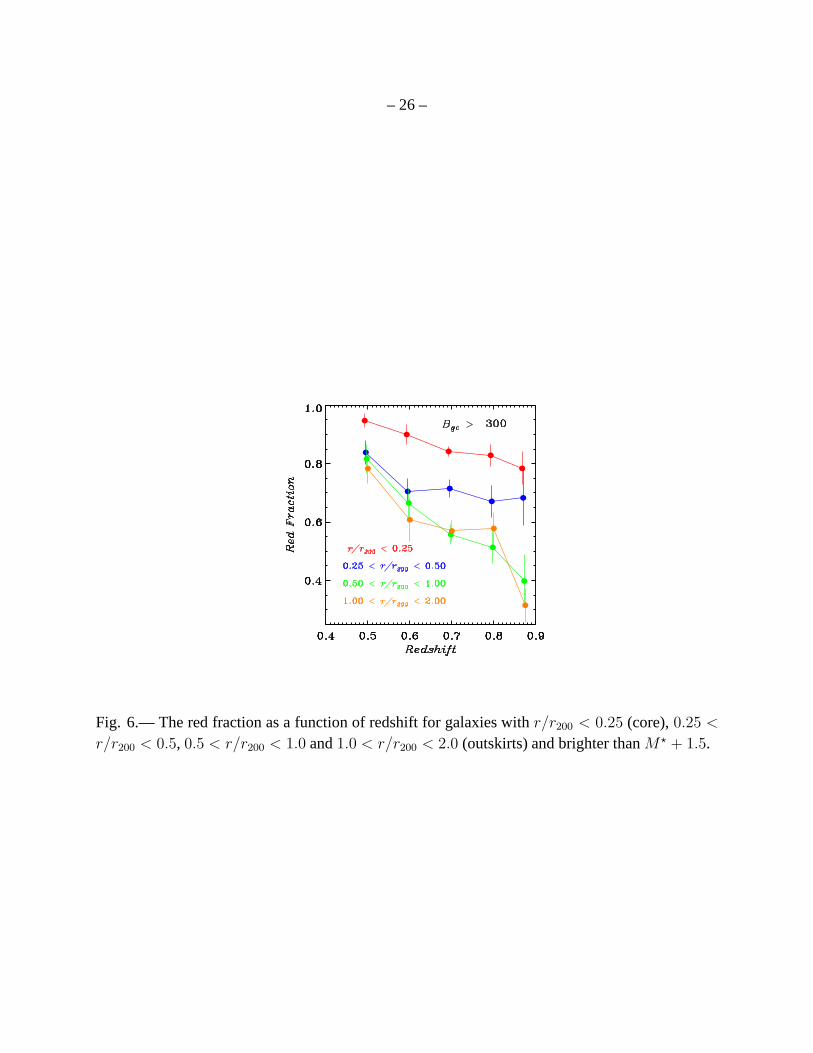
The cumulative red fraction as a function of redshift is shown in Figure 6. The fraction of redgalaxies decreases as a function of redshift for all scaled radii r/r200. Particularly relevant to theButcher-Oemler phenomenon is the gradual decline in red fraction at the cluster core (0.25 r200)from ∼ 95% at z ≈ 0.5 to ∼ 80% atz ≈ 0.9. The red fraction value of our lowest redshift bin

– 11 –

is high compared with the original Butcher & Oemler (1984) study and many subsequent analyseswhich showed red fractions of about0.7 atz ∼ 0.4. Part of this discrepancy comes from the way inwhich the red fraction is measured; using a fixed color cut in the bimodal distribution will tend toincrease the blue fraction if the observational scatter is significant. Our values are more consistentwith recent studies using X-ray-selected cluster samples at z ∼ 0.3 (Wake et al. 2005) andz ∼ 0.6

(Andreon, Lobo & Iovino 2004).

At face value, our result is inconsistent with the K-band analysis of De Propris et al. (2003)which probed a similar redshift range, but was based on a moremassive (on average) and het-erogeneous sample of33 optical, X-ray and radio-selected clusters. They fitted their data with aconstantfB ∼ 0.1 out toz ∼ 0.9. They confirmed the Butcher-Oemler effect as observed in anoptically-defined sample, but noted little evolution when using a K-band selected sample. Theyconcluded that any evolutionary effect may be due to a population of bursting dwarf galaxies,whose K-band luminosities (hence the stellar mass of the galaxies) are too faint for inclusion in aconsistent K-band galaxy selection.

Our use ofk + e corrected magnitude in thez′-bandpass is not a perfect proxy for galaxystellar mass but is less affected by recent star formation and has a much smallerk + e correctioncompared with other optical bandpasses. Hence, we expect a reasonable agreement with K-bandresults. However, we find that our analyses differ significantly in the division of red versus bluegalaxies. Like Butcher & Oemler (1984), De Propris et al. usea fixed∆(B − V ) = 0.2 mag butk-corrected to their observed bandpasses using an effectiveSED derived from Sa + Sc mixture togive an effective∆(color) at higher redshift. Unlike Butcher & Oemler whose color histogramshave an observed red sequence width of≈ 0.2 mag, the color histograms from De Propris et al.display a narrower red sequence width compared with the effective ∆(color) – often as large as0.5 mag – used in their analysis. Their chosen∆(color) allows the inclusion of galaxies of laterspectral type in the red fraction, suppressing their blue fraction measurements relative to ours,which model the observational scatter. On examination of the individual color histograms of theirhigh redshift clusters, we find that our method would producesubstantial blue counts beyond thered sequence, and hence we find no evidence of inconsistency between our results and theirs.

We further note that the De Propris et al.’s results are derived using a fixed aperture of rela-tively small size (0.25− 0.45h−1 Mpc), whereas our red fractions are measured using apertures ofscaled radiir/r200. Observations made within a fixed metric radius tend to sample only the redderinner cores for massive clusters, and atz > 0.6, their sample is likely biased toward the mostmassive systems for which ther200 values are typically as large as1.5 to 2.0h−1 Mpc. As Figure 6for the RCS sample shown, at radii smaller than0.5r200, there is only a moderate evolution in thered fraction betweenz ∼ 0.4 and0.9.

Our definition of red fraction is sensitive to our assumptionthat the red sequence color spread

– 12 –

is symmetric, and dominated by observational uncertainties. This appears to be the case for mostof our data. However, in our two lowest redshift slices0.45 < zph < 0.50 and0.50 < zph < 0.55,we find that the chosen filters are not ideal separators of the red and blue distributions. In these twobins, the blue galaxies scatter underneath the red sequenceso that our reflection of the red wingof the distribution will tend to oversubtract by a small amount. This effect is more problematic atfainter magnitudes because of the larger fraction of blue galaxies. For this redshift bin we fit the redsequence separately in four different magnitude bins to better separate the two distributions. Evenso, the red fraction measured in this bin may be slightly too large by at most5%. The problemonly occurs in the lowest redshift slice, since at higher redshifts, the blue cloud is more widelyseparated in color space from the red peak for these filters. Inclusion of data from bluer filters willallow a better separation of the red and blue galaxies at the lower redshifts. An analysis using fourcolor data (Hsieh et al. 2005) over a smaller area will be explored in a future paper.

4.2. Radial Dependence

A population gradient is seen for all redshifts in that the red fraction is larger in the clustercores at all redshifts. In Figure 6 we plot the red fraction asa function of redshift for galaxieswithin r/r200 < 0.25, 0.25 < r/r200 < 0.50, 0.50 < r/r200 < 1.00 and1.00 < r/r200 < 2.00.This result is similar to many low-redshift studies of clusters (e.g., Andreon et al. 2006; Goto et al.2004; Ellingson et al. 2001). In their analysis, Goto et al. (2004) found a break atr/r200 ∼ 0.3−0.8

at their highest redshift bin (0.2 < zph < 0.3). Our results indicate a similar change in the radialgradient of the red fraction atr/r200 & 0.50. We caution such interpretations in light of thesomewhat uncertain mass estimates of the clusters. Both statistical and systematic uncertaintiesin the cluster masses may affect our measures of the evolution of the red fraction and its radialdependence. Mass estimates fromBgc measurements have∼ 60% uncertainties for individualsystems, which translate to30% uncertainties inr200. Population gradients will be smoothed onthis scale, possibly flattening any radial gradients on thisscale, but most likely not affecting thecomparison of evolution between0.25 r200 and1.00 r200.

The decline in red fraction with redshift is significantly steeper in the outskirts (1.00 <

r/r200 < 2.00) compared to the core (r/r200 < 0.25). Our results qualitatively agree with ear-lier work by Ellingson et al. (2001) and Kodama & Bower (2001)who found a milder decrease inred fraction at the core compared to the outskirts/field using an X-ray-selected clusters sample withspectroscopic redshifts. A possible interpretation is that this effect comes from a relative declinein the infall rates of bluer galaxies into clusters, as new additions to the cluster should generallylie at larger radii. We note that while systematic errors in our estimates of cluster masses, galaxyluminosity functions andk-corrections may affect our calculation of red fractions, this differential

– 13 –

effect with respect to radius will remain, suggesting that the population in the cores of clusterschanges with time differently from the population in the outskirts.

Our result on the radial dependence of the red fraction requires an accurate determinationof each cluster center. A detailed description for determining RCS cluster centers was given inGladders & Yee (2005). In brief, the location of a cluster is first selected from the color- positiondata-cube with a magnitude weighting towards galaxies brighter thanM⋆; the positioning is thenrefined by an interative Gaussian kernel of250h−1 kpc. To the extent that the RCS algorithm isaccurate, then the centering should be better than< 250h−1 kpc. Note that clusters in reality arenot round objects and often there are double clusters, or galaxy overdensities along filamentarystructures. If a cluster is indeed elliptical and has a well-defined center, we argue here that wewill get the right center to better than half our searching scale (i.e. 125h−1 kpc). If the clusteror galaxy overdensity is filamentary, then our assumption ofself- similar spherical clusters breaksdown. Indeed our results atr < 0.25r200 maybe affected by centering problems, but not for thelarger radii. If we are not systematically deviating in our cluster center determination, then thejackknife procedure in our error calculation would capturethe diversity and uncertainty of our redfraction determination.

Because cluster galaxy populations show such marked radialgradients, any systematic varia-tions of theBgc – r200 relation with redshift may also change our red fraction as a function redshift,with any systematic tendency to overestimate cluster masses leading to a trend towards a lower redfraction. However, a significant systematic is required: even if our estimates ofr200 are off by a fac-tor of 3 at z ∼ 0.8, compared toz ∼ 0.5, we would still see an evolution with redshift. Currently,no such redshift dependence is found in the RCS mass estimates when the same cluster sample isanalysed using a global self-calibration procedure (e.g.,Hu 2003; Majumdar & Mohr 2004) whichreflects standard cosmological parameters (Gladders et al.2007). Ongoing work is currently beingdone to calibrate the mass of a subset of high redshift clusters using X-ray (Hicks et al. 2007),multi-object spectroscopy (Gilbank et al. 2007; Barrientos et al., in prep), weak lensing analyses(Hoekstra et al., in prep.) and mid-IR (Ellingson et al., in prep.) observations to constrain any suchbiases.

4.3. The Blue Galaxy Distribution

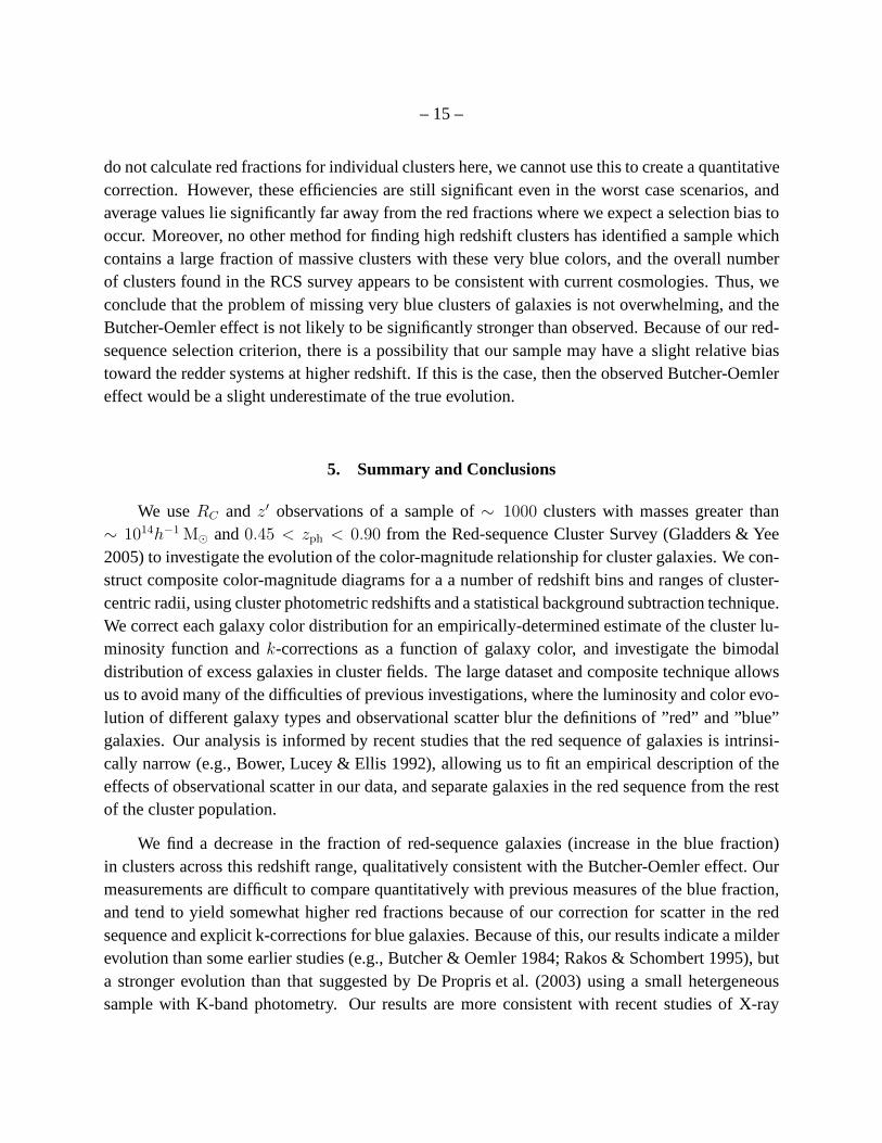
Figure 7 shows the blue distribution of galaxies after removing the fitted red distribution. Theshaded vertical bands are the expected color for galaxies ofdifferent (late) spectral type, rangingfrom Sab (far right) to starburst (SB; far left), synthesized using a single representative SED foreach type (cf. Figure 4). The width of the band reflects the finite redshift range in each subsampleand the color variation as the filters shift along the SED withredshift. The blue distribution,

– 14 –

when compared with spectral type, appears to change slightly with redshift, becoming bluer athigher redshifts. The broadening towards the red tail at thehighest redshift sample may be dueto photometric uncertainty (0.10 − 0.15 mag), but this cannot account for the longer tail to theblue. We find that the median galaxy spectral type for non-red-sequence galaxies changes byapproximately half a spectral type betweenz = 0.4 andz = 0.9, (dashed line in Figure 7, and theseries of six blue squares in the middle panel of Figure 4), and the fraction of blue galaxies withcolors bluer than Im increases from10% to≈ 40%, between redshifts0.5 and0.9. Studies of colorbimodality in field galaxies (Strateva et al. 2001; Bell et al. 2004; Blanton 2006) suggest that fieldgalaxies have colors consistent with slightly later types at these redshifts.

The Butcher-Oemler effect has been attributed by some studies to a population of very bluestarburst galaxies in clusters at high redshift (e.g., Rakos & Schombert 1995; De Propris et al.2003). We investigate this possibilty by examining the redshift behavior of the fractions of bluegalaxies with colors bluer then Im spectral type. The contribution from galaxies with spectraltype similar to unobscured starbursts (we take the color mid-point between the the two models)is < 5%, even for the highest redshift slice. This is an upper boundbecause we expect leakagesfrom the more abundant redder galaxies to the blue tail due tophotometric errors. Looking fainterinto the luminosity function (> M⋆ +1.5) would increase the contribution from galaxies with laterspectral types, but we show that the Butcher-Oemler effect as detected here is not driven by low-mass starbursts, and includes a component of brighter galaxies with colors consistent with normalcoeval field galaxies. Recently, works from Elbaz et al. (2007) and Cooper et al. (2007b) havefound an increase in the number of bright blue, normal (i.e. not low mass or starburst) galaxiesin high density environments atz = 1 relative toz = 0 (which they suggest may drive an inver-sion of the star-formation – density relation). Although our survey only probes rich clusters, ourresults suggest that the Butcher-Oemler effect is driven bynormal galaxies, and are qualitativelyconsistent.

4.4. Selection Effects from the Red Sequence Method

By construction, our clusters are selected based on the red sequence method usingz′ andRc bandpasses, which will create a bias against finding clusters with very blue populations. Ourmeasurement of the Butcher-Oemler effect may thus be considered to be a lower limit. However,we do not expect that such incompleteness will create a largeadditional effect. Simulations ofcluster detection efficiency using the RCS method (Gladders2002) show that the least massiveclusters in our sample (corresponding toBgc ≈ 300 (h−1

50 Mpc)1.77) at z ∼ 0.9 are detected at highefficiency with red fractions as low as0.55. If the red fraction dips to only0.2, this efficiency dropsto 50%. More massive clusters may be detected at80% efficiency at a red fraction of0.2. Since we

– 15 –

do not calculate red fractions for individual clusters here, we cannot use this to create a quantitativecorrection. However, these efficiencies are still significant even in the worst case scenarios, andaverage values lie significantly far away from the red fractions where we expect a selection bias tooccur. Moreover, no other method for finding high redshift clusters has identified a sample whichcontains a large fraction of massive clusters with these very blue colors, and the overall numberof clusters found in the RCS survey appears to be consistent with current cosmologies. Thus, weconclude that the problem of missing very blue clusters of galaxies is not overwhelming, and theButcher-Oemler effect is not likely to be significantly stronger than observed. Because of our red-sequence selection criterion, there is a possibility that our sample may have a slight relative biastoward the redder systems at higher redshift. If this is the case, then the observed Butcher-Oemlereffect would be a slight underestimate of the true evolution.

5. Summary and Conclusions

We useRC and z′ observations of a sample of∼ 1000 clusters with masses greater than∼ 1014h−1 M⊙ and0.45 < zph < 0.90 from the Red-sequence Cluster Survey (Gladders & Yee2005) to investigate the evolution of the color-magnitude relationship for cluster galaxies. We con-struct composite color-magnitude diagrams for a a number ofredshift bins and ranges of cluster-centric radii, using cluster photometric redshifts and a statistical background subtraction technique.We correct each galaxy color distribution for an empirically-determined estimate of the cluster lu-minosity function andk-corrections as a function of galaxy color, and investigatethe bimodaldistribution of excess galaxies in cluster fields. The largedataset and composite technique allowsus to avoid many of the difficulties of previous investigations, where the luminosity and color evo-lution of different galaxy types and observational scatterblur the definitions of ”red” and ”blue”galaxies. Our analysis is informed by recent studies that the red sequence of galaxies is intrinsi-cally narrow (e.g., Bower, Lucey & Ellis 1992), allowing us to fit an empirical description of theeffects of observational scatter in our data, and separate galaxies in the red sequence from the restof the cluster population.

We find a decrease in the fraction of red-sequence galaxies (increase in the blue fraction)in clusters across this redshift range, qualitatively consistent with the Butcher-Oemler effect. Ourmeasurements are difficult to compare quantitatively with previous measures of the blue fraction,and tend to yield somewhat higher red fractions because of our correction for scatter in the redsequence and explicit k-corrections for blue galaxies. Because of this, our results indicate a milderevolution than some earlier studies (e.g., Butcher & Oemler1984; Rakos & Schombert 1995), buta stronger evolution than that suggested by De Propris et al.(2003) using a small hetergeneoussample with K-band photometry. Our results are more consistent with recent studies of X-ray

– 16 –

selected cluster samples (e.g., Wake et al. 2005). We argue that while the red sequence techniquemay miss some fraction of very poor, blue clusters, this effect is minor, and the Butcher-Oemlereffect is unlikely to be significantly stronger than seen here. We see consistent radial gradients inclusters, in that red fractions are higher in clusters coresthan within larger radii at all redshiftsstudied. We also find a mild differential in the rate at which populations evolve – more slowlywithin the inner cores of the clusters (r < 0.25 r200) than in the outer regions (1.00 < r/r200 <

2.00), consistent with previous results at0.3 < z < 0.6 (Ellingson et al. 2001; Kodama & Bower2001; Andreon et al. 2006). This differential may indicate that cosmologically-driven infall ofbluer galaxies into clusters may be partially responsible for the evolution in populations, as thesegalaxies will preferentially be found at larger radii. The decline in infall rates in low-densitycosmologies then contributes to the decline in this population over time (Ellingson 2003).

The color distribution of non-red-sequence galaxies appears to be consistent with a popula-tion of normal spirals, and shows a gradual evolution in the median color with redshift. Thereis only a minor contribution from galaxies with colors similar to unobscured starbursts. Thisplaces robust limits on interpretations of the Butcher-Oemler effect as being driven by starburst-ing dwarf galaxies that subsequently fade dramatically in clusters (e.g., Rakos & Schombert 1995;De Propris et al. 2003). However, the two-color data used here is insufficient to address quan-titatively the star formation rates in cluster galaxies, orassess the possibility that obscured star-burst and post-starburst galaxies play an important role inthe evolution of cluster populations(Poggianti et al. 1999). Additional studies of galaxy spectral energy distributions, morphologiesand star formation rates are underway to trace the evolutionof individual galaxies in clusters inthis sample.

YSL and EE thank the National Science Foundation (NSF) grantAST-0206154 for support.The RCS project is supported by grants from the Canada Research Chair Program, NSERC, andthe University of Toronto to H.K.C.Y. LFB’s research is partiatilly supported by FONDECYTunder proyecto 1040423 and Centro de Astrofisica FONDAP. YSLthanks Michael Strauss andJohn Stocke for discussions. We thank Kris Blindert for sharing the results of her analysis of themass-richness relation of intermediate redshift RCS clusters in advance of publication.

REFERENCES

Abraham, R.G., et al., ApJ, 471, 694

Andreon, S., 1998, ApJ, 501, 533

Andreon, S., & Ettori, S., 1999, ApJ, 516, 647

– 17 –

Andreon, S., Lobo, C., & Iovino, A., 2004, MNRAS,

Andreon, S., 2005, in “The Fabulous Destiny of Galaxies: Bridging past and present”, Marseille,June 2005

Andreon, S., et al., 2006, MNRAS, 365, 915

Annis, J., et al., 1999, BAAS, 31, 1391

Barrientos, L.F., et al., 2004, ApJ, 617, L17

Bell, E.F., et al., 2004, ApJ, 608, 752

Berlind, A.A., et al., 2006, ApJS, 167, 1

Baldry, I.K., et al., 2004, ApJ, 600, 681

Balogh, M.L., et al., 2004, ApJ, 615, L101

Blakeslee, J.P., et al., 2003, ApJ, 596, L143

Blanton, M.R., et al., 2003, ApJ, 594, 186

Blanton, M.R., 2006, ApJ, 648, 268

Blindert, K., 2006, PhD thesis, University of Toronto

Bower, R.G., Lucey, J.R., & Ellis, R.S., 1992, MNRAS, 254, 589

Brown, M.J.I., et al., 2007, ApJ, 654, 858

Butcher, H., & Oemler, A.Jr., 1978, ApJ, 219, 18

Butcher, H., & Oemler, A.Jr., 1984, ApJ, 285. 426

Crawford, C.S., et al., 1999, MNRAS, 306, 857

Coleman, G.D., Wu, C.-C., & Weedman, D.W., 1980, ApJS, 43, 393

Colless, M., 1989, MNRAS, 237, 799

Colless, M., et al., 2001, MNRAS, 2001, 328, 1039

Cool, R.J., et al., 2006, AJ, 131, 736

Cooper, M.C., et al., 2007a, MNRAS, 376, 1445

– 18 –

Cooper, M.C., et al., 2007b, astro-ph/0706.4089

Cucciati, O., et al., 2006, astro-ph/0612120

De Propris, R., et al., 2003, MNRAS, 342, 725

De Propris, R., et al., 2004, MNRAS, 351, 125

Dressler, A., 1980, ApJ, 236, 351

Dressler, A., & Gunn, J.E., 1982, ApJ, 270, 7

Dressler, A., & Gunn, J.E., 1992, ApJS, 78, 1

Eddington, A.S., 1913, MNRAS, 73, 359

Eke, V.R., et al., 2004, MNRAS, 348, 866

Elbaz, D., et al.(2007), astro-ph/0703653

Ellingson, E., et al., 2001, ApJ, 547, 609

Ellingson, E., 2003, Ap&SS, 285, 9

Faber, S., et al., 2005, astro-ph/0506044

Fabricant, D.G., McClintock, J.E., & Bautz, M.W., 1991, ApJ, 381, 33

Giacconi, R., et al., 2001, ApJ, 551, 624

Gilbank, D., et al., 2007, AJ, 134, 282

Gilbank, D., et al., 2008, ApJ, 673, 742

Gladders, M.D., et al., 1998, ApJ, 501, 571

Gladders, M.D., & Yee, H.K.C., 2000, AJ, 120, 2148

Gladders, M.D., 2002, Ph.D Thesis, University of Toronto

Gladders, M.D., & Yee H.K.C., 2005, ApJ, 157, 1

Gladders, M.D., et al., 2007, ApJ, 655, 128

Gomez, P.L., et al., 2003, ApJ, 584, 210

Goto, T., et al., 2002, AJ, 123, 1807

– 19 –

Goto, T., et al., 2003, PASJ, 55, 739

Goto, T., et al., 2004, MNRAS, 348, 515

Gunn, J.E., & Gott, J.R.III, 1972, ApJ, 176, 1

Gunn, J.E., Hoessel, J.G., & Oke, J.B., 1986, ApJ, 306, 30

Hansen, S.M., et al., 2005, ApJ, 633, 122

Hicks, A., et al., 2007, astro-ph/0710.5513

Hogg, D.W., et al., 2003, ApJ, 585, L5

Hsieh, B.C., et al., 2005, ApJS, 158, 161

Hu, W., 2003, PRD, 67, 081304

Kauffmann, G., 1999, MNRAS, 274, 153

Kim, R.S.J., et al., 2002, AJ, 123, 20

Kodama, T., & Bower, R.G., 2001, MNRAS, 321, 18

Koo, D.C., 1981, ApJ, 251, L75

Lavery, R.J., & Henry, J.P., 1988, ApJ, 330, 596

Le Fevre, O., et al., 2003, proc. of IAU Symp. 216, Maps of the Cosmos, Sydney, July 2003Colless, M., Staveley-Smith, L. (Eds)

Lewis, I., et al., 2002, MNRAS, 334, 673

Lima, M., & Hu, W., 2005, PRD, 72, 3006

Longair, M.S., & Seldner, M., 1979, MNRAS, 189, 433

Loh, Y.-S., & Strauss, M.A., 2006, MNRAS, 366, 373

Lonsdale, C.J., et al., 2003, PASP, 115, 897

Lopez-Cruz, O., Barkhouse, W.A., & Yee, H.K.C., 2004, ApJ,614, 679

Lubin, L.M., Oke, J.B., 2002, & Postman, M., AJ, 124, 1905

Majumdar, S., & Mohr, J.J., 2004, ApJ, 613, 41

– 20 –

Margoniner, V.E., & de Carvalho, R.R., 2000, AJ, 119, 1562

Margoniner, V.E., et al., 2001, ApJ, 548, L143

Mei, S., et al., 2006, ApJ, 639, 81

Melnick, J., & Sargent, W.L.W., 1977, ApJ, 215, 401

Merchan, M.E., & Zandivarez, A., 2002, MNRAS, 335, 216

Merchan, M.E., & Zandivarez, A., 2005, ApJ, 630, 759

Miller, C.J., et al., 2005, AJ, 130, 968

Moore, B., et al., 1996, Nature, 379, 613

Motl, P.M., et al., 2005, ApJ, 623, L63

Mulchaey, J.S., et al., 2003, ApJS, 145, 39

Newberry, M.V., Kirshner, R.P., & Boroson, T.A., 1988, ApJ,335, 629

Osmond, J.P.F., & Ponman, T.J., 2004, MNRAS, 350, 1511

Pierre, M., et al., 2004, JCAP, 09, 011

Poggianti, B.M., et al., 1999, ApJ, 518, 576

Poggianti, B.M., et al., 2006, ApJ, 642, 188

Popesso, P., et al., 2005, A&A, 433, 415

Postman, M.P., et al., 1996, AJ, 111, 615

Postman, M., et al., 2005, ApJ, 623, 731

Rakos, K.D., & Schombert, J.M., 1995, ApJ, 439,47

Rosati, P., et al., 1998, ApJ, 492, L21

Scarlata, C., et al., 2007, ApJS, 172, 494

Schechter, P., 1976, ApJ, 203, 297

Schlegel, D.J., Finkbeiner, D.P., & Davis, M., 1998, ApJ, 500, 525

Smail, I., et al., 1998, MNRAS, 293, 124

– 21 –

Smith, G., et al., 2005, ApJ, 620, 78

Strateva, I., et al., 2001, AJ, 122, 1861

Valotto, C.A., Moore, B., & Lambas, D.G., 2001, ApJ, 546, 157

Wake, D., et al., 2005, ApJ, 627, 186

Weinmann, M.S., et al., 2006, MNRAS, 366, 2

Whitmore, B.C., Gilmore, D.M., & Jones, C., 1993, ApJ, 407, 489

Wilson, G., Kaiser, N., & Luppino, G.A., 2001, ApJ, 556, 601

Wittman, D., et al., 2002, Proc. SPIE Vol. 4836

Wolf, C., et al., 2003, A&A, 401, 73

Yang, X., et al., 2005, MNRAS, 356, 1293

Yee, H.K.C., & Green, R.F., 1987, ApJ, 319, 28

Yee, H.K.C., 1991, PASP, 103, 396

Yee, H.K.C., Ellingson, E., & Carlberg, R.G., 1996, ApJS, 102, 269

Yee, H.K.C., & Lopez-Cruz, O., 1999, AJ, 117, 1985

Yee, H.K.C., et al., 2000, ApJS, 129, 475

Yee, H.K.C., & Ellingson, E., 2003, ApJ, 585, 215

Yee, H.K.C., et al., 2005, ApJ, 629, L77

York, D.G., et al., 2000, AJ, 120, 1579

This preprint was prepared with the AAS LATEX macros v5.2.

– 22 –

Table 1:redshift range Number of Clusters

0.45 < z < 0.55 171

0.55 < z < 0.65 203

0.65 < z < 0.75 229

0.75 < z < 0.85 263

0.85 < z < 0.90 118

Fig. 1.— The redshift histogram of RCS clusters used in our analysis. The three segments indicaterichness bins ofBgc > 800 (grey for rich clusters),500 < Bgc < 800 (hatched) and300 < Bgc <

500 (white for poor clusters).

– 23 –

Fig. 2.— (Left) The observed color-magnitude distributionfor all non-stellar sources withr < 0.5 r200 for 203 clusters with0.55 < zph < 0.65. (Middle) Patch-weighted backgrounddistribution (see text). (Right) Background-subtracted distribution of galaxies, calculated from thetwo preceding panels. The white dot indicatesM⋆ at the median redshift (∼ 0.61) while the dashedvertical line indicatesM⋆ + 1.5, the consistent flux limit used for the red fraction analysis. Thecompleteness of the photometry for extended sources (z′ < 23.1 andRc < 24.2) lies beyond theboundary of these figures.

Fig. 3.— Color-magnitude distribution afterk + e correction for0.45 < zph < 0.55 (1st and 2ndpanel from the left) and0.85 < zph < 0.90 (3rd and 4th). The axes of the plots are in units ofM⋆ andC⋆ at their respective redshifts. In the 1st and 3rd panel, thez′-band flux is correctedconsistently for red sequence galaxies only. In the 2nd and 4th panel, a differentialk-correction isbased on the expected color of galaxies of different spectral type. This latter correction not onlytightens the red sequence at low redshift, but also substantially reduces the counts of blueM < M⋆

galaxies at high redshift.

– 24 –

Fig. 4.— (Left) SyntheticRc − z′ colors for galaxies of different spectral type computed usinggalaxy template spectra from Coleman, Wu & Weedman (1980) and model starburst (SB1, SB2)galaxy spectra. The evolving red-sequenceM⋆ model is shown in red. The series of squares are themedian color of the non-red-sequence galaxies from RCS clusters (see section 4.3 and Figure 7) asa function of cluster redshift. (Right) Synthetic colors relative to a fiducial∼ M⋆ elliptical galaxyas a function of redshift. The y-axis is in units ofC⋆, the color relative to the colors of ellipticalsfrom the CWW models. The vertical dashed lines bracket the redshift range of our sample.

– 25 –

Fig. 5.— The top panels are the background subtracted color-magnitude distributions. The bottompanels are the color distribution afterk + e correction. The histogram and the solid line shows thedistribution after applying a differentialk-correction for non-red sequence galaxies (see section3.2.2) while the dashed lines show the distribution before such a correction was made. The redcurve is our model for the red distribution used to compute the red fraction. The plots for areredshift slices:0.45 < zph < 0.55 (left), 0.65 < zph < 0.75 (middle) and0.85 < zph < 0.90

(right).

– 26 –

Fig. 6.— The red fraction as a function of redshift for galaxies withr/r200 < 0.25 (core),0.25 <

r/r200 < 0.5, 0.5 < r/r200 < 1.0 and1.0 < r/r200 < 2.0 (outskirts) and brighter thanM⋆ + 1.5.

– 27 –

Fig. 7.— The blue distributions of galaxies after correction for the red sequence (solid histograms).The shaded bands in each plot are the expected color for different spectral types, ranging from Sab(far right), Sbc, Im, and starburst (SB1, SB2; far left), synthesized using a single representativeSED for each type (see text). The width of the band reflects thefinite redshift range in eachsubsample and the color variation as the filters shifts alongthe SED with redshift. The plots arefor redshift slices:0.45 < zph < 0.55 (left), 0.65 < zph < 0.75 (middle) and0.85 < zph < 0.90

(right). The vertical dashed lines indicate the median colors of the distributions, also plotted inFigure 4.