the charged klein-gordon equation in the de sitter-reissner
TRANSCRIPT
HAL Id: tel-02944782https://tel.archives-ouvertes.fr/tel-02944782
Submitted on 21 Sep 2020
HAL is a multi-disciplinary open accessarchive for the deposit and dissemination of sci-entific research documents, whether they are pub-lished or not. The documents may come fromteaching and research institutions in France orabroad, or from public or private research centers.
L’archive ouverte pluridisciplinaire HAL, estdestinée au dépôt et à la diffusion de documentsscientifiques de niveau recherche, publiés ou non,émanant des établissements d’enseignement et derecherche français ou étrangers, des laboratoirespublics ou privés.
The charged Klein-Gordon equation in the DeSitter-Reissner-Nordström metric
Nicolas Besset
To cite this version:Nicolas Besset. The charged Klein-Gordon equation in the De Sitter-Reissner-Nordström metric. Gen-eral Mathematics [math.GM]. Université Grenoble Alpes, 2019. English. NNT : 2019GREAM059.tel-02944782
THÈSE
Pour obtenir le grade de
DOCTEUR DE LA COMMUNAUTÉ UNIVERSITÉ GRENOBLE ALPES
Spécialité : MathématiquesArrêté ministérel : 25 mai 2016
Présentée par
Nicolas BESSET
Thèse dirigée par Dietrich HÄFNER et codirigée par Stéphane LABBÉ, Professeurs, Communauté Université Grenoble Alpes
Préparée au sein de l’Institut Fourier et du Laboratoire Jean Kuntzmann,École Doctorale Mathématiques, Sciences et technologies de l’information,
Informatique
L’équation chargée de Klein-Gordon enmétrique de De Sitter-Reissner-Nordström
Thèse soutenue publiquement le 11 décembre 2019, devant le jury composé de :
Monsieur DIETRICH HÄFNERPROFESSEUR, UNIVERSITÉ GRENOBLE ALPES, Directeur de thèse
Monsieur STÉPHANE LABBÉPROFESSEUR, UNIVERSITÉ GRENOBLE ALPES, Co-directeur de thèse
Monsieur FRANÇOIS ALOUGESPROFESSEUR, ÉCOLE POLYTECHNIQUE DE PALAISEAU, Examinateur
Monsieur JÉRÉMY FAUPINPROFESSEUR, UNIVERSITÉ DE LORRAINE, Président du jury
Monsieur CHRISTIAN GÉRARDPROFESSEUR, UNIVERSITÉ PARIS-SUD, Examinateur
Monsieur CLÉMENT JOURDANAMAÎTRE DE CONFÉRENCES, UNIVERSITÉ GRENOBLE ALPES, Examinateur
Monsieur JÉRÉMIE SZEFTELDIRECTEUR DE RECHERCHE, CNRS DÉLÉGATION PARIS-CENTRE, Rapporteur

Abstract/Résumé
In this thesis, we study the charged Klein-Gordon equation in the exterior De Sitter-Reissner-Nordström spacetime. We first show decay in time of the local energy by means of a resonanceexpansion of the local propagator. Then we construct a scattering theory for the equation andgive a geometric interpretation in an extended spacetime of asymptotic completeness in termsof traces at horizons. Exponential decay of local energy for solutions of the wave equation inthis extension up to and through horizons is obtained harmonic by harmonic. We next turn toa numerical study of an abstract Klein-Gordon type equation and introduce a scheme whichapproximate solutions up to an error we can control. Finally, we propose a numerical method tolocalize low frequency resonances.
Many results in the thesis are prerequisite to the construction of the Unruh state satisfying theHadamard property for the charged Klein-Gordon equation in the De Sitter-Reissner-Nordströmspacetime.
Dans cette thèse, nous étudions l’équation chargée de Klein-Gordon dans l’espace-temps extérieurde De Sitter-Reissner-Nordström. Nous montrons tout d’abord la décroissance en temps del’énergie locale au moyen d’une expansion en termes de résonances du propagateur local. Nousconstruisons ensuite une théorie de la diffusion pour l’équation et donnons une interprétationgéométrique dans un espace-temps étendu de la complétude asymptotique en termes de tracesaux horizons. La décroissance exponentielle de l’énergie locale pour les solutions de l’équationd’onde dans cette extension jusqu’aux et à travers les horizons est obtenue harmonique parharmonique. Nous nous intéressons ensuite à l’étude numérique d’une équation abstraite de typeKlein-Gordon et introduisons un schéma qui approche les solutions avec une erreur que l’on peutcontrôler. Finalement, nous proposons une méthode numérique pour localiser les résonances àbasse fréquence.
Plusieurs résultats de la thèse sont des prérequis à la construction de l’état de Unruh satisfaisantla propriété de Hadamard pour l’équation chargée de Klein-Gordon dans l’espace-temps de DeSitter-Reissner-Nordström.
iii

page iv
Contents
Abstract/Résumé iii
Acknowledgments vii
Introduction ix
Table of contents xxi
Notations 1
1 Decay of the Local Energy for the Charged Klein-Gordon Equation in theExterior De Sitter-Reissner-Nordström Spacetime 3
2 Scattering Theory for the Charged Klein-Gordon Equation in the Exterior DeSitter-Reissner-Nordström Spacetime 47
3 Decay of the Local Energy through the Horizons for the Wave Equation inthe Exterior Extended Spacetime 101
4 Numerical Study of an Abstract Klein-Gordon type Equation: Applicationsto the Charged Klein-Gordon Equation in the Exterior De Sitter-Reissner-Nordström Spacetime 111
5 Approximation of low frequency resonances 173
6 Discussions and Perspectives 223
Bibliography 229
v

page vi
Acknowledgments
I remember a talk about Riemannian geometry (or something like this) where the speaker startedwith this deep definition:
Definition 0.0.1. A thesis advisor is the person whom teaches you techniques to solve problemsyou would have never met without her/him.
As this is definitively true, I have to say that learning new problems and methods to solvethem is very rewarding. Many people actually contributed to my education and I would like towarmly thank them all now.
Starting with my first undergraduate year, I thank my mathematics teacher B. Dudin forhis kindness, my chemistry teacher M. Casida for is benevolence. Second year: my mathematicsteacher J.-P. Demailly who gave me my very first lecture of mathematical physics (about heatequation and Fourier series, I remember perfectly well!), this has triggered inside me the irrevocablewish to learn mathematics; I thank P. Brulard for his humor when teaching electromagnetism, myphysics teacher N. Boudjada for her patience and kindness when I came after almost surely eachlecture with N questions (let N goes to infinity...). Third year: J. Meyer who taught mathematicsfor physicists, F. Hekking and J. Ferreira for the analytical mechanics lectures, B. Grenier for thecrystallography lectures as well as L. Canet and V. Rossetto for the statistical mechanics lecture.Second third year: Th. Gallay for his kind help when I attempted to obtain my mathematicsBachelor degree, E. Russ to whom I do apologize for the overwhelming C∞ flux of questions andC. Leuridan for his help and patience during algebra lectures. Fourth year: I thank E. Dumas, D.Spehner, H. Pajot, R. Rossignol. Fifth year: O. Druet and A. Mikelić. Thanks to P. Millet forsome useful discussions during the thesis, particularly for his help for the geometric interpretationof the scattering.
I would like to also thank all the thesis examiners: François Alouges, Jérémy Faupin, ChristianGérard, Cécile Huneau, Clément Jourdana and Jérémie Szeftel. I do thank Jérémie Szeftel andAndràs Vasy for having accepted to report my manuscript.
Finally, I would like to express my utmost thanks to my Ph.D. advisors. I thank StéphaneLabbé for his presence (even during the lunch break, incontestable proof of his devotion for hisstudents), his kindness and for what he taught me during the thesis. The greatest teaching iswithout any doubt that a thesis advisor can take trivial toy models (such as the one-dimensionalLaplacian) when trying to understand what is going on with a discretized spectrum then sayto his student "... I let you write details for the general case..." when the general case is themeromorphic extension of a cut-off resolvent. I think I will remember it for a while!
vii
I thank Dietrich Häfner for having accepted to be my advisor and letting me discovering thiswonderful topic that General Relativity is. He also convinced me to attempt a Bachelor degree inmathematics after my education in physics: I owe him a lot for his advices. Although I rememberthe day when he drew on the black board a well with a ball and said "See? The equilibriumis unstable because the ball can roll downward..." as an answer to a question about normallyhyperbolic trapping in black hole type spacetimes, I have really enjoyed these three years underhis teaching. Thanks you very much!
page viii
Introduction
The theory of general relativity is geometric: gravity is curvature, manifestation of the intrinsicproperty of the spacetime to interact with its own content. The rigid Newtonian frameworkcontaining particles and interactions is gone, letting the Einstein’s dynamical container governingand being governed by the contained density of energy in the universe. From the mathematicalpoint of view, this is encoded by Einstein’s equations which can be written as
Ricg −1
2Rgg + Λg = T (1)
where Ricg is the Ricci tensor associated to the (unknown) metric g, Rg is the scalar curvature, Λis the cosmological constant and T is the energy-momentum tensor describing the energy densityin the model of universe we wish to study. They form a system of coupled non-linear partialdifferential equations whose the most famous explicit solution is the (De Sitter-)Kerr-Newmanfamily of charged rotating black holes, parametrized by the mass M > 0 of the black hole, itselectric charge Q and its angular momentum a (and the cosmological constant Λ > 0 in the DeSitter- case). A natural question we may ask is whether these spacetimes are stable as solutionsof the Einstein equations or not. Full non-linear stability has been shown for the De Sitter-Kerrspacetime by Hintz-Vasy [HiVa18] for small angular momentum, the De Sitter-Kerr-Newmanspacetime by Hintz [Hi18] for small angular momentum as well as for the Schwarzschild spacetimefor polarized perturbations by Klainerman-Szeftel [KlSz18]. Such results are based on the so-calledlinear stability results, meaning a precise description of the solutions of the linearized Einsteinequations around the given spacetime as a stationary part plus a part for which one obtains precisedecay estimates. Linear stability results have been obtained by Dafermos-Holzegel-Rodnianski[DHR16] for the Schwarzschild spacetime (see also Hung-Keller-Wang [HKW17]), by Giorgi[Gi19] for the sub-extremal Reissner-Nordström spacetime and by Andersson-Bäckdahl-Blue-Ma[ABBM19] as well as by Häfner-Hintz-Vasy [HaHiVa19] for the Kerr spacetime. We also mentionthe work of Finster-Smoller [FS16] for the Kerr spacetime but which does not contain precisedecay rates.
Einstein’s theory has successfully passed all the tests to be considered as one of the most reliabletheory we dispose of today. Yet, it fails to describe quantum particles in strong gravitationalfields (that is, not considered "infinitely far" from the source of gravitation). No satisfactoryquantum theory of gravity exists, but even the construction of a non-interacting quantum fieldtheory on a fixed curved background still faces some open questions. A fundamental problem isthe lack of symmetries: in this context, it is even not obvious how to construct an acceptable
ix
equivalent of the vaccuum state. We can try to construct the so-called Hadamard states whichare possible physical states of the non-interacting quantum field theory on a curved spacetime.One can construct Hadamard states in quite general geometric situations, see e.g. the works ofGérard-Wrochna [GW13] and [GW16]. Nevertheless not all of these Hadamard states are naturaland an important question is how to choose the phyiscally most meaningful. While black holespacetimes themselves do not admit enough symmetries, a lot of symmetries exist at infinity. Onecan therefore construct states invariant by certain symmetries at the horizons or null infinity andthen "send" them inside by scattering theory: these are the so-called Unruh states. Constructionof these states thus requires classical scattering theory. The questions whether these states fufillthe Hadamard condition and to which part of the maximal extension of the spacetime they extendturn out to be rather difficult. The Hadamard property of the Unruh state is known for bosons inthe Schwarzschild spacetime, see [DMP11], and for massless fermions in the Kerr case, see ungoingwork by Gérard-Häfner-Wrochna [GHW]. The boson case on Kerr spacetime is still open. Notethat very important obstructions to the construction of such states exist in Kerr spacetime dueto the absence of a global timelike Killing vector field, see [KW91]. Many of these obstructionsalready exist for the charged Klein-Gordon field on the De Sitter-Reissner-Nordström spacetime.
One can also consider a dynamical situation of the collapse of a star. The states then "evolve"when considered by a far away observer who will see the emergence of a thermal state even whenstarting with a vacuum state: this is the famous Hawking effect, see [Haw75]. Mathematicalrigorous descriptions of this effect exist now, see the series of works of Bachelot [Ba97], [Ba99]and [Ba00] for the spherically symmetric case and Häfner [Ha09] for the rotating case. For bothproblems, the construction of the Unruh state and the mathematically rigorous description of theHawking effect, a fundamental ingredient is scattering theory for the classical field. In this sense,understanding the classical equation is a first step in understanding the quantization of the field.
In this thesis, we will consider the charged Klein-Gordon equation((∇µ + iqAµ)(∇µ + iqAµ) +m2
)u = 0 (2)
where q is the charge of the field, m > 0 is its mass and A = Qr dt is the Coulombian 1-form
encoding the electrostatic interaction with the charged black hole (here t is a time coordinate).The natural spacetime to study equation (2) is the De Sitter-Reissner-Nordström (DSRN in thesequel) spacetime (M, g) introduced in the paragraph 1.1.1; the couple (g,A) solves (1) withT the Maxwell energy-momentum tensor associated to dA. The ultimate goal is to construct aUnruh state having the Hadamard property in a black hole context with no positive conservedenergy. Except for the the maximally symmetric Minkowski spacetime, there is no canonical wayto define the vacuum state; the Hadamard property is an extension of this concept in curvedspacetimes. In Schwarzschild spacetime, such a state has been constructed in [DMP11] In ourcontext, the strategy is first using the symmetry of the horizons for the construction of a Unruhstate then "propagating" it by back-scattering in the outer communication region of the spacetime.The prerequisite is therefore the study of the decay as well as the scattering properties of theequation (2).
The spherical symmetry of the problem makes its study easier. However, the coupling withA creates issues that doe not exist otherwise. For example, the existence of a global timelikeKilling vector field in the exterior DSRN spacetime is no longer enough to define conservedquantities associated to solutions of (2) because of negative contributions of At near horizons.All happens as if there was no such global timelike Killing vector field anymore after the coupling.
page x
The situation is in this regard similar to the Klein-Gordon equation in the exterior De Sitter-Kerrspacetime where the coupling of the field with the black hole is created by the non-zero angularmomentum of the black hole. In this latter case, the coupling has a geometric origin contraryto the situation we will care of in this thesis. To understand this phenomenon, we will need toadd by hand some geometric tools using an extension of the original spacetime, viewing then theelectrostatic interaction as a rotation in an extra dimension. This enriched background will allowus to interpret scattering for the charged Klein-Gordon equation as transport along principal nullgeodesics in the extended spacetime. We emphasize here that this interpretation only holds indimension 1 + 4 as no geodesics in the exterior DSRN spacetime contains the charge and themass of the field. Notice also that only the charge prevents us to give a geometric interpretationof the scattering in the original spacetime as the mass term vanishes near the horizons (so thatthe scattering process "does not see" it).
Equation (2) enters the general framework of [GGH17] that we recall now. Let H be a Hilbertspace (typically a L2 space). An abstract Klein-Gordon equation is an equation of the form
(∂2t − 2ik∂t + h)u = 0 (3)
where h and k two self-adjoint operators acting on H. Letting v := e−iktu, (3) reads
(∂2t + h(t))u = 0
with h(t) = e−ikt(h− k2)eikt. Therefore equation (3) is hyperbolic if and only if h0 := h− k2 ≥ 0.The natural conserved energy associated to a solution u of (3) is given by
‖u‖2 := 〈hu, u〉H + ‖∂tu‖2H.
However, this energy is not positive if h is not positive. In this situation, we define
‖u‖2E := 〈h0u, u〉H + ‖∂tu− iku‖2Hwhich is nonnegative, positive if h0 > 0, but in general not conserved. Indeed,
d
dt‖u‖2E = 〈[ik, h]u, u〉H (4)
which does not cancel if h and k does not commute. This means that this energy can grow intime. This phenomenon is called superradiance. It happens for example in the euclidean casewhen the scalar field interacts with an electric potential; the Hamiltonian associated to (3) isthen not self-adjoint on the underlying Hilbert space but can be realized as a self-adjoint operatoracting on a Krein space, see [Ge12]. In a quite general setting, boundary value of the resolventfor selfadjoint operators on Krein spaces as well as propagation estimates for the Klein–Gordonequation have been obtained in [GGH13] and [GGH15]. A new difficulty occurs when the operatork as different formal limits at the end of considered manifold. This time the Hamiltonian canno longer be realized as a self-adjoint operator on a Krein space and the results of both thelatter works are not applicable. This situation can already be encountered in the case of theone-dimensional charged Klein-Gordon equation, when coupling the Klein-Gordon field with astep-like electrostatic potential, see [Ba04].
Superradiance can occur in black hole type spacetimes when no global timelike Killing fieldexists. This is the case in the (De Sitter-)Kerr spacetimes. In addition the operator k (which is
page xi
linked to the rotation of the black hole) has different limits at the ends of the spacetime. Thisalso happens in our context where the coupling between the charged scalar field with the blackhole comes from the equation itself and not from the geometry.
Let us review the principal parts of this thesis.
Chapter 1: Decay of the local energy. The first question we will address to is the asymptotic-in-time behavior of solutions of the superradiant charged Klein-Gordon equation (2). To handlethis problem, we will use the theory of resonances. This is a powerful tool that allows us toestablish decay and non-decay results as well as asymptotic for solutions using resolvent estimates.Assume that [ik, h] . h0 (this hypothesis is satisfied in the present case as well as for theKlein-Gordon equation in the exterior De Sitter-Kerr spacetime). Then (4) entails
d
dt‖u‖2E . 〈h0u, u〉H . ‖u‖2E
which means by Grönwall’s inequality that there exists C, κ > 0 such that ‖u‖E ≤ Ceκ|t| for allt ∈ R. As an introduction example, we can consider the forward forcing problem:
(∂2t − 2ik∂t + h)u = f ∈ Hu(t, ·) = 0 ∀t < 0
.
Let (t, x) be local coordinates. Taking the time-dependent Fourier transform (denoted by thesymbol ˆ), we get
(h0 − (z − k)2)u = f .
Call p(z, k) the quadratic pencil h0−(z−k)2. Assuming that p(z, k)−1 is well-defined for ℑ(z)≫ 0,we can write
u = p(z, k)−1f .
We know that u can not grow exponentially too fast, so that we have the inversion formula
u(t, x) =1
2π
ˆ +∞+iν
−∞+iνe−iztp(z, k)−1f(z, x)dz
for some ν > κ > 0. If f is compactly supported in x, then
χu(t, x) =1
2π
ˆ +∞+iν
−∞+iνe−iztχp(z, k)−1χf(z, x)dz (5)
for any cut-off χ such that χ ≡ 1 on Supp f(t, ·). Assume now that χp(z, k)−1χ can be mero-morphically extended to a strip in ℑ(z) > −ν for some ν > 0. Then contour deformationscan be performed to obtain integrals in C− providing exponential decay. In the meanwhile, theresidue theorem makes appear poles of the meromorphic extension of χp(z, k)−1χ: they are calledresonances. Let Res(p) be the set of resonances; then the above procedure ultimately yields theasymptotic expansion
χu(t, x) =∑
z∈Res(p)ℑ(z)>−ν
m(z)∑
k=0
e−izttkΠχz,kf + E(t)u (6)
page xii
where m(z) is the multiplicity (as a pole of a meromorphic function) of z, Πχz,k are cut-off
projectors onto the resonant states associated to z and E(t) = O(e−νt). The error term isestimated thanks to resolvent estimates. See Theorem 1.3.2 for the exact statement of this resultin the DSRN context. Let us make some comments:
1. In the most elementary case of the wave equation in R, there is only one non-vanishingterm in (6) corresponding to the projection on the resonant state x 7→ 1 associated to aresonance at z = 0. The existence of the resonance 0 and the resonant state 1 hold in theDe Sitter-Schwarzschild case (see Bony-Häfner [BoHa08], formula (1.9); observe that theresonant state is r therein because of the transformation rP r−1 below equation (1.3)) aswell as in the De Sitter-Kerr metric (see Dyatlov [DQNM11], formula (1.5)).
2. A detailed analysis of the long-time behavior of linear and non-linear waves on metricssolving the vacuum Einstein’s equations with positive cosmological constant has been carriedout in [Hi15].
3. Since the work of Ralston [R69], we know that there is a loss of regularity in presence ofobstacles in local energy estimates. For the wave equation on the De Sitter-Schwarzschildand De Sitter-Kerr metrics where there exist trapping sets (the so-called photon sphere inthe spherically symmetric case), we lose angular derivatives, cf. respectively [BoHa08] and[DQNM11].
4. Expansion (5) provides the rate of decay or growth in time of solutions of (3) dependingof the localization of resonances. Any resonance in C+ gives exponentially growing terms(the corresponding resonant state is called growing mode); conversely, any resonance inC− gives exponentially decaying terms. The existence of real resonances has more subtleconsequences: it leads to polynomially growing terms if the multiplicity of the resonance(as a pole of the meromorphic extension) is greater than 1, or to a stationary term with nogrowth or decay in time for a resonance of multiplicity equal to 1 (this happens in [BoHa08]and [DQNM11]).
5. Formula (5) strongly relies on the existence of the meromorphic extension of the cut-offquadratic pencil. Besides, the exponential weight in contour deformations are usable becauseof the exponential decay of some metric coefficients near horizons. When Λ = 0, only apolynomial decay holds near +∞ and we only expect a polynomial decay in time of solutions(the Fourier transform in the above argument is replaced by a Mellin transform).
6. In [Va13], a general setting has been developped for the wave equation on asymptotically DeSitter-Kerr spacetimes. The key point is a general microlocal framework for the Fredholmanalysis of non-elliptic problems. We think that this framework could also be applied inthe present setting.
We will apply this scheme to our context. We will assume that the charge product s := qQ issufficiently small in order to use perturbation arguments from results in [BoHa08].
Chapter 2: Scattering theory. Having established the decay of local energy and localizedresonances (at least excluded their existence near and above the real axis), we will turn to thescattering theory for equation (3) assuming the charge product s small enough. Time dependent
page xiii
scattering theory describes large time scale interactions between a physical system (particles,waves) and its environment. The fundamental result that one may wish to establish is then theso-called asymptotic completeness which compares dynamics one is interested in to a simpler andwell-known one, a "free" dynamics.
Many works have considered the case when the Hamiltonian associated to the system isself-adjoint with respect to a Hilbert space structure. In the case when the naturally conservedenergy of solutions of the field equations is not positive along the flow of the dynamics, it is notpossible to realize the Hamiltonian as self-adjoint operator on the underlying Hilbert space. Thegenerator can have real and complex eigenfrequencies and the energy ‖ · ‖E can grow in timeat a polynomial or exponential rate. As explained above, this is the case for the superradiantKlein-Gordon equation (3). This also happens in the euclidean case, when the scalar field interactswith a strong electromagnetic potential. In this situation however, the Hamiltonian is self-adjointon a Krein space, see [Ge12]; in a quite general setting, boundary value of the resolvent forself-adjoint operators on Krein spaces as well as propagation estimates for the Klein–Gordonequation have been obtained in [GGH13] and [GGH15].
Another difficulty can occur however when the coupling term have two different limits atdifferent ends of the considered manifold. If no conserved energy is continuous with respect tothe energy ‖ · ‖E , then it is no longer possible to use a self-adjoint realization with respect toa Krein structure, cf. [GGH17]. This situation can already be encountered in the case of theone-dimensional charged Klein-Gordon equation, when coupling the Klein-Gordon field with astep-like electrostatic potential, see [Ba04]. This issue is also present in our context: the operatork in (3) has two formal distinct limit operators k± near horizons. Asymptotic completenessin Kerr spacetimes has been obtained in absence of cosmological constant in [DRSR18] usinggeometric techniques, and for positive cosmological constant and bounded angular momenta ofthe field in [GGH17] using spectral methods. We will use methods in [GGH17] to construct ourscattering theory.
As already emphasized, coupling "by hand" the field with the black hole removes any geometricmeaning of the coupling as the charged field is not taken into account in Einstein’s equations.Superradiance’s origin is then not clear as we dispose of the global timelike Killing vector field ∂tin the exterior DSRN spacetime (i.e. no ergoregion or dyadosphere exists a priori). It turns outthat scattering itself loses any geometric meaning in comparison to the Kerr case. Indeed, considerthe non-rotating exterior Kerr spacetime (that is the Schwarzschild solution). Scattering theoryin this context has been built in [N15] and is also provided with a geometric interpretation astransport along principal null geodesics. These geodesics are used to construct the event horizonand the conformal infinity and carry energy spaces thereon (the obtained energy on the horizonis then the flux through this hypersurface of its Killing generator). In absence of such geometricbackground, it is no longer possible to give a geometric interpretation of scattering for equation(3).
In order to encode the electrostatic interaction in the geometry, we add a fifth dimensionwhich represents this interaction. As the charge and the mass of the Klein-Gordon field are not inEinstein’s equation, we "remove" it from the Klein-Gordon operator to produce the gauge-invariantwave operator for an extended metric: this is what we have called the neutralization procedure.More precisely, we use the symbol of the operator in (3) to build a (1+ 4)-dimensional Lorentzianmanifold for which the latter operator can be seen as a wave operator. This consists somehowin quantizing on the unit circle the charge in k and the mass in h. The procedure however fails
page xiv
when m = 0. We obtain in this way a Kaluza-Klein extension of the DSRN spacetime. About onecentury ago, Kaluza proposed to encode the electromagnetic interaction in an extra dimension inhis paper [Kal21] where he tried to unify gravitation and electromagnetism. He proposed thatelectromagnetism could be encoded in a fifth dimension and formulated his theory using thecylinder condition, stating that no component of the new five-dimensional metric depends onthe fifth dimension (actually, this condition makes equations easier to handle and avoid extradegrees of freedom). With the then outbreaks of quantum mechanics, Klein interpreted thecylinder condition as a microscopic curling of the electromagnetic field along the extra dimension(see [Kle26])
The (very simple) neutralization procedure has several consequences. First of all, it turns theoriginal black hole into a black ring, the equivalent to black holes in 5 and more dimension, thedifference lying in the topology of the horizon (S1 × S2 in our situation); the black ring solvesa new Einstein equation whose energy-momentum tensor is the sum of a Maxwell tensor with
effective charge Q√1− q2
2m2 and a perfect fluid tensor acting in the plane generated by the timeand the extra variables. Next, with respect to the extended metric, ∂t is no longer timelike nearhorizons meaning that dyadorings exist in the extended spacetime (the equivalent of ergoregionsin Kerr’s terminology); the right future direction is then given by ∇t 6= ∂t. Finally, it providesus with principal null geodesics which can be used to interpret scattering as transport towardshorizons. More precisely, inverse wave operators are (up to unitary transforms) traces on horizons.This can be reformulated as stating that an abstract Goursat problem can be solved in energyspaces on horizons, the latter being obtained by transport along principal null geodesics. Thecorresponding energy is then nothing but the flux through the horizons of the correspondingKilling generator. Issues caused by decoupling the charged field to Einstein’s equation are thenfixed by this method. However, this interpretation can not be "projected" onto the originalspacetime due to the absence of appropriate geodesics; existence and unicity of the abstractGoursat problem is suspected to be false in 1 + 3 dimensions.
Chapter 3: Decay of the energy through the horizons in the Kaluza-Klein extension.Chapter 3 establish an exponential decay up to and through the horizons of the extended spacetimeusing the decay of the local energy of Theorem 1.3.2 as well as the red-shift effect near thehorizons introduced in [Da05]. We essentially follow [Dy11] which shows the same result for wavesin the exterior De Sitter-Kerr spacetime. The spherical symmetry simplifies some computationsbut is not necessary; the situation of an original slowly rotating black hole would require onlytiny modifications in the proof.
Chapter 4: Numerical approximations of solutions of the charged Klein-Gordonequation in the exterior DSRN spacetime. The fourth chapter of this thesis concernsnumerical approximations of solutions of (3) as well as low frequency resonances. Numericalapproximation consists in two steps: the first one is a control of the error committed when usingthe approximated objects, the second one is the optimization of the code used for numericalcomputations. The purpose of this chapter is to introduce a method for approximations with acareful control of the error. A good error estimate allows us to give precise statement about theconsidered problem from numerical computations.
In Chapter 4, we propose a numerical scheme which allows us to estimate the error ofapproximation of solutions for an abstract Klein-Gordon type equation with Dirichlet conditions.
page xv
Of course, equation (3) enters this setting, and approximated solutions can give some insights onwhat happens when the charge product qQ is not small with respect to the mass of the field m. Let(W1, ‖·‖W1
)and
(W0, ‖·‖W0
)be two functional spaces. Consider the equation Lu = 0 with u ∈ W1
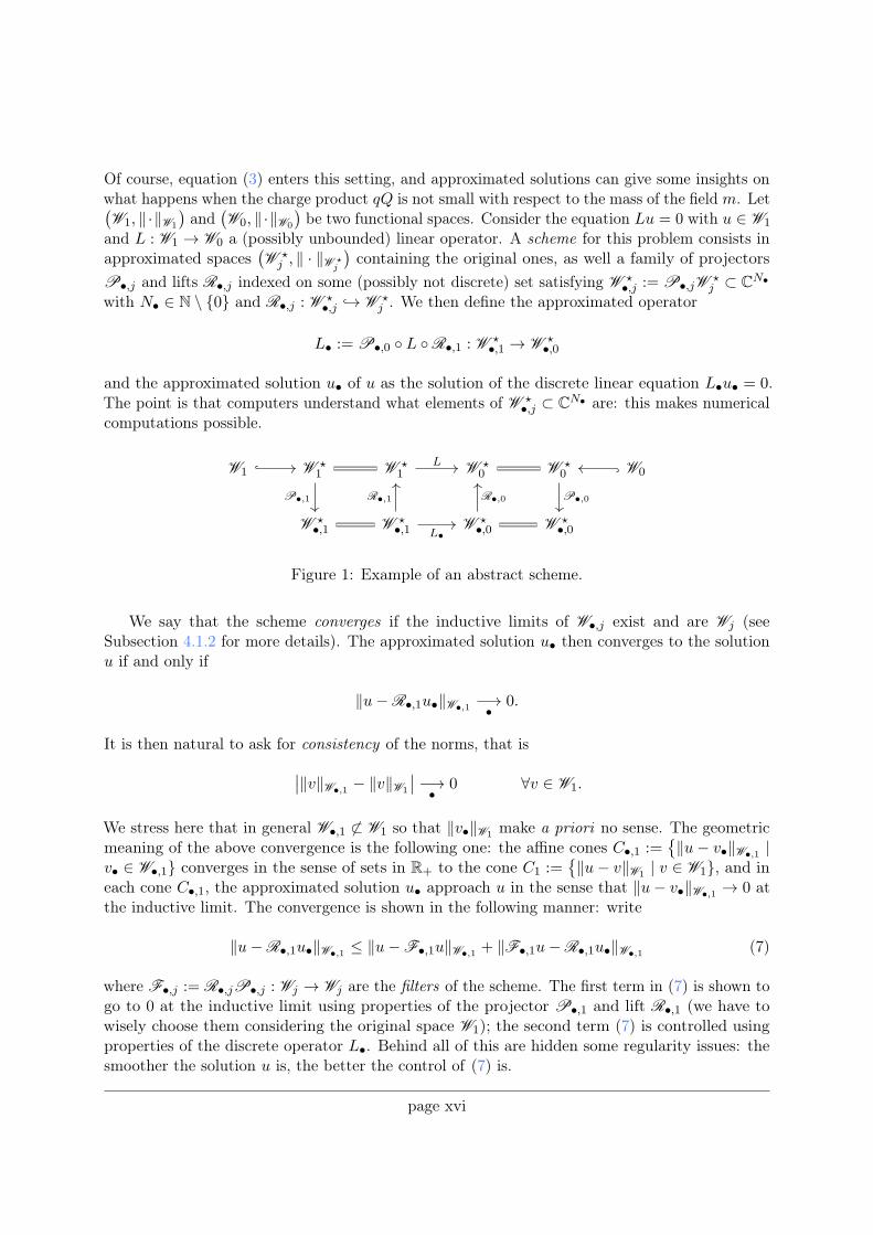
and L : W1 → W0 a (possibly unbounded) linear operator. A scheme for this problem consists inapproximated spaces
(W ⋆
j , ‖ · ‖W ⋆j
)containing the original ones, as well a family of projectors
P•,j and lifts R•,j indexed on some (possibly not discrete) set satisfying W ⋆•,j := P•,jW ⋆
j ⊂ CN•
with N• ∈ N \ 0 and R•,j : W ⋆•,j → W ⋆
j . We then define the approximated operator
L• := P•,0 L R•,1 : W⋆•,1 → W
⋆•,0
and the approximated solution u• of u as the solution of the discrete linear equation L•u• = 0.The point is that computers understand what elements of W ⋆
•,j ⊂ CN• are: this makes numericalcomputations possible.
W1 W ⋆1 W ⋆
1 W ⋆0 W ⋆
0 W0
W ⋆•,1 W ⋆
•,1 W ⋆•,0 W ⋆
•,0
P•,1
L
P•,0R•,1
L•
R•,0
Figure 1: Example of an abstract scheme.
We say that the scheme converges if the inductive limits of W•,j exist and are Wj (seeSubsection 4.1.2 for more details). The approximated solution u• then converges to the solutionu if and only if
‖u−R•,1u•‖W•,1 −→• 0.
It is then natural to ask for consistency of the norms, that is
∣∣‖v‖W•,1 − ‖v‖W1
∣∣ −→•
0 ∀v ∈ W1.
We stress here that in general W•,1 6⊂ W1 so that ‖v•‖W1 make a priori no sense. The geometricmeaning of the above convergence is the following one: the affine cones C•,1 :=
‖u− v•‖W•,1 |
v• ∈ W•,1 converges in the sense of sets in R+ to the cone C1 :=‖u− v‖W1 | v ∈ W1, and in
each cone C•,1, the approximated solution u• approach u in the sense that ‖u− v•‖W•,1 → 0 atthe inductive limit. The convergence is shown in the following manner: write
‖u−R•,1u•‖W•,1 ≤ ‖u−F•,1u‖W•,1 + ‖F•,1u−R•,1u•‖W•,1 (7)
where F•,j := R•,jP•,j : Wj → Wj are the filters of the scheme. The first term in (7) is shown togo to 0 at the inductive limit using properties of the projector P•,1 and lift R•,1 (we have towisely choose them considering the original space W1); the second term (7) is controlled usingproperties of the discrete operator L•. Behind all of this are hidden some regularity issues: thesmoother the solution u is, the better the control of (7) is.
page xvi
Chapter 5: Approximation of low frequency resonances. Chapter 5 is devoted to approx-imation of low frequency resonances of the charged Klein-Gordon equation in the exterior DSRNspacetime. Localization of resonances is an interesting but difficult task. High frequency resonancescan be localized in the(De Sitter-)Schwarzschild spacetime (see [SaZw97]); in Theorem 1.3.1, we have the same re-sult in the DSRN case for small charge product. Purely numerical approximations of these highfrequency resonances have been carried out in [CCDHJa] and [CCDHJb] based on Chebyshevtype polynomial interpolation. In these references, the authors compute approximated lowfrequency resonances in function of the charge product qQ: the resonance 0 of the uncharged andnon-massive case is shown to move into the upper complex half plane when qQ is not small inregard of m (Theorem 1.3.2 shows that resonances are repelled to the lower complex half planeotherwise) then go down to the lower half plane for higher values of qQ. That this resonanceeventually reaches a certain line ℑz = −κ/2 with κ > 0 is linked to the modern formulationof the Strong Cosmic Censorship (see [CCDHJb, Section I]). In this thesis, we adopt anothermethod based on complex analysis. We show in Subsection 1.2.3 that the kernel of the quadraticpencil p(z, s) := h0 − (z − sV )2 is inversely proportional to an analytic function W (z), calledthe Wronskian. This provides an explicit characterization of resonances as being the zeros of W .Using a scheme similar to the one introduced above, we can defined an approximated WronskianW•(z) which is analytic in z. Assume that we have a control of the error in the following sense:there exists C, h• > 0 such that for all z ∈ Γ ⊂ C where Γ is a positively oriented contour,
|W (z)−W•(z)| ≤ Ch•. (8)
The term h• tends to zero at the inductive limit of the scheme. Then Rouché’s theorem impliesthat W•(z) has as many zeros as W (z) inside Γ as the scheme converges. Hence, we can have thenumber N(Γ) of resonances (counted with their multiplicity) inside Γ at the inductive limit usingthe argument principle
N•(Γ) =1
2πi
˛
Γ
W ′• (z)
W•(z)dz.
The effectiveness of this method lies in the fact that the above formula gives an integer, so that asufficiently small error of approximation provides the exact number of resonances enclosed byΓ. Furthermore, if a resonance z0 is isolated inside Γ, then an approximated resonance z•(Γ) isgiven by
z•(Γ) =1
2πi
˛
ΓzW ′
• (z)W•(z)
dz.
The counterpart of such an ambitious precision is that the error can be very difficult to estimatein practice when W is not analytic below a line ℑ(z) = ǫ, ǫ ∈ R: estimates for the error thenworsen as the contour Γ approaches this line.
Chapter 6: Discussions and perspectives. The last part of this manuscript is devoted tosome concluding discussions and remarks about the work carried out during the thesis.
page xvii

page xviii
Contents
Abstract/Résumé iii
Acknowledgments vii
Introduction ix
Table of contents xxi
Notations 1
1 Decay of the Local Energy for the Charged Klein-Gordon Equation in theExterior De Sitter-Reissner-Nordström Spacetime 31.1 Functional framework . . . . . . . . . . . . . . . . . . . . . . . . . . . . . . . . . 4
1.1.1 The charged Klein-Gordon equation on the DSRN metric . . . . . . . . . 41.1.2 The Regge-Wheeler coordinate . . . . . . . . . . . . . . . . . . . . . . . . 51.1.3 The charge Klein-Gordon operator . . . . . . . . . . . . . . . . . . . . . . 61.1.4 The quadratic pencil . . . . . . . . . . . . . . . . . . . . . . . . . . . . . . 8
1.2 Meromorphic extension and resonances . . . . . . . . . . . . . . . . . . . . . . . . 81.2.1 Notations . . . . . . . . . . . . . . . . . . . . . . . . . . . . . . . . . . . . 91.2.2 Abstract setting . . . . . . . . . . . . . . . . . . . . . . . . . . . . . . . . 101.2.3 Study of the asymptotic Hamiltonians . . . . . . . . . . . . . . . . . . . . 131.2.4 Construction of the meromorphic extension of the weighted resolvent . . . 17
1.3 Resonance expansion for the charged Klein-Gordon equation . . . . . . . . . . . . 211.4 Estimates for the cut-off inverse of the quadratic pencil . . . . . . . . . . . . . . . 23
1.4.1 Estimates in the zone II . . . . . . . . . . . . . . . . . . . . . . . . . . . . 251.4.2 Estimates in the zone III . . . . . . . . . . . . . . . . . . . . . . . . . . . . 271.4.3 Estimates in the zone IV . . . . . . . . . . . . . . . . . . . . . . . . . . . . 30
1.5 Proof of the main theorem . . . . . . . . . . . . . . . . . . . . . . . . . . . . . . . 321.6 Appendix . . . . . . . . . . . . . . . . . . . . . . . . . . . . . . . . . . . . . . . . 38
1.6.1 Analytic extension of the coordinate r . . . . . . . . . . . . . . . . . . . . 381.6.2 Localization of high frequency resonances . . . . . . . . . . . . . . . . . . 401.6.3 Abstract Semiclassical Limiting Absorption Principle for a class of General-
ized Resolvents . . . . . . . . . . . . . . . . . . . . . . . . . . . . . . . . . 41
xix
2 Scattering Theory for the Charged Klein-Gordon Equation in the Exterior DeSitter-Reissner-Nordström Spacetime 472.1 The extended spacetime . . . . . . . . . . . . . . . . . . . . . . . . . . . . . . . . 48
2.1.1 The neutralization procedure . . . . . . . . . . . . . . . . . . . . . . . . . 482.1.2 Extended Einstein-Maxwell equations . . . . . . . . . . . . . . . . . . . . 502.1.3 Dominant energy condition . . . . . . . . . . . . . . . . . . . . . . . . . . 51
2.2 Global geometry of the extended spacetime . . . . . . . . . . . . . . . . . . . . . 542.2.1 Principal null geodesics . . . . . . . . . . . . . . . . . . . . . . . . . . . . 542.2.2 Surface gravities and Killing horizons . . . . . . . . . . . . . . . . . . . . . 562.2.3 Crossing rings . . . . . . . . . . . . . . . . . . . . . . . . . . . . . . . . . . 582.2.4 Black rings . . . . . . . . . . . . . . . . . . . . . . . . . . . . . . . . . . . 60
2.3 Analytic scattering theory . . . . . . . . . . . . . . . . . . . . . . . . . . . . . . . 642.3.1 Hamiltonian formulation of the extended wave equation . . . . . . . . . . 642.3.2 Comparison dynamics . . . . . . . . . . . . . . . . . . . . . . . . . . . . . 672.3.3 Transport along principal null geodesics . . . . . . . . . . . . . . . . . . . 702.3.4 Structure of the energy spaces for the comparison dynamics . . . . . . . . 722.3.5 Analytic scattering results . . . . . . . . . . . . . . . . . . . . . . . . . . . 77
2.4 Proof of the analytic results . . . . . . . . . . . . . . . . . . . . . . . . . . . . . . 792.4.1 Geometric hypotheses . . . . . . . . . . . . . . . . . . . . . . . . . . . . . 792.4.2 Proof of Theorem 2.3.8 . . . . . . . . . . . . . . . . . . . . . . . . . . . . . 802.4.3 Proof of Theorem 2.3.9 . . . . . . . . . . . . . . . . . . . . . . . . . . . . . 802.4.4 Proof of Theorem 2.3.10 . . . . . . . . . . . . . . . . . . . . . . . . . . . . 812.4.5 Proof of Theorem 2.3.11 . . . . . . . . . . . . . . . . . . . . . . . . . . . . 812.4.6 Proof of Proposition 2.3.13 . . . . . . . . . . . . . . . . . . . . . . . . . . 85
2.5 Geometric interpretation . . . . . . . . . . . . . . . . . . . . . . . . . . . . . . . . 872.5.1 Energy spaces on the horizons . . . . . . . . . . . . . . . . . . . . . . . . . 872.5.2 The full wave operators . . . . . . . . . . . . . . . . . . . . . . . . . . . . 882.5.3 Inversion of the full wave operators . . . . . . . . . . . . . . . . . . . . . . 912.5.4 Traces on the energy spaces . . . . . . . . . . . . . . . . . . . . . . . . . . 932.5.5 Solution of the Goursat problem . . . . . . . . . . . . . . . . . . . . . . . 94
2.6 Appendix: Remarkable tensors . . . . . . . . . . . . . . . . . . . . . . . . . . . . 95
3 Decay of the Local Energy through the Horizons for the Wave Equation inthe Exterior Extended Spacetime 1013.1 Statement of the main result . . . . . . . . . . . . . . . . . . . . . . . . . . . . . 1013.2 Construction of the red-shift vector field . . . . . . . . . . . . . . . . . . . . . . . 1023.3 Proof of the decay through the horizons . . . . . . . . . . . . . . . . . . . . . . . 104
4 Numerical Study of an Abstract Klein-Gordon type Equation: Applicationsto the Charged Klein-Gordon Equation in the Exterior De Sitter-Reissner-Nordström Spacetime 1114.1 The abstract problem . . . . . . . . . . . . . . . . . . . . . . . . . . . . . . . . . 112
4.1.1 Introduction of the abstract problem . . . . . . . . . . . . . . . . . . . . . 1124.1.2 Discretization of the abstract problem . . . . . . . . . . . . . . . . . . . . 1164.1.3 Matrix representation . . . . . . . . . . . . . . . . . . . . . . . . . . . . . 122
page xx
4.2 Consistency and stability . . . . . . . . . . . . . . . . . . . . . . . . . . . . . . . 1284.2.1 Error of interpolation . . . . . . . . . . . . . . . . . . . . . . . . . . . . . 1294.2.2 Consistency . . . . . . . . . . . . . . . . . . . . . . . . . . . . . . . . . . . 1404.2.3 Stability . . . . . . . . . . . . . . . . . . . . . . . . . . . . . . . . . . . . . 148
4.3 Convergence and application . . . . . . . . . . . . . . . . . . . . . . . . . . . . . . 1534.3.1 Convergence of the scheme . . . . . . . . . . . . . . . . . . . . . . . . . . 1534.3.2 Application to the charged Klein-Gordon equation in the DSRN spacetime 158
4.4 Appendix . . . . . . . . . . . . . . . . . . . . . . . . . . . . . . . . . . . . . . . . 1614.4.1 Computation of M• . . . . . . . . . . . . . . . . . . . . . . . . . . . . . . 1624.4.2 Computation of H⋆
• . . . . . . . . . . . . . . . . . . . . . . . . . . . . . . . 1624.4.3 Computation of the matrix coefficients of N• . . . . . . . . . . . . . . . . 163
5 Approximation of low frequency resonances 1735.1 Characterization of resonances . . . . . . . . . . . . . . . . . . . . . . . . . . . . . 1735.2 Approximation of the Wronskian . . . . . . . . . . . . . . . . . . . . . . . . . . . 175
5.2.1 Modified Jost solutions . . . . . . . . . . . . . . . . . . . . . . . . . . . . . 1755.2.2 Introduction of the scheme . . . . . . . . . . . . . . . . . . . . . . . . . . 176
5.3 Error of approximation . . . . . . . . . . . . . . . . . . . . . . . . . . . . . . . . . 1795.3.1 Constants in the scheme . . . . . . . . . . . . . . . . . . . . . . . . . . . . 1795.3.2 Convergence of the scheme . . . . . . . . . . . . . . . . . . . . . . . . . . 1825.3.3 Bounds for the modified Jost solutions . . . . . . . . . . . . . . . . . . . . 1855.3.4 Error of approximation for the Wronskian . . . . . . . . . . . . . . . . . . 185
5.4 Approximation of low frequency resonances . . . . . . . . . . . . . . . . . . . . . 1875.4.1 The method . . . . . . . . . . . . . . . . . . . . . . . . . . . . . . . . . . . 1875.4.2 Application . . . . . . . . . . . . . . . . . . . . . . . . . . . . . . . . . . . 1885.4.3 Discussion about the constants . . . . . . . . . . . . . . . . . . . . . . . . 193
5.5 Appendix: Proofs of technical results . . . . . . . . . . . . . . . . . . . . . . . . . 1955.5.1 Preliminary estimates . . . . . . . . . . . . . . . . . . . . . . . . . . . . . 1965.5.2 Proof of Lemma 5.3.1 . . . . . . . . . . . . . . . . . . . . . . . . . . . . . 1985.5.3 Proof of Lemma 5.3.2 . . . . . . . . . . . . . . . . . . . . . . . . . . . . . 2045.5.4 Proof of Lemma 5.5.3 . . . . . . . . . . . . . . . . . . . . . . . . . . . . . 2085.5.5 Proof of Lemma 5.3.5 . . . . . . . . . . . . . . . . . . . . . . . . . . . . . 2085.5.6 Proof of Corollary 5.3.6 . . . . . . . . . . . . . . . . . . . . . . . . . . . . 2095.5.7 Proof of Lemma 5.3.8 . . . . . . . . . . . . . . . . . . . . . . . . . . . . . 209
5.6 Appendix: Approximations . . . . . . . . . . . . . . . . . . . . . . . . . . . . . . 2135.6.1 Computation of the discretized operators for the scheme (5.9) . . . . . . . 2145.6.2 Discrete version of the argument principle . . . . . . . . . . . . . . . . . . 2165.6.3 Approximated resonances . . . . . . . . . . . . . . . . . . . . . . . . . . . 218
6 Discussions and Perspectives 2236.1 Discussions . . . . . . . . . . . . . . . . . . . . . . . . . . . . . . . . . . . . . . . 2236.2 Perspectives . . . . . . . . . . . . . . . . . . . . . . . . . . . . . . . . . . . . . . . 226
Bibliography 229
page xxi

page xxii
Notations and conventions
We present here the notations that we will use throughout this document.
The set z ∈ C | ℑz ≷ 0 will be denoted by C±. For any complex number λ ∈ C, we will
write 〈λ〉 :=(1 + |λ|2
)1/2, D(λ,R) will be the disc centered at λ ∈ C of radius R > 0 andD(λ,R)∁ its complementary set. For all ω = |ω|eiθ ∈ C\]−∞, 0], θ ∈ R, we will use the branchof the square root defined by
√ω :=
√|ω|eiθ/2. To emphasize some important dependences, the
symbol ≡ will be used: for example, a ≡ a(b) means "a depends on b". We will write u . v tomean u ≤ Cv for some constant C > 0 independant of u and v.
The notation Ckc will be used to denote the space of compactly supported Ck functions. Also,the Schwartz space on R will be denoted by S . If V,W are complex vector spaces, then L(V,W )will be the space of bounded linear operators V → W . We will denote by B(V ) (respectivelyB∞(V )) the space of all bounded (respectively compact) operators acting on V . If W ⊂ V is asubspace and ‖.‖ is a norm on V , then W ‖.‖ denotes the completion of W for the norm ‖.‖.
All the scalar products 〈· , ·〉 will be antilinear with respect to their first component and linearwith respect to their second component. For any function f , the support of f will be denoted bySupp f . If A is an operator, we will denote by D (A) its domain, σ (A) its spectrum and ρ (A)its resolvent set. A ≥ 0 will mean that 〈Au, u〉 ≥ 0 for all u ∈ D(A), and A > 0 will mean thatA ≥ 0 and ker(A) = 0.
Now we define the symbol classes on R2d
Sm,n :=a ∈ C∞(R2d,C) | ∀(α, β) ∈ N2d, ∃Cα,β > 0, |∂αξ ∂βxa(x, ξ)| ≤ Cα,β〈ξ〉m−|α|〈x〉n−|β|
for any (m,n) ∈ Z2d (here N and Z both include 0). We then define the semiclassical pseudodif-ferential operators classes
Ψm,n := aw(x, hD) | a ∈ Sm,n , Ψ−∞,n :=⋂
m∈ZΨm,n
with aw(x, hD) the Weyl quantization of the symbol a. For any c > 0, the notation P ∈ cΨm,n
means that P ∈ Ψm,n and the norm of P is bounded by a positive multiple of c.When using the standard spherical coordinates (θ, ϕ) ∈ ]0, π[× ]0, 2π[ on S2, we will always
ignore the singularities θ = 0, θ = π. We refer to [ON95, Lemma 2.2.2] to properly fix it.
1
Let I ⊂ R be a Lebesgue measurable set and let γ ∈ [0, 1]. We denote by Ck,γ(I,K) the spaceof k times continuously differentiable functions from I to K whose k-th derivative is γ-Hölder,and by Ck,γc (I,K) the space of all such functions with compact support in I. These spaces can beendowed with the following norm:
‖u‖Ck,γ(I,K) :=k∑
j=0
‖∂jru‖L∞(I,K) + supr,r′∈I
|(∂kr u)(r)− (∂kr u)(r′)|
|r − r′|γ .
The space of piece-wise Ck functions on I will be denoted by Ckpiece(I,K); any element u will bedefined everywhere on I by putting u(r0) := 0 at any discontinuity point r0.
Given ρ : I → ]0,+∞[ a Lebesgue measurable function, we define the weighted space
L2ρ :=
u : I → C | u ∈ L2(I, ρ(r)dr)
and write 〈. , .〉L2ρ
and ‖ . ‖L2ρ
for the associated weighted L2 right linear scalar product and norm,respectively. The standard norm on Lp(I,dr) (respectively on Hp(I,dr)) will be denoted by‖.‖Lp (respectively by ‖.‖Hp) for all 1 ≤ p ≤ +∞, and we will note 〈. , .〉Hp the standard scalarproduct on Hp(I, dr). Given a (pseudo-)differential operator P acting on L2
ρ which is self-adjointand such that P > 0 (that is P ≥ 0 and kerP = 0), we define for k ≥ 0 the scales of Sobolevspaces
H2k+1ρ :=
u : I → C |
⟨P 2k+1u, u
⟩L2ρ< +∞
,
H2kρ :=
u : I → C | ‖P ku‖L2
ρ< +∞
,
Hkρ := Hk
ρ ∩ L2ρ
with the corresponding norms
‖u‖H2k+1ρ
:=⟨P 2k+1u, u
⟩1/2L2ρ,
‖u‖H2kρ
:= ‖P ku‖L2ρ,
‖u‖Hkρ:=√‖u‖2
L2ρ+ ‖u‖2Hk
ρ.
(Scale of) Sobolev spaces with negative exponent are then defined as the dual spaces of thecorresponding (scale of) Sobolev spaces with positive exponent. When ρ ≡ 1 (i.e. ρ(r)dr is theLebesgue measure), we will simply use the subscript Lp instead of Lp
1 in the norms and scalarproducts (when p = 2). We will denote by Hk
ℓoc and Hkc respectively the space of locally or
compactly supported Hk functions.If u : R→ C is Lebesgue integrable for the measure µ, then for all Lebesgue measurable set
S ⊂ R such that µ(S) 6= 0, we defineˆ
–
Su(x) dµ(x) :=
1
µ(S)
ˆ
Su(x) dµ(x).
The set of Lebesgue points of u (in I) will be denoted by L (u).
page 2
Chapter 1Decay of the Local Energy for the ChargedKlein-Gordon Equation in the Exterior DeSitter-Reissner-Nordström Spacetime
In this chapter, we show a resonance expansion for the solutions of the charged Klein-Gordonequation on the DSRN metric. As a corollary we obtain exponential decay of the local energy forthese solutions. We restrict our study to the case where the product of black hole charge and thescalar field charge is small. Such a resonance expansion for the solutions of the wave equation hasbeen obtained first by Bony-Häfner for the wave equation on the De Sitter-Schwarzschild metric[BoHa08]. This result has been generalized to much more complicated situations which includeperturbations of the De Sitter-Kerr metric by Vasy [Va13]. This last paper has developed newmethods including a Fredholm theory for non elliptic problems. These methods could probablyalso be applied to the present case. In this chapter however we use the more elementary methodsof Bony-Häfner [BoHa08] and Georgescu-Gérard-Häfner [GGH17].
The smallness of the charge product is non-quantitative as it is determined from a compactnessargument. It allows us at many places to use perturbation arguments with respect to the non-charged case. As far as we are aware the absence of growing modes for the present system isnot known for general charge products. In contrast to that absence of growing modes is knownfor the wave equation on the Kerr metric for general angular momentum of the black hole, see[Wh89]. The question of the existence or not of such modes is a very subtle question and growingmodes appear for example for the Klein-Gordon equation on the Kerr metric, see [SR14].
Organization of the chapter. Chapter 1 is organized as follows. In Section 1.1 we give anintroduction to the DSRN metric and the charged Klein-Gordon equation on it. In Section 1.2, ameromorphic extension result is shown for the cut-off resolvent and resonances are introduced.The resonance expansion as well as the exponential decay through the horizons are presented inSection 1.3. Suitable resolvent-type estimates are obtained in Section 1.4. In section 1.5 we provethe main theorems by a suitable contour deformation and using the resolvent-type estimates ofSection 1.4. The appendix contains a semiclassical limiting absorption principle for a class ofgeneralized resolvents which might have some independent interest.
3
1.1 Functional framework
1.1 Functional framework
1.1.1 The charged Klein-Gordon equation on the DSRN metric
Let
F (r) := 1− 2M
r+Q2
r2− Λr2
3
with M > 0 the mass of the black hole, Q ∈ R \ 0 its electric charge and Λ > 0 the cosmologicalconstant. We assume that
∆ := 9M2 − 8Q2 > 0, max
0,
6(M −
√∆)
(3M −
√∆)3
< Λ <
6(M +
√∆)
(3M +
√∆)3 (1.1)
so that F has four distinct zeros −∞ < rn < 0 < rc < r− < r+ < +∞ and is positive for allr ∈ ]r−, r+[ (see [Hi18, Proposition 3.2]; see also [Mok17, Proposition 1] with Λ replaced by Λ/3for a different statement of the condition). We also assume that 9ΛM2 < 1 so that we can usethe work of Bony-Häfner [BoHa08]. The exterior DSRN spacetime is the Lorentzian manifold(M, g) with
M = Rt × ]r−, r+[r × S2ω, g = F (r) dt2 − F (r)−1 dr2 − r2dω2
where dω2 is the standard metric on the unit sphere S2.Let A := Q
r dt. Then the charged wave operator on (M, g) is
g = (∇µ − iqAµ) (∇µ − iqAµ) =1
F (r)
((∂t − i
r
)2
− F (r)
r2∂rr
2F (r)∂r −F (r)
r2∆S2
)
and the corresponding charged Klein-Gordon equation reads
gu+m2u = 0 m > 0.
We set s := qQ ∈ R the charge product (which appears in the perturbation term of the standardwave operator), X := ]r−, r+[r × S2ω and V (r) := r−1 so that the above equation reads
(∂t − isV )2 u+ P u = 0 (1.2)
with
P = −F (r)r2
∂r(r2F (r)∂r
)− F (r)
r2∆S2 +m2F (r)
= −F (r)2∂2r − F(2F (r)
r+∂F
∂r(r)
)∂r −
F (r)
r2∆S2 +m2F (r) (1.3)
defined on D(P ) :=u ∈ L2
(X,F (r)−1r2drdω
) ∣∣P u ∈ L2(X,F (r)−1r2drdω
) (this is the
spatial operator in [BoHa08] with the additional mass term m2F (r)). In the sequel, we will usethe following notations:
V± := limr→r±
V (r) = r−1± .
It turns out that the positive mass makes the study of the equation easier. Besides the fact thatmassless charged particles do not exist in physics, it is not excluded that the resonance 0 for thecase s = 0 (see [BoHa08]) can move to C+ in the case s 6= 0 and m = 0.
page 4
1.1 Functional framework
1.1.2 The Regge-Wheeler coordinate
We introduce the Regge-Wheeler coordinate x ≡ x (r) defined by the differential relation
dx
dr:=
1
F (r). (1.4)
Using the four roots rα of F , α ∈ I := n, c,−,+, we can write
1
F (r)= −3r2
Λ
∑
α∈I
Aα
r − rα
where Aα =∏
β∈I\α(rα − rβ)−1 for all α ∈ I, and ±A± > 0. Integrating (1.4) then yields
x (r) = − 3
Λ
∑
α∈IAαr
2α ln
∣∣∣∣r − rαr− rα
∣∣∣∣ (1.5)
with r := 12
(3M +
√9M2 − 8Q2
)(we will explain this choice below); observe that |Q| < 3√
8M
if (??) holds (see the discussion below (17) in [Mok17]). Therefore, we have
|r − rα| = |r− rα|∏
β∈I\α
∣∣∣∣r − rβr− rβ
∣∣∣∣−Aβr
2β/(Aαr2α)
exp
(− Λ
3Aαr2αx
)∀α ∈ I
which entails the asymptotic behaviours
F (r (x)) + |r (x)− r±| . exp
(− Λ
3A±r2±x
)x→ ±∞. (1.6)
Note here that
− Λ
3A±r2±= F ′(r±) = 2κ± (1.7)
where κ− > 0 is the surface gravity at the event horizon and κ+ < 0 is the surface gravity at thecosmological horizon. Recall that κ± is defined by the relation
Xµ∇µXν = −2κ±Xν X = ∂t
where the above equation is to be considered at the corresponding horizon.In Appendix 1.6.1, we follow [BaMo93, Proposition IV.2] to show the extension result:
Proposition 1.1.1. There exists a constant A > 0 such that the function x 7→ r(x) extendsanalytically to λ ∈ C | |ℜλ| > A .
On L2 (X, dxdω), define the operator P := rP r−1, given in the coordinates (x, ω) by theexpression
P = −r−1∂xr2∂xr
−1 − F (r)
r2∆S2 +m2F (r) = −∂2x −W0∆S2 +W1 (1.8)
page 5
1.1 Functional framework
where
W0 (x) :=F (r (x))
r (x)2, W1 (x) :=
F (r (x))
r (x)
∂F
∂r(r (x)) +m2F (r (x)) . (1.9)
It will happen in the sequel that we write F (x) for F (r (x)) and also V (x) for V (r (x)). Observethat the potentials W0 and W1 satisfy the same estimate as in (1.6).
As
dW0
dx= F (r)
dW0
dr=
2F (r)
r5(3Mr − 2Q2 − r2
),
we see that the (unstable) maximum ofW0 occurs when x = 0, i.e. r = r = 12
(3M +
√9M2 − 8Q2
):
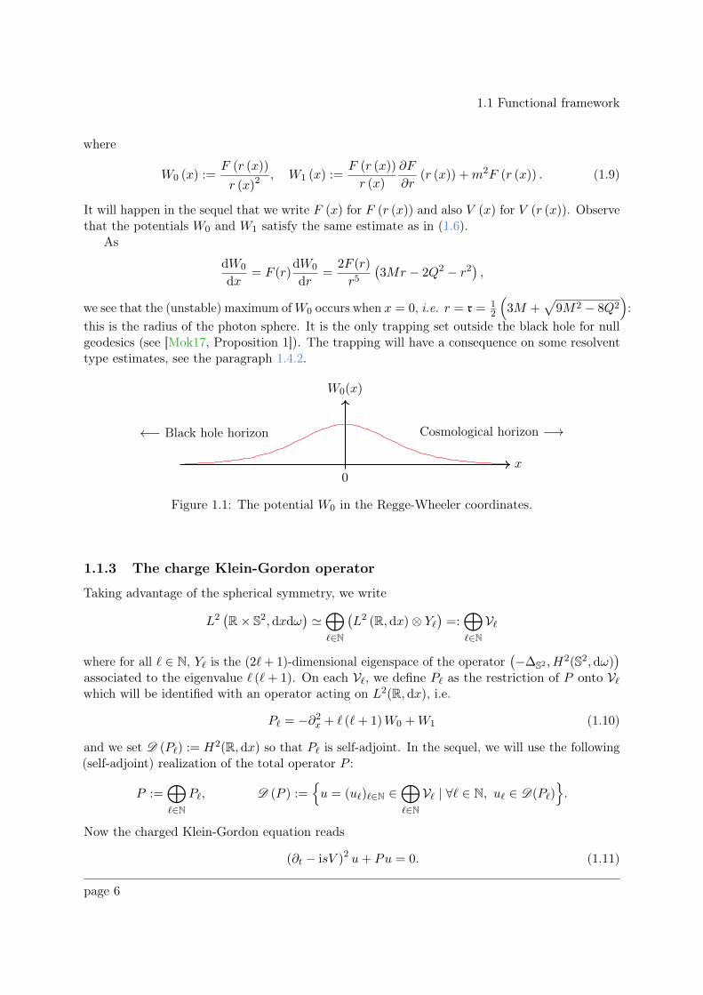
this is the radius of the photon sphere. It is the only trapping set outside the black hole for nullgeodesics (see [Mok17, Proposition 1]). The trapping will have a consequence on some resolventtype estimates, see the paragraph 1.4.2.
W0(x)
x
←− Black hole horizon Cosmological horizon −→
0
Figure 1.1: The potential W0 in the Regge-Wheeler coordinates.
1.1.3 The charge Klein-Gordon operator
Taking advantage of the spherical symmetry, we write
L2(R× S2, dxdω
)≃⊕
ℓ∈N
(L2 (R, dx)⊗ Yℓ
)=:⊕
ℓ∈NVℓ
where for all ℓ ∈ N, Yℓ is the (2ℓ+ 1)-dimensional eigenspace of the operator(−∆S2 , H
2(S2, dω))
associated to the eigenvalue ℓ (ℓ+ 1). On each Vℓ, we define Pℓ as the restriction of P onto Vℓwhich will be identified with an operator acting on L2(R, dx), i.e.
Pℓ = −∂2x + ℓ (ℓ+ 1)W0 +W1 (1.10)
and we set D (Pℓ) := H2(R, dx) so that Pℓ is self-adjoint. In the sequel, we will use the following(self-adjoint) realization of the total operator P :
P :=⊕
ℓ∈NPℓ, D (P ) :=
u = (uℓ)ℓ∈N ∈
⊕
ℓ∈NVℓ | ∀ℓ ∈ N, uℓ ∈ D(Pℓ)
.
Now the charged Klein-Gordon equation reads
(∂t − isV )2 u+ Pu = 0. (1.11)
page 6
1.1 Functional framework
The point is to see that if u is a solution of (1.11), then v := (u,−i∂tu− sV u) solves the firstorder equation
−i∂tv = K(s)v (1.12)
where
K (s) :=
(sV 1
P sV
)(1.13)
is the charge Klein-Gordon operator. Conversely, if v = (v0, v1) solves (1.12), then v0 solves(1.11). We also define Kℓ ≡ Kℓ(s)
1 with Pℓ in place of P for any ℓ ∈ N. Following [GGH17,Section 3], we realize Kℓ with the domain
D(Kℓ) :=u ∈ P−1/2
ℓ L2(R, dx)⊕ L2(R, dx) | Kℓu ∈ P−1/2ℓ L2(R, dx)⊕ L2(R, dx)
and realize the operator K as the direct sum on N ∋ ℓ of the Kℓ.Let Eℓ be the completion of P−1/2
ℓ L2(R, dx)⊕ L2(R, dx) for the norm2
‖u‖2Eℓ
:= 〈u0, Pℓu0〉L2(R,dx)+ ‖u1 − sV u0‖2
L2(R,dx)u = (u0, u1) ∈ Eℓ
and define(E , ‖.‖E
)as the direct sum of the spaces Eℓ. [GGH17, Lemma 3.19] shows that Kℓ
generates a continuous one-parameter group3 (e−itKℓ)t∈R on (Eℓ, ‖.‖Eℓ ). We similarly construct
the spaces(Eℓ, ‖.‖Eℓ
)and
(E , ‖.‖E
)with 〈Pℓ〉 instead of Pℓ. Let us mention here that for any
n ∈ R the quantity
〈v |v〉n := 〈v1 − nv0, v1 − nv0〉L2(R,dx)+ 〈(P − (sV − n)2 )v0, v0〉L2(R,dx)
(1.14)
is formally conserved if v = (u,−i∂tu) with u solution of (1.11) and is continuous with respect tothe norm ‖.‖E . However, it is in general not positive nor continuous with respect to the norm‖.‖E (see [GGH17, paragraph 3.4.3] for more details): this is superradiance. When Λ = 0 (that is,when the cosmological horizon is at infinity), the natural energy 〈. | .〉sV− is positive for s smallenough and it can be used to define a Hilbert space framework.
An important observation is the fact that the norms ‖.‖Eℓ
and ‖.‖Eℓ are locally equivalent,
meaning that for any v ∈ E and any cut-off χ ∈ C∞c (R,R), we have
‖χv‖E. ‖χv‖E . ‖χv‖
E. (1.15)
The first inequality is obvious, and the second one is established with the Hardy type estimate‖χv‖
L2 . ‖P 1/2v‖L2 (see [GGH17, Lemma 9.5]; the validity of this result in our setting is
discussed in Subsection 5.1 below).
1We will often drop the dependence in s.2Note that the norm ‖.‖2
Eℓ
is conserved if [Pℓ, sV ] = 0; it is the case if s = 0.
3The notation is abusive here as the group should be denoted by (eitKℓ)t∈R. We will however keep thisconvention in this chapter.
page 7
1.2 Meromorphic extension and resonances
1.1.4 The quadratic pencil
Let u be a solution of (1.11). If we look for u of the form u = eiztv with z ∈ C for some v, then vsatisfies the equation (P − (z − sV )2)v = 0. We define the harmonic quadratic pencil
pℓ (z, s) := Pℓ − (z − sV )2 , D(pℓ(z, s)) := 〈Pℓ〉−1L2(R, dx) = H2(R, dx)
and realize the total quadratic pencil as
p (z, s) :=⊕
ℓ∈Npℓ (z, s) ,
D(p(z, s)) :=u = (uℓ)ℓ∈N ∈
⊕
ℓ∈NVℓ∣∣∣ ∀ℓ ∈ N, uℓ ∈ D(pℓ(z, s)),
∑
ℓ∈N‖pℓ(z, s)uℓ‖2Vℓ
< +∞.
[GGH17, Proposition 3.15] sets the useful relations
ρ(Kℓ) ∩ C \ R =z ∈ C \ R
∣∣ pℓ (z, s) : H2(R, dx)→ L2(R, dx) is bijective
(1.16)
and
Rℓ (z, s) := (Kℓ(s)− z)−1 =
(pℓ (z, s)
−1 (z − sV ) pℓ (z, s)−1
1+ (z − sV ) pℓ (z, s)−1 (z − sV ) (z − sV ) pℓ (z, s)
−1
)(1.17)
for all z ∈ ρ(Kℓ) ∩ C \ R. In comparison, the relation (1.7) in [BoHa08] involves the resolvent ofPℓ, which corresponds to the case s = 0 for us. [GGH17, Proposition 3.12] shows that (1.17) isalso valid for z ∈ ρ(Kℓ) ∩ R when we work on (Eℓ, ‖.‖Eℓ ); by using the local equivalence (1.15) of
the norms ‖.‖Eℓ
and ‖.‖Eℓ , we can use (1.17) for z ∈ ρ(Kℓ)∩R if we consider the cut-off resolvent
χRℓ (z, s)χ with χ ∈ C∞c (R,R). In the sequel, we will simply call pℓ(z, s) the quadratic pencilwhen ℓ ∈ N will be fixed.
1.2 Meromorphic extension and resonances
We construct in this Section a meromorphic extension for the weighted resolvent of K(s). Themain result of this chapter, Theorem 1.3.2, which provides asymptotic decay (in time) for solutionsof the charged Klein-Gordon equation (4.37), relies on such a construction. The presence of themixed term sV ∂t in (4.37) prevents us to directly use Mazzeo-Melrose result [MaMe87]. However,p(z, s)−1 formally tends to (P − z2)−1 as s→ 0 for which [MaMe87] applies; moreover, the cases = 0 is very similar (even easier) to the case treated in [BoHa08]. We will therefore obtainresults for small s using perturbation arguments. Our strategy is the following one:
(i) Define first suitable "asymptotic" energy spaces by removing the troublesome negativecontributions from the electromagnetic potential sV near r± and define "asymptotic"selfadjoint Hamiltonians H±(s) (see the paragraph 1.2.1 below).
(ii) For s = 0, the situation is really similar to the Klein-Gordon equation on De Sitter-Schwarzschild metric: using the standard results [BoHa08] and [MaMe87], we can mero-morphically extend the weighted resolvent of H±(0) from C+ to C with no poles on andabove the real axis (see Lemma 1.2.1 and Lemma 1.2.2).
page 8
1.2 Meromorphic extension and resonances
(iii) If s remains small, we can use analytic Fredholm theory to get a meromorphic extensionfor the weighted resolvents of the asymptotic Hamiltonians H±(s) into a strip in C− (theperturbation argument entails a bound on the width of this strip which is directly linked tothe rate of decay of the potentials W0 and W1 in P near r±). We will also get the absenceof poles near the real axis (see Lemma 1.2.1 and Lemma 1.2.3).
(iv) Finally, we construct a parametrix for the resolvent of an equivalent operator to K(s) bygluing together the resolvent of H±(s) (see (1.25)). Using again the analytic Fredholmtheory for s sufficiently small, we show the existence of the weighted resolvent and also thatthe poles can only lie below the real axis (see Theorem 1.2.8).
The sequel of this Section is organized as follows: Subsection 1.2.1 introduces notations andtools (operators, functional spaces) from [GGH17] which will be used for the construction of themeromorphic extension of the weighted resolvent of K(s). Subsection 1.2.2 aims to show thatresults obtained in [GGH17] are available for us. Then Subsection 1.2.3 establishes the announcedresults for the asymptotic Hamiltonians H±(s). Subsection 5.1 eventually gives the proof of theexistence of the meromorphic extension of the weighted resolvent of K(s) and also shows thatthe poles in any compact neighbourhood of 0 lie below the real axis.
1.2.1 Notations
We introduce some notations following [GGH17, Section 2.1]. First observe that if u solves (4.37),then v := e−isV+tu satisfies
(∂2t − 2is(V (r)− V+)∂t − s2(V (r)− V+)2 + P )v = 0.
We can therefore work with the potential4 V := V − V+ = Or→r+(r+ − r) in this Section. Inorder not to overload notations, we will still denote V by V and limr→r± V (r) = V±.
Let us define H := L2 (X, drdω) and
P := rF (r)−1/2P r−1F (r)1/2 = −r−1F (r)1/2∂rr2F (r)∂rr
−1F (r)1/2 − F (r)
r2∆S2 +m2F (r)
(1.18)
with P given by (1.3). Since u 7→ r−1F 1/2u is an unitary isomorphism fromH to L2(X,F−1r2drdω
),
the results obtained below on P will also apply to P (and thus to P ). Observe that the space Ehas been defined in our setting with the operator P which is rP r−1 expressed with the Regge-Wheeler coordinate, and P is equivalent to P as explained above; in the sequel, we will denoteby E the completion of P−1/2H⊕H for the norm ‖(u0, u1)‖2
E:= 〈u0,Pu0〉H + ‖u1 − sV u0‖2H .
Let i±, j± ∈ C∞(]r−, r+[ ,R) such that
i± = j± = 0 close to r∓, i± = j± = 1 close to r±,
i2− + i2+ = 1, i±j± = j±, i−j+ = i+j− = 0.
4From a geometrical point of view, we are changing the gauge. Namely, Qrdt is replaced by
(Qr− Q
r+
)dt which
does not degenerate anymore at r = r+. To see this, we use the standard Eddington-Finkelstein advanced andretarded coordinates u = t− x, v = t+ x to define the horizons: we have locally near the cosmological horizon
dt = du+ dx, dt = dv − dx and then dtdr
= ±F (r)−1. We eventually use that(
1r− 1
r+
)F (r)−1 remains bounded
and does not vanish at r = r+.
page 9
1.2 Meromorphic extension and resonances
We then define the operators
k± := s(V ∓ j2∓V−), P± := P − k2±, P− := P − (sV− − k−)2.
We now define the isomorphism on E (see comments above Lemma 3.13 in [GGH17])
Φ(sV ) :=
(1 0sV 1
)
and we introduce the energy Klein-Gordon operator
H(s) = Φ(sV )K(s)Φ−1(sV ) =
(0 1
P − s2V 2 2sV
)
with domain
D(H(s)) =u ∈P
−1/2H⊕H | H(s)u ∈P−1/2H⊕H
as well as the asymptotic Hamiltonians
H±(s) =
(0 1
P± 2k±
)
with domains
D(H+(s)) =(P
−1/2+ H ∩P
−1+ H
)⊕ 〈P+〉−1/2H,
D(H−(s)) = Φ(sV−)(P
−1/2− H ∩ P
−1− H
)⊕ 〈P−〉−1/2H.
These operators are self-adjoint on the following spaces (see the beginning of the paragraph 5.2in [GGH17]):
E+ := P−1/2+ H⊕H,
E− := Φ(sr−1− )
(P
−1/2− H⊕H
).
In the sequel, we will also use the spaces E± defined as above but with the operators 〈P±〉 insteadof P±. Finally, we define the weight w(r) :=
√(r − r−)(r+ − r).
1.2.2 Abstract setting
Meromorphic extensions in our setting follow from the works of Mazzeo-Melrose [MaMe87] andGuillarmou [Gu04], as stated in [GGH17, Proposition 5.3]. The abstract setting in which thisresult can be used is recalled in this paragraph.
We first recall for the reader convenience the Abstract assumptions (A1)-(A3), the MeromorphicExtensions assumptions (ME1)-(ME2) as well as the "Two Ends" assumptions (TE1)-(TE3)
page 10
1.2 Meromorphic extension and resonances
of [GGH17]:
P > 0, (A1)
sV ∈ B(P−1/2L2) > 0,
if z 6= R then (z − sV )−1 ∈ B(P−1/2L2) and there exists n > 0such that ‖(z − sV )−1‖
B(P−1/2L2). |ℑz|−n,
there exists c > 0 such that ‖(z − sV )−1‖B(P−1/2L2)
.∣∣|z| − ‖sV ‖
L∞
∣∣if |z| ≥ c‖sV ‖
L∞
, (A2)
(a) wV w ∈ L∞,
(b) [V,w] = 0
(c) P−1/2[P, w−ǫ]wǫ/2 ∈ B(L2) for all 0 < ǫ ≤ 1,
(d) if ǫ > 0 then ‖w−ǫu‖L2 . ‖P1/2u‖
L2 for all u ∈P−1/2L2,
(e) w−1〈P〉−1 ∈ B(L2) is compact
, (ME1)
For all ǫ > 0 there exists δǫ > 0 such that w−ǫ(P − z2)−1w−ǫ extends from C+
to z ∈ C | ℑz > −δǫ as a finite meromorphic function with valuesin compact operators acting on L2
, (ME2)
[x, sV ] = 0,
x 7→ w(x) ∈ C∞(R,R),
χ1(x)Pχ2(x) = 0 for all χ1, χ2 ∈ C∞(R,R) bounded with all their derivativesand such that Suppχ1 ∩ Suppχ2 = ∅
, (TE1)
There exists ℓ− ∈ R such that (P+, k+) and (P−, (k− − ℓ−)) satisfy (A2), (TE2)
(a) wi+sV i+w,wi−(sV − ℓ−)i−w ∈ L∞,
(b) [P − s2V 2, i±] = i[P − s2V 2, i± ]i for some i ∈ C∞c (]−2, 2[ ,R) such that i [−1,1] ≡ 1
(c) (P+, k+, w) and (P−, (k− − ℓ−), w) fulfill (ME1) and (ME2),
(d) P1/2± i±P
−1/2± ,P1/2i±P−1/2 ∈ B(L2),
(e) w[(P − s2V 2), i±]wP−1/2± , w[(P − s2V 2), i±]wP−1/2, [(P − s2V 2), i±]P
−1/2± ,
(e) [(P − s2V 2), i±]P−1/2,P−1/2[w−1,P]w are bounded operators on L2,
(e) if ǫ > 0 then ‖w−ǫu‖L2 . ‖P1/2u‖
L2 for all u ∈P−1/2L2
.
(TE3)
[GGH17, Section 9] shows that all the above hypotheses actually follow from some geometricassumptions (the assumptions (G1)-(G7) of [GGH17, paragraph 2.1.1]). We show here thatthe charged Klein-Gordon equation in the exterior DSRN spacetime can be dealt within thisgeometric setting:
(G1) The operator P in [GGH17] is −∆S2 for us, and satisfies of course [∆S2 , ∂φ] = 0.
(G2) The operator h0,s in [GGH17] is P for us, that is α1(r) = α3(r) = r−1F (r)1/2, α2(r) =rF (r)1/2 and α4(r) = mF (r)1/2. These last coefficients are clearly smooth in r. Furthermore,
page 11
1.2 Meromorphic extension and resonances
since we can write F (r) = g(r)w(r)2 with g(r) = Λ3r2
(r− rn)(r− rc) & 1 for all r ∈ ]r−, r+[,it comes for all j ∈ 1, 2, 3, 4 as r → r±
αj(r)− w(r)(i−(r)α
−j + i+(r)α
+j
)= w(r)
(g(r)1/2 − α±
j
)= Or→r±
(w(r)2
),
α±1 = α±
3 =1
r2±
√Λ(r± − rn)(r± − rc)
3,
α±2 =
√Λ(r± − rn)(r± − rc)
3,
α±4 =
m
r±
√Λ(r± − rn)(r± − rc)
3.
Also, we clearly have αj(r) & w(r). Direct computations show that
∂mr ∂nω
(αj − w
(i− α
−j + i+ α
+j
))(r) = Or→r±
(w(r)2−2m
)
for all m,n ∈ N.
(G3) The operator ks in [GGH17] is sV (r) for us, so ks = ks,v and ks,r = 0. We have V (r)−V± =Or→r±(|r± − r|) = Or→r±
(w(r)2
)(with V+ = 0, recall the discussion at the beginning of
Subsection 1.2.1) and ∂mr ∂nωV (r) is bounded for any m,n ∈ N.
(G4) The perturbation k in [GGH17] is simply k = ks = sV for us, so that this assumption istrivially verified.
(G5) The operator h0 in [GGH17] is simply h0 = h0,s = P for us, and we have
P = −α1(r)∂rw(r)2r2g(r)∂rα1(r)− α1(r)
2∆S2 + α1(r)2m2r2
= α1(r)(−∂rw(r)2r2g(r)∂r −∆S2 +m2r2
)α1(r)
& α1(r)(−∂rw(r)2∂r −∆S2 + 1
)α1(r).
(G6) This assumption is trivial in our setting.
(G7) We check that (P+, k+) and (P−, k−−sV−) satisfy (G5). Since α1(r), k+(r) = Or→r±(|r±−r|), we can write for |s| < mr−
P+ = −α1(r)∂rw(r)2r2g(r)∂rα1(r)− α1(r)
2∆S2 + α1(r)2m2r2 − k+(r)2
= α1(r)
(−∂rw(r)2r2g(r)∂r −∆S2 +m2r2 − k+(r)
2
α1(r)2
)α1(r)
& α1(r)(−∂rw(r)2∂r −∆S2 + 1
)α1(r).
As k−(r)− sV− = Or→r±(|r± − r|) too, we get the same conclusion with P−.
To end this Subsection, we recall from [GGH17, Section 9] that
(G3) =⇒ (A1)-(A3), (G3) =⇒ (ME1), (G3)-(G5) =⇒ (TE1)-(TE3)
and (ME2) is satisfied by assumptions (G1), (G2) and (G7) on the form of the operator P usingMazzeo-Melrose standard result (see [GGH17, paragraph 9.2.2] and also [MaMe87] for the originalwork of Mazzeo-Melrose).
page 12
1.2 Meromorphic extension and resonances
1.2.3 Study of the asymptotic Hamiltonians
The aim of this paragraph is to show the existence of a meromorphic continuation of the weightedresolvent wδ(H±(s) − z)−1wδ from C+ into a strip in C− which is analytic in z in a tight boxnear 0. We start with the meromorphic extension.
Lemma 1.2.1. For all δ > δ′ > 0 and all s ∈ R, wδ(H±(s) − z)−1wδ has a meromorphicextension from C+ to ω ∈ C | ℑω > −δ′ with values in compact operators acting on E±.
Proof. Since hypotheses (G) are satisfied, we can apply [GGH17, Lemma 9.3] which shows thatwe can apply Mazzeo-Melrose result: the meromorphic extension of wδ(P±− z2)−1wδ exists fromC+ to a strip Oδ. This strip is explicitly given in the work of Guillarmou (cf. [Gu04, Theorem1.1]):
Oδ =
z ∈ C | z2 = λ(3− λ), ℜλ > 3
2− δ.
The absence of essential singularity is due to the fact that the metric g is even (see Theorem 1.4and also Definition 1.2 in [Gu04]). We have to check that the set Oδ contains a strip in C−. Tosee this, write λ = α+ iβ and z = a+ ib with α, β, a, b ∈ R, b ≤ 0 and z2 = λ(3− λ). Solving for
a2 − b2 = α(3− α) + β2
2ab = (3− 2α)β(1.19)
we findβ = ±
√12(a
2 − b2 − 9/4) + 12
√(a2 − b2 − 9/4)2 + 4a2b2
α = 32 − ab
β
and these expressions make sense since β = 0 can happen only if ab = 0, and
β = ± |a||b|√b2 + 9/4
+Oa→0(a), β = Ob→0(b).
If b = 0 then α = 3/2 and β solves a2 = 9/4 + β2, and conversely α = 3/2 implies b = 0.Hence α = 3/2 allows all z ∈ R. We may now assume b < 0 (hence α 6= 0). The conditionℜλ = α > 3/2 − δ reads ab
β < δ, and this condition is trivially satisfied if α ≥ 3/2 since (1.19)
implies that abβ ≤ 0 < δ. Otherwise, if α < 3/2 then (1.19) implies that ab
β > 0 and
b > −∣∣∣∣β
a
∣∣∣∣ δ.
We compute
(β
a
)′=aβ′ − βa2
page 13
1.2 Meromorphic extension and resonances
where ′ denotes here the derivative with respect to a, and
β′ =a
2β
(1 +
(a2 − b2 − 9/4) + 2b2√(a2 − b2 − 9/4)2 + 4a2b2
)
so that
aβ′ − β = 0 ⇐⇒ a2
(1 +
(a2 − b2 − 9/4) + 2b2√(a2 − b2 − 9/4)2 + 4a2b2
)= 2β2
⇐⇒ a2(a2 − b2 − 9/4) + 2a2b2
= −(b2 + 9/4)√(a2 − b2 − 9/4)2 + 4a2b2 + (a2 − b2 − 9/4)2 + 4a2b2
⇐⇒ (b2 + 9/4)2((a2 − b2 − 9/4)2 + 4a2b2) = (b4 + 81/16 + a2b2 − 9a2/4 + 9b2/2)2.
After some tedious simplifications, we obtain the very simple condition
aβ′ − β = 0 ⇐⇒ 9a4b2 = 0.
Thus a = 0 is the only possible extremum of β when b < 0. One can check that β → 1 asa→ ±∞, whence
z ∈ C | 0 ≥ ℑz > −δ ⊂ Oδ.
From there, we deduce the existence of the meromorphic extension of wδ(H±(s)− z)−1wδ forz ∈ ω ∈ C | ℑω > −δ′ thanks to Lemma 4.3 and Proposition 4.4 in [GGH17] (the parameters ǫand δǫ therein are identical in our situation, and δǫ/2 can be replaced by any δ′ < δǫ).
Before proving the analyticity near 0 of the weighted resolvent, we need to prove the followingresult:
Lemma 1.2.2. For all δ > 0, wδ(P − z2)−1wδ has no pole in R.
Proof. We can work with the operator P expressed in the Regge-Wheeler coordinate since P 7→P
is an unitary transform (as explained at the beginning of Subsection 1.2.1).For all ℓ ∈ N, Pℓ is selfadjoint and the potential W0 + ℓ(ℓ + 1)W1 (with W0 and W1 as in
(1.9)) is bounded on D(Pℓ) and tends to 0 at infinity exponentially fast; as a result, the Kato-Agmon-Simon theorem (cf. [RS4, Theorem XIII.57]) implies that Pℓ has no positive eigenvalue.As Pℓ ≥ 0, we deduce that there is no eigenvalue on R \ 0. Furthermore, [BaMo93, PropositionII.1] shows that 0 is not an eigenvalue for Pℓ thanks to the exponential decay of W0 + ℓ(ℓ+ 1)W1.Finally, Pℓ verifies the limiting absorption principle
supµ>0
∥∥〈x〉−α(Pℓ − (λ+ iµ))−1〈x〉−α∥∥
L2< +∞ ∀λ ∈ R \ 0, ∀α > 1,
see Mourre [Mou80]. The only issue then is z = 0 which could be a pole.We introduce then the Jost solutions following [Ba04, Section 2] (recall that we are considering
the case s = 0 in this Lemma so that the potential sV vanishes). Fix ℓ ∈ N and set Wℓ :=ℓ(ℓ+ 1)W0 +W1. Set
κ := minκ−, |κ+| (1.20)
page 14
1.2 Meromorphic extension and resonances
where κ± are the surface gravity at the event and cosmological horizons (cf. (1.7)). For anyα ∈ ]0, 2κ[,
ˆ +∞
−∞
∣∣Wℓ(x)∣∣eα|x|dx < +∞.
The convergence of the above integral comes from the exponential decay of Wℓ at infinity. For allz ∈ C such that ℑz > −κ, [Ba04, Proposition 2.1] shows that there exist two unique C2 functionsx 7→ e± (x, z, ℓ), that we will simply write e±(x) or e±(x, z), satisfying the Schrödinger equation
(∂2x + z2 − Wℓ(x))e±(x) = 0 ∀x ∈ R
with ∂xe± ∈ L∞ℓoc(Rx,C), and such that if ℑz > −κ, then ∂jxe± is analytic in z for all 0 ≤ j ≤ 1.
Moreover, they satisfy
limx→±∞
(∣∣e±(x)− e±izx∣∣+∣∣∂xe±(x)∓ ize±izx
∣∣)= 0. (1.21)
By checking the formula on C2c (R,C) first and then extending it on H2(R,dx) by density, oneeasily shows that the kernel K of (Pℓ − (z − sV )2)−1 : H2
c (R, dx)→ L2ℓoc(R, dx) for ℑz > −κ is
given by5
K(z;x, y) =1
W (z)
(e+(x, z)e−(y, z)1x≥y(x, y) + e+(y, z)e−(x, z)1y≥x(x, y)
)
where W (z) = e+(x)(e−)′(x)− (e+)′(x)e−(x) is the Wronskian between e+ and e−. Since W is
independent of x ∈ R (as shown at the very beginning of the proof of [Ba04, Proposition 2.1]), wesee using the non trivial limits for e± in (5.4) that a pole z of order n > 0 for wδ(Pℓ−(z−sV )2)−1wδ
with ℑz > −κ is a zero of order n of the Wronskian W , and e+(·, z) and e−(·, z) are then collinear.We now reproduce the computation (2.14) in [BoHa08]. Assume that z = 0 is a pole; for all
ℓ ∈ N, e+(·, 0, ℓ) ∈ L2ℓoc(R, dx) and satisfies Pℓe+ = 0, so that
0 =
ˆ R0
−R0
(Pℓe+) e+dx
=[re+∂x
(r−1e+
)]R0
−R0+
ˆ R0
−R0
∣∣r∂x(r−1e+
)∣∣2 dx+ ℓ (ℓ+ 1)
ˆ R0
−R0
F (r)∣∣r−1e+
∣∣2 dx
+m2
ˆ R0
−R0
F (r) |e+|2 dx.
Letting R0 → +∞ and using the decay of the derivative of e+ in (5.4) for z = 0 show that e+ = 0,a contradiction6.
We are now ready to prove the analyticity. In the next result, we will consider s as a complexnumber.
5Observe that in the example at the beginning of Section 1.2, the kernel R(z;x, y) is also given in terms of theJost functions e±(x, z) = e±izx.
6We may notice here that the positive mass term m2 allowed us to conclude that z = 0 is not a pole. For thewave equation as in [BoHa08], we do not have any positivity for ℓ = 0 and z = 0 is shown to be a pole.
page 15
1.2 Meromorphic extension and resonances
Proposition 1.2.3. Let 0 < δ < κ and R > 0. There exist ε0 ≡ ε0(δ) > 0 and σ ≡ σ(P, k±)such that the extension of wδ(H±(s) − z)−1wδ is holomorphic in (s, z) for s ∈ D(0, σ) andz ∈ ]−R,R[ + i ]−ε0, ε0[.
The restriction δ < κ comes from the fact that the extension of (H±(s)− z)−1 depends itselfon δ (see formula (1.22) in the proof). One can increase the exponent of the weight w but thewidth of the strip in C− in which the result of Proposition 1.2.3 holds is bounded by κ.
Proof. Observe that (H−(s)− z)−1 = (Φ(−sV−)H−(s)Φ(sV−)− z)−1 on E−, so it is sufficient to
prove the announced results for wδ(H+(s)− z)−1wδ and wδ(˜H−(s)− z)−1wδ with
˜H−(s) := Φ(−sV−)H−(s)Φ(sV−) =
(sV− 1
P− 2k− − sV−
).
Proceeding as in the proof of [GGH17, Proposition 4.4], we can work on the operators P−(z−k±)2with
k+ := k+, k− := k− − sV−
so that k± are now exponentially decaying potentials at infinity (and are polynomial in s).We reproduce the perturbation argument of [GGH17, Lemma 4.3]. Choose ε0 ∈ ]0, δ[
sufficiently small and pick z ∈ ]−R,R[ + i ]−ε0, ε0[ so that wδ(P − z2)−1wδ is holomorphic (it ispossible since there is no pole in R by Lemma 1.2.2) and wδ(P− (z− k±)2)−1wδ is meromorphic7
in z. Write then in H
wδ(P − z2)−1wδ = wδ(P − (z − k±)2)−1wδ(1+K±(s, z)
)(1.22)
with
K±(s, z) := w−δk±(2z − k±)w−δwδ(P − z2)−1wδ.
K±(s, z) is clearly analytic in s ∈ D(0, 1) and in z ∈ ]−R,R[+i ]−ε0, ε0[. Since k± = Or→r±
(w2κ
)
by (1.6) and (1.20), δ < κ and wδ(P − z2)−1wδ is compact by Lemma 1.2.1, we see thatK±(s, z) is compact. By two-dimensional analytic Fredholm theory, there exists a subvarietyS ⊂ D(0, 1) ×
(]−R,R[ + i ]−ε0, ε0[
)such that (1 + K±(s, z))−1 exists and is holomorphic in
(s, z) ∈(D(0, 1)×
(]−R,R[ + i ]−ε0, ε0[
))\ S. We then get the representation formula for the
extension:
wδ(P − (z − k±)2)−1wδ = wδ(P − z2)−1wδ(1+K±(s, z)
)−1. (1.23)
We claim that for σ > 0 sufficiently small, we have(D(0, σ)×
(]−R,R[ + i ]−ε0, ε0[
))∩ S = ∅. (1.24)
Otherwise, for every n ∈ N \ 0, there is a couple (sn, zn) ∈ D(0, 1/n)×(]−R,R[ + i ]−ε0, ε0[
)
such that 1+K(sn, zn) is not invertible. By compactness, we can assume that (sn, zn)→ (0, z0)
7Lemma 1.2.1 of course applies if we replace k− by k−.
page 16
1.2 Meromorphic extension and resonances
as n→ +∞ for some z0 ∈ [−R,R] + i[−ε0, ε0]. But 1+K(0, z0) = 1 is invertible for all z ∈ C, so1+K±(s, z) must be invertible too for all (s, z) in a small neighbourhood of (0, z0), a contradiction.
Assuming now that s is sufficiently small so that (1.24) is true, we deduce by (1.23) thatthe poles of wδ(P − (z − k±)2)−1wδ are exactly the poles of wδ(P − z2)−1wδ. Since forz ∈ ]−R,R[ + i ]−ε0, ε0[, wδ(P − z2)−1wδ has no pole, the same conclusion applies for wδ(P −(z − k±)2)−1wδ.
1.2.4 Construction of the meromorphic extension of the weighted resolvent
The aim of this paragraph is to show the existence of a meromorphic extension for wδ(K(s)−z)−1wδ
in a strip near 0 of width uniform in s. Since the operators K(s) and H(s) are equivalent modulothe isomorphism Φ(sV ) (by (3.19) in [GGH17]), we will work with the latter one.
We first need some preliminary results. The starting point is the following result:
Proposition 1.2.4 (Proposition 5.5 in [GGH17]). There is a finite set Z ∈ C \ R with Z = Zsuch that the spectrum of H(s) is included in R∪Z and the resolvent has a meromorphic extensionto C \ R. Moreover, the set Z consists of eigenvalues of finite multiplicity of H(s).
An important fact is that [GGH17, Proposition 3.6] shows that Z ≡ Z(s) is contained inthe disc D(0, C|s|) for some constant C > 0 (we can take C = 2‖V ‖
L∞ ). We show below thatZ(s) ∩ C+ = ∅ for s sufficiently small.
We henceforth use the Regge-Wheeler coordinate x introduced in Subsection 1.1.2. We willstill denote by P the operator defined in (1.18) expressed in the coordinates (x, ω):
P = −F (r(x))−1/2 ∂2x F (r(x))−1/2 −W0(x)∆S2 +W1(x)
Let also H = L2(R× S2ω, F (r(x))dxdω).
Lemma 1.2.5. For all δ > 0, wδ sends E into E± and E into itself.
Proof. Let u = (u0, u1) ∈ E . We only show that wδE ⊂ E−, the proof of the other statementsbeing slightly easier. We thus look for v = (v0, v1) ∈ P
−1/2− H ⊕ H such that (wδu0, w
δu1) =(v0, sV−v0 + v1). Since wδ is bounded on R, wδu1 ∈ H. Next, using the facts that (wδ)′u0,V+w
δu0 and W 1/2j wδu0 are in H thanks to (ME1) (d) (0 ≤ j ≤ 1), we compute
‖P1/2− wδu0‖2H =
⟨Pwδu0, w
δu0⟩H− ‖s2(V− − k−)2wδu0‖2H︸ ︷︷ ︸
. ‖P1/2u0‖2H
and working with the operators Pℓ defined as Pℓ (ℓ ∈ N), we get⟨Pℓw
δu0, wδu0⟩H= ‖∂xwδu0‖2H +
⟨(−ℓ(ℓ+ 1)W0 +W1)w
δu0, wδu0⟩H︸ ︷︷ ︸
. ‖P1/2ℓ u0‖2H
,
‖∂xwδu0‖2H . ‖(wδ)′u0‖2H + ‖wδu′0‖2H . ‖P1/2ℓ u0‖2H .
This proves that wδu0 ∈ P−1/2− H. Hence v0 := wδu0 ∈ P
1/2− H, and the problem boils down to
show that v1 := wδu1 − sV−v0 = wδu1 − sV−wδu0 is in H; this is a consequence of (ME1) (d)which implies that sV−wδu0 ∈ H.
page 17
1.2 Meromorphic extension and resonances
For all z ∈ C+ and s ∈ R, we introduce for the operator
Q(s, z) := i2−(H−(s)− z)−1 + i2+(H+(s)− z)−1 =∑
±i2±(H±(s)− z)−1.
In Subsection 1.2.3 above, we have studied the resolvents of the asymptotic Hamiltonians. Inparticular, we know that Q(s, z) meromorphically extends into a strip in C− and is analytic in asmall neighbourhood of R. We wish to show that (H(s)− z)−1 has the same properties. To dothis, we show that Q(s, z) is a parametrix for the resolvent on the energy space.
By Lemma 1.2.5, Q(s, z)wδ is well-defined in E . Using the potentials k± = s(V ∓ j2∓V−)introduced in Subsection 1.2.1 as well as the relations i±j∓ = 0, we compute:
i2±(H(s)− z)(H±(s)− z)−1 = i2±1− i2±(
0 0s2(V 2 − k2±) 2s(V − k±)
)(H±(s)− z)−1 = i2±1.
Since i2+ + i2− = 1, we obtain in E :
(H(s)− z)Q(s, z)wδ =
(1+
∑
±[H(s), i2±](H±(s)− z)−1
)wδ. (1.25)
It follows that for all z /∈ Z (see Proposition 1.2.4)
wδQ(s, z)wδ = wδ(H(s)− z)−1wδ(1+ K±(s, z)
)(1.26)
with
K±(s, z) := w−δ∑
±[H(s), i2±](H±(s)− z)−1wδ.
Lemma 1.2.6. The operators on the left and right-hand sides of (1.26) send E into itself.
Proof. For the left-hand side of (1.26), we successively use Lemma 1.2.5, the facts that (H±(s)−z)−1 sends E± into D(H±(s)) ⊂ E± and i± sends E± into E by [GGH17, Lemma 5.4], and againLemma 1.2.5.
We now deal with the right-hand side of (1.26). By Lemma 1.2.5, we only have to show thatw−δ[H(s), i±](H±(s)−z)−1 sends E± into E . Let u ∈ E± and write v = (v0, v1) : (H±(s)−z)−1u ∈E±. We have
w−δ[H(s), i±](H±(s)− z)−1u = w−δ
(0 0
[P, i±] 0
)(v0, v1) =
(0
w−δ [P, i±] v0
)=
(0
w−δ [P, i±]w−δwδv0
).
Since wδE± ⊂ E±, we can use (TE3) (e) to conclude that the second component is in H, whencew−δ[H(s), i±](H±(s)−z)−1E± ⊂ E (when ± = −, we use that P1/2P
−1/2− is bounded on H).
In the following, we will consider s as a complex number lying in a small neighbourhood of 0.
Lemma 1.2.7. Let 0 < δ < κ and R > R0. 1+ K±(s, z) is a holomorphic family of Fredholmoperators acting on E for (s, z) ∈ D(0, σ)×
(]−R,R[ + i ]−ε0, ε0[
), with σ > 0 sufficiently small
and ε0 > 0 as in Proposition 1.2.3.
page 18
1.2 Meromorphic extension and resonances
Proof. Write
K±(s, z) =∑
±w−δ[H(s), i2±]w
−δwδ(H±(s)− z)−1wδ.
By Lemma 1.2.1, wδ(H±(s) − z)−1wδ is compact on E± and Proposition 1.2.3 shows that theextension is holomorphic in (s, z). Furthermore,
w−δ[H(s), i2±]w−δ =
(0 0
w−δ[P, i2±
]w−δ 0
)
is bounded on E± (as a consequence of (TE3) (e), see the end of the proof of Lemma 1.2.6).Hence K±(s, z) is compact and thus 1+ K±(s, z) is Fredholm.
We are now ready to construct the meromorphic extension of the weighted resolvent. Forall s0 > 0, define R0 := 2Cs0. Proposition 1.2.4 and the remark below then show that Z(s) ⊂D(0, R/2) for all s ∈ ]−s0, s0[ and all R > R0.
Theorem 1.2.8. Let 0 < δ < κ and s ∈ ]−s0, s0[.1. For s small enough, wδ(H(s) − z)−1wδ has a meromorphic extension from C+ \ Z toω ∈ C | ℑω > −δ′ for all 0 < δ′ < δ with values in compact operators acting on E .
2. For all R > R0, there exists 0 < s1 < s0 such that for all s ∈ ]−s1, s1[, the extensionof wδ(H(s) − z)−1wδ is analytic in z ∈ ]−R,R[ + i ]−ε0, ε0[ with ε0 ≡ ε0(δ) > 0 as inProposition 1.2.3.
Proof. We first show Part 1. Let s ∈ C small enough and let z ∈ ]−R,R[ + i ]−δ′, δ′[. SinceH±(0) = H(0), we observe that K±(0, z) = 0 and Q(0, z) = (H(0)− z)−1. Hence the operator1+K±(0, z) = 1 is invertible for all z ∈ C. Finally, Lemma 1.2.1 shows that wδ(H±(s)−z)−1wδ ismeromorphic in z. We can therefore use the meromorphic Fredholm theory to invert 1+ K±(s, z)on E . Using (1.26), we have the representation formula
wδ(H(s)− z)−1wδ = wδQ(s, z)wδ(1+ K±(s, z)
)−1 (1.27)
which is valid for z ∈ ]−R,R[ + i ]−δ′, δ′[. This shows that wδ(H(s)− z)−1wδ has a meromorphicextension in this strip and Part 1 is settled.
Let us show Part 2. of the theorem. We pick this time (s, z) ∈ D(0, σ)×(]−R,R[+i ]−ε0, ε0[
)
with σ, ε0 > 0. Lemma 1.2.7 shows that, if σ is very small, 1+ K±(s, z) is a holomorphic familyof Fredholm operators acting on E . We can thus use the two-dimensional analytic Fredholmtheory which implies that there is a meromorphic extension D(0, σ)×
(]−R,R[ + i ]−ε0, ε0[
)∋
(s, z) 7→(1+ K±(s, z)
)−1, and (1.27) is valid for (s, z) ∈ D(0, σ)×(]−R,R[ + i ]−ε0, ε0[
)with
σ small. This shows that the poles of wδ(H(s)− z)−1wδ are the poles of (1+ K±(s, z))−1 andwδQ(s, z)wδ, the last ones being the poles of wδ(H±(s)− z)−1wδ.
The multidimensional analytic Fredholm theory also implies that there exists a (possiblyempty) subvariety S ⊂ D(0, σ) ×
(]−R,R[ + i ]−ε0, ε0[
)such that 1+ K(s, z) is invertible for
(s, z) /∈ S. We claim that we can take σ > 0 small enough so that(D(0, σ)×
(]−R,R[ + i ]−ε0, ε0[
))∩ S = ∅.
page 19
1.2 Meromorphic extension and resonances
Otherwise, for every n ∈ N \ 0, there is a couple (sn, zn) ∈ D(0, 1/n)×(]−R,R[ + i ]−ε0, ε0[
)
such that 1+ K(sn, zn) is not invertible. By compactness, we can assume that (sn, zn)→ (0, z0)as n→ +∞ for some z0 ∈ [−R,R] + i[−ε0, ε0]. But 1+ K(0, z0) = 1 is invertible for all z ∈ C, so1+K±(s, z) must be invertible too for all (s, z) in a small neighbourhood of (0, z0), a contradiction.
We now assume |s| < s1 where s1 is so small that 1 + K±(s, z) is invertible on E for z ∈]−R,R[+i ]−ε0, ε0[. Using then the formula (1.27), we conclude that the poles of wδ(H(s)−z)−1wδ
are precisely the poles of wδQ(s, z)wδ, which are the poles of wδ(H±(s)− z)−1wδ. We then useProposition 1.2.3 to conclude that there is no pole for z ∈ ]−R,R[ + i ]−ε0, ε0[. This completesthe proof.
As a first consequence, we deduce a holomorphy result for the resolvent.
Corollary 1.2.9. Let ε0 > 0 as in Proposition 1.2.3. Then for all s ∈ R such that |s| < s1 withCs1 < ε0, the resolvent (H(s)− z)−1 is holomorphic in z ∈ C+. Furthermore, the spectrum ofH(s) is contained in R.
Proof. We know by Theorem 1.2.8 that the weighted resolvent wδ(H(s)− z)−1wδ is holomorphicin z ∈ (]−R,R[ + i ]−ε0, ε0[)∩C+ ⊂ D(0, R/2) ⊂ C+ if we assume s < s1 by Part 2. of Theorem1.2.8.By Proposition 1.2.4, (H(s)− z)−1 is holomorphic in C+ \Z. Assume then that z0 ∈ C+ ∩Z is apole of order m0 ∈ N: there exist some finite rank operators A1, . . . , Am0 : H → H such that
(H(s)− z)−1 =
m0∑
j=1
Aj
(z − z0)j+ holomorphic term ∀z ∈ C+ near z0.
Since R > R0, Z ∩ C+ ⊂ D(0, R/2) ∩ C+ and then
wδ(H(s)− z)−1wδ =
m0∑
j=1
wδAjwδ
(z − z0)j+ holomorphic term
is holomorphic in z near zj , so that A1 = . . . = Am0 = 0 and (H(s) − z)−1 is holomorphic inz ∈ C+. By Proposition 1.2.4, this implies that the spectrum of H(s) in Z ∩ C+ is empty; bysymmetry, we deduce that Z ∩ C− = ∅ too.
Remark 1.2.10. Theorem 1.2.8 and Corollary 1.2.9 answer Bachelot’s open question of thenature of the sets σp (the eigenvalues in C+) and σss (the real resonances, also called hyperradiantmodes) defined in [Ba04] by equations (2.35) and (2.36), when the charge product s is sufficientlysmall: both are empty as he conjectured at the end of his paper.
We finally deduce the existence of the cut-off inverse of the quadratic pencil and defineresonances.
Corollary 1.2.11. Let s ∈ ]−s0, s0[ small enough. The operator χp(z, s)−1χ : L2(R,dx) →H2(R, dx) defines for any χ ∈ C∞c (R,R) a meromorphic function of z ∈ ω ∈ C | ℑω > −κ andanalytic if ℑz > −ε0 with ε0 > 0 given by Proposition 1.2.3.If χ is not identically 0, then the poles z of this extension are exactly the poles of the cut-offresolvent χ(H(s)− z)−1χ and are independent of the choice of χ. We call them resonances of pand write z ∈ Res(p). Similarly, we define Res(pℓ) as the poles of χpℓ(z, s)
−1χ for all ℓ ∈ N.
page 20
1.3 Resonance expansion for the charged Klein-Gordon equation
Proof. Let R > 0 and let z ∈ C with −R ≤ ℜz ≤ R and ℑz > −κ. The meromorphicextension wδ(H(s) − z)−1wδ : E → E (with 0 < δ < κ) entails the meromorphic extensionwδ(K(s)− z)−1wδ : E → E since H(s) and K(s) are equivalent on E modulo the isomorphismΦ(sV ) introduced in Subsection 1.2.1. Since w(x) is exponentially decaying by (1.6), we canwrite for any cut-off χ ∈ C∞c (R,R)
χ(K(s)− z)−1χ = (χw−δ)wδ(K(s)− z)−1wδ(w−δχ) : L2(R, dx)→ H2(R, dx)
using that χw−δ ∈ C∞c (R,R). In particular, if χ is not identically 0, the poles of χ(K(s)− z)−1χand wδ(K(s)− z)−1wδ coincide.
By formula (1.17) and the discussion below, we see that we can define the operator χp(z, s)−1χ :L2(R, dx)→ H2(R, dx) for any χ ∈ C∞c (R,R) as a meromorphic function of z, and its poles areprecisely the poles of χ(K(s)− z)−1χ.
To conclude the proof, it remains to prove the analyticity in the whole stripz ∈ C
∣∣ℑz > −ε0
(which excludes a possible accumulation of resonances to R at infinity): this follows from Theorem1.3.1 below.
1.3 Resonance expansion for the charged Klein-Gordon equation
We present in this section the main result of this chapter which is an extension of [BoHa08,Theorem 1.3]. By using the formula (1.16) and (1.17) as well as (3.21) in [GGH17] and thelocal equivalence (1.15) of the norms ‖.‖
Eℓand ‖.‖Eℓ if z ∈ R, we can define for ℑz > −κ the
meromorphic extension of the cut-off resolvent Rχ,ℓ(z) := χ(Kℓ − z)−1χ. For all resonancez0 ∈ Res(pℓ), denote by m(z0) ∈ N its multiplicity and set
Πχ,ℓj,k :=
1
2πi
˛
∂γ
(−i)kk!
Rχ,ℓ(z)(z − z0)kdz
defined for all integer k ≥ −(m(z0) + 1) with γ a small positively oriented circle enclosing z0 andno other resonance. We will denote by Rχ(z) and Πχ
j,k the cut-off resolvent of the full operator Kand the corresponding generalized projector, respectively. Recall that Res(p) is introduced inCorollary 1.2.11.
We first introduce the set of pseudo-poles of P whose points approximate high frequencyresonances. The proof is given in Appendix 1.6.2.
Theorem 1.3.1. There exist K > 0 and θ > 0 such that, for any C > 0, there exists an injectivemap b : Γ→ Res(p) with
Γ =
√F (r)
r
(±N \ 0 ± 1
2± qQ√
F (r)− i
2
√∣∣∣∣3−12M
r+
10Q2
r2
∣∣∣∣(N+
1
2
))
the set of pseudo-poles, such that all the poles in
ΩC =λ ∈ C
∣∣ |λ| > K,ℑλ > −maxC, θ|ℜλ|
are in the image of b. Furthermore, if µ ∈ Γ and b(µ) ∈ ΩC , then
lim|µ|→+∞
(b(µ)− µ) = 0.
page 21
1.3 Resonance expansion for the charged Klein-Gordon equation
If ℜµ =
√F (r)
r
(±ℓ± 1
2 ±qQ√F (r)
)for ℓ ∈ N\0, then the corresponding pole b(µ) has multiplicity
2ℓ+ 1.
We can now state our main result (the proof is given in Section 1.5):
Theorem 1.3.2 (Decay of the local energy). Let χ ∈ C∞c (R,R).
(i) Let ν > 0 such that ν /∈ Γ (Γ is the set of pseudo-poles as in Theorem 1.3.1), ν < κ andRes(p) ∩ λ ∈ C | ℑλ = −ν = ∅. There exists N > 0 such that, for all u ∈ E with〈−∆S2〉Nu ∈ E and s small enough, we have
χe−itKχu =∑
zj∈Res(p)ℑzj>−ν
m(zj)∑
k=0
e−izjttkΠχj,ku+ E(t)u (1.28)
for t > 0 sufficiently large, with
‖E(t)u‖E. e−νt‖〈−∆S2〉Nu‖E
and the sum is absolutely convergent in the sense that
∑
zj∈Res(p)ℑzj>−ν
m(zj)∑
k=0
‖Πχj,k〈−∆S2〉−N‖
E→E< +∞.
(ii) There exists ε > 0 such that, for any increasing positive function g with limx→+∞ g(x) = +∞and g(x) ≤ x for x≫ 0, for all u ∈ E with g(−∆S2)u ∈ E and s small enough, we have
‖χe−itKχu‖E . (g(eεt))−1‖g(−∆S2)u‖Efor t > 0 sufficiently large.
Remark 1.3.3. 1. Formula (1.28) provides a physical interpretation of resonances: they arethe frequencies and dumping rates of charged Klein-Gordon field in presence of the chargedblack hole (see Chapter 4.35 in [Ch92] for a discussion on the interpretation of resonances).
2. Part (ii) of Theorem 1.3.2 shows that a logarithmic derivative loss in the angular direction(ln〈−∆S2〉)αu ∈ E with α > 1 entails the integrability of the local energy:
∥∥∥∥ˆ +∞
0χe−it(K−z)χu dt
∥∥∥∥E
. ‖(ln〈−∆S2〉)αu‖E .
3. In the limits 9ΛM2 → 1− and Q → 0, the expansion in part (i) of Theorem 1.3.2 is notempty has (infinitely many) pseudo-poles of Γ (introduced in Theorem 1.3.1) lie in the stripz ∈ C | ℑ(z) > −κ
. To see this, it suffices to consider the case Q = 0. Then r = 3M and
min|Imλ| | λ ∈ Γ
=
√F (r)
4r
√∣∣∣∣3−12M
r
∣∣∣∣ =√1− 9ΛM2
12√3M
.
page 22
1.4 Estimates for the cut-off inverse of the quadratic pencil
We show that√1− 9ΛM2
12√3M
< |κ±|. (1.29)
Observe that for Q = 0, we have
F ′(r) =2M
r2− 2Λr
3=
1− F (r)r
− Λr
so that
F ′(r±) =1
r±− Λr±.
Thus (1.29) becomes
√1− 9ΛM2
6√3M
<|1− Λr2±|
r±. (1.30)
Set α := 3√ΛM < 1. The footnote page 6 in [SaZw97] shows that
r± =1√ΛIm
((∓√1− α2 + iα
)1/3). (1.31)
As ∓√1− α2+ iα has modulus one, we can write r± = sin θ±√
Λfor some θ± ∈ ]0, π[ (the roots
are positive) and thus (1.30) reads
√1− α2
6√3M
<cos2 θ±sin θ±
√Λ.
We eventually show that
√1− α2
2√3α
<cos2 θ±sin θ±
.
When α → 1−, the left-hand side above goes to 0 whereas the right-hand side remainspositive: this last assertion can be checked in (1.31) as then
Im
((∓√1− α2 + iα
)1/3)= Im
(i1/3)= Im
(eiπ/6
)=
1
26= 0.
1.4 Estimates for the cut-off inverse of the quadratic pencil
In this section, we show some estimates on the cut-off inverse of the quadratic pencil. We can workwith ℓ ∈ N fixed but our estimates have to be uniform in ℓ. Since
(χp(−z+2sV, s)χ
)∗= χp(z, s)χ,
we can restrict ourselves to consider z ∈ C with ℜz > −2s0‖V ‖L∞ for some fixed s0 > 0 suchthat 0 < |s| < s0. In the following, we are simply denoting by L2 the space L2(R, dx). For somereal numbers R,C0, C1 > 0 (determined by Theorem 1.4.1 below), we define the
page 23
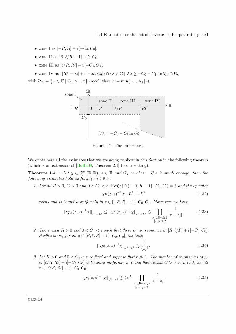
1.4 Estimates for the cut-off inverse of the quadratic pencil
• zone I as [−R,R] + i [−C0, C0],
• zone II as [R, ℓ/R] + i [−C0, C0],
• zone III as [ℓ/R,Rℓ] + i [−C0, C0],
• zone IV as ([Rℓ,+∞[ + i ]−∞, C0]) ∩ λ ∈ C | ℑλ ≥ −C0 − C1 ln〈λ〉 ∩ Ωκ
with Ωκ :=ω ∈ C | ℑω > −κ
(recall that κ := minκ−, |κ+|).
ℑλ = −C0 − C1 ln 〈λ〉
iR
R0
−iC0
−R R ℓ/R Rℓ
zone I
zone II zone III zone IV
Figure 1.2: The four zones.
We quote here all the estimates that we are going to show in this Section in the following theorem(which is an extension of [BoHa08, Theorem 2.1] to our setting):
Theorem 1.4.1. Let χ ∈ C∞c (R,R), s ∈ R and Ωκ as above. If s is small enough, then thefollowing estimates hold uniformly in ℓ ∈ N:
1. For all R > 0, C > 0 and 0 < C0 < ε, Res(p)∩ ([−R,R] + i [−C0, C]) = ∅ and the operator
χp (z, s)−1 χ : L2 → L2 (1.32)
exists and is bounded uniformly in z ∈ [−R,R] + i [−C0, C]. Moreover, we have
‖χpℓ (z, s)−1 χ‖L2→L2 ≤ ‖χp (z, s)−1 χ‖
L2→L2 .∏
zj∈Res(p)|zj |<2R
1
|z − zj |. (1.33)
2. There exist R > 0 and 0 < C0 < ε such that there is no resonance in [R, ℓ/R] + i [−C0, C0].Furthermore, for all z ∈ [R, ℓ/R] + i [−C0, C0], we have
‖χpℓ(z, s)−1χ‖L2→L2 .
1
〈z〉2 . (1.34)
3. Let R > 0 and 0 < C0 < ε be fixed and suppose that ℓ≫ 0. The number of resonances of pℓin [ℓ/R,Rℓ] + i[−C0, C0] is bounded uniformly in ℓ and there exists C > 0 such that, for allz ∈ [ℓ/R,Rℓ] + i[−C0, C0],
‖χpℓ(z, s)−1χ‖L2→L2 . 〈z〉C
∏
zj∈Res(pℓ)|z−zj |<1
1
|z − zj |. (1.35)
page 24
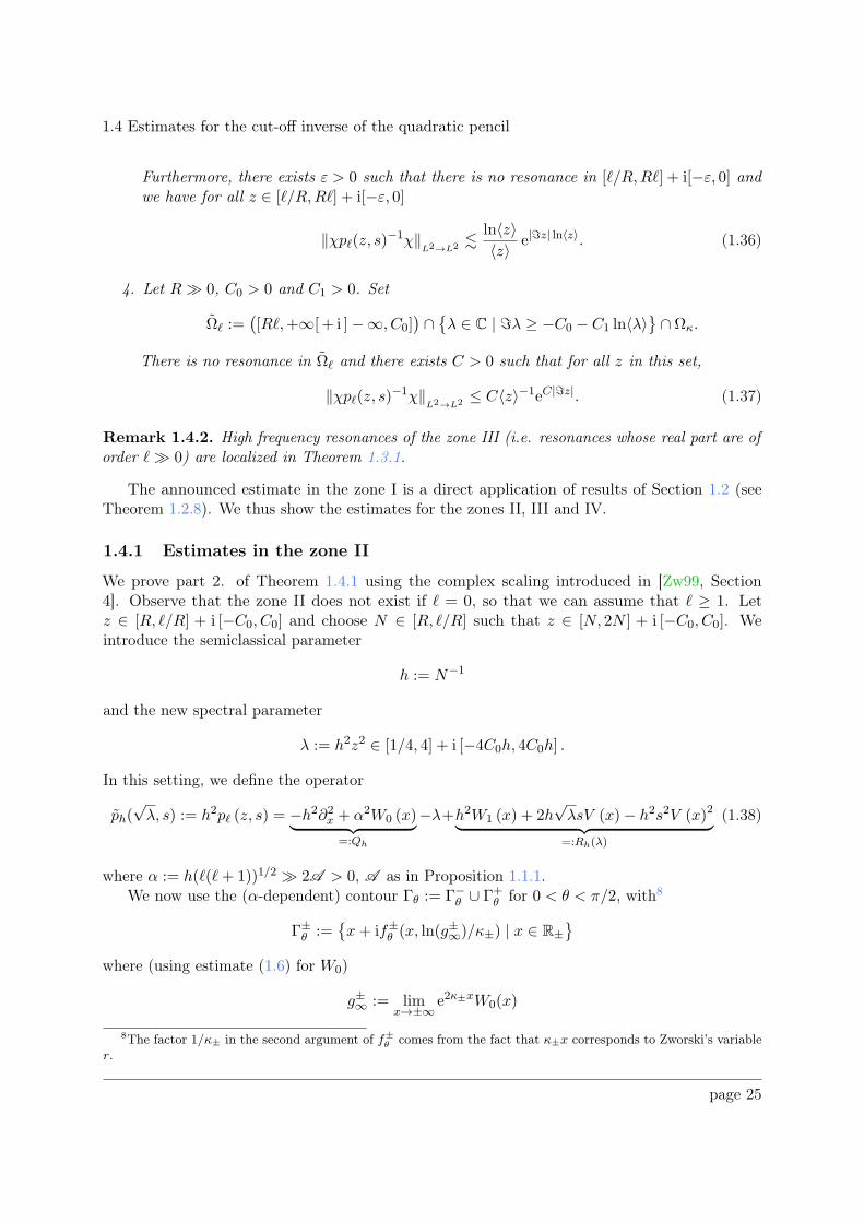
1.4 Estimates for the cut-off inverse of the quadratic pencil
Furthermore, there exists ε > 0 such that there is no resonance in [ℓ/R,Rℓ] + i[−ε, 0] andwe have for all z ∈ [ℓ/R,Rℓ] + i[−ε, 0]
‖χpℓ(z, s)−1χ‖L2→L2 .
ln〈z〉〈z〉 e|ℑz| ln〈z〉. (1.36)
4. Let R≫ 0, C0 > 0 and C1 > 0. Set
Ωℓ :=([Rℓ,+∞[ + i ]−∞, C0]
)∩λ ∈ C | ℑλ ≥ −C0 − C1 ln〈λ〉
∩ Ωκ.
There is no resonance in Ωℓ and there exists C > 0 such that for all z in this set,
‖χpℓ(z, s)−1χ‖L2→L2 ≤ C〈z〉−1eC|ℑz|. (1.37)
Remark 1.4.2. High frequency resonances of the zone III (i.e. resonances whose real part are oforder ℓ≫ 0) are localized in Theorem 1.3.1.
The announced estimate in the zone I is a direct application of results of Section 1.2 (seeTheorem 1.2.8). We thus show the estimates for the zones II, III and IV.
1.4.1 Estimates in the zone II
We prove part 2. of Theorem 1.4.1 using the complex scaling introduced in [Zw99, Section4]. Observe that the zone II does not exist if ℓ = 0, so that we can assume that ℓ ≥ 1. Letz ∈ [R, ℓ/R] + i [−C0, C0] and choose N ∈ [R, ℓ/R] such that z ∈ [N, 2N ] + i [−C0, C0]. Weintroduce the semiclassical parameter
h := N−1
and the new spectral parameter
λ := h2z2 ∈ [1/4, 4] + i [−4C0h, 4C0h] .
In this setting, we define the operator
ph(√λ, s) := h2pℓ (z, s) = −h2∂2x + α2W0 (x)︸ ︷︷ ︸
=:Qh
−λ+h2W1 (x) + 2h√λsV (x)− h2s2V (x)2︸ ︷︷ ︸=:Rh(λ)
(1.38)
where α := h(ℓ(ℓ+ 1))1/2 ≫ 2A > 0, A as in Proposition 1.1.1.We now use the (α-dependent) contour Γθ := Γ−
θ ∪ Γ+θ for 0 < θ < π/2, with8
Γ±θ :=
x+ if±θ (x, ln(g±∞)/κ±) | x ∈ R±
where (using estimate (1.6) for W0)
g±∞ := limx→±∞
e2κ±xW0(x)
8The factor 1/κ± in the second argument of f±θ comes from the fact that κ±x corresponds to Zworski’s variable
r.
page 25
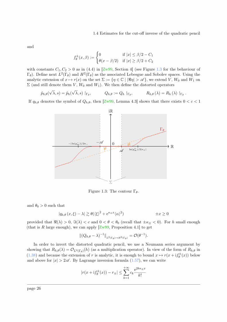
1.4 Estimates for the cut-off inverse of the quadratic pencil
and
f±θ (x, β) :=
0 if |x| ≤ β/2− C1
θ(x− β/2) if |x| ≥ β/2 + C2
with constants C1, C2 > 0 as in (4.4) in [Zw99, Section 4] (see Figure 1.3 for the behaviour ofΓθ). Define next L2(Γθ) and H2(Γθ) as the associated Lebesgue and Sobolev spaces. Using theanalytic extension of x 7→ r(x) on the set Σ := η ∈ C | |ℜη| > A , we extend V , W0 and W1 onΣ (and still denote them V , W0 and W1). We then define the distorted operators
ph,θ(√λ, s) = ph(
√λ, s) Γθ
, Qh,θ := Qh Γθ, Rh,θ (λ) = Rh (λ) Γθ
.
If qh,θ denotes the symbol of Qh,θ, then [Zw99, Lemma 4.3] shows that there exists 0 < c < 1
iR
R0−A
A
Σ
θθ
Γθ
ln(g+∞)/2|κ+|
−| ln(g−∞)|/2κ−
Figure 1.3: The contour Γθ.
and θ0 > 0 such that
|qh,θ (x, ξ)− λ| & θ(〈ξ〉2 + eκ±x〈α〉2) ±x ≥ 0
provided that ℜ(λ) > 0, ℑ(λ) < c and 0 < θ < θ0 (recall that ±κ± < 0). For h small enough(that is R large enough), we can apply [Zw99, Proposition 4.1] to get
‖(Qh,θ − λ)−1‖L2(Γθ)→H2(Γθ)
= O(θ−1).
In order to invert the distorted quadratic pencil, we use a Neumann series argument byshowing that Rh,θ(λ) = OL2(Γθ)(h) (as a multiplication operator). In view of the form of Rh,θ in(1.38) and because the extension of r is analytic, it is enough to bound x 7→ r(x+ if±θ (x)) belowand above for |x| > 2A . By Lagrange inversion formula (1.57), we can write
|r(x+ if±θ (x))− r±| ≤+∞∑
k=1
cke2kκ±x
k!
page 26
1.4 Estimates for the cut-off inverse of the quadratic pencil
for some coefficients ck > 0 (recall from Subsection 1.1.2 that 2κ± = Λ3A±r2±
), and the series
converges (because (1.57) converges uniformly when |ℜx| > A ). Since the sum is decreasing withrespect to x, we deduce r < +∞ on Γθ. On the other hand,
|r − r±| = C(r − rn)− Anr2n
A±r2± (r − rc)− Acr
2c
A±r2± |r − r∓|−A∓r2∓
A±r2± e2κ±x
with C ∈ R. Since no terms on the right-hand side can blow up when restricted on Γθ and sincethe exponential goes to zero when |x| → +∞, it follows that r → r± > 0 as x → ±∞. Wetherefore conclude that the restriction of r on Γθ ∩D(0, R0)
∁ is bounded from below and abovefor R0 ≫ 0, giving Rh,θ(λ) = OL2(Γθ)(h). Thus,
ph,θ(√λ, s)−1 =
(1 + (Qh,θ − λ)−1Rh,θ(λ)
)−1(Qh,θ − λ)−1.
We finally choose χ ∈ C∞c (R,R) and increase if necessary the value of the number A so thatSuppχ ⊂ [−A ,A ]. From [SjwZ91, Lemma 3.5], we have in the L2 sense
χph,θ(√λ, s)−1χ = χph(
√λ, s)−1χ
whence
‖χpℓ(z, s)−1χ‖L2→L2 = h2‖χph(
√λ, s)−1χ‖
L2→L2 . 〈z〉−2.
1.4.2 Estimates in the zone III
We turn to the proof of part 3. of Theorem 1.4.1. We define the semiclassical parameter
h := (ℓ(ℓ+ 1))−1/2
with again ℓ > 0 since the zone does not exist for ℓ = 0. For z ∈ [ℓ/R,Rℓ] + i [−C0, C0], we definea new spectral parameter
λ := h2z2 ∈[
1
3R2, R2
]+ i[−
√2C0Rh,
√2C0Rh] ⊂ [a, b] + i[−ch, ch]
for some 0 < a < b and c > 0. Finally, we set
Ph := h2Pℓ = −h2∂2x +W0 + h2W1, ph(√λ, s) := Ph − (
√λ− hsV )2
and write Pθ and pθ for the corresponding distorted operators on the contour Γθ as we did in theparagraph 1.4.1. We are still using the subscript L2 when we work with the distorted operators.
As W0 admits a non-degenerate maximum at x = 0 (see Section 1.1, Figure 1.1), (x, ξ) = (0, 0)is a trivial solution of the Hamilton equations associated to the principal symbol of Ph:
x = 2ξ
ξ = −W ′0(x)
.
Therefore the energy level E0 := W0(0) is trapping. For this reason, the zone III is called thetrapping zone.
We first show an adaptation of [BoMi04, Lemma 6.5] to our setting.
page 27
1.4 Estimates for the cut-off inverse of the quadratic pencil
Proposition 1.4.3. For θ = Nh with N > 0 large enough and s ∈ R sufficiently small, thereexist C ≡ C(N) > 0 and ε > 0 such that, for all E ∈ [E0− ε,E0 + ε] and |λ−E| ≤ εθ/2, it holds
‖(Pθ − (√λ− hsV )2)−1‖
L2→L2 = O(h−C)∏
λj∈Res(p)|λ−λj |<εθ
h
|λ− λj |.
Proof. The announced estimate is known for the resolvent (Pθ−λ)−1 = pθ(√λ, 0)−1 corresponding
to the case s = 0. The argument can be found in [TZ98] which uses techniques developed in[Sj96], and the authors of [BoMi04] adapted it for the one dimensional case of a non degeneratetrapping energy level E0. More precisely, for θ = Nh with N ≫ 0 large enough, one can constructa bounded operator K ∈ L
(L2, L2
)(see (6.15) in [BoMi04]) satisfying the following properties:
(i) ‖K‖L2→L2 = O(1),
(ii) r := rank K ≤ O(θh−1 ln(1/θ)),
(iii) for h small enough, there exists ε > 0 such that, for all E ∈ [E0 − ε,E0 + ε] and λ ∈[E − εθ, E + εθ],
‖(Pθ − iθK − λ)−1‖L2→D
≤ O(θ−1), D := D(Pθ).
In [SjwZ91, Lemma 3.2], it is shown that Pθ − λ is a Fredholm operator from its domain D toL2, so we can construct a well-posed Grushin problem
P(λ) :=(Pθ − λ R−R+ 0
Cr→Cr
): D ⊕ Cr → L2 ⊕ Cr (1.39)
where R− and R+ are constructed with Pθ − iθK − λ (see [Sj96], page 401, below (6.12) for theconstruction).
Now consider s 6= 0. If s is small enough, (Pθ − iθK − (√λ − hsV )2)−1 is invertible by
pseudodifferential calculus9 as for the case s = 0. By the resolvent identity, one can show that
‖(Pθ − iθK − (√λ− hsV )2)−1‖
L2→D≤ O(θ−1) +O(h|s|)‖(Pθ − iθK − (
√λ− hsV )2)−1‖
L2→DO(θ−1)
since |λ| ≤ h(|ℜz|+ |ℑz|) ≤ O(1) +O(h). Hence for s sufficiently small, we have
‖(Pθ − iθK − (√λ− hsV )2)−1‖
L2→D≤ O(θ−1) λ ∈ [E − εθ, E + εθ].
Because the quadratic pencil remains a Fredholm operator provided that ‖hsV ‖L∞ is sufficiently
small10, we can write a new well-posed Grushin problem
P(λ) :=(pθ(√λ, s) R−
R+ 0Cr→Cr
): D ⊕ Cr → L2 ⊕ Cr
9See the definition of the operator K at the beginning of the proof of Lemma 6.5 in [BoMi04].10Recall that the set of Fredholm operators in L(D , L2) is open for the norm topology.
page 28
1.4 Estimates for the cut-off inverse of the quadratic pencil
where this time R+ and R− are constructed with Pθ − iθK − (√λ− hsV )2. If we set
E(λ) := P(λ)−1 =
(E(λ) E+(λ)E−(λ) E0(λ)
): L2 ⊕ Cr → D ⊕ Cr,
then the relations E(λ)P(λ) = P(λ)E(λ) = 1 as well as the following estimate (which is aconsequence of properties (i) and (iii) above)
∥∥(Pθ − iθK − (√λ− hsV )2)−1(Pθ − (
√λ− hsV )2)
∥∥L2→L2
= O(1)
imply as in [BoMi04] that ‖E(λ)‖L2→D
, ‖E−(λ)‖L2→Cr= O(θ−1) and ‖E+(λ)‖Cr→D
, ‖E0(λ)‖Cr→Cr=
O(1). Applying formula (8.11) in [Sj96], we obtain
(Pθ − (√λ− hsV )2)−1 = E(λ)− E+(λ)E0(λ)
−1E−(λ)
which implies
‖(Pθ − (√λ− hsV )2)−1‖
L2→D= O(θ−1)
(1 + ‖E0(λ)
−1‖Cr→Cr
)
as in [BoMi04, Lemma 6.5], and we then follow the end of its proof to conclude.
We can now follow the arguments below [BoHa08, Lemma 2.2]. The set of pseudo-poles (2.28)and the injective map (2.29) in this reference exist in our setting by Theorem 1.3.1 (but are quitedifferent). This implies that there is no resonance in Ω(h) := [a/2, 2b]+ i[−εh, ch] provided that hand s are small enough. As a result, (1.35) holds true. As for the estimate (1.36), we use Burq’sLemma:
Lemma 1.4.4 (Lemma 2.3 in [BoHa08]). Suppose that f(λ, h) is a family of holomorphic functionsdefined for 0 < h < 1 in a neighbourhood of Ω(h) := [a/2, 2b] + i[−ch, ch] with 0 < a < b andc > 0, such that
|f(λ, h)| .
h−C′
in Ω(h)1
|ℑλ| in Ω(h) ∩ C+
for some C ′ > 0. Then there exists h0, C > 0 such that, for any 0 < h < h0 and anyλ ∈ [a, b] + i[−ch, 0],
|f(λ, h)| ≤ C | lnh|h
eC|ℑλ||lnh|/h.
We apply this result to the function f(λ, h) := ‖χ(Ph − (√λ− hsV )2)−1χ‖, observing that
for all λ ∈ Ω(h) ∩ C+ the resolvent identity gives
‖(Ph − (√λ− hsV )2)−1‖ ≤ 1
|ℑλ| + ‖(Ph − (√λ− hsV )2)−1‖O(h|s|)|ℑλ| .
1
|ℑλ|
because ‖(Ph − (√λ− hsV )2)−1‖ is uniformly bounded on this set for h and s small enough.
page 29
1.4 Estimates for the cut-off inverse of the quadratic pencil
1.4.3 Estimates in the zone IV
This last paragraph is devoted to the proof of part 4. of Theorem 1.4.1. For z ∈ ([Rℓ,+∞[ + i ]−∞, C0])∩λ ∈ C | ℑλ ≥ −C0 − C1 ln〈λ〉, there exists a number N > Rℓ > 0 such that z ∈ [N, 2N ] +i [−C lnN,C0]. We introduce the semiclassical parameters
h :=1
N, µ := ℓ (ℓ+ 1)h2, ν := h2.
Observe that these parameters are very small when N ≫ 0. Moreover, we can consider that h ≤ 1even if ℓ = 0, simply by taking R ≥ 1 in the zone I if it was not the case (R as in Theorem 1.4.1).We then define a new spectral parameter
λ := z2h2 ∈ [1, 2] + i [Ch lnh,C0h] ⊂ [a, b] + i [−ch |lnh| , ch]
where 0 < a ≤ 1 < 2 ≤ b < +∞ and max C,C0 < c < +∞ (observe that a and b do not dependon h). Let J := [a, b] and set
J+ := η ∈ C+ | ℜ(η) ∈ J.
Define then
Ph := h2Pℓ = −h2∂2x + µW0 + νW1, ph(√λ, s) := h2pℓ (z, s) = Ph − (
√λ− hsV )2.
Semiclassical limiting absorption principle for the quadratic pencil. As in [BoHa08],we first get a control until the real line by using a semiclassical limiting absorption principlefor the semiclassical quadratic pencil. The appendix 1.6.3 provides a proof, close to the ideadeveloped by Gérard [Ge08], of such a result for a class of perturbed resolvents, so we only haveto check if the required abstract assumptions are satisfied.
Introduce the generator of dilations A := −ih (x∂x + ∂xx) with domain D (A) :=u ∈ L2 | Au ∈ L2
.
We then pick ρ ∈ C∞c (R, [0, 1]) such that Supp ρ ⊂ [a/3, 3b] and ρ ≡ 1 on I := [a/2, 2b], and wedefine A as the closure of the operator ρ(P )Aρ(P ). In this setting, ρ(P )Aρ(P ) is well-defined onD(A), A is self-adjoint and we have P ∈ C2 (A) (cf. [BoHa08, Section 2.4]) so that (I) holds. Adirect computation shows that
ih−1[P,A] = 4P − 4µW0 − 4νW1 − 2µxW ′0 − 2νxW ′
1
so that, for µ and ν sufficiently small, we get the Mourre estimate (M) (uniform in µ, ν)
1I(P )[P, iA]1I(P ) ≥ ah1I(P ).
Since V ∈ B(D(P ), L2) it is clear that V ∈ L∞ℓoc(Ph). Moreover, assumption (C) is fulfilled for
f(z,B) := (√z − sB)2.
It remains to show that assumption (A) is satisfied for B = hV . Observe that this abstractassumption is particularly well adapted to semiclassical pseudodifferential calculus framework,especially the commutator estimate which provides the supplementary term h. In [Ha01], it isshown that A ∈ Ψ−∞,1 (A is the operator cχ in [Ha01], see above Lemma 3.3). We will use it toshow the following result:
page 30
1.4 Estimates for the cut-off inverse of the quadratic pencil
Lemma 1.4.5. Let σ ∈ [0, 1]. Then V ∈ B(D(〈A〉σ)) and [V, χ(Ph)] ∈ hB(D(〈A〉σ)).Proof. Let Ω := [0, 1] + iR and let z ∈ Ω. On D(〈A〉2)×D(〈A〉2), we define the sesquilinear form
Qz(ϕ, ψ) := 〈V 〈A〉−2zϕ, 〈A〉2zψ〉 ∀ϕ, ψ ∈ D(〈A〉2).By functional calculus, Qz is well-defined and analytic in z ∈ Ω. When z ∈ 0+iR, |(1+λ2)z/2| =1 for all λ ∈ R so that functional calculus first applied to 〈A〉2z and then to 〈A〉−2z gives
|Qz(ϕ, ψ)| ≤ |〈V 〈A〉−2zϕ, ψ〉|= |〈〈A〉−2zϕ, V ψ〉|≤ |〈ϕ, V ψ〉|≤ ‖V ‖
L∞‖ϕ‖L2‖ψ‖L2 .
When z = 1, pseudodifferential calculus shows that 〈A〉2V 〈A〉−2 ∈ Ψ0,0, so that for all z ∈ 1+iR(using again functional calculus for 〈A〉±2iℑz),
|Qz(ϕ, ψ)| ≤ |〈〈A〉2V 〈A〉−2〈A〉−2iℑzϕ, ψ〉|≤ ‖〈A〉2V 〈A〉−2‖
L2→L2‖〈A〉−2iℑzϕ‖L2‖ψ‖L2
≤ ‖〈A〉2V 〈A〉−2‖L2→L2‖ϕ‖L2‖ψ‖L2 .
By the maximum principle, there exists a constant C > 0 such that Qz is bounded by C for all0 ≤ ℜz ≤ 1. In particular, we can extend Qσ/2 on L2 ×D(〈A〉2) as a bounded sesquilinear formand for σ ∈ [0, 1] and ϕ ∈ L2, we have
|Qσ/2(ϕ, ψ)| ≤ C‖ϕ‖L2‖ψ‖L2 .
This means that the map D(〈A〉σ) ∋ ψ 7→ 〈V 〈A〉−σϕ, 〈A〉σψ〉 is continuous. By definition of theadjoint operator and because 〈A〉σ is self-adjoint, this implies that V 〈A〉−σϕ ∈ D(〈A〉σ) for allϕ ∈ L2.
Consider now the sesquilinear form
Qz(ϕ, ψ) := 〈[V, χ(Ph)]〈A〉−2zϕ, 〈A〉2zψ〉 ∀ϕ, ψ ∈ D(〈A〉2).By semiclassical pseudodifferential calculus, we have (see e.g. (4.4.19) in [?])
[V, χ(Ph)] =h
iV (x), χ(ξ2 + µW0(x) + νW1(x))w + h3Ψ−∞,0
= hΨ−∞,−∞ + h3Ψ−∞,0
because V (x) ∈ Ψ0,0, V ′(x) ∈ Ψ0,−∞ and χ(Ph) ∈ Ψ−∞,0. Despite the fact that the error termabove looks less regular than the main term, it is in fact more regular as it can be shown usingexpansion (4.4.15) in [?] (but we will not need such a regularity). Now we can proceed as abovewith Qz and V to conclude.
Now that all assumptions in appendix 1.6.3 have been checked, we can use Theorem 1.6.3 aswell as the fact that ‖〈x〉−σ〈A〉σ‖ . 1 for all σ ≤ 111: for σ ∈ ]1/2, 1] and h small enough, wehave uniformly in µ, ν
supλ∈J+
∥∥∥〈x〉−σph(√λ, s)−1〈x〉−σ
∥∥∥ ≤∥∥〈x〉−σ〈A〉σ
∥∥(
supλ∈J+
∥∥∥〈A〉−σph(√λ, s)−1〈A〉−σ
∥∥∥)∥∥〈A〉σ〈x〉−σ
∥∥ . h−1.
11We show it using the sesquilinear form (ϕ,ψ) 7→ 〈〈x〉−σ〈A〉σϕ,ψ〉 first well-defined on D(A2)×D(A2) because〈x〉−2 ∈ Ψ0,−2, and then extended to L2 × L2 by maximum principle.
page 31
1.5 Proof of the main theorem
Estimates below the real axis. Next, we can use the work of Martinez [Ma02] to get abound under the real line. Indeed, Section 4 of the last reference applies in our setting becauseph(√λ, s) is a differential operator (so that Proposition 3.1 and Corollary 3.2 of [Ma02] apply)
and because (λ− hsV (x))2 ∈ [λ− δ, λ+ δ] + i[ch lnh, 0] for all λ in the zone IV and all x ∈ R ifs is small enough (so that the estimate (4.6) in [Ma02] still holds). It follows that equation (4.13)holds with ph(
√λ, s) instead of Pθ − ρ12. In our setting, this reads
‖χph(√λ, s)−1χ‖ ≤ Ch−C (1.40)
for some C > 0.To get (1.37), we reproduce the argument at the end of the proof of [BoHa08, Lemma 2.4].
Choose f holomorphic satisfying the following conditions:
|f | < 1 for λ ∈ [a/2, 2b] + i[ch lnh, 0],
|f | ≥ 1 for λ ∈ [a, b] + i[ch lnh, 0],
|f | ≤ hC for λ ∈ [a/2, 2b] \ [2a/3, 3b/2] + i[ch lnh, 0]
where C > 0 is the constant in (1.40). Since f is holomorphic, the function
g(λ) := ln ‖χp(√λ, s)−1χ‖
L2→L2 + ln |f(λ)|+ C
chℑλ
is subharmonic. We can check that g(λ) . ln(h−1) on the boundary of [a/2, 2b] + i[ch lnh, 0]. Bythe maximum principle, this estimate holds for all λ ∈ [a/2, 2b] + i[ch lnh, 0], whence
‖χph(√λ, s)−1χ‖
L2→L2 . h−1eCch
|ℑλ|.
The desired estimate (1.37) then follows.
1.5 Proof of the main theorem
We prove in this Section Theorem 1.3.2. The resonance expansion (1.28) follows from the theoryof resonances as presented in [BoHa08, Section 3], and we can follow the proof of this paper. Weonly have to adapt [BoHa08, Proposition 3.1] to get an estimate for the resolvent Rχ,ℓ(z):
Proposition 1.5.1. Let ℓ ∈ N and let χ ∈ C∞c (R,R). There exists χ ∈ C∞c (R,R) satisfyingχχ = χ such that for all z ∈ C \Res(pℓ), the cut-off resolvent χ(Kℓ− z)−1χ is a bounded operatoron Eℓ and satisfies uniformly in ℓ
‖Rχ,ℓ(z)‖Eℓ→Eℓ. 〈z〉‖χpℓ(z, s)−1χ‖
L2→L2 .
Proof. Since the norms ‖.‖Eℓ and ‖.‖Eℓ
are locally equivalent thanks to the Hardy type estimate
‖χ.‖L2 . ‖P 1/2
ℓ .‖L2 uniformly in ℓ (cf. [GGH17, Lemma 9.5]), we can work on (Eℓ, ‖.‖Eℓ ). For
(u0, u1) ∈ Eℓ, we have
Rχ,ℓ(z)
(u0u1
)=
(χpℓ(z, s)
−1χ((z − sV )u0 + u1)χ(1 + (z − sV )pℓ(z, s)
−1(z − sV ))χu0 + (z − sV )χpℓ(z, s)−1χu1
)(1.41)
12We can in fact insert any pseudodifferential operator here provided that hypotheses of Section 2 in [Ma02] areverified.
page 32
1.5 Proof of the main theorem
and since it holds
‖(z − sV )χpℓ(z, s)−1χu1‖L2 ≤ (1 + |s|‖V ‖
L∞ )〈z〉‖χpℓ(z, s)−1χ‖L2→L2‖u1‖L2 ,
the Eℓ-norm of (1.41) can be bounded if we show the following estimates:
‖P 1/2ℓ χpℓ(z, s)
−1χ(z − sV )u0‖L2 ≤ Ca〈z〉‖χpℓ(z, s)−1χ‖L2→L2‖P
1/2ℓ u0‖L2 , (1.42a)
‖P 1/2ℓ χpℓ(z, s)
−1χu1‖L2 ≤ Cb〈z〉‖χpℓ(z, s)−1χ‖L2→L2‖u1‖L2 , (1.42b)
‖χ(1 + (z − sV )pℓ(z, s)−1(z − sV ))χu0‖L2 ≤ Cc〈z〉‖χpℓ(z, s)−1χ‖
L2→L2‖P1/2ℓ u0‖L2 . (1.42c)
We use complex interpolation.
Estimate (1.42a). Let us define
Λa(θ) := 〈z〉−2θP θℓ χpℓ(z, s)
−1χP−θℓ .
By functional calculus, Λa is analytic from [0, 1] + iR to L(L2, L2) because Pℓ > 0 and 〈z〉 > 0.We want to show that
‖Λa(1/2)u‖L2 ≤ Ca‖χpℓ(z, s)−1χ‖L2→L2‖u‖L2 ∀u ∈ L2
for some Ca > 0. By the maximum principle, it is sufficient to bound Λa(θ) for θ ∈ 0, 1+ iR,and since Pℓ is self-adjoint, it is sufficient by functional calculus to restrict ourselves to ℑθ = 0.If θ = 0, there is nothing to do. Now for θ = 1, we put u = (z − sV )u0 and try to show that
‖Pℓχpℓ(z, s)−1χu‖
L2→L2 ≤ Ca〈z〉‖χpℓ(z, s)−1χ‖L2→L2‖Pℓu‖L2 . (1.43)
Write
Pℓχpℓ(z, s)−1χ = [Pℓ, χ]pℓ(z, s)
−1χ︸ ︷︷ ︸=:A
+χPℓpℓ(z, s)−1χ︸ ︷︷ ︸
=:B
. (1.44)
We first deal with A. Pick z0 ∈ ρ(Kℓ) ∩ C+ so that pℓ(z0, s)−1 exists (cf. (1.16)). Then[Pℓ, χ
]pℓ(z, s)
−1 = pℓ(z0, s)−1[pℓ(z0, s),
[Pℓ, χ
]]pℓ(z, s)
−1 + pℓ(z0, s)−1[Pℓ, χ
]pℓ(z0, s)pℓ(z, s)
−1
with[Pℓ, χ
]= −χ∂x − χ′,
[pℓ(z0, s),
[Pℓ, χ
]]= 2χ′∂2x + (χ′ + χ′′)∂x + 2z0sV
′χ− 2s2V V ′χ.
By pseudodifferential calculus, we get:
pℓ(z0, s)−1 ∈ Ψ−2,0,
[Pℓ, χ
]∈ Ψ1,−∞,
[pℓ(z0, s),
[Pℓ, χ
]]∈ Ψ2,−∞.
page 33
1.5 Proof of the main theorem
On the other hand, we have
pℓ(z0, s)pℓ(z, s)−1 =
(pℓ(z, s) + (z2 − z20)− 2(z − z0)sV )
)pℓ(z, s)
−1
= 1 + pℓ(z, s)−1(z2 − z20)− 2(z − z0)sV pℓ(z, s)−1
= pℓ(z, s)−1(Pℓ − (z20 − 2zsV + s2V 2))− 2(z − z0)sV pℓ(z, s)−1. (1.45)
Using the identity
χpℓ(z, s)−1Pℓχ = χpℓ(z, s)
−1[Pℓ, χ
]+ χpℓ(z, s)
−1χPℓ
and the uniform bound in ℓ
‖χ′u′‖L2 . ‖χ1u‖L2 + ‖χ2u
′′‖L2 χj ∈ C∞c (R,R), Suppχj = Suppχ, (1.46)
we obtain from (1.44)
‖Au‖L2 ≤ Ca〈z〉‖χpℓ(z, s)−1χ‖
L2→L2‖u‖L2 (1.47)
where the constant Ca only depends on z0, s, V, V ′, χ, χ′, χ′′, χ1 and χ2.We now turn to B. Using again (1.45), we see that
‖χPℓpℓ(z, s)−1χu‖
L2 ≤ ‖χpℓ(z0, s)pℓ(z, s)−1χu‖L2
+ ‖χ(z20 − 2z0sV + s2V 2)pℓ(z, s)−1χu‖
L2
≤ ‖χpℓ(z, s)−1(Pℓ − (z20 − 2zsV + s2V 2))χu‖L2 + 2
(|z|+ |z0|
)|s|‖V ‖
L∞‖χpℓ(z, s)−1χu‖L2
+(|z0|2 + 2|z0||s|‖V ‖L∞ + s2‖V ‖2
L∞
)‖χpℓ(z, s)−1χu‖
L2
≤ ‖χpℓ(z, s)−1Pℓχv‖L2
+ 2⟨|z0|+ 2|s|‖V ‖
L∞
⟩2︸ ︷︷ ︸
=: ˜Ca
〈z〉‖χpℓ(z, s)−1χ‖L2→L2‖u‖L2 .
Commuting Pℓ with χ and using (1.46), we get (1.43) with Ca = maxCa, 1 +
˜Ca
.
Estimate (1.42b). Let us define
Λb(θ) = 〈z〉−2θP θℓ χpℓ(z, s)
−1χ θ ∈ [0, 1] + iR.
Λb is analytic from [0, 1]+ iR to L(L2, L2). As the above estimate, it is sufficient to show a boundon Λb(1), the imaginary part of θ playing no role and the case θ = 0 being trivial. We get (1.42b)if we show that
‖Pℓχpℓ(z, s)−1χu‖
L2 ≤ Cb〈z〉2‖χpℓ(z, s)−1χ‖L2‖u‖L2∀u ∈ L2 (1.48)
for some Cb > 0. Using the identity (1.44) and the estimate (1.47), we obtain
‖Pℓχpℓ(z, s)−1χu‖
L2→L2 ≤ Ca〈z〉‖χpℓ(z, s)−1χ‖L2→L2‖u‖L2 + ‖χpℓ(z, s)−1Pℓχu‖L2
but this time we ask for the L2 norm of u. Hence, we use that
pℓ(z, s)−1Pℓ = 1 + pℓ(z, s)
−1(z − sV )2
which yields (1.48) with Cb = maxCa, 2
⟨s‖V ‖
L∞
⟩2.
page 34
1.5 Proof of the main theorem
Estimate (1.42c). Let us define
Λc(θ) := 〈z〉2(θ−1)χ(1 + (z − (sV )2(1−θ))pℓ(z, s)−1(z − 22θ−1sV ))χP−θ
ℓ .
Once again, Λc is analytic from [0, 1] + iR to L(L2, L2) and (dropping the imaginary part)
‖Λc(0)‖L2→L2 ≤ (2 + |s|‖V ‖L∞ )3‖χpℓ(z, s)−1χ‖
L2→L2 .
We then get a bound on Λc(1): we prove
‖χ(1 + zpℓ(z, s)−1(z − 2sV ))χu‖
L2 ≤ Cc‖χpℓ(z, s)−1χ‖L2→L2‖Pℓu‖L2 ∀u ∈ L2.
We have
‖χ(1 + pℓ(z, s)−1z(z − 2sV ))χu‖
L2 ≤ ‖χ(1 + pℓ(z, s)−1(z − sV )2χ)u‖
L2 + ‖χpℓ(z, s)−1s2V 2χu‖L2
and
χ(1 + pℓ(z, s)−1(z − sV )2)χ = χpℓ(z, s)
−1Pℓχ.
Commuting Pℓ with χ and using (1.46) gives us
‖χpℓ(z, s)−1z(z − 2sV )χv‖L2 ≤ Cc‖χpℓ(z, s)−1χ‖
L2→L2‖〈Pℓ〉v‖L2
with Cc = max(1 + |s|‖V ‖
L∞ )3, ‖χ‖L∞ , ‖χ1‖L∞ + ‖χ2‖L∞
.
The proof is now the same as in [BoHa08, Section 3.2]. For ν > 0 fixed and for ℓ ∈ N, we defineL2ν(R, Eℓ) as the class of functions t 7→ v (t) with values in Eℓ such that t 7→ e−νtv(t) ∈ L2(R, Eℓ).
For u ∈ Eℓ, the componentwise defined function
v (t) =
e−itKℓu for t ≥ 0
0 for t < 0
is in L2ν(R, Eℓ) if ν is sufficiently large and thus
v(z) =
ˆ +∞
0eiztv(t)dt (1.49)
is well-defined as soon as ℑz ≥ ν. For all t ≥ 0, we have the inversion formula
v(t) =1
2π
ˆ +∞+iν
−∞+iνe−iztv(z)dz (1.50)
that is
e−itKℓu =1
2πi
ˆ +∞+iν
−∞+iνe−izt(Kℓ − z)−1udz
in the L2ν(R, Eℓ) sense. We then use the following result:
page 35
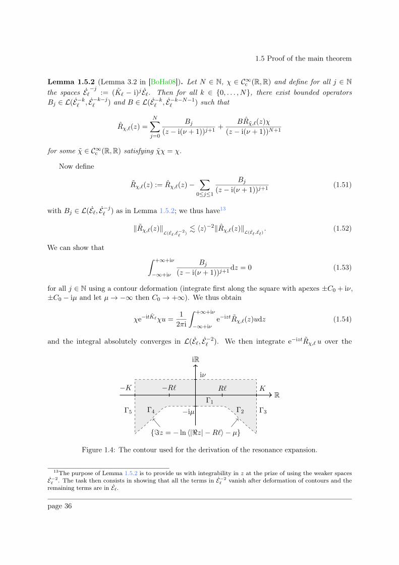
1.5 Proof of the main theorem
Lemma 1.5.2 (Lemma 3.2 in [BoHa08]). Let N ∈ N, χ ∈ C∞c (R,R) and define for all j ∈ N
the spaces Eℓ−j
:= (Kℓ − i)j Eℓ. Then for all k ∈ 0, . . . , N, there exist bounded operators
Bj ∈ L(E−kℓ , E−k−j
ℓ ) and B ∈ L(E−kℓ , E−k−N−1
ℓ ) such that
Rχ,ℓ(z) =
N∑
j=0
Bj
(z − i(ν + 1))j+1+
BRχ,ℓ(z)χ
(z − i(ν + 1))N+1
for some χ ∈ C∞c (R,R) satisfying χχ = χ.
Now define
Rχ,ℓ(z) := Rχ,ℓ(z)−∑
0≤j≤1
Bj
(z − i(ν + 1))j+1(1.51)
with Bj ∈ L(Eℓ, E−jℓ ) as in Lemma 1.5.2; we thus have13
‖Rχ,ℓ(z)‖L(Eℓ,E
−2ℓ
). 〈z〉−2‖Rχ,ℓ(z)‖L(Eℓ,Eℓ)
. (1.52)
We can show thatˆ +∞+iν
−∞+iν
Bj
(z − i(ν + 1))j+1dz = 0 (1.53)
for all j ∈ N using a contour deformation (integrate first along the square with apexes ±C0 + iν,±C0 − iµ and let µ→ −∞ then C0 → +∞). We thus obtain
χe−itKℓχu =1
2πi
ˆ +∞+iν
−∞+iνe−iztRχ,ℓ(z)udz (1.54)
and the integral absolutely converges in L(Eℓ, E−2ℓ ). We then integrate e−iztRχ,ℓ u over the
iR
R−K −Rℓ KRℓ
−iµ
iν
Γ1
Γ2 Γ3Γ4Γ5
ℑz = − ln 〈|ℜz| −Rℓ〉 − µ
Figure 1.4: The contour used for the derivation of the resonance expansion.
13The purpose of Lemma 1.5.2 is to provide us with integrability in z at the prize of using the weaker spacesE−2ℓ . The task then consists in showing that all the terms in E−2
ℓ vanish after deformation of contours and theremaining terms are in Eℓ.
page 36
1.5 Proof of the main theorem
(positively oriented) contour described in Figure 1.4 defined for K,µ > 0. Setting
Ij :=1
2πi
ˆ
Γj
e−iztRχ,ℓ(z)udz,
one obtains by the residue theorem:
1
2πi
ˆ K+iν
−K+iνe−iztRχ,ℓ(z)udz =
∑
zj∈Res(pℓ)ℑzj>−µ
m(zj)∑
k=0
e−izjttkΠχj,ku+
∑
1≤j≤5
Ij . (1.55)
Using the estimate (1.37) in the Zone IV as well as Proposition 1.5.1 and (1.52) above, we computefor t large enough:
‖I3‖E−2ℓ
.ˆ K+iν
K−i ln〈K〉‖e−iλtRχ,ℓ(λ)u‖
E−2ℓ
dλ
. ‖u‖Eℓ
ˆ ν
ln〈K〉〈z〉−2eλt+C|λ|dλ
. 〈K〉−2 eνt
t‖u‖
Eℓ.
We let K → +∞: the integrals I3 and I5 then vanish. We still denote by I2 and I4 the integralsover Γ2 and Γ4 which now go to infinity. As for (1.53), we can show that
ˆ
Γ4∪Γ1∪Γ2
Bj
(z − i(ν + 1))j+1dz = 0. (1.56)
Now, using (1.35) for I1 and (1.37) for I2 and I4, we get for t large enough:
‖I1‖Eℓ .ˆ Rℓ
−Rℓ‖e−µtRχ,ℓ(r − iµ)u‖
Eℓdr
. e−µt‖u‖Eℓ
ˆ Rℓ
−Rℓ〈r〉Cdr
. e−µtℓC+1‖u‖Eℓ,
‖I2‖Eℓ .ˆ +∞
0
∥∥∥∥e−i(Rℓ+λ−i(µ+ln〈λ〉)
)tRχ,ℓ
(Rℓ+ λ− i(µ+ ln〈λ〉)
)u
∥∥∥∥Eℓ
dλ
. e−µt‖u‖Eℓ
ˆ +∞
0e− ln〈λ〉t+C(ln〈λ〉+µ)dλ
. e−µt‖u‖Eℓ.
All these estimates hold in Eℓ, hence we have established part (i) of Theorem 1.3.2 with N =(C + 1)/2.
page 37
1.6 Appendix
Let us turn to part (ii). For µ < ε0 with ε0 as in part 2. of Theorem 1.2.8, we know thatthere is no resonance in formula 1.55. If ℓ < eε
′t for some ε′ > 0, then
‖I1‖Eℓ . e((C+1)ε′−µ)t‖u‖Eℓ.
Otherwise, if ℓ ≥ eε′t, then the exponential decay of the local energy as well as the hypotheses on
g imply together:
‖χe−itKℓχu‖Eℓ
. 1 .g(ℓ(ℓ+ 1))
g(e2ε′t).
It remains to take ε′ small enough and ε := min2ε′, µ− (C + 1)ε′ to conclude the proof.
1.6 Appendix
1.6.1 Analytic extension of the coordinate r
In this Appendix, we prove Proposition 1.1.1 which is analogous to [BaMo93, Proposition IV.2].Let r ∈ ]r−, r+[. By equation (1.5), we have
exp
(− Λ
3A±r2±x
)=∏
α∈I
∣∣∣∣r − rαr− rα
∣∣∣∣Aαr2αA±r2± .
Call the left-hand side z and the right-hand side g±(r). Observe that g±(r±) = 0. Since r 7→ x(r)is increasing and analytic, we can apply the Lagrange’s inversion theorem (see for example [De81],paragraph 2.2 and references therein) to write
r = r± +
+∞∑
ℓ=1
zℓ
ℓ!
[dℓ−1
drℓ−1
(r − r±g±(r)
)ℓ]
r=r±
. (1.57)
Let us introduce Kronecker’s symbol
δα,± :=
1 if α = ±0 otherwise
and the notation
B±,α :=Aαr
2α
A±r2±− δα,±.
Observe that B−,− = B+,+ = 0. We then have
dℓ−1
drℓ−1
(r − r±g±(r)
)ℓ
=
∏
α∈I\±|r− rα|ℓB±,α
dℓ−1
drℓ−1
∏
α∈I\±|r − rα|−ℓB±,α
.
page 38
1.6 Appendix
We now fix ± = + (the conclusion will not be changed if we choose ± = −). Then
dℓ−1
drℓ−1
∏
α∈I\+(r − rα)−ℓB+,α
=
∑
0≤k2≤k1≤ℓ
Cℓ,k1,k2
(dℓ−k1
drℓ−k1(r − rn)−ℓB+,n
)×
×(
dk1−k2
drk1−k2(r − rc)−ℓB+,c
)(dk2
drk2(r − r−)−ℓB+,−
)
where
Cℓ,k1,k2 =
(ℓk1
)(k1k2
).
Direct computation shows that
dp
drp(r − rα)−ℓB+,α = (−1)p(ℓB+,α)(ℓB+,α + 1) . . . (ℓB+,α + p− 1)(r − rα)−ℓB+,α−p.
If we let
K :=∏
α∈I\+(r− rα)B+,α , B+ := max
α∈I\+|B+,α|,
then it follows that
dℓ−1
drℓ−1
(r − r+g+(r)
)ℓ
= Kℓ∑
0≤k2≤k1≤ℓ
Cℓ,k1,k2(−1)ℓ×
× (ℓB+,n)(ℓB+,n + 1) . . . (ℓB+,n + (ℓ− k1)− 1)(r − rn)−ℓB+,n−(ℓ−k1)×× (ℓB+,c)(ℓB+,c + 1) . . . (ℓB+,c + (k1 − k2)− 1)(r − rc)−ℓB+,c−(k1−k2)×× (ℓB+,−)(ℓB+,− + 1) . . . (ℓB+,− + k2 − 1)(r − rα)−ℓB+,−−k2
and thus
∣∣∣∣∣dℓ−1
drℓ−1
(r − r+g+(r)
)ℓ∣∣∣∣∣ ≤ K
ℓℓℓ(B+ + 1)ℓ
∏
α∈I\+(r+ − rα)−B+,α
ℓ
×
×∑
0≤k2≤k1≤ℓ
Cℓ,k1,k2(r+ − rn)−(ℓ−k1)(r+ − rc)−(k1−k2)(r+ − r−)−k2
= Kℓℓℓ(B+ + 1)ℓ
∏
α∈I\+(r+ − rα)−B+,α
ℓ ∑
α∈I\+(r+ − rα)−1
ℓ
=
K(B+ + 1)
∏
α∈I\+(r+ − rα)−B+,α
∑
α∈I\+(r+ − rα)−1
ℓ
ℓℓ
=: Kℓℓℓ.
page 39
1.6 Appendix
Therefore, the convergence of the original series is absolute for z ∈ C if
(|z|ℓK)ℓ
ℓ!< ℓ−(1+ε)
for any ε > 0. Using Stirling approximation ℓ! ∼√2πℓℓ+1/2 for large values of ℓ, we see that it is
sufficient to have
K|z| < e−(1/2+ε) ln ℓ/ℓ
√2π
ℓ< 1.
This condition is fulfilled if
ℜx > 3A+r2+
Λln K.
1.6.2 Localization of high frequency resonances
We provide in this Appendix an asymptotic approximation of resonances near the maximal energyW0(0) = maxx∈RW0(x) as h→ 0. This a generalization of the main Theorem in [SaZw97] tothe case Q 6= 0. More precisely, we show that the resonances associated to the meromorphicextension of p(z, s)−1 are close to the ones associated with the extension of (P − z2)−1, providedthat Q is sufficiently small. This is a direct consequence of the fact that the extra term hsV inthe semiclassical quadratic pencil is O(hs).
As in the paragraph 1.4.2, we set h := (ℓ(ℓ+ 1))−1/2 with ℓ > 0 and consider z ∈ [ℓ/R,Rℓ] +i [−C0, C0]. We then define the spectral parameter λ := h2z2 and also Ph the semiclassical
operator associated to Pℓ. Recall also that r = 3M2
(1 +
√1− 8Q2
9M2
)is the radius of the photon
sphere and W0(0) = F (r)/r2 with our definition of the Regge-Wheeler coordinate x (see (1.5)).
Theorem 1.6.1. Let
Γ0(h) :=
W0(0) + h
(2√W0(0)sV (0) + i−1
√W ′′
0 (0)/2
(k +
1
2
))| k ∈ N
.
For all C0 > 0 such that ∂D(W0(0), C0h) ∩ Γ0(h) = ∅, there is a bijection b ≡ b(h) from Γ0(h)onto the set of resonances of Ph in D(W0(0), C0h) (counted with their natural multiplicity) suchthat
b(h)(µ)− µ = oh→0(h) uniformly for µ ∈ Γ0(h).
Proof. This is a direct application of the results of Sá Barreto-Zworski [SaZw97] which are basedon the work of Sjöstrand [Sj87] (see Theorem 0.1), the latter dealing with resonances generatedby non-degenerate critical points when the trapping set is reduced to a single point (the differencefor us is W0(0) 6= 0).
We recall that in the zone III the symbol of the semiclassical quadratic pencil is the function(x, ξ) 7→ ξ2 +W0(x) + h2W1(x)− (
√λ− hsV (x))2 =: p(x, ξ)− λ. We also recall the hypothesis
in [Sj87] for the case of a Schrödinger operator of the form (0.1) in the reference:
• The trapping set is reduced to the point (0, 0) ((0.3) in [Sj87]),
page 40
1.6 Appendix
• 0 is a non-degenerate critical point ((0.4) in [Sj87], which implies in the Schrödinger casethe more general assumptions (0.7) and (0.9) in the reference).
Although the symbol p depends on λ, its principal part p0 and subprincipal part p−1 do not:indeed, for λ ∈ D (W0(0), C0h) with C0 > 0, we can write when h≪ 1
p(x, ξ) = ξ2 +W0(x)︸ ︷︷ ︸p0(x,ξ)
+h 2√W0(0)sV (x)︸ ︷︷ ︸p−1(x,ξ)
+ lower order terms in h.
This is enough to apply [Sj87], Theorem 0.1: using formula (0.14) in the reference, we get theresult for the set
p0(0, 0) + h
(p−1(0, 0) + i−1
√W ′′
0 (0)/2
(k +
1
2
))| k ∈ N
which is Γ0(h).
Approximation of high frequency resonances Γ0(h) ∋ z2 = λ/h2 is obtained as in [SaZw97],by taking the square root of any element of Γ0(h) and using Taylor expansion for 0 < h ≪ 1(corresponding to ℓ≫ 0) as well as symmetry with respect to the imaginary axis (for the choiceof the sign of the square root). In our setting, we obtain the set Γ of Theorem 1.3.1.
Remark 1.6.2. 1. Let ΓDSS be the set of pseudo-poles in the De Sitter-Schwarzschild case(see the Theorem at the end of [SaZw97]). Then ΓDSS is the limit of Γ as Q → 0 in thesense of the sets, i.e. for all z ∈ Γ, there exists z0 ∈ ΓDSS such that z → z0 as Q→ 0.
2. The pseudo-poles in the charged case are shifted with respect to the uncharged case. Ifthe charges of the Klein-Gordon field and the black hole have the same sign (that is ifqQ > 0), then all the pseudo-poles go to infinity with a real part which never vanishes.However, if the charges have opposite sign (qQ < 0), then all the pseudo-poles real partcancels precisely when qQ = −(k + 1/2)
√F (r), k ∈ N \ 0, before going to infinity. Notice
that no pseudo-pole goes to C+ as |s| → +∞.
3. We can provide a physical interpretation of the set of pseudo-poles. First observe that√F (r)/r is nothing but the inverse of the impact parameter b = |E/L| of trapped null
geodesics with energy E and angular momentum L. Theorem 1.3.1 shows that resonancesnear the real line in the zone III are qQ-dependent multiples of this quantity: they thuscorrespond to impact parameters of trapped photons with high energy and angular momentum.
4. Observe that in Newtonian mechanics, the electromagnetism and gravitation do not interactwith chargeless and massless photons. As a consequence, photons are not deviated and onlyones with impact parameter |b| ≤ r− can “fall“ in the black hole. Hence, high frequencyresonances in zone III are expected to be multiple of r−1
− . As r− → 0, all resonances go toinfinity: the trajectory are now classical straight lines as there is no obstacle anymore.
1.6.3 Abstract Semiclassical Limiting Absorption Principle for a class of Gen-
eralized Resolvents
We show in this Appendix an abstract semiclassical limiting absorption principle for perturbedresolvents.
page 41
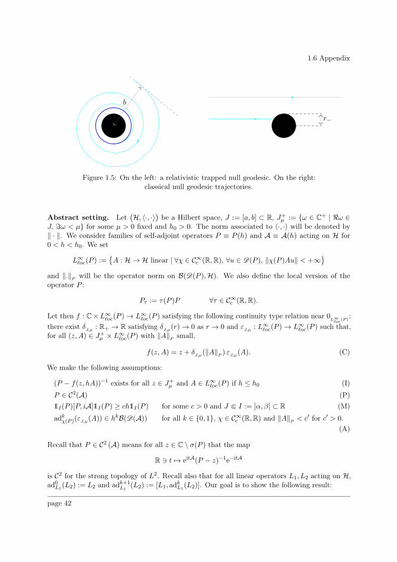
1.6 Appendix
b
r−
Figure 1.5: On the left: a relativistic trapped null geodesic. On the right:classical null geodesic trajectories.
Abstract setting. Let(H, 〈·, ·〉
)be a Hilbert space, J := [a, b] ⊂ R, J+
µ := ω ∈ C+ | ℜω ∈J, ℑω < µ for some µ > 0 fixed and h0 > 0. The norm associated to 〈·, ·〉 will be denoted by‖ · ‖. We consider families of self-adjoint operators P ≡ P (h) and A ≡ A(h) acting on H for0 < h < h0. We set
L∞ℓoc(P ) :=
A : H → H linear | ∀χ ∈ C∞c (R,R), ∀u ∈ D(P ), ‖χ(P )Au‖ < +∞
and ‖.‖P will be the operator norm on B(D(P ),H). We also define the local version of theoperator P :
Pτ := τ(P )P ∀τ ∈ C∞c (R,R).
Let then f : C×L∞ℓoc(P )→ L∞
ℓoc(P ) satisfying the following continuity type relation near 0L∞ℓoc
(P ):
there exist δJ,µ : R+ → R satisfying δJ,µ(r)→ 0 as r → 0 and εJ,µ : L∞ℓoc(P )→ L∞
ℓoc(P ) such that,for all (z,A) ∈ J+
µ × L∞ℓoc(P ) with ‖A‖P small,
f(z,A) = z + δJ,µ(‖A‖P ) εJ,µ(A). (C)
We make the following assumptions:
(P − f(z, hA))−1 exists for all z ∈ J+µ and A ∈ L∞
ℓoc(P ) if h ≤ h0 (I)
P ∈ C2(A) (P)
1I(P )[P, iA]1I(P ) ≥ ch1I(P ) for some c > 0 and J ⋐ I := ]α, β[ ⊂ R (M)
adkχ(P )(εJ,µ(A)) ∈ hkB(D(A)) for all k ∈ 0, 1, χ ∈ C∞c (R,R) and ‖A‖P < c′ for c′ > 0.
(A)
Recall that P ∈ C2 (A) means for all z ∈ C \ σ(P ) that the map
R ∋ t 7→ eitA(P − z)−1e−itA
is C2 for the strong topology of L2. Recall also that for all linear operators L1, L2 acting on H,ad0L1
(L2) := L2 and adk+1L1
(L2) := [L1, adkL1(L2)]. Our goal is to show the following result:
page 42
1.6 Appendix
Theorem 1.6.3. Assume hypotheses (C), (I), (P), (M) and (A). Then for all σ > 1/2,
supz∈J+
µ
‖〈A〉−σ(P − f(z, hB))−1〈A〉−σ‖ . h−1. (1.58)
In the sequel, we will write R(z, hB) := (P − f(z, hB))−1 and call it the generalized resolvent(of P ). Also, since J and µ are now fixed, we will simply write J, δ and ε instead of Jµ, δJ,µ andεJ,µ .
Preliminary results. The purpose of this paragraph is to show preliminary results used toprove Theorem 1.6.3. We first prove an adapted version of [Ge08, Lemma 2.1] to our situation.
Lemma 1.6.4. Let 0 ≤ σ ≤ 1, z ∈ J+ and let χ ∈ C∞c (R,R). If h is small enough, thenR(z, hB) and χ(P ) are bounded on D(〈A〉σ).
Proof. The result is true for (P − z)−1 and χ(P ) by [Ge08, Lemma 2.1]. Let us show thatR(z, hB)D(〈A〉σ) ⊂ D(〈A〉σ):
‖〈A〉σR(z, hB)〈A〉−σ‖ ≤ ‖〈A〉σ(P − z)−1〈A〉−σ‖+ ‖〈A〉σ(R(z, hB)− (P − z)−1)〈A〉−σ‖. 1 + ‖〈A〉σR(z, hB)(z − f(z, hB))(P − z)−1〈A〉−σ‖
and (using that ε(hB) ∈ B(D(A)) by Assumption (A) for k = 0)
‖〈A〉σR(z, hB)(z − f(z, hB))(P − z)−1〈A〉−σ‖≤ ‖〈A〉σR(z, hB)〈A〉−σ‖‖〈A〉σ(z − f(z, hB))〈A〉−σ‖‖〈A〉σ(P − z)−1〈A〉−σ‖. δ(h‖B‖P )‖〈A〉σε(hB)〈A〉−σ‖‖〈A〉σR(z, hB)〈A〉−σ‖.
We then use the uniformity in assumption (A) for k = 0 to write for h very small
δ(h‖B‖P )‖〈A〉σε(hB)〈A〉−σ‖‖〈A〉σR(z, hB)〈A〉−σ‖ < 1
2‖〈A〉σR(z, hB)〈A〉−σ‖.
The proof is complete.
Corollary 1.6.5. Let 0 ≤ σ ≤ 1, z ∈ J+ and τ, χ ∈ C∞c (R, [0, 1]) such that χ ≡ 1 on I andτχ = χ. If h is small enough, then (Pτ − f(z, hB))χ(P ), (Pτ − f(z, hB))χ(P )(P + i)−1 and(P − f(z, hB))(P + i)−1 preserve D(〈A〉σ).
Proof. We have
〈A〉σ(Pτ − f(z, hB))χ(P )〈A〉−σ = 〈A〉σ(Pτ − z)χ(P )〈A〉−σ
+ 〈A〉σ(z − f(z, hB))〈A〉−σ〈A〉σχ(P )〈A〉−σ
which is bounded by assumption (A) for k = 0, Lemma 1.6.4 and the fact that Pτχ(P ) = ϕ(P )with ϕ ∈ C∞c (R,R) by functional calculus. Next, [Ge08, Lemma 2.1] implies that (P + i)−1
preserves D(A), so we can write
〈A〉σ(Pτ − f(z, hB))χ(P )(P + i)−1〈A〉−σ = 〈A〉σ(Pτ − f(z, hB))χ(P )〈A〉−σ〈A〉σ(P + i)−1〈A〉−σ
page 43
1.6 Appendix
which is clearly bounded thanks to the above computation. Finally,
〈A〉σ(P − f(z, hB))(P + i)−1〈A〉−σ = 〈A〉σ(P + i− i− z + z − f(z, hB))(P + i)−1〈A〉−σ
= 1− (i + z)〈A〉σ(P + i)−1〈A〉−σ
+ 〈A〉σ(z − f(z, hB))〈A〉−σ〈A〉σ(P + i)−1〈A〉−σ
and we again use [Ge08, Lemma 2.1] and assumption (A) for k = 0.
The next result is an adaptation of [Ge08, Lemma 3.1] to our setting.
Lemma 1.6.6. Let 0 < σ ≤ 1 and let τ, χ ∈ C∞c (R, [0, 1]) such that χ ≡ 1 on I and τχ = χ.Consider the following three statements:
(i) supz∈J+
‖〈A〉−σR(z, hB)〈A〉−σ‖ . h−1;
(ii) For all z ∈ J+ and all u ∈ (P + i)−1D(〈A〉σ),
‖〈A〉−σu‖ . h−1‖(P − f(z, hB))u‖+ h−1‖〈A〉σ(P − f(z, hB))χ(P )u‖;
(iii) For all z ∈ J+ and all u ∈ D(〈A〉σ),
‖〈A〉−σχ(P )u‖ . h−1‖〈A〉σ(Pτ − f(z, hB))χ(P )u‖.
If h is sufficiently small, then (iii) implies (ii) and (ii) implies (i).
Proof. First of all, observe that (i) makes sense by Lemma (1.6.4), and (ii), (iii) make sense byCorollary 1.6.5 and because Pχ(P ) = Pτχ(P ).
• We show that (ii) implies (i). Let u ∈ H and let v := R(z, hB)〈A〉−σu. Then
w := u− 〈A〉σ(f(z, hB)− i)R(z, hB)〈A〉−σu ∈ H.
This makes sense if h is small enough because R(z, hB) preserves D(〈A〉σ) by Lemma 1.6.4and because
〈A〉σ(f(z, hB)− i)〈A〉−σ = 〈A〉σ(f(z, hB)− z)〈A〉−σ + (z − i)
is bounded by assumption (A) for k = 0. Next, using the resolvent identity (P + i)−1 −R(z, hB) = (P + i)−1(f(z, hB)− i)R(z, hB), we see that
(P + i)−1〈A〉−σw =((P + i)−1 − (P + i)−1(f(z, hB)− i)R(z, hB)
)〈A〉−σu
= R(z, hB)〈A〉−σu
= v
so that v ∈ (P + i)−1D(〈A〉σ). Hence, applying (ii) to v yields
‖〈A〉−σR(z, hB)〈A〉−σu‖ = ‖〈A〉−σv‖. h−1‖〈A〉−σu‖+ h−1‖〈A〉σ(P − f(z, hB))χ(P )R(z, hB)〈A〉−σu‖. h−1‖〈A〉−σu‖+ h−1‖〈A〉σ[P − f(z, hB), χ(P )]R(z, hB)〈A〉−σu‖+ h−1‖〈A〉σχ(P )〈A〉−σu‖.
page 44
1.6 Appendix
By assumption (A) for k = 1 and Lemma 1.6.4, we have
‖〈A〉σ[P − f(z, hB), χ(P )]R(z, hB)〈A〉−σu‖= ‖〈A〉σ[z − f(z, hB), χ(P )]R(z, hB)〈A〉−σu‖≤ δ(h‖B‖P )‖〈A〉σ[ε(hB), χ(P )]〈A〉−σ‖‖〈A〉σR(z, hB)〈A〉−σu‖. hδ(h‖B‖P ).
Therefore, (i) follows from (ii) if h is small enough.
• We show that (iii) implies (ii). Let χ := 1− χ and let u ∈ (P + i)−1D (〈A〉σ). We write
‖〈A〉−σu‖ ≤ ‖〈A〉−σχ(P )u‖+ ‖〈A〉−σχ(P )u‖ (1.59)
and (iii) implies that
‖〈A〉−σχ(P )u‖ . h−1‖〈A〉σ(P − f(z, hB))χ(P )u‖
because τ ≡ 1 on Suppχ. In order to control the term involving χ(P ) in (1.59), we writeχ = ψ−+ψ+ with ψ± ∈ C∞ (R, [0, 1]) such that Supp ψ− ⊂ ]−∞, α] and Supp ψ+ ⊂ [β,+∞[.We also pick ρ ∈ C∞c (R,R) such that ρψ− = ψ−. Since B ∈ L∞
ℓoc(P ), we have for anyv ∈ D(P )
ℜ⟨ψ−(P )
2(f(z, hB)− P )v, v⟩
= ℜ⟨ψ−(P )
2zv, v⟩+ ℜ
⟨ψ−(P )
2δ(h‖B‖P )ε(hB)v, v⟩−ℜ
⟨ψ−(P )
2Pv, v⟩
≥ a‖ψ−(P )v‖2 − δ(h‖B‖P )‖ρ(P )ε(hB)‖P ‖ψ−(P )v‖2 − α‖ψ−(P )2v‖2
≥ c−‖ψ−(P )v‖2 (1.60)
where c− > 0 if h is sufficiently small. Using Cauchy-Schwarz inequality, we get ‖ψ−(P )(P−f(z, hB))v‖ ≥ c−‖ψ−(P )v‖ and thus ‖ψ−(P )R(z, hB)v‖ . ‖ψ−(P )v‖. Similarly, one canshow ‖ψ+(P )R(z, hB)v‖ . ‖ψ+(P )v‖. These inequalities and χ2 = (ψ−+ψ+)
2 = ψ2−+ψ2
+
then imply
‖χ(P )R(z, hB)v‖ . ‖χ(P )v‖
which in turn implies for u ∈ D(P )
‖〈A〉−σχ(P )u‖ . ‖χ(P )u‖= ‖χ(P )R(z, hB)(P − f(z, hB))u‖. ‖χ(P )(P − f(z, hB))u‖. ‖(P − f(z, hB))u‖.
page 45
1.6 Appendix
Proof of Theorem 1.6.3. We show that the regularity (P) and the Mourre estimate (M) areenough to establish (1.58). As pointed out at the beginning of [Ge08], the key point is the followingenergy estimate: for any self-adjoint operators H acting on H, u ∈ D (H), τ ∈ C∞c (R, [0, 1]) andPτ := τ(P )P , we have
2ℑ⟨Hu, (Pτ − f(z, hB))u
⟩=⟨u, [Pτ , iH]u
⟩− 2ℑ
⟨u, f(z, hB)Hu
⟩(1.61)
where the commutator must be understood as a quadratic form on D(H).We follow the proof of [Ge08, Theorem 1]. Let τ, χ ∈ C∞c (R, [0, 1]) such that χ ≡ 1 on I and
τχ = χ and let
F (ξ) := −ˆ +∞
ξg(ζ)2dζ
with g ∈ C∞ (R, [0, 1]) satisfying g (ξ) = 0 for ξ ≥ 2 and g (ξ) = 1 for ξ ≤ 1. By Lemma 1.6.6, itis sufficient to prove the following estimate: for any z ∈ J+ and u ∈ D(〈A〉σ),
‖〈A〉−σχ(P )u‖ . h−1‖〈A〉σ(Pτ − f(z, hB))χ(P )u‖.
As P ∈ C2 (A), P and A are self-adjoint and satisfy the Mourre estimate (M) on I, we can applythe estimate (3.30) in the proof of [Ge08, Theorem 1]:
χ(P )[Pτ , iF (A)]χ(P ) & hχ(P )〈A〉−2σχ(P ). (1.62)
Now we apply the identity (1.61) with H = F (A): for all u ∈ D(A),
2ℑ⟨F (A)u, (Pτ − f(z, hB))u
⟩=⟨u, [Pτ , iF (A)]u
⟩+ 2ℑ
⟨f(z, hB)u, F (A)u
⟩.
Since F < 0 is bounded and ℑz > 0, we can write for all h sufficiently small
2ℑ⟨F (A)u, (Pτ − f(z, hB))u
⟩
=⟨u, [Pτ , iF (A)]u
⟩− 2(ℑz)
⟨u, F (A)u
⟩− 2δ(h‖B‖P )ℑ
⟨u, ε(hB)F (A)u
⟩
>⟨u, [Pτ , iF (A)]u
⟩− 2δ(h‖B‖P )‖ε(hB)u‖‖F (A)u‖
where we used that that ε(hB) ∈ B(D(A)) by Assumption (A). It thus follows
2ℑ⟨F (A)u, (Pτ − f(z, hB))u
⟩≥⟨u, [Pτ , iF (A)]u
⟩. (1.63)
Plugging the estimate (1.62) into inequality (1.63) and putting χ(P )u instead of u yield
‖〈A〉−σχ(P )u‖2 = 〈u, χ(P )〈A〉−2σχ(P )u〉. h−1
⟨u, χ(P )[Pτ , iF (A)]χ(P )u
⟩
≤ h−1∣∣⟨F (A)χ(P )u, (Pτ − f(z, hB))χ(P )u
⟩∣∣.
Using again the boundedness of F , we get
‖〈A〉−σχ(P )u‖2 . h−1‖〈A〉−σχ(P )u‖‖〈A〉σ(Pτ − f(z, hB))χ(P )u‖
which establishes the point (iii) and thus the point (i) in Lemma 1.6.6.
page 46
Chapter 2
Scattering Theory for the ChargedKlein-Gordon Equation in the Exterior DeSitter-Reissner-Nordström Spacetime
This chapter deals with scattering results associated to the charged Klein-Gordon equation(4.37). The mass term mF (r) vanishes at the horizons but not the electrostatic potentialsV (r)→ sr−1
± 6= 0. This means that the comparison dynamics have to contain the charge termtoo. It turns out that scattering can not be interpreted as a transport along principal nullgeodesics as it can be in the (De Sitter-)Kerr spacetime, as the metric is independent of thecharge of the field. This is just a consequence of the fact that the Klein-Gordon field does notappear in Einstein equation that yields the DSRN spacetime (M, g).
This motivates us to use an extended spacetime which encodes the charge and the mass ofthe field. There are a priori many ways to proceed. The one we choose, yet very simple, leads toa rich extension of the original manifold in which all the information carried on by the scalarfield is caught. The extended spacetime, which is nothing but a Kaluza-Klein extension of theoriginal one, verifies a non-trivial Einstein equation in 1 + 4 dimension and provides a naturalinterpretation of the asymptotic completeness. We stress out here that this interpretation is falsein the original spacetime as the principal null geodesics used in the extension do not exist there.
Plan of the chapter. Chapter 2 is organized as follows. In Section 2.1, we construct andpresent some important properties of the Kaluza-Klein extension of the DSRN spacetime. InSection 2.2, we build the Killing horizons with the principal null geodesics as well as the conformalboundary at infinity of the extension. Section 2.3 is devoted to the statement of the analyticscattering results whose proofs are given in Section 2.4. Finally, in Section 2.5, we interpret thewave operators as transports along the principal null geodesics. Asymptotic completeness is usedto define traces on the horizons and solve an abstract Goursat problem.
47
2.1 The extended spacetime
2.1 The extended spacetime
This Section introduces the basic notions and objects used throughout this chapter. Subsection2.1.1 presents the neutralization procedure which extends the original spacetime using the chargedKlein-Gordon operator. We next show in Subsection 2.1.2 how the neutralization affects Einstein-Maxwell equations. We then deduce in Subsection 2.1.3 a dominant energy condition that fulfillthe energy-momentum tensor associated to (M, g) under some assumption on the cosmologicalconstant Λ.
2.1.1 The neutralization procedure
In this chapter, we will use a slightly different definition of the horizon function: we let
F (r) := 1− 2M
r+Q2
2r2− Λr2
3.
with M > 0 the mass of the black hole, Q ∈ R \ 0 its electric charge and Λ > 0 the cosmologicalconstant. We then assume (1.1) with Q2/2 instead of Q2 (so that now ∆ = 9M2 − 4Q2) whichensures that F has four distinct zeros −∞ < rn < 0 < rc < r− < r+ < +∞ and is positive for allr ∈ ]r−, r+[. We also assume that 9ΛM2 < 1. With these conventions, (g,A = (Q/r)dt) solvesthe Einstein-Maxwell field equation
Ricµν −1
2Rgµν − Λgµν = −Tµν , Tµν = FµσF
σν −
1
4gµνF
σρFσρ (2.1)
where Ric is the Ricci tensor, R the scalar curvature and F = dA the electromagnetic tensor.We now introduce a fifth dimension labeled z ∈ S1 in order to reinterpret the charged Klein-
Gordon operator in the De Sitter-Reissner-Nordström spacetime as a wave operator in a 1 + 4spacetime. Define
L :=1
F (r)(∂t − sV (r)∂z)
2 − 1
r2∂rr
2F (r)∂r −1
r2∆S2 −m2∂2z .
Diagonalizing −i∂z on the unit circle, we can recover P by restriction to the harmonic −i∂z = 1.We construct a new metric g such that g = L: the extended metric in the extended Boyer-Lindquist coordinates (t, z, r, ω) with signature (+,−,−,−,−) is defined as
g :=
(F (r)− s2V (r)2
m2
)dt2 − sV (r)
m2(dtdz + dzdt)− 1
m2dz2 − 1
F (r)dr2 − r2dω2.
It is non-degenerate since the determinant is equal to −r4 sin2 θ/m2 < 0 (notice here the crucialhypothesis m 6= 0). The inverse extended metric is given by
g−1 =1
F (r)∂t ⊗ ∂t −
sV (r)
F (r)(∂t ⊗ ∂z + ∂z ⊗ ∂t) +
(s2V (r)2
F (r)−m2
)∂z ⊗ ∂z
− F (r)∂r ⊗ ∂r −1
r2∂θ ⊗ ∂θ −
1
r2 sin2 θ∂ϕ ⊗ ∂ϕ.
Let us define the four blocks
M1 := Rt × S1z × ]0, rc[r × S2ω, M2 := Rt × S1z × ]rc, r−[r × S2ω,
M3 := Rt × S1z × ]r−, r+[r × S2ω, M4 := Rt × S1z × ]r+,+∞[r × S2ω.
page 48
2.1 The extended spacetime
The extended spacetime is then the (1 + 4)-dimensional manifold(Mext, g
)with
Mext :=
4⋃
j=1
Mj .
In the sequel, we will consider more carefully the outer space
M := Rt × S1z × ]r−, r+[r × S2ω
which we will simply call the extended spacetime when no confusion can occur. In M, we will usethe timelike vector field ∇t = F (r)−1(∂t − sV (r)∂z) to define an orientation on M: any causalvector field X ∈ TM will be said future-pointing if and only if
g(∇t,X) > 0.
We can easily check that the outer space is a globally hyperbolic spacetime. Besides, we cancheck that Xα := ∂t − sVα∂z are timelike Killing vector fields for α ∈ c,−,+ (they will beuseful in Subsection 2.2.2).
Remark 2.1.1 (Dyadorings). For s small enough, the shifted horizon function
F(r) := F (r)− s2V 2
m2= 1− 2M
r+Q2
2r2
(1− 2q2
m2
)− Λr2
3
has four roots with two1 inside ]r−, r+[; call them r1, r2 with r− < r1 < r2 < r+. We can checkthat ∂t becomes spacelike when r ∈ ]r−, r1[ ∪ ]r2, r+[. We then define the dyadorings
D− := Rt × S1z × ]r−, r1[r × S2ω, D+ := Rt × S1z × ]r2, r+[r × S2ω.
We may observe that if s is too large, namely if
|s| ≥ mrF (r)1/2 ∀r ∈ ]r−, r+[ ,
then the dyadorings cover the entire outer space M.
The wave equation on (M, g) reads
gu =1
F (r)
((∂t − sV (r)∂z
)2 − F (r)
r2∂rr
2F (r)∂r −F (r)
r2∆S2 −m2F (r)∂2z
)u = 0
with u ∈ L2(Rt × S1z × ]r−, r+[r × S2ω, r2F (r)−1dtdzdrdω). It will be convenient for Section 2.3
to rewrite this equation as(∂2t − 2sV (r)∂z∂t + P
)u = 0 (2.2)
where
P = −F (r)r2
∂rr2F (r)∂r −
F (r)
r2∆S2 −
(m2F (r)− s2V (r)2
)∂2z (2.3)
acts on L2(S1z × ]r−, r+[r × S2ω, r2F (r)−1dzdrdω). Restricting u to ker(i∂z + z), we get back the
original charge Klein-Gordon operator with the modified mass mz and charge sz.1It is a simple consequence of the intermediate value theorem since F < F , F > 0 inside ]r−, r+[ and F cancels
at r = r±.
page 49
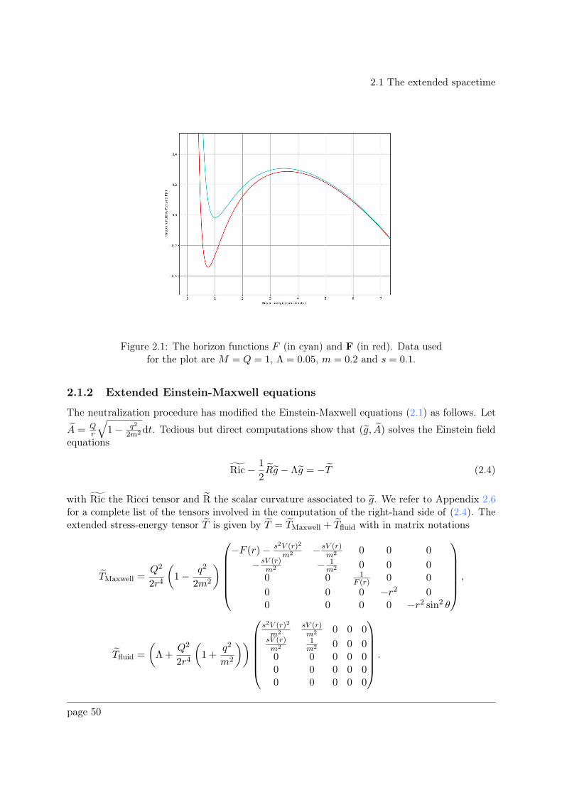
2.1 The extended spacetime
Figure 2.1: The horizon functions F (in cyan) and F (in red). Data usedfor the plot are M = Q = 1, Λ = 0.05, m = 0.2 and s = 0.1.
2.1.2 Extended Einstein-Maxwell equations
The neutralization procedure has modified the Einstein-Maxwell equations (2.1) as follows. Let
A = Qr
√1− q2
2m2dt. Tedious but direct computations show that (g, A) solves the Einstein fieldequations
Ric− 1
2Rg − Λg = −T (2.4)
with Ric the Ricci tensor and R the scalar curvature associated to g. We refer to Appendix 2.6for a complete list of the tensors involved in the computation of the right-hand side of (2.4). Theextended stress-energy tensor T is given by T = TMaxwell + Tfluid with in matrix notations
TMaxwell =Q2
2r4
(1− q2
2m2
)
−F (r)− s2V (r)2
m2 − sV (r)m2 0 0 0
− sV (r)m2 − 1
m2 0 0 00 0 1
F (r) 0 0
0 0 0 −r2 00 0 0 0 −r2 sin2 θ
,
Tfluid =
(Λ +
Q2
2r4
(1 +
q2
m2
))
s2V (r)2
m2sV (r)m2 0 0 0
sV (r)m2
1m2 0 0 0
0 0 0 0 00 0 0 0 00 0 0 0 0
.
page 50
2.1 The extended spacetime
TMaxwell is nothing but the Maxwell electromagnetic tensor associated to g and A; Tfluid describesas for itself a perfect fluid:
Tfluid = ρ(r)u⊗ u
with ρ(r) = Λ + Q2
2r4
(1 + q2
m2
)the energy density in the fluid and u = 1
m
(sV (r)dt+ dz
)the dual
vector field of the fluid’s velocity which is given by
vµ = gµνuν = −m∂z =1
m
(sV (r)∇t+∇z
). (2.5)
Observe that the energy density of the fluid as measured by an observer at rest is zero:
(Tfluid)µν∇µt∇νt = 0.
Observe also that taking the divergence on both sides of (2.4) yields
div(ρ(r)u⊗ u) = ρ(r)F (r)W (r)W ′(r)2m2
∂r =: −∇P
with
P (r) = − q2Q2
4m2r2
(Λ +
Q2(1 + q2
m2 )
6r4
)≤ 0.
Moreover, we can see that
div(ρu) = 0.
Thus u obeys compressible Euler law for a static fluid with mass density ρ, pressure P and nointernal source term:
∂t(ρu) + div(ρu⊗ u) = −∇P∂tρ+ div(ρu) = 0
.
The second equation above is the conservation of the mass.
2.1.3 Dominant energy condition
In all this Subsection, we will assume that |q| < 2m. Let us rewrite
−T = Q(r)(F (r)dt2 − F (r)−1dr2 + r2dω2
)−D(r)
(sV (r)dt+ dz
)2
where
Q(r) =Q2
2r4
(1− q2
2m2
), D(r) =
(Λ
m2+
3q2Q2
4m4r4
).
Consider then the following condition:
m2D(r) ≤ Q(r) (2.6)
which is equivalent to Λ ≤ Q2
2r4+
(1− 2q2
m2
).
page 51
2.1 The extended spacetime
Lemma 2.1.2. The condition (2.6) implies that for all timelike vector field X, we have
−TµνXµXν ≥ 0. (2.7)
If Q 6= 0, then both the above conditions are equivalent.
Proof. Let X = Xt∂t +Xz∂z +Xr∂r +Xθ∂θ +Xϕ∂ϕ be a timelike vector field:
(F (r)− s2V (r)2
m2
)(Xt)2 − 2
sV (r)
m2XtXz − 1
m2(Xz)2 − F (r)−1(Xr)2 − r2(Xθ)2 − r2 sin2 θ(Xϕ)2 > 0.
Assume first (2.6). Then
−TµνXµXν = Q(r)
(g(X,X) +
(1
m2− D(r)
Q(r)
)(s2V (r)2(Xt)2 + 2sV (r)XtXz + (Xz)2
)
A
Q+ 2r2(Xθ)2 + 2r2 sin2 θ(Xϕ)2
)
≥ Q(r)
(1
m2− D(r)
Q(r)
)(s2V (r)2(Xt)2 + 2sV (r)XtXz + (Xz)2
).
Furthermore,
(1
m2− D(r)
Q(r)
)(s2V (r)2 sV (r)sV (r) 1
)≥ 0
as quadratic form since the spectrum of the matrix on the left-hand side is0, 1 + s2V (r)2
(the
eigenvalue 0 is associated to ∇t). It follows that −TµνXµXν ≥ 0.Assume now that (2.6) is not verified and Q 6= 0 (so that Q(r) 6= 0). Put
α(r) :=1
m2− D(r)
Q(r)< 0.
Let δ, ε ∈ C∞(]r−, r+[ , ]0,+∞[) with ε supported far away from the dyadorings and set X :=δ(r)
(∂t − sV (r)(1 + ε(r))∂z
). Taking ε sufficiently small, we get
g(X,X) = δ(r)
(F (r)− s2V (r)2ε(r)2
m2
)> 0.
Taking now δ large enough, we find
−TµνXµXν = Q(r)(g(X,X) + α(r)ε(r)2δ(r)2s2V (r)2
)
= Q(r)δ(r)
(F (r)− s2V (r)2ε(r)2
m2+ α(r)ε(r)2δ(r)s2V (r)2
)
< 0
for r ∈ Supp ε. This completes the proof.
page 52
2.1 The extended spacetime
Proposition 2.1.3 (Dominant energy condition). Assume Q 6= 0. Then the condition (2.6) isverified if and only if
−TµνXµXν ≥ 0 for all timelike vector field X,
If X is a future-pointing causal vector field, then so is for −TµνXν ≥ 0
. (2.8)
Proof. Lemma 2.1.2 shows that (2.6) is equivalent to the first condition in (2.8) provided thatQ 6= 0. Next, a direct computation shows that
−Tµν = −gµσTσν = Q(r)∂t ⊗ dt+
(m2D(r)−Q(r)
)sV (r)∂z ⊗ dt+m2D(r)∂z ⊗ dz
+Q(r)∂r ⊗ dr −Q(r)∂θ ⊗ dθ −Q(r)∂ϕ ⊗ dϕ.
Let X = Xt∂t +Xz∂z +Xr∂r +Xθ∂θ +Xϕ∂ϕ be a future-pointing causal vector field:
g(∇t,X) = Xt > 0, g(X,X) ≥ 0.
We compute:
−TµνX
ν = Q(r)Xt∂t +((m2D(r)−Q(r))sV (r)Xt +m2D(r)Xz
)∂z
+Q(r)Xr∂r −Q(r)Xθ∂θ −Q(r)Xϕ∂ϕ.
Then the vector field −TµνXν is future-pointing if and only if
g(∇t,−TµνX
ν) = −T tνX
ν = Q(r)Xt > 0
which is always true when Q 6= 0. Furthermore:
Q(r)−2g(TµνX
ν , TµνX
ν) =
(F (r)− s2V (r)2
m2
(m2D(r)
Q(r)
)2)(Xt)2 − 2
sV (r)
m2
(m2D(r)
Q(r)
)2
XtXz
− 1
m2
(m2D(r)
Q(r)
)2
(Xz)2 − F (r)−1(Xr)2
= g(X,X)
+
(1−
(m2D(r)
Q(r)
)2)(
s2V (r)2
m2(Xt)2 + 2
sV (r)
m2XtXz +
1
m2(Xz)2
).
Using g(X,X) ≥ 0, we get:
Q(r)−2g(TµνX
ν , TµνX
ν) ≥(1−
(m2D(r)
Q(r)
)2)(
s2V (r)2
m2(Xt)2 + 2
sV (r)
m2XtXz +
1
m2(Xz)2
)
and this quantity is nonnegative if and only if m2D(r) ≤ Q(r) as in the proof of Lemma 2.1.2 (thesame vector field as therein shows the necessity of the condition). This completes the proof.
Remark 2.1.4. The condition (2.6) is called the dominant energy condition. It will allow us todefine constant surface gravities in Subsection 2.2.2. In the De Sitter-Reissner-Nordström case,
page 53
2.2 Global geometry of the extended spacetime
Proposition 2.1.3 is always true. Indeed, denoting by T the corresponding stress-energy tensor as
well as Q(r) = Q2
2r4, we have
TµνXµXν = Q(r)
(F (r)(Xt)2 − F (r)−1(Xr)2 + r2(Xθ)2 + r2 sin2 θ(Xϕ)2
),
g(∂t, TµνX
ν) = Q(r)Xt,
g(TµνX
ν , TµνX
ν) = Q(r)Xtg(X,X)
for any vector field X.
Remark 2.1.5. We may notice that condition (1.1) implies a lower bound to Λ if |Q| ≥M . Inthis situation and for a small charge q, the dominant energy condition (2.6) is not satisfied.
2.2 Global geometry of the extended spacetime
This Section is devoted to the study of the geometry of the extended spacetime. The goal istwo-fold: first, the study of the geometric objects is interesting in its own right as it describesin details a new solution to Einstein-Maxwell equations in 5 dimensions. On the other hand,the construction of some geometric objects (such as principal null geodesics and horizons) areprerequisites to formulate the scattering theory developed in Section 2.3. We will henceforthassume the dominant energy condition (2.6).
Let us outline here the plan of this Section. Subsection 2.2.1 introduces first special nullgeodesics and local coordinates used to build horizons. In Subsection 2.2.2, we define surfacegravities. In Subsection 2.2.3, we add crossing rings to complete the construction of the horizons.Finally, we define the conformal infinity in Subsection 2.2.4 and show that the extended spacetimecontains black rings.
2.2.1 Principal null geodesics
We introduce in this Subsection a family of null geodesics which send data from the blocks Mj
to the horizons located at the roots of F . They will be used for the geometric interpretation ofthe scattering in Section 2.5. We follow the standard procedure (see for example the constructionin [ON95, Section 2.5] in the Kerr spacetime).
Let γ : R ∋ µ 7→ (t(µ), z(µ), r(µ), ω(µ)) ∈ M be a null geodesic. Denoting by ˙ the derivativewith respect to µ, we have
(F (r)− s2V (r)2
m2
)t2 − 2sV (r)
m2tz − 1
m2z2 − 1
F (r)r2 = 0 (2.9)
if ω = r2θ2 + r2 sin2 θϕ = 0. Since ∂z is Killing2, there exists a constant Z ∈ R such that
g(γ, ∂z) = sV (r)t+ z = −m2Z. (2.10)
Plugging (2.10) into (2.9) then yields
F (r)t2 − 1
F (r)r2 = m2Z2. (2.11)
2This is a reformulation of the cylinder condition in the Kaluza-Klein theory.
page 54
2.2 Global geometry of the extended spacetime
We build our geodesics so that Z = 0. This is not only a convenient choice that makes computationseasier and explicit: the geometric interpretation is that
g(γ, ∂z) = 0
that is, the principal null geodesics will be g-orthogonal to the velocity vector field of the perfectfluid appearing in the stress-energy tensor after neutralization (see (2.5)). Solving (2.10) and(2.11) for Z = 0, we get
dt
dr= ±F (r)−1,
dz
dr= ∓sV (r)F (r)−1.
In particular, we can parametrize our geodesic by µ = ±r.The incoming principal null geodesic γin(µ) = (t(µ), z(µ), r(µ), ω(µ)) is the null geodesic
parametrized by µ = −r and defined by
t(µ) = F (r)−1
z(µ) = −sV (r)F (r)−1
r(µ) = −1ω(µ) = 0
.
We then define the extended-star coordinates3 (t⋆, z⋆, r, ω) with
t⋆ := t+ T (r), T (r) :=
ˆ r
r
dρ
F (ρ)=
∑
α∈n,c,−,+
1
2καln
∣∣∣∣r − rαr− rα
∣∣∣∣ , (2.12)
z⋆ := z + Z(r), Z(r) := −ˆ r
r
sV (ρ)dρ
F (ρ)= −
∑
α∈n,c,−,+
s
2rακαln
∣∣∣∣r
r
r − rαr− rα
∣∣∣∣ (2.13)
for some r ∈ Mext. Here we have used the factorization
F (r) =Λ
3r2(r − rn)(r − rc)(r − r−)(r+ − r) (2.14)
as well as the surface gravities κn := F ′(rn)/2 > 0, κc := F ′(rc)/2 < 0, κ− := F ′(r−)/2 > 0 andκ+ := F ′(r+)/2 < 0 (we will give a more precise meaning of them in Subsection 2.2.2). Thefunction T is the so-called Regge-Wheeler (or tortoise) coordinate, and will be denoted by x inSection 2.3 and Section 2.5. The expression of the extended metric in these coordinates is givenby
g⋆ =
(F (r)− s2V (r)2
m2
)(dt⋆)2 − sV (r)
m2(dt⋆dz⋆ + dz⋆dt⋆)− 1
m2(dz⋆)2 − (dt⋆dr + drdt⋆)− r2dω2
with inverse
(g⋆)−1 = −m2∂⊗2
z⋆ − (∂t⋆ ⊗ ∂r + ∂r ⊗ ∂t⋆) + sV (r) (∂z⋆ ⊗ ∂r + ∂r ⊗ ∂z⋆)
− F (r)∂⊗2r −
1
r2∂⊗2θ −
1
r2 sin2 θ∂⊗2ϕ .
3The map (t, z, r, ω) 7→ (t⋆, z⋆, r, ω) is one-to-one in each block M2, M3 and M4 since T and Z are (theirderivative are respectively F−1 and −(sV F )−1 which have constant signs) and its Jacobian determinant is 1; ittherefore defines a coordinates chart.
page 55
2.2 Global geometry of the extended spacetime
Observe that, by construction, we have t⋆ = z⋆ = 0: this shows that t→ ±∞ as r → (r±)∓ (butt⋆ remains smooth because t⋆ = 0). The same conclusion can be drawn for z.
We similarly define the outgoing principal null geodesic γout(µ) = (t(µ), z(µ), r(µ), ω(µ)) asthe null geodesic parametrized by µ = r and defined by
t(µ) = F (r)−1
z(µ) = −sV (r)F (r)−1
r(µ) = 1
ω(µ) = 0
.
We then define the star-extended coordinates (⋆t, ⋆z, r, ω) with
⋆t := t− T (r), ⋆z := z − Z(r)
with T and Z as in (2.12) and (2.13). The expression of the extended metric in these coordinatesis given by
⋆g =
(F (r)− s2V (r)2
m2
)(d⋆t)2 − sV (r)
m2(d⋆td⋆z + d⋆zd⋆t)− 1
m2(d⋆z)2 + (d⋆tdr + drd⋆t)− r2dω2
with inverse
(⋆g)−1 = −m2∂⊗2
z⋆ + (∂t⋆ ⊗ ∂r + ∂r ⊗ ∂t⋆)− sV (r) (∂z⋆ ⊗ ∂r + ∂r ⊗ ∂z⋆)
− F (r)∂⊗2r −
1
r2∂⊗2θ −
1
r2 sin2 θ∂⊗2ϕ .
We have ⋆t = ⋆z = 0 which entails t→ ∓∞ and z → ∓∞ as r → (r±)∓.
2.2.2 Surface gravities and Killing horizons
Surface gravities are accelerations felt in the incoming direction locally near a hypersurface by anunit test mass due to the gravitational force (measured infinitely far away from the hypersurface).We compute in this Subsection the surface gravities κα at r = rα for all α ∈ c,−,+.
Consider the following normalization of the velocity vector field ∇t associated to a staticobserver:
F (r)∇t = ∂t − sV (r)∂z. (2.15)
For De Sitter Kerr black holes, ∇t√∇it∇it
is the velocity vector field which follows the rotation of
the black hole; it tends to ∂t − ar2±+a2
∂ϕ as r → r± which provides two Killing vector fields in
the ergoregions near the horizons. The equivalent in our setting of the rotations at the horizonsa
r2±+a2are the terms sVα, α ∈ c,−,+. We thus consider the Killing vector fields
Xc := ∂t⋆ − sVc∂z⋆ , X− := ∂t⋆ − sV−∂z⋆ , X+ := ∂t⋆ − sV+∂z⋆ (2.16)
which are null at r = rα, α ∈ c,−,+:
g⋆(Xα, Xα) = F − s2(V − Vα)2m2
.
page 56
2.2 Global geometry of the extended spacetime
Remark 2.2.1. We used the extended-starr coordinates to define surface gravities. It is perfectlyfine doing it with the star-extended coordinates, the only difference being the opposite sign we haveto put in formula (2.17) below.
The physical interpretation of the surface gravities leads to the following Newtonian forcesequilibrium4:
(∇XαXα) r=rα = −καXα r=rα κα ∈ R. (2.17)
The constants κα are well defined since the surface gravities are constant on r = rα by thedominant energy condition (2.6) (see e.g. [Wa84, equation (12.5.31)]). It is easy to see that∇µ((Xα)
ν(Xα)ν)= −2κα(Xα)
µ on the corresponding horizon (cf. [Wa84, equation (12.5.2)]).We then compute:
∇µ((Xα)
ν(Xα)ν)
r=rα =
((g⋆)
µr∂r
(F − s2(V − Vα)2
m2
))
r=rα.
Since (g⋆)tr = −1 and (g⋆)
zr = sV (r) are the only non-zero coefficients of the form (g⋆)µr, we get
in all cases:
κα =F ′(rα)
2=
(3rα − 3M − 2Λr2α)
3r2α.
Observe that κα is nothing but the De Sitter-Reissner-Nordström surface gravity at the corre-sponding horizon (we show in the next Subsection that r = rα are still Killing horizons in theextended spacetime). Using the signs of F ′ at r = rα, we get:
κc < 0, κ− > 0, κ+ < 0.
The surface gravities κα provide the rate of convergence of the Boyer-Lindquist coordinater to rα in terms of the Regge-Wheeler coordinate T (r) introduced in equation (2.12): indeed,using the factorization (4.40), we find
|r − rα| = |r− rα|
∏
β∈n,c,−,+β 6=α
∣∣∣∣r− rβr − rβ
∣∣∣∣κακβ
e2καT (r) = Or→r±
(e2καT (r)
). (2.18)
Let now r0 > 0 and define the hypersurface Σr0 := Rt × S1z × r = r0 × S2ω. Using then theinverse metric expression in the extended-star coordinates, we compute
nΣr0:= ∇r = −∂t⋆ + sV (r)∂z⋆ − F (r)
(∂
∂r
)
E⋆
(2.19)
where(
∂∂r
)E⋆
is the vector field ∂r in the extended-star coordinates. Since
g⋆
(nΣr0
,−(∂
∂r
)
E⋆
)= 1,
4Using that orthogonal null vector fields are collinear, we only know in general that κα is at least a smoothfunction r = rα → R.
page 57
2.2 Global geometry of the extended spacetime
nΣr0is a incoming normal vector field to Σr0 . Besides,
g⋆(nΣr0, nΣr0
) = −F (r)so that the incoming normal nΣrα
is also tangent to Σrα and this hypersurface is null (we couldhave also seen this by observing that det(g⋆ Σrα
) = 0). As
det(g⋆) =r4 sin2 θ
m2= det(⋆g)
does not vanish at r = rα, Σrα is not degenerate. Since ∇r → Xα as r → rα, α ∈ c,−,+, thishypersurface r = rα is a Killing horizon, that is a non-degenerate null hypersurface generatedby a Killing vector field. We then define:
H+c := Rt⋆ × S1z⋆ × rcr × S2ω (future Cauchy horizon),
H−c := R⋆t × S1⋆z × rcr × S2ω (past Cauchy horizon),
H+ := Rt⋆ × S1z⋆ × r−r × S2ω (future event horizon),
H− := R⋆t × S1⋆z × r−r × S2ω (past event horizon),
I+ := Rt⋆ × S1z⋆ × r+r × S2ω (future cosmological horizon),
I− := R⋆t × S1⋆z × r+r × S2ω (past cosmological horizon).
Observe that the construction of the horizons is not complete so far: we need to add two 3-surfaceswhere H + and H − on the one hand, I + and I − on the other hand, meet. This will be donein Subsection 2.2.3.
2.2.3 Crossing rings
In the previous Subsections, we have constructed Killing horizons. We now build sets of codimen-sion 2 which will complete the construction of the hypersurfaces r = rα for all α ∈ c,−,+.As only the event and cosmological horizons will be concerned in the next Sections, we will onlydetail computations related to them.
We start with the event horizon. Following (8.19) and (8.20) in [HaNi04], we define theKruskal-Boyer-Lindquist coordinates
u := e−κ−⋆t, v := eκ−t⋆ , z♯ := z −
(z⋆
t⋆
)
r=r−
t = z + sV−t.
The variable z♯ must be understood as an element of S1 (i.e. it is defined modulo 2π), the rotationdirection on the circle being imposed by the sign of the charge product s. It is introduced tofollow the "rotation" of the event horizon (by analogy with the Kerr case); concretely, it cancels
the "rotation" term s2V (r)2
m2 in front of dt2 in the extended metric as r → r−. The extendedmetric g now reads in these coordinates
g =s2(V (r)− V−
)2
4m2κ2−u2v2
(uv(dudv + dvdu
)− u2dv2 − v2du2
)
− s(V (r)− V−
)
2m2κ−uv
((udv − vdu
)dz♯ + dz♯
(udv − vdu
))− 1
m2(dz♯)2 − r2dω2.
page 58
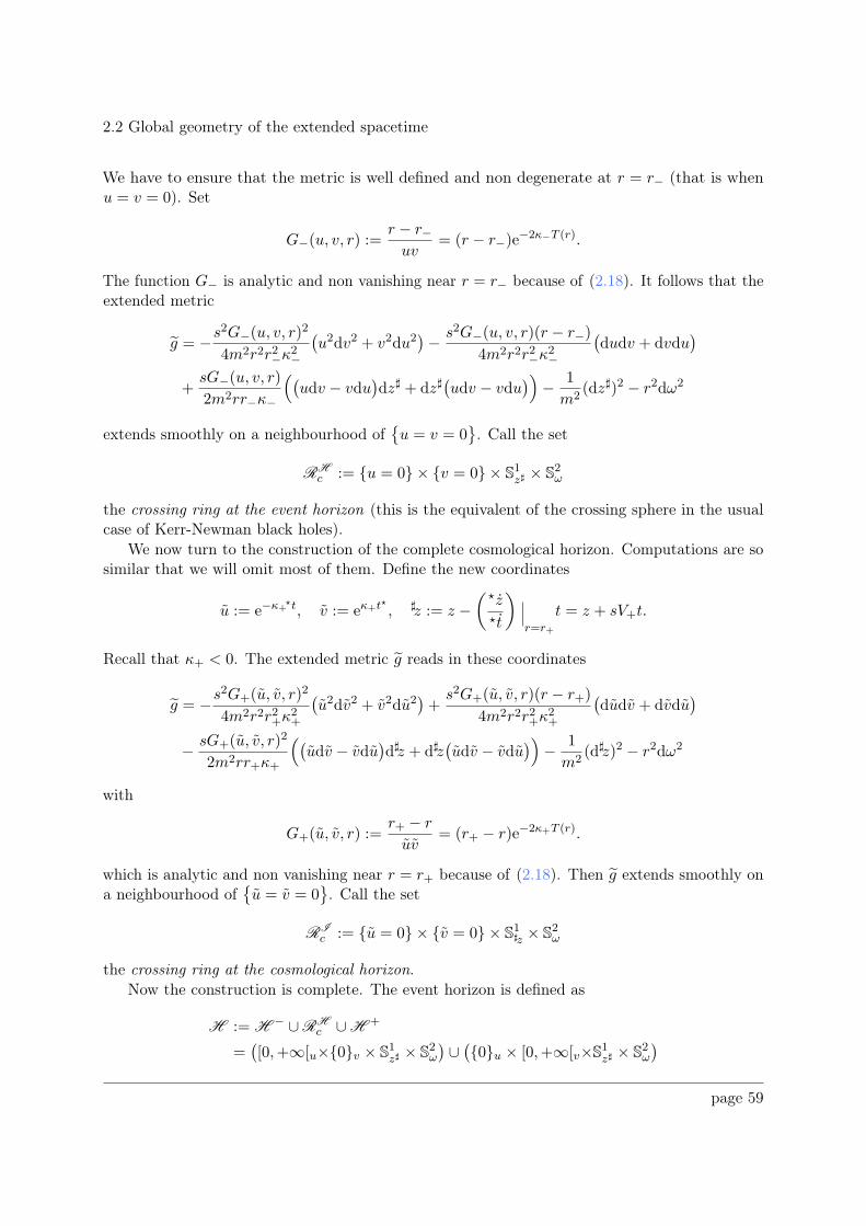
2.2 Global geometry of the extended spacetime
We have to ensure that the metric is well defined and non degenerate at r = r− (that is whenu = v = 0). Set
G−(u, v, r) :=r − r−uv
= (r − r−)e−2κ−T (r).
The function G− is analytic and non vanishing near r = r− because of (2.18). It follows that theextended metric
g = −s2G−(u, v, r)2
4m2r2r2−κ2−
(u2dv2 + v2du2
)− s2G−(u, v, r)(r − r−)
4m2r2r2−κ2−
(dudv + dvdu
)
+sG−(u, v, r)2m2rr−κ−
((udv − vdu
)dz♯ + dz♯
(udv − vdu
))− 1
m2(dz♯)2 − r2dω2
extends smoothly on a neighbourhood ofu = v = 0
. Call the set
RHc := u = 0 × v = 0 × S1z♯ × S2ω
the crossing ring at the event horizon (this is the equivalent of the crossing sphere in the usualcase of Kerr-Newman black holes).
We now turn to the construction of the complete cosmological horizon. Computations are sosimilar that we will omit most of them. Define the new coordinates
u := e−κ+⋆t, v := eκ+t⋆ , ♯z := z −
(⋆z⋆t
)
r=r+
t = z + sV+t.
Recall that κ+ < 0. The extended metric g reads in these coordinates
g = −s2G+(u, v, r)
2
4m2r2r2+κ2+
(u2dv2 + v2du2
)+s2G+(u, v, r)(r − r+)
4m2r2r2+κ2+
(dudv + dvdu
)
− sG+(u, v, r)2
2m2rr+κ+
((udv − vdu
)d♯z + d♯z
(udv − vdu
))− 1
m2(d♯z)2 − r2dω2
with
G+(u, v, r) :=r+ − ruv
= (r+ − r)e−2κ+T (r).
which is analytic and non vanishing near r = r+ because of (2.18). Then g extends smoothly ona neighbourhood of
u = v = 0
. Call the set
RIc := u = 0 × v = 0 × S1♯z × S2ω
the crossing ring at the cosmological horizon.Now the construction is complete. The event horizon is defined as
H := H− ∪R
Hc ∪H
+
=([0,+∞[u×0v × S1z♯ × S2ω
)∪(0u × [0,+∞[v×S1z♯ × S2ω
)
page 59
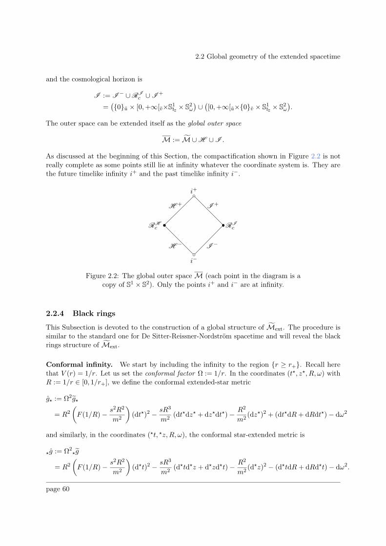
2.2 Global geometry of the extended spacetime
and the cosmological horizon is
I := I− ∪R
Ic ∪I
+
=(0u × [0,+∞[v×S1♯z × S2ω
)∪([0,+∞[u×0v × S1♯z × S2ω
).
The outer space can be extended itself as the global outer space
M := M ∪H ∪I .
As discussed at the beginning of this Section, the compactification shown in Figure 2.2 is notreally complete as some points still lie at infinity whatever the coordinate system is. They arethe future timelike infinity i+ and the past timelike infinity i−.
RHc RI
c
i+
i−
H + I +
H − I −
Figure 2.2: The global outer space M (each point in the diagram is acopy of S1 × S2). Only the points i+ and i− are at infinity.
2.2.4 Black rings
This Subsection is devoted to the construction of a global structure of Mext. The procedure issimilar to the standard one for De Sitter-Reissner-Nordström spacetime and will reveal the blackrings structure of Mext.
Conformal infinity. We start by including the infinity to the region r ≥ r+. Recall herethat V (r) = 1/r. Let us set the conformal factor Ω := 1/r. In the coordinates (t⋆, z⋆, R, ω) withR := 1/r ∈ [0, 1/r+], we define the conformal extended-star metric
g⋆ := Ω2g⋆
= R2
(F (1/R)− s2R2
m2
)(dt⋆)2 − sR3
m2(dt⋆dz⋆ + dz⋆dt⋆)− R2
m2(dz⋆)2 + (dt⋆dR+ dRdt⋆)− dω2
and similarly, in the coordinates (⋆t, ⋆z,R, ω), the conformal star-extended metric is
⋆g := Ω2⋆g
= R2
(F (1/R)− s2R2
m2
)(d⋆t)2 − sR3
m2(d⋆td⋆z + d⋆zd⋆t)− R2
m2(d⋆z)2 − (d⋆tdR+ dRd⋆t)− dω2.
page 60
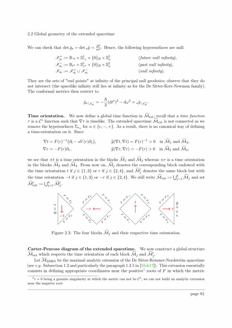
2.2 Global geometry of the extended spacetime
We can check that det g⋆ = det ⋆g = R2
m2 . Hence, the following hypersurfaces are null:
I+∞ := R⋆t × S1⋆z × 0R × S2ω (future null infinity),
I−∞ := Rt⋆ × S1z⋆ × 0R × S2ω (past null infinity),
I∞ := I+∞ ∪I
−∞ (null infinity).
They are the sets of "end points" at infinity of the principal null geodesics; observe that they donot intersect (the spacelike infinity still lies at infinity as for the De Sitter-Kerr-Newman family).The conformal metrics then restrict to
g⋆ I−∞
= −Λ
3(dt⋆)2 − dω2 = ⋆g I
+∞.
Time orientation. We now define a global time function in Mext; recall that a time functionτ is a C1 function such that ∇τ is timelike. The extended spacetime Mext is not connected as weremove the hypersurfaces Σrα for α ∈ c,−,+. As a result, there is no canonical way of defininga time-orientation on it. Since
∇t = F (r)−1(∂t − sV (r)∂z
), g(∇t,∇t) = F (r)−1 > 0 in M1 and M3,
∇r = −F (r)∂r, g(∇r,∇r) = −F (r) > 0 in M2 and M4,
we see that ±t is a time orientation in the blocks M1 and M3 whereas ±r is a time orientationin the blocks M2 and M4. From now on, Mj denotes the corresponding block endowed withthe time orientation t if j ∈ 1, 3 or r if j ∈ 2, 4, and M′
j denotes the same block but with
the time orientation −t if j ∈ 1, 3 or −r if j ∈ 2, 4. We still write Mext :=⋃4
j=1 Mj and set
M′ext :=
⋃4j=1 M′
j .
r=r c
r=rcr
=0
−t r=rc r
=r−
r=r−r
=r c
−rr=r− r
=r+
r=r+r
=r−
t
r=r+
r=
+∞r
=r+
r
Figure 2.3: The four blocks Mj and their respective time orientation.
Carter-Penrose diagram of the extended spacetime. We now construct a global structureMext which respects the time orientation of each block Mj and M′
j .LetMDSRN be the maximal analytic extension of the De Sitter-Reissner-Nordström spacetime
(see e.g. Subsection 1.2 and particularly the paragraph 1.2.5 in [Mok17]). This extension essentiallyconsists in defining appropriate coordinates near the positive5 roots of F in which the metric
5r = 0 being a genuine singularity at which the metric can not be C2, we can not build an analytic extensionnear the negative root.
page 61
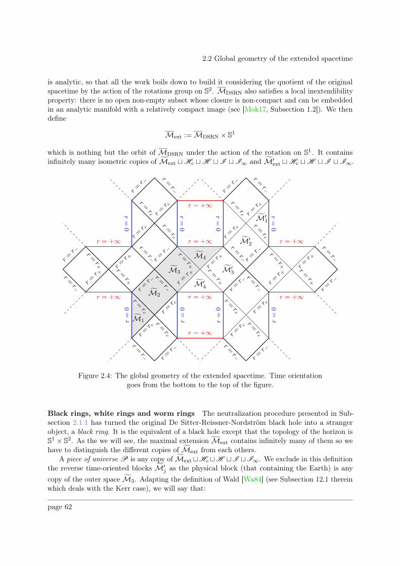
2.2 Global geometry of the extended spacetime
is analytic, so that all the work boils down to build it considering the quotient of the originalspacetime by the action of the rotations group on S2. MDSRN also satisfies a local inextendibilityproperty: there is no open non-empty subset whose closure is non-compact and can be embeddedin an analytic manifold with a relatively compact image (see [Mok17, Subsection 1.2]). We thendefine
Mext :=MDSRN × S1
which is nothing but the orbit of MDSRN under the action of the rotation on S1. It containsinfinitely many isometric copies of Mext ⊔Hc ⊔H ⊔I ⊔I∞ and M′
ext ⊔Hc ⊔H ⊔I ⊔I∞.
r=r−
r=r−
r=r c
r=
0
r=rcr
=0
r=r c
r=rc
r=r+
r=r−
r=r−
r=r+
r=r−
r=r+
r=r+
r=r−
r=rc r
=r c
r=r c
r=
0
r=rc
r=
0
r=r− r
=r−
r=r+
r = +∞
r=r−
r=r−
r=rcr
=r c
r=r−
r=r c
r=rc r
=0
r=
0
r=r−r
=r−
r=r+
r=r+
r = +∞
r = +∞
r=r−
r=r−
r=r+
r=r+
r=r+
r = +∞
r=r+
r = +∞
r=r+
r = +∞r=r−
r=r−
r=r−
r=rc r
=r c
r=rc
r=
0
r=
0
r=r c
r=r− r
=r−
r = +∞
r = +∞
M1
M2
M3
M4
M′1
M′2
M′3
M′4
Figure 2.4: The global geometry of the extended spacetime. Time orientationgoes from the bottom to the top of the figure.
Black rings, white rings and worm rings The neutralization procedure presented in Sub-section 2.1.1 has turned the original De Sitter-Reissner-Nordström black hole into a strangerobject, a black ring. It is the equivalent of a black hole except that the topology of the horizon isS1 × S2. As the we will see, the maximal extension Mext contains infinitely many of them so wehave to distinguish the different copies of Mext from each others.
A piece of universe P is any copy of Mext⊔Hc⊔H ⊔I ⊔I∞. We exclude in this definitionthe reverse time-oriented blocks M′
j as the physical block (that containing the Earth) is any
copy of the outer space M3. Adapting the definition of Wald [Wa84] (see Subsection 12.1 thereinwhich deals with the Kerr case), we will say that:
page 62
2.2 Global geometry of the extended spacetime
• a non-empty closed subset B ⊂ Mext is a black ring if ∂B = R × S1 × S2 and if for allinextendible causal future-pointing geodesic γ : R→Mext starting in M3 and entering Bat some µ0, then
⋃
µ≥µ0
γ(µ) ∩ M4 ∩P = ∅;
• a non-empty subset W ⊂ Mext is a white ring if it is a black ring for the reverse timeorientation;
• a non-empty subset S ⊂Mext is a worm ring S if there exist a black ring B and a whitering W such that S = B ∩W.
A black ring thus prevents any inextendible causal future-pointing geodesic entering inside it toescape at infinity in the same piece of universe: it can escape only in another copy of the universe.Observe that ∂B and ∂W are necessarily null.
We can similarly define the more standard notions of black/white/worm holes by requiringthe topology R × S3 for the boundary. It turns that the extended spacetime contains onlyblack/white/worm rings.
Lemma 2.2.2. 1. All the copies of M′2 ⊔Hc ⊔H are black rings.
2. All the copies of M2 ⊔Hc ⊔H are white rings.
3. All the copies of M1 ⊔Hc ⊔H and M′1 ⊔Hc ⊔H are worm rings.
4. There is no other black/white/worm ring in Mext. Furthermore, Mext contains no black-/white/worm hole.
Proof. 1. Let γ = (t, z, r, ω) be an inextendible causal future-pointing geodesic which starts in]r−, r+[ and such that r(µ0) ∈ ]rc, r−[ for some µ0 ∈ I (such a curve exists, take e.g. theincoming principal null geodesics γin). Since r(µ) < r− for some µ < µ0, there exists aproper time µ ∈ I, µ ≤ µ0, such that r(µ) < 0. Using that −r is a time orientation in M′
2,we have
r = ∇γr = gµν γµ∇νr ≤ 0.
As a result, r ≤ 0 along the flow of γ with equality as long as γ lies on r = r−. Thus γwill stay in the block M2 or will cross r = rc, entailing that it can escape to r = +∞only in another piece of universe.
2. and 3. follow from 1.
4. Removing all the black/white/worm rings from Mext, it only remains copies of M3, M′3,
M4 and M′4 (with the cosmological horizons at r = r+). Starting in any of these blocks,
the outgoing principal null geodesics γout can escape to r = +∞, meaning that no blackhole (and thus no white and worm hole) lies there.
Remark 2.2.3. All the black and white rings contained in the global extended spacetime Mext
are delimited by horizons. In particular, the timelike singularity r = 0 lying in all the wormring copies is always hidden by horizons. The weak Cosmic Censorship is therefore respected.
page 63
2.3 Analytic scattering theory
2.3 Analytic scattering theory
This section is devoted to the scattering theory associated to the extended wave equation (2.2).We will show existence and completeness of wave operators associated to several comparisondynamics for fixed momenta i∂z = z ∈ Z 6= 0 of the scalar field. The case z = 1 correspondsto the charged Klein-Gordon equation. Most of the results below follows from the work ofGeorgescu-Gérard-Häfner [GGH17].
In Subsection 2.3.1, we introduce the Hamiltonian formalism associated to equation (2.2).The different comparison dynamics used for the scattering are introduced in Subsection 2.3.2. InSubsection 2.3.3, we explicit the action of the geometric dynamics in term of transport alongprincipal null geodesics The structure of the energy spaces for the comparison dynamics relatedto transport is analyzed in Subsection 2.3.4 in order to prepare the proof of the scattering results.The analytic scattering results are then presented in Subsection 2.3.5 and proved in Section 2.4.
2.3.1 Hamiltonian formulation of the extended wave equation
We introduce in this Subsection the full dynamics associated to (2.2).
The full dynamics. Observe first of all that if u solves (2.2) then v := e−isV+t∂zu satisfies(∂2t − 2sV (r)∂z∂t + P
)u = 0, V (r) := V (r)− V+. (2.20)
We can therefore work with the potential6 V in this Section and use the results in [GGH17]. Inorder not to overload notations, we will still denote V by V ; to keep track of the potential V , wewill often write V+ in the sequel even though it is the constant 0. Note here that we can againcompare sV+ to the Kerr rotation Ω+ = a
r2++a2: the unitary transform performed above is the
equivalent operation in our setting to the variable change ϕ 7→ ϕ− Ω+t at the very beginning ofSection 13 in [GGH17].
We introduce the Regge-Wheeler coordinate
dx
dr:= T ′(r) =
1
F (r)
so that x ≡ x(r) is equal to the function T up to an additive constant; in particular, x ∈ R andx→ ±∞ if and only if r → r±. In the sequel, we will denote by ′ the derivative with respect tothe variable r.
Next, let us define H := L2(S1z × ]r−, r+[r × S2ω, T
′(r)dzdrdω)= L2
(S1z × Rx × S2ω, dzdxdω
)
and
h := rP r−1
= −r−1∂xr2∂xr
−1 − F (r)
r2∆S2 −
(m2F (r)− s2V (r)2
)∂2z
= −∂2x + F (r)
(− 1
r2∆S2 +
F ′(r)r−m2∂2z
)+ s2V (r)2∂2z .
6Working with this potential is actually equivalent to use the gauge Aµ =(
Qr− Q
r+
)dt.
page 64
2.3 Analytic scattering theory
with P given by (2.3). Here the variable r has to be understood as a function r(x) of theRegge-Wheeler coordinate. The operator ∂z plays a similar role as ∂ϕ for the De Sitter-Kerr case(cf. [GGH17, equation (13.3)]). Observe here that h is not positive in the dyadorings D± (becausesV −m2F < 0 near r = r±). This problem is very similar to the failure of ∂t to be timelike in theextended spacetime (or in Kerr spacetime). Considering the timelike (but not Killing) vector field∇t = F (r)−1(∂t − sV (r)∂z) instead, we add the extra "rotating" term −sV (r)∂z which cancelsthe negative parts of g(∂t, ∂t) near r = r±.
Introduce now cut-offs i±, j± ∈ C∞(]r−, r+[ ,R) satisfying
Supp i− = ]−∞, 1] , Supp i+ = [−1,+∞[ ,
i2− + i2+ = 1, i±j± = j±, i±j∓ = 0.
They will be useful to separate incoming and outgoing parts of solutions for the scattering. Wenext introduce the following operators:
k := −isV (r)∂z,
k± := −isV±∂z,k± := k ∓ j2∓k−,
h0 := h+ k2 = −r−1∂xr2∂xr
−1 − F (r)
r2∆S2 −m2F (r)∂2z
= −∂2x + F (r)
(− 1
r2∆S2 +
F ′(r)r−m2∂2z
),
h± := h0 − (k − k±)2.
Observe that h0 ≥ 0 which witnesses of the hyperbolic nature of the equation (2.2) (cf. [GGH17,Remark 2.2]). Observe also that if s is sufficiently small (that we will always assume in thesequel), then h± ≥ 0 to since k − k± as the same exponential decay at infinity as F , cf. (2.18).
Using the spherical symmetries of the problem, that is, using the diagonalizations −∆S2 =ℓ(ℓ+ 1) and −i∂z = z with (ℓ, z) ∈ N× Z, we define
hℓ,z0 := −r−1∂xr2∂xr
−1 − F (r)
r2ℓ(ℓ+ 1) +m2F (r)z2 = −∂2x + F (r)
(ℓ(ℓ+ 1)
r2+F ′(r)r
+m2z2
),
D(hℓ,z0 ) :=u ∈ H
∣∣hℓ,z0 u ∈ H.
In their work [BaMo93], Bachelot and Motet-Bachelot show in Proposition II.1 that −∂2x + V(x)has no 0 eigenvalue if the potential V(x) has some polynomial decay at infinity; this is the casefor hℓ,z0 which is then an elliptic second order differential operator, thus self-adjoint on H. Werealize h0 as the direct sum of the harmonic operators hℓ,z0 i.e.
D(h0) :=
u =
∑
ℓ,z
uℓ,z
∣∣∣∣ uℓ,z ∈ D(hℓ,z0 ),∑
ℓ,z
∥∥hℓ,z0 uℓ,z∥∥2H < +∞
which is in turn elliptic and self-adjoint. Finally, as k ∈ B(H), we can also realize h as a self-adjoint operator on the domain D(h) = D(h0). In the sequel, we will use the elliptic self-adjointrealizations (h±,D(h±)) defined as above for h0.
page 65
2.3 Analytic scattering theory
Energy spaces for the full dynamics. We now turn to the definition of the energy spacesassociated to the Hamiltonian H following [GGH17] (see the paragraphs 3.4.1 and 3.4.2 therein).
We define the inhomogeneous energy spaces
E := 〈h0〉−1/2H×H
equipped with the norm7
‖(u0, u1)‖2E := 〈(1 + h0)u0, u0〉H + ‖u1 − ku0‖2H.
Using that h0 ≥ 0 has no kernel in H, we can also define the homogeneous energy space E as thecompletion of E for the norm8
‖(u0, u1)‖2E := 〈h0u0, u0〉H + ‖u1 − ku0‖2H.
Observe that, as explained in paragraph 3.4.3 of [GGH17], this energy is not conserved in general.The natural conserved energies 〈· | ·〉ℓ defined for all ℓ ∈ R by
〈(u0, u1) | (u0, u1)〉ℓ := 〈(h0 − (k − ℓ)2)u0, u0〉H + ‖u1 − ℓu0‖2Hare not in general positive (because of the existence of the dyadorings). In contrast, the (positive)energy ‖ · ‖E is not conserved along the flow of ∂t and may grow in time: this is superradiance.From the geometric point of view, superradiance occurs because of the existence of the dyadoringsand we are using the timelike vector field ∇t of (2.15) instead of ∂t to get a positive quantitynear the dyadorings; the cost to pay for this is the non conservation of the energy since ∇t is notKilling.
Define next the asymptotic energy spaces9
˙E± := Φ(k±)(h−1/2± H×H
)
where
Φ(k±) :=
(1 0
k± 1
).
The spaces ˙E± are equipped with the norms
‖(u0, u1)‖2˙E±
:= 〈h±u0, u0〉H + ‖u1 − k±u0‖2H.
As discussed above Lemma 3.13 in [GGH17], the operators Φ(k±) : h−1/2± H × H → ˙E± are
isomorphisms with inverses Φ(−k±).The Hamiltonian form of (2.20) is given by −i∂tu = Hu with
H =
(0 1
h 2k
), D(H) =
u ∈ E | Hu ∈ E
7We use here that h0 ≥ 0.8We use here that h0 > 0.9Now we use that h± > 0.
page 66
2.3 Analytic scattering theory
is the energy Klein-Gordon operator. We will also need to use the asymptotic Hamiltonians
˙H± =
(0 1
h± 2k±
), D(
˙H±) := Φ(k±)
(h−1/2± H ∩ h−1
± H× 〈h±〉−1/2H).
Given now z ∈ Z, we define on ker(i∂z + z) the restricted operators hz, hz0, kz, Hz, etc. as well
as the spaces Hz, Ez, Ez in the obvious way. The operator hz0 is the one in (1.8) with (s,m)
replaced by (sz,mz). Furthermore, if z 6= 0, then 〈h0〉−1/2Hz = h−1/20 Hz = (hz0)
−1/2Hz.
[Ha01, Lemma 2.2] shows10 that ( ˙H z
±,D(˙H z
±)) are self-adjoint. The difference with (Hz,D(Hz))
is that for the asymptotic operators, we have∥∥kz±u
∥∥Hz
.⟨hz±u, u
⟩Hz
for all u ∈ D((hz±)
1/2)
(asrequired by (2.22) in [Ha01]); such an estimate is false with kz and hz.
[GGH17, Lemma 3.19] shows that H is the generator of a continuous group (eitH)t∈R on E .If u = (u0, u1) solves −i∂tu = Hu, then u0 is a solution of (2.2) and conversely, if u solves (2.2)then v = (u,−i∂tu) satisfies −i∂tv = Hv.
2.3.2 Comparison dynamics
We present in this Subsection the comparison dynamics we will use for the scattering.
Separable comparison dynamics. The first dynamics we will compare (eitHz
)t∈R to are thefollowing separable comparison dynamics. Define the operators
h±∞ := −∂2x −F (r)
r2∆S2 −
(m2F (r)− s2V 2
±)∂2z , k±∞ := −isV±∂z.
The associated second order equation reads(∂2t − 2ik±∞∂t + h±∞
)u = 0. (2.21)
The corresponding Hamiltonian is given by
H±∞ =
(0 1
h±∞ 2k±∞
), D(H±∞) =
u ∈ E±∞ | H±∞u ∈ E±∞
where the spaces(E±∞, ‖ · ‖E±∞
)are defined in the canonical way i.e. E±∞ is the completion of
smooth compactly supported functions with respect to the norm
‖(u0, u1)‖2E±∞:=⟨(h±∞ + k2±∞
)u0, u0
⟩H + ‖u1 − k±∞u0‖2H.
Denote by hz±∞, kz
±∞, Hz
±∞ and Ez±∞ the restrictions on ker(i∂z + z) for z ∈ Z of the aboveoperators and spaces. If u ∈ Ez solves (2.21), then
1
2
d
dt‖(u,−i∂tu)‖2Ez
±∞= ℜ
(⟨(hz±∞ + (kz±∞)2
)u, ∂tu
⟩H +
⟨∂2t u− ikz±∞∂tu, ∂tu− ikz±∞u
⟩H
)
= ℜ(⟨(
h±∞ + (kz±∞)2)u, ∂tu
⟩H +
⟨ikz±∞∂tu− h±∞u, ∂tu− ikz±∞u
⟩H
)
= ℜ(⟨
ikz±∞∂tu, ∂tu⟩H +
⟨h±∞u, ik
z
±∞u⟩H
)
= 0
10H2 must be replaced by its completion with respect to the homogeneous norm as pointed out by the author ofthis paper in [Ha03], above Lemma 2.1.1.
page 67
2.3 Analytic scattering theory
because
sign(sz)×⟨h±∞u, ik
z
±∞u⟩H = i
∥∥|kz±∞|1/2∂xu∥∥2H + i
∥∥r−1F (r)1/2|kz±∞|1/2∇S2u∥∥2H
+ i∥∥mF (r)1/2|kz±∞|1/2u
∥∥2H − i
∥∥|kz±∞|3/2∂zu∥∥2H.
Notice here that the above conservation law strongly relies on the fact that [∂x, k±∞] = 0 (incomparison, [∂x, k] 6= 0). It results that the associated dynamics (eitH
z
±∞)t∈R are unitary onHz ×Hz and the infinitesimal generators (Hz
±∞,D(Hz
±∞)) are self-adjoint by Stone’s theorem.
Theorem 2.3.9 states that the operators e−itHz
i±eitHz
±∞ and e−itHz
±∞i±eitHz
have strong limitsin B(Ez±∞, Ez) and B(Ez, Ez±∞) as |t| → +∞.
Asymptotic profiles. We next introduce the asymptotic profiles : they consist in the simplestpossible asymptotic comparison dynamics obtained by formally taking the limit x→ ±∞ in hand k. Set
h−/+ := −∂2x + s2V 2−/+∂
2z , k−/+ := −isV−/+∂z.
The associated second order equation reads
(∂2t − 2ik−/+∂t + h−/+
)u = 0. (2.22)
Notice the following factorization :
∂2t − 2sV−/+∂z∂t + h−/+ = (∂t − ∂x − sV−/+∂z)(∂t + ∂x − sV−/+∂z).
We call incoming respectively outgoing solutions of (2.22) are the solutions of (∂t−∂x−sV−/+∂z)u =0 respectively (∂t + ∂x − sV−/+∂z)u = 0. Define the corresponding Hamiltonians
H−/+ =
(0 1
h−/+ 2k−/+
), D(H−/+) =
u ∈ E−/+ | H−/+u ∈ E−/+
with the canonical energy spaces(E−/+, ‖ · ‖E−/+
)and the homogeneous norms
‖(u0, u1)‖2E−/+ :=⟨(h−/+ + k2−/+
)u0, u0
⟩H + ‖u1 − k−/+u0‖2H.
Put hz−/+, kz
−/+, Hz
−/+ and Ez−/+ for the restrictions of the above operators and spaces on ker(i∂z+z).
Then (eitHz
−/+)t∈R is unitary and (Hz
−/+,D(Hz
−/+)) self-adjoint (the argument is the same as forthe separable comparison dynamics above).
Theorem 2.3.10 below states that there exists a dense subspace Dfin,z−/+ ⊂ Ez−/+ such that
e−itHz
i2−/+eitHz
−/+ and e−itHz
−/+i2−/+eitHz
have strong limits in B(Dfin,z−/+ , Ez) and B(Ez, Ez−/+) as
|t| → +∞.
page 68
2.3 Analytic scattering theory
Geometric profiles. Finally, let us introduce two last profiles we will refer to later on as thegeometric profiles. We want them to describe a transport along principal null geodesics γin/out
introduced in Subsection 2.2.1.The generators of time-parametrized11 principal null geodesics are given by
vin = ∂t + LH , LH := −∂x − sV (r)∂z,
vout = ∂t + LI , LI := ∂x − sV (r)∂z.
The natural equation one may want to consider to describe transport along γin/out would be
1
2
(vinvout + voutvin
)= 0
However, [LH , LI ] 6= 0 (because [∂x, V ] 6= 0) and no conserved positive energy can be associatedto this equation.
The idea is to use instead new dynamics with natural conserved energies whose incoming andoutgoing parts are vin and vout. Let us define
L+ := −LH − 2sV−∂z = ∂x + s(V (r)− 2V−)∂z,
L− := −LI − 2sV+∂z = −∂x + s(V (r)− 2V+)∂z
and set
hH/I := −(LH/I + sV−/+∂z
)2= −
(∂x +/− s(V (r)− V−/+)∂z
)2, kH/I := −isV−/+∂z.
The associated second order equation reads((∂t − ikH/I )2 + hH/I
)u = ∂2t u− 2ikH/I ∂tu+ LH/IL+/−u = 0 (2.23)
so that we have the factorizations
(∂t − ikH )2 + hH =(∂t + LH
)(∂t + L+
),
(∂t − ikI )2 + hI =(∂t + LI
)(∂t + L−
)
with this time [LH , L+] = [LI , L−] = 0. The incoming part(∂t + LH
)describes a transport
towards H along γin whereas the outgoing part(∂t+LI
)describes a transport towards I along
γout. The artificial parts(∂t + L+/−
)describe transports towards I /H along modified principal
null geodesics; they will disappear when we will send data on the horizons later on.The corresponding Hamiltonians
HH/I =
(0 1
hH/I − k2H/I 2kH/I
), D(HH/I ) =
u ∈ EH/I | HH/I u ∈ EH/I
act on their energy spaces(EH/I , ‖ · ‖EH/I
)with
‖(u0, u1)‖2EH/I:=⟨hH/I u0, u0
⟩H + ‖u1 − kH/I u0‖2H.
11We can parametrize the principal null geodesics by the time variable t as dtdr
= ±F (r)−1, cf. Subsection 2.2.1).
page 69
2.3 Analytic scattering theory
Notice here that hH/I plays the role of h0 for the full dynamics, so that we have to subtract k2H/I
in the Hamiltonians HH/I ; besides, we can check that hH/I > 0 since kerHz(hH/I ) = 0 for
all z ∈ Z. By construction, the energies ‖ · ‖EH/Iare conserved and the evolutions (eitHH/I )t∈R
are unitary on H×H.Using as above the notation z for the restriction on ker(i∂z + z), Theorem 2.3.11 below
states that that there exists a dense subspace Dfin,zH/I ⊂ EzH/I such that e−itHz
i−/+eitHz
H/I and
e−itHz
H/I −−/+ eitHz
have strong limits in B(Dfin,zH/I , Ez) and B(Ez, Ez
H/I ). These limits will begiven a geometric sense in Subsection 2.5.4.
Remark 2.3.1. 1. We implicitly used [GGH17, Lemma 3.19] to define all the above dynamics.We refer to Section 3 therein for a detailed discussion about the energy spaces and theHamiltonian formalism associated to abstract Klein-Gordon equations.
2. The self-jointedness of the different Hamiltonians (and thus the unitarity of the associateddynamics) have different origins:
(i) For the asymptotic Hamiltonians˙H z
±, self-adjointness is due to the decay rate kz± =
Ox→±∞(e2κ±x
)which ensures that kz± . hz±.
(ii) For the comparison Hamiltonians Hz
±∞, Hz
−/+ and Hz
H/I , self-adjointness is entailedby the conservation of the associated homogeneous energies, which relies on the com-mutation of ∂x with kz±∞ = kz−/+ = kz
H/I .
3. Let Σt′ := t = t′ × S1z × Rx × S2ω. In all the above statements, we implicitly identify theslices Σ0 and Σt for all t ∈ R using the curves t = constant. All the energy spaces E , E±∞and E−/+ use coordinates (z, x, ω) in Σ0.
2.3.3 Transport along principal null geodesics
The purpose of this paragraph is to explicit the action of the Hamiltonians HH/I . The sameconsiderations hold for H−/+, but we omit details here as this case has been treated in [GGH17],paragraph 13.3.
Let H1H/I be the completions of C∞c (Σ0) with respect to the norms
‖u‖H1H/I
:=∥∥(LH/I + ikH/I )u
∥∥H =
∥∥(∂x +/− s(V (r)− V−/+)∂z)u∥∥H.
When s = 0, we have hH/I = −∂2x and H1H/I are nothing but the standard homogeneous
Sobolev space H1(R,dx) naturally associated to the one-dimensional wave equation. Considerthe following canonical transformations:
ΨH :=1√2
(1 1
iLH iL+
): H1
H × H1H −→ EH ,
ΨI :=1√2
(1 1
iL− iLI
): H1
I × H1I −→ EI .
While the second column of ΨH is artificial, the first one is related to the principal null geodesicsγin: for an incoming/outgoing solution uin, that is (∂t + LH )uin = 0, we have ΨH (uin, 0) =
page 70
2.3 Analytic scattering theory
(uin,−i∂tuin) so ΨH prepare initial data for evolution along γin. Similarly, the second column ofΨI is related to transport along γout.
Lemma 2.3.2. The transformations ΨH/I are invertible isometries with inverses
Ψ−1H
=√2
(L+ i−LH −i
)(L+ − LH )−1, Ψ−1
I=√2
(LI i−L− −i
)(LI − L−)
−1.
Proof. We only treat the H case. Let (u0, u1) ∈ H1H× H1
H. Using the parallelogram law
‖a+ b‖2 + ‖a− b‖2 = 2‖a‖2 + 2‖b‖2, we compute:
∥∥ΨH (u0, u1)∥∥2EH
=1
2
∥∥(LH + ikH )(u0 + u1)∥∥2H +
1
2
∥∥i(LH + ikH )u0 + i(L+ + ikH )u1∥∥2H
=1
2
∥∥(LH + ikH )(u0 + u1)∥∥2H +
1
2
∥∥(LH + ikH )(u0 − u1)∥∥2H
= ‖(u0, u1)‖2H1H
×H1H
.
Next, the expression for Ψ−1H
makes sense since L+ − LH = −2(LH + ikH ) have a trivial kernelin H and we have((LH + ikH )−1φ
)(z, x, ω) = −
ˆ x
0e−isz
´ xy (V (y′)−V−)dy′φ(z, y, ω)dy ∀φ ∈ C∞c (Σ0) ∩ ker(i∂z + z).
To check that Ψ−1H
indeed inverts ΨH , we use that [LH , L+] = 0.
Lemma 2.3.3. The transformations ΨH/I diagonalize the Hamiltonians HH/I :
Ψ−1HHH ΨH = HH := i
(LH 00 L+
): Ψ−1
HD(HH ) −→ H1
H × H1H ,
Ψ−1IHI ΨI = HI := i
(LI 00 L−
): Ψ−1
ID(HI ) −→ H1
I × H1I .
The dynamics (eitHH/I )t∈R have therefore unitary extensions on H1H/I × H1
H/I .
Proof. We only treat the H case. Recall that L+ = −LH − 2ikH and hH − k2H = LH L+. Wecompute:
HH ΨH =
(0 1
LH L+ 2kH
)(1 1
iLH iL+
)=
1√2
(iLH iL+
−L2H−L2
+
),
ΨH HH =
(1 1
iLH iL+
)(iLH 00 iL+
)=
1√2
(iLH iL+
−L2H−L2
+
).
This gives the desired formula.
We can now interpret the dynamics (eitHH/I )t∈R as mixed transports towards the horizons.Introduce the time-parametrized curves γ+ and γ− defined in the (z, r, ω) coordinates by
γ+(t) :=
(1, s(V (r(t))− 2V−), F (r(t)), 0
),
γ−(t) :=(1, s(V (r(t))− 2V+),−F (r(t)), 0
) . (2.24)
page 71
2.3 Analytic scattering theory
The curve γ+ carries data to I + whereas γ− carries data to H +. By Lemma 2.3.3, we have forall (φ0, φ1) ∈ C∞c (Σ0)× C∞c (Σ0) and all t ∈ R:
eitHH/I
(φ0φ1
)=
(e−tLH/I 0
0 e−tL+/−
)(φ0φ1
)=
(φ0 γin/out(t)
φ1 γ+/−(t)
),
eitHH/I
(φ0φ1
)=
1
2
(−L+/−φ0 − iφ1
iLH/I
(− L+/−φ0 − iφ1
)) γin/out(t) +
1
2
(LH/I φ0 + iφ1
iL+/−(LH/I φ0 + iφ1
)) γ+/−(t)
=1
2
(φ0 − i
(φ1 − kH /I φ0
)
iLH/I
[φ0 − i
(φ1 − kH /I φ0
)]) γin/out(t)
+1
2
(φ0 + i
(φ1 − kH /I φ0
)
iL+/−[φ0 + i
(φ1 − kH /I φ0
)]) γ+/−(t) (2.25)
where φj := (LH/I + ikH/I )−1φj . At t = 0, we get (φ0, φ1) back on the right-hand side above.
2.3.4 Structure of the energy spaces for the comparison dynamics
We analyze in this Subsection the structure of the energy spaces associated to the asymptoticand geometric comparison dynamics introduced in Subsection 2.3.2. We will obtain explicitrepresentation formulas on dense subspaces in smooth compactly supported functions. This willhelp us to show existence and completeness of the wave operators in Theorem 2.3.10 and Theorem2.3.11. In all this Section, we will restrict ourselves to ker(i∂z + z) with z ∈ Z.
Structure of the energy spaces for the asymptotic profiles
The solutions of the initial value problem associated to (2.22)
(∂2t − 2ikz−/+∂t + hz−/+
)u = 0
u|Σ0= u0 ∈ C∞c (Σ0)
(−i∂tu)|Σ0= u1 ∈ C∞c (Σ0)
are given by the Kirchhoff type formula:
u(t, z, x, ω) =eisztV−/+
2
(u0(z, x+ t, ω) + i
ˆ x+t
0
(u1 − sV−/+zu0
)(z, y, ω)
)
+eisztV−/+
2
(u0(z, x− t, ω) + i
ˆ 0
x−t
(u1 − sV−/+zu0
)(z, y, ω)
). (2.26)
They are a linear combination of incoming and outgoing solutions of (2.22).The simplicity of the asymptotic profiles has a cost: all the angular information has been lost
in the construction of Hz
−/+. As a result, as explained in [GGH17], there is no chance that thelimits
Wl/ru = lim|t|→+∞
e−itHz
i−/+eitHz
−/+u
page 72
2.3 Analytic scattering theory
exist for all u ∈ Ez−/+ since Hz is built from hz which acts on the angular part of u. The strategyis to define the limits first on a suitable dense subspace then to extend the corresponding operatorby continuity on the whole space Ez−/+. We define the spaces
Efin,zl/r :=
u ∈ E
z
l/r
∣∣∣∣ ∃ℓ0 > 0 ; u ∈(L2(S1 × R, dzdx)⊗
⊕
ℓ≤ℓ0
Yℓ)×(L2(S1 × R, dzdx)⊗
⊕
ℓ≤ℓ0
Yℓ)
where Yℓ is the eigenspace associated to the eigenvalue ℓ(ℓ + 1) of the self-adjoint realization(−∆S2 , H
2(S2,dω)). In order to exploit (2.26) and decompose elements of Efin,zl/r into incoming
and outgoing solutions of (2.22), we will use the following spaces:
EL,z−/+ :=
(u0, u1) ∈ E−/+
∣∣∣ u1 − sV−/+zu0 ∈ L1(R, dx ; (S1 × S2, dzdω)
),
ˆ
R
(u1 − sV−/+zu0
)(z, x, ω)dx = 0 a.e. in z, ω
.
[GGH17, Lemma 13.3] shows that12
EL,z−/+ = E in,z−/+ ⊕ E
out,z−/+ (2.27)
with the spaces of incoming and outgoing initial data
E in,z−/+ =
(u0, u1) ∈ EL,z−/+
∣∣u1 = −i∂xu0 − sV−/+zu0,
Eout,z−/+ =
(u0, u1) ∈ EL,z−/+
∣∣u1 = i∂xu0 − sV−/+zu0.
Solutions in EL,z−/+ verify a Huygens principle (cf. [GGH17, Remark 13.4]). The cancellation of theintegral in particular removes the resonance at 0 of the wave equation; the non-vanishing term ast→ ±∞ is the projection of compactly supported data on the resonant state which is nothingbut the constant solution 1 6∈ H (see the De Sitter-Schwarzschild case for s = 0 in [BoHa08],Proposition 1.2 and Theorem 1.3; here the resonant state is r⊗ ω0 with ω0 ∈ Y0 the fundamentalspherical harmonic because we use the conjugated spatial operator rP r−1).
Finally, set
Dfin,zl/r :=
(C∞c (S1 × R× S2)× C∞c (S1 × R× S2)
)∩ Efin,z
l/r ∩ EL−/+.
Then [GGH17, Lemma 13.5] shows that Dfin,zl/r is dense in
(Efin,zl/r , ‖ · ‖Ez
−/+
)(and thus in
(Ez−/+, ‖ · ‖Ez
−/+
)). We will show similar results for the geometric profiles in the next paragraph.
Structure of the energy spaces for the geometric profiles
The solutions of the initial value problem associated to (2.23)
(∂2t − 2ikz
H/I ∂t + Lz
H/ILz
+/−)u = 0
u|Σ0= u0 ∈ C∞c (Σ0)
(−i∂tu)|Σ0= u1 ∈ C∞c (Σ0)
12Observe the different gauge used therein (the initial time-derivative is ∂tu). To obtain the incoming/outgoingspaces of [GGH17], we need to replace u1 by iu1 below; this of course does not modify the results.
page 73
2.3 Analytic scattering theory
are given by the Kirchhoff type formula (we drop the dependence in (z, ω) ∈ S1 × S2):
uH (t, x) =1
2eisz
´ x+tx V (x′)dx′
(u0(x+ t) + i
ˆ x+t
0e−isz
´ x+ty (V (y′)−V−)dy′(u1 − szV−u0
)(y)dy
)
+1
2eisz
´ x−tx (V (x′)−2V−)dx′
(u0(x− t)− i
ˆ x−t
0e−isz
´ x−ty (V (y′)−V−)dy′(u1 − szV−u0
)(y)dy
),
(2.28)
0uI (t, x) =1
2e−isz
´ x+tx (V (x′)−2V+)dx′
(u0(x+ t) + i
ˆ x+t
0eisz
´ x+ty (V (y′)−V+)dy′(u1 − szV+u0
)(y)dy
)
+1
2e−isz
´ x−tx V (x′)dx′
(u0(x− t)− i
ˆ x−t
0eisz
´ x−ty (V (y′)−V+)dy′(u1 − szV+u0
)(y)dy
).
(2.29)
The solution uH is a linear combination of an incoming solution transported along the principalnull geodesic γin and and outgoing solution transported along the artificial curve γ+; the solutionuI is a linear combination of an incoming solution transported along the artificial curve γ− andand outgoing solution transported along the principal null geodesic γout. Formulas (2.28) and
(2.29) display the first components of eitHz
H/I u: we can easily check them using (2.25) with (weomit the dependence in (z, ω) ∈ S1 × S2)
((Lz
H/I + ikzH/I )−1(u1 − kzH/I u0)
)(x) = −/+
ˆ x
0e−/+isz
´ xy (V (y′)−V−/+)dy′(u1 − szV−/+u0
)(y)dy.
It will be useful below using the following simplified forms:
uH (t, x) =eisztV−
2
(∑
±eisz
´ x±tx (V (x′)−V−)dx′
u0(x± t) + i
ˆ x+t
x−teisz
´ yx (V (x′)−V−)dx′(
u1 − szV−u0)(y)dy
),
(2.30)
0uI (t, x) =
eisztV+
2
(∑
±e−isz
´ x±tx (V (x′)−V+)dx′
u0(x± t) + i
ˆ x+t
x−te−isz
´ yx (V (x′)−V+)dx′(
u1 − szV+u0)(y)dy
).
(2.31)
As for the asymptotic profiles of the paragraph 2.3.4, we need to control the angular directionson S2ω if we wish to compare the geometric dynamics with the full one. We thus define
Efin,zH/I :=
u ∈ E
z
H/I
∣∣∣∣ ∃ℓ0 > 0 ; u ∈(L2(S1 × R, dzdx)⊗
⊕
ℓ≤ℓ0
Yℓ)×(L2(S1 × R, dzdx)⊗
⊕
ℓ≤ℓ0
Yℓ) .
Formulas (2.28) and (2.29) makes a priori no sense in Efin,zH/I and the integral terms are not
controlled in H. We thus introduce the following spaces:
EL,zH/I :=
(u0, u1) ∈ EH/I
∣∣∣ u1 − szV−/+u0 ∈ L1(R, dy ; (S1 × S2, dzdω)
),
ˆ
R
e+/−isz´ y0 (V (x′)−V−/+)dx′(
u1 − szV−/+u0)(z, y, ω)dy = 0 a.e. in z, ω
.
We now establish a result similar to [GGH17, Lemma 13.3]: it gives a deeper meaning to incomingand outgoing data.
page 74
2.3 Analytic scattering theory
Lemma 2.3.4. Let
E in,zH
=(u0, u1) ∈ EL,zH
∣∣∣u1 = iLH u0
, Eout,z
H=(u0, u1) ∈ EL,zH
∣∣∣u1 = iL+u0
,
E in,zI
=(u0, u1) ∈ EL,zI
∣∣∣u1 = iL−u0, Eout,z
I=(u0, u1) ∈ EL,zI
∣∣∣u1 = iLI u0
.
The following decompositions into incoming and outgoing solutions of (2.23) hold:
EL,zH/I = E in,z
H/I ⊕ Eout,zH/I .
Furthermore, if u = uin + uout ∈ EL,zH/I is supported in S1z × [R1, R2]x × S2ω for some R1, R2 ∈ R,
then
Suppuin ⊂ S1z × ]−∞, R2]x × S2ω, Suppuout ⊂ S1z × [R1,+∞[x × S2ω. (2.32)
Proof. We only show the lemma for EL,zH
. Recall that
iLH u0 = −i∂xu0 + szV u0, iL+u0 = i∂xu0 − sz(V − 2V−)u0.
Let u = (u0, u1) ∈ EL,zHand put u(x) := eisz
´ x0 (V (y)−V−)dyu(x). Then u ∈ E in,z
Hif and only if
u1 = −i∂xu0 + szV−u0
whereas u ∈ Eout,zH
if and only if
u1 = i∂xu0 + szV−u0.
These conditions define incoming and outgoing states for the asymptotic profiles (see [GGH17],above Lemma 13.3 with u1 therein being iu1 for us). We then define13 (omitting the dependencein (z, ω) ∈ S1 × S2):
uin0 (x) =
1
2
ˆ +∞
x
[−∂yu0 − i(u1 − szV−u0)
](y)dy,
uin1 (x) =
1
2
[−i∂xu0 + (u1 − szV−u0)
](x) +
szV−2
ˆ +∞
x
[−∂yu0 − i(u1 − szV−u0)
](y)dy,
uout0 (x) =
1
2
ˆ x
−∞
[∂yu0 − i(u1 − szV−u0)
](y)dy,
uout1 (x) =
1
2
[i∂xu0 + (u1 − szV−u0)
](x) +
szV−2
ˆ x
−∞
[∂yu0 − i(u1 − szV−u0)
](y)dy.
Direct computations show that
uin1 = −i∂xuin
0 + szV−uin0 , uout
1 = i∂xuout0 + szV−u
out0 , (u0, u1) = (uin
0 + uout0 , uin
1 + uout1 ).
13We use formula (13.8) of [GGH17, Lemma 13.3].
page 75
2.3 Analytic scattering theory
Here we use thatˆ +∞
−∞(u1 − szV−u0)(y)dy =
ˆ +∞
−∞eisz
´ y0 (V (y′)−V−)dy′
(u1 − szV−u0
)(y)dx = 0.
It follows that
uin/out := e−isz´ x0 (V (y)−V−)dy
(u
in/out0 , u
in/out1
)
satisfy uin/out ∈ E in/out,zH
and u = uin + uout.The support condition (2.32) for uin/out directly reads on the above expressions and is in turn
verified for uin/out as multiplication by eisz´ x0 (V (y)−V−)dy does not modify supports.
It remains to show that E in,zH∩ Eout,z
H= 0. If u lies in the intersection, then u satisfies
u1 = −i∂xu0 + szV−u0u1 = i∂xu0 + szV−u0
.
Adding and subtracting both the conditions, we see that u0 is constant and u1 = szV−u0 in H,whence u0 = u1 = 0. This entails u = 0 and we are done.
Remark 2.3.5. Using the definitions of ΨH/I in the paragraph 2.3.3, we easily show that
E in,zH
= ΨH
(H1,z
H× 0
)∩ EL,z
H, Eout,z
I= ΨI
(0 × H1,z
I
)∩ EL,z
I.
We then have the following adaptation of [GGH17, Lemma 13.5] to our framework:
Lemma 2.3.6. Let
Dfin,zH/I :=
(C∞c (S1 × R× S2)× C∞c (S1 × R× S2)
)∩ Efin,z
H/I ∩ EL,zH/I .
Then Dfin,zH/I is dense in
(Ez
H/I , ‖ · ‖Ez
H/I
).
Proof. First of all, Efin,zH/I is dense in Ez
H/I by definition of the homogeneous spaces and because
the Hilbert direct sum of the eigenspaces Yℓ is L2(S2, dω).Next,
(C∞c (S1z×Rx×S2ω)×C∞c (S1z×Rx×S2ω)
)∩Efin,,z
H/I is dense in Efin,,zH/I by standard regularization
arguments.Finally, let ψ ∈ C∞c (S1z × Rx × S2ω)× C∞c (S1z × Rx × S2ω) such that ψ ≥ 0, ‖ψ‖L1(S1×R×S2) = 1
and put ψn(z, x, ω) := ψ(z, n−1x, ω) for each n ∈ N\0. Pick u ∈(C∞c (S1z×Rx×S2ω)×C∞c (S1z×
Rx × S2ω))∩ Efin,z
in and defineun0 := u0,
un1 := u1 − n−1ψne−/+isz
´ x0 (V (x′)−V−/+)dx′
ˆ
R
e+/−isz´ y0 (V (x′)−V−/+)dx′(
u1 − szV−/+u0)(z, y, ω)dy
.
Then un := (un0 , un1 ) ∈
(C∞c (S1z × Rx × S2ω)× C∞c (S1z × Rx × S2ω)
)∩ Efin,z
in ∩ EL,zin and we have
‖un1 − u1‖Hz ≤ n−1/2‖n−1/2ψn‖Hz‖u1 − szV−/+u0‖L1(S1×R×S2)
≤ Cn−1/2‖u1 − szV−/+u0‖L1(S1×R×S2)
for some constant C > 0 independent of n. It remains to let n→ +∞ to conclude the proof.
page 76
2.3 Analytic scattering theory
Remark 2.3.7 (Minimal propagation speed). Let u = uin+uout ∈ Dfin,zH
and v = vin+vout ∈ Dfin,zI
such that Suppu, Supp v ⊂ S1z × [R1, R2]x × S2ω for some R1, R2 ∈ R. Using the relations
uin1 = −i∂xuin
0 + szV uin0 , uout
1 = i∂xuout0 − sz(V − 2V−)u
out0 ,
vin1 = −i∂xvin
0 − sz(V − 2V+)vin0 , vout
1 = i∂xvout0 + szV vout
0 ,
we can integrate by parts in the Kirchhoff formulas (2.30) and (2.31) to obtain(eitH
z
H uin)0(z, x, ω) = eisz
´ x+tx V (x′)dx′
uin0 (z, x+ t, ω),
(eitH
z
H uout)0(z, x, ω) = eisz
´ x−tx (V (x′)−2V−)dx′
uout0 (z, x− t, ω),
(eitH
z
I vin)0(z, x, ω) = e−isz
´ x+tx (V (x′)−2V+)dx′
vin0 (z, x+ t, ω),
(eitH
z
I vout)0(z, x, ω) = e−isz
´ x−tx V (x′)dx′
vout0 (z, x− t, ω).
It follows:
Supp(eitH
z
H uin), Supp
(eitH
z
I vin)⊂ S1z × ]−∞, R2 − t]x × S2ω,
Supp(eitH
z
H uout), Supp
(eitH
z
I vout)⊂ S1z × [R1 + t,+∞[x × S2ω.
The dynamics (eitHz
H/I )t∈R thus verifies the Huygens principle on Dfin,zH/I .
2.3.5 Analytic scattering results
We state in this Subsection the scattering results we will prove in Section 2.4. For all of them, weneed to first restrict to ker(i∂z + z) with z ∈ Z in order to apply the abstract theory of [GGH17]for Klein-Gordon equations with a non zero mass term, then to |s| sufficiently small to use [?,Theorem 3.8].
The first result concerns the uniform boundedness of the propagator (eitHz
)t∈R. The proof isgiven in Subsection 2.4.2.
Theorem 2.3.8 (Uniform boundedness of the evolution). Let z ∈ Z \ 0. There exists s0 > 0such that for all s ∈ ]−s0, s0[, there exists a constant C ≡ C(z, s0) > 0 such that
∥∥eitHz
u∥∥Ez≤ C‖u‖Ez
∀t ∈ R, ∀u ∈ Ez.The next result concerns the asymptotic completeness between the full dynamics and the
separable comparison dynamics. The proof is given in Subsection 2.4.3.
Theorem 2.3.9 (Asymptotic completeness, separable comparison dynamics). Let z ∈ Z \ 0.There exists s0 > 0 such that for all s ∈ ]−s0, s0[, the following strong limits
Wf± := s− lim
t→+∞e−itHz
i±eitHz
±∞ ,
Wp± := s− lim
t→−∞e−itHz
i±eitHz
±∞ ,
Ωf± := s− lim
t→+∞e−itHz
±∞i±eitHz
,
Ωp± := s− lim
t→−∞e−itHz
±∞i±eitHz
exist as bounded operators Wf/p± ∈ B(Ez±∞, Ez) and Ω
f/p± ∈ B(Ez, Ez±∞).
page 77
2.3 Analytic scattering theory
We now state an asymptotic completeness result with the asymptotic profiles. The proof isgiven in Subsection 2.4.4.
Theorem 2.3.10 (Asymptotic completeness, asymptotic profiles). Let z ∈ Z \ 0. There existss0 > 0 such that for all s ∈ ]−s0, s0[, the following holds:
1. For all u ∈ Dfin,zl/r , the limits
Wfl/ru = lim
t→+∞e−itHz
i−/+eitHz
−/+u,
Wpl/ru = lim
t→−∞e−itHz
i−/+eitHz
−/+u
exist in Ez. The operators Wf/pl/r extend to bounded operators W
f/pl/r ∈ B(Ez−/+, Ez).
2. The inverse wave operators
Ωfl/ru = s− lim
t→+∞e−itHz
−/+i−/+eitHz
,
Ωpl/ru = s− lim
t→−∞e−itHz
−/+i−/+eitHz
exist in B(Ez, Ez−/+).
Finally, we state a last asymptotic completeness result using the geometric profiles. We willprove the following theorem in Subsection 2.4.5 and give a geometric interpretation in Subsection2.5.4 (see Remark 2.5.8).
Theorem 2.3.11 (Asymptotic completeness, geometric profiles). Let z ∈ Z \ 0. There existss0 > 0 such that for all s ∈ ]−s0, s0[, the following holds:
1. For all u ∈ Dfin,zH/I , the limits
WfH/I u = lim
t→+∞e−itHz
i−/+eitHz
H/I u,
WpH/I u = lim
t→−∞e−itHz
i−/+eitHz
H/I u
exist in Ez. The operators Wf/pH/I extend to bounded operators W
f/pH/I ∈ B(EzH/I , Ez).
2. The inverse future/past wave operators
ΩfH/I = s− lim
t→+∞e−itHz
H/I i−/+eitHz
,
ΩpH/I = s− lim
t→−∞e−itHz
H/I i−/+eitHz
exist in B(Ez, EzH/I ).
Remark 2.3.12. Because of the cut-offs i±, wave operators and inverse wave operators are notinverse. We will however justify this designation for the geometric profiles in Subsection 2.5.2.
page 78
2.4 Proof of the analytic results
The geometric wave and inverse wave operators satisfy the following properties (the proof isgiven in Subsection 2.4.6):
Proposition 2.3.13. Under the hypotheses of Theorem 2.3.11, it holds:
Ωf/pHEz ⊂ ΨH
(H1,z
H× 0
), Ω
f/pH
Wf/pH
= 1ΨH (H1,z
H×0),
Ωf/pIEz ⊂ ΨI
(0 × H1,z
I
), Ω
f/pI
Wf/pI
= 1ΨI (0×H1,z
I).
2.4 Proof of the analytic results
This Section is devoted to the proofs of the scattering results stated in Subsection 2.3.5. Theorems2.3.8, 2.3.9 and 2.3.10 are direct consequences of the results obtained in [GGH17] once somegeometric hypotheses are checked. Theorem 2.3.11 follows from standard arguments as well aspropagation estimates of the full dynamics showed in [GGH17].
2.4.1 Geometric hypotheses
In this paragraph, we check that the geometric hypotheses (G) of [GGH17] are verified in oursetting on ker(i∂z + z), z ∈ Z \ 0 (z must not be zero to conserve a mass term). We use theweight w(r) :=
√(r − r−)(r+ − r) defined for all r ∈ ]r−, r+[.
(G1) The operator P in [GGH17] is14 −∆S2 −m2r2∂2z for us, and satisfies of course [P, ∂z] = 0.
(G2) Set
hz0,s := F (r)−1/2hz0F (r)1/2 = −r−1F (r)1/2∂rr
2F (r)∂rr−1F (r)1/2 − r−2F (r)∆S2 +m2F (r)z2.
Then α1(r) = α3(r) = r−1F (r)1/2, α2(r) = rF (r)1/2 and α4(r) = mF (r)1/2z. Thesecoefficients are clearly smooth in r. Furthermore, since we can write F (r) = g(r)w(r)2 withg(r) = Λ
3r2(r − rn)(r − rc) & 1 for all r ∈ ]r−, r+[, it comes for all j ∈ 1, 2, 3, 4
αj(r)− w(r)(i−(r)α
−j + i+(r)α
+j
)= w(r)
(g(r)1/2 − α±
j
)= Or→r±
(w(r)2
)
for
α±1 = α±
3 =α±2
r2±=r±α
±4
mz=
1
r2±
√Λ(r± − rn)(r± − rc)
3.
Also, we clearly have αj(r) & w(r). Direct computations show that
∂mr ∂nω
(αj − w
(i− α
−j + i+ α
+j
))(r) = Or→r±
(w(r)2−2m
)
for all m,n ∈ N.
14It is assumed in [GGH17] that the coefficients of P are independent of r; we can check however that thisrestriction can be relaxed to a broader class of operators including the one we use.
page 79
2.4 Proof of the analytic results
(G3) Set kzs,v := kzs := kz and kzs,r := 0, and put kz,−s,v := sV− and kz,+s,r := sV+. We haveV (r) − V± = Or→r±(|r+ − r±|) = Or→r±
(w(r)2
)and ∂mr ∂
nωV (r) is bounded for any
m,n ∈ N.
(G4) & (G6) Our perturbed operator hz0,s is the same as in [GGH17] at the beginning of the paragraph13.1 with ∆r = F , but without the bounded term λ(r2 + a2). We then copy the proof,details are omitted.
(G5) Because z 6= 0, we clearly have
hz0 = −α1(r)∂rw(r)2r2g(r)∂rα1(r)− α1(r)
2∆S2 + α1(r)2m2r2z2
= α1(r)(−∂rw(r)2r2g(r)∂r −∆S2 +m2r2z2
)α1(r)
& α1(r)(−∂rw(r)2∂r −∆S2 + 1
)α1(r).
(G7) We check that (h0−k2+, k+) and (h0−(k−−k−)2, k−−k−) satisfy (G5). Since α1(r), k±(r)−sV± = Or→r±(|r± − r|), we can write for |s| < mr−:
h± = −α1(r)∂rw(r)2r2g(r)∂rα1(r)− α1(r)
2∆S2 + α1(r)2m2r2z2 − (k±(r)− sV±)2
= α1(r)
(−∂rw(r)2r2g(r)∂r −∆S2 +m2r2z2 − (k±(r)− V±)2
α1(r)2
)α1(r)
& α1(r)(−∂rw(r)2∂r −∆S2 + 1
)α1(r).
The geometric hypotheses are thus satisfied and we can apply the scattering results of Section 10in [GGH17].
2.4.2 Proof of Theorem 2.3.8
Let us show Theorem 2.3.8. This result is similar to [GGH17, Theorem 12.1].First, pick δ > 0 and set w(r) :=
√(r − r−)(r+ − r) defined for all r ∈ ]r−, r+[. In [?],
Subsections 3.3 and 3.4, it is shown that for a positive mass m2 > 0 (which correspond to anyz 6= 0 here), there exists ε > 0 such that for all s ∈ R sufficiently small, the weighted resolvents
wδ(˙Hz
± − z)−1wδ :˙E± → ˙E±, wδ(Hz − z)−1wδ : E → E
extend form C+ into the stripλ ∈ C | ℑλ > −ε
as meromorphic operators. The poles are
called resonances. Then Proposition 3.3 and Theorem 3.8 state that for both the above operators,there is no resonance in a tighter strip
λ ∈ C | ℑλ > −ε′
for some ε′ ∈ ]0, ε[. Furthermore, [?,
Corollary 3.9] shows that the spectrum of H is real provided that s is small enough.We can now follow the proof of [GGH17, Theorem 12.1] in Subsection 13.2 therein. It follows
from [GGH17, Theorem 7.1] since Hz has no eigenvalue and both ˙H
z
± and Hz have no resonanceon R.
2.4.3 Proof of Theorem 2.3.9
Let us show Theorem 2.3.9. It is similar to [GGH17, Theorem 12.2 ] for n 6= 0 which follows fromTheorem 10.5 therein once we have showed the absence of complex pure point spectrum of Hand also the absence of real resonances of H±∞. These conditions follow again from [GGH17,Proposition 13.1] for s small enough and z 6= 0.
page 80
2.4 Proof of the analytic results
2.4.4 Proof of Theorem 2.3.10
Theorem 2.3.10 is similar to [GGH17, Theorem 12.3] and the proof therein applies to our setting.As we will show below the same result for the slightly more complicated geometric profiles (cf.Subsection 2.4.5), we omit the details here.
2.4.5 Proof of Theorem 2.3.11
The proof of Theorem 2.3.11 uses the following fact:
Lemma 2.4.1. The operators i−/+ : Ez → EzH/I are bounded.
Proof. We only show the result for i−. Let u = (u0, u1) ∈ E and write
‖i−u‖2Ez
H
=∥∥(∂x − i(kz − kzH ))i−u0
∥∥2Hz
+∥∥i−(u1 − ikzH u0)
∥∥2Hz
.∥∥[∂x, i−]u0
∥∥2Hz
+ ‖∂xu0‖2Hz +∥∥(kz − kzH )i−u0
∥∥2Hz
+ ‖u1 − ikzu0‖2Hz +∥∥i−(kz − kzH )u0
∥∥2Hz
. ‖u‖2Ez+ ‖fu0‖2Hz
where f ∈ C∞(Rx,R) is exponentially decaying at infinity. Using Hardy type inequality (ii) of[GGH17, Lemma 9.5], we get
‖fu0‖Hz . ‖h1/20 u0‖Hz . ‖u‖Ez
and the lemma follows.
Remark 2.4.2. We may notice that i−/+EzH/I → Ez are not bounded operators. However, the
proof of the existence of the direct future wave operator WfH
below will show that
i−/+eitHz
H/I : EzH/I → Ez
are bounded at the limits t → ±∞ as extensions of bounded operators defined on the densesubspaces Dfin,z
H/I .
Proof of Theorem 2.3.11. We will only show the theorem for the future operators in the H case.We closely follow the proof of [GGH17, Theorem 12.3].
Existence of the future direct wave operator WfH
. Let u = uin + uout ∈ Dfin,zH
. ByRemark 2.3.7,
(eitHz
H uin)0(z, x, ω) = eisz´ x+tx V (x′)dx′
uin0 (z, x+ t, ω),
(eitH
z
H uout)0(z, x, ω) = eisz
´ x−tx (V (x′)−2V−)dx′
uout0 (z, x− t, ω)
and then WfHuout = 0 because of the support of i−. From now on, we write u = uin. We use
Cook’s method: a sufficient condition for the limit to exist in Ez is
d
dt
(e−itHz
i−eitHz
H u)= ie−itHz
(Hzi− − i−Hz
H
)eitH
z
H u ∈ L1(R+t , dt; Ez).
page 81
2.4 Proof of the analytic results
Put v = (v0, v1) := eitHz
H u. The above expression makes sense since v is smooth and compactlysupported. Recalling the definition of the operators hz and kz in Subsection 2.3.1 as well as hz
H
and kzH
Subsection 2.3.2, we compute
Hzi− − i−Hz
H
=
(0 0
hzi− − i−(hzH − (kzH)2) 2i−(kz − kzH )
)
=
(0 0
−[∂2x, i−] + i−(Vℓ(r)− isz
(∂xW(r) +W(r)∂x
)− 2s2z2V (r)2W(r)
)−2i−iszW(r)
).
(2.33)
where
Vℓ(r) := F (r)
r−1F ′(r) + r−2
∑
0≤ℓ≤ℓ0
ℓ(ℓ+ 1) +m2z2
, W(r) := V (r)− V−.
Using the minimal speed of v0 (cf. Remark 2.3.7), the uniform boundedness of eitHz
(cf. Theorem2.3.8) as well as the exponential decay of F and V − V− (cf. (2.18)), we get:
∥∥∥∥d
dt
(e−itHz
i−eitHz
H u)∥∥∥∥
Ez
. (1 + ℓ0)3e−2κ−t
(‖v0‖Hz + ‖∂xv0‖Hz + ‖v1‖Hz
)
. (1 + ℓ0)3e−2κ−t
(‖v0‖Hz + ‖(∂x − isz(V − V−))v0‖Hz
+ ‖v1 − iszV−v0‖Hz
)
. (1 + ℓ0)3e−2κ−t
(‖v0‖Hz + ‖v‖Ez
H
). (2.34)
Here the symbol . contains no dependence in ℓ0 (but depends on z). We have ‖v‖Ez
H
= ‖u‖Ez
H
and ‖v0(t)‖Hz = ‖uin0 (·+ t)‖Hz = ‖uin
0 ‖Hz as translations are unitary on Hz. In particular, thesenorms are uniformly bounded in time. This provides a sufficient decay as t→ +∞ in (2.34) andproves the existence of the limit W
fH
on Dfin,zH
.To extend the existence of the future wave operator to Ez
H, we use a density argument: we
show that there exists a constant C > 0 such that for all u ∈ Dfin,zH
,
‖W fHu‖Ez
≤ C‖u‖Ez
H
.
Using again the uniform boundedness of eitHz
, we can write:
‖e−itHz
i−eitHz
H u‖2Ez. ‖i−eitH
z
H u‖2Ez
.⟨hz0i−v0, i−v0
⟩Hz
+ ‖i−(v1 − kzv0)‖2Hz
.⟨i−h
z
0v0, i−v0⟩Hz
+⟨[hz0, i−]v0, i−v0
⟩Hz
+ ‖i−(v1 − kzv0)‖2Hz
.⟨i−(h
z
0 − hzH )v0, i−v0⟩Hz
+⟨hzH v0, v0
⟩Hz
+⟨[h0, i−]v0, i−v0
⟩Hz
+ ‖i−(kzH − kz)v0)‖2Hz + ‖v1 − kzH v0‖2Hz
. ‖v‖2Ez
H
+ r(t)
. ‖u‖2Ez
H
+ r(t)
page 82
2.4 Proof of the analytic results
where r(t) = Ot→+∞(e−4κ−t‖v0‖2Hz) is a rest similar to the right-hand side of (2.34). Lettingt→ +∞ thus gives the desired result.
Existence of the future inverse wave operator ΩfH
. The existence of ΩfH
necessarily
relies on a propagation estimate for the full dynamics (eitHz
)t∈R. In [GGH17, Proposition 6.8], itis shown that for all δ > 0 and all u ∈ Ez, we have
ˆ
R
∥∥wδeitHz
χ(Hz)u∥∥Ezdt . ‖u‖Ez
(2.35)
where w(r(x)) =√(r(x)− r−)(r+ − r(x)) and χ ∈ C∞c (R) (χ must cancel in a neighborhood of
the real resonances of H in [GGH17], but [?, Theorem 3.8] shows that no resonance lies on R forus). The operator χ(Hz) is defined with a Helffer-Sjöstrand type formula and is bounded on Ez,see [GGH17, Subsection 5.5].
To prove that ΩfH
exists, we show that the sequence(e−itHz
H i−eitHz
u)t>0
is Cauchy in EzH
.
Let ε > 0 and u ∈ Ez. First of all, the uniform boundedness of eitHz
H and eitHz
as well as Lemma2.4.1 imply that e−itHz
H i−eitHz ∈ B(Ez, EzH) for all t ∈ R. The spherical symmetry allows us to
use the decomposition
Ez =⊕
ℓ∈NEzℓ , Ezℓ :=
v =
∑
ℓ∈Nvℓ
∣∣∣∣ ‖v‖2Ez=∑
ℓ∈N‖vℓ‖2Ez
ℓ< +∞
.
The harmonic vℓ are such that ω 7→ vℓ(z, x, ω) ∈ H2(S2,dω) and −∆S2vℓ = ℓ(ℓ+ 1)vℓ on Ezℓ foralmost every (z, x) ∈ S1z × Rx. Then we have by dominated convergence
∥∥∥∥∥∥e−itHz
H i−eitHz
u− e−it′Hz
H i−eit′Hz
∑
0≤ℓ≤ℓ0
uℓ
∥∥∥∥∥∥
2
Ez
H
=
∥∥∥∥∥∥e−itHz
H i−eitHz
χ(Hz)∑
ℓ>ℓ0
uℓ
∥∥∥∥∥∥
2
Ez
H
≤ C
∥∥∥∥∥∥∑
ℓ>ℓ0
uℓ
∥∥∥∥∥∥
2
Ez
= C∑
ℓ>ℓ0
‖uℓ‖2Ez
ℓ
< (ε/6)2
for ℓ0 large enough as the remainder of a convergent series. Fix such a ℓ0 and call again u thetruncated sum
∑0≤ℓ≤ℓ0
uℓ. Next,
∥∥e−itHz
H i−eitHz
u− e−it′Hz
H i−eit′Hz
u∥∥Ez
H
≤∥∥e−itHz
H i−eitHz
(1− χ(Hz))u∥∥Ez
H
+∥∥e−it′Hz
H i−eit′Hz
(1− χ(Hz))u∥∥Ez
H
+∥∥e−itHz
H i−eitHz
χ(Hz)u− e−it′Hz
H i−eit′Hz
χ(Hz)u∥∥Ez
H
.
We will show that the right-hand side above is lesser than 2ε/3 for t, t′ sufficiently large.
page 83
2.4 Proof of the analytic results
Using again the uniform boundedness of eitHz
H and eitHz
as well as Lemma 2.4.1, we can write
∥∥e−itHz
H i−eitHz
(1− χ(Hz))u∥∥Ez
H
+∥∥e−it′Hz
H i−eit′Hz
(1− χ(Hz))u∥∥Ez
H
≤ 2C∥∥(1− χ(Hz))u
∥∥Ez.
By [GGH17, Proposition 5.11] combined with the fact that Hz has no eigenvalue if s is smallenough (see the proof of Theorem 2.3.8 in Subsection 2.4.2),
s− limL→+∞
χ(Hz/L) = 1. (2.36)
Fix χ so that∥∥(1− χ(Hz))u
∥∥Ez< ε/6C. Thus
∥∥e−itHz
H i−eitHz
(1− χ(Hz))u∥∥Ez
H
+∥∥e−it′Hz
H i−eit′Hz
(1− χ(Hz))u∥∥Ez
H
<ε
3.
It remains to show that∥∥e−itHz
H i−eitHz
χ(Hz)u− e−it′Hz
H i−eit′Hz
χ(Hz)u∥∥Ez
H
<ε
3
for t, t′ large enough.Pick δ ∈ ]0, 2[ and compute:
d
dt
(e−itHz
H i−eitHz
χ(Hz)u)= ie−itHz
H
(Hz
H i− − i−Hz
)w−δwδeitH
z
χ(Hz)u
Then (2.33) above shows that for all v = (v0, v1) ∈ Ez,∥∥∥(Hz
H i− − i−Hz
)w−δv
∥∥∥Ez
H
. (1 + ℓ0)3 (‖fv0‖Hz + ‖gv1‖Hz)
for some smooth functions f, g ∈ O|x|→+∞(e(δ−2κ−)|x|). Using the Hardy type inequality (ii) of
[GGH17, Lemma 9.5], it follows∥∥∥(Hz
H i− − i−Hz
)w−δv
∥∥∥Ez
H
. (1 + ℓ0)3(‖h1/20 v0‖Hz + ‖v1 − kzv0‖Hz
). (1 + ℓ0)
3‖v‖Ez.
With Lemma 2.4.1, this gives
e−itHz
H
(Hz
H i− − i−Hz
)w−δ ∈ B(EzH , Ez).
The propagation estimate (2.35) then implies that
d
dt
(e−itHz
H i−eitHz
χ(Hz)u)∈ L1(R, dt)
whence∥∥e−itHz
H i−eitHz
χ(Hz)u− e−it′Hz
H i−eit′Hz
χ(Hz)u∥∥Ez
H
< ε/3
for t, t′ large enough. The proof is complete.
page 84
2.4 Proof of the analytic results
2.4.6 Proof of Proposition 2.3.13
We only show the f , H case:
ΩfHEz ⊂ ΨH
(H1,z
H× 0
), (2.37)
ΩfHW
fH
= 1ΨH (H1,z
H×0). (2.38)
Proof of (2.37). We follow the proof of a similar proposition in [Mi]. Let
ΥH : EzH ∋ u = (u0, u1) 7−→ u1 − iLH u0 ∈ Hz.
It defines a continuous operator as
‖ΥH u‖Hz = ‖u1 − iLH u0‖Hz ≤ ‖(LH + ikH )u0‖Hz + ‖u1 − kH u0‖Hz = ‖u‖Ez
H
.
Clearly kerΥH = ΨH
(H1,z
H× 0
)so we will show that
ΥH ΩfH
= 0.
We claim that∥∥ΥH eitH
z
H u∥∥Hz
=√2∥∥ΥH u
∥∥Hz
∀u ∈ EzH . (2.39)
To see this, write ΥH = i√2(L+ − LH )π1Ψ
−1H
with π1(u0, u1) := u1. Now (2.39) follows from
Ψ−1H
eitHz
H = eitHz
H Ψ−1H
and the unitarity of eitHz
H Ψ−1H
: EzH→ H1,z
H× H1,z
Hand LH + ikH =
−12(L+ − iLH ) : H1,z
H→ Hz.
Let now u ∈ Ez. In view of (2.39), we are boiled to show that15
limt→+∞
∥∥ΥH i−eitHz
u∥∥Hz
= 0. (2.40)
Fix ε > 0 and pick ℓ0 ∈ N so that
∥∥ΥH i−eitHz
u∥∥Hz≤
∥∥∥∥∥∥ΥH i−e
itHz∑
0≤ℓ≤ℓ0
uℓ
∥∥∥∥∥∥Hz
+
∥∥∥∥∥∥ΥH i−e
itHz
u−
∑
0≤ℓ≤ℓ0
uℓ
∥∥∥∥∥∥Hz
≤
∥∥∥∥∥∥ΥH i−e
itHz∑
0≤ℓ≤ℓ0
uℓ
∥∥∥∥∥∥Hz
+ ε/2 (2.41)
where −∆S2uℓ = ℓ(ℓ + 1)uℓ as in the proof of Theorem 2.3.11 (we used the continuity ofΥH i−eitH
z
: Ez → Hz as well as dominated convergence). We will write again u for∑
0≤ℓ≤ℓ0uℓ.
Set v(t) := eitHz
u and compute:
i(∂t + L+)ΥH i−eitHz
u = (∂t + L+)(∂t + LH )i−v0(t)
=((∂t − ikH )2 + hH
)i−v0(t)
=([hH , i−]− i−(k2H − k2) + i−(hH − h)
)v0(t) + 2i−(kH − k)v1(t)
=: Ξ(t). (2.42)
15Recall that i− ∈ B(Ez, Ez
H
), cf. Lemma 2.4.1.
page 85
2.4 Proof of the analytic results
This expression makes sense in Hz: we have
‖Ξ(t)‖Hz . ‖f1(x)v0‖Hz + ‖f2(x)∂xv0‖Hz + ‖f3(x)v1‖Hz
. ‖g(x)v0‖Hz + ‖∂xv0‖Hz + ‖v1 − kv0‖Hz
with |fj(x)|, |g(x)| ≤ Cjℓ30e
−2κ|x|, then Hardy type inequality [GGH17, Lemma 9.5] as well asuniform boundedness of eitH
z
yield
‖Ξ(t)‖Hz . ‖g(x)wδv(t)‖Ez. ‖g(x)wδu‖Ez
with δ ∈ ]0, 2κ[ and |g(x)| ≤ Cℓ30e−2κ|x|−δ. By [GGH17, Proposition 6.8], we have Ξ ∈ L1(Rt,Hz).From (2.42) and the fact that L+ generates a strongly continuous group on Hz, we then deducethe following Kirchhoff type formula
ΥH i−eitHz
u = ie−tL+ΥH i−u+ i
ˆ t
0e−(t−t′)L+Ξ(t′)dt′
which we can rewritten as
ΥH i−e−itHz
u = ie−tL+
(ΥH i−u+ i
ˆ +∞
0et
′L+Ξ(t′)dt′)+ ot→+∞(1) (2.43)
in the L1(Rt,Hz) sense. Finally, write i− = j−i− so that
ΥH i−eitHz
u = ij′−i−(eitHz
u)0 + j−ΥH i−eitHz
u. (2.44)
Since j′− is supported near 0, [GGH17, Proposition 6.5] shows that the first term above goes to 0as t→ +∞; the second term above also falls off at the limit using (2.43) since j−e−tL+φ→ 0 ast→ +∞ for any φ ∈ Hz. This shows that the expression in (2.44) is smaller than ε/2 for t≫ 0;back into (2.41), this gives (2.40).
Proof of (2.38). Notice that we can define ΩfH
using j− instead of i− in part 2. of Theorem2.3.11; this will immediately cancel mixed terms j−i+ below16.
Let first u ∈ ΨH (H1,zH×0)∩Dfin,z
Hso that W f
Hu is the limit of e−itHz
i−eitHz
Hu as t→ +∞.Since u1 = iLH , we obtain as in Remark 2.3.7
(eitH
z
H u)0(x) = eisz
´ x+tx V (x′)dx′
u0(x+ t) = e−tLH u0(x) (2.45)
where we omit the dependence in (z, ω) ∈ S1 × S2. Set then u := eitHz
H u; integrating by parts inKirchhoff formula (2.30), we get:
(e−itHz
H j−u)0(x)
=e−isztV−
2
(∑
±eisz
´ x±tx (V (x′)−V−)dx′
j−(x± t)u0(x± t)
+i
ˆ x−t
x+teisz
´ yx (V (x′)−V−)dx′
j−(y)(u1 − szV−u0
)(y)dy
)
= j−(x− t)u0(x)−e−isztV−
2
ˆ x−t
x+teisz
´ yx (V (x′)−V−)dx′
eisz´ y+ty V (x′)dx′
j′−(y)u0(y + t)dy.
16Otherwise, we have to involve a propagation estimate to make i−i+eitHz
H vanish at the limit t→ +∞.
page 86
2.5 Geometric interpretation
Since j−(x− t)→ 1 as t→ +∞, j−(x− t)u0(x) = u0(x) for t≫ 0. The integral term vanishesfor large t because j′ is supported near 0 whereas Suppu0(x+ t) leaves any neighborhood of 0.This means that
(e−itHz
H j−eitHz
H u)0= u0 in finite time and then
(e−itHz
H j−eitHz
H u)1= iLH u0
using (2.45).By Theorem 2.3.11, W f
Hand Ω
fH
are bounded operators so that
s− limt→+∞
(e−itHz
H j−eitHz
)(e−itHz
H i−eitHz
)= Ω
fHW
fH.
The above computations show that the left-hand side above is 1ΨH (H1,z
H×0) (first proved on a
dense subspace then extended to ΨH (H1,zH× 0) by continuity) which entails (2.38).
2.5 Geometric interpretation
We provide the geometric interpretation of the scattering associated to the dynamics HH/I ofSubsection 2.3.2. We will show how the inverse wave operators of Theorem 2.3.11 are related totraces onto the horizons H and I . We adapt [HaNi04] which deals with Dirac equation in Kerrspacetime.
This section is organized as follows: in Subsection 2.5.1, we define energy spaces on horizonsusing the principal null geodesics; we construct in Subsection 2.5.2 full wave and inverse waveoperators using Theorem 2.3.11; Subsection 2.5.3 then shows that they are indeed inverse; inSubsection 2.5.4, we extend the trace operators from smooth compactly supported data to energyspaces as bounded invertible operators; finally, we solve an abstract Goursat problem in Subsection2.5.5.
2.5.1 Energy spaces on the horizons
We define in this Subsection the energy spaces on the horizons obtained by transport of theprincipal null geodesics. This will allow us to define traces in Subsection 2.5.4 and extend themas abstract operators acting on energy spaces.
First, we explicit the correspondence between horizons and the initial data slice Σ0 usingprincipal null geodesics. Recall from Subsection 2.2.1 the extended-star (t⋆, z⋆, ω⋆) and starextended (⋆t, ⋆z, ⋆ω) coordinates which describe the horizons:
t⋆ = t+ T (r), ⋆t = t− T (r),z⋆ = z + Z(r), ⋆z = z − Z(r),ω⋆ = ⋆ω = ω
with T = x and
T ′(r) = F (r)−1, Z ′(r) = −sV (r)F (r)−1.
Then
H+ = Rt⋆ × S1z⋆ × −r−r × S2ω, I
+ = R⋆t × S1⋆z × r+r × S2ω
H− = R⋆t × S1⋆z × r−r × S2ω, I
− = Rt⋆ × S1z⋆ × −r+r × S2ω.
page 87
2.5 Geometric interpretation
Let (t0, z0, r0, ω0) ∈ M. Since t⋆ and z⋆ (respectively ⋆t and ⋆z) are constant along γin (respectivelyalong γout), we find
limr→r−
γin(r) = (t0 + T (r0), z0 + Z(r0),−r−, ω0) ∈H+,
limr→r+
γout(r) =(t0 − T (r0), z − Z(r0), r+, ω0
)∈ I
+,
limr→r−
γout(r) =(t0 − T (r0), z − Z(r0), r−, ω0
)∈H
−,
limr→r+
γin(r) =(t0 + T (r0), z + Z(r0),−r+, ω0
)∈ I
−
for the end points of the principal null geodesics intersecting (t0, z0, r0, ω0) at r = r0 (the explicitexpressions of T (r) = x(r) and Z(r) are given in (2.12) and (2.13)). As T, Z : ]r−, r+[→ R aresmooth diffeomorphisms, the applications F
±H
: H ± → Σ0 and F±I
: I ± → Σ0 defined by
F−/+H
(limr→r−
γout/in(r)(p0)
):= p0, F
−/+I
(limr→r+
γin/out(r)(p0)
):= p0
for all p0 ∈ Σ0 are well-defined diffeomorphisms which identify end points on the future/pasthorizons to the initial point on Σ0.
Let us turn to the definition of the energy spaces on the horizons. We define the asymptoticfuture/past energy spaces E z
± := ((F±H)−1)∗H1
H× ((F±
I)−1)∗H1
Iand their restrictions E z
± toker(i∂z + z) endowed with the norms
‖(ξ, ζ)‖2E±
:=∥∥(LH + ikH )
((F±
H)−1)∗ξ∥∥2H +
∥∥(LI + ikI )((F±
I)−1)∗ζ∥∥2H.
Using the coordinates recalled in Subsection 2.5.1, we can write
∂x = ∂t⋆ − sV (r)∂z⋆ , ∂z = ∂z⋆ ,
∂x = −∂⋆t + sV (r)∂⋆z, ∂z = ∂⋆z.
Using LH = −∂x − sV ∂z and LI = ∂x − sV ∂z, we explicitly get:
∥∥(LH + ikH )((F+
H)−1)∗ξ∥∥2H =
ˆ
Rt⋆×S1z⋆×S2ω
(∂t⋆ξ − sV−∂z⋆ξ
)2(t⋆, z⋆, ω)dt⋆dz⋆dω,
∥∥(LI + ikI )((F+)−1
)∗ζ∥∥2H =
ˆ
R⋆t×S1⋆z×S2ω
(∂⋆tζ − sV+∂⋆zζ
)2(⋆t, ⋆z, ω)d⋆td⋆zdω.
Similar formulas hold on H − and I −.
Remark 2.5.1. The asymptotic energies on the horizons are nothing but the flux of the Killinggenerators X− := ∂t⋆ − sV−∂z⋆ , X+ := ∂⋆t − sV+∂⋆z defined in (2.16) through the correspondinghorizon.
2.5.2 The full wave operators
The operators in Theorem 2.3.11 are not inverse despite their name because the cut-offs i± canceloutgoing/incoming data. In this Subsection, we construct full wave and inverse wave operatorswhich encode scattering in both the ends of the spacetime.
page 88

2.5 Geometric interpretation
Pick z ∈ Z \ 0. Let Π0 : H1,zH× H1,z
I∋ (u0, u1) 7→ (u0, 0) ∈ H1,z
H, Π1 : H1,z
H× H1,z
I∋
(u0, u1) 7→ (0, u1) ∈ H1,zI
and Π0 : EzH∋ (u0, u1) 7→ (u0, 0) ∈ H1,z
H× 0, Π1 : Ez
I∋ (u0, u1) 7→
(0, u0) ∈ 0 × H1,zI
. For all t ∈ R, we define the following operators:
W (t) :=√2e−itHi−ΨH eitHH Π0 +
√2e−itHi+ΨI eitHI Π1, (2.46)
Ω(t) := e−itHH Π0j−eitHz
+ e−itHI Π1j+eitHz
. (2.47)
Recall that j−/+ ∈ B(Ez, Ez
H/I
)by Lemma 2.4.1 so that (2.47) makes sense.
Lemma 2.5.2. Let z ∈ Z \ 0. There exists s0 > 0 such that for all s ∈ ]−s0, s0[, the followingholds:
1. For all u = (u0, u1) such that (u0, 0) ∈ Ψ−1H
(Dfin,z
H
)and (0, u1) ∈ Ψ−1
I
(Dfin,z
I
), the limits
W±u := limt→±∞
W (t)u = Wf/pH
ΨH Π0u+Wf/pI
ΨI Π1u
exist in Ez. The operators W± extend to bounded operators W± ∈ B(H1,z
H× H1,z
I, Ez).
We call W± the full future/past wave operators.
2. The following strong limits exist:
Ω± := s− lim
t→±∞Ω(t) = Ψ−1
HΩ
f/pH
+Ψ−1I
Ωf/pI∈ B
(Ez, H1,z
H× H1,z
I
).
The operators Ω± are the full future/past inverse wave operators.
Proof. 1. Let πj : (u0, u1) 7→ uj be the projection onto the j-th component, j ∈ 0, 1. The
existence of the strong limits on π0
(Ψ−1
H
(Dfin,z
H
))× π1
(Ψ−1
I
(Dfin,z
I
))follows from part
1. of Theorem 2.3.11 as ΨH/I eitHH/I = eitHH/I ΨH/I . To define the operator on anyu ∈ H1,z
H× H1,z
I, it suffices to observe that
H1,zH× H1,z
I= π0
(Ψ−1
H
(Dfin,z
H
))× π1
(Ψ−1
I
(Dfin,z
I
))‖·‖H
1,zH
×H1,zI . (2.48)
This follows from the facts that Dfin,zH/I are dense in Ez
H/I (cf. Lemma 2.3.6), that ΨH/I
are homeomorphisms (cf. Lemma 2.3.2) and that projections are continuous with respectto the product topology. We then conclude using that W
f/pH
and Wf/pI
have continuousextensions by part 1. of Theorem 2.3.11.
2. Let us write
Ω(t) = e−itHz
H Π0eitHz
H
(e−itHz
H j−eitHz
)+ e−itHz
I Π1eitHz
I
(e−itHz
I j+eitHz
)
where
e−itHz
H Π0eitHz
H ∈ B(Ez, H1,z
H× H1,z
H
), e−itHz
I Π1eitHz
I ∈ B(Ez, H1,z
I× H1,z
I
)
page 89
2.5 Geometric interpretation
uniformly in t ∈ R. Theorem 2.3.11 then implies that
Ω(t)
(φ0φ1
)= e−itHz
H Π0eitHz
H ΩfH
(φ0φ1
)+ e−itHz
I Π1eitHz
I ΩfI
(φ0φ1
)+ ot→+∞(1).
Next, Proposition 2.3.13 shows that ΩfHEz ⊂ ΨH
(H1,z
H×0
)and Ω
fIEz ⊂ ΨI
(0×H1,z
I
).
Since ΨH Π0 projects onto states u satisfying u1 = iLH u0, it comes:
e−itHz
H Π0eitHz
H ΩfH
(φ0φ1
)= e−itHz
H Π0eitHz
H ΨH Π0Ψ−1H
ΩfH
(φ0φ1
)
= e−itHz
H Π0ΨH eitHz
H Π0Ψ−1H
ΩfH
(φ0φ1
)
=
(etL
z
H 00 etL
z
H
)Π0ΨH
(e−tLz
H 00 e−tLz
H
)Π0Ψ
−1H
ΩfH
(φ0φ1
)
= Π0ΨH Π0Ψ−1H
ΩfH
(φ0φ1
)
= Ψ−1H
ΩfH
(φ0φ1
).
Similarly, we have
Ψ−1I
e−itHz
I ΨI Π1eitHz
I ΩfI
(φ0φ1
)= Ψ−1
IΩ
fI
(φ0φ1
)
whence finally:
Ω(t)
(φ0φ1
)= Ψ−1
HΩ
fH
(φ0φ1
)+Ψ−1
IΩ
fI
(φ0φ1
)+ ot→+∞(1).
Remark 2.5.3. We have
kerΩ± = kerΩ
f/pH∩ kerΩ
f/pI. (2.49)
Indeed, let u = (u0, u1) ∈ Ez. Using that Ψ−1H/I are isometries by Lemma 2.3.2, we can write
∥∥Ω±u∥∥2H1,z
H×H1,z
I
=∥∥∥(Ω
f/pHu)0
∥∥∥2
H1,zH
+∥∥∥(Ω
f/pIu)0
∥∥∥2
H1,zI
≤∥∥∥Ωf/p
Hu∥∥∥2
Ez
H
+∥∥∥Ωf/p
Iu∥∥∥2
Ez
I
(2.50)
so that kerΩ± ⊃ kerΩ
f/pH∩ kerΩf/p
I. Since Ω
f/pHEz ⊂ ΨH
(H1,z
H×0
)and Ω
f/pIEz ⊂ ΨI
(0×
H1,zI
)by Proposition 2.3.13,
(Ω
f/pH/I u
)0= 0 entails
(Ω
f/pH/I u
)1= 0. This means that the left-hand
side in (2.50) vanishes if and only if the right-hand side does, and (2.49) follows.
We will show in the proof of Theorem 2.5.5 that both the sets in (2.49) are actually trivial.
page 90
2.5 Geometric interpretation
2.5.3 Inversion of the full wave operators
In this Subsection, we show that the full wave operators and the full inverse wave operators areindeed inverses in the energy spaces.
Lemma 2.5.4. Let z ∈ Z \ 0 and pick17 χ ∈ C∞c (R). For all u ∈ Ez,
lim|t|→+∞
∣∣∣∣∥∥i−/+eitH
z
χ(Hz)u∥∥Ez−∥∥i−/+eitH
z
χ(Hz)u∥∥Ez
H/I
∣∣∣∣ = 0.
Proof. We only treat the −,H case. As in the proof of the existence of the future inverse waveoperator in Theorem 2.3.11 (cf. Subsection 2.4.5), we can assume that −∆S2u =
∑0≤ℓ≤ℓ0
ℓ(ℓ+1)u.
Set v := eitHz
u ∈ Ez. Then∣∣∣‖i−v‖2Ez
H
− ‖i−v‖2Ez
∣∣∣ ≤∣∣⟨(hH − h0)i−v0, i−v0
⟩Hz
∣∣+∣∣⟨i−(v1 − iszV−v0), i−i(V − V−)v0
⟩Hz
∣∣
+∣∣⟨i−i(V − V−)v0, i−(v1 − iszV v0)
⟩Hz
∣∣
.∣∣⟨(f(x) + (V − V−)∂x)i−v0, i−v0
⟩Hz
∣∣+∥∥v1 − iszV−v0
∥∥Hz
∥∥i−(V − V−)v0∥∥Hz
+∥∥i−(V − V−)v0‖Hz
∥∥v1 − iszV v0∥∥Hz
.∣∣⟨g(x)i−v0, i−v0
⟩Hz
∣∣+ ‖∂xv0‖Hz‖i−(V − V−)v0∥∥Hz
+∥∥i−(V − V−)v0‖Hz
∥∥v1 − iszV v0∥∥Hz
with |f(x)|, |g(x)| . (1+ ℓ30)e−2κ|x| and κ := minκ−, |κ+| (as in (2.34), . is ℓ0-independent but
depends on z). It follows∣∣∣‖i−v‖2Ez
H
− ‖i−v‖2Ez
∣∣∣ .∣∣⟨w2v0, v0
⟩Hz
∣∣+ ‖v‖Ez‖w2v0
∥∥Hz
where w(r(x)) =√
(r(x)− r−)(r+ − r(x)) = O|x|→+∞(e−2κ|x|). The Hz norms make sensethanks to Hardy type inequality [GGH17, Lemma 9.5]:
∣∣∣‖i−v‖2Ez
H
− ‖i−v‖2Ez
∣∣∣ . ‖h1/20 w1/2v0‖2Hz + ‖v‖Ez‖h1/20 w1/2v0
∥∥Hz
. ‖w1/2v‖2Ez+ ‖v‖Ez
‖w1/2v‖Ez
. ‖w1/2v‖Ez.
Fix now ε > 0 arbitrarily small and pick (φn)∈R a sequence of smooth compactly supportedfunctions such that φn → u in Ez as n→ +∞. We have
‖w1/2eitHz
u‖Ez. ‖w1/2eitH
z
(φn − u)‖Ez+ ‖w1/2eitH
z
φn‖Ez.
Fix N ≫ 0 so that
‖w1/2eitHz
(φN − u)‖Ez< ε/2
17Recall as in the proof of Theorem 2.3.11 that there is no restriction on the support of χ because we assume ssmall enough so that [?, Theorem 3.8] implies that there is no resonance on R; in the general case, χ must cancelin a neighborhood of the real resonances.
page 91

2.5 Geometric interpretation
then apply [GGH17, Proposition 6.7] to get∥∥w1/2eitH
z
χ(Hz)φN∥∥Ez≤∥∥w1/2eitH
z
χ(Hz)w1/2∥∥B(Ez)
∥∥w−1/2φN∥∥Ez≤ CN 〈t〉−1
with CN > 0 depending on the support of φN . Choose t ≫ 0 (depending on N) so thatCN 〈t〉−1 < ε/2. Hence, for t large enough, we have
∣∣∣∥∥i−eitH
z
χ(Hz)u∥∥Ez−∥∥i−eitH
z
χ(Hz)u∥∥Ez
H
∣∣∣ < Cε
for some C > 0 (independent of φN ). This completes the proof.
Theorem 2.5.5 (Inversion of the full wave operators). Let z ∈ Z \ 0. There exists s0 > 0 suchthat for all s ∈ ]−s0, s0[,
Ω±W± = 1H1,z
H×H1,z
I
, (2.51)
W±Ω± = 1Ez
. (2.52)
Proof. Let us show (2.51). Since√2ΨH Π0 (respectively
√2ΨIΠ1) is the projection onto
ΨH
(H1,z
H×0
)(respectively onto ΨH
(0×H1,z
I
)), this identity directly follows from Proposition
2.3.13.Let us show (2.52). It is sufficient to show that Ω
± is one-to-one, since then the right-inverseis also a left-inverse18. By Remark 2.5.3, it is sufficient to show that
kerΩf/pH/I = 0. (2.53)
Let u ∈ Ez such that
Ωf/pHu = Ω
f/pIu = 0. (2.54)
Pick ε > 0, t ∈ R and χ ∈ C∞c (R) as in Lemma 2.5.4 then write:
‖u‖Ez.∥∥χ(Hz)u
∥∥Ez
+∥∥(1− χ(Hz))u
∥∥Ez, (2.55)
∥∥χ(Hz)u∥∥Ez
.∥∥eitHz
χ(Hz)u∥∥Ez
.∥∥(i2− + i2+)e
itHz
χ(Hz)u∥∥Ez
.∥∥i−eitH
z
χ(Hz)u∥∥Ez
+∥∥i+eitH
z
χ(Hz)u∥∥Ez.
We have used above the boundedness on Ez of eitHz
(cf. Theorem 2.3.8) and i± (cf. [GGH17,
Lemma 5.4]). Next, using Lemma 2.5.4 as well as the unitarity of eitHz
H/I , we get for |t| ≫ 0:∥∥χ(Hz)u
∥∥Ez
.∥∥i−eitH
z
χ(Hz)u∥∥Ez
H
+∥∥i+eitH
z
χ(Hz)u∥∥Ez
I
+ε
6
.∥∥e−itHz
H i−eitHz
χ(Hz)u∥∥Ez
H
+∥∥e−itHz
I i+eitHz
χ(Hz)u∥∥Ez
I
+ε
6
.∥∥e−itHz
H i−eitHz
u∥∥Ez
H
+∥∥e−itHz
I i+eitHz
u∥∥Ez
I
+ ‖e−itHz
H i−eitHz
(1− χ(Hz))u∥∥Ez
H
+∥∥e−itHz
I i+eitHz
(1− χ(Hz))u∥∥Ez
I
+ε
6.
(2.56)
18Indeed, assume that AB = 1 and A has been shown to be one-to-one. Then A = (AB)A and the injectivityallows us to simplify the equation on its left, that is 1 = BA.
page 92
2.5 Geometric interpretation
By part 2. of Theorem 2.3.11, we have for t sufficiently large:
‖e−itHz
H i−eitHz
u∥∥Ez
H
≤∥∥Ωf/p
Hu∥∥Ez
H
+ε
6,
∥∥e−itHz
I i+eitHz
u∥∥Ez
I
≤∥∥Ωf/p
Iu∥∥Ez
I
+ε
6.
Furthermore,
‖e−itHz
H/I i−/+eitHz
(1− χ(Hz))u∥∥Ez
H/I
. ‖(1− χ(Hz))u∥∥Ez
by uniform boundedness of the evolutions as well as boundedness of i−/+ : Ez → EzH/I (cf. Lemma
2.4.1). Back into (2.56), we obtain:∥∥χ(Hz)u
∥∥Ez
.∥∥Ωf/p
Hu∥∥Ez
H
+∥∥Ωf/p
Iu∥∥Ez
I
+ 2‖(1− χ(Hz))u∥∥Ez
+ε
2. (2.57)
Plugging (2.57) into (2.55) and letting the support of χ widespread enough in order to use (2.36),we obtain with assumption (2.54):
∥∥u∥∥Ez
.∥∥Ωf/p
Hu∥∥Ez
H
+∥∥Ωf/p
Iu∥∥Ez
I
+ ε . ε.
As ε was arbitrary, we have shown (2.53). This completes the proof.
2.5.4 Traces on the energy spaces
Let (φ0, φ1) ∈ C∞c (Σ0)×C∞c (Σ0). By Leray’s theorem (cf. [Le53]), there exists an unique solutionφ ∈ C∞(M) of
gφ = 0
φ|Σ0= φ0
(−i∂tφ)|Σ0= φ1
. (2.58)
Moreover, φ extends to a smooth function φ ∈ C∞(M). In particular, φ has traces (ξ±, ζ±) ∈C∞(H ±) × C∞(I ±). The future/past trace operators are then defined on smooth compactlysupported data by
T± : C∞c (Σ0)× C∞c (Σ0) ∋ (φ0, φ1) 7−→ (ξ±, ζ±) ∈ C∞(H ±)× C∞(I ±). (2.59)
The purpose of this Subsection is to extend the traces on the asymptotic energy spaces E z
±. Todo so, we will use completeness of wave operators.
Using the identification diffeomorphisms of Subsection 2.5.1, we first link traces on the horizonsto the operators Ω
±:
Lemma 2.5.6 (Pointwise traces). Define the isometries
U± :=
((F±
H)∗ 0
0 (F±I)∗
)∈ B
(H1
H × H1I , E±
).
For all φ = (φ0, φ1) ∈ C∞c (Σ0)× C∞c (Σ0),
T±(φ0φ1
)= U±
Ω±(φ0φ1
).
page 93
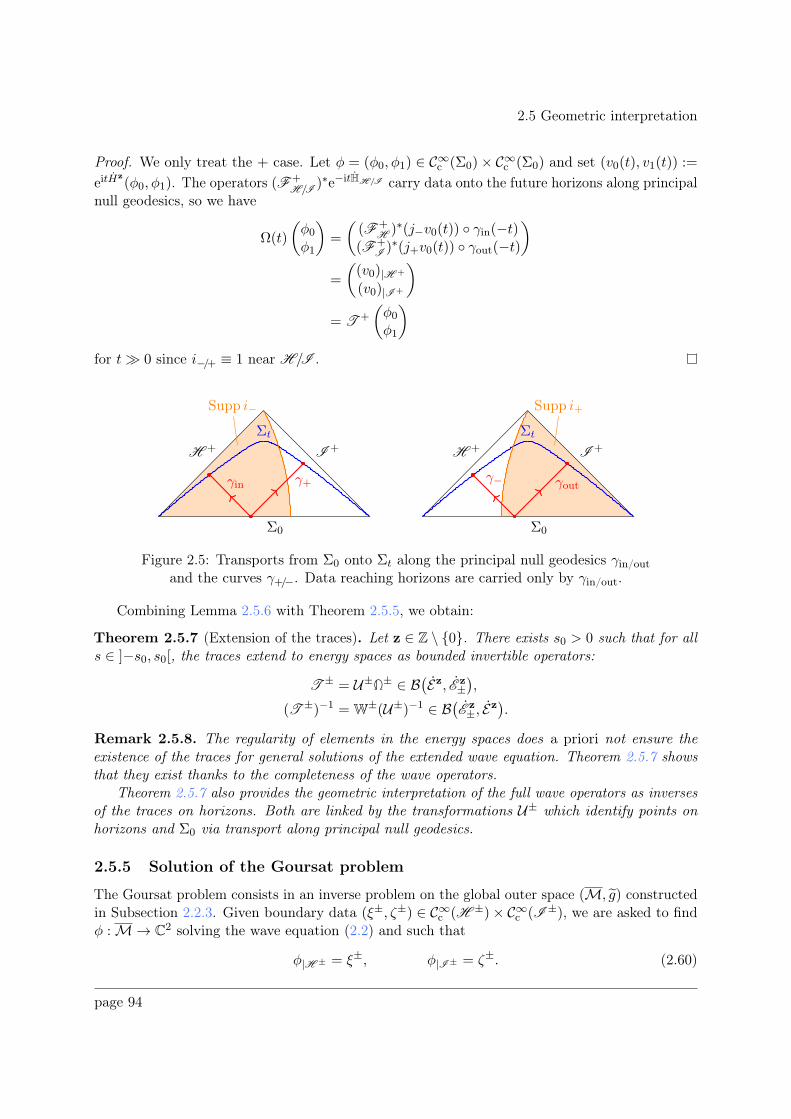
2.5 Geometric interpretation
Proof. We only treat the + case. Let φ = (φ0, φ1) ∈ C∞c (Σ0)× C∞c (Σ0) and set (v0(t), v1(t)) :=
eitHz
(φ0, φ1). The operators (F+H/I )∗e−itHH/I carry data onto the future horizons along principal
null geodesics, so we have
Ω(t)
(φ0φ1
)=
((F+
H)∗(j−v0(t)) γin(−t)
(F+I)∗(j+v0(t)) γout(−t)
)
=
((v0)|H +
(v0)|I +
)
= T+
(φ0φ1
)
for t≫ 0 since i−/+ ≡ 1 near H/I .
Supp i−
γin γ+
Σt
Σ0
H + I +
Supp i+
γ− γout
Σt
Σ0
H + I +
Figure 2.5: Transports from Σ0 onto Σt along the principal null geodesics γin/out
and the curves γ+/−. Data reaching horizons are carried only by γin/out.
Combining Lemma 2.5.6 with Theorem 2.5.5, we obtain:
Theorem 2.5.7 (Extension of the traces). Let z ∈ Z \ 0. There exists s0 > 0 such that for alls ∈ ]−s0, s0[, the traces extend to energy spaces as bounded invertible operators:
T± = U±
Ω± ∈ B
(Ez, E z
±),
(T ±)−1 = W±(U±)−1 ∈ B(E
z
±, Ez).
Remark 2.5.8. The regularity of elements in the energy spaces does a priori not ensure theexistence of the traces for general solutions of the extended wave equation. Theorem 2.5.7 showsthat they exist thanks to the completeness of the wave operators.
Theorem 2.5.7 also provides the geometric interpretation of the full wave operators as inversesof the traces on horizons. Both are linked by the transformations U± which identify points onhorizons and Σ0 via transport along principal null geodesics.
2.5.5 Solution of the Goursat problem
The Goursat problem consists in an inverse problem on the global outer space (M, g) constructedin Subsection 2.2.3. Given boundary data (ξ±, ζ±) ∈ C∞c (H ±)× C∞c (I ±), we are asked to findφ :M→ C2 solving the wave equation (2.2) and such that
φ|H ± = ξ±, φ|I ± = ζ±. (2.60)
page 94
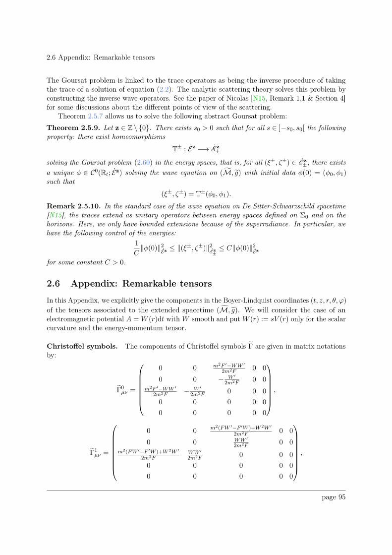
2.6 Appendix: Remarkable tensors
The Goursat problem is linked to the trace operators as being the inverse procedure of takingthe trace of a solution of equation (2.2). The analytic scattering theory solves this problem byconstructing the inverse wave operators. See the paper of Nicolas [N15, Remark 1.1 & Section 4]for some discussions about the different points of view of the scattering.
Theorem 2.5.7 allows us to solve the following abstract Goursat problem:
Theorem 2.5.9. Let z ∈ Z \ 0. There exists s0 > 0 such that for all s ∈ ]−s0, s0[ the followingproperty: there exist homeomorphisms
T± : Ez −→ Ez
±
solving the Goursat problem (2.60) in the energy spaces, that is, for all (ξ±, ζ±) ∈ E z
±, there exists
a unique φ ∈ C0(Rt; Ez) solving the wave equation on (M, g) with initial data φ(0) = (φ0, φ1)such that
(ξ±, ζ±) = T±(φ0, φ1).
Remark 2.5.10. In the standard case of the wave equation on De Sitter-Schwarzschild spacetime[N15], the traces extend as unitary operators between energy spaces defined on Σ0 and on thehorizons. Here, we only have bounded extensions because of the superradiance. In particular, wehave the following control of the energies:
1
C‖φ(0)‖2Ez
≤ ‖(ξ±, ζ±)‖2E z
±≤ C‖φ(0)‖2Ez
for some constant C > 0.
2.6 Appendix: Remarkable tensors
In this Appendix, we explicitly give the components in the Boyer-Lindquist coordinates (t, z, r, θ, ϕ)of the tensors associated to the extended spacetime (M, g). We will consider the case of anelectromagnetic potential A =W (r)dt with W smooth and put W (r) := sV (r) only for the scalarcurvature and the energy-momentum tensor.
Christoffel symbols. The components of Christoffel symbols Γ are given in matrix notationsby:
Γ0µν =
0 0 m2F ′−WW ′
2m2F0 0
0 0 − W ′
2m2F0 0
m2F ′−WW ′
2m2F− W ′
2m2F0 0 0
0 0 0 0 0
0 0 0 0 0
,
Γ1µν =
0 0 m2(FW ′−F ′W )+W 2W ′
2m2F0 0
0 0 WW ′
2m2F0 0
m2(FW ′−F ′W )+W 2W ′
2m2FWW ′
2m2F0 0 0
0 0 0 0 0
0 0 0 0 0
,
page 95
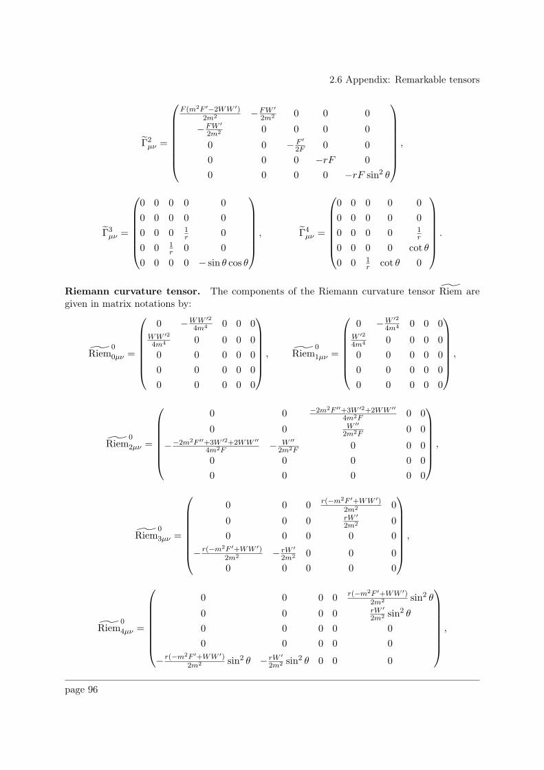
2.6 Appendix: Remarkable tensors
Γ2µν =
F (m2F ′−2WW ′)2m2 −FW ′
2m2 0 0 0
−FW ′
2m2 0 0 0 0
0 0 − F ′
2F 0 0
0 0 0 −rF 0
0 0 0 0 −rF sin2 θ
,
Γ3µν =
0 0 0 0 0
0 0 0 0 0
0 0 0 1r 0
0 0 1r 0 0
0 0 0 0 − sin θ cos θ
, Γ4
µν =
0 0 0 0 0
0 0 0 0 0
0 0 0 0 1r
0 0 0 0 cot θ
0 0 1r cot θ 0
.
Riemann curvature tensor. The components of the Riemann curvature tensor Riem aregiven in matrix notations by:
Riem0
0µν =
0 −WW ′2
4m4 0 0 0WW ′2
4m4 0 0 0 0
0 0 0 0 0
0 0 0 0 0
0 0 0 0 0
, Riem
0
1µν =
0 −W ′2
4m4 0 0 0W ′2
4m4 0 0 0 0
0 0 0 0 0
0 0 0 0 0
0 0 0 0 0
,
Riem0
2µν =
0 0 −2m2F ′′+3W ′2+2WW ′′
4m2F0 0
0 0 W ′′
2m2F0 0
−−2m2F ′′+3W ′2+2WW ′′
4m2F− W ′′
2m2F0 0 0
0 0 0 0 0
0 0 0 0 0
,
Riem0
3µν =
0 0 0 r(−m2F ′+WW ′)2m2 0
0 0 0 rW ′
2m2 0
0 0 0 0 0
− r(−m2F ′+WW ′)2m2 − rW ′
2m2 0 0 0
0 0 0 0 0
,
Riem0
4µν =
0 0 0 0 r(−m2F ′+WW ′)2m2 sin2 θ
0 0 0 0 rW ′
2m2 sin2 θ
0 0 0 0 0
0 0 0 0 0
− r(−m2F ′+WW ′)2m2 sin2 θ − rW ′
2m2 sin2 θ 0 0 0
,
page 96
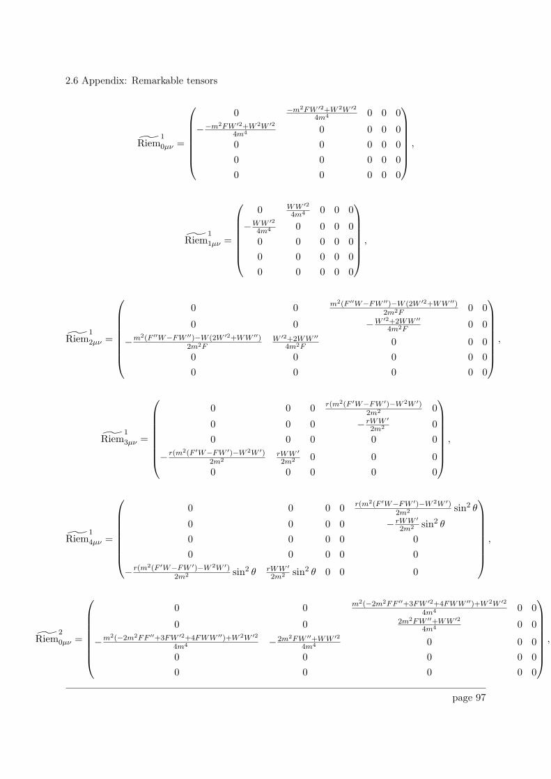
2.6 Appendix: Remarkable tensors
Riem1
0µν =
0 −m2FW ′2+W 2W ′2
4m4 0 0 0
−−m2FW ′2+W 2W ′2
4m4 0 0 0 0
0 0 0 0 0
0 0 0 0 0
0 0 0 0 0
,
Riem1
1µν =
0 WW ′2
4m4 0 0 0
−WW ′2
4m4 0 0 0 0
0 0 0 0 0
0 0 0 0 0
0 0 0 0 0
,
Riem1
2µν =
0 0 m2(F ′′W−FW ′′)−W (2W ′2+WW ′′)2m2F
0 0
0 0 −W ′2+2WW ′′
4m2F0 0
−m2(F ′′W−FW ′′)−W (2W ′2+WW ′′)2m2F
W ′2+2WW ′′
4m2F0 0 0
0 0 0 0 0
0 0 0 0 0
,
Riem1
3µν =
0 0 0 r(m2(F ′W−FW ′)−W 2W ′)2m2 0
0 0 0 − rWW ′
2m2 0
0 0 0 0 0
− r(m2(F ′W−FW ′)−W 2W ′)2m2
rWW ′
2m2 0 0 0
0 0 0 0 0
,
Riem1
4µν =
0 0 0 0 r(m2(F ′W−FW ′)−W 2W ′)2m2 sin2 θ
0 0 0 0 − rWW ′
2m2 sin2 θ
0 0 0 0 0
0 0 0 0 0
− r(m2(F ′W−FW ′)−W 2W ′)2m2 sin2 θ rWW ′
2m2 sin2 θ 0 0 0
,
Riem2
0µν =
0 0 m2(−2m2FF ′′+3FW ′2+4FWW ′′)+W 2W ′2
4m4 0 0
0 0 2m2FW ′′+WW ′2
4m4 0 0
−m2(−2m2FF ′′+3FW ′2+4FWW ′′)+W 2W ′2
4m4 −2m2FW ′′+WW ′2
4m4 0 0 0
0 0 0 0 0
0 0 0 0 0
,
page 97
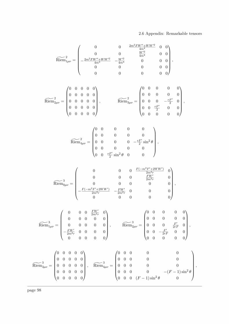
2.6 Appendix: Remarkable tensors
Riem2
1µν =
0 0 2m2FW ′′+WW ′2
4m4 0 0
0 0 W ′2
4m4 0 0
−2m2FW ′′+WW ′2
4m4 −W ′2
4m4 0 0 0
0 0 0 0 0
0 0 0 0 0
,
Riem2
2µν =
0 0 0 0 0
0 0 0 0 0
0 0 0 0 0
0 0 0 0 0
0 0 0 0 0
, Riem
2
3µν =
0 0 0 0 0
0 0 0 0 0
0 0 0 − rF ′
2 0
0 0 rF ′
2 0 0
0 0 0 0 0
,
Riem2
4µν =
0 0 0 0 0
0 0 0 0 0
0 0 0 0 − rF ′
2 sin2 θ
0 0 0 0 0
0 0 rF ′
2 sin2 θ 0 0
,
Riem3
0µν =
0 0 0 F (−m2F ′+2WW ′)2m2r
0
0 0 0 FW ′
2m2r0
0 0 0 0 0
−F (−m2F ′+2WW ′)2m2r
− FW ′
2m2r0 0 0
0 0 0 0 0
,
Riem3
1µν =
0 0 0 FW ′
2m2r0
0 0 0 0 0
0 0 0 0 0
− FW ′
2m2r0 0 0 0
0 0 0 0 0
, Riem
3
2µν =
0 0 0 0 0
0 0 0 0 0
0 0 0 F ′
2rF 0
0 0 − F ′
2rF 0 0
0 0 0 0 0
,
Riem3
3µν =
0 0 0 0 0
0 0 0 0 0
0 0 0 0 0
0 0 0 0 0
0 0 0 0 0
, Riem
3
4µν =
0 0 0 0 0
0 0 0 0 0
0 0 0 0 0
0 0 0 0 −(F − 1) sin2 θ
0 0 0 (F − 1) sin2 θ 0
,
page 98
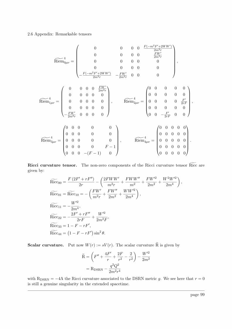
2.6 Appendix: Remarkable tensors
Riem4
0µν =
0 0 0 0 F (−m2F ′+2WW ′)2m2r
0 0 0 0 FW ′
2m2r
0 0 0 0 0
0 0 0 0 0
−F (−m2F ′+2WW ′)2m2r
− FW ′
2m2r0 0 0
,
Riem4
1µν =
0 0 0 0 FW ′
2m2r
0 0 0 0 0
0 0 0 0 0
0 0 0 0 0
− FW ′
2m2r0 0 0 0
, Riem
4
2µν =
0 0 0 0 0
0 0 0 0 0
0 0 0 0 F ′
2rF
0 0 0 0 0
0 0 − F ′
2rF 0 0
,
Riem4
3µν =
0 0 0 0 0
0 0 0 0 0
0 0 0 0 0
0 0 0 0 F − 1
0 0 0 −(F − 1) 0
, Riem
4
4µν =
0 0 0 0 0
0 0 0 0 0
0 0 0 0 0
0 0 0 0 0
0 0 0 0 0
.
Ricci curvature tensor. The non-zero components of the Ricci curvature tensor Ricc aregiven by:
Ricc00 =F (2F ′ + rF ′′)
2r−(2FWW ′
m2r+FWW ′′
m2+FW ′2
2m2+W 2W ′2
2m4
),
Ricc01 = Ricc10 = −(FW ′
m2r+FW ′′
2m2+WW ′2
2m4
),
Ricc11 = −W ′2
2m4,
Ricc22 = −2F ′ + rF ′′
2rF+
W ′2
2m2F,
Ricc33 = 1− F − rF ′,
Ricc44 =(1− F − rF ′) sin2 θ.
Scalar curvature. Put now W (r) := sV (r). The scalar curvature R is given by
R =
(F ′′ +
4F ′
r+
2F
r2− 2
r2
)− W ′2
2m2
= RDSRN −q2Q2
2m2r4
with RDSRN = −4Λ the Ricci curvature associated to the DSRN metric g. We see here that r = 0is still a genuine singularity in the extended spacetime.
page 99
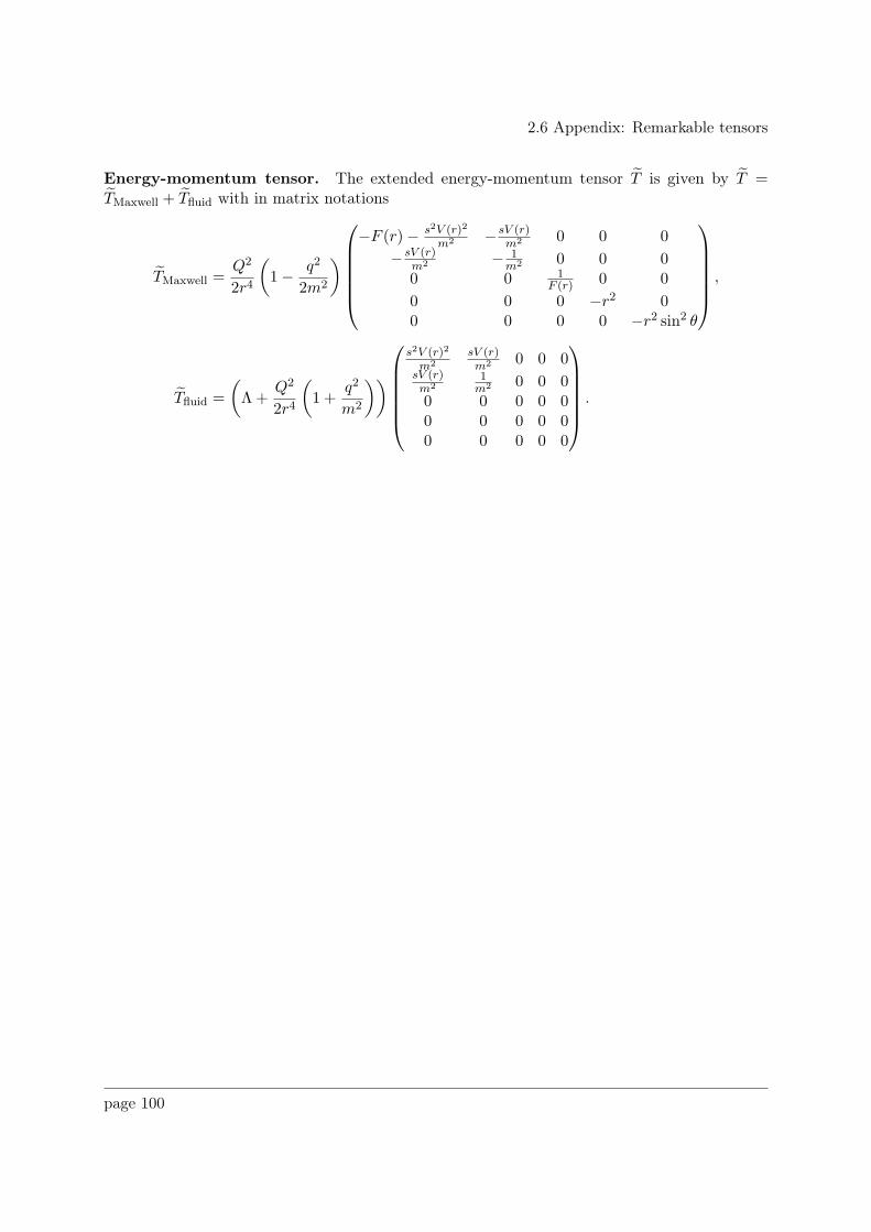
2.6 Appendix: Remarkable tensors
Energy-momentum tensor. The extended energy-momentum tensor T is given by T =TMaxwell + Tfluid with in matrix notations
TMaxwell =Q2
2r4
(1− q2
2m2
)
−F (r)− s2V (r)2
m2 − sV (r)m2 0 0 0
− sV (r)m2 − 1
m2 0 0 00 0 1
F (r) 0 0
0 0 0 −r2 00 0 0 0 −r2 sin2 θ
,
Tfluid =
(Λ +
Q2
2r4
(1 +
q2
m2
))
s2V (r)2
m2sV (r)m2 0 0 0
sV (r)m2
1m2 0 0 0
0 0 0 0 00 0 0 0 00 0 0 0 0
.
page 100
Chapter 3Decay of the Local Energy through theHorizons for the Wave Equation in theExterior Extended Spacetime
Having established the decay of the local energy Theorem 1.3.2 in the exterior DSRN spacetime,it is possible to obtain decay estimates through the horizons in the Kaluza-Klein extension ofChapter 2 following Dyatlov paper [Dy11]. The main idea is to use the so-called red-shift vectorfield method introduced by Dafermos and Rodnianski in order to obtain decay near horizonsby the red-shif effect, see e.g. [Da05], [DaRo07] and [DaRo09]. This method is applicable indimension 1 + 4 even for extensions of non-spherical rotating black holes, provided that therotation remains small.
In all this chapter, we will use the notations of Chapter 2, particularly those in Subsection2.3.1. For example, E is the inhomogeneous energy space defined in the extended spacetime (andnot in the original DSRN spacetime).
3.1 Statement of the main result
Introduce a new time coordinate τ smooth near r = r± and set for all δ > 0
Xδ := S1z × ]r− − δ, r+ + δ[r × S2ω.
Denote by Hσ(Xδ), σ ∈ R, the inhomogeneous Sobolev spaces associated to L2(S1ζ × ]r−, r+[r ×S2ω, F (r)−1dζdrdω) and wet Hσ
z(Xδ) for the restriction to ker(i∂z+z), z ∈ Z. As we are interested
in large time estimate, we will implicitly use the convention that Sobolev spaces in time are definedon ]0,+∞[.
From the decay of the local energy of Theorem 1.3.2 and the fact that the inhomogeneousenergy ‖ · ‖Ez
coincide with the inhomogeneous energy defined in the DSRN spacetime (with acharge term sz), we immediatly deduce the following result:
Lemma 3.1.1. Let z ∈ Z 6= 0 and χ ∈ Xδ. For s sufficiently small, there exists ν > 0 such thatfor all u ∈ Ez solving gu with initial data u(0) = u0 compactly supported in S1z × ]r−, r+[r × S2ω,
101
3.2 Construction of the red-shift vector field
we have for t > 0 large enough:
‖χu‖Ez. e−νt‖u0‖Ez
.
We then have the following result (the proof is given in Subsection 3.3):
Theorem 3.1.2 (Decay of the energy through the horizons). Let z ∈ Z 6= 0, δ > 0, ε > 0,σ ≥ 0 and let u be the solution of the initial value problem:
gu = 0
u(0, ·) = u0 ∈ Hσ+2+εz
(Xδ)
(∂τu)(0, ·) = u1 ∈ Hσ+1+εz
(Xδ)
(3.1)
If δ is sufficiently small, then there exist ν0 ≡ ν0(δ, ε) > 0 and C > 0 (independent of u) suchthat, for all ν ∈ ]0, ν0[ and s ∈ R sufficiently small, the following estimate holds:
‖u(τ, ·)‖Hσ+1z
(Xδ)≤ Ce−ντ
(‖u0‖Hσ+2+ε
z(Xδ)
+ ‖u1‖Hσ+1+εz
(Xδ)
)∀τ > 0. (3.2)
One may notice that (3.2) is not a global energy decay as estimates are restricted on a part ofthe extended spacetime (M, g), cf. Remark 3.3.1.
3.2 Construction of the red-shift vector field
The extension of decay estimates beyond the horizons relies on the construction of the red-shiftvector field. We first need to extend g near r = r±. Define the new coordinates
τ := t− T (r), ζ := z −Z(r)
where T ,Z ∈ C∞(]r−, r+[r ,R) satisfy
T ′(r) =ρ(r)
F (r)+ α(r), Z ′(r) = −sV (r)T ′(r) near r±.
Here ρ ∈ C∞(]0,+∞[ ,R), ρ ≡ ±1 near r± and α ∈ C∞(]0,+∞[ ,R) are two bounded functions tobe chosen later on. In order to simplify the proof of Lemma 3.2.1 below, we let α depend on thecharge product s ∈ R so that ‖α‖L∞(]0,+∞[,R) = Os→0(|s|). Observe that ∂t = ∂τ and ∂z = ∂ζ .
The extended metric g reads in these new coordinates:
g =
(F (r)− s2V (r)2
m2
)dτ2 − sV (r)
m2(dτdζ + dζdτ)− 1
m2dζ2 +
(α(r)F (r) + ρ(r)
)(dτdr + drdτ)
+
(ρ2 − 1
F (r)+ α(r)
(α(r)F (r) + 2ρ(r)
))dr2 − r2dω2.
page 102
3.2 Construction of the red-shift vector field
The determinant is still r4 sin2 θ/m2 so that the metric is smooth and does not degenerate aslong as α remains smooth. The inverse metric is given by
g−1 = −(ρ(r)2 − 1
F (r)+ α(r)
(α(r)F (r) + 2ρ(r)
))∂⊗2τ
+ sV (r)
(ρ(r)2 − 1
F (r)+ α(r)
(α(r)F (r) + 2ρ(r)
))(∂τ ⊗ ∂ζ + ∂ζ ⊗ ∂τ )
−(m2 + s2V (r)2
(ρ(r)2 − 1
F (r)+ α(r)
(α(r)F (r) + 2ρ(r)
)))∂⊗2ζ
+(α(r)F (r) + ρ(r)
)(∂τ ⊗ ∂r + ∂r ⊗ ∂τ )− sV (r)
(α(r)F (r) + ρ(r)
)(∂ζ ⊗ ∂r + ∂r ⊗ ∂ζ)
− F (r)∂⊗2r −
1
r2∂⊗2θ −
1
r2 sin2 θ∂⊗2ϕ .
We introduced the function α to make the hypersurfaces Στ0 := τ = τ0 spacelike near r± forall τ0 ∈ R:
∇τ = −(ρ(r)2 − 1
F (r)+ α(r)
(α(r)F (r) + 2ρ(r)
))∂τ
+ sV (r)
(ρ(r)2 − 1
F (r)+ α(r)
(α(r)F (r) + 2ρ(r)
))∂ζ +
(α(r)F (r) + ρ(r)
)∂r
and
g(∇τ,∇τ) = −(ρ(r)2 − 1
F (r)+ α(r)
(α(r)F (r) + 2ρ(r)
)).
Since F (r±) = 0 and ρ(r)2 − 1 = 0 for r near r±, ∇τ is timelike in Rτ × ]r± − δ, r± + δ[× S2ω forδ > 0 small enough if αρ < 0 there; asking for |ρ| < 1 as well as αF+2ρ < 0 for r ∈ [r− + δ, r+ − δ],we obtain that ∇τ is timelike in the whole Rτ × ]r− − δ, r+ + δ[× S2ω. This result is independentof s in α as long as it is non-zero and small enough.
For δ > 0 sufficiently small, the metric g thus smoothly extends to
Mδ := Rτ × S1ζ × Mδ, Mδ := ]r− − δ, r+ + δ[r × S2ω.
Let now
Kδ := Rτ × S1ζ ×Kδ × S2ω, Kδ := ]r− + δ, r+ − δ[r ⊂ Mδ.
For all vector field X ∈ TMδ, we define
KXij :=
1
2(LX g)ij −
1
4Trg(LX g) gij .
The red-shift vector field can now be constructed:
Lemma 3.2.1. For δ > 0 and s ∈ R sufficiently small, there exits a vector field X ∈ TMδ suchthat:
• [X, ∂τ ] = 0;
page 103
3.3 Proof of the decay through the horizons
• On Mδ \K2δ, X is timelike and Xτ > 0, ±Xr > 0 near r±;
• The tensor field KX is negative definite on Mδ \K2δ.
Proof. As in [Dy11], we only show the proposition for s = 0 and at the horizons; the result willthen follow by smoothness for δ > 0 and s ∈ R sufficiently small.
For s = 0, the extended metric and its inverse become near the horizons
g = F (r)dτ2 − 1
m2dζ2 ± (dτdr + drdτ)− r2dω2,
g−1 = −m2∂⊗2ζ ± (∂τ∂r + ∂r∂τ )− F (r)∂⊗2
r −1
r2∂⊗2θ −
1
r2 sin2 θ∂⊗2ϕ .
Take now X = Xτ (r)∂τ +Xr(r)∂r with Xτ , Xr smooth in r ∈ Mδ. Clearly [X, ∂τ ] = 0 and wehave
g(X,X) = Xτ (F (r)Xτ ± 2Xr)
which is timelike near r± if Xτ ≡ 1 and ±Xr ≡ 1 there. Besides, this choice trivially implies thatXτ = Xτ > 0 and ±Xr = ±X(r) > 0 near the horizons.
Next, using the formula
(LXT ) =(Xk∂kTij + Tkj∂iX
k + Tik∂jXk)dxidxj
for any bilinear form field T , we compute:
(LX g) = Xr(F ′(r)dτ2 − 2rdω2
)+(F (r)∂rX
τ ± ∂rXr)(dτdr + drdτ)± 2∂rX
τdr2,
γ := Trg(LX g) = ±2F (r)∂rXτ + 2∂rXr ∓ 2F (r)∂rX
τ +4
r,
2KX =(XrF ′(r)− γ
2F (r)
)dτ2 ±
(∂rX
r − γ
2
)(dτdr + drdτ) +
γ
2m2dζ2
± 2∂rXτdr2 − r
(2− γr
2
)dθ2 − r sin2 θ
(2− γr
2
)dϕ2
r=r±= XrF ′(r±)dτ
2 ∓ 2
r±(dτdr + drdτ) +
1
m2
(∂rX
r +2
r±
)dζ2
± 2∂rXτdr2 + r2±∂rX
rdω2.
The expression of KX above looks like to the one in [Dy11] with a metric on S1z × S2ω instead. Wecan use similar conditions: if ∓∂rXτ ≫ 0 and ∂rXr < −2/r± at r±, then KX is indeed negativedefinite at the horizons.
3.3 Proof of the decay through the horizons
As in [Dy11], we will obtain decay for solutions of the initial value problem (3.1) by dealing withthe forward problem
gu = f ∈ Hσ+1+ε
z(Mδ) for all σ ≥ 0
Suppu ⊂ τ > −T for some T > 0. (3.3)
page 104
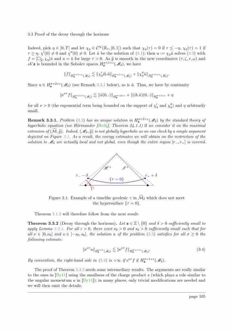
3.3 Proof of the decay through the horizons
Indeed, pick η ∈ ]0, T [ and let χη ∈ C∞(Rτ , [0, 1]) such that χη(τ) = 0 if τ ≤ −η, χη(τ) = 1 ifτ ≥ η, χ′(0) 6= 0 and χ′′(0) 6= 0. Let u be the solution of (3.1); then u := χηu solves (3.3) withf = [g, χη]u and u = u for large τ > 0. As g is smooth in the new coordinates (τ, ζ, r, ω) andsV z is bounded in the Sobolev spaces Hσ+1+ε
z(Mδ), we have
‖f‖Hσ+1+εz
(Mδ). ‖χ′
η∂τ u‖Hσ+1+εz
(Mδ)+ ‖χ′′
ηu‖Hσ+1+εz
(Mδ).
Since u ∈ Hσ+2+εz
(Mδ) (see Remark 3.3.1 below), so is u. Thus, we have by continuity
‖eντf‖Hσ+1+εz
(Mδ). ‖u(0, ·)‖Hσ+2+ε
z
+ ‖(∂τ u)(0, ·)‖Hσ+1+εz
+ η
for all ν > 0 (the exponential term being bounded on the support of χ′η and χ′′
η) and η arbitrarilysmall.
Remark 3.3.1. Problem (3.3) has an unique solution in Hσ+2+εz
(Mδ) by the standard theory ofhyperbolic equation (see Hörmander [Ho94], Theorem 24.1.1) if we consider it on the maximal
extension of (M, g). Indeed, (Mδ, g) is not globally hyperbolic as we can check by a simple argumentdepicted on Figure 3.1. As a result, the energy estimates we will obtain on the restriction of thesolution to Mδ are actually local and not global, even though the entire region [r−, r+] is covered.
τ = 0
H + I +
γ
r+ + δr− − δ
Figure 3.1: Example of a timelike geodesic γ in Mδ which does not meetthe hypersurface τ = 0.
Theorem 3.1.2 will therefore follow from the next result:
Theorem 3.3.2 (Decay through the horizons). Let z ∈ Z \ 0 and δ > 0 sufficiently small toapply Lemma 3.2.1. For all ε > 0, there exist ν0 > 0 and s0 > 0 sufficiently small such that forall ν ∈ ]0, ν0[ and s ∈ ]−s0, s0[, the solution u of the problem (3.3) satisfies for all σ ≥ 0 thefollowing estimate:
‖eντu‖Hσ+1z
(Mδ). ‖eντf‖Hσ+1+ε
z(Mδ)
. (3.4)
By convention, the right-hand side in (3.4) is +∞ if eντf /∈ Hσ+1+εz
(Mδ).
The proof of Theorem 3.3.2 needs some intermediary results. The arguments are really similarto the ones in [Dy11] using the smallness of the charge product s (which plays a role similar tothe angular momentum a in [Dy11]); in many places, only trivial modifications are needed andwe will then omit the details.
page 105
3.3 Proof of the decay through the horizons
We first link energy estimates on Mδ by energy estimates on Kδ. The proof is the same as in[Dy11]; the induction step is even easier as our extended metric has more symmetries that themetric of De Sitter-Kerr has1.
Lemma 3.3.3 (Proposition 1.7 in [Dy11]). Let δ > 0 and s ∈ R sufficiently small to applyLemma 3.2.1 and pick ψ ∈ C∞(]r−, r+[ ,R) such that ψ ≥ 0 outside ]r− + δ, r+ − δ[. There existsν0 > 0 such that for all ν ∈ ]0, ν0[, the solution u of the problem
(g + ψX
)u = f ∈ C∞c (Mδ)
Suppu ⊂ τ > −T for some T > 0
satisfies for all σ ≥ 0 the following estimate:
‖eντu‖Hσ+1(Mδ) . ‖eντf‖Hσ(Mδ) + ‖eντu‖Hσ+1(Kδ). (3.5)
We now turn to local estimates. We want to establish the equivalent of Proposition 2.1 in[Dy11] which we do using a slightly different proof.
Lemma 3.3.4. Let z ∈ Z \ 0, δ > 0 and σ ≥ 0. For all ε > 0, there exist ν0 > 0 and s0 > 0such that for all ν ∈ ]0, ν0[ and s ∈ ]−s0, s0[, the solution u of the problem
gu = f ∈ C∞c (Kδ)
Suppu ⊂ τ > −T for some T > 0(3.6)
satisfies the following estimate:
‖eνtu‖Hσ+1z
(Kδ). ‖eνtf‖Hσ+1+ε
z(Kδ)
. (3.7)
Here both the weights eνt and eντ are equivalent since |t− τ | is bounded in Kδ.
Proof. We show the result for σ = 0 and σ ∈ 2N+1, the general case following from interpolationsbetween Sobolev spaces. We will use the Hamiltonian form of the problem:
−i∂tU = K(s)U − F, U =
(u
−i∂tu− sV u
), F =
(0f
).
We will prove the result for each harmonic ℓ ∈ N (with uniform bounds in ℓ); in order to notoverload notations, we will omit the dependence in ℓ (so u will be uℓ, K(s) will be Kℓ(s) and soon).
Let us start with σ = 0. Since f is smooth and compactly supported, so is F and then U issmooth too. For ν ′ > 0 large enough, we have U ∈ L2
ν′(R∗+, Ez) (see the short argument proving
Proposition 1.1 in [DQNM11] for the existence of such ν ′, or, equivalently, the proof of Lemma3.19 in [GGH17]), hence we can define the time-dependent Fourier transforms of U and F forℑz ≥ ν ′ and t > 0:
U(z, ·) :=ˆ +∞
−∞eiztU(t, ·)dt, F (z, ·) :=
ˆ +∞
−∞eiztF (t, ·)dt.
1To be really concrete, the proof uses that the term [g, Y ] is zero for any Killing vector field Y on S2ω or
Y = ∂ζ ; in comparison, [g, Y ] = O(a) in [Dy11] which is handled assuming the angular momentum a sufficientlysmall.
page 106
3.3 Proof of the decay through the horizons
We then have:
(K(s)− z)U = F .
The resolvent of K(s) is analytic in C+ for s sufficiently small by Corollary 1.2.9; moreover,z 7→ U(z, ·) and z 7→ F (z, ·) are in L2(R, Ez) provided that ℑz ≥ ν ′. Thus, for t > 0 (whichmeans τ > −T for some T > 0), Fourier inversion formula yields
U(t, ·) = 1
2π
ˆ +∞+iν′
−∞+iν′e−izt(K(s)− z)−1F (z, ·)dz
as elements of L2ν′(R
∗+, Ez). Now let χ ∈ C∞c (]r−, r+[ ,R) such that χ ≡ 1 on the spatial support of
F (which is the same as for F ) and proceed as in the proof of Theorem 1.3.2. Using the modifiedcut-off resolvent Rχ(z) of (1.51), we can write
χU(t, ·) = 1
2π
ˆ +∞+iν′
−∞+iν′e−iztRχ(z)F (z, ·)dz
this time as elements of E−2z
:= (K(s)− i)2Ez. This formula is the equivalent of formula (1.54)(and also of formula (2.1) in [Dy11]). After a contour deformation2 using the contour in the proofof Theorem 1.3.2 but with Γ4 ∪ Γ1 ∪ Γ2 replaced by ℑz = −µ, we obtain
χU(t, ·) = 1
2π
ˆ +∞−iµ
−∞−iµe−iztRχ(z)F (z, ·)dz
if we choose µ < ε0, ε0 of part 2. of Theorem 1.2.8 (so that we exclude all the resonances insidethe contour). Using then estimate (1.36) for the zone III (which is worst than (1.37) for the zoneIV) as well as (1.56), we get for all ν ∈ ]0, µ[:
‖(1 + ∂t)eνtχU(t, ·)‖
Ez.ˆ +∞−iµ
−∞−iµe(ν−ℑz)t〈z〉‖Rχ(z)F (z, ·)‖Ezdz
.ˆ +∞−iµ
−∞−iµe(ν−ℑz)t〈z〉 ln〈z〉e|ℑz| ln〈z〉‖F (z, ·)‖
Ezdz
. e(ν−µ)t
ˆ +∞
−∞〈z〉1+2µ‖f(z, ·)‖Hz
dz
. e(ν−µ)t‖eνtf‖H
1+2µz
(Kδ). (3.8)
On the other hand, since the norms ‖.‖E and ‖.‖E
are locally equivalent, we have
‖χu‖H1z
. ‖χU(t, ·)‖Ez . ‖χU(t, ·)‖Ez .
Thus, integrating (3.8) in time over R+ yields (3.11) with σ = 0 and ε = 2µ.
2Here we use that F (z) is still well-defined for ℑz < 0 since F is smooth and compactly supported in time.This is not the case for U(z) which can be defined a priori only for ℑz > 0 sufficiently large (this is the onlyreason why we used the space L2
ν′(R∗+, Ez)).
page 107
3.3 Proof of the decay through the horizons
Let now σ = 2n+ 1 with n ∈ N \ 0. Compute first∥∥Pnχu
∥∥Hz
.∥∥[Pn, χ]u
∥∥Hz
+∥∥χPnu
∥∥Hz
.
Since the commutator only contains the terms χ(n), χ(n−1)∂x, . . . , χ′∂n−1
x , we find
‖χu‖H2nz
.∥∥Pnχu
∥∥Hz
.∥∥χPn−1u
∥∥Hz
+∥∥χPnu
∥∥Hz
. (3.9)
Next, let us write
K(s)2n−1 = (K(0) + sV 1)2n−1 =22n−1∑
j=1
sAj
where A1 = K(0)2n−1/s and Aj a homogeneous polynomial in s with nonnegative degree forj 6= 1. For s small enough (depending on n), it turns that
∥∥χK(s)2n−1U∥∥2Ez =
∥∥∥∥∥∥χ
22n−1∑
j=1
sAjU
∥∥∥∥∥∥
2
Ez
=
22n−1∑
j=1
‖χsAjU‖2Ez + 2∑
j 6=k
ℜ⟨χsAjU, χsAkU
⟩Ez
≥22n−1∑
j=1
‖χsAjU‖2Ez − 2|s|∑
j 6=k
∣∣∣⟨χAjU, χAkU
⟩Ez
∣∣∣
&22n−1∑
j=1
‖χsAjU‖2Ez
≥ ‖χK(0)2n−1U∥∥2Ez . (3.10)
As
K(0)2n−1 =
(0 Pn−1
Pn 0
),
it follows from (3.9) and (3.10)
‖χu‖H2nz
.∥∥χPnu
∥∥Hz
≤ ‖χK(0)2n−1U∥∥Ez .
∥∥χK(s)2n−1U∥∥Ez .
We have
K(s)2n−1U(t, ·) = 1
2π
ˆ +∞+iν′
−∞+iν′e−izt(K(s)− z)−1K(s)2n−1F (z, ·)dz
and thus
∂2nt χK(s)2n−1U(t, ·) = 1
2π
ˆ +∞+iν′
−∞+iν′e−izt(iz)2nRχ(z)K(s)2n−1F (z, ·)dz.
page 108
3.3 Proof of the decay through the horizons
From there, we can proceed as in (3.8) with Rχ(z)K(s)2n−1F (z, ·) instead of Rχ(z)F (z, ·) and〈z〉2n+2µ instead of 〈z〉1+2µ. We need to use that
∥∥K(s)2n−1F∥∥Ez =
∥∥(K(0) + sV 1)2n−1F∥∥Hz
.∥∥Pnf
∥∥Hz
+
n−1∑
j=0
∥∥Bj f∥∥Hz
where Bj contains commutator terms of the form adj+1P (sV ), adksV (P
j+1) which provides Sobolevnorms controlled by
∥∥Pn−1f∥∥Hz
. This settles (3.11) with σ = 2n− 1 for all n ∈ N \ 0.
Corollary 3.3.5 (Proposition 2.2 in [Dy11]). Let z ∈ Z \ 0, δ > 0 and s ∈ R sufficiently smallto apply Lemma 3.2.1. For all ε > 0, there exists ν0 > 0 such that for all ν ∈ ]0, ν0[, the solutionu of the problem (3.6) satisfies for all σ ≥ 0 the following estimate:
‖eντu‖Hσ+1z
(Mδ). ‖eντf‖Hσ+1+ε
z(Kδ)
. (3.11)
Proof. We show the result for σ ≥ 0 integer, the general case following from interpolation betweenSobolev spaces. By Lemma 3.3.3, it holds
‖eντu‖Hσ+1z
(Mδ). ‖eντf‖Hσ
z(Mδ) + ‖eντu‖Hσ+1
z(Kδ)
.
We can use here the restrictions on the kernel of i∂z + z because ∂z = ∂ζ commutes with g.Applying Lemma 3.3.4 with τ instead of t, it comes
‖eντu‖Hσ+1z
(Kδ). ‖eντf‖Hσ+1+ε
z(Kδ)
which provides the desired estimate.
The last step is to show an exponential decay on a small neighborhood of the horizons.
Lemma 3.3.6 (Proposition 2.3 in [Dy11]). Let δ > 0 and s ∈ R sufficiently small to applyLemma 3.2.1. There exists ν0 > 0 such that for all ν ∈ ]0, ν0[, the solution v of the problem
gv = f ∈ C∞c (Mδ \Kδ)
Supp v ⊂ τ > −T for some T > 0
v|∂K2δ≡ 0
(3.12)
satisfies for all σ ≥ 0 the following estimate:
‖eντv‖Hσ+1(Mδ\K2δ) . ‖eντf‖Hσ(Mδ\K2δ). (3.13)
We can now show the exponential decay through the horizons:
Proof of Theorem 3.3.2. Let u be the solution of (3.3) with first f ∈ C∞c (Mδ) and v be thesolution of (3.12). Set w := u− χv and take χ ∈ C∞(Kδ) such that χ ≡ 0 near K2δ and χ ≡ 1outside Kδ. We have
gw = (1− χ)f − [g, χ]v
page 109
3.3 Proof of the decay through the horizons
which is supported in Kδ. We have
‖eντgw‖Hσ+1+εz
(Mδ). ‖eντ (1− χ)fw‖Hσ+1+ε
z(Mδ)
+ ‖eντ [g, χ]w‖Hσ+1+εz
(Mδ)
. ‖eντ (1− χ)f‖Hσ+1+εz
(Kδ)+ ‖eντχ′∂rw‖Hσ+1+ε
z(Mδ)
. ‖eντf‖Hσ+1+εz
(Mδ)
where we applied Lemma 3.3.6 to the term χ′. By Corollary 3.3.5,
‖eντw‖Hσ+1z
(Mδ). ‖eντgw‖Hσ+1+ε
z(Mδ)
. ‖eντf‖Hσ+1+εz
(Mδ)
since gw is supported in Kδ. Since χ vanishes on Kδ, we can apply Lemma 3.3.6 again and find:
‖eντu‖Hσ+1z
(Mδ). ‖eντw‖Hσ+1+ε
z(Mδ)
+ ‖eντv‖Hσ+1z
(Mδ)
. ‖eντf‖Hσ+1+εz
(Mδ)+ ‖eντf‖Hσ+1
z(Mδ)
.
Finally, the functional(C∞c (Mδ), ‖eντ · ‖Hσ+1+ε
z(Mδ)
)∋ f 7−→ u ∈
(Hσ+1
z(Mδ), ‖eντ · ‖Hσ+1
z(Mδ)
)
being continuous, we can extend it to eντHσ+1+εz
(Mδ). This concludes the proof.
page 110
Chapter 4Numerical Study of an AbstractKlein-Gordon type Equation: Applications tothe Charged Klein-Gordon Equation in theExterior De Sitter-Reissner-NordströmSpacetime
Chapter 4 proposes a numerical scheme to investigate some important features linked to thecharged Klein-Gordon equation in the exterior DSRN spacetime (such as localization of resonances,see Chapter 5). The first step is to approximate solutions of the equation using "discretized"operators, spaces and norms.
In a more abstract setting, a numerical scheme is a method which allows one to discretize agiven problem i.e. transform data in some abstract normed functional space into data in CN forsome N ∈ N\0. The transformation is carried out by means of some projectors and embeddingswhich send data from a space to another one. To these operators are associated spaces and normsthat approximate the initial ones. Given a set of indices (N in general, but this is not mandatory),we construct a family of such operators, spaces and norms. We are then interested in the inductivelimit over the indices (n→ +∞ for indices n ∈ N). Given an abstract equation between normedspaces, we wish to find a family of approximated solutions to the discrete version of the equation(that is, taken in approximated spaces with approximated operators) and then show that thisfamily converges at the inductive limit to the "true" solution of the "true" equation.
In this chapter, we will be interested in an abstract Klein-Gordon type equation. We proposea method based on polynomial interpolation. Convergence is then obtained and given a geometricinterpretation in Theorem 4.3.1 and Theorem 4.3.4. A difficulty is to respect the structure of thespaces: we will not assume data to be smooth enough in order to facilitate estimates. We willalso take care of the error we commit by following each constants in our estimates. As we will see,this will lead to painful computations. For the sake of clarity, we have postponed each technicalcomputation to the Appendix, so that the main body of the chapter only contains importantdemonstrations. The error is controlled on some compact set in space and grows as the maximal
111

4.1 The abstract problem
time T ; the approximation becomes useful as we know that the local energy decays in time (or isat least bounded).
Organization of the chapter. Chapter 4 is organized as follows: Section 4.1 introduce theabstract problem we will deal with as well as the scheme and some notations. Consistency andstability are shown in Section 4.2: they amount of how good the approximation is. In Section 4.3,we prove that the approximated solution of the abstract problem converges to the "true" solutionas the mesh converges (briefly: the scheme converges) using consistency and stability. We thenapply these results to the charged Klein-Gordon equation in the exterior DSRN spacetime.
4.1 The abstract problem
In this Section, we first introduce the abstract problem we are interested in with some assumptions.In a second time, we introduce a discretization of the problem in order to numerically solve it.
4.1.1 Introduction of the abstract problem
General assumptions
For 0 < r− < r+ < +∞, let I = ]r−, r+[ ⊂ R, ρ0 > 0 and ρ : I → ]ρ0,+∞[ be a Lebesguemeasurable function. We assume that
ρ ∈ L1
ℓoc(I, dr),
ρ(r) = Or→r±
(|r − r±|−(1+ζ±)
)with ζ± ≥ 0
. (AP1)
We next consider a second order partial differential operator P > 0 of the form
P = a(r)∂2r + b(r)∂r + c(r)
self-adjoint on some domain in L2ρ and such that kerP = 0. We ask for the condition
Hkρ ⊂ Hk
ℓoc (I,C) ∀k ∈ 0, 1, 2. (AP2)
We shall refer to this Assumption for k > 2 if needed by explicitly specifying it. Also, thecoefficients of P must satisfy
a, b, c ∈ L∞(I,R) (AP3)
Let (H,D(H)) be an operator acting in L2ρ × L2
ρ of the form
H =
(Q 1
P Q
), D(H) =
u = (u0, u1) ∈ H1
ρ × L2ρ | Hu ∈ H1
ρ × L2ρ
. (AP4)
where Q is self-adjoint acting on L2ρ and 1 is the identity operator on L2
ρ. We assume that
Q ∈ B(H1
ρ),
Q is local: Supp (Qu) ⊂ Suppu for all u ∈ H1ρ
. (AP5)
page 112
4.1 The abstract problem
We are interested in the numerical resolution of the abstract Dirichlet problem−i∂tu = Hu ∀t ∈ [0, T ]
u(0, ·) ∈ D(H) is compactly supported in I(ADP)
with u ∈ C0([0, T ] ,D(H))∩C1([0, T ] , H1ρ×L2
ρ) for some fixed T > 0. Finally, we define the norm
‖(u0, u1)‖2Eρ := ‖u0‖2H1ρ+ ‖u1 −Qu0‖2L2
ρ
and the space Eρ := H1ρ × L2
ρ
‖.‖Eρ . We make two last assumptions:
H generates on Eρ a strongly continuous one parameter group (eitH)0≤t≤T , (AP6)
If ϕ is compactly supported in I, then ∪0≤t≤T Supp (eitHϕ) is a compact subset of I. (AP7)
Remark 4.1.1. Assumption (AP1) means that the weight ρ can explode in the L1 sense onlyat the boundary of I. It is of course possible to consider cases where this happens at finitelymany points in I by splitting I at these points and applying the theory developed in the setting ofAssumption (AP1).
Remark 4.1.2. The coefficients a and b are linked by the symmetry of P . To see how, pickχ1, χ2 ∈ C∞c (I,R). We have
⟨Pχ1, χ2
⟩L2ρ=⟨χ1, Pχ2
⟩L2ρ+
ˆ
Iχ1(r)
(χ2(r)
((aρ)′′ − (bρ)′
)(r) + 2χ′
2(r)((aρ)′ − (bρ)
)(r))dr.
The symmetry of P implies thatˆ
Iχ1(r)
(χ2(r)
((aρ)′′ − (bρ)′
)(r) + 2χ′
2(r)((aρ)′ − (bρ)
)(r))dr.
This means that in the distribution sense, w := (aρ)′ − (bρ) satisfies:
χ2(r)w′(r)− χ′
2(r)w(r) = 0. (4.1)
Since χ2 is smooth and has fast decay at the boundary of I, the operator χ2∂r − χ′2 is hypoelliptic,
hence the above equality implies that w ∈ C∞(I,R). Now take χ2 ≡ 1 on a compact set K ⊂ I:this gives
((aρ)′ − (bρ)
)(r) = C ∈ R ∀r ∈ K.
Back into (4.1), we discover (aρ)′ = bρ on K (that is C = 0). As K was arbitrary, this holdsin I. Observe also that aρ ∈ W 1,1(I,R) because bρ ∈ L1(I,R). Furthermore, for all u, v ∈ H1
ρ
compactly supported, the integration by partsˆ
Ia(r)(∂2ru)(r)v(r)ρ(r)dr = −
ˆ
Ia(r)(∂ru)(r)(∂rv)(r)ρ(r)dr −
ˆ
Ib(r)(∂ru)(r)v(r)ρ(r)dr
is legitimate thanks to Assumption (AP2).In fact, it can be said a little bit more on the coefficient a: let a := a/ρ, b := b/ρ. Since
ρ > ρ0 > 0, a, b ∈ L∞(I,R). But a′ = b so a ∈W 1,k(I,R) for all k ≥ 1, whence a ∈ C0,1(I,R) islocally Lipschitz in I. Note that in the case where ρ is constant (it is the case for the Lebesguemeasure), this implies that a′ = b and then P is a divergence type operator:
P = ∂r(a(r)∂r
)+ c(r).
page 113
4.1 The abstract problem
Remark 4.1.3. The positivity of P also implies c > 0 Lebesgue everywhere in I. Indeed, takeχ ∈ C∞c (I,R) and compute:
0 <⟨Pχ, χ
⟩L2ρ=
ˆ
I
(a(r)χ′′(r) + b(r)χ′(r) + c(r)χ(r)
)χ(r)ρ(r)dr.
For any compact K ⊂ I, take χ so that χ ≡ 1 on K: this entails
0 <
ˆ
Kc(r)χ(r)2ρ(r)dr.
Since χ2ρ > 0, we conclude that c > 0 almost everywhere on K. As K was arbitrary, the claim isproved.
Remark 4.1.4. The method developed in this chapter can also deal with Hamiltonian H de-fined with two different operators Q1 and Q2 in Assumption (AP4), provided they both satisfyAssumption (AP5). We yet consider the case Q1 = Q2 = Q in order to make computations morereadable. Moreover, we will consider multiplication operator for some concrete applications in thischapter, even if it is possible to adapt it for more general operators at the prize of increasing thecomplexity of the problem (for example, Q could be a differential operator, but then we would haveto discretize it as it will be done for the operator P ).
Remark 4.1.5. Assumption (AP7) is a (finite speed) propagation estimate which witnesses ofthe wave-type nature of the equation. This gives useful information on the support of the solutionat any time provided that the initial data is compactly supported. The counter part is that thepropagator e−itH is not assumed to be regularizing. One can of course not assume this hypothesisand consider the truncated propagator χe−itH for some cut-off χ ∈ C∞c (I,R).
There is a priori no restriction on the existence of e−itH . We can consider that it exists forany time t > 0, for any time t ≤ T , or that some microlocalization hypotheses have been made onthe initial data in order to avoid singularities as t increases. We refer to [GGH17, Section 3] forthe existence of the propagator associated to an abstract Klein-Gordon equation.
Remark 4.1.6. Lemma 4.1.7 below implies some minimum regularity for initial data ϕ in (ADP):indeed, it must satisfy
ϕ ∈(H1
ρ ∩ H2ρ
)×H1
ρ, (ϕ1 −Qϕ0) ∈ H1ρ.
But ϕ is also compactly supported, so Assumption (AP2) implies that ϕ ∈ H2c (I, dr)×H1
c (I, dr)and ϕ1 −Qϕ0 ∈ H1
c if Q since local by Assumption (AP5). By Sobolev embedding theorem, we
deduce that ϕ ∈ C1,1/2c (I,C)× C0,1/2c (I,C) and ϕ1 −Qϕ0 ∈ C0,1/2c (I,C).
Regularity of solutions
Let t ≥ 0 and let ϕ = (ϕ0, ϕ1) ∈ D(H) and ψ = (ψ0, ψ1) = eitH(ϕ0, ϕ1).
Lemma 4.1.7. For all t ≥ 0, we have
ψ(t, ·) ∈ (H1ρ ∩ H2
ρ)×H1ρ, ψ1(t, ·)−Qψ0(t, ·) ∈ H1
ρ.
page 114
4.1 The abstract problem
Proof. Every element of D(H) is by definition in H1ρ × L2
ρ. Since (eitH)t≥0 is a continuous oneparameter group by assumption (AP6), there exists C > 0 such that
‖Hkψ‖Eρ ≤ eC|t|‖Hkϕ‖Eρ ∀k ∈ N, ∀t ∈ R (4.2)
provided that Hkϕ ∈ Eρ (it is always true for k ∈ 0, 1). Then ψ satisfiesψ0 ∈ H1
ρ
ψ1 −Qψ0 ∈ L2ρ
,
Qψ0 + ψ1 ∈ H1
ρ
(P −Q2)ψ0 ∈ L2ρ
.
Since Qψ0 ∈ H1ρ by Assumption (AP5), the first line on the right hand side implies ψ1 ∈ H1
ρ.On the other hand, the second line on the right hand side implies Pψ0 ∈ H−1
ρ ∩ (L2ρ + H1
ρ) =
H−1ρ + L2
ρ ⊂ L2ρ whence ψ0 ∈ H2
ρ. Finally, we have ψ1 − Qψ0 ∈ H1ρ since Q ∈ B(H1
ρ) andψ0 ∈ H1
ρ.
Corollary 4.1.8. If ψ is a solution of (ADP) then for all t ≥ 0, we have
ψ(t, ·) ∈ C1,1/2c (I,C)× C0,1/2c (I,C), ψ1(t, ·)−Qψ0(t, ·) ∈ C0,1/2c (I,C) if Q is local.
Proof. As ϕ is compactly supported, so is for ψ(t, ·) by Assumption (AP7). It turns thatψ ∈ H2
c ×H1c by Assumption (AP2) and Sobolev embedding theorem then gives the announced
result for ψ. The same argument holds for ψ1 −Qψ0 if Q is local.
Solutions regularity increases as does initial data’s if we add some assumption on the opera-tor Q:
Lemma 4.1.9. Let ϕ ∈ D(H). If Hkϕ ∈ D(H) and Q ∈ ∩k+1ℓ=1B(Hℓ
ρ) for some k ∈ N \ 0, thenfor all t ≥ 0, we have
(ψ0(t, ·), ψ1(t, ·)) ∈(∩k+2ℓ=1 Hℓ
ρ
)×(∩k+1ℓ=1 Hℓ
ρ
).
Proof. We show the result by induction. For k = 0 and k = 1, the semi-group estimate (4.2) givesQψ0 + ψ1 ∈ H1
ρ
(P −Q2)ψ0 ∈ L2ρ
,
Q(Qψ0 + ψ1) + (Pψ0 +Qψ1) ∈ H1
ρ
(P −Q2)(Qψ0 + ψ1) ∈ L2ρ
.
Since ψ ∈ D(H), we have ψ ∈ H1ρ × L2
ρ. The assumption Q ∈ B(H1ρ) combined the first line on
the left hand side then gives ψ ∈ H1ρ and the first line on the right hand side entails Pψ0 ∈ H1
ρ,so ψ0 ∈ H3
ρ. Back on the left hand side, the second line combined gives
Pψ0 ∈ H−1ρ ∩ (L2
ρ + H1ρ) ⊂ L2
ρ
so that ψ0 ∈ H2ρ. The same argument applies in the second line on the right hand side and gives
Qψ0 + ψ1 ∈ H2ρ. If we assume Q ∈ B(H2
ρ) then it follows that ψ1 ∈ H2ρ.
Assume now the result settled for some k ∈ N \ 0. We know that ψ ∈ H1ρ × L2
ρ becauseψ ∈ D(H). We want to show that if ϕ,Hk+1ϕ ∈ D(H) then the evolution ψ(t, ·) satisfiesψ ∈
(∩2k+2ℓ=1 Hℓ
ρ
)×(∩2k+1ℓ=1 Hℓ
ρ
). Put then
ϕ := Hϕ, ψ := Hψ.
page 115
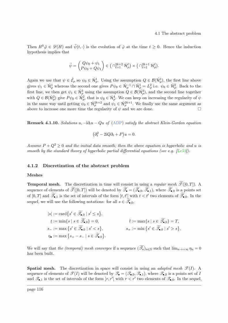
4.1 The abstract problem
Then Hkϕ ∈ D(H) and ψ(t, ·) is the evolution of ϕ at the time t ≥ 0. Hence the inductionhypothesis implies that
ψ =
(Qψ0 + ψ1
Pψ0 +Qψ1
)∈(∩2k+2ℓ=1 Hℓ
ρ
)×(∩2k+1ℓ=1 Hℓ
ρ
).
Again we use that ψ ∈ Eρ so ψ0 ∈ H1ρ. Using the assumption Q ∈ B(H1
ρ), the first line abovegives ψ1 ∈ H1
ρ whereas the second one gives Pψ0 ∈ H−1ρ ∩ H1
ρ = L2ρ i.e. ψ0 ∈ H2
ρ. Back to thefirst line, we then get ψ1 ∈ H3
ρ using the assumption Q ∈ B(H3ρ), and the second line together
with Q ∈ B(H2ρ) give Pψ0 ∈ H2
ρ, that is ψ0 ∈ H4ρ. We can keep on increasing the regularity of ψ
in the same way until getting ψ0 ∈ H2k+2ρ and ψ1 ∈ H2k+1
ρ . We finally use the same argument asabove to increase one more time the regularity of ψ and we are done.
Remark 4.1.10. Solutions u,−i∂tu−Qu of (ADP) satisfy the abstract Klein-Gordon equation
(∂2t − 2iQ∂t + P
)u = 0.
Assume P +Q2 ≥ 0 and the initial data smooth; then the above equation is hyperbolic and u issmooth by the standard theory of hyperbolic partial differential equations (see e.g. [Le53]).
4.1.2 Discretization of the abstract problem
Meshes
Temporal mesh. The discretization in time will consist in using a regular mesh T ([0, T ]). Asequence of elements of T ([0, T ]) will be denoted by T• = (T•,0, T•,1), where T•,0 is a points setof [0, T ] and T•,1 is the set of intervals of the form ]t, t′[ with t < t′ two elements of T•,0. In thesequel, we will use the following notations: for all s ∈ T•,0,
|s| := cards′ ∈ T•,0 | s′ ≤ s
,
t := mins | s ∈ T•,0 = 0, t := maxs | s ∈ T•,0 = T,
s− := maxs′ ∈ T•,0 | s′ < s
, s+ := min
s′ ∈ T•,0 | s′ > s
,
η• := maxs+ − s− | s ∈ T•,0
.
We will say that the (temporal) mesh converges if a sequence (Tn)n∈N such that limn→+∞ ηn = 0has been built.
Spatial mesh. The discretization in space will consist in using an adapted mesh T (I). Asequence of elements of T (I) will be denoted by T• = (T•,0,T•,1), where T•,0 is a points set of Iand T•,1 is the set of intervals of the form ]r, r′[ with r < r′ two elements of T•,0. In the sequel,
page 116
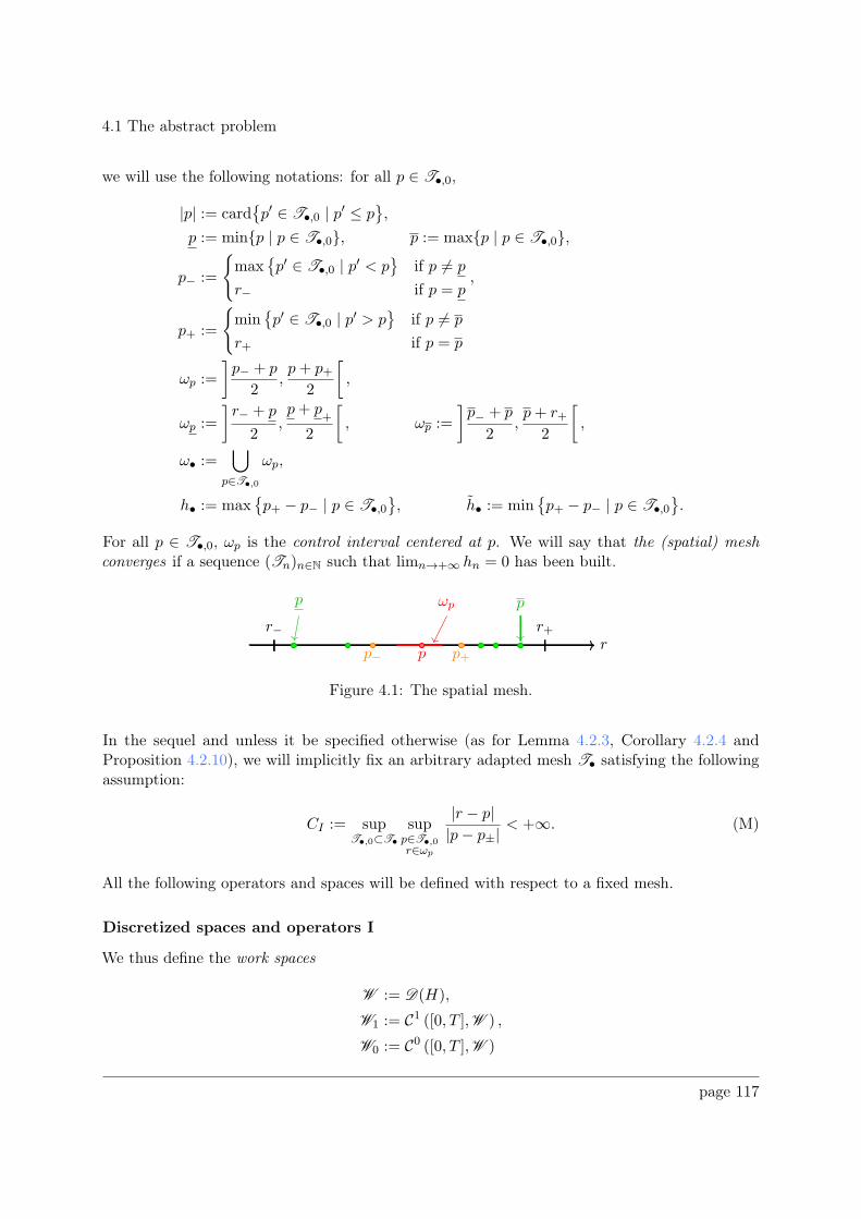
4.1 The abstract problem
we will use the following notations: for all p ∈ T•,0,
|p| := cardp′ ∈ T•,0 | p′ ≤ p
,
p := minp | p ∈ T•,0, p := maxp | p ∈ T•,0,
p− :=
max
p′ ∈ T•,0 | p′ < p
if p 6= p
r− if p = p,
p+ :=
min
p′ ∈ T•,0 | p′ > p
if p 6= p
r+ if p = p
ωp :=
]p− + p
2,p+ p+
2
[,
ωp :=
]r− + p
2,p+ p
+
2
[, ωp :=
]p− + p
2,p+ r+
2
[,
ω• :=⋃
p∈T•,0
ωp,
h• := maxp+ − p− | p ∈ T•,0
, h• := min
p+ − p− | p ∈ T•,0
.
For all p ∈ T•,0, ωp is the control interval centered at p. We will say that the (spatial) meshconverges if a sequence (Tn)n∈N such that limn→+∞ hn = 0 has been built.
r
ωpp p
r− r+
p+pp−
Figure 4.1: The spatial mesh.L
In the sequel and unless it be specified otherwise (as for Lemma 4.2.3, Corollary 4.2.4 andProposition 4.2.10), we will implicitly fix an arbitrary adapted mesh T• satisfying the followingassumption:
CI := supT•,0⊂T•
supp∈T•,0r∈ωp
|r − p||p− p±|
< +∞. (M)
All the following operators and spaces will be defined with respect to a fixed mesh.
Discretized spaces and operators I
We thus define the work spaces
W := D(H),
W1 := C1 ([0, T ],W ) ,
W0 := C0 ([0, T ],W )
page 117
4.1 The abstract problem
and the approximated spaces
W⋆ := H1
ρ ×H1ρ
‖.‖Eρ ,
W⋆H := H1
ρ × L2ρ
‖.‖Eρ = Eρ,
W⋆1 := C0 ([0, T ],W ⋆) ,
W⋆1,H := C0 ([0, T ],W ⋆
H) ,
W⋆0 := L2([0, T ],W ⋆
H).
Solutions of (ADP) are thus elements of W1. Observe that
W ⊂ W⋆ ⊂ W
⋆H (4.3)
the first inclusion being a direct consequence of Lemma 4.1.7 (see also Remark 4.1.6). As a result,we have
W1 ⊂ W⋆1 ⊂ W
⋆1,H ⊂ W
⋆0 . (4.4)
Next, let
B := i∂t +H
so that the equation in (ADP) boils down to solve Bu = 0 for u ∈ C1([0, T ],W ) with compactlysupported initial data in W . For all u ∈ W ⋆
1 and all (t, r) ∈ [0, T ]× I, we define the approximatedoperators
(∂⋆t u)(t, ·) :=(∂tu)(t, .) if u is C1(U ,W ⋆) for some neighborhood U ∋ t0 otherwise
,
(P ⋆u0)(t, r) :=
(Pu0)(t, r) if u0 ∈ H1
ρ(V) for some neighborhood V ∋ r0 otherwise
.
We finally define H⋆ as H with P ⋆ instead of P , and we set
B⋆ := i∂⋆t +H⋆ : W⋆1 −→ W
⋆0 .
Projectors, lifts and filters
Let u : [0, T ] × I → C be a function. The temporal Lagrange interpolation of u over the setA = a1, . . . , am ⊂ [0, T ] is defined where it makes sense by
(I
tempA
u)(t, r) :=
m∑
j=1
lAj (t)u(aj , r), lAj (t) :=∏
1≤j′≤mj′ 6=j
t− aj′aj − aj′
.
Similarly, the spatial Lagrange interpolation of u over the set B = b1, . . . , bn ⊂ I is defined by
(I
spatB
u)(t, r) :=
n∑
k=1
lBk (r)u(t, bk) lBk (r) :=∏
1≤k′≤nk′ 6=k
r − bk′bk − bk′
.
The following operators are defined after having chosen a mesh T•,0.
page 118
4.1 The abstract problem
Temporal projectors. The projectors we will use in the temporal scheme are the followingones:
(P
temp•,1 u
)(t, r) :=
∑
s∈T•,0
(I
temps,s+u
)(t, r)1[s,s+[(t),
(P
temp•,0 u
)(t, r) :=
∑
s∈T•,0
(ˆ
∼[s,s+[,A
u(τ, r)dτ
)1[s,s+[(t)
whereˆ
∼[s,s+[,A
u(τ, r)dτ :=
ˆ 1
0
(I
tempA
u) (
(s+−s)τ ′ + s, r)dτ ′, A ⊂ [0, 1].
When A = 0 one says the scheme is explicit ; when A = 1, the scheme is implicit.
Spatial operators. The operators we will use in the spatial scheme are the following ones:(P
spat•,1 u
)(t, r) :=
∑
p∈T•,0
(I
spatSp
u)(t, r)1ωp(r)
with
Sp :=
p−, p, p+ if p /∈ p, pr−, p if p = p
p, r+ if p = p
,
and
(P
spat•,0 u
)(t, r) :=
∑
p∈T•,0
(I
spatSp
u)(t, r)1ωp(r) if T•,0 ⊂ L (u)
0 otherwise.
Remark 4.1.11. The projector Pspat•,1 is well defined on W ⋆
1 since one evaluates functionsonly at interior points,which makes sense thanks to Assumption (AP2) and Sobolev embeddingH1(I, dr) ⊂ C0,1/2(I,C).
As for the projector Pspat•,0 , its action on the first component of elements of W ⋆
0 is welldefined as explained above whereas its action on the second component is well defined by Lebesguedifferentiation theorem for meshes defined on L (u) (which is a full measure subset of I). IndeedLebesgue’s theorem applies for locally L1 functions, so if u ∈ L2
ρ then for all compact subsetK ⊂ I,
∣∣∣∣ˆ
Ku(r)dr
∣∣∣∣ ≤ |K|1/2(ˆ
K|u(r)|2dr
)1/2
≤( |I|ρ0
)1/2
‖u‖L2ρ< +∞.
Pspat•,0 filters "bad behaviors" with respect to the measure ρ(r)dr.
If we assume the second component more regular than L2ρ, say continuous, then P
spat•,0 is
perfectly well defined for any mesh since in this case L (u) = I.
page 119
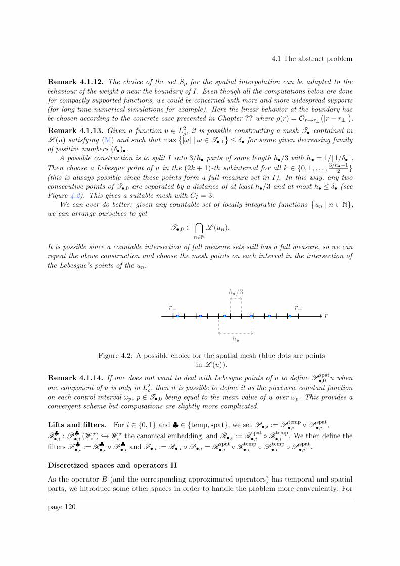
4.1 The abstract problem
Remark 4.1.12. The choice of the set Sp for the spatial interpolation can be adapted to thebehaviour of the weight ρ near the boundary of I. Even though all the computations below are donefor compactly supported functions, we could be concerned with more and more widespread supports(for long time numerical simulations for example). Here the linear behavior at the boundary hasbe chosen according to the concrete case presented in Chapter ?? where ρ(r) = Or→r±
(|r − r±|
).
Remark 4.1.13. Given a function u ∈ L2ρ, it is possible constructing a mesh T• contained in
L (u) satisfying (M) and such that max|ω| | ω ∈ T•,1
≤ δ• for some given decreasing family
of positive numbers (δ•)•.A possible construction is to split I into 3/h• parts of same length h•/3 with h• = 1/⌈1/δ•⌉.
Then choose a Lebesgue point of u in the (2k + 1)-th subinterval for all k ∈ 0, 1, . . . , 3/h•−12
(this is always possible since these points form a full measure set in I). In this way, any twoconsecutive points of T•,0 are separated by a distance of at least h•/3 and at most h• ≤ δ• (seeFigure 4.2). This gives a suitable mesh with CI = 3.
We can ever do better: given any countable set of locally integrable functionsun | n ∈ N,
we can arrange ourselves to get
T•,0 ⊂⋂
n∈NL (un).
It is possible since a countable intersection of full measure sets still has a full measure, so we canrepeat the above construction and choose the mesh points on each interval in the intersection ofthe Lebesgue’s points of the un.
rr−
h•/3
h•
r+
Figure 4.2: A possible choice for the spatial mesh (blue dots are pointsin L (u)).
Remark 4.1.14. If one does not want to deal with Lebesgue points of u to define Pspat•,0 u when
one component of u is only in L2ρ, then it is possible to define it as the piecewise constant function
on each control interval ωp, p ∈ T•,0 being equal to the mean value of u over ωp. This provides aconvergent scheme but computations are slightly more complicated.
Lifts and filters. For i ∈ 0, 1 and ♣ ∈ temp, spat, we set P•,i := Ptemp•,i P
spat•,i ,
R♣•,i : P
♣•,i (W
⋆i ) → W ⋆
i the canonical embedding, and R•,i := Rspat•,i R
temp•,i . We then define the
filters F♣•,i := R
♣•,i P
♣•,i and F•,i := R•,i P•,i = R
spat•,i R
temp•,i P
temp•,i P
spat•,i .
Discretized spaces and operators II
As the operator B (and the corresponding approximated operators) has temporal and spatialparts, we introduce some other spaces in order to handle the problem more conveniently. For
page 120
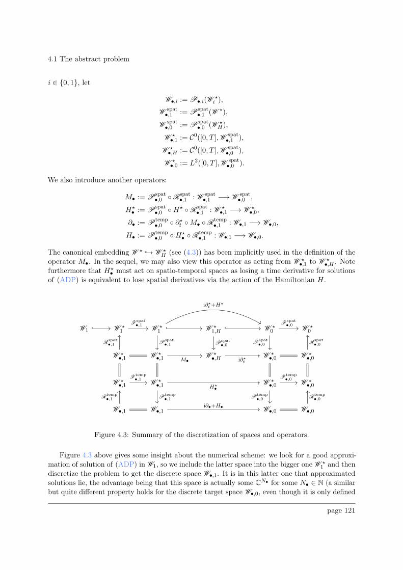
4.1 The abstract problem
i ∈ 0, 1, let
W•,i := P•,i(W⋆i ),
Wspat•,1 := P
spat•,1 (W ⋆),
Wspat•,0 := P
spat•,0 (W ⋆
H),
W⋆•,1 := C0([0, T ],W spat
•,1 ),
W⋆•,H := C0([0, T ],W spat
•,0 ),
W⋆•,0 := L2([0, T ],W spat
•,0 ).
We also introduce another operators:
M• := Pspat•,0 R
spat•,1 : W
spat•,1 −→ W
spat•,0 ,
H⋆• := P
spat•,0 H⋆ R
spat•,1 : W
⋆•,1 −→ W
⋆•,0,
∂• := Ptemp•,0 ∂⋆t M• R
temp•,1 : W•,1 −→ W•,0,
H• := Ptemp•,0 H⋆
• Rtemp•,1 : W•,1 −→ W•,0.
The canonical embedding W ⋆ → W ⋆H (see (4.3)) has been implicitly used in the definition of the
operator M•. In the sequel, we may also view this operator as acting from W ⋆•,1 to W ⋆
•,H . Notefurthermore that H⋆
• must act on spatio-temporal spaces as losing a time derivative for solutionsof (ADP) is equivalent to lose spatial derivatives via the action of the Hamiltonian H.
W1 W ⋆1 W ⋆
1 W ⋆1,H W ⋆
0 W ⋆0
W ⋆•,1 W ⋆
•,1 W ⋆•,H W ⋆
•,0 W ⋆•,0
W ⋆•,1 W ⋆
•,1 W ⋆•,0 W ⋆
•,0
W•,1 W•,1 W•,0 W•,0
Fspat•,1
Pspat•,1
i∂⋆t +H⋆
Pspat•,0
Fspat•,0
Pspat•,0R
spat•,1
M• i∂⋆t
Rspat•,0
Ftemp•,1
H⋆•
Ptemp•,1
Ftemp•,0
Ptemp•,0R
temp•,1
i∂•+H•
Rtemp•,0
Figure 4.3: Summary of the discretization of spaces and operators.
Figure 4.3 above gives some insight about the numerical scheme: we look for a good approxi-mation of solution of (ADP) in W1, so we include the latter space into the bigger one W ⋆
1 and thendiscretize the problem to get the discrete space W•,1. It is in this latter one that approximatedsolutions lie, the advantage being that this space is actually some CN• for some N• ∈ N (a similarbut quite different property holds for the discrete target space W•,0, even though it is only defined
page 121
4.1 The abstract problem
to give sense to the operators defined above). In a short sentence, the numerical scheme providesarrows between the two main objects which are W1 (the space of solutions) and W•,1 (the finitedimensional vector space used for the numerical programming).
Once an approximate solution in W•,1 is exhibited, we still have to show how it consists in agood approximation of the real one, in the sens that we have to show that the difference betweenthe solution and its approximation goes to 0 in some sense; in this purpose we have to constructan approximated norm on the whole space W ⋆
1 . We will deal with all these points in the nextSection.
4.1.3 Matrix representation
We investigate in this Section the matrix representations of the operators and the norms used forthe discretization of the abstract problem. As concrete computations will be carried out in thesequel, we will sometimes need to specify Q. We thus add the following assumption:
Q is a C2(I,R) multiplication operator on I (Q)
that is: for all u ∈ Lp(I,dr), (Qu)(r) = q(r)u(r) with q ∈ C2(I,R). Since Q is assumed to beself-adjoint, q is necessarily real. Besides, for k ∈ 1, 2, Q ∈ B(Hk
ρ(J)) for all open set J ⋐ I
since then Hkρ(J) ⊂ Hk(J) by Assumption (AP2). Therefore Assumption (AP5) is locally verified
for multiplication operators.
Remark 4.1.15. Actually, we will only need q ∈ H2ℓoc(I,R) in Proposition 4.2.10, but this
requires to ask for T•,0 ⊂ L (q) for each considered sequence T•. For the sake of simplicity, wewill restrict ourselves to the case of Assumption (Q) above.
Discrete vector spaces
We introduce in this paragraph the discrete spaces which are used for the numerical programmingFor all u, v ∈ W
spat•,1 , we define
uR v ⇐⇒ u(p) = v(p) ∀p ∈ T•,0
and similarly, if u, v ∈ Wspat•,0 , we define
uRH v ⇐⇒ u(p) = v(p) ∀p ∈ T•,0.
We will note [·] and [·]H the corresponding equivalence classes in the quotient spaces Wspat•,1 /R
and Wspat•,0 /RH , respectively.
Remark 4.1.16. If one define the projector Pspat•,0 as in Remark 4.1.14, then we can work on
the entire work space Wspat•,0 and the equivalence relation RH can be defined as follows:
uRH v ⇐⇒ˆ
–
ωp
u(ξ)dξ =
ˆ
–
ωp
v(ξ)dξ ∀p ∈ T•,0.
It turns out that the spaces Wspat•,1 and W
spat•,0 can be identified respectively to W
spat•,1 /R and
Wspat•,0 /RH , which basically means that we can "drop" all the information but the values at the
mesh points p. In fact, we have a little bit more:
page 122
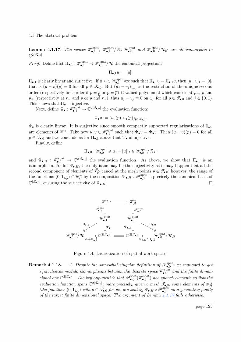
4.1 The abstract problem
Lemma 4.1.17. The spaces Wspat•,1 , W
spat•,1 /R, W
spat•,0 and W
spat•,0 /RH are all isomorphic to
C2|T•,0|.
Proof. Define first Π•,1 : Wspat•,1 → W
spat•,1 /R the canonical projection:
Π•,1u := [u].
Π•,1 is clearly linear and surjective. If u, v ∈ Wspat•,1 are such that Π•,1u = Π•,1v, then [u−v]1 = [0]1
that is (u − v)(p) = 0 for all p ∈ T•,0. But (uj − vj) ωpis the restriction of the unique second
order (respectively first order if p = p or p = p) C-valued polynomial which cancels at p−, p andp+ (respectively at r− and p or p and r+), thus uj − vj ≡ 0 on ωp for all p ∈ T•,0 and j ∈ 0, 1.This shows that Π• is injective.
Next, define Ψ• : Wspat•,1 → C2|T•,0| the evaluation function:
Ψ•u := (u0(p), u1(p))p∈T•,0 .
Ψ• is clearly linear. It is surjective since smooth compactly supported regularizations of 1ωp
are elements of W ⋆. Take now u, v ∈ Wspat•,1 such that Ψ•u = Ψ•v. Then (u− v)(p) = 0 for all
p ∈ T•,0 and we conclude as for Π•,1 above that Ψ• is injective.Finally, define
Π•,0 : Wspat•,0 ∋ u := [u]H ∈ W
spat•,0 /RH
and Ψ•,H : Wspat•,0 → C2|T•,0| the evaluation function. As above, we show that Π•,0 is an
isomorphism. As for Ψ•,H , the only issue may be the surjectivity as it may happen that all thesecond component of elements of V ⋆
H cancel at the mesh points p ∈ T•,0; however, the range ofthe functions (0,1ωp) ∈ W ⋆
H by the composition Ψ•,H Pspat•,0 is precisely the canonical basis of
C|T•,0|, ensuring the surjectivity of Ψ•,H .
W ⋆ W ⋆H
Wspat•,1 W
spat•,0
Wspat•,1 /R C2|T•,0| C2|T•,0| W
spat•,0 /RH
Pspat•,1
Ψ•
Π•,1Ψ•,H
Π•,0
Pspat•,0
Ψ•Π−1•,1 Ψ•,HΠ−1
•,0
Figure 4.4: Discretization of spatial work spaces.
Remark 4.1.18. 1. Despite the somewhat singular definition of Pspat•,0 , we managed to get
equivalences modulo isomorphisms between the discrete space Wspat•,0 and the finite dimen-
sional one C2|T•,0|. The key argument is that Pspat•,0 (W spat
•,0 ) has enough elements so that the
evaluation function spans C2|T•,0|; more precisely, given a mesh T•,0, some elements of W ⋆H
(the functions (0,1ωp) with p ∈ T•,0 for us) are sent by Ψ•,H Pspat•,0 on a generating family
of the target finite dimensional space. The argument of Lemma 4.1.17 fails otherwise.
page 123
4.1 The abstract problem
2. A similar commutative diagram as above can be drawn for the temporal discretization. Forthe sake of brevity, we will omit details in the sequel.
Approximated norms
As we wish to evaluate the approximation error of a solution of (ADP), our task consists now indefining an adequate approximated norm on W ⋆
1 and then giving a natural matrix representation.On W ⋆ and W ⋆
H , we define the spatial approximated norm
N 2• (v) :=
⟨P ⋆R•,jP•,jv0,R•,jP•,jv0
⟩L2ρ+∥∥R•,jP•,jv1 −R•,jP•,jQv0
∥∥2L2ρ
where
P•,jvk =(P
spat•,j v
)k, R•,jvk =
(R
spat•,j v
)k
for all j, k ∈ 0, 1. We placed Q in the definition of N• so that computations in Appendix 4.4.3are easier. On W ⋆
1 and W ⋆0 , we then define the approximated norm
[[u]]• := supt∈[0,T ]
N•(u(t, ·))
The corresponding approximated operator norm is
|||L•|||• := supu 6=0
N•(L•u)N•(u)
.
Note that N 2• is an hermitian form on W ⋆ (because P is non-negative and self-adjoint), so we
can associate to it the (right linear) sesquilinear form
N 2• (u, v) :=
⟨P ⋆R•,1P•,1u0,R•,1P•,1v0
⟩L2ρ+⟨R•,1P•,1 (u1 −Qu0) ,R•,1P•,1 (v1 −Qv0)
⟩L2ρ.
It turns out that the approximated norm N• is not convenient to show convergence. We thusintroduce two other ones:
|||(u0, u1)|||Eρ := ‖u0‖H1ρ+ ‖u1 −Qu0‖L2
ρ(u0, u1) ∈ Eρ,
N•((u0, u1)) :=⟨P ⋆R•,1P•,1u0,R•,1P•,1u0
⟩1/2L2ρ+∥∥R•,1P•,1u1 −R•,1P•,1Qu0
∥∥L2ρ
(u0, u1) ∈ W⋆.
Certainly these norms are respectively equivalent to ‖ · ‖Eρ and N•(·):
||| · |||Eρ ≤√2 ‖ · ‖Eρ ≤
√2 ||| · |||Eρ , (4.5)
N•(·) ≤√2N•(·) ≤
√2 N•(·). (4.6)
Note however that these norms do not satisfy the parallelogram law (and thus do not definesesquilinear forms). Our goal is then to show that N•(·) converges to ||| · |||Eρ is some sense (seeCorollary 4.2.8). Then decay and non-decay results numerically computed with N•(·) will applyto N•(·), hence to ||| · |||Eρ modulo an error which vanishes as the mesh converges, and finally to‖ · ‖Eρ by equivalence of the norms.
page 124
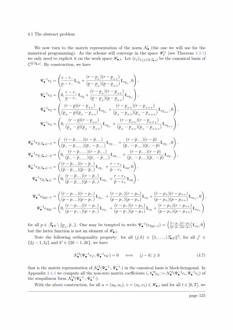
4.1 The abstract problem
We now turn to the matrix representation of the norm N• (the one we will use for thenumerical programming). As the scheme will converge in the space W ⋆
1 (see Theorem 4.3.1)we only need to explicit it on the work space W•,1. Let (ej)1≤j≤2|T•,0| be the canonical basis ofC2|T•,0|. By construction, we have
Ψ−1• e1 =
(r − r−p− r−
1ωp +(r − p
+)(r − p
++)
(p− p+)(p− p
++)1ωp
+, 0
),
Ψ−1• e2 =
(0,r − r−p− r−
1ωp +(r − p
+)(r − p
++)
(p− p+)(p− p
++)1ωp
+
),
Ψ−1• e3 =
((r − p)(r − p
++)
(p+− p)(p
+− p
++)1ωp
++
(r − p++
)(r − p+++
)
(p+− p
++)(p
+− p
+++)1ωp
++, 0
),
Ψ−1• e4 =
(0,
(r − p)(r − p++
)
(p+− p)(p
+− p
++)1ωp
++
(r − p++
)(r − p+++
)
(p+− p
++)(p
+− p
+++)1ωp
++
),
Ψ−1• e2|T•,0|−3 =
((r − p−−−)(r − p−−)
(p− − p−−−)(p− − p−−)1ωp−−
+(r − p−−)(r − p)
(p− − p−−)(p− − p)1ωp−
, 0
),
Ψ−1• e2|T•,0|−2 =
(0,
(r − p−−−)(r − p−−)
(p− − p−−−)(p− − p−−)1ωp−−
+(r − p−−)(r − p)
(p− − p−−)(p− − p)1ωp−
),
Ψ−1• e2|T•,0|−1 =
((r − p−−)(r − p−)(p− p−−)(p− p−)
1ωp−+r − r+p− r+
1ωp , 0
),
Ψ−1• e2|T•,0| =
(0,
(r − p−−)(r − p−)(p− p−−)(p− p−)
1ωp−+r − r+p− r+
1ωp
),
Ψ−1• e2|p|−1 =
((r − p−−)(r − p−)(p− p−−)(p− p−)
1ωp−+
(r − p−)(r − p+)(p− p−)(p− p+)
1ωp +(r − p+)(r − p++)
(p− p+)(p− p++)1ωp+
, 0
),
Ψ−1• e2|p| =
(0,
(r − p−−)(r − p−)(p− p−−)(p− p−)
1ωp−+
(r − p−)(r − p+)(p− p−)(p− p+)
1ωp +(r − p+)(r − p++)
(p− p+)(p− p++)1ωp+
)
for all p ∈ T•,0 \ p+, p−. One may be tempted to write Ψ−1• (e2|p|−1) =
((r−p−)(r−p+)(p−p−)(p−p+)1ωp , 0
)
but the latter function is not an element of W•,1.
Note the following orthogonality property: for all (j, k) ∈ 1, . . . , |T•,0|2, for all j′ ∈2j − 1, 2j and k′ ∈ 2k − 1, 2k, we have
N 2• (Ψ
−1• ej′ ,Ψ
−1• ek′) = 0 ⇐⇒ |j − k| ≥ 3 (4.7)
that is the matrix representation of N 2• (Ψ−1
• ·,Ψ−1• ·) in the canonical basis is block-hexagonal. In
Appendix 4.4.3 we compute all the non-zero matrix coefficients (N 2• )ij := N 2
• (Ψ−1• ei,Ψ
−1• ej) of
the sesquilinear form N 2• (Ψ
−1• ·,Ψ−1
• ·).With the above construction, for all u = (u0, u1), v = (v0, v1) ∈ W•,1 and for all t ∈ [0, T ], we
page 125
4.1 The abstract problem
have
N 2• (R
spat•,1 u,Rspat
•,1 v)
=∑
(p,p′)∈(T•,0)2
N 2•(Ψ−1
• (e2|p|−1)u0(t, p) + Ψ−1• (e2|p|)u1(t, p),Ψ
−1• (e2|p′|−1)v0(t, p
′) + Ψ−1• (e2|p′|)v1(t, p
′))
=∑
(p,p′)∈(T•,0)2
[(N 2
• )2|p|−1,2|p′|−1u0(t, p)v0(t, p′) + (N•)2|p|−1,2|p′|u0(t, p)v1(t, p
′)
+ (N 2• )2|p|,2|p′|−1u1(t, p)v0(t, p
′) + (N•)2|p|,2|p′|u1(t, p)v1(t, p′)]
=⟨U(t),N 2
• V (t)⟩C2|T•,0|
where
U(t) = (u0(t, p), u1(t, p))p∈T•,0 , V (t) = (v0(t, p), v1(t, p))p∈T•,0 .
Approximated operators
We now explicit the matrix representation of the approximated operators.
Discrete norm N•. Let u ∈ W•,1 and U := Ψ•u ∈ C2|T•,0| its discretized version (Ψ• acts onthe spatial part of u). Then
N•(Rspat•,1 u) =
√⟨U,N 2• U
⟩C2|T•,0| =
√√√√√2|T•,0|∑
i=1
2|T•,0|∑
j=1
(N 2• )ijU iUj .
Matrix associated to M•. The discrete version of the operator M• and is given by
M• := Ψ•M•Ψ−1•,H : C2|T•,0| → C2|T•,0|
This makes sense since M : W ⋆•,1 → W ⋆
•,H and W ⋆•,1, W ⋆
•,H are isomorphic to C2|T•,0| by Lemma4.1.17. For all j, k ∈ 1, . . . , 2|T•,0| we have
(M•)jk =⟨ej ,Ψ•M•Ψ
−1•,Hek
⟩C2|T•,0| .
In Appendix 4.4.1, we show that
(M•u)(p) = u(p) ∀p ∈ T•,0
whence
(M•)jk =⟨ej , ek
⟩C2|T•,0| = δjk
that is M• is the identity matrix. Since Ψ• is an isomorphism, we deduce that M• itself isinvertible.
W ⋆•,1 C2|T•,0|
W ⋆•,H C2|T•,0|
Ψ•
M•M•
Ψ•,H
page 126
4.1 The abstract problem
Matrix associated to H⋆• . The discrete version of the operator H⋆
• and is given by
H⋆• := Ψ•H
⋆•Ψ
−1•,H .
For all j, k ∈ 1, . . . , 2|T•,0| we have
(H ⋆• )jk =
⟨ej ,Ψ•H
⋆•Ψ
−1•,Hek
⟩C2|T•,0| .
Assume (Q). In Appendix 4.4.2, we show that for all u = (u0, u1) ∈ Wspat•,1
(H⋆•u)0 (t, p) = q(p)u0(t, p) + u1(t, p),
(H⋆•u)1 (t, p) =
∑
k∈K
2a(p) + b(p)(2p− (pk′ + pk′′)
)
(pk − pk′)(pk − pk′′)u0(t, pk) + c(p)u0(t, p) + q(p)u1(t, p)
whence:
(H ⋆• )j1 =
⟨ej , Q(p)e1 +
b(p) + c(p)(p− r−)p− r−
e2 +2a(p
+) + b(p
+)(p
+− p
++)
(p− p+)(p− p
++)
e4
⟩
C2|T•,0|
= Q(p)δj1 +b(p) + c(p)(p− r−)
p− r−δj2 +
2a(p+) + b(p
+)(p
+− p
++)
(p− p+)(p− p
++)
δj4,
(H ⋆• )j2 =
⟨ej , e1 +Q(p)e2
⟩C2|T•,0| = δj1 +Q(p)δj2,
(H ⋆• )j3 =
⟨ej , Q(p
+)e3 +
(2a(p
+) + b(p
+)(2p
+− (p+ p
++))
(p+− p)(p
+− p
++)
+ c(p+)
)e4
+2a(p
++) + b(p
++)(p
++− p
+++)
(p+− p
++)(p
+− p
+++)
e6
⟩
C2|T•,0|
= Q(p+)δj3 +
(2a(p
+) + b(p
+)(2p
+− (p+ p
++))
(p+− p)(p
+− p
++)
+ c(p+)
)δj4
+2a(p
++) + b(p
++)(p
++− p
+++)
(p+− p
++)(p
+− p
+++)
δj6,
(H ⋆• )j4 =
⟨ej , e3 +Q(p
+)e4
⟩C2|T•,0|
= δj3 +Q(p+)δj4,
(H ⋆• )j,2|T•,0|−3 =
⟨ej , Q(p−)e2|T•,0|−3 +
2a(p−−) + b(p−−)(p−− − p−−−)
(p− − p−−−)(p− − p−−)e2|T•,0|−4
+
(2a(p−) + b(p−)(2p− − (p−− + p))
(p− − p−−)(p− − p)+ c(p−)
)e2|T•,0|−2
⟩
C2|T•,0|
= Q(p−)δj,2|T•,0|−3 +2a(p−−) + b(p−−)(p−− − p−−−)
(p− − p−−−)(p− − p−−)δj,2|T•,0|−4
+
(2a(p−) + b(p−)(2p− − (p−− + p))
(p− − p−−)(p− − p)+ c(p−)
)δj,2|T•,0|−2,
page 127
4.2 Consistency and stability
(H ⋆• )j,2|T•,0|−2 =
⟨ej , e2|T•,0|−3 +Q(p−)e2|T•,0|−2
⟩C2|T•,0| = δj,2|T•,0|−3 +Q(p−)δj,2|T•,0|−2,
(H ⋆• )j,2|T•,0|−1 =
⟨ej , Q(p)e2|T•,0|−1 +
2a(p−) + b(p−)(p− − p−−)
(p− p−−)(p− p−)e2|T•,0|−2
+b(p) + c(p)(p− r+)
p− r+e2|T•,0|
⟩
C2|T•,0|
= Q(p)δj,2|T•,0|−1 +2a(p−) + b(p−)(p− − p−−)
(p− p−−)(p− p−)δj,2|T•,0|−2
+b(p) + c(p)(p− r+)
p− r+δj,2|T•,0|,
(H ⋆• )j,2|T•,0| =
⟨ej , e2|T•,0|−1 +Q(p)e2|T•,0|
⟩C2|T•,0| = δj,2|T•,0|−1 +Q(p)δj,2|T•,0|,
(H ⋆• )j,2|p|−1 =
⟨ej , Q(p)e2|p|−1 +
2a(p−) + b(p−)(p− − p−−)(p− p−−)(p− p−)
e2|p|−2
+
(2a(p) + b(p)(2p− (p− + p+))
(p− p−)(p− p+)+ c(p)
)e2|p|
+2a(p+) + b(p+)(p+ − p++)
(p− p+)(p− p++)e2|p|+2
⟩
C2|T•,0|
= Q(p)δj,2|p|−1 +2a(p−) + b(p−)(p− − p−−)
(p− p−−)(p− p−)δj,2|p|−2
+
(2a(p) + b(p)(2p− (p− + p+))
(p− p−)(p− p+)+ c(p)
)δj,2|p| +
2a(p+) + b(p+)(p+ − p++)
(p− p+)(p− p++)δj,2|p|+2,
(H ⋆• )j,2|p| =
⟨ej , e2|p|−1 +Q(p)e2|p|
⟩C2|T•,0| = δj,2|p|−1 +Q(p)δj,2|p|
for all p ∈ T•,0 \ p+, p−.
4.2 Consistency and stability
In this Section, we study the consistency of the operators and the stability of the scheme introducedin Chapter 4.1 under the hypotheses (AP) of Section 4.1.1. We will consider compactly supportedsolutions, motivated by the propagation result Proposition 4.3.5. Roughly speaking, consistencymeans that the approximated operators converges to the "true" ones as the mesh converges forthe strong topology of the working spaces; stability says that solutions of a perturbed discreteproblem will stay close to the solution of the unperturbed problem provided that both have sameinitial data and the perturbation is small.
The discrete problem consists in solving
B• = 0 (4.8)
page 128
4.2 Consistency and stability
where (using definitions and notations of the paragraph 4.1.2)
B• := P•,0 B⋆ R•,1
= Ptemp•,0 P
spat•,0 (i∂⋆t +H⋆) R
spat•,1 R
temp•,1
= Ptemp•,0
(iPspat
•,0 ∂⋆t Rspat•,1 + P
spat•,0 H⋆ R
spat•,1
)R
temp•,1
= Ptemp•,0 (i∂⋆t M• +H•) R
temp•,1
with
M• = Pspat•,0 R
spat•,1
and
H• = Pspat•,0 H⋆ R
spat•,1 .
We implicitly used the canonical embedding W ⋆1 → W ⋆
0 .
4.2.1 Error of interpolation
We investigate in this Section the error of interpolation with respect to the projector Pspat•,1
(considering Pspat•,0 as being the same). The obtained results will be used in Section 4.2.2 when
we will show the consistency of the spatial operators of the scheme.As one may expect, the error worsens as the regularity of the interpolated function decreases.
Assumption (AP2) and Lemma 4.1.9 entail that Hölder spaces is a natural framework.
Lemma 4.2.1. Assume (M). Let p ∈ T•,0 and let u ∈ Ck,γ (I,C) for some k ∈ 0, 1, 2 andγ ∈ [0, 1]. There exists a constant CI,u > 0 depending only on CI and ‖u‖Ck,γ(I,C) such that
∥∥∂ℓr(I
spatSp
u− u)∥∥
L∞(I,C)≤ CI,uh
maxmin1,k−ℓ,γ• ∀ 0 ≤ ℓ ≤ k.
Proof. Assume k = 0 and let r ∈ ωp. We write
(I spatSp
u)(r) =
((r − p)(r − p+)
(p− − p)(p− − p+)+
(r − p−)(r − p+)(p− p−)(p− p+)
+(r − p−)(r − p)
(p+ − p−)(p+ − p)
)u(p)
+(r − p)(r − p+)
(p− − p)(p− − p+)(u(p−)− u(p)) +
(r − p−)(r − p)(p+ − p−)(p+ − p)
(u(p+)− u(p)). (4.9)
Since
(r − p)(r − p+)(p− − p)(p− − p+)
+(r − p−)(r − p+)(p− p−)(p− p+)
+(r − p−)(r − p)
(p+ − p−)(p+ − p)= 1
and |u(r)− u(p)|, |u(p±)− u(p)| ≤ Kuhγ• with Ku > 0 the Hölder constant of u, it comes
∣∣((IBu)− u)(r)∣∣ ≤
(1 + 2CI
)Kuh
γ• .
page 129
4.2 Consistency and stability
Assume now k ≥ 1. Write for all r ∈ ωp
u(p±) =k∑
j=0
u(j)(p)
j!(p± − p)j + (p± − p)k
ˆ 1
0
(1− t)k−1
(k − 1)!
(u(k) (p+ t (p± − p))− u(k)(p)
)dt
and∣∣∣∣ˆ 1
0
(1− t)k−1
(k − 1)!
(u(k) (p+ t (p± − p))− u(k)(p)
)dt
∣∣∣∣ ≤Ku(k)
(k + 1)!(p± − p)γ
with Ku(k) > 0 the Hölder constant of u(k). Then
(I spatSp
u)(r) =
((r − p)(r − p+)
(p− − p)(p− − p+)+
(r − p−)(r − p+)(p− p−)(p− p+)
+(r − p−)(r − p)
(p+ − p−)(p+ − p)
)u(p)
+
k∑
j=1
1
j!
((r − p)(r − p+) (p− − p)j
(p− − p+) (p− − p)+
(r − p−)(r − p) (p+ − p)j(p+ − p−) (p+ − p)
)u(j)(p)
+(r − p)(r − p+)(p− − p)k
(p− − p)(p− − p+)
ˆ 1
0
(1− t)k−1
(k − 1)!
(u(k) (p+ t (p− − p))− u(k)(p)
)dt
+(r − p−)(r − p)(p+ − p)k
(p+ − p−)(p+ − p)
ˆ 1
0
(1− t)k−1
(k − 1)!
(u(k) (p+ t (p+ − p))− u(k)(p)
)dt
= u(p) +k∑
j=1
u(j)(p)
j!(r − p)j +
∑
±±(r − p)(r − p∓)(p± − p)k
(p± − p)(p+ − p−)× integral term.
(4.10)
For ℓ = 0, we deduce
∣∣∣(I
spatSp
u− u)(r)∣∣∣ ≤ ‖u′‖L∞(I,C)h• +
k∑
j=1
‖u(j)‖L∞(I,C)hj•j!
+ 2CIKu(k)hk+γ•
≤ ‖u‖Ck,γ(I,C)
(5
2+ 2CI
)h•.
whereas for k = ℓ = 1, we get∣∣∣∂r(I
spatSp
u− u)(r)∣∣∣ ≤ Ku′
(1 + 2CI
)hγ• .
When k = 2 and ℓ = 1, we find∣∣∣∂r(I
spatSp
u− u)(r)∣∣∣ ≤ 2‖u′′‖L∞(I,C)h• +
2
3CIKu′′h1+γ
•
≤ 2‖u‖C2,γ(I,C)
(1 +
CI
3
)h•
and finally, if k = ℓ = 2, we have∣∣∣∂2r(I
spatSp
u− u)(r)∣∣∣ ≤ Ku′′
(1 +
2CI
3
)hγ• .
This completes the proof.
page 130
4.2 Consistency and stability
We now turn to the general case of a L2ρ function. The main argument in the proof relies on a
the construction of a suitable mesh which depends on the given function. This is the object ofthe next lemma.
Lemma 4.2.2. Let K = [a, b] ⊂ R, η > 0, η ≪ |K|, and let Iη ⊂ K be a measurable subset suchthat |Iη| < η. For all δ > 0 (possibly much smaller than η), there exists a mesh T• dependingonly on K and Iη satisfying all the following properties:
1. K =⋃
ω∈T•,1
ω.
2. For all ω ∈ T•,1, δ/9 ≤ |ω| ≤ δ.
3. If p ∈ T•,0 ∩Iη, then ωp ⊂ Iη.
4. CK := maxp∈T•,0
p+ − p−|p± − p|
is uniformly bounded (in particular, it does not depend on η).
Proof. We may assume that δ > 0 is such that δ−1 =: N ∈ N for we can always shrink it otherwise.Let I1 := [a, a+ δ/3], I2 := [aδ/3, a+ 2δ/3], . . . , I3N := [b− δ/3, b] so that
K =3N⋃
j=1
Ij , |Ij | = δ/3.
For each Ij , define
I−j :=
[min Ij ,
min Ij +max Ij2
], I+j :=
[min Ij +max Ij
2,max Ij
].
We first choose the mesh points T•,0. For all j ∈ 1, . . . , 3N odd :
1. If Ij \Iη 6= ∅, then take any pj ∈ Ij \Iη.
2. If Ij ⊂ Iη, then take any point pj in[min Ij+max Ij
3 ,2(min Ij+max Ij)
3
].
We now turn to the control intervals T•,1. For all p ∈ T•,0, we will write ω±p the left and right
parts of ωp, that is
ωp = ω−p ∪ ω+
p , ω±p ⊂ p ∪ r ∈ K | r ≶ p.
Now let p, p+ ∈ T•,0 with say p ∈ Ij and p+ ∈ Ij+2.
1. If p, p+ /∈ Iη, then take ω+p :=
[p, p+p+
2
[and ω−
p+ :=[p+p+
2 , p+
[. Both sets ω+
p and
ω−p+ have length greater or equal to δ/6 (the equality occurring when p = max Ij andp+ = min Ij+2).
2. If p ∈ Iη and p+ /∈ Iη, then take
ω+p :=
[p, infr ∈ [p,max Ij + δ/6] | [p, r[∈ Iη
[,
ω−p+ :=
]infr ∈ [p,max Ij + δ/6] | [p, r[∈ Iη, p+
].
It follows that ω+p ∈ Iη, |ω+
p | ∈ [δ/9, 5δ/9] and |ω−p+ | ≥ δ/6.
page 131
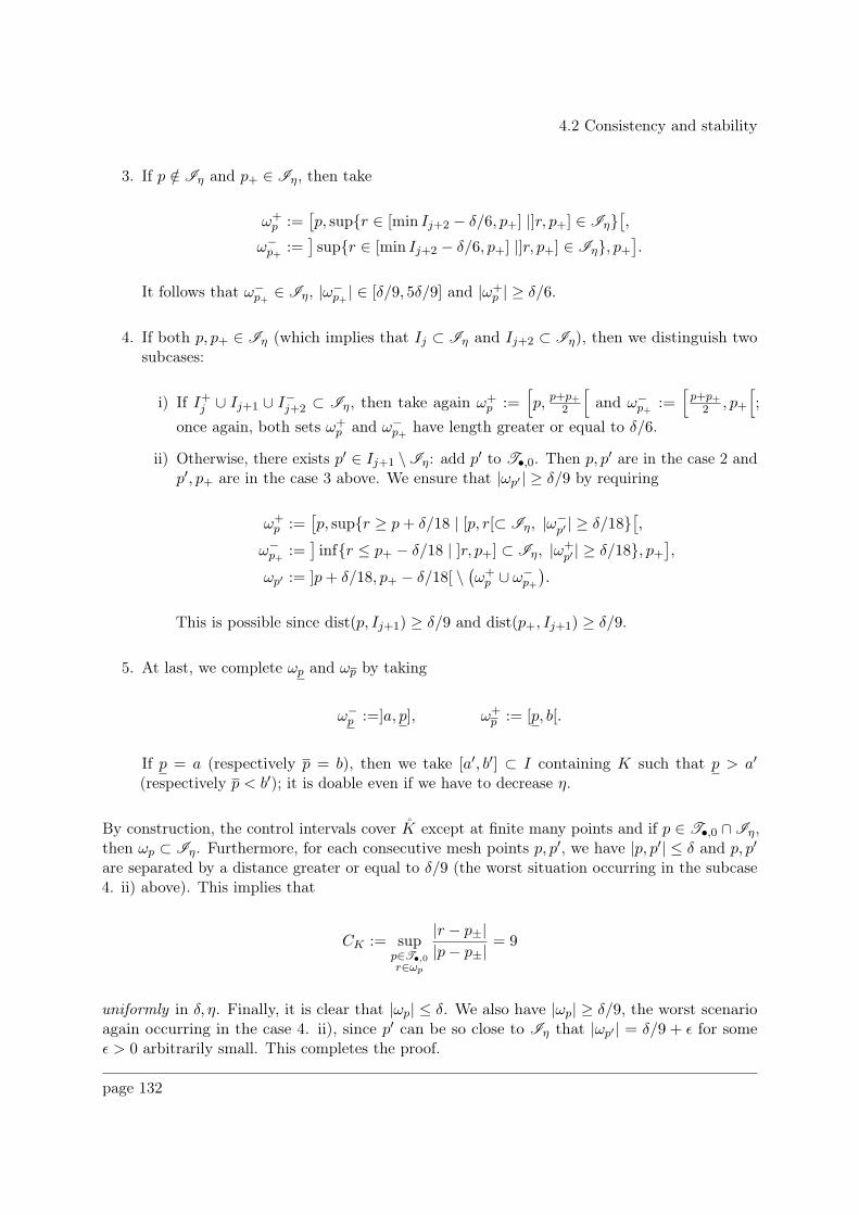
4.2 Consistency and stability
3. If p /∈ Iη and p+ ∈ Iη, then take
ω+p :=
[p, supr ∈ [min Ij+2 − δ/6, p+] |]r, p+] ∈ Iη
[,
ω−p+ :=
]supr ∈ [min Ij+2 − δ/6, p+] |]r, p+] ∈ Iη, p+
].
It follows that ω−p+ ∈ Iη, |ω−
p+ | ∈ [δ/9, 5δ/9] and |ω+p | ≥ δ/6.
4. If both p, p+ ∈ Iη (which implies that Ij ⊂ Iη and Ij+2 ⊂ Iη), then we distinguish twosubcases:
i) If I+j ∪ Ij+1 ∪ I−j+2 ⊂ Iη, then take again ω+p :=
[p, p+p+
2
[and ω−
p+ :=[p+p+
2 , p+
[;
once again, both sets ω+p and ω−
p+ have length greater or equal to δ/6.
ii) Otherwise, there exists p′ ∈ Ij+1 \Iη: add p′ to T•,0. Then p, p′ are in the case 2 andp′, p+ are in the case 3 above. We ensure that |ωp′ | ≥ δ/9 by requiring
ω+p :=
[p, supr ≥ p+ δ/18 | [p, r[⊂ Iη, |ω−
p′ | ≥ δ/18[,
ω−p+ :=
]infr ≤ p+ − δ/18 | ]r, p+] ⊂ Iη, |ω+
p′ | ≥ δ/18, p+],
ωp′ := ]p+ δ/18, p+ − δ/18[ \(ω+p ∪ ω−
p+
).
This is possible since dist(p, Ij+1) ≥ δ/9 and dist(p+, Ij+1) ≥ δ/9.
5. At last, we complete ωp and ωp by taking
ω−p :=]a, p], ω+
p := [p, b[.
If p = a (respectively p = b), then we take [a′, b′] ⊂ I containing K such that p > a′
(respectively p < b′); it is doable even if we have to decrease η.
By construction, the control intervals cover K except at finite many points and if p ∈ T•,0 ∩Iη,then ωp ⊂ Iη. Furthermore, for each consecutive mesh points p, p′, we have |p, p′| ≤ δ and p, p′
are separated by a distance greater or equal to δ/9 (the worst situation occurring in the subcase4. ii) above). This implies that
CK := supp∈T•,0r∈ωp
|r − p±||p− p±|
= 9
uniformly in δ, η. Finally, it is clear that |ωp| ≤ δ. We also have |ωp| ≥ δ/9, the worst scenarioagain occurring in the case 4. ii), since p′ can be so close to Iη that |ωp′ | = δ/9 + ǫ for someǫ > 0 arbitrarily small. This completes the proof.
page 132
4.2 Consistency and stability
Ij Ij+2
rp+ p+
2
p p+
δ/6 δ/6
(Case 1.)
Ij Ij+2
r
p p+
δ/9 δ/3
ω+p ω−
p+
(Case 2.)
Ij Ij+2
r
p p′ p+
δ/9 δ/9
ω−p′ ω+
p′
(Case 4. ii))
Figure 4.5: Examples of "bad" situations in the construction of T•. Theset Iη is drawn in red.
Lemma 4.2.3. Let u ∈ L2ρ and K = [a, b] ⊂ I. For all ε > 0, there exist a mesh T• depending
on u and K, as well as a constant C > 0 depending on the mesh, ‖u‖L2(K,C) and ‖ρ‖L1(K,C) suchthat
∥∥Rspat•,1 P
spat•,1 u− u
∥∥L2ρ(K,C)
≤ Cε.
Proof. Fix η > 0 such that η ≪ |K|. We will show that there exists a subset Sη ⊂ K dependingon K, u and η, satisfying |Sη| ≤ 10η and such that
∥∥Rspat•,1 P
spat•,1 u− u
∥∥L2ρ(K,C)
≤ C∥∥ ((1 + |u|2
)1Sη + ε2
)ρ∥∥1/2L1(K,C)
with C > 0 as in the hypotheses of the lemma. Letting η → 0, we can make the right hand sideabove smaller than Cε (if ρ ∈ L1+θ(K,R) with θ > 0, we can choose η = ε
1+θθ /10).
By standard measure theory arguments, we can construct a continuous function v : I → C
such that the set
Iη :=r ∈ I | v(r) 6= u(r)
page 133
4.2 Consistency and stability
satisfies |Iη| ≤ η (it is a consequence of Lusin’s theorem, see e.g. the book of Evans & Gariepy[EvGa91], Theorem 1.15.). Since K is compact, Heine’s theorem implies that there exists aconstant δ > 0 (possibly smaller than η) such that for all r, r′ ∈ K
|r − r′| ≤ δ =⇒ |v(r)− v(r′)| ≤ ε.
We now construct a mesh as in Lemma 4.2.2 (we can add to it any mesh point as in Remark4.1.13 outside the compact set K, it does not matter since u ≡ 0 there). Observe that we canmake it so that T•,0 ⊂ L (u) since Lebesgue’s points of u form a full measure set in K. Moreover,the support of the interpolation of u is contained in K by the point 5. in the proof Lemma 4.2.2.
The strategy to get the announced estimate is to replace u by v when it is possible and use acontinuity argument to get an estimate; otherwise, we use a rough bound for the integrand andintegrate over ωp which is sufficiently small in some sense. Using formula (4.9), we can write forall p ∈ T•,0
(I spatSp
u)(r) = u(p) +∑
±± (r − p)(r − p∓)(p± − p)(p+ − p−)
(u(p±)− u(p)
).
It follows:ˆ
K
∣∣∣(R
spat•,1 P
spat•,1 u− u
)(r)∣∣∣2ρ(r)dr =
∑
p∈T•,0∩Iη
ˆ
ωp
∣∣∣(R
spat•,1 P
spat•,1 u− u
)(r)∣∣∣2ρ(r)dr
+∑
p∈T•,0∩I ∁η
ˆ
ωp
∣∣∣(R
spat•,1 P
spat•,1 u− u
)(r)∣∣∣2ρ(r)dr
≤ 2∑
p∈T•,0∩Iη
ˆ
ωp
|u(p)− u(r)|2 ρ(r)dr
+ 4∑
p∈T•,0∩Iη
ˆ
ωp
∑
±
∣∣∣∣(r − p)(r − p∓)
(p± − p)(p+ − p−)(u(p±)− u(p)
)∣∣∣∣2
ρ(r)dr
+ 2∑
p∈T•,0∩I ∁η
ˆ
ωp
|u(p)− u(r)|2 ρ(r)dr
+ 4∑
p∈T•,0∩I ∁η
ˆ
ωp
∑
±
∣∣∣∣(r − p)(r − p∓)
(p± − p)(p+ − p−)(u(p±)− u(p)
)∣∣∣∣2
ρ(r)dr
=: I + II + III + IV.
Estimate for I & II. The crucial point here is that since p ∈ Iη, we have ωp ⊂ Iη. Thereforeˆ
ωp
|u(p)− u(r)|2 ρ(r)dr =ˆ
ωp∩Iη
|u(p)− u(r)|2 ρ(r)dr
≤ 2 |u(p)|2ˆ
ωp∩Iη
ρ(r)dr + 2
ˆ
ωp∩Iη
|u(r)|2 ρ(r)dr
≤ 2(1 + |u(p)|2
) ˆ
ωp∩Iη
(1 + |u(r)|2
)ρ(r)dr
page 134
4.2 Consistency and stability
and similarly
ˆ
ωp
∑
±
∣∣∣∣(r − p)(r − p∓)
(p± − p)(p+ − p−)(u(p±)− u(p)
)∣∣∣∣2
ρ(r)dr
=∑
±
ˆ
ωp∩Iη
∣∣∣∣(r − p)(r − p∓)
(p± − p)(p+ − p−)(u(p±)− u(p)
)∣∣∣∣2
ρ(r)dr
≤ 2C2K
(|u(p−)|2 + |u(p+)|2 + 2|u(p)|2
) ˆ
ωp∩Iη
ρ(r)dr.
Since p ∈ L (u), Lebesgue’s differentiation theorem implies
|u(p)|2 = limǫ→0+
ˆ
–
]−ǫ,ǫ[|u(p+ ξ)|2dξ
= limǫ→0+
ˆ
–
]−1,1[|u(p+ tǫ)|2dt
≤ 1
2
ˆ
K|u(ξ)|21ωp∩K(ξ)dξ
≤ 1
2
ˆ
K|u(ξ)|2dξ
≤ 1
2‖u‖2L2(K,C). (4.11)
The above computation relies on the fact that for any p ∈ T•,0, we have |u(p+ •)|1[−ǫ,ǫ] ≤ |u|1K
for ǫ≪ 1. We deduce that
2
ˆ
ωp∩Iη
|u(p)− u(r)|2 ρ(r)dr + 4
ˆ
ωp∩Iη
∑
±
∣∣∣∣(r − p)(r − p∓)
(p± − p)(p+ − p−)(u(p±)− u(p)
)∣∣∣∣2
ρ(r)dr
≤ 2(2 + ‖u‖2L2(K,C)
)∥∥(1 + |u|2)ρ1ωp∩Iη
∥∥L1(K,C)
+ 16C2K‖u‖2L2(K,C)
∥∥ρ1ωp∩Iη
∥∥L1(K,C)
whence
2∑
p∈T•,0∩Iη
ˆ
ωp
|u(p)− u(r)|2 ρ(r)dr + 4∑
p∈T•,0∩Iη
ˆ
ωp
∑
±
∣∣∣∣(r − p)(r − p∓)
(p± − p)(p+ − p−)(u(p±)− u(p)
)∣∣∣∣2
ρ(r)dr
≤ 2(2 + ‖u‖2L2(K,C)
)∥∥(1 + |u|2)ρ1Iη
∥∥L1(K,C)
+ 16C2K‖u‖2L2(K,C)
∥∥ρ1Iη
∥∥L1(K,R)
. (4.12)
Estimate for III. Since p ∈ I ∁η , we can write
ˆ
ωp
|u(p)− u(r)|2 ρ(r)dr =ˆ
ωp∩Iη
|u(p)− u(r)|2 ρ(r)dr +ˆ
ωp∩I ∁η
|v(p)− v(r)|2 ρ(r)dr.
On the one hand, we haveˆ
ωp∩Iη
|u(p)− u(r)|2 ρ(r)dr ≤ 2 |u(p)|2ˆ
ωp∩Iη
ρ(r)dr + 2
ˆ
ωp∩Iη
|u(r)|2 ρ(r)dr
page 135
4.2 Consistency and stability
and thus (4.11) givesˆ
ωp∩Iη
|u(p)− u(r)|2 ρ(r)dr ≤(2 + ‖u‖2L2(K,C)
)∥∥(1 + |u|)ρ1ωp∩Iη
∥∥L1(K,C)
.
On the other hand, using the uniform continuity of v on K as well as the fact that |p− r| < δ forall r ∈ ωp, we find
ˆ
ωp∩I ∁η
|v(p)− v(r)|2 ρ(r)dr ≤ ε2‖ρ1ωp‖L1(K,C).
As a consequence, we obtain:
∑
p∈T•,0∩I ∁η
ˆ
ωp
|u(p)− u(r)|2 ρ(r)dr ≤(2 + ‖u‖2L2(K,C)
)∥∥(1 + |u|2)ρ1Iη
∥∥L1(K,C)
+ ‖ρ‖L1(K,C)ε2.
(4.13)
Estimate for IV. Writeˆ
ωp
∑
±
∣∣∣∣(r − p)(r − p∓)
(p± − p)(p+ − p−)(u(p±)− u(p)
)∣∣∣∣2
ρ(r)dr ≤ C2K
∑
±
ˆ
ωp
∣∣(u(p±)− u(p))∣∣2 ρ(r)dr.
There is a difficulty here because we do not know whether or not p± ∈ Iη. It can be overcome inthe following way: let
A :=p ∈ T•,0 | p− ∈ Iη or p+ ∈ Iη
, nA := card(A ).
Since all the control intervals has a length greater or equal to δ/9, for each p ∈ A , a contributionof at least δ/9 (and at most 2δ if both ωp± are in Iη and have a length equal to δ) in the lengthof Iη comes from ωp− or (and) ωp+ . For nA points in A , we thus have a contribution of at least2nA δ/9 (and at most 2nA δ). This means that
nA ≤9η
δ.
Therefore, if p± ∈ Iη, then we have using (4.11)ˆ
ωp
∣∣(u(p±)− v(p))∣∣2 ρ(r)dr ≤ ‖u‖2L2(K,C)‖ρ1ωp‖L1(K,C)
and thus
∑
p∈T•,0∩I ∁η∩A
ˆ
ωp
∑
±
∣∣∣∣(r − p)(r − p∓)
(p± − p)(p+ − p−)(u(p±)− u(p)
)∣∣∣∣2
ρ(r)dr ≤ 2C2K‖u‖2L2(K,C)‖ρ1⊔
p∈Aωp‖L1(K,R)
(4.14)
with∣∣∣∣∣∣⊔
p∈A
ωp
∣∣∣∣∣∣=∑
p∈A
|ωp| ≤ nA δ ≤ 9η.
page 136
4.2 Consistency and stability
In the simpler case where p± ∈ I ∁η , we get
∑
p∈T•,0∩I ∁η∩A ∁
ˆ
ωp
∑
±
∣∣∣∣(r − p)(r − p∓)
(p± − p)(p+ − p−)(u(p±)− u(p)
)∣∣∣∣2
ρ(r)dr ≤ 2C2Kε
2‖ρ‖L1(K,C). (4.15)
Combining (4.14) and (4.15) then yields
∑
p∈T•,0∩I ∁η
ˆ
ωp
∑
±
∣∣∣∣(r − p)(r − p∓)
(p± − p)(p+ − p−)(u(p±)− u(p)
)∣∣∣∣2
ρ(r)dr
≤ 2C2K
(‖u‖2L2(K,C)‖ρ1⊔
p∈Aωp‖L1(K,R) + ε2‖ρ‖L1(K,C)
). (4.16)
Conclusion. Collecting the estimates (4.12), (4.13) and (4.16), we finally get:
∥∥Rspat•,1 P
spat•,1 u− u
∥∥2L2ρ(K,C)
≤ 3(2 + ‖u‖2L2(K,C)
)∥∥(1 + |u|2)ρ1Iη
∥∥L1(K,C)
+ 16C2K‖u‖2L2(K,C)
∥∥ρ1Iη
∥∥L1(K,R)
+(1 + 2C2
K
)ε2‖ρ‖L1(K,C)
+ 2C2K‖u‖2L2(K,C)‖ρ1⊔
p∈Aωp‖L1(K,R).
We then take:
C2 := 7 + 2C2K +
(3 + 18C2
K
)‖u‖2L2(K,C), Sη := Iη ∪
⊔
p∈A
ωp
.
The proof is complete.
We then deduce two results which will be useful for the proof of the consistency of the norms(Proposition 4.2.8) and the Hamiltonians (Proposition 4.2.2).
Corollary 4.2.4. Let T > 0 and u = (u0, u1) ∈ W1 be the solution of (ADP). Note KT :=∪0≤t≤T Suppu(t, ·) (it is a compact subset of I by Assumption (AP7)) and pick1 UT ⊂ I containingKT .
For all ε > 0, there exist a mesh T• depending on u and K, as well as a constant C > 0depending on the mesh, ‖u‖H2(UT ,C) and ‖ρ‖L1(UT ,C) such that
∥∥Pspat•,0(∂2ru− (∂⋆r )
2R
spat•,1 P
spat•,1 u
)∥∥L2ρ≤ Cε, (4.17)
∥∥Pspat•,0(∂ru− (∂⋆r )R
spat•,1 P
spat•,1 u
)∥∥L2ρ≤ Cε, (4.18)
∥∥∂⋆r ((Hu)0 −Rspat•,0 P
spat•,0 (Hu)0
)∥∥L2ρ≤ Cε. (4.19)
1The open set UT is only needed to use Sobolev and Morrey’s embeddings in Section 4.2.2.
page 137
4.2 Consistency and stability
Proof. The argument is similar to the one used to prove Lemma (4.2.3). Fix η > 0 and build twocontinuous functions v1 and v2 using Theorem 1.15 of [EvGa91] such that
Iη =2⋃
k=1
Ikη , I
1η =
r ∈ I | ∂2ru(r) 6= v1(r), I
2η =
r ∈ I | (Hu)0(r) 6= v2(r)
We may as well assume that KT = [a, b] for we can always find a, b ∈ I such that KT ⊂ [a, b] ⊂ Iotherwise. Furthermore, we can ask for T•,0 ⊂ L (u)∩L (u′)∩L (u′′)∩L ((Hu)′0) as Lebesgue’spoints of measurable functions form a set of full measure.
We start with the estimate (4.17) (estimate (4.18) is obtained is a similar way). Using formula(4.10) available at the Lebesgue’s points of u′′, we can write for all r ∈ I
Pspat•,0
(∂2ru− (∂⋆r )
2R
spat•,1 P
spat•,1 u
)(r)
=∑
p∈T•,0
[∑
±± (r − p)(r − p∓)(p± − p)(p+ − p−)
(u′′(p±)− u′′(p)
)
+∑
±± p± − pp+ − p−
ˆ 1
0(1− t)
(u′′(p+ t(p± − p)
)− u′′(p)
)dt
]1ωp(r).
The first term on the right hand side is dealt in the same way as in the proof of Lemma 4.2.3(see estimates (4.12) and (4.16)): we find
∑
p∈T•,0
ˆ
ωp
∑
±
∣∣∣∣(r − p)(r − p∓)
(p± − p)(p+ − p−)(u(p±)− u(p)
)∣∣∣∣2
ρ(r)dr ≤ 18C2K‖u′′‖2L2(K,C)
∥∥ρ1Sη
∥∥L1(K,R)
+ 2C2Kε
2‖ρ‖L1(K,C)
where Sη ⊂ K is a measurable set satisfying |Sη| ≤ 10η.
We now deal with the remaining terms. For all p ∈ T•,0, Jensen’s inequality applied to theconvex function x 7→ x2 gives
∣∣∣∣ˆ 1
0(1− t)
(u′′(p+ t(p± − p)
)− u′′(p)
)dt
∣∣∣∣2
≤ˆ 1
0
∣∣∣u′′(p+ t(p± − p)
)− u′′(p)
∣∣∣2dt.
If p ∈ Iη (which means by Lemma 4.2.2 that ωp ⊂ Iη) then we can use (4.11) to get the roughbound
ˆ 1
0
∣∣∣u′′(p+ t(p± − p)
)− u′′(p)
∣∣∣2dt ≤ 2‖u′′1±[p,p±]‖2L2(K,C) + 2|u′′(p)|2 ≤ 3‖u′′‖2L2(K,C)
because ‖ρ1ωp‖L1(K,R) = ‖ρ1ωp∩Iη‖L1(K,R) becomes small when η goes to 0 (by convention,
page 138
4.2 Consistency and stability
±[c, d] := [d, c] for all real numbers c, d). Otherwise, if p ∈ I ∁η , then write
ˆ 1
0
∣∣∣u′′(p+ t(p± − p)
)− u′′(p)
∣∣∣2dt =
ˆ
–
±[0,p±−p]
∣∣∣u′′(p+ ξ)− u′′(p)∣∣∣2dξ
=
ˆ
–
±[0,p±−p]
∣∣∣u′′(p+ ξ)− u′′(p)∣∣∣21Iη(ξ)dξ
+
ˆ
–
±[0,p±−p]
∣∣∣v(p+ ξ)− v(p)∣∣∣21
I ∁η(ξ)dξ
≤ 2‖u′′1±[p,p±]∩Iη‖2L2(K,C) + ‖u′′‖2L2(K,C)
∣∣± [p, p±] ∩Iη
∣∣
+ ε2∣∣± [p, p±] ∩I
∁η
∣∣.
We finally sum up all the above estimates over p ∈ T•,0: it comes∥∥Pspat
•,0(∂2ru0 − (∂⋆r )
2R
spat•,1 P
spat•,1 u0
)∥∥2L2ρ
≤ 18C2K‖u′′‖2L2(K,C)
∥∥ρ1Sη
∥∥L1(K,R)
+ 2C2Kε
2‖ρ‖L1(K,C)
+ 2C2K
(3‖u′′‖2L2(K,C)‖ρ1Iη‖L1(K,R) +
(2‖u′′1Iη‖2L2(K,C) + ‖u′′‖2L2(K,C)
∣∣Iη
∣∣+ ε2)‖ρ‖L1(K,R)
).
Recall that the constant CK is uniformly bounded by Lemma 4.2.2. As η can be chosen as smallas desired to make all the terms containing Iη and Sη lesser than ε, we can get the announcedestimate by taking
C := 4C2K
(6‖u′′‖2L2(K,C) + ‖ρ‖L1(K,R)
). (4.20)
We now turn to the estimate (4.19). Using again formula (4.10) for w := (Hu)0, we can writefor all p ∈ T•,0 and r ∈ ωp ∩L (w′):
∂⋆r(w − (∂⋆r )
2R
spat•,1 P
spat•,1 w
)(r) = w′(p)− w′(r)
+∑
±±(r − p) + (r − p∓)
p+ − p−
ˆ 1
0(1− t)
(w′(p+ t(p± − p)
)− w′(p)
)dt.
Since w′ ∈ L2ρ, we can apply Lemma 4.2.3 for the difference w′(p) − w′(r). As for the other
terms, we can imitate the proof of the estimate (4.17) above with u′′ replaced by w′. The proofis complete.
To end this Section, we show a simple yet useful identity involving the operator M−1• .
Lemma 4.2.5. Let u = (u0, u1) ∈ W ⋆H . Then for any mesh T• such that T•,0 ⊂ L (u), we have
Rspat•,1 M−1
• Pspat•,0 u = P
spat•,0 u in C[X].
Proof. Let j ∈ 0, 1 and choose a mesh T• as in Remark 4.1.13. Since M−1• P
spat•,0 uj ∈P
spat•,1 W ⋆,
there exists (at least one) v ∈ W ⋆ such that M•Pspat•,1 vj = P
spat•,0 uj in W
spat•,0 . Recalling that
W ⋆ ⊂ W ⋆H (so that v can be seen as an element of W ⋆
H) and M• = Pspat•,0 R
spat•,1 , we see that
Pspat•,0 uj =M•P
spat•,1 vj = P
spat•,0 R
spat•,1 P
spat•,1 vj = P
spat•,0 vj in C[X].
page 139
4.2 Consistency and stability
It follows that uj = vj on the mesh points T•,0 (this is exactly what means M = 1C2|T•,0| in the
paragraph 4.1.3). As Pspat•,j v is determined by the values of v at the mesh points, we get
Pspat•,0 uj = P
spat•,0 vj = P
spat•,1 vj =M−1
• Pspat•,0 uj in C[X]
which completes the proof.
4.2.2 Consistency
We investigate in this Section the consistency of the spatial scheme for solutions of (ADP).All the bounds will implicitly depend on the maximal existence time T via the support of theconsidered solutions. If one wish to get uniformity, then one need to make more assumptions;asking solutions to be in H2(I,C) ×H1(I,C) for all time t ≥ 0 is enough (see Corollary 4.2.8and Corollary 4.2.11). Moreover, getting a convergence rate costs another derivative for the firstcomponent of a solution (see Corollary 4.2.11).
Consistency of the norms
We prove in this paragraph the consistency of N• with |||.|||Eρ . As the speed of convergencedepends on the regularity of the argument in the norm, we distinguish two cases.
Proposition 4.2.6. Let u = (u0, u1) ∈ C1,γc (I,C) × C0,γ′
c (I,C) for some γ, γ′ ∈ [0, 1] such thatthat
Qu0 ∈ C0,γc (I,C). (4.21)
There exist a mesh T• satisfying (M) and a constant CI,u,Q > 0 depending only on the constantCI of Assumption (M), ‖u‖C1,γ
c (I,C)×C0,γ′c (I,C)
and ‖Qu0‖C0,γc (I,C)
such that
∣∣∣N•(u)− |||u|||Eρ∣∣∣ ≤ CI,u,Q
(hγ•‖aρ1ω•‖1/2L1 + h•‖cρ1ω•‖1/2L1 + h
minγ,γ′• ‖ρ1ω•‖1/2L1
).
Proof. Choose T• as in Remark 4.1.13 and such that the supports of u0 and u1 are contained inω•. By definition, we have
N•(u)− |||u|||E =(⟨P ⋆R•,1P•,1u0,R•,1P•,1u0
⟩1/2L2ρ−⟨Pu0, u0
⟩1/2L2ρ
)
+(∥∥R•,1P•,1u1 −R•,1P•,1Qu0
∥∥L2ρ−∥∥u1 −Qu0
∥∥L2ρ
)
=: I + II.
Bound for the term I. Let us write∣∣∣⟨P ⋆R•,1P•,1u0,R•,1P•,1u0
⟩1/2L2ρ−⟨Pu0, u0
⟩1/2L2ρ
∣∣∣ ≤√∣∣∣⟨P ⋆R•,1P•,1u0,R•,1P•,1u0
⟩L2ρ−⟨Pu0, u0
⟩L2ρ
∣∣∣
≤∣∣∣⟨P ⋆(R•,1P•,1u0 − u0
),(R•,1P•,1u0 − u0
)⟩L2ρ
∣∣∣1/2
+∣∣∣⟨P ⋆u0,
(R•,1P•,1u0 − u0
)⟩L2ρ
∣∣∣1/2
+∣∣∣⟨P ⋆(R•,1P•,1u0 − u0
), u0⟩L2ρ
∣∣∣1/2
=: A+B + C.
page 140
4.2 Consistency and stability
(i) We first deal with the term A. Since u0 is compactly supported, we can integrate by partsusing Remark 4.1.2 to get
A2 = −∑
p∈T•,0
ˆ
ωp
a(r) |∂r (R•,1P•,1u0 − u0)(r)|2(r)ρ(r)dr
+∑
p∈T•,0
ˆ
ωp
c(r) |(R•,1P•,1u0 − u0)(r)|2 ρ(r)dr.
Using Hölder inequalities, Lemma 4.2.1 and Assumption (M), we obtain
∣∣A2∣∣ ≤
∑
p∈T•,0
ˆ
ωp
|a(r)| |∂r (R•,1P•,1u0 − u0)(r)|2ρ(r)dr
+∑
p∈T•,0
ˆ
ωp
|c(r)| |(R•,1P•,1u0 − u0)(r)|2 ρ(r)dr
≤ supp∈T•,0
(‖(∂r (R•,1P•,1u0 − u0))1ωp‖L∞
)2 ∑
p∈T•,0
‖aρ1ωp‖L1
+ supp∈T•,0
(‖(R•,1P•,1u0 − u0)1ωp‖L∞
)2 ∑
p∈T•,0
‖cρ1ωp‖L1
≤ CI,u
(h2γ• ‖aρ1ω•‖L1(I,R) + h2•‖cρ1ω•‖L1(I,R)
)
where CI,u > 0 only depends on the Hölder norm of u0 and of CI . We thus have
|A| ≤ CI,u
(hγ•‖aρ1ω•‖1/2L1(I,R)
+ h•‖cρ1ω•‖1/2L1(I,R)
)
where CI,u > 0 is another constant depending on the Hölder norm of u0 and of CI .
(ii) We now deal with the term B. We have
B2 = −∑
p∈T•,0
ˆ
ωp
a(r)(∂ru0) (r)(∂r(R•,1P•,1u0 − u0
))(r)ρ(r)dr
+∑
p∈T•,0
ˆ
ωp
c(r)u0(r)(R•,1P•,1u0 − u0
)(r)ρ(r)dr.
Using again Hölder inequalities, Lemma 4.2.1 and Assumption (M), one obtains
∣∣B2∣∣ ≤
∑
p∈T•,0
ˆ
ωp
|a(r)| |(∂ru0) (r)|∣∣(∂r
(R•,1P•,1u0 − u0
))(r)∣∣ ρ(r)dr
+∑
p∈T•,0
ˆ
ωp
|c(r)| |u0(r)|∣∣(R•,1P•,1u0 − u0
)(r)∣∣ ρ(r)dr.
and thus
|B| ≤ CI,u‖u‖C1,γ(I,C)
(hγ/2• ‖aρ1ω•‖1/2L1(I,R)
+ h1/2• ‖cρ1ω•‖1/2L1(I,R)
).
page 141
4.2 Consistency and stability
(iii) We finally bound the term C. Since
C =∑
p∈T•,0
⟨P(R•,1P•,1u0 − u0
), u0⟩L2ρ(ωp)
=∑
p∈T•,0
⟨Pu0,
(R•,1P•,1u0 − u0
)⟩L2ρ(ωp)
,
we clearly have |C| = |B|.
Bound for the term II. Let us write
∥∥R•,1P•,1u1 −R•,1P•,1Qu0∥∥L2ρ≤∥∥R•,1P•,1u1 − u1
∥∥L2ρ+∥∥u1 −Qu0
∥∥L2ρ
+∥∥ (Qu0 −R•,1P•,1Qu0)
∥∥L2ρ.
By Lemma 4.2.1 and Assumption (M), we have
∥∥R•,1P•,1u1 − u1∥∥L2ρ≤ CI,uh
γ′
• ‖ρ1ω•‖1/2L1
and (using that Qu0 ∈ C0,γc (I,C) by Assumption (4.21))
∥∥Qu0 −R•,1P•,1Qu0∥∥L2ρ≤ CI,u,Qh
γ′
• ‖ρ1ω•‖1/2L1
where CI,u,Q > 0 only depends on the Hölder norm of Qu0 and of CI . It follows
II ≤ CI,u,Qhminγ,γ′• ‖ρ1ω•‖1/2L1
where CI,u,Q > 0 denotes another constant depending only on u, Q and CI . Collecting all theabove estimates and writing again CI,u,Q for the sum of all the previous constants CI,u, CI,u,Q,we get the result.
Remark 4.2.7. If R•,1P•,1u0 had no discontinuity point, then we could have directly written
∣∣∣⟨P ⋆R•,1P•,1u0,R•,1P•,1u0
⟩1/2L2ρ−⟨Pu0, u0
⟩1/2L2ρ
∣∣∣ =∣∣∣‖P 1/2R•,1P•,1u0‖L2
ρ− ‖P 1/2u0‖L2
ρ
∣∣∣
≤ ‖P 1/2(R•,1P•,1u0 − u0
)‖L2
ρ
=⟨P(R•,1P•,1u0 − u0
),(R•,1P•,1u0 − u0
)⟩1/2L2ρ
≤ CI,u,Qhγ• .
The discontinuity obliges us to use the linear forms⟨·, u0
⟩L2ρ
and⟨P ⋆u0, ·
⟩L2ρ
instead of the norm
‖ · ‖1/2Hρ.
Proposition 4.2.8 (Consistency of the norms). Assume (AP1)-(AP7). Let T > 0 and u =(u0, u1) ∈ W1 be the solution of (ADP). Note KT := ∪0≤t≤T Suppu(t, ·) (it is a compact subsetof I by Assumption (AP7)) and pick UT ⊂ I containing KT .
page 142
4.2 Consistency and stability
1. There exist a mesh T• satisfying (M) and a constant C1 ≡ C1(I,KT , u,Q) > 0 dependingonly on the constant CI of Assumption (M), ‖u(t, ·)‖H2(UT ,C)×H1(UT ,C) and ‖Qu0(t, ·)‖H1(UT ,C)
such that for all t ∈ [0, T ], we have
∣∣∣N•(u(t, ·))− |||u(t, ·)|||Eρ∣∣∣ ≤ C1
(h1/2• ‖aρ1ω•‖1/2L1(UT ,R)
+ h•‖cρ1ω•‖1/2L1(UT ,R)+ h
1/2• ‖ρ1ω•‖1/2L1(UT ,R)
).
For all ε > 0, there exist a mesh T• depending on v, v′′ and KT , as well as a con-stant C2 ≡ C2(I,KT , Hu,Q) > 0 depending on the mesh, ‖Hu(t, ·)‖H1(UT ,C)×L2(UT ,C),‖Qu0(t, ·)‖H1(UT ,C) and ‖ρ‖L1(UT ,R) such that
∣∣∣N•(Hu(t, ·))− |||Hu(t, ·)|||Eρ∣∣∣ ≤ C2ε.
Proof. 1. We choose T• as in Remark 4.1.13 and such that the supports of KT is containedin ω•. Assumption (AP2) combined with Lemma 4.1.7 imply that (u0(t, ·), u1(t, ·)) ∈H2 (I,C) × H1 (I,C). Sobolev embedding theorem then implies that (u0(t, ·), u1(t, ·)) ∈C1,1/2 (I,C)×C0,1/2 (I,C) with support included in KT . Finally, Assumption (AP5) impliesthat Qu0 ∈ H1
ρ and thus Sobolev embedding theorem implies that Qu0 ∈ C0,1/2 (I,C) withsupport included in KT by Assumption (AP5).
We can then apply Proposition 4.2.6. We get the announced norms in the constant CI,KT ,u,Q
using u ∈ C0([0, T ],D(H)) and Morrey’s inequality ‖ · ‖Ck,1/2(UT ,C) ≤ CUT‖ · ‖Hk+1(UT ,C)
(here CUT> 0 is a constant which only depends on UT , and thus on KT ).
2. Since Hu ∈ C0([0, T ], Eρ), we do not dispose of a sufficient regularity to directly applyProposition 4.2.6. Nevertheless, by looking carefully at the proof of this lemma, we realizeit is enough to estimate the following terms:
∥∥∂⋆r(R•,1P•,1(Hu)0 − (Hu)0
)∥∥L2ρ, ‖R•,1P•,1(Hu)0 − (Hu)0‖L2
ρ,
‖R•,1P•,1(Hu)1 − (Hu)1‖L2ρ, ‖R•,1P•,1Q(Hu)0 −Q(Hu)0‖L2
ρ.
The first two terms above come form the term I in the proof of Lemma 4.2.6 whereas the twoothers come from the term II. Since u is a solution of (ADP), (Hu)0 ∈ H1
ρ ⊂ C0,1/2(I,C);furthermore, Q(Hu)0 ∈ H1
ρ ⊂ C0,1/2(I,C) by Assumption (AP5). We therefore see that weonly need to estimate both the terms
∥∥∂⋆r(R•,1P•,1(Hu)0 − (Hu)0
)∥∥L2ρ, ‖R•,1P•,1(Hu)1 − (Hu)1‖L2
ρ.
Applying (4.19) of Corollary 4.2.4 for the first term and Lemma 4.2.3 for the second one,we are done.
Corollary 4.2.9. Assume (AP1)-(AP7). Let T > 0 and u = (u0, u1) ∈ W1 be the solution of(ADP).
If ζ := maxζ−, ζ+ < 2 and if u(t, ·) ∈ H2(I,C)×H1(I,C) for all t ∈ [0, T ], then there exista mesh T• satisfying (M) and a constant C ≡ C(I, u,Q) > 0 depending only on the constant
page 143
4.2 Consistency and stability
CI of Assumption (M), ‖u‖L∞([0,T ],H2(I,C)×H1(I,C)) and ‖Qu0‖L∞([0,T ],H1(I,C)) such that for allt ∈ [0, T ], we have
∣∣∣N•(u(t, ·))− |||u(t, ·)|||Eρ∣∣∣ ≤ C
h1/2−ζ/2• if ζ± > 0
h1/2• ln1/2(h•) if ζ± = 0
−→•
0.
Proof. Apply part 1. of Proposition 4.2.8 with the mesh of Remark 4.1.13: it clearly verifiesh• = h• so that the announced estimate follows from Assumption (AP1) and Assumption(AP3).
Consistency of the operator H⋆•
We show in this paragraph the show the consistency of the operator H⋆• with the Hamiltonian H
on the solutions of (ADP). The convergence rate will of course depend on the regularity of theconsidered solution, which depends itself on the initial data; for the general case, no rate can beexhibited.
Proposition 4.2.10 (Consistency of the Hamiltonians). Assume (AP1)-(AP7) and (Q). LetT > 0 and u = (u0, u1) ∈ W1 be the solution of (ADP). Note KT := ∪0≤t≤T Suppu(t, ·) (it is acompact subset of I by Assumption (AP7)) and pick UT ⊂ I containing KT .
1. For all ε > 0, there exist a mesh T• depending on u, u′′ and KT , as well as a constantC1 ≡ C1(I,KT , u, a, b, c) > 0 depending on the mesh, ‖u(t, ·)‖H2(UT ,C)×H1(UT ,C), ‖ρ‖L1(UT ,R)
and ‖a‖L∞(I,R), ‖b‖L∞(I,R), ‖c‖L∞(I,R) such that
N•(R
spat•,1 M−1
•(P
spat•,0 Hu(t, ·)−H⋆
•Pspat•,1 u(t, ·)
))≤ C1ε.
2. If the initial data ϕ satisfies Hϕ ∈ D(H), then for any mesh satisfying (M), there existsa constant C2 ≡ C2(I,KT , u) > 0 depending only on the constant CI of Assumption (M),‖u(t, ·)‖H3(UT ,C)×H1(UT ,C) and ‖ρ‖L1(UT ,R) such that
N•(R
spat•,1 M−1
•(P
spat•,0 Hu(t, ·)−H⋆
•Pspat•,1 u(t, ·)
))
≤ C2
(‖a2ρ1ω•‖1/2L1(UT ,R)
+ ‖b2ρ1ω•‖1/2L1(UT ,R)+ ‖c2ρ1ω•‖1/2L1(UT ,R)
)h1/2• .
Proof. If u = (u0, u1) ∈ W1, then (AP7) implies that uj(t, .) is compactly supported in I forj ∈ 0, 1. Fix a mesh T• as in Corollary 4.2.4 in the first case (and note CI the uniform constantCK given by Lemma 4.2.3) and any mesh satisfying (M) for the second case, both being suchthat the supports of u0 and u1 are contained in ω•. First observe that
(P
spat•,0 Hu−H⋆
•Pspat•,1 u
)0= P
spat•,0(Qu0 + u1
)−P
spat•,0(QR
spat•,1 P
spat•,1 u0 + R
spat•,1 P
spat•,1 u1
)
= Pspat•,0 Qu0 −P
spat•,0 QR
spat•,1 P
spat•,1 u0 (4.22)
since Pspat•,0 R
spat•,1 P
spat•,1 = P
spat•,0 . But Assumption (Q) also implies
Pspat•,0 Qu0 = P
spat•,0 QR
spat•,1 P
spat•,1 u0
page 144
4.2 Consistency and stability
so that (4.22) is identically 0. Next write(P
spat•,0 Hu−H⋆
•Pspat•,1 u
)1= P
spat•,0(Pu0 +Qu1
)−P
spat•,0(P ⋆
Rspat•,1 P
spat•,1 u0 +QR
spat•,1 P
spat•,1 u1
)
= Pspat•,0(Pu0 − P ⋆
Rspat•,1 P
spat•,1 u0
).
By Lemma 4.2.5, we have pointwisely Rspat•,1 M−1
• Pspat•,0 v = P
spat•,0 v when v is an element of W ⋆
H .We are thus boiled down to estimate the L2
ρ norm of the term above.Since u0 ∈ C1,1/2(I,C) by Assumption (AP2) and Sobolev embedding theorem, we can sum
up the estimates of Lemma 4.2.1 over p ∈ T•,0 such that ωp ∈ KT to obtain
∥∥Pspat•,0((b∂⋆r + c)(Rspat
•,1 Pspat•,1 u0 − u0)
)‖L2
ρ≤ CI‖b2ρ‖1/2L1(UT ,R)
h1/2• + CI‖c2ρ‖1/2L1(UT ,R)
h•.
We used the obvious estimate ‖Pspat•,0 w‖L∞(I,C) ≤ CI(r+ − r−)‖w‖L∞(I,C). It remains to deal
with the second derivative term.
1. If ε > 0 has been fixed, then (4.17) of Corollary 4.2.4 shows that∥∥Pspat
•,0(∂2ru− (∂⋆r )
2R
spat•,1 P
spat•,1 u
)∥∥L2ρ≤ ‖a‖L∞(I,C)
∥∥Pspat•,0(∂2ru− (∂⋆r )
2R
spat•,1 P
spat•,1 u
)∥∥L2ρ≤ Cε
where C > 0 is a constant which depends on the mesh, ‖u‖H2(UT ,C) and ‖ρ‖L1(UT ,C). Thisgives the announced estimate for part 1.
2. If we allow a loss of derivative for the initial data, then Lemma 4.1.9 for k = 1 showsin particular that u0 ∈ H3
ρ (note that Assumption (Q) implies that Q ∈ B(H2ρ)). By
Assumption (AP2) for k = 3, u0 ∈ H3(K,C) and Sobolev embedding theorem then impliesthat u0 ∈ C2,1/2(K,C). It follows
‖a∂2r (Rspat•,1 P
spat•,1 u0 − u0)‖L2
ρ≤ Cu‖a2ρ1ω•‖1/2L1(UT ,R)
h1/2•
where Cu > 0 depends on ‖u′′0‖C0,1/2(UT ,C) (giving the dependence in ‖u0‖H3(UT ,C) byMorrey’s embedding) and on the mesh (see the proof of Lemma 4.2.1). Collecting all theobtained estimates gives the announced estimate for part 2.
Corollary 4.2.11. Assume (AP1)-(AP7) and (Q). Let T > 0 and u = (u0, u1) ∈ W1 be thesolution of (ADP).
If u(t, ·) ∈ H2(I,C)×H1(I,C) for all t ∈ [0, T ], then there exist a mesh T• satisfying (M)and a constant C ≡ C(I, u) > 0 depending only on the constant CI of Assumption (M) and‖u‖L∞([0,T ],H2(I,C)×H1(I,C)) such that for all t ∈ [0, T ], we have
N•(R
spat•,1 M−1
•(P
spat•,0 Hu(t, ·)−H⋆
•Pspat•,1 u(t, ·)
))≤ Cε.
If furthermore ζ := maxζ−, ζ+ < 2 and u0 ∈ H3(I,C), then
N•(R
spat•,1 M−1
•(P
spat•,0 Hu(t, ·)−H⋆
•Pspat•,1 u(t, ·)
))≤ C
h1/2−ζ/2• if ζ± > 0
h1/2• ln1/2(h•) if ζ± = 0
−→•
0.
page 145
4.2 Consistency and stability
For the proof of the convergence of the scheme, we will also need a time consistency aresult:
Lemma 4.2.12 (Temporal consistency). Assume (AP1)-(AP7) and (Q). Let T > 0 and v =(v0, v1) ∈ W1 be the solution of (ADP). Note KT := ∪0≤t≤T Supp v(t, ·) (it is a compact subsetof I by Assumption (AP7)) and pick UT ⊂ I containing KT .
For all ε > 0, there exists a mesh T• as well as two constants C1, C2 > 0 which only dependon the mesh, on ‖u(t, ·)‖H2(UT ,C)×H1(UT ,C), ‖ρ‖L1(UT ,R), ‖a‖L∞(I,R), ‖b‖L∞(I,R), ‖c‖L∞(I,R) and on‖q‖L∞(I,R) for C2, such that, for all t ∈ [0, T ], we have
N•(v −F
temp•,1 v
)≤ C1ε, (4.23)
N•(F
spat•,0 F
temp•,0
(∂⋆t (v −F
temp•,1 v)
))≤ C2ε. (4.24)
Proof. Fix a mesh T• as in Corollary 4.2.4 (and note CI the uniform constant CK of this corollary).Since v ∈ C0([0, T ],D(H)) ∩ C1([0, T ], Eρ), there exists δ > 0 such that for all t, t′ ∈ [0, T ], wehave
|t− t′| ≤ δ =⇒ ‖v(t, ·)− v(t′, ·)‖Eρ + ‖∂tv(t, ·)− ∂tv(t′, ·)‖Eρ ≤ ε.
Let then t ∈ [0, T [ and s ∈ T•,0 the unique element such that t ∈ [s, s+[; we have
v(t, ·)−(F
temp•,1 v
)(t, ·) = v(t, ·)−
(t− s+s− s+
v(s, ·) + t− ss+ − s
v(s+, ·))
=(v(t, ·)− v(s, ·)
)+t− s+s− s+
(v(s+, ·)− v(s, ·)
)
so that∥∥∥v(t, ·)−
(F
temp•,1 v
)(t, ·)
∥∥∥Eρ≤ 2ε
as soon as η• ≤ δ, which can be assumed for we can always choose T• so that this conditions isrealized. Using the norm equivalences (4.5) and (4.6), we get
N•(v −F
temp•,1 v
)≤ N•
(v −F
temp•,1 v
)
≤∣∣∣N•
(v −F
temp•,1 v
)−∣∣∣∣∣∣v −F
temp•,1 v
∣∣∣∣∣∣Eρ
∣∣∣+∣∣∣∣∣∣v −F
temp•,1 v
∣∣∣∣∣∣Eρ
≤∣∣∣N•
(v −F
temp•,1 v
)−∣∣∣∣∣∣v −F
temp•,1 v
∣∣∣∣∣∣Eρ
∣∣∣+√2∥∥v −F
temp•,1 v
∥∥Eρ .
Now the consistency of the norms showed in Proposition 4.2.8 implies the existence of aconstant C1 ≡ C1(I,KT , v,Q) > 0 depending only on CI , ‖v‖L∞([0,T ],H2(UT ,C)×H1(UT ,C)) and‖Qv0‖L∞([0,T ],H1(UT ,C)) such that
∣∣∣N•(v −F
temp•,1 v
)−∣∣∣∣∣∣v −F
temp•,1 v
∣∣∣∣∣∣Eρ
∣∣∣
≤ C1
(h1/2• ‖aρ1ω•‖1/2L1(UT ,R)
+ h•‖cρ1ω•‖1/2L1(UT ,R)+ h
1/2• ‖ρ1ω•‖1/2L1(UT ,R)
)+ 2√2ε.
page 146
4.2 Consistency and stability
This settles (4.23) with another constant C1 and for h• sufficiently small.Next, for all t ∈ [0, T ], we have (dropping the spatial component of v)
Ptemp•,1 v(t) =
∑
s∈T•,0
(v(s) + (t− s)∂tv(s) + (t− s)
ˆ 1
0
(∂tv(s+ τ(s+ − s)
)− ∂tv(s)
)dτ
)1[s,s+[(t),
(∂⋆t F
temp•,1 v − ∂tv
)(t) =
∑
s∈T•,0
((∂tv(s)− ∂tv(t)
)+
ˆ 1
0
(∂tv(s+ τ(s+ − s)
)− ∂tv(s)
)dτ
)1[s,s+[(t)
whence
Ptemp•,0
(∂⋆t F
temp•,1 v − ∂tv
)(t)
=∑
s∈T•,0
ˆ
∼[s,s+[, 1
(∂⋆t F
temp•,1 v − ∂tv
)(τ)dτ 1[s,s+[(t)
=∑
s∈T•,0
ˆ 1
0
[∂tv(s)−
((s+ − s)τ + s− s+
s− s+∂tv(s) +
(s+ − s)τs+ − s
∂tv(s+)
)∣∣τ=1
+
ˆ 1
0
(∂tv(s+ τ ′(s+ − s)
)− ∂tv(s)
)dτ ′]dτ 1[s,s+[(t)
=∑
s∈T•,0
[(∂tv(s)− ∂tv(s+)
)+
ˆ 1
0
(∂tv(s+ τ ′(s+ − s)
)− ∂tv(s)
)dτ ′]1[s,s+[(t). (4.25)
In order to prove (4.24), we can not use the consistency of the norms because of the temporalderivative. Using Assumption (AP3), Remark 4.1.2 and Assumption (Q), we see that it issufficient to estimate the L2
ρ norm of the following terms:
(∂⋆r )k(F
temp•,0 F
spat•,0
(∂tv0 − ∂⋆t F temp
•,1 v0))
∀k ∈ 0, 1, (4.26)(F
temp•,0 F
spat•,0 Q
(∂tv0 − ∂⋆t F temp
•,1 v0)), (4.27)
Ftemp•,0 F
spat•,0
(∂tv1 − ∂⋆t F temp
•,1 v1). (4.28)
We start with (4.26). Let w0 := Ftemp•,0
(∂tv0 − ∂⋆t F temp
•,1 v0)
and write∥∥(∂⋆r )k
(F
temp•,0 F
spat•,0
(∂tv0 − ∂⋆t F temp
•,1 v0))∥∥
L2ρ=∥∥(∂⋆r )kF spat
•,0 w0
∥∥L2ρ
≤∥∥(∂⋆r )kF spat
•,0 w0 − ∂krw0
∥∥L2ρ+∥∥∂krw0
∥∥L2ρ.
Since w0 ∈ H1ρ by (4.25), the first term on the right hand side is estimated by Lemma 4.2.1 for
k = 0 and by Corollary 4.2.4 for k = 1, whereas the remaining term is estimated as follows:∥∥∂krw0
∥∥L∞([0,T ],L2
ρ)≤ ‖w‖L∞([0,T ],Eρ) ≤ 2ε
where we assumed again η• ≤ δ and used that v ∈ C1([0, T ], Eρ). We thus get:
∥∥(∂⋆r )k(F
temp•,0 F
spat•,0
(∂tv0 − ∂⋆t F temp
•,1 v0))∥∥
L2ρ≤C2h
1/2• + 2ε if k = 0
C3ε+ 2ε if k = 1
page 147
4.2 Consistency and stability
where the constants C2, C3 > 0 are as in Lemma 4.2.1 and Corollary 4.2.4, respectively.The term (4.27) is estimated in the same way since Q is a multiplication operator by a C2(I,R)function q, the only difference being that the constants will also depend on ‖q‖L∞(I,R). As forthe term (4.28), let w1 := F
temp•,0
(∂tv1 − ∂⋆t F temp
•,1 v1)
and write
∥∥F temp•,0 F
spat•,0
(∂tv1 − ∂⋆t F temp
•,1 v1)∥∥
L2ρ≤∥∥F spat
•,0 w1 − w1
∥∥L2ρ+∥∥w1
∥∥L2ρ
≤∥∥F spat
•,0 w1 − w1
∥∥L2ρ+∥∥w∥∥Eρ .
By Lemma 4.2.3, there exists a constant C4 > 0 such that
∥∥F temp•,0 F
spat•,0
(∂tv1 − ∂⋆t F temp
•,1 v1)∥∥
L2ρ≤ C4ε+ 2ε.
This gives (4.24) with another constant C2 and concludes the proof of the lemma.
4.2.3 Stability
In this Section, we interest ourselves in the stability of the scheme in the special case of Assumption(Q). We recall here some notations introduced in the paragraph 4.1.2:
η• := maxs+ − s− | s ∈ T•,0,h• := maxp+ − p− | p ∈ T•,0.
Lemma 4.2.13. Assume (Q) and
(1 + 2‖q‖L∞ + ‖c‖L∞
)(t+ − t) < 1 ∀t ∈ T•,0 \ T. (4.29)
Then 1− (t+ − t)M−1• H• is invertible for all t ∈ Tn,0 \ T and we have the uniform bound
N•(R
spat•,1 (1− (t+ − t)M−1
• H•)−1u
)≤ N•(u) ∀u ∈ W
⋆•,1. (4.30)
Equality occurs if and only if the operator is applied on ker(H⋆• ). In particular,
|||Rspat•,1 (1− (t+ − t)M−1
• H•)−1|||• = 1. (4.31)
Proof. Recall that we showed in the paragraph 4.1.3 that M• is equivalent to M• (which is theidentity on C2|T•,0|) modulo the invertible operator Ψ•, so is invertible too. As for the operator1− i(t+ − t)M−1
• H•, we shall show that i(t+ − t)M−1• H• has a norm smaller than 1.
Let u ∈ W ⋆•,1 and write U = Ψ−1
• u ∈ C2|T•,0| its discrete version. Using that
2a(p)
(p+ − p−)(p+ − p)+
2a(p)
(p− − p)(p− − p+)+
2a(p)
(p− p−)(p− p+)= 0,
b(p)(p− p−)(p+ − p−)(p+ − p)
+b(p)(p− p+)
(p− − p)(p− − p+)+b(p)(2p− (p− + p+)
(p− p−)(p− p+)= 0
page 148
4.2 Consistency and stability
as well as the discrete version of M• is the identity operator (see paragraph 4.1.3), we compute:
N•(Rspat•,1 M−1
• H⋆•u) =
⟨H
⋆• U,N•H
⋆• U⟩C2|T•,0|
=
2|T•,0|∑
i=1
2|T•,0|∑
j=1
(N•)ij(H ⋆• U)i(H⋆• U)j
=
2|T•,0|∑
i=1
2|T•,0|∑
j=1
2|T•,0|∑
k=1
2|T•,0|∑
ℓ=1
(N•)ij(H ⋆• )ik(H⋆• )jℓUkUℓ,
2|T•,0|∑
j=1
(N•)ij
2|T•,0|∑
ℓ=1
(H ⋆• )jℓUℓ
=
2|T•,0|∑
j=1
(N•)ij∑
ℓ=2|p|−1
p∈T•,0
Uℓ
[Q(p)δj,2|p|−1 +
∑
±
2a(p±) + b(p±)(p± − p±±)(p− p±±)(p− p±)
δj,2|p|±2
+
(2a(p) + b(p)(2p− (p− + p+))
(p− p−)(p− p+)+ c(p)
)δj,2|p|
]
+
2|T•,0|∑
j=1
(N•)ij∑
ℓ=2|p|p∈T•,0
Uℓ
[δj,2|p|−1 +Q(p)δj,2|p|
]
=∑
j=2|p|−1
p∈T•,0
(N•)ijUj
[1 +Q(p)
]
+∑
j=2|p|p∈T•,0
(N•)ijUj
[Q(p) +
2a(p) + b(p)(p− p−)(p+ − p−)(p+ − p)
+2a(p) + b(p)(p− p+)(p− − p)(p− − p+)
+
(2a(p) + b(p)(2p− (p− + p+))
(p− p−)(p− p+)+ c(p)
)]
=∑
j=2|p|−1
p∈T•,0
(N•)ijUj
[1 +Q(p)
]+∑
j=2|p|p∈T•,0
(N•)ijUj [Q(p) + c(p)]
and similarly
2|T•,0|∑
i=1
(N•)ij
2|T•,0|∑
k=1
(H ⋆• )ik Uk =∑
i=2|p|−1
p∈T•,0
(N•)ijUi
[1 +Q(p)
]+∑
i=2|p|p∈T•,0
(N•)ijUi
[Q(p) + c(p)
].
page 149
4.2 Consistency and stability
Using now the symmetry and the positive semi definiteness of N•, one gets:
N•(Rspat•,1 M−1
• H⋆•u) =
∑
i=2|p|−1
p∈T•,0
∑
j=2|p′|−1
p′∈T•,0
(N•)ijUiUj
[1 +Q(p)
][1 +Q(p′)
]
+∑
i=2|p|−1
p∈T•,0
∑
j=2|p′|p′∈T•,0
(N•)ijU iUj
[1 +Q(p)
][Q(p′) + c(p′)
]
+∑
i=2|p|p∈T•,0
∑
j=2|p′|−1
p′∈T•,0
(N•)ijUiUj
[Q(p) + c(p)
][1 +Q(p′)
]
+∑
i=2|p|p∈T•,0
∑
j=2|p′|p′∈T•,0
(N•)ijU iUj
[Q(p) + c(p)
][Q(p′) + c(p′)
]
=∑
i=2|p|−1
p∈T•,0
(N•)ii|Ui|2∣∣1 +Q(p)
∣∣2
+ 2ℜ∑
i=2|p|−1
p∈T•,0
∑
j=2|p′|−1
p′∈T•,0
j 6=i
(N•)ijUiUj
[1 +Q(p)
][1 +Q(p′)
]
+ 2ℜ∑
i=2|p|−1
p∈T•,0
∑
j=2|p′|p′∈T•,0
(N•)ijU iUj
[1 +Q(p)
][Q(p′) + c(p′)
]
+∑
i=2|p|p∈T•,0
(N•)ii|Ui|2∣∣Q(p) + c(p)
∣∣2
+ 2ℜ∑
i=2|p|p∈T•,0
∑
j=2|p′|p′∈T•,0
j 6=i
(N•)ijU iUj
[Q(p) + c(p)
][Q(p′) + c(p′)
]
≤(1 + 2‖q‖L∞ + ‖c‖L∞
)22|T•,0|∑
i=1
2|T•,0|∑
j=1
(N•)ijU iUj
that is |||Rspat•,1 M−1
• H⋆• |||• ≤
(1 + 2‖q‖L∞ + ‖c‖L∞
). The invertibility then follows from (4.29) by
a Neumann series argument.We now look for a bound to the inverse of 1 − i(t+ − t)H⋆
• . Let again u ∈ W ⋆•,1 and
U = Ψ−1• u ∈ C2|T•,0| its discrete version. Compute:
N•(R
spat•,1 (1− i(t+ − t)M−1
• H⋆• )u)= N•(R
spat•,1 u) + (t+ − t)2N•(R
spat•,1 M−1
• H⋆•u)
+ 2(t+ − t)ℑN•(Rspat•,1 u,Rspat
•,1 M−1• H⋆
•u).
page 150
4.2 Consistency and stability
Using again that M• is the identity matrix, one can write
N•(Rspat•,1 u,Rspat
•,1 M−1• H⋆
•u)
=
2|T•,0|∑
i=1
2|T•,0|∑
j=1
2|T•,0|∑
k=1
(N•)ij(H⋆• )jkU iUk
=
2|T•,0|∑
i=1
2|T•,0|∑
j=1
(N•)ijU i
∑
k=2|p|−1
p∈T•,0
Uk
[Q(p)δj,2|p|−1 +
∑
±
2a(p±) + b(p±)(p± − p±±)(p− p±±)(p− p±)
δj,2|p|±2
+
(2a(p) + b(p)(2p− (p− + p+))
(p− p−)(p− p+)+ c(p)
)δj,2|p|
]
+
2|T•,0|∑
i=1
2|T•,0|∑
j=1
(N•)ijU i
∑
k=2|p|p∈T•,0
Uk
[δj,2|p|−1 +Q(p)δj,2|p|
]
=
2|T•,0|∑
i=1
∑
j=2|p|−1
p∈T•,0
(N•)ijU iUj
[1 +Q(p)
]+
2|T•,0|∑
i=1
∑
j=2|p|p∈T•,0
(N•)ijU iUj [Q(p) + c(p)] .
As Q is a real multiplication operator, the above computation shows thatℑN•(R
spat•,1 u,Rspat
•,1 M−1• H⋆
•u) = 0 and therefore
N•(R
spat•,1 (1− i(t+ − t)M−1
• H⋆• )u)= N•(R
spat•,1 u) + (t+ − t)2N•(R
spat•,1 M−1
• H⋆•u) ≥ N•((R
spat•,1 u)
with equality if and only if u ∈ ker(H⋆• ). But for any invertible linear operator L acting on some
normed vector space (E, ‖ · ‖), if the operator norm satisfies |||L||| ≥ δ > 0, then for all vectorE ∋ y = Lx 6= 0 we have
‖L−1y‖‖y‖ =
‖L−1Lx‖‖Lx‖ =
‖x‖‖Lx‖ ≤
1
δ.
Taking L = (1− i(t+ − t)H⋆• ) and δ = 1, the estimate (4.30) follows with equality on (1− i(t+ −
t)H⋆• ) ker(H
⋆• ) = ker(H⋆
• ). This completes the proof.
Proposition 4.2.14 (Stability of the scheme). Assume (Q) and (4.29). Consider the implicitscheme (that is A = 1 in the definition of P
temp•,0 in the paragraph 4.1.2). For all u, v ∈ W•,1
and ε• ∈ W•,0 satisfying
(i∂• +H•)u = 0
(i∂• +H•)v = ε•v(t, ·) = u(t, ·)
,
we have
[[R•,1(u− v) ]]• ≤ (1 + T )[[R•,1M−1• ε• ]]•.
page 151
4.2 Consistency and stability
Proof. Set w := v − u so that
(i∂• +H•)w = ε•w(t, ·) = ε•(t, ·)
. (4.32)
We can write
w(t, r) =∑
s∈T•,0
(t− s+s− s+
w(s, r) +t− ss+ − s
w(s+, r)
)1[s,s+[(t) ∀(t, r) ∈ [0, T ]× I
for some w ∈ W ⋆1 . Compute:
(∂•w)(t, r) =∑
s∈T•,0
((M•w)(s+, r)− (M•w)(s, r)
s+ − s
)1[s,s+[(t),
ˆ t+
t(∂•w)(τ, r)dτ = (M•w)(s+, r)− (M•w)(s, r),
(Ptemp•,0 w)(t, r)
=∑
s∈T•,0
(ˆ 1
0
((s+ − s)τ + s− s+
s− s+(M•w)(s, r) +
(s+ − s)τ ′s+ − s
(M•w)(s+, r)
)∣∣τ=1
dτ
)1[s,s+[(t),
=∑
s∈T•,0
(M•w)(s+, r)1[s,s+[(t),
ˆ t+
t(H•w)(τ, r)dτ = (t+ − t)H⋆
• w(t+, r).
Let now t ∈ T•,0 \ T. Integrating the first line of (4.32) over [t, t+[ yields (we drop thedependence in r and view w(t) and w(t+) as functions of r)
iM•(w(t+)− w(t)
)+ (t+ − t)H⋆
•w(t+) =ˆ t+
tε•(τ)dτ.
Using that M• and 1− (t+ − t)M−1• H⋆
• are invertible if η• is small enough (see Lemma 4.2.13),we can write
w(t+) =(1− i(t+ − t)M−1
• H⋆•)−1
w(t) + i(1+ (t+ − t)M−1
• H⋆•)−1ˆ t+
tM−1
• ε•(τ)dτ.
By induction, we discover the general formula
w(t+) =∏
s≤t
(1− i(s+ − s)M−1
• H⋆•)−1
w(t)
+ i∑
s≤t
∏
s<s′≤t
(1− i(s′+ − s′)M−1
• H⋆•)−1
(1+ (s+ − s)M−1
• H⋆•)−1ˆ s+
sM−1
• ε•(τ)dτ.
page 152
4.3 Convergence and application
where products over the empty set are equal to 1 by convention. We now use the estimate (4.31)to get
N•(R•,1w(t+)) ≤ C |t|• N•(R•,1w(t)) + C
|t|•
ˆ t+
tN•(R•,1M
−1• ε•(τ))dτ (4.33)
where 0 < C•, C• ≤ 1 and C• = 1 if and only if w(t) ∈ ker(H⋆• ). Taking the supremum over
t ∈ [0, T ] and using w(t) = ε•(t, ·) then yield
[[R•,1w ]]• ≤ (1 + T )[[R•,1M−1• ε• ]]•.
The proof is complete.
Remark 4.2.15. Equation (4.33) shows that if u is a solution of B•u = 0 (that is ε• = 0 in
(4.32)), then T•,0 ∋ t 7→ u(t, ·) is exponentially decreasing in the sense that N•(R•,1u(t, ·)) ≤α(t)|t|N•(R•,1u(t, ·)) for some positive function α : R+ → [0, 1]. However, it may happen thatα(t)|t| → ǫ > 0 as t → +∞ even if we are not in the unlikely case u(t, ·) ∈ ker(H⋆
• ) for all
t ∈ T•,0: indeed, if we have uniformly in n≫ 0
Nn(Rn,1M−1n H⋆
nu) ≥ CNn(u)
for some constant C > 0, then Lemma 4.2.13 shows that
α(t)|t| =(1 + C(t+ − t)2
)−t= exp
(− |t| ln(1 + C(t+ − t)2)
)
provided that u(t, ·) 6∈ ker(H⋆n). If we take a uniform mesh ηn =
√T/N for some N ≡ N(n),
then we get
limT→+∞
α(T )T = exp(−C).
Recall that here |T | = N is the position of T in the mesh point T•,0.
4.3 Convergence and application
This Section is devoted to the proof of the convergence of the scheme in the abstract setting.We then apply the obtained results to the charged Klein-Gordon equation in the exterior DSRNspacetime.
4.3.1 Convergence of the scheme
We can now prove the scheme convergence using the consistency and stability results showedabove. In the following, we will consider the implicit scheme (that is A = 1 in thedefinition of P
temp•,0 in paragraph 4.1.2).
As usual, if more regularity is assumed, then one can get a precise speed for the convergence.We will distinguish both the cases of low regularity (the general case) and higher regularity (theparticular case where we allow a loss of derivative for the initial data).
page 153
4.3 Convergence and application
For the reader’s convenience, we recall here some notations of Subsection 4.1.2: we haveB• = i∂• +H• with (see paragraph 4.1.2)
M• := Pspat•,0 R
spat•,1 : W
spat•,1 −→ W
spat•,0 ,
∂• := Ptemp•,0 ∂⋆t M• R
temp•,1 : W•,1 −→ W•,0,
H• := Ptemp•,0 P
spat•,0 H⋆ R
spat•,1 R
temp•,1 : W•,1 −→ W•,0.
Furthermore, the filters F♣•,i := R
♣•,i P
♣•,i (♣ ∈ temp, spat) and F•,i := R•,i P•,i =
Rspat•,i R
temp•,i P
temp•,i P
spat•,i are defined in paragraph 4.1.2. As usual, we will omit the
composition symbol .The idea of the proof of Theorem 4.3.1 below is quite simple: we compare the solution v of
(ADP) to its filtered version F•,1v by splitting F•,1 into its temporal and spatial parts. We usethen consistency results of Section 4.2.2 to handle the spatial part, and we use the regularityv ∈ C0([0, T ],D(H)) ∩ C1([0, T ], Eρ) to deal with the temporal one. The main theorem of thischapter is the following:
Theorem 4.3.1 (Convergence of the scheme, low regularity). Assume (AP1)-(AP7) and (Q).Let T > 0 and v = (v0, v1) ∈ W1 be the solution of (ADP):
(i∂t +H)v = 0 ∀t ∈ [0, T ]
v(0, ·) = ϕ is compactly supported in I.
Note KT := ∪0≤t≤T Supp v(t, ·) (it is a compact subset of I by Assumption (AP7)) and pickUT ⊂ I containing KT .
For all ε > 0, there exists a mesh T• as well as a constant C > 0 which only depend onthe mesh, on ‖u(t, ·)‖H2(UT ,C)×H1(UT ,C), ‖ρ‖L1(UT ,R), ‖a‖L∞(I,R), ‖b‖L∞(I,R), ‖c‖L∞(I,R) and on‖q‖L∞(I,R), such that the unique solution u• ∈ W ⋆
•,1 of the discrete problem
(i∂• +H•)u• = 0 ∀t ∈ T•,0u•(0, ·) = P•,1ϕ
verifies
[[v −R•,1u•]]• ≤ C1(1 + T )ε. (4.34)
In particular, the approximated solution u• converges to the continuous solution v in norm: thereexists a constant C2 > 0 depending on the same parameters as C1 above such that, for all t ∈ [0, T ],
∣∣∣N•(R•,1u•(t, ·)
)− |||v(t, ·)|||Eρ
∣∣∣ ≤ C2(1 + T )ε. (4.35)
Proof. Fix a mesh T• as in Corollary 4.2.4 for the spatial part and such that the stability condition(4.29) is satisfied (this last condition ensures that the discrete problem has a unique solution, seeProposition 4.2.14). We will settle uniform bounds in t ∈ [0, T ] using the spatial norm N•. Letus write
N•(v −R•,1u•
)≤ N•
(v −F•,1v
)+N•
(F•,1v −R•,1u•
)=: I + II.
page 154
4.3 Convergence and application
Estimate for I. For the first term, we have
N•(v −F•,1v
)≤ N•
(v −F
temp•,1 v
)+N•
(F
temp•,1 v −F•,1v
).
On the one hand, (4.23) of Lemma 4.2.12 shows that there exists a constants C1 > 0 such that∣∣∣N•
(v −F
temp•,1 v
)−∣∣∣∣∣∣v −F
temp•,1 v
∣∣∣∣∣∣Eρ
∣∣∣ ≤ C1ε.
On the other hand, since Fspat•,1 F
spat•,1 = F
spat•,1 on W ⋆
1 , and since Q is a multiplication operator,we trivially have2
N•(F
temp•,1 v −F•,1v
)= 0.
This gives an estimate for the term I.
Estimate for II. We use the stability of the scheme in order to bound the term II: byProposition 4.2.14, we have
N•(F•,1v −R•,1u•
)≤ (1 + T )N•
(R•,1M
−1• B•(P•,1v − u•)
).
Since B•u• = Bv = 0, we can replace B•u• by P•,0Bv on the right hand side:
N•(F•,1v −R•,1u•
)≤ (1 + T )N•
(R•,1M
−1• (B•P•,1v −P•,0Bv)
). (4.36)
Consider first the temporal part of the difference in (4.36):
∂•P•,1v −P•,0∂tv = Ptemp•,0 P
spat•,0
((∂⋆t F
temp•,1 F
spat•,1 v − ∂⋆t F temp
•,1 v)+(∂⋆t F
temp•,1 v − ∂tv
)).
We use that ∂⋆t commutes with Fspat•,1 as well as ∂⋆t v = ∂tv and P
spat•,0 F
spat•,1 = P
spat•,0 (using the
inclusion W ⋆ ⊂ W ⋆H) to get
N•(R•,1M
−1• P
temp•,0 P
spat•,0(∂⋆t F
temp•,1 F
spat•,1 v − ∂⋆t F temp
•,1 v))
= N•(R•,1M
−1• P
temp•,0 P
spat•,0(F
spat•,1 ∂⋆t F
temp•,1 v − ∂⋆t F temp
•,1 v))
= N•(R•,1M
−1• P
temp•,0 P
spat•,0(∂⋆t F
temp•,1 v − ∂⋆t F temp
•,1 v))
= 0.
As for the other term, we use Lemma 4.2.5 to write
N•(R•,1M
−1• P
temp•,0 P
spat•,0(∂⋆t F
temp•,1 v − ∂tv
))
= N•(R
spat•,0 P
spat•,0 R
temp•,0 P
temp•,0 (∂⋆t F
temp•,1 v − ∂tv)
)
= N•(F
spat•,0 F
temp•,0 (∂⋆t F
temp•,1 v − ∂tv)
).
and conclude with (4.24) of Lemma 4.2.12 that
N•(R•,1M
−1• P
temp•,0 P
spat•,0(∂⋆t F
temp•,1 v − ∂tv
))≤ C2ε
2This property is the consistency of the spatial filter Fspat•,1 with the identity operator on W
⋆.
page 155
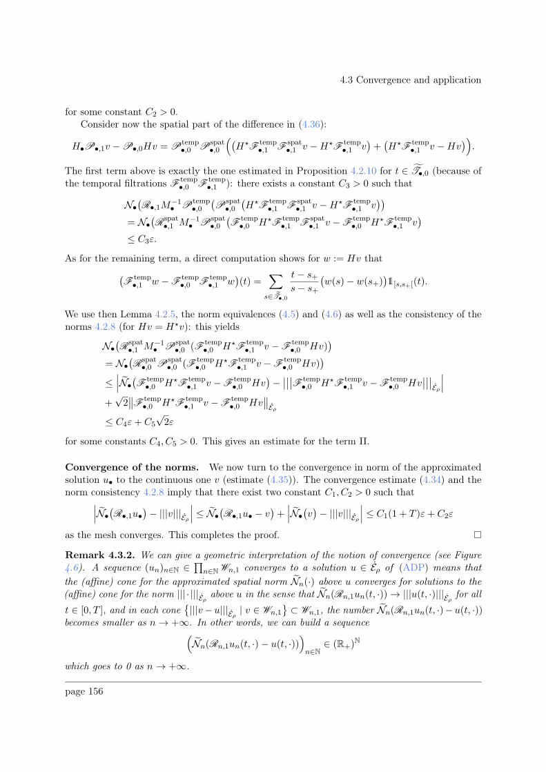
4.3 Convergence and application
for some constant C2 > 0.Consider now the spatial part of the difference in (4.36):
H•P•,1v −P•,0Hv = Ptemp•,0 P
spat•,0
((H⋆
Ftemp•,1 F
spat•,1 v −H⋆
Ftemp•,1 v
)+(H⋆
Ftemp•,1 v −Hv
)).
The first term above is exactly the one estimated in Proposition 4.2.10 for t ∈ T•,0 (because ofthe temporal filtrations F
temp•,0 F
temp•,1 ): there exists a constant C3 > 0 such that
N•(R•,1M
−1• P
temp•,0
(P
spat•,0(H⋆
Ftemp•,1 F
spat•,1 v −H⋆
Ftemp•,1 v
))
= N•(R
spat•,1 M−1
• Pspat•,0(F
temp•,0 H⋆
Ftemp•,1 F
spat•,1 v −F
temp•,0 H⋆
Ftemp•,1 v
)
≤ C3ε.
As for the remaining term, a direct computation shows for w := Hv that
(F
temp•,1 w −F
temp•,0 F
temp•,1 w
)(t) =
∑
s∈T•,0
t− s+s− s+
(w(s)− w(s+)
)1[s,s+[(t).
We use then Lemma 4.2.5, the norm equivalences (4.5) and (4.6) as well as the consistency of thenorms 4.2.8 (for Hv = H⋆v): this yields
N•(R
spat•,1 M−1
• Pspat•,0 (F temp
•,0 H⋆F
temp•,1 v −F
temp•,0 Hv)
)
= N•(R
spat•,0 P
spat•,0 (F temp
•,0 H⋆F
temp•,1 v −F
temp•,0 Hv)
)
≤∣∣∣N•
(F
temp•,0 H⋆
Ftemp•,1 v −F
temp•,0 Hv
)−∣∣∣∣∣∣F temp
•,0 H⋆F
temp•,1 v −F
temp•,0 Hv
∣∣∣∣∣∣Eρ
∣∣∣+√2∥∥F temp
•,0 H⋆F
temp•,1 v −F
temp•,0 Hv
∥∥Eρ
≤ C4ε+ C5
√2ε
for some constants C4, C5 > 0. This gives an estimate for the term II.
Convergence of the norms. We now turn to the convergence in norm of the approximatedsolution u• to the continuous one v (estimate (4.35)). The convergence estimate (4.34) and thenorm consistency 4.2.8 imply that there exist two constant C1, C2 > 0 such that
∣∣∣N•(R•,1u•
)− |||v|||Eρ
∣∣∣ ≤ N•(R•,1u• − v
)+∣∣∣N•
(v)− |||v|||Eρ
∣∣∣ ≤ C1(1 + T )ε+ C2ε
as the mesh converges. This completes the proof.
Remark 4.3.2. We can give a geometric interpretation of the notion of convergence (see Figure4.6). A sequence (un)n∈N ∈
∏n∈N Wn,1 converges to a solution u ∈ Eρ of (ADP) means that
the (affine) cone for the approximated spatial norm Nn(·) above u converges for solutions to the(affine) cone for the norm ||| · |||Eρ above u in the sense that Nn(Rn,1un(t, ·))→ |||u(t, ·)|||Eρ for all
t ∈ [0, T ], and in each cone|||v−u|||Eρ | v ∈ Wn,1
⊂ Wn,1, the number Nn(Rn,1un(t, ·)−u(t, ·))
becomes smaller as n→ +∞. In other words, we can build a sequence(Nn(Rn,1un(t, ·)− u(t, ·))
)n∈N∈ (R+)
N
which goes to 0 as n→ +∞.
page 156
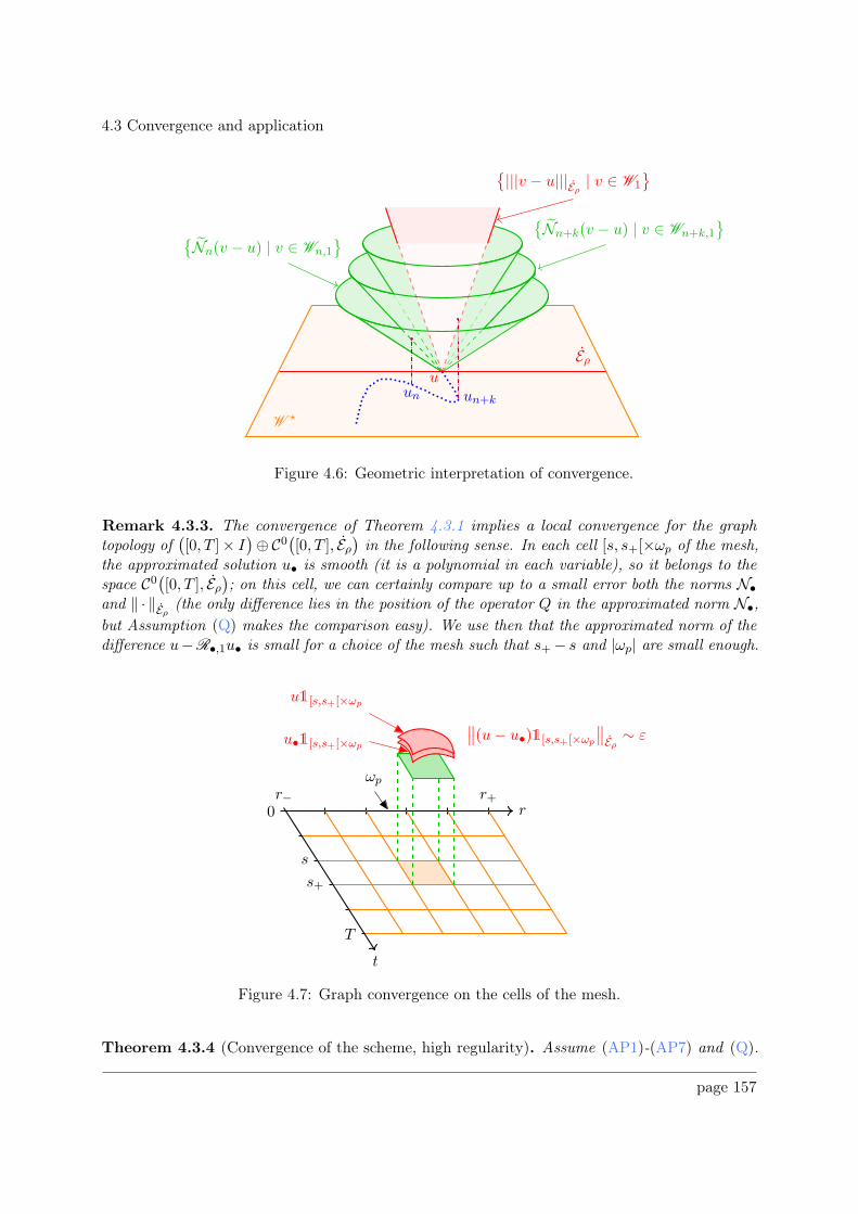
4.3 Convergence and application
W⋆
Eρu
Nn(v − u) | v ∈ Wn,1
Nn+k(v − u) | v ∈ Wn+k,1
|||v − u|||Eρ | v ∈ W1
un un+k
Figure 4.6: Geometric interpretation of convergence.
Remark 4.3.3. The convergence of Theorem 4.3.1 implies a local convergence for the graphtopology of
([0, T ]× I
)⊕ C0
([0, T ], Eρ
)in the following sense. In each cell [s, s+[×ωp of the mesh,
the approximated solution u• is smooth (it is a polynomial in each variable), so it belongs to thespace C0
([0, T ], Eρ
); on this cell, we can certainly compare up to a small error both the norms N•
and ‖ · ‖Eρ (the only difference lies in the position of the operator Q in the approximated norm N•,but Assumption (Q) makes the comparison easy). We use then that the approximated norm of thedifference u−R•,1u• is small for a choice of the mesh such that s+− s and |ωp| are small enough.
r
ωp
r− r+
s
s+
0
T
t
u•1[s,s+[×ωp
u1[s,s+[×ωp
∥∥(u− u•)1[s,s+[×ωp
∥∥Eρ ∼ ε
Figure 4.7: Graph convergence on the cells of the mesh.
Theorem 4.3.4 (Convergence of the scheme, high regularity). Assume (AP1)-(AP7) and (Q).
page 157
4.3 Convergence and application
Let T > 0 and v = (v0, v1) ∈ W1 be the solution of (ADP):
(i∂t +H)v = 0 ∀t ∈ [0, T ]
v(0, ·) = ϕ is compactly supported in I.
Note KT := ∪0≤t≤T Supp v(t, ·) (it is a compact subset of I by Assumption (AP7)) and pickUT ⊂ I containing K.
If Hϕ ∈ D(H), then for all mesh satisfying Assumption (M) as well as the stability condition(4.29), there exists a constant C1 > 0 depending only on the constant CI of Assumption (M),‖u(t, ·)‖H3(UT ,C)×H1(UT ,C) and ‖q‖C1(I,R) such that the unique solution u• ∈ W ⋆
•,1 of the discreteproblem
(i∂• +H•)u• = 0 ∀t ∈ T•,0u•(0, ·) = P•,1ϕ
verifies
[[v −R•,1u•]]• ≤ C1(1 + T )(‖aρ1ω•‖1/2L1(UT ,R)
+ h1/2• ‖cρ1ω•‖1/2L1(UT ,R)
+ ‖ρ1ω•‖1/2L1(UT ,R)
)h1/2• .
In particular, the approximated solution u• converges to the continuous solution v in norm: thereexists a constant C2 > 0 depending on the same parameters as C1 above such that, for all t ∈ [0, T ],
∣∣∣N•(R•,1u•(t, ·)
)− |||v(t, ·)|||Eρ
∣∣∣
≤ C2(1 + T )(‖aρ1ω•‖1/2L1(UT ,R)
+ h1/2• ‖cρ1ω•‖1/2L1(UT ,R)
+ ‖ρ1ω•‖1/2L1(UT ,R)
)h1/2• .
If furthermore we assume ζ := maxζ−, ζ+ < 2, then Assumption (AP1) implies
[[v −R•,1u•]]• −→• 0.
Proof. Lemma 4.1.9 implies that the solution u of (ADP) satisfies u ∈ H3ρ×H2. Using Assumption
(AP2) and Sobolev embedding theorem, we see that u ∈ C2,1/2(UT ,C)× C1,1/2(UT ,C) so that allthe error of interpolation and consistency results obtained in Section 4.2.2 apply for a greaterregularity, yielding the better convergence rate. We then just have to mimic the proof of Theorem4.3.1 with these better estimates.
4.3.2 Application to the charged Klein-Gordon equation in the DSRN space-
time
We apply in this Section the numerical scheme introduced previously to the charged Klein-Gordonequation on the DSRN metric.
Notations
We recall some notations and results from Chapter 1. Let V (r) := r−1. For r ∈ ]r−, r+[, thecharged Klein-Gordon equation reads
(∂t − iqQV )2 u+ Pu = 0, (4.37)
page 158
4.3 Convergence and application
with
P := −r−2F (r)∂rr2F (r)∂r − r−2F (r)∆S2 +m2F (r)
= −F (r)2∂2r − F (r)(2F (r)
r+ F ′(r)
)∂r −
F (r)
r2∆S2 +m2F (r).
Here, (m, q) ∈ ]0,+∞[×R is the couple formed with the mass and the charge of the scalar fieldwhose evolution is governed by the Klein-Gordon equation. We then define on L2
(]r−, r+[× S2, F−1(r)drdω
)
the new spatial operator
P := rPr−1 = −r−1F (r)∂rr2F (r)∂rr
−1 − r−2F (r)∆S2 +m2F (r)
= −F (r)∂rF (r)∂r −F (r)
r2∆S2 + F (r)
(F ′(r)r
+m2
)(4.38)
We will denote by Pℓ the operator P restricted on ker(∆S2 + ℓ(ℓ + 1)) for all ℓ ∈ N. TheRegge-Wheeler coordinate x := φ(r) is defined by
x ≡ φ(r) =∑
α∈n,c,−,+
1
2καln
∣∣∣∣r − rαr− rα
∣∣∣∣ (4.39)
where κα := F ′(rα)/2 are the surface gravities and r ∈ ]r−, r+[ (we do not necessarily choose r asthe radius of the photon sphere as in Subsection 1.1.2). Then φ : ]r−, r+[ ∋ r 7→ x ≡ x(r) ∈ R isan increasing bijection. Using the factorization
F (r) =Λ
3r2(r − rn)(r − rc)(r − r−)(r+ − r) ∀r ∈ ]r−, r+[ , (4.40)
we see that
|r − r±| = |r− r±|
∏
α∈n,c,∓
∣∣∣∣r− rαr − rα
∣∣∣∣
κ±κα
e2κ±x = Or→±∞
(e2κ±x
)(4.41)
which is an exponential decay as κ− > 0 and κ+ < 0. In the coordinates (x, ω) ∈ R × S2, thespatial operator P takes the form
P = −r−2∂xr2∂xr
−1 − r−2F (r)∆S2 +m2F (r)
where r is now to be read as a function of x, and P acts on L2(R× S2; dxdω
).
We henceforth use the notation s := qQ ∈ R for the charge product. The charge Klein-Gordonoperator is defined as
K(s) :=
(sV 1
P sV
). (4.42)
We can also define Kℓ(s) with Pℓ instead of P . We can check that if u solves (4.37) thenv = (u,−i∂tu− su) solves
−i∂tv = K(s)v. (4.43)
Conversely, if v = (v0, v1) solves (4.43) then v0 solves (4.37). Theorem 1.3.2 shows that thesolutions of (ADP) decay exponentially fast in time.
page 159
4.3 Convergence and application
Application of the mumerical shceme
We easily check that the charged Klein-Gordon equation in the exterior DSRN spacetime enterthe abstract setting introduced in Section 4.1. Only the propagation estimate for of solutionsv = (v0, v1) = (v0,−i∂tv0 − sV v0) of (4.43) is not immediate, so we give the argument in thefollowing lemma. Since v± := e−isr−1
± tv satisfies(∂2t − 2isV±∂t − s2V 2
± + P)v±0 = 0
with V± := V − r−1± and e−isr−1
± t is unitary for all t ≥ 0, the supports of v and v± are the same.
Lemma 4.3.5 (Propagation estimate). Assume Supp v(0, .) ⊂ [R,R′] for some real constantsR,R′ such that R,R′ ∈ [r−, r+]. If
s2 <
m2 Λr+
3r (r − rn)(r − rc)(r − r−) for all r ≥ R′
m2 Λr−3r (r − rn)(r − rc)(r+ − r) for all r ≤ R
, (4.44)
then
Supp v(t, .) ⊂[φ−1(φ(R)− t) , φ−1
(φ(R′) + t
)]∀t ≥ 0.
Proof. We work on R with the Regge-Wheeler coordinate x = φ(r) ∈ R. For the sake of clarity,we will consider that ℓ = 0 (one must add otherwise a non negative extra term ℓ(ℓ+ 1)|v0(t, x)|2below which is easily handled).
Define for all t ≥ 0 the function
E+(t) :=
ˆ +∞
φ(R′)+t
[|∂tv+0 (t, x)|2 + |r∂xr−1v+0 (t, x)|2 +
(m2F (r(x))− s2V+(r(x))2
)|v+0 (t, x)|2
]dx.
The derivative is given by
E+(t) = −(|∂tv+0 (t, φ(R′) + t)|2 +
∣∣r∂xr−1v+0 (t, φ(R′) + t)
∣∣2
+(m2F (r(φ(R′) + t))− s2V+(r(φ(R′) + t))2
) ∣∣v+0 (t, φ(R′) + t)∣∣2)
+ 2ℜˆ +∞
φ(R′)+t
[∂tv
+0 (t, x)∂
2t v
+0 (t, x) + r∂xr−1v+0 (t, x)r∂xr
−1∂tv+0 (t, x)
+(m2F (r(x))− s2V+(r(x))2
)v+0 (t, x)∂tv
+0 (t, x)
]dx
and an integration by part for the second term of the integrand yields
ℜˆ +∞
φ(R′)+t
[∂tv
+0 (t, x)∂
2t v
+0 (t, x) + r∂xr−1v+0 (t, x)r∂xr
−1∂tv+0 (t, x)
+(m2F (r(x))− s2V+(r(x))2
)v+0 (t, x)∂tv
+0 (t, x)
]dx
= ℜˆ +∞
φ(R′)+t∂tv
+0 (t, x)
[∂2t v
+0 (t, x)− r−1∂xr
2∂xr−1v+0 (t, x) +
(m2F (r(x))− s2V+(r(x))2
)v+0 (t, x)
]dx
+ ℜ(∂tv
+0 (t, φ(R
′) + t)r∂xr−1v+0 (t, x)
)
= ℜˆ +∞
φ(R′)+t∂tv
+0 (t, x)
[2isV+(r(x))∂tv
+0 (t, x)
]dx+ ℜ
(∂tv
+0 (t, φ(R
′) + t)r∂xr−1v+0 (t, x)
).
page 160
4.4 Appendix
Since sV+ is real, the last integral above is zero, whence
E+(t) = −( ∣∣∂tv+0 (t, φ(R′) + t)− r∂xr−1v+0 (t, φ(R
′) + t)∣∣2
+(m2F (r(φ(R′) + t))− s2V+(r(φ(R′) + t))2
) ∣∣v+0 (t, φ(R′) + t)∣∣2).
If now we assume (4.44), then
m2F (r(φ(R′) + t))− s2V+(r(φ(R′) + t))2 > 0
for all t ≥ 0 (we used that F and V+ decay at r+ at the same rate r+ − r). In this condition,E(t) ≤ 0 for all t ≥ 0, and thus
E+(t) ≤ E+(0)
=
ˆ +∞
φ(R′)+t
[|∂tv+0 (t, x)|2 + |r∂xr−1v+0 (t, x)|2 +
(m2F (r(x))− s2V+(r(x))2
)|v+0 (t, x)|2
]dx.
Since by assumption, we have v+0 (0, x) = 0 for all x > φ(R′), it follows that E+(t) ≤ E+(0) = 0for all t ≥ 0, whence v+0 (t, φ(R
′) + t) = 0 and thus v+(t, φ(R′) + t) = 0.In a similar way, we can show that for any t ≥ 0, we have
E−(t) :=ˆ φ(R)−t
−∞
[|∂tv−0 (t, x)|2 + |r∂xr−1v−0 (t, x)|2 +
(m2F (r(x))− s2V−(r(x))2
)|v−0 (t, x)|2
]dx = 0
so that v−(t, φ(R′) + t) = 0 for all t ≥ 0. This completes the proof.
Remark 4.3.6. If one wants to get a uniform upper bound for |s| in (4.44) in order to applyProposition 4.3.5, we can replace R and R′ in the latter assumption by any r0 < r1 in I;however, the cost to pay is that the conclusion applies only for long times (long enough so thatφ−1
(φ(R′) + t
)> r1 and φ−1
(φ(R)− t
)< r0).
4.4 Appendix
In this Appendix, we give compute the discrete operators introduced throughout this Chapterand in the particular case of the charged Klein-Gordon equation in the DSRN spacetime.
As all the operators we will be interested in are spatial ones, we will only work on the discretespaces W ⋆ and W ⋆
H . We will assume (Q) and choose a mesh T•,0 satisfying (M). Furthermore,for a given function u ∈ W ⋆
H , we will assume that the mesh is included in the Lebesgue points setL (u) (see Remark 4.1.13). In this setting, we have P
spat•,0 u = P
spat•,1 u.
We introduce here some notations used in the sequel. Let K :=−, ,+
. We then define for
all k ∈ K and all r ∈ I
σk(p, r) =(r − pk′)(r − pk′′)(pk − pk′)(pk − pk′′)
k′, k′′ ∈ K \ k.
page 161
4.4 Appendix
4.4.1 Computation of M•
Let u ∈ W ⋆•,1 and let (t, r) ∈ [0, T ]× ]r−, r+[. Recall that
M• := Pspat•,0 R
spat•,1 : W
⋆•,1 → W
⋆•,H .
Since Rspat•,1 is the canonical embedding W ⋆
•,1 → W ⋆1 and P
spat•,0 P
spat•,1 = P
spat•,1 , we simply have
(M•u)(t, r) =∑
p∈T•,0
∑
k∈Kσk(p, r)u(t, pk)1ωp(r) +
r − r−p− r−
u(t, p)1ωp(r) +r − r+p− r+
u(t, p)1ωp(r).
Observe that (M•u)(p) = u(p) for all p ∈ T•,0.
4.4.2 Computation of H⋆•
Let u = (u0, u1) ∈ W ⋆•,1 and let (t, r) ∈ [0, T ]× ]r−, r+[. Recall that
H• := Pspat•,0 H⋆ R
spat•,1 : W
⋆•,1 → W
⋆•,0.
We will compute Pspat•,0 P
spat•,1 u, viewing P
spat•,1 u as an element of W ⋆
•,1 ⊂ W ⋆•,0. Write v :=
Pspat•,1 u. Then
(∂⋆rv)(t, r) = ∂⋆r
∑
p∈T•,0
∑
k∈Kσk(p, r)u(t, pk)1ωp(r) +
r − r−p− r−
u(t, p)1ωp(r) +r − r+p− r+
u(t, p)1ωp(r)
=∑
p∈T•,0
∑
k∈K
2r − (pk′ + pk′′)
(pk − pk′)(pk − pk′′)u(t, pk)1ωp(r) +
u(t, p)
p− r−1ωp(r) +
u(t, p)
p− r+1ωp(r)
(4.45)
and
((∂⋆r )
2v)(t, r) = 2
∑
p∈T•,0
∑
k∈K
u(t, pk)
(pk − pk′)(pk − pk′′)1ωp(r) (4.46)
where we used above the convention k′, k′′ ∈ K \ k when k ∈ K was fixed. We have
(H⋆v)(t, r) =
((Qv0)(t, r) + v1(t, r)
(P ⋆v0)(t, r) + (Qv1)(t, r)
)=
((Qv0)(t, r) + v1(t, r)(
a(r)(∂⋆r )2 + b(r)∂⋆r + c(r)
)v0(t, r) + (Qv1)(t, r)
).
We then componentwise apply the projector Pspat•,0 :
(H⋆•u)0 (t, r) =
∑
p∈T•,0
∑
k∈Kσk(p, r)
(q(pk)u0(t, pk) + u1(t, pk)
)1ωp(r)
+r − r−p− r−
(q(p)u0(t, p) + u1(t, p))1ωp(r) +
r − r+p− r+
(q(p)u0(t, p) + u1(t, p))1ωp(r),
page 162
4.4 Appendix
(H⋆•u)1 (t, r) = 2
∑
p∈T•,0
∑
k∈Kσk(p, r)a(pk)
(∑
ℓ∈K
u0(t, pkℓ)
(pkℓ − pkℓ′)(pkℓ − pkℓ′′)
)1ωp(r)
+∑
p∈T•,0
∑
k∈Kσk(p, r)b(pk)
(∑
ℓ∈K
(2pk − (pkℓ′ + pkℓ′′)
)
(pkℓ − pkℓ′)(pkℓ − pkℓ′′)u0(t, pkℓ)
)1ωp(r)
+b(p)(r − r−)(p− r−)2
u0(t, p)1ωp(r) +b(p)(r − r+)(p− r+)2
u0(t, p)1ωp(r)
+∑
p∈T•,0
∑
k∈Kσk(p, r)c(pk)u0(t, pk)1ωp(r)
+c(p)(r − r−)p− r−
u0(t, p)1ωp(r) +c(p)(r − r+)p− r+
u0(t, p)1ωp(r)
+∑
p∈T•,0
∑
k∈Kσk(p, r)
(q(pk)u1(t, pk)
)1ωp(r)
+r − r−p− r−
(q(pk)u1(t, pk)
)(t, p)1ωp(r) +
r − r+p− r+
(q(pk)u1(t, pk)
)(t, p)1ωp(r).
Observe that for all p ∈ T•,0, we have
(H⋆•u)0 (t, p) = q(p)u0(t, p) + u1(t, p),
(H⋆•u)1 (t, p) =
∑
k∈K
2a(p) + b(p)(2p− (pk′ + pk′′)
)
(pk − pk′)(pk − pk′′)u0(t, pk) + c(p)u0(t, p) + q(p)u1(t, p).
4.4.3 Computation of the matrix coefficients of N•
Abstract case
We use the notations of Subsection 4.1.3. Assume (Q). The non-zero matrix coefficients(N 2
• )ij := N 2• (Ψ
−1• ei,Ψ
−1• ej) of the sesquilinear formN 2
• (Ψ−1• ·,Ψ−1
• ·) acting on W•,1 and expressedin the canonical basis (ej)1≤j≤2|T•,0| of C2|T•,0| are given by:
(N 2• )11 =
ˆ
ωp
[(b(r) + c(r)(r − r−)
p− r−
)r − r−p− r−
+
∣∣∣∣Q(p)
(r − r−p− r−
)∣∣∣∣2]ρ(r)dr
+
ˆ
ωp+
(2a(r) + b(r)(2r − (p
++ p
++)) + c(r)(r − p
+)(r − p
++)
(p− p+)(p− p
++)
)(r − p
+)(r − p
++)
(p− p+)(p− p
++)
+
∣∣∣∣∣Q(p)
((r − p
+)(r − p
++)
(p− p+)(p− p
++)
)∣∣∣∣∣
2 ρ(r)dr,
page 163
4.4 Appendix
(N 2• )12 = (N 2• )21 = −
ˆ
ωp
Q(p)
(r − r−p− r−
)r − r−p− r−
ρ(r)dr
−ˆ
ωp+
Q(p)
((r − p
+)(r − p
++)
(p− p+)(p− p
++)
)(r − p
+)(r − p
++)
(p− p+)(p− p
++)ρ(r)dr,
(N 2• )13 = (N 2• )31
=
ˆ
ωp+
(2a(r) + b(r)(2r − (p
++ p
++)) + c(r)(r − p
+)(r − p
++)
(p− p+)(p− p
++)
)(r − p)(r − p
++)
(p+− p)(p
+− p
++)
+ Q(p)Q(p+)
((r − p
+)(r − p
++)
(p− p+)(p− p
++)
)(r − p)(r − p
++)
(p+− p)(p
+− p
++)
ρ(r)dr,
(N 2• )14 = (N 2• )41 = −
ˆ
ωp+
Q(p)
((r − p
+)(r − p
++)
(p− p+)(p− p
++)
)(r − p)(r − p
++)
(p+− p)(p
+− p
++)ρ(r)dr,
(N 2• )15 = (N 2• )51
=
ˆ
ωp+
(2a(r) + b(r)(2r − (p
++ p
++)) + c(r)(r − p
+)(r − p
++)
(p− p+)(p− p
++)
)(r − p)(r − p
+)
(p++− p)(p
++− p
+)
+ Q(p)Q(p++
)
((r − p
+)(r − p
++)
(p− p+)(p− p
++)
)(r − p)(r − p
+)
(p++− p)(p
++− p
+)
ρ(r)dr,
(N 2• )16 = (N 2• )61 = −
ˆ
ωp+
Q(p)
((r − p
+)(r − p
++)
(p− p+)(p− p
++)
)(r − p)(r − p
+)
(p++− p)(p
++− p
+)ρ(r)dr,
(N 2• )22 =
ˆ
ωp
∣∣∣∣r − r−p− r−
∣∣∣∣2
ρ(r)dr +
ˆ
ωp+
∣∣∣∣∣(r − p
+)(r − p
++)
(p− p+)(p− p
++)
∣∣∣∣∣
2
ρ(r)dr,
page 164
4.4 Appendix
(N 2• )23 = (N 2• )32 = −
ˆ
ωp+
((r − p
+)(r − p
++)
(p− p+)(p− p
++)
)Q(p
+)
(r − p)(r − p++
)
(p+− p)(p
+− p
++)ρ(r)dr,
(N 2• )24 = (N 2• )42 =
ˆ
ωp+
((r − p
+)(r − p
++)
(p− p+)(p− p
++)
)(r − p)(r − p
++)
(p+− p)(p
+− p
++)ρ(r)dr,
(N 2• )25 = (N 2• )52 = −
ˆ
ωp+
((r − p
+)(r − p
++)
(p− p+)(p− p
++)
)Q(p
++)
(r − p)(r − p+)
(p++− p)(p
++− p
+)ρ(r)dr,
(N 2• )26 = (N 2• )62 =
ˆ
ωp+
((r − p
+)(r − p
++)
(p− p+)(p− p
++)
)(r − p)(r − p
+)
(p++− p)(p
++− p
+)ρ(r)dr,
(N 2• )33 =
ˆ
ωp+
(2a(r) + b(r)(2r − (p+ p
++)) + c(r)(r − p)(r − p
++)
(p+− p)(p
+− p
++)
)(r − p)(r − p
++)
(p+− p)(p
+− p
++)
+
∣∣∣∣∣Q(p+)
((r − p)(r − p
++)
(p+− p)(p
+− p
++)
)∣∣∣∣∣
2 ρ(r)dr
+
ˆ
ωp++
(2a(r) + b(r)(2r − (p
+++ p
+++)) + c(r)(r − p
++)(r − p
+++)
(p+− p
++)(p
+− p
+++)
)(r − p
++)(r − p
+++)
(p+− p
++)(p
+− p
+++)
+
∣∣∣∣∣Q(p+)
((r − p
++)(r − p
+++)
(p+− p
++)(p
+− p
+++)
)∣∣∣∣∣
2 ρ(r)dr,
(N 2• )34 = (N 2• )43 = −
ˆ
ωp+
Q(p+)
∣∣∣∣∣(r − p)(r − p
++)
(p+− p)(p
+− p
++)
∣∣∣∣∣
2
ρ(r)dr
−ˆ
ωp++
Q(p+)
∣∣∣∣∣(r − p
++)(r − p
+++)
(p+− p
++)(p
+− p
+++)
∣∣∣∣∣
2
ρ(r)dr,
page 165
4.4 Appendix
(N 2• )35 = (N 2• )53
=
ˆ
ωp+
(2a(r) + b(r)(2r − (p+ p
++)) + c(r)(r − p)(r − p
++)
(p+− p)(p
+− p
++)
)(r − p)(r − p
+)
(p++− p)(p
++− p
+)
+ Q(p+)Q(p
++)
((r − p)(r − p
++)
(p+− p)(p
+− p
++)
)(r − p)(r − p
+)
(p++− p)(p
++− p
+)
ρ(r)dr
+
ˆ
ωp++
(2a(r) + b(r)(2r − (p
+++ p
+++)) + c(r)(r − p
++)(r − p
+++)
(p+− p
++)(p
+− p
+++)
)(r − p
+)(r − p
+++)
(p++− p
+)(p
++− p
+++)
+ Q(p+)Q(p
++)
((r − p
++)(r − p
+++)
(p+− p
++)(p
+− p
+++)
)(r − p
+)(r − p
+++)
(p++− p
+)(p
++− p
+++)
ρ(r)dr,
(N 2• )36 = (N 2• )63 = −
ˆ
ωp+
Q(p+)
((r − p)(r − p
++)
(p+− p)(p
+− p
++)
)(r − p)(r − p
+)
(p++− p)(p
++− p
+)ρ(r)dr
−ˆ
ωp++
Q(p+)
((r − p
++)(r − p
+++)
(p+− p
++)(p
+− p
+++)
)(r − p
+)(r − p
+++)
(p++− p
+)(p
++− p
+++)ρ(r)dr,
(N 2• )37 = (N 2• )73
=
ˆ
ωp++
(2a(r) + b(r)(2r − (p
+++ p
+++)) + c(r)(r − p
++)(r − p
+++)
(p+− p
++)(p
+− p
+++)
)(r − p
+)(r − p
++)
(p+++
− p+)(p
+++− p
++)
+ Q(p+)Q(p
+++)
((r − p
++)(r − p
+++)
(p+− p
++)(p
+− p
+++)
)(r − p
+)(r − p
++)
(p+++
− p+)(p
+++− p
++)
ρ(r)dr,
(N 2• )38 = (N 2• )83 = −
ˆ
ωp++
Q(p+)
((r − p
++)(r − p
+++)
(p+− p
++)(p
+− p
+++)
)(r − p
+)(r − p
++)
(p+++
− p+)(p
+++− p
++)ρ(r)dr,
(N 2• )44 =
ˆ
ωp+
∣∣∣∣∣(r − p)(r − p
++)
(p+− p)(p
+− p
++)
∣∣∣∣∣
2
ρ(r)dr +
ˆ
ωp++
∣∣∣∣∣(r − p
++)(r − p
+++)
(p+− p
++)(p
+− p
+++)
∣∣∣∣∣
2
ρ(r)dr,
page 166
4.4 Appendix
(N 2• )45 = (N 2• )54 = −
ˆ
ωp+
((r − p)(r − p
++)
(p+− p)(p
+− p
++)
)Q(p
++)
(r − p)(r − p+)
(p++− p)(p
++− p
+)ρ(r)dr
−ˆ
ωp++
((r − p
++)(r − p
+++)
(p+− p
++)(p
+− p
+++)
)Q(p
++)
(r − p+)(r − p
+++)
(p++− p
+)(p
++− p
+++)ρ(r)dr,
(N 2• )46 = (N 2• )64 =
ˆ
ωp+
((r − p)(r − p
++)
(p+− p)(p
+− p
++)
)(r − p)(r − p
+)
(p++− p)(p
++− p
+)ρ(r)dr
=
ˆ
ωp++
((r − p
++)(r − p
+++)
(p+− p
++)(p
+− p
+++)
)(r − p
+)(r − p
+++)
(p++− p
+)(p
++− p
+++)ρ(r)dr,
(N 2• )47 = (N 2• )74 = −
ˆ
ωp++
((r − p
++)(r − p
+++)
(p+− p
++)(p
+− p
+++)
)Q(p
+++)
(r − p+)(r − p
++)
(p+++
− p+)(p
+++− p
++)ρ(r)dr,
(N 2• )48 = (N 2• )84 =
ˆ
ωp++
((r − p
++)(r − p
+++)
(p+− p
++)(p
+− p
+++)
)(r − p
+)(r − p
++)
(p+++
− p+)(p
+++− p
++)ρ(r)dr,
(N 2• )2|p|−1,2|p|−1 =
ˆ
ωp−
[(2a(r) + b(r)(2r − (p−− + p−)) + c(r)(r − p−−)(r − p−)
(p− p−−)(p− p−)
)(r − p−−)(r − p−)(p− p−−)(p− p−)
+
∣∣∣∣Q(p)
((r − p−−)(r − p−)(p− p−−)(p− p−)
)∣∣∣∣2]ρ(r)dr
+
ˆ
ωp
[(2a(r) + b(r)(2r − (p− + p+)) + c(r)(r − p−)(r − p+)
(p− p−)(p− p+)
)(r − p−)(r − p+)(p− p−)(p− p+)
+
∣∣∣∣Q(p)
((r − p−)(r − p+)(p− p−)(p− p+)
)∣∣∣∣2]ρ(r)dr
+
ˆ
ωp+
[(2a(r) + b(r)(2r − (p+ + p++)) + c(r)(r − p+)(r − p++)
(p− p+)(p− p++)
)(r − p+)(r − p++)
(p− p+)(p− p++)
+
∣∣∣∣Q(p)
((r − p+)(r − p++)
(p− p+)(p− p++)
)∣∣∣∣2]ρ(r)dr,
(N 2• )2|p|−1,2|p| = (N 2• )2|p|,2|p|−1 = −
ˆ
ωp−
Q(p)
∣∣∣∣(r − p−−)(r − p−)(p− p−−)(p− p−)
∣∣∣∣2
ρ(r)dr
−ˆ
ωp
Q(p)
∣∣∣∣(r − p−)(r − p+)(p− p−)(p− p+)
∣∣∣∣2
ρ(r)dr −ˆ
ωp+
Q(p)
∣∣∣∣(r − p+)(r − p++)
(p− p+)(p− p++)
∣∣∣∣2
ρ(r)dr,
page 167
4.4 Appendix
(N 2• )2|p|−1,2|p|+1 = (N 2• )2|p|+1,2|p|−1
=
ˆ
ωp
[(2a(r) + b(r)(2r − (p− + p+)) + c(r)(r − p−)(r − p+)
(p− p−)(p− p+)
)(r − p−)(r − p)
(p+ − p−)(p+ − p)
+ Q(p)Q(p+)
((r − p−)(r − p+)(p− p−)(p− p+)
)(r − p−)(r − p)
(p+ − p−)(p+ − p)
]ρ(r)dr
+
ˆ
ωp+
[(2a(r) + b(r)(2r − (p+ + p++)) + c(r)(r − p+)(r − p++)
(p− p+)(p− p++)
)(r − p)(r − p++)
(p+ − p)(p+ − p++)
+ Q(p)Q(p+)
((r − p+)(r − p++)
(p− p+)(p− p++)
)(r − p)(r − p++)
(p+ − p)(p+ − p++)
]ρ(r)dr,
(N 2• )2|p|−1,2|p|+2 = (N 2• )2|p|+2,2|p|−1 = −
ˆ
ωp
Q(p)
((r − p−)(r − p+)(p− p−)(p− p+)
)(r − p−)(r − p)
(p+ − p−)(p+ − p)ρ(r)dr
−ˆ
ωp+
Q(p)
((r − p+)(r − p++)
(p− p+)(p− p++)
)(r − p)(r − p++)
(p+ − p)(p+ − p++)ρ(r)dr,
(N 2• )2|p|−1,2|p|+3 = (N 2• )2|p|+3,2|p|−1
=
ˆ
ωp+
[(2a(r) + b(r)(2r − (p+ + p++)) + c(r)(r − p+)(r − p++)
(p− p+)(p− p++)
)(r − p)(r − p+)
(p++ − p)(p++ − p+)
+ Q(p)Q(p++)
((r − p+)(r − p++)
(p− p+)(p− p++)
)(r − p)(r − p+)
(p++ − p)(p++ − p+)
]ρ(r)dr,
(N 2• )2|p|−1,2|p|+4 = (N 2• )2|p|+4,2|p|−1 = −
ˆ
ωp+
Q(p)
((r − p+)(r − p++)
(p− p+)(p− p++)
)(r − p)(r − p+)
(p++ − p)(p++ − p+)ρ(r)dr,
(N 2• )2|p|,2|p| =
ˆ
ωp−
∣∣∣∣(r − p−−)(r − p−)(p− p−−)(p− p−)
∣∣∣∣2
ρ(r)dr +
ˆ
ωp
∣∣∣∣(r − p−)(r − p+)(p− p−)(p− p+)
∣∣∣∣2
ρ(r)dr
+
ˆ
ωp+
∣∣∣∣(r − p+)(r − p++)
(p− p+)(p− p++)
∣∣∣∣2
ρ(r)dr,
(N 2• )2|p|,2|p|+1 = (N 2• )2|p|+1,2|p| = −
ˆ
ωp
((r − p−)(r − p+)(p− p−)(p− p+)
)Q(p+)
(r − p−)(r − p)(p+ − p−)(p+ − p)
ρ(r)dr
−ˆ
ωp+
((r − p+)(r − p++)
(p− p+)(p− p++)
)Q(p+)
(r − p)(r − p++)
(p+ − p)(p+ − p++)ρ(r)dr,
page 168
4.4 Appendix
(N 2• )2|p|,2|p|+2 = (N 2• )2|p|+2,2|p| =
ˆ
ωp
((r − p−)(r − p+)(p− p−)(p− p+)
)(r − p−)(r − p)
(p+ − p−)(p+ − p)ρ(r)dr
+
ˆ
ωp+
((r − p+)(r − p++)
(p− p+)(p− p++)
)(r − p)(r − p++)
(p+ − p)(p+ − p++)ρ(r)dr,
(N 2• )2|p|,2|p|+3 = (N 2• )2|p|+3,2|p| = −
ˆ
ωp+
((r − p+)(r − p++)
(p− p+)(p− p++)
)Q(p++)
(r − p)(r − p+)(p++ − p)(p++ − p+)
ρ(r)dr,
(N 2• )2|p|,2|p|+4 = (N 2• )2|p|+4,2|p| =
ˆ
ωp+
((r − p+)(r − p++)
(p− p+)(p− p++)
)(r − p)(r − p+)
(p++ − p)(p++ − p+)ρ(r)dr,
(N 2• )2|T•,0|−3,2|T•,0|−3
=
ˆ
ωp−−
[(2a(r) + b(r)(2r − (p−−− + p−−)) + c(r)(r − p−−−)(r − p−−)
(p− − p−−−)(p− − p−−)
)(r − p−−−)(r − p−−)
(p− − p−−−)(p− − p−−)
+
∣∣∣∣Q(p−)
((r − p−−−)(r − p−−)
(p− − p−−−)(p− − p−−)
)∣∣∣∣2]ρ(r)dr
+
ˆ
ωp−
[(2a(r) + b(r)(2r − (p−− + p)) + c(r)(r − p−−)(r − p)
(p− − p−−)(p− − p)
)(r − p−−)(r − p)
(p− − p−−)(p− − p)
+
∣∣∣∣Q(p−)
((r − p−−)(r − p)
(p− − p−−)(p− − p)
)∣∣∣∣2]ρ(r)dr,
(N 2• )2|T•,0|−3,2|T•,0|−2 = (N 2• )2|T•,0|−2,2|T•,0|−3 = −
ˆ
ωp−−
Q(p−)
∣∣∣∣(
(r − p−−−)(r − p−−)
(p− − p−−−)(p− − p−−)
)∣∣∣∣2
ρ(r)dr
−ˆ
ωp−
Q(p−)
∣∣∣∣(
(r − p−−)(r − p)(p− − p−−)(p− − p)
)∣∣∣∣2
ρ(r)dr,
(N 2• )2|T•,0|−3,2|T•,0|−1 = (N 2• )2|T•,0|−1,2|T•,0|−3
=
ˆ
ωp−
[(2a(r) + b(r)(2r − (p−− + p)) + c(r)(r − p−−)(r − p)
(p− − p−−)(p− − p)
)(r − p−−)(r − p−)(p− p−−)(p− p−)
+ Q(p−)Q(p)
((r − p−−)(r − p)
(p− − p−−)(p− − p)
)(r − p−−)(r − p−)(p− p−−)(p− p−)
]ρ(r)dr,
(N 2• )2|T•,0|−3,2|T•,0| = (N 2• )2|T•,0|,2|T•,0|−3
= −ˆ
ωp−
Q(p−)
((r − p−−)(r − p)
(p− − p−−)(p− − p)
)(r − p−−)(r − p−)(p− p−−)(p− p−)
ρ(r)dr,
page 169
4.4 Appendix
(N 2• )2|T•,0|−2,2|T•,0|−2 =
ˆ
ωp−−
∣∣∣∣(
(r − p−−−)(r − p−−)
(p− − p−−−)(p− − p−−)
)∣∣∣∣2
ρ(r)dr
+
ˆ
ωp−
∣∣∣∣((r − p−−)(r − p−)(p− p−−)(p− p−)
)∣∣∣∣2
ρ(r)dr,
(N 2• )2|T•,0|−2,2|T•,0|−1 = (N 2• )2|T•,0|−1,2|T•,0|−2
= −ˆ
ωp−
((r − p−−)(r − p)
(p− − p−−)(p− − p)
)Q(p)
(r − p−−)(r − p−)(p− p−−)(p− p−)
ρ(r)dr,
(N 2• )2|T•,0|−2,2|T•,0| = (N 2• )2|T•,0|,2|T•,0|−2
=
ˆ
ωp−
((r − p−−)(r − p)
(p− − p−−)(p− − p)
)(r − p−−)(r − p−)(p− p−−)(p− p−)
ρ(r)dr,
(N 2• )2|T•,0|−1,2|T•,0|−1
=
ˆ
ωp−
[(2a(r) + b(r)(2r − (p−− + p−)) + c(r)(r − p−−)(r − p−)
(p− p−−)(p− p−)
)(r − p−−)(r − p−)(p− p−−)(p− p−)
+
∣∣∣∣Q(p)
((r − p−−)(r − p−)(p− p−−)(p− p−)
)∣∣∣∣2]ρ(r)dr
+
ˆ
ωp
[(b(r) + c(r)(r − r+)
p− r+
)r − r+p− r+
+
∣∣∣∣Q(p)
(r − r+p− r+
)∣∣∣∣2]ρ(r)dr,
(N 2• )2|T•,0|−1,2|T•,0| = (N 2• )2|T•,0|,2|T•,0|−1 = −
ˆ
ωp−
Q(p)
∣∣∣∣(r − p−−)(r − p−)(p− p−−)(p− p−)
∣∣∣∣2
ρ(r)dr
−ˆ
ωp
Q(p)
∣∣∣∣r − r+p− r+
∣∣∣∣2
ρ(r)dr,
(N 2• )2|T•,0|,2|T•,0| =
ˆ
ωp−
∣∣∣∣(r − p−−)(r − p−)(p− p−−)(p− p−)
∣∣∣∣2
ρ(r)dr +
ˆ
ωp
∣∣∣∣r − r+p− r+
∣∣∣∣2
ρ(r)dr,
for all p ∈ T•,0.
page 170
4.4 Appendix
DSRN case
Consider the operator Pℓ with ℓ ∈ N. Then
a(r) = −F (r)2,b(r) = −2F (r)2
r − F (r)F ′(r),
c(r) = F (r)r2
(ℓ(ℓ+ 1) +m2r2
),
ρ(r) = r2
F (r)
.
Let next J :=n, c,−,+
. Put
Aα,β,γ,δ = (α+ β) + 2(γ + δ), Bα,β,γ,δ = (α+ β)(γ + δ) + 2γδ,
Cα,β,γ,δ = α+ β + γ + δ, Dα,β,γ,δ = αβ + αγ + αδ + βγ + βδ + γδ,
Eα,β,γ,δ = αβγ + αβδ + αγδ + βγδ.
The coefficients of N 2• are computed by using the following antiderivatives:
ˆ
(r − α)(r − β) ρ(r)dr = 1
2Λ2
(9∑
ν∈J
Kν,α,β ln |r − rν |3(M − rν) + 2Λr3ν
−(6(Λαβ + 3)r − 3Λ(α+ β)r2 + 2Λr3
))+ C
where
Kν,α,β =(ΛQ2(α+ β) + 2M(Λαβ + 3)
)rν −
(Λ(Q2 + αβ + 2M(α+ β)) + 3
)r2ν
+(2ΛM + (α+ β)
)r3ν −Q2(Λαβ + 3),
ˆ
(r − α)(r − β)(r − γ)(r − δ) ρ(r)dr
=1
2Λ3
(9∑
ν∈J
Kν,α,β,γ,δ ln |r − rν |3(M − rν) + 2Λr3ν
− 6(3ΛQ2 + 6ΛMCα,β,γ,δ + Λαβγδ + 3ΛDα,β,γ,δ + 9
)r
+3Λ(6M + ΛEα,β,γ,δ + 3Cα,β,γ,δ
)r2 − 2Λ
(ΛDα,β,γ,δ + 3
)r3 +
3Λ2Cα,β,γ,δ r4
2− 6Λ2r5
5
)
where
Kν,α,β,γ,δ = −(3ΛQ2 + 6ΛMCα,β,γ,δ + Λ2αβγδ + 3
(ΛDα,β,γ,δ + 3
))Q2
+((
12M + ΛEα,β,γ,δ + 3Cα,β,γ,δ
)ΛQ2 + 12ΛM2Cα,β,γ,δ + 2M
(Λ2αβγδ + 3ΛDα,β,γ,δ + 9
))rν
−(ΛQ2
(ΛDα,β,γ,δ + 6
)+ 12ΛM2 + 2ΛM
(ΛEα,β,γ,δ + 6Cα,β,γ,δ
)+ Λ2αβγδ + 3
(ΛDα,β,γ,δ + 3
))r2ν
+ Λ(ΛQ2Cα,β,γ,δ + 2M
(ΛDα,β,γ,δ + 6
)+ ΛEα,β,γ,δ + 3Cα,β,γ,δ
)r3ν ,
ˆ (b(r) + c(r)(r − α)
)(r − α) ρ(r)dr = 4Λr5
15− Λαr4
3− 2r3
3+ (M + α)r2
− (r − α)330
(m2(6r2 + 3αr + α2) + 10ℓ(ℓ+ 1)
)+ C,
page 171
4.4 Appendix
ˆ
2a(r) + b(r)(2r − (α+ β)) + c(r)(r − α)(r − β)(r − γ)(r − δ) ρ(r)dr
= 2
[−Q2γδr +
(2Mγδ +Q2(γ + δ)
)r22−(2M(γ + δ) +Q2 + (γ + δ)
)r33
+(2M + (γ + δ)
)r44
+
(Λ
3γδ − 1
)r5
5− Λ
3(γ + δ)
r6
6+
Λ
3
r7
7
]
+ 2
[−2M(α+ β)γδr +
(2MBα,β,γ,δ + (α+ β)γδ
)r22−(2MAα,β,γ,δ +Bα,β,γ,δ
)r33
+
(2M − 2Λ
3(α+ β)γδ +Aα,β,γ,δ
)r4
4+ 2
(Λ
3Bα,β,γ,δ − 1
)r5
5− 2Λ
3Aα,β,γ,δ
r6
6+
4Λ
3
r7
7
]
+
[ℓ(ℓ+ 1)αβγδr − ℓ(ℓ+ 1)Eα,β,γ,δ
r2
2+(ℓ(ℓ+ 1)Dα,β,γ,δ +m2αβγδ
)r33
−(ℓ(ℓ+ 1)Cα,β,γ,δ +m2Eα,β,γ,δ
)r44
+(ℓ(ℓ+ 1) +m2Dα,β,γ,δ
)r55−m2Cα,β,γ,δ
r6
6+m2 r
7
7
]+ C
=(− 2M(α+ β)γδ − 2Q2γδ + ℓ(ℓ+ 1)αβγδ
)r
+(2(2M(Bα,β,γ,δ + γδ) +Q2(γ + δ)
)+ 2(α+ β)γδ − ℓ(ℓ+ 1)Eα,β,γ,δ
)r22
+(− 2(2M(Aα,β,γ,δ + (γ + δ)) +Q2 +Bα,β,γ,δ + (γ + δ)
)+ ℓ(ℓ+ 1)Dα,β,γ,δ +m2αβγδ
)r33
+
(2
(4M − 2Λ
3(α+ β)γδ +Aα,β,γ,δ + (γ + δ)
)−(ℓ(ℓ+ 1)Cα,β,γ,δ +m2Eα,β,γ,δ
)) r4
4
+
(2Λ
3(2Bα,β,γ,δ + γδ) + ℓ(ℓ+ 1) +m2Bα,β,γ,δ − 6
)r5
5−(2Λ
3(2Aα,β,γ,δ + (γ + δ))−m2Cα,β,γ,δ
)r6
6
+
(10Λ
3+m2
)r7
7+ C.
page 172
Chapter 5Approximation of low frequency resonances
This chapter is devoted to localization and approximation of low frequency resonances of thecharged Klein-Gordon operator on the DSRN metric. We propose a method based on complexanalysis to precisely compute the number of resonances inside a positively oriented contour in thecomplex plane. It relies on a convenient characterization of resonances as zeros of an analyticfunction and allow us to give an estimate of the error of approximation.
As we have a good knowledge of the distribution of high frequency resonances in C− (cf.Theorem 1.3.1), the low frequency ones are really hard to localize. Yet they could provideinteresting information about our universe: as we do not dispose today of sufficiently precisedetection devices to fully study signals such as gravitational waves, the exact localization of thenearest resonance to the real axis would be very helpful. It is also linked to the modern statementof the Strong Cosmic Censorship (cf. [CCDHJa] and [CCDHJb]).
Organization of the chapter. In Section 5.1, we use the Jost solutions as well as the Wronskianintroduced in Chapter 1 in order to characterize resonances. Section 5.2 introduces the schemeused to approximate the Wronskian. Convergence and estimate for the error of approximation ofthe Wronskian are dealt with in Section 5.3.
we will focus in Section 5.2 on the construction of a scheme which provides a good approxi-mation of the resonances. Obtained results will be presented in Section 4.3.2.
5.1 Characterization of resonances
Recall from Chapter 1 that there exists δ0 > 0 such that for a sufficiently small charge prod-uct s = qQ, the cut-off resolvent of the charge Klein-Gordon operator has a meromorphicextension from C+ to
z ∈ C | ℑ(z) > −δ0
with value in compact operators acting on
L2(]r−, r+[× S2, F−1(r)r2drdω
): for all χ ∈ C∞c (R,R) and all z ∈ C such that ℑ(z) > −δ0,
χ(K(s)− z)−1χ ∈ B∞(L2(]r−, r+[× S2, F−1(r)r2drdω
) ). (5.1)
The constant δ0 is linked to the surface gravities κα:
δ0 < κ := minκ−, |κ+| κα :=F ′(rα)
2, ∀α ∈ n, c,−,+.
173
5.1 Characterization of resonances
Recall also here that
κn, κ− > 0, κc, κ+ < 0.
We now recall the definition and properties of the Jost solutions (they have already been introducedin Chapter 1, cf. the proof of Lemma 1.2.2; see [?, Section 2] for the proof of their existence anduniqueness). Fix (ℓ, s) ∈ N× R and put
Wℓ(r) := F (r)
(ℓ(ℓ+ 1)
r2+F ′(r)r
+m2
). (5.2)
For all z ∈ C such that ℑ(z) > −κ−, the (outgoing) Jost solutions x 7→ e± (x, z, s, ℓ), that wewill simply write e±(x) or e±(x, z), are the two unique C2 functions satisfying the Schrödingertype equation
(∂2x + (z − sV )2 −Wℓ(x))e±(x) = 0 ∀x ∈ R (5.3)
and such that
e+(x) = ei(z−sV+)x+is´+∞x (V (y)−V+)dy
(1 + ε+(x)
),
e−(x) = e−i(z−sV−)x+is´ x−∞(V (y)−V−)dy(1 + ε−(x)
).
Furthermore, ∂xe± ∈ L∞ℓoc(Rx,C) and if ℑ(z) > −κ−, then ∂jxe± is analytic in z for all 0 ≤ j ≤ 1
and
limx→±∞
(|ε±(x)|+ |(∂xε±)(x)|
)= 0. (5.4)
The kernel K of (Pℓ − (z − sV )2)−1 : H2c (R, dx)→ L2
ℓoc(R, dx) for ℑ(z) > −κ− is given by
K(x, y, z) =1
W (z)
(e+(x, z)e−(y, z)1x≥y(x, y) + e+(y, z)e−(x, z)1y≥x(x, y)
)
where
W (z) = e+(x)e′−(x)− e′+(x)e−(x)
is the Wronskian between e+ and e−. Since W is independent of x ∈ R (as shown at the verybeginning of the proof of [Ba04, Proposition 2.1]), we see using the non trivial limits for e± in(5.4) that a pole z of order n > 0 for (Pℓ − (z − sV )2)−1 with ℑ(z) > −κ− is a zero of order n ofthe Wronskian W , and e+(·, z) and e−(·, z) are then collinear. We therefore have a convenientcharacterization of resonances
Proposition 5.1.1 (Characterization of resonances). The poles of the meromorphic extension(5.1) counted with their multiplicity are exactly the zeros of the wronskian W in the set λ ∈ C |ℑ(λ) > −κ.
The numerical scheme therefore consists in approximating first the Wronskian using the Jostsolutions at a given frequency z ∈ C with ℑ(z) > −κ then computing its zeros.
page 174
5.2 Approximation of the Wronskian
5.2 Approximation of the Wronskian
We present in this Section a numerical scheme to approximate the Wronskian W .
5.2.1 Modified Jost solutions
The oscillations at infinity of Jost solutions prevent us to construct a well defined initial boundaryvalues problem. We thus introduce an ansatz which remove the singular oscillating part at r± ofe±. Let us define the modified Jost solutions
f±(x) := e∓i(z−sV±)xe±(x)
solving on R
[∂2x ± 2i(z − sV±)∂x
]f± =
(Wℓ(x) + s(V (x)− V±)
(2z − s(V (x) + V±)
))f±. (5.5)
Using (5.4), ∂x = F (r)∂r as well as V (r)−V± → 0 as r → r±, we obtain the following well-definedboundary values:
limr→r±
f±(r) = 1, limr→r±
F (r)(∂rf±)(r) = 0.
Let us derive integral representations for f±. For all λ ∈ C, the formal kernels K± of theoperators (∂2x ± 2iλ∂x)
−1 are given by
K±(x, y) :=
D+λ(y − x)1y≥x(y) if ± = +
D−λ(x− y)1y≤x(y) if ± = −, D±λ(x) :=
sin(λx)
λe±iλx if λ ∈ C \ 0
x if λ = 0.
By formal kernels, we mean that if u± solves[∂2x ± 2iλ∂x
]u± = g±
then
u+(x) = ℓ+ +
ˆ +∞
xD+λ(y − x)g+(y)dy, u−(x) = ℓ− +
ˆ x
−∞D−λ(x− y)g−(y)dy
provided that |u±− ℓ±| → 0 as x→ ±∞ and g± decays sufficiently fast at ±∞. For z ∈ C+ withℑ(z) > −κ = max−κ−, κ+, we define from now on
ω± := z − sV±.
Thus (5.5) entails the semi implicit forms for ±λ := ±ω±:
f+(x) = 1 +
ˆ +∞
xDω+(y − x)
(Wℓ(y) + s(V (y)− V+)
(2z − s(V (y) + V+)
))f+(y)dy,
f−(x) = 1 +
ˆ x
−∞Dω−(x− y)
(Wℓ(y) + s(V (y)− V−)
(2z − s(V (y) + V−)
))f−(y)dy.
page 175
5.2 Approximation of the Wronskian
Formula (4.41) implies the exponential decay of Wℓ and V − V± at x→ ±∞ which ensures theconvergence of the above integrals: we have |Wℓ(x)|+ |V (x)− V±| = Ox→±∞(e2κ±|x|) and
|Dω±(x)| ≤ Ce∓2ℑ(ω±)x
for some constant C > 0. Taking the derivative with respect to x then yields
(∂xf+)(x) = −ˆ +∞
x(∂xDω+)(y − x)
(Wℓ(y) + s(V (y)− V+)
(2z − s(V (y) + V+)
))f+(y)dy,
(∂xf−)(x) =ˆ x
−∞(∂xDω−)(x− y)
(Wℓ(y) + s(V (y)− V−)
(2z − s(V (y) + V−)
))f−(y)dy
with
(∂xDω±)(x) =
e±2iω±x if ω± ∈ C \ 01 if ω± = 0
.
Hence, back into the interval I = ]r−, r+[ using the diffeomorphism φ : I → R (φ(r) is nothingbut the Regge-Wheeler coordinate x), we can write for a fixed r = φ−1(x) ∈ I:
(f±(r)
F (r)(∂rf±)(r)
)=
(10
)±ˆ r±
rA±(r;σ)
(f±(σ)
F (σ)(∂σf±)(σ)
)dσ
F (σ)(5.6)
with
A+(r;σ) :=
(Dω+
(φ(σ)− φ(r)
)W+,ℓ(σ) 0
−(∂xDω+)(φ(σ)− φ(r)
)W+,ℓ(σ) 0
), A−(r;σ) :=
(Dω−
(φ(r)− φ(σ)
)W−,ℓ(σ) 0
(∂xDω−)(φ(r)− φ(σ)
)W−,ℓ(σ) 0
)
and W±,ℓ(r) :=Wℓ(r) + s(V (r)− V±)(2z − s(V (r) + V±)
).
5.2.2 Introduction of the scheme
We introduce the scheme we will use in order to solves the integral equations (5.6). Set
Ir− := ]r−, r] , Ir+ := [r, r+[
with r ∈ ]r−, r+[ (it is not necessarily the radius of the photon sphere). Putting
U±(r) :=
(f±(r)
F (r)(∂rf±)(r)
),
we can rewrite (5.6) as the following fixed point problem
Find U± ∈ E± such that
U±(r) = G±(U±)(r) ∀r ∈ Ir±U±(r±) = (1, 0)
(5.7)
with
G±(U±)(r) :=
(10
)±ˆ r±
rA±(r;σ)U±(σ)
dσ
F (σ).
page 176
5.2 Approximation of the Wronskian
We introduce the spaces(E±, ‖ · ‖E±
)defined by
E± :=(u, F∂ru) | u ∈ C2(Ir±,C)
, ‖(u, F∂ru)‖E± := ‖u‖C1(Ir±,C).
Certainly U± ∈ E±. The space of bounded linear operators B(E±) is equipped with the naturaloperator norm:
|||L|||E± := supu∈E±
‖u‖E±=1
‖Lu‖E± ∀L ∈ B(E±).
In this setting, G± ∈ B(E±) for ℑ(z) > −κ thanks to the decay of W±,ℓ near r±. We define nextthe work spaces and approximated norms. Let
∂†ru : Ir± ∋ r 7−→ :=
(∂ru)(r) if u ∈ C1 on a neighborhood of r
0 otherwise
where the neighborhoods on Ir± are defined by the topology inherited from R. We define theBanach space
(E†
±, ‖ · ‖E†±
)as
E†± :=
(u, F∂†ru) | u ∈ C2piece(I
r±,C)
, ‖(u, F∂ru)‖E†
±:= ‖u‖C1(I
r
±,C)
and B(E†±) is equipped with its natural operators norm. Recall our convention that u ∈
Ckpiece(Ir±,C) is defined everywhere on Ir± by defining u(r0) := 0 at any point r0 which admits no
neighborhood on which u is Ck. The above norms are thus well-defined modulo the identificationof functions null almost everywhere on Ir±.
We will use (spatial) meshes T ±• = (T ±
•,0,T±•,1) as in Subsection 4.1.2 except that Ir± ⊂ T
±•,0
(we include the endpoint r), minp−∣∣p ∈ T
−•,0= r− and ωp is replaced by ω+
p := [p, p+[ andω−p = ]p−, p] for all p ∈ T
±•,0. Such a mesh being fixed, we define the projectors1
P•,± : E†± ∋
(u
F∂†ru
)7−→
(u•,±
(F∂†ru)•,±
)∈P•,±
(E†
±)=: E†
•,±,
u•,±(r) :=1
2
∑
p∈T±•,0
(u(p) + u(p±)
)1ω±
p(r) ∀r ∈ Ir±
u•,±(r±) := u±(r±)
,
the canonical embeddings
R•,± : E†•,± → E†
±
1This choice of projection is unusual. There are two reasons that motivate it: first of all, we do not need totake derivatives of the functions which are sufficiently smooth anyway, so that the degree of the interpolationpolynomial can be zero; on the other hand, adding terms as r−p
p+−pwould make impossible explicit computations
for the numerical programming as it would yield integrals without known antiderivative, see below.
page 177
5.2 Approximation of the Wronskian
as well as the filters
F•,± : R•,± P•,± : E†± −→ E†
±.
Finally, we define the discrete version of the functional G±:
G•,± := P•,± G± R•,± : E†•,± −→ E†
•,±.
We summarize all these definitions in the commutative diagram 5.1. The numerical scheme
E†± E†
± E†± E†
±
E†•,± E†
•,± E†•,± E†
•,±
F•,± G±
P•,± P•,±
F•,±
R•,±
G•,±
R•,±
Figure 5.1: The work spaces and operators associated to (5.7).
consists in solving the discrete version of fixed point problem (5.7):
Find U•,± ∈ E†•,± such that
U•,±(r) = G•,±(U•,±)(r) ∀r ∈ Ir±U•,±(r±) = (1, 0)
. (5.8)
We do not know a priori whether U•,± = (f•,±, (F∂rf)•,±) or not.It turns out that no antiderivative of
(A•,±(p, r)
)j0/F (r) is known. We thus need to modify
the discrete operators G•,±. Using the factorization (4.40) as well as formula (4.41), we can writeW±,ℓ(r) =: g±,ℓ(r)k±(r)e2κ±φ(r) for ±(r − r) ≥ 0 where
g±,ℓ(r) =Λ(r − rn)(r − rc)|r − r±|
3r2Wℓ(r)±
s
rr±
(2z − s(r± + r)
rr±
),
Wℓ(r) =Wℓ(r)
F (r)=ℓ(ℓ+ 1)
r2+F ′(r)r
+m2,
k±(r) = |r− r±|
∏
α∈n,c,∓
(r− rαr − rα
)κ±κα
.
We define the modified discrete operator
G±(U•,±)(r) :=
(10
)±ˆ r±
rA±(r;σ)U•,±(σ)
dσ
F (σ)
where
A•,+(r;σ) :=
(Dω+
(φ(σ)− φ(r)
)0
−(∂xDω+)(φ(σ)− φ(r)
)0
)e2κ+φ(σ)
∑
p∈T+•,0
g+,ℓ(p)k+(p)1ω+p(σ),
A•,−(r;σ) :=
(Dω−
(φ(σ)− φ(r)
)0
(∂xDω−)(φ(σ)− φ(r)
)0
)e2κ−φ(σ)
∑
p∈T−•,0
g−,ℓ(p)k−(p)1ω−p(σ).
page 178
5.3 Error of approximation
We will therefore look for the solution of the following problem:
Find U•,± ∈ E†•,± such that
U•,±(r) = G•,±(U•,±)(r) ∀r ∈ Ir±U•,±(r±) = (1, 0)
. (5.9)
Computations for the numerical programming are carried out in Appendix 5.6.1.
Remark 5.2.1. The scheme (5.9) gives an approximation of (f±, F∂rf±). It is not possible toget ∂rf± alone, at least near r± because F cancels there. It is nonetheless not troublesome as wewill never be interested only in the values of ∂rf±(r) as the Wronskian uses ∂xf± = F∂rf±.
5.3 Error of approximation
In this Section, we prove the convergence of the numerical scheme introduced in Subsection 5.2.2and give an estimate of the error.
5.3.1 Constants in the scheme
Control of the error of approximation of the modified Jost solutions (and thus of the Wronskian)involves many constants (which actually depends on z and s). We gather all of them in thisparagraph to make the sequel clearer. For the sake of clarity, we give upper bounds for errorterms appearing in the proof of the lemmas and proposition mentioned below. We stress outhere that this does not yield an optimal estimate of the error; following each proof using optimalestimates presumably increases the final estimate.
Let z ∈ C such that ℑ(z) > −κ and set ω+ := z − sV±. First of all, we define
K± := |r± − r|(
r− rnr± − rn
)κ±κn∣∣∣∣r∓ − r
r+ − r−
∣∣∣∣
κ±κ∓
, (5.10)
C±(z) := K±
[2|κ+|r2+r2−
(ℓ(ℓ+ 1)
r2−+‖F ′‖L∞(I,R)
r−+m2
)+|s|r−r±
(2|z|+ |s|
(1
r−+
1
r±
))],
(5.11)
G±(z) =
1
2(|κ±|+ ℑ(z)−)|ω±|if |ω±| ≥ |κ±|
√13
8(|κ±|+ ℑ(z)−)2if 0 < |ω±| < |κ±|
1
4κ2±if ω± = 0
. (5.12)
Let us briefly explain the role of these constants:
• K± is such that |r − r±| ≤ K±e2κ±x as ±x ≥ 0, cf. the exponential decay (4.41).
• C±(z) is such that∣∣∣Wℓ(x) + s(V (x) − V±)
(2z − s(V (x) + V±)
)∣∣∣ ≤ C±(z)e2κ±x whenever
±x ≥ 0; this uses the factorization (4.40) as well as2|κ+|r2+
r2−= Λ
3r2−(r+−rn)(r+−rc)(r+−r−).
page 179
5.3 Error of approximation
• G±(z) is used to bound integrals of the formˆ X
x
∣∣Dω±(y − x)∣∣(|Wℓ(x)|+ |s||V (x)− V±|
(2|z|+ |s||V (x) + V±|
))dy.
From these constants, we define the following ones:
For Lemma 5.3.1:
qC±,0(z) =
(1
4(|κ±|+ ℑ(z))+ 4G±(z)max
1, |κ±|+ ℑ(z)−
)qC±(z), (5.13)
qC±,1(z) =
(1 +
max3, |ω±|
2(|κ±|+ ℑ(z))
)qC±(z) (5.14)
with
qC±(z) = C±(z)
∑
α∈n,∓
1
|κα||r− rα|+max
1,
1
|κ±|
|r± − r|±
|κ±|+ℑ(z)−
κ±
(r± − rcr− rc
)∓ |κ±|+ℑ(z)−
κc
.
(5.15)
For Lemma 5.3.2:
Ψ±(z) =∥∥(U•,±)1
∥∥L∞(Ir±,C)
Ξ±(z) +C±(z)
2(|κ±|+ ℑ(z))∥∥(U•,±)0
∥∥L∞(Ir±,C)
Ξ±(z)
×(1 + C±(z)G±(z) exp
(C±(z)G±(z)
)), (5.16)
with∥∥(U•,±
)0
∥∥L∞(Ir±,C)
≤ 1 +Π(z)K±G±(z) exp(Π(z)K±G±(z)
),
∥∥(U•,±)1
∥∥L∞(Ir±,C)
≤ Π(z)K±2(|κ±|+ ℑ(z))
(1 +Π(z)K±G±(z) exp
(Π(z)K±G±(z)
)),
Ξ±(z) =(Υ±(z)K± +Π(z)Θ±
)max
G±(z),
1
2(|κ±|+ ℑ(z))
,
Υ−(z) =Λ
3
∥∥∥∥∥(r − rn)(r − rc)Wℓ
r2
∥∥∥∥∥L∞(]r−,r[,R)
+Λ(r+ − r−)
3
∥∥∥∥∥(r − rn)Wℓ
r2
∥∥∥∥∥L∞(]r−,r[,R)
+Λ(r− r−)(r− rc)
3
∥∥∥∥∥Wℓ
r2
∥∥∥∥∥L∞(]r−,r[,R)
+Λ
3
∥∥∥∥(r − rn)(r − rc)(r+ − r)
r
∥∥∥∥L∞(]r−,r[,R)
∥∥∥∥∥Wℓ
r2
∥∥∥∥∥L∞(]r−,r[,R)
+Λ
3
∥∥∥∥(r − rn)(r − rc)(r+ − r)
r2
∥∥∥∥L∞(]r−,r[,R)
∥∥∥∥∥Wℓ
r
∥∥∥∥∥L∞(]r−,r[,R)
+∥∥∥W ′
ℓ
∥∥∥L∞(]r−,r[,R)
+|s|r3−
(2|z|+ 3|s|
r−
), (5.17)
page 180
5.3 Error of approximation
Υ+(z) =Λ
3
∥∥∥∥∥(r − rn)(r − rc)Wℓ
r2
∥∥∥∥∥L∞(]r,r+[,R)
+Λ(r+ − r−)
3
∥∥∥∥∥(r − rn)Wℓ
r2
∥∥∥∥∥L∞(]r,r+[,R)
+Λ(r+ − r−)(r+ − rc)
3
∥∥∥∥∥Wℓ
r2
∥∥∥∥∥L∞(]r,r+[,R)
+Λ
3
∥∥∥∥(r − rn)(r − rc)(r − r−)
r
∥∥∥∥L∞(]r,r+[,R)
∥∥∥∥∥Wℓ
r2
∥∥∥∥∥L∞(]r,r+[,R)
+Λ
3
∥∥∥∥(r − rn)(r − rc)(r − r−)
r2
∥∥∥∥L∞(]r,r+[,R)
∥∥∥∥∥Wℓ
r
∥∥∥∥∥L∞(]r,r+[,R)
+∥∥∥W ′
ℓ
∥∥∥L∞(]r,r+[,R)
+|s|r+r2
(2|z|+ |s|
(1
r++
2
r
)), (5.18)
Wℓ(r) =ℓ(ℓ+ 1)
r2+F ′(r)r
+m2,
Π(z) =Λ(r+ − rn)(r+ − rc)(r+ − r−)
3r2−‖Wℓ‖L∞(I,R) +
|s|r2−
(2|z|+ 2|s|
r−
), (5.19)
Θ± = |r− r±|∑
(α1,α2,α3)∈n,c,∓3α1 6=α2 6=α3 6=α1
(ϑ±)′α1ϑ±α2
ϑ±α3(5.20)
and
ϑ±n =
(r− rnr± − rn
)κ±κn
, ϑ±c = 1, ϑ±∓ =
∣∣∣∣r− r∓r+ − r−
∣∣∣∣
κ±κ∓
,
(ϑ±)′n =
∣∣∣∣κ±κn
∣∣∣∣max
1,
(r− rnr± − rn
)κ±κn
−1
1
(r− rn)2,
(ϑ±)′c =
∣∣∣∣κ±κc
∣∣∣∣max
1,
(r− rcr± − rc
)κ±κc
−1
1
(r− rc)2,
(ϑ±)′∓ =
∣∣∣∣κ±κ∓
∣∣∣∣∣∣∣∣r− r∓r+ − r−
∣∣∣∣
κ±κ∓
−1 1
(r− r∓)2.
For Lemma 5.3.4:
C±(z) = maxC±,0(z), C±,1(z)
(5.21)
with
C±,0(z) = 2C±(z)G±(z),
C±,1(z) =C±(z)
(|κ±|+ ℑ(z)).
page 181
5.3 Error of approximation
For Proposition 5.3.7:
C•(z) =∑
±
[Z±,0(z)
C∓(z)2(|κ∓|+ ℑ(z))
‖f∓‖L∞(Ir∓,C) + Z±,1(z)‖f∓‖L∞(Ir∓,C)
+ Z±,0(z)Z∓,1(z) +|s|(r+ − r−)
r+r−Z±,0(z)‖f∓‖L∞(Ir∓,C)
]+ Z+,0(z)Z−,0(z)
(5.22)
with
Z±,j(z) = Ψ±(z)h|ℑ(z)−|
κ• + C±(z)‖f±‖L∞(Ir±,C)qC±,j(z).
The constants qC±,j(z) are defined in (5.13), (5.14) and Ψ±(z) is as (5.16). Upper bounds forC±(z) and f± are respectively given in Lemma 5.3.4 and Lemma 5.3.5.
For Lemma 5.3.8:
qK(z) =∑
±α±(z)
(1 + β±(z)e
β±(z))(
γ∓(z) + γ±(z) +|s|(r+ − r−)
r−r+
)+ δ±(z) (5.23)
where
α±(z) =2|s|K±r−r±
G±(z) + C±(z) qG±(z),
qG±(z) =
1
|ω±|
(1
||κ±|+ ℑ(z)|+ G±(z)
)if |ω+| ≥ |κ±|
5
4|κ±|3if ℑ(z) ≥ 0 and 0 ≤ |ω+| < |κ±|
1
4||κ±|+ ℑ(z)|3if ℑ(z) < 0 and 0 < |ω+| < |κ±|
(5.24)
β±(z) = C±(z)G±(z),
γ±(z) =C±(z)
2||κ±|+ ℑ(z)|,
δ±(z) =C±(z)
2(|κ±|+ ℑ(z))2+
|s|K±||κ±|+ ℑ(z)|r−r+
.
Recall that C±(z) and G±(z) are defined in (5.11) and (5.12) above.
5.3.2 Convergence of the scheme
We show in this paragraph the convergence of the above scheme using slightly different norms,the convergence in the spaces E†
± being then a corollary of the results below. This will allow usto identify bounds for the error of approximation of f± and f ′± alone.
Let U± := (f±, F∂rf±) ∈ E± be the fixed point in (5.7) and let U•,±, U•,± ∈ E†•,± be the fixed
points in (5.8) and (5.9). We start with the consistency of the filters with respect to the identityoperator (the proof is given in Appendix 5.5.2).
page 182
5.3 Error of approximation
Lemma 5.3.1. Let z ∈ C such that ℑ(z) > −κ and set ω± := z − sV±. Assume for simplicitythat2
the mesh is regular,1
|r± − r|
∣∣∣∣r± − rcr− rc
∣∣∣∣
κ±κc
h• ≤ 1. (5.25)
Then for all r ∈ Ir± and, we have
∣∣(U± −F•,±U±)j(r)∣∣ ≤ ‖f±‖L∞(Ir±,C)
qC±,j(z)h1−
∣∣∣∣ℑ(z)−
κ±
∣∣∣∣• ∀j ∈ 0, 1 (5.26)
where qC±,0(z), qC±,1(z) are defined in (5.13) and (5.14).
As expected, approximations of the modified Jost solutions (5.26) worsen as ℑ(z)→ −κ. Thenext result gives an estimate for the error committed whence replacing the solution of (5.8) by(5.9) (the proof is given in Appendix 5.5.3).
Lemma 5.3.2. For all r ∈ Ir±, we have
∣∣R•,±(U•,± − U•,±
)j(r)∣∣ ≤ Ψ±(z)h• ∀j ∈ 0, 1
where Ψ±(z) is defined in (5.16).
From Lemma 5.3.1 and Lemma 5.3.2, we can deduce the convergence of the scheme (5.9):
Proposition 5.3.3. Assume (5.25). For all r ∈ Ir±, we have
∣∣(U± −R•,±U•,±)j(r)∣∣ ≤ Ψ±(z)h• + C±(z)‖f±‖L∞(Ir±,C)
qC±,j(z)h1−
∣∣∣∣ℑ(z)−
κ±
∣∣∣∣• ∀j ∈ 0, 1
where Ψ±(z), qC±,0(z), qC±,1(z) are respectively defined in (5.16), (5.13) and (5.14), and with
C±(z) = maxj∈0,1
1± 2
ˆ r±
r
∣∣(A±)j0(r;σ)∣∣ exp
(±2ˆ r±
σ
∣∣(A±)j0(r;σ′)∣∣ dσ′
F (σ′)
)dσ
F (σ)
. (5.27)
Proof. We only treat the + case. Pick r ∈ Ir+: there exists p ∈ T+•,0 such that r ∈ ω+
p = [p, p+[.By the triangle inequality, we first write
∣∣(U± −R•,±U•,±)j(r)∣∣ ≤
∣∣R•,±(U•,± − U•,±
)j(r)∣∣+∣∣(U± −R•,±U•,±
)j(r)∣∣
and the first term on the right-hand side above is bounded by Ψ±(z)h• by in Lemma 5.3.2. Next,we compute:
(F•,+G+(U+ −R•,+U•,+))(r) =r − p+p− p+
ˆ r+
pA+(r;σ)(U+ −R•,+U•,+)(σ)
dσ
F (σ)
+r − pp+ − p
ˆ r+
p+
A+(r;σ)(U+ −R•,+U•,+)(σ)dσ
F (σ).
2Recall that the mesh is regular means that for all p ∈ T±•,0, p+ − p = h•. This hypothesis is absolutely not
necessary but is assumed to make clearer the proof of this lemma. The other hypothesis on the size of h•, satisfiedfor h• sufficiently small, allows us to conveniently compare the term in (5.25) with similar ones to the power
1−∣∣∣ℑ(z)−
κ±
∣∣∣.
page 183
5.3 Error of approximation
It follows for all j ∈ 0, 1:∣∣(F•,+G+(U+ −R•,+U•,+))j(r)
∣∣ ≤ 2
ˆ r+
p
∣∣(A+)j0(r;σ)∣∣∣∣(U+ −R•,+U•,+)j(σ)
∣∣ dσ
F (σ). (5.28)
Write then
∣∣(U+ −R•,+U•,+)(r)∣∣ ≤
∣∣(U+ −F•,+U+)(r)∣∣+∣∣(F•,+U+ −R•,+U•,+)(r)
∣∣≤∣∣(U+ −F•,+U+)(r)
∣∣+∣∣F•,+G+(U+ −R•,+U•,+)(r)
∣∣. (5.29)
Combining (5.28) and (5.29) with Grönwall’s inequality, we obtain:
∣∣(U+ −R•,+U•,+)j(r)∣∣ ≤
∣∣(U+ −F•,+U+)j(r)∣∣+ 2
ˆ r+
p
∣∣(U+ −F•,+U+)j(σ)∣∣∣∣(A+)j0(r;σ)
∣∣
× exp
(2
ˆ r+
σ
∣∣(A+)j0(r;σ′)∣∣ dσ′
F (σ′)
)dσ
F (σ)
≤∥∥(U± −F•,±U±)j
∥∥L∞(Ir±,C)
×(1 + 2
ˆ r+
p
∣∣(A+)j0(r;σ)∣∣ exp
(2
ˆ r+
σ
∣∣(A+)j0(r;σ′)∣∣ dσ′
F (σ′)
)dσ
F (σ)
).
It remains to take p = σ = r in the above integrals and apply (5.26) to complete the proof.
It is worth for the sequel explicating the dependence in z of the constants C±(z). This is thepurpose of the next result.
Lemma 5.3.4. Let z ∈ C such that ℑ(z) > −κ and set ω+ := z − sV±. Then
C±(z) ≤ 2(1 + C±(z) exp
(C±(z)
))
with C±(z) as in (5.21).
Proof. We only treat the + case. Consider first j = 0. Recalling the definition of Wℓ in (5.2) andusing (4.41) and (4.40), we compute:
2
ˆ r+
σ
∣∣(A+)00(r;σ)∣∣ dσ
F (σ)≤ 2C+(z)
ˆ +∞
x
∣∣Dω+(y − x)∣∣e2κ+ydy
where the constant C+(z) is defined in (5.11). The integral on the right-hand side is dealt as inLemma 5.5.1; we get:
ˆ +∞
x
∣∣Dω+(y − x)∣∣e2κ+ydy ≤
1
2||κ+|+ ℑ(z)−||ω+|if |ω+| ≥ |κ+|
√13
8(|κ+|+ ℑ(z)−)2if 0 < |ω+| < |κ+|
1
4κ2+if ω+ = 0
.
page 184
5.3 Error of approximation
Next,ˆ r+
σ
∣∣(A+)01(r;σ)∣∣ dσ
F (σ)≤ C+(z)
ˆ +∞
x
∣∣(∂xDω+)(y − x)∣∣e2κ+ydy.
We have:ˆ +∞
x
∣∣(∂xDω+)(y − x)∣∣e2κ+ydy =
e2κ+x
2|κ+ −ℑ(z)|.
Recall here that κ+ −ℑ(z) 6= 0 since ℑ(z) > −κ ≥ κ+. This concludes the proof.
5.3.3 Bounds for the modified Jost solutions
While the functions f± are not exactly known, we can use their integral representations derivedin the paragraph 5.2.1 in order to estimate their norms. This together with Proposition 5.3.3 willyield an estimate for the error of approximation of the Wronskian in the paragraph 5.3.4.
We start by showing the following result (the proof is given in Appendix 5.5.5):
Lemma 5.3.5. Let z ∈ C with ℑ(z) > −κ and set ω± := z − sV±. Then
‖f±‖L∞(Ir±,C) ≤
1 +C±(z)
2(|κ±|+ ℑ(z)−)|ω±|exp
(C±(z)
2(|κ±|+ ℑ(z)−)|ω±|
)if |ω±| ≥ |κ±|
1 +
√13C±(z)
8(|κ±|+ ℑ(z)−)2exp
( √13C±(z)
8(|κ±|+ ℑ(z)−)2
)if 0 < |ω±| < |κ±|
1 +C±(z)
4κ2±exp
(C±(z)
4κ2±
)if ω± = 0
.
We then deduce a bound for the first derivative in x using the following estimates (see the proofin Appendix 5.5.6):
Corollary 5.3.6. Let z ∈ C with ℑ(z) > −κ. Then
‖∂xf±‖L∞(I±,C) ≤C±(z)
2(|κ±|+ ℑ(z))‖f±‖L∞(Ir±,C).
5.3.4 Error of approximation for the Wronskian
Proposition 5.3.3 entails a bound for the error of approximation for the Wronskian W . Indeed, asW (z) is independent of x ∈ R for ℑ(z) > −κ, we can choose x = 0 which corresponds to r = r.Using
e±(x) := e±i(z−sV±)xf±(x) ∀x ∈ R,
we see that e±(0) = f±(r) and (∂xe±)(0) = i(z − sV±)f±(r) + F (r)f ′±(r), whence:
W (z) = f+(r)(i(z − sV−)f−(r) + F (r)f ′−(r)
)−(i(z − sV+)f+(r) + F (r)f ′+(r)
)f−(r)
= F (r)(f+(r)f
′−(r)− f ′+(r)f−(r)
)+ is
(V+ − V−
)f+(r)f−(r).
page 185
5.3 Error of approximation
Letting U±(r) := (f±(r), F (r)(∂rf±)(r), we get (we omit the dependence in r):
W (z) = (U+)0(U−)1 − (U+)1(U−)0 + is(V+ − V−
)(U+)0(U−)0. (5.30)
Formula (5.30) is exactly the one we will use to compute resonances. Set then
W•(z) = (R•,+U•,+)0(R•,−U•,−)1 − (R•,+U•,+)1(R•,−U•,−)0 + is(V+ − V−
)(R•,+U•,+)0(R•,−U•,−)0
evaluated at r = r. We have (we omit the dependence in r):
W (z)−W•(z) =(U+ −R•,+U•,+
)0(U−)1 + (U+)0
((U−)1 − (R•,−U•,−)1
)
−((U+)1 − (R•,+U•,+)1
)(U−)0 − (U+)1
(U− −R•,−U•,−
)0
−(U+ −R•,+U•,+
)0
((U−)1 − (R•,−U•,−)1
)+((U+)1 − (R•,+U•,+)1
)(U− −R•,−U•,−
)0
+ is(V+ − V−)[(U+ −R•,+U•,+
)0(U−)0 + (U+)0
(U− −R•,−U•,−
)0
−(U+ −R•,+U•,+
)0
(U− −R•,−U•,−
)0
]
whence
∣∣W (z)−W•(z)∣∣ ≤
∑
±
[∣∣(U± −R•,±U•,±)0(r)∣∣‖∂xf∓‖L∞(Ir∓,C) +
∣∣(U± −R•,±U•,±)1(r)∣∣‖f∓‖L∞(Ir∓,C)
+∣∣(U± −R•,±U•,±
)0(r)∣∣∣∣(U∓ −R•,∓U•,∓
)1(r)∣∣]
+|s|(r+ − r−)
r+r−
[∑
±
∣∣(U± −R•,±U•,±)0(r)∣∣‖f∓‖L∞(Ir∓,C)
+∣∣(U+ −R•,+U•,+
)0(r)∣∣∣∣(U− −R•,−U•,−
)0(r)∣∣].
Using Proposition 5.3.3, we finally obtain:
Proposition 5.3.7 (Error of approximation for the Wronskian). Assume (5.25). Let z ∈ C suchthat ℑ(z) > −κ. Then
|W (z)−W•(z)| ≤ C•(z)h1− |ℑ(z)−|
κ•
where C•(z) is as in (5.22).
We will also need a bound for W ′(z) := (∂zW )(z) (see Appendix 5.5.7):
Lemma 5.3.8. Let z ∈ C such that ℑ(z) > −κ and set ω+ := z − sV±. Then
|W ′(z)| ≤ qK(z)‖f+(·, z)‖L∞(Ir+,C)‖f−(·, z)‖L∞(Ir−,C)
where qK(z) is defined in (5.23).
page 186
5.4 Approximation of low frequency resonances
5.4 Approximation of low frequency resonances
We present in this Section a method to approximate the zeros of the Wronskian W (which are theresonances). We will concentrate on low frequencies, that is, on the zeros contained in a compactneighborhood of 0 in the complex plane. As explained in the introduction ??, we know that noresonance lies in the set λ ∈ C | ℑ(λ) > −δ0 for some δ0 > 0 (this number is not explicit as itcomes from a compactness argument). We will be limited by the line −iκ as the meromorphicextension (5.1) is a priori not defined beyond this threshold. The research zone will be then ofthe form
Γ := [−R,R] + i[−C0, C1] (5.31)
with R,C0, C1 > 0 and C0 < κ. Observe that for z ∈ C with ℑ(z) ≤ −κ, the estimates on themodified Jost solutions in Lemma 5.3.5 are no longer workable.
5.4.1 The method
In general, it is not easy to determine whether or not a function f cancels at some point becauseof the unavoidable error one does commit during a numerical approximation. How worth is it tosay that f cancels at z0 because |f(z0)| < 10−3? What if actually |f(z0)| = 10−999 6= 0? Thesituation is however far better if f is analytic. Indeed, we can in this situation exactly localize itszeros using the argument principle:
1
2πi
˛
Γ
f ′(z)f(z)
dz = N(Γ) ∈ N. (5.32)
Here Γ ⊂ C is a positively oriented contour and N(Γ) is the number of zeros of f counted withtheir multiplicity enclosed by Γ. This formula however requires that no zero of f lies on Γ. Ofcourse, the exact position of the zeros are what we look for and it is not possible to know it apriori ; however, if the zeros are not to close each other, then this difficulty is easily overcome ifwe modify the contour as soon as we detect a low value for |f(z)| (a threshold is arbitrarily fixedhere). The power of this method relies on the fact that (5.32) is an integer: if N(Γ) = 3.026, theneven a precision of 0.5 is sufficient to determine that Γ contains exactly 3 zeros of f (countedwith their multiplicity).
Another interesting point is that if Γ encloses (but does not intersect) N(Γ) zeros z1, . . . , zN(Γ)
of f , then
1
2πi
˛
Γzkf ′(z)f(z)
dz = zk1 + . . .+ zkN(Γ) ∀k ∈ N. (5.33)
In particular, if N(Γ) = 1 then it is possible to approximate the only zero z0 inside Γ even ifdist(z0,Γ) is not small (which avoids some trouble caused by the term 1/f(z) in the contourintegral). If we find N(Γ) = 2 and if the two zeros are too close to be separated into two differentcontours, then we can solve the algebraic system
z1 + z2 = α
z21 + z22 = β
page 187
5.4 Approximation of low frequency resonances
where α and β are respectively the right-hand sides of (5.33) for k = 1 and k = 2. In thissituation, we get
z1 =α±
√2β − α2
2, z2 =
α∓√
2β − α2
2.
More generally, if we have to deal with N(Γ) close zeros, then we can solve for
z1 + z2 + . . .+ zN(Γ) = α1
z21 + z22 + . . .+ z2N(Γ) = α2
...
zN(Γ)1 + z
N(Γ)2 + . . .+ z
N(Γ)N(Γ) = αN(Γ)
where α1, α2, . . . , αN(Γ) are respectively the right-hand sides of (5.33) for k = 1, 2, . . . , N(Γ).While the system becomes tougher to deal with as N(Γ) becomes large (as we look for the rootsof polynomials of degrees 1, 2, . . . , N(Γ)), this alternative can be worthier than looking for anappropriate contour which separates very close zeros.
5.4.2 Application
We now apply the methods described in the paragraph 5.4.1. Fix Γ ⊂ C a positively orientedcontour. Write
Γ =4⋃
ℓ=1
Γℓ
and choose M,N > 0 as well as a precision h• > 0 (we will assume that it is the same as inProposition 5.3.7 even if we can choose a different one) so that Γ can be discretized using fourmeshes T
Γ1M,N , T
Γ2M,N , T
Γ3M,N and T
Γ4M,N whose elements are respectively:
(x1,k)1≤k≤N such that Γ1 = [x1,1, x1,N ] and max0≤k≤N
|x1,k − x1,k+1| ≤ h•,
(yj,1)1≤j≤M such that Γ2 = [y1,1, yM,1] and max0≤j≤M
|yj,1 − yj+1,1| ≤ h•,
(xM,k)1≤k≤N such that Γ3 = [xM,1, xM,N ] and max0≤k≤N
|xM,k − xM,k+1| ≤ h•,
(yj,N )1≤j≤M such that Γ4 = [y1,N , yM,N ] and max0≤j≤M
|yj,N − yj+1,N | ≤ h•.
The numbers x1,k, xM,k are all real whereas the numbers yj,1, yj,N are all purely imaginary. Inpractice, they will be the same as the one used in the paragraph 5.2 for the scheme (5.9).
For all z ∈ Γ, let
W•(z) :=∑
ξ∈⋃4ℓ=1T
ΓℓMz,Nz
(z − ξ+ξ − ξ+
W•(ξ) +z − ξξ+ − ξ
W•(ξ+)
)1[ξ,ξ+[(z).
and define
N•(Γ) :=1
2πi
˛
Γ
W ′• (z)
W•(z)dz.
page 188
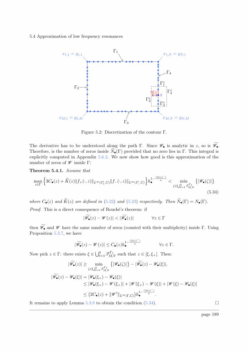
5.4 Approximation of low frequency resonances
Γ1
Γ2
Γ3
Γ4
x1,1 = y1,1
xM,1 = y1,M xM,N = yN,M
x1,N = yN,1
z
Γz1
Γz2
Γz3
Γz4η(z)
Figure 5.2: Discretization of the contour Γ.
The derivative has to be understood along the path Γ. Since W• is analytic in z, so is W•.Therefore, is the number of zeros inside N•(Γ) provided that no zero lies in Γ. This integral isexplicitly computed in Appendix 5.6.2. We now show how good is this approximation of thenumber of zeros of W inside Γ:
Theorem 5.4.1. Assume that
maxz∈Γ
3C•(z) + qK(z)‖f+(·, z)‖L∞(Ir+,C)‖f−(·, z)‖L∞(Ir−,C)
h1− |ℑ(z)−|
κ• < minζ∈
⋃4ℓ=1T
ΓℓM,N
|W•(ζ)|
(5.34)
where C•(z) and qK(z) are defined in (5.22) and (5.23) respectively. Then N•(Γ) = N•(Γ).
Proof. This is a direct consequence of Rouché’s theorem: if
|W•(z)−W (z)| < |W•(z)| ∀z ∈ Γ
then W• and W have the same number of zeros (counted with their multiplicity) inside Γ. UsingProposition 5.3.7, we have
|W•(z)−W (z)| ≤ C•(z)h1− |ℑ(z)−|
κ• ∀z ∈ Γ.
Now pick z ∈ Γ: there exists ξ ∈ ⋃4ℓ=1T
ΓℓM,N such that z ∈ [ξ, ξ+[. Then:
|W•(z)| ≥ minζ∈
⋃4ℓ=1T
ΓℓM,N
|W•(ζ)|
− |W•(z)−W•(ξ)|,
|W•(z)−W•(ξ)| = |W•(ξ+)−W•(ξ)|≤ |W•(ξ+)−W (ξ+)|+ |W (ξ+)−W (ξ)|+ |W (ξ)−W•(ξ)|
≤(2C•(z) + ‖W ′‖L∞(Γ,C)
)h1− |ℑ(z)−|
κ• .
It remains to apply Lemma 5.3.8 to obtain the condition (5.34).
page 189
5.4 Approximation of low frequency resonances
Remark 5.4.2. If h• is sufficiently small, then formula (5.34) allows us to directly read on theminimal value of the approximated Wronskian W• on the mesh points whether or not N•(Γ) = N(Γ).As h• → 0, the left-hand side goes to 0 so that the scheme necessarily gives the right numberof resonances enclosed by Γ, unless we detect a zero on Γ (that is, an element z ∈ Γ such that
|W•(z)| ≤ h•). As for Proposition 5.3.7, the estimate worsens as ℑ(z)→ κ.
Note that it is possible to take maximum and minimum over each Γℓ in (5.34) to improve thecondition.
To end this Subsection, we show that the scheme also allows us to find a simple resonance upto an error which tends to 0 as h• does. The purpose here is not giving a sharp estimate but onlyproving that we can approximate resonances with our scheme. In order to avoid estimates forW ′ −W ′
• and W ′′• , we use the analyticity of the functions as follows: we can obtain W ′ from W
using Cauchy formula
W ′(z) =1
(2πi)2
˛
Γz
W (ω)
(ω − z)2dω ∀z ∈ Γ
where Γz is a positively oriented rectangle enclosing z ∈ Γ (any other Γz′ is a translation of Γz).We write Γz :=
⋃4ℓ=1 Γ
zℓ and discretize Γz as we did for Γ: we choose M z, N z > 0 and construct
four meshes TΓ1,zMz ,Nz , T
Γ2,zMz ,Nz , T
Γ3,zMz ,Nz and T
Γ4,zMz ,Nz whose elements are respectively (xz1,k)1≤k≤Nz ,
(xzMz ,k)1≤k≤Nz , (yzj,1)1≤j≤Mz and (yzj,Nz)1≤j≤Mz . We construct them so that the larger distance
between two mesh points is at most h1− |ℑ(z)−|
κ• . Furthermore, we choose Γz so that (see Figure5.2)
η(z) := dist(z,Γz
)> 0.
We also assume that
|W (z)| > ǫ > 2C•(Γ)h1− |ℑ(z)−|
κ• > 0, C•(Γ) := maxz∈Γ
C•(z)
(5.35)
Having |W (z)| ≤ C•(Γ)h1− |ℑ(z)−|
κ• means that |W (z)| can be 0 in practice; the above conditioncan be checked by evaluating the minimum value of W•(z), z ∈ Γ, then using Proposition 5.3.7.Let z0 ∈ C be a simple resonance inside Γ and define
z•,0 :=1
(2πi)2
˛
Γ
z
W•(z)
(˛
Γz
W•(ω)(ω − z)2dω
)dz.
The explicit expression of z•,0 is given in Appendix 5.6.3.
Theorem 5.4.3. Assume (5.25). Let z ∈ C such that ℑ(z) > −κ. Then
|z0 − z•,0| ≤ maxz∈Γ
|z|C•(Γ)h
1− |ℑ(z0)−|
κ•
page 190
5.4 Approximation of low frequency resonances
where
C•(Γ) =maxz∈Γ
|z||Γ|
(2π)2(ǫ− C•(Γ)h•
) maxz∈Γ
|Γz|η(z)2
(‖W ′‖L∞(Γz ,C) + 3C•(z)
)
×(2 +
h•(ǫ− C•(Γ)h•
) maxz∈Γ
3
2‖W ′‖L∞(Γz ,C) + 3C•(z)
).
The dependence in z of C•(z) and |W ′(z)| are respectively shown in (5.22) and Lemma 5.3.8.
Proof. Form (5.33) for k = 1, we can obviously get the term maxz∈Γ|z|
out of the integral.We start by writing
W (ω)W•(z)−W (z)W•(ω) = W•(z)(W (ω)− W•(ω)
)+(W•(ω)−W (ω)
)(W•(z)−W (z)
)
+(W (ω)−W (z)
)(W•(z)−W (z)
)+ W (z)
(W•(z)−W (z)
).
It follows: Let ξ ∈4⋃
ℓ=1
TΓℓM,N such that z ∈ [ξ, ξ+[. We have
W (z)− W•(z) =(W (z)−W•(ξ)
)+
z − ξξ+ − ξ
(W•(ξ)−W•(ξ+)
)
=(W (z)−W (ξ)
)+(W (ξ)−W•(ξ)
)
+z − ξξ+ − ξ
((W•(ξ)−W (ξ)
)+(W (ξ)−W (ξ+)
)+(W (ξ+)−W•(ξ+)
))
with
W (z)−W (ξ) = (z − ξ)ˆ 1
0W
′(ξ + t(z − ξ))dt
and a similar formula holds for W (ξ)−W (ξ+). Using that∣∣∣ z−ξξ+−ξ
∣∣∣ ≤ 1, we obtain:
∣∣∣W (z)− W•(z)∣∣∣ ≤ 2|z − ξ|‖W ′‖L∞(Γ,C) + 3‖W −W•‖L∞(Γ,C). (5.36)
Likewise, let ξz ∈4⋃
ℓ=1
TΓℓ,zMz,Nz such that z ∈ [ξz, ξz+[; we have:
∣∣∣W (ω)− W•(ω)∣∣∣ ≤ 2|ω − ξz|‖W ′‖L∞(Γz ,C) + 3‖W −W•‖L∞(Γz ,C). (5.37)
We also have:∣∣W (ω)−W (z)
∣∣ ≤ |ω − z|‖W ′‖L∞ (Γz ,C). (5.38)
Here Γz denotes abusively the set of complex numbers enclosed by Γz.
page 191
5.4 Approximation of low frequency resonances
Now integrate:
∣∣∣N(Γ)− N•(Γ)∣∣∣ ≤ 1
(2π)2
˛
Γ
˛
Γz
∣∣∣∣∣W (ω)
W (z)− W•(ω)
W•(z)
∣∣∣∣∣|dω||dz||ω − z|2
≤ 1
(2π)2
˛
Γ
˛
Γz
∣∣W (ω)− W•(ω)∣∣
|W (z)||dω||dz||ω − z|2
+1
(2π)2
˛
Γ
˛
Γz
∣∣W•(z)−W (z)∣∣
|W•(z)||dω||dz||ω − z|2
+1
(2π)2
˛
Γ
˛
Γz
∣∣W•(z)−W (z)∣∣(∣∣W•(ω)−W (ω)
∣∣+∣∣W (ω)−W (z)
∣∣)
∣∣W (z)W•(z)∣∣
|dω||dz||ω − z|2
=: I + II + III.
First, using (5.37), we find:
I ≤ 1
(2π)2
˛
Γ
˛
Γz
∣∣W (ω)− W•(ω)∣∣
|W (z)||dω||dz||ω − z|2
≤ 1
(2π)2
˛
Γ
∑
ξz∈⋃4
ℓ=1TΓℓ,z
Mz,Nz
ˆ ξz+
ξz
2|ω − ξz|‖W ′‖L∞(Γz ,C) + 3‖W −W•‖L∞(Γz ,C)
|W (z)||dω||dz||ω − z|2
≤ |Γ|(2π)2ǫ
maxz∈Γ
|Γz|η(z)2
(h•‖W ′‖L∞(Γz ,C) + 3‖W −W•‖L∞(Γz ,C)
).
Next, (5.36) as well as the fact that |W•(z)| ≥ |W (z)| − C•(Γ)h• (by Proposition 5.3.4 andassumption (5.35)) imply:
II ≤ 1
(2π)2
˛
Γ
˛
Γz
∣∣W•(z)−W (z)∣∣
|W•(z)||dω||dz||ω − z|2
≤ 1
(2π)2
∑
ξ∈⋃4ℓ=1T
ΓℓM,N
ˆ ξ+
ξ
˛
Γz
2|z − ξ|‖W ′‖L∞(Γ,C) + 3‖W −W•‖L∞(Γ,C)∣∣W•(z)∣∣
|dω||dz||ω − z|2
≤ |Γ|(2π)2
(ǫ− C•(Γ)h•
)(h•‖W ′‖L∞(Γ,C) + 3‖W −W•‖L∞(Γ,C)
)maxz∈Γ
|Γz|η(z)2
.
Finally, (5.36), (5.37), (5.38) yield:
III ≤ 1
(2π)2
˛
Γ
˛
Γz
∣∣W•(z)−W (z)∣∣(∣∣W•(ω)−W (ω)
∣∣+∣∣W (ω)−W (z)
∣∣)
∣∣W (z)W•(z)∣∣
|dω||dz||ω − z|2
≤ |Γ|(2π)2ǫ
(ǫ− C•(Γ)h•
)(h•‖W ′‖L∞(Γ,C) + 3‖W −W•‖L∞(Γ,C)
)
×maxz∈Γ
|Γz|η(z)2
(h•‖W ′‖L∞(Γz ,C) + 3‖W −W•‖L∞(Γz ,C) +
h•2‖W ′‖L∞ (Γz ,C)
).
page 192
5.4 Approximation of low frequency resonances
By Proposition 5.3.7 and Lemma 5.3.8, we have:
|W (z)−W•(z)| ≤ C•(z)h1− |ℑ(z)−|
κ• ,
|W ′(z)| ≤ qK(z)‖f+(·, z)‖L∞(Ir+,C)‖f−(·, z)‖L∞(Ir−,C).
By checking the dependences in s, z of the constants C•(z) (defined in (5.22)), qK(z) (definedin (5.23)) and ‖f±(·, z)‖L∞(Ir±,C) (cf. Lemma 5.3.5), we see that the estimates increase as
max1, |s||z| or (|κ±| − ℑ(z)−)−k for some k ∈ N. Now the theorem follows from
‖W −W•‖L∞(Γ,C) ≤ ‖W −W•‖L∞(Γz ,C),
‖W ′‖L∞(Γ,C) ≤ ‖W ′‖L∞ (Γz ,C) = ‖W ′‖L∞(Γz ,C)
since Γ ⊂ ⋃z∈Γ Γz. This completes the proof.
Remark 5.4.4. To get a better estimate, we can also start as follows:
W ′(z)W (z)
− W ′• (z)
W•(z)=
W•(z)(W ′(z)− W ′
• (z))− W ′
• (z)(W (z)− W•(z)
)
W (z)W•(z),
W′(z)− W
′• (z) = W
′(z)− W•(ξ+)−W•(ξ)ξ+ − ξ
=(W
′(z)−W′• (ξ)
)+ (ξ+ − ξ)
ˆ 1
0(1− t)W ′′
•(ξ + t(ξ+)
)dt.
But as explained above, this would require a control of W ′ −W ′• as well as W ′′
• , which in turnrequires tedious computations and much time.
5.4.3 Discussion about the constants
We discuss in this Subsection the different values the constant C•(z) can take depending on allthe parameters M,Q,Λ, ℓ,m and s.
Computing the approximation W•(z) of the Wronskian, we discover that its modulus is smallin practice: |W•(z)| ≃ 10−6 for s ≃ 10−3, |W•(z)| ≃ 10−2 for s ≃ 10−1. Besides, we need tomore than 48 hours to compute W•(z) for z ranging over a regular mesh with h• = 10−3 on therectangle Γ of vertexes 0.5 + 0.5i, −0.5 + 0.5i, −0.5 and 0.5. This means that "good" values forC•(z) would satisfy C•(z) ≃ 10−3 for s ≃ 10−3, C•(z) ≃ 10 for s ≃ 10−1.
Unfortunately, we did not found such satisfying values for C•(z) as C•(z) ≥ 1010 in practicewhen z is near 0. It even happens that the value of C•(z) is so huge that computer answers"inf" (+∞). We however noticed that more decent values are obtained near the extremal case9ΛM2 = 1 − ǫ with ǫ > 0 very small. The optimal configuration we have found so far is thefollowing one:
M = 491, Q = 230, Λ =0.8175
9M2, ℓ = 0. (5.39)
page 193
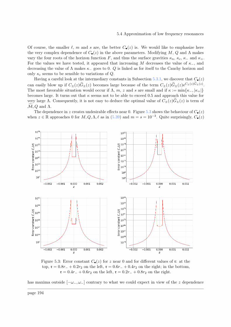
5.4 Approximation of low frequency resonances
Of course, the smaller ℓ, m and s are, the better C•(z) is. We would like to emphasize herethe very complex dependence of C•(z) in the above parameters. Modifying M , Q and Λ makesvary the four roots of the horizon function F , and thus the surface gravities κn, κc, κ− and κ+.For the values we have tested, it appeared that increasing M decreases the value of κ−, anddecreasing the value of Λ makes κ− goes to 0. Q is linked as for itself to the Cauchy horizon andonly κc seems to be sensible to variations of Q.
Having a careful look at the intermediary constants in Subsection 5.3.1, we discover that C•(z)
can easily blow up if C±(z)G±(z) becomes large because of the term C±(z)G±(z)eC±(z)G±(z).The most favorable situation would occur if Λ, m, z and s are small and if κ := minκ−, |κ+|becomes large. It turns out that κ seems not to be able to exceed 0.5 and approach this value forvery large Λ. Consequently, it is not easy to deduce the optimal value of C±(z)G±(z) is term ofM, Q and Λ.
The dependence in z creates undesirable effects near 0. Figure 5.3 shows the behaviour of C•(z)when z ∈ R approaches 0 for M,Q,Λ, ℓ as in (5.39) and m = s = 10−3. Quite surprisingly, C•(z)
Figure 5.3: Error constant C•(z) for z near 0 and for different values of r: at thetop, r = 0.8r− + 0.2r2 on the left, r = 0.6r− + 0.4r2 on the right; in the bottom,
r = 0.4r− + 0.6r2 on the left, r = 0.2r− + 0.8r2 on the right.
has maxima outside [−ω−, ω−] contrary to what we could expect in view of the z dependence
page 194
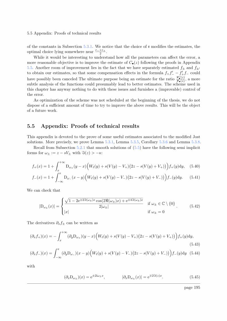
5.5 Appendix: Proofs of technical results
of the constants in Subsection 5.3.1. We notice that the choice of r modifies the estimates, theoptimal choice lying somewhere near r−+r+
2 .While it would be interesting to understand how all the parameters can affect the error, a
more reasonable objective is to improve the estimate of C•(z) following the proofs in Appendix5.5. Another room of improvement lies in the fact that we have separately estimated f± and f±′
to obtain our estimates, so that some compensation effects in the formula f+f ′− − f ′+f− could
have possibly been canceled The ultimate purpose being an estimate for the ratio W ′• (z)
W•(z), a more
subtle analysis of the functions could presumably lead to better estimates. The scheme used inthis chapter has anyway nothing to do with these issues and furnishes a (improvable) control ofthe error.
As optimization of the scheme was not scheduled at the beginning of the thesis, we do notdispose of a sufficient amount of time to try to improve the above results. This will be the objectof a future work.
5.5 Appendix: Proofs of technical results
This appendix is devoted to the prove of some useful estimates associated to the modified Jostsolutions. More precisely, we prove Lemma 5.3.1, Lemma 5.3.5, Corollary 5.3.6 and Lemma 5.3.8.
Recall from Subsection 5.2.1 that smooth solutions of (5.5) have the following semi implicitforms for ω± := z − sV± with ℑ(z) > −κ:
f+(x) = 1 +
ˆ +∞
xDω+(y − x)
(Wℓ(y) + s(V (y)− V+)
(2z − s(V (y) + V+)
))f+(y)dy, (5.40)
f−(x) = 1 +
ˆ x
−∞Dω−(x− y)
(Wℓ(y) + s(V (y)− V−)
(2z − s(V (y) + V−)
))f−(y)dy. (5.41)
We can check that
|Dω±(x)| =
√1− 2e∓2ℑ(ω±)x cos(2ℜ(ω±)x) + e∓4ℑ(ω±)x
2|ω±|if ω± ∈ C \ 0
|x| if ω± = 0
. (5.42)
The derivatives ∂xf± can be written as
(∂xf+)(x) = −ˆ +∞
x(∂yDω+)(y − x)
(Wℓ(y) + s(V (y)− V+)
(2z − s(V (y) + V+)
))f+(y)dy,
(5.43)
(∂xf−)(x) =ˆ x
−∞(∂yDω−)(x− y)
(Wℓ(y) + s(V (y)− V−)
(2z − s(V (y) + V−)
))f−(y)dy (5.44)
with
(∂xDω±)(x) = e±2iω±x, |∂xDω±(x)| = e∓2ℑ(z)x. (5.45)
page 195
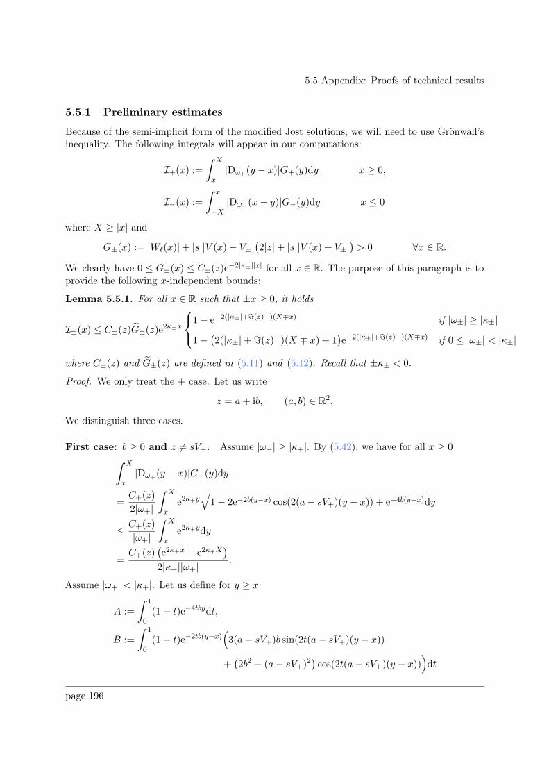
5.5 Appendix: Proofs of technical results
5.5.1 Preliminary estimates
Because of the semi-implicit form of the modified Jost solutions, we will need to use Grönwall’sinequality. The following integrals will appear in our computations:
I+(x) :=ˆ X
x|Dω+(y − x)|G+(y)dy x ≥ 0,
I−(x) :=ˆ x
−X|Dω−(x− y)|G−(y)dy x ≤ 0
where X ≥ |x| and
G±(x) := |Wℓ(x)|+ |s||V (x)− V±|(2|z|+ |s||V (x) + V±|
)> 0 ∀x ∈ R.
We clearly have 0 ≤ G±(x) ≤ C±(z)e−2|κ±||x| for all x ∈ R. The purpose of this paragraph is toprovide the following x-independent bounds:
Lemma 5.5.1. For all x ∈ R such that ±x ≥ 0, it holds
I±(x) ≤ C±(z)G±(z)e2κ±x
1− e−2(|κ±|+ℑ(z)−)(X∓x) if |ω±| ≥ |κ±|
1−(2(|κ±|+ ℑ(z)−)(X ∓ x) + 1
)e−2(|κ±|+ℑ(z)−)(X∓x) if 0 ≤ |ω±| < |κ±|
where C±(z) and G±(z) are defined in (5.11) and (5.12). Recall that ±κ± < 0.
Proof. We only treat the + case. Let us write
z = a+ ib, (a, b) ∈ R2.
We distinguish three cases.
First case: b ≥ 0 and z 6= sV+. Assume |ω+| ≥ |κ+|. By (5.42), we have for all x ≥ 0
ˆ X
x|Dω+(y − x)|G+(y)dy
=C+(z)
2|ω+|
ˆ X
xe2κ+y
√1− 2e−2b(y−x) cos(2(a− sV+)(y − x)) + e−4b(y−x)dy
≤ C+(z)
|ω+|
ˆ X
xe2κ+ydy
=C+(z)
(e2κ+x − e2κ+X
)
2|κ+||ω+|.
Assume |ω+| < |κ+|. Let us define for y ≥ x
A :=
ˆ 1
0(1− t)e−4tbydt,
B :=
ˆ 1
0(1− t)e−2tb(y−x)
(3(a− sV+)b sin(2t(a− sV+)(y − x))
+(2b2 − (a− sV+)2
)cos(2t(a− sV+)(y − x))
)dt
page 196
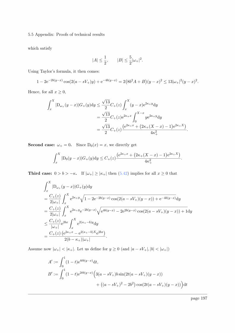
5.5 Appendix: Proofs of technical results
which satisfy
|A| ≤ 1
2, |B| ≤ 5
2|ω+|2.
Using Taylor’s formula, it then comes:
1− 2e−2b(y−x) cos(2(a− sV+)y) + e−4b(y−x) = 2(8b2A+B
)(y − x)2 ≤ 13|ω+|2(y − x)2.
Hence, for all x ≥ 0,
ˆ X
x|Dω+(y − x)|G+(y)dy ≤
√13
2C+(z)
ˆ X
x(y − x)e2κ+ydy
=
√13
2C+(z)e
2κ+x
ˆ X−x
0ye2κ+ydy
=
√13
2C+(z)
(e2κ+x +
(2κ+(X − x)− 1
)e2κ+X
)
4κ2+.
Second case: ω+ = 0. Since D0(x) = x, we directly get
ˆ X
x|D0(y − x)|G+(y)dy ≤ C+(z)
(e2κ+x +
(2κ+(X − x)− 1
)e2κ+X
)
4κ2+.
Third case: 0 > b > −κ. If |ω+| ≥ |κ+| then (5.42) implies for all x ≥ 0 that
ˆ X
x|Dω+(y − x)|G+(y)dy
=C+(z)
2|ω+|
ˆ X
xe2κ+y
√1− 2e−2b(y−x) cos(2(a− sV+)(y − x)) + e−4b(y−x)dy
=C+(z)
2|ω+|
ˆ X
xe2κ+ye−2b(y−x)
√e4b(y−x) − 2e2b(y−x) cos(2(a− sV+)(y − x)) + 1dy
≤ C+(z)
|ω+|e2bxˆ X
xe2(κ+−b)ydy
=C+(z)
(e2κ+x − e2(κ+−b)Xe2bx
)
2(b− κ+)|ω+|.
Assume now |ω+| < |κ+|. Let us define for y ≥ 0 (and |a− sV+|, |b| < |ω+|)
A′ :=ˆ 1
0(1− t)e4tb(y−x)dt,
B′ :=ˆ 1
0(1− t)e2tb(y−x)
(3(a− sV+)b sin(2t(a− sV+)(y − x))
+((a− sV+)2 − 2b2
)cos(2t(a− sV+)(y − x))
)dt
page 197
5.5 Appendix: Proofs of technical results
which satisfy
|A′| ≤ 1
2, |B′| ≤ 5
2|ω+|2.
By Taylor’s formula, we have
1− 2e−2b(y−x) cos(2(a− sV+)(y − x)) + e−4b(y−x)
= e−4b(y−x)(e4b(y−x) − 2e2b(y−x) cos(2(a− sV+)(y − x)) + 1
)
= 2e−4b(y−x)(8b2A′ −B′)(y − x)2
≤ 13|ω+|2(y − x)2e−4b(y−x).
Hence, for all x ≥ 0,
ˆ X
x|Dω+(y − x)|G+(y)dy ≤
√13
2C+(z)e
2bx
ˆ X
x(y − x)e2(κ+−b)ydy
=
√13
2C+(z)e
2κ+x
ˆ X−x
0ye2(κ+−b)ydy
=
√13
2C+(z)
(e2κ+x +
(2(κ+ − b)(X − x)− 1
)e2(κ+−b)Xe2bx
)
4(b− κ+)2.
This completes the proof.
5.5.2 Proof of Lemma 5.3.1
We only treat the + case. Let r ∈ Ir+; there exists an unique p ∈ T+•,0 such that r ∈ ω+
p = [p, p+[.
First component
We have
(f+ −F•,+f+
)(r) =
f+(r)− f+(p)2
+f+(r)− f+(p+)
2. (5.46)
Having a bound for the first term on the right-hand side will be enough. The proof is differentwhether p+ = r+ or not.
1. First case: p+ 6= r+. In this case r+ − r ≥ h•. We have
(f+(r)− f+(p)
)=
ˆ +∞
φ(r)
(Dω+(y − φ(r))−Dω+(y − φ(p))
)W+,ℓ(y)f+(y)dy
−ˆ φ(r)
φ(p)Dω+(y − φ(p))W+,ℓ(y)f+(y)dy
=: I + II
withW+,ℓ(x) :=Wℓ(r(x))+s(V (r(x))−V+)(2z−s(V (r(x))+V+)
). Notice that |W+,ℓ(x)| ≤
C+(z)e2κ+x.
page 198
5.5 Appendix: Proofs of technical results
Let us deal with I. When ω+ 6= 0, observe that
Dω+(y − φ(r))−Dω+(y − φ(p)) =e2iω+(y−φ(r)) − 1
2iω+− e2iω+(y−φ(p)) − 1
2iω+
=
e2iω+(y−φ(r))
2iω+
(1− e2iω+(φ(r)−φ(p))
)if ℑ(z) ≥ 0
e2iω+(y−φ(p))
2iω+
(e2iω+(φ(p)−φ(r)) − 1
)if ℑ(z) < 0
=
−e2iω+(y−φ(r))(φ(r)− φ(p))ˆ 1
0e2iω+t(φ(r)−φ(p))dt if ℑ(z) ≥ 0
e2iω+(y−φ(p))(φ(p)− φ(r))ˆ 1
0e2iω+t(φ(p)−φ(r))dt if ℑ(z) < 0
and all the integral terms are bounded in norm by 1 since 0 ≤ φ(p) ≤ φ(r) (recall here thatφ(r′) ≥ 0 if and only if r′ ≥ r). It then follows:
|I| ≤ ‖f+‖L∞(Ir+,C)C+(z)(φ(r)− φ(p))2(|κ+|+ ℑ(z))
e2κ+φ(r) if ℑ(z) ≥ 0
e2(κ+−ℑ(z))φ(r)e2ℑ(z)φ(p) if ℑ(z) < 0. (5.47)
When ω+ = 0, we simply get
|I| ≤ ‖f+‖L∞(Ir+,C)C+(z)(φ(r)− φ(p))
2|κ+|e2κ+φ(r)
which is contained in estimate (5.47). Next, formula (4.39) entails with the fact thatκc, κ+ < 0:
φ(r)− φ(p) =∑
α∈n,c,−,+
1
2καln
∣∣∣∣r − rαr− rα
∣∣∣∣−∑
α∈n,c,−,+
1
2καln
∣∣∣∣p− rαr− rα
∣∣∣∣
=∑
α∈n,c,−
1
2καln
(1 +
r − pp− rα
)+
1
2κ+ln
(1− r − p
r+ − p
)
=∑
α∈n,c,−
1
2κα
r − pp− rα
ˆ 1
0
dt
1 + t r−pp−rα
− 1
2κ+
r − pr+ − p
ˆ 1
0
dt
1− t r−pr+−p
≤∑
α∈n,−
1
2κα
r − pp− rα
− 1
2κ+
r − pr+ − r
≤∑
α∈n,−
1
2κα
r − pr− rα
+1
2|κ+|r − pr+ − r
. (5.48)
Using (4.41), we can write
e2κ+φ(r) =r+ − rr+ − r
∏
α∈n,c,−
(r − rαr− rα
)κ+κα
(5.49)
page 199
5.5 Appendix: Proofs of technical results
so that
e2(κ+−ℑ(z)−)φ(r)
r+ − r=
(e2κ+φ(r)
)κ+−ℑ(z)−
κ+
r+ − r=
(r+ − r)−ℑ(z)−
κ+
(r+ − r)κ+−ℑ(z)−
κ+
∏
α∈n,c,−
(r − rαr− rα
)κ+−ℑ(z)−
κα
.
Since r − p ≤ h• and r+ − r ≥ h•, we eventually find:
|I| ≤ ‖f+‖L∞(Ir+,C)C+(z)
2(|κ+|+ ℑ(z))
∑
α∈n,−
1
2κα
h•r− rα
+1
2|κ+|(r − p)e2(κ+−ℑ(z)−)φ(r)
r+ − r
≤ ‖f+‖L∞(Ir+,C)C+(z)
4(|κ+|+ ℑ(z))
×
∑
α∈n,−
hℑ(z)−
κ+•
κα(r− rα)+
(r+ − r)|κ+|+ℑ(z)−
κ+
|κ+|
(r+ − rcr− rc
)κ+−ℑ(z)−
κc
h
1−ℑ(z)−
κ+• . (5.50)
Let us turn to II. Applying Lemma 5.5.1 with X = φ(r) and x = φ(p), we get
|II| ≤ ‖f+‖L∞(Ir+,C)C+(z)G+(z)e2κ+φ(p)
×
1− e−2(|κ+|+ℑ(z)−)(φ(r)−φ(p)) if |ω+| ≥ |κ+|
1−(2(|κ+|+ ℑ(z)−)(φ(r)− φ(p)) + 1
)e−2(|κ+|+ℑ(z)−)(φ(r)−φ(p)) if 0 ≤ |ω+| < |κ+|
.
We have
e−2(|κ+|+ℑ(z)−)(φ(r)−φ(p)) = 1− 2(|κ+|+ ℑ(z)−)(φ(r)− φ(p))ˆ 1
0e−2(|κ+|+ℑ(z)−)t(φ(r)−φ(p))dt
and the integral in bounded by 1. If |ω+| ≥ |κ+|, then
|II| ≤ 2‖f+‖L∞(Ir+,C)C+(z)G+(z)(|κ+|+ ℑ(z)−)e2κ+φ(p)(φ(r)− φ(p))
≤ 2‖f+‖L∞(Ir+,C)C+(z)G+(z)(|κ+|+ ℑ(z)−)e2κ+φ(p)
∑
α∈n,−
1
2κα
r − pr− rα
+1
2|κ+|r − pr+ − r
.
Using (5.49) with r = p as well as r+−pr+−r ≤ 2 (because p+ 6= r+), we can write
e2κ+φ(p)
r+ − r≤ 2
r+ − r
(r+ − rcr− rc
)κ+κc
.
It follows for |ω+| ≥ |κ+|:
|II| ≤ 2‖f+‖L∞(Ir+,C)C+(z)G+(z)(|κ+|+ ℑ(z)−)
×
∑
α∈n,−
1
2κα(r− rα)+
1
|κ+|(r+ − r)
(r+ − rcr− rc
)κ+κc
h•.
page 200
5.5 Appendix: Proofs of technical results
Finally, assume 0 ≤ |ω+| < |κ+|. Writing∣∣∣1−
(2(|κ+|+ ℑ(z)−)(φ(r)− φ(p)) + 1
)e−2(|κ+|+ℑ(z)−)(φ(r)−φ(p))
∣∣∣
≤∣∣∣1− e−2(|κ+|+ℑ(z)−)(φ(r)−φ(p))
∣∣∣+ 2(|κ+|+ ℑ(z)−)(φ(r)− φ(p))e−2(|κ+|+ℑ(z)−)(φ(r)−φ(p))
≤ 4(|κ+|+ ℑ(z)−)(φ(r)− φ(p)),
we obtain two times the precedent bound for |II|:
|II| ≤ 4‖f+‖L∞(Ir+,C)C+(z)G+(z)(|κ+|+ ℑ(z)−)
×
∑
α∈n,−
1
2κα(r− rα)+
1
|κ+|(r+ − r)
(r+ − rcr− rc
)κ+κc
h•. (5.51)
2. Second case: p+ = r+. This time r+ − p = h•. As above, we only show the computationsfor3 f+(r)− f+(p) in (5.46). We have
∣∣f+(r)− f+(p)∣∣ ≤ ‖f+‖L∞(Ir+,C)
(ˆ +∞
φ(r)
(∣∣Dω+(y − φ(r))∣∣+∣∣Dω+(y − φ(p))
∣∣)∣∣W+,ℓ(y)
∣∣dy
+
ˆ φ(r)
φ(p)
∣∣Dω+(y − φ(p))∣∣∣∣W+,ℓ(y)
∣∣dy)
≤ ‖f+‖L∞(Ir+,C)
(ˆ +∞
φ(r)
∣∣Dω+(y − φ(r))∣∣e2κ+ydy + 2
ˆ +∞
φ(p)
∣∣Dω+(y − φ(p))∣∣e2κ+ydy
).
Recalling that φ(r) ≥ φ(p), we can use Lemma 5.5.1 for X = +∞ and x = φ(p):∣∣f+(r)− f+(p)
∣∣ ≤ 3‖f+‖L∞(Ir+,C)C+(z)G+(z)e2κ+φ(p).
It remains to use (5.49) as well as r+ − p = h• to obtain
∣∣f+(r)− f+(p)∣∣ ≤ 3‖f+‖L∞(Ir+,C)C+(z)G+(z)
1
r+ − r
(r+ − rcr− rc
)κ+κc
h•. (5.52)
3. Conclusion: comparing the bounds in (5.50), (5.51) and (5.52), we find with assumption(5.25):
∣∣f+(r)− f+(p)∣∣ ≤ ‖f+‖L∞(Ir+,C)C+(z)
(1
4(|κ+|+ ℑ(z))+ 4G+(z)max
1, |κ+|+ ℑ(z)−
)
×
∑
α∈n,−
1
κα(r− rα)+ max
1,
1
|κ+|
(r+ − r)
|κ+|+ℑ(z)−
κ+
(r+ − rcr− rc
)κ+−ℑ(z)−
κc
× h1−ℑ(z)−
κ+• . (5.53)
This establishes (5.26) for j = 0.3The other term is dealt using that f+(r+) = 1.
page 201
5.5 Appendix: Proofs of technical results
Second component
Let us write:
(F (r)∂rf+ −F•,+F (r)∂ru
)(r) =
F (r)f ′+(r)− F (p)f ′+(p)2
+F (r)f ′+(r)− F (p+)f ′+(p+)
2.
Once again, it is sufficient to get an estimate for the first term on the right-hand side. We have:
F (r)f ′+(r)− F (p)f ′+(p) = (∂xf+)(φ(r))− (∂xf+)(φ(p))
= −ˆ +∞
φ(r)(∂yDω+)(y − φ(r))W+,ℓ(y)f+(y)dy
+
ˆ +∞
φ(p)(∂yDω+)(y − φ(p))W+,ℓ(y)f+(y)dy
= −ˆ +∞
φ(r)
((∂yDω+)(y − φ(r))− (∂yDω+)(y − φ(p))
)W+,ℓ(y)f+(y)dy
+
ˆ φ(r)
φ(p)(∂yDω+)(y − φ(p))W+,ℓ(y)f+(y)dy
=: A′ +B′.
We distinguish two cases.
1. First case: p+ 6= r+. We start with A′. We have
(∂yDω+)(y − φ(r))− (∂yDω+)(y − φ(p))= e2iω+(y−φ(r)) − e2iω+(y−φ(p))
=
e2iω+(y−φ(r))(1− e2iω+(φ(r)−φ(p))
)if ℑ(z) ≥ 0
e2iω+(y−φ(p))(e2iω+(φ(p)−φ(r)) − 1
)if ℑ(z) < 0
=
−2iω+e2iω+(y−φ(r))(φ(r)− φ(p))
ˆ 1
0e2iω+t(φ(r)−φ(p))dt if ℑ(z) ≥ 0
2iω+e2iω+(y−φ(p))(φ(p)− φ(r))
ˆ 1
0e2iω+t(φ(p)−φ(r))dt if ℑ(z) < 0
and all the integral terms above have norm lesser than 1. It then follows
|A′| ≤ ‖f+‖L∞(Ir+,C)C+(z)|ω+|(φ(r)− φ(p))|κ+|+ ℑ(z)
e2(κ+−ℑ(z)−)φ(r)e2ℑ(z)−φ(p)
which is a multiple of (5.47). The bound (5.50) then gives
|A′| ≤ ‖f+‖L∞(Ir+,C)C+(z)|ω+|
2(|κ+|+ ℑ(z))
×
∑
α∈n,−
hℑ(z)−
κ+•
κα(r− rα)+
(r+ − r)|κ+|+ℑ(z)−
κ+
|κ+|
(r+ − rcr− rc
)κ+−ℑ(z)−
κc
h
1−ℑ(z)−
κ+• . (5.54)
page 202
5.5 Appendix: Proofs of technical results
For the term B′, we compute:ˆ φ(r)
φ(p)
∣∣(∂yDω+)(y − φ(p))∣∣∣∣W+,ℓ(y)
∣∣dy ≤ C+(z)
ˆ φ(r)
φ(p)e−2ℑ(z)(y−φ(p))e2κ+ydy
= C+(z)e2κ+φ(p)
2(|κ+|+ ℑ(z))(1− e2(κ+−ℑ(z))(φ(r)−φ(p))
).
By (5.48),
1− e2(κ+−ℑ(z))(φ(r)−φ(p)) = 2(|κ+|+ ℑ(z))(φ(r)− φ(p))ˆ 1
0e2(κ+−ℑ(z))t(φ(r)−φ(p))dt
≤ 2(|κ+|+ ℑ(z))(φ(r)− φ(p))
≤ 2(|κ+|+ ℑ(z))
∑
α∈n,−
1
2κα
r − pr− rα
+1
2|κ+|r − pr+ − r
and (5.49) for r = p implies
e2κ+φ(p)
r+ − r≤ 1
r+ − r
(r+ − rcr− rc
)κ+κc r+ − pr+ − r
.
As a result, since r+−pr+−r ≤ 2, we find:
|B′| ≤ ‖f+‖L∞(Ir+,C)C+(z)
∑
α∈n,−
1
2κα(r− rα)+
1
|κ+|(r+ − r)
(r+ − rcr− rc
)κ+κc
h•.
(5.55)
2. Second case: p+ = r+. We compute:∣∣(F (r)∂rf+ −F•,+F (r)∂ru
)(r)∣∣
≤ ‖f+‖L∞(Ir+,C)
(ˆ +∞
φ(r)
(∣∣(∂yDω+)(y − φ(r))∣∣+∣∣(∂yDω+)(y − φ(p))
∣∣)∣∣W+,ℓ(y)
∣∣dy
+
ˆ φ(r)
φ(p)
∣∣(∂yDω+)(y − φ(p))∣∣∣∣W+,ℓ(y)
∣∣dy)
≤ ‖f+‖L∞(Ir+,C)C+(z)
(ˆ +∞
φ(r)
∣∣(∂yDω+)(y − φ(r))∣∣e2κ+ydy + 2
ˆ +∞
φ(p)
∣∣(∂yDω+)(y − φ(p))∣∣e2κ+ydy
)
= ‖f+‖L∞(Ir+,C)C+(z)
2(|κ+|+ ℑ(z))(e2κ+φ(r) + 2e2κ+φ(p)
)
≤ 3‖f+‖L∞(Ir+,C)C+(z)
2(|κ+|+ ℑ(z))e2κ+φ(p).
Using (5.49) for r = p as well as r+ − p = h•, we finally obtain:
∣∣(F (r)∂rf+ −F•,+F (r)∂ru)(r)∣∣ ≤ 3‖f+‖L∞(Ir+,C)
C+(z)
2(|κ+|+ ℑ(z))1
r+ − r
(r+ − rcr− rc
)κ+κc
h•.
(5.56)
page 203
5.5 Appendix: Proofs of technical results
3. Conclusion: comparing all the estimates (5.54), (5.55) and (5.56) using assumption (5.25),we find
∣∣(F (r)∂rf+ −F•,+F (r)∂ru)(r)∣∣
≤ ‖f+‖L∞(Ir+,C)C+(z)
(1 +
max3, |ω+|
2(|κ+|+ ℑ(z))
)
×
∑
α∈n,−
1
κα(r− rα)+
(r+ − r)|κ+|+ℑ(z)−
κ+
|κ+|
(r+ − rcr− rc
)κ+−ℑ(z)−
κc
h
1−ℑ(z)−
κ+• .
This gives estimate (5.26) for j = 1 and completes the proof.
5.5.3 Proof of Lemma 5.3.2
We only treat the + case and omit to write R•,+ as it plays no role in the estimates. Let r ∈ Ir+.We have
(U•,+ − U•,+
)(r) =
(G•,+U•,+ − G•,+U•,+
)(r)
=(G•,+ − G•,+
)U•,+(r) + G•,+
(U•,+ − U•,+
)(r). (5.57)
The left-hand side appears on the right-hand side, so we want to apply Grönwall’s inequality. Todo this, we need two intermediary results. Recall that the constants K±, G±(z), Υ±(z), Π(z)and Θ± are respectively defined in (5.10), (5.12), (5.17), (5.18), (5.19) and (5.20).
Lemma 5.5.2. For all r ∈ Ir±, we have
∣∣((G•,± − G•,±)U•,±
)j(r)∣∣ ≤
∥∥(U•,±)j∥∥L∞(Ir±,C)
Ξ±(z)h•
where
Ξ±(z) =(Υ±(z)K± +Π(z)Θ±
)max
G±(z),
1
2(|κ±|+ ℑ(z))
.
The next result is proved in Appendix 5.5.4.
Lemma 5.5.3. For all r ∈ Ir±, we have
∥∥(U•,±)0
∥∥L∞(Ir±,C)
≤ 1 +Π(z)K±G±(z) exp(Π(z)K±G±(z)
),
∥∥(U•,±)1
∥∥L∞(Ir±,C)
≤ Π(z)K±2(|κ±|+ ℑ(z))
(1 +Π(z)K±G±(z) exp
(Π(z)K±G±(z)
)).
Assume temporarily these lemmas proved (we give their proofs below). Then we deduce from(5.57) that∣∣(U•,+ − U•,+
)j(r)∣∣ ≤
∣∣((G•,+ − G•,+)U•,+
)j(r)∣∣+∣∣(G•,+
(U•,+ − U•,+
))j(r)∣∣
≤∥∥(U•,+)j
∥∥L∞(Ir+,C)
Ξ+(z)h•
+ C+(z)
ˆ r+
r
∣∣(∂jxDω+)(φ(σ)− φ(r)
)∣∣e2κ+φ(σ)∣∣(U•,+ − U•,+
)0(σ)∣∣ dσ
F (σ)
page 204
5.5 Appendix: Proofs of technical results
When j = 0, Grönwall’s inequality implies∣∣(U•,+ − U•,+
)0(r)∣∣
≤∥∥(U•,+)0
∥∥L∞(Ir+,C)
Ξ+(z)h•
(1 + C+(z)
ˆ r+
r
∣∣Dω+
(φ(σ)− φ(r)
)∣∣e2κ+φ(σ)
× exp
(C+(z)
ˆ r+
σ
∣∣Dω+
(φ(σ′)− φ(r)
)∣∣e2κ+φ(σ′) dσ′
F (σ′)
)dσ
F (σ)
).
We can then apply Lemma 5.5.1 with X = +∞ and x = 0 ≤ φ(r) to get∣∣(U•,+ − U•,+
)0(r)∣∣ ≤
∥∥(U•,+)0∥∥L∞(Ir+,C)
Ξ+(z)(1 + C+(z)G+(z) exp
(C+(z)G+(z)
))h•.
The case j = 1 easily follows. We have∣∣(U•,+ − U•,+
)1(r)∣∣
≤∥∥(U•,+)1
∥∥L∞(Ir+,C)
Ξ+(z)h• + C+(z)∥∥(U•,+)0
∥∥L∞(Ir+,C)
Ξ+(z)(1 + C+(z)G+(z) exp
(C+(z)G+(z)
))h•
׈ r+
r
∣∣(∂xDω+)(φ(σ)− φ(r)
)∣∣e2κ+φ(σ) dσ
F (σ)
withˆ r+
r
∣∣(∂xDω+)(φ(σ)− φ(r)
)∣∣e2κ+φ(σ) dσ
F (σ)=
ˆ +∞
φ(r)e2(κ+−ℑ(z))ydy =
e2κ+φ(r)
2(|κ+|+ ℑ(z))
whence
∣∣(U•,+ − U•,+)1(r)∣∣ ≤
[∥∥(U•,+)1∥∥L∞(Ir+,C)
Ξ+(z) +C+(z)
2(|κ+|+ ℑ(z))∥∥(U•,+)0
∥∥L∞(Ir+,C)
Ξ+(z)
×(1 + C+(z)G+(z) exp
(C+(z)G+(z)
))]h•.
This completes the proof of Lemma 5.3.2.
Proof of Lemma 5.5.2
Let σ ∈ [r, r+[ and p ∈ T+•,0 such that σ ∈ [p, p+[.
1. Estimate for g+,ℓ. Recall that
g+,ℓ(σ) =Λ(σ − rn)(σ − rc)(σ − r−)
3σ2Wℓ(σ) +
s
r+σ
(2z − s(r+ + σ)
σr+
)
with
Wℓ(σ) =ℓ(ℓ+ 1)
σ2+F ′(σ)σ
+m2
so that
‖g+,ℓ‖L∞(I,R) ≤Λ(r+ − rn)(r+ − rc)(r+ − r−)
3r2−‖Wℓ‖L∞(I,R) +
|s|r2−
(2|z|+ 2|s|
r−
)=: Π(z).
page 205
5.5 Appendix: Proofs of technical results
We haveΛ(σ − rn)(σ − rc)(σ − r−)
3σ2Wℓ(σ)−
Λ(p− rn)(p− rc)(p− r−)3p2
Wℓ(p)
=Λ
3σ2Wℓ(σ)
((σ − rn)(σ − rc)(σ − r−)− (p− rn)(p− rc)(p− r−)
)
+Λ(p− rn)(p− rc)(p− r−)
3Wℓ(σ)
(1
σ2− 1
p2
)
+Λ(p− rn)(p− rc)(p− r−)
3p2(Wℓ(σ)− Wℓ(p)
)
and
(σ − rn)(σ − rc)(σ − r−)− (p− rn)(p− rc)(p− r−) = (σ − rn)((σ − rc)(σ − p) + (p− r−)(σ − p)
)
+ (p− rc)(p− r−)(σ − p).Furthermore,
s
r+σ
(2z − s(V (σ) + V+)
)− s
r+p
(2z − s(V (p) + V+)
)=s(σ − p)r+pσ
(−2z + s
(1
r++σ + p
σp
)).
It follows using the mean value theorem:∣∣g+,ℓ(σ)− g+,ℓ(p)
∣∣ ≤[(
Λ(σ − rn)(σ − rc)3σ2
+Λ(r+ − r−)(σ − rn)
3σ2+
Λ(r+ − rc)(r+ − r−)3σ2
+Λ(p− rn)(p− rc)(p− r−)
3p2σ+
Λ(p− rn)(p− rc)(p− r−)3pσ2
)∣∣Wℓ(σ)∣∣
+Λ(p− rn)(p− rc)(p− r−)
3p2∣∣Wℓ(σ)− Wℓ(p)
∣∣
+|s|r+pσ
(2|z|+ |s|
(1
r++σ + p
σp
))](σ − p)
≤ Υ+(z)h•. (5.58)
2. Estimate for k+. Recall that
k+(σ) = (r+ − r)
∏
α∈n,c,−
(r− rασ − rα
)κ+κα
.
We have
‖k+‖L∞(I,R) ≤ (r+ − r)
(r− rnr+ − rn
)κ+κn(
r− r−r+ − r−
)κ+κ−
= K+
where K+ is as in (5.10). Set θα(r) :=(
r−rαr−rα
)κ+κα and compute:
k+(σ)− k+(p) = (r+ − r)(θn(σ)θc(σ)θ−(σ)− θn(p)θc(p)θ−(p)
)
= (r+ − r)(θn(σ)
[θc(σ)
(θ−(σ)− θ−(p)
)+(θc(σ)− θc(p)
)θ−(p)
]
+(θn(σ)− θc(p)
)θc(p)θ−(p)
).
page 206
5.5 Appendix: Proofs of technical results
It comes with the mean value theorem:∣∣k+(σ)− k+(p)
∣∣ ≤ (r+ − r)(‖θ′n‖L∞(Ir+,R)‖θc‖L∞(Ir+,R)‖θ−‖L∞(Ir+,R)
+ ‖θn‖L∞(Ir+,R)‖θ′c‖L∞(Ir+,R)‖θ−‖L∞(Ir+,R)
+ ‖θn‖L∞(Ir+,R)‖θc‖L∞(Ir+,R)‖θ′−‖L∞(Ir+,R)
)h•.
Since κn > 0, κc < 0, κ− > 0 and κ+ < 0, we have:
‖θn‖L∞(Ir+,R) ≤(
r− rnr+ − rn
)κ+κn
, ‖θc‖L∞(Ir+,R) ≤ 1, ‖θ−‖L∞(Ir+,R) ≤(
r− r−r+ − r−
)κ+κ−
,
‖θ′n‖L∞(Ir+,R) ≤∣∣∣∣κ+κn
∣∣∣∣(
r− rnr+ − rn
)κ+κn
−1 1
(r− rn)2,
‖θ′c‖L∞(Ir+,R) ≤∣∣∣∣κ+κc
∣∣∣∣max
1,
(r− rcr+ − rc
)κ+κc
−1
1
(r− rc)2,
‖θ′−‖L∞(Ir+,R) ≤∣∣∣∣κ+κ−
∣∣∣∣(
r− r−r+ − r−
)κ+κ−
−1 1
(r− r−)2.
Whence:∣∣k+(σ)− k+(p)
∣∣ ≤ Θ+h•. (5.59)
3. Conclusion: combining (5.58) with (5.59), we find
∣∣W+,ℓ(σ)−W+,ℓ(p)∣∣ ≤
(∣∣g+,ℓ(σ)− g+,ℓ(p)∣∣‖k+‖L∞(I,R) + ‖g+,ℓ‖L∞(I,R)
∣∣k+(σ)− k+(p)∣∣)e2κ+φ(σ)
≤ h•(Υ+(z)K+ +Π(z)Θ+
)e2κ+φ(σ).
We thus have:
∣∣((G•,+ − G•,+)U•,+
)j(r)∣∣ ≤ˆ r+
r
∣∣(∂jxDω+)(φ(σ)− φ(r)
)∣∣∣∣W+,ℓ(σ)−W+,ℓ(p)∣∣∥∥(U•,+)j
∥∥L∞(Ir+,C)
dσ
F (σ)
≤∥∥(U•,+)j
∥∥L∞(Ir+,C)
(Υ+(z)K+ +Π(z)Θ+
)h•
׈ r+
r
∣∣(∂jxDω+)(φ(σ)− φ(r)
)∣∣e2κ+φ(σ) dσ
F (σ).
When j = 0, we can use Lemma 5.5.1 with X = +∞ and x = φ(r) (but without theconstant C+(z)): we find
∣∣((G•,+ − G•,+)U•,+
)0(r)∣∣ ≤
∥∥(U•,+)0∥∥L∞(Ir+,C)
(Υ+(z)K+ +Π(z)Θ+
)G+(z)h•.
When j = 1, we can directly use thatˆ r+
r
∣∣(∂xDω+)(φ(σ)− φ(r)
)∣∣e2κ+φ(σ) dσ
F (σ)= e2ℑ(z)φ(r)
ˆ +∞
φ(r)e2(κ+−ℑ(z))ydy =
e2κ+φ(r)
2(|κ+|+ ℑ(z)).
page 207
5.5 Appendix: Proofs of technical results
to get∣∣((G•,+ − G•,+
)U•,+
)1(r)∣∣ ≤
∥∥(U•,+)1∥∥L∞(Ir+,C)
(Υ+(z)K+ +Π(z)Θ+
) h•2(|κ+|+ ℑ(z))
.
This completes the proof of the lemma.
5.5.4 Proof of Lemma 5.5.3
By definition of the fixed point U•,+,
U•,+(r) =
(10
)+
ˆ r+
rA+(r;σ)U•,+(σ)
dσ
F (σ)
and thus∣∣(U•,+
)j(r)∣∣ ≤ δj0 +
∑
p∈T+•,0
|g+,ℓ(p)||k+(p)|ˆ
]r,r+[∩ω+p
∣∣(∂jxDω+)(φ(σ)− φ(r)
)∣∣e2κ+φ(σ)∣∣(U•,+
)0(σ)∣∣ dσ
F (σ)
≤ δj0 +Π(z)K+
ˆ r+
r
∣∣(∂jxDω+)(φ(σ)− φ(r)
)∣∣e2κ+φ(σ)∣∣(U•,+
)0(σ)∣∣ dσ
F (σ)
where K+ is as in (5.10) and Π(z) as in (5.19). When j = 0, we use Grönwall’s inequality:∣∣(U•,+
)0(r)∣∣ ≤ 1 +Π(z)K+
ˆ r+
r
∣∣Dω+
(φ(σ)− φ(r)
)∣∣e2κ+φ(σ)
× exp
(Π(z)K+
ˆ r+
σ
∣∣Dω+
(φ(σ′)− φ(r)
)∣∣e2κ+φ(σ′) dσ′
F (σ′)
)dσ
F (σ).
It remains to apply Lemma 5.5.1 with X = +∞, x = 0 ≤ φ(r) and G+(y) replaced byΠ(z)K+e
2κ+y. From there we immediately deduce the case j = 1:∣∣(U•,+
)1(r)∣∣ ≤
∥∥(U•,+)0
∥∥L∞(Ir+,C)
Π(z)K+
ˆ r+
r
∣∣(∂xDω+)(φ(σ)− φ(r)
)∣∣e2κ+φ(σ) dσ
F (σ)
=∥∥(U•,+
)0
∥∥L∞(Ir+,C)
Π(z)K+e2ℑ(z)φ(r)
ˆ +∞
φ(r)e2(κ+−ℑ(z))ydy
=∥∥(U•,+
)0
∥∥L∞(Ir+,C)
Π(z)K+e2κ+φ(r)
2(|κ+|+ ℑ(z)).
This yields the announced formulas.
5.5.5 Proof of Lemma 5.3.5
We only treat the + case. By (5.40), we have:
|f+(x)| ≤ 1 +
ˆ +∞
x|Dω+(y − x)|G+(y)|f+(y)|dy.
By Grönwall’s inequality, we get
|f+(x)| ≤ 1 +
ˆ +∞
x|Dω+(y − x)|G+(y) exp
(ˆ +∞
y|Dω+(y − y′)|G+(y
′)dy′)dy.
As r = r corresponds to x = 0, we are only needed to estimate the above terms for x = y = 0. Itremains to use Lemma 5.5.1 with X = +∞ to conclude.
page 208
5.5 Appendix: Proofs of technical results
5.5.6 Proof of Corollary 5.3.6
We only treat the + case. Using equation (5.43), we can write for all x ≥ 0:
∣∣(∂xf+)(x)∣∣ ≤ ‖f+‖L∞(Ir+,C)
ˆ +∞
x
∣∣(∂yDω+)(y − x)∣∣G+(y)dy (5.60)
with |∂xDω+(x)| = e−2ℑ(z)x (cf. (5.45)). It follows:
‖∂xf+‖L∞([0,+∞[,C) ≤ C+(z)‖f+‖L∞(I+,C)
ˆ +∞
xe−2ℑ(z)(y−x)e2κ+ydy
=C+(z)‖f+‖L∞(I+,C)e
2κ+x
2||κ±|+ ℑ(z)|.
This completes the proof.
5.5.7 Proof of Lemma 5.3.8
To make appear the dependence in z, we will write f±(x) := f±(x, z). Formula (5.30) reads inthe Regge-Wheeler coordinate:
W (z) = f+(0, z)(∂xf−)(0, z)− (∂xf+)(0, z)f−(0, z) + is(V+ − V−
)f+(0, z)f−(0, z).
Taking the derivative with respect to z yields:
W′(z) = (∂zf+)(0, z)(∂xf−)(0, z) + f+(0, z)(∂z∂xf−)(0, z)
− (∂z∂xf+)(0, z)f−(0, z) + (∂xf+)(0, z)(∂zf−)(0, z)
+ is(V+ − V−
)((∂zf+)(0, z)f−(0, z) + f+(0, z)(∂zf−)(0, z)
).
We will thus get a bound on W ′(z) if we can estimate ‖(∂zf±)(·, z)‖L∞(Ir±,C) and ‖(∂z∂xf±)(·, z)‖L∞(Ir±,C).We will only treat the + case. Lemma 5.3.8 then follows from (5.62)−(5.67) below, as well asLemma 5.3.5 and Corollary 5.3.6.
Let z ∈ C such that ℑ(z) > −κ. We will write z = a+ib with (a, b) ∈ R2 and use the constantG+(z) defined in (5.12) so that
ˆ +∞
x
∣∣Dω+(y − x)∣∣e2κ+ydy ≤ G+(z).
Estimate of the first derivatives
Let us compute
(∂zf+)(x, z) =
ˆ +∞
x
((∂zDω+)(y − x)f+(y, z) + Dω+(y − x)(∂zf+)(y, z)
)
×(Wℓ(y) + s(V (y)− V+)
(2z − s(V (y) + V+)
))dy,
+ 2s
ˆ +∞
xDω+(y − x)f+(y, z)(V (y)− V+)dy
page 209
5.5 Appendix: Proofs of technical results
with
(∂zDω±)(x) =
1
ω±
(xe±2iω±x −Dω±(x)
)if ω± ∈ C \ 0
±ix2 if ω± = 0.
We have∣∣(∂zf+)(x, z)
∣∣ ≤ ‖f+(·, z)‖L∞(Ir+,C)
ˆ +∞
x
∣∣(∂zDω+)(y − x)∣∣G+(y, z)dy
+ 2|s|‖f+(·, z)‖L∞(Ir+,C)
ˆ +∞
x
∣∣Dω+(y − x)(V (y)− V+)∣∣dy
+
ˆ +∞
x
∣∣Dω+(y − x)∣∣∣∣(∂zf+)(y, z)
∣∣G+(y, z)dy.
Recall that G+(x, z) := |Wℓ(x)| + |s||V (x) − V+|(2|z| + |s||V (x) + V+|
)≤ C+(z)e
2κ+x for allx ≥ 0. Let
I1(x) :=ˆ +∞
x
∣∣(∂zDω+)(y − x)∣∣G+(y, z)dy,
I2(x) :=ˆ +∞
x
∣∣Dω+(y − x)(V (y)− V+)∣∣dy,
I3(x) :=ˆ +∞
x
∣∣Dω+(y − x)∣∣G+(y, z)dy.
Then Grönwall’s inequality implies:∣∣(∂zf+)(x, z)
∣∣ ≤ ‖f+(·, z)‖L∞(Ir+,C)
(I1(0) + 2|s|I2(0)
)(1 + I3(0) exp
(I3(0)
)). (5.61)
It is therefore sufficient to get an x-independent bound for each Ij(x), j ∈ 1, 2, 3. Observethat we already proved that I3(x) ≤ C+(z)G+(z) for all x ≥ 0 in Subsection 5.5.5. Observefurthermore that, using |r − r+| ≤ K+e
2κ+x when x ≥ 0, we directly get
I2(x) ≤K+
r−r+
ˆ +∞
x
∣∣Dω+(y − x)∣∣e2κ+ydy ≤ K+
r−r+G+(z).
We therefore only need to bound I1(x) for all x ≥ 0.
1. First case: b ≥ 0 and z 6= sV+. Assume first |ω+| ≥ |κ+|. We compute:
I1(x) ≤C+(z)
|ω+|
ˆ +∞
x
((y − x)e2bxe2(κ+−b)y +
∣∣Dω+(y − x)∣∣e2κ+y
)dy
≤ C+(z)
|ω+|
(e2κ+x
b− κ++ G+(z)
)
We then deduce from (5.61):
∣∣(∂zf+)(x, z)∣∣ ≤ ‖f+(·, z)‖L∞(Ir+,C)
(C+(z)
|ω+|
(1
b− κ++ G+(z)
)+
2|s|K+
r−r+G+(z)
)
×(1 +
C+(z)
2|κ+||ω+|exp
(C+(z)
2|κ+||ω+|
)). (5.62)
page 210
5.5 Appendix: Proofs of technical results
Assume now |ω+| < |κ+|. Let
A :=
ˆ 1
0(1− t)e2iω+t(y−x)dt, B :=
ˆ 1
0
(1− t)22
e2iω+t(y−x)dt.
If y − x ≥ 0 then
|A| ≤ 1
2, |B| ≤ 1
6.
It follows∣∣(∂zDω+)(y − x)
∣∣ =∣∣i(y − x)2 + 4iω+(y − x)3(A−B)
∣∣ ≤ (y − x)2 + 8
3ω+(y − x)3
whence
I1(x) ≤ C+(z)
ˆ +∞
x
((y − x)2 + 8
3ω+(y − x)3
)e2κ+ydy
= C+(z)e2κ+x
ˆ +∞
0
(y2 +
8
3|ω+|y3
)e2κ+ydy
≤ C+(z)e2κ+x
(1
4|κ+|3+|ω+|κ4+
)
≤ C+(z)e2κ+x 5
4|κ+|3.
Estimate (5.61) then gives:
∣∣(∂zf+)(x, z)∣∣ ≤ ‖f+(·, z)‖L∞(Ir+,C)
(5C+(z)
4|κ+|3+
2|s|K+
r−r+G+(z)
)
×(1 +
√13C+(z)
8κ2+exp
(√13C+(z)
8κ2+
)). (5.63)
2. Second case: ω+ = 0. We have
I1(x) ≤ C+(z)
ˆ +∞
x
((y − x)2 + (y − x)
)e2κ+ydy
= C+(z)e2κ+x
ˆ +∞
0
(y2 + y
)e2κ+ydy
= C+(z)e2κ+x
(1
4|κ+|3+
1
4κ2+
).
It follows from (5.61):
∣∣(∂zf+)(x, z)∣∣ ≤ ‖f+(·, z)‖L∞(Ir+,C)
(C+(z)
(1
4|κ+|3+
1
4κ2+
)+
2|s|K+
r−r+G+(z)
)
×(1 +
C+(z)
4κ2+exp
(C+(z)
4κ2+
)).
(5.64)
page 211
5.5 Appendix: Proofs of technical results
3. Third case: 0 > b > −κ. Assume first |ω+| ≥ |κ+|. The computation carried out for thefirst case shows that
I1(x) ≤C+(z)
|ω+|
(e2κ+x
b− κ++ G+(z)
)
hence estimate (5.61) becomes:
∣∣(∂zf+)(x, z)∣∣ ≤ ‖f+(·, z)‖L∞(Ir+,C)
(C+(z)
|ω+|
(1
b− κ++ G+(z)
)+
2|s|K+
r−r+G+(z)
)
×(1 +
C+(z)
2|κ+||ω+|exp
(C+(z)
2|κ+||ω+|
)).
(5.65)
Assume eventually |ω+| < |κ+|. Define
A′ :=ˆ 1
0(1− t)e−2iω+t(y−x)dt
with
|A′| ≤ 1
2
if y − x ≥ 0. We then get
∣∣(∂zDω+)(y − x)∣∣ =
∣∣∣∣∣e2iω+(y−x)
ω+
((y − x)− 1− e−2iω+(y−x)
2iω+
)∣∣∣∣∣= e−2b(y−x)|2i(y − x)2A′|≤ (y − x)2e−2b(y−x)
whence
I1(x) ≤ C+(z)e2bx
ˆ +∞
x(y − x)2e2(κ+−b)ydy
= C+(z)e2κ+x
ˆ +∞
0y2e2(κ+−b)ydy
≤ C+(z)e2κ+x
4|κ+ − b|3.
From (5.61) we obtain:
∣∣(∂zf+)(x, z)∣∣ ≤ ‖f+(·, z)‖L∞(Ir+,C)
(C+(z)
4|κ+ − b|3+
2|s|K+
r−r+G+(z)
)
×(1 +
√13C+(z)
8(b− κ+)2exp
(√13C+(z)
8(b− κ+)2
)). (5.66)
page 212
5.6 Appendix: Approximations
Estimate for the mixed derivatives
The mixed derivative is given by
(∂z∂xf+)(x, z) = −ˆ +∞
x
((∂z∂yDω+)(y − x)f+(y, z) + (∂yDω+)(y − x)(∂zf+)(y, z)
)
×(Wℓ(y) + s(V (y)− V+)
(2z − s(V (y) + V+)
))dy,
− 2s
ˆ +∞
x(∂yDω+)(y − x)f+(y, z)(V (y)− V+)dy
with
(∂z∂xDω+)(x) = 2ixe2iω+x.
Since ‖f+(·, z)‖L∞(Ir+,C) and ‖(∂zf+)(·, z)‖L∞(Ir+,C) have been already estimated, we only have 3integrals to bound. First, we compute
ˆ +∞
x
∣∣(∂z∂yDω+)(y − x)∣∣G+(y, z)dy ≤ 2C+(z)e
2ℑ(z)x
ˆ +∞
x(y − x)e2(κ+−ℑ(z))ydy
= 2C+(z)e2κ+x
ˆ +∞
0ye2(κ+−ℑ(z))ydy
=C+(z)e
2κ+x
2(κ+ −ℑ(z))2.
Next, we have
ˆ +∞
x
∣∣(∂yDω+)(y − x)∣∣G+(y, z)dy ≤ C+(z)e
2ℑ(z)x
ˆ +∞
xe2(κ+−ℑ(z))ydy =
C+(z)e2κ+x
2|κ+ −ℑ(z)|.
Finally,
ˆ +∞
x
∣∣(∂yDω+)(y − x)(V (y)− V+)∣∣dy ≤ K+
r−r+e2ℑ(z)x
ˆ +∞
xe2(κ+−ℑ(z))ydy =
K+e2κ+x
2|κ+ −ℑ(z)|r−r+.
We eventually obtain the following estimate for all x ≥ 0:
∣∣(∂z∂xf+)(x, z)∣∣ ≤
(C+(z)
2(κ+ −ℑ(z))2+
|s|K+
|κ+ −ℑ(z)|r−r+
)‖f+(·, z)‖L∞(Ir+,C)
+C+(z)
2|κ+ −ℑ(z)|‖(∂zf+)(·, z)‖L∞(Ir+,C). (5.67)
It remains to use the estimates collected in the above paragraph to conclude the proof.
5.6 Appendix: Approximations
This appendix gives explicit formulas for the discrete version of some operators associated to thescheme as well as the integral giving the number of resonances in a path Γ ⊂ C.
page 213
5.6 Appendix: Approximations
5.6.1 Computation of the discretized operators for the scheme (5.9)
In this Section, we compute the coefficients of the discrete operators G•,± for the numericalprogramming.
Let U± ∈ E†± such that P•,±U± = U•,± ∈ E†
•,± (all the functions in E†± satisfying this
property coincide on the mesh points in T±•,0; as the mesh converges, we know by Proposition
5.3.3 that the only function with this property is the modified Jost solution f± ∈ E± ⊂ E†±).
Set
D+(p;σ) :=
(Dω+
(φ(σ)− φ(p)
)
−(∂xDω+)(φ(σ)− φ(p)
)), D−(p;σ) :=
(Dω−
(φ(p)− φ(σ)
)
(∂xDω−)(φ(p)− φ(σ)
))
and define the vectors of C2(|T ±•,0|+1):
(~U•,−
)0= 1,
(~U•,−
)1= 0
(~U•,−
)2|p|+δj1
=1
2
(U−(p) + U−(p−)
)j,
(~U•,+
)2|T ±
•,0|= 1,
(~U•,+
)2|T ±
•,0|+1= 0
(~U•,+
)2(|p|−1)+δj1
=1
2
(U+(p) + U+(p+)
)j.
Recall the convention that |p| is the number of elements p′ ∈ T±•,0 such that p′ ≤ p. For example,
|(r−)+| = 1 and |(r+)−| = |T +•,0|. Notice that the boundary terms for ~U•,− are in the first
components 0, 1 whereas they are for ~U•,+ is the last components 2|T ±•,0|, 2|T ±
•,0|+ 1.
We identify ~U•,± with U•,± via the evaluation morphism E†± → C
2(|T ±•,0|+1). For p0 ∈ T
±•,0
and j ∈ 0, 1, we have by definition of the problem (5.9):
(G•,±U•,±
)j(p0) = δj0 ±
ˆ r±
p0
D±j (p0;σ)e
2κ±φ(σ)
∑
p∈T±•,0
g±,ℓ(p)k±(p)1ωp±(σ)
×
1
2
∑
p′∈T±•,0
((U±)0(p
′) + (U±)0(p′±))1ω±
p′(σ)
dσ
F (σ)
= δj0 ±∑
p∈T±•,0
±(|p|−|p0|)≥0
1
2g±,ℓ(p)k±(p)
((U±)0(p) + (U±)0(p±)
)
׈ p±
pD±j (p0;σ)e
2κ±φ(σ) dσ
F (σ).
The operators G•,± can then be viewed as affine functions acting on C2(|T ±
•,0|+1):
(~U•,−
)2|p0|+δj1
=(U•,−
)j(p0)
=(G•,−U•,−
)j(p0)
= δj0 +∑
p∈T−•,0
|p|≤|p0|
(g−,ℓ(p)k−(p)
ˆ p
p−
D−j (p0;σ)e
2κ−φ(σ) dσ
F (σ)
)(~U•,−
)2|p|, (5.68)
page 214
5.6 Appendix: Approximations
(~U•,+
)2(|p0|−1)+δj1
=(U•,+
)j(p0)
=(G•,+U•,+
)j(p0)
= δj0 +∑
p∈T+•,0
|p|≥|p0|
(g+,ℓ(p)k+(p)
ˆ p+
pD+j (p0;σ)e
2κ+φ(σ) dσ
F (σ)
)(~U•,+
)2(|p|−1)
.
(5.69)
Recall here that r± /∈ T±•,0. In other words,
G•,± = (δj even)0≤j≤2|T ±•,0|+1 + A•,±
where the non-zero coefficients of the matrices A•,± are given by
(A•,−
)2|p0|,2|p| =
(g−,ℓ(p)k−(p)
ˆ p
p−
D−0 (p0;σ)e
2κ−φ(σ) dσ
F (σ)
)δ|p|≤|p0|
(A•,−
)2|p0|+1,2|p| =
(g−,ℓ(p)k−(p)
ˆ p
p−
D−1 (p0;σ)e
2κ−φ(σ) dσ
F (σ)
)δ|p|≤|p0|
(A•,+
)2(|p0|−1),2(|p|−1)
=
(g+,ℓ(p)k+(p)
ˆ p+
pD+0 (p0;σ)e
2κ+φ(σ) dσ
F (σ)
)δ|p|≥|p0|
(A•,+
)2|p0|−1,2(|p|−1)
=
(g+,ℓ(p)k+(p)
ˆ p+
pD+1 (p0;σ)e
2κ+φ(σ) dσ
F (σ)
)δ|p|≥|p0|
for all p0, p ∈ T±•,0. Notice that A•,− (respectively A•,+) is lower triangular (respectively upper
triangular) and has non-zero coefficients only in the columns with even index.We can use (5.68) and (5.69) to inductively find ~U•,± starting from the known boundary
values. From there it is straightforward deducing U±(p) for all p ∈ T±•,0:
(U−)j(p) = 2(~U•,−
)2|p|+δj1
− (U−)j(p−),
(U+)j(p) = 2(~U•,+
)2(|p|−1)+δj1
− (U+)j(p+).
Let us compute the integrals in the coefficients of A•,±. Using dφdσ (σ) = 1
F (σ) , we find forω± 6= 0:
ˆ p+
pD+0 (p0;σ)e
2κ+φ(σ) dσ
F (σ)=
ˆ p+
p
(e2iω+(φ(σ)−φ(p0)) − 1
2iω+
)e2κ+φ(σ) dσ
F (σ)
=
[1
2iω+
(e2(κ++iω+)φ(σ)e−2iω+φ(p0)
2(κ+ + iω+)− e2κ+φ(σ)
2κ+
)]p+
p
,
ˆ p
p−
D−0 (p0;σ)e
2κ−φ(σ) dσ
F (σ)=
ˆ p
p−
(e2iω−(φ(p0)−φ(σ)) − 1
2iω−
)e2κ−φ(σ) dσ
F (σ)
=
[1
2iω−
(e2(κ−−iω−)φ(σ)e2iω−φ(p0)
2(κ− − iω−)− e2κ−φ(σ)
2κ−
)]p
p−
,
page 215
5.6 Appendix: Approximations
ˆ p+
pD+1 (p0;σ)e
2κ+φ(σ) dσ
F (σ)= −
ˆ p+
pe2iω+(φ(σ)−φ(p0))e2κ+φ(σ) dσ
F (σ)= −
[e2(κ++iω+)φ(σ)e−2iω+φ(p0)
2(κ+ + iω+)
]p+
p
,
ˆ p
p−
D−1 (p0;σ)e
2κ−φ(σ) dσ
F (σ)=
ˆ p
p−
e2iω−(φ(p0)−φ(σ))e2κ−φ(σ) dσ
F (σ)=
[e2(κ−−iω−)φ(σ)e2iω−φ(p0)
2(κ− − iω−)
]p
p−
.
If ω± = 0, then we get:
ˆ p+
pD+0 (p0;σ)e
2κ+φ(σ) dσ
F (σ)=
ˆ p+
p(φ(σ)− φ(p0))e2κ+φ(σ) dσ
F (σ)
=
[(φ(σ)− φ(p0)
2κ+− 1
4κ2+
)e2κ+φ(σ)
]p+
p
,
ˆ p
p−
D−0 (p0;σ)e
2κ−φ(σ) dσ
F (σ)=
ˆ p
p−
(φ(p0)− φ(σ))e2κ−φ(σ) dσ
F (σ)
=
[(φ(p0)− φ(σ)
2κ−+
1
4κ2−
)e2κ−φ(σ)
]p
p−
,
±ˆ p±
pD±1 (p0;σ)e
2κ±φ(σ) dσ
F (σ)= ∓ˆ p±
pe2κ±φ(σ) dσ
F (σ)= ∓
[e2κ±φ(σ)
2κ±
]p±
p
.
5.6.2 Discrete version of the argument principle
In this Appendix, we give an explicit formula for
N•(Γ) :=1
2πi
˛
Γ
W ′• (z)
W•(z)dz
where Γ ⊂ C is a positively oriented contour contained no zero of W•, say Γ = [R0, R1] + i[C0, C1]with R0, R1, C0, C1 > 0 and R0 < R1, C0 < C1. Recall that this formula is used in the paragraph5.4.2 to approximate the number of resonances inside Γ.
Let us write Γ =⋃4
ℓ=1 Γℓ where Γ1 = [R1, R0] + iC1, Γ2 = R0 + i[C1, C0], Γ3 = [R0, R1] + iC0
and Γ3 = R1 + i[C0, C1]. Call Iℓ the integral over Γℓ:
Iℓ :=
ˆ
Γℓ
W ′• (z)
W•(z)dz =
∑
ξ∈T ℓ•,0
(W•(ξ+)−W•(ξ))ˆ ξ+
ξ
dz
W•(ξ+)(z − ξ)−W•(ξ)(z − ξ+).
page 216
5.6 Appendix: Approximations
Put W•(ξ+) := u+ + iv+ and W•(ξ) := u+ iv with u, v, u+, v+ ∈ R. On Γ1, ξ+ = ξ − h•; on Γ2,ξ+ = ξ − ih•; on Γ3, ξ+ = ξ + h•; on Γ4, ξ+ = ξ + ih•. We compute4:
I1 =∑
ξ∈T 1•,0
(W•(ξ+)−W•(ξ))ˆ −h•
0
dt
W•(ξ+)t−W•(ξ)(t+ h•)
=∑
ξ∈T 1•,0
((u+ − u) + i(v+ − v)
) ˆ −h•
0
((u+ − u)t− uh•
)− i((v+ − v)t− vh•
)((u+ − u)t− uh•
)2+((v+ − v)t− vh•
)2dt
=∑
ξ∈T 1•,0
(u+ − u) + i(v+ − v)2 ((v+ − v)2 + (u+ − u)2)
×(u+ − u) ln
∣∣∣∣u2+ + v2+u2 + v2
∣∣∣∣− 2(v+ − v) arctan(u+(u− u+) + v+(v − v+)
uv+ − u+v
)
+ 2(v+ − v) arctan(u(u− u+) + v(v − v+)
uv+ − u+v
)
− i
[(v+ − v) ln
∣∣∣∣u2+ + v2+u2 + v2
∣∣∣∣+ 2(u+ − u) arctan(u+(u− u+) + v+(v − v+)
uv+ − u+v
)
− 2(u+ − u) arctan(u(u− u+) + v(v − v+)
uv+ − u+v
)]
=∑
ξ∈T 1•,0
ln
√u2+ + v2+u2 + v2
+ i
[arctan
(u(u− u+) + v(v − v+)
uv+ − u+v
)
− arctan
(u+(u− u+) + v+(v − v+)
uv+ − u+v
)]
and same computations show that
Iℓ =∑
ξ∈T ℓ•,0
ln
√u2+ + v2+u2 + v2
+ i
[arctan
(u(u− u+) + v(v − v+)
uv+ − u+v
)
− arctan
(u+(u− u+) + v+(v − v+)
uv+ − u+v
)]
for all ℓ ∈ 1, . . . , 4. We therefore obtain the following formula:
N•(Γ) =1
2πi
4∑
ℓ=1
Iℓ
=1
2π
4∑
ℓ=1
∑
ξ∈T ℓ•,0
(arctan
(u(u− u+) + v(v − v+)
uv+ − u+v
)− arctan
(u+(u− u+) + v+(v − v+)
uv+ − u+v
)).
4The computation carried out assumes that uv+ − u+v 6= 0, that is W (ξ) and W (ξ+) are not collinear aselements of R2. In practice, this never happens; it is anyway possible to pick ξ′ ∈ ]ξ, ξ+[ then work on the intervalsξ′ ∈ [ξ, ξ′[ and ξ′ ∈ [ξ′, ξ+[.
page 217
5.6 Appendix: Approximations
5.6.3 Approximated resonances
In this Appendix, we give an explicit formula for
z•,0 :=1
2πi
˛
ΓzW ′
• (z)
W•(z)dz
using the notations of Appendix 5.6.2. Call Jℓ the integral over Γℓ:
Jℓ :=
ˆ
Γℓ
zW ′
• (z)
W•(z)dz =
∑
ξ∈T ℓ•,0
(W•(ξ+)−W•(ξ))ˆ ξ+
ξ
zdz
W•(ξ+)(z − ξ)−W•(ξ)(z − ξ+).
Put W•(ξ+) := u+ + iv+ and W•(ξ) := u+ iv with u, v, u+, v+ ∈ R. Let us write
Jℓ = Kℓ + Lℓ
where
Kℓ =∑
ξ∈T ℓ•,0
(W•(ξ+)−W•(ξ))ˆ ξ+
ξ
(z − ξ)dzW•(ξ+)(z − ξ)−W•(ξ)(z − ξ+)
,
Lℓ =∑
ξ∈T ℓ•,0
(W•(ξ+)−W•(ξ)) ξˆ ξ+
ξ
dz
W•(ξ+)(z − ξ)−W•(ξ)(z − ξ+)
=∑
ξ∈T ℓ•,0
ξ
ln
√u2+ + v2+u2 + v2
+ i
[arctan
(u(u− u+) + v(v − v+)
uv+ − u+v
)
− arctan
(u+(u− u+) + v+(v − v+)
uv+ − u+v
)].
The integral in Lℓ had already been computed in Appendix 5.6.2. Put
Kℓ :=∑
ξ∈T ℓ•,0
(W•(ξ+)−W•(ξ))ˆ ξ+
ξ
(z − ξ)dzW•(ξ+)(z − ξ)−W•(ξ)(z − ξ+)
.
page 218
5.6 Appendix: Approximations
We compute:
K1 =∑
ξ∈T 1•,0
(W•(ξ+)−W•(ξ))ˆ −h•
0
tdt
W•(ξ+)t−W•(ξ)(t+ h•)
=∑
ξ∈T 1•,0
((u+ − u) + i(v+ − v)
) ˆ −h•
0
((u+ − u)t− uh•
)t− i
((v+ − v)t− vh•
)t
((u+ − u)t− uh•
)2+((v+ − v)t− vh•
)2 dt
= −∑
ξ∈T 1•,0
(u+ − u) + i(v+ − v)2 ((u+ − u)2 + (v+ − v)2)2
×(u(v2+ − v2) + 2u+v(v − v+)− u(u+ − u)2
)h• ln
∣∣∣∣u2+ + v2+u2 + v2
∣∣∣∣
+ 2(u+ − u)((u+ − u)2 + (v+ − v)2
)h•
− 2(v(u2+ − u2) + 2uv+(u− u+)− v(v+ − v)2
)h•
(arctan
(u+(u− u+) + v+(v − v+)
uv+ − u+v
)
− arctan
(u(u− u+) + v(v − v+)
uv+ − u+v
))
− i
[(v(u2+ − u2) + 2uv+(u− u+)− v(v+ − v)2
)h• ln
∣∣∣∣u2+ + v2+u2 + v2
∣∣∣∣+ 2(v+ − v)
((u+ − u)2 + (v+ − v)2
)h•
+ 2(u(v2+ − v2) + 2u+v(v − v+)− u(u+ − u)2
)h•
(arctan
(u+(u− u+) + v+(v − v+)
uv+ − u+v
)
− arctan
(u(u− u+) + v(v − v+)
uv+ − u+v
))]
=∑
ξ∈T 1•,0
h•
(u+ − u)− i(v+ − v)(u+ − u)2 + (v+ − v)2
(u+ iv) ln
√u2+ + v2+u2 + v2
− 1
− i(u+ − u)− i(v+ − v)(u+ − u)2 + (v+ − v)2
(u+ iv)
[arctan
(u(u− u+) + v(v − v+)
uv+ − u+v
)
− arctan
(u+(u− u+) + v+(v − v+)
uv+ − u+v
)].
page 219
5.6 Appendix: Approximations
We then deduce:
K2 =∑
ξ∈T 2•,0
(W•(ξ+)−W•(ξ))ˆ −ih•
0
tdt
W•(ξ+)t−W•(ξ)(t+ ih•)
= i∑
ξ∈T 2•,0
(W•(ξ+)−W•(ξ))ˆ −h•
0
tdt
W•(ξ+)t−W•(ξ)(t+ h•)
= i∑
ξ∈T 2•,0
h•
(u+ − u)− i(v+ − v)(u+ − u)2 + (v+ − v)2
(u+ iv) ln
√u2+ + v2+u2 + v2
− 1
− i(u+ − u)− i(v+ − v)(u+ − u)2 + (v+ − v)2
(u+ iv)
[arctan
(u(u− u+) + v(v − v+)
uv+ − u+v
)
− arctan
(u+(u− u+) + v+(v − v+)
uv+ − u+v
)],
K3 =∑
ξ∈T 3•,0
(W•(ξ+)−W•(ξ))ˆ h•
0
tdt
W•(ξ+)t−W•(ξ)(t− h•)
= −∑
ξ∈T 3•,0
(W•(ξ+)−W•(ξ))ˆ −h•
0
tdt
W•(ξ+)t−W•(ξ)(t+ h•)
= −∑
ξ∈T 3•,0
h•
(u+ − u)− i(v+ − v)(u+ − u)2 + (v+ − v)2
(u+ iv) ln
√u2+ + v2+u2 + v2
− 1
− i(u+ − u)− i(v+ − v)(u+ − u)2 + (v+ − v)2
(u+ iv)
[arctan
(u(u− u+) + v(v − v+)
uv+ − u+v
)
− arctan
(u+(u− u+) + v+(v − v+)
uv+ − u+v
)],
K4 =∑
ξ∈T 4•,0
(W•(ξ+)−W•(ξ))ˆ ih•
0
tdt
W•(ξ+)t−W•(ξ)(t− ih•)
= −i∑
ξ∈T 4•,0
(W•(ξ+)−W•(ξ))ˆ −h•
0
tdt
W•(ξ+)t−W•(ξ)(t+ h•)
= −i∑
ξ∈T 4•,0
h•
(u+ − u)− i(v+ − v)(u+ − u)2 + (v+ − v)2
(u+ iv) ln
√u2+ + v2+u2 + v2
− 1
− i(u+ − u)− i(v+ − v)(u+ − u)2 + (v+ − v)2
(u+ iv)
[arctan
(u(u− u+) + v(v − v+)
uv+ − u+v
)
− arctan
(u+(u− u+) + v+(v − v+)
uv+ − u+v
)].
page 220
5.6 Appendix: Approximations
It remains to evaluate:
z•,0 =1
2πi
4∑
ℓ=1
Jℓ =1
2πi
4∑
ℓ=1
(Kℓ + Lℓ
).
page 221

5.6 Appendix: Approximations
page 222
Chapter 6Discussions and Perspectives
This final chapter gathers conclusions, comments and perspectives for the work carried out duringthe thesis.
Let us start by summarizing the main results obtained in the previous chapters:
• Decay of local energy for solutions of the charged Klein-Gordon equation in the exteriorDSRN spacetime has been proved in Chapter 1 (cf. Theorem 1.3.2). It is based on theexclusion of resonances from a neighborhood of C+ which in turn uses a study at lowfrequency (cf. Theorem 1.2.8) as well as a precise localization of high frequency resonances(cf. Theorem 1.3.1).
• A scattering theory has been constructed in Chapter 2 for this equation. In particular,asymptotic completeness has been established for different comparison dynamics (cf. Sub-section 2.3.5). Using a Kaluza-Klein extension of the original spacetime constructed fromthe symbol of the charged Klein-Gordon operator, we have introduced geometric profilesrelated to transport along principal null geodesics. This gave us a satisfying geometricinterpretation of scattering as traces on horizons (cf. Theorem 2.5.7). Completeness of waveoperators then allowed us to solve the Goursat problem on the horizons (cf. Theorem 2.5.9).These geometric results do however not hold (and are unlikely) in the original spacetimebecause of the absence of the (q,m)-dependent geodesics therein.
• Using the Kaluza-Klein extension, we can deduce the decay of the local energy proved inChapter 1 in the extended spacetime until and through the horizons of the black ring (cf.theorem 3.1.2).
• Finally, in Chapter 5, we constructed a numerical scheme based on polynomial interpo-lations to approximate solutions of the charged Klein-Gordon equation and localize lowfrequency resonances. We paid attention to the error associated to the method and obtainedconvergence results with rates depending on initial data regularity (cf. Theorems 4.3.1,4.3.4 and 5.4.1).
6.1 Discussions
We now comment some parts of the thesis.
223
6.1 Discussions
Decay of the local energy. The results of Chapter 1 can be certainly extended to the moregeneral setting of the charged Klein-Gordon equation in the exterior De Sitter-Kerr-Newmanspacetime for small angular momentum a and charge of the field q. The heavy machinerydeveloped by Vasy in [Va13] is likely powerful enough to tackle down this problem. However,perturbation techniques used in this manuscript, based on (multidimensional) Fredholm theory,may be sufficient to obtain satisfying precise decay estimates. Moreover, the red-shift vectorfield method introduced by Dafermos [Da05] may allow us to extend exponential decay resultsthrough horizons. This result in the extended spacetime does not "project" onto the DSRNspacetime, but similar arguments (using the work of Dyatlov [Dy11]) may lead to this result;the energy-momentum tensor associated to the wave equation has to be replaced by the oneassociated to the Klein-Gordon equation such as in [DiNi15], the smallness of the charge productprobably appearing then as a perturbation we can absorb in the positive part of the tensor.
Scattering theory. It is possible to construct a scattering theory for the charged Klein-Gordonequation in the exterior De Sitter-Kerr-Newman spacetime (with a and q small) using similarmethods to the one introduced in Chapter 2. Proving the absence of real resonances is likely theonly result we need to proceed. Let us give some explanations.
The De Sitter-Kerr Newman metric is given in Boyer-Lindquist coordinates (t, r, θ, ϕ) by
g :=∆r
ρ2
(dt− a sin2 θdϕ
λ
)2
− ∆θ sin2 θ
ρ2
(adt− (r2 + a2)dϕ
λ
)2
− ρ2
∆rdr2 − ρ2
∆θdθ2,
g−1 =σ2λ2
ρ2∆r∆θ∂t ⊗ ∂t −
aλ2(∆r − (r2 + a2)∆θ
)
ρ2∆r∆θ(∂t ⊗ ∂ϕ + ∂ϕ ⊗ ∂t)
− λ2(∆r − a2∆θ sin
2 θ)
ρ2∆r∆θ sin2 θ
∂ϕ ⊗ ∂ϕ −∆r
ρ2∂r ⊗ ∂r −
∆θ
ρ2∂θ ⊗ ∂θ
where
ρ2 = r2 + a2 cos2 θ, λ = 1 +Λa2
3,
∆r =
(1− Λr2
3
)(r2 + a2)− 2Mr +
Q2
2,
∆θ = 1 +Λa2
3cos2 θ,
σ2 = (r2 + a2)2∆θ − a2∆r sin2 θ.
If a is sufficiently small, g > 0 as a bilinear form define on the tangent bundle of M :=Rt × ]r−, r+[r × S2θ,ϕ, where 0 < r− < r+ < +∞ are the two largest roots of ∆r. Let
ω =qQr
ρ2
(dt− a sin2 θ
Mdϕ
).
The charge Klein-Gordon operator on (M, g) then reads
g +m2 = gtt(∂t − iωt)2 + gϕϕ(∂ϕ − iωϕ)
2 + 2gtϕ (∂t∂ϕ − iωϕ∂t − iωt∂ϕ − ωtωϕ)
+1√|g|∂r√|g|grr∂r +
1√|g|∂θ√|g|gθθ∂θ +m2 (6.1)
page 224
6.1 Discussions
with |g| = ρ4 sin2 θλ4 . The neutralization procedure now yields the extended spacetime M =
Rt × S1z × ]r−, r+[r × S2θ,ϕ endowed with the extended metric1
g = gϕϕ(gttω2
t −m2) dt2
Ξ+(gttgϕϕ − (gtϕ)2
) dz2Ξ
+ gtt(gϕϕω2
ϕ −m2) dϕ2
Ξ
+ gϕϕ(gttωt − gtϕωϕ
) (dtdz + dzdt)
Ξ+ gtt
(gϕϕωϕ − gtϕωt
) (dzdϕ+ dϕdz)
Ξ
+(gttgϕϕωtωϕ − gttgtϕω2
t − gtϕgϕϕω2ϕ −m2gtϕ
) (dtdϕ+ dϕdt)
Ξ+ grrdr
2 + gθθdθ2
where
Ξ = −gtϕ(gttgtϕω2
t − 2gttgϕϕωtωϕ + gtϕgϕϕω2ϕ
)−m2
(gttgϕϕ − (gtϕ)2
)=m2r4
F (r)2+Oa→0(a)
and F is the horizon function of the DSRN metric. The wave operator in (M, g) is then given by(6.1) where now ωt and ωϕ are multiplied by ∂z and m2 becomes m2∂2z .
Introduce the extended coordinates
t⋆ := t+ T (r), z⋆ := z + Z(r), ϕ⋆ := ϕ+Φ(r)
where T, Z,Φ are such that
(T ′ Z ′ Φ′)
gtt gtz gtφgtz gzz gzφgtφ gzφ gφφ
︸ ︷︷ ︸=:A
T ′
Z ′
Φ′
= grr.
For a small enough, tedious computations show that the real symmetric matrix A has one positiveeigenvalue and two negative ones, so that T, Z,Φ are well-defined (and uniquely determined up toan integration constant). As in Subsection 2.2.1, we can then define the principal null geodesicsof the Kaluza-Klein extension.
Following [GGH17, Subsection 11.2], we can write the operator (6.1) as an abstract Klein-Gordon operator as introduced in (3). To obtain the scattering results of [GGH17], we needto localize real resonances (if there exists any) and also to fit in the geometric hypotheses (G)introduced in [GGH17, Subsection 2.1]. The only issue here is Assumptions (G2)-(G3) whichask for θ-independent limit operators as r → r±, which is not the case here since ωϕ(r±) =aqQr±
ρ(r±)2Msin2 θ. To overcome this difficulty, we can use a new variable y defined by
ωt +gtφ
gttωφ =:
y.
We can check that y = r(1 +Oa→0(a
2))
and ∂y∂r = 1 +Oa→0(a
2) so that (r, θ) 7→ (y(r, θ), θ) is awell-defined change of variables. Now if u solves the charged Klein-Gordon equation, then
v = e−i 2qQ
y+
(t+ φ
Ω+
)
u, Ω± := limr→r±
gtφ
gtt
1It would be interested to see how Einstein-Maxwell equation has been modified in this context and particularlyhow the angular momentum a is involved in the new equation.
page 225
6.2 Perspectives
solves another charged Klein-Gordon equation with ωt := ωt − qQ2y+
and ωϕ := ωϕ − qQ2y+Ω+
; thelimit operators at r± are this time θ-independent. Though computations are tougher than theDSRN case, it may be then possible to follow Chapter 2 to construct a scattering theory in thiscontext.
Numerical approximations. There are many rooms of improvement in Chapter 4 and Chapter5.
First of all, the error of approximation of a solution u in Theorems 4.3.1 and 4.3.4 depends onthe local H2 norm of the solution u. This is not a problem since u ∈ H2
ρ ⊂ H2ℓoc(I,C), but such
an error blows up as we approach the boundary of the interval I. A careful look at the differentproofs of the error estimate makes us observe that we can replace the H2 norm by the morenatural H2
ρ norm (which does not worsen estimates near the boundary of I). This is certainlyachievable by not splitting into two different parts the estimates for (a(r)∂2r + b(r)∂r)u.
The rate of convergence for general data could also be improved using a weak topology. Indeed,the local energy is measured using a cut-off χ; giving some derivatives of u to χ may increasethe rate of decay of the error (that is, the exponent α of hα• ). Modifications to carry out in theproof of the stability of the scheme (cf. Proposition 4.2.14) do however not seem straightforward.Besides, this may make impossible the use of the H2
ρ norm for the error of approximation, obligingus to stay far away from the boundary of I.
We should be able to add the spherical Laplacian −∆S2 in the second order operator P of theabstract problem introduced in Section 4.1. As an example, we can consider
P := ∂r(a(r)∂r)− b(r)∆S2 + c(r)
with a < 0, b > 0 and c ≥ 0 almost everywhere. More generally, numerical approximation ofsolutions of the charged Klein-Gordon equation on De Sitter-Kerr(-Newman) metric is withineasy reach as it only requires adding the angular derivative ∂θ.
Finally, concerning the localization and approximation of resonances, the lake of analyticity ofJost solutions beyond the line z ∈ C | ℑ(z) > −κ is the major difficulty when we wish do somenumerical computations. We emphasize here that this issue has nothing to do with the scheme.The problem comes from the fact that Jost solutions are defined by an implicit integral, so thatonly Grönwall’s inequality allowed us to bound them together with their derivatives. Furthermore,for the sake of readability, we drastically simplified the error of approximation associated to thescheme (and still many constants were needed to write the error, cf. Subsection 5.3.1). As aresult, the error has been overestimated. Notice that the black hole and scalar field parametersM,Q,Λ, q,m play an important role in the estimation of the error: some combinations yieldbetter estimates than others. The conclusion is that a numerical optimization seems to be neededin order to bring the error estimate back to decent reaches.
6.2 Perspectives
As explained in the introduction of this manuscript, the aim of the present work is the constructionof the Unruh state satisfying the Haddamard property in the exterior DSRN spacetime. Thestrategy is first constructing it on the horizons, then sending it inside the Carter-Penrose diagramvia the scattering channel and finally extending its existence beyond the event horizon. Such
page 226
6.2 Perspectives
a construction for Dirac equation in De Sitter-Kerr spacetime is in progress in [GHW]. In ourcontext, the scattering properties of the charged Klein-Gordon equation for small charge productChapter 1 and Chapter 2 are a prerequisite to proceed. Having shown satisfying approximationresults, the method developed in Chapter 4 could also be helpful from the point of view of thequantum field theory.
All along this manuscript, we investigated several problems assuming the charge products small as the general case seems out of reach for now. This allowed in many places to useperturbation arguments from the well-known situation of the Klein-Gordon equation on the DeSitter-Schwarzschild metric. In particular, exponential decay of the local energy is made possiblethanks to the mass m & |s| which repels the resonance 0 of the wave equation into C−. However,perturbation of the wave equation on the De Sitter-Schwarzschild metric for s,m small enoughreveals that growing modes exist when the charge product is greater to the mass term. This timethe resonance 0 of the wave equation moves to C+. This work [BeHa] is still in preparation. Thisconfirms the non-decay of the local energy we observed in Chapter 4 (cf. Subsection 4.3.2); thisalso confirms the numerical results in [CCDHJb] for small charge product s and mass of the fieldm. Knowing the full trajectory of this resonance 0 in function of s is a very difficult problemwhich will certainly not be overcome by simple perturbation arguments. The charged black holebackground still has some interesting questions in supsense...
page 227

6.2 Perspectives
page 228
Bibliography
[ABBM19] Andersson, L., Bäckdahl, T., Blue, P., Ma, S.: Stability for linearized gravity on theKerr spacetime, arXiv:1903.03859 (2019)
[Ba97] Bachelot, A., Scattering of scalar fields by spherical gravitational collapse, J. Math. PuresAppl. (9)76, 155–210 (1997)
[Ba99] Bachelot, A., The Hawking effect, Ann. Inst. H. Poincaré Phys. Théor. 70, 41–99 (1999)
[Ba00] Bachelot., A., Creation of fermions at the charged black-hole horizon, Ann. Henri Poincaré,1(6):1043–1095 (2000)
[Ba04] Bachelot, A.: Superradiance and scattering of the charged Klein–Gordon field by a step-likeelectrostatic potential, J. Math. Pures et Appl., 83, 1179-1239 (2004)
[BaMo93] Bachelot, A., Motet-Bachelot, A.: Les résonances d’un trou noir de Schwarzschild,Ann. Inst. H. Poincaré, Phys. Théor. 59(1), 3–68 (1993)
[BeHa] Besset, N., Häfner, D.: Exponential growing modes for the charged Klein-Gordon equationon the De Sitter-Kerr-Newman spacetime, in preparation
[Bo02] Bony, J.-F.: Résonances dans des petits domaines près d’une énergie critique, Ann. HenriPoincaré 3(4), 693–710 (2002)
[BoHa08] Bony, J.-F. and Häfner, D.: Decay and non-decay of the local energy for the waveequation on the De Sitter-Schwarzschild metric, Comm. Math. Phys., 282, 697-719 (2004)
[BoMi04] Bony, J.-F. and Michel, L.: Microlocalization of resonant states and estimates of theresidue of the scattering amplitude, Commun. Math. Phys. 246(2), 375–402 (2004)
[CCDHJa] Cardoso, V., Costa, J., Destounis, K., Hintz, P., Jansen, A.: Quasinormal modes andstrong cosmic censorship, Phys. Rev. Lett. 120(3), 031103 (2018)
[CCDHJb] Cardoso, V., Costa, J., Destounis, K., Hintz, P., Jansen, A.: Strong cosmic censorshipin charged black-hole spacetimes: still subtle, Phys. Rev. D 98(10), 104007 (2018)
[Ch92] Chandrasekhar, S.: The mathematical theory of black holes, International Series ofMonographs on Physics, Vol. 69, The Clarendon Press, Oxford: Oxford University Press(1992)
229
BIBLIOGRAPHY
[Da05] Dafermos, M.: The interior of charged black holes and the problem of uniqueness ingeneral relativity, Comm. Pure Appl. Math. 58, 0445–0504 (2005)
[DHR16] Dafermos, M., Holzegel, G., Rodnianski, I.: Boundedness and decay for the Teukolskyequation on Kerr spacetimes I: the case |a| < M , arXiv:1711.07944 (2016)
[DaRo07] Dafermos, M., Rodnianski, I.: The wave equation on Schwarzschild-de Sitter spacetimes,arXiv:0709.2766 (2007)
[DaRo09] Dafermos, M., Rodnianski, I.: The redshift effect and radiation decay on black holespacetimes, Comm. Pure. Appl. Math. 62, 859–919 (2009)
[DRSR18] Dafermos, M., Rodnianski, I., Shlapentokh-Rothman, Y.: A scattering theory for thewave equation on Kerr black hole exteriors, Ann. Sci. ENS 51(2), 371-486 (2018)
[DMP11] Dappiaggi, C., Moretti, V., Pinamonti, N.: Rigorous construction and Hadamardproperty of the Unruh state in Schwarzschild spacetime, Adv.Theor.Math.Phys. 15(2), 355-447 (2011)
[De81] De Bruijin, N. G.: Asymptotic Methods in Analysis, Dover, New York (1981)
[DiNi15] Di Menza, L., Nicolas, J.-P.: Superradiance on the Reissner-Nordström metric, ClassicalQuantum Gravity, 32(14):145013, 28 (2015)
[Dy11] Dyatlov, S.: Exponential energy decay for Kerr-de Sitter black holes beyond event horizons,Math. Res Lett. 18, 1023-1035 (2011)
[DQNM11] Dyatlov, S.: Quasi-normal modes and exponential energy decay for the Kerr-de Sitterblack hole, Commun. Math. Phys. 306, 119–163 (2011)
[El03] Elvang, H.: A Charged rotating black ring, Phys.Rev. D68 (2003)
[EmRe02] Emparan, R., Reall, H. S.: A Rotating Black Ring Solution in Five Dimensions, Phys.Rev. Lett. 88:101101 (2002)
[EmRe08] Emparan, R., Reall, H. S.: A Rotating Black Ring Solution in Five Dimensions, LivingRev. Rel. 11:6 (2008)
[EvGa91] Evans, L. C., Gariepy, R. F. : Measure Theory and Fine Properties of Functions, CRCPress, (1991)
[FS16] Finster, F., Smoller, J.: Linear stability of the non-extreme Kerr black hole,arXiv:1606.08005 (2016)
[GGH13] Georgescu, V., Gérard, C. and Häfner, D.: Boundary values of resolvents of selfadjointoperators in Krein spaces, J. Fun. Ana. 265, 3245-3304 (2013)
[GGH15] Georgescu, V., Gérard, C., Häfner, D.: Resolvent and propagation estimates forKlein–Gordon equations with non-positive energy, J. Spectr. Theory 5, 113–192 (2015)
page 230

BIBLIOGRAPHY
[GGH17] Georgescu, V., Gérard, C. and Häfner, D.: Asymptotic completeness for superradiantKlein–Gordon equations and applications to the De Sitter–Kerr metric, J. Eur. Math. Soc.19, 2171–2244 (2017)
[Ge08] Gérard, C.: A proof of the abstract limiting absorption principle by energy estimates, J.Fun. Ana., 2707-2724 (2008)
[Ge12] Gérard, C.: Scattering theory for Klein–Gordon equations with non-positive energy, Ann.Henri Poincaré 13, 883–941 (2012)
[GHW] Gérard, C., Häfner, D., Wrochna, M.: The Unruh state for massless fermions on Kerrspacetime and its Hadamard property, in preparation
[GW13] Gérard, C., Wrochna, M.: Construction of Hadamard states by pseudodifferential calculus,Comm. Math. Phys. 325, 713-755 (2013)
[GW16] Gérard, C., Wrochna, M.: Construction of Hadamrd states by characteristic Cauchyproblem, Analysis and PDE 9, 111-149 (2016)
[Gi19] Giorgi, E.: The linear stability of Reissner-Nordström spacetime: the full subextremal range|Q| < M , arXiv:1910.05630 (2019)
[Gu04] Guillarmou, C.: Meromorphic Properties of the Resolvent on Asymptotically HyperbolicManifolds, Duke Math. J. 129(1), 1-37 (2005)
[Ha01] Häfner, D.: Complétude asymptotique pour l’équation des ondes dans une classe d’espaces-temps stationnaires et asymptotiquement plats, Ann. Institut Fourier, 51(3), 779-833 (2001)
[Ha03] Häfner, D.: Sur la théorie de la diffusion pour l’équation de Klein-Gordon dans la métriquede Kerr, Dissertationes Mathematicae 421 (2003)
[Ha09] Häfner, D.: Creation of fermions by rotating charged black holes, Mémoires de la SMF117, 158 pp. (2009)
[HaHiVa19] D. Häfner, P. Hintz, A. Vasy, Linear stability of slowly rotating Kerr black holes,arXiv:1906.00860 (2019)
[HaNi04] Häfner, D., Nicolas, J.-P.: Scattering of massless Dirac fields by a Kerr black hole, Rev.in Math. Phys. 16(1), 29-123 (2004)
[Haw75] Hawking, S.: Particle creation by black holes, Commun. Math. Phys. 43(3), 199-220(1975)
[Hi15] Hintz, P., Global analysis of linear and nonlinear wave equations on cosmological spacetimes,Ph.D. thesis (2015)
[Hi18] Hintz, P.: Nonlinear stability of the Kerr-Newman-de Sitter family of charged black holes,Annals of PDE 4 (2018).
[HiVa18] Hintz, P., Vasy, A.: The global non-linear stability of the Kerr-de Sitter family of blackholes, Acta Mathematica 220, 1-206 (2018).
page 231
BIBLIOGRAPHY
[HiZw17] Hintz, P., Zworski, M.: Wave decay for star-shaped obstacles in R3: papers of Morawetzand Ralston revisited, Mathematical Proceedings of the Royal Irish Academy, 117A(2), 47-62(2017)
[Ho94] Hörmander, L.: The Analysis of Linear Partial Differential Operators III, Srpinger (1994)
[HKW17] Hung, P.-K., Keller, J., Wang, M.-T.: Linear stability of Schwarzschild spacetime:decay of metric coefficients, arXiv:1702.02843v3 (2017)
[Kal21] Kaluza, T.: Zum Unitätsproblem in der Physik, Sitzungsber. Preuss. Akad. Wiss. Berlin.(Math. Phys.), 966–972 (1921)
[KW91] Kay, B., Wald, R.: Theorems on the uniqueness and thermal properties of stationary,nonsingular, quasifree states on space-times with a bifurcate Killing horizon, Phys. Rept. 207,49-136 (1991)
[KlSz18] Klainerman, S., Szeftel, J.: Global nonlinear stability of Schwarzschild spacetime underpolarized perturbations, arXiv:1711.07597 (2018).
[Kle26] Klein, O.: Quantentheorie und fünfdimensionale Relativitätstheorie, Zeitschrift für PhysikA. 37(12), 895–906 (1926)
[Le53] Leray, J.: Hyperbolic differential equations, The Institute for Advanced Study, Princeton,N. J., 240 pages (1953).
[Ma02] Martinez, A.: Resonance free domains for non globally analytic potentials, Ann. HenriPoincaré, 4, 739-756 (2002)
[MaMe87] Mazzeo, R., Melrose, R.: Meromorphic extension of the resolvent on complete spaceswith asymptotically constant negative curvature. J. Funct. Anal. 75(2), 260–310 (1987)
[Mi] Millet, P.: The Goursat problem at the horizons for the Klein-Gordon equation on the DeSitter Kerr metric, in preparation
[Mok17] Mokdad, M.: Reissner-Nordström-de Sitter Manifold: Photon Sphere and MaximalAnalytic Extension, Class. Quantum Grav. 34, 175014 (2017)
[Mou80] Mourre, E.: Absence of singular continuous spectrum for certain selfadjoint operators,Commun. Math. Phys. 78(3), 391–408 (1980)
[N15] Nicolas, J.-P.: Conformal scattering on the Schwarzschild metric, Ann. Institut FourierTome 66, No. 3, 1175-1216 (2016)
[ON95] O’Neill, B.: The Geometry of Kerr Black Holes, A.K. Peters, Wellesley (1995)
[R69] Ralston, J.: Solutions of the wave equation with localized energy, Commun. Pure Appl.Math. 22, 807–823 (1969)
[RS1] Reed, M. and Simon, B.: Methods of modern mathematical physics, Volume I, New York:Academic Press
page 232
BIBLIOGRAPHY
[RS4] Reed, M., Simon, B.: Methods of modern mathematical physics, Volume IV, New York:Academic Press
[SaZw97] Sá Barreto, A., Zworski, M.: Distribution of resonances for spherical black holes, Math.Res. Lett. 4(1), 103–121 (1997)
[SR14] Shlapentokh-Rothman, Y.: Exponentially growing finite energy solutions for the Klein-Gordon equation on sub-extremal Kerr spacetimes, Comm. Math. Phys. 329, 859-891 (2014)
[Sj87] Sjöstrand, J.: Semiclassical resonances generated by non-degenerate critical points, LectureNotes in Math., Vol.1256, pp. 402-429 (2006)
[Sj96] Sjöstrand, J.: A trace formula and review of some estimates for resonances, Microlocalanalysis and spectral theory (Lucca, 1996), NATO Adv. Sci. Inst. Ser. C Math. Phys. Sci.,Vol.490, Dordrecht: Kluwer Acad. Publ., pp. 377–437 (1997)
[SjwZ91] Sjöstrand, J. and Zworski, M.: Complex scaling and the distribution of scattering poles,J. Amer. Math. Soc., 4(4), 729-769 (1991)
[TZ98] Tang, S.-H., Zworski, M.: From quasimodes to resonances, Math. Res. Lett. 5(3), 261–272(1998)
[Vai89] Vaınberg, B: Asymptotic methods in equations of mathematical physics, Gordon & BreachScience Publishers (1989)
[Va13] Vasy, A.: Microlocal analysis of asymptotically hyperbolic and Kerr-De Sitter spaces (withan appendix by Semyon Dyatlov), Inventiones 194(2), 381-513 (2013)
[Wa84] Wald, R. M.: General Relativity, The University of Chicago Press (1984)
[Wh89] Whiting, B.: Mode stability of the Kerr black hole, J. Math. Phys. 30, 1301-1305 (1989)
[Zh05] Zhang, F.: The Schur complement and its applications, Numerical Methods and Algorithms,Vol. 4, Springer (2005)
[Zw99] Zworski, M.: Dimension of the limit set and the density of resonances for convex co-compact hyperbolic surfaces, Invent. Math., 136(2), 353-409 (1999)
[Zw12] Zworski, M.: Semiclassical analysis, Amer. Math. Soc. (2012)
page 233