the association between trading recommendations and broker-analysts' earnings forecasts

P1: GPL Qu: 21

Journal of Accounting Research BL034A-05 December 7, 2001 21:2

Journal of Accounting ResearchVol. 40 No. 1 March 2002

Printed in U.S.A.

The Association BetweenTrading Recommendations and

Broker-Analysts’ Earnings Forecasts

M I C H A E L E A M E S ,∗ S T E V E N M . G L O V E R ,†A N D J A N E K E N N E D Y‡

Received 9 February 1999; received in revised form 17 September 2001

ABSTRACT

This study examines analyst forecast errors within the context of stock re-commendations. We predict positive forecast error (i.e., optimism) for buyrecommendations and negative forecast error (i.e., pessimism) for sell recom-mendations. We offer two explanations for this prediction: (1) the unconscioustendency to process information in a manner that supports one’s goal, whichwe refer to as the “objectivity illusion” hypothesis, and (2) the economic in-centive to boost trade, which we refer to as the “trade boosting” hypothesis.The pattern of analyst forecast bias we predict (i.e., optimism for buys and pes-simism for sells) is opposite in direction to that predicted by the managementrelations hypothesis—a commonly cited hypothesis for analyst forecast bias.

We find broker-analyst earnings forecast errors are significantly op-timistic for buy recommendations and significantly pessimistic for sell

∗ Santa Clara University; †Brigham Young University and PricewaterhouseCoopers;‡ University of Washington. We are grateful for the comments of Sudipta Basu, Robert Bowen,Dave Burgstahler, James Jiambalvo, Laureen Maines, Dawn Matsumoto, James Meyers, EricNoreen, Kay Stice and participants at the 1999 Universities of British Columbia, Oregon, andWashington (UBCOW) Conference, the 1999 European Accounting Conference, the 1999Western Regional Meeting of the AAA, the 1999 AAA Annual Meeting, the 2000 GlobalizationConference, and accounting workshops at Brigham Young University, Santa Clara University,and the University of Utah. We thank the PricewaterhouseCoopers Foundation, the Mary andEllis Fund at Brigham Young University and the Accounting Development Funds at the Uni-versity of Washington and Santa Clara University for financial support. We thank Ralph Arvizufor his excellent research assistance.

85

Copyright C©, University of Chicago on behalf of the Institute of Professional Accounting, 2002

P1: GPL


86 M. EAMES, S. M. GLOVER, AND J. KENNEDY

recommendations, consistent with the objectivity illusion and trade boostinghypotheses. Our study indicates that the pattern of results reported in prior re-search (i.e., increasingly optimistic earnings forecasts as the stock recommen-dation becomes less favorable) is likely driven by a correlated omitted variable,actual earnings. Results of an analysis to distinguish between trade boostingand objectivity illusion appear more consistent with the objectivity illusion.

1. Introduction

This paper investigates the influence of two factors on the accuracy ofanalyst earnings forecasts: the incentive to boost trading, and motivatedreasoning—the tendency to process information in a manner that supportsone’s goal. We predict these factors lead to forecasts that are greater thanactual earnings (i.e., positive forecast errors or optimistic forecasts) in as-sociation with buy recommendations and forecasts that are less than actualearnings (i.e., negative forecast errors or pessimistic forecasts) in associationwith sell recommendations.

The pattern of forecast error we predict is opposite to that predicted bythe “management relations” hypothesis—a commonly cited hypothesis usedto explain analyst forecast bias (Francis and Philbrick [1993]). The man-agement relations hypothesis suggests that analysts intentionally issue opti-mistic earnings forecasts in order to curry favor with management, and thisforecast optimism is particularly pronounced in association with sell recom-mendations because analysts wish to counter negative effects on the analyst-management relation generated by sell recommendations. The empiricalevidence supporting the management relations hypothesis (i.e., increasinglyoptimistic forecasts as the stock recommendation becomes less favorable)appears to be driven by a correlated but previously omitted variable—actualearnings. It is important to include earnings in the analysis of forecast errorsand recommendations because both forecast errors and recommendationsare significantly correlated with earnings. When we control for the relationbetween earnings and forecast errors we obtain results strikingly differentfrom those reported in prior research.

Based on an extensive broker-analyst data set, we find evidence that ana-lyst earnings forecast errors are significantly optimistic for buy recommen-dations and significantly pessimistic for sell recommendations, consistentwith both the incentive to boost trading and a form of motivated reasoningwe label the objectivity illusion. Motivated reasoning, or the tendency to pro-cess information in a manner that makes the desired outcome more likely,is a well-known concept in the behavioral decision literature (e.g., Kunda[1990]).

2. Background and Hypotheses

Research generally finds that analyst earnings forecasts are: (1) more ac-curate than time-series predictions of earnings (e.g., Affleck-Graves, Davis,

P1: GPL


TRADING RECOMMENDATIONS 87

and Mendenhall [1991], Brown, Griffin, Hagerman, and Zmijewski [1987]),

Au:changeR.R.H.ok?

(2) imperfect proxies for market expectations of earnings (Brown et al.[1987], O’Brien [1988]), (3) less accurate in predicting future earningsthan a simple model incorporating analyst forecasts and past time-seriesproperties of earnings (Ali et al. [1992]), and (4) optimistic on average (e.g.,O’Brien [1988], Lys and Sohn [1990], Mendenhall [1991], Brown [1993],Dugar and Nathan [1995], Das, Levine, and Sivaramakrishnan [1998]).Attempts to explain this forecast optimism generally focus on analysts’responses to institutional incentives.

2.1 MANAGEMENT RELATIONS AND TRADE BOOSTING

Francis and Philbrick [1993] hypothesize that analysts intentionally issueoptimistic earnings forecasts to curry favor with management and therebygain greater access to management’s private information (the “managementrelations hypothesis”). Francis and Philbrick contend that such intentionaloptimism is particularly pronounced in association with sell recommen-dations because analysts wish to counter negative effects on the broker-management relation generated by the sell recommendation. Consistentwith their hypothesis, Francis and Philbrick find that Value Line analysts’earnings forecasts are optimistic on average and that the extent of optimismin earnings forecasts increases as the Value Line timeliness ranking becomesless favorable. Several subsequent studies rely on the management relationshypothesis (e.g., Das et al. [1998], Lim [1998], Dugar and Nathan [1995])to generate predictions of intentional analyst forecast bias.

Kim and Lustgarten [1998] suggest that broker-analysts have incentives tobias their forecasts to both maintain favorable relations with managementand to stimulate stock trading. Their “trade boosting” hypothesis asserts thatbroker-analysts’ trade boosting incentives dominate management relationsincentives, and result in more optimistically biased forecasts for buy than forhold stocks and more pessimistically biased forecasts for sell than for holdstocks. However, they find that broker-analysts’ earnings forecasts are moreoptimistically biased for sell and hold stocks than for buy stocks and concludethat, for broker-analysts, management relations incentives dominate tradeboosting incentives.

While the management relations hypothesis appears to be supported inthe extant literature, this hypothesis conflicts with important institutionalfactors and recent academic research. Once actual earnings are announced,forecast errors for all publicly issued forecasts are easily computed. If repu-tation is important in the broker-analyst business, the negative reputationeffects associated with inaccurate forecasts should reduce the incentive toissue intentionally biased forecasts.1 The management relations hypothesisalso fails to consider the fact that managers have incentives to avoid negative

1 Analyst pay is often based, in part, on analyst position on the Institutional Investor All-AmericanResearch Team. Forecast accuracy is one of the four criteria used to determine membership onthe team.

P1: GPL



earnings surprises (i.e., managers seek to meet or beat analyst forecasts)and thus may be displeased with optimistic earnings forecasts. Burgstahlerand Eames [2000] present evidence that managers alter both earnings andforecasts to avoid negative earnings surprises. Matsumoto [2001] arguesthat managers prefer relatively pessimistic forecasts for reasons includingthe market’s reaction to negative earnings surprises, and presents resultsconsistent with this position. Numerous articles in the popular financialpress (e.g., Ip [1997a, b], McGee [1997]) reiterate that optimistic earningsforecasts are not an effective way to curry management favor.

2.2 MOTIVATED REASONING, FORECAST ERROR,AND RECOMMENDATIONS

Individuals often make judgments in an environment in which they aremotivated to reach a particular conclusion, such as to support a projector oppose a merger with another company. Normatively, an individualshould consider all relevant information in an unbiased manner and makean accurate judgment without being influenced by motives to reach aparticular conclusion. In reality, it is difficult to set aside existing preferenceswhen processing information. Prior research suggests that motivation for aparticular conclusion (i.e., directional motivation) may bias the judgmentprocess. For example, individuals tend to evaluate information that isconsistent with the desired conclusion less critically than contradictory in-formation (Festinger [1957], Ditto and Lopez [1992], Snyder and Swann[1978]). Directionally motivated individuals adopt information-processingstrategies most likely to yield the desired conclusion. This phenomenon hasbeen labeled motivated reasoning (Kunda [1990]).

Research on motivated reasoning suggests that, because individuals wantto construct rational justifications for conclusions they wish to draw, theysearch for relevant information and construct beliefs that logically supporttheir desired conclusion (Kunda [1990], and Boiney, Kennedy, and Nye[1997]). If they succeed in finding such information, they draw the desiredconclusion while maintaining an illusion of objectivity. The objectivity ofthis process is considered illusory because individuals do not realize that theprocess is biased by their goals. They do not realize that they are accessingonly a subset of their relevant knowledge and that they would probablyaccess different beliefs and rules in the presence of different directionalgoals. They are unaware that they constructed their decision process tomake the desired conclusion more likely.

Security analysis provides the basis for selecting stocks to buy and sell. Theultimate judgment within a sell-side financial analyst’s formal report evalu-ating a firm’s securities is a “buy, sell, or hold” recommendation. Givoly andLakonishok [1984] contend that “next to stock recommendations, earn-ings forecasts are perhaps the most notable output of financial analysts,”but forecasting earnings appears subordinate to the task of issuing stockrecommendations and writing reports supporting these recommendations.Although a stock recommendation may follow a carefully prepared earnings

P1: GPL



forecast, there is evidence that earnings forecasts play a relatively minorrole as input to analysts’ recommendation decisions (Balog [1991], Biggs[1984]).

We posit that, in generating earnings forecasts, analysts tend to processinformation in a manner that biases forecasts in the direction that supportstheir stock recommendation. Therefore, we predict that analyst earningsforecasts will be optimistic for buy recommendations and pessimistic forsell recommendations. We do not expect hold recommendations to resultin significant bias. We refer to the behavior leading to this pattern of bias asthe objectivity illusion, consistent with the idea that while analysts may perceivetheir earnings forecasting behavior as objective, this objectivity is illusory.

Our hypotheses focus on analyst forecast errors conditioned on stockrecommendations. The null hypothesis is:

H1: Analyst earnings forecast errors are independent of stock reco-mmendations.

Our discussion of prior research on intentional biases (i.e., management re-lations and trade boosting) and the objectivity illusion suggest the followingtwo competing alternative hypotheses:2

H1a: Analysts’ earnings forecast optimism increases as the stock recom-mendation becomes less favorable (consistent with the manage-ment relations hypothesis).

H1b: Analyst earnings forecasts are optimistic for favorable stock recom-mendations and pessimistic for unfavorable stock recommenda-tions (con-sistent with the objectivity illusion and trade boostinghypotheses).

3. Data

We obtain individual analyst recommendations and actual and forecastedearnings-per-share (EPS) values for the years 1988 to 1996 from the ZacksInvestment Research database.Recommendations in the database are ex-pressed on a scale of 1.0 to 6.0 where: 1.0 = strong buy, 1.1 to 2.0 = moderatebuy, 2.1 to 3.0 = hold, 3.1 to 4.0 = moderate sell, 4.1 to 5.0 = strong sell, and6.0 denotes that a recommendation is not available for the particular analystand time period. Zacks adds records to the database when an analyst initi-ates coverage of a firm and issues a first recommendation, when an analystchanges a previous recommendation, and when an analyst issues a recom-mendation and the previously recorded recommendation in the databaseis at least a year old.

2 None of the alternative hypotheses specifically mentions hold recommendations. However,we anticipate that earnings forecast errors associated with such intermediate recommendationswill lie between observations for more extreme recommendations.

P1: GPL



The Zacks earnings forecast and earnings surprise databases include ana-lyst forecasts of EPS and actual EPS, in conformance with Zacks’ proprietarydefinition of operating earnings-per-share before extraordinary and non-recurring items. For each fiscal period, the earnings forecast database in-cludes numerous forecasts released at various dates by a number of analysts.Each annual EPS forecast record in the Zacks earnings forecast databaserepresents a forecast associated with the initiation of coverage, a changein an analyst’s forecast for a fiscal period, or the reiteration of a previousforecast that is at least 120 days old.

We scale total earnings and total forecast values by beginning of the yearmarket value of equity.3 Scaling by beginning of the year market value of equ-ity provides for consistency with prior research (e.g., Francis and Philbrick[1993] and Kim and Lustgarten [1998]) and controls for firm size. We obtainannual forecasted and actual earnings by multiplying Zacks annual EPSforecasts and Zacks actual EPS values by the number of common sharesused to calculate EPS (Compustat annual data item # 54 × Compustat item# 27). We obtain beginning of the year market value of equity by multiplyingcommon shares outstanding (Compustat item # 25) and price per share(Compustat item # 199), both obtained for the end of the prior fiscal year.We ensure comparability of forecasted and actual earnings by obtainingboth of these numbers from Zacks.

We use only December fiscal year-end firms for the years 1988 to 1996,and eliminate financial (SIC codes 4400 to 5000) and utility (SIC codes6000 to 6500) firms. We match each individual analyst annual earning fore-cast recorded in January, February, and March with the contemporaneouslyreported recommendation by the same analyst if this is available. If thereis no such contemporaneous recommendation then we match the fore-cast to the most recent preceding recommendation by the same analyst.4

For example, suppose an analyst issues a buy recommendation in August,a sell recommendation in the following December, and a month later inJanuary issues an earnings forecast without an accompanying recommen-dation. Then the January forecast is matched to the December recommen-dation. However, had the analyst issued a recommendation on the samedate as the January forecast then the contemporaneous recommendation,rather than the December recommendation, would have been matched tothe forecast. We calculate scaled forecast errors, defined as the differencebetween forecasted and realized earnings divided by beginning of the yearmarket value of equity, for 62,908 observations. We further limit the datato the 35,482 observations of annual earnings forecasts for the fiscal year

3 We obtain essentially equivalent results when we scale by beginning of the year book valueof equity and end of the year market value of equity.

4 We limit the sample to December year-end firms and January through March forecastsfor consistency with prior research and to obtain more powerful tests, since annual earningsforecast accuracy is known to improve over time within the fiscal year (Burgstahler and Eames[2000]).

P1: GPL



ending from nine to eleven months after the date of forecast release (i.e.,we eliminate forecasts issued after fiscal year-end and for years beyond thecurrent fiscal year). For all analyses requiring analyst recommendations,we eliminate the 870 observations with unavailable recommendations (i.e.,Zacks recommendation = 6) and employ a final sample size of 34,612.5

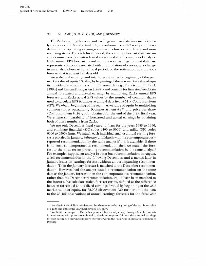
Sample distributions for observations by month, year and recommenda-tion are presented in table 1 (panels A, B, and C). Panels A and B illus-trate that sample observations are relatively evenly distributed between themonths of the first quarter and approximately three quarters of the totalobservations come in the last five years of the nine years included in thesample. Panel C indicates that strong and moderate buy recommendationsare much more frequent than strong and moderate sells.

Table 1, panel D presents distribution statistics for calendar days betweenearnings forecasts and the most recently preceding or contemporaneousrecommendation, firm market value of equity, scaled earnings, and scaledforecast error. Only 15.7% of the earnings forecasts represent a joint issuanceof a recommendation and forecast, all other earnings forecasts are issued inthe context of a previously reported recommendation. Approximately 75%of our earnings forecasts follow the currently outstanding recommendationreport date by more than 30 days. These results confirm that earnings fore-casts are typically issued in the presence of an existing recommendationthat has been outstanding for at least one month. The second and thirdcolumns of panel D indicate that our sample is comprised of predominatelylarge firms with an average return on equity of 6%. The last column of panelD reports that the mean and median scaled forecast errors are .75 and .21percent of market value of equity respectively, consistent with the findingsof analyst forecast optimism reported in numerous prior studies.

4. Results

4.1 EARNINGS FORECAST ERROR AND THE LEVEL OF EARNINGS

Accumulating evidence shows that forecast errors are not the same acrosslevels of earnings scaled by market value of equity. For example, researchhas documented different forecast error patterns for positive and negativeearnings (Brown [1999], Butler and Saraoglu [1999], Hwang, Jan, and Basu[1996]). Brown [1999] suggests that forecast errors should be investigatedseparately for positive and negative earnings firms because the distribu-tions of earnings forecast errors differ substantially. Hwang et al. [1996]identify an inverse relationship between analyst earnings forecast errorsand reported earnings. Similarly, Eames, Glover, and Stice [2001] reportthat earnings forecasts exhibit greater optimism as earnings decline belowthe mean earnings for all firms and greater pessimism as earnings increase

5 We also conducted analyses on samples that deleted forecast errors greater than 20% ofmarket value, and on samples that excluded the largest 5 and 10 percent of scaled forecast errors(ranked using absolute values). The results were virtually identical to the results presented here.

P1: GPL



T A B L E 1Sample Characteristics: First Quarter Forecasts of Annual Earnings, Realized Annual Earnings,Recommendations, and Earnings Forecast Errors, and Market Value of Equity Based on Zacks

Investment Research Values for December Fiscal Year End Firms

Panel A: Sample Distribution by MonthMonth Observations % of Total

January 13,391 38%February 11,369 32%March 10,722 30%

Total 35,482 100%

Panel B: Sample Distribution by YearYear Observations % of Total

1988 2,009 5.7%1989 1,627 4.6%1990 2,713 7.6%1991 3,159 8.9%1992 4,010 11.3%1993 4,433 12.5%1994 5,147 14.5%1995 5,701 16.1%1996 6,683 18.8%

Total 35,482 100.0%

Panel C: Sample Distribution by RecommendationRecommendation Observations % of Total

Strong Buy (1) 11,047 31.1%Moderate buy (2) 7,886 22.2%Hold (3) 13,916 39.2%Moderate Sell (4) 960 2.7%Strong Sell (5) 803 2.3%Not Available (6) 870 2.5%

Total 35,482 100.0%

Panel D: Days Between Recommendation and Earnings Forecast, Market Value of Equity,Actual Earnings, and Earnings Forecast Error Distribution Statistics

EarningsNumber of Days Market Value Earnings as a Forecast Errors

Recommendation of Equity Percent of as a Percent ofPrecedes Forecastb ($ millions) Market Value Market Value

Mean 109 6,434 5.93 .75Median 92 1,797 6.11 .21Quartile 1 29 418 3.80 −.73Quartile 3 178 5,738 8.56 2.02Minimum 0 6 −83.97 −68.12Maximum 360 119,989 70.38 93.29Standard Deviation 91 12,214 7.41 5.46

a Sample observations comprise forecasts matched with the contemporaneous or the most recent preced-ing recommendation by the same analyst, provided the recommendation does not precede the forecast bymore than one year. Forecast errors are defined as forecasted earnings less actual earnings.

b Zacks adds new recommendation records to the database when an analyst issues a first recommenda-tion or changes a recommendation or when the analyst reiterates a prior recommendation that is at least ayear old.

Au: Pls. ref.

P1: GPL



above the mean earnings of all firms. They conclude this relation is due,in part, to unanticipated earnings shocks. Unexpected positive (negative)earnings shocks result in higher (lower) unanticipated earnings and willgenerally be associated with more negative (positive) forecast errors. Moreformally, suppose that reported scaled earnings at time t for firm i, Eit, canbe decomposed into a predictable component, EPit, and an unpredictablecomponent or earnings shock, eUit ∼ N(0, σ). Then Eit = EPit + eUit. We canmodel the analysts’ scaled forecasts, Fit, of Eit as a function of the predictablecomponent: Fit = EPit + fit, where a non-zero mean value for the error term,fit, is consistent with forecast bias (either intentional or unintentional). Wedefine forecast error as: FEit = Fit − Eit = (EPit + fit) − (EPit + eUit), or FEit =fit − eUit. Thus, assuming no forecast bias, unpredictable earnings shocks willresult in an inverse relation between forecast error and reported earnings.6

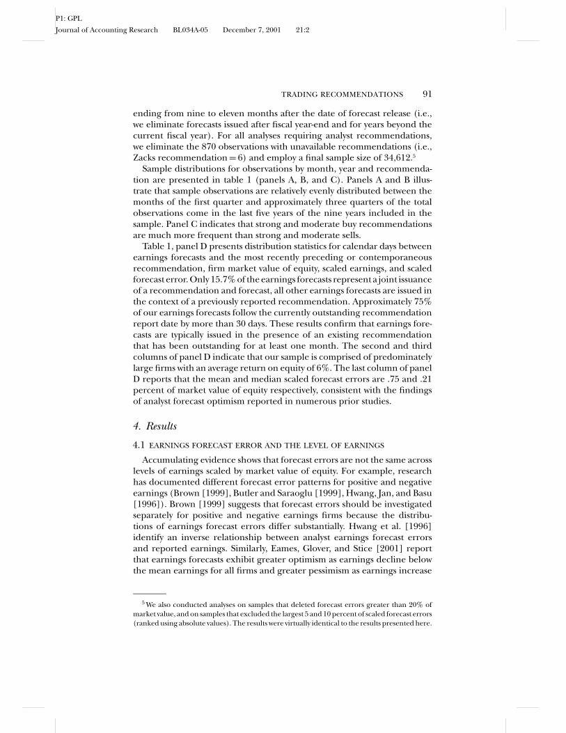
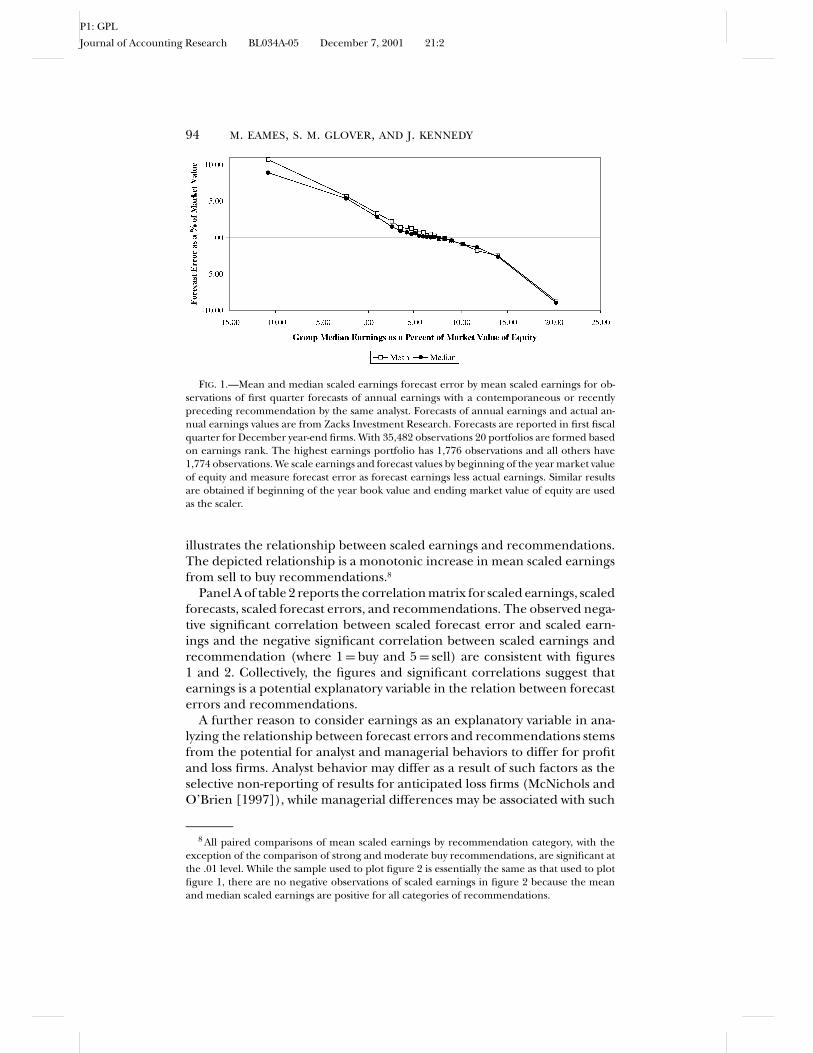
To plot the relationship between scaled forecast error and scaled earningswe divide our sample of 35,482 observations (including the 870 observationswith unavailable recommendations) into 20 equally-sized portfolios basedon the magnitude of scaled earnings. Figure 1 illustrates portfolio mean andmedian scaled forecast errors plotted by portfolio median scaled earnings.The inverse relationship depicted in figure 1 is consistent with results inEames, Glover, and Stice [2001] that, on average, firms experiencing largepositive (negative) earnings shocks are more likely to have positive (nega-tive) earnings and negative (positive) forecast errors.7 Regressing scaledanalyst forecast errors on scaled actual earnings results in an R-squared of48 percent and a negative slope significant at the .001 level (table 2, panel B).

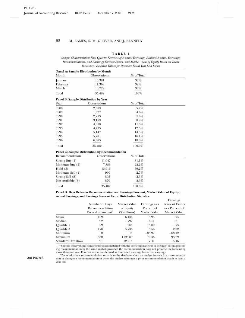
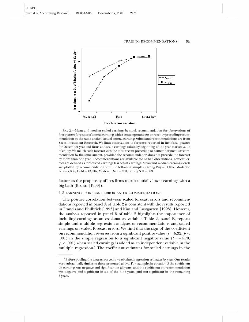
If earnings are also associated with analyst recommendations, earn-ings could be an important correlated omitted variable in prior studiesexamining the relationship between forecast errors and recommendations.Figure 2 plots mean and median scaled earnings by recommendation and

6 Because earnings is included on both the right and left-hand side of the equation, i.e.,FEit = Fit − Eit = B0 + B1Eit + eit, there may be concern that this linear model will force analgebraic inverse association between FEit and Eit. However, an algebraic association betweenforecast error and earnings does not necessitate an observed inverse association. Fit is a functionof Eit,thus we do not necessarily expect a negative value for B1, and only obtain a negative valueunder restrictive assumptions regarding the behavior of Fit with respect to Eit. To see this, wedifferentiate both sides of the preceding equation with respect to Eit, obtain ∂ F

∂ E − 1 = B1, andnote that B1 is negative only if ∂ F

∂ E < 1, and B1 = −1 only if ∂ F∂ E = 0. There is no basis for asserting

either of these conditions a priori. For our sample ∂ F∂ E = .48 and is significantly different from

zero at the 1% level. Thus, the inverse association between forecast error and earnings isnot algebraic. Rather, a systematic inverse relationship between forecast errors and earningsrequires systematic analyst behavior. For example, the inability of analysts to forecast somecomponent or portion of earnings. Because we focus on scaled earnings, we assume that thescaled earnings shock has constant variance across firms.

7 The optimistic forecast errors associated with lower earnings are consistent with the man-agement relations hypothesis given that sell recommendations are commonly associated withlow earnings. Although the management relations hypothesis could be contributing to the ob-served relation between forecast error and earnings, it cannot explain the pessimism observedat higher earnings observations because the management relations hypothesis predicts onlyoptimism.

P1: GPL



FIG. 1.—Mean and median scaled earnings forecast error by mean scaled earnings for ob-servations of first quarter forecasts of annual earnings with a contemporaneous or recentlypreceding recommendation by the same analyst. Forecasts of annual earnings and actual an-nual earnings values are from Zacks Investment Research. Forecasts are reported in first fiscalquarter for December year-end firms. With 35,482 observations 20 portfolios are formed basedon earnings rank. The highest earnings portfolio has 1,776 observations and all others have1,774 observations. We scale earnings and forecast values by beginning of the year market valueof equity and measure forecast error as forecast earnings less actual earnings. Similar resultsare obtained if beginning of the year book value and ending market value of equity are usedas the scaler.

illustrates the relationship between scaled earnings and recommendations.The depicted relationship is a monotonic increase in mean scaled earningsfrom sell to buy recommendations.8

Panel A of table 2 reports the correlation matrix for scaled earnings, scaledforecasts, scaled forecast errors, and recommendations. The observed nega-tive significant correlation between scaled forecast error and scaled earn-ings and the negative significant correlation between scaled earnings andrecommendation (where 1 = buy and 5 = sell) are consistent with figures1 and 2. Collectively, the figures and significant correlations suggest thatearnings is a potential explanatory variable in the relation between forecasterrors and recommendations.

A further reason to consider earnings as an explanatory variable in ana-lyzing the relationship between forecast errors and recommendations stemsfrom the potential for analyst and managerial behaviors to differ for profitand loss firms. Analyst behavior may differ as a result of such factors as theselective non-reporting of results for anticipated loss firms (McNichols andO’Brien [1997]), while managerial differences may be associated with such

8 All paired comparisons of mean scaled earnings by recommendation category, with theexception of the comparison of strong and moderate buy recommendations, are significant atthe .01 level. While the sample used to plot figure 2 is essentially the same as that used to plotfigure 1, there are no negative observations of scaled earnings in figure 2 because the meanand median scaled earnings are positive for all categories of recommendations.

P1: GPL



FIG. 2.—Mean and median scaled earnings by stock recommendation for observations offirst quarter forecasts of annual earnings with a contemporaneous or recently preceding recom-mendation by the same analyst. Actual annual earnings values and recommendations are fromZacks Investment Research. We limit observations to forecasts reported in first fiscal quarterfor December year-end firms and scale earnings values by beginning of the year market valueof equity. We match each forecast with the most recent preceding or contemporaneous recom-mendation by the same analyst, provided the recommendation does not precede the forecastby more than one year. Recommendations are available for 34,612 observations. Forecast er-rors are defined as forecasted earnings less actual earnings. Mean and median earnings levelsare plotted by recommendation with the following samples: Strong Buy = 11,047, ModerateBuy = 7,886, Hold = 13,916, Moderate Sell = 960, Strong Sell = 803.

factors as the propensity of loss firms to substantially lower earnings with abig bath (Brown [1999]).

4.2 EARNINGS FORECAST ERROR AND RECOMMENDATIONS

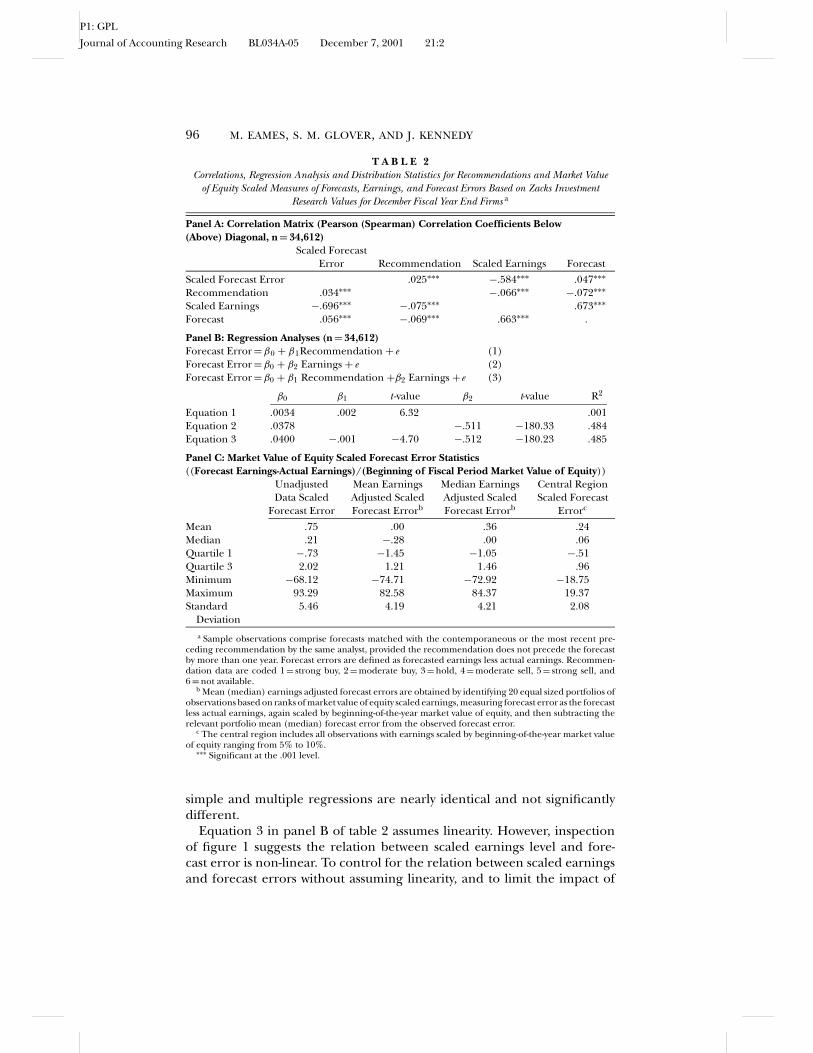
The positive correlation between scaled forecast errors and recommen-dations reported in panel A of table 2 is consistent with the results reportedin Francis and Philbrick [1993] and Kim and Lustgarten [1998]. However,the analysis reported in panel B of table 2 highlights the importance ofincluding earnings as an explanatory variable. Table 2, panel B, reportssimple and multiple regression analyses of recommendations and scaledearnings on scaled forecast errors. We find that the sign of the coefficienton recommendation reverses from a significant positive value (t = 6.32, p <

.001) in the simple regression to a significant negative value (t = −4.70,p < .001) when scaled earnings is added as an independent variable in themultiple regression.9 The coefficient estimates for scaled earnings in the

9 Before pooling the data across years we obtained regression estimates by year. Our resultswere substantially similar to those presented above. For example, in equation 3 the coefficienton earnings was negative and significant in all years, and the coefficient on recommendationwas negative and significant in six of the nine years, and not significant in the remaining3 years.

P1: GPL



T A B L E 2Correlations, Regression Analysis and Distribution Statistics for Recommendations and Market Value

of Equity Scaled Measures of Forecasts, Earnings, and Forecast Errors Based on Zacks InvestmentResearch Values for December Fiscal Year End Firms a

Panel A: Correlation Matrix (Pearson (Spearman) Correlation Coefficients Below(Above) Diagonal, n = 34,612)

Scaled ForecastError Recommendation Scaled Earnings Forecast

Scaled Forecast Error .025∗∗∗ −.584∗∗∗ .047∗∗∗Recommendation .034∗∗∗ −.066∗∗∗ −.072∗∗∗Scaled Earnings −.696∗∗∗ −.075∗∗∗ .673∗∗∗Forecast .056∗∗∗ −.069∗∗∗ .663∗∗∗ .

Panel B: Regression Analyses (n = 34,612)Forecast Error = β0 + β1Recommendation + e (1)Forecast Error = β0 + β2 Earnings + e (2)Forecast Error = β0 + β1 Recommendation +β2 Earnings +e (3)

β0 β1 t -value β2 t-value R2

Equation 1 .0034 .002 6.32 .001Equation 2 .0378 −.511 −180.33 .484Equation 3 .0400 −.001 −4.70 −.512 −180.23 .485

Panel C: Market Value of Equity Scaled Forecast Error Statistics((Forecast Earnings-Actual Earnings)/(Beginning of Fiscal Period Market Value of Equity))

Unadjusted Mean Earnings Median Earnings Central RegionData Scaled Adjusted Scaled Adjusted Scaled Scaled Forecast

Forecast Error Forecast Errorb Forecast Errorb Errorc

Mean .75 .00 .36 .24Median .21 −.28 .00 .06Quartile 1 −.73 −1.45 −1.05 −.51Quartile 3 2.02 1.21 1.46 .96Minimum −68.12 −74.71 −72.92 −18.75Maximum 93.29 82.58 84.37 19.37Standard 5.46 4.19 4.21 2.08

Deviationa Sample observations comprise forecasts matched with the contemporaneous or the most recent pre-

ceding recommendation by the same analyst, provided the recommendation does not precede the forecastby more than one year. Forecast errors are defined as forecasted earnings less actual earnings. Recommen-dation data are coded 1 = strong buy, 2 = moderate buy, 3 = hold, 4 = moderate sell, 5 = strong sell, and6 = not available.

b Mean (median) earnings adjusted forecast errors are obtained by identifying 20 equal sized portfolios ofobservations based on ranks of market value of equity scaled earnings, measuring forecast error as the forecastless actual earnings, again scaled by beginning-of-the-year market value of equity, and then subtracting therelevant portfolio mean (median) forecast error from the observed forecast error.

c The central region includes all observations with earnings scaled by beginning-of-the-year market valueof equity ranging from 5% to 10%.

∗∗∗ Significant at the .001 level.

simple and multiple regressions are nearly identical and not significantlydifferent.

Equation 3 in panel B of table 2 assumes linearity. However, inspectionof figure 1 suggests the relation between scaled earnings level and fore-cast error is non-linear. To control for the relation between scaled earningsand forecast errors without assuming linearity, and to limit the impact of

P1: GPL



outliers, we obtain earnings-portfolio adjusted scaled forecast errors usingthe same 20 equal-sized portfolios formed to plot figure 1.10 We obtain mean(median) adjusted scaled forecast errors by subtracting the relevant port-folio mean (median) scaled forecast error from observed scaled forecasterrors. The resulting adjusted scaled forecast errors are similar to residualsfrom a regression of scaled forecast error on actual scaled earnings, howeverthe portfolio adjustment does not assume linearity and is not significantlyimpacted by outliers.11

A third method of “controlling” for the relationship between earningsand forecast errors is to restrict our analysis to the 15,701 observations ina “central region” of scaled earnings where visual inspection of figure 1suggests the relation between scaled earnings and scaled forecast error isrelatively weak. We define this central region to be all observations withearnings of 5 to 10 percent of beginning-of-year market value of equity.12

We select this 5 to 10 percent region for analysis because: (1) there is ahigh density of forecasts in this area (15,701 of the 34,612 observations),(2) dispersion in analysts forecast errors is relatively low for the region, (3)this region includes the mean and median scaled earnings (6% of marketvalue of equity) and excludes extreme values of earnings, and (4) earningslevel is only moderately related to forecast error in this region.13 Regressingscaled forecast error on scaled earning in the central region results in anR-squared of only 6%, although the relation is still negative and significant(p < .001).

Table 2, panel C presents distribution statistics for the mean and medianearnings-portfolio-adjusted and central region forecast errors. For ease ofcomparison, this panel also repeats the values for unadjusted scaled forecast

10 Another advantage of the portfolio adjustment technique over regression is that it lendsitself to the analysis of absolute forecast optimism and pessimism across recommendationcategories. Analysis via regression coefficients focuses only on the trend in forecast error acrossrecommendations.

11 Our results are robust to alternative methods of controlling for earnings. All reported re-sults examining the portfolio adjusted forecast errors are similar to results obtained examiningresiduals from a regression of forecast error on actual earnings. Because the plot illustratedin figure 1 suggests the relationship between forecast error and earnings is nonlinear, we alsoused a three-part piecewise regression with breaks in the earnings value at 5 and 10 percent ofmarket value. The results of analyzing residuals from the piecewise regressions are also simi-lar to analysis of portfolio earnings level adjusted forecast errors. Because we believe that ourearnings-portfolio adjusted forecast errors are superior to regression residuals, we limit ourdiscussion to analysis of the earnings-portfolio adjusted forecast errors.

12 We also analyzed various central regions with ranges of actual earnings of from as small as7 to 8 percent to as large as 1 to 13 percent. Results for all these ranges displayed qualitativelysimilar relationships between forecast error and recommendation to the relationship reportedfor the 5 to 10 percent range.

13 As an alternative measure of how extreme large (small) observations in figure 1 are, datapoints can be converted to a ratio approximating PE ratios (recall that we scale by beginningmarket value). In other words, firms reporting realized earnings that are 20% of beginningmarket value have a PE ratio of 5.

P1: GPL



errors that are reported in table 1. Both mean and median adjusted scaledforecast errors and central region scaled forecast errors are significantlyless optimistic than unadjusted scaled forecast errors. Note that while wereplicate previous studies (e.g., Francis and Philbrick [1993]) by analyzingunadjusted scaled forecasts errors, our primary focus is on adjusted scaledforecast errors and observations in the central region because we argue thesetwo latter data sets appropriately consider the association between forecasterror and earnings.

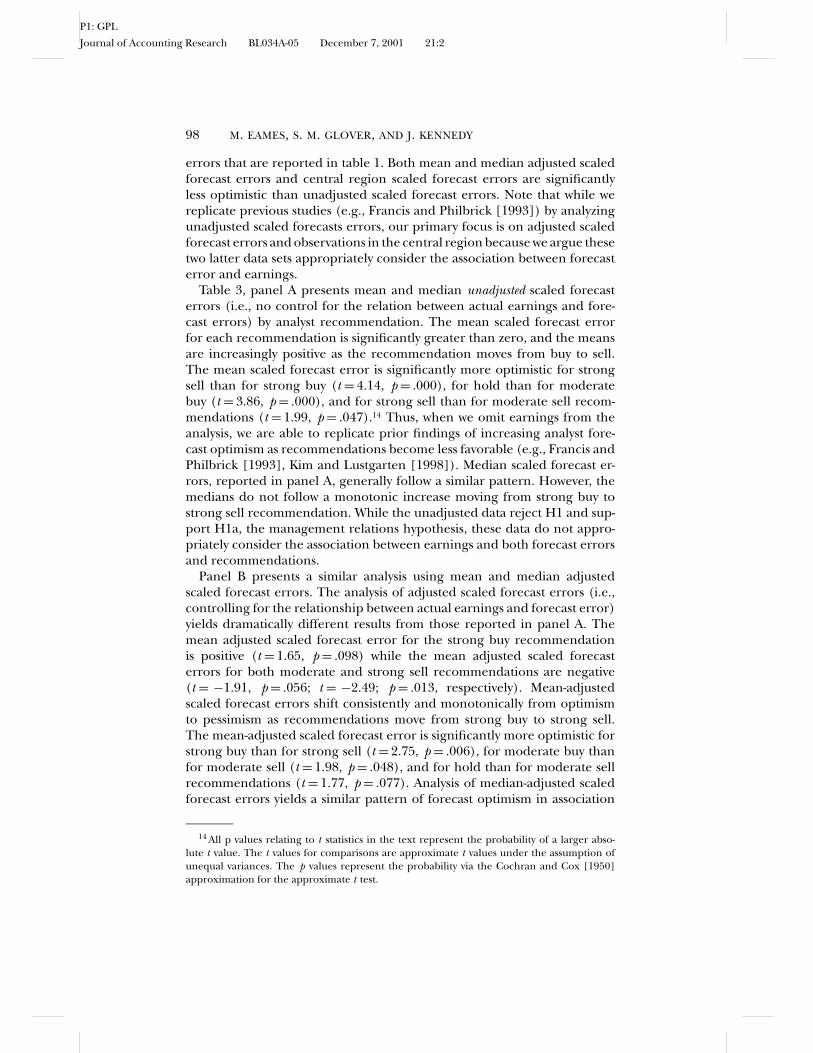
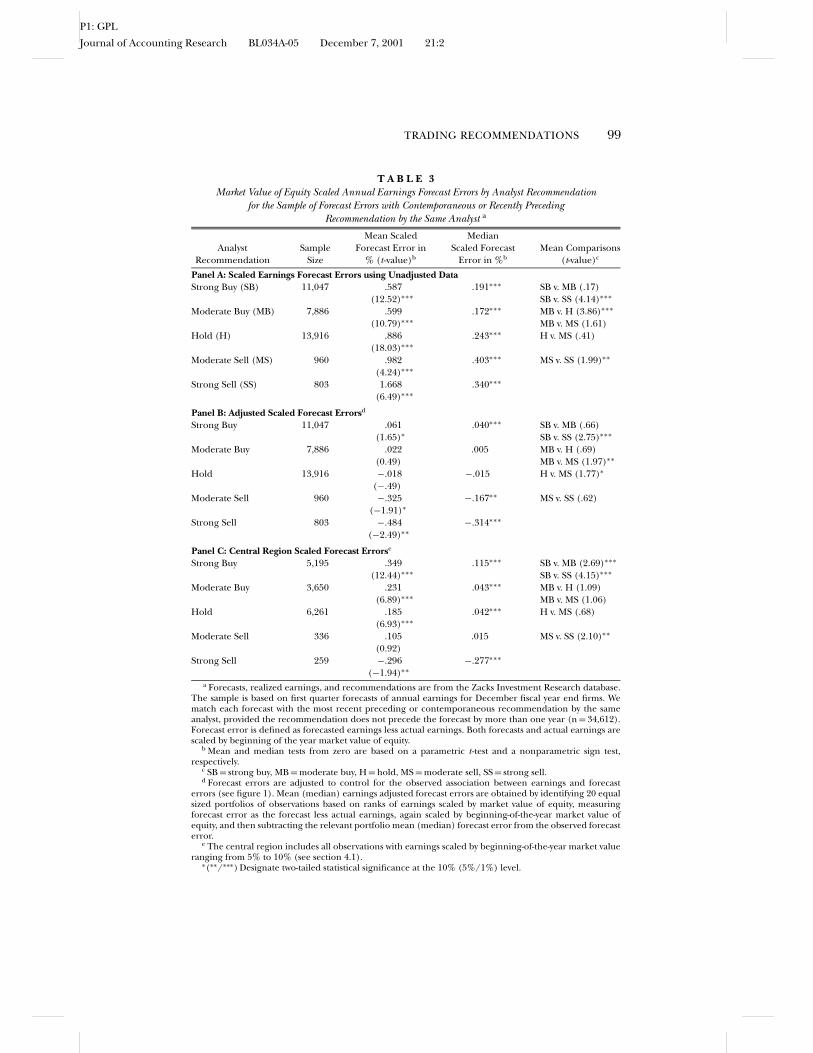
Table 3, panel A presents mean and median unadjusted scaled forecasterrors (i.e., no control for the relation between actual earnings and fore-cast errors) by analyst recommendation. The mean scaled forecast errorfor each recommendation is significantly greater than zero, and the meansare increasingly positive as the recommendation moves from buy to sell.The mean scaled forecast error is significantly more optimistic for strongsell than for strong buy (t = 4.14, p = .000), for hold than for moderatebuy (t = 3.86, p = .000), and for strong sell than for moderate sell recom-mendations (t = 1.99, p = .047).14 Thus, when we omit earnings from theanalysis, we are able to replicate prior findings of increasing analyst fore-cast optimism as recommendations become less favorable (e.g., Francis andPhilbrick [1993], Kim and Lustgarten [1998]). Median scaled forecast er-rors, reported in panel A, generally follow a similar pattern. However, themedians do not follow a monotonic increase moving from strong buy tostrong sell recommendation. While the unadjusted data reject H1 and sup-port H1a, the management relations hypothesis, these data do not appro-priately consider the association between earnings and both forecast errorsand recommendations.

Panel B presents a similar analysis using mean and median adjustedscaled forecast errors. The analysis of adjusted scaled forecast errors (i.e.,controlling for the relationship between actual earnings and forecast error)yields dramatically different results from those reported in panel A. Themean adjusted scaled forecast error for the strong buy recommendationis positive (t = 1.65, p = .098) while the mean adjusted scaled forecasterrors for both moderate and strong sell recommendations are negative(t = −1.91, p = .056; t = −2.49; p = .013, respectively). Mean-adjustedscaled forecast errors shift consistently and monotonically from optimismto pessimism as recommendations move from strong buy to strong sell.The mean-adjusted scaled forecast error is significantly more optimistic forstrong buy than for strong sell (t = 2.75, p = .006), for moderate buy thanfor moderate sell (t = 1.98, p = .048), and for hold than for moderate sellrecommendations (t = 1.77, p = .077). Analysis of median-adjusted scaledforecast errors yields a similar pattern of forecast optimism in association

14 All p values relating to t statistics in the text represent the probability of a larger abso-lute t value. The t values for comparisons are approximate t values under the assumption ofunequal variances. The p values represent the probability via the Cochran and Cox [1950]approximation for the approximate t test.

P1: GPL



T A B L E 3Market Value of Equity Scaled Annual Earnings Forecast Errors by Analyst Recommendation

for the Sample of Forecast Errors with Contemporaneous or Recently PrecedingRecommendation by the Same Analyst a

Mean Scaled MedianAnalyst Sample Forecast Error in Scaled Forecast Mean Comparisons

Recommendation Size % (t -value)b Error in %b (t-value)c

Panel A: Scaled Earnings Forecast Errors using Unadjusted DataStrong Buy (SB) 11,047 .587 .191∗∗∗ SB v. MB (.17)

(12.52)∗∗∗ SB v. SS (4.14)∗∗∗

Moderate Buy (MB) 7,886 .599 .172∗∗∗ MB v. H (3.86)∗∗∗

(10.79)∗∗∗ MB v. MS (1.61)Hold (H) 13,916 .886 .243∗∗∗ H v. MS (.41)

(18.03)∗∗∗

Moderate Sell (MS) 960 .982 .403∗∗∗ MS v. SS (1.99)∗∗

(4.24)∗∗∗

Strong Sell (SS) 803 1.668 .340∗∗∗

(6.49)∗∗∗

Panel B: Adjusted Scaled Forecast Errorsd

Strong Buy 11,047 .061 .040∗∗∗ SB v. MB (.66)(1.65)∗ SB v. SS (2.75)∗∗∗

Moderate Buy 7,886 .022 .005 MB v. H (.69)(0.49) MB v. MS (1.97)∗∗

Hold 13,916 −.018 −.015 H v. MS (1.77)∗

(−.49)Moderate Sell 960 −.325 −.167∗∗ MS v. SS (.62)

(−1.91)∗

Strong Sell 803 −.484 −.314∗∗∗

(−2.49)∗∗

Panel C: Central Region Scaled Forecast Errorse

Strong Buy 5,195 .349 .115∗∗∗ SB v. MB (2.69)∗∗∗

(12.44)∗∗∗ SB v. SS (4.15)∗∗∗

Moderate Buy 3,650 .231 .043∗∗∗ MB v. H (1.09)(6.89)∗∗∗ MB v. MS (1.06)

Hold 6,261 .185 .042∗∗∗ H v. MS (.68)(6.93)∗∗∗

Moderate Sell 336 .105 .015 MS v. SS (2.10)∗∗

(0.92)Strong Sell 259 −.296 −.277∗∗∗

(−1.94)∗∗a Forecasts, realized earnings, and recommendations are from the Zacks Investment Research database.

The sample is based on first quarter forecasts of annual earnings for December fiscal year end firms. Wematch each forecast with the most recent preceding or contemporaneous recommendation by the sameanalyst, provided the recommendation does not precede the forecast by more than one year (n = 34,612).Forecast error is defined as forecasted earnings less actual earnings. Both forecasts and actual earnings arescaled by beginning of the year market value of equity.

b Mean and median tests from zero are based on a parametric t -test and a nonparametric sign test,respectively.

c SB = strong buy, MB = moderate buy, H = hold, MS = moderate sell, SS = strong sell.d Forecast errors are adjusted to control for the observed association between earnings and forecast

errors (see figure 1). Mean (median) earnings adjusted forecast errors are obtained by identifying 20 equalsized portfolios of observations based on ranks of earnings scaled by market value of equity, measuringforecast error as the forecast less actual earnings, again scaled by beginning-of-the-year market value ofequity, and then subtracting the relevant portfolio mean (median) forecast error from the observed forecasterror.

e The central region includes all observations with earnings scaled by beginning-of-the-year market valueranging from 5% to 10% (see section 4.1).

∗(∗∗/∗∗∗) Designate two-tailed statistical significance at the 10% (5%/1%) level.

P1: GPL



with buy recommendations and pessimism for sell recommendations.Consequently, when we analyze scaled forecast errors, adjusted to controlforecast error to control for the relationship between earnings level andforecast error, we again reject hypothesis H1, but now the results supportthe objectivity illusion and trade boosting hypotheses (H1b) and not themanagement relations hypotheses (H1a). These results also provide evi-dence that the relation between recommendation and forecast error is notdriven solely by the relation between scaled earnings and forecast error. Ifthat were the case, we would expect no relation between recommendationsand adjusted forecast errors.

Results for scaled forecast errors in the central region (i.e., where the rela-tion between scaled earnings and scaled forecast error is weak) are presentedin panel C, and are consistent with results presented in panel B for mean andmedian adjusted scaled forecast errors. Again we observe optimistic meanscaled forecast error for strong buy recommendations and pessimistic meanscaled forecast error for strong sell recommendations, with scaled forecasterrors for intermediate recommendations monotonically aligning betweenthe extremes. The mean scaled forecast error is significantly more optimisticfor strong buy than for strong sell (t = 4.15, p = .000), for strong buy thanfor moderate buy (t = 2.69, p = .007), and for moderate sell than for strongsell recommendations (t = 2.11, p = .036). Median scaled forecast errorsdecrease in magnitude going from strong buy to strong sell recommenda-tions, and exhibit optimism for buy recommendations and pessimism forstrong sell recommendations. Results in panel C provide a control for theassociation between earnings and forecast errors by examining a subset ofthe unadjusted data reported in panel A.15 These results support the tradeboosting and objectivity illusion hypotheses (H1b), but not the manage-ment relations hypotheses (H1a). A comparison of panels A and C alsohighlights the key role extreme earnings observations likely play in priorresearch. Panels B and C suggest that evidence in previous studies support-ing the management relations hypothesis (panel A) is driven by the relationbetween analyst forecast error and scaled earnings levels outside the centralregion.

15 Additional evidence that we have not “adjusted away” management relations is obtainedby investigating the relation between forecast errors and forecasts. If recommendations inducebiased forecast errors and if recommendations are associated with the level of forecast (i.e.,buy (sell) recommendations are generally associated with higher (lower) forecasted earnings),we expect to observe a significant relation between forecast error and forecast. For tradeboosting and the objectivity illusion (management relations) we expect a positive (negative)association between forecast error and forecast. As expected, the relation between forecasterror and forecasts is positive and highly significant (R-squared = 67%). Just as earnings aresignificantly correlated with recommendations (see figure 2), we find a similar correlation(p < .001, see also panel A, table 2) between forecasted earnings and recommendations. Theobserved positive relationship is consistent with the pattern predicted by objectivity illusion andtrade boosting but not management relations and provides additional evidence that analysts’earnings forecasts are systematically biased. We thank the reviewer for suggesting this analysis.

P1: GPL



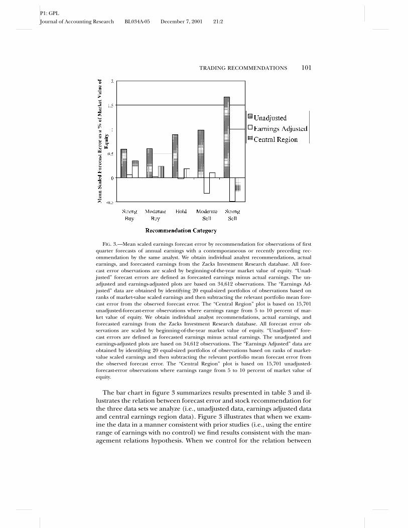
FIG. 3.—Mean scaled earnings forecast error by recommendation for observations of firstquarter forecasts of annual earnings with a contemporaneous or recently preceding rec-ommendation by the same analyst. We obtain individual analyst recommendations, actualearnings, and forecasted earnings from the Zacks Investment Research database. All fore-cast error observations are scaled by beginning-of-the-year market value of equity. “Unad-justed” forecast errors are defined as forecasted earnings minus actual earnings. The un-adjusted and earnings-adjusted plots are based on 34,612 observations. The “Earnings Ad-justed” data are obtained by identifying 20 equal-sized portfolios of observations based onranks of market-value scaled earnings and then subtracting the relevant portfolio mean fore-cast error from the observed forecast error. The “Central Region” plot is based on 15,701unadjusted-forecast-error observations where earnings range from 5 to 10 percent of mar-ket value of equity. We obtain individual analyst recommendations, actual earnings, andforecasted earnings from the Zacks Investment Research database. All forecast error ob-servations are scaled by beginning-of-the-year market value of equity. “Unadjusted” fore-cast errors are defined as forecasted earnings minus actual earnings. The unadjusted andearnings-adjusted plots are based on 34,612 observations. The “Earnings Adjusted” data areobtained by identifying 20 equal-sized portfolios of observations based on ranks of market-value scaled earnings and then subtracting the relevant portfolio mean forecast error fromthe observed forecast error. The “Central Region” plot is based on 15,701 unadjusted-forecast-error observations where earnings range from 5 to 10 percent of market value ofequity.

The bar chart in figure 3 summarizes results presented in table 3 and il-lustrates the relation between forecast error and stock recommendation forthe three data sets we analyze (i.e., unadjusted data, earnings adjusted dataand central earnings region data). Figure 3 illustrates that when we exam-ine the data in a manner consistent with prior studies (i.e., using the entirerange of earnings with no control) we find results consistent with the man-agement relations hypothesis. When we control for the relation between

P1: GPL



earnings and forecast errors by examining the “adjusted” and “central re-gion” data we find strikingly different results; the relation between forecasterrors and recommendations no longer supports the management relationshypothesis.16

4.3 OBJECTIVITY ILLUSION AND TRADE BOOSTING

Both the objectivity illusion and trade boosting hypotheses predict op-timistic forecast errors for buys and pessimistic forecast errors for sells.While both factors could certainly exist simultaneously, we examine whetherour results are more supportive of the trade boosting or objectivity illusionhypothesis.

Analysts’ incentives to intentionally bias earnings forecasts to boost tradeare likely greater for strong recommendations than for moderate recom-mendations, since analysts can boost trading on stocks that do not have anextreme recommendation with a shift to a more extreme recommendation,as well as by intentionally biasing the earnings forecast. Analysts likely preferrecommendation-related trade boosting over earnings-forecast-based tradeboosting because recommendation shifts are a stronger signal to investorsthan an unspecified level of forecast error at the time of forecast issuanceand because forecast errors are more readily measurable than are recom-mendation errors. Therefore, for the trade-boosting hypothesis we expectno significant relation between forecast error and recommendations for in-termediate recommendation levels, significant optimistic forecast bias forstrong buy recommendations, and significant pessimistic forecast bias forstrong sell recommendations.

The objectivity illusion predicts forecast errors associated with both mod-erate and strong recommendations and the degree of bias should increaseas recommendations become stronger. Thus, greater absolute forecast errorfor strong buy and strong sell recommendations and a significant relationbetween forecast bias and recommendation for intermediate recommenda-tions would lend support for the objectivity illusion.

Panel B of table 3 reports that mean and median adjusted scaled fore-cast errors are significantly optimistic for strong buy recommendations,significantly pessimistic for strong sell recommendations, and exhibit a con-tinuum in forecast bias across all levels of recommendations. Consistentwith the objectivity illusion hypothesis and not with trade boosting, meanadjusted forecast errors differ significantly between moderate buy and mod-erate sell recommendations (t = 1.97, p = .048) and between moderate selland hold recommendations (t = 1.77, p = .077).

16 To preclude the possibility that a correlated error structure in our data might be drivingthe significant results we obtain in panels B and C of table 3, we also examined our data ona year-by-year basis. Although significance was generally reduced due to the smaller samplesemployed, the year-by-year results were highly consistent with results obtained for the entiresample.

P1: GPL



5. Summary and Conclusion

We examine the relation between analysts’ earnings forecast errors andstock recommendations. Prior research has generally found both brokerand non-broker-analyst earnings forecasts to be optimistic on average, andincreasingly optimistic as the stock recommendation becomes less favorable.Prior research posits that analysts intentionally issue optimistic forecasts inorder to curry management favor (the management relations hypothesis).However, this explanation contradicts conventional wisdom reported in thefinancial press as well as recent academic research suggesting managers mayactually prefer slightly pessimistic forecasts.

We believe that prior results supporting the management relations hy-pothesis are driven by omitting an important correlated variable, earnings.When we control for the relation between forecast error and earnings, wefind that analyst forecast errors are optimistic for buy recommendations andpessimistic for sell recommendations. These results are not consistent withthe management relations hypothesis but are consistent with both the tradeboosting and objectivity illusion hypotheses. The trade boosting hypothesiscontends that analysts intentionally bias their forecasts to boost trade. Theobjectivity illusion hypothesis contends that analysts unintentionally biastheir forecasts to achieve consistency with their stock recommendations.Results of an analysis to distinguish between trade boosting and objectivityillusion appear more consistent with the objectivity illusion.

REFERENCES

AFFLECK-GRAVES, J.; L. DAVIS; AND R. R. MENDENHALL. “Forecasts of Earnings Per Share: PossibleSources of Analyst Superiority and Bias.” Contemporary Accounting Research (Spring 1990):501–17.

ALI, A.; A. KLEIN; AND J. ROSENFELD. “Analysts’ Use of Information about Permanent and Tran-sitory Earnings Components in Forecasting Annual EPS.” The Accounting Review 67 (1992):183–98.

BALOG, S. “What an Analyst Wants from You.” Financial Executive ( July/August 1991): 47–52.BIGGS, S. “Financial Analysts’ Information Search in the Assessment of Corporate Earnings

Power.” Accounting, Organizations and Society 9 (1984): 313–23.BOINEY, L.; J. KENNEDY; AND P. NYE. “Instrumental Bias in Motivated Reasoning: More When

More is Needed.” Organizational Behavior and Human Decision Processes 72 (October 1997):1–24.

BROWN, L. “Earnings Forecasting Research: Its Implications for Capital Markets Research.”International Journal of Forecasting 9 (1993): 295–320.

BROWN, L. “Managerial Behavior and the Bias in Analysts’ Earnings Forecasts.” Working paper,Georgia State University, 1999.

BROWN, L.; P. GRIFFIN; R. HAGERMAN; AND M. ZMIJEWSKI. “An Evaluation of Alternative Proxiesfor Market’s Assessment of Unexpected Earnings.” Journal of Accounting and Economics 11(1987): 159–93.

BURGSTAHLER, D., AND M. EAMES. “Management of Earnings and Analyst Forecasts.” Workingpaper, University of Washington, 2000.

BUTLER, K. C., AND H. SARAOGLU. “Improving Analysts’ Negative Earnings Forecasts.” FinancialAnalysts’ Journal (May/June 1999): 48–56.

COCHRAN, W., AND G. COX. Experimental Designs. New York. John Wiley and Sons, Inc.

P1: GPL



DAS, S.; C. B. LEVINE; AND K. SIVARAMAKRISHNAN. “Earnings Predictability and Bias in Analysts’Earnings Forecasts.” The Accounting Review 73 (April 1998): 277–94.

DITTO, P. H., AND D. F. LOPEZ. “Motivated Skepticism: Use of Differential Decision Criteria forPreferred and Nonpreferred Conclusions.” Journal of Personality and Social Psychology (1992):568–84.

DUGAR, A., AND S. NATHAN. “The Effect of Investment Banking Relationships on FinancialAnalysts’ Earnings Investment Recommendations.” Contemporary Accounting Research 12 (Fall1995): 131–60.

EAMES, M.; S. GLOVER; AND K. STICE, “The Relation between Earnings and Earnings ForecastError.” Working Paper, Brigham Young University, 2001.

FESTINGER, L. “A Theory of Cognitive Dissonance.” Stanford, CA: Standford University Press,1957.

FRANCIS, J., AND D. R. PHILBRICK. “Analysts’ Decisions as Products of a Multi-Task Environment.”Journal of Accounting Research 31 (Autumn 1993): 216–30.

GIVOLY, AND LAKONISHOK. “Properties of Analysts’ Forecasts of Earnings: A Review and Analysisof the Research.” Journal of Accounting Literature 3 (1984): 117–52.Au:

firstinitials?

HWANG, L.; C. JAN; AND S. BASU. “Loss Firms and Analysts’ Earnings Forecast Errors,” The Journalof Financial Statement Analysis (Winter) 1996: 18–29.

IP, G. “Traders Laugh Off the Official Estimate on Earnings, Act on Whispers.” Wall Street Journal,January 16 (1997a).

IP, G. “Rise in Profit Guidance Dilutes Positive Surprises.” Wall Street Journal, June 23 (1997b).KIM, C., AND S. LUSTGARTEN. “Broker-Analysts’ Trade-Boosting Incentive and Their Earnings

Forecast Bias.” Working paper, Queens College of the City University of New York, 1998.KUNDA, Z. “The Case for Motivated Reasoning.” Psychological Bulletin 108 (1990): 480–98.LIM, T. “Rationality and Analyst’s Forecast Bias.” Working Paper, Dartmouth College. 1998.LYS, T., AND S. SOHN. “The Association Between Revisions of Analysts’ Earnings Forecasts and

Security-Price Changes.” Journal of Accounting and Economics 13 (December 1990): 341–63.MATSUMOTO, D. A. “Management’s Incentives to Avoid Negative Earnings Surprises.” Working

paper, University of Washington, 2001.MCNICHOLS, M., AND P. C. O’BRIEN. “Self-Selection and Analyst coverage.” Journal of Accounting

Research (Supplement 1997): 167–99.MCGEE, S. “As Stock Market Surges Ahead, ‘Predictable’ Profits are Driving It.” Wall Street

Journal, C1, May 5 (1997).MENDENHALL, R. R. “Evidence on the Possible Underweighting of Earnings-Related Informa-

tion.” Journal of Accounting Research 29 (Spring 1991): 170–79.O’BRIEN, P. C. “Analysts’ Forecasts as Earnings Expectation.” Journal of Accounting and Economics

10 (1988): 53–83.SNYDER, M., AND W. B. SWANN, JR. “Hypothesis-Testing Processes in Social Interaction.” Journal

of Personality and Social Psychology 36 (1978): 1202–12.

the association between trading recommendations and broker-analysts' earnings forecasts

Documents