the application of airborne lidar for large area archaeological prospection
TRANSCRIPT
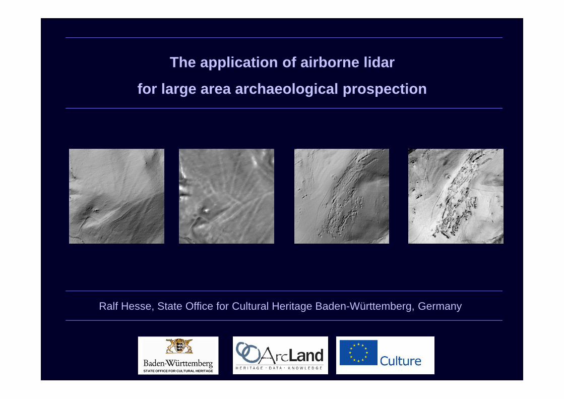
Ralf Hesse, State Office for Cultural Heritage Baden-Württemberg, Germany
STATE OFFICE FOR CULTURAL HERITAGE
The application of airborne lidar
for large area archaeological prospection
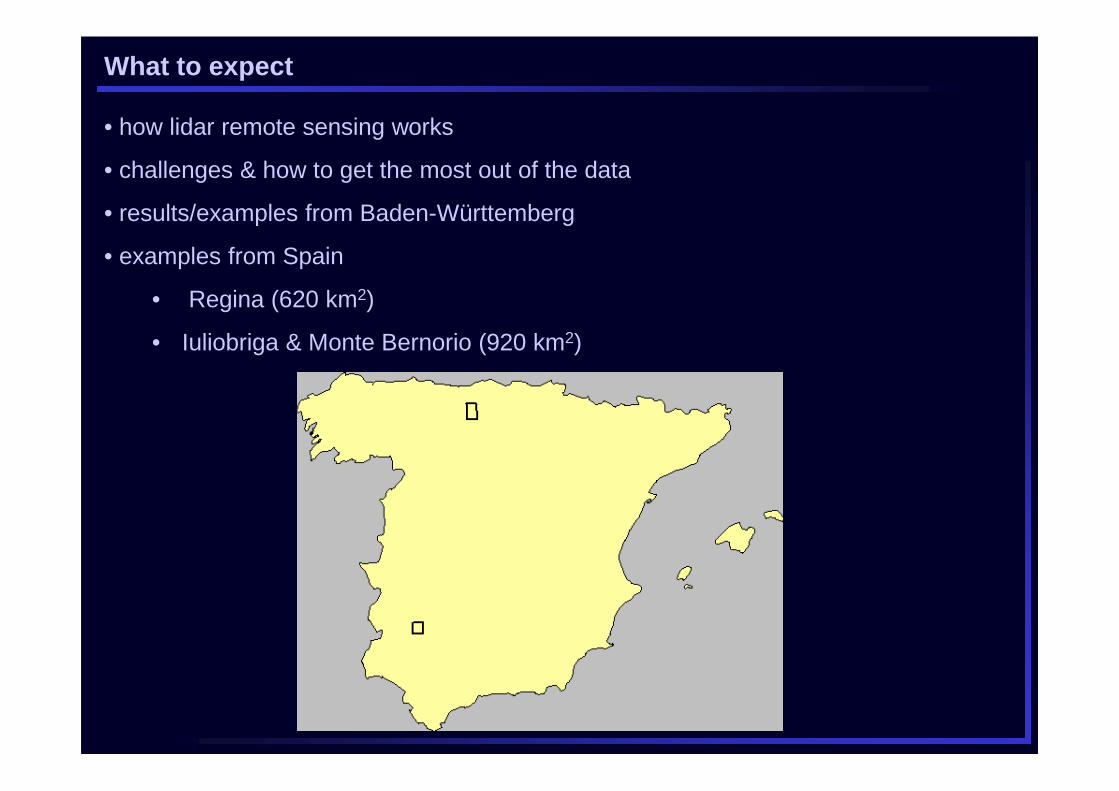
What to expect
• how lidar remote sensing works
• challenges & how to get the most out of the data
• results/examples from Baden-Württemberg
• examples from Spain
• Regina (620 km2)
• Iuliobriga & Monte Bernorio (920 km2)
Topography and human activities
• all human activities take place on and surrounded by topography
• topography does not determine human activities
• culture (values, intentions, taboos...)
• technology
• adaptation
• e.g. agriculture
• human activities leave traces in the topography
• movement/transport
• agriculture
• mineral resource exploitation
• habitation
• protection
• ...
� topographic traces of past activities recognisable in DEMs
T
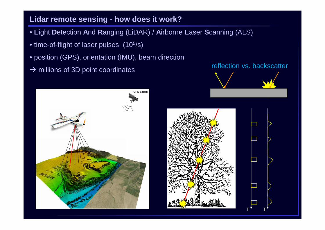
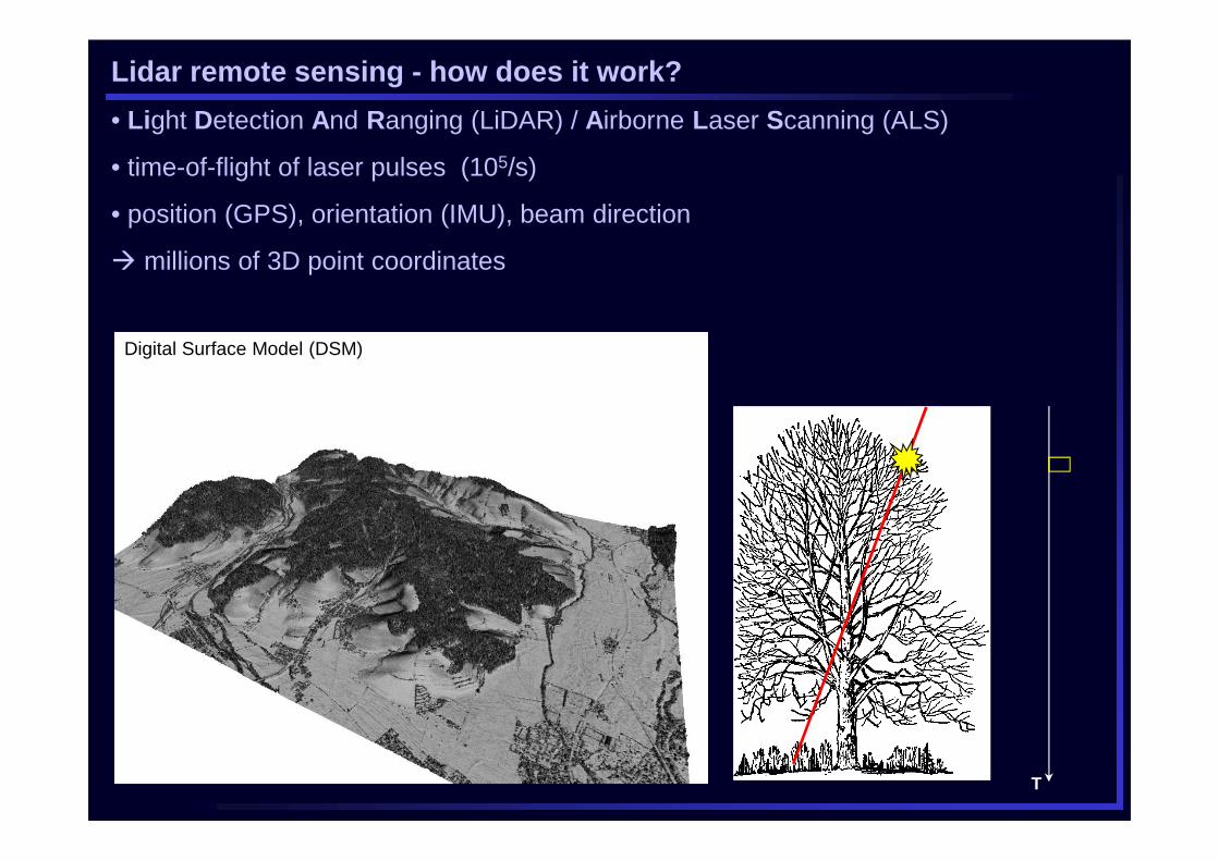
Lidar remote sensing - how does it work?
• Light Detection And Ranging (LiDAR) / Airborne Laser Scanning (ALS)
• time-of-flight of laser pulses (105/s)
• position (GPS), orientation (IMU), beam direction
� millions of 3D point coordinates reflection vs. backscatter
T
T
Digital Surface Model (DSM)
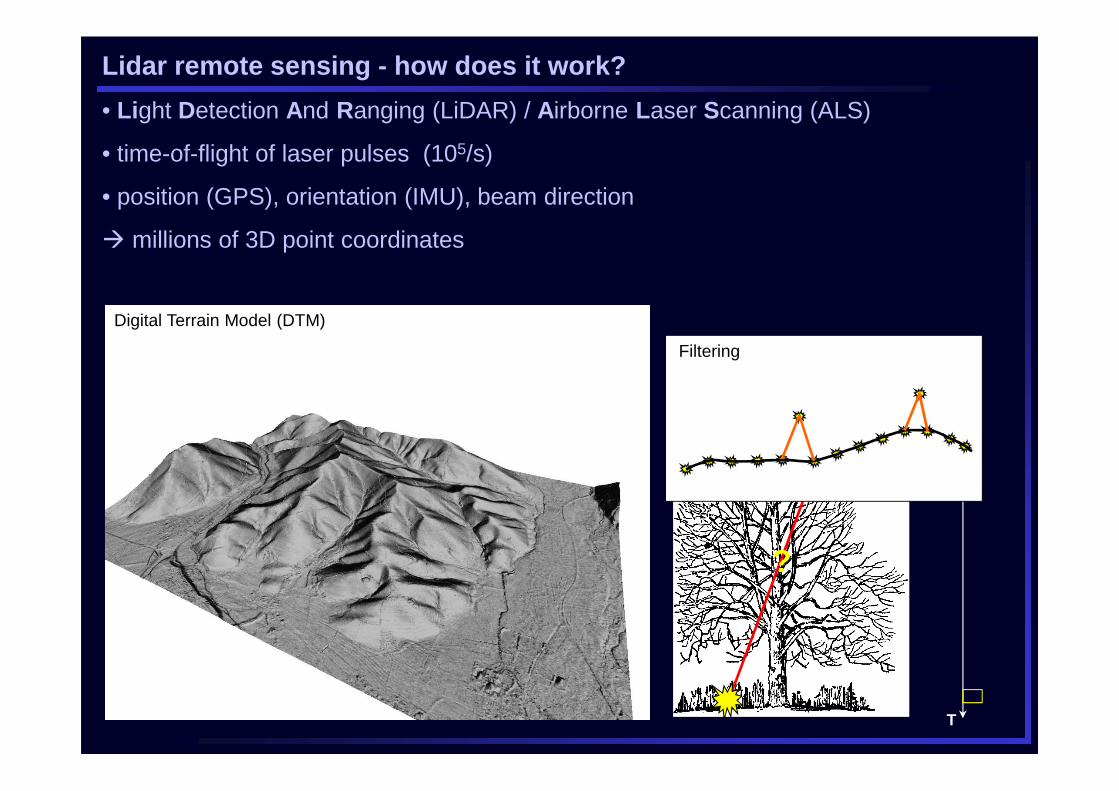
Lidar remote sensing - how does it work?
• Light Detection And Ranging (LiDAR) / Airborne Laser Scanning (ALS)
• time-of-flight of laser pulses (105/s)
• position (GPS), orientation (IMU), beam direction
� millions of 3D point coordinates
T
Digital Terrain Model (DTM)
Filtering
?
Lidar remote sensing - how does it work?
• Light Detection And Ranging (LiDAR) / Airborne Laser Scanning (ALS)
• time-of-flight of laser pulses (105/s)
• position (GPS), orientation (IMU), beam direction
� millions of 3D point coordinates
Lidar remote sensing - how does it work?
• parameters
• footprint size
• pulse rate, flight altitude and velocity � ground point density
• single/dual/multiple return, full waveform
• survey season (central Europe)
• autumn-spring (trees without leaves)
• ideally: early spring after snowmelt
• laser colour
• infrared: absorption by water, ice and snow
• green: suitable for shallow water
• problems:
• very dense vegetation (spuce regrowth etc.)
• low vegetation (blackberry bushes etc.)
• steep slopes
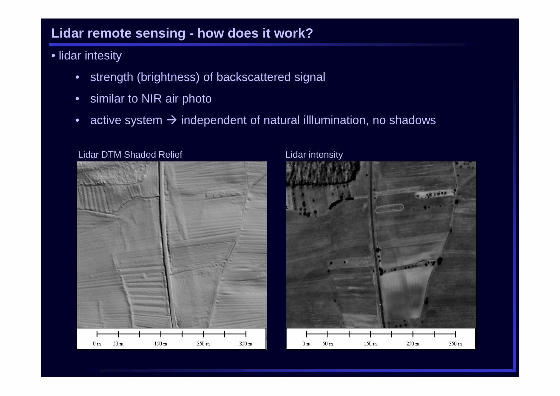
Lidar DTM Shaded Relief Lidar intensity
Lidar remote sensing - how does it work?
• lidar intesity
• strength (brightness) of backscattered signal
• similar to NIR air photo
• active system � independent of natural illlumination, no shadows
Challenge 1: Data availability
• Germany:
• restricted
• ≥20 €/km2
• coverage, quality and price depends on federal state
• in Baden-Württemberg: access for heritage management
• Spain:
• freely available via pnoa.ign.es
• commercial lidar surveys: 500-1000 €/km2
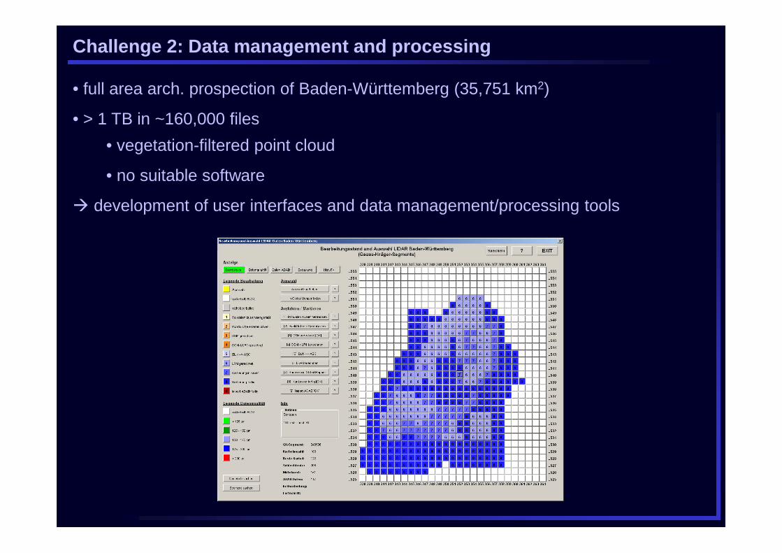
Challenge 2: Data management and processing
• full area arch. prospection of Baden-Württemberg (35,751 km2)
• > 1 TB in ~160,000 files
• vegetation-filtered point cloud
• no suitable software
� development of user interfaces and data management/processing tools
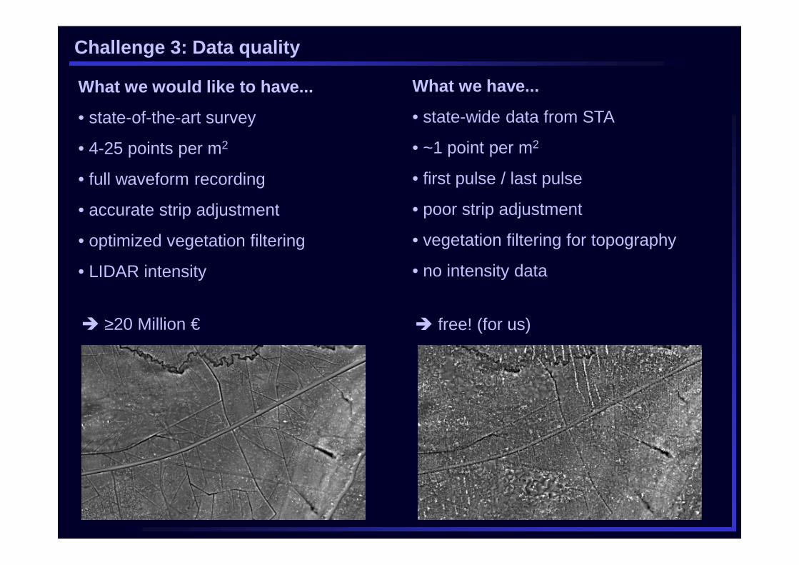
Challenge 3: Data quality
What we would like to have...
• state-of-the-art survey
• 4-25 points per m2
• full waveform recording
• accurate strip adjustment
• optimized vegetation filtering
• LIDAR intensity
What we have...
• state-wide data from STA
• ~1 point per m2
• first pulse / last pulse
• poor strip adjustment
• vegetation filtering for topography
• no intensity data
� ≥20 Million € � free! (for us)
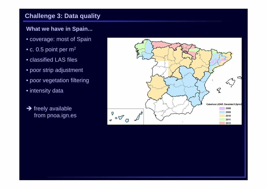
Challenge 3: Data quality
What we have in Spain...
• coverage: most of Spain
• c. 0.5 point per m2
• classified LAS files
• poor strip adjustment
• poor vegetation filtering
• intensity data
� freely availablefrom pnoa.ign.es
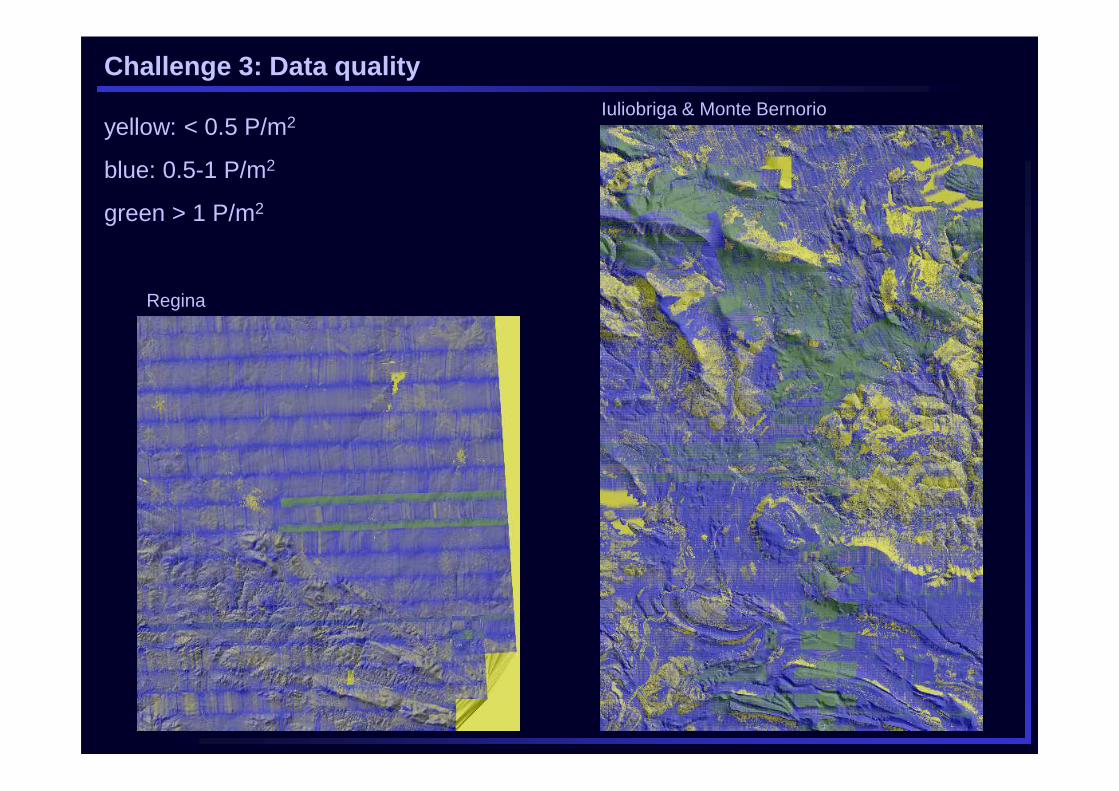
Challenge 3: Data quality
yellow: < 0.5 P/m2
blue: 0.5-1 P/m2
green > 1 P/m2
Iuliobriga & Monte Bernorio
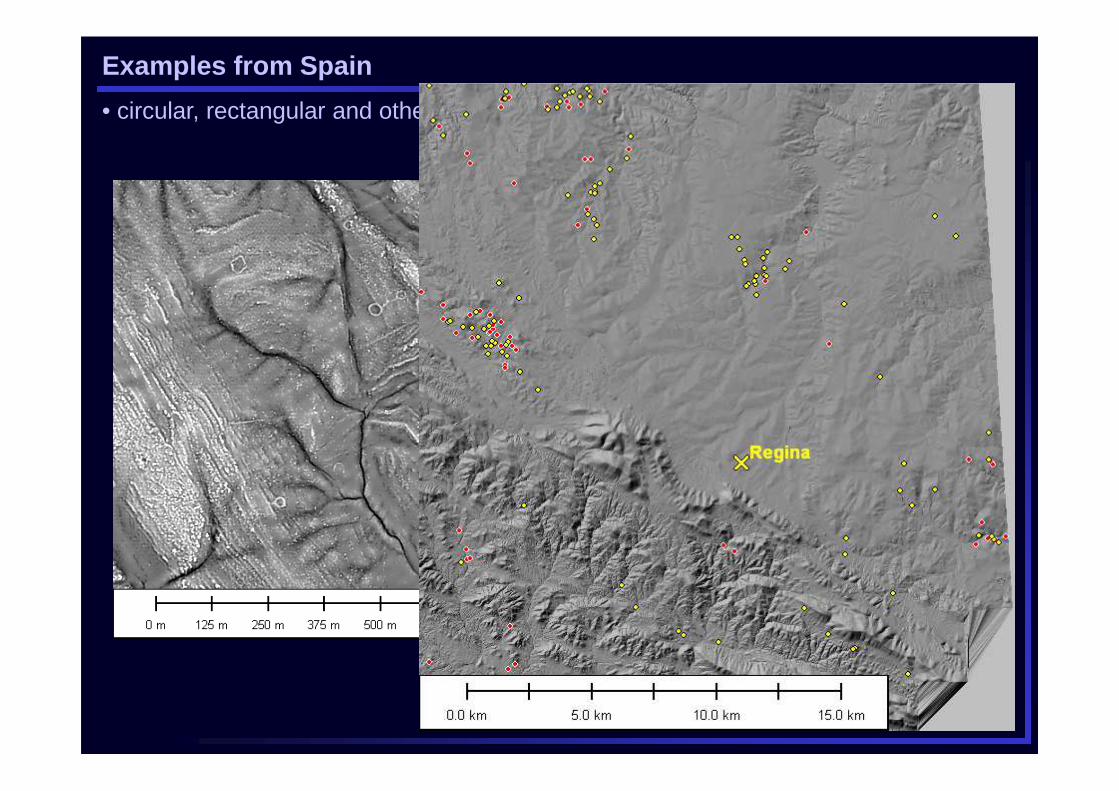
Regina
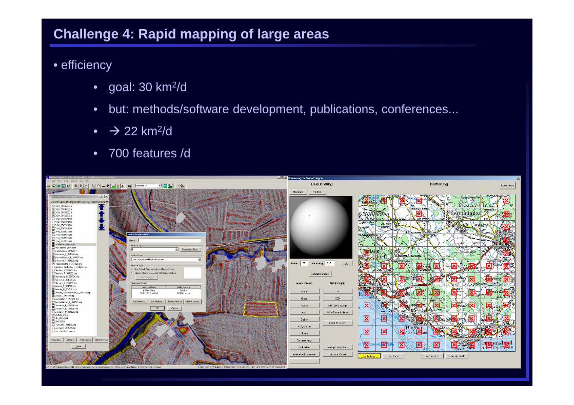
Challenge 4: Rapid mapping of large areas
• efficiency
• goal: 30 km2/d
• but: methods/software development, publications, conferences...
• � 22 km2/d
• 700 features /d
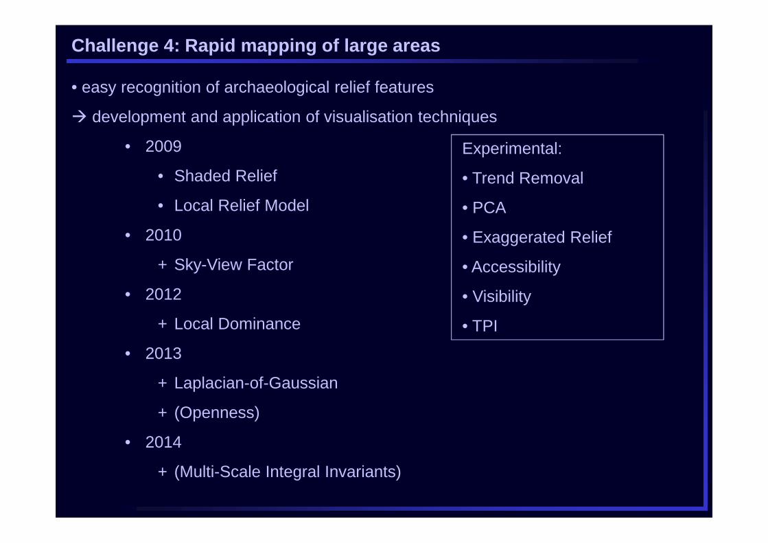
Challenge 4: Rapid mapping of large areas
• easy recognition of archaeological relief features
� development and application of visualisation techniques
• 2009
• Shaded Relief
• Local Relief Model
• 2010
+ Sky-View Factor
• 2012
+ Local Dominance
• 2013
+ Laplacian-of-Gaussian
+ (Openness)
• 2014
+ (Multi-Scale Integral Invariants)
Experimental:
• Trend Removal
• PCA
• Exaggerated Relief
• Accessibility
• Visibility
• TPI
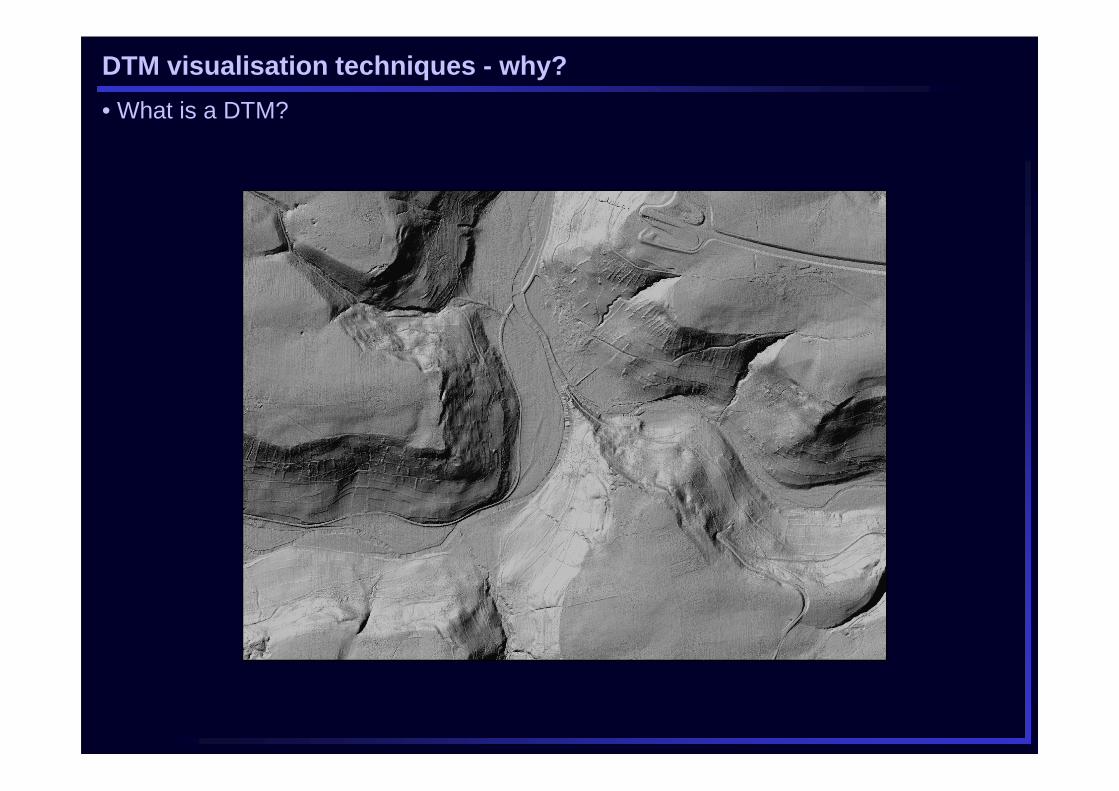
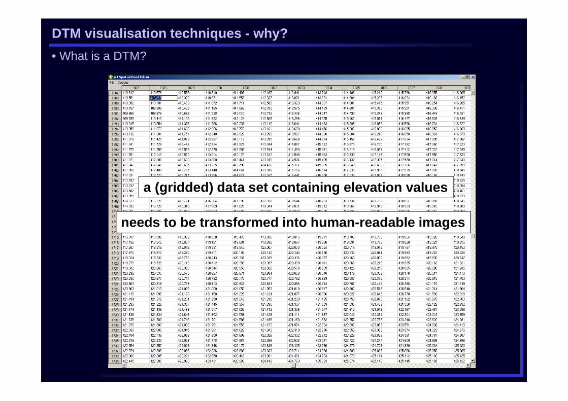
DTM visualisation techniques - why?
• What is a DTM?
DTM visualisation techniques - why?
• What is a DTM?
a (gridded) data set containing elevation values
needs to be transformed into human-readable images
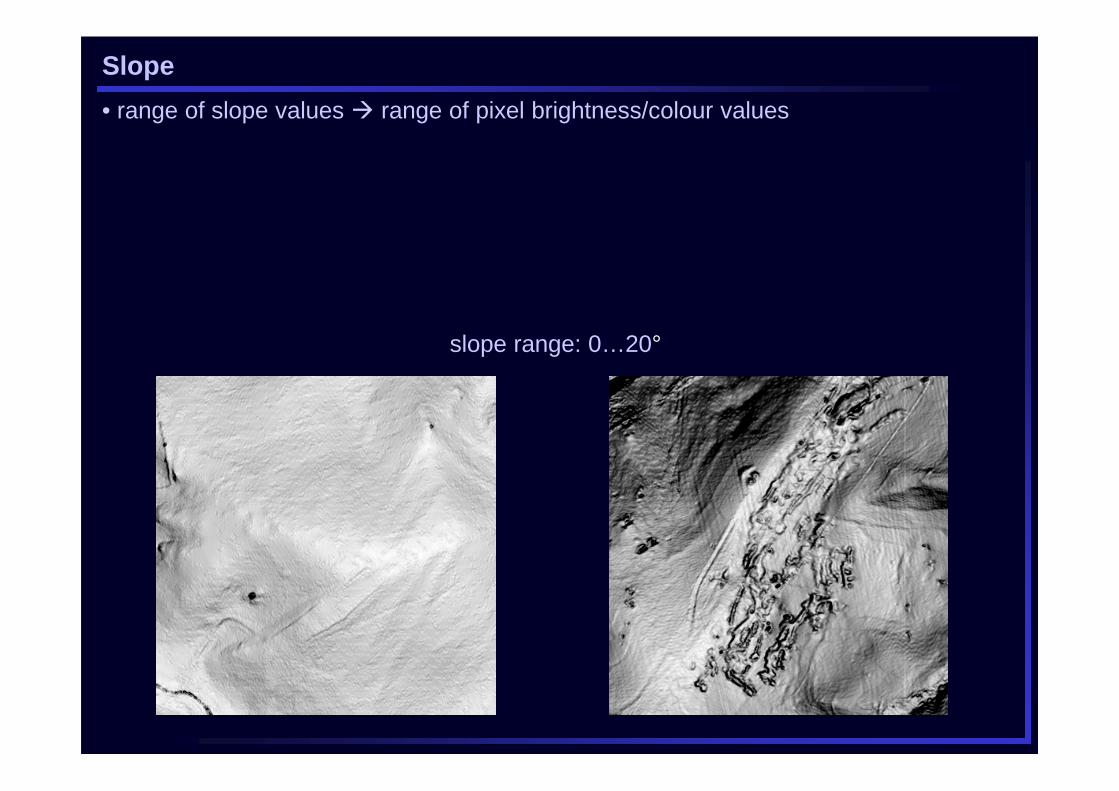
slope range: 0…20°
Slope
• range of slope values � range of pixel brightness/colour values
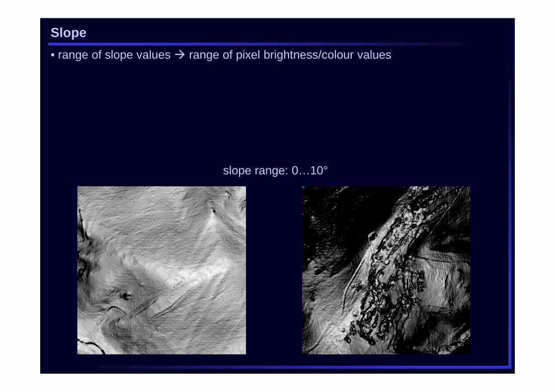
slope range: 0…10°
Slope
• range of slope values � range of pixel brightness/colour values
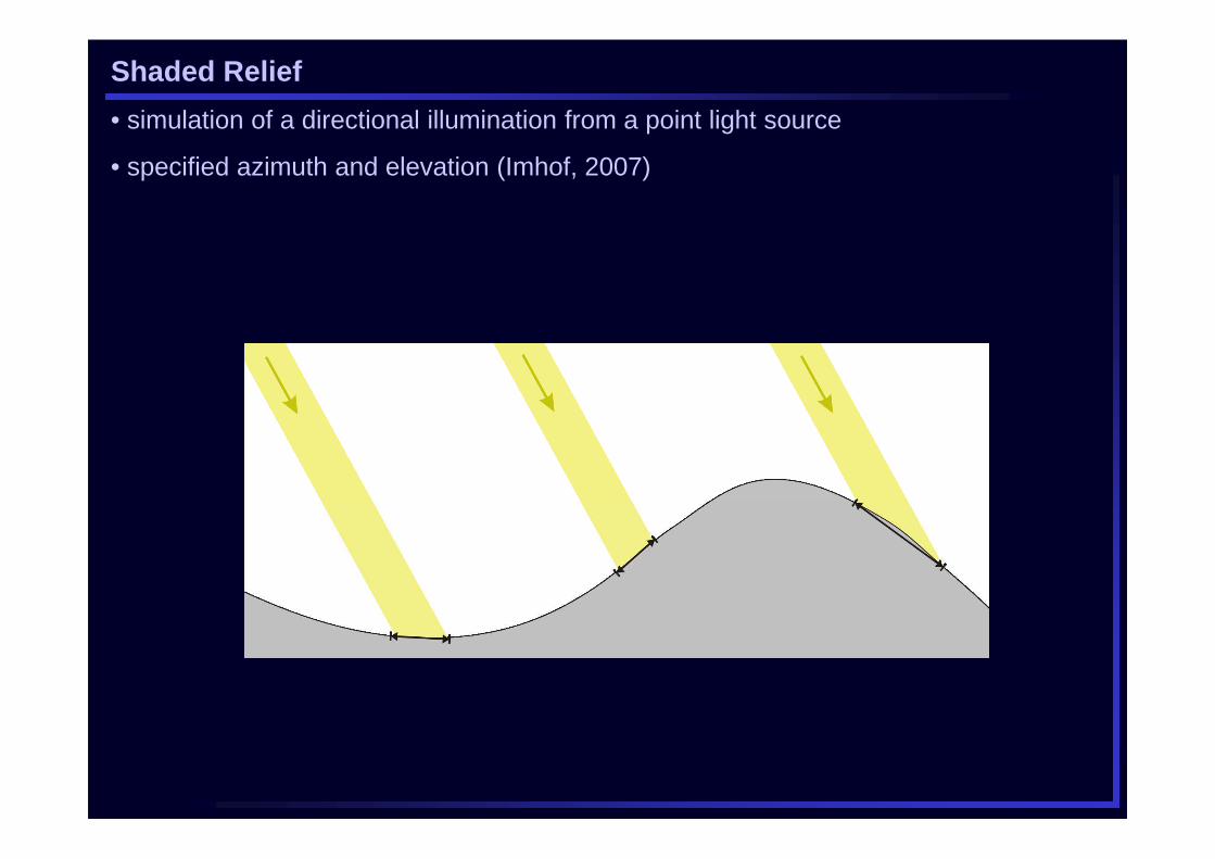
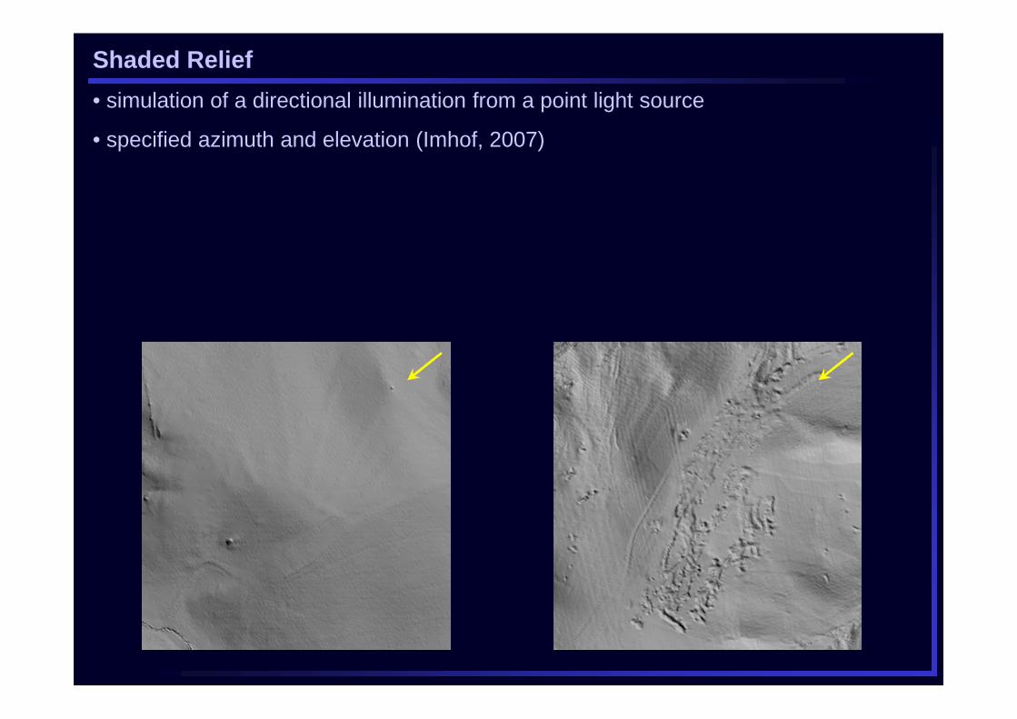
Shaded Relief
• simulation of a directional illumination from a point light source
• specified azimuth and elevation (Imhof, 2007)
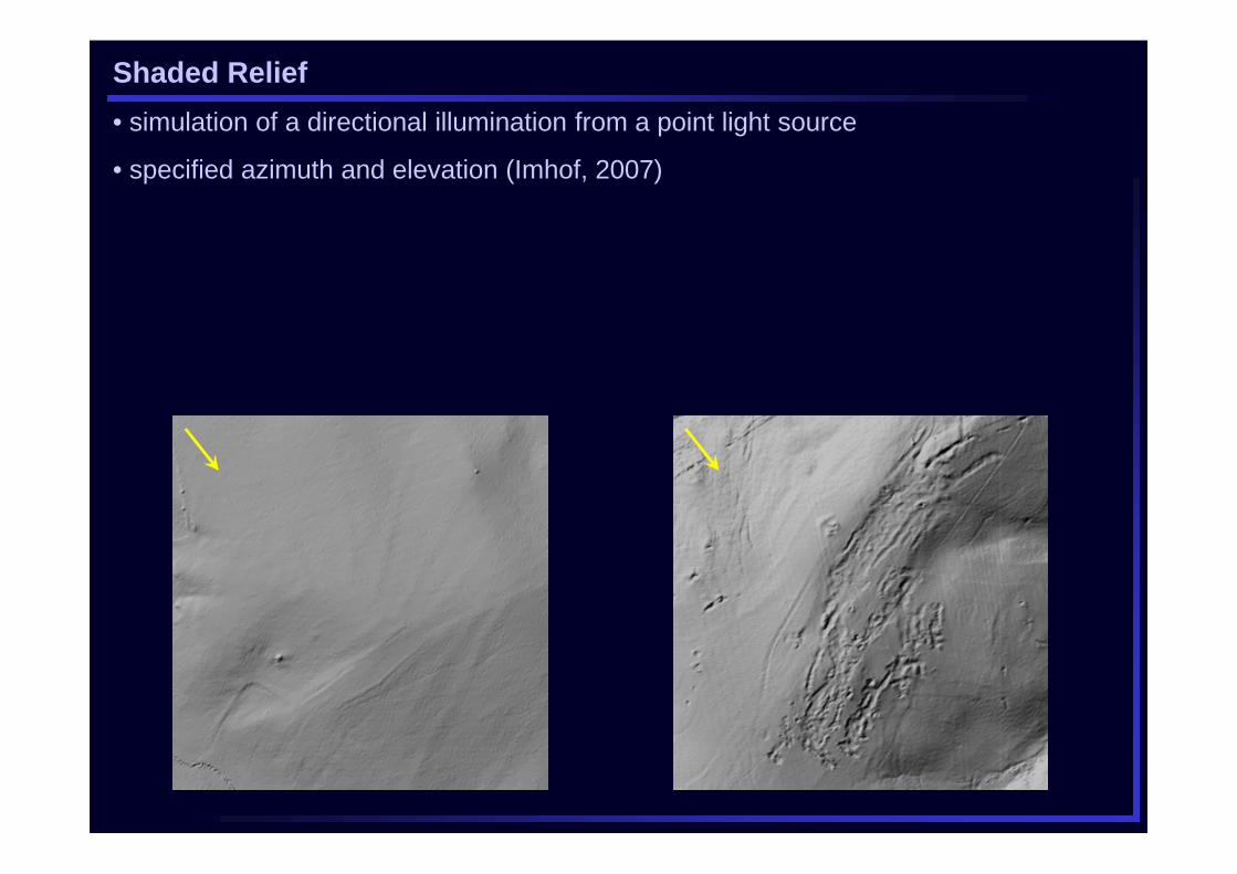
Shaded Relief
• simulation of a directional illumination from a point light source
• specified azimuth and elevation (Imhof, 2007)
Shaded Relief
• simulation of a directional illumination from a point light source
• specified azimuth and elevation (Imhof, 2007)
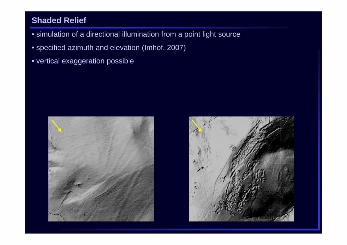
Shaded Relief
• simulation of a directional illumination from a point light source
• specified azimuth and elevation (Imhof, 2007)
• vertical exaggeration possible
Shaded Relief
• poor visibility of linear features aligned parallel with illumination azimuth
• bright/dark areas on slopes facing towards/away from illumination
• multiple illumination directions required
• optical illusions for illumination azimuths 90-270°
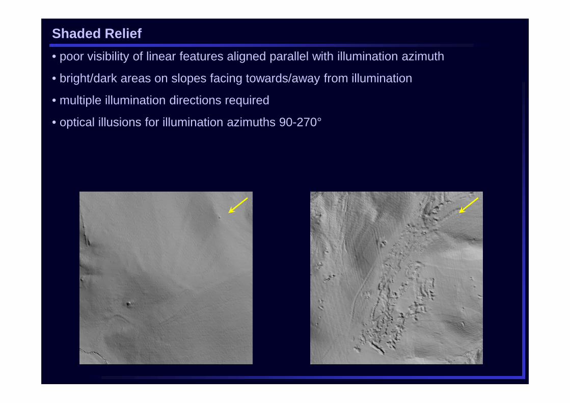
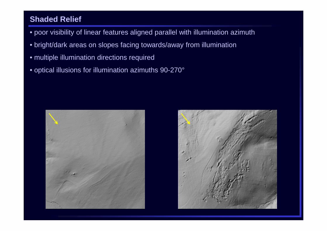
Shaded Relief
• poor visibility of linear features aligned parallel with illumination azimuth
• bright/dark areas on slopes facing towards/away from illumination
• multiple illumination directions required
• optical illusions for illumination azimuths 90-270°
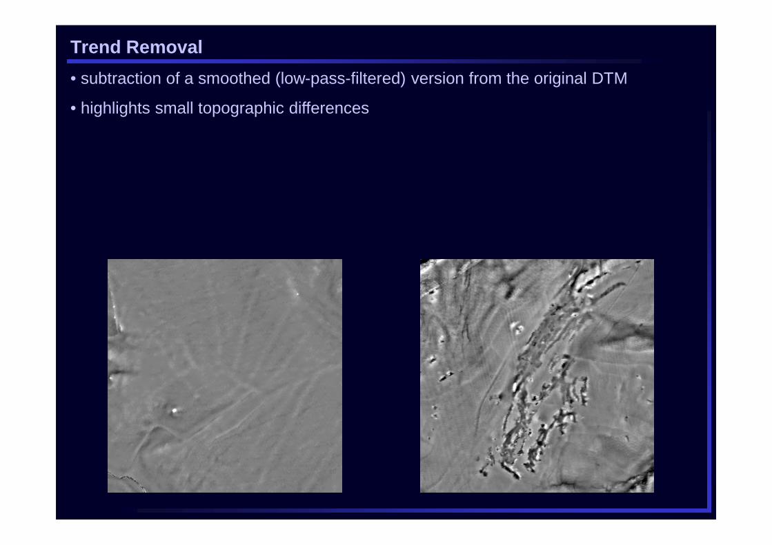
Trend Removal
• subtraction of a smoothed (low-pass-filtered) version from the original DTM
• highlights small topographic differences
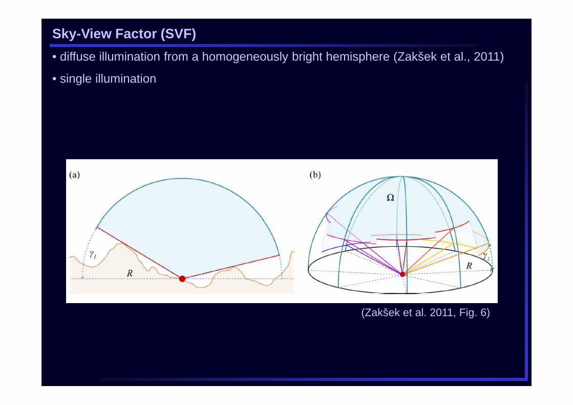
Sky-View Factor (SVF)
• diffuse illumination from a homogeneously bright hemisphere (Zakšek et al., 2011)
• single illumination
(Zakšek et al. 2011, Fig. 6)
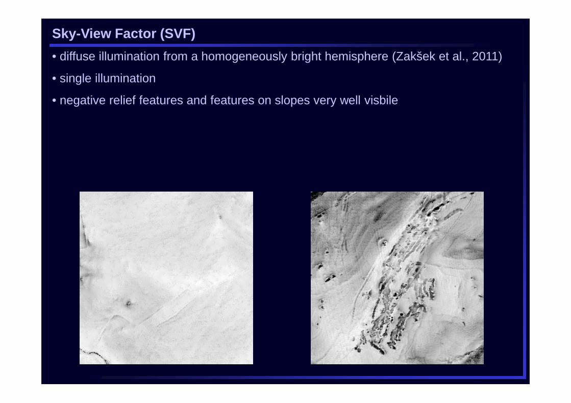
Sky-View Factor (SVF)
• diffuse illumination from a homogeneously bright hemisphere (Zakšek et al., 2011)
• single illumination
• negative relief features and features on slopes very well visbile
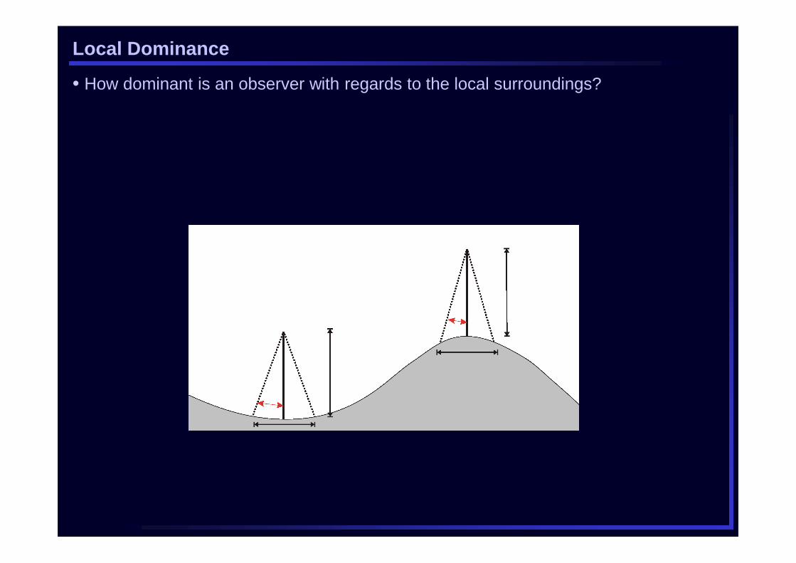
Local Dominance
• How dominant is an observer with regards to the local surroundings?
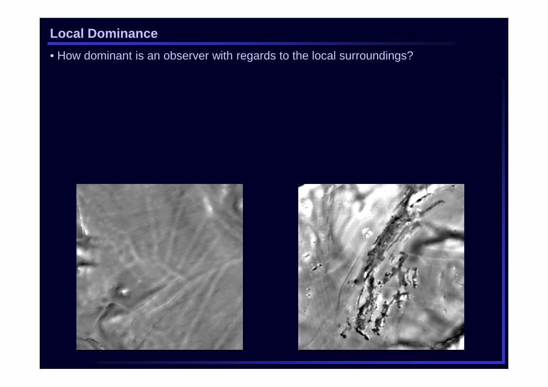
Local Dominance
• How dominant is an observer with regards to the local surroundings?
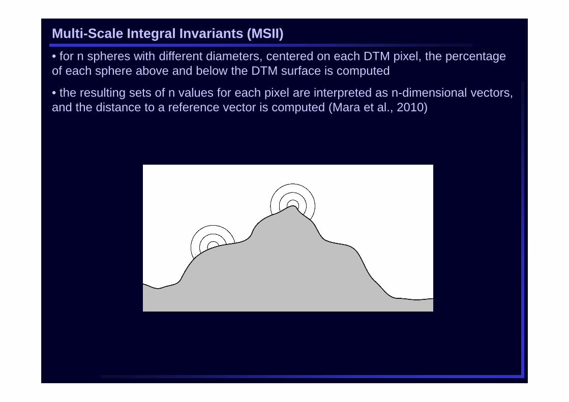
Multi-Scale Integral Invariants (MSII)
• for n spheres with different diameters, centered on each DTM pixel, the percentage of each sphere above and below the DTM surface is computed
• the resulting sets of n values for each pixel are interpreted as n-dimensional vectors, and the distance to a reference vector is computed (Mara et al., 2010)
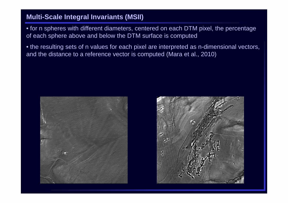
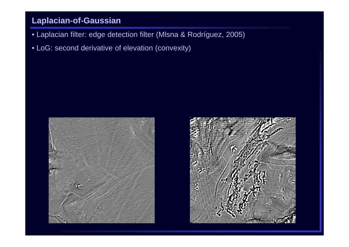
Laplacian-of-Gaussian
• Laplacian filter: edge detection filter (Mlsna & Rodríguez, 2005)
• LoG: second derivative of elevation (convexity)
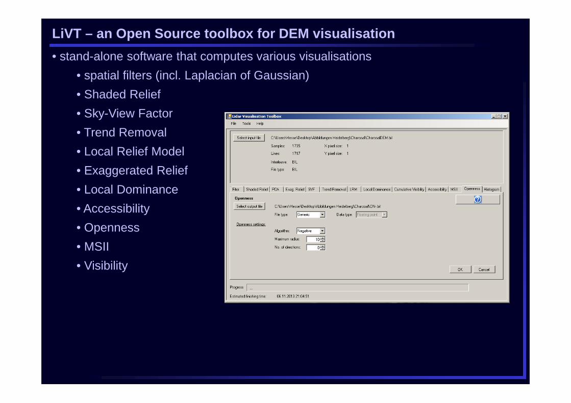
LiVT – an Open Source toolbox for DEM visualisation
• stand-alone software that computes various visualisations
• spatial filters (incl. Laplacian of Gaussian)
• Shaded Relief
• Sky-View Factor
• Trend Removal
• Local Relief Model
• Exaggerated Relief
• Local Dominance
• Accessibility
• Openness
• MSII
• Visibility
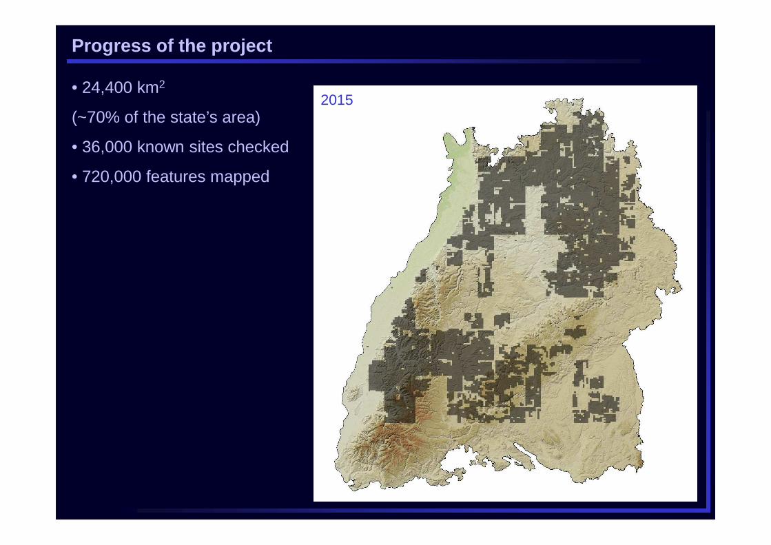
Progress of the project
• 24,400 km2
(~70% of the state’s area)
• 36,000 known sites checked
• 720,000 features mapped
2012201320142015
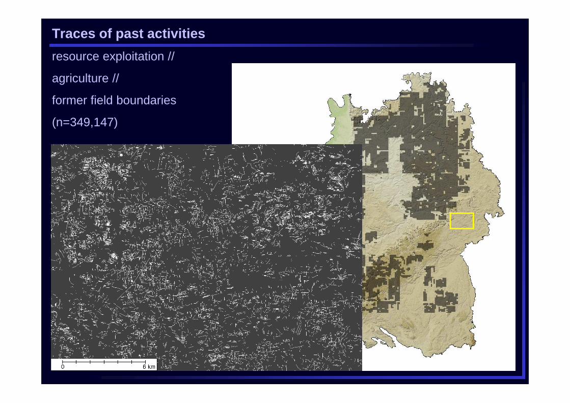
Traces of past activities
resource exploitation //
agriculture //
former field boundaries
(n=349,147)
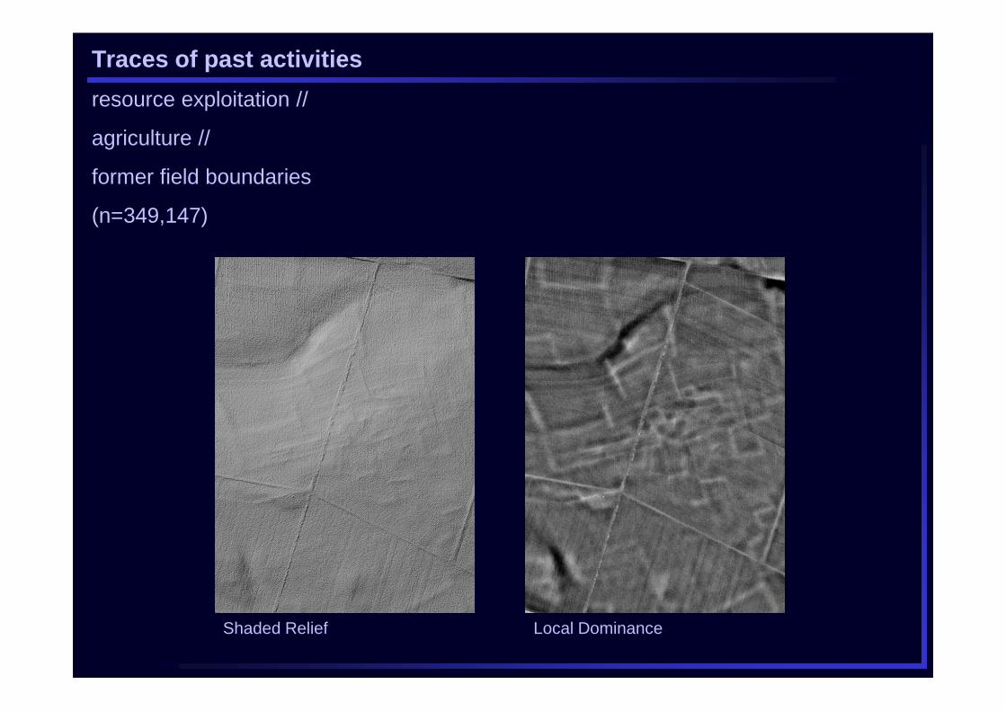
Traces of past activities
resource exploitation //
agriculture //
former field boundaries
(n=349,147)
Shaded Relief Local Dominance
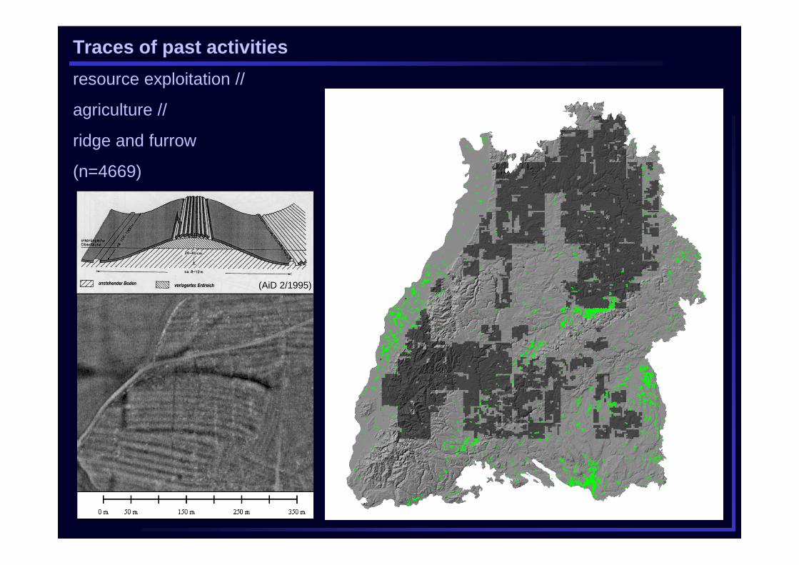
Traces of past activities
resource exploitation //
agriculture //
ridge and furrow
(n=4669)
(AiD 2/1995)
LoG & LD
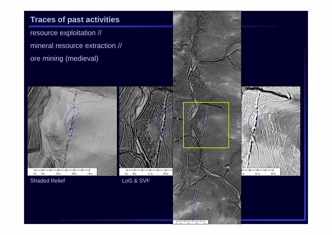
Traces of past activities
resource exploitation //
mineral resource extraction //
ore mining (medieval)
Shaded Relief LoG & SVF
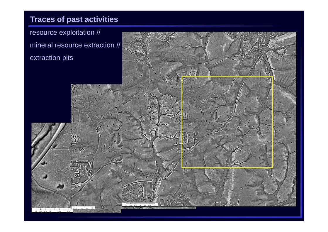
Traces of past activities
resource exploitation //
mineral resource extraction //
extraction pits
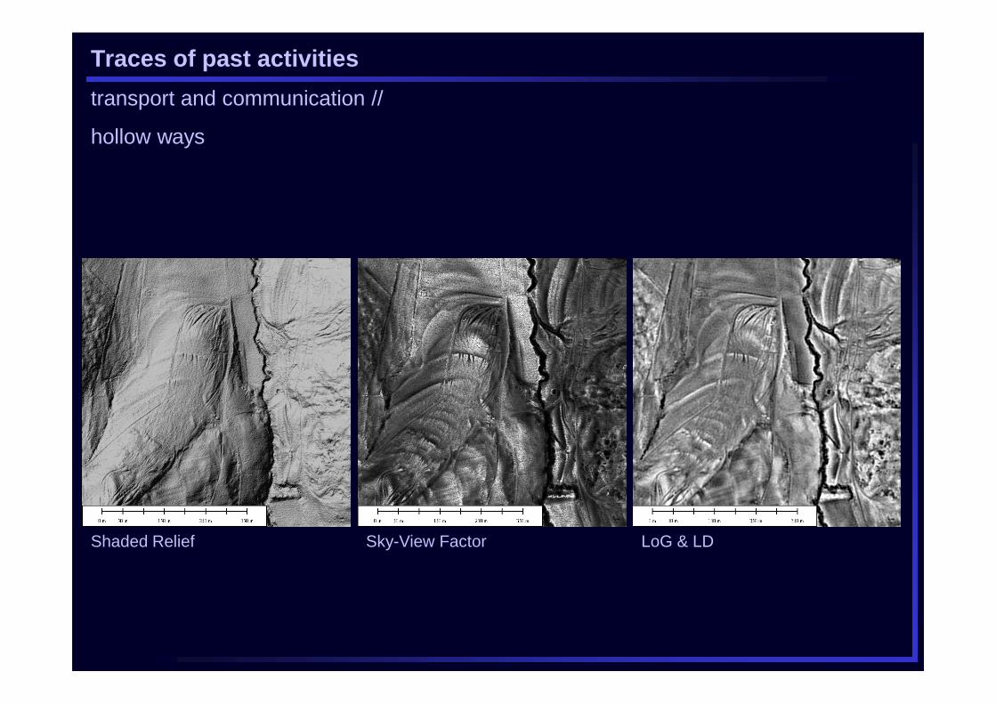
Traces of past activities
transport and communication //
hollow ways
LoG & LDShaded Relief Sky-View Factor
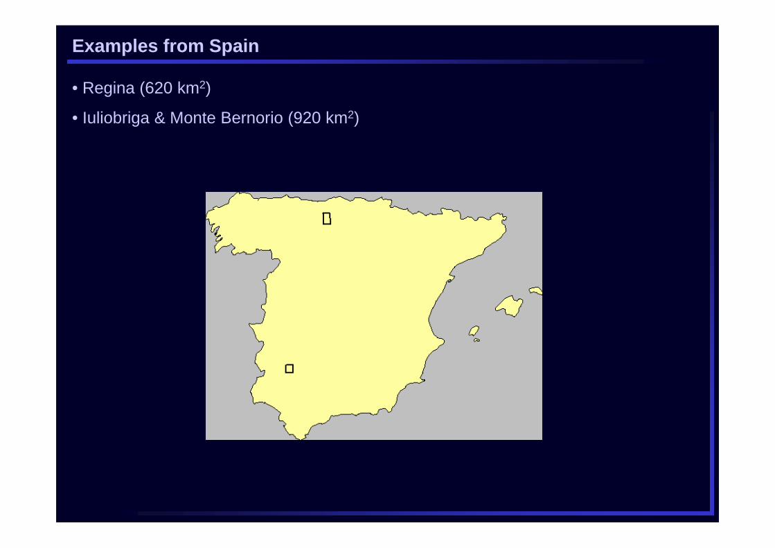
Examples from Spain
• Regina (620 km2)
• Iuliobriga & Monte Bernorio (920 km2)
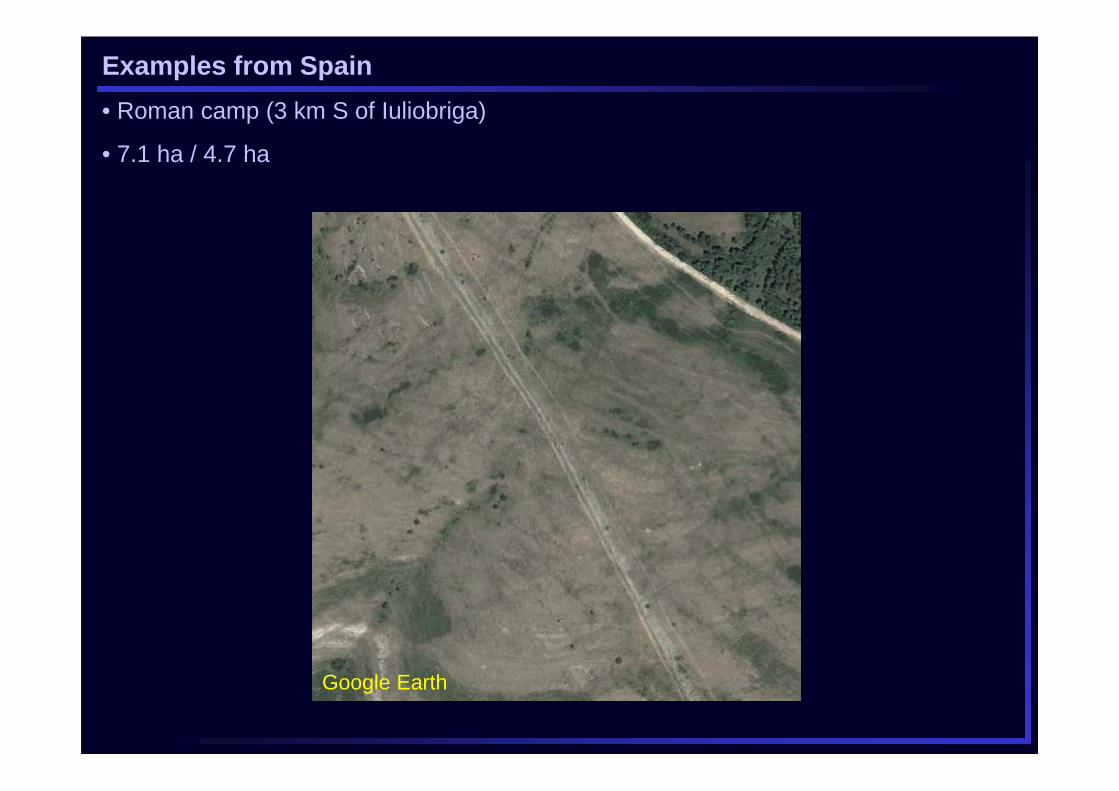
Examples from Spain
• Roman camp (3 km S of Iuliobriga)
• 7.1 ha / 4.7 ha
Google Earth
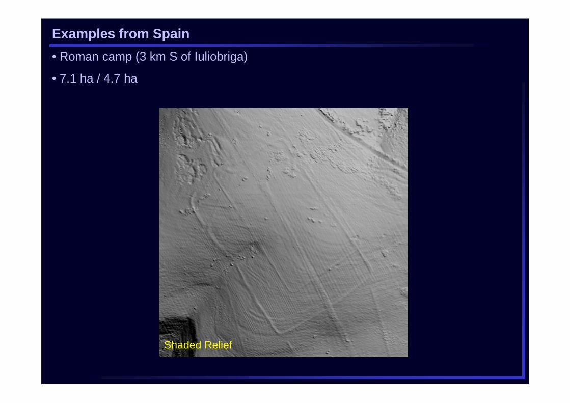
Shaded Relief
Examples from Spain
• Roman camp (3 km S of Iuliobriga)
• 7.1 ha / 4.7 ha
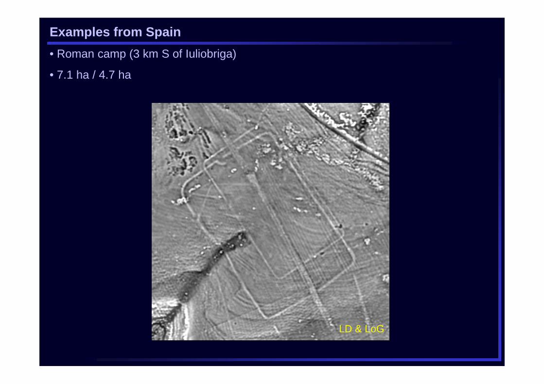
LD & LoG
Examples from Spain
• Roman camp (3 km S of Iuliobriga)
• 7.1 ha / 4.7 ha

Examples from Spain
• Roman camp (3 km S of Iuliobriga)
• 7.1 ha / 4.7 ha
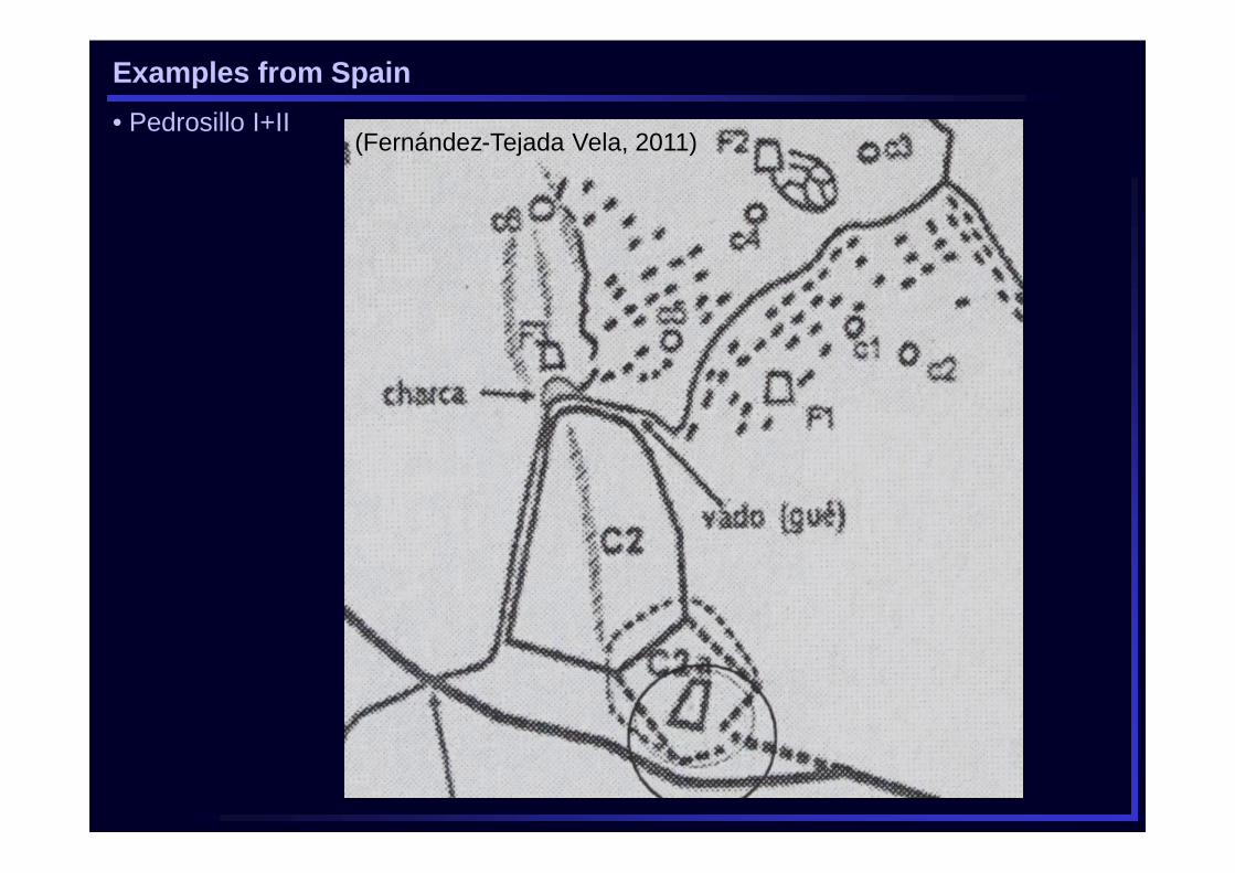
(Fernández-Tejada Vela, 2011)
Examples from Spain
• Pedrosillo I+II
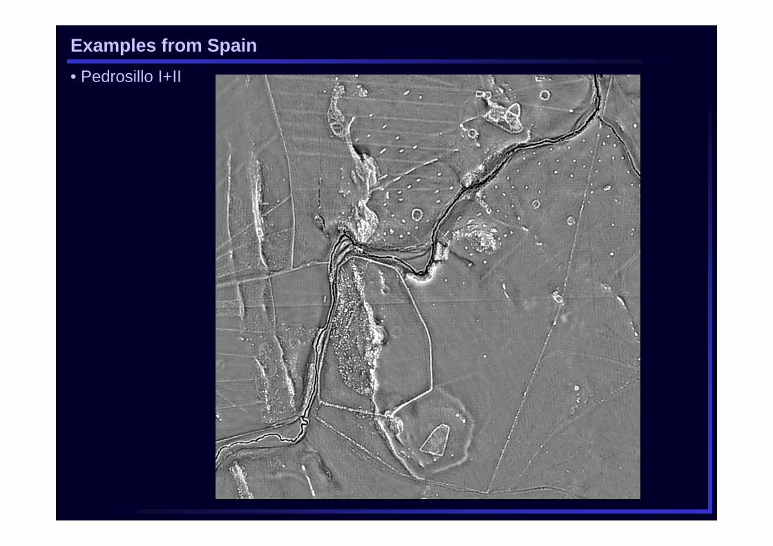
Examples from Spain
• Pedrosillo I+II
Examples from Spain
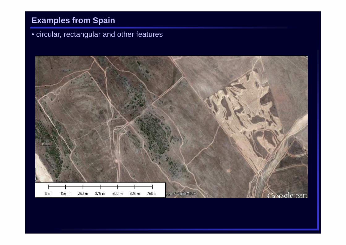
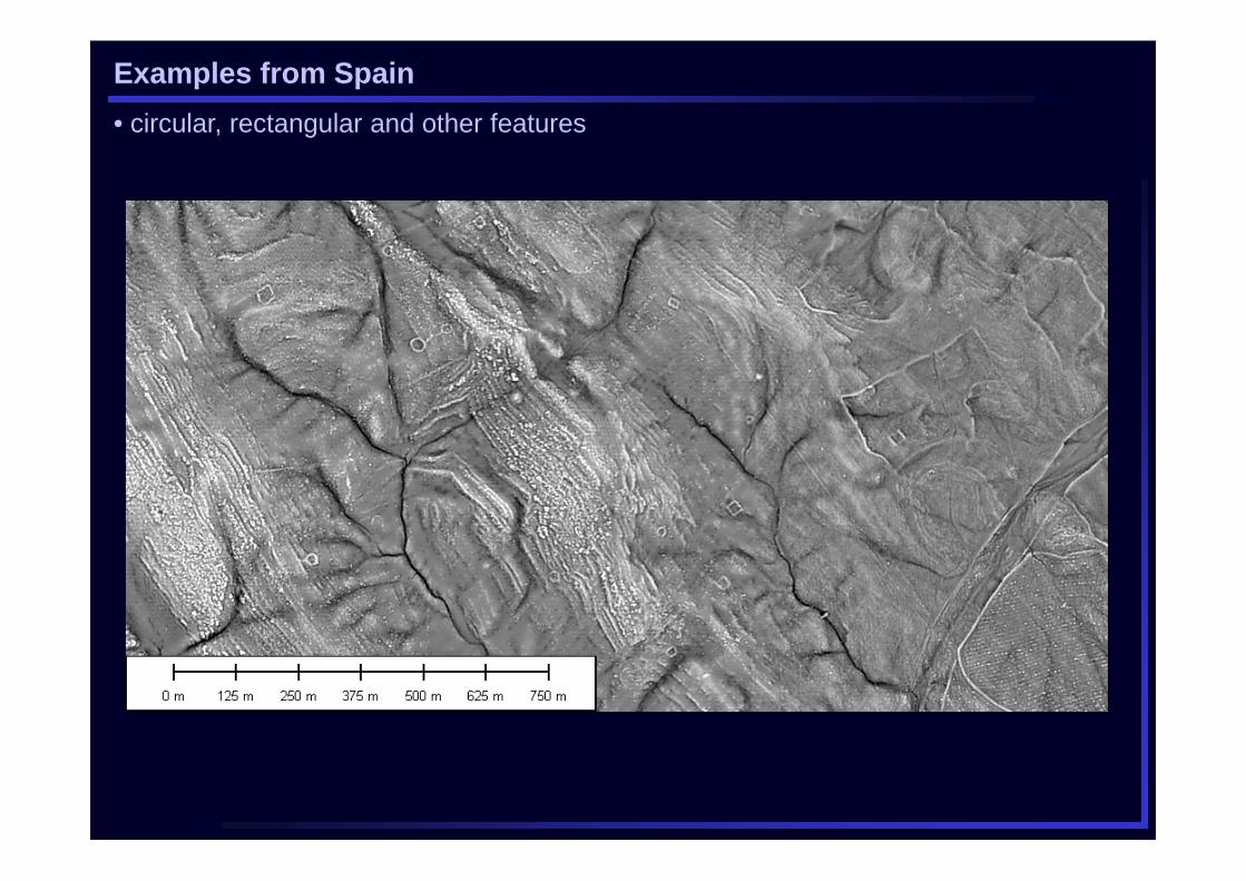
• circular, rectangular and other features
Examples from Spain
• circular, rectangular and other features
Examples from Spain
• circular, rectangular and other features
Examples from Spain
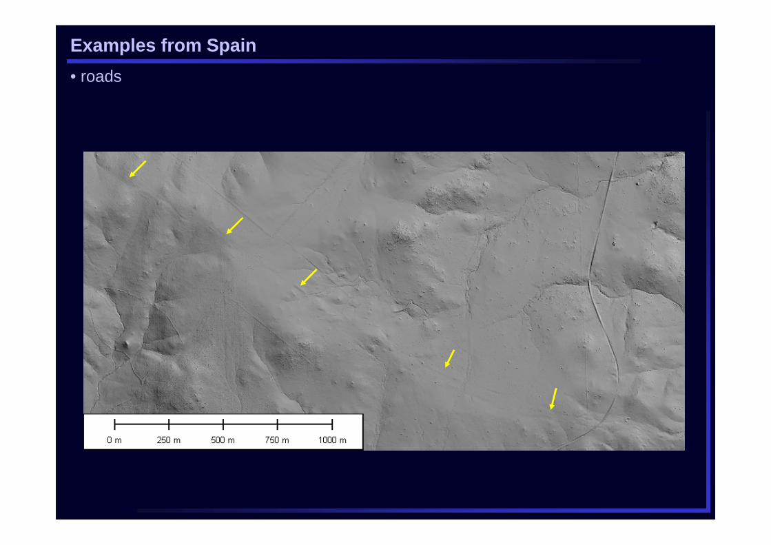
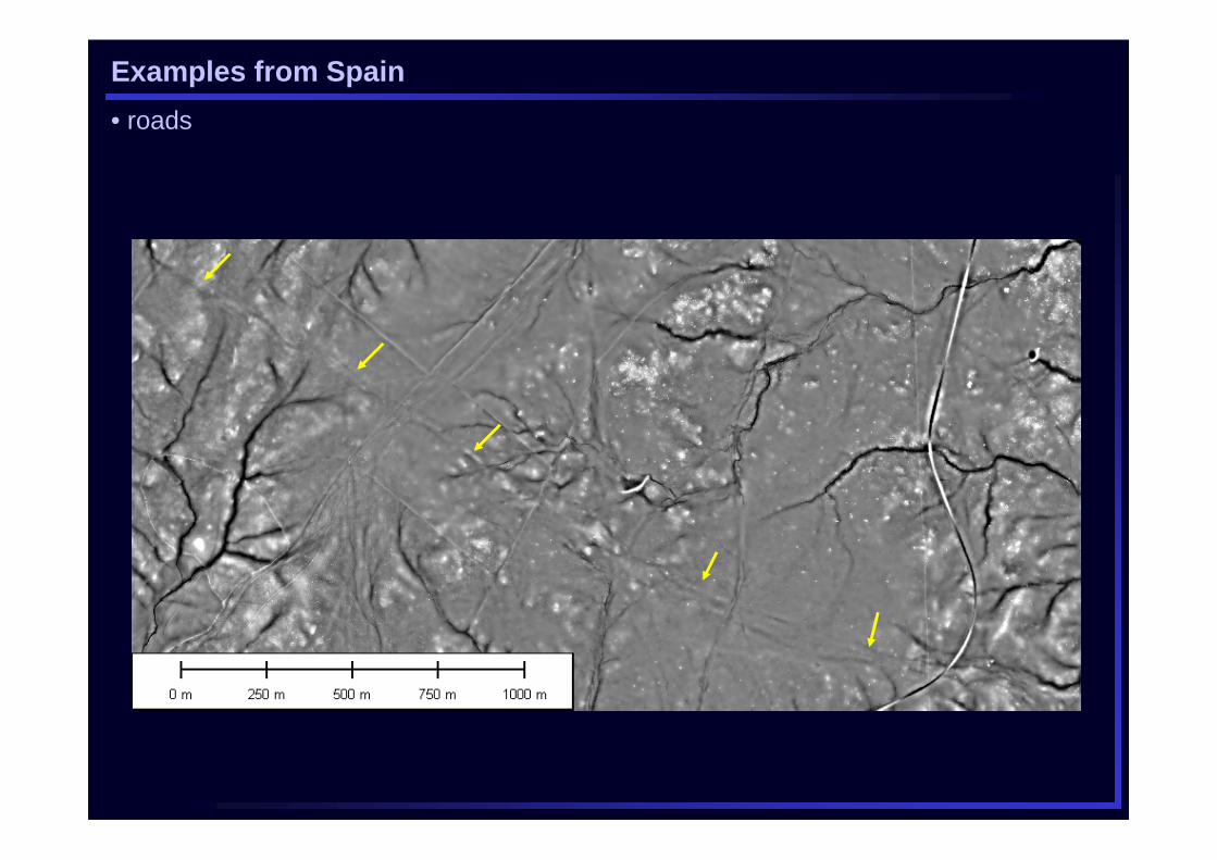
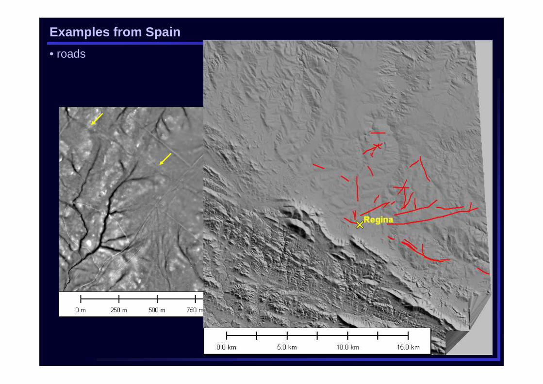
• roads
Examples from Spain
• roads
Examples from Spain
• roads
Examples from Spain
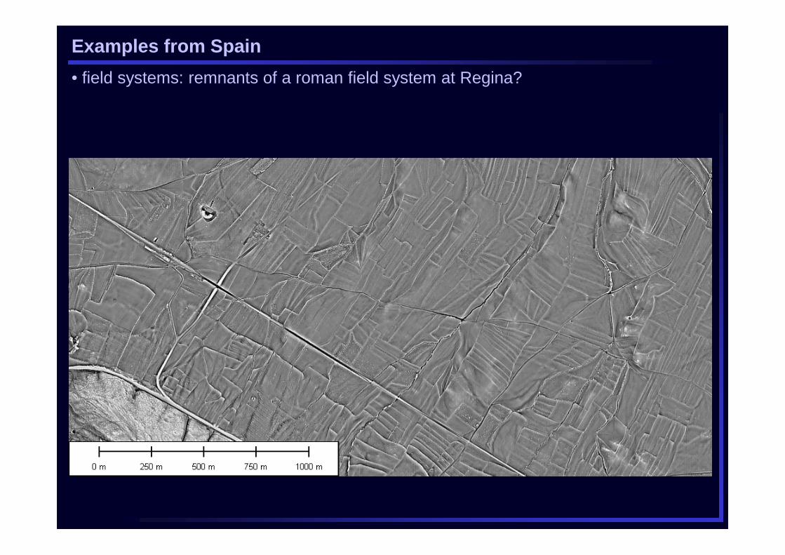
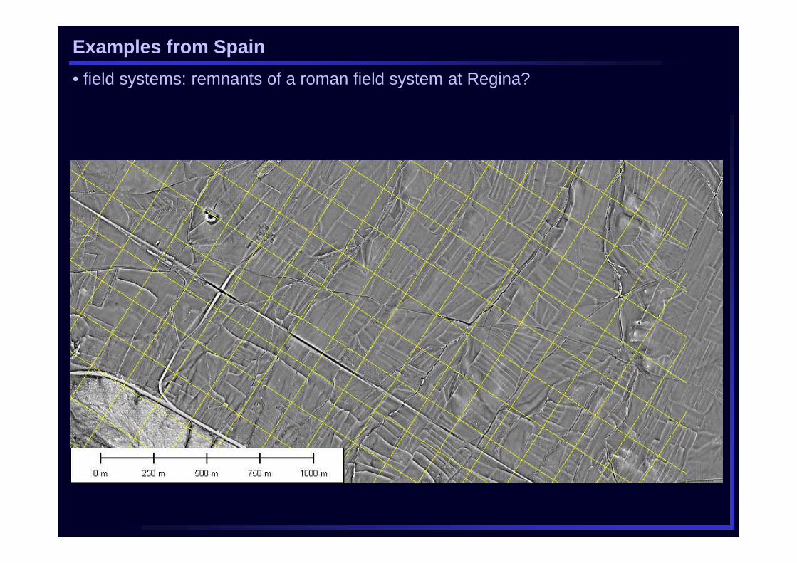
• field systems: remnants of a roman field system at Regina?
Examples from Spain
• field systems: remnants of a roman field system at Regina?
Examples from Spain
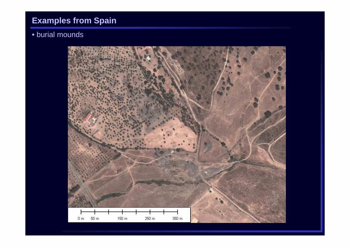
• burial mounds

Examples from Spain
• burial mounds
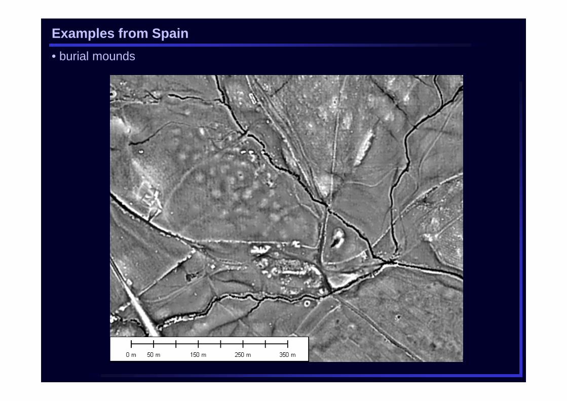
Examples from Spain
• burial mounds

Examples from Spain
• mining traces
Examples from Spain
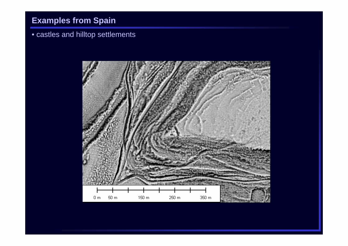
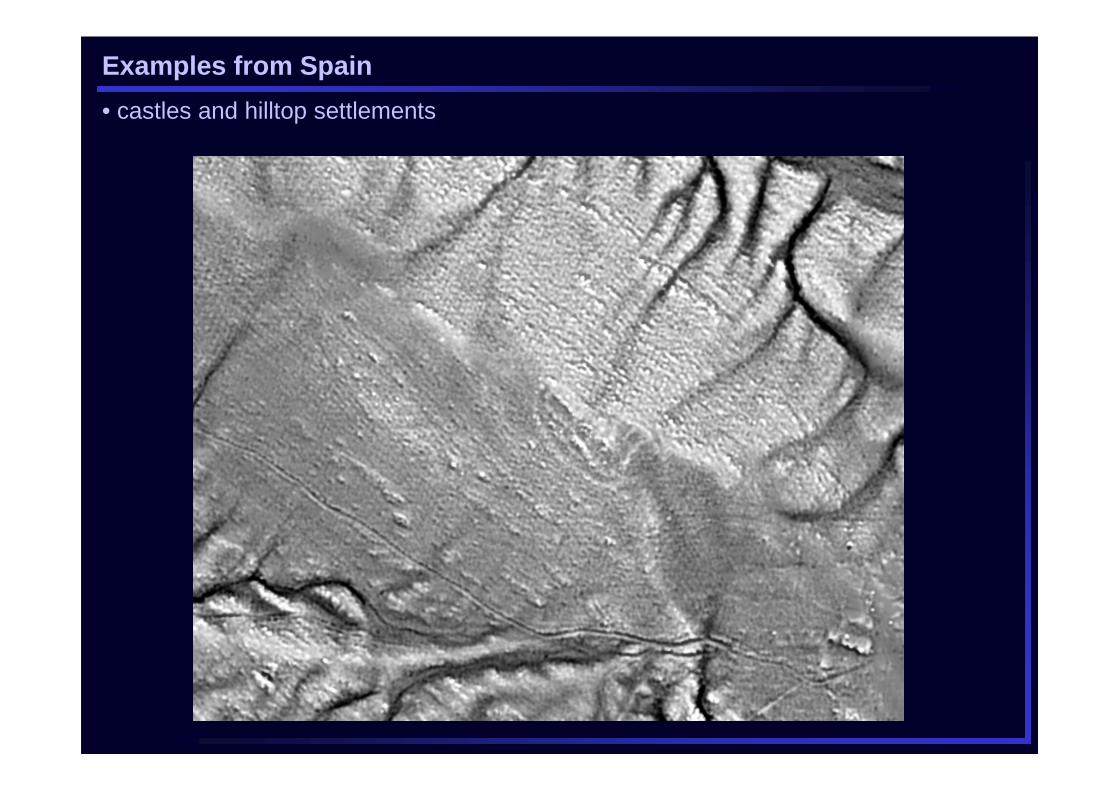
• castles and hilltop settlements
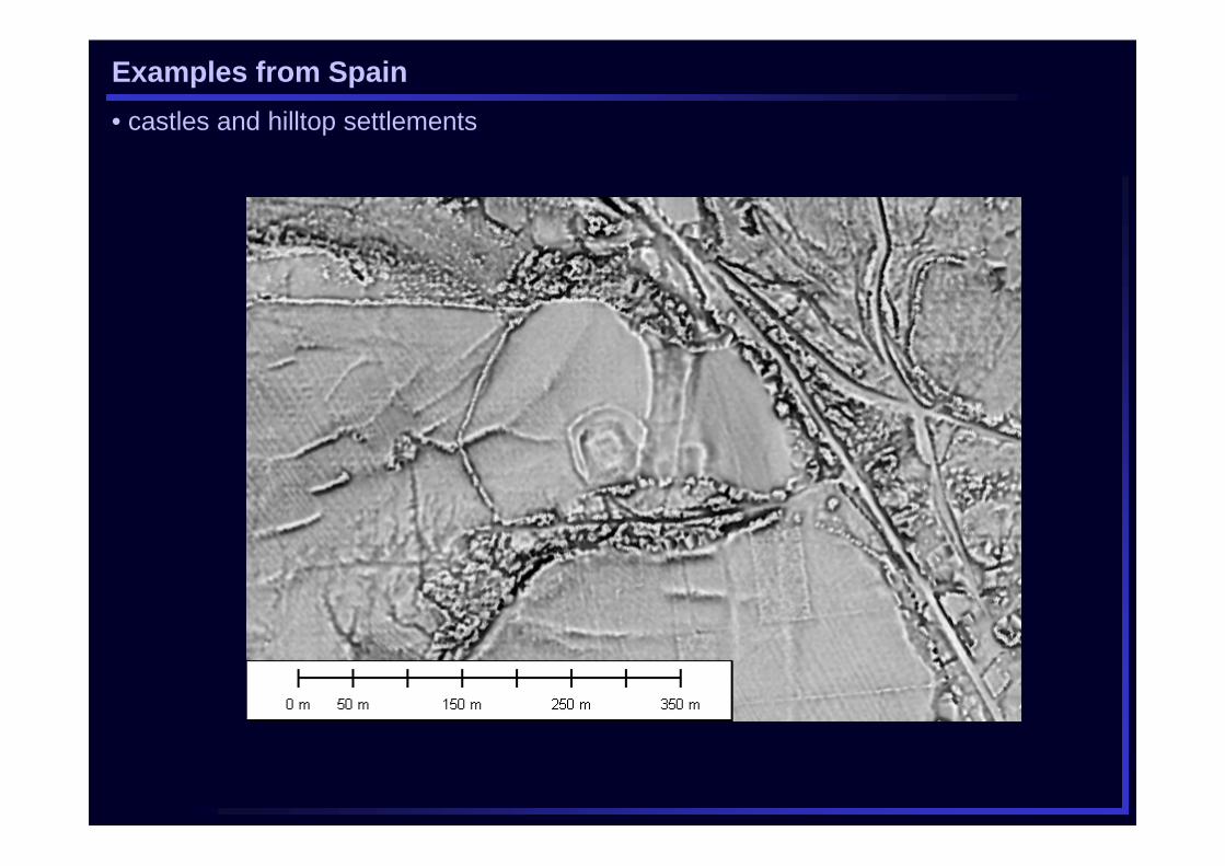
Examples from Spain
• castles and hilltop settlements
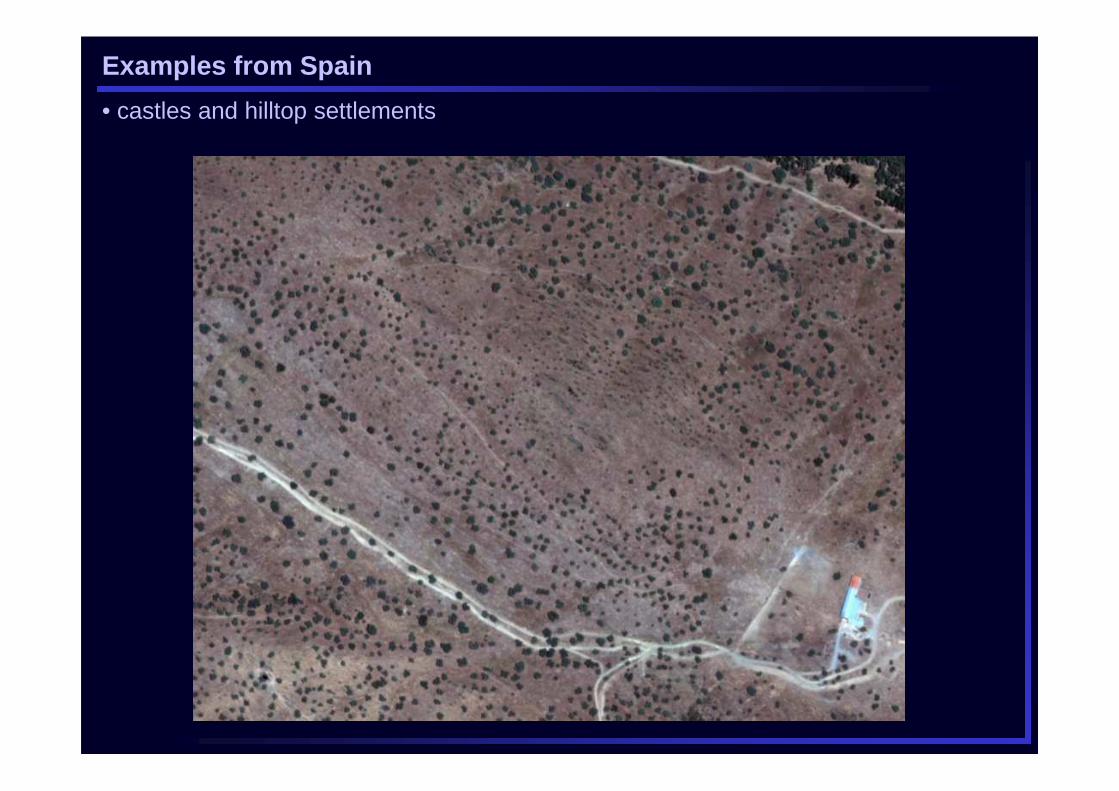
Examples from Spain
• castles and hilltop settlements
Examples from Spain
• castles and hilltop settlements
Examples from Spain
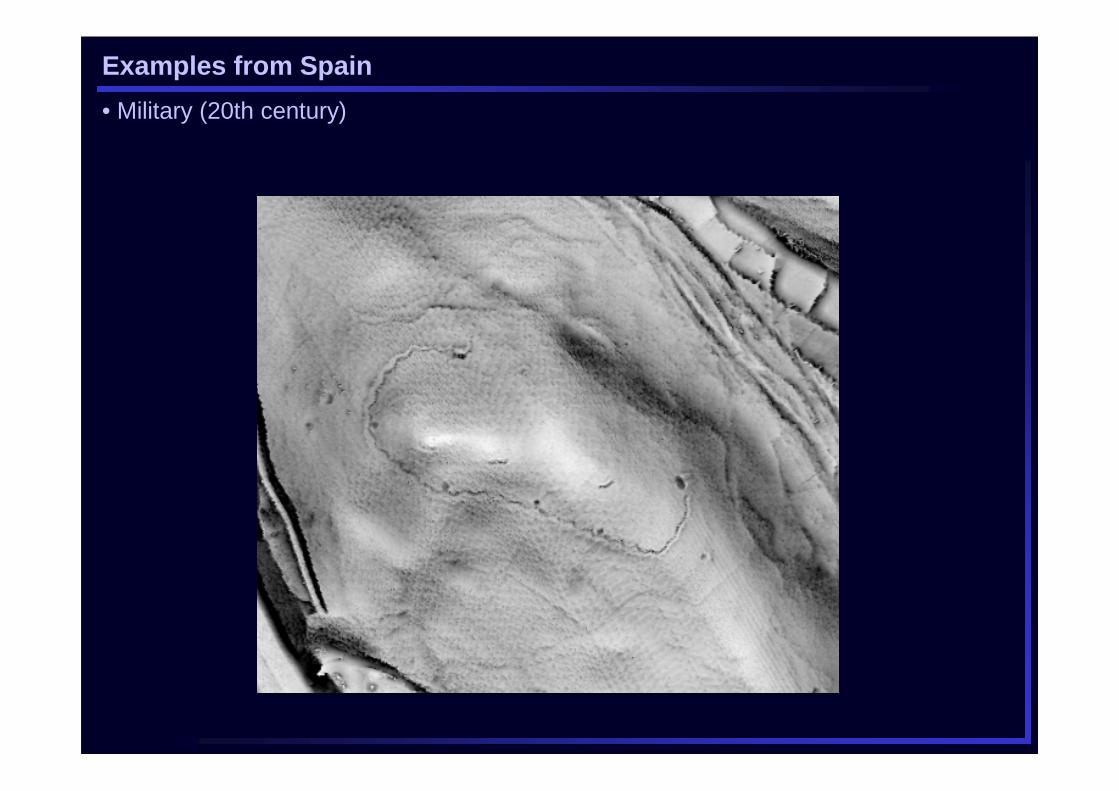
• Military (20th century)
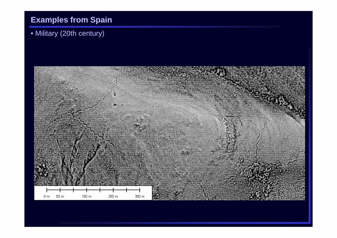
Examples from Spain
• Military (20th century)
Examples from Spain
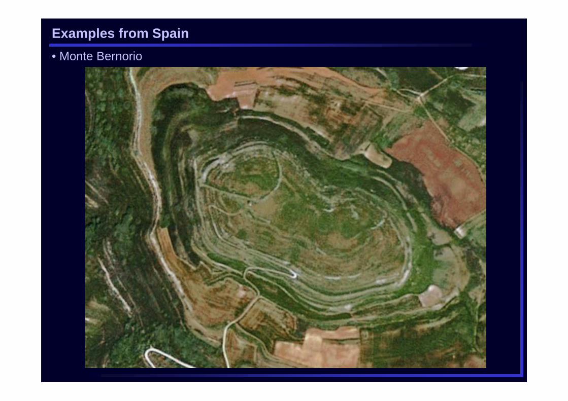
• Monte Bernorio
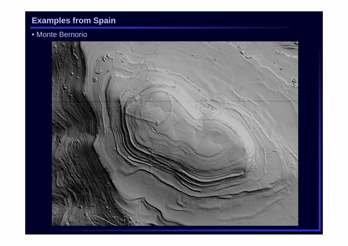
Examples from Spain
• Monte Bernorio
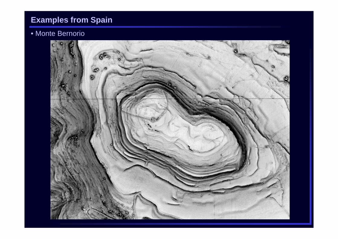
Examples from Spain
• Monte Bernorio
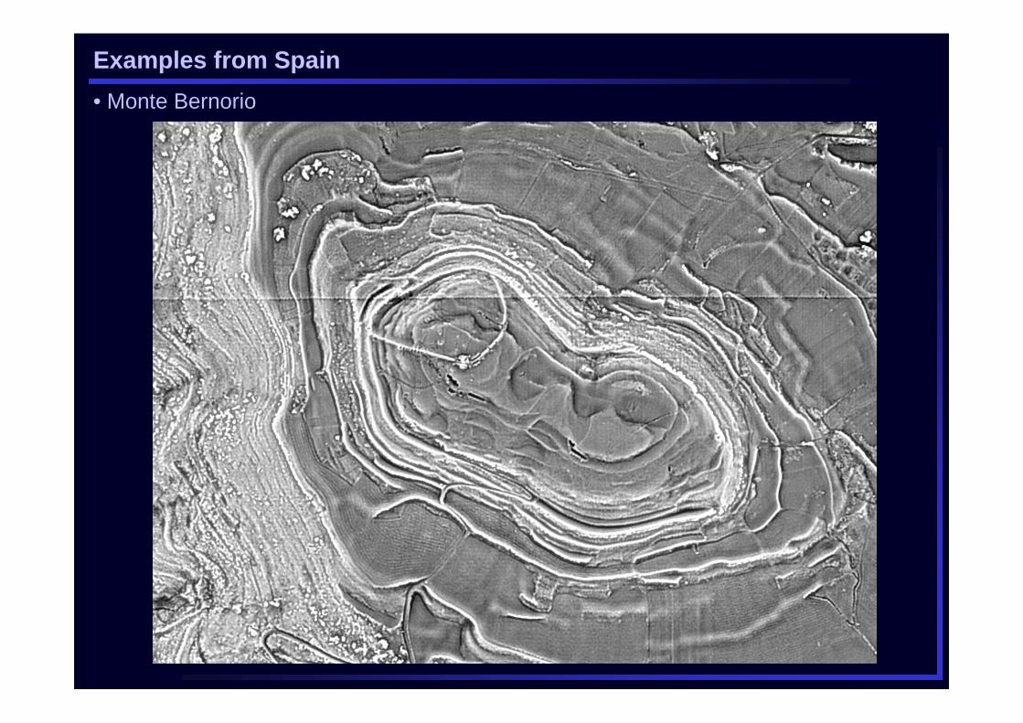
Examples from Spain
• Monte Bernorio
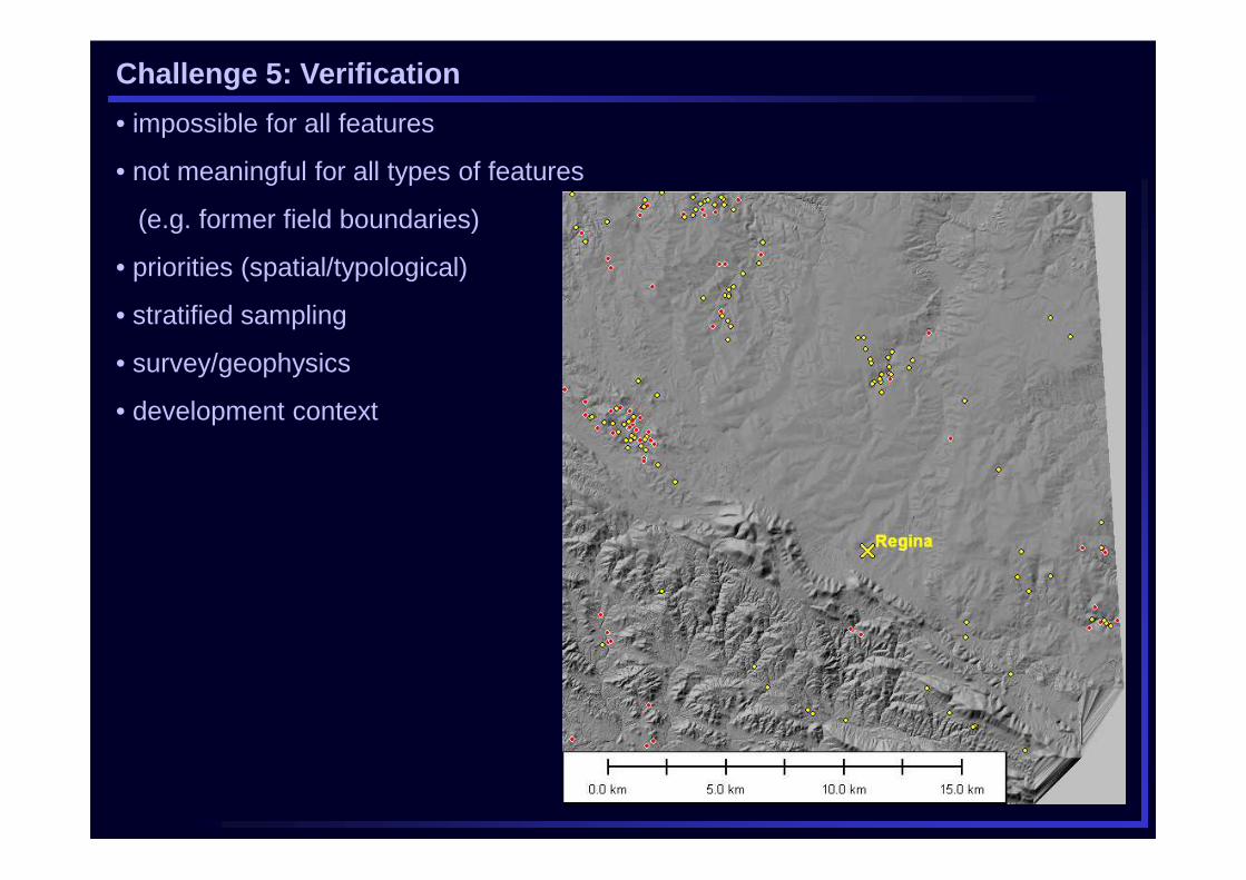
Challenge 5: Verification
• impossible for all features
• not meaningful for all types of features
(e.g. former field boundaries)
• priorities (spatial/typological)
• stratified sampling
• survey/geophysics
• development context
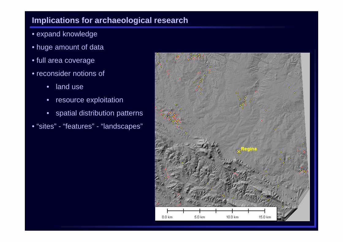
Implications for archaeological research
• expand knowledge
• huge amount of data
• full area coverage
• reconsider notions of
• land use
• resource exploitation
• spatial distribution patterns
• “sites” - “features” - “landscapes”
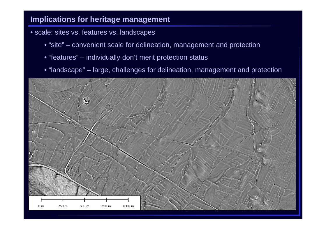
Implications for heritage management
• scale: sites vs. features vs. landscapes
• “site” – convenient scale for delineation, management and protection
• “features” – individually don’t merit protection status
• “landscape” – large, challenges for delineation, management and protection
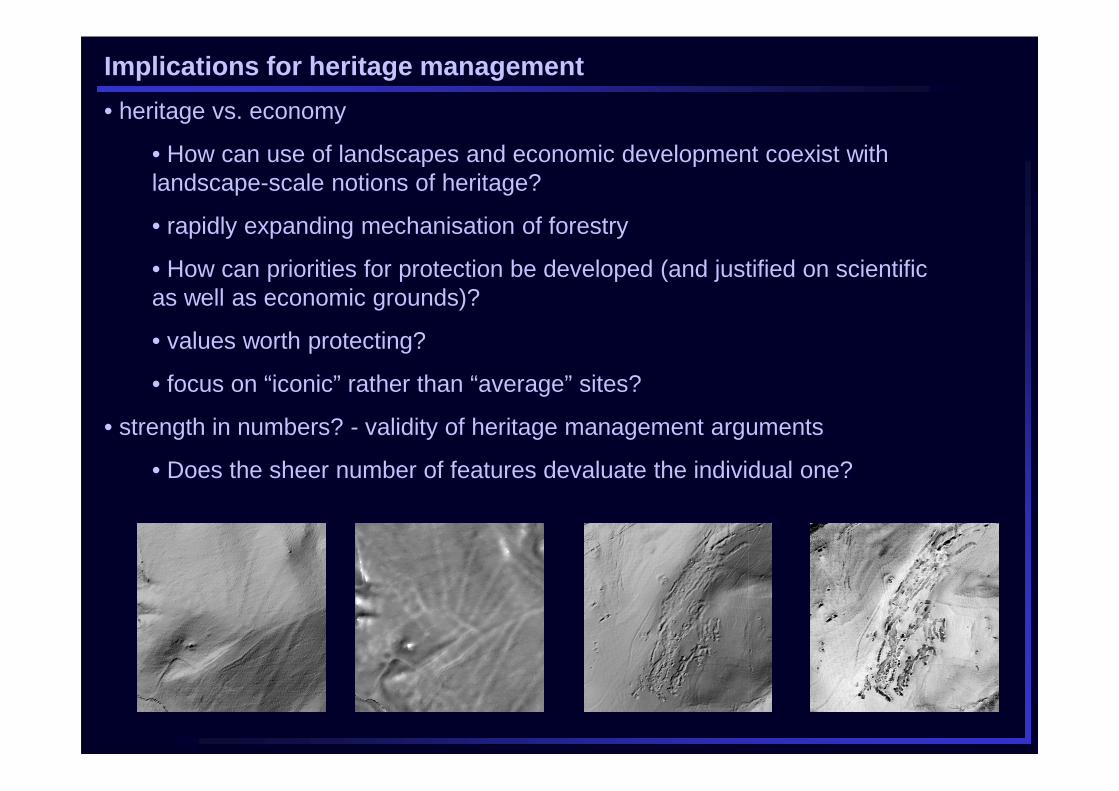
Implications for heritage management
• heritage vs. economy
• How can use of landscapes and economic development coexist with landscape-scale notions of heritage?
• rapidly expanding mechanisation of forestry
• How can priorities for protection be developed (and justified on scientific as well as economic grounds)?
• values worth protecting?
• focus on “iconic” rather than “average” sites?
• strength in numbers? - validity of heritage management arguments
• Does the sheer number of features devaluate the individual one?
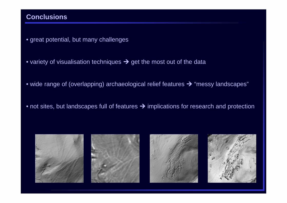
Conclusions
• great potential, but many challenges
• variety of visualisation techniques � get the most out of the data
• wide range of (overlapping) archaeological relief features � “messy landscapes”
• not sites, but landscapes full of features � implications for research and protection
ReferencesDevereux, B.J., Amable, G.S., Crow, P., 2008. Visualisation of LiDAR terrain models for archaeological feature detection. Antiquity 82, 470–479.
Doneus, M., 2013. Openness as visualization technique for interpretative mapping of airborne LiDAR derived digital terrain models. Remote Sensing 5, 6427-6442.
Hesse, R. 2010. LiDAR-derived Local Relief Models – a new tool for archaeological prospection. Archaeological Prospection 17, 67–72.
Imhof, E., 2007. Cartographic relief representation. English language edition edited by H.J. Steward. Redlands: ESRI Press.
Jolliffe, I.T., 2002. Principal component analysis. Second edition. Spinger, New York.
Mara, H., Krömker, S., Jakob, S., Breuckmann, B., 2010. GigaMesh and Gilgamesh – 3D Multiscale Integral Invariant Cuneiform Character Extraction, In: Artusi, A., Joly-Parvex, M., Lucet, G., Ribes, A., Pitzalis, D. (eds.), The 11th International Symposium on Virtual Reality, Archaeology and Cultural Heritage VAST (Paris, France, 2010), pp. 131–138.
Miller, G., 1994. Efficient algorithm for local and global accessibility shading. Computer Graphics Proceedings, Annual Conference Series SIGGRAPH, 319–325.Mlekuž, D., 2012. Messy landscapes: lidar and the pr actices of landscaping. In: Cowley, D.C., Opitz, R.S ., (eds.), Interpreting archaeological topography: las ers, 3D data, observation, visualisation and applic ations. Oxbow, Oxford, pp. 90-101.Mlsna, P.A., Rodríguez, J.J., 2005. Gradient and Laplacian edge detection. In: Bovik, A.C. (ed.), Handbook of image and video processing. 2nd. edition. Elsevier, Amsterdam. pp. 535–553.
Rusinkiewicz, S., Burns, M., DeCarlo, D., 2006. Exaggerated Shading for depicting shape and detail. ACM Transactions on Graphics (Proceedings SIGGRAPH) 25(3), 1199–1205.
Yokoyama, R., Shirasawa, M., Pike, R.J., 2002. Visualizing topography by openness: a new application of image processing to digital elevation models. Photogrammetric Engineering & Remote Sensing 68(3), 257–265.
Zakšek, K., Oštir, K., Kokalj, Z., 2011. Sky-View Factor as a relief visualisation technique. Remote Sensing 3, 398–415.
LIDAR data: LGL/LAD Baden-Württemberg; IGN Spain