Springer Tracts in Modern Physics 274

Friedrich Jegerlehner

The Anomalous Magnetic Moment of the Muon Second Edition

Springer Tracts in Modern Physics

Volume 274

Series editors

Yan Chen, Department of Physics, Fudan University, Shanghai, ChinaAtsushi Fujimori, Department of Physics, University of Tokyo, Tokyo, JapanThomas Müller, Institut für Experimentelle Kernphysik, Universität Karlsruhe,Karlsruhe, GermanyWilliam C. Stwalley, Storrs, CT, USA

Springer Tracts in Modern Physics provides comprehensive and critical reviews oftopics of current interest in physics. The following fields are emphasized:

– Elementary Particle Physics– Condensed Matter Physics– Light Matter Interaction– Atomic and Molecular Physics– Complex Systems– Fundamental Astrophysics

Suitable reviews of other fields can also be accepted. The Editors encourageprospective authors to correspond with them in advance of submitting a manuscript.For reviews of topics belonging to the above mentioned fields, they should addressthe responsible Editor as listed in “Contact the Editors”.

More information about this series at http://www.springer.com/series/426

Friedrich Jegerlehner

The Anomalous MagneticMoment of the Muon

Second Edition

123

Friedrich JegerlehnerInstitut für PhysikHumboldt-Universität zu BerlinBerlinGermany

and

Deutsches Elektronen-Synchrotron (DESY)ZeuthenGermany

ISSN 0081-3869 ISSN 1615-0430 (electronic)Springer Tracts in Modern PhysicsISBN 978-3-319-63575-0 ISBN 978-3-319-63577-4 (eBook)DOI 10.1007/978-3-319-63577-4

Library of Congress Control Number: 2017946671

1st edition: © Springer-Verlag Berlin Heidelberg 20082nd edition: © Springer International Publishing AG 2017This work is subject to copyright. All rights are reserved by the Publisher, whether the whole or partof the material is concerned, specifically the rights of translation, reprinting, reuse of illustrations,recitation, broadcasting, reproduction on microfilms or in any other physical way, and transmissionor information storage and retrieval, electronic adaptation, computer software, or by similar or dissimilarmethodology now known or hereafter developed.The use of general descriptive names, registered names, trademarks, service marks, etc. in thispublication does not imply, even in the absence of a specific statement, that such names are exempt fromthe relevant protective laws and regulations and therefore free for general use.The publisher, the authors and the editors are safe to assume that the advice and information in thisbook are believed to be true and accurate at the date of publication. Neither the publisher nor theauthors or the editors give a warranty, express or implied, with respect to the material contained herein orfor any errors or omissions that may have been made. The publisher remains neutral with regard tojurisdictional claims in published maps and institutional affiliations.

Printed on acid-free paper

This Springer imprint is published by Springer NatureThe registered company is Springer International Publishing AGThe registered company address is: Gewerbestrasse 11, 6330 Cham, Switzerland

The closer you look the more there is to see

Preface to the Second Edition

Ten years later, where are we? Why a second edition? The two next generationmuon g� 2 experiments at Fermilab in the US and at J-PARC in Japan have beendesigned to reach a four times better precision of 16� 10�11 (from 0.54 ppm to0.14 ppm) and the challenge for the theory side is to keep up in precision ifpossible. This has triggered a lot of new research activities which justify an updateof the first edition. The main motivation is the persisting 3 to 4 r deviation betweenstandard theory and experiment. As Standard Model predictions almost withoutexception match perfectly all experimental information, the deviation in one of themost precisely measured quantities in particle physics remains a mystery andinspires the imagination of model builders. A flush of speculations are aiming toexplain what beyond the Standard Model effects could fill the gap. Here very highprecision experiments are competing with searches for new physics at the highenergy frontier set by the Large Hadron Collider at CERN. Actually, the tension isincreasing day-by-day as no new states are found which could accommodate theðgl � 2Þ discrepancy. With the new muon g� 2 experiments this discrepancywould go up at least to 6 to 10 r, in case the central values do not move, the 10 rcould be reached if the present theory error could be reduced by a factor of two.

The anomalous magnetic moment of the muon is a number represented by onoverlay of a large number of individual quantum corrections, which depend on afew fundamental parameters. An update of the latter actually changes almost allnumbers in the last digits. Besides this, there has been remarkable progress in thecalculation of the higher order corrections. Aoyama, Hayakawa, Kinoshita and Niomanaged to evaluate the five-loop QED correction, which includes about 13 000diagrams and which account for a small 5� 10�11, thereby reducing the uncertaintyof the QED part which has been dominated by the missing Oða5Þ correction. Morerecently a seminal article by Laporta the essentially exact universal 4-loop contri-bution has been presented. The corresponding contributions to the electron g� 2together with the extremely precise determination of ðge � 2Þ by Gabrielse et al.allows one to determine a more precise value of the fine structure constant a, which

vii

in turn affect the numbers predicted for ðgl � 2Þ. Also more precise lepton massratios recommended by the CODATA group are slightly affecting the predictions.To the weak interaction contribution the uncertainty could be reduced mainlybecause of the fact that after the discovery of the Higgs particle by ATLAS andCMS at the Large Hadron Collider at CERN, the last relevant missing StandardModel parameter could be determined with remarkable precision.

Still the largest uncertainties in the SM prediction come from the leadinghadronic contributions: the hadronic vacuum polarization and the hadroniclight-by-light scattering insertions. The hadronic vacuum polarization at Oða2Þ,evaluated in terms of eþ e�-annihilation data via a dispersion relation has beenimproved substantially mainly with new data from initial state radiation approachthat the U factory DAFNE at Frascati with the KLOE detector and at the B factoryat SLAC with the BaBar detector. Lately also new results from BEPC-II at Beijingwith the BES-III detector and from VEPP-2000 at Novosibirsk with the CMD-3 andSND detectors contributed to further reduce the uncertainties. On the theory side the¿-decay spectra versus eþ e�-annihilation data which should essentially agree afteran isospin rotation has been resolved by including missing � � q0 mixing effects.Besides the NLO vacuum polarization new the NNLO amounting to 12� 10�11

roughly a 1 r effects has been calculated by Kurz et al. recently. In the meantimealso non-perturbative ab initio lattice QCD calculations come closer to be com-petitive with the eþ e�-data based approach. I therefore included an introduction tothe lattice QCD approach at the end of Chap. 5. The activity here has been dra-matically developed. While ten years ago there has been essentially one group onlyactive, now there are a least six groups competing.

The most challenging problem remains the hadronic light-by-light contributionof Oða3Þ. Unlike the hadronic vacuum polarization which is a one scale problem,the hadronic light-by-light scattering involves three different scales and there aremany different hadronic channels contributing. The only fairly complete calcula-tions are based on low energy effective hadronic models, which unfortunately sillare not constrained by data to a satisfactory degree. Quite recently, a new approachhas been worked out by Colangelo, Hoferichter, Procura and Stoffer, and Pauk andVanderhaeghen which attempts to rely completely on hadronic light-by-lightscattering data in conjunction with dispersion relations. This sounds to implementthe successful hadronic vacuum polarization technique to the multi channel multiscale light-by-light case. Apart from being much more elaborate the data pool is byfar not as complete as in the eþ e� data case. In spite of the fact that data for acomplete evaluation are largely missing there is definitely progress possible withexploiting existing data for �� ! …þ…�;…0…0 in particular, where new data fromBelle are of good quality, which allows one to get more solid evaluations thanexisting ones. For the singly tagged pion transition form factor there have been newuseful data from BaBar and Belle which cover a much larger energy range now.Also in this case lattice QCD starts to be a new player in the field, and first useful

viii Preface to the Second Edition

information concerning the doubly tagged pion transition form factor has beenevaluated and provides an important new constraint.

The main focus of the book is a detailed account of the Standard Modelprediction.

Acknowledgements and Thanks

For numerous discussions which have been helpful in preparing the second edition Ithank Oliver Baer, Maurice Benayoun, Christine Davies, Karl Jansen, LauentLellouch, Harvey Meyer, Andreas Nyffeler, Massimo Passera, Graziano Venanzoniand Hartmut Wittig.

I gratefully acknowledge the support of our topical workshop1 on Hadroniccontributions to the muon anomalous magnetic moment: strategies for improve-ments of the accuracy of the theoretical prediction, 1–5 April 2014, WaldthausenCastle near Mainz, by the PRISMA Cluster of Excellence, the Mainz Institute forTheoretical Physics MITP, and the Deutsche Forschungsgemeinschaft DFGthrough the Collaborative Research Center The Low-Energy Frontier of theStandard Model (SFB 1044).

Wildau/Berlin, Germany Friedrich JegerlehnerMarch 2017

1Organized by: Tom Blum, Univ. of Connecticut; Simon Eidelman, INP Novosibirsk; FredJegerlehner, HU Berlin; Dominik Stöckinger, TU Dresden; Achim Denig, Marc Vanderhaeghen,JGU Mainz (see https://indico.mitp.uni-mainz.de/event/13/).

Preface to the Second Edition ix

Preface to the First Edition

It seems to be a strange enterprise to attempt write a physics book about a singlenumber. It was not my idea to do so, but why not. In mathematics, maybe, onewould write a book about …. Certainly, the muon’s anomalous magnetic moment isa very special number and today reflects almost the full spectrum of effectsincorporated in today’s Standard Model (SM) of fundamental interactions,including the electromagnetic, the weak and the strong forces. The muon g� 2,how it is also called, is a truly fascinating theme both from an experimental andfrom a theoretical point of view and it has played a crucial role in the developmentof QED which finally developed into the SM by successive inclusion of the weakand the strong interactions. The topic has fascinated a large number of particlephysicists last but not least it was always a benchmark for theory as a monitor foreffects beyond what was known at the time. As an example, nobody could believethat a muon is just a heavy version of an electron, why should nature repeat itself, ithardly can make sense. The first precise muon g� 2 experiment at CERN answeredthat question: yes the muon is just a heavier replica of the electron! Today we knowwe have a 3-fold replica world, there exist three families of leptons, neutrinos,up-quarks and down-quarks, and we know we need them to get in a way for free atiny breaking at the per mill level of the fundamental symmetry of time-reversalinvariance, by a phase in the family mixing matrix. At least three families must bethere to allow for this possibility. This symmetry breaking also know asCP-violation is mandatory for the existence of all normal matter in our universewhich clustered into galaxies, stars, planets, and after all allowed life todevelop. Actually, this observed matter-antimatter asymmetry, to our presentknowledge, cries for additional CP violating interactions, beyond what is exhibitedin the SM. And maybe it is al which already gives us a hint how such a basicproblem could find its solution. The muon was the first replica particle found. At thetime, the existence of the muon surprised physicists so much that the Nobel laureateIsidor I. Rabi exclaimed, “Who ordered that?”. But the muon is special in manyother respects and its unique properties allow us to play experiment and theory tothe extreme in precision.

xi

One of the key points of the anomalous magnetic moment is its simplicity as anobservable. It has a classical static meaning while at the same time it is a highlynon-trivial quantity reflecting the quantum structure of nature in many facets. Thissimplicity goes along with an unambiguous definition and a well understood quasiclassical behavior in a static perfectly homogeneous magnetic field. At the sametime the anomalous magnetic moment is tricky to calculate in particular if onewants to know it precisely. To start with, the problem is the same as for the electron,and how tricky it was one may anticipate if one considers the 20 years it took for themost clever people of the time to go form Dirac’s prediction of the gyromagneticratio g ¼ 2 to the anomalous g� 2 ¼ a=… of Schwinger.

Today the single number al ¼ ðgl � 2Þ=2 in fact is an overlay of truly manynumbers, in a sense hundreds or thousands (as many as there are Feynman diagramscontributing), of different signs and sizes and only if each of these numbers iscalculated with sufficient accuracy the correct answer can be obtained; if one singlesignificant contribution fails to be correct also our single number ceases to have anymeaning beyond that wrong digit. So high accuracy is the requirement andchallenge.

For the unstable short lived muon which decays after about 2 micro seconds, fora long time nobody knew how one could measure its anomalous magnetic moment.Only when parity violation was discovered by end of the 1950’s one immediatelyrealized how to polarize muons and how to study the motion of the spin in amagnetic field and to measure the Larmor precession frequency which allows toextract al. The muon g� 2 is very special, it is in many respect much moreinteresting than the electron g� 2, and the g� 2 of the ¿ , for example, we are noteven able to confirm that g¿ � 2 because the ¿ is by far too short lived to allow for ameasurement of its anomaly with presently available technology. So the muon is areal lucky case as a probe for investigating physics at the frontier of our knowledge.By now, with the advent of the recent muon g� 2 experiment, performed atBrookhaven National Laboratory with an unprecedented precision of 0.54 parts permillion, the anomalous magnetic moment of the muon is not only one of the mostprecisely measured quantities in particle physics, but theory and experiment lieapart by three standard deviations, the biggest “discrepancy” among all wellmeasured and understood precision observables at present.

This promises nearby new physics, which future accelerator experiments arecertainly going to disentangle. It may indicate that we are at the beginning of a newunderstanding of fundamental physics beyond or behind the SM. Note however,that this is a small deviation and usually a 5 standard deviation is required to beaccepted as a real deviation, i.e. there is a small chance that the gap is a statisticalfluctuation only.

One would expect that it is very easy to invent new particles and/or interactionsto account for the missing contribution from the theory side. Surprisingly otherexperimental constraints, in particular the absence of any other real deviation fromthe SM makes it hard to find a simple explanation. Most remarkable, in spiteof these tensions between different experiments, the minimal supersymmetric

xii Preface to the First Edition

extension of the standard model, which promised new physics to be “around thecorner”, is precisely what could fit. So the presently observed deviation in g� 2of the muon feeds hopes that the end of the SM is in sight.

About the book: in view of the fact that there now exist a number of excellentmore or less extended reviews, rather than adding another topical report, I tried towrite a self-contained book not only about the status of the present knowledge onthe anomalous magnetic moment of the muon, but also remembering the readerabout its basic context and its role it played in developing the basic theoreticalframework of particle theory. After all, the triumph this scientific achievementmarks, for both theory and experiment, has its feedback on its roots as it ever had inthe past. I hope it makes the book more accessible for non-experts and it is the goalto reach a broader community to learn about this interesting topic without com-promising with respect to provide a basic understanding of what it means.

So the books is addressed to graduate students and experimenters interested indeepening some theoretical background and to learn in some detail how it reallyworks. Thus, the book is not primarily addressed to the experts, but neverthelessgives an up-to-date status report on the topic. Knowledge of special relativity andquantum mechanics and a previous encounter with QED are expected.

While the structural background of theory is indispensable for putting intoperspective its fundamental aspects, it is in the nature of the theme that numbers andthe comparison with the experiment play a key role in this book.

The book is organized as follows: Part I presents a brief history of the subjectfollowed in Chap. 2 by an outline of the concepts of quantum field theory and anintroduction into QED including one-loop renormalization and a calculation of theleading lepton anomaly as well as some tools like the renormalization group, scalarQED for pions and a sketch of QCD. Chapter 3 first discusses the motion of leptonsin an external field in the classical limit and then overviews the profile of thephysics which comes into play and what is the status for the electron and the muong� 2’s. The basic concept and tools for calculating higher order effects areoutlined.

In Part II the contributions to the muon g� 2 are discussed in detail. Chapter 4reviews the QED calculations. Chapter 5 is devoted to the hadronic contributions inparticular to the problems of evaluating the leading vacuum polarization contri-butions from electron-positron annihilation data. Also hadronic light-by-lightscattering is critically reviewed. Chapter 6 describes the principle of the experimentin some detail as well as some other background relevant for determining gl � 2.The final Chap. 7 gives a detailed comparison of theory with the experiment anddiscusses possible impact for physics beyond the standard theory and futureperspectives.

Preface to the First Edition xiii

Acknowledgements and Thanks

It is a pleasure to thank all my friends and colleagues for the many stimulatingdiscussions which contributed to the existence of this book. I am specially gratefulto my colleagues at the Humboldt University at Berlin for the kind hospitality andsupport.

For careful and critical reading of various chapters of the manuscript my specialthanks go to Oliver Baer, Beat Jegerlehner, Dominik Stöckinger, Oleg Tarasov andGraziano Venanzoni. I am particularly grateful to Wolfgang Kluge for hisinvaluable help in preparing the manuscript, for his careful reading of the book, hiscontinuous interest, critical remarks, for many interesting discussions and advice.

I have particularly profited from numerous enlightening discussions with SimonEidelman, Andreas Nyffeler, Heiri Leutwyler, Jürg Gasser, Gilberto Colangelo,Klaus Jungmann, Klaus Mönig, Achim Stahl, Mikhail Kalmykov, Rainer Sommerand Oleg Tarasov.

Thanks to B. Lee Roberts and members of the E821 collaboration for manyhelpful discussions over the years and for providing me some of the illustrations.I am grateful also to Keith Olive, Dominik Stöckinger and Sven Heinemeyer forpreparing updated plots which are important additions to the book. Many thanksalso to Günter Werth and his collaborators who provided the pictures concerningthe electron and ion traps and for critical comments.

I have received much stimulation and motivation from my visits to Frascati and Igratefully acknowledge the kind hospitality extended to me by Frascati NationalLaboratory and the KLOE group.

Much pleasure came with the opportunities of European Commission’s Trainingand Research Networks EURODAFNE and EURIDICE under the guidance ofGiulia Pancheri and the TARI Project lead by Wolfgang Kluge which kept me insteady contact with a network of colleagues and young researchers which have beenvery active in the field and contributed substantially to the progress. In fact resultsfrom the Marseille, Lund/Valencia, Bern, Vienna, Karlsruhe/Katowice, Warsawand Frascati nodes were indispensable for preparing this book. The work wassupported in part by EC-Contracts HPRN-CT-2002-00311 (EURIDICE) andRII3-CT-2004-506078 (TARI).

Ultimately, my greatest thanks go to my wife Marianne whose constantencouragement, patience and understanding was essential for the completion of thisbook.

Wildau/Berlin, Germany Friedrich JegerlehnerMarch 2007

xiv Preface to the First Edition

Contents

Part I Basic Concepts, Introduction to QED, g � 2 in a Nutshell,General Properties and Tools

1 Introduction . . . . . . . . . . . . . . . . . . . . . . . . . . . . . . . . . . . . . . . . . . . . . . 3References. . . . . . . . . . . . . . . . . . . . . . . . . . . . . . . . . . . . . . . . . . . . . . . . 18

2 Quantum Field Theory and Quantum Electrodynamics . . . . . . . . . . . 232.1 Quantum Field Theory Background . . . . . . . . . . . . . . . . . . . . . . . . 23

2.1.1 Concepts, Conventions and Notation . . . . . . . . . . . . . . . . . 232.1.2 C, P, T and CPT . . . . . . . . . . . . . . . . . . . . . . . . . . . . . . . . 31

2.2 The Origin of Spin . . . . . . . . . . . . . . . . . . . . . . . . . . . . . . . . . . . . . 362.3 Quantum Electrodynamics . . . . . . . . . . . . . . . . . . . . . . . . . . . . . . . 47

2.3.1 Perturbation Expansion, Feynman Rules . . . . . . . . . . . . . . 502.3.2 Transition Matrix–Elements, Particle–Antiparticle

Crossing . . . . . . . . . . . . . . . . . . . . . . . . . . . . . . . . . . . . . . 552.3.3 Cross Sections and Decay Rates . . . . . . . . . . . . . . . . . . . . 58

2.4 Regularization and Renormalization . . . . . . . . . . . . . . . . . . . . . . . . 602.4.1 The Structure of the Renormalization Procedure . . . . . . . . 602.4.2 Dimensional Regularization. . . . . . . . . . . . . . . . . . . . . . . . 64

2.5 Tools for the Evaluation of Feynman Integrals . . . . . . . . . . . . . . . . 712.5.1 � ¼ 4� d Expansion, � ! þ 0 . . . . . . . . . . . . . . . . . . . . . 712.5.2 Bogolubov–Schwinger Parametrization . . . . . . . . . . . . . . . 722.5.3 Feynman Parametric Representation . . . . . . . . . . . . . . . . . 732.5.4 Euclidean Region, Wick–Rotations . . . . . . . . . . . . . . . . . . 732.5.5 The Origin of Analyticity . . . . . . . . . . . . . . . . . . . . . . . . . 762.5.6 Scalar One–Loop Integrals . . . . . . . . . . . . . . . . . . . . . . . . 852.5.7 Tensor Integrals. . . . . . . . . . . . . . . . . . . . . . . . . . . . . . . . . 88

2.6 One–Loop Renormalization . . . . . . . . . . . . . . . . . . . . . . . . . . . . . . 912.6.1 The Photon Propagator and the Photon Self–Energy . . . . . 912.6.2 The Electron Self–Energy . . . . . . . . . . . . . . . . . . . . . . . . . 101

xv

2.6.3 Charge Renormalization . . . . . . . . . . . . . . . . . . . . . . . . . . 1082.6.4 Dyson– and Weinberg–Power-Counting Theorems . . . . . . 1172.6.5 The Running Charge and the Renormalization Group . . . . 1202.6.6 Bremsstrahlung and the Bloch–Nordsieck Prescription . . . 131

2.7 Pions in Scalar QED and Vacuum Polarizationby Vector Mesons . . . . . . . . . . . . . . . . . . . . . . . . . . . . . . . . . . . . . 143

2.8 Note on QCD: The Feynman Rules and the RenormalizationGroup . . . . . . . . . . . . . . . . . . . . . . . . . . . . . . . . . . . . . . . . . . . . . . . 148

References. . . . . . . . . . . . . . . . . . . . . . . . . . . . . . . . . . . . . . . . . . . . . . . . 158

3 Lepton Magnetic Moments: Basics. . . . . . . . . . . . . . . . . . . . . . . . . . . . 1633.1 Equation of Motion for a Lepton in an External Field . . . . . . . . . . 1633.2 Magnetic Moments and Electromagnetic Form Factors . . . . . . . . . 168

3.2.1 Main Features: An Overview. . . . . . . . . . . . . . . . . . . . . . . 1683.2.2 The Anomalous Magnetic Moment of the Electron . . . . . . 1933.2.3 The Anomalous Magnetic Moment of the Muon. . . . . . . . 199

3.3 Structure of the Electromagnetic Vertex in the SM . . . . . . . . . . . . 2013.4 Dipole Moments in the Non–Relativistic Limit . . . . . . . . . . . . . . . 2053.5 Projection Technique . . . . . . . . . . . . . . . . . . . . . . . . . . . . . . . . . . . 2073.6 Properties of the Form Factors . . . . . . . . . . . . . . . . . . . . . . . . . . . . 2133.7 Dispersion Relations . . . . . . . . . . . . . . . . . . . . . . . . . . . . . . . . . . . . 214

3.7.1 Dispersion Relations and the Vacuum Polarization . . . . . . 2163.8 Dispersive Calculation of Feynman Diagrams . . . . . . . . . . . . . . . . 2263.9 f –Values, Polylogarithms and Related Special Functions . . . . . . . 236References. . . . . . . . . . . . . . . . . . . . . . . . . . . . . . . . . . . . . . . . . . . . . . . . 241

Part II A Detailed Account of the Theory, Outline of Conceptsof the Experiment, Status and Perspectives

4 Electromagnetic and Weak Radiative Corrections . . . . . . . . . . . . . . . 2494.1 g� 2 in Quantum Electrodynamics . . . . . . . . . . . . . . . . . . . . . . . . 249

4.1.1 One–Loop QED Contribution . . . . . . . . . . . . . . . . . . . . . . 2514.1.2 Two–Loop QED Contribution . . . . . . . . . . . . . . . . . . . . . . 2524.1.3 Three–Loop QED Contribution . . . . . . . . . . . . . . . . . . . . . 2554.1.4 Four–Loop QED Contribution . . . . . . . . . . . . . . . . . . . . . . 2614.1.5 Five–Loop QED Contribution . . . . . . . . . . . . . . . . . . . . . . 2704.1.6 Four- and Five–Loop Analytic Results

and Crosschecks . . . . . . . . . . . . . . . . . . . . . . . . . . . . . . . . 2734.2 Weak Contributions . . . . . . . . . . . . . . . . . . . . . . . . . . . . . . . . . . . . 287

4.2.1 Weak One–Loop Effects . . . . . . . . . . . . . . . . . . . . . . . . . . 2944.2.2 Weak Two–Loop Effects . . . . . . . . . . . . . . . . . . . . . . . . . . 2954.2.3 Two–Loop Electroweak Contributions to ae . . . . . . . . . . . 334

References. . . . . . . . . . . . . . . . . . . . . . . . . . . . . . . . . . . . . . . . . . . . . . . . 337

xvi Contents

5 Hadronic Effects . . . . . . . . . . . . . . . . . . . . . . . . . . . . . . . . . . . . . . . . . . 3435.1 Hadronic Vacuum Polarization . . . . . . . . . . . . . . . . . . . . . . . . . . . . 345

5.1.1 Vacuum Polarization Effects and eþ e� Data. . . . . . . . . . . 3455.1.2 Integrating the Experimental Data and Estimating

the Error . . . . . . . . . . . . . . . . . . . . . . . . . . . . . . . . . . . . . . 3565.1.3 The Cross–Section eþ e� ! Hadrons . . . . . . . . . . . . . . . . 3605.1.4 Photon Vacuum Polarization

and the Complex aQEDðsÞ . . . . . . . . . . . . . . . . . . . . . . . . . 3645.1.5 R(s) in Perturbative QCD . . . . . . . . . . . . . . . . . . . . . . . . . 3695.1.6 Non–Perturbative Effects, Operator

Product Expansion. . . . . . . . . . . . . . . . . . . . . . . . . . . . . . . 3745.1.7 Leading Hadronic Contribution

to ðg� 2Þ of the Muon . . . . . . . . . . . . . . . . . . . . . . . . . . . 3775.1.8 Addendum I: The Hadronic Contribution

to the Running Fine Structure Constant. . . . . . . . . . . . . . . 3925.1.9 Addendum II: The Hadronic Contribution

to the Running SUð2ÞL Gauge Coupling . . . . . . . . . . . . . . 3965.1.10 Addendum III: ¿ Spectral Functions versus

eþ e� Annihilation Data . . . . . . . . . . . . . . . . . . . . . . . . . . 4005.1.11 A Minimal Model: VMD þ sQED Resolving

the ¿ versus eþ e� Puzzle . . . . . . . . . . . . . . . . . . . . . . . . . 4025.1.12 Hadronic Higher Order Contributions . . . . . . . . . . . . . . . . 4205.1.13 Next-to-Next Leading Order Hadronic Contributions . . . . 427

5.2 Hadronic Light–by–Light Scattering . . . . . . . . . . . . . . . . . . . . . . . . 4295.2.1 Calculating the Hadronic LbL Contribution. . . . . . . . . . . . 4345.2.2 Sketch on Hadronic Models . . . . . . . . . . . . . . . . . . . . . . . 4385.2.3 Pion–Exchange Contribution . . . . . . . . . . . . . . . . . . . . . . . 4455.2.4 The …0�� Transition Form Factor . . . . . . . . . . . . . . . . . . . 4505.2.5 Exchanges of Axial-Vector Mesons. . . . . . . . . . . . . . . . . . 4875.2.6 Exchanges of Scalar Mesons . . . . . . . . . . . . . . . . . . . . . . . 4935.2.7 Tensor Exchanges . . . . . . . . . . . . . . . . . . . . . . . . . . . . . . . 4965.2.8 The Pion–Loop . . . . . . . . . . . . . . . . . . . . . . . . . . . . . . . . . 4975.2.9 The Quark-Loop . . . . . . . . . . . . . . . . . . . . . . . . . . . . . . . . 5015.2.10 A Summary of Results . . . . . . . . . . . . . . . . . . . . . . . . . . . 5035.2.11 The Dispersive Approach . . . . . . . . . . . . . . . . . . . . . . . . . 506

5.3 Lattice QCD . . . . . . . . . . . . . . . . . . . . . . . . . . . . . . . . . . . . . . . . . . 5285.3.1 Lattice QCD Approach to HVP. . . . . . . . . . . . . . . . . . . . . 5355.3.2 Lattice QCD Approach to HLbL . . . . . . . . . . . . . . . . . . . . 550

References. . . . . . . . . . . . . . . . . . . . . . . . . . . . . . . . . . . . . . . . . . . . . . . . 558

Contents xvii

6 The g� 2 Experiments . . . . . . . . . . . . . . . . . . . . . . . . . . . . . . . . . . . . . 5716.1 Overview on the Principle of the Experiment . . . . . . . . . . . . . . . . . 5716.2 Particle Dynamics. . . . . . . . . . . . . . . . . . . . . . . . . . . . . . . . . . . . . . 5776.3 Magnetic Precession for Moving Particles . . . . . . . . . . . . . . . . . . . 580

6.3.1 g� 2 Experiment and Magic Momentum . . . . . . . . . . . . . 5826.4 Theory: Production and Decay of Muons . . . . . . . . . . . . . . . . . . . . 5876.5 Muon g� 2 Results . . . . . . . . . . . . . . . . . . . . . . . . . . . . . . . . . . . . 5956.6 Ground State Hyperfine Structure of Muonium . . . . . . . . . . . . . . . 5976.7 Single Electron Dynamics and the Electron g� 2 . . . . . . . . . . . . . 5996.8 The Upcoming Experiments: What Is New?. . . . . . . . . . . . . . . . . . 603References. . . . . . . . . . . . . . . . . . . . . . . . . . . . . . . . . . . . . . . . . . . . . . . . 606

7 Comparison Between Theory and Experiment and FuturePerspectives . . . . . . . . . . . . . . . . . . . . . . . . . . . . . . . . . . . . . . . . . . . . . . 6097.1 Experimental Results Confront Standard Theory . . . . . . . . . . . . . . 6097.2 New Physics in g� 2 . . . . . . . . . . . . . . . . . . . . . . . . . . . . . . . . . . . 614

7.2.1 Generic Contributions from Physics Beyond the SM . . . . 6217.2.2 Flavor Changing Processes . . . . . . . . . . . . . . . . . . . . . . . . 6267.2.3 Anomalous Couplings . . . . . . . . . . . . . . . . . . . . . . . . . . . . 6287.2.4 Two-Higgs Doublet Models . . . . . . . . . . . . . . . . . . . . . . . 6297.2.5 Supersymmetry . . . . . . . . . . . . . . . . . . . . . . . . . . . . . . . . . 6397.2.6 Dark Photon/Z and Axion Like Particles . . . . . . . . . . . . . . 661

7.3 Outlook on the Upcoming Experiments . . . . . . . . . . . . . . . . . . . . . 6647.4 Perspectives for the Future . . . . . . . . . . . . . . . . . . . . . . . . . . . . . . . 665References. . . . . . . . . . . . . . . . . . . . . . . . . . . . . . . . . . . . . . . . . . . . . . . . 674

Appendix A: List of Acronyms . . . . . . . . . . . . . . . . . . . . . . . . . . . . . . . . . 683

Index . . . . . . . . . . . . . . . . . . . . . . . . . . . . . . . . . . . . . . . . . . . . . . . . . . . . . . 687

xviii Contents

Part IBasic Concepts, Introduction to QED,g − 2 in a Nutshell, General Properties

and Tools

Chapter 1Introduction

The book gives an introduction to the basics of the anomalous magnetic moments ofleptons and reviews the current state of our knowledge of the anomalous magneticmoment (g − 2) of the muon and related topics. The muon usually is denoted byμ. The last g − 2 experiment E821 performed at Brookhaven National Laboratory(BNL) in the USA has reached the impressive precision of 0.54 parts per million(ppm) [1]. The anomalous magnetic moment of the muon is now one of the mostprecisely measured quantities in particle physics and allows us to test relativisticlocal Quantum Field Theory (QFT) in its depth, with unprecedented accuracy. Itputs severe limits on deviations from the standard theory of elementary particles andat the same time opens a window to new physics. The book describes the fascinatingstory of uncovering the fundamental laws of nature to the deepest by an increasinglyprecise investigation of a single observable. The anomalous magnetic moment of themuon not only encodes all the known but also the as of yet unknown non–Standard-Model physics.1 The latter, however, is still hidden and is waiting to be discoveredon the way to higher precision which allows us to see smaller and smaller effects.

In fact a persisting 3 − 4σ deviation between theory and experiment, probablythe best established substantial deviation among the many successful SM predic-tions which have been measured in a multitude of precision experiments, motivateda next generation of muon g − 2 experiments. A new followup experiment E989at Fermilab in the US [2–6], will operate very similar as later CERN and the BNLexperiments, working with ultrarelativistic magic-energy muons. A second exper-iment E34 planned at J-PARC in Japan [7–10] will work with ultra-cold muons,and thus can provide an important cross-check between very different experimen-tal setups. While the Fermilab experiment will be able to reduce the experimental

1As a matter of principle, an experimentally determined quantity always includes all effects, knownand unknown, existing in the real world. This includes electromagnetic, strong, weak and gravita-tional interactions, plus whatever effects we might discover in future.

© Springer International Publishing AG 2017F. Jegerlehner, The Anomalous Magnetic Moment of the Muon,Springer Tracts in Modern Physics 274, DOI 10.1007/978-3-319-63577-4_1

3

4 1 Introduction

uncertainty by a factor four to 0.14ppm, the conceptually novel J-PARC experimentis expected to reach the precision of the previous BNL experiment in a first phase.

In order to understand what is so special about the muon anomalous magneticmoment we have to look at leptons in general. The muon (μ−), like the much lighterelectron (e−) or the much heavier tau (τ−) particle, is one of the 3 known chargedleptons: elementary spin 1/2 fermions of electric charge −1 in units of the positroncharge e, as free relativistic one particle states described by the Dirac equation. Eachof the leptons has its positively charged antiparticle, the positron e+, the μ+ and theτ+, respectively, as required by any local relativistic quantum field theory [11].2

Of course the charged leptons are never really free, they interact electromagnet-ically with the photon and weakly via the heavy gauge bosons W and Z , as wellas very much weaker also with the Higgs boson. Puzzling enough, the three leptonshave identical properties, except for themasseswhich are given byme = 0.511MeV,mμ = 105.658 MeV and mτ = 1776.99 MeV, respectively. In reality, the leptonmasses differ by orders of magnitude and actually lead to a very different behaviorof these particles. As mass and energy are equivalent according to Einstein’s rela-tion E = mc2, heavier particles in general decay into lighter particles plus kineticenergy. An immediate consequence of the very different masses are the very differ-ent lifetimes of the leptons. Within the Standard Model (SM) of elementary particleinteractions the electron is stable on time scales of the age of the universe, while theμ has a short lifetime of τμ = 2.197 × 10−6 s and the τ is even more unstable witha lifetime ττ = 2.906 × 10−13 s only. Also, the decay patterns are very different: theμ decays very close to 100% into electrons plus two neutrinos (eνeνμ), however,the τ decays to about 65% into hadronic states π−ντ , π−π0ντ , , . . . while themain leptonic decay modes only account for 17.36% μ−νμντ and 17.85% e−νeντ ,respectively. This has a dramatic impact on the possibility to study these particlesexperimentally and to measure various properties precisely. The most precisely stud-ied lepton is the electron, but the muon can also be explored with extreme precision.Since the muon, the much heavier partner of the electron, turns out to be much moresensitive to hypothetical physics beyond the SM than the electron itself, the muonis much more suitable as a “crystal ball” which could give us hints about not yetuncovered physics. The reason is that some effects scale with powers of m2

� , as wewill see below. Unfortunately, the τ is so short lived, that corresponding experimentsare not possible with present technology.

A direct consequence of the pronounced mass hierarchy is the fundamentallydifferent role the different leptons play in nature. While the stable electrons, besidesprotons and neutrons, are everywhere in ordinary matter, in atoms, molecules, gases,liquids, metals, other condensed matter states etc., muons seem to be very rare andtheir role in our world is far from obvious. Nevertheless, even though we may notbe aware of it, muons as cosmic ray particles are also part of our everyday life. Theyare continuously created when highly energetic particles from deep space, mostlyprotons, collide with atoms from the Earth’s upper atmosphere. The initial collisions

2Dirac’s theory of electrons, positrons and photons was an early version of what later developedinto Quantum Electrodynamics (QED), as it is known since around 1950.

1 Introduction 5

create pions which then decay into muons. The highly energetic muons travel atnearly the speed of light down through the atmosphere and arrive at ground level ata rate of about 1 muon per cm2 and minute. The relativistic time dilatation therebyis responsible that the muons have time enough to reach the ground. As we willsee later the basic mechanisms observed here are the ones made use of in the muong − 2 experiments. Also remember that the muon was discovered in cosmic raysby Anderson & Neddermeyer in 1936 [12], a few years after Anderson [13] haddiscovered antimatter in form of the positron, a “positively charged electron” aspredicted by Dirac, in cosmic rays in 1932.

Besides charge, spin, mass and lifetime, leptons have other very interesting static(classical) electromagnetic and weak properties like the magnetic and electric dipolemoments. Classically the dipole moments can arise from either electrical chargesor currents. A well known example is the circulating current, due to an orbitingparticle with electric charge e and massm, which exhibits a magnetic dipole momentμL = 1

2c e r × v given by

μL = e

2mcL (1.1)

whereL = mr × v is the orbital angular momentum (r position, v velocity). An elec-trical dipole moment can exist due to relative displacements of the centers of positiveand negative electrical charge distributions. Thus both electrical and magnetic prop-erties have their origin in the electrical charges and their currents. Magnetic chargesare not necessary to obtain magnetic moments. This aspect carries over from thebasic asymmetry between electric andmagnetic phenomena inMaxwell’s equations.3

While electric charges play the fundamental role of the sources of the electromag-netic fields, elementary magnetic charges, usually called magnetic monopoles, areabsent. A long time ago, Dirac [14] observed that the existence of magnetic chargeswould allow us to naturally explain the quantization of both the electric charge e andthe magnetic charge m. They would be related by

em = 1

2n�c , where n is an integer.

Apparently, nature does not make use of this possibility and the question of the exis-tence of magnetic monopoles remains a challenge for the future in particle physics.

Whatever the origin of magnetic and electric moments are, they contribute tothe electromagnetic interaction Hamiltonian (interaction energy) of the particle withmagnetic and electric fields

H = −μm · B − de · E , (1.2)

where B and E are the magnetic and electric field strengths and μm and de the mag-netic and electric dipole moment operators. Usually, we measure magnetic moments

3It should be noted that a duality E ↔ B of Maxwell electromagnetism is not realized, because theHamiltonian changes sign and the dual system would be unstable.

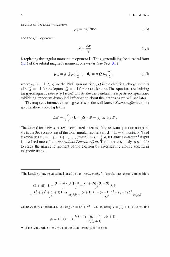
6 1 Introduction

in units of the Bohr magnetonμ0 = e�/2mc (1.3)

and the spin operator

S = �σ

2(1.4)

is replacing the angular momentum operatorL. Thus, generalizing the classical form(1.1) of the orbital magnetic moment, one writes (see Sect. 3.1)

μm = g Q μ0σ

2, de = η Q μ0

σ

2, (1.5)

where σi (i = 1, 2, 3) are the Pauli spin matrices, Q is the electrical charge in unitsof e, Q = −1 for the leptons Q = +1 for the antileptons. The equations are definingthe gyromagnetic ratio g (g-factor) and its electric pendant η, respectively, quantitiesexhibiting important dynamical information about the leptons as we will see later.

The magnetic interaction term gives rise to the well known Zeeman effect: atomicspectra show a level splitting

ΔE = e

2mc(L + gS) · B = gJ μ0 m j B .

The second form gives the result evaluated in terms of the relevant quantum numbers.m j is the 3rd component of the total angular momentum J = L + S in units of � andtakes valuesm j = − j,− j + 1, . . . , j with j = l ± 1

2 . gJ is Landé’s g–factor.4 If spin

is involved one calls it anomalous Zeeman effect. The latter obviously is suitableto study the magnetic moment of the electron by investigating atomic spectra inmagnetic fields.

4The Landé gJ may be calculated based on the “vector model” of angular momentum composition:

(L + gS) · B = (L + gS) · JJ

J · BJ

= (L + gS) · (L + S)

J 2Jz B

= L2 + gS2 + (g + 1) L · SJ 2

m j�B = (g + 1) J 2 − (g − 1) L2 + (g − 1) S2

2J 2m j�B

where we have eliminated L · S using J 2 = L2 + S2 + 2L · S. Using J = j ( j + 1) � etc. we find

gJ = 1 + (g − 1)j ( j + 1) − l(l + 1) + s(s + 1)

2 j ( j + 1).

With the Dirac value g = 2 we find the usual textbook expression.

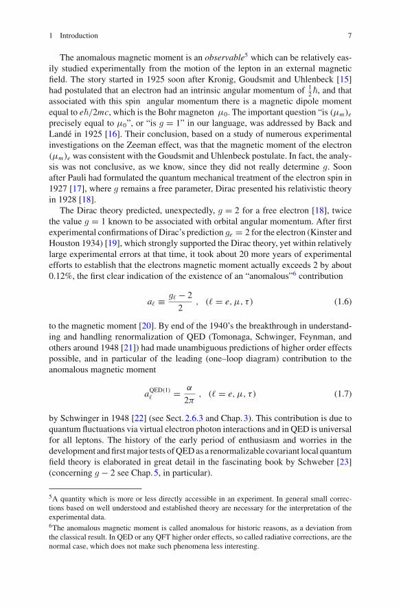
1 Introduction 7

The anomalous magnetic moment is an observable5 which can be relatively eas-ily studied experimentally from the motion of the lepton in an external magneticfield. The story started in 1925 soon after Kronig, Goudsmit and Uhlenbeck [15]had postulated that an electron had an intrinsic angular momentum of 1

2�, and thatassociated with this spin angular momentum there is a magnetic dipole momentequal to e�/2mc, which is the Bohr magneton μ0. The important question “is (μm)eprecisely equal to μ0”, or “is g = 1” in our language, was addressed by Back andLandé in 1925 [16]. Their conclusion, based on a study of numerous experimentalinvestigations on the Zeeman effect, was that the magnetic moment of the electron(μm)e was consistent with the Goudsmit and Uhlenbeck postulate. In fact, the analy-sis was not conclusive, as we know, since they did not really determine g. Soonafter Pauli had formulated the quantum mechanical treatment of the electron spin in1927 [17], where g remains a free parameter, Dirac presented his relativistic theoryin 1928 [18].

The Dirac theory predicted, unexpectedly, g = 2 for a free electron [18], twicethe value g = 1 known to be associated with orbital angular momentum. After firstexperimental confirmations of Dirac’s prediction ge = 2 for the electron (Kinster andHouston 1934) [19], which strongly supported the Dirac theory, yet within relativelylarge experimental errors at that time, it took about 20 more years of experimentalefforts to establish that the electrons magnetic moment actually exceeds 2 by about0.12%, the first clear indication of the existence of an “anomalous”6 contribution

a� ≡ g� − 2

2, (� = e, μ, τ) (1.6)

to the magnetic moment [20]. By end of the 1940’s the breakthrough in understand-ing and handling renormalization of QED (Tomonaga, Schwinger, Feynman, andothers around 1948 [21]) had made unambiguous predictions of higher order effectspossible, and in particular of the leading (one–loop diagram) contribution to theanomalous magnetic moment

aQED(1)� = α

2π, (� = e, μ, τ) (1.7)

by Schwinger in 1948 [22] (see Sect. 2.6.3 and Chap.3). This contribution is due toquantum fluctuations via virtual electron photon interactions and in QED is universalfor all leptons. The history of the early period of enthusiasm and worries in thedevelopment andfirstmajor tests ofQEDas a renormalizable covariant local quantumfield theory is elaborated in great detail in the fascinating book by Schweber [23](concerning g − 2 see Chap.5, in particular).

5A quantity which is more or less directly accessible in an experiment. In general small correc-tions based on well understood and established theory are necessary for the interpretation of theexperimental data.6The anomalous magnetic moment is called anomalous for historic reasons, as a deviation fromthe classical result. In QED or any QFT higher order effects, so called radiative corrections, are thenormal case, which does not make such phenomena less interesting.

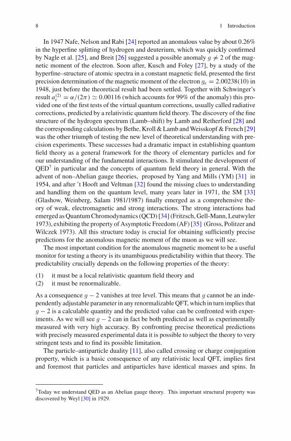
8 1 Introduction

In 1947 Nafe, Nelson and Rabi [24] reported an anomalous value by about 0.26%in the hyperfine splitting of hydrogen and deuterium, which was quickly confirmedby Nagle et al. [25], and Breit [26] suggested a possible anomaly g �= 2 of the mag-netic moment of the electron. Soon after, Kusch and Foley [27], by a study of thehyperfine–structure of atomic spectra in a constant magnetic field, presented the firstprecision determination of themagnetic moment of the electron ge = 2.00238(10) in1948, just before the theoretical result had been settled. Together with Schwinger’sresult a(2)

e = α/(2π) � 0.00116 (which accounts for 99% of the anomaly) this pro-vided one of the first tests of the virtual quantum corrections, usually called radiativecorrections, predicted by a relativistic quantum field theory. The discovery of the finestructure of the hydrogen spectrum (Lamb–shift) by Lamb and Retherford [28] andthe corresponding calculations byBethe,Kroll&Lamb andWeisskopf&French [29]was the other triumph of testing the new level of theoretical understanding with pre-cision experiments. These successes had a dramatic impact in establishing quantumfield theory as a general framework for the theory of elementary particles and forour understanding of the fundamental interactions. It stimulated the development ofQED7 in particular and the concepts of quantum field theory in general. With theadvent of non–Abelian gauge theories, proposed by Yang and Mills (YM) [31] in1954, and after ’t Hooft and Veltman [32] found the missing clues to understandingand handling them on the quantum level, many years later in 1971, the SM [33](Glashow, Weinberg, Salam 1981/1987) finally emerged as a comprehensive the-ory of weak, electromagnetic and strong interactions. The strong interactions hademerged asQuantumChromodynamics (QCD) [34] (Fritzsch,Gell-Mann, Leutwyler1973), exhibiting the property ofAsymptotic Freedom (AF) [35] (Gross, Politzer andWilczek 1973). All this structure today is crucial for obtaining sufficiently precisepredictions for the anomalous magnetic moment of the muon as we will see.

The most important condition for the anomalous magnetic moment to be a usefulmonitor for testing a theory is its unambiguous predictability within that theory. Thepredictability crucially depends on the following properties of the theory:

(1) it must be a local relativistic quantum field theory and(2) it must be renormalizable.

As a consequence g − 2 vanishes at tree level. This means that g cannot be an inde-pendently adjustable parameter in any renormalizableQFT,which in turn implies thatg − 2 is a calculable quantity and the predicted value can be confronted with exper-iments. As we will see g − 2 can in fact be both predicted as well as experimentallymeasured with very high accuracy. By confronting precise theoretical predictionswith precisely measured experimental data it is possible to subject the theory to verystringent tests and to find its possible limitation.

The particle–antiparticle duality [11], also called crossing or charge conjugationproperty, which is a basic consequence of any relativistic local QFT, implies firstand foremost that particles and antiparticles have identical masses and spins. In

7Today we understand QED as an Abelian gauge theory. This important structural property wasdiscovered by Weyl [30] in 1929.

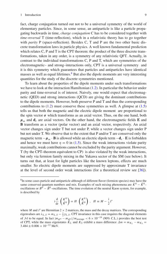
1 Introduction 9

fact, charge conjugation turned out not to be a universal symmetry of the world ofelementary particles. Since, in some sense, an antiparticle is like a particle propa-gating backwards in time, charge conjugation C has to be considered together withtime-reversal T (time-reflection), which in a relativistic theory has to go togetherwith parity P (space-reflection). Besides C, T and P are the two other basic dis-crete transformation laws in particle physics. A well known fundamental predictionwhich relates C, P and T is the CPT theorem: the product of the three discrete trans-formations, taken in any order, is a symmetry of any relativistic QFT. Actually, incontrast to the individual transformations C, P and T, which are symmetries of theelectromagnetic– and strong–interactions only, CPT is a universal symmetry andit is this symmetry which guarantees that particles and antiparticles have identicalmasses as well as equal lifetimes.8 But also the dipole moments are very interestingquantities for the study of the discrete symmetries mentioned.

To learn about the properties of the dipole moments under such transformationswe have to look at the interaction Hamiltonian (1.2). In particular the behavior underparity and time-reversal is of interest. Naively, one would expect that electromag-netic (QED) and strong interactions (QCD) are giving the dominant contributionsto the dipole moments. However, both preserve P and T and thus the correspondingcontributions to (1.2) must conserve these symmetries as well. A glimpse at (1.5)tells us that both the magnetic and the electric dipole moment are proportional tothe spin vector σ which transforms as an axial vector. Thus, on the one hand, bothμm and de are axial vectors. On the other hand, the electromagnetic fields E andB transform as a vector (polar vector) and an axial vector, respectively. An axialvector changes sign under T but not under P, while a vector changes sign under Pbut not under T. We observe that to the extent that P and/or T are conserved only themagnetic term−μm · B is allowed while an electric dipole term−de · E is forbiddenand hence we must have η = 0 in (1.5). Since the weak interactions violate paritymaximally, weak contributions cannot be excluded by the parity argument. However,T (by the CPT–theorem equivalent to CP) is also violated by the weak interactions,but only via fermion family mixing in the Yukawa sector of the SM (see below). Itturns out that, at least for light particles like the known leptons, effects are muchsmaller. So electric dipole moments are suppressed by approximate T invarianceat the level of second order weak interactions (for a theoretical review see [36]).

8In some cases particle and antiparticle although of different flavor (fermion species) may have thesame conserved quantum numbers and mix. Examples of such mixing phenomena are K 0 − K 0–oscillations or B0 − B0–oscillations. The time evolution of the neutral Kaon system, for example,is described by

id

dt

(K 0

K 0

)= H

(K 0

K 0

), H ≡ M − i

2Γ

where M and Γ are Hermitian 2 × 2 matrices, the mass and the decay matrices. The correspondingeigenvalues are λL ,S = mL ,S − i

2γL ,S . CPT invariance in this case requires the diagonal elementsof M to be equal. In fact |mK 0 − mK 0 |/maverage < 6 × 10−19 (90% C.L.) provides the best testof CPT, while the mass eigenstates KL and KS exhibit a mass difference Δm = mKL − mKS =3.484 ± 0.006 × 10−12 MeV.

10 1 Introduction

In fact experimental bounds tell us that they are very tiny. The previous best limit|de| < 1.6 × 10−27 e · cm at 90%C.L. [37] has been superseded recently by [38]9

|de| < 8.7 × 10−29 e · cm at 90%C.L. (1.8)

This will also play an important role in the interpretation of the g − 2 experimentsas we will see later. The planned J-PARC muon g − 2 experiment will also providea new dedicated experiment for measuring the muon electric dipole moment [9, 39].

As already mentioned, the anomalous magnetic moment of a lepton is a dimen-sionless quantity, a pure number, which may be computed order by order as a per-turbative expansion in the fine structure constant α in QED, and beyond QED, in theSM of elementary particles or extensions of it. As an effective interaction term ananomalous magnetic moment is induced by the interaction of the lepton with photonsor other particles. It corresponds to a dimension 5 operator and since a renormaliz-able theory is constrained to exhibit terms of dimension 4 or less only, such a termmust be absent for any fermion in any renormalizable theory at tree level. It is theabsence of such a possible Pauli term that leads to the prediction g = 2 + O(α). Ona formal level it is the requirement of renormalizability which forbids the presenceof a Pauli term in the Lagrangian defining the theory (see Sect. 2.4.2).

In 1956 ae was already well measured by Crane et al. [40] and Berestetskii etal. [41] pointed out that the sensitivity of a� to short distance physics scales like

δa�

a�

∼ m2�

Λ2(1.9)

where Λ is a UV cut–off characterizing the scale of new physics. It was thereforeclear that the anomalousmagneticmoment of themuonwould be amuch better probefor possible deviations fromQED. However, parity violation of weak interaction wasnot yet known at that time and nobody had an idea how to measure aμ.

As already discussed at the beginning of this introduction, the origin of the vastlydifferent behavior of the three charged leptons is due to the very different massesm�,implying completely different lifetimes τe = ∞, τ� = 1/Γ� ∝ 1/G2

Fm5� (� = μ, τ )

and vastly different decay patterns. GF is the Fermi constant, known from weakradioactive decays. In contrast to muons, electrons exist in atoms which opens thepossibility to investigate ae directly via the spectroscopy of atoms in magnetic fields.This possibility does not exist for muons.10 However, Crane et al. [40] already used adifferentmethod tomeasure ae. They produced polarized electrons by shooting high–energy electrons on a gold foil. The part of the electron bunch which is scatteredat right angles, is partially polarized and trapped in a magnetic field, where spinprecession takes place for some time. The bunch is then released from the trap andallowed to strike a second gold foil, which allows one to analyze the polarization

9The unit e · cm is the dipole moment of an e+e−–pair separated by 1cm. Since d = η2

e�c2mc2

, the

conversion factor needed is �c = 1.9733 · 10−11 MeVcm and e = 1.10We discard here the possibility to form and investigate muonic atoms.

1 Introduction 11

and to determine ae. Although this technique is in principle very similar to the onelater developed to measure aμ, it is obvious that in practice handling the muons ina similar way is not possible. One of the main questions was: how is it possible topolarize such short lived particles like muons?

After the proposal of parity violation in weak transitions by Lee and Yang [42] in1957, it immediately was realized that muons produced in weak decays of the pion(π+ → μ++ neutrino) should be longitudinally polarized. In addition, the decaypositron of the muon (μ+ → e+ + 2 neutrinos) could indicate the muon spin direc-tion. This was confirmed by Garwin, Lederman andWeinrich [43] and Friedman andTelegdi [44].11 The first of the two papers for the first time determined gμ = 2.00within 10% by applying the muon spin precession principle (see Chap.6). Now theroad was free to seriously think about the experimental investigation of aμ.

It should bementioned that at that time the nature of themuonwas quite amystery.While today we know that there are three lepton–quark families with identical basicproperties except for differences in masses, decay times and decay patterns, at thesetimes it was hard to believe that the muon is just a heavier version of the electron(μ − e–puzzle). For instance, it was expected that the μ exhibited some unknownkind of interaction, not shared by the electron, which was responsible for the muchhigher mass. So there was plenty of motivation for experimental initiatives to exploreaμ.

The big interest in the muon anomalous magnetic moment was motivated byBerestetskii’s argument of dramatically enhanced short distance sensitivity. As wewill see later, one of the main features of the anomalous magnetic moment of lep-tons is that it mediates helicity flip transitions. The helicity is the projection of thespin vector onto the momentum vector which defines the direction of motion and thevelocity. If the spin is parallel to the direction ofmotion the particle is right–handed, ifit is antiparallel it is called left–handed.12 For massless particles the helicities wouldbe conserved by the SM interactions and helicity flips would be forbidden. For mas-sive particles helicity flips are allowed and their transition amplitude is proportionalto the mass of the particle. Since the transition probability goes with the modulussquare of the amplitude, for the lepton’s anomalous magnetic moment this implies,generalizing (1.9), that quantum fluctuations due to heavier particles or contributionsfrom higher energy scales are proportional to

δa�

a�

∝ m2�

M2(M m�) , (1.10)

where M may be

11The latter reference for the first time points out that P and C are violated simultaneously, in factP is maximally violated while CP is to very good approximation conserved in this decay.12Handedness is used here in a naive sense of the “right–hand rule”. Naive because the handednessdefined in this way for a massive particle is frame dependent. The proper definition of handednessin a relativistic QFT is in terms of the chirality (see Sect. 2.2). Only for massless particles the twodifferent definitions of handedness coincide.

12 1 Introduction

• the mass of a heavier SM particle, or• the mass of a hypothetical heavy state beyond the SM, or• an energy scale or an ultraviolet cut–off where the SM ceases to be valid.

On one hand, this means that the heavier the new state or scale the harder it is to see(it decouples as M → ∞). Typically, the best sensitivity we have for nearby newphysics, which has not yet been discovered by other experiments. On the other hand,the sensitivity to “new physics” grows quadratically with the mass of the lepton,which means that the interesting effects are magnified in aμ relative to ae by a factor(mμ/me)

2 ∼ 4 × 104. This is what makes the anomalous magnetic moment of themuon aμ the predestinated “monitor for new physics”. By far the best sensitivitywe have for aτ the measurement of which however is beyond present experimentalpossibilities, because of the very short lifetime of the τ .

The first measurement of the anomalous magnetic moment of the muon wasperformed at Columbia in 1960 [45] with a result aμ = 0.00122(8) at a precision ofabout 5%. Shortly after in 1961, the first precision determination was possible at theCERN cyclotron (1958–1962) [46, 47]. Surprisingly, nothing special was observedwithin the 0.4% level of accuracy of the experiment. It was the first real evidencethat the muon was just a heavy electron. In particular this meant that the muon waspoint–like and no extra short distance effects could be seen. This latter point of courseis a matter of accuracy and the challenge to go further was evident.

The idea of amuon storage ringswas put forward next. Afirst onewas successfullyrealized at CERN (1962–1968) [48–50]. It allowed one to measure aμ for both μ+andμ− at the samemachine. Results agreedwell within errors and provided a preciseverification of the CPT theorem for muons. An accuracy of 270 ppm was reachedand an insignificant 1.7 σ (1 σ = 1 Standard Deviation (SD)) deviation from theorywas found. Nevertheless the latter triggered a reconsideration of theory. It turned outthat in the estimate of the three–loop O(α3)QED contribution the leptonic light–by–light scattering part (dominated by the electron loop) was missing. Aldins et al. [51]then calculated this and after including it, perfect agreement between theory andexperiment was obtained.

One also should keep in mind that the first theoretical successes of QED pre-dictions and the growing precision of the ae experiments challenged theoreticians totackle the much more difficult higher order calculations for ae as well as for aμ. Soonafter Schwinger’s resultKarplus andKroll 1949 [52] calculated the two–loop term forae. In 1957, shortly after the discovery of parity violation and a first feasibility proofin [43], dedicated experiments to explore aμ were discussed. This also renewed theinterest in the two–loop calculation which was reconsidered, corrected and extendedto the muon by Sommerfield [53] and Petermann [54], in the same year. Vacuumpolarization insertions with fermion loops with leptons different from the externalonewere calculated in [55, 56]. About 10 years later with the new generation of g − 2experiments at the first muon storage ring at CERN O(α3) calculations were startedby Kinoshita [57], Lautrup and de Rafael [58] and Mignaco and Remiddi [59]. Itthen took about 30 years until Laporta and Remiddi [60] found a final analyticresult in 1996. Many of these calculations would not have been possible withoutthe pioneering computer algebra programs, like ASHMEDAI [61], SCHOONSHIP

1 Introduction 13

[62, 63] and REDUCE [64]. More recently Vermaseren’s FORM [65] package evolvedinto a standard tool for large scale calculations. Commercial software packages likeMACSYMA or the more up–to–date ones MATEMATICA and MAPLE, too, play animportant role as advanced tools to solve difficult problems by means of computers.Of course, the dramatic increase of computer performance and the use of more effi-cient computing algorithms have been crucial for the progress achieved. In particularcalculations like the ones needed for g − 2 had a direct impact on the developmentof these computer algebra systems.

In an attempt to overcome the systematic difficulties of the first a second muonstorage ring was built (1969–1976) [66, 67]. The precision of 7 ppm reached wasan extraordinary achievement at that time. For the first time the m2

μ/m2e–enhanced

hadronic contribution came into play. Again no deviations were found. With theachieved precision the muon g − 2 remained a benchmark for beyond the SM theorybuilders ever since. Only 20 years later the BNL experiment E821, again amuon stor-age ring experiment, was able to set new standards in precision. Now, at the presentlevel of accuracy the complete SM is needed in order to be able tomake predictions atthe appropriate level of precision. As already mentioned, at present further progressis hampered by the difficulties to include properly the non–perturbative strong inter-action part. At a certain level of precision hadronic effects become important and weare confronted with the question of how to evaluate them reliably. At low energiesQCD gets strongly interacting and a perturbative calculation is not possible. For-tunately, analyticity and unitarity allow us to express the leading hadronic vacuumpolarization (HVP) contributions via a dispersion relation (analyticity) in terms ofexperimental data [68]. The key relation here is the optical theorem (unitarity) whichdetermines the imaginary part of the vacuum polarization amplitude through the totalcross section for electron–positron annihilation into hadrons. First estimations wereperformed in [69–71] after the discovery of the ρ– and the ω–resonances,13 andin [74], after first e+e− cross–section measurements were performed at the collidingbeam machines VEPP-2 and ACO in Novosibirsk [75] and Orsay [76], respectively.One drawback of this method is that now the precision of the theoretical prediction ofaμ is limited by the accuracy of experimental data. We will say more on this later on.

The success of the CERN muon anomaly experiment and the progress in theconsolidation of the SM, together with given possibilities for experimental improve-ments, were a good motivation for Vernon Hughes and other interested colleaguesto push for a new experiment at Brookhaven. There the intense proton beam ofthe Alternating Gradient Synchrotron (AGS) was available which would allow toincrease the statistical accuracy substantially [77]. The main interest was a precisetest of the electroweak contribution due to virtual W and Z exchange, which hadbeen calculated immediately after the renormalizability of the SM had been settled

13The ρ is a ππ resonance which was discovered in pion nucleon scattering π− + p → π−π0 pand π− + p → π−π+n [72] in 1961. The neutral ρ0 is a tall resonance in the π+π− channelwhich may be directly produced in e+e−–annihilation and plays a key role in the evaluation of thehadronic contributions to ahadμ . The ρ contributes about 70% to ahadμ which clearly demonstratesthe non–perturbative nature of the hadronic effects. Shortly after the ρ also the ω–resonance wasdiscovered as a π+π0π− peak in proton–antiproton annihilation p p → π+π+π0π−π− [73].

14 1 Introduction

in 1972 [78]. An increase in precision by a factor of 20 was required for this goal.On the theory side the ongoing discussion motivated, in the early 1980’s already,Kinoshita and his collaborators to start the formidable task to calculate the O(α4)

contribution with 891 four–loop diagrams. The direct numerical evaluation was theonly promising method to get results within a reasonable time. Early results [79, 80]could be improved continuously [81] and culminated in 2012 with the first completeO(α5) calculation for both the electron [82] and the muon [83] g − 2 (involving12672 five-loop diagrams). Very recently Laporta [84] has been able to obtain aquasi–exact 4–loop result for the 891 universal diagrams, which improves the elec-tron g − 2 essentially. Increasing computing power was and still is a crucial factorin this extreme project. Beyond the full analytic O(α3) calculation, only a subsetof diagrams are known analytically (see Sect. 4.1 for many more details and a morecomplete list of references). The size of the O(α4) contribution is about 6 σ ’s interms of the present experimental accuracy and thus mandatory for the interpretationof the experimental result. The improvement achieved with the evaluation of theO(α5) term, which itself is about 0.07 σ ’s only, resulted in a substantial reductionof the uncertainty of the QED contribution.

A general problem in electroweak precision physics are the higher order contri-butions from hadrons (quark loops) at low energy scales. While leptons primarilyexhibit the fairly weak electromagnetic interaction, which can be treated in pertur-bation theory, the quarks are strongly interacting via confined gluons where anyperturbative treatment breaks down. Considering the lepton anomalous magneticmoments one distinguishes three types of non-perturbative corrections: (a)HadronicVacuum Polarization (HVP) of order O(α2), O(α3), O(α4); (b) Hadronic Light-by-Light (HLbL) scattering at O(α3); (c) hadronic effects at O(αGFm2

μ) in 2-loopelectroweak (EW) corrections, in all cases quark-loops appear as hadronic “blobs”.The hadronic contributions are limiting the precision of the predictions.

As mentioned already before, the evaluation of non-perturbative hadronic effectsis possible by using experimental data in conjunction with Dispersion Relations(DR), by low energy effective modeling via a Resonance Lagrangian Approach(RLA) (Vector Meson Dominance (VMD) implemented in accord with chiral struc-ture of QCD) [85–87], like the Hidden Local Symmetry (HLS) or the ExtendedNambu Jona-Lasinio (ENJL) models, or by lattice QCD. Specifically: (a) HVP viaa dispersion integral over e+e− → hadrons data (1 independent amplitude to bedetermined by one specific data channel) (see e.g. [88, 89]), by the HLS effectiveLagrangian approach [90], or by lattice QCD [91–95]; (b) hadronic Light-by-Light(HLbL) scattering effects via a RLA together with operator product expansion (OPE)methods [96–99], by a dispersive approach using γ γ → hadrons data (19 indepen-dent amplitudes to be determined by as many independent data sets in principle)[100, 101] or by lattice QCD [102]; (c) EW quark-triangle diagrams are wellunder control, because the possible large corrections are related to the Adler-Bell-Jackiw (ABJ) anomaly which is perturbative and non-perturbative at the same time.Since VVV = 0 by the Furry theorem, only VVA (of γ γ Z -vertex, V = vector,A = axialvector) contributes. In fact leading effects are of short distance type

1 Introduction 15

(MZ mass scale) and cancel against lepton-triangle loops (anomaly cancellation)[103, 104].

In the early 1980’s the hadronic contributions were known with rather limitedaccuracy only. Much more accurate e+e−–data from experiments at the electronpositron storage ring VEPP-2M at Novosibirsk allowed a big step forward in theevaluation of the leading hadronic vacuum polarization effects [80, 105, 106] (seealso [107]). A more detailed analysis based on a complete up–to–date collectionof data followed about 10 years later [88]. Further improvements were possiblethanks to new hadronic cross section measurements by BES-II [108] (BEPC ring)at Beijing and by CMD-2 [109] at Novosibirsk. A new approach of cross sectionmeasurements via the radiative return or initial state radiation (ISR) mechanism,pioneered by the KLOE Collaboration [110] (DAΦNE ring) at Frascati, started toprovide high statistics data at about the time when Brookhaven stopped their muong − 2 experiment. The results are in fair agreement with the later CMD-2 and SNDdata [111, 112]. In the meantime ISR data for the dominating π+π− channel havebeen collected by KLOE [113–115] at the φ factory by BaBar at the B factory [116]and a first measurement by BES-III [117] at the BEPCII collider. Still one of themain issue in HVP are hadronic cross-sections in the region 1.2 to 2.4 GeV, whichactually has been improved dramatically by the exclusive channel measurements byBaBar in the past decade (see [118] and references therein). The most important 20out of more than 30 channels are measured, many known at the 10 to 15% level. Theexclusive channel therefore has a much better quality than the very old inclusive datafrom Frascati. Attempts to include τ spectral functions via isospin relations will bediscussed in Sect. 5.1.10.

The physics of the anomalous magnetic moments of leptons has challenged theparticle physics community for more than 60 years now and experiments as well astheory in the meantime look rather intricate. For a long time ae and aμ provided themost precise tests of QED in particular and of relativistic local QFT as a commonframework for elementary particle theory in general.

Of course it was the hunting for deviations from theory and the theorists specu-lations about “new physics around the corner” which challenged new experimentsagain and again. The reader may find more details about historical aspects and theexperimental developments in the interesting review: “The 47 years of muon g-2”by Farley and Semertzidis [119].

Until about 1975 searching for “new physics” via aμ in fact essentially meantlooking for physics beyond QED. As we will see later, also standard model hadronicand weak interaction effect carry the enhancement factor (mμ/me)

2, and this is goodnews and bad news at the same time. Good news because of the enhanced sensitivityto many details of SM physics like the weak gauge boson contributions, bad newsbecause of the enhanced sensitivity to the hadronic contributions which are verydifficult to control and in fact limit our ability to make predictions at the desiredprecision. This is the reason why quite some fraction of the book will have to dealwith these hadronic effects (see Chap.5).

The pattern of lepton anomalous magnetic moment physics which emerges isthe following: ae is a quantity which is dominated by QED effects up to very high

16 1 Introduction

precision, presently at the .66 parts per billion (ppb) level! The sensitivity to hadronicandweak effects aswell as the sensitivity to physics beyond theSM is very small. Thisallows for a very solid and model independent (essentially pure QED) high precisionprediction of ae [82, 84]. The very precise experimental value [120, 121] (at 0.24ppb) and the very good control of the theory part in fact allows us to determine the finestructure constant α with the highest accuracy [121–123] in comparison with othermethods (see Sect. 3.2.2). A very precise value for α of course is needed as an inputto be able to make precise predictions for other observables like aμ, for example.While ae, theory wise, does not attract too much attention, although it required topush the QED calculation to O(α5), aμ is a much more interesting and theoreticallychallenging object, sensitive to all kinds of effects and thus probing the SM to muchdeeper level (see Chap.4). Note that in spite of the fact that ae has been measuredabout 2250 times more precisely than aμ the sensitivity of the latter to “new physics”is still about 19 times larger. However, in order to use ae as a monitor for new physicsone requires the most precise ae independent determination of α which comes fromatomic interferometry [124] and is about a factor 5.3 less precise than the one basedon ae. Taking this into account aμ is about a factor 43 more sensitive to new physicsat present.

The experimental accuracy achieved in the past few years at BNL is at the level of0.54 parts permillion (ppm) and better than the accuracy of the theoretical predictionswhich are still obscured by hadronic uncertainties. A discrepancy at the 2 to 3 σ

level persisted [125–127] since the first new measurement in 2000 up to the one in2004 (four independent measurements during this time), the last for the time being(see Chap.7). Again, the “disagreement” between theory and experiment, suggestedby the first BNL measurement, rejuvenated the interest in the subject and entaileda reconsideration of the theory predictions. The most prominent error found thistime in previous calculations concerned the problematic hadronic light–by–lightscattering contribution which turned out to be in error by a sign [128]. The changeimproved the agreement between theory and experiment by about 1 σ . Problemswith the hadronic e+e−–annihilation data used to evaluate the hadronic vacuumpolarization contribution led to a similar shift in opposite direction, such that adiscrepancy persists.

Speculations about what kind of effects could be responsible for the deviationwill be presented in Sect. 7.2. With the advent of the Large Hadron Collider (LHC)the window of possibilities to explain the observed deviation by a contribution froma new heavy particle have substantially narrowed, such that the situation is ratherpuzzling at the time. No real measurement yet exists for aτ . Bounds are in agreementwith SM expectations14 [129]. Advances in experimental techniques one day couldpromote aτ to a new “telescope” which would provide new perspectives in exploringthe short distance tail of the unknown real world, we are continuously hunting for.The point is that the relative weights of the different contributions are quite differentfor the τ in comparison to the μ.

14Theory predicts (gτ − 2)/2 = 117721(5) × 10−8; the experimental limit from the LEP experi-ments OPAL and L3 is −0.052 < aτ < 0.013 at 95%C.L.

1 Introduction 17

In the meantime activities are expected to go on to improve the impressive level ofprecision reached by the muon g − 2 experiment E821 at BNL. Since the error wasstill dominated by statistical errors rather than by systematic ones, further progressis possible in any case. But also new ideas to improve on sources of systematic errorsplay an important role for future projects. Plans for an upgrade of the Brookhavenexperiment lead to a new experiment which presently is realized at Fermilab. Themuon storage ringwill be the same and has beenmoved to the new location some timeago, most of the other elements like production and injection of the polarized muonsaswell as the detection of themuondecay electronswill be new.An alternative projectdesigned to work with ultra-cold muon is being buildup at J-PARC in Japan. Thenew experiments are expected to be able to improve the accuracy by a factor of 5 orso [2–5]. For the theory such improvement factors are a real big challenge and requiremuch progress in our understanding of non–perturbative strong interaction effects.In addition, challenging higher order computations have to be pushed further withinthe SM and beyond. Another important aspect: the large hadron collider LHC nowin operation at CERN will certainly provide important hints about how the SM hasto be completed by new physics. Progress in the theory of aμ will come certainly inconjunction with projects to measure hadronic electron–positron annihilation cross–sections with substantially improved accuracy (see Sect. 7.4). These cross sectionsare an important input for reducing the hadronic vacuum polarization uncertaintieswhich yield the dominating source of error at present. Although progress is slow,there is evident progress in reducing the hadronic uncertainties, most directly byprogress in measuring the relevant hadronic cross-sections. Near future progress weexpect fromBINPNovosibirsk/Russia and from IHEPBeijing/China. Energy scan aswell as ISRmeasurement of cross-sections in the region from 1.4 to 2.5 GeV aremostimportant to reduce the errors to a level competitive with the factor 4 improvementachievable by the upcoming new muon g − 2 experiments at Fermilab/USA and atJ-PARC/Japan [5, 7–9]. Also BaBar data are still being analyzed and are importantfor improving the results. Promising is that lattice QCD evaluations come closer tobe competitive. In any case there is good reason to expect also in future interestingpromises of physics beyond the SM from this “crystal ball” of particle physicists.

Besides providing a summary of the status of the physics of the anomalous mag-netic moment of the muon, the aim of this book is an introduction to the theory of themagnetic moments of leptons also emphasizing the fundamental principles behindour present understanding of elementary particle theory. Many of the basic conceptsare discussed in details such that physicists with only some basic knowledge of quan-tum field theory and particle physics should get the main ideas and learn about thetechniques applied to get theoretical predictions of such high accuracy, and why it ispossible to measure anomalous magnetic moments so precisely.

Once thought as a QED test, today the precision measurement of the anomalousmagneticmoment of themuon is a test ofmost aspects of the SMwith the electromag-netic, the strong and the weak interaction effects and beyond, maybe supersymmetryis responsible for the observed deviation.

There are many excellent and inspiring introductions and reviews on the sub-ject [130–148], which were very helpful in writing this book. A topical workshop

18 1 Introduction

held in 2014 at the Mainz Institute for Theoretical Physics (MITP) has been gath-ering people with new ideas to work on the improvement of the predictions of thehadronic contributions, in particular on the challenging hadronic light-by-light scat-tering problem. A short account of the topics discussed the reader may find in the“mini proceedings” [149]. It addresses the next steps required on the theory side tocompete with the experimental progress to come.

For further reading I also recommend the reviews [150, 151], which are focusingon theory issues and the article [152], which especially reviews the experimentalaspects in much more depth than this book. For a recent brief view into the futurealso see [153].

References

1. G.W. Bennett et al., Muon (g-2) Collab. Phys. Rev. Lett. 92, 161802 (2004)2. B.L. Roberts Nucl. Phys. B (Proc. Suppl.) 131 (2004) 157; R. M. Carey et al., Proposal of the

BNL Experiment E969, 2004 (www.bnl.gov/henp/docs/pac0904/P969.pdf); J-PARC Letterof Intent L17

3. J. Grange et al. [Muon g-2 Collab.], arXiv:1501.06858 [physics.ins-det]4. [Fermilab E989 Collab.], Nucl. Part. Phys. Proc. PoS EPS -HEP2015 (2015) 568. 273–275,

584 (2016)5. D.W. Hertzog, EPJ Web Conf. 118, 01015 (2016)6. Fermilab Muon g-2 Collab, http://muon-g-2.fnal.gov7. H. Iinuma, J-PARC muon g-2/EDM Collab. J. Phys. Conf. Ser. 295, 012032 (2011)8. T. Mibe [J-PARC g-2 Collab.], Nucl. Phys. Proc. Suppl. 218, 242 (2011)9. N. Saito, J-PARC g-2/EDM Collab. AIP Conf. Proc. 1467, 45 (2012)

10. J-PARC g-2/EDM Collab, http://g-2.kek.jp11. P.A.M. Dirac, Proc. Roy. Soc. A 126, 360 (1930)12. C.D. Anderson, S.H. Neddermeyer, Phys. Rep. C 50 (1936) 263; S.H. Neddermeyer, C.D.

Anderson, Phys. Rep. C 51, 884 (1937)13. C.D. Anderson, Phys. Rep. C 43, 491 (1933)14. Phys. Rep. C Proc. Roy. Soc. A 133 (1931) 60. 74, 817 (1948)15. G.E. Uhlenbeck, S. Goudsmit, Naturwissenschaften 13 (1925) 953. Nature 117, 264 (1926)16. E. Back, A. Landé, Zeemaneffekt und Multiplettstruktur der Spektrallinien, 1st edn

(J. Springer, Berlin 1925), pp 213; see also: H.A. Bethe, E.E. Salpeter, Quantum Mechanicsof One- and Two-Electron Systems, Handbuch der Physik, Band XXXV, Atoms I, SpringerVerlag, Berlin (1957)

17. W. Pauli, Zeits. Phys. 43, 601 (1927)18. A Proc. Roy. Soc. A 117 (1928) 610. 118, 351 (1928)19. L.E. Kinster, W.V. Houston, Phys. Rep. C 45, 104 (1934)20. P. Kusch, Science 123 (1956) 207. Phys. Today 19, 23 (1966)21. S. Tomonaga, Riken Iho, Progr. Theor. Phys. 1 (1946) 27; J. Schwinger, Phys. Rep. C 74

(1948) 1439; R. P. Feynman, Phys. Rep. C 76 (1949) 749; F. Dyson, Phys. Rep. C 75 (1949)486, ibid. (1736)

22. J.S. Schwinger, Phys. Rev. 73, 416 (1948)23. S.S. Schweber,QED and the MenWhoMade It: Dyson, Feynman, Schwinger, and Tomonaga,

1st edn. (Princeton, Princeton University Press, 1994), p. 73224. J.E. Nafe, E.B. Nelson, I.I. Rabi, Phys. Rep. C 71, 914 (1947)25. D.E. Nagle, R.S. Julian, J.R. Zacharias, Phys. Rev. 72, 971 (1947)26. G. Breit, Phys. Rep. C 72, 984 (1947)

References 19

27. P. Kusch, H .M. Foley, Phys. Rev. 73 (1948) 421. Phys. Rep. C 74, 250 (1948)28. W.E. Lamb Jr., R.C. Retherford, Phys. Rep. C 72, 241 (1947)29. H. A. Bethe, Phys. Rep. C 72 (1947) 339; N. M. Kroll, W. E. Lamb Jr, Phys. Rep. C 75 (1949)

388; V. Weisskopf, J. B. French, Phys. Rep. C 75, 1240 (1949)30. H. Weyl, I. Zeits, Phys. 56, 330 (1929)31. C.N. Yang, R.L. Mills, Phys. Rep. C 96, 191 (1954)32. G. ’t Hooft, Nucl. Phys. B 33 (1971) 173; 35 (1971) 167; G. ’t Hooft, M. Veltman, Nucl. Phys.

B 50, 318 (1972)33. S. L. Glashow, Nucl. Phys. B 22 (1961) 579; S. Weinberg, Phys. Rev. Lett. 19 (1967) 1264;

A. Salam, Weak and electromagnetic interactions. In: Elementary Particle Theory, ed by N.Svartholm, Amquist and Wiksells, Stockholm, pp 367–377 (1969)

34. H. Fritzsch, M. Gell-Mann, H. Leutwyler, Phys. Lett. 47, 365 (1973)35. H.D. Politzer, Phys. Rev. Lett. 30 (1973) 1346; D. Gross, F. Wilczek. Phys. Rev. Lett. 30,

1343 (1973)36. W. Bernreuther, M. Suzuki, Erratum-ibid. 64 (1991) 313. Rev. Mod. Phys. 63, 633 (1992)37. B.C. Regan, E.D. Commins, C.J. Schmidt, D. DeMille, Phys. Rev. Lett. 88, 071805 (2002)38. J. Baron et al., ACME Collab. Sci. 343, 269 (2014)39. F. J. M. Farley et al., Phys. Rev. Lett. 93 (2004) 052001; M. Aoki et al. [J-PARC Letter of

Intent]: Search for a Permanent Muon Electric Dipole Moment at the ×10−24 e· cm Level,http://www-ps.kek.jp/jhf-np/LOIlist/pdf/L22.pdf

40. W. H. Luisell, R. W. Pidd, H. R. Crane, Phys. Rep. C 91 (1953) 475; ibid. 94 (1954) 7;A. A. Schupp, R. W. Pidd, H. R. Crane, Phys. Rep. C 121 (1961) 1; H. R. Crane, Sci.American 218, 72 (1968)

41. V.B. Berestetskii, O.N. Krokhin, A.X. Klebnikov, Zh Eksp, Teor. Fiz. 30 (1956) 788 [Sov.Phys. JETP 3 (1956) 761]; W. S. Cowland. Nucl. Phys. B 8, 397 (1958)

42. T.D. Lee, C.N. Yang, Phys. Rep. C 104, 254 (1956)43. R.L. Garwin, L. Lederman, M. Weinrich, Phys. Rep. C 105, 1415 (1957)44. J.I. Friedman, V.L. Telegdi, Phys. Rep. C 105, 1681 (1957)45. R.L. Garwin, D.P. Hutchinson, S. Penman, G. Shapiro, Phys. Rev. 118, 271 (1960)46. G. Charpak, F. J. M. Farley, R. L. Garwin, T. Muller, J. C. Sens, V. L. Telegdi, A. Zichichi,

Phys. Rev. Lett. 6 (1961) 128; G. Charpak, F. J. M. Farley, R. L. Garwin, T. Muller, J. C. Sens,A. Zichichi, Nuovo Cimento 22 (1961) 1043; Phys. Lett. 1, 16 (1962)

47. G. Charpak, F.J.M. Farley, R.L. Garwin, T. Muller, J.C. Sens, A. Zichichi, Nuovo Cimento37, 1241 (1965)

48. F.J.M. Farley, J. Bailey, R.C.A. Brown, M. Giesch, H. Jöstlein, S. van der Meer, E. Picasso,M. Tannenbaum, Nuovo Cimento 45, 281 (1966)

49. J. Bailey et al., Phys. Lett. B 28, 287 (1968)50. J. Bailey, W. Bartl, G. von Bochmann, R.C.A. Brown, F.J.M. Farley, M. Giesch, H. Jöstlein,

S. van der Meer, E. Picasso, R.W. Williams, Nuovo Cimento A 9, 369 (1972)51. J. Aldins, T. Kinoshita, S .J. Brodsky, A .J. Dufner, Phys. Rev. Lett. 23 (1969). Phys. Rev. D

1, 2378 (1970)52. R. Karplus, N.M. Kroll, Phys. Rep. C 77, 536 (1950)53. C .M. Sommerfield, Phys. Rev. 107 (1957) 328. Ann. Phys. (N.Y.) 5, 26 (1958)54. A. Petermann, Helv. Phys. Acta 30 (1957) 407. Nucl. Phys. 5, 677 (1958)55. H. Suura, E. Wichmann, Phys. Rev. 105 (1957) 1930; A. Petermann. Phys. Rev. 105, 1931

(1957)56. H.H. Elend, Erratum-ibid. 21 (1966) 720. Phys. Lett. 20, 682 (1966)57. T. Kinoshita, Nuovo Cim. B 51, 140 (1967)58. B.E. Lautrup, E. De Rafael, Phys. Rev. 174, 1835 (1968)59. J.A. Mignaco, E. Remiddi, Nuovo Cim. A 60, 519 (1969)60. S. Laporta, E. Remiddi, Phys. Lett. B 379, 283 (1996)61. M. I. Levine, ASHMEDAI. Comput. Phys. I (1967) 454; R. C. Perisho, ASHMEDAI User’s

Guide, U.S. AEC Report No. COO-3066-44 (1975)62. M. .J. G. Veltman, SchoonShip, CERN Report (1967)

20 1 Introduction

63. H. Strubbe, Comput. Phys. Commun. 8 (1974) 1. Comput. Phys. Commun. 18, 1 (1979)64. A. C. Hearn, REDUCE User’s Manual, Stanford University, Report No. ITP- 292, 1967, rev.

1968; A. C. Hearn, REDUCE 2 User’s Manual. Stanford Artificial Intelligence Project MemoAIM-133, (unpublished) (1970 )

65. J.A.M.Vermaseren,SymbolicmanipulationwithFORM (ComputerAlgebraNederland,Ams-terdam, 1991)

66. J. Bailey et al. [CERN Muon Storage Ring Collab.], Phys. Lett. B 67 (1977) 225 [Phys. Lett.B 68 (1977) 191]

67. J. Bailey et al., CERN-Mainz-Daresbury Collab. Nucl. Phys. B 150, 1 (1979)68. N. Cabibbo, R. Gatto, Phys. Rev. Lett. 4 (1960) 313. Phys. Rep. C 124, 1577 (1961)69. C. Bouchiat, L. Michel, J. Phys. Radium 22, 121 (1961)70. L. Durand, III Erratum-ibid. 129 (1963) 2835. Phys. Rep. C 128, 441 (1962)71. T. Kinoshita, R.J. Oakes, Phys. Lett. 25, 143 (1967)72. A.R. Erwin, R. March, W.D. Walker, E. West, Phys. Rev. Lett. 6 (1961) 628; D. Stonehill

et al., Phys. Rev. Lett. 6 (1961) 624; E. Pickup, D. K. Robinson, E. O. Salant, Phys. Rev. Lett.7 (1961) 192; D. McLeod, S. Richert, A. Silverman, Phys. Rev. Lett. 7 (1961) 383; D. D.Carmony, R. T. Van de Walle, Phys. Rev. Lett. 8 (1962) 73; J. Button, G. R. Kalbfleisch, G.R. Lynch, B. C. Maglic, A. H. Rosenfeld, M. L. Stevenson. Phys. Rev. 126, 1858 (1962)

73. B.C. Maglic, L.W. Alvarez, A.H. Rosenfeld, M.L. Stevenson, Phys. Rev. Lett. 7 (1961) 178;N. H. Xuong, G. R. Lynch, Phys. Rev. Lett. 7 (1961) 327; A. Pevsner et al., Phys. Rev. Lett. 7(1961) 421; M. L. Stevenson, L. W. Alvarez, B. C. Maglic, A. H. Rosenfeld. Phys. Rev. 125,687 (1962)

74. M. Gourdin, E. De Rafael, Nucl. Phys. B 10, 667 (1969)75. V.L. Auslander, G.I. Budker, Ju. N. Pestov, A. V. Sidorov, A. N. Skrinsky. A. G. Kbabakhpa-

shev. Phys. Lett. B 25, 433 (1967)76. J .E. Augustin et al., Phys. Lett. B 28, 503, 508, 513, 517 (1969)77. C. Heisey et al., A new precision measurement of the muon g-2 value at the level of 6.35 ppm,

Brookhaven AGS Proposal 821, revised (1986). Design Report for AGS 821, (1989) (1985)78. R. Jackiw, S. Weinberg, Phys. Rev. D 5 (1972) 2396; I. Bars, M. Yoshimura, Phys. Rev. D 6

(1972) 374; G. Altarelli, N. Cabibbo, L. Maiani, Phys. Lett. B 40 (1972) 415; W. A. Bardeen,R. Gastmans, B. Lautrup, Nucl. Phys. B 46 (1972) 319; K. Fujikawa, B. W. Lee, A. I. Sanda.Phys. Rev. D 6, 2923 (1972)

79. T. Kinoshita, W.B. Lindquist, Phys. Rev. Lett. 47, 1573 (1981)80. T. Kinoshita, B. Nizic, Y. Okamoto, Phys. Rev. Lett. 52 (1984) 717. Phys. Rev. D 31, 2108

(1985)81. T. Kinoshita, M. Nio, Phys. Rev. Lett. 90 (2003) 021803. Phys. Rev. D 70, 113001 (2004)82. T. Aoyama, M. Hayakawa, T. Kinoshita, M. Nio, Phys. Rev. Lett. 109, 111807 (2012)83. T. Aoyama, M. Hayakawa, T. Kinoshita, M. Nio, Phys. Rev. Lett. 109, 111808 (2012)84. S. Laporta, arXiv:1704.06996 [hep-ph]85. M. Hayakawa, T. Kinoshita, A .I. Sanda, Phys. Rev. Lett. 75 (1995) 790. Phys. Rev. D 54,

3137 (1996)86. J. Bijnens, E. Pallante, J. Prades, Phys. Rev. Lett. 75 (1995) 1447 [Erratum-ibid. 75 (1995)

3781]; Nucl. Phys. B 474 (1996) 379; [Erratum-ibid. 626 (2002) 410]; J. Bijnens. J. PradesMod. Phys. Lett. A 22, 767 (2007)

87. J. Bijnens, EPJ Web Conf. 118, 01002 (2016)88. S. Eidelman, F. Jegerlehner, Z. Phys. C 67 (1995) 585; F. Jegerlehner, Nucl. Phys. (Proc.

Suppl.) C 51 (1996) 131; J. Phys. G 29 (2003) 101; Nucl. Phys. Proc. Suppl. 126, 325 (2004)89. F. Jegerlehner, EPJ Web Conf. 118, 01016 (2016)90. M. Benayoun, P. David, L. DelBuono, F. Jegerlehner, Eur. Phys. J. C 72 (2012) 1848; Eur.

Phys. J. C 73 (2013) 2453; Eur. Phys. J. C 75, 613 (2015)91. P. Boyle, L. Del Debbio, E. Kerrane, J. Zanotti, Phys. Rev. D 85, 074504 (2012)92. X. Feng et al., Phys. Rev. D 88, 034505 (2013)93. C. Aubin, T. Blum, M. Golterman, S. Peris, Phys. Rev. D 88, 074505 (2013)94. A. Francis et al., Nucl. Part. Phys. Proc. (2016) 273-275, arXiv:1411.3031 [hep-lat]

References 21

95. R. Malak et al. [Budapest-Marseille-Wuppertal Collab.], PoS LATTICE 2014, 161 (2015)96. M. Knecht, A. Nyffeler, Phys. Rev. D 65, 073034 (2002)97. K. Melnikov, A. Vainshtein, Phys. Rev. D 70, 113006 (2004)98. M. Knecht, Nucl. Part. Phys. Proc. 258-259 (2015) 235. EPJ Web Conf. 118, 01017 (2016)99. A. Nyffeler, EPJ Web Conf. 118, 01024 (2016)100. V. Pauk, M. Vanderhaeghen, Eur. Phys. J. C 74, 3008 (2014)101. G. Colangelo, M. Hoferichter, B. Kubis, M. Procura, P. Stoffer, Phys. Lett. B 738, 6 (2014)102. T. Blum, S. Chowdhury, M. Hayakawa, T. Izubuchi, Phys. Rev. Lett. 114 (2015) 012001;

T. Blum, N. Christ, M. Hayakawa, T. Izubuchi, L. Jin, C. Lehner. Phys. Rev. D 93, 014503(2016)

103. M. Knecht, S. Peris, M. Perrottet, E. de Rafael, JHEP 0211, 003 (2002)104. A. Czarnecki, W .J. Marciano, A. Vainshtein, Erratum-ibid. D 73 (2006) 119901. Phys. Rev.

D 67, 073006 (2003)105. L.M. Barkov et al., Nucl. Phys. B 256, 365 (1985)106. J.A. Casas, C. Lopez, F.J. Ynduráin, Phys. Rev. D 32, 736 (1985)107. F. Jegerlehner, Z. Phys, C 32, 195 (1986)108. J. Z. Bai et al. [BES Collab.], Phys. Rev. Lett. 84 (2000) 594; Phys. Rev. Lett. 88, 101802

(2002)109. R.R. Akhmetshin et al., CMD-2 Collab. Phys. Lett. B 578, 285 (2004)110. A. Aloisio et al., KLOE Collab. Phys. Lett. B 606, 12 (2005)111. V. M. Aulchenko et al. [CMD-2 Collab.], JETP Lett. 82 (2005) 743 [Pisma Zh. Eksp. Teor.

Fiz. 82 (2005) 841]; R. R. Akhmetshin et al., JETP Lett. 84 (2006) 413 [Pisma Zh. Eksp.Teor. Fiz. 84 (2006) 491]; Phys. Lett. B 648, 28 (2007)

112. M. N. Achasov et al. [SND Collab.], J. Exp. Theor. Phys. 103 (2006) 380 [Zh. Eksp. Teor.Fiz. 130 (2006) 437]

113. A. Aloisio [KLOE Collab.], Phys. Lett. B 606 (2005) 12; F. Ambrosino et al. et al., KLOECollab. Phys. Lett. B 670, 285 (2009)

114. F. Ambrosino et al., KLOE Collab. Phys. Lett. B 700, 102 (2011)115. D. Babusci et al., KLOE Collab. Phys. Lett. B720, 336 (2013)116. B. Aubert et al., [BABAR Collab.], Phys. Rev. Lett. 103 (2009) 231801; J. P. Lees et al. Phys.

Rev. D86, 032013 (2012)117. M. Ablikim et al., BESIII Collab. Phys. Lett. B 753, 629 (2016)118. D. Bernard [BaBar Collab.], arXiv:1604.07641 [hep-ex]119. F.J.M. Farley, Y.K. Semertzidis, Prog. Part. Nucl. Phys. 52, 1 (2004)120. B. Odom, D. Hanneke, B. D’Urso, G. Gabrielse. Phys. Rev. Lett. 97, 030801 (2006)121. D. Hanneke, S. Fogwell, G. Gabrielse, Phys. Rev. Lett. 100, 120801 (2008)122. G. Gabrielse, D. Hanneke, T. Kinoshita, M. Nio, B. Odom, Erratum-ibid. 99 (2007) 039902.

Phys. Rev. Lett. 97, 030802 (2006)123. T. Aoyama, M. Hayakawa, T. Kinoshita, M. Nio, Phys. Rev. Lett. 99, 110406 (2007)124. R. Bouchendira et al., Phys. Rev. Lett. 106, 080801 (2011)125. H.N. Brown et al., Muon (g-2) Collab. Phys. Rev. D 62, 091101 (2000)126. H.N. Brown et al., Muon (g-2) Collab. Phys. Rev. Lett. 86, 2227 (2001)127. G. W. Bennett et al. [Muon (g-2) Collab.], Phys. Rev. Lett. 89 (2002) 101804 [Erratum-ibid.

89 (2002) 129903]128. M. Knecht, A. Nyffeler, Phys. Rev. D 65 (2002) 073034; A. Nyffeler, hep-ph/0210347 (and

references therein)129. K. Ackerstaff et al. [OPAL Collab.], Phys. Lett. B 431 (1998) 188; M. Acciarri et al. [L3

Collab.], Phys. Lett. B 434 (1998) 169; W. Lohmann, Nucl. Phys. B (Proc. Suppl.) 144, 122(2005)

130. J. Bailey, E. Picasso, Progr. Nucl. Phys. 12, 43 (1970)131. B.E. Lautrup, A. Peterman, E. de Rafael, Phys. Reports 3C, 193 (1972)132. F. Combley, E. Picasso, Phys. Reports 14C, 1 (1974)133. F.J.M. Farley, Contemp. Phys. 16, 413 (1975)

22 1 Introduction

134. T. Kinoshita, Quantum Electrodynamics, 1st edn (World Scientific, Singapore 1990) pp. 997,and contributions therein

135. F. J. M. Farley, E. Picasso, In: Quantum Electrodynamics, ed T. Kinoshita (World Scientific,Singapore 1990) pp. 479–559

136. T. Kinoshita, W. J. Marciano, In: Quantum Electrodynamics, ed. T. Kinoshita (World Scien-tific, Singapore 1990) pp. 419–478

137. V.W. Hughes, T. Kinoshita, Rev. Mod. Phys. 71, S133 (1999)138. A. Czarnecki, W .J. Marciano, Nucl. Phys. B (Proc. Suppl.) 76, 245 (1999)139. A. Czarnecki, W.J. Marciano, Phys. Rev. D 64, 013014 (2001)140. V.W. Hughes, The anomalous magnetic moment of the muon. In: Intern. School of Subnuclear

Physics: 39th Course: New Fields and Strings in Subnuclear Physics, Erice, Italy, 29 Aug - 7Sep 2001; Int. J. Mod. Phys. A 18S1, 215 (2003)

141. E. deRafael,Themuong-2 revisited. In:XVILesRencontres de Physique de laVallee d’Aoste:Results and Perspectives in Particle Physics, La Thuile, Aosta Valley, Italy, 3–9 March 2002;hep-ph/0208251

142. A. Nyffeler, Acta Phys. Polon. B 34 (2003) 5197; Nucl. Phys. B (Proc. Suppl.) 131 (2004)162; hep-ph/0305135

143. M. Knecht, The anomalous magnetic moment of the muon: A theoretical introduction, In: 41stInternational University School of Theoretical Physics: Flavor Physics (IUTP 41), Schlad-ming, Styria, Austria, 22–28 Febuary 2003; hep-ph/0307239

144. M. Passera, J. Phys. G 31, R75 (2005)145. K.P. Jungmann, Precision measurements at the frontiers of standard theory: The Magnetic

Anomaly of Leptons. DPG Frühjahrstagung, Berlin 4–9, (March 2005)146. P.J. Mohr, B.N. Taylor, Rev. Mod. Phys. 72 (2000) 351; Rev. Mod. Phys. 77 (2005) 1; P. J.

Mohr, B. N. Taylor, D. B. Newell, Rev. Mod. Phys. 84 (2012) 1527; P. J. Mohr, D. B. Newell,B. N. Taylor. Rev. Mod. Phys. 88, 035009 (2016)

147. T. Kinoshita, Nucl. Phys. B (Proc. Suppl.) 144, 206 (2005)148. M. Passera, Nucl. Phys. Proc. Suppl. 169, 213 (2007)149. M. Benayoun et al., Hadronic contributions to the muon anomalous magnetic moment Work-

shop. (g − 2)μ: Quo vadis? Workshop. Mini proceedings, arXiv:1407.4021 [hep-ph]150. K. Melnikov, A. Vainshtein, Theory of the Muon Anomalous Magnetic Moment (Springer,

Berlin, 2006)151. F. Jegerlehner, A. Nyffeler, Phys. Rept. 477, 1 (2009)152. J.P. Miller, E. de Rafael, B.L. Roberts, Rept. Prog. Phys. 70, 795 (2007)153. T. Blum, A. Denig, I. Logashenko, E. de Rafael, B. Lee Roberts, T. Teubner, G. Venanzoni,

arXiv:1311.2198 [hep-ph]

Chapter 2Quantum Field Theory and QuantumElectrodynamics

One of the main reasons why quantities like the anomalous magnetic moment ofthe muon attract so much attention is their prominent role in basic tests of QFTin general and of Quantum Electrodynamics (QED) and the Standard Model (SM)in particular. QED and the SM provide a truly basic framework for the propertiesof elementary particles and allow us to make unambiguous theoretical predictionswhich may be confronted with clean experiments which allows one to control sys-tematic errors with amazing precision. In order to set up notation we first summarizesome basic concepts. The reader familiar with QED, its renormalization and leadingorder radiative corrections may skip this introductory section, which is a modernizedversion of material covered by classical textbooks [1, 2]. Since magnetic momentsof elementary particles are intimately related to the spin the latter plays a key rolefor this book. In a second section, therefore, we will have a closer look at how theconcept of spin comes into play in quantum field theory.

2.1 Quantum Field Theory Background

2.1.1 Concepts, Conventions and Notation

We briefly sketch some basic concepts and fix the notation. A relativistic quan-tum field theory (QFT), which combines special relativity with quantum mechan-ics [3], is defined on the configuration space of space–time events described by points(contravariant vector)

xμ = (x0, x1, x2, x3) = (

x0, x) ; x0 = t (= time)

© Springer International Publishing AG 2017F. Jegerlehner, The Anomalous Magnetic Moment of the Muon,Springer Tracts in Modern Physics 274, DOI 10.1007/978-3-319-63577-4_2

23

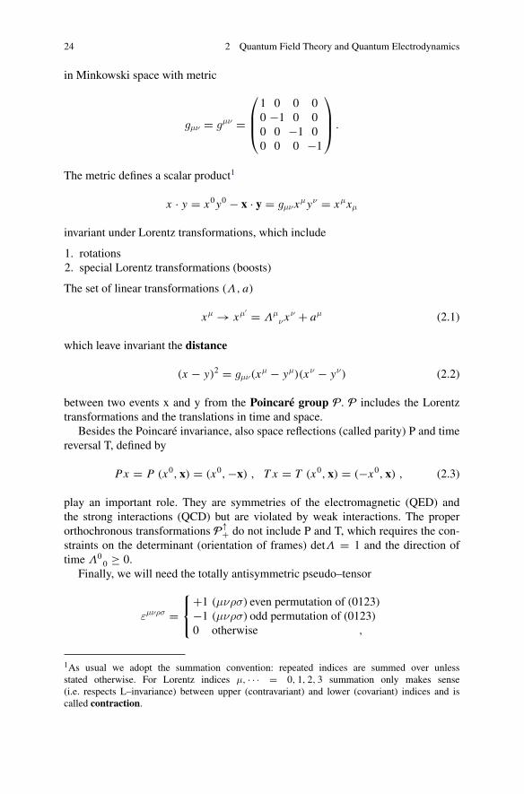
24 2 Quantum Field Theory and Quantum Electrodynamics

in Minkowski space with metric

gμν = gμν =

⎛

⎜⎜⎝

1 0 0 00 −1 0 00 0 −1 00 0 0 −1

⎞

⎟⎟⎠ .

The metric defines a scalar product1

x · y = x0y0 − x · y = gμν xμyν = xμxμ

invariant under Lorentz transformations, which include

1. rotations2. special Lorentz transformations (boosts)

The set of linear transformations (Λ, a)

xμ → xμ′ = Λμν xν + aμ (2.1)

which leave invariant the distance

(x − y)2 = gμν(xμ − yμ)(xν − yν) (2.2)

between two events x and y from the Poincaré group P. P includes the Lorentztransformations and the translations in time and space.

Besides the Poincaré invariance, also space reflections (called parity) P and timereversal T, defined by

Px = P (x0, x) = (x0,−x) , T x = T (x0, x) = (−x0, x) , (2.3)

play an important role. They are symmetries of the electromagnetic (QED) andthe strong interactions (QCD) but are violated by weak interactions. The properorthochronous transformations P↑+ do not include P and T, which requires the con-straints on the determinant (orientation of frames) detΛ = 1 and the direction oftime Λ0

0 ≥ 0.Finally, we will need the totally antisymmetric pseudo–tensor

εμνρσ =⎧⎨

⎩

+1 (μνρσ) even permutation of (0123)−1 (μνρσ) odd permutation of (0123)0 otherwise ,

1As usual we adopt the summation convention: repeated indices are summed over unlessstated otherwise. For Lorentz indices μ, · · · = 0, 1, 2, 3 summation only makes sense(i.e. respects L–invariance) between upper (contravariant) and lower (covariant) indices and iscalled contraction.

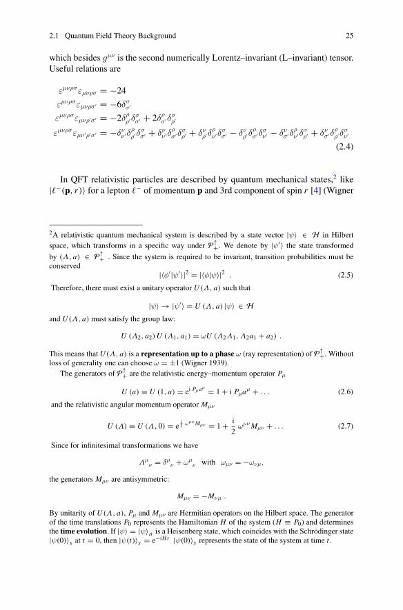
2.1 Quantum Field Theory Background 25

which besides gμν is the second numerically Lorentz–invariant (L–invariant) tensor.Useful relations are

εμνρσεμνρσ = −24εμνρσεμνρσ′ = −6δσ

σ′

εμνρσεμνρ′σ′ = −2δρρ′δ

σσ′ + 2δρ

σ′δσρ′

εμνρσεμν ′ρ′σ′ = −δνν ′δ

ρρ′δ

σσ′ + δν

ν ′δρσ′δ

σρ′ + δν

ρ′δρν ′δ

σσ′ − δν

ρ′δρσ′δ

σν ′ − δν

σ′δρν ′δ

σρ′ + δν

σ′δρρ′δ

σν ′

(2.4)

In QFT relativistic particles are described by quantum mechanical states,2 like|�−(p, r)〉 for a lepton �− of momentum p and 3rd component of spin r [4] (Wigner

2A relativistic quantum mechanical system is described by a state vector |ψ〉 ∈ H in Hilbertspace, which transforms in a specific way under P↑+. We denote by |ψ′〉 the state transformed

by (Λ, a) ∈ P↑+ . Since the system is required to be invariant, transition probabilities must beconserved

|〈φ′|ψ′〉|2 = |〈φ|ψ〉|2 . (2.5)

Therefore, there must exist a unitary operator U (Λ, a) such that

|ψ〉 → |ψ′〉 = U (Λ, a) |ψ〉 ∈ Hand U (Λ, a) must satisfy the group law:

U (Λ2, a2) U (Λ1, a1) = ωU (Λ2Λ1,Λ2a1 + a2) .

This means that U (Λ, a) is a representation up to a phase ω (ray representation) of P↑+. Withoutloss of generality one can choose ω = ±1 (Wigner 1939).

The generators of P↑+ are the relativistic energy–momentum operator Pμ

U (a) ≡ U (1, a) = ei Pμaμ = 1+ i Pμaμ + . . . (2.6)

and the relativistic angular momentum operator Mμν

U (Λ) ≡ U (Λ, 0) = ei2 ωμν Mμν = 1+ i

2ωμν Mμν + . . . (2.7)

Since for infinitesimal transformations we have

Λμν = δμ

ν + ωμν with ωμν = −ωνμ,

the generators Mμν are antisymmetric:

Mμν = −Mνμ .

By unitarity of U (Λ, a), Pμ and Mμν are Hermitian operators on the Hilbert space. The generatorof the time translations P0 represents the Hamiltonian H of the system (H ≡ P0) and determinesthe time evolution. If |ψ〉 = |ψ〉H is a Heisenberg state, which coincides with the Schrödinger state|ψ(0)〉S at t = 0, then |ψ(t)〉S = e−iHt |ψ(0)〉S represents the state of the system at time t .

26 2 Quantum Field Theory and Quantum Electrodynamics

states). Spin will be considered in more detail in the next section. These states carryL–invariant mass p2 = m2 and spin s, and may be obtained by applying correspond-ing creation operators a+(p, r) to the ground state |0〉, called vacuum:

|p, r〉 = a+(p, r) |0〉 . (2.8)

The energy of the particle is p0 = ωp =√

p2 + m2. The Hermitian adjoints of thecreation operators, the annihilation operators a(p, r)

.= (a+(p, r))+, annihilate astate of momentum p and 3rd component of spin r ,

a(p, r)|p′, r ′〉 = (2π)3 2ωp δ(3)(p− p ′) δrr ′ |0〉

and since the vacuum is empty, in particular, they annihilate the vacuum

a(p, r) |0〉 = 0 . (2.9)

The creation and annihilation operators for leptons (spin 1/2 fermions), a and a+,and the corresponding operators b and b+ for the antileptons, satisfy the canonicalanticommutation relations (Fermi statistics)

{a(p, r), a+(p ′, r ′)

} = {b(p, r), b+(p ′, r ′)

} = (2π)3 2ωp δ(3)(p−p ′) δrr ′ (2.10)

with all other anticommutators vanishing.Note, the powers of 2π appearing at variousplaces are convention dependent. Corresponding creation and annihilation operatorsfor photons (spin 1 bosons) satisfy the commutation relations (Bose statistics)

[c(p,λ), c+(p ′,λ′)

] = (2π)3 2ωp δ(3)(p− p ′) δλλ′ . (2.11)

In configuration space particles have associated fields [5–7]. The leptons are rep-resented by Dirac fields ψα(x), which are four–component spinors α = 1, 2, 3, 4,and the photon by the real vector potential field Aμ(x) fromwhich derives the electro-magnetic field strength tensor Fμν = ∂μ Aν − ∂ν Aμ. The free fields are representedin terms of the creation and annihilation operators

ψα(x) =∑

r=±1/2

∫dμ(p)

{uα(p, r) a(p, r) e−ipx + vα(p, r) b+(p, r) eipx

}(2.12)

for the fermion, and

Aμ(x) =∑

λ=±

∫dμ(p)

{εμ(p,λ) c(p,λ) e−ipx + h.c.

}(2.13)

for the photon (h.c. = Hermitian conjugation). The Fourier transformation has torespect that the physical state is on the mass–shell and has positive energy (spectral

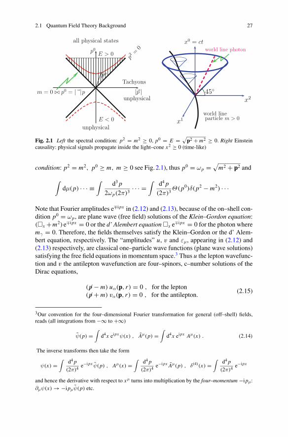
2.1 Quantum Field Theory Background 27

Tachyons

|�p |unphysical

all physical states

E > 0p0

E < 0unphysical

m = 0 �� p0 = |� p|

p2 =

0

pμ

x2

x0 = ct

x1

world line photon

world lineparticle m > 0

45◦

Fig. 2.1 Left the spectral condition: p2 = m2 ≥ 0, p0 = E = √p2 + m2 ≥ 0. Right Einstein

causality: physical signals propagate inside the light–cone x2 ≥ 0 (time-like)

condition: p2 = m2, p0 ≥ m, m ≥ 0 see Fig. 2.1), thus p0 = ωp =√

m2 + p2 and

∫dμ(p) · · · ≡

∫d3 p

2ωp(2π)3· · · =

∫d4 p

(2π)3Θ(p0)δ(p2 − m2) · · ·

Note that Fourier amplitudes e∓ipx in (2.12) and (2.13), because of the on–shell con-dition p0 = ωp, are plane wave (free field) solutions of the Klein–Gordon equation:(�x +m2) e∓ipx = 0 or the d’ Alembert equation �x e∓ipx = 0 for the photon wheremγ = 0. Therefore, the fields themselves satisfy the Klein–Gordon or the d’ Alem-bert equation, respectively. The “amplitudes” u, v and εμ, appearing in (2.12) and(2.13) respectively, are classical one–particle wave functions (plane wave solutions)satisfying the free field equations in momentum space.3 Thus u the lepton wavefunc-tion and v the antilepton wavefunction are four–spinors, c–number solutions of theDirac equations,

( �p − m) uα(p, r) = 0 , for the lepton( �p + m) vα(p, r) = 0 , for the antilepton.

(2.15)

3Our convention for the four–dimensional Fourier transformation for general (off–shell) fields,reads (all integrations from −∞ to +∞)

ψ(p) =∫

d4x eipxψ(x) , Aμ(p) =∫

d4x eipx Aμ(x) . (2.14)

The inverse transforms then take the form

ψ(x) =∫

d4 p

(2π)4e−ipx ψ(p) , Aμ(x) =

∫d4 p

(2π)4e−ipx Aμ(p) , δ(4)(x) =

∫d4 p

(2π)4e−ipx

and hence the derivative with respect to xμ turns into multiplication by the four–momentum −ipμ:∂μψ(x) →−ipμψ(p) etc.

28 2 Quantum Field Theory and Quantum Electrodynamics

As usual, we use the short notation � p .= γμ pμ = γ0 p0 − γp (repeated indicessummed over). Note that the relations (2.15) directly infer that the Dirac field is asolution of the Dirac equation (iγμ∂μ − m) ψ(x) = 0.

The γ−matrices are 4× 4 matrices which satisfy the Dirac algebra4:

{γμ, γν} = γμγν + γνγμ = 2gμν (2.16)

The L–invariant parity odd matrix γ5 (under parity γ0 → γ0, γi →−γi i = 1, 2, 3)

γ5 = iγ0γ1γ2γ3 = i

4! εμνρσγμγνγργσ ; γ25 = 1 ; γ5 = γ+5 (2.17)

satisfies the anticommutation relation

{γ5, γμ} = γ5γμ + γμγ5 = 0 (2.18)

and is required for the formulation of parity violating theories like the weak inter-action part of the Standard Model (SM) and for the projection of Dirac fields toleft–handed (L) and right–handed (R) chiral fields

ψR = Π+ψ ; ψL = Π−ψ (2.19)

4Dirac’s γ–matrices are composed from Pauli matrices. In quantummechanics spacial rotations aredescribed by the group of unitary, unimodular (detU = 1) complex 2 × 2 matrix transformationsSU(2) rather than by classical O(3) rotations. The structure constants are given by εikl (i, k, l =1, 2, 3) the fully antisymmetric permutation tensor. The generators of SU(2) are given by Ti =σi2 ; σi (i = 1, 2, 3) in terms of the 3 Hermitian and traceless Pauli matrices

σ1 =(0 11 0

), σ2 =

(0 −ii 0

), σ3 =

(1 00 −1

)

one of which (σ3) is diagonal. The properties of the Pauli matrices are

[σi ,σk ] = 2iεiklσl , {σi ,σk} = 2δik

σ+i = σi , σ2i = 1 , Tr σi = 0

σi σk = 1

2{σi ,σk} + 1

2[σi ,σk ] = δik + iεiklσl

As usual we denote by [A, B] = AB−B A the commutator, by {A, B} = AB+B A the anticommu-tator. Dirac’s γ–matrices in standard representation (as an alternative to the helicity representation,considered below) are

γ0 =(1 00 −1

), γi =

(0 σi

−σi 0

), γ5 =

(0 11 0

)

.

2.1 Quantum Field Theory Background 29

where

Π± = 1

2(1± γ5) (2.20)

are Hermitian chiral projection matrices5

Π+ +Π− = 1 , Π+Π− = Π−Π+ = 0 , Π2− = Π− and Π2

+ = Π+ .

Note that ψ+ψ or u+u, which might look like the natural analog of |ψ|2 = ψ∗ψof the lepton wave function in quantum mechanics, are not scalars (invariants) underLorentz transformations. In order to obtain an invariant we have to sandwich thematrix A which implements Hermitian conjugation of the Dirac matrices Aγμ A−1 =γ+μ . One easily checks that wemay identify A = γ0. Thus defining the adjoint spinor

by ψ.= ψ+γ0 we may write ψ+Aψ = ψψ etc.

The standard basis of 4 × 4 matrices in four–spinor space is given by the 16elements

Γi = 1 , γ5 , γμ , γμγ5 and σμν = i

2

[γμ, γν

]. (2.22)

The corresponding products ψΓiψ are scalars in spinor space and transform as ordi-nary scalar (S), pseudo–scalar (P), vector (V), axial–vector (A) and tensor (T), respec-tively, under Lorentz transformations.

5Usually, the quantization of a massive particle with spin is defined relative to the z–axis as astandard frame. In general, the direction of polarization ξ , ξ 2 = 1 in the rest frame may be chosenarbitrary. For a massive fermion of momentum p

Π± = 1

2(1± γ5n/)

define the general from of covariant spin projection operators, where n is a space like unit vectororthogonal to p

n2 = −1 ; n · p = 0 .

The general form of n is obtained by applying Lorentz–boost Lp to the polarization vector in therest frame

n = Lp (0, ξ ) =(

p · ξm

, ξ + p · ξm (p0 + m)

p)

. (2.21)

When studying polarization phenomena the polarization vectors n enter as independent additionalvectors in covariant decompositions of amplitudes, besides the momentum vectors.

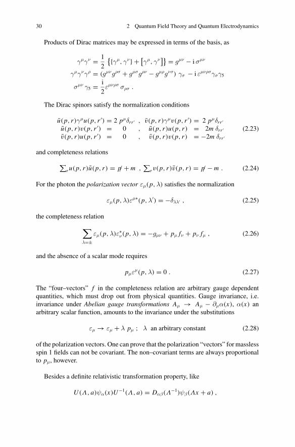
30 2 Quantum Field Theory and Quantum Electrodynamics

Products of Dirac matrices may be expressed in terms of the basis, as

γμγν = 1

2

{{γμ, γν} + [γμ, γν

]} = gμν − iσμν

γμγνγρ = (gμνgρσ + gμσgρν − gμρgνσ) γσ − i εμνρσγσγ5

σμν γ5 = i

2εμνρσ σρσ .

The Dirac spinors satisfy the normalization conditions

u(p, r)γμu(p, r ′) = 2 pμδrr ′ ,

u(p, r)v(p, r ′) = 0 ,

v(p, r)u(p, r ′) = 0 ,

v(p, r)γμv(p, r ′) = 2 pμδrr ′

u(p, r)u(p, r) = 2m δrr ′

v(p, r)v(p, r) = −2m δrr ′(2.23)

and completeness relations

∑r u(p, r)u(p, r) = p/+ m ,

∑rv(p, r)v(p, r) = p/− m . (2.24)

For the photon the polarization vector εμ(p,λ) satisfies the normalization

εμ(p,λ)εμ∗(p,λ′) = −δλλ′ , (2.25)

the completeness relation

∑

λ=±εμ(p,λ)ε∗ν(p,λ) = −gμν + pμ fν + pν fμ , (2.26)

and the absence of a scalar mode requires

pμεμ(p,λ) = 0 . (2.27)

The “four–vectors” f in the completeness relation are arbitrary gauge dependentquantities, which must drop out from physical quantities. Gauge invariance, i.e.invariance under Abelian gauge transformations Aμ → Aμ − ∂μα(x), α(x) anarbitrary scalar function, amounts to the invariance under the substitutions

εμ → εμ + λ pμ ; λ an arbitrary constant (2.28)

of the polarization vectors. One can prove that the polarization “vectors” for masslessspin 1 fields can not be covariant. The non–covariant terms are always proportionalto pμ, however.

Besides a definite relativistic transformation property, like

U (Λ, a)ψα(x)U−1(Λ, a) = Dαβ(Λ−1)ψβ(Λx + a) ,

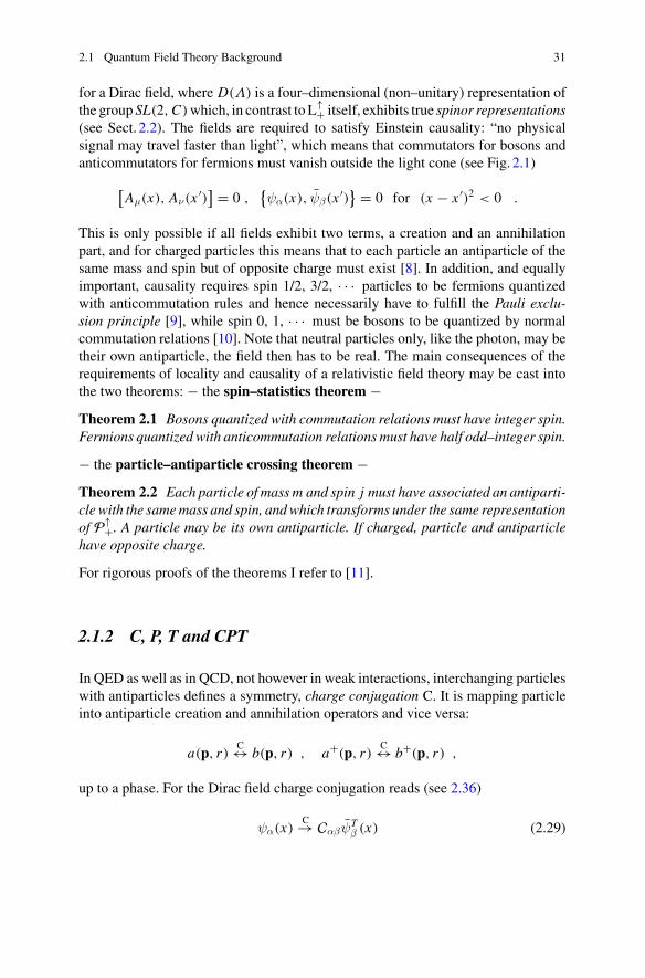
2.1 Quantum Field Theory Background 31

for a Dirac field, where D(Λ) is a four–dimensional (non–unitary) representation ofthe group SL(2, C)which, in contrast to L↑+ itself, exhibits true spinor representations(see Sect. 2.2). The fields are required to satisfy Einstein causality: “no physicalsignal may travel faster than light”, which means that commutators for bosons andanticommutators for fermions must vanish outside the light cone (see Fig. 2.1)

[Aμ(x), Aν(x ′)

] = 0 ,{ψα(x), ψβ(x ′)

} = 0 for (x − x ′)2 < 0 .

This is only possible if all fields exhibit two terms, a creation and an annihilationpart, and for charged particles this means that to each particle an antiparticle of thesame mass and spin but of opposite charge must exist [8]. In addition, and equallyimportant, causality requires spin 1/2, 3/2, · · · particles to be fermions quantizedwith anticommutation rules and hence necessarily have to fulfill the Pauli exclu-sion principle [9], while spin 0, 1, · · · must be bosons to be quantized by normalcommutation relations [10]. Note that neutral particles only, like the photon, may betheir own antiparticle, the field then has to be real. The main consequences of therequirements of locality and causality of a relativistic field theory may be cast intothe two theorems: − the spin–statistics theorem −Theorem 2.1 Bosons quantized with commutation relations must have integer spin.Fermions quantized with anticommutation relations must have half odd–integer spin.

− the particle–antiparticle crossing theorem −Theorem 2.2 Each particle of mass m and spin j must have associated an antiparti-cle with the same mass and spin, and which transforms under the same representationof P↑+. A particle may be its own antiparticle. If charged, particle and antiparticlehave opposite charge.

For rigorous proofs of the theorems I refer to [11].

2.1.2 C, P, T and CPT

In QED as well as in QCD, not however in weak interactions, interchanging particleswith antiparticles defines a symmetry, charge conjugation C. It is mapping particleinto antiparticle creation and annihilation operators and vice versa:

a(p, r)C↔ b(p, r) , a+(p, r)

C↔ b+(p, r) ,

up to a phase. For the Dirac field charge conjugation reads (see 2.36)

ψα(x)C→ CαβψT

β (x) (2.29)

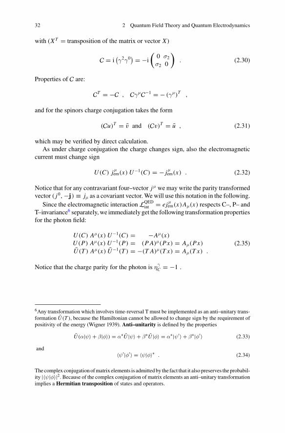
32 2 Quantum Field Theory and Quantum Electrodynamics

with (X T = transposition of the matrix or vector X )

C = i(γ2γ0) = −i

(0 σ2

σ2 0

). (2.30)

Properties of C are:

CT = −C , CγμC−1 = − (γμ)T ,

and for the spinors charge conjugation takes the form

(Cu)T = v and (Cv)T = u , (2.31)

which may be verified by direct calculation.As under charge conjugation the charge changes sign, also the electromagnetic

current must change sign

U (C) jμem(x) U−1(C) = − jμ

em(x) . (2.32)

Notice that for any contravariant four–vector jμ wemay write the parity transformedvector ( j0,−j) ≡ jμ as a covariant vector. We will use this notation in the following.

Since the electromagnetic interactionLQEDint = ejμ

em(x)Aμ(x) respects C–, P– andT–invariance6 separately,we immediately get the following transformation propertiesfor the photon field:

U (C) Aμ(x) U−1(C) = −Aμ(x)

U (P) Aμ(x) U−1(P) = (P A)μ(Px) = Aμ(Px)

U (T ) Aμ(x) U−1(T ) = −(T A)μ(T x) = Aμ(T x) .

(2.35)

Notice that the charge parity for the photon is ηγC = −1 .

6Any transformation which involves time-reversal T must be implemented as an anti–unitary trans-formation U (T ), because the Hamiltonian cannot be allowed to change sign by the requirement ofpositivity of the energy (Wigner 1939). Anti–unitarity is defined by the properties

U (α|ψ〉 + β|φ〉) = α∗U |ψ〉 + β∗U |φ〉 = α∗|ψ′〉 + β∗|φ′〉 (2.33)

and〈ψ′|φ′〉 = 〈ψ|φ〉∗ . (2.34)

The complex conjugationofmatrix elements is admitted by the fact that it also preserves the probabil-ity |〈ψ|φ〉|2. Because of the complex conjugation of matrix elements an anti–unitary transformationimplies a Hermitian transposition of states and operators.

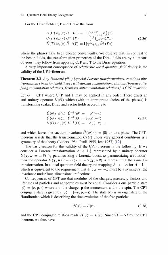
2.1 Quantum Field Theory Background 33

For the Dirac fields C, P and T take the form

U (C) ψα(x) U−1(C) = i(γ2γ0

)αβ

ψTβ (x)

U (P) ψα(x) U−1(P) = (γ0)αβ

ψβ(Px)

U (T ) ψα(x) U−1(T ) = i(γ2γ5

)αβ

ψTβ (T x)

(2.36)

where the phases have been chosen conveniently. We observe that, in contrast tothe boson fields, the transformation properties of the Dirac fields are by no meansobvious; they follow from applying C, P and T to the Dirac equation.

A very important consequence of relativistic local quantum field theory is thevalidity of the CPT–theorem:

Theorem 2.3 Any Poincaré (P↑+) [special Lorentz transformations, rotations plustranslations] invariant field theory with normal commutation relations [bosons satis-fying commutation relations, fermions anticommutation relations] is CPT invariant.

Let Θ = CPT where C, P and T may be applied in any order. There exists ananti–unitary operator U (Θ) which (with an appropriate choice of the phases) istransforming scalar, Dirac and vector fields according to

U (Θ) φ(x) U−1(Θ) = φ∗(−x)

U (Θ) ψ(x) U−1(Θ) = iγ5ψ(−x)

U (Θ) Aμ(x) U−1(Θ) = −Aμ(−x) ,

(2.37)

and which leaves the vacuum invariant: U (Θ)|0〉 = |0〉 up to a phase. The CPT–theorem asserts that the transformation U (Θ) under very general conditions is asymmetry of the theory (Lüders 1954, Pauli 1955, Jost 1957) [12].

The basic reason for the validity of the CPT–theorem is the following: If weconsider a Lorentz transformation Λ ∈ L↑+ represented by a unitary operatorU (χ,ω = n θ) (χ parametrizing a Lorentz–boost, ω parametrizing a rotation),then the operator U (χ, n (θ + 2π)) = −U (χ, n θ) is representing the same L–transformation. In a local quantum field theory the mapping Λ →−Λ for Λ ∈ L↑+,which is equivalent to the requirement that Θ : x → −x must be a symmetry: theinvariance under four–dimensional reflections.

Consequences of CPT are that modulus of the charges, masses, g–factors andlifetimes of particles and antiparticles must be equal. Consider a one particle state|ψ〉 = |e, p, s〉 where e is the charge, p the momentum and s the spin. The CPTconjugate state is given by ˜|ψ〉 = |−e, p,−s〉. The state |ψ〉 is an eigenstate of theHamiltonian which is describing the time evolution of the free particle:

H |ψ〉 = E |ψ〉 (2.38)

and the CPT conjugate relation reads H ˜|ψ〉 = E ˜|ψ〉. Since H = H by the CPTtheorem, we thus have

34 2 Quantum Field Theory and Quantum Electrodynamics

H ˜|ψ〉 = E ˜|ψ〉 . (2.39)

At p = 0 the eigenvalue E reduces to the mass and therefore the two eigenvalueequations say that the mass of particle and antiparticle must be the same:

m = m . (2.40)

The equality of the g–factors may be shown in the same way, but with a Hamiltonianwhich describes the interaction of the particle with a magnetic field B. Then (2.38)holds with eigenvalue

E = m − g

(e�

2mc

)s · B . (2.41)

The CPT conjugate state (e → −e, s → −s, m → m, g → g, B → B) accordingto (2.39) will have the same eigenvalue

E = m − g

(e�

2mc

)s · B . (2.42)

and since m = m we must have

g = g (2.43)

For the proof of the equality of the lifetimes

τ = τ (2.44)

we refer to the textbook [13]. Some examples of experimental tests of CPT, relevantin our context, are (see [14])

|qe+ + qe− |/e < 4× 10−8(me+ − me−)/maverage < 8× 10−9 90% CL(ge+ − ge−)/gaverage (−0.5± 2.1)× 10−12(gμ+ − gμ−)/gaverage (−0.11± 0.12)× 10−8(τμ+ − τμ−)/τaverage (2± 8)× 10−5 .

The best test of CPT comes from the neural Kaon mass difference∣∣∣∣m

K0 − mK 0

mK 0

∣∣∣∣ ≤ 0.6× 10−18 at CL = 90% .

The existence of a possible electric dipole moment we have discussed earlier onp. 9 of the Introduction. An electric dipole moment requires a T violating theoryand the CPT theorem implies that equivalently CP must be violated. In fact, CPinvariance alone (independently of CPT and T) gives important predictions relating

2.1 Quantum Field Theory Background 35

decay properties of particles and antiparticles. We are interested here particularly inμ–decay, which plays a crucial role in the muon g−2 experiment. Consider a matrixelement for a particle a with spin sa at rest decaying into a bunch of particles b, c,· · · with spins sb, sc, · · · and momenta pb, pc, · · · :

M = 〈pb, sb; pc, sc; · · · |Hint|0, sa〉 . (2.45)

Under CP we have to substitute sa → sa, pa →−pa, etc. such that, providedHint

is CP symmetric we obtain

M = 〈−pb, sb; −pc, sc; · · · |Hint|0, sa〉 ≡M . (2.46)

The modulus square of these matrix–elements gives the transition probability for therespective decays, and (2.46) tells us that the decay rate of a particle into a particularconfiguration of final particles is identical to the decay rate of the antiparticle intothe same configuration of antiparticles with all momenta reversed.

For the muon decay μ− → e−νeνμ, after integrating out the unobserved neutrinovariables, the decay electron distribution is of the form

dNe−

dx d cos θ= A(x)+ B(x) sμ · pe− , (2.47)

where x = 2pe−/mμ with pe− the electron momentum in the muon rest frame andcos θ = sμ · pe−, sμ and pe− the unit vectors in direction of sμ and pe−.

The corresponding expression for the antiparticle decay μ+ → e+νeνμ reads

dNe+

dx d cos θ= A(x)+ B(x) sμ · pe+ , (2.48)

and therefore for all angles and all electron momenta

A(x)+ B(x) cos θ = A(x)− B(x) cos θ

or

A(x) = A(x) , B(x) = −B(x) . (2.49)

It means that the decay asymmetry is equal in magnitude but opposite in sign for μ−and μ+. This follows directly from CP and independent of the type of interaction(V−A, V+A, S, P or T) and whether P is violated or not. In spite of the fact thatthe SM exhibits CP violation (see the Introduction to Sect. 4.2), as implied by a CPviolating phase in the quark family mixing matrix in the charged weak current, inμ–decay CP violation is a very small higher order effect and by far too small to haveany detectable trace in the decay distributions, i.e., CP symmetry is perfectly realizedin this case. The strong correlation between the muon polarization and charge on the

36 2 Quantum Field Theory and Quantum Electrodynamics

one side (see Chap. 6) and the decay electron/positron momentum is a key elementof tracing spin polarization information in the muon g − 2 experiments.

CP violation, and the associated T violation plays an important role in determiningthe electric dipole moment of electrons and muons. In principle it is possible to testT invariance in μ–decay by searching for T odd matrix elements like

se ·(sμ × pe

). (2.50)

This is very difficult and has not been performed. Amethod which works is the studyof the effect of an electric dipole moment on the spin precession in the muon g − 2experiment. This will be studied in Sect. 6.3.1 on p. 584.

Until recently, the best limit for the electron (1.8) has been obtained by inves-tigating T violation in Thallium (205Tl) where the EDM is enhanced by the ratioR = datom/de, which in the atomic Thallium ground state studied is R = −585.Investigated are v×E terms in high electrical fields E in an atomic beam magnetic–resonance device [15]. A new experiment [16], using the polar molecule Thoriummonoxide (ThO), finds

de = (2.1± 3.7 stat ± 2.5 syst)× 10−29 e · cm .

This corresponds to an upper limit of |de| < 8.7×10−29 e ·cm with 90% confidence,an order of magnitude improvement in sensitivity compared to the previous bestlimits.

2.2 The Origin of Spin

As promised at the beginning of the chapter the intimate relation of the anomalousmagnetic moment to spin is a good reason to have a closer look at how spin comesinto play in particle physics. The spin and the magnetic moment of the electron didbecome evident from the deflection of atoms in an inhomogeneous magnetic fieldand the observation of the fine structure by optical spectroscopy [17–19].7 Spin isthe intrinsic “self–angular momentum” of a point–particle and when it was observedby Goudsmit and Uhlenbeck it was completely unexpected. The question aboutthe origin of spin is interesting because it is not obvious how a point–like objectcan possess its own angular momentum. A first theoretical formulation of spin inquantum mechanics was given by Pauli in 1927 [20], where spin was introduced asa new degree of freedom saying that there are two species of electrons in a doublet.

In modern relativistic terms, in the SM, particles and in particular leptons andquarks are considered to be massless originally, as required by chiral symmetry. Allparticles acquire their mass due to symmetry breaking via the Higgs mechanism: a

7Particle spin has been discovered by Ralph Kronig (well known for the Kramers Kronig relation)in 1925 before the Uhlenbeck and Goudsmit publication.

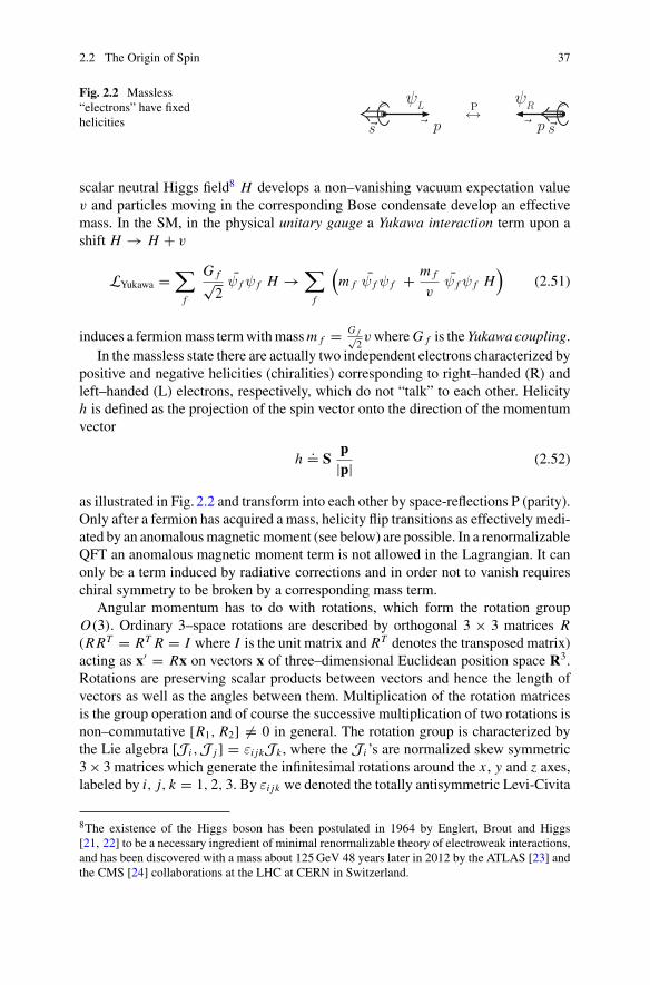
2.2 The Origin of Spin 37

Fig. 2.2 Massless“electrons” have fixedhelicities � p�s

ψL⇐◦> P↔

� p �s

ψR ⇐◦>

scalar neutral Higgs field8 H develops a non–vanishing vacuum expectation valuev and particles moving in the corresponding Bose condensate develop an effectivemass. In the SM, in the physical unitary gauge a Yukawa interaction term upon ashift H → H + v

LYukawa =∑

f

G f√2

ψ f ψ f H →∑

f

(m f ψ f ψ f + m f

vψ f ψ f H

)(2.51)

induces a fermionmass termwithmassm f = G f√2vwhereG f is theYukawa coupling.

In the massless state there are actually two independent electrons characterized bypositive and negative helicities (chiralities) corresponding to right–handed (R) andleft–handed (L) electrons, respectively, which do not “talk” to each other. Helicityh is defined as the projection of the spin vector onto the direction of the momentumvector

h.= S

p|p| (2.52)

as illustrated in Fig. 2.2 and transform into each other by space-reflections P (parity).Only after a fermion has acquired a mass, helicity flip transitions as effectively medi-ated by an anomalousmagneticmoment (see below) are possible. In a renormalizableQFT an anomalous magnetic moment term is not allowed in the Lagrangian. It canonly be a term induced by radiative corrections and in order not to vanish requireschiral symmetry to be broken by a corresponding mass term.

Angular momentum has to do with rotations, which form the rotation groupO(3). Ordinary 3–space rotations are described by orthogonal 3 × 3 matrices R(R RT = RT R = I where I is the unit matrix and RT denotes the transposed matrix)acting as x′ = Rx on vectors x of three–dimensional Euclidean position space R3.Rotations are preserving scalar products between vectors and hence the length ofvectors as well as the angles between them. Multiplication of the rotation matricesis the group operation and of course the successive multiplication of two rotations isnon–commutative [R1, R2] �= 0 in general. The rotation group is characterized bythe Lie algebra [Ji ,J j ] = εi jkJk , where the Ji ’s are normalized skew symmetric3× 3 matrices which generate the infinitesimal rotations around the x , y and z axes,labeled by i, j, k = 1, 2, 3. By εi jk we denoted the totally antisymmetric Levi-Civita

8The existence of the Higgs boson has been postulated in 1964 by Englert, Brout and Higgs[21, 22] to be a necessary ingredient of minimal renormalizable theory of electroweak interactions,and has been discovered with a mass about 125GeV 48 years later in 2012 by the ATLAS [23] andthe CMS [24] collaborations at the LHC at CERN in Switzerland.

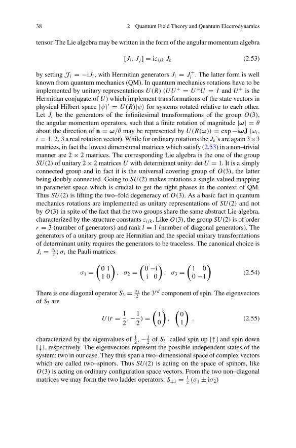
38 2 Quantum Field Theory and Quantum Electrodynamics

tensor. The Lie algebra may be written in the form of the angular momentum algebra

[Ji , Jj ] = iεi jk Jk (2.53)

by setting Ji = −iJi , with Hermitian generators Ji = J+i . The latter form is wellknown from quantum mechanics (QM). In quantum mechanics rotations have to beimplemented by unitary representations U (R) (UU+ = U+U = I and U+ is theHermitian conjugate of U ) which implement transformations of the state vectors inphysical Hilbert space |ψ〉′ = U (R)|ψ〉 for systems rotated relative to each other.Let Ji be the generators of the infinitesimal transformations of the group O(3),the angular momentum operators, such that a finite rotation of magnitude |ω| = θabout the direction of n = ω/θ may be represented by U (R(ω)) = exp−iωJ (ωi ,i = 1, 2, 3 a real rotation vector).While for ordinary rotations the Jk’s are again 3×3matrices, in fact the lowest dimensional matrices which satisfy (2.53) in a non–trivialmanner are 2 × 2 matrices. The corresponding Lie algebra is the one of the groupSU(2) of unitary 2× 2 matrices U with determinant unity: detU = 1. It is a simplyconnected group and in fact it is the universal covering group of O(3), the latterbeing doubly connected. Going to SU(2) makes rotations a single valued mappingin parameter space which is crucial to get the right phases in the context of QM.Thus SU(2) is lifting the two–fold degeneracy of O(3). As a basic fact in quantummechanics rotations are implemented as unitary representations of SU(2) and notby O(3) in spite of the fact that the two groups share the same abstract Lie algebra,characterized by the structure constants εi jk . Like O(3), the group SU(2) is of orderr = 3 (number of generators) and rank l = 1 (number of diagonal generators). Thegenerators of a unitary group are Hermitian and the special unitary transformationsof determinant unity requires the generators to be traceless. The canonical choice isJi = σi

2 ;σi the Pauli matrices

σ1 =(0 11 0

), σ2 =

(0 −ii 0

), σ3 =

(1 00 −1

)(2.54)

There is one diagonal operator S3 = σ32 the 3rd component of spin. The eigenvectors

of S3 are

U (r = 1

2,−1

2) =

(10

),

(01

). (2.55)

characterized by the eigenvalues of 12 ,− 1

2 of S3 called spin up [↑] and spin down[↓], respectively. The eigenvectors represent the possible independent states of thesystem: two in our case. They thus span a two–dimensional space of complex vectorswhich are called two–spinors. Thus SU(2) is acting on the space of spinors, likeO(3) is acting on ordinary configuration space vectors. From the two non–diagonalmatrices we may form the two ladder operators: S±1 = 1

2 (σ1 ± iσ2)

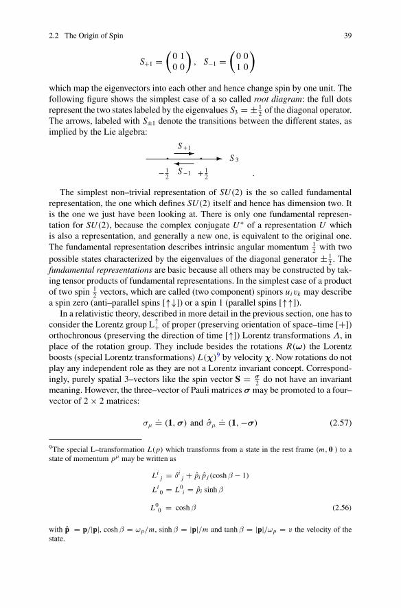
2.2 The Origin of Spin 39

S+1 =(0 10 0

), S−1 =

(0 01 0

)

which map the eigenvectors into each other and hence change spin by one unit. Thefollowing figure shows the simplest case of a so called root diagram: the full dotsrepresent the two states labeled by the eigenvalues S3 = ± 1

2 of the diagonal operator.The arrows, labeled with S±1 denote the transitions between the different states, asimplied by the Lie algebra:

12

12

S 3

S 1

S 1

The simplest non–trivial representation of SU(2) is the so called fundamentalrepresentation, the one which defines SU(2) itself and hence has dimension two. Itis the one we just have been looking at. There is only one fundamental represen-tation for SU(2), because the complex conjugate U ∗ of a representation U whichis also a representation, and generally a new one, is equivalent to the original one.The fundamental representation describes intrinsic angular momentum 1

2 with twopossible states characterized by the eigenvalues of the diagonal generator ± 1

2 . Thefundamental representations are basic because all others may be constructed by tak-ing tensor products of fundamental representations. In the simplest case of a productof two spin 1

2 vectors, which are called (two component) spinors uivk may describea spin zero (anti–parallel spins [↑↓]) or a spin 1 (parallel spins [↑↑]).

In a relativistic theory, described in more detail in the previous section, one has toconsider the Lorentz group L↑+ of proper (preserving orientation of space–time [+])orthochronous (preserving the direction of time [↑]) Lorentz transformations Λ, inplace of the rotation group. They include besides the rotations R(ω) the Lorentzboosts (special Lorentz transformations) L(χ)9 by velocity χ. Now rotations do notplay any independent role as they are not a Lorentz invariant concept. Correspond-ingly, purely spatial 3–vectors like the spin vector S = σ

2 do not have an invariantmeaning. However, the three–vector of Pauli matrices σ may be promoted to a four–vector of 2× 2 matrices:

σμ.= (1,σ) and σμ

.= (1,−σ) (2.57)

9The special L–transformation L(p) which transforms from a state in the rest frame (m, 0 ) to astate of momentum pμ may be written as

Lij = δi

j + pi p j (cosh β − 1)

Li0 = L0

i = pi sinh β

L00 = cosh β (2.56)

with p = p/|p|, cosh β = ωp/m, sinh β = |p|/m and tanh β = |p|/ωp = v the velocity of thestate.

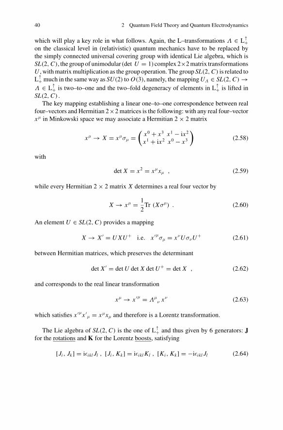
40 2 Quantum Field Theory and Quantum Electrodynamics

which will play a key role in what follows. Again, the L–transformations Λ ∈ L↑+on the classical level in (relativistic) quantum mechanics have to be replaced bythe simply connected universal covering group with identical Lie algebra, which isSL(2, C), the group of unimodular (det U = 1) complex 2×2matrix transformationsU , withmatrixmultiplication as the group operation. The group SL(2, C) is related toL↑+much in the sameway as SU(2) to O(3), namely, themappingUΛ ∈ SL(2, C) →Λ ∈ L↑+ is two–to–one and the two–fold degeneracy of elements in L↑+ is lifted inSL(2, C) .

The key mapping establishing a linear one–to–one correspondence between realfour–vectors and Hermitian 2×2matrices is the following: with any real four–vectorxμ in Minkowski space we may associate a Hermitian 2× 2 matrix

xμ → X = xμσμ =(

x0 + x3 x1 − ix2

x1 + ix2 x0 − x3

)(2.58)

with

det X = x2 = xμxμ , (2.59)

while every Hermitian 2× 2 matrix X determines a real four vector by

X → xμ = 1

2Tr (Xσμ) . (2.60)

An element U ∈ SL(2, C) provides a mapping

X → X ′ = U XU+ i.e. x ′μσμ = xνUσνU+ (2.61)

between Hermitian matrices, which preserves the determinant

det X ′ = detU det X detU+ = det X , (2.62)

and corresponds to the real linear transformation

xμ → x ′μ = Λμν xν (2.63)

which satisfies x ′μx ′μ = xμxμ and therefore is a Lorentz transformation.

The Lie algebra of SL(2, C) is the one of L↑+ and thus given by 6 generators: Jfor the rotations and K for the Lorentz boosts, satisfying

[Ji , Jk] = iεikl Jl , [Ji , Kk] = iεikl Kl , [Ki , Kk] = −iεikl Jl (2.64)

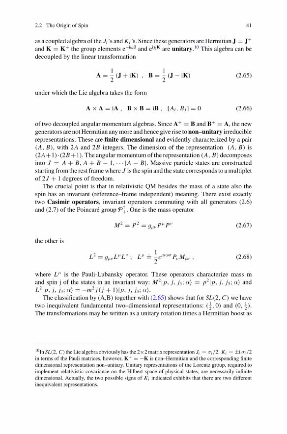
2.2 The Origin of Spin 41

as a coupled algebra of the Ji ’s and Ki ’s. Since these generators areHermitian J = J+and K = K+ the group elements e−iωJ and eiχK are unitary.10 This algebra can bedecoupled by the linear transformation

A = 1

2(J+ iK) , B = 1

2(J− iK) (2.65)

under which the Lie algebra takes the form

A× A = iA , B× B = iB , [Ai , B j ] = 0 (2.66)

of two decoupled angular momentum algebras. Since A+ = B and B+ = A, the newgenerators are notHermitian anymore and hence give rise tonon–unitary irreduciblerepresentations. These are finite dimensional and evidently characterized by a pair(A, B), with 2A and 2B integers. The dimension of the representation (A, B) is(2A+1)·(2B+1). The angular momentum of the representation (A, B) decomposesinto J = A + B, A + B − 1, · · · |A − B|. Massive particle states are constructedstarting from the rest framewhere J is the spin and the state corresponds to amultipletof 2J + 1 degrees of freedom.

The crucial point is that in relativistic QM besides the mass of a state also thespin has an invariant (reference–frame independent) meaning. There exist exactlytwo Casimir operators, invariant operators commuting with all generators (2.6)and (2.7) of the Poincaré group P↑+. One is the mass operator

M2 = P2 = gμν Pμ Pν (2.67)

the other is

L2 = gμν LμLν ; Lμ .= 1

2εμνρσ Pν Mρσ , (2.68)

where Lμ is the Pauli-Lubansky operator. These operators characterize mass mand spin j of the states in an invariant way: M2|p, j, j3;α〉 = p2|p, j, j3;α〉 andL2|p, j, j3;α〉 = −m2 j ( j + 1)|p, j, j3;α〉.

The classification by (A,B) together with (2.65) shows that for SL(2, C) we havetwo inequivalent fundamental two–dimensional representations: ( 12 , 0) and (0, 1

2 ).The transformations may be written as a unitary rotation times a Hermitian boost as

10In SL(2, C) theLie algebra obviously has the 2×2matrix representation Ji = σi /2, Ki = ±iσi /2in terms of the Pauli matrices, however, K+ = −K is non–Hermitian and the corresponding finitedimensional representation non–unitary. Unitary representations of the Lorentz group, required toimplement relativistic covariance on the Hilbert space of physical states, are necessarily infinitedimensional. Actually, the two possible signs of Ki indicated exhibits that there are two differentinequivalent representations.

42 2 Quantum Field Theory and Quantum Electrodynamics

follows11:

UΛ = U (χ,ω ) = D( 12 )(Λ) = e χ σ

2 e−iω σ2 for

(12 , 0

)

UΛ = U+Λ−1 = D( 1

2 )(Λ) = e−χ σ2 e−iω σ

2 for(0, 1

2

).

(2.69)

While σμ (2.57) is a covariant vector

UΛσμU+Λ = Λν

μ σν (2.70)

with respect to the representation UΛ = D( 12 )(Λ), the vector σμ (2.57) is covariant

with respect to UΛ = D( 12 )(Λ)

UΛσμU+Λ = Λν

μ σν . (2.71)

Note that

U (χ, nθ) and U (χ, n (θ + 2π)) = −U (χ, nθ) (2.72)

represent the same Lorentz transformation. UΛ is therefore a double–valued repre-sentation of L↑+.

An important theorem [25] says that

Theorem 2.4 A massless particle of helicity λ may be only in the representationssatisfying (A, B) = (A, A− λ), where 2A and 2(A− λ) are non—negative integernumbers.

Thus the simplest representations for massless fields are the spin 1/2 states

λ = + 12 :

(12 , 0

)right − handed (R)

− 12 :

(0, 1

2

)left − handed (L)

(2.73)

of helicity + 12 and − 1

2 , respectively.The finite dimensional irreducible representations of SL(2, C) to mass 0 and spin

j are one–dimensional and characterized by the helicity λ = ± j . To a given spinj > 0 there exist exactly two helicity states. Each of the two possible states isinvariant by itself under L↑+, however, the two states get interchanged under paritytransformations:

UP h U−1P = −h . (2.74)

Besides the crucial fact of the validity of the spin–statistics theorem (valid in anyrelativistic QFT), here we notice another important difference between spin in

11Again, these finite dimensional representations UΛ, UP (below), etc. should not be confusedwith the corresponding infinite dimensional unitary representations U (Λ), U (P), etc. acting on theHilbert space of physical states considered in the preceding section.

2.2 The Origin of Spin 43

non–relativistic QM and spin in QFT. In QM spin 1/2 is a system of two degrees offreedom as introduced by Pauli, while in QFT where we may consider the masslesscase we have two independent singlet states. Parity P, as we know, acts on four–vectors like Px = (x0,−x ) and satisfies12 P2 = 1. With respect to the rotationgroup O3, P2 is just a rotation by the angle 2π and thus in the context of the rotationgroup P has no special meaning. This is different for the Lorentz group. While

UP J = JUP (2.75)

commutes

UP K = −KUP (2.76)

does not. As a consequence, we learn that

UPU (χ, n θ) = U (−χ, n θ)UP (2.77)

and hence

UPUΛ = UΛUP . (2.78)

Thus under parity a left–handed massless fermion is transformed into a right–handedone and vice versa, which of course is also evident from Fig. 2.2, if we take intoaccount that a change of frame by a Lorentz transformation (velocity v ≤ c) cannotflip the spin of a massless particle.

The necessity to work with SL(2, C) becomes obvious once we deal with spinors.On a classical level, two–spinors or Weyl spinorsw are elements of a vector space Vof two complex entries, which transform under SL(2, C) by matrix multiplication:w′ = Uw, w ∈ V , U ∈ SL(2, C)

w =(

ab

); a, b ∈ C . (2.79)

Corresponding to the two representations there exist two local Weyl spinor fields(see (2.12))

ϕa(x) =∑

r=±1/2

∫dμ(p)

{ua(p, r) a(p, r) e−ipx + va(p, r) b+(p, r) eipx

}

χa(x) =∑

r=±1/2

∫dμ(p)

{ua(p, r) a(p, r) e−ipx + va(p, r) b+(p, r) eipx

},

(2.80)

12Note that while P2 = 1 the phase ηP of its unitary representation UP is constrained by U2P = ±1

only, i.e. ηP = ±1 or ±i.

44 2 Quantum Field Theory and Quantum Electrodynamics

with two components a = 1, 2, which satisfy the Weyl equations

i(σμ∂μ

)ab ϕb(x) = mχa(x)

i(σμ∂μ

)ab

χb(x) = mϕa(x) . (2.81)

The appropriate one–particle wave functions u(p, r) etc. may be easily constructedas follows: for a massive particle states are constructed by starting in the rest framewhere rotations act as (ω = |ω|, ω = ω/ω)

D( 12 ) (R(ω )) = D( 1

2 ) (R(ω )) = e−iωσ2 = 1 cos

ω

2− i σ · ω sin

ω

2. (2.82)

Notice that this SU(2) rotation is a rotation by half of the angle, only, of the corre-sponding classical O3 rotation. Here the non–relativistic construction of the statesapplies and the spinors at rest are given by (2.55). The propagating particles car-rying momentum p are then obtained by performing a Lorentz–boost to the statesat rest. A boost L(p) (2.56) of momentum p is given by D( 1

2 ) (L(p )) = eχ σ2 =

N−1 (pμσμ + m)and D( 1

2 ) (L(p )) = e−χ σ2 = N−1 (pμσμ + m

), respectively, in

the two basic representations. N = (2m (p0 + m))− 12 is the normalization factor.

The one–particle wave functions (two–spinors) of aWeyl particle and its antiparticleare thus given by

u(p, r) = N−1 (pμσμ + m)

U (r) and v(p, r) = N−1 (pμσμ + m)

V (r) ,

respectively, where U (r) and V (r) = −iσ2U (r) are the rest frame spinors (2.55).The last relation one has to require for implementing the charge conjugation propertyfor the spinors (2.31) in terms of the matrix (2.30). For the adjoint representation,similarly,

u(p, r) = N−1 (pμσμ + m)

U (r) and v(p, r) = −N−1 (pμσμ + m)

V (r) .

The − sign in the last equation, (−1)2 j for spin j , is similar to the −iσ2 in therelation between U and V , both are required to make the fields local and with propertransformation properties. We can easily derive (2.81) now. We may write σμ pμ =ωp1−σp = 2|p|( ωp

2|p | 1−h)where h ≡ σ2

p|p | is the helicity operator, and formassless

states, where ωp = |p |, we have σμ pμ = 2|p | ( 12 −h) a projection operator on stateswith helicity − 1

2 , while σμ pμ = 2|p | ( 12 + h) a projection operator on states withhelicity+ 1

2 . Furthermore, we observe that pμ pνσμσν = pμ pνσμσν = p2 = m2 andone easily verifies the Weyl equations using the given representations of the wavefunctions.

In the massless limit m → 0 : p0 = ωp = |p | we obtain two decoupledequations

2.2 The Origin of Spin 45

i(σμ∂μ

)ab ϕb(x) = 0

i(σμ∂μ

)ab χb(x) = 0 .

In momentum space the fields are just multiplied by the helicity projector and theequations say that the massless fields have fixed helicities:

(1

2, 0

): ϕ ∼ ψR

(0,

1

2

): χ ∼ ψL (2.83)

which suggests to rewrite the transformations as

ψa L , R (x) → ψ′a L , R(x ′) = (

ΛL , R

)ab ψb L , R (Λx) (2.84)

with (ΛL , R

)ab =

(e±χ σ

2 e−iωσ2

)

ab(Λ+

R= Λ−1

L) . (2.85)

Using σ2σiσ2 = −σ∗i one can show that σ2ΛLσ2 = Λ∗R . Thus, ψ

cL ≡ σ2ψ

∗L (up to an

arbitrary phase) is defining a charge conjugate spinor which transforms as ψcL ∼ ψR .

Indeed ΛRψcL = ΛRσ2ψ

∗L = σ2Λ

∗Lψ∗L = σ2ψ

∗′L = ψc′

L and thus ψcL ≡ σ2ψ

∗L ≡

ϕ ∼ ψR . Similarly, ψcR ≡ σ2ψ

∗R ≡ χ ∼ ψL . We thus learn, that for massless fields,

counting particles and antiparticles separately, we may consider all fields to be left–handed. The second term in the field, the antiparticle creation part, in each caseautomatically includes the right–handed partners.

The Dirac field is the bispinor field obtained by combining the irreducible fieldsϕa(x) and χa(x) into one reducible field ( 12 , 0)⊕ (0, 1

2 ). It is the natural field to beused to describe fermions participating parity conserving interactions like QED andQCD. Explicitly, the Dirac field is given by

ψα(x) =(

ϕaχa

)(x) =

∑

r

∫dμ(p)

{uα(p, r) a(p, r) e−ipx + vα(p, r) b+(p, r) eipx

}

where

uα =(

ua

ua

); vα =

(va

va

). (2.86)

ψα(x) satisfies the Dirac equation:

(iγμ∂μ − m

)αβ

ψβ(x) = 0

where

γμ .=(

0 σμ

σμ 0

)(2.87)

are the Dirac matrices in the helicity representation (Weyl basis).

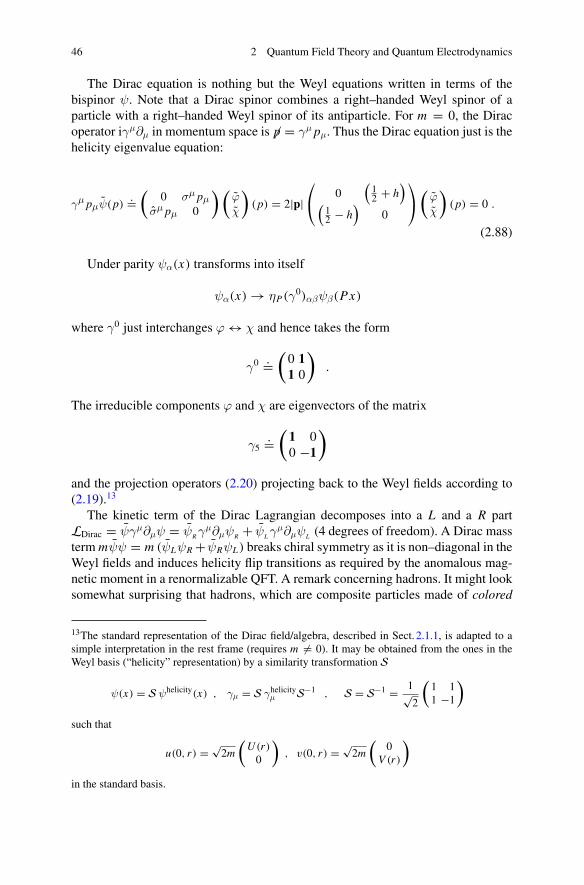
46 2 Quantum Field Theory and Quantum Electrodynamics

The Dirac equation is nothing but the Weyl equations written in terms of thebispinor ψ. Note that a Dirac spinor combines a right–handed Weyl spinor of aparticle with a right–handed Weyl spinor of its antiparticle. For m = 0, the Diracoperator iγμ∂μ in momentum space is �p = γμ pμ. Thus the Dirac equation just is thehelicity eigenvalue equation:

γμ pμψ(p).=(

0 σμ pμ

σμ pμ 0

)(ϕχ

)(p) = 2|p|

⎛

⎝0

(12 + h

)

(12 − h

)0

⎞

⎠(

ϕχ

)(p) = 0 .

(2.88)

Under parity ψα(x) transforms into itself

ψα(x) → ηP(γ0)αβψβ(Px)

where γ0 just interchanges ϕ ↔ χ and hence takes the form

γ0 .=(0 11 0

).

The irreducible components ϕ and χ are eigenvectors of the matrix

γ5.=(

1 00 −1

)

and the projection operators (2.20) projecting back to the Weyl fields according to(2.19).13

The kinetic term of the Dirac Lagrangian decomposes into a L and a R partLDirac = ψγμ∂μψ = ψR γ

μ∂μψR + ψL γμ∂μψL (4 degrees of freedom). A Dirac mass

term mψψ = m (ψLψR+ ψRψL) breaks chiral symmetry as it is non–diagonal in theWeyl fields and induces helicity flip transitions as required by the anomalous mag-netic moment in a renormalizable QFT. A remark concerning hadrons. It might looksomewhat surprising that hadrons, which are composite particles made of colored

13The standard representation of the Dirac field/algebra, described in Sect. 2.1.1, is adapted to asimple interpretation in the rest frame (requires m �= 0). It may be obtained from the ones in theWeyl basis (“helicity” representation) by a similarity transformation S

ψ(x) = S ψhelicity(x) , γμ = S γhelicityμ S−1 , S = S−1 = 1√

2

(1 11 −1

)

such that

u(0, r) = √2m

(U (r)

0

), v(0, r) = √2m

(0

V (r)

)

in the standard basis.

2.2 The Origin of Spin 47

quarks and gluons, in many respects look like “elementary particles” which are welldescribed as Wigner particles (if one switches off the electromagnetic interactionwhich cause a serious IR problem which spoils the naive Wigner state picture aswe will describe below), particles of definite mass and spin and charge quantizedin units of e and have associated electromagnetic form factors and in particular adefinite magnetic moment. However, for the proton for example, the gyromagneticratio gP from the relation μP = gP e�/(2m P c) s turns out to be gP ∼ 2.8 oraP = (gP − 2)/2 ∼ 0.4 showing that the proton is not really a Dirac particle andits anomalous magnetic moment indicates that the proton is not a point particle buthas internal structure. This was first shown long time ago by atomic beam magneticdeflection experiments [26], before the nature of the muon was clarified. For thelatter it was the measurement at CERN which yielded aμ = 0.00119(10) [27] andrevealed the muon to be just a heavy electron. Within errors at that time the muonturned out to have the same value of the anomalous magnetic moment as the electron,which is known to be due to virtual radiative corrections.

The analysis of the spin structure on a formal level, discussing the quantummechanical implementation of relativistic symmetry principles, fits very naturallywith the observed spin phenomena. In particular the existence of the fundamentalspin 1

2 particles which must satisfy Pauli’s exclusion principle has dramatic conse-quences for real life. Without the existence of spin as an extra fundamental quantumnumber in general and the spin 1

2 fermions in particular, stability of nuclei againstCoulomb collapse and of stars against gravitational collapse would be missing andthe universe would not be ours.

2.3 Quantum Electrodynamics

The lepton–photon interaction is described by QED, which is structured by localU (1) gauge invariance14

ψ(x) → e−ieα(x)ψ(x)

Aμ(x) → Aμ(x)− ∂μα(x) , (2.89)

with an arbitrary scalar functionα(x), implying lepton–photon interaction accordingto minimal coupling, which means that we have to perform the substitution ∂μ →

14The known elementary particle interactions, the strong, electromagnetic and weak forces, allderive from a local gauge symmetry principle. This was first observed byWeyl [28] for the AbelianQEDand later extended to non–Abelian gauge theories byYang andMills [29]. The gauge symmetrygroup governing the Standard Model of particle physics is SU(3)c ⊗ SU(2)L ⊗U (1)Y .

48 2 Quantum Field Theory and Quantum Electrodynamics

Dμ = ∂μ − ieAμ(x) in the Dirac equation (iγμ∂μ − m)ψ(x) = 0 of a free lepton.15

This implies that the electromagnetic interaction is described by the bare Lagrangian

LQED = −1

4Fμν Fμν − 1

2ξ−1

(∂μ Aμ

)2 + ψ(iγμ Dμ − m

)ψ

= Lξ0A +L0ψ + ejμ

em(x)Aμ(x) , (2.90)

and the corresponding field equations read16

(iγμ∂μ − m

)ψ(x) = −e : Aμ(x)γμψ(x) :

(�gμν − (

1− ξ−1)∂μ∂ν

)Aν(x) = −e : ψ(x)γμψ(x) : .

(2.91)

The interaction part of the Lagrangian is

Lint = ejμem(x)Aμ(x) , (2.92)

while the bilinear free field parts Lξ0A and L0ψ define the propagators of the photon

and the leptons, respectively (given below).As in classical electrodynamics the gaugepotential Aμ is an auxiliary fieldwhich exhibits unphysical degrees of freedom, and isnot uniquely determinedbyMaxwell’s equations. In order to get awell definedphotonpropagator a gauge fixing condition is required.We adopt the linear covariant Lorentzgauge : ∂μ Aμ = 0, which is implemented via the Lagrange multiplier method, withLagrange multiplier λ = 1/ξ, ξ is called gauge parameter.17 The gauge invarianceof physical quantities infers that they do not depend on the gauge parameter.

Above we have denoted by e the charge of the electron, which by convention istaken to be negative. In the following we will explicitly account for the sign of thecharge and use e to denote the positive value of the charge of the positron. The chargeof a fermion f is then given by Q f e, with Q f the charge of a fermion in units ofthe positron charge e. A collection of charged fermions f enters the electromagneticcurrent as

jμem =

∑

fQ f ψ f γ

μψ f , (2.93)

15Themodified derivative Dμ = ∂μ−ieAμ(x) is called covariant derivative. e is the gauge coupling.The minimal substitution promotes the global gauge symmetry of the free Dirac Lagrangian to alocal gauge symmetry of the electron–photon system, i.e., the interacting systemhasmore symmetrythan the free electron.16The prescription : · · · : means Wick ordering of products of fields: write the fields in terms ofcreation and annihilation operators and order them such that all annihilation operators are to theright of all creation operators, assuming the operators to commute (bosons) or to anticommute(fermions). This makes the vacuum expectation value of the field product vanish.17The parametrization of the gauge dependence by the inverse of the Lagrange multiplier ξ = 1/λis just a commonly accepted convention.

2.3 Quantum Electrodynamics 49

for the leptons alone jμ lepem = −∑� ψ�γ

μψ� (� = e,μ, τ ). If not specified otherwiseψ(x) in the following will denote a lepton field carrying negative charge −e.

The electric charge is a conserved quantity as a consequence of Noether’stheorem:

Theorem 2.5 If the Lagrangian L(ψ, ∂μψ · · · ) of a system is invariant under ar–parametric group of global field transformations ψ(x) → ψ(x) + δψ(x), · · ·then there exist r conserved currents ∂μ j μ

i (x) = 0 , i = 1, · · · , r which imply theexistence of r conserved charges

Qi =∫

d3x j 0i (t, x) ; dQi

dt= 0 , i = 1, · · · , r . (2.94)

The global symmetry in our QED case is the global U (1)em gauge symmetry (i.e.transformations (2.89) with gauge function α = constant).

One important object we need for our purpose is the unitary scattering matrix Swhich encodes the perturbative lepton–photon interaction processes and is given by

S = T(ei∫d4x L(0)

int (x))∣∣∣⊗

. (2.95)

The prescription⊗ says that all graphs (see below) which include vacuum diagrams(disconnected subdiagrams with no external legs) as factors have to be omitted. Thiscorresponds to the proper normalization of the S–operator. Unitarity requires

SS+ = S+S = 1 ⇔ S+ = S−1 (2.96)

and infers the conservation of quantum mechanical transition probabilities. The pre-scription T means time ordering of all operators, like

T {φ(x)φ(y)} = Θ(x0 − y0)φ(x)φ(y)±Θ(y0 − x0)φ(y)φ(x) (2.97)

where the+ sign holds for boson fields and the− sign for fermion fields. Under theT prescription all fields are commuting (bosons) or anticommuting (fermions). Allfields in (2.95) may be taken to be free fields. With the help of S we may calculatethe basic objects of a QFT, the Green functions. These are the vacuum expectationvalues of time ordered or chronological products of fields like the electromagneticcorrelator

Gμ,αβ(x, y, y).= 〈0|T {

Aμ(x)ψα(y)ψβ(y)} |0〉 . (2.98)

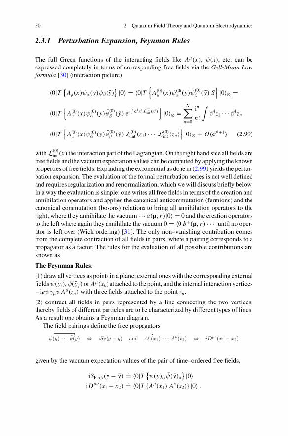
50 2 Quantum Field Theory and Quantum Electrodynamics

2.3.1 Perturbation Expansion, Feynman Rules

The full Green functions of the interacting fields like Aμ(x), ψ(x), etc. can beexpressed completely in terms of corresponding free fields via the Gell-Mann Lowformula [30] (interaction picture)

〈0|T {Aμ(x)ψα(y)ψβ(y)

} |0〉 = 〈0|T{

A(0)μ (x)ψ(0)

α (y)ψ(0)β (y) S

}|0〉⊗ =

〈0|T{

A(0)μ (x)ψ(0)

α (y)ψ(0)β (y) ei

∫d4x ′ L(0)

int (x ′)}|0〉⊗ =

N∑

n=0

in

n!∫

d4z1 · · · d4zn

〈0|T{

A(0)μ (x)ψ(0)

α (y)ψ(0)β (y) L(0)

int (z1) · · · L(0)int (zn)

}|0〉⊗ + O(eN+1) (2.99)

withL(0)int (x) the interaction part of theLagrangian.On the right hand side all fields are

free fields and the vacuumexpectation values can be computed by applying the knownproperties of free fields. Expanding the exponential as done in (2.99) yields the pertur-bation expansion. The evaluation of the formal perturbation series is not well definedand requires regularization and renormalization, which wewill discuss briefly below.In a way the evaluation is simple: one writes all free fields in terms of the creation andannihilation operators and applies the canonical anticommutation (fermions) and thecanonical commutation (bosons) relations to bring all annihilation operators to theright, where they annihilate the vacuum · · · a(p, r)|0〉 = 0 and the creation operatorsto the left where again they annihilate the vacuum 0 = 〈0|b+(p, r) · · · , until no oper-ator is left over (Wick ordering) [31]. The only non–vanishing contribution comesfrom the complete contraction of all fields in pairs, where a pairing corresponds to apropagator as a factor. The rules for the evaluation of all possible contributions areknown as

The Feynman Rules:

(1) draw all vertices as points in a plane: external oneswith the corresponding externalfieldsψ(yi ), ψ(y j )or Aμ(xk) attached to the point, and the internal interactionvertices−ieψγμψAμ(zn) with three fields attached to the point zn .

(2) contract all fields in pairs represented by a line connecting the two vertices,thereby fields of different particles are to be characterized by different types of lines.As a result one obtains a Feynman diagram.

The field pairings define the free propagators

ψ(y) · · · ψ(y) ⇔ iSF(y − y) and Aμ(x1) · · · Aν(x2) ⇔ iDμν(x1 − x2)

given by the vacuum expectation values of the pair of time–ordered free fields,

iSF αβ(y − y).= 〈0|T {

ψ(y)αψ(y)β} |0〉

iDμν(x1 − x2).= 〈0|T {Aμ(x1) Aν(x2)} |0〉 .

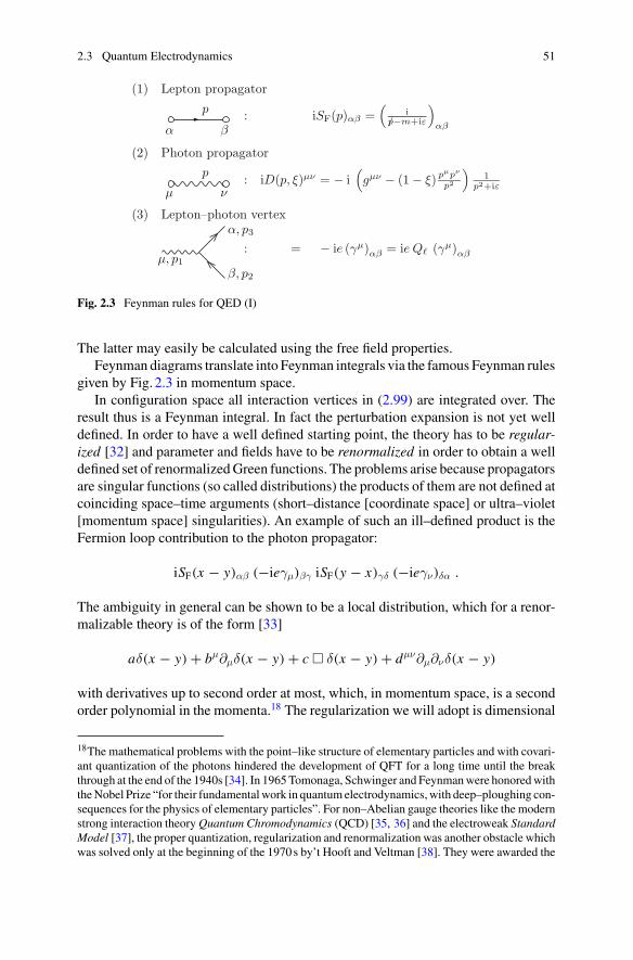
2.3 Quantum Electrodynamics 51

(1) Lepton propagator

: iSF(p)αβ =(

i/p−m+iε

)αβ

(2) Photon propagator

: iD(p, ξ)μν = − i(gμν − (1 − ξ) pμpν

p2

)1

p2+iε

(3) Lepton–photon vertex

: = − ie (γμ)αβ = ie Q� (γμ)αβ

p

α β

p

μ ν

μ, p1

α, p3

β, p2

Fig. 2.3 Feynman rules for QED (I)

The latter may easily be calculated using the free field properties.Feynman diagrams translate into Feynman integrals via the famous Feynman rules

given by Fig. 2.3 in momentum space.In configuration space all interaction vertices in (2.99) are integrated over. The

result thus is a Feynman integral. In fact the perturbation expansion is not yet welldefined. In order to have a well defined starting point, the theory has to be regular-ized [32] and parameter and fields have to be renormalized in order to obtain a welldefined set of renormalizedGreen functions. The problems arise because propagatorsare singular functions (so called distributions) the products of them are not defined atcoinciding space–time arguments (short–distance [coordinate space] or ultra–violet[momentum space] singularities). An example of such an ill–defined product is theFermion loop contribution to the photon propagator:

iSF(x − y)αβ (−ieγμ)βγ iSF(y − x)γδ (−ieγν)δα .

The ambiguity in general can be shown to be a local distribution, which for a renor-malizable theory is of the form [33]

aδ(x − y)+ bμ∂μδ(x − y)+ c � δ(x − y)+ dμν∂μ∂νδ(x − y)

with derivatives up to second order at most, which, in momentum space, is a secondorder polynomial in the momenta.18 The regularization we will adopt is dimensional

18The mathematical problems with the point–like structure of elementary particles and with covari-ant quantization of the photons hindered the development of QFT for a long time until the breakthrough at the end of the 1940s [34]. In 1965Tomonaga, Schwinger and Feynmanwere honoredwiththeNobel Prize “for their fundamentalwork in quantumelectrodynamics,with deep–ploughing con-sequences for the physics of elementary particles”. For non–Abelian gauge theories like the modernstrong interaction theory Quantum Chromodynamics (QCD) [35, 36] and the electroweak StandardModel [37], the proper quantization, regularization and renormalization was another obstacle whichwas solved only at the beginning of the 1970s by’t Hooft and Veltman [38]. They were awarded the

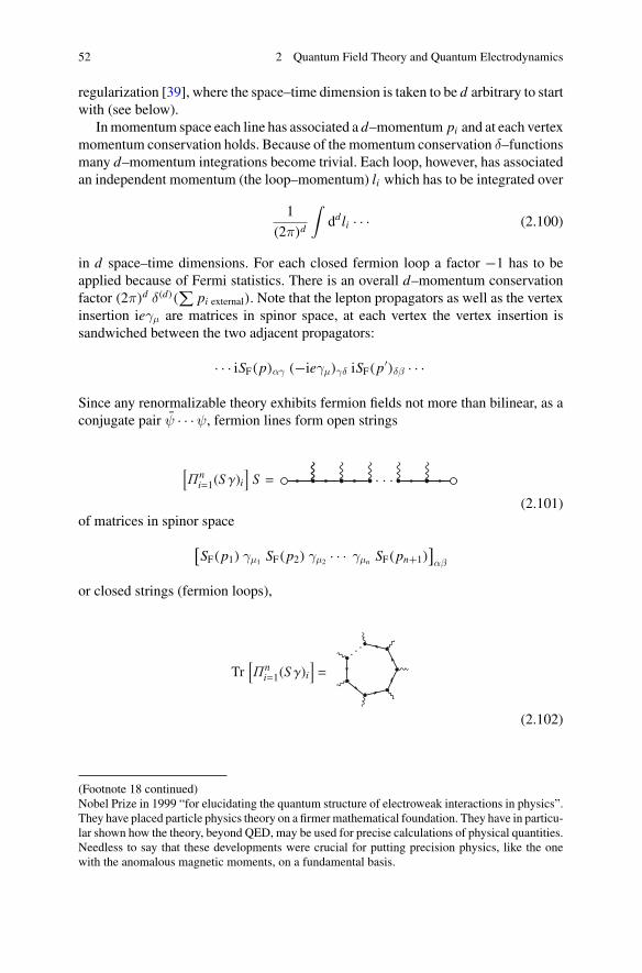
52 2 Quantum Field Theory and Quantum Electrodynamics

regularization [39], where the space–time dimension is taken to be d arbitrary to startwith (see below).

Inmomentum space each line has associated a d–momentum pi and at each vertexmomentum conservation holds. Because of the momentum conservation δ–functionsmany d–momentum integrations become trivial. Each loop, however, has associatedan independent momentum (the loop–momentum) li which has to be integrated over

1

(2π)d

∫ddli · · · (2.100)

in d space–time dimensions. For each closed fermion loop a factor −1 has to beapplied because of Fermi statistics. There is an overall d–momentum conservationfactor (2π)d δ(d)(

∑pi external). Note that the lepton propagators as well as the vertex

insertion ieγμ are matrices in spinor space, at each vertex the vertex insertion issandwiched between the two adjacent propagators:

· · · iSF(p)αγ (−ieγμ)γδ iSF(p′)δβ · · ·

Since any renormalizable theory exhibits fermion fields not more than bilinear, as aconjugate pair ψ · · ·ψ, fermion lines form open strings

(2.101)of matrices in spinor space

[SF(p1) γμ1 SF(p2) γμ2 · · · γμn SF(pn+1)

]αβ

or closed strings (fermion loops),

(2.102)

(Footnote 18 continued)Nobel Prize in 1999 “for elucidating the quantum structure of electroweak interactions in physics”.They have placed particle physics theory on a firmermathematical foundation. They have in particu-lar shown how the theory, beyond QED, may be used for precise calculations of physical quantities.Needless to say that these developments were crucial for putting precision physics, like the onewith the anomalous magnetic moments, on a fundamental basis.

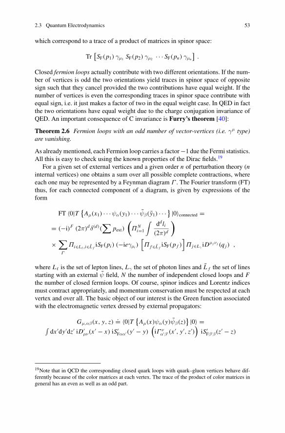
2.3 Quantum Electrodynamics 53

which correspond to a trace of a product of matrices in spinor space:

Tr[SF(p1) γμ1 SF(p2) γμ2 · · · SF(pn) γμn

].

Closed fermion loops actually contribute with two different orientations. If the num-ber of vertices is odd the two orientations yield traces in spinor space of oppositesign such that they cancel provided the two contributions have equal weight. If thenumber of vertices is even the corresponding traces in spinor space contribute withequal sign, i.e. it just makes a factor of two in the equal weight case. In QED in factthe two orientations have equal weight due to the charge conjugation invariance ofQED. An important consequence of C invariance is Furry’s theorem [40]:

Theorem 2.6 Fermion loops with an odd number of vector-vertices (i.e. γμ type)are vanishing.

As alreadymentioned, each Fermion loop carries a factor−1 due the Fermi statistics.All this is easy to check using the known properties of the Dirac fields.19

For a given set of external vertices and a given order n of perturbation theory (ninternal vertices) one obtains a sum over all possible complete contractions, whereeach one may be represented by a Feynman diagram Γ . The Fourier transform (FT)thus, for each connected component of a diagram, is given by expressions of theform

FT 〈0|T {Aμ(x1) · · ·ψα(y1) · · · ψβ(y1) · · ·

} |0〉connected == (−i)F (2π)dδ(d)(

∑pext)

(Π N

i=1

∫ddli

(2π)d

)

×∑

Γ

Πi∈L�,i∈L fiSF(pi ) (−ieγμi )

[Π f ∈L f

iSF(p f )]Π j∈Lγ

iDμ j ν j (q j ) ,

where L� is the set of lepton lines, Lγ the set of photon lines and L f the set of linesstarting with an external ψ field, N the number of independent closed loops and Fthe number of closed fermion loops. Of course, spinor indices and Lorentz indicesmust contract appropriately, and momentum conservation must be respected at eachvertex and over all. The basic object of our interest is the Green function associatedwith the electromagnetic vertex dressed by external propagators:

Gμ,αβ(x, y, z).= 〈0|T {

Aμ(x)ψα(y)ψβ(z)} |0〉 =

∫dx ′dy′dz′ iD′

μν(x ′ − x) iS′Fαα′(y′ − y)(iΓ ν

α′β′(x ′, y′, z′))iS′Fβ′β(z′ − z)

19Note that in QCD the corresponding closed quark loops with quark–gluon vertices behave dif-ferently because of the color matrices at each vertex. The trace of the product of color matrices ingeneral has an even as well as an odd part.

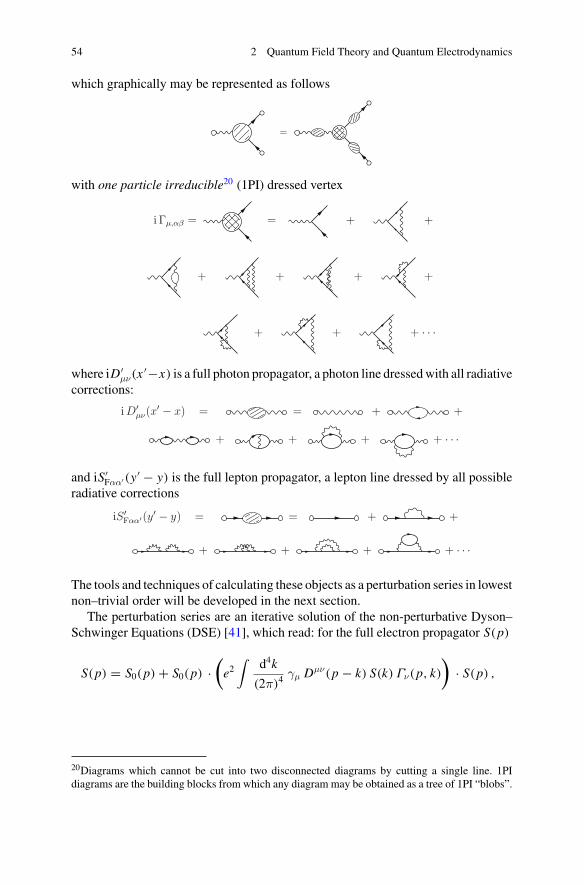
54 2 Quantum Field Theory and Quantum Electrodynamics

which graphically may be represented as follows

=

with one particle irreducible20 (1PI) dressed vertex

i Γμ,αβ = = + +

+ + + +

+ + + · · ·

where iD′μν(x ′−x) is a full photon propagator, a photon line dressedwith all radiative

corrections:

i D′μν(x

′ − x) = = + +

+ + + + · · ·

and iS′Fαα′(y′ − y) is the full lepton propagator, a lepton line dressed by all possibleradiative corrections

iS ′Fαα′(y′ − y) = = + +

+ + + + · · ·

The tools and techniques of calculating these objects as a perturbation series in lowestnon–trivial order will be developed in the next section.

The perturbation series are an iterative solution of the non-perturbative Dyson–Schwinger Equations (DSE) [41], which read: for the full electron propagator S(p)

S(p) = S0(p)+ S0(p) ·(

e2∫

d4k

(2π)4γμ Dμν(p − k) S(k) Γν(p, k)

)· S(p) ,

20Diagrams which cannot be cut into two disconnected diagrams by cutting a single line. 1PIdiagrams are the building blocks from which any diagram may be obtained as a tree of 1PI “blobs”.

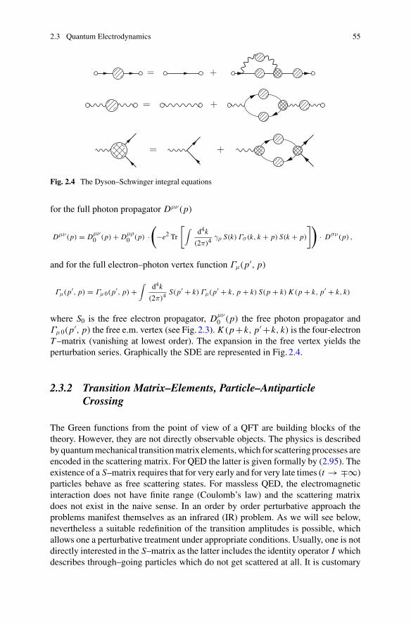
2.3 Quantum Electrodynamics 55

= +

= +

= +

Fig. 2.4 The Dyson–Schwinger integral equations

for the full photon propagator Dμν(p)

Dμν (p) = Dμν0 (p)+ Dμρ

0 (p) ·(

−e2 Tr

[∫d4k

(2π)4γρ S(k) Γσ(k, k + p) S(k + p)

])

· Dσν (p) ,

and for the full electron–photon vertex function Γμ(p′, p)

Γμ(p′, p) = Γμ 0(p′, p)+∫

d4k

(2π)4S(p′ + k) Γμ(p′ + k, p + k) S(p + k) K (p + k, p′ + k, k)

where S0 is the free electron propagator, Dμν0 (p) the free photon propagator and

Γμ 0(p′, p) the free e.m. vertex (see Fig. 2.3). K (p+k, p′ +k, k) is the four-electronT –matrix (vanishing at lowest order). The expansion in the free vertex yields theperturbation series. Graphically the SDE are represented in Fig. 2.4.

2.3.2 Transition Matrix–Elements, Particle–AntiparticleCrossing

The Green functions from the point of view of a QFT are building blocks of thetheory. However, they are not directly observable objects. The physics is describedbyquantummechanical transitionmatrix elements,which for scattering processes areencoded in the scattering matrix. For QED the latter is given formally by (2.95). Theexistence of a S–matrix requires that for very early and for very late times (t →∓∞)particles behave as free scattering states. For massless QED, the electromagneticinteraction does not have finite range (Coulomb’s law) and the scattering matrixdoes not exist in the naive sense. In an order by order perturbative approach theproblems manifest themselves as an infrared (IR) problem. As we will see below,nevertheless a suitable redefinition of the transition amplitudes is possible, whichallows one a perturbative treatment under appropriate conditions. Usually, one is notdirectly interested in the S–matrix as the latter includes the identity operator I whichdescribes through–going particles which do not get scattered at all. It is customary

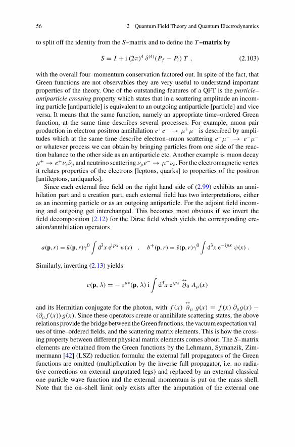
56 2 Quantum Field Theory and Quantum Electrodynamics

to split off the identity from the S–matrix and to define the T –matrix by

S = I + i (2π)4 δ(4)(Pf − Pi ) T , (2.103)

with the overall four–momentum conservation factored out. In spite of the fact, thatGreen functions are not observables they are very useful to understand importantproperties of the theory. One of the outstanding features of a QFT is the particle–antiparticle crossing property which states that in a scattering amplitude an incom-ing particle [antiparticle] is equivalent to an outgoing antiparticle [particle] and viceversa. It means that the same function, namely an appropriate time–ordered Greenfunction, at the same time describes several processes. For example, muon pairproduction in electron positron annihilation e+e− → μ+μ− is described by ampli-tudes which at the same time describe electron–muon scattering e−μ− → e−μ−or whatever process we can obtain by bringing particles from one side of the reac-tion balance to the other side as an antiparticle etc. Another example is muon decayμ+ → e+νeνμ and neutrino scattering νμe− → μ−νe. For the electromagnetic vertexit relates properties of the electrons [leptons, quarks] to properties of the positron[antileptons, antiquarks].

Since each external free field on the right hand side of (2.99) exhibits an anni-hilation part and a creation part, each external field has two interpretations, eitheras an incoming particle or as an outgoing antiparticle. For the adjoint field incom-ing and outgoing get interchanged. This becomes most obvious if we invert thefield decomposition (2.12) for the Dirac field which yields the corresponding cre-ation/annihilation operators

a(p, r) = u(p, r)γ0∫

d3x eipx ψ(x) , b+(p, r) = v(p, r)γ0∫

d3x e−ipx ψ(x) .

Similarly, inverting (2.13) yields

c(p,λ) = − εμ∗(p,λ) i∫

d3x eipx↔∂ 0 Aμ(x)

and its Hermitian conjugate for the photon, with f (x)↔∂μ g(x) ≡ f (x) ∂μg(x) −

(∂μ f (x)) g(x). Since these operators create or annihilate scattering states, the aboverelations provide the bridgebetween theGreen functions, the vacuumexpectationval-ues of time–ordered fields, and the scattering matrix elements. This is how the cross-ing property between different physical matrix elements comes about. The S–matrixelements are obtained from the Green functions by the Lehmann, Symanzik, Zim-mermann [42] (LSZ) reduction formula: the external full propagators of the Greenfunctions are omitted (multiplication by the inverse full propagator, i.e. no radia-tive corrections on external amputated legs) and replaced by an external classicalone particle wave function and the external momentum is put on the mass shell.Note that the on–shell limit only exists after the amputation of the external one

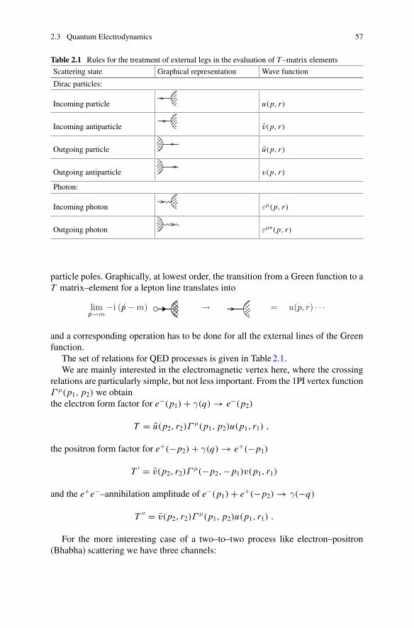
2.3 Quantum Electrodynamics 57

Table 2.1 Rules for the treatment of external legs in the evaluation of T –matrix elements

Scattering state Graphical representation Wave function

Dirac particles:

Incoming particle u(p, r)

Incoming antiparticle v(p, r)

Outgoing particle u(p, r)

Outgoing antiparticle v(p, r)

Photon:

Incoming photon εμ(p, r)

Outgoing photon εμ∗(p, r)

particle poles. Graphically, at lowest order, the transition from a Green function to aT matrix–element for a lepton line translates into

limp/→m

−i (p/ − m) → = u(p, r) · · ·

and a corresponding operation has to be done for all the external lines of the Greenfunction.

The set of relations for QED processes is given in Table2.1.We are mainly interested in the electromagnetic vertex here, where the crossing

relations are particularly simple, but not less important. From the 1PI vertex functionΓ μ(p1, p2) we obtainthe electron form factor for e−(p1)+ γ(q) → e−(p2)

T = u(p2, r2)Γμ(p1, p2)u(p1, r1) ,

the positron form factor for e+(−p2)+ γ(q) → e+(−p1)

T ′ = v(p2, r2)Γμ(−p2,−p1)v(p1, r1)

and the e+e−–annihilation amplitude of e−(p1)+ e+(−p2) → γ(−q)

T ′′ = v(p2, r2)Γμ(p1, p2)u(p1, r1) .

For the more interesting case of a two–to–two process like electron–positron(Bhabha) scattering we have three channels:

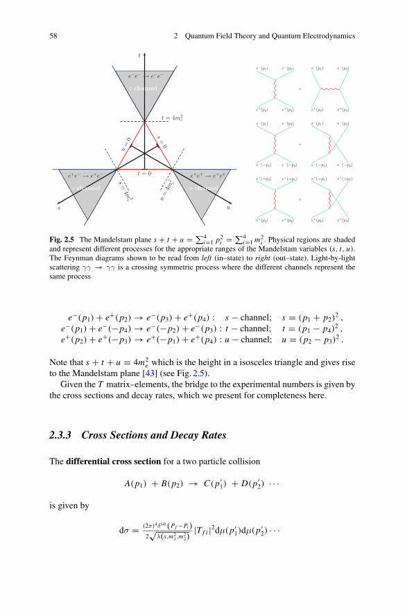
58 2 Quantum Field Theory and Quantum Electrodynamics

s=

0

s=

4m2e

e+e− → e+e−

s channel

s

e+e+ → e+e+

u channel

u

e−e− → e−e−

t channel

t

u=

0

u=

4m2 e

t = 0

t = 4m2e

e−(p1)

e+(p2)

e−(p3)

e+(p4)

+

e−(p1)

e+(p2)

e−(p3)

e+(p4)

e−(p1)

e−(−p4)

e−(p3)

e−(−p2)

+

e−(p1)

e−(−p4)

e−(p3)

e−(−p2)

e+(−p3)

e+(p2)

e+(−p1)

e+(p4)

+

e+(−p3)

e+(p2)

e+(−p1)

e+(p4)

Fig. 2.5 The Mandelstam plane s + t + u = ∑4i=1 p2i =

∑4i=1 m2

i . Physical regions are shadedand represent different processes for the appropriate ranges of the Mandelstam variables (s, t, u).The Feynman diagrams shown to be read from left (in–state) to right (out–state). Light-by-lightscattering γγ → γγ is a crossing symmetric process where the different channels represent thesame process

e−(p1)+ e+(p2) → e−(p3)+ e+(p4) : s − channel; s = (p1 + p2)2 ,

e−(p1)+ e−(−p4) → e−(−p2)+ e−(p3) : t − channel; t = (p1 − p4)2 ,

e+(p2)+ e+(−p3) → e+(−p1)+ e+(p4) : u − channel; u = (p2 − p3)2 .

Note that s + t + u = 4m2e which is the height in a isosceles triangle and gives rise

to the Mandelstam plane [43] (see Fig. 2.5).Given the T matrix–elements, the bridge to the experimental numbers is given by

the cross sections and decay rates, which we present for completeness here.

2.3.3 Cross Sections and Decay Rates

The differential cross section for a two particle collision

A(p1) + B(p2) → C(p′1) + D(p′2) · · ·

is given by

dσ = (2π)4δ(4)(Pf−Pi)2√

λ(s,m21,m

22)|T f i |2dμ(p′1)dμ(p′2) · · ·

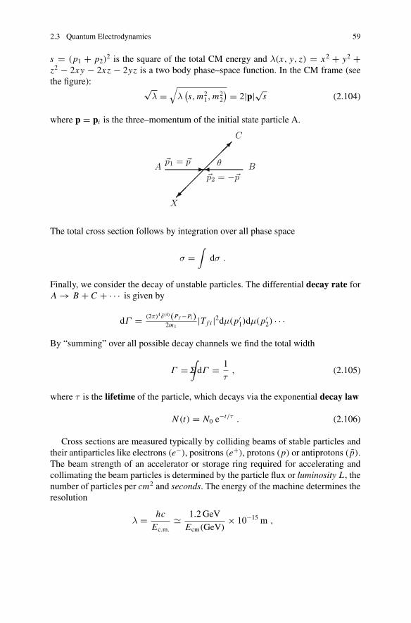
2.3 Quantum Electrodynamics 59

s = (p1 + p2)2 is the square of the total CM energy and λ(x, y, z) = x2 + y2 +

z2 − 2xy − 2xz − 2yz is a two body phase–space function. In the CM frame (seethe figure): √

λ =√

λ(s, m2

1, m22

) = 2|p|√s (2.104)

where p = pi is the three–momentum of the initial state particle A.

The total cross section follows by integration over all phase space

σ =∫

dσ .

Finally, we consider the decay of unstable particles. The differential decay rate forA → B + C + · · · is given by

dΓ = (2π)4δ(4)(Pf−Pi)2m1

|T f i |2dμ(p′1)dμ(p′2) · · ·

By “summing” over all possible decay channels we find the total width

Γ =∫ΣdΓ = 1

τ, (2.105)

where τ is the lifetime of the particle, which decays via the exponential decay law

N (t) = N0 e−t/τ . (2.106)

Cross sections are measured typically by colliding beams of stable particles andtheir antiparticles like electrons (e−), positrons (e+), protons (p) or antiprotons ( p).The beam strength of an accelerator or storage ring required for accelerating andcollimating the beam particles is determined by the particle flux or luminosity L , thenumber of particles per cm2 and seconds. The energy of the machine determines theresolution

λ = hc

Ec.m.

� 1.2GeV

Ecm(GeV)× 10−15 m ,

60 2 Quantum Field Theory and Quantum Electrodynamics

while the luminosity determines the collision rate

ΔN

Δt= L · σ ,

and the cross section σ is thus given by dividing the observed event rate by theluminosity

σ = 1

L

ΔN

Δt. (2.107)

2.4 Regularization and Renormalization

The vertex and self–energy functions, as well as all other Green functions, on thelevel of the bare theory are well defined order by order in perturbation theory onlyafter smoothing the short distance or ultraviolet (UV) divergences by appropriateregularization. Here we assume QED or the SM to be regularized by dimensionalregularization [39]. By going to lower dimensional space–times the features of thetheory, in particular the symmetries, remain the same, however, the convergence ofthe Feynman integrals gets improved. For a renormalizable theory, in principle, onecan always choose the dimension lowenough, d < 2, such that the integrals converge.By one or two partial integrations one can analytically continue the integrals in stepsfrom d to d + 1, such that the perturbation expansion is well defined for d = 4− εwith ε a small positive number. For ε → 0 (d → 4) the perturbative series in thefine structure constant α = e2/4π exhibits poles in ε:

A =N∑

n=0αn

n∑

m=0anm(1/ε)n−m

and the limit d → 4 to the real physical space–time does not exist, at first. Theproblems turn out to be related to the fact that the bare objects are not physicalones, they are not directly accessible to observation and require some adjustments.This in particular is the case for the bare parameters, the bare fine structure constant(electric charge) which is modified by vacuum polarization (quantum fluctuations),and the bare masses. Also the bare fields are not the ones which interpolate suitablyto the physical states they are assumed to describe. The appropriate entities are infact obtained by a simple reparametrization in terms of new parameters and fields,which is called renormalization.

2.4.1 The Structure of the Renormalization Procedure

Renormalization may be performed in three steps:

(i) Shift of the mass parameters or mass renormalization: replace the bare massparameters of the bare Lagrangian by renormalized ones

2.4 Regularization and Renormalization 61

m f 0 = m f ren + δm f for fermionsM2

b0 = M2bren + δM2

b for bosons(2.108)

(ii) Multiplicative renormalization of the bare fields or wave function renormaliza-tion: replace the bare fields in the bare Lagrangian by renormalized ones

ψ f 0 =√

Z f ψ f ren , Aμ0 =

√Zγ Aμ

ren (2.109)

and correspondingly for the other fields of the SM. To leading order Zi = 1 andhence

Zi = 1+ δZi ,√

Zi = 1+ 1

2δZi + · · · (2.110)

(iii) Vertex renormalization or coupling constant renormalization: substitute the barecoupling constant by the renormalized one

e0 = eren + δe . (2.111)

The renormalization theorem (see e.g. [1, 33, 38]) states that

Theorem 2.7 Order by order in the perturbation expansion all UV divergencesshowing up in physical quantities (S–matrix elements) get eliminated by an appro-priate choice of the counter terms δm f , δM2

b , δe and δZi = Zi − 1. Physicalamplitudes parametrized in terms of physical parameters thus are finite and free ofcutoff effects in the large cutoff limit.

In other words, suitably normalized physical amplitudes expressed in terms of mea-surable physical parameters are finite in the limit ε → 0, i.e., they allow us to takeaway the regularization (cut–off Λ → ∞ if a UV cut–off was used to regularizethe bare theory). Note that for Green functions, which are not gauge invariant ingeneral, also the fictitious gauge parameter has to be renormalized in order to obtainfinite Green functions. Unitarity requires the counter terms to be real. Therefore thecounter terms are determined by the real parts of the location and residues of theone particle poles. Also note: the Z-factors are gauge dependent and in order to getgauge invariant S-matrix elements there is no freedom in the choice of the wavefunction renormalization factors. Only the Z-factors fixed by the LSZ-conditions forthe individual fields lead to the physical S-matrix [38, 44]. In fact bare on–shellmatrix–elements are not gauge invariant, they become gauge invariant only afterwave-function renormalization normalized by the LSZ conditions.

The reparametrization of the bare Lagrangian (2.90) in terms of renormalizedquantities reads

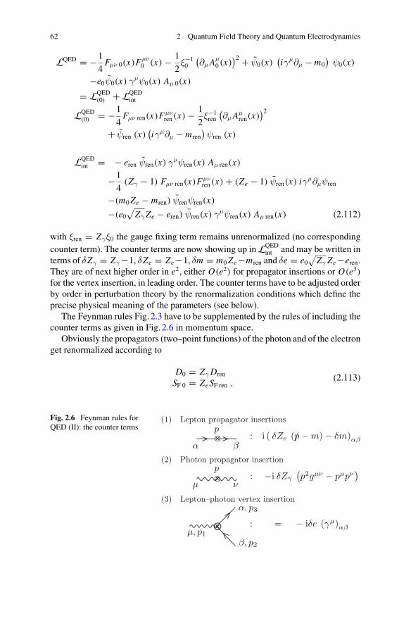
62 2 Quantum Field Theory and Quantum Electrodynamics

LQED = −1

4Fμν 0(x)Fμν

0 (x)− 1

2ξ−10

(∂μ Aμ

0 (x))2 + ψ0(x)

(iγμ∂μ − m0

)ψ0(x)

−e0ψ0(x) γμψ0(x) Aμ 0(x)

= LQED(0) +LQED

int

LQED(0) = −1

4Fμν ren(x)Fμν

ren(x)− 1

2ξ−1ren

(∂μ Aμ

ren(x))2

+ ψren (x)(iγμ∂μ − mren

)ψren (x)

LQEDint = − eren ψren(x) γμψren(x) Aμ ren(x)

−1

4(Zγ − 1) Fμν ren(x)Fμν

ren(x)+ (Ze − 1) ψren(x) iγμ∂μψren

−(m0Ze − mren) ψrenψren(x)

−(e0√

Zγ Ze − eren) ψren(x) γμψren(x) Aμ ren(x) (2.112)

with ξren = Zγξ0 the gauge fixing term remains unrenormalized (no correspondingcounter term). The counter terms are now showing up inLQED

int and may be written interms of δZγ = Zγ−1, δZe = Ze−1, δm = m0Ze−mren and δe = e0

√Zγ Ze−eren.

They are of next higher order in e2, either O(e2) for propagator insertions or O(e3)for the vertex insertion, in leading order. The counter terms have to be adjusted orderby order in perturbation theory by the renormalization conditions which define theprecise physical meaning of the parameters (see below).

The Feynman rules Fig. 2.3 have to be supplemented by the rules of including thecounter terms as given in Fig. 2.6 in momentum space.

Obviously the propagators (two–point functions) of the photon and of the electronget renormalized according to

D0 = Zγ Dren

SF 0 = Ze SF ren .(2.113)

Fig. 2.6 Feynman rules forQED (II): the counter terms

(1) Lepton propagator insertions

⊗ : i ( δZe (p/ − m) − δm)αβ

(2) Photon propagator insertion

⊗ : −i δZγ p2gμν − pμpν)

(3) Lepton–photon vertex insertion

⊗ : = − iδe (γμ)αβ

p

α β

p

μ ν

μ, p1

α, p3

β, p2

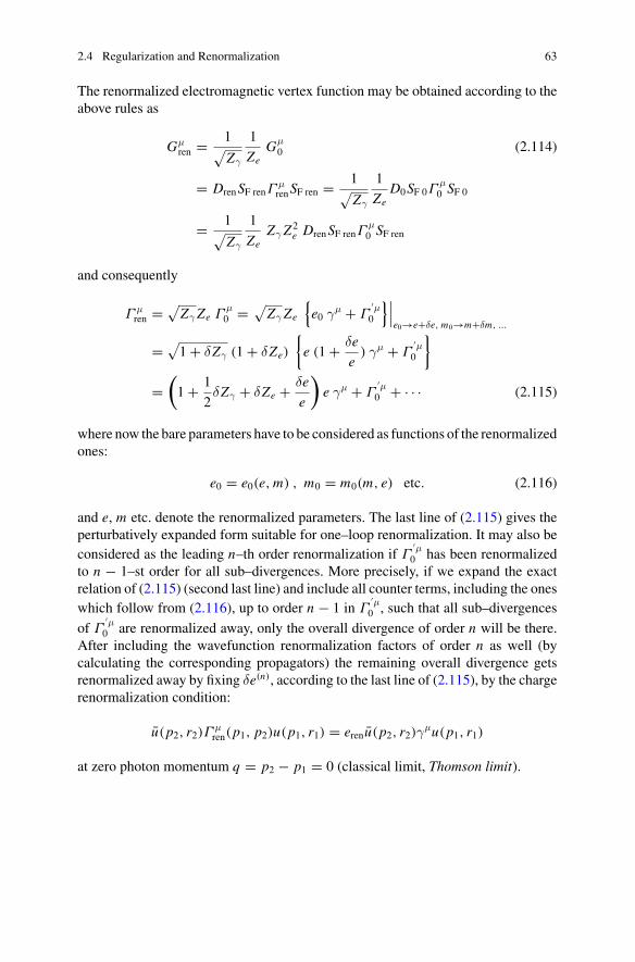
2.4 Regularization and Renormalization 63

The renormalized electromagnetic vertex function may be obtained according to theabove rules as

Gμren =

1√

Zγ

1

ZeGμ

0 (2.114)

= DrenSF renΓμrenSF ren = 1

√Zγ

1

ZeD0SF 0Γ

μ0 SF 0

= 1√

Zγ

1

ZeZγ Z2

e DrenSF renΓμ0 SF ren

and consequently

Γ μren =

√Zγ Ze Γ

μ0 =

√Zγ Ze

{e0 γμ + Γ

′μ0

}∣∣∣e0→e+δe, m0→m+δm, ...

= √1+ δZγ (1+ δZe)

{e (1+ δe

e) γμ + Γ

′μ0

}

=(1+ 1

2δZγ + δZe + δe

e

)e γμ + Γ

′μ0 + · · · (2.115)

where now the bare parameters have to be considered as functions of the renormalizedones:

e0 = e0(e, m) , m0 = m0(m, e) etc. (2.116)

and e, m etc. denote the renormalized parameters. The last line of (2.115) gives theperturbatively expanded form suitable for one–loop renormalization. It may also beconsidered as the leading n–th order renormalization if Γ

′μ0 has been renormalized

to n − 1–st order for all sub–divergences. More precisely, if we expand the exactrelation of (2.115) (second last line) and include all counter terms, including the oneswhich follow from (2.116), up to order n − 1 in Γ

′μ0 , such that all sub–divergences

of Γ′μ0 are renormalized away, only the overall divergence of order n will be there.

After including the wavefunction renormalization factors of order n as well (bycalculating the corresponding propagators) the remaining overall divergence getsrenormalized away by fixing δe(n), according to the last line of (2.115), by the chargerenormalization condition:

u(p2, r2)Γμren(p1, p2)u(p1, r1) = erenu(p2, r2)γ

μu(p1, r1)

at zero photon momentum q = p2 − p1 = 0 (classical limit, Thomson limit).

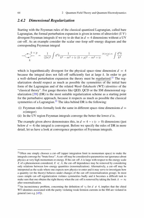
64 2 Quantum Field Theory and Quantum Electrodynamics

2.4.2 Dimensional Regularization

Starting with the Feynman rules of the classical quantized Lagrangian, called bareLagrangian, the formal perturbation expansion is given in terms of ultraviolet (U V )

divergent Feynman integrals if we try to do that in d = 4 dimensions without a UVcut–off. As an example consider the scalar one–loop self–energy diagram and thecorresponding Feynman integral

=1

(2π)d

∫ddk

1k2 − m2 + iε

1(k + p)2 − m2 + iε

|k|�|p|,m∼∫

ddk

k4

k

k + p

which is logarithmically divergent for the physical space–time dimension d = 4because the integral does not fall–off sufficiently fast at large k. In order to geta well–defined perturbation expansion the theory must be regularized.21 The reg-ularization should respect as much as possible the symmetries of the initial bareform of the Lagrangian and of the related Ward–Takahashi (WT) identities of the“classical theory”. For gauge theories like QED, QCD or the SM dimensional reg-ularization [39] (DR) is the most suitable regularization scheme as a starting pointfor the perturbative approach, because it respects as much as possible the classicalsymmetries of a Lagrangian.22 The idea behind DR is the following:

(i) Feynman rules formally look the same in different space–time dimensions d =n(integer)

(ii) In the UV region Feynman integrals converge the better the lower d is.

The example given above demonstrates this, in d = 4 − ε (ε > 0) dimensions (justbelow d = 4) the integral is convergent. Before we specify the rules of DR in moredetail, let us have a look at convergence properties of Feynman integrals.

21Often one simply chooses a cut–off (upper integration limit in momentum space) to make theintegrals converge by “brute force”. A cut–offmay be considered to parametrize our ignorance aboutphysics at very high momentum or energy. If the cut–off Λ is large with respect to the energy scaleE of a phenomenon considered, E � Λ, the cut–off dependence may be removed by consideringonly relations between low–energy quantities (renormalization). Alternatively, a cut–off may beinterpreted as the scale where one expects new physics to enter and it may serve to investigate howa quantity (or the theory) behaves under changes of the cut–off (renormalization group). In mostcases simple cut–off regularization violates symmetries badly and it becomes a difficult task tomake sure that one obtains the right theory when the cut–off is removed by taking the limitΛ →∞after renormalization.22An inconsistency problem, concerning the definition of γ5 for d �= 4, implies that the chiralWT identities associated with the parity violating weak fermion currents in the SM are violated ingeneral (see e.g. [45]).

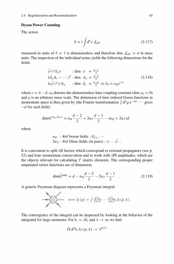
2.4 Regularization and Renormalization 65

Dyson Power Counting

The action

S = i∫dd x Leff (2.117)

measured in units of � = 1 is dimensionless and therefore dim Leff = d in massunits. The inspection of the individual terms yields the following dimensions for thefields:

ψγμ∂μψ : dim ψ = d−12

(∂μ Aν − · · · )2 : dim Aμ = d−22

e0ψγμψAμ : dim e0 = 4−d2 ⇒ e0 = e0με/2

(2.118)

where ε = 4− d, e0 denotes the dimensionless bare coupling constant (dim e0 = 0)and μ is an arbitrary mass scale. The dimension of time ordered Green functions inmomentum space is then given by (the Fourier transformation

∫ddq e−iqx · · · gives

−d for each field):

dimG(nB ,2nF ) = nBd − 2

2+ 2nF

d − 1

2− (nB + 2nF )d

where

nB : #of boson fields : Giμ, · · ·2nF : #of Dirac fields (in pairs) : ψ · · · ψ .

It is convenient to split off factors which correspond to external propagators (see p.52) and four–momentum conservation and to work with 1PI amplitudes, which arethe objects relevant for calculating T matrix elements. The corresponding properamputated vertex functions are of dimension

dimGamp = d − nBd − 2

2− 2nF

d − 1

2. (2.119)

A generic Feynman diagram represents a Feynman integral

⇐⇒ IΓ(p) =∫ ddk1

(2π)d · · · ddkm

(2π)d JΓ(p, k) .

The convergence of the integral can be inspected by looking at the behavior of theintegrand for large momenta: For ki = λki and λ →∞ we find

Πiddki JΓ (p, k) → λd(Γ )

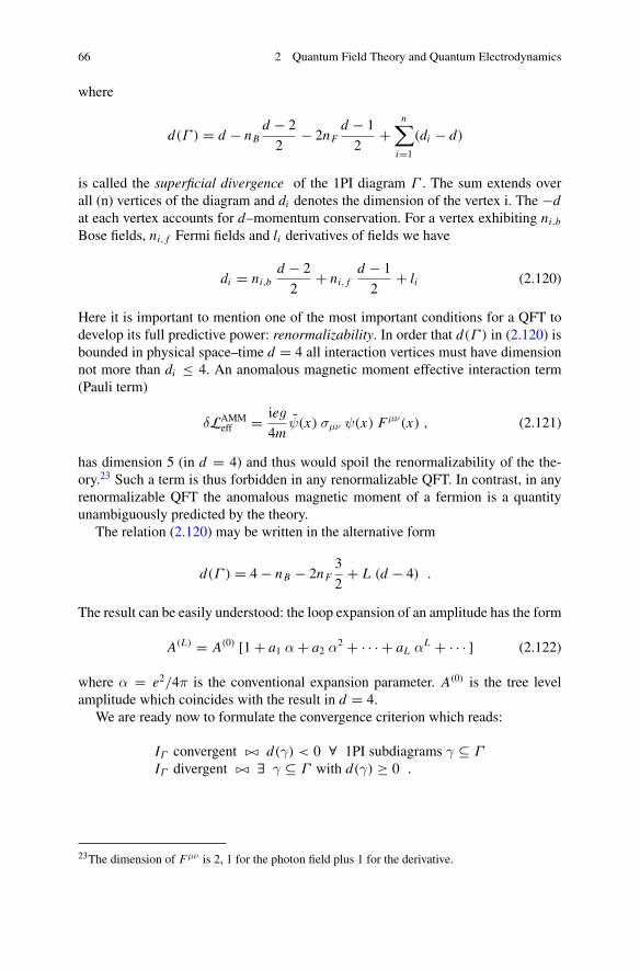
66 2 Quantum Field Theory and Quantum Electrodynamics

where

d(Γ ) = d − nBd − 2

2− 2nF

d − 1

2+

n∑

i=1(di − d)

is called the superficial divergence of the 1PI diagram Γ . The sum extends overall (n) vertices of the diagram and di denotes the dimension of the vertex i. The −dat each vertex accounts for d–momentum conservation. For a vertex exhibiting ni,b

Bose fields, ni, f Fermi fields and li derivatives of fields we have

di = ni,bd − 2

2+ ni, f

d − 1

2+ li (2.120)

Here it is important to mention one of the most important conditions for a QFT todevelop its full predictive power: renormalizability. In order that d(Γ ) in (2.120) isbounded in physical space–time d = 4 all interaction vertices must have dimensionnot more than di ≤ 4. An anomalous magnetic moment effective interaction term(Pauli term)

δLAMMeff = ieg

4mψ(x) σμν ψ(x) Fμν(x) , (2.121)

has dimension 5 (in d = 4) and thus would spoil the renormalizability of the the-ory.23 Such a term is thus forbidden in any renormalizable QFT. In contrast, in anyrenormalizable QFT the anomalous magnetic moment of a fermion is a quantityunambiguously predicted by the theory.

The relation (2.120) may be written in the alternative form

d(Γ ) = 4− nB − 2nF3

2+ L (d − 4) .

The result can be easily understood: the loop expansion of an amplitude has the form

A(L) = A(0) [1+ a1 α+ a2 α2 + · · · + aL αL + · · · ] (2.122)

where α = e2/4π is the conventional expansion parameter. A(0) is the tree levelamplitude which coincides with the result in d = 4.

We are ready now to formulate the convergence criterion which reads:

IΓ convergent �� d(γ) < 0 ∀ 1PI subdiagrams γ ⊆ Γ

IΓ divergent �� ∃ γ ⊆ Γ with d(γ) ≥ 0 .

23The dimension of Fμν is 2, 1 for the photon field plus 1 for the derivative.

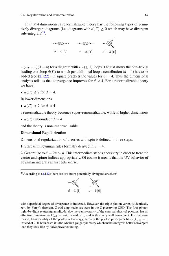
2.4 Regularization and Renormalization 67

In d ≤ 4 dimensions, a renormalizable theory has the following types of primi-tively divergent diagrams (i.e., diagrams with d(Γ ) ≥ 0 which may have divergentsub–integrals)24:

d − 2 [2] d − 3 [1] d − 4 [0]

+(LΓ −1)(d − 4) for a diagram with LΓ (≥ 1) loops. The list shows the non–trivialleading one–loop d(Γ ) to which per additional loop a contribution (d − 4) has to beadded (see (2.122)), in square brackets the values for d = 4. Thus the dimensionalanalysis tells us that convergence improves for d < 4. For a renormalizable theorywe have

• d(Γ ) ≤ 2 for d = 4.

In lower dimensions

• d(Γ ) < 2 for d < 4

a renormalizable theory becomes super–renormalizable, while in higher dimensions

• d(Γ ) unbounded! d > 4

and the theory is non–renormalizable.

Dimensional Regularization

Dimensional regularization of theories with spin is defined in three steps.

1. Start with Feynman rules formally derived in d = 4.

2. Generalize to d = 2n > 4. This intermediate step is necessary in order to treat thevector and spinor indices appropriately. Of course it means that the UV behavior ofFeynman integrals at first gets worse.

24According to (2.122) there are two more potentially divergent structures

d − 3 [1] d − 4 [0]

with superficial degree of divergence as indicated. However, the triple photon vertex is identicallyzero by Furry’s theorem, C odd amplitudes are zero in the C preserving QED. The four photonlight–by–light scattering amplitude, due the transversality of the external physical photons, has aneffective dimension d(Γ )eff = −4, instead of 0, and is thus very well convergent. For the samereason, transversality of the photon self–energy, actually the photon propagator has d(Γ )eff = 0instead of 2. In both cases it is the Abelian gauge symmetry whichmakes integrals better convergentthan they look like by naive power counting.

68 2 Quantum Field Theory and Quantum Electrodynamics

(1) For fermions we need the d = 2n–dimensional Dirac algebra:

{γμ, γν} = 2gμν1 ; {γμ, γ5} = 0 (2.123)

where γ5 must satisfy γ25 = 1 and γ+5 = γ5 such that 1

2 (1 ± γ5) are the chiralprojection matrices. The metric has dimension d

gμνgμν = gμμ = d ; gμν =

⎛

⎜⎜⎜⎝

1 0 · · ·0 −1...

. . .

−1

⎞

⎟⎟⎟⎠

.

By 1 we denote the unit matrix in spinor space. In order to have the usual relationfor the adjoint spinors we furthermore require

γμ+ = γ0γμγ0 . (2.124)

Simple consequences of this d–dimensional algebra are:

γαγα = d 1

γαγμγα = (2− d) γμ

γαγμγνγα = 4gμν 1+ (d − 4) γμγν

γαγμγνγργα = −2γργνγμ + (4− d)γμγνγρ etc.

(2.125)

Traces of strings of γ–matrices are very similar to the ones in 4–dimensions. Ind = 2n dimensions one can easily write down 2d/2–dimensional representations ofthe Dirac algebra [46]. Then

Tr 1 = f (d) = 2d/2

Tr∏2n−1

i=1 γμi (γ5) = 0

Tr γμγν = f (d) gμν

Tr γμγνγργσ = f (d) (gμνgρσ − gμρgνσ + gμσgνρ) etc.

(2.126)

One can show that for renormalized quantities the only relevant property of f (d) isf (d) → 4 for d → 4. Very often the convention f (d) = 4 (for any d) is adopted.Bare quantities and the related minimally subtracted MS or modified minimallysubtracted MS quantities (see below for the precise definition) depend upon thisconvention (by terms proportional to ln 2).

In anomaly free theories we can assume γ5 to be fully anticommuting! But then

Tr γμγνγργσγ5 = 0 for all d �= 4! (2.127)

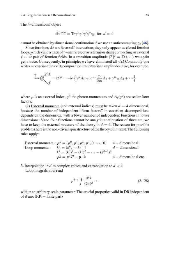
2.4 Regularization and Renormalization 69

The 4–dimensional object

4iεμνρσ = Tr γμγνγργσγ5 for d = 4

cannot be obtained by dimensional continuation if we use an anticommuting γ5 [46].Since fermions do not have self interactions they only appear as closed fermion

loops, which yield a trace of γ–matrices, or as a fermion string connecting an externalψ · · · ψ pair of fermion fields. In a transition amplitude |T |2 = Tr (· · · ) we againget a trace. Consequently, in principle, we have eliminated all γ’s! Commonly onewrites a covariant tensor decomposition into invariant amplitudes, like, for example,

= iΓ μ = −ie{γμA1 + iσμν qν

2mA2 + γμγ5A3 + · · ·

}f

f

γ

where μ is an external index, qμ the photon momentum and Ai (q2) are scalar formfactors.

(2) External momenta (and external indices) must be taken d = 4 dimensional,because the number of independent “form factors” in covariant decompositionsdepends on the dimension, with a fewer number of independent functions in lowerdimensions. Since four functions cannot be analytic continuation of three etc. wehave to keep the external structure of the theory in d = 4. The reason for possibleproblems here is the non–trivial spin structure of the theory of interest. The followingrules apply:

External momenta : pμ = (p0, p1, p2, p3, 0, · · · , 0) 4− dimensionalLoop momenta : kμ = (k0, · · · kd−1) d − dimensional

k2 = (k0)2 − (k1)2 − · · · − (kd−1)2pk = p0k0 − p · k 4− dimensional etc.

3. Interpolation in d to complex values and extrapolation to d < 4.Loop integrals now read

μ4−d∫

ddk

(2π)d· · · (2.128)

with μ an arbitrary scale parameter. The crucial properties valid in DR independentof d are: (F.P. = finite part)

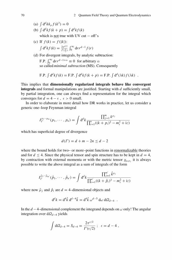
70 2 Quantum Field Theory and Quantum Electrodynamics

(a)∫ddkkμ f (k2) = 0

(b)∫ddk f (k + p) = ∫

ddk f (k)

which is not true with UV cut − off’s

(c) If f (k) = f (|k|):∫ddk f (k) = 2πd/2

Γ ( d2 )

∫∞0 drrd−1 f (r)

(d) For divergent integrals, by analytic subtraction:

F.P.∫∞0 drrd−1+α ≡ 0 for arbitrary α

so calledminimal subtraction (MS). Consequently

F.P.∫ddk f (k) = F.P.

∫ddk f (k + p) = F.P.

∫dd(λk) f (λk) .

This implies that dimensionally regularized integrals behave like convergentintegrals and formal manipulations are justified. Starting with d sufficiently small,by partial integration, one can always find a representation for the integral whichconverges for d = 4− ε , ε > 0 small.

In order to elaborate in more detail how DR works in practice, let us consider ageneric one–loop Feynman integral

I μ1···μmΓ (p1, · · · , pn) =

∫ddk

∏mj=1 kμ j

∏ni=1((k + pi )2 − m2

i + iε)

which has superficial degree of divergence

d(Γ ) = d + m − 2n ≤ d − 2

where the bound holds for two– or more–point functions in renormalizable theoriesand for d ≤ 4. Since the physical tensor and spin structure has to be kept in d = 4,by contraction with external momenta or with the metric tensor gμi μ j it is alwayspossible to write the above integral as a sum of integrals of the form

I μ1···μm′Γ ( p1, · · · , pn′) =

∫ddk

∏m ′j=1 kμ j

∏n′i=1((k + pi )2 − m2

i + iε)

where now μ j and pi are d = 4–dimensional objects and

ddk = d4k dd−4k = d4k ωd−5 dω dΩd−4 .

In the d−4–dimensional complement the integrand depends on ω only! The angularintegration over dΩd−4 yields

∫dΩd−4 = Sd−4 = 2πε/2

Γ (ε/2); ε = d − 4 ,

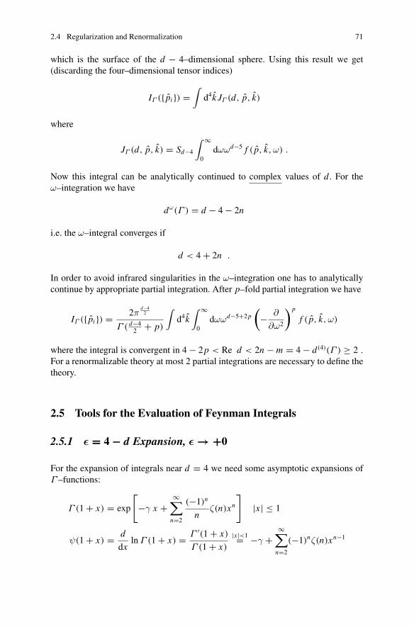
2.4 Regularization and Renormalization 71

which is the surface of the d − 4–dimensional sphere. Using this result we get(discarding the four–dimensional tensor indices)

IΓ ({ pi }) =∫

d4k JΓ (d, p, k)

where

JΓ (d, p, k) = Sd−4∫ ∞

0dωωd−5 f ( p, k,ω) .

Now this integral can be analytically continued to complex values of d. For theω–integration we have

dω(Γ ) = d − 4− 2n

i.e. the ω–integral converges if

d < 4+ 2n .

In order to avoid infrared singularities in the ω–integration one has to analyticallycontinue by appropriate partial integration. After p–fold partial integration we have

IΓ ({ pi }) = 2πd−42

Γ ( d−42 + p)

∫d4k

∫ ∞

0dωωd−5+2p

(− ∂

∂ω2

)p

f ( p, k,ω)

where the integral is convergent in 4− 2p < Re d < 2n − m = 4− d(4)(Γ ) ≥ 2 .

For a renormalizable theory at most 2 partial integrations are necessary to define thetheory.

2.5 Tools for the Evaluation of Feynman Integrals

2.5.1 ε = 4 − d Expansion, ε → +0

For the expansion of integrals near d = 4 we need some asymptotic expansions ofΓ –functions:

Γ (1+ x) = exp

[

−γ x +∞∑

n=2

(−1)n

nζ(n)xn

]

|x | ≤ 1

ψ(1+ x) = d

dxlnΓ (1+ x) = Γ ′(1+ x)

Γ (1+ x)

|x |<1= −γ +∞∑

n=2(−1)nζ(n)xn−1

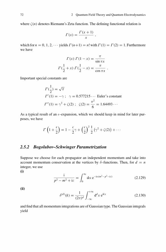
72 2 Quantum Field Theory and Quantum Electrodynamics

where ζ(n) denotes Riemann’s Zeta function. The defining functional relation is

Γ (x) = Γ (x + 1)

x,

which for n = 0, 1, 2, · · · yieldsΓ (n+1) = n!withΓ (1) = Γ (2) = 1. Furthermorewe have

Γ (x) Γ (1− x) = π

sin πx

Γ (1

2+ x) Γ (

1

2− x) = π

cosπx.

Important special constants are

Γ (1

2) = √π

Γ ′(1) = −γ ; γ = 0.577215 · · · Euler’s constantΓ ′′(1) = γ2 + ζ(2) ; ζ(2) = π2

6= 1.64493 · · ·

As a typical result of an ε–expansion, which we should keep in mind for later pur-poses, we have

Γ(1+ ε

2

)= 1− ε

2γ +

( ε

2

)2 12

(γ2 + ζ(2)

)+ · · ·

2.5.2 Bogolubov–Schwinger Parametrization

Suppose we choose for each propagator an independent momentum and take intoaccount momentum conservation at the vertices by δ–functions. Then, for d = ninteger, we use(i)

i

p2 − m2 + iε=∫ ∞

0dα e−iα(m2−p2−iε) (2.129)

(ii)

δ(d)(k) = 1

(2π)d

∫ +∞

−∞dd x eikx (2.130)

and find that all momentum integrations are of Gaussian type. The Gaussian integralsyield

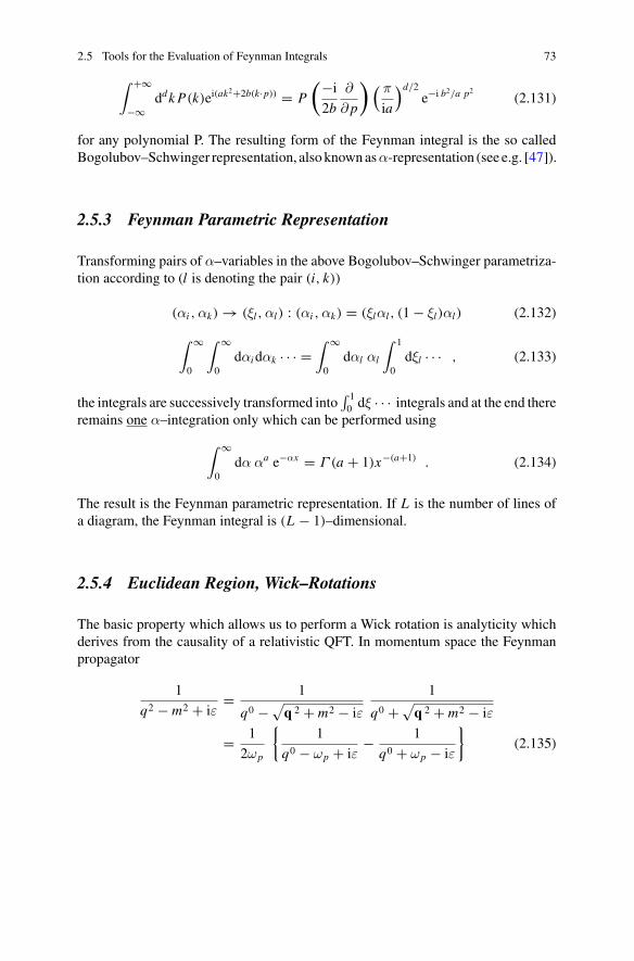
2.5 Tools for the Evaluation of Feynman Integrals 73

∫ +∞

−∞ddk P(k)ei(ak2+2b(k·p)) = P

(−i2b

∂

∂ p

)( π

ia

)d/2e−i b2/a p2

(2.131)

for any polynomial P. The resulting form of the Feynman integral is the so calledBogolubov–Schwinger representation, alsoknownasα-representation (see e.g. [47]).

2.5.3 Feynman Parametric Representation

Transforming pairs of α–variables in the above Bogolubov–Schwinger parametriza-tion according to (l is denoting the pair (i, k))

(αi ,αk) → (ξl,αl) : (αi ,αk) = (ξlαl, (1− ξl)αl) (2.132)

∫ ∞

0

∫ ∞

0dαidαk · · · =

∫ ∞

0dαl αl

∫ 1

0dξl · · · , (2.133)

the integrals are successively transformed into∫ 10 dξ · · · integrals and at the end there

remains one α–integration only which can be performed using

∫ ∞

0dα αa e−αx = Γ (a + 1)x−(a+1) . (2.134)

The result is the Feynman parametric representation. If L is the number of lines ofa diagram, the Feynman integral is (L − 1)–dimensional.

2.5.4 Euclidean Region, Wick–Rotations

The basic property which allows us to perform a Wick rotation is analyticity whichderives from the causality of a relativistic QFT. In momentum space the Feynmanpropagator

1

q2 − m2 + iε= 1

q0 −√q 2 + m2 − iε

1

q0 +√q 2 + m2 − iε

= 1

2ωp

{1

q0 − ωp + iε− 1

q0 + ωp − iε

}(2.135)

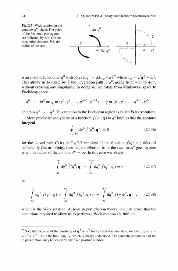
74 2 Quantum Field Theory and Quantum Electrodynamics

Fig. 2.7 Wick rotation in thecomplex q0–plane. The polesof the Feynman propagatorare indicated by ⊗’s. C is anintegration contour, R is theradius of the arcs

⊗

⊗

⊗

⊗

Im q0

Re q0

C

R

is an analytic function in q0 with poles at q0 = ±(ωp−iε)25 whereωp =√

q 2 + m2.This allows us to rotate by π

2 the integration path in q0, going from −∞ to +∞,without crossing any singularity. In doing so, we rotate from Minkowski space toEuclidean space

q0 →−iqd ⇒ q = (q0, q1, . . . , qd−2, qd−1) → q = (q1, q2, . . . , qd−1, qd)

and thus q2 →−q2. This rotation to the Euclidean region is called Wick rotation.

More precisely: analyticity of a function f (q0, q ) in q0 implies that the contourintegral ∮

C(R)

dq0 f (q0, q ) = 0 (2.136)

for the closed path C(R) in Fig. 2.7 vanishes. If the function f (q0, q ) falls offsufficiently fast at infinity, then the contribution from the two “arcs” goes to zerowhen the radius of the contour R →∞. In this case we obtain

∞∫

−∞dq0 f (q0, q )+

−i∞∫

+i∞dq0 f (q0, q ) = 0 (2.137)

or

∞∫

−∞dq0 f (q0, q ) =

+i∞∫

−i∞dq0 f (q0, q ) = −i

+∞∫

−∞dqd f (−iqd , q ) , (2.138)

which is the Wick rotation. At least in perturbation theory, one can prove that theconditions required to allow us to perform a Wick rotation are fulfilled.

25Note that because of the positivity of q 2 + m2 for any non–vacuum state, we have ωp − iε =√q 2 + m2 − iε in the limit limε→0, which is always understood. The symbolic parameter ε of the

iε prescription, may be scaled by any fixed positive number.

2.5 Tools for the Evaluation of Feynman Integrals 75

We notice that the Euclidean Feynman propagator obtained by the Wick rotation

1

q2 − m2 + iε→− 1

q2 + m2

has no singularities (poles) and an iε–prescription is not needed any longer.In configuration space a Wick rotation implies going to imaginary time x0 →

ix0 = xd such that qx →−qx and hence

x0 →−ixd ⇒ x2 →−x2 , �x →−Δx , i∫

dd x · · · →∫

dd x · · · .

While inMinkowski space x2 = 0 defines the light–cone x0 = ±|x|, in the Euclideanregion x2 = 0 implies x = 0. Note that possible singularities on the light–cone like1/x2, δ(x2) etc. turn into singularities at the point x = 0. This simplification of thesingularity structure is the merit of the positive definite metric in Euclidean space.

Inmomentum space the Euclidean propagators are positive (discarding the overallsign) and any Feynman amplitude in Minkowski space may be obtained via

IM(p) = (−i)Nint (−i)V−1 IE (p)∣∣

p4=ip0 ; m2→m2−iε

from its Euclidean version. Here, Nint denotes the number of internal lines (propaga-tors) and V the number of vertices if we use the substitutions (convention dependent)

1

p2 − m2 + iε→ 1

p2 + m2; igi → i (igi ) = −gi ;

∫ddk →

∫ddk

to define the Euclidean Feynman amplitudes. By gi we denote the gauge couplings.For the dimensionally regularized amplitudes, where potentially divergent inte-

grals are defined via analytic continuation from regions in the complex d–planewhere integrals are manifestly convergent, the terms from the arc segments canalways be dropped. Also note that dimensional regularization and the power count-ing rules (superficial degree of divergence etc.) hold irrespective of whether we workin d–dimensional Minkowski space–time or in d–dimensional Euclidean space. Themetric is obviously not important for the UV–behavior of the integrals.

The relationship between Euclidean and Minkowski quantum field theory is notonly a very basic and surprising general feature of any local relativistic field theorybut is a property of central practical importance for the non–perturbative approachto QFT via the Euclidean path–integral (e.g., lattice QCD). In a QFT satisfyingthe Wightman axioms the continuation of the vacuum–expectation values of time–ordered products of local fields (the time–ordered Green functions) fromMinkowskispace to four–dimensional Euclidean space is always possible [11]. Conversely, theOsterwalder–Schrader theorem [48] ascertains that

76 2 Quantum Field Theory and Quantum Electrodynamics

Theorem 2.8 In a local relativistic QFT the time–ordered Green functions exhibitan analytic continuation to Euclidean space. Vice versa, the Euclidean correlationfunctions of an Euclidean QFT can be analytically continued to Minkowski space,provided we have a local action which satisfies the so–called reflection positivitycondition.

Accordingly, the full Minkowski QFT including its S–matrix, if it exists, can bereconstructed from the knowledge of the Euclidean correlation functions and from amathematical point of view the Minkowski and the Euclidean version of a QFT arecompletely equivalent.

2.5.5 The Origin of Analyticity

At the heart of analyticity is the causality. The time ordered Green functions whichencode all information of the theory in perturbation theory are given by integralsover products of causal propagators (z = x − y)

iSF(z) = 〈0|T{ψ(x)ψ(y)

} |0〉= Θ(x0 − y0)〈0|ψ(x)ψ(y)|0〉 −Θ(y0 − x0)〈0|ψ(y)ψ(x)|0〉= Θ(z0) iS+(z)+Θ(−z0) iS−(z) (2.139)

exhibiting a positive frequency part propagating forward in time and a negativefrequency part propagating backward in time. TheΘ function of time orderingmakesthe Fourier–transform to be analytic in a half–plane in momentum space. For K (τ =z0) = Θ(z0)iS+(z), for example, we have

K (ω) =+∞∫

−∞dτ K (τ ) eiωτ =

+∞∫

0

dτ K (τ ) e−ητeiξτ (2.140)

such that K (ω = ξ + iη) is a regular analytic function in the upper half ω–planeη > 0. This of course only works because τ is restricted to be positive.

In a relativistically covariant world, in fact, we always need two terms (see(2.139)), a positive frequency partΘ(z0 = t−t ′)S+(z), corresponding to the particlepropagating forward in time, and a negative frequency part Θ(−z0 = t ′ − t) S−(z),corresponding to the antiparticle propagating backward in time. The two terms cor-respond in momentum space to the two terms of (2.135).

Of course, for a free Dirac field we know what the Stückelberg-Feynman propa-gator in momentum space looks like

SF(q) = �q + m

q2 − m2 + iε

2.5 Tools for the Evaluation of Feynman Integrals 77

and its analytic properties are manifest. It is an analytic function in q0 with poles atq0 = ±( ωp − iε) where ωp =

√q 2 + m2.

Analyticity is an extremely important basic property of a QFT and a powerfulinstrument which helps to solve seemingly purely “technical” problems as we willsee. For example it allows us to perform a Wick rotation to Euclidean space and inEuclidean space a QFT looks like a classical statistical system and one can applythe methods of statistical physics to QFT [49]. In particular the numerical approachto the intrinsically non–perturbative QCD via lattice QCD is based on analyticity.The objects which manifestly exhibit the analyticity properties and are providing thebridge to the Euclidean world are the time ordered Green functions.

Note that by far not all objects of interest in a QFT are analytic. For example, anysolution of the homogeneous (no source) Klein–Gordon equation

( �x + m2 ) Δ(x − y;m2) = 0 ,

like the so called positive frequency part Δ+ or the causal commutator Δ of a freescalar field ϕ(x), defined by

< 0|ϕ(x),ϕ(y)|0 > = i Δ+(x − y;m2)

[ϕ(x),ϕ(y)] = i Δ(x − y;m2) ,

which, given the properties of the free field, may easily be evaluated to have arepresentation

Δ+(z;m2) = −i (2π)−3∫

d4 p Θ(p0) δ(p2 − m2) e−ipz

Δ(z;m2) = −i (2π)−3∫

d4 p ε(p0) δ(p2 − m2) e−ipz .

Thus, in momentum space, as solutions of

(p2 − m2) Δ(p) = 0 ,

only singular ones exist. For the positive frequency part and the causal commutatorthey read

Θ(p0) δ(p2 − m2) and ε(p0) δ(p2 − m2) ,

respectively. The Feynman propagator, in contrast, satisfies an inhomogeneous (withpoint source) Klein–Gordon equation

( �x + m2 ) ΔF (x − y;m2) = −δ(4)(x − y) .

78 2 Quantum Field Theory and Quantum Electrodynamics

The δ function comes from differentiating the Θ function factors of the T product.Now we have

〈0|T {ϕ(x),ϕ(y)} |0〉 = i ΔF (x − y;m2)

with

ΔF (z;m2) = (2π)−4∫

d4 p1

p2 − m2 + iεe−ipz

and in momentum space

(p2 − m2) ΔF (p) = 1 ,

obviously has analytic solutions, a particular one being the scalar Feynman propa-gator

1

p2 − m2 + iε= P

(1

p2 − m2

)− i π δ(p2 − m2) . (2.141)

The iε prescription used here precisely correspond to the boundary condition imposedby the time ordering prescription T in configuration space. The symbol P denotesthe principal value; the right hand side exhibits the splitting into real and imaginarypart.

Analyticity will play a crucial role later on and is the basic property from whichdispersion relations derive (see Sect. 3.7).

Digression on the configuration space representation of Lorentz invariant distribu-tions

Usually particle physics is practiced in momentum space, perturbative calculationsare performed using momentum space Feynman rules and one calculates Feynmanintegrals and cross sections etc. as functions of energies and momenta (see below).This is in contrast to non- perturbative lattice field theory, where calculations haveto be performed on a discretized finite Euclidean space–imaginary-time lattice inconfiguration space, by numerically evaluating (2.99), reformulated as a path integral,without expanding the exponential (see Sect. 5.3 below). It is therefore instructive todo a short excursion considering the properties of free fields in configuration space.For later reference we consider here the singularity structure of the solutions of theKlein–Gordon equation in configuration space. We first list some one–dimensionalFourier transforms of distributions as boundary values limε→0 of analytic functions:

2.5 Tools for the Evaluation of Feynman Integrals 79

δ(x) = 1

2π

∫ +∞

−∞dp e−ipx ; 1 =

∫dx δ(x) eipx

e−εx Θ(x) = − 1

2π

∫ +∞

−∞dp

e−ipx

p + iε; i

p + iε=∫

dx Θ(x) e−εx eipx

eεx Θ(x) = 1

2π

∫ +∞

−∞dp

e−ipx

p − iε; −i

p + iε=∫

dx Θ(−x) eεx eipx

where limε→0 is understood. The solutions of the Klein–Gordon equation:

(�+ m2

)G(x) = −δ(x) ; inhomogeneous case

(�+ m2

)F(x) = 0 ; homogeneous case

exhibit several special solutions:

F(x) = Δ+ , Δ− , Δ and Δ(1) ,

the positive frequency part Δ+, the negative frequency part Δ−, the causal commu-tator Δ = Δ+ +Δ− and Δ(1) = Δ+ −Δ−, and

G(x) = ΔR , ΔA , ΔP and ΔF ,

the retarded (future time) ΔR = Θ(x0)Δ, the advanced (past time) ΔA =−Θ(−x0)Δ, the principal valueΔP and theFeynmanpropagatorΔF = Θ(x0)Δ+−Θ(−x0)Δ−. The general homogeneous solution is

F(x) = αΔ+(x)+ βΔ−(x)

and the general inhomogeneous one

G(x) = ΔP(x)+ F(x) ; ΔP(x) = −1

2ε(x0)Δ(x) ,

where ΔP(x) is the particular principle value solution. All these solutions are L↑+invariant, where the invariant pieces in configuration space are:

L+ : x0 > 0 , x2 > 0 ; future cone

L− : x0 < 0 , x2 > 0 ; past cone

L0 : x2 < 0 ; space− like region

C+ : x0 > 0 , x2 = 0 ; forward light cone

C− : x0 < 0 , x2 = 0 ; backward light cone

80 2 Quantum Field Theory and Quantum Electrodynamics

This implies that a general invariant Green function must be of the form

Δinv = Θ(x0)Θ(x2) f (x2)+Θ(−x0)Θ(x2) g(x2)+Θ(−x2) h(−x2)

+Θ(x0) δ(x2) a +Θ(−x0) δ(x2) b

and applying the Klein–Gordon operator ∂20−Δ+m2 one obtains a set of differential

equations of the form

z2d2w±

dz2+ z

dw±

dz± z2 w± − ν2w± = 0

with ν2 = 1, z = m√|λ| and λ ≡ x2. The functions f (x2) and g(x2) are of type

w+(z), which represents a Bessel function J±ν(z), a Neumann function Nν(z) or oneof the Hankel functions H (1)(z) = Jν(z)+ i Nν(z) or H (2)(z) = Jν(z)− i Nν(z) (see[50]). The function h(−x2) is of type w−(z), which represents a modified Besselfunctions I±ν(z) or Kν(z). As ν2 = 1, only index ν = 1 functions play a role here.With the appropriate boundary condition, which fixes the right species of solutionone finds

Δ±(x) = 1

4πε(x0) δ(λ)− m

8π√

λΘ(λ)

{ε(x0) J1(m

√λ)± i N1(m

√λ)}

± im

4π2√−λ

Θ(−λ) K1(m√−λ)

� 1

4πε(x0) δ(λ)± i

1

4π2λ∓ i

m2

8π2ln

m√|λ|2

− m2

16πε(x0)Θ(λ)

+ O(√|λ| ln |λ|) , (λ → 0) ,

which reveals the light cone singularities δ(x2), Θ(x2), 1/x2 and ln |x2|. Interestingis also the causal commutator function Δ(x) which is vanishing for x2 < 0:

Δ(x) = Δ+(x)+Δ−(x) = 1

2πε(x0) δ(λ)− m

4π√

λΘ(λ) ε(x0) J1(m

√|λ|)

� 1

2πε(x0) δ(λ)− m

8πΘ(λ) ε(x0)+ O(λ) , (λ → 0) .

For the Feynman propagator we have

ΔF (x) = 1

4πδ(λ)− m

8π√

λΘ(λ)

{J1(m

√λ)− i N1(m

√λ)}

+ im

4π2√−λ

Θ(−λ) K1(m√−λ)

2.5 Tools for the Evaluation of Feynman Integrals 81

� 1

4πδ(λ)− i

1

4π2λ− i

m2

8π2ln

m√

λ

2− m2

16πΘ(λ)

+ O(√|λ| ln |λ|) , (λ → 0)

It is instructive to evaluate

ΔF (x) =∫

d4 p

(2π)4

i

p2 − m2 + iεe−ipx ; i

p2 − m2 + iε=

∞∫

0

dα e−iα [m2−p2−iε]

directly, using the Bogolubov–Schwinger representation (2.129):

ΔF (x) =∞∫

0

dα∫

d4 p

(2π)4e−i(px+α[m2−p2−iε])

together with (2.131)

∫d4 p

(2π)4ei(αp2−px) = 1

(2π)4

( π

iα

)2e−i x2/4α

such that

ΔF (x) = −116π2

∞∫

0

dα

α2e−i x2/4α e−iαm2

e−αε

which upon a change of the integration variable α → ω = 1/4α takes the form

ΔF (x) = 1

4π2

∞∫

0

dω e−i(ωx2+m2/4ω) e−ε/4ω

always understood that limε→0 is to be taken. Now, using the integral representa-tion [51] of the Hankel function (for properties see [50])

∞∫

0

dω

ωων ei (aω+b/4ω) = 2

(b

4a

)ν/2

iπ

2eiπν/2 H (1)

ν (√

ab) and(

H (1)ν (z)

)∗ = H (2)ν (z∗) ,

we obtain

ΔF (x) = im2

8π

H (2)1 (m

√x2)

m√

x2; x2 > 0 .

82 2 Quantum Field Theory and Quantum Electrodynamics

If x2 < 0 we may continue

√x2 →−i

√−x2 , H (2)

1 (z) = H (1)1 (−z) and

iπ

2

H (1)ν (iz)

(iz)ν= Kν(z)

zν

in order to find

ΔF (x) = m2

4π2

K1(m√−x2)

m√−x2

; x2 < 0 .

It is interesting to see what happens upon a Wick rotation p, x → pE , xE tothe Euclidean region. The Euclidean version will be central for the non-perturbativelattice QCD approach considered in Sect. 5.3 later. Which of the light-cone sectors inconfiguration space will take over? The Euclidean correlation function of the scalarfield is the Wick rotated Feynman propagator as mentioned above. Again we mayuse the representation

ΔF (x)E =∫

d4 pE

(2π)4

1

p2E+ m2

e+i(px)E ; 1

p2E+ m2

=∞∫

0

dαe−α(p2e+m2)

to obtain

ΔF (x)E =∞∫

0

dα∫

d4 pE

(2π)4e−α(p2

e+m2)+i(px)E ,

and a quadratic completion achieved by the shift pE → p′E= pE − i xE /2α leads to

a simple Gaussian pE integration. The integration measure being invariant under thetranslation, with

∫ +∞−∞ dpi e−αp2

i = √πα(of each of the components) we arrive at

ΔF (x)E =1

16π2

∞∫

0

dα

α2e−x2

E/4α e−αm2 = −1

16π2

∞∫

0

dω e−(x2Eω+m2/4ω)

Again this is related to a Bessel type integral, namely

∞∫

0

dω

ωων e−(aω+b/4ω) = 2

(b

4a

)ν/2

Kν(√

ab) ,

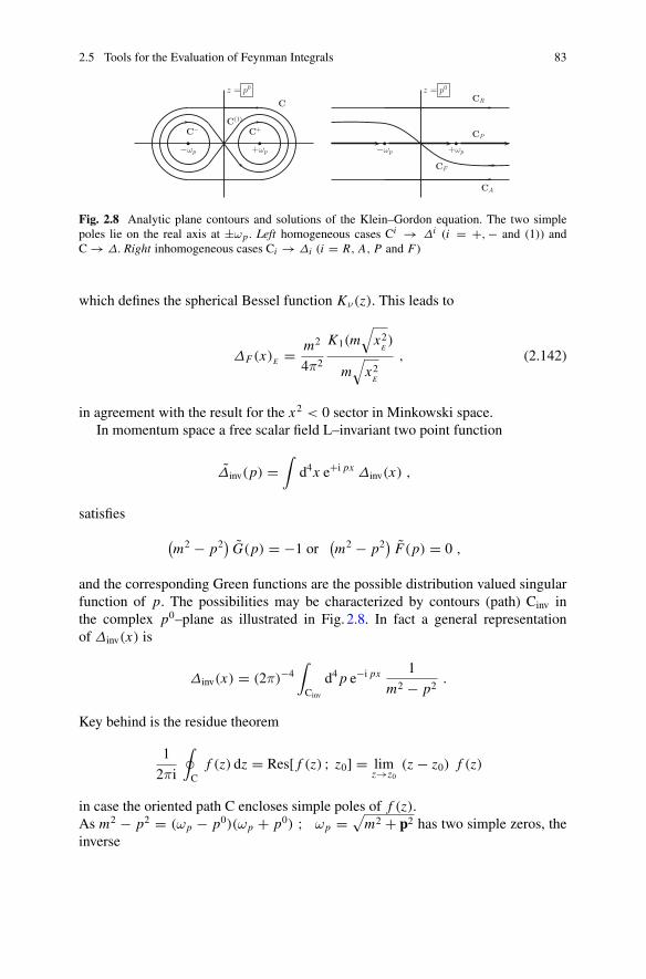
2.5 Tools for the Evaluation of Feynman Integrals 83

C− C+

C

C(1)

−ωp +ωp

z = p0

CR

CA

CP

CF

−ωp +ωp

z = p0

Fig. 2.8 Analytic plane contours and solutions of the Klein–Gordon equation. The two simplepoles lie on the real axis at ±ωp . Left homogeneous cases Ci → Δi (i = +,− and (1)) andC→ Δ. Right inhomogeneous cases Ci → Δi (i = R, A, P and F)

which defines the spherical Bessel function Kν(z). This leads to

ΔF (x)E =m2

4π2

K1(m√

x2E)

m√

x2E

, (2.142)

in agreement with the result for the x2 < 0 sector in Minkowski space.In momentum space a free scalar field L–invariant two point function

Δinv(p) =∫

d4x e+i px Δinv(x) ,

satisfies

(m2 − p2) G(p) = −1 or (

m2 − p2) F(p) = 0 ,

and the corresponding Green functions are the possible distribution valued singularfunction of p. The possibilities may be characterized by contours (path) Cinv inthe complex p0–plane as illustrated in Fig. 2.8. In fact a general representationof Δinv(x) is

Δinv(x) = (2π)−4∫

Cinv

d4 p e−i px 1

m2 − p2.

Key behind is the residue theorem

1

2πi

∮

Cf (z) dz = Res[ f (z) ; z0] = lim

z→z0(z − z0) f (z)

in case the oriented path C encloses simple poles of f (z).As m2 − p2 = (ωp − p0)(ωp + p0) ; ωp =

√m2 + p2 has two simple zeros, the

inverse

84 2 Quantum Field Theory and Quantum Electrodynamics

1

m2 − p2= 1

(ωP − p0)(ωp + p0)= −1

2ωp

(1

p0 − ωp− 1

p0 + ωp

)

has two simple poles. For the evaluation of the contour integrals on uses the fact thatthe contour can be closed in one of the half planes at infinity, depending on whetherx0 > 0 or x0 < 0, as discussed before.

In Euclidean space a more direct calculation shows how Bessel functions emergefrom a Fourier transform of a radial function on Rn

f (P) =∫

dn X f (X) e−iP X

with X, P ∈Rn and r = |X |. We first remember that the area of the unit sphereSn−1 ⊆Rn is

Sn−1 = 2πn/2/Γ (n/2) .

Let f (X) = F(r), then, in polar coordinates we can choose axes such that P X =sr cos θ. Then

f (P) = Fn(s) =∞∫

0

π∫

0

e−i sr cos θ F(r) Sn−2 (sin θ)n−2 dθ rn−1dr .

The angular integral is related to a Bessel function by

J n−22

(t) = tn−22

(2π)n2

Sn−2

π∫

0

e−i t cos θ (sin θ)n−2dθ

such that the Fourier transformation of a radial function takes the form

Fn(s) = (2π)n2 s−

n−22

∞∫

0

J n−22

(sr) F(r) r−n−22 rn−1dr .

Thus the n dimensional Fourier transform of a radial function is a radial functiontoo. These results will be useful later when discussing the lattice QCD evaluation ofthe hadronic light-by-light scattering in n = 4 Euclidean space, where

F(s = |P|) =∫

d4X F(r = |X |) e−iP X = (2π)2 s−1∞∫

0

J1(sr) F(r) r2 dr .

(2.143)End of the Digression.

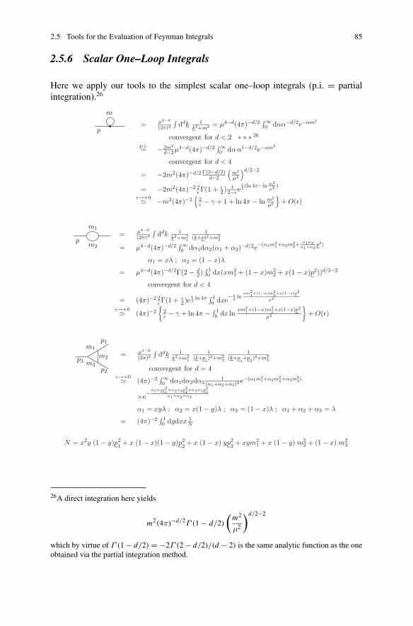
2.5 Tools for the Evaluation of Feynman Integrals 85

2.5.6 Scalar One–Loop Integrals

Here we apply our tools to the simplest scalar one–loop integrals (p.i. = partialintegration).26

= μ4−d

(2π)d

∫ddk 1

k2+m2 = μ4−d(4π)−d/2 ∫ ∞0 dαα−d/2e−αm2

convergent for d < 2 ∗ ∗ ∗ 26

p.i.= −2m2

d−2μ4−d(4π)−d/2 ∫ ∞0 dαα1−d/2e−αm2

convergent for d < 4

= −2m2(4π)−d/2 Γ(2−d/2)d−2

(m2

μ2

)d/2−2

= −2m2(4π)−2 2ε Γ(1 + ε

2 ) 12−εe

ε2 (ln 4π−ln m2

μ2 )

ε→+0 −m2(4π)−2{

2ε − γ + 1 + ln 4π − ln m2

μ2

}+ O(ε)

m

p

= μ4−d

(2π)d

∫ddk 1

k2+m21

1(k+p)2+m2

2

= μ4−d(4π)−d/2 ∫ ∞0 dα1dα2(α1 + α2)−d/2e−(α1m2

1+α2m22+

α1α2α1+α2

p2)

α1 = xλ ; α2 = (1 − x)λ

= μ4−d(4π)−d/2Γ(2 − d2)

∫ 10 dx(xm2

1 + (1 − x)m22 + x(1 − x)p2))d/2−2

convergent for d < 4

= (4π)−2 2ε Γ(1 + ε

2)eε2 ln 4π ∫ 1

0 dxe− ε2 ln

xm21+(1−x)m2

2+x(1−x)p2

μ2

ε→+0 (4π)−2{

2ε − γ + ln 4π − ∫ 1

0 dx lnxm2

1+(1−x)m22+x(1−x)p2

μ2

}+ O(ε)

m1

m2p

= μ4−d

(2π)d

∫ddk 1

k2+m21

1(k+p

1)2+m2

2

1(k+p

1+p

2)2+m2

3

convergent for d = 4ε→+0 (4π)−2 ∫ ∞

0 dα1dα2dα31

(α1+α2+α3)2e−(α1m2

1+α2m22+α3m2

3)

×e− α1α2p21+α2α3p22+α3α1p23α1+α2+α3

α1 = xyλ ; α2 = x(1 − y)λ ; α3 = (1 − x)λ ; α1 + α2 + α3 = λ

= (4π)−2 ∫ 10 dydxx 1

N

p3

p1

p2

m1

m3

m2

N = x2y (1 − y)p21 + x (1 − x)(1 − y)p2

2 + x (1 − x) yp23 + xym2

1 + x (1 − y) m22 + (1 − x) m2

3

26A direct integration here yields

m2(4π)−d/2Γ (1− d/2)

(m2

μ2

)d/2−2

which by virtue of Γ (1− d/2) = −2Γ (2− d/2)/(d − 2) is the same analytic function as the oneobtained via the partial integration method.

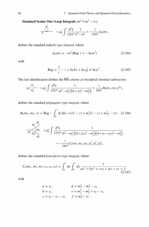
86 2 Quantum Field Theory and Quantum Electrodynamics

Standard Scalar One–Loop Integrals (m2 =m2 − iε).

defines the standard tadpole type integral, where

A0(m) = −m2(Reg+ 1− lnm2) (2.144)

with

Reg = 2

ε− γ + ln 4π + ln μ2

0 ≡ ln μ2 . (2.145)

The last identification defines the MS scheme of (modified) minimal subtraction.

defines the standard propagator type integral, where

B0(m1, m2; s) = Reg−∫ 1

0dz ln(−sz(1− z)+ m2

1(1− z)+ m22z − iε) . (2.146)

defines the standard form factor type integral, where

C0(m1, m2, m3; s1, s2, s3) =∫ 1

0dx∫ x

0dy

1

ax2 + by2 + cxy + dx + ey + f(2.147)

with

a = s2, d = m22 − m2

3 − s2,

b = s1, e = m21 − m2

2 + s2 − s3,

c = s3 − s1 − s2, f = m23 − iε .

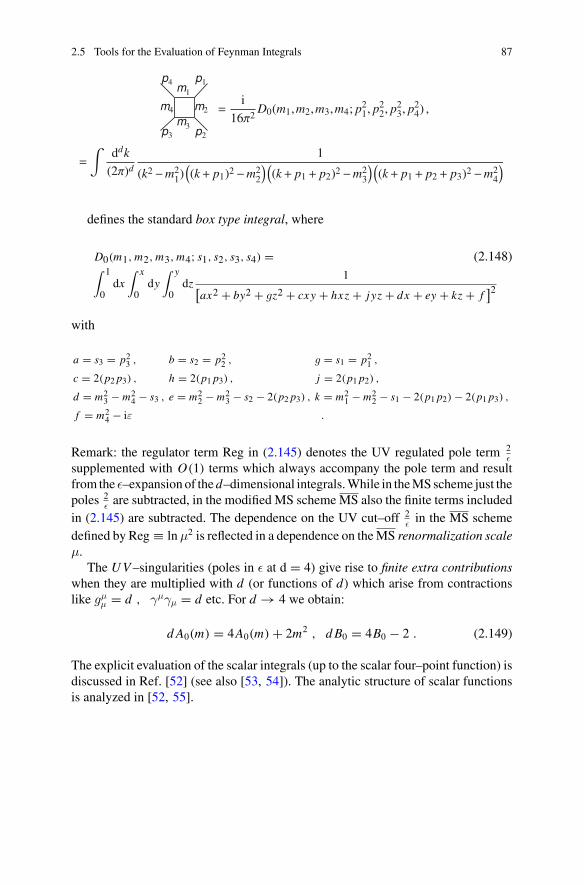
2.5 Tools for the Evaluation of Feynman Integrals 87

defines the standard box type integral, where

D0(m1, m2, m3, m4; s1, s2, s3, s4) = (2.148)∫ 1

0dx∫ x

0dy∫ y

0dz

1[ax2 + by2 + gz2 + cxy + hxz + j yz + dx + ey + kz + f

]2

with

a = s3 = p23 , b = s2 = p22 , g = s1 = p21 ,

c = 2(p2 p3) , h = 2(p1 p3) , j = 2(p1 p2) ,

d = m23 − m2

4 − s3 , e = m22 − m2

3 − s2 − 2(p2 p3) , k = m21 − m2

2 − s1 − 2(p1 p2)− 2(p1 p3) ,

f = m24 − iε .

Remark: the regulator term Reg in (2.145) denotes the UV regulated pole term 2ε

supplemented with O(1) terms which always accompany the pole term and resultfrom the ε–expansion of thed–dimensional integrals.While in theMSscheme just thepoles 2

εare subtracted, in the modified MS scheme MS also the finite terms included

in (2.145) are subtracted. The dependence on the UV cut–off 2εin the MS scheme

defined by Reg ≡ ln μ2 is reflected in a dependence on theMS renormalization scaleμ.

The U V –singularities (poles in ε at d = 4) give rise to finite extra contributionswhen they are multiplied with d (or functions of d) which arise from contractionslike gμ

μ = d , γμγμ = d etc. For d → 4 we obtain:

d A0(m) = 4A0(m)+ 2m2 , d B0 = 4B0 − 2 . (2.149)

The explicit evaluation of the scalar integrals (up to the scalar four–point function) isdiscussed in Ref. [52] (see also [53, 54]). The analytic structure of scalar functionsis analyzed in [52, 55].

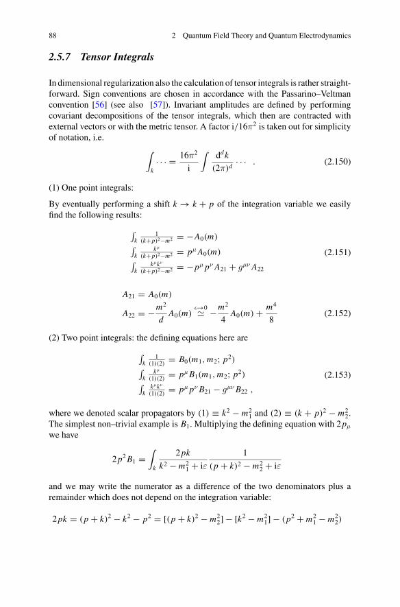
88 2 Quantum Field Theory and Quantum Electrodynamics

2.5.7 Tensor Integrals

In dimensional regularization also the calculation of tensor integrals is rather straight-forward. Sign conventions are chosen in accordance with the Passarino–Veltmanconvention [56] (see also [57]). Invariant amplitudes are defined by performingcovariant decompositions of the tensor integrals, which then are contracted withexternal vectors or with the metric tensor. A factor i/16π2 is taken out for simplicityof notation, i.e.

∫

k· · · = 16π2

i

∫ddk

(2π)d· · · . (2.150)

(1) One point integrals:

By eventually performing a shift k → k + p of the integration variable we easilyfind the following results:

∫k

1(k+p)2−m2 = −A0(m)

∫k

kμ

(k+p)2−m2 = pμ A0(m)∫

kkμkν

(k+p)2−m2 = −pμ pν A21 + gμν A22

(2.151)

A21 = A0(m)

A22 = −m2

dA0(m)

ε→0� −m2

4A0(m)+ m4

8(2.152)

(2) Two point integrals: the defining equations here are

∫k

1(1)(2) = B0(m1, m2; p2)

∫k

kμ

(1)(2) = pμ B1(m1, m2; p2)∫

kkμkν

(1)(2) = pμ pν B21 − gμν B22 ,

(2.153)

where we denoted scalar propagators by (1) ≡ k2 − m21 and (2) ≡ (k + p)2 − m2

2.The simplest non–trivial example is B1. Multiplying the defining equation with 2pμ

we have

2p2B1 =∫

k

2pk

k2 − m21 + iε

1

(p + k)2 − m22 + iε

and we may write the numerator as a difference of the two denominators plus aremainder which does not depend on the integration variable:

2pk = (p + k)2 − k2 − p2 = [(p + k)2 − m22] − [k2 − m2

1] − (p2 + m21 − m2

2)

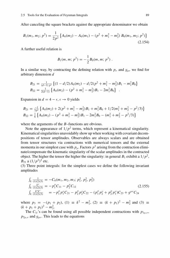
2.5 Tools for the Evaluation of Feynman Integrals 89

After canceling the square brackets against the appropriate denominator we obtain

B1(m1, m2; p2) = 1

2p2

{A0(m2)− A0(m1)− (p2 + m2

1 − m22) B0(m1, m2; p2)

}

(2.154)

A further useful relation is

B1(m, m; p2) = −1

2B0(m, m; p2) .

In a similar way, by contracting the defining relation with pν and gμν we find forarbitrary dimension d

B21 = 1(d−1) p2

{(1− d/2)A0(m2)− d/2(p2 + m2

1 − m22)B1 − m2

1B0}

B22 = 12(d−1)

{A0(m2)− (p2 + m2

1 − m22)B1 − 2m2

1B0}

.

Expansion in d = 4− ε, ε → 0 yields

B21 = −13p2

{A0(m2)+ 2(p2 + m2

1 − m22)B1 + m2

1B0 + 1/2(m21 + m2

2 − p2/3)}

B22 = 16

{A0(m2)− (p2 + m2

1 − m22)B1 − 2m2

1B0 − (m21 + m2

2 − p2/3)}

where the arguments of the B–functions are obvious.Note the appearance of 1/p2 terms, which represent a kinematical singularity.

Kinematical singularities unavoidably show upwhenworkingwith covariant decom-positions of tensor amplitudes. Observables are always scalars and are obtainedfrom tensor structures via contractions with numerical tensors and the externalmomenta in our simplest case with pμ. Factors p2 arising from the contraction elimi-nate/compensate the kinematic singularity of the scalar amplitudes in the contractedobject. The higher the tensor the higher the singularity: in general B1 exhibit a 1/p2,B21 a (1/p2)2 etc.(3) Three point integrals: for the simplest cases we define the following invariantamplitudes

∫k

1(1)(2)(3) = −C0(m1, m2, m3; p2

1, p22, p2

3)∫k

kμ

(1)(2)(3) = −pμ1C11 − pμ

2C12∫

kkμkν

(1)(2)(3) = −pμ1 pν

1C21 − pμ2 pν

2C22 − (pμ1 pν

2 + pμ2 pν

1 )C23 + gμνC24

(2.155)

where p3 = −(p1 + p2), (1) ≡ k2 − m21, (2) ≡ (k + p1)

2 − m22 and (3) ≡

(k + p1 + p2)2 − m2

3.The C1i ’s can be found using all possible independent contractions with p1μ,ν ,

p2μ,ν and gμν . This leads to the equations

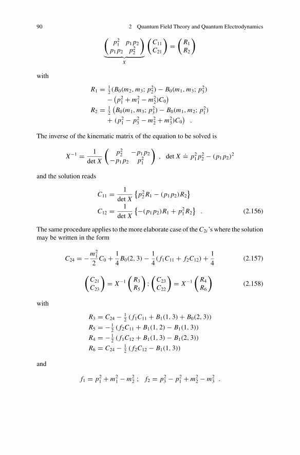
90 2 Quantum Field Theory and Quantum Electrodynamics

(p21 p1 p2

p1 p2 p22

)

︸ ︷︷ ︸X

(C11

C21

)=(

R1

R2

)

with

R1 = 12 (B0(m2, m3; p2

2)− B0(m1, m3; p23)

− (p21 + m2

1 − m22)C0

)

R2 = 12

(B0(m1, m3; p2

3)− B0(m1, m2; p21)

+ (p21 − p2

3 − m22 + m2

3)C0)

.

The inverse of the kinematic matrix of the equation to be solved is

X−1 = 1

det X

(p22 −p1 p2

−p1 p2 p21

), det X

.= p21 p2

2 − (p1 p2)2

and the solution reads

C11 = 1

det X

{p22 R1 − (p1 p2)R2

}

C12 = 1

det X

{−(p1 p2)R1 + p21 R2

}. (2.156)

The same procedure applies to themore elaborate case of theC2i ’s where the solutionmay be written in the form

C24 = −m21

2C0 + 1

4B0(2, 3)− 1

4( f1C11 + f2C12)+ 1

4(2.157)

(C21

C23

)= X−1

(R3

R5

);(

C23

C22

)= X−1

(R4

R6

)(2.158)

with

R3 = C24 − 12 ( f1C11 + B1(1, 3)+ B0(2, 3))

R5 = − 12 ( f2C11 + B1(1, 2)− B1(1, 3))

R4 = − 12 ( f1C12 + B1(1, 3)− B1(2, 3))

R6 = C24 − 12 ( f2C12 − B1(1, 3))

and

f1 = p21 + m2

1 − m22 ; f2 = p2

3 − p21 + m2

2 − m23 .

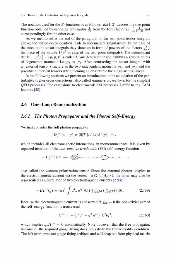
2.5 Tools for the Evaluation of Feynman Integrals 91

The notation used for the B–functions is as follows: B0(1, 2) denotes the two pointfunction obtained by dropping propagator 1

(3) from the form factor i.e.∫

k1

(1)(2) andcorrespondingly for the other cases.

As we mentioned at the end of the paragraph on the two point tensor integralsabove, the tensor decomposition leads to kinematical singularities. In the case ofthe three point tensor integrals they show up in form of powers of the factors 1

det X(in place of the simple 1/p2 in case of the two point integrals). The determinantdet X = p2

1 p22 − (p1 p2)

2 is called Gram determinant and exhibits a zero at pointsof degenerate momenta i.e. p2 ∝ p1. After contracting the tensor integral withan external tensor structure in the two independent moments p1μ and p2μ and thepossible numerical tensors when forming an observable the singularities cancel.

In the following sections we present an introduction to the calculation of the per-turbative higher order corrections, also called radiative corrections, for the simplestQED processes. For extensions to electroweak SM processes I refer to my TASIlectures [58].

2.6 One–Loop Renormalization

2.6.1 The Photon Propagator and the Photon Self–Energy

We first consider the full photon propagator

iDμν ′γ (x − y) = 〈0|T {Aμ(x)Aν(y)} |0〉 ,

which includes all electromagnetic interactions, in momentum space. It is given byrepeated insertion of the one–particle irreducible (1PI) self–energy function

also called the vacuum polarization tensor. Since the external photon couples tothe electromagnetic current via the vertex iejμ

em(x)Aμ(x), the latter may also berepresented as a correlator of two electromagnetic currents (2.93):

− iΠμνγ (q) = (ie)2

∫d4x eiqx 〈0|T {

jμem(x) jν

em(y)} |0〉 . (2.159)

Because the electromagnetic current is conserved ∂μ jμem = 0 the non–trivial part of

the self–energy function is transversal

Πμν = − (qμqν − q2 gμν)

Π ′(q2) (2.160)

which implies qνΠμν = 0 automatically. Note however, that the free propagator,

because of the required gauge fixing does not satisfy the transversality condition.The left over terms are gauge fixing artifacts and will drop out from physical matrix

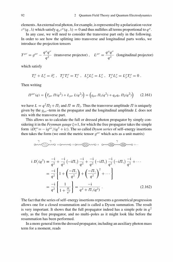
92 2 Quantum Field Theory and Quantum Electrodynamics

elements.An external real photon, for example, is represented by a polarization vectorεμ(q,λ)which satisfy qμε

μ(q,λ) = 0 and thus nullifies all terms proportional to qμ.In any case, we will need to consider the transverse part only in the following.

In order to see how the splitting into transverse and longitudinal parts works, weintroduce the projection tensors

T μν = gμν − qμqν

q2(transverse projector) , Lμν = qμqν

q2(longitudinal projector)

which satisfy

T μν + Lμ

ν = δμν , T μ

ρ T ρν = T μ

ν , Lμρ Lρ

ν = Lμν , T μ

ρ Lρν = Lμ

ρ T ρν = 0 .

Then writing

Πμν(q) =(

Tμν Π(q2)+ Lμν L(q2))=(gμν Π1(q

2)+ qμqν Π2(q2))

(2.161)

we have L = q2Π2+Π1 andΠ ≡ Π1. Thus the transverse amplitudeΠ is uniquelygiven by the gμν–term in the propagator and the longitudinal amplitude L does notmix with the transverse part.

This allows us to calculate the full or dressed photon propagator by simply con-sidering it in the Feynman gauge ξ=1, for which the free propagator takes the simpleform iDμν

γ =− igμν/(q2 + iε). The so called Dyson series of self–energy insertionsthen takes the form (we omit the metric tensor gμν which acts as a unit matrix)

γ γ= + +

γ+···

i D′γ(q

2) ≡ −iq2+ −i

q2

(−iΠγ

) −iq2+ −i

q2

(−iΠγ

) −iq2

(−iΠγ

) −iq2+ · · ·

= −iq2

{

1+(−Πγ

q2

)+(−Πγ

q2

)2

+ · · ·}

= −iq2

{1

1+ Πγ

q2

}

= −iq2 +Πγ(q2)

. (2.162)

The fact that the series of self–energy insertions represents a geometrical progressionallows one for a closed resummation and is called a Dyson summation. The resultis very important. It shows that the full propagator indeed has a simple pole in q2

only, as the free propagator, and no multi–poles as it might look like before theresummation has been performed.

In amore general form the dressed propagator, including an auxiliary photonmassterm for a moment, reads

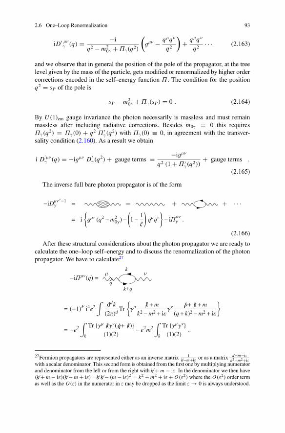
2.6 One–Loop Renormalization 93

iD′ μνγ (q) = −i

q2 − m20γ +Πγ(q2)

(gμν − qμqν

q2

)+ qμqν

q2· · · (2.163)

and we observe that in general the position of the pole of the propagator, at the treelevel given by the mass of the particle, gets modified or renormalized by higher ordercorrections encoded in the self–energy function Π . The condition for the positionq2 = sP of the pole is

sP − m20γ +Πγ(sP) = 0 . (2.164)

By U (1)em gauge invariance the photon necessarily is massless and must remainmassless after including radiative corrections. Besides m0γ = 0 this requiresΠγ(q2) = Πγ(0) + q2 Π ′

γ(q2) with Πγ(0) ≡ 0, in agreement with the transver-

sality condition (2.160). As a result we obtain

i D′μνγ (q) = −igμν D′

γ(q2)+ gauge terms = −igμν

q2 (1+Π ′γ(q

2))+ gauge terms .

(2.165)

The inverse full bare photon propagator is of the form

(2.166)

After these structural considerations about the photon propagator we are ready tocalculate the one–loop self–energy and to discuss the renormalization of the photonpropagator. We have to calculate27

27Fermion propagators are represented either as an inverse matrix 1�k−m+iε or as a matrix �k+m−iε

k2−m2+iεwith a scalar denominator. This second form is obtained from the first one bymultiplying numeratorand denominator from the left or from the right with �k + m − iε. In the denominator we then have(�k +m − iε)( �k −m + iε) =�k �k − (m − iε)2 = k2 −m2 + iε+ O(ε2) where the O(ε2) order termas well as the O(ε) in the numerator in ε may be dropped as the limit ε → 0 is always understood.

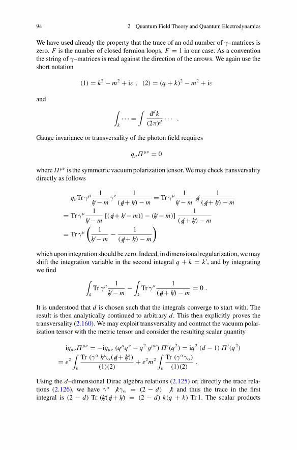
94 2 Quantum Field Theory and Quantum Electrodynamics

We have used already the property that the trace of an odd number of γ–matrices iszero. F is the number of closed fermion loops, F = 1 in our case. As a conventionthe string of γ–matrices is read against the direction of the arrows. We again use theshort notation

(1) = k2 − m2 + iε , (2) = (q + k)2 − m2 + iε

and

∫

k· · · =

∫ddk

(2π)d· · · .

Gauge invariance or transversality of the photon field requires

qμΠμν = 0

whereΠμν is the symmetric vacuumpolarization tensor.Wemay check transversalitydirectly as follows

qνTr γμ 1

�k − mγν 1

( �q+ �k)− m= Tr γμ 1

�k − m�q 1

( �q+ �k)− m

= Tr γμ 1

�k − m[( �q+ �k − m)} − ( �k − m)] 1

( �q+ �k)− m

= Tr γμ

(1

�k − m− 1

( �q+ �k)− m

)

which upon integration should be zero. Indeed, in dimensional regularization,wemayshift the integration variable in the second integral q + k = k ′, and by integratingwe find

∫

kTr γμ 1

�k − m−∫

kTr γμ 1

( �q+ �k)− m= 0 .

It is understood that d is chosen such that the integrals converge to start with. Theresult is then analytically continued to arbitrary d. This then explicitly proves thetransversality (2.160). We may exploit transversality and contract the vacuum polar-ization tensor with the metric tensor and consider the resulting scalar quantity

igμνΠμν = −igμν (qμqν − q2 gμν) Π ′(q2) = iq2 (d − 1) Π ′(q2)

= e2∫

k

Tr (γα �kγα( �q+ �k))

(1)(2)+ e2m2

∫

k

Tr (γαγα)

(1)(2).

Using the d–dimensional Dirac algebra relations (2.125) or, directly the trace rela-tions (2.126), we have γα � kγα = (2 − d) � k and thus the trace in the firstintegral is (2 − d) Tr ( �k( �q+ �k) = (2 − d) k(q + k) Tr 1. The scalar products

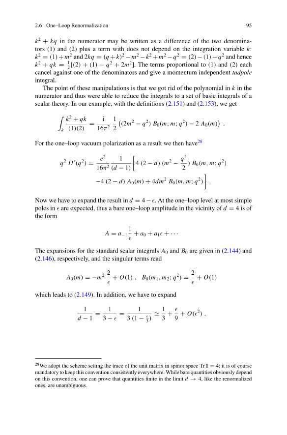
2.6 One–Loop Renormalization 95

k2 + kq in the numerator may be written as a difference of the two denomina-tors (1) and (2) plus a term with does not depend on the integration variable k:k2 = (1)+m2 and 2kq = (q+ k)2−m2− k2+m2−q2 = (2)− (1)−q2 and hencek2 + qk = 1

2 [(2) + (1) − q2 + 2m2]. The terms proportional to (1) and (2) eachcancel against one of the denominators and give a momentum independent tadpoleintegral.

The point of these manipulations is that we got rid of the polynomial in k in thenumerator and thus were able to reduce the integrals to a set of basic integrals of ascalar theory. In our example, with the definitions (2.151) and (2.153), we get

∫

k

k2 + qk

(1)(2)= i

16π2

1

2

((2m2 − q2) B0(m, m; q2)− 2 A0(m)

).

For the one–loop vacuum polarization as a result we then have28

q2 Π ′(q2) = e2

16π2

1

(d − 1)

{4 (2− d) (m2 − q2

2) B0(m, m; q2)

−4 (2− d) A0(m)+ 4dm2 B0(m, m; q2)

}.

Now we have to expand the result in d = 4− ε. At the one–loop level at most simplepoles in ε are expected, thus a bare one–loop amplitude in the vicinity of d = 4 is ofthe form

A = a−11

ε+ a0 + a1ε+ · · ·

The expansions for the standard scalar integrals A0 and B0 are given in (2.144) and(2.146), respectively, and the singular terms read

A0(m) = −m2 2

ε+ O(1) , B0(m1, m2; q2) = 2

ε+ O(1)

which leads to (2.149). In addition, we have to expand

1

d − 1= 1

3− ε= 1

3 (1− ε3 )� 1

3+ ε

9+ O(ε2) .

28We adopt the scheme setting the trace of the unit matrix in spinor space Tr 1 = 4; it is of coursemandatory to keep this convention consistently everywhere.While bare quantities obviously dependon this convention, one can prove that quantities finite in the limit d → 4, like the renormalizedones, are unambiguous.

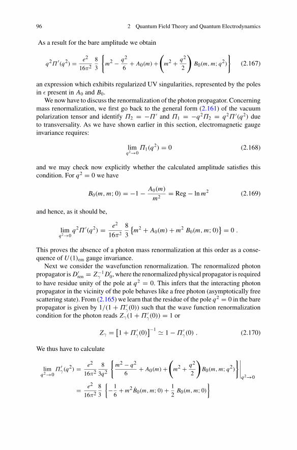
96 2 Quantum Field Theory and Quantum Electrodynamics

As a result for the bare amplitude we obtain

q2Π ′(q2) = e2

16π28

3

{

m2 − q2

6+ A0(m)+

(

m2 + q2

2

)

B0(m, m; q2)

}

(2.167)

an expression which exhibits regularized UV singularities, represented by the polesin ε present in A0 and B0.

We now have to discuss the renormalization of the photon propagator. Concerningmass renormalization, we first go back to the general form (2.161) of the vacuumpolarization tensor and identify Π2 = −Π ′ and Π1 = −q2Π2 = q2Π ′(q2) dueto transversality. As we have shown earlier in this section, electromagnetic gaugeinvariance requires:

limq2→0

Π1(q2) = 0 (2.168)

and we may check now explicitly whether the calculated amplitude satisfies thiscondition. For q2 = 0 we have

B0(m, m; 0) = −1− A0(m)

m2= Reg− lnm2 (2.169)

and hence, as it should be,

limq2→0

q2Π ′(q2) = e2

16π2

8

3

{m2 + A0(m)+ m2 B0(m, m; 0)} = 0 .

This proves the absence of a photon mass renormalization at this order as a conse-quence of U (1)em gauge invariance.

Next we consider the wavefunction renormalization. The renormalized photonpropagator is D′

ren = Z−1γ D′0, where the renormalized physical propagator is required

to have residue unity of the pole at q2 = 0. This infers that the interacting photonpropagator in the vicinity of the pole behaves like a free photon (asymptotically freescattering state). From (2.165) we learn that the residue of the pole q2 = 0 in the barepropagator is given by 1/(1 +Π ′

γ(0)) such that the wave function renormalizationcondition for the photon reads Zγ(1+Π ′

γ(0)) = 1 or

Zγ =[1+Π ′

γ(0)]−1 � 1−Π ′

γ(0) . (2.170)

We thus have to calculate

limq2→0

Π ′γ(q2) = e2

16π28

3q2

{m2 − q2

6+ A0(m)+

(

m2 + q2

2

)

B0(m, m; q2)

}∣∣∣∣∣q2→0

= e2

16π28

3

{−1

6+ m2 B0(m, m; 0)+ 1

2B0(m, m; 0)

}

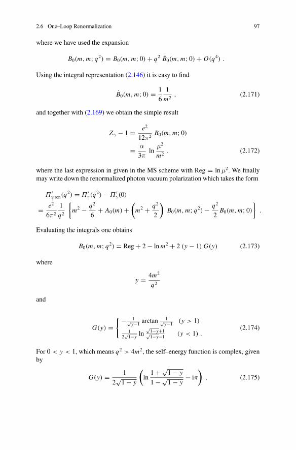
2.6 One–Loop Renormalization 97

where we have used the expansion

B0(m, m; q2) = B0(m, m; 0)+ q2 B0(m, m; 0)+ O(q4) .

Using the integral representation (2.146) it is easy to find

B0(m, m; 0) = 1

6

1

m2, (2.171)

and together with (2.169) we obtain the simple result

Zγ − 1 = e2

12π2B0(m, m; 0)

= α

3πln

μ2

m2. (2.172)

where the last expression in given in the MS scheme with Reg = ln μ2. We finallymay write down the renormalized photon vacuum polarization which takes the form

Π ′γ ren(q

2) = Π ′γ(q

2)−Π ′γ(0)

= e2

6π2

1

q2

{m2 − q2

6+ A0(m)+

(m2 + q2

2

)B0(m, m; q2)− q2

2B0(m, m; 0)

}.

Evaluating the integrals one obtains

B0(m, m; q2) = Reg+ 2− lnm2 + 2 (y − 1) G(y) (2.173)

where

y = 4m2

q2

and

G(y) ={− 1√

y−1 arctan1√y−1 (y > 1)

12√1−y

ln√1−y+1√1−y−1 (y < 1) .

(2.174)

For 0 < y < 1, which means q2 > 4m2, the self–energy function is complex, givenby

G(y) = 1

2√1− y

(ln

1+√1− y

1−√1− y− iπ

). (2.175)

98 2 Quantum Field Theory and Quantum Electrodynamics

The imaginary part in the time–like region q2 > 0 for√

q2 > 2m is a consequence ofthe fact that an electron–positron pair can be actually produced as real particles whenthe available energy exceeds the sum of the rest masses of the produced particles. Thevacuum polarization function is thus an analytic function in the complex q2–planewith a cut along the positive real axis starting at q2 = 4m2, which is the thresholdfor pair–creation.29

The final result for the renormalized vacuum polarization then reads

Π ′γ ren(q

2) = α

3π

{5

3+ y − 2 (1+ y

2) (1− y) G(y)

}(2.176)

which in fact is a function of q2/m2. This renormalized vacuum polarization functionwill play a crucial role in different places later. For later purposes it is useful to notethat it may be written in compact form as the following integral30

29As a rule, a cut diagram

m2

m1

q

contributes to the imaginary part if the cut diagram kinematically allows physical intermediatestates: q2 ≥ (m1+m2)

2. In place of the virtual photon (a real photon requires q2 = 0 and does notdecay) let us consider the massive charged weak gauge boson W . The W is an unstable particle anddecays predominantly as W− → �−ν� (� = e,μ, τ ) leptonically, and W− → du, bc hadronically.Looking at the transversal self–energy function ΠW (q2) of the W on the mass shell q2 = M2

W wehave

Im ΠW (q2 = M2W ) = MW ΓW �= 0

defining the finite width ΓW of the W–particle. Note that W− → bt is not allowed kinematicallybecause the top quark t is heavier than the W (MW = 80.385 ± 0.015GeV, mt = 173.21 ±0.87GeV, mb = 4.18± 0.03GeV) for an on–shell W and hence does not contribute to the width.

Cutting lines means applying the substitution (see (2.141))

1

p2 − m2 + iε→−i π δ(p2 − m2)

for the corresponding propagators. In general the imaginary part is given by cutting sets of linesof a diagram in all possible ways such that the diagram is cut into two disconnected parts. A cutcontributes if the cut lines can be viewed as external lines of a real physical subprocess. Note thatthe imaginary part of an n–loop amplitude is given by cut diagrams exhibiting n − 1 closed loopsat most. The imaginary part therefore is less UV divergent in general. In particular, the imaginarypart of a one–loop diagram is always finite.30Which derives from

B0(m, m; q2) = Reg− lnm2 −∫ 1

0dz ln(1− z (1− z) q2/m2)

2.6 One–Loop Renormalization 99

Π ′γ ren(q

2/m2) = −α

π

1∫

0

dz 2z (1− z) ln(1− z (1− z) q2/m2)

= α

π

1∫

0

dt t2 (1− t2/3)1

4m2/q2 − (1− t2). (2.177)

The result (2.176) may be easily extended to include the other fermion contri-butions. In the MS scheme, defined by setting Reg = ln μ2 in the bare form, wehave

Π ′γ(q

2) = α

3π

∑

f

Q2f Ncf

[

lnμ2

m2f

+ G

]

(2.178)

where f labels the different fermion flavors (fermion species), Q f is the charge inunits of e and Ncf the color factor, Ncf = 3 for quarks and Ncf = 1 for the leptons.We have introduced the auxiliary function

G = 5

3+ y − 2 (1+ y

2) (1− y) G(y) �

{G = 0 , q2 = 0

Re G = − ln |q2|m2

f+ 5

3 , |q2| # m2f

which vanishes at q2 = 0. The imaginary part is given by the simple formula

Im Π ′γ(q

2) = α

3

∑

f

Q2f Ncf

((1+ y

2)√1− y

). (2.179)

Using the given low and high energy limits we get

Π ′γ(0) =

α

3π

∑

f

Q2f Ncf ln

μ2

m2f

(2.180)

and

Re Π ′γ(q

2) = α

3π

∑

f

Q2f Ncf

(ln

μ2

|q2| +5

3

); |q2| # m2

f . (2.181)

(Footnote 30 continued)(see (2.146)). The second form is obtained from the first one by a transformation of variablesz → t = 2z − 1, noting that

∫ 10 dz · · · = 2

∫ 112dz · · · , and performing a partial integration with

respect to the factor z (1− z) = (1− t2)/4 = ddt t (1− t2/3)/4 in front of the logarithm.

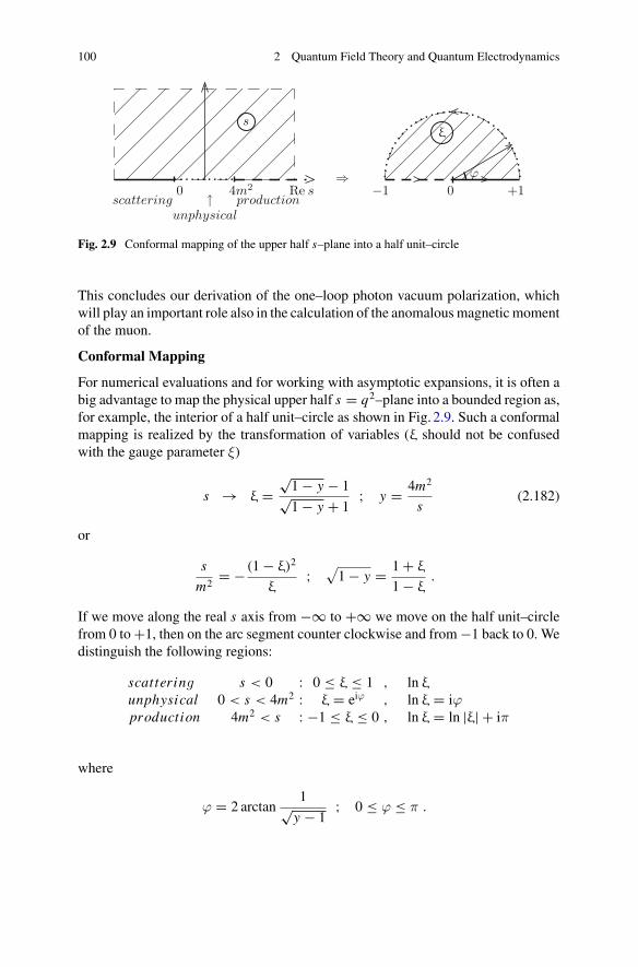
100 2 Quantum Field Theory and Quantum Electrodynamics

⇒scattering production↑

unphysical

0 4m2 Re s

sξ

ϕ

0−1 +1

Fig. 2.9 Conformal mapping of the upper half s–plane into a half unit–circle

This concludes our derivation of the one–loop photon vacuum polarization, whichwill play an important role also in the calculation of the anomalousmagnetic momentof the muon.

Conformal Mapping

For numerical evaluations and for working with asymptotic expansions, it is often abig advantage to map the physical upper half s = q2–plane into a bounded region as,for example, the interior of a half unit–circle as shown in Fig. 2.9. Such a conformalmapping is realized by the transformation of variables (ξ should not be confusedwith the gauge parameter ξ)

s → ξ =√1− y − 1√1− y + 1

; y = 4m2

s(2.182)

or

s

m2= − (1− ξ)2

ξ; √

1− y = 1+ ξ

1− ξ.

If we move along the real s axis from −∞ to +∞ we move on the half unit–circlefrom 0 to+1, then on the arc segment counter clockwise and from−1 back to 0. Wedistinguish the following regions:

scattering s < 0 : 0 ≤ ξ ≤ 1 , ln ξ

unphysical 0 < s < 4m2 : ξ = eiϕ , ln ξ = iϕproduction 4m2 < s : −1 ≤ ξ ≤ 0 , ln ξ = ln |ξ| + iπ

where

ϕ = 2 arctan1√

y − 1; 0 ≤ ϕ ≤ π .

2.6 One–Loop Renormalization 101

On the arc holds 1/y = sin2 ϕ2 . The function G(y) has now the representation

G(y) =

⎧⎪⎨

⎪⎩

− 121−ξ1+ξ

ln ξ , 0 > s

− 12 ϕ tan ϕ

2 , 4m2 > s > 0

− 121−ξ1+ξ

(ln |ξ| + iπ) , s > 4m2 .

As an application we may write the photon vacuum polarization amplitude (2.176)in the form

Πγ ren(s) = q2Π ′γ ren(s)

= α m2

3π

{− 223 + 5

3

(ξ−1 + ξ

) + (ξ−1 + ξ− 4

)1+ξ1−ξ

ln ξ , s < 0

− 203 sin2 ϕ

2 − 4+ 2(1+ 2 sin2 ϕ

2

)ϕ cot ϕ

2 , 0 < s < 4m2 .

For s > 4m2 the first form holds with ln ξ = ln |ξ| + iπ. Corresponding representa-tions are used for the vertex function as well as for the kernel function of the vacuumpolarization integral contributing to g − 2 (see Sect. 5.1.7).

2.6.2 The Electron Self–Energy

Next we study the full propagator of a Dirac fermion f

iS′f (x − y) = 〈0|T {ψ f (x)ψ f (y)

} |0〉

in momentum space. Again, the propagator has the structure of a repeated insertionof the 1PI self–energy −iΣ f (p)

f f = + +

f+···

i S′f (p) ≡ i

�p − m f+ i

�p − m f

(−iΣ f) i

�p − m f

+ i

�p − m f

(−iΣ f) i

�p − m f

(−iΣ f) i

�p − m f+ · · ·

= i

�p − m f

{

1+(

Σ f

�p − m f

)+(

Σ f

�p − m f

)2

+ · · ·}

= i

�p − m f

⎧⎨

⎩1

1− Σ f

�p−m f

⎫⎬

⎭= i

�p − m f −Σ f. (2.183)

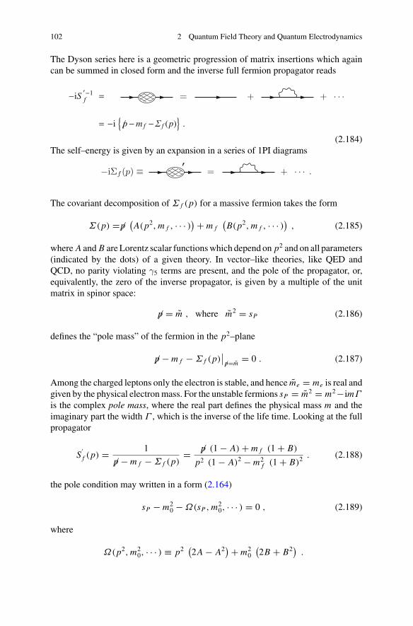
102 2 Quantum Field Theory and Quantum Electrodynamics

The Dyson series here is a geometric progression of matrix insertions which againcan be summed in closed form and the inverse full fermion propagator reads

(2.184)The self–energy is given by an expansion in a series of 1PI diagrams

The covariant decomposition of Σ f (p) for a massive fermion takes the form

Σ(p) =�p (A(p2, m f , · · · )

)+ m f(B(p2, m f , · · · )

), (2.185)

where A and B are Lorentz scalar functionswhich depend on p2 and on all parameters(indicated by the dots) of a given theory. In vector–like theories, like QED andQCD, no parity violating γ5 terms are present, and the pole of the propagator, or,equivalently, the zero of the inverse propagator, is given by a multiple of the unitmatrix in spinor space:

�p = m , where m2 = sP (2.186)

defines the “pole mass” of the fermion in the p2–plane

�p − m f −Σ f (p)∣∣ �p=m = 0 . (2.187)

Among the charged leptons only the electron is stable, and hence me = me is real andgiven by the physical electronmass. For the unstable fermions sP = m2 = m2−imΓ

is the complex pole mass, where the real part defines the physical mass m and theimaginary part the width Γ , which is the inverse of the life time. Looking at the fullpropagator

S′f (p) = 1

�p − m f −Σ f (p)= �p (1− A)+ m f (1+ B)

p2 (1− A)2 − m2f (1+ B)2

. (2.188)

the pole condition may written in a form (2.164)

sP − m20 −Ω(sP , m2

0, · · · ) = 0 , (2.189)

where

Ω(p2, m20, · · · ) ≡ p2

(2A − A2

)+ m20

(2B + B2

).

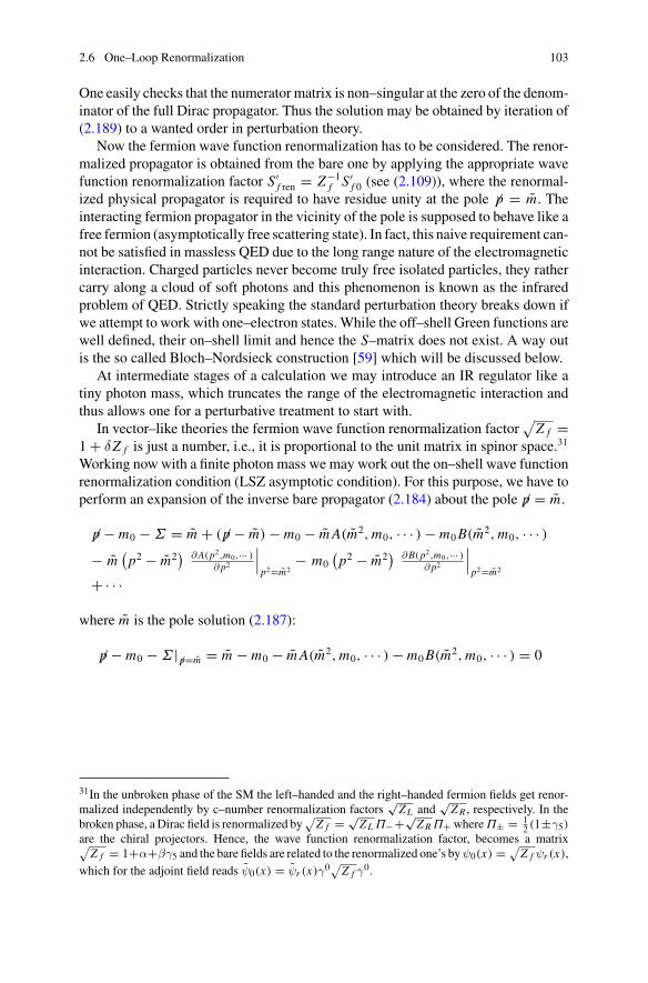
2.6 One–Loop Renormalization 103

One easily checks that the numerator matrix is non–singular at the zero of the denom-inator of the full Dirac propagator. Thus the solution may be obtained by iteration of(2.189) to a wanted order in perturbation theory.

Now the fermion wave function renormalization has to be considered. The renor-malized propagator is obtained from the bare one by applying the appropriate wavefunction renormalization factor S′f ren = Z−1f S′f 0 (see (2.109)), where the renormal-ized physical propagator is required to have residue unity at the pole � p = m. Theinteracting fermion propagator in the vicinity of the pole is supposed to behave like afree fermion (asymptotically free scattering state). In fact, this naive requirement can-not be satisfied in massless QED due to the long range nature of the electromagneticinteraction. Charged particles never become truly free isolated particles, they rathercarry along a cloud of soft photons and this phenomenon is known as the infraredproblem of QED. Strictly speaking the standard perturbation theory breaks down ifwe attempt to work with one–electron states. While the off–shell Green functions arewell defined, their on–shell limit and hence the S–matrix does not exist. A way outis the so called Bloch–Nordsieck construction [59] which will be discussed below.

At intermediate stages of a calculation we may introduce an IR regulator like atiny photon mass, which truncates the range of the electromagnetic interaction andthus allows one for a perturbative treatment to start with.

In vector–like theories the fermion wave function renormalization factor√

Z f =1+ δZ f is just a number, i.e., it is proportional to the unit matrix in spinor space.31

Working now with a finite photon mass we may work out the on–shell wave functionrenormalization condition (LSZ asymptotic condition). For this purpose, we have toperform an expansion of the inverse bare propagator (2.184) about the pole �p = m.

�p − m0 −Σ = m + ( �p − m)− m0 − m A(m2, m0, · · · )− m0B(m2, m0, · · · )− m

(p2 − m2

) ∂ A(p2,m0,··· )∂ p2

∣∣∣p2=m2

− m0(

p2 − m2) ∂B(p2,m0,··· )

∂ p2

∣∣∣p2=m2

+ · · ·

where m is the pole solution (2.187):

�p − m0 −Σ |�p=m = m − m0 − m A(m2, m0, · · · )− m0B(m2, m0, · · · ) = 0

31In the unbroken phase of the SM the left–handed and the right–handed fermion fields get renor-malized independently by c–number renormalization factors

√ZL and

√Z R , respectively. In the

broken phase, a Dirac field is renormalized by√

Z f = √ZL Π−+√Z R Π+ whereΠ± = 12 (1±γ5)

are the chiral projectors. Hence, the wave function renormalization factor, becomes a matrix√Z f = 1+α+βγ5 and the bare fields are related to the renormalized one’s byψ0(x) = √

Z f ψr (x),which for the adjoint field reads ψ0(x) = ψr (x)γ0

√Z f γ

0.

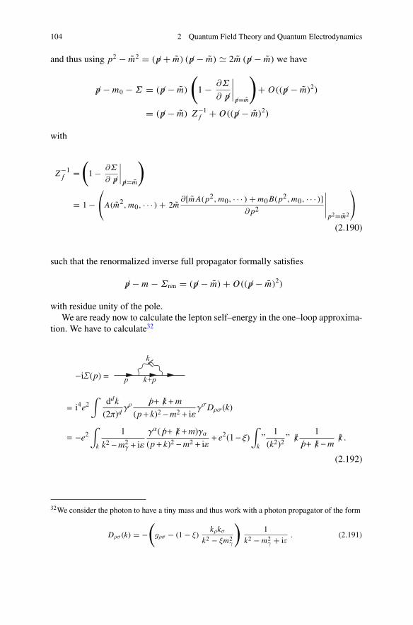
104 2 Quantum Field Theory and Quantum Electrodynamics

and thus using p2 − m2 = ( �p + m) ( �p − m) � 2m ( �p − m) we have

�p − m0 −Σ = ( �p − m)

(

1− ∂Σ

∂ �p∣∣∣∣ �p=m

)

+ O(( �p − m)2)

= ( �p − m) Z−1f + O(( �p − m)2)

with

Z−1f =(

1− ∂Σ

∂ �p∣∣∣∣ �p=m

)

= 1−⎛

⎝A(m2, m0, · · · )+ 2m∂[m A(p2, m0, · · · )+ m0B(p2, m0, · · · )]

∂ p2

∣∣∣∣∣

p2=m2

⎞

⎠

(2.190)

such that the renormalized inverse full propagator formally satisfies

�p − m −Σren = ( �p − m)+ O(( �p − m)2)

with residue unity of the pole.We are ready now to calculate the lepton self–energy in the one–loop approxima-

tion. We have to calculate32

(2.192)

32We consider the photon to have a tiny mass and thus work with a photon propagator of the form

Dρσ(k) = −(

gρσ − (1− ξ)kρkσ

k2 − ξm2γ

)1

k2 − m2γ + iε

. (2.191)

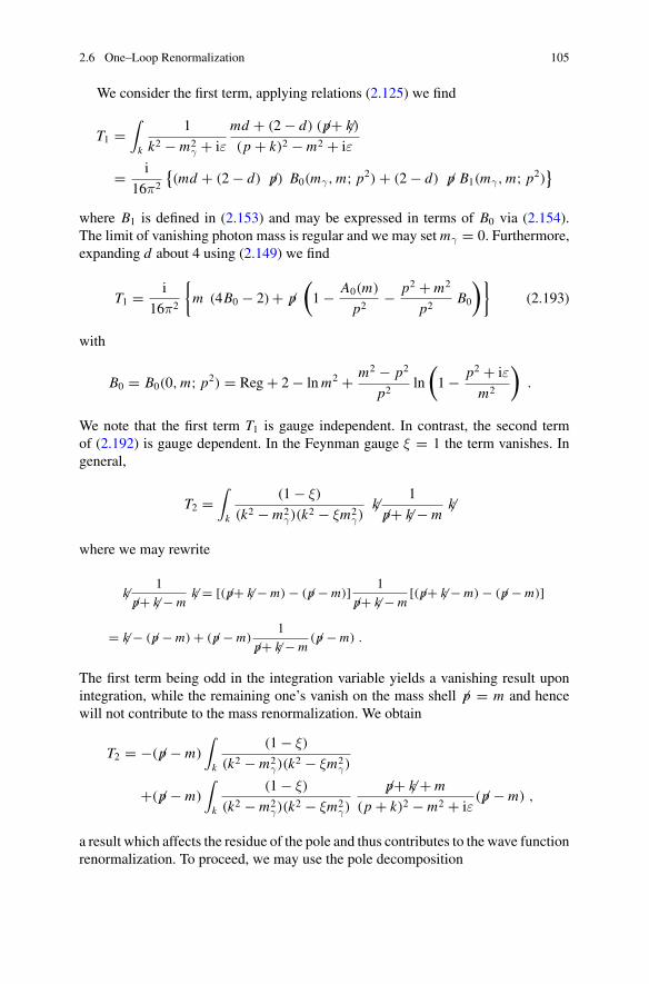
2.6 One–Loop Renormalization 105

We consider the first term, applying relations (2.125) we find

T1 =∫

k

1

k2 − m2γ + iε

md + (2− d) ( �p+ �k)

(p + k)2 − m2 + iε

= i

16π2

{(md + (2− d) �p) B0(mγ, m; p2)+ (2− d) �p B1(mγ, m; p2)

}

where B1 is defined in (2.153) and may be expressed in terms of B0 via (2.154).The limit of vanishing photon mass is regular and we may set mγ = 0. Furthermore,expanding d about 4 using (2.149) we find

T1 = i

16π2

{m (4B0 − 2)+ �p

(1− A0(m)

p2− p2 + m2

p2B0

)}(2.193)

with

B0 = B0(0, m; p2) = Reg+ 2− lnm2 + m2 − p2

p2ln

(1− p2 + iε

m2

).

We note that the first term T1 is gauge independent. In contrast, the second termof (2.192) is gauge dependent. In the Feynman gauge ξ = 1 the term vanishes. Ingeneral,

T2 =∫

k

(1− ξ)

(k2 − m2γ)(k

2 − ξm2γ)�k 1

�p+ �k − m�k

where we may rewrite

�k 1

�p+ �k − m�k = [( �p+ �k − m)− ( �p − m)] 1

�p+ �k − m[( �p+ �k − m)− ( �p − m)]

= �k − ( �p − m)+ ( �p − m)1

�p+ �k − m( �p − m) .

The first term being odd in the integration variable yields a vanishing result uponintegration, while the remaining one’s vanish on the mass shell � p = m and hencewill not contribute to the mass renormalization. We obtain

T2 = −( �p − m)

∫

k

(1− ξ)

(k2 − m2γ)(k

2 − ξm2γ)

+( �p − m)

∫

k

(1− ξ)

(k2 − m2γ)(k

2 − ξm2γ)

�p+ �k + m

(p + k)2 − m2 + iε( �p − m) ,

a result which affects the residue of the pole and thus contributes to the wave functionrenormalization. To proceed, we may use the pole decomposition

106 2 Quantum Field Theory and Quantum Electrodynamics

(1− ξ)1

k2 − m2γ

1

k2 − ξm2γ

= 1

m2γ

(1

k2 − m2γ

− 1

k2 − ξm2γ

)

.

Then all integrals are of the type we already know and the result may be worked outeasily. Since these terms must cancel in physical amplitudes, we will not work themout in full detail here. Note that the second term is of order O(( � p − m)2) near themass shell and hence does not contribute to the residue of the pole and hence to thewave function renormalization. The first term is very simple and given by

T2 = ( �p − m)

{−(1− ξ)

i

16π2B0(mγ,

√ξmγ; 0)

}+ O(( �p − m)2) .

(2.194)We now consider the mass renormalization. The latter is gauge invariant and we

may start from Σ = −ie2T1 + ie2T2 in the Feynman gauge

Σξ=1 = −ie2T1 = A(p2) �p + B(p2) m

= e2

16π2

{�p(1− A0(m)

p2− p2 + m2

p2B0

)+ m (4B0 − 2)

}.

The physical on–shell mass renormalization counter term is determined by

�p − m0 −Σ |�p=m = �p − m − δm −Σ |�p=m = 0 or δm = −Σ |�p=m

and hence

δm

m= − (

A(p2)+ B(p2))∣∣

p2→m2

= e2

16π2

{1+ A0(m)

m2− 2B0(mγ, m;m2)

}= e2

16π2

{3

A0(m)

m2− 1

}

where we have used

B0(0, m;m2) = 1− A0(m)

m2= Reg+ 2− lnm2 .

As a result the mass renormalization counter term is gauge invariant and infraredfinite for mγ = 0. The gauge dependent amplitude T2 does not contribute. Using(2.144) we may write

δm

m= α

2π

{3

2ln

m2

μ2− 2

}. (2.195)

2.6 One–Loop Renormalization 107

The wave function renormalization at one–loop order is given by33

Z f − 1 =(

A(p2)+ 2m2 ∂(A+B)(p2)

∂ p2

)∣∣∣p2→m2

= e2

16π2

{1+ A0(m)

m2 + 4m2 B0(mγ, m;m2)+ (1− ξ) B0(mγ,√

ξmγ; 0)}

.

A calculation of B0 in the limit of a small photon mass yields

B0(mγ, m;m2)mγ→0� − 1

m2

(

1+ 1

2ln

m2γ

m2

)

a result which exhibits an IR singularity and shows that in massless QED the residueof the pole does not exist. An asymptotically small photon mass mγ is used as an IRregulator here. In IR regularized QED we may write the result in the form

Z f − 1 = α

2π

{1

2ln

m2

μ2− 2+ 2 ln

m

mγ+ 1

2(1− ξ)

(

1− lnm2

γ

μ2

)

+ 1

2ξ ln ξ

}

.

(2.197)

The important message here is that the residue of the pole of the bare fermionpropagator is gauge dependent and infrared singular. What it means is that the LSZasymptotic condition for a charged particle cannot be satisfied. The cloud of softphotons accompanying any charged state would have to be included appropriately.However, usually in calculating cross sections the Bloch–Nordsieck construction isapplied. This will be elaborated on below.

33Note that with T2 from (2.194) we have

Σξ �=1 = ie2T2 = (�p − m) Aξ �=1

where

Aξ �=1 = (1− ξ)e2

16π2 B0(mγ ,√

ξmγ; 0)

and Bξ �=1 = −Aξ �=1, such that Aξ �=1 + Bξ �=1 = 0. This leads to a contribution

δZ ξ �=1f = e2

16π2 (1− ξ) B0(mγ ,√

ξmγ; 0)

= e2

16π2

{(1− ξ)

(Reg+ 1− lnm2

γ

)+ ξ ln ξ

} (2.196)

to the wave function renormalization.

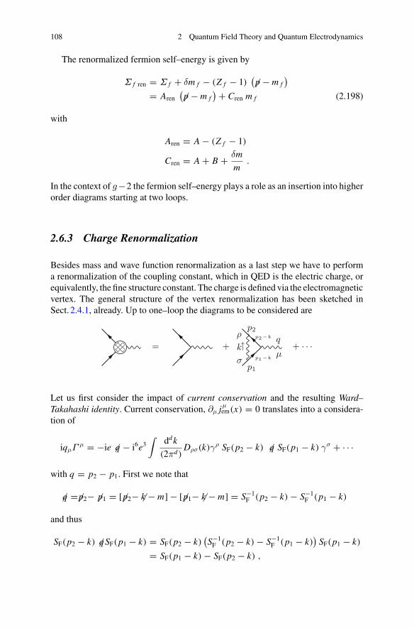
108 2 Quantum Field Theory and Quantum Electrodynamics

The renormalized fermion self–energy is given by

Σ f ren = Σ f + δm f − (Z f − 1)(�p − m f

)

= Aren(�p − m f

)+ Cren m f (2.198)

with

Aren = A − (Z f − 1)

Cren = A + B + δm

m.

In the context of g−2 the fermion self–energy plays a role as an insertion into higherorder diagrams starting at two loops.

2.6.3 Charge Renormalization

Besides mass and wave function renormalization as a last step we have to performa renormalization of the coupling constant, which in QED is the electric charge, orequivalently, the fine structure constant. The charge is defined via the electromagneticvertex. The general structure of the vertex renormalization has been sketched inSect. 2.4.1, already. Up to one–loop the diagrams to be considered are

= + + · · ·ρ

k

σp1

p2

μ

q

p1−k

p2−k

↑

Let us first consider the impact of current conservation and the resulting Ward–Takahashi identity. Current conservation, ∂μ jμ

em(x) = 0 translates into a considera-tion of

iqμΓμ = −ie �q − i6e3

∫ddk

(2πd)Dρσ(k)γρ SF(p2 − k) �q SF(p1 − k) γσ + · · ·

with q = p2 − p1. First we note that

�q =�p2− �p1 = [�p2− �k − m] − [�p1− �k − m] = S−1F (p2 − k)− S−1F (p1 − k)

and thus

SF(p2 − k) �q SF(p1 − k) = SF(p2 − k)(S−1F (p2 − k)− S−1F (p1 − k)

)SF(p1 − k)

= SF(p1 − k)− SF(p2 − k) ,

2.6 One–Loop Renormalization 109

which means that contracted with qμ the tree–point function reduces to a differenceof two two–point functions (self–energies). Therefore, for the non–trivial one–looppart, using (2.192) we obtain

iqμΓμ (1) = +e3

∫

kDρσ(k)γρ SF(p1 − k) γσ − e3

∫

kDρσ(k)γρ SF(p2 − k) γσ

= ie{Σ(1)(p2)−Σ(1)(p1)

}

which yields the electromagnetic Ward–Takahashi (WT) identity

qμΓμ(p2, p1) = −e ([�p2 − m −Σ(p2)] − [�p1 − m −Σ(p1)])

= −e(

S′−1F (p2)− S

′−1F (p1)

)(2.199)

which is the difference of the full inverse electron propagators. This relation can beshown easily to be true to all orders of perturbation theory. It has an important conse-quence for the renormalization of QED since it relates the vertex renormalization tothe one of the charge (factor e) and the multiplicative wave function renormalizationof the electron propagator. Combining the general form of the vertex renormaliza-tion (2.115) and S

′F0 = Ze S

′F ren with the bare form of the WT identity we obtain the

relationship

√Zγ ZeqμΓ

μ0 (p2, p1) = −e0

√Zγ Ze

(S′−1F0 (p2)− S

′−1F0 (p1)

)

= qμΓμren(p2, p1) = −e0

√Zγ

(S′−1F ren(p2)− S

′−1F ren(p1)

)

= −eren(

S′−1F ren(p2)− S

′−1F ren(p1)

).

We note that Ze dropped out from the renormalized relation and we obtain theWard–Takahashi identity

e0√

Zγ = eren or 1+ δe

e= 1√1+ δZγ

=√1+Π ′

γ(0) . (2.200)

The WT identity thus has the important consequence that the charge gets renor-malized only by the photon vacuum polarization! This fact will play a crucial rolelater, when we are going to evaluate the hadronic contributions to the effective finestructure constant.

Another important consequence of the WT identity (2.199) we obtain by takingthe limit qμ → 0:

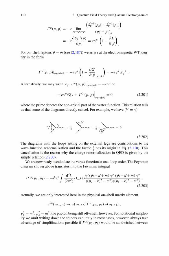
110 2 Quantum Field Theory and Quantum Electrodynamics

Γ μ(p, p) = −e limp2→p1=p

(S′−1F (p2)− S

′−1F (p1)

)

(p2 − p1)μ

= −e∂S

′−1F (p)

∂ pμ= eγμ

(1− ∂Σ

∂ �p)

.

For on–shell leptons �p = m (see (2.187)) we arrive at the electromagnetic WT iden-tity in the form

Γ μ(p, p)|on−shell = −eγμ

(1− ∂Σ

∂ �p∣∣∣∣ �p=m

)= −eγμ Z−1f .

Alternatively, we may write Z f Γ μ(p, p)|on−shell = −eγμ or

− eγμδZ f + Γ′μ(p, p)

∣∣∣on−shell

= 0 (2.201)

where the prime denotes the non–trivial part of the vertex function. This relation tellsus that some of the diagrams directly cancel. For example, we have (V = γ)

Vγ

+ 12

V+ 1

2 V= 0

(2.202)

The diagrams with the loops sitting on the external legs are contributions to thewave function renormalization and the factor 1

2 has its origin in Eq. (2.110). Thiscancellation is the reason why the charge renormalization in QED is given by thesimple relation (2.200).

We are now ready to calculate the vertex function at one–loop order. The Feynmandiagram shown above translates into the Feynman integral

iΓ μ(p2, p1) = −i6e3∫

ddk

(2πd)Dρσ(k)

γρ( �p2− �k + m) γμ ( �p1− �k + m) γσ

((p2 − k)2 − m2)((p1 − k)2 − m2).

(2.203)

Actually, we are only interested here in the physical on–shell matrix element

Γ μ(p2, p1) → u(p2, r2) Γ μ(p2, p1) u(p1, r1) ,

p21 = m2, p2

2 = m2, the photon being still off–shell, however. For notational simplic-ity we omit writing down the spinors explicitly in most cases, however, always takeadvantage of simplifications possible if Γ μ(p2, p1) would be sandwiched between

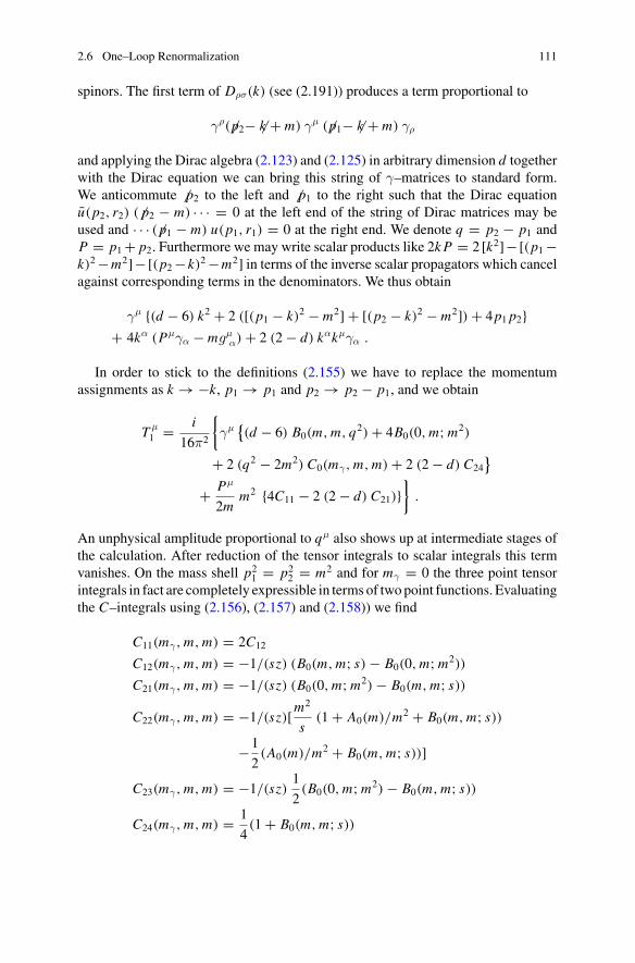
2.6 One–Loop Renormalization 111

spinors. The first term of Dρσ(k) (see (2.191)) produces a term proportional to

γρ( �p2− �k + m) γμ ( �p1− �k + m) γρ

and applying the Dirac algebra (2.123) and (2.125) in arbitrary dimension d togetherwith the Dirac equation we can bring this string of γ–matrices to standard form.We anticommute � p2 to the left and � p1 to the right such that the Dirac equationu(p2, r2) ( � p2 − m) · · · = 0 at the left end of the string of Dirac matrices may beused and · · · ( �p1 − m) u(p1, r1) = 0 at the right end. We denote q = p2 − p1 andP = p1+ p2. Furthermore we may write scalar products like 2k P = 2 [k2]−[(p1−k)2−m2]−[(p2−k)2−m2] in terms of the inverse scalar propagators which cancelagainst corresponding terms in the denominators. We thus obtain

γμ {(d − 6) k2 + 2 ([(p1 − k)2 − m2] + [(p2 − k)2 − m2])+ 4p1 p2}+ 4kα (Pμγα − mgμ

α)+ 2 (2− d) kαkμγα .

In order to stick to the definitions (2.155) we have to replace the momentumassignments as k →−k, p1 → p1 and p2 → p2 − p1, and we obtain

T μ1 =

i

16π2

{γμ{(d − 6) B0(m, m, q2)+ 4B0(0, m;m2)

+ 2 (q2 − 2m2) C0(mγ, m, m)+ 2 (2− d) C24}

+ Pμ

2mm2 {4C11 − 2 (2− d) C21)}

}.

An unphysical amplitude proportional to qμ also shows up at intermediate stages ofthe calculation. After reduction of the tensor integrals to scalar integrals this termvanishes. On the mass shell p2

1 = p22 = m2 and for mγ = 0 the three point tensor

integrals in fact are completely expressible in terms of twopoint functions. Evaluatingthe C–integrals using (2.156), (2.157) and (2.158)) we find

C11(mγ, m, m) = 2C12

C12(mγ, m, m) = −1/(sz) (B0(m, m; s)− B0(0, m;m2))

C21(mγ, m, m) = −1/(sz) (B0(0, m;m2)− B0(m, m; s))

C22(mγ, m, m) = −1/(sz)[m2

s(1+ A0(m)/m2 + B0(m, m; s))

−1

2(A0(m)/m2 + B0(m, m; s))]

C23(mγ, m, m) = −1/(sz)1

2(B0(0, m;m2)− B0(m, m; s))

C24(mγ, m, m) = 1

4(1+ B0(m, m; s))

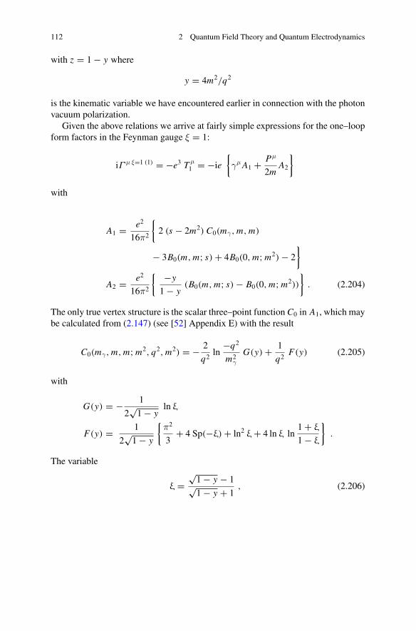
112 2 Quantum Field Theory and Quantum Electrodynamics

with z = 1− y where

y = 4m2/q2

is the kinematic variable we have encountered earlier in connection with the photonvacuum polarization.

Given the above relations we arrive at fairly simple expressions for the one–loopform factors in the Feynman gauge ξ = 1:

iΓ μ ξ=1 (1) = −e3 T μ1 = −ie

{γμ A1 + Pμ

2mA2

}

with

A1 = e2

16π2

{2 (s − 2m2) C0(mγ, m, m)

− 3B0(m, m; s)+ 4B0(0, m;m2)− 2

}

A2 = e2

16π2

{ −y

1− y(B0(m, m; s)− B0(0, m;m2))

}. (2.204)

The only true vertex structure is the scalar three–point function C0 in A1, which maybe calculated from (2.147) (see [52] Appendix E) with the result

C0(mγ, m, m;m2, q2, m2) = − 2

q2ln−q2

m2γ

G(y)+ 1

q2F(y) (2.205)

with

G(y) = − 1

2√1− y

ln ξ

F(y) = 1

2√1− y

{π2

3+ 4 Sp(−ξ)+ ln2 ξ+ 4 ln ξ ln

1+ ξ

1− ξ

}.

The variable

ξ =√1− y − 1√1− y + 1

, (2.206)

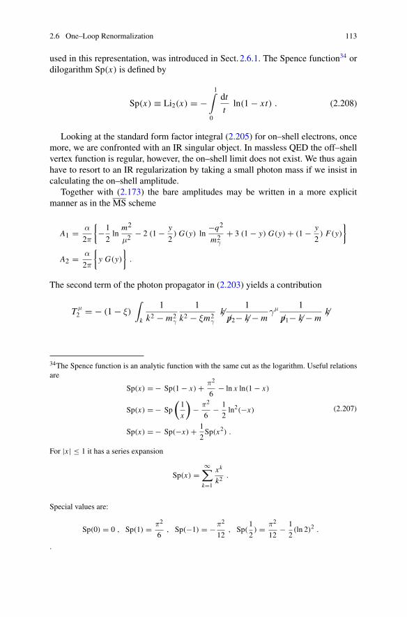
2.6 One–Loop Renormalization 113

used in this representation, was introduced in Sect. 2.6.1. The Spence function34 ordilogarithm Sp(x) is defined by

Sp(x) ≡ Li2(x) = −1∫

0

dt

tln(1− xt) . (2.208)

Looking at the standard form factor integral (2.205) for on–shell electrons, oncemore, we are confronted with an IR singular object. In massless QED the off–shellvertex function is regular, however, the on–shell limit does not exist. We thus againhave to resort to an IR regularization by taking a small photon mass if we insist incalculating the on–shell amplitude.

Together with (2.173) the bare amplitudes may be written in a more explicitmanner as in the MS scheme

A1 = α

2π

{−1

2ln

m2

μ2− 2 (1− y

2) G(y) ln

−q2

m2γ+ 3 (1− y) G(y)+ (1− y

2) F(y)

}

A2 = α

2π

{y G(y)

}.

The second term of the photon propagator in (2.203) yields a contribution

T μ2 = − (1− ξ)

∫

k

1

k2 − m2γ

1

k2 − ξm2γ

�k 1

�p2− �k − mγμ 1

�p1− �k − m�k

34The Spence function is an analytic function with the same cut as the logarithm. Useful relationsare

Sp(x) =− Sp(1− x)+ π2

6− ln x ln(1− x)

Sp(x) =− Sp

(1

x

)− π2

6− 1

2ln2(−x)

Sp(x) =− Sp(−x)+ 1

2Sp(x2) .

(2.207)

For |x | ≤ 1 it has a series expansion

Sp(x) =∞∑

k=1

xk

k2.

Special values are:

Sp(0) = 0 , Sp(1) = π2

6, Sp(−1) = −π2

12, Sp(

1

2) = π2

12− 1

2(ln 2)2 .

.

114 2 Quantum Field Theory and Quantum Electrodynamics

and for the on–shell vertex, applying the Dirac equation, one easily verifies that

u2 �k 1

�p2− �k − mγμ 1

�p1− �k − m�k u1 = u2 γμ u1

and hence this gauge dependent and UV divergent but q2 independent term onlycontributes to the amplitude A1 and is given by

iδΓ μ ξ �=1 (1) = −e3 T μ2 = −ieγμ Aξ �=1

1 = −ieγμ

(

− e2

16π2(1− ξ) B0(mγ ,

√ξmγ; 0)

)

.

(2.209)

This term exactly cancels against the gauge parameter dependent lepton part of thewave function renormalization (2.196):

⊗+

⊗= −ieγμδZe = −ieγμ

(e2

16π2 (1 − ξ) B0(mγ ,√

ξmγ ; 0))

.

In view of the discussion after (2.201), this cancellation is again a consequence ofthe WT identity. As it should be the gauge dependent term does not contribute toany physical amplitude after the appropriate wave function renormalization has beenapplied, i.e., the terms do not appear in the renormalized Dirac form factor A1. ThePauli form factor in any case is not affected, it is gauge invariant and UV finite andis not subject to renormalization.

In order to discuss charge renormalization, we have to write the form factors interms of the Dirac (electric) plus a Pauli (magnetic) term. This we may do with thehelp of the Gordon identity

u(p2)iσμνqν

2mu(p1) = u(p2)

(γμ − Pμ

2m

)u(p1) .

Starting from our form factor decomposition, which is more convenient from a cal-culational point of view, we obtain

iΓ μ(p2, p1) = −ie{γμ A10(q

2)+ Pμ

2mA20(q

2)

}

= −ie{γμ (A10 + A20) (q2)− iσμα qα

2mA20(q

2)}

= −ie{γμδFE(q

2)+ iσμα qα

2mFM(q2)

}.

Charge renormalization, according to (2.115), is fixed by the condition that eren = eat q2 = 0 (classical charge). We therefore have to require

2.6 One–Loop Renormalization 115

δFE ren(0) = A10(0)+ A20(0)+ δZe + 1

2δZγ + δe

e= 0 .

The complete Dirac form factor, including the tree level value is given by

FE ren(q2) = 1+ δFE ren(q

2) (2.210)

and satisfies the charge renormalization condition

FE ren(0) = 1 . (2.211)

However, the electromagnetic Ward–Takahashi identity (2.201) infers

A10 + A20 + δZe = 0

such that, in agreement with (2.200), the charge renormalization condition fixes thecharge counter term to the wave function renormalization constant of the photon

δe

e= −1

2δZγ = 1

2Π ′

γ(0) = −α

2π

1

3ln

m2

μ2(2.212)

with the explicit result given in the MS scheme Reg = ln μ2.As a result the renormalized one–loop virtual photon contributions to the lepton

electric (E) and magnetic (M) form factors read

δFE = (A10 + A20 + δZe)

= α

2π

{

lnm2

m2γ− (2− y) G(y) ln

−q2

m2γ− 2+ (3− 2y)G(y)+

(1− y

2

)F(y)

}

FM = −A20 = α

2π{−y G(y)} . (2.213)

In the scattering region q2 < 0 (y < 0) with 0 ≤ ξ ≤ 1 the form factors are real;in the production region q2 > 4m2 (0 < y < 1) with −1 ≤ ξ ≤ 0 we have animaginary part (using ln(ξ) = ln(−ξ)+ iπ, ln(−q2/m2 − iε) = ln(q2/m2)− iπ)

1

πIm FE = α

4π

1√1− y

{

(2− y) lnq2 − 4m2

m2γ

− 3+ 2y

}

1

πIm FM = α

4π

y√1− y

(2.214)

The Dirac form factor for q2 �= 0 (on–shell electron, off–shell photon) at this stage isstill IR singular in the limit of vanishing photon mass and cannot be physical. Before

116 2 Quantum Field Theory and Quantum Electrodynamics

we continue the discussion of the result we have to elaborate on the infrared problemin massless QED and the difficulties to define scattering states for charged particles.

However, the Pauli form factor, of primary interest to us turns out to be IR save. It isa perturbatively calculable quantity, which seems not to suffer from any of the usualproblems of gauge dependence, UV divergences and the related renormalizationscheme dependence. We thus are able to calculate the leading contribution to theanomalous magnetic moment without problems. The anomalous magnetic momentof a lepton is given by FM(0) where FM(q2) is given in (2.213). We hence have tocalculate −y G(y) for Q2 = −q2 > 0 and Q2 → 0 or y < 0 and |y| → ∞. Letz = −y = |y| and z be large; the expansion yields

√1− y = √z + 1 � √z

(1+ 1

2z+ · · ·

)

ln

√1− y − 1√1− y + 1

= ln

√z + 1− 1√z + 1+ 1

� − 2√z+ · · ·

and therefore

−y G(y)|−y→∞ = −z

2√

z + 1ln

√z + 1− 1√z + 1+ 1

∣∣∣∣∣z→∞

� 1+ O

(1√|y|

).

We thus arrive at

FM(0) = α

2π� 0.0011614 · · · (2.215)

which is Schwinger’s classic result for the anomalous magnetic moment of the elec-tron and which is universal for all charged leptons.

An important cross check of our calculation of FE is also possible at this stage.Namely, we may check directly the WT identity (2.201), which now reads δFE(0) =0. Taking the limit q2 → 0 for space–like momentum transfer q2 < 0, we mayuse the expansion just presented for calculating FM(0) = α/2π. For y < 0 and|y| → ∞ we have ξ ∼ 1 − 2/

√|y| and the somewhat involved expansion of F(y)

in (2.213) yields that yF(y) → 0 in this limit. Since−yG(y) → 1 we get preciselythe cancellations needed to prove δFE(q2) → 0 for q2 → 0.35 The leading term for|q2| � 4m2 reads

35One also may check this directly on the level of the standard scalar integrals A0, B0 and C0.Denoting by AA(m) = A0(m)/m2 we have

δFE(q2)q2→0∼ ∝ ([−4m2C0 − 3B0(m, m; 0)+ 4B0(0, m;m2)− 2]A1

+[B0(m, m; 0)− B0(0, m;m2)]A2 + [1+ AA(m)+ 4m2 B0(mγ , m;m2)]δZe

).

2.6 One–Loop Renormalization 117

δFE(q2) = α

3π

q2

m2

(ln

m

mγ− 3

8

)+ O(q4/m4)

and is IR singular and hence non–physical without including soft real photon emis-sion. The leading behavior of the form factors for large |q2| # m2 reads

δFE(q2) ∼ − α

2π

(1

2ln2|q2|m2

+ 2 lnm

mγln|q2|m2

− 2 lnm

mγ− 3

2ln|q2|m2

+ 2− π2

6

−Θ(q2 − 4m2)π2

2

)+Θ(q2 − 4m2) i

α

2

(

lnq2

m2γ

− 3

2

)

FM(q2) ∼ −α

π

m2

q2ln|q2|m2

+Θ(q2 − 4m2) iαm2

q2.

As in the examples discussed so far, often we will need to know the behavior ofFeynman amplitudes for large momenta or equivalently for small masses. The toolsfor estimating the asymptotic behavior of amplitudes are discussed next.

2.6.4 Dyson– and Weinberg–Power-Counting Theorems

Since, in momentum space, any amplitude may be obtained as a product of 1PIbuilding blocks, the vertex functions Γ (p1, · · · , pn), it is sufficient to know theasymptotic behavior of the latter. This behavior may be obtained by consideringthe contributions form individual Feynman integrals ΓG(p1, · · · , pn), the index Gdenoting the corresponding Feynman graph. As we know already from Sect. 2.4.2,power counting theorems play an important role for evaluating

1. the convergence of Feynman integrals (UV divergences),2. the behavior of Feynman amplitudes for large momenta.

Weinberg’s power-counting theorem is an extension of Dyson’s power–countingtheorem, and describes the off–shell behavior of vertex functions (amputated n–point functions with n ≥ 2)

(Footnote 35 continued)Using the relations

C0(mγ , m, m;m2, 0, m2) = −14m2

(B0(0, m;m2)− 1− AA(m)+ 2AA(mγ)

)

B0(m, m; 0) = −1− AA(m)

B0(0, m;m2) = 1− AA(m)

m2 B0(mγ , m;m2) = −1− 12 AA(mγ)+ 1

2 AA(m)

one easily finds that indeed δFE(q2)q2→0∼ 0. This kind of approach is usually utilizedwhenworking

with computer algebra methods.

118 2 Quantum Field Theory and Quantum Electrodynamics

Γ (p1, · · · , pn) =∑

GΓG(p1, · · · , pn)

for large pi (i = 1, . . . , m) in a subspace of the momenta

Γ (λp1, · · · ,λpm, pm+1, · · · , pn)λ→∞−→ ?

where (p1, · · · , pn) is a fixed set of momenta, 2 ≤ m ≤ n and λ a real positivestretching (dilatation) factor, which we are taking to go to infinity. The sum is overall possible Feynman graphs G which can contribute.

We first introduce some notions and notation. A set of external momenta (p1, · · · ,

pm) is called non-exceptional if no subsum of momenta vanishes, i.e., the set isgeneric. The set of external lines which carry momenta going to infinity is denotedby E∞. By appropriate relabeling of the momenta we may always achieve that thefirst m of the momenta are the ones which go to infinity. Primarily the power count-ing theorems hold in the Euclidean region (after Wick-rotation) or in the Minkowskiregion for space–like momenta, which will be sufficient for our purpose. Also formassless theories there may be additional complications [60].

Dyson’s power-counting theorem [61] states that

Theorem 2.9 For all non-exceptional sets of momenta when all momenta are goingto infinity a vertex function behaves as

Γ (λp1, · · · ,λpn) = O(λαΓ (ln λ)βΓ ) ; λ →∞ ,

where αΓ = maxG∈G

d(G) with d(G) the superficial degree of divergence of a diagram

G, and G the set of diagrams which contribute to Γ (p1, · · · , pn).

d(G) has been introduced in Sect. 2.4.2. The asymptotic coefficient βΓ giving theleading power of the logarithm may also be characterized in terms of diagrams [62],but will not be discussed here as we will need the asymptotic behavior modulo loga-rithms only. For an individual 1PI diagramG theDyson power-counting theorem saysthat provided all momenta go to infinity, and the set of momenta is non-exceptionalthe behavior is determined by the superficial degree of divergence d(G) of the cor-responding diagram. The crucial point is that in a renormalizable theory d(G) isindependent of the particular graph G and given by the dimension of the vertex func-tion dimΓ which only depends on type and number of external legs as discussedbefore in Sect. 2.4.2. In fact, in d = 4 dimensions,

Γ (λp1, · · · ,λpn) = O(λ4−b− 32 f (ln λ)�) .

with b = nB the number of boson lines and f = nF the number of fermion lines. � isa non-negative integer depending on the order of perturbation theory. Its maximumpossible value � ≤ L is given by the number L of loops.

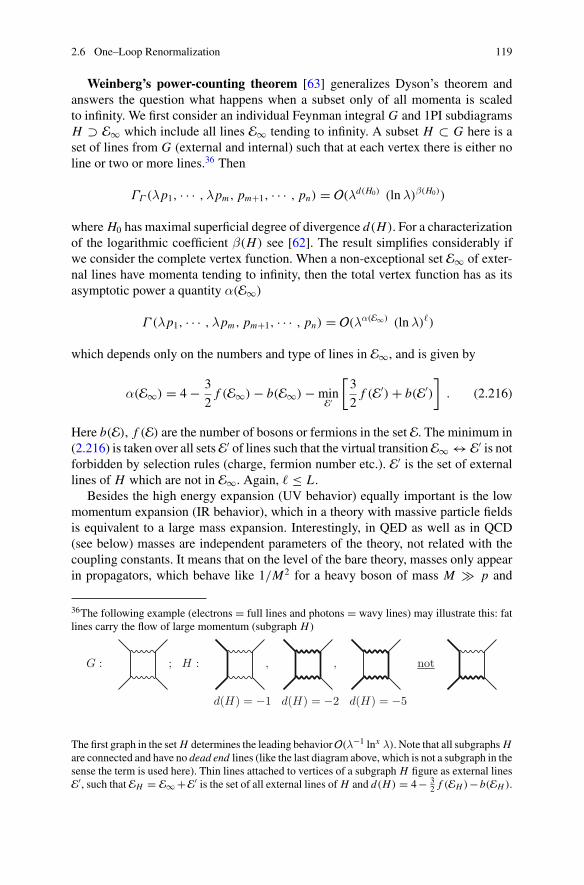
2.6 One–Loop Renormalization 119

Weinberg’s power-counting theorem [63] generalizes Dyson’s theorem andanswers the question what happens when a subset only of all momenta is scaledto infinity. We first consider an individual Feynman integral G and 1PI subdiagramsH ⊃ E∞ which include all lines E∞ tending to infinity. A subset H ⊂ G here is aset of lines from G (external and internal) such that at each vertex there is either noline or two or more lines.36 Then

ΓΓ (λp1, · · · ,λpm, pm+1, · · · , pn) = O(λd(H0) (ln λ)β(H0))

where H0 has maximal superficial degree of divergence d(H). For a characterizationof the logarithmic coefficient β(H) see [62]. The result simplifies considerably ifwe consider the complete vertex function. When a non-exceptional set E∞ of exter-nal lines have momenta tending to infinity, then the total vertex function has as itsasymptotic power a quantity α(E∞)

Γ (λp1, · · · ,λpm, pm+1, · · · , pn) = O(λα(E∞) (ln λ)�)

which depends only on the numbers and type of lines in E∞, and is given by

α(E∞) = 4− 3

2f (E∞)− b(E∞)−min

E′

[3

2f (E′)+ b(E′)

]. (2.216)

Here b(E), f (E) are the number of bosons or fermions in the set E. The minimum in(2.216) is taken over all sets E′ of lines such that the virtual transitionE∞ ↔ E′ is notforbidden by selection rules (charge, fermion number etc.). E′ is the set of externallines of H which are not in E∞. Again, � ≤ L .

Besides the high energy expansion (UV behavior) equally important is the lowmomentum expansion (IR behavior), which in a theory with massive particle fieldsis equivalent to a large mass expansion. Interestingly, in QED as well as in QCD(see below) masses are independent parameters of the theory, not related with thecoupling constants. It means that on the level of the bare theory, masses only appearin propagators, which behave like 1/M2 for a heavy boson of mass M # p and

36The following example (electrons = full lines and photons = wavy lines) may illustrate this: fatlines carry the flow of large momentum (subgraph H )

G : ; H : , , not

d(H) = −1 d(H) = −2 d(H) = −5

The first graph in the set H determines the leading behaviorO(λ−1 lnx λ). Note that all subgraphs Hare connected and have no dead end lines (like the last diagram above, which is not a subgraph in thesense the term is used here). Thin lines attached to vertices of a subgraph H figure as external linesE′, such that EH = E∞+E′ is the set of all external lines of H and d(H) = 4− 3

2 f (EH )−b(EH ).

120 2 Quantum Field Theory and Quantum Electrodynamics

like 1/M for a heavy Dirac fermion of mass M # p. However, in loop integrals wecannot simply interchange limits M →∞with p →∞ as the O(1/p2) behavior ofa boson propagator or a O(1/p) behavior of a fermion propagator are crucial for theconvergence of the loop integrals. Indeed masses in general affect renormalizationcounterterms as we have seen in our one–loop renormalization calculations above.However, these residual mass effects drop out after renormalization (subtraction ofthe potentialUVsingularities). The property that very heavy particles do not affect thephysics atmuch lower scales is called “decoupling” (of the heavy states), which looksto be a natural property of physics in general. Surprisingly, in the weak interactionsector of the electroweak SM decoupling is no longer true as masses and couplingsare interrelated (mass generation via the Higgs mechanism, see below). Thus in thebroken phase of the SM decoupling only holds in the QCD and QED sectors, andthere is controlled by the Appelquist-Carazzone decoupling theorem [64].

Theorem 2.10 If all external momenta of a process or in the corresponding ampli-tude are small relative to the mass M of a heavy state, then the “light fields only”Green functions of the full theory differ from the theory which has no heavy fields atall, only by finite renormalizations of couplings, masses and fields of the light theory,up to terms which are suppressed by inverse powers of the heavy mass. Thus furthercorrections are of the form (μ/M)x with x ≥ 1.

It means that only the renormalization subtraction constants are dependent on M(logarithms) and this M–dependence gets renormalized away by physical subtractionconditions. The decoupling theorem is the root of the famous δa� ∝ m2

�/M2 behavior(1.9) of the lepton anomalies, and plays an important role in the classification of thevarious types of contributions to ae and aμ, as we will see.

For useful refinements of asymptotic expansion theorems in momenta and massessee e.g. [65] and references therein. Another tool to study the asymptotic behaviorof Green- or vertex-functions is the renormalization group which we will considernext and in particular allows us to control effects due to the large UV logarithms.

2.6.5 The Running Charge and the Renormalization Group

Charge renormalization is governed by a renormalization group [66] (RG), whichcontrols the response of the theory with respect to a change of the renormalizationscale parameter μ in the MS scheme, like for example in the charge renormaliza-tion according to (2.212). It gives rise to the definition of an effective or runningcharge α(μ) and running mass m(μ) as a function of the renormalization scale μ.However, the RG not only governs the dependence of a renormalized QFT on therenormalization scale, it yields the behavior of the theory with respect to dilata-tions, the simultaneous stretching of all momenta, and hence allows one to discussthe asymptotic behavior for small and large momenta. The RG serves as a tool tosystematically include large logarithmic radiative corrections, in fact, it permits theresummation to all orders of the perturbation expansion, of leading logarithms (LL),

2.6 One–Loop Renormalization 121

next to leading logarithms (NLL) etc. It thus allows us to estimate leading radiativecorrections of higher order without the need to actually perform elaborate calcula-tions, under the condition that large scale changes are involved. Besides the all ordersDyson summation of self–energy corrections and the soft photon exponentiation tobe discussed in the next section, the RG is a third method which allows us to predictleading higher order corrections from low order calculations. The RG generalizes theclassical concept of dimensional analysis to QFT, where renormalization anomaliesof the dilatation current [67] lead to a breaking of dilatation invariance by quantumeffects (see Sect. 5.1.6 footnote on p. 375).

The RGmay be obtained by starting from the bare vertex functions (the amputatedGreen functions) mentioned already briefly in Sect. 2.4.2. Note that the renormal-ization scale parameter μ is entering in DR by the fact that in the d–dimensionalQFT the bare coupling constant e0 must have a dimension 4−d

2 , i.e., e0 = e0με/2 withe0 dimensionless (see (2.118)). This gives rise to the factors μ4−d in the definitionsof the standard integrals in Sect. 2.5.6 when working with the dimensionless barecoupling e0. As a result the μ dependence formally comes in via the UV regulatorterm (2.145). Since μ only enters via the bare coupling e0 all bare quantities, like thevertex function Γ0, at fixed e0 are independent of μ:

μdΓ0

dμ

∣∣∣∣e0

≡ 0 . (2.217)

The bare vertex functions in d = 4− ε dimensions

Γ(n A,2nψ)

0 ({p}; e0, m0, ξ0)ε

are homogeneous under simultaneous dilatation of all momenta and all dimensionfulparameters including the scale μ. According to (2.119) we have

Γ(n A,2nψ)

0

({κp}; e0 (κμ)ε/2,κm0, ξ0) = κdimΓ Γ

(n A,2nψ)

0

({p}; e0 (μ)ε/2, m0, ξ0)

(2.218)

with

dimΓ = d − n Ad − 2

2− 2nψ

d − 1

2.

The renormalized vertex functions are obtained by renormalizing parameters andfields: A0 = √Z A Ar , ψ0 =

√Zψψr , e0 = Zger and m0 = Zmmr and thus

Γ(n A,2nψ)

0 ({p}; e0, m0, ξ0)ε = (Z A)− n A

2ε

(Zψ

)−nψ

εΓ

(n A,2nψ)ren ({p}; er , mr , ξr ,μ)ε

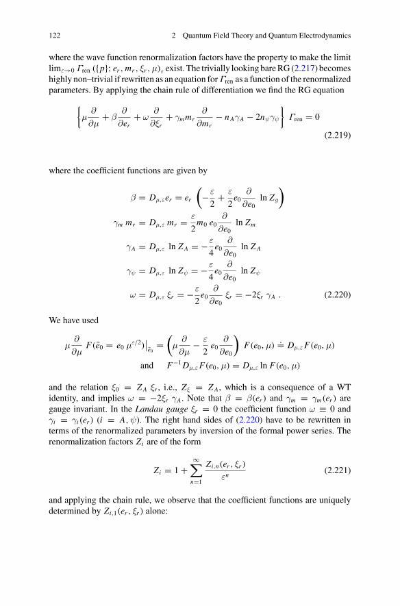
122 2 Quantum Field Theory and Quantum Electrodynamics

where the wave function renormalization factors have the property to make the limitlimε→0 Γren ({p}; er , mr , ξr ,μ)ε exist. The trivially looking bareRG (2.217) becomeshighly non–trivial if rewritten as an equation forΓren as a function of the renormalizedparameters. By applying the chain rule of differentiation we find the RG equation

{μ

∂

∂μ+ β

∂

∂er+ ω

∂

∂ξr+ γmmr

∂

∂mr− n AγA − 2nψγψ

}Γren = 0

(2.219)

where the coefficient functions are given by

β = Dμ,εer = er

(−ε

2+ ε

2e0

∂

∂e0ln Zg

)

γm mr = Dμ,ε mr = ε

2m0 e0

∂

∂e0ln Zm

γA = Dμ,ε ln Z A = −ε

4e0

∂

∂e0ln Z A

γψ = Dμ,ε ln Zψ = −ε

4e0

∂

∂e0ln Zψ

ω = Dμ,ε ξr = −ε

2e0

∂

∂e0ξr = −2ξr γA . (2.220)

We have used

μ∂

∂μF(e0 = e0 με/2)

∣∣e0=(

μ∂

∂μ− ε

2e0

∂

∂e0

)F(e0,μ)

.= Dμ,εF(e0,μ)

and F−1Dμ,εF(e0,μ) = Dμ,ε ln F(e0,μ)

and the relation ξ0 = Z A ξr , i.e., Zξ = Z A, which is a consequence of a WTidentity, and implies ω = −2ξr γA. Note that β = β(er ) and γm = γm(er ) aregauge invariant. In the Landau gauge ξr = 0 the coefficient function ω ≡ 0 andγi = γi (er ) (i = A,ψ). The right hand sides of (2.220) have to be rewritten interms of the renormalized parameters by inversion of the formal power series. Therenormalization factors Zi are of the form

Zi = 1+∞∑

n=1

Zi,n(er , ξr )

εn(2.221)

and applying the chain rule, we observe that the coefficient functions are uniquelydetermined by Zi,1(er , ξr ) alone:

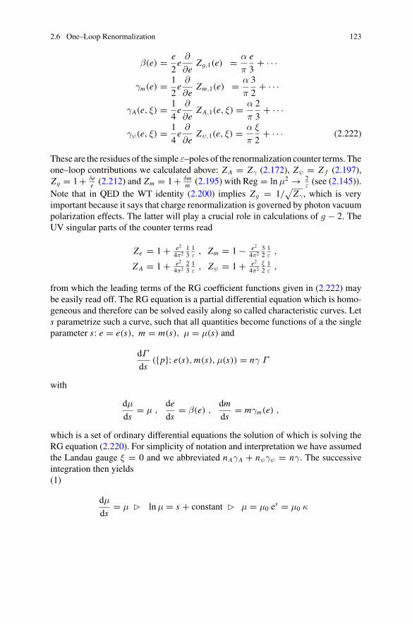
2.6 One–Loop Renormalization 123

β(e) = e

2e

∂

∂eZg,1(e) = α

π

e

3+ · · ·

γm(e) = 1

2e

∂

∂eZm,1(e) = α

π

3

2+ · · ·

γA(e, ξ) = 1

4e

∂

∂eZ A,1(e, ξ) = α

π

2

3+ · · ·

γψ(e, ξ) = 1

4e

∂

∂eZψ,1(e, ξ) = α

π

ξ

2+ · · · (2.222)

These are the residues of the simple ε–poles of the renormalization counter terms. Theone–loop contributions we calculated above: Z A = Zγ (2.172), Zψ = Z f (2.197),Zg = 1+ δe

e (2.212) and Zm = 1+ δmm (2.195) with Reg = ln μ2 → 2

ε(see (2.145)).

Note that in QED the WT identity (2.200) implies Zg = 1/√

Zγ , which is veryimportant because it says that charge renormalization is governed by photon vacuumpolarization effects. The latter will play a crucial role in calculations of g − 2. TheUV singular parts of the counter terms read

Ze = 1+ e2

4π2131ε

, Zm = 1− e2

4π2321ε

,

Z A = 1+ e2

4π2231ε

, Zψ = 1+ e2

4π2ξ21ε

,

from which the leading terms of the RG coefficient functions given in (2.222) maybe easily read off. The RG equation is a partial differential equation which is homo-geneous and therefore can be solved easily along so called characteristic curves. Lets parametrize such a curve, such that all quantities become functions of a the singleparameter s: e = e(s), m = m(s), μ = μ(s) and

dΓ

ds({p}; e(s), m(s),μ(s)) = nγ Γ

with

dμ

ds= μ ,

de

ds= β(e) ,

dm

ds= mγm(e) ,

which is a set of ordinary differential equations the solution of which is solving theRG equation (2.220). For simplicity of notation and interpretation we have assumedthe Landau gauge ξ = 0 and we abbreviated n AγA + nψγψ = nγ. The successiveintegration then yields(1)

dμ

ds= μ � ln μ = s + constant � μ = μ0 e

s = μ0 κ

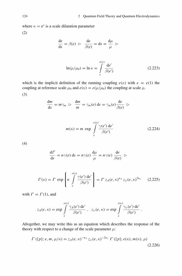
124 2 Quantum Field Theory and Quantum Electrodynamics

where κ = es is a scale dilatation parameter

(2)

de

ds= β(e) � de

β(e)= ds = dμ

μ�

ln(μ/μ0) = ln κ =e(κ)∫

e

de′

β(e′)(2.223)

which is the implicit definition of the running coupling e(κ) with e = e(1) thecoupling at reference scale μ0 and e(κ) = e(μ/μ0) the coupling at scale μ.

(3)

dm

ds= mγm � dm

m= γm(e) ds = γm(e)

de

β(e)�

m(κ) = m exp

e(κ)∫

e

γ(e′) de′

β(e′)(2.224)

(4)

dΓ

ds= nγ(e) ds = nγ(e)

dμ

μ= nγ(e)

de

β(e)�

Γ (κ) = Γ exp

⎧⎨

⎩n

e(κ)∫

e

γ(e′) de′

β(e′)

⎫⎬

⎭= Γ z A(e,κ)n A zψ(e,κ)2nψ (2.225)

with Γ = Γ (1), and

z A(e,κ) = exp

e(κ)∫

e

γA(e′) de′

β(e′), zψ(e,κ) = exp

e(κ)∫

e

γψ(e′) de′

β(e′).

Altogether, we may write this as an equation which describes the response of thetheory with respect to a change of the scale parameter μ:

Γ ({p}; e, m,μ/κ) = z A(e,κ)−n A zψ(e,κ)−2nψ Γ ({p}; e(κ), m(κ),μ)

(2.226)

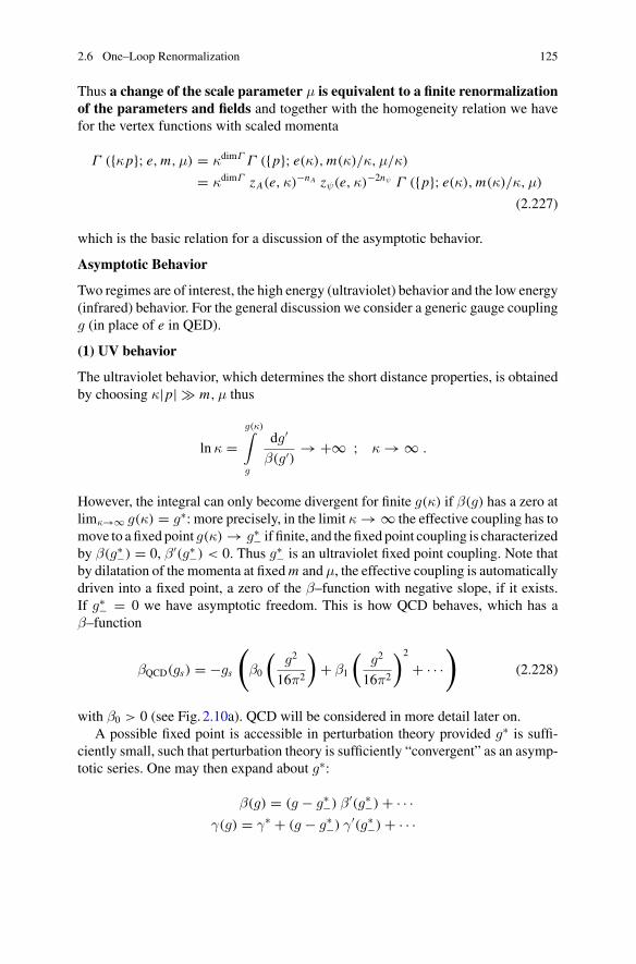
2.6 One–Loop Renormalization 125

Thus a change of the scale parameter μ is equivalent to a finite renormalizationof the parameters and fields and together with the homogeneity relation we havefor the vertex functions with scaled momenta

Γ ({κp}; e, m,μ) = κdimΓ Γ ({p}; e(κ), m(κ)/κ,μ/κ)

= κdimΓ z A(e,κ)−n A zψ(e,κ)−2nψ Γ ({p}; e(κ), m(κ)/κ,μ)

(2.227)

which is the basic relation for a discussion of the asymptotic behavior.

Asymptotic Behavior

Two regimes are of interest, the high energy (ultraviolet) behavior and the low energy(infrared) behavior. For the general discussion we consider a generic gauge couplingg (in place of e in QED).

(1) UV behavior

The ultraviolet behavior, which determines the short distance properties, is obtainedby choosing κ|p| # m,μ thus

ln κ =g(κ)∫

g

dg′

β(g′)→+∞ ; κ →∞ .

However, the integral can only become divergent for finite g(κ) if β(g) has a zero atlimκ→∞ g(κ) = g∗: more precisely, in the limit κ →∞ the effective coupling has tomove to a fixed point g(κ) → g∗− if finite, and the fixed point coupling is characterizedby β(g∗−) = 0, β′(g∗−) < 0. Thus g∗− is an ultraviolet fixed point coupling. Note thatby dilatation of the momenta at fixed m and μ, the effective coupling is automaticallydriven into a fixed point, a zero of the β–function with negative slope, if it exists.If g∗− = 0 we have asymptotic freedom. This is how QCD behaves, which has aβ–function

βQCD(gs) = −gs

(

β0

(g2

16π2

)+ β1

(g2

16π2

)2

+ · · ·)

(2.228)

with β0 > 0 (see Fig. 2.10a). QCD will be considered in more detail later on.A possible fixed point is accessible in perturbation theory provided g∗ is suffi-

ciently small, such that perturbation theory is sufficiently “convergent” as an asymp-totic series. One may then expand about g∗:

β(g) = (g − g∗−) β′(g∗−)+ · · ·γ(g) = γ∗ + (g − g∗−) γ′(g∗−)+ · · ·

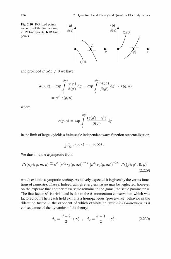
126 2 Quantum Field Theory and Quantum Electrodynamics

Fig. 2.10 RG fixed pointsare zeros of the β–function:a UV fixed points, b IR fixedpoints

β(g)

g

g∗−

→ ←

QCD

β(g)

gg∗+

→ ←

QED

(a) (b)

and provided β′(g∗−) �= 0 we have

a(g,κ) = exp

g(κ)∫

g

γ(g′)β(g′)

dg′ = exp

g(κ)∫

g

γ(g∗−)

β(g′)dg′ · r(g,κ)

= κγ∗ r(g,κ)

where

r(g,κ) = exp

g(κ)∫

g

(γ(g′)− γ∗)β(g′)

dg′

in the limit of large κ yields a finite scale independent wave function renormalization

limκ→∞ r(g,κ) = r(g,∞) .

We thus find the asymptotic from

Γ ({κp}; g, m,μ)→∼ κd

(κdA rA(g,∞)

)−n A(κdψ rψ(g,∞)

)−2nψΓ ({p}; g∗−, 0,μ)

(2.229)

which exhibits asymptotic scaling. As naively expected it is given by the vertex func-tions of amassless theory. Indeed, at high energiesmassesmay be neglected, howeveron the expense that another mass scale remains in the game, the scale parameter μ.The first factor κd is trivial and is due to the d–momentum conservation which wasfactored out. Then each field exhibits a homogeneous (power–like) behavior in thedilatation factor κ, the exponent of which exhibits an anomalous dimension as aconsequence of the dynamics of the theory:

dA = d − 2

2+ γ∗A , dψ = d − 1

2+ γ∗ψ . (2.230)

2.6 One–Loop Renormalization 127

The first term is the naive or engineers dimension the second part is the anomalouspart which is a quantum effect, a relict of the breaking of scale invariance, wheng �= g∗. While naively we would expect that in d = 4 dimensions the masslesstheory has scaling: for example a scalar two–point function, the only dimensionfulphysical quantity being the momentum, one would expect G(p; g) ∼ 1/p2 as G hasdimension 2. However, if there would be a non–trivial UVfixed point onewould haveG(p, g,μ) ∼ (μ2)γ

∗/(p2)1+γ∗ (γ∗ > 0) which shows the role and unavoidability of

the scale parameter μ, which has to eat up the extra dimension γ∗ induced by thedynamics of the theory. Otherwise only truly free theories could have scaling, calledcanonical scaling in this case. The discovery of asymptotic freedom of QCD [36] isthe prime example of a dynamical theory, nota bene of the theory of strong interac-tions, exhibiting asymptotic canonical scaling (Bjorken scaling) of liberated quarks(quark partonmodel) [68]. The latter was discovered before in the pioneering investi-gations concerning Deep Inelastic Scattering (DIS) [69] of electrons on protons andbound neutrons by Friedman, Kendall and Taylor (Nobel prize 1990). These exper-iments have been of essential importance for the development of the quark modeland to the discovery of QCD as the theory of the strong interactions.

(2) IR behavior

The infrared behavior corresponds to the long distance properties of a system. Herethe regime of interest is κ|p| � m,μ and the discussion proceeds essentially asbefore: now as κ → 0 the effective g(κ) → g∗+ where g∗+ is a zero of the β–functionwith positive slope, see Fig. 2.10b, β(g∗+) = 0 and β′(g∗+) > 0. This is the typicalsituation in the construction of low energy effective theories, particularly in thediscussion of critical phenomena of statistical systems (keywords: critical behavior,critical exponents, scaling laws, universality). If g∗+ = 0 the effective theory isinfrared free (the opposite of asymptotic freedom), also called Gaussian (Gaussianfixed point). Here the well known examples are QED

βQED(e) = e3

12π2

∑

f

Ncf Q2f + · · · (2.231)

or the self–interacting scalar field φ4–theory

β(λ) = −ελ+ 3λ2

16π2+ · · ·

in d = 4 dimensions. For QED the running coupling to leading order thus followsfrom

ln κ =e(κ)∫

e

1

β(e′)de′ = 12π2

∑f Ncf Q2

f

e(κ)∫

e

1

(e′)3de′ = 24π2

∑f Ncf Q2

f

(1

e2− 1

e(κ)2

)

128 2 Quantum Field Theory and Quantum Electrodynamics

where the sum extends over all light flavors f : m f < μ.37 The running fine structureconstant thus at leading order is given by

α(μ) = α

1− 2α3π

∑f Ncf Q2

f ln μ/μ0(2.232)

where μ0 is the scale where the lightest particle starts to contribute, which is theelectron μ0 = me. We then may identify α(μ0) = α the classical low energy valueof the fine structure constant, with the proviso that only logarithmic accuracy is takeninto account (see below). The running α is equivalent to the Dyson summation ofthe transversal part of the photon self–energy to the extent that only the logs arekept. The RG running takes into account the leading radiative corrections in the casethe logs are dominating over constant terms, i.e., provided large scale changes areinvolved.

In the calculation of the contributions from electron loops in photon propagatorsto the muon anomaly aμ, such large scale changes from me to mμ are involved andindeed one may calculate such two–loop contributions starting from the lowest orderresult

a(2)μ = α

2πvia the substitution α → α(mμ) (2.233)

where

α(mμ) = α

1− 23

απln mμ

me

= α

(1+ 2

3

α

πln

mμ

me+ · · ·

)(2.234)

such that we find

a(4) LLμ (vap, e) = 1

3ln

mμ

me

(α

π

)2

which indeed agrees with the leading log result obtained in [70] long time ago by adirect calculation. Themethod has been further developed and refined byLautrup andde Rafael [71]. In the calculation of aμ only the electron VP insertions are governedby the RG and the corresponding one–flavor QED β–function has been calculatedto three loops

β(α) = 2

3

(α

π

)+ 1

2

(α

π

)2 − 121

144

(α

π

)3 + · · · (2.235)

37This latter restriction takes into account the decoupling of heavy flavors, valid in QED and QCD.Since in the MS scheme, i.e., renormalization by the substitution Reg → ln μ2, which we areconsidering here, decoupling is not automatic, one has to impose it by hand. At a given scale oneis thus considering an effective theory, which includes only those particles with masses below thescale μ.

2.6 One–Loop Renormalization 129

long time ago by [72], which thus allows us to calculate leading αn (lnmμ/me)n ,

next–to–leading αn (lnmμ/me)n−1 and next–to–next–to–leading αn (lnmμ/me)

n−2log corrections. At present β(α) is known to five loops [73, 74] which allows one tocalculate leading log aμ contributions to six loops [75].

As α(μ) is increasing with μ, at some point this resummed effective coupling(2.232) exhibits a pole, the so called Landau pole at which the coupling becomesinfinite: lim

μ<→μL

α(μ) = ∞ . The “fixed point” very likely is an artifact of per-turbation theory, which of course ceases to be valid when the one–loop correctionapproaches 1. What this tells us is that we actually do not know what the high energyasymptotic behavior of QED is. This is in contrast to QCD, which exhibits the highenergy asymptotic behavior of a free (non-interacting) field theory, which means thatperturbation theory gets the better the higher the energy,

α in the on–shell versus α in the MS scheme

In our discussion of renormalizing QEDwe were considering originally the on–shellrenormalization scheme, while the RG providesα in theMS scheme. Here we brieflydiscuss the relationship between the OS and theMS fine structure constantsαOS = αand αMS, respectively. Since the bare fine structure constant

α0 = αMS

(1+ δα

α

∣∣∣∣MS

)= αOS

(1+ δα

α

∣∣∣∣OS

)(2.236)

is independent of the renormalization scheme. The one–loop calculation in the SMyields (including the charged W contribution for completeness)

δα

α

∣∣∣∣MS

= α

3π

∑Q2

f Ncf lnμ2

m2f

− α

3π

21

4ln

μ2

M2W

δα

α

∣∣∣∣OS

= Π ′γ(0)+

α

πln

M2W

μ2

= δα

α

∣∣∣∣MS

− α

6π

and thus

α−1MS

(0) = α−1 + 1

6π(2.237)

as a low energy matching condition. The α–shift in the MS scheme is very simple,just the UV logs,

ΔαMS(μ) = α

3π

∑Q2

f Ncf lnμ2

m2f

− α

3π

21

4ln

μ2

M2W

(2.238)

130 2 Quantum Field Theory and Quantum Electrodynamics

such that

ΔαMS(μ) = ΔαOS(μ)+ α

3π

5

3

∑Q2

f Ncf (2.239)

where the sum goes over all fermions f with Ncf = 1 for leptons and Ncf = 3 forquarks.

In perturbation theory, the leading light fermion (m f � MW ,√

s) contributionin the OS scheme is given by

Δα(s) = α

3π

∑

f

Q2f Ncf

(

lns

m2f

− 5

3

)

. (2.240)

We distinguish the contributions from the leptons, for which the perturbative expres-sion is appropriate, the five light quarks (u, d, s, c, b) and the top

Δα = Δαlep +Δαhad +Δαtop . (2.241)

Since the top quark is heavy we cannot use the light fermion approximation for it. Avery heavy top in fact decouples like

Δαtop � − α

3π

4

15

s

m2t→ 0

whenmt # s. Since pQCD does not apply at low energies,Δαhad has to be evaluatedvia dispersion relations from e+e−–annihilation data.

Note that in d = 4 dimensions both for QCD and QED very likely there is no RGfixed point at finite value of g except g = 0, which always is a fixed point, either aUV one (QCD) or an IR one (QED). In QCD this could mean that αs(μ) →∞ forμ → 0 (infrared slavery, confinement). In perturbation theory a Landau pole showsup at finite scale ΛQCD when coming from higher energy scales, where αs →∞ for

μ>→ ΛQCD. In QED likely α(μ) →∞ for μ →∞.It is important to emphasize that the RG only accounts for the UV logarithms,

which in DR are related to the UV poles in d = 4 − ε dimensions. Large logs mayalso be due to IR singular behavior, like the terms proportional to lnmγ which wehave regulated with an infinitesimally small photon mass in the on–shell lepton wavefunction renormalization factor Zψ = Z f (2.197). In spite of the fact that this termappears in the UV renormalization counter term, it has nothing to do with a UV sin-gularity and does not contribute in the RG coefficients. In DR also IR singularitiesmay be regularized by analytic continuation in d, however, by dimensional contin-uation to d = 4 + εIR, and corresponding IR poles at negative εUV. Also the termsproportional to ln −q2

m2γshowing up in the electric form factor (2.213) is not covered

by the RG analysis. As will be explained in the next section, the IR singularitieshave their origin in the attempt to define free charged particle states as simple iso-

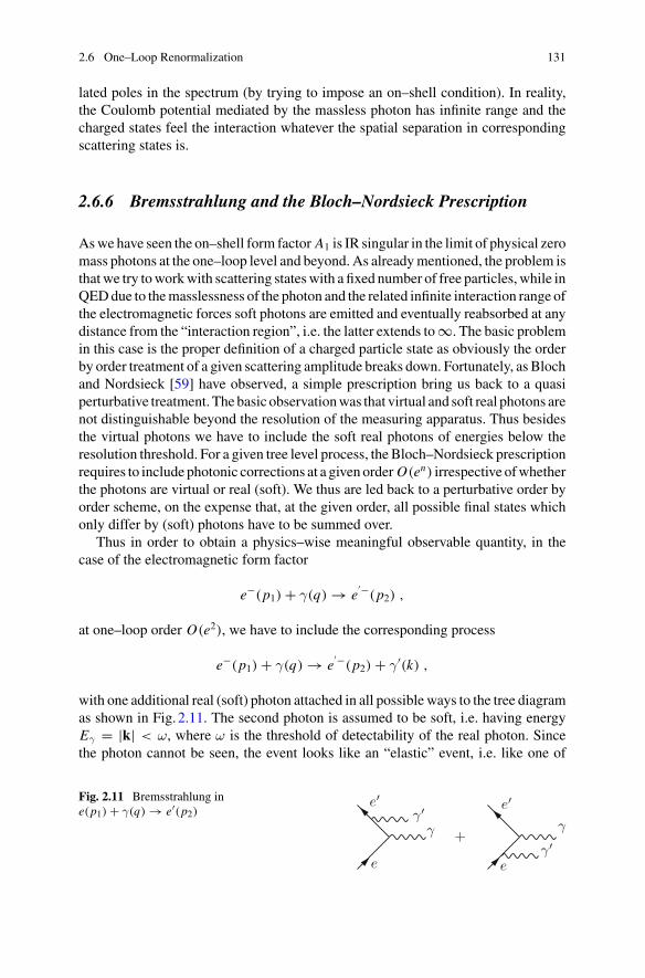
2.6 One–Loop Renormalization 131

lated poles in the spectrum (by trying to impose an on–shell condition). In reality,the Coulomb potential mediated by the massless photon has infinite range and thecharged states feel the interaction whatever the spatial separation in correspondingscattering states is.

2.6.6 Bremsstrahlung and the Bloch–Nordsieck Prescription

Aswe have seen the on–shell form factor A1 is IR singular in the limit of physical zeromass photons at the one–loop level and beyond. As alreadymentioned, the problem isthatwe try toworkwith scattering stateswith a fixed number of free particles, while inQEDdue to themasslessness of the photon and the related infinite interaction range ofthe electromagnetic forces soft photons are emitted and eventually reabsorbed at anydistance from the “interaction region”, i.e. the latter extends to∞. The basic problemin this case is the proper definition of a charged particle state as obviously the orderby order treatment of a given scattering amplitude breaks down. Fortunately, as Blochand Nordsieck [59] have observed, a simple prescription bring us back to a quasiperturbative treatment. Thebasic observationwas that virtual and soft real photons arenot distinguishable beyond the resolution of the measuring apparatus. Thus besidesthe virtual photons we have to include the soft real photons of energies below theresolution threshold. For a given tree level process, the Bloch–Nordsieck prescriptionrequires to include photonic corrections at a given order O(en) irrespective ofwhetherthe photons are virtual or real (soft). We thus are led back to a perturbative order byorder scheme, on the expense that, at the given order, all possible final states whichonly differ by (soft) photons have to be summed over.

Thus in order to obtain a physics–wise meaningful observable quantity, in thecase of the electromagnetic form factor

e−(p1)+ γ(q) → e′−(p2) ,

at one–loop order O(e2), we have to include the corresponding process

e−(p1)+ γ(q) → e′−(p2)+ γ′(k) ,

with one additional real (soft) photon attached in all possible ways to the tree diagramas shown in Fig. 2.11. The second photon is assumed to be soft, i.e. having energyEγ = |k| < ω, where ω is the threshold of detectability of the real photon. Sincethe photon cannot be seen, the event looks like an “elastic” event, i.e. like one of

Fig. 2.11 Bremsstrahlung ine(p1)+ γ(q) → e′(p2)

γγ′

e

e′

+γ

γ′e

e′

132 2 Quantum Field Theory and Quantum Electrodynamics

the same final state as the tree level process. The soft photons thus factorize intothe Born term of the original process times a soft photon correction, with the softphotons integrated out up to energy ω. The correction given by the bremsstrahlungcross section is proportional to the square |Tbre|2 of the sum of the matrix elementsof the two diagrams which reads

Tbre = i3e2u(p2)

{γρ �p2+ �k + m

(p2 + k)2 − m2γμ + γμ �p1− �k + m

(p1 − k)2 − m2γρ

}u(p1) ε∗ρ(k,λ) .

(2.242)

In the soft photon approximation k ∼ 0 and hence p1 + q = p2 + k � p2

we may neglect the � k terms in the numerator. Using the Dirac–algebra and theDirac equation we may write, in the first term, u(p2) �ε∗( �p2 +m) = u(p2) [2ε∗ p2 +(− � p2 + m) � ε∗] = u(p2)2ε∗ p2, in the second term, ( � p1 + m) � ε∗u(p1) =[2ε∗ p1+ �ε∗(− �p1 + m)]u(p1) = 2ε∗ p1u(p1). Furthermore, in the bremsstrahlungintegral the scalar propagators take a very special form, which comes about due tothe on–shellness of the electrons and of the bremsstrahlung photon: (p2+k)2−m2 =p22 + 2(kp2)+ k2 −m2 = 2(kp2) and (p1 − k)2 −m2 = p2

1 − 2(kp1)+ k2 −m2 =−2(kp1) as p2

1 = p22 = m2 and k2 = 0. Therefore, the soft bremsstrahlung matrix

element factorizes into the Born term times a radiation factor

T softbre � −ieu(p2) γμ u(p1)

{−2e

(ε∗ p1

kp1− ε∗ p2

kp2

)}

and one obtains

dσ = dσ04e2

(2π)3

∣∣∣∣εp1

kp1− εp2

kp2

∣∣∣∣

2 d3k

2ωk

where dσ0 denotes the lowest order cross section for the absorption of a virtualphoton by an electron. If we sum over the two photon polarizations λ indexing thepolarization vector and use the completeness relation (2.26) we find

dσ = −dσ04e2

(2π)3

(p1

kp1− p2

kp2

)2 d3k

2ωk. (2.243)

Actually, the integral for massless photons does not exist as it is logarithmically IRsingular ∫

|k|<ω

d3k

|k|3 · · · = ∞ .

Again an IR regularization is required and we introduce a tiny photon mass such that

ωk =√

k2 + m2γ . As a correction to the cross section, we may write the inclusive

cross section for

2.6 One–Loop Renormalization 133

e−(p1)+ γ(q) → e′−(p2) , e

′−(p2)+ γ′(k, soft)

as

dσinc = dσ0 (1+ Cbre)

which, for the vertex on the amplitude level reads

iΓ μinc = −ieγμ

(1+ 1

2Cbre + · · ·

)� −ieγμ + iδΓ μ

bre

where

iδΓ μbre = −ieγμ 1

2Cbre (2.244)

with

Cbre = e2

2π3

∫

|k|<ω

d3k

2ωk

{2(p1 p2)

(kp1)(kp2)− m2

(kp1)2− m2

(kp2)2

}(2.245)

is the O(α) contribution to the Dirac form factor due to bremsstrahlung. The firstterm is the interference from the two diagrams, the second and third correspond tothe squares of the first and the second diagram, respectively. For a finite photon massthe integral is finite and may be worked out (see e.g. [52] Sect. 7). The result may bewritten in the form

Cbre = α

π

{(1− y

2)

(4G ′(y) ln

2ω

mγ− F ′(y)

)− 2 ln

2ω

mγ+ 2G ′(y)

}

with (ξ = (√1− y − 1)/(

√1− y + 1) as defined in (2.182))

G ′(y) = − 1

4√1− y

ln(ξ2)

F ′(y) = 1

2√1− y

{2π2

3− 4Sp(−ξ)+ ln2(−ξ)− 4 ln(−ξ) ln(1+ ξ)

}

where, for simplicity, F ′ is given for the production channel

γ(q) → e−(−p1)+ e′−(p2) , e−(−p1)+ e

′−(p2)+ γ′(k, soft)

where 0 < y < 1 (−1 < ξ < 0). In spite of the fact that the soft bremsstrahlungfactor (2.245) looks universal, the result of the evaluation of the integrals is processdependent: apart from the universal terms, which in particular include the IR singularones, the function F ′(y) depends on the channel considered. Note that, in contrast to

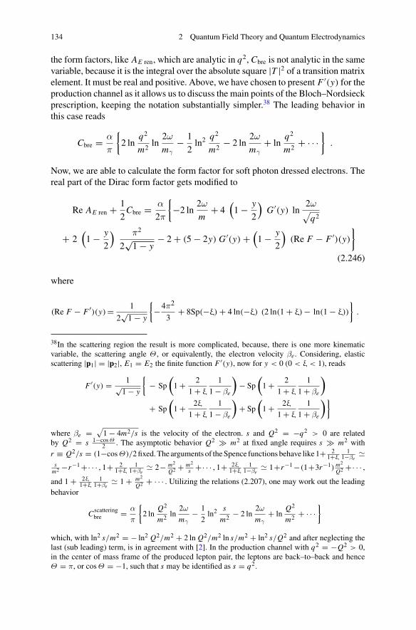
134 2 Quantum Field Theory and Quantum Electrodynamics

the form factors, like AE ren, which are analytic in q2, Cbre is not analytic in the samevariable, because it is the integral over the absolute square |T |2 of a transition matrixelement. It must be real and positive. Above, we have chosen to present F ′(y) for theproduction channel as it allows us to discuss the main points of the Bloch–Nordsieckprescription, keeping the notation substantially simpler.38 The leading behavior inthis case reads

Cbre = α

π

{2 ln

q2

m2ln

2ω

mγ− 1

2ln2

q2

m2− 2 ln

2ω

mγ+ ln

q2

m2+ · · ·

}.

Now, we are able to calculate the form factor for soft photon dressed electrons. Thereal part of the Dirac form factor gets modified to

Re AE ren + 1

2Cbre = α

2π

{−2 ln 2ω

m+ 4

(1− y

2

)G ′(y) ln

2ω√

q2

+ 2(1− y

2

) π2

2√1− y

− 2+ (5− 2y) G ′(y)+(1− y

2

)(Re F − F ′)(y)

}

(2.246)

where

(Re F − F ′)(y)= 1

2√1− y

{−4π2

3+ 8Sp(−ξ)+ 4 ln(−ξ) (2 ln(1+ ξ)− ln(1− ξ))

}.

38In the scattering region the result is more complicated, because, there is one more kinematicvariable, the scattering angle Θ , or equivalently, the electron velocity βe. Considering, elasticscattering |p1| = |p2|, E1 = E2 the finite function F ′(y), now for y < 0 (0 < ξ < 1), reads

F ′(y) = 1√1− y

{− Sp

(1+ 2

1+ ξ

1

1− βe

)− Sp

(1+ 2

1+ ξ

1

1+ βe

)

+ Sp

(1+ 2ξ

1+ ξ

1

1− βe

)+ Sp

(1+ 2ξ

1+ ξ

1

1+ βe

)}

where βe =√1− 4m2/s is the velocity of the electron. s and Q2 = −q2 > 0 are related

by Q2 = s 1−cosΘ2 . The asymptotic behavior Q2 # m2 at fixed angle requires s # m2 with

r ≡ Q2/s = (1−cosΘ)/2fixed.The arguments of theSpence functions behave like 1+ 21+ξ

11−βe

�s

m2 −r−1+· · · , 1+ 21+ξ

11+βe

� 2− m2

Q2 + m2

s +· · · , 1+ 2ξ1+ξ

11−βe

� 1+r−1−(1+3r−1) m2

Q2 +· · · ,and 1+ 2ξ

1+ξ1

1+βe� 1+ m2

Q2 + · · · . Utilizing the relations (2.207), one may work out the leadingbehavior

Cscatteringbre = α

π

{2 ln

Q2

m2 ln2ω

mγ− 1

2ln2

s

m2 − 2 ln2ω

mγ+ ln

Q2

m2 + · · ·}

which, with ln2 s/m2 = − ln2 Q2/m2 + 2 ln Q2/m2 ln s/m2 + ln2 s/Q2 and after neglecting thelast (sub leading) term, is in agreement with [2]. In the production channel with q2 = −Q2 > 0,in the center of mass frame of the produced lepton pair, the leptons are back–to–back and henceΘ = π, or cosΘ = −1, such that s may be identified as s = q2.

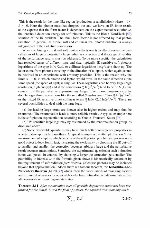
2.6 One–Loop Renormalization 135

This is the result for the time–like region (production or annihilation) where −1 ≤ξ ≤ 0. Here the photon mass has dropped out and we have an IR finite result,at the expense that the form factor is dependent on the experimental resolution ω,the threshold detection energy for soft photons. This is the Bloch–Nordsieck [59]solution of the IR problem. The Pauli form factor is not affected by real photonradiation. In general, as a rule, soft and collinear real photon radiation is alwaysintegral part of the radiative corrections.

When combining virtual and soft photon effects one typically observes the can-cellations of large or potentially large radiative correction and the range of validityof the perturbative results must be addressed. To be more specific, the calculationhas revealed terms of different type and size: typically IR sensitive soft photonslogarithms of the type ln(m/2ω), or collinear logarithms ln(q2/m2) show up. Thelatter come from photons traveling in the direction of a lepton, which again cannotbe resolved in an experiment with arbitrary precision. This is the reason why thelimit m → 0, in which photon and lepton would travel in the same direction at thesame speed (the speed of light) is singular. These logarithms can be very large (highresolution, high energy) and if the corrections α

πln(q2/m2) tend to be of O(1) one

cannot trust the perturbative expansion any longer. Even more dangerous are thedouble logarithmic corrections like the so called Sudakov logarithms α

πln2(q2/m2)

or the mixed IR sensitive times collinear terms απln(m/2ω) ln(q2/m2). There are

several possibilities to deal with the large logs:

(a) the leading large terms are known also in higher orders and may thus beresummed. The resummation leads to more reliable results. A typical example hereis the soft photon exponentiation according to Yennie–Frautschi–Suura [76].

(b) UV sensitive large logs may by resummed by the renormalization group, asdiscussed above.

(c) Some observable quantities may have much better convergence properties ina perturbative approach than others. A typical example is the attempt of an exclusivemeasurement of a lepton, which because of the soft photon problematic per se is not agood object to look for. In fact, increasing the exclusivity by choosing the IR cut–offω smaller and smaller, the correction becomes arbitrary large and the perturbativeresult becomes meaningless. Somehow the experimental question in such a situationis not well posed. In contrast, by choosing ω larger the correction gets smaller. Thepossibility to increase ω in the formula given above is kinematically constraint bythe requirement of soft radiation factorization. Of course photons may be includedbeyond that approximation. Indeed, there is a famous theorem, the Kinoshita–Lee–Nauenberg theorem (KLN) [77] which infers the cancellations of mass singularitiesand infrared divergences for observableswhich are defined to include summationoverall degenerate or quasi degenerate states:

Theorem 2.11 After a summation over all possible degenerate states has been per-formed for the initial (i ) and the final ( f ) states, the squared transition amplitude

∑

i, f|T f i |2 (2.247)

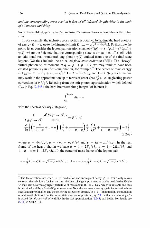
136 2 Quantum Field Theory and Quantum Electrodynamics

and the corresponding cross section is free of all infrared singularities in the limitof all masses vanishing.

Such observables typically are “all inclusive” cross–sections averaged over the initialspin.

In our example, the inclusive cross section is obtained by adding the hard photonsof energy Eγ > ω up to the kinematic limit Eγ max =

√q2 − 4m2/2. To illustrate the

point, let us consider the lepton pair creation channel γ∗(q) → �−(p−)+ �+(p+)+γ(k), where the ∗ denote that the corresponding state is virtual, i.e. off–shell, withan additional real bremsstrahlung photon γ(k) emitted from one of the final stateleptons. We thus include the so called final state radiation (FSR). The “heavy”virtual photon γ∗ of momentum q = p− + p+ + k, we may think to have beencreated previously in e+e−–annihilation, for example.39 The center of mass energyis Ecm = E− + E+ + Eγ =

√q2. Let λ = 2ω/Ecm and 1 − λ # y such that we

may work in the approximation up to terms of order O(α m2

q2 ), i.e., neglecting power

corrections in m2/q2. Relaxing from the soft photon approximation which definedCbre in Eq. (2.245), the hard bremsstrahlung integral of interest is

∫ Ecm/2

ω

dEγ · · ·

with the spectral density (integrand)

1

Γ0(γ∗ → ��)

d2Γ (γ∗ → ��γ)

dudv= P(u, v)

= α

2π

{(2

u

1− u+ 1− u

) (1

v+ 1

1− u − v

)a

2

(1

v2+ 1

(1− u − v)2

)− 2

}

.

(2.248)

where a = 4m2/q2, u = (p− + p+)2/q2 and v = (q − p−)2/q2. In the restframe of the heavy photon we have u = 1 − 2Eγ/Mγ , v = 1 − 2E−/Mγ and1− u − v = 1− 2E+/Mγ . In the center of mass frame of the lepton pair

v = 1

2(1− u) (1−√

1− y cosΘ+) ; 1− u − v = 1

2(1− u) (1−√

1− y cosΘ−)

39The factorization into e+e− → γ∗ production and subsequent decay γ∗ → �+�− only makessense at relatively low q2, when the one–photon exchange approximation can be used. In the SM theγ∗ may also be a “heavy light” particle Z of mass about MZ � 91GeV which is unstable and thusis described well by a Breit–Wigner resonance. Near the resonance energy again factorization is anexcellent approximation and the following discussion applies. In e+e−–annihilation, the radiationof additional photons from the initial state electron or positron (Fig. 2.11 with e′ an incoming e+)is called initial state radiation (ISR). In the soft approximation (2.243) still holds. For details see(5.11) in Sect. 5.1.3.

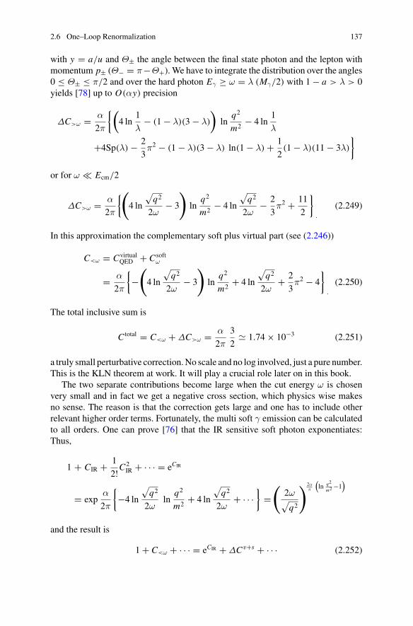
2.6 One–Loop Renormalization 137

with y = a/u and Θ± the angle between the final state photon and the lepton withmomentum p± (Θ− = π−Θ+). We have to integrate the distribution over the angles0 ≤ Θ± ≤ π/2 and over the hard photon Eγ ≥ ω = λ (Mγ/2) with 1− a > λ > 0yields [78] up to O(αy) precision

ΔC>ω = α

2π

{(4 ln

1

λ− (1− λ)(3− λ)

)ln

q2

m2− 4 ln

1

λ

+4Sp(λ)− 2

3π2 − (1− λ)(3− λ) ln(1− λ)+ 1

2(1− λ)(11− 3λ)

}

or for ω � Ecm/2

ΔC>ω = α

2π

{(

4 ln

√q2

2ω− 3

)

lnq2

m2− 4 ln

√q2

2ω− 2

3π2 + 11

2

}

.

(2.249)

In this approximation the complementary soft plus virtual part (see (2.246))

C<ω = CvirtualQED + C soft

ω

= α

2π

{−(

4 ln

√q2

2ω− 3

)

lnq2

m2+ 4 ln

√q2

2ω+ 2

3π2 − 4

}

.

(2.250)

The total inclusive sum is

C total = C<ω +ΔC>ω = α

2π

3

2� 1.74× 10−3 (2.251)

a truly small perturbative correction.No scale and no log involved, just a pure number.This is the KLN theorem at work. It will play a crucial role later on in this book.

The two separate contributions become large when the cut energy ω is chosenvery small and in fact we get a negative cross section, which physics wise makesno sense. The reason is that the correction gets large and one has to include otherrelevant higher order terms. Fortunately, the multi soft γ emission can be calculatedto all orders. One can prove [76] that the IR sensitive soft photon exponentiates:Thus,

1 + CIR + 1

2!C2IR + · · · = eCIR

= expα

2π

{−4 ln

√q2

2ωln

q2

m2+ 4 ln

√q2

2ω+ · · ·

}=(

2ω√

q2

) 2απ

(ln q2

m2 −1)

and the result is

1+ C<ω + · · · = eCIR +ΔCv+s + · · · (2.252)

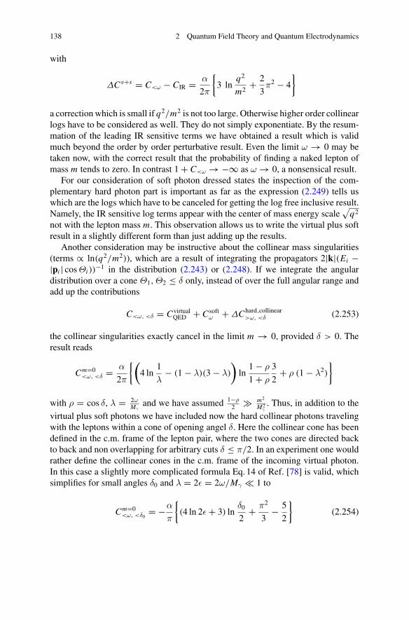
138 2 Quantum Field Theory and Quantum Electrodynamics

with

ΔCv+s = C<ω − CIR = α

2π

{3 ln

q2

m2+ 2

3π2 − 4

}

a correction which is small if q2/m2 is not too large. Otherwise higher order collinearlogs have to be considered as well. They do not simply exponentiate. By the resum-mation of the leading IR sensitive terms we have obtained a result which is validmuch beyond the order by order perturbative result. Even the limit ω → 0 may betaken now, with the correct result that the probability of finding a naked lepton ofmass m tends to zero. In contrast 1+ C<ω →−∞ as ω → 0, a nonsensical result.

For our consideration of soft photon dressed states the inspection of the com-plementary hard photon part is important as far as the expression (2.249) tells uswhich are the logs which have to be canceled for getting the log free inclusive result.Namely, the IR sensitive log terms appear with the center of mass energy scale

√q2

not with the lepton mass m. This observation allows us to write the virtual plus softresult in a slightly different form than just adding up the results.

Another consideration may be instructive about the collinear mass singularities(terms ∝ ln(q2/m2)), which are a result of integrating the propagators 2|k|(Ei −|pi | cosΘi ))

−1 in the distribution (2.243) or (2.248). If we integrate the angulardistribution over a cone Θ1,Θ2 ≤ δ only, instead of over the full angular range andadd up the contributions

C<ω, <δ = CvirtualQED + C soft

ω +ΔChard,collinear>ω, <δ (2.253)

the collinear singularities exactly cancel in the limit m → 0, provided δ > 0. Theresult reads

Cm=0<ω, <δ =

α

2π

{(4 ln

1

λ− (1− λ)(3− λ)

)ln

1− ρ

1+ ρ

3

2+ ρ (1− λ2)

}

with ρ = cos δ, λ = 2ωMγ

and we have assumed 1−ρ2 # m2

M2γ. Thus, in addition to the

virtual plus soft photons we have included now the hard collinear photons travelingwith the leptons within a cone of opening angel δ. Here the collinear cone has beendefined in the c.m. frame of the lepton pair, where the two cones are directed backto back and non overlapping for arbitrary cuts δ ≤ π/2. In an experiment one wouldrather define the collinear cones in the c.m. frame of the incoming virtual photon.In this case a slightly more complicated formula Eq.14 of Ref. [78] is valid, whichsimplifies for small angles δ0 and λ = 2ε = 2ω/Mγ � 1 to

Cm=0<ω, <δ0

= −α

π

{(4 ln 2ε+ 3) ln

δ0

2+ π2

3− 5

2

}(2.254)

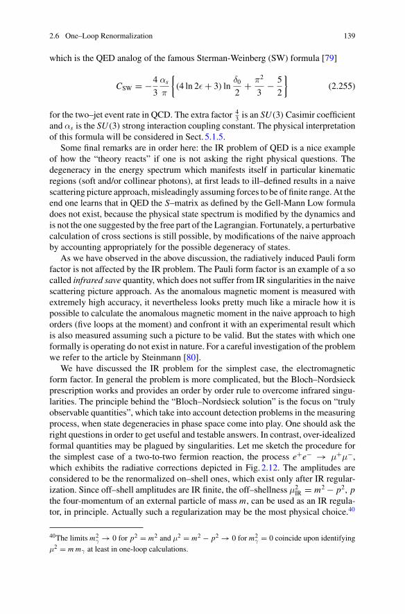
2.6 One–Loop Renormalization 139

which is the QED analog of the famous Sterman-Weinberg (SW) formula [79]

CSW = −4

3

αs

π

{(4 ln 2ε+ 3) ln

δ0

2+ π2

3− 5

2

}(2.255)

for the two–jet event rate in QCD. The extra factor 43 is an SU(3) Casimir coefficient

and αs is the SU(3) strong interaction coupling constant. The physical interpretationof this formula will be considered in Sect. 5.1.5.

Some final remarks are in order here: the IR problem of QED is a nice exampleof how the “theory reacts” if one is not asking the right physical questions. Thedegeneracy in the energy spectrum which manifests itself in particular kinematicregions (soft and/or collinear photons), at first leads to ill–defined results in a naivescattering picture approach, misleadingly assuming forces to be of finite range. At theend one learns that in QED the S–matrix as defined by the Gell-Mann Low formuladoes not exist, because the physical state spectrum is modified by the dynamics andis not the one suggested by the free part of the Lagrangian. Fortunately, a perturbativecalculation of cross sections is still possible, by modifications of the naive approachby accounting appropriately for the possible degeneracy of states.

As we have observed in the above discussion, the radiatively induced Pauli formfactor is not affected by the IR problem. The Pauli form factor is an example of a socalled infrared save quantity, which does not suffer from IR singularities in the naivescattering picture approach. As the anomalous magnetic moment is measured withextremely high accuracy, it nevertheless looks pretty much like a miracle how it ispossible to calculate the anomalous magnetic moment in the naive approach to highorders (five loops at the moment) and confront it with an experimental result whichis also measured assuming such a picture to be valid. But the states with which oneformally is operating do not exist in nature. For a careful investigation of the problemwe refer to the article by Steinmann [80].

We have discussed the IR problem for the simplest case, the electromagneticform factor. In general the problem is more complicated, but the Bloch–Nordsieckprescription works and provides an order by order rule to overcome infrared singu-larities. The principle behind the “Bloch–Nordsieck solution” is the focus on “trulyobservable quantities”, which take into account detection problems in the measuringprocess, when state degeneracies in phase space come into play. One should ask theright questions in order to get useful and testable answers. In contrast, over-idealizedformal quantities may be plagued by singularities. Let me sketch the procedure forthe simplest case of a two-to-two fermion reaction, the process e+e− → μ+μ−,which exhibits the radiative corrections depicted in Fig. 2.12. The amplitudes areconsidered to be the renormalized on–shell ones, which exist only after IR regular-ization. Since off–shell amplitudes are IR finite, the off–shellness μ2

IR = m2− p2, pthe four-momentum of an external particle of mass m, can be used as an IR regula-tor, in principle. Actually such a regularization may be the most physical choice.40

40The limits m2γ → 0 for p2 = m2 and μ2 = m2 − p2 → 0 for m2

γ = 0 coincide upon identifying

μ2 = m mγ at least in one-loop calculations.

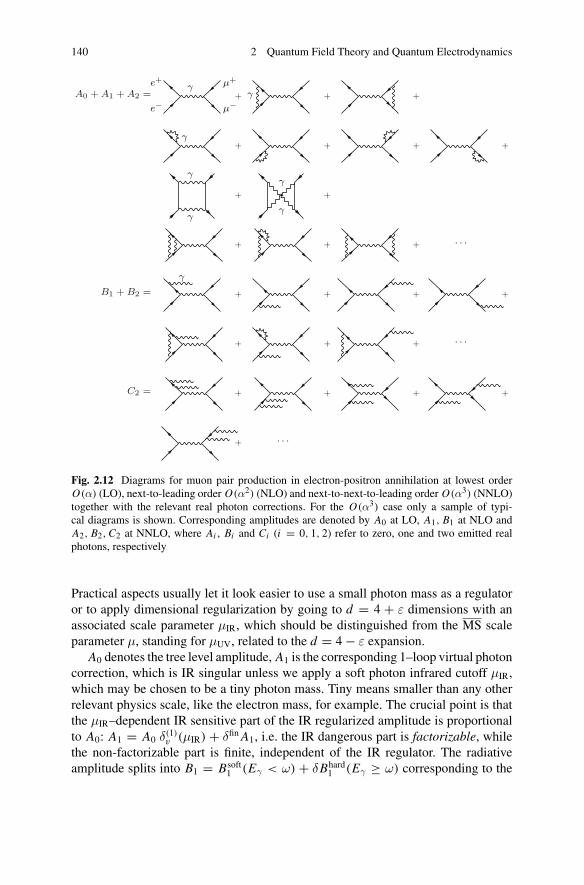
140 2 Quantum Field Theory and Quantum Electrodynamics

A0 + A1 + A2 = + + +

+ + + +

+ +

+ + + · · ·

B1 + B2 = + + + +

+ + + · · ·

C2 = + + + +

+ · · ·

e+ μ+

e− μ−

γγ

γ

γ

γ

γ

γ

γ

Fig. 2.12 Diagrams for muon pair production in electron-positron annihilation at lowest orderO(α) (LO), next-to-leading order O(α2) (NLO) and next-to-next-to-leading order O(α3) (NNLO)together with the relevant real photon corrections. For the O(α3) case only a sample of typi-cal diagrams is shown. Corresponding amplitudes are denoted by A0 at LO, A1, B1 at NLO andA2, B2, C2 at NNLO, where Ai , Bi and Ci (i = 0, 1, 2) refer to zero, one and two emitted realphotons, respectively

Practical aspects usually let it look easier to use a small photon mass as a regulatoror to apply dimensional regularization by going to d = 4 + ε dimensions with anassociated scale parameter μIR, which should be distinguished from the MS scaleparameter μ, standing for μUV, related to the d = 4− ε expansion.

A0 denotes the tree level amplitude, A1 is the corresponding 1–loop virtual photoncorrection, which is IR singular unless we apply a soft photon infrared cutoff μIR,which may be chosen to be a tiny photon mass. Tiny means smaller than any otherrelevant physics scale, like the electron mass, for example. The crucial point is thatthe μIR–dependent IR sensitive part of the IR regularized amplitude is proportionalto A0: A1 = A0 δ(1)

v (μIR) + δfin A1, i.e. the IR dangerous part is factorizable, whilethe non-factorizable part is finite, independent of the IR regulator. The radiativeamplitude splits into B1 = Bsoft

1 (Eγ < ω) + δBhard1 (Eγ ≥ ω) corresponding to the

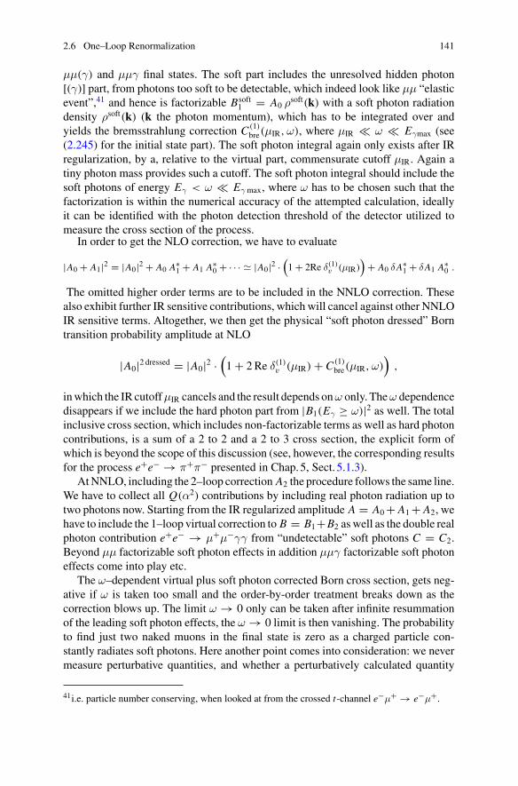
2.6 One–Loop Renormalization 141

μμ(γ) and μμγ final states. The soft part includes the unresolved hidden photon[(γ)] part, from photons too soft to be detectable, which indeed look like μμ “elasticevent”,41 and hence is factorizable Bsoft

1 = A0 ρsoft(k) with a soft photon radiationdensity ρsoft(k) (k the photon momentum), which has to be integrated over andyields the bremsstrahlung correction C (1)

bre(μIR,ω), where μIR � ω � Eγmax (see(2.245) for the initial state part). The soft photon integral again only exists after IRregularization, by a, relative to the virtual part, commensurate cutoff μIR. Again atiny photon mass provides such a cutoff. The soft photon integral should include thesoft photons of energy Eγ < ω � Eγ max, where ω has to be chosen such that thefactorization is within the numerical accuracy of the attempted calculation, ideallyit can be identified with the photon detection threshold of the detector utilized tomeasure the cross section of the process.

In order to get the NLO correction, we have to evaluate

|A0 + A1|2 = |A0|2 + A0 A∗1 + A1 A∗0 + · · · � |A0|2 ·(1+ 2Re δ(1)

v (μIR))+ A0 δA∗1 + δA1 A∗0 .

The omitted higher order terms are to be included in the NNLO correction. Thesealso exhibit further IR sensitive contributions, which will cancel against other NNLOIR sensitive terms. Altogether, we then get the physical “soft photon dressed” Borntransition probability amplitude at NLO

|A0|2 dressed = |A0|2 ·(1+ 2Re δ(1)

v (μIR)+ C (1)bre(μIR,ω)

),

inwhich the IR cutoffμIR cancels and the result depends onω only. Theω dependencedisappears if we include the hard photon part from |B1(Eγ ≥ ω)|2 as well. The totalinclusive cross section, which includes non-factorizable terms as well as hard photoncontributions, is a sum of a 2 to 2 and a 2 to 3 cross section, the explicit form ofwhich is beyond the scope of this discussion (see, however, the corresponding resultsfor the process e+e− → π+π− presented in Chap.5, Sect. 5.1.3).

AtNNLO, including the 2–loop correction A2 the procedure follows the same line.We have to collect all Q(α2) contributions by including real photon radiation up totwo photons now. Starting from the IR regularized amplitude A = A0+ A1+ A2, wehave to include the 1–loop virtual correction to B = B1+B2 aswell as the double realphoton contribution e+e− → μ+μ−γγ from “undetectable” soft photons C = C2.Beyond μμ factorizable soft photon effects in addition μμγ factorizable soft photoneffects come into play etc.

The ω–dependent virtual plus soft photon corrected Born cross section, gets neg-ative if ω is taken too small and the order-by-order treatment breaks down as thecorrection blows up. The limit ω → 0 only can be taken after infinite resummationof the leading soft photon effects, the ω → 0 limit is then vanishing. The probabilityto find just two naked muons in the final state is zero as a charged particle con-stantly radiates soft photons. Here another point comes into consideration: we nevermeasure perturbative quantities, and whether a perturbatively calculated quantity

41i.e. particle number conserving, when looked at from the crossed t-channel e−μ+ → e−μ+.

142 2 Quantum Field Theory and Quantum Electrodynamics

approximates a measured object well depends on the experimental conditions. For acertain range ofω’s the predictionmaywell be perfect within experimental precision,while going to smallerω’s convergence of the perturbative series breaks down. Quan-tities sharing such behavior are called infrared unsafe. Good observables preferablyshould be defined such that they are infrared save and collinear save. Infrared safemeans that the quantity, in order to be a true observable, should not change discon-tinuously if one adds a soft particle to the final state. Similarly, collinear safe meansthat the quantity should not change abruptly if one splits one final state particle intotwo particles with equal momentum. A more concrete account will be presented inChap.5, Sect. 5.1.3 for the process e+e− → π+π−, which plays an important role inevaluation the leading hadronic contribution to aμ.

Onmore aspect has to bementioned here: what is “detectable” is device dependentand therefore not what is of primary theoretical interest. It is therefore commonpractice to unfold experimental data from radiative effects. In our case, this amountsto “undress” the physical cross section, by comparisonwith the theoretical prediction,in order to recover the “bare” cross section as the quantity of interest. This in any caseallows to extract the relevant parameters like couplings and masses which enter theundressed cross section. In many cases undressing attempts to separate for examplestrong interaction effects from electromagnetic ones.

Concluding remarks: we note that the problem with the non-existence of elec-trically charged one-particle states imply that the S-matrix in the naive LSZ sensein QED does not exist. In perturbation theory the Bloch–Nordsieck approximationand its Yennie–Frautschi–Suura improvement provides an acceptable perturbativelyimprovable framework for making well defined predictions which can be confrontedwith experimental data of a given precision. Interestingly, such infrared type problemis absent for charged particles in atoms or molecules, because radiation in bound sys-tems is subject to quantum mechanics with a discrete spectrum and soft or collineardegeneracies of states are not an issue. For what concerns the non-Abelian part of theSM: the physical state space exhibits no other massless particle besides the photon.The weak SU(2) gauge bosons get masses via the Higgs mechanism and are actuallyvery heavy and therefore very unstable such that they never can show up as true LSZWigner states, because the track they leave in a real world detector is by far too shortto ever be resolved as a particle track. Nevertheless the neutral Z boson shows upas a very pronounced resonance as ΓZ/MZ � 0.0274, such that its quasi on–shellproperties can be investigated very precisely, and as performed at the LEP ring atCERN at the beginning of the 90ies. This information, however is only accessiblevia the decay products which are seen in the detector. Similarly for the W boson,except that the W as a charged state in addition exhibits the same types of prob-lems as the charged leptons in QED. In principle one could integrate out the W andthe Z fields, which however would result in a very complicated non-local effectiveLagrangian. Certainly one better sticks to the standard SM approach, treating theweak gauge bosons as quasi LSZ states, in a production and decay chain, which canbe implemented order by order in perturbation theory. The strong interaction sectorsolves its problems with the massless gluons in its own way: by confinement. Allfields in the QCD Lagrangian have no asymptotic states themselves but form color

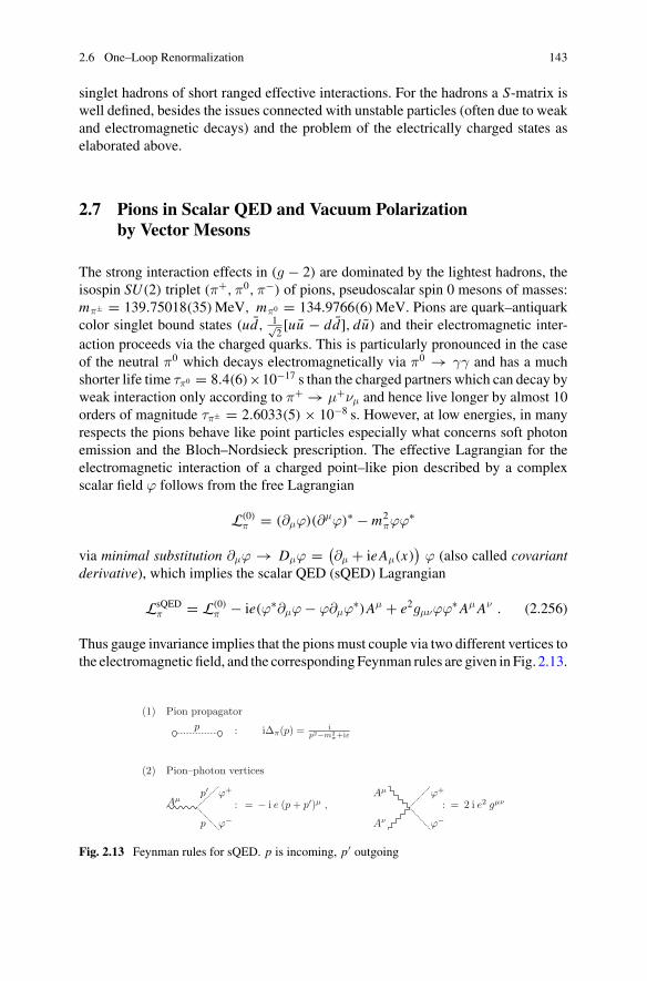
2.6 One–Loop Renormalization 143

singlet hadrons of short ranged effective interactions. For the hadrons a S-matrix iswell defined, besides the issues connected with unstable particles (often due to weakand electromagnetic decays) and the problem of the electrically charged states aselaborated above.

2.7 Pions in Scalar QED and Vacuum Polarizationby Vector Mesons

The strong interaction effects in (g − 2) are dominated by the lightest hadrons, theisospin SU(2) triplet (π+,π0,π−) of pions, pseudoscalar spin 0 mesons of masses:mπ± = 139.75018(35)MeV, mπ0 = 134.9766(6)MeV. Pions are quark–antiquarkcolor singlet bound states (ud, 1√

2[uu − dd], du) and their electromagnetic inter-

action proceeds via the charged quarks. This is particularly pronounced in the caseof the neutral π0 which decays electromagnetically via π0 → γγ and has a muchshorter life time τπ0 = 8.4(6)×10−17 s than the charged partners which can decay byweak interaction only according to π+ → μ+νμ and hence live longer by almost 10orders of magnitude τπ± = 2.6033(5) × 10−8 s. However, at low energies, in manyrespects the pions behave like point particles especially what concerns soft photonemission and the Bloch–Nordsieck prescription. The effective Lagrangian for theelectromagnetic interaction of a charged point–like pion described by a complexscalar field ϕ follows from the free Lagrangian

L(0)π = (∂μϕ)(∂μϕ)∗ − m2

πϕϕ∗

via minimal substitution ∂μϕ → Dμϕ =(∂μ + ieAμ(x)

)ϕ (also called covariant

derivative), which implies the scalar QED (sQED) Lagrangian

LsQEDπ = L(0)

π − ie(ϕ∗∂μϕ− ϕ∂μϕ∗)Aμ + e2gμνϕϕ∗Aμ Aν . (2.256)

Thus gauge invariance implies that the pions must couple via two different vertices tothe electromagnetic field, and the corresponding Feynman rules are given in Fig. 2.13.

(1) Pion propagator

: iΔπ(p) = ip2−m2

π+iε

(2) Pion–photon vertices

: = − i e (p + p′)μ , : = 2 i e2 gμν

p

Aμϕ+

ϕ−

p′

p

Aμ

Aν

ϕ+

ϕ−

Fig. 2.13 Feynman rules for sQED. p is incoming, p′ outgoing

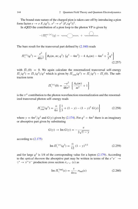
144 2 Quantum Field Theory and Quantum Electrodynamics

The bound state nature of the charged pion is taken care off by introducing a pionform factor e → e Fπ(q2), e2 → e2 |Fπ(q2)|2.

In sQED the contribution of a pion loop to the photon VP is given by

The bare result for the transversal part defined by (2.160) reads

Π(π)γ (q2) = e2

48π2

{B0(m, m; q2)

(q2 − 4m2

)− 4 A0(m)− 4m2 + 2

3q2

}

(2.257)

with Πγ(0) = 0. We again calculate the renormalized transversal self–energyΠ

′γ(q

2) = Πγ(q2)/q2 which is given by Π′γren(q

2) = Π′γ(q

2) − Π′γ(0). The sub-

traction term

Π′(π)γ (0) = −e2

48π2

{A0(m)

m2+ 1

}

is the π± contribution to the photon wavefunction renormalization and the renormal-ized transversal photon self–energy reads

Π′ (π)γren (q

2) = α

6π

{1

3+ (1− y)− (1− y)2 G(y)

}(2.258)

where y = 4m2/q2 and G(y) given by (2.174). For q2 > 4m2 there is an imaginaryor absorptive part given by substituting

G(y) → Im G(y) = − π

2√1− y

according to (2.175)

Im Π′ (π)γ (q2) = α

12(1− y)3/2 (2.259)

and for large q2 is 1/4 of the corresponding value for a lepton (2.179). Accordingto the optical theorem the absorptive part may be written in terms of the e+e− →γ∗ → π+π− production cross section σπ+π−(s) as

Im Π′ hadγ (s) = s

4πασhad(s) (2.260)

2.7 Pions in Scalar QED and Vacuum Polarization by Vector Mesons 145

which hence we can read off to be

σπ+π−(s) = πα2

3sβ3

π (2.261)

with βπ =√

(1− 4m2π/s) the pion velocity in the CM frame. Often, one writes

hadronic cross sections as a ratio

R(s).= σhad(s)/

4πα2

3s(2.262)

in units of the high energy asymptotic form of the cross section σ(e+e− → γ∗ →μ+μ−) for muon pair production in e+e−–annihilation. Given the cross section orimaginary part, conversely, the real part of the renormalized vacuum polarizationfunction may be obtained by integrating the appropriate dispersion relation (seeSect. 3.7), which reads

Re Π′ hadγren (s) = s

4π2αP∫ s2

s1

ds ′σhad(s ′)s ′ − s

= α

3πP∫ s2

s1

ds ′{

1

s ′ − s− 1

s ′

}R(s ′) .

(2.263)

This is another way, the dispersive approach, to get the result (2.258) via the easierto calculate imaginary part, which here is just given by the tree level cross sectionfor γ∗ → π+π−.

As already mentioned, sometimes one has to resort to sQED in particular inconnection with the soft photon radiation problem of charged particles, where sQEDprovides a gooddescription of the problem.However, the photon vacuumpolarizationdue to an elementary charged spin 0 pion, we just have been calculating, includeshard photons in the region of interest above the π+π− production threshold to about1GeV, say. As we will see sQED in this case gives a rather bad approximation.In reality e+e− → γ∗ → π+π− is non–perturbative and exhibits a pronouncedresonance, the neutral spin 1 meson ρ0, and the hadron production cross section ismuch better parametrized by a Breit–Wigner (BW) resonance shape. The relevantparameters are MR the mass, Γ the width and Γe+e−/Γ the branching fraction forρ → e+e−. We briefly present the different possible parametrizations and how aBW resonance contributes to the renormalized photon vacuum polarization whenintegrated over a range (s1, s2) with 4m2

π ≤ s1 < s2 ≤ ∞ [81]:

• Narrow width resonance

The contribution from a zero width resonance

σNW(s) = 12π2

MRΓe+e−δ(s − M2

R) (2.264)

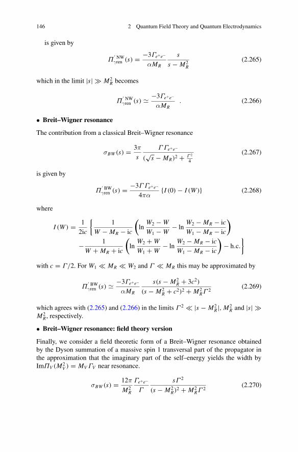
146 2 Quantum Field Theory and Quantum Electrodynamics

is given by

Π′ NWγren (s) = −3Γe+e−

αMR

s

s − M2R

(2.265)

which in the limit |s| # M2R becomes

Π′ NWγren (s) � −3Γe+e−

αMR. (2.266)

• Breit–Wigner resonance

The contribution from a classical Breit–Wigner resonance

σBW (s) = 3π

s

Γ Γe+e−

(√

s − MR)2 + Γ 2

4

(2.267)

is given by

Π′ BWγren (s) = −3Γ Γe+e−

4πα{I (0)− I (W )} (2.268)

where

I (W ) = 1

2ic

{1

W − MR − ic

(ln

W2 −W

W1 −W− ln

W2 − MR − ic

W1 − MR − ic

)

− 1

W + MR + ic

(ln

W2 +W

W1 +W− ln

W2 − MR − ic

W1 − MR − ic

)− h.c.

}

with c = Γ/2. For W1 � MR � W2 and Γ � MR this may be approximated by

Π′ BWγren (s) � −3Γe+e−

αMR

s(s − M2R + 3c2)

(s − M2R + c2)2 + M2

RΓ 2(2.269)

which agrees with (2.265) and (2.266) in the limits Γ 2 � |s − M2R|, M2

R and |s| #M2

R , respectively.

• Breit–Wigner resonance: field theory version

Finally, we consider a field theoretic form of a Breit–Wigner resonance obtainedby the Dyson summation of a massive spin 1 transversal part of the propagator inthe approximation that the imaginary part of the self–energy yields the width byImΠV (M2

V ) = MV ΓV near resonance.

σBW (s) = 12π

M2R

Γe+e−

Γ

sΓ 2

(s − M2R)2 + M2

RΓ 2(2.270)

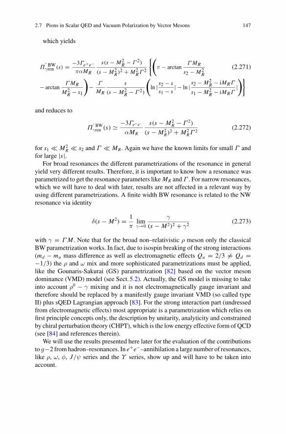
2.7 Pions in Scalar QED and Vacuum Polarization by Vector Mesons 147

which yields

Π′ BWγren (s) = −3Γe+e−

παMR

s(s − M2R − Γ 2)

(s − M2R)2 + M2

RΓ 2

{(

π − arctanΓ MR

s2 − M2R

(2.271)

− arctanΓ MR

M2R − s1

)

− Γ

MR

s

(s − M2R − Γ 2)

(

ln | s2 − s

s1 − s| − ln | s2 − M2

R − iMRΓ

s1 − M2R − iMRΓ

|)}

and reduces to

Π′ BWγren (s) � −3Γe+e−

αMR

s(s − M2R − Γ 2)

(s − M2R)2 + M2

RΓ 2(2.272)

for s1 � M2R � s2 and Γ � MR . Again we have the known limits for small Γ and

for large |s|.For broad resonances the different parametrizations of the resonance in general

yield very different results. Therefore, it is important to know how a resonance wasparametrized to get the resonance parameters like MR andΓ . For narrow resonances,which we will have to deal with later, results are not affected in a relevant way byusing different parametrizations. A finite width BW resonance is related to the NWresonance via identity

δ(s − M2) = 1

πlimγ→0

γ

(s − M2)2 + γ2(2.273)

with γ = Γ M . Note that for the broad non–relativistic ρ meson only the classicalBW parametrization works. In fact, due to isospin breaking of the strong interactions(md − mu mass difference as well as electromagnetic effects Qu = 2/3 �= Qd =−1/3) the ρ and ω mix and more sophisticated parametrizations must be applied,like the Gounaris-Sakurai (GS) parametrization [82] based on the vector mesondominance (VMD) model (see Sect. 5.2). Actually, the GS model is missing to takeinto account ρ0 − γ mixing and it is not electromagnetically gauge invariant andtherefore should be replaced by a manifestly gauge invariant VMD (so called typeII) plus sQED Lagrangian approach [83]. For the strong interaction part (undressedfrom electromagnetic effects) most appropriate is a parametrization which relies onfirst principle concepts only, the description by unitarity, analyticity and constrainedby chiral perturbation theory (CHPT), which is the low energy effective form of QCD(see [84] and references therein).

We will use the results presented here later for the evaluation of the contributionsto g−2 fromhadron–resonances. In e+e−–annihilation a large number of resonances,like ρ, ω, φ, J/ψ series and the Υ series, show up and will have to be taken intoaccount.

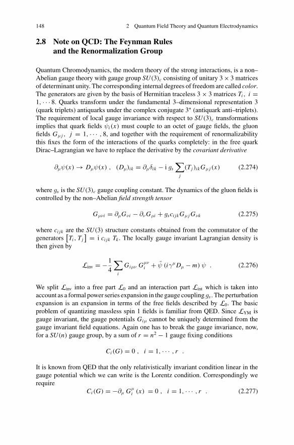
148 2 Quantum Field Theory and Quantum Electrodynamics

2.8 Note on QCD: The Feynman Rulesand the Renormalization Group

Quantum Chromodynamics, the modern theory of the strong interactions, is a non–Abelian gauge theory with gauge group SU(3)c consisting of unitary 3× 3 matricesof determinant unity. The corresponding internal degrees of freedom are called color.The generators are given by the basis of Hermitian traceless 3× 3 matrices Ti , i =1, · · · 8. Quarks transform under the fundamental 3–dimensional representation 3(quark triplets) antiquarks under the complex conjugate 3∗ (antiquark anti–triplets).The requirement of local gauge invariance with respect to SU(3)c transformationsimplies that quark fields ψi (x) must couple to an octet of gauge fields, the gluonfields Gμ j , j = 1, · · · , 8, and together with the requirement of renormalizabilitythis fixes the form of the interactions of the quarks completely: in the free quarkDirac–Lagrangian we have to replace the derivative by the covariant derivative

∂μψ(x) → Dμψ(x) , (Dμ)ik = ∂μδik − i gs

∑

j

(Tj )ik Gμ j (x) (2.274)

where gs is the SU(3)c gauge coupling constant. The dynamics of the gluon fields iscontrolled by the non–Abelian field strength tensor

Gμνi = ∂μGνi − ∂νGμi + gsci jk Gμ j Gνk (2.275)

where ci jk are the SU(3) structure constants obtained from the commutator of thegenerators

[Ti , Tj

] = i ci jk Tk . The locally gauge invariant Lagrangian density isthen given by

Linv = −1

4

∑

i

Giμν Gμνi + ψ (iγμ Dμ − m) ψ . (2.276)

We split Linv into a free part L0 and an interaction part Lint which is taken intoaccount as a formal power series expansion in the gauge coupling gs . The perturbationexpansion is an expansion in terms of the free fields described by L0. The basicproblem of quantizing massless spin 1 fields is familiar from QED. Since LYM isgauge invariant, the gauge potentials Giμ cannot be uniquely determined from thegauge invariant field equations. Again one has to break the gauge invariance, now,for a SU(n) gauge group, by a sum of r = n2 − 1 gauge fixing conditions

Ci (G) = 0 , i = 1, · · · , r .

It is known from QED that the only relativistically invariant condition linear in thegauge potential which we can write is the Lorentz condition. Correspondingly werequire

Ci (G) = −∂μ Gμi (x) = 0 , i = 1, · · · , r . (2.277)

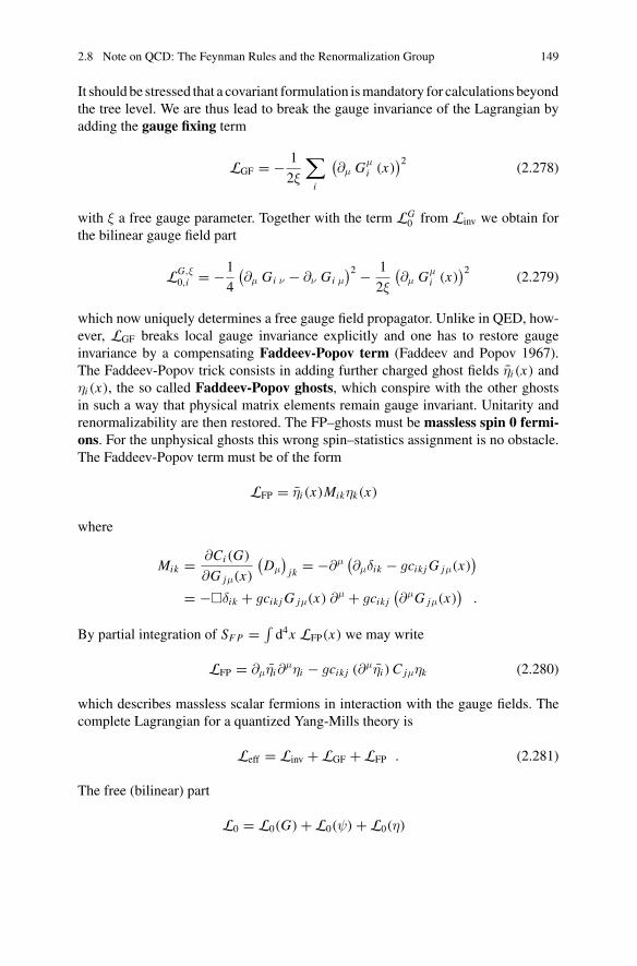
2.8 Note on QCD: The Feynman Rules and the Renormalization Group 149

It should be stressed that a covariant formulation ismandatory for calculations beyondthe tree level. We are thus lead to break the gauge invariance of the Lagrangian byadding the gauge fixing term

LGF = − 1

2ξ

∑

i

(∂μ Gμ

i (x))2

(2.278)

with ξ a free gauge parameter. Together with the term LG0 from Linv we obtain for

the bilinear gauge field part

LG,ξ0,i = −

1

4

(∂μ Gi ν − ∂ν Gi μ

)2 − 1

2ξ

(∂μ Gμ

i (x))2

(2.279)

which now uniquely determines a free gauge field propagator. Unlike in QED, how-ever, LGF breaks local gauge invariance explicitly and one has to restore gaugeinvariance by a compensating Faddeev-Popov term (Faddeev and Popov 1967).The Faddeev-Popov trick consists in adding further charged ghost fields ηi (x) andηi (x), the so called Faddeev-Popov ghosts, which conspire with the other ghostsin such a way that physical matrix elements remain gauge invariant. Unitarity andrenormalizability are then restored. The FP–ghosts must be massless spin 0 fermi-ons. For the unphysical ghosts this wrong spin–statistics assignment is no obstacle.The Faddeev-Popov term must be of the form

LFP = ηi (x)Mikηk(x)

where

Mik = ∂Ci (G)

∂G jμ(x)

(Dμ

)jk = −∂μ

(∂μδik − gcik j G jμ(x)

)

= −�δik + gcik j G jμ(x) ∂μ + gcik j(∂μG jμ(x)

).

By partial integration of SF P =∫d4x LFP(x) we may write

LFP = ∂μηi∂μηi − gcik j (∂μηi ) C jμηk (2.280)

which describes massless scalar fermions in interaction with the gauge fields. Thecomplete Lagrangian for a quantized Yang-Mills theory is

Leff = Linv +LGF +LFP . (2.281)

The free (bilinear) part

L0 = L0(G)+L0(ψ)+L0(η)

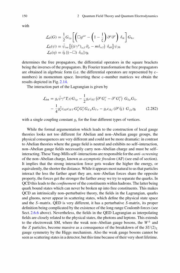
150 2 Quantum Field Theory and Quantum Electrodynamics

with

L0(G) = 1

2Giμ

[(�gμν −

(1− 1

ξ

)∂μ∂ν

)δik

]Gkν

L0(ψ) = ψαa[(

(iγμ)αβ ∂μ − mδαβ

)δab]ψβb

L0(η) = ηi [(−�) δik] ηk

determines the free propagators, the differential operators in the square bracketsbeing the inverses of the propagators. By Fourier transformation the free propagatorsare obtained in algebraic form (i.e. the differential operators are represented by c–numbers) in momentum space. Inverting these c–number matrices we obtain theresults depicted in Fig. 2.14.

The interaction part of the Lagrangian is given by

Lint = gsψγμTiψGiμ − 1

2gscikl

(∂μGν

i − ∂νGμi

)GkμGlν

− 1

4g2s ciklcik ′l ′G

μk Gν

l Gk ′μGl ′ν − gscik j (∂μηi ) G jμηk (2.282)

with a single coupling constant gs for the four different types of vertices.

While the formal argumentation which leads to the construction of local gaugetheories looks not too different for Abelian and non–Abelian gauge groups, thephysical consequences are very different and could not be more dramatic: in contrastto Abelian theories where the gauge field is neutral and exhibits no self–interaction,non–Abelian gauge fields necessarily carry non–Abelian charge and must be self–interacting. TheseYang-Mills self–interactions are responsible for theanti–screeningof the non–Abelian charge, known as asymptotic freedom (AF) (see end of section).It implies that the strong interaction force gets weaker the higher the energy, orequivalently, the shorter the distance.While it appearsmost natural to us that particlesinteract the less the farther apart they are, non–Abelian forces share the oppositeproperty, the forces get the stronger the farther away we try to separate the quarks. InQCD this leads to the confinement of the constituents within hadrons. The latter beingquark bound states which can never be broken up into free constituents. This makesQCD an intrinsically non–perturbative theory, the fields in the Lagrangian, quarksand gluons, never appear in scattering states, which define the physical state spaceand the S–matrix. QED is very different, it has a perturbative S-matrix, its properdefinition being complicated by the existence of the long range Coulomb forces (seeSect. 2.6.6 above). Nevertheless, the fields in the QED Lagrangian as interpolatingfields are closely related to the physical states, the photons and leptons. This extendsto the electroweak SM, where the weak non–Abelian gauge bosons, the W± andthe Z particles, become massive as a consequence of the breakdown of the SU(2)L

gauge symmetry by the Higgs mechanism. Also the weak gauge bosons cannot beseen as scattering states in a detector, but this time because of their very short lifetime.

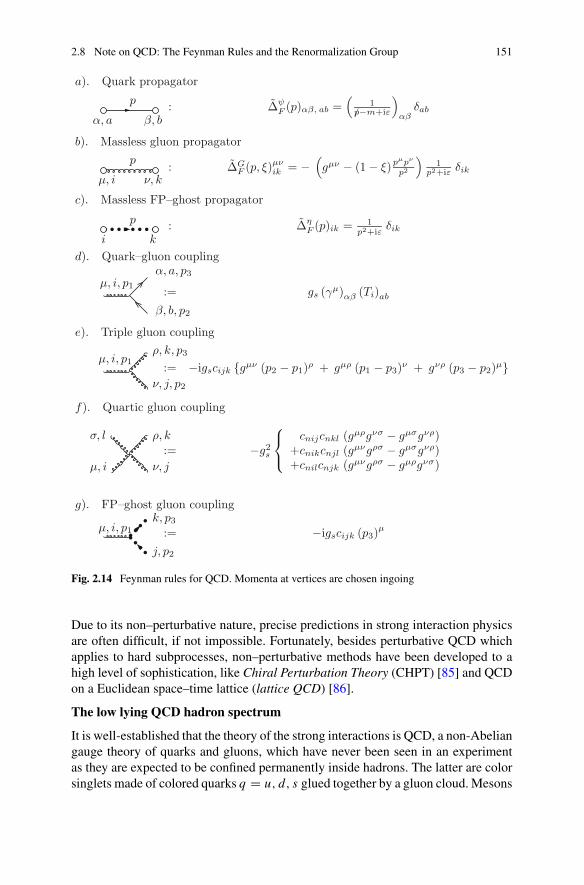
2.8 Note on QCD: The Feynman Rules and the Renormalization Group 151

a). Quark propagator

: ΔψF (p)αβ, ab =

(1

/p−m+iε

)αβ

δab

b). Massless gluon propagator

: ΔGF (p, ξ)μν

ik = −(gμν − (1 − ξ)pμpν

p2

)1

p2+iε δik

c). Massless FP–ghost propagator

: ΔηF (p)ik = 1

p2+iε δik

d). Quark–gluon coupling

:= gs (γμ)αβ (Ti)ab

e). Triple gluon coupling

:= −igscijk {gμν (p2 − p1)ρ + gμρ (p1 − p3)ν + gνρ (p3 − p2)μ}

f). Quartic gluon coupling

:= −g2s

⎧⎨⎩

cnijcnkl (gμρgνσ − gμσgνρ)+cnikcnjl (gμνgρσ − gμσgνρ)+cnilcnjk (gμνgρσ − gμρgνσ)

g). FP–ghost gluon coupling

:= −igscijk (p3)μ

p

α, a β, b

p

μ, i ν, k

p

i k

μ, i, p1

α, a, p3

β, b, p2

μ, i, p1ρ, k, p3

ν, j, p2

μ, i ν, j

ρ, kσ, l

μ, i, p1k, p3

j, p2

Fig. 2.14 Feynman rules for QCD. Momenta at vertices are chosen ingoing

Due to its non–perturbative nature, precise predictions in strong interaction physicsare often difficult, if not impossible. Fortunately, besides perturbative QCD whichapplies to hard subprocesses, non–perturbative methods have been developed to ahigh level of sophistication, like Chiral Perturbation Theory (CHPT) [85] and QCDon a Euclidean space–time lattice (lattice QCD) [86].

The low lying QCD hadron spectrum

It is well-established that the theory of the strong interactions is QCD, a non-Abeliangauge theory of quarks and gluons, which have never been seen in an experimentas they are expected to be confined permanently inside hadrons. The latter are colorsinglets made of colored quarks q = u, d, s glued together by a gluon cloud. Mesons

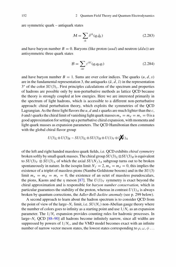
152 2 Quantum Field Theory and Quantum Electrodynamics

are symmetric quark – antiquark states

M =∑

ik

δik(qi qk) (2.283)

and have baryon number B = 0. Baryons (like proton (uud) and neutron (ddu)) areantisymmetric three quark states

B =∑

ikl

εikl(qi qkql) (2.284)

and have baryon number B = 1. Sums are over color indices. The quarks (u, d, s)are in the fundamental representation 3, the antiquarks (u, d, s) in the representation3∗ of the color SU(3)c. First principles calculations of the spectrum and propertiesof hadrons are possible only by non-perturbative methods as lattice QCD becausethe theory is strongly coupled at low energies. Here we are interested primarily inthe spectrum of light hadrons, which is accessible to a different non-perturbativeapproach: chiral perturbation theory, which exploits the symmetries of the QCDLagrangian. As the three light flavors the u, d and s quarks aremuch lighter than the c,b and t quarks the chiral limit of vanishing light quarkmassesmu = md = ms = 0 is agood approximation for setting up a perturbative chiral expansion, withmomenta andlight quark masses as expansion parameters. The QCD Hamiltonian then commuteswith the global chiral flavor group

of the left and right handed massless quark fields, i.e. QCD exhibits chiral symmetrybroken softly by small quarkmasses. The chiral group SU(3)L⊗SU(3)R is equivalentto SU(3)V ⊗ SU(3)A of which the axial SU(N f )A subgroup turns out to be brokenspontaneously in nature. In the isospin limit N f = 2, mu = md = 0, this implies theexistence of a triplet of massless pions (Nambu-Goldstone bosons) and in the SU(3)limit mu = md = ms = 0, the existence of an octet of massless pseudoscalars,the pions, Kaons and the η meson [87]. The U (1)V symmetry is exact beyond thechiral approximation and is responsible for baryon number conservation, which inparticular guarantees the stability of the proton, whereas in contrast U (1)A is alwaysbroken by quantum corrections, the Adler-Bell-Jackiw anomaly (see p. 299 below).

A second approach to learn about the hadron spectrum is to consider QCD fromthe point of view of the large–Nc limit, i.e. SU(Nc) non-Abelian gauge theory wherethe number of colors goes to infinity as a starting point and use 1/Nc as an expansionparameter. The 1/Nc expansion provides counting rules for hadronic processes. Inlarge–Nc QCD [88–90] all hadrons become infinitely narrow, since all widths aresuppressed by powers of 1/Nc, and the VMD model becomes exact with an infinitenumber of narrow vector meson states, the lowest states corresponding to ρ, ω, φ . . .

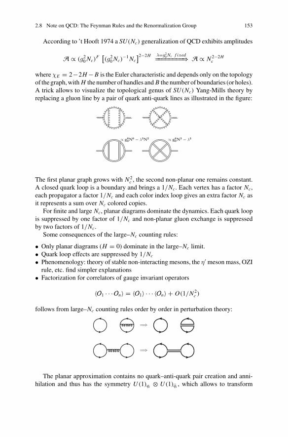
2.8 Note on QCD: The Feynman Rules and the Renormalization Group 153

According to ’t Hooft 1974 a SU(Nc) generalization of QCD exhibits amplitudes

A ∝ (g20 Nc)F[(g20 Nc)

−1Nc]2−2H λ=g20 Nc f i xed========⇒ A ∝ N 2−2H

c

whereχE = 2−2H−B is the Euler characteristic and depends only on the topologyof the graph,with H the number of handles and B the number of boundaries (or holes).A trick allows to visualize the topological genus of SU(Nc) Yang-Mills theory byreplacing a gluon line by a pair of quark anti-quark lines as illustrated in the figure:

∝ g60N

6 = λ3N2 ∝ g60N

3 = λ3

The first planar graph grows with N 2c , the second non-planar one remains constant.

A closed quark loop is a boundary and brings a 1/Nc. Each vertex has a factor Nc,each propagator a factor 1/Nc and each color index loop gives an extra factor Nc asit represents a sum over Nc colored copies.

For finite and large Nc, planar diagrams dominate the dynamics. Each quark loopis suppressed by one factor of 1/Nc and non-planar gluon exchange is suppressedby two factors of 1/Nc.

Some consequences of the large–Nc counting rules:

• Only planar diagrams (H = 0) dominate in the large–Nc limit.• Quark loop effects are suppressed by 1/Nc

• Phenomenology: theory of stable non-interacting mesons, the η′ meson mass, OZIrule, etc. find simpler explanations

• Factorization for correlators of gauge invariant operators

〈O1 · · ·On〉 = 〈O1〉 · · · 〈On〉 + O(1/N 2c )

follows from large–Nc counting rules order by order in perturbation theory:

=⇒

=⇒

The planar approximation contains no quark–anti-quark pair creation and anni-hilation and thus has the symmetry U (1)qi ⊗ U (1)qi , which allows to transform

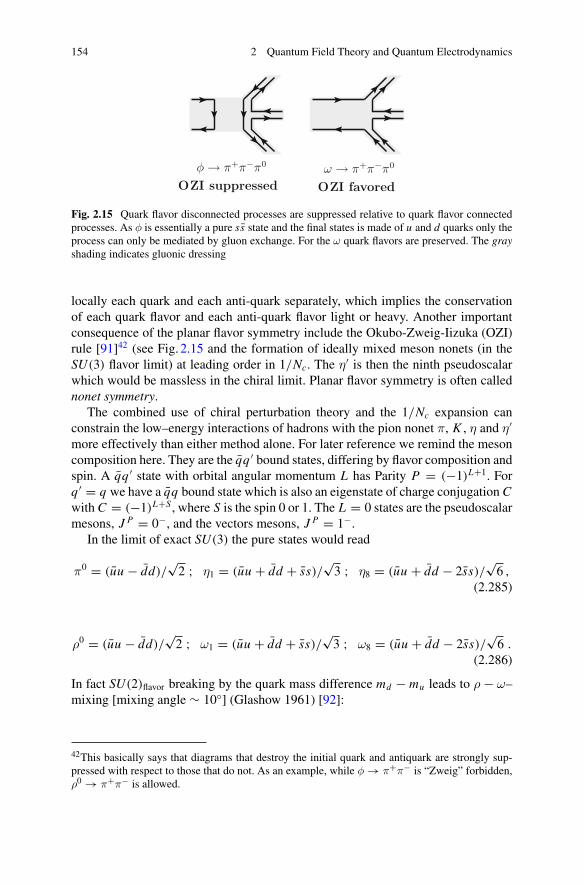
154 2 Quantum Field Theory and Quantum Electrodynamics

φ → π+π−π0

OZI suppressedω → π+π−π0

OZI favored

Fig. 2.15 Quark flavor disconnected processes are suppressed relative to quark flavor connectedprocesses. As φ is essentially a pure ss state and the final states is made of u and d quarks only theprocess can only be mediated by gluon exchange. For the ω quark flavors are preserved. The grayshading indicates gluonic dressing

locally each quark and each anti-quark separately, which implies the conservationof each quark flavor and each anti-quark flavor light or heavy. Another importantconsequence of the planar flavor symmetry include the Okubo-Zweig-Iizuka (OZI)rule [91]42 (see Fig. 2.15 and the formation of ideally mixed meson nonets (in theSU(3) flavor limit) at leading order in 1/Nc. The η′ is then the ninth pseudoscalarwhich would be massless in the chiral limit. Planar flavor symmetry is often callednonet symmetry.

The combined use of chiral perturbation theory and the 1/Nc expansion canconstrain the low–energy interactions of hadrons with the pion nonet π, K , η and η′more effectively than either method alone. For later reference we remind the mesoncomposition here. They are the qq ′ bound states, differing by flavor composition andspin. A qq ′ state with orbital angular momentum L has Parity P = (−1)L+1. Forq ′ = q we have a qq bound state which is also an eigenstate of charge conjugation Cwith C = (−1)L+S , where S is the spin 0 or 1. The L = 0 states are the pseudoscalarmesons, J P = 0−, and the vectors mesons, J P = 1−.

In the limit of exact SU(3) the pure states would read

π0 = (uu − dd)/√2 ; η1 = (uu + dd + ss)/

√3 ; η8 = (uu + dd − 2ss)/

√6 ,

(2.285)

ρ0 = (uu − dd)/√2 ; ω1 = (uu + dd + ss)/

√3 ; ω8 = (uu + dd − 2ss)/

√6 .

(2.286)

In fact SU(2)flavor breaking by the quark mass difference md − mu leads to ρ − ω–mixing [mixing angle ∼ 10◦] (Glashow 1961) [92]:

42This basically says that diagrams that destroy the initial quark and antiquark are strongly sup-pressed with respect to those that do not. As an example, while φ → π+π− is “Zweig” forbidden,ρ0 → π+π− is allowed.

2.8 Note on QCD: The Feynman Rules and the Renormalization Group 155

ρ0 = cos θ ρ′ + sin θ ω′

ω = − sin θ ρ′ + cos θ ω′ (2.287)

Similarly, the substantially larger SU(3)flavor breaking by the quark masses, leadsto large ω − φ–mixing [mixing angle ∼ 36◦ close to so called ideal mixing whereφ ∼ is a pure ss state] (Okubo 1963) [93]:

φ = cos θ ω8 + sin θ ω1

ω = − sin θ ω8 + cos θ ω1 (2.288)

The angle in case of ideal mixing is given by tan θ = 1/√2 or θ = 35.3◦.

In the isospin limit and in absence of e.m. interaction the pion triplet (π+,π0,π−)

exhibits G–parity as a symmetry. It represents a generalization of charge conjugation(C–parity) to strong interactions. The strong interaction does not distinguish thecharges of the pions, therefore a rotation by 180◦ about the 3rd axis in isospin spaceG = exp iπ I3, which rotates π± ↔ π∓ up to a phase, does not change the tripletfield modulo a phase ηG = ±1. For particles (u,d mesons) of isospin I , the G–paritynumber is given by G = (−1)I C , where C is the charge conjugation number ofthe neutral member of the multiplet. As π0 has charge conjugation parity C = +1the e.m. decay π0 → γγ requires Gπ0 = −1 and thus also G|π±〉 = −|π±〉 whileC |π±〉 = −|π∓〉. Therefore, non-electromagnetic decays of flavor SU(2) resonancesin the isospin limit can decay either into an even or an odd number of pions only:ρ0(I = 1) → 2π, ω(I = 0) → 3π. As isospin is broken by the small quark massdifferencemd �= mu actually π± and π0 have different masses andG–parity is brokenaccordingly, and ω → 2π is allowed with a small branching fraction.

The RG of QCD in Short

The renormalization group, introduced in Sect. 2.6.5, for QCD plays a particularlyimportant role for a quantitative understanding of AF as well as a tool for improvingthe convergence of the perturbative expansion [36, 94]. For QCD the RG is givenby

μd

dμgs(μ) = β (gs(μ))

μd

dμmi (μ) = −γ (gs(μ)) mi (μ) (2.289)

with

β(g) = −β0g3

16π2− β1

g5

(16π2)2+ O(g7)

γ(g) = γ0g2

4π2+ γ1

g4

(4π2)2+ O(g6) (2.290)

156 2 Quantum Field Theory and Quantum Electrodynamics

where, in the MS scheme (Sect. 2.5.6),

β0 = 11− 23 N f ; γ0 = 2

β1 = 102− 383 N f ; γ1 = 101

12 − 518 N f

(2.291)

and N f is the number of quark flavors. The RG for QCD is known to 5 loops[95–97]. It allows one to define effective parameters in QCD, which incorporate thesummation of leading logarithmic (1–loop), next–to–leading logarithmic (2–loop),· · · corrections (RG improved perturbation theory). The solution of (2.289) for therunning coupling constant αs(μ) = g2s (μ)/(4π) yields (see (2.223))

4π

β0αs(μ)− β1

β20

ln

(4π

β0αs(μ)+ β1

β20

)=

ln μ2/μ20 +

4π

β0αs(μ0)− β1

β20

ln

(4π

β0αs(μ0)+ β1

β20

)≡ ln μ2/Λ2 (2.292)

with reference scale (integration constant)

ΛQCD = Λ(N f )

MS= μ exp

{

− 4π

2β0αs(μ)

(

1+ αs(μ)

4π

β1

β0ln

β0αs(μ)

4π + β1

β0αs(μ)

)}

(2.293)

which can be shown easily to be independent of the reference scale μ. It is RGinvariant

μd

dμΛQCD = 0 ,

and thus QCD has its own intrinsic scale ΛQCD which is related directly to thecoupling strength (dimensional transmutation). This is most obvious at the one–looplevel where we have the simple relation

αs(μ) = 1β0

4π ln μ2

Λ2

. (2.294)

Thus ΛQCD incorporates the reference coupling αs(μ0) measured at scale μ0 in ascale invariant manner, i.e., each experiment measures the same ΛQCD irrespectiveof the reference energy μ0 at which the measurement of αs(μ0) is performed.

The solution of (2.289) for the effective masses mi (μ) reads (see (2.224))

mi (μ) = mi (μ0)r(μ)

r(μ0)≡ mir(μ) (2.295)

2.8 Note on QCD: The Feynman Rules and the Renormalization Group 157

with

r(μ) = exp−2{

γ0

β0ln

4π

β0αs(μ)+(

γ0

β0− 4γ1

β1

)ln(1+ β1

β0

αs(μ)

4π)

}. (2.296)

Note that also the mi are RG invariant masses (integration constants) and for themasses play a role similar toΛQCD for the coupling. The solution of the RG equation

may be expanded in the large log L ≡ ln μ2

Λ2 , which of course only makes sense if Lis large (μ # Λ),

αs(μ) = 4π

β0 L

⎛

⎝1− β1

β20

ln(L + β1

β20)

L+ · · ·

⎞

⎠

mi (μ) = mi

(L

2

)− γ0β0(1− 2β1γ0

β30

ln L + 1

L+ 8γ1

β20 L+ · · ·

). (2.297)

If L is not large one should solve (2.292) or its higher order version numericallyby iteration for αs(μ). For the experimental proof of the running of the strong cou-pling constant [98] see Fig. 3.3 in Sect. 3.2.1 and the most actual update presented inFig. 9.3 in [99]. The non-perturbative calculations in lattice QCD are able to demon-strate a surprisingly good agreement with perturbative results (see [100–103] andreferences therein). Most interestingly the non-perturbative strong coupling persistsbeing monotonically increasing at very low scales, in clear contrast to speculationsabout a possible IR freezing limμ→0 αs(μ) → const .

Note on the RG of the SM

The electroweak sector of the SM will be introduced in Sect. 4.2. But a commenton the RG of the full SM is in order here. After the discovery of the Higgs bosonall SM couplings are known via the mass–coupling relations (4.46) and so are theβ–functions. The main couplings are the gauge couplings of the SM local gaugegroup SU(3)c⊗ SU(2)L ⊗U (1)Y : g1, g2 and g3 and the top quark Yukawa couplingyt and the Higgs boson self–coupling λ. The SM renormalization group in the MSscheme is known to three loops. The key point concerning the behavior of the effectiveparameters wemay understand when we look at the leading terms of the β-functions.At the Z boson mass scale the couplings are given by g1 � 0.350, g2 � 0.653,g3 � 1.220, yt � 0.935 and λ � 0.807. While the gauge couplings behave asexpected, g1 is infrared (IR) free, g2 and g3 are asymptotically (ultraviolet) free(AF), with leading coefficients exhibiting the related coupling only,

β1 = 41

6g31 c � 0.00185 ; β2 = −19

6g22 c � −0.00558 ; β3 = −7 g33 c � −0.08049 ,

with c = 116π2 , the leading top Yukawa β-function given by

158 2 Quantum Field Theory and Quantum Electrodynamics

βyt =(9

2y3t −

17

12g21 yt − 9

4g22 yt − 8 g23 yt

)c

� 0.02327− 0.00103− 0.00568− 0.07048

� −0.05391

not only depends on yt , but also onmixed termswith the gauge couplings which havea negative sign. In fact the QCD correction is the leading contribution and determinesthe behavior. Notice the critical balance between the dominant strong and the topYukawa couplings: QCD dominance requires g3 > 3

4 yt in the “gaugeless” limitg1 = g2 = 0.

Similarly, the β-function of the Higgs self-coupling, given by

βλ = (4λ2 − 3 g21 λ− 9λ g22 + 12 y2t λ+ 9

4g41 +

9

2g21 g22 +

27

4g42 − 36 y4t ) c

� 0.01650− 0.00187− 0.01961+ 0.05358+ 0.00021+ 0.00149+ 0.00777

−0.17401 � −0.11595

is dominated by the top Yukawa contribution and not by the λ coupling itself. Atleading order it is not subject to QCD corrections. Here, the yt dominance condition

reads λ < 3 (√5−1)2 y2t in the gaugeless limit. The top Yukawa coupling is turned

from an intrinsically IR free to an AF coupling by the QCD term and similarly theHiggs self–coupling is transmuted from IR free to AF by the dominating top Yukawaterm. Including known higher order terms, except from βλ, which exhibits a zero atabout μλ ∼ 1017 GeV, all other β-functions do not exhibit a zero in the range fromμ = MZ to μ = MPlanck. So, apart form the U (1)Y coupling g1, which increasesmoderately only, all other couplings decrease and perturbation theory works wellup to the Planck scale. Actually, at μ = MPlanck gauge couplings are all close togi ∼ 0.5, while yt ∼ 0.35 and

√λ ∼ 0.36 (see [104] and references therein).

References

1. J.D. Bjorken, S.D. Drell, Relativistic Quantum Mechanics, 1st edn. (McGraw-Hill, New York1964), 300 p; Relativistic Quantum Fields, 1st edn. (McGraw-Hill, New York, 1965), 396 p

2. V.B. Berestetskii, E.M. Lifshitz, L.P. Pitaevskii, Quantum electrodynamics, Landau and Lif-shitz Course of Theoretical Physics, vol. 4, 2nd edn. (Pergamon, London, 1982), 652 p

3. P.A.M. Dirac, Proc. R. Soc. A 114, 243 (1927); Proc. R. Soc. A 126, 360 (1930); Proc. R.Soc. A 136, 453 (1932)

4. E.P. Wigner, Ann. Math. 40, 149 (1939)5. P. Jordan, E.P. Wigner, Zeits. Phys. 47, 631 (1928)6. W. Heisenberg, W. Pauli, Zeits. Phys. 56, 1 (1929); Zeits. Phys. 59, 168 (1930); P.A.M. Dirac,

V.A. Fock, B. Podolsky, Phys. Zeits. Sowjetunion 3, 64 (1932)7. H. Joos, Fortsch. Phys. 10, 65 (1962); S. Weinberg, Phys. Rev. 133, B1318 (1964); Phys. Rev.

134, B882 (1964)8. P.A.M. Dirac, Proc. R. Soc. A 114, 243 (1927); A 117, 610 (1928)9. W. Pauli, Zeits. Physik 31, 765 (1925)

References 159

10. W. Pauli, Phys. Rev. 58, 716 (1940)11. R.F. Streater, A.S. Wightman, CPT, Spin and Statistics and All That (Benjamin, New York,

1964)12. G. Lüders, K. Danske Vidensk, Selsk. Mat.-Fys. Medd. 28(5) (1954); W. Pauli, Exclusion

principle, Lorentz group and reflection of space-time and charge, in Niels Bohr and theDevelopment of Physics, ed. byW. Pauli (Pergamon Press, London, 1955, reissued 1962), pp.30–51; W. Pauli, II Nuovo Cim. 6, 204 (1957); G. Lüders, Ann. Phys. N. Y. 2, 1 (1957); G.Lüders, B. Zumino, Phys. Rev. 106, 345 (1957); R. Jost, Helv. Phys. Acta 30, 409 (1957)

13. S. Gasiorovicz, Elementary Particle Physics (Wiley, New York, 1966)14. S. Eidelman et al. [Particle Data Group], Phys. Lett. B 592, 1 (2004); K.A. Olive et al. [Particle

Data Group], Chin. Phys. C 38, 090001 (2014) and 2015 update15. B.C. Regan, E.D. Commins, C.J. Schmidt, D. DeMille, Phys. Rev. Lett. 88, 071805 (2002)16. J. Baron et al. [ACME Collab.], Science 343, 269 (2014)17. W. Gerlach, O. Stern, Zeits. Physik 8, 110 (1924)18. R. Kronig (1925 unpublished), https://en.wikipedia.org/wiki/Ralph_Kronig19. G.E. Uhlenbeck, S. Goudsmit, Naturwissenschaften 13, 953 (1925); Nature 117, 264 (1926)20. W. Pauli, Zeits. Phys. 43, 601 (1927)21. F. Englert, R. Brout, Phys. Rev. Lett. 13, 321 (1964)22. P.W. Higgs, Phys. Lett. 12, 132 (1964)23. G. Aad et al. [ATLAS Collab.], Phys. Lett. B 716, 1 (2012); Science 338, 1576 (2012)24. S. Chatrchyan et al. [CMS Collab.], Phys. Lett. B 716, 30 (2012); Science 338, 1569 (2012)25. S. Weinberg, Phys. Rev. 134, B882 (1964)26. R. Frisch, O. Stern, Zeits. Physik 85, 4 (1933); I. Estermann, O. Stern, ibid. 85, 17 (1933)27. G. Charpak, F.J.M. Farley, R.L. Garwin, T. Muller, J.C. Sens, A. Zichichi, Phys. Lett. 1B, 16

(1962)28. H. Weyl, Zeits. Phys. 56, 330 (1929)29. C.N. Yang, R.L. Mills, Phys. Rev. 96, 191 (1954)30. M. Gell-Mann, F. Low, Phys. Rev. 95, 1300 (1954)31. G.C. Wick, Phys. Rev. 80, 268 (1950)32. W. Pauli, F. Villars, Rev. Mod. Phys. 21, 434 (1949)33. N.N. Bogoliubov, D.V. Shirkov, Introduction to the Theory of Quantized Fields, 1st & 2nd

edn. (Wiley, New York, 1957, 1980), 720 p34. S. Tomonaga, R. Iho, Progr. Theor. Phys. 1, 27 (1946); J. Schwinger, Phys. Rev. 74, 1439

(1948); R.P. Feynman, Phys. Rev. 76, 749 (1949); F. Dyson, Phys. Rev. 75, 486 (1949), ibid.1736

35. H. Fritzsch, M. Gell-Mann, H. Leutwyler, Phys. Lett. 47B, 365 (1973)36. H.D. Politzer, Phys. Rev. Lett. 30, 1346 (1973); D. Gross, F. Wilczek, Phys. Rev. Lett. 30,

1343 (1973)37. S.L. Glashow, Nucl. Phys. B 22, 579 (1961); S. Weinberg, Phys. Rev. Lett. 19, 1264 (1967);

A. Salam, Weak and electromagnetic interactions, in Elementary Particle Theory, ed. by N.Svartholm (Amquist and Wiksells, Stockholm, 1969), pp. 367–377

38. G. ’t Hooft, Nucl. Phys. B 33, 173 (1971); 35, 167 (1971); G. ’t Hooft, M. Veltman, Nucl.Phys. B 50, 318 (1972)

39. G. t’ Hooft, M. Veltman, Nucl. Phys. B 44, 189 (1972)40. W.H. Furry, Phys. Rev. 51, 125 (1937)41. F. Dyson, Phys. Rev. 75, 1736 (1949); J.S. Schwinger, Proc. Nat. Acad. Sci. 37, 452–459

(1951)42. H. Lehmann, K. Symanzik, W. Zimmermann, Nuovo Cim. 1, 205 (1955); Nuovo Cim. 6, 319

(1957)43. S. Mandelstam, Phys. Rev. 112, 1344 (1958)44. I. Białynicki-Birula, Phys. Rev. D 2, 2877 (1970)45. F. Jegerlehner, Eur. Phys. J. C 18, 673 (2001)46. D. Akyeampong, R. Delbourgo, Nuovo Cim. 17A, 47 (1973); W.A. Bardeen, R. Gastmans,

B. Lautrup, Nucl. Phys. B 46, 319 (1972); M. Chanowitz, M. Furman, I. Hinchliffe, Nucl.Phys. B 159, 225 (1979)

160 2 Quantum Field Theory and Quantum Electrodynamics

47. M.C. Bergère, F. David, J. Math. Phys. 20, 1244 (1979)48. K. Osterwalder, R. Schrader, Commun. Math. Phys. 31, 83 (1973); ibid. 42, 281 (1975)49. K.G. Wilson, Phys. Rev. D 10, 2445 (1974)50. M. Abramowitz, I. Stegun, Handbook of Mathematical Functions (Dover, New York, 1965)

(Chap. 9 and formulas 9.1.39/9.1.40/9.6.4 there)51. I.S. Gradshteyn, I.M. Ryzhik, Table of Integrals, Series, and Products, eds. by A. Jeffery, D.

Zwanziger (Academic Press, London, 2015[1943]) (Formulas 3.471.9/11)52. G. t’Hooft, M. Veltman, Nucl. Phys. B 153, 365 (1979)53. A.I. Davydychev, M.Y. Kalmykov, Nucl. Phys. B 605, 266 (2001)54. J. Fleischer, F. Jegerlehner, O.V. Tarasov, Nucl. Phys. B 672, 303 (2003)55. J.S. Frederiksen,W.S.Woolcock, Nucl. Phys. B 28, 605 (1971); Aust. J. Phys. 26, 691 (1973);

Ann. Phys. 75, 503 (1973); ibid. 80, 86 (1973)56. G. Passarino, M. Veltman, Nucl. Phys. B 160, 151 (1979)57. K.G. Chetyrkin, F.V. Tkachov, Nucl. Phys. B 192, 159 (1981)58. F. Jegerlehner, Renormalizing the standard model, in Testing the Standard Model, eds. by

M. Cvetic, P. Langacker (World Scientific, Singapore, 1991), pp. 476–590, http://www-com.physik.hu-berlin.de/~fjeger/books.html

59. F. Bloch, A. Nordsieck, Phys. Rev. D 52, 54 (1937)60. Y.Hahn,W.Zimmermann,Commun.Math. Phys. 10, 330 (1968);W.Zimmermann,Commun.

Math. Phys. 11, 1 (1968); J.H. Lowenstein, W. Zimmermann, Commun. Math. Phys. 44, 73(1975)

61. F.J. Dyson, Phys. Rev. 75, 1736 (1949)62. J.P. Fink, J. Math. Phys. 9, 1389 (1968); E.B. Manoukian, J. Math. Phys. 19, 917 (1978)63. S. Weinberg, Phys. Rev. 118, 838 (1960)64. T. Appelquist, J. Carazzone, Phys. Rev. D 11, 2856 (1975)65. V.A. Smirnov, Mod. Phys. Lett. A 10, 1485 (1995) (and references therein)66. E.C.G. Stueckelberg, A. Petermann, Helv. Phys. Acta 26, 499 (1953); M. Gell-Mann, F.E.

Low, Phys. Rev. 95, 1300 (1954)67. G. Mack, Nucl. Phys. B 5, 499 (1968)68. J.D. Bjorken, Phys. Rev. 179, 1547 (1969); J.D. Bjorken, E.A. Paschos, Phys. Rev. 185, 1975

(1969)69. D.H. Coward et al., Phys. Rev. Lett. 20, 292 (1968); E.D. Bloom et al., Phys. Rev. Lett. 23,

930 (1969); G. Miller et al., Phys. Rev. D 5, 528 (1972)70. H. Suura, E. Wichmann, Phys. Rev. 105, 1930 (1957); A. Petermann, Phys. Rev. 105, 1931

(1957)71. B.E. Lautrup, E. de Rafael, Nucl. Phys. B 70, 317 (1974)72. E. de Rafael, J.L. Rosner, Ann. Phys. (N.Y.) 82, 369 (1974)73. A.L. Kataev, S.A. Larin, Pisma Zh. Eksp. Teor. Fiz. 96, 64 (2012) [JETP Lett. 96, 61 (2012)]74. P.A. Baikov, K.G. Chetyrkin, J.H. Kühn, C. Sturm, Nucl. Phys. B 867, 182 (2013)75. P.A. Baikov, K.G. Chetyrkin, J.H. Kühn, J. Rittinger, JHEP 1207, 017 (2012)76. D.R. Yennie, S.C. Frautschi, H. Suura, Ann. Phys. 13, 379 (1961); D.R. Yennie, Phys. Lett.

34B, 239 (1975); J.D. Jackson, D.L. Scharre, Nucl. Instr. 128, 13 (1975); M. Greco, G.Pancheri, Y. Srivastava, Nucl. Phys. B 101, 234 (1975)

77. T. Kinoshita, J. Math. Phys. 3, 650 (1962); T.D. Lee, M. Nauenberg, Phys. Rev. D 133, B1549(1964)

78. J. Fleischer, F. Jegerlehner, Z. Phys. C 26, 629 (1985)79. G. Sterman, S. Weinberg, Phys. Rev. Lett. 39, 1436 (1977)80. O. Steinmann, Commun. Math. Phys. 237, 181 (2003)81. F. Jegerlehner, Nucl. Phys. B (Proc. Suppl.) 51C, 131 (1996)82. G.J. Gounaris, J.J. Sakurai, Phys. Rev. Lett. 21, 244 (1968); A. Quenzer et al., Phys. Lett. B

76, 512 (1978)83. F. Jegerlehner, R. Szafron, Eur. Phys. J. C 71, 1632 (2011)84. H. Leutwyler, Electromagnetic form factor of the pion, inContinuous Advances in QCD 2002:

Proceedings, eds. by K.A. Olive, M.A. Shifman, M.B. Voloshin (World Scientific, Singapore,2002), 646 p, arXiv:hep-ph/0212324

References 161

85. J. Gasser, H. Leutwyler, Ann. Phys. 158, 142 (1984); Nucl. Phys. B 250, 465 (1985)86. K.G. Wilson, Phys. Rev. D 10, 2445 (1974); M. Creutz, Phys. Rev. D 21, 2308 (1980)87. Y. Nambu, Phys. Rev. Lett. 4, 380 (1960)88. G. ’t Hooft, Nucl. Phys. B 72, 461 (1974); ibid. 75, 461 (1974); E. Witten, Nucl. Phys. B 160,

57 (1979)89. A.V. Manohar, Hadrons in the 1/N expansion, in At the frontier of Particle Physics, vol. 1,

ed. M. Shifman (World Scientific, Singapore, 2001)pp. 507–56890. H. Leutwyler, Nucl. Phys. Proc. Suppl. 64, 223 (1998); R. Kaiser, H. Leutwyler, Eur. Phys.

J. C 17, 623 (2000)91. S. Okubo, Phys. Lett. 5, 1975 (1963); G. Zweig, CERN Report No.8419/TH412 (1964); J.

Iizuka. Prog. Theor. Phys. Suppl. 37, 38 (1966)92. S.L. Glashow, Phys. Rev. Lett. 7, 469 (1961)93. S. Okubo, Phys. Lett. 5, 165 (1963)94. W.E. Caswell, Phys. Rev. Lett. 33, 244 (1974); D.R.T. Jones, Nucl. Phys. B 75, 531 (1974);

E. Egorian, O.V. Tarasov, Theor. Math. Phys. 41, 863 (1979) [Teor. Mat. Fiz. 41, 26 (1979)]95. O.V. Tarasov,A.A.Vladimirov,A.Y. Zharkov, Phys. Lett. B 93, 429 (1980); S.A. Larin, J.A.M.

Vermaseren, Phys. Lett. B 303, 334 (1993)96. T. van Ritbergen, J.A.M. Vermaseren, S.A. Larin, Phys. Lett. B 400, 379 (1997); M. Czakon,

Nucl. Phys. B 710, 485 (2005); K.G. Chetyrkin, Nucl. Phys. B 710, 499 (2005)97. P.A. Baikov, K.G. Chetyrkin, J.H. Kühn, Phys. Rev. Lett. 118, 082002 (2017)98. S. Bethke, Phys. Rep. 403–404, 203 (2004)99. K.A. Olive et al. (Particle Data Group), Chin. Phys. C 38, 090001 (2014); Quantum Chromo-

dynamics eds. by S. Bethke, G. Dissertori, G.P. Salam (therein)100. M. Della Morte, R. Frezzotti, J. Heitger, J. Rolf, R. Sommer, U. Wolff, Nucl. Phys. B 713,

378 (2005)101. F. Tekin et al. [ALPHA Collab.], Nucl. Phys. B 840, 114 (2010)102. M. Dalla Brida et al. [ALPHA Collab.], Phys. Rev. D 95, 014507 (2017)103. M. Bruno et al., Nucl. Part. Phys. Proc. 285–286, 132 (2016); PoS Lattice 2016, 197 (2016),

arXiv:1701.03075 [hep-lat]104. F. Jegerlehner, Acta Phys. Polon. B 45, 1167 (2014)

Chapter 3Lepton Magnetic Moments: Basics

3.1 Equation of Motion for a Lepton in an External Field

For the measurement of the anomalous magnetic moment of a lepton we have toinvestigate the motion of a relativistic point–particle of charge Q� e (e the positroncharge) and mass m� in an external electromagnetic field Aext

μ (x). The equation ofmotion of a charged Dirac particle in an external field is given by (see (2.91))

(i�γμ∂μ + Q�

ec γ

μ(Aμ + Aextμ (x)) − m�c

)ψ�(x) = 0(

�gμν − (1 − ξ−1

)∂μ∂ν

)Aν(x) = −Q�eψ�(x)γμψ�(x) .

(3.1)

What we are looking for is the solution of the Dirac equation with an external fieldas a relativistic one–particle problem, neglecting the radiation field in a first step. Wethus are interested in a solution of the first of the above equations, which we maywrite as

i�∂ψ�

∂t=(

−c α(

i�∇ − Q�

e

cA)

− Q� e Φ + β m�c2

)ψ� , (3.2)

with β = γ0, α = γ0γ and Aμ ext = (Φ, A). For the interpretation of the solutionthe non–relativistic limit plays an important role, because many relativistic problemsin QED may be most easily understood in terms of the non–relativistic problem as astarting point, which usually is easier to solve. We will consider a lepton e−, μ− orτ− with Q� = −1 in the following and drop the index �.

1. Non–relativistic limit

For studying the non–relativistic limit of the motion of a Dirac particle in an externalfield it is helpful and more transparent to work in natural units.1 In order to get from

1The general rules of translation read: pμ → pμ, dμ(p) → �−3dμ(p), m → mc, e →

e/(�c), eipx → ei px� , spinors : u, v → u/

√c, v/

√c.

© Springer International Publishing AG 2017F. Jegerlehner, The Anomalous Magnetic Moment of the Muon,Springer Tracts in Modern Physics 274, DOI 10.1007/978-3-319-63577-4_3

163

164 3 Lepton Magnetic Moments: Basics

the Dirac spinor ψ the two component Pauli spinors in the non–relativistic limit,one has to perform an appropriate unitary transformation, called Foldy–Wouthuysentransformation. Looking at the Dirac equation (3.2)

i�∂ψ

∂t= Hψ , H = c α

(p − e

cA)

+ β mc2 + e Φ

with

β = γ0 =(

1 00 −1

), α = γ0γ =

(0 σσ 0

),

we note that H has the form

H = β mc2 + c O + e Φ

where [β, Φ] = 0 is commuting and {β,O} = 0 anti–commuting. In the absence ofan external field spin is a conserved quantity in the rest frame, i.e. the Dirac equationmust be equivalent to the Pauli equation. This fixes the unitary transformation to beperformed in the case Aext

μ = 0:

ψ′ = U ψ , H′ = U

(H − i�

∂

∂t

)U−1 = UHU−1 (3.3)

where the time–independence of U has been used, and we obtain

i�∂ψ′

∂t= H′ψ′ ; ψ′ =

(ϕ′0

), (3.4)

where ϕ′ is the Pauli spinor. In fact U is a Lorentz boost matrix

U = 1 cosh θ + n γ sinh θ = eθnγ (3.5)

with

n = p|p| , θ = 1

2arccosh

p0

mc= arcsinh

|p|mc

and we obtain, with p0 = √p2 + m2c2,

H′ = cp0β ; [H′,Σ] = 0 , Σ = α γ5 =

(σ 00 σ

)(3.6)

3.1 Equation of Motion for a Lepton in an External Field 165

where Σ is the spin operator. Actually, there exist two projection operators U oneto the upper and one to the lower components:

U+ψ =(

ϕ′0

), U−ψ =

(0χ

),

given by

U+ = (p0 + mc) 1 + pγ√

2p0√

p0 + mc, U− = (p0 + mc) 1 − pγ

√2p0

√p0 + mc

.

For the spinors we have

U+u(p, r) =√

2p0

c

(U (r)

0

), U−v(p, r) =

√2p0

c

(0

V (r)

)

with U (r) and V (r) = iσ2U (r) the two component spinors in the rest system.We now look at the lepton propagator. The Feynman propagator reads

iSFαβ(x − y) ≡ 〈0|T {ψα(x)ψβ(y)}|0〉=∫

d4 p

(2π)4

�p + mc

p2 − m2c2 + iεe−ip(x−y)

where2

SFαβ(z; m2) = (i�γμ∂μ + mc

)ΔF(z; m2) = Θ(z0) S+(z) + Θ(−z0) S−(z)

with retarded positive frequency part represented by

Θ(z0) S+(z) =∫

d4 p

(2π)4

c

2ωp

∑r uα(p, r) uβ(p, r)

p0 − ωp + i0e−ipz

2The positive frequency part is given by

iS+αβ(x − y) ≡ 〈0|ψα(x)ψβ(y)|0〉

= c∑

r

∫dμ(p) uα(p, r) uβ(p, r) e−ip(x−y) =

∫dμ(p) (�p + mc) e−ip(x−y)

and the negative frequency part by

− iS−αβ(x − y) ≡ 〈0|ψβ(y)ψα(x)|0〉

= c∑

r

∫dμ(p) vα(p, r) vβ(p, r) eip(x−y) =

∫dμ(p) (�p − mc) eip(x−y) .

.

166 3 Lepton Magnetic Moments: Basics

and the advanced negative frequency part by

Θ(−z0) S−(z) = −∫

d4 p

(2π)4

c

2ωp

∑r vα(p, r) vβ(p, r)

p0 − ωp + i0eipz .

Using

∑

r

uα(p, r) uβ(p, r) = 2ωp

cU(p) γ+ U(p)

∑

r

vα(p, r) vβ(p, r) = 2ωp

cU(p) γ− U(p)

with

γ± = 1

2

(1 ± γ0

) ; γ0γ± = ±γ± , γ+γ− = γ−γ+ = 0

the projection matrices for the upper and lower components, respectively. We thusarrive at our final representation which allows one to perform a systematic expansionin 1/c:

SF(x − y) =∫

d4 p

(2π)4 e−ip(x−y) U(p )

(γ+

p0 − ωp + i0− γ−

p0 + ωp − i0

)U(p ) . (3.7)

The 1/c–expansion simply follows by expanding the matrix U:

U(p ) = exp θp|p|γ = exp θ

pγ

2mc; θ =

∞∑

n=0

(−1)n

2n + 1

(p2

m2c2

)n

.

The non–relativistic limit thus reads:

SF(x − y)NR =∫

d4 p

(2π)4 e−ip(x−y)

⎛

⎝ γ+p0 − (mc2 + p2

2m ) + i0− γ−

p0 + (mc2 + p2

2m ) − i0

⎞

⎠

i.e.SF(x − y) = SF(x − y)NR + O(1/c) .

2. Non–relativistic lepton with Aextμ �= 0

Again we start from the Dirac equation (3.2). In order to get the non–relativisticrepresentation for small velocities we have to split off the phase of the Dirac field,which is due to the rest energy of the lepton:

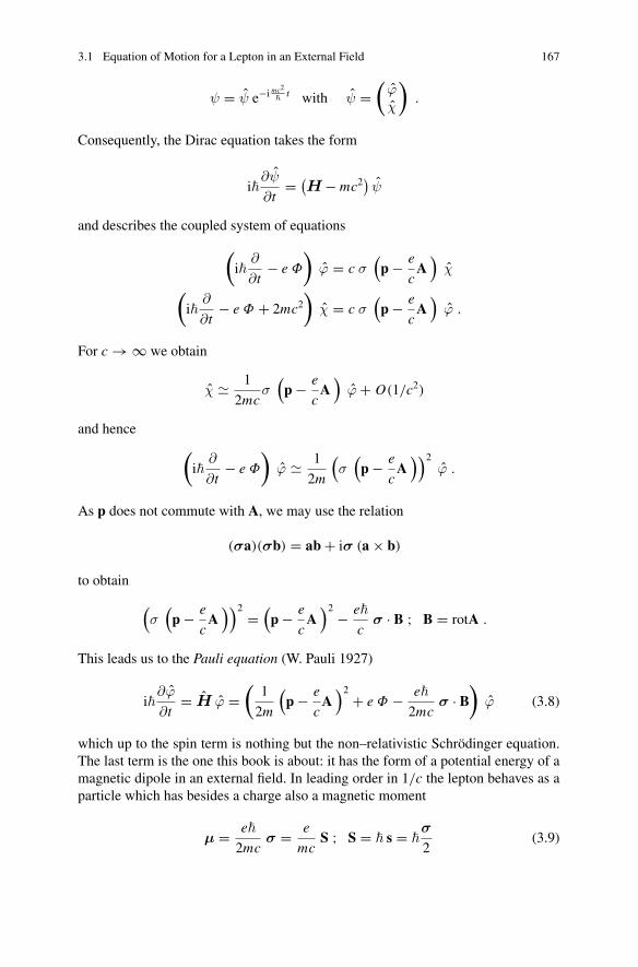
3.1 Equation of Motion for a Lepton in an External Field 167

ψ = ψ e−i mc2

�t with ψ =

(ϕχ

).

Consequently, the Dirac equation takes the form

i�∂ψ

∂t= (

H − mc2) ψ

and describes the coupled system of equations

(i�

∂

∂t− e Φ

)ϕ = c σ

(p − e

cA)

χ

(i�

∂

∂t− e Φ + 2mc2

)χ = c σ

(p − e

cA)

ϕ .

For c → ∞ we obtain

χ 1

2mcσ(

p − e

cA)

ϕ + O(1/c2)

and hence(

i�∂

∂t− e Φ

)ϕ 1

2m

(σ(

p − e

cA))2

ϕ .

As p does not commute with A, we may use the relation

(σa)(σb) = ab + iσ (a × b)

to obtain

(σ(

p − e

cA))2 =

(p − e

cA)2 − e�

cσ · B ; B = rotA .

This leads us to the Pauli equation (W. Pauli 1927)

i�∂ϕ

∂t= H ϕ =

(1

2m

(p − e

cA)2 + e Φ − e�

2mcσ · B

)ϕ (3.8)

which up to the spin term is nothing but the non–relativistic Schrödinger equation.The last term is the one this book is about: it has the form of a potential energy of amagnetic dipole in an external field. In leading order in 1/c the lepton behaves as aparticle which has besides a charge also a magnetic moment

μ = e�

2mcσ = e

mcS ; S = � s = �

σ

2(3.9)

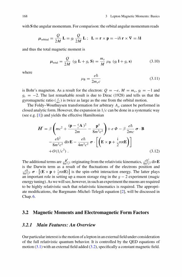
168 3 Lepton Magnetic Moments: Basics

with S the angular momentum. For comparison: the orbital angular momentum reads

μorbital = Q

2ML = gl

Q

2ML ; L = r × p = −i� r × ∇ = �l

and thus the total magnetic moment is

μtotal = Q

2M(gl L + gs S) = me

MμB (gl l + gs s) (3.10)

where

μB = e�

2mec(3.11)

is Bohr’s magneton. As a result for the electron: Q = −e, M = me, gl = −1 andgs = −2. The last remarkable result is due to Dirac (1928) and tells us that thegyromagnetic ratio ( e

mc ) is twice as large as the one from the orbital motion.The Foldy–Wouthuysen transformation for arbitrary Aμ cannot be performed in

closed analytic form. However, the expansion in 1/c can be done in a systematic way(see e.g. [1]) and yields the effective Hamiltonian

H′ = β

(

mc2 + (p − ec A )2

2m− p4

8m3c2

)

+ e Φ − βe�

2mcσ · B

− e�2

8m2c2divE − e�

4m2c2σ ·

[(E × p + i

2rotE

)]

+O(1/c3) . (3.12)

The additional terms are p4

8m3c2 originating from the relativistic kinematics, e�2

8m2c2 divEis the Darwin term as a result of the fluctuations of the electrons position and

e�

4m2c2 σ · [(E × p + i2 rotE)

]is the spin–orbit interaction energy. The latter plays

an important role in setting up a muon storage ring in the g − 2 experiment (magicenergy tuning). As we will see, however, in such an experiment the muons are requiredto be highly relativistic such that relativistic kinematics is required. The appropri-ate modifications, the Bargmann–Michel–Telegdi equation [2], will be discussed inChap. 6.

3.2 Magnetic Moments and Electromagnetic Form Factors

3.2.1 Main Features: An Overview

Our particular interest is the motion of a lepton in an external field under considerationof the full relativistic quantum behavior. It is controlled by the QED equations ofmotion (3.1) with an external field added (3.2), specifically a constant magnetic field.

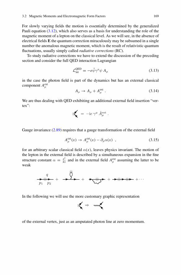
3.2 Magnetic Moments and Electromagnetic Form Factors 169

For slowly varying fields the motion is essentially determined by the generalizedPauli equation (3.12), which also serves as a basis for understanding the role of themagnetic moment of a lepton on the classical level. As we will see, in the absence ofelectrical fields E the quantum correction miraculously may be subsumed in a singlenumber the anomalous magnetic moment, which is the result of relativistic quantumfluctuations, usually simply called radiative corrections (RC).

To study radiative corrections we have to extend the discussion of the precedingsection and consider the full QED interaction Lagrangian

LQEDint = −eψγμψ Aμ (3.13)

in the case the photon field is part of the dynamics but has an external classicalcomponent Aext

μ

Aμ → Aμ + Aextμ . (3.14)

We are thus dealing with QED exhibiting an additional external field insertion “ver-tex”:

⊗ = −ie γμ Aextμ .

Gauge invariance (2.89) requires that a gauge transformation of the external field

Aextμ (x) → Aext

μ (x) − ∂μα(x) , (3.15)

for an arbitrary scalar classical field α(x), leaves physics invariant. The motion ofthe lepton in the external field is described by a simultaneous expansion in the finestructure constant α = e2

4πand in the external field Aext

μ assuming the latter to beweak

p1 p2

q⊗ +

⊗+ ⊗ + ⊗ ⊗ + · · ·

In the following we will use the more customary graphic representation

⊗ ⇒

of the external vertex, just as an amputated photon line at zero momentum.

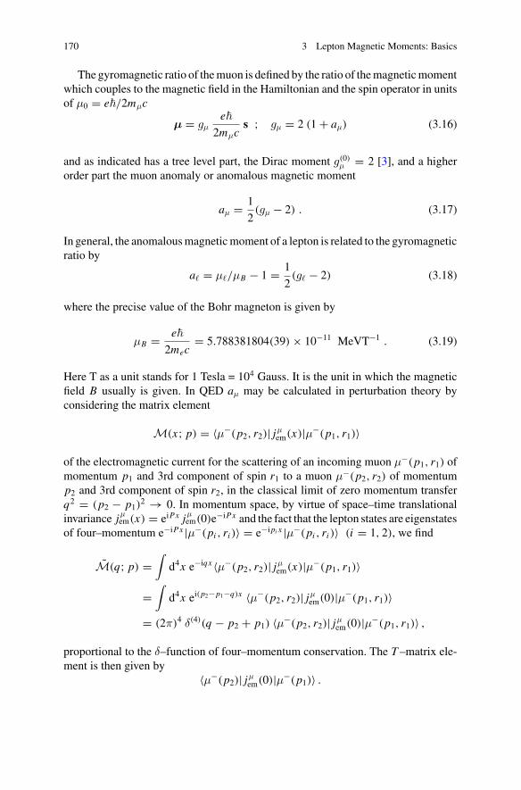
170 3 Lepton Magnetic Moments: Basics

The gyromagnetic ratio of the muon is defined by the ratio of the magnetic momentwhich couples to the magnetic field in the Hamiltonian and the spin operator in unitsof μ0 = e�/2mμc

μ = gμe�

2mμcs ; gμ = 2 (1 + aμ) (3.16)

and as indicated has a tree level part, the Dirac moment g(0)μ = 2 [3], and a higher

order part the muon anomaly or anomalous magnetic moment

aμ = 1

2(gμ − 2) . (3.17)

In general, the anomalous magnetic moment of a lepton is related to the gyromagneticratio by

a� = μ�/μB − 1 = 1

2(g� − 2) (3.18)

where the precise value of the Bohr magneton is given by

μB = e�

2mec= 5.788381804(39) × 10−11 MeVT−1 . (3.19)

Here T as a unit stands for 1 Tesla = 104 Gauss. It is the unit in which the magneticfield B usually is given. In QED aμ may be calculated in perturbation theory byconsidering the matrix element

M(x; p) = 〈μ−(p2, r2)| jμem(x)|μ−(p1, r1)〉

of the electromagnetic current for the scattering of an incoming muon μ−(p1, r1) ofmomentum p1 and 3rd component of spin r1 to a muon μ−(p2, r2) of momentump2 and 3rd component of spin r2, in the classical limit of zero momentum transferq2 = (p2 − p1)

2 → 0. In momentum space, by virtue of space–time translationalinvariance jμ

em(x) = eiPx jμem(0)e−iPx and the fact that the lepton states are eigenstates

of four–momentum e−iPx |μ−(pi , ri )〉 = e−ipi x |μ−(pi , ri )〉 (i = 1, 2), we find

M(q; p) =∫

d4x e−iqx 〈μ−(p2, r2)| jμem(x)|μ−(p1, r1)〉

=∫

d4x ei(p2−p1−q)x 〈μ−(p2, r2)| jμem(0)|μ−(p1, r1)〉

= (2π)4 δ(4)(q − p2 + p1) 〈μ−(p2, r2)| jμem(0)|μ−(p1, r1)〉 ,

proportional to the δ–function of four–momentum conservation. The T –matrix ele-ment is then given by

〈μ−(p2)| jμem(0)|μ−(p1)〉 .

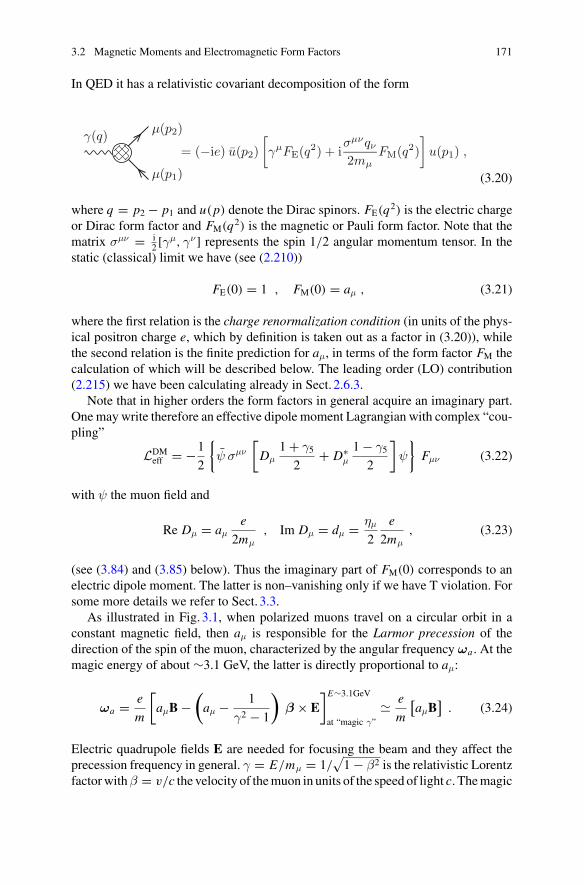
3.2 Magnetic Moments and Electromagnetic Form Factors 171

In QED it has a relativistic covariant decomposition of the form

= (−ie) u(p2)[γμFE(q2) + i

σμνqν

2mμFM(q2)

]u(p1) ,

γ(q) μ(p2)

μ(p1) (3.20)

where q = p2 − p1 and u(p) denote the Dirac spinors. FE(q2) is the electric chargeor Dirac form factor and FM(q2) is the magnetic or Pauli form factor. Note that thematrix σμν = i

2 [γμ, γν] represents the spin 1/2 angular momentum tensor. In thestatic (classical) limit we have (see (2.210))

FE(0) = 1 , FM(0) = aμ , (3.21)

where the first relation is the charge renormalization condition (in units of the phys-ical positron charge e, which by definition is taken out as a factor in (3.20)), whilethe second relation is the finite prediction for aμ, in terms of the form factor FM thecalculation of which will be described below. The leading order (LO) contribution(2.215) we have been calculating already in Sect. 2.6.3.

Note that in higher orders the form factors in general acquire an imaginary part.One may write therefore an effective dipole moment Lagrangian with complex “cou-pling”

LDMeff = −1

2

{ψ σμν

[Dμ

1 + γ5

2+ D∗

μ

1 − γ5

2

]ψ

}Fμν (3.22)

with ψ the muon field and

Re Dμ = aμe

2mμ, Im Dμ = dμ = ημ

2

e

2mμ, (3.23)

(see (3.84) and (3.85) below). Thus the imaginary part of FM(0) corresponds to anelectric dipole moment. The latter is non–vanishing only if we have T violation. Forsome more details we refer to Sect. 3.3.

As illustrated in Fig. 3.1, when polarized muons travel on a circular orbit in aconstant magnetic field, then aμ is responsible for the Larmor precession of thedirection of the spin of the muon, characterized by the angular frequency ωa . At themagic energy of about ∼3.1 GeV, the latter is directly proportional to aμ:

ωa = e

m

[aμB −

(aμ − 1

γ2 − 1

)β × E

]E∼3.1GeV

at “magic γ”

e

m

[aμB

]. (3.24)

Electric quadrupole fields E are needed for focusing the beam and they affect theprecession frequency in general. γ = E/mμ = 1/

√1 − β2 is the relativistic Lorentz

factor with β = v/c the velocity of the muon in units of the speed of light c. The magic

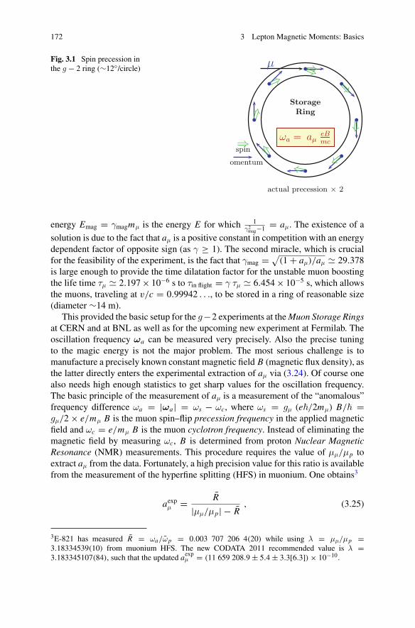
172 3 Lepton Magnetic Moments: Basics

Fig. 3.1 Spin precession inthe g − 2 ring (∼12◦/circle) ⇒

⇒

⇒⇒

⇒⇒

⇒⇒

⇒μ

⇒spinomentum

StorageRing

ωa = aμeBmc

actual precession × 2

energy Emag = γmagmμ is the energy E for which 1γ2

mag−1 = aμ. The existence of a

solution is due to the fact that aμ is a positive constant in competition with an energydependent factor of opposite sign (as γ ≥ 1). The second miracle, which is crucialfor the feasibility of the experiment, is the fact that γmag = √

(1 + aμ)/aμ 29.378is large enough to provide the time dilatation factor for the unstable muon boostingthe life time τμ 2.197 × 10−6 s to τin flight = γ τμ 6.454 × 10−5 s, which allowsthe muons, traveling at v/c = 0.99942 . . ., to be stored in a ring of reasonable size(diameter ∼14 m).

This provided the basic setup for the g−2 experiments at the Muon Storage Ringsat CERN and at BNL as well as for the upcoming new experiment at Fermilab. Theoscillation frequency ωa can be measured very precisely. Also the precise tuningto the magic energy is not the major problem. The most serious challenge is tomanufacture a precisely known constant magnetic field B (magnetic flux density), asthe latter directly enters the experimental extraction of aμ via (3.24). Of course onealso needs high enough statistics to get sharp values for the oscillation frequency.The basic principle of the measurement of aμ is a measurement of the “anomalous”frequency difference ωa = |ωa| = ωs − ωc, where ωs = gμ (e�/2mμ) B/� =gμ/2 × e/mμ B is the muon spin–flip precession frequency in the applied magneticfield and ωc = e/mμ B is the muon cyclotron frequency. Instead of eliminating themagnetic field by measuring ωc, B is determined from proton Nuclear MagneticResonance (NMR) measurements. This procedure requires the value of μμ/μp toextract aμ from the data. Fortunately, a high precision value for this ratio is availablefrom the measurement of the hyperfine splitting (HFS) in muonium. One obtains3

aexpμ = R

|μμ/μp| − R, (3.25)

3E-821 has measured R = ωa/ωp = 0.003 707 206 4(20) while using λ = μμ/μp =3.18334539(10) from muonium HFS. The new CODATA 2011 recommended value is λ =3.183345107(84), such that the updated aexp

μ = (11 659 208.9 ± 5.4 ± 3.3[6.3]) × 10−10.

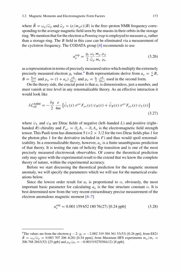
3.2 Magnetic Moments and Electromagnetic Form Factors 173

where R = ωa/ωp and ωp = (e/m pc)〈B〉 is the free–proton NMR frequency corre-sponding to the average magnetic field seen by the muons in their orbits in the storagering. We mention that for the electron a Penning trap is employed to measure ae ratherthan a storage ring. The B field in this case can be eliminated via a measurement ofthe cyclotron frequency. The CODATA group [4] recommends to use

aexpμ = ge

2

ωa

ωp

mμ

me

μp

μe(3.26)

as a representation in terms of precisely measured ratios which multiply the extremelyprecisely measured electron ge value.4 Both representations derive from aμ = e

m B,B = �ωP

2μPand μμ = (1 + aμ)

e�

2mμc and μe = ge

2e�

2mec used in the second form.On the theory side, the crucial point is that a� is dimensionless, just a number, and

must vanish at tree level in any renormalizable theory. As an effective interaction itwould look like

δLAMMeff = −δg

2

e

4m

{ψL(x) σμν Fμν(x) ψR(x) + ψR(x) σμν Fμν(x) ψL(x)

}

(3.27)

where ψL and ψR are Dirac fields of negative (left–handed L) and positive (right–handed R) chirality and Fμν = ∂μ Aν − ∂ν Aμ is the electromagnetic field strengthtensor. This Pauli term has dimension 5 (=2 × 3/2 for the two Dirac fields plus 1 forthe photon plus 1 for the derivative included in F) and thus would spoil renormal-izability. In a renormalizable theory, however, aμ is a finite unambiguous predictionof that theory. It is testing the rate of helicity flip transition and is one of the mostprecisely measured electroweak observables. Of course the theoretical predictiononly may agree with the experimental result to the extend that we know the completetheory of nature, within the experimental accuracy.

Before we start discussing the theoretical prediction for the magnetic momentanomaly, we will specify the parameters which we will use for the numerical evalu-ations below.

Since the lowest order result for a� is proportional to α, obviously, the mostimportant basic parameter for calculating aμ is the fine structure constant α. It isbest determined now from the very recent extraordinary precise measurement of theelectron anomalous magnetic moment [4–7]

aexpe = 0.001 159 652 180 76(27) [0.24 ppb] (3.28)

4The values are from the electron g − 2: ge = −2.002 319 304 361 53(53) [0.26 ppt], from E821R = ωa/ωp = 0.003 707 206 4(20) [0.54 ppm], from Muonium HFS experiments mμ/me =206.768 2843(52) [25 ppb] and μp/μe = −0.001519270384(12) [8 ppb].

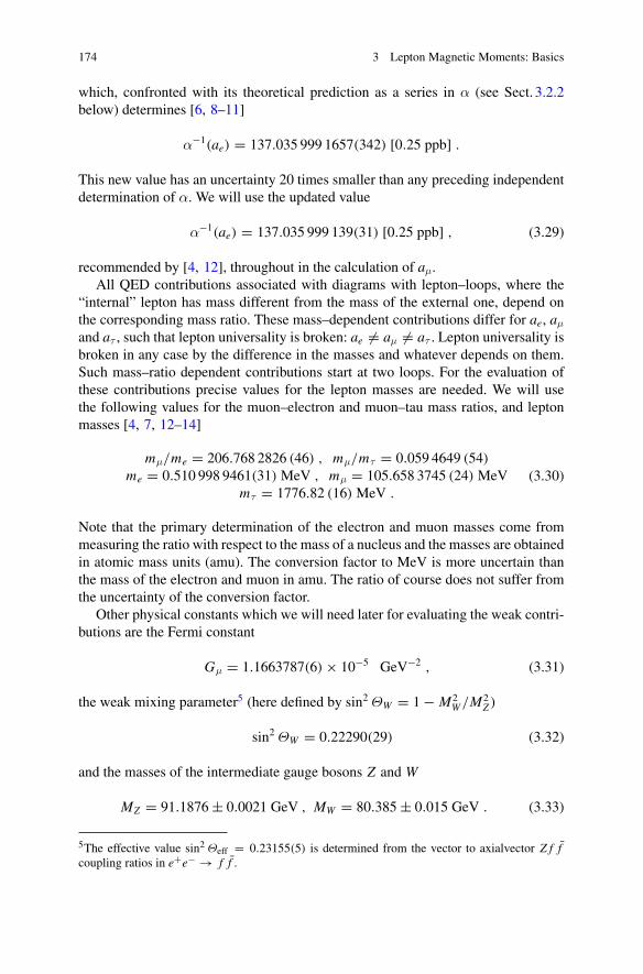
174 3 Lepton Magnetic Moments: Basics

which, confronted with its theoretical prediction as a series in α (see Sect. 3.2.2below) determines [6, 8–11]

α−1(ae) = 137.035 999 1657(342) [0.25 ppb] .

This new value has an uncertainty 20 times smaller than any preceding independentdetermination of α. We will use the updated value

α−1(ae) = 137.035 999 139(31) [0.25 ppb] , (3.29)

recommended by [4, 12], throughout in the calculation of aμ.All QED contributions associated with diagrams with lepton–loops, where the

“internal” lepton has mass different from the mass of the external one, depend onthe corresponding mass ratio. These mass–dependent contributions differ for ae, aμ

and aτ , such that lepton universality is broken: ae �= aμ �= aτ . Lepton universality isbroken in any case by the difference in the masses and whatever depends on them.Such mass–ratio dependent contributions start at two loops. For the evaluation ofthese contributions precise values for the lepton masses are needed. We will usethe following values for the muon–electron and muon–tau mass ratios, and leptonmasses [4, 7, 12–14]

mμ/me = 206.768 2826 (46) , mμ/mτ = 0.059 4649 (54)

me = 0.510 998 9461(31) MeV , mμ = 105.658 3745 (24) MeVmτ = 1776.82 (16) MeV .

(3.30)

Note that the primary determination of the electron and muon masses come frommeasuring the ratio with respect to the mass of a nucleus and the masses are obtainedin atomic mass units (amu). The conversion factor to MeV is more uncertain thanthe mass of the electron and muon in amu. The ratio of course does not suffer fromthe uncertainty of the conversion factor.

Other physical constants which we will need later for evaluating the weak contri-butions are the Fermi constant

Gμ = 1.1663787(6) × 10−5 GeV−2 , (3.31)

the weak mixing parameter5 (here defined by sin2 ΘW = 1 − M2W /M2

Z )

sin2 ΘW = 0.22290(29) (3.32)

and the masses of the intermediate gauge bosons Z and W

MZ = 91.1876 ± 0.0021 GeV , MW = 80.385 ± 0.015 GeV . (3.33)

5The effective value sin2 Θeff = 0.23155(5) is determined from the vector to axialvector Z f fcoupling ratios in e+e− → f f .

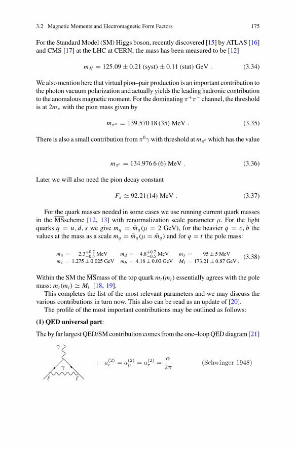
3.2 Magnetic Moments and Electromagnetic Form Factors 175

For the Standard Model (SM) Higgs boson, recently discovered [15] by ATLAS [16]and CMS [17] at the LHC at CERN, the mass has been measured to be [12]

m H = 125.09 ± 0.21 (syst) ± 0.11 (stat) GeV . (3.34)

We also mention here that virtual pion–pair production is an important contribution tothe photon vacuum polarization and actually yields the leading hadronic contributionto the anomalous magnetic moment. For the dominating π+π− channel, the thresholdis at 2mπ with the pion mass given by

mπ± = 139.570 18 (35) MeV . (3.35)

There is also a small contribution from π0γ with threshold at mπ0 which has the value

mπ0 = 134.976 6 (6) MeV . (3.36)

Later we will also need the pion decay constant

Fπ 92.21(14) MeV . (3.37)

For the quark masses needed in some cases we use running current quark massesin the MSscheme [12, 13] with renormalization scale parameter μ. For the lightquarks q = u, d, s we give mq = mq(μ = 2 GeV), for the heavier q = c, b thevalues at the mass as a scale mq = mq(μ = mq) and for q = t the pole mass:

mu = 2.3+0.7−0.5 MeV md = 4.8+0.7

−0.5 MeV ms = 95 ± 5 MeVmc = 1.275 ± 0.025 GeV mb = 4.18 ± 0.03 GeV Mt = 173.21 ± 0.87 GeV .

(3.38)

Within the SM the MSmass of the top quark mt (mt ) essentially agrees with the polemass: mt (mt ) Mt [18, 19].

This completes the list of the most relevant parameters and we may discuss thevarious contributions in turn now. This also can be read as an update of [20].

The profile of the most important contributions may be outlined as follows:

(1) QED universal part:

The by far largest QED/SM contribution comes from the one–loop QED diagram [21]

: a(2)e = a(2)

μ = a(2)τ =

α

2π(Schwinger 1948)

γ

� �

γ

176 3 Lepton Magnetic Moments: Basics

which we have calculated in Sect. 2.6.3, and which is universal for all charged lep-tons. As it is customary we indicate the perturbative order in powers of e, i.e., a(n)

denotes an O(en) term, in spite of the fact that the perturbation expansion is usuallyrepresented as an expansion in α = e2/4π. Typically, analytic results for higherorder terms may be expressed in terms of the Riemann zeta function

ζ(n) =∞∑

k=1

1

kn(3.39)

and of the polylogarithmic integrals6

Lin(x) = (−1)n−1

(n − 2)!1∫

0

lnn−2(t) ln(1 − t x)

tdt =

∞∑

k=1

xk

kn, (3.40)

where Li2(x) is often referred to as the Spence function Sp(x) (see (2.208) inSect. 2.6.3 and [23] and references therein). Special ζ(n) values we will need are

ζ(2) = π2

6, ζ(3) = 1.202 056 903 . . . , ζ(4) = π4

90, ζ(5) = 1.036 927 755 . . . .

(3.41)Also the constants

Lin(1) = ζ(n) , Lin(−1) = −[1 − 21−n] ζ(n)

a4 ≡ Li4

(1

2

)=

∞∑

n=1

1/(2nn4) = 0.517 479 061 674 . . . , (3.42)

related to polylogarithms, will be needed later for the evaluation of analytical results.Since aμ is a number all QED contributions calculated in “one flavor QED”, withjust one species of lepton, which exhibits one physical mass scale only, equal to themass of the external lepton, are universal. The following universal contributions (oneflavor QED) are known:

• 2–loop diagrams [7 diagrams] with one type of fermion lines yield

a(4)� =

[197

144+ π2

12− π2

2ln 2 + 3

4ζ(3)

] (α

π

)2. (3.43)

The first calculation performed by Karplus and Kroll (1950) [24] later was recalcu-lated and corrected by Petermann (1957) [25] and, independently, by Sommerfield

6The appearance of transcendental numbers like ζ(n) and higher order polylogarithms Lin(x) or socalled harmonic sums is directly connected to the number of loops of a Feynman diagram. Typically,2–loop results exhibit ζ(3) 3–loop ones ζ(5) etc. of increasing transcendentality [22].

3.2 Magnetic Moments and Electromagnetic Form Factors 177

(1957) [26]. An instructive compact calculation based on the dispersion theoreticapproach is due to Terentev (1962) [27].• 3–loop diagrams [72 diagrams] with common fermion lines

a(6)� =

[28259

5184+ 17101

810π2 − 298

9π2 ln 2 + 139

18ζ(3)

+100

3

{Li4

(1

2

)+ 1

24ln4 2 − 1

24π2 ln2 2

}

− 239

2160π4 + 83

72π2ζ(3) − 215

24ζ(5)

] (α

π

)3(3.44)

This is the famous analytical result of Laporta and Remiddi (1996) [28], whichlargely confirmed an earlier numerical result of Kinoshita [29]. For the evaluation of(3.44) one needs the constants given in (3.41) and (3.42) before.• 4–loop diagrams [891 diagrams] with common fermion lines so far have beencalculated by numerical methods mainly by Kinoshita and collaborators. The sta-tus had been summarized by Kinoshita and Marciano (1990) [30] some time ago.Since then, the result has been further improved by Kinoshita and his collaborators(2002/2005/2007/2012/2014) [9, 10, 31–33]. They find

− 1.91298(84)(α

π

)4,

by improving earlier results. In a seminal paper Laporta [11] obtained the highprecision (quasi–exact) result

− 1.912 245 764 9 . . .(α

π

)4,

which agrees to 0.9σ with the previous result from [10] and we will use in thefollowing.

Recently, for the first time, the universal 5–loop result has been worked out in [10,33–35]. An evaluation of all 12672 diagrams with the help of an automated codegenerator yields the result

7.795(336)(α

π

)5.

The error is due to the statistical fluctuation in the Monte-Carlo integration of theFeynman amplitudes by the VEGAS routine. With the new result for the universal5–loop term the largest uncertainty in the prediction of ae has reduced by a factor of4.5 from the previous one.

178 3 Lepton Magnetic Moments: Basics

Collecting the universal terms we have

auni� = 0.5

(α

π

)− 0.328 478 965 579 193 78 . . .

(α

π

)2

+1.181 241 456 587 . . .(α

π

)3 − 1.912 245 764 9 . . .(α

π

)4 + 7.795(336)(α

π

)5

= 0.001 159 652 176 42(26)(4)[26] · · · (3.45)

for the one–flavor QED contribution. The three errors are from the error of α givenin (3.29) and from the numerical uncertainties of the α5 coefficients, respectively.

It is interesting to note that the first term a(2)� 0.00116141 · · · contributes the

first three significant digits. Thus the anomalous magnetic moment of a lepton is aneffect of about 0.12%, g�/2 1.00116 · · · , but in spite of the fact that it is so smallwe know ae and aμ more precisely than most other precision observables.

(2) QED mass dependent part:

Since fermions, as demanded by the SM,7 only interact via photons or other spin onegauge bosons, mass dependent corrections only may show up at the two–loop levelvia photon vacuum polarization effects. There are two different regimes for the massdependent effects [36, 37]:

• LIGHT internal masses give rise to potentially large logarithms of mass ratioswhich get singular in the limit m light → 0

e

a(4)μ (vap, e) =

[13ln

mμ

me− 25

36+ O

(me

mμ

)] (α

π

)2.

γ γμ

γ

Here we have a typical result for a light field which produces a large logarithmln mμ

me 5.3, such that the first term ∼2.095 is large relative to a typical constant

second term −0.6944. Here8 the exact two–loop result is

a(4)μ (vap, e) 1.094 258 3092(72)

(α

π

)2 = 5.90406006(4) × 10−6 .

The error is due to the uncertainty in the mass ratio (me/mμ).The kind of leading short distance log contribution just discussed, which is related

to the UV behavior,9 in fact may be obtained from a renormalization group typeargument. In Sect. 2.6.5 (2.233) we have shown that if we replace in the one–loopresult α → α(mμ) we obtain

7Interactions are known to derive from a local gauge symmetry principle, which implies the structureof gauge couplings, which must be of vector (V) or axial–vector (A) type.8The leading terms shown yield 5.84199477 × 10−6.9The muon mass mμ here serves as a UV cut–off, the electron mass as an IR cut–off, and therelevant integral reads

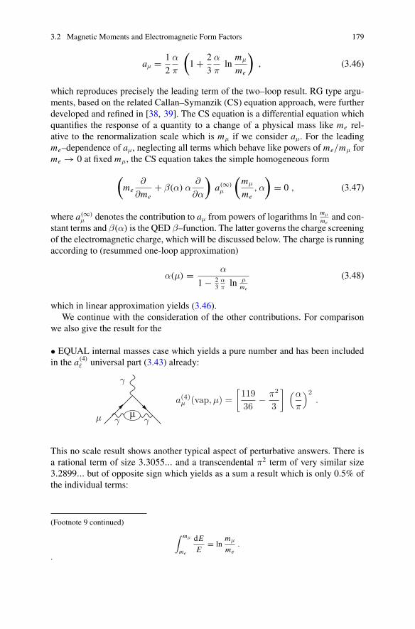
3.2 Magnetic Moments and Electromagnetic Form Factors 179

aμ = 1

2

α

π

(1 + 2

3

α

πln

mμ

me

), (3.46)

which reproduces precisely the leading term of the two–loop result. RG type argu-ments, based on the related Callan–Symanzik (CS) equation approach, were furtherdeveloped and refined in [38, 39]. The CS equation is a differential equation whichquantifies the response of a quantity to a change of a physical mass like me rel-ative to the renormalization scale which is mμ if we consider aμ. For the leadingme–dependence of aμ, neglecting all terms which behave like powers of me/mμ forme → 0 at fixed mμ, the CS equation takes the simple homogeneous form

(me

∂

∂me+ β(α) α

∂

∂α

)a(∞)

μ

(mμ

me,α

)= 0 , (3.47)

where a(∞)μ denotes the contribution to aμ from powers of logarithms ln mμ

meand con-

stant terms and β(α) is the QED β–function. The latter governs the charge screeningof the electromagnetic charge, which will be discussed below. The charge is runningaccording to (resummed one-loop approximation)

α(μ) = α

1 − 23

απ

ln μme

(3.48)

which in linear approximation yields (3.46).We continue with the consideration of the other contributions. For comparison

we also give the result for the

• EQUAL internal masses case which yields a pure number and has been includedin the a(4)

� universal part (3.43) already:

μa(4)

μ (vap, μ) =[11936

− π2

3

] (α

π

)2.

γ γμ

γ

This no scale result shows another typical aspect of perturbative answers. There isa rational term of size 3.3055... and a transcendental π2 term of very similar size3.2899... but of opposite sign which yields as a sum a result which is only 0.5% ofthe individual terms:

(Footnote 9 continued)∫ mμ

me

dE

E= ln

mμ

me.

.

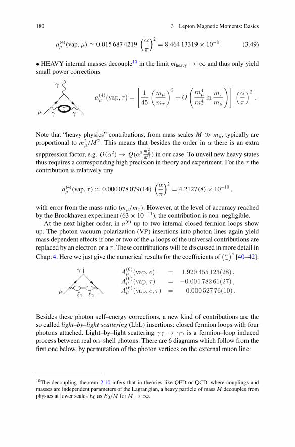
180 3 Lepton Magnetic Moments: Basics

a(4)μ (vap,μ) 0.015 687 4219

(α

π

)2 = 8.464 13319 × 10−8 . (3.49)

• HEAVY internal masses decouple10 in the limit mheavy → ∞ and thus only yieldsmall power corrections

τa(4)

μ (vap, τ) =

[145

(mμ

mτ

)2

+ O

(m4

μ

m4τ

lnmτ

mμ

)] (α

π

)2.

γ γμ

γ

Note that “heavy physics” contributions, from mass scales M � mμ, typically areproportional to m2

μ/M2. This means that besides the order in α there is an extra

suppression factor, e.g. O(α2) → Q(α2 m2μ

M2 ) in our case. To unveil new heavy statesthus requires a corresponding high precision in theory and experiment. For the τ thecontribution is relatively tiny

a(4)μ (vap, τ ) 0.000 078 079(14)

(α

π

)2 = 4.2127(8) × 10−10 ,

with error from the mass ratio (mμ/mτ ). However, at the level of accuracy reachedby the Brookhaven experiment (63 × 10−11), the contribution is non–negligible.

At the next higher order, in a(6) up to two internal closed fermion loops showup. The photon vacuum polarization (VP) insertions into photon lines again yieldmass dependent effects if one or two of the μ loops of the universal contributions arereplaced by an electron or a τ . These contributions will be discussed in more detail inChap. 4. Here we just give the numerical results for the coefficients of

(απ

)3[40–42]:

A(6)μ (vap, e) = 1.920 455 123(28) ,

A(6)μ (vap, τ) = −0.001 782 61(27) ,

A(6)μ (vap, e, τ) = 0.000 527 76(10) .

�2�1μ

γ

Besides these photon self–energy corrections, a new kind of contributions are theso called light–by–light scattering (LbL) insertions: closed fermion loops with fourphotons attached. Light–by–light scattering γγ → γγ is a fermion–loop inducedprocess between real on–shell photons. There are 6 diagrams which follow from thefirst one below, by permutation of the photon vertices on the external muon line:

10The decoupling–theorem 2.10 infers that in theories like QED or QCD, where couplings andmasses are independent parameters of the Lagrangian, a heavy particle of mass M decouples fromphysics at lower scales E0 as E0/M for M → ∞.

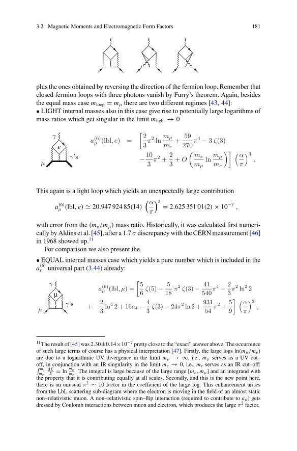
3.2 Magnetic Moments and Electromagnetic Form Factors 181

plus the ones obtained by reversing the direction of the fermion loop. Remember thatclosed fermion loops with three photons vanish by Furry’s theorem. Again, besidesthe equal mass case m loop = mμ there are two different regimes [43, 44]:• LIGHT internal masses also in this case give rise to potentially large logarithms ofmass ratios which get singular in the limit m light → 0

ea(6)

μ (lbl, e) =[23π2 ln

mμ

me+

59270

π4 − 3 ζ(3)

−103

π2 +23+ O

(me

mμln

mμ

me

)] (α

π

)3.γ’s

μ

γ

This again is a light loop which yields an unexpectedly large contribution

a(6)μ (lbl, e) 20.947 924 85(14)

(α

π

)3 = 2.625 351 01(2) × 10−7 ,

with error from the (me/mμ) mass ratio. Historically, it was calculated first numeri-cally by Aldins et al. [45], after a 1.7 σ discrepancy with the CERN measurement [46]in 1968 showed up.11

For comparison we also present the

• EQUAL internal masses case which yields a pure number which is included in thea(6)

� universal part (3.44) already:

μa(6)

μ (lbl, μ) =[56

ζ(5) − 518

π2 ζ(3) − 41540

π4 − 23π2 ln2 2

+23ln4 2 + 16a4 − 4

3ζ(3) − 24π2 ln 2 +

93154

π2 +59

] (α

π

)3,γ’s

μ

γ

11The result of [45] was 2.30±0.14×10−7 pretty close to the “exact” answer above. The occurrenceof such large terms of course has a physical interpretation [47]. Firstly, the large logs ln(mμ/me)

are due to a logarithmic UV divergence in the limit mμ → ∞, i.e., mμ serves as a UV cut–off, in conjunction with an IR singularity in the limit me → 0, i.e., me serves as an IR cut–off:∫ mμ

me

dEE = ln mμ

me. The integral is large because of the large range [me, mμ] and an integrand with

the property that it is contributing equally at all scales. Secondly, and this is the new point here,there is an unusual π2 ∼ 10 factor in the coefficient of the large log. This enhancement arisesfrom the LbL scattering sub-diagram where the electron is moving in the field of an almost staticnon–relativistic muon. A non–relativistic spin–flip interaction (required to contribute to aμ) getsdressed by Coulomb interactions between muon and electron, which produces the large π2 factor.

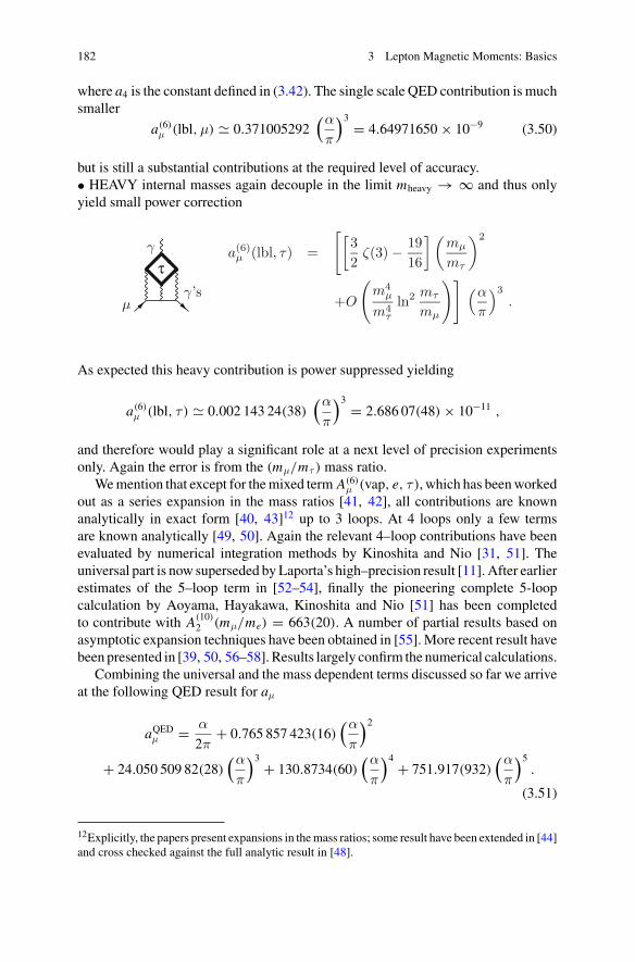
182 3 Lepton Magnetic Moments: Basics

where a4 is the constant defined in (3.42). The single scale QED contribution is muchsmaller

a(6)μ (lbl,μ) 0.371005292

(α

π

)3 = 4.64971650 × 10−9 (3.50)

but is still a substantial contributions at the required level of accuracy.• HEAVY internal masses again decouple in the limit mheavy → ∞ and thus onlyyield small power correction

τa(6)

μ (lbl, τ) =

[[32

ζ(3) − 1916

] (mμ

mτ

)2

+O

(m4

μ

m4τ

ln2mτ

mμ

)] (α

π

)3.

γ’sμ

γ

As expected this heavy contribution is power suppressed yielding

a(6)μ (lbl, τ ) 0.002 143 24(38)

(α

π

)3 = 2.686 07(48) × 10−11 ,

and therefore would play a significant role at a next level of precision experimentsonly. Again the error is from the (mμ/mτ ) mass ratio.

We mention that except for the mixed term A(6)μ (vap, e, τ ), which has been worked

out as a series expansion in the mass ratios [41, 42], all contributions are knownanalytically in exact form [40, 43]12 up to 3 loops. At 4 loops only a few termsare known analytically [49, 50]. Again the relevant 4–loop contributions have beenevaluated by numerical integration methods by Kinoshita and Nio [31, 51]. Theuniversal part is now superseded by Laporta’s high–precision result [11]. After earlierestimates of the 5–loop term in [52–54], finally the pioneering complete 5-loopcalculation by Aoyama, Hayakawa, Kinoshita and Nio [51] has been completedto contribute with A(10)

2 (mμ/me) = 663(20). A number of partial results based onasymptotic expansion techniques have been obtained in [55]. More recent result havebeen presented in [39, 50, 56–58]. Results largely confirm the numerical calculations.

Combining the universal and the mass dependent terms discussed so far we arriveat the following QED result for aμ

aQEDμ = α

2π+ 0.765 857 423(16)

(α

π

)2

+ 24.050 509 82(28)(α

π

)3 + 130.8734(60)(α

π

)4 + 751.917(932)(α

π

)5.

(3.51)

12Explicitly, the papers present expansions in the mass ratios; some result have been extended in [44]and cross checked against the full analytic result in [48].

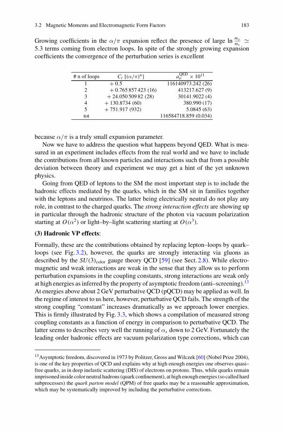
3.2 Magnetic Moments and Electromagnetic Form Factors 183

Growing coefficients in the α/π expansion reflect the presence of large ln mμ

me

5.3 terms coming from electron loops. In spite of the strongly growing expansioncoefficients the convergence of the perturbation series is excellent

# n of loops Ci [(α/π)n] aQEDμ × 1011

1 + 0.5 116140973.242 (26)2 + 0.765 857 423 (16) 413217.627 (9)3 + 24.050 509 82 (28) 30141.9022 (4)4 + 130.8734 (60) 380.990 (17)5 + 751.917 (932) 5.0845 (63)tot 116584718.859 (0.034)

because α/π is a truly small expansion parameter.Now we have to address the question what happens beyond QED. What is mea-

sured in an experiment includes effects from the real world and we have to includethe contributions from all known particles and interactions such that from a possibledeviation between theory and experiment we may get a hint of the yet unknownphysics.

Going from QED of leptons to the SM the most important step is to include thehadronic effects mediated by the quarks, which in the SM sit in families togetherwith the leptons and neutrinos. The latter being electrically neutral do not play anyrole, in contrast to the charged quarks. The strong interaction effects are showing upin particular through the hadronic structure of the photon via vacuum polarizationstarting at O(α2) or light–by–light scattering starting at O(α3).

(3) Hadronic VP effects:

Formally, these are the contributions obtained by replacing lepton–loops by quark–loops (see Fig. 3.2), however, the quarks are strongly interacting via gluons asdescribed by the SU(3)color gauge theory QCD [59] (see Sect. 2.8). While electro-magnetic and weak interactions are weak in the sense that they allow us to performperturbation expansions in the coupling constants, strong interactions are weak onlyat high energies as inferred by the property of asymptotic freedom (anti–screening).13

At energies above about 2 GeV perturbative QCD (pQCD) may be applied as well. Inthe regime of interest to us here, however, perturbative QCD fails. The strength of thestrong coupling “constant” increases dramatically as we approach lower energies.This is firmly illustrated by Fig. 3.3, which shows a compilation of measured strongcoupling constants as a function of energy in comparison to perturbative QCD. Thelatter seems to describes very well the running of αs down to 2 GeV. Fortunately theleading order hadronic effects are vacuum polarization type corrections, which can

13Asymptotic freedom, discovered in 1973 by Politzer, Gross and Wilczek [60] (Nobel Prize 2004),is one of the key properties of QCD and explains why at high enough energies one observes quasi–free quarks, as in deep inelastic scattering (DIS) of electrons on protons. Thus, while quarks remainimprisoned inside color neutral hadrons (quark confinement), at high enough energies (so called hardsubprocesses) the quark parton model (QPM) of free quarks may be a reasonable approximation,which may be systematically improved by including the perturbative corrections.

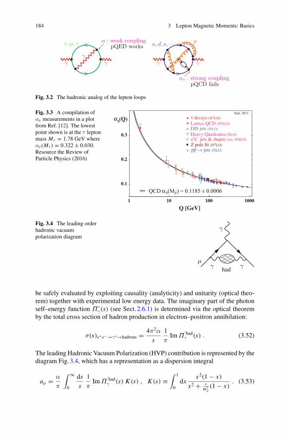
184 3 Lepton Magnetic Moments: Basics

γ γγ

e, μ, τ <

>

α : weak couplingpQED works↙

γ γ

gu, d, s, · · ·<

>αs : strong coupling

pQCD fails

↗

Fig. 3.2 The hadronic analog of the lepton loops

Fig. 3.3 A compilation ofαs measurements in a plotfrom Ref. [12]. The lowestpoint shown is at the τ leptonmass Mτ = 1.78 GeV whereαs(Mτ ) = 0.322 ± 0.030.Resource the Review ofParticle Physics (2016)

QCD αs(Mz) = 0.1185 ± 0.0006

Z pole fit

0.1

0.2

0.3

αs (Q)

1 10 100

Q [GeV]

Heavy Quarkonia (NLO)e+e– jets & shapes (res. NNLO)

DIS jets (NLO)

Sept. 2013

Lattice QCD (NNLO)

(N3LO)

τ decays (N3LO)

1000

pp –> jets (NLO)(–)

Fig. 3.4 The leading orderhadronic vacuumpolarization diagram

had

μ

γ

γ γ

be safely evaluated by exploiting causality (analyticity) and unitarity (optical theo-rem) together with experimental low energy data. The imaginary part of the photonself–energy function Π ′

γ(s) (see Sect. 2.6.1) is determined via the optical theoremby the total cross section of hadron production in electron–positron annihilation:

σ(s)e+e−→γ∗→hadrons = 4π2α

s

1

πIm Π

′hadγ (s) . (3.52)

The leading Hadronic Vacuum Polarization (HVP) contribution is represented by thediagram Fig. 3.4, which has a representation as a dispersion integral

aμ = α

π

∫ ∞

0

ds

s

1

πIm Π

′hadγ (s) K (s) , K (s) ≡

∫ 1

0dx

x2(1 − x)

x2 + sm2

μ(1 − x)

. (3.53)

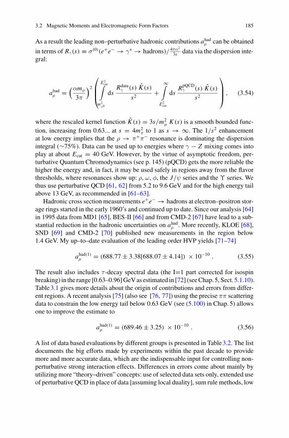
3.2 Magnetic Moments and Electromagnetic Form Factors 185

As a result the leading non–perturbative hadronic contributions ahadμ can be obtained

in terms of Rγ(s) ≡ σ(0)(e+e− → γ∗ → hadrons)/ 4πα2

3s data via the dispersion inte-gral:

ahadμ =

(αmμ

3π

)2

⎛

⎜⎜⎝

E2cut∫

m2π0

dsRdata

γ (s) K (s)

s2+

∞∫

E2cut

dsRpQCD

γ (s) K (s)

s2

⎞

⎟⎟⎠ , (3.54)

where the rescaled kernel function K (s) = 3s/m2μ K (s) is a smooth bounded func-

tion, increasing from 0.63... at s = 4m2π to 1 as s → ∞. The 1/s2 enhancement

at low energy implies that the ρ → π+π− resonance is dominating the dispersionintegral (∼75%). Data can be used up to energies where γ − Z mixing comes intoplay at about Ecut = 40 GeV. However, by the virtue of asymptotic freedom, per-turbative Quantum Chromodynamics (see p. 145) (pQCD) gets the more reliable thehigher the energy and, in fact, it may be used safely in regions away from the flavorthresholds, where resonances show up: ρ, ω, φ, the J/ψ series and the ϒ series. Wethus use perturbative QCD [61, 62] from 5.2 to 9.6 GeV and for the high energy tailabove 13 GeV, as recommended in [61–63].

Hadronic cross section measurements e+e− → hadrons at electron–positron stor-age rings started in the early 1960’s and continued up to date. Since our analysis [64]in 1995 data from MD1 [65], BES-II [66] and from CMD-2 [67] have lead to a sub-stantial reduction in the hadronic uncertainties on ahad

μ . More recently, KLOE [68],SND [69] and CMD-2 [70] published new measurements in the region below1.4 GeV. My up–to–date evaluation of the leading order HVP yields [71–74]

ahad(1)μ = (688.77 ± 3.38[688.07 ± 4.14]) × 10−10 . (3.55)

The result also includes τ -decay spectral data (the I=1 part corrected for isospinbreaking) in the range [0.63–0.96] GeV as estimated in [72] (see Chap. 5, Sect. 5.1.10).Table 3.1 gives more details about the origin of contributions and errors from differ-ent regions. A recent analysis [75] (also see [76, 77]) using the precise ππ scatteringdata to constrain the low energy tail below 0.63 GeV (see (5.100) in Chap. 5) allowsone to improve the estimate to

ahad(1)μ = (689.46 ± 3.25) × 10−10 . (3.56)

A list of data based evaluations by different groups is presented in Table 3.2. The listdocuments the big efforts made by experiments within the past decade to providemore and more accurate data, which are the indispensable input for controlling non-perturbative strong interaction effects. Differences in errors come about mainly byutilizing more “theory–driven” concepts: use of selected data sets only, extended useof perturbative QCD in place of data [assuming local duality], sum rule methods, low

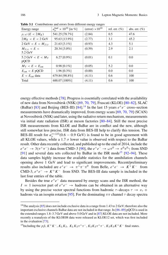
186 3 Lepton Magnetic Moments: Basics

Table 3.1 Contributions and errors from different energy ranges

Energy range ahadμ × 1010 [in %] (error) ×1010 rel. err. (%) abs. err. (%)

ρ,ω (E < 2MK ) 541.25 [78.7%] (2.84) 0.5 47.6

2MK < E < 2 GeV 95.63 [13.9%] (2.77) 3.1 45.2

2 GeV < E < MJ/ψ 21.63 [3.1%] (0.93) 4.3 5.1

MJ/ψ < E <

5.2 GeV20.34 [3.0%] (0.59) 2.9 2.1

5.2 GeV < E < Mϒ

pQCD6.27 [0.9%] (0.01) 0.1 0.0

Mϒ < E < Ecut 0.98 [0.1%] (0.05) 5.2 0.0

Ecut < E pQCD 1.96 [0.3%] (0.00) 0.0 0.0

E < Ecut data 679.84 [98.8%] (4.11) 0.6 100

Total 688.07 [100%] (4.11) 0.6 100

energy effective methods [78]. Progress is essentially correlated with the availabilityof new data from Novosibirsk (NSK) [69, 70, 79], Frascati (KLOE) [80–82], SLAC(BaBar) [83] and Beijing (BES-III) [84].14 In the last 15 years e+e− cross–sectionmeasurements have dramatically improved, from energy scans [69, 70, 79] (SCAN)at Novosibirsk (NSK) and later, using the radiative return mechanism, measurementsvia initial state radiation (ISR) at meson factories [80–84]. Still the most preciseISR measurements from KLOE and BaBar are in conflict and the new, althoughstill somewhat less precise, ISR data from BES-III help to clarify this tension. TheBES-III result for aππ,LO

μ (0.6 − 0.9 GeV) is found to be in good agreement withall KLOE values, while a 1.7 σ lower value is observed with respect to the BaBarresult. Other data recently collected, and published up to the end of 2014, include thee+e− → 3(π+π−) data from CMD–3 [90], the e+e− → ωπ0 → π0π0γ from SND[91] and several data sets collected by BaBar in the ISR mode15 [92–94]. Thesedata samples highly increase the available statistics for the annihilation channelsopening above 1 GeV and lead to significant improvements. Recent/preliminaryresults also included are e+e− → π+π−π0 from Belle, e+e− → K +K − fromCMD-3, e+e− → K +K − from SND. The BES-III data sample is included in thelast four entries of the table.

Besides the true e+e− data measured by energy scans and the ISR method, theI = 1 isovector part of e+e− → hadrons can be obtained in an alternative wayby using the precise vector spectral functions from hadronic τ–decays τ → ντ +hadrons via an isospin rotation [95]. For the dominating ππ channel τ decay spectra

14The analysis [85] does not include exclusive data in a range from 1.43 to 2 GeV; therefore also theimportant exclusive channels BaBar data are not included in that range. In [86–89] pQCD is used inthe extended ranges 1.8–3.7 GeV and above 5.0 GeV and in [87] KLOE data are not included. Morerecently a reanalysis of the KLOE08 data were released as KLOE12 set, which was first includedin the evaluation [73].15Including the p p, K +K −, KL KS, KL KSπ+π−, KS KSπ+π−, KS KS K +K − final states.

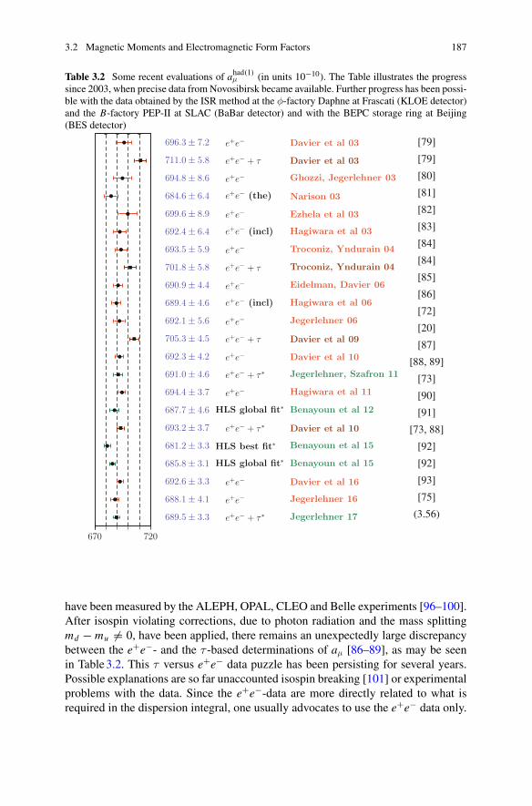
3.2 Magnetic Moments and Electromagnetic Form Factors 187

Table 3.2 Some recent evaluations of ahad(1)μ (in units 10−10). The Table illustrates the progress

since 2003, when precise data from Novosibirsk became available. Further progress has been possi-ble with the data obtained by the ISR method at the φ-factory Daphne at Frascati (KLOE detector)and the B-factory PEP-II at SLAC (BaBar detector) and with the BEPC storage ring at Beijing(BES detector)

670 720

696.3 ± 7.2 e+e− Davier et al 03

711.0 ± 5.8 e+e− + τ Davier et al 03

694.8 ± 8.6 e+e− Ghozzi, Jegerlehner 03

684.6 ± 6.4 e+e− (the) Narison 03

699.6 ± 8.9 e+e− Ezhela et al 03

692.4 ± 6.4 e+e− (incl) Hagiwara et al 03

693.5 ± 5.9 e+e− Troconiz, Yndurain 04

701.8 ± 5.8 e+e− + τ Troconiz, Yndurain 04

690.9 ± 4.4 e+e− Eidelman, Davier 06

689.4 ± 4.6 e+e− (incl) Hagiwara et al 06

692.1 ± 5.6 e+e− Jegerlehner 06

705.3 ± 4.5 e+e− + τ Davier et al 09

692.3 ± 4.2 e+e− Davier et al 10

691.0 ± 4.6 e+e− + τ ∗ Jegerlehner, Szafron 11

694.4 ± 3.7 e+e− Hagiwara et al 11

687.7 ± 4.6 HLS global fit∗ Benayoun et al 12

693.2 ± 3.7 e+e− + τ ∗ Davier et al 10

681.2 ± 3.3 HLS best fit∗ Benayoun et al 15

685.8 ± 3.1 HLS global fit∗ Benayoun et al 15

692.6 ± 3.3 e+e− Davier et al 16

688.1 ± 4.1 e+e− Jegerlehner 16

689.5 ± 3.3 e+e− + τ ∗ Jegerlehner 17

[79]

[79]

[80]

[81]

[82]

[83]

[84]

[84]

[85]

[86]

[72]

[20]

[87]

[88, 89]

[73]

[90]

[91]

[73, 88]

[92]

[92]

[93]

[75]

(3.56)

have been measured by the ALEPH, OPAL, CLEO and Belle experiments [96–100].After isospin violating corrections, due to photon radiation and the mass splittingmd − mu �= 0, have been applied, there remains an unexpectedly large discrepancybetween the e+e−- and the τ -based determinations of aμ [86–89], as may be seenin Table 3.2. This τ versus e+e− data puzzle has been persisting for several years.Possible explanations are so far unaccounted isospin breaking [101] or experimentalproblems with the data. Since the e+e−-data are more directly related to what isrequired in the dispersion integral, one usually advocates to use the e+e− data only.

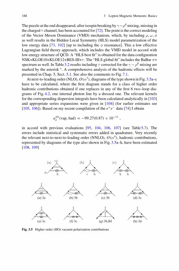
188 3 Lepton Magnetic Moments: Basics

The puzzle at the end disappeared, after isospin breaking by γ−ρ0 mixing, missing inthe charged τ channel, has been accounted for [72]. The point is the correct modelingof the Vector Meson Dominance (VMD) mechanism, which, by including ρ,ω,φas well results in the Hidden Local Symmetry (HLS) model parametrization of thelow energy data [73, 102] [up to including the φ resonance]. This a low effectiveLagrangian field theory approach, which includes the VMD model in accord withlow energy structure of QCD. A “HLS best fit” is obtained for the data configurationNSK+KLOE10+KLOE12+BES-III+τ . The “HLS global fit” includes the BaBar ππspectrum as well. In Table 3.2 results including τ corrected for the γ −ρ0 mixing aremarked by the asterisk ∗. A comprehensive analysis of the hadronic effects will bepresented in Chap. 5, Sect. 5.1. See also the comments to Fig. 7.1.

At next-to-leading order (NLO), O(α3), diagrams of the type shown in Fig. 3.5a–chave to be calculated, where the first diagram stands for a class of higher orderhadronic contributions obtained if one replaces in any of the first 6 two–loop dia-grams of Fig. 4.2, one internal photon line by a dressed one. The relevant kernelsfor the corresponding dispersion integrals have been calculated analytically in [103]and appropriate series expansions were given in [104] (for earlier estimates see[105, 106]). Based on my recent compilation of the e+e− data [74] I obtain

a(6)μ (vap, had) = −99.27(0.87) × 10−11 ,

in accord with previous evaluations [95, 104, 106, 107] (see Table 5.7). Theerrors include statistical and systematic errors added in quadrature. Very recentlythe relevant next-to-next-to-leading order (NNLO), O(α4), hadronic contributions,represented by diagrams of the type also shown in Fig. 3.5a–h, have been estimated[108, 109]

h e h h hμ

γ(a) (b) (c)

(a) 3a (b) 3b (c) 3b (d) 3c

(e) 3c (f) 3c (g) 3b,lbl (h) 3d

Fig. 3.5 Higher order (HO) vacuum polarization contributions

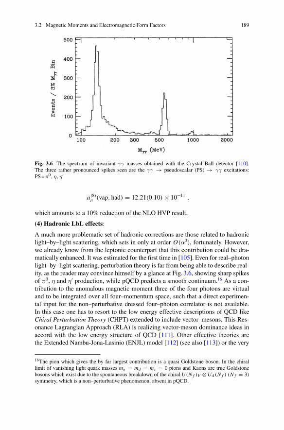
3.2 Magnetic Moments and Electromagnetic Form Factors 189

Fig. 3.6 The spectrum of invariant γγ masses obtained with the Crystal Ball detector [110].The three rather pronounced spikes seen are the γγ → pseudoscalar (PS) → γγ excitations:PS =π0, η, η′

a(8)μ (vap, had) = 12.21(0.10) × 10−11 ,

which amounts to a 10% reduction of the NLO HVP result.

(4) Hadronic LbL effects:

A much more problematic set of hadronic corrections are those related to hadroniclight–by–light scattering, which sets in only at order O(α3), fortunately. However,we already know from the leptonic counterpart that this contribution could be dra-matically enhanced. It was estimated for the first time in [105]. Even for real–photonlight–by–light scattering, perturbation theory is far from being able to describe real-ity, as the reader may convince himself by a glance at Fig. 3.6, showing sharp spikesof π0, η and η′ production, while pQCD predicts a smooth continuum.16 As a con-tribution to the anomalous magnetic moment three of the four photons are virtualand to be integrated over all four–momentum space, such that a direct experimen-tal input for the non–perturbative dressed four–photon correlator is not available.In this case one has to resort to the low energy effective descriptions of QCD likeChiral Perturbation Theory (CHPT) extended to include vector–mesons. This Res-onance Lagrangian Approach (RLA) is realizing vector-meson dominance ideas inaccord with the low energy structure of QCD [111]. Other effective theories arethe Extended Nambu-Jona-Lasinio (ENJL) model [112] (see also [113]) or the very

16The pion which gives the by far largest contribution is a quasi Goldstone boson. In the chirallimit of vanishing light quark masses mu = md = ms = 0 pions and Kaons are true Goldstonebosons which exist due to the spontaneous breakdown of the chiral U (N f )V ⊗ UA(N f ) (N f = 3)

symmetry, which is a non–perturbative phenomenon, absent in pQCD.

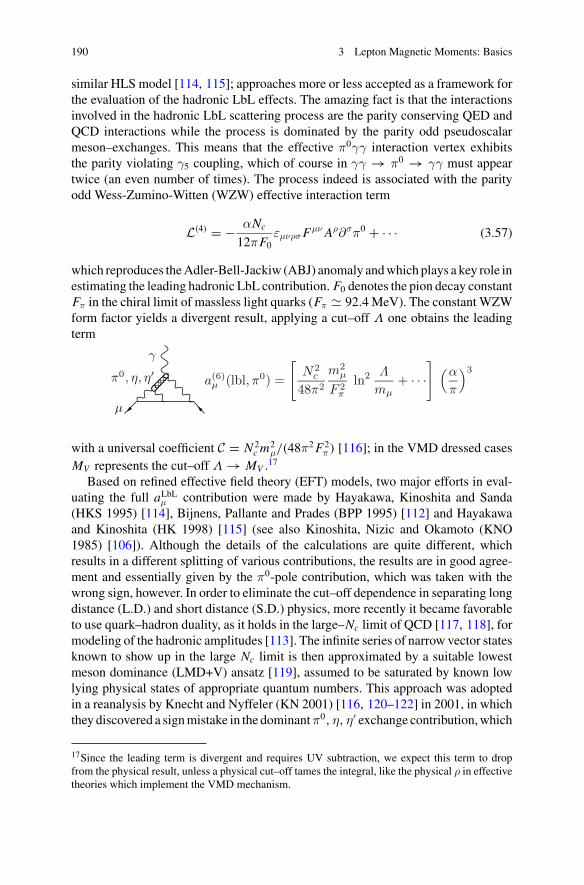
190 3 Lepton Magnetic Moments: Basics

similar HLS model [114, 115]; approaches more or less accepted as a framework forthe evaluation of the hadronic LbL effects. The amazing fact is that the interactionsinvolved in the hadronic LbL scattering process are the parity conserving QED andQCD interactions while the process is dominated by the parity odd pseudoscalarmeson–exchanges. This means that the effective π0γγ interaction vertex exhibitsthe parity violating γ5 coupling, which of course in γγ → π0 → γγ must appeartwice (an even number of times). The process indeed is associated with the parityodd Wess-Zumino-Witten (WZW) effective interaction term

L(4) = − αNc

12πF0εμνρσ Fμν Aρ∂σπ0 + · · · (3.57)

which reproduces the Adler-Bell-Jackiw (ABJ) anomaly and which plays a key role inestimating the leading hadronic LbL contribution. F0 denotes the pion decay constantFπ in the chiral limit of massless light quarks (Fπ 92.4 MeV). The constant WZWform factor yields a divergent result, applying a cut–off Λ one obtains the leadingterm

a(6)μ (lbl, π0) =

[N2

c

48π2

m2μ

F 2π

ln2Λ

mμ+ · · ·

] (α

π

)3π0, η, η′

μ

γ

with a universal coefficient C = N 2c m2

μ/(48π2 F2π ) [116]; in the VMD dressed cases

MV represents the cut–off Λ → MV .17

Based on refined effective field theory (EFT) models, two major efforts in eval-uating the full aLbL

μ contribution were made by Hayakawa, Kinoshita and Sanda(HKS 1995) [114], Bijnens, Pallante and Prades (BPP 1995) [112] and Hayakawaand Kinoshita (HK 1998) [115] (see also Kinoshita, Nizic and Okamoto (KNO1985) [106]). Although the details of the calculations are quite different, whichresults in a different splitting of various contributions, the results are in good agree-ment and essentially given by the π0-pole contribution, which was taken with thewrong sign, however. In order to eliminate the cut–off dependence in separating longdistance (L.D.) and short distance (S.D.) physics, more recently it became favorableto use quark–hadron duality, as it holds in the large–Nc limit of QCD [117, 118], formodeling of the hadronic amplitudes [113]. The infinite series of narrow vector statesknown to show up in the large Nc limit is then approximated by a suitable lowestmeson dominance (LMD+V) ansatz [119], assumed to be saturated by known lowlying physical states of appropriate quantum numbers. This approach was adoptedin a reanalysis by Knecht and Nyffeler (KN 2001) [116, 120–122] in 2001, in whichthey discovered a sign mistake in the dominant π0, η, η′ exchange contribution, which

17Since the leading term is divergent and requires UV subtraction, we expect this term to dropfrom the physical result, unless a physical cut–off tames the integral, like the physical ρ in effectivetheories which implement the VMD mechanism.

3.2 Magnetic Moments and Electromagnetic Form Factors 191

changed the central value by +167×10−11, a 2.8 σ shift, and which reduces a largerdiscrepancy between theory and experiment. More recently Melnikov and Vainshtein(MV 2004) [123] found additional problems in previous calculations, this time in theshort distance constraints (QCD/OPE) used in matching the high energy behavior ofthe effective models used for the π0, η, η′ exchange contribution. Another importantchange concerns the contributions from the axialvector exchanges which have beenmodeled in [123] violating the Landau–Yang theorem. We will elaborate on this inmuch more detail in Sect. 5.2.

We advocate to use consistently dressed form factors as inferred from the res-onance Lagrangian approach. However, other effects which were first consideredin [123] must be taken into account: (i) the constraint on the twist four (1/q4)-termin the OPE requires h2 = −10 GeV2 in the Knecht-Nyffeler form factor [120]:δaμ +5 ± 0 relative to h2 = 0, (ii) the contributions from the f1 and f ′

1 isoscalaraxial–vector mesons: δaμ +6 ± 2 (using dressed photons, and implementingthe Landau–Yang condition), (iii) for the remaining effects, scalars ( f0) + dressedπ±, K ± loops + dressed quark loops: δaμ −5 ± 13. Note that this last group ofterms have been evaluated in [112, 114] only. The splitting into the different termsis model dependent and only the sum should be considered; the results read −5 ± 13(BPP) and 5.2 ± 13.7 (HKS) and hence the contribution remains unclear.18 As anestimate based on [112, 114, 120, 123, 124] we adopt π0, η, η′ [95 ± 12] + axial–vector [8 ± 3] + scalar [−6 ± 1] + π, K loops [−20 ± 5] + quark loops [22 ± 4] +tensor [1 ± 0] + NLO [3 ± 2] which yields

a(6)μ (lbl, had) = (103 ± 29) × 10−11 .

The result differs little from the “agreed” value (105±26)×10−11 presented in [125]and (116±39)×10−11 estimated in [20]. Both included a wrong, too large, Landau–Yang theorem violating axial–vector contribution from [123], correcting for this weobtain our reduced value relative to [20].

(5) Weak interaction corrections:

The last set of corrections are due to the weak interaction as described by the elec-troweak SM. The weak corrections are those mediated by the weak currents whichcouple to the heavy spin 1 gauge bosons, the charged W ± or the neutral “heavylight” particle Z or by exchange of a Higgs particle H (see Fig. 3.7; masses are givenin (3.33), (3.34)). What is most interesting is the occurrence of the first diagram ofFig. 3.7, which exhibits a non–Abelian triple gauge vertex and the correspondingcontribution provides a test of the Yang–Mills structure involved. It is of course notsurprising that the photon couples to the charged W boson the way it is dictatedby electromagnetic gauge invariance. In spite of the fact that the contribution is ofleading one–loop order, it is vastly suppressed by the fact that the corrections aremediated by the exchange of very heavy states which makes them suppressed by

18We adopt the result of [112] as the sign has to be negative in any case (see [121]).

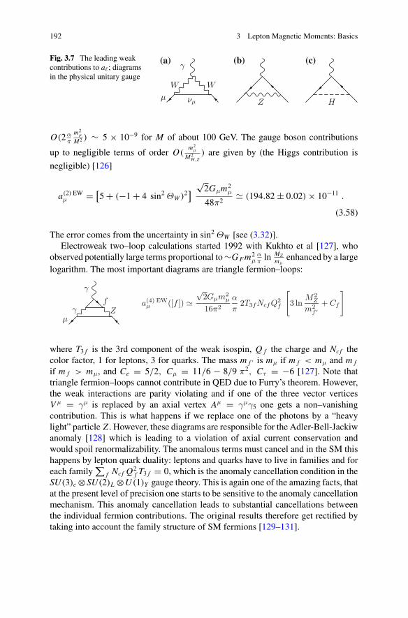
192 3 Lepton Magnetic Moments: Basics

Fig. 3.7 The leading weakcontributions to a�; diagramsin the physical unitary gauge

W W

νμ Z Hμ

γ(a) (b) (c)

O(2 απ

m2μ

M2 ) ∼ 5 × 10−9 for M of about 100 GeV. The gauge boson contributions

up to negligible terms of order O(m2

μ

M2W,Z

) are given by (the Higgs contribution is

negligible) [126]

a(2) EWμ = [

5 + (−1 + 4 sin2 ΘW )2]√

2Gμm2μ

48π2 (194.82 ± 0.02) × 10−11 .

(3.58)

The error comes from the uncertainty in sin2 ΘW [see (3.32)].Electroweak two–loop calculations started 1992 with Kukhto et al [127], who

observed potentially large terms proportional to ∼G F m2μ

απ

ln MZmμ

enhanced by a largelogarithm. The most important diagrams are triangle fermion–loops:

a(4) EWμ ([f ]) �

√2Gμm2

μ

16π2

α

π2T3fNcfQ2

f

[3 ln

M2Z

m2f ′

+ Cf

]γ Z

f

μ

γ

where T3 f is the 3rd component of the weak isospin, Q f the charge and Ncf thecolor factor, 1 for leptons, 3 for quarks. The mass m f ′ is mμ if m f < mμ and m f

if m f > mμ, and Ce = 5/2, Cμ = 11/6 − 8/9 π2, Cτ = −6 [127]. Note thattriangle fermion–loops cannot contribute in QED due to Furry’s theorem. However,the weak interactions are parity violating and if one of the three vector verticesV μ = γμ is replaced by an axial vertex Aμ = γμγ5 one gets a non–vanishingcontribution. This is what happens if we replace one of the photons by a “heavylight” particle Z . However, these diagrams are responsible for the Adler-Bell-Jackiwanomaly [128] which is leading to a violation of axial current conservation andwould spoil renormalizability. The anomalous terms must cancel and in the SM thishappens by lepton quark duality: leptons and quarks have to live in families and foreach family

∑f Ncf Q2

f T3 f = 0, which is the anomaly cancellation condition in theSU(3)c ⊗SU(2)L ⊗U (1)Y gauge theory. This is again one of the amazing facts, thatat the present level of precision one starts to be sensitive to the anomaly cancellationmechanism. This anomaly cancellation leads to substantial cancellations betweenthe individual fermion contributions. The original results therefore get rectified bytaking into account the family structure of SM fermions [129–131].

3.2 Magnetic Moments and Electromagnetic Form Factors 193

For more sophisticated analyses we refer to [129, 130, 132] which was correctedand refined in [131, 133]. Including subleading effects yields −5.0 × 10−11 for thefirst two families. The 3rd family of fermions including the heavy top quark canbe treated in perturbation theory and was worked out to be −8.2 × 10−11 in [134].Subleading fermion loops contribute −5.3 × 10−11. There are many more diagramscontributing, in particular the calculation of the bosonic contributions (1678 dia-grams) is a formidable task and has been performed 1996 by Czarnecki, Krauseand Marciano as an expansion in (mμ/MV )2 and (MV /m H )2 [135]. Later completecalculations, valid also for lighter Higgs masses, were performed [136, 137], whichconfirmed the previous result −22.3 × 10−11. The 2–loop result reads19

a(4) EWμ = −41(1) × 10−11 .

The complete weak contribution may be summarized by [133]

aEWμ =

√2Gμ m2

μ

16π2

{5

3+ 1

3(1 − 4 sin2 ΘW )2 − α

π[155.5(4)(2)]

}

= (154 ± 1[had] ± 0.4[mH, mt, 3 − loop]) × 10−11 (3.59)

with errors from triangle quark–loops. For the Higgs we use the recent LHC observa-tion m H 125.1 ± 0.3 GeV. The 3–loop effect has been estimated tobe small [131,133] (see (4.124)).

This closes our overview of the various contributions to the anomalous magneticmoment of the muon. More details about the higher order QED corrections as wellas the weak and strong interaction corrections will be discussed in detail in the nextChap. 4. First we give a brief account of the status of the theory in comparison to theexperiments. We will consider the electron and the muon in turn.

3.2.2 The Anomalous Magnetic Moment of the Electron

The electron magnetic moment anomaly likely is the experimentally most preciselyknown quantity. For almost 20 years the value was based on the extraordinary precisemeasurements of electron and positron anomalous magnetic moments

19The authors of [127] reporteda(4) EWμ = −42 × 10−11

for what they thought was the leading correction, which is very close to the complete weak two–loopcorrections, however, this coincidence looks to be a mere accident. Nevertheless, the sign and theorder of magnitude turned out to be correct.

194 3 Lepton Magnetic Moments: Basics

aexpe− = 0.001 159 652 188 4(43),

aexpe+ = 0.001 159 652 187 9(43), (3.60)

by Van Dyck et al. (1987) [138]. The experiment used the ion trap technique, whichhas made it possible to study a single electron with extreme precision.20 The resultimpressively confirms the conservation of CPT: ae+ = ae− . Being a basic predictionof any QFT, CPT symmetry will be assumed to hold in the following. This allowsus to average the electron and positron values with the result [14]

ae = μe/μB − 1 = (ge − 2)/2 = 1.159 652 1883(42) × 10−3 . (3.61)

The relative standard uncertainty is 3.62 ppb. A big step forward has been achievedmore recently by Gabrielse et al. [5, 6, 139] in an experiment at Harvard Universityusing a one–electron quantum cyclotron. The new result is

ae = 1.159 652 180 73(28)[0.24 ppb] × 10−3 , (3.62)

with an accuracy nearly 15 times better than (3.61) and shifting down the centralvalue of ae by 1.8 standard deviations.

The measurements of ae not only played a key role in the history of precisiontests of QED in particular, and of QFT concepts in general, today we may usethe anomalous magnetic moment of the electron to get the most precise indirectmeasurement of the fine structure constant α. This possibility of course hangs on ourability to pin down the theoretical prediction with very high accuracy. Indeed ae ismuch saver to predict reliably than aμ. The reason is that non–perturbative hadroniceffects as well as the sensitivity to unknown physics beyond the SM are suppressedby the large factor m2

μ/m2e 42 753 in comparison to aμ. This suppression has to be

put into perspective with the 2250 times higher precision with which we know ae.We thus can say that effectively ae is a factor 19 less sensitive to model dependentphysics than aμ.

The reason why it is so interesting to have such a precise measurement of ae ofcourse is that it can be calculated with comparable accuracy in theory. The predictionis given by a perturbation expansion of the form

ae =N∑

n=1

Cn(α/π)n , (3.63)

20The ion trap technique was introduced and developed by Paul and Dehmelt, whom was awardedthe Nobel Prize in 1989. The ion traps utilize electrical quadrupole fields obtained with hyperboloidshaped electrodes. The Paul trap works with dynamical trapping using r.f. voltage, the Penning trapused by Dehmelt works with d.c. voltage and a magnetic field in z-direction.

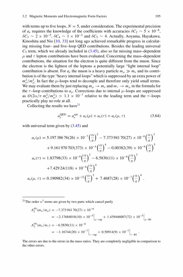
3.2 Magnetic Moments and Electromagnetic Form Factors 195

with terms up to five loops, N = 5, under consideration. The experimental precisionof ae requires the knowledge of the coefficients with accuracies δC2 ∼ 5 × 10−8,δC3 ∼ 2 × 10−5, δC4 ∼ 1 × 10−2 and δC5 ∼ 4. Actually, Aoyama, Hayakawa,Kinoshita and Nio [10, 33] not long ago achieved remarkable progress in calculat-ing missing four– and five–loop QED contributions. Besides the leading universalC5 term, which we already included in (3.45), also so far missing mass–dependentμ and τ lepton contributions have been evaluated. Concerning the mass–dependentcontributions, the situation for the electron is quite different from the muon. Sincethe electron is the lightest of the leptons a potentially large “light internal loop”contribution is absent. For ae the muon is a heavy particle mμ � me and its contri-bution is of the type “heavy internal loops” which is suppressed by an extra power ofm2

e/m2μ. In fact the μ–loops tend to decouple and therefore only yield small terms.

We may evaluate them by just replacing mμ → me and mτ → mμ in the formula forthe τ–loop contributions to aμ. Corrections due to internal μ–loops are suppressedas O(2α/π m2

e/m2μ) 1.1 × 10−7 relative to the leading term and the τ–loops

practically play no role at all.Collecting the results we have21

aQEDe = auni

e + ae(μ) + ae(τ ) + ae(μ, τ ) (3.64)

with universal term given by (3.45) and

ae(μ) = 5.197 386 76(26) × 10−7(α

π

)2 − 7.373 941 70(27) × 10−6(α

π

)3

+ 9.161 970 703(373) × 10−4(α

π

)4 − 0.00382(39) × 10−6(α

π

)5

ae(τ ) = 1.83798(33) × 10−9(α

π

)2 − 6.5830(11) × 10−8(α

π

)3

+7.429 24(118) × 10−6(α

π

)4

ae(μ, τ ) = 0.190982(34) × 10−12(α

π

)3 + 7.4687(28) × 10−7(α

π

)4.

21The order α3 terms are given by two parts which cancel partly

A(6)2 (me/mμ) = −7.373 941 70(27) × 10−6

= −2.17684018(10) × 10−5∣∣∣μ−vap

+ 1.439446007(72) × 10−5∣∣∣μ−lbl

A(6)2 (me/mτ ) = −6.5830(11) × 10−8

= −1.16744(20) × 10−7∣∣∣τ−vap

+ 0.50914(9) × 10−7∣∣∣τ−lbl

.

The errors are due to the errors in the mass ratios. They are completely negligible in comparison tothe other errors.

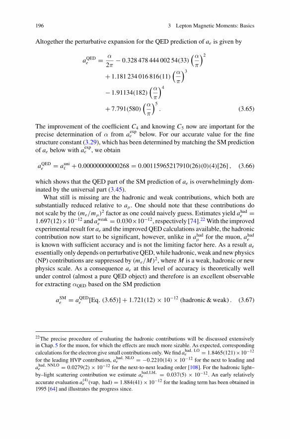
196 3 Lepton Magnetic Moments: Basics

Altogether the perturbative expansion for the QED prediction of ae is given by

aQEDe = α

2π− 0.328 478 444 002 54(33)

(α

π

)2

+ 1.181 234 016 816(11)(α

π

)3

− 1.91134(182)(α

π

)4

+ 7.791(580)(α

π

)5. (3.65)

The improvement of the coefficient C4 and knowing C5 now are important for theprecise determination of α from aexp

e below. For our accurate value for the finestructure constant (3.29), which has been determined by matching the SM predictionof ae below with aexp

e , we obtain

aQEDe = auni

� + 0.00000000000268 = 0.00115965217910(26)(0)(4)[26] , (3.66)

which shows that the QED part of the SM prediction of ae is overwhelmingly dom-inated by the universal part (3.45).

What still is missing are the hadronic and weak contributions, which both aresubstantially reduced relative to aμ. One should note that these contributions donot scale by the (me/mμ)

2 factor as one could naively guess. Estimates yield ahade =

1.697(12)×10−12 and aweake = 0.030×10−12, respectively [74].22 With the improved

experimental result for ae and the improved QED calculations available, the hadroniccontribution now start to be significant, however, unlike in ahad

μ for the muon, ahade

is known with sufficient accuracy and is not the limiting factor here. As a result ae

essentially only depends on perturbative QED, while hadronic, weak and new physics(NP) contributions are suppressed by (me/M)2, where M is a weak, hadronic or newphysics scale. As a consequence ae at this level of accuracy is theoretically wellunder control (almost a pure QED object) and therefore is an excellent observablefor extracting αQED based on the SM prediction

aSMe = aQED

e [Eq. (3.65)] + 1.721(12) × 10−12 (hadronic & weak) . (3.67)

22The precise procedure of evaluating the hadronic contributions will be discussed extensivelyin Chap. 5 for the muon, for which the effects are much more sizable. As expected, correspondingcalculations for the electron give small contributions only. We find ahad, LO

e = 1.8465(121)×10−12

for the leading HVP contribution, ahad, NLOe = −0.2210(14) × 10−12 for the next to leading and

ahad, NNLOe = 0.0279(2) × 10−12 for the next-to-next leading order [108]. For the hadronic light–

by–light scattering contribution we estimate ahad,LbLe = 0.037(5) × 10−12. An early relatively

accurate evaluation a(4)e (vap, had) = 1.884(41) × 10−12 for the leading term has been obtained in

1995 [64] and illustrates the progress since.

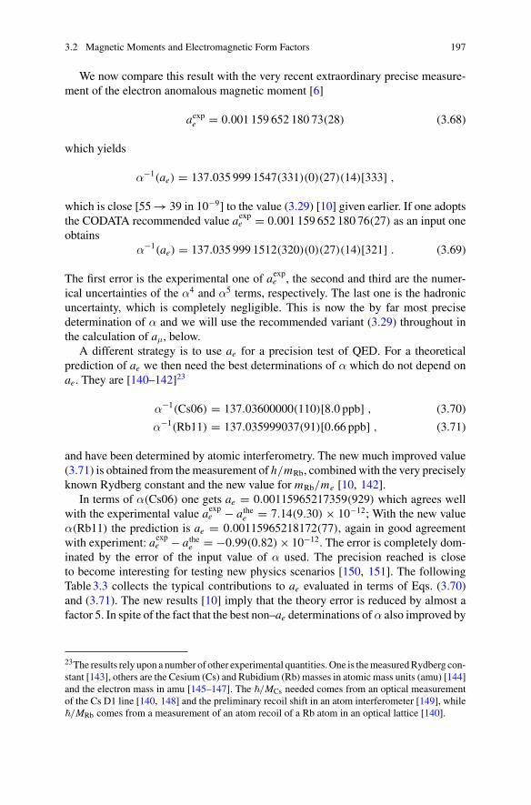
3.2 Magnetic Moments and Electromagnetic Form Factors 197

We now compare this result with the very recent extraordinary precise measure-ment of the electron anomalous magnetic moment [6]

aexpe = 0.001 159 652 180 73(28) (3.68)

which yields

α−1(ae) = 137.035 999 1547(331)(0)(27)(14)[333] ,

which is close [55 → 39 in 10−9] to the value (3.29) [10] given earlier. If one adoptsthe CODATA recommended value aexp

e = 0.001 159 652 180 76(27) as an input oneobtains

α−1(ae) = 137.035 999 1512(320)(0)(27)(14)[321] . (3.69)

The first error is the experimental one of aexpe , the second and third are the numer-

ical uncertainties of the α4 and α5 terms, respectively. The last one is the hadronicuncertainty, which is completely negligible. This is now the by far most precisedetermination of α and we will use the recommended variant (3.29) throughout inthe calculation of aμ, below.

A different strategy is to use ae for a precision test of QED. For a theoreticalprediction of ae we then need the best determinations of α which do not depend onae. They are [140–142]23

α−1(Cs06) = 137.03600000(110)[8.0 ppb] , (3.70)

α−1(Rb11) = 137.035999037(91)[0.66 ppb] , (3.71)

and have been determined by atomic interferometry. The new much improved value(3.71) is obtained from the measurement of h/mRb, combined with the very preciselyknown Rydberg constant and the new value for mRb/me [10, 142].

In terms of α(Cs06) one gets ae = 0.00115965217359(929) which agrees wellwith the experimental value aexp

e − athee = 7.14(9.30) × 10−12; With the new value

α(Rb11) the prediction is ae = 0.00115965218172(77), again in good agreementwith experiment: aexp

e − athee = −0.99(0.82) × 10−12. The error is completely dom-

inated by the error of the input value of α used. The precision reached is closeto become interesting for testing new physics scenarios [150, 151]. The followingTable 3.3 collects the typical contributions to ae evaluated in terms of Eqs. (3.70)and (3.71). The new results [10] imply that the theory error is reduced by almost afactor 5. In spite of the fact that the best non–ae determinations of α also improved by

23The results rely upon a number of other experimental quantities. One is the measured Rydberg con-stant [143], others are the Cesium (Cs) and Rubidium (Rb) masses in atomic mass units (amu) [144]and the electron mass in amu [145–147]. The �/MCs needed comes from an optical measurementof the Cs D1 line [140, 148] and the preliminary recoil shift in an atom interferometer [149], while�/MRb comes from a measurement of an atom recoil of a Rb atom in an optical lattice [140].

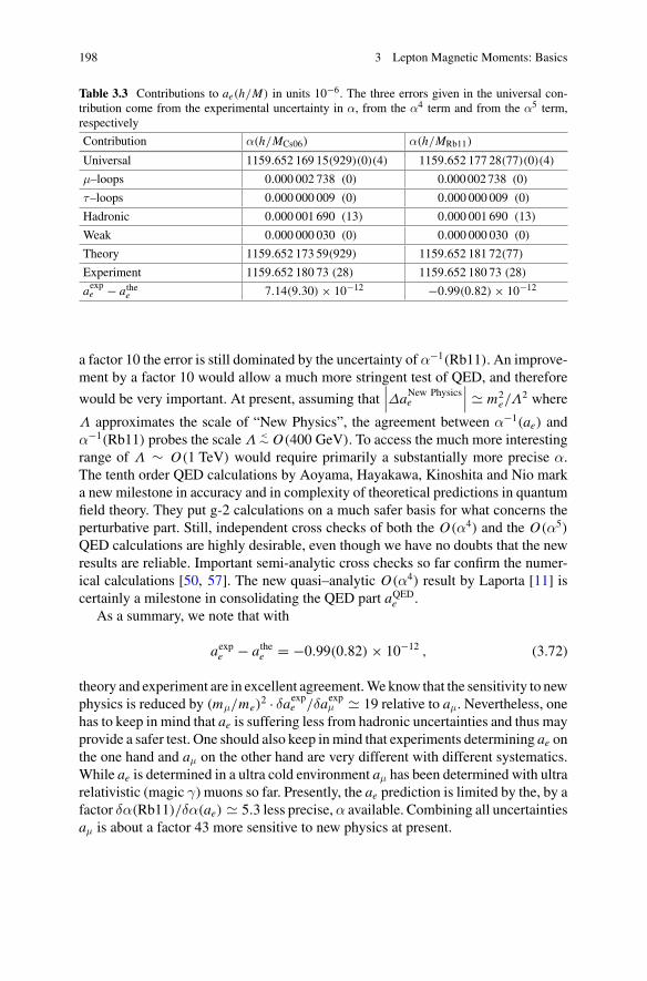
198 3 Lepton Magnetic Moments: Basics

Table 3.3 Contributions to ae(h/M) in units 10−6. The three errors given in the universal con-tribution come from the experimental uncertainty in α, from the α4 term and from the α5 term,respectively

Contribution α(h/MCs06) α(h/MRb11)

Universal 1159.652 169 15(929)(0)(4) 1159.652 177 28(77)(0)(4)

μ–loops 0.000 002 738 (0) 0.000 002 738 (0)

τ–loops 0.000 000 009 (0) 0.000 000 009 (0)

Hadronic 0.000 001 690 (13) 0.000 001 690 (13)

Weak 0.000 000 030 (0) 0.000 000 030 (0)

Theory 1159.652 173 59(929) 1159.652 181 72(77)

Experiment 1159.652 180 73 (28) 1159.652 180 73 (28)

aexpe − athe

e 7.14(9.30) × 10−12 −0.99(0.82) × 10−12

a factor 10 the error is still dominated by the uncertainty of α−1(Rb11). An improve-ment by a factor 10 would allow a much more stringent test of QED, and therefore

would be very important. At present, assuming that∣∣∣ΔaNew Physics

e

∣∣∣ m2e/Λ

2 where

Λ approximates the scale of “New Physics”, the agreement between α−1(ae) andα−1(Rb11) probes the scale Λ <∼ O(400 GeV). To access the much more interestingrange of Λ ∼ O(1 TeV) would require primarily a substantially more precise α.The tenth order QED calculations by Aoyama, Hayakawa, Kinoshita and Nio marka new milestone in accuracy and in complexity of theoretical predictions in quantumfield theory. They put g-2 calculations on a much safer basis for what concerns theperturbative part. Still, independent cross checks of both the O(α4) and the O(α5)

QED calculations are highly desirable, even though we have no doubts that the newresults are reliable. Important semi-analytic cross checks so far confirm the numer-ical calculations [50, 57]. The new quasi–analytic O(α4) result by Laporta [11] iscertainly a milestone in consolidating the QED part aQED

e .As a summary, we note that with

aexpe − athe

e = −0.99(0.82) × 10−12 , (3.72)

theory and experiment are in excellent agreement. We know that the sensitivity to newphysics is reduced by (mμ/me)

2 · δaexpe /δaexp

μ 19 relative to aμ. Nevertheless, onehas to keep in mind that ae is suffering less from hadronic uncertainties and thus mayprovide a safer test. One should also keep in mind that experiments determining ae onthe one hand and aμ on the other hand are very different with different systematics.While ae is determined in a ultra cold environment aμ has been determined with ultrarelativistic (magic γ) muons so far. Presently, the ae prediction is limited by the, by afactor δα(Rb11)/δα(ae) 5.3 less precise, α available. Combining all uncertaintiesaμ is about a factor 43 more sensitive to new physics at present.

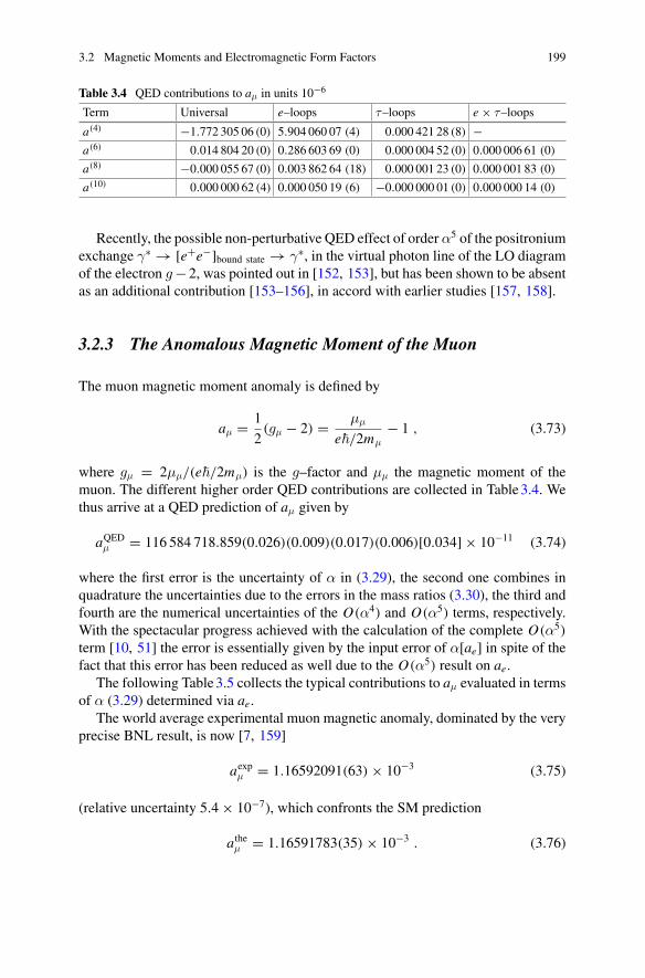
3.2 Magnetic Moments and Electromagnetic Form Factors 199

Table 3.4 QED contributions to aμ in units 10−6

Term Universal e–loops τ–loops e × τ–loops

a(4) −1.772 305 06 (0) 5.904 060 07 (4) 0.000 421 28 (8) −a(6) 0.014 804 20 (0) 0.286 603 69 (0) 0.000 004 52 (0) 0.000 006 61 (0)

a(8) −0.000 055 67 (0) 0.003 862 64 (18) 0.000 001 23 (0) 0.000 001 83 (0)

a(10) 0.000 000 62 (4) 0.000 050 19 (6) −0.000 000 01 (0) 0.000 000 14 (0)

Recently, the possible non-perturbative QED effect of order α5 of the positroniumexchange γ∗ → [e+e−]bound state → γ∗, in the virtual photon line of the LO diagramof the electron g − 2, was pointed out in [152, 153], but has been shown to be absentas an additional contribution [153–156], in accord with earlier studies [157, 158].

3.2.3 The Anomalous Magnetic Moment of the Muon

The muon magnetic moment anomaly is defined by

aμ = 1

2(gμ − 2) = μμ

e�/2mμ− 1 , (3.73)

where gμ = 2μμ/(e�/2mμ) is the g–factor and μμ the magnetic moment of themuon. The different higher order QED contributions are collected in Table 3.4. Wethus arrive at a QED prediction of aμ given by

aQEDμ = 116 584 718.859(0.026)(0.009)(0.017)(0.006)[0.034] × 10−11 (3.74)

where the first error is the uncertainty of α in (3.29), the second one combines inquadrature the uncertainties due to the errors in the mass ratios (3.30), the third andfourth are the numerical uncertainties of the O(α4) and O(α5) terms, respectively.With the spectacular progress achieved with the calculation of the complete O(α5)

term [10, 51] the error is essentially given by the input error of α[ae] in spite of thefact that this error has been reduced as well due to the O(α5) result on ae.

The following Table 3.5 collects the typical contributions to aμ evaluated in termsof α (3.29) determined via ae.

The world average experimental muon magnetic anomaly, dominated by the veryprecise BNL result, is now [7, 159]

aexpμ = 1.16592091(63) × 10−3 (3.75)

(relative uncertainty 5.4 × 10−7), which confronts the SM prediction

atheμ = 1.16591783(35) × 10−3 . (3.76)

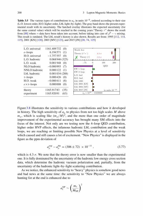
200 3 Lepton Magnetic Moments: Basics

Table 3.5 The various types of contributions to aμ in units 10−6, ordered according to their size(L.O. lowest order, H.O. higher order, LbL light–by–light). The gray band shows the present exper-imental result with its uncertainty. The hatched overlay illustrates the expected uncertainty (forthe same central value) which will be reached in the coming years.“Theory τ” shows the resultfrom [88] where τ–data have been taken into account, before taking into care of ρ0 − γ mixing.This result is outdated. The LbL result’s history is also shown. Results are from: 1995 [112, 114,115], 2001 [KN] [120], 2003 [MV] [123], and 2015 [JN] [20, 74, 125]

Figure 3.8 illustrates the sensitivity to various contributions and how it developedin history. The high sensitivity of aμ to physics from not too high scales M abovemμ, which is scaling like (mμ/M)2, and the more than one order of magnitudeimprovement of the experimental accuracy has brought many SM effects into thefocus of the interest. Not only are we testing now the 4–loop QED contribution,higher order HVP effects, the infamous hadronic LbL contribution and the weakloops, we are reaching or limiting possible New Physics at a level of sensitivitywhich caused and still causes a lot of excitement. “New Physics” is displayed in thefigure as the ppm deviation of

aexpμ − athe

μ = (306 ± 72) × 10−11 , (3.77)

which is 4.3 σ. We note that the theory error is now smaller than the experimentalone. It is fully dominated by the uncertainty of the hadronic low energy cross sectiondata, which determine the hadronic vacuum polarization and, partially, from theuncertainty of the hadronic light–by–light scattering contribution.

As we notice, the enhanced sensitivity to “heavy” physics is somehow good newsand bad news at the same time: the sensitivity to “New Physics” we are alwayshunting for at the end is enhanced due to

aNP� ∼

(m�

MNP

)2

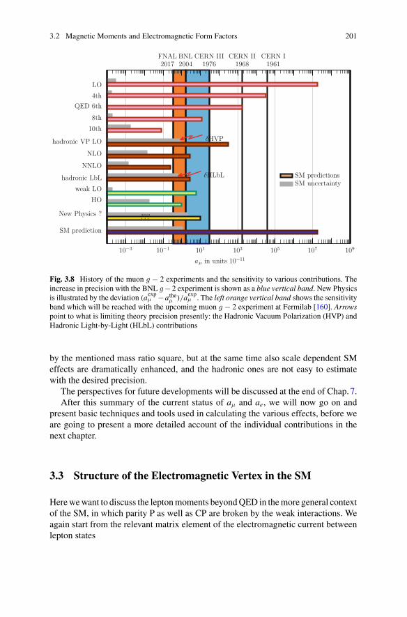
3.2 Magnetic Moments and Electromagnetic Form Factors 201

aμ in units 10−11

10−3 10−1 101 103 105 107 109

FNAL BNL CERN ICERN IICERN III169140027102 19681976

LO

4thQED 6th

8th

10th

hadronic VP LO

NLO

NNLO

hadronic LbL

weak LO

HO

New Physics ?

SM prediction

???

SM predictionsSM uncertainty

δHVP

δHLbL

Fig. 3.8 History of the muon g − 2 experiments and the sensitivity to various contributions. Theincrease in precision with the BNL g − 2 experiment is shown as a blue vertical band. New Physicsis illustrated by the deviation (aexp

μ −atheμ )/aexp

μ . The left orange vertical band shows the sensitivityband which will be reached with the upcoming muon g − 2 experiment at Fermilab [160]. Arrowspoint to what is limiting theory precision presently: the Hadronic Vacuum Polarization (HVP) andHadronic Light-by-Light (HLbL) contributions

by the mentioned mass ratio square, but at the same time also scale dependent SMeffects are dramatically enhanced, and the hadronic ones are not easy to estimatewith the desired precision.

The perspectives for future developments will be discussed at the end of Chap. 7.After this summary of the current status of aμ and ae, we will now go on and

present basic techniques and tools used in calculating the various effects, before weare going to present a more detailed account of the individual contributions in thenext chapter.

3.3 Structure of the Electromagnetic Vertex in the SM

Here we want to discuss the lepton moments beyond QED in the more general contextof the SM, in which parity P as well as CP are broken by the weak interactions. Weagain start from the relevant matrix element of the electromagnetic current betweenlepton states

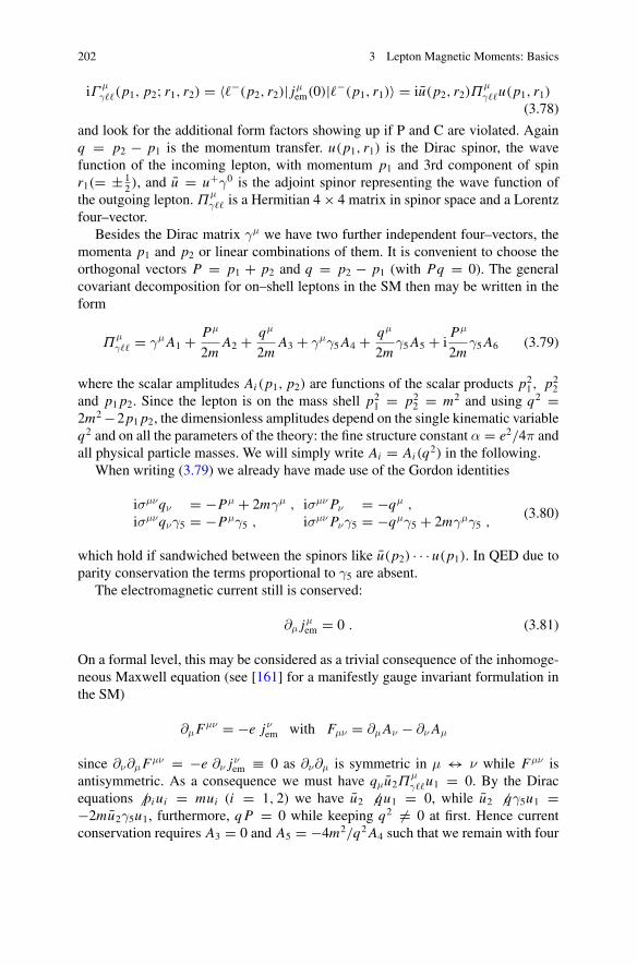
202 3 Lepton Magnetic Moments: Basics

iΓ μγ��(p1, p2; r1, r2) = 〈�−(p2, r2)| jμ

em(0)|�−(p1, r1)〉 = iu(p2, r2)Πμγ��u(p1, r1)

(3.78)

and look for the additional form factors showing up if P and C are violated. Againq = p2 − p1 is the momentum transfer. u(p1, r1) is the Dirac spinor, the wavefunction of the incoming lepton, with momentum p1 and 3rd component of spinr1(= ± 1

2 ), and u = u+γ0 is the adjoint spinor representing the wave function ofthe outgoing lepton. Π

μγ�� is a Hermitian 4 × 4 matrix in spinor space and a Lorentz

four–vector.Besides the Dirac matrix γμ we have two further independent four–vectors, the

momenta p1 and p2 or linear combinations of them. It is convenient to choose theorthogonal vectors P = p1 + p2 and q = p2 − p1 (with Pq = 0). The generalcovariant decomposition for on–shell leptons in the SM then may be written in theform

Πμγ�� = γμ A1 + Pμ

2mA2 + qμ

2mA3 + γμγ5 A4 + qμ

2mγ5 A5 + i

Pμ

2mγ5 A6 (3.79)

where the scalar amplitudes Ai (p1, p2) are functions of the scalar products p21, p2

2and p1 p2. Since the lepton is on the mass shell p2

1 = p22 = m2 and using q2 =

2m2 −2p1 p2, the dimensionless amplitudes depend on the single kinematic variableq2 and on all the parameters of the theory: the fine structure constant α = e2/4π andall physical particle masses. We will simply write Ai = Ai (q2) in the following.

When writing (3.79) we already have made use of the Gordon identities

iσμνqν = −Pμ + 2mγμ , iσμν Pν = −qμ ,

iσμνqνγ5 = −Pμγ5 , iσμν Pνγ5 = −qμγ5 + 2mγμγ5 ,(3.80)

which hold if sandwiched between the spinors like u(p2) · · · u(p1). In QED due toparity conservation the terms proportional to γ5 are absent.

The electromagnetic current still is conserved:

∂μ jμem = 0 . (3.81)

On a formal level, this may be considered as a trivial consequence of the inhomoge-neous Maxwell equation (see [161] for a manifestly gauge invariant formulation inthe SM)

∂μFμν = −e jνem with Fμν = ∂μ Aν − ∂ν Aμ

since ∂ν∂μFμν = −e ∂ν jνem ≡ 0 as ∂ν∂μ is symmetric in μ ↔ ν while Fμν is

antisymmetric. As a consequence we must have qμu2Πμγ��u1 = 0. By the Dirac

equations � pi ui = mui (i = 1, 2) we have u2 � qu1 = 0, while u2 � qγ5u1 =−2mu2γ5u1, furthermore, q P = 0 while keeping q2 �= 0 at first. Hence currentconservation requires A3 = 0 and A5 = −4m2/q2 A4 such that we remain with four

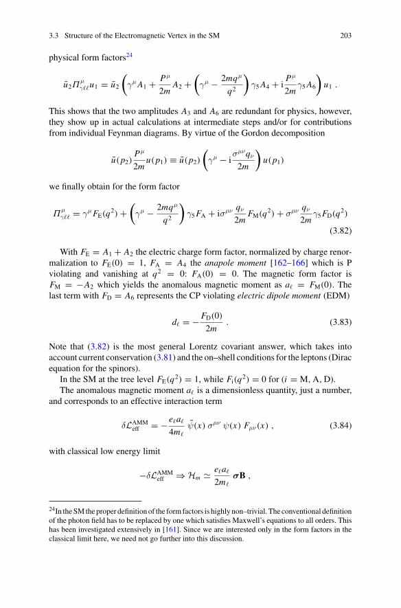
3.3 Structure of the Electromagnetic Vertex in the SM 203

physical form factors24

u2Πμγ��u1 = u2

(γμ A1 + Pμ

2mA2 +

(γμ − 2mqμ

q2

)γ5 A4 + i

Pμ

2mγ5 A6

)u1 .

This shows that the two amplitudes A3 and A6 are redundant for physics, however,they show up in actual calculations at intermediate steps and/or for contributionsfrom individual Feynman diagrams. By virtue of the Gordon decomposition

u(p2)Pμ

2mu(p1) ≡ u(p2)

(γμ − i

σμνqν

2m

)u(p1)

we finally obtain for the form factor

Πμγ�� = γμFE(q2) +

(γμ − 2mqμ

q2

)γ5 FA + iσμν qν

2mFM(q2) + σμν qν

2mγ5 FD(q2)

(3.82)

With FE = A1 + A2 the electric charge form factor, normalized by charge renor-malization to FE(0) = 1, FA = A4 the anapole moment [162–166] which is Pviolating and vanishing at q2 = 0: FA(0) = 0. The magnetic form factor isFM = −A2 which yields the anomalous magnetic moment as a� = FM(0). Thelast term with FD = A6 represents the CP violating electric dipole moment (EDM)

d� = − FD(0)

2m. (3.83)

Note that (3.82) is the most general Lorentz covariant answer, which takes intoaccount current conservation (3.81) and the on–shell conditions for the leptons (Diracequation for the spinors).

In the SM at the tree level FE(q2) = 1, while Fi(q2) = 0 for (i = M, A, D).The anomalous magnetic moment a� is a dimensionless quantity, just a number,

and corresponds to an effective interaction term

δLAMMeff = −e�a�

4m�

ψ(x) σμν ψ(x) Fμν(x) , (3.84)

with classical low energy limit

−δLAMMeff ⇒ Hm e�a�

2m�

σB ,

24In the SM the proper definition of the form factors is highly non–trivial. The conventional definitionof the photon field has to be replaced by one which satisfies Maxwell’s equations to all orders. Thishas been investigated extensively in [161]. Since we are interested only in the form factors in theclassical limit here, we need not go further into this discussion.

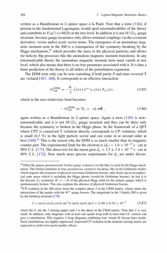
204 3 Lepton Magnetic Moments: Basics

written as a Hamiltonian in 2–spinor space à la Pauli. Note that a term (3.84), ifpresent in the fundamental Lagrangian, would spoil renormalizability of the theoryand contribute to Fi(q2) (i=M,D) at the tree level. In addition it is not SU(2)L gaugeinvariant, because gauge invariance only allows minimal couplings via the covariantderivative: vector and/or axial–vector terms. The emergence of an anomalous mag-netic moment term in the SM is a consequence of the symmetry breaking by theHiggs mechanism,25 which provides the mass to the physical particles and allowsfor helicity flip processes like the anomalous magnetic moment transitions. In anyrenormalizable theory the anomalous magnetic moment term must vanish at treelevel, which also means that there is no free parameter associated with it. It is thus afinite prediction of the theory to all orders of the perturbation expansion.

The EDM term only can be non–vanishing if both parity P and time–reversal Tare violated [167, 168]. It corresponds to an effective interaction

δLEDMeff = −d�

2ψ(x) i σμνγ5 ψ(x) Fμν(x) , (3.85)

which in the non–relativistic limit becomes

− δLEDMeff ⇒ He −d� σE , (3.86)

again written as a Hamiltonian in 2–spinor space. Again a term (3.85) is non–renormalizable and it is not SU(2)L gauge invariant and thus can be there onlybecause the symmetry is broken in the Higgs phase. In the framework of a QFTwhere CPT is conserved T violation directly corresponds to CP violation, whichis small (0.3 %) in the light particle sector and can come in at second order atbest [169].26 This is the reason why the EDM is so much smaller than its magneticcounter part. The experimental limit for the electron is |de| < 1.6 × 10−27 e · cm at90% C.L. [171]. The direct test for the muon gave dμ = 3.7 ± 3.4 × 10−19 e · cm at90% C.L. [172]. New much more precise experiments for dμ are under discus-

25Often the jargon spontaneously broken gauge symmetry (or the like) is used for the Higgs mech-anism. The formal similarity to true spontaneous symmetry breaking, like in the Goldstone model,which requires the existence of physical zero mass Goldstone bosons, only shows up on an unphys-ical state space which is including the Higgs ghosts (would be Goldstone bosons). In fact it isthe discrete Z2 symmetry H ↔ −H of the physical Higgs field (in the unitary gauge) which isspontaneously broken. This also explains the absence of physical Goldstone bosons.26CP-violation in the SM arises from the complex phase δ in the CKM matrix, which enters theinteractions of the quarks with the W ± gauge bosons. The magnitude in the 3 family SM is givenby the Jarlskog invariant [170]

J = cos θ1 cos θ2 cos θ3 sin2 θ1 sin θ2 sin θ3 sin δ = (2.88 ± 0.33) × 10−5 (3.87)

where the θi are the 3 mixing angles and δ is the phase in the CKM matrix. Note that J is verysmall. In addition, only diagrams with at least one quark–loop with at least four CC vertices cangive a contribution. This requires 3–loop diagrams exhibiting four virtual W –boson lines inside.Such contributions are highly suppressed. Expected CP violation in the neutrino mixing matrix areexpected to yield even much smaller effects.

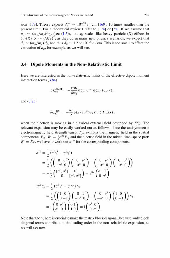
3.3 Structure of the Electromagnetic Vertex in the SM 205

sion [173]. Theory expects d thee ∼ 10−28 e · cm [169], 10 times smaller than the

present limit. For a theoretical review I refer to [174] or [35]. If we assume thatημ ∼ (mμ/me)

2 ηe (see (1.5)), i.e., η� scales like heavy particle (X) effects inδa�(X) ∝ (m�/MX )2, as they do in many new physics scenarios, we expect thatdμ ∼ (mμ/me) de, and thus dμ ∼ 3.2 × 10−25 e · cm. This is too small to affect theextraction of aμ, for example, as we will see.

3.4 Dipole Moments in the Non–Relativistic Limit

Here we are interested in the non–relativistic limits of the effective dipole momentinteraction terms (3.84)

δLAMMeff = −e�a�

4m�

ψ(x) σμν ψ(x) Fμν(x) ,

and (3.85)

δLEDMeff = −d�

2ψ(x) i σμνγ5 ψ(x) Fμν(x) ,

when the electron is moving in a classical external field described by Fextμν . The

relevant expansion may be easily worked out as follows: since the antisymmetricelectromagnetic field strength tensor Fμν exhibits the magnetic field in the spatialcomponents Fik : Bl = 1

2 εikl Fik and the electric field in the mixed time–space part:Ei = F0i , we have to work out σμν for the corresponding components:

σik = i

2

(γiγk − γkγi

)

= i

2

((0 σi

−σi 0

)(0 σk

−σk 0

)−(

0 σk

−σk 0

)(0 σi

−σi 0

))

= − i

2

( [σi ,σk] 00 [σi ,σk]

)= εikl

(σl 00 σl

)

σ0iγ5 = i

2

(γ0γi − γiγ0

)γ5

= i

2

((1 00 −1

)(0 σi

−σi 0

)−(

0 σi

−σi 0

)(1 00 −1

))γ5

= i

(0 σi

σi 0

)(0 11 0

)= i

(σi 00 σi

)

.

Note that the γ5 here is crucial to make the matrix block diagonal, because, only blockdiagonal terms contribute to the leading order in the non–relativistic expansion, aswe will see now.

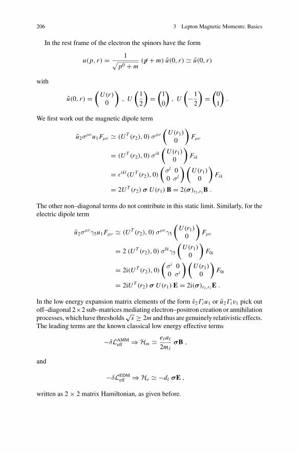
206 3 Lepton Magnetic Moments: Basics

In the rest frame of the electron the spinors have the form

u(p, r) = 1√

p0 + m( �p + m) u(0, r) u(0, r)

with

u(0, r) =(

U (r)

0

), U

(1

2

)=(

1

0

), U

(−1

2

)=(

0

1

).

We first work out the magnetic dipole term

u2σμνu1 Fμν (U T (r2), 0) σμν

(U (r1)

0

)Fμν

= (U T (r2), 0) σik

(U (r1)

0

)Fik

= εikl(U T (r2), 0)

(σl 00 σl

)(U (r1)

0

)Fik

= 2U T (r2) σ U (r1) B = 2(σ)r2,r1 B .

The other non–diagonal terms do not contribute in this static limit. Similarly, for theelectric dipole term

u2σμνγ5u1 Fμν (U T (r2), 0) σμνγ5

(U (r1)

0

)Fμν

= 2 (U T (r2), 0) σ0iγ5

(U (r1)

0

)F0i

= 2i(U T (r2), 0)

(σi 00 σi

)(U (r1)

0

)F0i

= 2iU T (r2) σ U (r1) E = 2i(σ)r2,r1 E .

In the low energy expansion matrix elements of the form v2Γi u1 or u2Γiv1 pick outoff–diagonal 2×2 sub–matrices mediating electron–positron creation or annihilationprocesses, which have thresholds

√s ≥ 2m and thus are genuinely relativistic effects.

The leading terms are the known classical low energy effective terms

−δLAMMeff ⇒ Hm e�a�

2m�

σB ,

and

−δLEDMeff ⇒ He −d� σE ,

written as 2 × 2 matrix Hamiltonian, as given before.

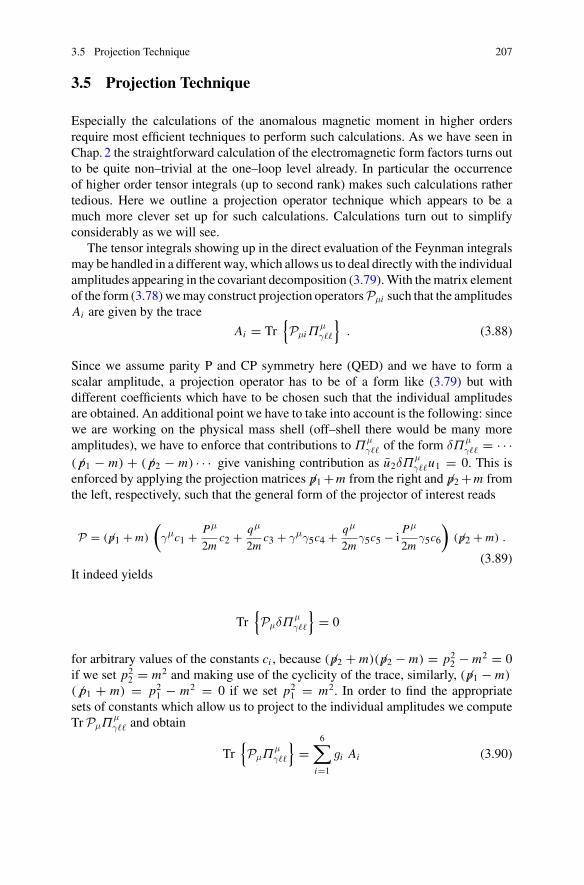
3.5 Projection Technique 207

3.5 Projection Technique

Especially the calculations of the anomalous magnetic moment in higher ordersrequire most efficient techniques to perform such calculations. As we have seen inChap. 2 the straightforward calculation of the electromagnetic form factors turns outto be quite non–trivial at the one–loop level already. In particular the occurrenceof higher order tensor integrals (up to second rank) makes such calculations rathertedious. Here we outline a projection operator technique which appears to be amuch more clever set up for such calculations. Calculations turn out to simplifyconsiderably as we will see.

The tensor integrals showing up in the direct evaluation of the Feynman integralsmay be handled in a different way, which allows us to deal directly with the individualamplitudes appearing in the covariant decomposition (3.79). With the matrix elementof the form (3.78) we may construct projection operators Pμi such that the amplitudesAi are given by the trace

Ai = Tr{PμiΠ

μγ��

}. (3.88)

Since we assume parity P and CP symmetry here (QED) and we have to form ascalar amplitude, a projection operator has to be of a form like (3.79) but withdifferent coefficients which have to be chosen such that the individual amplitudesare obtained. An additional point we have to take into account is the following: sincewe are working on the physical mass shell (off–shell there would be many moreamplitudes), we have to enforce that contributions to Π

μγ�� of the form δΠ

μγ�� = · · ·

( � p1 − m) + ( � p2 − m) · · · give vanishing contribution as u2δΠμγ��u1 = 0. This is

enforced by applying the projection matrices �p1 +m from the right and �p2 +m fromthe left, respectively, such that the general form of the projector of interest reads

P = ( �p1 + m)

(γμc1 + Pμ

2mc2 + qμ

2mc3 + γμγ5c4 + qμ

2mγ5c5 − i

Pμ

2mγ5c6

)( �p2 + m) .

(3.89)It indeed yields

Tr{PμδΠ

μγ��

}= 0

for arbitrary values of the constants ci , because ( �p2 + m)( �p2 − m) = p22 − m2 = 0

if we set p22 = m2 and making use of the cyclicity of the trace, similarly, ( �p1 − m)

( � p1 + m) = p21 − m2 = 0 if we set p2

1 = m2. In order to find the appropriatesets of constants which allow us to project to the individual amplitudes we computeTr PμΠ

μγ�� and obtain

Tr{PμΠ

μγ��

}=

6∑

i=1

gi Ai (3.90)

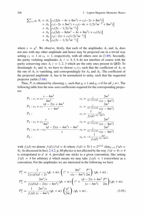
208 3 Lepton Magnetic Moments: Basics

∑6i=1 gi Ai = A1

[c1(2ds − 4s + 8m2) + c2(−2s + 8m2)

]

+ A2[c1(−2s + 8m2) + c2(−4s + 1/2s2m−2 + 8m2)

]

+ A3[c3(2s − 1/2s2m−2)

]

+ A4[c4(2ds − 8dm2 − 4s + 8m2) + c5(2s)

]

+ A5[c4(−2s) + c5(1/2s2m−2)

]

+ A6[c6(2s − 1/2s2m−2)

]

where s = q2. We observe, firstly, that each of the amplitudes A3 and A6 doesnot mix with any other amplitude and hence may be projected out in a trivial waysetting c3 = 1 or c6 = 1, respectively, with all others zero in (3.89). Secondly,the parity violating amplitudes Ai i = 4, 5, 6 do not interfere of course with theparity conserving ones Ai i = 1, 2, 3 which are the only ones present in QED. Todisentangle A1 and A2 we have to choose c1/c2 such that the coefficient of A2 orthe one of A1 is vanishing, and correspondingly for A4 and A5. The coefficient ofthe projected amplitude Ai has to be normalized to unity, such that the requestedprojector yields (3.88).

Thus, Pi is obtained by choosing c j such that gi = 1 and g j = 0 for all j �= i . Thefollowing table lists the non–zero coefficients required for the corresponding projec-tor:

P1 : c1 = c2s − 4m2

4m2c2 = 1

(d−2) f1(d)

2m2

s(s − 4m2)

P2 : c2 = c1(d − 2)s + 4m2

s − 4m2c1 = 1

(d−2) f1(d)

2m2

s(s − 4m2)

P3 : c3 = 1

f1(d)2m2

s(s−4m2)

P4 : c4 = c5s

4m2c5 = 1

(d−2) f1(d)

2m2

s(s − 4m2)

P5 : c5 = −c4(d − 2)(s − 4m2) − 4m2

sc4 = 1

(d−2) f1(d)

2m2

s(s − 4m2)

P6 : c6 = −i1

f1(d)2m2

s(s−4m2)

with f1(d) we denote f (d)/ f (d = 4) where f (d).= Tr 1 = 2(d/2) (limd→4 f (d) =

4). As discussed in Sect. 2.4.2, p. 68 physics is not affected by the way f (d = 4) = 4is extrapolated to d �= 4, provided one sticks to a given convention, like settingf (d) = 4 for arbitrary d which means we may take f1(d) = 1 everywhere as aconvention. For the amplitudes we are interested in the following we have

Pμ1 = 1

2 f1(d)(d − 2)( �p1 + m)

(γμ + 4m2

s(s − 4m2)

Pμ

2m

)( �p2 + m) ,

Pμ2 = 2m2/s

f1(d)(d − 2)(s − 4m2)( �p1 + m)

(γμ + (d − 2)s + 4m2

(s − 4m2)

Pμ

2m

)( �p2 + m),

Pμ3 = 1

f1(d)

2m2/s

(s − 4m2)( �p1 + m)

(qμ

2m

)( �p2 + m) . (3.91)

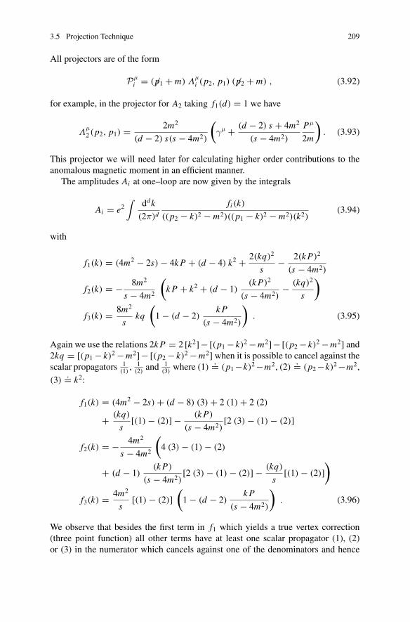
3.5 Projection Technique 209

All projectors are of the form

Pμi = ( �p1 + m) Λ

μi (p2, p1) ( �p2 + m) , (3.92)

for example, in the projector for A2 taking f1(d) = 1 we have

Λμ2 (p2, p1) = 2m2

(d − 2) s(s − 4m2)

(γμ + (d − 2) s + 4m2

(s − 4m2)

Pμ

2m

). (3.93)

This projector we will need later for calculating higher order contributions to theanomalous magnetic moment in an efficient manner.

The amplitudes Ai at one–loop are now given by the integrals

Ai = e2∫

ddk

(2π)d

fi (k)

((p2 − k)2 − m2)((p1 − k)2 − m2)(k2)(3.94)

with

f1(k) = (4m2 − 2s) − 4k P + (d − 4) k2 + 2(kq)2

s− 2(k P)2

(s − 4m2)

f2(k) = − 8m2

s − 4m2

(k P + k2 + (d − 1)

(k P)2

(s − 4m2)− (kq)2

s

)

f3(k) = 8m2

skq

(1 − (d − 2)

k P

(s − 4m2)

). (3.95)

Again we use the relations 2k P = 2 [k2]− [(p1 − k)2 − m2]− [(p2 − k)2 − m2] and2kq = [(p1 − k)2 − m2]− [(p2 − k)2 − m2] when it is possible to cancel against thescalar propagators 1

(1), 1

(2)and 1

(3)where (1)

.= (p1 −k)2 −m2, (2).= (p2 −k)2 −m2,

(3).= k2:

f1(k) = (4m2 − 2s) + (d − 8) (3) + 2 (1) + 2 (2)

+ (kq)

s[(1) − (2)] − (k P)

(s − 4m2)[2 (3) − (1) − (2)]

f2(k) = − 4m2

s − 4m2

(4 (3) − (1) − (2)

+ (d − 1)(k P)

(s − 4m2)[2 (3) − (1) − (2)] − (kq)

s[(1) − (2)]

)

f3(k) = 4m2

s[(1) − (2)]

(1 − (d − 2)

k P

(s − 4m2)

). (3.96)

We observe that besides the first term in f1 which yields a true vertex correction(three point function) all other terms have at least one scalar propagator (1), (2)or (3) in the numerator which cancels against one of the denominators and hence

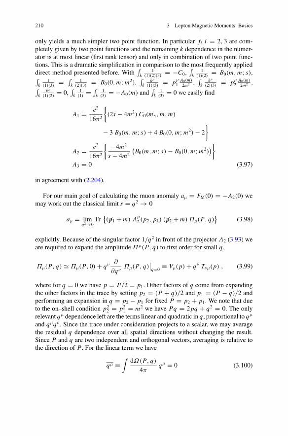
210 3 Lepton Magnetic Moments: Basics

only yields a much simpler two point function. In particular fi i = 2, 3 are com-pletely given by two point functions and the remaining k dependence in the numer-ator is at most linear (first rank tensor) and only in combination of two point func-tions. This is a dramatic simplification in comparison to the most frequently applieddirect method presented before. With

∫k

1(1)(2)(3)

= −C0,∫

k1

(1)(2)= B0(m, m; s),

∫k

1(1)(3)

= ∫k

1(2)(3)

= B0(0, m; m2),∫

kkμ

(1)(3)= pμ

1A0(m)

2m2 ,∫

kkμ

(2)(3)= pμ

2A0(m)

2m2 ,∫

kkμ

(1)(2)= 0,

∫k

1(1)

= ∫k

1(3)

= −A0(m) and∫

k1

(3)= 0 we easily find

A1 = e2

16π2

{(2s − 4m2) C0(mγ, m, m)

− 3 B0(m, m; s) + 4 B0(0, m; m2) − 2

}

A2 = e2

16π2

{ −4m2

s − 4m2

(B0(m, m; s) − B0(0, m; m2)

)}

A3 = 0 (3.97)

in agreement with (2.204).

For our main goal of calculating the muon anomaly aμ = FM(0) = −A2(0) wemay work out the classical limit s = q2 → 0

aμ = limq2→0

Tr{( �p1 + m) Λ

μ2 (p2, p1) ( �p2 + m) Πμ(P, q)

}(3.98)

explicitly. Because of the singular factor 1/q2 in front of the projector Λ2 (3.93) weare required to expand the amplitude Πμ(P, q) to first order for small q,

Πμ(P, q) Πμ(P, 0) + qν ∂

∂qνΠμ(P, q)

∣∣q=0 ≡ Vμ(p) + qν Tνμ(p) , (3.99)

where for q = 0 we have p = P/2 = p1. Other factors of q come from expandingthe other factors in the trace by setting p2 = (P + q)/2 and p1 = (P − q)/2 andperforming an expansion in q = p2 − p1 for fixed P = p2 + p1. We note that dueto the on–shell condition p2

2 = p21 = m2 we have Pq = 2pq + q2 = 0. The only

relevant qμ dependence left are the terms linear and quadratic in q, proportional to qμ

and qμqν . Since the trace under consideration projects to a scalar, we may averagethe residual q dependence over all spatial directions without changing the result.Since P and q are two independent and orthogonal vectors, averaging is relative tothe direction of P . For the linear term we have

qμ ≡∫

dΩ(P, q)

4πqμ = 0 (3.100)

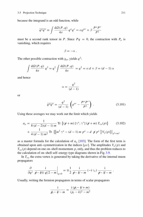
3.5 Projection Technique 211

because the integrand is an odd function, while

qμqν ≡∫

dΩ(P, q)

4πqμqν = αgμν + β

Pμ Pν

P2

must be a second rank tensor in P . Since Pq = 0, the contraction with Pμ isvanishing, which requires

β = −α .

The other possible contraction with gμν yields q2:

∫dΩ(P, q)

4πq2 = q2

∫dΩ(P, q)

4π= q2 = α d + β = (d − 1) α

and hence

α = q2

(d − 1)

or

qμqν = q2

(d − 1)

(gμν − Pμ Pν

P2

). (3.101)

Using these averages we may work out the limit which yields

aμ = 1

8 (d − 2)(d − 1) mTr

{( �p + m) [γμ, γν] ( �p + m) Tνμ(p)

}(3.102)

+ 1

4 (d − 1) m2Tr

{[m2 γμ − (d − 1) m pμ − d �p pμ

]Vμ(p)

}∣∣p2=m2

as a master formula for the calculation of aμ [103]. The form of the first term isobtained upon anti–symmetrization in the indices [μν]. The amplitudes Vμ(p) andTνμ(p) depend on one on–shell momentum p, only, and thus the problem reduces tothe calculation of on–shell self–energy type diagrams shown in Fig. 3.9.

In Tνμ the extra vertex is generated by taking the derivative of the internal muonpropagators

∂

∂qν

i

�p− �k∓ �q/2 − m

∣∣∣∣q=0

= ∓1

2

i

�p− �k − m(−i γν)

i

�p− �k − m.

Usually, writing the fermion propagators in terms of scalar propagators

i

�pi− �k − m= i ( �pi− �k + m)

(pi − k)2 − m2

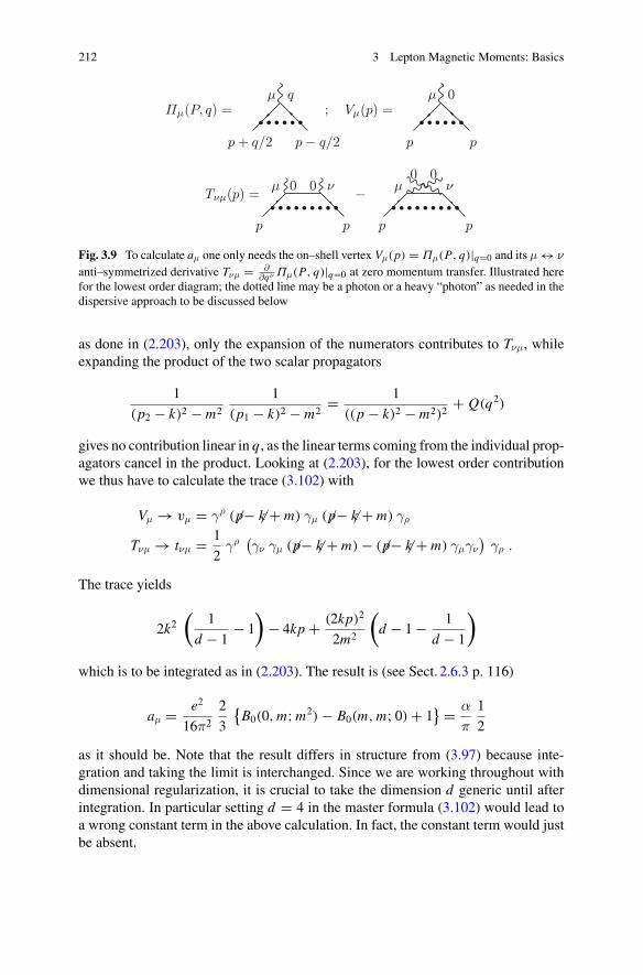
212 3 Lepton Magnetic Moments: Basics

Πμ(P, q) = ; Vμ(p) =

Tνμ(p) = −

p − q/2p + q/2

μ q

pp

μ 0

p p

μ 0 0 ν

p p

μ0

ν0

Fig. 3.9 To calculate aμ one only needs the on–shell vertex Vμ(p) = Πμ(P, q)|q=0 and its μ ↔ ν

anti–symmetrized derivative Tνμ = ∂∂qν Πμ(P, q)|q=0 at zero momentum transfer. Illustrated here

for the lowest order diagram; the dotted line may be a photon or a heavy “photon” as needed in thedispersive approach to be discussed below

as done in (2.203), only the expansion of the numerators contributes to Tνμ, whileexpanding the product of the two scalar propagators

1

(p2 − k)2 − m2

1

(p1 − k)2 − m2= 1

((p − k)2 − m2)2+ Q(q2)

gives no contribution linear in q, as the linear terms coming from the individual prop-agators cancel in the product. Looking at (2.203), for the lowest order contributionwe thus have to calculate the trace (3.102) with

Vμ → vμ = γρ ( �p− �k + m) γμ ( �p− �k + m) γρ

Tνμ → tνμ = 1

2γρ

(γν γμ ( �p− �k + m) − ( �p− �k + m) γμγν

)γρ .

The trace yields

2k2

(1

d − 1− 1

)− 4kp + (2kp)2

2m2

(d − 1 − 1

d − 1

)

which is to be integrated as in (2.203). The result is (see Sect. 2.6.3 p. 116)

aμ = e2

16π2

2

3

{B0(0, m; m2) − B0(m, m; 0) + 1

} = α

π

1

2

as it should be. Note that the result differs in structure from (3.97) because inte-gration and taking the limit is interchanged. Since we are working throughout withdimensional regularization, it is crucial to take the dimension d generic until afterintegration. In particular setting d = 4 in the master formula (3.102) would lead toa wrong constant term in the above calculation. In fact, the constant term would justbe absent.

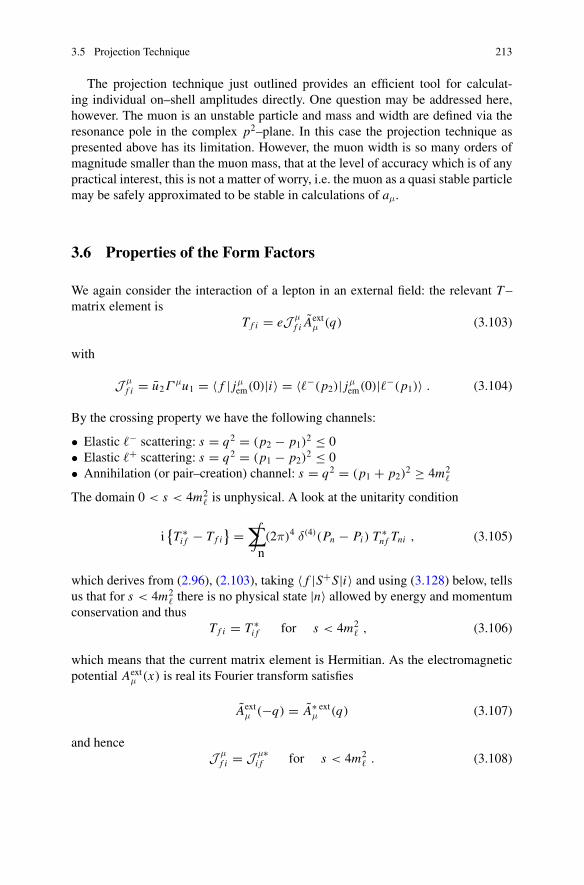
3.5 Projection Technique 213

The projection technique just outlined provides an efficient tool for calculat-ing individual on–shell amplitudes directly. One question may be addressed here,however. The muon is an unstable particle and mass and width are defined via theresonance pole in the complex p2–plane. In this case the projection technique aspresented above has its limitation. However, the muon width is so many orders ofmagnitude smaller than the muon mass, that at the level of accuracy which is of anypractical interest, this is not a matter of worry, i.e. the muon as a quasi stable particlemay be safely approximated to be stable in calculations of aμ.

3.6 Properties of the Form Factors

We again consider the interaction of a lepton in an external field: the relevant T –matrix element is

T f i = eJ μf i Aext

μ (q) (3.103)

with

J μf i = u2Γ

μu1 = 〈 f | jμem(0)|i〉 = 〈�−(p2)| jμ

em(0)|�−(p1)〉 . (3.104)

By the crossing property we have the following channels:

• Elastic �− scattering: s = q2 = (p2 − p1)2 ≤ 0

• Elastic �+ scattering: s = q2 = (p1 − p2)2 ≤ 0

• Annihilation (or pair–creation) channel: s = q2 = (p1 + p2)2 ≥ 4m2

�

The domain 0 < s < 4m2� is unphysical. A look at the unitarity condition

i{T ∗

i f − T f i} =

∑∫

n(2π)4 δ(4)(Pn − Pi ) T ∗

n f Tni , (3.105)

which derives from (2.96), (2.103), taking 〈 f |S+S|i〉 and using (3.128) below, tellsus that for s < 4m2

� there is no physical state |n〉 allowed by energy and momentumconservation and thus

T f i = T ∗i f for s < 4m2

� , (3.106)

which means that the current matrix element is Hermitian. As the electromagneticpotential Aext

μ (x) is real its Fourier transform satisfies

Aextμ (−q) = A∗ ext

μ (q) (3.107)

and henceJ μ

f i = J μ∗i f for s < 4m2

� . (3.108)

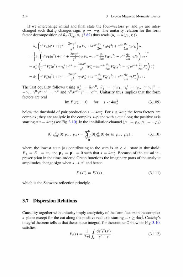
214 3 Lepton Magnetic Moments: Basics

If we interchange initial and final state the four–vectors p1 and p2 are inter-changed such that q changes sign: q → −q. The unitarity relation for the formfactor decomposition of u2 Π

μγ�� u1 (3.82) thus reads (ui = u(pi , ri ))

u2

(γμ FE(q2) + [γμ − 2mqμ

q2 ]γ5 FA + iσμν qν

2mFM(q2) + σμν qν

2mγ5 FD

)u1

={

u1

(γμ FE(q2) + [γμ + 2mqμ

q2 ]γ5 FA − iσμν qν

2mFM(q2) − σμν qν

2mγ5 FD

)u2

}∗

= u+2

(γμ+ F∗

E (q2) + γ+5 [γμ+ + 2mqμ

q2 ]F∗A + iσμν+ qν

2mF∗

M(q2) − γ+5 σμν+ qν

2mF∗

D

)u+

1

= u2

(γμ F∗

E (q2) + [γμ − 2mqμ

q2 ]γ5 F∗A + iσμν qν

2mF∗

M(q2) + σμν qν

2mγ5 F∗

D

)u1 .

The last equality follows using u+2 = u2γ

0, u+1 = γ0u1, γ+

5 = γ5, γ0γ5γ0 =

−γ5, γ0γμ+γ0 = γμ and γ0σμν+γ0 = σμν . Unitarity thus implies that the formfactors are real

Im F(s)i = 0 for s < 4m2e (3.109)

below the threshold of pair production s = 4m2e . For s ≥ 4m2

e the form factors arecomplex; they are analytic in the complex s–plane with a cut along the positive axisstarting at s = 4m2

e (see Fig. 3.10). In the annihilation channel (p− = p2, p+ = −p1)

〈0| jμem(0)|p−, p+〉 =

∑∫

n〈0| jμ

em(0)|n〉〈n|p−, p+〉 , (3.110)

where the lowest state |n〉 contributing to the sum is an e+e− state at threshold:E+ = E− = me and p+ = p− = 0 such that s = 4m2

e . Because of the causal iε–prescription in the time–ordered Green functions the imaginary parts of the analyticamplitudes change sign when s → s∗ and hence

Fi (s∗) = F∗

i (s) , (3.111)

which is the Schwarz reflection principle.

3.7 Dispersion Relations

Causality together with unitarity imply analyticity of the form factors in the complexs–plane except for the cut along the positive real axis starting at s ≥ 4m2

� . Cauchy’sintegral theorem tells us that the contour integral, for the contour C shown in Fig. 3.10,satisfies

Fi (s) = 1

2πi

∮

C

ds ′F(s ′)s ′ − s

. (3.112)

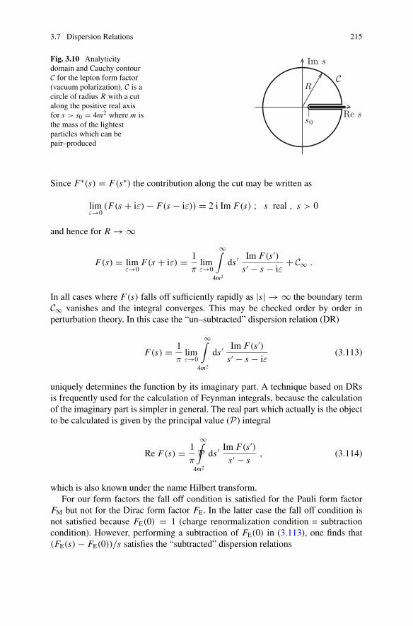
3.7 Dispersion Relations 215

Fig. 3.10 Analyticitydomain and Cauchy contourC for the lepton form factor(vacuum polarization). C is acircle of radius R with a cutalong the positive real axisfor s > s0 = 4m2 where m isthe mass of the lightestparticles which can bepair–produced

Im s

Re s

CR

|s0

Since F∗(s) = F(s∗) the contribution along the cut may be written as

limε→0

(F(s + iε) − F(s − iε)) = 2 i Im F(s) ; s real , s > 0

and hence for R → ∞

F(s) = limε→0

F(s + iε) = 1

πlimε→0

∞∫

4m2

ds ′ Im F(s ′)s ′ − s − iε

+ C∞ .

In all cases where F(s) falls off sufficiently rapidly as |s| → ∞ the boundary termC∞ vanishes and the integral converges. This may be checked order by order inperturbation theory. In this case the “un–subtracted” dispersion relation (DR)

F(s) = 1

πlimε→0

∞∫

4m2

ds ′ Im F(s ′)s ′ − s − iε

(3.113)

uniquely determines the function by its imaginary part. A technique based on DRsis frequently used for the calculation of Feynman integrals, because the calculationof the imaginary part is simpler in general. The real part which actually is the objectto be calculated is given by the principal value (P) integral

Re F(s) = 1

πP∞∫

4m2

ds ′ Im F(s ′)s ′ − s

, (3.114)

which is also known under the name Hilbert transform.For our form factors the fall off condition is satisfied for the Pauli form factor

FM but not for the Dirac form factor FE. In the latter case the fall off condition isnot satisfied because FE(0) = 1 (charge renormalization condition = subtractioncondition). However, performing a subtraction of FE(0) in (3.113), one finds that(FE(s) − FE(0))/s satisfies the “subtracted” dispersion relations

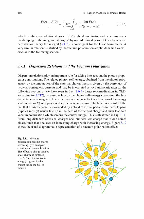
216 3 Lepton Magnetic Moments: Basics

F(s) − F(0)

s= 1

πlimε→0

∞∫

4m2

ds ′ Im F(s ′)s ′(s ′ − s − iε)

, (3.115)

which exhibits one additional power of s ′ in the denominator and hence improvesthe damping of the integrand at large s ′ by one additional power. Order by order inperturbation theory the integral (3.115) is convergent for the Dirac form factor. Avery similar relation is satisfied by the vacuum polarization amplitude which we willdiscuss in the following section.

3.7.1 Dispersion Relations and the Vacuum Polarization

Dispersion relations play an important role for taking into account the photon propa-gator contributions. The related photon self–energy, obtained from the photon prop-agator by the amputation of the external photon lines, is given by the correlator oftwo electromagnetic currents and may be interpreted as vacuum polarization for thefollowing reason: as we have seen in Sect. 2.6.3 charge renormalization in QED,according to (2.212), is caused solely by the photon self–energy correction; the fun-damental electromagnetic fine structure constant α in fact is a function of the energyscale α → α(E) of a process due to charge screening. The latter is a result of thefact that a naked charge is surrounded by a cloud of virtual particle–antiparticle pairs(dipoles mostly) which line up in the field of the central charge and such lead to avacuum polarization which screens the central charge. This is illustrated in Fig. 3.11.From long distances (classical charge) one thus sees less charge than if one comescloser, such that one sees an increasing charge with increasing energy. Figure 3.12shows the usual diagrammatic representation of a vacuum polarization effect.

Fig. 3.11 Vacuumpolarization causing chargescreening by virtual paircreation and re–annihilation.The effective charge seen bya test charge at distancer = �/E (E the collisionenergy) is given by thecharge inside the ball ofradius r

+ −

+−+

−

+−

+−

+− +

−

+−

+ −

+−

+−

+−

+−

+−

+−

+ −r

−

−

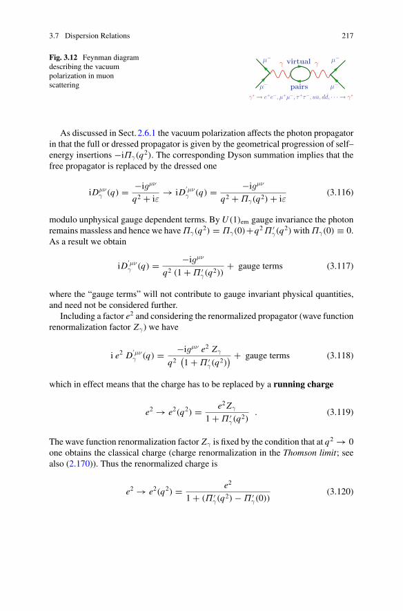
3.7 Dispersion Relations 217

Fig. 3.12 Feynman diagramdescribing the vacuumpolarization in muonscattering

γ virtual

pairs

γ

μ− μ−

μ− μ−

γ∗ → e+e−, μ+μ−, τ+τ−, uu, dd, · · · → γ∗

As discussed in Sect. 2.6.1 the vacuum polarization affects the photon propagatorin that the full or dressed propagator is given by the geometrical progression of self–energy insertions −iΠγ(q2). The corresponding Dyson summation implies that thefree propagator is replaced by the dressed one

iDμνγ (q) = −igμν

q2 + iε→ iD

′μνγ (q) = −igμν

q2 + Πγ(q2) + iε(3.116)

modulo unphysical gauge dependent terms. By U (1)em gauge invariance the photonremains massless and hence we have Πγ(q2) = Πγ(0)+q2 Π ′

γ(q2) with Πγ(0) ≡ 0.

As a result we obtain

iD′μνγ (q) = −igμν

q2 (1 + Π ′γ(q

2))+ gauge terms (3.117)

where the “gauge terms” will not contribute to gauge invariant physical quantities,and need not be considered further.

Including a factor e2 and considering the renormalized propagator (wave functionrenormalization factor Zγ) we have

i e2 D′μνγ (q) = −igμν e2 Zγ

q2(1 + Π ′

γ(q2)) + gauge terms (3.118)

which in effect means that the charge has to be replaced by a running charge

e2 → e2(q2) = e2 Zγ

1 + Π ′γ(q

2). (3.119)

The wave function renormalization factor Zγ is fixed by the condition that at q2 → 0one obtains the classical charge (charge renormalization in the Thomson limit; seealso (2.170)). Thus the renormalized charge is

e2 → e2(q2) = e2

1 + (Π ′γ(q

2) − Π ′γ(0))

(3.120)

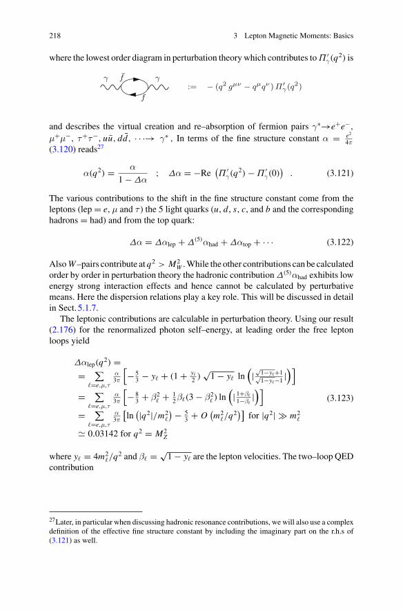
218 3 Lepton Magnetic Moments: Basics

where the lowest order diagram in perturbation theory which contributes to Π ′γ(q

2) is

:= − (q2 gμν − qμqν)Π′γ(q

2)γ γf

f

and describes the virtual creation and re–absorption of fermion pairs γ∗→e+e−,

μ+μ−, τ+τ−, uu, dd, · · ·→ γ∗ , In terms of the fine structure constant α = e2

4π(3.120) reads27

α(q2) = α

1 − Δα; Δα = −Re

(Π ′

γ(q2) − Π ′

γ(0))

. (3.121)

The various contributions to the shift in the fine structure constant come from theleptons (lep = e, μ and τ ) the 5 light quarks (u, d, s, c, and b and the correspondinghadrons = had) and from the top quark:

Δα = Δαlep + Δ(5)αhad + Δαtop + · · · (3.122)

Also W –pairs contribute at q2 > M2W . While the other contributions can be calculated

order by order in perturbation theory the hadronic contribution Δ(5)αhad exhibits lowenergy strong interaction effects and hence cannot be calculated by perturbativemeans. Here the dispersion relations play a key role. This will be discussed in detailin Sect. 5.1.7.

The leptonic contributions are calculable in perturbation theory. Using our result(2.176) for the renormalized photon self–energy, at leading order the free leptonloops yield

Δαlep(q2) == ∑

�=e,μ,τ

α3π

[− 5

3 − y� + (1 + y�

2 )√

1 − y� ln(|√

1−y�+1√1−y�−1

|)]

= ∑

�=e,μ,τ

α3π

[− 8

3 + β2� + 1

2β�(3 − β2� ) ln

(| 1+β�

1−β�|)]

= ∑

�=e,μ,τ

α3π

[ln(|q2|/m2

�

) − 53 + O

(m2

�/q2)]

for |q2| � m2�

0.03142 for q2 = M2Z

(3.123)

where y� = 4m2�/q2 and β� = √

1 − y� are the lepton velocities. The two–loop QEDcontribution

27Later, in particular when discussing hadronic resonance contributions, we will also use a complexdefinition of the effective fine structure constant by including the imaginary part on the r.h.s of(3.121) as well.

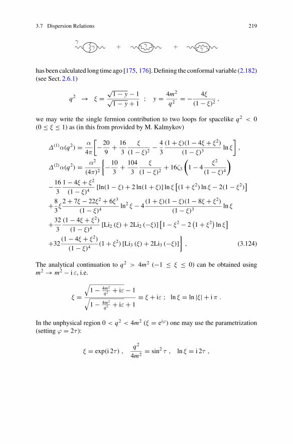
3.7 Dispersion Relations 219

γγ γ

γ+ +

has been calculated long time ago [175, 176]. Defining the conformal variable (2.182)(see Sect. 2.6.1)

q2 → ξ =√

1 − y − 1√1 − y + 1

; y = 4m2

q2= − 4ξ

(1 − ξ)2,

we may write the single fermion contribution to two loops for spacelike q2 < 0(0 ≤ ξ ≤ 1) as (in this from provided by M. Kalmykov)

Δ(1)α(q2) = α

4π

[−20

9+ 16

3

ξ

(1 − ξ)2− 4

3

(1 + ξ)(1 − 4ξ + ξ2)

(1 − ξ)3ln ξ

],

Δ(2)α(q2) = α2

(4π)2

{−10

3+ 104

3

ξ

(1 − ξ)2+ 16ζ3

(1 − 4

ξ2

(1 − ξ)4

)

−16

3

1 − 4ξ + ξ2

(1 − ξ)4[ln(1 − ξ) + 2 ln(1 + ξ)] ln ξ

[(1 + ξ2) ln ξ − 2(1 − ξ2)

]

+8

3ξ

2 + 7ξ − 22ξ2 + 6ξ3

(1 − ξ)4ln2 ξ − 4

(1 + ξ)(1 − ξ)(1 − 8ξ + ξ2)

(1 − ξ)3ln ξ

+32

3

(1 − 4ξ + ξ2)

(1 − ξ)4[Li2 (ξ) + 2Li2 (−ξ)]

[1 − ξ2 − 2

(1 + ξ2

)ln ξ

]

+32(1 − 4ξ + ξ2)

(1 − ξ)4(1 + ξ2) [Li3 (ξ) + 2Li3 (−ξ)]

}, (3.124)

The analytical continuation to q2 > 4m2 (−1 ≤ ξ ≤ 0) can be obtained usingm2 → m2 − i ε, i.e.

ξ =√

1 − 4m2

q2 + iε − 1√

1 − 4m2

q2 + iε + 1≡ ξ + iε ; ln ξ = ln |ξ| + i π .

In the unphysical region 0 < q2 < 4m2 (ξ = eiϕ) one may use the parametrization(setting ϕ = 2τ ):

ξ = exp(i 2τ ) ,q2

4m2= sin2 τ , ln ξ = i 2τ ,

220 3 Lepton Magnetic Moments: Basics

to obtain

Δα(1)(s) = α

4π

{− 20

9+ 4

3

τ cos τ

sin3 τ

(1 + 2 sin2 τ

)− 4

3

1

sin2 τ

},

Δα(2)(s) = α2

(4π)2

{16

[2Cl3 (2τ ) + 4Cl3 (π − 2τ ) + ζ3

] [1 − 1

4 sin4 τ

]

+ 16

3

[Cl2 (2τ ) − 2Cl2 (π − 2τ )

][8τ

[1 − 1

4 sin4 τ

]− cos τ (1 + 2 sin2 τ )

sin3 τ

]

+ 32

3

[ln (2 sin τ ) + 2 ln (2 cos τ )

][2τ2

[1 − 1

4 sin4 τ

]− τ cos τ (1 + 2 sin2 τ )

sin3 τ

]

− 10

3+ 4

τ cos τ (3 + 2 sin2 τ )

sin3 τ− 26

3

1

sin2 τ+ 14

3

τ2

sin4 τ+ 16

3

τ2

sin2 τ− 32τ2

}. (3.125)

The Clausen function is defined by Cln (ϕ) = Im Lin(eiϕ

) = ∑∞m=1

sin(m ϕ)

mn . Thegluonic perturbative QCD correction is given by the same formulas multiplied bythe color factor Nc = 3 and the SU(3) Casimir coefficient CF = 4/3 [177].

For α = 137.036, me = 0.510998902, mμ105.658357, mτ = 1776.99 we get

Δα(MZ ) × 104 e μ τ e + μ + τ

1–loop 174.34669 91.78436 48.05954 314.190592–loop 0.379829 0.235999 0.160339 0.7761677

Thus the leading contribution is affected by small electromagnetic correctionsonly in the next to leading order. For large q2 the leptonic contribution is actuallyknown to three loops [178] at which it takes the value

Δαleptons(M2Z ) 314.98 × 10−4. (3.126)

As already mentioned, in contrast, the corresponding free quark loop contributiongets substantially modified by low energy strong interaction effects, which cannot becalculated reliably by perturbative QCD. The evaluation of the hadronic contributionwill be discussed later.

Vacuum polarization effects are large when large scale changes are involved (largelogarithms) and because of the large number of light fermionic degrees of freedom(see (2.181)) as we infer from the asymptotic form in perturbation theory

Δαpert(q2) α

3π

∑

f

Q2f Ncf

(

ln|q2|m2

f

− 5

3

)

; |q2| � m2f . (3.127)

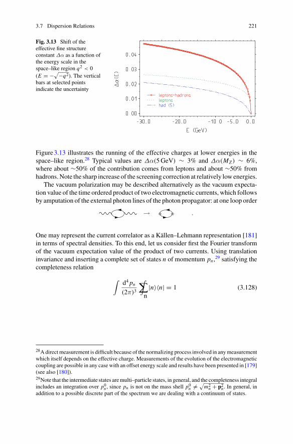
3.7 Dispersion Relations 221

Fig. 3.13 Shift of theeffective fine structureconstant Δα as a function ofthe energy scale in thespace–like region q2 < 0(E = −√−q2). The verticalbars at selected pointsindicate the uncertainty

Figure 3.13 illustrates the running of the effective charges at lower energies in thespace–like region.28 Typical values are Δα(5 GeV) ∼ 3% and Δα(MZ ) ∼ 6%,where about ∼50% of the contribution comes from leptons and about ∼50% fromhadrons. Note the sharp increase of the screening correction at relatively low energies.

The vacuum polarization may be described alternatively as the vacuum expecta-tion value of the time ordered product of two electromagnetic currents, which followsby amputation of the external photon lines of the photon propagator: at one loop order

→ ⊗ ⊗ .

One may represent the current correlator as a Källen–Lehmann representation [181]in terms of spectral densities. To this end, let us consider first the Fourier transformof the vacuum expectation value of the product of two currents. Using translationinvariance and inserting a complete set of states n of momentum pn ,29 satisfying thecompleteness relation

∫d4 pn

(2π)3

∑∫

n|n〉〈n| = 1 (3.128)

28A direct measurement is difficult because of the normalizing process involved in any measurementwhich itself depends on the effective charge. Measurements of the evolution of the electromagneticcoupling are possible in any case with an offset energy scale and results have been presented in [179](see also [180]).29Note that the intermediate states are multi–particle states, in general, and the completeness integralincludes an integration over p0

n , since pn is not on the mass shell p0n �= √

m2n + p2

n . In general, inaddition to a possible discrete part of the spectrum we are dealing with a continuum of states.

222 3 Lepton Magnetic Moments: Basics

where∫∑

n includes, for fixed total momentum pn , integration over the phase spaceavailable to particles of all possible intermediate physical states |n〉, we have

i∫

d4x eiqx 〈0| jμ(x) jν(0)|0〉 = i∫

d4 pn

(2π)3

∫d4x ei(q−pn)x

∑∫

n〈0| jμ(0)|n〉〈n| jν(0)|0〉

= i∫

d4 pn

(2π)3

∑∫

n(2π)4 δ(4)(q − pn)〈0| jμ(0)|n〉〈n| jν(0)|0〉

= i 2π∑∫

n〈0| jμ(0)|n〉〈n| jν(0)|0〉∣∣pn=q .

Key ingredient of the representation we are looking for is the spectral functiontensor ρμν(q) defined by

ρμν(q).=∑∫

n〈0| jμ(0)|n〉〈n| jν(0)|0〉|pn=q . (3.129)

Taking into account that q is the momentum of a physical state (spectral conditionq2 ≥ 0, q0 ≥ 0), the relativistic covariant decomposition may be written as

ρμν(q) = Θ(q0)Θ(q2){[

qμqν − q2 gμν]ρ1(q

2) + qμqνρ0(q2)}

(3.130)

and current conservation ∂μ jμ = 0 ⇔ qμρμν = 0 implies ρ0 ≡ 0, which is

the transversality condition. For non–conserved currents, like the ones of the weakinteractions, a longitudinal component ρ0 exists in addition to the transversal one ρ1.Note that Θ(p2) may be represented as

Θ(q2) =∞∫

0

dm2δ(q2 − m2)

and therefore we may write

i∫

d4x eiqx 〈0| jμ(x) jν(0)|0〉 (3.131)

=∞∫

0

dm2{[

m2gμν − qμqν]ρ1(m

2) − qμqνρ0(m2)} (

−2πiΘ(q0)δ(q2 − m2)

),

which is the Källen–Lehmann representation for the positive frequency part of thecurrent correlator. The latter, according to (2.141), is twice the imaginary part of thecorresponding time–ordered current correlation function

3.7 Dispersion Relations 223

i∫

d4x eiqx 〈0|T jμ(x) jν(0)|0〉 (3.132)

=∞∫

0

dm2{[

m2gμν − qμqν]ρ1(m

2) − qμqνρ0(m2)} (

1

q2 − m2 + iε

)

constrained to positive q0.In our case, for the conserved electromagnetic current, only the transversal ampli-

tude is present: thus ρ0 ≡ 0 and we denote ρ1 by ρ, simply.30 Thus, formally, inFourier space we have

i∫

d4x eiqx 〈0|T jμem(x) jν

em(0)|0〉 =∞∫

0

dm2 ρ(m2)(m2 gμν − qμqν

) 1

q2 − m2 + iε

= − (q2gμν − qμqν

)Π ′

γ(q2) (3.133)

where Π ′γ(q

2) up to a factor e2 is the photon vacuum polarization function intro-duced before (see (2.159) and (2.160)):

Π ′γ(q

2) = e2Π ′γ(q

2) . (3.134)

With this bridge to the photon self–energy function Π ′γ we can get its imaginary part

by substituting1

q2 − m2 + iε→ −π i δ(q2 − m2)

in (3.133), which if constrained to positive q0 yields back half of (3.131) with ρ0 = 0.Thus contracting (3.131) with 2Θ(q0)gμν and dividing by gμν(q2 gμν −qμqν) = 3q2

we obtain

2Θ(q0) Im Π ′γ(q

2) = Θ(q0) 2π ρ(q2) (3.135)

= − 1

3q22π

∑∫

n〈0| jμ

em(0)|n〉〈n| jμ em(0)|0〉∣∣pn=q .

Again causality implies analyticity and the validity of a dispersion relation. Infact the electromagnetic current correlator exhibits a logarithmic UV singularity andthus requires one subtraction such that from (3.133) we find

30In the case of a conserved current, where ρ0 ≡ 0, we may formally derive that ρ1(s) is real andpositive ρ1(s) ≥ 0. To this end we consider the element ρ00

ρ00(q)=∑∫

n〈0| j0(0)|n〉〈n| j0(0)|0〉

∣∣∣q=pn

=∑∫

n|〈0| j0(0)|n〉|2q=pn

≥ 0 = Θ(q0) Θ(q2) q2 ρ1(q2)

from which the statement follows.

224 3 Lepton Magnetic Moments: Basics

Π ′γ(q

2) − Π ′γ(0) = q2

π

∞∫

0

dsIm Π ′

γ(s)

s (s − q2 − iε). (3.136)

Unitarity (3.105) implies the optical theorem, which is obtained from this relationin the limit of elastic forward scattering | f 〉 → |i〉 where

2Im Tii =∑∫

n(2π)4 δ(4)(Pn − Pi ) |Tni |2 . (3.137)

which tells us that the imaginary part of the photon propagator is proportional to thetotal cross section σtot(e+e− → γ∗ → anything) (“anything” means any possiblestate). The precise relationship reads (see Sect. 5.1.5)

Im Π ′γ(s) = 1

12πR(s) (3.138)

Im Π ′γ(s) = e2 Im Π ′

γ(s) = α

3R(s) = α s

4π |α(s)|2 σtot(e+e− → γ∗ → anything)

where

R(s) = σtot/4π|α(s)|2

3s. (3.139)

The normalization factor is the point cross section (tree level) σμμ(e+e− → γ∗ →μ+μ−) in the limit s � 4m2

μ. Taking into account the mass effects the R(s) whichcorresponds to the production of a lepton pair reads

R�(s) =√

1 − 4m2�

s

(1 + 2m2

�

s

), (� = e,μ, τ ) (3.140)

which may be read of from the imaginary part given in (2.179). This result provides analternative way to calculate the renormalized vacuum polarization function (2.176),namely, via the DR (3.136) which now takes the form

Π′�γ ren(q

2) = αq2

3π

∫ ∞

4m2�

dsR�(s)

s(s − q2 − iε)(3.141)

yielding the vacuum polarization due to a lepton–loop.In contrast to the leptonic part, the hadronic contribution cannot be calculated

analytically as a perturbative series, but it can be expressed in terms of the crosssection of the reaction e+e− → hadrons, which is known from experiments. Via

Rhad(s) = σ(e+e− → hadrons)/4π|α(s)|2

3s. (3.142)

3.7 Dispersion Relations 225

we obtain the relevant hadronic vacuum polarization

Π′hadγ ren(q

2) = αq2

3π

∫ ∞

4m2π

dsRhad(s)

s(s − q2 − iε). (3.143)

Thus, including the five quarks u, d, s, c and b subject to non-perturbative QCDeffects, we may evaluate

Δ(5)αhad(q2) = −Π

′hadγ ren(q

2) = −αq2

3π

∫ ∞

4m2π

dsRhad(s)

s(s − q2 − iε), (3.144)

by utilizing experimental e+e−–data up to energies where γ − Z mixing comes intoplay, at about 20 GeV, and for the high energy tail we may use perturbative QCD bythe virtue of asymptotic freedom. Note that real and imaginary parts are obtained bythe identity

1

s − q2 − iε= P

s − q2+ i π δ(s − q2)

where P denotes the finite part prescription

P∫ ∞

4m2π

dsRhad(s)

s(s − q2 − iε)= lim

ε→0

{∫ q2−ε

4m2π

dsRhad(s)

s(s − q2)+∫ ∞

q2+ε

dsRhad(s)

s(s − q2)

}

and the imaginary part is indeed given by Im Π′hadγ ren(q

2) = α3 Rhad(q2), with the low

energy α as a factor, as claimed before. Corresponding relations hold for the leptonicand as well as other contributions.

At low energies, where the final state necessarily consists of two pions, thecross section is given by the square of the electromagnetic form factor of the pion(undressed from VP effects),

Rhad(s) = 1

4

(1 − 4m2

π

s

) 32

|F (0)π (s)|2 , s < 9 m2

π , (3.145)

which directly follows from the corresponding imaginary part (2.259) of the photonvacuum polarization. There are three differences between the pionic loop integraland those belonging to the lepton loops:

• the masses are different• the spins are different• the pion is composite – the Standard Model leptons are elementary

The compositeness manifests itself in the occurrence of the form factor Fπ(s), whichgenerates an enhancement: at the ρ peak, |Fπ(s)|2 reaches values about 45, while thequark parton model would give about 7. The remaining difference in the expressionsfor the quantities R�(s) and Rh(s) in (3.140) and (3.145), respectively, originates

226 3 Lepton Magnetic Moments: Basics

in the fact that the leptons carry spin 12 , while the spin of the pion vanishes. Near

threshold, the angular momentum barrier suppresses the function Rh(s) by threepowers of momentum, while R�(s) is proportional to the first power. The suppressionlargely compensates the enhancement by the form factor – by far the most importantproperty is the mass.

3.8 Dispersive Calculation of Feynman Diagrams

Dispersion relations (DR) may be used to calculate Feynman integrals in a waydifferent from the Feynman parametric approach described in Sect. 2.5. The reasonis simply because the imaginary part of an amplitude in general is much easier tocalculate than the amplitude itself, which then follows from the imaginary part by aone–fold integral. The imaginary part in principle may be obtained by the unitarityrelation of the form (3.105) which translate into Cutkosky rules [182], which may beobtained using Veltman’s [183] largest time equation in coordinate space. The lattermake use of the splitting of the Feynman propagator into real and imaginary part(2.141) and contributes to the imaginary part of a Feynman integral if the substitution

1

p2 − m2 + iε→ −π i δ(p2 − m2)

replacing a virtual particle (un–cut line) by a physical state (cut line) is made for anodd number of propagators, and provided the corresponding state is physical, i.e.,is admissible by energy–momentum conservation and all other physical conserva-tion laws (charge, lepton number etc.). With a diagram we may associate a specificphysical channel by specifying which external lines are in–coming and which areout–going. For a given channel then the imaginary part of the diagram is given bycutting internal lines of the diagram between the in–coming and the out–going linesin all possible ways into two disconnected parts. A cut contributes if the cut linescan be viewed as external lines of a real physical subprocess. On the right hand sideof the cut the amplitude has to be taken complex conjugate, since the out–goingstate produced by the cut on the left hand side becomes the in–coming state on theright hand side. Due to the many extra δ–functions (on–shell conditions) part of theintegrations become phase space integrations, which in general are easier to do. As arule, the complexity is reduced from n–loop to a n −1–loop problem, on the expensethat the last integration, a dispersion integral, still has to be done. A very instructivenon–trivial example has been presented by Terentev [27] for the complete two–loopcalculation of g − 2 in QED.

Cut diagrams in conjunction with DRs play a fundamental role also beyond beingjust a technical trick for calculating Feynman integrals. They not only play a key rolefor the evaluation of non–perturbative hadronic effects but allows one to calculatenumerically or sometimes analytically all kinds of VP effects in higher order diagramsas we will see. Before we discuss this in more detail, let us summarize the keyingredients of the method, which we have considered before, once more:

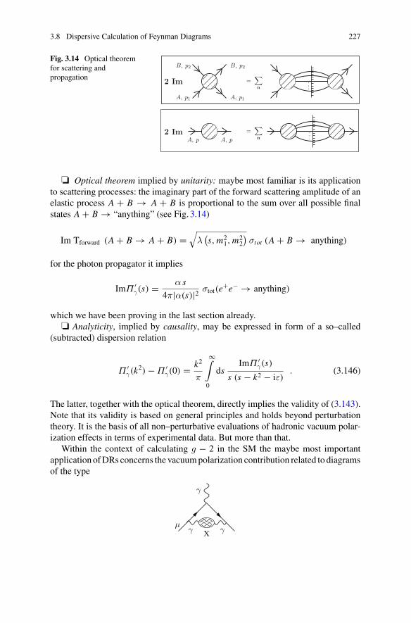
3.8 Dispersive Calculation of Feynman Diagrams 227

Fig. 3.14 Optical theoremfor scattering andpropagation =

∑n

2 Im

A, p1

B, p2

A, p1

B, p2

=∑n

2 ImA, p A, p

❏ Optical theorem implied by unitarity: maybe most familiar is its applicationto scattering processes: the imaginary part of the forward scattering amplitude of anelastic process A + B → A + B is proportional to the sum over all possible finalstates A + B → “anything” (see Fig. 3.14)

Im Tforward (A + B → A + B) =√

λ(s, m2

1, m22

)σtot (A + B → anything)

for the photon propagator it implies

ImΠ ′γ(s) = α s

4π|α(s)|2 σtot(e+e− → anything)

which we have been proving in the last section already.❏ Analyticity, implied by causality, may be expressed in form of a so–called

(subtracted) dispersion relation

Π ′γ(k

2) − Π ′γ(0) = k2

π

∞∫

0

dsImΠ ′

γ(s)

s (s − k2 − iε). (3.146)

The latter, together with the optical theorem, directly implies the validity of (3.143).Note that its validity is based on general principles and holds beyond perturbationtheory. It is the basis of all non–perturbative evaluations of hadronic vacuum polar-ization effects in terms of experimental data. But more than that.

Within the context of calculating g − 2 in the SM the maybe most importantapplication of DRs concerns the vacuum polarization contribution related to diagramsof the type

Xμ

γ

γ γ

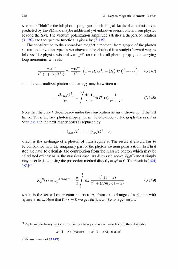
228 3 Lepton Magnetic Moments: Basics

where the “blob” is the full photon propagator, including all kinds of contributions aspredicted by the SM and maybe additional yet unknown contributions from physicsbeyond the SM. The vacuum polarization amplitude satisfies a dispersion relation(3.136) and the spectral function is given by (3.139).

The contribution to the anomalous magnetic moment from graphs of the photonvacuum polarization type shown above can be obtained in a straightforward way asfollows: The physics wise relevant gμν–term of the full photon propagator, carryingloop momentum k, reads

−igμν

k2 (1 + Π ′γ(k

2)) −igμν

k2

(1 − Π ′

γ(k2) + (

Π ′γ(k

2))2 − · · ·

)(3.147)

and the renormalized photon self–energy may be written as

− Π ′γ ren(k

2)

k2=

∞∫

0

ds

s

1

πIm Π ′

γ(s)1

k2 − s. (3.148)

Note that the only k dependence under the convolution integral shows up in the lastfactor. Thus, the free photon propagator in the one–loop vertex graph discussed inSect. 2.6.3 in the next higher order is replaced by

−igμν/k2 → −igμν/(k2 − s)

which is the exchange of a photon of mass square s. The result afterward has tobe convoluted with the imaginary part of the photon vacuum polarization. In a firststep we have to calculate the contribution from the massive photon which may becalculated exactly as in the massless case. As discussed above FM(0) most simplymay be calculated using the projection method directly at q2 = 0. The result is [184,185]31

K (2)μ (s) ≡ a(2) heavy γ

μ = α

π

1∫

0

dxx2 (1 − x)

x2 + (s/m2μ)(1 − x)

, (3.149)

which is the second order contribution to aμ from an exchange of a photon withsquare mass s. Note that for s = 0 we get the known Schwinger result.

31Replacing the heavy vector exchange by a heavy scalar exchange leads to the substitution

x2 (1 − x) (vector) → x2 (1 − x/2) (scalar)

in the numerator of (3.149).

3.8 Dispersive Calculation of Feynman Diagrams 229

Utilizing this result and (3.148), the contribution from the “blob” to g − 2 reads

a(X)μ = 1

π

∞∫

0

ds

sIm Π

′(X)γ (s) K (2)

μ (s) . (3.150)

If we exchange integrations and evaluating the DR we arrive at

a(X)μ = α

π

1∫

0

dx (1 − x)

∞∫

0

ds

s

1

πIm Π

′(X)γ (s)

x2

x2 + (s/m2μ)(1 − x)

= α

π

1∫

0

dx (1 − x)[−Π

′(X)γ (sx )

](3.151)

where

sx = − x2

1 − xm2

μ .

The last simple representation in terms of Π′(X)γ (sx ) follows using

x2

x2 + (s/m2μ)(1 − x)

= −sx1

s − sx.

In this context a convenient one–fold integral representation of the VP func-tion is (2.177)

Π′�γ ren

(−x2

1 − xm2

μ

)

= −α

π

1∫

0

dz 2z (1 − z) ln

(

1 + x2

1 − x

m2μ

m2�

z (1 − z)

)

, (3.152)

which together with (3.151) leads to a two–fold integral representation of the VPcontribution by lepton loops at two–loop order.

This kind of dispersion integral representation can be generalized to higher orderand sequential VP insertions corresponding to the powers of Π ′(k2) in (3.147).

Denoting ρ(s)=ImΠ ′γ ren(s)/π we may write (3.148) in the form −Π ′

γ ren(k2)=

∞∫

0

dss

ρ(s) k2

k2−s such that the n–th term of the propagator expansion (3.147) is given by

(−Π ′

γ ren(k2))n

/k2 = 1

k2

n∏

i=1

∞∫

0

dsi

siρ(si )

k2

k2 − si

=n∑

j=1

∞∫

0

ds j

s jρ(s j )

1

k2 − s j

∏

i �= j

∞∫

0

dsi

siρ(si )

s j

s j − si,

230 3 Lepton Magnetic Moments: Basics

where we have been applying the partial fraction decomposition

1

k2

n∏

i=1

k2

k2 − si=

n∑

k=1

1

k2 − s j

∏

i �= j

s j

s j − si.

We observe that the integration over the loop momentum k of the one–loop muonvertex proceeds exactly as before, with the photon replaced by a single heavy photonof mass s j . Thus, the contribution to aμ reads

a(X)μ = α

π

1∫

0

dx (1 − x)

n∑

j=1

∞∫

0

ds j

s jρ(s j )

−sx

s j − sx

∏

i �= j

∞∫

0

dsi

siρ(si )

s j

s j − si

= α

π

1∫

0

dx (1 − x)

⎛

⎝n∏

k=1

1∫

0

dsk

skρ(sk)

⎞

⎠ sx

⎛

⎝n∑

j=1

1

sx − s j

∏

i �= j

s j

s j − si

⎞

⎠ .

Under the integral, to the last factor, we may apply the above partial fraction decom-position backward

n∑

j=1

1

sx − s j

∏

i �= j

s j

s j − si= 1

sx

n∏

i=1

sx

sx − si

which proves that the si –integrals factorize and we find [186]

a(X)μ = α

π

1∫

0

dx (1 − x)

⎛

⎝∞∫

0

ds

sρ(s)

−sx

s − sx

⎞

⎠

n

= α

π

1∫

0

dx (1 − x)(−Π ′

γ ren(sx))n

(3.153)

We are thus able to write formally the result for the one–loop muon vertex when wereplace the free photon propagator by the full transverse propagator as [187]

a(X)μ = α

π

1∫

0

dx (1 − x)

(1

1 + Π ′γ ren(sx )

)

= 1

π

1∫

0

dx (1 − x) α(sx ) , (3.154)

3.8 Dispersive Calculation of Feynman Diagrams 231

which according to (3.120) is equivalent to the contribution of a free photon interact-ing with dressed charge (effective fine structure constant). However, since Π ′

γ ren(k2)

is negative and grows logarithmically with k2 the full photon propagator develops a socalled Landau pole where the effective fine structure constant becomes infinite. Thusresumming the perturbation expansion under integrals may produce a problem andone better resorts to the order by order approach, by expanding the full propagatorinto its geometrical progression. Nevertheless (3.154) is a very useful bookkeep-ing device, collecting effects from different contributions and different orders. Inparticular if we expand the 1PI photon self–energy into order by order contributions

Π ′γ ren(k

2) = Π′(2)γ ren(k

2) + Π′(4)γ ren(k

2) + · · ·

and also write ρ = ρ(2) + ρ(4) + · · · for the spectral densities.Coming back to the single VP insertion formula (3.151) we may use (3.152) as

well as the second form given in (2.177) which reads

Π′�γ ren

(q2/m2

) = −α

π

q2

m2

1∫

0

dtρ2(t)

q2

m2 − 4/(1 − t2), (3.155)

with32

ρ2(t) = t2 (1 − t2/3)

1 − t2, (3.156)

and we may write

a(X)μ =

(α

π

)21∫

0

dx (1 − x)

1∫

0

dtρ2(t)

Wt (x), (3.157)

where

1/Wt (x) = q2

m2

1q2

m2 − 41−t2

∣∣∣∣∣

q2

m2 =− x21−x

m2μ

m2

and hence

Wt (x) = 1 + 4m2

(1 − t2) m2μ

1 − x

x2. (3.158)

32We adopt the notation of Kinoshita [186] and mention that the densities ρ(t) used here are not tobe confused with the ρ(s) used just before, although they are corresponding to each other.

232 3 Lepton Magnetic Moments: Basics

If n equal loops are inserted we have

a(X)μ = α

π

1∫

0

dx (1 − x)

⎛

⎝α

π

1∫

0

dtρ(t)

Wt (x)

⎞

⎠

n

(3.159)

according to the factorization theorem demonstrated before. This formula is suitablefor calculating the contribution to the lepton anomalous magnetic moment once thespectral function ρ(t) is known. For the one–loop 1PI self–energy we have ρ2(t)given by (3.156) and the corresponding density for the two–loop case reads [175,176, 188]

ρ4(t) = 2t

3 (1 − t2)

{(3 − t2) (1 + t2)

2

(Li2 (1) + ln

1 + t

2ln

1 + t

1 − t

+ 2

(Li2

(1 − t

1 + t

)+ Li2

(1 + t

2

)− Li2

(1 − t

2

))− 4 Li2 (t) + Li2

(t2))

+(

11

16(3 − t2) (1 + t2) + 1

4t4 − 3

2t (3 − t2)

)ln

1 + t

1 − t

+ t (3 − t2)

(3 ln

1 + t

2− 2 ln t

)+ 3

8t (5 − 3t2)

}. (3.160)

The corresponding result for the three–loop photon self–energy has been calculatedin [189]. For four–loops an approximate result is available [190]. Generally, thecontribution to aμ which follow from the lowest order lepton (�) vertex diagram bymodifying the photon propagator with l electron loops of order 2i , m muon loops oforder 2 j and n tau loops of order 2k is given by

a� =(α

π

)(1+il+ jm+kn)1∫

0

dx (1 − x)

⎛

⎜⎝

1∫

0

dt1ρ2i (t1)

1 + 41−t2

1

1−xx2

(mem�

)2

⎞

⎟⎠

l

·⎛

⎜⎝

1∫

0

dt2ρ2 j (t2)

1 + 41−t2

2

1−xx2

(mμ

m�

)2

⎞

⎟⎠

m

·⎛

⎜⎝

1∫

0

dt3ρ2k(t3)

1 + 41−t2

3

1−xx2

(mτ

m�

)2

⎞

⎟⎠

n

.

(3.161)

The same kind of approach works for the calculation of diagrams with VP inser-tions not only for the lowest order vertex. For any group of diagrams we may calculatein place of the true QED contribution the one obtained in massive QED with a photonof mass

√s, and then convolute the result with the desired density of the photon VP

analogous to (3.150) where (3.149) gets replaced by a different more complicatedkernel function (see e.g. [103, 191] and below). It also should be noted that the rep-resentation presented here only involve integration over finite intervals ([0,1]) and

3.8 Dispersive Calculation of Feynman Diagrams 233

hence are particularly suited for numerical integration of higher order contributionswhen analytic results are not available.

The formalism developed here also is the key tool to evaluate the hadronic con-tributions, for which perturbation theory fails because of the strong interactions. Inthis case we represent Im Π

′ hadγ (s) via (3.139) in terms of

σhad(s) = σ(e+e− → hadrons)

where

σhad(s) = 4π2 |α(s)|2α s

1

πIm Π

′ hadγ (s) (3.162)

or in terms of the cross section ratio R(s) defined by (3.139) where both σhad(s) orequivalently Rhad(s) will be taken from experiment, since they are not yet calculablereliably from first principles at present.

Starting point is the basic integral representation (from (3.150) using (3.139))

ahadμ = α

π

∞∫

0

ds

s

1∫

0

dxx2 (1 − x)

x2 + (1 − x) s/m2μ

α

3πR(s) . (3.163)

If we first integrate over x we find the well known standard representation

ahadμ = α

3π

∞∫

0

ds

sK (2)

μ (s) R(s) (3.164)

as an integral along the cut of the vacuum polarization amplitude in the time–likeregion, while an interchange of the order of integrations yields the analog of (3.151):an integral over the hadronic shift of the fine structure constant (3.121) in the space–like domain [192]:

ahadμ = α

π

1∫

0

dx (1 − x) Δα(5)had

(−Q2(x))

(3.165)

where Q2(x) ≡ x2

1−x m2μ is the space–like square momentum–transfer or

x = Q2

2m2μ

⎛

⎝

√

1 + 4m2μ

Q2− 1

⎞

⎠ .

In Fig. 3.15 we display the integrand of the representation (3.165) Alternatively, bywriting (1 − x) = − 1

2d

dx (1 − x)2 and performing a partial integration in (3.165) one

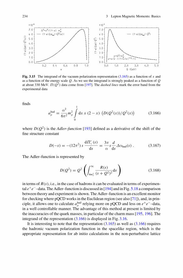
234 3 Lepton Magnetic Moments: Basics

Fig. 3.15 The integrand of the vacuum polarization representation (3.165) as a function of x andas a function of the energy scale Q. As we see the integrand is strongly peaked as a function of Qat about 330 MeV. Π(Q2) data come from [197]. The dashed lines mark the error band from theexperimental data

finds

ahadμ = α2

6π2m2

μ

1∫

0

dx x (2 − x)(D(Q2(x))/Q2(x)

)(3.166)

where D(Q2) is the Adler–function [193] defined as a derivative of the shift of thefine structure constant

D(−s) = −(12π2) sdΠ ′

γ (s)

ds= 3π

αs

d

dsΔαhad(s) . (3.167)

The Adler–function is represented by

D(Q2) = Q2

(∫ ∞

4m2π

R(s)

(s + Q2)2ds

)

(3.168)

in terms of R(s), i.e., in the case of hadrons it can be evaluated in terms of experimen-tal e+e−–data. The Adler–function is discussed in [194] and in Fig. 5.18 a comparisonbetween theory and experiment is shown. The Adler–function is an excellent monitorfor checking where pQCD works in the Euclidean region (see also [71]), and, in prin-ciple, it allows one to calculate ahad

μ relying more on pQCD and less on e+e−–data,in a well controllable manner. The advantage of this method at present is limited bythe inaccuracies of the quark masses, in particular of the charm mass [195, 196]. Theintegrand of the representation (3.166) is displayed in Fig. 3.16.

It is interesting to note that the representation (3.165) as well as (3.166) requiresthe hadronic vacuum polarization function in the spacelike region, which is theappropriate representation for ab initio calculations in the non-perturbative lattice

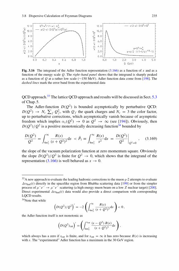
3.8 Dispersive Calculation of Feynman Diagrams 235

Fig. 3.16 The integrand of the Adler function representation (3.166) as a function of x and as afunction of the energy scale Q. The right–hand panel shows that the integrand is sharply peakedas a function of Q at a rather low scale (∼150 MeV). Adler function data come from [198]. Thedashed lines mark the error band from the experimental data

QCD approach.33 The lattice QCD approach and results will be discussed in Sect. 5.3of Chap. 5.

The Adler-function D(Q2) is bounded asymptotically by perturbative QCD:D(Q2) → Nc

∑f Q2

f , with Q f the quark charges and Nc = 3 the color factor,up to perturbative corrections, which asymptotically vanish because of asymptoticfreedom which implies αs(Q2) → 0 as Q2 → ∞ (see [194]). Obviously, thenD(Q2)/Q2 is a positive monotonically decreasing function34 bounded by

D(Q2)

Q2=∫ ∞

4m2π

R(s)

(s + Q2)2ds < P1 ≡

∫ ∞

4m2π

R(s)

s2ds = D(Q2)

Q2

∣∣∣∣Q2=0

, (3.169)

the slope of the vacuum polarization function at zero momentum square. Obviouslythe slope D(Q2)/Q2 is finite for Q2 → 0, which shows that the integrand of therepresentation (3.166) is well behaved as x → 0.

33A new approach to evaluate the leading hadronic corrections to the muon g-2 attempts to evaluateΔαhad(t) directly in the spacelike region from Bhabha scattering data [199] or from the simplerprocess of μ−e− → μ−e− scattering (a high energy muon beam on a low Z nuclear target) [200].Direct experimental Δαhad(t) data would also provide a direct comparison with correspondingLQCD results.34Note that while

(D(Q2)/Q2

)′ = −2

(∫ ∞

4m2π

R(s)

(s + Q2)3 ds

)

< 0 ,

the Adler function itself is not monotonic as

(D(Q2)cut

)′ =(∫ scut

4m2π

(s − Q2) R(s)

(s + Q2)3 ds

)

,

which always has a zero if scut is finite, and for scut = ∞ it has zero because R(s) is increasingwith s. The “experimental” Adler function has a maximum in the 30 GeV region.

236 3 Lepton Magnetic Moments: Basics

Note that alternatively, using (3.167) we may write

P1 = −3π

α

d

dsΔαhad(s)|s=−Q2,Q2→0 . (3.170)

Therefore, (3.168) together with (3.166) yields a bound (see also [113])

ahadμ <

α2

6π2m2

μ

2

3P1 . (3.171)

The integral over a compilation of R(s)–data, discussed in detail later in Chap. 5,yields P1 = 11.83(8) GeV−2 and hence

ahadμ < 791(5) × 10−10 . (3.172)

As we will see an evaluation of (3.164) yields a value substantially lower: ahadμ

688.1 ± 4.1 × 10−10.Actually, we may write (3.164) in the form

ahadμ =

(α mμ

3π

)2∞∫

0

ds

s2K (s) R(s) (3.173)

where

K (s) = 3s

m2μ

K (2)μ (s) , (3.174)

in which K (s) is a bounded monotonically increasing function, with K (4m2π) 0.63

increasing to 1 at s → ∞. Setting K (s) = 1 we obtain the bound presented above.A lower bound then is obtained by setting K (s) = K (4m2

π) ≈ 0.63, which impliesahad

μ > 498(3) × 10−10 again a very rough bound only, but a true bound.The bound (3.171) can be improved by a moment expansion of the kernel as

advocated in Ref. [201] and analyzed in detail in [202].The best checks is to compare lattice results in terms of the Adler function as

it enters in the representation (3.166) as advocated in [195] and actually performedin [203, 204] recently. An up-to-date evaluation of the “experimental” Adler functionis available via the link [198].

3.9 ζ–Values, Polylogarithms and Related SpecialFunctions

For later reference we list some transcendental constants and definitions of specialfunctions which are encountered in higher order Feynman graph calculations. Typi-

3.9 ζ–Values, Polylogarithms and Related Special Functions 237

cally analytic results for the mass independent universal lepton g − 2 contributionsare of the form of sums of terms exhibiting rational numbers as coefficients of tran-scendental objects. The most frequent such object are the Riemann zeta function

ζ(n) =∞∑

k=1

1

kn(3.175)

and the polylogarithmic integrals

Lin(x) = (−1)n−1

(n − 2)!∫ 1

0

lnn−2(t) ln(1 − xt)

tdt =

∞∑

k=1

xk

kn, (3.176)

where the dilogarithm Li2(x) is often referred to as the Spence function which weencountered in Sect. 2.6.3 (2.208). The series representation holds for |x | ≤ 1. Thedilogarithm is an analytic function with the same cut as the logarithm. Useful relationsare

Sp(x) = −Sp(1 − x) + π2

6− ln x ln(1 − x),

Sp(x) = −Sp

(1

x

)− π2

6− 1

2ln2(−x),

Sp(x) = −Sp(−x) + 1

2Sp(x2) . (3.177)

Special values are:

Sp(0) = 0 , Sp(1) = π2

6, Sp(−1) = −π2

12, Sp

(1

2

)= π2

12− 1

2(ln 2)2 .

(3.178)Special ζ(n) values we will need are

ζ(2) = π2

6, ζ(3) = 1.202 056 903 . . . , ζ(4) = π4

90, ζ(5) = 1.036 927 755 . . . .

(3.179)Also the constants

Lin(1) = ζ(n) , Lin(−1) = −[1 − 21−n] ζ(n),

a4 ≡ Li4(1

2) =

∞∑

n=1

1/(2nn4) = 0.517 479 061 674 . . . , (3.180)

related to polylogarithms, will be needed for the evaluation of analytical results. Ageneralization are the Nielsen integrals

238 3 Lepton Magnetic Moments: Basics

Sn,p(x) = (−1)n+p−1

(n − 1)!p!∫ 1

0

lnn−1(t) lnp(1 − xt)

tdt , (3.181)

which have representations as sums of the type

S1,2(x) =∞∑

2

xk

k2S1(k − 1) ; S2,2(x) =

∞∑

2

xk

k3S1(k − 1) ,

where

S1(k) =k∑

1

1

l

is a harmonic sum. And higher sums are obtained by the recurrences

d

dxSn,p(x) = 1

xSn−1,p(x) ;

∫ x

0

Sn,p(t)

tdt = Sn+1,p(x) .

The general harmonic series are defined by [205]

Sm(n) =n∑

i=1

1

im; S−m(n) =

n∑

i=1

(−1)i

im, (3.182)

in which m > 0. Higher harmonic series are defined by the recurrences

Sm, j1,..., jp (n) =n∑

i=1

1

imS j1,..., jp (i) ; S−m, j1,..., jp (n) =

n∑

i=1

(−1)i

imS j1,..., jp (i) , (3.183)

where again m > 0. The m and the ji are referred to as the indices of the harmonicseries. Hence, for example

S1,−5,3(n) =n∑

i=1

1

i

i∑

j=1

(−1) j

j5

j∑

k=1

1

k3. (3.184)

Basic transcendental constants of increasing transcendental weight are (exampleswe will find in Chap. 4)

{[S1(∞), ln(2)] ; ζ2; ζ3; Li4(1/2); (ζ5, Li5(1/2)) ; [Li6(1/2), S−5,−1(∞)

] ;[ζ7, Li7(1/2), S−5,1,1(∞), S5,−1,−1(∞)

] ; . . .

}(3.185)

3.9 ζ–Values, Polylogarithms and Related Special Functions 239

where S... = S...(∞). The numerical values have been calculated in [205]:

Li4(1/2) = 0.51747906167389938633

Li5(1/2) = 0.50840057924226870746

Li6(1/2) = 0.50409539780398855069

Li7(1/2) = 0.50201456332470849457

S−5,−1(∞) = 0.98744142640329971377

−S−5,1,1(∞) = 0.95296007575629860341

S5,−1,−1(∞) = 1.02912126296432453422 . (3.186)

The harmonic polylogarithms (HPL) H (a1, . . . , ak; x) are functions of one vari-able x labeled by a vector a = (a1, . . . , ak). The dimension k of the vector a is calledthe weight of the HPL [206]. Given the functions

f1(x) = 1

1 − x; f0(x) = 1

x; f−1(x) = 1

1 + x, (3.187)

the HPLs are defined recursively through integration of these functions. For weightone we have

H(1; x) =x∫

0

f1(t) dt =x∫

0

1

1 − tdt = − log(1 − x)

H(0; x) = log(x)

H(−1; x) =x∫

0

f−1(t) dt =x∫

0

1

1 + tdt = log(1 + x), (3.188)

and for higher weights

H(n0; x) = 1

n! logn x ; H(a, a1,...,k; x) =x∫

0

fa(t)H(a1,...,k; t) dt , (3.189)

where we used the notations ni = i, . . . , i︸ ︷︷ ︸n

, and a1,...,k = a1, . . . , ak .

Examples are,

H(0, 0, 1, 1; x) = S2,2(x) ; H(−1, 0, 0, 1; x) =∫ x

0

dz

1 + zLi3(z) .

240 3 Lepton Magnetic Moments: Basics

The formula for the derivative of the HPLs follows directly from their definition

d

dxH(a, a1,...,k; x) = fa(x)H(a1,...,k; x) . (3.190)

An elliptic integral is defined as any function f which can be expressed in theform [207]

f (x) =∫ x

cR(

t,√

P(t))

dt

where R is a rational function of its two arguments, P is a polynomial of degree 3 or4 with no repeated roots, and c is a constant. In general, integrals in this form cannotbe expressed in terms of elementary functions. Exceptions to this general rule arewhen P has repeated roots, or when R(x, y) contains no odd powers of y. However,with the appropriate reduction formula, every elliptic integral can be brought into aform that involves integrals over rational functions and the three canonical forms, theelliptic integrals of the first, second and third kind. The incomplete elliptic integralof the first kind F is defined as

F(ϕ; m) =∫ ϕ

0

dθ√

1 − m sin2 θ=∫ x=sin ϕ

0

dt√(

1 − t2) (

1 − mt2) .

The incomplete elliptic integral of the second kind E may be defined as

E(ϕ; m) =∫ ϕ

0dθ

√1 − m sin2 θ =

∫ x=sin ϕ

0

√1 − mt2

√1 − t2

dt .

The incomplete elliptic integral of the third kind Π is defined by

Π(n;ϕ | m) =∫ ϕ

0

1

1 − n sin2 θ

dθ√

1 − m sin2 θ=∫ x=sin ϕ

0

1

1 − nt2dt

√(1 − t2

) (1 − mt2

) ,

where m = sin2 α is a parameter. For ϕ = π/2 and x = 1 we obtain the completeelliptic integrals.

The simplest diagram leading to an elliptic integral is the scalar massive triple line

graph (sunrise diagram) , which plays a role in the self–energy of the ωvector meson which decays predominantly via ω → π+π−π0 (see also [208]). In thecontext of dimensional regularization and ε–expansion various types of generalizedand Appell hypergeometric functions show up [209–213]. For further reading seee.g. [214–217] and references therein.

References 241

References

1. J.D. Bjorken, S.D. Drell, Relativistic Quantum Mechanics, 1st edn. (McGraw-Hill, New York,1964), 300 p; Relativistic Quantum Fields, 1st edn. (McGraw-Hill, New York, 1965), p. 396

2. L.H. Thomas, Philos. Mag. 3, 1 (1927); V. Bargmann, L. Michel, V.A. Telegdi. Phys. Rev.Lett. 2, 435 (1959)

3. P.A.M. Dirac, Proc. R. Soc. A 117, 610 (1928); A 118, 351 (1928)4. P.J. Mohr, D.B. Newell, B.N. Taylor, Rev. Mod. Phys. 88, 035009 (2016)5. B. Odom, D. Hanneke, B. D’Urso, G. Gabrielse, Phys. Rev. Lett. 97, 030801 (2006)6. D. Hanneke, S. Fogwell, G. Gabrielse, arXiv:0801.1134 [physics.atom-ph]7. P.J. Mohr, B.N. Taylor, D.B. Newell, Rev. Mod. Phys. 84, 1527 (2012)8. G. Gabrielse, D. Hanneke, T. Kinoshita, M. Nio, B. Odom, Phys. Rev. Lett. 97, 030802 (2006)

[Erratum-ibid. 99, 039902 (2007)]9. T. Aoyama, M. Hayakawa, T. Kinoshita, M. Nio, Phys. Rev. Lett. 99, 110406 (2007)

10. T. Aoyama, M. Hayakawa, T. Kinoshita, M. Nio, Phys. Rev. Lett. 109, 111807 (2012)11. S. Laporta, arXiv:1704.06996 [hep-ph]12. K.A. Olive et al. [Particle Data Group], Chin. Phys. C 38, 090001 (2014); C. Patrignani et al.,

Part. Data Group Chin. Phys. C 40, 100001 (2016)13. S. Eidelman et al. [Particle Data Group], Phys. Lett. B 592, 1 (2004)14. P.J. Mohr, B.N. Taylor, Rev. Mod. Phys. 72, 351 (2000); 77, 1 (2005)15. F. Gianotti (the ATLAS Collab.), CERN Seminar, July 4th, 2012; J. Incandela (the CMS

Collab.), CERN Seminar, July 4th, 201216. G. Aad et al. [ATLAS Collab.], Phys. Lett. B 716, 1 (2012). Science 338, 1576 (2012)17. S. Chatrchyan et al. [CMS Collab.], Phys. Lett. B 716, 30 (2012) Science 338, 1569 (2012);18. F. Jegerlehner, M.Y. Kalmykov, B.A. Kniehl, Phys. Lett. B 722, 123 (2013)19. B.A. Kniehl, A.F. Pikelner, O.L. Veretin, Nucl. Phys. B 896, 19 (2015)20. F. Jegerlehner, A. Nyffeler, Phys. Rep. 477, 1 (2009)21. J.S. Schwinger, Phys. Rev. 73, 416 (1948)22. D.J. Broadhurst, D. Kreimer, J. Symb. Comput. 27, 581 (1999); Int. J. Mod. Phys. C 6, 519

(1995); Phys. Lett. B 393, 403 (1997); D.J. Broadhurst, J.A. Gracey, D. Kreimer, Z. Phys. C75, 559 (1997)

23. A. Devoto, D.W. Duke, Riv. Nuovo Cimento 7N6, 1 (1984)24. R. Karplus, N.M. Kroll, Phys. Rep. C 77, 536 (1950)25. A. Petermann, Helv. Phys. Acta 30, 407 (1957); Nucl. Phys. 5, 677 (1958)26. C.M. Sommerfield, Phys. Rev. 107, 328 (1957); Ann. Phys. (N.Y.) 5, 26 (1958)27. M.V. Terentev, Sov. Phys. JETP 16, 444 (1963); [Zh. Eksp. Teor. Fiz. 43, 619 (1962)]28. S. Laporta, E. Remiddi, Phys. Lett. B 379, 283 (1996)29. T. Kinoshita, Phys. Rev. Lett. 75, 4728 (1995)30. T. Kinoshita, W.J. Marciano, in Quantum Electrodynamics, ed. by T. Kinoshita (World Sci-

entific, Singapore, 1990), pp. 419–47831. T. Kinoshita, M. Nio, Phys. Rev. Lett. 90, 021803 (2003); Phys. Rev. D 70, 113001 (2003)32. T. Kinoshita, M. Nio, Phys. Rev. D 73, 013003 (2006)33. T. Aoyama, M. Hayakawa, T. Kinoshita, M. Nio, Phys. Rev. D 91, 033006 (2015)34. T. Kinoshita, Int. J. Mod. Phys. A 29, 1430003 (2014)35. M. Hayakawa, Springer Tracts Mod. Phys. 256, 41 (2014)36. H. Suura, E. Wichmann, Phys. Rev. 105, 1930 (1957); A. Petermann, Phys. Rev. 105, 1931

(1957)37. H.H. Elend, Phys. Lett. 20, 682 (1966); Erratum-ibid, 21, 720 (1966)38. B.E. Lautrup, E. de Rafael, Nucl. Phys. B 70, 317 (1974)39. P.A. Baikov, K.G. Chetyrkin, J.H. Kühn, C. Sturm, Nucl. Phys. B 867, 182 (2013)40. S. Laporta, Nuovo Cimento A 106, 675 (1993)41. A. Czarnecki, M. Skrzypek, Phys. Lett. B 449, 354 (1999)42. S. Friot, D. Greynat, E. De Rafael, Phys. Lett. B 628, 73 (2005)

242 3 Lepton Magnetic Moments: Basics

43. S. Laporta, E. Remiddi, Phys. Lett. B 301, 440 (1993)44. J.H. Kühn, A.I. Onishchenko, A.A. Pivovarov, O.L. Veretin, Phys. Rev. D 68, 033018 (2003)45. J. Aldins, T. Kinoshita, S.J. Brodsky, A.J. Dufner, Phys. Rev. Lett. 23, 441 (1969); Phys. Rev.

D 1, 2378 (1970)46. J. Bailey et al., Phys. Lett. B 28, 287 (1968)47. A.S. Elkhovsky, Sov. J. Nucl. Phys. 49, 656 (1989); [Yad. Fiz. 49, 1059 (1989)]48. M. Passera, J. Phys. G 31, R75 (2005); Phys. Rev. D 75, 013002 (2007)49. M. Caffo, S. Turrini, E. Remiddi, Phys. Rev. D 30, 483 (1984); E. Remiddi, S.P. Sorella,

Lett. Nuovo Cim. 44, 231 (1985); D.J. Broadhurst, A.L. Kataev, O.V. Tarasov, Phys. Lett. B298, 445 (1993); S. Laporta, Phys. Lett. B 312, 495 (1993); P.A. Baikov, D.J. Broadhurst,arXiv:hep-ph/9504398

50. A.L. Kataev, Phys. Rev. D 86, 013010 (2012)51. T. Aoyama, M. Hayakawa, T. Kinoshita, M. Nio, Phys. Rev. Lett. 109, 111808 (2012)52. S.G. Karshenboim, Phys. At. Nucl. 56, 857 (1993); [Yad. Fiz. 56N6, 252 (1993)]53. T. Kinoshita, M. Nio, Phys. Rev. D 73, 053007 (2006)54. A.L. Kataev, Nucl. Phys. Proc. Suppl. 155, 369 (2006); arXiv:hep-ph/0602098; Phys. Rev. D

74, 073011 (2006)55. P.A. Baikov, K.G. Chetyrkin, C. Sturm, Nucl. Phys. Proc. Suppl. 183, 8 (2008)56. R. Lee, P. Marquard, A.V. Smirnov, V.A. Smirnov, M. Steinhauser, JHEP 1303, 162 (2013)57. A. Kurz, T. Liu, P. Marquard, A.V. Smirnov, V.A. Smirnov, M. Steinhauser, Phys. Rev. D 92,

073019 (2015)58. A. Kurz, T. Liu, P. Marquard, A. Smirnov, V. Smirnov, M. Steinhauser, Phys. Rev. D 93,

053017 (2016)59. H. Fritzsch, M. Gell-Mann, H. Leutwyler, Phys. Lett. 47B, 365 (1973)60. H.D. Politzer, Phys. Rev. Lett. 30, 1346 (1973); D. Gross, F. Wilczek, Phys. Rev. Lett. 30,

1343 (1973)61. S.G. Gorishnii, A.L. Kataev, S.A. Larin, Phys. Lett. B 259, 144 (1991); L.R. Surguladze, M.A.

Samuel, Phys. Rev. Lett. 66, 560 (1991) [Erratum-ibid. 66, 2416 (1991)]; K.G. Chetyrkin,Phys. Lett. B 391, 402 (1997)

62. K.G. Chetyrkin, J.H. Kühn, Phys. Lett. B 342, 356 (1995); K.G. Chetyrkin, R.V. Harlander,J.H.Kühn, Nucl. Phys. B 586, 56 (2000) [Erratum-ibid. B 634, 413 (2002)]

63. R.V. Harlander, M. Steinhauser, Comput. Phys. Commun. 153, 244 (2003)64. S. Eidelman, F. Jegerlehner, Z. Phys. C 67, 585 (1995)65. A.E. Blinov et al. [MD-1 Collab.], Z. Phys. C 70, 31 (1996)66. J.Z. Bai et al. [BES Collab.], Phys. Rev. Lett. 84, 594 (2000); Phys. Rev. Lett. 88, 101802

(2002)67. R.R. Akhmetshin et al. [CMD-2 Collab.], Phys. Lett. B 578, 285 (2004); Phys. Lett. B 527,

161 (2002)68. A. Aloisio et al. [KLOE Collab.], Phys. Lett. B 606, 12 (2005)69. M.N. Achasov et al. [SND Collab.], J. Exp. Theor. Phys. 103, 380 (2006) [Zh. Eksp. Teor.

Fiz. 130, 437 (2006)]70. V. M. Aulchenko et al. [CMD-2], JETP Lett. 82 (2005) 743 [Pisma Zh. Eksp. Teor. Fiz. 82

(2005) 841]; R. R. Akhmetshin et al., JETP Lett. 84 (2006) 413 [Pisma Zh. Eksp. Teor. Fiz.84 (2006) 491]; Phys. Lett. B 648 (2007) 28

71. F. Jegerlehner, Nucl. Phys. Proc. Suppl. 162, 22 (2006), arXiv:hep-ph/060832972. F. Jegerlehner, R. Szafron, Eur. Phys. J. C 71, 1632 (2011)73. F. Jegerlehner, Acta Phys. Pol. B 44, 2257 (2013)74. F. Jegerlehner, EPJ Web Conf. 118, 01016 (2016). arXiv:1705.00263 [hep-ph]75. B. Ananthanarayan, I. Caprini, D. Das, I.S. Imsong, Phys. Rev. D 93, 116007 (2016)76. H. Leutwyler, Electromagnetic form factor of the pion, in Continuous Advances in QCD 2002:

Proceedings ed. by K.A. Olive, M.A. Shifman, M.B. Voloshin (World Scientific, Singapore,2002), 646p, arXiv:hep-ph/0212324

77. G. Colangelo, Nucl. Phys. Proc. Suppl. 131, 185 (2004); ibid. 162, 256 (2006)

References 243

78. H. Leutwyler, Electromagnetic form factor of the pion, in Continuous Advances in QCD 2002:Proceedings, ed. by K.A. Olive, M.A. Shifman, M.B. Voloshin (World Scientific, Singapore,2002), 646p, arXiv:hep-ph/0212324; G. Colangelo, Nucl. Phys. Proc. Suppl. 131, 185 (2004);ibid. 162, 256 (2006)

79. R.R. Akhmetshin et al. [CMD-2 Collab.], Phys. Lett. B 578, 285 (2004)80. A. Aloisio et al. [KLOE Collab.], Phys. Lett. B 606, 12 (2005); F. Ambrosino et al. [KLOE

Collab.], Phys. Lett. B 670, 285 (2009)81. F. Ambrosino et al. [KLOE Collab.], Phys. Lett. B 700, 102 (2011)82. D. Babusci et al. [KLOE Collab.], Phys. Lett. B 720, 336 (2013)83. B. Aubert et al. [BABAR Collab.], Phys. Rev. Lett. 103, 231801 (2009); J.P. Lees et al., Phys.

Rev. D 86, 032013 (2012)84. M. Ablikim et al. [BESIII Collab.], Phys. Lett. B 753, 629 (2016)85. K. Hagiwara, A.D. Martin, D. Nomura, T. Teubner, Phys. Lett. B 649, 173 (2007)86. M. Davier, S. Eidelman, A. Höcker, Z. Zhang, Eur. Phys. J. C 27, 497 (2003); ibid. 31, 503

(2003)87. S. Eidelman, Proceedings of the XXXIII International Conference on High Energy Physics,

July 27 – August 2, 2006, Moscow (Russia), World Scientific, to appear; M. Davier, Nucl.Phys. Proc. Suppl. 169, 288 (2007)

88. M. Davier et al., Eur. Phys. J. C 66, 127 (2010)89. M. Davier, A. Höcker, B. Malaescu, Z. Zhang, Eur. Phys. J. C 71, 1515 (2011)[Erratum-ibid.

C 72, 1874 (2012)]90. R. Akhmetshin et al. [CMD-3 Collab.], Phys. Lett. B 723, 82 (2013)91. M. Achasov et al. [SND Collab.], Phys. Rev. D 88, 054013 (2013)92. J. Lees et al. [BABAR Collab.], Phys. Rev. D 87, 092005 (2013)93. J. Lees et al. [BABAR Collab.], Phys. Rev. D 88, 032013 (2013)94. J. Lees et al. [BABAR Collab.], Phys. Rev. D 89, 092002 (2014)95. R. Alemany, M. Davier, A. Höcker, Eur. Phys. J. C 2, 123 (1998)96. R. Barate et al. [ALEPH Collab.], Z. Phys. C 76, 15 (1997); Eur. Phys. J. C 4 (1998) 409;

S. Schael et al. [ALEPH Collab.], Phys. Rep. 421, 191 (2005)97. M. Davier et al., Eur. Phys. J. C 74, 2803 (2014)98. K. Ackerstaff et al. [OPAL Collab.], Eur. Phys. J. C 7, 571 (1999)99. S. Anderson et al. [CLEO Collab.], Phys. Rev. D 61, 112002 (2000)

100. M. Fujikawa et al. [Belle Collab.], Phys. Rev. D 78, 072006 (2008)101. S. Ghozzi, F. Jegerlehner, Phys. Lett. B 583, 222 (2004)102. M. Benayoun, P. David, L. DelBuono, F. Jegerlehner, Eur. Phys. J. C 72, 1848 (2012)103. R. Barbieri, E. Remiddi, Phys. Lett. B 49, 468 (1974); Nucl. Phys. B 90, 233 (1975)104. B. Krause, Phys. Lett. B 390, 392 (1997)105. J. Calmet, S. Narison, M. Perrottet, E. de Rafael, Phys. Lett. B 61, 283 (1976)106. T. Kinoshita, B. Nizic, Y. Okamoto, Phys. Rev. Lett. 52, 717 (1984); Phys. Rev. D 31, 2108

(1985)107. K. Hagiwara, A.D. Martin, D. Nomura, T. Teubner, Phys. Lett. B 557, 69 (2003); Phys. Rev.

D 69, 093003 (2004)108. A. Kurz, T. Liu, P. Marquard, M. Steinhauser, Phys. Lett. B 734, 144 (2014)109. A. Kurz, T. Liu, P. Marquard, A.V. Smirnov, V.A. Smirnov, M. Steinhauser, EPJ Web Conf.

118, 01033 (2016)110. H. Kolanoski, P. Zerwas, Two-photon physics, in High Energy Electron-Positron Physics, ed.

by A. Ali, P. Söding (World Scientific, Singapore, 1988), pp. 695–784; D. Williams et al.[Crystal Ball Collab.], SLAC-PUB-4580, 1988, unpublished

111. G. Ecker, J. Gasser, A. Pich, E. de Rafael, Nucl. Phys. B 321, 311 (1989); G. Ecker, J. Gasser,H. Leutwyler, A. Pich, E. de Rafael. Phys. Lett. B 223, 425 (1989)

112. J. Bijnens, E. Pallante, J. Prades, Phys. Rev. Lett. 75, 1447 (1995) [Erratum-ibid. 75, 3781(1995)]; Nucl. Phys. B 474, 379 (1996); [Erratum-ibid. 626, 410 (2002)]

113. E. de Rafael, Phys. Lett. B 322, 239 (1994); J.S. Bell, E. de Rafael, Nucl. Phys. B 11, 611(1969)

244 3 Lepton Magnetic Moments: Basics

114. M. Hayakawa, T. Kinoshita, A.I. Sanda, Phys. Rev. Lett. 75, 790 (1995); Phys. Rev. D 54,3137 (1996)

115. M. Hayakawa, T. Kinoshita, Phys. Rev. D 57, 465 (1998) [Erratum-ibid. D 66, 019902 (2002)]116. M. Knecht, A. Nyffeler, M. Perrottet, E. De Rafael, Phys. Rev. Lett. 88, 071802 (2002)117. G. ’t Hooft, Nucl. Phys. B 72, 461 (1974); ibid. 75, 461 (1974)118. A.V. Manohar, Hadrons in the 1/N Expansion, in At the frontier of Particle Physics, vol. 1,

ed. by M. Shifman (World Scientific, Singapore, 2001), pp. 507–568119. S. Peris, M. Perrottet, E. de Rafael, JHEP 9805, 011 (1998); M. Knecht, S. Peris, M. Perrottet,

E. de Rafael, Phys. Rev. Lett. 83, 5230 (1999); M. Knecht, A. Nyffeler. Eur. Phys. J. C 21,659 (2001)

120. M. Knecht, A. Nyffeler, Phys. Rev. D 65, 073034 (2002)121. I. Blokland, A. Czarnecki, K. Melnikov, Phys. Rev. Lett. 88, 071803 (2002)122. M. Ramsey-Musolf, M.B. Wise, Phys. Rev. Lett. 89, 041601 (2002)123. K. Melnikov, A. Vainshtein, Phys. Rev. D 70, 113006 (2004)124. A. Nyffeler, Nucl. Phys. B (Proc. Suppl.) 131, 162 (2004)125. J. Prades, E. de Rafael, A. Vainshtein, Adv. Ser. Direct. High Energy Phys. 20, 303 (2009);

ed. by B.L. Roberts, W. Marciano, arXiv:0901.0306 [hep-ph]126. R. Jackiw, S. Weinberg, Phys. Rev. D 5, 2396 (1972); I. Bars, M. Yoshimura, Phys. Rev. D 6,

374 (1972); G. Altarelli, N. Cabibbo, L. Maiani, Phys. Lett. B 40, 415 (1972); W.A. Bardeen,R. Gastmans, B. Lautrup, Nucl. Phys. B 46, 319 (1972); K. Fujikawa, B.W. Lee, A.I. Sanda,Phys. Rev. D 6, 2923 (1972)

127. E.A. Kuraev, T.V. Kukhto, A. Schiller, Sov. J. Nucl. Phys. 51, 1031 (1990) [Yad. Fiz. 51,1631 (1990)]; T.V. Kukhto, E.A. Kuraev, A. Schiller, Z.K. Silagadze, Nucl. Phys. B 371, 567(1992)

128. S.L. Adler, Phys. Rev. 177, 2426 (1969); J.S. Bell, R. Jackiw, Nuovo Cimento 60A, 47 (1969);W.A. Bardeen, Phys. Rev. 184, 1848 (1969); C. Bouchiat, J. Iliopoulos, P. Meyer, Phys. Lett.38B, 519 (1972); D. Gross, R. Jackiw, Phys. Rev. D 6, 477 (1972); C.P. Korthals Altes, M.Perrottet, Phys. Lett. 39B, 546 (1972)

129. S. Peris, M. Perrottet, E. de Rafael, Phys. Lett. B 355, 523 (1995)130. A. Czarnecki, B. Krause, W. Marciano, Phys. Rev. D 52, R2619 (1995)131. G. Degrassi, G.F. Giudice, Phys. Rev. 58D, 053007 (1998)132. M. Knecht, S. Peris, M. Perrottet, E. de Rafael, JHEP 0211, 003 (2002)133. A. Czarnecki, W.J. Marciano, A. Vainshtein, Phys. Rev. D 67, 073006 (2003) [Erratum-ibid.

D 73, 119901 (2006)]134. E. D’Hoker, Phys. Rev. Lett. 69, 1316 (1992)135. A. Czarnecki, B. Krause, W.J. Marciano, Phys. Rev. Lett. 76, 3267 (1996)136. S. Heinemeyer, D. Stöckinger, G. Weiglein, Nucl. Phys. B 699, 103 (2004)137. T. Gribouk, A. Czarnecki, Phys. Rev. D 72, 053016 (2005)138. R.S. Van Dyck, P.B. Schwinberg, H.G. Dehmelt, Phys. Rev. Lett. 59, 26 (1987)139. D. Hanneke, S.F. Hoogerheide, G. Gabrielse, Phys. Rev. A 83, 052122 (2011)140. P. Cladé et al., Phys. Rev. Lett. 96, 033001 (2006)141. V. Gerginov et al., Phys. Rev. A 73, 032504 (2006)142. R. Bouchendira, P. Clade, S. Guellati-Khelifa, F. Nez, F. Biraben, Phys. Rev. Lett. 106, 080801

(2011)143. C. Schwob et al., Phys. Rev. Lett. 82, 4960 (1999)144. M.P. Bradley et al., Phys. Rev. Lett. 83, 4510 (1999)145. T. Beier et al., Phys. Rev. Lett. 88, 011603 (2002)146. D.L. Farnham, R.S. Van Dyck, P.B. Schwinberg, Phys. Rev. Lett. 75, 3598 (1995)147. S. Sturm, F. Köhler, J. Zatorski, A. Wagner, Z. Harman, G. Werth, W. Quint, C.H. Keitel et al.,

Nature 506(7489), 467 (2014)148. T. Udem et al., Phys. Rev. Lett. 82, 3568 (1999)149. A. Wicht et al., in Proceedings of the 6th Symposium on Frequency Standards and Metrology

(World Scientific, Singapore, 2002), pp. 193–212; Phys. Scr. T102 (2002) 82150. G.F. Giudice, P. Paradisi, M. Passera, JHEP 1211, 113 (2012)

References 245

151. F. Terranova, G.M. Tino, Phys. Rev. A 89, 052118 (2014)152. G. Mishima, arXiv:1311.7109 [hep-ph]153. M. Fael, M. Passera, Phys. Rev. D 90, 056004 (2014)154. K. Melnikov, A. Vainshtein, M. Voloshin, Phys. Rev. D 90, 017301 (2014)155. M.I. Eides, Phys. Rev. D 90, 057301 (2014)156. M. Hayakawa, arXiv:1403.0416 [hep-ph]157. M.A. Braun, Zh. Eksp. Teor. Fiz. 54, 1220 (1968) [Sov. Phys. JETP. 27, 652 (1968)]158. R. Barbieri, P. Christillin, E. Remiddi, Phys. Rev. A 8, 2266 (1973)159. G.W. Bennett et al. [Muon (g-2) Collab.], Phys. Rev. Lett. 92, 161802 (2004)160. J. Grange et al. [Muon g-2 Collab.], arXiv:1501.06858 [physics.ins-det]161. F. Jegerlehner, J. Fleischer, Phys. Lett. B 151, 65 (1985); Acta Phys. Pol. B 17, 709 (1986)162. Ya B. Zeldovich, Sov. Phys. JETP 6, 1184 (1958)163. Ya B. Zeldovich, A.M. Perelomov, Sov. Phys. JETP 12, 777 (1961)164. R.E. Marshak, Riazuddin, C.P. Ryan, Theory of Weak Interactions in Particle Physics (Wiley-

Interscience, New York, 1969), p. 776165. H. Czyz, K. Kołodziej, M. Zrałek, P. Khristova, Can. J. Phys. 66, 132 (1988); H. Czyz, M.

Zrałek. Can. J. Phys. 66, 384 (1988)166. A. Gongora, R.G. Stuart, Z. Phys. C 55, 101 (1992)167. L.D. Landau, Nucl. Phys. 3, 127 (1957); Sov. Phys. JETP 5, 336 (1957) [Zh. Eksp. Teor. Fiz.

32, 405 (1957)]168. Ya.B. Zeldovich, Sov. Phys. JETP 12, 1030 (1960) [Zh. Eksp. Teor. Fiz. 39, 1483 (1960)]169. F. Hoogeveen, Nucl. Phys. B 341, 322 (1990)170. C. Jarlskog, Phys. Rev. Lett. 55, 1039 (1985)171. B.C. Regan, E.D. Commins, C.J. Schmidt, D. DeMille, Phys. Rev. Lett. 88, 071805 (2002)172. J. Bailey et al., Nucl. Phys. B 150, 1 (1979)173. F.J.M. Farley et al., Phys. Rev. Lett. 93, 052001 (2004); M. Aoki et al. [J-PARC Letter of

Intent], Search for a Permanent Muon Electric Dipole Moment at the ×10−24 e· cm Level,http://www-ps.kek.jp/jhf-np/LOIlist/pdf/L22.pdf

174. W. Bernreuther, M. Suzuki, Rev. Mod. Phys. 63, 313 (1991) [Erratum-ibid. 64, 633 (1992)]175. G. Källén, A. Sabry, K. Dan, Vidensk. Selsk. Mat.-Fys. Medd. 29, 17 (1955)176. R. Barbieri, E. Remiddi, Nuovo Cimento A 13, 99 (1973)177. D.J. Broadhurst, Phys. Lett. 101, 423 (1981); S. Generalis, Open University preprint OUT-

4102-13; T.H. Chang, K.J.F. Gaemers, W.L. van Neerven, Nucl. Phys. B 202, 407 (1982); L.J.Reinders, H.R. Rubinstein, S. Yazaki, Phys. Rep. 127, 1 (1985); B.A. Kniehl, Nucl. Phys. B347, 86 (1990)

178. M. Steinhauser, Phys. Lett. B 429, 158 (1998)179. M. Acciarri et al. [L3 Collab.], Phys. Lett. B 476, 40 (2000); G. Abbiendi et al. [OPAL Collab.],

Eur. Phys. J. C 45, 1 (2006)180. L. Trentadue, Nucl. Phys. Proc. Suppl. 162, 73 (2006)181. G. Källén, Helv. Phys. Acta 25, 417 (1952); H. Lehmann, Nuovo Cimento 11, 342 (1954)182. L.D. Landau, Nucl. Phys. 13, 181 (1959); S. Mandelstam, Phys. Rev. 112, 1344 (1958); 115,

1741 (1959); R.E. Cutkosky, J. Math. Phys. 1, 429 (1960)183. M.J.G. Veltman, Physica 29, 186 (1963)184. V.B. Berestetskii, O.N. Krokhin, A.K. Khelbnikov, Sov. Phys. JETP 3, 761 (1956) [Zh. Eksp.

Teor. Fiz. 30, 788 (1956)]185. S.J. Brodsky, E. De Rafael, Phys. Rev. 168, 1620 (1968)186. T. Kinoshita, Nuovo Cimento B 51, 140 (1967); T. Kinoshita, W.B. Lindquist, Phys. Rev. D

27, 867 (1983)187. B. Lautrup, Phys. Lett. B 69, 109 (1977)188. T. Kinoshita, W.B. Lindquist, Phys. Rev. D 27, 877 (1983)189. A.H. Hoang, J.H. Kühn, T. Teubner, Nucl. Phys. B 452, 173 (1995)190. D.J. Broadhurst, A.L. Kataev, O.V. Tarasov, Phys. Lett. B 298, 445 (1993); P.A. Baikov,

D.J. Broadhurst, in Proceedings of the 4th International Workshop on Software Engineeringand Artificial Intelligence for High Energy and Nuclear Physics (AIHENP95), Pisa, Italy(1995), p. 167, arXiv:hep-ph/9504398

246 3 Lepton Magnetic Moments: Basics

191. M. Caffo, E. Remiddi, S. Turrini, Nucl. Phys. B 141, 302 (1978); J.A. Mignaco, E. Remiddi(1969) (unpublished)

192. B.E. Lautrup, A. Peterman, E. de Rafael, Phys. Rep. 3C, 193 (1972)193. S.L. Adler, Phys. Rev. D 10, 3714 (1974); A. De Rujula, H. Georgi, Phys. Rev. D 13, 1296

(1976)194. S. Eidelman, F. Jegerlehner, A.L. Kataev, O. Veretin, Phys. Lett. B 454, 369 (1999)195. F. Jegerlehner, J. Phys. G 29, 101 (2003)196. F. Jegerlehner, in Radiative Corrections, ed. by J. Solà (World Scientific, Singapore, 1999),

pp. 75–89197. http://www-com.physik.hu-berlin.de/~fjeger/alphaQED.tar.gz, http://www-com.physik.hu-

berlin.de/~fjeger/alphaQED.pdf198. http://www-com.physik.hu-berlin.de/~fjeger/pQCDAdler.tar.gz, http://www-com.physik.

hu-berlin.de/~fjeger/pQCDAdler.pdf199. C.M. Carloni Calame, M. Passera, L. Trentadue, G. Venanzoni, Phys. Lett. B 746, 325 (2015)200. G. Abbiendi et al., Eur. Phys. J. C 77, 139 (2017)201. E. de Rafael, Phys. Lett. B 736, 522 (2014)202. M. Benayoun, P. David, L. DelBuono, F. Jegerlehner, arXiv:1605.04474 [hep-ph]203. M. Della Morte, A. Francis, G. Herdoíza, H. Horch, B. Jäger, A. Jüttner, H. Meyer, H. Wittig,

PoS LATTICE 2014, 162 (2014)204. A. Francis, G. Herdoíza, H. Horch, B. Jäger, H.B. Meyer, H. Wittig, PoS LATTICE 2014,

163 (2014)205. J.A.M. Vermaseren, Int. J. Mod. Phys. A 14, 2037 (1999)206. E. Remiddi, J.A.M. Vermaseren, Int. J. Mod. Phys. A 15, 725 (2000)207. M. Abramowitz, I. Stegun, Handbook of Mathematical Functions (Dover, New York, 1965)

(Chap. 17 and formulas 17.2.7/17.2.9/17.2.15 there)208. O.V. Tarasov, Phys. Lett. B 638, 195 (2006)209. A.I. Davydychev, Phys. Rev. D 61, 087701 (2000)210. J. Fleischer, F. Jegerlehner, O.V. Tarasov, Nucl. Phys. B 672, 303 (2003)211. M.Y. Kalmykov, JHEP 0604, 056 (2006)212. A. Erdèly et al., Higher Transcendental Functions, vol. 1 (McGraw-Hill, New York, 1953)213. P. Appell, J. Kampé de Fériet, Fonctions Hypergeometriques et Hyperspheriques. Polynome

d’Hermite (Gauthier-Villars, Paris, 1926)214. O.V. Tarasov, Phys. Lett. B 670, 67 (2008)215. O.V. Tarasov, arXiv:1512.09024 [hep-ph]216. A.I. Davydychev, M.Y. Kalmykov, Nucl. Phys. B 605, 266 (2001)217. S. Moch, P. Uwer, S. Weinzierl, J. Math. Phys. 43, 3363 (2002)218. S. Bethke, Phys. Rep. 403–404, 203 (2004)219. S. Narison, Phys. Lett. B 568, 231 (2003)220. V.V. Ezhela, S.B. Lugovsky, O.V. Zenin, arXiv:hep-ph/0312114221. J.F. de Troconiz, F.J. Yndurain, Phys. Rev. D 71, 073008 (2005)222. K. Hagiwara, R. Liao, A.D. Martin, D. Nomura, T. Teubner, J. Phys. G G 38, 085003 (2011)223. M. Benayoun, P. David, L. DelBuono, F. Jegerlehner, Eur. Phys. J. C 73, 2453 (2013)224. M. Benayoun, P. David, L. DelBuono, F. Jegerlehner, Eur. Phys. J. C 75, 613 (2015)225. M. Davier, arXiv:1612.02743 [hep-ph]

Part IA Detailed Account of the Theory, Outlineof Concepts of the Experiment, Status and

Perspectives

Chapter 4Electromagnetic and Weak RadiativeCorrections

4.1 g − 2 in Quantum Electrodynamics

The by far largest contribution to the anomalous magnetic moment is of pure QEDorigin. This is of course the reason why the measurements of ae and aμ until notso long time ago may have been considered as precision tests of QED. The cleardominance to more than 99.99% of just one type of interaction, the interaction ofthe charged leptons e, μ and τ with the photon, historically, was very importantfor the development of QFT and QED, since it allowed us to test QED as a modeltheory under very simple, clean and unambiguous conditions. This was very crucialin strengthening our confidence in QFT as a basic theoretical framework. We shouldremember that it took about 20 years from the invention of QED (Dirac 1928 [ge = 2])until the first reliable results could be established (Schwinger 1948 [a(1)

e = α/2π])after a covariant formulation and renormalization was understood and settled in itsmain aspects. As precision of experiments improved, the QED part by itself becamea big challenge for theorists, because higher order corrections are sizable, and asthe order of perturbation theory increases, the complexity of the calculations growdramatically. Thus experimental tests were able to check QED up to 7 digits inthe prediction which requires to evaluate the perturbation expansion up to 5 loops(5 terms in the expansion). The anomalous magnetic moment as a dimensionlessquantity exhibits contributions which are just numbers expanded in powers of α,what one would get in QED with just one species of leptons, and contributionsdepending on the mass ratios if different leptons come into play. Thus taking intoaccount all three leptons we obtain functions of the ratios of the lepton masses me,mμ and mτ . Considering aμ, we can cast it into the following form [1, 2]

aQEDμ = A1 + A2(mμ/me) + A2(mμ/mτ ) + A3(mμ/me, mμ/mτ ) (4.1)

The term A1 in QED is universal for all leptons. It represents all diagrams includingthose with closed lepton loops that have the same mass as the external lepton. Thecontribution A2 has one scale and only shows up if an additional lepton loop of a

© Springer International Publishing AG 2017F. Jegerlehner, The Anomalous Magnetic Moment of the Muon,Springer Tracts in Modern Physics 274, DOI 10.1007/978-3-319-63577-4_4

249

250 4 Electromagnetic and Weak Radiative Corrections

lepton different from the external one is involved. This requires at least one moreloop, thus two at least: for the muon as external lepton we have two possibilities:an additional electron–loop (light–in–heavy) A2(mμ/me) or an additional τ–loop(heavy–in–light) A2(mμ/mτ ) two contributions of quite different character. The firstproduces large logarithms ∝ ln(mμ/me)

2 and accordingly large effects while thesecond, because of the decoupling of heavy particles in QED like theories, producesonly small effects of order ∝ (mμ/mτ )

2. The two–scale contribution requires a lightas well as a heavy extra loop and hence starts at three loop order. We will discussthe different types of contributions in the following. Each of the terms is given inrenormalized perturbation theory by an appropriate expansion in α:

A1 = A(2)1

(απ

) + A(4)1

(απ

)2 + A(6)1

(απ

)3 + A(8)1

(απ

)4 + A(10)1

(απ

)5 + · · ·A2 = A(4)

2

(απ

)2 + A(6)2

(απ

)3 + A(8)2

(απ

)4 + A(10)2

(απ

)5 + · · ·A3 = A(6)

3

(απ

)3 + A(8)3

(απ

)4 + A(10)3

(απ

)5 + · · ·

and later we will write

a� = C1

(α

π

)+ C2

(α

π

)2 + C3

(α

π

)3 + C4

(α

π

)4 + C5

(α

π

)5 + · · ·

where

CL = A(2L)1 + A(3L)

2 (m�/m ′�) + A(4L)

3 (m�/m ′�, m�/m ′′

�) (4.2)

denote the total L–loop coefficient of the (α/π)L term. While A(2L)1 is the mass-

independent (universal) contributions in one-flavor QED, A(3L)2 (m�/m ′

�) and A(4L)3

(m�/m ′�, m�/m ′′

�) are the mass-dependent (non-universal) contributions in three-flavor QED. For ae the A(3L)

2 (me/mμ), A(4L)3 (me/mμ, me/mτ ) and A(3L)

2 (me/mτ )

are subleading as suppressed according to the decoupling-theorem. For aμ in con-trast A(3L)

2 (mμ/me) is leading since it is enhanced by the large logarithms, whileA(4L)

3 (mμ/me, mμ/mτ ) and A(3L)2 (mμ/mτ ) are suppressed by decoupling again.

In collecting various contributions we should always keep in mind the precisionof the present experimental result [3]

aexpμ = 116592080(63) × 10−11

and the future prospects of possible improvements [4] which could reach an ultimateprecision

δafinμ ∼ 15 × 10−11 . (4.3)

For the n–loop coefficients multiplying (α/π)n this translates into the required accu-racies given in Table 4.1. To match the current accuracy one has to multiply eachentry with a factor 6, which is the experimental error in units of 10−10.

4.1 g − 2 in Quantum Electrodynamics 251

Table 4.1 Numerical precision of coefficients up to five loops

δC1 δC2 δC3 δC4 δC5

6.5 × 10−8 3 × 10−5 1 × 10−2 5 2 × 103

As we will see many contributions are enhancement by large short–distance loga-rithms of the type ln mμ/me. These terms are controlled by the RG equation of QEDor equivalently by the homogeneous Callan–Symanzik (CS) equation [5]

(me

∂

∂me+ β(α) α

∂

∂α

)a(∞)

μ

(mμ

me,α

)= 0

where β(α) is the QED β–function associated with charge renormalization.a(∞)

μ (mμ

me,α) is the leading form of aμ in the sense that it includes powers of logs of

mass ratios and constant terms but powers of me/mμ are dropped.1 The solution ofthe CS equation amounts to replace α by the running fine structure constant α(mμ)

in a(∞)μ (

mμ

me,α), which implies taking into account the leading logs of higher orders.

Since β is known to three loops and also aμ is known analytically at three loops, it ispossible to obtain the important higher leading logs quite easily. The basic RG con-cepts have been discussed in Sect. 2.6.5. For the evaluation of the mass dependentcontributions the knowledge of precise mass ratios is mandatory. We will use themost recent compilation by the CODATA group [6]. Our updated results presentedin the following supersede results of the 2009 review of the muon g − 2 [7].

4.1.1 One–Loop QED Contribution

For completeness we mention this contribution represented by Fig. 4.1 here oncemore. According to (3.154) the leading order contribution may be written in theform

a(2) QEDμ = α

π

1∫

0

dx (1 − x) = α

π

1

2(4.4)

which is trivial to evaluate.

1aμ itself satisfies an exact CS equation which is inhomogeneous, the inhomogeneity being a massinsertion (me) on aμ; this inhomogeneous part is O(me/mμ) and thus drops from the CS equation

for the asymptotic approximation a(∞)μ .

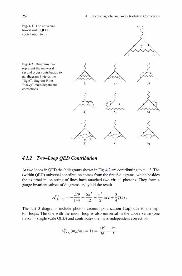
252 4 Electromagnetic and Weak Radiative Corrections

Fig. 4.1 The universallowest order QEDcontribution to a�

γ

γ

��

Fig. 4.2 Diagrams 1–7represent the universalsecond order contribution toa�, diagram 8 yields the“light”, diagram 9 the“heavy” mass dependentcorrections

1) 2) 3)

4) 5) 6)

7) 8) 9)

γ γμ e τμ

γ

4.1.2 Two–Loop QED Contribution

At two loops in QED the 9 diagrams shown in Fig. 4.2 are contributing to g − 2. The(within QED) universal contribution comes from the first 6 diagrams, which besidesthe external muon string of lines have attached two virtual photons. They form agauge invariant subset of diagrams and yield the result

A(4)1 [1−6] = −279

144+ 5π2

12− π2

2ln 2 + 3

4ζ(3) .

The last 3 diagrams include photon vacuum polarization (vap) due to the lep-ton loops. The one with the muon loop is also universal in the above sense (oneflavor = single scale QED) and contributes the mass independent correction

A(4)1 vap(mμ/m� = 1) = 119

36− π2

3.

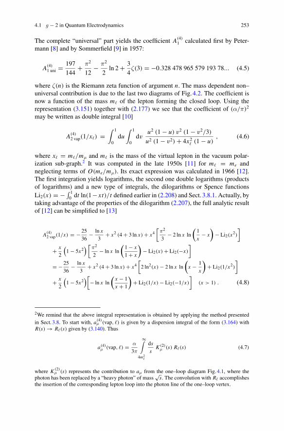
4.1 g − 2 in Quantum Electrodynamics 253

The complete “universal” part yields the coefficient A(4)1 calculated first by Peter-

mann [8] and by Sommerfield [9] in 1957:

A(4)1 uni = 197

144+ π2

12− π2

2ln 2 + 3

4ζ(3) = −0.328 478 965 579 193 78... (4.5)

where ζ(n) is the Riemann zeta function of argument n. The mass dependent non–universal contribution is due to the last two diagrams of Fig. 4.2. The coefficient isnow a function of the mass m� of the lepton forming the closed loop. Using therepresentation (3.151) together with (2.177) we see that the coefficient of (α/π)2

may be written as double integral [10]

A(4)2 vap(1/x�) =

∫ 1

0du∫ 1

0dv

u2 (1 − u) v2 (1 − v2/3)

u2 (1 − v2) + 4x2� (1 − u)

, (4.6)

where x� = m�/mμ and m� is the mass of the virtual lepton in the vacuum polar-ization sub-graph.2 It was computed in the late 1950s [11] for m� = me andneglecting terms of O(me/mμ). Its exact expression was calculated in 1966 [12].The first integration yields logarithms, the second one double logarithms (productsof logarithms) and a new type of integrals, the dilogarithms or Spence functionsLi2(x) = − ∫ 1

0 dt ln(1− xt)/t defined earlier in (2.208) and Sect. 3.8.1. Actually, bytaking advantage of the properties of the dilogarithm (2.207), the full analytic resultof [12] can be simplified to [13]

A(4)2 vap(1/x) = −25

36− ln x

3+ x2 (4 + 3 ln x) + x4

[π2

3− 2 ln x ln

(1

x− x

)− Li2(x2)

]

+ x

2

(1 − 5x2

) [π2

2− ln x ln

(1 − x

1 + x

)− Li2(x) + Li2(−x)

]

= −25

36− ln x

3+ x2 (4 + 3 ln x) + x4

[2 ln2(x) − 2 ln x ln

(x − 1

x

)+ Li2(1/x2)

]

+ x

2

(1 − 5x2

)[− ln x ln

(x − 1

x + 1

)+ Li2(1/x) − Li2(−1/x)

](x > 1) . (4.8)

2We remind that the above integral representation is obtained by applying the method presentedin Sect. 3.8. To start with, a(4)

μ (vap, �) is given by a dispersion integral of the form (3.164) withR(s) → R�(s) given by (3.140). Thus

a(4)μ (vap, �) = α

3π

∞∫

4m2�

ds

sK (2)

μ (s) R�(s) (4.7)

where K (2)μ (s) represents the contribution to aμ from the one–loop diagram Fig. 4.1, where the

photon has been replaced by a “heavy photon” of mass√

s. The convolution with R� accomplishesthe insertion of the corresponding lepton loop into the photon line of the one–loop vertex.

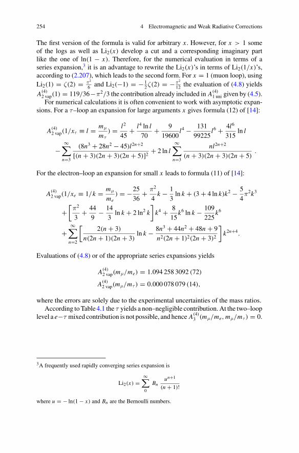
254 4 Electromagnetic and Weak Radiative Corrections

The first version of the formula is valid for arbitrary x . However, for x > 1 someof the logs as well as Li2(x) develop a cut and a corresponding imaginary partlike the one of ln(1 − x). Therefore, for the numerical evaluation in terms of aseries expansion,3 it is an advantage to rewrite the Li2(x)’s in terms of Li2(1/x)’s,according to (2.207), which leads to the second form. For x = 1 (muon loop), usingLi2(1) = ζ(2) = π2

6 and Li2(−1) = − 12ζ(2) = − π2

12 the evaluation of (4.8) yields

A(4)2 vap(1) = 119/36−π2/3 the contribution already included in A(4)

1 uni given by (4.5).For numerical calculations it is often convenient to work with asymptotic expan-

sions. For a τ–loop an expansion for large arguments x gives formula (12) of [14]:

A(4)2 vap(1/xτ ≡ l = mμ

mτ) = l2

45+ l4 ln l

70+ 9

19600l4 − 131

99225l6 + 4l6

315ln l

−∞∑

n=3

(8n3 + 28n2 − 45)l2n+2

[(n + 3)(2n + 3)(2n + 5)]2+ 2 ln l

∞∑

n=3

nl2n+2

(n + 3)(2n + 3)(2n + 5).

For the electron–loop an expansion for small x leads to formula (11) of [14]:

A(4)2 vap(1/xe ≡ 1/k = mμ

me) = −25

36+ π2

4k − 1

3ln k + (3 + 4 ln k)k2 − 5

4π2k3

+[π2

3+ 44

9− 14

3ln k + 2 ln2 k

]k4 + 8

15k6 ln k − 109

225k6

+∞∑

n=2

[2(n + 3)

n(2n + 1)(2n + 3)ln k − 8n3 + 44n2 + 48n + 9

n2(2n + 1)2(2n + 3)2

]k2n+4.

Evaluations of (4.8) or of the appropriate series expansions yields

A(4)2 vap(mμ/me) = 1.094 258 3092 (72)

A(4)2 vap(mμ/mτ ) = 0.000 078 079 (14),

where the errors are solely due to the experimental uncertainties of the mass ratios.According to Table 4.1 the τ yields a non–negligible contribution. At the two–loop

level a e−τ mixed contribution is not possible, and hence A(4)3 (mμ/me, mμ/mτ ) = 0.

3A frequently used rapidly converging series expansion is

Li2(x) =∞∑

0

Bnun+1

(n + 1)!

where u = − ln(1 − x) and Bn are the Bernoulli numbers.

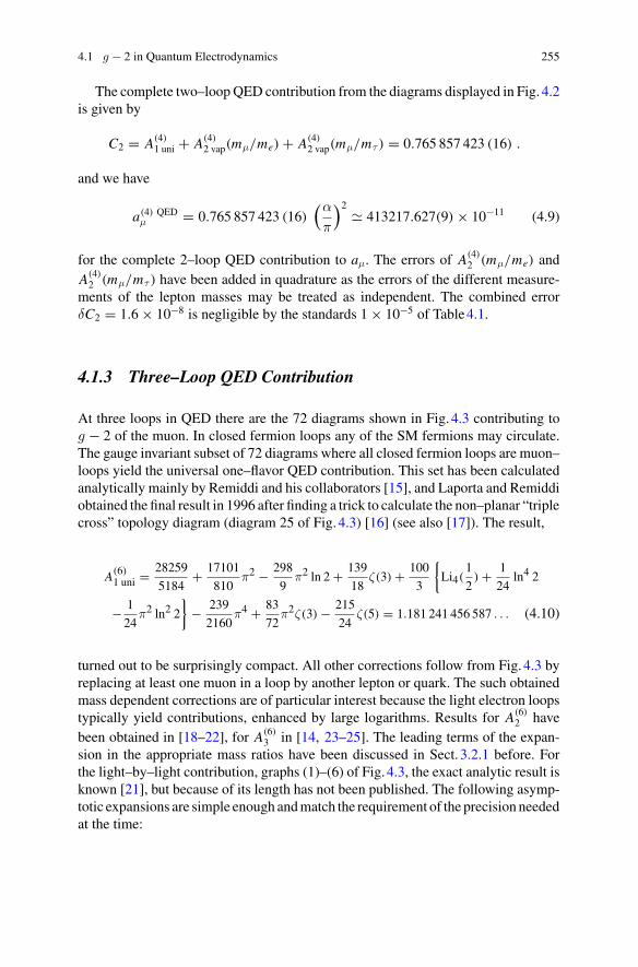
4.1 g − 2 in Quantum Electrodynamics 255

The complete two–loop QED contribution from the diagrams displayed in Fig. 4.2is given by

C2 = A(4)1 uni + A(4)

2 vap(mμ/me) + A(4)2 vap(mμ/mτ ) = 0.765 857 423 (16) .

and we have

a(4) QEDμ = 0.765 857 423 (16)

(α

π

)2 413217.627(9) × 10−11 (4.9)

for the complete 2–loop QED contribution to aμ. The errors of A(4)2 (mμ/me) and

A(4)2 (mμ/mτ ) have been added in quadrature as the errors of the different measure-

ments of the lepton masses may be treated as independent. The combined errorδC2 = 1.6 × 10−8 is negligible by the standards 1 × 10−5 of Table 4.1.

4.1.3 Three–Loop QED Contribution

At three loops in QED there are the 72 diagrams shown in Fig. 4.3 contributing tog − 2 of the muon. In closed fermion loops any of the SM fermions may circulate.The gauge invariant subset of 72 diagrams where all closed fermion loops are muon–loops yield the universal one–flavor QED contribution. This set has been calculatedanalytically mainly by Remiddi and his collaborators [15], and Laporta and Remiddiobtained the final result in 1996 after finding a trick to calculate the non–planar “triplecross” topology diagram (diagram 25 of Fig. 4.3) [16] (see also [17]). The result,

A(6)1 uni = 28259

5184+ 17101

810π2 − 298

9π2 ln 2 + 139

18ζ(3) + 100

3

{Li4(

1

2) + 1

24ln4 2

− 1

24π2 ln2 2

}− 239

2160π4 + 83

72π2ζ(3) − 215

24ζ(5) = 1.181 241 456 587 . . . (4.10)

turned out to be surprisingly compact. All other corrections follow from Fig. 4.3 byreplacing at least one muon in a loop by another lepton or quark. The such obtainedmass dependent corrections are of particular interest because the light electron loopstypically yield contributions, enhanced by large logarithms. Results for A(6)

2 havebeen obtained in [18–22], for A(6)

3 in [14, 23–25]. The leading terms of the expan-sion in the appropriate mass ratios have been discussed in Sect. 3.2.1 before. Forthe light–by–light contribution, graphs (1)–(6) of Fig. 4.3, the exact analytic result isknown [21], but because of its length has not been published. The following asymp-totic expansions are simple enough and match the requirement of the precision neededat the time:

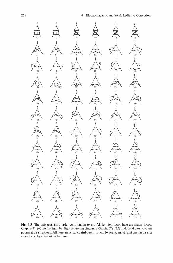
256 4 Electromagnetic and Weak Radiative Corrections

1) 2) 3) 4) 5) 6)

7) 8) 9) 10) 11) 12)

13) 14) 15) 16) 17) 18)

19) 20) 21) 22) 23) 24)

25) 26) 27) 28) 29) 30)

31) 32) 33) 34) 35) 36)

37) 38) 39) 40) 41) 42)

43) 44) 45) 46) 47) 48)

49) 50) 51) 52) 53) 54)

55) 56) 57) 58) 59) 60)

61) 62) 63) 64) 65) 66)

67) 68) 69) 70) 71) 72)

Fig. 4.3 The universal third order contribution to aμ. All fermion loops here are muon–loops.Graphs (1)–(6) are the light–by–light scattering diagrams. Graphs (7)–(22) include photon vacuumpolarization insertions. All non–universal contributions follow by replacing at least one muon in aclosed loop by some other fermion

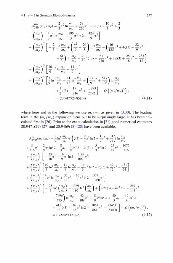
4.1 g − 2 in Quantum Electrodynamics 257

A(6)2 lbl(mμ/me) = 2

3π2 ln

mμ

me+ 59

270π4 − 3ζ(3) − 10

3π2 + 2

3

+(

me

mμ

) [4

3π2 ln

mμ

me− 196

3π2 ln 2 + 424

9π2]

+(

me

mμ

)2 [− 2

3ln3 mμ

me+(

π2

9− 20

3

)

ln2 mμ

me−(

16

135π4 + 4ζ(3) − 32

9π2

+61

3

)ln

mμ

me+ 4

3π2ζ(3) − 61

270π4 + 3 ζ(3) + 25

18π2 − 283

12

]

+(

me

mμ

)3 [10

9π2 ln

mμ

me− 11

9π2]

+(

me

mμ

)4 [7

9ln3 mμ

me+ 41

18ln2 mμ

me+(

13

9π2 + 517

108

)ln

mμ

me

+1

2ζ(3) + 191

216π2 + 13283

2592

]+ O

((me/mμ

)5),

= 20.947 924 85(14) (4.11)

where here and in the following we use me/mμ as given in (3.30). The leadingterm in the (me/mμ) expansion turns out to be surprisingly large. It has been cal-culated first in [26]. Prior to the exact calculation in [21] good numerical estimates20.9471(29) [27] and 20.9469(18) [28] have been available.

A(6)2 vap(mμ/me) = 2

9ln2 mμ

me+(

ζ(3) − 2

3π2 ln 2 + 1

9π2 + 31

27

)ln

mμ

me

+ 11

216π4 − 2

9π2 ln2 2 − 8

3a4 − 1

9ln4 2 − 3ζ(3) + 5

3π2 ln 2 − 25

18π2 + 1075

216

+(

me

mμ

) [− 13

18π3 − 16

9π2 ln 2 + 3199

1080π2]

+(

me

mμ

)2 [10

3ln2 mμ

me− 11

9ln

mμ

me− 14

3π2 ln 2 − 2ζ(3) + 49

12π2 − 131

54

]

+(

me

mμ

)3 [4

3π2 ln

mμ

me+ 35

12π3 − 16

3π2 ln 2 − 5771

1080π2]

+(

me

mμ

)4 [− 25

9ln3(

mμ

me

)− 1369

180ln2(

mμ

me

)+(

−2ζ(3) + 4π2 ln 2 − 269

144π2

−7496

675

)ln

mμ

me− 43

108π4 + 8

9π2 ln2 2 + 80

3a4 + 10

9ln4 2

+ 411

32ζ(3) + 89

48π2 ln 2 − 1061

864π2 − 274511

54000

]+ O

((me/mμ

)5),

= 1.920 455 123(28) (4.12)

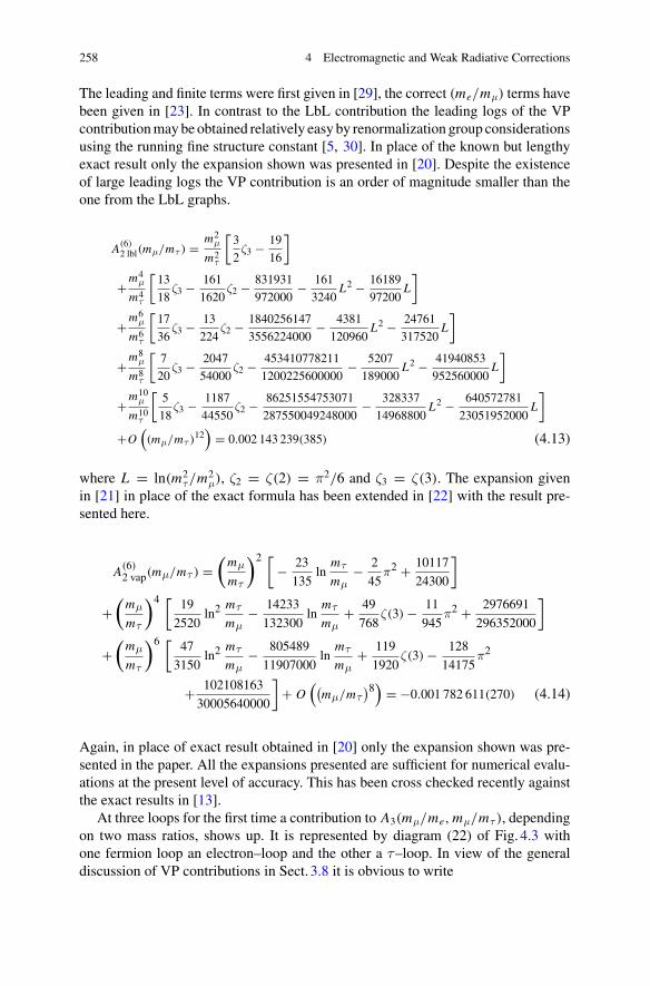
258 4 Electromagnetic and Weak Radiative Corrections

The leading and finite terms were first given in [29], the correct (me/mμ) terms havebeen given in [23]. In contrast to the LbL contribution the leading logs of the VPcontribution may be obtained relatively easy by renormalization group considerationsusing the running fine structure constant [5, 30]. In place of the known but lengthyexact result only the expansion shown was presented in [20]. Despite the existenceof large leading logs the VP contribution is an order of magnitude smaller than theone from the LbL graphs.

A(6)2 lbl(mμ/mτ ) = m2

μ

m2τ

[3

2ζ3 − 19

16

]

+m4μ

m4τ

[13

18ζ3 − 161

1620ζ2 − 831931

972000− 161

3240L2 − 16189

97200L

]

+m6μ

m6τ

[17

36ζ3 − 13

224ζ2 − 1840256147

3556224000− 4381

120960L2 − 24761

317520L

]

+m8μ

m8τ

[7

20ζ3 − 2047

54000ζ2 − 453410778211

1200225600000− 5207

189000L2 − 41940853

952560000L

]

+m10μ

m10τ

[5

18ζ3 − 1187

44550ζ2 − 86251554753071

287550049248000− 328337

14968800L2 − 640572781

23051952000L

]

+O((mμ/mτ )

12)

= 0.002 143 239(385) (4.13)

where L = ln(m2τ/m2

μ), ζ2 = ζ(2) = π2/6 and ζ3 = ζ(3). The expansion givenin [21] in place of the exact formula has been extended in [22] with the result pre-sented here.

A(6)2 vap(mμ/mτ ) =

(mμ

mτ

)2 [− 23

135ln

mτ

mμ− 2

45π2 + 10117

24300

]

+(

mμ

mτ

)4 [ 19

2520ln2 mτ

mμ− 14233

132300ln

mτ

mμ+ 49

768ζ(3) − 11

945π2 + 2976691

296352000

]

+(

mμ

mτ

)6 [ 47

3150ln2 mτ

mμ− 805489

11907000ln

mτ

mμ+ 119

1920ζ(3) − 128

14175π2

+ 102108163

30005640000

]+ O

((mμ/mτ

)8) = −0.001 782 611(270) (4.14)

Again, in place of exact result obtained in [20] only the expansion shown was pre-sented in the paper. All the expansions presented are sufficient for numerical evalu-ations at the present level of accuracy. This has been cross checked recently againstthe exact results in [13].

At three loops for the first time a contribution to A3(mμ/me, mμ/mτ ), dependingon two mass ratios, shows up. It is represented by diagram (22) of Fig. 4.3 withone fermion loop an electron–loop and the other a τ–loop. In view of the generaldiscussion of VP contributions in Sect. 3.8 it is obvious to write

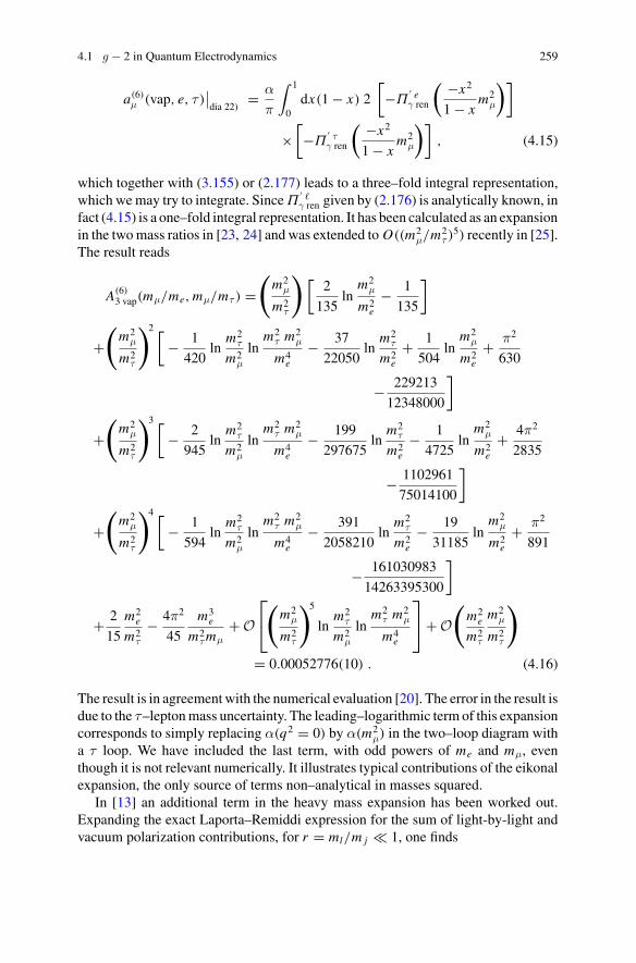
4.1 g − 2 in Quantum Electrodynamics 259

a(6)μ (vap, e, τ )

∣∣dia 22)

= α

π

∫ 1

0dx(1 − x) 2

[−Π

′ eγ ren

( −x2

1 − xm2

μ

)]

×[−Π

′ τγ ren

( −x2

1 − xm2

μ

)], (4.15)

which together with (3.155) or (2.177) leads to a three–fold integral representation,which we may try to integrate. Since Π

′ �γ ren given by (2.176) is analytically known, in

fact (4.15) is a one–fold integral representation. It has been calculated as an expansionin the two mass ratios in [23, 24] and was extended to O((m2

μ/m2τ )

5) recently in [25].The result reads

A(6)3 vap(mμ/me, mμ/mτ ) =

(m2

μ

m2τ

) [2

135ln

m2μ

m2e

− 1

135

]

+(

m2μ

m2τ

)2 [− 1

420ln

m2τ

m2μ

lnm2

τ m2μ

m4e

− 37

22050ln

m2τ

m2e

+ 1

504ln

m2μ

m2e

+ π2

630

− 229213

12348000

]

+(

m2μ

m2τ

)3 [− 2

945ln

m2τ

m2μ

lnm2

τ m2μ

m4e

− 199

297675ln

m2τ

m2e

− 1

4725ln

m2μ

m2e

+ 4π2

2835

− 1102961

75014100

]

+(

m2μ

m2τ

)4 [− 1

594ln

m2τ

m2μ

lnm2

τ m2μ

m4e

− 391

2058210ln

m2τ

m2e

− 19

31185ln

m2μ

m2e

+ π2

891

− 161030983

14263395300

]

+ 2

15

m2e

m2τ

− 4π2

45

m3e

m2τ mμ

+ O⎡

⎣(

m2μ

m2τ

)5

lnm2

τ

m2μ

lnm2

τ m2μ

m4e

⎤

⎦+ O(

m2e

m2τ

m2μ

m2τ

)

= 0.00052776(10) . (4.16)

The result is in agreement with the numerical evaluation [20]. The error in the result isdue to the τ–lepton mass uncertainty. The leading–logarithmic term of this expansioncorresponds to simply replacing α(q2 = 0) by α(m2

μ) in the two–loop diagram witha τ loop. We have included the last term, with odd powers of me and mμ, eventhough it is not relevant numerically. It illustrates typical contributions of the eikonalexpansion, the only source of terms non–analytical in masses squared.

In [13] an additional term in the heavy mass expansion has been worked out.Expanding the exact Laporta–Remiddi expression for the sum of light-by-light andvacuum polarization contributions, for r = ml/m j 1, one finds

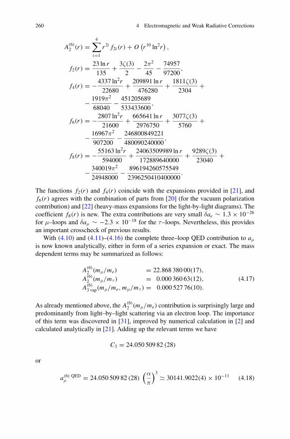
260 4 Electromagnetic and Weak Radiative Corrections

A(6)2 (r) =

4∑

i=1

r2i f2i (r) + O(r10 ln2r

),

f2(r) = 23 ln r

135+ 3ζ(3)

2− 2π2

45− 74957

97200,

f4(r) = −4337 ln2r

22680+ 209891 ln r

476280+ 1811ζ(3)

2304+

− 1919π2

68040− 451205689

533433600,

f6(r) = −2807 ln2r

21600+ 665641 ln r

2976750+ 3077ζ(3)

5760+

− 16967π2

907200− 246800849221

480090240000,

f8(r) = −55163 ln2r

594000+ 24063509989 ln r

172889640000+ 9289ζ(3)

23040+

− 340019π2

24948000− 896194260575549

2396250410400000.

The functions f2(r) and f4(r) coincide with the expansions provided in [21], andf6(r) agrees with the combination of parts from [20] (for the vacuum polarizationcontribution) and [22] (heavy-mass expansions for the light-by-light diagrams). Thecoefficient f8(r) is new. The extra contributions are very small δae ∼ 1.3 × 10−26

for μ–loops and δaμ ∼ −2.3 × 10−18 for the τ–loops. Nevertheless, this providesan important crosscheck of previous results.

With (4.10) and (4.11)–(4.16) the complete three–loop QED contribution to aμ

is now known analytically, either in form of a series expansion or exact. The massdependent terms may be summarized as follows:

A(6)2 (mμ/me) = 22.868 380 00(17),

A(6)2 (mμ/mτ ) = 0.000 360 63(12),

A(6)3 vap(mμ/me, mμ/mτ ) = 0.000 527 76(10).

(4.17)

As already mentioned above, the A(6)2 (mμ/me) contribution is surprisingly large and

predominantly from light–by–light scattering via an electron loop. The importanceof this term was discovered in [31], improved by numerical calculation in [2] andcalculated analytically in [21]. Adding up the relevant terms we have

C3 = 24.050 509 82 (28)

or

a(6) QEDμ = 24.050 509 82 (28)

(α

π

)3 30141.9022(4) × 10−11 (4.18)

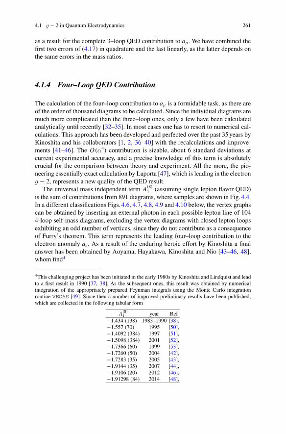
4.1 g − 2 in Quantum Electrodynamics 261

as a result for the complete 3–loop QED contribution to aμ. We have combined thefirst two errors of (4.17) in quadrature and the last linearly, as the latter depends onthe same errors in the mass ratios.

4.1.4 Four–Loop QED Contribution

The calculation of the four–loop contribution to aμ is a formidable task, as there areof the order of thousand diagrams to be calculated. Since the individual diagrams aremuch more complicated than the three–loop ones, only a few have been calculatedanalytically until recently [32–35]. In most cases one has to resort to numerical cal-culations. This approach has been developed and perfected over the past 35 years byKinoshita and his collaborators [1, 2, 36–40] with the recalculations and improve-ments [41–46]. The O(α4) contribution is sizable, about 6 standard deviations atcurrent experimental accuracy, and a precise knowledge of this term is absolutelycrucial for the comparison between theory and experiment. All the more, the pio-neering essentially exact calculation by Laporta [47], which is leading in the electrong − 2, represents a new quality of the QED result.

The universal mass independent term A(8)1 (assuming single lepton flavor QED)

is the sum of contributions from 891 diagrams, where samples are shown in Fig. 4.4.In a different classifications Figs. 4.6, 4.7, 4.8, 4.9 and 4.10 below, the vertex graphscan be obtained by inserting an external photon in each possible lepton line of 1044-loop self-mass diagrams, excluding the vertex diagrams with closed lepton loopsexhibiting an odd number of vertices, since they do not contribute as a consequenceof Furry’s theorem. This term represents the leading four–loop contribution to theelectron anomaly ae. As a result of the enduring heroic effort by Kinoshita a finalanswer has been obtained by Aoyama, Hayakawa, Kinoshita and Nio [43–46, 48],whom find4

4This challenging project has been initiated in the early 1980s by Kinoshita and Lindquist and leadto a first result in 1990 [37, 38]. As the subsequent ones, this result was obtained by numericalintegration of the appropriately prepared Feynman integrals using the Monte Carlo integrationroutine VEGAS [49]. Since then a number of improved preliminary results have been published,which are collected in the following tabular form

A(8)1 year Ref

−1.434 (138) 1983–1990 [38],−1.557 (70) 1995 [50],−1.4092 (384) 1997 [51],−1.5098 (384) 2001 [52],−1.7366 (60) 1999 [53],−1.7260 (50) 2004 [42],−1.7283 (35) 2005 [43],−1.9144 (35) 2007 [44],−1.9106 (20) 2012 [46],−1.91298 (84) 2014 [48],

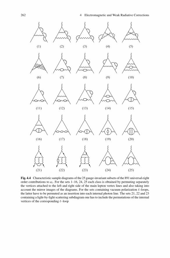
262 4 Electromagnetic and Weak Radiative Corrections

(1) (2) (3) (4) (5)

(6) (7) (8) (9) (10)

(11) (12) (13) (14) (15)

(16) (17) (18) (19) (20)

(21) (22) (23) (24) (25)

Fig. 4.4 Characteristic sample diagrams of the 25 gauge-invariant subsets of the 891 universal eightorder contributions to a�. For the sets 1–16, 24, 25 each class is obtained by permuting separatelythe vertices attached to the left and right side of the main lepton vertex lines and also taking intoaccount the mirror images of the diagrams. For the sets containing vacuum polarization �–loops,the latter have to be permuted as an insertion into each internal photon line. The sets 21, 22 and 23containing a light-by-light scattering subdiagram one has to include the permutations of the internalvertices of the corresponding �–loop

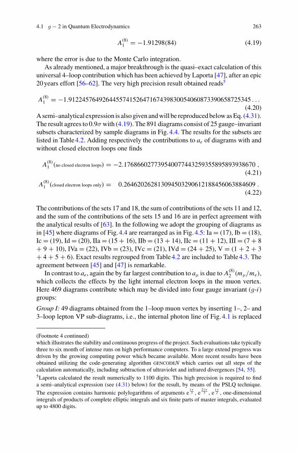
4.1 g − 2 in Quantum Electrodynamics 263

A(8)1 = −1.91298(84) (4.19)

where the error is due to the Monte Carlo integration.As already mentioned, a major breakthrough is the quasi–exact calculation of this

universal 4–loop contribution which has been achieved by Laporta [47], after an epic20 years effort [56–62]. The very high precision result obtained reads5

A(8)1 = −1.912245764926445574152647167439830054060873390658725345 . . .

(4.20)A semi–analytical expression is also given and will be reproduced below as Eq. (4.31).The result agrees to 0.9σ with (4.19). The 891 diagrams consist of 25 gauge–invariantsubsets characterized by sample diagrams in Fig. 4.4. The results for the subsets arelisted in Table 4.2. Adding respectively the contributions to ae of diagrams with andwithout closed electron loops one finds

A(8)1 (no closed electron loops) = −2.176866027739540077443259355895893938670 ,

(4.21)

A(8)1 (closed electron loops only) = 0.264620262813094503290612188456063884609 .

(4.22)

The contributions of the sets 17 and 18, the sum of contributions of the sets 11 and 12,and the sum of the contributions of the sets 15 and 16 are in perfect agreement withthe analytical results of [63]. In the following we adopt the grouping of diagrams asin [45] where diagrams of Fig. 4.4 are rearranged as in Fig. 4.5: Ia = (17), Ib = (18),Ic = (19), Id = (20), IIa = (15 + 16), IIb = (13 + 14), IIc = (11 + 12), III = (7 + 8+ 9 + 10), IVa = (22), IVb = (23), IVc = (21), IVd = (24 + 25), V = (1 + 2 + 3+ 4 + 5 + 6). Exact results regrouped from Table 4.2 are included to Table 4.3. Theagreement between [45] and [47] is remarkable.

In contrast to ae, again the by far largest contribution to aμ is due to A(8)2 (mμ/me),

which collects the effects by the light internal electron loops in the muon vertex.Here 469 diagrams contribute which may be divided into four gauge invariant (g-i)groups:

Group I: 49 diagrams obtained from the 1–loop muon vertex by inserting 1–, 2– and3–loop lepton VP sub-diagrams, i.e., the internal photon line of Fig. 4.1 is replaced

(Footnote 4 continued)which illustrates the stability and continuous progress of the project. Such evaluations take typicallythree to six month of intense runs on high performance computers. To a large extend progress wasdriven by the growing computing power which became available. More recent results have beenobtained utilizing the code-generating algorithm gencodeN which carries out all steps of thecalculation automatically, including subtraction of ultraviolet and infrared divergences [54, 55].5Laporta calculated the result numerically to 1100 digits. This high precision is required to finda semi–analytical expression (see (4.31) below) for the result, by means of the PSLQ technique.

The expression contains harmonic polylogarithms of arguments ei π3 , e

2 i π3 , e

i π2 , one-dimensional

integrals of products of complete elliptic integrals and six finite parts of master integrals, evaluatedup to 4800 digits.

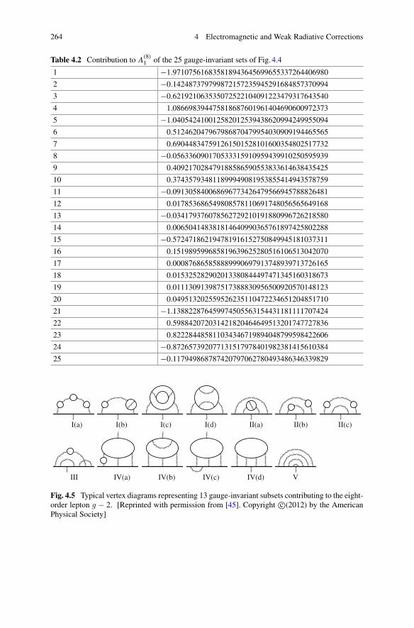
264 4 Electromagnetic and Weak Radiative Corrections

Table 4.2 Contribution to A(8)1 of the 25 gauge-invariant sets of Fig. 4.4

1 −1.971075616835818943645699655337264406980

2 −0.142487379799872157235945291684857370994

3 −0.621921063535072522104091223479317643540

4 1.086698394475818687601961404690600972373

5 −1.040542410012582012539438620994249955094

6 0.512462047967986870479954030909194465565

7 0.690448347591261501528101600354802517732

8 −0.056336090170533315910959439910250595939

9 0.409217028479188586590553833614638435425

10 0.374357934811899949081953855414943578759

11 −0.091305840068696773426479566945788826481

12 0.017853686549808578110691748056565649168

13 −0.034179376078562729210191880996726218580

14 0.006504148381814640990365761897425802288

15 −0.572471862194781916152750849945181037311

16 0.151989599685819639625280516106513042070

17 0.000876865858889990697913748939713726165

18 0.015325282902013380844497471345160318673

19 0.011130913987517388830956500920570148123

20 0.049513202559526235110472234651204851710

21 −1.138822876459974505563154431181111707424

22 0.598842072031421820464649513201747727836

23 0.822284485811034346719894048799598422606

24 −0.872657392077131517978401982381415610384

25 −0.117949868787420797062780493486346339829

I(a) I(b) I(c) I(d) II(a) II(c)II(b)

III IV(a) IV(b) IV(c) IV(d) V

Fig. 4.5 Typical vertex diagrams representing 13 gauge-invariant subsets contributing to the eight-order lepton g − 2. [Reprinted with permission from [45]. Copyright c©(2012) by the AmericanPhysical Society]

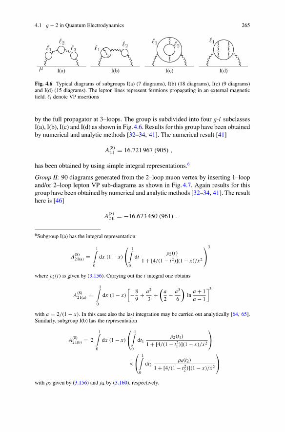
4.1 g − 2 in Quantum Electrodynamics 265

I(a) I(b) I(c) I(d)μ

�1�2

�3 �1�2

�1 �2�1

Fig. 4.6 Typical diagrams of subgroups I(a) (7 diagrams), I(b) (18 diagrams), I(c) (9 diagrams)and I(d) (15 diagrams). The lepton lines represent fermions propagating in an external magneticfield. �i denote VP insertions

by the full propagator at 3–loops. The group is subdivided into four g-i subclassesI(a), I(b), I(c) and I(d) as shown in Fig. 4.6. Results for this group have been obtainedby numerical and analytic methods [32–34, 41]. The numerical result [41]

A(8)2 I = 16.721 967 (905) ,

has been obtained by using simple integral representations.6

Group II: 90 diagrams generated from the 2–loop muon vertex by inserting 1–loopand/or 2–loop lepton VP sub-diagrams as shown in Fig. 4.7. Again results for thisgroup have been obtained by numerical and analytic methods [32–34, 41]. The resulthere is [46]

A(8)2 II = −16.673 450 (961) .

6Subgroup I(a) has the integral representation

A(8)2 I(a) =

1∫

0

dx (1 − x)

⎛

⎝1∫

0

dtρ2(t)

1 + [4/(1 − t2)](1 − x)/x2

⎞

⎠

3

where ρ2(t) is given by (3.156). Carrying out the t integral one obtains

A(8)2 I(a) =

1∫

0

dx (1 − x)

[−8

9+ a2

3+(

a

2− a3

6

)ln

a + 1

a − 1

]3

with a = 2/(1 − x). In this case also the last integration may be carried out analytically [64, 65].Similarly, subgroup I(b) has the representation

A(8)2 I(b) = 2

1∫

0

dx (1 − x)

⎛

⎝1∫

0

dt1ρ2(t1)

1 + [4/(1 − t21 )](1 − x)/x2

⎞

⎠

×⎛

⎝1∫

0

dt2ρ4(t2)

1 + [4/(1 − t22 )](1 − x)/x2

⎞

⎠

with ρ2 given by (3.156) and ρ4 by (3.160), respectively.

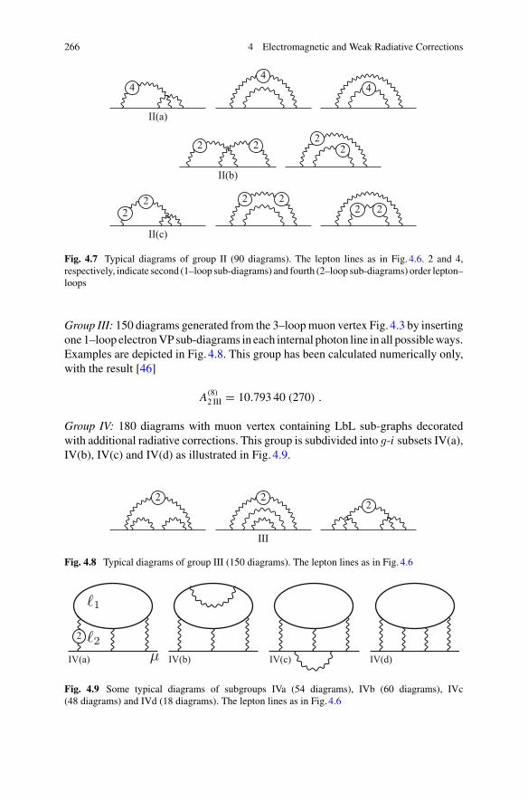
266 4 Electromagnetic and Weak Radiative Corrections

II(a)

44

4

II(b)

2 2 22

II(c)

22 2 2

2 2

Fig. 4.7 Typical diagrams of group II (90 diagrams). The lepton lines as in Fig. 4.6. 2 and 4,respectively, indicate second (1–loop sub-diagrams) and fourth (2–loop sub-diagrams) order lepton–loops

Group III: 150 diagrams generated from the 3–loop muon vertex Fig. 4.3 by insertingone 1–loop electron VP sub-diagrams in each internal photon line in all possible ways.Examples are depicted in Fig. 4.8. This group has been calculated numerically only,with the result [46]

A(8)2 III = 10.793 40 (270) .

Group IV: 180 diagrams with muon vertex containing LbL sub-graphs decoratedwith additional radiative corrections. This group is subdivided into g-i subsets IV(a),IV(b), IV(c) and IV(d) as illustrated in Fig. 4.9.

2

III

22

Fig. 4.8 Typical diagrams of group III (150 diagrams). The lepton lines as in Fig. 4.6

2

IV(a) IV(b) IV(c) IV(d)μ�2

�1

Fig. 4.9 Some typical diagrams of subgroups IVa (54 diagrams), IVb (60 diagrams), IVc(48 diagrams) and IVd (18 diagrams). The lepton lines as in Fig. 4.6

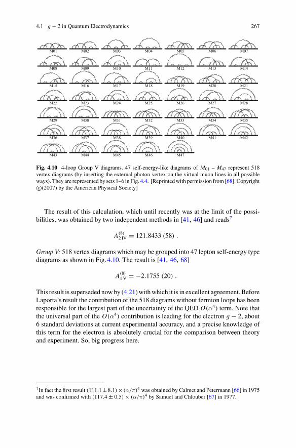
4.1 g − 2 in Quantum Electrodynamics 267

M01 M02 M03 M04 M05 M06 M07

M08 M09 M10 M11 M12 M13 M14

M15 M16 M17 M18 M19 M20 M21

M22 M23 M24 M25 M26 M27 M28

M29 M30 M31 M32 M33 M34 M35

M36 M37 M38 M39 M40 M41 M42

M43 M44 M45 M46 M47

Fig. 4.10 4-loop Group V diagrams. 47 self-energy-like diagrams of M01 – M47 represent 518vertex diagrams (by inserting the external photon vertex on the virtual muon lines in all possibleways). They are represented by sets 1–6 in Fig. 4.4. [Reprinted with permission from [68]. Copyrightc©(2007) by the American Physical Society]

The result of this calculation, which until recently was at the limit of the possi-bilities, was obtained by two independent methods in [41, 46] and reads7

A(8)2 IV = 121.8433 (58) .

Group V: 518 vertex diagrams which may be grouped into 47 lepton self-energy typediagrams as shown in Fig. 4.10. The result is [41, 46, 68]

A(8)1 V = −2.1755 (20) .

This result is superseded now by (4.21) with which it is in excellent agreement. BeforeLaporta’s result the contribution of the 518 diagrams without fermion loops has beenresponsible for the largest part of the uncertainty of the QED O(α4) term. Note thatthe universal part of the O(α4) contribution is leading for the electron g − 2, about6 standard deviations at current experimental accuracy, and a precise knowledge ofthis term for the electron is absolutely crucial for the comparison between theoryand experiment. So, big progress here.

7In fact the first result (111.1 ± 8.1)× (α/π)4 was obtained by Calmet and Petermann [66] in 1975and was confirmed with (117.4 ± 0.5) × (α/π)4 by Samuel and Chlouber [67] in 1977.

268 4 Electromagnetic and Weak Radiative Corrections

Adding up the results from the different groups the new value for A(8)2 (mμ/me)

readsA(8)

2 (mμ/me) = 132.6852(60)[127.50(41)] , (4.23)

in brackets an old value which was presented in [40]. In order to get some impressionabout the techniques and difficulties which have to be mastered we recommend thereader to study more carefully the original work like the recent articles [41, 43, 44].

There is also a small contribution from the term A(8)3 , which depends on 3 masses,

and which arises from 102 diagrams containing two or three closed loops of VPand/or LbL type. The contributions come from the classes I (30 diagrams), II (36diagrams) and IV (36 diagrams) defined above and the results calculated in [41] read

A(8)3 I (mμ/me, mμ/mτ ) = 0.007 627 (0)

A(8)3 II(mμ/me, mμ/mτ ) = −0.028 650 (2)

A(8)3 IV(mμ/me, mμ/mτ ) = 0.083 739 (36)

(4.24)

which sum up to the value

A(8)3 (mμ/me, mμ/mτ ) = 0.06272(4) . (4.25)

Improved estimates for the τ–loops contribution obtained in [46] yield the sub-class results 0.00139(0) [I], −0.01461(1) [II], 0.04504(14) [III] and 0.01052(12)[IV], which sum to

A(8)2 (mμ/mτ ) = 0.04234(12) . (4.26)

In summary: all mass dependent as well as the mass independent O(α4) QED contri-butions to aμ have been recalculated by different methods by Kinoshita’s group [41,43, 44]. There is also substantial progress in analytic calculations [69–75]. Theeighth-order light-by-light QED contributions from leptons with heavier masses havebeen reconsidered based on analytic results which are largely supporting and confirm-ing the recent results [45, 46]. Contributions from specified sub-groups of diagramsshown in Fig. 4.5 are listed in Table 4.3 for the electron, including the universal part,and in Table 4.4 for the muon.

Collecting the A(8) terms for the muon discussed above we obtain

C4 = 130.8734(60)

or

a(8) QEDμ = 130.873 4 (60)

(α

π

)4 380.990(17) × 10−11 (4.27)

as a result for the complete 4–loop QED contribution to aμ.

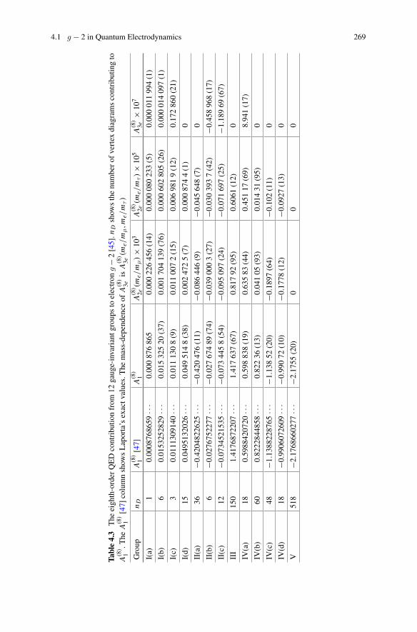
4.1 g − 2 in Quantum Electrodynamics 269

Table4.3

The

eigh

th-o

rder

QE

Dco

ntri

butio

nfr

om12

gaug

e-in

vari

antg

roup

sto

elec

tron

g−

2[4

5].n

Dsh

ows

the

num

ber

ofve

rtex

diag

ram

sco

ntri

butin

gto

A(8

)1

.The

A(8

)1

[47]

colu

mn

show

sL

apor

ta’s

exac

tval

ues.

The

mas

s-de

pend

ence

ofA

(8)

3eis

A(8

)3e

(me/

mμ,m

e/m

τ)

Gro

upn

DA

(8)

1[4

7]A

(8)

1A

(8)

2e(m

e/m

μ)×

103

A(8

)2e

(me/

mτ)×

105

A(8

)3e

×10

7

I(a)

10.

0008

7686

59···

0.00

087

686

50.

000

226

456

(14)

0.00

008

023

3(5

)0.

000

011

994

(1)

I(b)

60.

0153

2528

29···

0.01

532

520

(37)

0.00

170

413

9(7

6)0.

000

602

805

(26)

0.00

001

409

7(1

)

I(c)

30.

0111

3091

40···

0.01

113

08

(9)

0.01

100

72

(15)

0.00

698

19

(12)

0.17

286

0(2

1)

I(d)

150.

0495

1320

26···

0.04

951

48

(38)

0.00

247

25

(7)

0.00

087

44

(1)

0

II(a

)36

−0.4

2048

2262

5···

−0.4

2047

6(1

1)−0

.086

446

(9)

−0.0

4564

8(7

)0

II(b

)6

−0.0

2767

5227

7···

−0.0

2767

489

(74)

−0.0

3900

03

(27)

−0.0

3039

37

(42)

−0.4

5896

8(1

7)

II(c

)12

−0.0

7345

2153

5···

−0.0

7344

58

(54)

−0.0

9509

7(2

4)−0

.071

697

(25)

−1.1

8969

(67)

III

150

1.41

7687

2207

···1.

417

637

(67)

0.81

792

(95)

0.60

61(1

2)0

IV(a

)18

0.59

8842

0720

···0.

598

838

(19)

0.63

583

(44)

0.45

117

(69)

8.94

1(1

7)

IV(b

)60

0.82

2284

4858

···0.

822

36(1

3)0.

041

05(9

3)0.

014

31(9

5)0

IV(c

)48

−1.1

3882

2876

5···

−1.1

3852

(20)

−0.1

897

(64)

−0.1

02(1

1)0

IV(d

)18

−0.9

9060

7260

9···

−0.9

9072

(10)

−0.1

778

(12)

−0.0

927

(13)

0

V51

8−2

.176

8660

277

···−2

.175

5(2

0)0

00

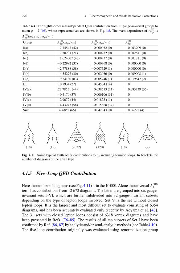
270 4 Electromagnetic and Weak Radiative Corrections

Table 4.4 The eighth-order mass-dependent QED contribution from 11 gauge-invariant groups tomuon g − 2 [46], whose representatives are shown in Fig. 4.5. The mass-dependence of A(8)

3μ is

A(8)3μ (mμ/me, mμ/mτ )

Group A(8)2μ (mμ/me) A(8)

2μ (mμ/mτ ) A(8)3μ

I(a) 7.74547 (42) 0.000032 (0) 0.003209 (0)

I(b) 7.58201 (71) 0.000252 (0) 0.002611 (0)

I(c) 1.624307 (40) 0.000737 (0) 0.001811 (0)

I(d) −0.22982 (37) 0.000368 (0) 0.000000 (0)

II(a) −2.77888 (38) −0.007329 (1) 0.000000 (0)

II(b) −4.55277 (30) −0.002036 (0) −0.009008 (1)

II(c) −9.34180 (83) −0.005246 (1) −0.019642 (2)

III 10.7934 (27) 0.04504 (14) 0

IV(a) 123.78551 (44) 0.038513 (11) 0.083739 (36)

IV(b) −0.4170 (37) 0.006106 (31) 0

IV(c) 2.9072 (44) −0.01823 (11) 0

IV(d) −4.43243 (58) −0.015868 (37) 0

Sum 132.6852 (65) 0.04234 (10) 0.06272 (4)

(18) (18) (2072) (120) (18) (2)

Fig. 4.11 Some typical tenth order contributions to a� including fermion loops. In brackets thenumber of diagrams of the given type

4.1.5 Five–Loop QED Contribution

Here the number of diagrams (see Fig. 4.11) is in the 10 000. Alone the universal A(10)1

term has contributions from 12 672 diagrams. The latter are grouped into six gauge-invariant sets I–VI, which are further subdivided into 32 gauge-invariant subsetsdepending on the type of lepton loops involved. Set V is the set without closedlepton loops. It is the largest and most difficult set to evaluate consisting of 6354diagrams, and has been accurately evaluated only recently by Aoyama et al. [48].The 31 sets with closed lepton loops consist of 6318 vertex diagrams and havebeen presented in Refs. [76–85]. The results of all ten subsets of Set I have beenconfirmed by Ref. [86, 87] by analytic and/or semi-analytic methods (see Table 4.10).The five-loop contribution originally was evaluated using renormalization group

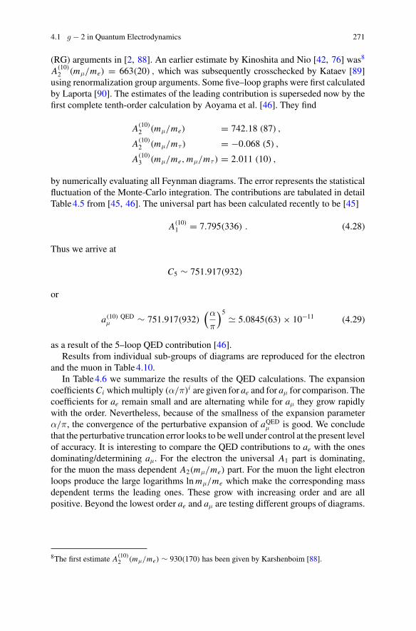
4.1 g − 2 in Quantum Electrodynamics 271

(RG) arguments in [2, 88]. An earlier estimate by Kinoshita and Nio [42, 76] was8

A(10)2 (mμ/me) = 663(20) , which was subsequently crosschecked by Kataev [89]

using renormalization group arguments. Some five–loop graphs were first calculatedby Laporta [90]. The estimates of the leading contribution is superseded now by thefirst complete tenth-order calculation by Aoyama et al. [46]. They find

A(10)2 (mμ/me) = 742.18 (87) ,

A(10)2 (mμ/mτ ) = −0.068 (5) ,

A(10)3 (mμ/me, mμ/mτ ) = 2.011 (10) ,

by numerically evaluating all Feynman diagrams. The error represents the statisticalfluctuation of the Monte-Carlo integration. The contributions are tabulated in detailTable 4.5 from [45, 46]. The universal part has been calculated recently to be [45]

A(10)1 = 7.795(336) . (4.28)

Thus we arrive at

C5 ∼ 751.917(932)

or

a(10) QEDμ ∼ 751.917(932)

(α

π

)5 5.0845(63) × 10−11 (4.29)

as a result of the 5–loop QED contribution [46].Results from individual sub-groups of diagrams are reproduced for the electron

and the muon in Table 4.10.In Table 4.6 we summarize the results of the QED calculations. The expansion

coefficients Ci which multiply (α/π)i are given for ae and for aμ for comparison. Thecoefficients for ae remain small and are alternating while for aμ they grow rapidlywith the order. Nevertheless, because of the smallness of the expansion parameterα/π, the convergence of the perturbative expansion of aQED

μ is good. We concludethat the perturbative truncation error looks to be well under control at the present levelof accuracy. It is interesting to compare the QED contributions to ae with the onesdominating/determining aμ. For the electron the universal A1 part is dominating,for the muon the mass dependent A2(mμ/me) part. For the muon the light electronloops produce the large logarithms ln mμ/me which make the corresponding massdependent terms the leading ones. These grow with increasing order and are allpositive. Beyond the lowest order ae and aμ are testing different groups of diagrams.

8The first estimate A(10)2 (mμ/me) ∼ 930(170) has been given by Karshenboim [88].

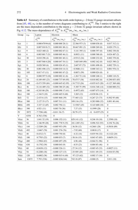
272 4 Electromagnetic and Weak Radiative Corrections

Table 4.5 Summary of contributions to the tenth-order lepton g−2 from 32 gauge-invariant subsetsfrom [45, 48]. nF is the number of vertex diagrams contributing to A(10)

1 . The 3 entries to the rightare the mass-dependent contribution to the muon g − 2 from 32 gauge-invariant subsets shown inFig. 4.12. The mass-dependence of A(10)

3μ is A(10)3μ (mμ/me, mμ/mτ )

Group nD Lepton Electron Muon

A(10)1 A(10)

2e (me/mμ) A(10)2μ (mμ/me) A(10)

2μ (mμ/mτ ) A(10)3μ

I(a) 1 0.000 470 94 (6) 0.000 000 28 (1) 22.566 973 (3) 0.000 038 (0) 0.017 312 (1)

I(b) 9 0.007 010 8 (7) 0.000 001 88 (1) 30.667 091 (3) 0.000 269 (0) 0.020 179 (1)

I(c) 9 0.023 468 (2) 0.000 002 67 (1) 5.141 395 (1) 0.000 397 (0) 0.002 330 (0)

I(d) 6 0.003 801 7 (5) 0.000 005 46 (1) 8.8921 (11) 0.000 388 (0) 0.024 487 (2)

I(e) 30 0.010 296 (4) 0.000 001 60 (1) −0.9312 (24) 0.000 232 (0) 0.002 370 (0)

I(f) 3 0.007 568 4 (20) 0.000 047 54 (1) 3.685 049 (90) 0.002 162 (0) 0.023 390 (2)

I(g) 9 0.028 569 (6) 0.000 024 45 (1) 2.607 87 (72) 0.001 698 (0) 0.002 729 (1)

I(h) 30 0.001 696 (13) −0.000 010 14 (3) −0.5686 (11) 0.000 163 (1) 0.001 976 (3)

I(i) 105 0.017 47 (11) 0.000 001 67 (2) 0.0871 (59) 0.000 024 (0) 0

I(j) 6 0.000 397 5 (18) 0.000 002 41 (6) −1.263 72 (14) 0.000 168 (1) 0.000 110 (5)

II(a) 24 −0.109 495 (23) −0.000 737 69 (95) −70.4717 (38) −0.018 882 (8) −0.290 853 (85)

II(b) 108 −0.473 559 (84) −0.000 645 62 (95) −34.7715 (26) −0.035 615 (20) −0.127 369 (60)

II(c) 36 −0.116 489 (32) −0.000 380 25 (46) −5.385 75 (99) −0.016 348 (14) −0.040 800 (51)

II(d) 180 −0.243 00 (29) −0.000 098 17 (41) 0.4972 (65) −0.007 673 (14) 0

II(e) 180 −1.344 9 (10) −0.000 465 0 (40) 3.265 (12) −0.038 06 (13) 0

II(f) 72 −2.433 6 (15) −0.005 868 (39) −77.465 (12) −0.267 23 (73) −0.502 95 (68)

III(a) 300 2.127 33 (17) 0.007 511 (11) 109.116 (33) 0.283 000 (32) 0.891 40 (44)

III(b) 450 3.327 12 (45) 0.002 794 (1) 11.9367 (45) 0.143 600 (10) 0

III(c) 390 4.921 (11) 0.003 70 (36) 7.37 (15) 0.1999 (28) 0

IV 2072 −7.7296 (48) −0.011 36 (7) −38.79 (17) −0. 0.4357 (25) 0

V 6354 8.762 (336) 0 0

VI(a) 36 1.041 32 (19) 0.006 152 (11) 629.141 (12) 0.246 10 (18) 2.3590 (18)

VI(b) 54 1.346 99 (28) 0.001 778 9 (35) 181.1285 (51) 0.096 522 (93) 0.194 76 (26)

VI(c) 144 −2.5289 (28) −0.005 953 (59) −36.58 (12) −0.2601 (28) −0.5018 (89)

VI(d) 492 1.8467 (70) 0.001 276 (76) −7.92 (60) 0.0818 (17) 0

VI(e) 48 −0.4312 (7) −0.000 750 (8) −4.32 (14) −0.035 94 (32) −0.1122 (24)

VI(f) 180 0.7703 (22) 0.000 033 (7) −38.16 (15) 0.043 47 (85) 0.0659 (31)

VI(g) 480 −1.5904 (63) −0.000 497 (29) 6.96 (48) −0.044 51 (96) 0

VI(h) 630 0.1792 (39) 0.000 045 (9) −8.55 (23) 0.004 85 (46) 0

VI(i) 60 −0.0438 (12) −0.000 326 (1) −27.34 (12) −0.003 45 (33) −0.0027 (11)

VI(j) 54 −0.2288 (18) −0.000 127 (13) −25.505 (20) −0.011 49 (33) −0.016 03 (58)

VI(k) 120 0.6802 (38) 0.000 015 6 (40) 97.123 (62) 0.002 17 (16) 0

Sum 12672 7.793 (336) −0.003 824(144) 742.18 (87) −0.068 (5) 2.011 (10)

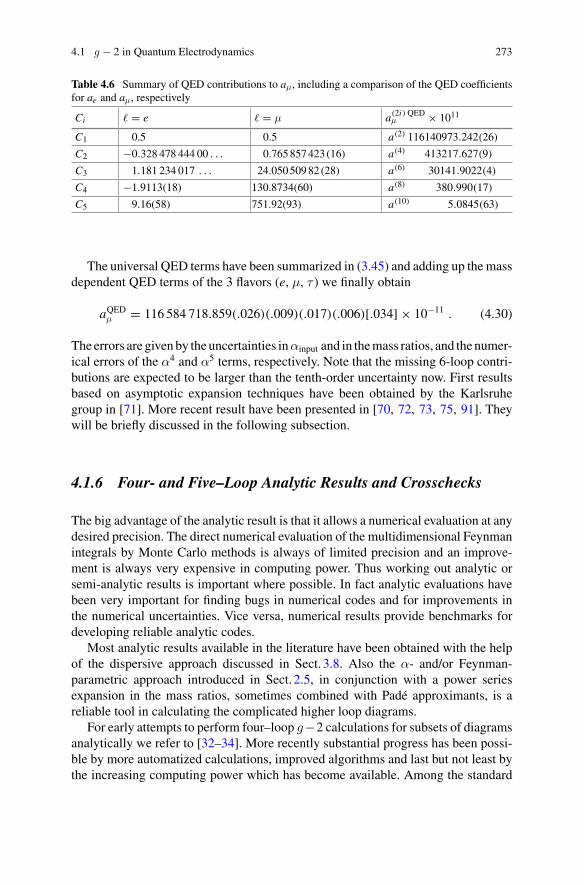
4.1 g − 2 in Quantum Electrodynamics 273

Table 4.6 Summary of QED contributions to aμ, including a comparison of the QED coefficientsfor ae and aμ, respectively

Ci � = e � = μ a(2i) QEDμ × 1011

C1 0.5 0.5 a(2) 116140973.242(26)

C2 −0.328 478 444 00 . . . 0.765 857 423 (16) a(4) 413217.627(9)

C3 1.181 234 017 . . . 24.050 509 82 (28) a(6) 30141.9022(4)

C4 −1.9113(18) 130.8734(60) a(8) 380.990(17)

C5 9.16(58) 751.92(93) a(10) 5.0845(63)

The universal QED terms have been summarized in (3.45) and adding up the massdependent QED terms of the 3 flavors (e, μ, τ ) we finally obtain

aQEDμ = 116 584 718.859(.026)(.009)(.017)(.006)[.034] × 10−11 . (4.30)

The errors are given by the uncertainties inαinput and in the mass ratios, and the numer-ical errors of the α4 and α5 terms, respectively. Note that the missing 6-loop contri-butions are expected to be larger than the tenth-order uncertainty now. First resultsbased on asymptotic expansion techniques have been obtained by the Karlsruhegroup in [71]. More recent result have been presented in [70, 72, 73, 75, 91]. Theywill be briefly discussed in the following subsection.

4.1.6 Four- and Five–Loop Analytic Results and Crosschecks

The big advantage of the analytic result is that it allows a numerical evaluation at anydesired precision. The direct numerical evaluation of the multidimensional Feynmanintegrals by Monte Carlo methods is always of limited precision and an improve-ment is always very expensive in computing power. Thus working out analytic orsemi-analytic results is important where possible. In fact analytic evaluations havebeen very important for finding bugs in numerical codes and for improvements inthe numerical uncertainties. Vice versa, numerical results provide benchmarks fordeveloping reliable analytic codes.

Most analytic results available in the literature have been obtained with the helpof the dispersive approach discussed in Sect. 3.8. Also the α- and/or Feynman-parametric approach introduced in Sect. 2.5, in conjunction with a power seriesexpansion in the mass ratios, sometimes combined with Padé approximants, is areliable tool in calculating the complicated higher loop diagrams.

For early attempts to perform four–loop g−2 calculations for subsets of diagramsanalytically we refer to [32–34]. More recently substantial progress has been possi-ble by more automatized calculations, improved algorithms and last but not least bythe increasing computing power which has become available. Among the standard

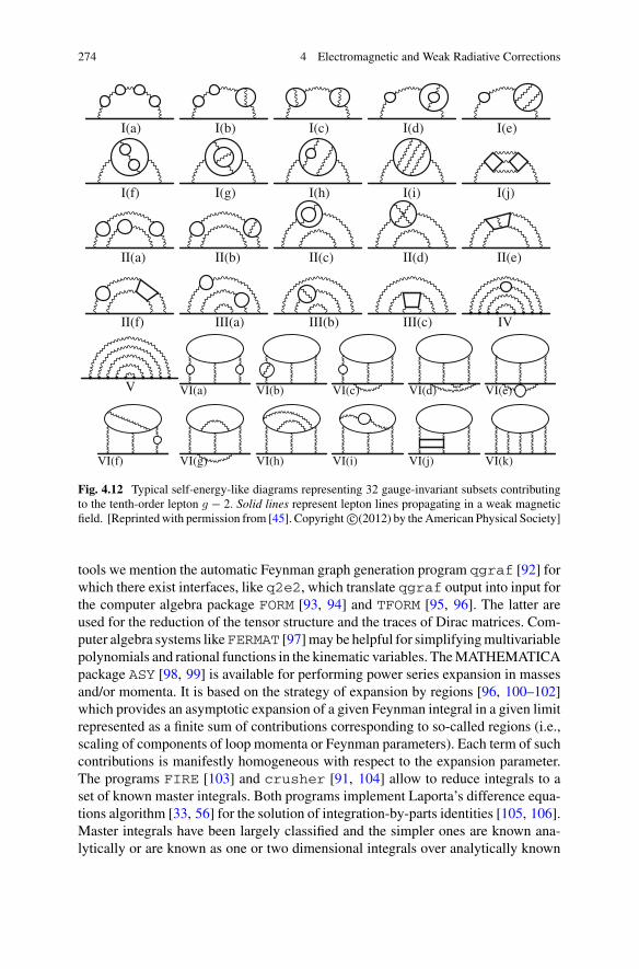
274 4 Electromagnetic and Weak Radiative Corrections

I(a) I(b) I(c) I(d) I(e)

I(f) I(g) I(h) I(i) I(j)

II(a) II(b) II(c) II(d) II(e)

II(f) III(a) III(b) III(c) IV

V VI(a) VI(b) VI(c) VI(d) VI(e)

VI(f) VI(g) VI(h) VI(i) VI(j) VI(k)

Fig. 4.12 Typical self-energy-like diagrams representing 32 gauge-invariant subsets contributingto the tenth-order lepton g − 2. Solid lines represent lepton lines propagating in a weak magneticfield. [Reprinted with permission from [45]. Copyright c©(2012) by the American Physical Society]

tools we mention the automatic Feynman graph generation program qgraf [92] forwhich there exist interfaces, like q2e2, which translate qgraf output into input forthe computer algebra package FORM [93, 94] and TFORM [95, 96]. The latter areused for the reduction of the tensor structure and the traces of Dirac matrices. Com-puter algebra systems likeFERMAT [97] may be helpful for simplifying multivariablepolynomials and rational functions in the kinematic variables. The MATHEMATICApackage ASY [98, 99] is available for performing power series expansion in massesand/or momenta. It is based on the strategy of expansion by regions [96, 100–102]which provides an asymptotic expansion of a given Feynman integral in a given limitrepresented as a finite sum of contributions corresponding to so-called regions (i.e.,scaling of components of loop momenta or Feynman parameters). Each term of suchcontributions is manifestly homogeneous with respect to the expansion parameter.The programs FIRE [103] and crusher [91, 104] allow to reduce integrals to aset of known master integrals. Both programs implement Laporta’s difference equa-tions algorithm [33, 56] for the solution of integration-by-parts identities [105, 106].Master integrals have been largely classified and the simpler ones are known ana-lytically or are known as one or two dimensional integrals over analytically known

4.1 g − 2 in Quantum Electrodynamics 275

functions. The more complicated ones may be evaluated using Mellin–Barnes tech-niques [107, 108], which has been implemented in the MATHEMATICA programMB [109]. Also the ε = 4 − d expansion, ε → +0 introduced in Sect. 2.5 has beenimplemented in a computer code. The ε expansion of the remaining master integralsmay be computed numerically with the help of FIESTA [110]. In many cases thePSLQ approach [111], an integer relation finding algorithm, allows one to find exactanalytic results form very high precision numerical ones, as one in general knowswhat type of transcendental elements (πn , ζ(n), log’s, polylogs etc.) could show upin the results.

In the following we review the status of the four- and five-loop results at the levelof a numerical comparison. The analytic results, often available as a series expansion,typically are lengthy and will not be reproduced here. We refer the interested readerto the original literature, where also the technical details of the calculations may befound.

Four-Loop Analytic Results and Crosschecks

We remind that loop calculations require regularization and renormalization. Apply-ing dimensional regularization always requires the appropriate ε–expansion, beforetaking the limit ε → 0. In higher–loop calculations this by itself is a formidabletask and a mater of efficient computer algebra codes. Most remarkably the 4–loopuniversal contribution A8

1 (4.20) can be considered to be known analytically aftertwo decennials of efforts by Laporta [47]. The contributions from all 891 diagramsare expressed algebraically by means of 334 master integrals (it corresponds to thegeneralization of the reduction of the tensor integral in terms of scalar integrals (socalled master integrals) disentangled form the particle spin complications, which weoutlined in Sect. 2.5.7) belonging to 220 topologies. The method used for the compu-tation of the master integrals with a precision up to 9600 digits is largely based on thedifference equation method [56, 57] and the differential equation method [112–114].Thereby large systems of difference and differential equations are solved numericallyon high performance computers. Most master integrals are related the polylogarith-mic and harmonic polylogarithmic integrals which have been well investigated in theliterature. The most complicated master integrals are of elliptical type (see Fig. 4.13).One obtains a family of one–dimensional integrals of products of elliptic integrals(itself defined by one–dimensional integrals see Sect. 3.8.1). Laporta then has fittedthe analytical expressions to high precision numerical values of all master integralsand diagram contributions using the PSLQ algorithm.9

9Let me explain this in case of the universal 3–loop result (4.10). Suppose you have a very highprecision numerical value for A(6)

1 uni on the l.h.s. and you know which transcendental objects fromthe list (3.185) could show up (knowing the types of master integrals and the transcendentals whichare associated with them) one can find the rational coefficients on the r.h.s. of (4.10) by fitting ther.h.s. to the value on the l.h.s. Since one can multiply the equation with the common divisor ofthe rational coefficients the general problem requires to find integers ai , not all zero, which fit anequation of the form a1x1 + a2x2 +· · ·+ an xn = 0 where (x1, x2, · · · , xn) is a given vector of realor complex numbers (from a basis of transcendentals). Often this method is the only known way tofind a closed analytic expression of an integral.

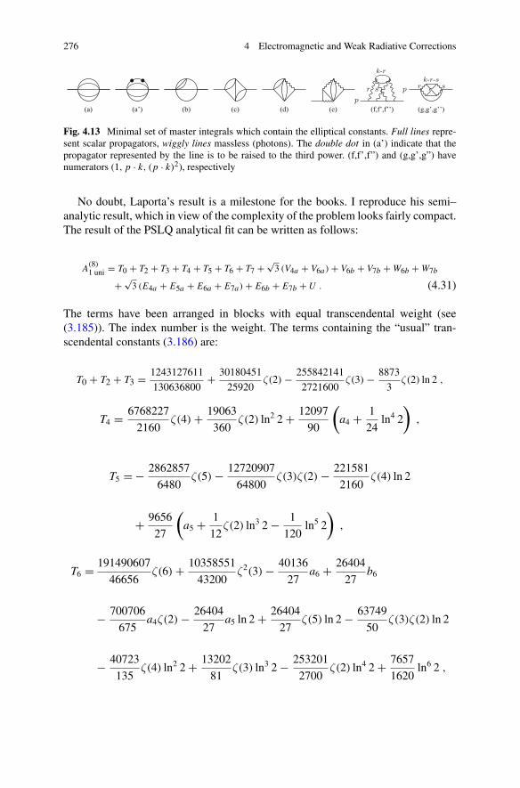
276 4 Electromagnetic and Weak Radiative Corrections

(a) (a’) (b) (c) (d) (e) (f,f’,f’’) (g,g’,g’’)p

sr

k-r

p r sk-r-s

Fig. 4.13 Minimal set of master integrals which contain the elliptical constants. Full lines repre-sent scalar propagators, wiggly lines massless (photons). The double dot in (a’) indicate that thepropagator represented by the line is to be raised to the third power. (f,f’,f”) and (g,g’,g”) havenumerators (1, p · k, (p · k)2), respectively

No doubt, Laporta’s result is a milestone for the books. I reproduce his semi–analytic result, which in view of the complexity of the problem looks fairly compact.The result of the PSLQ analytical fit can be written as follows:

A(8)1 uni = T0 + T2 + T3 + T4 + T5 + T6 + T7 + √

3 (V4a + V6a) + V6b + V7b + W6b + W7b

+ √3 (E4a + E5a + E6a + E7a) + E6b + E7b + U . (4.31)

The terms have been arranged in blocks with equal transcendental weight (see(3.185)). The index number is the weight. The terms containing the “usual” tran-scendental constants (3.186) are:

T0 + T2 + T3 = 1243127611

130636800+ 30180451

25920ζ(2) − 255842141

2721600ζ(3) − 8873

3ζ(2) ln 2 ,

T4 = 6768227

2160ζ(4) + 19063

360ζ(2) ln2 2 + 12097

90

(a4 + 1

24ln4 2

),

T5 = − 2862857

6480ζ(5) − 12720907

64800ζ(3)ζ(2) − 221581

2160ζ(4) ln 2

+ 9656

27

(a5 + 1

12ζ(2) ln3 2 − 1

120ln5 2

),

T6 = 191490607

46656ζ(6) + 10358551

43200ζ2(3) − 40136

27a6 + 26404

27b6

− 700706

675a4ζ(2) − 26404

27a5 ln 2 + 26404

27ζ(5) ln 2 − 63749

50ζ(3)ζ(2) ln 2

− 40723

135ζ(4) ln2 2 + 13202

81ζ(3) ln3 2 − 253201

2700ζ(2) ln4 2 + 7657

1620ln6 2 ,

4.1 g − 2 in Quantum Electrodynamics 277

T7 = 2895304273

435456ζ(7) + 670276309

193536ζ(4)ζ(3) + 85933

63a4ζ(3) + 7121162687

967680ζ(5)ζ(2)

− 142793

18a5ζ(2) − 195848

21a7 + 195848

63b7 − 116506

189d7

− 4136495

384ζ(6) ln 2 − 1053568

189a6 ln 2 + 233012

189b6 ln 2 + 407771

432ζ2(3) ln 2

− 8937

2a4ζ(2) ln 2 + 833683

3024ζ(5) ln2 2 − 3995099

6048ζ(3)ζ(2) ln2 2 − 233012

189a5 ln2 2

+ 1705273

1512ζ(4) ln3 2 + 602303

4536ζ(3) ln4 2 − 1650461

11340ζ(2) ln5 2 + 52177

15876ln7 2 .

The terms containing harmonic polylogarithms of eiπ3 , e

2iπ3 :

V4a = −14101

480Cl4

(π

3

)− 169703

1440ζ(2)Cl2

(π

3

),

V6a = 494

27Im H0,0,0,1,−1,−1

(ei π

3

)+ 494

27Im H0,0,0,1,−1,1

(ei 2π

3

)

+ 494

27Im H0,0,0,1,1,−1

(ei 2π

3

)

+ 19Im H0,0,1,0,1,1

(ei 2π

3

)+ 437

12Im H0,0,0,1,1,1

(ei 2π

3

)+ 29812

297Cl6(π

3

)

+ 4940

81a4Cl2

(π

3

)− 520847

69984ζ(5)π − 129251

81ζ(4)Cl2

(π

3

)

− 892

15Im H0,1,1,−1

(ei 2π

3

)ζ(2) − 1784

45Im H0,1,1,−1

(ei π

3

)ζ(2)

+ 1729

54ζ(3)Im H0,1,−1

(ei π

3

)

+ 1729

36ζ(3)Im H0,1,1

(ei 2π

3

)+ 837190

729Cl4(π

3

)ζ(2) + 25937

4860ζ(3)ζ(2)π

− 223

243ζ(4)π ln 2 + 892

9Im H0,1,−1

(ei π

3

)ζ(2) ln 2 + 446

3Im H0,1,1

(ei 2π

3

)ζ(2) ln 2

− 7925

81Cl2(π

3

)ζ(2) ln2 2 + 1235

486Cl2(π

3

)ln4 2 ,

278 4 Electromagnetic and Weak Radiative Corrections

V6b = 13487

60Re H0,0,0,1,0,1

(ei π

3

)+ 13487

60Cl4

(π

3

)Cl2

(π

3

)+ 136781

360Cl22

(π

3

)ζ(2) ,

V7b = 651

4Re H0,0,0,1,0,1,−1

(ei π

3)+ 651Re H0,0,0,0,1,1,−1

(ei π

3)

− 17577

32Re H0,0,1,0,0,1,1

(ei 2π

3

)

− 87885

64Re H0,0,0,1,0,1,1

(ei 2π

3

)− 17577

8Re H0,0,0,0,1,1,1

(ei 2π

3

)

+ 651

4Cl4

(π

3

)Im H0,1,−1

(ei π

3)

+ 1953

8Cl4

(π

3

)Im H0,1,1

(ei 2π

3

)+ 31465

176Cl6

(π

3

)π

+ 211

4Re H0,1,0,1,−1

(ei π

3)ζ(2)

+ 211

2Re H0,0,1,1,−1

(ei π

3)ζ(2) + 1899

16Re H0,1,0,1,1

(ei 2π

3

)ζ(2)

+ 1899

8Re H0,0,1,1,1

(ei 2π

3

)ζ(2)

+ 211

4Im H0,1,−1

(ei π

3)

Cl2

(π

3

)ζ(2) + 633

8Im H0,1,1

(ei 2π

3

)Cl2

(π

3

)ζ(2) .

The terms containing harmonic polylogarithms of eiπ2 :

W6b = − 28276

25ζ(2)Cl2

(π

2

)2,

W7b= 104

(4Re H0,1,0,1,1

(ei π

2

)ζ(2) + 4Im H0,1,1

(ei π

2

)Cl2

(π

2

)ζ(2) − 2Cl4

(π

2

)ζ(2)π

+ Cl22

(π

2

)ζ(2) ln 2

).

The terms containing elliptic constants:

E4a = π

(−28458503

691200B3 + 250077961

18662400C3

),

4.1 g − 2 in Quantum Electrodynamics 279

E5a = 483913

77760π f2(0, 0, 1) ,

E6a = π

(4715

1944ln 2 f2(0, 0, 1) + 270433

10935f2(0, 2, 0) − 188147

4860f2(0, 1, 1)

+ 188147

12960f2(0, 0, 2)

),

E6b = −4715

1458ζ(2) f1(0, 0, 1) ,

E7a = π

(826595

248832ζ(2) f2(0, 0, 1) − 5525

432ln 2 f2(0, 0, 2) + 5525

162ln 2 f2(0, 1, 1)

− 5525

243ln 2 f2(0, 2, 0) + 526015

248832f2(0, 0, 3) − 4675

768f2(0, 1, 2)

+ 1805965

248832f2(0, 2, 1)

− 3710675

1119744f2(0, 3, 0) − 75145

124416f2(1, 0, 2) − 213635

124416f2(1, 1, 1)

+ 168455

62208f2(1, 2, 0)

+ 75145

248832f2(2, 0, 1) + 69245

124416f2(2, 1, 0)

),

E7b = ζ(2)

(2541575

82944f1(0, 0, 2) − 556445

6912f1(0, 1, 1) + 54515

972f1(0, 2, 0)

−75145

20736f1(1, 0, 1)

).

The term containing the ε0 coefficients of the ε−expansion of six master integrals(see f, f ′, f ′′, g, g′, g′′ of Fig. 4.13):

U = −541

300C81a − 629

60C81b + 49

3C81c − 327

160C83a + 49

36C83b + 37

6C83c .

The numerical values of entries in (4.31) may be found in Table 3 of [47]. In theabove expressions ζ(n) = ∑∞

i=1 i−n , an = ∑∞i=1 2−i i−n , b6 = H0,0,0,0,1,1

(12

),

280 4 Electromagnetic and Weak Radiative Corrections

b7 = H0,0,0,0,0,1,1(

12

), d7 = H0,0,0,0,1,−1,−1(1), Cln (θ) = ImLin(eiθ). Hi1,i2,...(x) are

the harmonic polylogarithms. The integrals f j are defined as follows:

f1(i, j, k) =∫ 9

1ds D2

1(s)

(s − 9

5

)lni (9 − s) ln j (s − 1) lnk (s) ,

f2(i, j, k) =∫ 9

1ds D1(s)Re

(√3D2(s)

)(s − 9

5

)lni (9 − s) ln j (s − 1) lnk (s) ,

D1(s) = 2√

(√

s + 3)(√

s − 1)3K

((√

s − 3)(√

s + 1)3

(√

s + 3)(√

s − 1)3

),

D2(s) = 2√

(√

s + 3)(√

s − 1)3K

(1 − (

√s − 3)(

√s + 1)3

(√

s + 3)(√

s − 1)3

);

K (x) is the complete elliptic integral of the first kind. Note that D1(s) = 2J (1,9)2 (s),

with J (1,9)2 defined in Eq. (A.12) of Ref. [115]. The integrals f1(0, 0, 0) and f2(0, 0, 0)

were studied in Ref. [61]. The constants A3, B3 and C3, defined in Ref. [61], admitthe hypergeometric representations10:

A3 =∫ 1

0dx

Kc(x)Kc(1-x)√1 − x

= 2π32

3

(Γ 2( 7

6 )Γ ( 13 )

Γ 2( 23 )Γ ( 5

6 )4 F3

(16

13

13

12

56

56

23

; 1

)− Γ 2( 5

6 )Γ (− 13 )

Γ 2( 13 )Γ ( 1

6 )4 F3

(12

23

23

56

76

76

43

; 1

))

,

B3 =∫ 1

0dx

K 2c (x)√1 − x

= 4π32

3

(Γ 2( 7

6 )Γ ( 13 )

Γ 2( 23 )Γ ( 5

6 )4 F3

(16

13

13

12

56

56

23

; 1

)+ Γ 2( 5

6 )Γ (− 13 )

Γ 2( 13 )Γ ( 1

6 )4 F3

(12

23

23

56

76

76

43

; 1

))

,

C3 =∫ 1

0dx

E2c (x)√1 − x

= 486π2

19257 F6

(74 − 1

313

23

43

32

32

34 1 7

6116

136

176

; 1

),

Kc(x) = 2π√27

2 F1

(13

23

1; x)

, Ec(x) = 2π√27

2 F1

(13 − 1

31

; x)

.

10For relations between Gauss hypergeometric functions and Feynman diagrams see e.g. [116] andreferences therein.

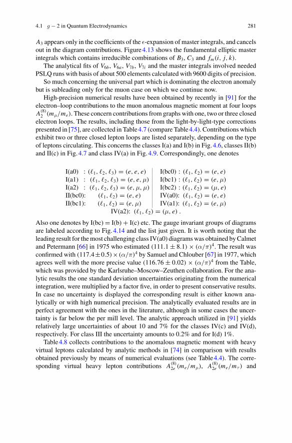
4.1 g − 2 in Quantum Electrodynamics 281

A3 appears only in the coefficients of the ε-expansion of master integrals, and cancelsout in the diagram contributions. Figure 4.13 shows the fundamental elliptic masterintegrals which contains irreducible combinations of B3, C3 and fm(i, j, k).

The analytical fits of V6b, V6a , V7b, V7i and the master integrals involved neededPSLQ runs with basis of about 500 elements calculated with 9600 digits of precision.

So much concerning the universal part which is dominating the electron anomalybut is subleading only for the muon case on which we continue now.

High-precision numerical results have been obtained by recently in [91] for theelectron–loop contributions to the muon anomalous magnetic moment at four loopsA(8)

2 (mμ/me). These concern contributions from graphs with one, two or three closedelectron loops. The results, including those from the light-by-light-type correctionspresented in [75], are collected in Table 4.7 (compare Table 4.4). Contributions whichexhibit two or three closed lepton loops are listed separately, depending on the typeof leptons circulating. This concerns the classes I(a) and I(b) in Fig. 4.6, classes II(b)and II(c) in Fig. 4.7 and class IV(a) in Fig. 4.9. Correspondingly, one denotes

I(a0) : (�1, �2, �3) = (e, e, e) I(bc0) : (�1, �2) = (e, e)I(a1) : (�1, �2, �3) = (e, e,μ) I(bc1) : (�1, �2) = (e,μ)

I(a2) : (�1, �2, �3) = (e,μ,μ) I(bc2) : (�1, �2) = (μ, e)II(bc0): (�1, �2) = (e, e) IV(a0): (�1, �2) = (e, e)II(bc1): (�1, �2) = (e,μ) IV(a1): (�1, �2) = (e,μ)

IV(a2): (�1, �2) = (μ, e) .

Also one denotes by I(bc) = I(b) + I(c) etc. The gauge invariant groups of diagramsare labeled according to Fig. 4.14 and the list just given. It is worth noting that theleading result for the most challenging class IV(a0) diagrams was obtained by Calmetand Petermann [66] in 1975 who estimated (111.1 ± 8.1) × (α/π)4. The result wasconfirmed with (117.4±0.5)× (α/π)4 by Samuel and Chlouber [67] in 1977, whichagrees well with the more precise value (116.76 ± 0.02) × (α/π)4 from the Table,which was provided by the Karlsruhe–Moscow–Zeuthen collaboration. For the ana-lytic results the one standard deviation uncertainties originating from the numericalintegration, were multiplied by a factor five, in order to present conservative results.In case no uncertainty is displayed the corresponding result is either known ana-lytically or with high numerical precision. The analytically evaluated results are inperfect agreement with the ones in the literature, although in some cases the uncer-tainty is far below the per mill level. The analytic approach utilized in [91] yieldsrelatively large uncertainties of about 10 and 7% for the classes IV(c) and IV(d),respectively. For class III the uncertainty amounts to 0.2% and for I(d) 1%.

Table 4.8 collects contributions to the anomalous magnetic moment with heavyvirtual leptons calculated by analytic methods in [74] in comparison with resultsobtained previously by means of numerical evaluations (see Table 4.4). The corre-sponding virtual heavy lepton contributions A(8)

2e (me/mμ), A(8)2e (me/mτ ) and

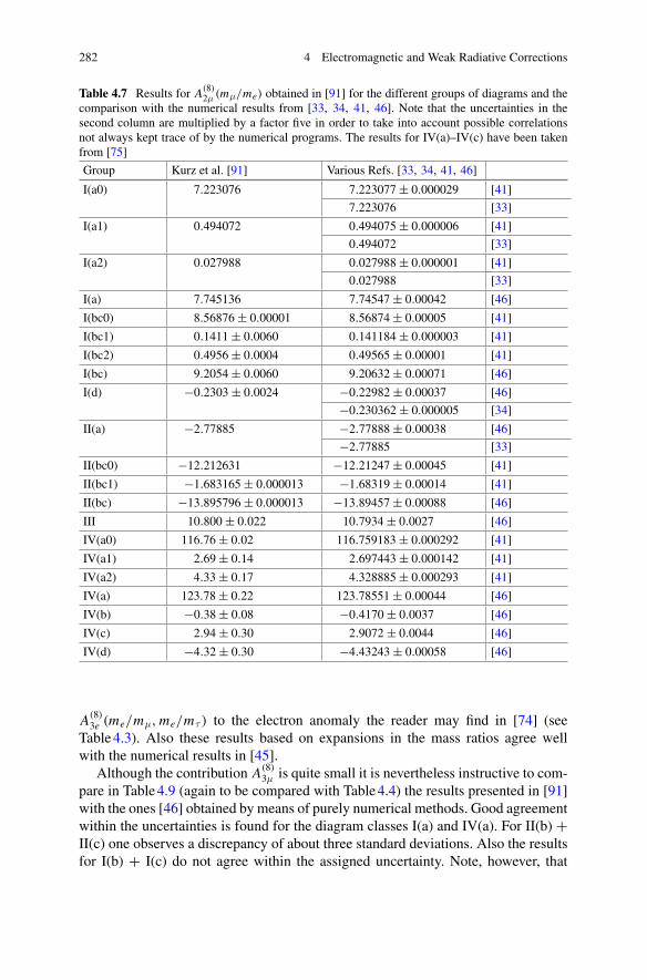
282 4 Electromagnetic and Weak Radiative Corrections

Table 4.7 Results for A(8)2μ (mμ/me) obtained in [91] for the different groups of diagrams and the

comparison with the numerical results from [33, 34, 41, 46]. Note that the uncertainties in thesecond column are multiplied by a factor five in order to take into account possible correlationsnot always kept trace of by the numerical programs. The results for IV(a)–IV(c) have been takenfrom [75]

Group Kurz et al. [91] Various Refs. [33, 34, 41, 46]

I(a0) 7.223076 7.223077 ± 0.000029 [41]

7.223076 [33]

I(a1) 0.494072 0.494075 ± 0.000006 [41]

0.494072 [33]

I(a2) 0.027988 0.027988 ± 0.000001 [41]

0.027988 [33]

I(a) 7.745136 7.74547 ± 0.00042 [46]

I(bc0) 8.56876 ± 0.00001 8.56874 ± 0.00005 [41]

I(bc1) 0.1411 ± 0.0060 0.141184 ± 0.000003 [41]

I(bc2) 0.4956 ± 0.0004 0.49565 ± 0.00001 [41]

I(bc) 9.2054 ± 0.0060 9.20632 ± 0.00071 [46]

I(d) −0.2303 ± 0.0024 −0.22982 ± 0.00037 [46]

−0.230362 ± 0.000005 [34]

II(a) −2.77885 −2.77888 ± 0.00038 [46]

−2.77885 [33]

II(bc0) −12.212631 −12.21247 ± 0.00045 [41]

II(bc1) −1.683165 ± 0.000013 −1.68319 ± 0.00014 [41]

II(bc) −13.895796 ± 0.000013 −13.89457 ± 0.00088 [46]

III 10.800 ± 0.022 10.7934 ± 0.0027 [46]

IV(a0) 116.76 ± 0.02 116.759183 ± 0.000292 [41]

IV(a1) 2.69 ± 0.14 2.697443 ± 0.000142 [41]

IV(a2) 4.33 ± 0.17 4.328885 ± 0.000293 [41]

IV(a) 123.78 ± 0.22 123.78551 ± 0.00044 [46]

IV(b) −0.38 ± 0.08 −0.4170 ± 0.0037 [46]

IV(c) 2.94 ± 0.30 2.9072 ± 0.0044 [46]

IV(d) −4.32 ± 0.30 −4.43243 ± 0.00058 [46]

A(8)3e (me/mμ, me/mτ ) to the electron anomaly the reader may find in [74] (see

Table 4.3). Also these results based on expansions in the mass ratios agree wellwith the numerical results in [45].

Although the contribution A(8)3μ is quite small it is nevertheless instructive to com-

pare in Table 4.9 (again to be compared with Table 4.4) the results presented in [91]with the ones [46] obtained by means of purely numerical methods. Good agreementwithin the uncertainties is found for the diagram classes I(a) and IV(a). For II(b) +II(c) one observes a discrepancy of about three standard deviations. Also the resultsfor I(b) + I(c) do not agree within the assigned uncertainty. Note, however, that

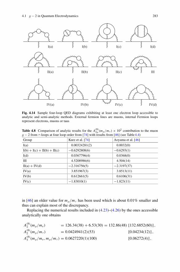
4.1 g − 2 in Quantum Electrodynamics 283

I(a) I(b) I(c) I(d)

II(a) II(b) II(c) III

IV(a) IV(b) IV(c) IV(d)

Fig. 4.14 Sample four-loop QED diagrams exhibiting at least one electron loop accessible toanalytic and semi-analytic methods. External fermion lines are muons, internal Fermion loopsrepresent electrons, muons or taus

Table 4.8 Comparison of analytic results for the A(8)2μ (mμ/mτ ) × 102 contribution to the muon

g − 2 from τ -loops at four loop order from [74] with results from [46] (see Table 4.4)

Group Kurz et al. [74] Aoyama et al. [46]

I(a) 0.00324281(2) 0.0032(0)

I(b) + I(c) + II(b) + II(c) −0.6292808(6) −0.6293(1)

I(d) 0.0367796(4) 0.0368(0)

III 4.5208986(6) 4.504(14)

II(a) + IV(d) −2.316756(5) −2.3197(37)

IV(a) 3.851967(3) 3.8513(11)

IV(b) 0.612661(5) 0.6106(31)

IV(c) −1.83010(1) −1.823(11)

in [46] an older value for mμ/mτ has been used which is about 0.01% smaller andthus can explain most of the discrepancy.

Replacing the numerical results included in (4.23)–(4.26) by the ones accessibleanalytically one obtains

A(8)2 (mμ/me) = 126.34(38) + 6.53(30) = 132.86(48) [132.6852(60)] ,

A(8)2 (mμ/mτ ) = 0.0424941(2)(53) [0.04234(12)] ,

A(8)3 (mμ/me, mμ/mτ ) = 0.0627220(1)(100) [0.06272(4)] ,

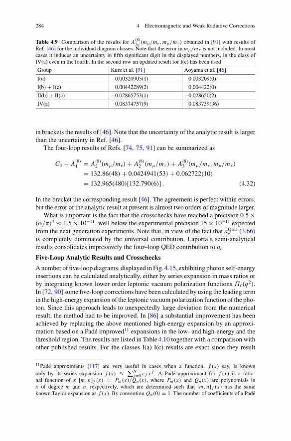
284 4 Electromagnetic and Weak Radiative Corrections

Table 4.9 Comparison of the results for A(8)3μ (mμ/me, mμ/mτ ) obtained in [91] with results of

Ref. [46] for the individual diagram classes. Note that the error in mμ/mτ is not included. In mostcases it induces an uncertainty in fifth significant digit in the displayed numbers, in the class ofIV(a) even in the fourth. In the second row an updated result for I(c) has been used

Group Kurz et al. [91] Aoyama et al. [46]

I(a) 0.00320905(1) 0.003209(0)

I(b) + I(c) 0.00442289(2) 0.004422(0)

II(b) + II(c) −0.02865753(1) −0.028650(2)

IV(a) 0.08374757(9) 0.083739(36)

in brackets the results of [46]. Note that the uncertainty of the analytic result is largerthan the uncertainty in Ref. [46].

The four-loop results of Refs. [74, 75, 91] can be summarized as

C4 − A(8)1 = A(8)

2 (mμ/me) + A(8)2 (mμ/mτ ) + A(8)

3 (mμ/me, mμ/mτ )

= 132.86(48) + 0.0424941(53) + 0.062722(10)

= 132.965(480)[132.790(6)] . (4.32)

In the bracket the corresponding result [46]. The agreement is perfect within errors,but the error of the analytic result at present is almost two orders of magnitude larger.

What is important is the fact that the crosschecks have reached a precision 0.5 ×(α/π)4 ≈ 1.5 × 10−11, well below the experimental precision 15 × 10−11 expectedfrom the next generation experiments. Note that, in view of the fact that aQED

e (3.66)is completely dominated by the universal contribution, Laporta’s semi-analyticalresults consolidates impressively the four–loop QED contribution to ae

Five-Loop Analytic Results and Crosschecks

A number of five-loop diagrams, displayed in Fig. 4.15, exhibiting photon self-energyinsertions can be calculated analytically, either by series expansion in mass ratios orby integrating known lower order leptonic vacuum polarization functions Π�(q2).In [72, 90] some five-loop corrections have been calculated by using the leading termin the high-energy expansion of the leptonic vacuum polarization function of the pho-ton. Since this approach leads to unexpectedly large deviation from the numericalresult, the method had to be improved. In [86] a substantial improvement has beenachieved by replacing the above mentioned high-energy expansion by an approxi-mation based on a Padé improved11 expansions in the low- and high-energy and thethreshold region. The results are listed in Table 4.10 together with a comparison withother published results. For the classes I(a) I(c) results are exact since they result

11Padé approximants [117] are very useful in cases when a function, f (x) say, is knownonly by its series expansion f (x) ≈ ∑N

j=0 c j x j . A Padé approximant for f (x) is a ratio-nal function of x [m, n] f (x) = Pm(x)/Qn(x), where Pm(x) and Qn(x) are polynomials inx of degree m and n, respectively, which are determined such that [m, n] f (x) has the sameknown Taylor expansion as f (x). By convention Qn(0) = 1. The number of coefficients of a Padé

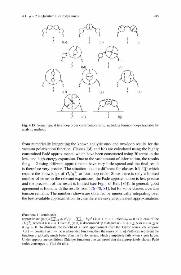
4.1 g − 2 in Quantum Electrodynamics 285

I(a) I(b) I(c)

I(d) I(e)

I(f) I(g) I(h)

I(i) I(j)

Fig. 4.15 Some typical five loop order contributions to a� including fermion loops tractable byanalytic methods

from numerically integrating the known analytic one- and two-loop results for thevacuum polarization function. Classes I(d) and I(e) are calculated using the highlyconstrained Padé approximants, which have been constructed using 30 terms in thelow- and high-energy expansion. Due to the vast amount of information, the resultsfor g − 2 using different approximants have very little spread and the final resultis therefore very precise. The situation is quite different for classes I(f)–I(j) whichrequire the knowledge of Π�(q2) at four-loop order. Since there is only a limitednumber of terms in the relevant expansions, the Padé approximation is less preciseand the precision of the result is limited (see Fig. 1 of Ref. [86]). In general, goodagreement is found with the results from [76–78, 81], but for some classes a certaintension remains. The numbers shown are obtained by numerically integrating overthe best available approximation. In case there are several equivalent approximations

(Footnote 11 continued)approximant [m,n]=

∑mk=0 ak xk/(1 +∑n

k=1 bk xk) is n + m + 1 unless a0 = 0 as in case of theΠ(q2), where it is n +m. Given N , [m,n] is determined up to degree n +m +1 ≤ N or n +m ≤ Nif a0 = 0. To illustrate the benefit of a Padé approximant over the Taylor series lets supposef (x) ∼ constant as x → ∞ is a bounded function, then the series of [n, n] Padés can represent thefunction f globally much better than the Taylor series, which completely fails when x gets larger.Under appropriate conditions (Stieltjes function) one can proof that the appropriately chosen Padéseries converges to f (x) for all x .

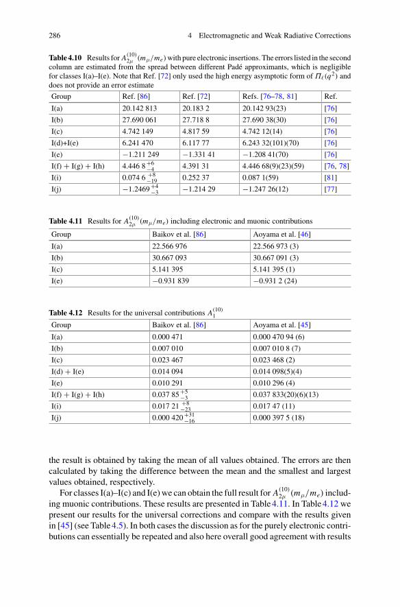
286 4 Electromagnetic and Weak Radiative Corrections

Table 4.10 Results for A(10)2μ (mμ/me) with pure electronic insertions. The errors listed in the second

column are estimated from the spread between different Padé approximants, which is negligiblefor classes I(a)–I(e). Note that Ref. [72] only used the high energy asymptotic form of Π�(q2) anddoes not provide an error estimate

Group Ref. [86] Ref. [72] Refs. [76–78, 81] Ref.

I(a) 20.142 813 20.183 2 20.142 93(23) [76]

I(b) 27.690 061 27.718 8 27.690 38(30) [76]

I(c) 4.742 149 4.817 59 4.742 12(14) [76]

I(d)+I(e) 6.241 470 6.117 77 6.243 32(101)(70) [76]

I(e) −1.211 249 −1.331 41 −1.208 41(70) [76]

I(f) + I(g) + I(h) 4.446 8 +6−4 4.391 31 4.446 68(9)(23)(59) [76, 78]

I(i) 0.074 6 +8−19 0.252 37 0.087 1(59) [81]

I(j) −1.2469 +4−3 −1.214 29 −1.247 26(12) [77]

Table 4.11 Results for A(10)2μ (mμ/me) including electronic and muonic contributions

Group Baikov et al. [86] Aoyama et al. [46]

I(a) 22.566 976 22.566 973 (3)

I(b) 30.667 093 30.667 091 (3)

I(c) 5.141 395 5.141 395 (1)

I(e) −0.931 839 −0.931 2 (24)

Table 4.12 Results for the universal contributions A(10)1

Group Baikov et al. [86] Aoyama et al. [45]

I(a) 0.000 471 0.000 470 94 (6)

I(b) 0.007 010 0.007 010 8 (7)

I(c) 0.023 467 0.023 468 (2)

I(d) + I(e) 0.014 094 0.014 098(5)(4)

I(e) 0.010 291 0.010 296 (4)

I(f) + I(g) + I(h) 0.037 85 +5−3 0.037 833(20)(6)(13)

I(i) 0.017 21 +8−23 0.017 47 (11)

I(j) 0.000 420 +31−16 0.000 397 5 (18)

the result is obtained by taking the mean of all values obtained. The errors are thencalculated by taking the difference between the mean and the smallest and largestvalues obtained, respectively.

For classes I(a)–I(c) and I(e) we can obtain the full result for A(10)2μ (mμ/me) includ-

ing muonic contributions. These results are presented in Table 4.11. In Table 4.12 wepresent our results for the universal corrections and compare with the results givenin [45] (see Table 4.5). In both cases the discussion as for the purely electronic contri-butions can essentially be repeated and also here overall good agreement with results

4.1 g − 2 in Quantum Electrodynamics 287

available in the literature is observed. Nevertheless it should be noted that for singlediagram classes a certain tension remains.

So far five–loop contributions to the muon g − 2 could be calculated by analyticmeans for diagrams from class I which are including known photon vacuum polariza-tion insertions. Results largely confirm the previous numerical results by Kinoshita’sgroup. While corresponding four–loop results cover a large fraction of the completecontribution, at five loops the calculations are rather partial yet.

4.2 Weak Contributions

The weak interaction contribution to g − 2 attracted attention of theoreticians longtime before it started to play a relevant role in the comparison with the experimentalresult. Actually the “weak contribution sensitivity” was reached only with the recentBNL experiment. With the emergence of the SM [118] and establishing its renormal-izability [119] for the first time it was possible to make real predictions for aμ beyondQED. Before, in non–renormalizable low energy effective theories, correspondingattempts were not convincing, since, as we discussed earlier only in a renormalizabletheory aμ is a finite unambiguously predictable quantity and hence an unambiguousmonitor for testing the theory. Soon after a unified electroweak theory seemed estab-lished a number of groups presented the one–loop result for aμ in 1972 [120]. At thattime, the weak term turned out to be almost two orders of magnitude smaller thenthe experimental accuracy of the CERN g − 2 experiment. At present the weak termis an effect of almost three standard deviations.

Weak interaction effects are mediated by exchange of the heavy weak gaugebosons W ±, which mediate charged current (CC) processes, and Z , which medi-ates the neutral current (NC) processes. Beyond the electroweak SU(2)L ⊗ U (1)Y

Yang-Mills gauge theory, a Higgs sector is required which allows to generate themasses of the gauge bosons W and Z , as well as the masses of the fermions,without spoiling renormalizability.12 Thereby the gauge symmetry is broken downSU(2)L ⊗ U (1)Y → U (1)em to the Abelian subgroup of QED, and an additionalphysical particle has to be taken into account, the famous Higgs particle, predictedby Brout, Englert and Higgs in 1964 [121], discovered 48 years later by the ATLASand CMS Collaborations [122–124] at the Large Hadron Collider (LHC) at CERN.

12In different terms: renormalizability of a massive non-Abelian gauge theory requires the existenceof a scalar boson, which interacts with all massive particles with a coupling proportional to the massof the particle to which it couples. The corresponding Higgs boson exchange contributions preciselycancel the non-renormalizable terms (exhibiting bad high energy behavior) which one would obtainin S–matrix elements in absence of the Higgs. The pattern of the 15 required SM Higgs bosoncouplings, which directly manifests in its decay pattern is actually what identifies the scalar bosonas the Higgs boson.

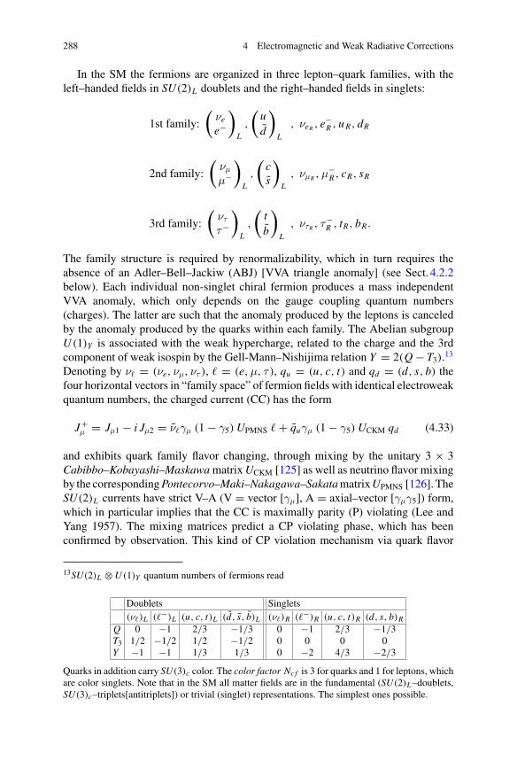
288 4 Electromagnetic and Weak Radiative Corrections

In the SM the fermions are organized in three lepton–quark families, with theleft–handed fields in SU(2)L doublets and the right–handed fields in singlets:

1st family:

(νe

e−

)

L

,

(ud

)

L

, νeR , e−R , u R, dR

2nd family:

(νμ

μ−

)

L

,

(cs

)

L

, νμR ,μ−R , cR, sR

3rd family:

(ντ

τ−

)

L

,

(tb

)

L

, ντR , τ−R , tR, bR .

The family structure is required by renormalizability, which in turn requires theabsence of an Adler–Bell–Jackiw (ABJ) [VVA triangle anomaly] (see Sect. 4.2.2below). Each individual non-singlet chiral fermion produces a mass independentVVA anomaly, which only depends on the gauge coupling quantum numbers(charges). The latter are such that the anomaly produced by the leptons is canceledby the anomaly produced by the quarks within each family. The Abelian subgroupU (1)Y is associated with the weak hypercharge, related to the charge and the 3rdcomponent of weak isospin by the Gell-Mann–Nishijima relation Y = 2(Q − T3).13

Denoting by ν� = (νe, νμ, ντ ), � = (e,μ, τ ), qu = (u, c, t) and qd = (d, s, b) thefour horizontal vectors in “family space” of fermion fields with identical electroweakquantum numbers, the charged current (CC) has the form

J+μ = Jμ1 − i Jμ2 = ν�γμ (1 − γ5) UPMNS � + quγμ (1 − γ5) UCKM qd (4.33)

and exhibits quark family flavor changing, through mixing by the unitary 3 × 3Cabibbo–Kobayashi–Maskawa matrix UCKM [125] as well as neutrino flavor mixingby the corresponding Pontecorvo–Maki–Nakagawa–Sakata matrix UPMNS [126]. TheSU(2)L currents have strict V–A (V = vector [γμ], A = axial–vector [γμγ5]) form,which in particular implies that the CC is maximally parity (P) violating (Lee andYang 1957). The mixing matrices predict a CP violating phase, which has beenconfirmed by observation. This kind of CP violation mechanism via quark flavor

13SU(2)L ⊗ U (1)Y quantum numbers of fermions read

Doublets Singlets(ν�)L (�−)L (u, c, t)L (d, s, b)L (ν�)R (�−)R (u, c, t)R (d, s, b)R

Q 0 −1 2/3 −1/3 0 −1 2/3 −1/3T3 1/2 −1/2 1/2 −1/2 0 0 0 0Y −1 −1 1/3 1/3 0 −2 4/3 −2/3

Quarks in addition carry SU(3)c color. The color factor Ncf is 3 for quarks and 1 for leptons, whichare color singlets. Note that in the SM all matter fields are in the fundamental (SU(2)L –doublets,SU(3)c–triplets[antitriplets]) or trivial (singlet) representations. The simplest ones possible.

4.2 Weak Contributions 289

mixing requires a minimum of three fermion families. Indeed what we see to berealized in nature. CP violation also implies the existence of a very tiny electricaldipole moment (EDM). In a local QFT a non–vanishing EDM is possible only if CPis violated, as we noted earlier. For the magnetic moments CP has no special impactand the CP violating effects are too small to play any role. For our purpose the 3 × 3family mixing matrices may be taken to be unit matrices. The neutral current (NC)is strictly flavor conserving

J Zμ = Jμ3 − 2 sin2 ΘW j em

μ =∑

f

ψ f γμ(v f − a f γ5)ψ f (4.34)

with

j emμ =

∑

f

Q f ψ f γμψ f (4.35)

the P conserving electromagnetic current.14 The weak mixing parameter sin2 ΘW

is responsible for the γ − Z mixing. The sums extend over the individual fermionflavors f (and color). In our convention the NC vector and axial–vector neutralcurrent coefficients are given by

v f = T3 f − 2Q f sin2 ΘW , a f = T3 f (4.36)

where T3 f is the weak isospin (± 12 ) of the fermion f . The matter field Lagrangian

thus takes the form

Lmatter =∑

f

ψ f iγμ∂μψ f + g

2√

2(J+

μ Wμ− + h.c.) + g

2 cos ΘWJ Zμ Zμ + ej em

μ Aμ (4.37)

where g is the SU(2)L gauge coupling constant and e = g sin ΘW is the charge ofthe positron (unification condition).

We should mention that before symmetry breaking the theory has the two gaugecouplings g and g′ as free parameters, after the breaking we have in addition thevacuum expectation value (VEV) of the Higgs field v, thus three parameters in total,if we disregard the fermion masses and their mixing parameters for the moment. Themost precisely known parameters are the fine structure constant α (electromagneticcoupling strength), the Fermi constant Gμ (weak interaction strength) and the Z massMZ . Apart from the unification relation

α = e2

4π, e = g sin ΘW , tan ΘW = g′/g

14An important property of the weak currents is the absence of Flavor Changing Neutral Currents(FCNC), as a consequence of the GIM mechanism [127], i.e., in the SM neutral currents areautomatically diagonal in the Fermi fields.

290 4 Electromagnetic and Weak Radiative Corrections

we have the mass generation by the Higgs mechanism which yields

MW = gv

2, MZ = gv

2 cos ΘW,

while lowest order CC Fermi decay defines the Fermi or muon decay constant

Gμ = g2

4√

2M2W

= 1√2v2

.

The defining equation for Gμ in terms of the experimental μ life-time reads[128–130]

Γμ ≡ 1

τμ= G2

μm5μ

192π3 F

(m2

e

m2μ

)(

1 + 3

5

m2μ

M2W

)[

1 + α(mμ)

π

(25

8− π2

2

)

+ α2(mμ)

π2 C2

]

,

(4.38)

whereF(x) = 1 − 8x + 8x3 − x4 − 12x2 ln x ,

C2 = 156815

5184− 518

81π2 − 895

36ζ(3) + 67

720π4 + 53

6π2 ln 2 ,

and

α(mμ)−1 = α−1 − 2

3πln

mμ

me+ 1

6π.

The neutral to charged current ratio, called ρ–parameter, follows from

GNC = g2

4√

2M2Z cos2 ΘW

= ρ√2v2

,

with ρ0 = 1 at the tree level. These relations are subject to radiative corrections.Given α, Gμ and MZ as input parameters, all further parameters like MW , sin2 ΘW ,g, etc. are dependent parameters. Typically, when calculating versions of the weakmixing parameter sin2 Θi in terms of the input parameters one obtains

sin2 Θi cos2 Θi = πα√2 Gμ M2

Z

1

1 − Δri, (4.39)

where

Δri = Δri (α, Gμ, MZ , m H , m f �=t , mt )

4.2 Weak Contributions 291

includes the higher order corrections which can be calculated in the SM or in alter-native models. For example,

Δρ = Nc√

2Gμ

16π2

(

m2t + m2

b − 2m2t m2

b

m2t − m2

b

lnm2

t

m2b

)

≈√

2Gμ

16π2 3 m2t = 3 y2

t

32π2 , (4.40)

which measures the weak-isospin breaking by the Yukawa couplings y f of the heavyfermions at zero momentum. It is a large correction proportional to m2

t due to theheavy top [131]. After the discovery of the Higgs, we also know the Higgs masswithin a rather narrow error band: m H = 125.1 ± 0.3 GeV. Thus, for the firsttime, all relevant parameters of the SM are known with impressive accuracy. Beforethe Higgs has been observed m H was the only relevant unknown parameter andby confronting the calculated with the experimentally determined value of sin2 Θi

one obtained important indirect constraints on the Higgs mass. Δri depends on thedefinition of sin2 Θi . The various definitions coincide at tree level and hence onlydiffer by quantum effects. From the weak gauge boson masses, the electroweak gaugecouplings and the neutral current couplings of the charged fermions we obtain

sin2 ΘW = 1 − M2W

M2Z

sin2 Θg = e2/g2 = πα√2 Gμ M2

W

(4.41)

sin2 Θ f = 1

4|Q f |(

1 − v f

a f

), f �= ν ,

for the most important cases and the general form of Δri (i = W, g, f ) reads

Δri = Δα − fi (sin2 Θi )Δρ + Δri rem

with fW (sin2 ΘW ) = cos2 ΘW / sin2 ΘW ; fg(sin2 Θg) = f f (sin2 Θ f ) = 1 and auniversal term Δα which affects the predictions of MW via sin2 ΘW , etc. For MW

we have [132]

M2W = ρM2

Z

2

(

1 +√

1 − 4A20

ρM2Z

(1

1 − Δα+ Δrrem

) )

, (4.42)

with

A0 =√

πα/√

2Gμ = 37.2802(3) GeV .

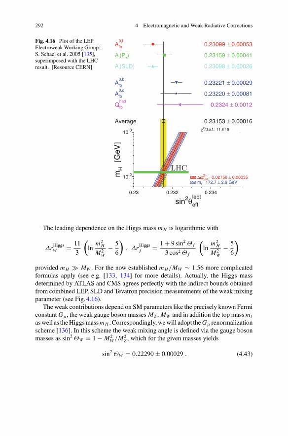
292 4 Electromagnetic and Weak Radiative Corrections

Fig. 4.16 Plot of the LEPElectroweak Working Group:S. Schael et al. 2005 [135],superimposed with the LHCresult. [Resource CERN]

10 2

10 3

0.23 0.232 0.234

sin2θlept

eff

mH [

GeV

]χ2/d.o.f.: 11.8 / 5

A0,l

fb 0.23099 ± 0.00053

Al(Pτ) 0.23159 ± 0.00041

Al(SLD) 0.23098 ± 0.00026

A0,b

fb 0.23221 ± 0.00029

A0,c

fb 0.23220 ± 0.00081

Qhad

fb 0.2324 ± 0.0012

Average 0.23153 ± 0.00016

Δαhad= 0.02758 ± 0.00035Δα(5)

mt= 172.7 ± 2.9 GeV

LHC

The leading dependence on the Higgs mass m H is logarithmic with

ΔrHiggsW = 11

3

(ln

m2H

M2W

− 5

6

), ΔrHiggs

f = 1 + 9 sin2 Θ f

3 cos2 Θ f

(ln

m2H

M2W

− 5

6

)

provided m H � MW . For the now established m H/MW ∼ 1.56 more complicatedformulas apply (see e.g. [133, 134] for more details). Actually, the Higgs massdetermined by ATLAS and CMS agrees perfectly with the indirect bounds obtainedfrom combined LEP, SLD and Tevatron precision measurements of the weak mixingparameter (see Fig. 4.16).

The weak contributions depend on SM parameters like the precisely known Fermiconstant Gμ, the weak gauge boson masses MZ , MW and in addition the top mass mt

as well as the Higgs mass m H . Correspondingly, we will adopt the Gμ renormalizationscheme [136]. In this scheme the weak mixing angle is defined via the gauge bosonmasses as sin2 ΘW = 1 − M2

W /M2Z , which for the given masses yields

sin2 ΘW = 0.22290 ± 0.00029 . (4.43)

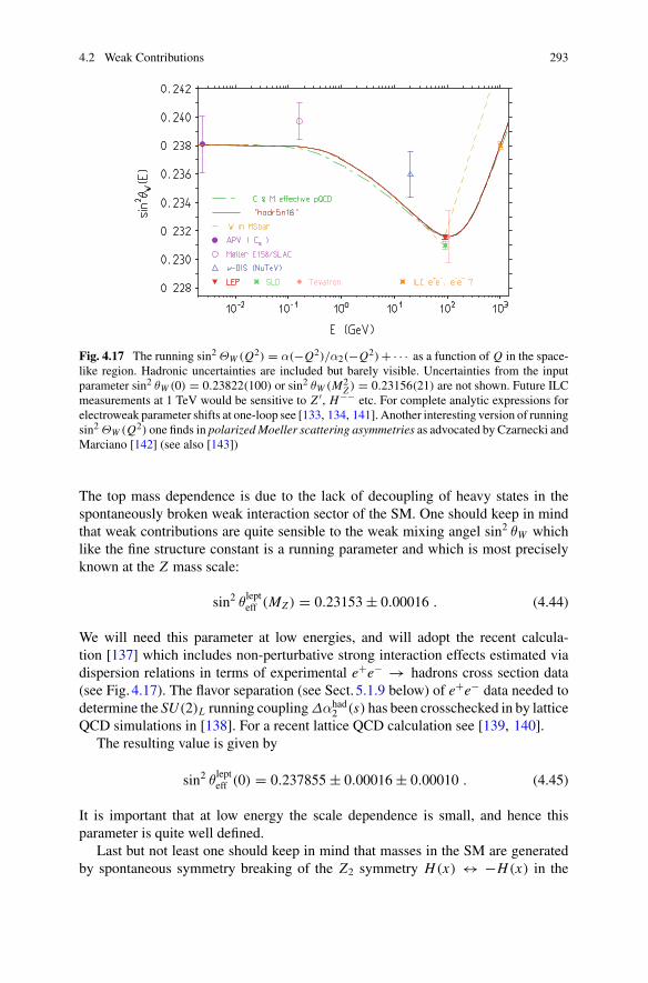
4.2 Weak Contributions 293

Fig. 4.17 The running sin2 ΘW (Q2) = α(−Q2)/α2(−Q2) + · · · as a function of Q in the space-like region. Hadronic uncertainties are included but barely visible. Uncertainties from the inputparameter sin2 θW (0) = 0.23822(100) or sin2 θW (M2

Z ) = 0.23156(21) are not shown. Future ILCmeasurements at 1 TeV would be sensitive to Z ′, H−− etc. For complete analytic expressions forelectroweak parameter shifts at one-loop see [133, 134, 141]. Another interesting version of runningsin2 ΘW (Q2) one finds in polarized Moeller scattering asymmetries as advocated by Czarnecki andMarciano [142] (see also [143])

The top mass dependence is due to the lack of decoupling of heavy states in thespontaneously broken weak interaction sector of the SM. One should keep in mindthat weak contributions are quite sensible to the weak mixing angel sin2 θW whichlike the fine structure constant is a running parameter and which is most preciselyknown at the Z mass scale:

sin2 θlepteff (MZ ) = 0.23153 ± 0.00016 . (4.44)

We will need this parameter at low energies, and will adopt the recent calcula-tion [137] which includes non-perturbative strong interaction effects estimated viadispersion relations in terms of experimental e+e− → hadrons cross section data(see Fig. 4.17). The flavor separation (see Sect. 5.1.9 below) of e+e− data needed todetermine the SU(2)L running coupling Δαhad

2 (s) has been crosschecked in by latticeQCD simulations in [138]. For a recent lattice QCD calculation see [139, 140].

The resulting value is given by

sin2 θlepteff (0) = 0.237855 ± 0.00016 ± 0.00010 . (4.45)

It is important that at low energy the scale dependence is small, and hence thisparameter is quite well defined.

Last but not least one should keep in mind that masses in the SM are generatedby spontaneous symmetry breaking of the Z2 symmetry H(x) ↔ −H(x) in the

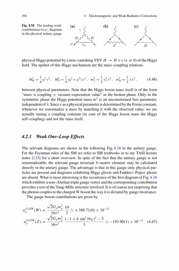
294 4 Electromagnetic and Weak Radiative Corrections

Fig. 4.18 The leading weakcontributions to a�; diagramsin the physical unitary gauge

W W

νμ Z Hμ

γ(a) (b) (c)

physical Higgs potential by a non–vanishing VEV H → H +v (v �= 0) of the Higgsfield. The upshot of this Higgs mechanism are the mass–coupling relations

M2W = 1

4g2 v2 , M2

Z = 1

4(g2 + g′2) v2 , m2

f = 1

2y2

f v2 , m2H = 1

3λ v2 , (4.46)

between physical parameters. Note that the Higgs boson mass itself is of the form“mass ∝ coupling × vacuum expectation value” in the broken phase. Only in thesymmetric phase the Higgs potential mass m2 is an unconstrained free parameter,independent ofλ. Sincev as a physical parameter is determined by the Fermi constant,whenever we renormalize a mass by matching it with the observed value, we areactually tuning a coupling constant (in case of the Higgs boson mass the Higgsself–coupling) and not the mass itself.

4.2.1 Weak One–Loop Effects

The relevant diagrams are shown in the following Fig. 4.18 in the unitary gauge.For the Feynman rules of the SM we refer to SM textbooks or to my TASI lecturenotes [133] for a short overview. In spite of the fact that the unitary gauge is notrenormalizable, the relevant gauge invariant S–matrix element, may be calculateddirectly in the unitary gauge. The advantage is that in this gauge only physical par-ticles are present and diagrams exhibiting Higgs ghosts and Faddeev–Popov ghostsare absent. What is most interesting is the occurrence of the first diagram of Fig. 4.18which exhibits a non–Abelian triple gauge vertex and the corresponding contributionprovides a test of the Yang-Mills structure involved. It is of course not surprising thatthe photon couples to the charged W boson the way it is dictated by gauge invariance.

The gauge boson contributions are given by

a(2) EWμ (W ) =

√2Gμm2

μ

16π2

10

3 + 388.71(0) × 10−11

a(2) EWμ (Z) =

√2Gμm2

μ

16π2

(−1 + 4 sin2 ΘW )2 − 5

3 −193.90(1) × 10−11 (4.47)

4.2 Weak Contributions 295

while the diagram with the Higgs exchange yields15

a(2) EWμ (H) =

√2Gμm2

μ

8π2

1∫

0

dy(2 − y) y2

y2 + (1 − y)(m H/mμ)2

√

2Gμm2μ

8π2

⎧⎨

⎩

m2μ

m2H

ln m2H

m2μ

for m H � mμ

32 for m H mμ

21.64 × 10−15 for m H ∼ 125 GeV . (4.48)

We remind that the Higgs mass now is known within a rather narrow error band.Employing the SM parameters given in (3.31) and (3.32) we obtain

a(2) EWμ = (194.81 ± 0.01) × 10−11 (4.49)

The error comes from the uncertainty in sin2 ΘW given above.

4.2.2 Weak Two–Loop Effects

Typical electroweak 2–loop corrections are the electromagnetic corrections of the1–loop diagrams Fig. 3.7 (part of the bosonic corrections) or fermionic loop insertionsas shown in Fig. 4.19. All these corrections are proportional to

K2 =√

2Gμ m2μ

16π2

α

π 2.70868284 × 10−12 . (4.50)

Part of the electroweak two–loop corrections were calculated first in 1992 by Kukhto,Kuraev, Schiller and Silagadze [144] with an unexpected result, the corrections turnedout to be enhanced by very large logarithms ln MZ/m f , which mainly come fromfermion triangular–loops like in Fig. 4.19a. In QED loops with three photons attacheddo not contribute due to Furry’s theorem and the γγγ–amplitude vanishes. In pres-ence of weak interactions, because of parity violation, contributions from the twoorientations of the closed fermion loops do not cancel such that the γγZ , γZ Z and

15The exact analytic result for the Higgs reads

a(2) EWμ (H) =

√2Gμm2

μ

8π2

{ξ (1 − ξ) ln(−ξ) + ξ−2 (1 − ξ)(1 − ξ3) ln(1 − ξ) + ξ−1(1 − ξ)2 + 3

2

}

√

2Gμm2μ

8π2

{z−1 (ln z − 7

6) + z−2 (3 ln z − 13

4) + z−3 (9 ln z − 201

20) + O(z−4 ln z)

}

in which z = m2H /m2

μ, and ξ = (√

1 − y − 1)/(√

1 − y + 1) with y = 4/z.

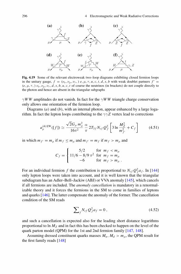
296 4 Electromagnetic and Weak Radiative Corrections

γ Z

f

μ μ

γ

μf

γ

γ Z μf

γ

Z Z

WWf

f ′

μ νμ

γ

W Wf ′f

μ νμ

γ

H γ, Zt

μ μ

γ

(a) (b) (c)

(d) (e) (f)

Fig. 4.19 Some of the relevant electroweak two–loop diagrams exhibiting closed fermion loopsin the unitary gauge, f = (νe, νμ, ντ , ) e,μ, τ , u, c, t, d, s, b with weak doublet partners f ′ =(e,μ, τ , ) νe, νμ, ντ , d, s, b, u, c, t of course the neutrinos (in brackets) do not couple directly tothe photon and hence are absent in the triangular subgraphs

γW W amplitudes do not vanish. In fact for the γW W triangle charge conservationonly allows one orientation of the fermion loop.

Diagrams (a) and (b), with an internal photon, appear enhanced by a large loga-rithm. In fact the lepton loops contributing to the γγZ vertex lead to corrections

a(4) EWμ ([ f ])

√2Gμ m2

μ

16π2

α

π2T3 f Ncf Q2

f

[3 ln

M2Z

m2f ′

+ C f

](4.51)

in which m f ′ = mμ if m f ≤ mμ and m f ′ = m f if m f > mμ and

C f =⎧⎨

⎩

5/2 for m f < mμ

11/6 − 8/9 π2 for m f = mμ

−6 for m f > mμ .

For an individual fermion f the contribution is proportional to Ncf Q2f a f . In [144]

only lepton loops were taken into account, and it is well known that the triangularsubdiagram has an Adler–Bell–Jackiw (ABJ) or VVA anomaly [145], which cancelsif all fermions are included. The anomaly cancellation is mandatory in a renormal-izable theory and it forces the fermions in the SM to come in families of leptonsand quarks [146]. The latter compensate the anomaly of the former. The cancellationcondition of the SM reads

∑

fNcf Q2

f a f = 0 , (4.52)

and such a cancellation is expected also for the leading short distance logarithmsproportional to ln MZ and in fact this has been checked to happen on the level of thequark parton model (QPM) for the 1st and 2nd fermion family [147, 148].

Assuming dressed constituent quarks masses Mu, Md > mμ, the QPM result forthe first family reads [148]

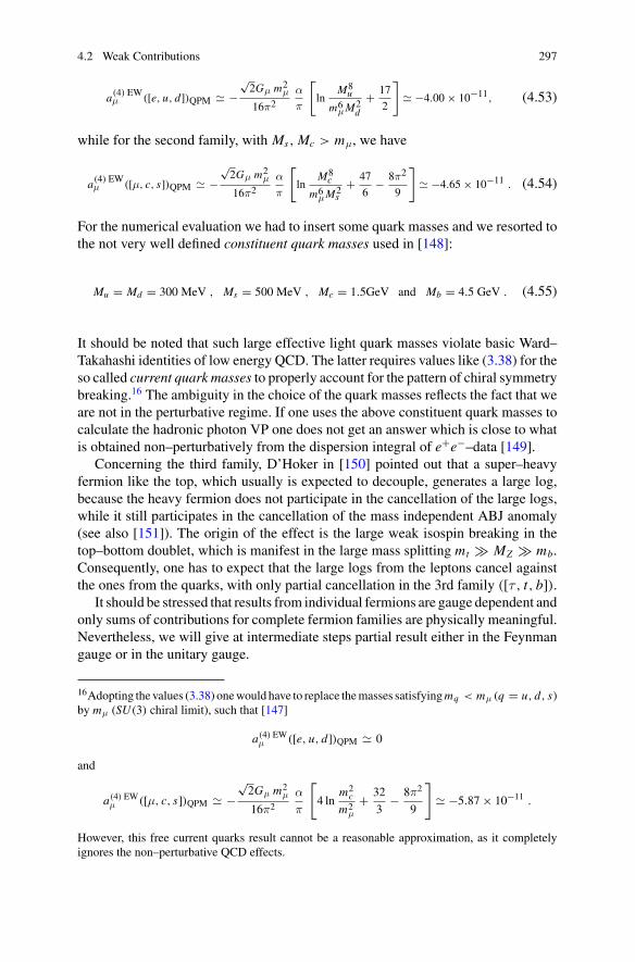
4.2 Weak Contributions 297

a(4) EWμ ([e, u, d])QPM −

√2Gμ m2

μ

16π2α

π

[

lnM8

u

m6μM2

d

+ 17

2

]

−4.00 × 10−11, (4.53)

while for the second family, with Ms, Mc > mμ, we have

a(4) EWμ ([μ, c, s])QPM −

√2Gμ m2

μ

16π2α

π

[

lnM8

c

m6μM2

s+ 47

6− 8π2

9

]

−4.65 × 10−11 . (4.54)

For the numerical evaluation we had to insert some quark masses and we resorted tothe not very well defined constituent quark masses used in [148]:

Mu = Md = 300 MeV , Ms = 500 MeV , Mc = 1.5GeV and Mb = 4.5 GeV . (4.55)

It should be noted that such large effective light quark masses violate basic Ward–Takahashi identities of low energy QCD. The latter requires values like (3.38) for theso called current quark masses to properly account for the pattern of chiral symmetrybreaking.16 The ambiguity in the choice of the quark masses reflects the fact that weare not in the perturbative regime. If one uses the above constituent quark masses tocalculate the hadronic photon VP one does not get an answer which is close to whatis obtained non–perturbatively from the dispersion integral of e+e−–data [149].

Concerning the third family, D’Hoker in [150] pointed out that a super–heavyfermion like the top, which usually is expected to decouple, generates a large log,because the heavy fermion does not participate in the cancellation of the large logs,while it still participates in the cancellation of the mass independent ABJ anomaly(see also [151]). The origin of the effect is the large weak isospin breaking in thetop–bottom doublet, which is manifest in the large mass splitting mt � MZ � mb.Consequently, one has to expect that the large logs from the leptons cancel againstthe ones from the quarks, with only partial cancellation in the 3rd family ([τ , t, b]).

It should be stressed that results from individual fermions are gauge dependent andonly sums of contributions for complete fermion families are physically meaningful.Nevertheless, we will give at intermediate steps partial result either in the Feynmangauge or in the unitary gauge.

16Adopting the values (3.38) one would have to replace the masses satisfying mq < mμ (q = u, d, s)by mμ (SU(3) chiral limit), such that [147]

a(4) EWμ ([e, u, d])QPM 0

and

a(4) EWμ ([μ, c, s])QPM −

√2Gμ m2

μ

16π2

α

π

[

4 lnm2

c

m2μ

+ 32

3− 8π2

9

]

−5.87 × 10−11 .

However, this free current quarks result cannot be a reasonable approximation, as it completelyignores the non–perturbative QCD effects.

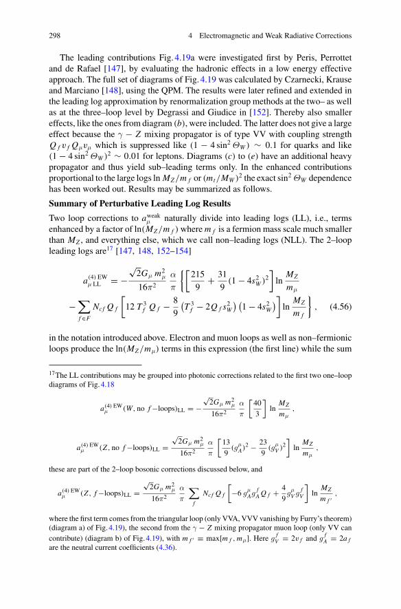
298 4 Electromagnetic and Weak Radiative Corrections

The leading contributions Fig. 4.19a were investigated first by Peris, Perrottetand de Rafael [147], by evaluating the hadronic effects in a low energy effectiveapproach. The full set of diagrams of Fig. 4.19 was calculated by Czarnecki, Krauseand Marciano [148], using the QPM. The results were later refined and extended inthe leading log approximation by renormalization group methods at the two– as wellas at the three–loop level by Degrassi and Giudice in [152]. Thereby also smallereffects, like the ones from diagram (b), were included. The latter does not give a largeeffect because the γ − Z mixing propagator is of type VV with coupling strengthQ f v f Qμvμ which is suppressed like (1 − 4 sin2 ΘW ) ∼ 0.1 for quarks and like(1 − 4 sin2 ΘW )2 ∼ 0.01 for leptons. Diagrams (c) to (e) have an additional heavypropagator and thus yield sub–leading terms only. In the enhanced contributionsproportional to the large logs ln MZ/m f or (mt/MW )2 the exact sin2 ΘW dependencehas been worked out. Results may be summarized as follows.

Summary of Perturbative Leading Log Results

Two loop corrections to aweakμ naturally divide into leading logs (LL), i.e., terms

enhanced by a factor of ln(MZ/m f ) where m f is a fermion mass scale much smallerthan MZ , and everything else, which we call non–leading logs (NLL). The 2–loopleading logs are17 [147, 148, 152–154]

a(4) EWμ LL = −

√2Gμ m2

μ

16π2

α

π

{[215

9+ 31

9(1 − 4s2

W )2

]ln

MZ

mμ

−∑

f ∈F

Ncf Q f

[12 T 3

f Q f − 8

9

(T 3

f − 2Q f s2W

) (1 − 4s2

W

)]

lnMZ

m f

}, (4.56)

in the notation introduced above. Electron and muon loops as well as non–fermionicloops produce the ln(MZ/mμ) terms in this expression (the first line) while the sum

17The LL contributions may be grouped into photonic corrections related to the first two one–loopdiagrams of Fig. 4.18

a(4) EWμ (W, no f −loops)LL = −

√2Gμ m2

μ

16π2

α

π

[40

3

]ln

MZ

mμ,

a(4) EWμ (Z , no f −loops)LL =

√2Gμ m2

μ

16π2

α

π

[13

9(g

μA)2 − 23

9(g

μV )2]

lnMZ

mμ,

these are part of the 2–loop bosonic corrections discussed below, and

a(4) EWμ (Z , f −loops)LL =

√2Gμ m2

μ

16π2

α

π

∑

f

Ncf Q f

[−6 g

μAg

fA Q f + 4

9g

μV g

fV

]ln

MZ

m f ′,

where the first term comes from the triangular loop (only VVA, VVV vanishing by Furry’s theorem)(diagram a) of Fig. 4.19), the second from the γ − Z mixing propagator muon loop (only VV cancontribute) (diagram b) of Fig. 4.19), with m f ′ ≡ max[m f , mμ]. Here g

fV = 2v f and g

fA = 2a f

are the neutral current coefficients (4.36).

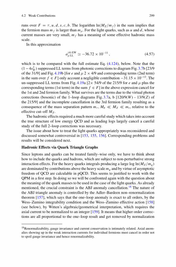
4.2 Weak Contributions 299

runs over F = τ , u, d, s, c, b. The logarithm ln(MZ/m f ) in the sum implies thatthe fermion mass m f is larger than mμ. For the light quarks, such as u and d, whosecurrent masses are very small, m f has a meaning of some effective hadronic massscale.

In this approximation

a(4) EWμ LL −36.72 × 10−11 , (4.57)

which is to be compared with the full estimate Eq. (4.124), below. Note that the(1−4s2

W ) suppressed LL terms from photonic corrections to diagram Fig. 3.7b [23/9of the 31/9] and Fig. 4.19b [for e and μ 2 × 4/9 and corresponding terms (2nd term)in the sum over f ∈ F] only account a negligible contribution −31.15 × 10−13. Theun-suppressed LL terms from Fig. 4.19a [2× 54/9 of the 215/9 for e and μ plus thecorresponding terms (1st term) in the sum f ∈ F] in the above expression cancel forthe 1st and 2nd fermion family. What survives are the terms due to the virtual photoncorrections (bosonic) of the 1–loop diagrams Fig. 3.7a, b [120/9(W ) - 13/9(Z ) ofthe 215/9] and the incomplete cancellation in the 3rd fermion family resulting as aconsequence of the mass separation pattern mτ , Mb MZ mt , relative to theeffective cut–off MZ .

The hadronic effects required a much more careful study which takes into accountthe true structure of low energy QCD and as leading logs largely cancel a carefulstudy of the full 2–loop corrections was necessary.

The issue about how to treat the light quarks appropriately was reconsidered anddiscussed somewhat controversial in [153, 155, 156]. Corresponding problems andresults will be considered next.

Hadronic Effects via Quark Triangle Graphs

Since leptons and quarks can be treated family–wise only, we have to think abouthow to include the quarks and hadrons, which are subject to non-perturbative stronginteraction effects. For the heavy quarks integrals producing a large log ln(MZ/mq)

are dominated by contributions above the heavy scale mq and by virtue of asymptoticfreedom of QCD are calculable in pQCD. This seems to justified to work with theQPM in a first step. In doing so we will be confronted again with the question aboutthe meaning of the quark masses to be used in the case of the light quarks. As alreadymentioned, the crucial constraint is the ABJ anomaly cancellation.18 The nature ofthe ABJ triangle anomaly is controlled by the Adler–Bardeen non–renormalizationtheorem [157], which says that the one–loop anomaly is exact to all orders, by theWess–Zumino integrability condition and the Wess–Zumino effective action [158](see below), by Witten’s algebraic/geometrical interpretation, which requires theaxial current to be normalized to an integer [159]. It means that higher order correc-tions are all proportional to the one–loop result and get removed by normalization

18Renormalizability, gauge invariance and current conservation is intimately related. Axial anom-alies showing up in the weak interaction currents for individual fermions must cancel in order notto spoil gauge invariance and hence renormalizability.

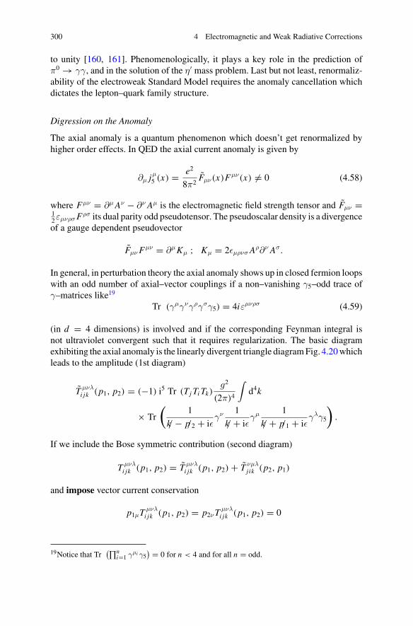
300 4 Electromagnetic and Weak Radiative Corrections

to unity [160, 161]. Phenomenologically, it plays a key role in the prediction ofπ0 → γγ, and in the solution of the η′ mass problem. Last but not least, renormaliz-ability of the electroweak Standard Model requires the anomaly cancellation whichdictates the lepton–quark family structure.

Digression on the Anomaly

The axial anomaly is a quantum phenomenon which doesn’t get renormalized byhigher order effects. In QED the axial current anomaly is given by

∂μ jμ5 (x) = e2

8π2Fμν(x)Fμν(x) �= 0 (4.58)

where Fμν = ∂μ Aν − ∂ν Aμ is the electromagnetic field strength tensor and Fμν =12εμνρσ Fρσ its dual parity odd pseudotensor. The pseudoscalar density is a divergenceof a gauge dependent pseudovector

Fμν Fμν = ∂μKμ ; Kμ = 2εμρνσ Aρ∂ν Aσ.

In general, in perturbation theory the axial anomaly shows up in closed fermion loopswith an odd number of axial–vector couplings if a non–vanishing γ5–odd trace ofγ–matrices like19

Tr (γμγνγργσγ5) = 4iεμνρσ (4.59)

(in d = 4 dimensions) is involved and if the corresponding Feynman integral isnot ultraviolet convergent such that it requires regularization. The basic diagramexhibiting the axial anomaly is the linearly divergent triangle diagram Fig. 4.20 whichleads to the amplitude (1st diagram)

T μνλi jk (p1, p2) = (−1) i5 Tr (Tj Ti Tk)

g2

(2π)4

∫d4k

× Tr

(1

k/ − p/2 + iεγν 1

k/ + iεγμ 1

k/ + p/1 + iεγλγ5

).

If we include the Bose symmetric contribution (second diagram)

T μνλi jk (p1, p2) = T μνλ

i jk (p1, p2) + T νμλj ik (p2, p1)

and impose vector current conservation

p1μT μνλi jk (p1, p2) = p2νT μνλ

i jk (p1, p2) = 0

19Notice that Tr(∏n

i=1 γμi γ5) = 0 for n < 4 and for all n = odd.

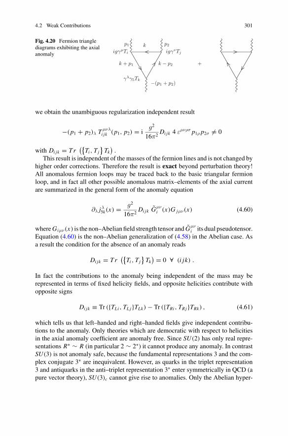
4.2 Weak Contributions 301

Fig. 4.20 Fermion trianglediagrams exhibiting the axialanomaly

p1 p2

−(p1 + p2)

k

k + p1 k − p2

igγμTi igγνTj

γλγ5Tk

+

we obtain the unambiguous regularization independent result

−(p1 + p2)λ T μνλi jk (p1, p2) = i

g2

16π2Di jk 4 εμνρσ p1ρ p2σ �= 0

with Di jk = T r({

Ti , Tj}

Tk)

.This result is independent of the masses of the fermion lines and is not changed by

higher order corrections. Therefore the result is exact beyond perturbation theory!All anomalous fermion loops may be traced back to the basic triangular fermionloop, and in fact all other possible anomalous matrix–elements of the axial currentare summarized in the general form of the anomaly equation

∂λ jλ5k(x) = g2

16π2Di jk Gμν

i (x)G jμν(x) (4.60)

where Giμν(x) is the non–Abelian field strength tensor and Gμνi its dual pseudotensor.

Equation (4.60) is the non–Abelian generalization of (4.58) in the Abelian case. Asa result the condition for the absence of an anomaly reads

Di jk = T r({

Ti , Tj}

Tk) = 0 ∀ (i jk) .

In fact the contributions to the anomaly being independent of the mass may berepresented in terms of fixed helicity fields, and opposite helicities contribute withopposite signs

Di jk ≡ Tr ({TLi , TL j }TLk) − Tr ({TRi , TR j }TRk) , (4.61)

which tells us that left–handed and right–handed fields give independent contribu-tions to the anomaly. Only theories which are democratic with respect to helicitiesin the axial anomaly coefficient are anomaly free. Since SU(2) has only real repre-sentations R∗ ∼ R (in particular 2 ∼ 2∗) it cannot produce any anomaly. In contrastSU(3) is not anomaly safe, because the fundamental representations 3 and the com-plex conjugate 3∗ are inequivalent. However, as quarks in the triplet representation3 and antiquarks in the anti–triplet representation 3∗ enter symmetrically in QCD (apure vector theory), SU(3)c cannot give rise to anomalies. Only the Abelian hyper-

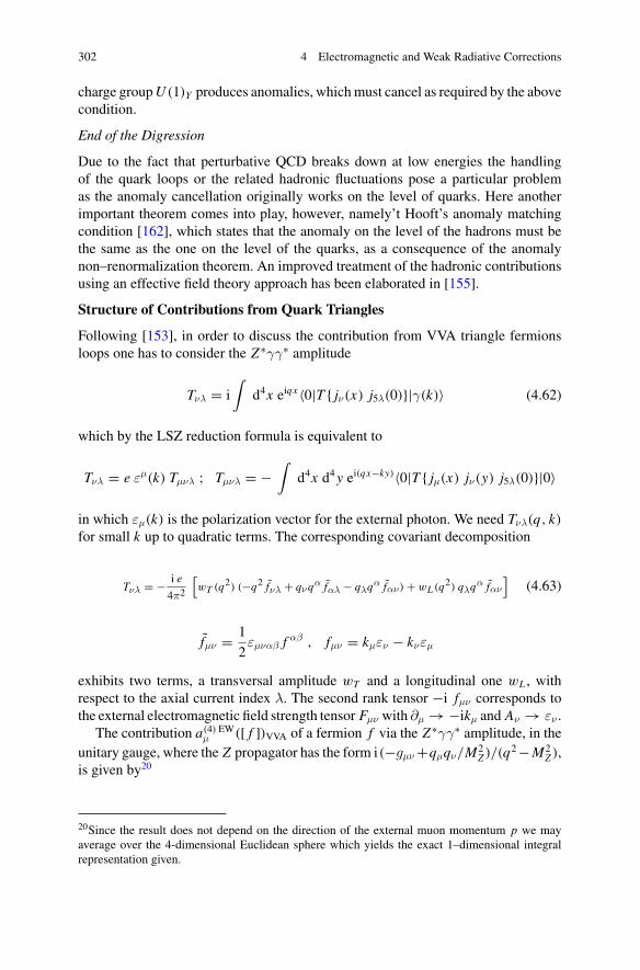
302 4 Electromagnetic and Weak Radiative Corrections

charge group U (1)Y produces anomalies, which must cancel as required by the abovecondition.

End of the Digression

Due to the fact that perturbative QCD breaks down at low energies the handlingof the quark loops or the related hadronic fluctuations pose a particular problemas the anomaly cancellation originally works on the level of quarks. Here anotherimportant theorem comes into play, however, namely’t Hooft’s anomaly matchingcondition [162], which states that the anomaly on the level of the hadrons must bethe same as the one on the level of the quarks, as a consequence of the anomalynon–renormalization theorem. An improved treatment of the hadronic contributionsusing an effective field theory approach has been elaborated in [155].

Structure of Contributions from Quark Triangles

Following [153], in order to discuss the contribution from VVA triangle fermionsloops one has to consider the Z∗γγ∗ amplitude

Tνλ = i∫

d4x eiqx 〈0|T { jν(x) j5λ(0)}|γ(k)〉 (4.62)

which by the LSZ reduction formula is equivalent to

Tνλ = e εμ(k) Tμνλ ; Tμνλ = −∫

d4x d4 y ei(qx−ky)〈0|T { jμ(x) jν(y) j5λ(0)}|0〉

in which εμ(k) is the polarization vector for the external photon. We need Tνλ(q, k)

for small k up to quadratic terms. The corresponding covariant decomposition

Tνλ = − i e

4π2

[wT (q2) (−q2 fνλ + qνqα fαλ − qλqα fαν ) + wL (q2) qλqα fαν

](4.63)

fμν = 1

2εμναβ f αβ , fμν = kμεν − kνεμ

exhibits two terms, a transversal amplitude wT and a longitudinal one wL , withrespect to the axial current index λ. The second rank tensor −i fμν corresponds tothe external electromagnetic field strength tensor Fμν with ∂μ → −ikμ and Aν → εν .

The contribution a(4) EWμ ([ f ])VVA of a fermion f via the Z∗γγ∗ amplitude, in the

unitary gauge, where the Z propagator has the form i(−gμν +qμqν/M2Z )/(q2 − M2

Z ),is given by20

20Since the result does not depend on the direction of the external muon momentum p we mayaverage over the 4-dimensional Euclidean sphere which yields the exact 1–dimensional integralrepresentation given.

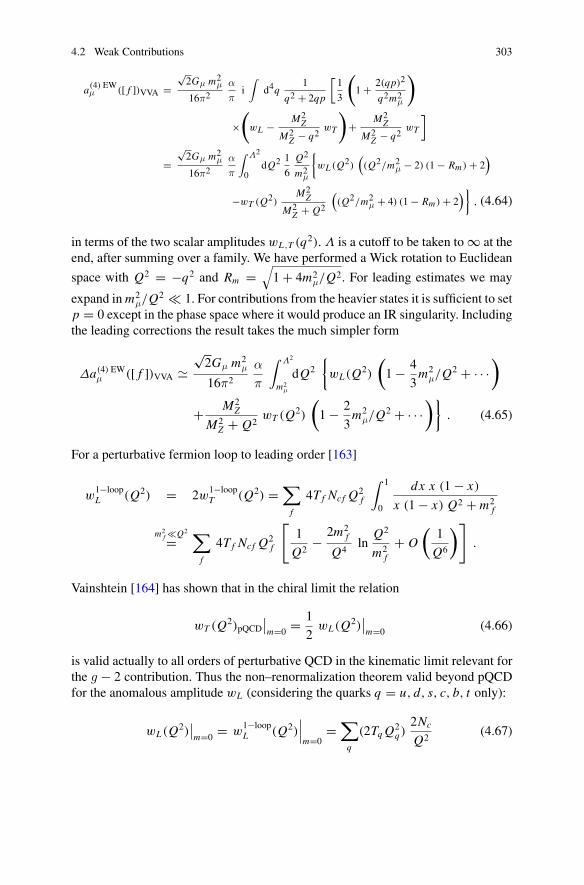
4.2 Weak Contributions 303

a(4) EWμ ([ f ])VVA =

√2Gμ m2

μ

16π2α

πi∫

d4q1

q2 + 2qp

[1

3

(

1 + 2(qp)2

q2m2μ

)

×(

wL − M2Z

M2Z − q2

wT

)

+ M2Z

M2Z − q2

wT

]

=√

2Gμ m2μ

16π2α

π

∫ Λ2

0dQ2 1

6

Q2

m2μ

{wL (Q2)

((Q2/m2

μ − 2) (1 − Rm ) + 2)

−wT (Q2)M2

Z

M2Z + Q2

((Q2/m2

μ + 4) (1 − Rm ) + 2)}

, (4.64)

in terms of the two scalar amplitudes wL ,T (q2). Λ is a cutoff to be taken to ∞ at theend, after summing over a family. We have performed a Wick rotation to Euclidean

space with Q2 = −q2 and Rm =√

1 + 4m2μ/Q2. For leading estimates we may

expand in m2μ/Q2 1. For contributions from the heavier states it is sufficient to set

p = 0 except in the phase space where it would produce an IR singularity. Includingthe leading corrections the result takes the much simpler form

Δa(4) EWμ ([ f ])VVA

√2Gμ m2

μ

16π2

α

π

∫ Λ2

m2μ

dQ2

{wL(Q2)

(1 − 4

3m2

μ/Q2 + · · ·)

+ M2Z

M2Z + Q2

wT (Q2)

(1 − 2

3m2

μ/Q2 + · · ·)}

. (4.65)

For a perturbative fermion loop to leading order [163]

w1−loopL (Q2) = 2w

1−loopT (Q2) =

∑

f

4T f Ncf Q2f

∫ 1

0

dx x (1 − x)

x (1 − x) Q2 + m2f

m2f Q2

=∑

f

4T f Ncf Q2f

[1

Q2− 2m2

f

Q4ln

Q2

m2f

+ O

(1

Q6

)]

.

Vainshtein [164] has shown that in the chiral limit the relation

wT (Q2)pQCD

∣∣m=0 = 1

2wL(Q2)

∣∣m=0 (4.66)

is valid actually to all orders of perturbative QCD in the kinematic limit relevant forthe g − 2 contribution. Thus the non–renormalization theorem valid beyond pQCDfor the anomalous amplitude wL (considering the quarks q = u, d, s, c, b, t only):

wL(Q2)∣∣m=0 = w

1−loopL (Q2)

∣∣∣m=0

=∑

q

(2Tq Q2q)

2Nc

Q2(4.67)

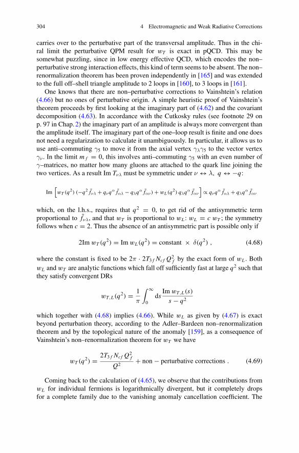
304 4 Electromagnetic and Weak Radiative Corrections

carries over to the perturbative part of the transversal amplitude. Thus in the chi-ral limit the perturbative QPM result for wT is exact in pQCD. This may besomewhat puzzling, since in low energy effective QCD, which encodes the non–perturbative strong interaction effects, this kind of term seems to be absent. The non–renormalization theorem has been proven independently in [165] and was extendedto the full off–shell triangle amplitude to 2 loops in [160], to 3 loops in [161].

One knows that there are non–perturbative corrections to Vainshtein’s relation(4.66) but no ones of perturbative origin. A simple heuristic proof of Vainshtein’stheorem proceeds by first looking at the imaginary part of (4.62) and the covariantdecomposition (4.63). In accordance with the Cutkosky rules (see footnote 29 onp. 97 in Chap. 2) the imaginary part of an amplitude is always more convergent thanthe amplitude itself. The imaginary part of the one–loop result is finite and one doesnot need a regularization to calculate it unambiguously. In particular, it allows us touse anti–commuting γ5 to move it from the axial vertex γλγ5 to the vector vertexγν . In the limit m f = 0, this involves anti–commuting γ5 with an even number ofγ–matrices, no matter how many gluons are attached to the quark line joining thetwo vertices. As a result Im Tνλ must be symmetric under ν ↔ λ, q ↔ −q:

Im[wT (q2) (−q2 fνλ + qνqα fαλ − qλqα fαν) + wL (q2) qλqα fαν

]∝ qνqα fαλ + qλqα fαν

which, on the l.h.s., requires that q2 = 0, to get rid of the antisymmetric termproportional to fνλ, and that wT is proportional to wL : wL = c wT ; the symmetryfollows when c = 2. Thus the absence of an antisymmetric part is possible only if

2Im wT (q2) = Im wL(q2) = constant × δ(q2) , (4.68)

where the constant is fixed to be 2π · 2T3 f Ncf Q2f by the exact form of wL . Both

wL and wT are analytic functions which fall off sufficiently fast at large q2 such thatthey satisfy convergent DRs

wT,L(q2) = 1

π

∫ ∞

0ds

Im wT,L(s)

s − q2

which together with (4.68) implies (4.66). While wL as given by (4.67) is exactbeyond perturbation theory, according to the Adler–Bardeen non–renormalizationtheorem and by the topological nature of the anomaly [159], as a consequence ofVainshtein’s non–renormalization theorem for wT we have

wT (q2) = 2T3 f Ncf Q2f

Q2+ non − perturbative corrections . (4.69)

Coming back to the calculation of (4.65), we observe that the contributions fromwL for individual fermions is logarithmically divergent, but it completely dropsfor a complete family due to the vanishing anomaly cancellation coefficient. The

4.2 Weak Contributions 305

contribution from wT is convergent for individual fermions due to the damping bythe Z propagator. In fact it is the leading 1/Q2 term of the wT amplitude whichproduces the ln MZ

m terms. However, the coefficient is the same as the one for theanomalous term and thus for each complete family also the ln MZ terms must dropout. Due to the non–renormalization theorem (4.66) the perturbative leading 1/Q2

term of wT has to carry over to a low energy effective approach of QCD (see below).

Results for Contributions from Fermion Loops

For the third family the calculation is perturbative and thus straight forward with theresult [147, 148, 155]

a(4) EWμ ([τ , b, t]) = −

√2Gμ m2

μ

16π2

α

π

[8

3ln

m2t

M2Z

− 2

9

M2Z

m2t

(ln

m2t

M2Z

+ 5

3

)

+ lnM2

Z

m2b

+ 3 lnM2

Z

m2τ

− 8

3+ · · ·

]

−√

2Gμ m2μ

16π2

α

π× 30.2(3) −8.19(10) × 10−11 . (4.70)

Small terms of order m2μ/m2

τ , m2b/M2

Z , M4Z/m4

t and smaller mass ratios have beenneglected.

While the QPM results presented above, indeed confirmed the complete cancel-lation of the ln MZ terms for the 1st and 2nd family, in the third family the corre-sponding terms ln MZ/mτ and ln MZ/mb remain unbalanced by a corresponding topcontribution.

Since in the perturbative regime QCD corrections are of O(αs(μ2)/π), where μ

is in the range from m f to MZ , pQCD is applicable for c, b and t quarks, only (seeFig. 3.3). For the lighter quarks u, d and s, however, the QPM estimate certainlyis not appropriate because strong interaction corrections are expected to contributebeyond perturbation theory and assuming that non–perturbative effects just lead toa dressing of the quark masses into constituent quarks masses certainly is an oversimplification of reality. Most importantly, pQCD does not account for the fact thatthe chiral symmetry is spontaneously broken the mechanism responsible for theemergence of the pions as quasi Nambu–Goldstone bosons. The failure of the QPMwe have illustrated in the discussion following p. 183 for the much simpler case ofthe hadronic vacuum polarization, already. We thus have to think about other meansto take into account properly the low energy hadronic effects, if possible.

Digression on the Chiral Structure of Low Energy Effective QCD

Fortunately, a firm low energy effective theory of QCD exists and is very well devel-oped: Chiral Perturbation Theory (CHPT) [166], an expansion for low momentap and in the light current quark masses as chiral symmetry breaking parame-ters. CHPT is based on the chiral flavor structure SU(3)L ⊗ SU(3)R of the lowlying hadron spectrum (u, d, s quark bound states). The SU(3)V vector currents

306 4 Electromagnetic and Weak Radiative Corrections

jμk = ∑

i j ψi (Tk)i j γμψ j as well as the SU(3)A axial currents jμ5k = ∑

i j ψi

(Tk)i j γμγ5ψ j21 are partially conserved in the SU(3) sector of the (u, d, s) quark fla-

vors, and strictly conserved in the chiral limit of vanishing quark massesmu, md , ms → 0, modulo the axial anomaly in the axial singlet current. The partialconservation of the chiral currents22 derives from ∂μ(ψ1γ

μψ2) = i(m1 − m2) ψ1ψ2

(CVC in the isospin limit mu = md ) and ∂μ(ψ1γμγ5ψ2) = i(m1 + m2) ψ1γ5ψ2

(PCAC) and the setup of a perturbative scheme is based on the phenomenologicallyobserved smallness of the current quark masses (3.38).

The chiral expansion of the effective Lagrangian is an expansion in �

Leff = L2 + �L4 + �2L6 + · · · (4.71)

which is equivalent to an expansion in powers of derivatives and quark masses. Instandard chiral counting one power of quark mass counts as two powers of deriv-atives, or momentum p in momentum space. In chiral SU(3) there exists an octetof massless pseudoscalar particles (π, K , η), the Nambu–Goldstone bosons in thechiral limit. The leading term of the expansion is the non–linear σ–model, where thepseudoscalars are encoded in a unitary 3 × 3 matrix field

U (φ) = exp

(−i

√2

φ(x)

F

)(4.72)

with (Ti the SU(3) generators)

φ(x) =∑

i

Tiφi =

⎛

⎜⎜⎝

π0√2

+ η√6

π+ K +

π− −π0√2

+ η√6

K 0

K − K0 −2 η√

6

⎞

⎟⎟⎠+ 1√

3

⎛

⎝η′

η′η′

⎞

⎠ (4.73)

where the second term is the diagonal singlet contribution by the η′ meson. The latteris not a Nambu–Goldstone boson, however it is of leading order in 1/Nc. The leadingorder Lagrangian at O(p2) is then given by

L2 = F2

4Tr {DμU DμU † + M2 (U + U †)} (4.74)

where, in absence of external fields, the covariant derivative DμU = ∂μU coincideswith the normal derivative. Furthermore, M2 = 2Bm, where B is proportional tothe quark condensate 〈0|uu|0〉 and m = 1

2 (mu + md). In the chiral limit of exactSU(3)R ⊗ SU(3)L symmetry we have

21Tk (k = 1, . . . , 8) are the generators of the global SU(3) transformations and i, j = u, d, s flavorindices.22Especially in the SU(2) isospin subspace, the small mass splitting |m1 − m2| m1 + m2motivates the terminology: conserved vector current (CVC) and partially conserved axial vectorcurrent (PCAC) (see next page).

4.2 Weak Contributions 307

〈0|uu|0〉 = 〈0|dd|0〉 = 〈0|ss|0〉 .

The parameters M and F are the leading order versions of the pion mass and thepion decay constant, respectively:

m2π = M2 [1 + O(m)] , Fπ = F [1 + O(m)] .

The low energy effective currents again are nonlinear in the pion fields and in CHPTagain appear expanded in the derivatives of U and the quark masses. For vector andaxial–vector current one obtains

V iμ = iF2

4〈σi (U † DμU + U DμU †)〉 + O(p3) = [εi jkφ j∂μφ

k + O(φ3)]+ O(p3) ,

Aiμ = iF2

4〈σi (U † DμU − U DμU †)〉 + O(p3) = [−F∂μφ

i + O(φ3)]+ O(p3) ,

which implies the conserved vector current (CVC) and the partially conservedaxial vector current (PCAC) relations. Despite the fact that this Lagrangian is non–renormalizable, one can use it to calculate matrix elements like in standard pertur-bation theory. However, unlike in renormalizable theories where only terms alreadypresent in the original bare Lagrangian get reshuffled by renormalization, in non–renormalizable theories order by order in the expansion new vertices of increasingdimensions and associated new free couplings called low energy constants show upand limit the predictive power of the effective theory.

At physical quark masses the value of the condensate is estimated to be 〈mqqq〉 ∼−(0.098 GeV)4 for q = u, d. The key relation to identify the quark conden-sates in terms of physical quantities is the Gell-Mann, Oakes and Renner (GMOR)[167, 168] relation. In the chiral limit the mass operators qRuL , or qLu R transformunder (3∗, 3) of the chiral group SU(3)L ⊗ SU(3)R . Hence the quark condensateswould have to vanish identically in the case of an exact chirally symmetric world.In fact the symmetry is spontaneously broken and the vacuum of the real world isnot chirally symmetric. Therefore the quark condensates do not have to vanish. Inorder to determine the quark condensates, consider the charged axial currents andthe related pseudoscalar density

Aμ = dγμγ5u

P = d iγ5u

and the OPE of the product

Aμ(x) P+(y) =∑

i

Ciμ(x − y) Oi (

x + y

2) .

In QCD we may inspect the short distance expansion and study its consequences.One observation is that taking the VEV only the scalar operators contribute and oneobtains the exact relation

308 4 Electromagnetic and Weak Radiative Corrections

〈0|Aμ(x) P+(y)|0〉 = (x − y)μ

2π2 (x − y)4〈0|uu + dd|0〉 . (4.75)

The spectral representation (see (3.131)) for the two–point function on the l.h.s. isof the form pμ ρ(p2) and current conservation requires p2 ρ(p2) = 0 such that onlythe Nambu–Goldstone modes, the massless pions, contribute, such that with

〈0|Aμ(0)|π+〉 = i Fπ pμ

〈0|P+(0)|π+〉 = gπ

we get

Fπgπ = −〈0|uu + dd|0〉 .

For non-vanishing quark masses the PCAC relation ∂μ Aμ = (mu + md) P thenimplies the exact relation

Fπm2π+ = (mu + md) gπ

and the famous GMOR relation

F2π m2

π+ = −(mu + md) 〈0|uu + dd|0〉 (4.76)

follows from the last two relations. Note that the quark condensates must be negative!They are a measure for the asymmetry of the vacuum in the chiral limit, and thus aretrue order parameters. If both Fπ and 〈0|uu + dd|0〉 have finite limits as mq → 0the pion mass square must go to zero linear with the quark masses

m2π+ = B (mu + md) ; B ≡ − 1

F2π

〈0|uu + dd|0〉 ; B > 0 .

The deviation from the chiral limit is controlled by CHPT. The quark masses aswell as the quark condensates depend on the renormalization scale μ, however, theproduct 〈0|mqqq|0〉 is RG invariant as is inferred by the GMOR relation.

For later reference we are interested in the momentum space version of (4.75). Welook at the time-ordered vacuum expectation value and using translational invariancewe may choose y = 0 and thus consider

∫d4xeipx 〈0|T {Aμ(x) P+(0)

} |0〉 = pμ

p2 + iε〈0|uu + dd|0〉 . (4.77)

Since the Fourier transform of the singular r.h.s of (4.75) is not trivial to performdirectly, we can derive the result as follows: first the result obviously is proportional tothe quark condensate, which we may denote by 〈qq〉. We note that Aμ, P and 〈qq〉 allhave dimension dim = 3. Furthermore the result is a function of the four momentum

4.2 Weak Contributions 309

p only and a covariant vector thereof. The dimension then requires another factor1/(p2 + iε) with the usual iε prescription for Feynman type propagators. Indeed the1/p2 factor is nothing but the propagator of the pion (in the chiral limit) to which Pis the interpolating field:

P

.

End of the Digression

In [147] the light quark contribution to Fig. 4.19a were evaluated using the low energyeffective form of QCD which is CHPT. To lowest order in the chiral expansion, thehadronic Zγγ interaction is dominated by the pseudoscalar meson (the quasi Nambu–Goldstone bosons) exchange. The corresponding effective couplings are given by

L(2) = − e

2 sin ΘW cos ΘWFπ∂μ

(π0 + 1√

3η8 − 1√

6η0

)Zμ , (4.78)

which is the relevant part of the O(p2) chiral effective Lagrangian, and the effectiveO(p4) coupling

LWZW = α

π

Nc

12Fπ

(

π0 + 1√3

η8 + 2

√2

3η0

)

Fμν Fμν , (4.79)

which is the Wess–Zumino–Witten Lagrangian. The latter reproduces the ABJ anom-aly on the level of the hadrons. π0 is the neutral pion field, Fπ the pion decay constant(Fπ = 92.4 MeV). The pseudoscalars η8, η0 are mixing into the physical states η, η′.The [u, d, s] contribution with long distance (L.D.) part (E < μ) evaluated in CHPTand a short distance (S.D.) part (E > μ) to be evaluated in the QPM. The cut–off formatching L.D. and S.D. part typically is MΛ = m P ∼ 1 GeV to MΛ = Mτ ∼ 2 GeV.The corresponding diagrams are shown in Fig. 4.21, which together with its crossedversion in the unitary gauge and in the chiral limit, up to terms suppressed by m2

μ/M2Λ,

yields23

23The simplest way to implement the lower cut–off MΛ to the low energy effective field theory(EFT) is to write in (4.65)

1

M2Z + Q2

= 1

M2Λ + Q2

︸ ︷︷ ︸E FT

+ 1

M2Z + Q2

− 1

M2Λ + Q2

︸ ︷︷ ︸Q P M

by using the QPM for the second term. In the first term MZ is replaced by MΛ, in the second termconstant terms drop out in the difference as the quark masses in any case have values far below thecut–offs.

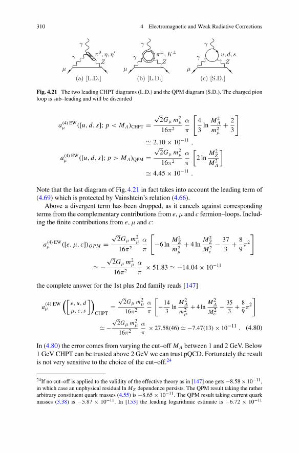
310 4 Electromagnetic and Weak Radiative Corrections

γZ

π0, η, η′

μ

γ

(a) [L.D.]

γZ

π±, K±

μ

γ

(b) [L.D.]

γZ

u, d, s

μ

γ

(c) [S.D.]

Fig. 4.21 The two leading CHPT diagrams (L.D.) and the QPM diagram (S.D.). The charged pionloop is sub–leading and will be discarded

a(4) EWμ ([u, d, s]; p < MΛ)CHPT =

√2Gμ m2

μ

16π2

α

π

[4

3ln

M2Λ

m2μ

+ 2

3

]

2.10 × 10−11 ,

a(4) EWμ ([u, d, s]; p > MΛ)QPM =

√2Gμ m2

μ

16π2

α

π

[2 ln

M2Z

M2Λ

]

4.45 × 10−11 .

Note that the last diagram of Fig. 4.21 in fact takes into account the leading term of(4.69) which is protected by Vainshtein’s relation (4.66).

Above a divergent term has been dropped, as it cancels against correspondingterms from the complementary contributions from e, μ and c fermion–loops. Includ-ing the finite contributions from e, μ and c:

a(4) EWμ ([e,μ, c])Q P M =

√2Gμ m2

μ

16π2

α

π

[

−6 lnM2

Z

m2μ

+ 4 lnM2

Z

M2c

− 37

3+ 8

9π2

]

−√

2Gμ m2μ

16π2

α

π× 51.83 −14.04 × 10−11

the complete answer for the 1st plus 2nd family reads [147]

a(4) EWμ

([e, u, dμ, c, s

])

CHPT=

√2Gμ m2

μ

16π2α

π

[

−14

3ln

M2Λ

m2μ

+ 4 lnM2

Λ

M2c

− 35

3+ 8

9π2

]

−√

2Gμ m2μ

16π2α

π× 27.58(46) −7.47(13) × 10−11 . (4.80)

In (4.80) the error comes from varying the cut–off MΛ between 1 and 2 GeV. Below1 GeV CHPT can be trusted above 2 GeV we can trust pQCD. Fortunately the resultis not very sensitive to the choice of the cut–off.24

24If no cut–off is applied to the validity of the effective theory as in [147] one gets −8.58 × 10−11,in which case an unphysical residual ln MZ dependence persists. The QPM result taking the ratherarbitrary constituent quark masses (4.55) is −8.65 × 10−11. The QPM result taking current quarkmasses (3.38) is −5.87 × 10−11. In [153] the leading logarithmic estimate is −6.72 × 10−11

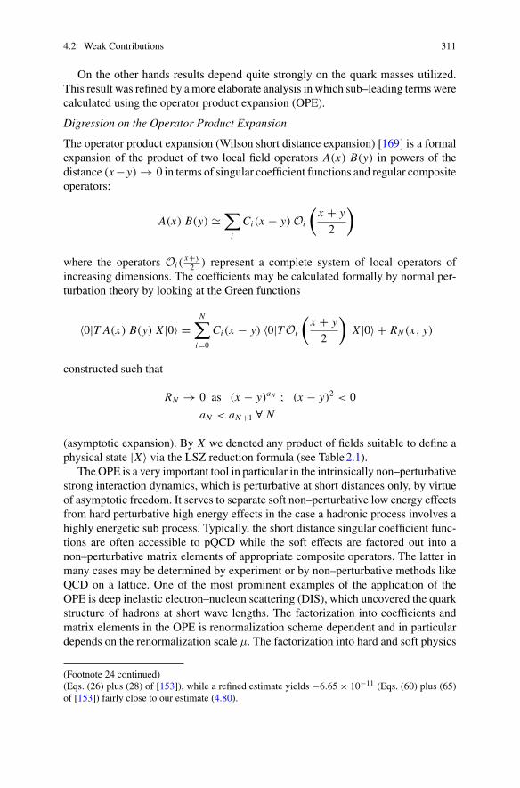
4.2 Weak Contributions 311

On the other hands results depend quite strongly on the quark masses utilized.This result was refined by a more elaborate analysis in which sub–leading terms werecalculated using the operator product expansion (OPE).

Digression on the Operator Product Expansion

The operator product expansion (Wilson short distance expansion) [169] is a formalexpansion of the product of two local field operators A(x) B(y) in powers of thedistance (x −y) → 0 in terms of singular coefficient functions and regular compositeoperators:

A(x) B(y) ∑

i

Ci (x − y) Oi

(x + y

2

)

where the operators Oi (x+y

2 ) represent a complete system of local operators ofincreasing dimensions. The coefficients may be calculated formally by normal per-turbation theory by looking at the Green functions

〈0|T A(x) B(y) X |0〉 =N∑

i=0

Ci (x − y) 〈0|T Oi

(x + y

2

)X |0〉 + RN (x, y)

constructed such that

RN → 0 as (x − y)aN ; (x − y)2 < 0

aN < aN+1 ∀ N

(asymptotic expansion). By X we denoted any product of fields suitable to define aphysical state |X〉 via the LSZ reduction formula (see Table 2.1).

The OPE is a very important tool in particular in the intrinsically non–perturbativestrong interaction dynamics, which is perturbative at short distances only, by virtueof asymptotic freedom. It serves to separate soft non–perturbative low energy effectsfrom hard perturbative high energy effects in the case a hadronic process involves ahighly energetic sub process. Typically, the short distance singular coefficient func-tions are often accessible to pQCD while the soft effects are factored out into anon–perturbative matrix elements of appropriate composite operators. The latter inmany cases may be determined by experiment or by non–perturbative methods likeQCD on a lattice. One of the most prominent examples of the application of theOPE is deep inelastic electron–nucleon scattering (DIS), which uncovered the quarkstructure of hadrons at short wave lengths. The factorization into coefficients andmatrix elements in the OPE is renormalization scheme dependent and in particulardepends on the renormalization scale μ. The factorization into hard and soft physics

(Footnote 24 continued)(Eqs. (26) plus (28) of [153]), while a refined estimate yields −6.65 × 10−11 (Eqs. (60) plus (65)of [153]) fairly close to our estimate (4.80).

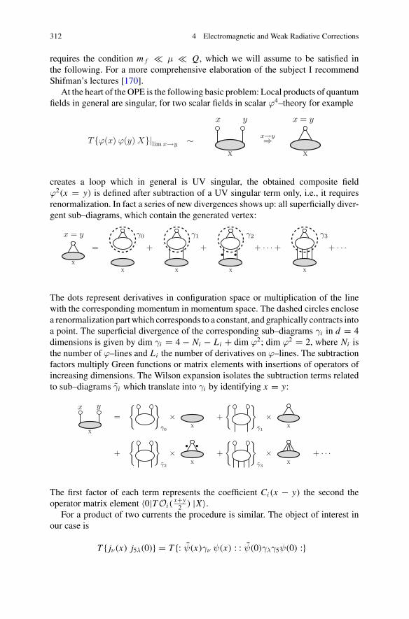
312 4 Electromagnetic and Weak Radiative Corrections

requires the condition m f μ Q, which we will assume to be satisfied inthe following. For a more comprehensive elaboration of the subject I recommendShifman’s lectures [170].

At the heart of the OPE is the following basic problem: Local products of quantumfields in general are singular, for two scalar fields in scalar ϕ4–theory for example

T {ϕ(x) ϕ(y) X}|limx→y ∼X

x→y⇒X

x y x = y

creates a loop which in general is UV singular, the obtained composite fieldϕ2(x = y) is defined after subtraction of a UV singular term only, i.e., it requiresrenormalization. In fact a series of new divergences shows up: all superficially diver-gent sub–diagrams, which contain the generated vertex:

X

=

X

+

X

+

X

+ · · · +

X

+ · · ·x = y γ0 γ1 γ2 γ3

The dots represent derivatives in configuration space or multiplication of the linewith the corresponding momentum in momentum space. The dashed circles enclosea renormalization part which corresponds to a constant, and graphically contracts intoa point. The superficial divergence of the corresponding sub–diagrams γi in d = 4dimensions is given by dim γi = 4 − Ni − Li + dim ϕ2; dim ϕ2 = 2, where Ni isthe number of ϕ–lines and Li the number of derivatives on ϕ–lines. The subtractionfactors multiply Green functions or matrix elements with insertions of operators ofincreasing dimensions. The Wilson expansion isolates the subtraction terms relatedto sub–diagrams γi which translate into γi by identifying x = y:

x y

X

=

{ }γ0

×X

+

{ }γ1

×X

+

{ }γ2

×X

+

{ }γ3

×X

+ · · ·

The first factor of each term represents the coefficient Ci (x − y) the second theoperator matrix element 〈0|T Oi (

x+y2 ) |X〉.

For a product of two currents the procedure is similar. The object of interest inour case is

T { jν(x) j5λ(0)} = T {: ψ(x)γν ψ(x) : : ψ(0)γλγ5ψ(0) :}

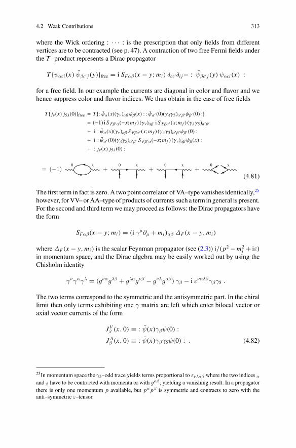
4.2 Weak Contributions 313

where the Wick ordering : · · · : is the prescription that only fields from differentvertices are to be contracted (see p. 47). A contraction of two free Fermi fields underthe T –product represents a Dirac propagator

T {ψαci (x) ψβc′ j (y)}free = i SFαβ(x − y; mi ) δcc′δi j− : ψβc′ j (y) ψαci (x) :

for a free field. In our example the currents are diagonal in color and flavor and wehence suppress color and flavor indices. We thus obtain in the case of free fields

(4.81)

The first term in fact is zero. A two point correlator of VA–type vanishes identically,25

however, for VV– or AA–type of products of currents such a term in general is present.For the second and third term we may proceed as follows: the Dirac propagators havethe form

SFαβ(x − y; mi ) = (i γμ∂μ + mi )αβ ΔF (x − y, mi )

where ΔF (x − y, mi ) is the scalar Feynman propagator (see (2.3)) i/(p2 − m2i + iε)

in momentum space, and the Dirac algebra may be easily worked out by using theChisholm identity

γνγαγλ = (gναgλβ + gλαgνβ − gνλgαβ) γβ − i εναλβγβγ5 .

The two terms correspond to the symmetric and the antisymmetric part. In the chirallimit then only terms exhibiting one γ matrix are left which enter bilocal vector oraxial vector currents of the form

J Vβ (x, 0) ≡ : ψ(x)γβψ(0) :

J Aβ (x, 0) ≡ : ψ(x)γβγ5ψ(0) : . (4.82)

25In momentum space the γ5–odd trace yields terms proportional to ενλαβ where the two indices α

and β have to be contracted with momenta or with gαβ , yielding a vanishing result. In a propagatorthere is only one momentum p available, but pα pβ is symmetric and contracts to zero with theanti–symmetric ε–tensor.

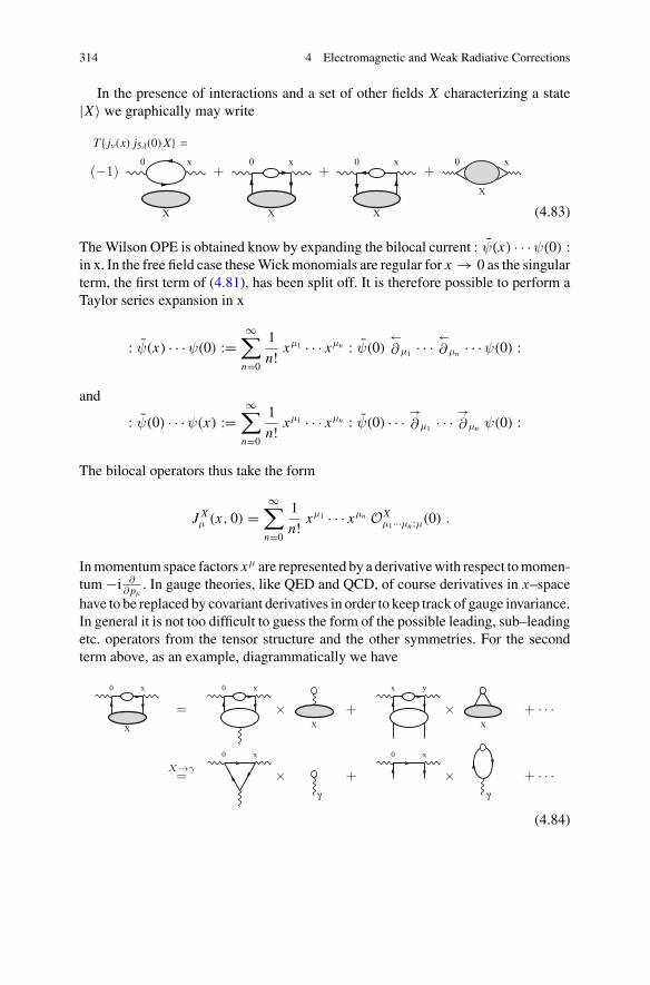
314 4 Electromagnetic and Weak Radiative Corrections

In the presence of interactions and a set of other fields X characterizing a state|X〉 we graphically may write

(4.83)

The Wilson OPE is obtained know by expanding the bilocal current : ψ(x) · · · ψ(0) :in x. In the free field case these Wick monomials are regular for x → 0 as the singularterm, the first term of (4.81), has been split off. It is therefore possible to perform aTaylor series expansion in x

: ψ(x) · · · ψ(0) :=∞∑

n=0

1

n! xμ1 · · · xμn : ψ(0)←∂ μ1 · · · ←

∂ μn · · ·ψ(0) :

and

: ψ(0) · · · ψ(x) :=∞∑

n=0

1

n! xμ1 · · · xμn : ψ(0) · · · →∂ μ1 · · · →

∂ μn ψ(0) :

The bilocal operators thus take the form

J Xμ (x, 0) =

∞∑

n=0

1

n! xμ1 · · · xμn OXμ1···μn;μ(0) .

In momentum space factors xμ are represented by a derivative with respect to momen-tum −i ∂

∂ pμ. In gauge theories, like QED and QCD, of course derivatives in x–space

have to be replaced by covariant derivatives in order to keep track of gauge invariance.In general it is not too difficult to guess the form of the possible leading, sub–leadingetc. operators from the tensor structure and the other symmetries. For the secondterm above, as an example, diagrammatically we have

(4.84)

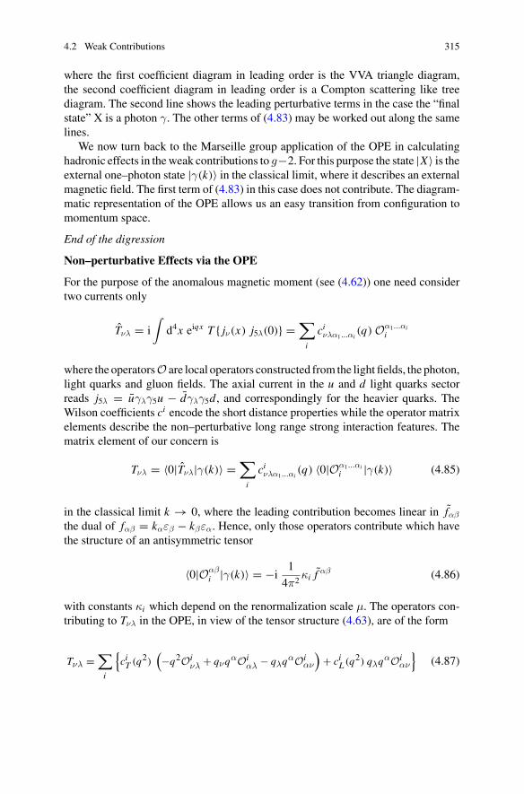
4.2 Weak Contributions 315

where the first coefficient diagram in leading order is the VVA triangle diagram,the second coefficient diagram in leading order is a Compton scattering like treediagram. The second line shows the leading perturbative terms in the case the “finalstate” X is a photon γ. The other terms of (4.83) may be worked out along the samelines.

We now turn back to the Marseille group application of the OPE in calculatinghadronic effects in the weak contributions to g−2. For this purpose the state |X〉 is theexternal one–photon state |γ(k)〉 in the classical limit, where it describes an externalmagnetic field. The first term of (4.83) in this case does not contribute. The diagram-matic representation of the OPE allows us an easy transition from configuration tomomentum space.

End of the digression

Non–perturbative Effects via the OPE

For the purpose of the anomalous magnetic moment (see (4.62)) one need considertwo currents only

Tνλ = i∫

d4x eiqx T { jν(x) j5λ(0)} =∑

i

ciνλα1...αi

(q) Oα1...αii

where the operators O are local operators constructed from the light fields, the photon,light quarks and gluon fields. The axial current in the u and d light quarks sectorreads j5λ = uγλγ5u − dγλγ5d, and correspondingly for the heavier quarks. TheWilson coefficients ci encode the short distance properties while the operator matrixelements describe the non–perturbative long range strong interaction features. Thematrix element of our concern is

Tνλ = 〈0|Tνλ|γ(k)〉 =∑

i

ciνλα1...αi

(q) 〈0|Oα1...αii |γ(k)〉 (4.85)

in the classical limit k → 0, where the leading contribution becomes linear in fαβ

the dual of fαβ = kαεβ − kβεα. Hence, only those operators contribute which havethe structure of an antisymmetric tensor

〈0|Oαβi |γ(k)〉 = −i

1

4π2κi f αβ (4.86)

with constants κi which depend on the renormalization scale μ. The operators con-tributing to Tνλ in the OPE, in view of the tensor structure (4.63), are of the form

Tνλ =∑

i

{ci

T (q2)(−q2Oi

νλ + qνqαOiαλ − qλqαOi

αν

)+ ci

L (q2) qλqαOiαν

}(4.87)

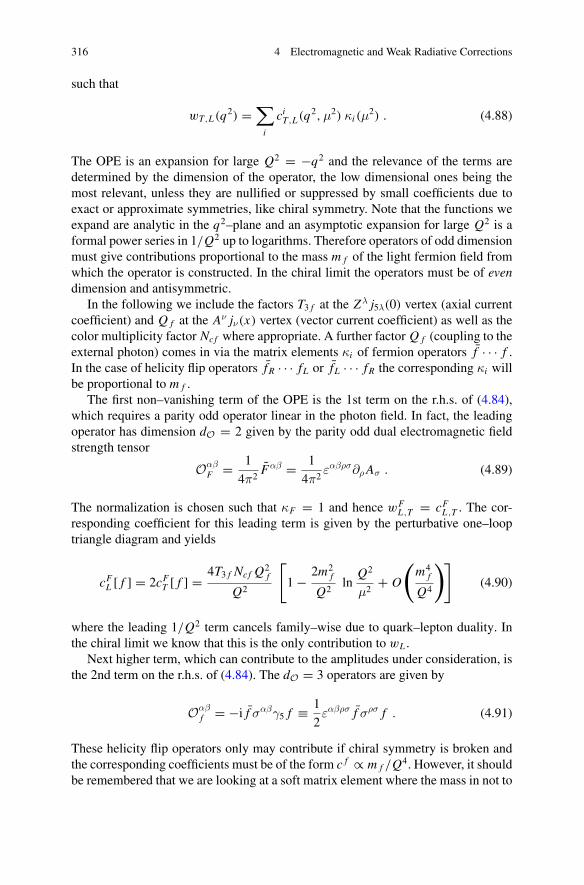
316 4 Electromagnetic and Weak Radiative Corrections

such that

wT,L(q2) =∑

i

ciT,L(q2,μ2) κi (μ

2) . (4.88)

The OPE is an expansion for large Q2 = −q2 and the relevance of the terms aredetermined by the dimension of the operator, the low dimensional ones being themost relevant, unless they are nullified or suppressed by small coefficients due toexact or approximate symmetries, like chiral symmetry. Note that the functions weexpand are analytic in the q2–plane and an asymptotic expansion for large Q2 is aformal power series in 1/Q2 up to logarithms. Therefore operators of odd dimensionmust give contributions proportional to the mass m f of the light fermion field fromwhich the operator is constructed. In the chiral limit the operators must be of evendimension and antisymmetric.

In the following we include the factors T3 f at the Zλ j5λ(0) vertex (axial currentcoefficient) and Q f at the Aν jν(x) vertex (vector current coefficient) as well as thecolor multiplicity factor Ncf where appropriate. A further factor Q f (coupling to theexternal photon) comes in via the matrix elements κi of fermion operators f · · · f .In the case of helicity flip operators f R · · · fL or fL · · · fR the corresponding κi willbe proportional to m f .

The first non–vanishing term of the OPE is the 1st term on the r.h.s. of (4.84),which requires a parity odd operator linear in the photon field. In fact, the leadingoperator has dimension dO = 2 given by the parity odd dual electromagnetic fieldstrength tensor

OαβF = 1

4π2Fαβ = 1

4π2εαβρσ∂ρ Aσ . (4.89)

The normalization is chosen such that κF = 1 and hence wFL ,T = cF

L ,T . The cor-responding coefficient for this leading term is given by the perturbative one–looptriangle diagram and yields

cFL [ f ] = 2cF

T [ f ] = 4T3 f Ncf Q2f

Q2

[

1 − 2m2f

Q2ln

Q2

μ2+ O

(m4

f

Q4

)]

(4.90)

where the leading 1/Q2 term cancels family–wise due to quark–lepton duality. Inthe chiral limit we know that this is the only contribution to wL .

Next higher term, which can contribute to the amplitudes under consideration, isthe 2nd term on the r.h.s. of (4.84). The dO = 3 operators are given by

Oαβf = −i f σαβγ5 f ≡ 1

2εαβρσ f σρσ f . (4.91)

These helicity flip operators only may contribute if chiral symmetry is broken andthe corresponding coefficients must be of the form c f ∝ m f /Q4. However, it shouldbe remembered that we are looking at a soft matrix element where the mass in not to

4.2 Weak Contributions 317

be identified with a current quark mass, rather a constituent mass is adequate whichdoes not vanish in the chiral limit (see (5.155) in Sect. 5.2.2). These coefficients aredetermined by tree level diagrams of Compton scattering type and again contributeequally to both amplitudes

c fL [ f ] = 2c f

T [ f ] = 8T3 f Q f m f

Q4.

Misusing the spirit of the OPE for the moment and neglecting the soft strong inter-action effects, we may calculate the soft photon quark matrix element in the QPMfrom the one–loop diagram shown in (4.84) (last diagram) which is UV divergentand in the MS scheme yields

κ f = −Q f Ncf m f lnμ2

m2f

. (4.92)

Inserting this in

Δ(dO=3)wL = 2Δ(dO=3)wT = 8

Q4

∑

f

T3 f Q f m f κ f

one recovers precisely the 1/Q4 term of (4.90). So far we have reproduced the knownperturbative result. Nevertheless the calculation illustrates the use of the OPE. Whilethe leading 1/Q2 term is not modified by soft gluon interactions, i.e., κF = 1 is exactas the state |γ〉 represents a physical on–shell photon, undressed from possible self–energy corrections, the physical κ f cannot be obtained from pQCD. So far it is anunknown constant. Here again, the spontaneous breakdown of the chiral symmetryand the existence of, in the chiral limit, non–vanishing quark condensates 〈ψψ〉0 �= 0plays a central role. Now, unlike in perturbation theory, κ f need not be proportionalto m f . In fact it is proportional to 〈ψψ〉0. As the condensate is of dimensionality 3,another quantity must enter carrying dimension of a mass and which is finite in thechiral limit. In the u, d quark sector this is either the pion decay constant F0 or theρ mass Mρ0 . As it is given by the matrix element (4.86) (see also the last graph ofEq. (4.84)) κ f must be proportional to Ncf Q f such that

κ f = Ncf Q f〈ψ f ψ f 〉0

F20

and hence [155, 164]

Δ(dO=3)wL = 2Δ(dO=3)wT = 8

Q4

∑

f

Ncf T3 f Q2f m f

〈ψ f ψ f 〉0

F20

. (4.93)

An overall constant, in fact is not yet fixed, however, it was chosen such that it repro-duces the expansion of non–perturbative modification of wL as a pion propagatorbeyond the chiral limit:

318 4 Electromagnetic and Weak Radiative Corrections

wL [mu,d �= 0] = 2

Q2 + m2π

= 2

Q2− 2m2

π

Q4+ · · ·

as we will see below. Identifying the 1/Q4 correction with the one of (4.93) is thepion dominance hypothesis used as a constraint to fix the normalization in [164]. Inthe isospin sector (4.93) gives

ΔwL = 8Ncf

Q4× 1

2

(4

9mu − 1

9mu

) 〈ψ f ψ f 〉0

F20

and for mu ≈ md ≈ mu+md2 and using the GMOR relation (mu + md) 〈ψ f ψ f 〉0 =

−F2π m2

π and with F0 ≈ Fπ we indeed have ΔwL = − 2m2π

Q4 . Note that the quark massdifference mu − md is small relative to mu + md , and is not important here. It leadsto a small mixing with heavier pseudoscalar states.

For later use we mention that κ f can be represented in terms of the magneticsusceptibility χ introduced by Ioffe and Smilga [171]

κ f = −4π2 Q f 〈ψ f ψ f 〉0 χ (4.94)

In our case, under the pion pole dominance assumption (see [164] for a more detaileddiscussion), one obtains

χ = − Nc

4π2 F2π

− 1

(335 MeV)2. (4.95)

All operators of dO = 4 may be reduced via the equation of motion to dO = 3operators carrying a factor of mass in front:

f (Dαγβ − Dβγα) γ5 f = −m f f σαβγ5 f .

They thus do not yield new type of corrections and will not be considered further, asthey are suppressed by the light quark masses as m2

f /Q4.Similarly the dimension dO = 5 operators

f f Fαβ, f γ5 f Fαβ, · · ·

which are contributing to the 1/Q6 coefficient, require a factor m f and thus againare suppressed by nearby chiral symmetry.

More important are the dimension dO = 6 operators, which yield 1/Q6 termsand give non–vanishing contributions in the chiral limit. Here again the specific lowenergy structure of QCD comes into play, namely the spontaneous symmetry break-ing of the chiral symmetry (in the symmetry limit). The latter is characterized by the

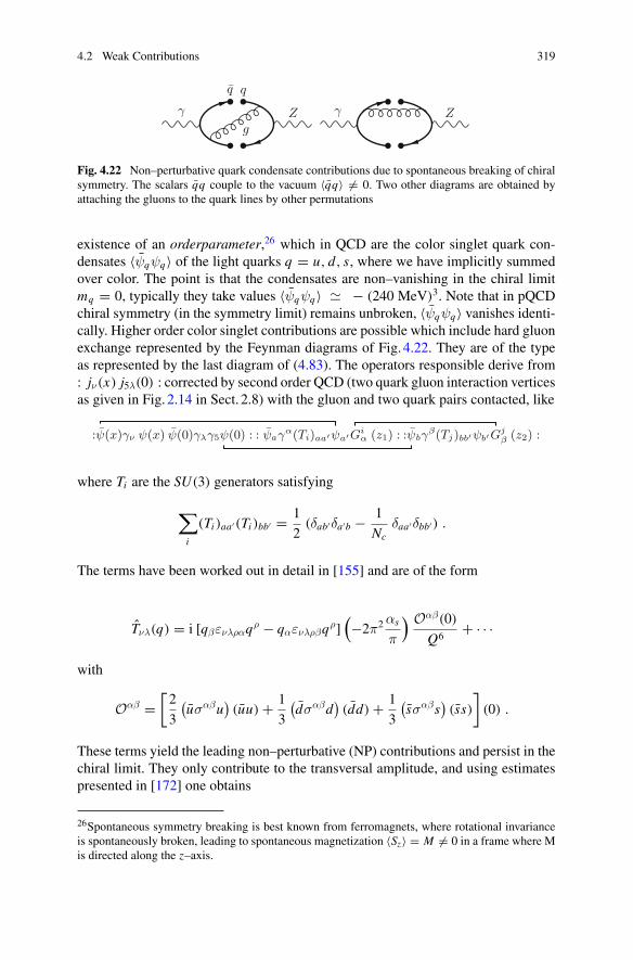
4.2 Weak Contributions 319

γ Z γ Z

qq

g

Fig. 4.22 Non–perturbative quark condensate contributions due to spontaneous breaking of chiralsymmetry. The scalars qq couple to the vacuum 〈qq〉 �= 0. Two other diagrams are obtained byattaching the gluons to the quark lines by other permutations

existence of an orderparameter,26 which in QCD are the color singlet quark con-densates 〈ψqψq〉 of the light quarks q = u, d, s, where we have implicitly summedover color. The point is that the condensates are non–vanishing in the chiral limitmq = 0, typically they take values 〈ψqψq〉 − (240 MeV)3. Note that in pQCDchiral symmetry (in the symmetry limit) remains unbroken, 〈ψqψq〉 vanishes identi-cally. Higher order color singlet contributions are possible which include hard gluonexchange represented by the Feynman diagrams of Fig. 4.22. They are of the typeas represented by the last diagram of (4.83). The operators responsible derive from: jν(x) j5λ(0) : corrected by second order QCD (two quark gluon interaction verticesas given in Fig. 2.14 in Sect. 2.8) with the gluon and two quark pairs contacted, like

:ψ(x)γν ψ(x) ψ(0)γλγ5ψ(0) : : ψaγα(Ti)aa′ψa′Giα (z1) : :ψbγ

β(Tj)bb′ψb′Gjβ (z2) :

where Ti are the SU(3) generators satisfying

∑

i

(Ti )aa′(Ti )bb′ = 1

2(δab′δa′b − 1

Ncδaa′δbb′) .

The terms have been worked out in detail in [155] and are of the form

Tνλ(q) = i [qβενλραqρ − qαενλρβqρ](−2π2 αs

π

) Oαβ(0)

Q6+ · · ·

with

Oαβ =[

2

3

(uσαβu

)(uu) + 1

3

(dσαβd

)(dd) + 1

3

(sσαβs

)(ss)

](0) .

These terms yield the leading non–perturbative (NP) contributions and persist in thechiral limit. They only contribute to the transversal amplitude, and using estimatespresented in [172] one obtains

26Spontaneous symmetry breaking is best known from ferromagnets, where rotational invarianceis spontaneously broken, leading to spontaneous magnetization 〈Sz〉 = M �= 0 in a frame where Mis directed along the z–axis.

320 4 Electromagnetic and Weak Radiative Corrections

wT (Q2)NP −16

9π2 2

F20

αs

π

〈ψψ〉2

Q6(4.96)

for large enough Q2, the ρ mass being the typical scale. This NP contribution breaksthe degeneracy wT (Q2) = 1

2wL(Q2) which is valid in perturbation theory.27 Takinginto account the quark condensates together with explicit chiral symmetry breaking,according to (4.93), also a term

ΔwT (Q2)NP = 1

2ΔwL(Q2)NP 4

9

3

2F20

(4mu − md − ms)〈ψψ〉Q4

, (4.97)

yields an NP contribution, but this time to both wT and wL . The consequences ofthe OPE for the light quarks u, d and s in the chiral limit may be summarized asfollows [153]:

wL [u, d]mu,d=0 = −3 wL [s]ms=0 = 2

Q2, (4.98)

wT [u, d]mu,d=0 = −3 wT [s]ms=0 = 1

Q2− 32παs

9 Q6

〈ψψ〉20

F2π

+ O(Q−8) .

The condensates are fixed essentially by the Gell-Mann-Oakes-Renner (GMOR)relations (4.76)

(mu + md) 〈ψψ〉0 = −F20 m2

π

ms〈ψψ〉0 −F20 M2

K .

and the last term of (4.98) numerically estimates to

wT (Q2)NP ∼ −αs (0.772 GeV)4/Q6 ,

i.e., the scale is essentially the ρ mass. Our estimates are rough leading order estimatesin the sense of CHPT. The index 0 denotes quantities in the chiral limit. Except fromthe masses of the pseudoscalars, which vanish in the chiral limit, we do not distinguishbetween quantities like the pseudoscalar decay constants F0, Fπ and FK . Similarly,we assume the light quark condensates 〈ψψ〉0 to be approximately equal for u, d ands quarks. Furthermore, we use m2

η 43 m2

K and M2η′ M2

0 with M0 950 MeV(for CHPT refinements we refer to [166]). Also isospin symmetry will be assumedwhere appropriate.

In fact the non–perturbative refinements of the leading π0, η, η′ exchange contri-butions in wL requires the inclusion of vector–meson exchanges which contribute towT . More precisely, for the transversal function the intermediate states have to be

27The OPE only provides information on wT for Q2 large. At low Q2 we only know that wT (0) =128π2 CW

22 where CW22 is one of the unknown CHPT constants in the O(p6) parity odd part of the

chiral Lagrangian [173].

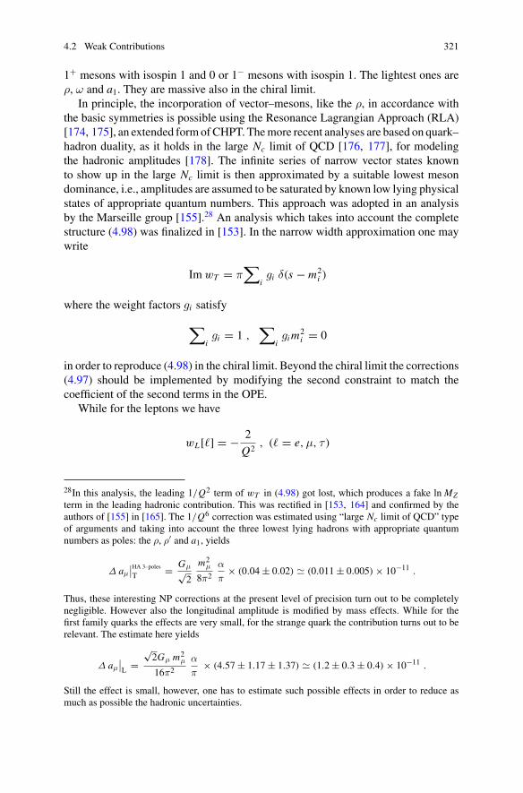
4.2 Weak Contributions 321

1+ mesons with isospin 1 and 0 or 1− mesons with isospin 1. The lightest ones areρ, ω and a1. They are massive also in the chiral limit.

In principle, the incorporation of vector–mesons, like the ρ, in accordance withthe basic symmetries is possible using the Resonance Lagrangian Approach (RLA)[174, 175], an extended form of CHPT. The more recent analyses are based on quark–hadron duality, as it holds in the large Nc limit of QCD [176, 177], for modelingthe hadronic amplitudes [178]. The infinite series of narrow vector states knownto show up in the large Nc limit is then approximated by a suitable lowest mesondominance, i.e., amplitudes are assumed to be saturated by known low lying physicalstates of appropriate quantum numbers. This approach was adopted in an analysisby the Marseille group [155].28 An analysis which takes into account the completestructure (4.98) was finalized in [153]. In the narrow width approximation one maywrite

Im wT = π∑

igi δ(s − m2

i )

where the weight factors gi satisfy

∑

igi = 1 ,

∑

igi m

2i = 0

in order to reproduce (4.98) in the chiral limit. Beyond the chiral limit the corrections(4.97) should be implemented by modifying the second constraint to match thecoefficient of the second terms in the OPE.

While for the leptons we have

wL [�] = − 2

Q2, (� = e,μ, τ )

28In this analysis, the leading 1/Q2 term of wT in (4.98) got lost, which produces a fake ln MZterm in the leading hadronic contribution. This was rectified in [153, 164] and confirmed by theauthors of [155] in [165]. The 1/Q6 correction was estimated using “large Nc limit of QCD” typeof arguments and taking into account the three lowest lying hadrons with appropriate quantumnumbers as poles: the ρ, ρ′ and a1, yields

Δ aμ

∣∣HA 3–poles

T = Gμ√2

m2μ

8π2

α

π× (0.04 ± 0.02) (0.011 ± 0.005) × 10−11 .

Thus, these interesting NP corrections at the present level of precision turn out to be completelynegligible. However also the longitudinal amplitude is modified by mass effects. While for thefirst family quarks the effects are very small, for the strange quark the contribution turns out to berelevant. The estimate here yields

Δ aμ

∣∣L =

√2Gμ m2

μ

16π2

α

π× (4.57 ± 1.17 ± 1.37) (1.2 ± 0.3 ± 0.4) × 10−11 .

Still the effect is small, however, one has to estimate such possible effects in order to reduce asmuch as possible the hadronic uncertainties.

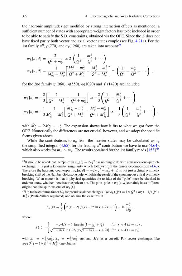
322 4 Electromagnetic and Weak Radiative Corrections

the hadronic amplitudes get modified by strong interaction effects as mentioned: asufficient number of states with appropriate weight factors has to be included in orderto be able to satisfy the S.D. constraints, obtained via the OPE. Since the Z does nothave fixed parity both vector and axial vector states couple (see Fig. 4.21a). For the1st family π0, ρ(770) and a1(1260) are taken into account29

wL [u, d] = 2

Q2 + m2π

2

(1

Q2− m2

π

Q4+ · · ·

)

wT [u, d] = 1

M2a1

− M2ρ

[M2

a1− m2

π

Q2 + M2ρ

− M2ρ − m2

π

Q2 + M2a1

](

1

Q2− m2

π

Q4+ · · ·

),

for the 2nd family η′(960), η(550), φ(1020) and f1(1420) are included

wL [s] = −2

3

[2

Q2 + M2η′

− 1

Q2 + m2η

] −2

3

(1

Q2− M2

η

Q4+ · · ·

)

wT [s] = −1

3

1

M2f1

− M2φ

[M2

f1− m2

η

Q2 + M2φ

− M2φ − m2

η

Q2 + M2f1

] −1

3

(1

Q2− m2

η

Q4+ · · ·

)

.

with M2η = 2M2

η′ − m2η. The expansion shows how it fits to what we got from the

OPE. Numerically the differences are not crucial, however, and we adopt the specificforms given above.

While the contributions to aμ from the heavier states may be calculated usingthe simplified integral (4.65), for the leading π0 contribution we have to use (4.64),which also works for mπ ∼ mμ. The results obtained for the 1st family reads [153]30

29It should be noted that the “pole” in wL [�] = 2/q2 has nothing to do with a massless one–particleexchange, it is just a kinematic singularity which follows from the tensor decomposition (4.63).Therefore the hadronic counterpart wL [u, d] = −2/(q2 − m2

π + iε) is not just a chiral symmetrybreaking shift of the Nambu–Goldstone pole, which is the result of the spontaneous chiral symmetrybreaking. What matters is that in physical quantities the residue of the “pole” must be checked inorder to know, whether there is a true pole or not. The pion–pole in wL [u, d] certainly has a differentorigin than the spurious one of wL [�].30Up to the common factorK2 for pseudoscalar exchanges like wL (Q2) = 1/(Q2 +m2

π)−1/(Q2 +M2

Z ) (Pauli–Villars regulated) one obtains the exact result

FL (x) = 1

6

(x (x + 2) f (x) − x2 ln x + 2x + 3

)− ln

m2μ

M2Z

,

where

f (x) ={ −√

4/x − 1(arcsin

(1 − x

2

)+ π2

)for x < 4 (x = xπ) ,√

1 − 4/x ln(−2/(x

√1 − 4/x − x + 2)

)for x > 4 (x = xη) ,

with xπ = m2π/m2

μ, xη = m2η/m2

μ etc. and MZ as a cut-off. For vector exchanges like

wT (Q2) = 1/(Q2 + M2ρ ) one obtains

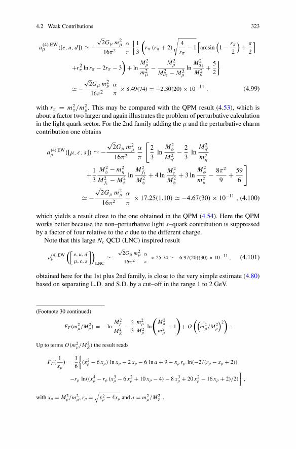
4.2 Weak Contributions 323

a(4) EWμ ([e, u, d]) −

√2Gμ m2

μ

16π2α

π

{1

3

(rπ (rπ + 2)

√4

rπ− 1

[arcsin

(1 − rπ

2

)+ π

2

]

+r2π ln rπ − 2rπ − 3

)+ ln

M2ρ

m2μ

− M2ρ

M2a1 − M2

ρ

lnM2

a1

M2ρ

+ 5

2

}

−√

2Gμ m2μ

16π2α

π× 8.49(74) = −2.30(20) × 10−11 . (4.99)

with rπ = m2π/m2

μ. This may be compared with the QPM result (4.53), which isabout a factor two larger and again illustrates the problem of perturbative calculationin the light quark sector. For the 2nd family adding the μ and the perturbative charmcontribution one obtains

a(4) EWμ ([μ, c, s]) −

√2Gμ m2

μ

16π2

α

π

[2

3ln

M2φ

M2η′

− 2

3ln

M2η′

m2η

+1

3

M2φ − m2

η

M2f1

− M2φ

lnM2

f1

M2φ

+ 4 lnM2

c

M2φ

+ 3 lnM2

φ

m2μ

− 8π2

9+ 59

6

]

−√

2Gμ m2μ

16π2

α

π× 17.25(1.10) −4.67(30) × 10−11 , (4.100)

which yields a result close to the one obtained in the QPM (4.54). Here the QPMworks better because the non–perturbative light s–quark contribution is suppressedby a factor of four relative to the c due to the different charge.

Note that this large Nc QCD (LNC) inspired result

a(4) EWμ

([e, u, dμ, c, s

])

LNC −

√2Gμ m2

μ

16π2α

π× 25.74 −6.97(20)(30) × 10−11 , (4.101)

obtained here for the 1st plus 2nd family, is close to the very simple estimate (4.80)based on separating L.D. and S.D. by a cut–off in the range 1 to 2 GeV.

(Footnote 30 continued)

FT (m2μ/M2

ρ ) = − lnM2

ρ

M2Z

− 2

3

m2μ

M2ρ

ln

(M2

ρ

m2μ

+ 1

)

+ O

((m2

μ/M2ρ

)2)

.

Up to terms O(m2μ/M2

Z ) the result reads

FT (1

xρ) = 1

6

{(x2

ρ − 6 xρ) ln xρ − 2 xρ − 6 ln a + 9 − xρ rρ ln(−2/(rρ − xρ + 2))

−rρ ln((x4ρ − rρ (x3

ρ − 6 x2ρ + 10 xρ − 4) − 8 x3

ρ + 20 x2ρ − 16 xρ + 2)/2)

},

with xρ = M2ρ/m2

μ, rρ =√

x2ρ − 4xρ and a = m2

μ/M2Z .

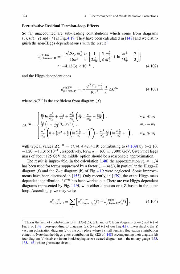
324 4 Electromagnetic and Weak Radiative Corrections

Perturbative Residual Fermion–loop Effects

So far unaccounted are sub–leading contributions which come from diagrams(c), (d), (e) and ( f ) in Fig. 4.19. They have been calculated in [148] and we distin-guish the non-Higgs dependent ones with the result31

a(4) EWμ;f-rem,no H = −

√2Gμ m2

μ

16π2

α

π

{1

2s2W

[5

8

m2t

M2W

+ lnm2

t

M2W

+ 7

3

]}

−4.12(3) × 10−11 , (4.102)

and the Higgs dependent ones

a(4) EWμ;t-rem,Hγ = −

√2Gμ m2

μ

16π2

α

πΔCt H (4.103)

where ΔCt H is the coefficient from diagram ( f )

ΔCt H =

⎧⎪⎪⎪⎪⎪⎪⎨

⎪⎪⎪⎪⎪⎪⎩

169 ln m2

tm2

H+ 104

27 + m2H

m2t

(415 ln m2

tm2

H+ 104

225

), m H mt

323

(1 − 1√

3Cl2 (π/3)

), m H = mt

m2t

m2H

(

8 + 89π2 + 8

3

(ln

m2H

m2t

− 1

)2)

− m4t

m4H

323

(ln

m2H

m2t

+ 1

), m H � mt

with typical values ΔCt H = (7.74, 4.42, 4.19) contributing to (4.109) by (−2.10,

−1.20, −1.13)×10−11, respectively, for m H = (60, mt , 300) GeV. Given the Higgsmass of about 125 GeV the middle option should be a reasonable approximation.

The result is improvable. In the calculation [148] the approximation s2W ≈ 1/4

has been used for terms suppressed by a factor (1 − 4s2W ), in particular the Higgs–Z

diagram (f) and the Z–γ diagram (b) of Fig. 4.19 were neglected. Some improve-ments have been discussed in [153]. Only recently, in [179], the exact Higgs massdependent contribution ΔCt H has been worked out. There are two Higgs-dependentdiagrams represented by Fig. 4.19f, with either a photon or a Z-boson in the outerloop. Accordingly, we may write

a(4)EWμ;f-rem,H =

∑

f

[a(4)EW

μ;f-rem,Hγ( f ) + a(4)EWμ;f-rem,HZ( f )

], (4.104)

31This is the sum of contributions Eqs. (13)–(15), (21) and (27) from diagrams (a)–(c) and (e) ofFig. 1 of [148], corresponding to diagrams (d), (e) and (c) of our Fig. 4.19. Interestingly, the Zvacuum polarization diagram (c) is the only place where a small neutrino fluctuation contributioncomes in. Note that the Higgs-ghost contribution Eq. (22) of [148] accompanying their diagram (d)(our diagram (a)) is absent in our bookkeeping, as we treated diagram (a) in the unitary gauge [153,155, 165] where ghosts are absent.

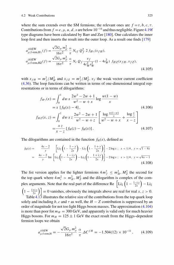
4.2 Weak Contributions 325

where the sum extends over the SM fermions; the relevant ones are f = t, b, c, τ .Contributions from f = e,μ, u, d, s are below 10−14 and thus negligible. Figure 4.19ftype diagrams have been calculated by Barr and Zee [180]. One calculates the innerloop first and then inserts the result into the outer loop. As a result one finds [179]

a(4)EWμ;f-rem,Hγ( f ) =

√2Gμ m2

μ

16π2α

πNcf Q2

f 2 fHγ(x f H ),

a(4)EWμ;f-rem,HZ( f ) =

√2Gμ m2

μ

16π2α

πNc Q f

v f

4c2W s2

W

(1 − 4s2W ) fH Z (x f H , x f Z ),

(4.105)

with x f H = m2f /M2

H and x f Z = m2f /M2

Z . v f the weak vector current coefficient(4.36). The loop functions can be written in terms of one-dimensional integral rep-resentations or in terms of dilogarithms:

fHγ(x) =∫ 1

0dw x

2w2 − 2w + 1

w2 − w + xlog

w(1 − w)

x

= x [ fH(x) − 4] , (4.106)

fH Z (x, z) =∫ 1

0dw x z

2w2 − 2w + 1

w2 − w + z

[log w(1−w)

x

w2 − w + x+ log x

z

x − z

]

= x z

x − z[ fH(z) − fH(x)] . (4.107)

The dilogarithms are contained in the function fH(x), defined as

fH(x) = 4x − 2

y

[Li2

(1 − 1 − y

2x

)− Li2

(1 − 1 + y

2x

)]− 2 log x ; x < 1/4 , y = √

1 − 4x

= 4x − 2

yIm

[Li2

(1 − 1 − i y

2x

)− Li2

(1 − 1 + i y

2x

)]− 2 log x ; x > 1/4 , y = √

4x − 1

(4.108)

The fist version applies for the lighter fermions 4 m2f ≤ m2

H , M2Z the second for

the top quark where 4 m2t > m2

H , M2Z and the dilogarithm is complex of the com-

plex arguments. Note that the real part of the difference Re[Li2(

1 − 1−i y2x

)− Li2

(1 − 1+i y

2x

)]= 0 vanishes, obviously the integrals above are real for real x, z > 0.

Table 4.13 illustrates the relative size of the contributions from the top quark loopsolely and including b, c and τ as well, the H − Z contribution is suppressed by anorder of magnitude for not too light Higgs boson masses. The approximation (4.104)is more than poor for m H = 300 GeV, and apparently is valid only for much heavierHiggs bosons. For m H = 125 ± 1 GeV the exact result from the Higgs–dependentfermion loops we obtain

a(4)EWμ;f-rem,H = −

√2Gμ m2

μ

16π2

α

πΔC f H = −1.504(12) × 10−11 , (4.109)

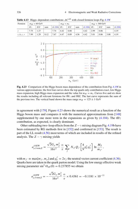
326 4 Electromagnetic and Weak Radiative Corrections

Table 4.13 Higgs–dependent contributions ΔCt H with closed fermion loops Fig. 4.19fFermion m H = 60 GeV m H = mt m H = 300 GeV

Hγ H Z sum (4.104) Hγ H Z sum (4.104) Hγ H Z sum (4.104)

t 7.75 1.27 7.74 4.42 0.08 4.42 2.99 0.06 4.19

t, b, c, τ 7.99 1.29 8.12 7.67 4.47 0.09 4.56 4.42 3.01 0.06 3.08 4.19

Fig. 4.23 Comparison of the Higgs boson mass dependence of the contribution from Fig. 4.19f invarious approximations: the first four curves show the top quark only contribution exact, low Higgsmass expansion, high Higgs mass expansion and the value for m H = mt . Curves five and six showthe results including all relevant fermions for fHγ and fHZ. The last curve represents the sum ofthe previous two. The vertical band shown the mass range m H = 125 ± 1 GeV

in agreement with [179]. Figure 4.23 shows the numerical result as a function of theHiggs boson mass and compares it with the numerical approximations from [148]supplemented by one more term in the expansions as given by (4.104). The tHγcontribution, as expected, is clearly dominant.

Other subleading two–loop effects from the Z −γ mixing diagram Fig. 4.19b havebeen estimated by RG methods first in [152] and confirmed in [153]. The result ispart of the LL result (4.56) most terms of which are included in results of the refinedanalysis. The Z − γ mixing yields

a(4)EWμ;f-rem,Z =

√2Gμ m2

μ

16π2

α

π

∑

f

Ncf Q f

[4

9g

μV g

fV

]ln

MZ

m f ′,

with m f ′ ≡ max[m f , mμ] and gfV = 2v f the neutral vector current coefficient (4.36).

Quarks here are taken in the quark parton model. Using the low energy effective weakmixing parameter sin2 Θeff(0) = 0.237855 we obtain

a(4)EWμ;f-rem,Z = −

√2Gμ m2

μ

16π2

α

π× 0.4361 = −0.1181 × 10−11

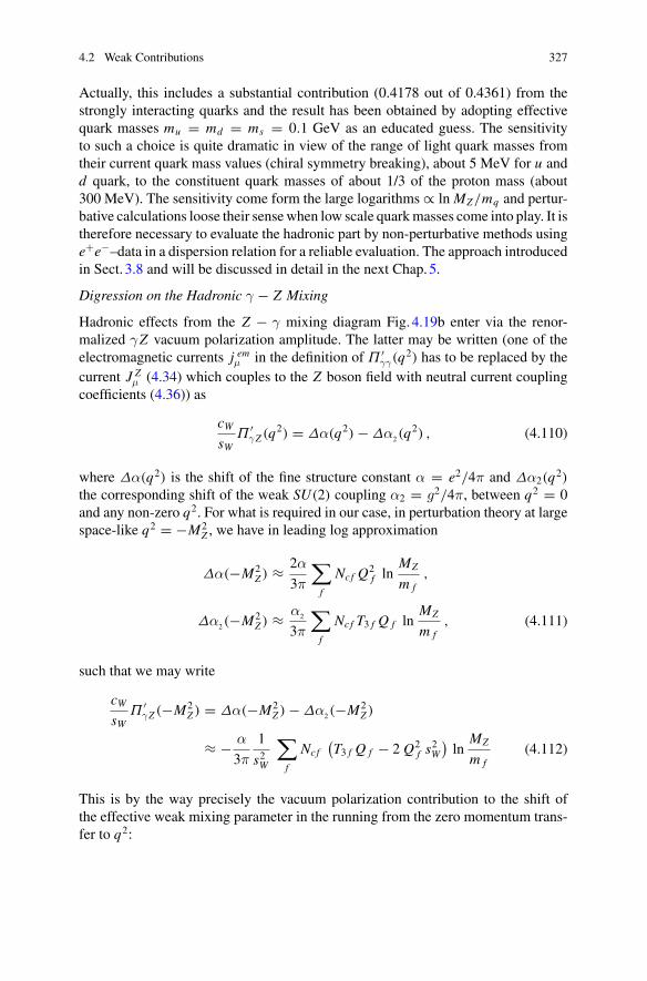
4.2 Weak Contributions 327

Actually, this includes a substantial contribution (0.4178 out of 0.4361) from thestrongly interacting quarks and the result has been obtained by adopting effectivequark masses mu = md = ms = 0.1 GeV as an educated guess. The sensitivityto such a choice is quite dramatic in view of the range of light quark masses fromtheir current quark mass values (chiral symmetry breaking), about 5 MeV for u andd quark, to the constituent quark masses of about 1/3 of the proton mass (about300 MeV). The sensitivity come form the large logarithms ∝ ln MZ/mq and pertur-bative calculations loose their sense when low scale quark masses come into play. It istherefore necessary to evaluate the hadronic part by non-perturbative methods usinge+e−–data in a dispersion relation for a reliable evaluation. The approach introducedin Sect. 3.8 and will be discussed in detail in the next Chap. 5.

Digression on the Hadronic γ − Z Mixing

Hadronic effects from the Z − γ mixing diagram Fig. 4.19b enter via the renor-malized γZ vacuum polarization amplitude. The latter may be written (one of theelectromagnetic currents j em

μ in the definition of Π ′γγ(q

2) has to be replaced by thecurrent J Z

μ (4.34) which couples to the Z boson field with neutral current couplingcoefficients (4.36)) as

cW

sWΠ ′

γZ (q2) = Δα(q2) − Δα2(q2) , (4.110)

where Δα(q2) is the shift of the fine structure constant α = e2/4π and Δα2(q2)

the corresponding shift of the weak SU(2) coupling α2 = g2/4π, between q2 = 0and any non-zero q2. For what is required in our case, in perturbation theory at largespace-like q2 = −M2

Z , we have in leading log approximation

Δα(−M2Z ) ≈ 2α

3π

∑

f

Ncf Q2f ln

MZ

m f,

Δα2(−M2Z ) ≈ α2

3π

∑

f

Ncf T3 f Q f lnMZ

m f, (4.111)

such that we may write

cW

sWΠ ′

γZ (−M2Z ) = Δα(−M2

Z ) − Δα2(−M2Z )

≈ − α

3π

1

s2W

∑

f

Ncf(T3 f Q f − 2 Q2

f s2W

)ln

MZ

m f(4.112)

This is by the way precisely the vacuum polarization contribution to the shift ofthe effective weak mixing parameter in the running from the zero momentum trans-fer to q2:

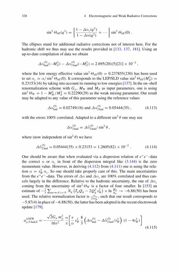
328 4 Electromagnetic and Weak Radiative Corrections

sin2 Θeff(q2) =

{1 − Δα2(q

2)

1 − Δα(q2)+ · · ·

}sin2 Θeff(0) .

The ellipses stand for additional radiative corrections not of interest here. For thehadronic shift we thus may use the results provided in [133, 137, 181]. Using anup-to-date compilation of data we obtain

Δα(5)had(−M2

Z ) − Δα(5)2 had(−M2

Z ) = 2.695(20)(5)[21] × 10−2 ,

where the low energy effective value sin2 Θeff(0) = 0.237855(230) has been usedto set α2 = α/ sin2 Θeff(0). It corresponds to the LEP/SLD value sin2 Θeff(M2

Z ) =0.23153(16) by taking into account its running to low energies [137]. In the on–shellrenormalization scheme with Gμ, MW and MZ as input parameters, one is usingsin2 ΘW = 1 − M2

W /M2Z = 0.22290(29) as the weak mixing parameter. Our result

may be adapted to any value of this parameter using the reference values

Δα(5)had = 0.02749(16) and Δα(5)

2 had = 0.05444(35) , (4.113)

with the errors 100% correlated. Adapted to a different sin2 θ one may use

Δα(5)2 had = Δα(5)

2 had/ sin2 θ ,

where (now independent of sin2 θ) we have

Δα(5)2 had = 0.05444(35) × 0.23153 = 1.2605(82) × 10−2 . (4.114)

One should be aware that when evaluated via a dispersion relation of e+e−–datathe correct α or α2 in front of the dispersion integral like (3.144) is the zeromomentum value. However, in deriving (4.112) from (4.111) one is using the rela-tion α = s2

W α2 . So one should take properly care of this. The main uncertaintiesfrom the e+e−–data. The errors of Δα and Δα2 are 100% correlated and thus can-cels largely in the difference. Relative to the hadronic uncertainty, the one of Δα2

coming from the uncertainty of sin2 ΘW is a factor of four smaller. In [153] anestimate of − 2

3

∑q=u,d,s,c,b Nq

(Tq Qq − 2Q2

q s2W

)× ln MZmq

→ −6.88(50) has beenused. The relative normalization factor is α

2πs2W

, such that our result corresponds to

−5.87(4) in place of −6.88(50), the latter has been adopted in the recent electroweakupdate [179].

a(4)EWμ;5-had,Z = −

√2Gμ m2

μ

16π2

α

π

[π

αs2

W

8

3

(Δα(5)

had − Δα(5)2 had/s2

W

)(1 − 4s2

W )

]

(4.115)

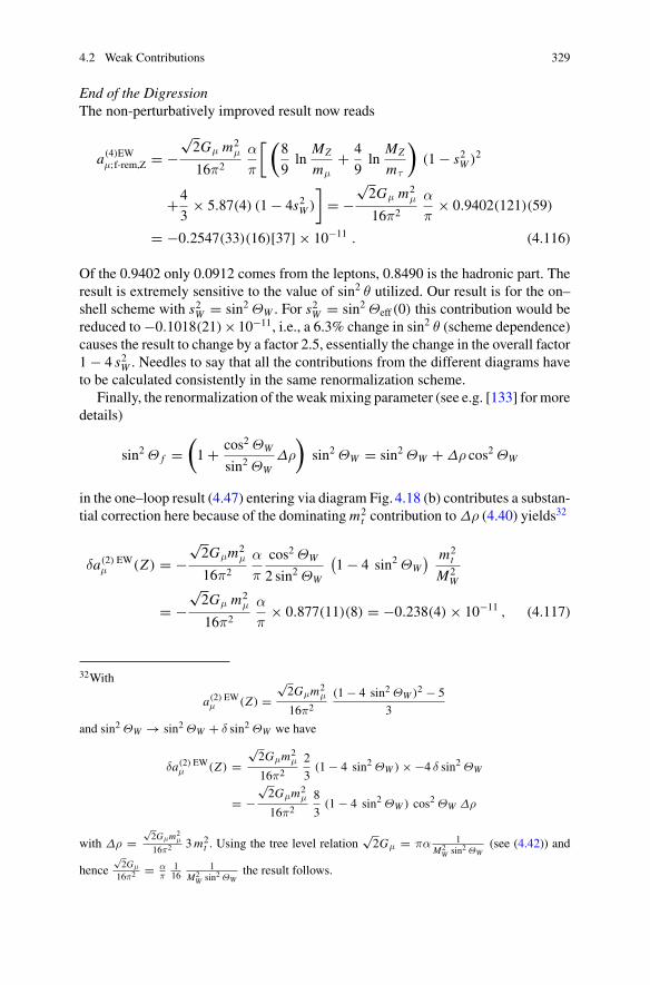
4.2 Weak Contributions 329

End of the DigressionThe non-perturbatively improved result now reads

a(4)EWμ;f-rem,Z = −

√2Gμ m2

μ

16π2

α

π

[(8

9ln

MZ

mμ+ 4

9ln

MZ

mτ

)(1 − s2

W )2

+4

3× 5.87(4) (1 − 4s2

W )

]= −

√2Gμ m2

μ

16π2

α

π× 0.9402(121)(59)

= −0.2547(33)(16)[37] × 10−11 . (4.116)

Of the 0.9402 only 0.0912 comes from the leptons, 0.8490 is the hadronic part. Theresult is extremely sensitive to the value of sin2 θ utilized. Our result is for the on–shell scheme with s2

W = sin2 ΘW . For s2W = sin2 Θeff(0) this contribution would be

reduced to −0.1018(21)× 10−11, i.e., a 6.3% change in sin2 θ (scheme dependence)causes the result to change by a factor 2.5, essentially the change in the overall factor1 − 4 s2

W . Needles to say that all the contributions from the different diagrams haveto be calculated consistently in the same renormalization scheme.

Finally, the renormalization of the weak mixing parameter (see e.g. [133] for moredetails)

sin2 Θ f =(

1 + cos2 ΘW

sin2 ΘWΔρ

)sin2 ΘW = sin2 ΘW + Δρ cos2 ΘW

in the one–loop result (4.47) entering via diagram Fig. 4.18 (b) contributes a substan-tial correction here because of the dominating m2

t contribution to Δρ (4.40) yields32

δa(2) EWμ (Z) = −

√2Gμm2

μ

16π2

α

π

cos2 ΘW

2 sin2 ΘW

(1 − 4 sin2 ΘW

) m2t

M2W

= −√

2Gμ m2μ

16π2

α

π× 0.877(11)(8) = −0.238(4) × 10−11 , (4.117)

32With

a(2) EWμ (Z) =

√2Gμm2

μ

16π2

(1 − 4 sin2 ΘW )2 − 5

3

and sin2 ΘW → sin2 ΘW + δ sin2 ΘW we have

δa(2) EWμ (Z) =

√2Gμm2

μ

16π2

2

3(1 − 4 sin2 ΘW ) × −4 δ sin2 ΘW

= −√

2Gμm2μ

16π2

8

3(1 − 4 sin2 ΘW ) cos2 ΘW Δρ

with Δρ =√

2Gμm2μ

16π2 3 m2t . Using the tree level relation

√2Gμ = πα 1

M2W sin2 ΘW

(see (4.42)) and

hence√

2Gμ

16π2 = απ

116

1M2

W sin2 ΘWthe result follows.

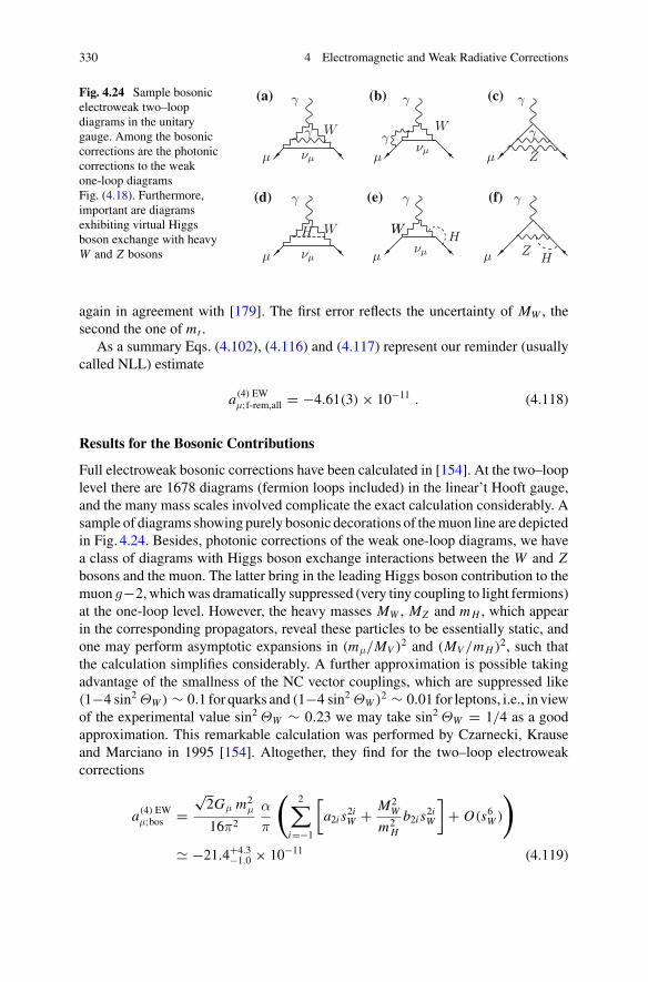
330 4 Electromagnetic and Weak Radiative Corrections

Fig. 4.24 Sample bosonicelectroweak two–loopdiagrams in the unitarygauge. Among the bosoniccorrections are the photoniccorrections to the weakone-loop diagramsFig. (4.18). Furthermore,important are diagramsexhibiting virtual Higgsboson exchange with heavyW and Z bosons

μ

W

γ

γ

νμ

γ

γW

μνμ

γ

γ

μ Z

μ

W

γ

H

νμ

WH

μνμ

γ

W

Hμ Z

γ

(b) (c)(a)

(e) (f)(d)

again in agreement with [179]. The first error reflects the uncertainty of MW , thesecond the one of mt .

As a summary Eqs. (4.102), (4.116) and (4.117) represent our reminder (usuallycalled NLL) estimate

a(4) EWμ;f-rem,all = −4.61(3) × 10−11 . (4.118)

Results for the Bosonic Contributions

Full electroweak bosonic corrections have been calculated in [154]. At the two–looplevel there are 1678 diagrams (fermion loops included) in the linear’t Hooft gauge,and the many mass scales involved complicate the exact calculation considerably. Asample of diagrams showing purely bosonic decorations of the muon line are depictedin Fig. 4.24. Besides, photonic corrections of the weak one-loop diagrams, we havea class of diagrams with Higgs boson exchange interactions between the W and Zbosons and the muon. The latter bring in the leading Higgs boson contribution to themuon g−2, which was dramatically suppressed (very tiny coupling to light fermions)at the one-loop level. However, the heavy masses MW , MZ and m H , which appearin the corresponding propagators, reveal these particles to be essentially static, andone may perform asymptotic expansions in (mμ/MV )2 and (MV /m H )2, such thatthe calculation simplifies considerably. A further approximation is possible takingadvantage of the smallness of the NC vector couplings, which are suppressed like(1−4 sin2 ΘW ) ∼ 0.1 for quarks and (1−4 sin2 ΘW )2 ∼ 0.01 for leptons, i.e., in viewof the experimental value sin2 ΘW ∼ 0.23 we may take sin2 ΘW = 1/4 as a goodapproximation. This remarkable calculation was performed by Czarnecki, Krauseand Marciano in 1995 [154]. Altogether, they find for the two–loop electroweakcorrections

a(4) EWμ;bos =

√2Gμ m2

μ

16π2

α

π

(2∑

i=−1

[a2i s

2iW + M2

W

m2H

b2i s2iW

]+ O(s6

W )

)

−21.4+4.3−1.0 × 10−11 (4.119)

4.2 Weak Contributions 331

for MW = 80.392 GeV (sin2 ΘW = 1 − M2W /M2

Z ) and m H = 250 GeV rangingbetween m H = 100 GeV and m H = 500 GeV. The expansion coefficients maybe found in [154]. The result from this expansion is displayed in Fig. 4.25 togetherwith the known exact bosonic two–loop result. Since m H ≈ 125 GeV, the largem H � MW expansion still provides a good crosscheck for the exact result, butis not expected to yield a good approximation at the physical Higgs mass. The onmass–shell renormalization prescription has been used. Part of the two–loop bosoniccorrections have been absorbed into the lowest order result, by expressing the one–loop contributions in (4.47) in terms of the muon decay constant Gμ.33 For thelower Higgs masses the heavy Higgs mass expansion is not accurate and an exactcalculation has been performed by Heinemeyer, Stöckinger and Weiglein [183] andby Gribouk and Czarnecki [184]. The result has the form

a(4) EWμ;bos = −

√2Gμ m2

μ

16π2

α

π

(

cbos,2LL ln

M2W

m2μ

− cbos,2L0

)

, (4.120)

where the coefficient of the large logarithm ln M2W

m2μ

∼ 13.27 is given by the simple

expression

cbos,2LL = 1

18[107 + 23 (1 − 4s2

W )2] ∼ 5.96 .

In contrast to the leading term the Higgs mass dependent function cbos,2L0 in its exact

analytic form is rather unwieldy and therefore has not been published. It has beencalculated numerically first in [183]. The result was confirmed in [184] which alsopresents a number of semi–analytic intermediate results which give more insightinto the calculation. After knowing the Higgs mass to have a value m H ∼ MV

rather than MV /m H 1 in was important to work out the exact Higgs mass depen-dence of cbos,2L

0 . An updated result has been presented by Gnendiger, Stöckinger andStöckinger-Kim [179] recently.

In the range of interest, m H = 50 GeV to m H = 350 GeV, say, one may expandthe result as a function of the Higgs mass in terms of Tschebycheff polynomialsdefined on the interval [-1,1], for example. With

x = (2m H − 400 GeV)/(300 GeV)

33In [182] using asymptotic expansions and setting m H ∼ MW and sin2 ΘW ∼ 0 an approximateform for the bosonic corrections

a(4) EWμ;bos = −

√2Gμ m2

μ

16π2

α

π

[65

9ln

M2W

m2μ

+ O(sin2 ΘW lnM2

W

m2μ

)

]

was given, which is not too far from the result (4.119).

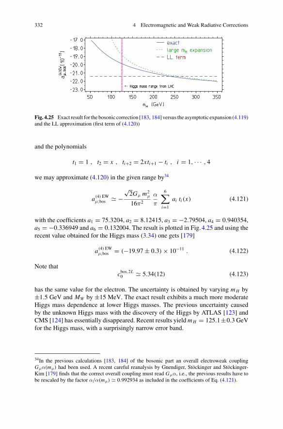
332 4 Electromagnetic and Weak Radiative Corrections

Fig. 4.25 Exact result for the bosonic correction [183, 184] versus the asymptotic expansion (4.119)and the LL approximation (first term of (4.120))

and the polynomials

t1 = 1 , t2 = x , ti+2 = 2xti+1 − ti , i = 1, · · · , 4

we may approximate (4.120) in the given range by34

a(4) EWμ;bos −

√2Gμ m2

μ

16π2

α

π

6∑

i=1

ai ti (x) (4.121)

with the coefficients a1 = 75.3204, a2 = 8.12415, a3 = −2.79504, a4 = 0.940354,a5 = −0.336949 and a6 = 0.132004. The result is plotted in Fig. 4.25 and using therecent value obtained for the Higgs mass (3.34) one gets [179]

a(4) EWμ;bos = (−19.97 ± 0.3) × 10−11 . (4.122)

Note thatcbos,2L

0 5.34(12) (4.123)

has the same value for the electron. The uncertainty is obtained by varying m H by±1.5 GeV and MW by ±15 MeV. The exact result exhibits a much more moderateHiggs mass dependence at lower Higgs masses. The previous uncertainty causedby the unknown Higgs mass with the discovery of the Higgs by ATLAS [123] andCMS [124] has essentially disappeared. Recent results yield m H = 125.1±0.3 GeVfor the Higgs mass, with a surprisingly narrow error band.

34In the previous calculations [183, 184] of the bosonic part an overall electroweak couplingGμα(mμ) had been used. A recent careful reanalysis by Gnendiger, Stöckinger and Stöckinger-Kim [179] finds that the correct overall coupling must read Gμα, i.e., the previous results have tobe rescaled by the factor α/α(mμ) 0.992934 as included in the coefficients of Eq. (4.121).

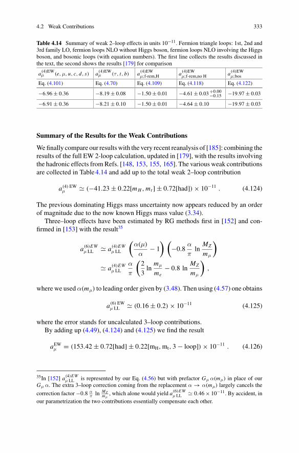
4.2 Weak Contributions 333

Table 4.14 Summary of weak 2–loop effects in units 10−11. Fermion triangle loops: 1st, 2nd and3rd family LO, fermion loops NLO without Higgs boson, fermion loops NLO involving the Higgsboson, and bosonic loops (with equation numbers). The first line collects the results discussed inthe text, the second shows the results [179] for comparison

a(4)EWμ (e, μ, u, c, d, s) a(4)EW

μ (τ , t, b) a(4)EWμ;f-rem,H a(4)EW

μ;f-rem,no H a(4)EWμ;bos

Eq. (4.101) Eq. (4.70) Eq. (4.109) Eq. (4.118) Eq. (4.122)

−6.96 ± 0.36 −8.19 ± 0.08 −1.50 ± 0.01 −4.61 ± 0.03 +0.00−0.15 −19.97 ± 0.03

−6.91 ± 0.36 −8.21 ± 0.10 −1.50 ± 0.01 −4.64 ± 0.10 −19.97 ± 0.03

Summary of the Results for the Weak Contributions

We finally compare our results with the very recent reanalysis of [185]: combining theresults of the full EW 2-loop calculation, updated in [179], with the results involvingthe hadronic effects from Refs. [148, 153, 155, 165]. The various weak contributionsare collected in Table 4.14 and add up to the total weak 2–loop contribution

a(4) EWμ (−41.23 ± 0.22[m H , mt ] ± 0.72[had]) × 10−11 . (4.124)

The previous dominating Higgs mass uncertainty now appears reduced by an orderof magnitude due to the now known Higgs mass value (3.34).

Three–loop effects have been estimated by RG methods first in [152] and con-firmed in [153] with the result35

a(6)EWμ LL a(4)EW

μ LL

(α(μ)

α− 1

) (−0.8

α

πln

MZ

mμ

)

a(4)EWμ LL

α

π

(2

3ln

mμ

me− 0.8 ln

MZ

mμ

),

where we used α(mμ) to leading order given by (3.48). Then using (4.57) one obtains

a(6) EWμ LL (0.16 ± 0.2) × 10−11 (4.125)

where the error stands for uncalculated 3–loop contributions.By adding up (4.49), (4.124) and (4.125) we find the result

aEWμ = (153.42 ± 0.72[had] ± 0.22[mH, mt, 3 − loop]) × 10−11 . (4.126)

35In [152] a(4)EWμ LL is represented by our Eq. (4.56) but with prefactor Gμ α(mμ) in place of our

Gμ α. The extra 3–loop correction coming from the replacement α → α(mμ) largely cancels the

correction factor −0.8 απ ln MZ

mμ, which alone would yield a(6)EW

μ LL 0.46 × 10−11. By accident, inour parametrization the two contributions essentially compensate each other.

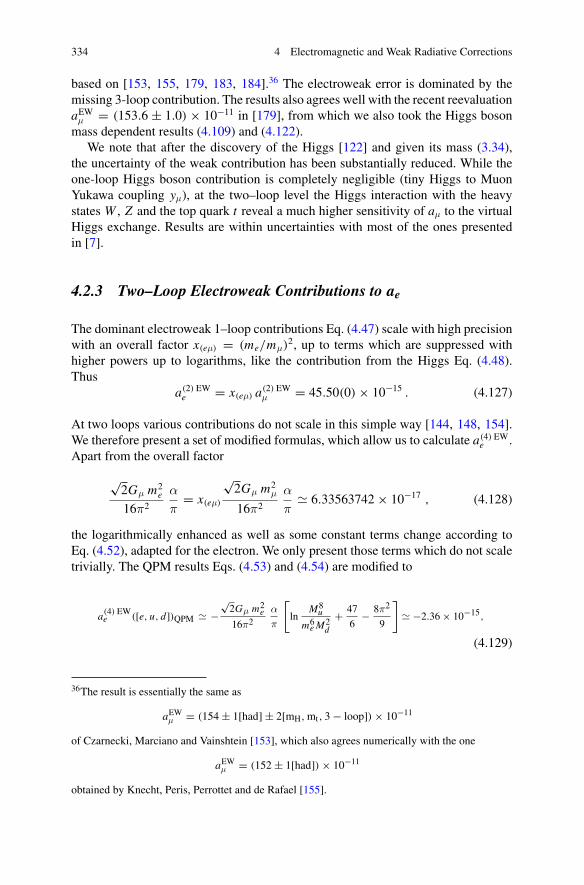
334 4 Electromagnetic and Weak Radiative Corrections

based on [153, 155, 179, 183, 184].36 The electroweak error is dominated by themissing 3-loop contribution. The results also agrees well with the recent reevaluationaEW

μ = (153.6 ± 1.0) × 10−11 in [179], from which we also took the Higgs bosonmass dependent results (4.109) and (4.122).

We note that after the discovery of the Higgs [122] and given its mass (3.34),the uncertainty of the weak contribution has been substantially reduced. While theone-loop Higgs boson contribution is completely negligible (tiny Higgs to MuonYukawa coupling yμ), at the two–loop level the Higgs interaction with the heavystates W , Z and the top quark t reveal a much higher sensitivity of aμ to the virtualHiggs exchange. Results are within uncertainties with most of the ones presentedin [7].

4.2.3 Two–Loop Electroweak Contributions to ae

The dominant electroweak 1–loop contributions Eq. (4.47) scale with high precisionwith an overall factor x(eμ) = (me/mμ)

2, up to terms which are suppressed withhigher powers up to logarithms, like the contribution from the Higgs Eq. (4.48).Thus

a(2) EWe = x(eμ) a(2) EW

μ = 45.50(0) × 10−15 . (4.127)

At two loops various contributions do not scale in this simple way [144, 148, 154].We therefore present a set of modified formulas, which allow us to calculate a(4) EW

e .Apart from the overall factor

√2Gμ m2

e

16π2

α

π= x(eμ)

√2Gμ m2

μ

16π2

α

π 6.33563742 × 10−17 , (4.128)

the logarithmically enhanced as well as some constant terms change according toEq. (4.52), adapted for the electron. We only present those terms which do not scaletrivially. The QPM results Eqs. (4.53) and (4.54) are modified to

a(4) EWe ([e, u, d])QPM −

√2Gμ m2

e

16π2α

π

[

lnM8

u

m6e M2

d

+ 47

6− 8π2

9

]

−2.36 × 10−15,

(4.129)

36The result is essentially the same as

aEWμ = (154 ± 1[had] ± 2[mH, mt, 3 − loop]) × 10−11

of Czarnecki, Marciano and Vainshtein [153], which also agrees numerically with the one

aEWμ = (152 ± 1[had]) × 10−11

obtained by Knecht, Peris, Perrottet and de Rafael [155].

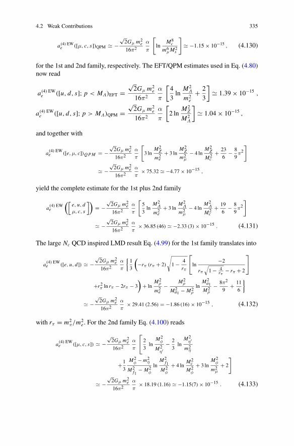
4.2 Weak Contributions 335

a(4) EWe ([μ, c, s])QPM −

√2Gμ m2

e

16π2

α

π

[

lnM8

c

m6μM2

s

]

−1.15 × 10−15 , (4.130)

for the 1st and 2nd family, respectively. The EFT/QPM estimates used in Eq. (4.80)now read

a(4) EWe ([u, d, s]; p < MΛ)EFT =

√2Gμ m2

e

16π2

α

π

[4

3ln

M2Λ

m2e

+ 2

3

] 1.39 × 10−15 ,

a(4) EWe ([u, d, s]; p > MΛ)QPM =

√2Gμ m2

e

16π2

α

π

[2 ln

M2Z

M2Λ

] 1.04 × 10−15 ,

and together with

a(4) EWe ([e, μ, c])Q P M = −

√2Gμ m2

e

16π2α

π

[

3 lnM2

Z

m2e

+ 3 lnM2

Z

m2μ

− 4 lnM2

Z

M2c

+ 23

6− 8

9π2

]

−√

2Gμ m2e

16π2α

π× 75.32 −4.77 × 10−15 ,

yield the complete estimate for the 1st plus 2nd family

a(4) EWe

([e, u, dμ, c, s

])= −

√2Gμ m2

e

16π2α

π

[5

3ln

M2Λ

m2e

+ 3 lnM2

Λ

m2μ

− 4 lnM2

Λ

M2c

+ 19

6− 8

9π2

]

−√

2Gμ m2e

16π2α

π× 36.85 (46) −2.33 (3) × 10−15 . (4.131)

The large Nc QCD inspired LMD result Eq. (4.99) for the 1st family translates into

a(4) EWe ([e, u, d]) −

√2Gμ m2

e

16π2α

π

{1

3

(−rπ (rπ + 2)

√

1 − 4

rπ

⎡

⎣ln−2

rπ√

1 − 4rπ

− rπ + 2

⎤

⎦

+r2π ln rπ − 2rπ − 3

)+ ln

M2ρ

m2e

− M2ρ

M2a1 − M2

ρ

lnM2

a1

M2ρ

− 8π2

9+ 11

6

}

−√

2Gμ m2e

16π2α

π× 29.41 (2.56) = −1.86 (16) × 10−15 , (4.132)

with rπ = m2π/m2

e . For the 2nd family Eq. (4.100) reads

a(4) EWe ([μ, c, s]) −

√2Gμ m2

e

16π2α

π

⎡

⎣ 2

3ln

M2φ

M2η′

− 2

3ln

M2η′

m2η

+ 1

3

M2φ − m2

η

M2f1

− M2φ

lnM2

f1

M2φ

+ 4 lnM2

c

M2φ

+ 3 lnM2

φ

m2μ

+ 2

]

−√

2Gμ m2e

16π2α

π× 18.19 (1.16) −1.15(7) × 10−15 . (4.133)

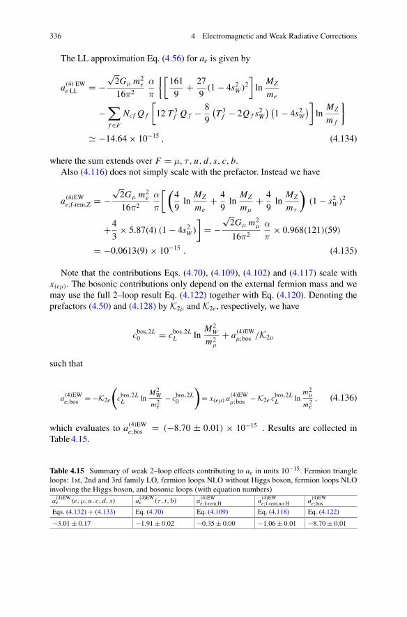
336 4 Electromagnetic and Weak Radiative Corrections

The LL approximation Eq. (4.56) for ae is given by

a(4) EWe LL = −

√2Gμ m2

e

16π2

α

π

{[161

9+ 27

9(1 − 4s2

W )2

]ln

MZ

me

−∑

f ∈F

Ncf Q f

[12 T 3

f Q f − 8

9

(T 3

f − 2Q f s2W

) (1 − 4s2

W

)]

lnMZ

m f

}

−14.64 × 10−15 , (4.134)

where the sum extends over F = μ, τ , u, d, s, c, b.Also (4.116) does not simply scale with the prefactor. Instead we have

a(4)EWe;f-rem,Z = −

√2Gμ m2

e

16π2

α

π

[(4

9ln

MZ

me+ 4

9ln

MZ

mμ+ 4

9ln

MZ

mτ

)(1 − s2

W )2

+4

3× 5.87(4) (1 − 4s2

W )

]= −

√2Gμ m2

μ

16π2

α

π× 0.968(121)(59)

= −0.0613(9) × 10−15 . (4.135)

Note that the contributions Eqs. (4.70), (4.109), (4.102) and (4.117) scale withx(eμ). The bosonic contributions only depend on the external fermion mass and wemay use the full 2–loop result Eq. (4.122) together with Eq. (4.120). Denoting theprefactors (4.50) and (4.128) by K2μ and K2e, respectively, we have

cbos,2L0 = cbos,2L

L lnM2

W

m2μ

+ a(4)EWμ;bos /K2μ

such that

a(4)EWe;bos = −K2e

(

cbos,2LL ln

M2W

m2e

− cbos,2L0

)

= x(eμ) a(4)EWμ;bos − K2e cbos,2L

L lnm2

μ

m2e

, (4.136)

which evaluates to a(4)EWe;bos = (−8.70 ± 0.01) × 10−15 . Results are collected in

Table 4.15.

Table 4.15 Summary of weak 2–loop effects contributing to ae in units 10−15. Fermion triangleloops: 1st, 2nd and 3rd family LO, fermion loops NLO without Higgs boson, fermion loops NLOinvolving the Higgs boson, and bosonic loops (with equation numbers)

a(4)EWe (e, μ, u, c, d, s) a(4)EW

e (τ , t, b) a(4)EWe;f-rem,H a(4)EW

e;f-rem,no H a(4)EWe;bos

Eqs. (4.132) + (4.133) Eq. (4.70) Eq. (4.109) Eq. (4.118) Eq. (4.122)

−3.01 ± 0.17 −1.91 ± 0.02 −0.35 ± 0.00 −1.06 ± 0.01 −8.70 ± 0.01

4.2 Weak Contributions 337

As a result we obtain the total weak 2–loop contribution

a(4) EWe (−15.04 ± 0.02[m H , mt ] ± 0.23[had]) × 10−15 . (4.137)

The total weak contribution thus is given by

aEWe (30.53 ± 0.02[m H , mt ] ± 0.23[had]) × 10−15 . (4.138)

This is very close to ae(weak) = 29.73(52) × 10−15 used in [6, 45]. The valuecorrects the result estimated in [7].

Note that the leading log approximation in Eq. (4.134) utilizing constituent quarksin this case is very close to the result in Eq. (4.137). Using this approximation wewould get the value aEW

e 30.95×10−15, which often has been adopted in the past.

References

1. T. Kinoshita, B. Nizic, Y. Okamoto, Phys. Rev. D 41, 593 (1990)2. T. Kinoshita, W.J. Marciano, in Quantum Electrodynamics, ed. by T. Kinoshita (World Sci-

entific, Singapore, 1990), pp. 419–4783. G.W. Bennett et al., Muon (g-2) Collab. Phys. Rev. Lett. 92, 161802 (2004)4. B.L. Roberts, Nucl. Phys. B (Proc. Suppl.) 131 57 (2004); R.M. Carey et al., Proposal of the

BNL Experiment E969 (2004), www.bnl.gov/henp/docs/pac0904/P969.pdf; J-PARC Letterof Intent L17, B.L. Roberts contact person

5. B.E. Lautrup, E. de Rafael, Nucl. Phys. B 70, 317 (1974)6. P.J. Mohr, B.N. Taylor, Rev. Mod. Phys. 77, 1 (2005); P.J. Mohr, B.N. Taylor, D.B. Newell,

Rev. Mod. Phys. 84, 1527 (2012)7. F. Jegerlehner, A. Nyffeler, Phys. Rept. 477, 1 (2009)8. A. Petermann, Helv. Phys. Acta 30, 407 (1957); Nucl. Phys. 5, 677 (1958)9. C.M. Sommerfield, Phys. Rev. 107, 328 (1957); Ann. Phys. (NY) 5, 26 (1958)

10. B.E. Lautrup, E. De Rafael, Nuovo Cim. A 64, 322 (1969)11. H. Suura, E. Wichmann, Phys. Rev. 105, 1930 (1957); A. Petermann, Phys. Rev. 105, 1931

(1957)12. H.H. Elend, Phys. Lett. 20, 682 (1966); Erratum-ibid 21, 720 (1966)13. M. Passera, J. Phys, G 31 R75 (2005); Phys. Rev. D 75, 013002 (2007)14. G. Li, R. Mendel, M.A. Samuel, Phys. Rev. D 47, 1723 (1993)15. J.A. Mignaco, E. Remiddi, Nuovo Cim. A 60, 519 (1969); R. Barbieri, E. Remiddi, Phys.

Lett. B 49, 468 (1974); Nucl. Phys. B 90, 233 (1975); R. Barbieri, M. Caffo, E. Remiddi,Phys. Lett. B 57, 460 (1975); M.J. Levine, E. Remiddi, R. Roskies, Phys. Rev. D 20, 2068(1979); S. Laporta, E. Remiddi, Phys. Lett. B 265, 182 (1991); S. Laporta, Phys. Rev. D 47,4793 (1993); Phys. Lett. B 343, 421 (1995); S. Laporta, E. Remiddi, Phys. Lett. B 356, 390(1995)

16. S. Laporta, E. Remiddi, Phys. Lett. B 379, 283 (1996)17. T. Kinoshita, Phys. Rev. Lett. 75, 4728 (1995)18. T. Kinoshita, Nuovo Cim. B 51, 140 (1967)19. B.E. Lautrup, E. De Rafael, Phys. Rev. 174, 1835 (1968); B.E. Lautrup, M.A. Samuel, Phys.

Lett. B 72, 114 (1977)20. S. Laporta, Nuovo Cim. A 106, 675 (1993)21. S. Laporta, E. Remiddi, Phys. Lett. B 301, 440 (1993)

338 4 Electromagnetic and Weak Radiative Corrections

22. J.H. Kühn, A.I. Onishchenko, A.A. Pivovarov, O.L. Veretin, Phys. Rev. D 68, 033018 (2003)23. M.A. Samuel, G. Li, Phys. Rev. D 44, 3935 (1991) [Errata-ibid. D 46, 4782 (1992); D 48,

1879 (1993)]24. A. Czarnecki, M. Skrzypek, Phys. Lett. B 449, 354 (1999)25. S. Friot, D. Greynat, E. De Rafael, Phys. Lett. B 628, 73 (2005)26. B.E. Lautrup, M.A. Samuel, Phys. Lett. B 72, 114 (1977)27. T. Kinoshita, Phys. Rev. Lett. 61, 2898 (1988)28. M.A. Samuel, Phys. Rev. D 45, 2168 (1992)29. R. Barbieri, E. Remiddi, Nucl. Phys. B 90, 233 (1975)30. R. Barbieri, E. Remiddi, Phys. Lett. B 57, 273 (1975)31. J. Aldins, T. Kinoshita, S.J. Brodsky, A.J. Dufner, Phys. Rev. Lett. 23, 441 (1969); Phys. Rev.

D 1, 2378 (1970)32. M. Caffo, S. Turrini, E. Remiddi, Phys. Rev. D 30, 483 (1984); E. Remiddi, S.P. Sorella, Lett.

Nuovo Cim. 44, 231 (1985); R.N. Faustov, A.L. Kataev, S.A. Larin, V.V. Starshenko, Phys.Lett. B 254, 241 (1991); D.J. Broadhurst, A.L. Kataev, O.V. Tarasov, Phys. Lett. B 298, 445(1993)

33. S. Laporta, Phys. Lett. B 312, 495 (1993)34. P.A. Baikov, D.J. Broadhurst, Three–loop QED Vacuum Polarization and the Four–loop Muon

Anomalous Magnetic Moment, in New Computing Techniques in Physics Research IV. Inter-national Workshop on Software Engineering and Artificial Intelligence for High Energy,Nuclear Physics, ed by B. Denby, D. Perret-Gallix (World Scientific, Singapore 1995), pp.167–172, arXiv:hep-ph/9504398

35. J.P. Aguilar, D. Greynat, E. De Rafael, Phys. Rev. D 77, 093010 (2008)36. T. Kinoshita, W.B. Lindquist, Phys. Rev. Lett. 47, 1573 (1981)37. T. Kinoshita, W.B. Lindquist, Phys. Rev. D 27, 867 (1983); Phys. Rev. D 27, 877 (1983);

Phys. Rev. D 27, 886 (1983); Phys. Rev. D 39, 2407 (1989); Phys. Rev. D 42, 636 (1990)38. T. Kinoshita, in Quantum Electrodynamics, ed. by T. Kinoshita (World Scientific, Singapore,

1990), pp. 218–32139. T. Kinoshita, Phys. Rev. D 47, 5013 (1993)40. V.W. Hughes, T. Kinoshita, Rev. Mod. Phys. 71, S133 (1999)41. T. Kinoshita, M. Nio, Phys. Rev. Lett. 90, 021803 (2003); Phys. Rev. D 70, 113001 (2004)42. T. Kinoshita, Nucl. Phys. B (Proc. Suppl.) 144, 206 (2005)43. T. Kinoshita, M. Nio, Phys. Rev. D 73, 013003 (2006)44. T. Aoyama, M. Hayakawa, T. Kinoshita, M. Nio, Phys. Rev. Lett. 99, 110406 (2007)45. T. Aoyama, M. Hayakawa, T. Kinoshita, M. Nio, Phys. Rev. Lett. 109, 111807 (2012). doi:10.

1103/PhysRevLett.109.11180746. T. Aoyama, M. Hayakawa, T. Kinoshita, M. Nio, Phys. Rev. Lett. 109, 111808 (2012). doi:10.

1103/PhysRevLett.109.11180847. S. Laporta, arXiv:1704.06996 [hep-ph]48. T. Aoyama, M. Hayakawa, T. Kinoshita, M. Nio, Phys. Rev. D 91, 033006 (2015). doi:10.

1103/PhysRevD.91.03300649. G.P. Lepage, J. Comput. Phys. 27, 192 (1978)50. T. Kinoshita, I.E.E.E. Trans, Instrum. Meas. 44, 498 (1995)51. T. Kinoshita, I.E.E.E. Trans, Instrum. Meas. 46, 108 (1997)52. V.W. Hughes, T. Kinoshita, Rev. Mod. Phys. 71, S133 (1999); T. Kinoshita, IEEE Trans.

Instrum. Meas. 50, 568 (2001)53. T. Kinoshita, Recent Developments of the Theory of Muon and Electron g-2, in In Memory of

Vernon Willard Hughes, ed. by E.W. Hughes, E. Iachello (World Scientific, Singapore, 2004),pp. 58–77

54. T. Aoyama, M. Hayakawa, T. Kinoshita, M. Nio, Nucl. Phys. B 740, 138 (2006)55. T. Aoyama, M. Hayakawa, T. Kinoshita, M. Nio, Nucl. Phys. B 796, 184 (2008)56. S. Laporta, Int. J. Mod. Phys. A 15, 5087 (2000)57. S. Laporta, Phys. Lett. B 504, 188 (2001)58. S. Laporta, Phys. Lett. B 523, 95 (2001)

References 339

59. S. Laporta, Acta Phys. Polon. B 34, 5323 (2003)60. S. Laporta, P. Mastrolia, E. Remiddi, Nucl. Phys. B 688, 165 (2004)61. S. Laporta, Int. J. Mod. Phys. A 23, 5007 (2008)62. S. Laporta, Subnucl. Ser. 45, 409 (2009)63. M. Caffo, S. Turrini, E. Remiddi, Phys. Rev. D 30, 483 (1984)64. M.A. Samuel, Lett. Nuovo Cim. 21, 227 (1978)65. M.L. Laursen, M.A. Samuel, J. Math. Phys. 22, 1114 (1981)66. J. Calmet, A. Peterman, Phys. Lett. B 56, 383 (1975)67. M.A. Samuel, C. Chlouber, Phys. Rev. Lett. 36, 442 (1976); C. Chlouber, M.A. Samuel, Phys.

Rev. D 16, 3596 (1977)68. T. Aoyama, M. Hayakawa, T. Kinoshita, M. Nio, Phys. Rev. D 77, 053012 (2008). doi:10.

1103/PhysRevD.77.05301269. S. Laporta, P. Mastrolia, E. Remiddi, Nucl. Phys. B 688 (2004) 165; P. Mastrolia, E. Remiddi,

Nucl. Phys. B (Proc. Suppl.) 89, 76 (2000)70. A.L. Kataev, Phys. Rev. D 86, 013010 (2012)71. P.A. Baikov, K.G. Chetyrkin, C. Sturm, Nucl. Phys. Proc. Suppl. 183, 8 (2008)72. P.A. Baikov, K.G. Chetyrkin, J.H. Kühn, C. Sturm, Nucl. Phys. B 867, 182 (2013)73. R. Lee, P. Marquard, A.V. Smirnov, V.A. Smirnov, M. Steinhauser, JHEP 1303, 162 (2013)74. A. Kurz, T. Liu, P. Marquard, M. Steinhauser, Nucl. Phys. B 879, 1 (2014)75. A. Kurz, T. Liu, P. Marquard, A.V. Smirnov, V.A. Smirnov, M. Steinhauser, Phys. Rev. D 92,

073019 (2015)76. T. Kinoshita, M. Nio, Phys. Rev. D 73, 053007 (2006)77. T. Aoyama, M. Hayakawa, T. Kinoshita, M. Nio, N. Watanabe, Phys. Rev. D 78, 053005

(2008)78. T. Aoyama, M. Hayakawa, T. Kinoshita, M. Nio, Phys. Rev. D 78, 113006 (2008)79. T. Aoyama, M. Hayakawa, T. Kinoshita, M. Nio, Phys. Rev. D 82, 113004 (2010)80. T. Aoyama, K. Asano, M. Hayakawa, T. Kinoshita, M. Nio, N. Watanabe, Phys. Rev. D 81,

053009 (2010)81. T. Aoyama, M. Hayakawa, T. Kinoshita, M. Nio, Phys. Rev. D 83, 053003 (2011)82. T. Aoyama, M. Hayakawa, T. Kinoshita, M. Nio, Phys. Rev. D 83, 053002 (2011)83. T. Aoyama, M. Hayakawa, T. Kinoshita, M. Nio, Phys. Rev. D 84, 053003 (2011)84. T. Aoyama, M. Hayakawa, T. Kinoshita, M. Nio, Phys. Rev. D 85, 033007 (2012)85. T. Aoyama, M. Hayakawa, T. Kinoshita, M. Nio, Phys. Rev. D 85, 093013 (2012)86. P. Baikov, A. Maier, P. Marquard, Nucl. Phys. B 877, 647 (2013)87. P.A. Baikov, A. Maier, P. Marquard, Acta Phys. Polon. B 44, 2267 (2013)88. S.G. Karshenboim, Phys. Atom. Nucl. 56, 857 (1993) [Yad. Fiz. 56N6, 252 (1993)]89. A.L. Kataev, Nucl. Phys. Proc. Suppl. 155, 369 (2006), arXiv:hep-ph/0602098; Phys. Rev. D

74, 073011 (2006)90. S. Laporta, Phys. Lett. B 328, 522 (1994)91. A. Kurz, T. Liu, P. Marquard, A. Smirnov, V. Smirnov, M. Steinhauser, Phys. Rev. D 93,

053017 (2016)92. P. Nogueira, Automatic feynman graph generation. J. Comput. Phys. 105, 279 (1993)93. J.A.M. Vermaseren, arXiv:math-ph/001002594. J. Kuipers, T. Ueda, J.A.M. Vermaseren, J. Vollinga, Comput. Phys. Commun. 184, 1453

(2013)95. M. Tentyukov, J.A.M. Vermaseren, Comput. Phys. Commun. 181, 1419 (2010)96. M. Steinhauser, T. Ueda, J.A.M. Vermaseren, Nucl. Part. Phys. Proc. 261–262 4597. R.H. Lewis, Fermat s User Guide, http://www.bway.net/~lewis/98. A. Pak, A. Smirnov, Eur. Phys. J. C 71, 1626 (2011)99. B. Jantzen, A.V. Smirnov, V.A. Smirnov, Eur. Phys. J. C 72, 2139 (2012)

100. M. Beneke, V.A. Smirnov, Nucl. Phys. B 522, 321 (1998)101. V.A. Smirnov, Springer Tracts Mod. Phys. 177, 1 (2002)102. V.A. Smirnov, Springer Tracts Mod. Phys. 250, 1 (2012)103. A.V. Smirnov, Comput. Phys. Commun. 189, 182 (2015)

340 4 Electromagnetic and Weak Radiative Corrections

104. P. Marquard, D. Seidel, unpublished105. K.G. Chetyrkin, F.V. Tkachov, Nucl. Phys. B 192, 159 (1981)106. L.V. Avdeev, Comput. Phys. Commun. 98, 15 (1996)107. V.A. Smirnov, Phys. Lett. B 460, 397 (1999)108. J.B. Tausk, Phys. Lett. B 469, 225 (1999)109. M. Czakon, Comput. Phys. Commun. 175, 559 (2006)110. A.V. Smirnov, Comput. Phys. Commun. 185, 2090 (2014)111. D.H. Bailey, A Portable High Performance Multiprecision Package. NASA Ames Research

Center, RNR Technical Report RNR-90-022 (E-mail: dbailey@nas.nasa.gov); H.R.P. Fergu-son, D.H. Bailey, S. Arno, Analysis of PSLQ, An Integer Relation Finding Algorithm. Math.Comput. 68, 351–369 (1999)

112. A.V. Kotikov, Phys. Lett. B 254, 158 (1991)113. E. Remiddi, Nuovo Cim. A 110, 1435 (1997)114. T. Gehrmann, E. Remiddi, Nucl. Phys. B 580, 485 (2000)115. S. Laporta, E. Remiddi, Nucl. Phys. B 704, 349 (2005)116. M.Y. Kalmykov, JHEP 0604, 056 (2006)117. G.A. Baker, Jr., J.L. Gammel, J.G. Wills, J. Math. Anal. Appl. 2, 405 (1961); G.A. Baker, Jr.,

Essentials of Pad é Approximants, Academic Press (1975)118. S.L. Glashow, Nucl. Phys. B 22, 579 (1961); S. Weinberg, Phys. Rev. Lett. 19, 1264 (1967);

A. Salam, Weak and electromagnetic interactions, in Elementary Particle Theory, ed by N.Svartholm (Amquist and Wiksells, Stockholm, 1969), pp. 367–377

119. G. ’t Hooft, Nucl. Phys. B 33, 173 (1971); 35, 167 (1971); G. ’t Hooft, M. Veltman, Nucl.Phys. B 50, 318 (1972)

120. R. Jackiw, S. Weinberg, Phys. Rev. D 5, 2396 (1972); I. Bars, M. Yoshimura, Phys. Rev. D 6,374 (1972); G. Altarelli, N. Cabibbo, L. Maiani, Phys. Lett. B 40, 415 (1972); W.A. Bardeen,R. Gastmans, B. Lautrup, Nucl. Phys. B 46, 319 (1972); K. Fujikawa, B.W. Lee, A.I. Sanda.Phys. Rev. D 6, 2923 (1972)

121. P.W. Higgs, Phys. Lett. 12B, 132 (1964); Phys. Rev. Lett. 13, 508 (1964); Phys. Rev. 145,1156 (1966); F. Englert, R. Brout, Phys. Rev. Lett. 13, 321 (1964); G.S. Guralnik, C.R. Hagen,T.W.B. Kibble, Phys. Rev. Lett. 13, 585 (1964); T.W.B. Kibble, Phys. Rev. 155, 1554 (1967)

122. F. Gianotti (the ATLAS Collab.). CERN Seminar, July 4th, 2012; J. Incandela (the CMSCollab.). CERN Seminar, July 4th, 2012

123. G. Aad et al., [ATLAS Collab.], Phys. Lett. B 716, 1 (2012). Science 338, 1576 (2012)124. S. Chatrchyan et al., [CMS Collab.], Phys. Lett. B 716, 30 (2012). Science 338, 1569 (2012)125. N. Cabibbo, Phys. Rev. Lett. 10, 531 (1963). M. Kobayashi, K. Maskawa. Prog. Theor. Phys.

49, 652 (1973)126. B. Pontecorvo, Sov. Phys. JETP 6, 429 (1957) [Zh. Eksp. Teor. Fiz. 33, 549 (1957)]; Sov.

Phys. JETP 26, 984 (1968) [Zh. Eksp. Teor. Fiz. 53, 1717 (1967)]; Z. Maki, M. Nakagawa,S. Sakata, Prog. Theor. Phys. 28, 870 (1962)

127. S.L. Glashow, J. Iliopoulos, L. Maiani, Phys. Rev. D 2, 1285 (1970)128. W.J. Marciano, A. Sirlin, Phys. Rev. Lett. 61, 1815 (1988)129. T. van Ritbergen, R.G. Stuart, Phys. Rev. Lett. 82, 488 (1999)130. M. Awramik, M. Czakon, Phys. Lett. B 568, 48 (2003)131. M. Veltman, Nucl. Phys. B 123, 89 (1977); M.S. Chanowitz et al., Phys. Lett. 78B, 1 (1978);

M. Consoli, S. Lo Presti, L. Maiani, Nucl. Phys. B 223, 474 (1983); J. Fleischer, F. Jegerlehner,Nucl. Phys. B 228, 1 (1983)

132. M. Consoli, W. Hollik, F. Jegerlehner, Phys. Lett. B 227, 167 (1989)133. F. Jegerlehner, Renormalizing the Standard Model, in Testing the Standard Model, ed. by

M. Cvetic, P. Langacker (World Scientific, Singapore, 1991), pp. 476–590, http://www-com.physik.hu-berlin.de/~fjeger/books.html

134. F. Jegerlehner, Prog. Part. Nucl. Phys. 27, 1 (1991), http://www-com.physik.hu-berlin.de/~fjeger/books.html

135. S. Schael et al., [ALEPH and DELPHI and L3 and OPAL and SLD and LEP ElectroweakWorking Group and SLD Electroweak Group and SLD Heavy Flavour Group Collab.s], Phys.Rept. 427, 257 (2006)

References 341

136. J. Fleischer, F. Jegerlehner, Phys. Rev. D 23, 2001 (1981)137. F. Jegerlehner, Nuovo Cim. C 034S1, 31 (2011)138. A. Francis, G. von Hippel, H.B. Meyer, F. Jegerlehner, PoS LATTICE 2013, 320 (2013),

arXiv:1312.0035 [hep-lat]139. F. Burger, K. Jansen, M. Petschlies, G. Pientka, JHEP 1511, 215 (2015)140. A. Francis, V. Gülpers, G. Herdoza, H. Horch, B. Jäger, H.B. Meyer, H. Wittig, PoS LATTICE

2015, 110 (2015), arXiv:1511.04751 [hep-lat]141. F. Jegerlehner, Precision Tests of Electroweak-Interaction Parameters, in Testing the Standard

Model, ed. by M. Zrałek, R. Manka (World Scientific, Singapore, 1988), pp. 33–108142. A. Czarnecki, W.J. Marciano, Phys. Rev. D 53, 1066 (1996); Int. J. Mod. Phys. A 15, 2365

(2000)143. J. Erler, M.J. Ramsey-Musolf, Phys. Rev. D 72, 073003 (2005)144. T.V. Kukhto, E.A. Kuraev, A. Schiller, Z.K. Silagadze, Nucl. Phys. B 371, 567 (1992)145. S.L. Adler, Phys. Rev. 177, 2426 (1969); J.S. Bell, R. Jackiw, Nuovo Cim. 60A, 47 (1969);

W.A. Bardeen, Phys. Rev. 184, 1848 (1969)146. C. Bouchiat, J. Iliopoulos, P. Meyer, Phys. Lett. 38B, 519 (1972); D. Gross, R. Jackiw, Phys.

Rev. D 6, 477 (1972); C.P. Korthals Altes, M. Perrottet, Phys. Lett. 39B, 546 (1972)147. S. Peris, M. Perrottet, E. de Rafael, Phys. Lett. B 355, 523 (1995)148. A. Czarnecki, B. Krause, W. Marciano, Phys. Rev. D 52, R2619 (1995)149. F. Jegerlehner, Nucl. Phys. (Proc. Suppl.) C 51, 131 (1996)150. E. D’Hoker, Phys. Rev. Lett. 69, 1316 (1992)151. T. Sterling, M.J.G. Veltman, Nucl. Phys. B 189, 557 (1981)152. G. Degrassi, G.F. Giudice, Phys. Rev. 58D, 053007 (1998)153. A. Czarnecki, W.J. Marciano, A. Vainshtein, Phys. Rev. D 67, 073006 (2003) [Erratum-ibid.

D 73, 119901 (2006)]154. A. Czarnecki, B. Krause, W.J. Marciano, Phys. Rev. Lett. 76, 3267 (1996)155. M. Knecht, S. Peris, M. Perrottet, E. de Rafael, JHEP 0211, 003 (2002); E. de Rafael, The

muon g − 2 revisited, arXiv:hep-ph/0208251156. A. Czarnecki, W.J. Marciano, A. Vainshtein, Acta Phys. Polon. B 34, 5669 (2003)157. S.L. Adler, W.A. Bardeen, Phys. Rev. 182, 1517 (1969)158. J. Wess, B. Zumino, Phys. Lett. B 37, 95 (1971)159. E. Witten, Nucl. Phys. B 223, 422 (1983)160. F. Jegerlehner, O.V. Tarasov, Phys. Lett. B 639, 299 (2006)161. J. Mondejar, K. Melnikov, Phys. Lett. B 718, 1364 (2013)162. G. ’t Hooft, Recent Developments in Gauge Theories, in Proceedings of the Summer-Institute,

Cargese, France, 1979, ed. by G. ’t Hooft, et al. NATO Advanced Study Institute Series B:Physics, vol. 59 (Plenum Press, New York, 1980)

163. L. Rosenberg, Phys. Rev. 129, 2786 (1963)164. A. Vainshtein, Phys. Lett. B 569, 187 (2003)165. M. Knecht, S. Peris, M. Perrottet, E. de Rafael, JHEP 0403, 035 (2004)166. J. Gasser, H. Leutwyler, Annals Phys. 158, 142 (1984); Nucl. Phys. B 250, 465 (1985)167. M. Gell-Mann, R.J. Oakes, B. Renner, Phys. Rev. 175, 2195 (1968)168. J. Gasser. H. Leutwyler, Phys. Rept. 87, 77 (1982)169. K.G. Wilson, Phys. Rev. 179, 1499 (1969); K.G. Wilson, J.B. Kogut, Phys. Rept. 12, 75

(1974); V.A. Novikov, M.A. Shifman, A.I. Vainshtein, V.I. Zakharov, Nucl. Phys. B 249, 445(1985) [Yad. Fiz. 41, 1063 (1985)]

170. M.A. Shifman, World Sci. Lect. Notes Phys. 62, 1 (1999) (Chap. 1,2)171. B.L. Ioffe, A.V. Smilga, Nucl. Phys. B 232, 109 (1984)172. S. Peris, M. Perrottet, E. de Rafael, JHEP 9805, 011 (1998); M. Knecht, S. Peris, M. Perrottet,

E. de Rafael, Phys. Rev. Lett. 83, 5230 (1999); M. Knecht, A. Nyffeler. Eur. Phys. J. C 21,659 (2001)

173. J. Bijnens, L. Girlanda, P. Talavera, Eur. Phys. J. C 23, 539 (2002)174. G. Ecker, J. Gasser, A. Pich, E. de Rafael, Nucl. Phys. B 321, 311 (1989)175. G. Ecker, J. Gasser, H. Leutwyler, A. Pich, E. de Rafael, Phys. Lett. B 223, 425 (1989)

342 4 Electromagnetic and Weak Radiative Corrections

176. G. ’t Hooft, Nucl. Phys. B 72, 461 (1974); ibid. 75, 461 (1974)177. A.V. Manohar, Hadrons in the 1/N Expansion, in At the frontier of Particle Physics, ed

M. Shifman, vol. 1 (World Scientific, Singapore 2001), pp. 507–568178. E. de Rafael, Phys. Lett. B 322, 239 (1994)179. C. Gnendiger, D. Stöckinger, H. Stöckinger-Kim, Phys. Rev. D 88, 053005 (2013)180. S.M. Barr, A. Zee, Phys. Rev. Lett. 65, 21 (1990) [Erratum-ibid. 65, 2920 (1990)]181. F. Jegerlehner, Z. Phy., C 32, 195 (1986)182. V.A. Smirnov, Mod. Phys. Lett. A 10, 1485 (1995)183. S. Heinemeyer, D. Stöckinger, G. Weiglein, Nucl. Phys. B 699, 103 (2004)184. T. Gribouk, A. Czarnecki, Phys. Rev. D 72, 053016 (2005)185. H.G. Fargnoli, C. Gnendiger, S. Paßehr, D. Stöckinger, H. Stöckinger-Kim, PoS LL 2014,

067 (2014)

Chapter 5Hadronic Effects

The basic problems we are confronted with when we have to include the non–perturbative hadronic contributions to g − 2, we have outlined in Sect. 3.2.1 p. 183ffand in Sect. 4.2.2 p. 298ff, already. We will distinguish three types of contributions,which will be analyzed in different subsections below:

(i) The most sizable hadronic effect is the O(α2) hadronic vacuum polarization(HVP) insertion in the internal photon line of the leading one–loop muon vertexdiagram Fig. 5.1.

The hadronic “blob” can be calculated with help of the method discussed inSect. 3.7.1. While perturbation theory fails and ab initio non–perturbative latticeQCD calculations are not yet ready at the required precision, it may be obtained via aDR from the measured cross section e+e− → hadrons via (3.143) and (3.142). Here1 independent amplitude is to be determined by one specific data channel. Global fitsbased on the Resonance Lagrangian Approach (RLA), specifically, the Hidden LocalSymmetry (HLS) phenomenological Lagrangian, allow to improve the data-drivenevaluations.(ii)An order ofmagnitude smaller but still sizable are theHVP insertions contributingat order O(α3). They are represented by diagrams exhibiting one additional VPinsertion, leptonic or hadronic, in the photon line or by diagrams with an additionalvirtual photon attached in all possible ways in Fig. 5.1. As long as hadronic effectsenter via photon vacuum polarization only, they can be safely evaluated in termsof experimental data via the basic DR (3.143). The errors of the data here appearsuppressed by one power in α relative to the leading hadronic contribution andtherefore are not problematic concerning the required precision.Also the orderO(α4)

effect involving HVP insertions is known with sufficient accuracy.(iii) More involved and problematic is the hadronic light–by–light (HLbL) contribu-tion, represented by the diagram Fig. 5.2, and entering at O(α3). Here, a low energyEffective Field Theory (EFT) approach beyond Chiral Perturbation Theory (CHPT)(see p. 305) is needed and some model assumptions are unavoidable. Unfortunately,

© Springer International Publishing AG 2017F. Jegerlehner, The Anomalous Magnetic Moment of the Muon,Springer Tracts in Modern Physics 274, DOI 10.1007/978-3-319-63577-4_5

343

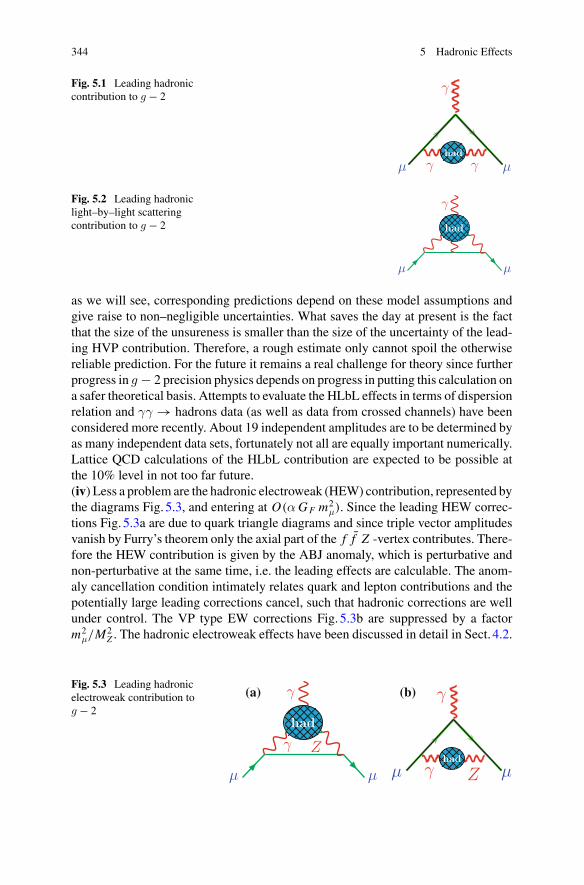
344 5 Hadronic Effects

Fig. 5.1 Leading hadroniccontribution to g − 2

μ μγ γ

γ

had

Fig. 5.2 Leading hadroniclight–by–light scatteringcontribution to g − 2

μ

γ

had

μ

had

as we will see, corresponding predictions depend on these model assumptions andgive raise to non–negligible uncertainties. What saves the day at present is the factthat the size of the unsureness is smaller than the size of the uncertainty of the lead-ing HVP contribution. Therefore, a rough estimate only cannot spoil the otherwisereliable prediction. For the future it remains a real challenge for theory since furtherprogress in g − 2 precision physics depends on progress in putting this calculation ona safer theoretical basis. Attempts to evaluate the HLbL effects in terms of dispersionrelation and γγ → hadrons data (as well as data from crossed channels) have beenconsidered more recently. About 19 independent amplitudes are to be determined byas many independent data sets, fortunately not all are equally important numerically.Lattice QCD calculations of the HLbL contribution are expected to be possible atthe 10% level in not too far future.(iv) Less a problem are the hadronic electroweak (HEW) contribution, represented bythe diagrams Fig. 5.3, and entering at O(αGF m2

μ). Since the leading HEW correc-tions Fig. 5.3a are due to quark triangle diagrams and since triple vector amplitudesvanish by Furry’s theorem only the axial part of the f f Z -vertex contributes. There-fore the HEW contribution is given by the ABJ anomaly, which is perturbative andnon-perturbative at the same time, i.e. the leading effects are calculable. The anom-aly cancellation condition intimately relates quark and lepton contributions and thepotentially large leading corrections cancel, such that hadronic corrections are wellunder control. The VP type EW corrections Fig. 5.3b are suppressed by a factorm2

μ/M2Z . The hadronic electroweak effects have been discussed in detail in Sect. 4.2.

Fig. 5.3 Leading hadronicelectroweak contribution tog − 2

μ

γ

had

γ Z

μ

had

μ μγ Z

γ

had

(a) (b)

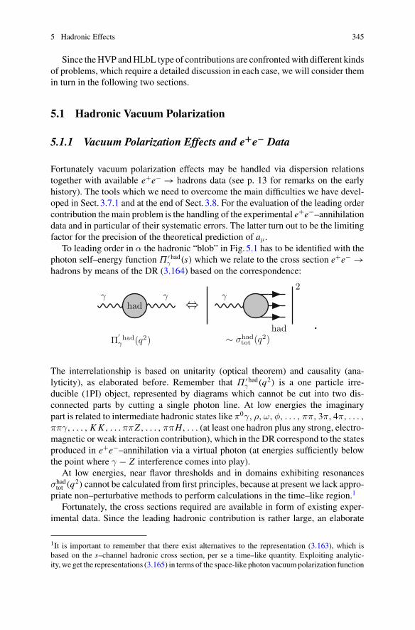
5 Hadronic Effects 345

Since theHVP andHLbL type of contributions are confrontedwith different kindsof problems, which require a detailed discussion in each case, we will consider themin turn in the following two sections.

5.1 Hadronic Vacuum Polarization

5.1.1 Vacuum Polarization Effects and e+e− Data

Fortunately vacuum polarization effects may be handled via dispersion relationstogether with available e+e− → hadrons data (see p. 13 for remarks on the earlyhistory). The tools which we need to overcome the main difficulties we have devel-oped in Sect. 3.7.1 and at the end of Sect. 3.8. For the evaluation of the leading ordercontribution themain problem is the handling of the experimental e+e−–annihilationdata and in particular of their systematic errors. The latter turn out to be the limitingfactor for the precision of the theoretical prediction of aμ.

To leading order in α the hadronic “blob” in Fig. 5.1 has to be identified with thephoton self–energy function Π ′ had

γ (s) which we relate to the cross section e+e− →hadrons by means of the DR (3.164) based on the correspondence:

γ γhad ⇔

Π′ hadγ (q2)

γ

had

2

∼ σhadtot (q2)

·

The interrelationship is based on unitarity (optical theorem) and causality (ana-lyticity), as elaborated before. Remember that Π ′ had

γ (q2) is a one particle irre-ducible (1PI) object, represented by diagrams which cannot be cut into two dis-connected parts by cutting a single photon line. At low energies the imaginarypart is related to intermediate hadronic states like π0γ, ρ,ω,φ, . . . , ππ, 3π, 4π, . . . ,

ππγ, . . . , KK , . . . ππZ , . . . , ππH, . . . (at least one hadron plus any strong, electro-magnetic or weak interaction contribution), which in the DR correspond to the statesproduced in e+e−–annihilation via a virtual photon (at energies sufficiently belowthe point where γ − Z interference comes into play).

At low energies, near flavor thresholds and in domains exhibiting resonancesσhadtot (q2) cannot be calculated from first principles, because at present we lack appro-

priate non–perturbative methods to perform calculations in the time–like region.1

Fortunately, the cross sections required are available in form of existing exper-imental data. Since the leading hadronic contribution is rather large, an elaborate

1It is important to remember that there exist alternatives to the representation (3.163), which isbased on the s–channel hadronic cross section, per se a time–like quantity. Exploiting analytic-ity, we get the representations (3.165) in terms of the space-like photon vacuumpolarization function

346 5 Hadronic Effects

handling of the experimental data is mandatory because the experimental errors aresubstantial and of course limit the precision of the “theoretical” prediction of aμ. Likethe deep inelastic electron–nucleon scattering experiments, the e+e−–annihilationexperiments played an eminent role in establishing QCD as the underlying theoryof the strong interaction and they have a long history. Touschek initiated the con-struction of an e+e− storage ring accelerator in the early 1960s at Frascati nearRome. Improved e+e− storage ring facilities and first cross section measurementsfollowed at Orsay, Novosibirsk and Frascati. The observed rise in the total hadroniccross section at these times looked very puzzling, as actually a drop as 1/E2 wasexpected at high energies from unitarity arguments. The CEA experiment [1], how-ever, which operated at slightly higher energy, left no room for doubts that the crosssection was far higher than theoretical expectations at these times. Apart from itsrole in explaining Bjorken scaling in deep inelastic ep–scattering [2], QCD, forthe first time, predicted a cross section enhanced by the color multiplicity factorNc = 3, which was clearly favored by experiment and as we know in the sequelrevolutionized strong interaction physics [3–5]. SLAC and DESY, reaching higherenergies, followed and unexpectedly new states were discovered at SLAC, the τlepton, the charm quark c and the bottom quark b. The highest energies so far werereached with LEP at CERN going up to 200 GeV. Important for the evaluation ofthe hadronic contributions to g − 2 are recent and ongoing hadronic cross sectionmeasurements at Novosibirsk, Frascati, Stanford and Beijing which provided muchmore accurate e+e− data. Table5.1 gives a more complete overview of the historyof e+e− machines and experiments and the maximum center of mass energy theyreached. Unfortunately, some of the energy ranges have been covered only by oldexperiments with typically 20% systematic errors. The situation though, could beimproved substantially by exclusive channel measurement with BaBar as well aswith inclusive measurements with BES-II and KEDR. For a precise evaluation of thehadronic effects we need to combine data sets frommany experiments of very differ-ent quality and performed in different energy intervals. The key problem here is theproper handling of the systematic errors, which are of different origin and depend onthe experiment (machine and detector) as well as on theory input like radiative cor-rections. The statistical errors commonly are assumed to be Gaussian and hence maybe added in quadrature. A problem here may be the low statistics of many of the olderexperiments which may not always justify this treatment. In the low energy regionparticularly important for g − 2, however, data have improved dramatically in recentyears (CMD-2, CMD-3 SND/Novosibirsk, BES-II, BES-III/Beijing, CLEO/Cornell,KLOE/Frascati, BaBar/SLAC) and the statistical errors are a minor problem now.

(Footnote 1 continued)Π ′ had

γ (−Q2) and (3.166) in terms of the space–like Adler–function D(Q2), which at low energiesare accessible to non–perturbative lattice QCD simulations. At higher energies pQCD is applicable(seeSect. 2.8). LatticeQCDfor the non-perturbative part togetherwith perturbation theorywill allowus to calculate ahadμ from the QCD Lagrangian. Several lattice QCD groups have made impressiveprogress in the past decade and LQCD results are expected to get competitive with the data-drivenapproach in the near future.

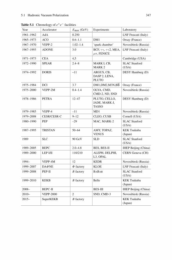
5.1 Hadronic Vacuum Polarization 347

Table 5.1 Chronology of e+e− facilities

Year Accelerator Emax (GeV) Experiments Laboratory

1961–1962 AdA 0.250 LNF Frascati (Italy)

1965–1973 ACO 0.6–1.1 DM1 Orsay (France)

1967–1970 VEPP-2 1.02–1.4 ’spark chamber’ Novosibirsk (Russia)

1967–1993 ADONE 3.0 BCF, γγ, γγ2, MEA,μπ, FENICE

LNF Frascati (Italy)

1971–1973 CEA 4,5 Cambridge (USA)

1972–1990 SPEAR 2.4–8 MARK I, CB,MARK 2

SLAC Stanford(USA)

1974–1992 DORIS –11 ARGUS, CB,DASP 2, LENA,PLUTO

DESY Hamburg (D)

1975–1984 DCI 3.7 DM1,DM2,M3N,BB Orsay (France)

1975–2000 VEPP-2M 0.4–1.4 OLYA, CMD,CMD-2, ND, SND

Novosibirsk (Russia)

1978–1986 PETRA 12–47 PLUTO, CELLO,JADE, MARK-J,TASSO

DESY Hamburg (D)

1979–1985 VEPP-4 –11 MD1 Novosibirsk (Russia)

1979–2008 CESR/CESR-C 9–12 CLEO, CUSB Cornell (USA)

1980–1990 PEP –29 MAC, MARK-2 SLAC Stanford(USA)

1987–1995 TRISTAN 50–64 AMY, TOPAZ,VENUS

KEK Tsukuba(Japan)

1989 SLC 90 GeV SLD SLAC Stanford(USA)

1989–2005 BEPC 2.0–4.8 BES, BES-II IHEP Beijing (China)

1989–2000 LEP I/II 110/210 ALEPH, DELPHI,L3, OPAL

CERN Geneva (CH)

1994– VEPP-4M 12 KEDR Novosibirsk (Russia)

1999–2007 DAΦNE Φ factory KLOE LNF Frascati (Italy)

1999–2008 PEP-II B factory BaBar SLAC Stanford(USA)

1999–2010 KEKB B factory Belle KEK Tsukuba(Japan)

2008– BEPC-II BES-III IHEP Beijing (China)

2010– VEPP-2000 2 SND, CMD-3 Novosibirsk (Russia)

2015– SuperKEKB B factory KEK Tsukuba(Japan)

348 5 Hadronic Effects

The main uncertainty, related to the systematic errors of the experimental data,is evaluated via a certain common sense type error handling, which often cannot bejustified unambiguously. This “freedom” of choice has lead to a large number ofestimates by different groups which mainly differ by individual taste and the levelof effort which is made in the analysis of the data. Issues here are: the completenessof the data utilized, interpolation and modeling procedures, e.g. direct integrationof the data by applying the trapezoidal rule versus fitting the data to some smoothfunctional form before integration, separation of energy ranges where data or theory(pQCD and/or hadronic models) are considered to be more reliable, combining thedata before or after integration etc.

A reliable combination of the data requires to know more or less precisely whatexperiments have actually measured and what they have published. As mentionedearlier, hadronic cross section data are represented usually by the cross section ratio2

Rhadγ (s) ≡ σ(e+e− → γ∗ → hadrons)

σ(e+e− → γ∗ → μ+μ−), (5.1)

whichmeasures the hadronic cross section in units of the leptonic point cross–section.One of the key questions here is:what is the precise definition of R(s) as a “measured”quantity? In theory we would consider (5.1), which also may be written in terms oflowest order cross sections, with respect to QED effects. In short notation

Rhadγ (s) ≡ σhad(s)

σμμ(s)= σ0

had(s)

σ0μμ(s)

which reveals R(s) defined in thisway as an undressedR (s) quantity, since in the ratiocommon effects, like dressing by VP effects (iterated VP insertions), normalization3

(luminositymeasurement) and the like, cancel from the ratio automatically.While the

2Definitions of R ratios like (3.142) may differ slightly modulo subleading corrections. Oftenwe simply denote it as R(s). In fact the standard definition (5.1) has to be corrected for theσ(e+e− → γ∗ → μ+μ−) specific effects like phase space and final state radiation. One has alwaysto keep inmind that it is the undressed hadronic cross section σ(e+e− → γ∗ → hadrons) |α/α(s)|2which matters in the DR for the hadronic contribution to the photon vacuum polarization. So infact (3.142) is more precisely what is meant when we write the basic DR (3.136) in the form(3.143). We also should be aware that it is the pseudo–observable σ(e+e− → γ∗ → hadrons)which is required for the DR, which has to be extracted from what is actually measurable, namelyσ(e+e− → hadrons). But also this total hadronic cross section is the result of a complicated “inter-pretation” of what has been seen in the detector, by disentangling the raw data from detector specificfeatures. Practically, in the most relevant low energy regime, the one photon exchange approxima-tion σ(e+e− → hadrons) ≈ σ(e+e− → γ∗ → hadrons) is an excellent approximation before atabout 40 GeV Z boson exchange mixes in. As included in Fig. 5.8, box diagram contributionsexhibiting two photon exchange are taken into account as radiative corrections. The latter are notreally understood when photons couple to hadrons composed of quarks.3Note that the initial state radiation (ISR) bremsstrahlung only cancels if the same cuts are appliedto hadro–production and to μ+μ− pair production, a condition, which usually is not satisfied. Weshould keep in mind that experimentally it is not possible to distinguish an initial state photon froma final state photon.

5.1 Hadronic Vacuum Polarization 349

dressed4 physical cross sections σhad(s) and σμμ(s) are proportional to the modulussquare of the effective running fine structure constant α(s) (see (3.121 and Fig. 3.13)the “bare” or “undressed” ones σ0

had(s) and σ0μμ(s) are proportional to the square of

the classical fine structure constant α determined at zero momentum transfer. Theratio obviously is insensitive to dressing by vacuum polarization. For the leadingdiagram Fig. 5.1 “dressed” would mean that the full photon propagator is inserted,“undressed” means that just the 1PI photon self–energy is inserted.

In principle, one could attempt to treat self–energy insertions in terms of the fullphoton propagator according to (3.154), however, vertices cannot be resummed in asimilar way such that working consistently with full propagators and full vertices asbuilding blocks, known as the “skeleton expansion”, is technically not feasible. Oneshould avoid as much as possible treating part of the contributions in a different waythan others. One has to remind that many fundamental properties of a QFT like gaugeinvariance, unitarity or locality, only can be controlled systematically order by orderin perturbation theory. We therefore advocate to stick as much as possible to an orderby order approach for what concerns the expansion in the electromagnetic couplingα, i.e. we will use (3.154) only in expanded form, which allows one to perform asystematic order by order treatment in α. In contrast, the strong interaction effectsare non-perturbative and appear as hadronic “blobs”, which, with respect to theperturbative electroweak sector, follow the counting in orders of α: HVP insertionsare O(α) and HLbL insertions are O(α2), as they represent electromagnetic currentcorrelators of two and four currents, respectively.

It turns out that at the level of accuracy we are aiming at, the quantity R(s) weneed is not really the ratio (5.1). We have seen that some unwanted effects cancelbut others do not. In particular all kinds of electromagnetic radiation effects do notcancel in the ratio. This is obvious if we consider the low energy region, particularlyimportant for the ahadμ evaluation, where π+π−–production dominates and accordingto (5.1) should be compared with μ+μ−–production. Neither the final state radiation(FSR) bremsstrahlung contributions nor the phase spaces are commensurate anddrop out, and the μ+μ−–production phase space in the threshold region of π+π−–pair production is certainly in the wrong place here. What we need is the hadroniccontribution to ImΠ ′

γ(s), which is what enters in the DR for Π ′γ(s). Thus, what one

has to extract from the measurements for the use in the DR is

Rhadγ (s) = 12πImΠ ′ had

γ (s) (5.2)

as accurately as possible,whereΠ ′ hadγ (s) is the hadronic component of the 1PI photon

self–energy.

4The terminus “dressed” refers to the inclusion of higher order effects which are always includedin measured quantities.

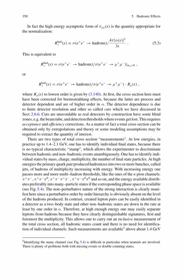
350 5 Hadronic Effects

In fact the high energy asymptotic form of σμμ(s) is the quantity appropriate forthe normalization:

Rhadγ (s) = σ(e+e− → hadrons)/

4π|α(s)|23s

. (5.3)

This is equivalent to

Rhadγ (s) = σ(e+e− → hadrons)/σ(e+e− → μ+μ−)|mμ=0 ,

or

Rhadγ (s) = σ(e+e− → hadrons)/σ(e+e− → μ+μ−) · Rμ(s) ,

where Rμ(s) to lowest order is given by (3.140). At first, the cross section here musthave been corrected for bremsstrahlung effects, because the latter are process anddetector dependent and are of higher order in α. The detector dependence is dueto finite detector resolution and other so called cuts which we have discussed inSect. 2.6.6. Cuts are unavoidable as real detectors by construction have some blindzones, e.g. the beam tube, anddetection thresholdswhere events get lost. This requiresacceptance and efficiency corrections. As a matter of fact a total cross section can beobtained only by extrapolations and theory or some modeling assumptions may berequired to extract the quantity of interest.

There are two types of total cross section “measurements”. At low energies, inpractice up to 1.4–2.1 GeV, one has to identify individual final states, because thereis no typical characteristic “stamp”, which allows the experimenter to discriminatebetween hadronic and non–hadronic events unambiguously. One has to identify indi-vidual states bymass, charge, multiplicity, the number of final state particles. At highenergies the primary quark pair produced hadronizes into two ormore bunches, calledjets, of hadrons of multiplicity increasing with energy. With increasing energy onepasses more and more multi–hadron thresholds, like the ones of the n pion channels:π+π−, π+π−π0, π+π−π+π−, π+π−π0π0 and so on, and the energy available distrib-utes preferably intomany–particle states if the corresponding phase space is available(see Fig. 5.4). The non–perturbative nature of the strong interaction is clearly mani-fest here since a perturbative order by order hierarchy is obviously absent on the levelof the hadrons produced. In contrast, created lepton pairs can be easily identified ina detector as a two–body state and other non–hadronic states are down in the rate atleast by one order in α. Therefore, at high enough energy one may easily separateleptons from hadrons because they have clearly distinguishable signatures, first andforemost the multiplicity. This allows one to carry out an inclusive measurement ofthe total cross section, all hadronic states count and there is no need for identifica-tion of individual channels. Such measurements are available5 above about 1.4 GeV

5Identifying the many channel (see Fig. 5.4) is difficult in particular when neutrals are involved.There is plenty of problems both with missing events or double counting states.

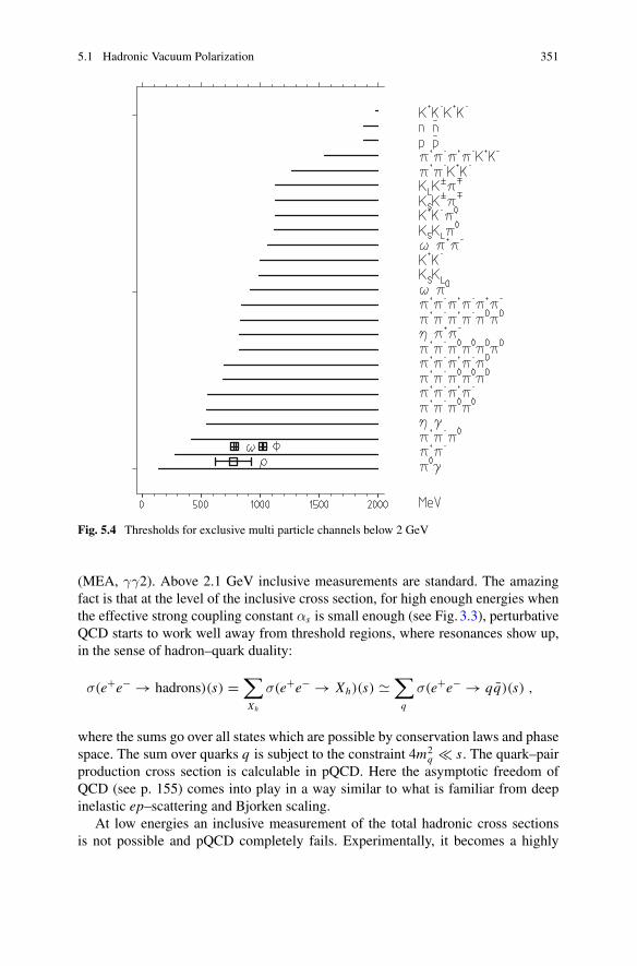
5.1 Hadronic Vacuum Polarization 351

Fig. 5.4 Thresholds for exclusive multi particle channels below 2 GeV

(MEA, γγ2). Above 2.1 GeV inclusive measurements are standard. The amazingfact is that at the level of the inclusive cross section, for high enough energies whenthe effective strong coupling constant αs is small enough (see Fig. 3.3), perturbativeQCD starts to work well away from threshold regions, where resonances show up,in the sense of hadron–quark duality:

σ(e+e− → hadrons)(s) =∑

Xh

σ(e+e− → Xh)(s) �∑

q

σ(e+e− → qq)(s) ,

where the sums go over all states which are possible by conservation laws and phasespace. The sum over quarks q is subject to the constraint 4m2

q � s. The quark–pairproduction cross section is calculable in pQCD. Here the asymptotic freedom ofQCD (see p. 155) comes into play in a way similar to what is familiar from deepinelastic ep–scattering and Bjorken scaling.

At low energies an inclusive measurement of the total hadronic cross sectionsis not possible and pQCD completely fails. Experimentally, it becomes a highly

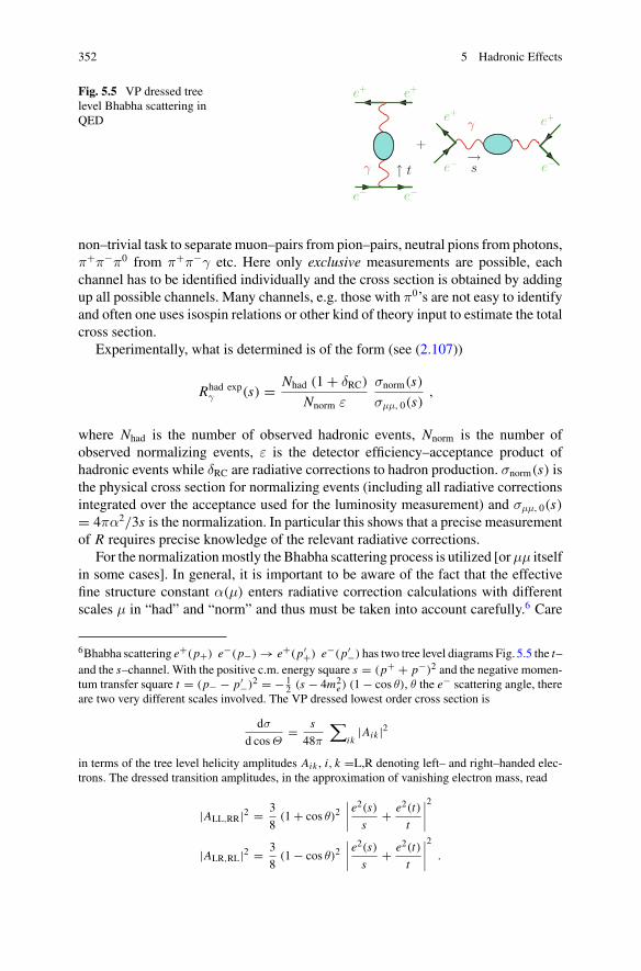
352 5 Hadronic Effects

Fig. 5.5 VP dressed treelevel Bhabha scattering inQED

non–trivial task to separate muon–pairs from pion–pairs, neutral pions from photons,π+π−π0 from π+π−γ etc. Here only exclusive measurements are possible, eachchannel has to be identified individually and the cross section is obtained by addingup all possible channels. Many channels, e.g. those with π0’s are not easy to identifyand often one uses isospin relations or other kind of theory input to estimate the totalcross section.

Experimentally, what is determined is of the form (see (2.107))

Rhad expγ (s) = Nhad (1 + δRC)

Nnorm ε

σnorm(s)

σμμ, 0(s),

where Nhad is the number of observed hadronic events, Nnorm is the number ofobserved normalizing events, ε is the detector efficiency–acceptance product ofhadronic events while δRC are radiative corrections to hadron production. σnorm(s) isthe physical cross section for normalizing events (including all radiative correctionsintegrated over the acceptance used for the luminosity measurement) and σμμ, 0(s)= 4πα2/3s is the normalization. In particular this shows that a precise measurementof R requires precise knowledge of the relevant radiative corrections.

For the normalizationmostly the Bhabha scattering process is utilized [orμμ itselfin some cases]. In general, it is important to be aware of the fact that the effectivefine structure constant α(μ) enters radiative correction calculations with differentscales μ in “had” and “norm” and thus must be taken into account carefully.6 Care

6Bhabha scattering e+(p+) e−(p−) → e+(p′+) e−(p′−) has two tree level diagrams Fig. 5.5 the t–and the s–channel. With the positive c.m. energy square s = (p+ + p−)2 and the negative momen-tum transfer square t = (p− − p′−)2 = − 1

2 (s − 4m2e) (1 − cos θ), θ the e− scattering angle, there

are two very different scales involved. The VP dressed lowest order cross section is

dσ

d cosΘ= s

48π

∑ik

|Aik |2

in terms of the tree level helicity amplitudes Aik , i, k =L,R denoting left– and right–handed elec-trons. The dressed transition amplitudes, in the approximation of vanishing electron mass, read

|ALL,RR|2 = 3

8(1 + cos θ)2

∣∣∣∣e2(s)

s+ e2(t)

t

∣∣∣∣2

|ALR,RL|2 = 3

8(1 − cos θ)2

∣∣∣∣e2(s)

s+ e2(t)

t

∣∣∣∣2

.

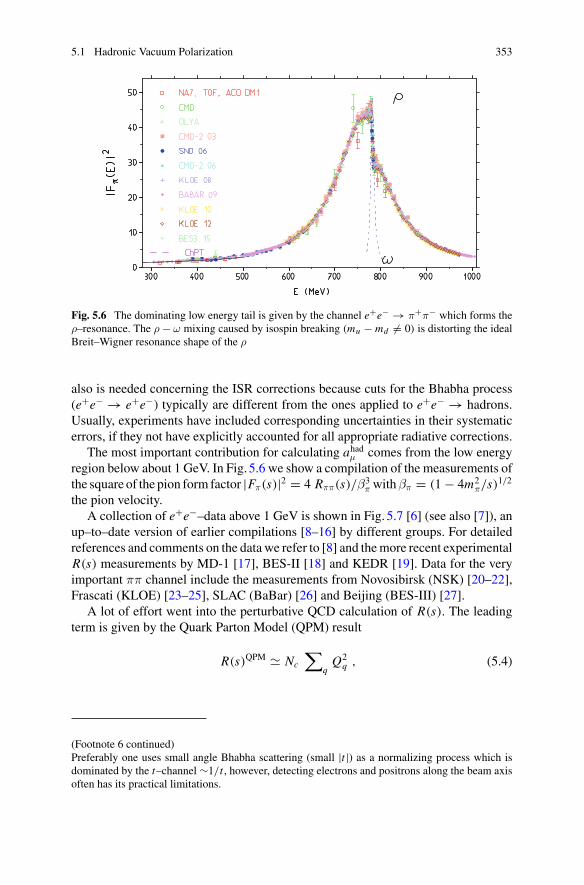
5.1 Hadronic Vacuum Polarization 353

Fig. 5.6 The dominating low energy tail is given by the channel e+e− → π+π− which forms theρ–resonance. The ρ − ω mixing caused by isospin breaking (mu − md = 0) is distorting the idealBreit–Wigner resonance shape of the ρ

also is needed concerning the ISR corrections because cuts for the Bhabha process(e+e− → e+e−) typically are different from the ones applied to e+e− → hadrons.Usually, experiments have included corresponding uncertainties in their systematicerrors, if they not have explicitly accounted for all appropriate radiative corrections.

The most important contribution for calculating ahadμ comes from the low energyregion below about 1 GeV. In Fig. 5.6 we show a compilation of the measurements ofthe square of the pion form factor |Fπ(s)|2 = 4 Rππ(s)/β3

π withβπ = (1 − 4m2π/s)

1/2

the pion velocity.A collection of e+e−–data above 1 GeV is shown in Fig. 5.7 [6] (see also [7]), an

up–to–date version of earlier compilations [8–16] by different groups. For detailedreferences and comments on the data we refer to [8] and themore recent experimentalR(s) measurements by MD-1 [17], BES-II [18] and KEDR [19]. Data for the veryimportant ππ channel include the measurements from Novosibirsk (NSK) [20–22],Frascati (KLOE) [23–25], SLAC (BaBar) [26] and Beijing (BES-III) [27].

A lot of effort went into the perturbative QCD calculation of R(s). The leadingterm is given by the Quark Parton Model (QPM) result

R(s)QPM � Nc

∑qQ2

q , (5.4)

(Footnote 6 continued)Preferably one uses small angle Bhabha scattering (small |t |) as a normalizing process which isdominated by the t–channel ∼1/t , however, detecting electrons and positrons along the beam axisoften has its practical limitations.

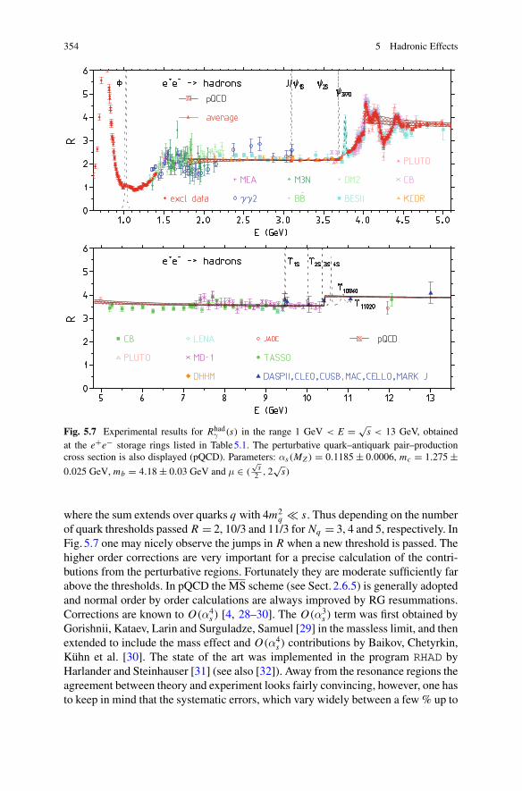
354 5 Hadronic Effects

Fig. 5.7 Experimental results for Rhadγ (s) in the range 1 GeV < E = √

s < 13 GeV, obtainedat the e+e− storage rings listed in Table5.1. The perturbative quark–antiquark pair–productioncross section is also displayed (pQCD). Parameters: αs(MZ ) = 0.1185 ± 0.0006, mc = 1.275 ±0.025 GeV, mb = 4.18 ± 0.03 GeV and μ ∈ (

√s2 , 2

√s)

where the sum extends over quarks q with 4m2q � s. Thus depending on the number

of quark thresholds passed R = 2, 10/3 and 11/3 for Nq = 3, 4 and 5, respectively. InFig. 5.7 one may nicely observe the jumps in R when a new threshold is passed. Thehigher order corrections are very important for a precise calculation of the contri-butions from the perturbative regions. Fortunately they are moderate sufficiently farabove the thresholds. In pQCD the MS scheme (see Sect. 2.6.5) is generally adoptedand normal order by order calculations are always improved by RG resummations.Corrections are known to O(α4

s ) [4, 28–30]. The O(α3s ) term was first obtained by

Gorishnii, Kataev, Larin and Surguladze, Samuel [29] in the massless limit, and thenextended to include the mass effect and O(α4

s ) contributions by Baikov, Chetyrkin,Kühn et al. [30]. The state of the art was implemented in the program RHAD byHarlander and Steinhauser [31] (see also [32]). Away from the resonance regions theagreement between theory and experiment looks fairly convincing, however, one hasto keep in mind that the systematic errors, which vary widely between a few % up to

5.1 Hadronic Vacuum Polarization 355

10% are not shown in the plot. Typically, the theory result is much more accuratethan the experimental one, in regions where it applies. This is possible, because, theQCD parametersαs and the charm and bottom quark masses relevant here are knownfrom plenty of all kinds of experiments rather accurately now. Nevertheless, it is notobvious that applying pQCD in place of the data, as frequently done, is not missingsome non–perturbative contributions. The non–perturbative quark condensate terms(1/Q4 power corrections) which enter the OPE are not a real problem in our contextas they are small at energies where pQCD applies [33]. There are other kinds of NPphenomena like bound states, resonances, instantons and in particular the hadroniza-tion of the quarks. In applying pQCD to describe real physical cross sections ofhadro–production one needs a “rule” which bridges the asymptotic freedom regimewith the confinement regime, since the hadronization of the colored partons producedin the hard kicks into color singlet hadrons eludes a quantitative understanding. Therule is referred to as quark hadron duality7 [35, 36], which states that for large s theaverage non–perturbative hadron cross section equals the perturbative quark crosssection:

σ(e+e− → hadrons)(s) �∑

qσ(e+e− → qq)(s) , (5.5)

where the averaging extends from threshold up to the given s value which must liefar enough above a threshold (global duality). Approximately, such duality relationsthen would hold for energy intervals which start just below the last threshold passedup to s. Qualitatively, such a behavior is visible in the data, however, for precisereliable predictions it has not yet been possible to quantify the accuracy of the dualityconjecture. A quantitative check would require much more precise cross sectionmeasurements than the ones available today. Ideally, one should attempt to reach theaccuracy of pQCD predictions. In addition, in dispersion integrals the cross sectionsare weighted by different s–dependent kernels, while the duality statement is claimedto hold for weight unity. One procedure definitely is contradicting duality reasonings:to “take pQCD plus resonances” or to “take pQCDwhere R(s) is smooth and data inthe complementary ranges”. Also adjusting the normalization of experimental datato conform with pQCD within energy intervals (assuming local duality) has no solidfoundation.

In view of the problematic quality of the data in some regions a “theory–driven”approach replacing data by pQCD results in smaller or larger intervals [37–39] maywell be adequate to reduce the hadronic uncertainties. However, the uncertainty of thepQCD results evaluated by varying just the QCD parametersαs(μ), the quarkmassesmq(μ) and the renormalization scale μ, conventionally, in a range μ ∈ (

√s2 , 2

√s),

generally does not account for possible non–perturbative uncertainties, related to thehadronization process. Thus the problem of the theory driven approach is a reliableerror estimate, and not the shift in the central value, which may well be shifted inthe right direction. In the following we generally present a conservative approach of

7Quark–hadron duality was first observed phenomenologically for the structure function in deepinelastic electron–proton scattering [34].

356 5 Hadronic Effects

the evaluation of the hadronic effects, taking the data and directly integrating themin all regions where pQCD cannot be trusted in the sense as advocated in [31].

The following data integration procedure has been used for the evaluation of thedispersion integral:

1. Take data as they are and apply the trapezoidal rule (connecting data points bystraight lines) for integration.

2. To combine results from different experiments: (i) integrate data for individualexperiments and combine the results, (ii) combine data fromdifferent experimentsbefore integration and integrate the combined “integrand”. Check consistency ofthe two possible procedures to estimate the reliability of the results.

3. Error analysis: (1) statistical errors are added in quadrature, (2) systematic errorsare added linearly for different experiments, (3) combined results are obtained bytaking weighted averages. (4) all errors are added in quadrature for “independent”data sets. We assume this to be allowed in particular for different energy regionsand/or different accelerators. (5) best: apply the true covariancematrix if available,this is the case for the ISR measurements from meson factories.

4. The ρ–resonance region is integrated using the Gounaris–Sakurai (GS)parametrization of the pion form factor [40]. Other pronounced resonances havebeen parametrized by Breit–Wigner shapes with parameters taken from the Par-ticle Data Tables [41, 42].

5.1.2 Integrating the Experimental Data and Estimatingthe Error

Here we briefly elaborate on procedures and problems related to the integrationof the function R(s) given in terms of experimental data sets with statistical andsystematic errors. Obviously one needs some interpolation procedure between thedata points. The simplest is to use the trapezoidal rule in which data points arejoined by straight lines. This procedure is problematic if data points are sparse inrelation to the functional shape of R(s). Note that in pQCD R(s) is close to piece-wise constant away from thresholds and resonances (where pQCD fails) and thetrapezoidal rule should work reliably. For resonances the trapezoidal rule is notvery suitable and therefor one uses Breit–Wigner type parametrizations in termsof resonance parameters given in the particle data table. Here it is important tocheck which type of BW parametrization has been used to determine the resonanceparameters (see [8] for a detailed discussion). Some analyses use other smoothingprocedures, by fitting the data to some guessed functional form (see e.g. [43, 44]).

While statistical errors commonly are added in quadrature (Gaussian error prop-agation), the systematic errors of an experiment have to be added linearly, becausethey encode overall errors like normalization or acceptance errors. Usually the exper-iments give systematic errors as a relative systematic uncertainty and the systematicerror to be added linearly is given by the central value times the relative uncertainty.

5.1 Hadronic Vacuum Polarization 357

For data from different experiments the combination of the systematic errors is moreproblematic. If one would add systematic errors linearly everywhere, the error wouldbe obviously overestimated since one would not take into account the fact that inde-pendent experiments have been performed. However, often experiments use commonsimulation techniques for acceptance and luminosity determinations and the samestate–of–the–art calculations for radiative corrections such that correlations betweendifferent experiments cannot be excluded. Since we are interested in the integral overthe data only, a natural procedure seems to be the following: for a given energy range(scan region) we integrate the data points for each individual experiment and thentake a weightedmean, based on the quadratically combined statistical and systematicerror, of the experiments which have been performed in this energy range. By doingso we have assumed that different experiments have independent systematic errors,which of course often is only partially true.8 The problem with this method is thatthere exist regions where data are sparse yet the cross section varies rapidly. Theapplicability of the trapezoidal rule is then not reliable, but taking other models forthe extrapolation introduces another source of systematic errors. It was noticed sometime ago in [45] that fitting data to some function by minimizing χ2 may lead tomisleading results. The problem may be circumvented by the appropriate definitionof the χ2 to be minimized (see below). Fortunately, in the dominating ρ–resonanceregion the data base has been improving a lot during the past decade.

In order to start from a better defined integrand we do better to combine allavailable data points into a single dataset. If we would take just the collection ofpoints as if they were from one experiment we not only would get a too pessimisticerror estimate but a serious problem could be that scarcely distributed precise datapoints do not get the appropriate weight relative to densely spaced data point withlarger errors.What seems to bemore adequate is to take for eachpoint of the combinedset the weighted average of the given point and the linearly interpolated points of theother experiments:

R = 1

w

∑

i

wi Ri ,

with total error δtot = 1/√

w, where w = ∑i wi and wi = 1/δ2i tot . By δi tot =√

δ2i sta + δ2i sys we denote the combined error of the individual measurements. In

addition, to each point a statistical and a systematic error is assigned by takingweighted averages of the squared errors:

δsta =√

1

w

∑

i

wi δ2i sta , δsys =√

1

w

∑

i

wi δ2i sys .

8If there are known common errors, like the normalization errors for experiments performed atthe same facility, one has to add the common error after averaging. In some cases we correct forpossible common errors by scaling up the systematic error appropriately.

358 5 Hadronic Effects

There is of course an ambiguity in separating the well–defined combined error into astatistical and a systematic one. We may also calculate separately the total error andthe statistical one and obtain a systematic error δsys = √

δ2tot − δ2sta. Both proceduresgive very similar results. We also calculate χ2 = ∑

i wi (Ri − R)2 and compare itwith N − 1, where N is the number of experiments.Whenever S =√

χ2/(N − 1)>1,we scale the errors by the factor S, unless there are plausible arguments which allowone to discard inconsistent data points.

In order to extract the maximum of information, weighted averages of differentexperiments at a given energy are calculated. The solution of the averaging problemmay be found by minimizing χ2 as defined by

χ2 =Nexp∑

n=1

Nn∑

i, j=1

(Rni − Ri ) (Cn

i j )−1 (Rn

j − R j ) ,

where Rni is the Rmeasurement of the nth experiment at energy

√si , Nexp the number

of experiments, Cni j is the covariance matrix between the i th and j th data point of

the nth experiment, and R is the average to be determined. The covariance matrix isgiven by

Cni j =

{(δni sta)

2 + (δni sys)2 for j = i

δni sys · δnj sys for j = i, i, j = 1, . . . , Nn ,

where δni sta and δni sys denote the statistical and systematic error, respectively, of Rni .

The minimum condition dχ2

d Ri= 0, for all i yields the system of linear equations

Nexp∑

n=1

Nn∑

j=1

(Cni j )

−1 (Rnj − R j ) = 0 , i = 1, . . . , Nn .

The inverse covariance matrix C−1i j between the calculated averages Ri and R j is the

sum over the inverse covariances of every experiment

C−1i j =

Nexp∑

n=1

(Cni j )

−1 .

This procedure, if taken literally, would yield reliable fits only if the errors would besmall enough, which would require in particular sufficiently high statistics. In fact,many of the older experiments suffer from low statistics and uncertain normalizationand the fits obtained in this manner are biased towards too low values (compare [43]with [44], for example). The correct χ2 minimization requires to replace the experi-mental covariance matrices Cn

i j by the ones of the fit result Ci j [45]. This is possibleby iteration with the experimental covariance as a start value.

5.1 Hadronic Vacuum Polarization 359

Often one attempts tomodel a number Nexp of given differentmeasurements Rn ={Rn

i , i = 1, . . . Nn, n = 1, . . . Nexp} by theoretical expectation M(a) = {Mi , i =1, . . . Nn} weighted by the error covariance matrix Cn provided together with thedata. The vector a denoting the unknown internal model parameter list, is deter-mined by minimizing

χ2 =Nexp∑

n=1

Nn∑

i, j=1

[Rn − M(a)]Ti (Cni j )

−1 [Rn − M(a)] j , (5.6)

with respect to a which is providing the optimum value a0. This approach has beenexercised for the case of low energy e+e− → hadrons data in [44] using some phe-nomenologically inspired shape functions and more recently in [46] adopting theHLS phenomenological Lagrangian model, for example.

The notorious normalization uncertainties of data sets may pose a serious problemand therefore should be analyzed carefully too. This has been done in [47] againwithin the framework of the HLS model. A constant global scale uncertainty canbe written β = 1 + λ, where λ is a random variable with range on ] − 1,+∞[. Asthe expectation values are E(λ) = 0 and E(λ2) = σ2 with σ << 1, the Gaussianapproximation for λ is safe [48]. A data sample subject to a global scale uncertaintyprovides an individual contribution to an effective global χ2

glob, which is of the form

χ2 =Nexp∑

n=1

Nn∑

i, j=1

[Rn − M(a) − λA]Ti (Cni j )

−1 [Rn − M(a) − λA] j + λ2

σ2, (5.7)

where R, M , C and a have the same meaning as before, while λ and σ are the newelements. As for A, even if intuitively one may prefer A = R, the choice A = M(a)

has been shown to drop out any biasing issue9 [45, 48]. As M(a) is unknown atthe start of the fitting, A = R is the initial setting and A ≈ M(a) is achieved byiteration. Assuming that the unknown scale factor λ is solely of experimental origin– and, then, independent of the model parameters a – the solution to ∂χ2/∂λ = 0provides its most probable value λ0. After substituting the solution into (5.7) thelatter becomes

χ2 =Nexp∑

n=1

Nn∑

i, j=1

[Rn − M(a)]Ti (Cni j )

−1 [Rn − M(a)] j with C = C + σ2AAT ,

(5.8)

which exhibits a modified error covariance matrix C and only depends on the(physics) model parameters. More precisely, the single recollection of the scaleuncertainties λ shows up in its variance σ2 in the modified covariance matrix C .A detailed analysis of the low energy e+e− data has been performed recently in [47]where also more details on the implementation of the method may be found.

9This does not mean that the choice A = R necessarily leads to a significantly biased solution.

360 5 Hadronic Effects

5.1.3 The Cross–Section e+e− → Hadrons

The total cross section for hadron production in e+e−–annihilation (a typicals–channel process) may be written in the form

σhad(s) = α

s

4π√1 − 4m2

es

(1 + 2m2

e

s

)Im Π ′ had

γ (s)

� 4πα

sIm Π ′ had

γ (s) , since s ≥ 4m2π � m2

e ,

where Π ′ hadγ (s) is the hadronic part of the photon vacuum polarization with (see

(3.139) and Sect. 3.7.1)

Im Π ′ hadγ (s) = e2

12πRhad

γ (s) .

From (2.179) we easily get the lowest order quark/antiquark pair–production crosssection encoded in

RpQCDγ (s) =

∑

q

Ncq Q2q

√

1 − 4m2q

s

(1 + 2m2

q

s

), (5.9)

which however is a reasonable approximation to hadro–production only at high ener-gies away from thresholds and resonances (see below) and to the extent that quark–hadron duality (5.5) holds. At low energies 4m2

π < s < 9m2π the ππ–production

channel is the dominant hadro–production process. The pion–pair production iscommonly parametrized in terms of a non–perturbative amplitude, the pion formfactor Fπ(s),

Rhadγ (s) = 1

4

(1 − 4m2

π

s

) 32

|F (0)π (s)|2 , s < 9m2

π . (5.10)

For point–like pions we would have Fπ(s) = Fπ(0) = 1. At this point it is importantto remind the reader that we have been deriving a set of relations and formulas toleading order O(α2) in QED in Sect. 2.7. For a precise analysis of the hadroniceffects higher order QED corrections are important as well. Furthermore, we haveassumed that the center of mass energy E = √

s is small enough, typically, E ≤12 GeV say, such that virtual Z exchange contributions e+e− → Z∗ → hadrons ore+e− → Z∗ → μ+μ− are sufficiently suppressed relative to virtual γ∗ exchange atthe precision we are aiming at. Since ahadμ is rather insensitive to the high energy tailsuch a condition is not a problem.

In order to obtain the observed cross section, we have to include the QED cor-rections, the virtual, soft and hard photon effects. The basic problems have been

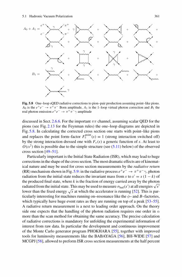
5.1 Hadronic Vacuum Polarization 361

Fig. 5.8 One–loop sQED radiative corrections to pion–pair production assuming point–like pions.A0 is the e+e− → π+π− Born amplitude, A1 is the 1–loop virtual photon correction and B1 thereal photon emission e+e− → π+π−γ amplitude

discussed in Sect. 2.6.6. For the important ππ channel, assuming scalar QED for thepions (see Fig. 2.13 for the Feynman rules) the one–loop diagrams are depicted inFig. 5.8. In calculating the corrected cross section one starts with point–like pionsand replaces the point form–factor Fpoint

π (s) ≡ 1 (strong interaction switched off)by the strong interaction dressed one with Fπ(s) a generic function of s. At least toO(α2) this is possible due to the simple structure (see (5.11) below) of the observedcross section [49–51].

Particularly important is the Initial State Radiation (ISR), which may lead to hugecorrections in the shape of the cross section. Themost dramatic effects are of kinemat-ical nature and may be used for cross section measurements by the radiative return(RR) mechanism shown in Fig. 5.9: in the radiative process e+e− → π+π−γ, photonradiation from the initial state reduces the invariant mass from s to s ′ = s (1 − k) ofthe produced final state, where k is the fraction of energy carried away by the photonradiated from the initial state. Thismay be used tomeasureσhad(s ′) at all energies

√s ′

lower than the fixed energy√s at which the accelerator is running [52]. This is par-

ticularly interesting for machines running on–resonance like the φ– and B–factories,which typically have huge event rates as they are running on top of a peak [53–55].A radiative return measurement is a next to leading order approach. On the theoryside one expects that the handling of the photon radiation requires one order in αmore than the scan method for obtaining the same accuracy. The precise calculationof radiative corrections is mandatory for unfolding the experimental information ofinterest from raw data. In particular the development and continuous improvementof the Monte Carlo generator program PHOKHARA [55], together with improvedtools for luminosity measurements like the BABAYAGA [56], BH-WIDE [57] andMCGPJ [58], allowed to preform ISR cross section measurements at the half percent

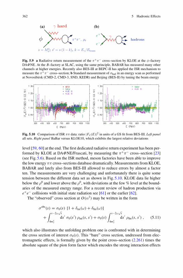
362 5 Hadronic Effects

γ

e−

e+

γ hard

s = M2φ; s′ = s (1 − k), k = Eγ/Ebeam

π+π−, ρ0φ hadrons

(a) (b)

Fig. 5.9 a Radiative return measurement of the π+π− cross–section by KLOE at the φ–factoryDAΦNE. At the B–factory at SLAC, using the same principle, BABAR has measured many otherchannels at higher energies. Recently also BES-III at BEPC-II has applied the ISR mechanism tomeasure the π+π− cross–section; b Standard measurement of σhad in an energy scan as performedat Novosibirsk (CMD-2, CMD-3, SND, KEDR) and Beijing (BES-II) by tuning the beam energy

Fig. 5.10 Comparison of ISR ππ data: ratio |Fπ(E)|2 in units of a GS fit from BES-III. Left panelall sets. Right panel BaBar versus KLOE10, which exhibits the largest relative deviations

level [59, 60] at the end. The first dedicated radiative return experiment has been per-formed by KLOE at DAΦNE/Frascati, by measuring the π+π− cross–section [23](see Fig. 5.6). Based on the ISR method, meson factories have been able to improvethe low energy ππ cross–sections database dramatically.Measurements fromKLOE,BABAR and lately also from BES-III allowed to reduce errors by almost a factorten. The measurements are very challenging and unfortunately there is quite sometension between the different data set as shown in Fig. 5.10. KLOE data lie higherbelow the ρ0 and lower above the ρ0, with deviations at the few% level at the bound-aries of the measured energy range. For a recent review of hadron production viae+e− collisions with initial state radiation see [61] or the earlier [62].

The “observed” cross section at O(α2) may be written in the form

σobs(s) = σ0(s) [1 + δini(ω) + δfin(ω)]

+∫ s−2ω

√s

4m2π

ds ′ σ0(s′) ρini(s, s

′) + σ0(s)∫ s−2ω

√s

4m2π

ds ′ ρfin(s, s′) , (5.11)

which also illustrates the unfolding problem one is confronted with in determiningthe cross section of interest σ0(s). This “bare” cross section, undressed from elec-tromagnetic effects, is formally given by the point cross–section (2.261) times theabsolute square of the pion form factor which encodes the strong interaction effects

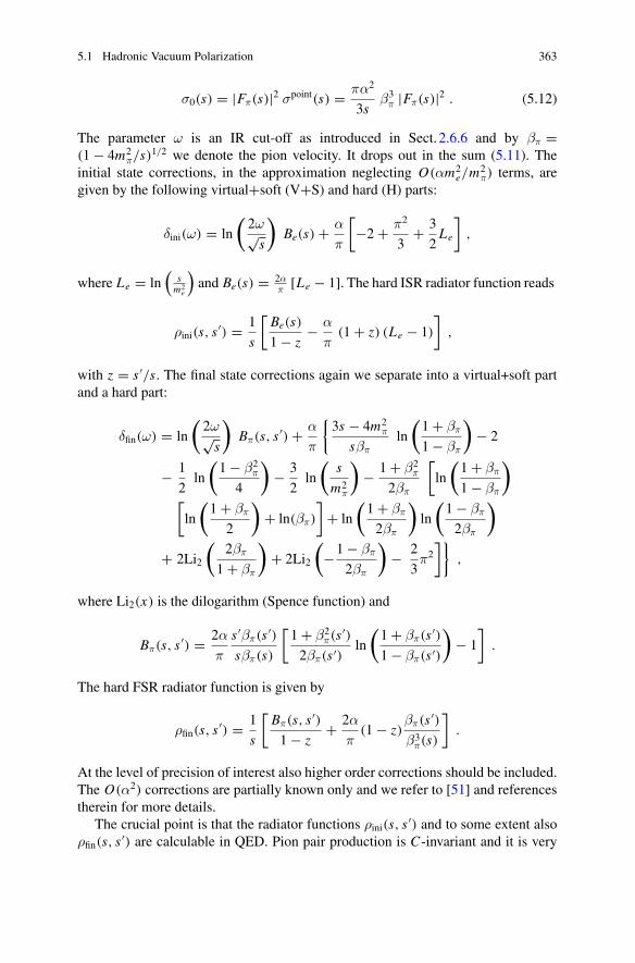
5.1 Hadronic Vacuum Polarization 363

σ0(s) = |Fπ(s)|2 σpoint(s) = πα2

3sβ3

π |Fπ(s)|2 . (5.12)

The parameter ω is an IR cut-off as introduced in Sect. 2.6.6 and by βπ =(1 − 4m2

π/s)1/2 we denote the pion velocity. It drops out in the sum (5.11). The

initial state corrections, in the approximation neglecting O(αm2e/m

2π) terms, are

given by the following virtual+soft (V+S) and hard (H) parts:

δini(ω) = ln

(2ω√s

)Be(s) + α

π

[−2 + π2

3+ 3

2Le

],

where Le = ln(

sm2

e

)and Be(s) = 2α

π[Le − 1]. The hard ISR radiator function reads

ρini(s, s′) = 1

s

[Be(s)

1 − z− α

π(1 + z) (Le − 1)

],

with z = s ′/s. The final state corrections again we separate into a virtual+soft partand a hard part:

δfin(ω) = ln

(2ω√s

)Bπ(s, s

′) + α

π

{3s − 4m2

π

sβπln

(1 + βπ

1 − βπ

)− 2

− 1

2ln

(1 − β2

π

4

)− 3

2ln

(s

m2π

)− 1 + β2

π

2βπ

[ln

(1 + βπ

1 − βπ

)

[ln

(1 + βπ

2

)+ ln(βπ)

]+ ln

(1 + βπ

2βπ

)ln

(1 − βπ

2βπ

)

+ 2Li2

(2βπ

1 + βπ

)+ 2Li2

(−1 − βπ

2βπ

)− 2

3π2

]},

where Li2(x) is the dilogarithm (Spence function) and

Bπ(s, s′) = 2α

π

s ′βπ(s ′)sβπ(s)

[1 + β2

π(s′)

2βπ(s ′)ln

(1 + βπ(s ′)1 − βπ(s ′)

)− 1

].

The hard FSR radiator function is given by

ρfin(s, s′) = 1

s

[Bπ(s, s ′)1 − z

+ 2α

π(1 − z)

βπ(s ′)β3

π(s)

].

At the level of precision of interest also higher order corrections should be included.The O(α2) corrections are partially known only and we refer to [51] and referencestherein for more details.

The crucial point is that the radiator functions ρini(s, s ′) and to some extent alsoρfin(s, s ′) are calculable in QED. Pion pair production is C-invariant and it is very

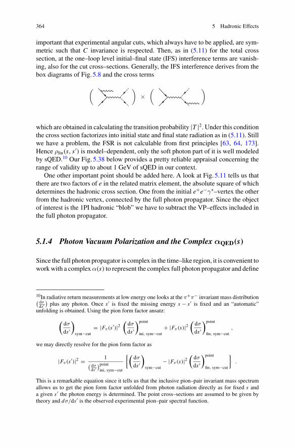
364 5 Hadronic Effects

important that experimental angular cuts, which always have to be applied, are sym-metric such that C invariance is respected. Then, as in (5.11) for the total crosssection, at the one–loop level initial–final state (IFS) interference terms are vanish-ing, also for the cut cross–sections. Generally, the IFS interference derives from thebox diagrams of Fig. 5.8 and the cross terms

( )×

( )

which are obtained in calculating the transition probability |T |2. Under this conditionthe cross section factorizes into initial state and final state radiation as in (5.11). Stillwe have a problem, the FSR is not calculable from first principles [63, 64, 173].Hence ρfin(s, s ′) is model–dependent, only the soft photon part of it is well modeledby sQED.10 Our Fig. 5.38 below provides a pretty reliable appraisal concerning therange of validity up to about 1 GeV of sQED in our context.

One other important point should be added here. A look at Fig. 5.11 tells us thatthere are two factors of e in the related matrix element, the absolute square of whichdetermines the hadronic cross section. One from the initial e+e−γ∗–vertex the otherfrom the hadronic vertex, connected by the full photon propagator. Since the objectof interest is the 1PI hadronic “blob” we have to subtract the VP–effects included inthe full photon propagator.

5.1.4 Photon Vacuum Polarization and the Complex αQED(s)

Since the full photon propagator is complex in the time–like region, it is convenient toworkwith a complexα(s) to represent the complex full photon propagator and define

10In radiative return measurements at low energy one looks at the π+π− invariant mass distribution( dσds′

)plus any photon. Once s′ is fixed the missing energy s − s′ is fixed and an “automatic”

unfolding is obtained. Using the pion form factor ansatz:

(dσ

ds′

)

sym−cut= |Fπ(s′)|2

(dσ

ds′

)point

ini, sym−cut+ |Fπ(s)|2

(dσ

ds′

)point

fin, sym−cut,

we may directly resolve for the pion form factor as

|Fπ(s′)|2 = 1( dσds′

)pointini, sym−cut

{(dσ

ds′

)

sym−cut− |Fπ(s)|2

(dσ

ds′

)point

fin, sym−cut

}.

This is a remarkable equation since it tells us that the inclusive pion–pair invariant mass spectrumallows us to get the pion form factor unfolded from photon radiation directly as for fixed s anda given s′ the photon energy is determined. The point cross–sections are assumed to be given bytheory and dσ/ds′ is the observed experimental pion–pair spectral function.

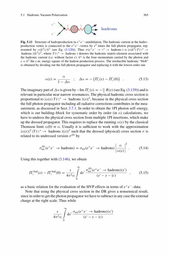
5.1 Hadronic Vacuum Polarization 365

γ γ

e−

e+

hadrons

Fig. 5.11 Structure of hadroproduction in e+e−–annihilation. The hadronic current at the hadro–production vertex is connected to the e+e−–vertex by e2 times the full photon propagator, rep-resented by α(k2)/k2 (see Eq. (3.120)). Thus σ(e+e− → γ∗ → hadrons ) ∝ |α(k2) T (γ∗ →hadrons )(k2)|2, where T (γ∗ → hadrons ) denotes the hadronic matrix-element associated withthe hadronic current (i.e. without factor e). kμ is the four–momentum carried by the photon ands = k2 the c.m. energy square of the hadron production process. The irreducible hadronic “blob”is obtained by dividing out the full photon propagator and replacing it with the lowest order one

α(s) = α

1 − Δα; Δα = − (

Π ′γ(s) − Π ′

γ(0))

. (5.13)

The imaginary part ofΔα is given by−Im Π ′γ(s) = −α

3 R(s) (see Eq. (3.139)) and isrelevant in particular near narrow resonances. The physical hadronic cross section isproportional to |α(s) T (γ∗ → hadrons )(s)|2, because in the physical cross sectionthe full photon propagator including all radiative corrections contributes in the mea-surement, as discussed in Sect. 3.7.1. In order to obtain the 1PI photon self–energy,which is our building–block for systematic order by order (in α) calculations, wehave to undress the physical cross section from multiple 1PI insertions, which makeup the dressed propagator. This requires to replace the running α(s) by the classicalThomson limit α(0) ≡ α. Usually it is sufficient to work with the approximation|α(s)|2 |T (γ∗ → hadrons )(s)|2 such that the dressed (physical) cross section σ isrelated to its undressed version σ(0) by

σ(0)tot (e

+e− → hadrons) = σtot(e+e− → hadrons)

∣∣∣∣α

α(s)

∣∣∣∣2

. (5.14)

Using this together with (3.146), we obtain

Π ′ hadγ (s) − Π ′ had

γ (0) = s

4π2α

∞∫

0

ds ′ σ(0)tot (e

+e− → hadrons)(s ′)(s ′ − s − iε)

, (5.15)

as a basic relation for the evaluation of the HVP effects in terms of e+e−–data.Note that using the physical cross section in the DR gives a nonsensical result,

since in order to get the photon propagator we have to subtract in any case the externalcharge at the right scale. Thus while

s

4π2α

∞∫

0

ds ′ σtot(e+e− → hadrons)(s ′)(s ′ − s − iε)

366 5 Hadronic Effects

is double counting the VP effects, and therefore does not represent something mean-ingful, the linearly |α/α(s)|–rescaled cross section

s

4π2

∞∫

0

ds ′ 1

|α(s ′)|σtot(e+e− → hadrons)(s ′)

(s ′ − s − iε),

yields the hadronic shift in the full photon propagator. Only at least once VP–subtracted physical cross sections are useful in DRs! However, this amounts toresumming electromagnetic effects to all orders in α, and is not useful in a sys-tematic order by order approach. Hence we stick to the basic DR (5.15) in all whatfollows.

In generalweknow the experimental physical cross sectionσtot(e+e− → hadrons)as well as the complex α(s), such that we can extract the required undressedσ(0)tot (e

+e− → hadrons) via (5.14). However, α(s) we only know after we know σhad,so usually we can determine σ(0)

had(s) only by iteration, provided this iteration con-verges. In most cases experiments do not directly extract the R–ratio (5.1) as a ratioof measured cross sections. The reason is that luminosity is usually monitored byBhabha–scattering and because σμμ(s) is much smaller than σhad(s) and has muchlower statistics especially in resonance regions. In case (5.1) is available we have

Im Π ′ hadγ (s) = α

3Rhad(s) = σhad(s)

σμμ(s)(5.16)

experimentally, which allows us the obtain

Re Π ′γ ren(s) = Re Π ′

γ(s) − Π ′γ(0) = s

πRe

∫ ∞

s0

ds ′ Im Π ′γ(s

′)s ′(s ′ − s − iε)

directly, such that Π ′γ ren is determined. However, what is measured when looking

at σhad in isolation (via normalization to Bhabha events) is σhad(s) = 4παs Im Π ′ had

γ

(s)∣∣1/(1 + Π ′

γ ren(s))∣∣2 and thus

Im Π ′ hadγ (s) = s

4πα

∣∣1 + Π ′γ ren(s)

∣∣2 σhad(s) , (5.17)

where Π ′(s) = Π ′ lep + Π ′ had is the full irreducible photon self-energy includingthe leptonic contributions, which is well known in perturbation theory. In terms ofdata alone to determine the two quantities Im Π ′(s) and Re Π ′(s) we need twomeasurements besides σhad ideally also σμμ, as performed recently in [65]. Thisworks locally point by point for each energy. If only σhad(s) is known, the standardprocedure is to expand (5.17) in Π ′, which then allows to solve iteratively for Π ′(s)with the real part determined by the DR (5.15). This requires to know σhad(s) for alls ≥ s0 and is thus not a local procedure. This works well when |Π ′(s)| � 1, which

5.1 Hadronic Vacuum Polarization 367

is what we usually expect for an e.m. correction. Unfortunately, in the vicinity ofsome resonances the convergence condition |Π ′(s)| < 1 in badly violated.

HVP Subtraction of Rhadγ (s): a Problem of the DR Method?

So far we have not addressed the question what happens if |Π ′γ(s)| ≥ 1. The problem

has been addressed recently in [6] and we include the discussion here. The fullphoton propagator (2.165) is usually obtained by Dyson resummation (2.162) ofthe 1PI part x = Π ′

γ(s). As we know this is a geometric series 1 + x + x2 + · · · =1/(1 − x) which only converges iff |x | < 1. Including the external e.m. couplingsand renormalization we have

i e2 D′γ(q

2) = −i

q2

e2

1 + Π ′γ ren(q

2).

The complex effective charge thus is given by the well-known expression

e2

1 + Π ′γ ren(s)

= e2

1 − Δα(s)= e2(s) .

Usually, Δα(s) is a correction i.e. |Δα(s)| � 1 and the Dyson series convergeswell. Indeed for any type of perturbative effects no problem is encountered (besidespossible Landau poles). For non-perturbative strong interaction physics there areexceptions. One would expect that, if there are problems, one would encounter themat low energy, but for the ρ, theω and the φ, in spite of huge resonance enhancements,the HVP contributions to the running charge are small relative to unity, as the effect issuppressed by the e.m. coupling e2. The exception, surprisingly, we find at pretty highenergies, at the very narrow Okubo–Zweig–Iizuka (OZI) suppressed resonances,11

which are extremely sharp, because they lie below corresponding qq-thresholds. Forthese Extremely Narrow Resonances (ENR) the strong interaction appears heavilysuppressed (3 gluons exchange) and the electromagnetic channel (1 photon exchange)appears almost as strong as the strong one (see Fig. 5.12). Actually, Γee is not muchsmaller thanΓQCD (i.e. strong decays). This phenomenon shows up for the resonancesJ/ψ,ψ2, Υ1, Υ2 and Υ3. The imaginary parts from the narrow resonances read

Im Π ′γ(s)) = α

3Rγ(s) = 3

α

Γee

Γ; s = M2

R

11The OZI rule formulated in 1963 independently by Okubo, Zweig and Iizuka [66], explains whycertain hadron decay channels appear substantially suppressed. Later it turned out to be a simpleconsequence of QCD. Diagrams representing OZI suppressed processes can be cut into an initialand a final state part by cutting gluon lines solely (see Fig. 5.12). An example is φ decay: sinceφ is essentially a ss state, the decay into strange meson states φ → K+K−, K 0K 0 is dominating(83%), while the decay into non-strange mesons φ → π+π−π0 is suppressed (15%)), in spite ofthe much larger phase space available.

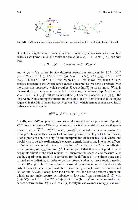
368 5 Hadronic Effects

Fig. 5.12 OZI suppressed strong decays let e.m. interaction look to be almost of equal strength

at peak, causing the sharp spikes, which are seen only by appropriate high resolutionscans, as we know. Let α(s) denotes the real α(s) = α/(1 + Re Π ′

γ ren(s)), we notethat,

|1 + Π ′γ ren(s)|2 − (α/α(s))2 = (Im Π ′

γ(s))2 ,

and at√s = MR values for the different resonances are given by 1.23 × 10−3

(ρ), 2.76 × 10−3 (ω), 1.56 × 10−2 (φ), 594.81 (J/ψ), 9.58 (ψ2), 2.66 × 10−4

(ψ3), 104.26 (Υ1), 30.51 (Υ2 ) and 55.58 (Υ3 ). This shows that near OZI sup-pressed resonances the Dyson series cannot converge. So we have a problem withthe dispersive approach, which requires Rγ(s) ∝ Im Π ′

γ(s) as an input. What ismeasured by an experiment is the full propagator, the summed up Dyson series,Z = |1/(1 + x + iy)|2, but we cannot extract y from that since for |x + iy| ≥ 1 theobservable Z has no representation in terms of x and y. Remember that the objectrequired in the DR is the undressed Rγ(s) in (5.3), which cannot be measured itself,rather we have to extract

Rbareγ = Rphys

γ |1 + Π ′γ ren(s)|2 .

Locally, near OZI suppressed resonances, the usual iterative procedure of gettingRbare

γ does not converge! The way out usually practiced is to utilize the smooth space-

like charge, i.e. Rbareγ = Rphys

γ |1 + Π ′γ ren(−s)|2 , expected to do the undressing “in

average”. This actually does not look too wrong as we see in Fig. 5.13. Nevertheless,I see a problem her, not only for the interpretation of resonance data, where onewould wish to be able to disentangle electromagnetic from strong interaction effects.

For what concerns the proper extraction of the hadronic effects contributingto the running of αQED and to ahadμ , I see no proof that this cannot produce non-negligible shifts! In the ENR regions, it is therefore indispensable to measure R(s)via the experimental ratio (5.1) corrected for the difference in the phase spaces andin final state radiation, in order to get the proper undressed cross section neededin the DR approach. Cross–sections measured by normalizing to Bhabha events(which is what most experiments have been doing except from the more recentBaBar and KLOE12 ones) have the problem that one has to perform correctionswhich are not under control perturbatively. Note that from measuring (5.17) with(1 + Π ′)(1 + Π ′∗) = 1 + 2Re Π ′ + (Re Π ′)2 + (Im Π ′)2 in the denominator, wecannot determine Im Π ′(s) and Re Π ′(s) locally unless we measure σμμ(s) as well.

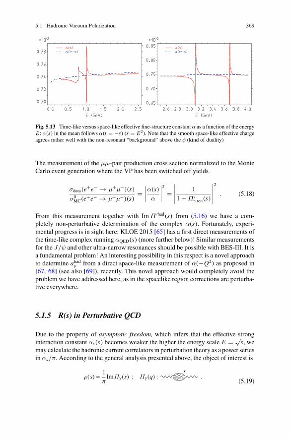
5.1 Hadronic Vacuum Polarization 369

Fig. 5.13 Time-like versus space-like effective fine-structure constant α as a function of the energyE : α(s) in the mean follows α(t = −s) (s = E2). Note that the smooth space-like effective chargeagrees rather well with the non-resonant “background” above the φ (kind of duality)

The measurement of the μμ–pair production cross section normalized to the MonteCarlo event generation where the VP has been switched off yields

σdata(e+e− → μ+μ−)(s)

σ0MC(e+e− → μ+μ−)(s)

=∣∣∣∣α(s)

α

∣∣∣∣2

=∣∣∣∣∣

1

1 + Π ′γ ren(s)

∣∣∣∣∣

2

. (5.18)

From this measurement together with Im Π ′had(s) from (5.16) we have a com-pletely non-perturbative determination of the complex α(s). Fortunately, experi-mental progress is in sight here: KLOE 2015 [65] has a first direct measurements ofthe time-like complex running αQED(s) (more further below)! Similar measurementsfor the J/ψ and other ultra-narrow resonances should be possible with BES-III. It isa fundamental problem! An interesting possibility in this respect is a novel approachto determine ahadμ from a direct space-like measurement of α(−Q2) as proposed in[67, 68] (see also [69]), recently. This novel approach would completely avoid theproblem we have addressed here, as in the spacelike region corrections are perturba-tive everywhere.

5.1.5 R(s) in Perturbative QCD

Due to the property of asymptotic freedom, which infers that the effective stronginteraction constant αs(s) becomes weaker the higher the energy scale E = √

s, wemay calculate the hadronic current correlators in perturbation theory as a power seriesin αs/π. According to the general analysis presented above, the object of interest is

(5.19)

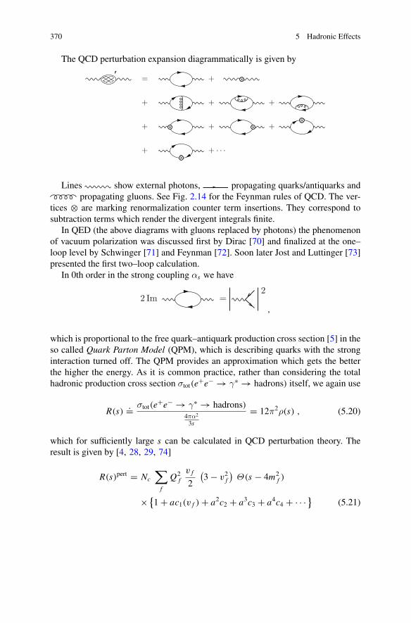
370 5 Hadronic Effects

The QCD perturbation expansion diagrammatically is given by

Lines show external photons, propagating quarks/antiquarks andpropagating gluons. See Fig. 2.14 for the Feynman rules of QCD. The ver-

tices ⊗ are marking renormalization counter term insertions. They correspond tosubtraction terms which render the divergent integrals finite.

In QED (the above diagrams with gluons replaced by photons) the phenomenonof vacuum polarization was discussed first by Dirac [70] and finalized at the one–loop level by Schwinger [71] and Feynman [72]. Soon later Jost and Luttinger [73]presented the first two–loop calculation.

In 0th order in the strong coupling αs we have

which is proportional to the free quark–antiquark production cross section [5] in theso called Quark Parton Model (QPM), which is describing quarks with the stronginteraction turned off. The QPM provides an approximation which gets the betterthe higher the energy. As it is common practice, rather than considering the totalhadronic production cross section σtot(e+e− → γ∗ → hadrons) itself, we again use

R(s).= σtot(e+e− → γ∗ → hadrons)

4πα2

3s

= 12π2ρ(s) , (5.20)

which for sufficiently large s can be calculated in QCD perturbation theory. Theresult is given by [4, 28, 29, 74]

R(s)pert = Nc

∑

f

Q2f

v f

2

(3 − v2

f

)Θ(s − 4m2

f )

× {1 + ac1(v f ) + a2c2 + a3c3 + a4c4 + · · · } (5.21)

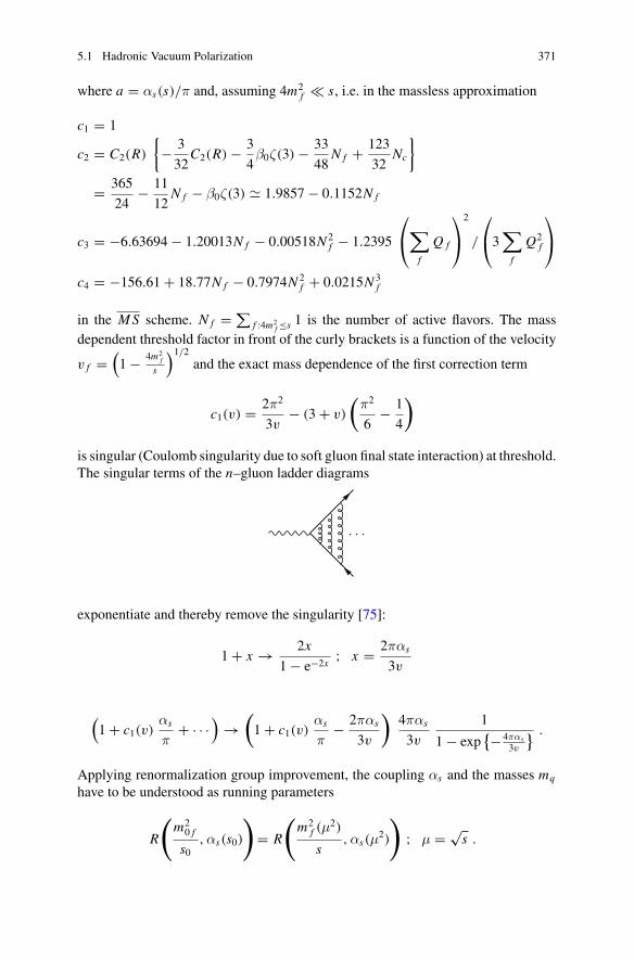
5.1 Hadronic Vacuum Polarization 371

where a = αs(s)/π and, assuming 4m2f � s, i.e. in the massless approximation

c1 = 1

c2 = C2(R)

{− 3

32C2(R) − 3

4β0ζ(3) − 33

48N f + 123

32Nc

}

= 365

24− 11

12N f − β0ζ(3) � 1.9857 − 0.1152N f

c3 = −6.63694 − 1.20013N f − 0.00518N 2f − 1.2395

⎛

⎝∑

f

Q f

⎞

⎠2

/

⎛

⎝3∑

f

Q2f

⎞

⎠

c4 = −156.61 + 18.77N f − 0.7974N 2f + 0.0215N 3

f

in the MS scheme. N f = ∑f :4m2

f ≤s 1 is the number of active flavors. The massdependent threshold factor in front of the curly brackets is a function of the velocity

v f =(1 − 4m2

f

s

)1/2and the exact mass dependence of the first correction term

c1(v) = 2π2

3v− (3 + v)

(π2

6− 1

4

)

is singular (Coulomb singularity due to soft gluon final state interaction) at threshold.The singular terms of the n–gluon ladder diagrams

· · ·

exponentiate and thereby remove the singularity [75]:

1 + x → 2x

1 − e−2x; x = 2παs

3v

(1 + c1(v)

αs

π+ · · ·

)→

(1 + c1(v)

αs

π− 2παs

3v

)4παs

3v

1

1 − exp{− 4παs

3v

} .

Applying renormalization group improvement, the coupling αs and the masses mq

have to be understood as running parameters

R

(m2

0 f

s0,αs(s0)

)= R

(m2

f (μ2)

s,αs(μ

2)

); μ = √

s .

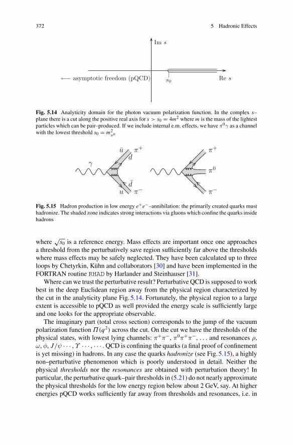
372 5 Hadronic Effects

Im s

Re s←− asymptotic freedom (pQCD)|s0

Fig. 5.14 Analyticity domain for the photon vacuum polarization function. In the complex s–plane there is a cut along the positive real axis for s > s0 = 4m2 wherem is the mass of the lightestparticles which can be pair–produced. If we include internal e.m. effects, we have π0γ as a channelwith the lowest threshold s0 = m2

π0

γ

π+

π−

π+

π−

π0

u

u

d

d

Fig. 5.15 Hadron production in low energy e+e−–annihilation: the primarily created quarks musthadronize. The shaded zone indicates strong interactions via gluons which confine the quarks insidehadrons

where√s0 is a reference energy. Mass effects are important once one approaches

a threshold from the perturbatively save region sufficiently far above the thresholdswhere mass effects may be safely neglected. They have been calculated up to threeloops by Chetyrkin, Kühn and collaborators [30] and have been implemented in theFORTRAN routine RHAD by Harlander and Steinhauser [31].

Where can we trust the perturbative result? Perturbative QCD is supposed to workbest in the deep Euclidean region away from the physical region characterized bythe cut in the analyticity plane Fig. 5.14. Fortunately, the physical region to a largeextent is accessible to pQCD as well provided the energy scale is sufficiently largeand one looks for the appropriate observable.

The imaginary part (total cross section) corresponds to the jump of the vacuumpolarization function Π(q2) across the cut. On the cut we have the thresholds of thephysical states, with lowest lying channels: π+π−, π0π+π−, . . . and resonances ρ,ω, φ, J/ψ · · · , Υ · · · , · · · . QCD is confining the quarks (a final proof of confinementis yet missing) in hadrons. In any case the quarks hadronize (see Fig. 5.15), a highlynon–perturbative phenomenon which is poorly understood in detail. Neither thephysical thresholds nor the resonances are obtained with perturbation theory! Inparticular, the perturbative quark–pair thresholds in (5.21) do not nearly approximatethe physical thresholds for the low energy region below about 2 GeV, say. At higherenergies pQCD works sufficiently far away from thresholds and resonances, i.e. in

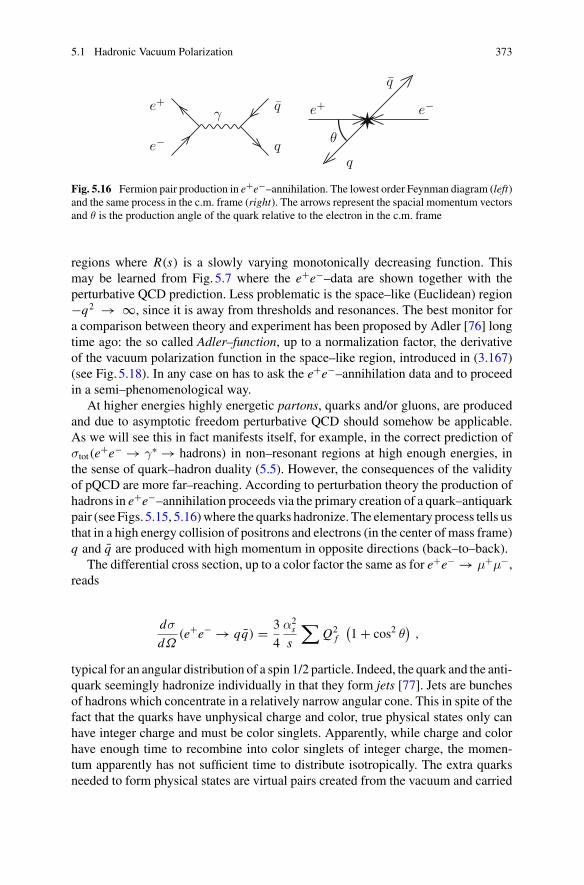
5.1 Hadronic Vacuum Polarization 373

Fig. 5.16 Fermion pair production in e+e−–annihilation. The lowest order Feynman diagram (left)and the same process in the c.m. frame (right). The arrows represent the spacial momentum vectorsand θ is the production angle of the quark relative to the electron in the c.m. frame

regions where R(s) is a slowly varying monotonically decreasing function. Thismay be learned from Fig. 5.7 where the e+e−–data are shown together with theperturbative QCD prediction. Less problematic is the space–like (Euclidean) region−q2 → ∞, since it is away from thresholds and resonances. The best monitor fora comparison between theory and experiment has been proposed by Adler [76] longtime ago: the so called Adler–function, up to a normalization factor, the derivativeof the vacuum polarization function in the space–like region, introduced in (3.167)(see Fig. 5.18). In any case on has to ask the e+e−–annihilation data and to proceedin a semi–phenomenological way.

At higher energies highly energetic partons, quarks and/or gluons, are producedand due to asymptotic freedom perturbative QCD should somehow be applicable.As we will see this in fact manifests itself, for example, in the correct prediction ofσtot(e+e− → γ∗ → hadrons) in non–resonant regions at high enough energies, inthe sense of quark–hadron duality (5.5). However, the consequences of the validityof pQCD are more far–reaching. According to perturbation theory the production ofhadrons in e+e−–annihilation proceeds via the primary creation of a quark–antiquarkpair (see Figs. 5.15, 5.16)where the quarks hadronize. The elementary process tells usthat in a high energy collision of positrons and electrons (in the center of mass frame)q and q are produced with high momentum in opposite directions (back–to–back).

The differential cross section, up to a color factor the same as for e+e− → μ+μ−,reads

dσ

dΩ(e+e− → qq) = 3

4

α2s

s

∑Q2

f

(1 + cos2 θ

),

typical for an angular distribution of a spin 1/2 particle. Indeed, the quark and the anti-quark seemingly hadronize individually in that they form jets [77]. Jets are bunchesof hadrons which concentrate in a relatively narrow angular cone. This in spite of thefact that the quarks have unphysical charge and color, true physical states only canhave integer charge and must be color singlets. Apparently, while charge and colorhave enough time to recombine into color singlets of integer charge, the momen-tum apparently has not sufficient time to distribute isotropically. The extra quarksneeded to form physical states are virtual pairs created from the vacuum and carried

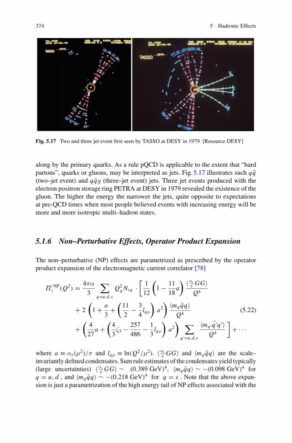
374 5 Hadronic Effects

Fig. 5.17 Two and three jet event first seen by TASSO at DESY in 1979 [Resource DESY]

along by the primary quarks. As a rule pQCD is applicable to the extent that “hardpartons”, quarks or gluons, may be interpreted as jets. Fig. 5.17 illustrates such qq(two–jet event) and qqg (three–jet event) jets. Three jet events produced with theelectron positron storage ring PETRA at DESY in 1979 revealed the existence of thegluon. The higher the energy the narrower the jets, quite opposite to expectationsat pre-QCD times when most people believed events with increasing energy will bemore and more isotropic multi–hadron states.

5.1.6 Non–Perturbative Effects, Operator Product Expansion

The non–perturbative (NP) effects are parametrized as prescribed by the operatorproduct expansion of the electromagnetic current correlator [78]

Π ′NPγ (Q2) = 4πα

3

∑

q=u,d,s

Q2q Ncq ·

[1

12

(1 − 11

18a

) 〈αsπGG〉Q4

+ 2

(1 + a

3+

(11

2− 3

4lqμ

)a2

) 〈mqqq〉Q4

(5.22)

+(

4

27a +

(4

3ζ3 − 257

486− 1

3lqμ

)a2

) ∑

q ′=u,d,s

〈mq ′ q ′q ′〉Q4

]+ · · ·

where a ≡ αs(μ2)/π and lqμ ≡ ln(Q2/μ2). 〈αs

πGG〉 and 〈mqqq〉 are the scale–

invariantly defined condensates. Sum rule estimates of the condensates yield typically(large uncertainties) 〈αs

πGG〉 ∼ (0.389 GeV)4, 〈mqqq〉 ∼ −(0.098 GeV)4 for

q = u, d , and 〈mqqq〉 ∼ −(0.218 GeV)4 for q = s . Note that the above expan-sion is just a parametrization of the high energy tail of NP effects associated with the

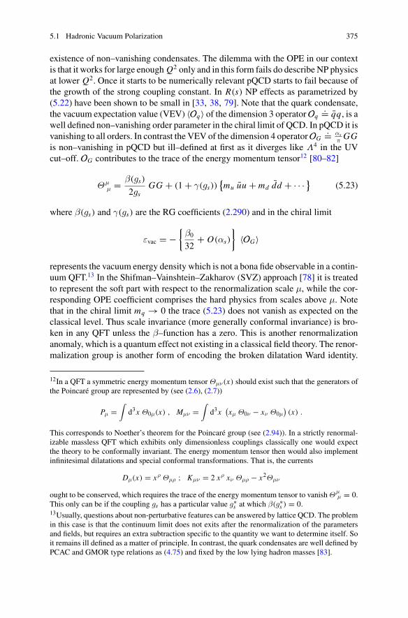
5.1 Hadronic Vacuum Polarization 375

existence of non–vanishing condensates. The dilemma with the OPE in our contextis that it works for large enough Q2 only and in this form fails do describe NP physicsat lower Q2. Once it starts to be numerically relevant pQCD starts to fail because ofthe growth of the strong coupling constant. In R(s) NP effects as parametrized by(5.22) have been shown to be small in [33, 38, 79]. Note that the quark condensate,the vacuum expectation value (VEV) 〈Oq〉 of the dimension 3 operatorOq

.= qq, is awell defined non–vanishing order parameter in the chiral limit of QCD. In pQCD it isvanishing to all orders. In contrast the VEV of the dimension 4 operatorOG

.= αsπGG

is non–vanishing in pQCD but ill–defined at first as it diverges like Λ4 in the UVcut–off. OG contributes to the trace of the energy momentum tensor12 [80–82]

Θμμ = β(gs)

2gsGG + (1 + γ(gs))

{mu uu + md dd + · · · } (5.23)

where β(gs) and γ(gs) are the RG coefficients (2.290) and in the chiral limit

εvac = −{

β0

32+ O(αs)

}〈OG〉

represents the vacuum energy density which is not a bona fide observable in a contin-uum QFT.13 In the Shifman–Vainshtein–Zakharov (SVZ) approach [78] it is treatedto represent the soft part with respect to the renormalization scale μ, while the cor-responding OPE coefficient comprises the hard physics from scales above μ. Notethat in the chiral limit mq → 0 the trace (5.23) does not vanish as expected on theclassical level. Thus scale invariance (more generally conformal invariance) is bro-ken in any QFT unless the β–function has a zero. This is another renormalizationanomaly, which is a quantum effect not existing in a classical field theory. The renor-malization group is another form of encoding the broken dilatation Ward identity.

12In a QFT a symmetric energy momentum tensor Θμν(x) should exist such that the generators ofthe Poincaré group are represented by (see (2.6), (2.7))

Pμ =∫

d3x Θ0μ(x) , Mμν =∫

d3x(xμ Θ0ν − xν Θ0μ

)(x) .

This corresponds to Noether’s theorem for the Poincaré group (see (2.94)). In a strictly renormal-izable massless QFT which exhibits only dimensionless couplings classically one would expectthe theory to be conformally invariant. The energy momentum tensor then would also implementinfinitesimal dilatations and special conformal transformations. That is, the currents

Dμ(x) = xρ Θμρ ; Kμν = 2 xρ xν Θμρ − x2Θμν

ought to be conserved, which requires the trace of the energy momentum tensor to vanish Θμμ = 0.

This only can be if the coupling gs has a particular value g∗s at which β(g∗

s ) = 0.13Usually, questions about non-perturbative features can be answered by lattice QCD. The problemin this case is that the continuum limit does not exits after the renormalization of the parametersand fields, but requires an extra subtraction specific to the quantity we want to determine itself. Soit remains ill defined as a matter of principle. In contrast, the quark condensates are well defined byPCAC and GMOR type relations as (4.75) and fixed by the low lying hadron masses [83].

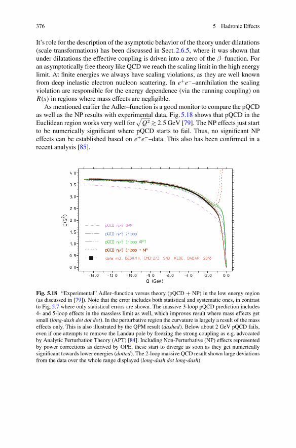
376 5 Hadronic Effects

It’s role for the description of the asymptotic behavior of the theory under dilatations(scale transformations) has been discussed in Sect. 2.6.5, where it was shown thatunder dilatations the effective coupling is driven into a zero of the β–function. Foran asymptotically free theory like QCD we reach the scaling limit in the high energylimit. At finite energies we always have scaling violations, as they are well knownfrom deep inelastic electron nucleon scattering. In e+e−–annihilation the scalingviolation are responsible for the energy dependence (via the running coupling) onR(s) in regions where mass effects are negligible.

As mentioned earlier the Adler–function is a good monitor to compare the pQCDas well as the NP results with experimental data, Fig. 5.18 shows that pQCD in theEuclidean region works very well for

√Q2 >∼ 2.5 GeV [79]. The NP effects just start

to be numerically significant where pQCD starts to fail. Thus, no significant NPeffects can be established based on e+e−–data. This also has been confirmed in arecent analysis [85].

Fig. 5.18 “Experimental” Adler–function versus theory (pQCD + NP) in the low energy region(as discussed in [79]). Note that the error includes both statistical and systematic ones, in contrastto Fig. 5.7 where only statistical errors are shown. The massive 3-loop pQCD prediction includes4- and 5-loop effects in the massless limit as well, which improves result where mass effects getsmall (long-dash dot dot dot). In the perturbative region the curvature is largely a result of the masseffects only. This is also illustrated by the QPM result (dashed). Below about 2 GeV pQCD fails,even if one attempts to remove the Landau pole by freezing the strong coupling as e.g. advocatedby Analytic Perturbation Theory (APT) [84]. Including Non-Perturbative (NP) effects representedby power corrections as derived by OPE, these start to diverge as soon as they get numericallysignificant towards lower energies (dotted). The 2-loop massive QCD result shown large deviationsfrom the data over the whole range displayed (long-dash dot long-dash)

5.1 Hadronic Vacuum Polarization 377

5.1.7 Leading Hadronic Contribution to (g − 2) of the Muon

We now are going to evaluate the hadronic vacuum polarization effects coming fromthe 5 “light” quarksq = u, d, s, c, b in terms of the experimental e+e− data.14 Quarkscontribute to the electromagnetic current according to their charge

j μ hadem =

∑

c

(2

3ucγ

μuc − 1

3dcγ

μdc − 1

3scγ

μsc + 2

3ccγ

μcc − 1

3bcγ

μbc + 2

3tcγ

μtc

).

The hadronic electromagnetic current j μ hadem is a color singlet and hence includes a

sum over colors indexed by c. Its contribution to the electromagnetic current cor-relator (3.133) defines Π ′ had

γ (s), which enters the calculation of the leading orderhadronic contribution to ahadμ , diagrammatically given by Fig. 5.1. The representa-tion as a dispersion integral has been developed in Sect. 3.8 on p. 233 (see also p. 224).Using (3.164) ahadμ may be directly evaluated in terms of Rγ(s) defined in (5.3). Moreprecisely we may write

ahadμ =(αmμ

3π

)2 (E2cut∫

m2π0

dsRdata

γ (s) K (s)

s2+

∞∫

E2cut

dsRpQCD

γ (s) K (s)

s2

), (5.24)

with a cut Ecut in the energy, separating the non–perturbative part to be evaluatedfrom the data and the perturbative high energy tail to be calculated using pQCD.15

The kernel K (s) is represented by (3.149) discarding the factor α/π. This integralcan be performed analytically. Written in terms of the variable

x = 1 − βμ

1 + βμ, βμ =

√1 − 4m2

μ/s

14The heavy top quark of mass mt � 173.21(0.87) GeV we certainly may treat perturbatively, asat the scale mt the strong interaction coupling is weak (see Fig. 3.3). Actually, the top quark tis irrelevant here since, as we know, heavy particles decouple in QED in the limit mt → ∞ andcontribute like a VP τ–loop with an extra factor NcQ2

t = 4/3, thus

15Actually, ahadμ , and therefore aμ itself, is only a safely predictable quantity by virtue of asymptotic

freedom ofQCD.Otherwise the high energy tail would remain in the dark. In spite of the 1/s2 kernelwewould be confrontedwith the question of a Landau pole, which in the “whatever non-QCD stronginteraction world” could show up elsewhere. It may be interesting to note that within the SM fromthe SU (3)c ⊗ SU (2)L ⊗U (1)Y gauge couplings only the weak hypercharge coupling g′ is notasymptotically free, what then shows up in the QED sector as well. The corresponding growth ofthe coupling with energy is however very moderate even up to the Planck scale. Surprisingly, withinthe SM also the top quark Yukawa coupling yt as well as the Higgs boson self-coupling λ show AFbehavior, i.e. they get weaker the higher the energy (see e.g. [86]).

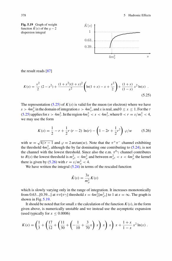
378 5 Hadronic Effects

Fig. 5.19 Graph of weightfunction K (s) of the g − 2dispersion integral

the result reads [87]

K (s) = x2

2(2 − x2) + (1 + x2)(1 + x)2

x2

(ln(1 + x) − x + x2

2

)+ (1 + x)

(1 − x)x2 ln(x) .

(5.25)

The representation (5.25) of K (s) is valid for the muon (or electron) where we haves > 4m2

μ in the domain of integration s > 4m2π , and x is real, and 0 ≤ x ≤ 1. For the τ

(5.25) applies for s > 4m2τ . In the region 4m

2π < s < 4m2

τ , where 0 < r = s/m2τ < 4,

we may use the form

K (s) = 1

2− r + 1

2r (r − 2) ln(r) −

(1 − 2r + 1

2r2)

ϕ/w (5.26)

with w = √4/r − 1 and ϕ = 2 arctan(w). Note that the π+π− channel exhibiting

the threshold 4m2π , although the by far dominating one contributing to (5.24), is not

the channel with the lowest threshold. Since also the e.m. π0γ channel contributesto R(s) the lowest threshold is m2

π0 < 4m2μ and between m2

π0 < s < 4m2μ the kernel

there is given by (5.26) with r = s/m2μ < 4.

We have written the integral (5.24) in terms of the rescaled function

K (s) = 3s

m2μ

K (s)

which is slowly varying only in the range of integration. It increases monotonicallyfrom 0.63...[0.39...] at ππ[πγ] threshold s = 4m2

π[m2π0 ] to 1 at s = ∞. The graph is

shown in Fig. 5.19.It should be noted that for small x the calculation of the function K (s), in the form

given above, is numerically unstable and we instead use the asymptotic expansion(used typically for x ≤ 0.0006)

K (s) =(1

3+

(17

12+

(11

30+

(− 1

10+ 3

70x

)x

)x

)x

)x + 1 + x

1 − xx2 ln(x) .

5.1 Hadronic Vacuum Polarization 379

Other representations of K (s), like the simpler–looking form

K (s) = 1

2− r + 1

2r (r − 2) ln(r) +

(1 − 2r + 1

2r2)

ln(x)/βμ ,

with r = s/m2μ, are much less suitable for numerical evaluation because of much

more severe numerical cancellations.Note the 1/s2–enhancement of contributions from low energies in aμ. Thus the

g − 2 kernel gives very highweight to the low energy range, in particular to the lowestlying resonance, the ρ0. Thus, this 1/E4 magnification of the low energy region bythe aμ kernel–function together with the existence of the pronounced ρ0 resonancein the π+π− cross–section are responsible for the fact that pion pair productione+e− → π+π− gives the by far largest contribution to ahadμ .16 The ρ is the lowestlying vector–meson resonance and shows up in π+π− → ρ0 at Mρ ∼ 770 MeV (seeFig. 5.6). This dominance of the low energy hadronic cross section by a single simpletwo–body channel is good luck for a precise determination of aμ, although a veryprecise determination of the π+π− cross–section is a rather difficult task. Belowabout 810MeV σhad

tot (s) � σππ(s) to a good approximation but at increasing energiesmore and more channels open (see Fig. 5.4) and “measurements of R” get moredifficult, before above about 2 GeV inclusive R measurements become reliable. Inthe light sector of q = u, d, s quarks, besides the ρ there is the ω, which is mixingwith the ρ, and the φ resonance, essentially a ss bound system. In the charm regionwe have the pronounced cc–resonances, the J/ψ1S,ψ2S, · · · resonance series and in

16As we need the VP–undressed hadronic cross section in the DR, the physical form factor Fπ(s)which includes VP effects has to be corrected accordingly:

|F (0)π (s)|2 = |Fπ(s)|2 |α/α(s)|2 . (5.27)

Figure5.25 shows Re Δα(s) = 1 − Re α/α(s) in the time–like region. The resonances lead topronounced variations of the effective charge (shown in the ρ − ω, φ and J/ψ region).

For an order by order in α procedure of including corrections in a systematic manner, finalstate radiation should be subtracted as suggested in Sect. 5.1.3. The initial state radiation must andcan be subtracted in any case, the final state radiation should be subtracted if possible. Note thatmeasurements unavoidably include all virtual plus the unobserved soft photons. However, the hardvirtual part for hadronic final states cannot be calculated in a model–independent manner, such thatthe subtraction seems not possible. It is therefore better to include as much as possible all photons inan inclusive measurement. The KLN theorem (see Sect. 2.6.6) infers that the inclusive cross sectionof virtual, soft plus hard real photons is O(α) without any logarithmic enhancement. Which alsomeans a moderate model–dependence of the FSR correction, as a consequence of the absence ofpotentially large logs. We thus include the FSR (including full photon phase space) as

|F (γ)π (s)|2 = |F (0)

π (s)|2(1 + η(s)

α

π

)(5.28)

to order O(α), where η(s) (5.1.12) is a known correction factor in sQED [203] (see p. 425 below).Here F (0)

π (s) is obtained from the measured cross section by subtracting photonic effects usingsQED under consideration of the applied experimental cuts on the real photons.

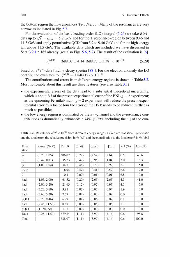
380 5 Hadronic Effects

the bottom region the bb–resonances Υ1S, Υ2S, . . .. Many of the resonances are verynarrow as indicated in Fig. 5.7.

For the evaluation of the basic leading order (LO) integral (5.24) we take R(s)–data up to

√s = Ecut = 5.2 GeV and for the Υ resonance–region between 9.46 and

11.5 GeV and apply perturbative QCD from 5.2 to 9.46 GeV and for the high energytail above 11.5 GeV. The available data which are included we have discussed inSect. 3.2.1 p.185 already (see also Figs. 5.6, 5.7). The result of the evaluation is [6]

ahad(1)μ = (688.07 ± 4.14)[688.77 ± 3.38] × 10−10 (5.29)

based on e+e−–data [incl. τ -decay spectra [88]]. For the electron anomaly the LOcontribution evaluates to ahad(1)e = 1.846(12) × 10−12.

The contributions and errors from different energy regions is shown in Table5.2.Most noticeable about this result are three features (see also Table3.1)

• the experimental errors of the data lead to a substantial theoretical uncertainty,which is about 2/3 of the present experimental error of the BNL g − 2 experiment;as the upcoming Fermilab muon g − 2 experiment will reduce the present exper-imental error by a factor four the error of the HVP needs to be reduced further asmuch as possible;

• the low energy region is dominated by the ππ–channel and the ρ–resonance con-tributions is dramatically enhanced: ∼74% [∼79% including the ω] of the con-

Table 5.2 Results for ahadμ × 1010 from different energy ranges. Given are statistical, systematic

and the total error, the relative precision in % [rel] and the contribution to the final error2 in % [abs]

Finalstate

Range (GeV) Result (Stat) (Syst) [Tot] Rel (%) Abs (%)

ρ (0.28, 1.05) 506.02 (0.77) (2.52) [2.64] 0.5 40.6

ω (0.42, 0.81) 35.23 (0.42) (0.95) [1.04] 3.0 6.3

φ (1.00, 1.04) 34.31 (0.48) (0.79) [0.92] 2.7 5.0

J/ψ 8.94 (0.42) (0.41) [0.59] 6.6 2.0

Υ 0.11 (0.00) (0.01) [0.01] 6.8 0.0

had (1.05, 2.00) 61.32 (0.20) (2.65) [2.65] 4.3 41.0

had (2.00, 3.20) 21.63 (0.12) (0.92) [0.93] 4.3 5.0

had (3.20, 3.60) 3.81 (0.02) (0.03) [0.04] 1.9 0.0

had (3.60, 5.20) 7.59 (0.04) (0.05) [0.07] 0.0 0.0

pQCD (5.20, 9.46) 6.27 (0.04) (0.06) [0.07] 0.1 0.0

had (9.46, 11.50) 0.87 (0.00) (0.05) [0.05] 5.7 0.0

pQCD (11.50, ∞) 1.96 (0.00) (0.00) [0.00] 0.0 0.0

Data (0.28, 11.50) 679.84 (1.11) (3.99) [4.14] 0.6 98.8

Total 688.07 (1.11) (3.99) [4.14] 0.6 100.0

5.1 Hadronic Vacuum Polarization 381

tribution and ∼41% [∼47% including the ω] of error of ahadμ comes from region2mπ <

√s < Mφ.

• the “intermediate” energy region, between 1 and 2 GeV, still gives a substantialcontribution of about 9% [14% including the φ]. Unfortunately, because of thelower quality of the R–data in the region, it contributes 41% [46% including theφ] of the total error, i.e. errors come in equal parts from below 1 GeV and from1 to 2 GeV, and together are the main source of uncertainty in the theoreticaldetermination of aμ.

Integration of various exclusive channels yields the results of Table5.3, which illus-trates the relative weight of different channels in the region of exclusive chan-nel measurements. Inclusive measurements are available above 1.2 GeV, however,recent progress in this problematic range comes from measurements based on theradiative return mechanism by BABAR [7, 89–92] for the exclusive channelse+e− → π+π−π0, π+π−π+π−, K+K−, KLKS , K+K−π+π−, KLKSπ

+π−,KSKSπ

+π−, 2(K+K−), KSKSK+K−, 3 (π+π−), 2(π+π−π0), K+K−2(π+π−)

and p p. These data cover a much broader energy interval and extend to much higherenergies than previous experiments. Together with recent scan data fromVEPP-2000[93–97] remarkable progress has been achieved in this difficult range.

The sum of the exclusive channels from Table5.3 is 637.73(3.69) which togetherwith the sum of contributions from energies E > 2 GeV 51.08(1.10) from Table5.2yields a slightly higher value 688.81(3.85) than the 687.04(4.21)we get by includingalso the inclusive data below 2 GeV. Results are well within errors and this is agood consistency test. Note that resonances like ω and ρ contribute to the exclusivechannels according to their branching fractions. When parametrized as relativisticBreit–Wigner shapes with a s–dependent width we have (see e.g. [98])

Γω(s) = Γ (ω → 3π, s) + Γ (ω → π0γ, s) + Γ (ω → 2π, s)

= s

M2ω

Γω

{Br(ω → 3π)

F3π(s)

F3π(M2ω)

+ Br(ω → π0γ)Fπγ(s)

Fπγ(M2ω)

+ Br(ω → 2π)F2π(s)

F2π(M2ω)

},

Γφ(s) = Γ (φ → K+K−, s) + Γ (φ → KSKL , s) + Γ (φ → 3π, s) + Γ (φ → π0γ, s) + Γ (φ → ηγ, s)

= s

M2φ

Γφ

{Br(φ → K+K−)

FK+K− (s)

FK+K− (M2φ)

+ Br(φ → KSKL )FKSKL (s)

FKSKL (M2φ)

+Br(φ → 3π)F3π(s)

F3π(M2φ)

+ Br(φ → π0γ)Fπγ(s)

Fπγ(M2φ)

+ Br(φ → ηγ)Fηγ(s)

Fηγ(M2φ)

}. (5.30)

The factors Br(V → X) denote the branching fraction for the channel X andFX (s) is the phase space function for the corresponding channel normalized suchthat FX (s) → const for s → ∞. For the two-body decays V → P1P2 we haveFP1P2(s) = (1 − (m1 + m2)

2/s)3/2. The channel V → 3π is dominated by V →ρπ → 3π and this fact is used when calculating F3π(s).

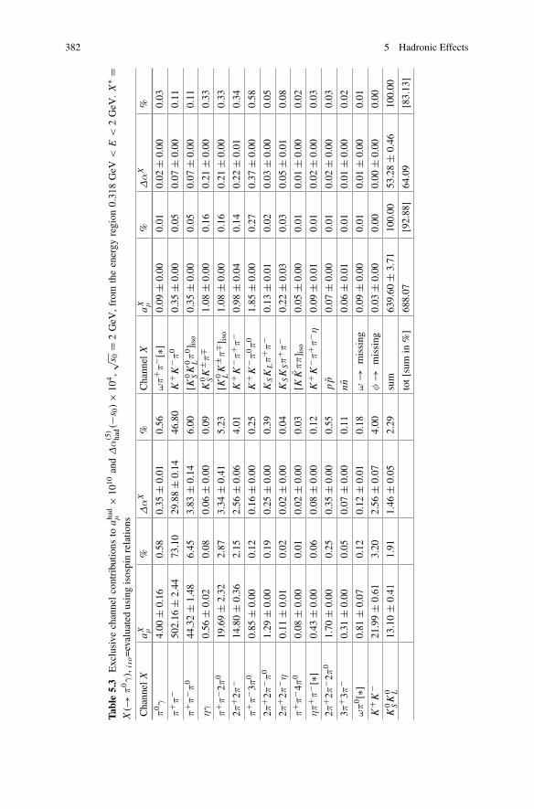
382 5 Hadronic Effects

Tabl

e5.

3Exclusive

channelcontributio

nsto

ahad

μ×

1010

and

Δα

(5)

had(−

s 0)×

104,√ s

0=

2GeV

,from

theenergy

region

0.318GeV

<E

<2GeV

.X

∗=

X(→

π0γ),

iso=evaluatedusingisospinrelatio

ns

Channel

XaX μ

%Δ

αX

%Channel

XaX μ

%Δ

αX

%

π0γ

4.00

±0.16

0.58

0.35

±0.01

0.56

ωπ

+ π− [

∗]0.09

±0.00

0.01

0.02

±0.00

0.03

π+ π

−502.16

±2.44

73.10

29.88

±0.14

46.80

K+K

− π0

0.35

±0.00

0.05

0.07

±0.00

0.11

π+ π

− π0

44.32

±1.48

6.45

3.83

±0.14

6.00

[K0 SK

0 Lπ0] iso

0.35

±0.00

0.05

0.07

±0.00

0.11

ηγ

0.56

±0.02

0.08

0.06

±0.00

0.09

K0 SK

± π∓

1.08

±0.00

0.16

0.21

±0.00

0.33

π+ π

− 2π0

19.69

±2.32

2.87

3.34

±0.41

5.23

[K0 LK

± π∓ ]

iso

1.08

±0.00

0.16

0.21

±0.00

0.33

2π+ 2

π−

14.80

±0.36

2.15

2.56

±0.06

4.01

K+K

− π+ π

−0.98

±0.04

0.14

0.22

±0.01

0.34

π+ π

− 3π0

0.85

±0.00

0.12

0.16

±0.00

0.25

K+K

− π0π0

1.85

±0.00

0.27

0.37

±0.00

0.58

2π+ 2

π− π

01.29

±0.00

0.19

0.25

±0.00

0.39

KSK

Lπ

+ π−

0.13

±0.01

0.02

0.03

±0.00

0.05

2π+ 2

π− η

0.11

±0.01

0.02

0.02

±0.00

0.04

KSK

Sπ

+ π−

0.22

±0.03

0.03

0.05

±0.01

0.08

π+ π

− 4π0

0.08

±0.00

0.01

0.02

±0.00

0.03

[KK

ππ] iso

0.05

±0.00

0.01

0.01

±0.00

0.02

ηπ

+ π− [

∗]0.43

±0.00

0.06

0.08

±0.00

0.12

K+K

− π+ π

− η0.09

±0.01

0.01

0.02

±0.00

0.03

2π+ 2

π− 2

π0

1.70

±0.00

0.25

0.35

±0.00

0.55

pp

0.07

±0.00

0.01

0.02

±0.00

0.03

3π+ 3

π−

0.31

±0.00

0.05

0.07

±0.00

0.11

nn0.06

±0.01

0.01

0.01

±0.00

0.02

ωπ0[∗]

0.81

±0.07

0.12

0.12

±0.01

0.18

ω→

missing

0.09

±0.00

0.01

0.01

±0.00

0.01

K+K

−21.99

±0.61

3.20

2.56

±0.07

4.00

φ→

missing

0.03

±0.00

0.00

0.00

±0.00

0.00

K0 SK

0 L13.10

±0.41

1.91

1.46

±0.05

2.29

sum

639.60

±3.71

100.00

53.28

±0.46

100.00

tot[s

umin

%]

688.07

[92.88]

64.09

[83.13]

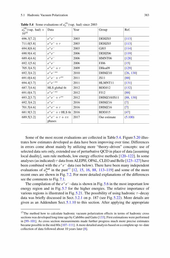
5.1 Hadronic Vacuum Polarization 383

Table 5.4 Some evaluations of a(4)μ (vap, had) since 2003

a(4)μ (vap, had) ×1010

Data Year Group Ref.

696.3[7.2] e+e− 2003 DEHZ03 [113]

711.0[5.8] e+e− + τ 2003 DEHZ03 [113]

694.8[8.6] e+e− 2003 GJ03 [114]

690.9[4.4] e+e− 2006 DEHZ06 [119]

689.4[4.6] e+e− 2006 HMNT06 [128]

692.1[5.6] e+e− 2006 FJ06 [15]

705.3[4.5] e+e− + τ 2009 DHea09 [129]

692.3[4.2] e+e−∗∗ 2010 DHMZ10 [26, 130]

691.0[4.6] e+e− + τ∗∗ 2011 JS11 [88]

694.4[3.7] e+e−∗∗ 2011 HLMNT11 [131]

687.7[4.6] HLS global fit 2012 BDDJ12 [132]

691.0[4.7] e+e−∗∗ 2012 FJ12 [88]

693.2[3.7] e+e− + τ∗∗ 2012 DHMZ10/JS11 [88, 130]

692.3[4.2] e+e− 2016 DHMZ16 [7]

701.5[4.6] e+e− + τ 2016 DHMZ16 [7]

681.9[3.2] e+e− + τ HLS fit 2016 BDDJ15 [47]

689.5[3.2] e+e− + τ + ππphases

2017 Our estimate (5.100)

Some of the most recent evaluations are collected in Table5.4. Figure5.20 illus-trates how estimates developed as data have been improving over time. Differencesin errors come about mainly by utilizing more “theory–driven” concepts: use ofselected data sets only, extended use of perturbative QCD in place of data [assuminglocal duality], sum rule methods, low energy effective methods [120–122]. In someanalyses (as indicated) τ data fromALEPH, OPAL, CLEO and Belle [123–127] havebeen combined with the e+e− data (see below). There have been many independentevaluations of ahadμ in the past17 [12, 15, 16, 88, 113–119] and some of the morerecent ones are shown in Fig. 7.2. For more detailed explanations of the differencessee the comments to Fig. 7.1.

The compilation of the e+e−–data is shown in Fig. 5.6 in the most important lowenergy region and in Fig. 5.7 for the higher energies. The relative importance ofvarious regions is illustrated in Fig. 5.21. The possibility of using hadronic τ–decaydata was briefly discussed in Sect. 3.2.1 on p. 187 (see Fig. 5.22). More details aregiven as an Addendum Sect. 5.1.10 to this section. After applying the appropriate

17The method how to calculate hadronic vacuum polarization effects in terms of hadronic crosssectionswas developed long time ago byCabibbo andGatto [133]. First estimationswere performedin [99–101]. As cross section measurements made further progress much more precise estimatesbecame possible in themid 80s [107–111]. Amore detailed analysis based on a complete up–to–datecollection of data followed about 10 years later [8].

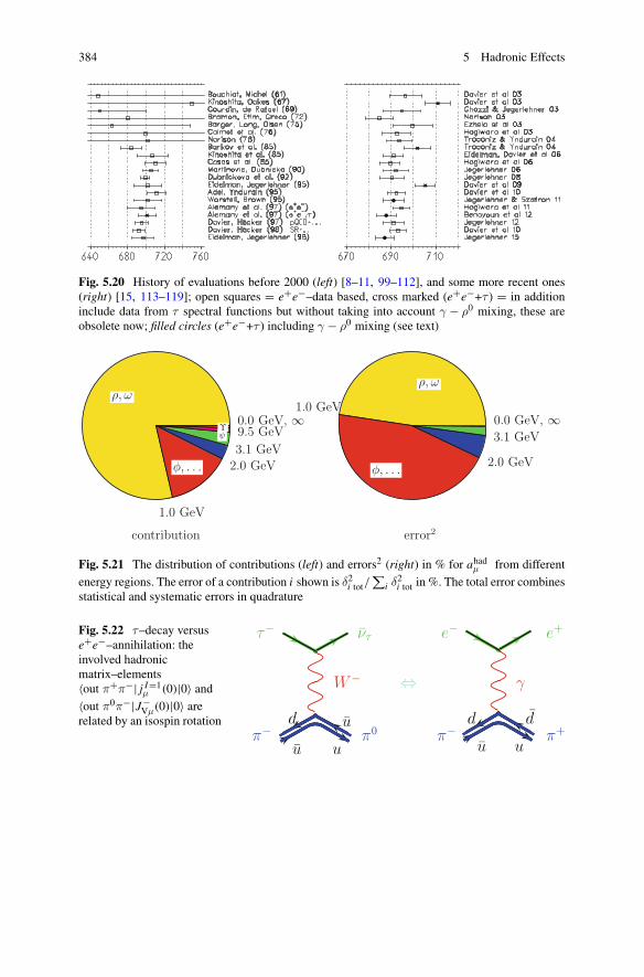
384 5 Hadronic Effects

Fig. 5.20 History of evaluations before 2000 (left) [8–11, 99–112], and some more recent ones(right) [15, 113–119]; open squares = e+e−–data based, cross marked (e+e−+τ ) = in additioninclude data from τ spectral functions but without taking into account γ − ρ0 mixing, these areobsolete now; filled circles (e+e−+τ ) including γ − ρ0 mixing (see text)

0.0 GeV, ∞ρ, ω

1.0 GeV

φ, . . . 2.0 GeV3.1 GeV

ψ 9.5 GeVΥ0.0 GeV, ∞

ρ, ω

1.0 GeV

φ, . . .2.0 GeV

3.1 GeV

contribution error2

Fig. 5.21 The distribution of contributions (left) and errors2 (right) in % for ahadμ from different

energy regions. The error of a contribution i shown is δ2i tot/∑

i δ2i tot in %. The total error combines

statistical and systematic errors in quadrature

Fig. 5.22 τ–decay versuse+e−–annihilation: theinvolved hadronicmatrix–elements〈out π+π−| j I=1

μ (0)|0〉 and〈out π0π−|J−

Vμ(0)|0〉 arerelated by an isospin rotation

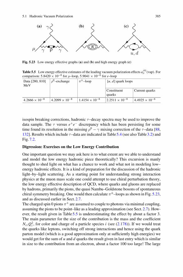
5.1 Hadronic Vacuum Polarization 385

ρ πγ γμ

γ

u, d

(a) (b) (c)

Fig. 5.23 Low energy effective graphs (a) and (b) and high energy graph (c)

Table 5.5 Low energy effective estimates of the leading vacuum polarization effects a(4)μ (vap). For

comparison: 5.8420 × 10−8 for μ–loop, 5.9041 × 10−6 for e–loop

Data [280, 810]MeV

ρ0–exchange π±–loop [u, d] quark loops

Constituentquarks

Current quarks

4.2666 × 10−8 4.2099 × 10−8 1.4154 × 10−8 2.2511 × 10−8 4.4925 × 10−6

isospin breaking corrections, hadronic τ–decay spectra may be used to improve thedata sample. The τ versus e+e− discrepancy which has been persisting for sometime found its resolution in the missing ρ0 − γ mixing correction of the τ–data [88,132]. Results which include τ–data are indicated in Table5.4 (see also Table3.2) andFig. 7.2.

Digression: Exercises on the Low Energy Contribution

One important question we may ask here is to what extent are we able to understandand model the low energy hadronic piece theoretically? This excursion is manlythought to shed light on what has a chance to work and what not in modeling low–energy hadronic effects. It is a kind of preparation for the discussion of the hadroniclight–by–light scattering. As a starting point for understanding strong interactionphysics at the muon mass scale one could attempt to use chiral perturbation theory,the low energy effective description of QCD, where quarks and gluons are replacedby hadrons, primarily the pions, the quasi Nambu–Goldstone bosons of spontaneouschiral symmetry breaking. One would then calculate π±–loops as shown in Fig. 5.23,and as discussed earlier in Sect. 2.7.The charged spin 0 pions π± are assumed to couple to photons via minimal coupling,assuming the pions to be point–like as a leading approximation (see Sect. 2.7). How-ever, the result given in Table5.5 is underestimating the effect by about a factor 3.The main parameter for the size of the contribution is the mass and the coefficientNci Q2

i , for color and charge of a particle species i (see (2.178)). If we would treatthe quarks like leptons, switching off strong interactions and hence using the quarkparton model (which is a good approximation only at sufficiently high energies) wewould get for the sum of u and d quarks the result given in last entry which is similarin size to the contribution from an electron, about a factor 100 too large! The large

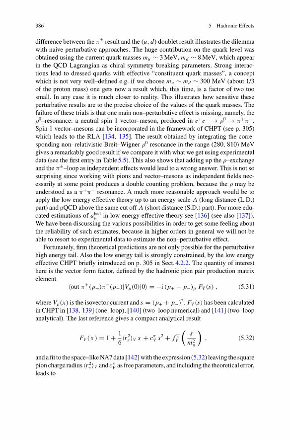
386 5 Hadronic Effects

difference between the π± result and the (u, d) doublet result illustrates the dilemmawith naive perturbative approaches. The huge contribution on the quark level wasobtained using the current quark masses mu ∼ 3MeV,md ∼ 8MeV, which appearin the QCD Lagrangian as chiral symmetry breaking parameters. Strong interac-tions lead to dressed quarks with effective “constituent quark masses”, a conceptwhich is not very well–defined e.g. if we choose mu ∼ md ∼ 300 MeV (about 1/3of the proton mass) one gets now a result which, this time, is a factor of two toosmall. In any case it is much closer to reality. This illustrates how sensitive theseperturbative results are to the precise choice of the values of the quark masses. Thefailure of these trials is that one main non–perturbative effect is missing, namely, theρ0–resonance: a neutral spin 1 vector–meson, produced in e+e− → ρ0 → π+π−.Spin 1 vector–mesons can be incorporated in the framework of CHPT (see p. 305)which leads to the RLA [134, 135]. The result obtained by integrating the corre-sponding non–relativistic Breit–Wigner ρ0 resonance in the range (280, 810) MeVgives a remarkably good result if we compare it with what we get using experimentaldata (see the first entry in Table5.5). This also shows that adding up the ρ–exchangeand the π±–loop as independent effects would lead to a wrong answer. This is not sosurprising since working with pions and vector–mesons as independent fields nec-essarily at some point produces a double counting problem, because the ρ may beunderstood as a π+π− resonance. A much more reasonable approach would be toapply the low energy effective theory up to an energy scale Λ (long distance (L.D.)part) and pQCD above the same cut off Λ (short distance (S.D.) part). For more edu-cated estimations of ahadμ in low energy effective theory see [136] (see also [137]).We have been discussing the various possibilities in order to get some feeling aboutthe reliability of such estimates, because in higher orders in general we will not beable to resort to experimental data to estimate the non–perturbative effect.

Fortunately, firm theoretical predictions are not only possible for the perturbativehigh energy tail. Also the low energy tail is strongly constrained, by the low energyeffective CHPT briefly introduced on p. 305 in Sect. 4.2.2. The quantity of interesthere is the vector form factor, defined by the hadronic pion pair production matrixelement

〈out π+(p+)π−(p−)|Vμ(0)|0〉 = −i (p+ − p−)μ FV (s) , (5.31)

where Vμ(x) is the isovector current and s = (p+ + p−)2. FV (s) has been calculatedin CHPT in [138, 139] (one–loop), [140] (two–loop numerical) and [141] (two–loopanalytical). The last reference gives a compact analytical result

FV ( s ) = 1 + 1

6〈r2π〉V s + cπ

V s2 + f UV

(s

m2π

), (5.32)

and afit to the space–likeNA7data [142]with the expression (5.32) leaving the squarepion charge radius 〈r2π〉V and cπ

V as free parameters, and including the theoretical error,leads to

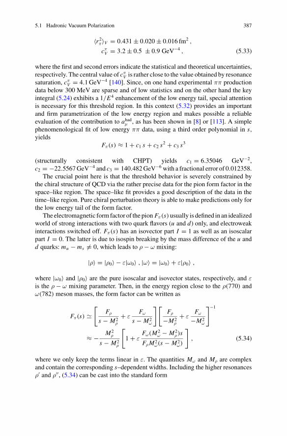
5.1 Hadronic Vacuum Polarization 387

〈r2π〉V = 0.431 ± 0.020 ± 0.016 fm2 ,

cπV = 3.2 ± 0.5 ± 0.9 GeV−4 , (5.33)

where the first and second errors indicate the statistical and theoretical uncertainties,respectively. The central value of cπ

V is rather close to the value obtained by resonancesaturation, cπ

V = 4.1GeV−4 [140]. Since, on one hand experimental ππ productiondata below 300 MeV are sparse and of low statistics and on the other hand the keyintegral (5.24) exhibits a 1/E4 enhancement of the low energy tail, special attentionis necessary for this threshold region. In this context (5.32) provides an importantand firm parametrization of the low energy region and makes possible a reliableevaluation of the contribution to ahadμ , as has been shown in [8] or [113]. A simplephenomenological fit of low energy ππ data, using a third order polynomial in s,yields

Fπ(s) ≈ 1 + c1 s + c2 s2 + c3 s

3

(structurally consistent with CHPT) yields c1 = 6.35046 GeV−2,c2 = −22.5567GeV−4 and c3 = 140.482GeV−6 with a fractional error of 0.012358.

The crucial point here is that the threshold behavior is severely constrained bythe chiral structure of QCD via the rather precise data for the pion form factor in thespace–like region. The space–like fit provides a good description of the data in thetime–like region. Pure chiral perturbation theory is able to make predictions only forthe low energy tail of the form factor.

The electromagnetic form factor of the pion Fπ(s)usually is defined in an idealizedworld of strong interactions with two quark flavors (u and d) only, and electroweakinteractions switched off. Fπ(s) has an isovector part I = 1 as well as an isoscalarpart I = 0. The latter is due to isospin breaking by the mass difference of the u andd quarks: mu − ms = 0, which leads to ρ − ω mixing:

|ρ〉 = |ρ0〉 − ε|ω0〉 , |ω〉 = |ω0〉 + ε|ρ0〉 ,

where |ω0〉 and |ρ0〉 are the pure isoscalar and isovector states, respectively, and εis the ρ − ω mixing parameter. Then, in the energy region close to the ρ(770) andω(782) meson masses, the form factor can be written as

Fπ(s) �[

Fρ

s − M2ρ

+ εFω

s − M2ω

][Fρ

−M2ρ

+ εFω

−M2ω

]−1

≈ − M2ρ

s − M2ρ

[1 + ε

Fω(M2ω − M2

ρ )s

FρM2ω(s − M2

ω)

], (5.34)

where we only keep the terms linear in ε. The quantities Mω and Mρ are complexand contain the corresponding s–dependent widths. Including the higher resonancesρ′ and ρ′′, (5.34) can be cast into the standard form

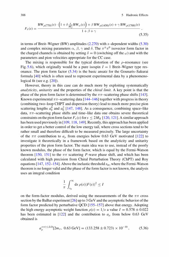
388 5 Hadronic Effects

Fπ(s) =BWρ(770)(s) ·

(1 + δ s

M2ωBWω(s)

)+ β BWρ(1450)(s) + γ BWρ(1700)(s)

1 + β + γ,

(5.35)

in terms of Breit–Wigner (BW) amplitudes (2.270) with s–dependent widths (5.30)and complex mixing parameters α, β, γ and δ. The π±π0 isovector form factor inthe charged channels is obtained by setting δ = 0 (switching off the ω) and with theparameters and pion velocities appropriate for the CC case.

The mixing is responsible for the typical distortion of the ρ–resonance (seeFig. 5.6), which originally would be a pure isospin I = 1 Breit–Wigner type res-onance. The pion form factor (5.34) is the basic ansatz for the Gounaris–Sakuraiformula [40] which is often used to represent experimental data by a phenomeno-logical fit (see e.g. [20]).

However, theory in this case can do much more by exploiting systematicallyanalyticity, unitarity and the properties of the chiral limit. A key point is that thephase of the pion form factor is determined by the ππ–scattering phase shifts [143].Known experimental ππ–scattering data [144–146] together with progress in theory(combining two–loop CHPT and dispersion theory) lead to much more precise pionscattering lengths a00 and a20 [147, 148]. As a consequence, combining space–likedata, ππ–scattering phase shifts and time–like data one obtains severe theoreticalconstraints on the pion form factor Fπ(s) for s ≤ 2MK [120, 121].A similar approachhas been used previously in [109, 118, 149]. Recently, this approach has been appliedin order to get a better control of the low energy tail, where cross sections tend to berather small and therefore difficult to be measured precisely. The large uncertaintyof the ππ contribution to aμ from energies below 0.63 GeV motivated [122] toinvestigate it theoretically in a framework based on the analyticity and unitarityproperties of the pion form factor. The main idea was to use, instead of the poorlyknown modulus, the phase of the form factor, which is equal by the Fermi-Watsontheorem [150, 151] to the ππ scattering P-wave phase shift, and which has beencalculated with high precision from Chiral Perturbation Theory (ChPT) and Royequations [147, 152–154]. Above the inelastic threshold sin, where the Fermi-Watsontheorem is no longer valid and the phase of the form factor is not known, the analysisuses an integral condition

1

π

∫ ∞

sin

ds ρ(s)|F(s)|2 ≤ I

on the form-factor modulus, derived using the measurements of the the ππ crosssection by the BaBar experiment [26] up to 3 GeV and the asymptotic behavior of theform factor predicted by perturbative QCD [155–157] above that energy. Adoptingthe high energy asymptotic weight function ρ(s) = 1/s a value I = 0.578 ± 0.022has been estimated in [122] and the contribution to aμ from below 0.63 GeVobtained is

aππ(γ),LOμ [2mπ, 0.63 GeV] = (133.258 ± 0.723) × 10−10 , (5.36)

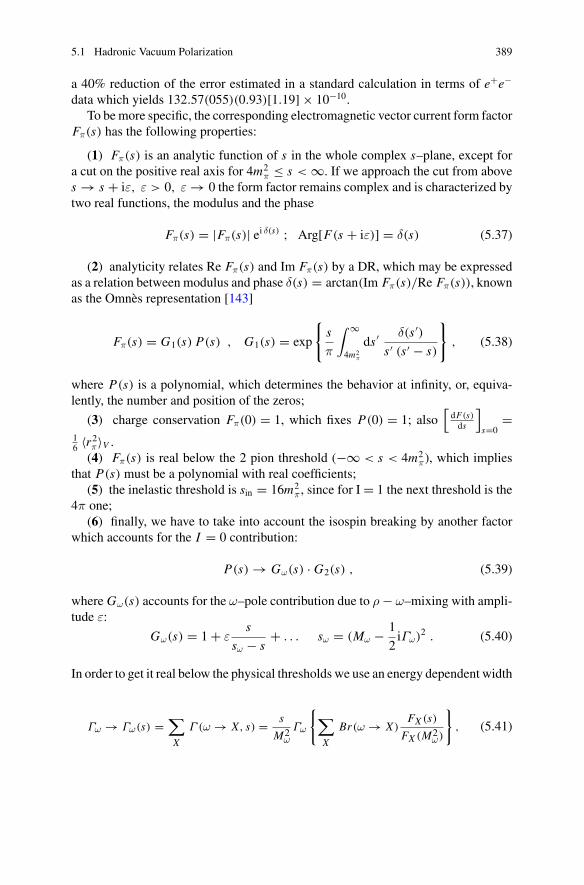
5.1 Hadronic Vacuum Polarization 389

a 40% reduction of the error estimated in a standard calculation in terms of e+e−data which yields 132.57(055)(0.93)[1.19] × 10−10.

To bemore specific, the corresponding electromagnetic vector current form factorFπ(s) has the following properties:

(1) Fπ(s) is an analytic function of s in the whole complex s–plane, except fora cut on the positive real axis for 4m2

π ≤ s < ∞. If we approach the cut from aboves → s + iε, ε > 0, ε → 0 the form factor remains complex and is characterized bytwo real functions, the modulus and the phase

Fπ(s) = |Fπ(s)| ei δ(s) ; Arg[F(s + iε)] = δ(s) (5.37)

(2) analyticity relates Re Fπ(s) and Im Fπ(s) by a DR, which may be expressedas a relation between modulus and phase δ(s) = arctan(Im Fπ(s)/Re Fπ(s)), knownas the Omnès representation [143]

Fπ(s) = G1(s) P(s) , G1(s) = exp

{s

π

∫ ∞

4m2π

ds ′ δ(s ′)s ′ (s ′ − s)

}, (5.38)

where P(s) is a polynomial, which determines the behavior at infinity, or, equiva-lently, the number and position of the zeros;

(3) charge conservation Fπ(0) = 1, which fixes P(0) = 1; also[dF(s)ds

]

s=0=

16 〈r2π〉V .

(4) Fπ(s) is real below the 2 pion threshold (−∞ < s < 4m2π), which implies

that P(s) must be a polynomial with real coefficients;(5) the inelastic threshold is sin = 16m2

π , since for I = 1 the next threshold is the4π one;

(6) finally, we have to take into account the isospin breaking by another factorwhich accounts for the I = 0 contribution:

P(s) → Gω(s) · G2(s) , (5.39)

where Gω(s) accounts for the ω–pole contribution due to ρ − ω–mixing with ampli-tude ε:

Gω(s) = 1 + εs

sω − s+ . . . sω = (Mω − 1

2iΓω)2 . (5.40)

In order to get it real below the physical thresholds we use an energy dependent width

Γω → Γω(s) =∑

X

Γ (ω → X, s) = s

M2ω

Γω

{∑

X

Br(ω → X)FX (s)

FX (M2ω)

}, (5.41)

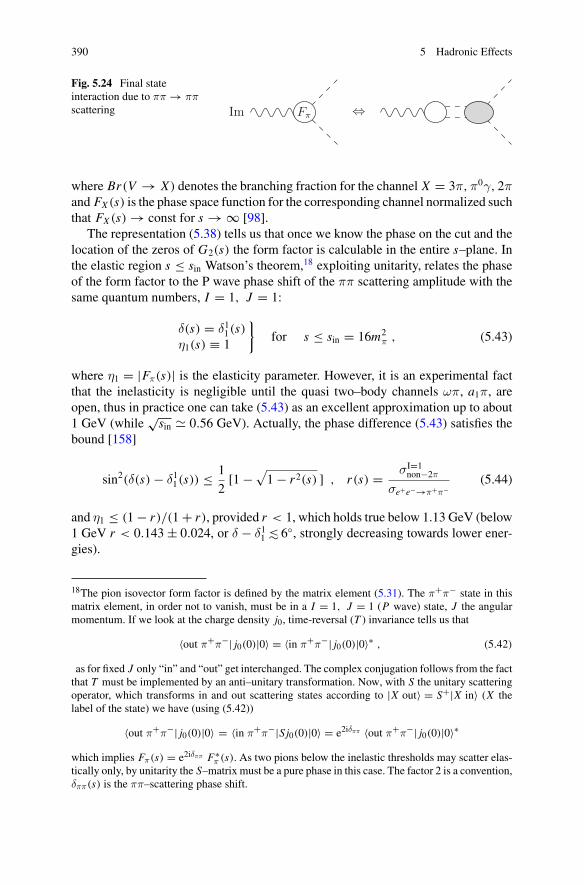
390 5 Hadronic Effects

Fig. 5.24 Final stateinteraction due to ππ → ππscattering FπIm ⇔

where Br(V → X) denotes the branching fraction for the channel X = 3π,π0γ, 2πand FX (s) is the phase space function for the corresponding channel normalized suchthat FX (s) → const for s → ∞ [98].

The representation (5.38) tells us that once we know the phase on the cut and thelocation of the zeros of G2(s) the form factor is calculable in the entire s–plane. Inthe elastic region s ≤ sin Watson’s theorem,18 exploiting unitarity, relates the phaseof the form factor to the P wave phase shift of the ππ scattering amplitude with thesame quantum numbers, I = 1, J = 1:

δ(s) = δ11(s)η1(s) ≡ 1

}for s ≤ sin = 16m2

π , (5.43)

where η1 = |Fπ(s)| is the elasticity parameter. However, it is an experimental factthat the inelasticity is negligible until the quasi two–body channels ωπ, a1π, areopen, thus in practice one can take (5.43) as an excellent approximation up to about1 GeV (while

√sin � 0.56 GeV). Actually, the phase difference (5.43) satisfies the

bound [158]

sin2(δ(s) − δ11(s)) ≤ 1

2[1 −

√1 − r2(s) ] , r(s) = σI=1

non−2π

σe+e−→π+π−(5.44)

and η1 ≤ (1 − r)/(1 + r), provided r < 1, which holds true below 1.13 GeV (below1 GeV r < 0.143 ± 0.024, or δ − δ11 <∼ 6◦, strongly decreasing towards lower ener-gies).

18The pion isovector form factor is defined by the matrix element (5.31). The π+π− state in thismatrix element, in order not to vanish, must be in a I = 1, J = 1 (P wave) state, J the angularmomentum. If we look at the charge density j0, time-reversal (T ) invariance tells us that

〈out π+π−| j0(0)|0〉 = 〈in π+π−| j0(0)|0〉∗ , (5.42)

as for fixed J only “in” and “out” get interchanged. The complex conjugation follows from the factthat T must be implemented by an anti–unitary transformation. Now, with S the unitary scatteringoperator, which transforms in and out scattering states according to |X out〉 = S+|X in〉 (X thelabel of the state) we have (using (5.42))

〈out π+π−| j0(0)|0〉 = 〈in π+π−|Sj0(0)|0〉 = e2iδππ 〈out π+π−| j0(0)|0〉∗

which implies Fπ(s) = e2iδππ F∗π (s). As two pions below the inelastic thresholds may scatter elas-

tically only, by unitarity the S–matrix must be a pure phase in this case. The factor 2 is a convention,δππ(s) is the ππ–scattering phase shift.

5.1 Hadronic Vacuum Polarization 391

The ππ scattering phase shift is due to elastic re–scattering of the pions in the finalstate (final state interaction) as illustrated by Fig. 5.24. The ππ scattering P-wavephase shift δ11(s) (data are displayed in Fig. 5.40) has been studied some time agoin the framework of the Roy equations, also exploiting chiral symmetry [147]. Asa result it turns out that δ11(s) is constrained to a remarkable degree of accuracy upto about E0 = 0.8 GeV (matching point). The behavior of δ11(s) in the region belowthe matching point is controlled by three parameters: two S–wave scattering lengthsa00 , a

20 and by the boundary value φ ≡ δ11(E0). One may treat φ as a free parameter

and rely on the very accurate predictions for a00 , a20 from chiral perturbation theory.

This information may be used to improve the accuracy of the pion form factor andthus to reduce the uncertainty of the hadronic contribution to the muon g − 2.

The remaining function G2(s) represents the smooth background that containsthe curvature generated by the remaining singularities. The 4π channel opens ats = 16 m2

π but phase space strongly suppresses the strength of the correspondingbranch point singularity of the form (1 − sin/s)9/2 – a significant inelasticity onlymanifests itself for s > sin = (Mω + mπ)

2. The conformal mapping

z =√sin − s1 − √

sin − s√sin − s1 + √

sin − s(5.45)

maps the plane cut along s > sin onto the unit disk in the z–plane. It contains afree parameter s1 - the value of s which gets maps into the origin. G2(s) may beapproximated by a polynomial in z:

G2(s) = 1 +nP∑

i=1

ci (zi − zi0) , (5.46)

where z0 is the image of s = 0. The shift of z by z → z − z0 is required to pre-serves the charge normalization condition G2(0) = 1. The form of the branch pointsingularity (1 − sin/s)9/2 imposes four constraints on the polynomial; a non–trivialcontribution from G2(s) thus requires a polynomial of fifth order at least. An impor-tant issue is the need for a normalization point at the upper end of the energy rangeunder consideration (Mρ · · · 2MK ). In fact, the present dispersion in the ππ–data (seeFig. 5.6) makes it difficult to fully exploit this approach as it seems not possible toget a convincing simultaneous fit to the different data sets. Details have been workedout in [120, 121].

For ππ → ππ scattering amplitudes of definite isospin I in the s-channel, onewrites a partial wave decomposition

F (I )(s, t) = 8

π

∑

(2 + 1)P(cos θ)t (I ) (s), (5.47)

t (I ) (s) =√s

2kf (I ) (s), f (I )

(s) = η(I ) (s)e2iδ

(I ) (s) − 1

2i,

392 5 Hadronic Effects

where δ(I ) (s) and η(I )

(s) are the phase shift and inelasticity of the I , partial wave,respectively, is the angular momentum, and k is the center of mass momentum. Inthe elastic case, η = 1 and

f (I ) (s) = sin δ(I )

(s) eiδ(I ) (s) . (5.48)

Given I = 0, 1, 2 we note that whenever I is even (odd) then is even (odd). Thescattering lengths and slope parameters a(I )

and b(I ) are defined by the threshold

parameters, which are the coefficients of the amplitude expansion in powers of centerof mass (CM) momenta around threshold:

s1/2

2Mπk2+1f (I ) (s) � a(I )

+ b(I ) k2 + O(k4) . (5.49)

The Roy equations are DRs for the ππ scattering amplitudes. Roy’s representa-tion [152] for the partial wave amplitudes t Il of elastic ππ scattering reads

t I (s) = k I (s) +2∑

I ′=0

∞∑

′=0

∫ ∞

4M2π

ds ′ K I I ′′ (s, s ′) Im t I

′′ (s ′) , (5.50)

where I and denote isospin and angular momentum, respectively and k I (s) isthe partial wave projection of the subtraction term. It shows up only in the S- andP-waves,

k I (s)α = αaI0 δ0 + s − 4M2

π

4M2π

(2a00 − 5a20)

(1

3δ I0 δ0 + 1

18δ I1 δ1 − 1

6δ I2 δ0

).

The kernels K I I ′′ (s, s ′) are explicitly known functions [147, 152].

5.1.8 Addendum I: The Hadronic Contributionto the Running Fine Structure Constant

By the same procedure, we have evaluated ahadμ , the renormalized VP function canbe calculated. The latter is identical to the shift in the fine structure constant, whichencodes the charge screening:

Δα(s) ≡ −Re[Π ′

γ(s) − Π ′γ(0)

]. (5.51)

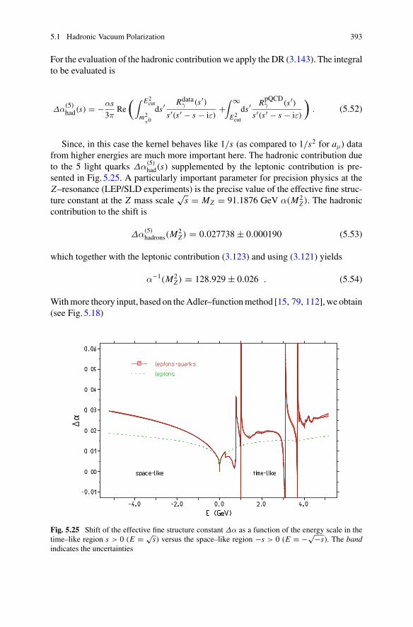
5.1 Hadronic Vacuum Polarization 393

For the evaluation of the hadronic contribution we apply the DR (3.143). The integralto be evaluated is

Δα(5)had(s) = −αs

3πRe

(∫ E2cut

m2π0

ds′Rdata

γ (s′)s′(s′ − s − iε)

+∫ ∞E2cut

ds′ RpQCDγ (s′)

s′(s′ − s − iε)

). (5.52)

Since, in this case the kernel behaves like 1/s (as compared to 1/s2 for aμ) datafrom higher energies are much more important here. The hadronic contribution dueto the 5 light quarks Δα(5)

had(s) supplemented by the leptonic contribution is pre-sented in Fig. 5.25. A particularly important parameter for precision physics at theZ–resonance (LEP/SLD experiments) is the precise value of the effective fine struc-ture constant at the Z mass scale

√s = MZ = 91.1876 GeV α(M2

Z ). The hadroniccontribution to the shift is

Δα(5)hadrons(M

2Z ) = 0.027738 ± 0.000190 (5.53)

which together with the leptonic contribution (3.123) and using (3.121) yields

α−1(M2Z ) = 128.929 ± 0.026 . (5.54)

Withmore theory input, based on theAdler–functionmethod [15, 79, 112], we obtain(see Fig. 5.18)

Fig. 5.25 Shift of the effective fine structure constant Δα as a function of the energy scale in thetime–like region s > 0 (E = √

s) versus the space–like region −s > 0 (E = −√−s). The bandindicates the uncertainties

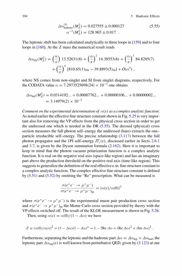
394 5 Hadronic Effects

Δα(5)hadrons(M

2Z ) = 0.027555 ± 0.000127 (5.55)

α−1(M2Z ) = 128.965 ± 0.017 .

The leptonic shift has been calculated analytically to three loops in [159] and to fourloops in [160]. At the Z mass the numerical result reads

Δαlep(M2Z ) =

(α

π

)13.52631(8) +

(α

π

)214.38553(6) +

(α

π

)384.8285(7)

+(α

π

)4 [810.65(1)NS − 39.8893(5)SI] + O(α5) ,

where NS comes from non-singlet and SI from singlet diagrams, respectively. Forthe CODATA value α = 7.2973525698(24) × 10−3 one obtains

Δαlep(M2Z ) = 0.0314192... + 0.00007762... + 0.00000106... + 0.00000002...

= 3.14979(2) × 10−2

Comment on the experimental determination of α(s) as a complex analytic function:As noted earlier the effective fine structure constant shown in Fig. 5.25 is very impor-tant also for removing the VP effects from the physical cross section in order to getthe undressed one which is needed in the DR (5.55). The dressed (physical) crosssection measures the full photon self–energy the undressed (bare) extracts the one–particle irreducible self–energy. The precise relationship (3.117) between the fullphoton propagator and the 1PI self–energy Π ′

γ(s), discussed earlier in Sects. 2.6.1and 3.7, is given by the Dyson summation formula (2.162). Here it is important tokeep in mind that the photon vacuum polarization function is a complex analyticfunction. It is real on the negative real axis (space-like region) and has an imaginarypart above the production threshold on the positive real axis (time-like region). Thissuggests to generalize the definition of the real effective e.m. fine structure constant toa complex analytic function. The complex effective fine structure constant is definedby (5.51) and (5.52) by omitting the “Re” prescription. What can be measured is

σ(e+e− → μ+μ−)

σ(e+e− → μ+μ−)pt= |α(s)/α(0)|2

where σ(e+e− → μ+μ−) is the experimental muon pair production cross sectionand σ(e+e− → μ+μ−)pt the Monte Carlo cross section provided by theory with theVP effects switched off. The result of the KLOE measurement is shown in Fig. 5.26.

Then, using α(s) = α(0)/(1 − Δα) we have

Z ≡ |α(0)/α(s)|2 = (1 − Δα)(1 − Δα)∗ = 1 − 2Re Δα + (Re Δα)2 + (Im Δα)2 .

Furthermore, separating the leptonic and the hadronic partΔα = Δαlep + Δαhad, theleptonic partΔαlep(s) is well known from perturbative QED, given by (3.123) at one

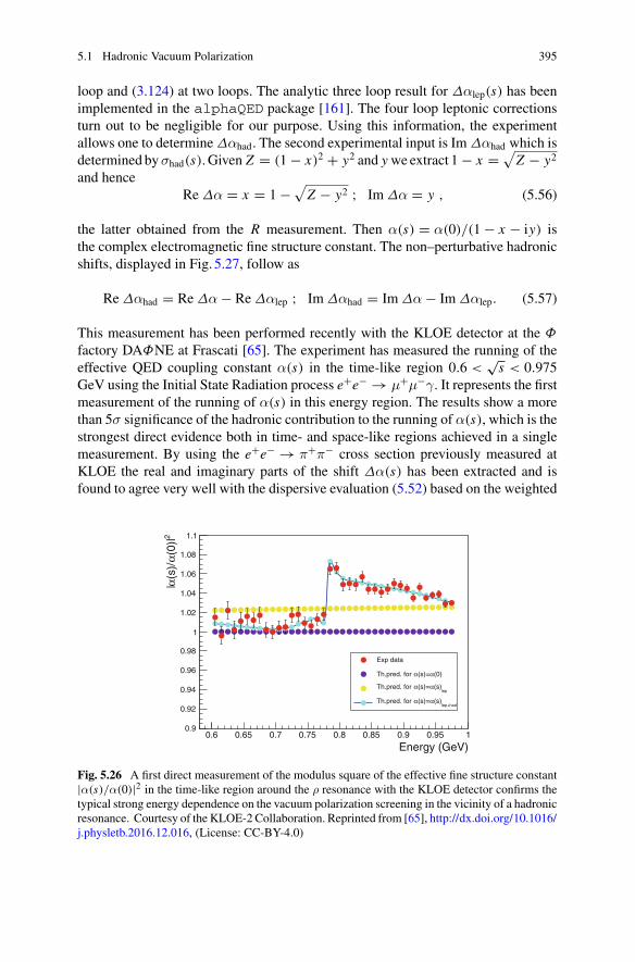
5.1 Hadronic Vacuum Polarization 395

loop and (3.124) at two loops. The analytic three loop result for Δαlep(s) has beenimplemented in the alphaQED package [161]. The four loop leptonic correctionsturn out to be negligible for our purpose. Using this information, the experimentallows one to determine Δαhad. The second experimental input is Im Δαhad which isdetermined byσhad(s). Given Z = (1 − x)2 + y2 and yweextract 1 − x = √

Z − y2

and henceRe Δα = x = 1 −

√Z − y2 ; Im Δα = y , (5.56)

the latter obtained from the R measurement. Then α(s) = α(0)/(1 − x − iy) isthe complex electromagnetic fine structure constant. The non–perturbative hadronicshifts, displayed in Fig. 5.27, follow as

Re Δαhad = Re Δα − Re Δαlep ; Im Δαhad = Im Δα − Im Δαlep. (5.57)

This measurement has been performed recently with the KLOE detector at the Φ

factory DAΦNE at Frascati [65]. The experiment has measured the running of theeffective QED coupling constant α(s) in the time-like region 0.6 <

√s < 0.975

GeV using the Initial State Radiation process e+e− → μ+μ−γ. It represents the firstmeasurement of the running of α(s) in this energy region. The results show a morethan 5σ significance of the hadronic contribution to the running of α(s), which is thestrongest direct evidence both in time- and space-like regions achieved in a singlemeasurement. By using the e+e− → π+π− cross section previously measured atKLOE the real and imaginary parts of the shift Δα(s) has been extracted and isfound to agree very well with the dispersive evaluation (5.52) based on the weighted

Energy (GeV)0.6 0.65 0.7 0.75 0.8 0.85 0.9 0.95 1

2(0

)|α

(s)/

α|

0.9

0.92

0.94

0.96

0.98

1

1.02

1.04

1.06

1.08

1.1

Exp data

(0)α(s)=αTh.pred. for

lep(s)α(s)=αTh.pred. for

lep+had(s)α(s)=αTh.pred. for

Fig. 5.26 A first direct measurement of the modulus square of the effective fine structure constant|α(s)/α(0)|2 in the time-like region around the ρ resonance with the KLOE detector confirms thetypical strong energy dependence on the vacuum polarization screening in the vicinity of a hadronicresonance. Courtesy of the KLOE-2 Collaboration. Reprinted from [65], http://dx.doi.org/10.1016/j.physletb.2016.12.016, (License: CC-BY-4.0)

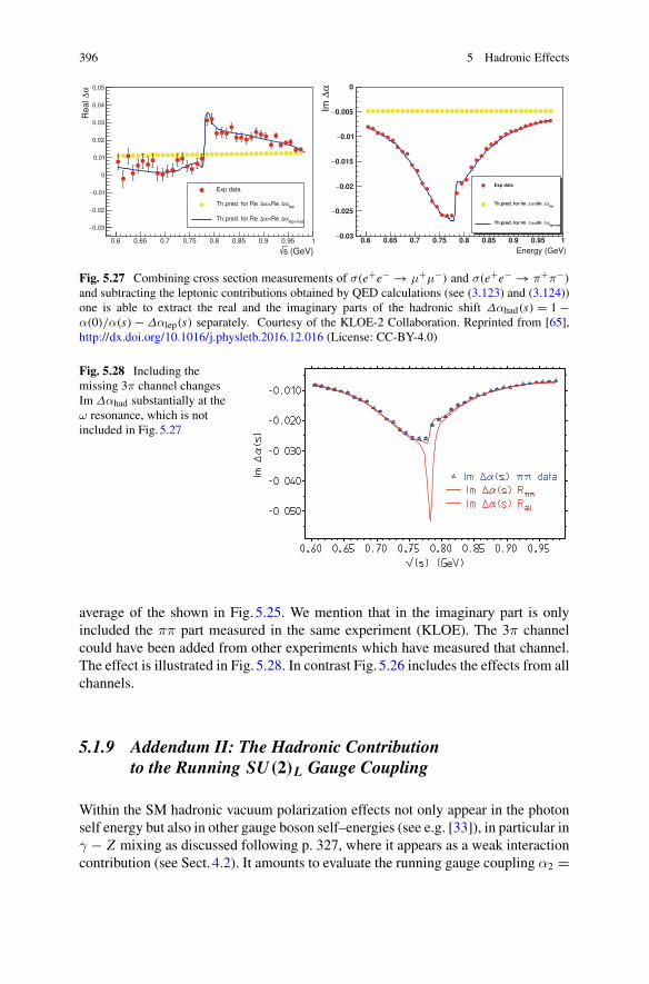
396 5 Hadronic Effects

Fig. 5.27 Combining cross section measurements of σ(e+e− → μ+μ−) and σ(e+e− → π+π−)

and subtracting the leptonic contributions obtained by QED calculations (see (3.123) and (3.124))one is able to extract the real and the imaginary parts of the hadronic shift Δαhad(s) = 1 −α(0)/α(s) − Δαlep(s) separately. Courtesy of the KLOE-2 Collaboration. Reprinted from [65],http://dx.doi.org/10.1016/j.physletb.2016.12.016 (License: CC-BY-4.0)

Fig. 5.28 Including themissing 3π channel changesIm Δαhad substantially at theω resonance, which is notincluded in Fig. 5.27

average of the shown in Fig. 5.25. We mention that in the imaginary part is onlyincluded the ππ part measured in the same experiment (KLOE). The 3π channelcould have been added from other experiments which have measured that channel.The effect is illustrated in Fig. 5.28. In contrast Fig. 5.26 includes the effects from allchannels.

5.1.9 Addendum II: The Hadronic Contributionto the Running SU(2)L Gauge Coupling

Within the SM hadronic vacuum polarization effects not only appear in the photonself energy but also in other gauge boson self–energies (see e.g. [33]), in particular inγ − Z mixing as discussed following p. 327, where it appears as a weak interactioncontribution (see Sect. 4.2). It amounts to evaluate the running gauge coupling α2 =

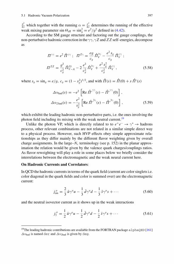
5.1 Hadronic Vacuum Polarization 397

g2

4π which together with the running α = e2

4π determines the running of the effectiveweak mixing parameter sinΘeff = sin2g = e2/g2 defined in (4.42).

According to the SM gauge structure and factoring out the gauge couplings, thenon-perturbative hadronic correction in theγγ,γZ and Z Z self–energies, decomposeas

Πγγ = e2 Πγγ ; Π Zγ = eg

cgΠ

3γV − e2 sg

cgΠ

γγV ;

Π Z Z = g2

c2gΠ33

V−A − 2e2

c2gΠ

3γV + e2 s2g

c2gΠ

γγV , (5.58)

where sg = sing = e/g, cg = (1 − s2g )1/2, and with Π(s) = Π(0) + s Π ′(s)

Δαhad(s) = −e2[Re Π ′γγ

(s) − Π ′γγ(0)

],

Δα2 had(s) = −e2

s2g

[Re Π ′3γ(s) − Π ′3γ(0)

], (5.59)

which exhibit the leading hadronic non-perturbative parts, i.e. the ones involving thephoton field including its mixing with the weak neutral current.19

Unlike the photon VP, which is directly related to to e+e− → γ∗ → hadronsprocess, other relevant combinations are not related in a similar simple direct wayto a physical process. However, such HVP effects obey simple approximate rela-tionships as they differ mainly by the different flavor weighting given by overallcharge assignments. In the large–Nc terminology (see p. 152) in the planar approx-imation the relation would be given by the valence quark charges/couplings ratios.As flavor reweighting will play a role in some places below we briefly consider theinterrelations between the electromagnetic and the weak neural current here.

On Hadronic Currents and Correlators:

In QCD the hadronic currents in terms of the quark field (current are color singlets i.e.color diagonal in the quark fields and color is summed over) are the electromagneticcurrent:

j μem = 2

3uγμu − 1

3dγμd − 1

3sγμs + · · · (5.60)

and the neutral isovector current as it shows up in the weak interactions

j μ3 = 1

2uγμu − 1

2dγμd − 1

2sγμs + · · · (5.61)

19The leading hadronic contributions are available from the FORTRAN package alphaQED [161]Δαhad is named der and Δα2had is given by deg.

398 5 Hadronic Effects

In current correlators, one has to distinguish valence quark connected and discon-nected contributions, where the latter need not be diagonal in flavor space and giverise to OZI suppressed transitions. In case the latter would be small relative to theflavor diagonal ones one would obtain a flavor weighting as in pQCD. The sepa-ration of the ud part based on isospin considerations not assuming OZI violatingterms to be small leads to a different reweighting, however, and which actually turnsout to be a much better approximation, as has been checked against lattice QCDsimulations [162, 163].

In the SU (3)flavor limit of the light quarks we haveΠ ss � Πdd � Πuu andΠds �Πus � Πud (ms � md � mu), which implies

Πγγ(uds)�

2

3

(Πuu − Πud

); Π

3γ(uds)�

1

3

(Πuu − Πud

); Π33

(uds) � 3

16

(Πuu − Πud

)+ 1

16Πud

These assumptions imply

Π3γ � 1

2Π

γγ(uds) + 3

8Π

γγ(c) + 3

4Π

γγ(b) (5.62)

and further assuming |Πud | � 3(Πuu − Πud

)we have

Π33 � 9

32Π

γγ(uds) + 9

64Π

γγ(c) + 9

16Π

γγ(b) . (5.63)

An attempt to proceed similarly in the SU (2)flavor limit of the light quarkswithΠdd �Πuu (md � mu),wefindno simple relationunless one assumesOZI suppressed termsto be negligible (see below). This leads to the reweighting as in perturbation theory,and leads to a 5% mismatch when compared with lattice simulations.

At low energy the VP effects are related to hadrons and a corresponding notethe reader may find on page p. 152 in Sect. 2.8. For energies where exclusivehadro–production channels are available i.e. below 2 GeV one may perform flavorseparation by hand:

since final state e.m. interactions violate isospin, we skip all final states involvingphotons like: π0γ, ηγ, η′γ etc. (see Table5.3)

• as ud, I = 0 we include states with odd number of pions, incl. the ω meson• as ud, I = 1 we include states with even number of pions, incl. the ρ meson• as ss we count all states with Kaons, incl. the φ meson

States ηX with X some other hadrons are collected separately, and then split intoq = u, d and s components by appropriate mixing.

For the resonance contributions in the spirit of the large–Nc vector mesondominance picture we proceed as follows: in terms of single quark currents j q ,where j qμ = qγμq, we may define currents associated with the resonances j ρ =12

(j u − j d

), j ω = 1

6

(j u + j d

)and j φ = − 1

3 j s , which corresponds to the ide-ally mixed J PC = 1−− states ρ0, ω0 and φ0, we may write

5.1 Hadronic Vacuum Polarization 399

j γ = j ρ + j ω + j φ + j J/ψ + j Υ

j 3 = 1

2j ρ + 3

4j φ + 3

8j J/ψ + 3

4j Υ (5.64)

Denoting the diagonal amplitudes by Π(V ) we obtain

Πγγ � Π(ρ) + Π(ω) + Π(φ) + Π(J/ψ) + Π(Υ )

Π3γ � 1

2Π(ρ) + 3

4Π(φ) + 3

8Π(J/ψ) + 3

4Π(Υ )

Π33 � 1

4Π(ρ) + 9

16Π(φ) + 9

64Π(J/ψ) + 9

16Π(Υ ) (5.65)

provided mixing is small. For the combination 3 Π33 − Π3γ = − 12Π

ρω + 38Π

(φ) −332Π(J/ψ) + · · · the (ud) contribution is solely due to ρ − ω mixing, as an example.In any case we apply the resonance reweighting for corresponding contributions ofTable5.2.

Besides the flavor SU (3) inspired weighting

Π3γuds = 1

2Π

γγuds

the ρ dominance (exact in the isospin limit) assignment

Π3γud = 1

2Π

γγud ; Π3γ

s = 3

4Πγγ

s

which agrees well with lattice data.Note that the “wrong” perturbative weighting

Π3γud = 9

20Π

γγud ; Π3γ

s = 3

4Πγγ

s

has been proven to clearly mismatch lattice results, while the correction 920 ⇒ 10

20 isin good agreement. This also means the OZI suppressed contributions should be atthe 5% level and not negligibly small.

Note that in the 1985 SU (3) flavor separation scheme [33] we assigned to non-φ(non-resonant) s component the weight 1/2, while in the updated scheme we assignthe weight 3/4 as for resonant φ. We take the difference as a systematic uncertainty.

SM gauge boson self-energy contributions are expressed in terms of Jμ3 = 1

2 j μ3

such that Π ′3γ(s) − Π ′3γ(0) ⇔ 12 Π3γ and Π ′33(s) − Π ′33(0) ⇔ 1

4 Π33. That weare using the proper recipe has been checked in lattice QCD calculations [162, 163].The running weak mixing parameter has been displayed in Fig. 4.17 in Sect. 4.2.

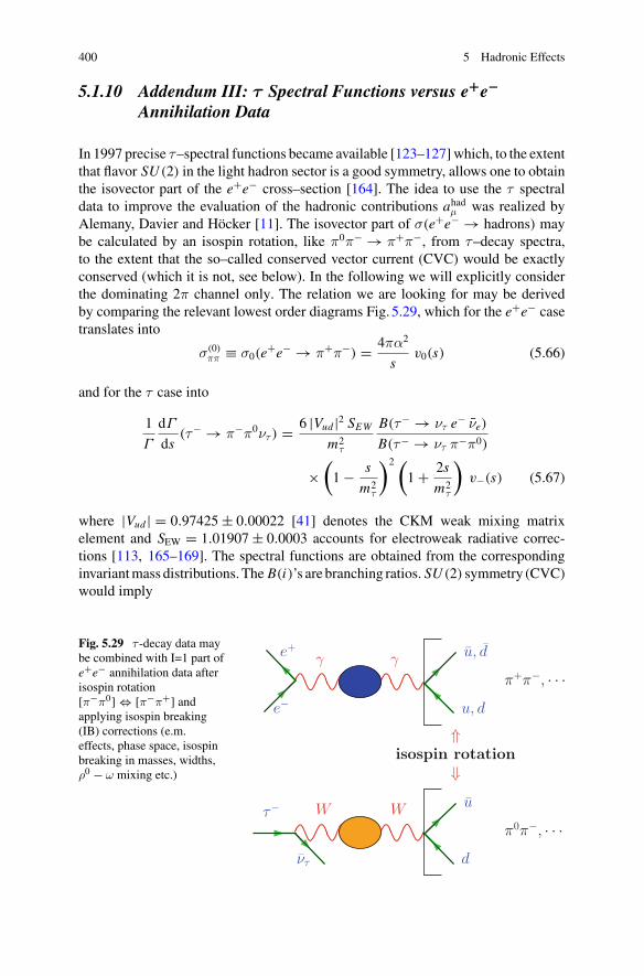
400 5 Hadronic Effects

5.1.10 Addendum III: τ Spectral Functions versus e+e−Annihilation Data

In 1997 precise τ–spectral functions became available [123–127]which, to the extentthat flavor SU (2) in the light hadron sector is a good symmetry, allows one to obtainthe isovector part of the e+e− cross–section [164]. The idea to use the τ spectraldata to improve the evaluation of the hadronic contributions ahadμ was realized byAlemany, Davier and Höcker [11]. The isovector part of σ(e+e− → hadrons) maybe calculated by an isospin rotation, like π0π− → π+π−, from τ–decay spectra,to the extent that the so–called conserved vector current (CVC) would be exactlyconserved (which it is not, see below). In the following we will explicitly considerthe dominating 2π channel only. The relation we are looking for may be derivedby comparing the relevant lowest order diagrams Fig. 5.29, which for the e+e− casetranslates into

σ(0)ππ ≡ σ0(e

+e− → π+π−) = 4πα2

sv0(s) (5.66)

and for the τ case into

1

Γ

dΓ

ds(τ− → π−π0ντ ) = 6 |Vud |2 SEW

m2τ

B(τ− → ντ e− νe)

B(τ− → ντ π−π0)

×(1 − s

m2τ

)2 (1 + 2s

m2τ

)v−(s) (5.67)

where |Vud | = 0.97425 ± 0.00022 [41] denotes the CKM weak mixing matrixelement and SEW = 1.01907 ± 0.0003 accounts for electroweak radiative correc-tions [113, 165–169]. The spectral functions are obtained from the correspondinginvariantmass distributions. The B(i)’s are branching ratios. SU (2) symmetry (CVC)would imply

Fig. 5.29 τ -decay data maybe combined with I=1 part ofe+e− annihilation data afterisospin rotation[π−π0] ⇔ [π−π+] andapplying isospin breaking(IB) corrections (e.m.effects, phase space, isospinbreaking in masses, widths,ρ0 − ω mixing etc.)

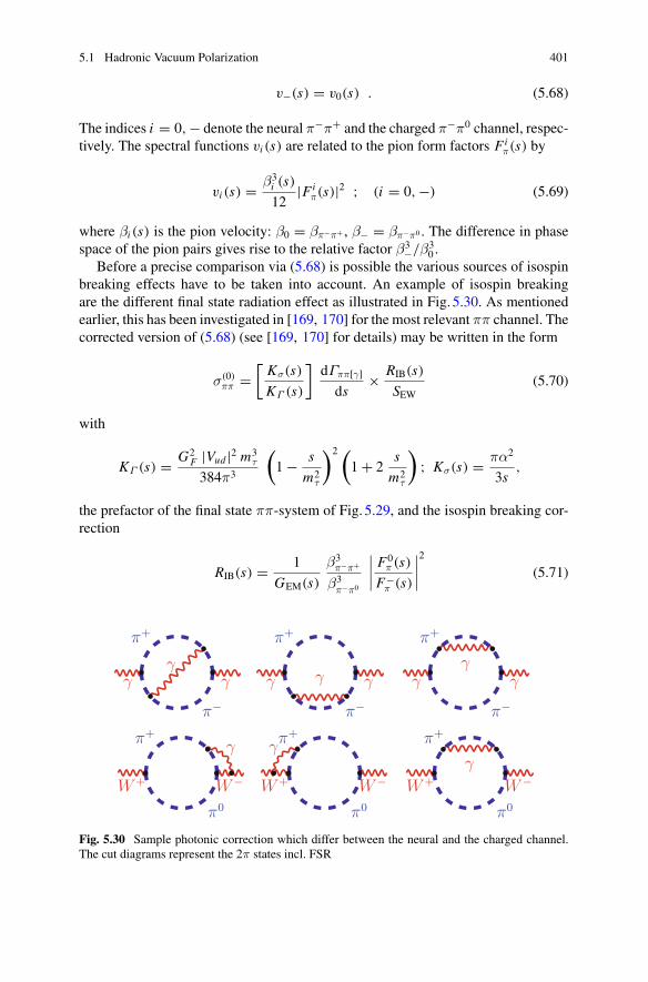
5.1 Hadronic Vacuum Polarization 401

v−(s) = v0(s) . (5.68)

The indices i = 0,− denote the neural π−π+ and the charged π−π0 channel, respec-tively. The spectral functions vi (s) are related to the pion form factors Fi

π(s) by

vi (s) = β3i (s)

12|Fi

π(s)|2 ; (i = 0,−) (5.69)

where βi (s) is the pion velocity: β0 = βπ−π+ , β− = βπ−π0 . The difference in phasespace of the pion pairs gives rise to the relative factor β3−/β3

0 .Before a precise comparison via (5.68) is possible the various sources of isospin

breaking effects have to be taken into account. An example of isospin breakingare the different final state radiation effect as illustrated in Fig. 5.30. As mentionedearlier, this has been investigated in [169, 170] for the most relevant ππ channel. Thecorrected version of (5.68) (see [169, 170] for details) may be written in the form

σ(0)ππ =

[Kσ(s)

KΓ (s)

]dΓππ[γ]ds

× RIB(s)

SEW(5.70)

with

KΓ (s) = G2F |Vud |2 m3

τ

384π3

(1 − s

m2τ

)2 (1 + 2

s

m2τ

); Kσ(s) = πα2

3s,

the prefactor of the final state ππ-system of Fig. 5.29, and the isospin breaking cor-rection

RIB(s) = 1

GEM(s)

β3π−π+

β3π−π0

∣∣∣∣F0

π (s)

F−π (s)

∣∣∣∣2

(5.71)

Fig. 5.30 Sample photonic correction which differ between the neural and the charged channel.The cut diagrams represent the 2π states incl. FSR

402 5 Hadronic Effects

includes the QED corrections to τ− → ντπ−π0 decay with virtual plus real soft and

hard photon radiation, integrated over all phase space.However, photon radiation by hadrons is poorly understood theoretically. The

commonly accepted recipe is to treat radiative corrections of the pions by scalarQED,except for the short distance (SD) logarithm proportional the lnMW/mπ which isreplaced by the quark parton model result and included in SEW by convention. ThisSD log is present only in the weak charged current transition W+∗ → π+π0 (γ),while in the charge neutral electromagnetic current transition γ∗ → π+π− (γ) thistype of leading log is absent. In any case there is an uncertainty in the correction ofthe isospin violations by virtual and real photon radiation which is hard to quantify.However, the γγ → π−π+,π0π0 data strongly suggest that sQED applies quite wellbelow about 1 GeV.

Originating from (5.69), β3π−π+/β3

π−π0 is a phase space correction due to the π± −π0 mass difference. F0

π (s) is theNCvector current form factor,which exhibits besidesthe I = 1 part an I = 0 contribution. The latter represents the ρ − ω mixing termwhich originates from the SU (2) breaking (md − mu mass difference). Finally, F−

π

is the CC I = 1 vector form factor. One of the leading isospin breaking effectsis the ρ − ω mixing correction included in |F0

π (s)|2. The form factor corrections,in principle, also should include the electromagnetic shifts in the masses and thewidths of the ρ’s.20 Up to this last mentioned effect, discussed in [114], which wasconsidered to be small, all the corrections were applied in [113] (see Fig. 5.34) butwere not able to eliminate the observed discrepancy between v−(s) and v0(s). Thedeviation is starting at the peak of the ρ and is increasing with energy to about10–20%. The origin of this difference is ρ0 − γ mixing, which occurs in the neutrale+e− channel, but obviously is absent in the charged τ–decay. This will be discussednext.

5.1.11 A Minimal Model: VMD + sQED Resolvingthe τ versus e+e− Puzzle

To come to the point, the “model” we apply here is a widely accepted model, with thedifference that previous models of the pion form factor in the neutral channel, knownas the Gounaris–Sakurai model, have been missing to take into account the one-loopdiagrams in the ρ0 − γ mixing amplitude. When modeling the pion form factor asa strong interaction object, photon radiation by the pions is usually not accountedfor. The latter is considered as an isospin breaking correction. Recently, in [88] an

20Because of the strong resonance enhancement, especially in the ρ region, a small isospin breakingshift in mass and width between ρ0 and ρ±, typically ΔMρ = Mρ± − Mρ0 ∼ 2.5 MeV and ΔΓρ =Γρ± − Γρ0 ∼ 1.5 MeV and similar for the higher resonances ρ′, ρ′′, . . . and the mixings of thesestates, causes a large effect in the tails by the kinematic shift this implies. Such large parametershifts can mimic to some extent a γ − ρ0 mixing effect (see Fig. 5.33) and is included by Davieret al. [129, 171] as part of the “normal” IB, as an alternative to γ − ρ0 mixing. Theory argumentsyield a small ΔMρ ∼ 0.8 MeV only.

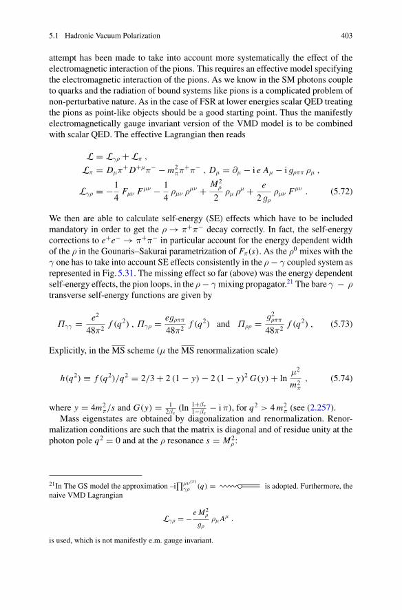
5.1 Hadronic Vacuum Polarization 403

attempt has been made to take into account more systematically the effect of theelectromagnetic interaction of the pions. This requires an effective model specifyingthe electromagnetic interaction of the pions. As we know in the SM photons coupleto quarks and the radiation of bound systems like pions is a complicated problem ofnon-perturbative nature. As in the case of FSR at lower energies scalar QED treatingthe pions as point-like objects should be a good starting point. Thus the manifestlyelectromagnetically gauge invariant version of the VMD model is to be combinedwith scalar QED. The effective Lagrangian then reads

L = Lγρ + Lπ ,

Lπ = Dμπ+D+μπ− − m2

ππ+π− , Dμ = ∂μ − i e Aμ − i gρππ ρμ ,

Lγρ = −1

4Fμν F

μν − 1

4ρμν ρμν + M2

ρ

2ρμ ρμ + e

2 gρρμν F

μν . (5.72)

We then are able to calculate self-energy (SE) effects which have to be includedmandatory in order to get the ρ → π+π− decay correctly. In fact, the self-energycorrections to e+e− → π+π− in particular account for the energy dependent widthof the ρ in the Gounaris–Sakurai parametrization of Fπ(s). As the ρ0 mixes with theγ one has to take into account SE effects consistently in the ρ − γ coupled system asrepresented in Fig. 5.31. The missing effect so far (above) was the energy dependentself-energy effects, the pion loops, in the ρ − γ mixing propagator.21 The bare γ − ρtransverse self-energy functions are given by

Πγγ = e2

48π2f (q2) , Πγρ = egρππ

48π2f (q2) and Πρρ = g2ρππ

48π2f (q2) , (5.73)

Explicitly, in the MS scheme (μ the MS renormalization scale)

h(q2) ≡ f (q2)/q2 = 2/3 + 2 (1 − y) − 2 (1 − y)2 G(y) + lnμ2

m2π

, (5.74)

where y = 4m2π/s and G(y) = 1

2βπ(ln 1+βπ

1−βπ− i π), for q2 > 4m2

π (see (2.257).Mass eigenstates are obtained by diagonalization and renormalization. Renor-

malization conditions are such that the matrix is diagonal and of residue unity at thephoton pole q2 = 0 and at the ρ resonance s = M2

ρ :

21In The GS model the approximation –i∏μν(π)

γρ (q) = is adopted. Furthermore, thenaive VMD Lagrangian

Lγρ = − e M2ρ

gρρμA

μ .

is used, which is not manifestly e.m. gauge invariant.

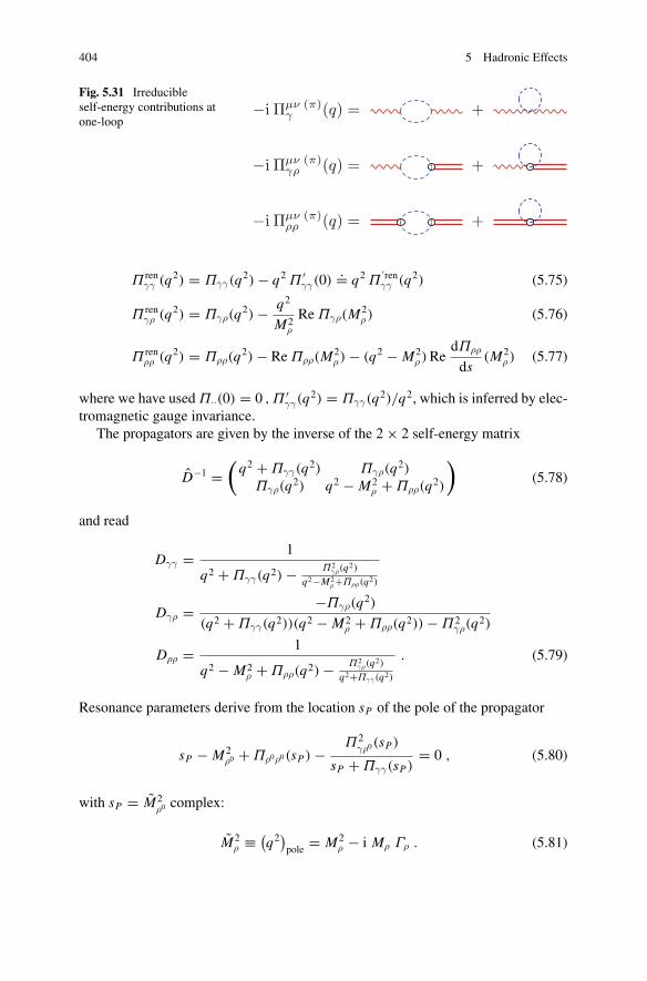
404 5 Hadronic Effects

Fig. 5.31 Irreducibleself-energy contributions atone-loop

Π renγγ (q2) = Πγγ(q

2) − q2 Π ′γγ(0)

.= q2 Π′renγγ (q2) (5.75)

Π renγρ (q2) = Πγρ(q

2) − q2

M2ρ

Re Πγρ(M2ρ ) (5.76)

Π renρρ (q2) = Πρρ(q

2) − Re Πρρ(M2ρ ) − (q2 − M2

ρ )RedΠρρ

ds(M2

ρ ) (5.77)

where we have used Π··(0) = 0 ,Π ′γγ(q

2) = Πγγ(q2)/q2, which is inferred by elec-tromagnetic gauge invariance.

The propagators are given by the inverse of the 2 × 2 self-energy matrix

D−1 =(q2 + Πγγ(q2) Πγρ(q2)

Πγρ(q2) q2 − M2ρ + Πρρ(q2)

)(5.78)

and read

Dγγ = 1

q2 + Πγγ(q2) − Π2γρ(q

2)

q2−M2ρ +Πρρ(q2)

Dγρ = −Πγρ(q2)

(q2 + Πγγ(q2))(q2 − M2ρ + Πρρ(q2)) − Π2

γρ(q2)

Dρρ = 1

q2 − M2ρ + Πρρ(q2) − Π2

γρ(q2)

q2+Πγγ(q2)

. (5.79)

Resonance parameters derive from the location sP of the pole of the propagator

sP − M2ρ0 + Πρ0ρ0(sP) − Π2

γρ0(sP)

sP + Πγγ(sP)= 0 , (5.80)

with sP = M2ρ0 complex:

M2ρ ≡ (

q2)pole = M2

ρ − i Mρ Γρ . (5.81)

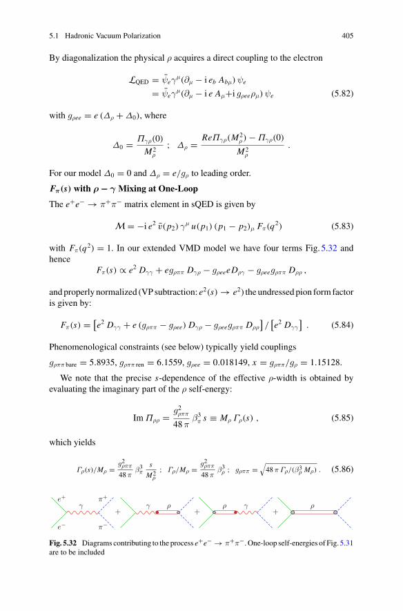
5.1 Hadronic Vacuum Polarization 405

By diagonalization the physical ρ acquires a direct coupling to the electron

LQED = ψeγμ(∂μ − i eb Abμ)ψe

= ψeγμ(∂μ − i e Aμ+i gρeeρμ)ψe (5.82)

with gρee = e (Δρ + Δ0), where

Δ0 = Πγρ(0)

M2ρ

; Δρ = ReΠγρ(M2ρ ) − Πγρ(0)

M2ρ

.

For our model Δ0 = 0 and Δρ = e/gρ to leading order.

Fπ(s) with ρ − γ Mixing at One-Loop

The e+e− → π+π− matrix element in sQED is given by

M = −i e2 v(p2) γμ u(p1) (p1 − p2)μ Fπ(q2) (5.83)

with Fπ(q2) = 1. In our extended VMD model we have four terms Fig. 5.32 andhence

Fπ(s) ∝ e2 Dγγ + egρππ Dγρ − gρeeeDργ − gρeegρππ Dρρ ,

andproperly normalized (VP subtraction: e2(s) → e2) the undressedpion form factoris given by:

Fπ(s) = [e2 Dγγ + e (gρππ − gρee) Dγρ − gρeegρππ Dρρ

]/[e2 Dγγ

]. (5.84)

Phenomenological constraints (see below) typically yield couplings

gρππ bare = 5.8935, gρππ ren = 6.1559, gρee = 0.018149, x = gρππ/gρ = 1.15128.

We note that the precise s-dependence of the effective ρ-width is obtained byevaluating the imaginary part of the ρ self-energy:

Im Πρρ = g2ρππ

48πβ3

π s ≡ Mρ Γρ(s) , (5.85)

which yields

Γρ(s)/Mρ = g2ρππ

48πβ3π

s

M2ρ

; Γρ/Mρ = g2ρππ

48πβ3ρ ; gρππ =

√48π Γρ/(β3

ρ Mρ) . (5.86)

Fig. 5.32 Diagrams contributing to the process e+e− → π+π−. One-loop self-energies of Fig. 5.31are to be included

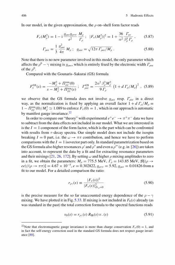
406 5 Hadronic Effects

In our model, in the given approximation, the ρ on–shell form factor reads

Fπ(M2ρ ) = 1 − i

gρeegρππ

e2Mρ

Γρ; |Fπ(M

2ρ )|2 = 1 + 36

α2

Γee

β3ρ Γρ

, (5.87)

Γρee = 1

3

g2ρee

4πMρ ; gρee = √

12π Γρee/Mρ . (5.88)

Note that there is no new parameter involved in this model, the only parameter whichaffects the ρ0 − γ mixing is gρee, which is entirely fixed by the electronic width Γρee

of the ρ0.Compared with the Gounaris–Sakurai (GS) formula

FGSπ (s) = −M2

ρ + Π renρρ (0)

s − M2ρ + Π ren

ρρ (s); Γ GS

ρee = 2α2 β3ρM

2ρ

9Γρ

(1 + d Γρ/Mρ

)2, (5.89)

we observe that the GS formula does not involve gρee resp. Γρee in a directway, as the normalization is fixed by applying an overall factor 1 + d Γρ/Mρ ≡1 − Π ren

ρρ (0)/M2ρ � 1.089 to enforce Fπ(0) = 1 ,which in our approach is automatic

by manifest gauge invariance.22

In order to compare our “theory” with experimental e+e− → π+π− data we haveto subtract from the data effects not included in our model. What we are interested inis the I = 1 component of the form factor, which is the part which can be confrontedwith results from τ -decay spectra. Our simple model does not include the isospinbreaking I = 0 part, i.e. the ω → ππ contribution, and hence we have to performcomparisons with the I = 1 isovector part only. In standard parametrization based ontheGS formula also higher resonances ρ′ and ρ′′ and even a ρ′′′ (e.g. in [26]) are takeninto account, to represent the data by a fit and for extracting resonance parametersand their mixings [21, 26, 172]. By setting ω and higher ρmixing amplitudes to zeroin a fit, we obtain the parameters: Mρ = 775.5 MeV, Γρ = 143.85 MeV, B[(ρ →ee)/(ρ → ππ)] = 4.67 × 10−5, e = 0.302822, gρππ = 5.92, gρee = 0.01826 from afit to our model. For a detailed comparison the ratio:

rργ(s) ≡ |Fπ(s)|2|Fπ(s)|2Dγρ=0

(5.90)

is the precise measure for the so far unaccounted energy dependence of the ρ − γmixing. We have plotted it in Fig. 5.33. If mixing is not included in F0(s) already (aswas standard in the past) the total correction formula to the spectral functions reads

v0(s) = rργ(s) RIB(s) v−(s) (5.91)

22Note that electromagnetic gauge invariance is more than charge conservation Fπ(0) = 1, andin fact the self-energy correction used in the standard GS formula does not respect gauge invari-ance [88].

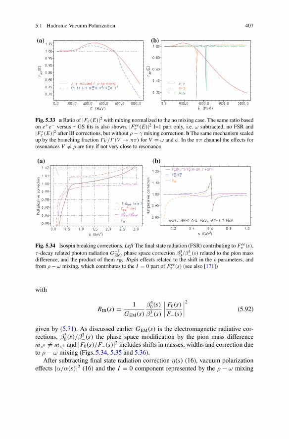
5.1 Hadronic Vacuum Polarization 407

(a) (b)

Fig. 5.33 a Ratio of |Fπ(E)|2 with mixing normalized to the no mixing case. The same ratio basedon e+e− versus τ GS fits is also shown. |Fee

π (E)|2 I=1 part only, i.e. ω subtracted, no FSR and|Fτ

π (E)|2 after IB corrections, but without ρ − γ mixing correction. b The same mechanism scaledup by the branching fraction ΓV /Γ (V → ππ) for V = ω and φ. In the ππ channel the effects forresonances V = ρ are tiny if not very close to resonance

(a) (b)

Fig. 5.34 Isospin breaking corrections. Left The final state radiation (FSR) contributing to Feeπ (s),

τ -decay related photon radiation G−1EM, phase space correction β3

0/β3−(s) related to the pion mass

difference, and the product of them rIB. Right effects related to the shift in the ρ parameters, andfrom ρ − ω mixing, which contributes to the I = 0 part of Fee

π (s) (see also [171])

with

RIB(s) = 1

GEM(s)

β30(s)

β3−(s)

∣∣∣∣F0(s)

F−(s)

∣∣∣∣2

(5.92)

given by (5.71). As discussed earlier GEM(s) is the electromagnetic radiative cor-rections, β3

0(s)/β3−(s) the phase space modification by the pion mass difference

mπ0 = mπ± and |F0(s)/F−(s)|2 includes shifts in masses, widths and correction dueto ρ − ω mixing (Figs. 5.34, 5.35 and 5.36).

After subtracting final state radiation correction η(s) (16), vacuum polarizationeffects |α/α(s)|2 (16) and the I = 0 component represented by the ρ − ω mixing

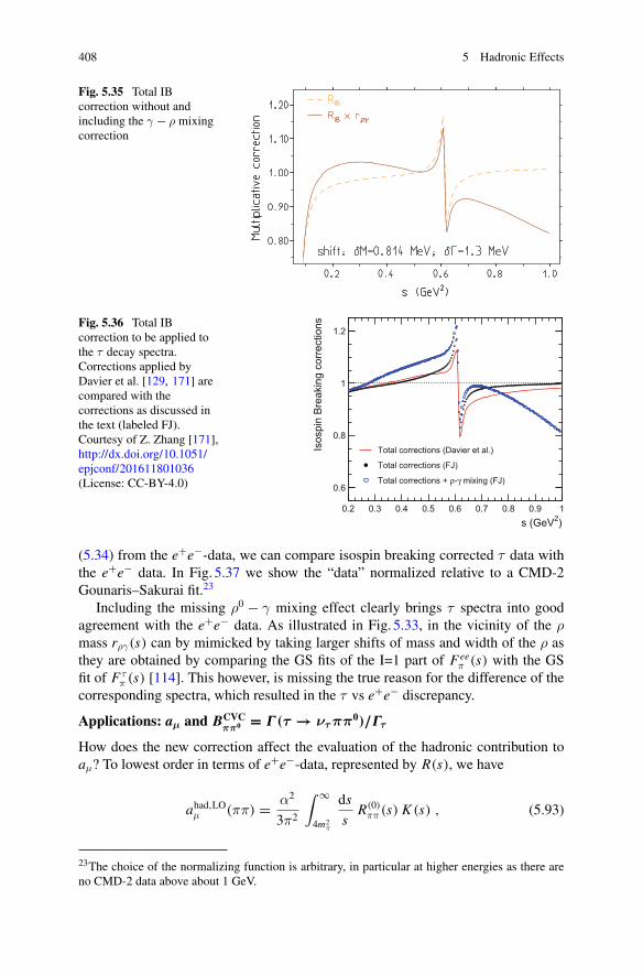
408 5 Hadronic Effects

Fig. 5.35 Total IBcorrection without andincluding the γ − ρ mixingcorrection

Fig. 5.36 Total IBcorrection to be applied tothe τ decay spectra.Corrections applied byDavier et al. [129, 171] arecompared with thecorrections as discussed inthe text (labeled FJ).Courtesy of Z. Zhang [171],http://dx.doi.org/10.1051/epjconf/201611801036(License: CC-BY-4.0)

(5.34) from the e+e−-data, we can compare isospin breaking corrected τ data withthe e+e− data. In Fig. 5.37 we show the “data” normalized relative to a CMD-2Gounaris–Sakurai fit.23

Including the missing ρ0 − γ mixing effect clearly brings τ spectra into goodagreement with the e+e− data. As illustrated in Fig. 5.33, in the vicinity of the ρmass rργ(s) can by mimicked by taking larger shifts of mass and width of the ρ asthey are obtained by comparing the GS fits of the I=1 part of Fee

π (s) with the GSfit of Fτ

π (s) [114]. This however, is missing the true reason for the difference of thecorresponding spectra, which resulted in the τ vs e+e− discrepancy.

Applications: aμ and BCVCππ0 = Γ (τ → ντ ππ0)/Γτ

How does the new correction affect the evaluation of the hadronic contribution toaμ? To lowest order in terms of e+e−-data, represented by R(s), we have

ahad,LOμ (ππ) = α2

3π2

∫ ∞

4m2π

ds

sR(0)

ππ (s) K (s) , (5.93)

23The choice of the normalizing function is arbitrary, in particular at higher energies as there areno CMD-2 data above about 1 GeV.

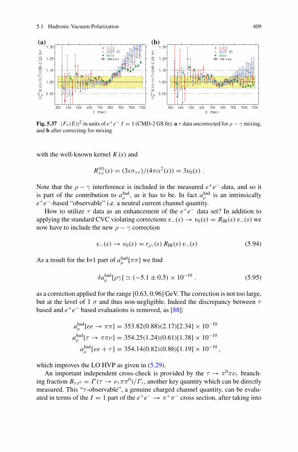
5.1 Hadronic Vacuum Polarization 409

(a) (b)

Fig. 5.37 |Fπ(E)|2 in units of e+e− I = 1 (CMD-2 GS fit): a τ data uncorrected for ρ − γ mixing,and b after correcting for mixing

with the well-known kernel K (s) and

R(0)ππ (s) = (3sσππ)/(4πα2(s)) = 3v0(s) .

Note that the ρ − γ interference is included in the measured e+e−-data, and so itis part of the contribution to ahadμ , as it has to be. In fact ahadμ is an intrinsicallye+e−-based “observable” i.e. a neutral current channel quantity.

How to utilize τ data as an enhancement of the e+e− data set? In addition toapplying the standard CVC violating corrections v−(s) → v0(s) = RIB(s) v−(s) wenow have to include the new ρ − γ correction

v−(s) → v0(s) = rργ(s) RIB(s) v−(s) (5.94)

As a result for the I=1 part of ahadμ [ππ] we find

δahadμ [ργ] � (−5.1 ± 0.5) × 10−10 . (5.95)

as a correction applied for the range [0.63, 0.96] GeV. The correction is not too large,but at the level of 1 σ and thus non-negligible. Indeed the discrepancy between τbased and e+e− based evaluations is removed, as [88]:

ahadμ [ee → ππ] = 353.82(0.88)(2.17)[2.34] × 10−10

ahadμ [τ → ππν] = 354.25(1.24)(0.61)[1.38] × 10−10

ahadμ [ee + τ ] = 354.14(0.82)(0.86)[1.19] × 10−10 ,

which improves the LO HVP as given in (5.29).An important independent cross-check is provided by the τ → π0πντ branch-

ing fraction Bππ0 = Γ (τ → ντππ0)/Γτ , another key quantity which can be directlymeasured. This “τ -observable”, a genuine charged channel quantity, can be evalu-ated in terms of the I = 1 part of the e+e− → π+π− cross section, after taking into

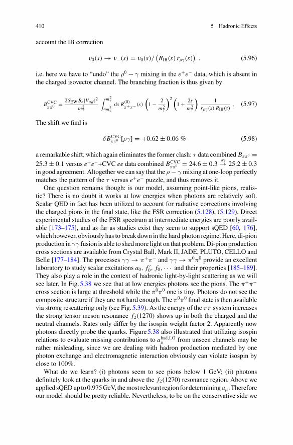
410 5 Hadronic Effects

account the IB correction

v0(s) → v−(s) = v0(s)/(RIB(s) rργ(s)

). (5.96)

i.e. here we have to “undo” the ρ0 − γ mixing in the e+e− data, which is absent inthe charged isovector channel. The branching fraction is thus given by

BCVCππ0

= 2SEWBe|Vud |2m2

τ

∫ m2τ

4m2π

ds R(0)π+π− (s)

(1 − 2

m2τ

)2 (1 + 2s

m2τ

)1

rργ(s) RIB(s), (5.97)

The shift we find is

δBCVCππ0 [ργ] = +0.62 ± 0.06 % (5.98)

a remarkable shift, which again eliminates the former clash: τ data combined Bππ0 =25.3 ± 0.1 versus e+e−+CVC ee data combined BCVC

ππ0 = 24.6 ± 0.3ργ→ 25.2 ± 0.3

in good agreement. Altogether we can say that the ρ − γ mixing at one-loop perfectlymatches the pattern of the τ versus e+e− puzzle, and thus removes it.

One question remains though: is our model, assuming point-like pions, realis-tic? There is no doubt it works at low energies when photons are relatively soft.Scalar QED in fact has been utilized to account for radiative corrections involvingthe charged pions in the final state, like the FSR correction (5.128), (5.129). Directexperimental studies of the FSR spectrum at intermediate energies are poorly avail-able [173–175], and as far as studies exist they seem to support sQED [60, 176],which however, obviously has to break down in the hard photon regime. Here, di-pionproduction inγγ fusion is able to shedmore light on that problem.Di-pion productioncross sections are available from Crystal Ball, Mark II, JADE, PLUTO, CELLO andBelle [177–184]. The processes γγ → π+π− and γγ → π0π0 provide an excellentlaboratory to study scalar excitations a0, f ′

0, f0, · · · and their properties [185–189].They also play a role in the context of hadronic light-by-light scattering as we willsee later. In Fig. 5.38 we see that at low energies photons see the pions. The π+π−cross section is large at threshold while the π0π0 one is tiny. Photons do not see thecomposite structure if they are not hard enough. The π0π0 final state is then availablevia strong rescattering only (see Fig. 5.39). As the energy of the ππ system increasesthe strong tensor meson resonance f2(1270) shows up in both the charged and theneutral channels. Rates only differ by the isospin weight factor 2. Apparently nowphotons directly probe the quarks. Figure5.38 also illustrated that utilizing isospinrelations to evaluate missing contributions to ahad,LOμ from unseen channels may berather misleading, since we are dealing with hadron production mediated by onephoton exchange and electromagnetic interaction obviously can violate isospin byclose to 100%.

What do we learn? (i) photons seem to see pions below 1 GeV; (ii) photonsdefinitely look at the quarks in and above the f2(1270) resonance region. Above weapplied sQEDup to0.975GeV, themost relevant region for determiningaμ. Thereforeour model should be pretty reliable. Nevertheless, to be on the conservative side we

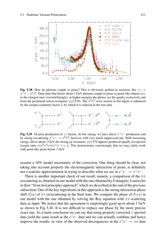
5.1 Hadronic Vacuum Polarization 411

Fig. 5.38 How do photons couple to pions? This is obviously probed in reactions like γγ →π+π−,π0π0. Data infer that below about 1 GeV photons couple to pions as point-like objects (i.e.to the charged ones overwhelmingly), at higher energies the photos see the quarks exclusively andform the prominent tensor resonance f2(1270). The π0π0 cross section in this figure is enhancedby the isospin symmetry factor 2, by which it is reduced in the true data

Fig. 5.39 Di-pion production in γγ fusion. At low energy we have direct π+π− production andby strong rescattering π+π− → π0π0, however with very much suppressed rate. With increasingenergy, above about 1 GeV, the strong qq resonance f2(1270 appears produced equally at expectedisospin ratio σ(π0π0)/σ(π+π−) = 1

2 . This demonstrates convincingly that we may safely workwith point-like pions below 1 GeV

assume a 10% model uncertainty of the correction. One thing should be clear, nottaking into account properly the electromagnetic interaction of pions, is definitelynot a realistic approximation in trying to describe what we see in e+e− → π+π−.

There is another important check of our result, namely, a comparison of the ππrescattering as obtained in our model with the one obtained by Colangelo, Leutwylerin their “fromfirst principles approach”whichwe described at the end of the previoussubsection. One of the key ingredients in this approach is the strong interaction phaseshift δ11(s) of ππ (re)scattering in the final state. We compare the phase of Fπ(s) inour model with the one obtained by solving the Roy equation with ππ-scatteringdata as input. We notice that the agreement is surprisingly good up to about 1 GeVas shown in Fig. 5.40. It is not difficult to replace our phase by the more preciseexact one. As a main conclusion we can say that using properly corrected τ spectraldata yield the same result as the e+e− data and we can actually combine and henceimprove the results: in view of the observed discrepancies in the e+e− → ππ data

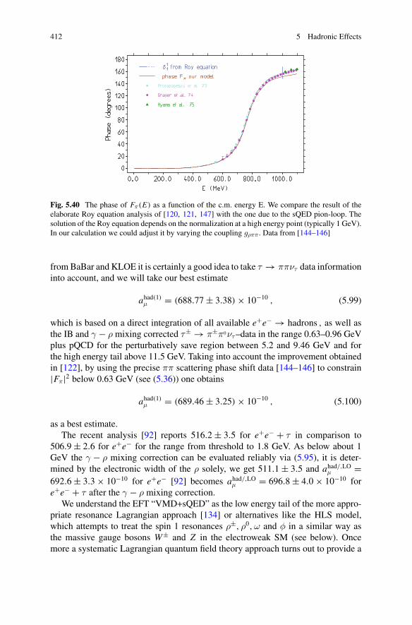
412 5 Hadronic Effects

Fig. 5.40 The phase of Fπ(E) as a function of the c.m. energy E. We compare the result of theelaborate Roy equation analysis of [120, 121, 147] with the one due to the sQED pion-loop. Thesolution of the Roy equation depends on the normalization at a high energy point (typically 1 GeV).In our calculation we could adjust it by varying the coupling gρππ . Data from [144–146]

from BaBar and KLOE it is certainly a good idea to take τ → ππντ data informationinto account, and we will take our best estimate

ahad(1)μ = (688.77 ± 3.38) × 10−10 , (5.99)

which is based on a direct integration of all available e+e− → hadrons , as well asthe IB and γ − ρ mixing corrected τ± → π±π0ντ–data in the range 0.63–0.96 GeVplus pQCD for the perturbatively save region between 5.2 and 9.46 GeV and forthe high energy tail above 11.5 GeV. Taking into account the improvement obtainedin [122], by using the precise ππ scattering phase shift data [144–146] to constrain|Fπ|2 below 0.63 GeV (see (5.36)) one obtains

ahad(1)μ = (689.46 ± 3.25) × 10−10 , (5.100)

as a best estimate.The recent analysis [92] reports 516.2 ± 3.5 for e+e− + τ in comparison to

506.9 ± 2.6 for e+e− for the range from threshold to 1.8 GeV. As below about 1GeV the γ − ρ mixing correction can be evaluated reliably via (5.95), it is deter-mined by the electronic width of the ρ solely, we get 511.1 ± 3.5 and ahad/,LOμ =692.6 ± 3.3 × 10−10 for e+e− [92] becomes ahad/,LOμ = 696.8 ± 4.0 × 10−10 fore+e− + τ after the γ − ρ mixing correction.

We understand the EFT “VMD+sQED” as the low energy tail of the more appro-priate resonance Lagrangian approach [134] or alternatives like the HLS model,which attempts to treat the spin 1 resonances ρ±, ρ0,ω and φ in a similar way asthe massive gauge bosons W± and Z in the electroweak SM (see below). Oncemore a systematic Lagrangian quantum field theory approach turns out to provide a

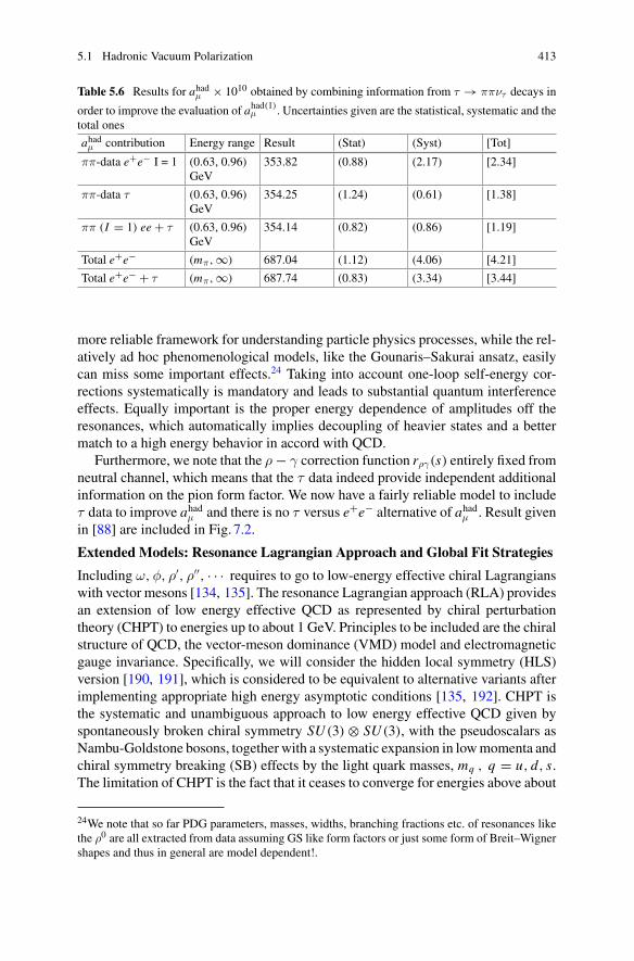
5.1 Hadronic Vacuum Polarization 413

Table 5.6 Results for ahadμ × 1010 obtained by combining information from τ → ππντ decays in

order to improve the evaluation of ahad(1)μ . Uncertainties given are the statistical, systematic and thetotal ones

ahadμ contribution Energy range Result (Stat) (Syst) [Tot]

ππ-data e+e− I = 1 (0.63, 0.96)GeV

353.82 (0.88) (2.17) [2.34]

ππ-data τ (0.63, 0.96)GeV

354.25 (1.24) (0.61) [1.38]

ππ (I = 1) ee + τ (0.63, 0.96)GeV

354.14 (0.82) (0.86) [1.19]

Total e+e− (mπ,∞) 687.04 (1.12) (4.06) [4.21]

Total e+e− + τ (mπ,∞) 687.74 (0.83) (3.34) [3.44]

more reliable framework for understanding particle physics processes, while the rel-atively ad hoc phenomenological models, like the Gounaris–Sakurai ansatz, easilycan miss some important effects.24 Taking into account one-loop self-energy cor-rections systematically is mandatory and leads to substantial quantum interferenceeffects. Equally important is the proper energy dependence of amplitudes off theresonances, which automatically implies decoupling of heavier states and a bettermatch to a high energy behavior in accord with QCD.

Furthermore, we note that the ρ − γ correction function rργ(s) entirely fixed fromneutral channel, which means that the τ data indeed provide independent additionalinformation on the pion form factor. We now have a fairly reliable model to includeτ data to improve ahadμ and there is no τ versus e+e− alternative of ahadμ . Result givenin [88] are included in Fig. 7.2.

Extended Models: Resonance Lagrangian Approach and Global Fit Strategies

Including ω,φ, ρ′, ρ′′, · · · requires to go to low-energy effective chiral Lagrangianswith vector mesons [134, 135]. The resonance Lagrangian approach (RLA) providesan extension of low energy effective QCD as represented by chiral perturbationtheory (CHPT) to energies up to about 1 GeV. Principles to be included are the chiralstructure of QCD, the vector-meson dominance (VMD) model and electromagneticgauge invariance. Specifically, we will consider the hidden local symmetry (HLS)version [190, 191], which is considered to be equivalent to alternative variants afterimplementing appropriate high energy asymptotic conditions [135, 192]. CHPT isthe systematic and unambiguous approach to low energy effective QCD given byspontaneously broken chiral symmetry SU (3) ⊗ SU (3), with the pseudoscalars asNambu-Goldstone bosons, together with a systematic expansion in lowmomenta andchiral symmetry breaking (SB) effects by the light quark masses, mq , q = u, d, s.The limitation of CHPT is the fact that it ceases to converge for energies above about

24We note that so far PDG parameters, masses, widths, branching fractions etc. of resonances likethe ρ0 are all extracted from data assuming GS like form factors or just some form of Breit–Wignershapes and thus in general are model dependent!.

414 5 Hadronic Effects

400 MeV, in particular it lacks to describe physics involving the vector resonancesρ,ω and φ.

The VMD is the effective theory implementing the direct coupling of the neu-tral spin 1 vector resonances ρ,ω,φ etc. to the photon. Such direct couplings area consequence of the fact that the neutral spin 1 resonances like the ρ0 are com-posed of charged quarks. The effect is well modeled by the VMD Lagrangian

Lγρ = e2gρ

ρμνFμν or = − eM2ρ

gρρμAμ, which has to be implement in low energy

effective QCD in a way which is consistent with the chiral structure of QCD.The construction of the HLS model may be outlined as follows: like in CHPT the

basic fields are the unitary matrix fields ξL ,R = exp [±i P/ fπ], where P = P8 + P0is the SU (3)matrix of pseudoscalar fields, with P0 and P8 the basic singlet and octetfields, respectively. The pseudoscalar field matrix P is represented by

P8 = 1√2

⎛

⎜⎜⎜⎜⎜⎝

1√2π3 + 1√

6η8 π+ K+

π− − 1√2π3 + 1√

6η8 K 0

K− K0 −

√2

3η8

⎞

⎟⎟⎟⎟⎟⎠, (5.101)

P0 = 1√6diag(η0, η0, η0) ; (π3, η8, η0) ⇔ (π0, η, η′) . (5.102)

The HLS ansatz is an extension of the CHPT non-linear sigma model to a non-linearchiral Lagrangian [Tr ∂μξ

+∂μξ] based on the symmetry patternGglobal/Hlocal, whereG = SU (3)L ⊗ SU (3)R is the chiral group ofQCDand H = SU (3)V the vector sub-group. The hidden local SU (3)V requires the spin 1 vector meson fields, representedby the SU (3) matrix field Vμ, to be gauge fields. The needed covariant derivativereads Dμ = ∂μ − i g Vμ, and allows to include the couplings to the electroweak gaugefields Aμ, Zμ and W±

μ in a natural way. The vector field matrix is usually written as

V = 1√2

⎛

⎜⎝(ρI + ω I )/

√2 ρ+ K ∗+

ρ− (−ρI + ω I )/√2 K ∗0

K ∗− K∗0

φI

⎞

⎟⎠ . (5.103)

The unbroken HLS Lagrangian is then given by

LHLS = LA + LV ; LA/V = − f 2π4

Tr [L ± R]2 , (5.104)

where L = [DμξL

]ξ+L and R = [

DμξR]

ξ+R . The covariant derivatives read

{DμξL = ∂μξL − igVμξL + iξLLμ

DμξR = ∂μξR − igVμξR + iξRRμ, (5.105)

5.1 Hadronic Vacuum Polarization 415

with known couplings to the Standard Model (SM) gauge bosons

⎧⎪⎨

⎪⎩

Lμ = eQAμ + g2

cos θW(Tz − sin2 θW )Zμ + g2√

2(W+

μ T+ + W−μ T−)

Rμ = eQAμ − g2

cos θWsin2 θW Zμ .

(5.106)

Like in the electroweak SM, masses of the spin 1 bosons may be generated by theHiggs-Kibble mechanism if one starts in place of the non-linear σ-model with theGell-Mann–Levy linear σ-model by a shift of the σ-field.

In fact the global chiral symmetry Gglobal is well known not to be realized as anexact symmetry in nature, which implies that the ideal HLS symmetry evidently isnot a symmetry of nature either. It evidently has to be broken appropriately in orderto provide a realistic low energy effective theory mimicking low energy effectiveQCD. Corresponding to the strength of the breaking, usually, this is done in twosteps, breaking of SU (3) in a first step and breaking the isospin SU (2) subgroupin a second step. Unlike in CHPT (perturbed non-linear σ–model) where one isperforming a systematic low energy expansion, expanding in low momenta and thequark masses, here we introduce symmetry breaking as a phenomenological patternwith parameters to be fixed from appropriate data, since a systematic low energyexpansion a lá CHPT ceases to converge at energies above about 400 MeV, while weattempt to model phenomenology up to including the φ resonance.

The broken HLS Lagrangian (BHLS) is then given by (see [132])

LBHLS = L′A + L′

V + L′tHooft ; L′A/V = − f 2π

4Tr

{[L ± R] XA/V

}2, (5.107)

with 6 phenomenological chiral SB parameters. The phenomenological SB patternsuggests XI = diag(qI , yI , zI ) , |qI − 1|, |yI − 1| � |zI − 1| , I = V, A .There isalso the parity odd anomalous sector, which is needed to account for reactions likeγ∗ → π0γ and γ∗ → π+π−π0 among others.

We note that this BHLS model would be a reliable low energy effective theoryif the QCD scale ΛQCD would be large relative to the scale of about 1 GeV up towhich we want to apply the model, which in reality is not the case. Nevertheless, asa phenomenological model applied to low multiplicity hadronic processes (specifiedbelow) it seems to work pretty well, as we have demonstrated by a global fit of theavailable data in [132]. The major achievement is a simultaneous consistent fit ofthe e+e− → π+π− data from CMD-2 [21], SND [22], KLOE [23–25], BaBar [26]and BES-III [27], and the τ → π−π0ντ decay spectral functions by ALEPH [123],OPAL [125], CLEO [126] and Belle [127]. The e+e− → π−π+ channel gives thedominant hadronic contribution to themuong − 2. Isospin symmetryπ−π0 ⇔ π−π+allows one to include existing high quality τ -data as advocated long time ago in [11].

We note that as long as higher order corrections are restricted to the mandatorypion- and Kaon-loop effects in the vector boson self-energies, renormalizability is

416 5 Hadronic Effects

not an issue. These contributions behave as in a strictly renormalizable theory andcorrespond to a reparametrization only.

A suitable extension of the HLS model which covers most channels in the rangeup to just above the φ resonance has been worked out and has been applied for anevaluation of ahadμ in [132, 193, 194]. The idea is to constrain the effective Lagrangianby fitting available data from all possible channels. Thereby uncertainties may bereduced by consistencywith effective field theory concepts. In [132] 45 different datasets in the range up to E0 = 1.05 GeV (6 annihilation channels and 10 partial widthdecays) are used to constrain the effective Lagrangian couplings. The phenomeno-logically constrained effective theory then is applied to predict the cross sections forthe channels π+π−, π0γ, ηγ, η′γ, π0π+π−, K+K−, K 0 K 0, which account for83.4% of ahadμ . The missing part, the channels 4π, 5π, 6π, ηππ,ωπ and the energyrange E > E0 is evaluated using data directly and pQCD for perturbative regionsand the tail. As we know, including self-energy effects is mandatory. They affect theneutral channel mixing between γ, ρ0,ω and φ as dynamical effects and provide theproper decay widths with proper phase space and energy dependence etc.

In the region covered by the HLS model the leading order HVP is obtained bysumming over the channels:

⎧⎨

⎩

ahadμ [HLS] = ∑i aμ(Hi )

aμ(Hi ) = 1

4π3

∫ scut

sHi

ds K (s)σHi (s) ,(5.108)

which relates the hadronic intermediate state contributions {Hi , i = 1 · · · n} to theannihilation cross sectionsσ(e+e− → Hi ) ≡ σHi (s). K (s) is the knownkernelwhichis enhancing the weight of the threshold region between sHi and scut = (1.05 GeV)2.The full LO ahadμ is obtained by adding to ahadμ [HLS] the missing channels below1.05 GeV, plus the remainder from energies above the model breakpoint, obtainedby the standard approach (see [47] for details).

According to [132] the method indeed works in reducing uncertainties by usingindirect constraints. This approach is able to reveal inconsistencies in the data. Akey point is that no inconsistencies between τ data and e+e− data show up. Incontrary τ data, which are not subject to complicated mixing effects, help to fixmore precisely the Lagrangian couplings and thus allow to reduce uncertainties ofthe predictions. We have included the result of this global fit in Fig. 7.2. Typically,some data sets get low weight as they conflict with the HLS global fit. This inparticular concerns the BaBar di-pion data which after taking into account standardIB corrections seem to agree well with the Belle τ–spectra, while not accounted forneutral channel mixing effects, like γ − ρ0 mixing, predict a substantial difference.As BaBar data treated with equal weight enhance the contribution to ahadμ by aboutδahadμ � 6 × 10−10 the HLS fit reduces this enhancement and yields a lower centralvalue at reduced uncertainty, which enhances the significance of δaμ = aexpμ − atheμ

to a 4–5 σ deviation.

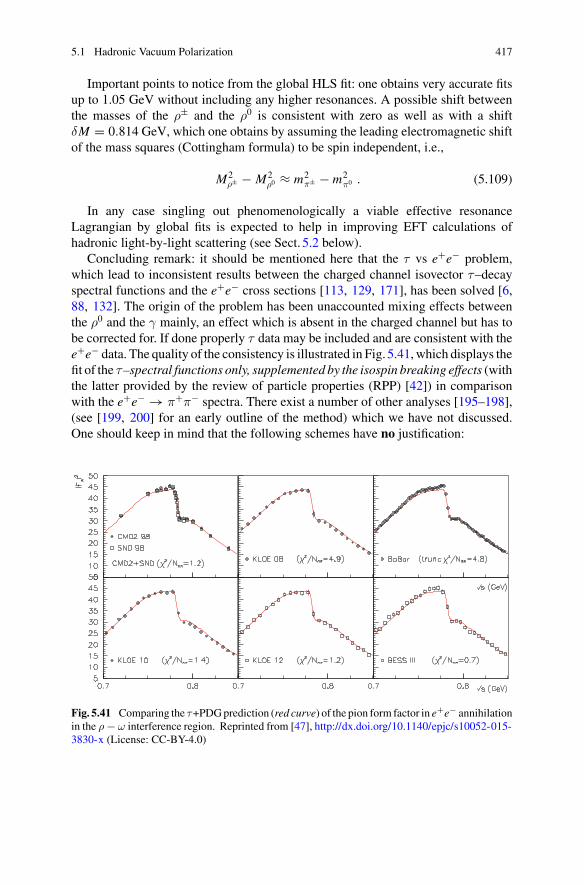
5.1 Hadronic Vacuum Polarization 417

Important points to notice from the global HLS fit: one obtains very accurate fitsup to 1.05 GeV without including any higher resonances. A possible shift betweenthe masses of the ρ± and the ρ0 is consistent with zero as well as with a shiftδM = 0.814 GeV, which one obtains by assuming the leading electromagnetic shiftof the mass squares (Cottingham formula) to be spin independent, i.e.,

M2ρ± − M2

ρ0 ≈ m2π± − m2

π0 . (5.109)

In any case singling out phenomenologically a viable effective resonanceLagrangian by global fits is expected to help in improving EFT calculations ofhadronic light-by-light scattering (see Sect. 5.2 below).

Concluding remark: it should be mentioned here that the τ vs e+e− problem,which lead to inconsistent results between the charged channel isovector τ–decayspectral functions and the e+e− cross sections [113, 129, 171], has been solved [6,88, 132]. The origin of the problem has been unaccounted mixing effects betweenthe ρ0 and the γ mainly, an effect which is absent in the charged channel but has tobe corrected for. If done properly τ data may be included and are consistent with thee+e− data. The quality of the consistency is illustrated in Fig. 5.41, which displays thefit of the τ–spectral functions only, supplemented by the isospin breaking effects (withthe latter provided by the review of particle properties (RPP) [42]) in comparisonwith the e+e− → π+π− spectra. There exist a number of other analyses [195–198],(see [199, 200] for an early outline of the method) which we have not discussed.One should keep in mind that the following schemes have no justification:

Fig. 5.41 Comparing the τ+PDGprediction (red curve) of the pion form factor in e+e− annihilationin the ρ − ω interference region. Reprinted from [47], http://dx.doi.org/10.1140/epjc/s10052-015-3830-x (License: CC-BY-4.0)

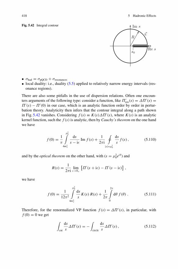
418 5 Hadronic Effects

Fig. 5.42 Integral contour Im s

Re s

CR

|s0

• σhad = σpQCD + σresonances

• local duality: i.e., duality (5.5) applied to relatively narrow energy intervals (res-onance regions).

There are also some pitfalls in the use of dispersion relations. Often one encoun-ters arguments of the following type: consider a function, like Π ′

ren(s) = ΔΠ ′(s) =Π ′(s) − Π ′(0) in our case, which is an analytic function order by order in pertur-bation theory. Analyticity then infers that the contour integral along a path shownin Fig. 5.42 vanishes. Considering f (s) ≡ K (s)ΔΠ ′(s), where K (s) is an analytickernel function, such the f (s) is analytic, then by Cauchy’s theorem on the one handwe have

f (0) = 1

π

μ20∫

4m2π

ds

s − iεIm f (s) + 1

2πi

∮

|s|=μ20

ds

sf (s) , (5.110)

and by the optical theorem on the other hand, with (s = μ20e

iθ) and

R(s) = 1

2πilim

ε→0+

[Π ′(s + iε) − Π ′(s − iε)

],

we have

f (0) = 1

12π2

μ20∫

4m2π

ds

sK (s) R(s) + 1

2π

2π∫

0

dθ f (θ) . (5.111)

Therefore, for the renormalized VP function f (s) = ΔΠ ′(s), in particular, withf (0) = 0 we get

∫

cut

ds

sΔΠ ′(s) = −

∫

circle

ds

sΔΠ ′(s) , (5.112)

5.1 Hadronic Vacuum Polarization 419

and for a large enough circle one is tempted to apply pQCD on the right hand side andthus obtain the integral of our interest, which exhibits the non-perturbative physics.What is usually forgotten is that the uncertainty is of the order of δ = 2πRε with εbeing the small error expected from the truncation of the perturbative series. δ easilycan turn out to be large (due to R large) such that we are not able to make a safeestimate for thewanted integral. Since analyticity is true order byorder in perturbationtheory, we precisely reproduce the perturbative answer for the left hand side if weuse perturbation theory on the right hand side. Taking into accountΠ ′NP

γ (s) in (5.22),known as an asymptotic OPE only, based on not too well constrained condensatesdoes not make the estimate much more reliable (see Sect. 5.1.6). Also, it is nottrue that from the asymptotic expansion of a function one can get back the originalfunction via this approach. While analyticity is a very powerful theoretical conceptit is difficult to be applied in numerical problems, because, small perturbations inone place typically cause large variations at remoter locations. In any case, non-perturbative physics cannot be accessed in this way in terms of the perturbative QCDexpansion.

In this context, exploiting analyticity, other tricks have been advocated in [196]:splitting off the most problematic low energy part of the dispersion integral (theremainder estimated by standard means)

ahad,LOμ (s1) =∫ s1

0K (s)R(s) ds , (5.113)

and noting (see Sect. 3.7) that R(s) = 12π Im Π ′γ(s) and 2 i Im Π(s) = Π(s + iε) −

Π(s − iε) on the cut yields Π(s) away from the cut. By Cauchy’s theorem

∫ s1

0p(s)R(s) ds − 6πi

∮

|s|=s1

p(s)Π ′γ(s) ds = 0 , (5.114)

where p(s) is an arbitrary analytic function. Therefore,

ahad,LOμ (s1) =∫ s1

0

[K (s) − p(s)

]R(s) ds + 6πi

∮

|s|=s1

p(s)Π ′γ(s) ds . (5.115)

We know that in the region between 1 and 2 GeV R(s) extracted from the availablee+e− data still carries large uncertainties, which limits an accurate evaluation of(5.113). Reference [196] advocates to fix p(s) such that the contribution from thisregion gets minimized by minimizing

Max

∣∣∣∣∣K (s) − p(s)

K (s)

∣∣∣∣∣ ,√s ∈ I ≡ [1GeV, 1.8GeV] (5.116)

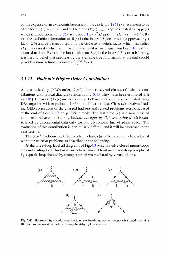
420 5 Hadronic Effects

on the expense of an extra contribution from the circle. In [196] p(s) is chosen to beof the form p(s) = a + b s and on the circle Π ′

γ(s)||s|=s1 is approximated byΠOPE(s)which is proportional to (5.22) (see Sect. 5.1.6): e2 ΠOPE(s) = Π ′NP

γ (s = −Q2). Bythis the available information on R(s) in the interval I gets erased (suppressed by afactor 2.5) and gets transported onto the circle as a weight factor which multipliesΠOPE, a quantity which is not well determined as we learn from Fig. 5.18 and thediscussion there. Even so the information on R(s) in the interval I is unsatisfactory,it is hard to belief that suppressing the available true information at the end shouldprovide a more reliable estimate of ahad,LOμ (s1).

5.1.12 Hadronic Higher Order Contributions

At next-to-leading (NLO) order, O(α3), there are several classes of hadronic con-tributions with typical diagrams shown in Fig. 5.43. They have been estimated firstin [105]. Classes (a) to (c) involve leading HVP insertions and may be treated usingDRs together with experimental e+e−–annihilation data. Class (d) involves lead-ing QED corrections of the charged hadrons and related problems were discussedat the end of Sect. 5.1.7 on p. 379, already. The last class (e) is a new class ofnon–perturbative contributions, the hadronic light–by–light scatteringwhich is con-strained by experimental data only for one exceptional line of phase space. Theevaluation of this contribution is particularly difficult and it will be discussed in thenext section.

The O(α3) hadronic contributions from classes (a), (b) and (c) may be evaluatedwithout particular problems as described in the following.

At the three–loop level all diagrams of Fig. 4.3 which involve closed muon–loopsare contributing to the hadronic corrections when at least one muon–loop is replacedby a quark–loop dressed by strong interactions mediated by virtual gluons.

(a) (b) (c)

(d) (e)

Fig. 5.43 Hadronic higher order contributions: a–c involving LO vacuum polarization, d involvingHO vacuum polarization and e involving light-by-light scattering

5.1 Hadronic Vacuum Polarization 421

Class (a) consists of a subset of 12 diagrams of Fig. 4.3: diagrams (7)–(18) plus 2diagrams obtained from diagram (22) by replacing one muon–loop by a hadronic“bubble”, and yields a contribution of the type

a(6) had[(a)]μ =

(α

π

)3 23

∞∫

4m2π

ds

sR(s) K [(a)] (s/m2

μ

), (5.117)

where K [(a)](s/m2μ) is a QED function which was obtained analytically by Barbieri

and Remiddi [201]. The kernel function is the contribution to aμ of the 14 two–loopdiagrams obtained from diagrams (1)–(7) of Fig. 4.2 by replacing one of the twophotons by a “heavy photon” of mass

√s. The convolution (5.117) then provides

the insertion of a photon self–energy part into the photon line represented by the“heavy photon” according to the method outlined in Sect. 3.8. Explicitly, the kernelis given by

K [(a)](b) = −139

144+ 115

72b +

(19

12− 7

36b + 23

144b2 + 1

b − 4

)ln b

+(

−4

3+ 127

36b − 115

72b2 + 23

144b3)

ln y√b(b − 4)

+(9

4+ 5

24b − 1

2b2 − 2

b

)ζ(2) + 5

96b2 ln2 b

+(

−1

2b + 17

24b2 − 7

48b3)

ln y√b(b − 4)

ln b

+(19

24+ 53

48b − 29

96b2 − 1

3b+ 2

b − 4

)ln2 y

+(

−2 b + 17

6b2 − 7

12b3)

Dp(b)√b(b − 4)

+(13

3− 7

6b + 1

4b2 − 1

6b3 − 4

b − 4

)Dm(b)√b(b − 4)

+(1

2− 7

6b + 1

2b2)

T (b) , (5.118)

where

y =√b − √

b − 4√b + √

b − 4,

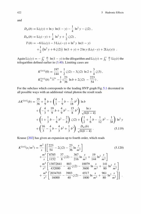
422 5 Hadronic Effects

and

Dp(b) = Li2(y) + ln y ln(1 − y) − 1

4ln2 y − ζ(2) ,

Dm(b) = Li2(−y) + 1

4ln2 y + 1

2ζ(2) ,

T (b) = −6 Li3(y) − 3 Li3(−y) + ln2 y ln(1 − y)

+1

2

(ln2 y + 6 ζ(2)

)ln(1 + y) + 2 ln y (Li2(−y) + 2Li2(y)) .

Again Li2(y) = − ∫ y0

dtt ln(1 − y) is the dilogarithm and Li3(y) = ∫ y

0dtt Li2(t) the

trilogarithm defined earlier in (3.40). Limiting cases are

K [(a)](0) = 197

144+ 1

2ζ(2) − 3ζ(2) ln 2 + 3

4ζ(3) ,

K [(a)]∞ (b)

b→∞= −1

b(23

36ln b + 2ζ(2) − 223

54) .

For the subclass which corresponds to the leading HVP graph Fig. 5.1 decorated inall possible ways with an additional virtual photon the result reads

ΔK [(a)](b) = 35

36+ 8

9b +

(4

3− 1

9b − 5

18b2)

ln b

+(

−4

3+ 19

9b + 4

9b2 − 15

8b3)

ln y√b(b − 4)

+(1 + 1

3b − 1

6b2 − 2

b

)ζ(2) +

(1

2+ 1

6b − 1

12b2 − 1

3b

)ln2 y

+(16

3− 4

3b − 4

3b2 + 1

3b3)

Dm(b)√b(b − 4)

. (5.119)

Krause [202] has given an expansion up to fourth order, which reads

K [(a)](s/m2) = m2

s

{[223

54− 2ζ(2) − 23

36ln

s

m2

](5.120)

+m2

s

[8785

1152− 37

8ζ(2) − 367

216ln

s

m2+ 19

144ln2

s

m2

]

+m4

s2

[13072841

432000− 883

40ζ(2) − 10079

3600ln

s

m2+ 141

80ln2

s

m2

]

+ m6

s3

[2034703

16000− 3903

40ζ(2) − 6517

1800ln

s

m2+ 961

80ln2

s

m2

]}.

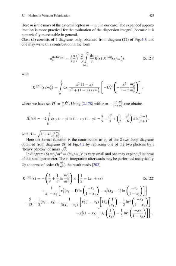
5.1 Hadronic Vacuum Polarization 423

Herem is the mass of the external leptonm = mμ in our case. The expanded approx-imation is more practical for the evaluation of the dispersion integral, because it isnumerically more stable in general.Class (b) consists of 2 diagrams only, obtained from diagram (22) of Fig. 4.3, andone may write this contribution in the form

a(6) had[(b)]μ =

(α

π

)3 23

∞∫

4m2π

ds

sR(s) K [(b)](s/m2

μ) , (5.121)

with

K [(b)](s/m2μ) =

1∫

0

dxx2 (1 − x)

x2 + (1 − x) s/m2μ

[−Π

′ eγ

(− x2

1 − x

m2μ

m2e

)],

where we have set Π′ = α

πΠ

′. Using (2.178) with z = − x2

1−xm2

μ

m2eone obtains

Π′ eγ (z) = − 2

1∫

0

dy y (1 − y) ln (1 − z y (1 − y)) = 8

9− β2

3+

(1

2− β2

6

)β ln

β − 1

β + 1,

with β =√1 + 41−x

x2m2

em2

μ.

Here the kernel function is the contribution to aμ of the 2 two–loop diagramsobtained from diagrams (8) of Fig. 4.2 by replacing one of the two photons by a“heavy photon” of mass

√s.

In diagram (b)m2f /m

2 = (me/mμ)2 is very small and one may expand β in terms

of this small parameter. The x–integration afterwards may be performed analytically.

Up to terms of order O(m2

f

m2 ) the result reads [202]

K [(b)](s) = −(5

9+ 1

3ln

m2f

m2

)×

{1

2− (x1 + x2) (5.122)

+ 1

x1 − x2

[x21 (x1 − 1) ln

( −x11 − x1

)− x22 (x2 − 1) ln

( −x21 − x2

)]}

− 5

12+ 1

3(x1 + x2) + 1

3(x1 − x2)

{x21 (1 − x1)

[Li2

(1

x1

)− 1

2ln2

( −x11 − x1

)]

−x22 (1 − x2)

[Li2

(1

x2

)− 1

2ln2

( −x21 − x2

)]},

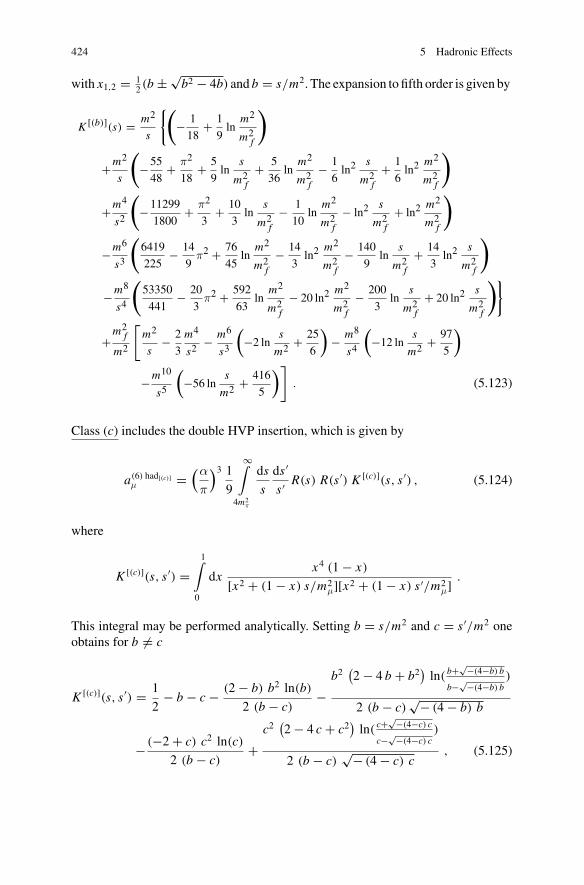
424 5 Hadronic Effects

with x1,2 = 12 (b ± √

b2 − 4b) and b = s/m2. The expansion to fifth order is given by

K [(b)](s) = m2

s

{(− 1

18+ 1

9ln

m2

m2f

)

+m2

s

(−55

48+ π2

18+ 5

9ln

s

m2f

+ 5

36ln

m2

m2f

− 1

6ln2

s

m2f

+ 1

6ln2

m2

m2f

)

+m4

s2

(−11299

1800+ π2

3+ 10

3ln

s

m2f

− 1

10ln

m2

m2f

− ln2s

m2f

+ ln2m2

m2f

)

−m6

s3

(6419

225− 14

9π2 + 76

45ln

m2

m2f

− 14

3ln2

m2

m2f

− 140

9ln

s

m2f

+ 14

3ln2

s

m2f

)

−m8

s4

(53350

441− 20

3π2 + 592

63ln

m2

m2f

− 20 ln2m2

m2f

− 200

3ln

s

m2f

+ 20 ln2s

m2f

)}

+m2

f

m2

[m2

s− 2

3

m4

s2− m6

s3

(−2 ln

s

m2 + 25

6

)− m8

s4

(−12 ln

s

m2 + 97

5

)

−m10

s5

(−56 ln

s

m2 + 416

5

)]. (5.123)

Class (c) includes the double HVP insertion, which is given by

a(6) had[(c)]μ =

(α

π

)3 19

∞∫

4m2π

ds

s

ds ′

s ′ R(s) R(s ′) K [(c)](s, s ′) , (5.124)

where

K [(c)](s, s ′) =1∫

0

dxx4 (1 − x)

[x2 + (1 − x) s/m2μ][x2 + (1 − x) s ′/m2

μ].

This integral may be performed analytically. Setting b = s/m2 and c = s ′/m2 oneobtains for b = c

K [(c)](s, s ′) = 1

2− b − c − (2 − b) b2 ln(b)

2 (b − c)−

b2(2 − 4 b + b2

)ln( b+

√−(4−b) b

b−√−(4−b) b)

2 (b − c)√− (4 − b) b

− (−2 + c) c2 ln(c)

2 (b − c)+

c2(2 − 4 c + c2

)ln( c+

√−(4−c) c

c−√−(4−c) c)

2 (b − c)√− (4 − c) c

, (5.125)

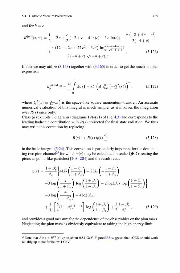
5.1 Hadronic Vacuum Polarization 425

and for b = c

K [(c)](s, s ′) = 1

2− 2 c + c

2(−2 + c − 4 ln(c) + 3 c ln(c)) + c

(−2 + 4 c − c2)

2(−4 + c)

+c(12 − 42 c + 22 c2 − 3 c3

)ln( c+

√(−4+c) c

c−√(−4+c) c

)

2 (−4 + c)√

(−4 + c) c. (5.126)

In fact we may utilize (3.153) together with (3.165) in order to get the much simplerexpression

a(6) had[(c)]μ = α

π

1∫

0

dx (1 − x)(Δα(5)

had

(−Q2(x)))2

, (5.127)

where Q2(x) ≡ x2

1−x m2μ is the space–like square momentum–transfer. An accurate

numerical evaluation of this integral is much simpler as it involves the integrationover R(s) once only.Class (d) exhibits 3 diagrams (diagrams 19)–(21) of Fig. 4.3) and corresponds to theleading hadronic contribution with R(s) corrected for final state radiation. We thusmay write this correction by replacing

R(s) → R(s) η(s)α

π(5.128)

in the basic integral (5.24). This correction is particularly important for the dominat-ing two pion channel25 for which η(s) may be calculated in scalar QED (treating thepions as point–like particles) [203, 204] and the result reads

η(s) = 1 + β2π

βπ

{4Li2

(1 − βπ

1 + βπ

)+ 2Li2

(−1 − βπ

1 + βπ

)

−3 log

(2

1 + βπ

)log

(1 + βπ

1 − βπ

)− 2 log(βπ) log

(1 + βπ

1 − βπ

)}

−3 log

(4

1 − β2π

)− 4 log(βπ)

+ 1

β3π

[5

4(1 + β2

π)2 − 2

]log

(1 + βπ

1 − βπ

)+ 3

2

1 + β2π

β2π

, (5.129)

and provides a goodmeasure for the dependence of the observables on the pionmass.Neglecting the pion mass is obviously equivalent to taking the high energy limit

25Note that R(s) ≈ Rππ(s) up to about 0.81 GeV. Figure5.38 suggests that sQED should workreliably up to not far below 1 GeV.

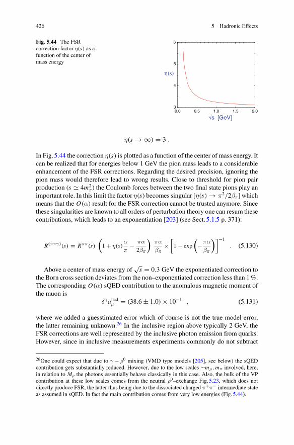
426 5 Hadronic Effects

Fig. 5.44 The FSRcorrection factor η(s) as afunction of the center ofmass energy

0.0 0.5 1.0 1.5 2.0

√s [GeV]

3

4

5

6

η(s)

η(s → ∞) = 3 .

In Fig. 5.44 the correction η(s) is plotted as a function of the center of mass energy. Itcan be realized that for energies below 1 GeV the pion mass leads to a considerableenhancement of the FSR corrections. Regarding the desired precision, ignoring thepion mass would therefore lead to wrong results. Close to threshold for pion pairproduction (s � 4m2

π) the Coulomb forces between the two final state pions play animportant role. In this limit the factor η(s) becomes singular [η(s) → π2/2βπ] whichmeans that the O(α) result for the FSR correction cannot be trusted anymore. Sincethese singularities are known to all orders of perturbation theory one can resum thesecontributions, which leads to an exponentiation [203] (see Sect. 5.1.5 p. 371):

R(ππγ)(s) = Rππ(s)

(1 + η(s)

α

π− πα

2βπ

)πα

βπ×

[1 − exp

(−πα

βπ

)]−1. (5.130)

Above a center of mass energy of√s = 0.3 GeV the exponentiated correction to

the Born cross section deviates from the non–exponentiated correction less than 1%.The corresponding O(α) sQED contribution to the anomalous magnetic moment ofthe muon is

δγahadμ = (38.6 ± 1.0) × 10−11 , (5.131)

where we added a guesstimated error which of course is not the true model error,the latter remaining unknown.26 In the inclusive region above typically 2 GeV, theFSR corrections are well represented by the inclusive photon emission from quarks.However, since in inclusive measurements experiments commonly do not subtract

26One could expect that due to γ − ρ0 mixing (VMD type models [205], see below) the sQEDcontribution gets substantially reduced. However, due to the low scales ∼mμ,mπ involved, here,in relation to Mρ the photons essentially behave classically in this case. Also, the bulk of the VPcontribution at these low scales comes from the neutral ρ0–exchange Fig. 5.23, which does notdirectly produce FSR, the latter thus being due to the dissociated charged π+π− intermediate stateas assumed in sQED. In fact the main contribution comes from very low energies (Fig. 5.44).

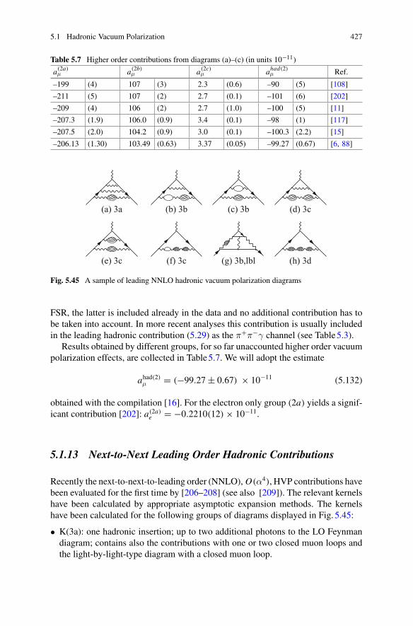
5.1 Hadronic Vacuum Polarization 427

Table 5.7 Higher order contributions from diagrams (a)–(c) (in units 10−11)

a(2a)μ a(2b)

μ a(2c)μ ahad(2)

μ Ref.

–199 (4) 107 (3) 2.3 (0.6) –90 (5) [108]

–211 (5) 107 (2) 2.7 (0.1) –101 (6) [202]

–209 (4) 106 (2) 2.7 (1.0) –100 (5) [11]

–207.3 (1.9) 106.0 (0.9) 3.4 (0.1) –98 (1) [117]

–207.5 (2.0) 104.2 (0.9) 3.0 (0.1) –100.3 (2.2) [15]

–206.13 (1.30) 103.49 (0.63) 3.37 (0.05) –99.27 (0.67) [6, 88]

(a) 3a (b) 3b (c) 3b (d) 3c

(e) 3c (f) 3c (g) 3b,lbl (h) 3d

Fig. 5.45 A sample of leading NNLO hadronic vacuum polarization diagrams

FSR, the latter is included already in the data and no additional contribution has tobe taken into account. In more recent analyses this contribution is usually includedin the leading hadronic contribution (5.29) as the π+π−γ channel (see Table5.3).

Results obtained by different groups, for so far unaccounted higher order vacuumpolarization effects, are collected in Table5.7. We will adopt the estimate

ahad(2)μ = (−99.27 ± 0.67) × 10−11 (5.132)

obtained with the compilation [16]. For the electron only group (2a) yields a signif-icant contribution [202]: a(2a)

e = −0.2210(12) × 10−11.

5.1.13 Next-to-Next Leading Order Hadronic Contributions

Recently the next-to-next-to-leading order (NNLO), O(α4), HVP contributions havebeen evaluated for the first time by [206–208] (see also [209]). The relevant kernelshave been calculated by appropriate asymptotic expansion methods. The kernelshave been calculated for the following groups of diagrams displayed in Fig. 5.45:

• K(3a): one hadronic insertion; up to two additional photons to the LO Feynmandiagram; contains also the contributions with one or two closed muon loops andthe light-by-light-type diagram with a closed muon loop.

428 5 Hadronic Effects

Table 5.8 NNLO contributions diagrams (a)–(h) (in units 10−11)

a(3a)μ a(3b)

μ a(3b,lbl)μ a(3c)

μ a(3d)μ ahad(3)μ Ref.

8.0 −4.1 9.1 −0.6 0.005 12.4 (1) [206]

7.834 (61) −4.033 (28) 9.005 (63) −0.569 (5) 0.00518 (12) 12.24 (10) [6]

• K(3b): one hadronic insertion and one or two closed electron loops and additionalphotonic corrections; the external photon couples to the muon.

• K(3b, lbl): light-by-light-type contribution with closed electron loop and onehadronic insertion; the external photon couples to the electron.

• K(3c): two hadronic insertions and additional photonic corrections and/or closedelectron or muon loops.

• K(3d): three hadronic insertions.

Class (3d) includes the leading triple HVP insertion, which is given by

a(8) had[(3d)]μ =

(α

π

)4 1

27

∞∫

m2π

ds

s

ds ′

s ′ds ′′

s ′′ R(s) R(s ′) R(s ′′) K [(3d)](s, s ′, s ′′) , (5.133)

where

K [(3d)](s, s′, s′′) =1∫

0

dxx6 (1 − x)

[x2 + (1 − x) s/m2μ][x2 + (1 − x) s′/m2

μ][x2 + (1 − x) s′′/m2μ] .

Againwemay utilize (3.153) and (3.165) in order to get themuch simpler expression

a(8) had[(3d)]μ = α

π

1∫

0

dx (1 − x)(Δα(5)

had

(−Q2(x)))3

, (5.134)

where Q2(x) ≡ x2

1−x m2μ is the space–like square momentum–transfer. An accurate

numerical evaluation of this integral is much simpler as it involves the integrationover R(s) once only, which also allows for a standard error estimate.

Table5.8 lists the different NNLO contributions obtained by Kurz et al. [206]together with my own evaluations based on my compilation of data discussed aboveevaluated with kernels from [206].

For the electron only group (3a) yields a significant contribution [206]: a(3a)e =

0.0279(2) × 10−12.

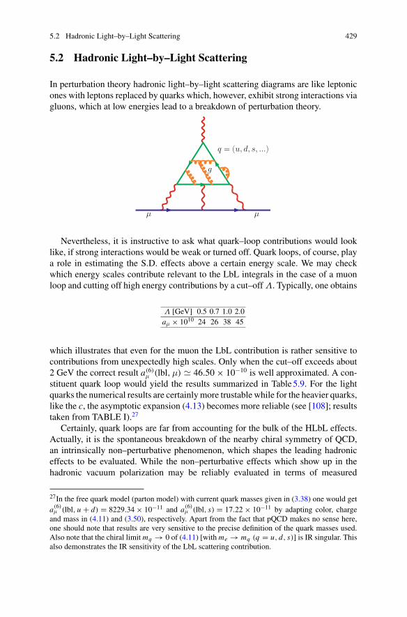
5.2 Hadronic Light–by–Light Scattering 429

5.2 Hadronic Light–by–Light Scattering

In perturbation theory hadronic light–by–light scattering diagrams are like leptonicones with leptons replaced by quarks which, however, exhibit strong interactions viagluons, which at low energies lead to a breakdown of perturbation theory.

Nevertheless, it is instructive to ask what quark–loop contributions would looklike, if strong interactions would be weak or turned off. Quark loops, of course, playa role in estimating the S.D. effects above a certain energy scale. We may checkwhich energy scales contribute relevant to the LbL integrals in the case of a muonloop and cutting off high energy contributions by a cut–off Λ. Typically, one obtains

Λ [GeV] 0.5 0.7 1.0 2.0aμ × 1010 24 26 38 45

which illustrates that even for the muon the LbL contribution is rather sensitive tocontributions from unexpectedly high scales. Only when the cut–off exceeds about2 GeV the correct result a(6)

μ (lbl,μ) � 46.50 × 10−10 is well approximated. A con-stituent quark loop would yield the results summarized in Table5.9. For the lightquarks the numerical results are certainlymore trustable while for the heavier quarks,like the c, the asymptotic expansion (4.13) becomes more reliable (see [108]; resultstaken from TABLE I).27

Certainly, quark loops are far from accounting for the bulk of the HLbL effects.Actually, it is the spontaneous breakdown of the nearby chiral symmetry of QCD,an intrinsically non–perturbative phenomenon, which shapes the leading hadroniceffects to be evaluated. While the non–perturbative effects which show up in thehadronic vacuum polarization may be reliably evaluated in terms of measured

27In the free quark model (parton model) with current quark masses given in (3.38) one would geta(6)μ (lbl, u + d) = 8229.34 × 10−11 and a(6)

μ (lbl, s) = 17.22 × 10−11 by adapting color, chargeand mass in (4.11) and (3.50), respectively. Apart from the fact that pQCD makes no sense here,one should note that results are very sensitive to the precise definition of the quark masses used.Also note that the chiral limit mq → 0 of (4.11) [with me → mq (q = u, d, s)] is IR singular. Thisalso demonstrates the IR sensitivity of the LbL scattering contribution.

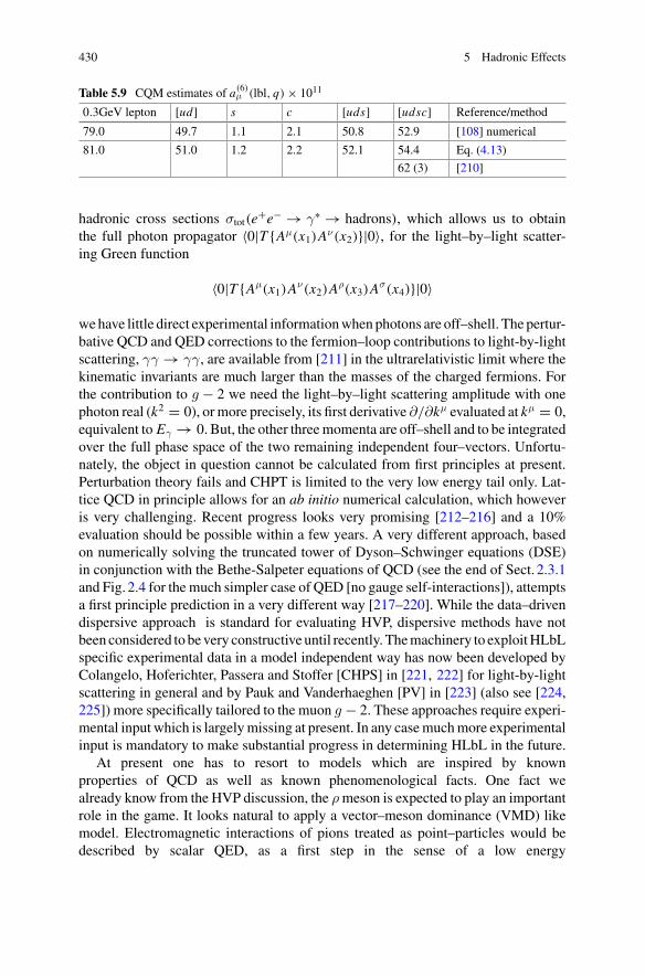
430 5 Hadronic Effects

Table 5.9 CQM estimates of a(6)μ (lbl, q) × 1011

0.3GeV lepton [ud] s c [uds] [udsc] Reference/method

79.0 49.7 1.1 2.1 50.8 52.9 [108] numerical

81.0 51.0 1.2 2.2 52.1 54.4 Eq. (4.13)

62 (3) [210]

hadronic cross sections σtot(e+e− → γ∗ → hadrons), which allows us to obtainthe full photon propagator 〈0|T {Aμ(x1)Aν(x2)}|0〉, for the light–by–light scatter-ing Green function

〈0|T {Aμ(x1)Aν(x2)A

ρ(x3)Aσ(x4)}|0〉

wehave little direct experimental informationwhenphotons are off–shell. The pertur-bative QCD and QED corrections to the fermion–loop contributions to light-by-lightscattering, γγ → γγ, are available from [211] in the ultrarelativistic limit where thekinematic invariants are much larger than the masses of the charged fermions. Forthe contribution to g − 2 we need the light–by–light scattering amplitude with onephoton real (k2 = 0), ormore precisely, its first derivative ∂/∂kμ evaluated at kμ = 0,equivalent to Eγ → 0. But, the other threemomenta are off–shell and to be integratedover the full phase space of the two remaining independent four–vectors. Unfortu-nately, the object in question cannot be calculated from first principles at present.Perturbation theory fails and CHPT is limited to the very low energy tail only. Lat-tice QCD in principle allows for an ab initio numerical calculation, which howeveris very challenging. Recent progress looks very promising [212–216] and a 10%evaluation should be possible within a few years. A very different approach, basedon numerically solving the truncated tower of Dyson–Schwinger equations (DSE)in conjunction with the Bethe-Salpeter equations of QCD (see the end of Sect. 2.3.1and Fig. 2.4 for the much simpler case of QED [no gauge self-interactions]), attemptsa first principle prediction in a very different way [217–220]. While the data–drivendispersive approach is standard for evaluating HVP, dispersive methods have notbeen considered to be very constructive until recently. Themachinery to exploitHLbLspecific experimental data in a model independent way has now been developed byColangelo, Hoferichter, Passera and Stoffer [CHPS] in [221, 222] for light-by-lightscattering in general and by Pauk and Vanderhaeghen [PV] in [223] (also see [224,225]) more specifically tailored to the muon g − 2. These approaches require experi-mental input which is largelymissing at present. In any casemuchmore experimentalinput is mandatory to make substantial progress in determining HLbL in the future.

At present one has to resort to models which are inspired by knownproperties of QCD as well as known phenomenological facts. One fact wealready know from the HVP discussion, the ρmeson is expected to play an importantrole in the game. It looks natural to apply a vector–meson dominance (VMD) likemodel. Electromagnetic interactions of pions treated as point–particles would bedescribed by scalar QED, as a first step in the sense of a low energy

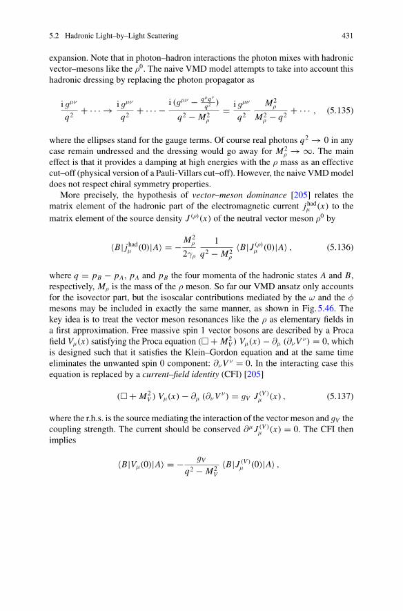
5.2 Hadronic Light–by–Light Scattering 431

expansion. Note that in photon–hadron interactions the photon mixes with hadronicvector–mesons like the ρ0. The naive VMD model attempts to take into account thishadronic dressing by replacing the photon propagator as

i gμν

q2+ · · · → i gμν

q2+ · · · − i (gμν − qμqν

q2 )

q2 − M2ρ

= i gμν

q2

M2ρ

M2ρ − q2

+ · · · , (5.135)

where the ellipses stand for the gauge terms. Of course real photons q2 → 0 in anycase remain undressed and the dressing would go away for M2

ρ → ∞. The maineffect is that it provides a damping at high energies with the ρ mass as an effectivecut–off (physical version of a Pauli-Villars cut–off). However, the naive VMDmodeldoes not respect chiral symmetry properties.

More precisely, the hypothesis of vector–meson dominance [205] relates thematrix element of the hadronic part of the electromagnetic current jhadμ (x) to thematrix element of the source density J (ρ)(x) of the neutral vector meson ρ0 by

〈B| jhadμ (0)|A〉 = −M2ρ

2γρ

1

q2 − M2ρ

〈B|J (ρ)μ (0)|A〉 , (5.136)

where q = pB − pA, pA and pB the four momenta of the hadronic states A and B,respectively, Mρ is the mass of the ρ meson. So far our VMD ansatz only accountsfor the isovector part, but the isoscalar contributions mediated by the ω and the φmesons may be included in exactly the same manner, as shown in Fig. 5.46. Thekey idea is to treat the vector meson resonances like the ρ as elementary fields ina first approximation. Free massive spin 1 vector bosons are described by a Procafield Vμ(x) satisfying the Proca equation (� + M2

V ) Vμ(x) − ∂μ (∂νV ν) = 0, whichis designed such that it satisfies the Klein–Gordon equation and at the same timeeliminates the unwanted spin 0 component: ∂νV ν = 0. In the interacting case thisequation is replaced by a current–field identity (CFI) [205]

(� + M2V ) Vμ(x) − ∂μ (∂νV

ν) = gV J (V )μ (x) , (5.137)

where the r.h.s. is the source mediating the interaction of the vector meson and gV thecoupling strength. The current should be conserved ∂μ J (V )

μ (x) = 0. The CFI thenimplies

〈B|Vμ(0)|A〉 = − gV

q2 − M2V

〈B|J (V )μ (0)|A〉 ,

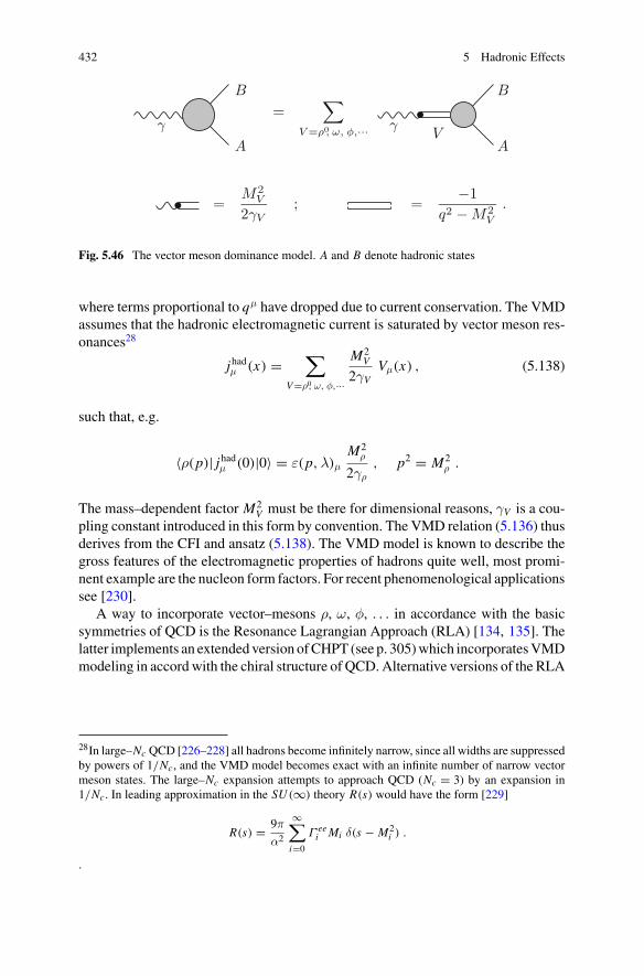
432 5 Hadronic Effects

=∑

V =ρ0, ω, φ,···

B

A

B

AV

γγ

=M2

V

2γV; =

−1q2 − M2

V

.

Fig. 5.46 The vector meson dominance model. A and B denote hadronic states

where terms proportional to qμ have dropped due to current conservation. The VMDassumes that the hadronic electromagnetic current is saturated by vector meson res-onances28

jhadμ (x) =∑

V=ρ0, ω, φ,···

M2V

2γVVμ(x) , (5.138)

such that, e.g.

〈ρ(p)| jhadμ (0)|0〉 = ε(p,λ)μM2

ρ

2γρ, p2 = M2

ρ .

The mass–dependent factor M2V must be there for dimensional reasons, γV is a cou-

pling constant introduced in this form by convention. The VMD relation (5.136) thusderives from the CFI and ansatz (5.138). The VMD model is known to describe thegross features of the electromagnetic properties of hadrons quite well, most promi-nent example are the nucleon form factors. For recent phenomenological applicationssee [230].

A way to incorporate vector–mesons ρ, ω, φ, . . . in accordance with the basicsymmetries of QCD is the Resonance Lagrangian Approach (RLA) [134, 135]. Thelatter implements an extended version ofCHPT (see p. 305)which incorporatesVMDmodeling in accordwith the chiral structure of QCD.Alternative versions of the RLA

28In large–Nc QCD [226–228] all hadrons become infinitely narrow, since all widths are suppressedby powers of 1/Nc, and the VMD model becomes exact with an infinite number of narrow vectormeson states. The large–Nc expansion attempts to approach QCD (Nc = 3) by an expansion in1/Nc. In leading approximation in the SU (∞) theory R(s) would have the form [229]

R(s) = 9π

α2

∞∑

i=0

Γ eei Mi δ(s − M2

i ) .

.

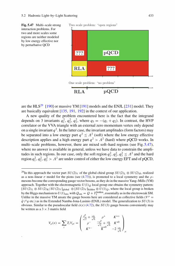
5.2 Hadronic Light–by–Light Scattering 433

Fig. 5.47 Multi–scale stronginteraction problems. Fortwo and more scales someregions are neither modeledby low energy effective norby perturbative QCD

Two scale problem: “open regions”

RLA

???

???

pQCD

One scale problem: “no problem”

RLA pQCD

are the HLS29 [190] or massive YM [191] models and the ENJL [231] model. Theyare basically equivalent [135, 191, 192] in the context of our application.

A new quality of the problem encountered here is the fact that the integranddepends on 3 invariants q2

1 , q22 , q

23 , where q3 = −(q1 + q2). In contrast, the HVP

correlator or the VVA triangle with an external zero momentum vertex only dependon a single invariant q2. In the latter case, the invariant amplitudes (form factors) maybe separated into a low energy part q2 ≤ Λ2 (soft) where the low energy effectivedescription applies and a high energy part q2 > Λ2 (hard) where pQCD works. Inmulti–scale problems, however, there are mixed soft–hard regions (see Fig. 5.47),where no answer is available in general, unless we have data to constrain the ampli-tudes in such regions. In our case, only the soft region q2

1 , q22 , q

23 ≤ Λ2 and the hard

region q21 , q

22 , q

23 > Λ2 are under control of either the low energy EFT and of pQCD,

29In this approach the vector part SU (2)V of the global chiral group SU (2)L ⊗ SU (2)R , realizedas a non–linear σ model for the pions (see (4.73)), is promoted to a local symmetry and the ρ–mesons become the corresponding gauge vector bosons, as they do in themassive Yang–Mills (YM)approach. Together with the electromagneticU (1)Q local group one obtains the symmetry pattern:[SU (2)L ⊗ SU (2)R/SU (2)V ]global ⊗ [SU (2)V ]hidden ⊗U (1)Q , where the local group is brokenby theHiggsmechanism toU (1)em, with Qem = Q + T hidden

3 , essentially as in the electroweak SM.Unlike in the massive YM ansatz the gauge bosons here are considered as collective fields (V μ =qγμq etc.) as in the Extended Nambu-Jona-Lasinio (ENJL) model. The generalization to SU (3) isobvious. Similar to the pseudoscalar field φ(x) (4.72), the SU (3) gauge bosons conveniently maybe written as a 3 × 3 matrix field

Vμ(x) =∑

i

Ti Vμi =

⎛

⎜⎜⎝

ρ0√2

+ ω8√6

ρ+ K ∗+

ρ− −ρ0√2

+ ω8√6

K ∗0

K ∗− K∗0 −2 ω8√

6

⎞

⎟⎟⎠

μ

.

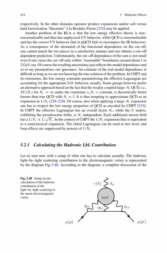
434 5 Hadronic Effects

respectively. In the other domains operator product expansions and/or soft versushard factorization “theorems” à la Brodsky-Farrar [232] may be applied.

Another problem of the RLA is that the low energy effective theory is non–renormalizable and thus has unphysical UV behavior, while QCD is renormalizableand has the correct UV behavior (but in pQCD fails to encompass the IR behavior).As a consequence of the mismatch of the functional dependence on the cut–off,one cannot match the two pieces in a satisfactory manner and one obtains a cut–offdependent prediction. Unfortunately, the cut–off dependence of the sum is not smalleven if one varies the cut–off only within “reasonable” boundaries around about 1 or2GeV, say. Of course the resulting uncertainty just reflects themodel dependence andso to say parametrizes our ignorance. An estimate of the real model dependence isdifficult as long as we are not knowing the true solution of the problem. In CHPT andits extensions, the low energy constants parametrizing the effective Lagrangian areaccounting for the appropriate S.D. behavior, usually. Some groups however preferan alternative approach based on the fact that the weakly coupled large–Nc QCD, i.e.,SU (Nc) for Nc → ∞ under the constraint αs Nc = constant, is theoretically betterknown than true QCD with Nc = 3. It is thus tempting to approximate QCD as anexpansion in 1/Nc [226–228]. Of course, also when applying a large–Nc expansionone has to respect the low energy properties of QCD as encoded by CHPT [233].In CHPT the effective Lagrangian has an overall factor Nc, while the U matrix,exhibiting the pseudoscalar fields, is Nc independent. Each additional meson fieldhas a 1/Fπ ∝ 1/

√Nc. In the context of CHPT the 1/Nc expansion thus is equivalent

to a semiclassical expansion. The chiral Lagrangian can be used at tree level, andloop effects are suppressed by powers of 1/Nc.

5.2.1 Calculating the Hadronic LbL Contribution

Let us start now with a setup of what one has to calculate actually. The hadroniclight–by–light scattering contribution to the electromagnetic vertex is representedby the diagram Fig. 5.48. According to the diagram, a complete discussion of the

Fig. 5.48 Setup for thecalculation of the hadroniccontribution of thelight–by–light scattering tothe muon electromagneticvertex

μ(p)

γ(k) kρ

had

μ(p′)

q1μq2νq3λ

5.2 Hadronic Light–by–Light Scattering 435

hadronic light–by–light contributions involves the full rank–four hadronic vacuumpolarization tensor30

Πμνλρ(q1, q2, q3) =∫

d4x1 d4x2 d

4x3 ei (q1x1+q2x2+q3x3)

×〈 0 | T { jμ(x1) jν(x2) jλ(x3) jρ(0)} | 0 〉 . (5.139)

Momentum k of the external photon is incoming, while the qi ’s of the virtual photonsare outgoing from the hadronic “blob”. Here jμ(x) denotes the light quark part ofthe electromagnetic current

jμ(x) = 2

3(uγμu)(x) − 1

3(dγμd)(x) − 1

3(sγμs)(x) ≡ q Qγμq(x) . (5.140)

It includes a summation over color of the color and flavor diagonal quark bilinears.Since the electromagnetic current jμ(x) is conserved, the tensor Πμνλρ(q1, q2, q3)satisfies the Ward-Takahashi identities

{qμ1 ; qν

2 ; qλ3 ; kρ}Πμνλρ(q1, q2, q3) = 0 , (5.141)

with k = (q1 + q2 + q3). Taking the derivative ∂∂kρ of kρΠμνλρ(q1, q2, k − q1 −

q2) = 0 implies

Πμνλρ(q1, q2, k − q1 − q2) = −kσ(∂/∂kρ) Πμνλσ(q1, q2, k − q1 − q2) , (5.142)

and thus tells us that the object of interest is linear in k when we go to the static limitkμ → 0 in which the anomalous magnetic moment is defined.

Up to one–loop the electromagnetic γ–vertex has been discussed in Sect. 2.6.3,its general structure in Sect. 3.3. Here we adopt the notation of Knecht and Nyf-feler [234] (q → k, p1 → p and p2 → p′). From the diagram we easily read off thecontribution of Πμνλσ(q1, q2, q3) to the electromagnetic vertex which is given by

〈μ−(p ′)|(ie) jρ(0)|μ−(p)〉 = (−ie) u(p ′) Πρ(p′, p) u(p)

=∫

d4q1(2π)4

d4q2(2π)4

(−i)3

q21 q

22 (q1 + q2 − k)2

i

(p ′ − q1)2 − m2

i

(p − q1 − q2)2 − m2

× (−ie)3 u(p ′) γμ( p ′− q1 + m) γν ( p− q1− q2 + m) γλ u(p)

× (ie)4Πμνλρ(q1, q2, k − q1 − q2) , (5.143)

30We remind that the light-by-light scatteringGreen function is overall convergent due to theAbeliangauge symmetry. The latter implies that integrals converge better than they look like by naive powercounting (see the Footnote p. 66).

436 5 Hadronic Effects

with kμ = (p ′ − p)μ. For the contribution to the form factors

u(p ′) Πρ(p′, p) u(p) = u(p ′)

[γρFE(k

2) + iσρτkτ

2mμFM(k2)

]u(p) , (5.144)

Equation (5.142) implies that Πρ(p ′, p) = kσΠρσ(p ′, p) with

u(p ′) Πρσ(p′, p) u(p) = −ie6×

∫d4q1(2π)4

d4q2(2π)4

1

q21 q

22 (q1 + q2 − k)2

1

(p ′ − q1)2 − m2

1

(p − q1 − q2)2 − m2

× u(p ′) γμ ( p ′− q1 + m) γν ( p− q1− q2 + m) γλ u(p)

× ∂

∂kρΠμνλσ(q1, q2, k − q1 − q2) . (5.145)

The WT–identity takes the form kρkσ u(p ′)Πρσ(p ′, p) u(p) = 0, which impliesδlblFE(0) = 0 and, in the terminology introduced at the end of Sect. 3.5, we haveVρ(p) = Πρ(p ′, p)|k=0 = 0 and Tρσ(p) = Πρσ(p ′, p)|k=0. Thus, using the projec-tion technique outlined in Sect. 3.5, the hadronic light–by–light contribution to themuon anomalous magnetic moment is equal to

FM(0) = 1

48mTr

{( p + m)[γρ, γσ]( p + m)Πρσ(p, p)

}. (5.146)

The basic trace of Dirac matrices to be evaluated thus is

Tr{( p + m)[γρ, γσ]( p + m) γμ ( p ′− q1 + m) γν ( p− q1− q2 + m) γλ

}

(5.147)such that finally

FM(0) = −ie6

48m

∫d4q1(2π)4

d4q2(2π)4

1

q21 q22 (q1 + q2)2

1

(p − q1)2 − m21

(p − q1 − q2)2 − m2

× Tr{( p + m)[γρ, γσ]( p + m) γμ ( p− q1 + m) γν ( p− q1− q2 + m) γλ

}

×(

∂

∂kρ Πμνλσ(q1, q2, k − q1 − q2)

)

k=0. (5.148)

This is what we actually need to calculate. The integral to be performed is 8 dimen-sional. Thereof 3 integrations can be done analytically. In general, one has to dealwith a 5 dimensional non–trivial integration over 3 angles and 2 moduli.

As mentioned before, the hadronic tensor Πμνλσ(q1, q2, k − q1 − q2) we have todeal with, is a problematic object, because it has an unexpectedly complex structureas we will see, in no way comparable with the leptonic counterpart. The generalcovariant decomposition involves 138 Lorentz structures [235, 236]:

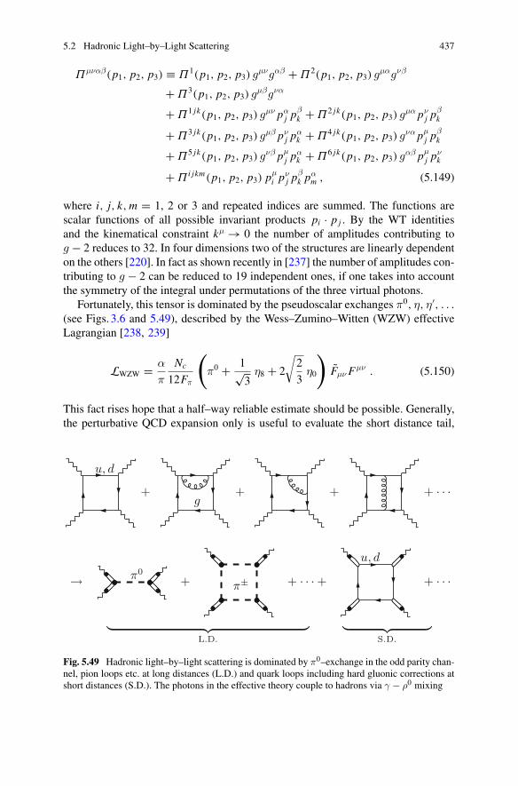
5.2 Hadronic Light–by–Light Scattering 437

Πμναβ(p1, p2, p3) ≡ Π1(p1, p2, p3) gμνgαβ + Π2(p1, p2, p3) gμαgνβ

+ Π3(p1, p2, p3) gμβgνα

+ Π1 jk(p1, p2, p3) gμν pαj p

βk + Π2 jk(p1, p2, p3) gμα pν

j pβk

+ Π3 jk(p1, p2, p3) gμβ pνj p

αk + Π4 jk(p1, p2, p3) gνα pμ

j pβk

+ Π5 jk(p1, p2, p3) gνβ pμj p

αk + Π6 jk(p1, p2, p3) gαβ pμ

j pνk

+ Π i jkm(p1, p2, p3) pμi p

νj p

βk p

αm , (5.149)

where i, j, k,m = 1, 2 or 3 and repeated indices are summed. The functions arescalar functions of all possible invariant products pi · p j . By the WT identitiesand the kinematical constraint kμ → 0 the number of amplitudes contributing tog − 2 reduces to 32. In four dimensions two of the structures are linearly dependenton the others [220]. In fact as shown recently in [237] the number of amplitudes con-tributing to g − 2 can be reduced to 19 independent ones, if one takes into accountthe symmetry of the integral under permutations of the three virtual photons.

Fortunately, this tensor is dominated by the pseudoscalar exchanges π0, η, η′, . . .(see Figs. 3.6 and 5.49), described by the Wess–Zumino–Witten (WZW) effectiveLagrangian [238, 239]

LWZW = α

π

Nc

12Fπ

(π0 + 1√

3η8 + 2

√2

3η0

)FμνF

μν . (5.150)

This fact rises hope that a half–way reliable estimate should be possible. Generally,the perturbative QCD expansion only is useful to evaluate the short distance tail,

+ + + + · · ·

→ + + · · · + + · · ·

L.D. S.D.

π0

π±

u, d

u, d

g

Fig. 5.49 Hadronic light–by–light scattering is dominated by π0–exchange in the odd parity chan-nel, pion loops etc. at long distances (L.D.) and quark loops including hard gluonic corrections atshort distances (S.D.). The photons in the effective theory couple to hadrons via γ − ρ0 mixing

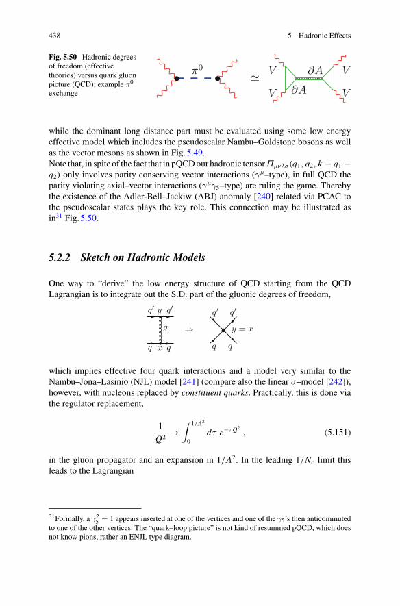
438 5 Hadronic Effects

Fig. 5.50 Hadronic degreesof freedom (effectivetheories) versus quark gluonpicture (QCD); example π0

exchange

�π0 V

V

V

V∂A

∂A

while the dominant long distance part must be evaluated using some low energyeffective model which includes the pseudoscalar Nambu–Goldstone bosons as wellas the vector mesons as shown in Fig. 5.49.Note that, in spite of the fact that in pQCDour hadronic tensorΠμνλσ(q1, q2, k − q1 −q2) only involves parity conserving vector interactions (γμ–type), in full QCD theparity violating axial–vector interactions (γμγ5–type) are ruling the game. Therebythe existence of the Adler-Bell–Jackiw (ABJ) anomaly [240] related via PCAC tothe pseudoscalar states plays the key role. This connection may be illustrated asin31 Fig. 5.50.

5.2.2 Sketch on Hadronic Models

One way to “derive” the low energy structure of QCD starting from the QCDLagrangian is to integrate out the S.D. part of the gluonic degrees of freedom,

which implies effective four quark interactions and a model very similar to theNambu–Jona–Lasinio (NJL) model [241] (compare also the linear σ–model [242]),however, with nucleons replaced by constituent quarks. Practically, this is done viathe regulator replacement,

1

Q2→

∫ 1/Λ2

0dτ e−τQ2

, (5.151)

in the gluon propagator and an expansion in 1/Λ2. In the leading 1/Nc limit thisleads to the Lagrangian

31Formally, a γ25 = 1 appears inserted at one of the vertices and one of the γ5’s then anticommuted

to one of the other vertices. The “quark–loop picture” is not kind of resummed pQCD, which doesnot know pions, rather an ENJL type diagram.

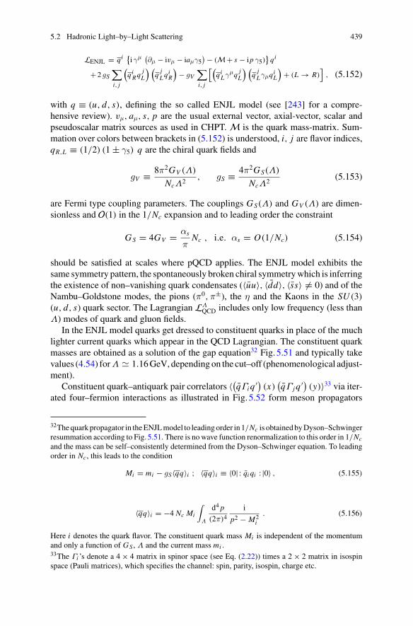
5.2 Hadronic Light–by–Light Scattering 439

LENJL = qi{i γμ (

∂μ − ivμ − iaμγ5) − (M + s − ip γ5)

}qi

+ 2 gS∑

i, j

(qiRq

jL

) (q jLq

iR

)− gV

∑

i, j

[(qiLγμq j

L

) (q jLγμq

iL

)+ (L → R)

], (5.152)

with q ≡ (u, d, s), defining the so called ENJL model (see [243] for a compre-hensive review). vμ, aμ, s, p are the usual external vector, axial-vector, scalar andpseudoscalar matrix sources as used in CHPT. M is the quark mass-matrix. Sum-mation over colors between brackets in (5.152) is understood, i, j are flavor indices,qR,L ≡ (1/2) (1 ± γ5) q are the chiral quark fields and

gV ≡ 8π2GV (Λ)

NcΛ2, gS ≡ 4π2GS(Λ)

NcΛ2(5.153)

are Fermi type coupling parameters. The couplings GS(Λ) and GV (Λ) are dimen-sionless and O(1) in the 1/Nc expansion and to leading order the constraint

GS = 4GV = αs

πNc , i.e. αs = O(1/Nc) (5.154)

should be satisfied at scales where pQCD applies. The ENJL model exhibits thesame symmetry pattern, the spontaneously broken chiral symmetrywhich is inferringthe existence of non–vanishing quark condensates (〈uu〉, 〈dd〉, 〈ss〉 = 0) and of theNambu–Goldstone modes, the pions (π0,π±), the η and the Kaons in the SU (3)(u, d, s) quark sector. The Lagrangian LΛ

QCD includes only low frequency (less thanΛ) modes of quark and gluon fields.

In the ENJL model quarks get dressed to constituent quarks in place of the muchlighter current quarks which appear in the QCD Lagrangian. The constituent quarkmasses are obtained as a solution of the gap equation32 Fig. 5.51 and typically takevalues (4.54) forΛ � 1.16GeV, dependingon the cut–off (phenomenological adjust-ment).

Constituent quark–antiquark pair correlators 〈(qΓi q ′) (x)(qΓ j q ′) (y)〉33 via iter-

ated four–fermion interactions as illustrated in Fig. 5.52 form meson propagators

32Thequarkpropagator in theENJLmodel to leadingorder in 1/Nc is obtainedbyDyson–Schwingerresummation according to Fig. 5.51. There is no wave function renormalization to this order in 1/Ncand the mass can be self–consistently determined from the Dyson–Schwinger equation. To leadingorder in Nc, this leads to the condition

Mi = mi − gS〈qq〉i ; 〈qq〉i ≡ 〈0| : qi qi : |0〉 , (5.155)

〈qq〉i = −4 Nc Mi

∫

Λ

d4 p

(2π)4

i

p2 − M2i

. (5.156)

Here i denotes the quark flavor. The constituent quark mass Mi is independent of the momentumand only a function of GS , Λ and the current mass mi .33The Γi ’s denote a 4 × 4 matrix in spinor space (see Eq. (2.22)) times a 2 × 2 matrix in isospinspace (Pauli matrices), which specifies the channel: spin, parity, isospin, charge etc.

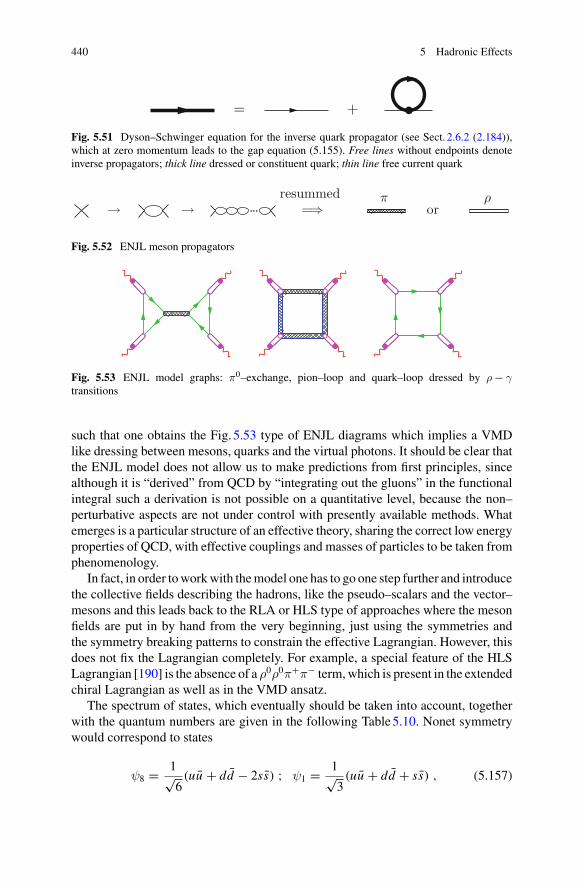
440 5 Hadronic Effects

= +

Fig. 5.51 Dyson–Schwinger equation for the inverse quark propagator (see Sect. 2.6.2 (2.184)),which at zero momentum leads to the gap equation (5.155). Free lines without endpoints denoteinverse propagators; thick line dressed or constituent quark; thin line free current quark

→ → =⇒ orπ ρresummed

Fig. 5.52 ENJL meson propagators

Fig. 5.53 ENJL model graphs: π0–exchange, pion–loop and quark–loop dressed by ρ − γtransitions

such that one obtains the Fig. 5.53 type of ENJL diagrams which implies a VMDlike dressing between mesons, quarks and the virtual photons. It should be clear thatthe ENJL model does not allow us to make predictions from first principles, sincealthough it is “derived” from QCD by “integrating out the gluons” in the functionalintegral such a derivation is not possible on a quantitative level, because the non–perturbative aspects are not under control with presently available methods. Whatemerges is a particular structure of an effective theory, sharing the correct low energyproperties of QCD, with effective couplings and masses of particles to be taken fromphenomenology.

In fact, in order toworkwith themodel one has to go one step further and introducethe collective fields describing the hadrons, like the pseudo–scalars and the vector–mesons and this leads back to the RLA or HLS type of approaches where the mesonfields are put in by hand from the very beginning, just using the symmetries andthe symmetry breaking patterns to constrain the effective Lagrangian. However, thisdoes not fix the Lagrangian completely. For example, a special feature of the HLSLagrangian [190] is the absence of a ρ0ρ0π+π− term,which is present in the extendedchiral Lagrangian as well as in the VMD ansatz.

The spectrum of states, which eventually should be taken into account, togetherwith the quantum numbers are given in the following Table5.10. Nonet symmetrywould correspond to states

ψ8 = 1√6(uu + dd − 2ss) ; ψ1 = 1√

3(uu + dd + ss) , (5.157)

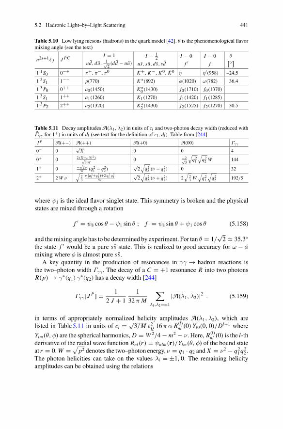
5.2 Hadronic Light–by–Light Scattering 441

Table 5.10 Low lying mesons (hadrons) in the quark model [42]. θ is the phenomenological flavormixing angle (see the text)

n2s+1J J PCI = 1

ud, du, 1√2(dd − uu)

I = 12

us, su, ds, sd

I = 0

f ′I = 0

f

θ[◦]

1 1S0 0−+ π+, π−, π0 K+, K−, K 0, K 0 η η′(958) –24.5

1 3S1 1−− ρ(770) K ∗(892) φ(1020) ω(782) 36.4

1 3P0 0++ a0(1450) K ∗0 (1430) f0(1710) f0(1370)

1 3S1 1++ a1(1260) K1(1270) f1(1420) f1(1285)

1 3P2 2++ a2(1320) K ∗2 (1430) f2(1525) f2(1270) 30.5

Table 5.11 Decay amplitudesA(λ1,λ2) in units of cl and two-photon decay width (reduced withΓγγ for 1+) in units of dl (see text for the definition of cl , dl ). Table from [244]

J P A(+−) A(++) A(+0) A(00) Γγγ

0− 0√X 0 0 4

0+ 0 2 (X+ν W 2)√3W

0 −2√3

√q21

√q22 W 144

1+ 0 −√2 ν

W (q21 − q22 )√2√q22 (ν − q21 ) 0 32

2+ 2W ν√

23

ν(q21+q22

)+2 q21 q22

W

√2√q22 (ν + q21 ) 2

√23 W

√q21

√q22 192/5

where ψ1 is the ideal flavor singlet state. This symmetry is broken and the physicalstates are mixed through a rotation

f ′ = ψ8 cos θ − ψ1 sin θ ; f = ψ8 sin θ + ψ1 cos θ (5.158)

and themixing angle has to be determined by experiment. For tan θ = 1/√2 � 35.3◦

the state f ′ would be a pure ss state. This is realized to good accuracy for ω − φmixing where φ is almost pure ss.

A key quantity in the production of resonances in γγ → hadron reactions isthe two–photon width Γγγ . The decay of a C = +1 resonance R into two photonsR(p) → γ∗(q1) γ∗(q2) has a decay width [244]

Γγγ[J P ] = 1

2 J + 1

1

32 π M

∑

λ1,λ2=±1

|A(λ1,λ2)|2 . (5.159)

in terms of appropriately normalized helicity amplitudes A(λ1,λ2), which arelisted in Table5.11 in units of cl = √

3/M e2Q 16π α R(l)nl (0) Yl0(0, 0)/D

l+1 where

Ylm(θ,φ) are the spherical harmonics, D = W 2/4 − m2 − ν. Here, R(l)nl (0) is the l-th

derivative of the radial wave function Rnl(r) = ψnlm(r)/Ylm(θ,φ) of the bound stateat r = 0.W = √

p2 denotes the two–photon energy, ν = q1 · q2 and X = ν2 − q21q

22 .

The photon helicities can take on the values λi = ±1, 0. The remaining helicityamplitudes can be obtained using the relations

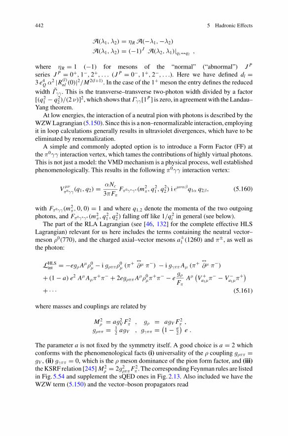
442 5 Hadronic Effects

A(λ1,λ2) = ηR A(−λ1,−λ2)

A(λ1,λ2) = (−1)J A(λ2,λ1)|q1↔q2 ,

where ηR = 1 (−1) for mesons of the “normal” (“abnormal”) J P

series J P = 0+, 1−, 2+, . . . (J P = 0−, 1+, 2−, . . .). Here we have defined dl =3 e4Q α2 |R(l)

nl (0)|2/M2(l+1). In the case of the 1+ meson the entry defines the reduced

width Γγγ . This is the transverse–transverse two-photon width divided by a factor[(q2

1 − q22 )/(2 ν)]2, which shows thatΓγγ[1P ] is zero, in agreement with the Landau–

Yang theorem.At low energies, the interaction of a neutral pion with photons is described by the

WZWLagrangian (5.150). Since this is a non–renormalizable interaction, employingit in loop calculations generally results in ultraviolet divergences, which have to beeliminated by renormalization.

A simple and commonly adopted option is to introduce a Form Factor (FF) atthe π0γγ interaction vertex, which tames the contributions of highly virtual photons.This is not just a model: the VMDmechanism is a physical process, well establishedphenomenologically. This results in the following π0γγ interaction vertex:

V μνπ0γγ(q1, q2) = αNc

3πFπFπ0γ∗γ∗(m2

π, q21 , q

22 ) i ε

μναβq1α q2β, (5.160)

with Fπ0γγ(m2π, 0, 0) = 1 and where q1,2 denote the momenta of the two outgoing

photons, and Fπ0γ∗γ∗(m2π, q

21 , q

22 ) falling off like 1/q

2i in general (see below).

The part of the RLA Lagrangian (see [46, 132] for the complete effective HLSLagrangian) relevant for us here includes the terms containing the neutral vector–meson ρ0(770), and the charged axial–vector mesons a±

1 (1260) and π±, as well asthe photon:

LHLSint = −egρA

μρ0μ − i gρππρ0μ (π+ ↔

∂μ π−) − i gγππAμ (π+ ↔∂μ π−)

+ (1 − a) e2 AμAμπ+π− + 2egρππA

μρ0μπ+π− − e

gρ

FπAμ

(V+a1μπ

− − V−a1μπ

+)

+ · · · (5.161)

where masses and couplings are related by

M2ρ = ag2V F

2π , gρ = agV F2

π ,

gρππ = 12 agV , gγππ = (

1 − a2

)e .

The parameter a is not fixed by the symmetry itself. A good choice is a = 2 whichconforms with the phenomenological facts (i) universality of the ρ coupling gρππ =gV , (ii) gγππ = 0, which is the ρ meson dominance of the pion form factor, and (iii)theKSRF relation [245]M2

ρ = 2g2ρππF2π . The corresponding Feynman rules are listed

in Fig. 5.54 and supplement the sQED ones in Fig. 2.13. Also included we have theWZW term (5.150) and the vector–boson propagators read

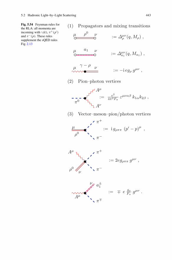
5.2 Hadronic Light–by–Light Scattering 443

Fig. 5.54 Feynman rules forthe RLA: all momenta areincoming with γ(k), π+(p′)and π−(p). These rulessupplement the sQED rulesFig. 2.13

(1) Propagators and mixing transitions

:= Δμνρ (q, Mρ) ,

:= Δμνa1

(q, Ma1) ,

:= −i egρ gμν ,

(2) Pion–photon vertices

:= e2

4π2Fπεμναβ k1αk2β ,

(3) Vector–meson–pion/photon vertices

:= i gρππ (p′ − p)μ,

:= 2egρππ gμν ,

:= ∓ egρ

Fπgμν .

ρ0μ ν

a1μ ν

μ νγ − ρ

π0

Aμ

Aν

ρ0μ

π+

π−

Aμ

ρ0ν

π+

π−

a±1

ν

π∓Aμ

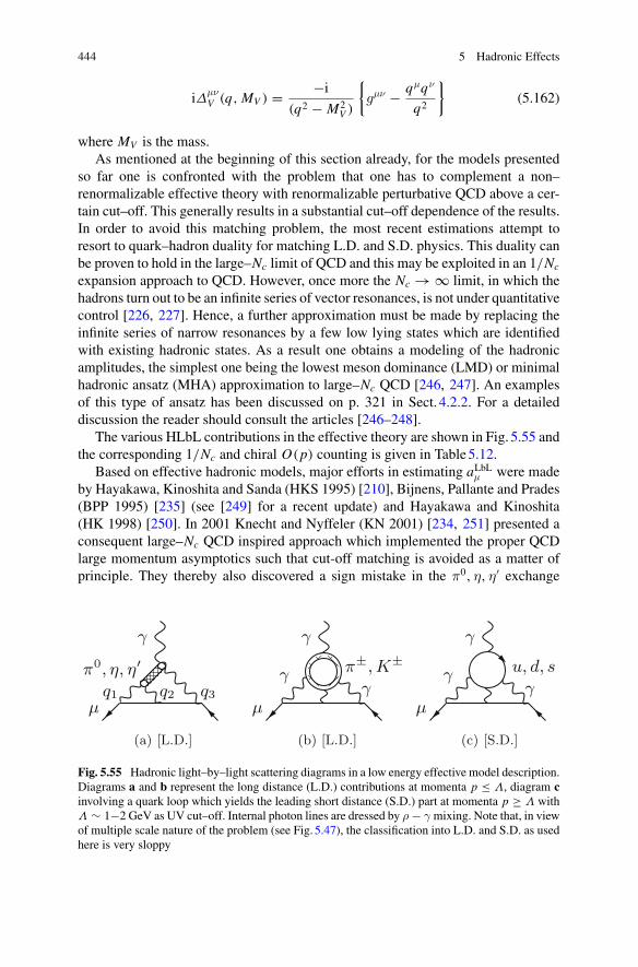
444 5 Hadronic Effects

iΔμνV (q, MV ) = −i

(q2 − M2V )

{gμν − qμqν

q2

}(5.162)

where MV is the mass.As mentioned at the beginning of this section already, for the models presented

so far one is confronted with the problem that one has to complement a non–renormalizable effective theory with renormalizable perturbative QCD above a cer-tain cut–off. This generally results in a substantial cut–off dependence of the results.In order to avoid this matching problem, the most recent estimations attempt toresort to quark–hadron duality for matching L.D. and S.D. physics. This duality canbe proven to hold in the large–Nc limit of QCD and this may be exploited in an 1/Nc

expansion approach to QCD. However, once more the Nc → ∞ limit, in which thehadrons turn out to be an infinite series of vector resonances, is not under quantitativecontrol [226, 227]. Hence, a further approximation must be made by replacing theinfinite series of narrow resonances by a few low lying states which are identifiedwith existing hadronic states. As a result one obtains a modeling of the hadronicamplitudes, the simplest one being the lowest meson dominance (LMD) or minimalhadronic ansatz (MHA) approximation to large–Nc QCD [246, 247]. An examplesof this type of ansatz has been discussed on p. 321 in Sect. 4.2.2. For a detaileddiscussion the reader should consult the articles [246–248].

The various HLbL contributions in the effective theory are shown in Fig. 5.55 andthe corresponding 1/Nc and chiral O(p) counting is given in Table5.12.

Based on effective hadronic models, major efforts in estimating aLbLμ were madeby Hayakawa, Kinoshita and Sanda (HKS 1995) [210], Bijnens, Pallante and Prades(BPP 1995) [235] (see [249] for a recent update) and Hayakawa and Kinoshita(HK 1998) [250]. In 2001 Knecht and Nyffeler (KN 2001) [234, 251] presented aconsequent large–Nc QCD inspired approach which implemented the proper QCDlarge momentum asymptotics such that cut-off matching is avoided as a matter ofprinciple. They thereby also discovered a sign mistake in the π0, η, η′ exchange

π0, η, η′

μ

γ

q1 q2 q3

(a) [L.D.]

γγ

π±, K±

μ

γ

(b) [L.D.]

γγ

u, d, s

μ

γ

(c) [S.D.]

Fig. 5.55 Hadronic light–by–light scattering diagrams in a low energy effective model description.Diagrams a and b represent the long distance (L.D.) contributions at momenta p ≤ Λ, diagram cinvolving a quark loop which yields the leading short distance (S.D.) part at momenta p ≥ Λ withΛ ∼ 1−2 GeV as UV cut–off. Internal photon lines are dressed by ρ − γ mixing. Note that, in viewof multiple scale nature of the problem (see Fig. 5.47), the classification into L.D. and S.D. as usedhere is very sloppy

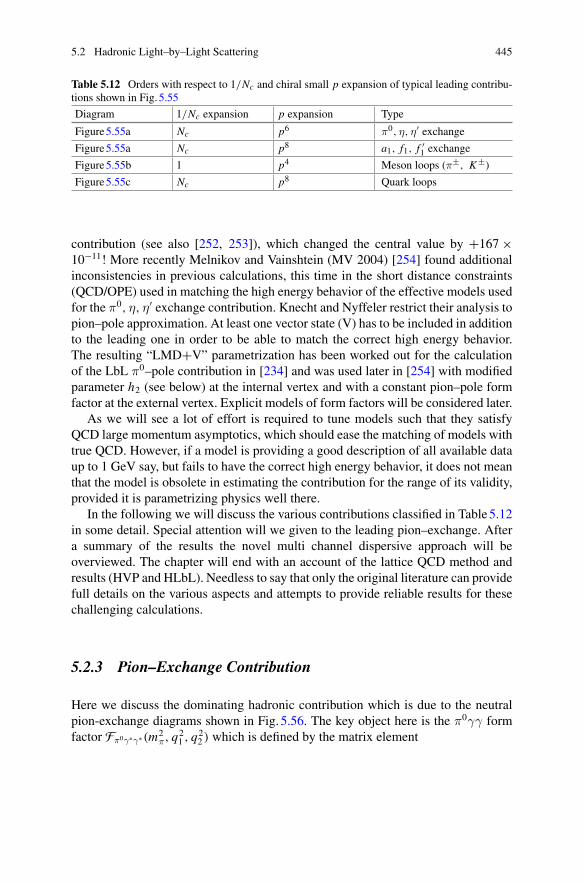
5.2 Hadronic Light–by–Light Scattering 445

Table 5.12 Orders with respect to 1/Nc and chiral small p expansion of typical leading contribu-tions shown in Fig. 5.55

Diagram 1/Nc expansion p expansion Type

Figure5.55a Nc p6 π0, η, η′ exchangeFigure5.55a Nc p8 a1, f1, f ′

1 exchange

Figure5.55b 1 p4 Meson loops (π±, K±)Figure5.55c Nc p8 Quark loops

contribution (see also [252, 253]), which changed the central value by +167 ×10−11! More recently Melnikov and Vainshtein (MV 2004) [254] found additionalinconsistencies in previous calculations, this time in the short distance constraints(QCD/OPE) used in matching the high energy behavior of the effective models usedfor the π0, η, η′ exchange contribution. Knecht and Nyffeler restrict their analysis topion–pole approximation. At least one vector state (V) has to be included in additionto the leading one in order to be able to match the correct high energy behavior.The resulting “LMD+V” parametrization has been worked out for the calculationof the LbL π0–pole contribution in [234] and was used later in [254] with modifiedparameter h2 (see below) at the internal vertex and with a constant pion–pole formfactor at the external vertex. Explicit models of form factors will be considered later.

As we will see a lot of effort is required to tune models such that they satisfyQCD large momentum asymptotics, which should ease the matching of models withtrue QCD. However, if a model is providing a good description of all available dataup to 1 GeV say, but fails to have the correct high energy behavior, it does not meanthat the model is obsolete in estimating the contribution for the range of its validity,provided it is parametrizing physics well there.

In the following we will discuss the various contributions classified in Table5.12in some detail. Special attention will we given to the leading pion–exchange. Aftera summary of the results the novel multi channel dispersive approach will beoverviewed. The chapter will end with an account of the lattice QCD method andresults (HVP and HLbL). Needless to say that only the original literature can providefull details on the various aspects and attempts to provide reliable results for thesechallenging calculations.

5.2.3 Pion–Exchange Contribution

Here we discuss the dominating hadronic contribution which is due to the neutralpion-exchange diagrams shown in Fig. 5.56. The key object here is the π0γγ formfactor Fπ0γ∗γ∗(m2

π, q21 , q

22 ) which is defined by the matrix element

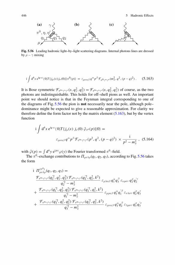
446 5 Hadronic Effects

π0, η, η′

μ

γ

q1 q3 q2

(a) (b) (c)

Fig. 5.56 Leading hadronic light–by–light scattering diagrams. Internal photons lines are dressedby ρ − γ mixing

i∫

d4x eiq·x 〈 0|T { jμ(x) jν (0)}|π0(p)〉 = εμναβ qα pβ Fπ0γ∗γ∗ (m2π, q2, (p − q)2) . (5.163)

It is Bose symmetric Fπ0∗γ∗γ∗(s, q21 , q

22 ) = Fπ0∗γ∗γ∗(s, q2

2 , q21 ) of course, as the two

photons are indistinguishable. This holds for off–shell pions as well. An importantpoint we should notice is that in the Feynman integral corresponding to one ofthe diagrams of Fig. 5.56 the pion is not necessarily near the pole, although pole–dominance might be expected to give a reasonable approximation. For clarity wetherefore define the form factor not by the matrix element (5.163), but by the vertexfunction

i∫

d4x eiq·x 〈 0|T { jμ(x) jν(0) ϕπ0(p)}|0〉 =

εμναβ qα pβ Fπ0∗γ∗γ∗(p2, q2, (p − q)2) × i

p2 − m2π

, (5.164)

with ϕ(p) = ∫d4y eipxϕ(y) the Fourier transformed π0–field.

The π0–exchange contributions to Πμνλρ(q1, q2, q3), according to Fig. 5.56 takesthe form

i Π(π0)

μνλρ(q1, q2, q3) =Fπ0∗γ∗γ∗(q

′22 , q2

1 , q23 ) Fπ0∗γ∗γ∗(q

′22 , q2

2 , k2)

q′22 − m2

π

εμλαβ qα1 q

β3 ενρστ q

σ2 q

′τ2

+ Fπ0∗γ∗γ∗(q′21 , q2

2 , q23 ) Fπ0∗γ∗γ∗(q

′21 , q2

1 , k2)

q′21 − m2

π

εμραβ qα1 q

′β1 ενλστ q

σ2 q

τ3

+ Fπ0∗γ∗γ∗(q′23 , q2

1 , q22 ) Fπ0∗γ∗γ∗(q

′23 , q2

3 , k2)

q′23 − m2

π

εμναβ qα1 q

β2 ελρστ q

σ3 q

′τ3

5.2 Hadronic Light–by–Light Scattering 447

with q ′i = qi + k. To compute aLbL;π0

μ ≡ FM(0)|LbL;π0 , we need

i∂

∂kρΠ

(π0)

μνλσ(q1, q2, k − q1 − q2) =Fπ0∗γ∗γ∗(q2

2 , q21 , q

23 ) Fπ0∗γ∗γ(q2

2 , q22 , 0)

q22 − m2

π

εμλαβ qα1 q

β2 ενσρτ q

τ2

+ Fπ0∗γ∗γ∗(q21 , q

22 , q

23 ) Fπ0∗γ∗γ(q2

1 , q21 , 0)

q21 − m2

π

εμστρ qτ1 ενλαβ q

α1 q

β2

+ Fπ0∗γ∗γ∗(q23 , q

21 , q

22 ) Fπ0∗γ∗γ(q2

3 , q23 , 0)

q23 − m2

π

εμναβ qα1 q

β2 ελσρτ q

τ3

+ O(k) . (5.165)

Here, we may set kμ = 0 such that q3 = −(q1 + q2). Inserting this last expressioninto (5.145) and computing the corresponding Dirac traces, one obtains [234]

aLbL;π0

μ = −e6∫

d4q1(2π)4

d4q2(2π)4

1

q21q

22 (q1 + q2)2[(p + q1)2 − m2][(p − q2)2 − m2]

×[Fπ0∗γ∗γ∗(q2

2 , q21 , q

23 ) Fπ0∗γ∗γ(q2

2 , q22 , 0)

q22 − m2

π

T1(q1, q2; p)

+ Fπ0∗γ∗γ∗(q23 , q

21 , q

22 ) Fπ0∗γ∗γ(q2

3 , q23 , 0)

q23 − m2

π

T2(q1, q2; p)]

, (5.166)

with

T1(q1, q2; p) = 16

3(p · q1) (p · q2) (q1 · q2) − 16

3(p · q2)2 q2

1

− 8

3(p · q1) (q1 · q2) q2

2 + 8(p · q2) q21 q

22 − 16

3(p · q2) (q1 · q2)2

+ 16

3m2 q2

1 q22 − 16

3m2 (q1 · q2)2 , (5.167)

T2(q1, q2; p) = 16

3(p · q1) (p · q2) (q1 · q2) − 16

3(p · q1)2 q2

2

+ 8

3(p · q1) (q1 · q2) q2

2 + 8

3(p · q1) q2

1 q22

+ 8

3m2 q2

1 q22 − 8

3m2 (q1 · q2)2 . (5.168)

Two of the three diagrams give equal contributions and T2 has been symmetrizedwith respect to the exchange q1 ↔ −q2. At this stage everything is known besidesthe π0γγ off–shell form factors.

For later reference it is interesting to note that the imaginary part obtained byapplying (2.141) to the pion propagator (unitarity cut) is given by

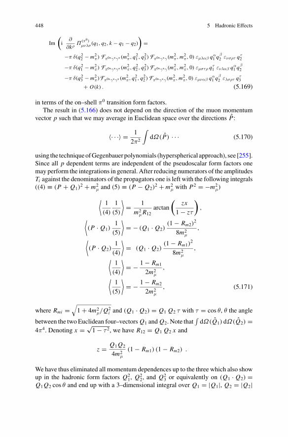
448 5 Hadronic Effects

Im

(i

∂

∂kρΠ

(π0)μνλσ(q1, q2, k − q1 − q2)

)=

−π δ(q22 − m2π) Fπ0∗γ∗γ∗ (m2

π, q21 , q23 ) Fπ0∗γ∗γ(m2π,m2

π, 0) εμλαβ qα1 q

β2 ενσρτ q

τ2

−π δ(q21 − m2π) Fπ0∗γ∗γ∗ (m2

π, q22 , q23 ) Fπ0∗γ∗γ(m2π,m2

π, 0) εμστρ qτ1 ενλαβ qα

1 qβ2

−π δ(q23 − m2π)Fπ0∗γ∗γ∗ (m2

π, q21 , q22 ) Fπ0∗γ∗γ(m2π,m2

π, 0) εμναβ qα1 q

β2 ελσρτ q

τ3

+ O(k) . (5.169)

in terms of the on–shell π0 transition form factors.The result in (5.166) does not depend on the direction of the muon momentum

vector p such that we may average in Euclidean space over the directions P:

〈· · ·〉 = 1

2π2

∫dΩ(P) · · · (5.170)

using the techniqueofGegenbauer polynomials (hyperspherical approach), see [255].Since all p dependent terms are independent of the pseudoscalar form factors onemay perform the integrations in general. After reducing numerators of the amplitudesTi against the denominators of the propagators one is left with the following integrals((4) ≡ (P + Q1)

2 + m2μ and (5) ≡ (P − Q2)

2 + m2μ with P2 = −m2

μ)

⟨1

(4)

1

(5)

⟩= 1

m2μR12

arctan

(zx

1 − zτ

),

⟨(P · Q1)

1

(5)

⟩= − (Q1 · Q2)

(1 − Rm2)2

8m2μ

,

⟨(P · Q2)

1

(4)

⟩= (Q1 · Q2)

(1 − Rm1)2

8m2μ

,

⟨1

(4)

⟩= − 1 − Rm1

2m2μ

,

⟨1

(5)

⟩= − 1 − Rm2

2m2μ

, (5.171)

where Rmi =√1 + 4m2

μ/Q2i and (Q1 · Q2) = Q1 Q2 τ with τ = cos θ, θ the angle

between the two Euclidean four–vectors Q1 and Q2. Note that∫dΩ(Q1) dΩ(Q2) =

4π4. Denoting x = √1 − τ 2, we have R12 = Q1 Q2 x and

z = Q1Q2

4m2μ

(1 − Rm1) (1 − Rm2) .

We have thus eliminated all momentum dependences up to the three which also showup in the hadronic form factors Q2

1, Q22, and Q2

3 or equivalently on (Q1 · Q2) =Q1Q2 cos θ and end up with a 3–dimensional integral over Q1 = |Q1|, Q2 = |Q2|

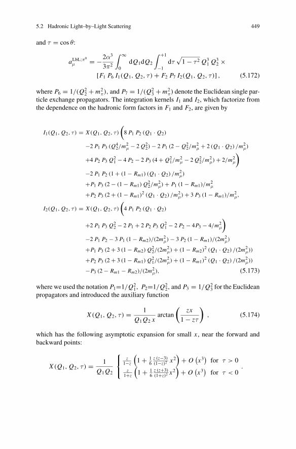
5.2 Hadronic Light–by–Light Scattering 449

and τ = cos θ:

aLbL;π0

μ = −2α3

3π2

∫ ∞

0dQ1dQ2

∫ +1

−1dτ

√1 − τ 2 Q3

1 Q32 ×

[F1 P6 I1(Q1, Q2, τ ) + F2 P7 I2(Q1, Q2, τ )] , (5.172)

where P6 = 1/(Q22 + m2

π), and P7 = 1/(Q23 + m2

π) denote the Euclidean single par-ticle exchange propagators. The integration kernels I1 and I2, which factorize fromthe dependence on the hadronic form factors in F1 and F2, are given by

I1(Q1, Q2, τ ) = X (Q1, Q2, τ )

(8 P1 P2 (Q1 · Q2)

−2 P1 P3 (Q42/m

2μ − 2 Q2

2) − 2 P1 (2 − Q22/m

2μ + 2 (Q1 · Q2) /m2

μ)

+4 P2 P3 Q21 − 4 P2 − 2 P3 (4 + Q2

1/m2μ − 2 Q2

2/m2μ) + 2/m2

μ

)

−2 P1 P2 (1 + (1 − Rm1) (Q1 · Q2) /m2μ)

+P1 P3 (2 − (1 − Rm1) Q22/m

2μ) + P1 (1 − Rm1)/m

2μ

+P2 P3 (2 + (1 − Rm1)2 (Q1 · Q2) /m2

μ) + 3 P3 (1 − Rm1)/m2μ,

I2(Q1, Q2, τ ) = X (Q1, Q2, τ )

(4 P1 P2 (Q1 · Q2)

+2 P1 P3 Q22 − 2 P1 + 2 P2 P3 Q

21 − 2 P2 − 4P3 − 4/m2

μ

)

−2 P1 P2 − 3 P1 (1 − Rm2)/(2m2μ) − 3 P2 (1 − Rm1)/(2m

2μ)

+P1 P3 (2 + 3 (1 − Rm2) Q22/(2m

2μ) + (1 − Rm2)

2 (Q1 · Q2) /(2m2μ))

+P2 P3 (2 + 3 (1 − Rm1) Q21/(2m

2μ) + (1 − Rm1)

2 (Q1 · Q2) /(2m2μ))

−P3 (2 − Rm1 − Rm2)/(2m2μ), (5.173)

where we used the notation P1=1/Q21, P2=1/Q2

2, and P3 = 1/Q23 for the Euclidean

propagators and introduced the auxiliary function

X (Q1, Q2, τ ) = 1

Q1Q2 xarctan

(zx

1 − zτ

), (5.174)

which has the following asymptotic expansion for small x , near the forward andbackward points:

X (Q1, Q2, τ ) = 1

Q1Q2

⎧⎨

⎩

z1−z

(1 + 1

6z (z−3)(1−z)2 x

2)

+ O(x3)for τ > 0

z1+z

(1 + 1

6z (z+3)(1+z)2 x

2)

+ O(x3)

for τ < 0.

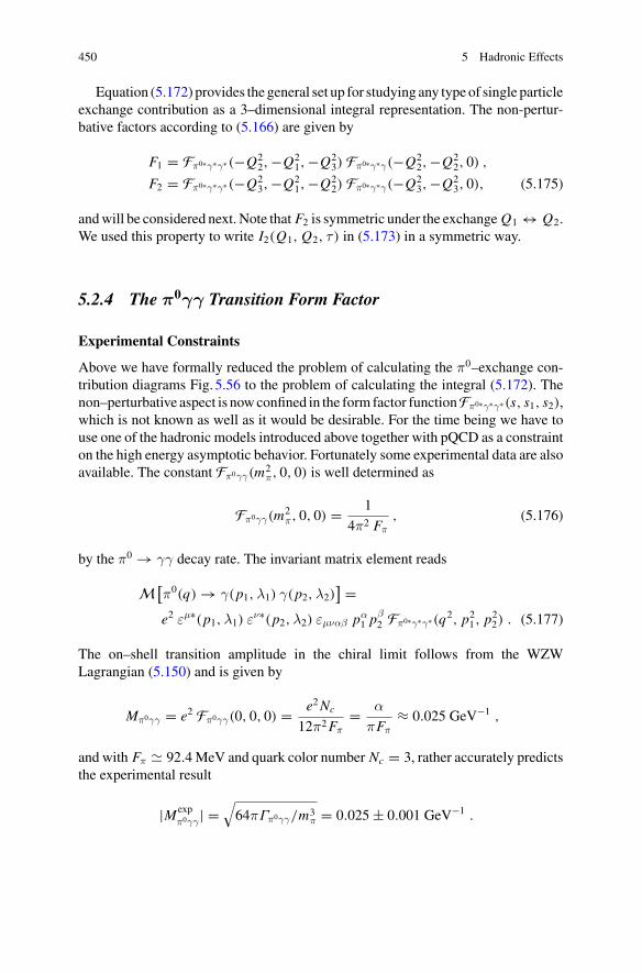
450 5 Hadronic Effects

Equation (5.172) provides the general set up for studying any type of single particleexchange contribution as a 3–dimensional integral representation. The non-pertur-bative factors according to (5.166) are given by

F1 = Fπ0∗γ∗γ∗(−Q22,−Q2

1,−Q23) Fπ0∗γ∗γ(−Q2

2,−Q22, 0) ,

F2 = Fπ0∗γ∗γ∗(−Q23,−Q2

1,−Q22) Fπ0∗γ∗γ(−Q2

3,−Q23, 0), (5.175)

andwill be considered next. Note that F2 is symmetric under the exchange Q1 ↔ Q2.We used this property to write I2(Q1, Q2, τ ) in (5.173) in a symmetric way.

5.2.4 The π0γγ Transition Form Factor

Experimental Constraints

Above we have formally reduced the problem of calculating the π0–exchange con-tribution diagrams Fig. 5.56 to the problem of calculating the integral (5.172). Thenon–perturbative aspect is nowconfined in the form factor functionFπ0∗γ∗γ∗(s, s1, s2),which is not known as well as it would be desirable. For the time being we have touse one of the hadronic models introduced above together with pQCD as a constrainton the high energy asymptotic behavior. Fortunately some experimental data are alsoavailable. The constant Fπ0γγ(m2

π, 0, 0) is well determined as

Fπ0γγ(m2π, 0, 0) = 1

4π2 Fπ, (5.176)

by the π0 → γγ decay rate. The invariant matrix element reads

M[π0(q) → γ(p1,λ1) γ(p2,λ2)

] =e2 εμ∗(p1,λ1) εν∗(p2,λ2) εμναβ pα

1 pβ2 Fπ0∗γ∗γ∗(q2, p21, p

22) . (5.177)

The on–shell transition amplitude in the chiral limit follows from the WZWLagrangian (5.150) and is given by

Mπ0γγ = e2 Fπ0γγ(0, 0, 0) = e2Nc

12π2Fπ= α

πFπ≈ 0.025 GeV−1 ,

and with Fπ � 92.4MeV and quark color number Nc = 3, rather accurately predictsthe experimental result

|Mexpπ0γγ | =

√64πΓπ0γγ/m3

π = 0.025 ± 0.001 GeV−1 .

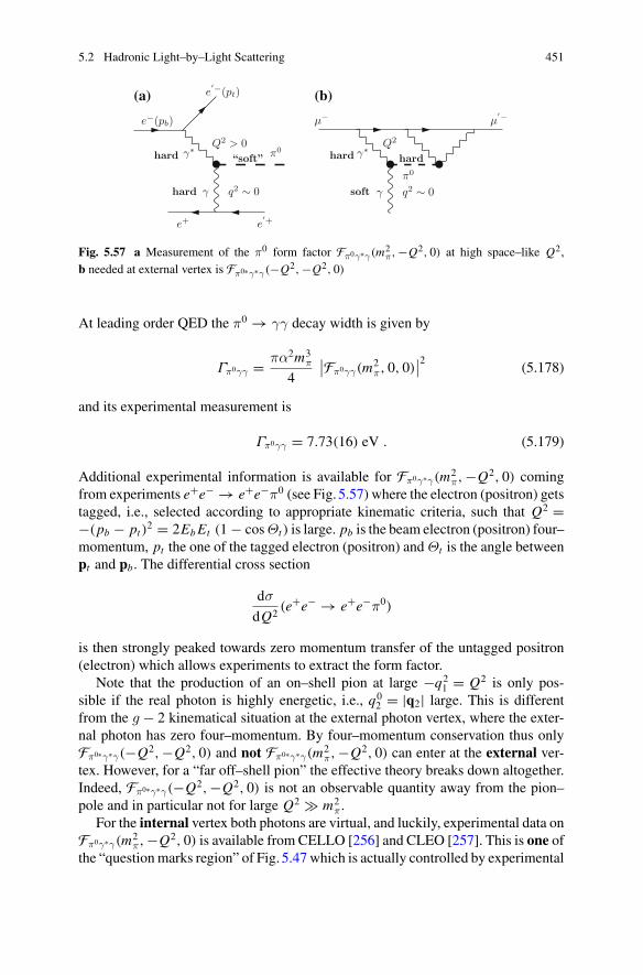
5.2 Hadronic Light–by–Light Scattering 451

π0

e−(pb)

e′−(pt)

e+ e′+

q2 ∼ 0

Q2 > 0

γ

γ∗

π0

μ− μ′−

q2 ∼ 0

Q2

γ

γ∗

hard soft

hard hard“soft” hard

(a) (b)

Fig. 5.57 a Measurement of the π0 form factor Fπ0γ∗γ(m2π,−Q2, 0) at high space–like Q2,

b needed at external vertex is Fπ0∗γ∗γ(−Q2,−Q2, 0)

At leading order QED the π0 → γγ decay width is given by

Γπ0γγ = πα2m3π

4

∣∣Fπ0γγ(m2π, 0, 0)

∣∣2 (5.178)

and its experimental measurement is

Γπ0γγ = 7.73(16) eV . (5.179)

Additional experimental information is available for Fπ0γ∗γ(m2π,−Q2, 0) coming

from experiments e+e− → e+e−π0 (see Fig. 5.57) where the electron (positron) getstagged, i.e., selected according to appropriate kinematic criteria, such that Q2 =−(pb − pt )2 = 2EbEt (1 − cosΘt ) is large. pb is the beam electron (positron) four–momentum, pt the one of the tagged electron (positron) and Θt is the angle betweenpt and pb. The differential cross section

dσ

dQ2(e+e− → e+e−π0)

is then strongly peaked towards zero momentum transfer of the untagged positron(electron) which allows experiments to extract the form factor.

Note that the production of an on–shell pion at large −q21 = Q2 is only pos-

sible if the real photon is highly energetic, i.e., q02 = |q2| large. This is different

from the g − 2 kinematical situation at the external photon vertex, where the exter-nal photon has zero four–momentum. By four–momentum conservation thus onlyFπ0∗γ∗γ(−Q2,−Q2, 0) and not Fπ0∗γ∗γ(m2

π,−Q2, 0) can enter at the external ver-tex. However, for a “far off–shell pion” the effective theory breaks down altogether.Indeed, Fπ0∗γ∗γ(−Q2,−Q2, 0) is not an observable quantity away from the pion–pole and in particular not for large Q2 � m2

π.For the internal vertex both photons are virtual, and luckily, experimental data on

Fπ0γ∗γ(m2π,−Q2, 0) is available from CELLO [256] and CLEO [257]. This is one of

the “questionmarks region” of Fig. 5.47 which is actually controlled by experimental

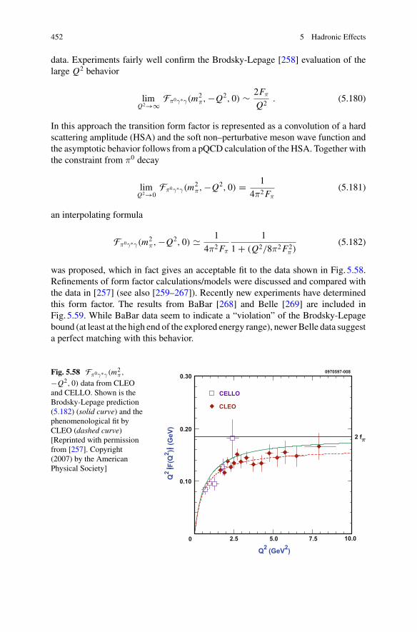
452 5 Hadronic Effects

data. Experiments fairly well confirm the Brodsky-Lepage [258] evaluation of thelarge Q2 behavior

limQ2→∞

Fπ0γ∗γ(m2π,−Q2, 0) ∼ 2Fπ

Q2. (5.180)

In this approach the transition form factor is represented as a convolution of a hardscattering amplitude (HSA) and the soft non–perturbative meson wave function andthe asymptotic behavior follows from a pQCD calculation of the HSA. Together withthe constraint from π0 decay

limQ2→0

Fπ0γ∗γ(m2π,−Q2, 0) = 1

4π2Fπ(5.181)

an interpolating formula

Fπ0γ∗γ(m2π,−Q2, 0) � 1

4π2Fπ

1

1 + (Q2/8π2F2π )

(5.182)

was proposed, which in fact gives an acceptable fit to the data shown in Fig. 5.58.Refinements of form factor calculations/models were discussed and compared withthe data in [257] (see also [259–267]). Recently new experiments have determinedthis form factor. The results from BaBar [268] and Belle [269] are included inFig. 5.59. While BaBar data seem to indicate a “violation” of the Brodsky-Lepagebound (at least at the high end of the explored energy range), newer Belle data suggesta perfect matching with this behavior.

Fig. 5.58 Fπ0γ∗γ(m2π,

−Q2, 0) data from CLEOand CELLO. Shown is theBrodsky-Lepage prediction(5.182) (solid curve) and thephenomenological fit byCLEO (dashed curve)[Reprinted with permissionfrom [257]. Copyright(2007) by the AmericanPhysical Society]

2.5 5.0 7.5 10.0

Q2 (GeV2)

Q2

F(Q

2 )(G

eV)

IIII

2 f

0970597-008

CELLO

CLEO

0.30

0.20

0.10

0

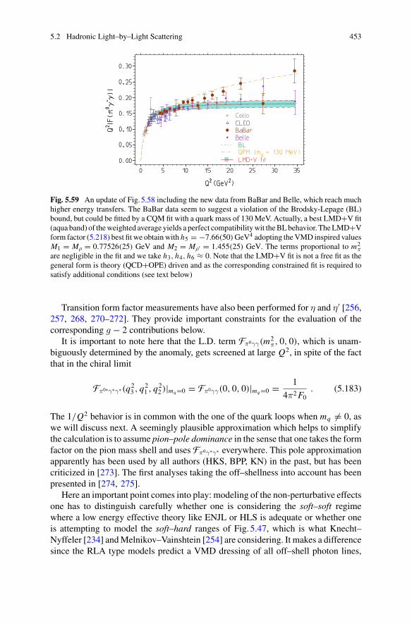
5.2 Hadronic Light–by–Light Scattering 453

Fig. 5.59 An update of Fig. 5.58 including the new data from BaBar and Belle, which reach muchhigher energy transfers. The BaBar data seem to suggest a violation of the Brodsky-Lepage (BL)bound, but could be fitted by a CQM fit with a quark mass of 130 MeV. Actually, a best LMD+V fit(aqua band) of theweighted average yields a perfect compatibilitywit theBLbehavior. TheLMD+Vform factor (5.218) best fit we obtainwith h5 = −7.66(50)GeV4 adopting theVMD inspired valuesM1 = Mρ = 0.77526(25) GeV and M2 = Mρ′ = 1.455(25) GeV. The terms proportional to m2

πare negligible in the fit and we take h3, h4, h6 ≈ 0. Note that the LMD+V fit is not a free fit as thegeneral form is theory (QCD+OPE) driven and as the corresponding constrained fit is required tosatisfy additional conditions (see text below)

Transition form factor measurements have also been performed for η and η′ [256,257, 268, 270–272]. They provide important constraints for the evaluation of thecorresponding g − 2 contributions below.

It is important to note here that the L.D. term Fπ0γγ(m2π, 0, 0), which is unam-

biguously determined by the anomaly, gets screened at large Q2, in spite of the factthat in the chiral limit

Fπ0∗γ∗γ∗(q23 , q

21 , q

22 )|mq=0 = Fπ0γγ(0, 0, 0)|mq=0 = 1

4π2F0. (5.183)

The 1/Q2 behavior is in common with the one of the quark loops when mq = 0, aswe will discuss next. A seemingly plausible approximation which helps to simplifythe calculation is to assume pion–pole dominance in the sense that one takes the formfactor on the pion mass shell and uses Fπ0γ∗γ∗ everywhere. This pole approximationapparently has been used by all authors (HKS, BPP, KN) in the past, but has beencriticized in [273]. The first analyses taking the off–shellness into account has beenpresented in [274, 275].

Here an important point comes into play: modeling of the non-perturbative effectsone has to distinguish carefully whether one is considering the soft–soft regimewhere a low energy effective theory like ENJL or HLS is adequate or whether oneis attempting to model the soft–hard ranges of Fig. 5.47, which is what Knecht–Nyffeler [234] andMelnikov–Vainshtein [254] are considering. It makes a differencesince the RLA type models predict a VMD dressing of all off–shell photon lines,

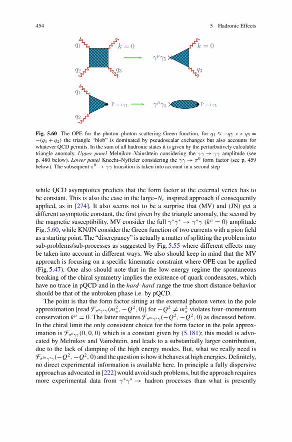
454 5 Hadronic Effects

q1

q2

k = 0

q3

γμγ5

k = 0

q3

×

q1

q2

P = i γ5 γμγ5× P = i γ5

Fig. 5.60 The OPE for the photon–photon scattering Green function, for q1 ≈ −q2 >> q3 =−(q1 + q2) the triangle “blob” is dominated by pseudoscalar exchanges but also accounts forwhatever QCD permits. In the sum of all hadronic states it is given by the perturbatively calculabletriangle anomaly. Upper panel Melnikov–Vainshtein considering the γγ → γγ amplitude (seep. 480 below). Lower panel Knecht–Nyffeler considering the γγ → π0 form factor (see p. 459below). The subsequent π0 → γγ transition is taken into account in a second step

while QCD asymptotics predicts that the form factor at the external vertex has tobe constant. This is also the case in the large–Nc inspired approach if consequentlyapplied, as in [274]. It also seems not to be a surprise that (MV) and (JN) get adifferent asymptotic constant, the first given by the triangle anomaly, the second bythe magnetic susceptibility. MV consider the full γ∗γ∗ → γ∗γ (kμ = 0) amplitudeFig. 5.60, while KN/JN consider the Green function of two currents with a pion fieldas a starting point. The “discrepancy” is actually amatter of splitting the problem intosub-problems/sub-processes as suggested by Fig. 5.55 where different effects maybe taken into account in different ways. We also should keep in mind that the MVapproach is focusing on a specific kinematic constraint where OPE can be applied(Fig. 5.47). One also should note that in the low energy regime the spontaneousbreaking of the chiral symmetry implies the existence of quark condensates, whichhave no trace in pQCD and in the hard–hard range the true short distance behaviorshould be that of the unbroken phase i.e. by pQCD.

The point is that the form factor sitting at the external photon vertex in the poleapproximation [read Fπ0γ∗γ(m2

π,−Q2, 0)] for −Q2 = m2π violates four–momentum

conservation kμ = 0. The latter requires Fπ0∗γ∗γ(−Q2,−Q2, 0) as discussed before.In the chiral limit the only consistent choice for the form factor in the pole approx-imation is Fπ0γγ(0, 0, 0) which is a constant given by (5.181); this model is advo-cated by Melnikov and Vainshtein, and leads to a substantially larger contribution,due to the lack of damping of the high energy modes. But, what we really need isFπ0∗γ∗γ(−Q2,−Q2, 0) and the question is how it behaves at high energies. Definitely,no direct experimental information is available here. In principle a fully dispersiveapproach as advocated in [222]would avoid such problems, but the approach requiresmore experimental data from γ∗γ∗ → hadron processes than what is presently

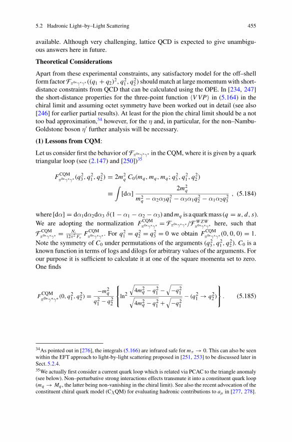
5.2 Hadronic Light–by–Light Scattering 455

available. Although very challenging, lattice QCD is expected to give unambigu-ous answers here in future.

Theoretical Considerations

Apart from these experimental constraints, any satisfactory model for the off–shellform factorFπ0∗γ∗γ∗((q1 + q2)2, q2

1 , q22 ) shouldmatch at largemomentumwith short-

distance constraints from QCD that can be calculated using the OPE. In [234, 247]the short-distance properties for the three-point function 〈VVP〉 in (5.164) in thechiral limit and assuming octet symmetry have been worked out in detail (see also[246] for earlier partial results). At least for the pion the chiral limit should be a nottoo bad approximation,34 however, for the η and, in particular, for the non–Nambu-Goldstone boson η′ further analysis will be necessary.

(1) Lessons from CQM:

Let us consider first the behavior ofFπ0∗γ∗γ∗ in the CQM, where it is given by a quarktriangular loop (see (2.147) and [250])35

FCQMπ0∗γ∗γ∗(q

23 , q

21 , q

22 ) = 2m2

q C0(mq ,mq ,mq; q23 , q

21 , q

22 )

≡∫

[dα] 2m2q

m2q − α2α3q2

1 − α3α1q22 − α1α2q2

3

, (5.184)

where [dα] = dα1dα2dα3 δ(1 − α1 − α2 − α3) andmq is a quarkmass (q = u, d, s).We are adopting the normalization FCQM

π0∗γ∗γ∗ = Fπ0∗γ∗γ∗/F WZWπ0∗γ∗γ∗ here, such that

F CQMπ0∗γ∗γ∗ = Nc

12π2 FπFCQM

π0∗γ∗γ∗ . For q21 = q2

2 = q23 = 0 we obtain FCQM

π0∗γ∗γ∗(0, 0, 0) = 1.

Note the symmetry of C0 under permutations of the arguments (q23 , q

21 , q

22 ). C0 is a

known function in terms of logs and dilogs for arbitrary values of the arguments. Forour purpose it is sufficient to calculate it at one of the square momenta set to zero.One finds

FCQMπ0∗γ∗γ∗(0, q

21 , q22 ) = −m2

q

q21 − q22

⎧⎨

⎩ln2

√4m2

q − q21 −√

−q21√4m2

q − q21 +√

−q21

− (q21 → q22 )

⎫⎬

⎭ . (5.185)

34As pointed out in [276], the integrals (5.166) are infrared safe for mπ → 0. This can also be seenwithin the EFT approach to light-by-light scattering proposed in [251, 253] to be discussed later inSect. 5.2.4.35We actually first consider a current quark loop which is related via PCAC to the triangle anomaly(see below). Non–perturbative strong interactions effects transmute it into a constituent quark loop(mq → Mq , the latter being non-vanishing in the chiral limit). See also the recent advocation of theconstituent chiral quark model (CχQM) for evaluating hadronic contributions to aμ in [277, 278].

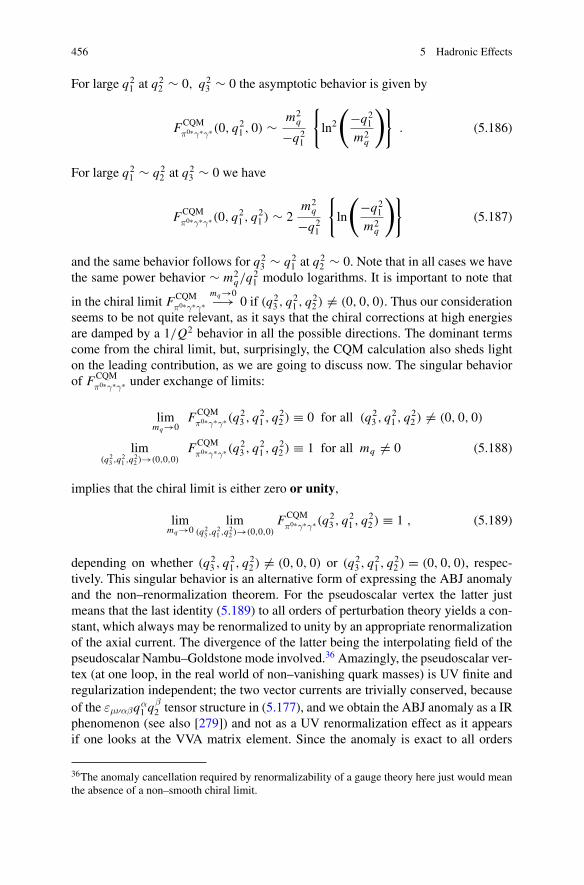
456 5 Hadronic Effects

For large q21 at q2

2 ∼ 0, q23 ∼ 0 the asymptotic behavior is given by

FCQMπ0∗γ∗γ∗(0, q

21 , 0) ∼ m2

q

−q21

{ln2

(−q2

1

m2q

)}. (5.186)

For large q21 ∼ q2

2 at q23 ∼ 0 we have

FCQMπ0∗γ∗γ∗(0, q

21 , q

21 ) ∼ 2

m2q

−q21

{ln

(−q2

1

m2q

)}(5.187)

and the same behavior follows for q23 ∼ q2

1 at q22 ∼ 0. Note that in all cases we have

the same power behavior ∼ m2q/q

21 modulo logarithms. It is important to note that

in the chiral limit FCQMπ0∗γ∗γ∗

mq→0−→ 0 if (q23 , q

21 , q

22 ) = (0, 0, 0). Thus our consideration

seems to be not quite relevant, as it says that the chiral corrections at high energiesare damped by a 1/Q2 behavior in all the possible directions. The dominant termscome from the chiral limit, but, surprisingly, the CQM calculation also sheds lighton the leading contribution, as we are going to discuss now. The singular behaviorof FCQM

π0∗γ∗γ∗ under exchange of limits:

limmq→0

FCQMπ0∗γ∗γ∗(q

23 , q

21 , q

22 ) ≡ 0 for all (q2

3 , q21 , q

22 ) = (0, 0, 0)

lim(q2

3 ,q21 ,q

22 )→(0,0,0)

FCQMπ0∗γ∗γ∗(q

23 , q

21 , q

22 ) ≡ 1 for all mq = 0 (5.188)

implies that the chiral limit is either zero or unity,

limmq→0

lim(q2

3 ,q21 ,q

22 )→(0,0,0)

FCQMπ0∗γ∗γ∗(q

23 , q

21 , q

22 ) ≡ 1 , (5.189)

depending on whether (q23 , q

21 , q

22 ) = (0, 0, 0) or (q2

3 , q21 , q

22 ) = (0, 0, 0), respec-

tively. This singular behavior is an alternative form of expressing the ABJ anomalyand the non–renormalization theorem. For the pseudoscalar vertex the latter justmeans that the last identity (5.189) to all orders of perturbation theory yields a con-stant, which always may be renormalized to unity by an appropriate renormalizationof the axial current. The divergence of the latter being the interpolating field of thepseudoscalar Nambu–Goldstone mode involved.36 Amazingly, the pseudoscalar ver-tex (at one loop, in the real world of non–vanishing quark masses) is UV finite andregularization independent; the two vector currents are trivially conserved, becauseof the εμναβqα

1 qβ2 tensor structure in (5.177), and we obtain the ABJ anomaly as a IR

phenomenon (see also [279]) and not as a UV renormalization effect as it appearsif one looks at the VVA matrix element. Since the anomaly is exact to all orders

36The anomaly cancellation required by renormalizability of a gauge theory here just would meanthe absence of a non–smooth chiral limit.

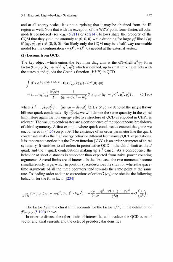
5.2 Hadronic Light–by–Light Scattering 457

and at all energy scales, it is not surprising that it may be obtained from the IRregion as well. Note that with the exception of the WZW point form–factor, all othermodels considered (see e.g. (5.211) or (5.214), below) share the property of theCQM that they yield the anomaly at (0, 0, 0) while dropping for large p2i like 1/p

2i

if (q21 , q

22 , p

23) = (0, 0, 0). But likely only the CQM may be a half–way reasonable

model for the configuration (−Q2,−Q2, 0) needed at the external vertex.

(2) Lessons from QCD:

The key object which enters the Feynman diagrams is the off–shell π0γγ formfactor Fπ0∗γ∗γ∗((q1 + q2)2, q2

1 , q22 ) which is defined, up to small mixing effects with

the states η and η′, via the Green’s function 〈VVP〉 in QCD∫

d4x d4y ei(q1·x+q2·y) 〈 0|T { jμ(x) jν(y)P3(0)}|0〉

= εμναβ qα1 q

β2

i〈ψψ〉Fπ

i

(q1 + q2)2 − m2π

Fπ0∗γ∗γ∗((q1 + q2)2, q2

1 , q22 ) , (5.190)

where P3 = ψiγ5 λ3

2 ψ = (uiγ5u − diγ5d

)/2. By 〈ψψ〉we denoted the single flavor

bilinear quark condensate. By 〈ψψ〉0 we will denote the same quantity in the chirallimit. Here again the low energy effective structure of QCD as encoded in CHPT isrelevant. The vacuum condensates are a consequence of the spontaneous breakdownof chiral symmetry. A first example where quark condensates entered the game weencountered in (4.76) on p. 309. The existence of an order parameter like the quarkcondensate makes the high energy behavior different from naive pQCD expectations.It is important to notice that the Green function 〈VVP〉 is an order parameter of chiralsymmetry. It vanishes to all orders in perturbative QCD in the chiral limit as the dquark and the u quark contributions making up P3 cancel. As a consequence thebehavior at short distances is smoother than expected from naive power countingarguments. Several limits are of interest. In the first case, the two momenta becomesimultaneously large,which in position space describes the situationwhere the space-time arguments of all the three operators tend towards the same point at the samerate. To leading order and up to corrections of orderO (αs) one obtains the followingbehavior for the form factor [234]

limλ→∞

Fπ0∗γ∗γ∗ ((λq1 + λq2)2, (λq1)

2, (λq2)2) = − F0

3

1

λ2

q21 + q22 + (q1 + q2)2

q21q22

+ O(

1

λ4

).

The factor F0 in the chiral limit accounts for the factor 1/Fπ in the definition ofFπ0∗γ∗γ∗ (5.190) above.

In order to discuss the other limits of interest let us introduce the QCD octet ofvector and axial currents and the octet of pseudoscalar densities

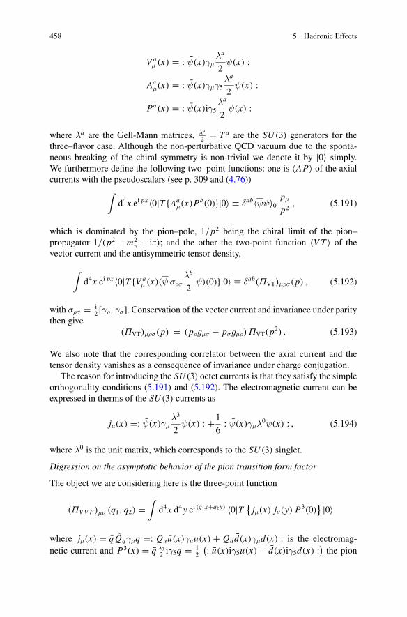
458 5 Hadronic Effects

V aμ (x) = : ψ(x)γμ

λa

2ψ(x) :

Aaμ(x) = : ψ(x)γμγ5

λa

2ψ(x) :

Pa(x) = : ψ(x)iγ5λa

2ψ(x) :

where λa are the Gell-Mann matrices, λa

2 = T a are the SU (3) generators for thethree–flavor case. Although the non-perturbative QCD vacuum due to the sponta-neous breaking of the chiral symmetry is non-trivial we denote it by |0〉 simply.We furthermore define the following two–point functions: one is 〈AP〉 of the axialcurrents with the pseudoscalars (see p. 309 and (4.76))

∫d4x ei px 〈0|T {Aa

μ(x)Pb(0)}|0〉 ≡ δab〈ψψ〉0 pμ

p2, (5.191)

which is dominated by the pion–pole, 1/p2 being the chiral limit of the pion–propagator 1/(p2 − m2

π + iε); and the other the two-point function 〈VT 〉 of thevector current and the antisymmetric tensor density,

∫d4x ei px 〈0|T {V a

μ (x)(ψ σρσλb

2ψ)(0)}|0〉 ≡ δab(ΠVT)μρσ(p) , (5.192)

with σρσ = i2 [γρ, γσ]. Conservation of the vector current and invariance under parity

then give(ΠVT)μρσ(p) = (pρgμσ − pσgμρ)ΠVT(p

2) . (5.193)

We also note that the corresponding correlator between the axial current and thetensor density vanishes as a consequence of invariance under charge conjugation.

The reason for introducing the SU (3) octet currents is that they satisfy the simpleorthogonality conditions (5.191) and (5.192). The electromagnetic current can beexpressed in therms of the SU (3) currents as

jμ(x) =: ψ(x)γμλ3

2ψ(x) : +1

6: ψ(x)γμλ

0ψ(x) : , (5.194)

where λ0 is the unit matrix, which corresponds to the SU (3) singlet.

Digression on the asymptotic behavior of the pion transition form factor

The object we are considering here is the three-point function

(ΠVV P)μν (q1, q2) =∫

d4x d4y ei (q1x+q2 y) 〈0|T {jμ(x) jν(y) P

3(0)} |0〉

where jμ(x) = q Qqγμq =: Quu(x)γμu(x) + Qdd(x)γμd(x) : is the electromag-netic current and P3(x) = q λ3

2 iγ5q = 12

(: u(x)iγ5u(x) − d(x)iγ5d(x) :) the pion

5.2 Hadronic Light–by–Light Scattering 459

interpolating field. Both Q and the Gell-Mann matrix λ3 are diagonal matrices inflavor space. The conserved electromagnetic current implies the WT–identities

qμ1 (ΠVV P)μν (q1, q2) = qν

2 (ΠVV P)μν (q1, q2) = 0 .

As a parity odd object 〈VVP〉 must have the tensor structure

(ΠVV P)μν (q1, q2) = εμνρσqρ1q

σ2HV (q2

1 , q22 , (q1 + q2)

2) .

We are going to study the high energy behavior when two of the three fields approacheach other in x–space. The object of interest is the time–ordered product

T{JΓ1(x) JΓ2 (y)

} = : ψ(x)Γ1ψ(x)ψ(y)Γ2ψ(y) :+ : ψ(x)Γ1 SF (x − y) Γ2ψ(y) : + : ψ(y)Γ2 SF (y − x) Γ1ψ(x) :−Tr [SF (y − x)Γ1SF (x − y)Γ2] (5.195)

of a pair of fermion bilinears

JΓ =: ψ(x)Γ ψ(x) : .

The free Feynman propagators

SF (x) = i∫

d4q

(2π)4e−i qx q + m

q2 − m2 + iε

are color and flavor diagonal spinor space matrices and the trace is over spinor, colorand flavor indices. The normal ordering means the self-contractions (tadpoles) areabsent. The structure holds beyond perturbation theory if propagators are full propa-gators and vertices dressed ones. We thus have the structure discussed in Sect. 4.2.2p. 316, graphically represented by Eq. (4.83) with appropriately chosen couplingmatrices.

In the chiral limit the quark mass is zero. We also have to expand the fields. Inthe Schwinger–Fock gauge the gluon fields satisfy xμGμ(x) = 0 and we have

ψ(x) = ψ(y) + (x − y)μ(Dμψ

)(y) + · · · ,

where the second term is a gluonic correction (see Eq.4.80) which is subleading andwe will neglect it in the following.We first consider (see Fig. 5.60)

limλ→∞ (ΠVV P )μν (λq1, q − λq1) =

∫d4y eiqy lim

λ→∞

∫d4x eiλq1(x−y) 〈0|T {

T{jμ(x) jν (y)

}P3(0)

} |0〉

=∫

d4y eiqy limλ→∞

∫d4z eiλq1z 〈0|T {

T{jμ(y + z) jν (y)

}P3(0)

} |0〉 ,

460 5 Hadronic Effects

where we have used translation invariance and changed the integration variable x →z = x − y and use that operators commute under the T –product and pairwise T –contractions can be done in any order. As 〈0|P3(0)|0〉 = 0 the last, potentially mostsingular term, will not contribute and the first term of (5.195) is regular as x → y sowe have to consider the second plus third term only, with Γ1 = Qγμ and Γ2 = Qγν .Then

limλ→∞

∫d4z eiλq1z〈0|T {

T{jμ(y + z) jν(y)

}P3(0)

} |0〉

= i

λ

qρ1

q21

〈0|T{: ψ(0)

(γμγρ γν − γνγργμ

)Q2ψ(0) : P3(0)

}|0〉 + O(1/λ2)

and using the Chisholm identity

γμγργν = (gμρgνσ + gνρgμσ − gμνgρσ) γσ − i εμρνσγσγ5 ,

which exhibits a symmetric and an anti-symmetric part (the first cancels while thesecond doubles) we get

γμγρ γν − γνγργμ = 2 i εμνρσγσγ5

and hence

limλ→∞ (ΠVV P )μν (λq1, p − λq1) = i

λ

qρ1

q212 i εμνρσ〈0|T

{: ψ(y)γσγ5 Q

2ψ(y) : P3(0)}

|0〉 + O(1/λ2) .

The factored out two point function in the chiral limit reads

i∫

d4y ei qy〈0|T{: ψ(y)γσγ5 Q

2ψ(y) : : ψ(0)λ3

2i γ5ψ(0) :

}|0〉 = 〈ψψ〉0 q

σ

q2,

such that

limλ→∞

(ΠVV P)μν (λq1, q − λq1) = i

λ

qρ1q

σ

q21q

22 i εμνρσ〈ψψ〉0 + O(1/λ2) .

This has to be compared with the exact three-point function (5.190). In the isospinsymmetry limit for the u and d quarks we have for the two electromagnetic currentseach a factor Qu + Qd = 1/3 and an overall color factor Nc = 3, and we obtain theresults

Fπ0∗γ∗γ∗(q2, (λq1)2, (q − λq1)

2) = −2F0

3

1

λ2

1

q2, (5.196)

5.2 Hadronic Light–by–Light Scattering 461

where we used i/((λq1 + q − λq1)2 − m2π + iε) = i/(q2 − m2

π + iε) → i/q2 in thechiral limit.

The second case of interest concerns

limλ→∞ (ΠVV P )μν (λq1, q2) =

∫d4y eiq2 y lim

λ→∞

∫d4x eiλq1x 〈0|T

{T{jμ(x)P3(0)

}jν (y)

}|0〉 ,

where again we have used that operators commute under the T –product and pairwiseT –contractions can be done in any order. Since 〈0| jν(y)|0〉 = 0 the contribution fromthe last term of (5.195) is absent, while the first term is regular as x → 0, such thatwe have to consider the second plus third term only, with Γ1 = Qγμ andΓ2 = λ3

2 iγ5.Then

limλ→∞

∫d4x eiλq1x 〈0|T

{T{jμ(x)P3(0)

}jν(y)

}|0〉

= i

λ

qρ1

q21〈0|T

{: ψ(0)

(γμγρ iγ5 − iγ5γργμ

)Q

λ3

2ψ(0) : jν(y)

}|0〉 + O(1/λ2) ,

and using

{γμ, γ5} = 0 , γμγρ = gμρ − i σμρ , σμρ = i

2[γμ, γρ] , σμργ5 = i

2εμραβσαβ ,

we get

γμγρ iγ5 − iγ5γργμ = 2σμργ5 = i εμραβσαβ ,

and hence

limλ→∞ (ΠVV P )μν (λq1, q2) = i

λ

qρ1

q21i εμραβ〈0|T

{: ψ(0)σαβ Q

λ3

2ψ(0) : jν(y)

}|0〉 + O(1/λ2) .

Now the vector–tensor (VT) vacuum expectation value unlike in pQCD does not van-ish due to the spontaneous breakdown of chiral symmetry (chiral quark condensates).So we define

i∫

d4y eı q2 y 〈0|T{

: ψ(0)σαβ Qλ3

2ψ(0) : : ψ(y)Qγνψ(y) :

}|0〉 ≡ (ΠVT )

αβν (q2)

(ΠV T )αβν (q2) =

(qα2 δ

βν − qβ

2 δαν

)ΠVT (q22 ) = qσ

2

(δασ δ

βν − δ

βσ δα

ν

)ΠV T (q22 ) . (5.197)

462 5 Hadronic Effects

Thus

limλ→∞ (ΠVV P )μν (λq1, q2) =

∫d4y eiq2 y lim

λ→∞

∫d4x eλq1x 〈0|T

{T{jμ(x)P3(0)

}jν(y)

}|0〉

= −21

λ

qρ1q

σ2

q21εμνρσ ΠVT (q22 ) . (5.198)

This has to be compared with the exact three-point function (5.190), which definedthe pion Transition Form Factor (TFF) Fπ0∗γ∗γ∗(p2π, q

21 , q

22 ). Then using i/((λq1 +

q2)2 − m2π + iε) → i/(λ2q2

1 ), again, in the isospin symmetry limit for the u and dquarks we have for the two electromagnetic currents each a factor Qu + Qd = 1/3and an overall color factor Nc = 3, and we obtain the results

Fπ0∗γ∗γ∗((λq1 + q2)2, (λq1)

2, q22 ) = −2

3

Fπ

〈ψψ〉 ΠVT (q22 ) . (5.199)

End of the Digression

In summary: the short-distance behavior of the form factor then reads

limλ→∞

Fπ0∗γ∗γ∗(q2, (λq1)2, (q − λq1)

2) = −2F0

3

1

λ2

1

q2+ O

(1

λ3

), (5.200)

when the space-time arguments of the two vector currents in 〈VVP〉 approach eachother and

limλ→∞

Fπ0∗γ∗γ∗((λq1 + q2)2, (λq1)

2, q22 ) = −2

3

F0

〈ψψ〉0ΠVT(q

22 ) + O

(1

λ

),

(5.201)

when the space-time argument of one of the vector currents approaches the one ofthe pseudoscalar density.

In particular, at the external vertex in light-by-light scattering in (5.166), thefollowing limit is relevant [274]

limλ→∞

Fπ0∗γ∗γ((λq1)2, (λq1)

2, 0) = −2

3

F0

〈ψψ〉0ΠVT(0) + O

(1

λ

). (5.202)

Note that there is no fall-off in this limit, unless ΠVT(0) vanishes. As pointed outin [280], the value of ΠVT(p2) at zero momentum is related to the quark condensatemagnetic susceptibility χ of QCD in the presence of a constant external electromag-netic field. It has been introduced in [281]

〈0|qσμνq|0〉F = e Qq χ 〈ψψ〉0 Fμν, (5.203)

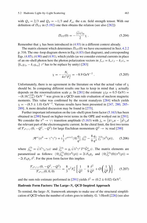
5.2 Hadronic Light–by–Light Scattering 463

with Qu = 2/3 and Qd = −1/3 and Fμν the e.m. field strength tensor. With ourdefinition of ΠVT in (5.192) one then obtains the relation (see also [282])

ΠVT(0) = −〈ψψ〉02

χ . (5.204)

Remember that χ has been introduced in (4.93) in a different context already.The matrix element which determines ΠVT(0)we have encountered in Sect. 4.2.2

p. 316. The one–loop diagram shown in Eq. (4.83) (last diagram), and correspondingEqs. (4.85), (4.90) and (4.91), which yields (as we consider external currents in placeof an on–shell photon here the photon polarization vectors in fαβ = kαεβ − kβεα =(kαgβρ − kβgαρ

)ερ has to be replace by unity) [283]

χ = − Nc

4π2F2π

= −8.9 GeV−2 . (5.205)

Unfortunately, there is no agreement in the literature on what the actual value of χshould be. In comparing different results one has to keep in mind that χ actuallydepends on the renormalization scale μ. In [281] the estimate χ(μ = 0.5 GeV) =−(8.16+2.95

−1.91) GeV−2 was given in a QCD sum rule evaluation of nucleon magnetic

moments. This value was confirmed by the recent reanalysis [284] which yieldsχ = −(8.5 ± 1.0) GeV−2. Various results have been presented in [247, 280, 285–289]. A more detailed discussion may be found in [275].

Further important information on the (on–shell) pion form factor (5.163) has beenobtained in [290] based on higher-twist terms in the OPE and worked out in [291].We consider the π0 → γγ transition amplitude (5.163) with jμ = 2

3 uγμu − 13 dγμd

the relevant part of the electromagnetic current. In the chiral limit, the first two termsof Fπ0γ∗γ∗(0,−Q2,−Q2) for large Euclidean momentum Q2 → ∞ read [290]

Aμν(π0 → γ∗γ∗) = i1

3εμναβ〈 0|qα

q2j (3)5β − 8

9

qα

q4j (3)β |π0(p)〉, (5.206)

where j (3)5μ = ψλ3γμγ5ψ and j (3)μ = gs ψλ3γρ T aGaρμψ. The matrix elements are

parametrized as follows: 〈 0| j (3)5μ (0)|π0(p)〉 = 2i F0 pμ and 〈 0| j (3)μ (0)|π0(p)〉 =−2i F0 pμ δ2. For the pion form factor this implies

Fπ0γ∗γ∗(0,−Q2,−Q2)

Fπ0γγ(0, 0, 0)= 8

3π2F2

0

{1

Q2− 8

9

δ2

Q4+ O

(1

Q6

)}, (5.207)

and the sum rule estimate performed in [291] yields δ2 = (0.2 ± 0.02) GeV2.

Hadronic Form Factors: The Large–Nc QCD Inspired Approach

To remind, the large–Nc framework attempts to make use of the structural simplifi-cation of QCDwhen the number of colors goes to infinity. G. ’t Hooft [226] (see also

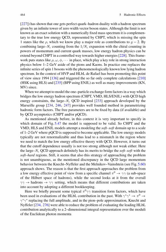
464 5 Hadronic Effects

[227]) has shown that one gets perfect quark–hadron duality with a hadron spectrumgiven by an infinite tower of zero width vector boson states. Although the limit is notknown as an exact solution with a numerically fixed mass spectrum it is complemen-tary to the true low energy QCD, represented by CHPT, which is missing the spin1 states like the ρ, which we know play a major role as contributions to g − 2. Bycombining large–Nc counting from the 1/Nc expansion with the chiral counting inpowers of momentum and current quark masses, low energy hadron physics can beextend beyond CHPT in a controlled way towards higher energies [228]. This frame-work puts states like ρ, ω, φ, · · · in place, which play a key role in strong interactionphysics below 1–2 GeV aside of the pions and Kaons. In practice one replaces theinfinite series of spin 1 bosons with the phenomenologically known low lying hadronspectrum. In the context of HVP and HLbL de Rafael has been promoting this pointof view since 1994 [136] and triggered the so far only complete calculations [210](HSK using HLS) and [235] (BPP using ENJL) as well as many improvements (KN,MV) since.

Whenwe attempt to model the one–particle exchange form factors in a waywhichbridges the low energy hadron spectrum (CHPT, VMD, HLS/ENJL) with QCD highenergy constraints, the large–Nc QCD inspired [233] approach developed by theMarseille group [234, 246, 247] provides well founded method in parametrizinghadronic form factors. The free parameters are to be fixed by data (if available) andby QCD asymptotics (CHPT and/or pQCD).

As mentioned already before, in this context it is very important to specify inwhich domain of Fig. 5.47 the model is supposed to be valid. So CHPT and theVMD, HLS and ENJL models attempt a modeling the soft–soft domain up to a scaleof 1–2 GeV where pQCD is supposed to become applicable. The low energy modelstypically are not renormalizable and thus lead to a mismatch in the region wherewe need to match the low energy effective theory with QCD. However, it turns outthat the cutoff dependence usually is not too strong although not weak either. Herethe large–Nc QCD approach definitely has its merits to bridge the soft–soft with thesoft–hard regions. Still, it seems that also this strategy of approaching the problemis not unambiguous, as the mentioned discrepancy in the QCD large momentumbehavior between the Knecht–Nyffeler and the Melnikov–Vainshtein (see Fig. 5.60)approach shows. The reason is that the first approach approaches the problem froma low energy effective point of view from a specific channel π0 → γγ (a sub-spaceof the Hilbert space of hadrons), while the second looks at it from the overallγγ → hadrons → γγ setting, which means that different contributions are takeninto account by adopting a different bookkeeping.

Here we briefly present some typical π0γγ transition form factors, which havebeen used in evaluations of the HLbL contribution in the past. With γ∗γ∗ → π0 →γ∗γ∗ replacing the full amplitude, and in the pion–pole approximation, Knecht andNyffeler [234, 276] were able to reduce the problem of evaluating the leading HLbLcontribution analytically to a 2–dimensional integral representation over the moduliof the Euclidean photon momenta

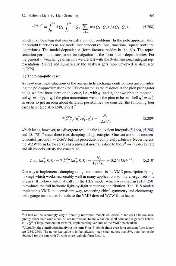
5.2 Hadronic Light–by–Light Scattering 465

aLbL;π0

μ =∫ ∞

0d Q1

∫ ∞

0d Q2

∑

i=1,2

wi (Q1, Q2) fi (Q1, Q2) , (5.208)

which may be integrated numerically without problems. In the pole approximationthe weight functions wi are model independent (rational functions, square roots andlogarithms). The model dependence (form factors) resides in the fi ’s. The repre-sentation permits a transparent investigation of the form factor dependencies. Forthe general π0–exchange diagrams we are left with the 3–dimensional integral rep-resentation (5.172) and numerically the analysis gets more involved as discussedin [275].

(1) The pion–pole case:

Asmost existing evaluations of the one-particle exchange contributions are consider-ing the pole approximation (the FFs evaluated as the residues at the pion propagatorpole), we first focus here on this case, i.e., with q1 and q2 the two photon momentaand q3 = −(q1 + q2) the pion momentum we take the pion to be on–shell q2

3 = m2π.

In order to get an idea about different possibilities we consider the following fourcases here: (see also [248, 292])37

FWZWπ0∗γ∗γ∗(q2

3 , q21 , q

22 ) = Nc

12π2Fπ, (5.209)

which leads, however, to a divergent result in the equivalent integrals (5.166), (5.208)and (5.172),38 since there is no damping at high energies. One can use somemomen-tumcutoff around1 − 2GeV,but this procedure is completely arbitrary.Nevertheless,the WZW form factor serves as a physical normalization to the π0 → γγ decay rateand all models satisfy the constraint

Fπ0γγ(m2π, 0, 0) = FWZW

π0γγ (m2π, 0, 0) = Nc

12π2Fπ= 0.274 GeV−1 . (5.210)

Oneway to implement a damping at highmomentum is the VMDprescription (γ − ρmixing) which works reasonably well in many applications to low-energy hadronicphysics. It follows automatically in the HLS model which was used in [210, 250]to evaluate the full hadronic light-by-light scattering contribution. The HLS modelsimplements VMD in a consistent way, respecting chiral symmetry and electromag-netic gauge invariance. It leads to the VMD dressed WZW form factor

37In fact all the seemingly very differently motivated models collected in Table5.13 below, mar-ginally differ from each other. All are normalized to theWZW on–shell point and in general behaveas 1/Q2 at large momentum transfer, implementing variants of the VMD mechanism.38Actually, the contribution involving the term T2 in (5.166) is finite even for a constant form factor,see [234, 250]. The numerical value is in fact always much smaller, less than 5%, than the resultsobtained for the part with T1 with more realistic form factors.

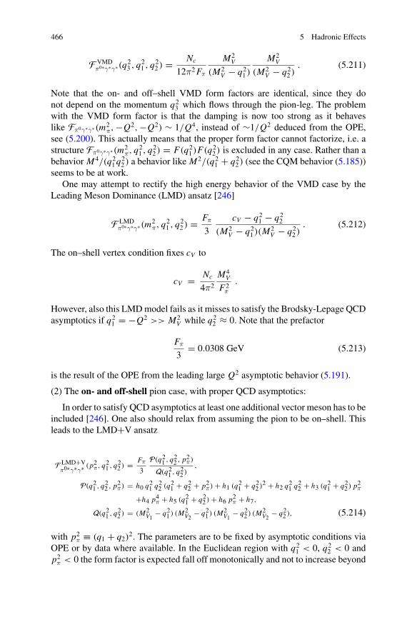
466 5 Hadronic Effects

F VMDπ0∗γ∗γ∗(q2

3 , q21 , q

22 ) = Nc

12π2Fπ

M2V

(M2V − q2

1 )

M2V

(M2V − q2

2 ). (5.211)

Note that the on- and off–shell VMD form factors are identical, since they donot depend on the momentum q2

3 which flows through the pion-leg. The problemwith the VMD form factor is that the damping is now too strong as it behaveslike Fπ0γ∗γ∗(m2

π,−Q2,−Q2) ∼ 1/Q4, instead of ∼1/Q2 deduced from the OPE,see (5.200). This actually means that the proper form factor cannot factorize, i.e. astructure Fπ0γ∗γ∗(m2

π, q21 , q

22 ) = F(q2

1 )F(q22 ) is excluded in any case. Rather than a

behavior M4/(q21q

22 ) a behavior like M

2/(q21 + q2

2 ) (see the CQM behavior (5.185))seems to be at work.

One may attempt to rectify the high energy behavior of the VMD case by theLeading Meson Dominance (LMD) ansatz [246]

F LMDπ0∗γ∗γ∗(m2

π, q21 , q

22 ) = Fπ

3

cV − q21 − q2

2

(M2V − q2

1 )(M2V − q2

2 ). (5.212)

The on–shell vertex condition fixes cV to

cV = Nc

4π2

M4V

F2π

.

However, also this LMDmodel fails as it misses to satisfy the Brodsky-Lepage QCDasymptotics if q2

1 = −Q2 >> M2V while q2

2 ≈ 0. Note that the prefactor

Fπ

3= 0.0308 GeV (5.213)

is the result of the OPE from the leading large Q2 asymptotic behavior (5.191).

(2) The on- and off-shell pion case, with proper QCD asymptotics:

In order to satisfy QCD asymptotics at least one additional vector meson has to beincluded [246]. One also should relax from assuming the pion to be on–shell. Thisleads to the LMD+V ansatz

F LMD+Vπ0∗γ∗γ∗ (p2π, q21 , q22 ) = Fπ

3

P(q21 , q22 , p2π)

Q(q21 , q22 ),

P(q21 , q22 , p2π) = h0 q21 q

22 (q21 + q22 + p2π) + h1 (q21 + q22 )2 + h2 q

21 q

22 + h3 (q21 + q22 ) p2π

+h4 p4π + h5 (q21 + q22 ) + h6 p2π + h7,

Q(q21 , q22 ) = (M2V1

− q21 ) (M2V2

− q21 ) (M2V1

− q22 ) (M2V2

− q22 ), (5.214)

with p2π ≡ (q1 + q2)2. The parameters are to be fixed by asymptotic conditions viaOPE or by data where available. In the Euclidean region with q2

1 < 0, q22 < 0 and

p2π < 0 the form factor is expected fall off monotonically and not to increase beyond

5.2 Hadronic Light–by–Light Scattering 467

the WZW value Fπ0γγ(0, 0, 0) (which fixes h7) in exceptional directions. This letus expect h0, h5, h6 ≤ 0, while h2, h3 + h4, h7 ≥ 0, as we will see h1 = 0 is oneof the asymptotic conditions to be satisfied. Indeed, this pattern is confirmed tothe extend that we have constraints by OPE or data. In spite of the fact that withpresently available experimental data we are not able to constrain unambiguouslyall parameters, we advocate to use the LMD+V off–shell form factor [234] for thenumerical evaluation of the pion-exchange contribution.

Note that in the pion–pole approximation in the chiral limit the parameters h3, h4and h6 are absent. The parameters of the off–shell pion form factor are fixed by thefollowing conditions: the low energy limit is given by

Fπ0γγ(0, 0, 0) = Fπ

3

h7M4

1 M42

= 1

4π2 Fπ⇒ h7 = 3M4

1 M42

4π2 F2π

and fixes h7. From the leading large q2 behavior in the different possible configura-tions we obtain

h0 = −1 ,

is fixed by the all virtualities large OPE condition (5.191). The Brodsky-Lepageasymptotics requires

Fπ0∗γ∗γ(p2π, q

2, 0) ∼ Fπ

3

h1M2

1 M22

+ · · · ⇒ h1 = 0

Fπ0∗γ∗γ(q2, q2, 0) ∼ Fπ

3

h3 + h4M2

1 M22

+ · · · = F0

3χ ⇒ h4 = −h3 + M2

1 M22 χ ,

where we used (5.202) and (5.204) and F0 ≈ Fπ . Note that values for χ in theliterature range from −2.2 GeV−2 to −8.9 GeV−2. We know that the pion exchangepicture is effective when two adjacent currents and hence one quark propagator of theoriginal LbLquark-boxFig. 5.49 (see alsoEq. 5.237below), carries largemomentum,the pionmomentum remaining close to the pionmass shell. For the diagramFig.5.56athis means q2

1 ∼ q22 � q3

3 and the OPE infers the pion dominance picture. The pionacquires large virtuality whenever q2

3 � m2π in fact the pion dominance picture is

expected to break down. In particular q21 ∼ q2

3 � q32 requires two adjacent quark

propagators of the original LbL quark-box to carry large momentum, this shrinks thetwo propagators to a contact term (as illustrated in Fig. 5.61), which carries a∼1/q2.

Nevertheless, using the above constraints we have

Fπ0∗γ∗γ∗(p2π, q2, q2) ∼ −2 Fπ

3

1

q2+ Fπ

3

(h2 − 4 (M2

1 + M22 ) − m2

π

) 1

q4+ · · · ,

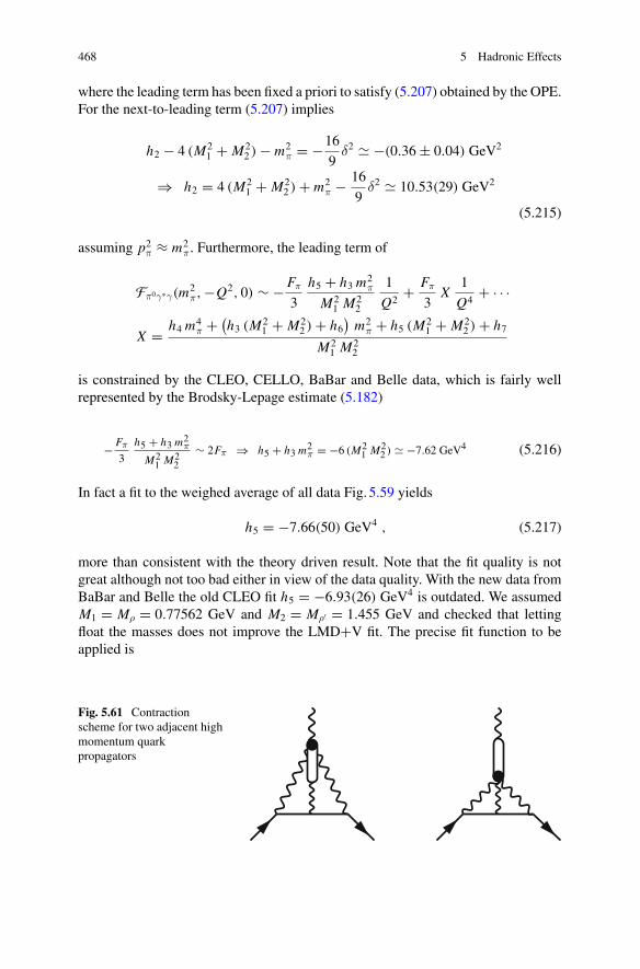
468 5 Hadronic Effects

where the leading term has been fixed a priori to satisfy (5.207) obtained by the OPE.For the next-to-leading term (5.207) implies

h2 − 4 (M21 + M2

2 ) − m2π = −16

9δ2 � −(0.36 ± 0.04) GeV2

⇒ h2 = 4 (M21 + M2

2 ) + m2π − 16

9δ2 � 10.53(29) GeV2

(5.215)

assuming p2π ≈ m2π. Furthermore, the leading term of

Fπ0γ∗γ(m2π,−Q2, 0) ∼ − Fπ

3

h5 + h3 m2π

M21 M2

2

1

Q2+ Fπ

3X

1

Q4+ · · ·

X = h4 m4π + (

h3 (M21 + M2

2 ) + h6)m2

π + h5 (M21 + M2

2 ) + h7M2

1 M22

is constrained by the CLEO, CELLO, BaBar and Belle data, which is fairly wellrepresented by the Brodsky-Lepage estimate (5.182)

− Fπ

3

h5 + h3 m2π

M21 M2

2

∼ 2Fπ ⇒ h5 + h3 m2π = −6 (M2

1 M22 ) � −7.62 GeV4 (5.216)

In fact a fit to the weighed average of all data Fig. 5.59 yields

h5 = −7.66(50) GeV4 , (5.217)

more than consistent with the theory driven result. Note that the fit quality is notgreat although not too bad either in view of the data quality. With the new data fromBaBar and Belle the old CLEO fit h5 = −6.93(26) GeV4 is outdated. We assumedM1 = Mρ = 0.77562 GeV and M2 = Mρ′ = 1.455 GeV and checked that lettingfloat the masses does not improve the LMD+V fit. The precise fit function to beapplied is

Fig. 5.61 Contractionscheme for two adjacent highmomentum quarkpropagators

5.2 Hadronic Light–by–Light Scattering 469

Fπ0γ∗γ(m2π, −Q2, 0) = 1

4π2Fπ

M21

M21 + Q2

M22

M22 + Q2

− Fπ

3

(h5Q

2 + h3m2πQ

2 − h4m4π − h6m

2π

)

M21M

22 (M2

1 + Q2)(M22 + Q2)

(5.218)

where the first term provides the correct on–shell limit. The terms proportional tom2

π are negligible in the range where data exist, such that h3, h4 and h6 cannot befitted and therefore are set to zero (no need for them). These terms are absent in thechiral limit anyway. Actually, h6 ≈ −m2

πh4 in order that the Q2 → 0 limit is givenby the first term. It should be noted that h7 has been fixed neglecting m2

π terms.We always assume that within the uncertainties we do not distinguish between theon–shell transition form factor and its chiral limit. In any case we must require thebound

|h6 + m2π h4| � 3M4

1M42

4π2F2πm

2π

≈ 794.2 GeV4 ∼ (5.3 GeV)4 , (5.219)

which is not a very good bound but it is a true bound.Finally, the configuration at the external vertex

Fπ0∗γ∗γ(−Q2, −Q2, 0) = Fπ

3

h3 + h4M21 M2

2

− Fπ

3

[h5 + h6M21 M2

2

+ h3 + h4M21 M2

2

(M21 + M2

2

)] 1

Q2 + · · ·

to leading order has been fixed by the magnetic susceptibility above already. Thenext to leading term exhibits the so far unknown parameter h6 on which we have noinformation, except the bound just given. In addition, alsoh3 + h4 only is constrained,so essentially h3 and h6 remain free parameters. Since except from [274, 275] nobodyhas done an analysis beyond the pole–approximation, where at least in the chiral limith3, h4 as well as h6 are absent, related problems have never been taken seriously.As it turned out, the results [275] agree within errors with the results obtained in thepole approximation, the difference is mainly in the larger uncertainty. For the poleapproximation the parameters of the LMD+V ansatz [234, 254, 274] are rather wellunder control, and we will also adopt it in the following. One should add here that inthe dispersive approach, to be discussed below in Sect. 5.2.11, everything is fixed inprinciple by physical data and off–shell extrapolations are controlled by analyticity,as far as analyticity helps to extrapolate data fixed only within given uncertainties.

We would like to point out that using the off–shell LMD+V form factor at theexternal vertex leads to a short-distance behavior which qualitatively agrees withthe OPE constraints derived by Melnikov and Vainshtein in [254]. As a matter offact, taking first q2

1 ∼ q22 � q2

3 and then q23 large, one obtains, together with the pion

propagator in (5.166), an overall 1/q23 behavior for the pion-exchange contribution,

as expected from (5.251), since, according to (5.202), F LMD+Vπ0∗γ∗γ (q2

3 , q23 , 0) ∼ const

for large q23 . This also qualitatively agrees with the 1/q2

3 fall-off obtained for thequark-box diagram in light-by-light scattering derived in [254].

470 5 Hadronic Effects

Whatever model for Fπ0γ∗γ∗(m2π, q

21 , q

22 ) is adopted, the low energy constraint

given by FWZWπ0γ∗γ∗(m2

π, 0, 0) is unambiguous. The WZW form factor is a constant andif used at both vertices leads to a divergent result. This is not so surprising as physicsrequires some kind of VMDmechanism as we know. The LMD form factor as well astheHLSand theENJLmodel do not satisfy the largemomentumasymptotics requiredby QCD. Using these models thus leads to cut–off dependent results, where the cut–off is to be varied between reasonable values which enlarges the model error ofsuch estimates. Nevertheless it should be stressed that such approaches are perfectlylegitimate39 and the uncertainties just reflect the lack of precise understanding ofthis kind of physics. For the large–Nc inspired form factors the proper high energybehavior can only by implemented by introducing at least two vector mesons: theρ(770) and the ρ′(1465), which is denoted by LMD+V. One may consider the twoVMD masses as effective masses to be fitted from the data, however the availabledata are not precise enough to establish better fits. For a discussion of form factorsbeyond the pole–approximation we refer also to [248].

Even if we adopt to utilize the LMD+V type form factor, there have been threedifferent version of implementations at the twoverticeswhere it enters. In the notationadapted to the first diagram of Fig. 5.56 the possibilities are:

• F LMD+Vπγ∗γ∗ (m2

π, q21 , q

22 ) · F LMD+V

πγ∗γ (m2π, q

23 , 0) ,

as advocated byKN. It implements the pion–pole approximationwithVMDdampingat internal and external vertex, but violates four momentum conservation at externalvertex.• F LMD+V

πγ∗γ∗ (m2π, q

21 , q

22 ) · FWZW

πγ∗γ (m2π, 0, 0) ,

as advocated byMV.At the internal vertex the LMD+V form factor is adopted, whilethe OPE analysis (considered below) predicts the constant WZW form factor for theexternal vertex. The OPE argument here is based on the asymptotics of the full LbLquark–loop box diagram which refers to the hard–hard regime of Fig. 5.47. VMDdamping in this case we have at internal vertex only. In a way this looks puzzling.How can it be that the off–shell photon at the external vertex does not mix with theρ, which would necessarily dress the form factor and provide a 1/Q2 behavior?• Fπ∗γ∗γ∗(q2

3 , q21 , q

22 ) · Fπ∗γ∗γ(q2

3 , q23 , 0) ,

as advocated by JN. This implements VMD damping for off–shell photons at bothvertices and preserves four momentum conservation at the external vertex. The OPEargument used here refers to the soft–hard regime. Admittedly, the second factorrepresenting a far off–shell pion form factor at spacelike momentum transfer looksobsolete, as not related to any directly observable feature. Why should quarks forma pion at such kinematic circumstances? But, it does not look unreasonable to expectthat it is qualitatively well described by the CQM form factor (see also [278]),which includes the WZW term, but, beyond the chiral limit, exhibits 1/q2 screening

39Suppose we have a perfect RLA parametrization of all data up to an energy Λ above whichpQCD is applicable. Then of course one gets a fully acceptable result even though the RLA isnon-renormalizable and its application may not make any sense beyond Λ. This is known to workperfectly in case of the HVP (see e.g. [46]). In the HLbL case it is the mixed soft–hard regionswhere new kinds of problems arise, and where the OPE analysis comes into play.

5.2 Hadronic Light–by–Light Scattering 471

of the latter, similar to the Brodsky-Lepage formula. If one argues with the chirallimit (no dependence on parameters h3, h4 and h6 which otherwise just enhancethe uncertainty) actually the three alternatives lead to compatible results. The chirallimit is expected to provide a viable approximation within the uncertainties usuallyassigned.

A new constraint on the pion TFF Fπγ∗γ∗(m2π,−Q2

1,−Q22) has been obtained by

a recent lattice QCD calculation [293, 294] for the (0,−Q2,−Q2) configuration,for which any information has been missing so far. Lattice data clearly see a 1/Q2

behavior for increasing Q2. This evidently rules out the naive VMD form factors,and together with the Brodsky–Lepage bound, largely confirmed by the availableexperimental data, only leaves the LMD+V ansatz as a viable parametrization.Whatremains an open problem is the (−Q2,−Q2, 0) configuration relevant at the externalvertex which is related to the problem of the magnetic susceptibility, which weaddressed before.

As an upshot of our elaboration we have sufficient evidence that the large–Nc

inspired LMD+V parametrization should provides a reliable estimation of the lead-ing π0 exchange contribution to aHLbLμ . Simpler parametrizations look to be obsoleteby now. With the parameters constrained above (including an updated π0γγ formfactor fit of the data (see Fig. 5.59) and the recent lattice QCD constraint [293, 294]the updated LMD+V result from [275] now reads

aLbLμ (π0) = (64.68 ± 12.40) × 10−11 (5.220)

The central value and error have been estimated by a scan in the LMD+V off–shell form factor parameter space. By varying those parameters which in theLMD+V ansatz remain only weakly constrained or are not unconstrained in theranges χ = −3.3 ± 1.1 GeV−2, h3, h4 = −10, 0,+10 GeV2 with the constrainth3 + h4 = m2

1m22χ and h6 = −10,−5, 0GeV4. Corresponding energy scales inGeV

units read 674MeV ≥ 1/√

χ ≥ 335MeV,√h3,4 ≤ 3.2GeVand (h6)1/4 ≤ 1.8GeV.

Higher Pseudoscalar Contributions

The higher pseudoscalars η and η′ may be included in a way similar to the π0. Wethus need the TFFs corresponding (5.175) and the adapted master integral (5.172).By the PCAC relation the interpolating fields of the PS mesons are proportional tothe divergence of the axial currents. It is convenient to decompose the axial cur-rent into the different possible flavor channels and write it as a linear combinationof isospin j (3)5μ = qλ3γμγ5q, hypercharge j (8)5μ = qλ8γμγ5q and the SU (3) singlet

j (0)5μ = qλ0γμγ5q, where λ3 = diag(1,−1, 0) and λ8 = diag(1, 1,−2) are the diag-onal Gell-Mann matrices of flavor SU (3) and λ0 is the unit matrix. Then

j5μ =∑

a=3,8,0

ca j (a)

5μ , ca = Tr [λa Q2]Tr [λ2

a]= (3, 1, 4)/18 . (5.221)

472 5 Hadronic Effects

The relative weight factors W (a) for the contributions from different SU (3) flavorstates follow from the flavor–decomposition (5.221) at the two pseudoscalar ver-tices W (a) ∼ c2a multiplied by Tr [λ2

a](= 2, 6, 3) as 1/√Tr [λ2

a] is needed for thenormalization of the states: π0 = (uu − dd)/

√2, η8 = (uu + dd − 2ss)/

√6, and

η0 = (uu + dd + ss)/√3. Thus

W (a) =(Tr [λa Q2]

)2

Tr [λ2a]Tr [Q4] ; W (3) = 1

4, W (8) = 1

12, W (0) = 2

3. (5.222)

where Tr [Q4] = 2/9 is the overall normalization such that∑

a W (a) = 1.The additional complication is the mixing of the pseudoscalar states. In the nonet

symmetry limit (see (5.157)) the relative weight factors are given by (5.222), whichalso follow from the WZW Lagrangian (5.150). Taking into account mixing of η8and η0 into the physical states η and η′ is complicated by the fact that there is agluonic anomaly contribution αs

πGG in the divergence of the axial singlet current

∂μqiγμγ5qi = 2mi qi iγ5qi + αs

πGG .

As we know this implies that η0 unlike the other pseudoscalars is not a Nambu–Goldstone boson in the chiral limit. The proper treatment of mixing in this caserequires two angles to specify the projections from the unmixed sates to mixed onesη and η′ [233]:

F8η = cos θ8F8 , F8

η′ = sin θ8F8

F0η = − sin θ0F0 , F0

η′ = cos θ0F0 .(5.223)

The parameters can be estimated in theory, using for instance large–Nc estimatestogether with the chiral expansion [233], or phenomenologically, using the decaywidths Γ (η → γγ) = 0.510 ± 0.025 keV and Γ (η′ → γγ) = 4.30 ± 0.15 keV andtwo more experimental constraints [295, 297] as an input.Note on the determination of the couplings as they derive from the decays widths

Γ (η → γγ) = α2m3η

64π3F2π

r2η , (η → η or η′ )

where, in the SU (3) octet-singlet basis [233, 297], with c0 = cos θ0, s0 = sin θ0 etc.one obtains

rη = Fπ√3

c0/F8 − 2√2 s8/F0

c0 c8 + s8 s0,

rη′ = Fπ√3

s0/F8 + 2√2 c8/F0

c0 c8 + s8 s0.

5.2 Hadronic Light–by–Light Scattering 473

In the equivalent qs–mixing scheme [295], starting from states |ηq〉 ∼ |uu + dd〉/√2and |ηs〉 ∼ |ss〉, one may write

rη = Fπ

Cπ

[Cq

Fqcosφ − Cs

Fssin φ

],

rη′ = Fπ

Cπ

[Cq

Fqsin φ + Cs

Fscosφ

]

where Cπ = 1/(3√2), Cq = 5/(9

√2) and Cs = 1/9 are charge factors. The angle

φ in leading order of flavor breaking is given by

sin φ =√

((m2η′ − m2

ss) (m2η − m2

qq))/((m2η′ − m2

η) (m2ss − m2

qq))

with m2qq = m2

π , m2ss = 2M2

K − m2π, Fq = Fπ and Fs =

√2 F2

K − F2π . The last two

parameters can be directly determined from the experimental 2γ widths of η andη′. The relative weights W (a) thus are given by (1, r2η , r2η′) since we normalized torπ0 = 1.

The results obtained typically read

F8 = (1.26 ± 0.05) Fπ and F0 = (1.17 ± 0.04) Fπ (5.224)

with mixing angles θ8 = −21.2◦ ± 1.8◦ θ0 = −9.2◦ ± 2.1◦. In the VMD typescreeningwe replace ρ, ρ′ byω,ω′ orφ,φ′. Themass effects alonemπ → mη → mη′

yields aLbL;π0

μ = 59.55 × 10−11 → 15.53 × 10−11 → 10.09 × 10−11. Togetherwith the π0 exchange result (5.220), taking into account the different couplingsand weights as described yields

aLbLμ (π0, η, η′) = (95.45[64.68 + 14.87 + 15.90] ± 12.40) × 10−11 . (5.225)

We are now ready to summarize the results for the pseudoscalar contributionsobtained by the different groups. A comparison of the different results also shedslight on the difficulties and the model dependencies in the theoretical estimationsachieved so far.

A very recent lattice QCD simulation [293, 294] of the doubly virtual π0 → γ∗γ∗form factor is well consistent with the LMD+V parametrization under considerationof other more or less well established constraints yields aHLbL;π0

μ;LMD+V = (65.0 ± 8.3) ×10−11. It is not surprising that the VMD form factor cannot be in agreement with thelattice data, while the LMD+V form factor can be matched.

Table5.13 collects results obtained by other groups, the main differences are dueto the implementation of additional S.D. constraints.

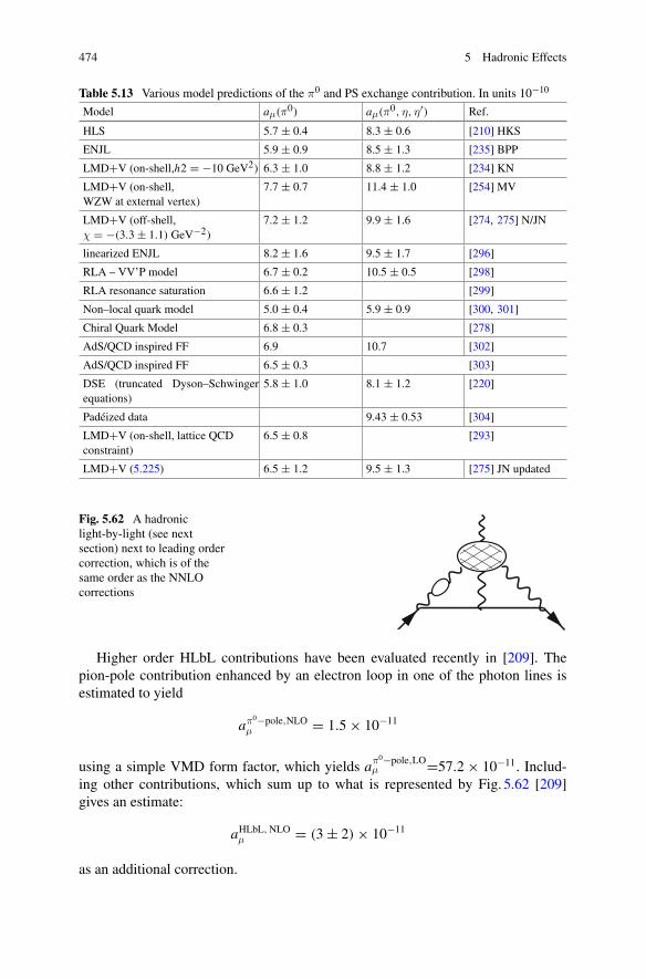
474 5 Hadronic Effects

Table 5.13 Various model predictions of the π0 and PS exchange contribution. In units 10−10

Model aμ(π0) aμ(π0, η, η′) Ref.

HLS 5.7 ± 0.4 8.3 ± 0.6 [210] HKS

ENJL 5.9 ± 0.9 8.5 ± 1.3 [235] BPP

LMD+V (on-shell,h2 = −10 GeV2) 6.3 ± 1.0 8.8 ± 1.2 [234] KN

LMD+V (on-shell,WZW at external vertex)

7.7 ± 0.7 11.4 ± 1.0 [254] MV

LMD+V (off-shell,χ = −(3.3 ± 1.1) GeV−2)

7.2 ± 1.2 9.9 ± 1.6 [274, 275] N/JN

linearized ENJL 8.2 ± 1.6 9.5 ± 1.7 [296]

RLA – VV’P model 6.7 ± 0.2 10.5 ± 0.5 [298]

RLA resonance saturation 6.6 ± 1.2 [299]

Non–local quark model 5.0 ± 0.4 5.9 ± 0.9 [300, 301]

Chiral Quark Model 6.8 ± 0.3 [278]

AdS/QCD inspired FF 6.9 10.7 [302]

AdS/QCD inspired FF 6.5 ± 0.3 [303]

DSE (truncated Dyson–Schwingerequations)

5.8 ± 1.0 8.1 ± 1.2 [220]

Padéized data 9.43 ± 0.53 [304]

LMD+V (on-shell, lattice QCDconstraint)

6.5 ± 0.8 [293]

LMD+V (5.225) 6.5 ± 1.2 9.5 ± 1.3 [275] JN updated

Fig. 5.62 A hadroniclight-by-light (see nextsection) next to leading ordercorrection, which is of thesame order as the NNLOcorrections

Higher order HLbL contributions have been evaluated recently in [209]. Thepion-pole contribution enhanced by an electron loop in one of the photon lines isestimated to yield

aπ0−pole,NLOμ = 1.5 × 10−11

using a simple VMD form factor, which yields aπ0−pole,LOμ =57.2 × 10−11. Includ-

ing other contributions, which sum up to what is represented by Fig. 5.62 [209]gives an estimate:

aHLbL,NLOμ = (3 ± 2) × 10−11

as an additional correction.

5.2 Hadronic Light–by–Light Scattering 475

Besides the methods elaborated so far various other approaches have been appliedto evaluate the pion-pole contribution. In Table5.13 we compare the various predic-tions. The agreement of many results is not an accident: all models must satisfythe π0 → γγ decay constraint and assume a VMD type ∝ 1/Q2 behavior for largeQ2. This latter constraint is implemented differently at the external vertex: in [254]and [274] (see also [282, 299]) a high energy boundary term is included such thatthe Brodsky-Lepage (VMD) ∝ 1/Q2 behavior is replaced by ∝ const at the exter-nal vertex. Corresponding evaluations lead to about 30% larger values which aresupposed to include the quark loop tail.

Before we are going to discuss the evaluation of the yet missing HLbL contribu-tions below in Sect. 5.2.5, we will discuss some more theoretical aspects in order toshed more light on light-by-light.

An Effective Field Theory Approach to HLbL

Analytic calculations of aLbL;hadμ based on simplified (non–RLA) Effective Field

Theory also provided instructive results: these studies are based on the O(Nc, p8)WZW Lagrangian

LWZW = αNc

24πFπεμναβ F μνFαβ

(π0 + 1√

3η

)+ · · · ,

the O(p6) chiral Lagrangian and assuming scalar QED for the interaction of thephoton with the charged pseudoscalars. The leading diagrams are shown in Fig. 5.63.Diagrams (a) and (b) in this approach are divergent and renormalized by the effectivecounter term Lagrangian

L(6) = (α2/4π2F0) δχ ψγμγ5ψ∂μπ0 + · · · (5.226)

generating diagrams (d) and (e). Diagram (c) is finite. The overall divergencerequires a lowest order anomalous magnetic moment type diagram (f). The effectiveLagrangian thus must include a term of type (3.84), with aμ → δaμ. Strictly speak-ing this spoils the predictive power of the effective theory by an overall subtraction,unless the divergence is removed by some other mechanism like the VMD modelagain, for example. Including the pion and Kaon loops of Fig. 5.55, the result maybe cast into the form [251]

aLbL;hadμ =

(α

π

)3 {Nc

(m2

μ

16π2F2π

Nc

3

) [ln2

μ0

mμ+ c1 ln

μ0

mμ+ c0

](5.227)

+ f

(mπ±

mμ,MK±

mμ

)+ O(

m2μ

μ20

× log s,m4

μ

μ40

Nc × log s)

}.

Since Fπ = O(√Nc), the leading term is O(Nc) (see Table5.12) and exhibits a log2

term with universal coefficient C = (N 2c m

2μ)/(48π

2F2π ) � 0.025 for Nc = 3 [251].

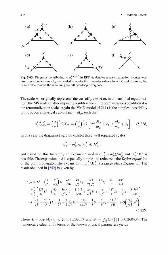
476 5 Hadronic Effects

⊗ ⊗

⊗

μ

π0γ

μ

(a) (b) (c)

(d) (e) (f)

Fig. 5.63 Diagrams contributing to aLbL;π0

μ in EFT. ⊗ denotes a renormalization counter terminsertion. Counter terms δχ are needed to render the triangular subgraphs of (a) and (b) finite, δaμ

is needed to remove the remaining overall two–loop divergence

The scale μ0, originally represents the cut–off μ0 = Λ or, in dimensional regulariza-tion, the MS scale or after imposing a subtraction (= renormalization) condition it isthe renormalization scale. Again the VMD model (5.211) is the simplest possibilityto introduce a physical cut–off μ0 = Mρ, such that

aLbL;π0

μ;VMD =(α

π

)3C Xπ0 =

(α

π

)3C

[ln2

Mρ

mμ+ c1 ln

Mρ

mμ+ c0

]. (5.228)

In this case the diagrams Fig. 5.63 exhibit three well separated scales:

m2π − m2

μ � m2μ � M2

ρ ,

and based on this hierarchy an expansion in δ ≡ (m2π − m2

μ)/m2μ and m2

μ/M2ρ is

possible. The expansion in δ is especially simple and reduces to the Taylor expansionof the pion propagator. The expansion in m2

μ/M2ρ is a Large Mass Expansion. The

result obtained in [252] is given by

Xπ0 = L2 +(1

2− π√

3

)L − 277

216+ 2π√

3S2 − 17π

72√3

+ 57

8S2 − ζ3

6− 11π2

324

+ m2μ

M2ρ

[155

27L2 −

(65

27+ 3π√

3

)L − 11915

1296+ 2π√

3S2 + 4π

3√3

+ 117

4S2 − 1

6ζ3 + 347π2

1944

]

+δ

[(2

3− 2π

3√3

)L − 1

27+ 5

2

π√3S2 − 11π

18√3

− 1

8S2 − 2

9ζ3 + 53π2

648

]+ O

(m4

μ

M4ρ

, δ2

),

(5.229)

where L = log(Mρ/mμ), ζ3 � 1.202057 and S2 = 49√3Cl2

(π3

) � 0.260434. Thenumerical evaluation in terms of the known physical parameters yields

5.2 Hadronic Light–by–Light Scattering 477

aLbL;π0

μ;VMD = [136 − 112 + 30] × 10−11 = +54 × 10−11,

and agrees with the LMD+V model result [234]. Note that there are large can-cellations between leading and subleading terms, although the leading log is siz-able ln(Mρ/mμ) � 1.98. Nyffeler obtained aLbL;π0

μ;VMD = [123 − 103 + 34] × 10−11 =+54 × 10−11 [305] confirming this pattern, by a fit of (5.228) to the representation(5.208) for the VMD model.

An alternative possibility to renormalize the EFT model is to use data froma related process, like a P → +− decay, to fix the counterterms, as performedin [253]. The effective Lagrangian for this process reads

LP+− = − Nc α2

48π2Fπχ μγ

λγ5μ

(∂λπ

0 + 1√3∂λη

)+ · · · ,

where μ denotes a lepton spinor, and using the P+− constraint, one obtainsresult similar to (5.228) with c1 = −2/3 δχ(μ0) + 0.237 = −0.93+0.67

−0.83. The valueof δχ here has been determined from the η → μ+μ− branching fraction, taken as arenormalization condition. This also provides the overall counterterm δaμ requiredto get a finite prediction. In this way one can avoid to refer to the VMD model foreliminating the overall counterterm and use an experimental constraint instead. Theresult obtained is aLbL;π0

μ;P+− = (57+50

−60

) × 10−11. The bare pion and Kaon loops (with

undressed photons) as expected yield a subleading correction with f(mπ±mμ

,MK±mμ

)=

−0.038or δaLbLμ;sQED(π±, K± − loops) � −48 × 10−11. This also agrees (as it should)with known undressed sQED results. Note that the uncertainties in this approach arevery large in general, as far as they have been estimated.

Hadronic Light-by-Light Scattering and the Triangle Anomaly

In order to develop a systematic framework to include also other single hadronexchange contributions we need some more insight into the mechanism of hadropro-duction in LbL scattering. To this end it is instructive to follow the approach advo-cated in [254] (MV’s OPE approach). The alternative way to look at the problemis to use the anomalous PCAC relation (5.232) and to relate π0γγ directly with theABJ anomaly (Bell–Jackiw approach). The profile of the ABJ anomaly we have dis-cussed in Sect. 4.2.2 on p. 299 within the context of the weak hadronic effects. Herewe are interested in the role of the triangle anomaly in the context of the hadroniclight–by-light contribution. We therefore consider the VVA three–point function

Wμνρ(q1, q2) = i∫

d4x1d4x2 e

i (q1·x1+q2·x2) 〈 0 |T{Vμ(x1)Vν(x2)Aρ(0)} | 0 〉(5.230)

of the flavor and color diagonal fermion currents

Vμ = ψγμ ψ, Aμ = ψγμγ5 ψ , (5.231)

478 5 Hadronic Effects

where ψ(x) is a quark field. The vector currents are strictly conserved ∂μV μ(x) = 0,while the axial vector current satisfies a PCAC relation plus the anomaly (indexedby 0 are bare parameters),

∂μAμ(x) = 2 im0 ψγ5ψ(x) + α0

4πεμνρσF

μνFρσ(x) . (5.232)

To leading order the correlator of interest is associatedwith the one–loop triangle dia-gram plus its crossed (q1,μ ↔ q2, ν) partner Fig. 4.20. The covariant decompositionof Wμνρ(q1, q2) into invariant functions has four terms

Wμνρ(q1, q2) = 1

8π2

{wL

(q21 , q

22 , q

23

)(q1 + q2)ρ εμναβ qα

1 qβ2

+ 3 transversal

}.

The longitudinal part is entirely fixed by the anomaly,

wL(q21 , q

22 , q

23

) = −2Nc

q23

, (5.233)

which is exact to all orders of perturbation theory, the famous Adler-Bardeen non–renormalization theorem.

Specifically, the WT identities restrict the covariant decomposition ofWμνρ(q1, q2) to four invariant functions40

Wμνρ(q1, q2) = − 1

8π2

{wL

(q21 , q22 , q23

)(q1 + q2)ρ εμναβ qα

1 qβ2 (5.234)

+ w(+)T

(q21 , q22 , q23

)t (+)μνρ(q1, q2)+ w

(−)T

(q21 , q22 , q23

)t (−)μνρ(q1, q2)+ w

(−)T

(q21 , q22 , q23

)t (−)μνρ (q1, q2)

},

with the transverse tensors given by

t (+)μνρ(q1, q2) = q1ν εμραβ qα

1 qβ2 − q2μ ενραβ qα

1 qβ2 − (q1 · q2) εμνρα (q1 − q2)

α

+ (q21 + q2

2 − q23 )/q

23 εμναβ qα

1 qβ2 (q1 + q2)ρ ,

t (−)μνρ(q1, q2) = [

(q1 − q2)ρ − (q21 − q2

2 )/(q1 + q2)2 (q1 + q2)ρ

]εμναβ qα

1 qβ2 ,

t (−)μνρ (q1, q2) = q1ν εμραβ qα

1 qβ2 + q2μ ενραβ qα

1 qβ2 − (q1 · q2) εμνρα (q1 + q2)

α .

40We closely follow the notation of [306].

5.2 Hadronic Light–by–Light Scattering 479

Bose symmetry (q1,μ ↔ q2, ν) implies

w(+)T

(q22 , q

21 , q

23

) = +w(+)T

(q21 , q

22 , q

23

),

w(−)T

(q22 , q

21 , q

23

) = −w(−)T

(q21 , q

22 , q

23

),

w(−)T

(q22 , q

21 , q

23

) = −w(−)T

(q21 , q

22 , q

23

).

In [306] the following three chiral symmetry relations between amplitudes werederived in pQCD:

[w

(+)T + w

(−)T

] (q21 , q

22 , q

23

) −[w

(+)T + w

(−)T

] (q23 , q

22 , q

21

) = 0 ,[w

(−)T + w

(−)T

] (q21 , q

22 , q

23

) +[w

(−)T + w

(−)T

] (q23 , q

22 , q

21

) = 0 ,[w

(+)T + w

(−)T

] (q21 , q

22 , q

23

) +[w

(+)T + w

(−)T

] (q23 , q

22 , q

21

) = wL(q23 , q

22 , q

21

)

−2

[(q2

2 + q1 · q2)q21

w(+)T

(q23 , q

22 , q

21

) − q1 · q2q21

w(−)T

(q23 , q

22 , q

21

)],

involving the transverse part of the 〈VV A〉 correlatorWμνρ(q1, q2), and which holdfor all values of the momentum transfers q2

1 , q22 and q2

3 .In the kinematic configuration relevant for g − 2 calculations, q1 = k ± q,

q2 = − k, expanding to linear order in k and noting that t (−)μνρ (q1, q2) ∼ t (+)

μνρ(q1, q2) =q2εμνρσkσ − qμενραβqαkβ − qρεμναβqαkβ + O(k2) and t (−)

μνρ(q1, q2) = O(k2), forQ2 = −q2, the relations (5.235) imply Vainshtein’s [283] non-renormalization the-orem: the amplitudes

wL(Q2) ≡ wL(−Q2, 0,−Q2) ,

wT (Q2) ≡ w(+)T (−Q2, 0,−Q2) + w

(−)T (−Q2, 0,−Q2) ,

in the chiral limit satisfy

wT (Q2)pQCD∣∣m=0 = 1

2wL(Q

2)∣∣m=0 , (5.235)

valid to all orders of perturbative QCD in the kinematic limit relevant for the g − 2contribution.

In order to obtain the coupling to pseudoscalars we have to take the derivative asrequired by the PCAC relation, and using (5.233) we obtain

(q1 + q2)ρWμνρ(q1, q2) = 1

8π2εμναβ qα

1 qβ2 wL

(q21 , q

22 , q

23

)q23

= − Nc

4π2εμναβ qα

1 qβ2 . (5.236)

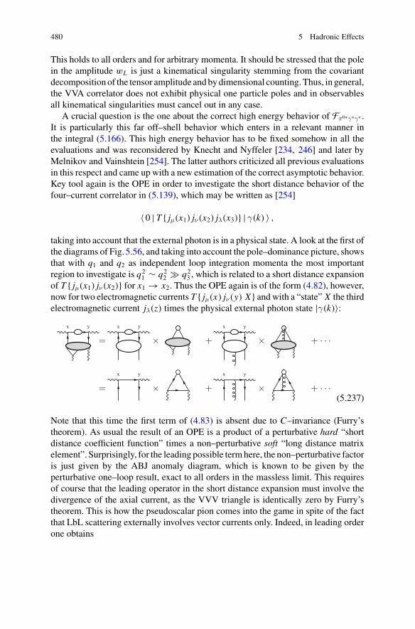
480 5 Hadronic Effects

This holds to all orders and for arbitrary momenta. It should be stressed that the polein the amplitude wL is just a kinematical singularity stemming from the covariantdecomposition of the tensor amplitude andbydimensional counting. Thus, in general,the VVA correlator does not exhibit physical one particle poles and in observablesall kinematical singularities must cancel out in any case.

A crucial question is the one about the correct high energy behavior of Fπ0∗γ∗γ∗ .It is particularly this far off–shell behavior which enters in a relevant manner inthe integral (5.166). This high energy behavior has to be fixed somehow in all theevaluations and was reconsidered by Knecht and Nyffeler [234, 246] and later byMelnikov and Vainshtein [254]. The latter authors criticized all previous evaluationsin this respect and came up with a new estimation of the correct asymptotic behavior.Key tool again is the OPE in order to investigate the short distance behavior of thefour–current correlator in (5.139), which may be written as [254]

〈 0 | T { jμ(x1) jν(x2) jλ(x3)} | γ(k) 〉 ,

taking into account that the external photon is in a physical state. A look at the first ofthe diagrams of Fig. 5.56, and taking into account the pole–dominance picture, showsthat with q1 and q2 as independent loop integration momenta the most importantregion to investigate is q2

1 ∼ q22 � q2

3 , which is related to a short distance expansionof T { jμ(x1) jν(x2)} for x1 → x2. Thus the OPE again is of the form (4.82), however,now for two electromagnetic currents T { jμ(x) jν(y) X} and with a “state” X the thirdelectromagnetic current jλ(z) times the physical external photon state |γ(k)〉:

(5.237)

Note that this time the first term of (4.83) is absent due to C–invariance (Furry’stheorem). As usual the result of an OPE is a product of a perturbative hard “shortdistance coefficient function” times a non–perturbative soft “long distance matrixelement”. Surprisingly, for the leading possible termhere, the non–perturbative factoris just given by the ABJ anomaly diagram, which is known to be given by theperturbative one–loop result, exact to all orders in the massless limit. This requiresof course that the leading operator in the short distance expansion must involve thedivergence of the axial current, as the VVV triangle is identically zero by Furry’stheorem. This is how the pseudoscalar pion comes into the game in spite of the factthat LbL scattering externally involves vector currents only. Indeed, in leading orderone obtains

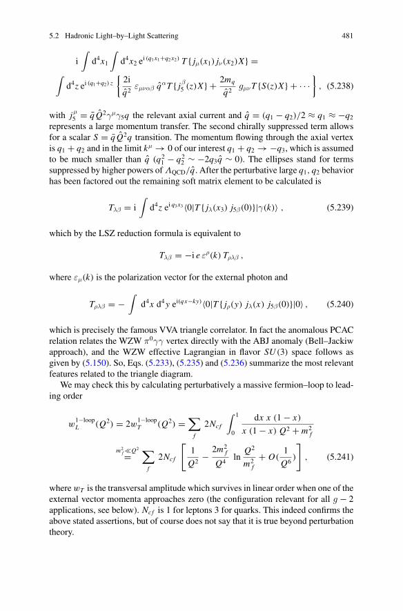
5.2 Hadronic Light–by–Light Scattering 481

i∫

d4x1

∫d4x2 e

i (q1x1+q2x2) T { jμ(x1) jν(x2)X} =∫

d4z ei (q1+q2) z

{2i

q2εμναβ qαT { jβ5 (z)X} + 2mq

q2gμνT {S(z)X} + · · ·

}, (5.238)

with jμ5 = q Q2γμγ5q the relevant axial current and q = (q1 − q2)/2 ≈ q1 ≈ −q2represents a large momentum transfer. The second chirally suppressed term allowsfor a scalar S = q Q2q transition. The momentum flowing through the axial vertexis q1 + q2 and in the limit kμ → 0 of our interest q1 + q2 → −q3, which is assumedto be much smaller than q (q2

1 − q22 ∼ −2q3q ∼ 0). The ellipses stand for terms

suppressed by higher powers ofΛQCD/q . After the perturbative large q1, q2 behaviorhas been factored out the remaining soft matrix element to be calculated is

Tλβ = i∫

d4z ei q3x3〈0|T { jλ(x3) j5β(0)}|γ(k)〉 , (5.239)

which by the LSZ reduction formula is equivalent to

Tλβ = −i e ερ(k) Tρλβ ,

where εμ(k) is the polarization vector for the external photon and

Tρλβ = −∫

d4x d4y ei(qx−ky)〈0|T { jρ(y) jλ(x) j5β(0)}|0〉 , (5.240)

which is precisely the famous VVA triangle correlator. In fact the anomalous PCACrelation relates the WZW π0γγ vertex directly with the ABJ anomaly (Bell–Jackiwapproach), and the WZW effective Lagrangian in flavor SU (3) space follows asgiven by (5.150). So, Eqs. (5.233), (5.235) and (5.236) summarize the most relevantfeatures related to the triangle diagram.

We may check this by calculating perturbatively a massive fermion–loop to lead-ing order

w1−loopL (Q2) = 2w1−loop

T (Q2) =∑

f

2Ncf

∫ 1

0

dx x (1 − x)

x (1 − x) Q2 + m2f

m2f �Q2

=∑

f

2Ncf

[1

Q2− 2m2

f

Q4ln

Q2

m2f

+ O(1

Q6)

], (5.241)

wherewT is the transversal amplitude which survives in linear order when one of theexternal vector momenta approaches zero (the configuration relevant for all g − 2applications, see below). Ncf is 1 for leptons 3 for quarks. This indeed confirms theabove stated assertions, but of course does not say that it is true beyond perturbationtheory.

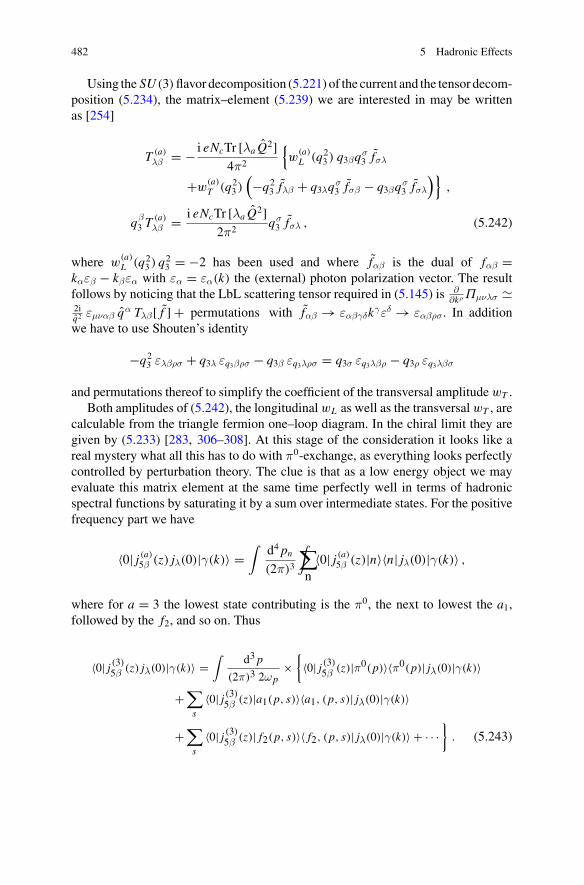
482 5 Hadronic Effects

Using the SU (3)flavor decomposition (5.221) of the current and the tensor decom-position (5.234), the matrix–element (5.239) we are interested in may be writtenas [254]

T (a)

λβ = − i eNcTr [λa Q2]4π2

{w

(a)L (q2

3 ) q3βqσ3 fσλ

+w(a)T (q2

3 )(−q2

3 fλβ + q3λqσ3 fσβ − q3βq

σ3 fσλ

)},

qβ3 T

(a)

λβ = i eNcTr [λa Q2]2π2

qσ3 fσλ , (5.242)

where w(a)L (q2

3 ) q23 = −2 has been used and where fαβ is the dual of fαβ =

kαεβ − kβεα with εα = εα(k) the (external) photon polarization vector. The resultfollows by noticing that the LbL scattering tensor required in (5.145) is ∂

∂kρ Πμνλσ �2iq2 εμναβ qα Tλβ[ f ] + permutations with fαβ → εαβγδkγεδ → εαβρσ. In additionwe have to use Shouten’s identity

−q23 ελβρσ + q3λ εq3βρσ − q3β εq3λρσ = q3σ εq3λβρ − q3ρ εq3λβσ

and permutations thereof to simplify the coefficient of the transversal amplitude wT .Both amplitudes of (5.242), the longitudinal wL as well as the transversal wT , are

calculable from the triangle fermion one–loop diagram. In the chiral limit they aregiven by (5.233) [283, 306–308]. At this stage of the consideration it looks like areal mystery what all this has to do with π0-exchange, as everything looks perfectlycontrolled by perturbation theory. The clue is that as a low energy object we mayevaluate this matrix element at the same time perfectly well in terms of hadronicspectral functions by saturating it by a sum over intermediate states. For the positivefrequency part we have

〈0| j (a)

5β (z) jλ(0)|γ(k)〉 =∫

d4 pn(2π)3

∑∫

n〈0| j (a)

5β (z)|n〉〈n| jλ(0)|γ(k)〉 ,

where for a = 3 the lowest state contributing is the π0, the next to lowest the a1,followed by the f2, and so on. Thus

〈0| j (3)5β (z) jλ(0)|γ(k)〉 =∫

d3 p

(2π)3 2ωp×

{〈0| j (3)5β (z)|π0(p)〉〈π0(p)| jλ(0)|γ(k)〉

+∑

s〈0| j (3)5β (z)|a1(p, s)〉〈a1, (p, s)| jλ(0)|γ(k)〉

+∑

s〈0| j (3)5β (z)| f2(p, s)〉〈 f2, (p, s)| jλ(0)|γ(k)〉 + · · ·

}. (5.243)

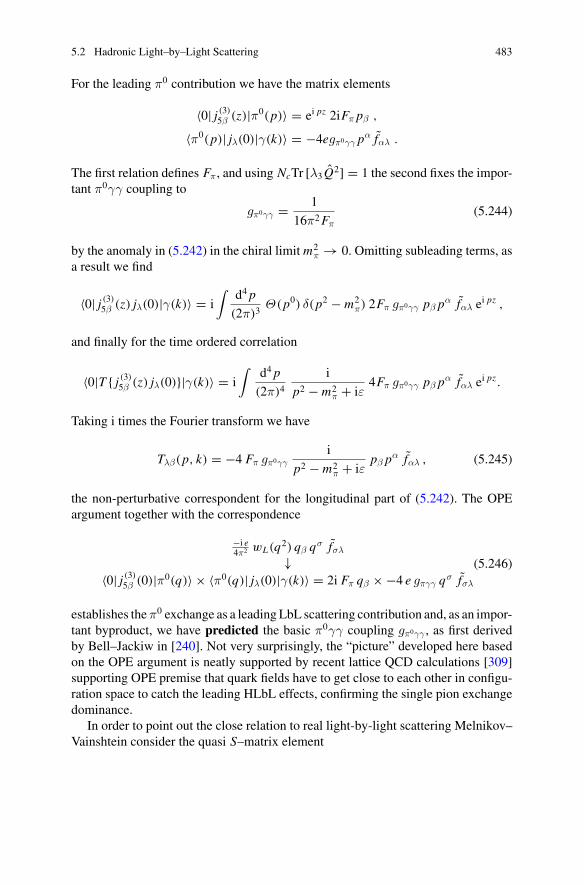
5.2 Hadronic Light–by–Light Scattering 483

For the leading π0 contribution we have the matrix elements

〈0| j (3)5β (z)|π0(p)〉 = ei pz 2iFπ pβ ,

〈π0(p)| jλ(0)|γ(k)〉 = −4egπ0γγ pα fαλ .

The first relation defines Fπ, and using NcTr [λ3 Q2] = 1 the second fixes the impor-tant π0γγ coupling to

gπ0γγ = 1

16π2Fπ(5.244)

by the anomaly in (5.242) in the chiral limit m2π → 0. Omitting subleading terms, as

a result we find

〈0| j (3)5β (z) jλ(0)|γ(k)〉 = i∫

d4 p

(2π)3Θ(p0) δ(p2 − m2

π) 2Fπ gπ0γγ pβ pα fαλ e

i pz ,

and finally for the time ordered correlation

〈0|T { j (3)5β (z) jλ(0)}|γ(k)〉 = i∫

d4 p

(2π)4

i

p2 − m2π + iε

4Fπ gπ0γγ pβ pα fαλ e

i pz .

Taking i times the Fourier transform we have

Tλβ(p, k) = −4 Fπ gπ0γγi

p2 − m2π + iε

pβ pα fαλ , (5.245)

the non-perturbative correspondent for the longitudinal part of (5.242). The OPEargument together with the correspondence

−i e4π2 wL(q2) qβ qσ fσλ

↓〈0| j (3)5β (0)|π0(q)〉 × 〈π0(q)| jλ(0)|γ(k)〉 = 2i Fπ qβ × −4 e gπγγ qσ fσλ

(5.246)

establishes theπ0 exchange as a leadingLbL scattering contribution and, as an impor-tant byproduct, we have predicted the basic π0γγ coupling gπ0γγ , as first derivedby Bell–Jackiw in [240]. Not very surprisingly, the “picture” developed here basedon the OPE argument is neatly supported by recent lattice QCD calculations [309]supporting OPE premise that quark fields have to get close to each other in configu-ration space to catch the leading HLbL effects, confirming the single pion exchangedominance.

In order to point out the close relation to real light-by-light scattering Melnikov–Vainshtein consider the quasi S–matrix element

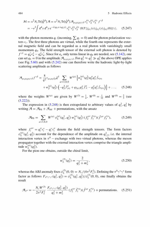
484 5 Hadronic Effects

M = α2NcTr[Q4]A = α2NcTr[Q4]Aμ1μ2μ3γδ εμ11 ε

μ22 ε

μ33 f γδ

= −e3∫

d4x d4y e−i (q1x+q2 y) εμ11 ε

μ22 ε

μ33 〈0|T { jμ1(x) jμ2 (y) jμ3(0)}|γ〉, (5.247)

with the photon momenta qi (incoming,∑

qi = 0) and the photon polarization vec-tors εi . The first three photons are virtual, while the fourth one represents the exter-nal magnetic field and can be regarded as a real photon with vanishingly smallmomentum q4. The field strength tensor of the external soft photon is denoted byf γδ = qγ

4 εδ4 − qδ

4εγ4 . Since for aμ only terms linear in q4 are needed, see (5.142), one

can set q4 = 0 in the amplitudeAμ1μ2μ3γδ . For q21 ≈ q2

2 � q23 the above OPE applies

(see Fig. 5.60) and with (5.242) one can therefore write the hadronic light-by-lightscattering amplitude as follows

Aμ1μ2μ3γδ fγδ = 8

q2εμ1μ2δρq

δ∑

a=3,8,0

W (a){w

(a)L (q23 )qρ

3qσ3 fσμ3

+w(a)T (q23 )

(−q23 f ρ

μ3 + q3μ3qσ3 f ρ

σ − qρ3q

σ3 fσμ3

)}+ . . . , (5.248)

where the weights W (a) are given by W (3) = 14 , W

(8) = 112 and W (0) = 2

3 (see(5.222)).

The expression in (5.248) is then extrapolated to arbitrary values of q21 , q

22 by

writingA = APS + AAV + permutations, with the ansatz

APS =∑

a=3,8,0

W (a) φ(a)L (q2

1 , q22 ) w

(a)L (q2

3 ) ( f μν2 f νμ

1 )( f ρσ f σρ3 ), (5.249)

where f μνi = qμ

i ενi − qν

i εμi denote the field strength tensors. The form factors

φ(a)L (q2

1 , q22 ) account for the dependence of the amplitude on q2

1,2, i.e. the internalinteraction vertex in π0 − exchange with two virtual photons, whereas the mesonpropagator together with the external interaction vertex comprise the triangle ampli-tude w

(a)L (q2

3 ).For the pion one obtains, outside the chiral limit,

w(3)L (q2

3 ) = 2

q23 + m2

π

, (5.250)

whereas the ABJ anomaly fixes φ(3)L (0, 0) = Nc/(4π2F2

π ). Defining the π0γ∗γ∗ formfactor as follows Fπ0γ∗γ∗(q2

1 , q22 ) = φ(3)

L (q21 , q

22 )/φ

(3)L (0, 0), one finally obtains the

result

Aπ0 = −NcW (3)

2π2F2π

Fπ0γ∗γ∗(q21 , q

22 )

q23 + m2

π

( f μν2 f νμ

1 )( f ρσ f σρ3 ) + permutations. (5.251)

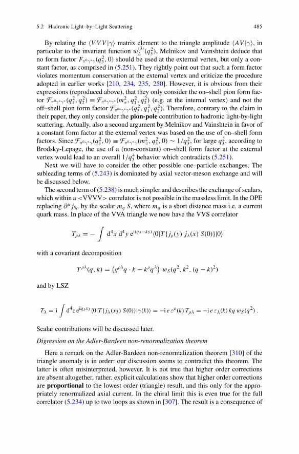
5.2 Hadronic Light–by–Light Scattering 485

By relating the 〈VVV |γ〉 matrix element to the triangle amplitude 〈AV |γ〉, inparticular to the invariant function w

(3)L (q2

3 ), Melnikov and Vainshtein deduce thatno form factor Fπ0γ∗γ(q2

3 , 0) should be used at the external vertex, but only a con-stant factor, as comprised in (5.251). They rightly point out that such a form factorviolates momentum conservation at the external vertex and criticize the procedureadopted in earlier works [210, 234, 235, 250]. However, it is obvious from theirexpressions (reproduced above), that they only consider the on–shell pion form fac-tor Fπ0γ∗γ∗(q2

1 , q22 ) ≡ Fπ0γ∗γ∗(m2

π, q21 , q

22 ) (e.g. at the internal vertex) and not the

off–shell pion form factor Fπ0∗γ∗γ∗(q23 , q

21 , q

22 ). Therefore, contrary to the claim in

their paper, they only consider the pion-pole contribution to hadronic light-by-lightscattering. Actually, also a second argument by Melnikov and Vainshtein in favor ofa constant form factor at the external vertex was based on the use of on–shell formfactors. Since Fπ0γ∗γ(q2

3 , 0) ≡ Fπ0γ∗γ(m2π, q

23 , 0) ∼ 1/q2

3 , for large q23 , according to

Brodsky-Lepage, the use of a (non-constant) on–shell form factor at the externalvertex would lead to an overall 1/q4

3 behavior which contradicts (5.251).Next we will have to consider the other possible one–particle exchanges. The

subleading terms of (5.243) is dominated by axial vector-meson exchange and willbe discussed below.

The second term of (5.238) is much simpler and describes the exchange of scalars,which within a<VVVV> correlator is not possible in the massless limit. In the OPEreplacing ∂μ j5μ by the scalar mq S, where mq is a short distance mass i.e. a currentquark mass. In place of the VVA triangle we now have the VVS correlator

Tρλ = −∫

d4x d4y ei(qx−ky)〈0|T { jρ(y) jλ(x) S(0)}|0〉

with a covariant decomposition

T ρλ(q, k) = (gρλq · k − kρqλ

)wS(q

2, k2, (q − k)2)

and by LSZ

Tλ = i∫

d4z eiq3x3 〈0|T { jλ(x3) S(0)}|γ(k)〉 = −i e ερ(k) Tρλ = −i e ελ(k) kq wS(q2) .

Scalar contributions will be discussed later.

Digression on the Adler-Bardeen non-renormalization theorem

Here a remark on the Adler-Bardeen non-renormalization theorem [310] of thetriangle anomaly is in order: our discussion seems to contradict this theorem. Thelatter is often misinterpreted, however. It is not true that higher order correctionsare absent altogether, rather, explicit calculations show that higher order correctionsare proportional to the lowest order (triangle) result, and this only for the appro-priately renormalized axial current. In the chiral limit this is even true for the fullcorrelator (5.234) up to two loops as shown in [307]. The result is a consequence of

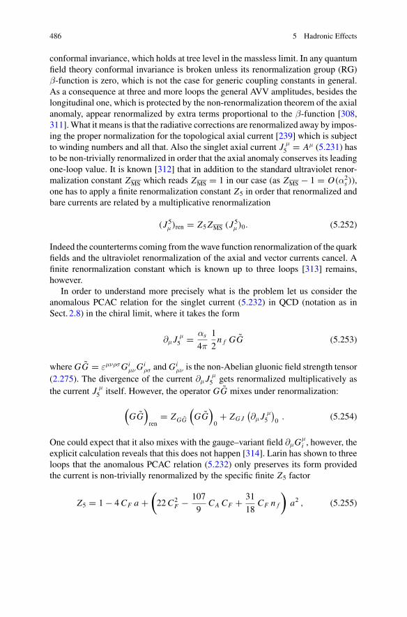
486 5 Hadronic Effects

conformal invariance, which holds at tree level in the massless limit. In any quantumfield theory conformal invariance is broken unless its renormalization group (RG)β-function is zero, which is not the case for generic coupling constants in general.As a consequence at three and more loops the general AVV amplitudes, besides thelongitudinal one, which is protected by the non-renormalization theorem of the axialanomaly, appear renormalized by extra terms proportional to the β-function [308,311].What it means is that the radiative corrections are renormalized away by impos-ing the proper normalization for the topological axial current [239] which is subjectto winding numbers and all that. Also the singlet axial current J μ

5 = Aμ (5.231) hasto be non-trivially renormalized in order that the axial anomaly conserves its leadingone-loop value. It is known [312] that in addition to the standard ultraviolet renor-malization constant ZMS which reads ZMS = 1 in our case (as ZMS − 1 = O(α2

s )),one has to apply a finite renormalization constant Z5 in order that renormalized andbare currents are related by a multiplicative renormalization

(J 5μ )ren = Z5ZMS (J 5

μ )0. (5.252)

Indeed the counterterms coming from thewave function renormalization of the quarkfields and the ultraviolet renormalization of the axial and vector currents cancel. Afinite renormalization constant which is known up to three loops [313] remains,however.

In order to understand more precisely what is the problem let us consider theanomalous PCAC relation for the singlet current (5.232) in QCD (notation as inSect. 2.8) in the chiral limit, where it takes the form

∂μ Jμ5 = αs

4π

1

2n f GG (5.253)

where GG = εμνρσGiμνG

iρσ and G

iμν is the non-Abelian gluonic field strength tensor

(2.275). The divergence of the current ∂μ Jμ5 gets renormalized multiplicatively as

the current J μ5 itself. However, the operator GG mixes under renormalization:

(GG

)

ren= ZGG

(GG

)

0+ ZGJ

(∂μ J

μ5

)0 . (5.254)

One could expect that it also mixes with the gauge–variant field ∂μGμi , however, the

explicit calculation reveals that this does not happen [314]. Larin has shown to threeloops that the anomalous PCAC relation (5.232) only preserves its form providedthe current is non-trivially renormalized by the specific finite Z5 factor

Z5 = 1 − 4CF a +(22C2

F − 107

9CA CF + 31

18CF n f

)a2 , (5.255)

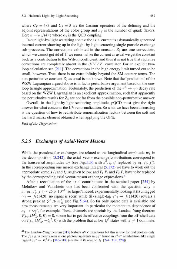
5.2 Hadronic Light–by–Light Scattering 487

where CF = 4/3 and CA = 3 are the Casimir operators of the defining and theadjoint representations of the color group and n f is the number of quark flavors.Here a = αs/(4π) where αs is the QCD coupling.

In our light-by-light scattering context the axial current is a dynamically generatedinternal current showing up in the light-by-light scattering single particle exchangesub-processes. The corrections exhibited in the constant Z5 are true corrections,which we cannot get rid of. If we renormalize the current as usual we get the constantback as a contribution to the Wilson coefficient, and thus it is not true that radiativecorrections are completely absent in the 〈VVVV 〉 correlator. For an explicit two-loop calculation see [211]. The corrections in the high energy limit turned out to besmall, however. True, there is no extra infinity beyond the SM counter terms. Thenon-perturbative constant Z5 as usual is not known. Note that the “prediction” of theWZW Lagrangian argued above is in fact a perturbative argument based on the one-loop triangle approximation. Fortunately, the prediction of the π0 → γγ decay ratebased on the WZW Lagrangian is an excellent approximation, such that apparentlythe perturbative results for Z5 are not far from the possible non-perturbative answer.

Overall, in the light-by-light scattering amplitude, pQCD must give the rightanswer for what concerns the UV renormalization. So what we have been discussingis the question of how to redistribute renormalization factors between the soft andthe hard matrix element obtained when applying the OPE.

End of the Digression

5.2.5 Exchanges of Axial-Vector Mesons

While the pseudoscalar exchanges are related to the longitudinal amplitude wL inthe decomposition (5.242), the axial–vector exchange contributions correspond tothe transversal amplitudes wT (see Fig. 5.56 with π0, η, η′ replaced by a1, f1, f ′

1).In the corresponding one meson exchange integral (5.172) we have to work out theappropriate kernels I1 and I2, as given below, and F1 P6 and F2 P7 have to be replacedby the corresponding axial vector-meson exchange expressions.41

After a reevaluation of the axial contributions in the seminal paper [254] byMelnikov and Vainshtein one has been confronted with the question why isaμ[a1, f ′

1, f1] ∼ 25 × 10−11 so large? Indeed, experimentally looking at (i) untaggedγγ → f1(1420) no signal is seen! while (ii) single-tag γ∗γ → f1(1420) reveals astrong peak at Q2 � m2

f1(see Fig. 5.64). So far only sparse data is available and

new measurements are very important, in particular the momentum dependence ofa1 → γγ∗, for example. These channels are special: by the Landau–Yang theoremFAγγ(M2

A, 0, 0) = 0, so one has to get the effective couplings from the off–shell dataon FAγγ(M2

A,−Q2, 0) with the problem that at low Q2 states with J = 1 dominate.

41The Landau–Yang theorem [315] forbids AVV transitions but this is true for real photons only.The f1 e.g. is clearly seen in one photon tag events in γγ∗ fusion in e+e− annihilation, like singletagged γγ∗ → K 0

s Kπ [316–318] (see the PDG note on f1 [244, 319, 320]).

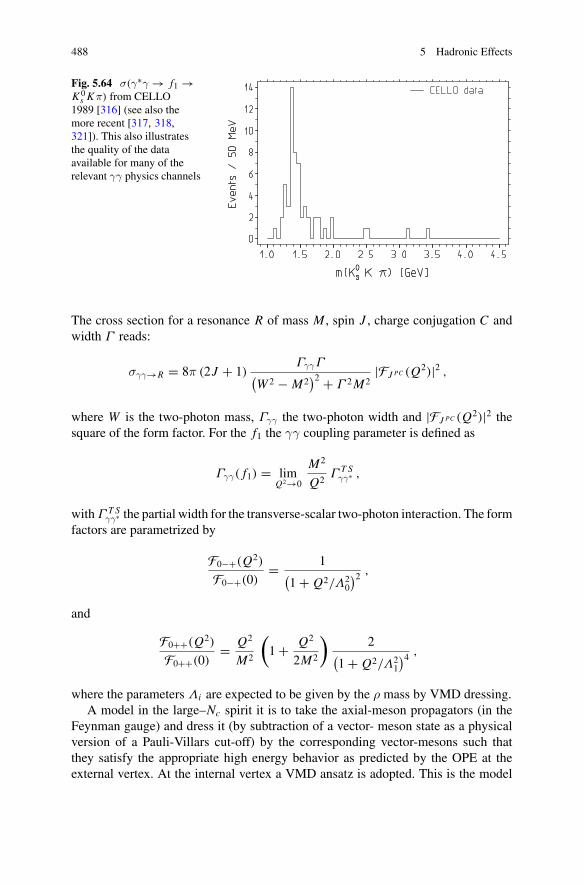
488 5 Hadronic Effects

Fig. 5.64 σ(γ∗γ → f1 →K 0s Kπ) from CELLO

1989 [316] (see also themore recent [317, 318,321]). This also illustratesthe quality of the dataavailable for many of therelevant γγ physics channels

The cross section for a resonance R of mass M , spin J , charge conjugation C andwidth Γ reads:

σγγ→R = 8π (2J + 1)ΓγγΓ

(W 2 − M2

)2 + Γ 2M2|FJ PC (Q2)|2 ,

where W is the two-photon mass, Γγγ the two-photon width and |FJ PC (Q2)|2 thesquare of the form factor. For the f1 the γγ coupling parameter is defined as

Γγγ( f1) = limQ2→0

M2

Q2Γ T S

γγ∗ ,

withΓ T Sγγ∗ the partial width for the transverse-scalar two-photon interaction. The form

factors are parametrized by

F0−+(Q2)

F0−+(0)= 1

(1 + Q2/Λ2

0

)2 ,

and

F0++(Q2)

F0++(0)= Q2

M2

(1 + Q2

2M2

)2

(1 + Q2/Λ2

1

)4 ,

where the parameters Λi are expected to be given by the ρ mass by VMD dressing.A model in the large–Nc spirit it is to take the axial-meson propagators (in the

Feynman gauge) and dress it (by subtraction of a vector- meson state as a physicalversion of a Pauli-Villars cut-off) by the corresponding vector-mesons such thatthey satisfy the appropriate high energy behavior as predicted by the OPE at theexternal vertex. At the internal vertex a VMD ansatz is adopted. This is the model

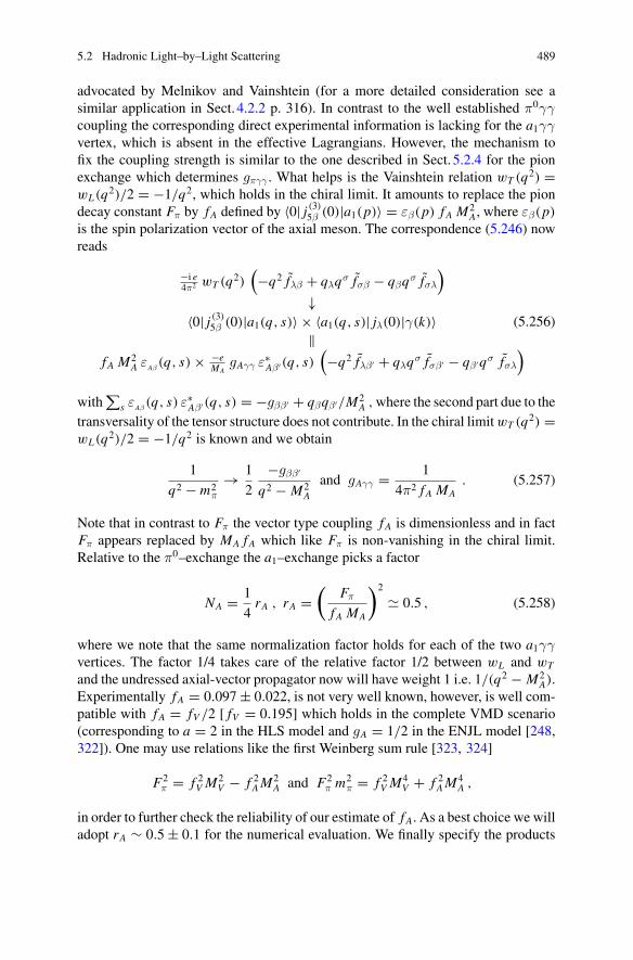
5.2 Hadronic Light–by–Light Scattering 489

advocated by Melnikov and Vainshtein (for a more detailed consideration see asimilar application in Sect. 4.2.2 p. 316). In contrast to the well established π0γγcoupling the corresponding direct experimental information is lacking for the a1γγvertex, which is absent in the effective Lagrangians. However, the mechanism tofix the coupling strength is similar to the one described in Sect. 5.2.4 for the pionexchange which determines gπγγ . What helps is the Vainshtein relation wT (q2) =wL(q2)/2 = −1/q2, which holds in the chiral limit. It amounts to replace the piondecay constant Fπ by f A defined by 〈0| j (3)5β (0)|a1(p)〉 = εβ(p) f A M2

A, where εβ(p)is the spin polarization vector of the axial meson. The correspondence (5.246) nowreads

−i e4π2 wT (q2)

(−q2 fλβ + qλqσ fσβ − qβqσ fσλ

)

↓〈0| j (3)5β (0)|a1(q, s)〉 × 〈a1(q, s)| jλ(0)|γ(k)〉

‖f A M2

A εAβ(q, s) × −e

MAgAγγ ε∗

Aβ′(q, s)(−q2 fλβ′ + qλqσ fσβ′ − qβ′qσ fσλ

)(5.256)

with∑

s εAβ(q, s) ε∗

Aβ′(q, s) = −gββ′ + qβqβ′/M2A ,where the second part due to the

transversality of the tensor structure does not contribute. In the chiral limitwT (q2) =wL(q2)/2 = −1/q2 is known and we obtain

1

q2 − m2π

→ 1

2

−gββ′

q2 − M2A

and gAγγ = 1

4π2 f A MA. (5.257)

Note that in contrast to Fπ the vector type coupling f A is dimensionless and in factFπ appears replaced by MA fA which like Fπ is non-vanishing in the chiral limit.Relative to the π0–exchange the a1–exchange picks a factor

NA = 1

4rA , rA =

(Fπ

f A MA

)2

� 0.5 , (5.258)

where we note that the same normalization factor holds for each of the two a1γγvertices. The factor 1/4 takes care of the relative factor 1/2 between wL and wT

and the undressed axial-vector propagator now will have weight 1 i.e. 1/(q2 − M2A).

Experimentally f A = 0.097 ± 0.022, is not very well known, however, is well com-patible with f A = fV /2 [ fV = 0.195] which holds in the complete VMD scenario(corresponding to a = 2 in the HLS model and gA = 1/2 in the ENJL model [248,322]). One may use relations like the first Weinberg sum rule [323, 324]

F2π = f 2V M

2V − f 2AM

2A and F2

π m2π = f 2V M

4V + f 2AM

4A ,

in order to further check the reliability of our estimate of f A. As a best choice we willadopt rA ∼ 0.5 ± 0.1 for the numerical evaluation. We finally specify the products

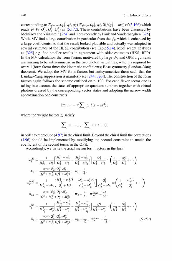
490 5 Hadronic Effects

corresponding toFπ0∗γ∗γ∗(q23 , q

21 , q

22 )Fπ0∗γ∗γ(q2

3 , q23 , 0)/(q

23 − m2

π) of (5.166) whichreads F2 P7(Q2

3, Q21, Q

22) in (5.172). These contributions have been discussed by

Melnikov andVainshtein [254] andmore recently by Pauk andVanderhaeghen [325].While MV find a large contribution in particular from the f1, which is enhanced bya large coefficients, so that the result looked plausible and actually was adopted inseveral estimates of the HLbL contribution (see Table5.14). More recent analysesas [325] e.g. find smaller results in agreement with older estimates (HKS, BPP).In the MV calculation the form factors motivated by large–Nc and OPE argumentsare missing to be antisymmetric in the two photon virtualities, which is required byoverall (form factor times the kinematic coefficients) Bose symmetry (Landau–Yangtheorem). We adopt the MV form factors but antisymmetrize them such that theLandau–Yang suppression is manifest (see [244, 320]). The construction of the formfactors again follows the scheme outlined on p. 190. For each flavor sector one istaking into account the states of appropriate quantum numbers together with virtualphotons dressed by the corresponding vector states and adopting the narrow widthapproximation one constructs

Im wT = π∑

igi δ(s − m2

i ) ,

where the weight factors gi satisfy

∑igi = 1 ,

∑igim

2i = 0 ,

in order to reproduce (4.97) in the chiral limit. Beyond the chiral limit the corrections(4.96) should be implemented by modifying the second constraint to match thecoefficient of the second terms in the OPE.

Accordingly, we write the axial meson form factors in the form

w(3)T = 1

M2a1 − M2

ρ

[M2a1 − m2

π

Q23 + M2

ρ

− M2ρ − m2

π

Q23 + M2

a1

)

]Q23

Q23 + M2

ρ

�(

1

Q23

− m2π

Q43

+ · · ·)

Φ3 = asym(Q22, Q

21) M

4ρ

(Q21 + M2

ρ ) (Q22 + M2

ρ ), W3 = 1

4,

w(ud)T = 1

M2f1

− M2ω

[M2f1

− m2η/5

Q23 + M2

ω

− M2ω − m2

η/5

Q23 + M2

f1

)

]Q23

Q23 + M2

ω

�(

1

Q23

− m2η/5

Q43

+ · · ·)

Φud = asym(Q22, Q

21) M

4ω

(Q21 + M2

ω) (Q22 + M2

ω), W8 = 2

3, W ideal

ud = 25

36,

w(s)T = 1

M2f ′1

− M2φ

[M2f ′1

− m2η

Q23 + M2

φ

−M2

φ − m2η

Q23 + M2

f ′1)

]Q23

Q23 + M2

φ

�(

1

Q23

− m2η

Q43

+ · · ·)

Φs =asym(Q2

2, Q21) M

4φ

(Q21 + M2

φ) (Q22 + M2

φ), W0 = 1

12, W ideal

s = 1

18, (5.259)

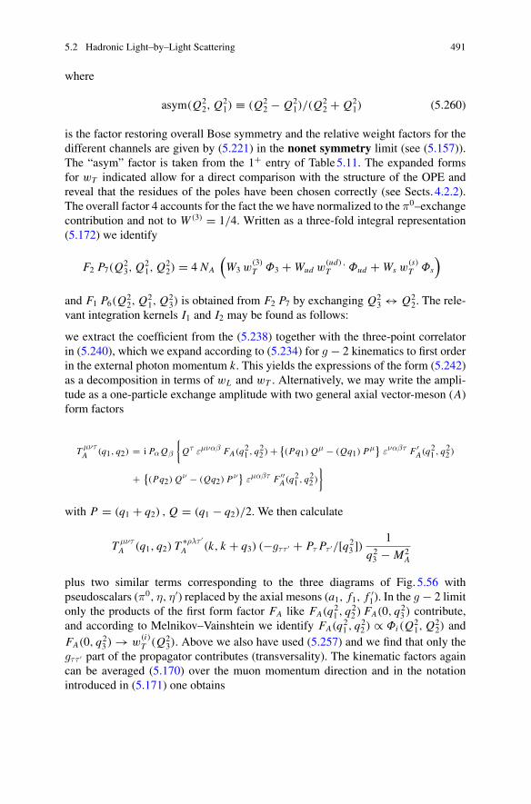
5.2 Hadronic Light–by–Light Scattering 491

where

asym(Q22, Q

21) ≡ (Q2

2 − Q21)/(Q

22 + Q2

1) (5.260)

is the factor restoring overall Bose symmetry and the relative weight factors for thedifferent channels are given by (5.221) in the nonet symmetry limit (see (5.157)).The “asym” factor is taken from the 1+ entry of Table5.11. The expanded formsfor wT indicated allow for a direct comparison with the structure of the OPE andreveal that the residues of the poles have been chosen correctly (see Sects. 4.2.2).The overall factor 4 accounts for the fact the we have normalized to the π0–exchangecontribution and not to W (3) = 1/4. Written as a three-fold integral representation(5.172) we identify

F2 P7(Q23, Q

21, Q

22) = 4 NA

(W3 w

(3)T Φ3 + Wud w

(ud) ,T Φud + Ws w

(s)T Φs

)

and F1 P6(Q22, Q

21, Q

23) is obtained from F2 P7 by exchanging Q2

3 ↔ Q22. The rele-

vant integration kernels I1 and I2 may be found as follows:

we extract the coefficient from the (5.238) together with the three-point correlatorin (5.240), which we expand according to (5.234) for g − 2 kinematics to first orderin the external photon momentum k. This yields the expressions of the form (5.242)as a decomposition in terms of wL and wT . Alternatively, we may write the ampli-tude as a one-particle exchange amplitude with two general axial vector-meson (A)form factors

TμντA (q1, q2) = i PαQβ

{Qτ εμναβ FA(q21 , q22 ) + {

(Pq1) Qμ − (Qq1) P

μ} εναβτ F ′A(q21 , q22 )

+ {(Pq2) Q

ν − (Qq2) Pν} εμαβτ F ′′

A(q21 , q22 )

}

with P = (q1 + q2) , Q = (q1 − q2)/2. We then calculate

T μντA (q1, q2) T

∗ρλτ ′A (k, k + q3) (−gττ ′ + Pτ Pτ ′/[q2

3 ])1

q23 − M2

A

plus two similar terms corresponding to the three diagrams of Fig. 5.56 withpseudoscalars (π0, η, η′) replaced by the axial mesons (a1, f1, f ′

1). In the g − 2 limitonly the products of the first form factor FA like FA(q2

1 , q22 ) FA(0, q2

3 ) contribute,and according to Melnikov–Vainshtein we identify FA(q2

1 , q22 ) ∝ Φi (Q2

1, Q22) and

FA(0, q23 ) → w

(i)T (Q2

3). Above we also have used (5.257) and we find that only thegττ ′ part of the propagator contributes (transversality). The kinematic factors againcan be averaged (5.170) over the muon momentum direction and in the notationintroduced in (5.171) one obtains

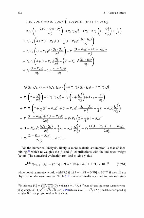
492 5 Hadronic Effects

I1(Q1, Q2, τ ) = X (Q1, Q2, τ )

(−8 P1 P2 (Q1 · Q2) + 4 P1 P3 Q

22

− 2 P1

(6 − 2 (Q1 · Q2)−Q2

2m2

μ

)−4 P2 P3 Q

21 + 4 P2 − 2 P3

(4 + Q2

1m2

μ

)+ 6

m2μ

)

+ P1 P2

(4 + 2 (1 − Rm1) (1 + 1

4(1 − Rm1))

(Q1 · Q2)

m2μ

)

− P1 P3

((1 − Rm2)

2 (Q1 · Q2)

m2μ

)− P1

((1 − Rm1) − 4 (1 − Rm2))

m2μ

− P2 P3

(4 + (1 − Rm1)

Q21

m2μ

− 1

2(1 − Rm1)

2 (Q1 · Q2)

m2μ

)

+ P2(1 − Rm1)

m2μ

− 2 P3(1 − Rm2)

m2μ

,

I2(Q1, Q2, τ ) = X (Q1, Q2τ )

(+4 P1 P2 (Q1 · Q2) − 2 P1 P3 Q

22

− P1

(2 + Q2

2

m2μ

)− 2 P2 P3 Q

21 − P2

(2 + Q2

1

m2μ

)+ 4 P3 − 4

m2μ

)

+ P1 P3

(2 + 1

4((1 − Rm1)

2 + (1 − Rm2)2)

(Q1 · Q2)

m2μ

+ 1

2(1 − Rm2)

Q22

m2μ

)

− P1((1 − Rm1) + 3 (1 − Rm2))

2m2μ

+ P2 P3

(2 + 1

4((1 − Rm1)

2

+ (1 − Rm2)2)

(Q1 · Q2)

m2μ

+ 1

2(1 − Rm1)

Q21

m2μ

)− P2

(3 (1 − Rm1) + (1 − Rm2))

2m2μ

+ P3(2 − Rm1 − Rm2)

2m2μ

− 2 P1 P2 .

For the numerical analysis, likely, a more realistic assumption is that of idealmixing,42 which re-weights the f1 and f1′ contributions with the indicated weightfactors. The numerical evaluation for ideal mixing yields

aLbLμ (a1, f1, f ′1) = (7.55[1.89 + 5.19 + 0.47] ± 2.71) × 10−11 (5.261)

while nonet symmetry would yield 7.58[1.89 + 4.98 + 0.70] × 10−11 if we still usephysical axial-meson masses. Table5.14 collects results obtained in previous stud-

42In this case( f ′f

) = (cos θ −sin θcos θ sin θ

)(ψ8ψ1

)with tan θ = 1/

√2 ( f ′ pure ss) and the nonet symmetry cou-

pling weights (1, 1/√3, 2

√2/

√3) (see (5.150)) turns into (1,−√

2/3, 5/3) and the correspondingweights W (a) are proportional to the squares.

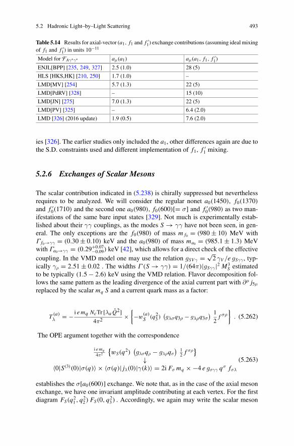
5.2 Hadronic Light–by–Light Scattering 493

Table 5.14 Results for axial-vector (a1, f1 and f ′1) exchange contributions (assuming ideal mixing

of f1 and f ′1) in units 10

−11

Model for FAγ∗γ∗ aμ(a1) aμ(a1, f1, f ′1)

ENJL[BPP] [235, 249, 327] 2.5 (1.0) 28 (5)

HLS [HKS,HK] [210, 250] 1.7 (1.0) –

LMD[MV] [254] 5.7 (1.3) 22 (5)

LMD[PdRV] [328] – 15 (10)

LMD[JN] [275] 7.0 (1.3) 22 (5)

LMD[PV] [325] – 6.4 (2.0)

LMD [326] (2016 update) 1.9 (0.5) 7.6 (2.0)

ies [326]. The earlier studies only included the a1, other differences again are due tothe S.D. constraints used and different implementation of f1, f ′

1 mixing.

5.2.6 Exchanges of Scalar Mesons

The scalar contribution indicated in (5.238) is chirally suppressed but neverthelessrequires to be analyzed. We will consider the regular nonet a0(1450), f0(1370)and f ′

0(1710) and the second one a0(980), f0(600)[= σ] and f ′0(980) as two man-

ifestations of the same bare input states [329]. Not much is experimentally estab-lished about their γγ couplings, as the modes S → γγ have not been seen, in gen-eral. The only exceptions are the f0(980) of mass m f0 = (980 ± 10) MeV withΓ f0→γγ = (0.30 ± 0.10) keV and the a0(980) of mass ma0 = (985.1 ± 1.3) MeVwith Γa0→γγ = (0.29+0.07

−0.09) keV [42], which allows for a direct check of the effectivecoupling. In the VMD model one may use the relation gSVγ = √

2 γV /e gSγγ , typ-ically γρ = 2.51 ± 0.02 . The widths Γ (S → γγ) = 1/(64π)|gSγγ |2 M3

S estimatedto be typically (1.5 − 2.6) keV using the VMD relation. Flavor decomposition fol-lows the same pattern as the leading divergence of the axial current part with ∂μ j5μreplaced by the scalar mq S and a current quark mass as a factor:

T (a)λ = − i e mq NcTr [λa Q2]

4π2×

{−w

(a)S (q23 )

(gλσq3ρ − gλρq3σ

) 1

2f σρ

}. (5.262)

The OPE argument together with the correspondence

i e mq

4π2

{wS(q2)

(gλσqρ − gλρqσ

)12 f

σρ}

↓〈0|S(3)(0)|σ(q)〉 × 〈σ(q)| jλ(0)|γ(k)〉 = 2i Fσ mq × −4 e gσγγ qσ fσλ

(5.263)

establishes the σ[a0(600)] exchange. We note that, as in the case of the axial mesonexchange, we have one invariant amplitude contributing at each vertex. For the firstdiagram FS(q2

1 , q22 ) FS(0, q2

3 ) . Accordingly, we again may write the scalar meson

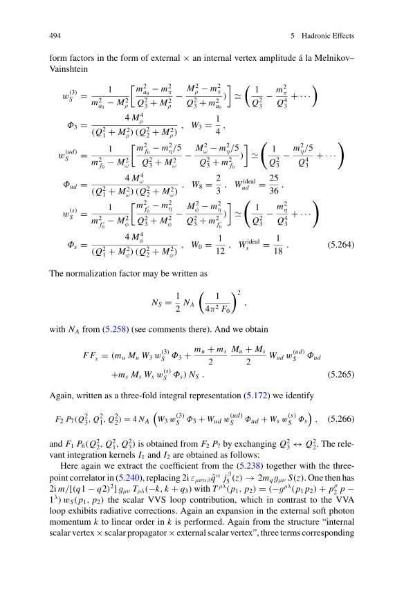
494 5 Hadronic Effects

form factors in the form of external × an internal vertex amplitude á la Melnikov–Vainshtein

w(3)S = 1

m2a0 − M2

ρ

[m2

a0 − m2π

Q23 + M2

ρ

− M2ρ − m2

π

Q23 + m2

a0

)

]�

(1

Q23

− m2π

Q43

+ · · ·)

Φ3 = 4M4ρ

(Q21 + M2

ρ ) (Q22 + M2

ρ ), W3 = 1

4,

w(ud)S = 1

m2f0

− M2ω

[m2

f0− m2

η/5

Q23 + M2

ω

− M2ω − m2

η/5

Q23 + m2

f0

)

]�

(1

Q23

− m2η/5

Q43

+ · · ·)

Φud = 4M4ω

(Q21 + M2

ω) (Q22 + M2

ω), W8 = 2

3, W ideal

ud = 25

36,

w(s)S = 1

m2f ′0− M2

φ

[m2f ′0− m2

η

Q23 + M2

φ

− M2φ − m2

η

Q23 + m2

f ′0

)

]�

(1

Q23

− m2η

Q43

+ · · ·)

Φs = 4M4φ

(Q21 + M2

φ) (Q22 + M2

φ), W0 = 1

12, W ideal

s = 1

18. (5.264)

The normalization factor may be written as

NS = 1

2NA

(1

4π2 F0

)2

,

with NA from (5.258) (see comments there). And we obtain

FFS = (mu Mu W3 w(3)S Φ3 + mu + ms

2

Mu + Ms

2Wud w

(ud)S Φud

+ms Ms Ws w(s)S Φs) NS . (5.265)

Again, written as a three-fold integral representation (5.172) we identify

F2 P7(Q23, Q

21, Q

22) = 4 NA

(W3 w

(3)S Φ3 + Wud w

(ud)S Φud + Ws w

(s)S Φs

), (5.266)

and F1 P6(Q22, Q

21, Q

23) is obtained from F2 P7 by exchanging Q2

3 ↔ Q22. The rele-

vant integration kernels I1 and I2 are obtained as follows:Here again we extract the coefficient from the (5.238) together with the three-

point correlator in (5.240), replacing 2i εμναβ qα jβ5 (z) → 2mqgμν S(z). One then has2im/[(q1 − q2)2] gμν Tρλ(−k, k + q3)with T ρλ(p1, p2) = (−gρλ(p1 p2) + pρ

2 p −1λ) wS(p1, p2) the scalar VVS loop contribution, which in contrast to the VVAloop exhibits radiative corrections. Again an expansion in the external soft photonmomentum k to linear order in k is performed. Again from the structure “internalscalar vertex× scalar propagator× external scalar vertex”, three terms corresponding

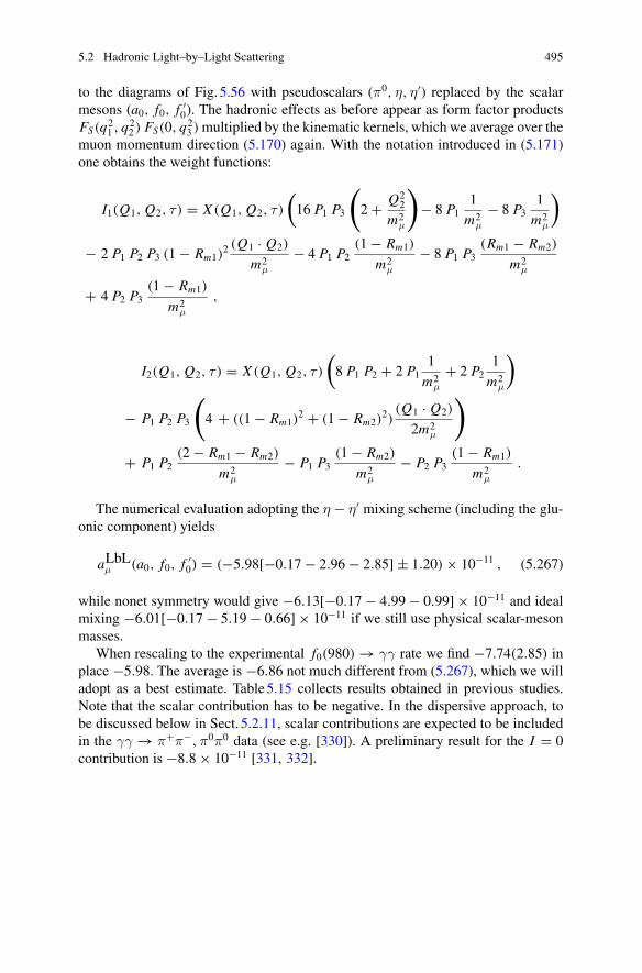
5.2 Hadronic Light–by–Light Scattering 495

to the diagrams of Fig. 5.56 with pseudoscalars (π0, η, η′) replaced by the scalarmesons (a0, f0, f ′

0). The hadronic effects as before appear as form factor productsFS(q2

1 , q22 ) FS(0, q2

3 )multiplied by the kinematic kernels, which we average over themuon momentum direction (5.170) again. With the notation introduced in (5.171)one obtains the weight functions:

I1(Q1, Q2, τ ) = X (Q1, Q2, τ )

(16 P1 P3

(2 + Q2

2

m2μ

)− 8 P1

1

m2μ

− 8 P31

m2μ

)

− 2 P1 P2 P3 (1 − Rm1)2 (Q1 · Q2)

m2μ

− 4 P1 P2(1 − Rm1)

m2μ

− 8 P1 P3(Rm1 − Rm2)

m2μ

+ 4 P2 P3(1 − Rm1)

m2μ

,

I2(Q1, Q2, τ ) = X (Q1, Q2, τ )

(8 P1 P2 + 2 P1

1

m2μ

+ 2 P21

m2μ

)

− P1 P2 P3

(4 + ((1 − Rm1)

2 + (1 − Rm2)2)

(Q1 · Q2)

2m2μ

)

+ P1 P2(2 − Rm1 − Rm2)

m2μ

− P1 P3(1 − Rm2)

m2μ

− P2 P3(1 − Rm1)

m2μ

.

The numerical evaluation adopting the η − η′ mixing scheme (including the glu-onic component) yields

aLbLμ (a0, f0, f ′0) = (−5.98[−0.17 − 2.96 − 2.85] ± 1.20) × 10−11 , (5.267)

while nonet symmetry would give −6.13[−0.17 − 4.99 − 0.99] × 10−11 and idealmixing −6.01[−0.17 − 5.19 − 0.66] × 10−11 if we still use physical scalar-mesonmasses.

When rescaling to the experimental f0(980) → γγ rate we find −7.74(2.85) inplace −5.98. The average is −6.86 not much different from (5.267), which we willadopt as a best estimate. Table5.15 collects results obtained in previous studies.Note that the scalar contribution has to be negative. In the dispersive approach, tobe discussed below in Sect. 5.2.11, scalar contributions are expected to be includedin the γγ → π+π−,π0π0 data (see e.g. [330]). A preliminary result for the I = 0contribution is −8.8 × 10−11 [331, 332].

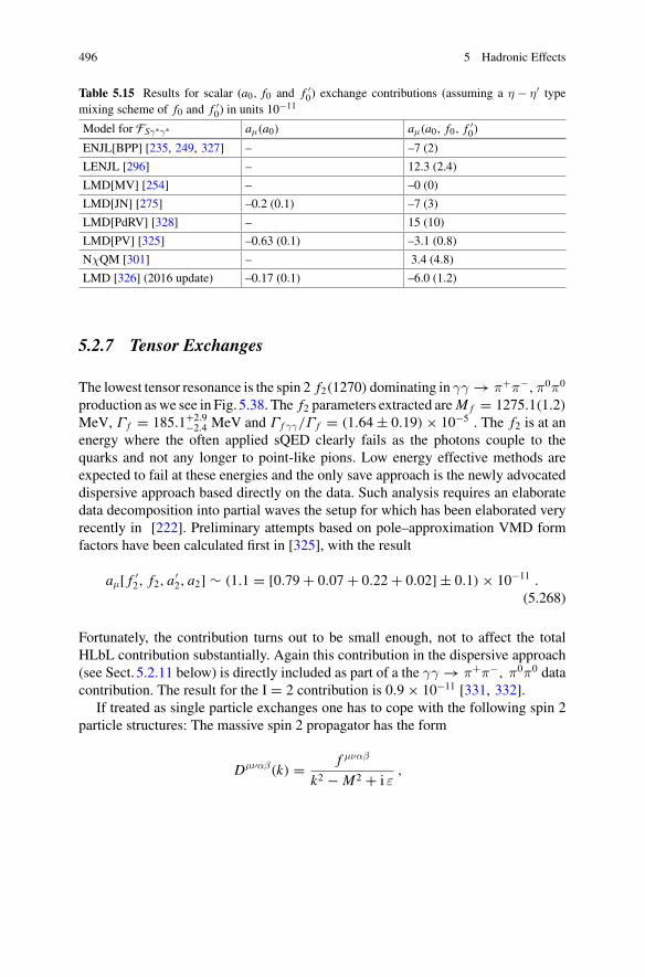
496 5 Hadronic Effects

Table 5.15 Results for scalar (a0, f0 and f ′0) exchange contributions (assuming a η − η′ type

mixing scheme of f0 and f ′0) in units 10−11

Model for FSγ∗γ∗ aμ(a0) aμ(a0, f0, f ′0)

ENJL[BPP] [235, 249, 327] – –7 (2)

LENJL [296] – 12.3 (2.4)

LMD[MV] [254] – –0 (0)

LMD[JN] [275] –0.2 (0.1) –7 (3)

LMD[PdRV] [328] – 15 (10)

LMD[PV] [325] –0.63 (0.1) –3.1 (0.8)

NχQM [301] – 3.4 (4.8)

LMD [326] (2016 update) –0.17 (0.1) –6.0 (1.2)

5.2.7 Tensor Exchanges

The lowest tensor resonance is the spin 2 f2(1270) dominating in γγ → π+π−,π0π0

production aswe see in Fig. 5.38. The f2 parameters extracted areM f = 1275.1(1.2)MeV, Γ f = 185.1+2.9

−2.4 MeV and Γ f γγ/Γ f = (1.64 ± 0.19) × 10−5 . The f2 is at anenergy where the often applied sQED clearly fails as the photons couple to thequarks and not any longer to point-like pions. Low energy effective methods areexpected to fail at these energies and the only save approach is the newly advocateddispersive approach based directly on the data. Such analysis requires an elaboratedata decomposition into partial waves the setup for which has been elaborated veryrecently in [222]. Preliminary attempts based on pole–approximation VMD formfactors have been calculated first in [325], with the result

aμ[ f ′2, f2, a

′2, a2] ∼ (1.1 = [0.79 + 0.07 + 0.22 + 0.02] ± 0.1) × 10−11 .

(5.268)

Fortunately, the contribution turns out to be small enough, not to affect the totalHLbL contribution substantially. Again this contribution in the dispersive approach(see Sect. 5.2.11 below) is directly included as part of a the γγ → π+π−, π0π0 datacontribution. The result for the I = 2 contribution is 0.9 × 10−11 [331, 332].

If treated as single particle exchanges one has to cope with the following spin 2particle structures: The massive spin 2 propagator has the form

Dμναβ(k) = f μναβ

k2 − M2 + i ε,

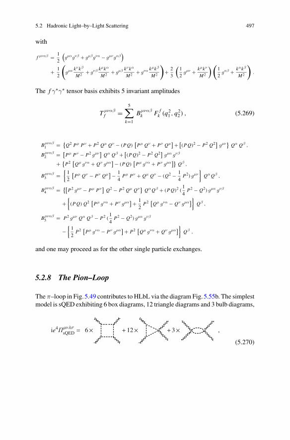
5.2 Hadronic Light–by–Light Scattering 497

with

f μναβ = 1

2

(gμαgνβ + gμβgνα − gμνgαβ

)

+ 1

2

(gμα kνkβ

M2 + gνβ kμkα

M2 + gμβ kνkα

M2 + gνα kμkβ

M2

)+ 2

3

(1

2gμν + kμkν

M2

) (1

2gαβ + kαkβ

M2

).

The f γ∗γ∗ tensor basis exhibits 5 invariant amplitudes

T μναβf =

5∑

k=1

Bμναβk F f

k (q21 , q

22 ) , (5.269)

Bμναβ1 = {

Q2 Pμ Pν + P2 Qμ Qν − (PQ)[Pμ Qν + Pν Qμ

] + [(PQ)2 − P2 Q2] gμν

}Qα Qβ ,

Bμναβ2 = [

Pμ Pν − P2 gμν]Qα Qβ + [

(PQ)2 − P2 Q2] gμα gνβ

+ {P2 [

Qμ gνα + Qν gμα] − (PQ)

[Pμ gνα + Pν gμα

]}Qβ ,

Bμναβ3 =

{1

2

[Pμ Qν − Pν Qμ

] − 1

4Pμ Pν + Qμ Qν − (Q2 − 1

4P2) gμν

}QαQβ ,

Bμναβ4 = {[

P2 gμν − Pμ Pν]Q2 − P2 Qμ Qν

}QαQβ + (PQ)2 (

1

4P2 − Q2) gμα gνβ

+{(PQ) Q2 [

Pμ gνα + Pν gμα] + 1

2P2 [

Qμ gνα − Qν gμα]}

Qβ ,

Bμναβ5 = P2 gμν Qα Qβ − P2 (

1

4P2 − Q2) gμα gνβ

−{1

2P2 [

Pμ gνα − Pν gμα] + P2 [

Qμ gνα + Qν gμα]}

Qβ ,

and one may proceed as for the other single particle exchanges.

5.2.8 The Pion–Loop

The π–loop in Fig. 5.49 contributes to HLbL via the diagram Fig. 5.55b. The simplestmodel is sQED exhibiting 6 box diagrams, 12 triangle diagrams and 3 bulb diagrams,

(5.270)

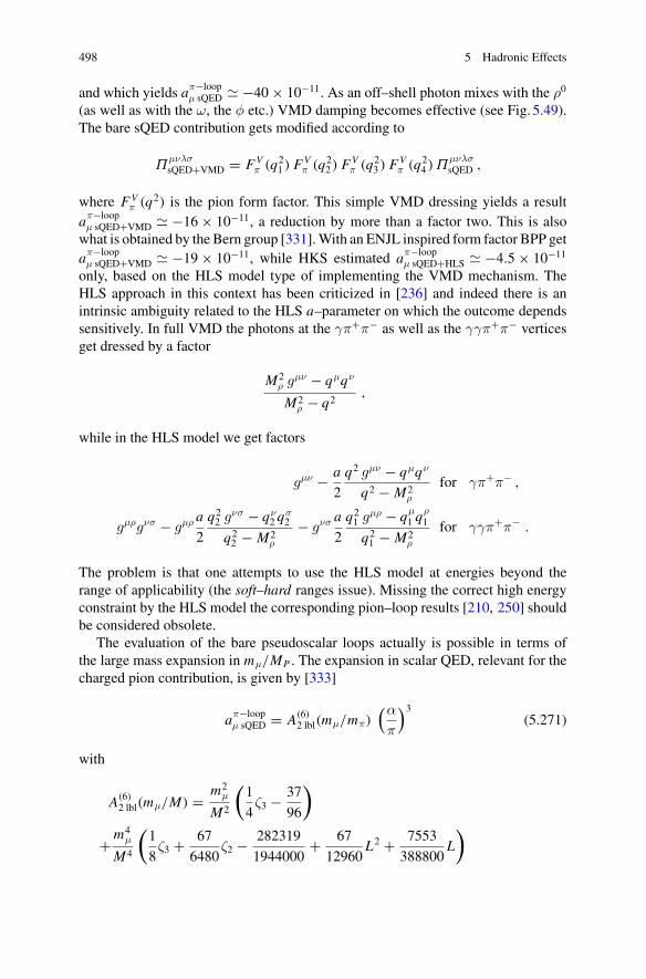
498 5 Hadronic Effects

and which yields aπ−loopμ sQED � −40 × 10−11. As an off–shell photon mixes with the ρ0

(as well as with the ω, the φ etc.) VMD damping becomes effective (see Fig. 5.49).The bare sQED contribution gets modified according to

ΠμνλσsQED+VMD = FV

π (q21 ) F

Vπ (q2

2 ) FVπ (q2

3 ) FVπ (q2

4 )ΠμνλσsQED ,

where FVπ (q2) is the pion form factor. This simple VMD dressing yields a result

aπ−loopμ sQED+VMD � −16 × 10−11, a reduction by more than a factor two. This is alsowhat is obtained by the Bern group [331].With an ENJL inspired form factor BPP getaπ−loop

μ sQED+VMD � −19 × 10−11, while HKS estimated aπ−loopμ sQED+HLS � −4.5 × 10−11

only, based on the HLS model type of implementing the VMD mechanism. TheHLS approach in this context has been criticized in [236] and indeed there is anintrinsic ambiguity related to the HLS a–parameter on which the outcome dependssensitively. In full VMD the photons at the γπ+π− as well as the γγπ+π− verticesget dressed by a factor

M2ρ gμν − qμqν

M2ρ − q2

,

while in the HLS model we get factors

gμν − a

2

q2 gμν − qμqν

q2 − M2ρ

for γπ+π− ,

gμρgνσ − gμρ a

2

q22 gνσ − qν

2 qσ2

q22 − M2

ρ

− gνσ a

2

q21 gμρ − qμ

1 qρ1

q21 − M2

ρ

for γγπ+π− .

The problem is that one attempts to use the HLS model at energies beyond therange of applicability (the soft–hard ranges issue). Missing the correct high energyconstraint by the HLS model the corresponding pion–loop results [210, 250] shouldbe considered obsolete.

The evaluation of the bare pseudoscalar loops actually is possible in terms ofthe large mass expansion in mμ/MP . The expansion in scalar QED, relevant for thecharged pion contribution, is given by [333]

aπ−loopμ sQED = A(6)

2 lbl(mμ/mπ)(α

π

)3(5.271)

with

A(6)2 lbl(mμ/M) = m2

μ

M2

(1

4ζ3 − 37

96

)

+m4μ

M4

(1

8ζ3 + 67

6480ζ2 − 282319

1944000+ 67

12960L2 + 7553

388800L

)

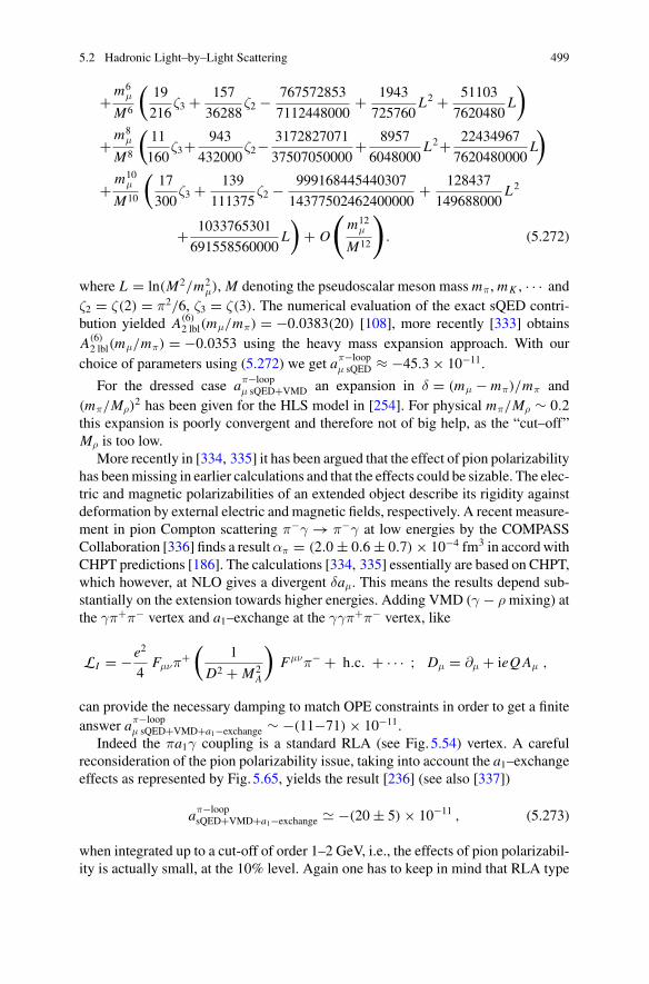
5.2 Hadronic Light–by–Light Scattering 499

+m6μ

M6

(19

216ζ3 + 157

36288ζ2 − 767572853

7112448000+ 1943

725760L2 + 51103

7620480L

)

+m8μ

M8

(11

160ζ3+ 943

432000ζ2− 3172827071

37507050000+ 8957

6048000L2+ 22434967

7620480000L

)

+ m10μ

M10

(17

300ζ3 + 139

111375ζ2 − 999168445440307

14377502462400000+ 128437

149688000L2

+ 1033765301

691558560000L

)+ O

(m12

μ

M12

). (5.272)

where L = ln(M2/m2μ), M denoting the pseudoscalar meson mass mπ , mK , · · · and

ζ2 = ζ(2) = π2/6, ζ3 = ζ(3). The numerical evaluation of the exact sQED contri-bution yielded A(6)

2 lbl(mμ/mπ) = −0.0383(20) [108], more recently [333] obtainsA(6)2 lbl(mμ/mπ) = −0.0353 using the heavy mass expansion approach. With our

choice of parameters using (5.272) we get aπ−loopμ sQED ≈ −45.3 × 10−11.

For the dressed case aπ−loopμ sQED+VMD an expansion in δ = (mμ − mπ)/mπ and

(mπ/Mρ)2 has been given for the HLS model in [254]. For physical mπ/Mρ ∼ 0.2

this expansion is poorly convergent and therefore not of big help, as the “cut–off”Mρ is too low.

More recently in [334, 335] it has been argued that the effect of pion polarizabilityhas beenmissing in earlier calculations and that the effects could be sizable. The elec-tric and magnetic polarizabilities of an extended object describe its rigidity againstdeformation by external electric and magnetic fields, respectively. A recent measure-ment in pion Compton scattering π−γ → π−γ at low energies by the COMPASSCollaboration [336] finds a resultαπ = (2.0 ± 0.6 ± 0.7) × 10−4 fm3 in accord withCHPT predictions [186]. The calculations [334, 335] essentially are based on CHPT,which however, at NLO gives a divergent δaμ. This means the results depend sub-stantially on the extension towards higher energies. Adding VMD (γ − ρ mixing) atthe γπ+π− vertex and a1–exchange at the γγπ+π− vertex, like

LI = −e2

4Fμνπ

+(

1

D2 + M2A

)Fμνπ− + h.c. + · · · ; Dμ = ∂μ + ieQAμ ,

can provide the necessary damping to match OPE constraints in order to get a finiteanswer aπ−loop

μ sQED+VMD+a1−exchange ∼ −(11−71) × 10−11.Indeed the πa1γ coupling is a standard RLA (see Fig. 5.54) vertex. A careful

reconsideration of the pion polarizability issue, taking into account the a1–exchangeeffects as represented by Fig. 5.65, yields the result [236] (see also [337])

aπ−loopsQED+VMD+a1−exchange � −(20 ± 5) × 10−11 , (5.273)

when integrated up to a cut-off of order 1–2 GeV, i.e., the effects of pion polarizabil-ity is actually small, at the 10% level. Again one has to keep in mind that RLA type

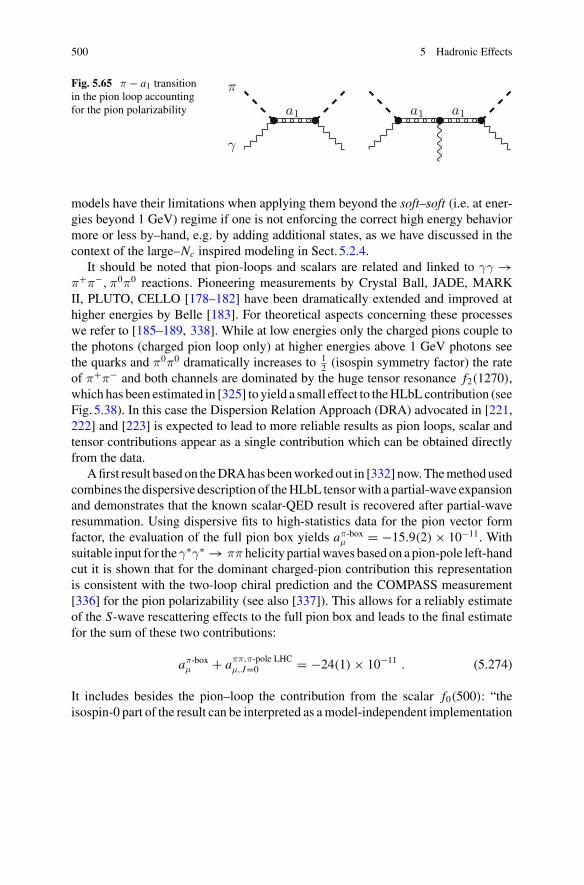
500 5 Hadronic Effects

Fig. 5.65 π − a1 transitionin the pion loop accountingfor the pion polarizability

γ

π

a1 a1 a1

models have their limitations when applying them beyond the soft–soft (i.e. at ener-gies beyond 1 GeV) regime if one is not enforcing the correct high energy behaviormore or less by–hand, e.g. by adding additional states, as we have discussed in thecontext of the large–Nc inspired modeling in Sect. 5.2.4.

It should be noted that pion-loops and scalars are related and linked to γγ →π+π−,π0π0 reactions. Pioneering measurements by Crystal Ball, JADE, MARKII, PLUTO, CELLO [178–182] have been dramatically extended and improved athigher energies by Belle [183]. For theoretical aspects concerning these processeswe refer to [185–189, 338]. While at low energies only the charged pions couple tothe photons (charged pion loop only) at higher energies above 1 GeV photons seethe quarks and π0π0 dramatically increases to 1

2 (isospin symmetry factor) the rateof π+π− and both channels are dominated by the huge tensor resonance f2(1270),which has been estimated in [325] to yield a small effect to theHLbLcontribution (seeFig. 5.38). In this case the Dispersion Relation Approach (DRA) advocated in [221,222] and [223] is expected to lead to more reliable results as pion loops, scalar andtensor contributions appear as a single contribution which can be obtained directlyfrom the data.

Afirst result basedon theDRAhas beenworkedout in [332] now.Themethodusedcombines the dispersive description of theHLbL tensorwith a partial-wave expansionand demonstrates that the known scalar-QED result is recovered after partial-waveresummation. Using dispersive fits to high-statistics data for the pion vector formfactor, the evaluation of the full pion box yields aπ-box

μ = −15.9(2) × 10−11. Withsuitable input for theγ∗γ∗ → ππ helicity partialwaves basedon apion-pole left-handcut it is shown that for the dominant charged-pion contribution this representationis consistent with the two-loop chiral prediction and the COMPASS measurement[336] for the pion polarizability (see also [337]). This allows for a reliably estimateof the S-wave rescattering effects to the full pion box and leads to the final estimatefor the sum of these two contributions:

aπ-boxμ + aππ,π-pole LHC

μ,J=0 = −24(1) × 10−11 . (5.274)

It includes besides the pion–loop the contribution from the scalar f0(500): “theisospin-0 part of the result can be interpreted as amodel-independent implementation

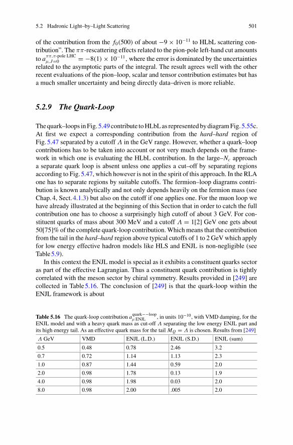
5.2 Hadronic Light–by–Light Scattering 501

of the contribution from the f0(500) of about −9 × 10−11 to HLbL scattering con-tribution”. The ππ-rescattering effects related to the pion-pole left-hand cut amountsto aππ,π-pole LHC

μ,J=0 = −8(1) × 10−11,where the error is dominated by the uncertaintiesrelated to the asymptotic parts of the integral. The result agrees well with the otherrecent evaluations of the pion–loop, scalar and tensor contribution estimates but hasa much smaller uncertainty and being directly data–driven is more reliable.

5.2.9 The Quark-Loop

Thequark–loops inFig. 5.49 contribute toHLbLas representedbydiagramFig. 5.55c.At first we expect a corresponding contribution from the hard–hard region ofFig. 5.47 separated by a cutoff Λ in the GeV range. However, whether a quark–loopcontributions has to be taken into account or not very much depends on the frame-work in which one is evaluating the HLbL contribution. In the large–Nc approacha separate quark loop is absent unless one applies a cut–off by separating regionsaccording to Fig. 5.47, which however is not in the spirit of this approach. In the RLAone has to separate regions by suitable cutoffs. The fermion–loop diagrams contri-bution is known analytically and not only depends heavily on the fermion mass (seeChap.4, Sect. 4.1.3) but also on the cutoff if one applies one. For the muon loop wehave already illustrated at the beginning of this Section that in order to catch the fullcontribution one has to choose a surprisingly high cutoff of about 3 GeV. For con-stituent quarks of mass about 300 MeV and a cutoff Λ = 1[2] GeV one gets about50[75]% of the complete quark-loop contribution.Whichmeans that the contributionfrom the tail in the hard–hard region above typical cutoffs of 1 to 2 GeVwhich applyfor low energy effective hadron models like HLS and ENJL is non-negligible (seeTable5.9).

In this context the ENJL model is special as it exhibits a constituent quarks sectoras part of the effective Lagrangian. Thus a constituent quark contribution is tightlycorrelated with the meson sector by chiral symmetry. Results provided in [249] arecollected in Table5.16. The conclusion of [249] is that the quark-loop within theENJL framework is about

Table 5.16 The quark-loop contribution aquark−−loopμ ENJL , in units 10−10, with VMD damping, for the

ENJL model and with a heavy quark mass as cut-off Λ separating the low energy ENJL part andits high energy tail. As an effective quark mass for the tail MQ = Λ is chosen. Results from [249]

Λ GeV VMD ENJL (L.D.) ENJL (S.D.) ENJL (sum)

0.5 0.48 0.78 2.46 3.2

0.7 0.72 1.14 1.13 2.3

1.0 0.87 1.44 0.59 2.0

2.0 0.98 1.78 0.13 1.9

4.0 0.98 1.98 0.03 2.0

8.0 0.98 2.00 .005 2.0

502 5 Hadronic Effects

aquark−−loopμ ENJL � 20(4) × 10−11 . (5.275)

Note that the choice MQ = Λ looks difficult to be justified and probably underesti-mates the contribution from the tail. But for a cutoff of 8 GeV the contribution fromthe tail in any case is expected to be small and the result should be reliable. The sumof pion-loop + quark-loop is very similar for BPP and HKS, and therefore shouldbe more reliable than the individual contributions, which turn out to be more modeldependent.43

At the beginning of this sectionwe already discussed how sensitive bareLbLquarkloops depend on the quark masses adopted and on a cutoff if applied. With smallconstituent quark masses, or in the extreme when using current quark masses (seeTable5.9 and Footnote 27), one can obtain much larger results. Also the implemen-tation of the VMD type shielding leads the very different results. It is therefore inter-esting to have alternative approaches like solving numerically the non-perturbativeDyson–Schwinger equations of QCD (for QED the DSE have been presented atthe end of Sect. 2.3.1). The DSE estimate of [219, 220] is 10.7(0.2) × 10−10 bya factor 5 larger than the ENJL result and by a factor 2 larger than the CQMresult. Similar size results are obtained in models with a low constituent quarkmass when no VMD-like damping is included. Examples are the non local chi-ral quark model [339] with 11.0(0.9) × 10−10 and a number of estimates withinthe chiral quark model (7.6 − 8.9) × 10−10 [278], (11.8 − 14.8) × 10−10 [340] and(7.6 − 12.5) × 10−10[341] (also see [342]). The last three estimates are thoughtas estimates of the full HLbL contribution and completely ignore the intrinsic non-perturbative feature of the hadronic light-by-light scattering process being dominatedby pseudoscalar meson exchanges.

As mentioned earlier, in the large–Nc resonance saturation approach (LMD+V)the S.D. behavior is incorporated as a boundary condition and no separate quarkloops contributions has to be accounted for concerning the light quark sector. Thereremains the small c–quark contribution

ac−quarkμ pQCD � 2.3 × 10−11 (5.276)

to be taken into account [328].The results from pseudoscalar- and quark-loops of the various evaluations may besummarized as follows.

43Note that within the ENJL framework quarks are constituent quarks and the constituent quarkloop is subject to the VMD mechanism. This differs from simply applying pQCD to the hard–harddomain of Fig. 5.47.

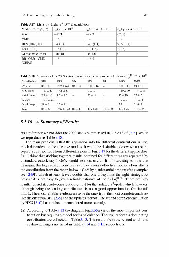
5.2 Hadronic Light–by–Light Scattering 503

Table 5.17 Light–by–Light: π±, K± & quark loops

Model π+π−γ∗(γ∗) aμ(π±) × 1011 aμ(π±, K±) × 1011 aμ(quarks) × 1011

Point −45.3 −49.8 62 (3)

VMD −16 – –

HLS [HKS, HK] −4 ( 8 ) −4.5 (8.1) 9.7 (11.1)

ENJL[BPP] −18 (13) −19 (13) 21 (3)

Guesstimate [MV] 0 (10) 0 (10) 0

DR sQED+VMD[CHPS]

−16 −16.5 −

Table 5.18 Summary of the 2009 status of results for the various contributions to aLbL;hadμ × 1011

Contribution BPP HKS KN MV BP PdRV N/JN

π0, η, η′ 85 ± 13 82.7 ± 6.4 83 ± 12 114 ± 10 – 114 ± 13 99 ± 16

π, K loops −19 ± 13 −4.5 ± 8.1 − 0 ± 10 – −19 ± 19 −19 ± 13

Axial vectors 2.5 ± 1.0 1.7 ± 1.7 − 22 ± 5 – 15 ± 10 22 ± 5

Scalars −6.8 ± 2.0 − − – – −7 ± 7 −7 ± 2

Quark loops 21 ± 3 9.7 ± 11.1 − – – 2.3 21 ± 3

Total 83 ± 32 89.6 ± 15.4 80 ± 40 136 ± 25 110 ± 40 105 ± 26 116 ± 39

5.2.10 A Summary of Results

As a reference we consider the 2009 status summarized in Table13 of [275], whichwe reproduce as Table5.18.

The main problem is that the separation into the different contributions is verymuch dependent on the effective models. It would be desirable to know what are theseparate contributions from different regions in Fig. 5.47 for the different approaches.I still think that sticking together results obtained for different ranges separated bya standard cutoff, say 1 GeV, would be most useful. It is interesting to note thatchanging the high energy constraints of low energy effective models often affectsthe contribution from the range below 1 GeV by a substantial amount (for examplessee [249]), which at least leaves doubts that one always has the right strategy. Atpresent it is not easy to give a reliable estimate of the full aHLbLμ . There are mayresults for isolated sub–contributions, most for the isolated π0–pole, which however,although being the leading contribution, is not a good approximation for the fullHLbL. Themost reliable results seem to be the ones from themost complete analyseslike the one fromBPP [235] and the updates thereof. The second complete calculationby HKS [210] has not been reconsidered more recently.

(a) According to Table5.12 the diagram Fig. 5.55a yields the most important con-tribution but requires a model for its calculation. The results for this dominatingcontribution are collected in Table5.13. The results from the related axial- andscalar-exchanges are listed in Tables5.14 and 5.15, respectively.

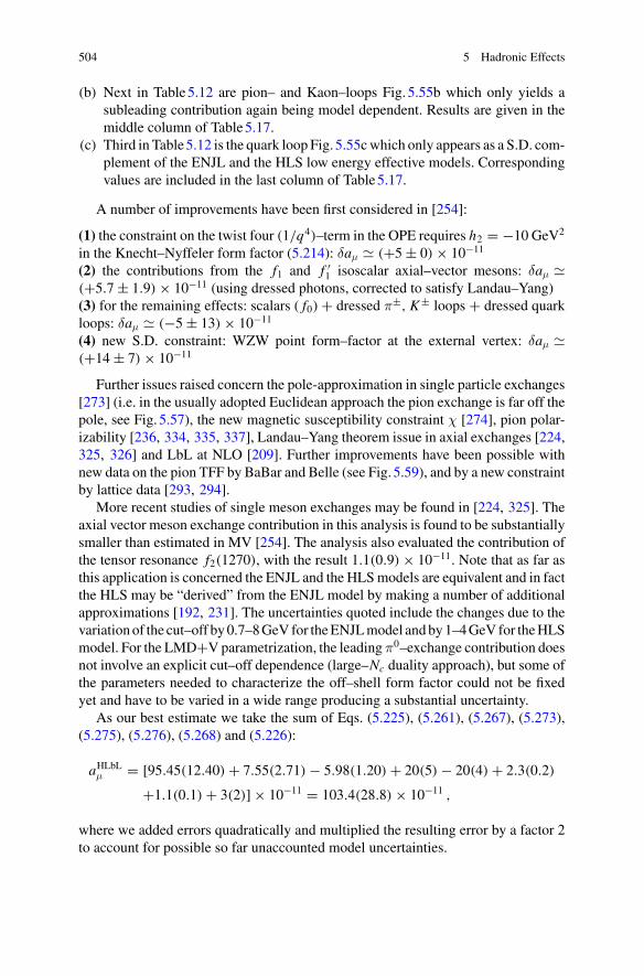
504 5 Hadronic Effects

(b) Next in Table5.12 are pion– and Kaon–loops Fig. 5.55b which only yields asubleading contribution again being model dependent. Results are given in themiddle column of Table5.17.

(c) Third in Table5.12 is the quark loop Fig. 5.55cwhich only appears as a S.D. com-plement of the ENJL and the HLS low energy effective models. Correspondingvalues are included in the last column of Table5.17.

A number of improvements have been first considered in [254]:

(1) the constraint on the twist four (1/q4)–term in the OPE requires h2 = −10 GeV2

in the Knecht–Nyffeler form factor (5.214): δaμ � (+5 ± 0) × 10−11

(2) the contributions from the f1 and f ′1 isoscalar axial–vector mesons: δaμ �

(+5.7 ± 1.9) × 10−11 (using dressed photons, corrected to satisfy Landau–Yang)(3) for the remaining effects: scalars ( f0) + dressed π±, K± loops + dressed quarkloops: δaμ � (−5 ± 13) × 10−11

(4) new S.D. constraint: WZW point form–factor at the external vertex: δaμ �(+14 ± 7) × 10−11

Further issues raised concern the pole-approximation in single particle exchanges[273] (i.e. in the usually adopted Euclidean approach the pion exchange is far off thepole, see Fig. 5.57), the new magnetic susceptibility constraint χ [274], pion polar-izability [236, 334, 335, 337], Landau–Yang theorem issue in axial exchanges [224,325, 326] and LbL at NLO [209]. Further improvements have been possible withnew data on the pion TFF by BaBar and Belle (see Fig. 5.59), and by a new constraintby lattice data [293, 294].

More recent studies of single meson exchanges may be found in [224, 325]. Theaxial vector meson exchange contribution in this analysis is found to be substantiallysmaller than estimated in MV [254]. The analysis also evaluated the contribution ofthe tensor resonance f2(1270), with the result 1.1(0.9) × 10−11. Note that as far asthis application is concerned the ENJL and the HLSmodels are equivalent and in factthe HLS may be “derived” from the ENJL model by making a number of additionalapproximations [192, 231]. The uncertainties quoted include the changes due to thevariationof the cut–off by0.7–8GeV for theENJLmodel andby1–4GeV for theHLSmodel. For the LMD+Vparametrization, the leading π0–exchange contribution doesnot involve an explicit cut–off dependence (large–Nc duality approach), but some ofthe parameters needed to characterize the off–shell form factor could not be fixedyet and have to be varied in a wide range producing a substantial uncertainty.

As our best estimate we take the sum of Eqs. (5.225), (5.261), (5.267), (5.273),(5.275), (5.276), (5.268) and (5.226):

aHLbLμ = [95.45(12.40) + 7.55(2.71) − 5.98(1.20) + 20(5) − 20(4) + 2.3(0.2)

+1.1(0.1) + 3(2)] × 10−11 = 103.4(28.8) × 10−11 ,

where we added errors quadratically and multiplied the resulting error by a factor 2to account for possible so far unaccounted model uncertainties.

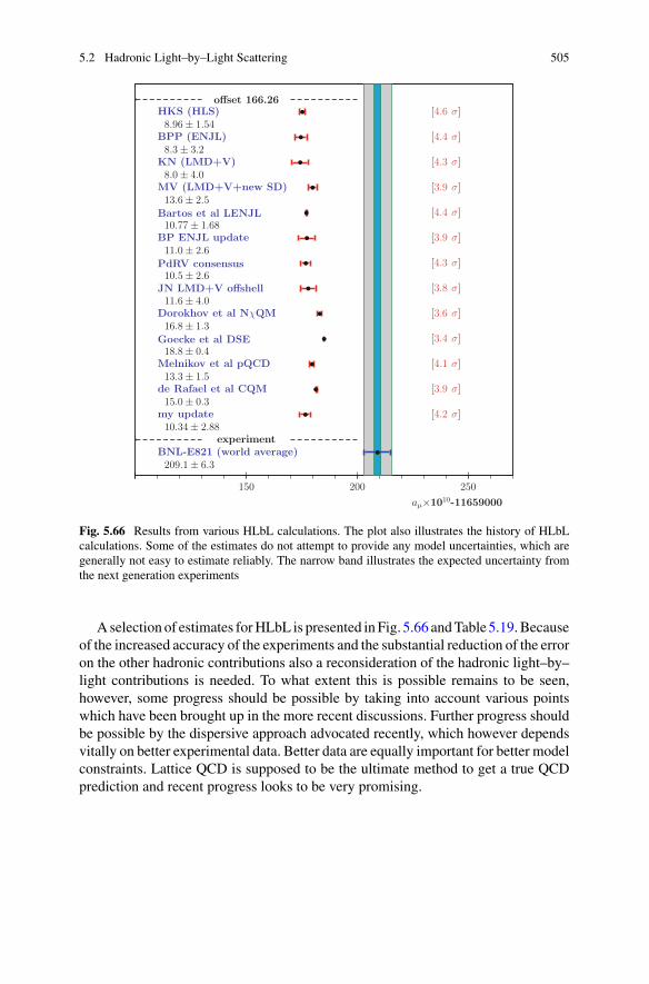
5.2 Hadronic Light–by–Light Scattering 505

Fig. 5.66 Results from various HLbL calculations. The plot also illustrates the history of HLbLcalculations. Some of the estimates do not attempt to provide any model uncertainties, which aregenerally not easy to estimate reliably. The narrow band illustrates the expected uncertainty fromthe next generation experiments

A selection of estimates forHLbL is presented in Fig. 5.66 andTable5.19.Becauseof the increased accuracy of the experiments and the substantial reduction of the erroron the other hadronic contributions also a reconsideration of the hadronic light–by–light contributions is needed. To what extent this is possible remains to be seen,however, some progress should be possible by taking into account various pointswhich have been brought up in the more recent discussions. Further progress shouldbe possible by the dispersive approach advocated recently, which however dependsvitally on better experimental data. Better data are equally important for better modelconstraints. Lattice QCD is supposed to be the ultimate method to get a true QCDprediction and recent progress looks to be very promising.

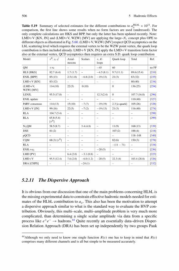
506 5 Hadronic Effects

Table 5.19 Summary of selected estimates for the different contributions to aHLbLμ × 1011. Forcomparison, the first line shows some results when no form factors are used (undressed). Theonly complete calculations are HKS and BPP, but only the latter has been updated recently. Note:LMD+V [KN, JN] and (LMD+V, WZW) [MV] are applying the large–Nc concept plus OPE todifferent objects as illustrated in Fig. 5.60. (LMD+V,WZW) [MV] respect QCD asymptotics on theLbL scattering level which requires the external vertex to be the WZW point vertex, the quark loopcontribution is then included already. LMD+V [KN, JN] apply the LMD+V transition form factoralso at the external vertex, QCD asymptotics then requires an extra S.D. quark loop contributionModel π0, η, η′ Axial-

mesonsScalars π, K -

loopsQuark-loop Total Ref.

QM +∞ – – −45 60 – no FF

HLS [HKS] 82.7 (6.4) 1.7 (1.7) – −4.5 (8.1) 9.7 (11.1) 89.6 (15.4) [210]

ENJL [BPP] 85 (13) 2.5 (1.0) −6.8 (2.0) −19 (13) 21 (3) 83 (32) [235]

LMD+V [KN] 83 (12) – – – – 80 (40) [234]

(LMD+V,WZW) [MV]

114 (10) 22 (5) 0 (10) 0 136 (25) [254]

LENJL 95.5 (17.0) – – 12.3 (2.4) 0 107.7 (16.8) [296]

ENJL update – – – – – 110 (40) [327]

PdRV consensus 114 (13) 15 (10) −7 (7) −19 (19) 2.3 [c-quark] 105 (26) [328]

LMD+V [JN] 99 (16) 22 (5) −7 (2) −19 (13) 21 (3) 116 (40) [274]

RLA 104.7 (5.4) – – – – – [298]

RLA 65.8 (5.4)[π0]

– – – – – [299]

NχQM 58.5 (8.7) – 3.4 (4.8) – 11 (9) 168 (13) [339]

DSE 81 (2) – – – 107 (2) 188 (4) [218]

pQCD – – – – – 118–148 [340]

CQM 68(3) [π0] – – – 82 (6) 150 (3) [278]

RLA – – – – −(11 − 71) – [334]

ENJL+a1 – – – −20 (5) – – [236]

LMD [PV] – 6.4 (2.0) −3.1 (0.8) – – – [223]

LMD+V 95.5 (12.4) 7.6 (2.0) −6.0 (1.2) −20 (5) 22.3 (4) 103.4 (28.8) [326]

DRA [CHPS] – – −24 (1) – – [332]

5.2.11 The Dispersive Approach

It is obvious from our discussion that one of the main problems concerning HLbL isthe missing experimental data to constrain effective hadronic models needed for esti-mates of the HLbL contribution to aμ. This also has been the motivation to attempta dispersive approach similar to what is the standard way to evaluate the HVP con-tribution. Obviously, this multi–scale, multi–amplitude problem is very much morecomplicated, than determining a single scalar amplitude via data from a specificprocess like e+e− → hadrons.44 Quite recently an essentially data–driven Disper-sion Relation Approach (DRA) has been set up independently by two groups Pauk

44Although we only need to know one single function R(s) one has to keep in mind that R(s)comprises many different channels and is all but simple to be measured accurately.

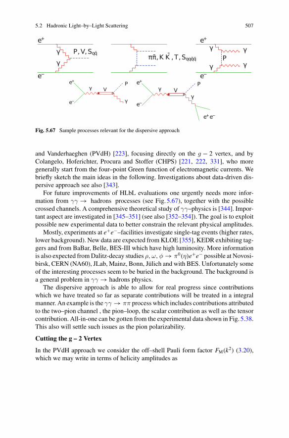
5.2 Hadronic Light–by–Light Scattering 507

Fig. 5.67 Sample processes relevant for the dispersive approach

and Vanderhaeghen (PVdH) [223], focusing directly on the g − 2 vertex, and byColangelo, Hoferichter, Procura and Stoffer (CHPS) [221, 222, 331], who moregenerally start from the four–point Green function of electromagnetic currents. Webriefly sketch the main ideas in the following. Investigations about data-driven dis-persive approach see also [343].

For future improvements of HLbL evaluations one urgently needs more infor-mation from γγ → hadrons processes (see Fig. 5.67), together with the possiblecrossed channels. A comprehensive theoretical study of γγ–physics is [344]. Impor-tant aspect are investigated in [345–351] (see also [352–354]). The goal is to exploitpossible new experimental data to better constrain the relevant physical amplitudes.

Mostly, experiments at e+e−–facilities investigate single-tag events (higher rates,lower background). New data are expected fromKLOE [355], KEDR exhibiting tag-gers and from BaBar, Belle, BES-III which have high luminosity. More informationis also expected fromDalitz-decay studies ρ,ω,φ → π0(η)e+e− possible at Novosi-birsk, CERN (NA60), JLab, Mainz, Bonn, Jülich and with BES. Unfortunately someof the interesting processes seem to be buried in the background. The background isa general problem in γγ → hadrons physics.

The dispersive approach is able to allow for real progress since contributionswhich we have treated so far as separate contributions will be treated in a integralmanner. An example is the γγ → ππ process which includes contributions attributedto the two–pion channel , the pion–loop, the scalar contribution as well as the tensorcontribution. All-in-one can be gotten from the experimental data shown in Fig. 5.38.This also will settle such issues as the pion polarizability.

Cutting the g – 2 Vertex

In the PVdH approach we consider the off–shell Pauli form factor FM(k2) (3.20),which we may write in terms of helicity amplitudes as

508 5 Hadronic Effects

F2(k2) = e6

∑

λ1,λ2,λ3,λ

(−1)λ+λ1+λ2+λ3

∫d4q1(2π)4

∫d4q2(2π)4

Lλ1λ2λ3λ(p, q1, k − q1 − q2, q2)

× Πλ1λ2λ3λ(q1, k − q1 − q2, q2, k)

q21q22 (k − q1 − q2)2

[(p + q1)2 − m2

] [(p + k − q2)2 − m2

] , (5.277)

which is the off–shell version of (5.148) derived earlier [with q2 ↔ q3]. Here, theFourier transform of the four-current correlator (5.139) has been projected onto thehelicity basis

Πλ1λ2λ3λ4(q1, q2, q3) = εμ(q1,λ1)εν(q2,λ2)ε

λ(q3,λ3)ερ(q4,λ4)Πμνλρ(q1, q2, q3)

by means of the photon polarization vectors ε(q,λ), by inserting the completenessrelation ∑

λ=±ε∗ν(p,λ)εμ(p,λ) = −gμν

modulo gauge terms (see (2.26)). The complementary coefficients correspondinglyread

Lλ1λ2λ3λ4 (p, q1, q2, q3) = ε∗μ(λ1, q1)ε

∗ν(λ2, q2)ε

∗λ(λ3, q3)ε

∗σ(λ4, q4)

× Tr[Λσ(p + q1 + q2, p)γ

λ( /p + /q1 + /q2 + m)γν( /p + /q1 + m)γμ],

with projector (3.92) and (3.93):

Λσ(p′, p) = m2

k2(4m2 − k2)( /p + m)

[γσ + k2 + 2m2

m(k2 − 4m2)(p′ + p)σ

]( /p′ + m).

serves to insert the LbL scattering tensor into the magnetic form factor.When analytically continued to complex values of the external photon’s virtuality

k2, the muon’s electromagnetic vertex function possesses branch point singularitiesjoining the physical production thresholds, as is dictated by unitarity45 (see Sects. 3.7and 3.8). Using Cauchy’s integral theorem, the off–shell form factor FM(k2) can berepresented as an integral along a closed contour avoiding the cuts and extended toinfinity. Assuming that the form factor vanishes uniformly when k2 tends to infin-ity the contour integral reduces to an integral of the form factor’s discontinuityDisck2FM(k2) along the cut in the k2-plane starting from the lowest branch point:

FM(0) = 1

2πi

∞∫

0

dk2

k2Disck2 FM(k2). (5.278)

45For the discussion of the anomalous thresholds of the three-point functions, located below thenormal thresholds, see [222].

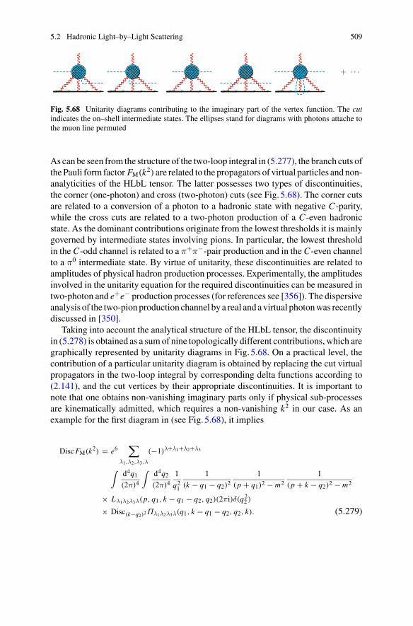
5.2 Hadronic Light–by–Light Scattering 509

+ · · ·

Fig. 5.68 Unitarity diagrams contributing to the imaginary part of the vertex function. The cutindicates the on–shell intermediate states. The ellipses stand for diagrams with photons attache tothe muon line permuted

As can be seen from the structure of the two-loop integral in (5.277), the branch cuts ofthePauli form factor FM(k2) are related to the propagators of virtual particles andnon-analyticities of the HLbL tensor. The latter possesses two types of discontinuities,the corner (one-photon) and cross (two-photon) cuts (see Fig. 5.68). The corner cutsare related to a conversion of a photon to a hadronic state with negative C-parity,while the cross cuts are related to a two-photon production of a C-even hadronicstate. As the dominant contributions originate from the lowest thresholds it is mainlygoverned by intermediate states involving pions. In particular, the lowest thresholdin the C-odd channel is related to a π+π−-pair production and in the C-even channelto a π0 intermediate state. By virtue of unitarity, these discontinuities are related toamplitudes of physical hadron production processes. Experimentally, the amplitudesinvolved in the unitarity equation for the required discontinuities can be measured intwo-photon and e+e− production processes (for references see [356]). The dispersiveanalysis of the two-pionproduction channel by a real and avirtual photonwas recentlydiscussed in [350].

Taking into account the analytical structure of the HLbL tensor, the discontinuityin (5.278) is obtained as a sumof nine topologically different contributions, which aregraphically represented by unitarity diagrams in Fig. 5.68. On a practical level, thecontribution of a particular unitarity diagram is obtained by replacing the cut virtualpropagators in the two-loop integral by corresponding delta functions according to(2.141), and the cut vertices by their appropriate discontinuities. It is important tonote that one obtains non-vanishing imaginary parts only if physical sub-processesare kinematically admitted, which requires a non-vanishing k2 in our case. As anexample for the first diagram in (see Fig. 5.68), it implies

DiscFM(k2) = e6∑

λ1,λ2,λ3,λ

(−1)λ+λ1+λ2+λ3

∫d4q1(2π)4

∫d4q2(2π)4

1

q21

1

(k − q1 − q2)21

(p + q1)2 − m2

1

(p + k − q2)2 − m2

× Lλ1λ2λ3λ(p, q1, k − q1 − q2, q2)(2πi)δ(q22 )

× Disc(k−q2)2Πλ1λ2λ3λ(q1, k − q1 − q2, q2, k). (5.279)

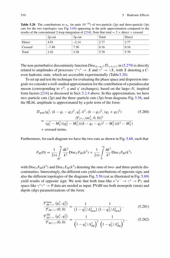
510 5 Hadronic Effects

Table 5.20 The contributions to aμ (in units 10−10) of two-particle (2p) and three-particle (3p)cuts for the two topologies (see Fig. 5.69) appearing in the pole approximation compared to theresults of the conventional 2-loop integration of [234]. Note that total = 2 × direct + crossed

2p-cut 3p-cut Total Direct

Direct 4.91 –2.14 2.77 2.77

Crossed –7.40 7.56 0.16 0.16

Total 2.42 3.28 5.70 5.70

The non-perturbative discontinuity function Disc(k−q2)2Πλ1λ2λ3λ in (5.279) is directlyrelated to amplitudes of processes γ∗γ∗ → X and γ∗ → γX , with X denoting a C-even hadronic state, which are accessible experimentally (Table5.20).

To set up and test the technique for evaluating the phase space and dispersion inte-grals we consider awell-studied approximation for the contribution of a pseudoscalarmeson (corresponding to π0, η and η′ exchanges), based on the large–Nc inspiredform factors [234] as discussed in Sect. 5.2.4 above. In this approximation, we havetwo–particle cuts (2p) and the three–particle cuts (3p) from diagrams Fig. 5.56, andthe HLbL amplitude is approximated by a pole term of the form:

Πpole(q21 , (k − q1 − q2)

2, q22 , k

2, (k − q1)2, (q1 + q2)

2) (5.280)

= |Fπ0γγ(m2π, 0, 0)|2

(q21 − M2

V )(q22 − M2

V )((k − q1 − q2)2 − M2V )(k2 − M2

V )

+ crossed terms.

Furthermore, for each diagram we have the two cuts as shown in Fig. 5.68, such that

FM(0) = 1

2πi

∞∫

M2

dk2

k2Disc2FM(k2) + 1

2πi

∞∫

0

dk2

k2Disc3FM(k2)

with Disc2FM(k2) and Disc3FM(k2) denoting the sum of two- and three-particle dis-continuities. Interestingly, the different cuts yield contributions of opposite sign, andalso the different topologies of the diagrams Fig. 5.56 (cut as illustrated in Fig. 5.69)yield results of opposite sign: We note that both time-like e+e− → γ∗ → Pγ andspace-like γ∗γ∗ → P data are needed as input. PVdH use both monopole (mon) anddipole (dip) parametrizations of the form:

F monMγ∗γ∗

(q21 , q

22

)

FMγ∗γ∗(0, 0)= 1(

1 − q21/Λ

2mon

) 1(1 − q2

2/Λ2mon

) , (5.281)

F dipMγ∗γ∗

(q21 , q

22

)

FMγ∗γ∗(0, 0)= 1

(1 − q2

1/Λ2dip

)21

(1 − q2

2/Λ2dip

)2 , (5.282)

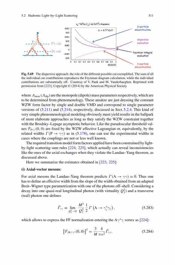
5.2 Hadronic Light–by–Light Scattering 511

Pγ cut

3γ cut

P

Fig. 5.69 The dispersive approach: the role of the different possible cut exemplified. The sum of allthe individual cut contributions reproduces the Feynman diagram calculation, while the individualcontributions are substantially off. Courtesy of V. Pauk and M. Vanderhaeghen. Reprinted withpermission from [223], Copyright © (2014) by the American Physical Society

whereΛmon (Λdip) are themonopole (dipole)mass parameters respectively,which areto be determined from phenomenology. These ansätze are just dressing the constantWZW form factor by single and double VMD and correspond to single parameterversions of (5.211) and (5.214), respectively, discussed in Sect. 5.2.4. This kind ofvery simple phenomenological modeling obviously must yield results in the ballparkof more elaborate approaches as long as they satisfy the WZW constraint togetherwith the Brodsky–Lepage asymptotic behavior. Like the pseudoscalar threshold val-ues FPγγ(0, 0) are fixed by the WZW effective Lagrangian or, equivalently, by therelated widths Γ (P → γγ) as in (5.178), one can use the experimental widths incases where the couplings are not or less well known.

The required transitionmodel form factors applied have been constrained by light-by-light scattering sum rules [224, 225], which actually can reveal inconsistencieslike the ones of the axial exchanges when they violate the Landau–Yang theorem, asdiscussed above.

Here we summarize the estimates obtained in [223, 225]:

(i) Axial-vector mesons:

For axial mesons the Landau–Yang theorem predicts Γ (A → γγ) ≡ 0. Thus onehas to define an effective width from the slope of the width obtained from an adaptedBreit–Wigner type parametrization with one of the photons off–shell. Considering adecay into one quasi-real longitudinal photon (with virtuality Q2

1) and a transverse(real) photon one defines

Γγγ ≡ limQ2

1→0

M2

Q21

1

2Γ

(A → γ∗

LγT

), (5.283)

which allows to express the FF normalization entering the Aγ∗γ vertex as [224]:

[FAγ∗γ∗(0, 0)

]2 = 3

M

4

πα2Γγγ . (5.284)

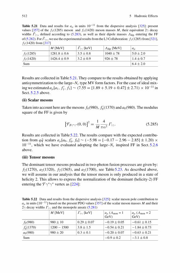
512 5 Hadronic Effects

Table 5.21 Data and results for aμ in units 10−11 from the dispersive analysis [325]: presentvalues [357] of the f1(1285) meson and f1(1420) meson masses M , their equivalent 2γ decaywidths Γγγ , defined according to (5.283), as well as their dipole masses Λdip entering the FFof (5.282). For Γγγ , we use the experimental results from theL3Collaboration: f1(1285) from [321],f1(1420) from [317]

M [MeV] Γγγ [keV] Λdip [MeV] aμ

f1(1285) 1281.8 ± 0.6 3.5 ± 0.8 1040 ± 78 5.0 ± 2.0

f1(1420) 1426.4 ± 0.9 3.2 ± 0.9 926 ± 78 1.4 ± 0.7

Sum 6.4 ± 2.0

Results are collected in Table5.21. They compare to the results obtained by applyingantisymmetrization to the large–Nc type MV form factors. For the case of ideal mix-ingwe estimated aμ[a1, f ′

1, f1] ∼ (7.55 = [1.89 + 5.19 + 0.47] ± 2.71) × 10−11 inSect. 5.2.5 above.

(ii) Scalar mesons

Taken into account here are themesons f0(980), f ′0(1370) and a0(980). Themodulus

square of the FF is given by

[FSγ∗γ∗(0, 0)

]2 = 1

M

4

πα2Γγγ . (5.285)

Results are collected in Table5.22. The results compare with the expected contribu-tion from qq scalars aμ[a0, f ′

0, f0] ∼ (−5.98 = [−0.17 − 2.96 − 2.85] ± 1.20) ×10−11, which we have evaluated adopting the large–Nc inspired FF in Sect. 5.2.6above.

(iii) Tensor mesons

The dominant tensor mesons produced in two-photon fusion processes are given by:f2(1270), a2(1320), f2(1565), and a2(1700), see Table5.23. As described above,we will assume in our analysis that the tensor meson is only produced in a state ofhelicity 2. This allows to express the normalization of the dominant (helicity-2) FFentering the Tγ∗γ∗ vertex as [224]:

Table 5.22 Data and results from the dispersive analysis [325]: scalar meson pole contribution toaμ in units [10−11] based on the present PDG values [357] of the scalar meson masses M and their2γ decay widths Γγγ and the monopole ansatz (5.281)

M [MeV] Γγγ [keV] aμ (Λmon = 1GeV)

aμ (Λmon = 2GeV)

f0(980) 980 ± 10 0.29 ± 0.07 −0.19 ± 0.05 −0.61 ± 0.15

f ′0(1370) 1200 − 1500 3.8 ± 1.5 −0.54 ± 0.21 −1.84 ± 0.73

a0(980) 980 ± 20 0.3 ± 0.1 −0.20 ± 0.07 −0.63 ± 0.21

Sum −0.9 ± 0.2 −3.1 ± 0.8

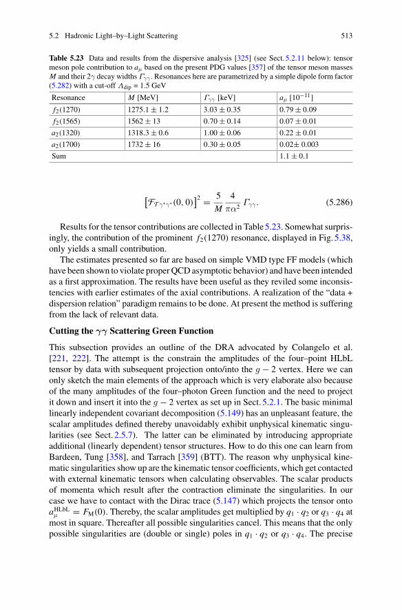
5.2 Hadronic Light–by–Light Scattering 513

Table 5.23 Data and results from the dispersive analysis [325] (see Sect. 5.2.11 below): tensormeson pole contribution to aμ based on the present PDG values [357] of the tensor meson massesM and their 2γ decay widths Γγγ . Resonances here are parametrized by a simple dipole form factor(5.282) with a cut-off Λdip = 1.5 GeV

Resonance M [MeV] Γγγ [keV] aμ [10−11]

f2(1270) 1275.1 ± 1.2 3.03 ± 0.35 0.79 ± 0.09

f2(1565) 1562 ± 13 0.70 ± 0.14 0.07 ± 0.01

a2(1320) 1318.3 ± 0.6 1.00 ± 0.06 0.22 ± 0.01

a2(1700) 1732 ± 16 0.30 ± 0.05 0.02± 0.003

Sum 1.1 ± 0.1

[FTγ∗γ∗(0, 0)

]2 = 5

M

4

πα2Γγγ . (5.286)

Results for the tensor contributions are collected in Table5.23. Somewhat surpris-ingly, the contribution of the prominent f2(1270) resonance, displayed in Fig. 5.38,only yields a small contribution.

The estimates presented so far are based on simple VMD type FF models (whichhave been shown to violate properQCDasymptotic behavior) and have been intendedas a first approximation. The results have been useful as they reviled some inconsis-tencies with earlier estimates of the axial contributions. A realization of the “data +dispersion relation” paradigm remains to be done. At present the method is sufferingfrom the lack of relevant data.

Cutting the γγ Scattering Green Function

This subsection provides an outline of the DRA advocated by Colangelo et al.[221, 222]. The attempt is the constrain the amplitudes of the four–point HLbLtensor by data with subsequent projection onto/into the g − 2 vertex. Here we canonly sketch the main elements of the approach which is very elaborate also becauseof the many amplitudes of the four–photon Green function and the need to projectit down and insert it into the g − 2 vertex as set up in Sect. 5.2.1. The basic minimallinearly independent covariant decomposition (5.149) has an unpleasant feature, thescalar amplitudes defined thereby unavoidably exhibit unphysical kinematic singu-larities (see Sect. 2.5.7). The latter can be eliminated by introducing appropriateadditional (linearly dependent) tensor structures. How to do this one can learn fromBardeen, Tung [358], and Tarrach [359] (BTT). The reason why unphysical kine-matic singularities show up are the kinematic tensor coefficients, which get contactedwith external kinematic tensors when calculating observables. The scalar productsof momenta which result after the contraction eliminate the singularities. In ourcase we have to contact with the Dirac trace (5.147) which projects the tensor ontoaHLbLμ = FM(0). Thereby, the scalar amplitudes get multiplied by q1 · q2 or q3 · q4 atmost in square. Thereafter all possible singularities cancel. This means that the onlypossible singularities are (double or single) poles in q1 · q2 or q3 · q4. The precise

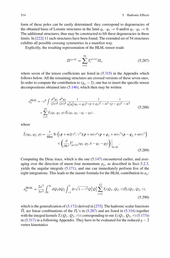
514 5 Hadronic Effects

form of these poles can be easily determined: they correspond to degeneracies ofthe obtained basis of Lorentz structures in the limit q1 · q2 → 0 and/or q3 · q4 → 0.The additional structures, thus may be constructed to lift these degeneracies in theselimits. In [222] 11 such structures have been found. The extended set of 54 structuresexhibits all possible crossing symmetries in a manifest way.

Explicitly, the resulting representation of the HLbL tensor reads

Πμνλσ =54∑

i=1

T μνλσi Πi , (5.287)

where seven of the tensor coefficients are listed in (5.315) in the Appendix whichfollows below. All the remaining structures are crossed versions of these seven ones.In order to compute the contribution to (gμ − 2), one has to insert the specific tensordecompositions obtained into (5.146), which then may be written

aHLbLμ = −e6∫

d4q1(2π)4

d4q2(2π)4

1

q21q22 (q1 + q2)2

1

(p + q1)2 − m21

(p − q2)2 − m2

×19∑

i=1

Ti (q1, q2; p) Πi (q1, q2, −q1 − q2) ,

(5.288)

where

Ti (q1, q2; p) = 1

48mTr

((/p + m)[γρ, γσ](/p + m)γμ(/p + /q1 + m)γλ(/p − /q2 + m)γν

)

×(

∂

∂kρ Tiμνλσ(q1, q2, k − q1 − q2)

) ∣∣∣∣k=0

.

(5.289)

Computing the Dirac trace, which is the one (5.147) encountered earlier, and aver-aging over the direction of muon four momentum pμ, as described in Sect. 5.2.3,yields the angular integrals (5.171), and one can immediately perform five of theeight integrations. This leads to the master formula for the HLbL contribution to aμ:

aHLbLμ = 2α3

3π2

∫ ∞0

dQ1dQ2

∫ 1

−1dτ

√1 − τ2Q3

1Q32

12∑

i=1

Ti (Q1, Q2, τ )Πi (Q1, Q2, τ ),

(5.290)

which is the generalization of (5.172) derived in [275]. The hadronic scalar functionsΠi are linear combinations of the Πi ’s in (5.287) and are listed in (5.316) togetherwith the integral kernels Ti (Q1, Q2, τ ) ( corresponding to our Ii (Q1, Q2, τ ) (5.173))in (5.317) in a following Appendix. They have to be evaluated for the reduced g − 2vertex kinematics

5.2 Hadronic Light–by–Light Scattering 515

s = −Q23 = −Q2

1 − 2Q1Q2τ − Q22, t = −Q2

2, u = −Q21,

q21 = −Q2

1, q22 = −Q2

2, q23 = −Q2

3 = −Q21 − 2Q1Q2τ − Q2

2, k2 = q24 = 0.(5.291)

It turns out that there are only 19 independent linear combinations of the structuresT μνλσi that contribute to (gμ − 2) at first. However, because of the symmetries under

the exchange of the momenta q1 ↔ −q2, only a subset of 12 of these functionsappears in the master formula (5.290). The integral kernels Ti listed in [222] are fullygeneral for any light-by-light process, while the scalar functions Πi parametrize thehadronic content of the master formula. A corresponding formula has been workedout in [236], which also lists the required integral kernels, corresponding to theT μνλσi ’s, but for the minimal decomposition (5.149).The idea here is to get the Πi ’s from dispersion relations with appropriate experi-

mental data as an input. Of course, as we have used it earlier, we as well can attemptto model the Πi ’s or try to get them from lattice QCD simulations.

How do we get the scalar amplitudes which are encoding all non-perturbativephysics entering aHLbLμ ? The basic ideas of utilizing dispersion relations have beendeveloped in Sect. 3.8 for the case of the HVP. Instead of calculating the hadronic“blobs”, which we so far cannot do with needed precision, we relate them to theimaginary parts which correspond to cut diagrams, where a cut puts intermedi-ate states to their mass shell, which in turn relates cut diagrams via on–shell T –matrix elements to physical cross sections. The possible cut diagrams in HLbL areshown in Fig. 5.70, which exhibit multi-hadron sub-processes which eventually are

Fig. 5.70 Unitarity diagrams according to the Mandelstam representation. Cuts are represented bythe dashed lines, where cut lines represent on-sell particles. Crossed diagrams have to be includedas well

≈

Fig. 5.71 Partial–wave approximation of multi–particle intermediate states by leading two-particlecut contributions

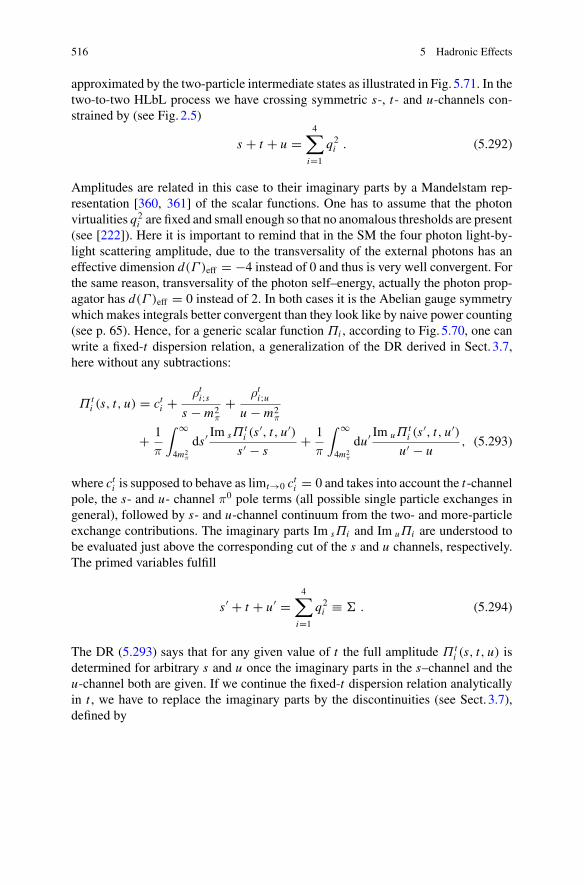
516 5 Hadronic Effects

approximated by the two-particle intermediate states as illustrated in Fig. 5.71. In thetwo-to-two HLbL process we have crossing symmetric s-, t- and u-channels con-strained by (see Fig. 2.5)

s + t + u =4∑

i=1

q2i . (5.292)

Amplitudes are related in this case to their imaginary parts by a Mandelstam rep-resentation [360, 361] of the scalar functions. One has to assume that the photonvirtualities q2

i are fixed and small enough so that no anomalous thresholds are present(see [222]). Here it is important to remind that in the SM the four photon light-by-light scattering amplitude, due to the transversality of the external photons has aneffective dimension d(Γ )eff = −4 instead of 0 and thus is very well convergent. Forthe same reason, transversality of the photon self–energy, actually the photon prop-agator has d(Γ )eff = 0 instead of 2. In both cases it is the Abelian gauge symmetrywhich makes integrals better convergent than they look like by naive power counting(see p. 65). Hence, for a generic scalar function Πi , according to Fig. 5.70, one canwrite a fixed-t dispersion relation, a generalization of the DR derived in Sect. 3.7,here without any subtractions:

Π ti (s, t, u) = cti + ρti;s

s − m2π

+ ρti;uu − m2

π

+ 1

π

∫ ∞

4m2π

ds ′ Im sΠti (s

′, t, u′)s ′ − s

+ 1

π

∫ ∞

4m2π

du′ Im uΠti (s

′, t, u′)u′ − u

, (5.293)

where cti is supposed to behave as limt→0 cti = 0 and takes into account the t-channelpole, the s- and u- channel π0 pole terms (all possible single particle exchanges ingeneral), followed by s- and u-channel continuum from the two- and more-particleexchange contributions. The imaginary parts Im sΠi and Im uΠi are understood tobe evaluated just above the corresponding cut of the s and u channels, respectively.The primed variables fulfill

s ′ + t + u′ =4∑

i=1

q2i ≡ � . (5.294)

The DR (5.293) says that for any given value of t the full amplitude Π ti (s, t, u) is

determined for arbitrary s and u once the imaginary parts in the s–channel and theu-channel both are given. If we continue the fixed-t dispersion relation analyticallyin t , we have to replace the imaginary parts by the discontinuities (see Sect. 3.7),defined by

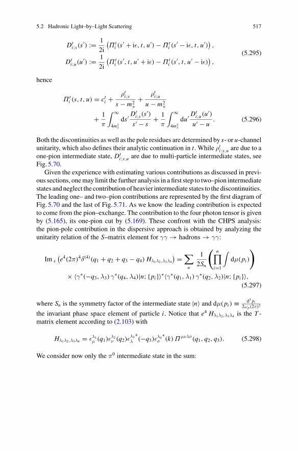
5.2 Hadronic Light–by–Light Scattering 517

Dti;s(s

′) := 1

2i

(Π t

i (s′ + iε, t, u′) − Π t

i (s′ − iε, t, u′)

),

Dti;u(u

′) := 1

2i

(Π t

i (s′, t, u′ + iε) − Π t

i (s′, t, u′ − iε)

),

(5.295)

hence

Π ti (s, t, u) = cti + ρti;s

s − m2π

+ ρti;uu − m2

π

+ 1

π

∫ ∞

4m2π

ds ′ Dti;s(s

′)s ′ − s

+ 1

π

∫ ∞

4m2π

du′ Dti;u(u

′)u′ − u

. (5.296)

Both the discontinuities aswell as the pole residues are determined by s- or u-channelunitarity, which also defines their analytic continuation in t . While ρti;s,u are due to aone-pion intermediate state, Dt

i;s,u are due to multi-particle intermediate states, seeFig. 5.70.

Given the experience with estimating various contributions as discussed in previ-ous sections, onemay limit the further analysis in a first step to two–pion intermediatestates andneglect the contribution of heavier intermediate states to the discontinuities.The leading one– and two–pion contributions are represented by the first diagram ofFig. 5.70 and the last of Fig. 5.71. As we know the leading contribution is expectedto come from the pion–exchange. The contribution to the four photon tensor is givenby (5.165), its one-pion cut by (5.169). These confront with the CHPS analysis:the pion-pole contribution in the dispersive approach is obtained by analyzing theunitarity relation of the S–matrix element for γγ → hadrons → γγ:

Im s(e4(2π)4δ(4)(q1 + q2 + q3 − q4) Hλ1λ2,λ3λ4

) =∑

n

1

2Sn

(n∏

i=1

∫dμ(pi )

)

× 〈γ∗(−q3,λ3) γ∗(q4,λ4)|n; {pi }〉∗〈γ∗(q1,λ1) γ∗(q2,λ2)|n; {pi }〉,(5.297)

where Sn is the symmetry factor of the intermediate state |n〉 and dμ(pi ) ≡ d3 pi2ωp(2π)3

the invariant phase space element of particle i . Notice that e4 Hλ1λ2,λ3λ4 is the T -matrix element according to (2.103) with

Hλ1λ2,λ3λ4 = ελ1μ (q1)ε

λ2ν (q2)ε

λ3λ

∗(−q3)ε

λ4σ

∗(k)Πμνλσ(q1, q2, q3). (5.298)

We consider now only the π0 intermediate state in the sum:

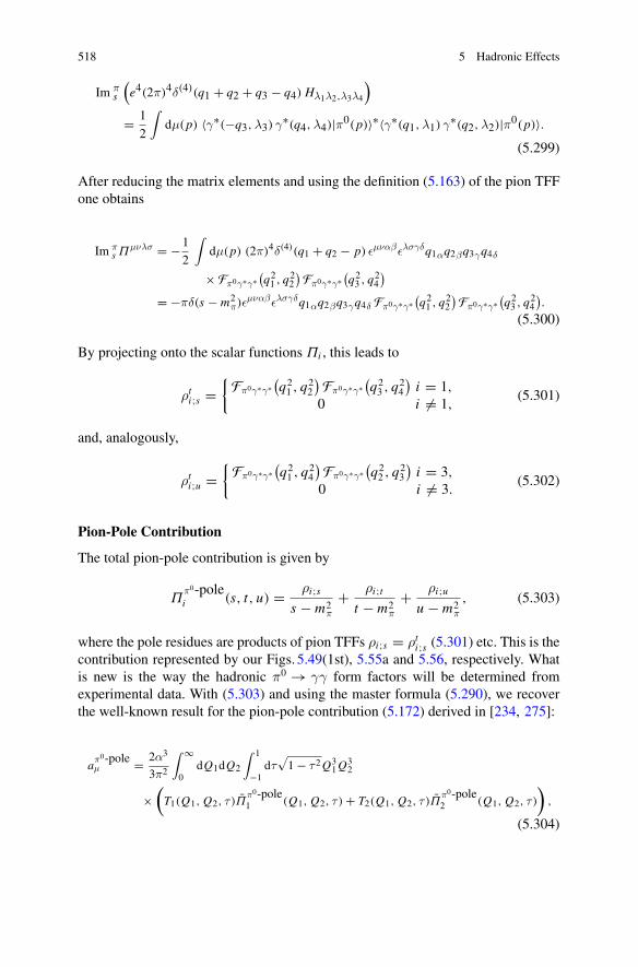
518 5 Hadronic Effects

Im πs

(e4(2π)4δ(4)(q1 + q2 + q3 − q4) Hλ1λ2,λ3λ4

)

= 1

2

∫dμ(p) 〈γ∗(−q3, λ3) γ∗(q4, λ4)|π0(p)〉∗〈γ∗(q1, λ1) γ∗(q2, λ2)|π0(p)〉.

(5.299)

After reducing the matrix elements and using the definition (5.163) of the pion TFFone obtains

Im πs Πμνλσ = −1

2

∫dμ(p) (2π)4δ(4)(q1 + q2 − p) εμναβελσγδq1αq2βq3γq4δ

× Fπ0γ∗γ∗(q21 , q22

)Fπ0γ∗γ∗

(q23 , q

24

)

= −πδ(s − m2π)εμναβελσγδq1αq2βq3γq4δ Fπ0γ∗γ∗

(q21 , q22

)Fπ0γ∗γ∗

(q23 , q

24

).

(5.300)

By projecting onto the scalar functions Πi , this leads to

ρti;s ={Fπ0γ∗γ∗

(q21 , q

22

)Fπ0γ∗γ∗

(q23 , q

24

)i = 1,

0 i = 1,(5.301)

and, analogously,

ρti;u ={Fπ0γ∗γ∗

(q21 , q

24

)Fπ0γ∗γ∗

(q22 , q

23

)i = 3,

0 i = 3.(5.302)

Pion-Pole Contribution

The total pion-pole contribution is given by

Ππ0-polei (s, t, u) = ρi;s

s − m2π

+ ρi;tt − m2

π

+ ρi;uu − m2

π

, (5.303)

where the pole residues are products of pion TFFs ρi;s = ρti;s (5.301) etc. This is thecontribution represented by our Figs. 5.49(1st), 5.55a and 5.56, respectively. Whatis new is the way the hadronic π0 → γγ form factors will be determined fromexperimental data. With (5.303) and using the master formula (5.290), we recoverthe well-known result for the pion-pole contribution (5.172) derived in [234, 275]:

aπ0-poleμ = 2α3

3π2

∫ ∞

0dQ1dQ2

∫ 1

−1dτ

√1 − τ2Q3

1Q32

×(T1(Q1, Q2, τ )Π

π0-pole1 (Q1, Q2, τ ) + T2(Q1, Q2, τ )Π

π0-pole2 (Q1, Q2, τ )

),

(5.304)

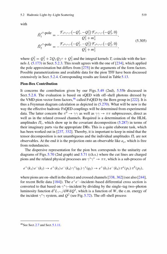
5.2 Hadronic Light–by–Light Scattering 519

with

Ππ0-pole1 = −Fπ0γ∗γ∗

(−Q21,−Q2

2

)Fπ0γ∗γ∗

(−Q23, 0

)

Q23 + m2

π

,

Ππ0-pole2 = −Fπ0γ∗γ∗

(−Q21,−Q2

3

)Fπ0γ∗γ∗

(−Q22, 0

)

Q22 + m2

π

,

(5.305)

where Q23 = Q2

1 + 2Q1Q2τ + Q22 and the integral kernels Ti coincide with the ker-

nels Ii (5.173) in Sect. 5.2.3. This result agrees with the one of [234], which appliedthe pole approximation but differs from [275] in the arguments of the form factors.Possible parametrizations and available data for the pion TFF have been discussedextensively in Sect. 5.2.4. Corresponding results are listed in Table5.13.

Pion-Box Contribution

It concerns the contribution given by our Figs. 5.49 (2nd), 5.55b discussed inSect. 5.2.8. The evaluation is based on sQED with off–shell photons dressed bythe VMD pion vector form factors,46 called FsQED by the Bern group in [222]. It isthus a Feynman diagram calculation as depicted in (5.270). What will be new is theway the effective hadronic FsQED couplings will be determined from experimentaldata. The latter concern the π0 → γγ as well as γγ → ππ subprocesses, direct aswell as in the related crossed channels. Required is a determination of the HLbLamplitudes Πi , which show up in the covariant decomposition (5.287) in terms oftheir imaginary parts via the appropriate DRs. This is a quite elaborate task, whichhas been worked out in [237, 332]. Thereby, it is important to keep in mind that thetensor decomposition is not unambiguous and the individual amplitudes Πi are notobservables. At the end it is the projection onto an observable like aμ, which is freefrom redundancies.

The dispersive representation for the pion box corresponds to the unitarity cutdiagrams of Figs. 5.70 (2nd graph) and 5.71 (r.h.s.) where the cut lines are chargedpions and the related physical processes are γ∗γ∗ → ππ, which is a sub-process of

e+(k1) e−(k2) → e+(k3) e

−(k4) γ∗(q1) γ∗(q2) → e+(k3) e−(k4)πa(p1)πb(p2),

where pions are on–shell in the direct and crossed channels [338, 362] (see also [244],for recent Belle data [184]). The e+e−–incident–based differential cross section isconverted to that based on γ∗γ–incident by dividing by the single–tag two–photonluminosity function d2Lγ∗γ/dWdQ2, which is a function of W , the c.m. energy ofthe incident γ∗γ system, and Q2 (see Fig. 5.72). The off–shell process

46See Sect. 2.7 and Sect. 5.1.11.

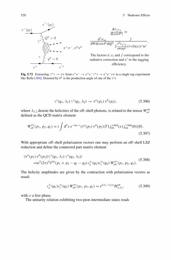
520 5 Hadronic Effects

Fig. 5.72 Extracting γ∗γ → ππ from e+e− → e+e−γ∗γ → e+e−ππ in a single tag experimentlike Belle [184]. Denoted by θ∗ is the production angle of one of the π’s

γ∗(q1,λ1) γ∗(q2,λ2) → πa(p1)πb(p2), (5.306)

where λ1,2 denote the helicities of the off–shell photons, is related to the tensor Wabμν

defined as the QCD matrix element

W μνab (p1, p2, q1) = i

∫d4x e−iq1·x 〈πa(p1)πb(p2)|T { j μ had

em (x) j ν hadem (0)}|0〉.

(5.307)

With appropriate off–shell polarization vectors one may perform an off–shell LSZreduction and define the connected part matrix element

〈πa(p1)πb(p2)|γ∗(q1,λ1) γ∗(q2,λ2)〉=ie2(2π)4δ(4)(p1 + p2 − q1 − q2) ελ1

μ (q1)ελ2ν (q2)W

μνab (p1, p2, q1).

(5.308)

The helicity amplitudes are given by the contraction with polarization vectors asusual:

ελ1μ (q1)ε

λ2ν (q2)W

μνab (p1, p2, q1) = ei(λ1−λ2)φHab

λ1λ2, (5.309)

with φ a free phase.The unitarity relation exhibiting two-pion intermediate states reads

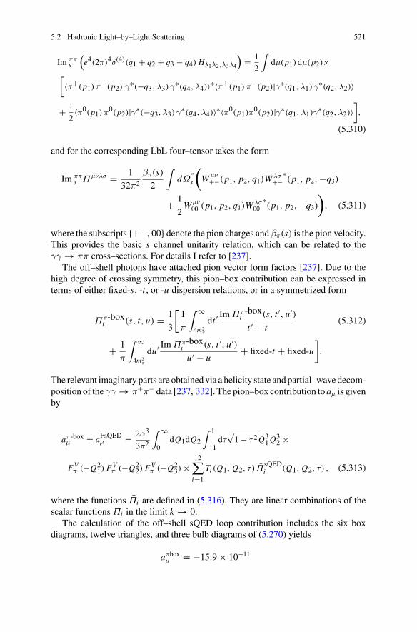
5.2 Hadronic Light–by–Light Scattering 521

Im ππs

(e4(2π)4δ(4)(q1 + q2 + q3 − q4) Hλ1λ2,λ3λ4

)= 1

2

∫dμ(p1) dμ(p2)×

[〈π+(p1) π−(p2)|γ∗(−q3,λ3) γ∗(q4, λ4)〉∗〈π+(p1) π−(p2)|γ∗(q1, λ1) γ∗(q2, λ2)〉

+ 1

2〈π0(p1) π0(p2)|γ∗(−q3, λ3) γ∗(q4, λ4)〉∗〈π0(p1)π0(p2)|γ∗(q1, λ1)γ

∗(q2,λ2)〉],

(5.310)

and for the corresponding LbL four–tensor takes the form

Im ππs Πμνλσ = 1

32π2

βπ(s)

2

∫dΩ

′′s

(W μν

+−(p1, p2, q1)Wλσ+−

∗(p1, p2,−q3)

+ 1

2W μν

00 (p1, p2, q1)Wλσ00

∗(p1, p2,−q3)

), (5.311)

where the subscripts {+−, 00} denote the pion charges and βπ(s) is the pion velocity.This provides the basic s channel unitarity relation, which can be related to theγγ → ππ cross–sections. For details I refer to [237].

The off–shell photons have attached pion vector form factors [237]. Due to thehigh degree of crossing symmetry, this pion–box contribution can be expressed interms of either fixed-s, -t , or -u dispersion relations, or in a symmetrized form

Ππ-boxi (s, t, u) = 1

3

[1

π

∫ ∞

4m2π

dt ′Im Ππ-box

i (s, t ′, u′)t ′ − t

(5.312)

+ 1

π

∫ ∞

4m2π

du′ Im Ππ-boxi (s, t ′, u′)u′ − u

+ fixed-t + fixed-u

].

The relevant imaginary parts are obtained via a helicity state and partial–wave decom-position of the γγ → π+π− data [237, 332]. The pion–box contribution to aμ is givenby

aπ-boxμ = aFsQEDμ = 2α3

3π2

∫ ∞0

dQ1dQ2

∫ 1

−1dτ

√1 − τ2Q3

1Q32 ×

FVπ (−Q2

1) FVπ (−Q2

2) FVπ (−Q2

3) ×12∑

i=1

Ti (Q1, Q2, τ ) ΠsQEDi (Q1, Q2, τ ) , (5.313)

where the functions Πi are defined in (5.316). They are linear combinations of thescalar functions Πi in the limit k → 0.

The calculation of the off–shell sQED loop contribution includes the six boxdiagrams, twelve triangles, and three bulb diagrams of (5.270) yields

aπboxμ = −15.9 × 10−11

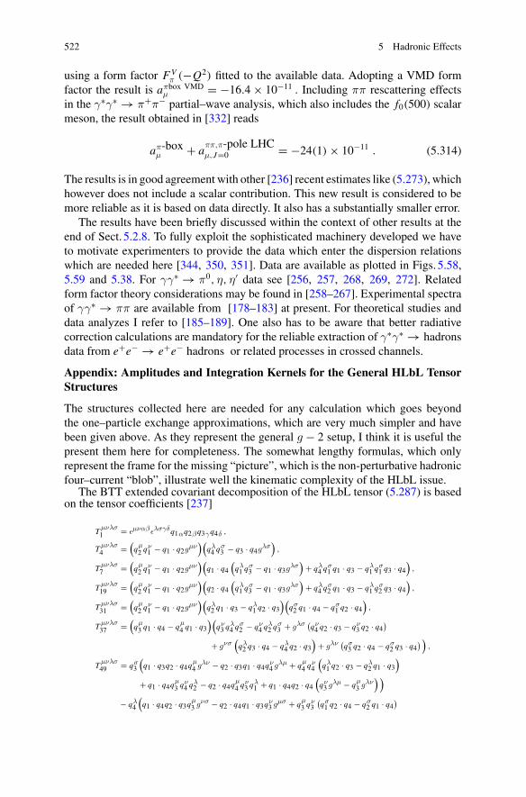
522 5 Hadronic Effects

using a form factor FVπ (−Q2) fitted to the available data. Adopting a VMD form

factor the result is aπbox VMDμ = −16.4 × 10−11 . Including ππ rescattering effects

in the γ∗γ∗ → π+π− partial–wave analysis, which also includes the f0(500) scalarmeson, the result obtained in [332] reads

aπ-boxμ + a

ππ,π-pole LHCμ,J=0 = −24(1) × 10−11 . (5.314)

The results is in good agreement with other [236] recent estimates like (5.273), whichhowever does not include a scalar contribution. This new result is considered to bemore reliable as it is based on data directly. It also has a substantially smaller error.

The results have been briefly discussed within the context of other results at theend of Sect. 5.2.8. To fully exploit the sophisticated machinery developed we haveto motivate experimenters to provide the data which enter the dispersion relationswhich are needed here [344, 350, 351]. Data are available as plotted in Figs. 5.58,5.59 and 5.38. For γγ∗ → π0, η, η′ data see [256, 257, 268, 269, 272]. Relatedform factor theory considerations may be found in [258–267]. Experimental spectraof γγ∗ → ππ are available from [178–183] at present. For theoretical studies anddata analyzes I refer to [185–189]. One also has to be aware that better radiativecorrection calculations are mandatory for the reliable extraction of γ∗γ∗ → hadronsdata from e+e− → e+e− hadrons or related processes in crossed channels.

Appendix: Amplitudes and Integration Kernels for the General HLbL TensorStructures

The structures collected here are needed for any calculation which goes beyondthe one–particle exchange approximations, which are very much simpler and havebeen given above. As they represent the general g − 2 setup, I think it is useful thepresent them here for completeness. The somewhat lengthy formulas, which onlyrepresent the frame for the missing “picture”, which is the non-perturbative hadronicfour–current “blob”, illustrate well the kinematic complexity of the HLbL issue.

The BTT extended covariant decomposition of the HLbL tensor (5.287) is basedon the tensor coefficients [237]

Tμνλσ1 = εμναβελσγδq1αq2βq3γq4δ ,

Tμνλσ4 =

(qμ2 q

ν1 − q1 · q2gμν

)(qλ4 q

σ3 − q3 · q4gλσ

),

Tμνλσ7 =

(qμ2 q

ν1 − q1 · q2gμν

)(q1 · q4

(qλ1 q

σ3 − q1 · q3gλσ

)+ qλ

4 qσ1 q1 · q3 − qλ

1 qσ1 q3 · q4

),

Tμνλσ19 =

(qμ2 q

ν1 − q1 · q2gμν

)(q2 · q4

(qλ1 q

σ3 − q1 · q3gλσ

)+ qλ

4 qσ2 q1 · q3 − qλ

1 qσ2 q3 · q4

),

Tμνλσ31 =

(qμ2 q

ν1 − q1 · q2gμν

)(qλ2 q1 · q3 − qλ

1 q2 · q3)(

qσ2 q1 · q4 − qσ

1 q2 · q4)

,

Tμνλσ37 =

(qμ3 q1 · q4 − qμ

4 q1 · q3)(

qν3 q

λ4 q

σ2 − qν

4 qλ2 q

σ3 + gλσ (

qν4 q2 · q3 − qν

3 q2 · q4)

+ gνσ(qλ2 q3 · q4 − qλ

4 q2 · q3)

+ gλν (qσ3 q2 · q4 − qσ

2 q3 · q4) )

,

Tμνλσ49 = qσ

3

(q1 · q3q2 · q4qμ

4 gλν − q2 · q3q1 · q4qν4 gλμ + qμ

4 qν4

(qλ1 q2 · q3 − qλ

2 q1 · q3)

+ q1 · q4qμ3 q

ν4 q

λ2 − q2 · q4qμ

4 qν3 q

λ1 + q1 · q4q2 · q4

(qν3 gλμ − qμ

3 gλν) )

− qλ4

(q1 · q4q2 · q3qμ

3 gνσ − q2 · q4q1 · q3qν3 gμσ + qμ

3 qν3(qσ1 q2 · q4 − qσ

2 q1 · q4)

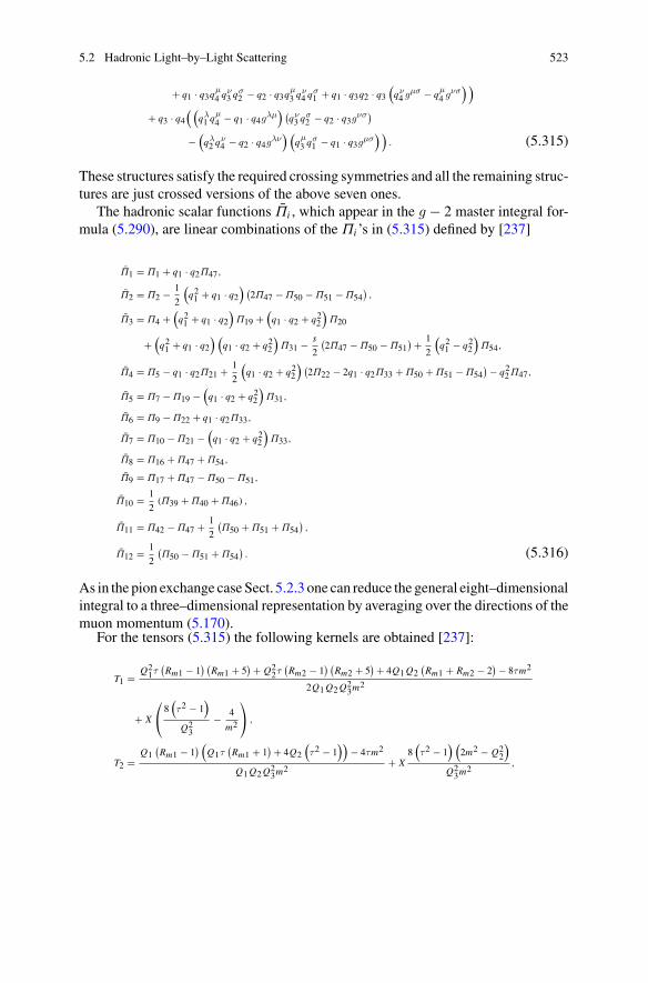
5.2 Hadronic Light–by–Light Scattering 523

+ q1 · q3qμ4 q

ν3 q

σ2 − q2 · q3qμ

3 qν4 q

σ1 + q1 · q3q2 · q3

(qν4 gμσ − qμ

4 gνσ) )

+ q3 · q4( (

qλ1 q

μ4 − q1 · q4gλμ

) (qν3 q

σ2 − q2 · q3gνσ)

−(qλ2 q

ν4 − q2 · q4gλν

) (qμ3 q

σ1 − q1 · q3gμσ

) ). (5.315)

These structures satisfy the required crossing symmetries and all the remaining struc-tures are just crossed versions of the above seven ones.

The hadronic scalar functions Πi , which appear in the g − 2 master integral for-mula (5.290), are linear combinations of the Πi ’s in (5.315) defined by [237]

Π1 = Π1 + q1 · q2Π47,

Π2 = Π2 − 1

2

(q21 + q1 · q2

) (2Π47 − Π50 − Π51 − Π54

),

Π3 = Π4 +(q21 + q1 · q2

)Π19 +

(q1 · q2 + q22

)Π20

+(q21 + q1 · q2

) (q1 · q2 + q22

)Π31 − s

2

(2Π47 − Π50 − Π51

) + 1

2

(q21 − q22

)Π54,

Π4 = Π5 − q1 · q2Π21 + 1

2

(q1 · q2 + q22

) (2Π22 − 2q1 · q2Π33 + Π50 + Π51 − Π54

) − q22Π47,

Π5 = Π7 − Π19 −(q1 · q2 + q22

)Π31,

Π6 = Π9 − Π22 + q1 · q2Π33,

Π7 = Π10 − Π21 −(q1 · q2 + q22

)Π33,

Π8 = Π16 + Π47 + Π54,

Π9 = Π17 + Π47 − Π50 − Π51,

Π10 = 1

2(Π39 + Π40 + Π46) ,

Π11 = Π42 − Π47 + 1

2

(Π50 + Π51 + Π54

),

Π12 = 1

2

(Π50 − Π51 + Π54

). (5.316)

As in the pion exchange caseSect. 5.2.3 one can reduce the general eight–dimensionalintegral to a three–dimensional representation by averaging over the directions of themuon momentum (5.170).

For the tensors (5.315) the following kernels are obtained [237]:

T1 = Q21τ

(Rm1 − 1

) (Rm1 + 5

) + Q22τ

(Rm2 − 1

) (Rm2 + 5

) + 4Q1Q2(Rm1 + Rm2 − 2

) − 8τm2

2Q1Q2Q23m

2

+ X

⎛

⎝8(τ2 − 1

)

Q23

− 4

m2

⎞

⎠ ,

T2 =Q1

(Rm1 − 1

) (Q1τ

(Rm1 + 1

) + 4Q2

(τ2 − 1

))− 4τm2

Q1Q2Q23m

2+ X

8(τ2 − 1

) (2m2 − Q2

2

)

Q23m

2,

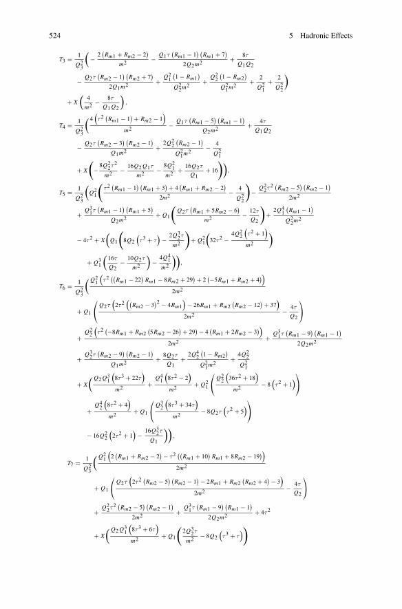
524 5 Hadronic Effects

T3 = 1

Q23

(− 2

(Rm1 + Rm2 − 2

)

m2− Q1τ

(Rm1 − 1

) (Rm1 + 7

)

2Q2m2+ 8τ

Q1Q2

− Q2τ(Rm2 − 1

) (Rm2 + 7

)

2Q1m2+ Q2

1(1 − Rm1

)

Q22m

2+ Q2

2(1 − Rm2

)

Q21m

2+ 2

Q21

+ 2

Q22

)

+ X

(4

m2− 8τ

Q1Q2

),

T4 = 1

Q23

( 4(τ2

(Rm1 − 1

) + Rm2 − 1)

m2− Q1τ

(Rm1 − 5

) (Rm1 − 1

)

Q2m2+ 4τ

Q1Q2

− Q2τ(Rm2 − 3

) (Rm2 − 1

)

Q1m2+ 2Q2

2(Rm2 − 1

)

Q21m

2− 4

Q21

+ X

(− 8Q2

2τ2

m2− 16Q2Q1τ

m2− 8Q2

1m2

+ 16Q2τ

Q1+ 16

)),

T5 = 1

Q23

(Q21

(τ2

(Rm1 − 1

) (Rm1 + 3

) + 4(Rm1 + Rm2 − 2

)

2m2− 4

Q22

)− Q2

2τ2 (Rm2 − 5

) (Rm2 − 1

)

2m2

+ Q31τ

(Rm1 − 1

) (Rm1 + 5

)

Q2m2+ Q1

(Q2τ

(Rm1 + 5Rm2 − 6

)

m2− 12τ

Q2

)+ 2Q4

1(Rm1 − 1

)

Q22m

2

− 4τ2 + X

(Q1

(8Q2

(τ3 + τ

)− 2Q3

2τ

m2

)+ Q2

1

(32τ2 −

4Q22

(τ2 + 1

)

m2

)

+ Q31

(16τ

Q2− 10Q2τ

m2

)− 4Q4

1m2

)),

T6 = 1

Q23

( Q21

(τ2

((Rm1 − 22

)Rm1 − 8Rm2 + 29

) + 2(−5Rm1 + Rm2 + 4

))

2m2

+ Q1

⎛

⎝Q2τ

(2τ2

((Rm2 − 3

)2 − 4Rm1

)− 26Rm1 + Rm2

(Rm2 − 12

) + 37)

2m2− 4τ

Q2

⎞

⎠

+Q22

(τ2

(−8Rm1 + Rm2(5Rm2 − 26

) + 29) − 4

(Rm1 + 2Rm2 − 3

))

2m2+ Q3

1τ(Rm1 − 9

) (Rm1 − 1

)

2Q2m2

+ Q32τ

(Rm2 − 9

) (Rm2 − 1

)

Q1m2+ 8Q2τ

Q1+ 2Q4

2(1 − Rm2

)

Q21m

2+ 4Q2

2

Q21

+ X

( Q2Q31

(8τ3 + 22τ

)

m2+

Q41

(8τ2 − 2

)

m2+ Q2

1

⎛

⎝Q22

(36τ2 + 18

)

m2− 8

(τ2 + 1

)⎞

⎠

+Q42

(8τ2 + 4

)

m2+ Q1

⎛

⎝Q32

(8τ3 + 34τ

)

m2− 8Q2τ

(τ2 + 5

)⎞

⎠

− 16Q22

(2τ2 + 1

)− 16Q3

2τ

Q1

)),

T7 = 1

Q23

( Q21

(2(Rm1 + Rm2 − 2

) − τ2((Rm1 + 10

)Rm1 + 8Rm2 − 19

))

2m2

+ Q1

⎛

⎝Q2τ

(2τ2

(Rm2 − 5

) (Rm2 − 1

) − 2Rm1 + Rm2(Rm2 + 4

) − 3)

2m2− 4τ

Q2

⎞

⎠

+ Q22τ

2 (Rm2 − 5) (

Rm2 − 1)

2m2+ Q3

1τ(Rm1 − 9

) (Rm1 − 1

)

2Q2m2+ 4τ2

+ X

( Q2Q31

(8τ3 + 6τ

)

m2+ Q1

(2Q3

2τ

m2− 8Q2

(τ3 + τ

))

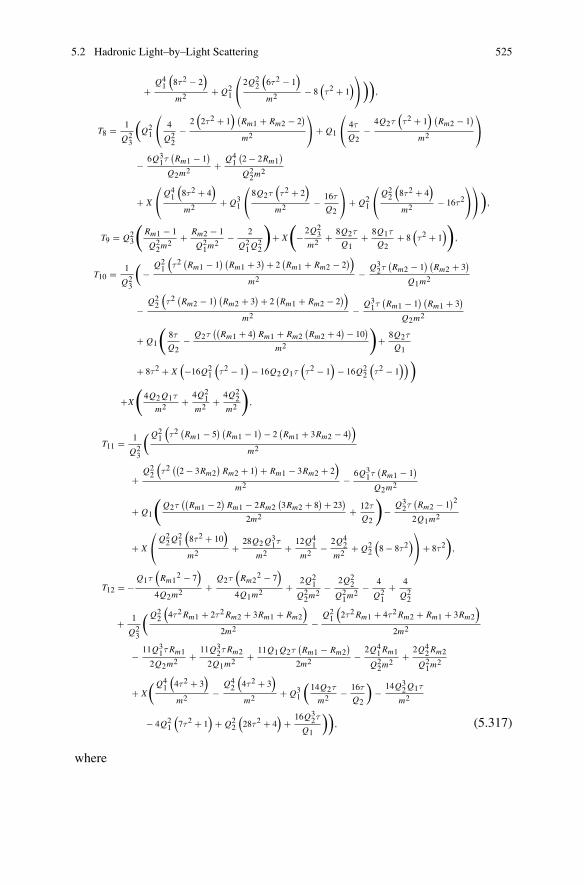
5.2 Hadronic Light–by–Light Scattering 525

+Q41

(8τ2 − 2

)

m2+ Q2

1

⎛

⎝2Q2

2

(6τ2 − 1

)

m2− 8

(τ2 + 1

)⎞

⎠))

,

T8 = 1

Q23

(Q21

⎛

⎝ 4

Q22

−2(2τ2 + 1

) (Rm1 + Rm2 − 2

)

m2

⎞

⎠ + Q1

⎛

⎝ 4τ

Q2−

4Q2τ(τ2 + 1

) (Rm2 − 1

)

m2

⎞

⎠

− 6Q31τ

(Rm1 − 1

)

Q2m2+ Q4

1(2 − 2Rm1

)

Q22m

2

+ X

⎛

⎝Q41

(8τ2 + 4

)

m2+ Q3

1

⎛

⎝8Q2τ

(τ2 + 2

)

m2− 16τ

Q2

⎞

⎠ + Q21

⎛

⎝Q22

(8τ2 + 4

)

m2− 16τ2

⎞

⎠

⎞

⎠)

,

T9 = Q23

(Rm1 − 1

Q22m

2+ Rm2 − 1

Q21m

2− 2

Q21Q

22

)+ X

(− 2Q2

3m2

+ 8Q2τ

Q1+ 8Q1τ

Q2+ 8

(τ2 + 1

)),

T10 = 1

Q23

(−

Q21

(τ2

(Rm1 − 1

) (Rm1 + 3

) + 2(Rm1 + Rm2 − 2

))

m2− Q3

2τ(Rm2 − 1

) (Rm2 + 3

)

Q1m2

−Q22

(τ2

(Rm2 − 1

) (Rm2 + 3

) + 2(Rm1 + Rm2 − 2

))

m2− Q3

1τ(Rm1 − 1

) (Rm1 + 3

)

Q2m2

+ Q1

(8τ

Q2− Q2τ

((Rm1 + 4

)Rm1 + Rm2

(Rm2 + 4

) − 10)

m2

)+ 8Q2τ

Q1

+ 8τ2 + X(−16Q2

1

(τ2 − 1

)− 16Q2Q1τ

(τ2 − 1

)− 16Q2

2

(τ2 − 1

)))

+X

(4Q2Q1τ

m2+ 4Q2

1m2

+ 4Q22

m2

),

T11 = 1

Q23

( Q21

(τ2

(Rm1 − 5

) (Rm1 − 1

) − 2(Rm1 + 3Rm2 − 4

))

m2

+Q22

(τ2

((2 − 3Rm2

)Rm2 + 1

) + Rm1 − 3Rm2 + 2)

m2− 6Q3

1τ(Rm1 − 1

)

Q2m2

+ Q1

(Q2τ

((Rm1 − 2

)Rm1 − 2Rm2

(3Rm2 + 8

) + 23)

2m2+ 12τ

Q2

)− Q3

2τ(Rm2 − 1

)2

2Q1m2

+ X

⎛

⎝Q22Q

21

(8τ2 + 10

)

m2+ 28Q2Q

31τ

m2+ 12Q4

1m2

− 2Q42

m2+ Q2

2

(8 − 8τ2

)⎞

⎠ + 8τ2)

,

T12 = −Q1τ

(Rm1

2 − 7)

4Q2m2+

Q2τ(Rm2

2 − 7)

4Q1m2+ 2Q2

1

Q22m

2− 2Q2

2

Q21m

2− 4

Q21

+ 4

Q22

+ 1

Q23

( Q22

(4τ2Rm1 + 2τ2Rm2 + 3Rm1 + Rm2

)

2m2−

Q21

(2τ2Rm1 + 4τ2Rm2 + Rm1 + 3Rm2

)

2m2

− 11Q31τ Rm1

2Q2m2+ 11Q3

2τ Rm2

2Q1m2+ 11Q1Q2τ

(Rm1 − Rm2

)

2m2− 2Q4

1Rm1

Q22m

2+ 2Q4

2Rm2

Q21m

2

+ X

( Q41

(4τ2 + 3

)

m2−

Q42

(4τ2 + 3

)

m2+ Q3

1

(14Q2τ

m2− 16τ

Q2

)− 14Q3

2Q1τ

m2

− 4Q21

(7τ2 + 1

)+ Q2

2

(28τ2 + 4

)+ 16Q3

2τ

Q1

)), (5.317)

where

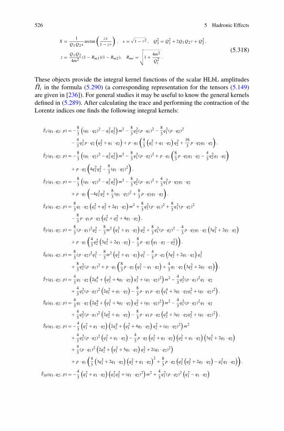
526 5 Hadronic Effects

X = 1

Q1Q2xarctan

(zx

1 − zτ

), x =

√1 − τ2 , Q2

3 = Q21 + 2Q1Q2τ + Q2

2 ,

z = Q1Q2

4m2(1 − Rm1)(1 − Rm2), Rmi =

√√√√1 + 4m2

Q2i

.

(5.318)

These objects provide the integral kernel functions of the scalar HLbL amplitudesΠi in the formula (5.290) (a corresponding representation for the tensors (5.149)are given in [236]). For general studies it may be useful to know the general kernelsdefined in (5.289). After calculating the trace and performing the contraction of theLorentz indices one finds the following integral kernels:

T1(q1, q2; p) = − 8

3

((q1 · q2)2 − q21q

22

)m2 − 8

3q22 (p · q1)2 − 8

3q21 (p · q2)2

− 4

3q21 p · q2

(q22 + q1 · q2

)+ p · q1

(4

3

(q21 + q1 · q2

)q22 + 16

3p · q2q1 · q2

),

T2(q1, q2; p) = − 8

3

((q1 · q2)2 − q21q

22

)m2 − 8

3q21 (p · q2)2 + p · q1

(8

3p · q2q1 · q2 − 4

3q22q1 · q2

)

+ p · q2(4q21q

22 − 8

3(q1 · q2)2

),

T3(q1, q2; p) = − 8

3

((q1 · q2)2 − q21q

22

)m2 − 8

3q22 (p · q1)2 + 4

3q21 p · q2q1 · q2

+ p · q1(

−4q21q22 + 8

3(q1 · q2)2 + 8

3p · q2q1 · q2

),

T4(q1, q2; p) = 8

3q1 · q2

(q21 + q22 + 2q1 · q2

)m2 + 8

3q22 (p · q1)2 + 8

3q21 (p · q2)2

− 8

3p · q1 p · q2

(q21 + q22 + 4q1 · q2

),

T5(q1, q2; p) = 8

3(p · q1)2q22 − 8

3m2

(q21 + q1 · q2

)q22 + 8

3q21 (p · q2)2 − 4

3p · q2q1 · q2

(3q21 + 2q1 · q2

)

+ p · q1(4

3q22

(3q21 + 2q1 · q2

)− 8

3p · q2

(q1 · q2 − q22

)),

T6(q1, q2; p) = 8

3(p · q2)2q21 − 8

3m2

(q22 + q1 · q2

)q21 − 4

3p · q2

(3q22 + 2q1 · q2

)q21

+ 8

3q22 (p · q1)2 + p · q1

(8

3p · q2

(q21 − q1 · q2

)+ 4

3q1 · q2

(3q22 + 2q1 · q2

)),

T7(q1, q2; p) = 4

3q1 · q2

(2q41 +

(q22 + 4q1 · q2

)q21 + (q1 · q2)2

)m2 − 4

3q22 (p · q1)2q1 · q2

+ 4

3q21 (p · q2)2

(2q21 + q1 · q2

)− 8

3p · q1 p · q2

(q41 + 3q1 · q2q21 + (q1 · q2)2

),

T8(q1, q2; p) = 4

3q1 · q2

(2q42 +

(q21 + 4q1 · q2

)q22 + (q1 · q2)2

)m2 − 4

3q21 (p · q2)2q1 · q2

+ 4

3q22 (p · q1)2

(2q22 + q1 · q2

)− 8

3p · q1 p · q2

(q42 + 3q1 · q2q22 + (q1 · q2)2

),

T9(q1, q2; p) = − 4

3

(q21 + q1 · q2

) (2q42 +

(q21 + 4q1 · q2

)q22 + (q1 · q2)2

)m2

+ 4

3q21 (p · q2)2

(q21 + q1 · q2

)− 4

3p · q2

(q21 + q1 · q2

) (q22 + q1 · q2

) (3q21 + 2q1 · q2

)

+ 4

3(p · q1)2

(2q42 +

(q21 + 5q1 · q2

)q22 + 2(q1 · q2)2

)

+ p · q1(4

3

(3q21 + 2q1 · q2

) (q22 + q1 · q2

)2 + 8

3p · q2

(q22

(q22 + 2q1 · q2

)− q21q1 · q2

)),

T10(q1, q2; p) = − 4

3

(q21 + q1 · q2

) (q21q

22 + (q1 · q2)2

)m2 + 4

3q21 (p · q2)2

(q21 − q1 · q2

)

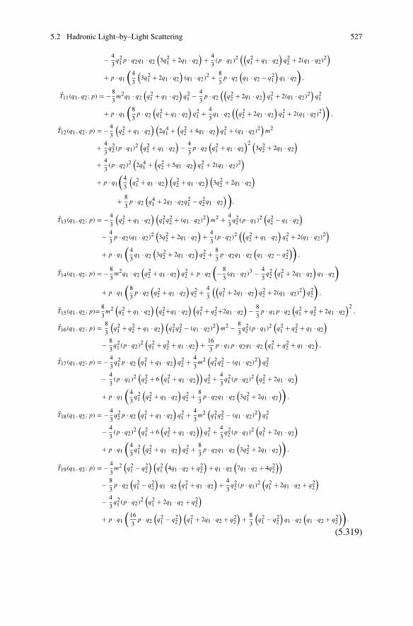
5.2 Hadronic Light–by–Light Scattering 527

− 4

3q21 p · q2q1 · q2

(3q21 + 2q1 · q2

)+ 4

3(p · q1)2

((q21 + q1 · q2

)q22 + 2(q1 · q2)2

)

+ p · q1(4

3

(3q21 + 2q1 · q2

)(q1 · q2)2 + 8

3p · q2

(q1 · q2 − q21

)q1 · q2

),

T11(q1, q2; p) = − 8

3m2q1 · q2

(q21 + q1 · q2

)q21 − 4

3p · q2

((q22 + 2q1 · q2

)q21 + 2(q1 · q2)2

)q21

+ p · q1(8

3p · q2

(q21 + q1 · q2

)q21 + 4

3q1 · q2

((q22 + 2q1 · q2

)q21 + 2(q1 · q2)2

)),

T12(q1, q2; p) = − 4

3

(q22 + q1 · q2

) (2q41 +

(q22 + 4q1 · q2

)q21 + (q1 · q2)2

)m2

+ 4

3q22 (p · q1)2

(q22 + q1 · q2

)− 4

3p · q2

(q21 + q1 · q2

)2 (3q22 + 2q1 · q2

)

+ 4

3(p · q2)2

(2q41 +

(q22 + 5q1 · q2

)q21 + 2(q1 · q2)2

)

+ p · q1(4

3

(q21 + q1 · q2

) (q22 + q1 · q2

) (3q22 + 2q1 · q2

)

+ 8

3p · q2

(q41 + 2q1 · q2q21 − q22q1 · q2

)),

T13(q1, q2; p) = − 4

3

(q22 + q1 · q2

) (q21q

22 + (q1 · q2)2

)m2 + 4

3q22 (p · q1)2

(q22 − q1 · q2

)

− 4

3p · q2(q1 · q2)2

(3q22 + 2q1 · q2

)+ 4

3(p · q2)2

((q22 + q1 · q2

)q21 + 2(q1 · q2)2

)

+ p · q1(4

3q1 · q2

(3q22 + 2q1 · q2

)q22 + 8

3p · q2q1 · q2

(q1 · q2 − q22

)),

T14(q1, q2; p) = − 8

3m2q1 · q2

(q22 + q1 · q2

)q22 + p · q2

(− 8

3(q1 · q2)3 − 4

3q22

(q21 + 2q1 · q2

)q1 · q2

)

+ p · q1(8

3p · q2

(q22 + q1 · q2

)q22 + 4

3

((q21 + 2q1 · q2

)q22 + 2(q1 · q2)2

)q22

),

T15(q1, q2; p)=8

3m2

(q21 + q1 · q2

) (q22+q1 · q2

) (q21 + q22+2q1 · q2

)− 8

3p · q1 p · q2

(q21 + q22 + 2q1 · q2

)2,

T16(q1, q2; p) = 8

3

(q21 + q22 + q1 · q2

) (q21q

22 − (q1 · q2)2

)m2 − 8

3q22 (p · q1)2

(q21 + q22 + q1 · q2

)

− 8

3q21 (p · q2)2

(q21 + q22 + q1 · q2

)+ 16

3p · q1 p · q2q1 · q2

(q21 + q22 + q1 · q2

),

T17(q1, q2; p) = − 4

3q21 p · q2

(q21 + q1 · q2

)q22 + 4

3m2

(q21q

22 − (q1 · q2)2

)q22

− 4

3(p · q1)2

(q22 + 6

(q21 + q1 · q2

))q22 + 4

3q21 (p · q2)2

(q22 + 2q1 · q2

)

+ p · q1(4

3q21

(q22 + q1 · q2

)q22 + 8

3p · q2q1 · q2

(3q21 + 2q1 · q2

)),

T18(q1, q2; p) = − 4

3q22 p · q2

(q21 + q1 · q2

)q21 + 4

3m2

(q21q

22 − (q1 · q2)2

)q21

− 4

3(p · q2)2

(q21 + 6

(q22 + q1 · q2

))q21 + 4

3q22 (p · q1)2

(q21 + 2q1 · q2

)

+ p · q1(4

3q21

(q22 + q1 · q2

)q22 + 8

3p · q2q1 · q2

(3q22 + 2q1 · q2

)),

T19(q1, q2; p) = − 4

3m2

(q21 − q22

) (q21

(4q1 · q2 + q22

)+ q1 · q2

(7q1 · q2 + 4q22

))

− 8

3p · q2

(q21 − q22

)q1 · q2

(q21 + q1 · q2

)+ 4

3q22 (p · q1)2

(q21 + 2q1 · q2 + q22

)

− 4

3q21 (p · q2)2

(q21 + 2q1 · q2 + q22

)

+ p · q1(16

3p · q2

(q21 − q22

) (q21 + 2q1 · q2 + q22

)+ 8

3

(q21 − q22

)q1 · q2

(q1 · q2 + q22

)).

(5.319)

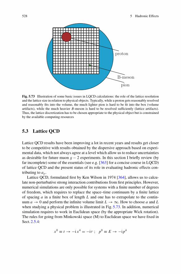
528 5 Hadronic Effects

proton

B-meson

pion

Fig. 5.73 Illustration of some basic issues in LQCD calculations: the role of the lattice resolutionand the lattice size in relation to physical objects. Typically, while a proton gets reasonably resolvedand reasonably fits into the volume, the much lighter pion is hard to be fit into the box (volumeartifacts), while the much heavier B-meson is hard to be resolved sufficiently (lattice artifacts).Thus, the lattice discretization has to be chosen appropriate to the physical object but is constrainedby the available computing resources

5.3 Lattice QCD

Lattice QCD results have been improving a lot in recent years and results get closerto be competitive with results obtained by the dispersive approach based on experi-mental data, which not always agree at a level which allow us to reduce uncertaintiesas desirable for future muon g − 2 experiments. In this section I briefly review (byfar incomplete) some of the essentials (see e.g. [363] for a concise course in LQCD)of lattice QCD and the present status of its role in evaluating hadronic effects con-tributing to aμ.

Lattice QCD, formulated first by Ken Wilson in 1974 [364], allows us to calcu-late non-perturbative strong interaction contributions from first principles. However,numerical simulations are only possible for systems with a finite number of degreesof freedom, which requires to replace the space–time continuum by a finite latticeof spacing a in a finite box of length L and one has to extrapolate to the contin-uum a → 0 and perform the infinite volume limit L → ∞. How to choose a and Lwhen studying a physical problem is illustrated in Fig. 5.73. In addition, numericalsimulation requires to work in Euclidean space (by the appropriate Wick rotation).The rules for going from Minkowski space (M) to Euclidean space we have fixed inSect. 2.5.4:

x0 ≡ t → −i x4 = −iτ ; p0 ≡ E → −ip4

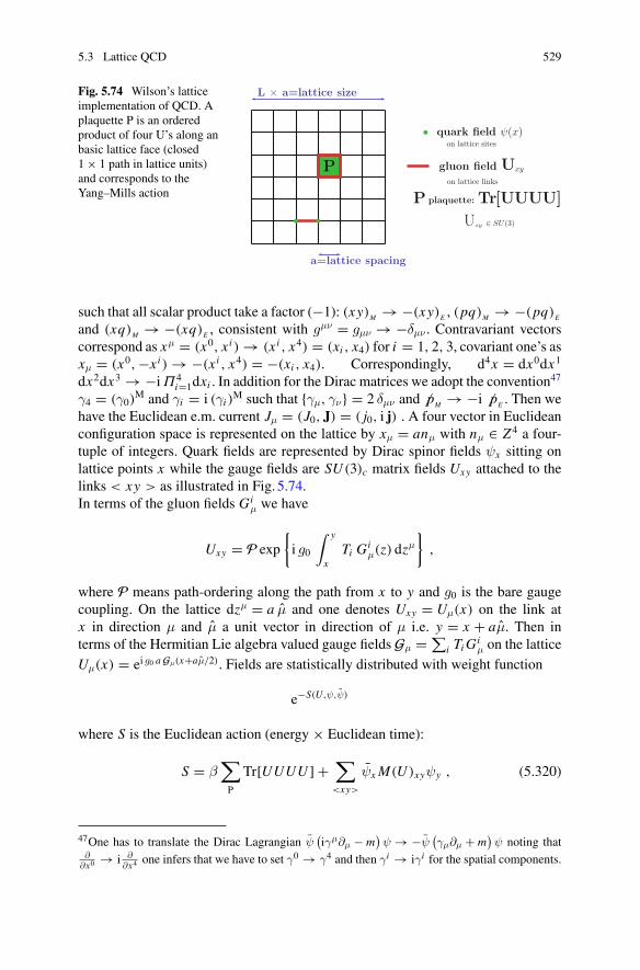
5.3 Lattice QCD 529

Fig. 5.74 Wilson’s latticeimplementation of QCD. Aplaquette P is an orderedproduct of four U’s along anbasic lattice face (closed1 × 1 path in lattice units)and corresponds to theYang–Mills action

P

• •

a=lattice spacing

L × a=lattice size

• quark field ψ(x)on lattice sites

gluon field Uxy

on lattice links

Pplaquette: Tr[UUUU]Uxy ∈ SU(3)

such that all scalar product take a factor (−1): (xy)M → −(xy)E , (pq)M → −(pq)E

and (xq)M → −(xq)E , consistent with gμν = gμν → −δμν . Contravariant vectorscorrespond as xμ = (x0, xi ) → (xi , x4) = (xi , x4) for i = 1, 2, 3, covariant one’s asxμ = (x0,−xi ) → −(xi , x4) = −(xi , x4). Correspondingly, d4x = dx0dx1

dx2dx3 → −iΠ4i=1dxi . In addition for the Dirac matrices we adopt the convention47

γ4 = (γ0)M and γi = i (γi )M such that {γμ, γν} = 2 δμν and pM → −i pE . Then we

have the Euclidean e.m. current Jμ = (J0, J) = ( j0, i j) . A four vector in Euclideanconfiguration space is represented on the lattice by xμ = anμ with nμ ∈ Z4 a four-tuple of integers. Quark fields are represented by Dirac spinor fields ψx sitting onlattice points x while the gauge fields are SU (3)c matrix fields Uxy attached to thelinks < xy > as illustrated in Fig. 5.74.In terms of the gluon fields Gi

μ we have

Uxy = P exp

{i g0

∫ y

xTi G

iμ(z) dz

μ

},

where P means path-ordering along the path from x to y and g0 is the bare gaugecoupling. On the lattice dzμ = a μ and one denotes Uxy = Uμ(x) on the link atx in direction μ and μ a unit vector in direction of μ i.e. y = x + aμ. Then interms of the Hermitian Lie algebra valued gauge fields Gμ = ∑

i TiGiμ on the lattice

Uμ(x) = ei g0 a Gμ(x+aμ/2). Fields are statistically distributed with weight function

e−S(U,ψ,ψ)

where S is the Euclidean action (energy × Euclidean time):

S = β∑

P

Tr[UUUU ] +∑

<xy>

ψx M(U )xyψy , (5.320)

47One has to translate the Dirac Lagrangian ψ(iγμ∂μ − m

)ψ → −ψ

(γμ∂μ + m

)ψ noting that

∂∂x0

→ i ∂∂x4

one infers that we have to set γ0 → γ4 and then γi → iγi for the spatial components.

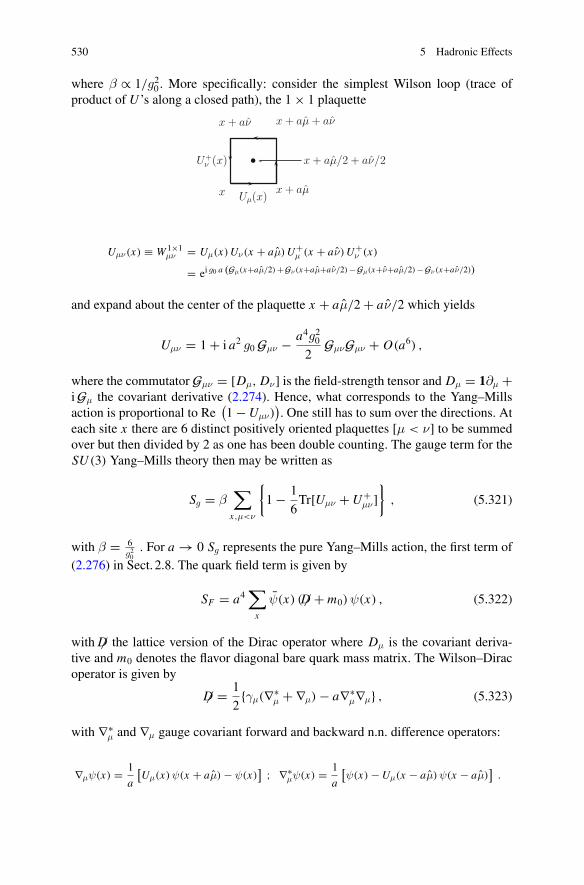
530 5 Hadronic Effects

where β ∝ 1/g20 . More specifically: consider the simplest Wilson loop (trace ofproduct of U ’s along a closed path), the 1 × 1 plaquette

Uμν(x) ≡ W 1×1μν = Uμ(x)Uν(x + aμ)U+

μ (x + aν)U+ν (x)

= ei g0 a (Gμ(x+aμ/2) +Gν (x+aμ+aν/2) −Gμ(x+ν+aμ/2) −Gν (x+aν/2))

and expand about the center of the plaquette x + aμ/2 + aν/2 which yields

Uμν = 1 + i a2 g0 Gμν − a4g202

GμνGμν + O(a6) ,

where the commutator Gμν = [Dμ, Dν] is the field-strength tensor and Dμ = 1∂μ +iGμ the covariant derivative (2.274). Hence, what corresponds to the Yang–Millsaction is proportional to Re

(1 −Uμν)

). One still has to sum over the directions. At

each site x there are 6 distinct positively oriented plaquettes [μ < ν] to be summedover but then divided by 2 as one has been double counting. The gauge term for theSU (3) Yang–Mills theory then may be written as

Sg = β∑

x,μ<ν

{1 − 1

6Tr[Uμν +U+

μν]}

, (5.321)

with β = 6g20

. For a → 0 Sg represents the pure Yang–Mills action, the first term of(2.276) in Sect. 2.8. The quark field term is given by

SF = a4∑

x

ψ(x) ( D + m0)ψ(x) , (5.322)

with D the lattice version of the Dirac operator where Dμ is the covariant deriva-tive and m0 denotes the flavor diagonal bare quark mass matrix. The Wilson–Diracoperator is given by

D = 1

2{γμ(∇∗

μ + ∇μ) − a∇∗μ∇μ} , (5.323)

with ∇∗μ and ∇μ gauge covariant forward and backward n.n. difference operators:

∇μψ(x) = 1

a

[Uμ(x) ψ(x + aμ) − ψ(x)

] ; ∇∗μψ(x) = 1

a

[ψ(x) −Uμ(x − aμ) ψ(x − aμ)

].

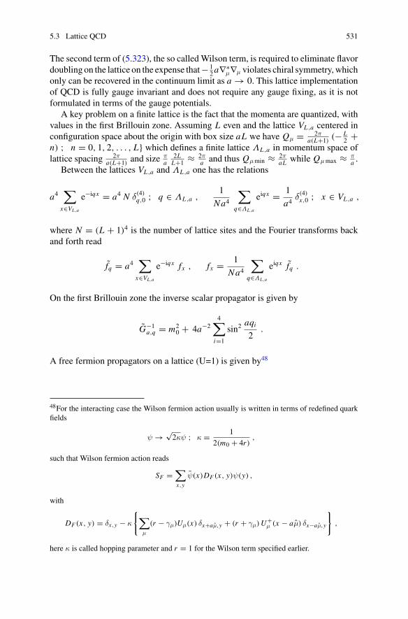
5.3 Lattice QCD 531

The second term of (5.323), the so called Wilson term, is required to eliminate flavordoubling on the lattice on the expense that− 1

2a∇∗μ∇μ violates chiral symmetry,which

only can be recovered in the continuum limit as a → 0. This lattice implementationof QCD is fully gauge invariant and does not require any gauge fixing, as it is notformulated in terms of the gauge potentials.

A key problem on a finite lattice is the fact that the momenta are quantized, withvalues in the first Brillouin zone. Assuming L even and the lattice VL ,a centered inconfiguration space about the origin with box size aL we have Qμ = 2π

a(L+1) (− L2 +

n) ; n = 0, 1, 2, . . . , L} which defines a finite lattice ΛL ,a in momentum space oflattice spacing 2π

a(L+1) and sizeπa

2LL+1 ≈ 2π

a and thus Qμmin ≈ 2πaL while Qμmax ≈ π

a .Between the lattices VL ,a and ΛL ,a one has the relations

a4∑

x∈VL ,a

e−iqx = a4 N δ(4)q,0 ; q ∈ ΛL ,a ,

1

Na4∑

q∈ΛL ,a

eiqx = 1

a4δ(4)x,0 ; x ∈ VL ,a ,

where N = (L + 1)4 is the number of lattice sites and the Fourier transforms backand forth read

fq = a4∑

x∈VL ,a

e−iqx fx , fx = 1

Na4∑

q∈ΛL ,a

eiqx fq .

On the first Brillouin zone the inverse scalar propagator is given by

G−1a,q = m2

0 + 4a−24∑

i=1

sin2aqi2

.

A free fermion propagators on a lattice (U=1) is given by48

48For the interacting case the Wilson fermion action usually is written in terms of redefined quarkfields

ψ → √2κψ ; κ = 1

2(m0 + 4r),

such that Wilson fermion action reads

SF =∑

x,y

ψ(x)DF (x, y)ψ(y) ,

with

DF (x, y) = δx,y − κ

{∑

μ

(r − γμ)Uμ(x) δx+aμ,y + (r + γμ)U+μ (x − aμ) δx−aμ,y

},

here κ is called hopping parameter and r = 1 for the Wilson term specified earlier.

532 5 Hadronic Effects

DF (x, y) =4∑

μ=1

γμδx+aμ,y − δx−aμ,y

2a+ m0 δxy ,

which has dimension nsites × ncolor × nDirac × nt rows and columns. The Fouriertransform yields

D−1F (p) = 1m0 + i

a

4∑

μ=1

γμ sin(apμ) ,

where in themassless limit DF (p) has 16 poles in the Brillouin zone such that a naiveFermion has “doublers”. Besides the pole at pμ = 0, poles also sit at points whereone or more of the components take values pμ = π/a (μ = 1, 2, 3, 4) in place of 0,by periodicity of the sin(apμ). The “doublers” are removed by adding the Wilsonterm which modifies the inverse Fermion propagator to

D−1F = 1m0 + i

a

4∑

μ=1

γμ sin(apμ) + 11

a

4∑

μ=1

(1 − cos(apμ)

),

making “doublers” heavy of mass proportional to 1/a such that they get removed inthe continuum limit.

Observables (physical quantities) are then obtained as weighted averages

< O >= 1

Z

∫· · ·

∫ ∏

x

dψxdψx

∏

<xy>

dUxy O(U,ψ, ψ) e−S(U,ψ,ψ) ,

where Z =< 1 > is the partition function which serves as a normalization here.The high demand of computational resources is easy to understand if we count

the many degrees of freedom involved. Per one gauge-field configuration {U } (a con-figuration being the set of U ’s on all links) one has 32–1 color degrees of freedomtimes the number of “links” (directions per site), which is 4, times the lattice size, i.e.8 × 4 × L3 × T , where T is the number of lattice points in Euclidean time (usuallyT is chosen bigger than L in order to have a better control of the Euclidean timeevolution). Per one quark propagator M−1 we have a color-factor 3×3 times the spinmultiplicity 4×4 times the square of the lattice size, i.e. 9 × 16 × L6 × T 2 . Thusthe dimension of integrals is D = 80 × L3 × T (32 real parameters of the U’s, 2×12 real parameters for ψ’s and the same number for ψ’s, which is 80 real entriesper site. The dimension of the complex quark matrices is N = 12 × L3 × T .

The method to deal with such incredibly high dimensional integrals is MonteCarlo integration together with the Metropolis “accept–reject” updating algorithm[365] and appropriate importance sampling. One generates a Markov chain of gaugeconfigurations distributed according to the probability measure (see below)

5.3 Lattice QCD 533

[dU ] e−Sg(U )∏

f

det(D(U ) + m f ) . (5.324)

Given the set of generated configurations, expectation values < O(U,ψ, ψ) > arecalculated by averaging over all configurations. For inverting the huge sparse matri-ces M the conjugate gradient algorithm [366] and improvements of it is applied.Substantial progress has been made and still is required by developing even betteralgorithms and methods of analysis as well as much faster computers.

One key problem of LQCD is the simulation with fermions (Grassmann fields= anti-commuting c-numbers). Fermions in comparison to bosons are much moredifficult to simulate. As the action is bilinear in the Grassmann quark fields onecan actually integrate out the fermions, which yields the fermion determinant in(5.324) as a weight factor of the remaining gauge configuration integrals. A genericcorrelation function then reads

< O1(x1)O2(x2) >= 1

Z

∏

<xy>

dUxy e−Sg(U ) det Mu · det Md · · · [O1(x1)O2(x2)]Wick ,

where the fermion fields in the correlator are pairwise Wick contracted to quarkpropagators M−1

u , M−1d etc. This however is very difficult/expensive to evaluate and

a direct numerical evaluation goes far beyond available computer resources. Fortu-nately, there are tricks to overcome the barrier: dynamical fermions are simulated bypseudofermions (auxiliary fermion fieldswith bosonic statistics) in theHybridMonteCarlo algorithm (molecular dynamics approach). Also statistical method requireslarge samples to be accurate. The accuracy ∼ 1√

Ncan be improved substantially

only by taking into account an enormous increase in computing time. Problem ofauto-correlations and possible zero modes come in addition. Also, the extrapolationsnecessary (volume, lattice distance, parameters)! require to repeat simulations fordifferent lattice spacings, different volumes and different physical parameters.

In order to improve the continuum extrapolation one may change the action insuch a way that the limit a → 0 scales with O(a2), rather than with O(a) as incase of the Wilson action. Sheikholeslami and Wohlert [367] have introduced theO(a) improved action by adding terms which also produces O(a) effects as theyare expected from dimension 5 operators:

Seff = SQCD + aS1 ; S1 = ∫d4x L1(x)

L1(x) = ∑ici (g0) Oi , dim

[Oi

] = 5 . (5.325)

The equation of motion allows one to eliminate most of the possible operators suchthat O(a) cut–off effects in on–shell matrix elements can be canceled by adding oneterm only to the Wilson action, namely a magnetic moment type term

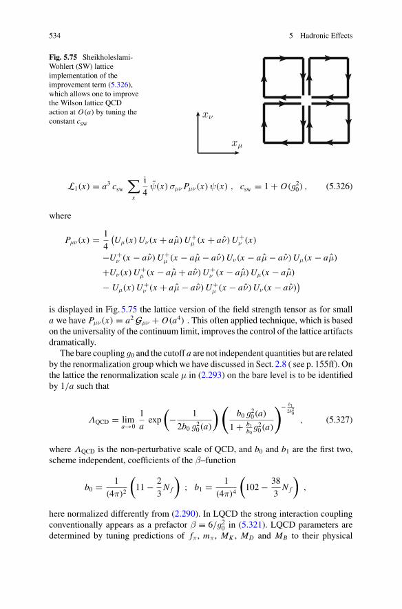
534 5 Hadronic Effects

Fig. 5.75 Sheikholeslami-Wohlert (SW) latticeimplementation of theimprovement term (5.326),which allows one to improvethe Wilson lattice QCDaction at O(a) by tuning theconstant cSW

xν

xμ

L1(x) = a3 cSW

∑

x

i

4ψ(x)σμνPμν(x)ψ(x) , cSW = 1 + O(g20) , (5.326)

where

Pμν(x) = 1

4

(Uμ(x)Uν(x + aμ)U+

μ (x + aν)U+ν (x)

−U+ν (x − aν)U+

μ (x − aμ − aν)Uν(x − aμ − aν)Uμ(x − aμ)

+Uν(x)U+μ (x − aμ + aν)U+

ν (x − aμ)Uμ(x − aμ)

− Uμ(x)U+ν (x + aμ − aν)U+

μ (x − aν)Uν(x − aν))

is displayed in Fig. 5.75 the lattice version of the field strength tensor as for smalla we have Pμν(x) = a2 Gμν + O(a4) . This often applied technique, which is basedon the universality of the continuum limit, improves the control of the lattice artifactsdramatically.

The bare coupling g0 and the cutoff a are not independent quantities but are relatedby the renormalization group which we have discussed in Sect. 2.8 ( see p. 155ff). Onthe lattice the renormalization scale μ in (2.293) on the bare level is to be identifiedby 1/a such that

ΛQCD = lima→0

1

aexp

(− 1

2b0 g20(a)

) (b0 g20(a)

1 + b1b0

g20(a)

)− b12b20

, (5.327)

where ΛQCD is the non-perturbative scale of QCD, and b0 and b1 are the first two,scheme independent, coefficients of the β–function

b0 = 1

(4π)2

(11 − 2

3N f

); b1 = 1

(4π)4

(102 − 38

3N f

),

here normalized differently from (2.290). In LQCD the strong interaction couplingconventionally appears as a prefactor β ≡ 6/g20 in (5.321). LQCD parameters aredetermined by tuning predictions of fπ , mπ, MK , MD and MB to their physical

5.3 Lattice QCD 535

(experimental) values. This fixes ΛQCD (equivalent to αs) and the quark massesm = (mu + md)/2,ms ,mc andmb. Any other quantity calculated then is a prediction.

The need for ab initio calculations of ahadμ is well motivated: – the problems todetermine non-perturbative contributions to the muon g − 2 from experimental dataat sufficient precision persists and is not easy to improve, – a model–independentextension of CHPT to the relevant energies ranges up to 2 GeV is missing while thenew experiments E989 @ FNAL and E34 @ J-PARC require and improvement ofthe hadronic uncertainties by a factor of four.

The hope is that LQCD can deliver estimates of accuracies

δaHVPμ /aHVPμ < 0.5% , δaHLbLμ /aHLbLμ<∼10% (5.328)

in the coming years.The main advantage of lattice regulated QCD is its model–independence and the

approximations are systematically improvable. With LQCD one may overcome thereliance on experimental data – except for simple hadronic quantities needed to fixthe bare parameters. Also, LQCD can providemodel independent results – except forchiral extrapolation and constraining the IR regime. One should note that latticeQCDcalculations of aHVPμ and aHLbLμ in principle are very straight forward as no analyticcontinuation or the like is needed. As static quantities they are directly accessible bythe Euclidean method. The challenge is the control of the approximations on whichthe method is based given the limitations of the computational resources.

5.3.1 Lattice QCD Approach to HVP

A very concise and inspiring status report has been given by Hartmut Wittig at theLattice 2016 Conference [368], and I will follow his synopsis. We know that inthe dispersive approach the HVP is dominated by the contribution of the ρ meson,which is characterized by its mass and width, on both of which the HVP dependssensitively. The lattice regularization has to be adapted accordingly and one hasto keep in mind that the width is determined predominantly by the ρ → ππ decaychannel (see e.g. [369]).While in the time-like region theρ peak is easy to catch, in theEuclidean regime, which is the one accessible to LQCD, the contribution appearssmeared over a larger range. We expect that a reasonable LQCD approximationrequires the ρ to be resolved sufficiently and at the same time two pions states shouldfit into the volume available. The primary object for calculating the HVP in LQCDis the electromagnetic current correlator in configuration space

〈Jμ(x, t) Jν(0, 0)〉 , (5.329)

where Jμ = 23 uγμu − 1

3 dγμd − 13 sγμs + · · · in terms of the quark fields u(x), d(x),

s(x), . . .. In principle, a Fourier transform

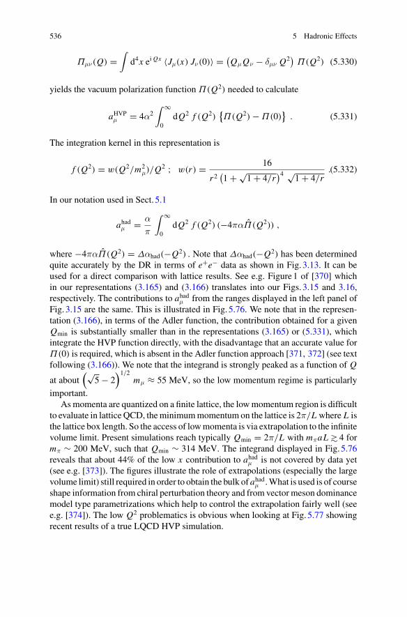
536 5 Hadronic Effects

Πμν(Q) =∫

d4x ei Qx 〈Jμ(x) Jν(0)〉 = (QμQν − δμν Q

2)

Π(Q2) (5.330)

yields the vacuum polarization function Π(Q2) needed to calculate

aHVPμ = 4α2∫ ∞

0dQ2 f (Q2)

{Π(Q2) − Π(0)

}. (5.331)

The integration kernel in this representation is

f (Q2) = w(Q2/m2μ)/Q

2 ; w(r) = 16

r2(1 + √

1 + 4/r)4 √

1 + 4/r.(5.332)

In our notation used in Sect. 5.1

ahadμ = α

π

∫ ∞

0dQ2 f (Q2) (−4παΠ(Q2)) ,

where −4παΠ(Q2) = Δαhad(−Q2) . Note that Δαhad(−Q2) has been determinedquite accurately by the DR in terms of e+e− data as shown in Fig. 3.13. It can beused for a direct comparison with lattice results. See e.g. Figure1 of [370] whichin our representations (3.165) and (3.166) translates into our Figs. 3.15 and 3.16,respectively. The contributions to ahadμ from the ranges displayed in the left panel ofFig. 3.15 are the same. This is illustrated in Fig. 5.76. We note that in the represen-tation (3.166), in terms of the Adler function, the contribution obtained for a givenQmin is substantially smaller than in the representations (3.165) or (5.331), whichintegrate the HVP function directly, with the disadvantage that an accurate value forΠ(0) is required, which is absent in the Adler function approach [371, 372] (see textfollowing (3.166)). We note that the integrand is strongly peaked as a function of Q

at about(√

5 − 2)1/2

mμ ≈ 55 MeV, so the low momentum regime is particularly

important.Asmomenta are quantized on a finite lattice, the lowmomentum region is difficult

to evaluate in lattice QCD, theminimummomentum on the lattice is 2π/L where L isthe lattice box length. So the access of lowmomenta is via extrapolation to the infinitevolume limit. Present simulations reach typically Qmin = 2π/L with mπaL >∼ 4 formπ ∼ 200 MeV, such that Qmin ∼ 314 MeV. The integrand displayed in Fig. 5.76reveals that about 44% of the low x contribution to ahadμ is not covered by data yet(see e.g. [373]). The figures illustrate the role of extrapolations (especially the largevolume limit) still required in order to obtain the bulk of ahadμ .What is used is of courseshape information from chiral perturbation theory and from vector meson dominancemodel type parametrizations which help to control the extrapolation fairly well (seee.g. [374]). The low Q2 problematics is obvious when looking at Fig. 5.77 showingrecent results of a true LQCD HVP simulation.

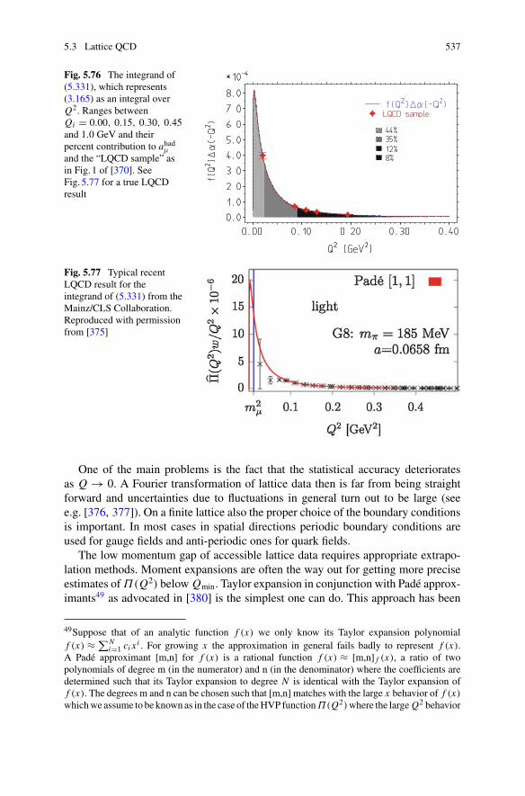
5.3 Lattice QCD 537

Fig. 5.76 The integrand of(5.331), which represents(3.165) as an integral overQ2. Ranges betweenQi = 0.00, 0.15, 0.30, 0.45and 1.0 GeV and theirpercent contribution to ahadμand the “LQCD sample” asin Fig. 1 of [370]. SeeFig. 5.77 for a true LQCDresult

Fig. 5.77 Typical recentLQCD result for theintegrand of (5.331) from theMainz/CLS Collaboration.Reproduced with permissionfrom [375]

One of the main problems is the fact that the statistical accuracy deterioratesas Q → 0. A Fourier transformation of lattice data then is far from being straightforward and uncertainties due to fluctuations in general turn out to be large (seee.g. [376, 377]). On a finite lattice also the proper choice of the boundary conditionsis important. In most cases in spatial directions periodic boundary conditions areused for gauge fields and anti-periodic ones for quark fields.

The low momentum gap of accessible lattice data requires appropriate extrapo-lation methods. Moment expansions are often the way out for getting more preciseestimates ofΠ(Q2) below Qmin. Taylor expansion in conjunction with Padé approx-imants49 as advocated in [380] is the simplest one can do. This approach has been

49Suppose that of an analytic function f (x) we only know its Taylor expansion polynomialf (x) ≈ ∑N

i=1 ci xi . For growing x the approximation in general fails badly to represent f (x).

A Padé approximant [m,n] for f (x) is a rational function f (x) ≈ [m,n] f (x), a ratio of twopolynomials of degree m (in the numerator) and n (in the denominator) where the coefficients aredetermined such that its Taylor expansion to degree N is identical with the Taylor expansion off (x). The degrees m and n can be chosen such that [m,n] matches with the large x behavior of f (x)whichwe assume to be known as in the case of theHVP functionΠ(Q2)where the large Q2 behavior

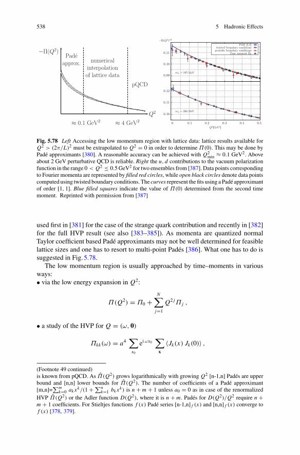
538 5 Hadronic Effects

−Π(Q2)Pade

approx. numericalinterpolationof lattice data

pQCD

≈ 0.1 GeV2 ≈ 4 GeV2

Q2×××××

××

××

××

××

××

××

××

××

×××

×××

××

××

××

××

××

××

××

××

××

×××

−Π(Q2)ud

mπ = 268

mπ = 185

Fig. 5.78 Left Accessing the low momentum region with lattice data: lattice results available forQ2 > (2π/L)2 must be extrapolated to Q2 = 0 in order to determine Π(0). This may be done byPadé approximants [380]. A reasonable accuracy can be achieved with Q2

min ≈ 0.1 GeV2. Aboveabout 2 GeV perturbative QCD is reliable. Right the u, d contributions to the vacuum polarizationfunction in the range 0 < Q2 ≤ 0.5GeV2 for two ensembles from [387]. Data points correspondingto Fourier momenta are represented by filled red circles, while open black circles denote data pointscomputed using twisted boundary conditions. The curves represent the fits using a Padé approximantof order [1, 1]. Blue filled squares indicate the value of Π(0) determined from the second timemoment. Reprinted with permission from [387]

used first in [381] for the case of the strange quark contribution and recently in [382]for the full HVP result (see also [383–385]). As momenta are quantized normalTaylor coefficient based Padé approximants may not be well determined for feasiblelattice sizes and one has to resort to multi-point Padés [386]. What one has to do issuggested in Fig. 5.78.

The low momentum region is usually approached by time–moments in variousways:• via the low energy expansion in Q2:

Π(Q2) = Π0 +N∑

j=1

Q2 jΠ j ,

• a study of the HVP for Q = (ω, 0)

Πkk(ω) = a4∑

x0

eiωx0∑

x

〈Jk(x) Jk(0)〉 ,

(Footnote 49 continued)is known from pQCD. As Π(Q2) grows logarithmically with growing Q2 [n-1,n] Padés are upperbound and [n,n] lower bounds for Π(Q2). The number of coefficients of a Padé approximant[m,n]=

∑mk=0 ak xk/(1 + ∑n

k=1 bk xk) is n + m + 1 unless a0 = 0 as in case of the renormalizedHVP Π(Q2) or the Adler function D(Q2), where it is n + m. Padés for D(Q2)/Q2 require n +m + 1 coefficients. For Stieltjes functions f (x) Padé series [n-1,n] f (x) and [n,n] f (x) converge tof (x) [378, 379].

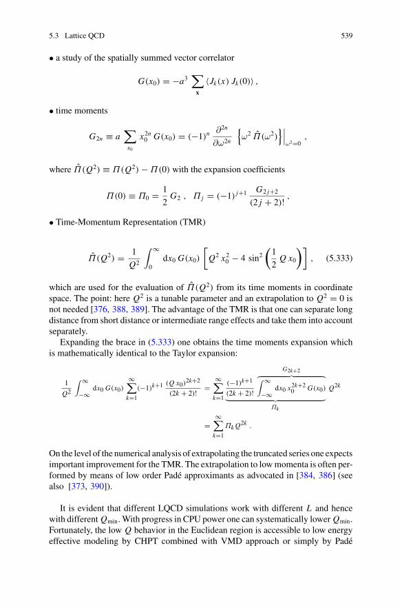
5.3 Lattice QCD 539

• a study of the spatially summed vector correlator

G(x0) = −a3∑

x

〈Jk(x) Jk(0)〉 ,

• time moments

G2n ≡ a∑

x0

x2n0 G(x0) = (−1)n∂2n

∂ω2n

{ω2 Π(ω2)

}∣∣∣ω2=0

,

where Π(Q2) ≡ Π(Q2) − Π(0) with the expansion coefficients

Π(0) ≡ Π0 = 1

2G2 , Π j = (−1) j+1 G2 j+2

(2 j + 2)! ,

• Time-Momentum Representation (TMR)

Π(Q2) = 1

Q2

∫ ∞

0dx0 G(x0)

[Q2 x20 − 4 sin2

(1

2Q x0

)], (5.333)

which are used for the evaluation of Π(Q2) from its time moments in coordinatespace. The point: here Q2 is a tunable parameter and an extrapolation to Q2 = 0 isnot needed [376, 388, 389]. The advantage of the TMR is that one can separate longdistance from short distance or intermediate range effects and take them into accountseparately.

Expanding the brace in (5.333) one obtains the time moments expansion whichis mathematically identical to the Taylor expansion:

1

Q2

∫ ∞−∞

dx0 G(x0)∞∑

k=1

(−1)k+1 (Q x0)2k+2

(2k + 2)! =∞∑

k=1

(−1)k+1

(2k + 2)!

G2k+2︷ ︸︸ ︷∫ ∞−∞

dx0 x2k+20 G(x0)

︸ ︷︷ ︸Πk

Q2k

=∞∑

k=1

Πk Q2k .

On the level of the numerical analysis of extrapolating the truncated series one expectsimportant improvement for the TMR. The extrapolation to lowmomenta is often per-formed by means of low order Padé approximants as advocated in [384, 386] (seealso [373, 390]).

It is evident that different LQCD simulations work with different L and hencewith different Qmin.With progress in CPU power one can systematically lower Qmin.Fortunately, the low Q behavior in the Euclidean region is accessible to low energyeffective modeling by CHPT combined with VMD approach or simply by Padé

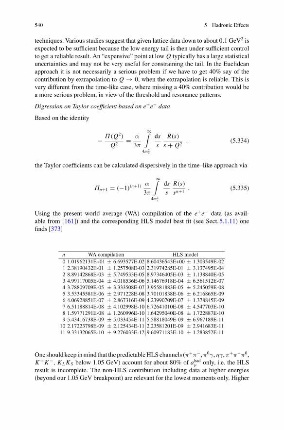
540 5 Hadronic Effects

techniques. Various studies suggest that given lattice data down to about 0.1 GeV2 isexpected to be sufficient because the low energy tail is then under sufficient controlto get a reliable result. An “expensive” point at low Q typically has a large statisticaluncertainties and may not be very useful for constraining the tail. In the Euclideanapproach it is not necessarily a serious problem if we have to get 40% say of thecontribution by extrapolation to Q → 0, when the extrapolation is reliable. This isvery different from the time-like case, where missing a 40% contribution would bea more serious problem, in view of the threshold and resonance patterns.

Digression on Taylor coefficient based on e+e− data

Based on the identity

− Π(Q2)

Q2= α

3π

∞∫

4m2π

ds

s

R(s)

s + Q2. (5.334)

the Taylor coefficients can be calculated dispersively in the time–like approach via

Πn+1 = (−1)(n+1) α

3π

∞∫

4m2π

ds

s

R(s)

sn+1. (5.335)

Using the present world average (WA) compilation of the e+e− data (as avail-able from [161]) and the corresponding HLS model best fit (see Sect. 5.1.11) onefinds [373]

n WA compilation HLS model0 1.01962131E+01 ± 6.693577E-02 8.60436543E+00 ± 1.303549E-021 2.38190432E-01 ± 1.257508E-03 2.31974285E-01 ± 3.137495E-042 8.89142868E-03 ± 5.749533E-05 8.97346405E-03 ± 1.138840E-053 4.99117005E-04 ± 4.018536E-06 5.14676918E-04 ± 6.561512E-074 3.78809709E-05 ± 3.333508E-07 3.95581883E-05 ± 5.245059E-085 3.53345581E-06 ± 2.971228E-08 3.70101838E-06 ± 6.216865E-096 4.06928851E-07 ± 2.867316E-09 4.23990709E-07 ± 1.378845E-097 6.51188814E-08 ± 4.102998E-10 6.72641010E-08 ± 4.547703E-108 1.59771291E-08 ± 1.260996E-10 1.64295040E-08 ± 1.722887E-109 5.43416738E-09 ± 5.033454E-11 5.58818049E-09 ± 6.967189E-11

10 2.17223798E-09 ± 2.125434E-11 2.23581201E-09 ± 2.941683E-1111 9.33132065E-10 ± 9.276033E-12 9.60971183E-10 ± 1.283852E-11

One should keep inmind that the predictableHLSchannels (π+π−,π0γ,ηγ,π+π−π0,K+K−, KLKS below 1.05 GeV) account for about 80% of ahadμ only, i.e. the HLSresult is incomplete. The non-HLS contribution including data at higher energies(beyond our 1.05 GeV breakpoint) are relevant for the lowest moments only. Higher

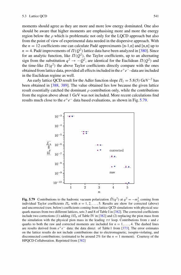
5.3 Lattice QCD 541

moments should agree as they are more and more low energy dominated. One alsoshould be aware that higher moments are emphasising more and more the energyregion below the ρ which is problematic not only for the LQCD approach but alsofrom the point of view of experimental data needed in the dispersive approach. Withthe n = 12 coefficients one can calculate Padé approximants [n-1,n] and [n,n] up ton = 4. Padé improvements ofΠ(Q2) lattice data have been analyzed in [380]. Sincefor an analytic function, like Π(Q2), the Taylor coefficients, up to an alternatingsign from the substitution q2 → −Q2, are identical for the Euclidean Π(Q2) andthe time-like Π(q2) the above Taylor coefficients directly compare with the onesobtained from lattice data, provided all effects included in the e+e−–data are includedin the Euclidean regime as well.

An early lattice QCD result for the Adler function slope Π1 = 5.8(5) GeV−2 hasbeen obtained in [388, 389]. The value obtained lies low because the given latticeresult essentially catched the dominant ρ contribution only, while the contributionsfrom the region above about 1 GeV was not included. More recent calculations findresults much close to the e+e− data based evaluations, as shown in Fig. 5.79.

Fig. 5.79 Contributions to the hadronic vacuum polarization Π(q2) at q2 = −m2μ coming from

individual Taylor coefficients Πn with n = 1, 2, . . . , 5. Results are show for corrected (above)and uncorrected (raw, below) coefficients coming from lattice QCD simulations with physical sea-quark masses from two different lattices, sets 3 and 8 of Table I in [382]. The corrected coefficientsinclude two corrections (1) adding δΠn of Table IV in [382] and (2) replacing the pion mass fromthe simulation with the physical pion mass in the leading ππ loop. Contributions from s and cquarks to both the raw and corrected moments are included for n = 1, . . . , 4. The dashed linesare results derived from e+e− data: the data direct of Table1 from [373]. The error estimateson the lattice results do not include contributions due to electromagnetic, isospin-violating, anddisconnected contributions; (estimated to be around 2% for the n = 1 moment). Courtesy of theHPQCD Collaboration. Reprinted from [382]

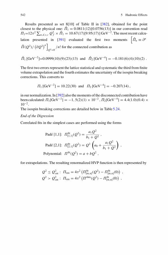
542 5 Hadronic Effects

Results presented as set 8[10] of Table II in [382], obtained for the pointclosest to the physical one: Π1 = 0.0811(12)[0.0756(13)] in our convention readΠ1=12π2 ∑

u,d,s,c Q2f × Π1 = 10.67(17)[9.95(17)]GeV−2. Themost recent calcu-

lation presented in [391] evaluated the first two moments[Πn ≡ ∂n

Π(Q2)/(∂Q2

)n]

Q2=0/n! for the connected contribution as

Π1 [GeV−2]=0.0999(10)(9)(23)(13) and Π2 [GeV−4] = −0.181(6)(4)(10)(2) .

The first two errors represent the lattice statistical and systematic the third from finitevolume extrapolation and the fourth estimates the uncertainty of the isospin breakingcorrections. This converts to

Π1 [GeV−2] = 10.22(30) and Π2 [GeV−4] = −0.207(14) ,

in our normalization. In [392] also themoments of the disconnected contribution havebeen calculated:Π1[GeV−2] = −1, 5(2)(1) × 10−2 ,Π2[GeV−4] = 4.4(1.0)(0.4) ×10−2.The isospin breaking corrections are detailed below in Table5.24.

End of the Digression

Correlated fits in the simplest cases are performed using the forms

Padé [1,1]: Πfit[1,1](Q

2) = a1Q2

b1 + Q2,

Padé [2,1]: Πfit[2,1](Q

2) = Q2

(a0 + a1Q2

b1 + Q2

),

Polynomial: Πfit(Q2) = a + bQ2 ,

for extrapolations. The resulting renormalized HVP function is then represented by

Q2 ≤ Q2cut : Πren = 4π2

(Πfit

[m,n](Q2) − Πfit

[m,n](0))

,

Q2 > Q2cut : Πren = 4π2

(Πdata(Q2) − Πfit

[m,n](0))

,

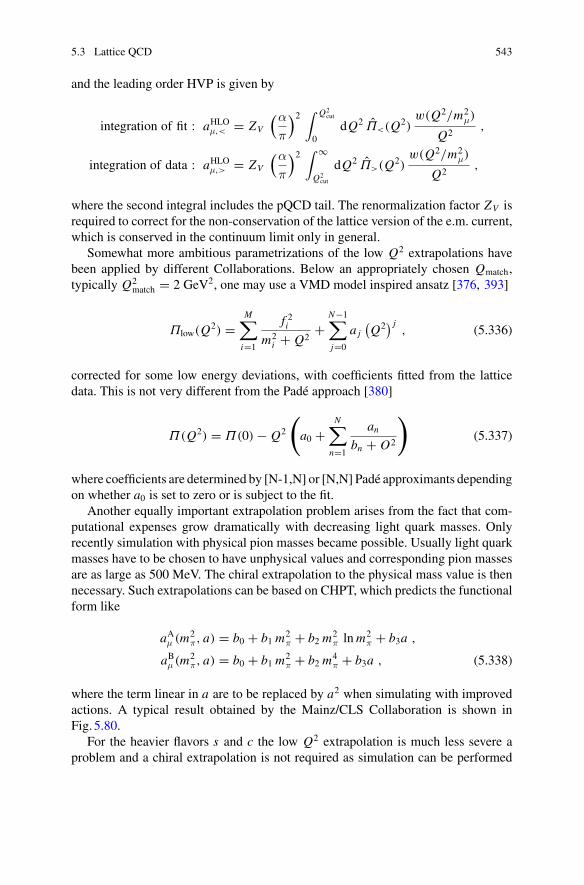
5.3 Lattice QCD 543

and the leading order HVP is given by

integration of fit : aHLOμ,< = ZV

(α

π

)2 ∫ Q2cut

0dQ2 Π<(Q2)

w(Q2/m2μ)

Q2,

integration of data : aHLOμ,> = ZV

(α

π

)2 ∫ ∞

Q2cut

dQ2 Π>(Q2)w(Q2/m2

μ)

Q2,

where the second integral includes the pQCD tail. The renormalization factor ZV isrequired to correct for the non-conservation of the lattice version of the e.m. current,which is conserved in the continuum limit only in general.

Somewhat more ambitious parametrizations of the low Q2 extrapolations havebeen applied by different Collaborations. Below an appropriately chosen Qmatch,typically Q2

match = 2 GeV2, one may use a VMD model inspired ansatz [376, 393]

Πlow(Q2) =M∑

i=1

f 2im2

i + Q2+

N−1∑

j=0

a j(Q2

) j, (5.336)

corrected for some low energy deviations, with coefficients fitted from the latticedata. This is not very different from the Padé approach [380]

Π(Q2) = Π(0) − Q2

(a0 +

N∑

n=1

anbn + O2

)(5.337)

where coefficients are determined by [N-1,N] or [N,N] Padé approximants dependingon whether a0 is set to zero or is subject to the fit.

Another equally important extrapolation problem arises from the fact that com-putational expenses grow dramatically with decreasing light quark masses. Onlyrecently simulation with physical pion masses became possible. Usually light quarkmasses have to be chosen to have unphysical values and corresponding pion massesare as large as 500 MeV. The chiral extrapolation to the physical mass value is thennecessary. Such extrapolations can be based on CHPT, which predicts the functionalform like

aAμ (m2π, a) = b0 + b1 m

2π + b2 m

2π lnm2

π + b3a ,

aBμ (m2π, a) = b0 + b1 m

2π + b2 m

4π + b3a , (5.338)

where the term linear in a are to be replaced by a2 when simulating with improvedactions. A typical result obtained by the Mainz/CLS Collaboration is shown inFig. 5.80.

For the heavier flavors s and c the low Q2 extrapolation is much less severe aproblem and a chiral extrapolation is not required as simulation can be performed

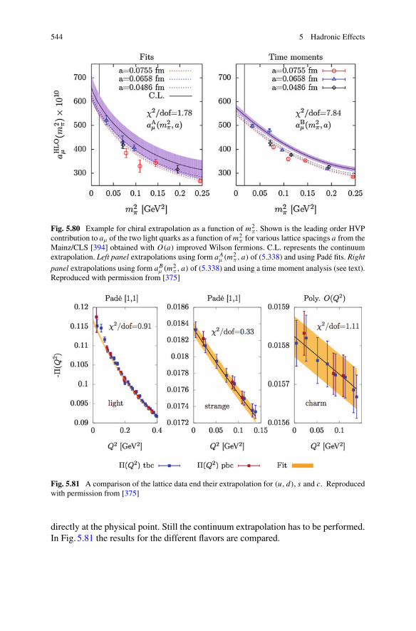
544 5 Hadronic Effects

Fig. 5.80 Example for chiral extrapolation as a function of m2π . Shown is the leading order HVP

contribution to aμ of the two light quarks as a function ofm2π for various lattice spacings a from the

Mainz/CLS [394] obtained with O(a) improved Wilson fermions. C.L. represents the continuumextrapolation. Left panel extrapolations using form aA

μ (m2π, a) of (5.338) and using Padé fits. Right

panel extrapolations using form aBμ (m2

π, a) of (5.338) and using a time moment analysis (see text).Reproduced with permission from [375]

Fig. 5.81 A comparison of the lattice data end their extrapolation for (u, d), s and c. Reproducedwith permission from [375]

directly at the physical point. Still the continuum extrapolation has to be performed.In Fig. 5.81 the results for the different flavors are compared.

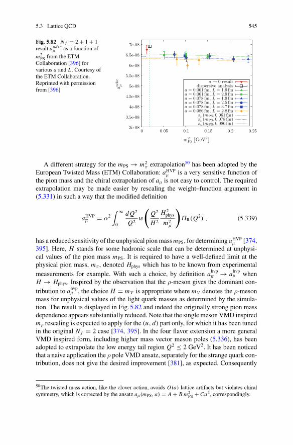
5.3 Lattice QCD 545

Fig. 5.82 N f = 2 + 1 + 1result audscμ as a function of

m2PS from the ETM

Collaboration [396] forvarious a and L . Courtesy ofthe ETM Collaboration.Reprinted with permissionfrom [396]

aμ(mPS, 0.086 fm)aμ(mPS, 0.078 fm)aμ(mPS, 0.061 fm)

a = 0.086 fm, L = 2.8 fma = 0.078 fm, L = 3.7 fma = 0.078 fm, L = 2.5 fma = 0.078 fm, L = 1.9 fma = 0.061 fm, L = 2.9 fma = 0.061 fm, L = 1.9 fm

dispersive analysisa → 0 result

m2PS

[GeV2]

auds

cμ

0.250.20.150.10.050

7e-08

6.5e-08

6e-08

5.5e-08

5e-08

4.5e-08

4e-08

3.5e-08

3e-08

A different strategy for the mPS → m2π extrapolation50 has been adopted by the

European Twisted Mass (ETM) Collaboration: aHVPμ is a very sensitive function ofthe pion mass and the chiral extrapolation of aμ is not easy to control. The requiredextrapolation may be made easier by rescaling the weight–function argument in(5.331) in such a way that the modified definition

aHVPμ = α2∫ ∞

0

dQ2

Q2w

(Q2

H 2

H 2phys

m2μ

)ΠR(Q2) , (5.339)

has a reduced sensitivity of the unphysical pionmassmPS, for determining aHVPμ [374,395]. Here, H stands for some hadronic scale that can be determined at unphysi-cal values of the pion mass mPS. It is required to have a well-defined limit at thephysical pion mass, mπ, denoted Hphys which has to be known from experimentalmeasurements for example. With such a choice, by definition ahvpμ → ahvpμ whenH → Hphys. Inspired by the observation that the ρ-meson gives the dominant con-tribution to ahvpμ , the choice H = mV is appropriate where mV denotes the ρ-mesonmass for unphysical values of the light quark masses as determined by the simula-tion. The result is displayed in Fig. 5.82 and indeed the originally strong pion massdependence appears substantially reduced. Note that the single meson VMD inspiredmρ rescaling is expected to apply for the (u, d) part only, for which it has been tunedin the original N f = 2 case [374, 395]. In the four flavor extension a more generalVMD inspired form, including higher mass vector meson poles (5.336), has beenadopted to extrapolate the low energy tail region Q2 ≤ 2 GeV2. It has been noticedthat a naive application the ρ pole VMD ansatz, separately for the strange quark con-tribution, does not give the desired improvement [381], as expected. Consequently

50The twisted mass action, like the clover action, avoids O(a) lattice artifacts but violates chiralsymmetry, which is corrected by the ansatz aμ(mPS, a) = A + B m2

PS + Ca2, correspondingly.

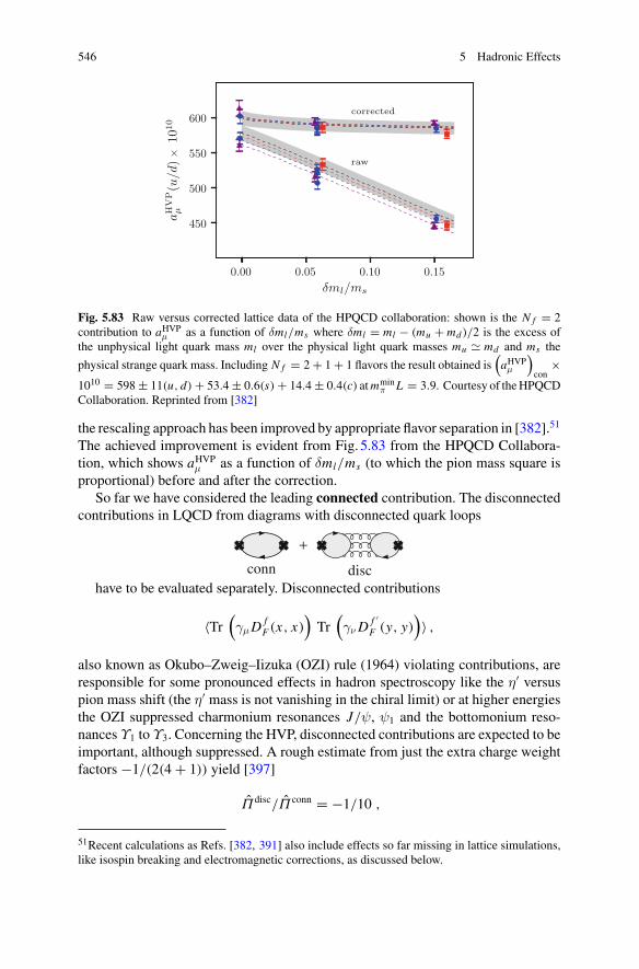
546 5 Hadronic Effects

0.00 0.05 0.10 0.15

l/ms

450

500

550

600

aHVP

μ(u

/d)

×10

10

corrected

raw

Fig. 5.83 Raw versus corrected lattice data of the HPQCD collaboration: shown is the N f = 2contribution to aHVPμ as a function of δml/ms where δml = ml − (mu + md )/2 is the excess ofthe unphysical light quark mass ml over the physical light quark masses mu � md and ms the

physical strange quark mass. Including N f = 2 + 1 + 1 flavors the result obtained is(aHVPμ

)

con×

1010 = 598 ± 11(u, d) + 53.4 ± 0.6(s) + 14.4 ± 0.4(c) atmminπ L = 3.9. Courtesy of theHPQCD

Collaboration. Reprinted from [382]

the rescaling approach has been improved by appropriate flavor separation in [382].51

The achieved improvement is evident from Fig. 5.83 from the HPQCD Collabora-tion, which shows aHVPμ as a function of δml/ms (to which the pion mass square isproportional) before and after the correction.

So far we have considered the leading connected contribution. The disconnectedcontributions in LQCD from diagrams with disconnected quark loops

have to be evaluated separately. Disconnected contributions

〈Tr(γμD

fF (x, x)

)Tr

(γνD

f ′F (y, y)

)〉 ,

also known as Okubo–Zweig–Iizuka (OZI) rule (1964) violating contributions, areresponsible for some pronounced effects in hadron spectroscopy like the η′ versuspion mass shift (the η′ mass is not vanishing in the chiral limit) or at higher energiesthe OZI suppressed charmonium resonances J/ψ, ψ1 and the bottomonium reso-nances Υ1 to Υ3. Concerning the HVP, disconnected contributions are expected to beimportant, although suppressed. A rough estimate from just the extra charge weightfactors −1/(2(4 + 1)) yield [397]

Πdisc/Π conn = −1/10 ,

51Recent calculations as Refs. [382, 391] also include effects so far missing in lattice simulations,like isospin breaking and electromagnetic corrections, as discussed below.

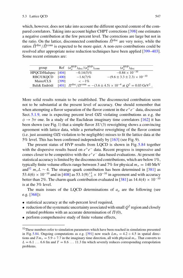
5.3 Lattice QCD 547

which, however, does not take into account the different spectral content of the com-pared correlators. Taking into account higher CHPT corrections [398] one estimatesa negative contribution at the few percent level. The corrections are large but not inthe ratio. On the lattice, disconnected contributions Πdisc are very noisy, while theratios Πdisc/Π conn is expected to be more quiet. A non-zero contributions could beresolved after appropriate noise reduction techniques have been applied [399–403].Some recent estimates are:

group Ref (aHVPμ )disc/(aHVPμ )conn (aHVPμ )disc

HPQCD/Hadspec [404] −0.14(5)% −0.84 × 10−10

RBC/UKQCD [400] −1.6(7)% −(9.6 ± 3.3 ± 2.3) × 10−10

Mainz/CLS [399] < −1%Bali& Endrödi [401] Πdisc/Πconn = −(3.6 ± 4.5) × 10−4 at Q2 = 0.03 GeV2 .

More solid results remain to be established. The disconnected contribution seemnot to be substantial at the present level of accuracy. One should remember thatwhen attempting a flavor separation of the flavor content in the e+e− data, discussedSect. 5.1.9, one is expecting percent level OZI violating contributions as e.g. theφ → 3π one. In a study of the Euclidean imaginary time correlators [162] it hasbeen shown (see Fig. 1) that a simple flavor SU (3) reweighting shows a convincingagreement with lattice data, while a perturbative reweighting of the flavor content(i.e. just assuming OZI violation to be negligible) misses to fit the lattice data at the5% level. This has been confirmed independently by [163] (see Fig. 9).

The present status of HVP results from LQCD is shown in Fig. 5.84 togetherwith the dispersive results based on e+e− data. Recent progress is impressive andcomes closer to be competitive with the e+e− data based evaluations. At present thestatistical accuracy is limited by the disconnected contributions, which are below 1%,typically finite volume effects range between 3 and 7% for physical mπ = 140 MeVand52 mπL ∼ 4. The strange quark contribution has been determined in [381] as53.4(6) × 10−10 and in [408] as 53.1(9)+1

−3 × 10−10 in agreement and with accuracybetter than 2%. The charm quark contribution evaluated in [381] as 14.4(4) × 10−10

is at the 3% level.The main issues of the LQCD determinations of aμ are the following (see

e.g. [368]):

• statistical accuracy at the sub-percent level required,• reduction of the systematic uncertainty associatedwith small Q2 region and closelyrelated problems with an accurate determination of Π(0),

• perform comprehensive study of finite volume effects,

52These numbers refer to simulation parameters which have been reached in simulations presentedin Fig. 5.84. Ongoing computations as e.g. [391] now reach Lmπ = 4.2 ÷ 4.5 in spatial direc-tions and Tmπ = 5.9 ÷ 7.7 in the imaginary time direction, all with physical mπ . That converts toL = 6.1 . . . 6.6 fm and T = 8.6 . . . 11.3 fm which severely reduces corresponding extrapolationproblems.

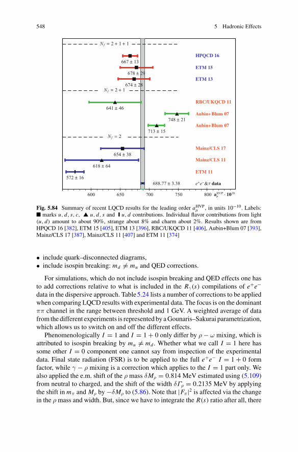
548 5 Hadronic Effects

600 650 700 750 800

Nf 2 1 1

HPQCD 16667 13

ETM 15678 29

ETM 13674 28

Nf 2 1

RBC/UKQCD 11641 46

Aubin+Blum 07748 21

Aubin+Blum 07713 15

Nf 2

Mainz/CLS 17654 38

Mainz/CLS 11618 64

ETM 11572 16

e e & data688 77 3 38

aHVP 1010

Fig. 5.84 Summary of recent LQCD results for the leading order aHVPμ , in units 10−10. Labels:■ marks u, d, s, c, ▲ u, d, s and ❙ u, d contributions. Individual flavor contributions from light(u, d) amount to about 90%, strange about 8% and charm about 2%. Results shown are fromHPQCD 16 [382], ETM 15 [405], ETM 13 [396], RBC/UKQCD 11 [406], Aubin+Blum 07 [393],Mainz/CLS 17 [387], Mainz/CLS 11 [407] and ETM 11 [374]

• include quark–disconnected diagrams,• include isospin breaking: md = mu and QED corrections.

For simulations, which do not include isospin breaking and QED effects one hasto add corrections relative to what is included in the Rγ(s) compilations of e+e−data in the dispersive approach. Table5.24 lists a number of corrections to be appliedwhen comparing LQCD results with experimental data. The focus is on the dominantππ channel in the range between threshold and 1 GeV. A weighted average of datafrom the different experiments is represented by aGounaris–Sakurai parametrization,which allows us to switch on and off the different effects.

Phenomenologically I = 1 and I = 1 + 0 only differ by ρ − ω mixing, which isattributed to isospin breaking by mu = md . Whether what we call I = 1 here hassome other I = 0 component one cannot say from inspection of the experimentaldata. Final state radiation (FSR) is to be applied to the full e+e− I = 1 + 0 formfactor, while γ − ρ mixing is a correction which applies to the I = 1 part only. Wealso applied the e.m. shift of the ρ mass δMρ = 0.814 MeV estimated using (5.109)from neutral to charged, and the shift of the width δΓρ = 0.2135 MeV by applyingthe shift in mπ and Mρ by −δMρ to (5.86). Note that |Fπ|2 is affected via the changein the ρ mass and width. But, since we have to integrate the R(s) ratio after all, there

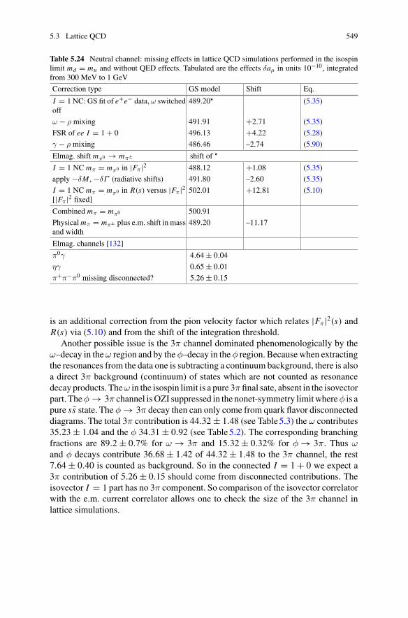
5.3 Lattice QCD 549

Table 5.24 Neutral channel: missing effects in lattice QCD simulations performed in the isospinlimit md = mu and without QED effects. Tabulated are the effects δaμ in units 10−10, integratedfrom 300 MeV to 1 GeV

Correction type GS model Shift Eq.

I = 1 NC: GS fit of e+e− data, ω switchedoff

489.20� (5.35)

ω − ρ mixing 491.91 +2.71 (5.35)

FSR of ee I = 1 + 0 496.13 +4.22 (5.28)

γ − ρ mixing 486.46 –2.74 (5.90)

Elmag. shift mπ0 → mπ± shift of �

I = 1 NC mπ = mπ0 in |Fπ|2 488.12 +1.08 (5.35)

apply −δM , −δΓ (radiative shifts) 491.80 –2.60 (5.35)

I = 1 NC mπ = mπ0 in R(s) versus |Fπ|2[|Fπ|2 fixed]

502.01 +12.81 (5.10)

Combined mπ = mπ0 500.91

Physicalmπ = mπ± plus e.m. shift in massand width

489.20 –11.17

Elmag. channels [132]

π0γ 4.64 ± 0.04

ηγ 0.65 ± 0.01

π+π−π0 missing disconnected? 5.26 ± 0.15

is an additional correction from the pion velocity factor which relates |Fπ|2(s) andR(s) via (5.10) and from the shift of the integration threshold.

Another possible issue is the 3π channel dominated phenomenologically by theω–decay in theω region and by theφ–decay in theφ region. Because when extractingthe resonances from the data one is subtracting a continuum background, there is alsoa direct 3π background (continuum) of states which are not counted as resonancedecay products. Theω in the isospin limit is a pure 3π final sate, absent in the isovectorpart. Theφ → 3π channel isOZI suppressed in the nonet-symmetry limitwhereφ is apure ss state. The φ → 3π decay then can only come from quark flavor disconnecteddiagrams. The total 3π contribution is 44.32 ± 1.48 (see Table5.3) the ω contributes35.23 ± 1.04 and the φ 34.31 ± 0.92 (see Table5.2). The corresponding branchingfractions are 89.2 ± 0.7% for ω → 3π and 15.32 ± 0.32% for φ → 3π. Thus ωand φ decays contribute 36.68 ± 1.42 of 44.32 ± 1.48 to the 3π channel, the rest7.64 ± 0.40 is counted as background. So in the connected I = 1 + 0 we expect a3π contribution of 5.26 ± 0.15 should come from disconnected contributions. Theisovector I = 1 part has no 3π component. So comparison of the isovector correlatorwith the e.m. current correlator allows one to check the size of the 3π channel inlattice simulations.

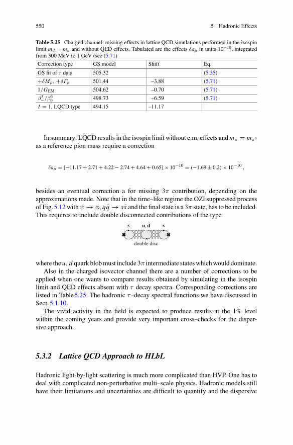
550 5 Hadronic Effects

Table 5.25 Charged channel: missing effects in lattice QCD simulations performed in the isospinlimit md = mu and without QED effects. Tabulated are the effects δaμ in units 10−10, integratedfrom 300 MeV to 1 GeV (see (5.71)

Correction type GS model Shift Eq.

GS fit of τ data 505.32 (5.35)

+δMρ, +δΓρ 501.44 –3.88 (5.71)

1/GEM 504.62 –0.70 (5.71)

β3−/β30 498.73 –6.59 (5.71)

I = 1, LQCD type 494.15 –11.17

In summary: LQCD results in the isospin limit without e.m. effects andmπ = mπ0

as a reference pion mass require a correction

δaμ = [−11.17 + 2.71 + 4.22 − 2.74 + 4.64 + 0.65] × 10−10 = (−1.69 ± 0.2) × 10−10 ,

besides an eventual correction a for missing 3π contribution, depending on theapproximations made. Note that in the time–like regime the OZI suppressed processof Fig. 5.12 withψ → φ, qq → ss and the final state is a 3π state, has to be included.This requires to include double disconnected contributions of the type

where the u, d quark blobmust include 3π intermediate stateswhichwould dominate.Also in the charged isovector channel there are a number of corrections to be

applied when one wants to compare results obtained by simulating in the isospinlimit and QED effects absent with τ decay spectra. Corresponding corrections arelisted in Table5.25. The hadronic τ–decay spectral functions we have discussed inSect. 5.1.10.

The vivid activity in the field is expected to produce results at the 1% levelwithin the coming years and provide very important cross–checks for the disper-sive approach.

5.3.2 Lattice QCD Approach to HLbL

Hadronic light-by-light scattering is much more complicated than HVP. One has todeal with complicated non-perturbative multi–scale physics. Hadronic models stillhave their limitations and uncertainties are difficult to quantify and the dispersive

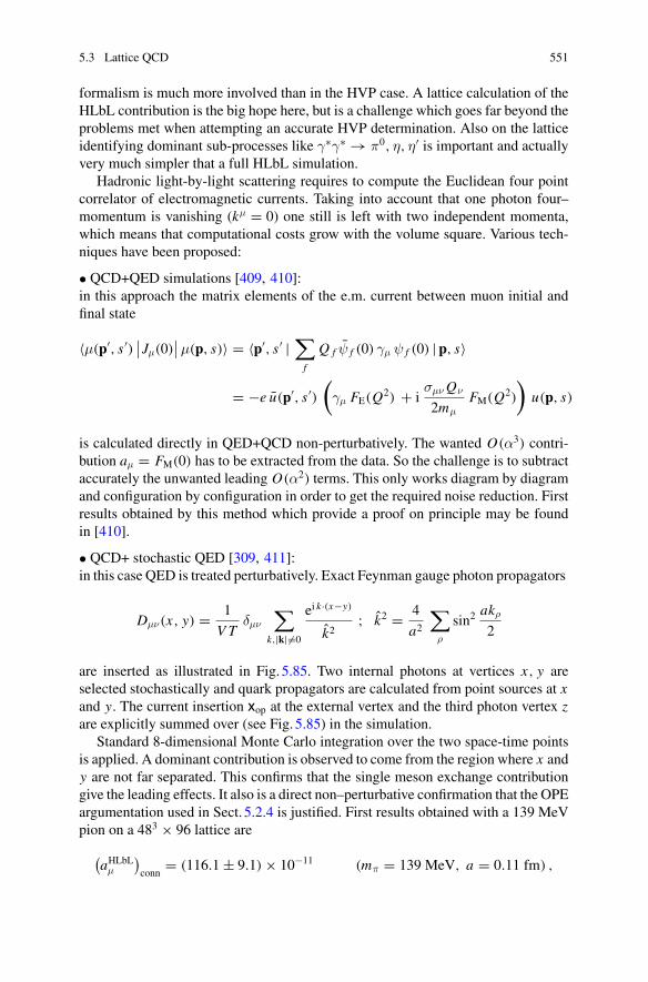
5.3 Lattice QCD 551

formalism is much more involved than in the HVP case. A lattice calculation of theHLbL contribution is the big hope here, but is a challenge which goes far beyond theproblems met when attempting an accurate HVP determination. Also on the latticeidentifying dominant sub-processes like γ∗γ∗ → π0, η, η′ is important and actuallyvery much simpler that a full HLbL simulation.

Hadronic light-by-light scattering requires to compute the Euclidean four pointcorrelator of electromagnetic currents. Taking into account that one photon four–momentum is vanishing (kμ = 0) one still is left with two independent momenta,which means that computational costs grow with the volume square. Various tech-niques have been proposed:

• QCD+QED simulations [409, 410]:in this approach the matrix elements of the e.m. current between muon initial andfinal state

〈μ(p′, s ′)∣∣Jμ(0)

∣∣μ(p, s)〉 = 〈p′, s ′ |∑

f

Q f ψ f (0) γμ ψ f (0) | p, s〉

= −e u(p′, s ′)(

γμ FE(Q2) + i

σμνQν

2mμFM(Q2)

)u(p, s)

is calculated directly in QED+QCD non-perturbatively. The wanted O(α3) contri-bution aμ = FM(0) has to be extracted from the data. So the challenge is to subtractaccurately the unwanted leading O(α2) terms. This only works diagram by diagramand configuration by configuration in order to get the required noise reduction. Firstresults obtained by this method which provide a proof on principle may be foundin [410].

• QCD+ stochastic QED [309, 411]:in this case QED is treated perturbatively. Exact Feynman gauge photon propagators

Dμν(x, y) = 1

VTδμν

∑

k,|k|=0

ei k·(x−y)

k2; k2 = 4

a2∑

ρ

sin2akρ

2

are inserted as illustrated in Fig. 5.85. Two internal photons at vertices x, y areselected stochastically and quark propagators are calculated from point sources at xand y. The current insertion xop at the external vertex and the third photon vertex zare explicitly summed over (see Fig. 5.85) in the simulation.

Standard 8-dimensional Monte Carlo integration over the two space-time pointsis applied. A dominant contribution is observed to come from the region where x andy are not far separated. This confirms that the single meson exchange contributiongive the leading effects. It also is a direct non–perturbative confirmation that the OPEargumentation used in Sect. 5.2.4 is justified. First results obtained with a 139 MeVpion on a 483 × 96 lattice are

(aHLbLμ

)conn

= (116.1 ± 9.1) × 10−11 (mπ = 139 MeV, a = 0.11 fm) ,

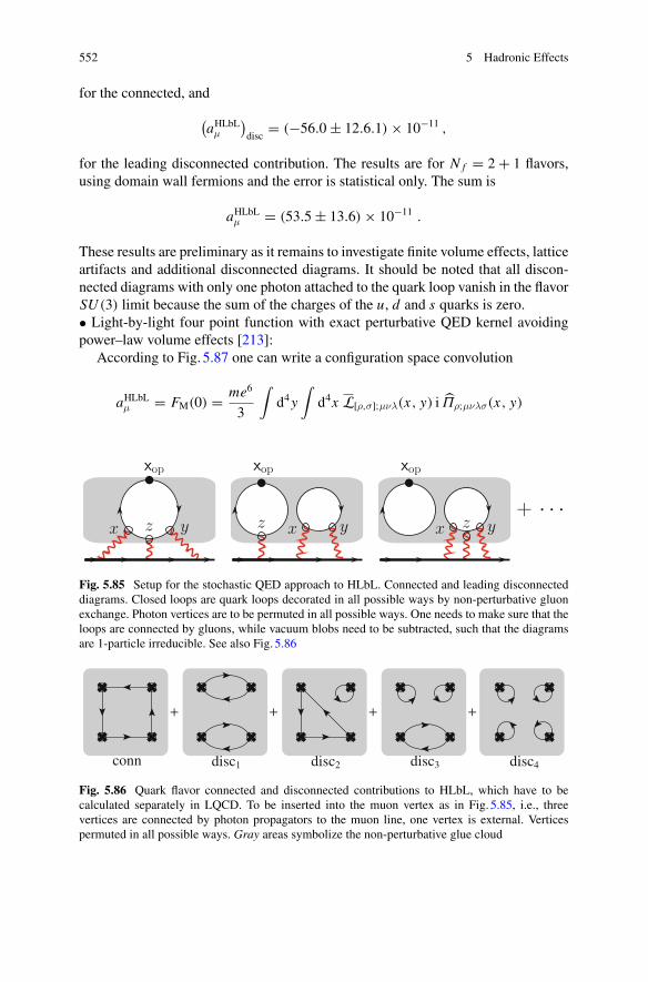
552 5 Hadronic Effects

for the connected, and

(aHLbLμ

)disc

= (−56.0 ± 12.6.1) × 10−11 ,

for the leading disconnected contribution. The results are for N f = 2 + 1 flavors,using domain wall fermions and the error is statistical only. The sum is

aHLbLμ = (53.5 ± 13.6) × 10−11 .

These results are preliminary as it remains to investigate finite volume effects, latticeartifacts and additional disconnected diagrams. It should be noted that all discon-nected diagrams with only one photon attached to the quark loop vanish in the flavorSU (3) limit because the sum of the charges of the u, d and s quarks is zero.• Light-by-light four point function with exact perturbative QED kernel avoidingpower–law volume effects [213]:

According to Fig. 5.87 one can write a configuration space convolution

aHLbLμ = FM(0) = me6

3

∫d4y

∫d4x L[ρ,σ];μνλ(x, y) i Πρ;μνλσ(x, y)

x yz

xop

z yx

xop

z yx

xop

+ · · ·

Fig. 5.85 Setup for the stochastic QED approach to HLbL. Connected and leading disconnecteddiagrams. Closed loops are quark loops decorated in all possible ways by non-perturbative gluonexchange. Photon vertices are to be permuted in all possible ways. One needs to make sure that theloops are connected by gluons, while vacuum blobs need to be subtracted, such that the diagramsare 1-particle irreducible. See also Fig. 5.86

Fig. 5.86 Quark flavor connected and disconnected contributions to HLbL, which have to becalculated separately in LQCD. To be inserted into the muon vertex as in Fig. 5.85, i.e., threevertices are connected by photon propagators to the muon line, one vertex is external. Verticespermuted in all possible ways. Gray areas symbolize the non-perturbative glue cloud

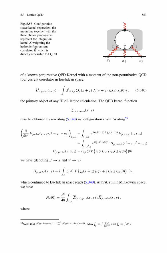
5.3 Lattice QCD 553

Fig. 5.87 Configurationspace kernel separation: themuon line together with thethree photon propagatorsrepresent the integrationkernel L weighting thehadronic four currentcorrelator Π which isdirectly accessible to LQCD

x zy

x1 x3x2

of a known perturbative QED Kernel with a moment of the non-perturbative QCDfour current correlator in Euclidean space,

Πρ;μνλσ(x, y) =∫

d4z zρ 〈Jμ(x + z) Jν(y + z) Jσ(z) Jλ(0)〉 , (5.340)

the primary object of any HLbL lattice calculation. The QED kernel function

L[ρ,σ];μνλ(x, y)

may be obtained by rewriting (5.148) in configuration space. Writing53

(∂

∂kρ Πμνλσ(q1, q2, k − q1 − q2)

)

k=0=

∫

x,y,zei(q1(x−z)+q2(y−z)) Πρ;μνλσ(x, y, z)

=∫

x ′,y′,zei(q1x

′+q2 y′) Πρ;μνλσ(x ′ + z, y′ + z, z)

Πρ;μνλσ(x, y, z) = i zρ 〈0|T {jμ(x) jν(y) jλ(z) jσ(0)

} |0〉

we have (denoting x ′ → x and y′ → y)

Πρ;μνλσ(x, y) = i∫

zzρ 〈0|T {

jμ(x + z) jν(y + z) jλ(z) jσ(0)} |0〉 ,

which continued to Euclidean space reads (5.340). At first, still in Minkowski space,we have

FM(0) = e6

48

∫

x,yL[ρ,σ];μνλ(x, y) i Πρ;μνλσ(x, y) ,

where

53Note that ei(q1x+q2 y+q3z)) k=0= ei(q1(x−z)+q2(y−z)). Also∫q ≡ ∫ d4q

(2π)4and

∫x ≡ ∫

d4x .

554 5 Hadronic Effects

L[ρ,σ];μνλ(x, y) ≡ i∫

q1,q2

1

q21 q22 (q1 + q2)2

1

(p − q1)2 − m21

(p − q1 − q2)2 − m2

× 1

mTr

{( p + m)[γρ, γσ]( p + m) γμ ( p− q1 + m) γν ( p+ q3 + m) γλ

}ei(q1x+q2y)

is a known QED kernel function. Rotated to Euclidean space (for conventions seethe begin of this Sect. 5.3) we have (all objects now in Euclidean metric)

L[ρ,σ];μνλ(x, y) ≡∫

q1,q2

1

q21 q22 (q1 + q2)2

1

(p − q1)2 + m2

1

(p − q1 − q2)2 + m2

× 1

mTr

{( p + im)[γρ, γσ]( p + im) γμ ( p− q1 + im) γν ( p+ q3 + im) γλ

}e−i(q1x+q2 y) ,

which we also may write as

L[ρ,σ];μνλ(x, y) =1

mTr

{(i p − m)[γρ, γσ](i p − m)γμ (i p+ ∂x − m) γν

(i p+ ∂x+ ∂y − m

)γλ

}J(ε, x, y) ,

J(ε, x, y) =∫

q1,q2

1

q21 q22 (q1 + q2)2

1

(p − q1)2 + m2

1

(p − q1 − q2)2 + m2 e−i(q1x+q2 y) .

(5.341)

The Fourier integral J is IR singular and required an IR regularization. It can berepresented in terms of position space scalar propagators. Using

i

q2 + m2=

∫

xΔF (x) e−iqx ; ΔF (x) = m2

4π2

K1(m|x |)m|x | , (5.342)

where K1(z) is a modified Bessel function (see (2.142)), one obtains [213]

J(ε, x, y) =∫

x1,x2,x3D(x1 − x)D(x2 − y)D(x3) ΔF (x1 − x2) e

−ip(x1−x2) ΔF (x2 − x3) e−ip(x2−x3) ,

where ΔF (xi − xk)) represent the Euclidean scalar muon propagator and D(xi ) theEuclidean scalar photon propagator, which we may regularize by an infinitesimalphoton mass. One can choose p = −imε, where ε is a unit vector in direction of themuon momentum, thus p2 = −m2 and then averaged over the muon direction

L[ρ,σ];μνλ(x, y) = 1

2π2

∫dΩεL[ρ,σ];μνλ(ε, x, y) ≡ ⟨

L[ρ,σ];μνλ(ε, x, y)⟩ε

. (5.343)

The result only depends on |x |, |y| and x · y = |x ||y| · β (β = cosϑ; ϑ the anglebetween the Euclidean four-vectors x and y) and one gets the 3-dimensional integralrepresentation in configuration space, with

5.3 Lattice QCD 555

∫

x,yf (|x |, |y|,β) = 8π3

∫ ∞

0d|x ||x |3

∫ ∞

0d|y||y|3

∫ π

0dβ sin2 β f (|x |, |y|,β) .

(5.344)The configuration space kernel can be worked out once for all and may be foundin [213]. I think this is a most promising approach to the HLbL problem and we arewaiting for its realization in a dedicated lattice QCD simulation.

At present LQCD HLbL evaluations reach a statistical accuracy at the 10% levelfor the connected contribution, disconnected contributions are sizable and have largerstatistical fluctuations at the 20% level but can be resolved. One expects to be ableto constrain/check phenomenological models in not too far future.

Lattice QCD Calculation of the π0 → γ∗γ∗ Form Factor

Lattice calculation of dominant subprocesses as presented in [293, 412] are veryuseful to constrain meson TFFs. As discussed earlier the dominating contributionto HLbL is related to pseudoscalar meson exchange, which we have discussed inSect. 5.2.4. A first lattice calculation of the dominant π0 → γ∗γ∗ subprocesses fordoubly virtual photon configurations has been obtained in [293] recently. Such newlattice data are very useful as corresponding experimental data are missing so far.

In Minkowski space the relevant matrix element is defined by (5.163). In momen-tum space [412]

Mμν(p, q1) = i∫

d4x ei qx 〈0|T {jμ(x) jν(0)

} |π0(p)〉 = εμναβqα1 q

β2 Fπ0γ∗γ∗ (m2

π; q21 , q22 ) ,

with p = q1 + q2, defines the invariant on–shell pion form factorFπ0γ∗γ∗(m2π; q2

1 , q22 )

for off–shell photons of virtualities q21 and q2

2 . On the Euclidean lattice one cancalculate the electromagnetic current correlator [293]

MEμν(ω1, q1) = −

∫dτ eω1τ

∫d3z e−iq1z 〈0|T {

Jμ(z, τ ) Jν(0, 0)} |π(p)〉 ,

where ω1 is a real parameter tuned such that q1 = (ω1, q1) is in the range q21,2 <

M2V = min(M2

ρ , 4m2π). A simulation of (5.190) is then obtained considering

MEμν ∼ C (3)

μν (τ , tπ; p, q1, q2)

= a6∑

x,z

〈T {Jμ (z, ti ) Jν(0, t f ) P

+ (x, t0)}〉 ei px e−i q1z , (5.345)

where τ = t f − ti is the time separation of the two currents and tπ = min(t f −t0, ti − t0) (see Fig. 5.88).

The projection to the pion pole is obtained in the large tπ limit:

Aμν(τ ) = limtπ→∞C (3)

μν (τ , tπ) eEπ tπ ,

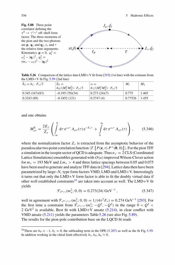
556 5 Hadronic Effects

Fig. 5.88 Three pointcorrelator defining theπ0 → γ∗γ∗ off–shell formfactor. The three-momenta ofthe pion and the two photonsare p, q1 and q2, tπ and τthe relative time arguments.Kinematics: p = 0, q21 =ω21 − |q1|2, q22 =

(mπ − ω1)2 − |q1|2

Table 5.26 Comparison of the lattice data LMD+V fit from [293] (1st line) with the estimate fromthe LMD+V fit Fig. 5.59 (2nd line)

h2 = h2 · Fπ/3 h5 =h5/(M2

1M22 ) · Fπ/3

α =h7/(M4

1M42 ) · Fπ/3

M1 M2

0.345 (167)(83) –0.195 (70)(34) 0.273 (24)(7) 0.775 1.465

0.3243 (89) –0.1852 (121) 0.2747 (4) 0.77526 1.455

and one obtains

MEμν = 2Eπ

Zπ

⎛

⎝0∫

−∞dτ eω1τ Aμν(τ ) e−Eπτ +

∞∫

0

dτ eω1τ Aμν(τ )

⎞

⎠ , (5.346)

where the normalization factor Zπ is extracted from the asymptotic behavior of thepseudoscalar twopoint correlation function 〈T {

P(z, t) P+(0, 0)}〉. For the pionTFF

a simulation in the isospin sector ofQCD is adequate. Thus n f = 2CLS (CoordinatedLattice Simulations) ensembles generatedwith O(a) improvedWilson-Clover actionfor mπ = 193 MeV and Lmπ > 4 and three lattice spacings between 0.05 and 0.075have been used to generate and analyze TFF data in [294]. Lattice data then have beenparametrized by large–Nc type form factors VMD, LMD and LMD+V. Interestinglyit turns out that only the LMD+V form factor is able to fit the doubly virtual data ifother well established constraints54 are taken into account as well. The LMD+V fityields

Fπ0γγ(m2π; 0, 0) = 0.273(24) GeV−1 , (5.347)

well in agreement with Fπ0∗γ∗γ∗(m2π; 0, 0) = 1/(4π2Fπ) = 0.274 GeV−1 [293]. For

the first time a constraint from Fπ0γ∗γ∗(m2π;−Q2,−Q2) in the range 0 < Q2 <

2 GeV2 is available. Best fit with LMD+V ansatz (5.214), in clear conflict withVMD ansatz (5.211) yields the parameters Table5.26 (see also Fig. 5.89).The results for the pion-pole contribution base on the LQCD fit reads

54These are h0 = −1, h1 = 0, the subleading term in the OPE (5.207) as well as the fit Fig. 5.59.In addition working in the chiral limit effectively h3, h4, h6 ≈ 0.

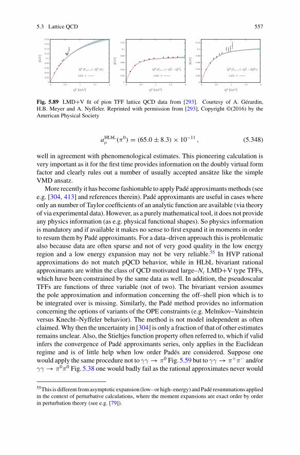
5.3 Lattice QCD 557

Fig. 5.89 LMD+V fit of pion TFF lattice QCD data from [293]. Courtesy of A. Gérardin,H.B. Meyer and A. Nyffeler. Reprinted with permission from [293], Copyright ©(2016) by theAmerican Physical Society

aHLbLμ (π0) = (65.0 ± 8.3) × 10−11 , (5.348)

well in agreement with phenomenological estimates. This pioneering calculation isvery important as it for the first time provides information on the doubly virtual formfactor and clearly rules out a number of usually accepted ansätze like the simpleVMD ansatz.

More recently it has become fashionable to apply Padé approximantsmethods (seee.g. [304, 413] and references therein). Padé approximants are useful in cases whereonly an number of Taylor coefficients of an analytic function are available (via theoryof via experimental data). However, as a purelymathematical tool, it does not provideany physics information (as e.g. physical functional shapes). So physics informationis mandatory and if available it makes no sense to first expand it in moments in orderto resum them by Padé approximants. For a data–driven approach this is problematicalso because data are often sparse and not of very good quality in the low energyregion and a low energy expansion may not be very reliable.55 In HVP rationalapproximations do not match pQCD behavior, while in HLbL bivariant rationalapproximants are within the class of QCD motivated large–Nc LMD+V type TFFs,which have been constrained by the same data as well. In addition, the pseudoscalarTFFs are functions of three variable (not of two). The bivariant version assumesthe pole approximation and information concerning the off–shell pion which is tobe integrated over is missing. Similarly, the Padé method provides no informationconcerning the options of variants of the OPE constraints (e.g. Melnikov–Vainshteinversus Knecht–Nyffeler behavior). The method is not model independent as oftenclaimed.Why then the uncertainty in [304] is only a fraction of that of other estimatesremains unclear. Also, the Stieltjes function property often referred to, which if validinfers the convergence of Padé approximants series, only applies in the Euclideanregime and is of little help when low order Padés are considered. Suppose onewould apply the same procedure not to γγ → π0 Fig. 5.59 but to γγ → π+π− and/orγγ → π0π0 Fig. 5.38 one would badly fail as the rational approximates never would

55This is different fromasymptotic expansion (low–or high–energy) andPadé resummations appliedin the context of perturbative calculations, where the moment expansions are exact order by orderin perturbation theory (see e.g. [79]).

558 5 Hadronic Effects

reproduce the Breit–Wigner type shape of the f2(1270). We should keep in mind thatafter all what we want to know and understand is what QCD should tell us (latticeQCD).

References

1. A. Litke et al., Phys. Rev. Lett. 30, 1189 (1973); G. Tarnopolsky et al. Phys. Rev. Lett. 32,432 (1974)

2. H.D. Politzer, Phys. Rev. Lett. 30, 1346 (1973); D. Gross, F. Wilczek. Phys. Rev. Lett. 30,1343 (1973)

3. H. Fritzsch, M. Gell-Mann, H. Leutwyler, Phys. Lett. 47, 365 (1973)4. T. Appelquist, H. Georgi, Phys. Rev. D 8, 4000 (1973); A. Zee. Phys. Rev. D 8, 4038 (1973)5. H. Fritzsch, Phys. Rev. D 10, 1624 (1974); H. Fritzsch, H. Leutwyler, Report CALT-68-416

(1974)6. F. Jegerlehner, EPJ Web Conf. 118, 01016 (2016), arXiv:1705.00263 [hep-ph]7. M. Davier, A. Höcker, B. Malaescu, Z. Zhang, Adv. Ser. Direct. High Energy Phys. 26, 129

(2016)8. S. Eidelman, F. Jegerlehner, Z. Phys. C 67, 585 (1995); F. Jegerlehner, Nucl. Phys. (Proc.

Suppl.) C 51, 131 (1996); J. Phys. G 29, 101 (2003); Nucl. Phys. Proc. Suppl. 126, 325 (2004)9. K. Adel, F.J. Yndurain, arXiv: 9509378

10. D.H. Brown, W.A. Worstell, Phys. Rev. D 54, 3237 (1996)11. R. Alemany, M. Davier, A. Höcker, Eur. Phys. J. C 2, 123 (1998)12. A.D. Martin, J. Outhwaite, M.G. Ryskin, Phys. Lett. B 492, 69 (2000). Eur. Phys. J. C 19,

681 (2001)13. O.V. Zenin et al., arXiv:hep-ph/011017614. M.R. Whalley, J. Phys. G 29, A1 (2003)15. F. Jegerlehner, Nucl. Phys. Proc. Suppl. 162, 22 (2006)16. F. Jegerlehner, Acta Phys. Polon. B 44(11), 2257 (2013)17. A.E. Blinov et al., Z. Phys. C 70, 31 (1996)18. J.Z. Bai et al., [BES Collab.], Phys. Rev. Lett. 84, 594 (2000); Phys. Rev. Lett. 88, 101802

(2002); M. Ablikim et al., Phys. Lett. B 677, 239 (2009)19. V.V. Anashin et al., Phys. Lett. B 753, 533 (2016), arXiv:1610.02827 [hep-ex]20. R.R. Akhmetshin et al., CMD-2 Collab. Phys. Lett. B 578, 285 (2004)21. V.M. Aulchenko et al., [CMD-2 Collab.], JETP Lett. 82, 743 (2005) [Pisma Zh. Eksp. Teor.

Fiz. 82, 841 (2005)]; R.R. Akhmetshin et al., JETP Lett. 84, 413 (2006) [Pisma Zh. Eksp.Teor. Fiz. 84, 491 (2006). Phys. Lett. B 648, 28 (2007)

22. M.N. Achasov et al., [SND Collab.], J. Exp. Theor. Phys. 103, 380 (2006) [Zh. Eksp. Teor.Fiz. 130, 437 (2006)]

23. A. Aloisio et al., [KLOE Collab.], Phys. Lett. B 606, 12 (2005); F. Ambrosino et al., [KLOECollab.], Phys. Lett. B 670, 285 (2009)

24. F. Ambrosino et al., KLOE Collab. Phys. Lett. B 700, 102 (2011)25. D. Babusci et al., KLOE Collab. Phys. Lett. B 720, 336 (2013)26. B. Aubert et al., [BABAR Collab.], Phys. Rev. Lett. 103, 231801 (2009); J.P. Lees et al. Phys.

Rev. D 86, 032013 (2012)27. M. Ablikim et al., BESIII Collab. Phys. Lett. B 753, 629 (2016)28. K.G. Chetyrkin, A.L. Kataev, F.V. Tkachov, Phys. Lett. B 85, 277 (1979); M. Dine, J.

Sapirstein, Phys. Rev. Lett. 43, 668 (1979); W. Celmaster, R.J. Gonsalves, Phys. Rev. Lett.44, 560 (1980); K.G. Chetyrkin. Phys. Lett. B 391, 402 (1997)

29. S.G. Gorishnii, A.L. Kataev, S.A. Larin, Phys. Lett. B 259, 144 (1991); L. R. Surguladze,M.A. Samuel, Phys. Rev. Lett. 66, 560 (1991); [Erratum-ibid. 66, 2416 (1991)]

References 559

30. K.G. Chetyrkin, J.H. Kühn, Phys. Lett. B 342, 356 (1995); K.G. Chetyrkin, J.H. Kühn, A.Kwiatkowski, Phys. Rept. 277, 189 (1996); K.G. Chetyrkin, J.H. Kühn, M. Steinhauser, Phys.Lett. B 371, 93 (1996); Nucl. Phys. B 482(213) (1996); 505, 40 (1997); K.G. Chetyrkin, R.Harlander, J.H. Kühn, M. Steinhauser, Nucl. Phys. B 503, 339 (1997); K.G. Chetyrkin, R.V.Harlander, J.H. Kühn, Nucl. Phys. B 586, 56 (2000); [Erratum-ibid. B 634, 413 (2002); P.A.Baikov, K.G. Chetyrkin, J.H. Kühn, Phys. Rev. Lett. 101, 012002 (2008); P.A. Baikov, K.G.Chetyrkin, J.H. Kühn. J. Rittinger Phys. Rev. Lett. 108, 222003 (2012)

31. R.V. Harlander, M. Steinhauser, Comput. Phys. Commun. 153, 244 (2003); 2009 update athttp://www.rhad.de/

32. K.G. Chetyrkin, J.H. Kühn, M. Steinhauser, Comput. Phys. Commun. 133, 43 (2000); B.Schmidt, M. Steinhauser. Comput. Phys. Commun. 183, 1845 (2012)

33. F. Jegerlehner, Z. Phys. C 32, 195 (1986)34. E.D. Bloom, F.J. Gilman, Phys. Rev. Lett. 25, 1140 (1970). Phys. Rev. D 4, 2901 (1971)35. E.C. Poggio, H.R. Quinn, S. Weinberg, Phys. Rev. D 13, 1958 (1976)36. M.A. Shifman, Quark–Hadron Duality, arXive:hep-ph/000913137. A.D. Martin, D. Zeppenfeld, Phys. Lett. B 345, 558 (1995)38. M. Davier, A. Höcker, Phys. Lett. B 419, 419 (1998). Phys. Lett. B 435(427), 427 (1998)39. J.H. Kühn, M. Steinhauser, Phys. Lett. B 437, 425 (1998)40. G.J. Gounaris, J.J. Sakurai, Phys. Rev. Lett. 21, 244 (1968)41. S. Eidelman et al., Particle Data Group. Phys. Lett. B 592, 1 (2004)42. W.M. Yao et al., Particle Data Group, J. Phys. G 33, 1 (2006); K.A. Olive et al., [Particle Data

Group], Chin. Phys. C 38, 090001 (2014); C. Patrignani et al., [Particle Data Group. Chin.Phys. C 40(10), 100001 (2016)

43. M.L. Swartz, SLAC-PUB-6710 (1994), arXive:hep-ph/9411353 unpublished44. M.L. Swartz, Phys. Rev. D 53, 5268 (1996)45. G. D’Agostini, Nucl. Inst. Meth. A 346, 306 (1994)46. M. Benayoun, P. David, L. DelBuono, F. Jegerlehner, Eur. Phys. J. C 73, 2453 (2013)47. M. Benayoun, P. David, L. DelBuono, F. Jegerlehner, Eur. Phys. J. C 75(12), 613 (2015),

http://dx.doi.org/10.1140/epjc/s10052-015-3830-x48. V. Blobel, Some Comments on χ2 Minimization Applications, eConf C030908, MOET002

(2003); Dealing with systematics for chi–square and for log likelihood goodness of fit, BanffInternational Research Station Statistical Inference Problems in High EnergyPhysics, http://www.desy.de/~blobel/banff.pdf (2006)

49. A.B. Arbuzov, V.A. Astakhov, A.V. Fedorov, G.V. Fedotovich, E.A. Kuraev, N.P. Merenkov,JHEP 9710, 006 (1997)

50. V.A. Khoze, M.I. Konchatnij, N.P. Merenkov, G. Pancheri, L. Trentadue, O.N. Shekhovzova,Eur. Phys. J. C 18, 481 (2001)

51. A. Hoefer, J. Gluza, F. Jegerlehner, Eur. Phys. J. C 24, 51 (2002)52. V.N. Baier, V.S. Fadin, Phys. Lett. B 27, 223 (1968)53. S. Spagnolo, Eur. Phys. J. C 6, 637 (1999); A.B. Arbuzov, E.A. Kuraev, N.P. Merenkov, L.

Trentadue, JHEP 12, 009 (1998); S. Binner, J.H. Kühn, K. Melnikov, Phys. Lett. B 459, 279(1999); M.I. Konchatnij, N.P. Merenkov, JETP Lett. 69, 811 (1999); V.A. Khoze et al., Eur.Phys. J. C 18, 481 (2001)

54. M. Benayoun, S.I. Eidelman, V.N. Ivanchenko, Z.K. Silagadze, Mod. Phys. Lett. A 14, 2605(1999)

55. H. Czyz, J.H. Kühn, Eur. Phys. J. C 18, 497 (2001); G. Rodrigo, A. Gehrmann-De Ridder, M.Guilleaume, J.H. Kühn, Eur. Phys. J. C 22, 81 (2001); G. Rodrigo, H. Czyz, J.H. Kühn, M.Szopa, Eur. Phys. J. C 24, 71 (2002); H. Czyz, A. Grzelinska, J.H. Kühn, G. Rodrigo, Eur.Phys. J. C 27, 563 (2003); Eur. Phys. J. C 33, 333 (2004). Eur. Phys. J. C 39, 411 (2005)

56. C.M. Carloni Calame, C. Lunardini, G. Montagna, O. Nicrosini, F. Piccinini, Nucl. Phys. B584, 459 (2000); C.M. Carloni Calame, G. Montagna, O. Nicrosini, F. Piccinini, Nucl. Phys.Proc. Suppl. 131, 48 (2004); G. Balossini, C.M. Carloni Calame, G. Montagna, O. Nicrosini,F. Piccinini, Nucl. Phys. B 758, 227 (2006); C.M. Carloni Calame et al., Nucl. Phys. Proc.Suppl. 225–227, 293 (2012)

560 5 Hadronic Effects

57. S. Jadach, W. Placzek, B.F.L. Ward, Phys. Lett. B 390, 298 (1997)58. A.B. Arbuzov, G.V. Fedotovich, F.V. Ignatov, E.A. Kuraev, A.L. Sibidanov, Eur. Phys. J. C

46, 689 (2006)59. A. Arbuzov et al., Phys. Lett. B 383, 238 (1996)60. S. Actis et al., Working Group on radiative corrections and Monte Carlo generators for low

energies. Eur. Phys. J. C 66, 585 (2010)61. V.P. Druzhinin, S.I. Eidelman, S.I. Serednyakov, E.P. Solodov, Rev. Mod. Phys. 83, 1545

(2011)62. W. Kluge, Nucl. Phys. Proc. Suppl. 181–182, 208 (2008)63. S.K. Dubinsky, A.Y. Korchin, N.P. Merenkov, J. Exp. Theor. Phys. 99, 225 (2004); [Zh. Eksp.

Teor. Fiz. 126, 259 (2004)]64. S. Dubinsky, A. Korchin, N. Merenkov, G. Pancheri, O. Shekhovtsova, Eur. Phys. J. C 40, 41

(2005)65. A. Anastasi et al. [KLOE-2 Collab.], http://dx.doi.org/10.1016/j.physletb.2016.12.01666. S. Okubo, Phys. Lett. 5, 1975 (1963); G. Zweig, CERN Report No.8419/TH412 (1964); J.

Iizuka. Prog. Theor. Phys. Suppl. 37, 38 (1966)67. C.M. Carloni Calame,M. Passera, L. Trentadue, G. Venanzoni, Phys. Lett. B 746, 325 (2015);

see also A.B. Arbuzov, D. Haidt, C. Matteuzzi, M. Paganoni, L. Trentadue. Eur. Phys. J. C34, 267 (2004)

68. G. Abbiendi et al., Eur. Phys. J. C 77, 139 (2017)69. G. Abbiendi et al., OPAL Collab. Eur. Phys. J. C 45, 1 (2006)70. P.A.M. Dirac, Théorie du positron, in Septième Conseile de Physique Solvay: Structure et

propriétés des noyaux atomique, October 22–29, 1933, (Gauthier-Villars, Paris 1934), pp.203–230; P.A.M. Dirac, Proc. Cambridge. Phil. Soc. 30, 150 (1934)

71. J. Schwinger, Phys. Rev. 75, 651 (1949)72. R.P. Feynman, Phys. Rev. 76, 749 (1949)73. R. Jost, J.M. Luttinger, Helv. Phys. Acta 23, 201 (1950)74. P.A. Baikov, K.G. Chetyrkin, J.H. Kühn, Phys. Rev. Lett. 101, 012002 (2008)75. V.A. Novikov, L.B. Okun, M.A. Shifman, A.I. Vainshtein, M.B. Voloshin, V.I. Zakharov,

Phys. Rept. 41, 1 (1978)76. S.L. Adler, Phys. Rev. D 10, 3714 (1974); A. De Rujula, H. Georgi. Phys. Rev. D 13, 1296

(1976)77. G. Sterman, S. Weinberg, Phys. Rev. Lett. 39, 1436 (1977)78. M.A. Shifman, A.I. Vainshtein, V.I. Zakharov, Nucl. Phys. B 147, 385 (1979)79. S. Eidelman, F. Jegerlehner, A.L. Kataev, O. Veretin, Phys. Lett. B 454, 369 (1999)80. R.J. Crewther, Phys. Rev. Lett. 28, 1421 (1972)81. M.S. Chanowitz, J.R. Ellis, Phys. Rev. D 7, 2490 (1973)82. S.L. Adler, J.C. Collins, A. Duncan, Phys. Rev. D 15, 1712 (1977); J.C. Collins, A. Duncan,

S.D. Joglekar. Phys. Rev. D 16, 438 (1977)83. J. Gasser. H. Leutwyler, Phys. Rept. 87, 77 (1982)84. D.V. Shirkov, I.L. Solovtsov, Phys. Rev. Lett. 79, 1209 (1997); D.V. Shirkov. Phys. Part. Nucl.

Lett. 10, 186 (2013). (And references therein)85. S. Bodenstein, C.A. Dominguez, S.I. Eidelman, H. Spiesberger, K. Schilcher, JHEP 1201,

039 (2012)86. F. Jegerlehner, Acta Phys. Polon. B 45(6), 1167 (2014)87. S.J. Brodsky, E. de Rafael, Phys. Rev. 168, 1620 (1968)88. F. Jegerlehner, R. Szafron, Eur. Phys. J. C 71, 1632 (2011)89. B. Aubert et al. [BABAR Collab.], Phys. Rev. D 70, 072004 (2004); 71, 052001 (2005); 73,

012005 (2006); 73, 052003 (2006)90. B. Aubert et al. [BABAR Collab.], Phys. Rev. D 76, 012008 (2007); ibid. 092005; ibid.

092006; D 77, 092002 (2008)91. J.P. Lees et al. [BaBar Collab.], Phys. Rev. D 85, 112009 (2012); Phys. Rev. D 86, 012008

(2012); Phys. Rev. D 87, 092005 (2013); Phys. Rev. D 88, 032013 (2013); Phys. Rev. D 89,092002 (2014); Phys. Rev. D 95, 052001 (2017), arXiv:1704.05009 [hep-ex]

References 561

92. M. Davier, Nucl. Part. Phys. Proc. 260, 102 (2015), arXiv:1612.02743 [hep-ph]93. M.N. Achasov et al. [SND Collab.], Phys. Rev. D 88(5), 054013 (2013); ibid. 90(11), 112007

(2014)94. V.M. Aulchenko et al., Phys. Rev. D 91(5), 052013 (2015)95. M.N. Achasov et al. [SND Collab.], Phys. Rev. D 93(9), 092001 (2016); ibid. 94(3), 032010;

(9), 092002; (11), 112001; 112006 (2016)96. R.R. Akhmetshin et al. [CMD-3 Collab.], Phys. Lett. B 723, 82 (2013); ibid. 759, 634 (2016)

63497. E.A. Kozyrev et al., CMD-3 Collab. Phys. Lett. B 760, 314 (2016)98. F.M. Renard, Nucl. Phys. B 82, 1 (1974); N.N. Achasov, N.M. Budnev, A.A. Kozhevnikov,

G.N. Shestakov, Sov. J. Nucl. Phys. 23, 320 (1976); N.N. Achasov, A.A. Kozhevnikov, M.S.Dubrovin, V.N. Ivanchenko, E.V. Pakhtusova. Int. J. Mod. Phys. A 7, 3187 (1992)

99. C. Bouchiat, L. Michel, J. Phys. Radium 22, 121 (1961)100. L. Durand, III., Phys. Rev. 128, 441 (1962); Erratum-ibid. 129, 2835 (1963)101. T. Kinoshita, R.J. Oakes, Phys. Lett. 25, 143 (1967)102. M. Gourdin, E. De Rafael, Nucl. Phys. B 10, 667 (1969)103. A. Bramòn, E. Etim, M. Greco, Phys. Lett. 39, 514 (1972)104. V. Barger, W.F. Long, M.G. Olsson, Phys. Lett. 60, 89 (1975)105. J. Calmet, S. Narison, M. Perrottet, E. de Rafael, Phys. Lett. B 61, 283 (1976). Rev. Mod.

Phys. 49, 21 (1977)106. S. Narison, J. Phys. G: Nucl. Phys. 4, 1849 (1978)107. L.M. Barkov et al., Nucl. Phys. B 256, 365 (1985)108. T. Kinoshita, B. Nizic, Y. Okamoto, Phys. Rev. Lett. 52, 717 (1984). Phys. Rev. D 31, 2108

(1985)109. J.A. Casas, C. Lopez, F.J. Ynduráin, Phys. Rev. D 32, 736 (1985)110. L. Martinovic, S. Dubnicka, Phys. Rev. D 42, 884 (1990)111. A.Z. Dubnicková, S. Dubnicka, P. Strizenec, Dubna-Report, JINR-E2-92-28 (1992)112. F. Jegerlehner, in J, ed. by Radiative Corrections Solà (World Scientific, Singapore, 1999),

pp. 75–89113. M. Davier, S. Eidelman, A. Höcker, Z. Zhang, Eur. Phys. J. C 27, 497 (2003). Eur. Phys. J. C

31, 503 (2003)114. S. Ghozzi, F. Jegerlehner, Phys. Lett. B 583, 222 (2004)115. S. Narison, Phys. Lett. B 568, 231 (2003)116. V.V. Ezhela, S.B. Lugovsky, O.V. Zenin, arXive:hep-ph/0312114117. K. Hagiwara, A.D. Martin, D. Nomura, T. Teubner, Phys. Lett. B 557, 69 (2003); Phys. Rev.

D 69, 093003 (2004). Phys. Lett. B 649, 173 (2007)118. J.F. De Troconiz, F.J. Yndurain, Phys. Rev. D 65, 093001 (2002). Phys. Rev. D 71, 073008

(2005)119. S. Eidelman, Status of (gμ − 2)/2 in StandardModel, inProceedings of the 33rd International

Conference on High Energy Physics 2006, “High Energy Physiccs, ICHEP’06”, Moscow(Russia), ed. by A. Sissakian, G. Kozlov, E. Kolganova (World Scientific, Singapore, 2007),p. 547; M. Davier, Nucl. Phys. Proc. Suppl. 169, 288 (2007)

120. H. Leutwyler, Electromagnetic form factor of the pion, in Proceedings of the ContinuousAdvances in QCD 2002, ed. by K.A. Olive, M.A. Shifman, M.B. Voloshin (World Scientific,Singapore, 2002). p. 646, arXiv:hep-ph/0212324

121. G. Colangelo, Nucl. Phys. Proc. Suppl. 131, 185 (2004); ibid. 162, 256 (2006)122. B. Ananthanarayan, I. Caprini, D. Das, I.S. Imsong, Phys. Rev. D 89, 036007 (2014). Phys.

Rev. D 93, 116007 (2016)123. R. Barate et al. [ALEPH Collab.], Z. Phys. C 76, 15 (1997); Eur. Phys. J. C 4, 409 (1998);

S. Schael et al. [ALEPH Collab.], Phys. Rept. 421, 191 (2005)124. M. Davier et al., Eur. Phys. J. C 74, 2803 (2014)125. K. Ackerstaff et al., OPAL Collab. Eur. Phys. J. C 7, 571 (1999)126. S. Anderson et al., CLEO Collab. Phys. Rev. D 61, 112002 (2000)127. M. Fujikawa et al., Belle Collab. Phys. Rev. D 78, 072006 (2008)

562 5 Hadronic Effects

128. K. Hagiwara, A.D.Martin, D. Nomura, T. Teubner, Phys. Lett. B 649, 173 (2007); T. Teubner,Nucl. Phys. Proc. Suppl. 181–182, 20 (2008)

129. M. Davier et al., Eur. Phys. J. C 66, 127 (2010)130. M. Davier, A. Höcker, B. Malaescu, Z. Zhang, Eur. Phys. J. C 71, 1515 (2011); [Erratum-ibid.

C 72, 1874 (2012)]131. K. Hagiwara, R. Liao, A.D. Martin, D. Nomura, T. Teubner, J. Phys. G G 38, 085003 (2011)132. M. Benayoun, P. David, L. DelBuono, F. Jegerlehner, Eur. Phys. J. C 72, 1848 (2012). (And

references therein)133. N. Cabibbo, R. Gatto, Phys. Rev. Lett. 4, 313, (1960). Phys. Rev. 124, 1577 (1961)134. G. Ecker, J. Gasser, A. Pich, E. de Rafael, Nucl. Phys. B 321, 311 (1989)135. G. Ecker, J. Gasser, H. Leutwyler, A. Pich, E. de Rafael, Phys. Lett. B 223, 425 (1989)136. E. de Rafael, Phys. Lett. B 322, 239 (1994); J.S. Bell, E. de Rafael. Nucl. Phys. B 11, 611

(1969)137. B.V. Geshkenbein, V.L. Morgunov, Phys. Lett. B 352, 456 (1995)138. J. Gasser, H. Leutwyler, Ann. Phys. (NY) 158, 142 (1984)139. J. Gasser, H. Leutwyler, Nucl. Phys. B 250, 517 (1985)140. J. Gasser, U.-G. Meißner, Nucl. Phys. B 357, 90 (1991)141. G. Colangelo, M. Finkemeier, R. Urech, Phys. Rev. D 54, 4403 (1996)142. S.R. Amendolia et al., NA7 Collab. Nucl. Phys. B 277, 168 (1986)143. R. Omnès, Nuovo Cim. 8, 316 (1958)144. B. Hyams et al., Nucl. Phys. B 64, 134 (1973)145. G. Grayer et al., Nucl. Phys. B 75, 189 (1974)146. S.D. Protopopescu et al., Phys. Rev. D 7, 1279 (1973)147. B. Ananthanarayan, G. Colangelo, J. Gasser, H. Leutwyler, Phys. Rept. 353, 207 (2001); G.

Colangelo, J. Gasser, H. Leutwyler, Nucl. Phys. B 603, 125 (2001); I. Caprini, G. Colangelo,J. Gasser, H. Leutwyler, Phys. Rev. D 68, 074006 (2003); B. Ananthanarayan, I. Caprini, G.Colangelo, J. Gasser, H. Leutwyler. Phys. Lett. B 602, 218 (2004)

148. H. Leutwyler, On the Dispersion Theory of ππ Scattering, arXiv:hep-ph/0612111; ππ Scat-tering, arXiv:hep-ph/0612112

149. B.V. Geshkenbein, Phys. Rev. D 61, 033009 (2000)150. E. Fermi, Nuovo Cim. 2S1, 17 (1955); [Riv. Nuovo Cim. 31, 1 (2008)]151. K.M. Watson, Phys. Rev. 95, 228 (1954)152. S.M. Roy, Phys. Lett. B 36, 353 (1971). Helv. Phys. Acta 63, 627 (1990)153. I. Caprini, G. Colangelo, H. Leutwyler, Eur. Phys. J. C 72, 1860 (2012)154. R. Garcia-Martin, R. Kaminski, J.R. Pelaez, J. Ruiz de Elvira, F.J. Yndurain, Phys. Rev. D

83, 074004 (2011)155. G.R. Farrar, D.R. Jackson, Phys. Rev. Lett. 43, 246 (1979)156. G.P. Lepage, S.J. Brodsky, Phys. Lett. 87B, 359 (1979)157. B. Melic, B. Nizic, K. Passek, Phys. Rev. D 60, 074004 (1999)158. L. Łukaszuk, Phys. Lett. B 47, 51 (1973); S. Eidelman, L. Łukaszuk. Phys. Lett. B 582, 27

(2004)159. M. Steinhauser, Phys. Lett. B 429, 158 (1998). doi:10.1016/S0370-2693(98)00503-6160. C. Sturm, Nucl. Phys. B 874, 698 (2013). doi:10.1016/j.nuclphysb.2013.06.009161. http://www-com.physik.hu-berlin.de/~fjeger/alphaQED.tar.gz ; http://www-com.physik.hu-

berlin.de/~fjeger/alphaQED.pdf162. A. Francis, G. von Hippel, H.B. Meyer, F. Jegerlehner, PoS LATTICE 2013, 320 (2013),

arXiv:1312.0035 [hep-lat]163. F. Burger, K. Jansen, M. Petschlies, G. Pientka, JHEP 1511, 215 (2015)164. Y.S. Tsai, Phys. Rev. D 4, 2821 (1971); [Erratum-ibid. D 13, 771 (1976)]165. W.J. Marciano, A. Sirlin, Phys. Rev. Lett. 61, 1815 (1988)166. E. Braaten, C.S. Li, Phys. Rev. D 42, 3888 (1990)167. R. Decker, M. Finkemeier, Nucl. Phys. B 438, 17 (1995)168. J. Erler, Rev. Mex. Fis. 50, 200 (2004), arXiv:hep-ph/0211345169. V. Cirigliano, G. Ecker, H. Neufeld, Phys. Lett. B 513, 361 (2001); JHEP 0208, 002 (2002)

References 563

170. F. Flores-Baez, A. Flores-Tlalpa, G. Lopez, Castro, G. Toledo Sanchez, Phys. Rev. D 74,071301 (2006); A. Flores-Tlalpa, F. Flores-Baez, G. Lopez Castro, G. Toledo Sanchez, Nucl.Phys. Proc. Suppl. 169, 250 (2007); F.V. Flores-Baez, G.L. Castro, G. Toledo Sanchez. Phys.Rev. D 76, 096010 (2007)

171. Z. Zhang, EPJ Web Conf. 118, 01036 (2016). doi:10.1051/epjconf/201611801036172. L.M. Barkov et al., (OLYA, CMD), Nucl. Phys. B 256, 365 (1985); R.R. Akhmetshin et al.

[CMD-2Collab.], arXiv:hep-ex/9904027; Phys. Lett. B 527, 161 (2002); ibid. 578, 285 (2004)173. J. Gluza, A. Hoefer, S. Jadach, F. Jegerlehner, Eur. Phys. J. C 28, 261 (2003)174. H. Czyz, A. Grzelinska, J.H. Kühn, Phys. Lett. B 611, 116 (2005)175. G. Pancheri, O. Shekhovtsova, G. Venanzoni, Phys. Lett. B 642, 342 (2006)176. F. Ambrosino et al., [KLOE Collab.], Phys. Lett. B 634, 148 (2006). Eur. Phys. J. C 49, 473

(2007)177. R. Brandelik et al., Tasso Collab. Z. Phys. C 10, 117 (1981)178. H. Marsiske et al. [Crystal Ball Collab.], Phys. Rev. D 41, 3324 (1990); J.K. Bienlein, DESY-

92-083B179. T. Oest et al., JADE Collab. Z. Phys. C 47, 343 (1990)180. J. Boyer et al., for the MARK II Collab. Phys. Rev. D 42, 1350 (1990)181. C. Berger et al., PLUTO Collab. Z. Phys. C 26, 199 (1984)182. H.J. Behrend et al., CELLO Collab. Z. Phys. C 56, 381 (1992)183. H. Nakazawa et al. [Belle Collab.], Phys. Lett. B 615, 39 (2005); S. Uehara et al., Phys. Rev.

D 79, 052009; (2009); Phys. Rev. D 78, 052004 (2008); H. Nakazawa [Belle Collab.], Nucl.Part. Phys. Proc. 260, 98 (2015)

184. M. Masuda et al., Belle Collab. Phys. Rev. D 93(3), 032003 (2016)185. G. Mennessier, Z. Phys, C 16, 241 (1983); G. Mennessier, S. Narison, W. Ochs. Phys. Lett.

B 665, 205 (2008)186. S. Bellucci, J. Gasser, M.E. Sainio, Nucl. Phys. B 423, 80 (1994); [Erratum-ibid. B 431, 413

(1994)]; J. Gasser, M.A. Ivanov, M.E. Sainio, Nucl. Phys. B 728, 31 (2005). Nucl. Phys. B745, 84 (2006)

187. M. Knecht, B. Moussallam, J. Stern, Nucl. Phys. B 429, 125 (1994); R. Garcia-Martin, B.Moussallam. Eur. Phys. J. C 70, 155 (2010)

188. N.N. Achasov, G.N. Shestakov, Phys. Rev. D 77, 074020 (2008); JETP Lett. 88, 295 (2008);[Pisma Zh. Eksp. Teor. Fiz. 88, 345 (2008)]

189. M.R. Pennington, T. Mori, S. Uehara, Y. Watanabe, Eur. Phys. J. C 56, 1 (2008); M.R. Pen-nington, arXiv:0906.1072

190. M. Bando, T. Kugo, S. Uehara, K. Yamawaki, T. Yanagida, Phys. Rev. Lett. 54, 1215 (1985);M. Bando, T. Kugo, K. Yamawaki, Phys. Rept. 164, 217 (1988); M. Harada, K. Yamawaki,Phys. Rept. 381, 1 (2003)

191. U.G. Meissner, Phys. Rept. 161, 213 (1988); see also S. Weinberg. Phys. Rev. 166, 1568(1968)

192. J. Prades, Z. Phys, C 63, 491 (1994); Erratum: Eur. Phys. J. C11, 571 (1999)193. M. Benayoun, P. David, L. DelBuono, O. Leitner, H.B. O’Connell, Eur. Phys. J. C 55, 199

(2008)194. M. Benayoun, P. David, L. DelBuono, O. Leitner, Eur. Phys. J. C 65, 211 (2010). Eur. Phys.

J. C 68, 355 (2010)195. S. Bodenstein, C.A. Dominguez, K. Schilcher, Phys. Rev. D 85, 014029 (2012); Erratum:

[Phys. Rev. D 87(7), 079902 (2013)]196. S. Bodenstein, C.A. Dominguez, K. Schilcher, H. Spiesberger, Phys. Rev. D 88(1), 014005

(2013)197. P. Masjuan et al., arXiv:1306.2045 [hep-ph]198. A.V. Nesterenko, arXiv:1701.00678 [hep-ph]199. N.F. Nasrallah, N.A. Papadopoulos, K. Schilcher, Phys. Lett. 126B, 379 (1983)200. N.A. Papadopoulos, J.A. Penarrocha, F. Scheck, K. Schilcher, Nucl. Phys. B 258, 1 (1985)201. R. Barbieri, E. Remiddi, Phys. Lett. B 49, 468 (1974). Nucl. Phys. B 90, 233 (1975)202. B. Krause, Phys. Lett. B 390, 392 (1997)

564 5 Hadronic Effects

203. J.S. Schwinger, Particles, Sources, Fields, vol. 3 (Addison–Wesley, Redwood City (USA)1989), p. 99; see also: M. Drees, K.I. Hikasa, Phys. Lett. B 252, 127 (1990); where a misprintin Schwinger’s formula is corrected

204. K. Melnikov, Int. J. Mod. Phys. A 16, 4591 (2001)205. J.J. Sakurai, Ann. Phys. (NY) 11, 1 (1960); H. Joos, Acta Phys. Austriaca Suppl. 4 (1967);

N.M. Kroll, T.D. Lee, B. Zumino. Phys. Rev. 157, 1376 (1967)206. A. Kurz, T. Liu, P. Marquard, M. Steinhauser, Phys. Lett. B 734, 144 (2014)207. A. Kurz, T. Liu, P. Marquard, M. Steinhauser, PoS LL 2014, 051 (2014)208. A. Kurz, T. Liu, P. Marquard, A.V. Smirnov, V.A. Smirnov, M. Steinhauser, EPJ Web Conf.

118, 01033 (2016)209. G. Colangelo, M. Hoferichter, A. Nyffeler, M. Passera, P. Stoffer, Phys. Lett. B 735, 90 (2014)210. M. Hayakawa, T. Kinoshita, A.I. Sanda, Phys. Rev. Lett. 75, 790 (1995). Phys. Rev. D 54,

3137 (1996)211. Z. Bern, A. De Freitas, L.J. Dixon, A. Ghinculov, H.L. Wong, JHEP 0111, 031 (2001)212. M. Hayakawa, T. Blum, N.H. Christ, T. Izubuchi, L.C. Jin, C. Lehner, PoS LATTICE 2015,

104 (2016), arXiv:1511.01493 [hep-lat]213. J. Green, O. Gryniuk, G. von Hippel, H.B. Meyer, V. Pascalutsa, Phys. Rev. Lett. 115(22),

222003 (2015)214. J. Green, N. Asmussen, O. Gryniuk, G. von Hippel, H.B. Meyer, A. Nyffeler, V. Pascalutsa,

PoS LATTICE 2015, 109 (2016), arXiv:1510.08384 [hep-lat]; N. Asmussen, J. Green, H.B.Meyer, A. Nyffeler, arXiv:1609.08454 [hep-lat]

215. T. Blum, N. Christ, M. Hayakawa, T. Izubuchi, L. Jin, C. Jung, C. Lehner, Phys. Rev. Lett.118(2), 022005 (2017)

216. L. Jin, T. Blum, N. Christ, M. Hayakawa, T. Izubuchi, C. Jung, C. Lehner, arXiv:1611.08685[hep-lat]

217. C.S. Fischer, T. Goecke, R.Williams, Eur. Phys. J. A 47, 28 (2011), arXiv:1009.5297 [hep-ph]218. T. Goecke, C.S. Fischer, R. Williams, Phys. Rev. D 83, 094006 (2011); [Erratum-ibid. D 86,

099901 (2012)]219. T. Goecke, C.S. Fischer, R. Williams, Phys. Rev. D 87, 034013 (2013)220. G. Eichmann, C.S. Fischer, W. Heupel, R. Williams, A.I.P. Conf, Proc. 1701, 040004 (2016),

arXiv:1411.7876 [hep-ph]221. G. Colangelo, M. Hoferichter, B. Kubis, M. Procura, P. Stoffer, Phys. Lett. B 738, 6 (2014)222. G. Colangelo, M. Hoferichter, M. Procura, P. Stoffer, JHEP 1409, 091 (2014)223. V. Pauk, M. Vanderhaeghen, Phys. Rev. D 90(11), 113012 (2014); http://dx.doi.org/10.1103/

PhysRevD.90.113012224. V. Pascalutsa, V. Pauk, M. Vanderhaeghen, Phys. Rev. D 85, 116001 (2012)225. I. Danilkin, M. Vanderhaeghen, arXiv:1611.04646 [hep-ph]226. G. ’t Hooft, Nucl. Phys. B 72, 461 (1974); ibid. 75, 461 (1974); E. Witten, Nucl. Phys. B 160,

57 (1979)227. A.V. Manohar, Hadrons, in the 1/N expansion, in At the Frontier of Particle Physics, ed. by

M. Shifman, vol. 1, (World Scientific, Singapore, 2001), pp. 507–568228. H. Leutwyler, Nucl. Phys. Proc. Suppl. 64, 223 (1998); R. Kaiser, H. Leutwyler. Eur. Phys.

J. C 17, 623 (2000)229. B.V. Geshkenbein, V.L. Morgunov, arXiv:hep-ph/9410252230. E. Czerwinski et al., MesonNet Workshop on Meson Transition Form Factors,

arXiv:1207.6556 [hep-ph]231. A. Dhar, R. Shankar, S.R.Wadia, Phys. Rev. D 31, 3256 (1985); D. Ebert, H. Reinhardt. Phys.

Lett. B 173, 453 (1986)232. S.J. Brodsky, G.R. Farrar, Phys. Rev. Lett. 31, 1153 (1973). Phys. Rev. D 11, 1309 (1975)233. H. Leutwyler, Nucl. Phys. Proc. Suppl. 64, 223 (1998); R. Kaiser, H. Leutwyler,

arXiv:hep-ph/9806336234. M. Knecht, A. Nyffeler, Phys. Rev. D 65, 073034 (2002)235. J. Bijnens, E. Pallante, J. Prades, Phys. Rev. Lett. 75, 1447 (1995); [Erratum-ibid. 75, 3781

(1995)]; Nucl. Phys. B 474, 379 (1996); [Erratum-ibid. 626, 410 (2002)]

References 565

236. J. Bijnens, J. Relefors, arXiv:1608.01454 [hep-ph]237. G. Colangelo, M. Hoferichter, M. Procura, P. Stoffer, JHEP 1509, 074 (2015)238. J. Wess, B. Zumino, Phys. Lett. B 37, 95 (1971)239. E. Witten, Nucl. Phys. B 223, 422 (1983)240. S.L. Adler, Phys. Rev. 177, 2426 (1969); J.S. Bell, R. Jackiw, Nuovo Cim. 60A, 47 (1969);

W.A. Bardeen. Phys. Rev. 184, 1848 (1969)241. Y. Nambu, G. Jona-Lasinio, Phys. Rev. 122, 345 (1961); ibid. 124, 246 (1961)242. M. Gell-Mann, M. Levy, Nuovo Cim. 16, 705 (1960)243. J. Bijnens, Phys. Rept. 265, 369 (1996)244. G.A. Schuler, F.A. Berends, R. van Gulik, Nucl. Phys. B 523, 423 (1998)245. K. Kawarabayashi, M. Suzuki, Phys. Rev. Lett. 16, 255 (1966); R. Fayyazuddin. Phys. Rev.

147, 1071 (1966)246. S. Peris, M. Perrottet, E. de Rafael, JHEP 9805, 011 (1998); M. Knecht, S. Peris, M. Perrottet,

E. de Rafael. Phys. Rev. Lett. 83, 5230 (1999)247. M. Knecht, A. Nyffeler, Eur. Phys. J. C 21, 659 (2001)248. J. Bijnens, E. Gamiz, E. Lipartia, J. Prades, JHEP 0304, 055 (2003)249. J. Bijnens, EPJ Web Conf. 118, 01002 (2016); see also J. Bijnens, M.Z. Abyaneh, EPJ Web

Conf. 37, 01007 (2012); M.Z. Abyaneh, The Anatomy of the Pion Loop Hadronic Light byLight Scattering Contribution to the Muon Magnetic Anomaly, arXiv:1208.2554 [hep-ph],master thesis

250. M.Hayakawa, T.Kinoshita, Phys. Rev.D 57, 465 (1998); [Erratum-ibid.D 66, 019902 (2002)]251. M. Knecht, A. Nyffeler, M. Perrottet, E. De Rafael, Phys. Rev. Lett. 88, 071802 (2002)252. I. Blokland, A. Czarnecki, K. Melnikov, Phys. Rev. Lett. 88, 071803 (2002)253. M. Ramsey-Musolf, M.B. Wise, Phys. Rev. Lett. 89, 041601 (2002)254. K. Melnikov, A. Vainshtein, Phys. Rev. D 70, 113006 (2004)255. J.L. Rosner, Ann. Phys. (N.Y.) 44, 11 (1967); Implicitly, the Method of Gegenbauer Polyno-

mials was Already used in the Following Papers: M. Baker, K. Johnson, R. Willey, Phys. Rev.136, B1111 (1964); 163, 1699 (1967); M.J. Levine, R. Roskies, Phys. Rev. D 9, 421 (1974);M.J. Levine, E. Remiddi, R. Roskies, ibid.20, 2068 (1979); R.Z. Roskies, E. Remiddi, M.J.Levine, inQuantum Electrodynamics, ed. by T. Kinoshita (World Scientific, Singapore, 1990)p. 162

256. H.J. Behrend et al., CELLO Collab. Z. Phys. C 49, 401 (1991)257. J. Gronberg et al., CLEO Collab. Phys. Rev. D 57, 33 (1998)258. G.P. Lepage, S.J. Brodsky, Phys. Rev. D 22, 2157 (1980); S.J. Brodsky, G.P. Lepage. Phys.

Rev. D 24, 1808 (1981)259. A.V. Efremov, A.V. Radyushkin, Phys. Lett. B 94, 245 (1980); A.V. Radyushkin, R. Ruskov,

Phys. Lett. B 374, 173 (1996); A.V. Radyushkin. Acta Phys. Polon. B 26, 2067 (1995)260. S. Ong, Phys. Rev. D 52, 3111 (1995); P. Kroll, M. Raulfs, Phys. Lett. B 387, 848 (1996); A.

Khodjamirian. Eur. Phys. J. C 6, 477 (1999)261. Y. Klopot, A. Oganesian, O. Teryaev, Phys. Rev. D 87(3), 036013 (2013); Erratum: [Phys.

Rev. D 88(5), 059902 (2013); A.G. Oganesian, A.V. Pimikov, N.G. Stefanis, O.V. Teryaev.Phys. Rev. D 93(5), 054040 (2016)

262. F. del Aguila, M.K. Chase, Nucl. Phys. B 193, 517 (1981); E. Braaten, Phys. Rev. D 28, 524(1983); E.P. Kadantseva, S.V. Mikhailov, A.V. Radyushkin, Yad. Fiz. 44, 507 (1986); [Sov. J.Nucl. Phys. 44, 326 (1986)]

263. A.E. Dorokhov, arXiv:1003.4693 [hep-ph]264. S.V. Mikhailov, A.V. Pimikov, N.G. Stefanis, Phys. Rev. D 82, 054020 (2010),

arXiv:1010.4711 [hep-ph]265. P. Kroll, arXiv:1012.3542 [hep-ph]266. S.S. Agaev, V.M. Braun, N. Offen, F.A. Porkert, arXiv:1012.4671 [hep-ph]267. T.N. Pham, X.Y. Pham, arXiv:1101.3177 [hep-ph]268. B. Aubert et al., BaBar Collab. Phys. Rev. D 80, 052002 (2009)269. S. Uehara et al., Belle Collab. Phys. Rev. D 86, 092007 (2012)270. S. Uehara et al., Belle Collab. Phys. Rev. D 80, 032001 (2009)

566 5 Hadronic Effects

271. S. Uehara et al., Belle Collab. Phys. Rev. D 82, 114031 (2010)272. P. del Amo Sanchez et al., BABAR Collab. Phys. Rev. D 84, 052001 (2011)273. F. Jegerlehner, Acta Phys. Polon. B 38, 3021 (2007)274. A. Nyffeler, Phys. Rev. D 79, 073012 (2009)275. F. Jegerlehner, A. Nyffeler, Phys. Rept. 477, 1 (2009)276. A. Nyffeler, Nucl. Phys. (Proc. Suppl.) 116, 225 (2003); Nucl. Phys. B (Proc. Suppl.) 131,

162 (2004)277. E. de Rafael, Phys. Lett. B 703, 60 (2011)278. D. Greynat, E. de Rafael, JHEP 1207, 020 (2012)279. A.D. Dolgov, V.I. Zakharov, Nucl. Phys. B 27, 525 (1971)280. V.M. Belyaev, Y.I. Kogan, Sov. J. Nucl. Phys. 40, 659 (1984); [Yad. Fiz. 40, 1035 (1984)]281. B.L. Ioffe, A.V. Smilga, Nucl. Phys. B 232, 109 (1984)282. V. Mateu, J. Portoles, Eur. Phys. J. C 52, 325 (2007)283. A. Vainshtein, Phys. Lett. B 569, 187 (2003)284. S. Narison, Phys. Lett. B 666, 455 (2008)285. A.E. Dorokhov, Eur. Phys. J. C 42, 309 (2005)286. V.Y. Petrov, M.V. Polyakov, R. Ruskov, C. Weiss, K. Goeke, Phys. Rev. D 59, 114018 (1999);

K. Goeke, H.C. Kim, M.M. Musakhanov, M. Siddikov. Phys. Rev. D 76, 116007 (2007)287. I.I. Balitsky, A.V. Yung, Phys. Lett. B 129, 328 (1983)288. I.I. Balitsky, A.V. Kolesnichenko, A.V. Yung, Sov. J. Nucl. Phys. 41, 178 (1985); [Yad. Fiz.

41, 282 (1985)]289. P. Ball, V.M. Braun, N. Kivel, Nucl. Phys. B 649, 263 (2003)290. E.V. Shuryak, A.I. Vainsthein, Nucl. Phys. B 199, 451 (1982)291. V.A. Novikov, M.A. Shifman, A.I. Vainshtein, M.B. Voloshin, V.I. Zakharov, Nucl. Phys. B

237, 525 (1984)292. J. Bijnens, F. Persson, Effects of Different form-factors in meson photon photon transitions

and the muon anomalous magnetic moment, arXiv:hep-ph/0106130293. A. Gérardin, H.B. Meyer, A. Nyffeler, Phys. Rev. D 94, 074507 (2016); PoS LATTICE 2016,

175 (2017)294. G. Antoine, H.B. Meyer, A. Nyffeler, arXiv:1611.02190 [hep-lat]295. T. Feldmann, P. Kroll, B. Stech, Phys. Lett. B 449, 339 (1999). Phys. Rev. D 58, 114006

(1998)296. E. Bartos, A.Z. Dubnickova, S. Dubnicka, E.A. Kuraev, E. Zemlyanaya, Nucl. Phys. B 632,

330 (2002)297. R. Escribano, J.M. Frère, JHEP 0506, 029 (2005)298. P. Roig, A. Guevara, G. Lpez, Castro. Phys. Rev. D 89(7), 073016 (2014), arXiv:1401.4099

[hep-ph]299. K. Kampf, J. Novotny, Phys. Rev. D 84, 014036 (2011)300. A.E. Dorokhov, W. Broniowski, Phys. Rev. D 78, 073011 (2008)301. A.E. Dorokhov, A.E. Radzhabov, A.S. Zhevlakov, JETP Lett. 100(2), 133 (2014); [Pisma Zh.

Eksp. Teor. Fiz. 100(2), 141 (2014)]302. D.K. Hong, D. Kim, Phys. Lett. B 680, 480 (2009)303. L. Cappiello, O. Cata, G. D’Ambrosio, Phys. Rev. D 83, 093006 (2011)304. P. Masjuan, P. Sanchez-Puertas, Phys. Rev. D 95, 054026 (2017)305. A. Nyffeler, Theoretical Status of the Muon g − 2, arXiv:hep-ph/0305135306. M. Knecht, S. Peris, M. Perrottet, E. de Rafael, JHEP 0403, 035 (2004)307. F. Jegerlehner, O.V. Tarasov, Phys. Lett. B 639, 299 (2006)308. J. Mondejar, K. Melnikov, Phys. Lett. B 718, 1364 (2013)309. T. Blum, N. Christ, M. Hayakawa, T. Izubuchi, L. Jin, C. Lehner, Phys. Rev. D 93(1), 014503

(2016)310. S.L. Adler, W.A. Bardeen, Phys. Rev. 182, 1517 (1969)311. E.J. Schreier, Phys. Rev. D 3, 980 (1971)312. T.L. Trueman, Phys. Lett. B 88, 331 (1979)313. S.A. Larin, Phys. Lett. B 303, 113 (1993)

References 567

314. D. Espriu, R. Tarrach, Z. Phys. C 16, 77 (1982)315. L.D. Landau, Dokl. Akad. Nauk., USSR 60, 207 (1948); C.N. Yang. Phys. Rev. 77, 242 (1950)316. H.J. Behrend et al., CELLO Collab. Z. Phys. C 42, 367 (1989)317. P. Achard et al. [L3 Collab.], JHEP 0703, 018 (2007)318. R. Ahohe et al., CLEO Collab. Phys. Rev. D 71, 072001 (2005)319. http://pdg.lbl.gov/rpp/book/page1484.ps320. G. Köpp, T.F. Walsh, P.M. Zerwas, Nucl. Phys. B 70, 461 (1974)321. P. Achard et al., L3 Collab. Phys. Lett. B 526, 269 (2002)322. J. Bijnens, J. Prades, Z. Phys. C 64, 475 (1994)323. S. Weinberg, Phys. Rev. Lett. 18, 507 (1967)324. E.G. Floratos, S. Narison, E. de Rafael, Nucl. Phys. B 155, 115 (1979)325. V. Pauk, M. Vanderhaeghen, Eur. Phys. J. C 74(8), 3008 (2014), http://dx.doi.org/10.1140/

epjc/s10052-014-3008-y326. F. Jegerlehner, talk presented at the workshop on Hadronic contributions to the muon anom-

alous magnetic moment: strategies for improvements of the accuracy of the theoretical pre-diction, 1–5 April 2014, Waldthausen Castle near Mainz

327. J. Bijnens, J. Prades, Mod. Phys. Lett. A 22, 767 (2007)328. J. Prades, E. de Rafael, A. Vainshtein, Advanced series on directions in high energy physics

20 (2009) 303, ed by B.L. Roberts, W. Marciano, arXiv:0901.0306 [hep-ph] (2009)329. S. Spanier, N.A. Törnqvist, Note on Scalar Mesons in [42]330. Y. Mao, X.G. Wang, O. Zhang, H.Q. Zheng, Z.Y. Zhou, Phys. Rev. D 79, 116008 (2009)331. M. Procura, G. Colangelo, M. Hoferichter, P. Stoffer, EPJ Web Conf. 118, 01030 (2016)332. G. Colangelo, M. Hoferichter, M. Procura, P. Stoffer, arXiv:1701.06554 [hep-ph];

arXiv:1702.07347 [hep-ph]333. J.H. Kühn, A.I. Onishchenko, A.A. Pivovarov, O.L. Veretin, Phys. Rev. D 68, 033018 (2003)334. K.T. Engel, H.H. Patel, M.J. Ramsey-Musolf, Phys. Rev. D 86, 037502 (2012); see also J.F.

Donoghue, B.R. Holstein. Phys. Rev. D 48, 137 (1993)335. K.T. Engel, M.J. Ramsey-Musolf, Phys. Lett. B 738, 123 (2014); K.T. Engel, Charged pion

contribution to the anomalous magnetic moment of the muon,Dissertation (Ph.D.), CaliforniaInstitute of Technology, http://resolver.caltech.edu/CaltechTHESIS:05212013-160540441

336. C. Adolph et al., COMPASS Collab. Phys. Rev. Lett. 114, 062002 (2015)337. L.Y. Dai, M.R. Pennington, Phys. Rev. D 94(11), 116021 (2016)338. H. Krasemann, J.A.M. Vermaseren, Nucl. Phys. B 184, 269 (1981)339. A.E. Dorokhov, A.E. Radzhabov, A.S. Zhevlakov, Eur. Phys. J. C 75(9), 417 (2015)340. R. Boughezal, K. Melnikov, Phys. Lett. B 704, 193 (2011)341. P. Masjuan, M. Vanderhaeghen, arXiv:1212.0357 [hep-ph]342. J. Erler, G. Toledo, Sanchez. Phys. Rev. Lett. 97, 161801 (2006)343. A. Nyffeler, EPJ Web Conf. 118, 01024 (2016)344. G. Mennessier, Z. Phys. C 16, 241 (1983) 241345. J. Bijnens, F. Cornet, Nucl. Phys. B 296, 557 (1988)346. M.R. Pennington, Mod. Phys. Lett. A 22, 1439 (2007)347. M.R. Pennington, T. Mori, S. Uehara, Y. Watanabe, Eur. Phys. J. C 56, 1 (2008)348. R. Garcia-Martin, B. Moussallam, Eur. Phys. J. C 70, 155 (2010)349. N.N. Achasov, G.N. Shestakov, Phys. Rev. D 81, 094029 (2010)350. B. Moussallam, Eur. Phys. J. C 73, 2539 (2013)351. L.Y. Dai, M.R. Pennington, Phys. Rev. D 90(3), 036004 (2014)352. D. Babusci et al., Eur. Phys. J. C 72, 1917 (2012)353. A. Nyffeler, PoS CD 12, 045 (2013), arXiv:1306.5987 [hep-ph]354. C.F. Redmer, EPJ Web Conf. 130, 01013 (2016)355. G. Amelino-Camelia et al., Eur. Phys. J. C 68, 619 (2010)356. M. Benayoun et al., Hadronic Contributions to the Muon Anomalous Magnetic Moment

Workshop. (g − 2)μ : Quo vadis? Workshop. Mini Proceedings, arXiv:1407.4021 [hep-ph]357. K. Nakamura et al. [Particle Data Group Collab.], J. Phys. G 37, 075021 (2010)

568 5 Hadronic Effects

358. W.A. Bardeen, W.K. Tung, Phys. Rev. 173, 1423 (1968); Erratum: [Phys. Rev. D 4, 3229(1971)]

359. R. Tarrach, Nuovo Cim. A 28, 409 (1975)360. S. Mandelstam, Phys. Rev. 112, 1344 (1958)361. A.D. Martin, T.D. Spearman, Elementary Particle Theory (North-Holland Publishing Com-

pany, Amsterdam, 1970)362. M. Poppe, Int. J. Mod. Phys. A 1, 545 (1986)363. F. Knechtli, M. Günther, M. Peardon, Lattice Quantum Chromodynamics, Practical Essen-

tials, Springer Briefs in Physics. doi:10.1007/978-94-024-0999-4364. K.G. Wilson, Phys. Rev. D 10, 2445 (1974)365. N. Metropolis, A.W. Rosenbluth, M.N. Rosenbluth, A.H. Teller, E. Teller, Equation of state

calculations by fast computing machines. J. Chem. Phys. 21, 1087 (1953)366. E. Stiefel, Über einige methoden der relaxationsrechnung. Z. Angew. Math. Phys. 3, 1–33

(1952); M.R. Hestenes, E. Stiefel, Methods of conjugate gradients for solving linear systems.J. Res. Natl. Bur. Stand. 49, 409–436 (1952)

367. B. Sheikholeslami, R. Wohlert, Nucl. Phys. B 259, 572 (1985)368. H. Wittig, Talk at Lattice (2016)369. X. Feng, K. Jansen, D.B. Renner, Phys. Rev. D 83, 094505 (2011)370. C. Aubin, T. Blum, P. Chau, M. Golterman, S. Peris, C. Tu, Phys. Rev. D 93, 054508 (2016)371. A. Francis, G. Herdoíza, H. Horch, B. Jäger, H.B. Meyer, H. Wittig, PoS LATTICE 2014,

163 (2014), arXiv:1412.6934 [hep-lat]372. M. Della Morte, A. Francis, G. Herdoíza, H. Horch, B. Jäger, A. Jüttner, H. Meyer, H. Wittig,

PoS LATTICE 2014, 162 (2014), arXiv:1411.1206 [hep-lat]373. M. Benayoun, P. David, L. DelBuono, F. Jegerlehner, arXiv:1605.04474 [hep-ph]374. X. Feng, K. Jansen, M. Petschlies, D.B. Renner, Phys. Rev. Lett. 107, 081802 (2011)375. H. Horch, Talk at Lattice 2016, in the leading order hadronic contribution of the anomalous

magneticmoment of themuonwith O(a)-improvedWilson fermions with Padé approximantsfrom fits and time moments. PoS LATTICE 2016, 165 (2016)

376. X. Feng, S. Hashimoto, G. Hotzel, K. Jansen, M. Petschlies, D.B. Renner, Phys. Rev. D 88,034505 (2013)

377. K. Jansen, X. Feng, S. Hashimoto, G. Hotzel, M. Petschlies, D. Renner, PoS LATTICE 2013,464 (2014)

378. G.D. Allen, C.K. Chui, W.R. Madych, F.J. Narcowich, P.W. Smith, J. Approx. Theory 14(4),302–316 (1975)

379. Y.L. Luke, Comput. Math. Appl. 3(4), 307–314 (1977)380. C. Aubin, T. Blum, M. Golterman, S. Peris, Phys. Rev. D 86, 054509 (2012)381. B. Chakraborty et al., HPQCD Collab. Phys. Rev. D 89, 114501 (2014)382. B. Chakraborty, C.T.H. Davies, P.G. de Oliviera, J. Koponen, G.P. Lepage, arXiv:1601.03071

[hep-lat]383. M. Della Morte, B. Jäger, A. Jüttner, H. Wittig, JHEP 1203, 055 (2012); A. Francis et al.,

arXiv:1411.3031 [hep-lat]384. K. Maltman, M. Golterman, S. Peris, PoS LATTICE 2014, 126 (2014), arXiv:1410.7068

[hep-lat]385. E.B. Gregory, C. McNeile, PoS LATTICE 2015, 113 (2016), arXiv:1512.00331 [hep-lat]386. M. Golterman, K. Maltman, S. Peris, Phys. Rev. D 90(7), 074508 (2014)387. M. Della Morte et al., arXiv:1705.01775 [hep-lat]388. D. Bernecker, H.B. Meyer, Eur. Phys. J. A 47, 148 (2011)389. A. Francis, B. Jäger, H.B. Meyer, H. Wittig, Phys. Rev. D 88, 054502 (2013)390. E. de Rafael, Phys. Lett. B 736, 522 (2014)391. S. Borsanyi et al., arXiv:1612.02364 [hep-lat]; K.Miura et al. [Budapest-Marseille-Wuppertal

Collab.], PoS LATTICE 2016, 174 (2017)392. T. Kawanai et al. [Budapest-Marseille-Wuppertal Collab.], PoS LATTICE 2016, 171 (2017)

171393. C. Aubin, T. Blum, Phys. Rev. D 75, 114502 (2007)

References 569

394. M. Della Morte, G. Herdoíza, H. Horch, B. Jäger, H. Meyer, H. Wittig, PoS LATTICE 2015,111 (2015)

395. D.B. Renner, X. Feng, K. Jansen, M. Petschlies, PoS LATTICE 2011, 022 (2012)396. F. Burger et al. [ETM Collab.], JHEP 1402, 099 (2014), http://dx.doi.org/10.1007/

JHEP02(2014)099397. M. Della Morte, A. Jüttner, JHEP 1011, 154 (2010)398. J. Bijnens, J. Relefors, arXiv:1609.01573 [hep-lat]399. V. Gülpers, A. Francis, B. Jäger, H. Meyer, G. von Hippel, H. Wittig, PoS LATTICE 2014,

128 (2014)400. T. Blum et al., Phys. Rev. Lett. 116, 232002 (2016)401. G. Bali, G. Endrödi, Phys. Rev. D 92, 054506 (2015)402. G.S. Bali, S. Collins, A. Schäfer, Comput. Phys. Commun. 181, 1570 (2010)403. T. Blum, T. Izubuchi, E. Shintani, Phys. Rev. D 88, 094503 (2013)404. B. Chakraborty, C.T.H. Davies, J. Koponen, G.P. Lepage, M.J. Peardon, S.M. Ryan, Phys.

Rev. D 93, 074509 (2016)405. F. Burger, X. Feng, K. Jansen, M. Petschlies, G. Pientka, D.B. Renner, EPJ Web Conf. 118,

01029 (2016)406. P. Boyle, L. Del Debbio, E. Kerrane, J. Zanotti, Phys. Rev. D 85, 074504 (2012)407. M. Della Morte, B. Jäger, A. Jüttner, H. Wittig, JHEP 1203, 055 (2012)408. T. Blum et al. [RBC/UKQCD Collab.], JHEP 1604, 063 (2016)409. M. Hayakawa, T. Blum, T. Izubuchi, N. Yamada, PoS LAT 2005, 353 (2006)410. T. Blum, S. Chowdhury, M. Hayakawa, T. Izubuchi, Phys. Rev. Lett. 114, 012001 (2015)411. A. Duncan, E. Eichten, H. Thacker, Phys. Rev. Lett. 76, 3894 (1996)412. X. Feng, S. Aoki, H. Fukaya, S. Hashimoto, T. Kaneko, J.i. Noaki, E. Shintani. Phys. Rev.

Lett. 109, 182001 (2012)413. P. Masjuan, P. Sanchez-Puertas, arXiv:1504.07001 [hep-ph]

Chapter 6The g − 2 Experiments

6.1 Overview on the Principle of the Experiment

The main concepts and early results from the CERN muon storage ring experimenthave been summarized in [1]. There are a number of excellent reviews on this subjectand I am following in parts the ones of Combley, Farley and Picasso [2, 3] and ofVernon Hughes [4]. See also the more recent overviews [5, 6]. Many details on theexperimental setup of the E821 experiment may be found in [7, 8], texts which werealso very helpful. New experiments are on the way: one at Fermilab (E989) [9–11]in the US and another one at J-PARC (E34) [12–14] in Japan. While the Fermilabexperiment represents a major upgrade of the Brookhaven experiment operating withultra relativistic muons (as the later CERN experiments), the J-PARC experimentis planned to use ultra cold muons and will be the first precise experiment using avery different approach with rather different systematics.

The principle of the BNLmuon g − 2 experiment involves the study of the orbitaland spin motion of highly polarized muons in a magnetic storage ring. This methodhas been applied in the last CERN experiment [15] already. The key improvementsof the BNL experiment include the very high intensity of the primary proton beamfrom the proton storage ring AGS (Alternating Gradient Synchrotron), the injectionofmuons instead of pions into the storage ring, and a super–ferric storage ringmagnet[16].

The muon g − 2 experiment at Brookhaven works as illustrated in Fig. 6.1[17–19]. Protons (mass about 1GeV, energy 24GeV) from the AGS hit a targetand produce pions (of mass about 140MeV). The pions are unstable and decay intomuons plus a neutrino where the muons carry spin and thus a magnetic momentwhich is directed along the direction of the flight axis. The longitudinally polarizedmuons from pion decay are then injected into a uniform magnetic field Bwhere theytravel in a circle. The ring is a doughnut–shaped structure with a diameter of 14m.A picture of the BNL muon storage ring is shown in Fig. 6.2. In the horizontal planeof the orbit the muons execute relativistic cyclotron motion with angular frequencyωc. By the motion of the muon magnetic moment in the homogeneous magnetic field

© Springer International Publishing AG 2017F. Jegerlehner, The Anomalous Magnetic Moment of the Muon,Springer Tracts in Modern Physics 274, DOI 10.1007/978-3-319-63577-4_6

571

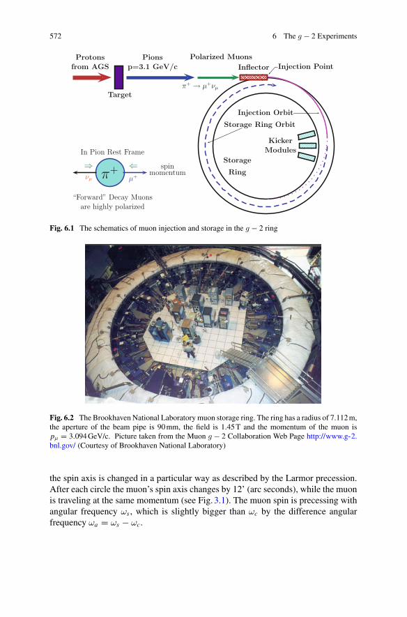
572 6 The g − 2 Experiments

π+Storage

Ring

Protonsfrom AGS

Target

Pionsp=3.1 GeV/c

π+ → μ+νμ

InflectorPolarized Muons

Injection Point

KickerModules

Injection Orbit

Storage Ring Orbit

νμ μ+

⇒ ⇐ spinmomentum

In Pion Rest Frame

“Forward” Decay Muonsare highly polarized

Fig. 6.1 The schematics of muon injection and storage in the g − 2 ring

Fig. 6.2 The Brookhaven National Laboratory muon storage ring. The ring has a radius of 7.112m,the aperture of the beam pipe is 90mm, the field is 1.45T and the momentum of the muon ispμ = 3.094GeV/c. Picture taken from the Muon g − 2 Collaboration Web Page http://www.g-2.bnl.gov/ (Courtesy of Brookhaven National Laboratory)

the spin axis is changed in a particular way as described by the Larmor precession.After each circle the muon’s spin axis changes by 12’ (arc seconds), while the muonis traveling at the same momentum (see Fig. 3.1). The muon spin is precessing withangular frequency ωs , which is slightly bigger than ωc by the difference angularfrequency ωa = ωs − ωc.

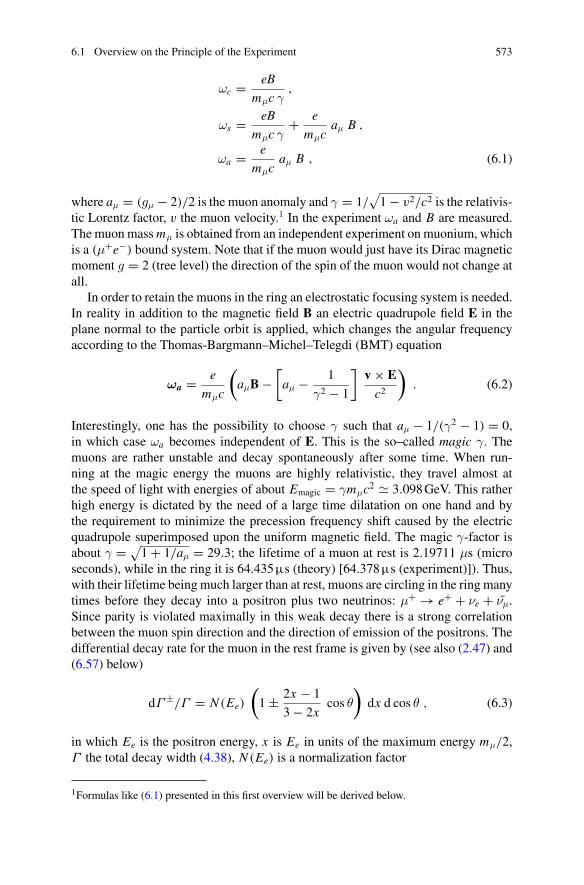
6.1 Overview on the Principle of the Experiment 573

ωc = eB

mμc γ,

ωs = eB

mμc γ+ e

mμcaμ B ,

ωa = e

mμcaμ B , (6.1)

where aμ = (gμ − 2)/2 is the muon anomaly and γ = 1/√1 − v2/c2 is the relativis-

tic Lorentz factor, v the muon velocity.1 In the experiment ωa and B are measured.The muonmassmμ is obtained from an independent experiment on muonium, whichis a (μ+e−) bound system. Note that if the muon would just have its Dirac magneticmoment g = 2 (tree level) the direction of the spin of the muon would not change atall.

In order to retain the muons in the ring an electrostatic focusing system is needed.In reality in addition to the magnetic field B an electric quadrupole field E in theplane normal to the particle orbit is applied, which changes the angular frequencyaccording to the Thomas-Bargmann–Michel–Telegdi (BMT) equation

ωa = e

mμc

(aμB −

[aμ − 1

γ2 − 1

]v × Ec2

). (6.2)

Interestingly, one has the possibility to choose γ such that aμ − 1/(γ2 − 1) = 0,in which case ωa becomes independent of E. This is the so–called magic γ. Themuons are rather unstable and decay spontaneously after some time. When run-ning at the magic energy the muons are highly relativistic, they travel almost atthe speed of light with energies of about Emagic = γmμc2 � 3.098GeV. This ratherhigh energy is dictated by the need of a large time dilatation on one hand and bythe requirement to minimize the precession frequency shift caused by the electricquadrupole superimposed upon the uniform magnetic field. The magic γ-factor isabout γ = √

1 + 1/aμ = 29.3; the lifetime of a muon at rest is 2.19711 μs (microseconds), while in the ring it is 64.435µs (theory) [64.378µs (experiment)]). Thus,with their lifetime being much larger than at rest, muons are circling in the ring manytimes before they decay into a positron plus two neutrinos: μ+ → e+ + νe + νμ.Since parity is violated maximally in this weak decay there is a strong correlationbetween the muon spin direction and the direction of emission of the positrons. Thedifferential decay rate for the muon in the rest frame is given by (see also (2.47) and(6.57) below)

dΓ ±/Γ = N (Ee)

(1 ± 2x − 1

3 − 2xcos θ

)dx d cos θ , (6.3)

in which Ee is the positron energy, x is Ee in units of the maximum energy mμ/2,Γ the total decay width (4.38), N (Ee) is a normalization factor

1Formulas like (6.1) presented in this first overview will be derived below.

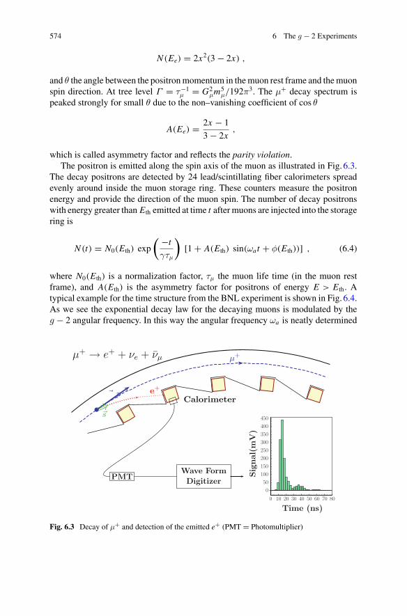
574 6 The g − 2 Experiments

N (Ee) = 2x2(3 − 2x) ,

and θ the angle between the positronmomentum in themuon rest frame and themuonspin direction. At tree level Γ = τ−1

μ = G2μm

5μ/192π

3. The μ+ decay spectrum ispeaked strongly for small θ due to the non–vanishing coefficient of cos θ

A(Ee) = 2x − 1

3 − 2x,

which is called asymmetry factor and reflects the parity violation.The positron is emitted along the spin axis of the muon as illustrated in Fig. 6.3.

The decay positrons are detected by 24 lead/scintillating fiber calorimeters spreadevenly around inside the muon storage ring. These counters measure the positronenergy and provide the direction of the muon spin. The number of decay positronswith energy greater than Eth emitted at time t after muons are injected into the storagering is

N (t) = N0(Eth) exp

( −t

γτμ

)[1 + A(Eth) sin(ωat + φ(Eth))] , (6.4)

where N0(Eth) is a normalization factor, τμ the muon life time (in the muon restframe), and A(Eth) is the asymmetry factor for positrons of energy E > Eth. Atypical example for the time structure from the BNL experiment is shown in Fig. 6.4.As we see the exponential decay law for the decaying muons is modulated by theg − 2 angular frequency. In this way the angular frequency ωa is neatly determined

⇒ ·

PMTWave FormDigitizer

μ+ → e+ + νe + νµ μ+

e+

Calorimeter� p

�s

0 10 20 30 40 50 60 70 80

050100150200250300350400450

Signal(m

V)

Time (ns)

Fig. 6.3 Decay of μ+ and detection of the emitted e+ (PMT = Photomultiplier)

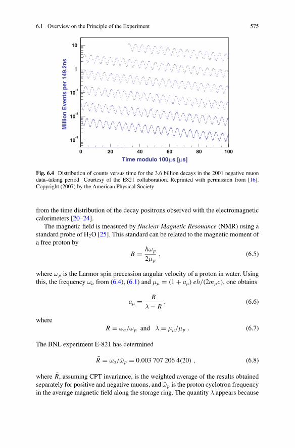
6.1 Overview on the Principle of the Experiment 575

s]µs [µTime modulo 1000 20 40 60 80 100

Mill

ion

Eve

nts

per

149

.2n

s

10-3

10-2

10-1

1

10

Fig. 6.4 Distribution of counts versus time for the 3.6 billion decays in the 2001 negative muondata–taking period Courtesy of the E821 collaboration. Reprinted with permission from [16].Copyright (2007) by the American Physical Society

from the time distribution of the decay positrons observed with the electromagneticcalorimeters [20–24].

The magnetic field is measured by Nuclear Magnetic Resonance (NMR) using astandard probe of H2O [25]. This standard can be related to the magnetic moment ofa free proton by

B = �ωp

2μp, (6.5)

where ωp is the Larmor spin precession angular velocity of a proton in water. Usingthis, the frequency ωa from (6.4), (6.1) and μμ = (1 + aμ) e�/(2mμc), one obtains

aμ = R

λ − R, (6.6)

whereR = ωa/ωp and λ = μμ/μp . (6.7)

The BNL experiment E-821 has determined

R = ωa/ωp = 0.003 707 206 4(20) , (6.8)

where R, assuming CPT invariance, is the weighted average of the results obtainedseparately for positive and negative muons, and ωp is the proton cyclotron frequencyin the average magnetic field along the storage ring. The quantity λ appears because

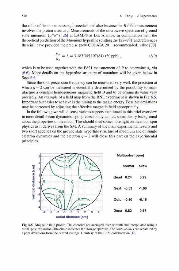
576 6 The g − 2 Experiments

the value of the muon mass mμ is needed, and also because the B field measurementinvolves the proton mass mp. Measurements of the microwave spectrum of groundstate muonium (μ+e−) [26] at LAMPF at Los Alamos, in combination with thetheoretical prediction of theMuoniumhyperfine splittingΔν [27–29] (and referencestherein), have provided the precise (new CODATA 2011 recommended) value [30]

μμ

μp= λ = 3.183 345 107(84) (30 ppb) , (6.9)

which is to be used together with the E821 measurement of R to determine aμ via(6.6). More details on the hyperfine structure of muonium will be given below inSect. 6.6.

Since the spin precession frequency can be measured very well, the precision atwhich g − 2 can be measured is essentially determined by the possibility to man-ufacture a constant homogeneous magnetic field B and to determine its value veryprecisely. An example of a field map from the BNL experiment is shown in Fig. 6.5.Important but easier to achieve is the tuning to the magic energy. Possible deviationsmay be corrected by adjusting the effective magnetic field appropriately.

In the following we will discuss various aspects mentioned in this brief overviewin more detail: beam dynamics, spin precession dynamics, some theory backgroundabout the properties of the muon. This should shed somemore light on the muon spinphysics as it derives from the SM. A summary of the main experimental results andtwo short addenda on the ground state hyperfine structure of muonium and on singleelectron dynamics and the electron g − 2 will close this part on the experimentalprinciples.

Multipoles [ppm]

normal skew

Quad 0.24 0.29

Sext -0.53 -1.06

Octu -0.10 -0.15

Decu 0.82 0.54

radial distance [cm]-4 -3 -2 -1 0 1 2 3 4

vert

ical

dis

tan

ce [

cm]

-4

-3

-2

-1

0

1

2

3

4

-1.5

-1.0

-1.0

-0.5

-0.5

000

0.5

0.5

1.0

1.01.5

Fig. 6.5 Magnetic field profile. The contours are averaged over azimuth and interpolated using amulti–pole expansion. The circle indicates the storage aperture. The contour lines are separated by1ppm deviations from the central average Courtesy of the E821 collaboration [16]

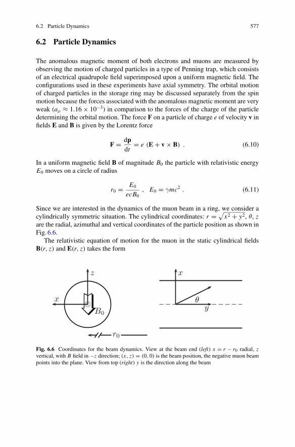
6.2 Particle Dynamics 577

6.2 Particle Dynamics

The anomalous magnetic moment of both electrons and muons are measured byobserving the motion of charged particles in a type of Penning trap, which consistsof an electrical quadrupole field superimposed upon a uniform magnetic field. Theconfigurations used in these experiments have axial symmetry. The orbital motionof charged particles in the storage ring may be discussed separately from the spinmotion because the forces associated with the anomalous magnetic moment are veryweak (aμ ≈ 1.16 × 10−3) in comparison to the forces of the charge of the particledetermining the orbital motion. The force F on a particle of charge e of velocity v infields E and B is given by the Lorentz force

F = dpdt

= e (E + v × B) . (6.10)

In a uniform magnetic field B of magnitude B0 the particle with relativistic energyE0 moves on a circle of radius

r0 = E0

ecB0, E0 = γmc2 . (6.11)

Since we are interested in the dynamics of the muon beam in a ring, we consider acylindrically symmetric situation. The cylindrical coordinates: r = √

x2 + y2, θ, zare the radial, azimuthal and vertical coordinates of the particle position as shown inFig. 6.6.

The relativistic equation of motion for the muon in the static cylindrical fieldsB(r, z) and E(r, z) takes the form

x

z

r0

B0

x

yθ⊗

Fig. 6.6 Coordinates for the beam dynamics. View at the beam end (left) x = r − r0 radial, zvertical, with B field in −z direction; (x, z) = (0, 0) is the beam position, the negative muon beampoints into the plane. View from top (right) y is the direction along the beam

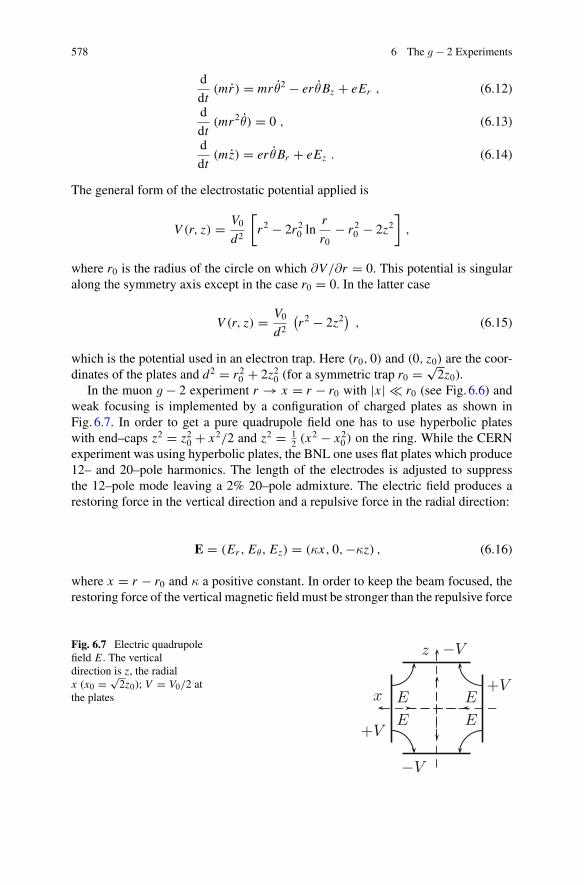
578 6 The g − 2 Experiments

d

dt(mr) = mr θ2 − er θBz + eEr , (6.12)

d

dt(mr2θ) = 0 , (6.13)

d

dt(mz) = er θBr + eEz . (6.14)

The general form of the electrostatic potential applied is

V (r, z) = V0

d2

[r2 − 2r20 ln

r

r0− r20 − 2z2

],

where r0 is the radius of the circle on which ∂V/∂r = 0. This potential is singularalong the symmetry axis except in the case r0 = 0. In the latter case

V (r, z) = V0

d2

(r2 − 2z2

), (6.15)

which is the potential used in an electron trap. Here (r0, 0) and (0, z0) are the coor-dinates of the plates and d2 = r20 + 2z20 (for a symmetric trap r0 = √

2z0).In the muon g − 2 experiment r → x = r − r0 with |x | � r0 (see Fig. 6.6) and

weak focusing is implemented by a configuration of charged plates as shown inFig. 6.7. In order to get a pure quadrupole field one has to use hyperbolic plateswith end–caps z2 = z20 + x2/2 and z2 = 1

2 (x2 − x20 ) on the ring. While the CERNexperiment was using hyperbolic plates, the BNL one uses flat plates which produce12– and 20–pole harmonics. The length of the electrodes is adjusted to suppressthe 12–pole mode leaving a 2% 20–pole admixture. The electric field produces arestoring force in the vertical direction and a repulsive force in the radial direction:

E = (Er , Eθ, Ez) = (κx, 0,−κz) , (6.16)

where x = r − r0 and κ a positive constant. In order to keep the beam focused, therestoring force of the vertical magnetic field must be stronger than the repulsive force

Fig. 6.7 Electric quadrupolefield E . The verticaldirection is z, the radialx (x0 = √

2z0); V = V0/2 atthe plates

+V

−V

+V

−V

E E

EE

z

x

6.2 Particle Dynamics 579

of the electrical field in the radial direction:

0 <eV0

d2<

e2B2

8mc. (6.17)

The radial force is

Fr = γmv2

r− e

cvBz + eEr , (6.18)

and since on the equilibrium orbit r = r0 and Er = 0 we have

γmv2

r0= e

cvBz . (6.19)

As r0 is large relative to the beam spread, we may expand r about r0:

1

r= 1

r0 + x� 1

r0

(1 − x

r0

).

Therefore, using (6.19) we may write

Fx = Fr = −eβBz (1 − n)x

r0⇒ γmx = −(1 − n)

γmv2

r20x , (6.20)

where β = v/c and n is the field index

n = κr0βB0

, B0 = Bz . (6.21)

For the vertical motion we have

Fz = −eκz ⇒ γmz = −eκz , (6.22)

and with ω0 = v/r0, using (6.19) and (6.21), the equations of motion take the form

x + (1 − n)ω20 x = 0 ,

z + eκ z = 0 , (6.23)

with the oscillatory solutions

x = A cos(√1 − n ω0 t) ,

z = B cos(√n ω0 t) . (6.24)

580 6 The g − 2 Experiments

We have used eκ = nω20 following from (6.21). The amplitudes depend on the

initial condition of the particle trajectory. This motion is called betatron oscilla-tion. The betatron frequencies are ωyBO = √

n ωc and ωxBO = √1 − n ωc where

ωc = ω0 = v/r0 is the cyclotron frequency. In the experiment a lattice of quadrupolesis distributed along the ring. For the BNL experiment the lattice has a four–fold sym-metry and the quadrupoles are covering 43%of the ring. The corresponding dynamicshas to be calculated taking into account the geometry of the configuration, but followsthe same principle.

The dynamics of an electron in a Penning trap and the principle of electron g − 2experiments will be considered briefly in Sect. 6.7 at the end of this part of the book.

6.3 Magnetic Precession for Moving Particles

The precession of spinning particles inmagnetic fields is a classic subject investigatedlong time ago [31]. Our exposition follows closely Bell’s lecture. In a magnetic fieldB the polarization P of a particle changes according to

dPdt

= ge

2mP × B ,

the component of P parallel to B remains constant, while the part of P perpendicularto B rotates about B with angular frequency

ω = ge

2mB , (6.25)

the non–relativistic cyclotron frequency. This holds in the rest frame O of the particle.For moving and even fast–moving particles we may get the motion in the laboratorysystem O ′ by a Lorentz transformation. In a pure L–transformation xμ′ = Lμ

νxν

[xμ = (ct, x)] L has the form2

L =(

γ −γ vc−γ v

c 1 + (γ − 1)n n·)

,

where n = v/v and γ = 1/√1 − v2/c2. For accelerated particles, the velocity is

changing and in the next moment the velocity is v′ = v + δv. In the laboratory framewe thus have xμ′ = Lμ

ν(v)xν and xμ′′ = Lμ

ν(v′)xν and expanding to linear order in

δv one obtains the motion as seen in the laboratory frame as

t ′′ = t ′ − δu′ · x′ ,x′′ = x′ + δθ′ × x′ − u′t ′ , (6.26)

2L is a matrix operator acting on four–vectors. The · operation at the right of the spacial submatrixmeans forming a scalar product with the spatial part of the vector on which L acts.

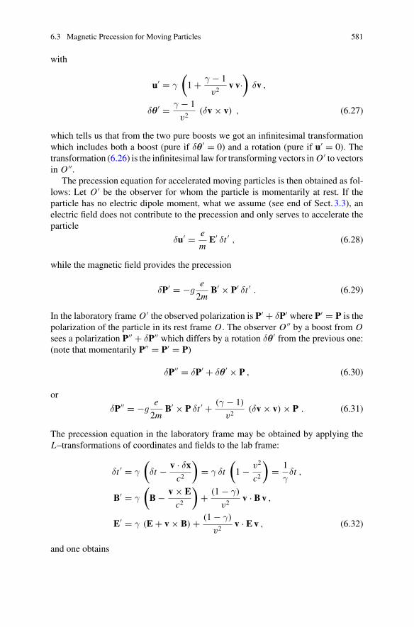
6.3 Magnetic Precession for Moving Particles 581

with

u′ = γ

(1 + γ − 1

v2v v·

)δv ,

δθ′ = γ − 1

v2(δv × v) , (6.27)

which tells us that from the two pure boosts we got an infinitesimal transformationwhich includes both a boost (pure if δθ′ = 0) and a rotation (pure if u′ = 0). Thetransformation (6.26) is the infinitesimal law for transforming vectors in O ′ to vectorsin O ′′.

The precession equation for accelerated moving particles is then obtained as fol-lows: Let O ′ be the observer for whom the particle is momentarily at rest. If theparticle has no electric dipole moment, what we assume (see end of Sect. 3.3), anelectric field does not contribute to the precession and only serves to accelerate theparticle

δu′ = e

mE′ δt ′ , (6.28)

while the magnetic field provides the precession

δP′ = −ge

2mB′ × P′ δt ′ . (6.29)

In the laboratory frame O ′ the observed polarization is P′ + δP′ where P′ = P is thepolarization of the particle in its rest frame O . The observer O ′′ by a boost from Osees a polarization P′′ + δP′′ which differs by a rotation δθ′ from the previous one:(note that momentarily P′′ = P′ = P)

δP′′ = δP′ + δθ′ × P , (6.30)

or

δP′′ = −ge

2mB′ × P δt ′ + (γ − 1)

v2(δv × v) × P . (6.31)

The precession equation in the laboratory frame may be obtained by applying theL–transformations of coordinates and fields to the lab frame:

δt ′ = γ

(δt − v · δx

c2

)= γ δt

(1 − v2

c2

)= 1

γδt ,

B′ = γ

(B − v × E

c2

)+ (1 − γ)

v2v · Bv ,

E′ = γ (E + v × B) + (1 − γ)

v2v · Ev , (6.32)

and one obtains

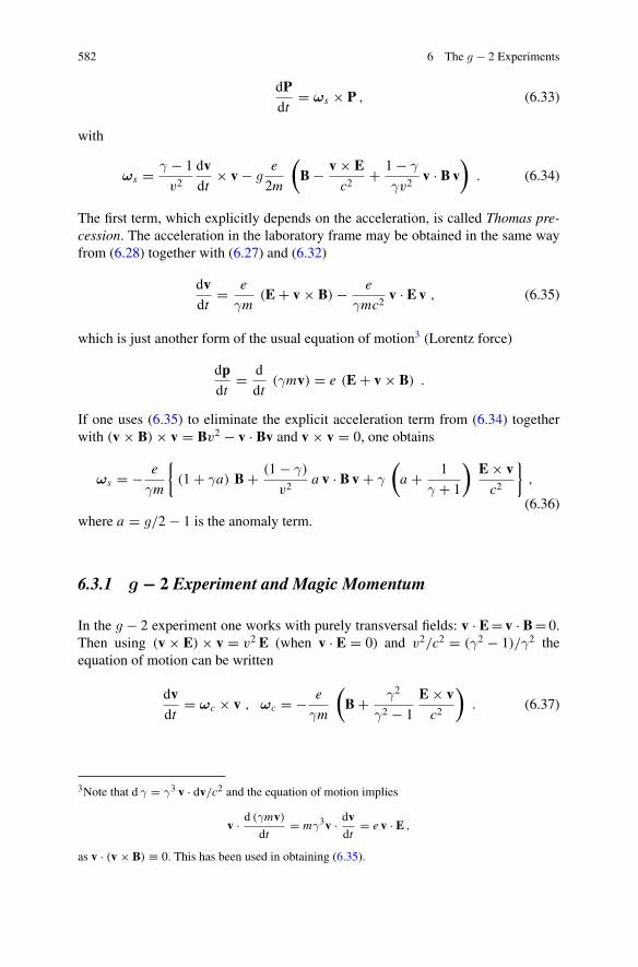
582 6 The g − 2 Experiments

dPdt

= ωs × P , (6.33)

with

ωs = γ − 1

v2

dvdt

× v − ge

2m

(B − v × E

c2+ 1 − γ

γv2v · Bv

). (6.34)

The first term, which explicitly depends on the acceleration, is called Thomas pre-cession. The acceleration in the laboratory frame may be obtained in the same wayfrom (6.28) together with (6.27) and (6.32)

dvdt

= e

γm(E + v × B) − e

γmc2v · Ev , (6.35)

which is just another form of the usual equation of motion3 (Lorentz force)

dpdt

= d

dt(γmv) = e (E + v × B) .

If one uses (6.35) to eliminate the explicit acceleration term from (6.34) togetherwith (v × B) × v = Bv2 − v · Bv and v × v = 0, one obtains

ωs = − e

γm

{(1 + γa) B + (1 − γ)

v2a v · Bv + γ

(a + 1

γ + 1

)E × vc2

},

(6.36)where a = g/2 − 1 is the anomaly term.

6.3.1 g − 2 Experiment and Magic Momentum

In the g − 2 experiment one works with purely transversal fields: v · E= v · B= 0.Then using (v × E) × v = v2 E (when v · E = 0) and v2/c2 = (γ2 − 1)/γ2 theequation of motion can be written

dvdt

= ωc × v , ωc = − e

γm

(B + γ2

γ2 − 1

E × vc2

). (6.37)

3Note that d γ = γ3 v · dv/c2 and the equation of motion implies

v · d (γmv)dt

= mγ3v · dvdt

= e v · E ,

as v · (v × B) ≡ 0. This has been used in obtaining (6.35).

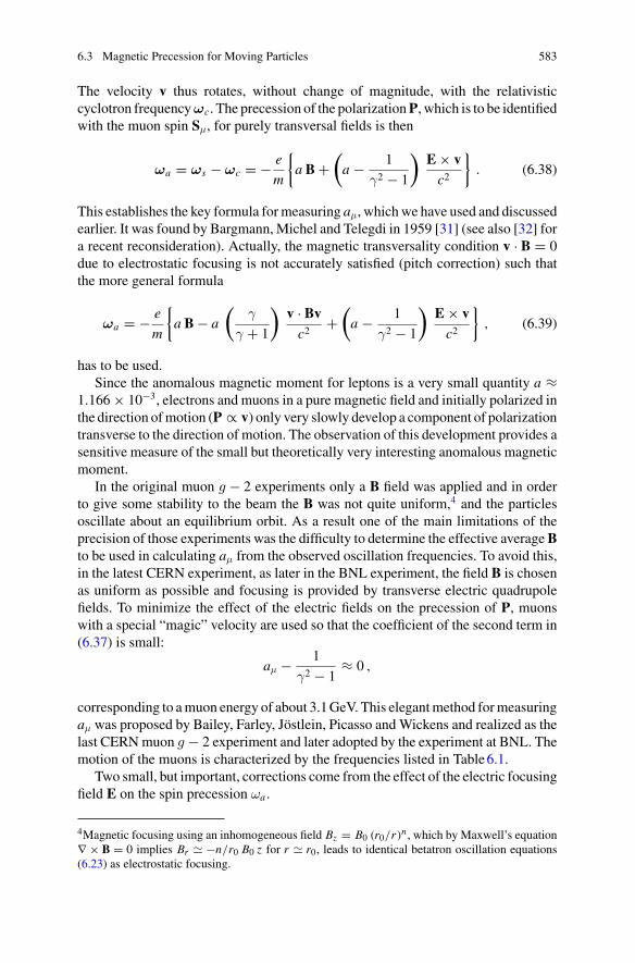
6.3 Magnetic Precession for Moving Particles 583

The velocity v thus rotates, without change of magnitude, with the relativisticcyclotron frequencyωc. The precession of the polarizationP, which is to be identifiedwith the muon spin Sμ, for purely transversal fields is then

ωa = ωs − ωc = − e

m

{a B +

(a − 1

γ2 − 1

)E × vc2

}. (6.38)

This establishes the key formula formeasuring aμ, whichwe have used and discussedearlier. It was found by Bargmann, Michel and Telegdi in 1959 [31] (see also [32] fora recent reconsideration). Actually, the magnetic transversality condition v · B = 0due to electrostatic focusing is not accurately satisfied (pitch correction) such thatthe more general formula

ωa = − e

m

{a B − a

(γ

γ + 1

)v · Bvc2

+(a − 1

γ2 − 1

)E × vc2

}, (6.39)

has to be used.Since the anomalous magnetic moment for leptons is a very small quantity a ≈

1.166 × 10−3, electrons and muons in a pure magnetic field and initially polarized inthe direction ofmotion (P ∝ v) only very slowly develop a component of polarizationtransverse to the direction of motion. The observation of this development provides asensitive measure of the small but theoretically very interesting anomalous magneticmoment.

In the original muon g − 2 experiments only a B field was applied and in orderto give some stability to the beam the B was not quite uniform,4 and the particlesoscillate about an equilibrium orbit. As a result one of the main limitations of theprecision of those experiments was the difficulty to determine the effective averageBto be used in calculating aμ from the observed oscillation frequencies. To avoid this,in the latest CERN experiment, as later in the BNL experiment, the field B is chosenas uniform as possible and focusing is provided by transverse electric quadrupolefields. To minimize the effect of the electric fields on the precession of P, muonswith a special “magic” velocity are used so that the coefficient of the second term in(6.37) is small:

aμ − 1

γ2 − 1≈ 0 ,

corresponding to amuon energy of about 3.1GeV. This elegantmethod formeasuringaμ was proposed by Bailey, Farley, Jöstlein, Picasso andWickens and realized as thelast CERNmuon g − 2 experiment and later adopted by the experiment at BNL. Themotion of the muons is characterized by the frequencies listed in Table6.1.

Two small, but important, corrections come from the effect of the electric focusingfield E on the spin precession ωa .

4Magnetic focusing using an inhomogeneous field Bz = B0 (r0/r)n , which by Maxwell’s equation∇ × B = 0 implies Br � −n/r0 B0 z for r � r0, leads to identical betatron oscillation equations(6.23) as electrostatic focusing.

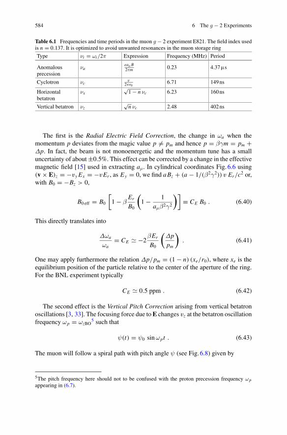
584 6 The g − 2 Experiments

Table 6.1 Frequencies and time periods in the muon g − 2 experiment E821. The field index usedis n = 0.137. It is optimized to avoid unwanted resonances in the muon storage ring

Type νi = ωi/2π Expression Frequency (MHz) Period

Anomalousprecession

νaeaμB2πm 0.23 4.37µs

Cyclotron νcv

2πr06.71 149ns

Horizontalbetatron

νx√1 − n νc 6.23 160ns

Vertical betatron νz√n νc 2.48 402ns

The first is the Radial Electric Field Correction, the change in ωa when themomentum p deviates from the magic value p �= pm and hence p = βγm = pm +Δp. In fact, the beam is not monoenergetic and the momentum tune has a smalluncertainty of about±0.5%. This effect can be corrected by a change in the effectivemagnetic field [15] used in extracting aμ. In cylindrical coordinates Fig. 6.6 using(v × E)z = −vy Ex = −vEr , as Ey = 0, we find aBz + (a − 1/(β2γ2)) v Er/c2 or,with B0 = −Bz > 0,

B0 eff = B0

[1 − β

Er

B0

(1 − 1

aμβ2γ2

)]≡ CE B0 . (6.40)

This directly translates into

Δωa

ωa= CE � −2

βEr

B0

(Δp

pm

). (6.41)

One may apply furthermore the relation Δp/pm = (1 − n) (xe/r0), where xe is theequilibrium position of the particle relative to the center of the aperture of the ring.For the BNL experiment typically

CE � 0.5 ppm . (6.42)

The second effect is the Vertical Pitch Correction arising from vertical betatronoscillations [3, 33]. The focusing force due toE changes vz at the betatron oscillationfrequency ωp = ωzBO

5 such that

ψ(t) = ψ0 sinωpt . (6.43)

The muon will follow a spiral path with pitch angle ψ (see Fig. 6.8) given by

5The pitch frequency here should not to be confused with the proton precession frequency ωpappearing in (6.7).

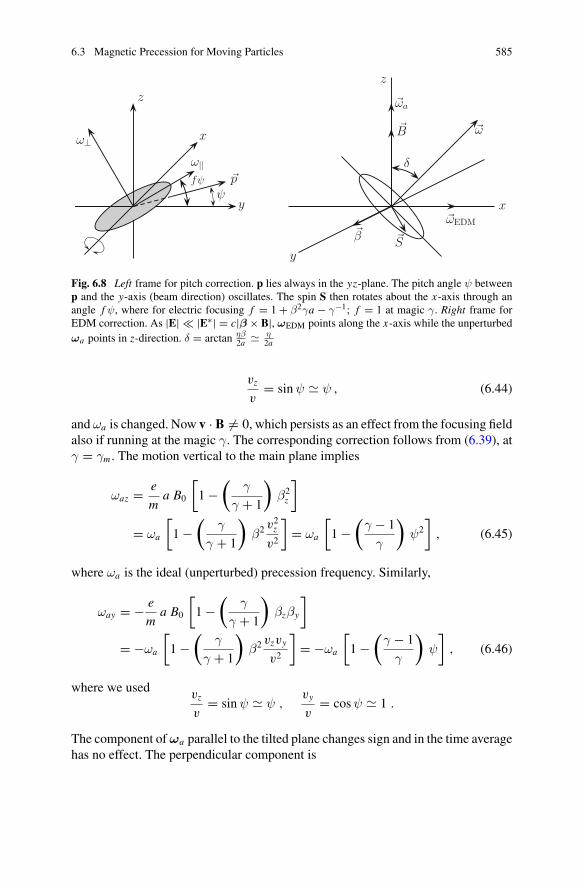
6.3 Magnetic Precession for Moving Particles 585

Fig. 6.8 Left frame for pitch correction. p lies always in the yz-plane. The pitch angle ψ betweenp and the y-axis (beam direction) oscillates. The spin S then rotates about the x-axis through anangle f ψ, where for electric focusing f = 1 + β2γa − γ−1; f = 1 at magic γ. Right frame forEDM correction. As |E| � |E∗| = c|β × B|, ωEDM points along the x-axis while the unperturbedωa points in z-direction. δ = arctan ηβ

2a � η2a

vz

v= sinψ � ψ , (6.44)

and ωa is changed. Now v · B �= 0, which persists as an effect from the focusing fieldalso if running at the magic γ. The corresponding correction follows from (6.39), atγ = γm . The motion vertical to the main plane implies

ωaz = e

ma B0

[1 −

(γ

γ + 1

)β2z

]

= ωa

[1 −

(γ

γ + 1

)β2 v2

z

v2

]= ωa

[1 −

(γ − 1

γ

)ψ2

], (6.45)

where ωa is the ideal (unperturbed) precession frequency. Similarly,

ωay = − e

ma B0

[1 −

(γ

γ + 1

)βzβy

]

= −ωa

[1 −

(γ

γ + 1

)β2 vzvy

v2

]= −ωa

[1 −

(γ − 1

γ

)ψ

], (6.46)

where we usedvz

v= sinψ � ψ ,

vy

v= cosψ � 1 .

The component ofωa parallel to the tilted plane changes sign and in the time averagehas no effect. The perpendicular component is

586 6 The g − 2 Experiments

ω⊥ = ωa = ωz cosψ − ωy sinψ � ωz − ωyψ , (6.47)

and hence

ω′a = ωa (1 − CP) = ωa

(1 − ψ2

2

). (6.48)

In the time average by (6.43) ψ 2 = 12ψ

20 and thus CP = 1

4ψ20. This holds provided

ωa � ωp otherwise the correction reads [33]

CP = 1

4ψ20 β2

(

1 − (aβγ)2ω2

p

(ω2a − ω2

p)

)

, (6.49)

with (aβγ)2 = 1/(βγ)2 at magic γ. For the BNL experiment the pitch correctionsis of the order

CP � 0.3 ppm . (6.50)

A third possible correction could be due to an EDMof the muon. If a large enoughelectric dipole moment6

de = η e

2mcS , (6.51)

(see (1.5), p. 34 in Sect. 2.1.2 and the discussion at the end of Sect. 3.3) would existthe applied electric field E (which is vanishing at the equilibrium beam position)and the motional electric field induced in the muon rest frame E∗ = γ β × B wouldadd an extra precession of the spin with a component along E and one about an axisperpendicular to B:

ωa′ = ωa + ωEDM = ωa − η e

2mμ

(Ec

+ β × B)

, (6.52)

orΔωa = −2dμ (β × B) − 2dμ E ,

which, for β ∼ 1 and dμ E ∼ 0, yields

ωa′ = B

√(e

mμaμ

)2

+ (2dμ

)2. (6.53)

Note that η is the dimensionless constant equivalent of magnetic moment g-factors.The result is that the plane of precession in no longer horizontal but tilted at an angle

6Remembering the normalization: themagnetic and electric dipolemoments are given byμ = g2

e�2mc

and d = η2

e�2mc , respectively.

6.3 Magnetic Precession for Moving Particles 587

δ ≡ arctanωEDM

ωa= arctan

η β

2a� η

2a, (6.54)

and the precession frequency is increased by a factor

ω′a = ωa

√1 + δ2 . (6.55)

The tilt gives rise to an oscillating vertical component of the muon polarization,and may be detected by recording separately the electrons which strike the countersabove and below the mid–plane of the ring. This measurement has been performedin the last CERN experiment on g − 2, and has been repeated at BNL.

6.4 Theory: Production and Decay of Muons

For the (gμ − 2) experiments one needs polarized muons. Basic symmetries of theweak interaction of the muons make it relatively easy to produce polarized muons.What helps is the maximal parity violation of the charged current weak interactions,mediated by the charged W± gauge bosons, which in its most pronounced formmanifests itself in the “non–existence” of right–handed neutrinos νR . What it meansmore precisely is that right handed neutrinos are “sterile” in the sense that they donot interact with any kinds of the gauge bosons, which we know are responsible forelectromagnetic (photon), weak (W - and Z -bosons) and strong (gluons) interactionsof matter. It means that their production rate in ordinary weak reactions is practicallyzero which amounts to lepton number conservation for all practical purposes inlaboratory experiments.7

Pion productionmaybedone by shooting protons (accumulated in a proton storagering) on a target material where pions are the most abundant secondary particles. Themost effective pion production mechanism proceeds via decays of resonances. Forpions it is dominated by the Δ33 isobar (Δ33 → Nπ) [basic processes p + p →p + n + π+ and p + n → p + p + π−]

p + (N , Z) → Δ∗ + X → “(N + 1, Z + 1 ∓ 1)” + π± ,

where the ratio σ(π+)/σ(π−) → 1 at high Z .8

7Only the recently established phenomenon of neutrino oscillations proves that lepton number infact is not a perfect quantum number. This requires that neutrinos must have tiny masses and thisrequires that right–handed neutrinos (νR’s) must exist. In fact, the smallness of the neutrino massesexplains the strong suppression of lepton number violating effects.8At Brookhaven the 24GeV proton beam extracted from the AGS with 60 × 1012 protons per AGScycle of 2.5 s impinges on a Nickel target of one interaction length and produces amongst otherdebris–particles a large number of low energy pions. The pions are momentum selected and thendecay in a straight section where about one third of the pions decay into muons. The latter aremomentum selected once more before they are injected into the g − 2 storage ring.

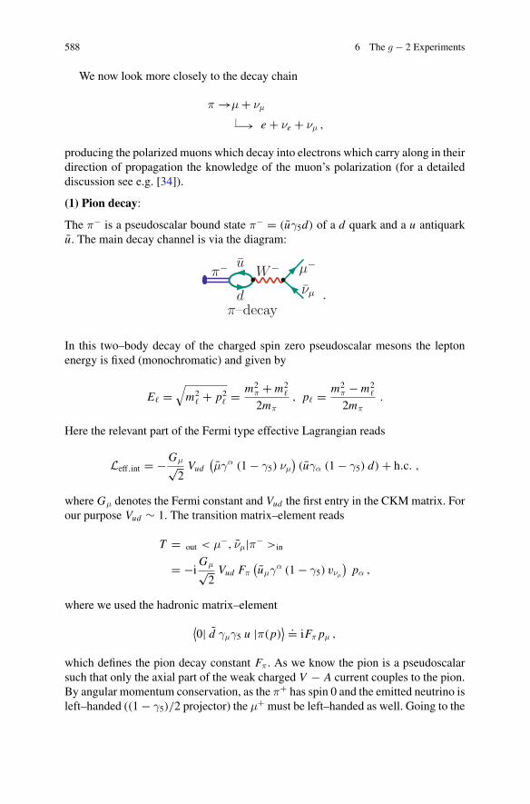
588 6 The g − 2 Experiments

We now look more closely to the decay chain

π →μ + νμ

|−→ e + νe + νμ ,

producing the polarized muons which decay into electrons which carry along in theirdirection of propagation the knowledge of the muon’s polarization (for a detaileddiscussion see e.g. [34]).

(1) Pion decay:

The π− is a pseudoscalar bound state π− = (uγ5d) of a d quark and a u antiquarku. The main decay channel is via the diagram:

W−π−

d

u μ−

νµ

π–decay·

In this two–body decay of the charged spin zero pseudoscalar mesons the leptonenergy is fixed (monochromatic) and given by

E� =√m2

� + p2� = m2π + m2

�

2mπ, p� = m2

π − m2�

2mπ.

Here the relevant part of the Fermi type effective Lagrangian reads

Leff,int = −Gμ√2Vud

(μγα (1 − γ5) νμ

)(uγα (1 − γ5) d) + h.c. ,

where Gμ denotes the Fermi constant and Vud the first entry in the CKMmatrix. Forour purpose Vud ∼ 1. The transition matrix–element reads

T = out < μ−, νμ|π− >in

= −iGμ√2Vud Fπ

(uμγ

α (1 − γ5) vνμ

)pα ,

where we used the hadronic matrix–element

⟨0| d γμγ5 u |π(p)

⟩ .= iFπ pμ ,

which defines the pion decay constant Fπ . As we know the pion is a pseudoscalarsuch that only the axial part of the weak charged V − A current couples to the pion.By angular momentum conservation, as the π+ has spin 0 and the emitted neutrino isleft–handed ((1 − γ5)/2 projector) the μ+ must be left–handed as well. Going to the

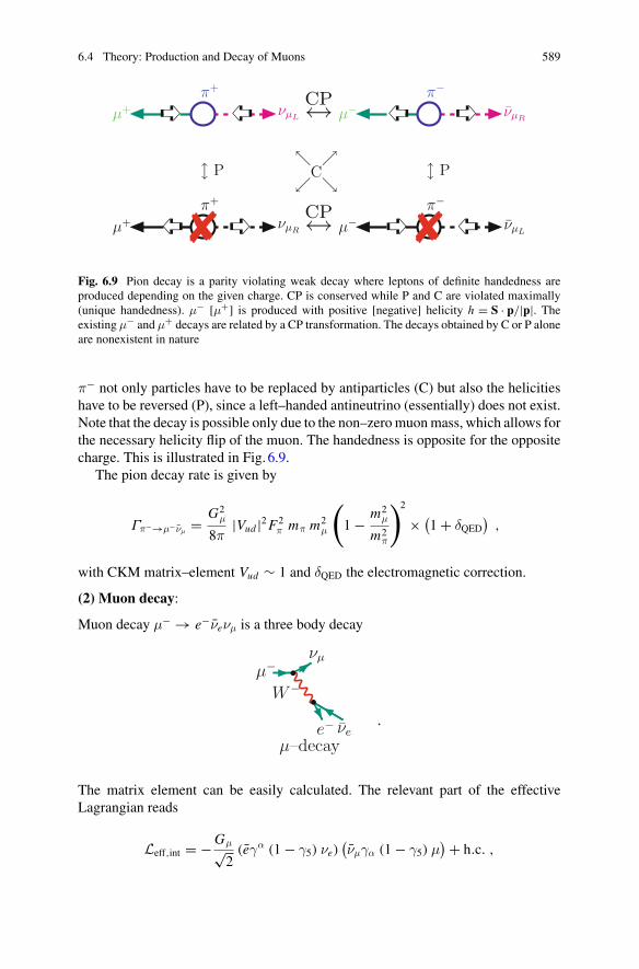
6.4 Theory: Production and Decay of Muons 589

π+

μ+ νµL

CP↔ π−

μ− νµR

π+

μ+ νµR

CP↔� P

π−

μ− νµL

� P↗↘

↖↙C

Fig. 6.9 Pion decay is a parity violating weak decay where leptons of definite handedness areproduced depending on the given charge. CP is conserved while P and C are violated maximally(unique handedness). μ− [μ+] is produced with positive [negative] helicity h = S · p/|p|. Theexisting μ− and μ+ decays are related by a CP transformation. The decays obtained by C or P aloneare nonexistent in nature

π− not only particles have to be replaced by antiparticles (C) but also the helicitieshave to be reversed (P), since a left–handed antineutrino (essentially) does not exist.Note that the decay is possible only due to the non–zeromuonmass, which allows forthe necessary helicity flip of the muon. The handedness is opposite for the oppositecharge. This is illustrated in Fig. 6.9.

The pion decay rate is given by

Γπ−→μ−νμ= G2

μ

8π|Vud |2F2

π mπ m2μ

(

1 − m2μ

m2π

)2

× (1 + δQED

),

with CKM matrix–element Vud ∼ 1 and δQED the electromagnetic correction.

(2) Muon decay:

Muon decay μ− → e−νeνμ is a three body decay

W−

e− νe

μ−νµ

μ–decay·

The matrix element can be easily calculated. The relevant part of the effectiveLagrangian reads

Leff,int = −Gμ√2

(eγα (1 − γ5) νe)(νμγα (1 − γ5) μ

) + h.c. ,

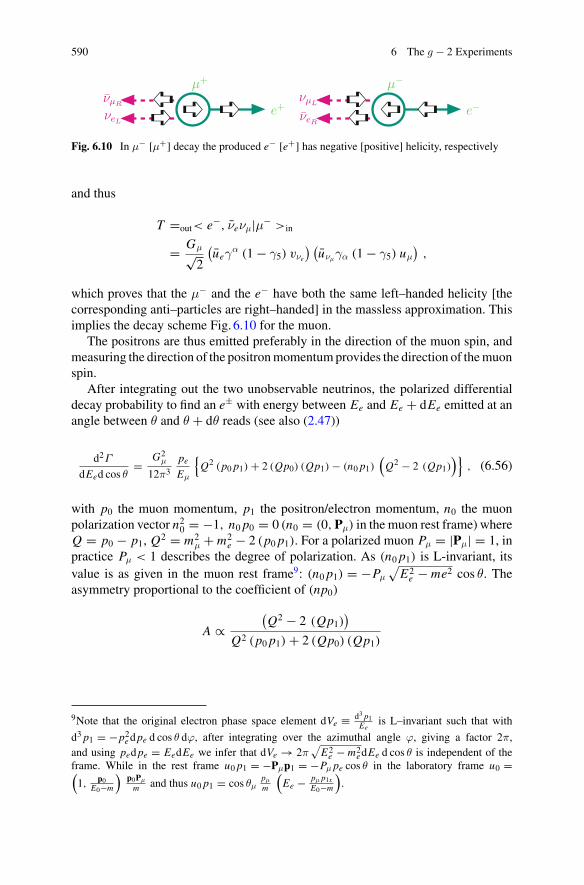
590 6 The g − 2 Experiments

μ+

e+νµR

νeL

μ−

e−νµL

νeR

Fig. 6.10 In μ− [μ+] decay the produced e− [e+] has negative [positive] helicity, respectively

and thus

T =out< e−, νeνμ|μ− >in

= Gμ√2

(ueγ

α (1 − γ5) vνe

) (uνμ

γα (1 − γ5) uμ

),

which proves that the μ− and the e− have both the same left–handed helicity [thecorresponding anti–particles are right–handed] in the massless approximation. Thisimplies the decay scheme Fig. 6.10 for the muon.

The positrons are thus emitted preferably in the direction of the muon spin, andmeasuring the direction of the positronmomentumprovides the direction of themuonspin.

After integrating out the two unobservable neutrinos, the polarized differentialdecay probability to find an e± with energy between Ee and Ee + dEe emitted at anangle between θ and θ + dθ reads (see also (2.47))

d2Γ

dEed cos θ= G2

μ

12π3

peEμ

{Q2 (p0 p1) + 2 (Qp0) (Qp1) − (n0 p1)

(Q2 − 2 (Qp1)

)}, (6.56)

with p0 the muon momentum, p1 the positron/electron momentum, n0 the muonpolarization vector n20 = −1, n0 p0 = 0 (n0 = (0,Pμ) in the muon rest frame) whereQ = p0 − p1, Q2 = m2

μ + m2e − 2 (p0 p1). For a polarized muon Pμ = |Pμ| = 1, in

practice Pμ < 1 describes the degree of polarization. As (n0 p1) is L-invariant, itsvalue is as given in the muon rest frame9: (n0 p1) = −Pμ

√E2e − me2 cos θ. The

asymmetry proportional to the coefficient of (np0)

A ∝(Q2 − 2 (Qp1)

)

Q2 (p0 p1) + 2 (Qp0) (Qp1)

9Note that the original electron phase space element dVe ≡ d3 p1Ee

is L–invariant such that with

d3 p1 = −p2edpe d cos θ dϕ, after integrating over the azimuthal angle ϕ, giving a factor 2π,and using pedpe = EedEe we infer that dVe → 2π

√E2e − m2

edEe d cos θ is independent of theframe. While in the rest frame u0 p1 = −Pμp1 = −Pμ pe cos θ in the laboratory frame u0 =(1, p0

E0−m

)p0Pμ

m and thus u0 p1 = cos θμpμ

m

(Ee − pμ p1x

E0−m

).

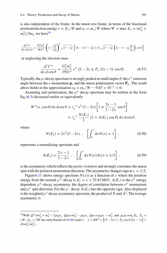
6.4 Theory: Production and Decay of Muons 591

is also independent of the frame. In the muon rest frame, in terms of the fractionalpositron/electron energy x = Ee/W and x0 = me/W whereW = max Ee = (m2

μ +m2

e)/2mμ we have10

d2Γ ±

dx d cos θ= G2

μm5μ

96π3

(

1 + m2e

m2μ

)4 √x2 − x20

{(3x − 2x2 − x20 ) ± Pμ

√x2 − x20

(2x − 1 − x0

me

mμ

)cos θ

},

or neglecting the electron mass

d2Γ ±

dx d cos θ= G2

μm5μ

192π3x2

(3 − 2x ± Pμ (2x − 1) cos θ

). (6.57)

Typically, theμ–decay spectrum is strongly peaked at small angles θ, the e± emissionangle between the e momentum pe and the muon polarization vector Pμ. The resultabove holds in the approximation x0 = me/W ∼ 9.67 × 10−3 � 0.

Assuming unit polarization, the μ± decay spectrum may be written in the formEq. (6.3) discussed earlier or equivalently

W±(x, cos θ) dx d cos θ = τ−1μ x2 (3 − 2x)

[1 ± 2x − 1

3 − 2xcos θ

]

= τ−1μ

N (Ee)

2[1 + A(Ee) cos θ] dx d cos θ ,

where

N (Ee) = 2x2(3 − 2x) ,

[∫ 1

0dxN (x) = 1

], (6.58)

represents a normalizing spectrum and

A(Ee) = 2 x − 1

3 − 2 x,

[∫ 1

0dxN (x)A(x) = 1/3

], (6.59)

is the asymmetry which reflects the parity violation and strongly correlates the muonspinwith the positronmomentumdirection. The asymmetry changes sign at x = 1/2.

Figure6.11 shows energy spectrum N (x)) as a function of x where the positronenergy from the normal μ±–decay is Ee = x × 52.83MeV. A(Ee) is the e± energydependent μ±–decay asymmetry, the degree of correlation between e± momentumand μ± spin direction. For the μ− decay A(Ee) has the opposite sign. Also displayedis the weightedμ+ decay asymmetry spectrum, the product of N and A2. The averageasymmetry is

10With Q2=m2μ + m2

e − 2p0 p1, Qp0=m2μ − p0 p1, Qp1=p0 p1 − m2

e , and p0 p1=mμEe, Ee =xW, mμ = 2W the curly bracket of (6.56) reads {· · · } = 8W 4 x

[(3 − 2x) + Pμ cos θ (2x − 1)

] +O(m2

e/m2μ).

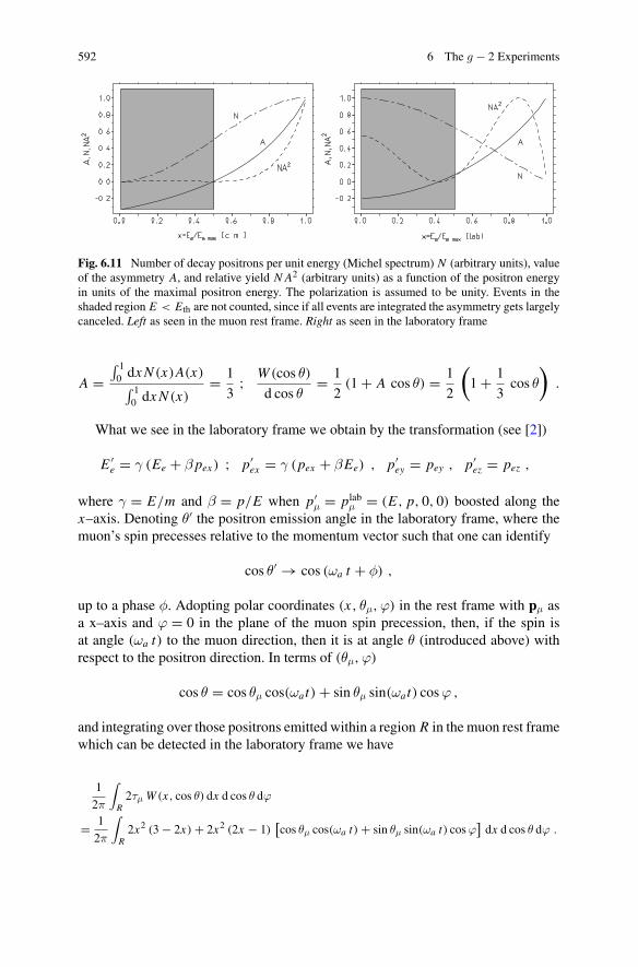
592 6 The g − 2 Experiments

Fig. 6.11 Number of decay positrons per unit energy (Michel spectrum) N (arbitrary units), valueof the asymmetry A, and relative yield N A2 (arbitrary units) as a function of the positron energyin units of the maximal positron energy. The polarization is assumed to be unity. Events in theshaded region E < Eth are not counted, since if all events are integrated the asymmetry gets largelycanceled. Left as seen in the muon rest frame. Right as seen in the laboratory frame

A =∫ 10 dxN (x)A(x)∫ 10 dxN (x)

= 1

3; W (cos θ)

d cos θ= 1

2(1 + A cos θ) = 1

2

(1 + 1

3cos θ

).

What we see in the laboratory frame we obtain by the transformation (see [2])

E ′e = γ (Ee + β pex ) ; p′

ex = γ (pex + βEe) , p′ey = pey , p′

ez = pez ,

where γ = E/m and β = p/E when p′μ = plabμ = (E, p, 0, 0) boosted along the

x–axis. Denoting θ′ the positron emission angle in the laboratory frame, where themuon’s spin precesses relative to the momentum vector such that one can identify

cos θ′ → cos (ωa t + φ) ,

up to a phase φ. Adopting polar coordinates (x, θμ,ϕ) in the rest frame with pμ asa x–axis and ϕ = 0 in the plane of the muon spin precession, then, if the spin isat angle (ωa t) to the muon direction, then it is at angle θ (introduced above) withrespect to the positron direction. In terms of (θμ,ϕ)

cos θ = cos θμ cos(ωat) + sin θμ sin(ωat) cosϕ ,

and integrating over those positrons emitted within a region R in the muon rest framewhich can be detected in the laboratory frame we have

1

2π

∫

R2τμ W (x, cos θ) dx d cos θ dϕ

= 1

2π

∫

R2x2 (3 − 2x) + 2x2 (2x − 1)

[cos θμ cos(ωa t) + sin θμ sin(ωa t) cosϕ

]dx d cos θ dϕ .

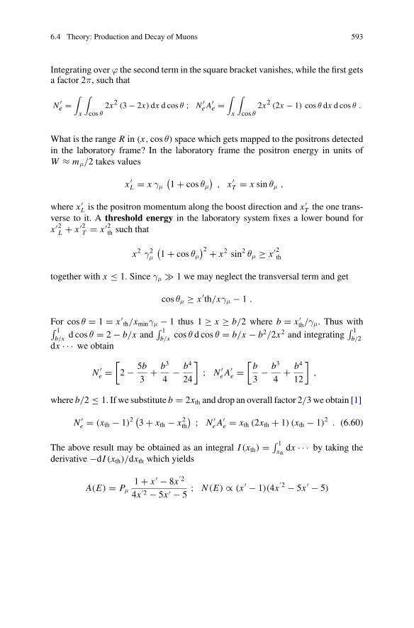
6.4 Theory: Production and Decay of Muons 593

Integrating over ϕ the second term in the square bracket vanishes, while the first getsa factor 2π, such that

N ′e =

∫

x

∫

cos θ2x2 (3 − 2x) dx d cos θ ; N ′

e A′e =

∫

x

∫

cos θ2x2 (2x − 1) cos θ dx d cos θ .

What is the range R in (x, cos θ) space which gets mapped to the positrons detectedin the laboratory frame? In the laboratory frame the positron energy in units ofW ≈ mμ/2 takes values

x ′L = x γμ

(1 + cos θμ

), x ′

T = x sin θμ ,

where x ′L is the positron momentum along the boost direction and x ′

T the one trans-verse to it. A threshold energy in the laboratory system fixes a lower bound forx ′2

L + x ′2T = x ′2

th such that

x2 γ2μ

(1 + cos θμ

)2 + x2 sin2 θμ ≥ x ′2th

together with x ≤ 1. Since γμ � 1 we may neglect the transversal term and get

cos θμ ≥ x ′th/xγμ − 1 .

For cos θ = 1 = x ′th/xminγμ − 1 thus 1 ≥ x ≥ b/2 where b = x ′

th/γμ. Thus with∫ 1b/x d cos θ = 2 − b/x and

∫ 1b/x cos θ d cos θ = b/x − b2/2x2 and integrating

∫ 1b/2

dx · · · we obtain

N ′e =

[2 − 5b

3+ b3

4− b4

24

]; N ′

e A′e =

[b

3− b3

4+ b4

12

],

where b/2 ≤ 1. If we substitute b = 2xth and drop an overall factor 2/3we obtain [1]

N ′e = (xth − 1)2

(3 + xth − x2th

) ; N ′e A

′e = xth (2xth + 1) (xth − 1)2 . (6.60)

The above result may be obtained as an integral I (xth) = ∫ 1xthdx · · · by taking the

derivative −dI (xth)/dxth which yields

A(E) = Pμ1 + x ′ − 8x

′2

4x ′2 − 5x ′ − 5; N (E) ∝ (x ′ − 1)(4x

′2 − 5x ′ − 5)

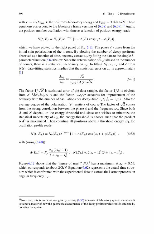
594 6 The g − 2 Experiments

with x ′ = E/Emax, E the positron’s laboratory energy and Emax = 3.098GeV. Theseequations correspond to the laboratory frame versions of (6.58) and (6.59).11 Again,the positron number oscillation with time as a function of positron energy reads

N (t, E) = N0(E) e−t/γτ [1 + A(E) cos(ωat + φ(E))] ,

which we have plotted in the right panel of Fig. 6.11. The phase φ comes from theinitial spin polarization of the muons. By plotting the number of decay positronsobserved as a function of time, one may extract ωa by fitting the data to the simple 5–parameter function (6.62) below.Since thedeterminationofωa is basedon thenumberof counts, there is a statistical uncertainty on ωa . In fitting N0, τ , ωa and φ fromN (t), data–fitting statistics implies that the statistical error on ωa is approximately[1]

δωa

ωa≈

√2

ωa γτ A〈P〉√N. (6.61)

The factor 1/√N is statistical error of the data sample, the factor 1/A is obvious

from N−1δN/δωa ∝ A and the factor 1/ωaγτ accounts for improvement of theaccuracy with the number of oscillations per decay–time ωat/

tγτ

= ωaγτ . Also the

average degree of the polarization 〈P〉 matters of course.The factor of√2 comes

from the strong correlation between the phase φ and the frequency ωa . Since bothA and N depend on the energy-threshold and since one wishes to minimize thestatistical uncertainty of ωa , the energy-threshold is chosen such that the productN A2 is maximized. Then counting all positrons above a threshold energy Eth theoscillation profile reads

N (t, Eth) = N0(Eth) e−t/γτ [1 + A(Eth) cos (ωa t + φ(Eth))] , (6.62)

with (using (6.60))

A(Eth) = Pμxth (2xth − 1)

3 + xth − x2th; N (Eth) ∝ (xth − 1)2(3 + xth − x2th) .

Figure6.12 shows that the “figure of merit” N A2 has a maximum at xth ≈ 0.65,which corresponds to about 2GeV. Equation (6.62) represents the actual time struc-ture which is confronted with the experimental data to extract the Larmor precessionangular frequency ωa .

11Note that, this is not what one gets by writing (6.56) in terms of laboratory system variables. Itis rather a matter of how the geometrical acceptance of the decay positrons/electrons is affected byboosting the system.

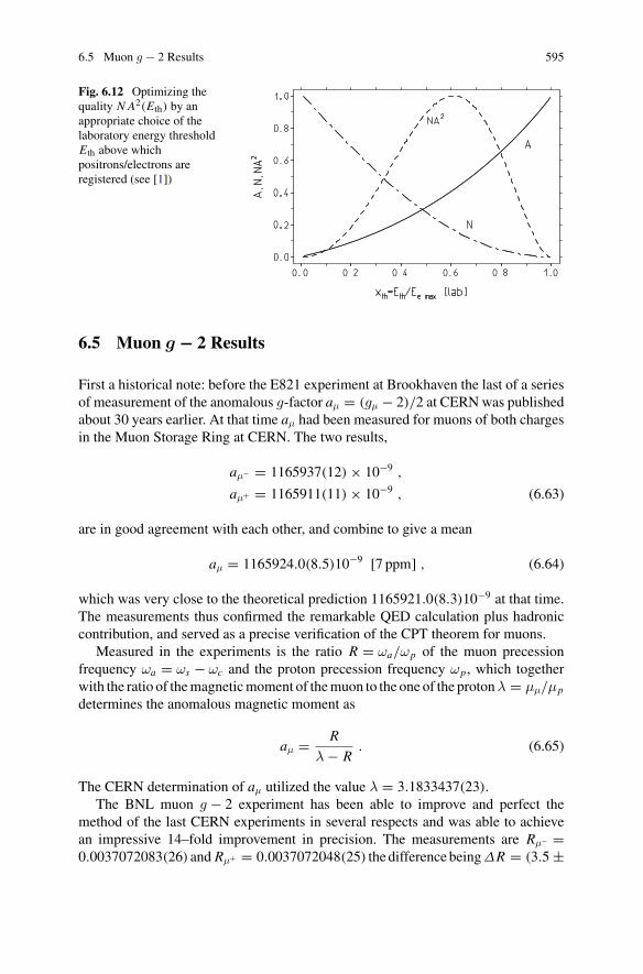
6.5 Muon g − 2 Results 595

Fig. 6.12 Optimizing thequality N A2(Eth) by anappropriate choice of thelaboratory energy thresholdEth above whichpositrons/electrons areregistered (see [1])

6.5 Muon g − 2 Results

First a historical note: before the E821 experiment at Brookhaven the last of a seriesof measurement of the anomalous g-factor aμ = (gμ − 2)/2 at CERNwas publishedabout 30 years earlier. At that time aμ had been measured for muons of both chargesin the Muon Storage Ring at CERN. The two results,

aμ− = 1165937(12) × 10−9 ,

aμ+ = 1165911(11) × 10−9 , (6.63)

are in good agreement with each other, and combine to give a mean

aμ = 1165924.0(8.5)10−9 [7 ppm] , (6.64)

which was very close to the theoretical prediction 1165921.0(8.3)10−9 at that time.The measurements thus confirmed the remarkable QED calculation plus hadroniccontribution, and served as a precise verification of the CPT theorem for muons.

Measured in the experiments is the ratio R = ωa/ωp of the muon precessionfrequency ωa = ωs − ωc and the proton precession frequency ωp, which togetherwith the ratio of themagneticmoment of themuon to the one of the protonλ = μμ/μp

determines the anomalous magnetic moment as

aμ = R

λ − R. (6.65)

The CERN determination of aμ utilized the value λ = 3.1833437(23).The BNL muon g − 2 experiment has been able to improve and perfect the

method of the last CERN experiments in several respects and was able to achievean impressive 14–fold improvement in precision. The measurements are Rμ− =0.0037072083(26) and Rμ+ = 0.0037072048(25) the differencebeingΔR = (3.5 ±

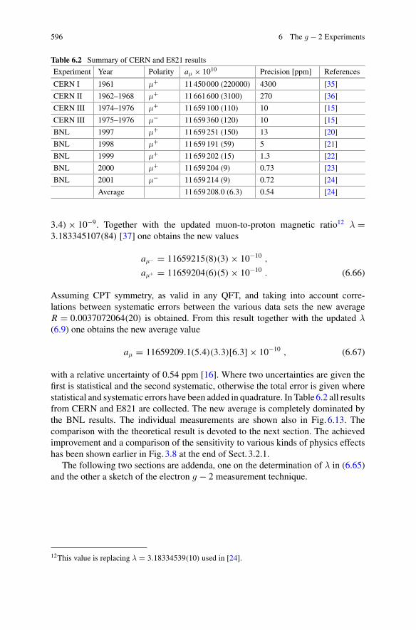
596 6 The g − 2 Experiments

Table 6.2 Summary of CERN and E821 results

Experiment Year Polarity aμ × 1010 Precision [ppm] References

CERN I 1961 μ+ 11450000 (220000) 4300 [35]

CERN II 1962–1968 μ+ 11661600 (3100) 270 [36]

CERN III 1974–1976 μ+ 11659100 (110) 10 [15]

CERN III 1975–1976 μ− 11659360 (120) 10 [15]

BNL 1997 μ+ 11659251 (150) 13 [20]

BNL 1998 μ+ 11659191 (59) 5 [21]

BNL 1999 μ+ 11659202 (15) 1.3 [22]

BNL 2000 μ+ 11659204 (9) 0.73 [23]

BNL 2001 μ− 11659214 (9) 0.72 [24]

Average 11659208.0 (6.3) 0.54 [24]

3.4) × 10−9. Together with the updated muon-to-proton magnetic ratio12 λ =3.183345107(84) [37] one obtains the new values

aμ− = 11659215(8)(3) × 10−10 ,

aμ+ = 11659204(6)(5) × 10−10 . (6.66)

Assuming CPT symmetry, as valid in any QFT, and taking into account corre-lations between systematic errors between the various data sets the new averageR = 0.0037072064(20) is obtained. From this result together with the updated λ(6.9) one obtains the new average value

aμ = 11659209.1(5.4)(3.3)[6.3] × 10−10 , (6.67)

with a relative uncertainty of 0.54 ppm [16]. Where two uncertainties are given thefirst is statistical and the second systematic, otherwise the total error is given wherestatistical and systematic errors have been added in quadrature. In Table6.2 all resultsfrom CERN and E821 are collected. The new average is completely dominated bythe BNL results. The individual measurements are shown also in Fig. 6.13. Thecomparison with the theoretical result is devoted to the next section. The achievedimprovement and a comparison of the sensitivity to various kinds of physics effectshas been shown earlier in Fig. 3.8 at the end of Sect. 3.2.1.

The following two sections are addenda, one on the determination of λ in (6.65)and the other a sketch of the electron g − 2 measurement technique.

12This value is replacing λ = 3.18334539(10) used in [24].

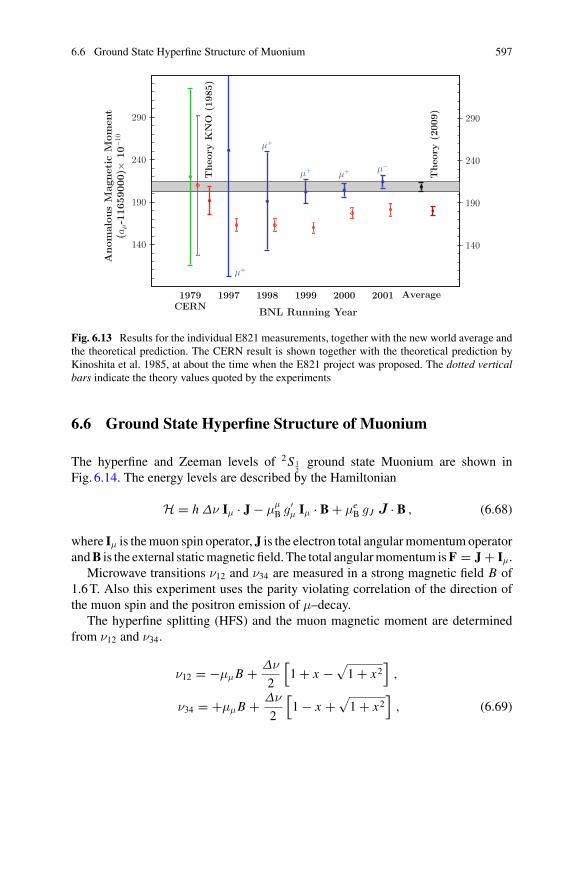
6.6 Ground State Hyperfine Structure of Muonium 597

290

240

190

140140

190

240

290

1979CERN

Theo

ryKNO

(198

5)

1997

μ+

1998

μ+

1999

μ+

2000

μ+

2001

μ−

Average

Theo

ry(2

009)

(aμ-116

5900

0)×

10− 1

0Anom

alou

sM

agnetic

Mom

ent

BNL Running Year

Fig. 6.13 Results for the individual E821 measurements, together with the new world average andthe theoretical prediction. The CERN result is shown together with the theoretical prediction byKinoshita et al. 1985, at about the time when the E821 project was proposed. The dotted verticalbars indicate the theory values quoted by the experiments

6.6 Ground State Hyperfine Structure of Muonium

The hyperfine and Zeeman levels of 2S 12ground state Muonium are shown in

Fig. 6.14. The energy levels are described by the Hamiltonian

H = h Δν Iμ · J − μμB g′

μ Iμ · B + μeB gJ J · B , (6.68)

where Iμ is themuon spin operator, J is the electron total angularmomentumoperatorandB is the external staticmagnetic field. The total angularmomentum isF = J + Iμ.

Microwave transitions ν12 and ν34 are measured in a strong magnetic field B of1.6T. Also this experiment uses the parity violating correlation of the direction ofthe muon spin and the positron emission of μ–decay.

The hyperfine splitting (HFS) and the muon magnetic moment are determinedfrom ν12 and ν34.

ν12 = −μμB + Δν

2

[1 + x −

√1 + x2

],

ν34 = +μμB + Δν

2

[1 − x +

√1 + x2

], (6.69)

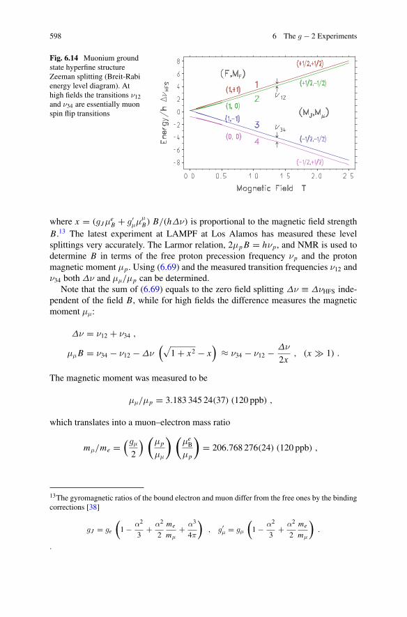
598 6 The g − 2 Experiments

Fig. 6.14 Muonium groundstate hyperfine structureZeeman splitting (Breit-Rabienergy level diagram). Athigh fields the transitions ν12and ν34 are essentially muonspin flip transitions

where x = (gJμeB + g′

μμμB) B/(hΔν) is proportional to the magnetic field strength

B.13 The latest experiment at LAMPF at Los Alamos has measured these levelsplittings very accurately. The Larmor relation, 2μp B = hνp, and NMR is used todetermine B in terms of the free proton precession frequency νp and the protonmagnetic moment μp. Using (6.69) and the measured transition frequencies ν12 andν34 both Δν and μμ/μp can be determined.

Note that the sum of (6.69) equals to the zero field splitting Δν ≡ ΔνHFS inde-pendent of the field B, while for high fields the difference measures the magneticmoment μμ:

Δν = ν12 + ν34 ,

μμB = ν34 − ν12 − Δν(√

1 + x2 − x)

≈ ν34 − ν12 − Δν

2x, (x � 1) .

The magnetic moment was measured to be

μμ/μp = 3.183 345 24(37) (120 ppb) ,

which translates into a muon–electron mass ratio

mμ/me =(gμ

2

) (μp

μμ

) (μeB

μp

)= 206.768 276(24) (120 ppb) ,

13The gyromagnetic ratios of the bound electron and muon differ from the free ones by the bindingcorrections [38]

gJ = ge

(1 − α2

3+ α2

2

me

mμ+ α3

4π

), g′

μ = gμ

(1 − α2

3+ α2

2

me

mμ

).

.

6.6 Ground State Hyperfine Structure of Muonium 599

when using gμ = 2 (1 + aμ) with aμ = 11 659 208.0(6.3) × 10−10 and μp/μeB =

1.521 032 206(15) × 10−3 [30]. The measured value of the zero field HFS is

Δνexp = 4 463 302 765(53) Hz (12 ppb) ,

in good agreement with the theoretical prediction [27, 28, 30, 39–41]

Δν the = 16

3c R∞ α2 me

mμ

(1 + me

mμ

)−3 (1 + δF(α,me/mμ)

)

= 4 463 302 905(272) Hz (61 ppb) ,

where the error is mainly due to the uncertainty in mμ/me. The correction δF(α,me/mμ) depends weakly on α and me/mμ,

R∞ = 10 973 731.568 525(37) m−1

is the Rydberg constant α2mec/2h [30]. A combined result was used to determine(6.9) used in the determination of aμ (see also [42]).

6.7 Single Electron Dynamics and the Electron g − 2

The basic principle of a muon g − 2 experiment is in many respects very similar tothe one of electron g − 2 experiments, although the scale of the experiment is verydifferent and the electron g − 2 experiment uses atomic spectroscopy type methodsto determine the frequencies. The particle dynamics considered in Sect. 6.2 applies tothe single electron or single ion Penning trap shown in Fig. 6.15. Electron motion ina hyperboloid Penning trap in the axial (vertical) direction is a harmonic oscillation

z(t) = A cos(ωz t) ,

withωz = 2

√eV0/md2 ,

(see (6.15)). In the radial direction it is an epicycloid motion with

x(t) = +ρm cos(ωmt) + ρc cos(ω′ct) ,

y(t) = −ρm sin(ωmt) − ρc sin(ω′ct) .

Here

ω′c = ω+ = 1

2(ωc +

√ω2c − 2ω2

z ) � ωc

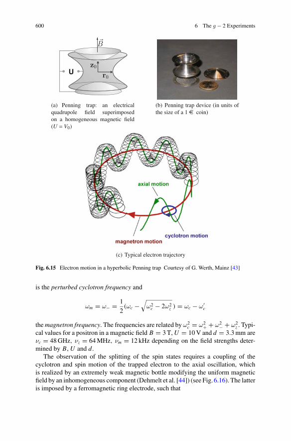
600 6 The g − 2 Experiments

Fig. 6.15 Electron motion in a hyperbolic Penning trap Courtesy of G. Werth, Mainz [43]

is the perturbed cyclotron frequency and

ωm = ω− = 1

2(ωc −

√ω2c − 2ω2

z ) = ωc − ω′c

themagnetron frequency. The frequencies are related by ω2c = ω2+ + ω2− + ω2

z . Typi-cal values for a positron in a magnetic field B = 3T,U = 10V and d = 3.3mm areνc = 48GHz, νz = 64MHz, νm = 12 kHz depending on the field strengths deter-mined by B, U and d.

The observation of the splitting of the spin states requires a coupling of thecyclotron and spin motion of the trapped electron to the axial oscillation, whichis realized by an extremely weak magnetic bottle modifying the uniform magneticfield by an inhomogeneous component (Dehmelt et al. [44]) (see Fig. 6.16). The latteris imposed by a ferromagnetic ring electrode, such that

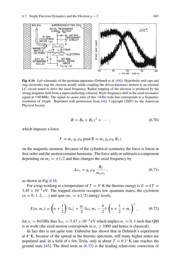
6.7 Single Electron Dynamics and the Electron g − 2 601

Fig. 6.16 Left schematic of the geonium apparatus (Dehmelt et al. [44]). Hyperbolic end caps andring electrodes trap the electron axially while coupling the driven harmonic motion to an externalLC circuit tuned to drive the axial frequency. Radial trapping of the electron is produced by thestrong magnetic field from a superconducting solenoid. Right frequency shift in the axial resonancesignal at ≈60MHz. The signal–to–noise ratio of this ≈8Hz wide line corresponds to a frequencyresolution of 10ppb. Reprinted with permission from [44]. Copyright (2007) by the AmericanPhysical Society

B = B0 + B2 z2 + · · · , (6.70)

which imposes a force

F = ms ge μB grad B = ms ge μB B2 z

on the magnetic moment. Because of the cylindrical symmetry the force is linear infirst order and themotion remains harmonic. The force adds or subtracts a componentdepending on ms = ±1/2 and thus changes the axial frequency by

Δωz = ge μBB2

meωz, (6.71)

as shown in Fig. 6.16.For a trap working at a temperature of T = 4◦ K the thermic energy is E = kT =

3.45 × 10−4 eV. The trapped electron occupies low quantum states, the cyclotron(n = 0, 1, 2, . . .) and spin (ms = ±1/2) energy levels,

E(n,ms) =(n + 1

2

)�ω′

c + ge

2�ωc ms − h

2δ

(n + 1

2+ ms

)2

, (6.72)

for νc = 84GHz thus �ωc = 3.47 × 10−4 eV which implies nc = 0, 1 such that QMis at work (the axial motion corresponds to nz � 1000 and hence is classical).

In fact this is not quite true: Gabrielse has shown that in Dehmelt’s experimentat 4◦ K, because of the spread in the thermic spectrum, still many higher states arepopulated and, in a field of a few Tesla, only at about T = 0.1◦ K one reaches theground state [45]. The third term in (6.72) is the leading relativistic correction of

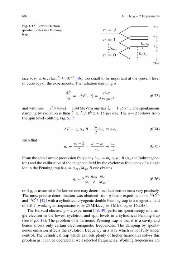
602 6 The g − 2 Experiments

Fig. 6.17 Lowest electronquantum states in a Penningtrap

n = 2

n = 1

n = 0ωc

ωs

ωa

+ 12

− 12

+ 12

− 12

+ 12

− 12

ms

size δ/νc ≡ hνc/(mc2) ≈ 10−9 [46], too small to be important at the present levelof accuracy of the experiments. The radiation damping is

dE

dt= −γE , γ = e2ω2

6πε0mc3, (6.73)

and with α�c = e2/(4πε0) = 1.44MeVfm one has γc = 1.75 s−1. The spontaneousdamping by radiation is then γz � γc/106 � 0.15 per day. The g − 2 follows fromthe spin level splitting Fig. 6.17

ΔE = ge μB B = ge

2�ωc ≡ �ωs , (6.74)

such that

ae ≡ ge − 2

2= ωs − ωc

ωc≡ ωa

ωc. (6.75)

From the spin Larmor precession frequency �ωs = me ge μB B (μB the Bohr magne-ton) and the calibration of the magnetic field by the cyclotron frequency of a singleion in the Penning trap �ωc = qion/Mion B one obtains

ge = 2ωs

ωc

qione

me

Mion, (6.76)

or if ge is assumed to be known one may determine the electron mass very precisely.The most precise determination was obtained from g-factor experiments on 12C5+and 16C7+ [47] with a cylindrical cryogenic double Penning trap in a magnetic fieldof 3.8 T [working at frequencies νc = 25MHz, νz = 1MHz, νm = 16 kHz].

The Harvard electron g − 2 experiment [48, 49] performs spectroscopy of a sin-gle electron in the lowest cyclotron and spin levels in a cylindrical Penning trap(see Fig. 6.18). The problem of a harmonic Penning trap is that it is a cavity andhence allows only certain electromagnetic frequencies. The damping by sponta-neous emission affects the cyclotron frequency in a way which is not fully undercontrol. The cylindrical trap which exhibits plenty of higher harmonics solves thisproblem as it can be operated at well selected frequencies. Working frequencies are

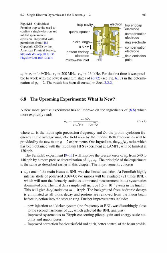
6.7 Single Electron Dynamics and the Electron g − 2 603

Fig. 6.18 CylindricalPenning trap cavity used toconfine a single electron andinhibit spontaneousemission. Reprinted withpermission from [48].Copyright (2008) by theAmerican Physical Society,http://dx.doi.org/10.1103/PhysRevLett.100.120801

top endcapelectrodecompensationelectrode

compensationelectrodefield emissionpoint

bottom endcapelectrode

nickel rings

microwave inlet

ring electrode

quartz spacer

trap cavity electron

0.5 cm

νs ≈ νc ≈ 149GHz, νz ≈ 200MHz, νm ≈ 134kHz. For the first time it was possi-ble to work with the lowest quantum states of (6.72) (see Fig. 6.17) in the determi-nation of ge − 2. The result has been discussed in Sect. 3.2.2.

6.8 The Upcoming Experiments: What Is New?

A new more precise experiment has to improve on the ingredients of (6.6) whichmore explicitly reads

aμ = ωa/ωp

μμ/μp − ωa/ωp, (6.77)

where ωa is the muon spin precession frequency and ωp the proton cyclotron fre-quency in the average magnetic field seen by the muons. Both frequencies will beprovided by the newmuon g − 2 experiments. One ingredient, theμμ/μp ratio,whichhas been obtained with the muonium HFS experiment at LAMPF, will be limited at120ppb.

The Fermilab experiment [9–11] will improve the present error of aμ from 540 to140ppb by a more precise determination of ωa/ωp. The principle of the experimentis the same as described earlier in this chapter. The improvements concern

• ωa : one of the main issues at BNL was the limited statistics. At Fermilab highlyintense shots of polarized 3.094GeV/c muons will be available (21 times BNL),which will turn the formerly statistics dominated measurement into a systematicsdominated one. The final data sample will include 1.5 × 1011 events in the final fit.This will give δωa(statistics) = 110 ppb. The background from hadronic decaysis eliminated as all pions decay and protons are removed from the muon beambefore injection into the storage ring. Further improvements include:

– new injection and kicker system (the frequency at BNL was disturbingly closeto the second harmonic of ωa , which affected the BNL analysis).

– Improved systematics to 70ppb concerning pileup, gain and energy scale sta-bility and muon losses.

– Improved correction for electric field andpitch, better control of the beamprofile.

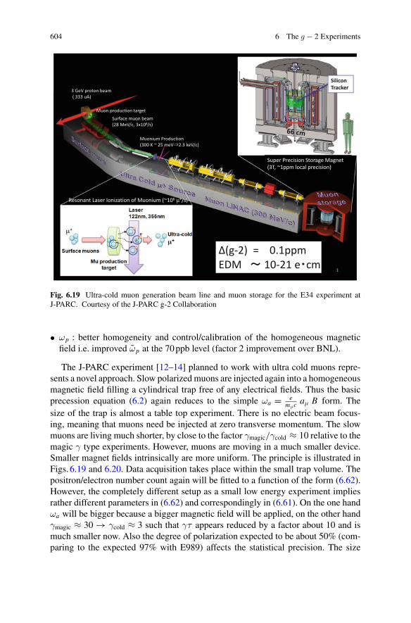
604 6 The g − 2 Experiments

Fig. 6.19 Ultra-cold muon generation beam line and muon storage for the E34 experiment atJ-PARC. Courtesy of the J-PARC g-2 Collaboration

• ωp : better homogeneity and control/calibration of the homogeneous magneticfield i.e. improved ωp at the 70ppb level (factor 2 improvement over BNL).

The J-PARC experiment [12–14] planned to work with ultra cold muons repre-sents a novel approach. Slow polarized muons are injected again into a homogeneousmagnetic field filling a cylindrical trap free of any electrical fields. Thus the basicprecession equation (6.2) again reduces to the simple ωa = e

mμcaμ B form. The

size of the trap is almost a table top experiment. There is no electric beam focus-ing, meaning that muons need be injected at zero transverse momentum. The slowmuons are living much shorter, by close to the factor γmagic/γcold ≈ 10 relative to themagic γ type experiments. However, muons are moving in a much smaller device.Smaller magnet fields intrinsically are more uniform. The principle is illustrated inFigs. 6.19 and 6.20. Data acquisition takes place within the small trap volume. Thepositron/electron number count again will be fitted to a function of the form (6.62).However, the completely different setup as a small low energy experiment impliesrather different parameters in (6.62) and correspondingly in (6.61). On the one handωa will be bigger because a bigger magnetic field will be applied, on the other handγmagic ≈ 30 → γcold ≈ 3 such that γτ appears reduced by a factor about 10 and ismuch smaller now. Also the degree of polarization expected to be about 50% (com-paring to the expected 97% with E989) affects the statistical precision. The size

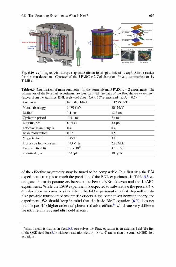
6.8 The Upcoming Experiments: What Is New? 605

Fig. 6.20 Left magnet with storage ring and 3-dimensional spiral injection. Right Silicon trackerfor positron detection. Courtesy of the J-PARC g-2 Collaboration. Private communication byT. Mibe

Table 6.3 Comparison of main parameters for the Fermilab and J-PARC g − 2 experiments. Theparameters of the Fermilab experiment are identical with the ones of the Brookhaven experiment(except from the statistics: BNL registered about 3.6 × 109 events, and had A = 0.3)

Parameter Fermilab E989 J-PARC E34

Muon lab energy 3.098GeV 300MeV

Radius 7.11m 33.3cm

Cyclotron period 149.1ns 7.4ns

Lifetime, γτ 64.4µs 6.6µs

Effective asymmetry A 0.4 0.4

Beam polarization 0.97 0.50

Magnetic field 1.45T 3.0T

Precession frequency ωa 1.43MHz 2.96MHz

Events in final fit 1.8 × 1011 8.1 × 1011

Statistical goal 140ppb 400ppb

of the effective asymmetry may be tuned to be comparable. In a first step the E34experiment attempts to reach the precision of the BNL experiment. In Table6.3 wecompare the main parameters between the Fermilab/Brookhaven and the J-PARCexperiments. While the E989 experiment is expected to substantiate the present 3 to4 σ deviation as a new physics effect, the E43 experiment in a first step will scruti-nize possible unaccounted systematic effects in the comparison between theory andexperiment. We should keep in mind that the basic BMT equation (6.2) does notinclude possible higher order real photon radiation effects14 which are very differentfor ultra relativistic and ultra cold muons.

14What I mean is that, as in Sect. 6.3, one solves the Dirac equation in en external field (the firstof the QED field Eq. (3.1) with zero radiation field Aμ(x) ≡ 0) rather than the coupled QED fieldequations.

606 6 The g − 2 Experiments

References

1. J. Bailey et al., Nuovo Cim. A 9, 369 (1972)2. F. Combley, E. Picasso, Phys. Rep. 14C, 1 (1974)3. F.J.M. Farley, E. Picasso, in Quantum Electrodynamics, ed. by T. Kinoshita (World Scientific,

Singapore 1990), p. 479; Adv. Ser. Direct. High Energy Phys. 7, 479 (1990)4. V.W. Hughes, The anomalous magnetic moment of the muon, in International School of Sub-

nuclear Physics: 39th Course: New Fields and Strings in Subnuclear Physics, Erice, Italy, 29Aug–7 Sep (2001); Int. J. Mod. Phys. A 18S1, 215 (2003)

5. F.J.M. Farley, Y.K. Semertzidis, Prog. Part. Nucl. Phys. 52, 1 (2004)6. D.W. Hertzog, W.M. Morse, Annu. Rev. Nucl. Part. Sci. 54, 141 (2004)7. J.M. Paley, Measurement of the anomalous magnetic moment of the negative muon to 0.7 parts

per million, Boston University Dissertation, 2004, Available from the UMI Thesis Server8. J.P. Miller, E. de Rafael, B.L. Roberts, Rep. Prog. Phys. 70, 795 (2007). doi:10.1088/0034-

4885/70/5/R039. J. Grange et al. [Muon g-2 Collab.], arXiv:1501.06858 [physics.ins-det]10. D.W. Hertzog, EPJ Web Conf. 118, 01015 (2016). doi:10.1051/epjconf/20161180101511. G. Venanzoni [Fermilab E989 Collab.], Nucl. Part. Phys. Proc. 273–275, 584 (2016). doi:10.

1016/j.nuclphysbps.2015.09.087; PoS EPS-HEP2015, 568 (2015)12. N. Saito [J-PARC g-2/EDMCollab.], AIP Conf. Proc. 1467, 45 (2012). doi:10.1063/1.474207813. H. Iinuma [J-PARC muon g-2/EDM Collab.], J. Phys. Conf. Ser. 295, 012032 (2011). doi:10.

1088/1742-6596/295/1/01203214. T. Mibe [J-PARC g-2 Collab.], Nucl. Phys. Proc. Suppl. 218, 242 (2011). doi:10.1016/j.

nuclphysbps.2011.06.03915. J. Bailey et al., Nucl. Phys. B 150, 1 (1979)16. G.W. Bennett et al. [Muon g-2 Collab.], Phys. Rev. D 73, 072003 (2006)17. G.T. Danby et al., Nucl. Instrum. Methods Phys. Res. A 457, 151 (2001)18. Y.K. Semertzidis, Nucl. Instrum. Methods Phys. Res. A 503, 458 (2003)19. E. Efstathiadis et al., Nucl. Instrum. Methods Phys. Res. A 496, 8 (2002)20. R.M. Carey et al., Phys. Rev. Lett. 82, 1632 (1999)21. H.N. Brown et al. [Muon (g-2) Collab.], Phys. Rev. D 62, 091101 (2000)22. H.N. Brown et al. [Muon (g-2) Collab.], Phys. Rev. Lett. 86, 2227 (2001)23. G.W. Bennett et al. [Muon g-2 Collab.], Phys. Rev. Lett. 89, 101804 (2002) [Erratum-ibid. 89,

129903 (2002)]24. G.W. Bennett et al. [Muon g-2 Collab.], Phys. Rev. Lett. 92, 161802 (2004)25. R. Prigl et al., Nucl. Instrum. Methods Phys. Res. A 374, 118 (1996); X. Fei, V. Hughes, R.

Prigl, Nucl. Instrum. Methods Phys. Res. A 394, 349 (1997)26. W. Liu et al., Phys. Rev. Lett. 82, 711 (1999)27. T. Kinoshita, M. Nio, Phys. Rev. D 53, 4909 (1996); M. Nio, T. Kinoshita, Phys. Rev. D 55,

7267 (1997); T. Kinoshita, arXiv:hep-ph/980835128. A.Czarnecki, S.I. Eidelman, S.G.Karshenboim,Phys.Rev.D65, 053004 (2002); S.G.Karshen-

boim, V.A. Shelyuto, Phys. Lett. B 517, 32 (2001)29. H. Lamm, Phys. Rev. A 95(1), 012505 (2017)30. P.J. Mohr, B.N. Taylor, Rev. Mod. Phys. 72, 351 (2000); 77, 1 (2005); P.J. Mohr, B.N. Taylor,

D.B. Newell, Rev. Mod. Phys. 84, 1527 (2012)31. L.H. Thomas, Phil. Mag. 3, 1 (1927); V. Bargmann, L. Michel, V.A. Telegdi, Phys. Rev. Lett.

2, 435 (1959); B.W. Montague, Phys. Rep. 113, 1 (1984); J.S. Bell, CERN-75-11, 38p (1975)32. C. Duval, Nucl. Phys. B 912, 450 (2016)33. F.J.N. Farley, Phys. Lett. B 42, 66 (1972)34. F. Scheck, Leptons, Hadrons and Nuclei (North Holland, Amsterdam, 1983)35. G. Charpak et al., Phys. Rev. Lett. 6, 128 (1961); G. Charpak et al., Nuovo Cim. 22, 1043

(1961)36. J. Bailey et al., Phys. Lett. B 28, 287 (1968); Nuovo Cim. A 9, 369 (1972)

References 607

37. S. Eidelman et al. [Particle Data Group], Phys. Lett. B 592, 1 (2004); K.A. Olive et al., Chin.Phys. C 38, 090001 (2014); C. Patrignani et al., Chin. Phys. C 40(10), 100001 (2016)

38. H. Grotch, R.A. Hegstrom, Phys. Rev. A 4, 59 (1971); R. Faustov. Phys. Lett. B 33, 422 (1970)39. K. Pachucki, Phys. Rev. A 54, 1994 (1996); ibid. 56, 297 (1997); S.G. Karshenboim, Z. Phys.

D 36, 11 (1996); S.A. Blundell, K.T. Cheng, J. Sapirstein, Phys. Rev. Lett. 78, 4914 (1997);M.I. Eides, H. Grotch, V.A. Shelyuto, Phys. Rev. D 58, 013008 (1998)

40. K. Melnikov, A. Yelkhovsky, Phys. Rev. Lett. 86, 1498 (2001)41. R.J. Hill, Phys. Rev. Lett. 86, 3280 (2001)42. K.P. Jungmann, Nucl. Phys. News 12, 23 (2002)43. F.G. Major, V.N. Gheorghe, G. Werth, Charged Particle Traps (Springer, Berlin, 2005)44. R.S. Van Dyck, P.B. Schwinberg, H.G. Dehmelt, Phys. Rev. D 34, 722 (1986)45. S. Peil, G. Gabrielse, Phys. Rev. Lett. 83, 1287 (1999)46. L.S. Brown, G. Gabrielse, Rev. Mod. Phys. 58, 233 (1986)47. T. Beier et al., Phys. Rev. Lett. 88, 011603 (2002); Nucl. Instrum. Methods B 205, 15 (2003)48. D. Hanneke, S. Fogwell, G. Gabrielse, Phys. Rev. Lett. 100, 120801 (2008). doi:10.1103/

PhysRevLett.100.120801, http://g2pc1.bu.edu/lept06/GabrielseTalk.pdf49. D. Hanneke, S.F. Hoogerheide, G. Gabrielse, Phys. Rev. A 83, 052122 (2011). doi:10.1103/

PhysRevA.83.052122

Chapter 7Comparison Between Theoryand Experiment and Future Perspectives

7.1 Experimental Results Confront Standard Theory

The anomalous magnetic moment of the muon provides one of the most precisetests of quantum field theory as a basic framework of elementary particle theoryand of QED and the electroweak SM in particular. With what has been reachedby the BNL muon g − 2 experiment (see Table7.1), namely the reduction of theexperimental uncertainty by a factor 14 to ∼63 × 10−11, a new quality in “divinginto the sea of quantum corrections” has been achieved: the four/five loop orderQED [∼381/5 × 10−11] known thanks to the heroic efforts of Aoyama, Hayakawa,Kinoshita and Nio [3, 4] and Laporta [5], the weak correction up to 2nd order[∼154×10−11] and the hadronic light–by–light scattering [∼100×10−11] are now inthe focus. The uncertainty of theweak corrections has been substantially reducedwiththe discovery of the Higgs boson, which revealed its mass within a small error band.The hadronic vacuum polarization effects which played a significant role already forthe last CERN experiment now is a huge effect of more than 11 SD’s. As a non–perturbative effect it still has to be evaluated largely in terms of experimental datawith unavoidable experimental uncertainties which yield the biggest contribution tothe uncertainty of theoretical predictions. However, due to substantial progress inthe measurement of total hadronic e+e−–annihilation cross sections, the uncertaintyfrom this source has reduced to a remarkable ∼35 × 10−11 only. This source oferror now is only slightly larger than the uncertainty in the theoretical estimates ofthe hadronic light–by–light scattering contribution [∼29× 10−11]. Nevertheless, wehave a solid predictionwith a total uncertainty of∼45×10−11, which is clearly belowthe experimental error of the muon g − 2 measurement. A graphical representationfor the sensitivity and the weight of the various contributions is presented in Fig. 3.8(see also Table7.2 and Fig. 7.3). For another recent summary see [6]. We now haveat the same time, a new very sensitive test of our current theoretical understanding ofthe fundamental forces and the particle spectrum, and a stringent bound on physicsbeyond the SM entering at scales below about 1 TeV. But, may be more important isthe actual deviation between theory and experiment at the 4 σ level which is a clear

© Springer International Publishing AG 2017F. Jegerlehner, The Anomalous Magnetic Moment of the Muon,Springer Tracts in Modern Physics 274, DOI 10.1007/978-3-319-63577-4_7

609

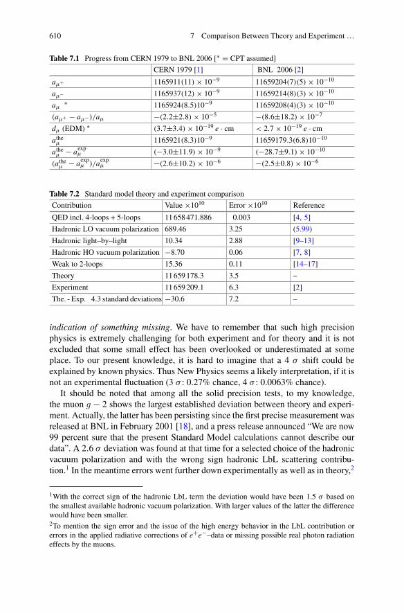
610 7 Comparison Between Theory and Experiment …

Table 7.1 Progress from CERN 1979 to BNL 2006 [∗ = CPT assumed]

CERN 1979 [1] BNL 2006 [2]

aμ+ 1165911(11) × 10−9 11659204(7)(5) × 10−10

aμ− 1165937(12) × 10−9 11659214(8)(3) × 10−10

aμ ∗ 1165924(8.5)10−9 11659208(4)(3) × 10−10

(aμ+ − aμ− )/aμ −(2.2±2.8) × 10−5 −(8.6±18.2) × 10−7

dμ (EDM) ∗ (3.7±3.4) × 10−19 e · cm < 2.7 × 10−19 e · cmatheμ 1165921(8.3)10−9 11659179.3(6.8)10−10

atheμ − aexpμ (−3.0±11.9) × 10−9 (−28.7±9.1) × 10−10

(atheμ − aexpμ )/aexpμ −(2.6±10.2) × 10−6 −(2.5±0.8) × 10−6

Table 7.2 Standard model theory and experiment comparison

Contribution Value ×1010 Error ×1010 Reference

QED incl. 4-loops + 5-loops 11658471.886 0.003 [4, 5]

Hadronic LO vacuum polarization 689.46 3.25 (5.99)

Hadronic light–by–light 10.34 2.88 [9–13]

Hadronic HO vacuum polarization −8.70 0.06 [7, 8]

Weak to 2-loops 15.36 0.11 [14–17]

Theory 11659178.3 3.5 –

Experiment 11659209.1 6.3 [2]

The. - Exp. 4.3 standard deviations −30.6 7.2 –

indication of something missing. We have to remember that such high precisionphysics is extremely challenging for both experiment and for theory and it is notexcluded that some small effect has been overlooked or underestimated at someplace. To our present knowledge, it is hard to imagine that a 4 σ shift could beexplained by known physics. Thus New Physics seems a likely interpretation, if it isnot an experimental fluctuation (3 σ : 0.27% chance, 4 σ : 0.0063% chance).

It should be noted that among all the solid precision tests, to my knowledge,the muon g − 2 shows the largest established deviation between theory and experi-ment. Actually, the latter has been persisting since the first precise measurement wasreleased at BNL in February 2001 [18], and a press release announced “We are now99 percent sure that the present Standard Model calculations cannot describe ourdata”. A 2.6 σ deviation was found at that time for a selected choice of the hadronicvacuum polarization and with the wrong sign hadronic LbL scattering contribu-tion.1 In the meantime errors went further down experimentally as well as in theory,2

1With the correct sign of the hadronic LbL term the deviation would have been 1.5 σ based onthe smallest available hadronic vacuum polarization. With larger values of the latter the differencewould have been smaller.2To mention the sign error and the issue of the high energy behavior in the LbL contribution orerrors in the applied radiative corrections of e+e−–data or missing possible real photon radiationeffects by the muons.

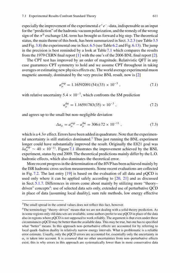
7.1 Experimental Results Confront Standard Theory 611

especially the improvement of the experimental e+e−–data, indispensable as an inputfor the “prediction” of the hadronic vacuumpolarization, and the remedyof thewrongsign of the π0 exchange LbL term has brought us forward a big step. The theoreticalstatus, the main theme of this book, has been summarized in Sect. 3.2.3 (see Table3.5and Fig. 3.8) the experimental one in Sect. 6.5 (see Table6.2 and Fig. 6.13). The jumpin the precision is best reminded by a look at Table7.1 which compares the resultsfrom the 1979 CERN final report [1] with the one’s of the 2006 BNL final report [2].

The CPT test has improved by an order of magnitude. Relativistic QFT in anycase guarantees CPT symmetry to hold and we assume CPT throughout in takingaverages or estimating newphysics effects etc. Theworld average experimentalmuonmagnetic anomaly, dominated by the very precise BNL result, now is [2]

aexpμ = 1.16592091(54)(33) × 10−3 , (7.1)

with relative uncertainty 5.4 × 10−7, which confronts the SM prediction

atheμ = 1.16591783(35) × 10−3 , (7.2)

and agrees up to the small but non–negligible deviation

Δaμ = aexpμ − atheμ = 306±72 × 10−11 , (7.3)

which is a 4.3σ effect. Errors have been added in quadrature.Note that the experimen-tal uncertainty is still statistics dominated.3 Thus just running the BNL experimentlonger could have substantially improved the result. Originally the E821 goal wasδaexpμ ∼ 40 × 10−11. Figure7.1 illustrates the improvement achieved by the BNLexperiment, status by end 2009. The theoretical predictions mainly differ by the L.O.hadronic effects, which also dominates the theoretical error.

More recent progress in the determination of theHVPhas been achievedmainly bythe ISR hadronic cross section measurements. Some recent evaluations are collectedin Fig. 7.2. The last entry [19] is based on the evaluation of all data and pQCD isused only where it can be applied safely according to [20, 21] and as discussedin Sect. 5.1.7. Differences in errors come about mainly by utilizing more “theory–driven” concepts4: use of selected data sets only, extended use of perturbative QCDin place of data [assuming local duality], sum rule methods, low energy effective

3The small spread in the central values does not reflect this fact, however.4The terminology “theory–driven” means that we are not dealing with a solid theory prediction. Asin some regions only old data sets are available, some authors prefer to use pQCD in place of the dataalso in regions where pQCD is not supposed to work reliably. The argument is that even under thesecircumstances pQCDmay be better than the available data. Thismay be true, but one has to specifiedwhat “better” means. In this approach non–perturbative effects are accounted for by referring tolocal quark–hadron duality in relatively narrow energy intervals. What is problematic is a reliableerror estimate. Usually, only the pQCD errors are accounted for, essentially only the uncertainty inαs is taken into account. It is assumed that no other uncertainties from non–perturbative effectsexist; this is why errors in this approach are systematically lower than in more conservative data

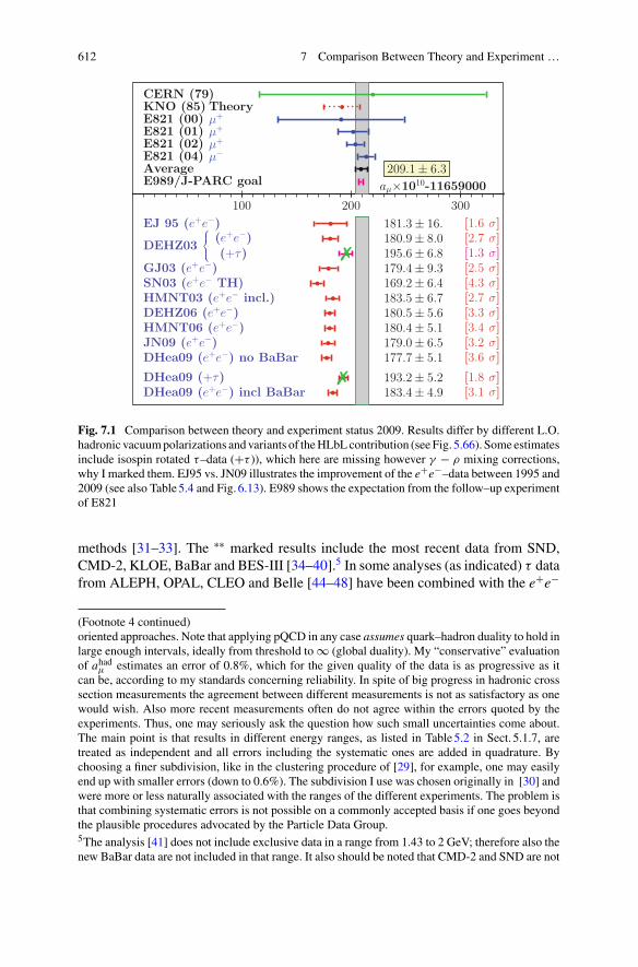
612 7 Comparison Between Theory and Experiment …

100 200 300

CERN (79)TheoryKNO (85)

E821 (00) μ+

E821 (01) μ+

E821 (02) μ+

E821 (04) μ−Average 209.1 ± 6.3E989/J-PARC goal

EJ 95 (e+e−) 181.3 ± 16. [1.6 σ]

DEHZ03

⎧⎨⎩

(e+e−)(+τ)

180.9 ± 8.0 [2.7 σ]195.6 ± 6.8 [1.3 σ]

GJ03 (e+e−) 179.4 ± 9.3 [2.5 σ]SN03 (e+e− TH) 169.2 ± 6.4 [4.3 σ]HMNT03 (e+e− incl.) 183.5 ± 6.7 [2.7 σ]DEHZ06 (e+e−) 180.5 ± 5.6 [3.3 σ]HMNT06 (e+e−) 180.4 ± 5.1 [3.4 σ]JN09 (e+e−) 179.0 ± 6.5 [3.2 σ]DHea09 (e+e−) no BaBar 177.7 ± 5.1 [3.6 σ]

DHea09 (+τ) 193.2 ± 5.2 [1.8 σ]DHea09 (e+e−) incl BaBar 183.4 ± 4.9 [3.1 σ]

aμ×1010-11659000

Fig. 7.1 Comparison between theory and experiment status 2009. Results differ by different L.O.hadronic vacuumpolarizations andvariants of theHLbLcontribution (seeFig. 5.66). Someestimatesinclude isospin rotated τ–data (+τ )), which here are missing however γ − ρ mixing corrections,why I marked them. EJ95 vs. JN09 illustrates the improvement of the e+e−–data between 1995 and2009 (see also Table5.4 and Fig. 6.13). E989 shows the expectation from the follow–up experimentof E821

methods [31–33]. The ∗∗ marked results include the most recent data from SND,CMD-2, KLOE, BaBar and BES-III [34–40].5 In some analyses (as indicated) τ datafrom ALEPH, OPAL, CLEO and Belle [44–48] have been combined with the e+e−

(Footnote 4 continued)oriented approaches. Note that applying pQCD in any case assumes quark–hadron duality to hold inlarge enough intervals, ideally from threshold to ∞ (global duality). My “conservative” evaluationof ahadμ estimates an error of 0.8%, which for the given quality of the data is as progressive as itcan be, according to my standards concerning reliability. In spite of big progress in hadronic crosssection measurements the agreement between different measurements is not as satisfactory as onewould wish. Also more recent measurements often do not agree within the errors quoted by theexperiments. Thus, one may seriously ask the question how such small uncertainties come about.The main point is that results in different energy ranges, as listed in Table5.2 in Sect. 5.1.7, aretreated as independent and all errors including the systematic ones are added in quadrature. Bychoosing a finer subdivision, like in the clustering procedure of [29], for example, one may easilyend up with smaller errors (down to 0.6%). The subdivision I use was chosen originally in [30] andwere more or less naturally associated with the ranges of the different experiments. The problem isthat combining systematic errors is not possible on a commonly accepted basis if one goes beyondthe plausible procedures advocated by the Particle Data Group.5The analysis [41] does not include exclusive data in a range from 1.43 to 2 GeV; therefore also thenew BaBar data are not included in that range. It also should be noted that CMD-2 and SND are not

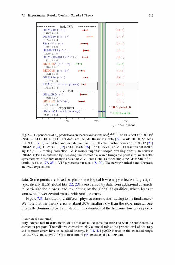
7.1 Experimental Results Confront Standard Theory 613

150 200 250

incl. ISRDHMZ10 (e+e−)180.2 ± 4.9

[3.6 σ]

DHMZ10 (e+e−+τ)189.4 ± 5.4

[2.4 σ]

JS11 (e+e−+τ)179.7 ± 6.0

[3.4 σ]

HLMNT11 (e+e−)182.8 ± 4.9

[3.3 σ]

DHMZ10/JS11 (e+e−+τ)181.1 ± 4.6

[3.6 σ]

BDDJ15# (e+e−+τ)170.4 ± 5.1

[4.8 σ]

BDDJ15∗ (e+e−+τ)175.0 ± 5.0

[4.2 σ]

DHMZ16 (e+e−)181.7 ± 4.2

[3.6 σ]

FJ17 (e+e−+τ+ππ phases)178.3 ± 3.5

[4.3 σ]

excl. ISRDHea09 (e+e−)178.8 ± 5.8

[3.5 σ]

BDDJ12∗ (e+e−+τ)175.4 ± 5.3

[4.1 σ]

experimentBNL-E821 (world average)209.1 ± 6.3

aµ×1010-11659000

∗ HLS global fit

# HLS best fit

Fig. 7.2 Dependence of aμ predictions on recent evaluations of ahad,LOμ . TheHLS best fit BDDJ15#

(NSK + KLOE10 + KLOE12) does not include BaBar ππ data [22], while BDDJ15∗ does.JS11/FJ16 [7, 8] is updated and include the new BES-III data. Further points are BDDJ12 [23],DHMZ10 [24], HLMNT11 [25] and DHea09 [26], The DHMZ10 (e+e−+τ ) result is not includ-ing the ρ − γ mixing correction, i.e. it misses important isospin breaking effects. In contrast,DHMZ10/JS11 is obtained by including this correction, which brings the point into much betteragreement with standard analyses based on e+e− data alone, as for example the DHMZ10 (e+e−)result. (see also [27, 28]). FJ17 represents our result (5.100). The narrow vertical band illustratesthe E989 expectation

data. Some points are based on phenomenological low energy effective Lagrangian(specifically HLS) global fits [22, 23], constrained by data from additional channels,in particular the τ ones, and rewighting by the global fit qualities, which leads tosomewhat lower central values with smaller errors.

Figure7.3 illustrates howdifferent physics contributions addup to thefinal answer.We note that the theory error is about 30% smaller now than the experimental one.It is fully dominated by the hadronic uncertainties of the hadronic low energy cross

(Footnote 5 continued)fully independent measurements; data are taken at the same machine and with the same radiativecorrection program. The radiative corrections play a crucial role at the present level of accuracy,and common errors have to be added linearly. In [42, 43] pQCD is used in the extended ranges1.8–3.7 GeV and above 5.0 GeV; furthermore [43] excludes the KLOE data.

614 7 Comparison Between Theory and Experiment …

−400 −200 0 200 400 600QED - 11659000

QED 8thEW 1–loopEW 2–loopLO hadHO hadLbL

in units 10−10

aµ× 1010-11659000

World Average BNLTheory (e+e−)Theory (+τ)Theory (+ππ phases)DHMZ16 (e+e−)DHMZ16 (+τ)

4.2 σ4.3 σ4.3 σ3.6 σ2.4 σ

Fig. 7.3 All kinds of physics meet. Shown are the various contributions which add up to the theoryprediction relative to the experimental result. The 8th order QED included in the QED part isshown separately. The 10th order QED is too small to be displayed here. For comparison also theextra contribution obtained by including the isospin rotated and isospin breaking corrected hadronicτ–decay data are shown. The “Theory” results are based on e+e− data (5.29), including τ afterγ − ρ mixing correction (5.99) and after including ππ phase shift data improvement [33] (5.100).The recent results DHMZ16 from [49] are also displayed. The second result DHMZ16 includesτ data without γ − ρ. The black heads on the bars represent the uncertainties. The black verticalband represents the future error band. Note that what seems to be a cancellation between “QED-11659000” and “LO had” is due to the QED off–set chosen. The complete QED and LO had areboth positive and just add up. In any case the uncertainties and the deviation between theory andexperiment look amazingly small in comparison to the various SM effect which are substantial fora precise prediction

section data on the one hand and not much less by the uncertainty of the hadroniclight–by–light scattering contribution on the other hand. The history of muon g − 2measurements together with the theory values with which results were compared arelisted once more in Table7.3.

7.2 New Physics in g − 2

The question about which unknown physics hides behind the SMwas and is the mainissue of theoretical particle physics since the emergence of the SM as the theory of“fundamental” particle interactions which we know today. Besides the SM’s mainshortcoming, which is that it lacks to include gravity, it rises many other questionsabout its structure, its many vastly different mass scales, and the answers always areattempts of embedding the SM into an extended theory. While the SM is very wellestablished and is able to explain a plenitude of experimental data, and this so well

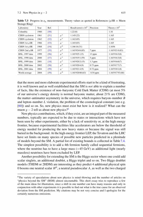
7.2 New Physics in g − 2 615

Table 7.3 Progress in aμ measurements. Theory values as quoted in References (μSR = MuonStorage Ring)Laboratory Year Ref. Result (error)×103 Precision Theory×103

Columbia 1960 [50] 1.22 (8) 1.16

CERN cyclotron 1961 [51] μ+ 1.145 (22) 1.165

CERN cyclotron 1962 [52] μ+ 1.162 (05) 1.165

CERN 1st μSR 1966 [53] μ− 1.165 (03) 1.165

CERN 1st μSR 1968 [54] μ± 1.16616 (31) 1.1656

CERN 2nd μSR 1977 [55] μ± 1.1659240 (85) 7 ppm 1.1659210 (83)

BNL, 1997 data 1999 [56] μ+ 1.165925 (15) 13 ppm 1.1659163(8)

BNL, 1998 data 2000 [57] μ+ 1.1659191 (59) 5 ppm 1.1659163(8)

BNL, 1999 data 2001 [18] μ+ 1.1659202 (15) 1.3 ppm 1.1659160(7)

BNL, 2000 data 2002 [58] μ+ 1.1659204 (9) 0.73 ppm 1.1659177(7)

BNL, 2001 data 2004 [59] μ− 1.1659214 (9) 0.72 ppm 1.1659181(8)

World average 2004 [59] μ± 1.16592080 (63) 0.54 ppm 1.16591793 (68)

that the more andmore elaborate experimental efforts start to be a kind of frustrating,it is well known and as well established that the SM is not able to explain a numberof facts, like the existence of non–baryonic Cold Dark Matter (CDM) (at most 5%of our universe’s energy density is normal baryonic matter, about 21% are CDM),the matter–antimatter asymmetry in the universe, which requires baryon–number Band lepton–number L violation, the problem of the cosmological constant (see e.g.[60]) and so on. So, new physics must exist but how is it realized? What can themuon g − 2 tell us about new physics?6

Newphysics contributions,which, if they exist, are an integral part of themeasurednumbers, typically are expected to be due to states or interactions which have notbeen seen by other experiments, either by a lack of sensitivity or, at the high energyfrontier, because experimental facilities like accelerators are below the threshold ofenergy needed for producing the new heavy states or because the signal was stillburied in the background. At the high energy frontier LEP, the Tevatron and the LHChave set limits on many species of possible new particles predicted in a plenitudeof models beyond the SM. A partial list of existing bounds is collected in Table7.4.The simplest possibility is to add a 4th fermion family called sequential fermions,where the neutrino has to have a large mass (>45 GeV) as additional light (nearlymassless) neutrinos have been excluded by LEP.

Another possibility for extending the SM is the Higgs sector where one could addscalar singlets, an additional doublet, a Higgs triplet and so on. Two Higgs doubletmodels (THDM or 2HDM) are interesting as they predict 4 additional physical spin0 bosons one neutral scalar H 0, a neutral pseudoscalar A, as well as the two charged

6The variety of speculations about new physics is mind–blowing and the number of articles on“physics beyond the SM” (BSM) almost uncountable. This short essay tries to reproduce a fewof the main ideas for illustration, since a shift in one number can have many reasons and only inconjunction with other experiments it is possible to find out what is the true cause for an observeddeviation from the SM prediction. My citations may be not very concise and I apologize for thecertainly numerous omissions.

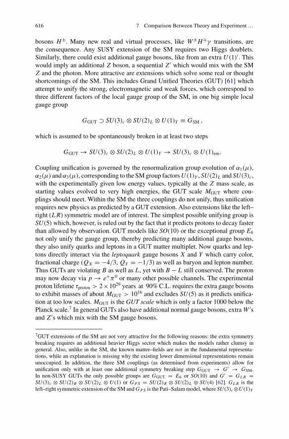
616 7 Comparison Between Theory and Experiment …

bosons H±. Many new real and virtual processes, like W±H∓γ transitions, arethe consequence. Any SUSY extension of the SM requires two Higgs doublets.Similarly, there could exist additional gauge bosons, like from an extra U (1)′. Thiswould imply an additional Z boson, a sequential Z ′ which would mix with the SMZ and the photon. More attractive are extensions which solve some real or thoughtshortcomings of the SM. This includes Grand Unified Theories (GUT) [61] whichattempt to unify the strong, electromagnetic and weak forces, which correspond tothree different factors of the local gauge group of the SM, in one big simple localgauge group

GGUT ⊃ SU(3)c ⊗ SU(2)L ⊗U (1)Y ≡ GSM ,

which is assumed to be spontaneously broken in at least two steps

GGUT → SU(3)c ⊗ SU(2)L ⊗U (1)Y → SU(3)c ⊗U (1)em.

Coupling unification is governed by the renormalization group evolution of α1(μ),α2(μ) andα3(μ), corresponding to the SMgroup factorsU (1)Y , SU(2)L and SU(3)c,with the experimentally given low energy values, typically at the Z mass scale, asstarting values evolved to very high energies, the GUT scale MGUT where cou-plings should meet. Within the SM the three couplings do not unify, thus unificationrequires new physics as predicted by a GUT extension. Also extensions like the left–right (LR) symmetric model are of interest. The simplest possible unifying group isSU(5)which, however, is ruled out by the fact that it predicts protons to decay fasterthan allowed by observation. GUT models like SO(10) or the exceptional group E6

not only unify the gauge group, thereby predicting many additional gauge bosons,they also unify quarks and leptons in a GUT matter multiplet. Now quarks and lep-tons directly interact via the leptoquark gauge bosons X and Y which carry color,fractional charge (QX = −4/3, QY = −1/3) as well as baryon and lepton number.Thus GUTs are violating B as well as L , yet with B − L still conserved. The protonmay now decay via p → e+π0 or many other possible channels. The experimentalproton lifetime τproton > 2×1029 years at 90%C.L. requires the extra gauge bosonsto exhibit masses of about MGUT > 1016 and excludes SU(5) as it predicts unifica-tion at too low scales. MGUT is the GUT scale which is only a factor 1000 below thePlanck scale.7 In general GUTs also have additional normal gauge bosons, extraW ′sand Z ′s which mix with the SM gauge bosons.

7GUT extensions of the SM are not very attractive for the following reasons: the extra symmetrybreaking requires an additional heavier Higgs sector which makes the models rather clumsy ingeneral. Also, unlike in the SM, the known matter–fields are not in the fundamental representa-tions, while an explanation is missing why the existing lower dimensional representations remainunoccupied. In addition, the three SM couplings (as determined from experiments) allow forunification only with at least one additional symmetry breaking step GGUT → G ′ → GSM.In non-SUSY GUTs the only possible groups are GGUT = E6 or SO(10) and G ′ = GLR =SU(3)c ⊗ SU(2)R ⊗ SU(2)L ⊗ U (1) or GPS = SU(2)R ⊗ SU(2)L ⊗ SU(4) [62]. GLR is theleft–right symmetric extension of the SM andGPS is the Pati–Salammodel, where SU(3)c⊗U (1)Y

7.2 New Physics in g − 2 617

Table 7.4 Present lower bounds on new physics states. Bounds are 95% C.L. limits from LEP(ALEPH, DELPHI, L3, OPAL), the Tevatron (CDF, D0) and the LHC (ATLAS, CMS)

Object mass bound comment

Heavy neutrino mMν′ > 39 GeV Majorana-ν [ν ≡ ν]

Heavy neutrino mDν′ > 45 GeV Dirac-ν [ν �= ν]

Heavy lepton mL > 100 GeV

4th family quark b′ mb′ > 199 GeV p p NC decays

W ′SM MW ′ > 800 GeV SM couplings

WR MWR > 715 GeV right–handed weak current

Z ′SM MZ ′ > 81.5 TeV SM couplings

ZLR (gR = gL ) MZLR > 630 GeV of GLR =SU(2)R ⊗ SU(2)L ⊗U (1)

Zχ (gχ = e/ cosΘW ) MZχ > 595 GeV of SO(10) → SU(5) ⊗U (1)χZψ (gψ = e/ cosΘW ) MZψ > 590 GeV of E6 → SO(10) ⊗U (1)ψZη (gη = e/ cosΘW ) MZη > 620 GeV of E6 → GLR ⊗U (1)ηh0 ≡ H0

1 Higgs mH01> 92.8 GeV SUSY (mH0

1< mH0

2)

A0 pseudoscalar Higgs mA > 93.4 GeV THDM, MSSM

H± charged Higgs mH± > 80.0 GeV THDM, MSSM

LHC results pp direct searches

4th family quark b′ mb′ > 755 GeV NC decays

4th family quark t ′ mt ′ > 782 GeV NC decays

W ′SM MW ′ > 3.71 TeV SM couplings

Z ′SM MZ ′ > 2.9 TeV SM couplings

ZLR (gR = gL ) MZLR > 1.16 TeV of GLR =SU(2)R ⊗ SU(2)L ⊗U (1)

Zχ (gχ = e/ cosΘW ) MZχ > 2.62 TeV of SO(10) → SU(5) ⊗U (1)χZψ (gψ = e/ cosΘW ) MZψ > 2.57 TeV of E6 → SO(10) ⊗U (1)ψZη (gη = e/ cosΘW ) MZη > 1.87 TeV of E6 → GLR ⊗U (1)η

In deriving bounds on New Physics it is important to respect constraints not onlyfrom aμ and the direct bounds of Table7.4, but also from other precision observableswhich are sensitive to new physics via radiative corrections. Important examples arethe electroweak precision observables [64, 65]:

MW = 80.385(15) GeV , (7.4)

(Footnote 7 continued)of the SM is contained in the SU(4) factor. Coupling unification requires the extra intermediatebreaking scale to lie very high M ′ ∼ 1010 GeV for GLR and M ′ ∼ 1014 GeV for GPS . Theseare the scales of new physics in these extensions, completely beyond of being phenomenologicallyaccessible. The advantage of SUSY GUTs is that they allow for unification of the couplings withthe new physics scale being as low as MZ to 1 TeV [63], and the supersymmetrized GGUT = SU(5)extension of the SM escapes to be excluded.

618 7 Comparison Between Theory and Experiment …

sin2 Θ�eff = 0.23152(5) , ρ0 = 1.00037(23) , (7.5)

which are both preciselymeasured and precisely predicted by the SMor in extensionsof it. The SM predictions use the very precisely known independent input parametersα, Gμ and MZ , but also the less precisely known top quark mass

mt = 173.21±0.87 GeV , (7.6)

and the Higgs boson mass [66]

mH = 125.09(24) GeV , (7.7)

are important.The parameter ρ0 is the tree level (SM radiative corrections subtracted) ratio of

the low energy effective weak neutral to charged current couplings: ρ = GNC/GCC

where GCC ≡ Gμ. This parameter is rather sensitive to new physics. In the SM attree level ρ0 ≡ 1 independent of any free parameter. This is due to the custodialsymmetry of the minimal SM Higgs sector and consequently ρ is a SM predictionvery similar to the anomalous lepton moments. In general, extensions of the SM, likeGUTs or models including Higgs triplets etc., violate the custodial symmetry and ifρ0 depends on parameters of the extension then ρ becomes a tunable quantity andone has a fine tuning problem [67]. The fact that ρ0 = 1 in the SM allowed one topredict the top quark mass from a precision measurement of Δρ (4.40) at LEP priorto the discovery of the top quark at the Tevatron. The leading top quark mass effectin Δρ ∝ m2

t is lost if ρ0 �= 1 and such extensions are disfavored (see e.g. [68]).Equally important are constraints by the B–physics branching fractions [69]

BR(b → sγ ) = (3.43±0.22) × 10−4 ; BR(Bs → μ+μ−) = 2.8+0.7−0.6 × 10−9. (7.8)

Concerning flavor physics, in particular the B factories Belle at KEK and BaBarat SLAC have set new milestones in confirming the flavor structure as inferred bythe SM. In the latter Flavor–Changing Neutral Currents (FCNC) are absent at treelevel due to the GIM mechanism and CP-violation and flavor mixing patterns seemto be realized in nature precisely as implemented by the three fermion–family CKMmixing scheme. Many new physics models have serious problems to accommodatethis phenomenologically largely confirmed structure in a natural way. Therefore,the criterion of Minimal Flavor Violation (MFV) [70] has been conjectured as aframework for constructing low energy effective theories which include the SMLagrangian without spoiling its flavor structure. The SM fermions are grouped intothree families with two SU(2)L doublets (QL and LL ) and three SU(2)L singlets(UR , DR and ER) and the largest group of unitary transformations which commutes

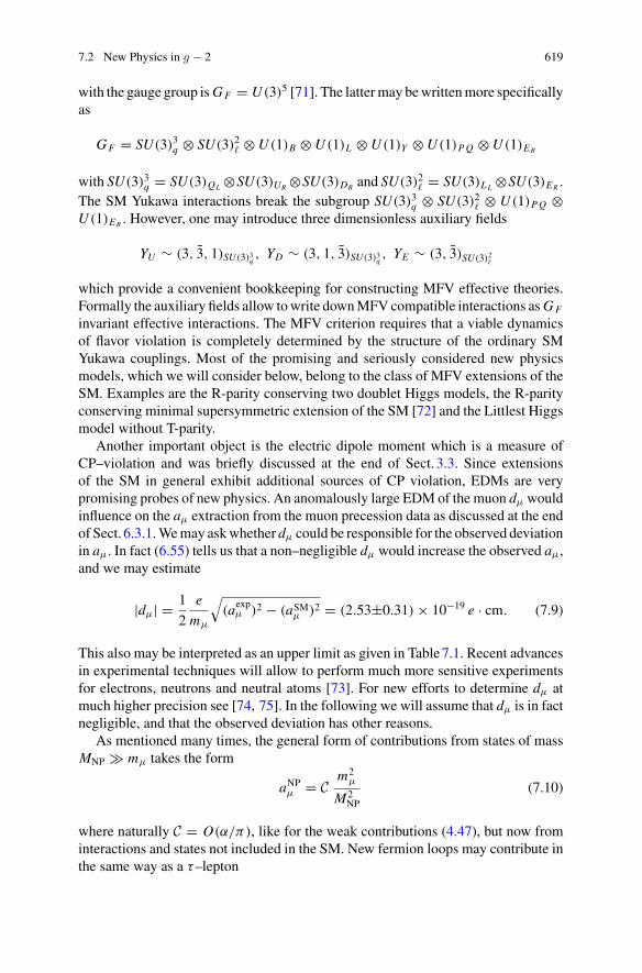
7.2 New Physics in g − 2 619

with the gauge group isGF = U (3)5 [71]. The lattermay bewrittenmore specificallyas

GF = SU(3)3q ⊗ SU(3)2� ⊗U (1)B ⊗U (1)L ⊗U (1)Y ⊗U (1)PQ ⊗U (1)ER

with SU(3)3q = SU(3)QL ⊗SU(3)UR ⊗SU(3)DR and SU(3)2� = SU(3)LL ⊗SU(3)ER .The SM Yukawa interactions break the subgroup SU(3)3q ⊗ SU(3)2� ⊗ U (1)PQ ⊗U (1)ER . However, one may introduce three dimensionless auxiliary fields

YU ∼ (3, 3, 1)SU(3)3q , YD ∼ (3, 1, 3)SU(3)3q , YE ∼ (3, 3)SU(3)2�

which provide a convenient bookkeeping for constructing MFV effective theories.Formally the auxiliary fields allow towrite downMFVcompatible interactions asGF

invariant effective interactions. The MFV criterion requires that a viable dynamicsof flavor violation is completely determined by the structure of the ordinary SMYukawa couplings. Most of the promising and seriously considered new physicsmodels, which we will consider below, belong to the class of MFV extensions of theSM. Examples are the R-parity conserving two doublet Higgs models, the R-parityconserving minimal supersymmetric extension of the SM [72] and the Littlest Higgsmodel without T-parity.

Another important object is the electric dipole moment which is a measure ofCP–violation and was briefly discussed at the end of Sect. 3.3. Since extensionsof the SM in general exhibit additional sources of CP violation, EDMs are verypromising probes of new physics. An anomalously large EDM of the muon dμ wouldinfluence on the aμ extraction from the muon precession data as discussed at the endof Sect. 6.3.1.Wemay askwhether dμ could be responsible for the observed deviationin aμ. In fact (6.55) tells us that a non–negligible dμ would increase the observed aμ,and we may estimate

|dμ| = 1

2

e

mμ

√(aexpμ )2 − (aSMμ )2 = (2.53±0.31) × 10−19 e · cm. (7.9)

This also may be interpreted as an upper limit as given in Table7.1. Recent advancesin experimental techniques will allow to perform much more sensitive experimentsfor electrons, neutrons and neutral atoms [73]. For new efforts to determine dμ atmuch higher precision see [74, 75]. In the following we will assume that dμ is in factnegligible, and that the observed deviation has other reasons.

As mentioned many times, the general form of contributions from states of massMNP mμ takes the form

aNPμ = C m2μ

M2NP

(7.10)

where naturally C = O(α/π), like for the weak contributions (4.47), but now frominteractions and states not included in the SM. New fermion loops may contribute inthe same way as a τ–lepton

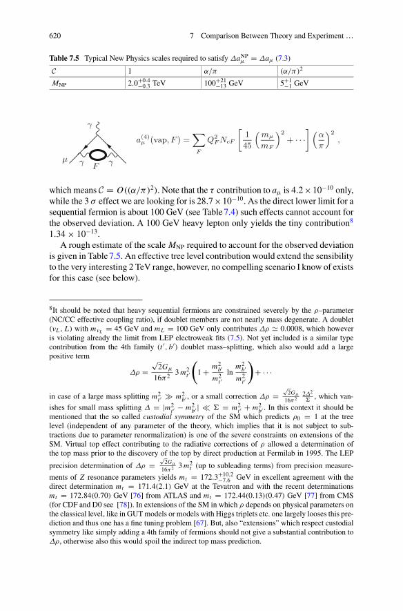
620 7 Comparison Between Theory and Experiment …

Table 7.5 Typical New Physics scales required to satisfy ΔaNPμ = Δaμ (7.3)

C 1 α/π (α/π)2

MNP 2.0+0.4−0.3 TeV 100+21

−13 GeV 5+1−1 GeV

a(4)µ (vap, F ) =

∑F

Q2FNcF

[145

(mµ

mF

)2+ · · ·

](α

π

)2,

γ γF

μ

γ

which means C = O((α/π)2). Note that the τ contribution to aμ is 4.2×10−10 only,while the 3 σ effect we are looking for is 28.7×10−10. As the direct lower limit for asequential fermion is about 100 GeV (see Table7.4) such effects cannot account forthe observed deviation. A 100 GeV heavy lepton only yields the tiny contribution8

1.34 × 10−13.A rough estimate of the scale MNP required to account for the observed deviation

is given in Table7.5. An effective tree level contribution would extend the sensibilityto the very interesting 2 TeV range, however, no compelling scenario I know of existsfor this case (see below).

8It should be noted that heavy sequential fermions are constrained severely by the ρ–parameter(NC/CC effective coupling ratio), if doublet members are not nearly mass degenerate. A doublet(νL , L) with mνL = 45 GeV and mL = 100 GeV only contributes Δρ � 0.0008, which howeveris violating already the limit from LEP electroweak fits (7.5). Not yet included is a similar typecontribution from the 4th family (t ′, b′) doublet mass–splitting, which also would add a largepositive term

Δρ =√2Gμ

16π2 3m2t ′

(1 + m2

b′

m2t ′

lnm2

b′

m2t ′

)+ · · ·

in case of a large mass splitting m2t ′ m2

b′ , or a small correction Δρ =√2Gμ

16π22Δ2

�, which van-

ishes for small mass splitting Δ = |m2t ′ − m2

b′ | � � = m2t ′ + m2

b′ . In this context it should bementioned that the so called custodial symmetry of the SM which predicts ρ0 = 1 at the treelevel (independent of any parameter of the theory, which implies that it is not subject to sub-tractions due to parameter renormalization) is one of the severe constraints on extensions of theSM. Virtual top effect contributing to the radiative corrections of ρ allowed a determination ofthe top mass prior to the discovery of the top by direct production at Fermilab in 1995. The LEP

precision determination of Δρ =√2Gμ

16π2 3m2t (up to subleading terms) from precision measure-

ments of Z resonance parameters yields mt = 172.3+10.2−7.6 GeV in excellent agreement with the

direct determination mt = 171.4(2.1) GeV at the Tevatron and with the recent determinationsmt = 172.84(0.70) GeV [76] from ATLAS and mt = 172.44(0.13)(0.47) GeV [77] from CMS(for CDF and D0 see [78]). In extensions of the SM in which ρ depends on physical parameters onthe classical level, like in GUTmodels or models with Higgs triplets etc. one largely looses this pre-diction and thus one has a fine tuning problem [67]. But, also “extensions” which respect custodialsymmetry like simply adding a 4th family of fermions should not give a substantial contribution toΔρ, otherwise also this would spoil the indirect top mass prediction.

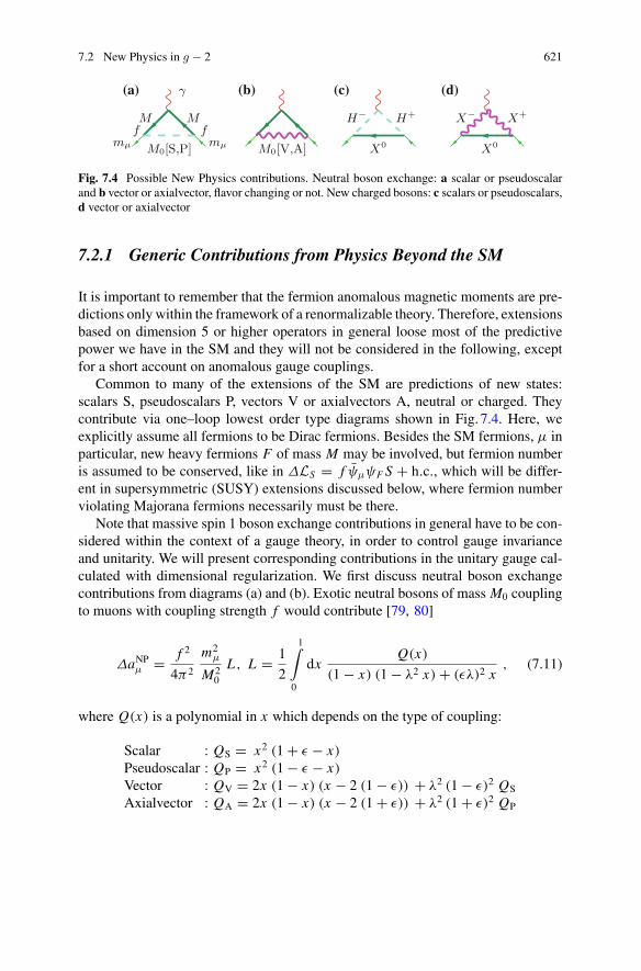
7.2 New Physics in g − 2 621

M Mf f

mµ mµM0[S,P] M0[V,A]

H+H−

X0

X− X+

X0

γ(a) (b) (c) (d)

Fig. 7.4 Possible New Physics contributions. Neutral boson exchange: a scalar or pseudoscalarand b vector or axialvector, flavor changing or not. New charged bosons: c scalars or pseudoscalars,d vector or axialvector

7.2.1 Generic Contributions from Physics Beyond the SM

It is important to remember that the fermion anomalous magnetic moments are pre-dictions only within the framework of a renormalizable theory. Therefore, extensionsbased on dimension 5 or higher operators in general loose most of the predictivepower we have in the SM and they will not be considered in the following, exceptfor a short account on anomalous gauge couplings.

Common to many of the extensions of the SM are predictions of new states:scalars S, pseudoscalars P, vectors V or axialvectors A, neutral or charged. Theycontribute via one–loop lowest order type diagrams shown in Fig. 7.4. Here, weexplicitly assume all fermions to be Dirac fermions. Besides the SM fermions, μ inparticular, new heavy fermions F of mass M may be involved, but fermion numberis assumed to be conserved, like in ΔLS = f ψμψF S + h.c., which will be differ-ent in supersymmetric (SUSY) extensions discussed below, where fermion numberviolating Majorana fermions necessarily must be there.

Note that massive spin 1 boson exchange contributions in general have to be con-sidered within the context of a gauge theory, in order to control gauge invarianceand unitarity. We will present corresponding contributions in the unitary gauge cal-culated with dimensional regularization. We first discuss neutral boson exchangecontributions from diagrams (a) and (b). Exotic neutral bosons of mass M0 couplingto muons with coupling strength f would contribute [79, 80]

ΔaNPμ = f 2

4π2

m2μ

M20

L , L = 1

2

1∫

0

dxQ(x)

(1 − x) (1 − λ2 x) + (ελ)2 x, (7.11)

where Q(x) is a polynomial in x which depends on the type of coupling:

Scalar : QS = x2 (1 + ε − x)Pseudoscalar : QP = x2 (1 − ε − x)Vector : QV = 2x (1 − x) (x − 2 (1 − ε)) + λ2 (1 − ε)2 QS

Axialvector : QA = 2x (1 − x) (x − 2 (1 + ε)) + λ2 (1 + ε)2 QP

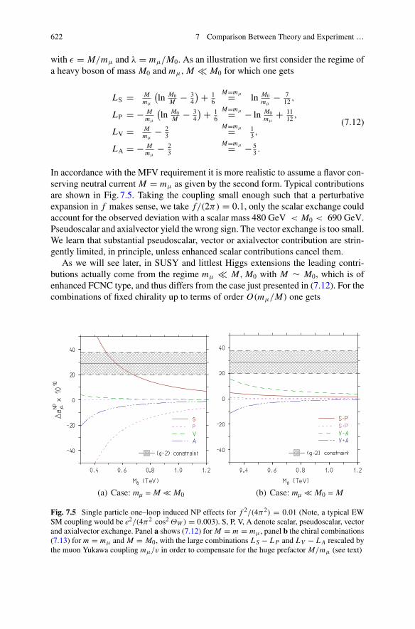
622 7 Comparison Between Theory and Experiment …

with ε = M/mμ and λ = mμ/M0. As an illustration we first consider the regime ofa heavy boson of mass M0 and mμ, M � M0 for which one gets

LS = Mmμ

(ln M0

M − 34

)+ 16

M=mμ= ln M0mμ

− 712 ,

LP = − Mmμ

(ln M0

M − 34

)+ 16

M=mμ= − ln M0mμ

+ 1112 ,

LV = Mmμ

− 23

M=mμ= 13 ,

LA = − Mmμ

− 23

M=mμ= − 53 .

(7.12)

In accordance with the MFV requirement it is more realistic to assume a flavor con-serving neutral current M = mμ as given by the second form. Typical contributionsare shown in Fig. 7.5. Taking the coupling small enough such that a perturbativeexpansion in f makes sense, we take f/(2π) = 0.1, only the scalar exchange couldaccount for the observed deviation with a scalar mass 480 GeV < M0 < 690 GeV.Pseudoscalar and axialvector yield the wrong sign. The vector exchange is too small.We learn that substantial pseudoscalar, vector or axialvector contribution are strin-gently limited, in principle, unless enhanced scalar contributions cancel them.

As we will see later, in SUSY and littlest Higgs extensions the leading contri-butions actually come from the regime mμ � M, M0 with M ∼ M0, which is ofenhanced FCNC type, and thus differs from the case just presented in (7.12). For thecombinations of fixed chirality up to terms of order O(mμ/M) one gets

Fig. 7.5 Single particle one–loop induced NP effects for f 2/(4π2) = 0.01 (Note, a typical EWSM coupling would be e2/(4π2 cos2 ΘW ) = 0.003). S, P, V, A denote scalar, pseudoscalar, vectorand axialvector exchange. Panel a shows (7.12) for M = m = mμ, panel b the chiral combinations(7.13) for m = mμ and M = M0, with the large combinations LS − LP and LV − LA rescaled bythe muon Yukawa coupling mμ/v in order to compensate for the huge prefactor M/mμ (see text)

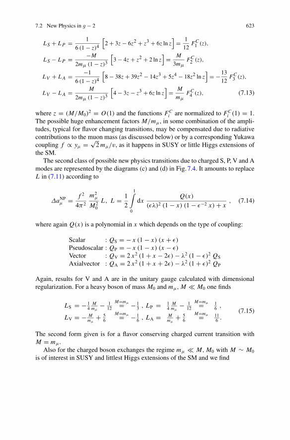
7.2 New Physics in g − 2 623

LS + LP = 1

6 (1 − z)4

[2 + 3z − 6z2 + z3 + 6z ln z

]= 1

12FC1 (z),

LS − LP = −M

2mμ (1 − z)3

[3 − 4z + z2 + 2 ln z

]= M

3mμFC2 (z),

LV + LA = −1

6 (1 − z)4

[8 − 38z + 39z2 − 14z3 + 5z4 − 18z2 ln z

]= −13

12FC3 (z),

LV − LA = M

2mμ (1 − z)3

[4 − 3z − z3 + 6z ln z

]= M

mμFC4 (z), (7.13)

where z = (M/M0)2 = O(1) and the functions FC

i are normalized to FCi (1) = 1.

The possible huge enhancement factors M/mμ, in some combination of the ampli-tudes, typical for flavor changing transitions, may be compensated due to radiativecontributions to the muon mass (as discussed below) or by a corresponding Yukawacoupling f ∝ yμ = √

2mμ/v, as it happens in SUSY or little Higgs extensions ofthe SM.

The second class of possible new physics transitions due to charged S, P, V and Amodes are represented by the diagrams (c) and (d) in Fig. 7.4. It amounts to replaceL in (7.11) according to

ΔaNPμ = f 2

4π2

m2μ

M20

L , L = 1

2

1∫

0

dxQ(x)

(ελ)2 (1 − x) (1 − ε−2 x) + x, (7.14)

where again Q(x) is a polynomial in x which depends on the type of coupling:

Scalar : QS = − x (1 − x) (x + ε)

Pseudoscalar : QP = − x (1 − x) (x − ε)

Vector : QV = 2 x2 (1 + x − 2ε) − λ2 (1 − ε)2 QS

Axialvector : QA = 2 x2 (1 + x + 2ε) − λ2 (1 + ε)2 QP

Again, results for V and A are in the unitary gauge calculated with dimensionalregularization. For a heavy boson of mass M0 and mμ, M � M0 one finds

LS = − 14

Mmμ

− 112

M=mμ= − 13 , LP = 1

4Mmμ

− 112

M=mμ= 16 ,

LV = − Mmμ

+ 56

M=mμ= − 16 , LA = M

mμ+ 5

6

M=mμ= 116 .

(7.15)

The second form given is for a flavor conserving charged current transition withM = mμ.

Also for the charged boson exchanges the regime mμ � M, M0 with M ∼ M0

is of interest in SUSY and littlest Higgs extensions of the SM and we find

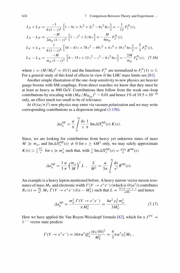
624 7 Comparison Between Theory and Experiment …

LS + LP = −1

6 (1 − z)4

[1 − 6z + 3z2 + 2z3 − 6z2 ln z

]= − 1

12FN1 (z),

LS − LP = −M

2mμ (1 − z)3

[1 − z2 + 2z ln z

]= − M

6mμFN2 (z),

LV + LA = 1

6 (1 − z)4

[10 − 43 z + 78 z2 − 49 z3 + 4 z4 + 18 z3 ln z

]= 5

3FN3 (z),

LV − LA = −M

mμ (1 − z)3

[4 − 15 z + 12 z2 − z3 − 6 z2 ln z

]= −2M

mμFN4 (z), (7.16)

where z = (M/M0)2 = O(1) and the functions FN

i are normalized to FNi (1) = 1.

For a general study of this kind of effects in view if the LHC mass limits see [81].Another simple illustration of the one–loop sensitivity to new physics are heavier

gauge bosons with SM couplings. From direct searches we know that they must beat least as heavy as 800 GeV. Contributions then follow from the weak one–loopcontributions by rescaling with (MW/MW ′

SM)2 ∼ 0.01 and hence 1% of 19.5×10−10

only, an effect much too small to be of relevance.At O((α/π)2) new physics may enter via vacuum polarization and we may write

corresponding contributions as a dispersion integral (3.150):

ΔaNPμ = α

π

∞∫

0

ds

s

1

πImΔΠNP

γ (s) K (s).

Since, we are looking for contributions from heavy yet unknown states of massM mμ, and ImΔΠNP

γ (s) �= 0 for s ≥ 4M2 only, we may safely approximate

K (s) � 13m2

μ

s for s m2μ such that, with 1

πImΔΠNP

γ (s) = α(s)π

RNP(s)

ΔaNPμ = 1

3

α

π

(mμ

M

)2L ,

L

M2= α

3π

∞∫

0

ds

s2RNP(s).

An example is a heavy lepton mentioned before. A heavy narrow vector meson reso-nance of massMV and electronic widthΓ (V → e+e−) (which is O(α2)) contributesRV (s) = 9π

α2 MV Γ (V → e+e−) δ(s − M2V ) such that L = 3Γ (V→e+e−)

αMVand hence

ΔaNPμ = m2μ Γ (V → e+e−)

πM3V

= 4α2 γ 2V m2

μ

3M2V

. (7.17)

Here we have applied the Van Royen-Weisskopf formula [82], which for a J PC =1− − vector state predicts

Γ (V → e+e−) = 16πα2Q2q

|ψV (0)|2M2

V

= 4

3πα2γ 2

V MV ,

7.2 New Physics in g − 2 625

where ψV (0) is the meson wave function at the origin (dim 3) and γV is the dimen-sionless effective photon vector–meson coupling defined by jμem(x) = γV M2

V V μ(x)with V μ(x) the interpolating vector–meson field. γV characterizes the strong inter-action properties of the γ − V coupling and typically has values 0.2 for the ρ to0.02 for the ϒ . For γV = 0.1 and MV = 200 GeV we get Δaμ ∼ 2 × 10−13. Thehadronic contribution of a 4th family quark doublet assuming mb′ = mt ′ = 200GeVwould yield Δaμ ∼ 5.6 × 10−14 only. Unless there exists a new type of stronginteractions like Technicolor9 [83–85]. New strong interaction resonances are notexpected, because new heavy sequential quarks would be too shortlived to be able toform resonances. As we know, due to the large mass and the large mass differencemt mb, the top quark is the first quark which decays, via t → Wb, as a barequark before it has time to form hadronic resonances. This is not so surprising asthe top Yukawa coupling responsible for the weak decay is stronger than the stronginteraction constant.

New physics effects here may be easily buried in the uncertainties of the hadronicvacuum polarization. In any case, we expect O((α/π)2) terms from heavy states notyet seen to be too small to play a role here. Possible light dark states are discussedlater in Sect. 7.2.6.

In general the effects related to single diagrams, discussed in this paragraph, arelarger than what one expects in a viable extension of the SM, usually required tobe a renormalizable QFT10 and to exhibit gauge interactions which typically causelarge cancellations between different contributions. But even if one ignores possiblecancellations, all the examples considered so far show how difficult it actually isto reconcile the observed deviation with NP effects not ruled out already by LEP,Tevatron and LHC new physics searches. Apparently a more sophisticated extensionof the SM is needed which is able to produce substantial radiative corrections in

9Searches forTechnicolor states like color–octet techni–ρwere negative up to 260–480GeVdepend-ing on the decay mode.10Of course, there are more non-renormalizable extensions of the SM than renormalizable ones.For the construction of the electroweak SM itself renormalizability was the key guiding principlewhich required the existence of neutral currents, of the weak gauge bosons, the quark-lepton familystructure and last but not least the existence of the Higgs. However, considered as a low energyeffective theory one expects all kinds of higher dimension transition operators coming into play athigher energies. Specific scenarios are anomalous gauge couplings, little Higgsmodels, models withextra space–dimensions à la Kaluza–Klein. In view of the fact that non-renormalizable interactionsprimarily change the high energy behavior of the theory, we expect corresponding effects to showup primarily at the high energy frontier. The example of anomalousW+W−γ couplings, consideredin the following subsection, confirms such an expectation. Also in non-renormalizable scenarios,effects are of the generic form (7.10) possiblywithMNP replaced by a cut-offΛNP.On a fundamentallevel we expect the Planck scale to provide the cut–off, whichwould imply that effective interactionsof non-renormalizable character show up at the 1 ppm level at about 1016 GeV . It is conceivablethat at the Planck scale a sort of cut-off theory which is modeling an “ether” is more fundamentalthan its long distance tail showing up as a renormalizable QFT [86]. Physics-wise such an effectivetheory, which we usually interpret to tell us the fundamental laws of nature, is different in characterfrom what we know from QCD where chiral perturbation theory or the resonance Lagrangian typemodels are non-renormalizable low energy tails of a known renormalizable theory, as is Fermi’snon-renormalizable low energy effective current–current type tail within the SM.

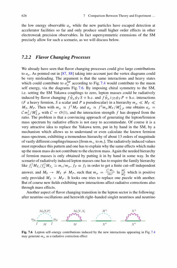
626 7 Comparison Between Theory and Experiment …

the low energy observable aμ while the new particles have escaped detection ataccelerator facilities so far and only produce small higher order effects in otherelectroweak precision observables. In fact supersymmetric extensions of the SMprecisely allow for such a scenario, as we will discuss below.

7.2.2 Flavor Changing Processes

We already have seen that flavor changing processes could give large contributionsto aμ. As pointed out in [87, 88] taking into account just the vertex diagrams couldbe very misleading. The argument is that the same interactions and heavy stateswhich could contribute to aNPμ according to Fig. 7.4 would contribute to the muonself energy, via the diagrams Fig. 7.6. By imposing chiral symmetry to the SM,i.e. setting the SM Yukawa couplings to zero, lepton masses could be radiativelyinduced by flavor changing f ψμψF S + h.c. and f ψμ i γ5ψF P + h.c. interactions(F a heavy fermion, S a scalar and P a pseudoscalar) in a hierarchy mμ � MF �MS, MP . Then with mμ ∝ f 2MF and aμ ∝ f 2mμMF/M2

S,P one obtains aμ =C m2

μ/M2S,P with C = O(1), and the interaction strength f has dropped from the

ratio. The problem is that a convincing approach of generating the lepton/fermionmass spectrum by radiative effects is not easy to accommodate. Of course it is avery attractive idea to replace the Yukawa term, put in by hand in the SM, by amechanism which allows us to understand or even calculate the known fermionmass-spectrum, exhibiting a tremendous hierarchy of about 13 orders of magnitudeof vastly different couplings/masses [frommνe tomt ]. The radiatively induced valuesmust reproduce this pattern and one has to explain why the same effects which makeup the muon mass do not contribute to the electron mass. Again the needed hierarchyof fermion masses is only obtained by putting it in by hand in some way. In thescenario of radiatively induced lepton masses one has to require the family hierarchylike f 2e MFe/ f

2μMFμ

� me/mμ, fP ≡ fS in order to get a finite cut–off independent

answer, and M0 → MS �= MP , such that mμ = f 2μ MFμ

16π2 ln M2S

M2Pwhich is positive

only provided MS > MP . It looks one tries to replace one puzzle with another.But of course new fields exhibiting new interactions affect radiative corrections alsothrough mass effects.

Another aspect of flavor changing transition in the lepton sector is the following:after neutrino oscillations and herewith right–handed singlet neutrinos and neutrino

Mf f

mµ mµ

M0[S,P] H±M0[V,A]

M X0

X±

X0

Fig. 7.6 Lepton self–energy contributions induced by the new interactions appearing in Fig. 7.4may generate mμ as a radiative correction effect

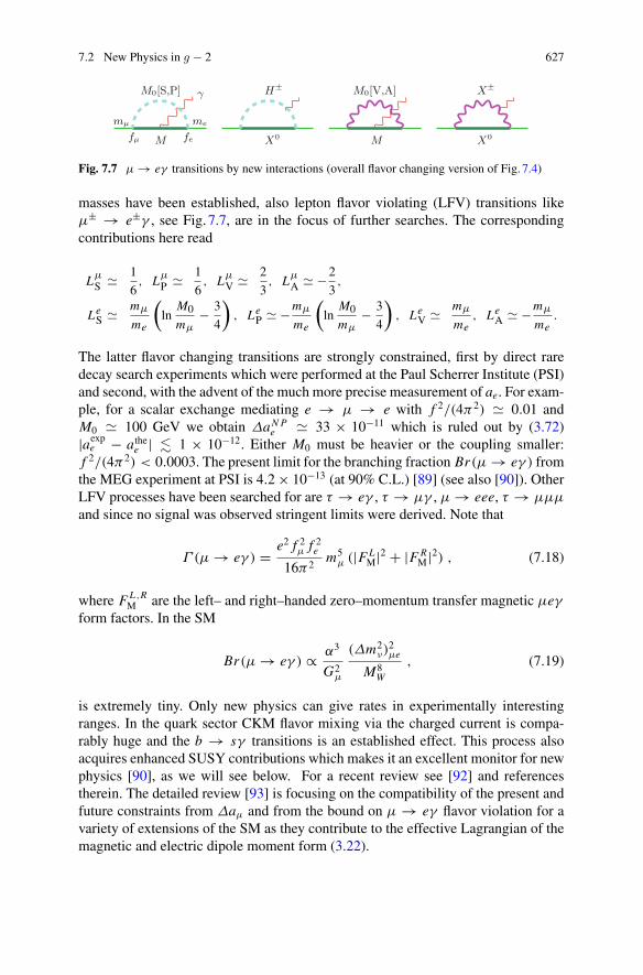
7.2 New Physics in g − 2 627

M X0 Mfµ fe

γ

mµ me

M0[S,P] M0[V,A]H± X±

X0

Fig. 7.7 μ → eγ transitions by new interactions (overall flavor changing version of Fig. 7.4)

masses have been established, also lepton flavor violating (LFV) transitions likeμ± → e±γ , see Fig. 7.7, are in the focus of further searches. The correspondingcontributions here read

LμS � 1

6, Lμ

P � 1

6, Lμ

V � 2

3, Lμ

A � −2

3,

LeS � mμ

me

(ln

M0

mμ− 3

4

), LeP � −mμ

me

(ln

M0

mμ− 3

4

), LeV � mμ

me, LeA � −mμ

me.

The latter flavor changing transitions are strongly constrained, first by direct raredecay search experiments which were performed at the Paul Scherrer Institute (PSI)and second, with the advent of the much more precise measurement of ae. For exam-ple, for a scalar exchange mediating e → μ → e with f 2/(4π2) � 0.01 andM0 � 100 GeV we obtain ΔaN P

e � 33 × 10−11 which is ruled out by (3.72)|aexpe − athee | � 1 × 10−12. Either M0 must be heavier or the coupling smaller:f 2/(4π2) < 0.0003. The present limit for the branching fraction Br(μ → eγ ) fromthe MEG experiment at PSI is 4.2× 10−13 (at 90% C.L.) [89] (see also [90]). OtherLFV processes have been searched for are τ → eγ , τ → μγ , μ → eee, τ → μμμ

and since no signal was observed stringent limits were derived. Note that

Γ (μ → eγ ) = e2 f 2μ f 2e16π2

m5μ (|FL

M|2 + |FRM|2) , (7.18)

where FL ,RM are the left– and right–handed zero–momentum transfer magnetic μeγ

form factors. In the SM

Br(μ → eγ ) ∝ α3

G2μ

(Δm2ν)

2μe

M8W

, (7.19)

is extremely tiny. Only new physics can give rates in experimentally interestingranges. In the quark sector CKM flavor mixing via the charged current is compa-rably huge and the b → sγ transitions is an established effect. This process alsoacquires enhanced SUSY contributions which makes it an excellent monitor for newphysics [90], as we will see below. For a recent review see [92] and referencestherein. The detailed review [93] is focusing on the compatibility of the present andfuture constraints from Δaμ and from the bound on μ → eγ flavor violation for avariety of extensions of the SM as they contribute to the effective Lagrangian of themagnetic and electric dipole moment form (3.22).

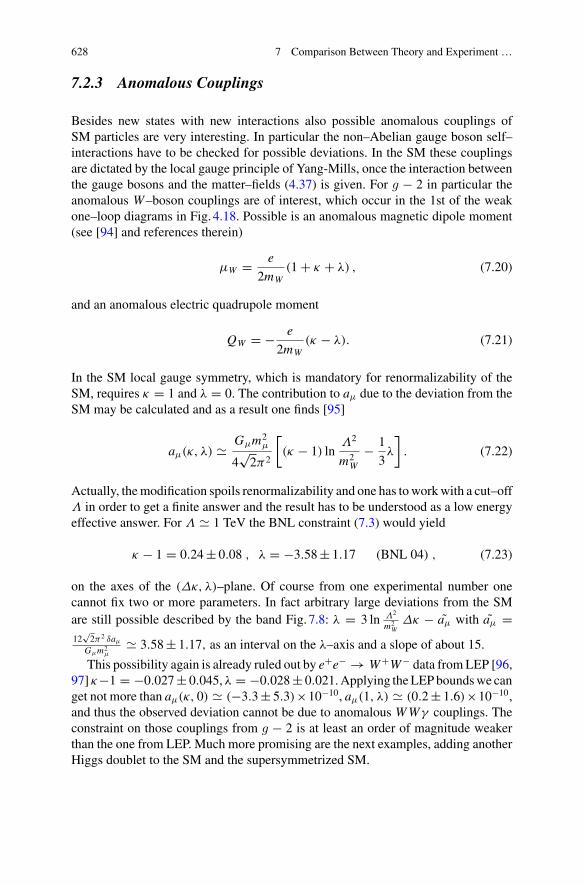
628 7 Comparison Between Theory and Experiment …

7.2.3 Anomalous Couplings

Besides new states with new interactions also possible anomalous couplings ofSM particles are very interesting. In particular the non–Abelian gauge boson self–interactions have to be checked for possible deviations. In the SM these couplingsare dictated by the local gauge principle of Yang-Mills, once the interaction betweenthe gauge bosons and the matter–fields (4.37) is given. For g − 2 in particular theanomalous W–boson couplings are of interest, which occur in the 1st of the weakone–loop diagrams in Fig. 4.18. Possible is an anomalous magnetic dipole moment(see [94] and references therein)

μW = e

2mW(1 + κ + λ) , (7.20)

and an anomalous electric quadrupole moment

QW = − e

2mW(κ − λ). (7.21)

In the SM local gauge symmetry, which is mandatory for renormalizability of theSM, requires κ = 1 and λ = 0. The contribution to aμ due to the deviation from theSM may be calculated and as a result one finds [95]

aμ(κ, λ) � Gμm2μ

4√2π2

[(κ − 1) ln

Λ2

m2W

− 1

3λ

]. (7.22)

Actually, themodification spoils renormalizability and one has toworkwith a cut–offΛ in order to get a finite answer and the result has to be understood as a low energyeffective answer. For Λ � 1 TeV the BNL constraint (7.3) would yield

κ − 1 = 0.24± 0.08 , λ = −3.58± 1.17 (BNL 04) , (7.23)

on the axes of the (Δκ, λ)–plane. Of course from one experimental number onecannot fix two or more parameters. In fact arbitrary large deviations from the SMare still possible described by the band Fig. 7.8: λ = 3 ln Λ2

m2WΔκ − aμ with aμ =

12√2π2 δaμ

Gμm2μ

� 3.58± 1.17, as an interval on the λ–axis and a slope of about 15.

This possibility again is already ruled out by e+e− → W+W− data fromLEP [96,97] κ−1 = −0.027± 0.045,λ = −0.028± 0.021.Applying theLEPboundswe canget not more than aμ(κ, 0) � (−3.3± 5.3)×10−10, aμ(1, λ) � (0.2± 1.6)×10−10,and thus the observed deviation cannot be due to anomalous WWγ couplings. Theconstraint on those couplings from g − 2 is at least an order of magnitude weakerthan the one from LEP. Much more promising are the next examples, adding anotherHiggs doublet to the SM and the supersymmetrized SM.

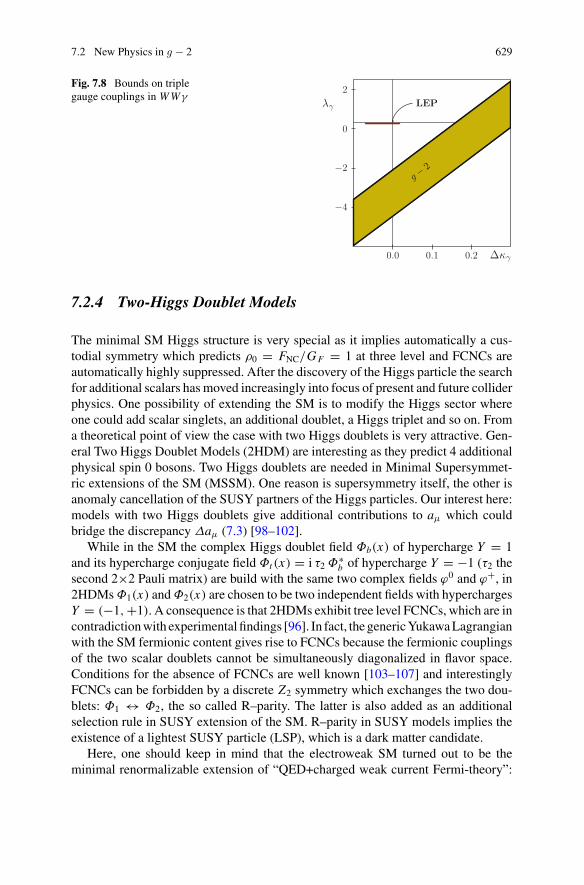
7.2 New Physics in g − 2 629

Fig. 7.8 Bounds on triplegauge couplings in WWγ

0.0 0.1 0.2

−4

−2

0

2LEPλγ

Δκγ

g − 2

7.2.4 Two-Higgs Doublet Models

The minimal SM Higgs structure is very special as it implies automatically a cus-todial symmetry which predicts ρ0 = FNC/GF = 1 at three level and FCNCs areautomatically highly suppressed. After the discovery of the Higgs particle the searchfor additional scalars has moved increasingly into focus of present and future colliderphysics. One possibility of extending the SM is to modify the Higgs sector whereone could add scalar singlets, an additional doublet, a Higgs triplet and so on. Froma theoretical point of view the case with two Higgs doublets is very attractive. Gen-eral Two Higgs Doublet Models (2HDM) are interesting as they predict 4 additionalphysical spin 0 bosons. Two Higgs doublets are needed in Minimal Supersymmet-ric extensions of the SM (MSSM). One reason is supersymmetry itself, the other isanomaly cancellation of the SUSY partners of the Higgs particles. Our interest here:models with two Higgs doublets give additional contributions to aμ which couldbridge the discrepancy Δaμ (7.3) [98–102].

While in the SM the complex Higgs doublet field Φb(x) of hypercharge Y = 1and its hypercharge conjugate field Φt (x) = i τ2 Φ∗

b of hypercharge Y = −1 (τ2 thesecond 2×2 Pauli matrix) are build with the same two complex fields ϕ0 and ϕ+, in2HDMsΦ1(x) andΦ2(x) are chosen to be two independent fields with hyperchargesY = (−1,+1). A consequence is that 2HDMs exhibit tree level FCNCs, which are incontradictionwith experimental findings [96]. In fact, the genericYukawaLagrangianwith the SM fermionic content gives rise to FCNCs because the fermionic couplingsof the two scalar doublets cannot be simultaneously diagonalized in flavor space.Conditions for the absence of FCNCs are well known [103–107] and interestinglyFCNCs can be forbidden by a discrete Z2 symmetry which exchanges the two dou-blets: Φ1 ↔ Φ2, the so called R–parity. The latter is also added as an additionalselection rule in SUSY extension of the SM. R–parity in SUSY models implies theexistence of a lightest SUSY particle (LSP), which is a dark matter candidate.

Here, one should keep in mind that the electroweak SM turned out to be theminimal renormalizable extension of “QED+charged weak current Fermi-theory”:

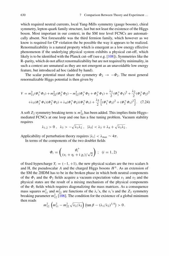
630 7 Comparison Between Theory and Experiment …

which required neutral currents, local Yang-Mills symmetry (gauge bosons), chiralsymmetry, lepton-quark family structure, last but not least the existence of the Higgsboson. Most important in our context, in the SM tree level FCNCs are automati-cally absent. Not foreseeable was the third fermion family, which however as weknow is required for CP violation the be possible the way it appears to be realized.Renormalizability is a natural property which is emergent as a low energy effectivephenomenon if the underlying physical system exhibits a physical cut-off, whichlikely is to be identified with the Planck cut–off (see e.g. [108]). Symmetries like theR–parity, which do not affect renormalizability but are not required by minimality, insuch a context are unnatural as they are not emergent as an unavoidable low energyfeature, but introduced ad hoc (added by hand).

The scalar potential must share the symmetry Φ2 → −Φ2. The most generalrenormalizable Higgs potential is then given by

V = m211(Φ

+1 Φ1) + m2

22(Φ+2 Φ2) − m2

12(Φ+1 Φ2 + Φ+

2 Φ1) + λ1

2(Φ+

1 Φ1)2 + λ2

2(Φ+

2 Φ2)2

+λ3(Φ+1 Φ1)(Φ

+2 Φ2) + λ4(Φ

+1 Φ2)(Φ

+2 Φ1) + λ5

2

[(Φ+

1 Φ2)2 + (Φ+

2 Φ1)2]. (7.24)

A soft Z2 symmetry breaking term∝ m212 has been added. This implies finite Higgs–

mediated FCNCs at one loop and one has a fine tuning problem. Vacuum stabilityrequires

λ1,2 > 0 , λ3 > −√λ1λ2 , |λ5| < λ3 + λ4 +√λ1λ2 .

Applicability of perturbation theory requires |λi | < λmax ∼ 4π .In terms of the components of the two doublet fields

Φi =(

φ+i

(vi + ηi + iχi )/√2

); (i = 1, 2)

of fixed hypercharge Yi = (−1,+1), the new physical scalars are the two scalars hand H, the pseudoscalar A and the charged Higgs bosons H±. As an extension ofthe SM the 2HDM has to be in the broken phase in which both neutral componentsof the Φ1 and the Φ2 fields acquire a vacuum expectation value v1 and v2 and thephysical states are the result of a mixing mechanism of the physical componentsof the Φi fields which requires diagonalizing the mass matrices. As a consequencemass squares m2

11 and m222 are functions of the λi ’s, the vi ’s and the Z2 symmetry

breaking parameter m212 [106]. The condition for the existence of a global minimum

then readsm2

12

(m2

11 − m222

√λ2/λ2

) (tan β − (λ1/λ2)

1/4) > 0 .

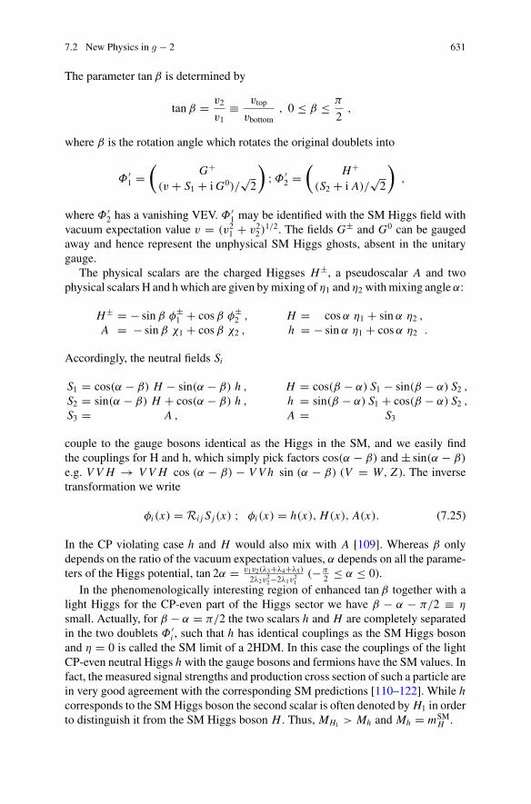
7.2 New Physics in g − 2 631

The parameter tan β is determined by

tan β = v2

v1≡ vtop

vbottom, 0 ≤ β ≤ π

2,

where β is the rotation angle which rotates the original doublets into

Φ ′1 =

(G+

(v + S1 + iG0)/√2

);Φ ′

2 =(

H+

(S2 + i A)/√2

),

where Φ ′2 has a vanishing VEV. Φ ′

1 may be identified with the SM Higgs field withvacuum expectation value v = (v21 + v22)

1/2. The fields G± and G0 can be gaugedaway and hence represent the unphysical SM Higgs ghosts, absent in the unitarygauge.

The physical scalars are the charged Higgses H±, a pseudoscalar A and twophysical scalars H and hwhich are given bymixing of η1 and η2 withmixing angle α:

H± = − sin β φ±1 + cosβ φ±

2 , H = cosα η1 + sin α η2 ,

A = − sin β χ1 + cosβ χ2 , h = − sin α η1 + cosα η2 .

Accordingly, the neutral fields Si

S1 = cos(α − β) H − sin(α − β) h , H = cos(β − α) S1 − sin(β − α) S2 ,S2 = sin(α − β) H + cos(α − β) h , h = sin(β − α) S1 + cos(β − α) S2 ,S3 = A , A = S3

couple to the gauge bosons identical as the Higgs in the SM, and we easily findthe couplings for H and h, which simply pick factors cos(α − β) and ± sin(α − β)

e.g. VV H → VV H cos (α − β) − VVh sin (α − β) (V = W, Z ). The inversetransformation we write

φi (x) = Ri j S j (x) ; φi (x) = h(x), H(x), A(x). (7.25)

In the CP violating case h and H would also mix with A [109]. Whereas β onlydepends on the ratio of the vacuum expectation values, α depends on all the parame-ters of the Higgs potential, tan 2α = v1v2(λ3+λ4+λ5)

2λ2v22−2λ1v21(−π

2 ≤ α ≤ 0).In the phenomenologically interesting region of enhanced tan β together with a

light Higgs for the CP-even part of the Higgs sector we have β − α − π/2 ≡ η

small. Actually, for β − α = π/2 the two scalars h and H are completely separatedin the two doublets Φ ′

i , such that h has identical couplings as the SM Higgs bosonand η = 0 is called the SM limit of a 2HDM. In this case the couplings of the lightCP-even neutral Higgs h with the gauge bosons and fermions have the SM values. Infact, the measured signal strengths and production cross section of such a particle arein very good agreement with the corresponding SM predictions [110–122]. While hcorresponds to the SMHiggs boson the second scalar is often denoted by H1 in orderto distinguish it from the SM Higgs boson H . Thus, MH1 > Mh and Mh = mSM

H .

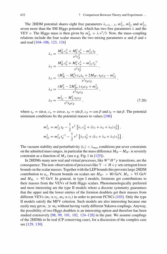
632 7 Comparison Between Theory and Experiment …

The 2HDM potential shares eight free parameters λi=1,··· ,5, m211, m

222 and m2

12,seven more than the SM Higgs potential, which has two free parameters λ and theVEV v. The Higgs mass is then given by m2

H = λ v2/3. Now, the mass–couplingrelations include the four scalar masses the two mixing parameters α and β and v

and read [104–106, 123, 124]

λ1 = M2H c2α + M2

h s2α − m2

12 tβv2c2β

,

λ2 = M2H s2α + M2

h c2α − m2

12 t−1β

v2s2β,

λ3 = (M2H − M2

h ) cαsα + 2MH± sβcβ − m212

v2sβcβ,

λ4 = (M2A − 2M2

H±) sβcβ + m212

v2sβcβ,

λ5 = m212 − M2

A sβcβv2sβcβ

, (7.26)

where sα = sin α, cα = cosα, sβ = sin β, cβ = cosβ and tβ = tan β. The potentialminimum conditions fix the potential masses to values [106]

m211 = m2

12 tβ − 1

2v2[λ1 c

2β + (λ3 + λ4 + λ5) s

2β

],

m222 = m2

12 t−1β − 1

2v2[λ2 s

2β + (λ3 + λ4 + λ5) c

2β

].

The vacuum stability and perturbativity |λi | < λmax conditions put sever constraintson the admitted mass ranges, in particular the mass difference MH −MH± is severelyconstraint as a function of MA (see e.g. Fig. 1 in [125]).

In 2HDMs many new real and virtual processes, likeW±H∓γ transitions, are theconsequence. The non–observation of processes likeϒ → H+γ sets stringent lowerbounds on the scalarmasses. Togetherwith theLEPbounds this prevents large 2HDMcontribution to aμ. Present bounds on scalars are MH± > 80 GeV, MA > 93 GeVand MH1 > 93 GeV. In general, in type I models, fermions get contributions totheir masses from the VEVs of both Higgs scalars. Phenomenologically preferredand most interesting are the type II models where a discrete symmetry guaranteesthat the upper and the lower entries of the fermion doublets get their masses fromdifferent VEVs (mt ∝ v2, mb ∝ v1) in order to prevent FCNCs [103]. Only the typeII models satisfy the MFV criterion. Such models are also interesting because oneeasilymay getmt mb without having vastly different Yukawa couplings. Anyway,the possibility of two Higgs doublets is an interesting option and therefore has beenstudied extensively [98, 99, 101, 102, 124–128] in the past. We assume couplingsof the 2HDMs to be real (CP conserving case), for a discussion of the complex casesee [129, 130].

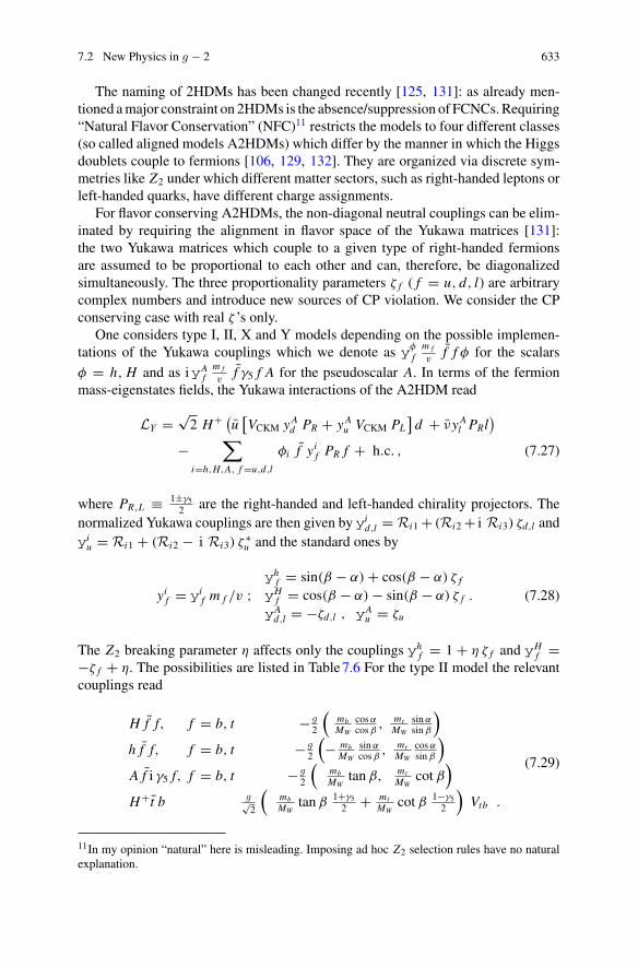
7.2 New Physics in g − 2 633

The naming of 2HDMs has been changed recently [125, 131]: as already men-tioned amajor constraint on 2HDMs is the absence/suppression of FCNCs.Requiring“Natural Flavor Conservation” (NFC)11 restricts the models to four different classes(so called aligned models A2HDMs) which differ by the manner in which the Higgsdoublets couple to fermions [106, 129, 132]. They are organized via discrete sym-metries like Z2 under which different matter sectors, such as right-handed leptons orleft-handed quarks, have different charge assignments.

For flavor conserving A2HDMs, the non-diagonal neutral couplings can be elim-inated by requiring the alignment in flavor space of the Yukawa matrices [131]:the two Yukawa matrices which couple to a given type of right-handed fermionsare assumed to be proportional to each other and can, therefore, be diagonalizedsimultaneously. The three proportionality parameters ζ f ( f = u, d, l) are arbitrarycomplex numbers and introduce new sources of CP violation. We consider the CPconserving case with real ζ ’s only.

One considers type I, II, X and Y models depending on the possible implemen-tations of the Yukawa couplings which we denote as yφ

fm f

vf f φ for the scalars

φ = h, H and as iyAfm f

vf γ5 f A for the pseudoscalar A. In terms of the fermion

mass-eigenstates fields, the Yukawa interactions of the A2HDM read

LY = √2 H+ (u [VCKM yA

d PR + yAu VCKM PL

]d + νyA

l PRl)

−∑

i=h,H,A, f =u,d,l

φi f yif PR f + h.c. , (7.27)

where PR,L ≡ 1±γ52 are the right-handed and left-handed chirality projectors. The

normalized Yukawa couplings are then given by yid,l = Ri1 + (Ri2 + i Ri3) ζd,l and

yiu = Ri1 + (Ri2 − i Ri3) ζ

∗u and the standard ones by

yif = yif m f /v ;

yhf = sin(β − α) + cos(β − α) ζ f

yHf = cos(β − α) − sin(β − α) ζ f

yAd,l = −ζd,l , yA

u = ζu

. (7.28)

The Z2 breaking parameter η affects only the couplings yhf = 1 + η ζ f and yH

f =−ζ f + η. The possibilities are listed in Table7.6 For the type II model the relevantcouplings read

H f f, f = b, t − g2

(mbMW

cosαcosβ ,

mtMW

sin αsin β

)

h f f, f = b, t − g2

(− mb

MW

sin αcosβ ,

mtMW

cosαsin β

)

A f i γ5 f, f = b, t − g2

(mbMW

tan β, mtMW

cot β)

H+ t b g√2

(mbMW

tan β1+γ52 + mt

MWcot β 1−γ5

2

)Vtb .

(7.29)

11In my opinion “natural” here is misleading. Imposing ad hoc Z2 selection rules have no naturalexplanation.

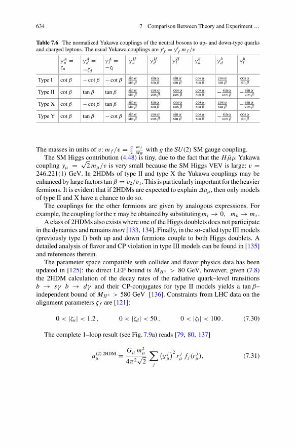
634 7 Comparison Between Theory and Experiment …

Table 7.6 The normalized Yukawa couplings of the neutral bosons to up- and down-type quarksand charged leptons. The usual Yukawa couplings are yif = yif m f /v

yAu =

ζu

yAd =

−ζd

yAl =

−ζl

yHu yH

d yHl yh

u yhd yh

l

Type I cot β − cot β − cot β sin αsin β

sin αsin β

sin αsin β

cosαsin β

cosαsin β

cosαsin β

Type II cot β tan β tan β sin αsin β

cosαcosβ

cosαcosβ

cosαsin β

− sin αcosβ − sin α

cosβ

Type X cot β − cot β tan β sin αsin β

sin αsin β

cosαcosβ

cosαsin β

cosαsin β

− sin αcosβ

Type Y cot β tan β − cot β sin αsin β

cosαcosβ

sin αsin β

cosαsin β

− sin αcosβ

cosαsin β

The masses in units of v: m f /v = g2

m f

MWwith g the SU(2) SM gauge coupling.

The SM Higgs contribution (4.48) is tiny, due to the fact that the H μμ Yukawacoupling yμ = √

2mμ/v is very small because the SM Higgs VEV is large: v =246.221(1) GeV. In 2HDMs of type II and type X the Yukawa couplings may beenhanced by large factors tan β = v2/v1. This is particularly important for the heavierfermions. It is evident that if 2HDMs are expected to explainΔaμ, then only modelsof type II and X have a chance to do so.

The couplings for the other fermions are given by analogous expressions. Forexample, the coupling for the τ maybeobtained by substitutingmt → 0, mb → mτ .

A class of 2HDMs also exists where one of the Higgs doublets does not participatein the dynamics and remains inert [133, 134]. Finally, in the so-called type III models(previously type I) both up and down fermions couple to both Higgs doublets. Adetailed analysis of flavor and CP violation in type III models can be found in [135]and references therein.

The parameter space compatible with collider and flavor physics data has beenupdated in [125]: the direct LEP bound is MH± > 80 GeV, however, given (7.8)the 2HDM calculation of the decay rates of the radiative quark–level transitionsb → sγ b → dγ and their CP-conjugates for type II models yields a tan β–independent bound of MH± > 580 GeV [136]. Constraints from LHC data on thealignment parameters ζ f are [121]:

0 < |ζu | < 1.2 , 0 < |ζd | < 50 , 0 < |ζl | < 100 . (7.30)

The complete 1–loop result (see Fig. 7.9a) reads [79, 80, 137]

a(2) 2HDMμ = Gμ m2

μ

4π2√2

∑j

(y j

μ

)2r jμ f j (r

jμ), (7.31)

7.2 New Physics in g − 2 635

h, Aμ

γ

h, A γτ, b

μ μ

γ

WH

μνµ

γ

W

Hμ Z

γ

h, A γH±

μ μ

γ

h, A γW±

μ μ

γ

H± W∓t, b

μ νµ

γ

H± W∓W∓[H∓]

h,A

μ νµ

γ

(a) (b) (c) (d)

(h)(g)(f)(e)

Fig. 7.9 Leading 2HDM graphs a and b contributing to aμ. Diagrams c and d, with H → h, H, A,are examples of subleading bosonic contributions which are modified with respect to the SM weakbosonic contributions due to the extended Higgs structure. Graphs e–h have been shown to givesubstantial contributions as well [109, 124]

where j = {h, H, A, H±}, r jμ = m2

μ/M2j , and

fh,H (r) =∫ 1

0dx

x2(2 − x)

1 − x + r x2= − ln r − 7/6 + O(r),

f A(r) =∫ 1

0dx

−x3

1 − x + r x2= + ln r + 11/6 + O(r),

fH±(r) =∫ 1

0dx

−x(1 − x)

1 − (1 − x)r= −1/6 + O(r).

(7.32)

The normalized Yukawa couplings yh,H,Aμ are listed in Table7.6, and yH

±μ = yA

μ . Inany case we have r � 1 such that fH±(r) is small relative to fh,H,A(r).

In case α ≈ β the enhanced terms are (see (7.25))

a(2) 2HDMμ (h) � Gμm2

μ

4π2√2tan2 β

m2μ

M2h

(ln

M2h

m2μ

− 7

6

)> 0 ,

a(2) 2HDMμ (A) � Gμm2

μ

4π2√2tan2 β

m2μ

M2A

(− ln

M2A

m2μ

+ 11

6

)< 0,

a(2) 2HDMμ (H±) � Gμm2

μ

4π2√2tan2 β

m2μ

M2H±

(−1

6

)< 0.

(7.33)

Since we need a positive contribution MA and MH± must be large (above 100 GeV)in order to make the negative contribution small and the contribution is entirely dueto the light scalar h, the mass of which we identify with the 125 GeV resonancefound at CERN. This then is the SM Higgs contribution (4.48) enhanced by tan2 β.If this should matchΔaμ it would require the unreasonably large value tan β ≈ 380.

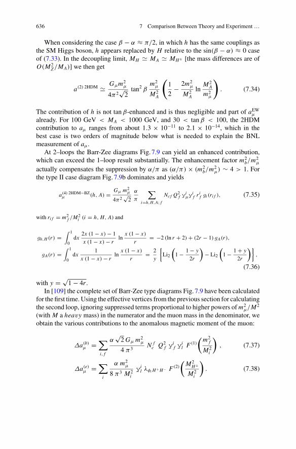
636 7 Comparison Between Theory and Experiment …

When considering the case β − α ≈ π/2, in which h has the same couplings asthe SM Higgs boson, h appears replaced by H relative to the sin(β − α) ≈ 0 caseof (7.33). In the decoupling limit, MH � MA � MH± [the mass differences are ofO(M2

Z/MA)] we then get

a(2) 2HDM � Gμm2μ

4π2√2tan2 β

m2μ

M2A

(1

2− 2m2

μ

M2A

lnM2

A

m2μ

). (7.34)

The contribution of h is not tan β-enhanced and is thus negligible and part of aEWμ

already. For 100 GeV < MA < 1000 GeV, and 30 < tan β < 100, the 2HDMcontribution to aμ ranges from about 1.3 × 10−11 to 2.1 × 10−14, which in thebest case is two orders of magnitude below what is needed to explain the BNLmeasurement of aμ.

At 2–loops the Barr-Zee diagrams Fig. 7.9 can yield an enhanced contribution,which can exceed the 1–loop result substantially. The enhancement factor m2

b/m2μ

actually compensates the suppression by α/π as (α/π) × (m2b/m

2μ) ∼ 4 > 1. For

the type II case diagram Fig. 7.9b dominates and yields

a(4) 2HDM−BZμ (h, A) = Gμ m2

μ

4π2√2

α

π

∑

i=h,H,A; fNc f Q

2f y

iμy

if r

if gi (ri f ), (7.35)

with ri f = m2f /M

2i (i = h, H, A) and

gh,H (r) =∫ 1

0dx

2x (1 − x) − 1

x (1 − x) − rln

x (1 − x)

r= −2 (ln r + 2) + (2r − 1) gA(r),

gA(r) =∫ 1

0dx

1

x (1 − x) − rln

x (1 − x)

r= 2

y

{Li2

(1 − 1 − y

2r

)− Li2

(1 − 1 + y

2r

)},

(7.36)

with y = √1 − 4r .

In [109] the complete set of Barr-Zee type diagrams Fig. 7.9 have been calculatedfor the first time. Using the effective vertices from the previous section for calculatingthe second loop, ignoring suppressed terms proportional to higher powers ofm2

μ/M2

(with M a heavy mass) in the numerator and the muon mass in the denominator, weobtain the various contributions to the anomalous magnetic moment of the muon:

Δa(b)μ =

∑i, f

α√2Gμ m2

μ

4 π3N fc Q2

f yif y

il F (1)

(m2

f

M2i

), (7.37)

Δa(e)μ =

∑i

α m2μ

8 π3 M2i

yil λφi H+H− F (2)

(M2

H±

M2i

). (7.38)

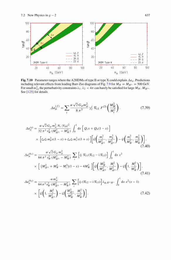
7.2 New Physics in g − 2 637

g-2

2σ

1σ

Fig. 7.10 Parameter ranges where theA2HDMs of type II or typeX could explainΔaμ. Predictionsincluding relevant effects from leading Barr-Zee diagrams of Fig. 7.9 for MH = MH± = 500 GeV.For smallm2

12 the perturbativity constraints λ1, λ2 < 4π can barely be satisfied for largeMH , MH± .See [125] for details

Δa( f )μ =∑

i

α√2Gμm2

μ

8 π3 yil Ri1 F(3)(M2

W

M2i

). (7.39)

Δa(g)μ = α

√2Gμ m2

μ Nc |Vtb|232 π3 s2W (M2

H± − M2W )

∫ 1

0dx[Qt x + Qb(1 − x)

]

×[ζdζl m

2bx(1 − x) + ζuζl m

2t x(1 + x)

][G(

m2t

M2H±

,m2

b

M2H±

)− G

(m2

t

M2W

,m2

b

M2W

)],

(7.40)

Δa(h1)μ = α

√2Gμ m2

μ

64 π3 s2W (M2H± − M2

W )

∑

i

[ζl Ri1(Ri2 − iRi3)

] ∫ 1

0dx x2

×[ (

M2H± + M2

W − M2i

)(1 − x) − 4M2

W

][G(

M2W

M2H±

,M2

i

M2H±

)− G

(1,

M2i

M2W

)],

(7.41)

Δa(h2)μ = αm2

μ

64π3 s2W (M2H± − M2

W )

∑

i

[ζl (Ri2 − iRi3)

]λφi H+H−

∫ 1

0dx x2(x − 1)

×[G(1,

M2i

M2H±

)− G

(M2

H±

M2W

,M2

i

M2W

)]. (7.42)

638 7 Comparison Between Theory and Experiment …

We denoted s2W = 1 − M2W/M2

Z . The needed loop functions are given by:

F (1)(r) = r

2

∫ 1

0dx

2x(1 − x) − 1

x(1 − x) − rln(x(1 − x)/r) , (7.43)

F (2)(r) = 1

2

∫ 1

0dx

x(x − 1)

x(1 − x) − rln(x(1 − x)/r) , (7.44)

F (3)(r) = 1

2

∫ 1

0dx

x [3x(4x − 1) + 10]r − x(1 − x)

x(1 − x) − rln(x(1 − x)/r) , (7.45)

and

G(ra, rb) =ln

(ra x + rb (1 − x)

x(1 − x)

)

x(1 − x) − ra x − rb (1 − x). (7.46)

The triple Higgs couplings λφi H+H− deriving from the Higgs potential is givenby [138]

λhH+H− = −1

v

[(M2

h − m212

sβcβ

)cβ+α

sβcβ+ (

2M2H± − M2

h

)sβ−α

].

The first two contributions are the well known classical results [98–102, 123, 125,137–141]. The analysis [125] has shown (see Fig. 7.10) that the parameter space ofthe A2HDMs allows for substantial contributions to the muon g − 2, when one ofthe neutral scalars is essentially degenerate with the charged scalar. The constraintsfrom collider and flavor physics only admit the type X model to possibly explainΔaμ.

A first complete 2–loopA2HDMcalculation has been presented recently in [124].The analysis confirms the results [109, 125] concerning the leading effects, justdiscussed. However, the bosonic correction calculated for the first time can contributeeffects of the size of the future experimental accuracy:

aBμ = (2 · · · 4) × 10−10

for η = 0, 0.1 constrained by 2 × 10−10 and η = −0.1 where the larger values areobtained.

As an illustration we present some values for 1–loop and 2–loop contributionsseparately and for the sum for selected parameters withMh = 125GeV and choosingMH± = MH in units of 10−11:

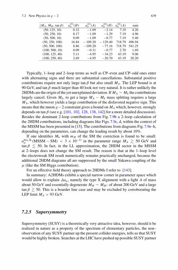
7.2 New Physics in g − 2 639

(MA, MH , tan β) a(2)μ (H) a(2)

μ (A) a(4)μ (H) a(4)

μ (A) sum(50, 125, 10) 0.32 −1.09 −2.14 7.19 4.26(50, 250, 10) 0.17 −1.09 −1.29 7.19 4.96(50, 500, 10) 0.09 −1.09 −0.77 7.19 5.40(50, 250, 100) 16.84 − 109.20 − 129.40 718.79 496.94(50, 500, 100) 8.86 −109.20 −77.16 718.79 541.25(100, 500, 10) 0.09 −0.31 −0.77 2.70 1.69(100, 125, 40) 5.11 −4.95 −34.23 43.19 9.06(100, 250, 40) 2.69 −4.95 −20.70 43.19 20.20

Typically, 1–loop and 2–loop terms as well as CP–even and CP–odd ones enterwith alternating signs and there are substantial cancellations. Substantial positivecontributions require not only large tan β but also small MA. The LEP bound is at90 GeV, and tan β much larger than 40 look not very natural. It is rather unlikely the2HDMs are the origin of the yet unexplained deviation. IfMA ∼ Mh the contributionslargely cancel. Given Mh , to get a large MA − Mh mass splitting requires a largeMA, which however yields a large contribution of the disfavored negative sign. Thismeans that the muon g−2 constraint gives a bound on MA which, however, stronglydepends on tan β (see e.g. [101, 102, 128, 138, 142] for a more detailed discussion).Besides the dominant 2-loop contributions from Fig. 7.9b a 2–loop calculation ofthe 2HDM contributions, including diagrams like Figs. 7.9c, d, within the context ofthe MSSM has been presented in [15]. The contributions from diagrams Fig. 7.9e–h,depending on the parameters, can change the leading result by about 10%.

If one identifies Mh with mH of the SM the correction is found to be small:abos,2Lμ (MSSM − SM) < 3 × 10−11 in the parameter range MA � 50 GeV andtan β � 50. In fact, in the LL approximation, the 2HDM sector in the MSSMat 2–loops does not change the SM result. The reason is that at the 1–loop levelthe electroweak SM result numerically remains practically unchanged, because theadditional 2HDM diagrams all are suppressed by the small Yukawa coupling of theμ (like the SM Higgs contribution).

For an effective field theory approach to 2HDMs I refer to [143].In summary: A2HDMs exhibit a special narrow corner in parameter space which

would allow to explain Δaμ, namely the type X alignment with a light A of massabout 50 GeV and essentially degenerate MH ∼ MH± of about 200 GeV and a largetan β � 50. This is a boarder line case and may be excluded by corroborating theLEP limit MA > 93 GeV.

7.2.5 Supersymmetry

Supersymmetry (SUSY) is a theoretically very attractive idea, however, should it berealized in nature as a property of the spectrum of elementary particles, the non–observation of any SUSY partner up the present collider energies, tells us that SUSYwould be highly broken. Searches at the LHC have pushed up possible SUSY partner

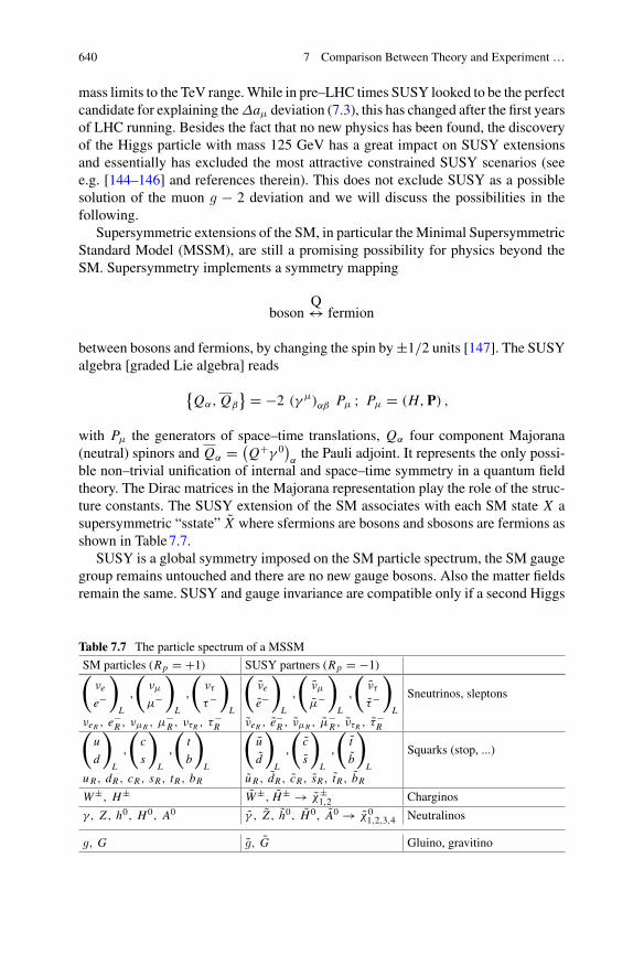
640 7 Comparison Between Theory and Experiment …

mass limits to the TeV range.While in pre–LHC times SUSY looked to be the perfectcandidate for explaining theΔaμ deviation (7.3), this has changed after the first yearsof LHC running. Besides the fact that no new physics has been found, the discoveryof the Higgs particle with mass 125 GeV has a great impact on SUSY extensionsand essentially has excluded the most attractive constrained SUSY scenarios (seee.g. [144–146] and references therein). This does not exclude SUSY as a possiblesolution of the muon g − 2 deviation and we will discuss the possibilities in thefollowing.

Supersymmetric extensions of the SM, in particular theMinimal SupersymmetricStandard Model (MSSM), are still a promising possibility for physics beyond theSM. Supersymmetry implements a symmetry mapping

bosonQ↔ fermion

between bosons and fermions, by changing the spin by±1/2 units [147]. The SUSYalgebra [graded Lie algebra] reads

{Qα, Qβ

} = −2 (γ μ)αβ Pμ ; Pμ = (H,P) ,

with Pμ the generators of space–time translations, Qα four component Majorana(neutral) spinors and Qα = (

Q+γ 0)αthe Pauli adjoint. It represents the only possi-

ble non–trivial unification of internal and space–time symmetry in a quantum fieldtheory. The Dirac matrices in the Majorana representation play the role of the struc-ture constants. The SUSY extension of the SM associates with each SM state X asupersymmetric “sstate” X where sfermions are bosons and sbosons are fermions asshown in Table7.7.

SUSY is a global symmetry imposed on the SM particle spectrum, the SM gaugegroup remains untouched and there are no new gauge bosons. Also the matter fieldsremain the same. SUSY and gauge invariance are compatible only if a second Higgs

Table 7.7 The particle spectrum of a MSSM

SM particles (Rp = +1) SUSY partners (Rp = −1)(νe

e−

)

L

,

(νμ

μ−

)

L

,

(ντ

τ−

)

L

(νe

e−

)

L

,

(νμ

μ−

)

L

,

(ντ

τ−

)

L

Sneutrinos, sleptons

νeR , e−R , νμR , μ−

R , ντR , τ−R νeR , e

−R , νμR , μ−

R , ντR , τ−R(

u

d

)

L

,

(c

s

)

L

,

(t

b

)

L

(u

d

)

L

,

(c

s

)

L

,

(t

b

)

L

Squarks (stop, ...)

uR, dR, cR, sR, tR, bR uR, dR, cR, sR, tR, bRW±, H± W±, H± → χ±

1,2 Charginos

γ, Z , h0, H0, A0 γ , Z , h0, H0, A0 → χ01,2,3,4 Neutralinos

g, G g, G Gluino, gravitino

7.2 New Physics in g − 2 641

doublet field is introduced where H1 induces the masses of all down–type fermionsand H2 the masses of all up–type fermions. A second complex Higgs doublet is alsorequired for the anomaly cancellation of the fermionic sboson sector. This means 4additional scalars (H 0, A0, H±) and their SUSY partners. The lighter neutral scalardenoted by h0 corresponds to the SM Higgs boson H . Both Higgs fields exhibita neutral scalar and acquire vacuum expectation values v1 and v2. The parametertan β = v2/v1 is one of the very important basic parameters as we will see. Asmt ∝ v2 and mb ∝ v1 in such a scenario the large mass splitting mt/mb ∼ 40could be “explained” by a large ratio v2/v1, which means a large tan β. So valuestan β ∼ 40 look natural.

Digression on Supergravity and SUSY Breaking

A very interesting question is what happens if one attempts to promote global SUSYto local SUSY. Since SUSY entangles internal with space–time symmetries of spe-cial relativity, local SUSY implies supergravity (SUGRA) as one has to go fromglobal Poincaré transformation to local ones. This means general coordinate invari-ance which in turn relates to geometry and gravity according to Einstein’s generalrelativity. SUGRA must include the spin 2 graviton and its superpartner, the spin3/2 gravitino. Such a QFT is necessarily non–renormalizable [148]. Neverthelessit is attractive to consider the MSSM as a low energy effective theory of a non–renormalizable SUGRA scenario with MPlanck → ∞ [149]. SUSY is spontaneouslybroken in the hidden sector by fields with no SU(3)c ⊗ SU(2)L ⊗ U (1)Y quantumnumbers and which couple to the observable sector only gravitationally. Denotingby MSUSY the SUSY breaking scale, the gravitino acquires a mass

m3/2 ∼ M2SUSY/MPlanck ,

with MPlanck the inherent scale of gravity.12 SUSY is not realized as a perfect symme-try in nature. SUSY partners of the known SM particles have not yet been observedbecause sparticles in general are heavier than the known particles. Like the SM localGSM symmetry is broken by the electroweak symmetry breaking (EWSB), SUGRAis broken at some higher scale MSUSY by a super–Higgs mechanism. The Lagrangiantakes the form

LMSSM = LSUSYglobal + LSUSY

breaking

with

LSUSYglobal = LSUSY(SU(3)c ⊗ SU(2)L ⊗U (1)Y ;W )

12MPl = (GN /c�)−1/2 � 1.22× 1019 GeV, GN Newton’s gravitational constant, c speed of light,� Planck constant.

642 7 Comparison Between Theory and Experiment …

with W the following gauge invariant and B and L conserving superpotential13

W = WY − μH1H2 ; WY =∑F

(hU QLUcL H2 + hD QL D

cL H1 + hL L E

cL H1)

(Y=Yukawa;F= families)where14 QL and L denote theSU(2)L doublets (UL , DL),(NL , EL) and U c

L , DcL , E

cL are the scalar partners of the right–handed quarks and

leptons, written as left–handed fields of the antiparticle (c = charge conjugation).SU(2)L and SU(3)c indices are summed over. hU , hD and hL are the Yukawa cou-plings, the complex 3 × 3 matrices in family space of the SM. In the MinimalSuper Gravity (mSUGRA) scheme, also related to the less constrained “ConstrainedMSSM” (CMSSM) [150], one assumes universality of all soft parameters.15 ThemSUGRA ansatz exhibits super gravity induced SUSY breaking with m3/2 = m0 atthe bare level. In addition the Kähler flat supergravity relation B0 = A0−m0 impliesthat tan β in mSUGRA is not a free parameter. So mSUGRA exhibits only 3 freeparameters m1/2, m0 and A0. The LSP in this scenario barely can accommodate theobserved dark matter relict density (see [150] and references therein). The CMSSMdrops the relation between B0 and A0 and assumes B0 and μ to be quantities relatedto the EW symmetry breaking scale. In addition there is no relation between m0 andthe gravitino mass.

In this case the SUSY breaking term has the form

LSUSYbreaking = −m2

∑i

|ϕi |2 − M∑a

λaλa + (Am WY − B m μH1H2 + h.c.) .

13One could add other gauge invariant couplings like

(U cL D

cL D

cL ) , (QL L D

cL ) , m(L H2) , (L L Ec

L )

which violate either B or L , however. In the minimal model they are absent.14We label U = (u, c, t), D = (d, s, b), N = (νe, νμ, ντ ) and E = (e, μ, τ).15Even with the constraints mentioned, SUSY extensions of the SM allow for about 100 freesymmetry breaking parameters. Free parameters typically aremasses andmixings of the neutralinos,the higgsino mass μ (the +μH1H2 term of the 2HDM Higgs potential) and tan β . This changes ifone merges GUT concepts with SUSY, in fact SUSY-GUTs (e.g. as based on SU(5)) are the onlytheories which allow for grand unification broken at a low scale (∼1 TeV). This provides strongconstraints on the SUSY breaking mechanism, specifically we distinguish the constrained CMSSMa SUSY-GUTwith soft breakingmasses universal at the GUT scale. The NUHM is as CMSSMwithnon-universal Higgs masses: • the CMSSM defined to have universal couplings at the GUT scalehas the free parameters:m0,m1/2, A0, tan β and sign(μ). •NUHM1 considers MA as an additionalfree parameter at the EW scale. •NUHM2 in addition assumesμ to be independent at the EW scale.These models assume many degeneracies of masses and couplings in order to restrict the number ofparameters. Typically, SM parameters are supplemented bym1/2 (scalar-matter mass, likemq ,m �

),m0 (the U (1)Y ⊗ SU(2)L gaugino masses, m γ , mZ , mW and gluino mass m g), sign(μ), tan β, A(trilinear soft breaking term), and more for less constrained models.

7.2 New Physics in g − 2 643

The essential new parameters are

• μ the supersymmetric higgsino mass• m is the universal mass term for all scalars ϕi

• M is the universal mass term to all gauginos λa

• A, B are the breaking terms in the superpotential W .

Thus in addition to the SM parameters we have 5 new parameters

μ,m, M, A and B.

The SUSY breaking lifts the degeneracy between particles and sparticle and essen-tially makes all sparticles to be heavier than all particles.

This scenario leads to universal masses for all SUSY partners:

• s–matter: mq = m � = mH = m1/2

• gauginos: M3 = M2 = M1 = m0

where M3, M2 and M1 are the mass scales of the spartners of the gauge bosons inSU(3)c, SU(2)L and U (1)Y , respectively. The non–observation of any sparticles sofar requires a mass bound of about m3/2,m1/2,m0 ∼ 100 ÷ 1000 GeV , which is ofthe order of the weak scale 246 GeV or higher.

In general one expects different masses for the different types of gauginos:

• M ′ the U (1)Y gaugino mass• M the SU(2)L gaugino mass• m g the SU(3)c gluino mass.

However, the grand unification assumption

M ′ = 5

3tan2 ΘW M = 5

3

α

cos2 ΘW αsm g ,

with sin2 ΘW = 1− M2W/M2

Z , leads back to the CMSSM scenario. A very attractivefeature of this scenario is the fact that the known SMYukawa couplings now may beunderstood by evolving couplings from the GUT scale down to low energy by thecorresponding RG equations. One interesting outcome is that the Higgs mechanismgets triggered naturally as one of the running mass squares, the one of the Higgsboson, gets negative for appropriate regions in SUSY parameter space (there existno–EWSB ranges as well). This also implies the form of the muon Yukawa couplingyμ ∝ tan β, as

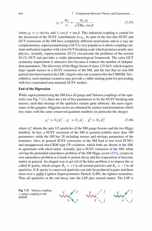
644 7 Comparison Between Theory and Experiment …

yμ = mμ

v1= mμ g2√

2MW cosβ(7.47)

where g2 = e/ sinΘW and 1/ cos β ≈ tan β. This enhanced coupling is central forthe discussion of the SUSY contributions to aμ. In spite of the fact that SUSY andGUT extensions of the SM have completely different motivations and in a way arecomplementary, supersymmetrizing a GUT is very popular as it allows coupling con-stant unification together with a lowGUT breaking scale which promises nearby newphysics. Actually, supersymmetric SU(5) circumvents the problems of the normalSU(5) GUT and provides a viable phenomenological framework. The extra GUTsymmetry requirement is attractive also because it reduces the number of indepen-dent parameters. The discovery of the Higgs boson of mass 125 GeV, which requireslarge squark masses in a SUSY extension of the SM, and the fact that no non-SMparticle has been found at the LHC, largely rules out scenarios like the CMSSM.Nev-ertheless, such minimal scenarios may provide a viable starting point for proceedingwith less constrained non-minimal SUSY models.

End of the Digression

While supersymmetrizing the SM fixes all gauge and Yukawa couplings of the spar-ticles (see Fig. 7.11), there are a lot of free parameters to fix the SUSY breaking andmasses, such that mixings of the sparticles remain quite arbitrary: the mass eigen-states of the gaugino–Higgsino sector are obtained by unitary transformations whichmix states with the same conserved quantum numbers (in particular the charge)

χ+i = Vi jψ

+j , χ−

i = Ui jψ−j , χ0

i = Ni jψ0j (7.48)

where ψaj denote the spin 1/2 sparticles of the SM gauge bosons and the two Higgs

doublets. In fact, a SUSY extension of the SM in general exhibits more than 100parameters, while the SM has 28 including masses and mixings parameters of theneutrinos. Also, in general SUSY extensions of the SM lead to tree level FCNCsand unsuppressed non-CKM type CP–violation, which both are absent in the SM,in agreement with observation. Actually, just a SUSY extension of the SM, whilesolving the pretended naturalness problem of the SM Higgs sector [151], creates itsown naturalness problem as it leads to proton decay and the evaporation of baryonicmatter in general. An elegant way to get rid of the latter problem is to impose the socalled R–parity, which assigns Rp = +1 to all normal particles and Rp = −1 to allsparticles. If R–parity is conserved sparticles can only be produced in pairs and theremust exist a stable Lightest Supersymmetric Particle (LSP), the lightest neutralino.Thus all sparticles at the end decay into the LSP plus normal matter. The LSP is

Fig. 7.11 Yukawa coupling= gauge coupling in theMSSM

g

V f

f g

V f

f g

V f

f

7.2 New Physics in g − 2 645

a Cold Dark Matter (CDM) candidate [152] if it is neutral and colorless. From theprecision mapping of the temperature and polarization anisotropies in the CosmicMicrowave Background (CMB), the Planck Collaboration has determined the relictdensity of cold dark matter to [96, 153, 154]

ΩCDM = ρCDM/ρcrit = 0.1186(20)h−2 = 0.258(11). (7.49)

This sets severe constraints on theSUSYparameter space [155–157].Note that SUSYis providing a new source for CP–violation, which could help in understanding thematter–antimatter asymmetry nB = (nb − nb)/nγ � 6 × 10−10 observed in ourworld.

However, what should cause R–parity to be conserved is another question. It justmeans that certain couplings one usually would assume to be there naturally areexcluded. If R is not conserved sparticles may be produced singly and the LSP isnot stable and would not provide a possible explanation of CDM. Then also (7.49)would not provide information on SUSY parameters.

The main theoretical motivation for a supersymmetric extension of the SM is thehierarchy or naturalness problem16 of the latter: chiral symmetry requires fermionsto be massless, local gauge symmetries require the gauge bosons to be massless, sothe only SM particle which is not required to be massless, before the spontaneoussymmetry breaking by the Higgs mechanism, is the scalar Higgs boson, togetherwith the mass–degenerate later Higgs–ghosts (all fields in the Higgs doublet). Thisargument, however, only is true in the symmetric phase. In the broken phase, triggeredby a negative bare Higgs potential mass square term, all masses including the Higgsparticle itself, exhibit a mass proportional to the Higgs VEV v according to (4.46).Therefore, the Higgs mass in the broken phase cannot be expected to be much largerthan the heavier of the SM particles, unless the dimensionless Higgs self-couplingλ for unknown reasons would be much larger than the gauge couplings or the topquark Yukawa coupling. What is actually tuned when renormalizing the Higgs massis λ because v is given as the universal electroweak scale, which is determinedby the Fermi constant, an object independent of any SM interaction parameters atleading order or to all orders by definition. The Higgs VEV v is to be viewed asan orderparameter, which breaks the symmetry of the vacuum (by a collective longrange order) and has no direct correlation to the short distance cutoff, which is thePlanck mass if one equips the bare SM with a Planck cutoff (see [108, 151]).

16Stating that a small parameter (like a small mass) is unnatural unless the symmetry is increased bysetting it to zero. The equivalent hierarchy problem addresses the fine–tuning problem encounteredin Higgs mass renormalization: the renormalized (observed) low energy effective mass square

m2ren = m2

bare − δm2

is O(v2) of the order of the electroweak scale square, while in the bare theory exhibiting the Planckmass as a UV cutoff, m2

bare and the counterterm δm2 are of order Λ2Planck. So the observed Higgs

mass appears as a highly fine–tuned difference of two very large numbers. Exact supersymmetryeliminates the fine–tuning by canceling positive bosonic contributions to δm2 exactly by negativefermionic ones, such that quadratic UV singularities are absent.

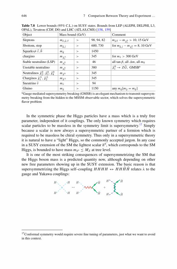
646 7 Comparison Between Theory and Experiment …

Table 7.8 Lower bounds (95% C.L.) on SUSY states. Bounds from LEP (ALEPH, DELPHI, L3,OPAL), Tevatron (CDF, D0) and LHC (ATLAS,CMS) [158, 159]

Object Mass bound (GeV) Comment

Sleptons me,μ,τ > 98, 94, 82 mμτ − mχ01> 10, 15 GeV

Sbottom, stop mb,t > 600, 730 for mb,t − mχ01

= 8, 10 GeV

Squarks �= t, b mq > 1450

chargino mχ±1

> 345 for m ν > 300 GeV

Stable neutralino (LSP) mχ01

> 46 all tan β, all Δm, all m0

Unstable neutralino mχ01

> 380 χ01 → ZG, GMSBa

Neutralinos χ02 , χ

03 , χ

04 mχ0 > 345

Charginos χ±1 , χ±

2 mχ± > 345

Sneutrino ν m ν > 94

Gluino m g > 1150 any mq [m g = mq ]aGauge mediated supersymmetry breaking (GMSB) is an elegant mechanism to transmit supersym-metry breaking from the hidden to the MSSM observable sector, which solves the supersymmetricflavor problem

In the symmetric phase the Higgs particles have a mass which is a truly freeparameter, independent of it couplings. The only known symmetry which requiresscalar particles to be massless in the symmetry limit is supersymmetry.17 Simplybecause a scalar is now always a supersymmetric partner of a fermion which isrequired to be massless be chiral symmetry. Thus only in a supersymmetric theoryit is natural to have a “light” Higgs, so the commonly accepted jargon. In any casein a SUSY extension of the SM the lightest scalar h0, which corresponds to the SMHiggs, is bounded to have mass mh0 ≤ MZ at tree level.

It is one of the most striking consequences of supersymmetrizing the SM thatthe Higgs boson mass is a predicted quantity now, although depending on othernew free parameters showing up in the SUSY extension. The basic reason is thatsupersymmetrizing the Higgs self–coupling HHHH ↔ HH H H relates λ to thegauge and Yukawa couplings:

H

H

H

H

H

H

H

H

↔ +

H

H

H

H

17Conformal symmetry would require severe fine tuning of parameters, just what we want to avoidin this context.

7.2 New Physics in g − 2 647

In the MSSM it implies constraints on the 2HDM potential (7.24):

λ1 = λ2 = −(λ3 + λ4 + λ5) = 1

4

(g2 + g′2

); λ4 = −1

2g2 ; λ5 = 0 ,

and as a consequence, in theminimal SUSYmodels themasses of the extraHiggses attree level are severely constrained by the followingmass- and coupling-relationships:

M2H± = M2

W + M2A , M2

H,h = 1

2

(M2

Z + M2A±√(M2

Z − M2A)

2 + 4M2Z M

2A sin2 2β

),

tan(2α) = tan(2β)M2

A + M2Z

M2A − M2

Z

, sin2(α − β) = M2H

M2A

M2Z − M2

H

M2Z + M2

A − 2M2H

. (7.50)

Only two independent parameters are left, which we may choose to be tan β andMA.18 This tree level Higgs mass prediction receives large radiative corrections fromthe t/t sector (see Fig. 7.12), which changes the upper bound to [160]

m2h0 ≤ M2

Z +√2Gμ

2π2 sin2 β3m4

t ln

(mt1 mt2

m2t

)+ · · · (7.51)

which in any case is well below 200GeV. For improved bounds obtained by includinghigher order corrections19 I refer to [161, 162] (see also [163]). In the MSSM one

18In [138] theCPconserving 2HDMcase is consideredwithout imposing theΦ2 → −Φ2 symmetry,which allows for twomore terms in the potentialV → V+[λ6

(Φ+

1 Φ1)+ λ7

(Φ+

2 Φ2)] (

Φ+1 Φ2

)+h.c.. The CP-even mass matrix is of the form

M2 =(λ1v

2 λ6v2

λ6v2 M2

A + λ5v2

)

and one has to distinguish the following special limits:

• Decoupling limit: M2A λiv

2 implying M2h ∼ λ1v

2 and |cβ−α � 1| and the lighter scalar h isthe SM like one.

• Alignment limits: λ6 = 0 with two possibilities:

(1) λ1 < λ5 + M2A/v

2 and again h is identical with the SM Higgs and cβ−α = 0(2) λ1 > λ5 + M2

A/v2 in which case H is identical with SM Higgs and cβ−α = 1. This is an

unexpected possibility, namely the discovered Higgs is to be identified the heavier scalar. Thelighter would have masses in the range 20–90 GeV and would have escaped detection so far,because of suppressed couplings to SM states.

19Denoting by M2h the corrected light Higgs on–shell mass, and by m2

h the tree level mass given in(7.50), then including leading logarithms in αs and yt up to 3 loops on finds

M2h = m2

h + v2 y4t[12 L κL − 12 L2 κ2L

(16 g23 − 3 y2t

)

+4 L3 κ3L

(736g43 − 240 g23 y

2t − 99 y4t

)+ · · ·

],

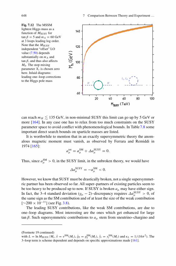
648 7 Comparison Between Theory and Experiment …

Fig. 7.12 The MSSMlightest Higgs mass as afunction of MSUSY fortan β = 5 and mA = 60 GeVat 3 loops leading log order.Note that the MSUSYindependent “offset” LOvalue (7.50) dependssubstantially on mA andtan β, and thus also affectsMh . The stop mixingparameter Xt is chosen zerohere. Inlaid diagrams:leading one–loop correctionsto the Higgs pole mass t

t

H H

tL, tR

+ + · · ·

can reach mH � 135 GeV, in non-minimal SUSY this limit can go up by 5 GeV ormore [164]. In any case one has to relax from too much constraints on the SUSYparameter space to avoid conflict with phenomenological bounds. In Table7.8 someimportant direct search bounds on sparticle masses are listed.

It is worthwhile to mention that in an exactly supersymmetric theory the anom-alous magnetic moment must vanish, as observed by Ferrara and Remiddi in1974 [165]:

atotμ = aSMμ + ΔaSUSYμ = 0.

Thus, since aSMμ > 0, in the SUSY limit, in the unbroken theory, we would have

ΔaSUSYμ = −aSMμ < 0.

However, we know that SUSYmust be drastically broken, not a single supersymmet-ric partner has been observed so far. All super–partners of existing particles seem tobe too heavy to be produced up to now. If SUSY is broken aμ may have either sign.In fact, the 3–4 standard deviation (gμ − 2)–discrepancy requires ΔaSUSYμ > 0, ofthe same sign as the SM contribution and of at least the size of the weak contribution[∼200 × 10−11] (see Fig. 3.8).

The leading SUSY contributions, like the weak SM contributions, are due toone–loop diagrams. Most interesting are the ones which get enhanced for largetan β. Such supersymmetric contributions to aμ stem from sneutrino–chargino and

(Footnote 19 continued)with L = lnMSUSY/Mt , v = vSM(Mt ), g3 = gSM3 (Mt ), yt = ySMt (Mt ) and κL = 1/(16π2). The3–loop term is scheme dependent and depends on specific approximations made [161].

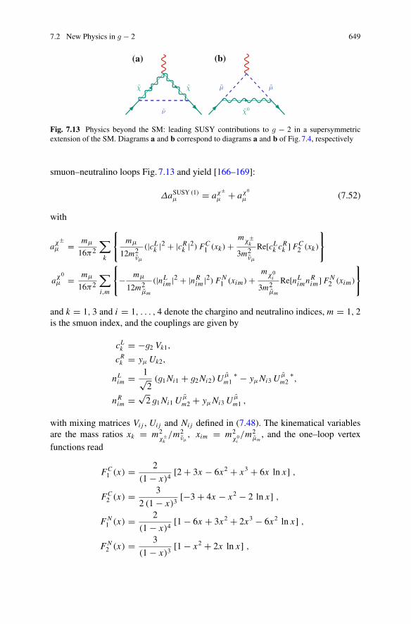
7.2 New Physics in g − 2 649

ν

χ χ

(a)

χ0

μ μ

(b)

Fig. 7.13 Physics beyond the SM: leading SUSY contributions to g − 2 in a supersymmetricextension of the SM. Diagrams a and b correspond to diagrams a and b of Fig. 7.4, respectively

smuon–neutralino loops Fig. 7.13 and yield [166–169]:

ΔaSUSY (1)μ = aχ±

μ + aχ0

μ (7.52)

with

aχ±

μ = mμ

16π2

∑

k

⎧⎨⎩

mμ

12m2νμ

(|cLk |2 + |cRk |2) FC1 (xk) +

mχ±k

3m2νμ

Re[cLk cRk ] FC2 (xk)

⎫⎬⎭

aχ0

μ = mμ

16π2

∑

i,m

⎧⎨⎩− mμ

12m2μm

(|nLim |2 + |nRim |2) FN1 (xim) +

mχ0i

3m2μm

Re[nLimnRim ] FN2 (xim)

⎫⎬⎭

and k = 1, 3 and i = 1, . . . , 4 denote the chargino and neutralino indices, m = 1, 2is the smuon index, and the couplings are given by

cLk = −g2 Vk1,

cRk = yμ Uk2,

nLim = 1√

2(g1Ni1 + g2Ni2)U

μ ∗m1 − yμNi3U

μ ∗m2 ,

nRim = √

2 g1Ni1Uμm2 + yμNi3U

μm1 ,

with mixing matrices Vi j , Ui j and Ni j defined in (7.48). The kinematical variablesare the mass ratios xk = m2

χ±k/m2

νμ, xim = m2

χ0i/m2

μm, and the one–loop vertex

functions read

FC1 (x) = 2

(1 − x)4[2 + 3x − 6x2 + x3 + 6x ln x] ,

FC2 (x) = 3

2 (1 − x)3[−3 + 4x − x2 − 2 ln x] ,

FN1 (x) = 2

(1 − x)4[1 − 6x + 3x2 + 2x3 − 6x2 ln x] ,

FN2 (x) = 3

(1 − x)3[1 − x2 + 2x ln x] ,

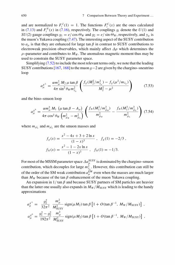
650 7 Comparison Between Theory and Experiment …

and are normalized to F Ji (1) = 1. The functions FC

i (x) are the ones calculatedin (7.13) and FN

i (x) in (7.16), respectively. The couplings gi denote the U (1) andSU(2) gauge couplings g1 = e/ cosΘW and g2 = e/ sinΘW , respectively, and yμ isthe muon’s Yukawa coupling (7.47). The interesting aspect of the SUSY contributionto aμ is that they are enhanced for large tan β in contrast to SUSY contributions toelectroweak precision observables, which mainly affect Δρ which determines theρ–parameter and contributes to MW . The anomalous magnetic moment thus may beused to constrain the SUSY parameter space.

Simplifying (7.52) to include themost relevant terms only, we note that the leadingSUSYcontributions [167, 168] to themuon g−2 are given by the chargino–sneutrinoloop

aχ±μ = αm2

μ M2 μ tan β

4π sin2 θWm2νμ

(fχ (M2

2/m2νμ) − fχ (μ2/m νμ )

M22 − μ2

)(7.53)

and the bino–smuon loop

aχ0

μ = αm2μ M1

(μ tan β − Aμ

)

4π cos2 θW(m2

μR− m2

μL

)(

fN (M21/m

2μR

)

m2μR

− fN (M21/m

2μL

)

m2μL

)(7.54)

where mμL and mμL are the smuon masses and

fχ (x) = x2 − 4x + 3 + 2 ln x

(1 − x)3, fχ (1) = −2/3 ,

fN (x) = x2 − 1 − 2x ln x

(1 − x)3, fN (1) = −1/3.

Formost of theMSSMparameter spaceΔaSUSYμ is dominated by the chargino–smuoncontribution, which decouples for large m2

νμ. However, this contribution can still be

of the order of the SMweak contribution aEWμ even when the masses are much largerthan MW because of the tan β enhancement of the muon Yukawa coupling.

An expansion in 1/ tan β and because SUSY partners of SM particles are heavierthan the latter one usually also expands in MW/MSUSY which is leading to the handyapproximations

aχ±μ = g22

32π2

m2μ

M2SUSY

sign(μM2) tan β[1 + O(tan β−1, MW/MSUSY)

],

aχ0

μ = g21 − g22192π2

m2μ

M2SUSY

sign(μM2) tan β[1 + O(tan β−1, MW/MSUSY)

],

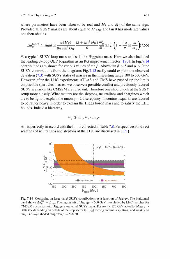
7.2 New Physics in g − 2 651

where parameters have been taken to be real and M1 and M2 of the same sign.Provided all SUSY masses are about equal to MSUSY and tan β has moderate valuesone then obtains

ΔaSUSYμ � sign(μ)α(MZ )

8π sin2 ΘW

(5 + tan2 ΘW )

6

m2μ

m2tan β

(1 − 4α

πln

m

mμ

)(7.55)

m a typical SUSY loop mass and μ is the Higgsino mass. Here we also includedthe leading 2–loop QED logarithm as an RG improvement factor [170]. In Fig. 7.14contributions are shown for various values of tan β. Above tan β ∼ 5 and μ > 0 theSUSY contributions from the diagrams Fig. 7.13 easily could explain the observeddeviation (7.3) with SUSY states of masses in the interesting range 100 to 500 GeV.However, after the LHC experiments ATLAS and CMS have pushed up the limitson possible sparticles masses, we observe a possible conflict and previously favoredSUSY scenarios like CMSSM are ruled out. Therefore one should look at the SUSYsetup more closely. What matters are the sleptons, neutralinos and charginos whichare to be light to explain the muon g−2 discrepancy. In contrast squarks are favoredto be rather heavy in order to explain the Higgs boson mass and to satisfy the LHCbounds. Indeed a hierarchy

mq m �,mχ± ,mχ0

still is perfectly in accordwith the limits collected in Table7.8. Perspectives for directsearches of neutralinos and sleptons at the LHC are discussed in [171].

Fig. 7.14 Constraint on large tan β SUSY contributions as a function of MSUSY. The horizontalband shows ΔaNPμ = Δaμ. The region left of MSUSY ∼ 500 GeV is excluded by LHC searches forCMSSM scenarios with MSUSY a universal SUSY mass. For mh ∼ 125 GeV actually MSUSY >

800 GeV depending on details of the stop sector ({t1, t2} mixing and mass splitting) and weakly ontan β. Orange shaded range tan β = 5 ÷ 50

652 7 Comparison Between Theory and Experiment …

More recently, also the tan2 β enhanced contributions havebeen calculated [172].20

They arise from the tan β enhanced shift Δμ ∝ α tan β in the on mass–shell muonmass renormalization:

mμ → mμ + δmμ = mμ

1 + Δμ

+ non− tan β−enhanced terms. (7.56)

In the case that all SUSY masses are equal and much larger than MW the correctionreads

Δμ � −0.0018 tan β sign(μ). (7.57)

Extracting tan β from aexpμ , the resulting value would be smaller by about 10% whentan β ∼ 50. Corrections can be even larger in certain regions of SUSY parameterspace. Typically, for large tan β they are larger than other 2–loop contributions.The contributions of the 2HDM sector of the MSSM have been discussed earlier inSect. 7.2.4.

The very large tan β regime (motivated by the possibility that v1 could be vanishingand the muon mass induced radiatively as advocated e.g. in [87]) has been studiedin [173]. In the simplified case that all SUSY masses are equal to MSUSY and tan β

is moderate the one loop SUSY result takes the form

ΔaSUSY,1Lμ ≈ 13 × 10−10 sign(μ) tan β

(100 GeV

MSUSY

)2

.

For large tan β higher order terms change the linear behavior in tan β. The higherorder terms can be resummed [172] to

ΔaSUSYμ = ΔaSUSY,1Lμ

1 + Δμ

,

which has finite limit

ΔaSUSYμ lim = limtan β→∞

ΔaSUSY,1Lμ

Δμ

≈ −72 × 10−10

(1 TeV

MSUSY

)2

still assuming degenerate SUSY masses. If we want to make SUSY effects respon-sible for positive deviation Δaμ the case that all SUSY masses are of similar size isruled out. In order to get a positive result one has to assume large mass splittings.Two possible regimes, which are not in conflict with bounds from other observables,have been considered in [173]:

• the BμL μR contributions dominate for M1,mL ,mR � μ: “large μ–limit”,• the B H μL contributions dominate for M1, μ,mR � mL : “μR–dominance”.

20The highest power in tan β at a given order L in the loop expansion is αL tanL β. As a correctiononly the leading one of order α2 tan2 β is numerically significant.

7.2 New Physics in g − 2 653

We remind that gauginos are denoted by W for the SU(2) and by B for the U (1)Ygauge groups. In both regimes the result changes to

ΔaSUSYμ lim ≈ 37 × 10−10

(1 TeV

MSUSY

)2

,

assuming MA = 50 GeV. Typically, of order 1 σ effects are obtained only forsufficiently small MA and sufficiently large tan β. This behavior is reflecting whathappens in general two Higgs doublet models of type II and X, as discussed before.

A remarkable 2–loop calculation within the MSSM has been performed byHeinemeyer, Stöckinger andWeiglein [140]. They evaluated the exact 2–loop correc-tion of the SM 1–loop contributions Figs. 4.1, and 4.18. These are all diagrams wherethe μ–lepton number is carried only by μ and/or νμ. In other words, SM diagramswith an additional insertion of a closed sfermion– or charginos/neutralino–loop. Thusthe full 2–loop result from the class of diagrams with closed sparticle loops is known.This class of SUSY contributions is interesting because it has a parameter depen-dence completely different from the one of the leading SUSY contribution and canbe large in regions of parameter space where the 1–loop contribution is small. Thesecond class of corrections are the 2–loop corrections to the SUSY 1–loop diagramsFig. 7.13, where the μ–lepton number is carried also by μ and/or νμ. This class ofcorrections is expected to have the same parameter dependence as the leading SUSY1–loop ones and only the leading 2–loopQEDcorrections are known [170] as alreadyincluded in (7.55). More recently, an extended more complete calculation has beenpresented in [174].

The prediction of ΔaSUSYμ as a function of the mass of the Lightest ObservableSUSY Particle MLOSP = min(mχ±

1,mχ0

2,m fi

), from a MSSM parameter scan withtan β = 50, including the 2–loop effects is shown inFig. 7.15. Plotted is themaximumvalue of aμ obtained by a scan of that part of SUSY parameter space which is allowedby the other observables like mh , MW and the b–decays. The 2–loop correctionsin general are moderate (few %). However, not so for lighter MLOSP in case ofheavy smuons and sneutrinos when corrections become large (see also [175]). Theremaining uncertainty of the calculation has been estimated to be below 3 × 10−10,which is satisfactory in the present situation. This may however depend on detailsof the SUSY scenario and of the parameter range considered. A comprehensivereview on supersymmetry, the different symmetry breaking scenarios and the muonmagnetic moment has been presented by Stöckinger [169]. Low energy precisiontest of supersymmetry and present experimental constraints also are reviewed anddiscussed in [176].

The results for the SUSYcontributions toaμ up to two-loopsmay be found in [169,172, 174], and may be written as

ΔaSUSYμ = ΔaSUSY,1Lμ

(1 − 4α

πlog

MSUSY

mμ

) (1

1 + Δμ

)+ a(χγ H)

μ + a( f γ H)μ

+ a(χ{W,Z}H)μ + a( f {W,Z}H)

μ + aSUSY,ferm,2Lμ + aSUSY,bos,2L

μ + . . . . (7.58)

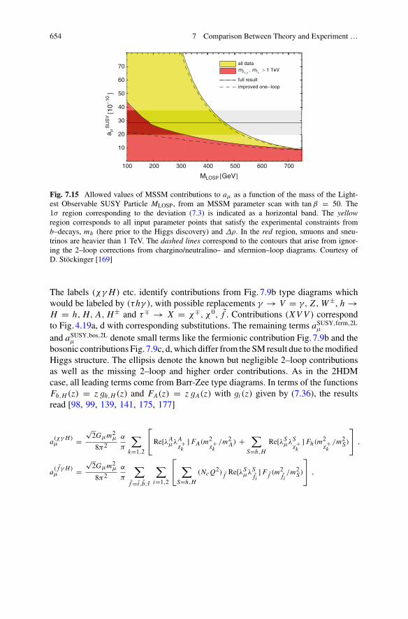
654 7 Comparison Between Theory and Experiment …

100 200 300 400 500 600 700

MLOSP GeV

10

20

30

40

50

60

70

aS

US

Y10

10

full resultimproved one loop

m1,2

, m 1 TeVall data

Fig. 7.15 Allowed values of MSSM contributions to aμ as a function of the mass of the Light-est Observable SUSY Particle MLOSP, from an MSSM parameter scan with tan β = 50. The1σ region corresponding to the deviation (7.3) is indicated as a horizontal band. The yellowregion corresponds to all input parameter points that satisfy the experimental constraints fromb–decays, mh (here prior to the Higgs discovery) and Δρ. In the red region, smuons and sneu-trinos are heavier than 1 TeV. The dashed lines correspond to the contours that arise from ignor-ing the 2–loop corrections from chargino/neutralino– and sfermion–loop diagrams. Courtesy ofD. Stöckinger [169]

The labels (χγ H) etc. identify contributions from Fig. 7.9b type diagrams whichwould be labeled by (τhγ ), with possible replacements γ → V = γ, Z ,W±, h →H = h, H, A, H± and τ∓ → X = χ∓, χ0, f . Contributions (XVV ) correspondto Fig. 4.19a, d with corresponding substitutions. The remaining terms aSUSY,ferm,2L

μ

and aSUSY,bos,2Lμ denote small terms like the fermionic contribution Fig. 7.9b and the

bosonic contributions Fig. 7.9c, d,which differ from the SM result due to themodifiedHiggs structure. The ellipsis denote the known but negligible 2–loop contributionsas well as the missing 2–loop and higher order contributions. As in the 2HDMcase, all leading terms come from Barr-Zee type diagrams. In terms of the functionsFh,H (z) = z gh,H (z) and FA(z) = z gA(z) with gi (z) given by (7.36), the resultsread [98, 99, 139, 141, 175, 177]

a(χγ H)μ =

√2Gμm2

μ

8π2α

π

∑

k=1,2

⎡⎣Re[λAμλA

χ+k

] FA(m2χ

+k/m2

A) +∑

S=h,H

Re[λSμλSχ

+k

] Fh(m2χ

+k/m2

S)

⎤⎦ ,

a( f γ H)μ =

√2Gμm2

μ

8π2α

π

∑

f =t,b,τ

∑

i=1,2

⎡⎣ ∑

S=h,H

(NcQ2) f Re[λSμλS

fi] F f (m

2fi/m2

S)

⎤⎦ ,

7.2 New Physics in g − 2 655

with Ff (z) = z (2 + ln z − FA(z))/2 and couplings (see Eqs. (7.29, 7.48))

λh,H,Aμ = (− sin α/ cosβ, cosα/ cosβ, tan β) ,

λh,H,Aχ

+k

= √2MW /m

χ+k

(Uk1Vk2 (cosα, sin α,− cosβ) +Uk2Vk1(− sin α, cosα,− sin β)) ,

λh,Hτi

= 2mτ /(m2τicosβ) (−μ∗ (cosα, sin α) + Aτ (− sin α, cosα)) (U τi1)∗U τi2 .

The last expression given for the τ applies to the bwith τ → b everywhere, and for thet with τ → t together with (μ, cosβ, cosα, sin α) → (−μ, sin β, sin α,− cosα).

For the potentially enhanced Barr-Zee type contributions the following simpleapproximations have been given [15, 169]:

a(χV H)μ ≈ 11 × 10−10

(tan β

50

)(100 GeV

MSUSY

)2

sign(μM2),

a(tγ H)μ ≈ −13 × 10−10

(tan β

50

)(mt

mt

)(μ

20MH

)sign(Xt ),

a(bγ H)μ ≈ −3.2 × 10−10

(tan β

50

)(mb tan β

mb

)(Ab

20MH

)sign(μ) .

The parameter Xt is determined by the SUSY breaking parameter A f , μ and tan β

by Xt = At − μ∗ cot β. Like for the leading 1–loop case, the first approximationapplies if all SUSY masses are approximately equal (e.g. μ ∼ M2 ∼ mA) (but therelevant masses are different in the two cases), and the second and third are validif the stop/sbottom mixing is large and the relevant stop/sbottom and Higgs massesare of similar size. We refer to the review by Stöckinger [169] for a more detailedpresentation of the higher order SUSY effects. The latter have been reconsidered andupdated recently in [174].

Constraints from MW

Here we are looking at SM precision observables likeGF (muon lifetime), Z observ-ables MZ , ΓZ , gV , gA, sin2 Θeff (LEP1/SLD)W boson and t quark observables MW ,ΓW , mt and Γt (LEP2/Tevatron/LHC). An important observable is the W mass pre-dicted to satisfy

M2W

(1 − M2

W

M2Z

)= πα√

2GF

(1 + Δr) , (7.59)

where Δr = f (α,GF , MZ ,mt , · · · ) represents the radiative correction to the treelevel mass-coupling relation, which depends on the independent parameters of thetheory. They differ from the SM by additional contributions in extensions of the SMand thus allow to constrain the parameter space of the extendedmodel. In SUSYmod-els MW is sensitive to the top/stop sector parameters and actually MW is essentiallythe only observable which tends to slightly improve the fit when including MSSM

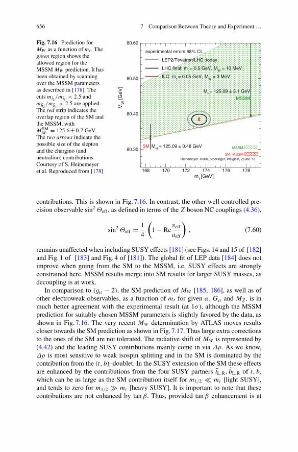
656 7 Comparison Between Theory and Experiment …

Fig. 7.16 Prediction forMW as a function of mt . Thegreen region shows theallowed region for theMSSM MW prediction. It hasbeen obtained by scanningover the MSSM parametersas described in [178]. Thecuts mt2/mt1 < 2.5 andmb2

/mb1< 2.5 are applied.

The red strip indicates theoverlap region of the SM andthe MSSM, withMSM

M = 125.6± 0.7 GeV.The two arrows indicate thepossible size of the sleptonand the chargino (andneutralino) contributions.Courtesy of S. Heinemeyeret al. Reproduced from [178]

168 170 172 174 176 178mt [GeV]

80.30

80.40

80.50

80.60

MW

[GeV

]

MSSM

MH = 125.09 ± 0.48 GeVSM

Mh = 125.09 ± 3.1 GeV

MSSM

SM, MSSM

experimental errors 68% CL

LEP2/Tevatron/LHC: today

LHC final: mt = 0.5 GeV, MW = 10 MeV

ILC: m t = 0.05 GeV, MW = 3 MeV

contributions. This is shown in Fig. 7.16. In contrast, the other well controlled pre-cision observable sin2 Θeff , as defined in terms of the Z boson NC couplings (4.36),

sin2 Θeff = 1

4

(1 − Re

veff

aeff

), (7.60)

remains unaffected when including SUSY effects [181] (see Figs. 14 and 15 of [182]and Fig. 1 of [183] and Fig. 4 of [181]). The global fit of LEP data [184] does notimprove when going from the SM to the MSSM, i.e. SUSY effects are stronglyconstrained here. MSSM results merge into SM results for larger SUSY masses, asdecoupling is at work.

In comparison to (gμ − 2), the SM prediction of MW [185, 186], as well as ofother electroweak observables, as a function of mt for given α, Gμ and MZ , is inmuch better agreement with the experimental result (at 1σ ), although the MSSMprediction for suitably chosen MSSM parameters is slightly favored by the data, asshown in Fig. 7.16. The very recent MW determination by ATLAS moves resultscloser towards the SM prediction as shown in Fig. 7.17. Thus large extra correctionsto the ones of the SM are not tolerated. The radiative shift of MW is represented by(4.42) and the leading SUSY contributions mainly come in via Δρ. As we know,Δρ is most sensitive to weak isospin splitting and in the SM is dominated by thecontribution from the (t, b)–doublet. In the SUSY extension of the SM these effectsare enhanced by the contributions from the four SUSY partners tL,R, bL,R of t, b,which can be as large as the SM contribution itself for m1/2 � mt [light SUSY],and tends to zero for m1/2 mt [heavy SUSY]. It is important to note that thesecontributions are not enhanced by tan β. Thus, provided tan β enhancement is at

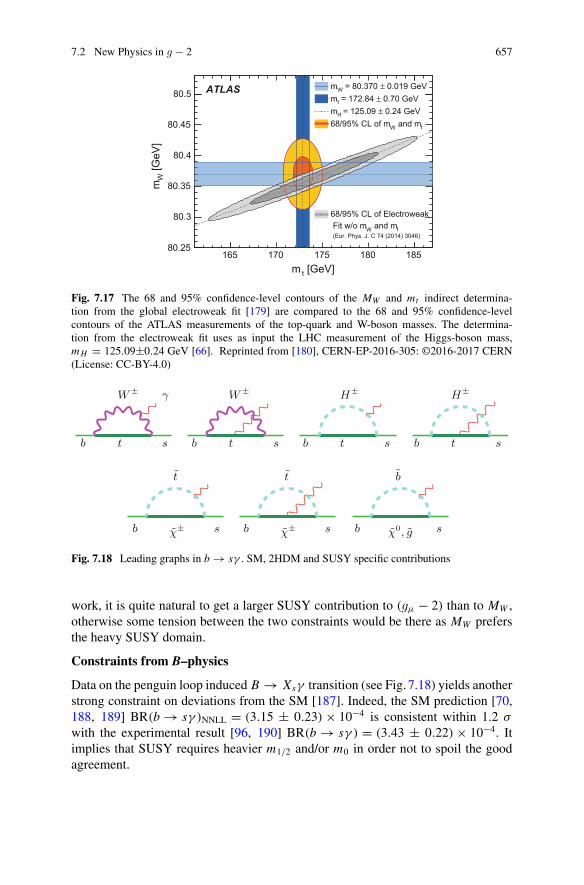
7.2 New Physics in g − 2 657

[GeV] tm165 170 175 180 185

[GeV

]W

m

80.25

80.3

80.35

80.4

80.45

80.5 ATLAS 0.019 GeV± = 80.370 Wm 0.70 GeV± = 172.84 tm 0.24 GeV± = 125.09 Hm

t and mW68/95% CL of m

68/95% CL of Electroweak

t and mW Fit w/o m(Eur. Phys. J. C 74 (2014) 3046)

Fig. 7.17 The 68 and 95% confidence-level contours of the MW and mt indirect determina-tion from the global electroweak fit [179] are compared to the 68 and 95% confidence-levelcontours of the ATLAS measurements of the top-quark and W-boson masses. The determina-tion from the electroweak fit uses as input the LHC measurement of the Higgs-boson mass,mH = 125.09±0.24 GeV [66]. Reprinted from [180], CERN-EP-2016-305: ©2016-2017 CERN(License: CC-BY-4.0)

γ

b s b s

W± W±

t t b s b s

H± H±

t t

t

χ±b s

t

χ±b s

b

χ0, gb s

Fig. 7.18 Leading graphs in b → sγ . SM, 2HDM and SUSY specific contributions

work, it is quite natural to get a larger SUSY contribution to (gμ − 2) than to MW ,otherwise some tension between the two constraints would be there as MW prefersthe heavy SUSY domain.

Constraints from B–physics

Data on the penguin loop induced B → Xsγ transition (see Fig. 7.18) yields anotherstrong constraint on deviations from the SM [187]. Indeed, the SM prediction [70,188, 189] BR(b → sγ )NNLL = (3.15 ± 0.23) × 10−4 is consistent within 1.2 σ

with the experimental result [96, 190] BR(b → sγ ) = (3.43 ± 0.22) × 10−4. Itimplies that SUSY requires heavier m1/2 and/or m0 in order not to spoil the goodagreement.

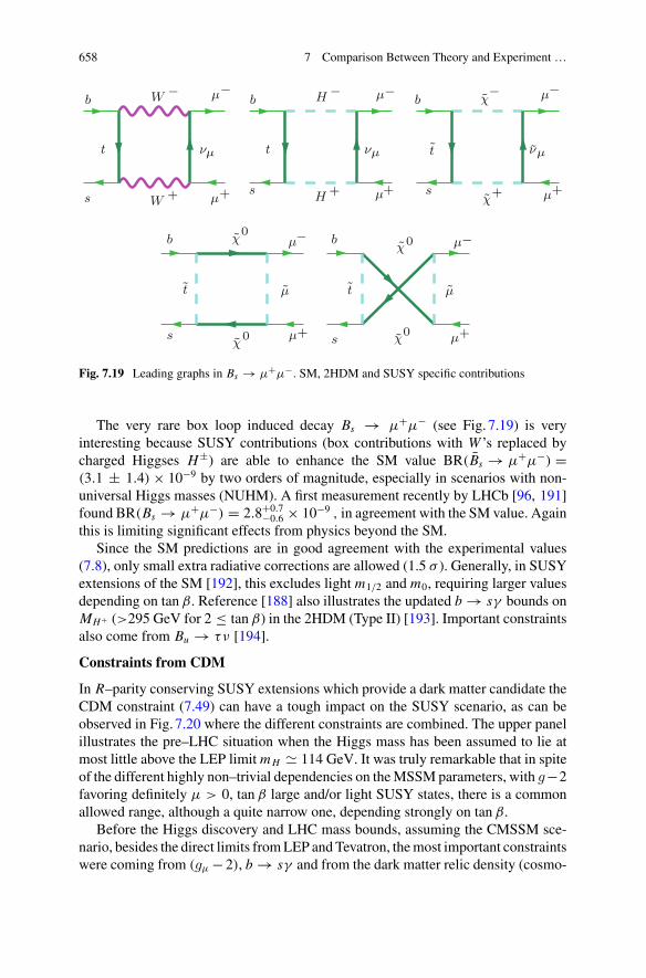
658 7 Comparison Between Theory and Experiment …

t νµ

b

s

μ−

μ+

W −

W+

t νµ

b

s

μ−

μ+

H −

H+

t νµ

b

s

μ−

μ+

χ−

χ+

t μ

b

s

μ−

μ+

χ0

χ0

t μ

b

s

μ−

μ+

χ0

χ0

Fig. 7.19 Leading graphs in Bs → μ+μ−. SM, 2HDM and SUSY specific contributions

The very rare box loop induced decay Bs → μ+μ− (see Fig. 7.19) is veryinteresting because SUSY contributions (box contributions with W ’s replaced bycharged Higgses H±) are able to enhance the SM value BR(Bs → μ+μ−) =(3.1 ± 1.4) × 10−9 by two orders of magnitude, especially in scenarios with non-universal Higgs masses (NUHM). A first measurement recently by LHCb [96, 191]found BR(Bs → μ+μ−) = 2.8+0.7

−0.6 × 10−9 , in agreement with the SM value. Againthis is limiting significant effects from physics beyond the SM.

Since the SM predictions are in good agreement with the experimental values(7.8), only small extra radiative corrections are allowed (1.5 σ ). Generally, in SUSYextensions of the SM [192], this excludes light m1/2 and m0, requiring larger valuesdepending on tan β. Reference [188] also illustrates the updated b → sγ bounds onMH+ (>295 GeV for 2 ≤ tan β) in the 2HDM (Type II) [193]. Important constraintsalso come from Bu → τν [194].

Constraints from CDM

In R–parity conserving SUSY extensions which provide a dark matter candidate theCDM constraint (7.49) can have a tough impact on the SUSY scenario, as can beobserved in Fig. 7.20 where the different constraints are combined. The upper panelillustrates the pre–LHC situation when the Higgs mass has been assumed to lie atmost little above the LEP limit mH � 114 GeV. It was truly remarkable that in spiteof the different highly non–trivial dependencies on theMSSMparameters, with g−2favoring definitely μ > 0, tan β large and/or light SUSY states, there is a commonallowed range, although a quite narrow one, depending strongly on tan β.

Before the Higgs discovery and LHC mass bounds, assuming the CMSSM sce-nario, besides the direct limits fromLEP andTevatron, themost important constraintswere coming from (gμ − 2), b → sγ and from the dark matter relic density (cosmo-

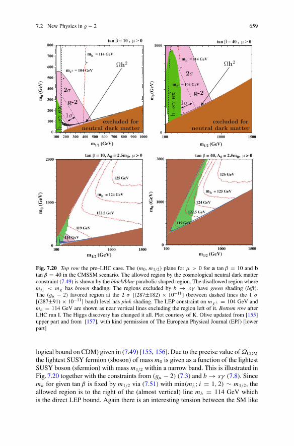
7.2 New Physics in g − 2 659

100 200 300 400 500 600 700 800 900 1000

100

0

200

300

400

500

600

700

800m

0 (G

eV)

m1/2 (GeV)

tan β = 10 , μ > 0

mh = 114 GeV

mχ± = 104 GeV

100 1000 15000

1000

m0 (

GeV

)m1/2 (GeV)

tan β = 40 , μ > 0

mh = 114 GeV

mχ± = 104 GeV

Ωh2

g-2

2σ

1σexcluded for

neutral dark matter

g-2

2σ

1σ

excluded forneutral dark matter

Ωh2b→

sγex b→

sγex

Fig. 7.20 Top row the pre–LHC case. The (m0,m1/2) plane for μ > 0 for a tan β = 10 and btan β = 40 in the CMSSM scenario. The allowed region by the cosmological neutral dark matterconstraint (7.49) is shown by the black/blue parabolic shaped region. The disallowed region wherem τ1 < mχ has brown shading. The regions excluded by b → sγ have green shading (left).The (gμ − 2) favored region at the 2 σ [(287±182) × 10−11] (between dashed lines the 1 σ

[(287±91) × 10−11] band) level has pink shading. The LEP constraint on mχ± = 104 GeV andmh = 114 GeV are shown as near vertical lines excluding the region left of it. Bottom row afterLHC run I. The Higgs discovery has changed it all. Plot courtesy of K. Olive updated from [155]upper part and from [157], with kind permission of The European Physical Journal (EPJ) [lowerpart]

logical bound on CDM) given in (7.49) [155, 156]. Due to the precise value ofΩCDM

the lightest SUSY fermion (sboson) of mass m0 is given as a function of the lightestSUSY boson (sfermion) with mass m1/2 within a narrow band. This is illustrated inFig. 7.20 together with the constraints from (gμ − 2) (7.3) and b → sγ (7.8). Sincemh for given tan β is fixed by m1/2 via (7.51) with min(mti ; i = 1, 2) ∼ m1/2, theallowed region is to the right of the (almost vertical) line mh = 114 GeV whichis the direct LEP bound. Again there is an interesting tension between the SM like

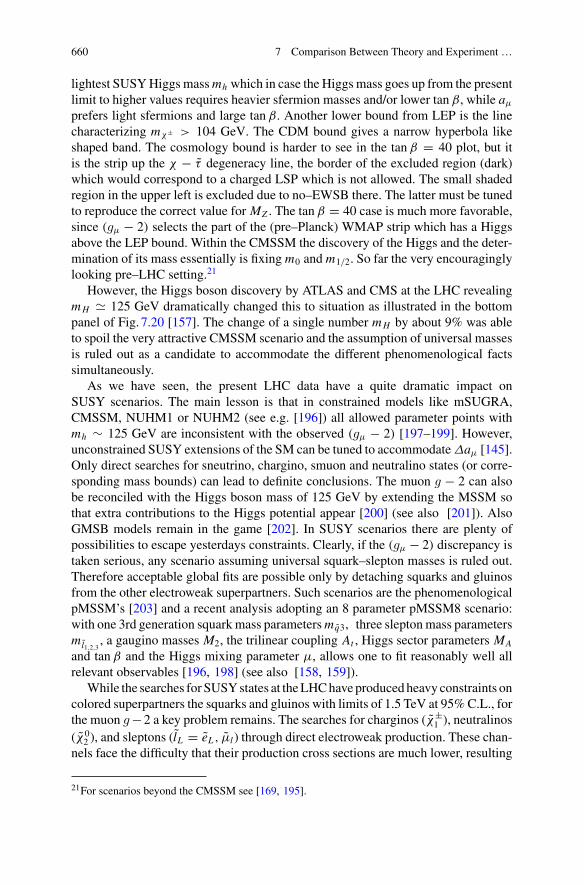
660 7 Comparison Between Theory and Experiment …

lightest SUSYHiggs massmh which in case the Higgs mass goes up from the presentlimit to higher values requires heavier sfermion masses and/or lower tan β, while aμ

prefers light sfermions and large tan β. Another lower bound from LEP is the linecharacterizing mχ± > 104 GeV. The CDM bound gives a narrow hyperbola likeshaped band. The cosmology bound is harder to see in the tan β = 40 plot, but itis the strip up the χ − τ degeneracy line, the border of the excluded region (dark)which would correspond to a charged LSP which is not allowed. The small shadedregion in the upper left is excluded due to no–EWSB there. The latter must be tunedto reproduce the correct value for MZ . The tan β = 40 case is much more favorable,since (gμ − 2) selects the part of the (pre–Planck) WMAP strip which has a Higgsabove the LEP bound. Within the CMSSM the discovery of the Higgs and the deter-mination of its mass essentially is fixing m0 and m1/2. So far the very encouraginglylooking pre–LHC setting.21

However, the Higgs boson discovery by ATLAS and CMS at the LHC revealingmH � 125 GeV dramatically changed this to situation as illustrated in the bottompanel of Fig. 7.20 [157]. The change of a single number mH by about 9% was ableto spoil the very attractive CMSSM scenario and the assumption of universal massesis ruled out as a candidate to accommodate the different phenomenological factssimultaneously.

As we have seen, the present LHC data have a quite dramatic impact onSUSY scenarios. The main lesson is that in constrained models like mSUGRA,CMSSM, NUHM1 or NUHM2 (see e.g. [196]) all allowed parameter points withmh ∼ 125 GeV are inconsistent with the observed (gμ − 2) [197–199]. However,unconstrained SUSY extensions of the SM can be tuned to accommodateΔaμ [145].Only direct searches for sneutrino, chargino, smuon and neutralino states (or corre-sponding mass bounds) can lead to definite conclusions. The muon g − 2 can alsobe reconciled with the Higgs boson mass of 125 GeV by extending the MSSM sothat extra contributions to the Higgs potential appear [200] (see also [201]). AlsoGMSB models remain in the game [202]. In SUSY scenarios there are plenty ofpossibilities to escape yesterdays constraints. Clearly, if the (gμ − 2) discrepancy istaken serious, any scenario assuming universal squark–slepton masses is ruled out.Therefore acceptable global fits are possible only by detaching squarks and gluinosfrom the other electroweak superpartners. Such scenarios are the phenomenologicalpMSSM’s [203] and a recent analysis adopting an 8 parameter pMSSM8 scenario:with one 3rd generation squarkmass parametersmq3, three sleptonmass parametersml1,2,3

, a gaugino masses M2, the trilinear coupling At , Higgs sector parameters MA

and tan β and the Higgs mixing parameter μ, allows one to fit reasonably well allrelevant observables [196, 198] (see also [158, 159]).

While the searches for SUSYstates at theLHChaveproducedheavy constraints oncolored superpartners the squarks and gluinos with limits of 1.5 TeV at 95%C.L., forthe muon g−2 a key problem remains. The searches for charginos (χ±

1 ), neutralinos(χ0

2 ), and sleptons (lL = eL , μl ) through direct electroweak production. These chan-nels face the difficulty that their production cross sections are much lower, resulting

21For scenarios beyond the CMSSM see [169, 195].

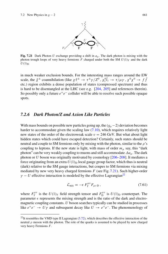
7.2 New Physics in g − 2 661

μ F F

U

γ γ

γ

Fig. 7.21 Dark Photon U exchange providing a shift in aμ. The dark photon is mixing with thephoton trough loops of very heavy fermions F charged under both the SM U (1)Y and the darkU (1)D

in much weaker exclusion bounds. For the interesting mass ranges around the EWscale, the χ± coannihilation (like χτ± → τ±γ /Z0 , χ0

1 l1 → τ/μγ , χ0χ0 → f fetc.) region exhibits a dense population of states (compressed spectrum) and thusis hard to be disentangled at the LHC (see e.g. [204, 205] and references therein).So possibly only a future e+e− collider will be able to resolve such possible opaquespots.

7.2.6 Dark Photon/Z and Axion Like Particles

Withmass bounds on possible new particles going up, the (gμ−2) deviation becomesharder to accommodate given the scaling law (7.10), which requires relatively lightnew states of the order of the electroweak scale v = 246 GeV. But what about lighthidden states which could have escaped detection? Certainly, such states should beneutral and couple to SM fermions only by mixing with the photon, similar to the ρ’scoupling to leptons. If the new state is light, with mass of order mμ say, this “darkphoton” can be veryweakly coupling tomuons and still accommodateΔaμ. The darkphoton orU boson was originally motivated by cosmology [206–208]. It mediates aforce originating from an extraU (1)D local gauge group factor, which thus is neutral(dark) relative to the SM gauge interactions, but coupes to SM fermions via mixingmediated by new very heavy charged fermions F (see Fig. 7.21). Such higher-orderγ −U effective interaction is modeled by the effective Lagrangian22

Lmix = −ε Fμν

Y Fμν D , (7.61)

where Fμν

Y is the U (1)Y field strength tensor and FμνD is U (1)D counterpart. The

parameter ε represents the mixing strength and is the ratio of the dark and electro-magnetic coupling constants.U boson searches typically can be studied in processeslike e+e− → Uγ and subsequent decay like U → e+e−. The phenomenology of

22It resembles the VMD type II Lagrangian (5.72), which describes the effective interaction of theneutral ρ meson with the photon. The role of the quarks is assumed to be played by new chargedvery heavy Fermions F .

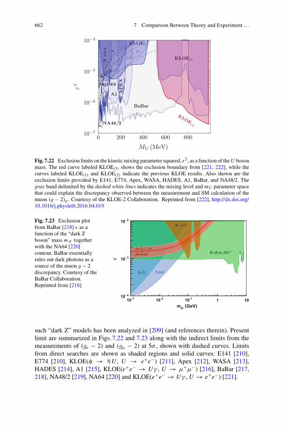
662 7 Comparison Between Theory and Experiment …

A1

KLOE(1)

aµ

KLOE(2)

KLOE (3)

APEX

WASA

HADES

aµ<

|2σ|)))))

A1

DES

)

APEX

A

DD

3)

KLOE(1)

<|2σ|

)K

aµ<

K

<

KK

HHHHADHHADHADHH

E (3)

K

µ

OEEKKKKKK

OELLKLLKLOE

W

KLLOE

KLLLLKKKLKOE

K

KLKKK

aµ

K

WASA

WW

KKK

OEE(2)KL E

NA48/2

BaBar

KLOE(4)ae

0 200 400 600 80010−7

10−6

10−5

10−4

MU (MeV)

ε2

Fig. 7.22 Exclusion limits on the kineticmixing parameter squared, ε2, as a function of theU bosonmass. The red curve labeled KLOE(3) shows the exclusion boundary from [221, 222], while thecurves labeled KLOE(1) and KLOE(2) indicate the previous KLOE results. Also shown are theexclusion limits provided by E141, E774, Apex, WASA, HADES, A1, BaBar, and NA48/2. Thegray band delimited by the dashed white lines indicates the mixing level and mU parameter spacethat could explain the discrepancy observed between the measurement and SM calculation of themuon (g − 2)μ. Courtesy of the KLOE-2 Collaboration. Reprinted from [222], http://dx.doi.org/10.1016/j.physletb.2016.04.019

Fig. 7.23 Exclusion plotfrom BaBar [218] ε as afunction of the “dark Zboson” mass mA′ togetherwith the NA64 [220]contour. BaBar essentiallyrules out dark photons as asource of the muon g − 2discrepancy. Courtesy of theBaBar Collaboration.Reprinted from [218]

e(g-2) NA64

ννπ→K

σ 5±μ

(g-2)favored BABAR 2017

(GeV)A'm

3−10 2−10 1−10 1 10

ε

4−10

3−10

2−10

such “dark Z” models has been analyzed in [209] (and references therein). Presentlimit are summarized in Figs. 7.22 and 7.23 along with the indirect limits from themeasurements of (ge − 2) and (gμ − 2) at 5σ , shown with dashed curves. Limitsfrom direct searches are shown as shaded regions and solid curves: E141 [210],E774 [210], KLOE(φ → ηU , U → e+e−) [211], Apex [212], WASA [213],HADES [214], A1 [215], KLOE(e+e− → Uγ , U → μ+μ−) [216], BaBar [217,218], NA48/2 [219], NA64 [220] and KLOE(e+e− → Uγ , U → e+e−) [221].

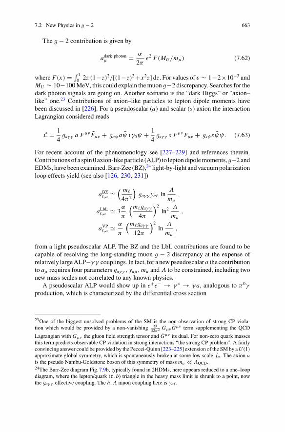
7.2 New Physics in g − 2 663

The g − 2 contribution is given by

adark photonμ = α

2πε2 F(MU/mμ) (7.62)

where F(x) = ∫ 10 2z (1−z)2/[(1−z)2+x2z] dz. For values of ε ∼ 1−2×10−3 and

MU ∼ 10−100MeV, this could explain themuon g−2 discrepancy. Searches for thedark photon signals are going on. Another scenario is the “dark Higgs” or “axion–like” one.23 Contributions of axion–like particles to lepton dipole moments havebeen discussed in [226]. For a pseudoscalar (a) and scalar (s) axion the interactionLagrangian considered reads

L = 1

4gaγ γ a Fμν Fμν + gaψaψ i γ5ψ + 1

4gsγ γ s F

μνFμν + gsψsψψ. (7.63)

For recent account of the phenomenology see [227–229] and references therein.Contributions of a spin 0 axion-like particle (ALP) to leptondipolemoments,g−2 andEDMs, have been examined.Barr-Zee (BZ),24 light-by-light and vacuumpolarizationloop effects yield (see also [126, 230, 231])

aBZ�,a �( m�

4π2

)gaγ γ ya� ln

Λ

ma,

aLbL�,a � 3α

π

(m�gaγ γ

4π

)2ln2

Λ

ma,

aVP�,a � α

π

(m�gaγ γ

12π

)2ln

Λ

ma,

from a light pseudoscalar ALP. The BZ and the LbL contributions are found to becapable of resolving the long-standing muon g − 2 discrepancy at the expense ofrelatively largeALP−γ γ couplings. In fact, for a newpseudoscalara the contributionto aμ requires four parameters gaγ γ , yaμ,ma andΛ to be constrained, including twonew mass scales not correlated to any known physics.

A pseudoscalar ALP would show up in e+e− → γ ∗ → γ a, analogous to π0γ

production, which is characterized by the differential cross section

23One of the biggest unsolved problems of the SM is the non-observation of strong CP viola-tion which would be provided by a non-vanishing Θ

32π2 Gμν Gμν term supplementing the QCD

Lagrangian with Gμν the gluon field strength tensor and Gμν its dual. For non-zero quark massesthis term predicts observable CP violation in strong interactions “the strong CP problem”. A fairlyconvincing answer could be provided by the Peccei-Quinn [223–225] extension of the SMby aU (1)approximate global symmetry, which is spontaneously broken at some low scale fa . The axion ais the pseudo Nambu-Goldstone boson of this symmetry of mass ma � ΛQCD.24The Barr-Zee diagram Fig. 7.9b, typically found in 2HDMs, here appears reduced to a one–loopdiagram, where the lepton/quark (τ, b) triangle in the heavy mass limit is shrunk to a point, nowthe gaγ γ effective coupling. The h, A muon coupling here is ya�.

664 7 Comparison Between Theory and Experiment …

dσ

d cos θ= α

64g2aγ γ

(1 − m2

a

s

)3 (1 + cos2 θ

),

where θ is the angle between the ALP and the beam axis in the center-of-mass. Asone believes to include all states e+e− → anything other than leptons, attributedto hadrons usually, within uncertainties it would just mean that the error estimateshave been missing a substantial contribution. Bounds on such effects are providedby e+e− annihilation facilities like LEP, KLOE [222], CMD, SND, BaBar, Belle andBES. For details I refer to [226]. For a comprehensive review see [232].

These dark hidden states scenarios are particularly interesting because they cannaturally bridge to the dark matter problem, one of the most mysterious missing partsof present day particle physics. However, some possibilities like the dark Z scenarioare essentially ruled out by data already.

There a numerous other beyond the SM scenarios (see e.g. [233–235]), whichexhibit new particles that could be contributing to the muon g − 2, and where para-meters are limited by phenomenology. From the examples we have discussed weleaned that it is by far not simple to obtain a 3 to 4 σ effects in aμ. Most of the mod-els yield contributions represented by diagrams either of the generic 1–loop type orby Barr-Zee type 2–loop diagrams only the masses and the couplings are specific asfar as they are known. For little Higgs models the correction to aμ have been com-puted in Ref. [236] and were found to be negligible aLH

μ ≈ 1×10−10. An interestingnew physics option are extra dimension scenarios, which however yield negativecontributions of order a(2)KK

μ ≈ −1×10−10 from the Kaluza-Klein excitations [237,238]. Short summaries of these topics and more references may be found in [13].

7.3 Outlook on the Upcoming Experiments

Next generationmuon (g−2) experiments are going to happen soon. The two experi-ments under constructionE989 at Fermilab [239–242] andE34 at J-PARC [243–245],both measure the difference between the spin precession and the cyclotron motionfor a muon in a magnetic field. In order to reach a high precision experiments haveto be setup such that the equation of motion

ωa = e

mμc

(aμB −

[aμ − 1

γ 2 − 1

]v × Ec2

), (7.64)

takes the form of a linear relation between the Larmor precession frequency and thehomogeneous magnetic field:

ωa = e

mμcaμB. (7.65)

The main point is to get rid of the effect from the electric field. This requires to workat magic γ by tuning the beam energy such that aμ −1/(γ 2 −1) = 0 or alternatively

7.3 Outlook on the Upcoming Experiments 665

to avoid any external electric field. The two experiments are complementary sincethey are using alternative possibilities. E989 is a traditional “magic γ ” experimentworking with highly relativistic muons of magic energy E ≈ 3.1 GeV.The muonenergy determines the size of the storage ring diameter to about 14m for a field of 1.5Tesla, which is what can be reached in practice. So the ring of the BNL experimentcan and actually is being used by the Fermilab experiment. The novel E34 experimentworking with slow muons (E ∼ 300 MeV) is a much smaller experiment (diameterof muon orbit 70 cm) working with a magnetic muon trap, with the main challenge torule out any external electric field. Needless to say that the two approaches have verydifferent systematic uncertainties. The E989 experimentwill reduce the experimentalerror by a factor four to

δaμ = 16 × 10−11. (7.66)

The BNL experimental error was statistics dominated, the Fermilab experiment willprovide a factor of 20 more in statistics, more muons at higher injection rate. Therewill be much less background from pion decays by having a longer beam line whichalso helps improving the polarization. Further improvements concern amore uniformmagnetic field, a more precise magnetic field calibration probe and a better centeredbeam using an improved focusing system. In addition, the signal processing will beimproved by segmented detectors, by pileup and muon loss reduction (using betterkickers), and by applying refined methods of analysis.

While the Fermilab experiment uses an approach which has been used and furtherdeveloped since the 1970s in the CERN experiment, the J-PARC experiment is anew “from scratch” design, where the most critical part seems to be the shielding ofelectric fields. In contrast to the Fermilab experiment the J-PARC experiment workswithout the need of beam focusing. As a big advantage one should note that it ismuch easier to provide a homogeneous magnetic field when the fiducial volume isvery much smaller. A shortcoming of an experiment with slow muons is that thedegree polarization appears reduced, which evidently reduces the signal. Still, onecan expect that a precision at the level of the BNL experiment can be reached suchthat the E34 experiment can provide a very important cross check of the BNL result.

In any case, the next generation experiments will scrutinize the presently seendeviation in (gμ − 2). If the deviation is confirmed at least a 5σ significance will bereached. If the deviation would get reduced one would have one more precision testof the SM and a severe constraint on possible SM extensions. The E989 experiment isscheduled to begin data taking in early 2017 and a newmeasurement can be expectedin about one year later.

7.4 Perspectives for the Future

The electron’s spin and magnetic moment were evidenced from the deflection ofatoms in an inhomogeneous magnetic field and the observation of fine structure byoptical spectroscopy [246, 247]. Ever since, magnetic moments and g–values of

666 7 Comparison Between Theory and Experiment …

particles in general and the g − 2 experiments with the electron and the muon inparticular, together with high precision atomic spectroscopy, have played a centralrole in establishing the modern theoretical framework for particle physics: relativis-tic quantum field theory in general and quantum electrodynamics in particular, theprototype theory which developed further into the SM of electromagnetic, weakand strong interactions based on a local gauge principle and spontaneous symmetrybreaking, with local gauge group SU(3)c ⊗ SU(2)L ⊗U (1)Y spontaneously brokento SU(3)c ⊗ U (1)em. Not only particle physics, also precision atomic physics andnuclear theory are based on relativistic QFT methods.25

New milestones have been achieved not too long ago with the BNL muon g − 2experiment together with the Harvard electron g − 2 experiment. Both experimentsexploited all ingenuity to reach the next level of precision, and together with theoryefforts maybe the next level of understanding of how it works. On the theory side,what we learned from theBNL experiment andwhatwewill learn from the upcomingexperiments depends a lot on howwell we can corroborate the theoretical prediction.There is certainly common agreement that the hadronic light–by–light scatteringcontribution is the most problematic one, since no theoretically established methodso far allowed us to calculate this contribution in a model independent way and witha satisfactorily controlled precision.

A very promising novel access of theHLbL is the data–driven dispersive approachadvocated in [248–250]. The detailed theoretical framework has been developedin [251]. The method could improve the reliability of HLbL estimates dramatically,provided the data basis can be ameliorated by dedicated experiments of hadron pro-duction in light-by-light processes. More experimental information is also importantfor better modeling by effective theories. A typical example where data is missing isthe π0γ ∗γ ∗ form factor for both photons off–shell or direct light–by–light scatteringin e+e− → e+e−γ ∗γ ∗ → e+e−γ γ or e+e−γ ∗γ with the virtual final state photonconverting to a pair.

Another big hope for the long term future are the non–perturbative calculations ofelectromagnetic current correlators by means of lattice QCD [252–255]. This has togo in steps from two–point amplitudes (vacuum polarization and/or Adler function)to three–point form factors (non-perturbative effects in VVA correlators) and thefour–point function linked to light–by–light scattering.

The hadronic vacuum polarization in principle may be substantially improvedby continuing e+e− → hadrons cross–section measurements with higher precision.Substantial differences in the dominating e+e− → ππ channel (at the few % level)between the KLOE results on the one hand and the BaBar result26 on the other hand

25Not to forget the role of QFT for other systems of infinite (large) numbers of degrees of freedom:condensed matter physics and critical phenomena in phase transitions (Ken Wilson 1971). TheHiggs mechanism as a variant of the Ginzburg-Landau effective theory of superconductivity (1950)and the role QFT and the renormalization group play in the theory of phase transitions are goodexamples for synergies between elementary particle physics and condensed matter physics.26The KLOE and BaBar measurements have been obtained via the radiative return methodwhich is a next to leading order approach. On the theory side one expects that the handling of thephoton radiation requires one order in αmore than the scanmethod for obtaining the same accuracy.

7.4 Perspectives for the Future 667

are persisting. Still, data taken with BaBar and Belle before the facilities were shutdown are being analyzed. Fortunately, ongoing measurements with BES-III [260]and at the VEPP-2000 [261] facility are improving the data collection, such thatthe error of the HVP estimates continues to get smaller. Here, the ab initio latticeQCD results are getting closer to the data–driven dispersion relations results. Sooncompetitive results will be available and provide important cross checks.

Another previously disturbing problem, the deviations at the 10% level betweene+e−–data and the isospin violations corrected hadronic τ–decay spectral functions,fortunately could be resolved in the meantime [7, 23]. If one corrects τ data formissing ρ0 −γ mixing, the τ data based results are in good agreement with the e+e−data based ones.

An interesting possibility in this respect is a novel approach to determine ahadμ viaa direct space-like measurement of α(−Q2) in μe scattering as proposed in [262],recently (see also [263]). This approach completely avoids a number of problemsone encounters with the standard time-like approach. In the latter case collectinghadron production data, applying radiative corrections to hadron production, vacuumpolarization subtraction and problems related to thresholds and resonances are ratherchallenging. In contrast, a single space-like process likeμe scattering ismuch simplerand the needed radiative corrections are under much better control of perturbationtheory.

There is no doubt that performing doable improvements on both the theory andthe experimental side allows to substantially sharpen (or diminish) the apparent gapbetween theory and experiment. Yet, even the present situation gives ample reason forspeculations. No other experimental result has as many problems to be understoodin terms of SM physics. One point should be noted in this context, however. Anexperiment at that level of accuracy, going one order of magnitude beyond anyprevious experiment, is a real difficult enterprise and only one such experiment hasbeen performed so far. There is also a certain possibility to overlook some newproblem which only shows up at higher precision and escaped the list of explicitlyaddressed problems by the experiment. It is for instance not 100% clear that what ismeasured in the experiment is precisely what theoreticians calculate. For example, itis believed that, because radiative corrections in g−2 are infrared finite to all orders,real photon radiation can be completely ignored, in spite of the fact that we know thatdue to the electric interaction via charges a naive S–matrix in QED does not exist.Muons, like any charged particles, produce and absorb continuously photon radiationand therefore are dressed by a photon cloud which is thought not to affect the g − 2

(Footnote 26 continued)Presently a possible deficit is on the theory side. What is urgently needed are full O(α2) QEDcalculations, for Bhabha luminosity monitoring, μ–pair production as a reference and test process,and π–pair production in sQED as a first step and direct measurements of the final state radiationfrom hadrons. The CMD-3 and SND measurements take data at the same accelerator (same lumi-nosity/normalization uncertainties) and use identical radiative corrections, such that for that partthey are strongly correlated and this should be taken into account appropriately in combining thedata. The present state-of-the-art event generator is PHOKHARA [256] for radiative return eventsand BABAYAGA [257] for the Bhabha channel (see also [258, 259]).

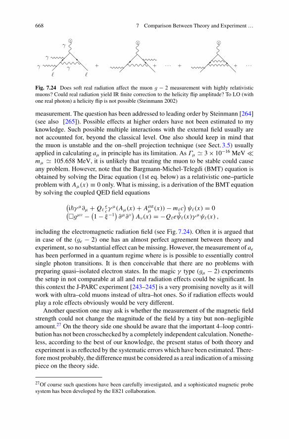
668 7 Comparison Between Theory and Experiment …

+ + · · · + + · · ·

γ

γ

⊗⊗⊗

� �

γ

γ

Fig. 7.24 Does soft real radiation affect the muon g − 2 measurement with highly relativisticmuons? Could real radiation yield IR finite correction to the helicity flip amplitude? To LO (withone real photon) a helicity flip is not possible (Steinmann 2002)

measurement. The question has been addressed to leading order by Steinmann [264](see also [265]). Possible effects at higher orders have not been estimated to myknowledge. Such possible multiple interactions with the external field usually arenot accounted for, beyond the classical level. One also should keep in mind thatthe muon is unstable and the on–shell projection technique (see Sect. 3.5) usuallyapplied in calculating aμ in principle has its limitation. As Γμ � 3× 10−16 MeV �mμ � 105.658 MeV, it is unlikely that treating the muon to be stable could causeany problem. However, note that the Bargmann-Michel-Telegdi (BMT) equation isobtained by solving the Dirac equation (1st eq. below) as a relativistic one–particleproblem with Aμ(x) ≡ 0 only. What is missing, is a derivation of the BMT equationby solving the coupled QED field equations

(i�γ μ∂μ + Q�

ecγ

μ(Aμ(x) + Aextμ (x)) − m�c

)ψ�(x) = 0(

�gμν − (1 − ξ−1

)∂μ∂ν

)Aν(x) = −Q�eψ�(x)γ μψ�(x) ,

including the electromagnetic radiation field (see Fig. 7.24). Often it is argued thatin case of the (ge − 2) one has an almost perfect agreement between theory andexperiment, so no substantial effect can be missing. However, the measurement of aehas been performed in a quantum regime where is is possible to essentially controlsingle photon transitions. It is then conceivable that there are no problems withpreparing quasi–isolated electron states. In the magic γ type (gμ − 2) experimentsthe setup in not comparable at all and real radiation effects could be significant. Inthis context the J-PARC experiment [243–245] is a very promising novelty as it willwork with ultra–cold muons instead of ultra–hot ones. So if radiation effects wouldplay a role effects obviously would be very different.

Another question one may ask is whether the measurement of the magnetic fieldstrength could not change the magnitude of the field by a tiny but non–negligibleamount.27 On the theory side one should be aware that the important 4–loop contri-bution has not been crosschecked by a completely independent calculation. Nonethe-less, according to the best of our knowledge, the present status of both theory andexperiment is as reflected by the systematic errors which have been estimated. There-foremost probably, the differencemust be considered as a real indication of amissingpiece on the theory side.

27Of course such questions have been carefully investigated, and a sophisticated magnetic probesystem has been developed by the E821 collaboration.

7.4 Perspectives for the Future 669

The anomalous magnetic moment of the muon is a beautiful example of “thecloser we look the more we see”,28 however, the efforts to dig even deeper into thestructure of matter remains a big adventure also in future.

The g − 2 measurement is like a peek through the keyhole, you see at the sametime an overlay of all things to a certain depth in one projection, but to make surethat what you see is there, you have to open the door and go to check. This will be amatter of accelerator physics, and an ILC would be the preferred and ideal facility toclarify the details. Of course and luckily, the LHC will tell us much sooner the grossdirection new physics will go and is able to reach the physics at much higher scales.But, it is not the physics at the highest scales you see first in g − 2 as we learned inthis book.

The Muon Storage Ring experiment on (gμ − 2) and similarly the Penning Trapexperiment on (ge−2) are likemicroscopeswhich allow us to look into the subatomicworld and the scales which we have reached with aμ is about 100 GeV, i.e., the scaleof theweak gauge bosonsW and Z which is the LEP energy scale. As aμ is effectivelyby a factor (mμ/me)

2 · δaexpe /δaexpμ � 19 more sensitive to new heavy physics themass scale which is tested by ae is about 100/

√19 ∼ 23 GeV only, an energy region

which we think we know very well as it has been explored by other means.We shouldkeep in mind that the fact that the experiments measuring aμ and ae, respectively,hardly can be directly compared from the point of view of the experimental setup andthe technical challenges they have to meet. This makes them two rather independentexperimental entities. Therefore, the electron (ge − 2), if not be used to determineα, is the ideal complementary probe of the SM or its failure.

Remember that at LEP-I by electron–positron annihilation predominantly “heavylight” particles Z or at LEP-II predominantly W+W−–pairs have been produced,states which were produced in nature mostly in the very early universe.29 Similarly,the Tevatron acted as a t t factory and the LHC reached the Higgs production stageand is hunting for the “new” in the TeV energy range, considerably above the SMspectrum.

Particle accelerators and storage rings are microscopes which allow us to investi-gates the nature in the subatomic range at distance < 10−15 m and at the same time

28which is not always true, for example if we read a newspaper or if you read this book.29An energy or an equivalent mass may always be translated into a temperature by means of theBoltzmann constant k which relates 1◦K ≡ 8.6× 10−5eV. Thus T = E/k is the temperature of anevent at energy E . As we know the universe expands and thereby cools down, thus looking at highertemperatures means looking further back in the history of the universe. By solving Friedmann’scosmological equations with the appropriate equations of state backwards in time, starting from thepresent with a cosmic microwave background radiation temperature of 2.728◦K and assuming thematter density to be the critical one Ωtot = 1, one may calculate the time at which temperaturesrealized at LEP with 100 to 200 GeV of center of mass energy where realized. This time is givenby t = 2.4/

√N (T ) (1 MeV/kT )2 sec, with N (T ) = ∑

bosons B gB(T ) + 78

∑fermions F gF (T ),

the effective number of degrees of freedom excited at temperature T (see Eq. (19.43) in [266]).For LEP energies mb � kT � MW the numbers gB/F (T ) counting spin, color and charge ofbosonic/fermionic states in the massless limit include all SM particles except W±, Z , H and t oneobtains N (T ) = 345/4. Thus LEP events happened to take place in nature t ∼ 0.3 × 10−10 secafter the Big Bang for T ∼ 100 GeV . With the LHC we reach tLHC ∼ 1.66 × 10−15 sec.

670 7 Comparison Between Theory and Experiment …

have the aim to directly produce new forms of matter, by pair creation, for example.The size of such machines is essentially determined by two parameters: the energywhich determines the resolution λ = hc/Ec.m. � 1.2GeV/Ec.m.(GeV) × 10−15 mand the collision rateΔN/Δt = L × σ � 1032 σ(cm2)/cm2 sec (luminosity L as ithas been reached LEP as an example). Usually projectiles must be stable particles orantiparticles like electrons, positrons and protons and antiprotons. TheMuon StorageRing experiments work with the rather unstable muons which are boosted to highlyrelativistic quasi–stable muons well selected in energy and polarization before theyare injected into the storage ring. The ring in this case more acts as a detector ratherthan an accelerator as it usually does in the case of typical high energy machines.This allows to study the motion of the muons at incredible precision with very littlebackground.

With the advent of the Large Hadron Collider (LHC) many things already havefound a new direction, as we have mentioned several times. Experiments at theLHC take place under extreme conditions. At the LHC one is producing enormousamounts of events, billions per second, of which the overwhelming part of eventsare too complex to be understood and the interesting “gold platted” events whichwill tell us about new physics one has to dig out like “searching for a needle in ahaystack”. Nevertheless, the physics accessible there hopefully will be found, whichcould tell us what we see in the (gμ −2) discrepancy. At LEP a big machine was ableto measure about 20 different observables associated with different final states at thelevel of 0.1%. The strength of the LHC is that it is able to go far beyond what we havereached so far in termsof the energy scale.But as important, theLHCalso is capable ofproducing milestones in precision physics, like the amazingly precise determinationof the Higgs bosonmass, the study of the Higgs bosons decay pattern or substantiallyimproving theW and the top quark mass measurements. Other milestones have beenachieved in rare processes, like the first observation of Bs → μ+μ− events by theLHCbdetector. The exclusion limits formanyhypothetical newparticles alreadyhavebeen moving up to much higher energies, such that several new physics scenarioscould be ruled out.

Themost remarkable event at theLHChas been the discovery of theHiggs particle.More surprising than its existence was the specific value of its mass found. This hasto do with the stability bound of Higgs potential in the SMwhich has been addressedmany times in the past. In 1995 the discovery of the top quark at the Tevatron alsoreviled itsmass andHambye andRiesselmann (HR) in 1996 [267] (see also referencestherein) analyzed the stability bound as a function of the yet unknown Higgs bosonmass,which is reproduced inFig. 7.25.TheHiggs bosonmass at that timehas been theonly relevant parameter which was not yet known.30 In a first 2-loop analysis, know-ing mt , HR estimated an upper bound of MH < 180 GeV , below which an extrap-olation of the SM Higgs system up to the Planck scale MPlanck � 1.22 × 1019 GeVwas possible within a small window. In fact the parameters m2 and λ in the Higgspotential

30A 95% CL lower bound of 77.5 GeV had been estimated by the LEP Collaborations [268] at thattime.

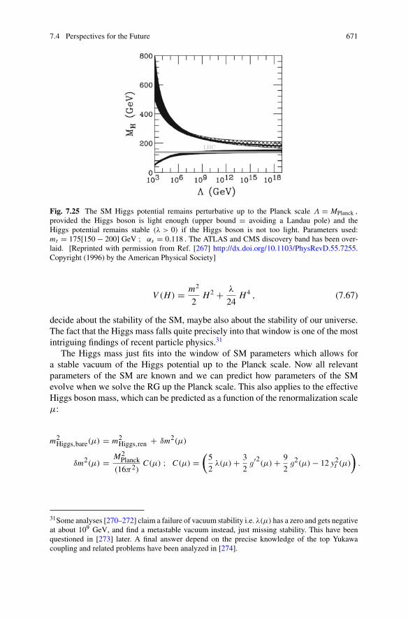
7.4 Perspectives for the Future 671

LHC

Fig. 7.25 The SM Higgs potential remains perturbative up to the Planck scale Λ = MPlanck ,

provided the Higgs boson is light enough (upper bound = avoiding a Landau pole) and theHiggs potential remains stable (λ > 0) if the Higgs boson is not too light. Parameters used:mt = 175[150 − 200] GeV ; αs = 0.118 . The ATLAS and CMS discovery band has been over-laid. [Reprinted with permission from Ref. [267] http://dx.doi.org/10.1103/PhysRevD.55.7255.Copyright (1996) by the American Physical Society]

V (H) = m2

2H 2 + λ

24H 4 , (7.67)

decide about the stability of the SM, maybe also about the stability of our universe.The fact that the Higgs mass falls quite precisely into that window is one of the mostintriguing findings of recent particle physics.31

The Higgs mass just fits into the window of SM parameters which allows fora stable vacuum of the Higgs potential up to the Planck scale. Now all relevantparameters of the SM are known and we can predict how parameters of the SMevolve when we solve the RG up the Planck scale. This also applies to the effectiveHiggs boson mass, which can be predicted as a function of the renormalization scaleμ:

m2Higgs,bare(μ) = m2

Higgs,ren + δm2(μ)

δm2(μ) = M2Planck

(16π2)C(μ) ; C(μ) =

(5

2λ(μ) + 3

2g′2(μ) + 9

2g2(μ) − 12 y2t (μ)

).

31Some analyses [270–272] claim a failure of vacuum stability i.e. λ(μ) has a zero and gets negativeat about 109 GeV, and find a metastable vacuum instead, just missing stability. This have beenquestioned in [273] later. A final answer depend on the precise knowledge of the top Yukawacoupling and related problems have been analyzed in [274].

672 7 Comparison Between Theory and Experiment …

The bare mass here appears as a function of μ as we keep the observed mass as aboundary condition (bottom up approach).32 Taking into account the running of theSM parameters, at the Planck scale we obtain

m2eff ∼ δm2 � M2

Planck

32π2C(μ = MPlanck) � (0.0295MPlanck)

2 � (3.6 × 1017 GeV

)2,

and indeed the effective Higgs potential massm(MPlanck) reaches a huge value whichstays clearly below MPlanck, however. The non-vanishing quartically enhanced vac-uum energy V (0) = 〈V (H(x))〉 provides a cosmological constant density

ρΛ bare = ρΛ ren + δρ(μ)

δρ(μ) = M4Planck

(16π2)2X (μ) ; X (μ) =

(5 λ + 3 g′2 + 9 g2 − 24 y2t

).

With SM running parameters at the Planck scale

ρeff � δρ ∼ (1.28MPlanck)4 ∼ (

1.57 × 1019 GeV)4

.

Surprisingly, because the bosonic couplings and the top quark Yukawa have a dif-ferent energy dependence both counterterms δm2(μ) and δρ(μ) vanish at a scaleμ = μCC, which for the specific parameter set happens at

μCC ≈ 3.1 × 1015 GeV (7.68)

clearly below the Planck scale again. There the effective mass changes sign andtriggers the Higgs mechanism and the Higgs field acquires a non-vanishing VEV〈H(x)〉 = v(μ), which vanishes identically at higher energies μ > μCC.

Above the Higgs phase transition point μCC we start to see the bare theory i.e. aSM with its bare short distance effective parameters, so in particular a very heavyHiggs boson, which can be moving at most very slowly, and thus naturally satisfiesthe slow roll condition that the potential energy dominates the kinetic energy 1

2 H2.

Note that the Higgs boson contributes to energy momentum tensor in Einstein’sequations a pressure and energy density (H the time derivative of H )

p = 1

2H 2 − V (H) ; ρ = 1

2H 2 + V (H) ,

which then appear inFriedmann’s cosmological solutions.Aswe approach thePlanckscale (bare theory) the slow–roll condition 1

2 H 2 � V (H) comes into play as we

32As we have consider the SM to exhibit at cutoff of the size of the Planck mass, we can alsocalculate the vacuum energy V (0) ≡ 〈V (H)〉 as a large but finite number. At high energies nearthe Planck scale the SM is in the symmetric phase i.e. 〈H〉 = 0, while 〈H2〉 and 〈H4〉 are non-vanishing. This requires a Wick reordering of the potential [60] which is shifting the effective masssuch that the coefficient proportional to λ changes from 2 to 5/2.

7.4 Perspectives for the Future 673

reach p ≈ −V (H), ρ ≈ +V (H) and hence p = −ρ, which is the equation ofstate of DARK ENERGY. The SM Higgs boson in the early universe provides ahuge dark energy, which triggers inflation. That inflation has happened in the earlyuniverse is an established fact. The so called hierarchy problem is not a problem itis the solution which promotes the Higgs boson to be the natural candidate for theinflaton. This however only works if no SUSY or GUT is sitting in-between us andthe Planck scale, and provided vacuum stability is holds within the SM.

Inflation tunes the total density to Ωtot = 1 or ρtot = ρcrit = (0.00216 eV)4. Thepresently observed dark energy density must be a part of it and actually has the valueρΛ = (0.002 eV)4 the known 74% of the total.

Still, darkmatter remains amystery although there are a number of candidates likeaxions [275], or an extra SU(4) version of QCD forming bound states which couldprovide bosonic dark matter [276]. So we hope we may soon add more experimen-tally established terms to the SM Lagrangian and extent our predictions to includethe yet unknown. That’s how it worked in the past with minimal extensions on theo-retical grounds. Why this works so successfully nobody really knows. One observesparticles, one associates with them a field, interactions are the simplest non–trivialproducts of fields (triple and quartic) at a spacetime point, one specifies the inter-action strength, puts everything into a renormalizable relativistic QFT and predictswhat should happen and it “really” happened essentially without exception. Maybethe muon g − 2 is the most prominent exception!

This book tried to shed light on the physics encoded in a single real number. Such asingle number in principle encodes an infinity of information, as each new significantdigit (each improvement should be at least by a factor ten in order to establish the nextsignificant digit) is a new piece of information. It is interesting to ask, what wouldwe know if we would know this number to infinite precision. Of course one cannotencode all we know in that single number. Each observable is a new view to realitywith individual sensitivity to the deep structure of matter. All these observables arecornerstones of one reality unified self–consistently to our present knowledge by theknowledge of the Lagrangian of a renormalizable quantum field theory. Theory andexperiments of the anomalous magnetic moment are one impressive example whatit means to understand physics at a fundamental level. The muon g − 2 reveals themajor ingredients of the SM and as we know now maybe even more.

On the theory part the fascinating thing is the technical complexity of higherorder SM (or beyond) calculations of in the meantime thousands of diagrams whichcan only be managed by the most powerful computers in analytical as well as inthe numerical part of such calculations. This book only gives little real insight intothe technicalities of such calculation. Performing higher order Feynman diagramcalculation could look like formal nonsense but at the end results in a number whichexperimenters indeedmeasure.Much of theoretical physics today takes place beyondthe Galilean rules, namely that sensible predictions must be testable. For anomalousmagnetic moment at least we still follow the successful tradition set up by GalileoGalilei, we definitely can check it, including all the speculations about it.

A nextmajor step in this field of researchwould be establishing experimentally theelectric dipole moment. This seems to be within reach thanks to a breakthrough in the

674 7 Comparison Between Theory and Experiment …

experimental techniques. The electric dipole moments are an extremely fine monitorfor CP violation beyond the SM which could play a key role for understanding theorigin of the baryon matter–antimatter asymmetry in the universe.

And now we are waiting for the new results on the muon g − 2 and for new datafrom the LHC to tell us where we go!

References

1. J. Bailey et al., Nucl. Phys. B 150, 1 (1979)2. G.W. Bennett et al., Muon g-2 Collab. Phys. Rev. D 73, 072003 (2006)3. T. Kinoshita, M. Nio, Phys. Rev. D 73, 053007 (2006)4. T. Aoyama, M. Hayakawa, T. Kinoshita, M. Nio, Phys. Rev. Lett. 109, 111808 (2012)5. S. Laporta, arXiv:1704.06996 [hep-ph]6. M. Knecht, EPJ Web Conf. 118, 01017 (2016)7. F. Jegerlehner, R. Szafron, Eur. Phys. J. C 71, 1632 (2011)8. F. Jegerlehner, EPJ Web Conf. 118, 01016 (2016), arXiv:1705.00263 [hep-ph]9. J. Bijnens, E. Pallante, J. Prades, Phys. Rev. Lett. 75, 1447 (1995) [Erratum-ibid. 75, 3781

(1995)]; Nucl. Phys. B 474, 379 (1996) [Erratum-ibid. 626, 410 (2002)]10. M. Hayakawa, T. Kinoshita, Phys. Rev. D 57, 465 (1998) [Erratum-ibid. D 66, 019902 (2002)]11. M. Knecht, A. Nyffeler, Phys. Rev. D 65, 073034 (2002)12. K. Melnikov, A. Vainshtein, Phys. Rev. D 70, 113006 (2004)13. F. Jegerlehner, A. Nyffeler, Phys. Rep. 477, 1 (2009)14. A. Czarnecki, W.J. Marciano, A. Vainshtein, Phys. Rev. D 67, 073006 (2003) [Erratum-ibid.

D 73, 119901 (2006)];M. Knecht, S. Peris,M. Perrottet, E. de Rafael, JHEP 0211, 003 (2002);E. de Rafael, The muon g-2 revisited, arXiv:hep-ph/0208251

15. S. Heinemeyer, D. Stöckinger, G. Weiglein, Nucl. Phys. B 699, 103 (2004)16. T. Gribouk, A. Czarnecki, Phys. Rev. D 72, 053016 (2005)17. C. Gnendiger, D. Stöckinger, H. Stöckinger-Kim, Phys. Rev. D 88, 053005 (2013)18. H.N. Brown et al., Muon (g-2) Collab. Phys. Rev. Lett. 86, 2227 (2001)19. F. Jegerlehner, Nucl. Phys. Proc. Suppl. 162, 22 (2006)20. K.G. Chetyrkin, J.H. Kühn, Phys. Lett. B 342, 356 (1995); K.G. Chetyrkin, J.H. Kühn,

A. Kwiatkowski, Phys. Rept. 277, 189 (1996); K.G. Chetyrkin, J.H. Kühn, M. Steinhauser,Phys. Lett. B 371, 93 (1996); Nucl. Phys. B 482, 213 (1996); 505, 40 (1997); K.G. Chetyrkin,R. Harlander, J.H. Kühn, M. Steinhauser, Nucl. Phys. B 503, 339 (1997) K.G. Chetyrkin,R.V. Harlander, J.H. Kühn, Nucl. Phys. B 586, 56 (2000) [Erratum-ibid. B 634, 413 (2002)]

21. R.V. Harlander, M. Steinhauser, Comput. Phys. Commun. 153, 244 (2003)22. M. Benayoun, P. David, L. DelBuono, F. Jegerlehner, Eur. Phys. J. C 75, 613 (2015)23. M. Benayoun, P. David, L. DelBuono, F. Jegerlehner, Eur. Phys. J. C 72, 1848 (2012) and

references therein24. M. Davier, A. Höcker, B. Malaescu, Z. Zhang, Eur. Phys. J. C 71, 1515 (2011) [Erratum-ibid.

C 72, 1874 (2012)]25. K. Hagiwara, R. Liao, A.D. Martin, D. Nomura, T. Teubner, J. Phys. G G 38, 085003 (2011)26. M. Davier et al., Eur. Phys. J. C 66, 127 (2010)27. M. Davier [BaBar Collab.], Nucl. Part. Phys. Proc. 260, 102 (2015)28. Z. Zhang, EPJ Web Conf. 118, 01036 (2016)29. K. Hagiwara, A.D. Martin, D. Nomura, T. Teubner, Phys. Lett. B 557, 69; Phys. Rev. D

69(2004), 093003 (2003)30. S. Eidelman, F. Jegerlehner, Z. Phys. C 67, 585 (1995); F. Jegerlehner, in Radiative Correc-

tions, ed. by J. Solà (World Scientific, Singapore, 1999) p. 75

References 675

31. H. Leutwyler, Electromagnetic form factor of the pion, inContinuous Advances inQCD2002:Proceedings ed. by K.A. Olive, M.A. Shifman, M.B. Voloshin (World Scientific, Singapore2002) p. 646, arXiv:hep-ph/0212324

32. G. Colangelo, Nucl. Phys. Proc. Suppl. 131, 185 (2004); ibid. 162, 256 (2006)33. B. Ananthanarayan, I. Caprini, D. Das, I.S. Imsong, Phys. Rev. D 93, 116007 (2016)34. V. M. Aulchenko et al. [CMD-2 Collab.], JETP Lett. 82, 743 (2005) [Pisma Zh. Eksp. Teor.

Fiz. 82, 841 (2005)]; R. R. Akhmetshin et al., JETP Lett. 84, 413 (2006) [Pisma Zh. Eksp.Teor. Fiz. 84, 491 (2006)]; Phys. Lett. B 648, 28 (2007)

35. M.N. Achasov et al. [SND Collab.], J. Exp. Theor. Phys. 103, 380 (2006) [Zh. Eksp. Teor.Fiz. 130, 437 (2006)]

36. A. Aloisio [KLOE Collab.], Phys. Lett. B 606 (2005) 12; F. Ambrosino et al. et al., KLOECollab. Phys. Lett. B 670, 285 (2009)

37. F. Ambrosino et al., KLOE Collab. Phys. Lett. B 700, 102 (2011)38. D. Babusci et al., KLOE Collab. Phys. Lett. B 720, 336 (2013)39. B. Aubert et al., [BABAR Collab.], Phys. Rev. Lett. 103, 231801 (2009); J.P. Lees et al. Phys.

Rev. D 86, 032013 (2012)40. M. Ablikim et al., BESIII Collab. Phys. Lett. B 753, 629 (2016)41. K. Hagiwara, A.D. Martin, D. Nomura, T. Teubner, Phys. Lett. B 649, 173 (2007)42. M. Davier, S. Eidelman, A. Höcker, Z. Zhang, Eur. Phys. J. C 27, 497 (2003); Eur. Phys. J. C

31, 503 (2003)43. S. Eidelman, in Proceedings of the XXXIII International Conference onHigh Energy Physics,

July 27–August 2 2006 (World Scientific,Moscow (Russia) to appear);M.Davier, Nucl. Phys.Proc. Suppl. 169, 288 (2007)

44. R. Barate et al., [ALEPH Collab.], Z. Phys. C 76, 15 (1997); Eur. Phys. J. C 4, 409 (1998);S. Schael et al., [ALEPH Collab.], Phys. Rept. 421, 191 (2005)

45. M. Davier et al., Eur. Phys. J. C 74, 2803 (2014)46. K. Ackerstaff et al., OPAL Collab. Eur. Phys. J. C 7, 571 (1999)47. S. Anderson et al., CLEO Collab. Phys. Rev. D 61, 112002 (2000)48. M. Fujikawa et al., Belle Collab. Phys. Rev. D 78, 072006 (2008)49. M. Davier, arXiv:1612.02743 [hep-ph]50. R.L. Garwin, D.P. Hutchinson, S. Penman, G. Shapiro, Phys. Rev. 118, 271 (1960)51. G. Charpak, F.J.M. Farley, R.L. Garwin, T. Muller, J.C. Sens, V.L. Telegdi, A. Zichichi,

Phys. Rev. Lett. 6, 128 (1961); G. Charpak, F.J.M. Farley, R.L. Garwin, T. Muller, J.C. Sens,A. Zichichi, Nuovo Cimento 22, 1043 (1961)

52. G. Charpak, F.J.M. Farley, R.L. Garwin, T. Muller, J.C. Sens, A. Zichichi, Phys. Lett. B 1, 16(1962); Nuovo Cimento 37, 1241 (1965)

53. F.J.M. Farley, J. Bailey, R.C.A. Brown, M. Giesch, H. Jöstlein, S. van der Meer, E. Picasso,M. Tannenbaum, Nuovo Cimento 45, 281 (1966)

54. J. Bailey et al., Phys. Lett. B 28, 287 (1968); Nuovo Cimento A 9, 369 (1972)55. J. Bailey [CERNMuon Storage Ring Collab.], Phys. Lett. B 55, 420 (1975); Phys. Lett. B 67,

225 (1977) [Phys. Lett. B 68, 191 (1977)]; J. Bailey et al., CERN-Mainz-Daresbury Collab.Nucl. Phys. B 150, 1 (1979)

56. R.M. Carey et al., Muon (g-2) Collab. Phys. Rev. Lett. 82, 1632 (1999)57. H.N. Brown et al., Muon (g-2) Collab. Phys. Rev. D 62, 091101 (2000)58. G.W. Bennett et al. [Muon (g-2) Collab.], Phys. Rev. Lett. 89, 101804 (2002) [Erratum-ibid.

89, 129903 (2002)]59. G.W. Bennett et al., Muon (g-2) Collab. Phys. Rev. Lett. 92, 161802 (2004)60. F. Jegerlehner, Acta Phys. Polon. B 45(6), 1215 (2014)61. J.C. Pati, A. Salam, Phys. Rev. Lett. 31, 661 (1973); Phys. Rev. D 8, 1240 (1973); H. Georgi,

S.L. Glashow, Phys. Rev. Lett. 32, 438 (1974); H. Fritzsch, P. Minkowski, Ann. Phys. 93, 193(1975)

62. A. Galli, Nuovo Cim. A 106, 1309 (1993)63. J.R. Ellis, S. Kelley, D.V. Nanopoulos, Phys. Lett. B 249, 441 (1990); ibid 260, 131 (1991);

U. Amaldi, W. de Boer, H.Fürstenau, Phys. Lett. B 260, 447 (1991); P. Langacker, M.x. Luo.Phys. Rev. D 44, 817 (1991)

676 7 Comparison Between Theory and Experiment …

64. LEP Electroweak Working Group (LEP EWWG), http://lepewwg.web.cern.ch/LEPEWWG/plots/summer2006 [ALEPH,DELPHI,L3,OPAL,SLDCollab.s],Precision electroweakmea-surements on the Z resonance, Phys. Rept. 427, 257 (2006), arXiv:0509008 [hep-ex/0509008];http://lepewwg.web.cern.ch/LEPEWWG/Welcome.html

65. J. Erler, P. Langacker, Electroweak model and constraints on new physics inW.M. Yao, et al.,Particle Data Group. J. Phys. G 33, 1 (2006)

66. G. Aad et al., ATLAS and CMS Collab. Phys. Rev. Lett. 114, 191803 (2015)67. M. Czakon, J. Gluza, F. Jegerlehner, M. Zrałek, Eur. Phys. J. C 13, 275 (2000)68. F. Jegerlehner, Prog. Part. Nucl. Phys. 27, 1 (1991)69. Heavy Flavor Averaging Group (HFAG), http://www.slac.stanford.edu/xorg/hfag/, http://

www-cdf.fnal.gov/physics/new/bottom/bottom.html70. G. D’Ambrosio, G.F. Giudice, G. Isidori, A. Strumia, Nucl. Phys. B 645, 155 (2002)71. R.S. Chivukula, H. Georgi, Phys. Lett. B 188, 99 (1987)72. W. Altmannshofer, A.J. Buras, D. Guadagnoli, JHEP 0711, 065 (2007)73. I.B. Khriplovich, S.K. Lamoreaux, CP Violation Without Strangeness: Electric Dipole

Moments of Particles, Atoms and Molecules (Springer, Berlin, 1997)74. F.J.M. Farley et al., Phys. Rev. Lett. 93, 052001 (2004); M. Aoki et al. [J-PARC Letter of

Intent]: Search for a Permanent Muon Electric Dipole Moment at the ×10−24 e· cm Level,http://www-ps.kek.jp/jhf-np/LOIlist/pdf/L22.pdf

75. A. Adelmann, K. Kirch, arXiv:hep-ex/060603476. M. Aaboud et al., ATLAS collab. Phys. Lett. B 761, 350 (2016)77. V. Khachatryan et al., CMS collab. Phys. Rev. D 93, 072004 (2016)78. R. Schwienhorst [CDF and D0 Collab.s], arXiv:1612.02311 [hep-ex]79. B.E. Lautrup, A. Peterman, E. de Rafael, Phys. Rep. 3C, 193 (1972)80. J.P. Leveille, Nucl. Phys. B 137, 63 (1978)81. A. Freitas, J. Lykken, S. Kell, S. Westhoff, JHEP 1405, 145 (2014) Erratum: [JHEP 1409,

155 (2014)]82. R.VanRoyen,V.F.Weisskopf, NuovoCim.A 50, 617 (1967) [Erratum-ibid. A 51, 583 (1967)]83. C.T. Hill, E.H. Simmons, Phys. Rep. 381, 235 (2003) [Erratum-ibid. 390, 553 (2004)]84. E. Eichten, K. Lane, Phys. Lett. B 669, 235 (2008)85. R. Foadi, M.T. Frandsen, T.A. Ryttov, F. Sannino, Phys. Rev. D 76, 055005 (2007); T.A.

Ryttov, F. Sannino. Phys. Rev. D 76, 105004 (2007)86. F. Jegerlehner, Helv. Phys. Acta 51, 783 (1978); F. Jegerlehner, The ‘ether-world’ and ele-

mentary particles, in Theory of Elementary Particles ed. by H. Dorn, D. Lüst, G. Weight(WILEY-VCH, Berlin, 1998) p. 386, arXiv:hep-th/9803021

87. A. Czarnecki, W.J. Marciano, Phys. Rev. D 64, 013014 (2001)88. H. Okada, K. Yagyu, Phys. Rev. D 89(5), 053008 (2014)89. A.M. Baldini et al. [MEG Collab.], Eur. Phys. J. C 76(8), 434 (2016)90. R. Barbieri, L.J. Hall, Phys. Lett. B 338, 212 (1994); R. Barbieri, L.J. Hall, A. Strumia, Nucl.

Phys. B 445, 219 (1995); J. Hisano, D. Nomura. Phys. Rev. D 59, 116005 (1999)91. W.C. Chiu, C.Q. Geng, D. Huang, Phys. Rev. D 91, 013006 (2015)92. P. Paradisi, EPJ Web Conf. 118, 01026 (2016)93. M. Lindner, M. Platscher, F.S. Queiroz, arXiv:1610.06587 [hep-ph]94. F. Jegerlehner, Nucl. Phys. B (Proc. Suppl.) 37, 129 (1994)95. P. Mery, S.E. Moubarik, M. Perrottet, F.M. Renard, Z. Phys. C 46, 229 (1990)96. W.M. Yao et al. [Particle Data Group], J. Phys. G 33, 1 (2006); K.A. Olive et al., Chin. Phys.

C 38, 090001 (2014); C. Patrignani et al., Chin. Phys. C 40(10), 100001 (2016)97. LEP Electroweak Working Group (LEP EWWG), http://lepewwg.web.cern.ch/LEPEWWG/

lepww/tgc/98. D. Chang, W.F. Chang, C.H. Chou, W.Y. Keung, Phys. Rev. D 63, 091301 (2001)99. K.M. Cheung, C.H. Chou, O.C.W. Kong, Phys. Rev. D 64, 111301 (2001)100. F. Larios, G. Tavares-Velasco, C.P. Yuan, Phys. Rev. D 64, 055004 (2001)101. M. Krawczyk, Acta Phys. Polon. B 33, 2621 (2002); PoS HEP2005, 335 (2006),

arXiv:0512371 [hep-ph/0512371]

References 677

102. K. Cheung, O.C.W. Kong, Phys. Rev. D 68, 053003 (2003)103. S.L. Glashow, S. Weinberg, Phys. Rev. D 15, 1958 (1977)104. A.G. Akeroyd, A. Arhrib, E.M. Naimi, Phys. Lett. B 490, 119 (2000)105. R. Santos, S.M. Oliveira, A. Barroso, arXiv:hep-ph/0112202106. J.F. Gunion, H.E. Haber, Phys. Rev. D 67, 075019 (2003)107. I.F. Ginzburg, M. Krawczyk, Phys. Rev. D 72, 115013 (2005)108. F. Jegerlehner, Acta Phys. Polon. B 45(6), 1167 (2014)109. V. Ilisie, JHEP 1504, 077 (2015)110. C.-Y. Chen, S. Dawson, Phys. Rev. D 87, 055016 (2013)111. C.-Y. Chen, S. Dawson, M. Sher, Phys. Rev. D 88, 015018 (2013)112. J. Baglio, O. Eberhardt, U. Nierste, M. Wiebusch, Phys. Rev. D 90, 015008 (2014)113. O. Eberhardt, U. Nierste, M. Wiebusch, JHEP 1307, 118 (2013)114. X.D. Cheng, Y.D. Yang, X.B. Yuan, Eur. Phys. J. C 74, 3081 (2014)115. A. Barroso, P.M. Ferreira, R. Santos, M. Sher, J.P. Silva, arXiv:1304.5225 [hep-ph]116. S. Chang, S.K. Kang, J.P. Lee, K.Y. Lee, S.C. Park, J. Song, JHEP 1305, 075 (2013)117. G. Belanger, B. Dumont, U. Ellwanger, J. Gunion, S. Kraml, Phys. Rev. D 88, 075008 (2013)118. V. Barger, L.L. Everett, H.E. Logan, G. Shaughnessy, Phys. Rev. D 88, 115003 (2013)119. S. Chang, S.K. Kang, J.P. Lee, K.Y. Lee, S.C. Park, J. Song, JHEP 1409, 101 (2014)120. K. Cheung, J.S. Lee, P.-Y. Tseng, JHEP 1401, 085 (2014)121. A. Celis, V. Ilisie, A. Pich, JHEP 1312, 095 (2013)122. P.M. Ferreira, R. Guedes, J.F. Gunion, H.E. Haber, M.O.P. Sampaio, R. Santos,

arXiv:1407.4396 [hep-ph]123. O.C.W. Kong, arXiv:hep-ph/0402010124. A. Cherchiglia, P. Kneschke, D. Stöckinger, H. Stöckinger-Kim, JHEP 1701, 007 (2017)125. A. Broggio, E.J. Chun, M. Passera, K.M. Patel, S.K. Vempati, JHEP 1411, 058 (2014)126. S.M. Barr, A. Zee, Phys. Rev. Lett. 65, 21 (1990) [Erratum-ibid. 65, 2920 (1990)]127. M. Krawczyk, J. Zochowski, Phys. Rev. D 55, 6968 (1997)128. A. Wahab El Kaffas, P. Osland, O. Magne, Ogreid. Phys. Rev. D 76, 095001 (2007)129. G.C. Branco, P.M. Ferreira, L. Lavoura, M.N. Rebelo, M. Sher, J.P. Silva, Phys. Rept. 516, 1

(2012)130. L. Basso, A. Lipniacka, F. Mahmoudi, S. Moretti, P. Osland, G.M. Pruna, M. Purmohammadi,

JHEP 1211, 011 (2012)131. A. Pich, P. Tuzon, Phys. Rev. D 80, 091702 (2009)132. M. Aoki, S. Kanemura, K. Tsumura, K. Yagyu, Phys. Rev. D 80, 015017 (2009)133. E. Ma, Verifiable radiative seesaw mechanism of neutrino mass and dark matter. Phys. Rev.

D 73, 077301 (2006)134. R. Barbieri, L.J. Hall, V.S. Rychkov, Phys. Rev. D 74, 015007 (2006)135. A. Crivellin, A. Kokulu, C. Greub, Phys. Rev. D 87, 094031 (2013)136. M. Misiak, M. Steinhauser, arXiv:1702.04571 [hep-ph]137. A. Dedes, H.E. Haber, JHEP 0105, 006 (2001)138. J.F. Gunion, JHEP 0908, 032 (2009)139. A. Arhrib, S. Baek, Phys. Rev. D 65, 075002 (2002)140. S. Heinemeyer, D. Stöckinger, G. Weiglein, Nucl. Phys. B 690, 62 (2004); ibid 699, 103

(2004)141. K. Cheung, O.C.W. Kong, J.S. Lee, JHEP 0906, 020 (2009)142. J. Ellis, T. Hahn, S. Heinemeyer, K.A. Olive, G. Weiglein, JHEP 0710, 092 (2007)143. A. Crivellin, M. Ghezzi, M. Procura, JHEP 1609, 160 (2016)144. F. Jegerlehner, Frascati Phys. Ser. 54, 42 (2012). [arXiv:1203.0806 [hep-ph]]145. P. Bechtle, H.E. Haber, S. Heinemeyer, O. Stål, T. Stefaniak, G. Weiglein, L. Zeune, Eur.

Phys. J. C 77, 67 (2017)146. S. Heinemeyer, arXiv:1612.08249 [hep-ph]147. J. Wess, B. Zumino, Nucl. Phys. B 70, 39 (1974); R. Haag, J. T. Lopuszanski, M. Sohnius.

Nucl. Phys. B 88, 257 (1975)

678 7 Comparison Between Theory and Experiment …

148. D.Z. Freedman, P. van Nieuwenhuizen, S. Ferrara, Phys. Rev. D 13, 3214 (1976); S. Deser,B. Zumino. Phys. Lett. B 62, 335 (1976)

149. H. P. Nilles, Phys. Rep. 110, 1 (1984); H.E. Haber, G.L. Kane, Phys. Rep. 117, 75 (1985);L. Ibáñez, Beyond the Standard Model, in CERN Yellow Report, CERN 92-06, 131–237(1992)

150. E. Dudas, Y. Mambrini, A. Mustafayev, K.A. Olive, Eur. Phys. J. C 72, 2138 (2012) Erratum:[Eur. Phys. J. C 73, 2340 (2013)]

151. F. Jegerlehner, arXiv:1305.6652 [hep-ph]; arXiv:1503.00809 [hep-ph]152. J.R. Ellis, J.S. Hagelin, D.V. Nanopoulos, K.A. Olive, M. Srednicki, Nucl. Phys. B 238, 453

(1984)153. C.L. Bennett et al., [WMAP Collab.], Astrophys. J. Suppl. 148, 1 (2003); D.N. Spergel et al.,

[WMAP Collab.], Astrophys. J. Suppl. 148, 175 (2003)154. P.A.R. Ade et al., Planck collab. Astron. Astrophys. 594, A13 (2016)155. J.R. Ellis, K.A. Olive, Y. Santoso, V.C. Spanos, Phys. Lett. B 565, 176 (2003); Phys. Rev. D

71, 095007 (2005)156. H. Baer, A. Belyaev, T. Krupovnickas, A. Mustafayev, JHEP 0406, 044 (2004); J. Ellis,

S. Heinemeyer, K.A. Olive, G.Weiglein, Indications of the CMSSMmass scale from precisionelectroweak data, arXiv:hep-ph/0604180

157. J. Ellis, K.A. Olive, Eur. Phys. J. C 72, 2005 (2012). doi:10.1140/epjc/s10052-012-2005-2158. G. Aad et al., [ATLAS Collab.], JHEP 1510, 134 (2015)159. V. Khachatryan et al., [CMS Collab.], JHEP 1610, 129 (2016)160. H.E. Haber, R. Hempfling, Phys. Rev. Lett. 66, 1815 (1991); Y. Okada, M. Yamaguchi, T.

Yanagida. Prog. Theor. Phys. 85, 1 (1991)161. P. Athron, J.h. Park, T. Steudtner, D. Stöckinger, A. Voigt, JHEP 1701, 079 (2017)162. R. Hempfling, A.H. Hoang, Phys. Lett. B 331, 99 (1994); H.E. Haber, R. Hempfling,

A.H. Hoang, Z. Phys. C 75, 539 (1997); S. Heinemeyer, W. Hollik, G. Weiglein, Phys. Lett.B 455, 179 (1999); Phys. Rept. 425, 265 (2006)

163. P. Bechtle, O. Brein, S. Heinemeyer, O. Stål, T. Stefaniak, G. Weiglein, K.E. Williams, Eur.Phys. J. C 74, 2693 (2014)

164. P. Diessner, J. Kalinowski,W.Kotlarski, D. Stöckinger, Adv. High Energy Phys. 2015, 760729(2015)

165. S. Ferrara, E. Remiddi, Phys. Lett. B 53, 347 (1974)166. J.L. Lopez, D.V. Nanopoulos, X. Wang, Phys. Rev. D 49, 366 (1994); U. Chattopadhyay, P.

Nath. Phys. Rev. D 53, 1648 (1996)167. T. Moroi, Phys. Rev. D 53, 6565 (1996) Erratum: [Phys. Rev. D 56, 4424 (1997)]168. S.P. Martin, J.D. Wells, Phys. Rev. D 64, 035003 (2001)169. D. Stöckinger, J. Phys. G: Nucl. Part. Phys. 34, 45 (2007)170. G. Degrassi, G.F. Giudice, Phys. Rev. D 58, 053007 (1998)171. M.A. Ajaib, B. Dutta, T. Ghosh, I. Gogoladze, Q. Shafi, Phys. Rev. D 92, 075033 (2015)172. S. Marchetti, S. Mertens, U. Nierste, D. Stöckinger, Phys. Rev. D 79, 013010 (2009)173. M. Bach, J.h. Park, D. Stöckinger, H. Stöckinger-Kim, JHEP 1510, 026 (2015)174. H. Fargnoli, C. Gnendiger, S. Paßehr, D. Stöckinger, H. Stöckinger-Kim, JHEP 1402, 070

(2014)175. T.F. Feng, X.Q. Li, L. Lin, J. Maalampi, H.S. Song, Phys. Rev. D 73, 116001 (2006)176. M.J. Ramsey-Musolf, S. Su, Low Energy Precision Test of Supersymmetry,

arXiv:hep-ph/0612057177. C.H. Chen, C.Q. Geng, Phys. Lett. B 511, 77 (2001)178. S. Heinemeyer, W. Hollik, G. Weiglein, L. Zeune, JHEP 1312, 084 (2013)179. M. Baak et al., Gfitter group. Eur. Phys. J. C 74, 3046 (2014)180. M. Aaboud et al., [ATLAS Collab.], arXiv:1701.07240 [hep-ex]181. O. Buchmueller et al., Phys. Lett. B 657, 87 (2007)182. S. Heinemeyer, W. Hollik, A.M. Weber, G. Weiglein, JHEP 0804, 039 (2008)183. O. Buchmueller et al., Phys. Rev. D 81, 035009 (2010)

References 679

184. ALEPH, CDF, D0, DELPHI, L3, OPAL, SLDCollab.s, the LEP ElectroweakWorking Group,the Tevatron ElectroweakWorking Group and the SLD electroweak and heavy flavour groups,arXiv:1012.2367 [hep-ex],

185. M. Awramik, M. Czakon, A. Freitas, G. Weiglein, Phys. Rev. D 69, 053006 (2004)186. S. Heinemeyer, W. Hollik, D. Stöckinger, A.M. Weber, G. Weiglein, JHEP 0608, 052 (2006)187. S. Bertolini, F. Borzumati, A. Masiero, G. Ridolfi, Nucl. Phys. B 353, 591 (1991)188. M. Misiak et al., Phys. Rev. Lett. 98, 022002 (2007)189. M. Misiak et al., Phys. Rev. Lett. 98, 022002 (2007). M. Ciuchini, G. Degrassi, P. Gambino,

G.F. Giudice, Nucl. Phys. B 534, 3 (1998); G. Degrassi, P. Gambino, G.F. Giudice, JHEP0012, 009 (2000); M.S. Carena, D. Garcia, U. Nierste, C.E.M. Wagner, Phys. Lett. B 499,141 (2001)

190. D. Asner et al., The Heavy Flavor Averaging Group, arXiv:1010.1589 [hep-ex]191. R. Aaij et al., LHCb collab. Phys. Rev. Lett. 111, 101805 (2013)192. R. Barbieri, G.F. Giudice, Phys. Lett. B 309, 86 (1993); M. Carena, D. Garcia, U. Nierste,

C.E.M. Wagner. Phys. Lett. B 499, 141 (2001)193. L.F. Abbott, P. Sikivie, M.B. Wise, Phys. Rev. D 21, 1393 (1980); M. Ciuchini, G. Degrassi,

P. Gambino, G.F. Giudice. Nucl. Phys. B 527, 21 (1998)194. G. Isidori, P. Paradisi, Phys. Lett. B 639, 499 (2006); G. Isidori, F. Mescia, P. Paradisi, D.

Temes. Phys. Rev. D 75, 115019 (2007)195. S.P. Martin, J.D. Wells, Phys. Rev. D 67, 015002 (2003)196. K.J. de Vries, Global fits of supersymmetric models after LHC Run 1,, Thesis; K.J. de Vries

[MasterCode Collab.], Nucl. Part. Phys. Proc. 273–275, 528 (2016)197. H. Baer, V. Barger, A. Mustafayev, Phys. Rev. D 85, 075010 (2012)198. P. Bechtle et al., Nucl. Part. Phys. Proc. 273–275, 589 (2016)199. J. Ellis, arXiv:1504.03654 [hep-ph]200. M. Endo, K. Hamaguchi, S. Iwamoto, T. Yoshinaga, JHEP 1401, 123 (2014)201. M. Endo, K. Hamaguchi, S. Iwamoto, N. Yokozaki, Phys. Rev. D 85, 095012 (2012); M.

Endo, K. Hamaguchi, S. Iwamoto, K. Nakayama, N. Yokozaki. Phys. Rev. D 85, 095006(2012)

202. G. Bhattacharyya, B. Bhattacherjee, T.T. Yanagida, N. Yokozaki, Phys. Lett. B 730, 231(2014)

203. A. Djouadi et al., [MSSM Working Group], arXiv:hep-ph/9901246204. T. Nihei, L. Roszkowski, R. Ruiz de Austri, JHEP 0207, 024 (2002)205. B. Dutta et al., Phys. Rev. D 91, 055025 (2015)206. P. Fayet, Phys. Rev. D 75, 115017 (2007)207. M. Pospelov, Phys. Rev. D 80, 095002 (2009)208. D. Tucker-Smith, I. Yavin, Phys. Rev. D 83, 101702 (R) (2011)209. H. Davoudiasl, H.S. Lee, W.J. Marciano, Phys. Rev. D 85, 115019 (2012)210. J.D. Bjorken et al., Phys. Rev. D 80, 075018 (2009)211. D. Babusci et al., KLOE-2 collab. Phys. Lett. B 720, 111 (2013)212. S. Abrahamyan et al., APEX collab. Phys. Rev. Lett. 107, 191804 (2011)213. P. Adlarson et al., WASA-at-COSY collab. Phys. Lett. B 726, 187 (2013)214. G. Agakishiev et al., HADES collab. Phys. Lett. B 731, 265 (2014)215. H. Merkel et al., A1 collab. Phys. Rev. Lett. 112, 221802 (2014)216. D. Babusci et al., KLOE-2 collab. Phys. Lett. B 736, 459 (2014)217. J.P. Lees et al., BaBar collab. Phys. Rev. Lett. 113, 201801 (2014)218. J.P. Lees et al., [BaBar Collab.], arXiv:1702.03327 [hep-ex]219. J.R. Batley et al., NA48/2 collab. Phys. Lett. B 746, 178 (2015)220. D. Banerjee et al., NA64 collab. Phys. Rev. Lett. 118, 011802 (2017)221. A. Anastasi et al., KLOE collab. Phys. Lett. B 750, 633 (2015)222. A. Anastasi et al., KLOE-2 collab. Phys. Lett. B 757, 356 (2016). doi:10.1016/j.physletb.

2016.04.019223. R.D. Peccei, H.R. Quinn, Phys. Rev. Lett. 38, 1440 (1977)224. S. Weinberg, Phys. Rev. Lett. 40, 223 (1978)

680 7 Comparison Between Theory and Experiment …

225. F. Wilczek, Phys. Rev. Lett. 40, 279 (1978)226. W.J. Marciano, A. Masiero, P. Paradisi, M. Passera, Phys. Rev. D 94, 115033 (2016)227. C.Y. Chen, H. Davoudiasl, W.J. Marciano, C. Zhang, Phys. Rev. D 93, 035006 (2016)228. L. Wang, X.F. Han, Phys. Lett. B 739, 416 (2014); X.F. Han, L. Wang, arXiv:1701.02678

[hep-ph]229. D. Zhuridov, Phys. Rev. D 93, 035025 (2016)230. M. Knecht, A. Nyffeler, M. Perrottet, E. De Rafael, Phys. Rev. Lett. 88, 071802 (2002)231. N.N. Achasov, A.V. Kiselev, JETP Lett. 75, 527 (2002) [Pisma Zh. Eksp. Teor. Fiz. 75, 643

(2002)]. doi:10.1134/1.1500713232. J.I. Collar et al., New light, weakly-coupled particles, in Fundamental Physics at the Intensity

Frontier, J.L. Hewett et al. (ed.). doi:10.2172/1042577, arXiv:1205.2671 [hep-ex]233. S.J. Brodsky, S.D. Drell, Phys. Rev. D 22, 2236 (1980)234. H. Chavez, J.A. Martins, Simoes. Nucl. Phys. B 783, 76 (2007)235. X. Calmet, H. Fritzsch, D. Holtmannspotter, Phys. Rev. D 64, 037701 (2001)236. S.C. Park, J.h. Song, Phys. Rev. D 69, 115010 (2004)237. T. Appelquist, B.A. Dobrescu, Phys. Lett. B 516, 85 (2001)238. G. Cacciapaglia, M. Cirelli, G. Cristadoro, Nucl. Phys. B 634, 230 (2002)239. B.L. Roberts Nucl. Phys. B (Proc. Suppl.) 131, 157 (2004); R.M. Carey et al., Proposal of the

BNL Experiment E969, 2004; J-PARC Letter of Intent L17240. J. Grange et al., [Muon g-2 Collab.], arXiv:1501.06858 [physics.ins-det]241. D.W. Hertzog, EPJ Web Conf. 118, 01015 (2016)242. G. Venanzoni, [Fermilab E989 Collab.], Nucl. Part. Phys. Proc. 273–275, 584 (2016). doi:10.

1016/j.nuclphysbps.2015.09.087; PoS EPS -HEP2015, 568 (2015)243. N. Saito, J-PARC g-2/EDM collab. AIP Conf. Proc. 1467, 45 (2012). doi:10.1063/1.4742078244. H. Iinuma, J-PARC muon g-2/EDM collab. J. Phys. Conf. Ser. 295, 012032 (2011). doi:10.

1088/1742-6596/295/1/012032245. T. Mibe, [J-PARC g-2 Collab.], Nucl. Phys. Proc. Suppl. 218, 242 (2011). doi:10.1016/j.

nuclphysbps.2011.06.039246. W. Gerlach, O. Stern, Zeits. Physik 8, 110 (1924)247. G.E. Uhlenbeck, S. Goudsmit, Naturwissenschaften 13, 953 (1925). Nature 117, 264 (1926)248. G. Colangelo, M. Hoferichter, B. Kubis, M. Procura, P. Stoffer, Phys. Lett. B 738, 6 (2014)249. V. Pauk, M. Vanderhaeghen, Phys. Rev. D 90, 113012 (2014)250. G. Colangelo, M. Hoferichter, M. Procura, P. Stoffer, JHEP 1409, 091 (2014)251. G. Colangelo, M. Hoferichter, M. Procura, P. Stoffer, JHEP 1509, 074 (2015)252. T. Blum, S. Chowdhury, M. Hayakawa, T. Izubuchi, Phys. Rev. Lett. 114, 012001 (2015)253. J. Green, O. Gryniuk, G. von Hippel, H.B. Meyer, V. Pascalutsa, Phys. Rev. Lett. 115, 222003

(2015)254. T. Blum, N. Christ, M. Hayakawa, T. Izubuchi, L. Jin, C. Lehner, Phys. Rev. D 93, 014503

(2016)255. J. Green, N. Asmussen, O. Gryniuk, G. von Hippel, H.B. Meyer, A. Nyffeler, V. Pascalutsa,

PoS LATTICE 2015, 109 (2016), arXiv:1510.08384256. H. Czyz, J.H. Kühn, Eur. Phys. J. C 18, 497 (2001); H. Czyz, A. Grzelinska, J.H.Kühn,

G. Rodrigo, Eur. Phys. J. C 39, 411 (2005); H. Czyz, Int. J. Mod. Phys. Conf. Ser. 35,1460402 (2014). doi:10.1142/S2010194514604025

257. C.M. Carloni Calame, C. Lunardini, G. Montagna, O. Nicrosini, F. Piccinini, Nucl. Phys. B584, 459 (2000); C.M. Carloni Calame, G. Montagna, O. Nicrosini, F. Piccinini, Nucl. Phys.Proc. Suppl. 131, 48 (2004); C.M. Carloni Calame et al., Nucl. Phys. Proc. Suppl. 225–227,293 (2012)

258. S. Actis et al., Working group on radiative corrections and Monte Carlo generators for lowenergies. Eur. Phys. J. C 66, 585 (2010)

259. F. Jegerlehner, K. Kołodziej, arXiv:1701.01837 [hep-ph]260. F.A. Harris, Nucl. Phys. Proc. Suppl. 162, 345 (2006)261. S. Eidelman, Nucl. Phys. Proc. Suppl. 162, 323 (2006)262. G. Abbiendi et al., Eur. Phys. J. C 77, 139 (2017)

References 681

263. C.M. Carloni Calame, M. Passera, L. Trentadue, G. Venanzoni, Phys. Lett. B 746, 325 (2015)264. O. Steinmann, Commun. Math. Phys. 237, 181 (2003)265. A.B. Arbuzov, T.V. Kopylova, Phys. Part. Nucl. Lett. 11, 339 (2014); EPJ Web Conf. 125,

04005 (2016)266. K.A. Olive, J.A. Peacock, Big-Bang cosmology, in S. Eidelman, et al., Particle Data Group.

Phys. Lett. B 592, 191–201 (2004)267. T. Hambye, K. Riesselmann, Phys. Rev. D 55, 7255 (1997). doi:10.1103/PhysRevD.55.7255268. P. Bock et al., [ALEPH, DELPHI, L3 and OPAL Collab.s], CERN-EP-98-046, CERN-EP-

98-46269. M. Baak et al., Gfitter group collab. Eur. Phys. J. C 74, 3046 (2014)270. F. Bezrukov, MYu. Kalmykov, B.A. Kniehl, M. Shaposhnikov, JHEP 1210, 140 (2012)271. S. Alekhin, A. Djouadi, S. Moch, Phys. Lett. B 716, 214 (2012)272. D. Buttazzo et al., JHEP 1312, 089 (2013)273. A.V.Bednyakov,B.A.Kniehl,A.F. Pikelner,O.L.Veretin, Phys. Rev. Lett. 115, 201802 (2015)274. F. Jegerlehner, M.Yu. Kalmykov, B.A. Kniehl, Phys.Lett. B 722, 123 (2013); J. Phys. Conf.

Ser. 608, 012074 (2015)275. R.D. Peccei, J. Korean Phys. Soc. 29, S199 (1996), arXiv:hep-ph/9606475276. T. Appelquist et al., Lattice strong dynamics (LSD) collab. Phys. Rev. D 89, 094508 (2014)

Appendix AList of Acronyms

ABJ Adler–Bell–Jackiw (anomaly)AF Asymptotic FreedomAGS Alternating Gradient SynchrotronALP Axion-Like ParticleBHLS Broken Hidden Local Symmetry (Lagrangian)BMT Bargmann–Michel–Telegdi (equation)BNL Brookhaven National LaboratoryBO Betatron OscillationsBPP Bijnens–Pallante–PradesBW Breit–Wigner (resonance)BZ Barr-Zee (diagrams)C Charge-conjugationCC Charged CurrentCDM Cold Dark MatterCERN European Organization for Nuclear ResearchCHPT Chiral Perturbation TheoryCHPS Colangelo–Hoferichter–Procura–StofferCKM Cabibbo–Kobayashi–Maskawa (quark flavor mixing matrix)C.L. Confidence LevelCM or c.m. Center of MassCP parity × charge-conjugation (symmetry)CPT time-reversal × parity × charge-conjugation (symmetry)CQM Constituent Quark ModelCS Callan–Symanzik (equation)CVC Conserved Vector CurrentDESY Deutsches Elektronen-SynchrotronDIS Deep Inelastic ScatteringDR Dispersion Relation/Dimensional RegularizationDRA Dispersion Relation Approach (to HLbL)DSE Dyson-Schwinger EquationED Extra Dimension (D − 4 ≥ 1)

© Springer International Publishing AG 2017F. Jegerlehner, The Anomalous Magnetic Moment of the Muon,Springer Tracts in Modern Physics 274, DOI 10.1007/978-3-319-63577-4

683

684 Appendix A: List of Acronyms

EDM Electric Dipole MomentEFT Effective Field Theoryem or e.m. ElectromagneticENJL Extended Nambu–Jona-Lasinio (model)ENR Extremely Narrow ResonancesEW Electro WeakEWSB Electro–Weak Symmetry Breakingexp (suffix/index) experimentalFCNC Flavor Changing Neutral CurrentsFNAL Fermi National Accelerator Laboratory (Batavia, Illinois, USA)FP Faddeev–Popov (Lagrangian)F.P. Finite Part (integral)FSR Final State RadiationGF Gauge Fixing (Lagrangian)GMOR Gell-Mann, Oakes and Renner (relation)GS Gounaris–Sakurai (parametrization)h.c. Hermitian conjugateHFS Hyper Fine StructureHK Hayakawa–KinoshitaHKS Hayakawa–Kinoshita–SandaHLbL Hadronic Light-by-LightHLS Hidden Local SymmetryH.O. or HO Higher OrderHVP Hadronic Vacuum PolarizationILC International Linear Collider (future e+e− collider)IR InfraRedISR Initial State RadiationJ-PARC Japan Proton Accelerator Research ComplexKEK High Energy Accelerator Research Organization, KEK, JapanKLN Kinoshita–Lee–Nauenberg (theorem)KN Knecht–NyffelerKNO Kinoshita–Nizic–OkamotoLAMPF Los Alamos Meson Physics FacilityLbL Light-by-LightL.D. or LD Long DistanceLEP Large Electron Positron (collider)LFV Lepton Flavor ViolationLHC Large Hadron ColliderLL Leading LogarithmLMD Leading Meson DominanceLNC Large Nc

L.O. or LO Lowest Order (Leading Order)LOSP Lightest Observable SUSY ParticleLSP Lightest Supersymmetric ParticleLSZ Lehmann, Symanzik, Zimmermann (reduction formalism)

Appendix A: List of Acronyms 685

MS Minimal SubtractionμSR Muon Storage RingMV Melnikov–VainshteinNC Neutral CurrentNJL Nambu–Jona-Lasinio (model)NLL Next to Leading LogarithmNLO Next to Leading OrderNNLO Next-to-Next Leading OrderNMR Nuclear Magnetic ResonanceNP New Physics/Non-PerturbativeNχQM Non-Local Chiral Quark Model1PI One Particle IrreducibleOPE Operator Product ExpansionOZI Okubo–Zweig–Iizuka (rule)P Parity (Space-reflection)PCAC Partially Conserved Axialvector CurrentPMT Photo Multiplier TubepQCD perturbative QCDPSI Paul Scherrer InstitutPV Pauk–VanderhaeghenQCD Quantum ChromodynamicsQED Quantum ElectrodynamicsQFT Quantum Field TheoryQM Quantum MechanicsQPM Quark Parton ModelRG Renormalization GroupRLA Resonance Lagrangian ApproachS.D. or SD Short DistanceSD Standard Deviation (1 SD = 1 σ )SLAC Stanford Linear Accelerator CenterSM Standard Model (of electroweak and strong interactions)sQED scalar QEDSSB Spontaneous Symmetry BreakingSUGRA SupergravitySUSY SupersymmetrySVZ Shifman–Vainshtein–ZakharovT Time-reversalTDHM Two Doublet Higgs ModelTEVATRON TeV Proton-Antiproton Collider at FNALTFF Transition Form Factorthe (suffix/index) theoreticalUV UltraVioletVEV Vacuum Expectation ValueVMD Vector Meson DominanceVP Vacuum Polarization

686 Appendix A: List of Acronyms

VVA Vector-Vector-Axialvector (amplitude)WMAP Wilkinson Microwave Anisotropy ProbeWT Ward–Takahashi (identity)WZW Wess–Zumino–Witten (Lagrangian)YM Yang–Mills

1

1KLOE, CMD, SND, MD, BaBar, Belle, BES, E821, NA7, CLEO, CELLO, TASSO are names ofdetectors, experiments or collaborations see Table5.1. ALEPH, DELPHI, L3 and OPAL are LEPdetector/collaborations, CDF and D0 are TEVATRON detectors/collaborations.

Index

AAccelerator

mass bounds, 615Adler–function, 234, 346, 373, 376Adler-Bell-Jackiw anomaly, 152, 190, 192,

288, 296, 297, 300ae

experiment, 599–603experimental value, 173, 194, 197lowest order result, 116QED prediction, 196SM prediction, 196theory, 193–198

α–representation, 72aμ, 11

experiment, 171, 571–576experimental value, 595, 611hadronic contribution

leading, 185, 188, 380, 412, 611subleading, 188, 427

hadronic light–by–light scattering, 183,190, 434–505

lowest order result, 116QED prediction, 199, 249–273SM prediction, 611theory, 199–200weak bosonic corrections, 330weak contribution, 13, 191–193, 333weak fermionic corrections, 296

Analyticity, 73, 76–78Anapole moment, 203Annihilation operator, 26, 50, 56Anomalous dimension, 126Anomalous precession, 583Anomaly

cancellation, 192, 296, 300, 456, 641Anti–screening, 150

Anti–unitarity, 32, 33, 390Anticommutation relations, 26Appell function, 240Appelquist-Carazzone theorem, see decou-

pling theoremAsymptotic condition, 56Asymptotic freedom, 8, 127, 150, 369Axion, 663Axion-like particle, 663

BBaryon number

conservation, 152violation, 615

Betatron oscillations, 583Bhabha scattering, 352Bloch–Nordsieck prescription, 131, 362Bohr magneton, 6, 7, 170Boost, 24, 41Bose condensate, 37Bosons, 26Bremsstrahlung, 131, 379

collinear, 138cuts, 350hard, 136, 363soft, 132, 363

exponentiation, 137

CC , see charge conjugationCabibbo-Kobayashi-Maskawa matrix, see

CKM matrixCanonical scaling, 127Casimir operator, 41Causality, 73, 76, 184

© Springer International Publishing AG 2017F. Jegerlehner, The Anomalous Magnetic Moment of the Muon,Springer Tracts in Modern Physics 274, DOI 10.1007/978-3-319-63577-4

687

688 Index

Einstein, 31Charge conjugation, 8, 31Chiral

currents, 305, 307fields, 28perturbation theory, 151, 189, 305–308,343, 385, 432

symmetry, 152symmetry breaking, 305

Chisholm identity, 313Chronological products, see time or-

dered productsCKM matrix, 35, 204, 288, 400, 588Clausen function, 220Cold Dark Matter, 615, 644–658Color, 46, 148

factor, 99, 288Commutation relations, 26Computer algebra, 12Confinement, 150Conformal invariance, 375Conformal mapping, 100, 391Constituent quarks, 305, 310, 386–439, 455

masses, 296, 297, 439model, 296

Counter terms, 61Covariant derivative, 48, 143, 148CP

strong CP problem, 663symmetry, 8violation, 204, 288, 619

CPTsymmetry, 8, 9theorem, 9

Creation operator, 26, 50, 56Cross section, 58, 60

bremsstrahlung, 132data, 353differential, 58dressed, 349, 365exclusive, 135, 352inclusive, 132, 136, 350total, 59, 350undressed, 348, 365, 379

Crossingparticle–antiparticle, 55, 56

Currentconserved, 108, 306dilatation, 121electromagnetic, 32, 377partially conserved, 306

Current–field identity, 431Current quarks, 305

masses, 175, 297Custodial symmetry, 620Cutkosky rules, 226, 304CVC, 306, 400Cyclotron frequency, 172, 583Cyclotron motion, 571

DD’ Alembert equation, 27Dark photon, 661Decay law, 59Decay rate, 58, 59Decoupling, 250Decoupling theorem, 120, 180Deep inelastic scattering, 127Detector acceptance, 350Detector efficiency, 350Dilatation current, 375Dilogarithm, 236Dipole moment, 5

non–relativistic limit, 205Dirac

algebra, 28helicity representation, 45standard representation, 28

equation, 27, 163field, 26, 31matrices, 28spinor, 27, 30

adjoint, 29Dispersion integral, 184Dispersion relation, 214, 215Dispersive approach toHLbL, 495, 496, 500,

506Dispersive approach, 145Duality

quark–hadron, 355quark–lepton, 296, 316

Dysonseries, 92summation, 92, 217

Dyson–Schwinger equations, 54, 430

EElectric dipole moment, 5, 9, 10, 36, 171,

203, 204, 289, 586, 619Electromagnetic

current, 32, 48, 216hadronic, 377

vertex, 108Electron

charge, 48

Index 689

EDM, 204mass, 174

Electron–positron annihilation, 184Elliptic integrals, 240e+e− cross–section, 353

in pQCD, 369–372e+e−–data, 184, 185, 345–359

flavor separation, 396Equation of motion, 163–168Error

correlations, 356propagation, 356

Euclidean field theory, 73Exclusion principle, 31Exponentiation

Coulomb singularity, 371soft photon, 135, 137

Extremely narrow resonances, 367

FFactorization, 135, 434Faddeev-Popov

ghosts, 149, 294term, 149

Fermion, 26flavor, 99loops, 53strings, 52

Feynman propagator, 50, 73Feynman rules, 50

EFT, 442QCD, 149QED, 51, 62resonance Lagrangian, 442sQED, 143

Fieldleft–handed, 28right–handed, 28

Field strength tensorAbelian, 26dual, 300, 316electromagnetic, 26non–Abelian, 148, 301

Final state radiation, 136, 379, 426, 548Fine structure constant, 60, 174

complex, 364effective, 216, 221, 365, 392–394

Flavorconservation, 289mixing, 288, 627violation, 288

Foldy–Wouthuysen transformation, 164

Four–momentum, 27conservation, 56

Four–spinor, 27Fourier transformation, 27

GG–parity, 155g–factor, 6, 170, 580, 598, 602γ γ → ππ , 410, 500, 507, 519γ − ρ mixing, 381, 407, 548Gauge

coupling, 48, 148, 289, 291, 628, 644Feynman, 92, 105, 106, 112, 297fixing, 149group, 47, 148invariance, 30, 47, 191, 204Landau, 122, 123parameter, 48, 149symmetry, 204unitary, 37, 192, 204, 294, 297

Gauge bosonmasses, 174, 291

Gauge theoryAbelian, 8non–Abelian, 8

Gauge transformationAbelian, 30

γ − Z mixing, 289, 327, 396Gell-Mann Low formula, 50Gluons, 46, 148, 183, 304, 315, 319, 370,

438jet, 374

GMOR relation, 308, 320Gordon identity, 114, 202Gram determinant, 91Grand Unified Theory, 616–617, 644

scale, 616, 643Green function, 49, 57

time ordered, 77

HHadronic

light–by–light scattering, 420Hadronic contribution, 233Hadronic effects, 13Hadronization, 372Hadrons

baryons, 152mesons, 151spectrum, 151

Handedness, see helicityHarmonic polylogarithms, 239

690 Index

Helicity, 11, 37, 301, 589, 590Helicity amplitudes, 507Hermitian transposition, 32Hierarchy problem, 645Higgs, 175, 193, 289, 294

boson, 191, 287contribution, 295, 331, 332dark energy, 673ghosts, 204, 294inflation, 673mass, 175, 291, 331mechanism, 36, 150, 204phase, 204two doublet model, 641vacuum expectation value, 289, 641

Hilbert space, 25HLS model, 412Hypergeometric functions, 240

IImaginary time, 73, 75Infrared behavior, 127Infrared problem, 47, 55, 103, 113, 116Infrared save, 139Initial state radiation, 136, 348, 361, 363, 379Integral

box integral, 87contour, 74, 214form factor, 86self–energy, 86tadpole, 86

Interactionelectromagnetic, 47final state, 391hadronic, 183, 343strong, 148, 183weak, 191, 287

InvarianceC, P, T , 33dilatation, 121gauge, 47relativistic, 24scale, 375

Isospinsymmetry, 400symmetry breaking, 402, 548

Isospin violation, 187

JJarlskog invariant, 204Jets, 373

gluon jet, 374Sterman-Weinberg formula, 139

KKinematical singularity, 89, 91, 513Kinoshita-Lee-Nauenberg, 135, 379Klein–Gordon equation, 27, 78

L�QCD, 156Landau pole, 129, 130, 231large–Nc, 434large–Nc expansion, 152Larmor precession, 171Lattice QCD, 77, 151, 157, 345, 430, 666Lepton

flavor violation, 288masses, 174quantum numbers, 288

Lepton flavor violation, 627Lepton–quark family, 288, 296, 300Lepton number

violation, 615Leptons, 192Leptoquarks, 616LHC

Higgs discovery, 639mass bounds, 639

Lifetime, 59Light–by–light scattering, 180

hadronic, 189, 429–505pion–pole dominance, 453

Logarithmleading, 120Sudakov, 135

Long distance behavior, 127Lorentz

boost, 29, 44, 164contraction, 24factor, 573force, 577, 582invariant distance, 24transformation, 24, 580

LSZ reduction formula, 56, 302Luminosity, 59

MMagnetic susceptibility, 318, 454Magnetic moment, 5, 167

anomalous, 116, 170Mandelstam

Index 691

plane, 58variables, 58

Mesonexchange, 321pseudoscalar (spin 0), 154vector (spin 1), 154

Minimalcoupling, 47substitution, 143

Minimal subtraction, 68, 70scheme, 86

Momentanon-exceptional, 118

μ±–decay, 589Muon

decay rate, 573, 590decay width, 290EDM, 205, 619life time, 4, 290magic momentum, 582magnetic precession, 580–582mass, 4, 174orbital motion, 577–580storage ring, 13, 172

Muonium, 172hyperfine splitting, 597

NNambu–Goldstone bosons, 306, 308, 385Nambu–Jona–Lasinio, 438Naturalness problem, 645Non–perturbative effects, 315, 355, 374Non–relativistic limit, 163–168, 205–206Nonet symmetry, 154Nuclear magnetic resonance, 172, 575

OOkubo-Zweig-Iizuka rule, 154Omnès representation, 389One–particle irreducible, 54, 91One loop integrals

scalar, 85, 86Operator Product Expansion (OPE), 307,

311–320, 355, 374, 4801PI, see one–particle irreducibleOptical theorem, 184Orderparameter, 319Oscillations

betatron, 580magnetron, 600

OZI rule, 367

PPadé approximants, 273, 284Parity, 8, 24, 31

violation, 288, 574Partial–wave expansion, 391Particles

axion-like, 663Partons, 373Pauli

equation, 163, 167matrices, 28term, 10, 66, 173

PCAC, 306, 479Penning trap, 173, 599

cylindrical, 602Perturbation expansion, 50π±–decay, 588Pion

charge radius, 386decay constant, 307form factor, 356, 360, 362, 363, 379,385–391Brodsky-Lepage, 452data, 353

mass, 175scattering, 390

lengths, 391phase shift, 390

Pion transition form factors, 450ππ–scattering, 411

lengths, 388, 392phase shifts, 388, 391

Pitch correction, 586Planck scale, 641, 645Poincaré group, 24

ray representation, 25Polarization, 29, 589, 590Polarization vector

photon, 30Pole mass, 102Polylogarithms, 176Power-counting theorem

Dyson, 118Weinberg, 118

Precession frequency, 172

QQED in external field, 163QPM, see quark parton modelQuantum Chromodynamics (QCD)

asymptotic freedom, 185, 351perturbative, 185, 351renormalization group, 155

692 Index

running coupling, 183Quantum Electrodynamics, 4, 47–49Quantum field theory, 3, 23–47Quantum mechanics

state space, 25time evolution, 25transition probability, 25

Quark, 46, 148, 183, 192, 315, 370condensates, 306, 308, 319, 355, 374quantum numbers, 288

Quark parton model, 183, 296, 370

RRadial electric field correction, 584Radiation

final state, 363, 379, 425, 548initial state, 136, 348, 361, 363, 379

Radiative corrections, 91, 135, 169, 249Radiative return, 361, 381Regularization, 51, 60Renormalizability, 66, 148, 173, 192, 287,

625Renormalization, 51, 60

charge, 108coupling constant, 61group, 120mass, 60MS scheme, 129on–shell scheme, 129scale, 87theorem, 61wave function, 61, 217

Renormalization group, 120, 179, 298QCD, 155QED, 129SM, 157

Representationfinite dimensional, 41fundamental, 39, 288, 616non–unitary, 41unitary, 41

Resonance, 185, 372Breit–Wigner, 146narrow width, 145

ρ–meson, 185ρ − γ mixing, 381, 407ρ − ω mixing, 353, 387, 548ρ–parameter, 290, 620, 650Rotation, 24, 41R–parity, 629, 645Running

charge, 120, 217

couplings, 157fine structure constant, 128mass, 120, 156

Running αs , 157, 183

SScaling, 126s–channel, 352, 360Schwinger–Dyson equations, 54, 430Self–energy

lepton, 101photon, 91

Short distance behavior, 125Shouten’s identity, 482S–matrix, 49, 55, 390Space–like, 221, 233, 346, 373Space-reflection, see paritySpecial Lorentz transformation, see boostSpectral condition, 26Spectral function, 222Spence function, 236Spin, 7, 36–47

operator, 6, 167Spinor

representation, 31Spontaneous symmetry breaking, 204, 319,

385Standard Model, 4, 13, 51, 287, 300Strong CP problem, 663Supersymmetry, 639–658

TT , see time-reversalTadpole, 95τ–data, 186, 400–402τ vs. e+e− puzzle, see resolvedt–channel, 352Tensor

antisymmetric, 25decomposition, 69energy momentum, 375integral, 88metric, 24permutation, 28vacuum polarization, 91

TheoremAdler–Bardeen non–renormalization,299, 304, 478

Cauchy’s, 214CPT , 33decoupling, 120, 180, 250Furry’s, 53

Index 693

Kinoshita-Lee-Nauenberg, 135, 379Noether’s, 49optical, 144, 184, 224, 227Osterwalder–Schrader, 75particle–antiparticle crossing, 31renormalization, 61spin–statistics, 31, 42Watson’s, 390

Thomas-Bargmann–Michel–Telegdi equa-tion, 573

Thomas precession, 582Thomson limit, 63, 217Threshold, 98, 372Time–like, 98Time-reversal, 8, 24, 31Time dilatation, 5, 172, 573Time ordered products, 49T –matrix, 56

element, 57Translation, 24Trilogarithm, 236

UUltraviolet behavior, 125Ultraviolet problem, 60, 64Unitarity, 49, 184, 390

VVacuum, 26Vacuum expectation value, 37, 289Vacuum polarization, 91, 100, 178, 216

hadronic, 183, 345–428leptonic, 100, 218

Vacuum stability, 671Van Royen-Weisskopf formula, 624Vector–meson, 321, 379

dominance, 147, 189, 426Vertex

dressed, 53electromagnetic, 53

Vertex functions, 117VMD model, 426, 430, 440, 469, 470

WWard–Takahashi identity, 64, 108Wave function, 27Weak

gauge bosons, 191hadronic effects, 296, 299hypercharge, 288interaction, 287isospin, 288

Wess–Zumino–Witten Lagrangian, 190, 309Wick

ordering, 48, 50rotation, 73, 74

Wigner state, 26

YYang-Mills

structure, 191theory, 8, 287, 294

Yennie–Frautschi–Suura, 135, 137Yukawa

coupling, 37, 643, 644interaction, 37, 642

ZZeeman effect, 6

anomalous, 6ζ -values, 236