telephone line data transmission, - harvest
TRANSCRIPT

Telephone Line Data Transmission,Using LocaiTaik
'
A Thesis Submitted to the College of
Graduate Studies and Research
in Partial Fulfillment of the Requirements
for the Degree ofMaster of Science
in the Department ofElectrical Engineering
University of Saskatchewan
Saskatoon
By
JunYe
Spring, 1997
@ Copyright Jun Yeo 1997. All rights reserved.

Permission to Use
In presenting this thesis in partial fulfillment of the requirements for a Postgraduate
degree from the University of Saskatchewan, I agree that the Libraries of this·university
may make it freely available for inspection. I further agree that permission for copying of
this thesis in any manner, in whole or i� part, for scholarly purposes may be granted by
the professor or professors who supervised my thesis work or, in their absence, by the
Head of the Department or the Dean of the College in which my thesis work was done. It
is understood that any copying or publication or use of this thesis or parts thereof for
fmancial gain shall not be allowed without my written permission. It is also understood
that due recognition shall be given to me and to the University of Saskatchewan in any
scholarly use which may be make of any material in my thesis.
..
Requests for permission to copy or to make any other use of the material in this
thesis in whole or in part should be addressed to:
Head of the Department of Electrical EngineeringUniversity of Saskatchewan
Saskatoon, Canada. S7N OWO
i

Telephone Line Data Transmission Using LocalTaik
Candidate: Jun Ye
Supervisor: David E. Dodds
Master of Science Thesis
Presented to the College ofGraduate Studies and Research
University of Saskatchewan
July 1997
Abstract
With the growth of the Internet, more and more people want their computers to be
connected to the Internet and to get information from the Internet as fast as possible.
Presently available remote network access methods are limited in speed and cannot
support simultaneous voice transmission. They do not fully satisfy the Internet users'
needs.
This thesis presents a new high speed network access tecbnology. With this
method, a residential telephone line can be used to connect home computers at 230 kbitsls
to the Internet without loss of the voice service. In order to put this system in practical
use, some problems, such as the interference between the voice and data, the limited.
transmission distance and the effect of a bridged tap on the telephone line, must be
solved. These problems and their solutions have been discussed in this thesis.
ii

Acknowledgments
I wish to express my special thanks to my supervisor Professor David E. Dodds. I
would like to thank him for his helpful guidance and wisdom during the course of this
work.
My work would not have been possible without the outstanding help from Greg
Erker and Garth ·Wells, the research engineers in TRLabs Saskatoon. I would like to
thank Cliff Klein, the director ofTRLabs Saskatoon, for the financial assistance, the first
class equipment and the excellent environment that TRLabs provided during this work.
The help that Leon Lipoth, Denard Lynch, Jack Hanson and others at TRLabs gave me is
greatly appreciated. I also would like to thank Trudy Gall.
Finally, I want to thank my wife, Yanping, my parents and my sister for their.
consistent encouragement and support.
iii

Table of .Contents
Permission to Use
Abstract
AcknowledgmentsTable ofContents
List of Tables
List ofFiguresList ofAbbreviations
Chapter 1 Introduction
1.1 Today's Network Access Methods
1.2 A New NetworkAccess Method
1.3 Thesis Objectives1.4 Thesis Overview
i
n
ill
iv
vn
Chapter 2 The LocalTaIk Local Area Network
2.1 AppleTalk Protocol2.2 LocalTalk Network Configurations2.3 LocalTalk Physical Layer
2.3.1 LocalTalk Connection Module
2.3.2 Transmitter and Receiver
2.3.3 Serial Communication Controller (SCC)2.3.4 Spectrum of the Apple LocalTalk signal
2.4 LocalTalk Link Access Protocol (LLAP)2.4.1 Link Access Management2.4.2 Data Framing2.4.3 Frame Transmission/Reception
. 2.4.4 Node Addressing2.5 Network Layer and Other Upper Layers
xii
1
1
4
6
7
8
8
11
13
14
17
20
21
23
23
24
26
29
29
iv

Chapter 3 Transmission Line. Theory 31
3.1 Transmission Line Model 31
3.2 Circuit Analysis of the Model 32
3.3 Tennination of the Transmission Line 37
3.4 Transmission Cables in Telephone Networks. 39
3.4.1 OpenWire Lines 39
3.4.2 Coaxial Cable 39
3.4.3 Paired Cables 41
Chapter 4 Data Transmission 46
4.1 Baseband Transmission 46
4.1.1 Coded Baseband Transmission 46
4.1.2 Baseband Pulse Transmission 50
4.2 Intersymbol Interference 51
4.3 Equalization and Predistortion 52
4.3.1 Frequency Domain Equalization 53
4.3.2 Time Domain Equalization 54
4.4 Eye Diagram 58
Chapter 5 Voice and Data Simultaneous Communication 61
5.1 Signals Transmitted on the Subscriber Line 61
5.2 The Interference Between Voice and Data Communication 64
5.3 Proposed Solutions for Voice and Data Simultaneous Transmission 68
5.4 The Circuit Design of the New LocalTalk Interface Module 70
Chapter 6 Extended Range Transmission 77
6.1 The Local Telephone Network 77
6.2 Design of the Equalizer.
78
6.2.1 Equalizer Type 79
6.2.2 Equalizer Circuit 79
6.2.3 The Results of the New LocalTalk Interface with Equalizer 86
6.3 Presdistorter and Equalizer Design 97
6.3.1 Predistorter Design 98
6.3.2 Circuits of the Predistorter and Equalizer 100
v

6.3.3 Test Results 105 .
6.4 Solutions to the Bridged Tap 106
6.4.1 Solution 1: Pure Resistor Termination to the Bridged Tap J08
6.4.2 Solution 2: R-C Termination to the Bridged Tap 110
6.5 Summary 112
Chapter 7 Conclusion 114
References 117
Appendix 1 Macintosh Serial Port 120
Appendix 2 Circuits of the Pseudo-Random Data Generatorand the Baseband Encoder 121
.. Appendix 3 Output Voltages of the Predistorter 122
vi

List of Tables
Table 2.1: The power distribution of the LocalTalk data. 22
Table 3.1: AWG wire size. 41
Table 5.1: Central office originated signals. 63
Table 6.1: The data communication quality at different cable lengths. 90
Table 6.2: Packet drop rate at different telephone signaling. 96
vii

List of Figures
Fig. 1.1: Network access by a voicband modem. 2
Fig. 1.2: The new network access method. 5
Fig. 2.1: AppleTalk protocol layers. 9
Fig. 2.2: Stand-alone LocalTalk network. 11
Fig. 2.3: The configuration of a local bridge. 11
Fig. 2.4: The configuration of a half.bridge. 12
Fig. 2.5: Diagram of LocalTalk hardware. 13
Fig. 2.6: Connection modules in a LocalTalk network. 14
Fig. 2.7: LocalTalk connection module. 15
Fig. 2.8: Common mode input signals. 16
Fig. 2.9: Star topology. 17
Fig. 2.10: LocalTalk line driver and balanced signals. 18
Fig. 2.11: The function of the LocalTalk receiver. 18
Fig. 2.12: Common mode noise rejection. 19
Fig. 2.13: Biphase space signal. 20
Fig. 2.14: Power spectraldensity. 21
Fig. 2.15: LLAPframe. 24
Fig. 2.16: Start of a LocalTalk RTS frame. 2S
Fig. 2.17: Directed data transmission dialog. 28
Fig. 3.1: Transmission line model. 32
Fig. 3.2: Voltages at different paints on a line. 37
viii

Fig. 3.3: Coaxial cable. 40
Fig. 3.4: Attenuation of different size cables vs. frequency. 42
Fig. 3.5: Delay of different sizecebles vs. frequency. 42
Fig. 3.6: Attenuation of AWG 26 cable at different temperature. .
43
Fig. 3.7: Delay of AWG 26 cable at different temperature. 43
Fig. 3.8: Characteristic impedance ofAWG 26 cable vs. frequency. 44.
Fig. 3.9: Angle of the characteristic impedance vs. frequency. 44
Fig. 3.10: Dlustration of delay distortion. 45
Fig. 4.1: Coded baseband transmission model. 47
Fig. 4.2: Channel codes formats. 47
Fig. 4.3: Example of differential coding. 49
Fig. 4.4: Baseband pulse transmission system model. 50
Fig. 4.5: The application of the equalizer, 52
Fig.4.6a: Ideal equalization (Attenuation). 53
Fig.4.6b: Ideal equalization (phase). 53
Fig. 4.7: Waveformwith zero ISL 55
Fig; 4.8: Transversal filter. 55
Fig. 4.9: System for laboratory eye diagram recording. 58
Fig. 4.10: Eye diagram of the undistorted data signal. 59
Fig. 4.11: Eye diagram of the distorted data signal. 60
Fig. 5.1: A simple test interface module between aMac and a subscriber line 64
Fig. 5.2: C-message weighting curve. 65
Fig. 5.3: Bit patterns of the biphase data. 67
Fig. 5.4: New LocalTalk interface module for data and voice simultaneouscommunication 68
ix

Fig. 5.5: New LocalTalk interface module. 71
Fig. 5.6: The response of the high pass filter when transmitting data. 72
Fig. 5.7: LocalTalk data before and after the high pass filter, 73
Fig. 5.8: The response of the low pass filter. 74
. Fig. 5.9: The total.attenuation of the data noise . 75
Fig. 5.10: The response of the high pass filter when receiving data. 75
Fig. 6.1: Loop plant of the telephone network. 78
Fig. 6.2: Frequency domain equalizer. 79
Fig. 6.3: Equalizer gain verse frequency. 80
Fig. 6.4: Obvious equalizer for LocalTalk data. 81
Fig. 6.5: The improved equalizer. 82
Fig. 6.6: Equalizer gain and cable attenuation verse frequency. 83
Fig. 6.7: New LocalTalk interface with equalizer. 84
Fig. 6.8: Equalizer with high pass filter C. 85
Fig. 6.9: Circuit balance test diagram. 86
Fig. 6.10: The unbalance of the two equalizer channels. 87
Fig. 6.11: Data noise measurement connection. 88
Fig. 6.12: The system to obtain eye diagram. 91
Fig. 6. 13a: Eye diagrams and waveforms at different cable length. 92
Fig. 6.13b: Eye diagrams and waveforms at different cable length. 93
Fig. 6.14: Eye diagram recording systems. 94
Fig. 6.15: Eye diagrams with/without high pass filter. 95
Fig. 6.16: System with predistorter and equalizer. 97
Fig. 6.17: Formation of a distorted signal. 98
Fig. 6.18: The systems for obtaining eye diagrams with predistorter. 99. .
x

Fig. 6.19: Eye diagrams of data with predistortion and without predistortion 100
Fig. 6.20: New interface with predistorter and equalizer.. 101
Fig. 6.21: Timing diagram of the delay circuit, 102
Fig. 6.22: Predistorted signal. 103
Fig. 6.23: Equalizer gain verse frequency. 104
Fig. 6.24: Eye diagrams of received data at 3300 m and 4600 m. 105
Fig. 6.25: IDustration of the bridged tap. 106
Fig� 6.26: 1500m cable attenuation with 200 m bridged tap. 107
Fig. 6.27: Eye diagrams with/without bridged tap. .108
Fig. 6.28: Subscriber loop with 200 m pure resistor terminated bridged tap. 109
Fig. 6.29: The attenuation of 1500m cable with 200 m bridged tap.
tenninated by a 100 n resistor. 109
Fig. 6.30: Eye diagram of 1500 m cable with 200 m bridged tap tenninatedby a 100 n resistor. 110
Fig. 6.31: Subscriber loop with 200mR-C tenninated bridged tap. 110
Fig. 6.32: Impedance of the R-C tennination. III
Fig. 6.33: Frequency response of a 1500m cable with R-C tenninated
bridged tap. III
Fig. 6.34: Eye diagram of a 1500 m cable with R-C tenninated bridged tap. 112
xi

ACK
ADSL
AWG
CATV
CCfIT
CSMAlCA
ers
CRC
dB
dc
dBm
dBrnC
DDP
DPIL
DSP
DTMF
ENQ
EPL
HDSL
lOG
IFG
List ofAbbreviations
Acknowledgment
Asymmetric Digital Subscriber Lines
America Wire Gauge
Community Antenna TV (Cable TV)
International Telegraph and Telephony Consultative Committee
Carrier SenseMultiple Access with Collision Avoidance
Clear-to-Send
Cyclic Redundancy Checking
Decibel
Direct Current
Decibels above One Milliwatt
Decibels above C-messaged Reference Noise
Datagram Delivery Protocol
Digital Phase LOcked Loop
Digital Signal Processing
Dual Tone Multifrequency
Enquiry
Equivalent Peak Level
High-bit-rate Digital Subscriber Lines
Inter-Dialog Gap
Interfame gap
xii

ISDN Integrated Services Digital Network
lSI Intersymbol Interference
ISP Internet Service Provider
JWI JumperWire Interface
FM-O Biphase Space
kbits/s Kilobits per Second
LLAP LocalTalk Link Access Protocol
Mac Macintosh
Mbits/s Megabits per Second
NRZ Nonreturn to Zero
NRZ-L Nonreturn to Zero Level
NRZ-S Nonretum to Zero Space
NRZ-M Nonreturn to Zero Mark
PBX Private Branch Exchange
PC Personal Computer
PIC Polyethylene Insulated Cable
PN Pseudo-noise
PCM Pulse CodeModulation
R-C Resistor - Capacitor
RTS Request-to-Send
RZ Return to Zero
SCC Serial Communications Controller
SIN Signal to Noise ratio
VU Volume Unit
xiii

Chapter 1: Introduction
With the extension of the Internet, more and more people are able to access this
network from their computers at home. One study shows that the Internet subscriptions
will increase up to 14 million by the end of this century [1]. On the other hand, the
information in the Internet grows larger and larger. On-line CD quality music, full
motion video and high resolution pictures are available on the Internet. However, these
kinds of data need a high speed access method to download. With the increasing demand
for higher speed on-line access, how to increase the Internet access speed to the home and
keep the cost low becomes one of the hot topics in network access studies.
1.1 Today's Network Access Methods
In order to reduce the cost, today's network access methods for the home are all
based on the already existing wire plant, such as subscriber lines in telephone networks
and cables in cable television networks.
The most popular and cheapest way to access the network information is realized by
a voiceband modem. Fig. 1.1 illustrates the network access via a modem.
1

ModemComputer'
Fig. 1.1 Network access by a voiceband modem
The computer is connected to the modem and the modem is connected to the
telephone network via a copper wire pair. When the computer transmits data, the modem
modulates the data to analog signals whose characteristics are suitable to telephone
network transmission. When receiving data, the modem needs to demodulate the analog
signals which come from the telephone network and to send the demodulated data to the
computer. On the other end, the Internet service provider (ISP) also needs a similar
modem to modulate or demodulate the data signals. Through the pair of modems, the
computer can dial up to ISP and access the Internet. The advantages of this method are
convenient and cheap. A user can access the Internet where a telephone is available. The
price of a modem is less than $150 and monthly charge by the ISP is about $20.
However, the throughput of the voice band modem is low. The maximum available data
rate for a voiceband modem is about 33.6 kbits/s and the speed will drop down if the
noise of the telephone line is large. If a modem is used, voice service can not be offered
at the same time on the telephone line. In addition, the Internet access via a voice modem
causes impact to the telephone networks as well. Since the modem users generate a lot
traffic and occupy excursive resources in the telephone networks, the service quality of
the telephone network decreases with the increase of Internet users.
The second commercial method which is available for Internet access is through
basic rate ISDN (Integrated Services Digital Network). ISDN attempts to combine
various telecommunications services, such as voice, fax and binary file transfer, into a
2

unified system [2]. ISDN needs digital switching systems and ISDN subscriber lines.
The ISDN Internet access is similar to Fig. 1.1, but the voiceband modems at the
computer side and the ISP side are substituted by a pair of ISDN terminal adapters (or
ISDN modems) that can support ISDN protocols. An ISDN modem can support two 64
kbits/s channels. A user can use one 64 kbits/s channel as a voice channel and another
one as a data channel or both channels as data channels. Therefore, ISDN can support
voice and 64 kbitsls data simultaneous transmission or exclusive 128 kbits/s data
transmission. Obviously, ISDN access is faster than voice modem access, but the price
for ISDN is higher. An ISDN modem costs about $300 and the rent for ISDN subscriber
line from the local telephone company is about $80 per month. The ISDN installation
requires careful integration of the telephone company service, the terminal adapter, the
computer and the software, which can not be conducted without knowledge of ISDN.
ISDN users still need to dial the ISP through the central office, therefore the switch
resources are still needed in ISDN calls.
Other high speed Internet access methods via the telephone copper wires, such as
HDSL (high-bit-rate digital subscriber lines) and ADSL (asymmetric digital subscriber
lines) are under development and have been put into commercial service on a limited
basis. HDSL is a scheme that initially will use twisted pairs to transport an unrepeated
symmetric duplex data within 3.2 km [3]. ADSL is another high speed access scheme
that supports 1.544 Mbitsls downstream (to customer) and as much as 640 kbitsls
upstream data transmission [4]. HDSL and ADSL are high speed Internet access methods
and are considered as transition technologies to optical fiber network access in the future
[5]. However, the cost of HDSL and ADSL are still very high and no commercial mass
deployment is available. According to the available information from the HDSL and
ADSL trials, a HDSL or ADSL modem at the customer side costs about $1000 to $2500
3

and HDSL or ADSL users will be charged at $60 to $100 per month for Internet access
[6].
Another high speed Internet access method, which is a competitor to ADSL, is the
cable modem. A cable modem is a device that allows high speed Internet access via a
cable TV (CATV) network [7]. A cable modem can deliver 10 to 30 Mbits/s downstream
data. However, this bandwidth is shared by hundreds of customers who are connecting to
the same cable segment Therefore, the actual speed that a user can achieve varies with
the traffic and the number of users connecting on the cable-. The speed of the upstream
channel is in the range of 500 kbits/s and this channel is also shared by all users on the
cable segment. Since today's cable network is built to provide television broadcast
services, it can support broadcast communications very well but not two-way
communications. Cable companies have to invest money to upgrade their networks to
two-way systems. Another critical problem of the cable network is that most business
offices are not connected to cable TV networks. This disadvantage prevents cable
modems being used in business offices. For home users, the price of the cable modem is .
still too high and there has not yet been mass deployment [8].
It is clear that today's network access methods have their advantages and
disadvantages. The voice modem is cheap and convenient, but access speed is too slow.
Although ISDN has higher data rate, the price is high and the service is not available
everywhere. HDSL, ADSL, and cable modem are extremely expensive and are not
affordable by today's Internet users.
1.2 A New Network Access Method
Is there any other way that-can provide fairly high speed network access with low
cost? The answer is positive. A new network access method, which has been developed
4

by Prof. D.E. Dodds,.is implemented in this project. The objective of this low cost
network . access method is to support voice. and.
230 kbitsls data transmission
simultaneously on the existing 26 gauge telephone lines. This work is based on the
interface module has been developed by Greg Erker and Garth Wells in TRLabs. The
interface module (will be introduced in Chapter 5) has a high pass filter and a low pass
filter that can separate the data signal and the voice signal in different frequency bands,
therefore, this interface module can realize the data and voice simultaneous transmission.
However, the data transmission distance is limited to 700 meters. Therefore, for practical
applications, the distance of the data transmission is proposed to be longer than 2 km,.
which is suitable for the applications in telephone network distribution area (see Chapter
6 for detail), small cities, hotels, hospitals and industrial parks. The Internet access
system with this new technology is illustrated in Fig. 1.2.
ISP
Twisted pair phone cable InterfaccVoice + 230 kbitsls data Module
Central office switcblPBX
Fig. 1.2 The new network access method
In this network access method, special interface modules are required ai the home
and central office or PBX (Private Branch Exchange) sides, The interface modulecan
combine/separate the data and voice signal to/from the telephone line without interrupting
the services offered by each other. At home, the telephones and the computers. are
5

connected to a telephone line via the special interface modules. On the other end, the
voice signal from the central office switch (or a PBX) and data from an ISP are also
connected to the telephone line via a similar interface module.
This new access technology uses commonly-used LocalTalk protocol ( described in
. Chapter 2). This protocol is built in all Macintosh computers and can be also performed
by all IBM PC compatible computers. The protocol is robust and allows multiple
computers to be connected to one link. Therefore, this access method is able to support
multiple computer network access, which is desirable by small business offices or those
that have multiple computers at home. Unlike voice modem or ISDN, the new network
access method has a permanent data connection to an ISP and has no impact on the
telephone network [9]. The speed of the new network access method is also higher than
the voice modem and ISDN (230 kbitsls vs 33.6 kbitsls and 128 kbitsls). Comparing to
the Cable modem and ADSL, the new network access method is much cheaper and has a
higher function to price ratio. Since the technology used in this project is less complex
and no extra wiring is required in the house and the subscriber line, the cost of this
network access is low..The proposed price for the interface module is about $100 to $150
[6], which is equal to today's voiceband modem, but the user can have 230 kbitsls
permanent data link and simultaneous voice service.
1.3 Thesis Objectives
The objectives of this thesis are to extend the 230 kbitsls data transmission distance
longer than 2 km and examine the data distortion caused by a bridged tap.
6

When the LocalTalk data are transmitted on a telephone cable, the telephone cable
will cause distortion to the data and limit the data transmission distance. In order to
extend the data transmission distance on the telephone line, we should understand how
the telephone cable distorts the LocalTalk data and find a way to compensate for the
distortion. Therefore, to understand the transmission line theory, the characteristics of
the telephone cable and the data transmission theory can help us to find solutions for
extending the data transmission distance.
The bridged taps in the telephone cable cause distortion in the high speed data. We
need to investigate the seriousness of the distortion that bridged taps can cause to the data
signal. Solutions to bridged tap distortion will be investigated,
1.4 Thesis Overview
In this thesis, Chapter 2 describes some background on AppleTalk computer
protocols and LocaITalk local area network. This chapter also examines why LocalTalk
is used in this project Transmission theory and the. characteristics of twisted pair cable
that is used in telephone subscriber loops are discussed in Chapter 3. Equalization,.
predistortion and some background on baseband data transmission are presented in
Chapter 4. Chapter 5 introduces a key circuit that can isolate the LocalTalk data from.
voice signals on the subscriber line. With this circuit, data and voice can be transmitted
simultaneously on the same phone line without interfering with each other. At the end,
Chapter 6 presents the effect of the bridged tap and methods that can be used to extend
the data transmission distance. Some experimental data based on laboratory tests is
presented in this ·chapter to support the success of the new technology.
7

Chapter 2:· The LocalTalk Local Area Network
The LocalTalkiAppleTalk local area network system is a set of hardware and
software specifications that allows a Macintosh computer to communicate with peripheral
devices. servers and other computers [10]. It was first developed by Apple Computer
Inc. in 1984 [11]. In June 1989, Apple Computer Inc. introduced AppleTalk phase 2,
which is compatible to the 1984 version and functions better in large network
environments [12].
Each Macintosh computer can perform AppleTalk protocols and has the standard
LocalTalk network interface hardware. The PC computer also can connect to a LocalTalk
network via a LocalTalk board. AppleTalk is a network protocol that was originally
designed to operate on the LocalTalk physical layer.
2.1 AppleTalk Protocol
As illustrated in Fig. 2.1, AppleTalk is a layered network protocol. The advantage
of the layered network protocol is that lower level layers offer transparent services to
higher layers, thus the developer can easily access, change or add certain layer protocols
without disturbing other layer protocols [13].
8

Application Program
---------------1---------------AppleTalk Filing Protocol
---------------1---------------AppleTalk Data Stream Protocol
AppleTalk Zone Information Protocol.AppleTalk Session Protocol
Printer Access Protocol- - - - - - - - - - - - - -
-1-- - - - - - - - - - - - - -
Routing Table Maintenance Protocol
AppleTalk Echo Protocol
Name Binding Protocol
AppleTalk Transaction Protocol- - - - - - - - - - - - - -
-1-- - - - - - - - - - - - - -
Datagram Delivery Protocol
-----1----------1----------1----LocalTalk EtherTalk TokenTalkLink Access Link Access Link AccessProtocol Protocol Protocol
-----I----------I----------r----LocalTalk EtherTalk TokenTalkHardware Hardware Hardware
Fig. 2.1 AppleTalk protocol layers
Application Layer
Presentation Layer
Session Layer
Transport Layer
Network Layer
Data Link Layer
Physical Layer
The upper layer AppleTalk (layers in bold) protocols can run on a variety of data
transmission media using different connectivity infrastructure; these upper layer
AppleTalk protocols are independent of the physical link. Any change in the
9

communication hardware (Physical layer) and the associated protocols for controlling
access to the hardware links (data link layer) is transparent to the upper layers of
AppleTalk protocols.
LocalTalk, EtherTalk and TokenTalk are names of different media access which are
used by upper layer AppleTalk protocols. EtherTalk uses standard Ethernet technology to
transmit data at 10Mbits/s. It makes higher layer AppleTalk protocols run on an Ethernet
network. TokenTalk provides connection to industry-standard token ring networks.
Similar to EtherTalk, TokenTalk can fully support higher layer AppleTalk protocols as
well. LocalTalk is a serial cable networking medium that transmits data at 230.4 kbits/s.
It has some interesting characteristics:
(1) The LocalTalk's receiver, transmitter and the LocalTalk Link Access protocol
are built into every Macintosh computer. An ordinary telephone cable can be used as a
LocalTalk common transmission link as well, so the network is easily set up and
inexpensive.
(2) 230.4 kbits/s data rate is fairly rapid compared to voice band modems and this
high speed data can be transmitted longer than 2 km, the average distance of the
telephone network distribution area (detailed in Chapter 6). The LocalTalk Link Access
protocol can also function properly within the delay associated with this range (described
in Section 2.4.3).
(3) The power spectral density of the LocalTalk signal is suitable for data and voice
simultaneous transmission (see Section 2.3.4).
These characteristics make LocalTalk the choice for this project More details
about the LocalTalk network are described in the following sections.
10

2.2 LocalTalk Network ConfigurationsA LocalTalk network can be configured as a stand-alone local area network, as
illustrated below in Fig. 2.2. This kind of configuration allows computers in the network
to exchange information and share resources such as printers and file servers. This group
of computing devices is known as a work group.
.
1 1 III I)- - -I
. FIg. 2.2 Stand-alone LocalTalk network
.
The stand-alone LocalTalk network can be expanded to a larger LocalTalk network
by the use of a bridge. There. are two kinds of bridges. One is called a local bridge as
shown in Fig. 2.3. The local bridge is used to interconnect several LocalTalk networks
that are close to each other.
111_ I.J
I_I
LocaITalk netwcrkA
Local.
Bridge
III _ LJ
I_I
LocalTalk network B LocaITalk networkC
Fig. 2.3 The configuration of a local bridge
11

Another type of bridge, called a half bridge, is shown in Fig. 2.4. Two half
bridges are interconnected by a long distance communication link. Each half bridge is
directly connected to a LocalTalk network. The two half bridges and the communication
link together have the same function as the local bridge. The advantage of the half bridge
configuration is that it can interconnect two or more Local'Ialk networks that are far away
from each other. But this advantage is attained at the cost of lower throughput and less
reliability due to the long distance communication link.
LocaITalk network A
Communication Unk
Half
Bridge
.
Half
BridgeLocalTalk netwoI'k B
FIg.1.4 The configuration of a halfbridge
Theoretically, a single LocalTalk network can support up to 254 devices and the
maximum number of LocalTalk networks that can be interconnected is 65,534 [11].
LocalTalk networks can be interconnected to EtherTalk and TokenTalk networks by an
AppleTalk Internet Router and also can be connected to other non-AppleTalk network
systems through a gateway [12].
12

2.3 LoealTaikPhysical Layer
LocalTalk physical layer performs the functions of bit encoding, decoding,. synchronization, signal transmission, reception and carrier sense. Fig. 2.5 shows the
. diagram ofLocalTalk hardware.
Serial Communications Controller
(SeC)
control Data H" " Data
r " r "
Transmitter Receiver"- + - � "- + .. �
T.......... 'j � Receiftd .L- - _, ,•• PIP •• l ,.-�----- .. __1iJI!I__ t - - --
LocaITaik Connection Module
Twiated PaIr ITwiatedPair
Serial InterfacePrinter Port
FIg. 2.5 Diagram of the LocalTalk hardware
The hardware of the Loca1Ta1lc physical layer is composed of a serial
communications controller (SeC), a transmitter, a receiver and a LocalTaik connection
module. . Data are encoded by the see and transmitted to the LocalTalk connection
module by the transmitter. On the inverse direction, the receiver receives data from the
LocalTaik connection module and sends the data to see for decoding. The transmitter,
receiver and the see are built in the Macintosh computer serial interface. Details of the
Macintosh serial interface are shown in Appendix 1 [14]. The LocalTalk connection
module is an intefface between the computer and the· network transmission media.
(twisted pair). With the LocalTa1lc connection module, Macintosh computers can be .
connected in physical daisy chain as shown in Fig. 2.6.
13

J2connection module
J1 J2
twisted pair.
Fig. 2.6 Connection modules in a LocalTalk network
In the following sections. each function block shown in Fig. 2.5 will be examined in
detail.
2.3.1 LocalTalk Connection Module
There are two versions of the LocalTalk connection modules. One is the standard
LocalTalk Connection Module which connects the Macintosh printer pon with shielded
twisted pairs. A simplified LocalTalk Connection Module is illustrated in Fig. 2.7.
There are two 3-pin miniature DIN connectors between transformer and twisted pair.
Each 3-pin connector ·has a coupled switch that can automatically connect a loon
termination (R2) across the line when only one of the connectors is used. Thus� with the
use of the connection module, a device can be removed freely from the network without
disturbing the network operation.
R3 and R4 are used to protect the receiver from overcurrent and Rl provides static
drain for the cable shield to ground [11].
14

Printer PortTxD+--------------
2
1
Fig.2.7 LocalTalk connection module
The shielded twisted pair cable used in LocalTalk has characteristic impedance of
78 O. The 100 0 termination resistor is selected to prevent signal reflection at the ends
of the cable. Detail explanations are described in Chapter 3 transmission line theory.
The transformer used in the connection module requires high common mode
rejection and sufficient bandwidth. The common mode signals are unwanted signals
which are applied to both transformer inputs with the same amplitude and polarity. As
shown in Fig. 2.8, Vii and Vi2 are common mode input signals. For an ideal transformer,
the output Vo should be 0 V when the input is a common mode signal. Practically, the
transformer can achieve high common mode rejection by using symmetric windings in
both the primary and the secondary.
Vi2
Vii
Vo
Fig. 2.8 Common mode input signals
15

In the LOcalTalk connection module, the transfonner is specified with a lower cutoff
frequency at 1.1 kHz and the upper cutoff frequency at 940 kHz, which is sufficient to
transfonn the LocalTalk data [15].
The LocalTalk network using the connection modules of Fig. 2.7 can interconnect
up to 32 nodes (computers, printers and servers) within a total cable length of 300 meters
[11].
Another version of the connection module is the PhoneNet connector that has been
developed by Farallon Computing Inc. This connector uses two RJ-l1 phone jacks
instead of the 3-pin miniature DIN connectors. The coupled switch does not exist in this
connector. The resistor R2 is replaced by an external 120 n resistor which is connected
manually to terminate the ends of the network. In addition, the PhoneNet connector is
designed to use ordinary unshielded 22 to 24 gauge phone cable, h uses the black and
yellow wires of a 4-wire phone cable, leaving the red and green wires available for the
normal telephone line. The use of PhoneNet connectors and telephone wire increases the
.
total length of the LocalTalk network up to 1000 m [10]. In addition to the series
network connection shown in Fig. 2.6, the connectors can be connected in a star topology
as illustrated in Fig. 2.9. The total length of all cable segments (such as segment A - B)
must be less than 1000 meters. The advantage of this topology is that a PhoneNet
connector can be plugged or unplugged from the backbone without affecting other
devices.
16

J1 J2 J1 J2 J1 J2PhoneNetconnector
A
TenninationTennination
Fig. 2.9 Star topology
2.3.2 Transmitter and Receiver
In older Macintosh computers, AM26LS30 and AM26LS32 integrated circuits were
used as the Apple LocalTalk transmitter and receiver. New computers use a single
transceiver chip to perform the functions of the AM26LS30 and AM26LS32 chips. The
AM26LS30 chip is supplied by both positive and negative voltage of S V. It has +S V, -S
VI 'and high impedance 3-state output [16]. When there is no data transmission, the
transmitter is switched to high impedance status (disabled) by the serial communication
controller (SCC). The high impedance state prevents idle transmitters from intetfering
with active ones. The function of the Apple LocalTalk line driver is illustrated in Fig.
2.10.
The unipolar input signal to the transmitter has low level amplitude at 0 V and high
level amplitude at S V. The transmitter generates two bipolar output signals, A and B.
, Signal B is nothing but the inverted copy of signal A. They are caned balanced signals.
If signal B is considered as a reference to signal A, there are ±10 V differences (see point
c and d) between them. Thus, we can treat the LocalTalk data as a bipolar signal with
±10V amplitude.
1 In practice, due to the sttucture of the driver, the outputs of the driver are about ±4 V. However, foreasier calculation and studying, ±S V is used in this thesis.
17

-5
Enable---....+5
A
+5
B
-5
Input signal Output signals
Fig. 2.10 LocalTalk line driver and balanced signals
The LocalTalk differential receiver uses single +5 V power supply. It receives the
balanced signals from the connection module and recovers them to an unipolar digital
signal D [17]. Fig. 2.11 shows the function of the receiver.
Input differential signal
Output+5V
ov
Fig. 2.11 The function of the LocalTalk receiver
The receiver only senses the difference between input signals. If the amplitude of
signal A is higher than that of signal B, the output is high voltage, otherwise the output is
18
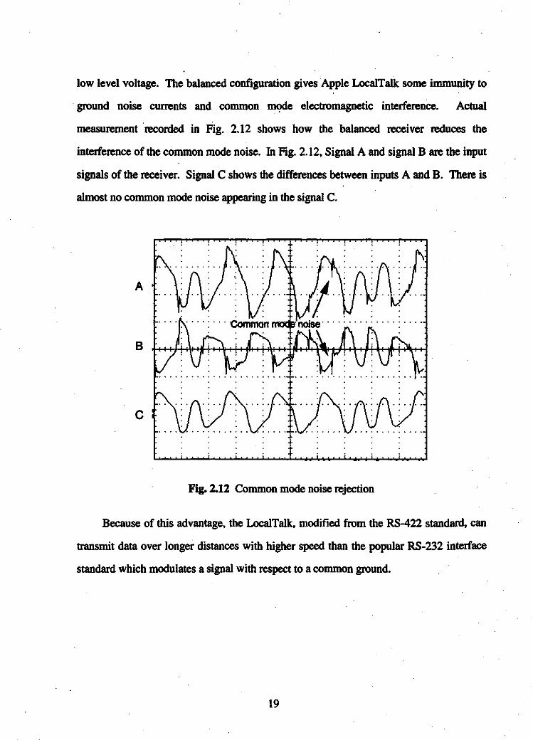
low level voltage. The balanced configuration gives Apple LocalTaIk some immunity to.
ground noise currents and common mode electromagnetic interference, Actual
measurement "recorded in Fig. 2.12 shows how the balanced receiver reduces the
interference of the common mode noise. In Fig. 2.12, Signal A and signal B are the input
signals of the receiver. Signal C shows the differences between inputs A and B. There is
almost no common mode noise appearing in the signal C.
B
A
c
Fig. 2.12 Common mode noise rejection
Because of this advantage, the LocalTalk, modified from the RS-422 standard, can
transmit data over longer distances with higher speed than the popular RS-232 intetface
standard which modulates a signal with respect to a common ground.
19

2.3.3 Serial Communication Controller (SCC)
The Zilog 8530 integrated circuit is used as the LocalTalk serial communication
controller. It performs physical layer functions and some data link layer functions as
well. Bit encoding/decoding, synchronization and carrier sense-
are carried out by this
controller.
The baseband bit encoding/decoding used in LocalTalk is biphase space (or FM-O).
The waveform is illustrated in Fig. 2.13. Note that each bit cell has a transition at its end.
The receiver uses this as synchronization information. There is an extra transition at the
middle of 0 bits. The Controller uses this mid-bit transition to decide whether the bit it
.receives is a 1 (mark character) or a 0 (space character).
I 1 I o I 1 I o I
Fig. 2.13 Biphase space signal
The see contains a Digital Phase Locked Loop (DPLL) to recover clock
information from the FM-O data stream. The DPLL is driven by a clock which is about
16 times the FM-O data rate [18]. The DPLL uses this clock, along with the data stream,
to construct a synchronized clock which is used to recover the received data.
The last function of physical layer is carrier sense. It is carried out by the SCC.
The see can detect whether there is a device on the net that is transmitting data, or
whether the clock of the data stream is missing. It reports such information to the Link
Access layer for further processing.
20

2.3.4 Spectrum of the Apple LocalTaik signal
If an infinite. length sequence of random binary data is assumed, after biphase
encoding, it bas the normalized power spectral density as in Eq. 2.1 [19].
rsin(!l!.)12P(f)-A7' 2' sin2(!l!.)-
, (!l!.) I 2
L 2 J Eq.2.1
where: P(f) is power spectral density (W1Hz).A is amplitude of signal (V).T is bit time (s),fis frequency (Hz). Range is -00<f< 00
For the 230.4 kbits/s LocalTalk data, Tis 4.34 us, If the amplitude A is 10 V, the
normalized power spectral density of the signal is illustrated in Fig. 2.14
0.25 • •••• 0.
· '"
· .
• ••••• 0
· .· .· .o ••••••
· .· .o ••••••
· .
0.05
¥ 0.2
�g� 0.15
'!Q)c... 0.1
�Q.
o����������--�����----��lk IOk lOOk 1M 10M
Frequency (Hz)
Fig. 2.14 Power spectral density ( showing only positive frequency)
21

The power spectral density of infmite random binary sequence with biphase space
encoding has some interesting characteristics.
The power in a specific frequency range can be calculated by Eq. 2.2.
E = 2J/2P(f)df/t
Power calculated in different bands is listed in Table 2.1.
ft ft Normalized power Percent of total(kHz) (kHz) (W) (ie.100W)
0 4 0�00086 0.00086%
4 30 0.3562 0.3562%
30 100 10.8253 10.8253%
100 150 18.9133 18.9133%
150 200 22.4102 22.4102%
200 250 18.2336 18.2336%
250 300 10.3084 10.3084%
300 350 3.7681 3.7681%
350 400 0.7179 0.7179%
400 460.8 0.0367 0.0367%
460.8 691.2 4.0065 4.0065%
691.2 Infmitv 10.4229 10.4229%
Table 2.1 The power distribution of the LocalTalk data
·22
Eq.2.2

.
The power distributed in the frequency band from de to 4 kHz, including the voice
band (300 - 3300 Hz), is about 0.86 mW (or -0.66 dBm), which is only 0.00086% of the
total power. The power is so small that a high pass filter can be used to eliminate it and
this will not cause any. significant distortion to the data signal.
The power of the signal in the frequency band from 30 kHz to 350 kHz has up to
89.22% of the total power. The first null in the frequency spectrum occurs at 460.8 kHz
and the power beyond 460.8 kHz is only about 14.43% of the total power. Thus, the main
power of the signal is concentrated between 30 kHz to 350 kHz and the components in
this frequency band should have as little distortion as possible .
.
2.4 LocalTalk Link Access Protocol (LLAP)
The main tasks of LocalTalk link Access Protocol are to provide link access
management, data framing, data frame transmission/reception and node addressing.
These tasks are conducted by the see and aSsociated software. The objective of this
protocol is to allow all devices on the LocalTalk network to share the same transmission
media and to tum the noisy physical channel to an errorless transmission line for the
network layer. The devices on the network which can perform this protocol are called
nodes. All nodes should be within a stand alone network (see Fig. 2.2)..
2.4.1 Link Access Management
All LocalTalk devices must be controlled by an access protocol to share the
common physical channel, otherwise the data transmission can not be reliable and
efficient. The LocalTalk link Access Protocol uses Carrier Sense Multiple Access with
23

Collision Avoidance(CSMAlCA). The hardware of LocalTalk can sense the carrier when
other nodes are transmitting, but it can't detect a collision. Collision avoidance is
realized by requiring the transmitter to wait for a randomly generated amount of time
after the bus has been sensed idle. Only after that random time can the transmitter send
its Request-to-Send control frame.
2.4.2 Data Framing
Information that is transmitted between data link layers is organized as frames. The
Apple LocalTalk link access protocol frame is shown in Fig. 2.15 .
•••
Flag Dest. Source Frame Data Field CRC Flag Abort
10 10 Type Sequence
(8 bits) (8 bits) (8bits) (8 bits) (0 to 4800 bits) (16 bits (8 bits) (8 bits)
Flag
(8 bits)-_.......
'-----------/'---------------------/'-------I:�-----/I IFrame preamble LLAP packet Frame trailer
(2 or more flag byte)
Flg. 2.1S LLAP frame
LocalTalk link access protocol uses bit oriented framing. Each frame starts with an
8-bit sequence (01111110) called a flag byte and each frame ends with the same flag byte.
The receiver uses these flag bytes to define the data packet boundaries. Therefore the flag
bit pattern is defmitely not allowed inside a data stream. In order to avoid the flag byte
sequence occurring inside the data stream which has arbitrary bit patterns, bit stuffmg is
necessary.. When transmitting data, if 5 consecutive Is are counted by the sender's link
access protocol, a 0 is automatically stuffed into the outgoing stream. The receiver's link
24

access protocol performs the process vise versa. When 5 consecutive Is followed by one
o is counted, the receiver deletes the 0 from the received data stream automatically.
Following the starting flag bytes, the frame has a destination ID byte and a source
ID byte which are the 8 bit addresses of the receiver and sender. The frame type byte
classifies the frames as control frames or data frames. The control frame doesn't have a
data field. There are two pairs of control frames used in !LAP. One pair is called
enquiry control (ENQ) and acknowledgment control (ACK) frame. They are used in
addressing (detailed in Section 2.4.4). The other control pairs are called Request-to-Send
(RTS) and Clear-to-Send (CTS) frames. They are used to control data packet
transmission (see 2.4.3).
The 16 CRC-ecrIT frame check sequence is applied to the LLAP packet. The
abort sequence indicates the end of the frame. All framing operations (adding/deleting
flag .
bytes, bit stuffing and CRC calculation/check)· are accomplished by the serial
communication controller (SCC).
A synchronization pulse is transmitted before a LLAP RTS frame. Fig. 2.16 shows
the sync pulse.
;yncPUIsef
- -
----
- - -
.._---, - � � � �
LocaITaik Data
Fig. 2.16 Start of a LocalTalk RTS frame
25.

All receivers on the network can take the transition of the synchronization pulse as a
clock, but shortly they will lose this clock due to the following idle period of sufficient
length. The missing clock detected by the receivers allows transmitters to synchronize
their access to the line and know right away that another transmission is about to take
place. The LLAP uses the synchronization pulse to help LocalTalk hardware detect the
channel status and to reduce the probability of collision.
2.4.3 Frame Transmission/Reception
Directed and broadcast transmission dialogs are two types of frame transmission in
LLAP. When two specific nodes in the network exchange information directly with each
other, it is called a directed transmission dialog, while a node sending its data frame to all
nodes on the network is called a broadcast dialog. There is only one dialog allowed on
the channel at one tinie. Between two dialogs, there must be at least 400 fJ.S gap (called
inter-dialog gap or lOG). Different frames in one dialog must be separated by less than
200 us (called interframe gap or IFG)
The implementation of the CSMAlCA protocol in a directed transmission dialog is
illustrated in Fig. 2.17. The implementation of a broadcast transmission dialog is similar
to that of a directed transmission dialog.
The operation of a receiver in the destination node is relatively simple. A node on
the network can receive broadcast packets or a frame whose destination address matches
the node's 10. Any bad frames which are caused by invalid frame type; synchronization
error or an incorrect CRC will be rejected by the receiving node.
26

According to the directed frame transmission dialog, the maximum valid range for
performing LLAP can be calculated. After transmitting the RTS frame, a sender must
receive the ers frame within the maximum inter-frame gap (TIFG). The IFG (inter-frame
·gap) starts from the end of the abort sequence of the previous frame's trailer to the first bit
of the current frame. Therefore, Eq. 2.3 must be satisfied.
TIFG � TIrl'D+ Tp Eq.2.3
where: TIFG = 200 J1S.
TIrl'D is the round trip delay between the sender and the receiver node.Tr is the time needed for receiver to answer the received RTS frame.
FromEq.2.3
TIrl'D � TIFG - Tp Eq.2.4
According to measurements in our laboratory, the longest time needed for the
receiver to answer a RTS frame (Tp) is about 104 us. Substituting Tp with 104 us and
TIFGwith 200 us, TRTD can be calculated from Eq. 2.4 as
TIrl'D s 96 JlS Eq.2.5
The speed of a signal that is transmitted in the twisted pair cable is about 213 of
light speed (c) [20]. The maximum TRTD is 96 JlS, thus the maximum valid range (£max)
that the LLAP can perform correctly is given by
2 .
-Xc x max(TIrl'D)Lmax = _3 _
2.. 9.6km
Eq.2.6
27

LLAP bas physical layer sense the channel
Keep sensing the channel for extrarandom time whose range is based oncollision and the deferment history
Defer thistransmission
Transmit synchronisation pulseand RTS conlrOl frame withdestination device address
Sender assumes acollision happened.This transmission
dialog failed
Fig. 2.17 Directed data transmission dialog
28
Step 1
Step 2
Step 3
Step 4
StepS
Step 6
Step 7
Step 8

"
2.4.4 Node Addressing
LocalTaIk uses a dynamic node address assignment scheme. Each node in the
network has an 8-bit address that ranges from 1 to 254. When a new node is connected to
the network, it randomly picks an initial address. In order to verify that this address is not
used by other nodes, the new node sends an enquiry control frame (ENQ) to the initial
address. If an acknowledgment control frame (ACK) is received, the new node knows
that the initial address is already used and it has to pick another address and verify it
again. If no response is received, this node can use this initial address as its address.
2.5 Network Layer and Other Upper Layers
The network layer in AppleTaIk uses Datagram Delivery Protocol (DDP). While
the LLAP protocol exchanges frames over a stand-alone network, DDP provides
datagrams delivery over an AppleTaIk internet (see Fig. 2.3 and Fig. 2.4). Network
addressing, packets circulating and packets routing algorithm are considered by DDP.
Transport layer in AppleTaIk can change the unreliable DDP datagram service to a
loss-free delivery [12]. This function gives upper layer a reliable data service. It also
provides routing table maintenance protocol for DDP routing algorithm, echo protocol for
network test and name binding protocol for easier access to the network.
Session layer is built on transport layer. It provides session establishment,
maintenance and cancellation. This layer also provides printer access protocol for work
stations to use printer service, Data Stream protocol for a reliable duplex data delivery,
and zone information protocol for network access management.
29

The presentation layer is built on the session lay�r. The:AppleTalk presentation
layer mainly provides AppleTalk filing protocol for remote file access.
Application layer usually refers to the application programs that use the network
services supported by AppleTalk.
30

Chapter 3: Transmission Line Theory
A transmission line can carry electrical signals over a certain distance. When the
length of the transmission line is longer than 1/8 wave length, the transmission of the
signal should be analyzed using transmission line theory [21]. Data transmission at 230
kbits/s on the telephone subscriber line must be analyzed with transmission line theory.
The speed and distance of data communication are limited by factors such as signal
attenuation and signal reflections.
3.1 Transmission LineModel
In practical cases, two transmission lines usually IUD in parallel and are separated
with a constant space,.therefore a relatively consistent capacitance exists between ·the two
lines. There is a small amount Qf leakage in the insulation between the two wires and
. causes conductance in every unit length of the line. The conductors of the line have
series resistance and inductance distributed on the line. Since the transmission line has
distributed electrical elements, it can not be simply modeled as a single circuit.
The transmission line model is shown in Fig. 3.1, where dx is an infinitely sbort
. length of the line an� x is measured from the load toward the sending end of the small
31

section dx. For simplicity, the inductance and resistance in the two wires are combined
and the model is presented with a ground reference. The distributed elements per unit
length are I (inductance), g (conductance) r (resistance) and c (capacitance). These
elements are fundamental electrical characteristics of the transmission line, so they are
also called primary constants. Voltage V and current I are functions of x. Both V and I
are vectors with magnitude and phase angle..
ILoad IV+dV
I
I I
� dx �I�
0 x
Fig. 3.1 Transmission line model
3.2 Circuit Analysis of the Model .
The distributed character of the line causes.
the current and voltage to change
continuously along the transmission line. Current at one end of a short section of line
differs from current at the other end because of the leakage current through the
distributed conductance and the shunted current through the capacitance from wire to
wire. Voltage also varies from point to point because of series inductance and resistance.
32

Because the line model has both series and shunt parameters distributed along the
circuit, it is necessary to analyze the transmission line model starting from any
intinitesimal length of the line (dx). The voltage drop on dx is
dV = (rdx+ joidx)I
or : = (r+jwl)IEq.3.1
where (I) is the radian frequency.
The current change in section dx is.
or
dl = (gdx+ j(J)Cdx)VdI -
;;; =(g+ jr«)V Eq.3.2
The voltage and current at point x can be obtained by solving Eq. 3.1 and Eq. 3.2:
V = Vlex.Jzy+ V2e-x.Jzy
I = Ilex.Jzy +be-x.JzyEq.3.3
Eq.3.4
where z = r + jOJl, y = g + j(J)C and x is the line length starting from the load.
The physical meaning of Sq. 3.3 and Eq. 3.4 is very important in the transmission
line theory. Eq. 3.3 can be explained as the voltage on a transmission line is the sum of
two traveling waves, one is the incident wave which travels toward the load and the other
is the reflected wave which is sent back from the load. Eq. 3.4 shows that the .current is
also the sum of an incident wave and a reflected wave. VI and V2 are incident and
reflected voltages at the load end (x = 0). _ II and 12 are the corresponding currents of VI
and V2. Some important transmission line parameters can be obtained from Eq. 3.3 and
Eq.3.4
33

Characteristic Impedance:
The relation between VI and V2 and their corresponding currents II and 12 can be
obtained by substituting Eq. 3.3 and Eq. 3.4 into Eq. 3.1 and Eq. 3.2 [22]. The results are
VI=i r+ j(J)/ IIg+ j(J)c
Eq.3.S
and
v2=_jr+,i(J)/12 .
g+ j(J)cEq.3.6
Eq. 3.5 and Eq. '3.6 show that the incident and reflected voltages and currents are
lated br+ joi
aIled h. . .
pedan U all h. . .
pedanore y .' c c aractensuc im ceo su y, c aractenstic 1M ces+ J(f}C
can be written as
7A=�where z = r + joi andy = g + j(f}C
Eq.3.7
Eq. 3.5 and Eq. 3.6 can be rewritten as
VI = Zoll Eq.3.8
.V2=-ZoI2 Eq.3.9
Each type of transmission line has its own characteristic impedance. It is based on
the distributed elements of the transmission line and not on the length of the line.
Propagation Constant
The·propagation constant ris defined as Eq. 3.10,
34

Eq.3.10
Since both % and y are complex numbers, the propagation constant is a complex
number as well. It has a realpart a and an imaginary part j!J.
r=a+jp Eq.3.11
The real part is called the attenuation constant, which quantifies the voltage or
current attenuation on the transmission line. The imaginary part is called the phase
constant, which is responsible for phase shift when the signal is measured at points along
the line. The delay at certain frequency can be calculated by .
pDeiay=
co Eq.3.12
where P is the phase shift, co is the radian frequency.
Because delay depends on the frequency, different frequency waves have different
transmission delay and therefore the delay has a nonlinear relation with frequency.
Since characteristic impedance (Zo) and propagation constant (» are derived from
the primary constants and are also used to describe the· transmission line characteristics,
they are called secondary parameters. The primary constants and the secondary
parameters are temperature dependent. The conductor's resistance changes with
temperature, so the attenuation is higher when temperature is higher.
.
The Reflection Factor
The voltage or current at every point of the line is the sum of the incident and
reflected voltages or currents. The reflection level of the reflected signal can be
3S

measured as the voltage ratio.
between reflected signal and the incident signal at the
receiving end (x = 0). This ratio is called the reflection factor.
According to definition, the reflection factor can be written as
V2o=x:V. Eq.3.13
where VI is the incident voltage at the receiving end and V2 is the reflected voltage.
The voltage (Vr) and current (Ir) at the receiving end can be obtained by
substituting x = 0 to Eq. 3.3 and Eq. 3.4.
Vr=VI+V2 Eq.3.14
Ir=II+12 Eq.3.1s
The impedance at the receiving end is
Zr=Vr
Ir Eq.3.16
To combine Eq. 3.16, Eq. 3.15, Eq. 3.14, Eq. 3.9 and Eq. 3.8 together, the relation
between VIand V2 can be obtained as
V2 Zr-ZoEq.3.17VI Zr+ZO
so the reflection factor can also be calculated as
Zt-Zo
·P=Zt+Zo Eq.3.18
36

3.3 Termination of the Transmission Line
When the transmission line is terminated by a load whose impedance Zr is equal
to the characteristic impedance Zo, the reflection factor pis 0 (see Eq. 3.18). This
means there is no reflection at the load. This is called impedance matching. If the
transmission line is terminated by any load whose impedance is not equal to Zo in
phase and magnitude, a reflection will appear.
One extreme impedance mismatch case is when the transmission line is an open
circuited line which has no load at the end. The bridged tap, which will be discussed in
Chapter 6, is similar to this case so it is necessary to know how waves travel in the
open-circuited line.
Because the load of the open circuited line is infinitely large (Zr ... (0), the limit of
the reflection factor is 1. This means that the total incident wave is reflected back to the
source. The voltages ofwaves at different points on an open-circuited line are shown in
Fig. 3.2.
Incident Voltage
V 1/4J.�,e
. IncidentVoltage
V 1/2J.�VI ,e
.. V(x=O) .... ..
..V(x=112t)
.........V2
Reflected
Reflected Voltage Voltage
V -1/4J.� V -1/2J..jzy2e ze
(a) (b) (c)
Reflected Voltage
V -3/4A�2e
V(x=314t)
Incident Voltage
V,e3/4J.�(d)
Fig. 3.2 Voltages at different points on a line
37

In Fig. 3.2a, VI and V2 are the incident and the reflected voltage at the load end (x =
0). At this point, VI and V2 are equal in phase and magnitude. Voltage V(PG) is the sum
ofVI and V2.
Fig. 3.2b shows the voltages at a point of 114 wavelength from the load end. The
reflected voltage at this point lags 90 degrees with respect to the reflected voltage at the
load end. The magnitude of the reflected voltage at this point is also smaller than the
reflected voltage at the load point because of the attenuation of the transmission line.
The incident voltage at this point leads the incident voltage at the load point by 90
degrees and has larger magnitude. Therefore the two vectors are opposite to each other
and result in a small sum voltage V(x=lI4A).
At 112 wavelength from the load point, the incident voltage and the reflected
voltage are in the same phase again but have 180 degrees difference to the voltages at the
load end (shown in Fig. 3.2c).
Fig. 3.2d shows the vectors ofthe incident voltage and the reflected voltage at 3/4
wavelength point. The phases of the incident voltage and the reflected voltage have 180
degrees difference. Again the sum of the two vectors is small.
According to Fig. 3.2, the voltage attenuation can be high if the point is. at 0/4
wavelength, where n is an odd number.
In low speed data transmission, the wavelength of the data is long, the reflected
signals have to travel' longer distance and lose more power to get the 114 wavelength
point. Therefore, a small amount of reflected signal is allowed and it is not necessary to
tenninate the transmission line by a load whose impedance exactly equals Zo.
Practically, impedance matching for the low speed data is usually realized by using only a .
38

matched resistor at the load, such as the termination used in LocalTalk network which is
discussed in Chapter 2. However, the wavelength of the high speed data is very short,
the reflected signals lose little power to get the 114 wavelength point and a small amount
of reflected signals can seriously interfere with the incident signals. As a result, the
impedance matching in phase is as importarit as in magnitude.
3.4 Transmission Cables in Telephone Networks.
Transmission cables play very important roles in telecommunication systems. Local
telephone and cable TV networks are mainly connected by transmission cables. Because.
the signals are transmitted in an guided manner, these cables are also called a guided.
transmission medium [23]. According to the structure, transmission cables can be
classified as open-wire lines, paired cables and coaxial cables.
3.4.1 OpenWire Lines
In the early years, telephone networks were connected by various forms ofmultiple
line wires which were hung between telephone poles. These open wires were subject to
cross talk and the effects of rain, frost, and ice on transmission [24]. Because of these
disadvantages and the 'high cost ofmaintenance, most open wire lines have been replaced
by coaxial cables and paired cables in modem telephone networks.
3.4.2 Coaxial Cable
The useable bandwidth of a coaxial cable is very high and up to 10,800 voice
channels can be carried by a single coaxial unit [25]. Although the cost of the coaxial
39

cable is high, the per-channel-mile cost is still low if it is used in a high traffic place.
Thus, the coaxial cables are often used as tol.1 cables in the telephone networks.
Because the inner conductor is surrounded by the cylindrical conductor, the coaxial
unit has excellent immunity to cross talk and outside noise than the twisted pair when
compared with twisted pair. The coaxial cable's attenuation is nearly proportional to the
square root of frequency and the velocity of propagation and characteristic impedance
vary slightly with frequency. Coaxial transmission line can be installed as a single
coaxial unit or as a cable made up of 4 to 22 coaxial units (See Fig. 3.3). Each coaxial
unit consists of a ho�ow cylindrical conductor surrounding a single wire conductor. The
space between the cylindrical shell and the inner conductor is filled with a plastic
insulator. A number of wires are packed in among the coaxial units and are used for.
maintenance support and control.
Fig. 3.3 Coaxial cable
(A copy from Principles ofElectricity applied to Telephone and Telegraph Work [24J)
40

3.4.3 Paired Cables
Telephone subscriber station sets are connected with paired wire cables to local
switching and transmission equipment. The average length of this subscriber
transmission line is approximately 3 km, Cable conductors are insulated with.
polyethylene or pulp papers, and twisted in pairs. Groups of such pairs can be twisted
into a rope-like unit. Several units are twisted together to form a cable core. This type of
strucmre can provide. equal interference exposure to each wire pair and minimize the .
electromagnetic interference from neighbor pairs, power lines and other sources. In order
to prevent damage to cables from water penetration, rodents and corrosive elements in
the soil, protective methods are necessary.
In North America; the size of the conductor in a paired cable is standardized as
America Wire Gauge (AWG). Table 3.1 shows some most commonly used AWG
conductor dimensions [21]. The primary constants of different size. cables are not the
same, so the propagation constants vary as shown in Fig. 3.4 and Fig. 3.5 [34].
AWG 19 22 24 26
Diameter (nun) 0.912 0.645 0.511 0.404
Table 3.1 AWG wire size
The attenuation of these cables is similar in the low frequency band but there are
significant differences at high frequency. With frequency increasing, the attenuation of
larger size cable (such as AWG 19) grows more slowly than that of smaller size cable
(such as AWG 26). Fig. 3.5 shows that the delay curves of different size cables are
almost the same at higher frequency; but the larger size cable has smaller delay in the low
41

frequency band. These two figures indicate that the larger size cable has a wider
bandwidth and is suitable to high speed data transmission and carrier systems. In the
telephone network, AWG 26 PIC (polyethylene insulated cable) is mostly used in a
subscriber loop whose main purpose is to transmit voice. AWG 24 and AWG 22 cables
are used in 1.544 Mbits/s Tl trunks or other types of toll trunks [21].
30
2S
j201%1
�g 15.;�=
! 10
5
01
PIC cables at 20 VC AWG26i;j;i ; AWG24i l. ,
/! AWG22l :' I.� :" /
.
.' s I
��� // AWGI9.� .... ,'
.�.�'�""""""",,�, .... ,
,.., .•....... �..,,,,,,,
",.�:...;;::..,-_......
.....�;,;f;..;;.....,.-
10 lOOk 1M100 It lot
Frequency (Hz)
Fig. 3A Attenuation of different size cables vs. frequency
1000
eiloo-
��.
10
PIC cable at 20°C
lL_--------�--------�10:k��100�k�.�lM10 100 lk
Frequency (Hz). bles vs. frequency
Fig. 3.5 Delay of different sIZe ca
1
42

As mentioned before, the propagation constants change with temperatures. The
propagation constants of AWG 26 PIC cable at different temperatures are illustrated in
Fig. 3.6 and Fig. 3.7 [34].
35------�--�--------�-------------
. 30.
m25:E.c�2 20a;::::scCD 15�
10
10 100 100k 1M1K 10k
Frequency (Hz)
Fig. 3.6 Attenuation of AWG 26 cable at different temperature
100004912C:20 12C: . . . . .
1000 -1812C: -----
�100::::I.
-
l;'a;0
10
10 1K 100k10k100
Frequency (Hz)
Fig.3.7 Delay ofAWG 26 cable at different temperature
43
1M

Fig. 3.7 and Fig. 3.8 show that the effects of the temperature are not serious. The
delay factor is almost unchanged and the attenuation only has a maximum difference of
3 dB from -18 OC to 49 OC.
The characteristic impedance of the cable also changes with frequency. For
example, Fig. 3.8 and Fig. 3.9 shows the characteristic impedance of the AWG 26 cable
at 20 OC.
lOOk
10k
c:Ik
�
100
10------�----------�----�----------I 100 It lot
Frequency (Hz)Fig. 3.8 Characteristic impedance ofAWG 26 cable vs frequency
10 lOOk 1M
o�----�----------------------------
-10
-
·1 -20c!.-
� -30
-��----�----�----�----�--��----I 10 100 It lot lOOk 1M
Frequency (Hz)
Fig. 3.9 Angle of the characteristic impedance vs frequency .
44

The characteristic impedance of the cable is high in the low frequency band and
changes to about 100 n with increasing frequency. The angle of the characteristic
impedance has a sharp curve from 10 kHz to 1 MHz, so it is not easy to completely. .
match the cable's characteristic impedance in magnitude and angle over a large frequency
band.
In this project, data are transmitted in an AWG 26 cable. This type of cable will
cause delay distortion (or phase distortion) and attenuation distortion in the data signal.
The distortion caused by the different attenuation between different frequencies is called
attenuation distortion. As shown in Fig. 3.4, the AWG 26 cable has the largest
attenuation distortion of the cable pair family. Delay distortion is caused by the lower
frequencies having longer delays than the higher frequencies (See Fig. 3.7). Since the
delay will create incorrect relative phase, it is also called phase distortion. The difference
in delay between different frequency components increases with transmission line length.:
As shown in Fig. 3.10A, Curve lA has two harmonics, a and b. If the delays of
harmonics a and b are not the same, a distorted Curve IB occurs as shown in Fig. 3.10B.·
1\,
.
. ,!
aa
A B
Fig. 3.10 Dlustration of delay distortion
45

Chapter 4: Data Transmission
In passband transmission, a carrier can be used to modulate the data before the
transmission. Alternatively the data can be sent directly without any modulation. and
this is called 'baseband transmission. The passband transmission can move the spectrum
of the data to a specific frequency range that is suitable for the requirement of the
communication channel. However, the passband transmission needs a modulator in the
transmitter and a demodulator in the receiver, therefore this system becomes relatively
complex. The baseband transmission only needs a transmitter and a receiver, so it is
simple and suitable for short distance communication. This project uses baseband
transmission.
4.1 Baseband Transmission
According to different analyzing requirements, baseband transmission can be
abstracted as coded baseband transmission or baseband pulse transmission._
4.1.1 Coded Baseband Transmission
A coded baseband transmission system can be block-diagrammed as in Fig. 4.1.
The line encoder encodes binary data to one specific channel code-
whose bandwidth,
46

spectrum, timing information, and error control are most suitable for the transmission.
The encoded signals are transmitted to the channel by the line driver. The receiver and
line decoder recover the binary data from the encoded signals at the end. The .
characteristics of the transmission channel and the receiver complexity determine which
channel code is the best choice.
Transmission Channel
Fig. 4.1 Coded baseband transmission model
Several common used channel codes are illustrated in Fig. 4.2.
cia1
1 0 1 1 0 0 0 1 11
.
RZ+01
+1 1NRZ-L 01 1
- 1 I 11 1
INRZ-M �I 1- 1 . 1
+1 INRZ-S 01- 1
Bipolar
. I
Fig. 4.2 Channel codes formats
47

Return to Zero (RZ) Code
A RZ code is an unipolar code. The binary 1 is represented by a positive pulse
for half-bit period then returning to zero and a' binary 0 is encoded to zero level. The
advantage of this coding technique is relatively simple, but it doesn't have
synchronization capability and has strong direct-current (de) component, Because of the
dc component in the signal, transmission equipment must be directly physically attached
and can not be coupled via a transformer. The direct connection is vulnerable to
interference due to the lack of electrical isolation.
Nonreturn to Zero (NRZ)
NRZ codes are polar codes. The binary 1 and 0 are represented by equal positive
and negative voltages whose levels are constant during a bit interval. Because NRZ-L
(NRZ level) is the simplest code to implement, it can be used to generate digital data by
data processing terminals and can be changed to other types of code by the transmission
system. The NRZ coding is very easy to be realized and has a narrow bandwidth, so is
widely used in the data communication systems. However, the problems with the de
component and synchronization are still remained in NRZ signals. NRZ-S (NRZ space)
andNRZ-M (NRZmark) are differential NRZ·codes.
In differential coding, the encoded differential data is generated by
en = doXOR en-t
where en is the encoded sequence.en-l has 1 bit delay to en.
dn is the input sequence.
Eq.4.1
The received data is decoded by
dn = en XOR en-l Eq.4.2
48

The advantage of differential codes may be illustrated by the differential encoding
and decoding example shown in Fig. 4.3 [19].
EncodingInput sequence cia 1 0 1 1 0
&.
i�1 1 0 1
en = dn XOR en-I 0. 1 0 1 1 Encoded sequenceReference digit
Decoding (with correct channel polarity)Received sequence e. O�l 1 0 1 1
Ca-. . 0 1 1 0 1
dn=en XOR en-t d. 1 0 1 1 0 Decoded sequence
Decoding (with inverted channel polarity)Received sequence e. l�O 0 1 0 0
&. 1 0 0 1 0
dn = en XOR en-l cia 1 0 1 1 0 Decoded sequence
Fig. 4.3 Example of differential coding
According to this example, an encoded sequence can be generated by inserting a
reference digit to the first bit of the sequence and encoded by Eq. 4.2. For decoding
operation, no matter whether the polarity of .received sequence is correct orinverted, the
received sequence can be always decoded correctly. This is a great advantage in the
complex transmission system where the sense of the polarity of the signal may be easily .
lost.
Biphase
Biphase coding has several advantages over NRZ and RZ coding techniques.
Because biphase coding requires at least one transition per bit interval, a receiver can use
these predictable transitions during each bit time to synchronize the received data.
Therefore, biphase codes are also known as self-clocking codes. The absence of an
·49

expected transition can be used to detect errors. Besides the .
advantages.
in
synchronization and error detection, biphase codes have no de components. This is
desirable in many applications. The disadvantage of biphase codes are that they have
wider bandwidths.
Biphase codes are widely used in network data. transmission. For example,
Ethernet uses Biphase-L �chester) codes and LocalTalk network uses Biphase-S
(differential) codes.
Bipolar
Bipolar coding uses 3 encoded signal levels (+, 0, -) to represent binary data (0,1).
Since successive I's have alternative positive and negative polarities, bipolar provides
some error-detection capability. Bipolar codes also have advantages of no de component
and having narrower bandwidth than biphase codes. In addition, Bipolar codes have
some synchronization capability. TI-PCM transmission uses bipolar coding.
4.1.2 Baseband Pulse Transmission
A baseband pulse transmission system model is shown in Fig. 4.4.
bnpt-tn1 (ready fi
ulses Pulse shaping � Channel Receiver and- - -
� filterH«(I)- &«(1) - filter 8-«(1)
-
l-n1) JJ(t) WM(I).
"'-(I)
FlatRecovered pulses
orsampliogdecoding)
"
Fig. 4A Baseband pulse transmission system model
A series of impulses is input into the pulse shaping filter (H(w» with the rate lIT.
The pulse shaping filter modifies the impulses to flat-topped pulses (W(t» and they are
so

changed to Win(t) after the pulses go through the channel (Hc(o»,. Wout(t) is the response
of the receiver filter (Hr(o>)) with the input of Win(t).
We may assume that the impulse response of the system is h(t), but when only
one impulse is input into the system, the output Wout(t) can be treated as an impulse
response of the system.
4.2 Intersymbol Interference
Based on Fig. 4.4, we assume G(0» to be the spectrum of a pulse. The spectrum
of the received pulse at the receiver is
Wout(O» = G(o»Hc(o»Hr«(J) Eq.4.1
If an undistorted pulse is wanted at the receiver, the following condition must be
satisfied:
{IHc(o»Hr«(J)1 = K 10>1 S en:
IG((J)I =0 1m! > en:Eq.4.2
where.en: is the channel cut off frequency.
However, the absolute bandwidth of a pulse is infinity. Therefore, if these pulses
are passed to a communication system with limited bandwidth, theywill smear out in the
time domain and interfere with adjacent pulses. The interference between data pulses
after being transmitted through a band limited channel is called the intersymbol
interference (lSI).
Intersymbol interference is an important issue in data communication. h will
worsen the noise immunity and cause decision errors at the receiver.
51

4.3 Equalization and Predistortion
In a practical transmission system, it is impossible to transmit data without
distortion. The bandwidth of the transmission channel is always limited and the
spectrum of the pulse extends to infinite frequency, so intersymbol interference is
unavoidable. In order to achieve a less distorted signal, it is necessary to compensate for
the magnitude and the phase characteristics of the transmission system..
This kind of
adjustment is called equalization if the adjustment is conducted to the received signal
before the receiver, or predistortion if the adjustment is made before the signal is
transmitted to the channel.
Usually the equalizer is placed in front of the receiver as shown in Fig. 4.5.
When the equalizer is located at the receiver, the distortion of the line can be determined
and automatically compensated by an adaptive equalizer. For this project, we are using a
fixed equalizer that has lower cost and less complexity .
...
Q).t:I1ii::::sI:TW
Distortedsignal in Decoder Received
data
Receiver
·Fig. 4.5 The application of the equalizer
The predistorter can be placedafter the line driver. The use of the predistorter
can reduce the complexity of the equalizer at the receiver side and increase the
performance of the system.
One specific predistorter that is used in this project will be described in Chapter 6.
Two categories of equalizers are described in the following two sections.
52

4.3.1 Frequency Domain Equalization
The objective of frequency domain equalization is to compensate for the
frequency dependent attenuation caused by the channel and to linearize the phase versus
frequency response of the channel. The ideal attenuation and phase equalizations are
shown in Fig. 4.6a and Fig. 4.6b. According to these two figures. we can see that the
gain and delay responses of an ideal equalizer are inverse curves of the line loss and
delay.
�� ------------��/T'I.....
.._.u..--III......... • •••••
......---
� ,
..
•...... ····���on after
«» ••••••••'
.- ideal equa1ization..................................... ,
o --_
-----� ...�
...............; ,_UIIe attenuation ..............
..........,""
-����I------�------�I-O------�I�oo�--��IOOOFrequency (kHz)
FIg. 4.68 Ideal equalization (Attenuation)
I.....
10�IfJ -10
�
ISO Delay after ideal pbareequaIizaaion
l� �_���-------------.,.,,,_,,
...
...... ,.,."............_ Delay iDIroduced
! tOO �"'" ��" by equalizer". ��r.- '.,
'9 �'"Q .
LA10"
'.. Delay iatroduced
V"1#
••••'." � by line
"
-."
........................................................................ .
0.1 10 100 1000FRqueac:y (kHz)
Fig. 4.6b Ideal equalization (Phase)
S3

Unfortunately it is impossible to flatten the magnitude or linearize the phase over
all frequencies. The equalizer can only compensate for the attenuation or linearize the
phase in a certain frequency range. Usually, the equalization is conducted over the
frequency range where the power of the signal is concentrated. For LocalTalk data. it has
high power density from 30 kHz to 350 kHz. The frequency domain equalizer should be
focused on this range.
Because frequency domain equalization must know the channel's frequency
responses; so only those channels whose frequency responses are well known, such as
twisted pair or coaxial cable, are -suitable for frequency domain equalization. The
compensation ability and precision of this kind of equalizer are not high, but frequency
domain equalizers are efficient for use in the system where the bandwidth is not strictly .
limited and the signal distortion is not very serious. Although there are some restrictions
in application, frequency domain equalizer has the advantages of simple design and low
cost.
4.3.2 Time Domain Equalization
If the equalization is performed in the time domain, it is called time domain
equalization. The key issue for time domain equalization is to minimize the intersymbol
interference. There are a lot of algorithms available for time domain equalization [26).
The simplest one that can be used to illustrate how the equalizer works is the zero forcing
algorithm. The objective of this algorithm is to let the system impulse response (h(t» of
the transmission system (see Fig. 4.4) satisfy the following conditions:
{C, k =0h(kn=
0, k¢OEq.4.3
Where T is the symbol (sample) clocking period.C is a non-zero constant and k is an integer ranged from -00 to +00.
54

If Eq. 4.3 is satisfied, a single flat-top pulse, generated from an impulseby the
pulse shaping filter (see Fig. 4.4) going through the transmission system, would have a
value Cat t = 0 but would not cause interference (h(t) = 0) at other sampling times (t =
kT, for k ¢ 0) (see Fig. 4.7). Therefore intersymbol interference is eliminated at each
sample moment.
..
"
Sample Points
t
Fig. 4.7 Waveform with zero lSI
. The zero forcing algorithm can be rea1ized by a transversal filter which is often
used for time domain equalization. As illustrated in Fig. 4.8, the transversal filter
consists of a tapped delay line where the tap outputs aremultiplied by a set of gains {Cn} �
The resulting weighted tap outputs are summed to produce the filter output WoUl{t). The
tap spacing is chosen to be equal to the symbol duration T or a fraction of the symbol
duration.
W-(t)
. OutputFig. 4.8 Transversal filter
55

The key issue in designing the transversal filter is to fmd the set {Cn} that can
eliminates lSI. In order to get the {Cn}, we have to start from the output of the filter.
The output of the filter is related to its input by
Wout(t) = C-NWin(t) + C-N+IWin(t-T) + ... + CNWin(t-2N1)
or
N
Wout(t) = LCnWin(t - (n + N)T)".-.N Eq.4.4
Evaluating the samples of Wout{t).at the sampling times t = kT, we getN
Wout(kT) = LCnWin(kT -(n+ N)T)".-N
N. = LCnWin«k - n - N)T)".-N Eq.4.5
According totbe zero forcing algorithm described by Eq. 4.3, Eq. 4.S should satisfy
and
S6

and
Wia(-NT) Wia(-(N-I)T) ••• Wia(-3NT)
·w.=Wia((-N+1)T) Wu.{-NT) ••• W",((-3N+I)T)
• •• •
• •
W#II(NT) Wtir((N-l)T) ••• Wu.{-NT)
To solve Eq. 4.7, the gain set {en} can be calculated as
C =Win-lWont Eq.4.8
In the practical circuit, it is not necessary to solve EquatiC?n 4.7. The equation can
be solved by an adaptive approach. There are two modes in operating this adaptive
equalizer. One is the training period. During this mode, a known sequence is transmitted
and a synchronized version of this signal is generated in the receiver simultaneously. The
equalizer compares the received version to the generated one and uses the errors between
the two versions to adjust the gain set {CII}. When the training period is completed, the
adaptive equalizer is switched to the decision directed mode. During this mode, the data
is received correctly with very high probability, so the system operates at a very low error
rate.
Digital technology is used in the implementation of the equalizer. The input
signal is sampled and quantized. The transversal ftIter is replaced by shift registers where
the quantized input signal is stored. The tap gains {Cn} are typically stored in the
memory of a micro-controller. Multiplication, addition, and {CII } adjusting are
performed by the micro processor [26].
Time domain equalization does not care about the channel frequency response.
No matter how complex the channel is, the equalizer only needs to adjust the impulse
response of the channel to be zero at the sampling point. If the number of the tapped
delay elements is large enough, the intersymbol interference can be reduced to a
. sufficiently small amount.
57

Generally time domain equalization has advantages over frequency domain
equalization. But the time domain equalizer is much more complex and costly than the
frequency domain equalizer. Therefore, frequency domain equalization still has its value
in some applications. ..
4.4 Eye Diagram
The eye diagram (or eye pattern) is a practical method to see the intersymbolinterference. In the laboratory, the eye diagram can be recorded by the system shown in
Fig. 4.9
A pseudo-noise (PN) signal generator generates a pseudo random data sequence.
The data is encoded to a certain channel code by the channel encoder and transmitted
over the channel. The circuit details of the PN signal generator and the encoder are
shown in Appendix 2.
Pseudo-noise
SignalGenerater
Encoder Line DriverCommunicationChannel·
Sco
Clock
Extern Trig VertReceiverBye Diagram
Fig. 4.9 System for laboratory eye diagram recording
The received signal is the input to the vertical deflection plates of an oscilloscopeand the data clock signal is used to trigger the scope. Thus" the scope overlays equal
length segments of the received wavefoim. The resulting display looks like human eyes,
so the result is called an eye diagram.
58

The eye diagram of the biphase code which is used in LocalTalk: is shown in Fig.
4.10. There are two smaller eyes in one big eye. After the data signals are transmitted
through the communication channel, the original data eye diagram (see Fig. 4.10) iso 0
distorted by the intersymbol interference and noise (see Fig. 4.11). Under normal
operating condition, the eyes are open. If there is a great deal of intersymbol interference
or noise, the eyes will close. This indicates that a lot of bit errors should occur at the
receiver.
The eye diagram provides an excellent way of analyzing the quality of the
received signal. The interior region of the eye diagram is called the eye opening. The
width of the eye opening (W in Fig. 4.11) defines the time interval over which the
received wave can be sampled without an error from the intersymbol interference. The
best time for sampling is at the point where the vertical opening of the eye is the largest
The sensitivity of timing error is given by the slope of the open eye and the noise Margin
of the system is given by the height of the eye opening (h in Fig. 4.11) [19]. Larger and
clearer eyes have less errors and higher noise immunity.
!
· . .. .
� - ..
· . .. .
· . .. ..
r-.••••••••••••••••••••••••__• • • • • • • • • • • • •• • ..
o • • • • • 0
· . . . .
••••
:••••••••••••••
:...... i"o0 ••• :
••••
:••••
:• 0
••• :••• __
,.. .....
i i i:
. -_...
·
·
.... _ ...
·
t-_· .
. . .. . ....
. ......
. .....
:
i
Fig. 4.10 Eye diagram of the undistorted data signal
S9

I.
. ...
:....
:....
:....
:�. �:....
:....
:....
:....
. ..
FIg. 4.11 Eye diagram of the distorted data signal
60

Chapter 5: Voice and Data Simultaneous
Communication '
There are problems when transmitting unfiltered LocalTalk data and voice .
simultaneously over a subscriber line. The telephone user can hear noise caused by the
data transmission. Also, the voice or address signaling in the telephone network causes
errors in the data. transmission. To realize voice and data communication
simultaneously, the interferenceproblem between data and voice must be solved.
Before further discussing the solutions to the interference problem, we need rust
to examine the characteristics of the signals transmitted on the subscriber line. After
understanding the signals transmitted on the subscriber line, we have to investigate why
this problem occurs, how serious it is and find a solution for this problem.
5.1 Signals Transmitted on the Subscriber Line
In the existing telephone network, the subscriber line can transmit voice,
subscriber address signaling and in-band modulated digital 'signals ( such as fax). In
addition, the subscriber line will have to carry the LocalTalk data according to this
specific project.
61

The main function of the subscriber line is to transmit voice signals. The full
frequency range of the voice signal which can be heard is 20 Hz to 20 kHz. However,
the power of the voice is mainly concentrated on the lower frequencies. Thus, in order
to achieve a fairly good voice quality with less cost, the telephone network is designed
to transmit voice frequencies that are lower than 4000 Hz. Traditionally, the average
voice levei in telephone communication is measured with a VU (volume unit) meter.
Studies show that the output of the telephone set is about -13 to -15 VU, with the
average talker. Because the volume unit meter is a special meter with specified ballistic
characteristics, the VU has no direct relation to dBm and it is hard to compare it to
other measurements in dBm. In orderto quantify the voice level indfrm, two new
measurements of voice signals are used [27]. They are called equivalent peak level
(EPL) and long-term conversational level. ' Both of them can be measured in dBm.
Tests indicate that the average EPL at 0 transmission point is about -12 dBm and the
average long-term conversational level is about -27 dBm.
In-band modulated digital signals are another type of signal that the subscriber
line has to carry, The telephone network treats the in-band modulated digital signals as
voice, but there are strict specifications for the transmission levels of this type of signal.
If the signal levels are too high, theywill cause problems to the network and decrease
the telephone .network service quality. The maximum allowed modulated signal level '
for the data terminal is -9 dBm.
Signaling is necessary to make terminals that are connected on the subscriber
work properly with the telephone switch. Signaling can be classified as subscriber
originated or central office originated signaling. There are two subscriber originated
signaling types. The first one is to initialize a call by seizing the line. This is operated
by taking the telephone handset off hook which places a 200 n or so impedance across,'
62

the phone line. As soon as the central office senses the de loop current caused by the
off hook, it will assign some necessary resources to this subscriber and send dial tone to
the telephone. The second subscriber originated signaling type is dialing. After dial
tone is received by the subscriber, the destination phone number can be sent to the
central office. There are two kinds of dialing methods. One is dial pulses. The pulses
are produced by opening and closing the subscriber loop. The normal pulse rate is 10
pulses per second. Another dialing method is dual tone mulifrequency (DTMF). Each
push button on the touch tone telephone is represented by two tones. The frequencies
of the tones range from 697 Hz to 1633 Hz, with power varying from -14 dBm to +4-
dBm.
The central office oriented signaling is used to control or inform the subscriber
terminal. The most often used signaling is listed in Table 5.1
Dial Tone------�--------------�------------�
-13 dBm
Busy Tone 480 + 620 Hz -24dBm------�--------------�------------�
Ringback Tone 480 Hz -19 dBm------�--------------�------------�
350 +440 Hz
16Hzto66HzRin,--------------------------------------
37dBV
Table S.1 Central office originated signals .
Dial tone is sent to those subscribers who are ready to dial the phone number and
tell them that the central office is ready to receive dialing numbers. A busy tone
indicates the called party is busy. When the called party is ringing, the calling party
63

receives a ringback tone. Except the ring, the power of this type of signaling is low. .
The ring has the highest power but the lowest frequency.
5.2 The Interference Between Voice and Data Communication
The LocalTalk data, which has been discussed in Chapter 2, is a balanced biphase
space data. It has 5 V amplitude with a special spectrum. The power of the data is
mostly concentrated on the frequencies that are higher than 30 kHz.
In order to investigate interference between voice signals and data signals; a
Macintosh (Mac) computer is connected to a subscriber line by a test LocalTalk
interface module shown in Fig. 5.1.
[QJTo phone line
Fig. 5.1 A simple test interface module between a Mac and a subscriber line
The LocalTalk data, which comes from a Macintosh computer, is transmitted as
balanced signal TxD+ and TxD- by the driver. The outgoing balanced LocalTalk data
is connected to a subscriber line at J 1 through a pair of large value capacitors. J2 is
connected to a telephone set. The incoming signals RxD+ and RxD- are connected to
the balanced receiver in the Macintosh computer.
The first experiment is to measure the data noise in the voice band. A unit called
dBmC is used. dBmC is the noise power weighted with a C-message weighted filter
64

and compared to a 1 pW reference noise which bas -90 dBm level. The C-message
frequency weighting curve is shown in Fig. 5.2.
��----------------------�------�100 200 SOO 1000
Frequency (Hz)2000 sooo
Fig. S.2 C-message weighting curve [21]
Studies show that, at low sound amplitude9 the hearing sensitivity of a human ear
varies with frequency. Human ears are most sensitive to frequencies around 1000 Hz.
Therefore, noise signals whose frequencies are in this range are most disturbing. The
C-message weighting curve is based on the frequency response of a telephone set and
the hearing sensitivity of human ears. This weighting curve can reflect the difference of
the disturbance that noise signals cause to human ears. For example, according to the
weighting curve, a 100 Hz noise signal with 0 dBm power is as disturbing as a 1000 Hz
noise signal with level-40 dBm.
The data noise is measured by a SAGE 930A communication test set This test
set can not only measure the important parameters of the telephone network, but also
can simulate a central office switch to supply de power to the loop and support most
subscriber loop signaling. In order to record the data noise that a telephone user can
hear, the test set, instead of the telephone, was connected to J2 in Fig. 5.1. According
to the specification of the communication test set, the noise measurements should be
65

conducted with the far end of the subscriber line terminated by a 600 n or 900 n
resistor in ·series with a 2.16 microfarad capacitor [28]. While the computer was
sending LocalTalk data packets. the data signal was measured at about 81 dBrnC noise
In the voice band. However. the noise caused by an idle telephone circuit is allowed to
be 23 dBrnC or less. Therefore. the data noise is much greater than the idle telephone
circuit and the data noise can be heard clearly.
The noise power in dBrnC can be expressed in dBm by the following relation
NdBm � NdBmC - 90 dBm . Eq.5.1
Acording to Eq. 5.1. the power of 81 dBrnC noise is larger than -9 dBm. Such high
power of the noise can seriously disturb voice band fax communication. For example•.
if a subscriber line is ':lsed to transmitted 14.4 kbps fax datil, a minimum SIN (signal to
noise) ratio of 28 dB is required [28].
According to specifications. the maximum output .power of a fax is -9 dBm and
in this case
SfN-SdBm
_
S-9dBm-
NdBm- �-9dBm
SINSO
Obviously a fax machine can not work properly under this condition.Eq.5.2
Why is there so much noise in the LocalTalk data?· In Chapter 2. the power
spectral density of a random infinite biphase space binary sequence are discussed. In
theory. there is no dc component and very little power in the voice band. However the
LocalTalk data packets are not infinite; some of them are quite short. The RTS and
ers control packets which are sent before each data packet are only 72 bits long. The
probability of each bit pattern is no longer equal and random.' There are four types of
bit patterns in a Local'Ialk data stream, which are shown in Fig. 5.3..
66

+A +A
-A---
(A) (8) (C) (D)Fig. 5.3 Bit patterns of the biphase data
Each ''0'' pattern (A or B) is a bipolar symmetric pulse and does not produce any.
de component. If the number of ''0'' patterns is not equal to an even number, they will
not cause any extra noise in the voice band. But if "1" patterns (C and D) are not even
in one of the packets, an extra positive or negative pulse will occur. It can result in de
and low frequency power in the packet. Even if the number of "1" patterns have an
even number in. one packet, The low frequency energy is still enhanced if they are
separated by several bit times, Another reason that the LocalTalk packets generate a lot
of voice band noise is due to the synchronization pulse. It is a single unipolar pulse (see
Fig. 2.16), added to the front of each packet. If the sync pulse occurs every 600 us
(IDG+IFG), the frequency is about 1600 Hz, which results in large energy in the voice
frequency range. Finally the output of the transmitter may not be equal on the positive
half and the negative half. This unbalanced amplitude will result in voice noise as well.
Another experiment is to test the voice interference to data communication. The
connection of the test system is the same as that of the last experiment. The Macintosh
computer keeps transmitting. data and the test set generates a 1000Hz tone. The
experiment result shows that only if the power of the tone is decreased below.-25 dBm,
will it stop disturbing the.data communication. Unfortunately, the power of voice band
signals which are normally transmitted on the subscriber line are much larger than -25
dBm and would therefore interfere with data transmission.
67

5.3 Proposed Solutions for Voice and Data SimultaneousTransmission
The objective ofa solution to the interference between data and voice is to isolate
voice and data signals and make them transmit on the same medium without sacrificing
the service quality offered by each of them separately.
One proposed method for reducing the data noise in voice band is to reorganize
the LocalTalk data. According to the causes of the data noise, the sync pulse could be
substituted by a "0" pattern (A or B. in Fig. 5.3). This type of sync pulse can play the.
same role as the 'I' patterns sync pulse do, but have the advantage of no de component.
A bit stuffed method could be used to make "l" patterns in a LocalTalk data packet be
even and not be separated too far away. This method can reduce the de and low
frequency components in a LocalTalk data packet. However, these methods have to be
realized at the data link layer, therefor the original LocalTalk design must be changed.
Obviously, this method is relatively complex, inflexible and cos�.
Another approach, which is similar to frequency division multiplexing, is
illustrated in Fig. 5.4.
...
a Tx:s
�(3Data in
High pass filter
Voice in/out
Subscriber.
line
Fig. 5.4 New l.ocalTalk interface module for data and voice simultaneous
communication
68

In this proposed method, a new LocalTalk interface module is designed. There is
one high pass filter and one low pass filter in this module. Both the computer and the
telephone set are connected to a subscriber line via this interface. The transmitted data
(Tx) from the computer have to pass the high pass filter before being transmitted on the
subscriber line and received signals from the subscriber line also have to go through the
high pass filter before being received by the computer. The signals communicating
between the telephone and the subscriber line are filtered by the low pass filter,
The high pass filter is used to restrict the LocalTalk data to the high frequency
band and to reduce the noise of the LocalTalk data in the voice band. Although the real
LocalTalk data packets generate noise in the voice band, their main power is still
distributed on the frequencies that are higher than voice band. Therefore, if the high
pass filter is designed properly, the voiceband power of the transmitted data can be
remarkably reduced without losing the main information needed for the receiver
decoding of the data. The high pass filter can also prevent voice band frequencies from
interfering with the received data signals, since the high pass filter only allows high
frequencies signals passing to the computer. The low pass filter also plays two roles
here. One is to prevent high frequency data signals from reaching the telephone.
Another role is to restrict the voice signals transmitted from the telephone to the low
frequency band. Because of these filters, voice signals and data are transmitted in the
same cable but in different frequency ranges
Using this new interface module, the original design of the computer and the
telephone set do not need to be changed. Therefore, this method is very simple, flexible
and cheap for application. These advantages are what this project needs.
69

5.4 The Circuit Design of the New LocalTalk InterfaceModule
The key issue of the new LocalTalk interface circuit is to design filters. The
objective of designing these filters is to separate LocalTalk data and voice signals to
different frequency.�ges which can prevent interfering with each other..
The new
LocalTalk module with highpass-Iowpass filters has been developed by Greg Erker and
Garth Wells of TRLabs. Design criteria and performance measurements are presented
in this section as background for the work described in Chapter 6.
Experiment has shown that LocalTalk data packets have up to 81 dBmC noise on
the voice band, if the data packets are transmitted to a subscriber line without any
filters. In order to make the data noise quieter than the telephone noise, the high pass.
filter, working with the low pass filter, should reduce the data noise to less than 23
dBmC. On the other hand, for the transmitted LocalTalk data, the pass band of the high
pass filter should start at about 20 kHz which is the highest frequency that human ear
can hear. We expect that the high pass filters can have as high attenuation as possible
.to the frequencies that are lower than 20 kHz. Frequencies that are higher than 30 kHz
carry the main power of the LocalTalk data, therefore, we do not want the high pass
filter to give too much attenuation to these high frequencies. When receiving data, the
high pass filter should have enough attenuation to the voice band signals for preventing
the interference to the received data signals. The pass band of the filter should still start
from 20 kHz or so to minimize the distortion to the received data. The alerting or
ringing signal has very high power but very low frequency, so the high pass filter
should also be able to reduce the power of the ringing signal to a very low level.
Since 4000 Hz is the highest voice band frequency on the telephone network, the
low pass filter should have pass band up to 4000 Hz and give as much attenuation as
possible to the frequencies that are higher than 4000 Hz.
The circuit of the new LocalTalk interface module is shown in Fig. 5.5.
70

1::
6!B Tx-.c:
if-5js.9 I
� Rx+
. R6220
� I • o....
.9£ I
Rx_1 R:7 �2� I SubsriberLine
Tx+
Fig. 5.5 New LocalTalk interface module

The high pass filter shown in Fig. 5.4 is separated, to high pass ftIter A and high
pass filter Al (see Fig 5.5). LocalTalk data at Tx+ and Tx- from the Macintosh
computer have to go through the high pass ftIters before being transmitted to the
subscriber line. To reduce the amplitude of the transmitted LocalTalk data, a 4 to I
ratio transformer is used. The incoming data is directly connected to the Rx- and Rx+
in the Macintosh printer port via R6 and R7.
The frequency response of the high pass filter A and Al to the outgoing data
(from point A to point B in Fig. 5.5) is shown in Fig. 5.6.
0
-10
-20
m -30:!!.
j-401i
�c:
I -50
-60
-70
, • I' 'I.
I , I I I.'·
..... ,. ... .,' ,., '" , ,.................. _-_ "' ..
. f.... ... .., 1.1 I • • • •••• .., ••• ,.
I • , • 'I,.. I t I I " Iitl • I I • , •••...... _-- - _--- _--_ __ ..
I I • I •• ,.. I I I I , .I.t, I' f • ".,
• , . . . •••• • .• I' •••....... - .. - .. __ -- -- ..
I I' I 1"". ., •• I I I.
, •• , I. I., • I . , • •••• • • I' t 'f.. .. .. .. .. .. .. .. .. .. .. .. .. .. .. .. .. .. .. .. .. .. .. .. .. .. .. .. .. .. ........
• I I' I • I •••• ,. •• I
��--..__------------...._----------------------------�
100 1000 10000
�(Hz)
100000 1000000
Fig. 5.6 The response of the high pass filter when transmitting data
The frequency response of the high pass filters give the LocalTalk data at least 40
dB attenuation to the frequencies that are lower than 4 kHz. Such high attenuation can
reduce the data noise to a very low level in this band. The frequencies that are higher
72

than 30 kHz have relatively flat frequency response and less attenuation. Such
frequency response can minimize the distortion to the data by maintaining the high
frequency power relatively unchanged. Fig. 5.7 shows the LocalTalk data before and
after the high pass filters.
Databefore high �.-....;;..-_.,
pass filter
Dataafter highpass filter
ChI :4.00V:. .
Cb2 i.oov
....................... ,
· . . .
· . . .
· . . .
· . . .
o w w � � � � w � � �
Tune ( microseconds)
Fig. 5.7 LocalTalk data before and after the high pass filter
Fig. 5.7 shows that the shape of each pulse in the original data (before high pass
filters) is changed to pulses that have a slight decrease curve (see the data after high
pass filters). which has less low frequency components. However, the width and the
transition point of each pulse. which are very important for receiver to decode the
signal. are unchanged. Therefore, this distortion has no harm to data communication.
There still exists some data noise at frequencies above the voiceband. This high.
frequency data noise is due to· the lower attenuation of the high pass filters to the
frequencies ranging from 4000 Hz to 20 kHz. The low pass filter can help to eliminate
this noise in the station set.
73

The low pass filter shown in Fig. 5.5 is composed by two 10 mH inductors (L2
and L3) with the load' of an ofthook telephone set. The frequency response of the low
pass filter (between point E and D in Fig. 5.5) is shown in Fig. 5.8.
0
-5.
-10-
m-15�
I-20c:
i -25
t-30c:
!
1 -35
-40
. _----
, I I It"" • I ••• t.t
......... __ .... _-- --- .. - .. _ .. --
I •• t. •••• ,., ., ."t
.. at ' � ,_!. 't , ' ' f..' !':'! '.'!.!
... -_ .... _ .. --_ ...... --- -- ----- -- -_ ....
• • I I I II.. I. I" "1' ,. I I ••• ,.
I ••• , .1.. I. f •• 1'1' I I , I I ••••_ .......... --- ..... -- ......... - .... --- .. _ .. _ ........
-4.6 I" -1·,- � � _.- .. "I" � - I�'� -I
I •• t, ., ••.
-50._------------------------------------------�
100 1000 10000
Frequency (HZ)
100000 1000000
Fig. 5.8 The response of the low pass filter
The response curve has less than 3 dB attenuation to the frequencies that are lower
than 2000 Hz, so this low pass fIlter shouldn't cause any troubles to the voice
communication. The attenuation to the high frequencies is about 17 dB per decade.
The frequency response of the low pass filter combined with the high pass filter, shown
in Fig. 5.9, gives the transfer response from the data signal to the telephone receiver.
Frequencies lower ·than 20 kHz are attenuated by at least 35 dB and frequencies less
than 4 kHz are attenuated by at least 50 dB. This response means that the telephone
user can not hear any data noise.
74

0
-10
m -20l!.I -30
I -40
I -50
-80
-70
-80
100
., · · · ,. · r , ., ., :, ,
· · · · ,. · r· · .
, .,· �
·
,· · ·
,. ·
;·
,· ·
,·
,·
, .,
·
,· · ·
,. ·
r· · ·
,· ·
, .,
· · ·
t· · ·
, �,
I' ., ... - ,-."
.
,. ,- .. '\ - '"', -. -
, ......'
.
,..........
....
I •• ,..........
1000
Frequency (Hz)
10000
Fig. 5.9 The total attenuation of the data noise
Because the outgoing data and the incoming signals to the computer have
different paths, the frequency response of the high pass filter A and Al to the incoming
data (point B to point C in Fig. 5.5) has different frequency response. The frequency
response is shown in Fig. 5.10. This frequency.response has less attenuation to the
voice band signals, but the pass band still starts from 20 kHz or so.
Fig. 5.10 The response of the high pass filter when receiving data
75

With helps of these filters, the new LocalTalk module can separate the voice and
data into two different frequency channels. Some tests regarding the interference
between the LocalTalk data and the voice with the new LocalTalk interface module will
. be presented in Chapter 6� Tests show that the LocalTalk data transmission has no
disturbance on the voice communication and the data communication between two
computers can perform well at distances up to 500 meters.
76

Chapter 6: Extended Range Transmission
Although the LocalTalk module developed in the previous chapter can realize voice
and data communication simultaneously, its communication .range is not long enough for
application in the entire local telephone network.
6.1 The Local Telephone Network
The local telephone network is composed of central office switches and wire
transmission links which connect subscriber equipment to the central office. An
illustration of the local telephone network is given in Fig. 6.1. The feeder cable usually
canies up to 3000 wire pairs. It starts at the central office and terminates at several drop
off points called jumper wire interfaces (JWI). The area from JWI to the subscriber is
called the distribution area. The length of the subscriber lines in the distribution area
range from several hundred meters to 2 km. Very few cables are longer than 2 km [21].
If the new LocalTatk interface is to be used in the distribution area between the subscriber
and the JWI, the communication distance must be up to 2.km.
77.

SubscriberI
lines
ISu 'ber
I
_...L
DistributionArea
- - - - - � __ - - .
Fig. 6.1 Loop plant of the telephone network
In Chapter 4, the equalization and predistortion, which can extend baseband
communication, were discussed. In this chapter, a practical equalizer, which is used in
extending the communication distance of the new LocalTalk interface, will be presented.
This along with the predistortion method will be discussed in this chapter. Finally the
effect of bridged taps will be investigated.
6.2 Design of the Equalizer
In order to use the new interface module in the distribution area, the communication
distance must be at least 2 km and the equalizer must be able to work .at different
distances and different temperatures. In this project, a low cost and high performance
equalizer circuit is desired and the equalizer should not alter voice frequency transmission
while supporting the simultaneous data and voice communication.
78

6.2.1 EqualiZer Type
Time domain arid frequency domain equalizers are mentioned in Chapter 4. The
time domain equalizer has several advantages over the frequency domain equalizer•. Jt
uses DSP technology and an effective equalization algorithm to adjust the signal shape
directly in the time domain. It has better performance in reducing intersymbol
interference than the frequency domain equalizer and achieves better communication
quality at higher speed and longer distance. However, this excellent performance is
costly. The time domain equalizer is much more complex and expensive than the
frequency domain one. In this project, the cost and the reliability are very important
factors, thus the equalization method must be practical and efficient without sacrificing
communication quality. The frequency domain equalizer is the first choice provided it
has satisfactory performance.
6.2.2 Equalizer Circuit
Because the twisted pair channel, which is discussed in Chapter 3, has higher
attenuation at higher frequencies and lower attenuation at lower frequencies, the equalizer
should have higher gain at higher frequencies and lower gain at lower frequencies, which
is the inverse characteristic of the twisted parr channel. A simple circuit is shown in Fig..
6.2
Vout
7
Fig. 6.2 Frequency domain equalizer
79

The operati0tlal amplifier gives necessary gain to the· incoming signal. R, C and Rf
can adjust the gail\ at different frequencies. The gain of this circuit is given by:
VDIItG=
Vin
Rt=1+
1R+
j211;fC
whert: Vout is the output voltage.Yin is the input voltage.f is the frequency.
Eq.6.1
By selecting component values, R = 110 0, Rf = 1100 a and C = 9500 pF, the
theoretical equalizer gain is very similar to the inverse attenuation of a 2900 m AWG26
twisted pair. Fig. 6.3 shows the nominal gain of the equalizer and the inverse attenuation
of the 2900 m AW026 twisted pair.
20-
�-
168....
�e
� 12G)-
-i� 8·s0
�4....
(;50�
00.1 1 10
Frequency (kHz)
Fag. 6.3 Equalizer gain verse frequency
100
80

Although the curve of the equalizer gain is not exactly the same as the attenuation
curve of the cable, the differences between the two curves are small at frequencies that
range from 30 kHz to 300 kHz, in which the LocalTalk data has the highest signal energy.
To achieve the exact inverse curve of the cable is difficult in the frequency domain and is
not essential for accurate data transmission.
LocalTalk uses a balanced signal, so it is convenient to use one equalizer for each
input line. The straight forward connection is shown as Fig. 6.4:
.>--.......-...·Vout-
Differential Sianal 'iCI�RI
Vout+
Fig. 6.4 Obvious equalizer for LocalTalk data
The fatal weakness of this circuit is that the balance of the equalizer can not be
guaranteed. The balanced signal requires that the equalizer of each line have the same
characteristic. Although the two operational amplifiers are quite similar and the values of
resistors can be very accurate, the capacitance of capacitors can have as high as 20%
errors over or below their labeled value. If the capacitance of Ci has plus 20% and C2
has minus 20% error, the unbalance frequency response of the circuit in Fig. 6.4 can go
81

up to I.S dB from 30 kHz to 300 kHz. In this frequency range, LocalTalk data has the
highest signal energy, so the unbalance of the equalizer certainly has negative effect to the
equalized signal. With the increase of the transmission distance and the decrease of the
signal to noise ratio, the negative effect of the unbalance of the equalizer is more notable.
An improved connection is shown in Fig. 6.5 [35].
>--......-�Vout.
>--....-� VOAJt+
Differential Signal
Fig. 6.5 The improved equalizer
RI6 and RI7 are used to protect the positive input of the amplifiers. Rs and R9 can
give the input signals which are coupled via a transformer reference voltages to ground.
The operational amplifier OP 1 and 2 share the same RIO and C9. Any error of C9 will
cause the same frequency response change to both equalizers. Thus, the balance between
the two channels still remains high. To maintain the balance of the circuit, R16, Rs and
RII must be equal to R17, R9 and Rl2 separately. In order to avoid decreasing the voltage
of input signal, Rs » RI6 andR9» Rt7. The gain of this circuit can be calculated by
82

2RrG(j) = 1+
1�
+RIOj2/"./,-,9
Eq.6.2
where Rf= Rn = R12,jis the frequency.
If Rs = 550 a, RIO = 110 a and C9 = 9500 pF, the circuit has the same frequency
response as Fig. 6.3.
The comprehensive circuit of the new LocalTalk interface with equalizer is drawn
in Fig. 6.7 (see next page). The core component of the equalizer is the operational'
amplifier. It should have wide bandwidth and can handle the 230 kbits/s data rate. The
TL082 integrated amplifier is selected for this project. It has unity-gain bandwidth of 3
MHz. Although the bandwidth will decrease while the gain increases, the bandwidth still
has 300 kHz at gain of 20 dB [29]. The amplifier's slew rate is about 13 V/JIS, which is
adequate for the LocalTalk data [30]. The frequency response of the real equalizer is
shown in Fig. 6.6
30.......
�. . . . . . . : : : : : :. iii' 25 ·········!·····+···�···�··�·!··�·�·�··········�······f···�···�··t·�·+�·;··········;·;···+···�···�··�·�·+�·�· : .
i ao ·········!·····:···r··'·.'·,·lLI··········,····l···I·,··1·r"I:·········I·····�t···· ·1··CD 15 ·········�······�···�···r··�·1·1"�·�··········�······;···�···r··!·1·�·1·;··········�······r···�···�··.r·�·�· : ·····t··i ill j j1111 j j 111;111 1 j 1 j j: :1 1
� l l lllllll l l llllljl l j l j ;:lll l
�10 u.
Tul!TTjttriTIl:luui ;ui lllJr·wuu uUT! 5' � : ! � .. !.!.�.!.! ! ? •. �••. � •• � .,.�.�.!..... , .. !... .� � ! .. !.�.�·i·!·········· � ..
df0 1 1 J 111111 ii' W!: '1111:'110.1 1 10
Frequency (kHz)100
Fig. 6.6 Equalizer gain and cable attenuation verse frequency
83
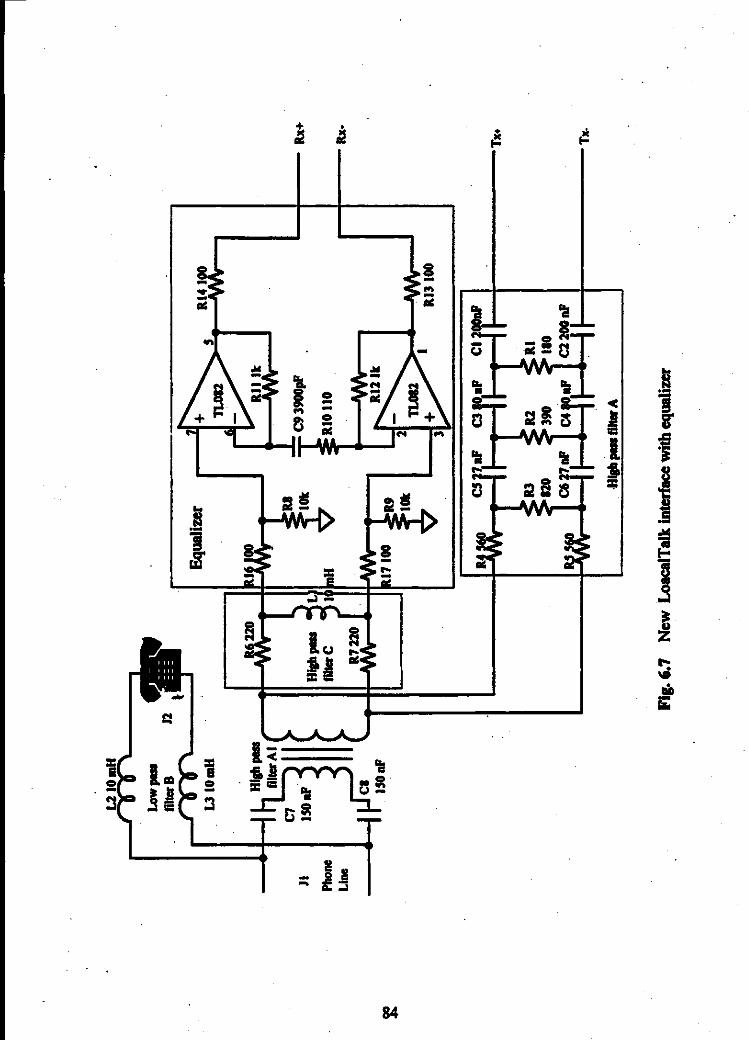
JI
Phone
Line
�
�
EqualizerL310mH
Blab passfllterC
---1.....-- Rx+
_.....---Rx·
, ''\1\1\;. II. II. I Tx+
Itl.
110
. ·BIab pass filterA
,
i"V\l\i. II • II • I Tx.
FII. 6.7 New LoacaITaik interface with equalizer

..
The res\)onse shows that the equalizer has very little gain in the frequencies from de
to 10 kHz wh.h i desirabl 'thi· 'Th is still
'
'I t th tte uati' f'�c IS 1. e 10 S project. e curve IS s sum ar 0 e a n on 0
the 2900m J\W026 twisted pair. The gain of the equalizer at frequencies above 100 kHz.
is higher th� the cable attenuation. It gives the '0' waveforms, which has more highfrequency c�lllponents and attenuates faster than the '1' waveforms, a strong
compensatiot\.. Clearly the equalizer can not recover the data signal without distortion,but it can �ver the important timing information as well as the amplitude that is
required by �e receiver. The result of the equalizer lets the eyes of the received signalopen widely�ithless timing jitter ( see Fig. 6.13 in Page 92 and Page 93).
The funCtion of the high pass filter� Al and the low pass filter B are described in
Chapter 5. 'the high pass filter C. gives the equalizer more attenuation at the lower
frequencies (See Fig, 6,8). It belps to reduce the interference from the voice,
30�----����----�--���--�����--�--�
. . .... . . . ... 1111
: :: ::: :
20
m 10�
oL-����--�����
......
...
,�a;;:,
a[ -10
0.1 10
Frequency (kHz)
Fig. 6.8 Equalizerwith high pass filter C
1001
85

6.2.3 The Test Results of the New LocalTaik Interface with Equalizer
The equalizer is tested with respect to the data communication distance, data noise
at voice band; telephone network signaling interference to data, and the circuit balance of
the equalizer.
Circuit Balance of the Equalizer:
The block diagram for testing the circuit balance is shown in Fig. 6.9.
Output
Network!SpectrumAnalizer
K
Fig. 6.9 Circuit balance test diagram
The sweep output of the network/spectrum analyzer is connected to the positive
input of each channel's equalizer. Since the spectnun analyzer only has one input port,
switch K is used to control which channel's output would be connected to the analyzer.
The spectrum analyzer has to sweep the circuits twice to get the frequency responses for
both channels. The unbalance of the two equalizer channels (shown in Fig. 6.10) is
obtained by comparing the sweep result of each channel, The result shows that the
unbalance of the two channels is well below 0.1 dB except three unbalance peaks•. The
86

three peaks are due to spurious noise which occurred during measurement. The circuit
balance of the equalizer is acceptable.
0.3
iii'� 0.25
.J!CDc
i 0.2ii
!0.15c
I
i 0.1
g.CII
! 0.05·c:s
0
I III: III
'.' �. .,.
""; "1""··· ..
E..
····r.
rf1T!i l : :
� � ; l � ; �.......
1 I ! Iii!
0.1 1 10
Frequency (kHz)
100
. Fig. 6.10 The unbalance of the two equalizer channels
Data Noise at Voice Band
The data noise is still measured by SAGE 930A communication test set. The test
system is shown in Fig. 6.11. The communication test set is connected to J2 of the
interface module A and performs as a central office switch as well as a test instrument.
.
dc power and the subscriber loop signaling are provided by this test set. This connection
can make the AWG 26 twisted pair function as a subscriber loop and simulate that the
new LocalTalk interface module is working on the real telephone network. The length of
the twisted pair is about 715 m. According to the specification of the communication test
set, the noise measurements are conducted with the far end of the subscriber line
87

terminated by a 600 Q or 900 Q resistor in series with a 2.16 microfarad capacitC>r. This
termination is called quiet termination and is connected to J2 of the new interface module
B. Computer A can communicate with computer B via the new LocalTalk interface
modules.
ComputerB
DCli I
930A g �CI""'CI-Cl-Cl-Cl-test DD CI
CICICIset 00 CICI CICICI
000.
CICICI 000
Fig. 6.11 Data noise measurement connection
When no data is transmitted on the twisted pair, the noise in the transmission loop is
o dBmC. If computerA and B continue sending data packets to each other, 4 to 6 dBmC
noise is measured. If we stop data transmission and substitute the quiet termination with
a telephone set in the off':'hook state, the noise is measured as 30 dBmC. Obviously the
noise caused by the telephone set on the subscriber loop is much higher than the data
noise (30 dBmC vs. 6 dBmC), so the data noise can not be heard when using the
telephone.
The signal to noise ratio (SIN) is measured by the. same system shown in Fig� 6.11
except the quiet termination is substituted by a 1000 Hz tone generator. The test set treats
the 1000 Hz tone as signal and other frequency components as noise. Experiments show
that when the power of the tone is larger than -25 dBm, the SIN ratio has no difference
. with or without the data transmission. Therefore, the new interface module can not have
88

any negative effects OR the fax or other voice band data communication whose output
level is usually higher than -25 dBm.
.
nata Communication without Telephone Signaling Interference
Two methods are used in measuring the quality of the data cominunication. One is
to use the echo protocol in the transport layer. Computer A keeps sending echo data
packets to computer B, while computer B receives a valid echo packet, it sends the packet'
back. The computer A can compare the number of echo packets being sent to the number
of valid packets coming back, therefore, the computer A gets the percentage of dropped
packets. The length of each data packet is 580 bytes and there are about 8000 packets
being transmitted in each test case. If the dropped packets are high, this means that the
transmission line or protocol has more errors.
Another method is to download a large random data file from computer B to
computer A. A 473 kbyte JPEG compressed file was used for this purpose. The time
needed to download this file is about 40 seconds by using AppleTalk protocols. A one to
two second variation is treated as normal.
The system shown in Fig. 6.11 is still used in this test, but the cable length is varied
from 0 m to 3360m and no termination is necessary at J2 in module B. In the laboratory,
an l l-pair AWG 26 cable roll is cut into two basic segments with lengths of 715 m and
1120 m. Several pairs in each segment can be connected to produce a longer pair. For
example, two 1120 m pairs can be connected to a 2240 m cable.
The results of the dropped packets and download time at different lengths of cable·
are shown in Table 6.1.
89

Lenzth of the cable Drooeed packets Average down load time
Om" '0.4% 38 seconds
715m <0.05% 39 seconds
1120m <0.05% 39 seconds
1430 m (2 x 715 m) <0.05% 39 seconds
1835 m (l12Om +715 m) <0.05% 39 seconds
2145 m (3 x 715 m) <0.05% 40 seconds
2550m (2x 715 m+1120m) <0.05% 40. seconds
2955 m(2x 1120m+715 m) <0.05% 40 seconds
3360 m (3 x 1120 m) <0.05% 40 seconds* 0 mmeans that the cable length is shorter than 2 m.
Table 6.1 The data communication quality at different cable lengths
The data shows that the new LocalTalk interface with the equalizer can work from
very short distance to 3360 m.
Eye diagrams and waveforms at difference cable lengths are obtained by the system
shown in Fig. 6.12. A similar system which is used to obtain eye diagrams has been
described in Section 4.4, Chapter 4. The difference here is that the encoded signal need
to be transmitted through the new LocalTalk module A and received via the interface
module B. The eye diagrams recorded after the equalizer are obtained by connecting the
90

output of the equalizer to the vertical inputs of the scope and the eye diagrams before the,
equalizer are recorded by connecting scope�s vertical inputs to points a and b in the
interface module B. Trace Ml in the scope is used to record the waveform of the
received signal after the equalizer and the trace M2 is used to record the waveform before
.
the equalizer.
Interface module A Interface module B
Clock'. Extern Trig
Fig.6.12 The system to obtain eye diagram.
Fig. 6.13a and Fig. 6.13b show that .the eye diagrams and wavefonns which are
recorded before and after the equalizer at different cable lengths. According to the
waveforms in Fig. 6.13a and Fig. 6.13b. we can see that. at the same distance. the
waveform recorded after the equalizer (trace Ml) has better shape over the wavefonn
recorded before the equalizer (trace M2) and at 0 meter distance, Ml becomes a square
wave, which means that the equalizer amplifiers are saturated by the large received.
voltage. According to the eye diagrams in Fig. 6.13a and Fig. 6.13b, we can easily.
determine that the-eye diagrams after the equalizer open wider and have clearer border.
Obviously the equalizer improves eye diagrams at every length.
91

Cable
lengthWaveform before/after equalizer Eye diagrams before equalizer Eye diagrams after equalizer
as
Om
.......
.. .
' iuft.hI.54V
Fig. 6.13a' Eye diagrams and waveforms at different cable length

Cablelength
2145m
�2955m
3360m
M2
M1
M2
M1
M2
M1
M1: wavetonn after Ihe equalizer;. M2: wavefonn before the_..... Fig. 6.13b Eye diagrams and waveforms at different cable length

Besides the equalizer, the high pass filter A and Al (see Fig. 6.7) also helps to
improve the communication distance. Generally, the frequency domain equalizer has
difficulty in accurately equalizing the phase distortion, but the high pass filters help the
equalizer recover some of this disadvantage. After the data goes through the high pass
fllters, the bandwidth of the data gets narrower and the spectrum of the data is restricted in
the high frequency band. In Chapter 3, Fig. 3.5 and Fig. 3.7 show that the delay of higher·
frequencies has less variation, so the cables give less phase distortion to the data that goes
through the high pass filterA and AI.
In order to illustrate the effects of the high pass filter A and AI, one of the
experimental test systems is set up as in Fig. 6.14. This system can be used to recordeye
diagrams without high pass filter A and At. Bye diagrams with high pass filer A and Al
are those unequalized eye diagrams which are shown in Fig. 6.13a and Fig. 6.13b.
-
:: Tl'IIISformer A:wu26_- . ·11'aDsformcr-
Scope
Encoderl PNsigDaIExtern Trig..
-
4- ... Clock Eye� :::.
Driver-
generator -
Fig. 6.14 Bye diagram recording system
Fig. 6.15 shows the effects of the high pass filter A and Al to eye diagrams at
different cable lengths. Bye A to Eye A3 are eye diagriuns without the high pass filters.
Eye B to Eye B3 are the eye diagrams with the high pass filters. At distances that are
shorter than 1.5 Ian, Eye A and Bye Al have better shapes than those of Bye B and Bye
Bt. However, with the increase of the cable length, the first small eyes of Bye Al get
much smaller at 2200 m (see Eye A2) and eventually disappear in Eye A3 at 3300 m•.On
the contrary, at 2200 m and 3300 m, the two small eyes in Eye B2 and B3 are still open.
Obviously the eye diagrams with the high pass filters are better at long distance.
. .
.
94

Wichout High Pass Filter
·Cablc I' ILength .
..__ __..A
·11-1�--
Om
1430
..
•!
With High Pass Filter
. Fig. 6.15 Eye diagrams witblwithout high pass filterA and At
95

Data Communication With Telephone Signaling Interference
The test system was again set up as Fig. 6.11 with substituting a telephone set in
place of the tennination. The SAGE 930A communication test set still takes the place of
the central office switch. The de power, test tones and some subscriber signaling are
provided by the test set The test results of dropped data packet rate at different distances
are listed in Table 6.2.
Si-.
'Cable lenirth 715m 1430m 2240m 2955ni 3::----
Ring supplied by SAGE 930A 0.0% 0.0% 0.0% 0.0% 0.0%'
DTMF dialing by SAGE 930A 0.0% 0.0% 0.0% 0.0% 0.0%
and telephone set.alternativelv
Pulse dialing by SAGE 930A and 0.3%- 0.2%- 0.3%- 0.2%- 0.2%-
telephone set alternatively 0.4% 0.3%' 0.4% 0.3% 0.3%
1 kHz tone supplied by SAGE 0.0% 0.0% 0.0% 0.0% 0.0%
930A; Output DOwer = 12 dBm
Table 6.2 Packet drop rate at different telephone signaling
According to the test results, ring and DTMF dialing have no effect to the data
communication at each cable length (The drop rate remains 0.0%). When the 1000 Hz
tone is added to the line by the test set, the output power of the tone can be as high as 12
dBm without any disturbing to the data transmission. Since the high pass filter C and the
transfonner in Fig. 6.7 have more attenuation at lower frequencies, it is very safe to say
that most signaling tones, such as busy tone, dial tone and ringback tone, whose
96

frequencies are lower than 1000 Hz and power is less than 12 dBm. have no negative
effect to the data tranSmission. When pulse dialing. the phone set \\;11 switch itself back.
and forth from on-hook to off-hook. This causes impulse noise which has very large
power and wide frequency range. The impulse noise causes some errors in the data
transmission.
The effects of several higher frequency tones are also examined. There are no
packets dropped at different cable lengths when a 1 dBm 2 kHz or a -7 dBm 3 kHz tone
are added to the trailsmission line. This test result shows that the immuni� of the data
transmission to the voice band signals decreases with the frequency increasing. However..
most of the voice power is concentrated around 1000 Hz. the voice signal"s equivalent
peak level is about -12 dBm and its. long-term conversational level is only about -27
dBni. Therefore, the nonnal conversation does not interfere With the data
communication.
6.3 Predistorter and Equalizer Design
Another possible way that data communication distance can be extended funher is
to use both predistorter at the transmitter side and equalizer at the receiver side. The
diagram.of the whole system is shown in Fig. 6.16.
Preclistoner/Equalizerinterface module A
PredistonerlEqualizerinterface module 8
Data Data
Fig. 6.16 Systemwith predistorter and equalizer
97

Tx data comes from the computer. When the data goes through the predistorter, the
data is distorted to a special shape which is suitable for longer distance transmission. At
the receiver side, an equalizer is still used to compensate for the distortion caused by the
transmission system.. The high pass filter A, AI, C and the low pass filter perform the
same roles as those described in Section 6.2. The following sections will describe the
predistorter and the equalizer in detail.
6.3.1 PredistorterDesign
The predistorter is based on the theory that a data signal whose spectrum is narrow
and restricted at high frequency band has less phase distortion after long distance
transmission, which is proved in Section 6.2.3 by using high pass filters. The method
Used in the predistorter is more effective.
The LocalTalk data distorted by the predistorter is illustrated in Fig. 6.17 C [31].
This distorted LocalTalk data has reduced amplitude of each later portion of each bit.
The special shape of .the distorted LocalTalk data can reduce the amplitude of the low
frequency bits to a relatively small fraction of their initial amplitude, thus the distorted
signal has less low frequency content. As shown in Fig. 6.17, the distorted LocalTalk
signal C can be easily obtained by adding a smaller signal B which is a delayed inverse
copy of A to the original signal A.
A I II----..I+
B Delay I
nc
Fig. 6.17 Formation of a distorted signal
98

In order to show the improvement of the data transmission at long distance .by using
the predistorter, experiment systems shown in Fig. 6.18 are set up to obtain eye diagrams.The system shown in Fig. 6.18A is used to record the eye diagrams of the predistorteddata. The unpredistored eye diagrams are recorded by the system shown in Fig. 6.18B.
Both systems have the same high pass (literA and AI.
Encoderl
(A) Driv_er_PN signalgenerator
ClockExtern Trig
Eye diagram ..,___
j •
Encoderl
(8) Driver-_-
PNsignaiacnenROr
ClockExtern Tria
Fig. '.18 The systems for obtaining eye diagrams with predistorter
The eye diagrams of the predistorted and the unpredistorted data are shown in Fig.
6.19. When the cable length. is 3300 m, both the Bye 1 of the predistorted data and the
Bye 2 of the unpredistorted data have open eyes, but the eye opening of the predistorted
data is slightly larger than that of the unpredistorted data. When the cable length extends
to 4000 m, the eyes of the unpredistorted data are closed (see Bye 4), but the predistorted
data still has two open eyes (see Bye 3). The improved eye diagrams of the predistorteddata can simplify the design of the equalizer at the receiver end.
99

Predistorted data Unpredistorted data
Eye4 �
. . .. .. .
....................... .
. . .. .
__ � ••0tIV �.oo�: : : :
Fig. 6.19 Eye diagrams of data with predistortion and without predistortion
6.3.2 Circuits of the Predistorter and Equalizer
The circuits of the interface with the predistorter and equalizer are shown in Fig.6.20. High pass filter A is the same as that in Fig 6.7. High pass filter A, Al and the low
pass filter B are still used to prevent the interference between the data and the voice.
Because the output amplitude of the predistorted data is small, a central output grounded
I to 1 ratio transformer is used here to achieve better circuit balance.
100

J1
PhoneLine
-
o-
low pass
filt�r B J21TelePhone(See Fig. 6.7) set..- C30.Oo1pF-·
- - -
Equalizer
281S30Predistorter
CD4030BE1
High pass. filter A
.
(See Fig. 6.7)
......----Rx+
-----Rx-
�"_"_"_"_"_�"_�"_"_"_-TX+
B
+5V
Fig. 6.28 NewLocal'Ialk interface with predistorter and equalizer

The pred.istorter is combined with a delay circuit [32] and a sum circuit MC14175,
74123 and the UI in CD4030 chip compose the delay circuit. Balanced data is input from
TX+ and TX-. When the data comes in, XOR gate U3 outputs '1' and U2 outputs '0' to
enable the Driver 1 and 2 in 26LS30 chip. C8 is used to erase the glitch in the enable
signal. U4 inverts the data in Tx- and is connected to the input of Driver 2. The XOR
gate Ul, C9 and R18 perform as a dual edge detector that can change the transitions of
the TX+ data to narrow pulses (See Fig. 6.21B). After these pulses go through the
multivibrator (74123), they are expanded to about 1.2 Jls equal wide pulses, the width of
the pulses are adjustable by C7 and RI7 [33]. These pulses are output to .the D Flip-Flop
(MCI4175) as the clock (See Fig. 6.21C). When the clock has a Low-to-High transition,
it loads the TX+ data and output to the RS-422 driver (26LS30). Because each Low-to
High transition has a 1.2 Jls delay to each original TX+ transition, therefore thedelayed
output data is the same as the original TX+ data (See Fig. 6.21 waveD).
D:AfterD
Flip-Flop
Delay:1.161015
A: LocalTalkData
B: AfterDual
edgedetector
c, After
Fig. 6.21 Timing diagram of the delay circuit
102

The RS-422 line driver (26LS30) and R13-R16 form the sum circuit. Driver 2 .
drives the undelayed data to RI5 and R16, while its delayed copy is output to RI3 and
R14. The positive and inverse outputs of"
Driver 1 are connected to the inverse and
positive outputs of Driver 2. The output voltages (referenced to ground) at point A and B
can be calculated as Eq. 6.2 (See Appendix 3 for detail explanation)
R16 Rl3VA = VOl + (-VOl)
R13+R16 R13+R16VA=-VB Eq.6.2
where voltage VOl is the positive output of Driver I.
voltage V02 is the positive output of Driver 2.
The output of the sum circuit ( voltage between point A and B ) is shown in Fig. 6.22.
" "
...........................................
"'--_." "
............
LocalTalkData
PredistortedData
.................................
Fig. 6.22 . Predistorted signal
The distorted signal still has noise on voice band. The high pass filter A and the
low pass filter B are still needed to eliminate the voice band noise. These filters are the
same as those in Fig. 6.7.
103

Because of the improvement caused by the predistorter, the eye diagrams of the
received signal are fairly good after long distance transmission, but the amplitude of the
received signal is very small. Therefore, a high gain equalizer is required at the receiver.
As mentioned in Section 6.2.2, the bandwidth of the amplifier will decrease with the
increase of the gain. In order to maintain the bandwidth and enough gain, a two-stage
amplifier is used in the equalizer. With this two-stage equalizer, it is easy to have up to
35 dB gain at. high frequency range. The Curve A in Fig. 6.23 shows the frequency
response of the two-stage equalizer. Although the gain of the amplifier at high frequency
. is what we want, the gain at low frequency, especially in voice band, is not acceptable..
Therefore, the high pass filter C is used to reduce the amplifier's gain at the low
frequency range. The frequency response of the two-stage equalizer with the high pass
filterC is shown in Fig. 6.23 Curve B.. It is easy to see that the high pass filter C reduces
the gain at the voice band remarkably.
�?-----------------------------------------�
� 10
=.; 0c
� ·10
1J,I,;l -20
I , • ,... I'" , I I" I I , , ••• , I ., I I I' I •
.. .. .. .. .. .. .. .. .. .. .. .. .. .. .. .. .. .. .. .. .. .. .. .. .. .. .. .. .. .. .. .. .. .. .. .. .. ... ..
30 ...'.. '.'. '.'.'�'.' ... 0
•• '. � .o� O.'�O•••
• I I I., o. t" I' 'II. ,., I ! , I. ,.11
o 0 0 " ,,0 0 0 0 , 0 "" "0 0 0 "" I-Curve A lo 0
.,' .". :. :. :.:� :.: ... : .. :. � .: � :.:;:... ; . ; .:. :.:.: :.:; . - -CurveD::'., • , •• ,' • I , • 1'1' • 0 •• , o. •
��------------------------------------------
100 1000 10000
Frequency (Hz)
100000 1000000
Fig. 6.23 Equalizer gain vs. frequency
104

6.3.3 Test Results
A system which is similar to Fig. 6.12 is used to record the eye diagrams, but the
interface module used in Fig 6.12 is substituted by the interface module with both
equalizer' and predistorter. The eye diagrams of the received signal at 3300 m and 4000
,
m are shown in Fig. 6.24. At 4000 m;Eye 3 is the eye diagram of the received signal
before equalizer and Eye 4 is the eye diagram of the same signal after the equalizer. Eye
3 and Eye 4 have similar shape, but Eye 4 has much larger eye opening. At 3300 m, Eye
1 and Eye 2 have similar relationship as that ofEye 3 and Eye 4.
Before equalizer After equalizer
· . . .Eye3
. . .
........................ .
· . .. .
:. : : :. ":
,,
� Eye4 �
4000m
.. ..
........................ .
· . .. .
· . . .
· . . .
· . . .
. . ,
...........................................
. . .. .
Fig. 6.24 Eye diagrams of received data at 3300 m and 4000 m
105

In order to test the
performance of the circuit, similar test systems and test steps used in Section 6.2.3 are .
adopted here. The test results show that the predistorter and the equalizer interface
module can work from 3300 m to 4000 m with 0.0% packets dropped and can download
the 472 kbytes file in 41 seconds or so. When. the data is transmitted through this
.
interface module, data has even quiet noise in voice band. In the worst case, the SAGE
930A communication test set only can record 2 dBmC noise that is generated by the data
transmission. In order to test the effect of voice interference to the data transmission, a 1
kHz tone is transmitted simultaneously with the data. The interface module still can
transmit and receive data without any packets dropped at 3300 m and 4000 m with the .
power of the tone increased up to 4 dBm.
6.4 Solutions to the Bridged Tap
Bridged taps are very common in telephone networks. Telephone companies often .
connect a pair of open circuit transmission lines to the subscriber loop between the central.
office and the terminal equipment. The open circuit pair is called bridged tap as shown in
Fig. 6.25.
TerminalSubscriber Loop
P---------------__�------------� EquipmemCentralOffice
Fig. 6.25 Dlustration of the bridged tap
106

In Chapter 3, the transmission theory shows that the open circuit transmission line
reflects all incoming signals. When the length of the open circuit is about 114 of the wave
length, the reflected signal will cause significant distortion to the signal transmitted in the
subscriber loop.
The 114 wave length of the voice band signal is over 15 Ian. The bridged tap
usually is not that long, and even if the bridgedtap happens to be 15 km, the reflected
signal is largely attenuated after the long round trip. However, the wave length of the
LocalTalk data can be very short. The first null of the LocalTalk data spectrum is about
430 kHz, 114 wave length of this frequency is as short as 120 m., Since the main power of
the LocalTalk data is concentrated from 30 kHz to 300 kHz, The bridged taps around 170
m or longer � of concern. Fig. 6.26 shows the frequency response of the 1500 m
AWG26 cable with a 200 m bridged tap.
-
1 10
Frequency (kHz)100
Fig. 6.26 1500 m cable attenuation with 200 m bridged tap
107

The frequency response of the cable with bridged tap has its first sharp attenuation
peak around 250 kHz. This unexpected attenuation can significantly affect the eye
diagram that is recorded at the terminal equipment side. Fig. 6.27 shows the effect of the
bridged tap to th� LocalTalk data. Eye A is the LocalTalk data being transmitted through
the 1500 m cable and equalized without bridged tap, Eye B is the bridged tap version.
Obviously the bridged tap is a problem to the data transmission.
Eye diagram without bridged tap· . .. ... ..
.... �y���!��� .....���.�.�.�...
· . " .
· . .. .
· . .. .
.. .. .
. .
................................................
· . .. .
· . .. .
· . .. .
· . .. .
....................... .
.. z.sov .z.so�
A B
Fig. 6:1.7 Eye diagrams with/without bridged tap
According to the transmission line theory, the ideal solution to the bridged tap is to
use a match terminator whose impedance is exactly the same as the characteristic
impedance of the cable. However, this is not possible and not necessary. Some easier
and effective methods-are discussed here.
6.4.1 Solution 1: Pure Resistor Termination to the Bridged Tap
The Fig. 3.S in Chapter 3 shows that the characteristic impedance of the phone cable
tends to 100 n with increasing frequency. Thus, a 100 n resistor can be used as a.
terminator to eliminate or decrease the high frequency signal reflection. A 200 m bridged
tap with a 100 n resistor termination is shown in Fig. 6.2S.
lOS

Central Termianal
OfficeSubscriber Loop Equipment
t
i]e
�
1m, � 100 terminationn
Fig. 6.28 Subscriber loop with 200 m pure resistor terminated bridged tap
Fig. 6.29 shows the frequency response of the 1500 m cable with a 200 m
terminated bridged tap, and Fig. 6.30 shows the eye diagram, which is recorded at the
terminal equipment side. of the transmitted signal after 1500 m cable with a 200 m
terminated bridged tap.
-
�-10
-20
�5������--�����--��������0.1 1 10010
Frequency (kHz)
Fig. 6.29.
The .attenuation of 1500 m cable with 200 m bridged tap terminated by a 100 n .
resistor
109

....................... .
· . . .
· . . .
· . . .
........................
· . . .
· . . .
· . . .
. .
.........................· . . .
· .' . .
· . . .
__ 2.50 V �.SOJ&S
....................... .
· ... ..
· .
· .
· .
....................... .
· . '. .
· . . .
· . . ..
· . . .
. . .
....................... .
· . . .
Fig.6.3O Eye diagram of 1500 m cable with 200 m bridged tap terminated by a 100 n
resistor
In Fig. 6.29, The terminated bridged tap doesn't have sharp attenuation to the cable
and the eye diagrams are good in Fig. 6.30, but the problem with this method is that the
termination causes much attenuation in the voice band and brings trouble to the telephone
network too. The loon terminator can make the central office treat the terminal .
equipment on the subscriber loop as being off-hooked.
6.4.2 Solution 2: R-C Tennination to the Bridged Tap
R-C termination is a better method to terminate the bridged tap. The termination is
realized by a resistor in series with a capacitor (shown in Fig. 6.31).
Central Terminal
Office Subscriber Loop Equipment
ti:fie
�WMI -4 R-C termination
Fig.6.31 Subscriber loop with 200 m R-C terminated bridged tap
110

Fig. 6. 32 shows the impedance of the R-C terminator whose R is 100 � �d C is
0.022 uFo It is easy to see that the impedance of the R-C terminator is l�r at low
frequency band and tends to 100 n at high frequency. This characteristic can reduce the
signal reflection of the LocalTalk data without disturbing the telephone network.
100
10
1
1 10 100
Frequency (kHz)Fig. 6.32 Impedance of the R-C termination
The frequency response of the 1500 m cable with a 200 m R-C terminated bridged
-5
-
! -10
.��! -15<
-20
-25L-�������_'�����__������0.1 1 10 100
Frequency (kHz)
Fig. 6.33 Frequency response of a 1500 m cable with R-C terminated bridged tap
111

In Fig. 6.33, the R-C terminated bridged tap curve is almost identical to the
response without bridged tap at voice band and there is no sharp attenuation peak at high
frequency.
. The eye diagram of the LocalTalk data transmitted after the 1500 m cable with a
200 m R-C terminated bridged tap is shown in Fig. 6.34. Again, this eye diagram is
recorded at the terminal equipment side. The eye diagram shows that the R-C termination
has almost the same shape as the 100 n terminator, and with this eye diagram, the
receiver can receive data correctly.
· .
....................... . ....................... .
. . . .
.. .
R-C terminated bridged tap
· . . .
....................... .
.. .
. .
· . . .' .. .
. . . . . . . . . . . . . . . . . . . . . . .. . ...
: .....:.. 13 J ul 1995 ..
_,. 2.00 V �.50JlS 10:53:18
Fig. 6.34 Eye diagram of a 1500m cable with 200 m R-C terminated bridged tap
6.5 Summary
In this chapter, We have presented two methods which .can extend the LocalTalk
communication distance and two solutions to the bridged taps.
The first method which can extend the range of the LocalTalk transmission is.
realized by an equalizer working with a new LocalTalk interface module that was
112

introduced in Chapter 5. The equalizer is a frequency domain equalizer which has
advantages of low cost and reliability. Because the LocalTalk uses a balanced signal, the
balance of the equalizer circuit is an important issue in the equalizer' design. In this
project, LocalTalk data is transmitted simultaneously with the voice, thus the equalizer
circuit is designed to obtain good equalization results to the data and avoid causing voice
interference to the data. Test data shows that the equalizer has satisfactory performance
at distances from 0m to 3300 m.
The second method which is used to extend the data transmission to longer
distances is conducted by a new LocalTalk interface module with a predistorter and a
two-stage equalizer. In this system, the transmitted data is distorted by the predistorter
and has better _ eye diagrams at longer distances. The two-stage equalizer can give
received data signals sufficient compensation within a wider bandwidth. The new
LocalTalk interface module with the predistorter and the equalizer can work properly at
distances from 3300 m to 4000 m.
The pure resistor and the R-C. termination are two solutions to the bridged taps
which are longer than 150 m. Although. both pure resistor termination and the R-C
termination have similar performances to the bridged tap, the R-C termination_
is
recommended for its trouble free to the telephone networks.
113

Chapter 7 Conclusion
This thesis presents a new high speed network access technology. This high speed
network access method can transmit 230 kbits/s data simultaneously with voice. on the
existing telephone line at very low cost.
The LocalTalk local area network protocol, which is used in this project, is a well
established robust protocol. In Chapter 2, the thesis has shown that the LocalTalk
protocol can operate normally at range up to 9.6 km and the LocalTalk data is suitable for
simultaneous transmission with voice. The use of the I,.ocalTalk protocol also simplifies
the design of this project and make it possible that the new network access method be
mass deployed.
In Chapter 5, the thesis has shown that carefully designed high pass and low pass
filters can be used to reduce the low frequency power of the data signal and prevent the
voice and the subscriber loop signaling from interfering with the data. The high pass
filters working with the low pass filter can reduce the LocalTalk data noise, which causes
interference to the voice communication, from 81 dBmC to. 6 dBmC and can also
support normal telephone conversation without disturbing the data transmission.
Experiments show that the new LocalTalk interface module with high pass and low pass
filters can work very well at short distances.
114

In Chapter 6, the thesis has investigated methods of extending the range of the
LocalTalk transmission. In order to achieve the data transmission distance that is longer
than 2 km, an equalizer that can compensate for the distortion caused by the subscriber
line is required at the receiver end. The equalizer shown in Fig. 6.7 is not complex and
expensive, but it has satisfying petformance at distances up to 3.3 km. For longer
distance data transmission, in addition to a equalizer being used at the receiver, a
predistorter is needed to predistort the data signal before it is transmitted. With
predistortion and equalization, the data transmission distance can be increased up to 4
.
km.
The impairment caused by bridged taps has also been investigated in Chapter 6. The
bridged tap in an analog telephone network is not harmful, but it is a disaster in a high
speed data network. In this project, the experimental results show that the bridged tap
should be shorter than 150 m, otherwise it must be terminated for signal frequencies of
data transmission.
Future improvements of this project can be achieved byupdating the receiver circuit
in the interface module. The high pass filter C in Fig. 6.7 and Fig. 6.20 can be substituted
by a more powerful band pass filer. The pass band of the band pass filter should be 20.
.
kHz to 400 kHz with sharp transition curves to stop band. The purpose of the pass band
filter is to significantly reduce the interference coming from the voice at the low
frequency band and the radio interference at the high frequency band Experiments
indicate that, different models of Macintosh computer and PC LocalTalk boards have
different performances on the same equalized signal. In order to ensure consistent good
performances under the same line condition for different LocalTalk receivers, an extra
circuit is needed to modify the received equalized signal to a standard signal level which
the LocalTalk receiver in every Macintosh or PC LocalTalk board can decode correctly.
115

TRLabs working with SaskTel have conducted some field trials on this new
network access technology. The results have been satisfactory and indicate strong
commercial potential.
116

References
1. Access 230 Technology Transfer Opportunity. TRLabs. 1996.
2. Charles K. Summers. ISDN Implementor's Guide -- Standards, Protocols, and
Services, McGraw-Hill, NY, 1995.
3. B. R. Saltzberg, T, R, Hsing, GuestEditorial, IEEE Journal on Selected Areas
in Communications, Vol. 9. No.6, August 1991.
4. William C. Barlet, A Copper-platedFull Service Network. Telephony, January
15, 1996.
5. J.W. Lechleider, High Bit RateDigital Subscriber Lines:A Review ofHDSL
Progress, IEEE Journal on Selected Areas in Communications, Vol. 9, No.6,
August, 1991.
6.· David E. Dodds, InternetAccess Study, TRLabs Saskatoon Report, June 7,1996..
7. Cable Modem FrequentlyAsked Question, http://www.cox.comlmodemfaq.html
8. Ray Smith, Catching up, Telephony, June 24, 1996
9. David E. Dodds, Greg Erker and GrahamBradley, InternetAccess at 230 kb/s -
Hardware Trial, Paper in Preparation, 1997.
10. Farallon"'PhoneNEr Connector User's Guide, Farallon Computing, Inc.
Berkeley, CA.
11..
G. S. Sidhu, R. F. Andrews, and A. B. Oppenheimer, InsideAppleTalk, 1st
Edition, Apple Computer, Inc. 1986.
12. G. S. Sidhu, R. F. Andrews, and A. B. Oppenheimer, Inside AppleTalk, 2nd.
Edition, Apple Computer, Inc. 1990.
117

13. A. S. Tanenbaum, ComputerNetworks, 2nd Edition, Prentice Hall, Englewood
Cliffs, New Jersey, 1988.
14. Macintosh Family Hardware Reference, Addison-Wesley Publishing Company,
Inc.
15. B. M.Wirth, Fiber Optic Extension ofApple LocalTalkNetworks, M.Sc. Thesis,
University of Saskatchewan, Saskatoon, Saskatchewan, 1989.
16. Data Sheet, "AM26LS30", BipolarMicroprocessor Logic and Interface Data
Book, Advanced Micro Devices, Sunnyvale, CA, 1985.
17. Data Sheet, "AM26LS32", BipolarMicroprocessorLogic and Interface Data
Book, Advanced Micro Devices, Sunnyvale,.CA, 1985.
18. Data Sheet, ''Z8030fZ8530 ", Zilog Serial Communication Controllers Data book;
Zilog, Campell, CA, 1994.
19. Leon W. Couch Il, Digital andAnalog Communication systems, Fourth Edition,
MaxwellMacmillan Canada, Toronto, 1993.
20. Bell Telephone Laboratories, Transmission Systemsfor Communications, Vol. 1,
Bell Telephone Laboratories, New York, N.Y.
21. David. E. Dodds, EE 816 TelephonyNotes, University of Saskatchewan,
Saskatoon, Saskatchewan, 1996
22. H. H. Skilling, Electric Transmission'Lines: Distributed Constants, Theory and
Applications,McGraw-Hill, New York., 1951.
23. AT&T, Bell Telephone Companies, and Bell Telephone Laboratories,
Telecommunications Transmission Engineering, Vol. 2, 1st Edition.
24. AT&T, Principles ofElectricityApplied to Telephone and Telegraph Work,
AT&T,1961.
25. J. G. Proakis, Digital Communications, 2nd Edition. McGraw-Hill, New York,
1991.
118

26. Shahid Qureshi, Adaptive Equalization, IEEE Communications Magazine, March,
1982.
27. W. D. Reeve, Subscriber Loop Signaling and Transmission Handbook: Analog,
IEEE Press, New York, 1992.
28. SAGE Instruments Model 930A Communications Test Set OperationsManual,
SAGE Instruments, Freedom CA, 1990.
29. Walter G. Jung, IC Op-Amp Cookbook, 3rd Edition, SAMS, Camel, Indiana.
30. Data sheet, "TW82", Linear Circuits Data Book, Vol. 1, Texas Instruments,
Dallas, Texas, 1992.
31. A. X. Widmer, N. Y. Katonah, United States Patent 3,980,826, International
Business Machines, Armonk, N.Y., 1975.
32. Rudolf F. Graf, The Encyclopedia ofElectronic Circuits, 1 st Edition, Vol. 3, Tab
Books, Blue Ridge Summit, PA, 1985.
33. Data sheet, "SN74123", TTL Logic Data Book, Texas Instruments, Dallas,
Texas, 1988.
34. Whiteham D. Reeve, Subscriber Loop Signaling and Transmission Handbook:
Digital, New York: IEEE Press, 1995.
35. Data sheet, "OPA2111", Burr-Brown ICData Book - Linear Products, Burr
Brown Corporation, Tucson, AZ, 1994
119

I53O(SCC)
TxOA I
IRTSA10E
3.612 MHz
JRTXCA
3/. of 26LS32
IOCOA
RxOA
ICTSA/TRXCA
1/2 of 9636.\ (or 34IIA) .
0-10TRA
IWIREQ,. 6522 (VIA)IWIREQa PA7
TxOaIRTSa
+5V
PClJ(-6V
IRTxCa-
lOCOa
RxDa
ICTSaJTRxCa
IOTRa
...
Appendix 1 Macintosh Serial Port
TXO"..TXOA+
HSKoA
TXOa-
HSKI
HSKoa
Note: Rl R2� .,.,.... :1""\1,,
;;,C(Rl + R2 • .«l to 60 ohms. C • 150 to 300 pf)
120

Appendix 2 Circuits of the Pseudo-Random Data Generatorand the Baseband Encoder
Baseband Encoder
Pseudo-Random Data Generator
121

Appendix 3 Output Voltage of the Predistorter
The sum circuit of the predistorter is redrawn as Fig. A3.1.
VB
FIg. Al.1 The sum circuit of the predistorter
The outputs of Driver I satisfy
V01=-VOl
and the outputs of Driver 2 have
V02=-V02
VB and VA can be calculated as.
VOl-VOlVA = V01-
R RR13
13+ 16
VOIRl6 +V02R13=-----
RI3+RI6·
122
VA
Eq. A3.1
Eq. A3.2
Eq. A3.3

VOZ-VOIVB=VOZ- RlS
R14+RlS
V02R14 +VOtRlS=-----
R14+RIS
Substitute Eq. A3.3 with Eq. A3.1 and Eq. A3.4 with Eq. A3.2, We get
VOIR16 - VOZR13VA=----
R13+R16R16 R13
= VOl + (-Voz)R13+ R16 R13+ R16
and
V02Ri4 - VOlR1SVB=-----
RIS+R14·R14 RlS
=
RIS+ R14V02 +
RIS + Rl4 (-VOl)
.
According to the sum circuit of the predistorter,
R1S=R16
and
R14=R13
Substitute Eq. A3.6 with Eq. A3.7 and Eq. A3.8, we get
R1S R14VA =
R RVOl +
R R(-Voz)
14+ IS 14+ IS
Comparing Eq. A3.6 to Eq. A3.9, we have
VA=-VB
123
.Eq. A3.4
Eq.A3.5
Eq. A3.6
Eq. A3.7
Eq. A3.8
Eq. A3.9 .
Eq.A3.10