Earth and Planetary Science Letters 413 (2015) 13–24

Contents lists available at ScienceDirect

Earth and Planetary Science Letters

www.elsevier.com/locate/epsl

Tearing of the Indian lithospheric slab beneath southern Tibetrevealed by SKS-wave splitting measurements

Yun Chen a,∗, Wei Li a,b, Xiaohui Yuan c, José Badal d, Jiwen Teng a

a State Key Laboratory of Lithospheric Evolution, Institute of Geology and Geophysics, Chinese Academy of Sciences, Beijing 100029, Chinab University of Chinese Academy of Sciences, Beijing 100049, Chinac Deutsches GeoForschungsZentrum GFZ, Telegrafenberg, 14473 Potsdam, Germanyd Physics of the Earth, Sciences B, University of Zaragoza, Pedro Cerbuna 12, 50009 Zaragoza, Spain

a r t i c l e i n f o a b s t r a c t

Article history:Received 3 September 2014Received in revised form 16 December 2014Accepted 22 December 2014Available online xxxxEditor: A. Yin

Keywords:seismic anisotropyshear wave splittingsubducting lithospheric slabslab tearingHimalayan–Tibetan collision zone

Shear wave birefringence is a direct diagnostic of seismic anisotropy. It is often used to infer the northern limit of the underthrusting Indian lithosphere, based on the seismic anisotropy contrast between the Indian and Eurasian plates. Most studies have been made through several near north–south trending passive-source seismic experiments in southern Tibet. To investigate the geometry and the nature of the underthrusting Indian lithosphere, an east–west trending seismic array consisting of 48 seismographs was operated in the central Lhasa block from September 2009 to November 2010. Splitting of SKS waves was measured and verified with different methods. Along the profile, the direction of fast wave polarization is about 60◦ in average with small fluctuations. The delay time generally increases from east to west between 0.2 s and 1.0 s, and its variation correlates spatially with north–south oriented rifts in southern Tibet. The SKS wave arrives 1.0–2.0 s later at stations in the eastern part of the profile than in the west. The source of the anisotropy, estimated by non-overlapped parts of the Fresnel zones at stations with different splitting parameters, is concentrated above ca. 195 km depth. All the first-order features suggest that the geometry of the underthrusting Indian lithospheric slab in the Himalayan–Tibetan collision zone beneath southern Tibet is characterized by systematic lateral variations. A slab tearing and/or breakoff model of Indian lithosphere with different subduction angles is likely a good candidate to explain the observations.

© 2014 Elsevier B.V. All rights reserved.

1. Introduction

Mountain belts created by continent–continent collisions are perhaps the most dominant geologic features of the surface on Earth. The most spectacular one of them is the Himalayan–Tibetan orogen, consisting of the east–west trending high-altitude Hi-malaya and Karakorum ranges in the south and the vast Tibetan Plateau in the north (e.g., Dewey and Burke, 1973; Yin and Harri-son, 2000). This orogenic system was largely created by the Indo-Asian collision over the past 50 Ma with an east–west extent of more than 2000 km from the Nanga Parbat syntaxis in the west to the Namche Barwa syntaxis in the east (Fig. 1). It is part of the greater Tethyan orogenic belt that extends from the Mediterranean Sea to the Sumatra arc over a distance of more than 7000 km (Yin and Harrison, 2000).

* Corresponding author. Tel.: +86 10 8299 8339; fax: +86 10 8299 8001.E-mail address: yunchen@mail.iggcas.ac.cn (Y. Chen).

http://dx.doi.org/10.1016/j.epsl.2014.12.0410012-821X/© 2014 Elsevier B.V. All rights reserved.

Plate motion and deformation can create distinct pattern in seismic anisotropy in the lithosphere and asthenosphere. Shear wave birefringence is viewed as a direct diagnostic of seismic anisotropy. Core-related phases (e.g., SKS, PKS or SmKS) are com-monly used to investigate the continental anisotropy (Silver and Chan, 1991; Savage, 1999). As P-to-S converted waves at the core-mantle boundary (CMB), they should be purely SV polarized in an isotropic Earth with a linear particle motion in the radial direc-tion. If a SKS wave propagates in an anisotropic region between the CMB and the receiver, it will split into two orthogonal waves with polarization in the fast and slow directions, respectively (Alsina and Snieder, 1995). The two waves arrive at a station with a time lag, resulting in birefringence and elliptic particle motion. Analyz-ing SKS splitting can provide detailed information of azimuthal anisotropy, defined by the fast speed direction and delay time. One advantage of the SKS phase is the good lateral resolution due to near-vertical incidence.

Over the last two decades several large-scale seismic exper-iments have been carried out in Tibet, including the1991–1992 PASSCAL (McNamara and Owens, 1994), INDEPTH

14 Y. Chen et al. / Earth and Planetary Science Letters 413 (2015) 13–24

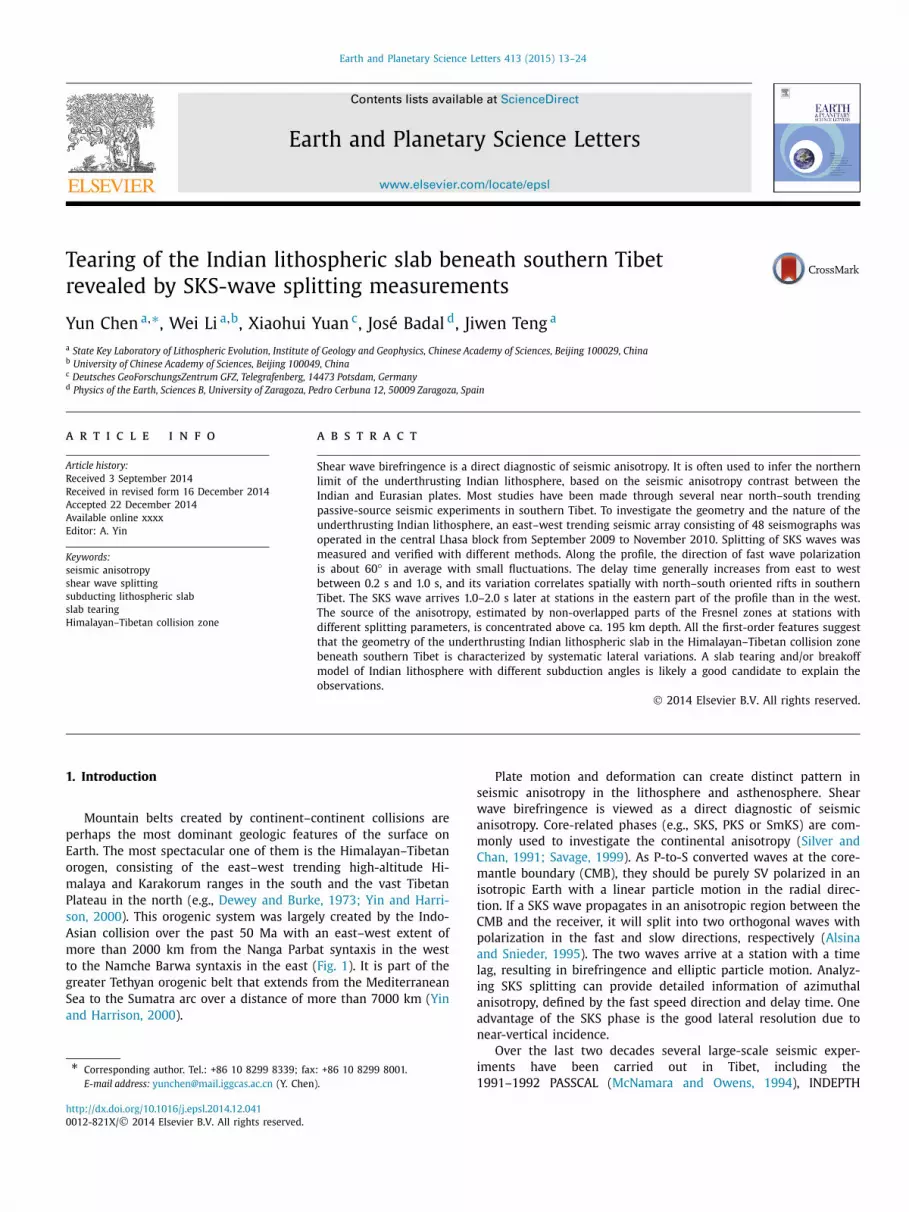
Fig. 1. Shaded topographic map showing the regional geologic features in southern Tibet and the location of the TIBET-31N seismic array. Geological structures are based on the HimaTibetMap-1.0 dataset (Styron et al., 2010). Red triangles indicate seismic stations. Green dots denote SKS-wave piercing points at 150-km depth. Blue areas are lakes. The upper-right inset is a map of the Tibetan Plateau where the study area is delimited by a red rectangle. The upper-left inset is the map showing the distribution of earthquakes used for the SKS-wave spitting measurements. The red triangle denotes the approximate location of the seismic array. The 42 events used for the SKS splitting analysis are represented as red circles, and they all lie in the Fiji–Tonga–Kermadec region with similar backazimuths and ray parameters. Abbreviations for tectonic blocks: HB, Himalayan block; LB, Lhasa block; QB, Qiangtang block. Abbreviations for sutures: IYS, Indus–Yarlung suture; BNS, Bangong–Nujiang suture. Abbreviations for rifts: LGR, Longgar rift; NTR, Nyima–Tingri rift; XDR, Xainza–Dingjye rift; YGR, Yadong–Gulu rift. NQT: Nyainqentanglha Mountains.

(Sandvol and Ni, 1997; Huang et al., 2000), Hi-CLIMB (Nabelek et al., 2009), ANTILOPE (Zhao et al., 2010, 2013, 2014), etc. Most of the seismic arrays are mainly north–south trending. Undoubt-edly the N–S trending transects are optimal to investigate the contacts among different blocks and the deep dynamic process of the N–S convergence between India and Eurasia. Shear wave splitting was used to measure the seismic anisotropy and to in-fer the frontiers of the northwards moving Indian plate. Sandvol and Ni (1997) analyzed the shear wave splitting of the INDEPTH-II seismic array. Their results show no evidence of significant seismic anisotropy in Lhasa block. Chen and Özalaybey (1998) modeled seismic anisotropy and Bouguer gravity anomalies along the profile from Yadong to Golmud (1991–1992 PASSCAL) by a juxtaposition of the Eurasian lithosphere over Indian lithosphere. The Eurasian mantle lithosphere appears only to north of 30◦N, while the Indian mantle lithosphere extends farther north to near 33◦N. Huang et al. (2000) suggested that the onset of measurable splitting at 32◦Nfrom the INDEPTH III seismic array most likely marks the north-ern limit of the underthrusting Indian lithosphere. Fu et al. (2008)combined the shear wave splitting results in Tibet and interpreted the nulls near the Indus–Yarlung suture as a result of a corner flow induced by the subvertical subduction of the Indian lithosphere south of the Bangong–Nujiang suture. Similarly, Zhao et al. (2010)measured the SKS anisotropy along the ANTILOPE-I and II profiles and defined the scope of the Indian lithosphere by the feature of weak anisotropy. Chen et al. (2010a) combined SKS splittings along the Hi-CLIMB profile with other observations, such as He iso-topes and gravity observations, and argued that the rapid increase in the splitting magnitude occurring about 100 km north of the Bangong–Nujiang suture reflects the northern leading edge of the underthrusting Indian mantle lithosphere. Kind and Yuan (2010)presented a comprehensive map of the northern boundary of the

Indian lithosphere at 200 km depth inferred from tomography, re-ceiver function and seismic anisotropy measurements. A point of agreement from most previous studies is that the Indian mantle lithosphere advancing northward and subducting beneath Tibet is accompanied by no or very weak anisotropy (Meissner et al., 2002;Kumar and Singh, 2008). Therefore the transition from null and weak shear wave splitting to strong splitting may indicate the leading edge of the northwards underthrusting Indian lithosphere (Hirn et al., 1995).

Supplementary to the N–S trending seismic experiments, east–west trending experiments in southern Tibet could help to trace lateral variations in the geometry and the nature of the under-thrusting Indian lithosphere. The Lhasa block, located between the Bangong–Nujiang suture to the north and the Indus–Yarlung su-ture to the south (Fig. 1), is an ideal place to investigate the lateral variations of the underthrusting Indian lithosphere. A 600-km-long east–west passive-source linear seismic array (TIBET-31N) was op-erated approximately along 31◦N latitude from Nam Tso to Cuoqin in the central Lhasa block, crossing some north–south oriented major rift-systems (or grabens) in southern Tibet (Fig. 1). In this experiment, 48 seismographs (equipped with Guralp CMG-3ESP sensors plus Reftek-72A or Reftek-130 data loggers) were oper-ated from September 2009 to November 2010 at an average station spacing of 15 km along with a co-operating profile of 10 seismo-graphs across Yadong–Gulu Rift (Zhang et al., 2013).

2. Data and methods

In this study, we used shear-wave splitting analysis to detect azimuthal anisotropy beneath the profile TIBET-31N. In order to identify the most salient first-order features of our splitting data

Y. Chen et al. / Earth and Planetary Science Letters 413 (2015) 13–24 15

Table 1Events used for SKS splitting analysis in this study.

Year Julian day

UTC time (hhmmss)

Latitude (deg.)

Longi-tude (deg.)

Mag. (Mw)

Depth (km)

2009 272 174810 −15.49 −172.10 8.1 182009 275 010739 −16.33 −173.47 6.1 82009 275 154709 −17.02 174.51 6.0 102009 281 211613 −12.91 166.31 5.9 352009 282 131232 −13.36 166.50 5.6 352009 283 142515 −14.12 166.69 5.8 352009 284 031213 −22.00 170.25 6.0 102009 284 044751 −13.00 166.12 5.7 442009 285 205938 −14.07 166.25 5.7 352009 287 180021 −14.91 −174.82 6.2 102009 292 224938 −15.36 −172.26 5.9 182009 296 151413 −12.20 166.05 5.9 312009 304 190951 −11.38 166.38 5.9 1332009 306 104713 −24.12 −175.17 6.1 92009 312 154609 −16.01 167.99 5.5 1792009 313 104454 −17.24 178.34 7.3 5852009 326 074820 −17.79 −178.43 6.3 5222009 326 224727 −31.57 179.47 6.2 4352009 327 183634 −12.62 166.25 5.7 352009 328 124715 −20.71 −174.04 6.7 182009 335 194258 −17.08 167.64 5.5 402009 343 094603 −22.15 170.96 6.4 452010 018 160914 −12.48 166.29 5.7 102010 024 181509 −18.51 167.90 5.6 152010 040 010344 −15.05 −173.49 6.0 102010 044 023428 −21.90 −174.77 6.0 112010 053 070052 −23.64 −176.04 5.9 252010 063 140227 −13.57 167.23 6.4 1762010 100 165424 −20.11 −176.22 5.9 2722010 101 021906 −12.97 166.52 5.8 102010 111 172029 −15.27 −173.22 6.1 352010 147 171446 −13.70 166.64 7.1 312010 152 164732 −17.88 169.10 5.6 402010 153 185107 −13.73 166.59 5.6 352010 160 232317 −18.60 169.49 6.0 122010 168 130646 −33.17 179.72 6.0 1702010 181 043102 −23.31 179.12 6.3 5812010 183 060403 −13.64 166.49 6.3 292010 203 050357 −15.15 168.17 5.9 102010 222 052344 −17.54 168.07 7.2 252010 222 231831 −14.46 167.35 5.9 1912010 228 193549 −20.80 −178.83 6.1 603

set and hence to infer the physical meanings by a simple pattern, the following strategies and approaches were adopted.

(1) Only SKS phases with high signal-to-noise ratio on the orig-inal trace were selected for analysis. To avoid complications and to ensure a high lateral resolution, other phases (e.g., SKKS waves) were not considered, because SKS phase has a steeper incidence at the receiver and a clearer arrival than other shear-wave phases for the same event (see Fig. 2a in Chen et al., 2013).

(2) We selected events located in the Fiji–Tonga subduction zone with similar backazimuths and ray parameters (Table 1). So, complicated propagating effects that might affect our mea-surements, such as a large spatial sampling difference of differ-ent ray paths, and superposition of unequal anisotropic prop-erties from different azimuths, are minimized. On the whole, 42 events are used for the SKS splitting analysis (Fig. 1). Loca-tions of the SKS piercing points at a depth of 150 km beneath the stations are shown in Fig. 1. They are distributed within a narrow band close to the profile.

(3) To enhance the signal-to-noise ratio, the records were band-pass filtered by two filters: a high-pass filter with a corner frequency of 0.02 Hz to suppress the long-period noise, and a low-pass filter with a corner frequency between 0.2 and

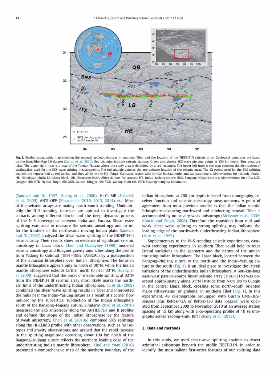
Fig. 2. Example for SKS-wave splitting analysis that makes reference to the event 2009313 recorded at the station C28 (see Tables 1 and 2 for locations of the sta-tion and the event). The Mw 7.3 earthquake was located at a depth of 585 km in the Tonga subduction zone. (a) Locations of station C28 (red triangle) and event 2009313 (red star). (b) Cross-section view of the SKS propagation path for the earthquake-station pair shown in (a). White arcs mark the positions of successive wavefronts at 60-s intervals along the SKS path.

1.0 Hz to remove the high-frequency scattering induced by small-scale heterogeneities.

(4) Different analyzing methods for shear wave splitting were used simultaneously for a same SKS phase. A measurement is considered valid if it is consistently rendered by different methods. Large measurement errors due to different meth-ods can thus be ruled out. We used the SplitLab software package developed by Wüstefeld et al. (2008) to measure the shear wave splitting. The rotation correlation method (RC method, Bowman and Ando, 1987), minimum energy method (SC method, Silver and Chan, 1991), and eigenvalue method (EV method, Silver and Chan, 1991) were used to determine the fast polarization direction and the delay time, simultane-ously.

3. Splitting results

An example of the outputs provided by the analysis for station C28 is shown in Fig. 3. The solution for the splitting parameters is given in the plot (b) and the intersection of the horizontal and vertical straight lines drawn in the plots (g) and (k), which pro-vide the fast wave direction and the delay time, respectively. This procedure is systematically used in any other case.

3.1. Splitting parameters and travel times for a single event

Here we show variations of splitting parameters along the pro-file obtained from a single event 2009313. The event occurred on 9th November 2009 (Julian day 313) at UTC time 10h:44m:54s with a large magnitude of Mw 7.3. It is located in the Tonga subduction zone with a large focal depth of 585 km (Table 1and Fig. 2). Clear SKS phases, well-separated from other phases, were recorded at almost all the stations with a high signal-to-noise ratio on both radial and transverse seismograms. The band-pass filtered radial- and transverse-component SKS waveforms are shown in Figs. 4a, 4b. The SKS waves have steep incidence an-gles ranging between 8.2◦ and 8.9◦ such as are calculated from the IASP91 model (Kennett and Engdahl, 1991), which leads to a high lateral resolution. The earthquake has similar backazimuths (103.3◦–106.2◦) and epicentral distances (96.394◦–101.378◦) along the profile (Fig. 4c).

The arrival times of SKS phases exhibit variations at stations close to the major rifts in the study area. We subtracted the the-oretical travel times predicted by the IASP91 model from the SKS arrivals and picked the maximum-phase amplitudes on the radial-component (Fig. 4a). In the enlarged window (Fig. 4d), the SKS travel-time residuals are clearly related to locations of the rifts. The SKS arrivals between YGR and XDR is up to 2.5 s later than

16Y.Chen

etal./Earth

andPlanetary

ScienceLetters

413(2015)

13–24

nels display the initial seismograms (a), information of the que: (d) seismogram components in fast (blue dashed) and correction (not normalized); (f) particle motion before (blue are similar with (d)–(g) in the middle panels.

Fig. 3. Example of SKS-wave splitting measurement using the SplitLab software package (Wüstefeld et al., 2008) for event 2009313 recorded at station C28. Upper paevent-station pair and the measurement result (b), and the stereoplot (c) centered at station C28. Middle panels display result of the rotation-correlation (RC) technislow (red solid) directions for RC-anisotropy system after RC-delay correction (normalized); (e) radial (Q, blue dashed) and transverse (T, red solid) components after RC-dashed) and after (red solid) RC-correction; and (g) map of correlation coefficients. Lower panels display result of the minimum energy (SC) technique. Sub-plots (h)–(k)

Y. Chen et al. / Earth and Planetary Science Letters 413 (2015) 13–24 17

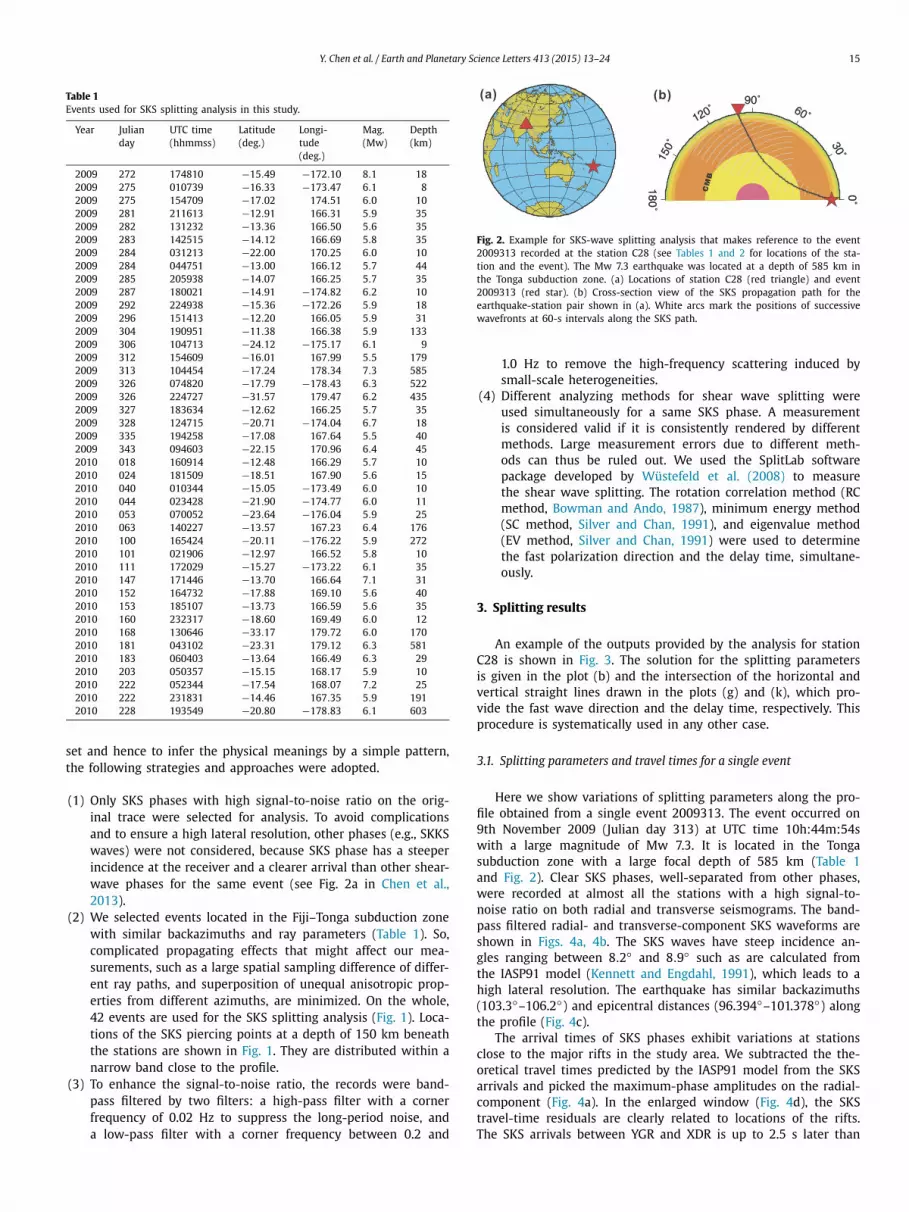
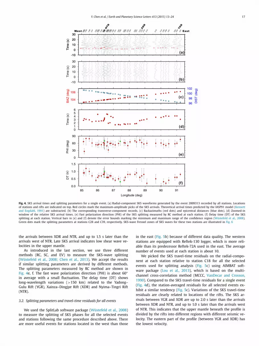
Fig. 4. SKS arrival times and splitting parameters for a single event. (a) Radial-component SKS waveforms generated by the event 2009313 recorded by all stations. Locations of stations and rifts are indicated on top. Red circles mark the maximum-amplitude picks of the SKS arrivals. Theoretical arrival times predicted by the IASP91 model (Kennett and Engdahl, 1991) are substracted. (b) The corresponding transverse-component records. (c) Backazimuths (red dots) and epicentral distances (blue dots). (d) Zoomed-in window of the relative SKS arrival times. (e) Fast polarization direction (PHI) of the SKS splitting measured by RC method at each station. (f) Delay time (DT) of the SKS splitting at each station. Vertical bars in (e) and (f) denote the error bounds marking the minimum and maximum range of the confidence region (Wüstefeld et al., 2008). Green dots mark the splitting parameters at stations C28 and C39, respectively. SKS-wave Fresnel zones of SKS waves for these two stations are illustrated in Fig. 6

the arrivals between XDR and NTR, and up to 1.5 s later than the arrivals west of NTR. Late SKS arrival indicates low shear wave ve-locities in the upper mantle.

As introduced in the last section, we use three different methods (RC, SC, and EV) to measure the SKS-wave splitting (Wüstefeld et al., 2008; Chen et al., 2013). We accept the results if similar splitting parameters are derived by different methods. The splitting parameters measured by RC method are shown in Fig. 4e, f. The fast wave polarization direction (PHI) is about 60◦in average with a small fluctuation. The delay time (DT) shows long-wavelength variations (>150 km) related to the Yadong–Gulu Rift (YGR), Xainza–Dingjye Rift (XDR) and Nyima–Tingri Rift (NTR).

3.2. Splitting parameters and travel-time residuals for all events

We used the SplitLab software package (Wüstefeld et al., 2008)to measure the splitting of SKS phases for all the selected events and stations following the same procedure described above. There are more useful events for stations located in the west than those

in the east (Fig. 5b) because of different data quality. The western stations are equipped with Reftek-130 logger, which is more reli-able than its predecessor Reftek-72A used in the east. The average number of events used at each station is about 10.

We picked the SKS travel-time residuals on the radial-compo-nent at each station relative to station C18 for all the selected events used for splitting analysis (Fig. 5c) using AIMBAT soft-ware package (Lou et al., 2013), which is based on the multi-channel cross-correlation method (MCCC, VanDecar and Crosson, 1990). Compared to the SKS travel-time residuals for a single event (Fig. 4d), the station-averaged residuals for all selected events ex-hibit a similar tendency (Fig. 5c). Variations of the SKS travel-time residuals are clearly related to locations of the rifts. The SKS ar-rivals between YGR and XDR are up to 2.0 s later than the arrivals between XDR and NTR, and up to 1.0 s later than the arrivals west of NTR. This indicates that the upper mantle beneath the profile is divided by the rifts into different regions with different seismic ve-locity. The eastern part of the profile (between YGR and XDR) has the lowest velocity.

18 Y. Chen et al. / Earth and Planetary Science Letters 413 (2015) 13–24

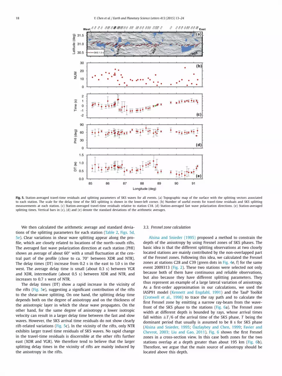
Fig. 5. Station-averaged travel-time residuals and splitting parameters of SKS waves for all events. (a) Topographic map of the surface with the splitting vectors associated to each station. The scale for the delay time of the SKS splitting is shown in the lower-left corner. (b) Number of useful events for travel-time residuals and SKS splitting measurements at each station. (c) Station-averaged travel-time residuals relative to station C18. (d) Station-averaged fast wave polarization directions. (e) Station-averaged splitting times. Vertical bars in (c), (d) and (e) denote the standard deviations of the arithmetic averages.

We then calculated the arithmetic average and standard devia-tions of the splitting parameters for each station (Table 2, Figs. 5d, 5e). Clear variations in shear wave splitting appear along the pro-file, which are closely related to locations of the north–south rifts. The averaged fast wave polarization direction at each station (PHI) shows an average of about 60◦ with a small fluctuation at the cen-tral part of the profile (close to ca. 70◦ between XDR and NTR). The delay times (DT) increase from 0.2 s in the east to 1.0 s in the west. The average delay time is small (about 0.3 s) between YGR and XDR, intermediate (about 0.5 s) between XDR and NTR, and increases to 0.7 s west of NTR.

The delay times (DT) show a rapid increase in the vicinity of the rifts (Fig. 5e), suggesting a significant contribution of the rifts to the shear-wave splitting. On one hand, the splitting delay time depends both on the degree of anisotropy and on the thickness of the anisotropic layer in which the shear wave propagates. On the other hand, for the same degree of anisotropy a lower isotropic velocity can result in a larger delay time between the fast and slow waves. However, the SKS arrival time residuals do not show clearly rift-related variations (Fig. 5c). In the vicinity of the rifts, only NTR exhibits larger travel time residuals of SKS waves. No rapid change in the travel-time residuals is discernible at the other rifts further east (XDR and YGR). We therefore tend to believe that the larger splitting delay times in the vicinity of rifts are mainly induced by the anisotropy in the rifts.

3.3. Fresnel zone calculation

Alsina and Snieder (1995) proposed a method to constrain the depth of the anisotropy by using Fresnel zones of SKS phases. The basic idea is that the different splitting observations at two closely located stations are mainly contributed by the non-overlapped part of the Fresnel zones. Following this idea, we calculated the Fresnel zones at stations C28 and C39 (green dots in Fig. 4e, f) for the same event 2009313 (Fig. 2). These two stations were selected not only because both of them have continuous and reliable observations, but also because they have different splitting parameters. They thus represent an example of a large lateral variation of anisotropy. As a first-order approximation in our calculations, we used the IASP91 model (Kennett and Engdahl, 1991) and the TauP Toolkit (Crotwell et al., 1998) to trace the ray path and to calculate the first Fresnel zone by emitting a narrow ray-beam from the wave-front of the SKS phase to the stations (Fig. 6a). The Fresnel zone width at different depth is bounded by rays, whose arrival times fall within ±T /6 of the arrival time of the SKS phase, T being the dominant period that usually is assumed to be 8 s for SKS phase (Alsina and Snieder, 1995; Öazlaybey and Chen, 1999; Favier and Chevrot, 2003; Liu and Gao, 2011). Fig. 6 shows the first Fresnel zones in a cross-section view. In this case both zones for the two stations overlap at a depth greater than about 195 km (Fig. 6b). Therefore, we argue that the main source of anisotropy should be located above this depth.

Y. Chen et al. / Earth and Planetary Science Letters 413 (2015) 13–24 19

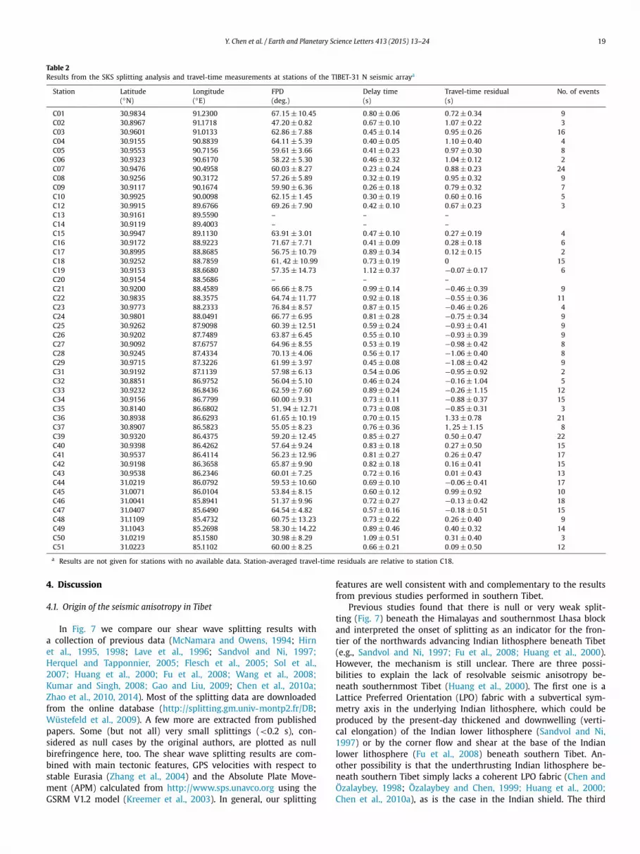
Table 2Results from the SKS splitting analysis and travel-time measurements at stations of the TIBET-31 N seismic arraya

Station Latitude (◦N)

Longitude (◦E)

FPD (deg.)

Delay time (s)

Travel-time residual (s)

No. of events

C01 30.9834 91.2300 67.15 ± 10.45 0.80 ± 0.06 0.72 ± 0.34 9C02 30.8967 91.1718 47.20 ± 0.82 0.67 ± 0.10 1.07 ± 0.22 3C03 30.9601 91.0133 62.86 ± 7.88 0.45 ± 0.14 0.95 ± 0.26 16C04 30.9155 90.8839 64.11 ± 5.39 0.40 ± 0.05 1.10 ± 0.40 4C05 30.9553 90.7156 59.61 ± 3.66 0.41 ± 0.23 0.97 ± 0.30 8C06 30.9323 90.6170 58.22 ± 5.30 0.46 ± 0.32 1.04 ± 0.12 2C07 30.9476 90.4958 60.03 ± 8.27 0.23 ± 0.24 0.88 ± 0.23 24C08 30.9256 90.3172 57.26 ± 5.89 0.32 ± 0.19 0.95 ± 0.32 9C09 30.9117 90.1674 59.90 ± 6.36 0.26 ± 0.18 0.79 ± 0.32 7C10 30.9925 90.0098 62.15 ± 1.45 0.30 ± 0.19 0.60 ± 0.16 5C12 30.9915 89.6766 69.26 ± 7.90 0.42 ± 0.10 0.67 ± 0.23 3C13 30.9161 89.5590 – – –C14 30.9119 89.4003 – – –C15 30.9947 89.1130 63.91 ± 3.01 0.47 ± 0.10 0.27 ± 0.19 4C16 30.9172 88.9223 71.67 ± 7.71 0.41 ± 0.09 0.28 ± 0.18 6C17 30.8995 88.8685 56.75 ± 10.79 0.89 ± 0.34 0.12 ± 0.15 2C18 30.9252 88.7859 61,42 ± 10.99 0.73 ± 0.19 0 15C19 30.9153 88.6680 57.35 ± 14.73 1.12 ± 0.37 −0.07 ± 0.17 6C20 30.9154 88.5686 – – –C21 30.9200 88.4589 66.66 ± 8.75 0.99 ± 0.14 −0.46 ± 0.39 9C22 30.9835 88.3575 64.74 ± 11.77 0.92 ± 0.18 −0.55 ± 0.36 11C23 30.9773 88.2333 76.84 ± 8.57 0.87 ± 0.15 −0.46 ± 0.26 4C24 30.9801 88.0491 66.77 ± 6.95 0.81 ± 0.28 −0.75 ± 0.34 9C25 30.9262 87.9098 60.39 ± 12.51 0.59 ± 0.24 −0.93 ± 0.41 9C26 30.9202 87.7489 63.87 ± 6.45 0.55 ± 0.10 −0.93 ± 0.39 9C27 30.9092 87.6757 64.96 ± 8.55 0.53 ± 0.19 −0.98 ± 0.42 8C28 30.9245 87.4334 70.13 ± 4.06 0.56 ± 0.17 −1.06 ± 0.40 8C29 30.9715 87.3226 61.99 ± 3.97 0.45 ± 0.08 −1.08 ± 0.42 9C31 30.9192 87.1139 57.98 ± 6.13 0.54 ± 0.06 −0.95 ± 0.92 2C32 30.8851 86.9752 56.04 ± 5.10 0.46 ± 0.24 −0.16 ± 1.04 5C33 30.9232 86.8436 62.59 ± 7.60 0.89 ± 0.24 −0.26 ± 1.15 12C34 30.9156 86.7799 60.00 ± 9.31 0.73 ± 0.11 −0.88 ± 0.37 15C35 30.8140 86.6802 51,94 ± 12.71 0.73 ± 0.08 −0.85 ± 0.31 3C36 30.8938 86.6293 61.65 ± 10.19 0.70 ± 0.15 1.33 ± 0.78 21C37 30.8907 86.5823 55.05 ± 8.23 0.76 ± 0.36 1,25 ± 1.15 8C39 30.9320 86.4375 59.20 ± 12.45 0.85 ± 0.27 0.50 ± 0.47 22C40 30.9398 86.4262 57.64 ± 9.24 0.83 ± 0.18 0.27 ± 0.50 15C41 30.9537 86.4114 56.23 ± 12.96 0.81 ± 0.27 0.26 ± 0.47 17C42 30.9198 86.3658 65.87 ± 9.90 0.82 ± 0.18 0.16 ± 0.41 15C43 30.9538 86.2346 60.01 ± 7.25 0.72 ± 0.16 0.01 ± 0.43 13C44 31.0219 86.0792 59.53 ± 10.60 0.69 ± 0.10 −0.06 ± 0.41 17C45 31.0071 86.0104 53.84 ± 8.15 0.60 ± 0.12 0.99 ± 0.92 10C46 31.0041 85.8941 51.37 ± 9.96 0.72 ± 0.27 −0.13 ± 0.42 18C47 31.0407 85.6490 64.54 ± 4.82 0.57 ± 0.16 −0.18 ± 0.51 15C48 31.1109 85.4732 60.75 ± 13.23 0.73 ± 0.22 0.26 ± 0.40 9C49 31.1043 85.2698 58.30 ± 14.22 0.89 ± 0.46 0.40 ± 0.32 14C50 31.0219 85.1580 30.98 ± 8.29 1.09 ± 0.51 0.31 ± 0.40 3C51 31.0223 85.1102 60.00 ± 8.25 0.66 ± 0.21 0.09 ± 0.50 12

a Results are not given for stations with no available data. Station-averaged travel-time residuals are relative to station C18.

4. Discussion

4.1. Origin of the seismic anisotropy in Tibet

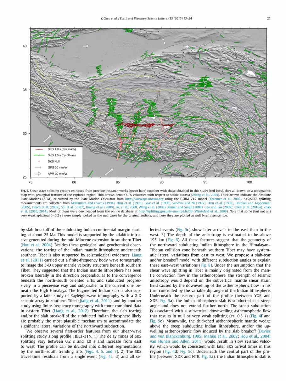
In Fig. 7 we compare our shear wave splitting results with a collection of previous data (McNamara and Owens, 1994; Hirn et al., 1995, 1998; Lave et al., 1996; Sandvol and Ni, 1997;Herquel and Tapponnier, 2005; Flesch et al., 2005; Sol et al., 2007; Huang et al., 2000; Fu et al., 2008; Wang et al., 2008;Kumar and Singh, 2008; Gao and Liu, 2009; Chen et al., 2010a;Zhao et al., 2010, 2014). Most of the splitting data are downloaded from the online database (http :/ /splitting .gm .univ-montp2 .fr /DB; Wüstefeld et al., 2009). A few more are extracted from published papers. Some (but not all) very small splittings (<0.2 s), con-sidered as null cases by the original authors, are plotted as null birefringence here, too. The shear wave splitting results are com-bined with main tectonic features, GPS velocities with respect to stable Eurasia (Zhang et al., 2004) and the Absolute Plate Move-ment (APM) calculated from http :/ /www.sps .unavco .org using the GSRM V1.2 model (Kreemer et al., 2003). In general, our splitting

features are well consistent with and complementary to the results from previous studies performed in southern Tibet.

Previous studies found that there is null or very weak split-ting (Fig. 7) beneath the Himalayas and southernmost Lhasa block and interpreted the onset of splitting as an indicator for the fron-tier of the northwards advancing Indian lithosphere beneath Tibet (e.g., Sandvol and Ni, 1997; Fu et al., 2008; Huang et al., 2000). However, the mechanism is still unclear. There are three possi-bilities to explain the lack of resolvable seismic anisotropy be-neath southernmost Tibet (Huang et al., 2000). The first one is a Lattice Preferred Orientation (LPO) fabric with a subvertical sym-metry axis in the underlying Indian lithosphere, which could be produced by the present-day thickened and downwelling (verti-cal elongation) of the Indian lower lithosphere (Sandvol and Ni, 1997) or by the corner flow and shear at the base of the Indian lower lithosphere (Fu et al., 2008) beneath southern Tibet. An-other possibility is that the underthrusting Indian lithosphere be-neath southern Tibet simply lacks a coherent LPO fabric (Chen and Özalaybey, 1998; Özalaybey and Chen, 1999; Huang et al., 2000;Chen et al., 2010a), as is the case in the Indian shield. The third

20 Y. Chen et al. / Earth and Planetary Science Letters 413 (2015) 13–24

Fig. 6. Cross-section view of SKS-wave Fresnel zones calculated for event 2009313 recorded at stations C28 and C39, indicated in Fig. 4e, f. (a) SKS paths for the two earthquake-station pairs in the Earth. Gray arcs mark the positions of successive wavefronts at 60-s intervals. (b) The enlarged zone outlined by the green square box in (a). Dotted lines mark the positions of successive wavefronts at 2-s intervals. Notice that the SKS-wave Fresnel zones for both branches are overlapped at depths deeper than about 195 km. As a first-order approximation the global Earth model IASP91 (Kennett and Engdahl, 1991) was used in the calculations.

model is that anisotropy in the Indian lithosphere and in the un-derlying asthenosphere are oriented in different directions with a big angle, thus effectively resulting in a null birefringence. The latter two models are based on the observations of null splitting at stations in the Indian plate (e.g., Chen and Özalaybey, 1998). However, many other measures of splitting made more recently at stations in India show large splitting (close to 1 s) and most of the azimuths corresponding to fast polarization direction can be explained by the APM-related strain (Kumar and Singh, 2008;Kumar et al., 2010; Saikia et al., 2010). So the latter two expla-nations employing a weak anisotropic Indian plate are unlikely to be true. In fact, most of the previous studies suggested that the splitting in Tibet is mainly originated from the mantle convection flow in the asthenosphere, which is related to the APM of Eurasia (McNamara and Owens, 1994; Hirn et al., 1995, 1998; Lave et al., 1996; Gao and Liu, 2009; Huang et al., 2000).

In the Indian shield, the fast polarization direction is aligned in the NNE direction, consisting with the Indian Plate motion approx-imately (Kumar and Singh, 2008; Kumar et al., 2010; Saikia et al., 2010). The dominant fast speed direction of 60◦ along our profile is similar to that observed in the Indian shield, implying a same source of anisotropy induced by the asthenospheric flow beneath the downgoing Indian plate. Alternatively the corner flow in the overlying mantle wedge induced by downdip motion of the Indian slab may contribute to the observed anisotropy in the same direc-tion.

With the caution that the splittings represent vertically inte-grated point measurements, whereas surface waves average hor-izontally over large distances, the comparison of both types of anisotropy based on the L–R discrepancy or else on shear wave splitting can be done with care (Wüstefeld et al., 2009). Under the simplest assumption of a vertical symmetry axis, the area with rel-atively strong radial anisotropy should have weak or no azimuthal anisotropy. The central Lhasa block has strong radial anisotropy (Chen et al., 2009) but weak azimuthal anisotropy within the upper mantle, which implies a subvertical orientation of α axis caused by the subduction of the Indian Plate (Savage, 1999).

4.2. Lateral variations of the subduction-related mantle structure

The 2000 km-long east–west Himalayan–Tibetan collision zone is in a complex tectonic setting consisting of six major tectonic domains (Yin, 2010). The shortening in the Cenozoic deformation estimated from geological observations in the Himalayan orogen shows several hundred kilometers with distinct lateral variations (Yin, 2010), which is also confirmed by the differential move-ment constrained by the present-day GPS data (Fig. 7). It would be very hard to keep a uniform geometry during such a large-scale collision accompanied by subduction in a so complex tec-tonic setting. Many geophysical observations have already provided insights into the significant lateral variations in the subduction-related mantle structure beneath this collision zone. The geometry and the nature of the subduction of the Indian plate may change distinctly in certain places. For example, the Indian plate is sub-ducting eastward and sinks into the mantle transition zone along the Burma arc (Li et al., 2008; Lei et al., 2009), which is very dif-ferent from the main Himalayan–Tibetan collision zone. Combin-ing seismic images derived by different techniques, such as body wave tomography (Tilmann et al., 2003; Zhou and Murphy, 2005;Li et al., 2008; He et al., 2010; Liang et al., 2012; Zhao et al., 2013), surface wave tomography (Brandon and Romanowicz, 1986;Priestley et al., 2006; Chen et al., 2010b; Li et al., 2013), receiver functions (Yuan et al., 1997; Kosarev et al., 1999; Kind et al., 2002;Kumar et al., 2006; Nabelek et al., 2009; Zhao et al., 2010; Zhao et al., 2011) and controlled-source seismic investigations (Zhao et., 1993), it has been suggested that the horizontal sliding distance of the Indian lithosphere under the Tibetan Plateau from west to east (Kind and Yuan, 2010) and that the dip angle of the subduct-ing Indian lithosphere varies laterally (Zhou and Murphy, 2005;Li et al., 2008).

4.3. Mechanism for lateral variations of the subduction

A mechanism is needed to accommodate the significant lateral variations of the geometry and the nature of the subducting In-dia lithospheric slab. Based on the data of the rift spaces, the age of rift initiation, and the instability analysis, Yin (2000) pro-posed a model, in which the Indian mantle lithosphere directly beneath the Himalaya is involved in east–west extension in Tibet and the rifts occur in the subducting Indian lithosphere. By com-paring the differences in lithospheric structure, magmatism and deformation styles between western and eastern Tibet, Xiao et al.(2007) proposed a slab-tearing model in which the Indian litho-sphere has been split into two parts separated by YGR: a part subducting northward steeply beneath the western plateau, and a northeastward subducting one with shallow angle beneath the eastern plateau. According to the features of the Gandese tectono-magmatic belt and the aeromagnetic anomalies in Tibet, Hou et al.(2006) suggested that the tearing of the Indian lithosphere proba-bly resulted in dischronal subduction along the Indo-Asian collision zone. Mahéo et al. (2002) argued that the Neogene magmatic and metamorphic evolution of the South Asian margin was controlled

Y. Chen et al. / Earth and Planetary Science Letters 413 (2015) 13–24 21

Fig. 7. Shear-wave splitting vectors extracted from previous research works (green bars) together with those obtained in this study (red bars), they all drawn on a topographic map with geological features of the explored region. Thin arrows denote GPS velocities with respect to stable Eurasia (Zhang et al., 2004). Thick arrows indicate the Absolute Plate Motions (APM), calculated by the Plate Motion Calculator from http :/ /www.sps .unavco .org using the GSRM V1.2 model (Kreemer et al., 2003). SKS/SKKS splitting measurements are collected from McNamara and Owens (1994), Hirn et al. (1995), Lave et al. (1996), Sandvol and Ni (1997), Hirn et al. (1998), Herquel and Tapponnier(2005), Flesch et al. (2005), Sol et al. (2007), Huang et al. (2000), Fu, et al., 2008, Wang et al. (2008), Kumar and Singh (2008), Gao and Liu (2009); Chen et al. (2010a), Zhao et al. (2010, 2014). Most of them were downloaded from the online database at http :/ /splitting .gm .univ-montp2 .fr /DB (Wüstefeld et al., 2009). Note that some (but not all) very weak splittings (<0.2 s) were simply looked as the null cases by the original authors, and here they are plotted as null birefringence, too.

by slab breakoff of the subducting Indian continental margin start-ing at about 25 Ma. This model is supported by the adakitic intru-sive generated during the mid-Miocene extension in southern Tibet (Hou et al., 2004). Besides these geological and geochemical obser-vations, the tearing of the Indian mantle lithosphere underneath southern Tibet is also supported by seismological evidences. Liang et al. (2011) carried out a finite-frequency body wave tomography to image the 3-D upper mantle velocity structure beneath southern Tibet. They suggested that the Indian mantle lithosphere has been broken laterally in the direction perpendicular to the convergence beneath the north–south oriented rifts, and subducted progres-sively in a piecewise way and subparallel to the current one be-neath the High Himalaya. The fragmented Indian slab is also sup-ported by a later study of Rayleigh-wave tomography with a 2-D seismic array in southern Tibet (Jiang et al., 2011), and by another study using finite-frequency tomography with more combined data in eastern Tibet (Liang et al., 2012). Therefore, the slab tearing and/or the slab breakoff of the subducted Indian lithosphere likely are probably the most plausible mechanism to accommodate the significant lateral variations of the northward subduction.

We observe several first-order features from our shear-wave splitting study along profile TIBET-31N. 1) The delay times of SKS splitting vary between 0.2 s and 1.0 s and increase from east to west. The profile can be divided into different segmentations by the north–south trending rifts (Figs. 4, 5, and 7). 2) The SKS travel-time residuals from a single event (Fig. 4a, d) and all se-

lected events (Fig. 5c) show later arrivals in the east than in the west. 3) The depth of the anisotropy is estimated to be above 195 km (Fig. 6). All these features suggest that the geometry of the northward subducting Indian lithosphere in the Himalayan–Tibetan collision zone beneath southern Tibet may have system-atic lateral variations from east to west. We propose a slab-tear and/or breakoff model with different subduction angles to explain these east–west variations (Fig. 8). Under the assumption that the shear wave splitting in Tibet is mainly originated from the man-tle convection flow in the asthenosphere, the strength of seismic anisotropy would depend on the subvertical mantle shear strain field caused by the downwelling of the asthenospheric flow in his turn controlled by the variable dip angle of the Indian lithosphere. Underneath the eastern part of the profile (between YGR and XDR, Fig. 5a), the Indian lithospheric slab is subducted at a steep angle and does not extend further north. The steep subduction is associated with a subvertical downwelling asthenospheric flow that results in null or very weak splitting (ca. 0.3 s) (Fig. 4f and Fig. 5e). Meanwhile, the thickened asthenospheric mantle wedge above the steep subducting Indian lithosphere, and/or the up-welling asthenospheric flow induced by the slab breakoff (Davies and von Blanckenburg, 1995; Maheo et al., 2002; Hou et al., 2004;van Hunen and Allen, 2011) would result in slow seismic veloc-ity, which would be consistent with later SKS arrival times in this region (Fig. 4d; Fig. 5c). Underneath the central part of the pro-file (between XDR and NTR, Fig. 5a), the Indian lithospheric slab is

22 Y. Chen et al. / Earth and Planetary Science Letters 413 (2015) 13–24

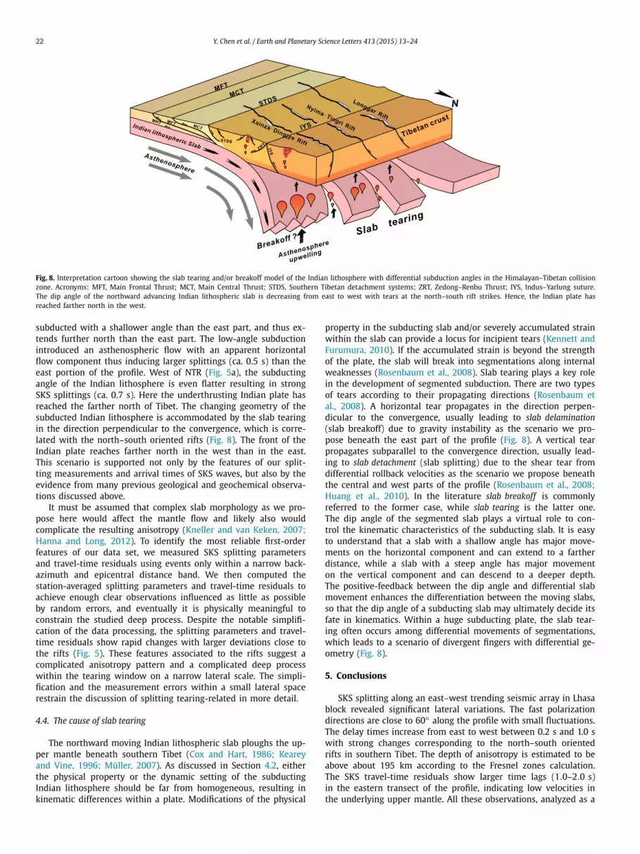
Fig. 8. Interpretation cartoon showing the slab tearing and/or breakoff model of the Indian lithosphere with differential subduction angles in the Himalayan–Tibetan collision zone. Acronyms: MFT, Main Frontal Thrust; MCT, Main Central Thrust; STDS, Southern Tibetan detachment systems; ZRT, Zedong–Renbu Thrust; IYS, Indus–Yarlung suture. The dip angle of the northward advancing Indian lithospheric slab is decreasing from east to west with tears at the north–south rift strikes. Hence, the Indian plate has reached farther north in the west.

subducted with a shallower angle than the east part, and thus ex-tends further north than the east part. The low-angle subduction introduced an asthenospheric flow with an apparent horizontal flow component thus inducing larger splittings (ca. 0.5 s) than the east portion of the profile. West of NTR (Fig. 5a), the subducting angle of the Indian lithosphere is even flatter resulting in strong SKS splittings (ca. 0.7 s). Here the underthrusting Indian plate has reached the farther north of Tibet. The changing geometry of the subducted Indian lithosphere is accommodated by the slab tearing in the direction perpendicular to the convergence, which is corre-lated with the north–south oriented rifts (Fig. 8). The front of the Indian plate reaches farther north in the west than in the east. This scenario is supported not only by the features of our split-ting measurements and arrival times of SKS waves, but also by the evidence from many previous geological and geochemical observa-tions discussed above.

It must be assumed that complex slab morphology as we pro-pose here would affect the mantle flow and likely also would complicate the resulting anisotropy (Kneller and van Keken, 2007;Hanna and Long, 2012). To identify the most reliable first-order features of our data set, we measured SKS splitting parameters and travel-time residuals using events only within a narrow back-azimuth and epicentral distance band. We then computed the station-averaged splitting parameters and travel-time residuals to achieve enough clear observations influenced as little as possible by random errors, and eventually it is physically meaningful to constrain the studied deep process. Despite the notable simplifi-cation of the data processing, the splitting parameters and travel-time residuals show rapid changes with larger deviations close to the rifts (Fig. 5). These features associated to the rifts suggest a complicated anisotropy pattern and a complicated deep process within the tearing window on a narrow lateral scale. The simpli-fication and the measurement errors within a small lateral space restrain the discussion of splitting tearing-related in more detail.

4.4. The cause of slab tearing

The northward moving Indian lithospheric slab ploughs the up-per mantle beneath southern Tibet (Cox and Hart, 1986; Kearey and Vine, 1996; Müller, 2007). As discussed in Section 4.2, either the physical property or the dynamic setting of the subducting Indian lithosphere should be far from homogeneous, resulting in kinematic differences within a plate. Modifications of the physical

property in the subducting slab and/or severely accumulated strain within the slab can provide a locus for incipient tears (Kennett and Furumura, 2010). If the accumulated strain is beyond the strength of the plate, the slab will break into segmentations along internal weaknesses (Rosenbaum et al., 2008). Slab tearing plays a key role in the development of segmented subduction. There are two types of tears according to their propagating directions (Rosenbaum et al., 2008). A horizontal tear propagates in the direction perpen-dicular to the convergence, usually leading to slab delamination(slab breakoff) due to gravity instability as the scenario we pro-pose beneath the east part of the profile (Fig. 8). A vertical tear propagates subparallel to the convergence direction, usually lead-ing to slab detachment (slab splitting) due to the shear tear from differential rollback velocities as the scenario we propose beneath the central and west parts of the profile (Rosenbaum et al., 2008;Huang et al., 2010). In the literature slab breakoff is commonly referred to the former case, while slab tearing is the latter one. The dip angle of the segmented slab plays a virtual role to con-trol the kinematic characteristics of the subducting slab. It is easy to understand that a slab with a shallow angle has major move-ments on the horizontal component and can extend to a farther distance, while a slab with a steep angle has major movement on the vertical component and can descend to a deeper depth. The positive-feedback between the dip angle and differential slab movement enhances the differentiation between the moving slabs, so that the dip angle of a subducting slab may ultimately decide its fate in kinematics. Within a huge subducting plate, the slab tear-ing often occurs among differential movements of segmentations, which leads to a scenario of divergent fingers with differential ge-ometry (Fig. 8).

5. Conclusions

SKS splitting along an east–west trending seismic array in Lhasa block revealed significant lateral variations. The fast polarization directions are close to 60◦ along the profile with small fluctuations. The delay times increase from east to west between 0.2 s and 1.0 s with strong changes corresponding to the north–south oriented rifts in southern Tibet. The depth of anisotropy is estimated to be above about 195 km according to the Fresnel zones calculation. The SKS travel-time residuals show larger time lags (1.0–2.0 s) in the eastern transect of the profile, indicating low velocities in the underlying upper mantle. All these observations, analyzed as a

Y. Chen et al. / Earth and Planetary Science Letters 413 (2015) 13–24 23

whole, suggest systematic lateral variations in the geometry of the underthrusting Indian lithosphere in the Himalayan–Tibetan colli-sion zone beneath southern Tibet. A slab tearing and/or breakoff model with different subduction angles is a good candidate to ex-plain our observations.

Acknowledgements

We would like to express the most sincere respect and the most deep memory to the former group leader and good friend, Prof. Zhongjie Zhang, who suddenly passed away in September 6th, 2013. It was Zhongjie who led, together with other colleagues, most of the fieldworks and research projects in Tibet undertak-ing by the group, including the deployment of the TIBET-31N seismic array. We would like to thank Drs. Tao Xu, Changqing Sun, Shaokun Si, Haiqiang Lan, and the vehicle drivers, Bianba and Duoji, and other field personnel for collecting the high qual-ity data in the hard conditions of central Tibet. We also wish to thank Profs. Yanghua Wang, Bihong Fu, Rui Gao, Fuqin Zhang, Car-los López Casado for their helpful discussions, and Profs. Xiaofeng Liang, Xiaobo Tian for significant improvement of the manuscript. Constructive comments and suggestions from anonymous review-ers significantly improved the quality of this paper. All figures were produced using the Generic Mapping Tools software pack-age (Wessel and Smith, 1998). The Strategic Priority Research Pro-gram (B) of Chinese Academy of Sciences (grant XDB03010700) and Sinoprobe-02-03 funded the TIBET-31N project. This research is also supported by the National Natural Science Foundation of China (grants 41374063 and 40830315). The Seismic Array Labora-tory, IGGCAS, provided the instrumental equipment.

References

Alsina, D., Snieder, R., 1995. Small-scale sublithospheric continental mantle de-formation: constraints from SKS splitting observations. Geophys. J. Int. 123, 431–448.

Bowman, J.R., Ando, M., 1987. Shear-wave splitting in the upper-mantle wedge above the Tonga subduction zone. Geophys. J. R. Astron. Soc. 88, 25–41.

Brandon, C., Romanowicz, B., 1986. A no-lid zone in the central Chang–Tang plat-form of Tibet – evidence from pure path phase-velocity measurements of long period Rayleigh-waves. J. Geophys. Res. 91 (B6), 6547–6564.

Chen, W.P., Özalaybey, S., 1998. Correlation between seismic anisotropy and Bouguer gravity anomalies in Tibet and its implications for lithospheric structures. Geo-phys. J. Int. 135, 93–101.

Chen, Y., Badal, J., Zhang, Z., 2009. Radial anisotropy in the crust and upper man-tle beneath the Qinghai–Tibet Plateau and surrounding regions. J. Asian Earth Sci. 36, 289–302.

Chen, W.P., Martin, M., Tseng, T.L., Nowack, R.L., Hung, S.H., Huang, B.S., 2010a. Shear-wave birefringence and current configuration of converging lithosphere under Tibet. Earth Planet. Sci. Lett. 295, 297–304.

Chen, Y., Badal, J., Hu, J.F., 2010b. Love and Rayleigh wave tomography of the Qinghai–Tibet Plateau and surrounding areas. Pure Appl. Geophys. 167, 1171–1203.

Chen, Y., Zhang, Z.J., Sun, C.Q., Badal, J., 2013. Crustal anisotropy from Moho con-verted Ps wave splitting analysis and geodynamic implications beneath the east-ern margin of Tibet and surrounding regions. Gondwana Res. 24 (3–4), 946–957.

Cox, A., Hart, R.B., 1986. Plate Tectonics: How It Works. Blackwell Science, Oxford, UK, pp. 337–351.

Crotwell, H.P., Owens, T.J., Ritsema, J., 1998. The TauP ToolKit: flexible seismic travel-time and raypath utilities. Seismol. Res. Lett. 70, 154–160.

Davies, J.H., von Blanckenburg, F., 1995. Slab breakoff: a model of lithosphere de-tachment and its test in the magmatism and deformation of collisional orogens. Earth Planet. Sci. Lett. 129, 85–102.

Dewey, J.F., Burke, K., 1973. Tibetan, Variscan and Precambrian basement reactiva-tion: products of continental collision. J. Geol. 81, 683–692.

Favier, N., Chevrot, S., 2003. Sensitivity kernels for shear wave splitting in transverse isotropic media. Geophys. J. Int. 153, 213–228.

Flesch, L.M., Holt, W.E., Silver, P.G., Stephenson, M., Wang, C.Y., Chan, W.W., 2005. Constraining the extent of crust-mantle coupling in central Asia using GPS, ge-ologic, and shear wave splitting data. Earth Planet. Sci. Lett. 238, 248–268.

Fu, Y.Y.V., Chen, Y.J., Li, A.B., Zhou, S.Y., Liang, X.F., Ye, G.Y., Jiang, M.M., Ning, J.Y., 2008. Indian mantle corner flow at southern Tibet revealed by shear wave split-ting measurements. Geophys. Res. Lett. 35, L02308. http://dx.doi.org/10.1029/2007GL031753.

Gao, S.S., Liu, K.H., 2009. Significant seismic anisotropy beneath the southern Lhasa Terrane, Tibetan Plateau. Geochem. Geophys. Geosyst. 10 (2), Q02008. http://dx.doi.org/10.1029/2008GC002227.

Hanna, J., Long, M.D., 2012. SKS splitting beneath Alaska: regional variability and implications for subduction processes at a slab edge. Tectonophysics 530–531, 272–285.

He, R.Z., Zhao, D.P., Gao, R., Zheng, H.W., 2010. Tracing the Indian lithospheric mantle beneath central Tibetan Plateau using teleseismic tomography. Tectono-physics 491, 230–243.

Herquel, G., Tapponnier, P., 2005. Seismic anisotropy in western Tibet. Geophys. Res. Lett. 32, L17306. http://dx.doi.org/10.1029/2005GL023561.

Hirn, A., Jiang, M., Sapin, M., Diaz, J., Nercessian, A., Lu, Q.T., Lepine, J.C., Shi, D.N., Sachpazl, M., Pandey, M.R., Ma, K., Gallart, J., 1995. Seismic anisotropy as an indicator of mantle flow beneath the Himalayas and Tibet. Nature 375 (15), 571–574.

Hirn, A., Diaz, J., Sapin, M., Veinante, J.L., 1998. Variation of shear-wave residuals and spitting parameter from array observations in southern Tibet. Pure Appl. Geophys. 151, 407–431.

Hou, Z.Q., Gao, Y.F., Qu, X.M., Rui, Z.Y., Mo, X.X., 2004. Origin of adakitic intru-sive generated during mid-Miocene east–west extension in southern Tibet. Earth Planet. Sci. Lett. 220, 139–155.

Hou, Z.Q., Zhao, Z.D., Gao, Y.F., Yang, Z.M., Jiang, W., 2006. Tearing and dischronal subduction of the Indian continental slab: evidence from Cenozoic Gangdese volcano-magmatic rocks in south Tibet. Acta Petrol. Sin. 22 (4), 761–774 (in Chinese with abstract in English).

Huang, W.C., Ni, J.F., Tilmann, F., Nelson, D., Guo, J.R., Zhao, W.J., Mechie, J., Kind, R., Saul, J., Rapine, R., Hearn, T.M., 2000. Seismic polarization anisotropy beneath the central Tibetan Plateau. J. Geophys. Res. 105 (B12), 27979–27989.

Huang, J.P., Vanacore, E., Niu, F.L., Levander, A., 2010. Mantle transition zone beneath the Caribbean–South American plate boundary and its tectonic implications. Earth Planet. Sci. Lett. 289, 105–111.

Jiang, M.M., Zhou, S.Y., Sandvol, E., Chen, X.F., Liang, X.F., Chen, Y.J., Fan, W.Y., 2011. 3-D lithospheric structure beneath southern Tibet from Rayleigh-wave tomogra-phy with a 2-D seismic array. Geophys. J. Int. 185, 593–608.

Kearey, P., Vine, F.J., 1996. Global Tectonics, 2nd edition. Blackwell Science, Oxford, UK, pp. 248–262.

Kennett, B.L.N., Engdahl, E.R., 1991. Traveltimes for global earthquake location and phase identification. Geophys. J. Int. 105, 429–465.

Kennett, B.L.N., Furumura, T., 2010. Tears or thinning? Subduction structures in the Pacific plate beneath the Japanese Islands. Phys. Earth Planet. Inter. 180, 52–58.

Kind, R., Yuan, X.H., 2010. Seismic images of the biggest crash on Earth. Science 329, 1479–1480.

Kind, R., Yuan, X.H., Saul, J., Nelson, D., Sobolev, S.V., Mechie, J., Zhao, W., Kosarev, G., Ni, J., Achauer, U., Jiang, M., 2002. Seismic images of crust and upper man-tle beneath Tibet: evidence for Eurasian plate subduction. Science 298 (5596), 1219–1221.

Kneller, E.A., van Keken, P.E., 2007. Trench parallel flow and seismic anisotropy in the Marianas and Andean subduction systems. Nature 450, 1222–1225.

Kosarev, G., Kind, R., Sovolev, S.V., Yuan, X., Hanka, W., Oreshin, S., 1999. Seismic evidence for a detached Indian lithospheric mantle beneath Tibet. Science 283, 1306–1309.

Kreemer, C., Holt, W.E., Haines, A.J., 2003. An integrated global model of present-day motions and plate boundary deformation. Geophys. J. Int. 154, 8–34.

Kumar, M.R., Singh, A., 2008. Evidence for plate motion related strain in the Indian shield from shear wave splitting measurements. J. Geophys. Res. 113, B08306. http://dx.doi.org/10.1029/2007JB005128.

Kumar, P., Yuan, X.H., Kind, R., Ni, J., 2006. Imaging the colliding Indian and Asian lithospheric plates beneath Tibet. J. Geophys. Res. 111, B06308.

Kumar, N., Kumar, M.R., Singh, A., Raju, P.S., Rao, N.P., 2010. Shear wave anisotropy of the Godavari rift in the south Indian shield: rift signature of APM related strain? Phys. Earth Planet. Inter. 181, 82–87.

Lavé, J., Avouac, J.P., Lacassin, R., Tapponnier, P., Montagner, J.P., 1996. Seismic anisotropy beneath Tibet: evidence for eastward extrusion of the Tibetan litho-sphere? Earth Planet. Sci. Lett. 140, 83–96.

Lei, J.S., Zhao, D.P., Su, Y.J., 2009. Insight into the origin of the Tengchong intraplate volcano and seismotectonics in southwest China from local and teleseismic data. J. Geophys. Res. 114, B05302. http://dx.doi.org/10.1029/2008JB005881.

Li, C., van der Hilst, R.D., Meltzer, A.S., Engdahl, E.R., 2008. Subduction of the Indian lithosphere beneath the Tibetan Plateau and Burma. Earth Planet. Sci. Lett. 274, 157–168.

Li, Y.H., Wu, Q.J., Pan, J.T., Zhang, F.X., Yu, D.X., 2013. An upper-mantle S-wave ve-locity model for East Asia from Rayleigh wave tomography. Earth Planet. Sci. Lett. 377–378, 367–377.

Liang, X.F., Shen, Y., Chen, Y.J., Ren, Y., 2011. Crustal and mantle velocity models of southern Tibet from finite frequency tomography. J. Geophys. Res. 116, B02408. http://dx.doi.org/10.1029/2009JB007159.

Liang, X.F., Sandvol, E., Chen, Y.J., Hearn, T., Ni, J., Klemperer, S., Shen, Y., Tilmann, F., 2012. A complex Tibetan upper mantle: a fragmented Indian slab and no south-verging subduction of Eurasian lithosphere. Earth Planet. Sci. Lett. 333–334, 101–111.

24 Y. Chen et al. / Earth and Planetary Science Letters 413 (2015) 13–24

Liu, K.H., Gao, S.S., 2011. Estimation of the depth of anisotropy using spatial co-herency of shear-wave splitting parameters. Bull. Seismol. Soc. Am. 101 (5), 2153–2161.

Lou, X.T., van der Lee, S., Lloyd, S., 2013. AIMBAT: a Python/Matplotlib tool for mea-suring teleseismic arrival times. Seismol. Res. Lett. 84 (1), 85–93.

Mahéo, G., Guillot, S., Blichert-Toft, J., Rolland, Y., Pêcher, A., 2002. A slab breakoff model for the Neogene thermal evolution of South Karakorum and South Tibet. Earth Planet. Sci. Lett. 195, 45–58.

McNamara, D.E., Owens, T.J., 1994. Shear wave anisotropy beneath the Tibetan Plateau. J. Geophys. Res. 99 (B7), 13655–13665.

Meissner, R., Moonery, W.D., Artemieva, I., 2002. Seismic anisotropy and mantle creep in young orogens. Geophys. J. Int. 149, 1–14.

Müller, R.D., 2007. An Indian cheetah. Nature 449, 795–796.Nabelek, J., et al., Hi-CLIMB Team, 2009. Underplating in the Himalaya–Tibet colli-

sion zone revealed by the Hi-CLIMB experiment. Science 325, 1371–1374.Özalaybey, S., Chen, W.P., 1999. Frequency-dependent analysis of SKS/SKKS wave-

forms observed in Australia: evidence for null birefringence. Phys. Earth Planet. Inter. 114, 197–210.

Priestley, K., Debayle, E., McKenzie, D., Pilidou, S., 2006. Upper mantle structure of eastern Asia from multimode surface waveform tomography. J. Geophys. Res. 111, B10304. http://dx.doi.org/10.1029/2005JB004082.

Rosenbaum, G., Gasparon, M., Lucente, F.P., Peccerillo, A., Miller, M.S., 2008. Kinemat-ics of slab tear faults during subduction segmentation and implications for Ital-ian magmatism. Tectonics 27, TC2008. http://dx.doi.org/10.1029/2007TC002143.

Saikia, D., Kumar, M.R., Singh, A., Mohan, G., Dattatrayam, R.S., 2010. Seismic anisotropy beneath the Indian continent from splitting of direct S waves. J. Geo-phys. Res. 115, B12315. http://dx.doi.org/10.1029/2009JB007009.

Sandvol, E., Ni, J., 1997. Seismic anisotropy beneath the southern Himalayas–Tibet collision zone. J. Geophys. Res. 102 (B8), 17813–17823.

Savage, M.K., 1999. Seismic anisotropy and mantle deformation: what have we learned from shear wave splitting? Rev. Geophys. 37 (1), 65–106.

Silver, P.G., Chan, W.W., 1991. Shear wave splitting and subcontinental mantle de-formation. J. Geophys. Res. 96, 16429–16454.

Sol, S., Meltzer, A., Burgmann, R., van der Hilst, R.D., King, R., Chen, Z., Koons, P.O., Lev, E., Liu, Y.P., Zeitler, P.K., Zhang, X., Zhang, J., Zurek, B., 2007. Geodynamics of the southeastern Tibetan Plateau from seismic anisotropy and geodesy. Geol-ogy 35 (6), 563–566.

Styron, R., Taylor, M., Okoronkwo, K., 2010. Database of active structures from the Indo-Asian collision. Trans. Am. Geophys. Union 91, 181–182.

Tilmann, F., Ni, J., INDEPTH Seismic Team, 2003. Seismic imaging of the downwelling Indian lithosphere beneath central Tibet. Science 300, 1424–1427.

van Hunen, J., Allen, M.B., 2011. Continental collision and slab break-off: a com-parison of 3-D numerical models with observations. Earth Planet. Sci. Lett. 302, 27–37.

VanDecar, J.C., Crosson, R.S., 1990. Determination of teleseismic relative phase ar-rival times using multi-channel cross-correlation and least squares. Bull. Seis-mol. Soc. Am. 80, 150–169.

Wang, C.Y., Flesch, L.M., Silver, P.G., Chang, L.J., Chan, W.W., 2008. Evidence for mechanically coupled lithosphere in central Asia and resulting implications. Ge-ology 36 (5), 363–366.

Wessel, P., Smith, W.H.F., 1998. New, improved version of the Generic Mapping Tools released. Trans. Am. Geophys. Union 79, 579.

Wüstefeld, A., Bokelmann, G., Barruol, G.H.R., Zaroli, C., 2008. SplitLab: a shear-wave splitting environment in Matlab. Comput. Geosci. 34, 515–528.

Wüstefeld, A., Bokelmann, G., Barruol, G.H.R., Barruol, G., Montagner, J.-P., 2009. Identifying global seismic anisotropy patterns by correlating shear-wave split-ting and surface waves data. Phys. Earth Planet. Inter. 176 (3–4), 198–212.

Xiao, L., Wang, C.Z., Pirajno, F., 2007. Is the underthrust India lithosphere split be-neath the Tibetan Plateau? Int. Geol. Rev. 49, 90–98.

Yin, A., 2000. Mode of Cenozoic east–west extension in Tibet suggesting a common origin of rifts in Asia during the Indo-Asian collision. J. Geophys. Res. 105 (B9), 21745–21759.

Yin, A., 2010. Cenozoic tectonic evolution of Asia: a preliminary synthesis. Tectono-physics 488, 293–325.

Yin, A., Harrison, T.M., 2000. Geologic evolution of the Himalayan–Tibetan orogen. Annu. Rev. Earth Planet. Sci. 28, 211–280.

Yuan, X.H., Ni, J., Kind, R., Mechie, J., Sandvol, E., 1997. Lithospheric and upper man-tle structure of southern Tibet from a seismological passive source experiment. J. Geophys. Res. 102, 27491–27500.

Zhang, P.Z., Shen, Z.K., Wang, M., Gan, W.J., Burgmaan, R., Monlnar, P., Wang, Q., Niu, Z.J., Sun, J.Z., Wu, J.C., Sun, H.R., You, X.Z., 2004. Continuous deformation of the Tibetan Plateau from global positioning system data. Geology 32 (9), 809–812.

Zhang, Z.J., Chen, Y., Yuan, X.H., Tian, X.B., Klemperer, S.L., Xu, T., Bai, Z.M., Zhang, H.S., Wu, J., Teng, J.W., 2013. Normal faulting from simple shear rifting in South Tibet, using evidence from passive seismic profiling across the Yadong–Gulu Rift. Tectonophysics 606, 178–186.

Zhao, W.J., Nelson, K.D., Project INDEPTH Team, 1993. Deep seismic–reflection evidence for continental underthrusting beneath southern Tibet. Nature 366, 557–559.

Zhao, J.M., Yuan, X.H., Liu, H.B., Kumar, P., Pei, S.P., Kind, R., Zhang, Z.J., Teng, J.W., Ding, L., Gao, X., Xu, Q., Wang, W., 2010. The boundary between the In-dian and Asian tectonic plates below Tibet. Proc. Natl. Acad. Sci. USA 107 (25), 11229–11233.

Zhao, W.J., Kumar, P., Mechie, J., Kind, R., Meissner, R., Wu, Z.H., Shi, D.N., Su, H.P., Xue, G.Q., Karplus, M., Tilmann, F., 2011. Tibetan plate overriding the Asian plate in central and northern Tibet. Nat. Geosci. 4, 870–873.

Zhao, J.M., Zhao, D.P., Zhang, H., Liu, H.B., Huang, Y., Cheng, H.G., Wang, W., 2013. P-wave tomography and dynamics of the crust and upper mantle beneath western Tibet. Gondwana Res. 25 (4), 1690–1699.

Zhao, J.M., Murodov, D., Huang, Y., Sun, Y.S., Pei, S.P., Liu, H.B., Zhang, H., Fu, Y.Y., Wang, W., Cheng, H.G., Tang, W., 2014. Upper mantle deformation beneath central–southern Tibet revealed by shear wave splitting measurements. Tectono-physics 627, 135–140.

Zhou, H.W., Murphy, M.A., 2005. Tomographic evidence for wholesale underthrust-ing of Indian beneath the entire Tibetan plateau. J. Asian Earth Sci. 25, 445–457.