target detection and reduction of interrupting signals in

بسى هللا انزح انزحى

Sudan University of Science and Technology

College of Graduate Studies

Target Detection and Reduction of Interrupting

Signals in Coherent MIMO Radar

المترابط في الرادار اإلشارات المقاطعة إكتشاف الهذف والحذ من

عذد المذخالت و المخرجات مت

A Thesis Submitted in Partial Fulfillment of the Requirements for the

Degree of M.Sc.in Electronic Engineering (Communications Engineering)

Prepared by:

Ali Omer Mohamed Aldow

Supervised by:

Dr. Fath-Elrahman Ismael Khalifa

January 2017

I

األــ

بسم هللا الرحمن الرحيم

قال هللا تعالي:

مات رب لنفد البحر قبل أن تنفد قل لو كن البحر مدادا لك

مات رب ولو جئنا بمثل مددا ما أن بش مثلك )901(ك هقل ا

ل واحد فمن كن ير لهك ا

ما ا ل أه

جوا لقاء ربه فليعمل عال يوح ا

(110)صالحا ول يشك بعبادة ربه أحدا

صدق هللا العظيم

سوره الكهف

II

Dedication

To My Family..…

III

ACKNOWLEDGEMENT

I thank god (ALLAH) for giving me the endurance and

perseverance to complete this work.

I am truly indebted and thankful to my supervisor Dr.

Fath-Elrahman Ismael Khalifa for his suggestions,

criticism and guidance throughout the thesis work.

I could not complete this work without the continuous

support of my family; I would like to give special thanks

to my family.

I am very thankful to my friend: Ahmed Nidal Ahmed

Nour-Eldeen for his constructive comments and

supporting in pursuing this work.

IV

ABSTRACT

In Multiple Input Multiple Output (MIMO) Radar every antenna element

transmits different waveforms, these waveform diversity enhanced MIMO

Radar system dramatically. Coherent MIMO radar array elements are close

enough so that every element sees the same target radar cross section

(RCS). The target response is mainly interrupted by the unwanted signals

(Noise, Clutter, and Jamming) associated with receiving signal that

degrades Probability of detection as well as performance of MIMO radar

system degrades. This thesis is proposed to eliminate unwanted part of the

receiving signals and evaluate the probability of detection at the receiver of

Coherent MIMO Radar; signal processing algorithm namely Space Time

Adaptive Processing (STAP) based on MATLAB was used to meet the

main objectives of this project. The simulation results show that PoD in

Coherent MIMO radar could be enhanced when Space Time Code (STC) is

used. This enhancement could be presented by significant improvement on

PoD by 19%.Furthermore, in lower SNR case, PoD could be improved by

reducing interrupting signals when STAP is used.

V

المستخلص

اثانائ يصزػ اث, أجخزان ةيخؼذد الث ذخان ةيخؼذد انزادارانذ ؼخذ ػه ائاث ف

حس ي ادائت ظاو انزادار اثانج ف اشكال ذا انخعي انجاث, يخخهفت أشكال زسمح

انخزابظ يخؼذد انذخالث زاداريصففت انػاصز يخؼذد انذخالث انخزجاث بشكم كبز.

. نهذف انؼزض انزادار قطغانانكفات بحذ كم ػصز ز فس قزبت با فخزجاث ان

انسخقبهت شارةباإليزحبطت شاراث أخز إػ طزق خى يقاطؼخا سخجابت انذفحذ أ إ

انكشف تحخانيا ؤد ان حقهم إخشش( ان ,انضجت ,يزغب فا )انضضاءغز اثإشار

قخزحج ذ األطزحت يخؼذد انذخالث انخزجاث. إ زادارظاو ان ئتأدا باإلضافت إن انخقهم ي

انكشف ف تحقى احخانباالضافت ان شارة انسخقبهت اإلزغب ف ي انجشء غز اننهقضاء ػه

ذ أذاف نخحقق, خزابظ يخؼذد انذخالث انخزجاثانزادار ان م يسخقبان طزف ات

. انحست( ة )خارسيت يؼانج انشيا انحشيؼانجت اإلشار تسخخذاو خارسياألطزحت حى إ

انخاسك يخؼذد انزادار ف حخانت انكشفأ اباسخخذاو بزايج انحاكاة ياحالب خائج حشز ان

حذ ؼكس , اسخخذاو ػه حزيش انقج انحش ػذا حؼششك انذخالث انخزجاث

اخفاضحضح انخائج أ ف حانت كا ,%91 بسبت إحخان انكشف ف سادة كبز انخحس ان

ؤد ان انحست خارسيت يؼانج انشيا انكا اسخخذاوسبت اإلشار إان انضضاء فئ

.انقاطؼت انذ بذر أحذد ححس ف احخانت انكشفاث ي اإلشارانحذ انخقهم

VI

Table of Contents

I ................................................................................................................. األــ

Dedication ..................................................................................................... II

ACKNOWLEDGEMENT .......................................................................... III

ABSTRACT ................................................................................................ IV

V ......................................................................................................... انسخخهص

Table of Contents ........................................................................................ VI

List of Figures ............................................................................................... X

List of Abbreviations ................................................................................. XII

List of symbols ......................................................................................... XIII

Chapter One: Introduction ......................................................................... 1

1.1 Preface ............................................................................................... 2

1.2 Problem Statement ............................................................................ 4

1.3 Proposed Solution .............................................................................. 4

1.4 Motivation ......................................................................................... 4

1.5 Objectives .......................................................................................... 5

1.6 Methodology ..................................................................................... 5

1.7 Thesis Outlines .................................................................................. 5

VII

Chapter Two: Literature Review ............................................................... 6

2.1 Introduction ....................................................................................... 7

2.2 MIMO Radar ..................................................................................... 7

2.2.1 Statistical MIMO ............................................................................ 9

2.2.2 Coherent MIMO ............................................................................. 9

2.2.3 Target Detection Phenomenon of MIMO Radar ......................... 11

2.3 Interrupt Signal in MIMO Radars ................................................... 12

2.3.1 Noise ............................................................................................. 12

2.3.2 Clutters ......................................................................................... 13

2.3.3 Jammers ........................................................................................ 15

2.3.3.1 Barrage Jammer ..................................................................... 15

2.3.3.2 Spot Jammer ........................................................................... 15

2.3.3.3 Sweep Jammer ....................................................................... 16

2.4 Doppler Shift ................................................................................... 16

2.5 Related Works ................................................................................. 18

Chapter Three: Coherent MIMO Radar ................................................. 20

3.1 Introduction ..................................................................................... 21

3.2 Coherent MIMO Radar ................................................................... 21

3.3 Coherent MIMO RADAR with STC Waveforms ........................... 25

3.4 Space Time Adaptive Processing .................................................... 27

3.4.1 Signal Only ................................................................................... 33

3.4.2 Interference Only .......................................................................... 34

3.4.3 Correlated Interference – SINR ................................................... 35

3.4.4 MIMO Radar STAP ..................................................................... 36

VIII

Chapter Four: Simulation and Results .................................................... 37

4.1 Introduction ..................................................................................... 38

4.2 Coherent MIMO Radar ................................................................... 38

4.2.1 Coherent MIMO Radar without STP for variable .................. 39

4.2.2 Coherent MIMO Radar without STP for variable ................. 40

4.2.3 Coherent MIMO Radar with STP variable ............................. 41

4.2.4 Coherent MIMO Radar with STP variable ............................ 42

4.2.5 Comparison between Coherent MIMO Radar with and without

STP 44

4.3 Coherent MIMO Radar using STAP ............................................... 45

4.3.1 Total Return Spectrum before STAP Detection .......................... 45

4.3.2 Detection of Target and Jammer by STAP and Removal of Clutter

47

4.3.3 Detection of Target by STAP, Removal of Clutter and Jammer . 48

Chapter Five: Conclusion and Recommendations ................................. 50

5.1 Conclusion ....................................................................................... 51

5.2 Recommendations ........................................................................... 51

References ................................................................................................... 52

Appendices .................................................................................................. 54

Appendix A: MATLAB code for Probability of detection for coherent

MIMO radar without STC waveforms ..................................................... 54

A.1 Coherent MIMO Radar without STC Waveform for variable .. 54

A.2 Coherent MIMO Radar without STC Waveform for variable . 55

IX

Appendix B: MATLAB code for Probability of detection for coherent

MIMO radar with STC waveforms ........................................................... 56

B.1 Coherent MIMO Radar with STC Waveform for variable ....... 56

B.2 Coherent MIMO Radar without STC Waveform for variable .. 57

Appendix C: MATLAB code for comparison between Coherent MIMO

Radar with and without STC Waveform .................................................. 58

Appendix D: MATLAB Code for removing the interference from the total

return signal using STAP .......................................................................... 59

X

List of Figures

Figure 1.1: Radar System Concept. ............................................................... 2

Figure 1.2 : MIMO Radar System concepts. ................................................. 3

Figure 2.1 : Receiver Structure of MIMO Radar. .......................................... 8

Figure 2.2 : radar environment ..................................................................... 12

Figure 2.3 : Type of Clutter (Sea, Ground, Rain, Birds) ............................. 13

Figure 3.1 : Coherent MIMO Radar Configuration. .................................... 21

Figure 3.2 : STC MIMO Radar Configuration. ........................................... 26

Figure 3.3 : The problem is to detect the target by enhancing radar

performance in this environment of interference. ........................................ 28

Figure 3.4 : The space-time adaptive processing (STAP) typically

performed in one radar coherent processing interval. ................................. 29

Figure 3.5 : Top-level diagram for the STAP 2-D adaptive filter ............... 32

Figure 4.1 : Probability of Detection plotted against SNR for Coherent

MIMO Radar without space time processing for variable Mt and constant

Mr. ................................................................................................................ 39

Figure 4.2 : Probability of Detection plotted against SNR for Coherent

MIMO Radar without space time processing at variable Mr and constant

Mt. ................................................................................................................ 40

Figure 4.3 : Probability of Detection plotted against SNR with space time

processed Coherent MIMO Radar varying number of transmitters, Mt and

constant Mr. ................................................................................................. 42

Figure 4.4 : Probability of Detection Plotted against SNR for STC Coherent

MIMO Radar at variable Mr ........................................................................ 43

Figure 4.5 : Comparison of Probability of Detection between with and

without Space Time Processing ................................................................... 44

XI

Figure 4.6 : Total return spectrum at the receiver end with target, clutter,

noise and jammer, before STAP detection. ................................................. 46

Figure 4.7 : 3-D plot of total return spectrum at the receiver end with target,

clutter, noise and jammer, before STAP detection. ..................................... 46

Figure 4.8 : STAP detection; removal of clutter and noise while target &

jammer remains. ........................................................................................... 47

Figure 4.9 : 3-D plot of STAP detection; removal of clutter and noise while

target & jammer remains. ............................................................................ 48

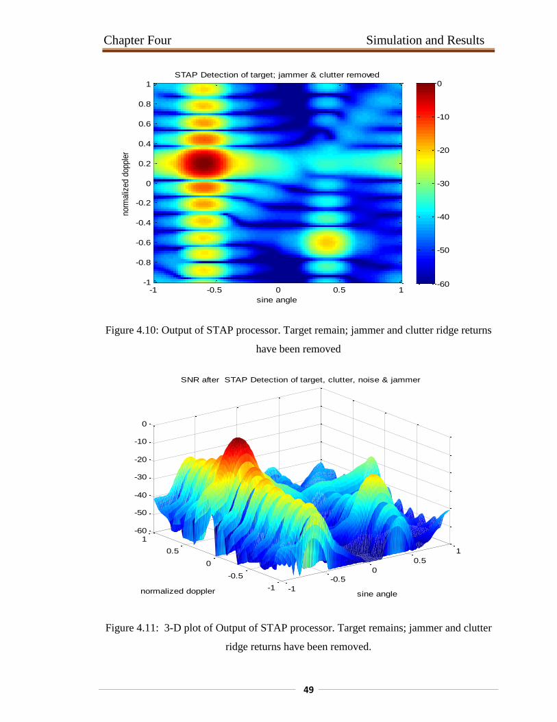
Figure 4.10 : Output of STAP processor. Target remain; jammer and clutter

ridge returns have been removed ................................................................. 49

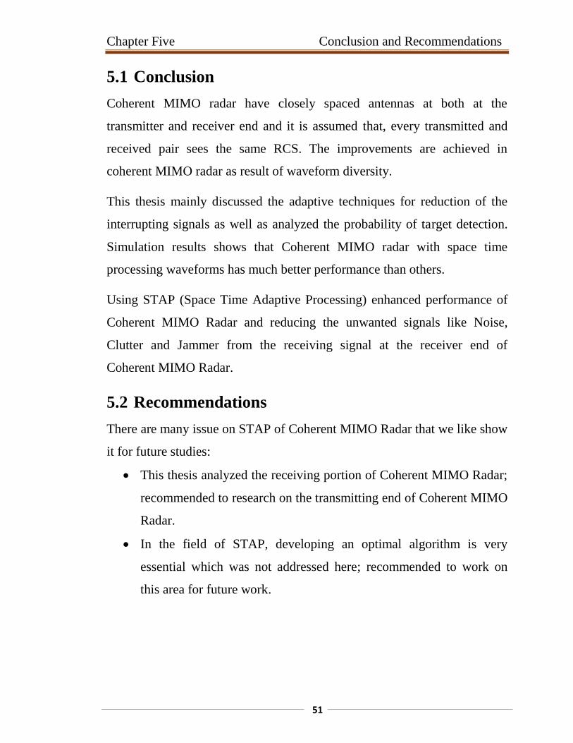
Figure 4.11 : 3-D plot of Output of STAP processor. Target remains;

jammer and clutter ridge returns have been removed. ................................. 49

XII

List of Abbreviations

1D One dimension

2D Two dimension

3D Three dimension

ECM Electronic Countermeasures

CPI Coherent Processing Interval

MATLAB Matrix laboratory

MIMO Multiple Input Multiple Output

OFDM Orthogonal Frequency Division

Multiplexing

RADAR Radio Detection and Ranging

SCNR Signal-to-Clutter-plus-Noise Ratio

SCR Signal-to-Clutter Ratio

SIMO Single Input Multiple Output

SIR Signal-to-Clutter+Noise-Ratio

STC Space Time Coding

STP Space Time Processing

STAP Space Time Adaptive Processing

XIII

List of symbols

Signal at target location

clutter area

Total average transmitted energy

complex noise vector

number of receiver array elements

number of transmit array elements

probability of detection

probability of false alarm

peak transmitted power

Received clutter only covariance matrix

Received jamming only covariance matrix

Received noise only covariance matrix

effective noise temperature

Noise voltage

Output of linear array

Received baseband signal by k-th transmit

antenna

XIV

Radar carrier frequency

complex vector

complex vector

Direction of target respect to receive array

clutter scattering coefficient

average clutter RCS

target RCS

time delay common to all transmit elements

time delay between the target and m-th

transmit antenna

kronecker product

H channel matrix

X space-time snap-shot of the input data

Radar operating bandwidth

Receiver noise figure

Received interference vector

Boltzman’s constant

Noise signal

XV

Total interference covariance matrix

STAP adaptive weight matrix

Optimal Input Detector

Output of STAP detector

Receive steering vector

Number of transmit space time coded

Transmit signal vector

Transmit steering vector

Direction of target respect to transmit array

Wavelength

Time delay

Chapter One

Introduction

Chapter One Introduction

2

1.1 Preface

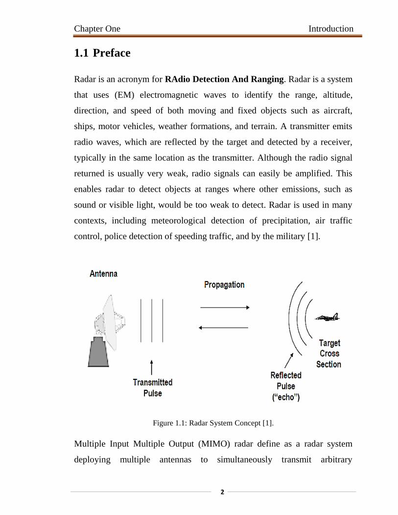
Radar is an acronym for RAdio Detection And Ranging. Radar is a system

that uses (EM) electromagnetic waves to identify the range, altitude,

direction, and speed of both moving and fixed objects such as aircraft,

ships, motor vehicles, weather formations, and terrain. A transmitter emits

radio waves, which are reflected by the target and detected by a receiver,

typically in the same location as the transmitter. Although the radio signal

returned is usually very weak, radio signals can easily be amplified. This

enables radar to detect objects at ranges where other emissions, such as

sound or visible light, would be too weak to detect. Radar is used in many

contexts, including meteorological detection of precipitation, air traffic

control, police detection of speeding traffic, and by the military [1].

Figure 1.1: Radar System Concept [1].

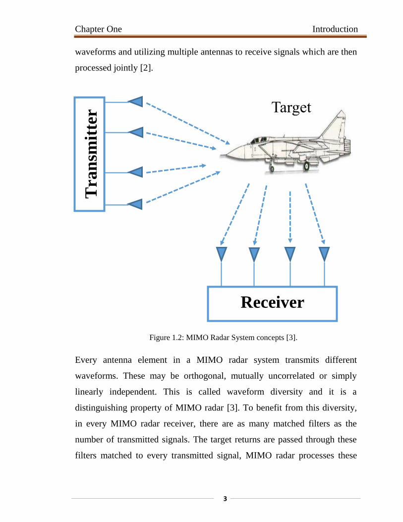
Multiple Input Multiple Output (MIMO) radar define as a radar system

deploying multiple antennas to simultaneously transmit arbitrary


3

waveforms and utilizing multiple antennas to receive signals which are then

processed jointly [2].

Figure 1.2: MIMO Radar System concepts [3].

Every antenna element in a MIMO radar system transmits different

waveforms. These may be orthogonal, mutually uncorrelated or simply

linearly independent. This is called waveform diversity and it is a

distinguishing property of MIMO radar [3]. To benefit from this diversity,

in every MIMO radar receiver, there are as many matched filters as the

number of transmitted signals. The target returns are passed through these

filters matched to every transmitted signal, MIMO radar processes these

Target

Tra

nsm

itte

r

Receiver


4

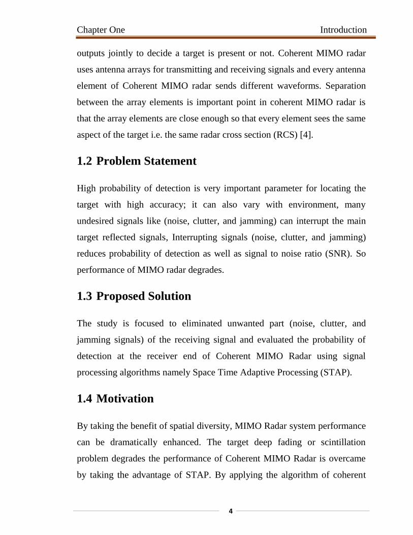
outputs jointly to decide a target is present or not. Coherent MIMO radar

uses antenna arrays for transmitting and receiving signals and every antenna

element of Coherent MIMO radar sends different waveforms. Separation

between the array elements is important point in coherent MIMO radar is

that the array elements are close enough so that every element sees the same

aspect of the target i.e. the same radar cross section (RCS) [4].

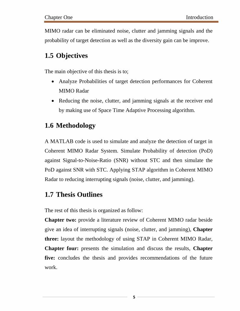
1.2 Problem Statement

High probability of detection is very important parameter for locating the

target with high accuracy; it can also vary with environment, many

undesired signals like (noise, clutter, and jamming) can interrupt the main

target reflected signals, Interrupting signals (noise, clutter, and jamming)

reduces probability of detection as well as signal to noise ratio (SNR). So

performance of MIMO radar degrades.

1.3 Proposed Solution

The study is focused to eliminated unwanted part (noise, clutter, and

jamming signals) of the receiving signal and evaluated the probability of

detection at the receiver end of Coherent MIMO Radar using signal

processing algorithms namely Space Time Adaptive Processing (STAP).

1.4 Motivation

By taking the benefit of spatial diversity, MIMO Radar system performance

can be dramatically enhanced. The target deep fading or scintillation

problem degrades the performance of Coherent MIMO Radar is overcame

by taking the advantage of STAP. By applying the algorithm of coherent


5

MIMO radar can be eliminated noise, clutter and jamming signals and the

probability of target detection as well as the diversity gain can be improve.

1.5 Objectives

The main objective of this thesis is to;

Analyze Probabilities of target detection performances for Coherent

MIMO Radar

Reducing the noise, clutter, and jamming signals at the receiver end

by making use of Space Time Adaptive Processing algorithm.

1.6 Methodology

A MATLAB code is used to simulate and analyze the detection of target in

Coherent MIMO Radar System. Simulate Probability of detection (PoD)

against Signal-to-Noise-Ratio (SNR) without STC and then simulate the

PoD against SNR with STC. Applying STAP algorithm in Coherent MIMO

Radar to reducing interrupting signals (noise, clutter, and jamming).

1.7 Thesis Outlines

The rest of this thesis is organized as follow:

Chapter two: provide a literature review of Coherent MIMO radar beside

give an idea of interrupting signals (noise, clutter, and jamming), Chapter

three: layout the methodology of using STAP in Coherent MIMO Radar,

Chapter four: presents the simulation and discuss the results, Chapter

five: concludes the thesis and provides recommendations of the future

work.

Chapter Two

Literature Review

Chapter Two Literature Review

7

2.1 Introduction

The concept of a multiple input multiple output (MIMO) radar system was

first proposed in 2004 in [5]. Since then, substantial research has been

conducted on the concept. Beside the multiple inputs multiple outputs

architecture, the idea of MIMO starts from diversity [6]. According to

diversity, receiving antenna elements should receive different information

and then improve the global performance of the system.

This thesis mainly described the Coherent mode of MIMO Radar and the

STAP for increasing the diversity gain at both transmitting and receiving

end [7]. If transmitters of the Coherent MIMO Radar are transmits space

time processed signal then at the receiving end target responses are detected

fast with lower SNR value. The target response is mainly interrupted by the

unwanted signal (Noise, Clutter and Jammer) associated with receiving

signal [8].

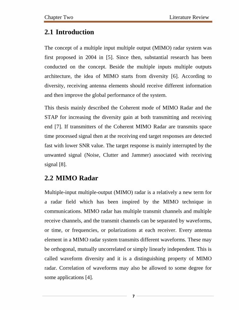
2.2 MIMO Radar

Multiple-input multiple-output (MIMO) radar is a relatively a new term for

a radar field which has been inspired by the MIMO technique in

communications. MIMO radar has multiple transmit channels and multiple

receive channels, and the transmit channels can be separated by waveforms,

or time, or frequencies, or polarizations at each receiver. Every antenna

element in a MIMO radar system transmits different waveforms. These may

be orthogonal, mutually uncorrelated or simply linearly independent. This is

called waveform diversity and it is a distinguishing property of MIMO

radar. Correlation of waveforms may also be allowed to some degree for

some applications [4].


8

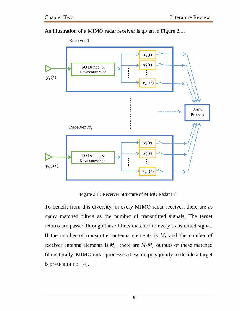
An illustration of a MIMO radar receiver is given in Figure 2.1.

Figure 2.1 : Receiver Structure of MIMO Radar [4].

To benefit from this diversity, in every MIMO radar receiver, there are as

many matched filters as the number of transmitted signals. The target

returns are passed through these filters matched to every transmitted signal.

If the number of transmitter antenna elements is and the number of

receiver antenna elements is , there are outputs of these matched

filters totally. MIMO radar processes these outputs jointly to decide a target

is present or not [4].

Receiver 1

I-Q Demod. &

Downconversion

𝒙𝟏∗ 𝒕

𝒙𝟐∗ 𝒕

𝒙𝑴𝒕∗ 𝒕

𝑦1 𝑡

Receiver 𝑀𝑟

I-Q Demod. &

Downconversion

𝒙𝟏∗ 𝒕

𝒙𝟐∗ 𝒕

𝒙𝑴𝒕∗ 𝒕

𝑦𝑀𝑟 𝑡

Joint

Process


9

Most works on MIMO radars can be broadly divided into two categories:

statistical MIMO and coherent MIMO.

2.2.1 Statistical MIMO

Statistical MIMO radar employs antenna arrays which are widely separated.

The inter element spacing in an array is also so large (several wavelengths)

that each transmit-receive pair sees a different aspect of the target and thus

sees different RCS due to target’s complex shape.

If the spacing between the antennas elements is wide enough, received

signals from each transmit receive pair become independent. This is called

Spatial or Angular Diversity [9]. Statistical MIMO radar focuses on this

property.

MIMO communication systems use the same principle to overcome fading

in the communication channel and to improve the system performance. The

concept of MIMO radar with widely separated antennas is inspired by this

property of MIMO communications and exploits the statistical properties of

target RCS [9].

2.2.2 Coherent MIMO

Coherent MIMO radar employs transmit and receive antenna arrays

containing elements which are closely spaced relatively to the working

wavelength (e.g. spaced by half the wavelength) so that the target is in the

far field of transmit and receive array [10]. The separation is always small

compared to the range extent of the target, while this configuration does not

provide spatial diversity; spatial resolution can be increased by combining

the information from all of the transmitting and receiving paths. This is


01

done by coherent processing: By exploiting the different time delays and/or

phase shifts, the received signals are coherently combined to form multiple

beams. This improvement in angular resolution means that more targets can

be detected and identified.

Coherent MIMO radars transmit orthogonal waveforms at each transmit

element, hence illuminating the scene of interest uniformly. While this

means that no beam scanning is necessary, transmit processing gain from a

focused beam is lost [11].

Diversity comes from the different waveforms transmitted by each transmit

element. In this case, sparse arrangement is possible within the sub-array,

hence improving resolutions further.

The main advantages of the coherent MIMO radar are [12]:

Improved angular resolutions;

Increased parameter identifiability, i.e. increased number of

targets that can be detected and localized by the array;

Direct application of adaptive techniques for parameter estimation

as the signals reflected back by the target are linearly independent;

Ability to null main-beam jamming and robustness to multipath;

Reduced interference to neighboring systems and more covert

operation due to the reduced spatial transmit power density of

omnidirectional transmission;

Flexibility for transmit beam-pattern design.


00

2.2.3 Target Detection Phenomenon of MIMO Radar

The basic functions of radar are detection, parameter estimation and

tracking. The most fundamental one among these functions is detection.

Detection is the process of determining whether the received signal is an

echo returning from a desired target or consists of noise only. The success

of the detection process is directly related to SNR at the receiver and the

ability of the radar to separate desired target echoes from unwanted

reflected signals. So, various techniques are developed to maximize the

SNR at the output of the receiver and to increase the ability of the radar to

separate targets from unwanted echoes and interference. After the detection

process if it turns out that a target really exists, several parameters of the

target like range, velocity and angle of arrival should be estimated from the

received signal. The choice of the radar transmit waveform is a major

contributor to the resolution of these parameters. After localization of a

target, radar can provide a target’s trajectory and track it by predicting

where it will be in the future by observing the target over time and using

dedicated filters. Some types of radar can perform more specialized tasks in

addition to these basic functions [2].

Here considerations of the Coherent MIMO radar scheme that can deal with

multiple targets. Due to the different phase shifts associated with the

different propagation paths from the transmitting antennas to targets, these

independent waveforms are linearly combined at the targets with different

phase factors. Detection of the presence of reflecting targets, is the most

fundamental function of the MIMO radar system [13]. To accomplish this

task, EM waveform is transmitted by the transmitter of MIMO Radar and it

will be reflected by targets if they are present.


02

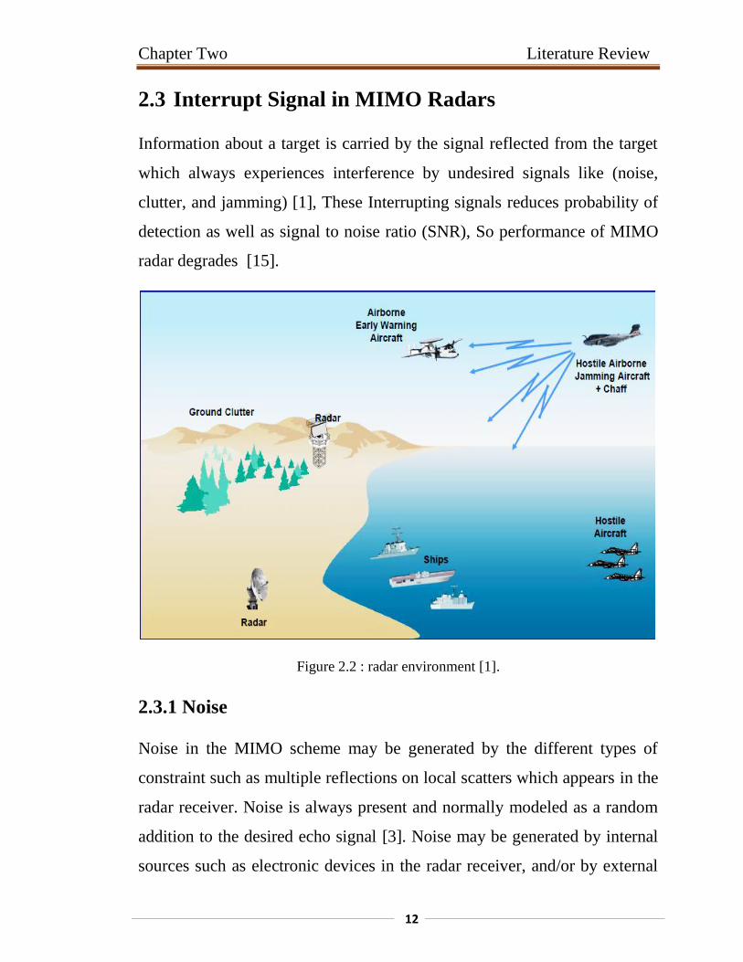
2.3 Interrupt Signal in MIMO Radars

Information about a target is carried by the signal reflected from the target

which always experiences interference by undesired signals like (noise,

clutter, and jamming) [1], These Interrupting signals reduces probability of

detection as well as signal to noise ratio (SNR), So performance of MIMO

radar degrades [15].

Figure 2.2 : radar environment [1].

2.3.1 Noise

Noise in the MIMO scheme may be generated by the different types of

constraint such as multiple reflections on local scatters which appears in the

radar receiver. Noise is always present and normally modeled as a random

addition to the desired echo signal [3]. Noise may be generated by internal

sources such as electronic devices in the radar receiver, and/or by external


03

sources like the background environment surrounding the target and the

receiver. Noise is always present and normally modeled as a random

addition to the desired echo signal.

2.3.2 Clutters

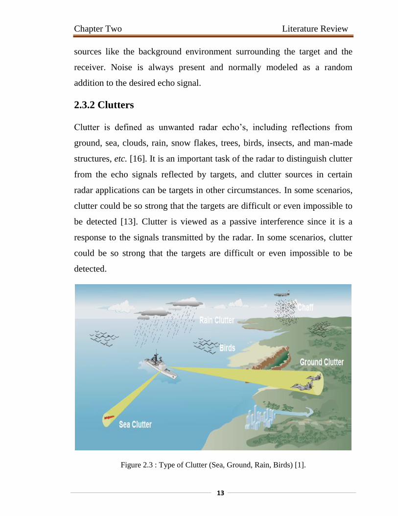
Clutter is defined as unwanted radar echo’s, including reflections from

ground, sea, clouds, rain, snow flakes, trees, birds, insects, and man-made

structures, etc. [16]. It is an important task of the radar to distinguish clutter

from the echo signals reflected by targets, and clutter sources in certain

radar applications can be targets in other circumstances. In some scenarios,

clutter could be so strong that the targets are difficult or even impossible to

be detected [13]. Clutter is viewed as a passive interference since it is a

response to the signals transmitted by the radar. In some scenarios, clutter

could be so strong that the targets are difficult or even impossible to be

detected.

Figure 2.3 : Type of Clutter (Sea, Ground, Rain, Birds) [1].


04

Clutter can be classified into two main categories: surface clutter and

airborne or volume clutter. Surface clutter includes trees, vegetation, ground

terrain, man-made structures, and sea surface (sea clutter). Volume clutter

normally has a large extent (size) and includes chaff, rain, birds, and

insects. Surface clutter changes from one area to another, while volume

clutter may be more predictable.

In many cases, the clutter signal level is much higher than the receiver noise

level. Thus, the radar’s ability to detect targets embedded in high clutter

background depends on the Signal-to-Clutter Ratio (SCR) rather than the

SNR. White noise normally introduces the same amount of noise power

across all radar range bins, while clutter power may vary within a single

range bin. Since clutter returns are target-like echoes, the only way a radar

can distinguish target returns from clutter echoes is based on the target RCS

, and the anticipated clutter RCS (via clutter map). Clutter RCS can be

defined as the equivalent radar cross section attributed to reflections from a

clutter area [17].

The average clutter RCS is given by:

(2.1)

where is the clutter scattering coefficient.

The radar SNR due to a target at range is:

(2.2)

where, is the peak transmitted power, is the antenna gain, is the

wavelength, is the target RCS, is Boltzmann’s constant, is the


05

effective noise temperature, is the radar operating bandwidth, is the

receiver noise figure, and is the total radar losses. Similarly, the

Clutter-to-Noise (CNR) at the radar is:

(2.3)

2.3.3 Jammers

Jamming arises from signals emitted by intentional hostile sources or

unintentional friendly sources which use the same frequency range as the

MIMO radar does. Jamming is considered as an active interference since it

is transmitted by devices outside the MIMO radar and is generally

independent of the MIMO radar signals. Jamming can severely degrade the

performances of radar by either masking real targets with high power noise

(confusion), or producing false signals which appear as echoes from real

targets (deception) [1].

Jammers can be categorized into three general types: barrage jammer, Spot

jammer, and sweep jammer [17].

2.3.3.1 Barrage Jammer

Barrage jammer is radiating noise over the entire range of frequencies to be

covered. Barrage jammers attempt to increase the noise level across the

entire radar operating bandwidth. Consequently, this lowers the receiver

SNR, and, in turn, makes it difficult to detect the desired targets [17].

2.3.3.2 Spot Jammer

Spot jamming occurs when a jammer focuses all of its power on a single

frequency. This would severely degrade the ability to track on the jammed


06

frequency. The spot jammer measures the transmitted radar signal

bandwidth and then jams only a specific range of frequencies [17].

2.3.3.3 Sweep Jammer

Sweep jamming is when a jammer’s full power is shifted from one

frequency to another. Swept jammers continuously scan a range of

operating frequencies, interfering with each in turn. As long as all operating

frequencies are covered, the threat radar will be regularly disrupted [17].

2.4 Doppler Shift

In radar technology the Doppler Effect is using for the following tasks:

Speed measuring;

MTI - Moving Target Indication;

The Doppler- Effect is the apparent change in frequency or pitch when a

sound source moves either toward or away from the listener, or when the

listener moves either toward or away from the sound source. This principle,

discovered by the Austrian physicist Christian Doppler, applies to all wave

motion.

The apparent change in frequency between the source of a wave and the

receiver of the wave is because of relative motion between the source and

the receiver. To understand the Doppler Effect, first assume that the

frequency of a sound from a source is held constant. The wavelength of the

sound will also remain constant. If both the source and the receiver of the

sound remain stationary, the receiver will hear the same frequency sound

produced by the source. This is because the receiver is receiving the same

number of waves per second that the source is producing.

http://www.christian-doppler.com/CD_FONDS/LEBENSLA.HTM


07

Now, if either the source or the receiver or both move toward the other, the

receiver will perceive a higher frequency sound. This is because the

receiver will receive a greater number of sound waves per second and

interpret the greater number of waves as a higher frequency sound.

Conversely, if the source and the receiver are moving apart, the receiver

will receive a smaller number of sound waves per second and will perceive

a lower frequency sound. In both cases, the frequency of the sound

produced by the source will have remained constant.

For example, the frequency of the whistle on a fast-moving car sounds

increasingly higher in pitch as the car is approaching than when the car is

departing. Although the whistle is generating sound waves of a constant

frequency, and though they travel through the air at the same velocity in all

directions, the distance between the approaching car and the listener is

decreasing. As a result, each wave has less distance to travel to reach the

observer than the wave preceding it. Thus, the waves arrive with decreasing

intervals of time between them [1].

The relationship between wavelength and frequency is:

(2.4)

where, is the wave frequency (Hz or cycles per second), is the

wavelength (meters), is the speed of light (approximately 3 x 108

meters/second).

The Doppler frequency shift can be calculated as follows:

(2.5)


08

2.5 Related Works

The author in [18] describe the fundamental principles of MIMO Radar to

stimulate new concepts, theories and applications of the topics related with

the ideas over MIMO techniques. he also analyzes the theory behind MIMO

techniques in detail and discussed techniques for target localization of

MIMO Radars, Also evaluates the adaptive signal design for MIMO Radars

with problem formulation, estimation and detection of the resultant signal

for better SINR (signal-interference-to-noise-ratio).Also describe the Space-

time Coding for MIMO Radar with the merits of the waveform diversity.

For implementing MIMO in any type of communication system or Radar

system, there must be some type of diversity present. It has already been

demonstrated in several articles [19-21].

The study in [4] explain the various mode of MIMO Radar, the author

work discusses the differential mode of MIMO Radar where the coherent

mode is evaluated precisely. A detailed concept about the Coherent MIMO

Radar is proposed in this paper with antenna formation of specific Coherent

mode. It also deals with the improvement that coherent MIMO offer, signal

model, higher resolution, parameter identification, applications of adaptive

array techniques of coherent MIMO and target detection enhancement of

coherent MIMO Radar. Here coherent mode is introduced by array patterns

of MIMO with collocated antennas.

The study in [7] introduce the optimum and adaptive, spatial (angle) and

temporal (doppler) processing. Also this work brings the basic phenomenon

of the optimum temporal (doppler/Pulse) processing besides at the angle of

arrival, optimum spatial (angle) beamforming and Adaptive 1-D Processing


09

of STAP. Also this work discuss some very important factors affecting

STAP such as both angle independent and dependent channel mismatch;

interference subspace leakage effects and antenna array misalignment. Also

[7] provide Algorithms and Performance of the STAP in the MIMO

systems.

The study in [22] contain information obtained from authentic and highly

regarded sources for radar system analysis and system design. It’s also

concentrates on radar fundamentals, principles, and rigorous mathematical

derivations. Also serve as a valuable reference for radar engineering and

system simulator in analyzing and understanding the many issues associated

with radar systems analysis and design.

The author in [23] address the problem of slow target detection in

heterogeneous clutter through dimensionality reduction. They proposed a

novel thinned STAP through selecting an optimum subset of antenna-pulse

pairs that achieves the maximum output signal-to-clutter-plus-noise ratio

(SCNR).

The study in [24] deals with moving target detection in low grazing angle

with orthogonal frequency division multiplexing (OFDM) multi-input

multi-output (MIMO) radar. Also discussed characteristic of OFDM MIMO

radar system and the multipath propagation model and demonstrate that the

detection performances of OFDM MIMO radar outperform the mono-static

OFDM radar

The study in [25] provide an overview of MIMO radar and the advantages

it offers as compared to its phased array counterpart. And discussed

transmit beamforming in MIMO radar and develop the signal model for it.

Chapter Three

Coherent MIMO Radar

Chapter Three Coherent MIMO Radar

20

𝒙𝟏 𝒕

𝒙𝟐 𝒕

𝒙𝒎 𝒕

𝒙𝑴𝒕 𝒕

𝒚𝟏 𝒕 𝒚𝟐 𝒕 𝒚𝒌 𝒕 𝒚𝑴𝒓 𝒕

𝜶

𝜶

𝜶

𝜶

3.1 Introduction

In the previous chapters, a brief overview of the MIMO RADAR literature

and interrupting signals are presented. On the other hand, in this chapter,

Coherent MIMO Radar and Space Time Adaptive Processing (STAP) are

explained in detail.

To study the problem of detection in Coherent MIMO so far the transmitted

signals by MIMO radar are assumed to be orthogonal and the detectors are

developed without including these STAP signals explicitly.

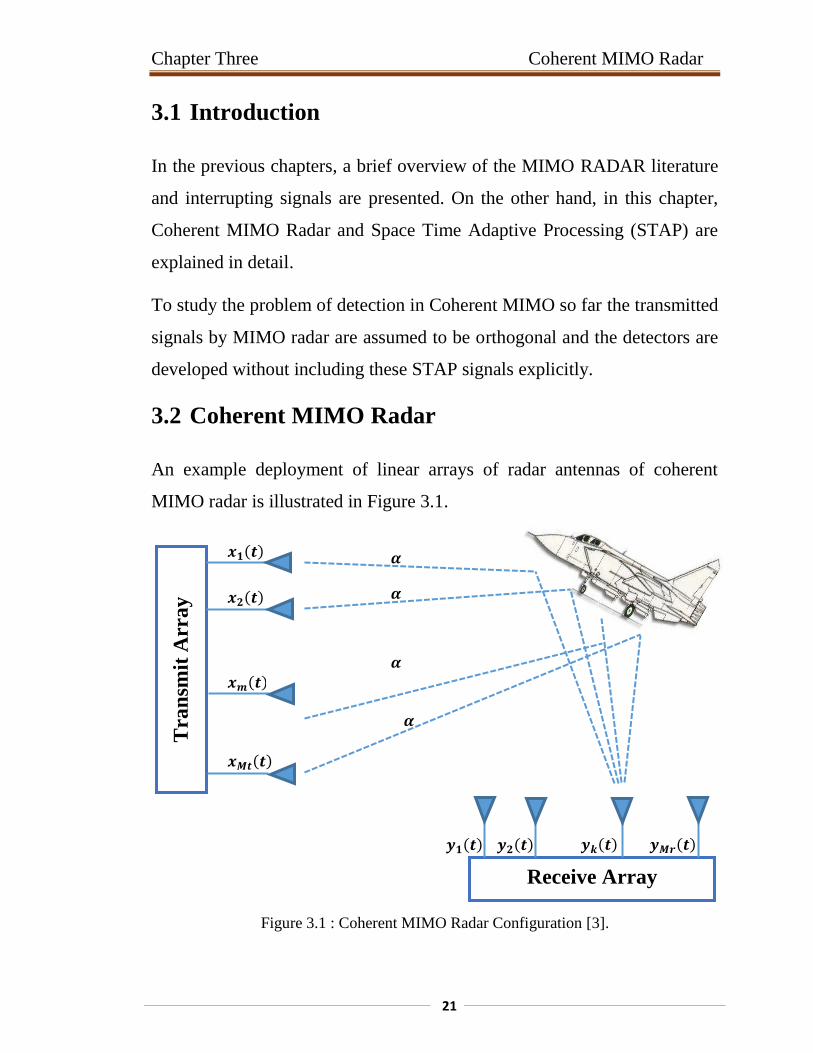
3.2 Coherent MIMO Radar

An example deployment of linear arrays of radar antennas of coherent

MIMO radar is illustrated in Figure 3.1.

Figure 3.1 : Coherent MIMO Radar Configuration [3].

Tra

nsm

it A

rra

y

Receive Array


22

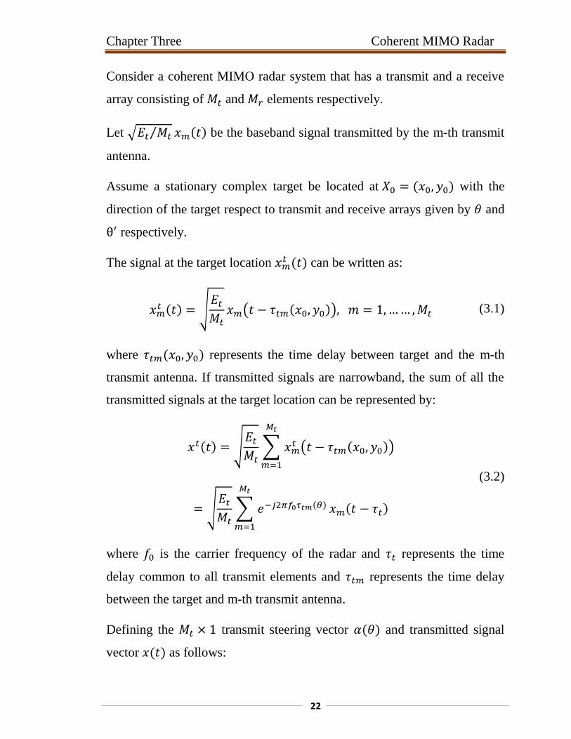
Consider a coherent MIMO radar system that has a transmit and a receive

array consisting of and elements respectively.

Let √ ⁄ be the baseband signal transmitted by the m-th transmit

antenna.

Assume a stationary complex target be located at with the

direction of the target respect to transmit and receive arrays given by and

respectively.

The signal at the target location can be written as:

√

( ) (3.1)

where represents the time delay between target and the m-th

transmit antenna. If transmitted signals are narrowband, the sum of all the

transmitted signals at the target location can be represented by:

√

∑

( )

1

√

∑

1

(3.2)

where is the carrier frequency of the radar and represents the time

delay common to all transmit elements and represents the time delay

between the target and m-th transmit antenna.

Defining the transmit steering vector and transmitted signal

vector as follows:


23

[

]

[ 1

]

Then can be written in the vector form as:

√

(3.3)

where denotes the baseband signal received by the k-th receive

antenna can be written as:

√

( ) (3.4)

where represents the time delay between target and the k-th

receive antenna and is a zero mean complex random process which

accounts for receiver noise and other disturbances.

Where is a complex constant that is proportional to the RCS seen by

k-th receive antenna. Since the antenna elements in the transmit and receive

arrays are closely spaced and . So can be

rewritten as:

√

( ) (3.5)

Then the transmitted signals can be written in the vector form as:


24

√

∗ (3.6)

where received signal vector , receive steering vector

and received interference vector are defined as

[

]

[ 1

]

[ 1

]

If a channel matrix is defined as:

∗ (3.7)

Then the received signal can be written as:

√

(3.8)

If this received signal is fed to a bank of matched filters each of which is

matched to , and the corresponding output is sampled at the time

instants , then the output of the matched filter bank can be written in the

vector form as:

√

(3.9)

where is a complex vector whose entries correspond to the

output of the each matched filter at every receiver, is a

complex noise vector, and is a complex vector defined as:


25

[ ∗ ∗ ] (3.10)

where denotes the Kronecker product.

Note that distribution of each entry of is equal to the distribution of

since elements of ∗ and ∗ are on the unit circle.

The probability of detection ( ) can be written in terms of SNR and

probability of false alarm rate as:

(

) (3.11)

Note that the probability of detection does not depend on the number of

transmit antennas but depends only on number of receive antennas and

SNR.

3.3 Coherent MIMO RADAR with STC Waveforms

In the detection problems studied so far for the coherent MIMO radar

which employs antenna are close enough are developed without including

the space time coded (STC) signals explicitly. STC, transmitted signals are

modeled as a train of rectangular pulses whose amplitudes are modulated

by space time codes and the corresponding detectors are developed. With

this approach, the transmitted signals can be further optimized to a better

given performance metric. Block diagram STC Coherent MIMO radar

configuration is shown in Figure 3.2 [3].

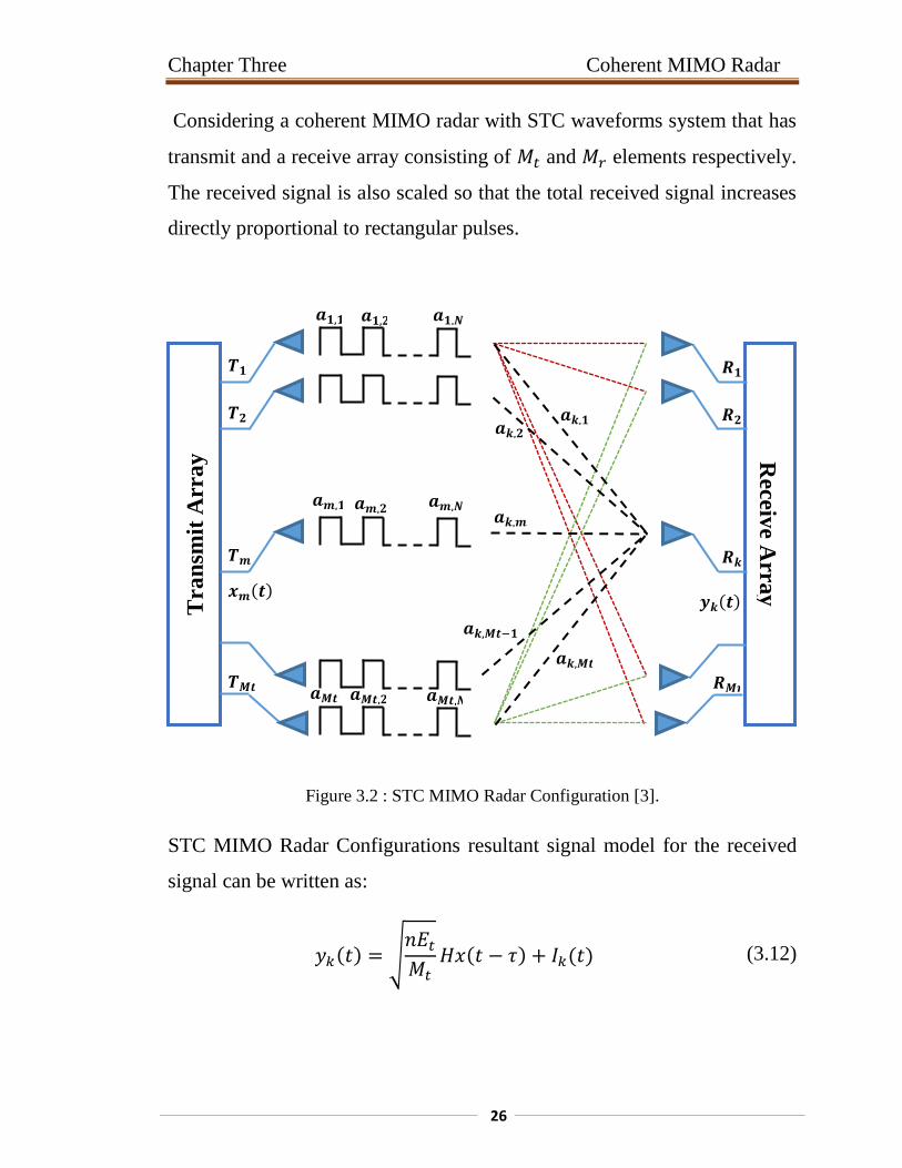
Considering a coherent MIMO radar with STC waveforms system that has

transmit and a receive array consisting of and elements respectively.


26

𝑻𝟏 𝑹𝟏

𝒂𝟏 𝟏 𝒂𝟏 𝟐 𝒂𝟏 𝑵

𝑻𝒎 𝑹𝒌

𝑻𝟐 𝑹𝟐

𝒙𝒎 𝒕

𝑻𝑴𝒕 𝑹𝑴𝒓

𝒚𝒌 𝒕

𝒂𝒎 𝟏 𝒂𝒎 𝟐 𝒂𝒎 𝑵

𝒂𝒌 𝟐 𝒂𝒌 𝟏

𝒂𝒌 𝑴𝒕

𝒂𝒌 𝑴𝒕 𝟏

𝒂𝒌 𝒎

𝒂𝑴𝒕 𝟏 𝒂𝑴𝒕 𝟐 𝒂𝑴𝒕 𝑵

Considering a coherent MIMO radar with STC waveforms system that has

transmit and a receive array consisting of and elements respectively.

The received signal is also scaled so that the total received signal increases

directly proportional to rectangular pulses.

Figure 3.2 : STC MIMO Radar Configuration [3].

STC MIMO Radar Configurations resultant signal model for the received

signal can be written as:

√

(3.12)

Tra

nsm

it A

rra

y R

eceive A

rray


27

where, √

denote the discrete time baseband signal transmitted

by the transmit antenna elements.

Where the input message signal with delay time , is the total

average transmitted energy and is the noise vector.

For coherent MIMO radar with STC waveforms, from the definition of

SNR for the radar system we can write:

∗ (3.13)

where is the numbers of space time coded transmitting pulse.

Then probability of detection ( ) can be written in terms of SNR and

probability of false alarm rate as:

∗ (3.14)

3.4 Space Time Adaptive Processing

Space-time adaptive processing (STAP) is a signal processing technique

most commonly used in radar systems. It involves adaptive array

processing algorithms to aid in target detection. Radar signal processing

benefits from STAP in areas where interference is a problem (i.e. ground

clutter, jamming, etc.). Through careful application of STAP, it is possible

to achieve order-of-magnitude sensitivity improvements in target detection.

STAP is basically an adaptive filter, which can filter over the spatial and

temporal (or time) domain. The goal of STAP is to take a hypothesis that

there is a target at a given location and velocity, and create a filter that has

https://en.wikipedia.org/wiki/Digital_signal_processing

https://en.wikipedia.org/wiki/Radar

https://en.wikipedia.org/wiki/Algorithms

https://en.wikipedia.org/wiki/Clutter_%28radar%29

https://en.wikipedia.org/wiki/Radar_jamming


28

high gain for that specific location and velocity, and apply proportional

attenuations of all signals (clutter, jammers and any other unwanted

returns). There can be many suspected targets to generate location and

velocity hypotheses for, and these are all normally processed together in

real time.

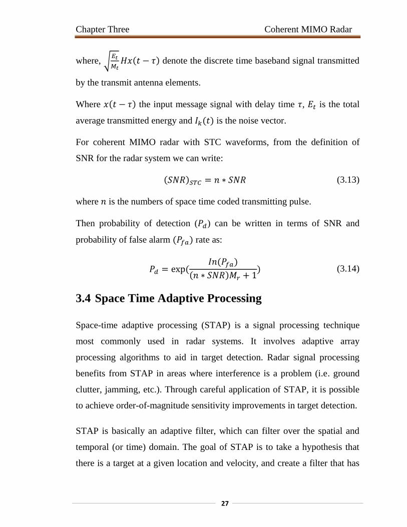
Figure 3.3 shows the signal-to-noise ratio (SNR) resulting from clutter and

a single jamming signal, as a function of angle and Doppler frequency.

Figure 3.3 also shows the view of the clutter characteristic from the

perspective of azimuth for a given Doppler frequency, and the view of the

clutter from the perspective of Doppler frequency for a given azimuth.

These views indicate that the problem is two-dimensional in nature because

filtering must be performed in each dimension.

Figure 3.3 : The problem is to detect the target by enhancing radar performance in this

environment of interference [7].


29

Data Cube

Det

ecti

on

s

Reduction dimension

space

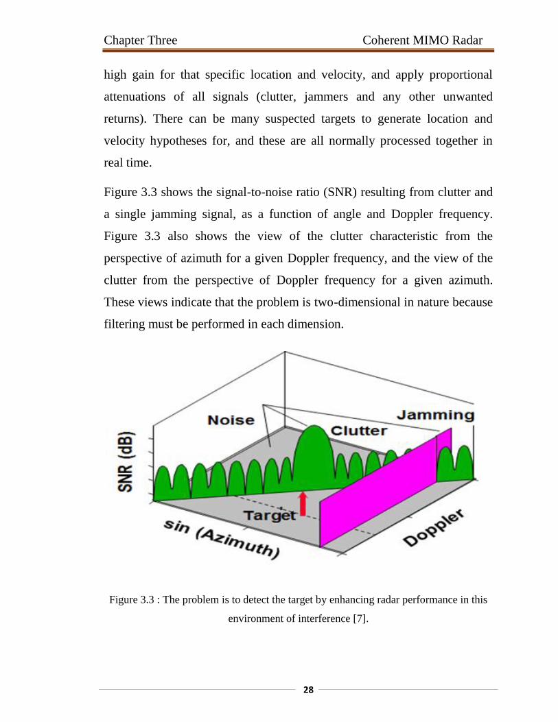
Figure 3.4 shows the STAP processing typically performed in one radar

coherent processing interval (CPI).

Figure 3.4 : The space-time adaptive processing (STAP) typically performed in one

radar coherent processing interval [7].

STAP requires sampling the radar returns at each element of an antenna

array, over a dwell encompassing several pulse repetition intervals. The

output of STAP is a linear combination or weighted sum of the input signal

samples.

The “Adaptive” in STAP refers to the fact that STAP weights are

computed to reflect the actual noise, clutter and jamming

environment in which the radar finds it.

The “Space” in STAP refers to the fact that the STAP weights

(applied to the signal samples at each of the elements of the antenna

array) at one instant of time define an antenna pattern in space. If

Pre

pro

cess

or

Apply

STAP

Weight

s

Compute

STAP

Weights

Estimate

Interference

Compute Steering

Vectors

Beam Angle &

Target

Doppler

Selection


31

there are jammers in the field of view, STAP will adapt the radar

antenna pattern by placing nulls in the directions of those jammers

thus rejecting jammer power.

The “Time” in STAP refers to the fact that the STAP weights applied

to the signal samples at one antenna array element over the entire

dwell define a system impulse response and, hence, a system

frequency response. The clutter spectrum seen by ground based

radars typically has a ridge at zero Doppler an can easily processed

by pulse pair processing while the clutter spectrum seen by airborne

radars is typically more complicated due to the combination of

platform motion and antenna pattern.

STAP processing adapts the radar frequency response to the actual

clutter spectrum in which the radar finds itself so that the radar will

preferentially admit signal power while simultaneously rejecting

clutter power.

The adaptive weights used by STAP are computed using a clutter plus-

noise covariance matrix estimated from data collected at successive ranges.

An accurate estimate of this matrix can be obtained only if the structure of

the clutter spectrum remains unchanged over the range interval used for the

estimation [7].

STAP radar processing combines temporal and spatial filtering that can be

used to both null jammers and detect slow moving targets. It requires very

high numerical processing rates as well as low latency processing, with

dynamic range requirements that generally require floating-point

processing.


30

STAP involves a two-dimensional filtering technique using a phased-array

antenna with multiple spatial channels. Coupling multiple spatial channels

with pulse-Doppler waveforms lends to the name "space-time." Applying

the statistics of the interference environment, an adaptive STAP weight

vector is formed. This weight vector is applied to the coherent samples

received by the radar.

STAP is essentially filtering in the space-time domain. This means that we

are filtering over multiple dimensions, and multi-dimensional signal

processing techniques must be employed. The goal is to find the optimal

space-time weights in -dimensional space, where is the number of

antenna elements (our spatial degrees of freedom) and is the number of

pulse-repetition interval (PRI) taps (our time degrees of freedom), to

maximize the signal-to-interference and noise ratio (SINR).Thus, the goal

is to suppress noise, clutter, jammers, etc., while keeping the desired radar

return. It can be thought of as a 2D finite-impulse response (FIR) filter,

with a standard 1D FIR filter for each channel (steered spatial channels

from an electronically steered array or individual elements), and the taps of

these 1D FIR filters corresponding to multiple returns (spaced at PRI time).

Having degrees of freedom in both the spatial domain and time domain is

crucial, as clutter can be correlated in time and space, while jammers tend

to be correlated spatially (along a specific bearing).

The basic functional diagram is shown in Figure 3.5. For each antenna, a

down conversion and analog-to-digital conversion step is typically

completed. Then, a 1D FIR filter with PRI length delay elements is used for

each steered antenna channel. The lexicographically ordered weights 1 to

https://en.wikipedia.org/wiki/Digital_filter

https://en.wikipedia.org/wiki/Phased-array

https://en.wikipedia.org/wiki/Pulse-doppler_radar

https://en.wikipedia.org/wiki/Statistics

https://en.wikipedia.org/wiki/Coherence_%28physics%29

https://en.wikipedia.org/wiki/Pulse_repetition_frequency

https://en.wikipedia.org/wiki/Signal-to-interference-plus-noise_ratio

https://en.wikipedia.org/wiki/2D_Filters

https://en.wikipedia.org/wiki/Finite_impulse_response


32

L PRI Taps

𝑾𝑳𝑴𝒓

𝑾𝟐𝑴𝒓 𝑾𝑴𝒓

L PRI Taps

𝑾 𝑳 𝟏 𝑴𝒓+𝟏 𝑾𝑴𝒓+𝟏

𝑾𝟏

L PRI Taps

𝑾 𝑳 𝟏 𝑴𝒓+𝟐 𝑾𝑴𝒓+𝟐 𝑾𝟐

To

Detecto

r

𝒁 𝒕

𝑴𝒓 Antennas

𝑿𝑴𝒓 𝒕

𝑿𝟐 𝒕

𝑿𝟏 𝒕

𝒀𝟏

𝒀𝟐

𝒀𝑴𝒓

𝒀𝟐𝑴𝒓

𝒀𝑳𝑴𝒓

𝒀 𝑳 𝟏 𝑴𝒓+𝟏

𝒀 𝑳 𝟏 𝑴𝒓+𝟐

𝒀𝑴𝒓+𝟏

𝒀𝑴𝒓+𝟐

are the degrees of freedom to be solved in the STAP problem. That

is, STAP aims to find the optimal weights for the antenna array.

Figure 3.5 : Top-level diagram for the STAP 2-D adaptive filter [7].

The output of the STAP beamformer is given by,

(3.15)

Where is the adaptive weights matrix and can define as:

T T T

T T T

T T T


33

[

1

] ( )

[

(

) 1 ]

( )

( ){ } (3.16)

where the symbol indicates the Kronecker product and

=

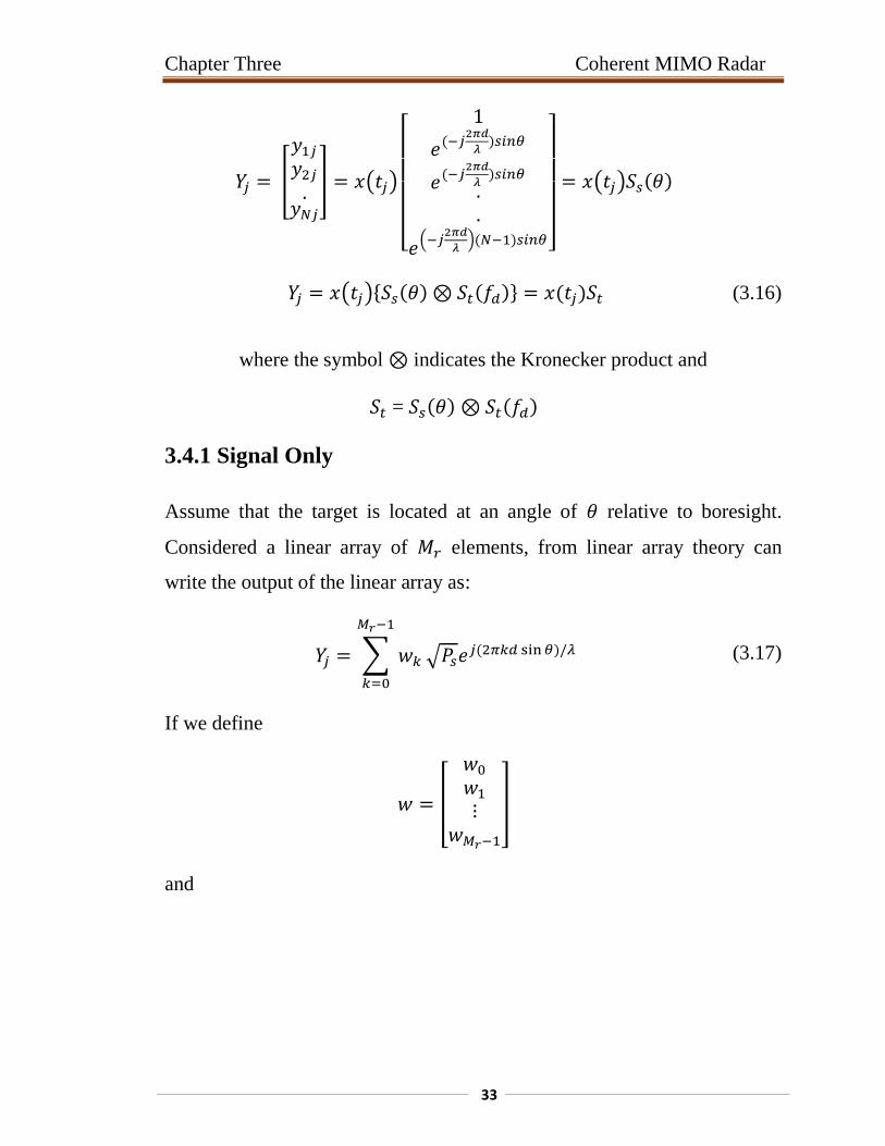
3.4.1 Signal Only

Assume that the target is located at an angle of relative to boresight.

Considered a linear array of elements, from linear array theory can

write the output of the linear array as:

∑

1

√ (3.17)

If we define

[

1

1

]

and


34

[

1

1]

[

1 ]

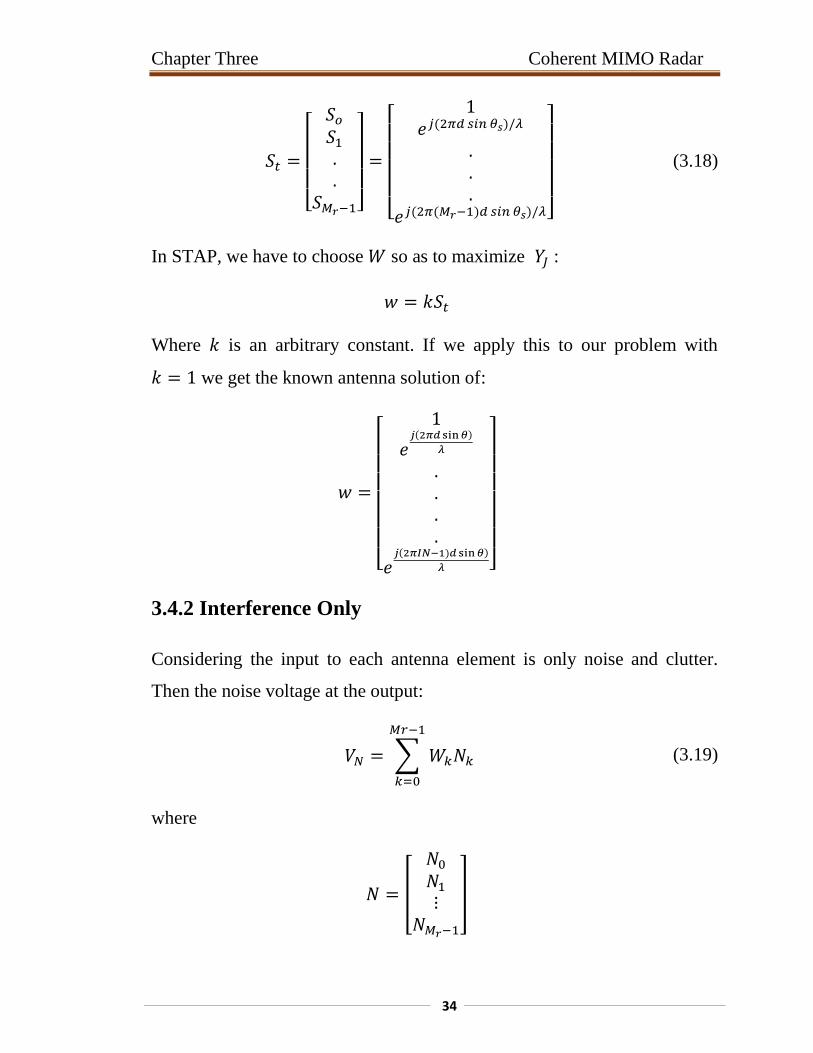
(3.18)

In STAP, we have to choose so as to maximize :

Where is an arbitrary constant. If we apply this to our problem with

we get the known antenna solution of:

[

]

3.4.2 Interference Only

Considering the input to each antenna element is only noise and clutter.

Then the noise voltage at the output:

∑

1

(3.19)

where

[

1

1

]


35

If we assume that is zero-mean and uncorrelated across the elements of

the array we can write:

(3.20)

In the above is termed the interference (receiver noise only) covariance

matrix.

The total space-time covariance matrix due to both clutter and receiver

noise is:

(3.21)

If clutter and jamming are both present, the total space-time interference

covariance matrix has the form

(3.22)

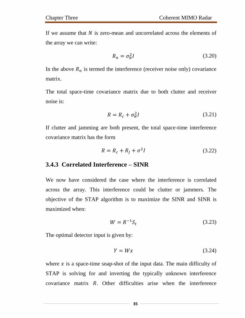
3.4.3 Correlated Interference – SINR

We now have considered the case where the interference is correlated

across the array. This interference could be clutter or jammers. The

objective of the STAP algorithm is to maximize the SINR and SINR is

maximized when:

1 (3.23)

The optimal detector input is given by:

(3.24)

where is a space-time snap-shot of the input data. The main difficulty of

STAP is solving for and inverting the typically unknown interference

covariance matrix . Other difficulties arise when the interference


36

covariance matrix is ill-conditioned, making the inversion numerically

unstable. In general, this adaptive filtering must be performed for each of

the unambiguous range bins in the system, for each target of interest (angle-

Doppler coordinates), making for a massive computational burden. Steering

losses can occur when true target returns do not fall exactly on one of the

points in our 2D angle-Doppler plane that we've sampled with our steering

vector [7].

3.4.4 MIMO Radar STAP

STAP has been extended for MIMO radar to improve spatial resolution for

clutter, using modified SIMO radar STAP techniques. New algorithms and

formulations are required that depart from the standard technique due to the

large rank of the jammer-clutter subspace created by MIMO radar virtual

arrays, which typically involving exploiting the block diagonal structure of

the MIMO interference covariance matrix to break the large matrix

inversion problem into smaller ones.

https://en.wikipedia.org/wiki/MIMO_radar

https://en.wikipedia.org/wiki/Single-Input_and_Single-Output

Chapter Four

Simulation and Results

Chapter Four Simulation and Results

38

4.1 Introduction

This chapter, provided simulation results for both the probability of

detection of Coherent MIMO Radar and reduction of interrupting signals

(noise, clutter, and jamming) from the receiving signal at the receiver end of

the Coherent MIMO Radar using STAP. The required materials and

methods for evaluating the probability of detection of Coherent MIMO

Radar were given in the previous chapter. Assumed the transmitted signals

of the Coherent MIMO Radar are space time processed and probability of

detection is evaluated by changing the number of transmitter and receiver of

Coherent MIMO Radar.

At first, simulated PoD against SNR without STC and then simulated the

PoD against SNR with STC. A comparison is made between two detection

schemes. And using STAP for reducing intercepting signals (Noise, Clutter

and Jammer)

4.2 Coherent MIMO Radar

All simulations are performed for Coherent MIMO Radar with multiple

transmitting and receiving antennas for a given signal to noise ratio and

probability of false alarm ( ).

Analysis of the Probability of detection of the target for Coherent MIMO

Radar is organized as follows,

Coherent MIMO Radar without Space time processing for variable

.

Coherent MIMO Radar without Space time processing for variable

.


39

Coherent MIMO Radar with Space time processing for variable .

Coherent MIMO Radar with Space time processing for variable .

Comparison of Probability of Detection for Coherent MIMO Radar

between with and without Space time processing.

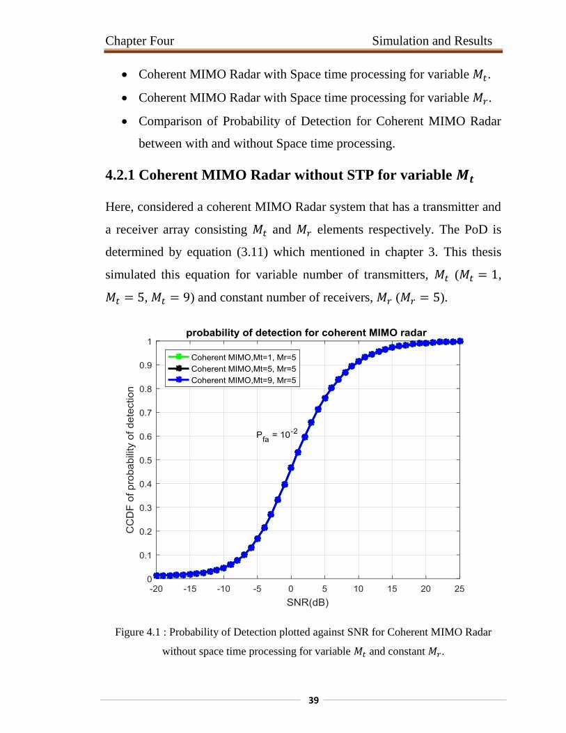
4.2.1 Coherent MIMO Radar without STP for variable

Here, considered a coherent MIMO Radar system that has a transmitter and

a receiver array consisting and elements respectively. The PoD is

determined by equation (3.11) which mentioned in chapter 3. This thesis

simulated this equation for variable number of transmitters, ( ,

, ) and constant number of receivers, ( ).

Figure 4.1 : Probability of Detection plotted against SNR for Coherent MIMO Radar

without space time processing for variable and constant .


41

The Figure 4.1 shows that the detection performance does not change with

the increase in . This is because the transmitted power is normalized and

it does not change with the number of transmit elements and also because

the noise power and the signal power in the received signal after coherent

summation increases at the same rate.

4.2.2 Coherent MIMO Radar without STP for variable

The main PoD equation (3.11) is simulated for variable number of receivers

( , , , ) and constant number of

transmitters ( ). The Figure 4.2 shows that the detection

performance of Coherent MIMO Radar improves with the increase of .

Figure 4.2 : Probability of Detection plotted against SNR for Coherent MIMO Radar

without space time processing at variable and constant .


40

This is because the transmitted power is normalized but it change with the

number of receiver elements, and also because the noise power and the

signal power in the received signal after coherent summation increases at

the same rate.

From the Figure 4.2, for SNR 5dB the PoD of Coherent MIMO Radar

without STP for is 0.32 in the scale of 1, PoD for for same

SNR is 0.76, PoD for for same SNR is 0.85, where the PoD of

Coherent MIMO Radar without STP for for same SNR is 0.90.

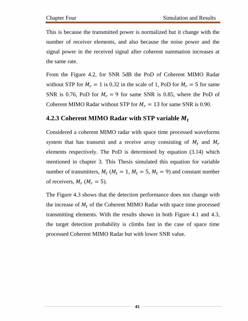
4.2.3 Coherent MIMO Radar with STP variable

Considered a coherent MIMO radar with space time processed waveforms

system that has transmit and a receive array consisting of and

elements respectively. The PoD is determined by equation (3.14) which

mentioned in chapter 3. This Thesis simulated this equation for variable

number of transmitters, ( , , ) and constant number

of receivers, ( ).

The Figure 4.3 shows that the detection performance does not change with

the increase of of the Coherent MIMO Radar with space time processed

transmitting elements. With the results shown in both Figure 4.1 and 4.3,

the target detection probability is climbs fast in the case of space time

processed Coherent MIMO Radar but with lower SNR value.


42

Figure 4.3 : Probability of Detection plotted against SNR with space time processed

Coherent MIMO Radar varying number of transmitters, and constant .

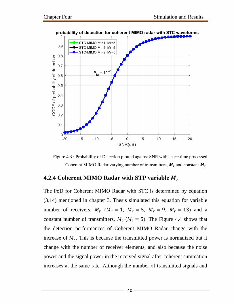
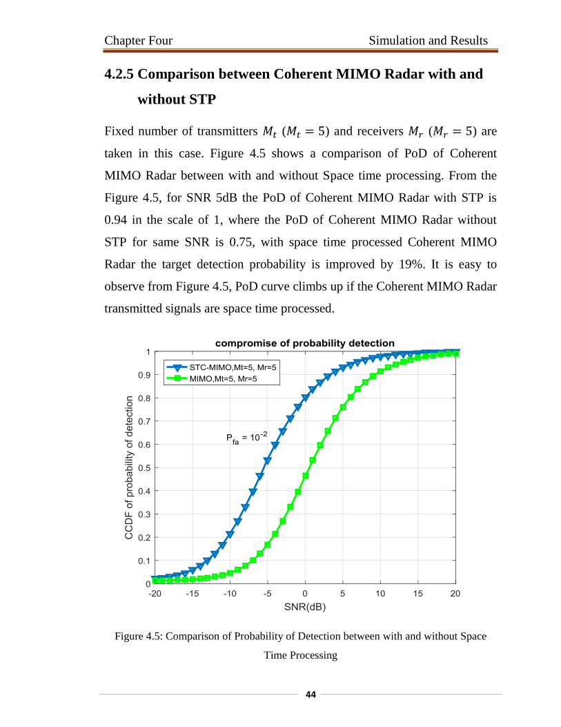
4.2.4 Coherent MIMO Radar with STP variable

The PoD for Coherent MIMO Radar with STC is determined by equation

(3.14) mentioned in chapter 3. Thesis simulated this equation for variable

number of receivers, ( , , , ) and a

constant number of transmitters, ( ). The Figure 4.4 shows that

the detection performances of Coherent MIMO Radar change with the

increase of . This is because the transmitted power is normalized but it

change with the number of receiver elements, and also because the noise

power and the signal power in the received signal after coherent summation

increases at the same rate. Although the number of transmitted signals and


43

the total transmitted power is the same in every situation, the detection

performance increases as the number of receive antennas increases since the

total received energy is increased.

Figure 4.4: Probability of Detection Plotted against SNR for STC Coherent MIMO

Radar at variable

From the Figure 4.4, for SNR 5dB the PoD of Coherent MIMO Radar with

STP for is 0.71 in the scale of 1, PoD for for same SNR is

0.92, PoD for for same SNR is 0.93, where the PoD of Coherent

MIMO Radar with STP for for same SNR is 0.94.


44

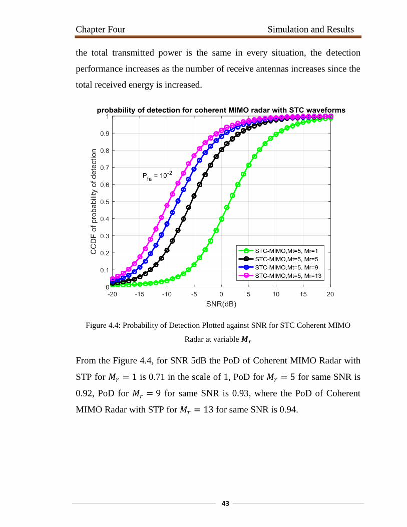
4.2.5 Comparison between Coherent MIMO Radar with and

without STP

Fixed number of transmitters ( ) and receivers ( ) are

taken in this case. Figure 4.5 shows a comparison of PoD of Coherent

MIMO Radar between with and without Space time processing. From the

Figure 4.5, for SNR 5dB the PoD of Coherent MIMO Radar with STP is

0.94 in the scale of 1, where the PoD of Coherent MIMO Radar without

STP for same SNR is 0.75, with space time processed Coherent MIMO

Radar the target detection probability is improved by 19%. It is easy to

observe from Figure 4.5, PoD curve climbs up if the Coherent MIMO Radar

transmitted signals are space time processed.

Figure 4.5: Comparison of Probability of Detection between with and without Space

Time Processing


45

4.3 Coherent MIMO Radar using STAP

This section, Evaluated the SINR (signal to interferences and noise ratio)

performance of STAP method and the rationale for joint space and time

(angle-Doppler) processing is presented. The detailed nature of the angle-

Doppler structure of clutter was thoroughly examined from a variety of

perspectives. A detailed analysis of the space-time clutter covariance matrix

was mentioned (3.22) at previous chapter. STAP was introduced via the

substitution of the ideal covariance matrix (unknown a priori) with an

estimation obtained from sample data.

In the STAP simulation portion, the estimated parameters are assumed

, , and k-th clutter bins equal to 2500. The clutter to noise

ratio (CNR) is 30dB. There are one jammers and one target present. The

jammer to signal ratio (JNR) for each jammer equals 0 dB. The signal to

noise ratio for target equals to 10 dB. The SINR is normalized so that the

maximum SINR equals 0 dB.

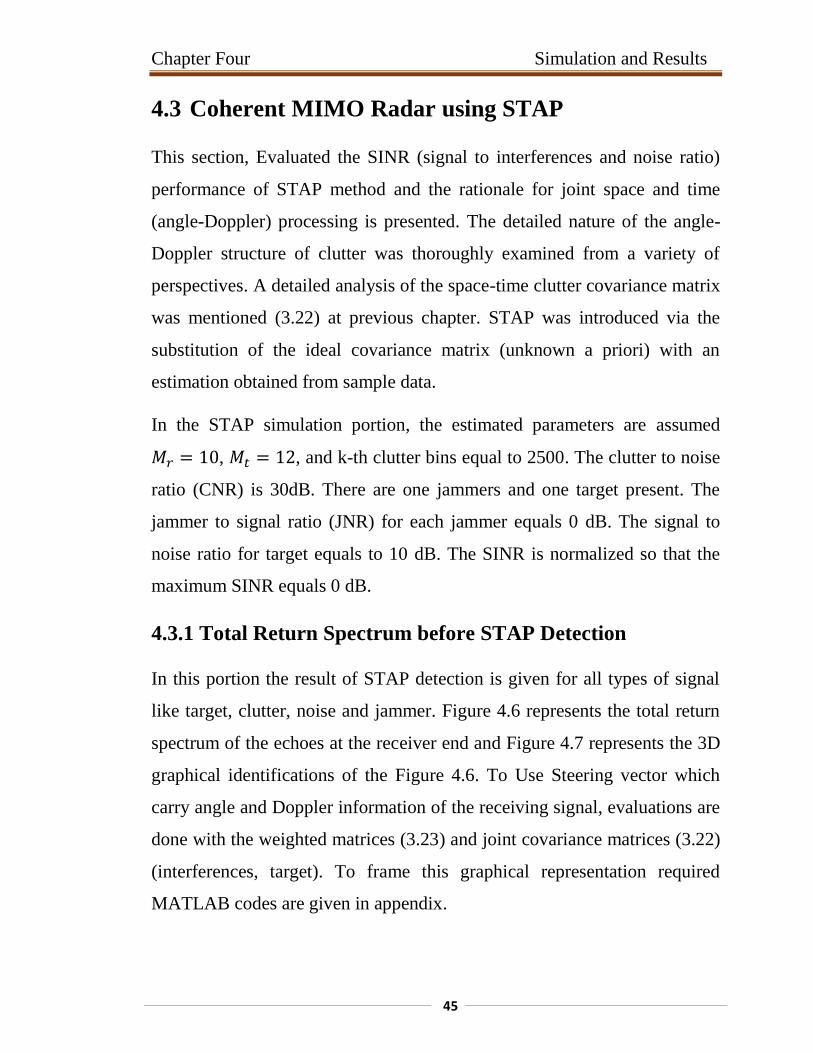
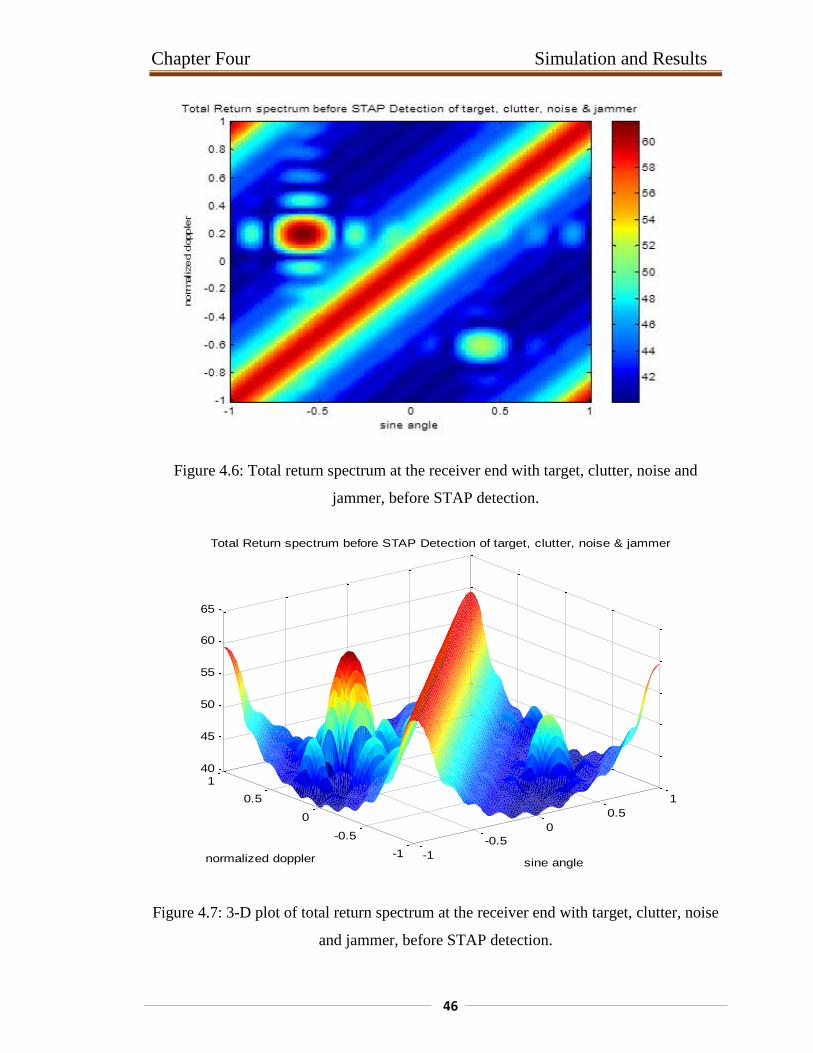
4.3.1 Total Return Spectrum before STAP Detection

In this portion the result of STAP detection is given for all types of signal

like target, clutter, noise and jammer. Figure 4.6 represents the total return

spectrum of the echoes at the receiver end and Figure 4.7 represents the 3D

graphical identifications of the Figure 4.6. To Use Steering vector which

carry angle and Doppler information of the receiving signal, evaluations are

done with the weighted matrices (3.23) and joint covariance matrices (3.22)

(interferences, target). To frame this graphical representation required

MATLAB codes are given in appendix.


46

Figure 4.6: Total return spectrum at the receiver end with target, clutter, noise and

jammer, before STAP detection.

Figure 4.7: 3-D plot of total return spectrum at the receiver end with target, clutter, noise

and jammer, before STAP detection.

-1

-0.5

0

0.5

1

-1

-0.5

0

0.5

140

45

50

55

60

65

sine angle

Total Return spectrum before STAP Detection of target, clutter, noise & jammer

normalized doppler


47

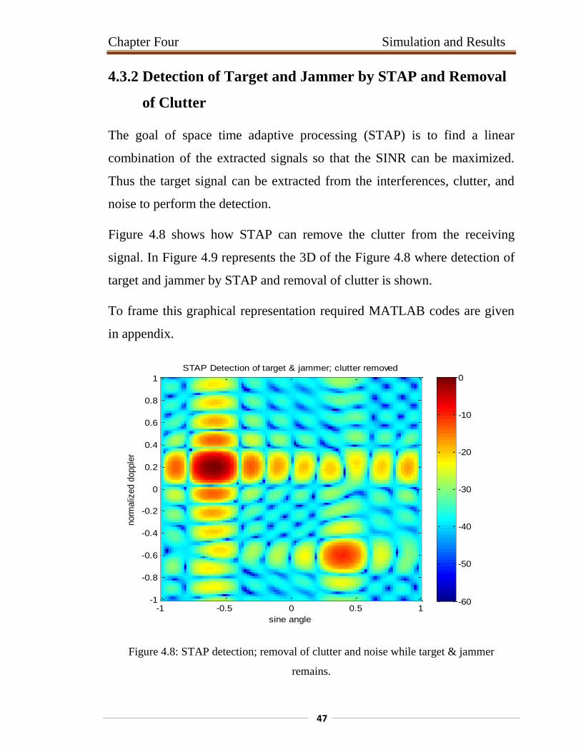
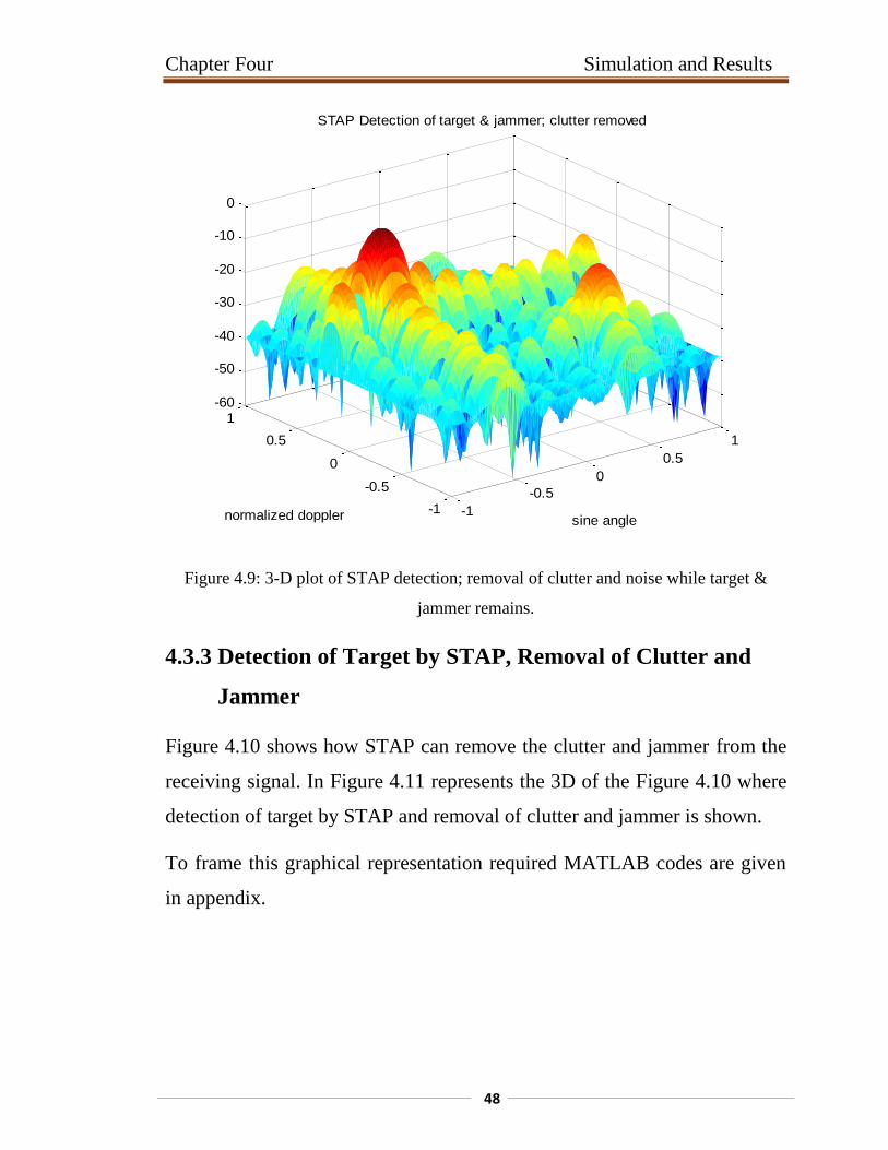
4.3.2 Detection of Target and Jammer by STAP and Removal

of Clutter

The goal of space time adaptive processing (STAP) is to find a linear

combination of the extracted signals so that the SINR can be maximized.

Thus the target signal can be extracted from the interferences, clutter, and

noise to perform the detection.

Figure 4.8 shows how STAP can remove the clutter from the receiving

signal. In Figure 4.9 represents the 3D of the Figure 4.8 where detection of

target and jammer by STAP and removal of clutter is shown.

To frame this graphical representation required MATLAB codes are given

in appendix.

Figure 4.8: STAP detection; removal of clutter and noise while target & jammer

remains.

sine angle

norm

aliz

ed d

opple

r

STAP Detection of target & jammer; clutter removed

-1 -0.5 0 0.5 1-1

-0.8

-0.6

-0.4

-0.2

0

0.2

0.4

0.6

0.8

1

-60

-50

-40

-30

-20

-10

0


48

Figure 4.9: 3-D plot of STAP detection; removal of clutter and noise while target &

jammer remains.

4.3.3 Detection of Target by STAP, Removal of Clutter and

Jammer

Figure 4.10 shows how STAP can remove the clutter and jammer from the

receiving signal. In Figure 4.11 represents the 3D of the Figure 4.10 where

detection of target by STAP and removal of clutter and jammer is shown.

To frame this graphical representation required MATLAB codes are given

in appendix.

-1

-0.5

0

0.5

1

-1

-0.5

0

0.5

1-60

-50

-40

-30

-20

-10

0

sine angle

STAP Detection of target & jammer; clutter removed

normalized doppler


49

Figure 4.10: Output of STAP processor. Target remain; jammer and clutter ridge returns

have been removed

Figure 4.11: 3-D plot of Output of STAP processor. Target remains; jammer and clutter

ridge returns have been removed.

sine angle

norm

aliz

ed d

oppl

er

STAP Detection of target; jammer & clutter removed

-1 -0.5 0 0.5 1-1

-0.8

-0.6

-0.4

-0.2

0

0.2

0.4

0.6

0.8

1

-60

-50

-40

-30

-20

-10

0

-1

-0.5

0

0.5

1

-1

-0.5

0

0.5

1-60

-50

-40

-30

-20

-10

0

sine angle

SNR after STAP Detection of target, clutter, noise & jammer

normalized doppler

Chapter Five

Conclusion and Recommendations

Chapter Five Conclusion and Recommendations

50

5.1 Conclusion

Coherent MIMO radar have closely spaced antennas at both at the

transmitter and receiver end and it is assumed that, every transmitted and

received pair sees the same RCS. The improvements are achieved in

coherent MIMO radar as result of waveform diversity.

This thesis mainly discussed the adaptive techniques for reduction of the

interrupting signals as well as analyzed the probability of target detection.

Simulation results shows that Coherent MIMO radar with space time

processing waveforms has much better performance than others.

Using STAP (Space Time Adaptive Processing) enhanced performance of

Coherent MIMO Radar and reducing the unwanted signals like Noise,

Clutter and Jammer from the receiving signal at the receiver end of

Coherent MIMO Radar.

5.2 Recommendations

There are many issue on STAP of Coherent MIMO Radar that we like show

it for future studies:

This thesis analyzed the receiving portion of Coherent MIMO Radar;

recommended to research on the transmitting end of Coherent MIMO

Radar.

In the field of STAP, developing an optimal algorithm is very

essential which was not addressed here; recommended to work on

this area for future work.

References

52

References

[1] M. Skolnik, "Introduction to Radar Systems," IEEE Aerospace and Electronic

Systems Magazine, vol. 16, pp. 19-19, 2001.

[2] J. Li and P. Stoica, "MIMO radar with colocated antennas," IEEE Signal

Processing Magazine, vol. 24, pp. 106-114, 2007.

[3] M. Jankiraman, Space-time codes and MIMO systems: Artech House, 2004.

[4] S. B. Akdemir, "An Overview of Detection in MIMO Radar," ODTU, 2010.

[5] M. A. Richards, J. A. Scheer, and W. A. Holm, Principles of modern radar:

Citeseer, 2010.

[6] M. Lesturgie, "Some relevant applications of MIMO to radar," in 2011 12th

International Radar Symposium (IRS), 2011, pp. 714-721.

[7] J. R. Guerci, Space-time adaptive processing for radar: Artech House, 2014.

[8] P. Tait, "Introduction to Radar Target Recognition (Radar, Sonar &

Navigation)," The Institution of Eng. and Tech. London, 2008.

[9] E. Fishler, A. Haimovich, R. S. Blum, L. J. Cimini, D. Chizhik, and R. A.

Valenzuela, "Spatial diversity in radars-models and detection performance,"

IEEE Transactions on Signal Processing, vol. 54, pp. 823-838, 2006.

[10] D. Bliss and K. Forsythe, "Multiple-input multiple-output (MIMO) radar and

imaging: degrees of freedom and resolution," in Signals, Systems and

Computers, 2004. Conference Record of the Thirty-Seventh Asilomar Conference

on, 2003, pp. 54-59.

[11] J. Li, P. Stoica, L. Xu, and W. Roberts, "On parameter identifiability of MIMO

radar," IEEE Signal Processing Letters, vol. 14, pp. 968-971, 2007.

[12] J. Tabrikian, "Performance bounds and techniques for target localization using

MIMO radars," MIMO Radar Signal Processing, J. Li and P. Stoica, Eds, pp.

153-191, 2009.

[13] J. S. McMahon and K. Teitelbaum, "Space-time adaptive processing on the Mesh

Synchronous Processor," in Parallel Processing Symposium, 1996., Proceedings

of IPPS'96, The 10th International, 1996, pp. 734-740.

References

53

[14] Du. Chaoran, "Performance evaluation and waveform design for MIMO radar,"

Edinburgh,2010.

[15] M. A. Richards, Fundamentals of radar signal processing: Tata McGraw-Hill

Education, 2005.

[16] G. P. Kulemin, Millimeter-wave radar targets and clutter: Artech House, 2003.

[17] R. M. Bassem and Z. E. Atef, "Matlab simulations for radar systems design," ed:

CRC Press, USA, 2004.

[18] J. L. a. P. Stoica, "MIMO radar signal processing," New Jersey, John Wiley &

Sons, Inc., Hoboken publication, 2009.

[19] A. M. Haimovich, "Distributed mimo radar for imaging and high resolution

target localization," New Jersey Institute of Tech Newark, 2012.

[20] P. Wang, H. Li, and B. Himed, "Moving target detection using distributed

MIMO radar in clutter with nonhomogeneous power," IEEE Transactions on

Signal Processing, vol. 59, pp. 4809-4820, 2011.

[21] Y. Chen, Y. Nijsure, C. Yuen, Y. H. Chew, Z. Ding, and S. Boussakta,

"Adaptive distributed MIMO radar waveform optimization based on mutual

information," IEEE Transactions on Aerospace and Electronic Systems, vol. 49,

pp. 1374-1385, 2013.

[22] B. R. Mahafza, Radar signal analysis and processing using MATLAB: CRC

Press, 2016.

[23] X. Wang, E. Aboutanios, and M. G. Amin, "Slow radar target detection in

heterogeneous clutter using thinned space-time adaptive processing," IET Radar,

Sonar & Navigation, vol. 10, pp. 726-734, 2015.

[24] Y. Xia, Z. Song, Z. Lu, and Q. Fu, "Target Detection in Low Grazing Angle with

OFDM MIMO Radar," Progress In Electromagnetics Research M, vol. 46, pp.

101-112, 2016.

[25] N. Pandey, "Beamfprming in MIMO Radar," National Institute of Technology

Reurkela , 2014.

Appendices

54

Appendices

Appendix A: MATLAB code for Probability of detection for

coherent MIMO radar without STC waveforms

A.1 Coherent MIMO Radar without STC Waveform for variable

clc

clearall

p=10^-2;%pfa=probability of false alarm

r=log(p);

for M=1:4:12

snr=-20:1:25;%SNR

snr1=10.^(snr./10);

N=5;

t=((snr1*N)+1);

Pd=(r./t);%pd=probability of detection

a=exp(Pd);

if M==1

plot(snr,a,'g*-','linewidth',2)

holdon

elseif M==5

plot(snr,a,'k*-','linewidth',2)

holdon

elseif M==9

plot(snr,a,'b*-','linewidth',2)

holdon

else

plot(snr,a,'m*-','linewidth',2)

holdon

end

gridon

axis([-20 25 0 1])

title('probability of detection for coherent MIMO radar ')

xlabel('SNR(dB)')

ylabel('probability of detection')

loc=legend('Coherent MIMO,Mt=1, Mr=5','Coherent MIMO,Mt=5,

Mr=5','Coherent MIMO,Mt=9, Mr=5')

set(loc,'Location','NorthWest')

set(loc,'Interpreter','none')

end

Appendices

55

A.2 Coherent MIMO Radar without STC Waveform for variable

clc

clearall


r=log(p);

%for M=1:4:12

snr=-20:1:20;%SNR

snr1=10.^(snr./10);

for N=1:4:13

t=((snr1*N)+1);


a=exp(Pd);

%ylim([0 1])

%xlim([-20 30])

if N==1


holdon

elseif N==5


holdon

elseif N==9


holdon

else


holdon

gridon

axis([-20 20 0 1])

end

end

title('probability of detection for coherent MIMO radar ')

xlabel('SNR(dB)')


loc=legend('Coherent MIMO,Mt=5, Mr=1','Coherent MIMO,Mt=5,

Mr=5','Coherent MIMO,Mt=5, Mr=9','Coherent MIMO,Mt=5,

Mr=13')

set(loc,'Location','northwest')


%end

Appendices

56

Appendix B: MATLAB code for Probability of detection for

coherent MIMO radar with STC waveforms

B.1 Coherent MIMO Radar with STC Waveform for variable

clc

clearall


r=log(p);

snr=-20:1:20;%SNR

snr1=10.^(snr./10);

for M=1:4:12

N=5;

t=((snr1*N*4)+1);


a=exp(Pd);

%ylim([0 1])

%xlim([-20 30])

%plot(snr,a,'m*-','linewidth',2)

if M==1


holdon

elseif M==5


holdon

elseif M==9


holdon

gridon

else


holdon

gridon

axis([-20 20 0 1])

end

end

title('probability of detection for coherent MIMO radar

with STC waveforms')

xlabel('SNR(dB)')


loc=legend('STC-MIMO,Mt=1, Mr=5','STC-MIMO,Mt=4,

Mr=5','STC-MIMO,Mt=9, Mr=5')



Appendices

57

B.2 Coherent MIMO Radar without STC Waveform for variable

clc

clearall


r=log(p);

snr=-20:1:20;%SNR

snr1=10.^(snr./10);

M=5;

for N=1:4:13;

t=((snr1*N*4)+1);


a=exp(Pd);

%ylim([0 1])

%xlim([-20 30])

%plot(snr,a,'*-','linewidth',2)

if N==1

plot(snr,a,'go-','linewidth',2)

holdon

elseif N==5

plot(snr,a,'ko-','linewidth',2)

holdon

elseif N==9

plot(snr,a,'bo-','linewidth',2)

holdon

else

plot(snr,a,'mo-','linewidth',2)

holdon

gridon

axis([-20 20 0 1])

end

holdon

gridon

axis([-20 20 0 1])

title('probability of detection for coherent MIMO radar

with STC waveforms')

xlabel('SNR(dB)')


end

loc=legend('STC-MIMO,Mt=5, Mr=1','STC-MIMO,Mt=5,

Mr=5','STC-MIMO,Mt=5, Mr=9','STC-MIMO,Mt=5, Mr=13')

set(loc,'Location','southeast')


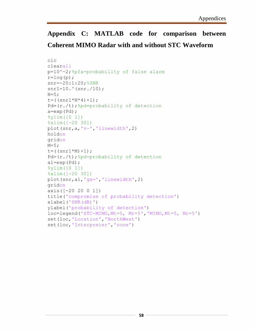
Appendices

58

Appendix C: MATLAB code for comparison between

Coherent MIMO Radar with and without STC Waveform

clc

clearall


r=log(p);

snr=-20:1:20;%SNR

snr1=10.^(snr./10);

N=5;

t=((snr1*N*4)+1);


a=exp(Pd);

%ylim([0 1])

%xlim([-20 30])

plot(snr,a,'v-','linewidth',2)

holdon

gridon

M=5;

t=((snr1*M)+1);


a1=exp(Pd);

%ylim([0 1])

%xlim([-20 30])

plot(snr,a1,'gs-','linewidth',2)

gridon

axis([-20 20 0 1])

title('compromise of probability detection')

xlabel('SNR(dB)')


loc=legend('STC-MIMO,Mt=5, Mr=5','MIMO,Mt=5, Mr=5')



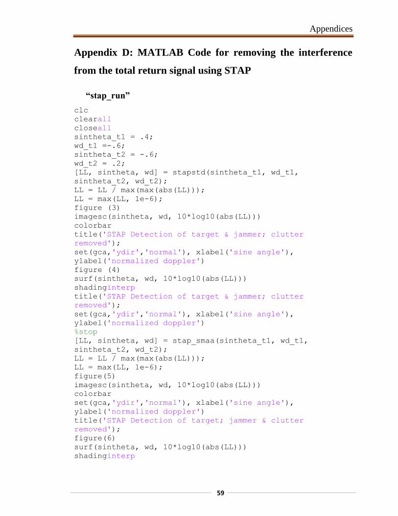
Appendices

59

Appendix D: MATLAB Code for removing the interference

from the total return signal using STAP

“stap_run”

clc

clearall

closeall

sintheta_t1 = .4;

wd_t1 =-.6;

sintheta_t2 = -.6;

wd_t2 = .2;

[LL, sintheta, wd] = stapstd(sintheta_t1, wd_t1,

sintheta_t2, wd_t2);

LL = LL / max(max(abs(LL)));

LL = max(LL, 1e-6);

figure (3)

imagesc(sintheta, wd, 10*log10(abs(LL)))

colorbar

title('STAP Detection of target & jammer; clutter

removed');

set(gca,'ydir','normal'), xlabel('sine angle'),

ylabel('normalized doppler')

figure (4)

surf(sintheta, wd, 10*log10(abs(LL)))

shadinginterp

title('STAP Detection of target & jammer; clutter

removed');



%stop

[LL, sintheta, wd] = stap_smaa(sintheta_t1, wd_t1,


LL = LL / max(max(abs(LL)));

LL = max(LL, 1e-6);

figure(5)

imagesc(sintheta, wd, 10*log10(abs(LL)))

colorbar



title('STAP Detection of target; jammer & clutter

removed');

figure(6)

surf(sintheta, wd, 10*log10(abs(LL)))

shadinginterp

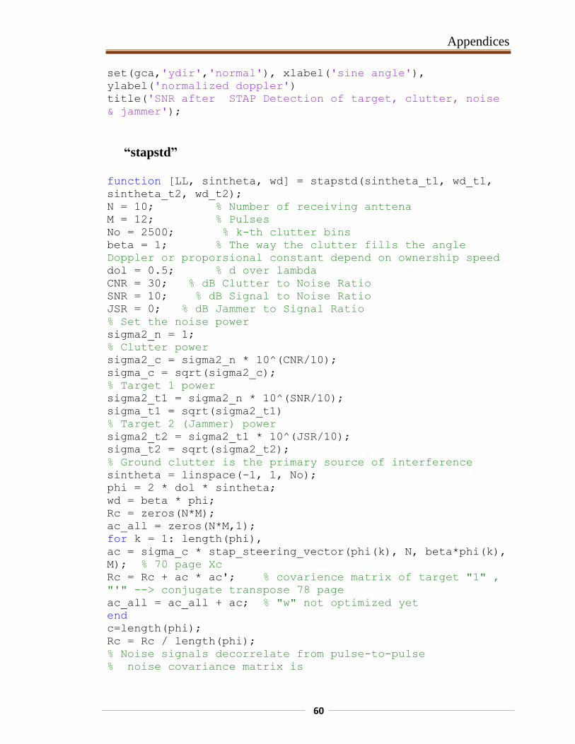
Appendices

61



title('SNR after STAP Detection of target, clutter, noise

& jammer');

“stapstd”

function [LL, sintheta, wd] = stapstd(sintheta_t1, wd_t1,


N = 10; % Number of receiving anttena

M = 12; % Pulses

No = 2500; % k-th clutter bins

beta = 1; % The way the clutter fills the angle

Doppler or proporsional constant depend on ownership speed

dol = 0.5; % d over lambda

CNR = 30; % dB Clutter to Noise Ratio

SNR = 10; % dB Signal to Noise Ratio

JSR = 0; % dB Jammer to Signal Ratio

% Set the noise power

sigma2_n = 1;

% Clutter power

sigma2_c = sigma2_n * 10^(CNR/10);

sigma_c = sqrt(sigma2_c);

% Target 1 power

sigma2_t1 = sigma2_n * 10^(SNR/10);

sigma_t1 = sqrt(sigma2_t1)

% Target 2 (Jammer) power

sigma2_t2 = sigma2_t1 * 10^(JSR/10);

sigma_t2 = sqrt(sigma2_t2);

% Ground clutter is the primary source of interference

sintheta = linspace(-1, 1, No);

phi = 2 * dol * sintheta;

wd = beta * phi;

Rc = zeros(N*M);

ac_all = zeros(N*M,1);

for k = 1: length(phi),

ac = sigma_c * stap_steering_vector(phi(k), N, beta*phi(k),

M); % 70 page Xc

Rc = Rc + ac * ac'; % covarience matrix of target "1" ,

"'" --> conjugate transpose 78 page

ac_all = ac_all + ac; % "w" not optimized yet

end

c=length(phi);

Rc = Rc / length(phi);

% Noise signals decorrelate from pulse-to-pulse

% noise covariance matrix is

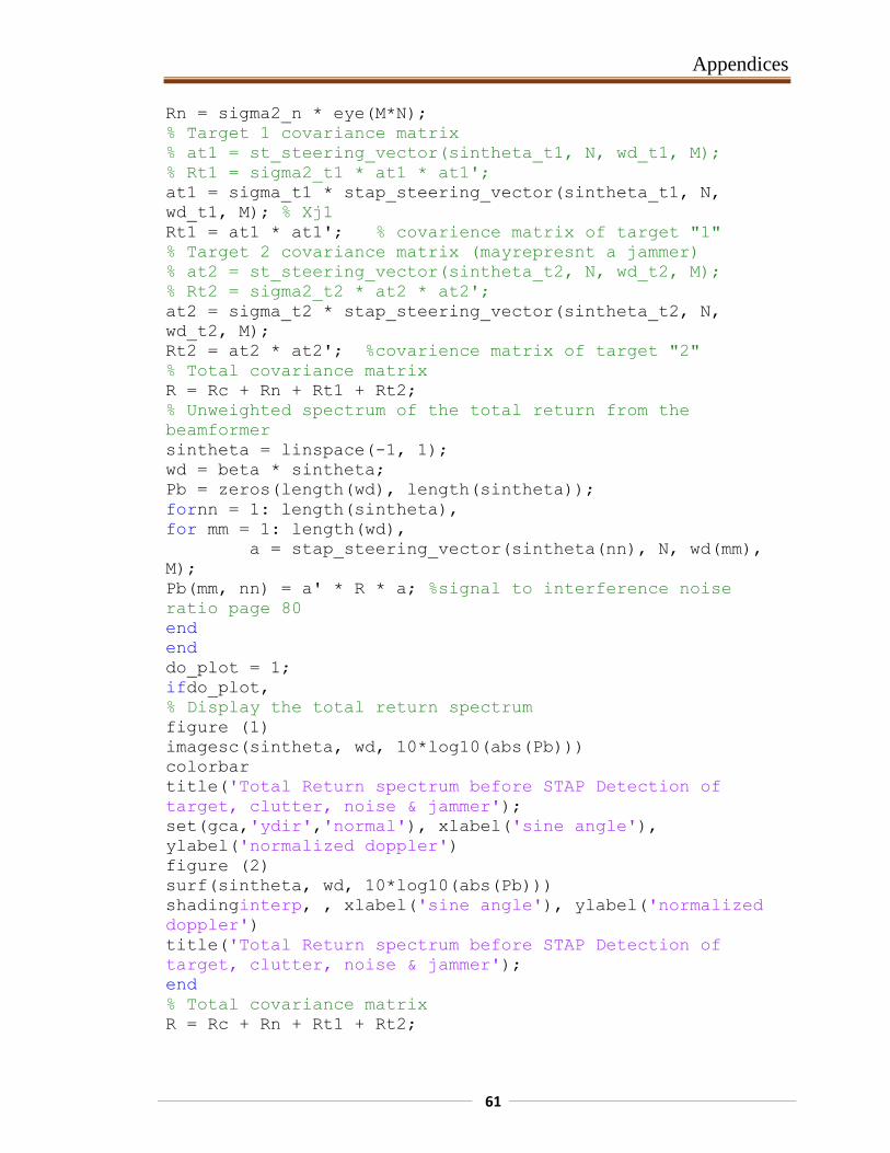
Appendices

60

Rn = sigma2_n * eye(M*N);

% Target 1 covariance matrix

% at1 = st_steering_vector(sintheta_t1, N, wd_t1, M);

% Rt1 = sigma2_t1 * at1 * at1';

at1 = sigma_t1 * stap_steering_vector(sintheta_t1, N,

wd_t1, M); % Xj1

Rt1 = at1 * at1'; % covarience matrix of target "1"

% Target 2 covariance matrix (mayrepresnt a jammer)

% at2 = st_steering_vector(sintheta_t2, N, wd_t2, M);

% Rt2 = sigma2_t2 * at2 * at2';

at2 = sigma_t2 * stap_steering_vector(sintheta_t2, N,

wd_t2, M);

Rt2 = at2 * at2'; %covarience matrix of target "2"

% Total covariance matrix

R = Rc + Rn + Rt1 + Rt2;

% Unweighted spectrum of the total return from the

beamformer

sintheta = linspace(-1, 1);

wd = beta * sintheta;

Pb = zeros(length(wd), length(sintheta));

fornn = 1: length(sintheta),

for mm = 1: length(wd),

a = stap_steering_vector(sintheta(nn), N, wd(mm),

M);

Pb(mm, nn) = a' * R * a; %signal to interference noise

ratio page 80

end

end

do_plot = 1;

ifdo_plot,

% Display the total return spectrum

figure (1)

imagesc(sintheta, wd, 10*log10(abs(Pb)))

colorbar

title('Total Return spectrum before STAP Detection of

target, clutter, noise & jammer');



figure (2)

surf(sintheta, wd, 10*log10(abs(Pb)))

shadinginterp, , xlabel('sine angle'), ylabel('normalized

doppler')

title('Total Return spectrum before STAP Detection of

target, clutter, noise & jammer');

end


R = Rc + Rn + Rt1 + Rt2;

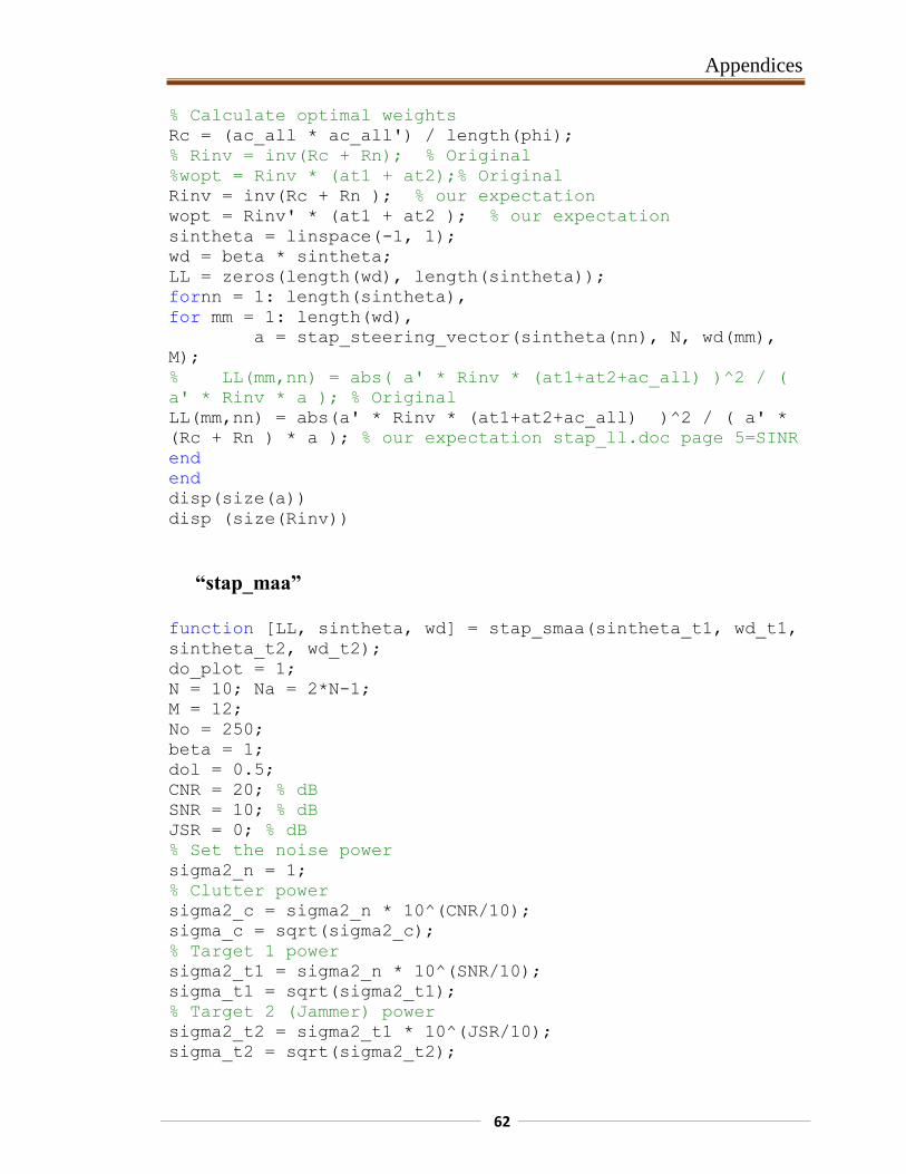
Appendices

62

% Calculate optimal weights

Rc = (ac_all * ac_all') / length(phi);

% Rinv = inv(Rc + Rn); % Original

%wopt = Rinv * (at1 + at2);% Original

Rinv = inv(Rc + Rn ); % our expectation

wopt = Rinv' * (at1 + at2 ); % our expectation



LL = zeros(length(wd), length(sintheta));



a = stap_steering_vector(sintheta(nn), N, wd(mm),

M);

% LL(mm,nn) = abs( a' * Rinv * (at1+at2+ac_all) )^2 / (

a' * Rinv * a ); % Original

LL(mm,nn) = abs(a' * Rinv * (at1+at2+ac_all) )^2 / ( a' *

(Rc + Rn ) * a ); % our expectation stap_ll.doc page 5=SINR

end

end

disp(size(a))

disp (size(Rinv))

“stap_maa”

function [LL, sintheta, wd] = stap_smaa(sintheta_t1, wd_t1,


do_plot = 1;

N = 10; Na = 2*N-1;

M = 12;

No = 250;

beta = 1;

dol = 0.5;

CNR = 20; % dB

SNR = 10; % dB

JSR = 0; % dB

% Set the noise power

sigma2_n = 1;

% Clutter power

sigma2_c = sigma2_n * 10^(CNR/10);

sigma_c = sqrt(sigma2_c);

% Target 1 power

sigma2_t1 = sigma2_n * 10^(SNR/10);


% Target 2 (Jammer) power

sigma2_t2 = sigma2_t1 * 10^(JSR/10);


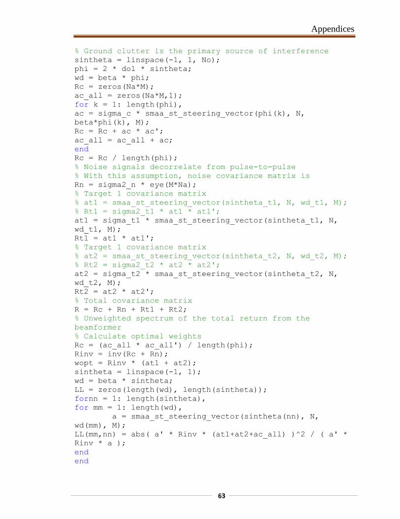
Appendices

63

% Ground clutter is the primary source of interference

sintheta = linspace(-1, 1, No);

phi = 2 * dol * sintheta;

wd = beta * phi;

Rc = zeros(Na*M);

ac_all = zeros(Na*M,1);

for k = 1: length(phi),

ac = sigma_c * smaa_st_steering_vector(phi(k), N,

beta*phi(k), M);

Rc = Rc + ac * ac';

ac_all = ac_all + ac;

end

Rc = Rc / length(phi);

% Noise signals decorrelate from pulse-to-pulse

% With this assumption, noise covariance matrix is

Rn = sigma2_n * eye(M*Na);


% at1 = smaa_st_steering_vector(sintheta_t1, N, wd_t1, M);

% Rt1 = sigma2_t1 * at1 * at1';

at1 = sigma_t1 * smaa_st_steering_vector(sintheta_t1, N,

wd_t1, M);

Rt1 = at1 * at1';


% at2 = smaa_st_steering_vector(sintheta_t2, N, wd_t2, M);

% Rt2 = sigma2_t2 * at2 * at2';

at2 = sigma_t2 * smaa_st_steering_vector(sintheta_t2, N,

wd_t2, M);

Rt2 = at2 * at2';


R = Rc + Rn + Rt1 + Rt2;

% Unweighted spectrum of the total return from the

beamformer

% Calculate optimal weights

Rc = (ac_all * ac_all') / length(phi);

Rinv = inv(Rc + Rn);

wopt = Rinv * (at1 + at2);



LL = zeros(length(wd), length(sintheta));



a = smaa_st_steering_vector(sintheta(nn), N,

wd(mm), M);

LL(mm,nn) = abs( a' * Rinv * (at1+at2+ac_all) )^2 / ( a' *

Rinv * a );

end

end

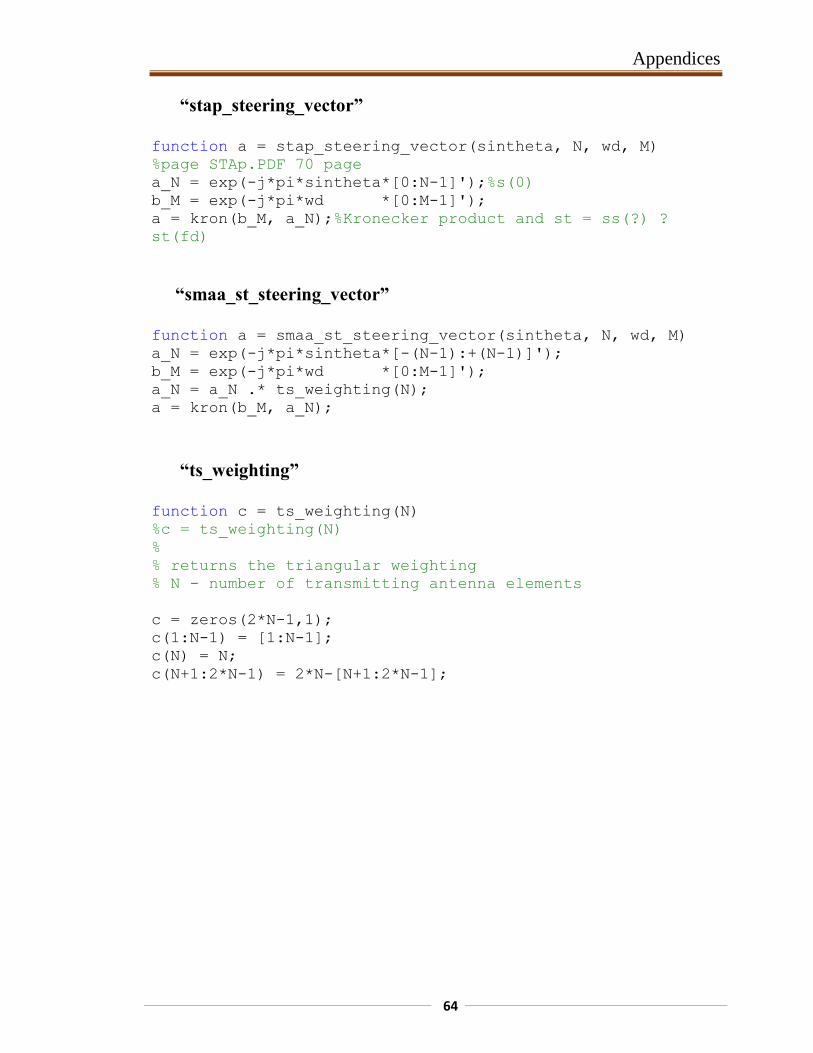
Appendices

64

“stap_steering_vector”

function a = stap_steering_vector(sintheta, N, wd, M)

%page STAp.PDF 70 page

a_N = exp(-j*pi*sintheta*[0:N-1]');%s(0)

b_M = exp(-j*pi*wd *[0:M-1]');

a = kron(b_M, a_N);%Kronecker product and st = ss(?) ?

st(fd)

“smaa_st_steering_vector”

function a = smaa_st_steering_vector(sintheta, N, wd, M)

a_N = exp(-j*pi*sintheta*[-(N-1):+(N-1)]');

b_M = exp(-j*pi*wd *[0:M-1]');

a_N = a_N .* ts_weighting(N);

a = kron(b_M, a_N);

“ts_weighting”

function c = ts_weighting(N)

%c = ts_weighting(N)

%

% returns the triangular weighting

% N - number of transmitting antenna elements

c = zeros(2*N-1,1);

c(1:N-1) = [1:N-1];

c(N) = N;

c(N+1:2*N-1) = 2*N-[N+1:2*N-1];

target detection and reduction of interrupting signals in

Documents