Superfluid turbulence and stability of BEC:using the Gross-Pitaevskii equation

Marc Brachet a

aLaboratoire de Physique Statistique, CNRS UMR 8550, \’Ecole Nor maleSup\’erieure, 24 rue Lhomond, 75231 Paris Cedex 05, France

–Abstract

The Gross-Pitaevskii equation, also called the nonlinear Schr\"odinger equation (NLSE),describes the dynamics low-temperature superflows and Bose-Einstein Condensates(BEC). We review some recent NLSE based numerical studies of superfluid turbu-lence and BEC stability. The relations with experiments are discussed.

Key words:–

Contents

1Introduction 2

2Hydrodynamics using the NLSE 3

2.1 Madelung transformation 3

2.2 Sound waves 5

2.3 Vortices in 2and 3D 6

3Superfluid turbulence 7

3.1 Tools for vortex dynamics 8

3.2 Numerical results 13

3.3 Experimental results 13

4 Stability of stationary solutions 16

4.1 Exact solution in 1D 1 fi4.1 Exact solution in ID 16

4.2 General formulation 1 $\mathrm{O}$ulation 19

数理解析研究所講究録 1226巻 2001年 176-218

176

4.3 Branch following methods 21

4.4 Stability of $2\mathrm{D}$ superflow around acylinder 24

4.5 Stability of attractive Bose-Einstein condensates 33

5 Conclusion 39

6Acknowledgments 39

References 39

References 40

1Introduction

The present paper is areview of results, obtained in the last 10 years or so,by numerically studying the nonlinear Schrodinger equation (NLSE). Directnumerical simulations (DSN) and branch-following methods were extensivelyused to investigate the dynamics and stability of NLSE solutions in 2and 3space dimensions.

Much work has been devoted to the determination of the critical velocity atwhich superfluidity breaks into aturbulent regime [1]. Amathematical modelof superfluid $4\mathrm{H}\mathrm{e}$ , valid at temperatures low enough for the normal fluid tobe negligible, is the nonlinear Schrodinger equation (NLSE), also called theGross-Pitaevskii equation [2-4]. In arelated context, dilute Bose-Einstein con-densates (BEC) have been recently produced experimentally [5-7]. The dy-namics of these compressible nonlinear quantum fluids is accurately describedby the NLSE allowing direct quantitative comparison between theory and ex-periment [8].

Several problems pertaining to superfluidity and BEC can thus be studiedin the framework of the NLSE. In this review, we concentrate on two suchproblems: (i) low-temperature superfluid turbulence [9-11] and (ii) stabilityof BEC in the presence of amoving obstacle [12-14] or an attractive interaction[15]. The paper is organized as follows: in section 2the basic definitions andproperties of the model of superflow are given. Ashort presentation of thehydrodynamic form, through Madelung’s transformation, of NLSE with anarbitrary nonlinearity is derived. Simple solutions are discussed.

Section 3is devoted to superfluid turbulence. The basic tools that are neededto numerically study $3\mathrm{D}$ turbulence using NLSE are developed and validated inSection 3.1. The NLSE numerical results are given in section 3.2. Experimenta

177

results are given in section 3.3.

The stability of BEC is studied in section 4. Exact ID results are given insection 4.1 and ageneral formulation of stability is given in section 4.2. Nu-merical branch following methods are explained in section 4.3. The stabilityof asuperflow around acylinder is studied in section 4.4. The stability of anattractive Bose-Einstein condensate is studied in section 4.5. Finally, section5is our conclusion.

2Hydrodynamics using the NLSE

The hydrodynamical form of NLSE with an arbitrary nonlinearity, correspond-ing to abarotropic fluid with an arbitrary equation of state is introduced inthis section. Basic hydrodynamical features such that acoustic propagationand vortex time independent solutions are also discussed.

2.1 Madelung transformation

The most direct way to understand the generality of the connexion betweenthe NLSE and fluid dynamics is to consider the following action [16] :

$A=2 \alpha\int dt\{d^{3}x\{$ (1)$\frac{i}{2}(\overline{\psi}\frac{\partial\psi}{\partial t}-\psi\frac{\partial\overline{\psi}}{\partial t}))-\mathcal{F}\}$

with

$\mathcal{F}=\int d^{3}x(\alpha|\nabla\psi|^{2}+f(|\psi|^{2}))$ (2)

1

where $\psi(\vec{x}, t)$ is acomplex wave field and $\overline{\psi}$ its complex conjugate, $\alpha$ is apositive real constant and $f$ is apolynomial in $|\psi|^{2}\equiv\overline{\psi}\psi$ with real coefficients:

$f(| \psi|^{2})=-\Omega|\psi|^{2}+\frac{\beta}{2}|\psi|^{4}+f_{3}|\psi|^{6}+\ldots+f_{n}|\psi|^{2n}$ (3)

The NLSE is the Euler-Lagrange equation of motion for $\psi$ corresponding to(1), it reads

$\frac{\partial\psi}{\partial t}=-i\frac{\delta \mathcal{F}}{\delta\overline{\psi}}$ ,

178

uq)$\ovalbox{\tt\small REJECT}\ovalbox{\tt\small REJECT}$

$\mathrm{i}(\mathrm{o}\mathrm{V}^{2}\mathrm{Q}-\mathrm{e}f’]\mathrm{e}|^{2}))$ (4)

Madelung’s transformation $[1,16]$

$\psi=\sqrt{\rho}\exp(i\frac{\varphi}{2\alpha})$ (5)

maps the nonlinear wave dynamics of $\psi$ into equations of motion for afluid ofdensity $\rho$ and velocity $\vec{v}=\nabla\varphi$ . Indeed with the help of (5), (1) can be written

$A=- \int dtd^{3}x(\rho\frac{\partial\varphi}{\partial t}+\frac{1}{2}\rho(\nabla\varphi)^{2}+2\alpha f(\rho)+\frac{1}{2}(2\alpha\nabla(\sqrt{\rho}))^{2})$ (6)

and the corresponding Euler-Lagrange equations of motion read

$\frac{\partial\rho}{\partial t}+\nabla$ . $(\rho\vec{v})=0$ (7)

$\frac{\partial\varphi}{\partial t}+\frac{1}{2}(\nabla\varphi)^{2}+2\alpha f’(\rho)-2\alpha^{2}\frac{\triangle\sqrt{\rho}}{\sqrt{\rho}}=0$ (8)

Without the last term of (8) (the s0-called “quantum pressure” term), theseequations are the continuity and Bernoulli equations [4] for an isentropic,compressible, irrotational fluid.

It is possible to use this identification to define the corresponding “therm0-dynamical functions”. Being isentropic $(S=0)$ , the fluid is barotropic, andthere is only one independent thermodynamical variable. First, the Bernoulliequation readily gives the fluid’s enthalpy per unit mass as

h $=2\alpha f’(\rho)$ . (9)

Second, the $\frac{1}{2}\rho(\nabla\varphi)^{2}$ term of (6) corresponds to kinetic energy. Thus the fluid’sinternal energy per unit mass is given by

e $= \frac{2\alpha f(\rho)}{\rho}$ . (10)

The general thermodynamical identity

h $=e+p/\rho$ , (11)

gives the expression

p $=2\alpha(\rho f’(\rho)-f(\rho))$ (1)

179

for the fluid’s pressure.

The physical dimensions of the variables used in (2) and (3) are fixed by thefollowing considerations. Madelung’s transformation (5) imposes that $[|\psi|^{2}]=$

$[\rho]=ML^{-3}$ and $[\alpha]=L^{2}T^{-1}$ . Using (10), one gets $[f(\rho)/\rho]=T^{-1}$ and thus,from (3), $[\Omega]=T^{-1}$ , $[\beta]=T^{-1}\rho^{-1}$ and $[f_{i}]=T^{-1}\rho^{1-i}$ . Note that, in the caseof aBose condensate of particles of mass $m$ , $\alpha$ has the value $\hslash/2m[17]$ .

2.2 Sound waves

2.2.1 Dispersion relation

The nature of the extra quantum pressure term in (8) can be understoodthrough the dispersion relation corresponding to acoustic (density) wavespropagating around aconstant density level $\rho_{0}$ . Setting $\rho=\rho_{0}+\delta\rho$ (with$\mathrm{f}(\mathrm{p}\mathrm{O})=0)$ , $\nabla\varphi=\delta u$ in (7) and in the gradient of (8), one gets (keeping onlythe linear terms) :

$\partial_{t}\delta\rho+\rho_{0}\nabla\delta u=0$

$\partial_{t}\delta u+2\alpha f’(\rho_{0})\nabla\delta\rho-2\alpha^{2}\Delta\frac{\nabla\delta\rho}{2\rho_{0}}=0$

or

$\partial_{t^{2}}\delta\rho=2\alpha\rho_{0}f’(\rho_{0})\triangle\delta\rho-\alpha^{2}\Delta^{2}\delta\rho$.

The dispersion relation for an acoustic wave $\delta\rho=\epsilon(\exp(i(\omega t -\vec{k}\cdot\vec{x}))+c.c.)$

(with $\epsilon\ll 1$ ) is thus

$\omega$

$=\sqrt{2\alpha\rho \mathrm{o}f’(\rho_{0})\vec{k}^{2}+\alpha^{2}\vec{k}^{4}}$ (13)

This relation shows that the quantum pressure has adispersive effect that be-comes important for large wave numbers. For small wavenumbers, one recoversthe usual propagation, with asound velocity given by

c $=( \frac{\partial p}{\partial\rho})^{\frac{1}{2}}=\sqrt{2\alpha\rho_{0}f’(\rho_{0})}$ .

The length scale $\xi=\sqrt{\alpha/(\rho_{0}f’(\rho_{0}))}$ at which dispersion becomes noticeableis known as the “coherence length”

180

2.2.2 Nonlinear acoustics

The description given by linear acoustic can be somewhat improved by includ-ing the dominant nonlinear effects. Such an equation was derived in [18].

Numerical simulations of NLSE in one space dimension using astandardFourier pseud0-spectral method [19] can be used to study the acoustic regimetriggered by an initial disturbance of the form :

$\psi(x)=1+ae^{-\frac{x^{2}}{\iota^{2}}}$ .

Such simulations were performed in ref. [18] where it was found that the shockswhich would have appeared under compressible Euler dynamics (i.e. followingEq. (8) without the last term in r.h.s.) are regularized by the dispersion. Therewas no evidence of finite-time singularity in our numerics: the spectrum of thesolution was well resolved, with aconspicuous exponential tail.

2.3 Vortices in 2and 3D

Further insight on the connexion between the NLSE and fluid dynamics canbe obtained by considering stationary solutions of the equations of motion.Indeed, by inspection of (1), time independent solutions of NLSE (4), are alsosolutions of the Real Ginzburg-Landau Equation (RGLE)

$\frac{\partial\psi}{\partial t}=-\frac{\delta \mathcal{F}}{\delta\overline{\psi}}=$ $(\alpha\nabla^{2}\psi-\psi f’(|\psi|^{2}))$ . (14)

They are thus extrema of the free energy $\mathcal{F}$ .

The simplest solution of this type corresponds to aconstant density fluid atrest. In this simple case, $\psi$ is constant in space and (14) reads

$f’(|\psi|^{2})=-\Omega+\beta|\psi|^{2}+3f_{3}|\psi|^{4}+\ldots+nf_{n}|\psi|^{2n-2}=0$. (15)

This equation, for given values of the coefficients $\beta$ and $f_{i}$ , $i=3$ , $\ldots$ , $n$ relatesthe fluid density $|\psi|^{2}$ to the value of Q. Note that the $\Omega$ term of $f$ does notplay acrucial role in the NLSE dynamics. Indeed, it could be removed fromthe Bernoulli equation (8) by the change of variable $\varphiarrow\varphi+2\alpha\Omega t$ thatamounts to achange of phase $\psi$ $arrow\psi e^{i\Omega t}$ in NLSE (4). It is however better, byconvention, not to perform these changes of variable. With this convention,stationary solutions of (14) coincide with stationary solutions of (4). The $\Omega$

term of $f$ is thus be fixed by the fluid’s density through (15).

Another important type of time-independent solutions of NLSE are the vortexsolutions. Madelung’s transformation is singular when $\rho=0$ (i.e. when both

181

$\Re(\psi)=0$ and $\propto s(\psi)=0$ . As two conditions are required, the singularitiesgenerically happen on points in two dimensions and lines in three dimensions.The circulation of $\vec{v}$ around such ageneric singularity is $\pm 4\pi\alpha$ . These topolog-ical defects are known in the context of superfluidity as “quantum vortices”[1]. Solutions of (14) with cylindrical symmetry can be obtained numerically[20]. The density profile of avortex admits ahorizontal asymptote near thecore while the velocity diverges as the inverse of the core distance. The m0-

mentum density $\rho\vec{v}$ is thus aregular quantity. It is important to realize thatsuch vortex solutions are regular solutions of the NLSE (4), the singularitystemming only from Madelung’s transformation (5).

3Superfluid turbulence

Superfluid flows ( $i.e$ . laboratory $4He$ flows) are described mathematically interms of Landau’s tw0- luid model [4]. When both normal fluid and superfluidvortices are present, their interaction, called “mutual friction”, must be takeninto account as pioneered by Schwarz [21]. At temperatures low enough for thenormal fluid to be negligible (in practice below $T=1^{\mathrm{o}}K$ for helium at normalpressure), an alternative mathematical description is given by the NonlinearSchrodinger Equation (NLSE), also called the Gross-Pitaevskii equation $[2,3]$ .In this section, we will use the simplest form for $f$ , corresponding to acubicnonlinearity in the NLSE (4). The NLSE, with convenient normalization, reads

$\partial_{t}\psi=ic/(\sqrt{2}\xi)(\psi-|\psi|^{2}\psi+\xi^{2}\nabla^{2}\psi)$ . (16)

Madelung’s transformation (5) takes the form

$\rho=|\psi|^{2}$ (17)$\rho v_{j}=ic\xi/\sqrt{2}(\psi\partial_{j}\overline{\psi}-\overline{\psi}\partial_{j}\psi)$ (18)

where 4is the s0-called “coherence length” and $c$ is the velocity of sound (whenthe mean density $\rho_{0}=1[1])$ . The superflow is irrotational, except near thenodal lines of $\psi$ which are known to follow Eulerian dynamics $[22,23]$ . Thesetopological defects correspond to the superfluid vortices that appear naturally,with the correct velocity circulation, in this model [17].

The basic goal of the present section is to qualify the degree of analogy betweenturbulence in low-temperature superfluids and incompressible viscous fluids.We will do this by comparing numerical simulations of NLSE with existingnumerical simulations of the Navier-Stokes equations, in particular the Taylor-Green (TG) vortex [24]. The TG vortex is the solution of the Navier-Stokes

182

equations with initial velocity field

$\mathrm{v}^{TG}=($ $\sin(x)\cos(y)\cos(z),$ $-\cos(x)\sin(y)\cos(z)$ , 0) (19)

. This flow is well documented in the literature [25-27]. It admits symmetriesthat are used to speed up computations: rotation by $\pi$ about the axis $(x=$

$z=\pi/2)$ , $(y=z=\pi/2)$ and $(x=y=\pi/2)$ and reflection symmetry withrespect to the planes $x=0$ , $\pi$ , $y=0$ , $\pi$ , $z=0$ , $\pi$ . The velocity is parallel tothese planes which form the sides of the impermeable box which confines theflow.

3.1 Tools for vortex dynamics

Under compressible fluid dynamics, an arbitrary chosen initial condition willgenerally lead to aregime dominated by acoustic radiation. In order to studyvortex dynamics using NLSE, we thus need to prepare the initial data in suchaway that the acoustic emission is as small as possible.

3.1.1 Preparation method

We now show how to construct avortex array whose NLSE dynamics mimicsthe vortex dynamics of the large scale flow $\mathrm{v}^{TG}$ . The first step of our method isbased on aglobal Clebsch representation of $\mathrm{v}^{TG}$ and the second step minimizesthe emission of acoustic waves [28].

The Clebsch potentials

$\lambda(x,$y,$z)=\cos(x)\sqrt{2|\cos(z)|}$ (20)

$\mu(x,$y,$z)=\cos(y)\sqrt{2|\cos(z)|}\mathrm{s}\mathrm{g}\mathrm{n}(\cos(z))$ (21)

(where sgn gives the sign of its argument) correspond to the TG flow in thesense that $\nabla\cross \mathrm{v}^{TG}=\nabla\lambda$ $\cross\nabla\mu$ and Aand $\mu$ are periodic functions of $(x, y, z)$ .These Clebsch potentials are used to map the physical space $(x, y, z)$ into the$(\lambda, \mu)$ plane. The complex field $\psi_{c}$ , corresponding to the large scale TG flowcirculation, is given by $\psi_{c}(x, y, z)=(\psi_{4}(\lambda, \mu))^{[\gamma d/4]}$ with $\gamma_{d}=2\sqrt{2}/(\pi c\xi)([]$

denotes the integer part of areal) and

$\psi_{4}(\lambda, \mu)=\psi_{e}(\lambda-1/\sqrt{2}, \mu)\psi_{e}(\lambda, \mu-1/\sqrt{2})\cross$

$\psi_{e}(\lambda+1/\sqrt{2}, \mu)\psi_{e}(\lambda, \mu+1/\sqrt{2})$ (22)

where $\psi_{e}(\lambda, \mu)=(\lambda+i\mu)\tanh(\sqrt{\lambda^{2}+\mu^{2}}/\sqrt{2}\xi)/\sqrt{\lambda^{2}+\mu^{2}}$.

183

Fig. 1. $\mathrm{T}\mathrm{h}\mathrm{r}\mathrm{e}\triangleright \mathrm{d}\mathrm{i}\mathrm{m}\mathrm{e}\mathrm{n}\mathrm{s}\mathrm{i}\mathrm{o}\mathrm{n}\mathrm{a}\mathrm{l}$ visualization of the vector field $\nabla\cross(\rho\vec{v})$ for the Tay-lor-Green flow at time $t=0$ with coherence length $\xi=0.1/(8\sqrt{2})$ , sound velocity$c=2$ and $N=512$ in the impermeable box $[0, \pi]$ $\cross[0, \pi]\cross[0, \pi]$ .

The second step of our procedure consists of integrating to convergence theAdvective Real Ginzburg-Landau Equation (ARGLE):

Ae $=c/(\sqrt{2}\xi)(\psi-|\psi|^{2}\psi+\xi^{2}\nabla^{2}\psi)-i\mathrm{v}^{TG}\cdot\nabla\psi-$

$(\mathrm{v}^{TG})^{2}/(2\sqrt{2}ae)\psi$ (23)

with initial data $\psi=\psi_{c}$ . It is shown in [9] that the TG symmetries can beused to expand $\psi(x,$y, z, t), solution of the ARGLE and NLSE equations as:

$\psi(x,$y, z,$t)= \sum_{m=0}^{N/2}\sum_{n=0}^{N/2}\sum_{p=0}^{N/2}\hat{\psi}(m,$n,p, t) $\cos mx\cos ny\cos pz$ (24)

where $N$ is the resolution and $\hat{\psi}(m, n,p, t)=0$ , unless $m$ , $n,p$ are either all evenor all odd integers. Furthermore $\hat{\psi}(m, n,p, t)$ satisfies the additional conditions$\hat{\psi}(m, n,p, t)=(-1)^{\mathrm{r}+1}\hat{\psi}(n, \mathrm{n},\mathrm{p}, t)$ where $r=1$ when $m$ , $n,p$ are all even and$r=2$ when $m$ , $n,p$ are all odd. Implementing this expansion in apseud0-spectral code yields asaving of afactor 64 in computational time and memorysize when compared to general Fourier expansions.

The ARGLE converged periodic vortex array obtained in this manner is dis-played on Fig. 1. with coherence length $\xi$ $=0.1/(8\sqrt{2})$ , sound velocity $c=2$

and resolution $N=512$

184

Fig. 2. Plot of the incompressible kinetic energy spectrum, $E_{kin}^{i}(k)$ . The bottomcurve (a) (circles) corresponds to time $t=0$ . The spectrum of asingle axisymmetric$2\mathrm{D}$ vortex multiplied by $(l/2\pi)=175$ is shown as the bottom solid line. The topcurve (b) (pluses) corresponds to time $t=5.5$ . Aleast-square fit over the interval$2\leq k\leq 16$ with apower law $E_{kin}^{i}(k)=Ak^{-}n$ gives $n=1.70$ (top solid line).

3.1.2 Energy spectra

The total energy of the vortex array, conserved by NLSE dynamics, can bedecomposed into three parts $E_{tot}=1/(2 \pi)^{3}\int d^{3}x(\mathcal{E}_{kin}+\mathcal{E}_{int}+\mathcal{E}_{q})$, with kineticenergy $\mathcal{E}_{kin}=1/2\rho v_{j}v_{j}$ , internal energy $\mathcal{E}_{int}=(c^{2}/2)(\rho-1)^{2}$ and quantumenergy $\mathcal{E}_{q}=c^{2}\xi^{2}(\partial_{j}\sqrt{\rho})^{2}$ . Each of these parts can be defined as the inte-gral of the square of afield, for example, $\mathcal{E}_{kin}=1/2(\sqrt{\rho}v_{j})^{2}$ . In order toseparate the kinetic energy corresponding to compressibility effects, $\mathcal{E}_{kin}$ canbe further decomposed into acompressible and incompressible parts using$\sqrt{\rho}v_{j}=(\sqrt{\rho}v_{j})^{c}+(\sqrt{\rho}v_{j})^{i}$ with $\nabla.(\sqrt{\rho}v_{j})^{i}=0$ . Using Parseval’s theorem, theangle-averaged kinetic energy spectrum is defined as:

$E[in(k)= \frac{1}{2}\int k^{2}\sin\theta d\theta d\phi$ $| \frac{1}{(2\pi)^{3}}\int d^{3}re^{ir_{j}k_{j}}\sqrt{\rho}v_{j1^{2}}$

which satisfies $E_{kin}=1/(2 \pi)^{3}\int d^{3}x\mathcal{E}_{kin}=\int_{0}^{\infty}dkE_{kin}(k)$ . The incompressiblekinetic energy spectrum, $E_{kin}^{i}(k)$ , is the single-averaged spectrum computingover shells in Fourier space. Amode $(m, n,p)$ belongs to the shell numberedas $k=[\sqrt{m^{2}+n^{2}+p^{2}}+1/2]$ .

The radius of curvature of the vortex lines in Fig. 1is large compared totheir radius. Thus these $3\mathrm{D}$ lines can be considered as straight, and thencompared to the $2\mathrm{D}$ axisymmetric vortices which are exact solutions to the

10

185

$\mathrm{a}\leq$”

Fig. 3. Total incompressible kinetic energy, $E_{kin}^{i}$ , plotted versus time for( $=0.1/(2\sqrt{2})$ , $N=128$ (long-dash line); $\xi=0.1/(4\sqrt{2})$ , $N=256$ (dash);$\xi=0.1/(6.25\sqrt{2})$ , $N=400$ (dot) and $\xi=0.1/(8\sqrt{2})$ , $N=512$ (solid line). Allruns are realized with $c=2$. The evolution of the total vortex filament length di-vided by $2\pi$ (crosses) for the $N=512$ run is also shown (scale given on the righty-axis).

Fig. 4. Same visualization as in Fig. 1but at time t $=4$ .

11

186

Fig. 5. Same visualization as in Fig. 1but at time t $=8$ .

$2\mathrm{D}$ NLSE. A $2\mathrm{D}$ vortex at the origin is given by $\psi^{vort}(r)=\sqrt{\rho(r)}\exp(im\varphi)$ ,$m=\pm 1$ , where $(r, \varphi)$ are polar coordinates. The vortex profile $\sqrt{\rho(r)}\sim r$

as $rarrow \mathrm{O}$ and $\sqrt{\rho(r)}=1+O(r^{-2})$ for $rarrow\infty$ . It can be computed numeri-cally using mapped Chebychev polynomials and an appropriate functional [9].The corresponding velocity field is azimuthal and is given by $v(r)=\sqrt{2}c\xi/r$ .Using the mapped Chebychev polynomials expansion for $\sqrt{\rho(r)}$ , the angle av-eraged spectrum of $\sqrt{\rho}v_{j}$ can then be computed with the formula $E_{kin}^{vot\iota}(k)=$

$c^{2} \xi^{2}/(2\pi k)(\int_{0}^{\infty}drJ_{0}(kr)\partial_{r}\sqrt{\rho})^{2}[9]$ , where $J_{0}$ is the zeroth order Bessel func-tion.

The incompressible kinetic energy spectrum $E_{kin}^{i}$ of the ARGLE convergedvortex array of Fig. 1is displayed on Fig. 2. For large wavenumbers, the spec-trum is well represented by extending acollection of $2\mathrm{D}$ vortices into $3\mathrm{D}$ vortexlines via $E_{kin}^{line}(k)\equiv const$ . $\cross E_{kin}^{vort}(k)$ . (We will see that the constant of propor-tionality is related to the length $l$ of vortex lines by const. $=l/(2\pi)=175$ attime $t=0.$ ) In contrast, the small wavenumber region cannot be representedby $E_{kin}^{line}$ . This stems from the average separation distance between the vortexlines in Fig. 1. Calling this distance $d_{bump}=k_{bump}^{-1}=1/16$ , the wavenum-ber range between the large-scale wavenumber $k=2$ and the characteristicseparation wavenumber $k_{bump}$ can be explained by interference effects. Dueto constructive interference, the energy spectrum at $k=2$ has avalue closeto its corresponding value in TG viscous flow (namely 0.125), which is muchabove the value of $E_{kin}^{line}(k=2)$ . In contrast, for $2<k\leq k_{bump}$ , destructiveinterference decreases $E_{kin}^{i}$ below $E_{kin}^{line}$ .

12

187

3.2 Numerical results

The evolution in time via NLSE (16) of the incompressible kinetic energy isshown in Fig. 3. The main quantitative result is the remarkable agreementof the energy dissipation rate, $-dE_{k\dot{\iota}n}^{\dot{l}}/dt$ , with the corresponding data in theincompressible viscous TG flow (see reference [25], and reference [29], figure5.12). Both the moment $t_{\max}\sim 5-10$ of maximum energy dissipation (theinflection point of Fig. 3) and its value $\epsilon(t_{\max})\sim 10^{-2}$ at that moment are inquantitative agreement. Furthermore, both $t_{\max}$ and $\epsilon(t_{\max})$ depend weaklyon $\xi$ .

Another important quantity studied in viscous decaying turbulence is the scal-ing of the kinetic energy spectrum during time evolution and, especially, atthe moment of maximum energy dissipation, where a $k^{-5/3}$ range can be ob-served (see reference [25]). Fig. 2(b) shows the energy spectrum at $t=5.5$ . Aleast-square fit over the interval $2\leq k\leq 16$ with apower law $E_{kin}^{i}(k)=Ak^{-n}$

gives $n=1.70$ (solid line). For $5<t<8$ , asimilar fit gives $n=1.6\pm 0.2$ (datanot shown). Fitting $E_{kin}^{l}(k)$ in the interval $30\leq k\leq 170$ with $l/(2\pi)$ times$E_{kin}^{vort}(k)$ leads to $l/2\pi=452$ , roughly three times the $t=0$ length of the vor-tex lines. The time evolution of $l/2\pi$ obtained by this procedure is displayedin Fig. 3, showing that the length continues to increase beyond $t_{\max}$ . Thecomputations were performed with $c=2$ corresponding to aroot-mean-squareMach number $M_{tms}\equiv|\mathrm{v}_{tms}^{TG}|/c=0.25$ . As it is very costly to decrease $M_{rms}$ ,we checked [9] that compressible effects were non-dominant at this value of$M_{rms}$ .

The vortex lines are visualized in physical space in Figs. 4and 5at time$t=4$ and $t=8$. At $t=4$ , no reconnection has yet taken place while acomplex vortex tangle is present at $t=8$ . Detailed visualizations (data notshown) demonstrate that reconnection occurs for $t>5$ . Note that the viscousTG vortex also undergoes aqualitative (and quantitative) change in vortexdynamics around $t\sim 5$ .

3. 3Experimental results

The TG flow is related to an experimentally studied swirling flow [30-32]. Therelation between the experimental flow and the TG vortex is asimilarity inoverall geometry [30]: ashear layer between two counter-rotating eddies. TheTG vortex, however, is periodic with free-slip boundaries while the experi-mental flow is contained inside atank between two counter-rotating disks.

The spectral behavior of NLSE can be compared to standard (viscous) turbu-lence only for k $\leq k_{bump}$ . It is thus of interest to estimate the scaling of $k_{bump}$

13

188

in terms of the characteristic parameters of the large scale flow and of thefluid. As seen above, $k_{bump}\sim d_{bump}^{-1}$ , where $d_{bump}$ is the average distance be-tween neighboring vortices. Consider aflow with characteristic integral scale$l_{0}$ and large scale velocity $u_{0}$ (in the case of the TG flow, $l_{0}\sim 1$ and $u_{0}\sim 1$ ).The fluid characteristics are the velocity of sound $c$ and the coherence length4(with corresponding wavenumber $k_{\xi}\sim\xi^{-1}$ ). The number $n_{d}$ of vortex linescrossing atypical large-scale $l_{0}^{2}$ area is given by the ratio of the large-scale flowcirculation $l_{0}u_{0}$ to the quantum of circulation $\Gamma=4\pi c\xi/\sqrt{2}$, $\mathrm{i}.\mathrm{e}n_{d}\sim l_{0}u_{0}/c\xi$ .On the other hand, the assumption that the vortices are uniformly spread overthe large scale area gives $n_{d}\sim l_{0}^{2}/d_{bump}^{2}$ . Equating these two evaluations of $n_{d}$

yields the relation $d_{bump}\sim l_{0}\sqrt{(c\xi)/(l_{0}u_{0})}$ .

In the case of helium, the viscosity at the critical point $(T=5.174^{\mathrm{o}}K$ , $P=$

$2.210^{5}Pa)$ is $\nu_{cp}=0.27\cross 10^{-7}m^{2}s^{-1}$ while the quantum of circulation,$\Gamma=h/m_{He}$ has the value $0.99\cross 10^{-7}m^{2}s^{-1}$ . Thus, $0.25\nu_{cp}\sim\Gamma$ . The order ofmagnitude for $d_{bump}$ is thus $d_{bump}=l_{0}/\sqrt{R_{cp}}\sim l_{\lambda}$ where $R_{cp}$ is the integralscale Reynolds number at the critical point and $l_{\lambda}$ the Taylor micr0-scale. Inother words, the value of $d_{bump}$ in asuperfluid helium experiment at $T=1^{\mathrm{o}}K$

is of the same order as the Taylor micr0-scale in the same experimental set-uprun with viscous helium at the critical point.

The experimental set-up is similar to the one described in [31]. Some modi-fications have been made to work down to $1.2\mathrm{A}\mathrm{T}$ . The flow is produced in acylinder, 8cm in diameter and 12 cm high, limited axially by two counter-rotating disks. One disk is flat and, on the other one, are fixed 8radial blades,forming an angle of $45^{o}$ between each other. Astator is mounted at half thetotal height of the cell in order to stabilize the turbulent shear region. Thetwo disks are driven by two DC motors rotating from 1to 30 Hz. The wholesystem is enclosed directly in aliquid Helium bath which is used as the ex-perimental fluid, the main difference with the set-up described in [31]. Thetemperature of the fluid is fixed by the pressure above the liquid bath, whichis itself controlled by the pumping system.

Local pressure fluctuations are measured by using small total-head pressuretubes, immersed in the flow. The pressure sensors are hollow metallic tubes,connected to aquartz pressure transducer WHM 112 A22 from PCB. Detailsare given in [11].

In normal fluids, the pressure measured at the tip of the total-head tube can berelated to the upstream flow $U(t)$ and the local pressure $P(t)$ using Bernoullitheorem:

$P_{\mathrm{m}\mathrm{e}\mathrm{a}\mathrm{s}}(t)=P(t)+\rho U^{2}(t)/2$ (25)

14

189

1 ..1 $\cdot 3$

$\vee\wedge--\cdot$

.$1|^{1}$

$\check{\mathrm{r}}\mathrm{c}$ 1 .1

1 ..1 $\cdot\cdot 1$

11 1 $\cdot$ . 1 $\cdots$

frequency (Hz)

Fig. 6. Experimental pressure fluctuation spectrum (in non-dimensional units) mea-sured with atotal head pressure tube immersed in the flow at $T=2.3K$ .In the flow region where the probe is immersed, awell established axial meanflow $U$ exists so that, after removing the mean parts of Equation (1), one gets:

Pmeas $(t)=p(t)+\rho Uu(t)$ (26)

where pmeas, $p$ and $u$ are the fluctuations of the measured pressure, the actualpressure, and the local velocity respectively. It is currently admitted that, inordinary turbulent situations, and at low fluctuation rates, Equation (2) isdominated by the dynamic term, so that, by measuring the pressure fluctua-tions at the total head tube, one has adirect access to the velocity fluctuations$u(t)$ .

The situation is less clear when the probe is immersed in the superfluid. It ishowever possible to write an equation similar to (2). Details can be found in[11].

The analysis of the pressure fluctuations obtained with the total head tubeplaced at 2cm above the mid plane and 2cm from the cylinder axis, yieldsinteresting informations. Figures 6and 7shows the spectra of the pressurefluctuations above and below $T_{\lambda}$ (i.e respectively at $2.3K$ and $1.4K$). Fig. 6clearly shows, as expected, that such fluctuations follow aKolmogorov regimebetween the injection scale (signaled by the peak at 25 Hz) and the largestresolved frequency, $\mathrm{i}.\mathrm{e}900$ Hz. The spectrum obtained at 1AK is similar tothat obtained at $T=2.\mathrm{S}\mathrm{K}$ (see Fig. 7). Aclear Kolmogorov like regime existsfor the same range of frequencies. The corresponding Kolmogorov constantturns out also to be indistinguishable from the classical value. We have fur-ther analyzed the deviations from Kolmogorov in the superfluid regime. The

15

190

1 $0^{*}$

$1$ $0^{3}$

$\vee-\wedge-\cdot$. 1 $0^{l}$

$\check{\mathrm{E}}\circ$ 1 $0^{1}$

10

1 $0^{\cdot}1$

10100 $1\cdot 00$

freq uency $(\mathrm{H}\mathrm{z})$

Fig. 7. Experimental pressure fluctuation spectrum (in non-dimensional units) mea-sured with atotal head pressure tube immersed in the flow at T $=1.4$ K.

striking result is that they have the same magnitude as in classical turbulence.More details are given in [33].

These observations -both on global and local quantities -agree pretty wellthe theoretical approach developed in the previous section. In particular, itseems rather clear that Kolmogorov cascade survives in the superfluid regime.

4Stability of stationary solutions

This section is devoted to the stability of BEC. Exact ID bifurcation results aregiven in section 4.1. Ageneral formulation of stability is given in section 4.2.Numerical branch following methods are explained in section 4.3. The stabilityof asuperflow around acylinder is studied in section 4.4 and attractive Bose-Einstein condensates are studied in section 4.5.

4.1 Exact solution in ID

4.1.1 Definition of the system

We consider apunctual impurity moving within aID superflow. In the frameof the moving impurity, the system can be described by the following action

16

191

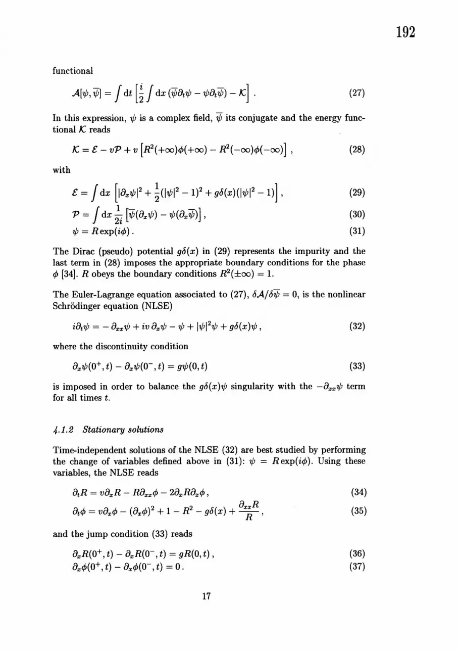
functional

$A[ \psi, \overline{\psi}]=\int \mathrm{d}t[\frac{i}{2}\int \mathrm{d}x(\overline{\psi}\partial_{t}\psi-\psi\partial_{t}\overline{\psi})-\mathcal{K}]$ (27)

In this expression, $\psi$ is acomplex field, $\overline{\psi}$ its conjugate and the energy func-tional $\mathcal{K}$ reads

$\mathcal{K}=\mathcal{E}-v\mathcal{P}+v[R^{2}(+\infty)\phi(+\infty)-R^{2}(-\infty)\phi(-\infty)]$ , (28)

with

$\mathcal{E}=\int \mathrm{d}x[|\partial_{x}\psi|^{2}+\frac{1}{2}(|\psi|^{2}-1)^{2}+g\delta(x)(|\psi|^{2}-1)]$ , (29)

$\mathcal{P}=\int \mathrm{d}x\frac{1}{2i}[\overline{\psi}(\partial_{x}\psi)-\psi(\partial_{x}\overline{\psi})]$ , (30)

$\psi=R\exp(i\phi)$ . (31)

The Dirac (pseudo) potential $g\delta(x)$ in (29) represents the impurity and thelast term in (28) imposes the appropriate boundary conditions for the phase$\phi$ $[34]$ . $R$ obeys the boundary conditions $R^{2}(\pm\infty)=1$ .

The Euler-Lagrange equation associated to (27), $\delta A/\delta\overline{\psi}=0$ , is the nonlinearSchr\"odinger equation (NLSE)

$i\partial_{t}\psi=-\partial_{xx}\psi+iv\partial_{x}\psi-\psi+|\psi|^{2}\psi+g\delta(x)\psi$ , (32)

where the discontinuity condition

$\partial_{x}\psi(0^{+}, t)-\partial_{x}\psi(0^{-}, t)=g\psi(0,$t) (33)

is imposed in order to balance the $g\delta(x)\psi$ singularity with the $-\partial_{xx}\psi$ termfor all times t.

4.1.2 Stationary solutions

Time-independent solutions of the NLSE (32) are best studied by performingthe change of variables defined above in (31): $\psi=R\exp(i\phi)$ . Using thesevariables, the NLSE reads

$\partial_{t}R=v\partial_{x}R-R\partial_{xx}\phi-2\partial_{x}R\partial_{x}\phi$ , (34)

$\partial_{t}\phi=v\partial_{x}\phi-(\partial_{x}\phi)^{2}+1-R^{2}-g\delta(x)+\frac{\partial_{xx}R}{R}$ , (35)

and the jump condition (33) reads

$\partial_{x}R(0^{+}, t)-\partial_{x}R(0^{-}, t)=gR(0,$t), (36)$\partial_{x}\phi(0^{+}, t)-\partial_{x}\phi(0^{-}, t)=0$ . (37)

17

192

Note that Eqs. (34) and (35) can be respectively interpreted as the continuityand Bernoulli equations for afluid of density p $\ovalbox{\tt\small REJECT}$ $\#^{2}(\ovalbox{\tt\small REJECT} \mathrm{z})$ and velocity u $\ovalbox{\tt\small REJECT}$ $2\mathrm{a}_{x}$

(as done in section 2).

Explicit time-independent solutions of Eqs. (34) and (35) were found by Hakim[lusing the s0-called gray solitons (a nonlinear optics terminology). Gray solitons$[35,36]$ are stationary solutions of Eqs. (34) and (35), without the potentialterm $g\delta(x)$ . They are localized density depletion of the form

$R_{\mathrm{G}\mathrm{S}}^{2}(x)=v^{2}/2+(1-v^{2}/2)\tanh^{2}[\sqrt{1/2-v^{2}/4}x]$ , (38)

$\phi_{\mathrm{G}\mathrm{S}}(x)=\arctan(\frac{v\sqrt{2-v^{2}}}{\exp[\sqrt{2-v^{2}}x]+v^{2}-1})$ . (39)

Patching together pieces of gray solitons, Hakim found the following 4-indexedstationary solutions of Eqs. (34) and (35), including the potential term $g\delta(x)$

$R_{\xi}(x)=R_{\mathrm{G}\mathrm{S}}(x\pm\xi)$ , x $<0>$ (40)$\phi_{\xi}(x)=\phi_{\mathrm{G}\mathrm{S}}(x\pm\xi)-\phi_{\mathrm{G}\mathrm{S}}(\pm\xi)$ , $x><0$ (41)

where the jump conditions (36) and (37) impose the relation

$g( \xi)=\sqrt{2}(1-v^{2}/2)^{3/2}\frac{\tanh[\sqrt{1/2-v^{2}/4}\xi]}{v^{2}/2+\sinh^{2}[\sqrt{1/2-v^{2}/4}\xi]}$ . (42)

The function $g(\xi)$ reaches amaximum $g_{c}=g(\xi_{c})$ at $\xi_{c}=\frac{\arg\cosh(\frac{1+\sqrt{1+4v^{2}}}{2}}{\sqrt{2-v^{2}}}$ with

$g_{c}=4(1-v^{2}/2) \frac{[\sqrt{1+4v^{2}}-(1+v^{2})]^{1/2}}{2v^{2}-1+\sqrt{1+4v^{2}}}$ . (43)

The two stationary solutions of (32) corresponding to $\xi_{+}(g)>\xi_{c}$ and $\xi_{-}(g)<$

$\xi_{c}$ obtained by inverting (42) for $g<g_{c}$ thus disappear, merging in asaddle-node bifurcation at acritical strength $g_{c}$ . Note that the bifurcation can also beobtained by varying $v$ and keeping $g$ constant. In the following, the strength$g$ of the delta function is used as the control parameter of our system, keeping$v$ constant.

The bifurcation diagram corresponding to the energy $\mathcal{K}$ (see Eq. (28)) isshown on fig.8, The energetically unstable and stable solutions $(\mathcal{K}(\xi_{-}(g))>$

$\mathcal{K}(\xi_{+}(g)))$ are also displayed on the figure. Note that the phase $\phi_{\xi}(x)$ , as de-fined in eq. (41), differs from that considered in [34] by an (x-independent)constant. The phase in [34] is set to 0at $x=+\infty$ , whereas (41) is antisym-metric in $x$ . This difference is unimportant because Eqs. (34) and (35) are

18

193

(a) (b)

$R$ $\phi$

Fig. 8. (a) Modulus $R$ of the stable (–) and unstable (—) stationary solutions ofeq.(32) (see eq.(40)) for $g=1.250$ and $v=0.5$ ;insert, energy functional $\mathcal{K}$ of thestationary solutions versus $g$ for $v=0.5$ (see eq.(28)); lower branch: energeticallystable branch, upper branch: energetically unstable branch. The bifurcation occursat $g=1.5514$ $(\mathrm{b})$ Phase $\phi$ of the stable (–) and unstable (—) stationary solutions(see eq.(41)), same conditions as in (a).

invariant under the constant phase shift

$\phi(x)\mapsto*\phi(x)+\varphi$ . (44)

4.2 General formulation

(45)

In this section we define and test the numerical tools needed to obtain thestationary solutions of the NLSE.

Consider the following action functional associated to the NLSE

$A= \int d\tilde{t}\{\int d\tilde{\mathrm{x}}\frac{i}{2}(\overline{\psi}\frac{\partial\psi}{\partial\tilde{t}}-\psi\frac{\partial\overline{\psi}}{\partial\tilde{t}})-\mathcal{F}\}$ ,

where $\psi$ is acomplex field, $\overline{\psi}$ its conjugate and $\mathcal{F}$ is the energy of the system.Here, $\mathrm{x}$ and $\tilde{t}$ correspond to adequately nondimensionalized space and timevariables respectively.

The Euler-Lagrange equation corresponding to (45) leads to the NLSE interms of the functional $\mathcal{F}$

$\frac{\partial\psi}{\partial\tilde{t}}=-\dot{\iota}\frac{\delta \mathcal{F}}{\delta\overline{\psi}}$ . (46)

This equation obviously admits $\psi_{S}$ as astationary solutions if $\delta \mathcal{F}/\delta\psi|_{\psi=\psi_{S}}=0$ .Thus, stationary solutions of (46) are extrema of T. In general, we are lookingfor an extremum of an energy functional $\mathcal{E}$ under some constraint $Q[\psi]=\mathrm{c}st$ .The usual Lagrange multiplier trick consists in introducing acontrol parameter

19

194

$7/\mathrm{a}\mathrm{n}\mathrm{d}$ , rather than solving for extrema of $\ovalbox{\tt\small REJECT} 5[\mathrm{e}]$ , searching for extrema of thenew functional $\ovalbox{\tt\small REJECT} \mathrm{F}[\mathrm{e}]\ovalbox{\tt\small REJECT} \mathrm{f}[\mathrm{e}]$ –&(2[e]. We thus solve for

$\frac{\delta \mathcal{F}}{\delta\psi}|_{\nu=\mathrm{c}\mathrm{s}\mathrm{t}}.=0$ . (47)

We now turn to the precise definitions, corresponding to the two systemsconsidered in this section :(a) Bose-Einstein Condensates and (b) Superflows.

4.2. 1Superflows

In the problem of asuperflow past an obstacle, $\mathcal{E}$ is the hydrodynamic energyand $\nu\equiv\vec{U}$ is the flow velocity with respect to the obstacle $[12,14]$ . This impliesthat $Q$ $\equiv\vec{P}$ is the flow momentum. Functional$\mathrm{s}$

$\mathcal{F}$, $\mathcal{E}$ and $\vec{P}$ are given by theexpressions

$\mathcal{F}=\mathcal{E}-P^{\prec}\cdot U^{\prec}$ (48)

$\mathcal{E}=c^{2}\int d^{3}x([-1+V(\vec{x})]|\psi|^{2}+\frac{1}{2}|\psi|^{4}+\xi^{2}|\nabla\psi|^{2})$ (49)

$\vec{P}=\sqrt{2}c\xi\int d^{3}x\frac{i}{2}(\psi\nabla\overline{\psi}-\overline{\psi}\nabla\psi)$ . (50)

Here, $c$ and 4are the physical parameters characterizing the superfluid. Theycorrespond to the speed of sound (c) for afluid with mean density $\rho_{0}=1$ ,and to the coherence length (4). The potential $V(x)\prec$ is used to represent acylindrical obstacle of diameter $D$ . The NLSE reads

$\frac{\partial\psi}{\partial t}=-\frac{i}{\sqrt{2}c\xi}\frac{\delta \mathcal{F}}{\delta\overline{\psi}}=i\frac{c}{\sqrt{2}\xi}([1-V(\vec{x})]\psi-|\psi|^{2}\psi+\xi^{2}\nabla^{2}\psi)+\vec{U}\cdot\nabla\psi$.

(51)

We will be interested in the solutions of $\delta \mathcal{F}/\delta\overline{\psi}=0$ , for agiven value of$\vec{U}$ . According to equation (47), these solutions are extrema of $\mathcal{E}$ at constantmomentum $\vec{P}$ .

4.2.2 Bose-Einstein Condensates

We consider acondensate of $N$ particles of mass $m$ and effective scatteringlength $a$ in aradial confining harmonic potential $V(r)=m\omega^{2}r^{2}/2[15]$ . Quan-tities are rescaled by the natural quantum harmonic oscillator units of time$\tau_{0}=1/\omega$ and length $L_{0}=\sqrt{\hslash/m\omega}$, thus obtaining the nondimensionalizedvariables $\tilde{t}=t/\tau_{0},\tilde{\mathrm{x}}=\mathrm{x}/L_{0}$ and $\tilde{a}=4\pi a/L_{0}$ . The control parameter $\nu$ be-comes in this context the chemical potential $\mu$ . The total number of particles

20

195

in the condensate is therefore given by q $\ovalbox{\tt\small REJECT}$

$\ovalbox{\tt\small REJECT}/\mathrm{V}^{\ovalbox{\tt\small REJECT}}$. Functionals ye and $\ovalbox{\tt\small REJECT} \mathrm{V}$ aregiven, in terms of rescaled variables, by

$\mathcal{F}=\mathcal{E}-\mu \mathcal{N}$ (52)

$\mathcal{E}=\int d^{3}\tilde{\mathrm{x}}(\frac{1}{2}|\nabla_{\overline{\mathrm{x}}}\psi|^{2}+V(\tilde{\mathrm{x}})|\psi|^{2}+\frac{\tilde{a}}{2}|\psi|^{4})$ (53)

$N= \int d^{3}\tilde{\mathrm{x}}|\psi|^{2}$ . (54)

Two different situations are possible, depending on the sign of the (rescaled)effective scattering length $\tilde{a}$ . When $\tilde{a}$ is positive the particles interact repul-sively. Anegative $\tilde{a}$ corresponds to an attractive interaction. The dynamicalequation is

$\frac{\partial\psi}{\partial\tilde{t}}=-i\frac{\delta \mathcal{F}}{\delta\overline{\psi}}=i[\frac{1}{2}\nabla\frac{2}{\mathrm{x}}\psi-\frac{1}{2}|\tilde{\mathrm{x}}|^{2}\psi-(\tilde{a}|\psi|^{2}-\mu)\psi]$ . (55)

We will be interested in the solutions of $\delta \mathcal{F}/\delta\overline{\psi}=0$ , for agiven value of$\mu$ . According to equation (47), these solutions are extrema of $\mathcal{E}$ at constantparticle number $N$.

4.3 Branch following methods

When the extremum of $\mathcal{F}$ is alocal minimum, the stationary solution $\psi_{S}$

of (51) can be reached by arelaxation method. If the extremum is not aminimum, Newton’s iterative method is used to solve for $\psi s$ .

4.3.1 Relasation method

In what remains of this section, we will write the NLSE under the followinggeneric form, which is valid for both the Bose-Einstein condensates and thesuperflow past an obstacle:

$\frac{\partial\psi}{\partial t}=-i\frac{\delta \mathcal{F}}{\delta\overline{\psi}}=i(\alpha\nabla^{2}\psi+[\Omega-V(\vec{x})]\psi-\beta|\psi|^{2}\psi)+\vec{U}\cdot\nabla\psi$ . (56)

When the extremum of $T$ is alocal minimum, the stationary solution $\psi_{S}$ of(56) can be reached by integrating to relaxation the associated real Ginzburg-Landau equation (RGLE)

$\frac{\partial\psi}{\partial t}=-\frac{\delta \mathcal{F}}{\delta\overline{\psi}}=\alpha\nabla^{2}\psi+[\Omega-V(\vec{x})]\psi$$-\beta|\psi|^{2}\psi-iU^{\prec}\cdot\nabla\psi$ . (57)

Indeed, (56) and (57) have the same stationary solutions.

21

196

$10^{0}$

$\overline{\mathrm{u}^{=}\mathrm{o}_{1}}10^{-10}$

$10^{-20}$

$10^{-30}$

Fig. 9. Two typical examples of the Newton method convergence towards the solu-tion of equation (60) for the problem of asuperflow past acylinder with $\xi/D=1/10$

and afield $\psi_{(j)}$ discretized into $n=128\cross 64=8190$ collocation points. The errormeasure is given by $\sum_{j=1}^{n}f_{(j)}^{2}(\psi)/n$ . The convergence is faster than exponential, asexpected for a Newton method.

In our numerical computations, equation (57) is integrated to convergence byusing the Forward-Euler/Backwards-Euler time stepping scheme

$\psi(t+\sigma)=^{-1}[(1-i\sigma\vec{U}\cdot\nabla)+\sigma([\Omega-V(_{X}^{\prec})]-\beta|\psi(t)|^{2})]\psi(t)$ (58)

with

$=[1-\sigma\alpha\nabla^{2}]$ . (59)

The advantage of this method is that it converges to the stationary solutionof (56) independently of the time step $\sigma$ .

4.3.2 Newton method

We use Newton’s method [37] to find unstable stationary solutions of theRGLE.

In order to work with awell-conditioned system [38], we search for the fixedpoints of (58). These can be found as the roots of

$f(\psi)=^{-1}[(1-i\sigma\vec{U}\cdot\nabla)+\sigma([\Omega-V(\vec{x})]-\beta|\psi(t)|^{2})]\psi(t)-\psi(t)$,(60)

where $-1$ was already introduced in equation (58). Calling $\psi_{(j)}$ the value ofthe field $\psi$ over the $\mathrm{j}$ -th collocation point, finding the roots of $f(\psi)$ is equivalent

22

197

Fig. 10. Two typical examples of a $\mathrm{b}\mathrm{i}$-conjugate gradient method convergence cor-responding to the case shown on figure 9. The convergence of the relative errorachieved for the $\mathrm{x}$ solution of $\mathrm{A}\mathrm{x}=\mathrm{b}$ is given by $|\mathrm{A}\mathrm{x}-\mathrm{b}|/|\mathrm{b}|$ , where $\mathrm{A}=[df_{(j)}/d\psi_{(k)}]$ ,$\mathrm{b}=-f_{(j)}(\psi)$ and $\mathrm{x}=\delta\psi_{(k)}$ .

iterating the Newton step

$\psi_{(j)}=\psi_{(j)}+\delta\psi_{(j)}$ (61)

up to convergence. Every Newton step (61) requires the solution for $\delta\psi_{(k)}$ of

$\sum_{k}[\frac{df_{(j)}}{d\psi_{(k)}}]\delta\psi_{(k)}=-f_{(j)}(\psi)$ . (62)

This solution is obtained by an iterative $\mathrm{b}\mathrm{i}$-conjugate gradient method (BCGM)[39]. The BCGM uses the direct application of $[df_{(j)}/d\psi(k)]$ over an arbitraryfield $\varphi$ to obtain an approximative solution of (62). Note that since the con-vergence of the time step (58) does not depend on $\sigma$ , the roots found throughthis Newton iteration are also independent of $\sigma$ . Therefore, $\sigma$ becomes afreeparameter that can be used to adjust the pre-conditioning of the system inorder to optimize the convergence of the BCGM [38].

4.3.3 Implementation

We use standard Fourier pseudo spectral methods [19]. Typical convergencesof the Newton and $\mathrm{b}\mathrm{i}$-conjugate gradient iterations are shown in figures 9and10.

In the case of the radially symmetric Bose Condensate, $\psi(r,\tilde{t})$ is expanded

$\mathrm{p}\mathrm{o}11\mathrm{y}\mathrm{n}\mathrm{o}\mathrm{m}\mathrm{i}\mathrm{a}1\hat{\psi}_{N_{R}}\mathrm{i}\mathrm{s}\mathrm{f}\mathrm{i}\mathrm{x}\mathrm{e}\mathrm{d}\mathrm{t}\mathrm{o}\mathrm{s}\mathrm{a}\mathrm{t}\mathrm{i}\mathrm{s}\mathrm{f}\mathrm{y}\mathrm{t}\mathrm{h}\mathrm{e}\mathrm{b}\mathrm{o}\mathrm{u}\mathrm{n}\mathrm{d}\mathrm{a}\mathrm{a}\mathrm{r}\mathrm{y}\mathrm{c}\mathrm{o}\mathrm{n}\mathrm{d}\mathrm{i}\mathrm{t}\mathrm{i}\mathrm{o}\mathrm{n}\psi(R,\tilde{t})=0\mathrm{a}\mathrm{s}\psi(r,\tilde{t})=\sum_{\mathrm{a}\mathrm{n}\mathrm{d}}n=0\hat{\psi}_{2n}(\tilde{t})T_{2n}(r/R)\mathrm{w}\mathrm{h}\mathrm{e}\mathrm{r}\mathrm{e}T_{n}\mathrm{i}\mathrm{s}\mathrm{t}\mathrm{h}\mathrm{e}n- \mathrm{t}\mathrm{h}\mathrm{o}\mathrm{r}\mathrm{d}\mathrm{e}\mathrm{r}\mathrm{C}\mathrm{h}\mathrm{e}\mathrm{b}\mathrm{y}\mathrm{c}\mathrm{h}.\mathrm{e}\mathrm{v}N_{R}/2$

23

198

The time integration of the NLSE is done by using afractional step (Operator-Splitting) method [40].

4.4 Stability of 2D superflow around a cylinder

In this section, following references [12-14], we investigate the stationary sta-ble and unstable (nucleation) solutions of the NLSE describing the superflowaround acylinder, using the numerical methods developed in section 4.3. Westudy adisc of diameter $D$ , moving at speed $\vec{U}$ in atw0-dimensional $(2\mathrm{D})$

superfluid at rest. The NLSE (51) can be mapped into two hydrodynamicalequations by applying Madelung’s transformation $[1,16]$ :

$\psi$ $= \sqrt{\rho}\exp(\frac{i\phi}{\sqrt{2}c\xi})$ . (63)

The real and imaginary parts of the NLSE produce for afluid of density $\rho$ andvelocity

$\vec{v}=\nabla\phi-\vec{U}$ , (64)

the following equations of motion

$\frac{\partial\rho}{\partial t}+\nabla(\rho v)\prec=0$ (65)

$[ \frac{\partial\phi}{\partial t}-\vec{U}\cdot\nabla\phi]+\frac{1}{2}(\nabla\phi)^{2}+c^{2}[\rho-\Omega(\vec{x})]-c^{2}\xi^{2}\frac{\nabla^{2}\sqrt{\rho}}{\sqrt{\rho}}=0$ . (66)

In the coordinate system $\vec{x}$ that follows the obstacle, these equations corre-spond to the continuity equation and to the Bernoulli equation [4] (with asupplementary quantum pressure term $c^{2}\xi^{2}\nabla^{2}\sqrt{\rho}/\sqrt{\rho}$ ) for an isentropic, com-pressible and irrotational flow. Note that, in the limit where $\xi/Darrow \mathrm{O}$ , thequantum pressure term vanishes and we recover the system of equations de-scribing an Eulerian flow.

4.4.1 Bifurcation diagram and scaling in 2D

In this section, varying the ratio of the coherence length 4to the cylinderdiameter D, we obtain scaling laws in the $\xi/Darrow \mathrm{O}$ limit.

Bifurcation diagram

We present results for $\xi/D=1/10$ which are representative of all ratios wecomputed. The functional $\mathcal{E}$ and energy $\mathcal{F}$ of the stationary solutions are

24

199

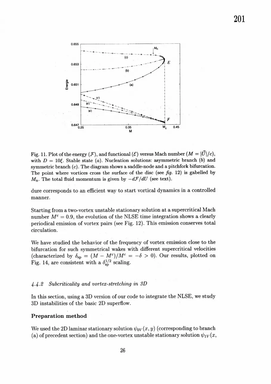
shown in Fig. 11 as afunction of the Mach number $(M=|\overline{U}|/c)$ . The stablebranch (a) disappears with the unstable solution (c) at asaddle-node bifur-cation when $M=M^{c}\approx 0.4286$ . The energy $T$ has acusp at the bifurcationpoint, which is the generic behavior for asaddle-node. There are no station-ary solutions beyond this point. When $M\approx 0.4282$ , the unstable symmetricbranch (c) bifurcates at apitchfork to apair of asymmetric branches (6). Theirnucleation energy barrier is given by $(\mathcal{F}_{\mathcal{U}}-\mathcal{F}_{a’})$ which is roughly half of thebarrier for the symmetric branch $(\mathcal{F}_{d}-\mathcal{F}_{a’})$ .

We can relate branches in Fig. 11 to the presence vortices in the solution.When $M^{\mathrm{p}\mathrm{f}}\leq M\leq M^{c}$ , solutions are irrotational ( $M^{\mathrm{p}\mathrm{f}}\sim 0.405$ as indicatedin Fig. 11). For $M\leq M^{\mathrm{p}\mathrm{f}}$ the stable branch (a) remains irrotational (Fig. $12\mathrm{A}$ )while the unstable branch (b) corresponds to aone vortex solution (Fig. $12\mathrm{B}$ )and the unstable branch (c), to atwo vortex solution (Fig. $12\mathrm{C}$). The dis-tance between the vortices and the obstacle in branches (b) and (c) increaseswhen $M$ is decreased. Branch (c) is precisely the situation described in [41].Furthermore, the value $M^{c}\approx 0.4286$ is close to the predicted value $\sqrt{2/11}$.Figure $12\mathrm{D}$ shows the result of integrating the NLSE forward in time with,as initial condition, aslightly perturbed unstable symmetric stationary state(Fig. $12\mathrm{C}$). The perturbation drives the system over the nucleation barrierand cycles it, after the emission of two vortices, back to astationary stable s0-

lution. This shows that the branch (c) corresponds to hyperbolic fixed pointsof NLSE.

Figures $12\mathrm{E},\mathrm{F}$ show the phase of the field at the surface of the disc $(r=D/2$

and $\mathit{0}\in[0,2\pi])$ for four different flow speeds. In both unstable branches, $2\pi-$

discontinuities, adiagnostic of vortex crossing, appear between $M=0.40$ and$M=0.41$ .

Scaling laws

We now characterize the dependence on $\xi/D$ of the main features of the bifur-cation diagram. When $\xi/D$ is decreased, $M^{c}$ and $M^{\mathrm{p}\mathrm{f}}$ become indistinguish-able. In the limit where $\xi/D=0$ , the critical Mach number $M^{c}$ will be thatof an Eulerian flow $M_{\mathrm{E}\mathrm{u}1\mathrm{e}\mathrm{r}}^{c}$ .

Figure 13 shows the convergence of $M^{c}$ to the Eulerian critical velocity.This convergence can be characterized by fitting the polynomial law $M^{c}=$

$K_{1}(\xi/D)^{K_{2}}+M_{\mathrm{E}\mathrm{u}1\mathrm{e}\mathrm{r}}^{c}$ to $M^{c}(\xi/D)$ . This fit is shown on Fig. 13 as adotted line,yielding $K_{1}=0.322$ , $K_{2}=0.615$ and $M_{\mathrm{E}\mathrm{u}1\mathrm{e}\mathrm{r}}^{c}=0.35$ .

Dynamical solutions The stationary solutions obtained in the above sub-section provide adequate initial data for the study of dynamical solutions.Indeed, after asmall perturbation, their integration in time will generate adynamical evolution with very small acoustic emission. Therefore, this proce-

25

200

$\mathrm{u}^{\mathrm{c}_{1}}\frac{}{\Phi}\frac{\Phi}{\Phi}$

Fig. 11. Plot of the energy $(\mathcal{F})$ , and functional $(\mathcal{E})$ versus Mach number $(M=|\vec{U}|/c)$ ,with $D=10\xi$ . Stable state (a). Nucleation solutions: asymmetric branch (b) andsymmetric branch (c). The diagram shows asaddle-node and apitchfork bifurcation.The point where vortices cross the surface of the disc (see fig. 12) is gabelled by$M_{\mathrm{n}}$ . The total fluid momentum is given by $-d\mathcal{F}/dU$ (see text).

dure corresponds to an efficient way to start vortical dynamics in acontrolledmanner.

Starting from atw0-vortex unstable stationary solution at asupercritical Machnumber $M^{c}=0.9$ , the evolution of the NLSE time integration shows aclearlyperiodical emission of vortex pairs (see Fig. 12). This emission conserves totalcirculation.

We have studied the behavior of the frequency of vortex emission close to thebifurcation for such symmetrical wakes with different supercritical velocities(characterized by $\delta_{\mathrm{s}\mathrm{p}}=(M-M^{c})/M^{c}=-\delta>0$). Our results, plotted onFig. 14, are consistent with a $\delta_{\mathrm{s}\mathrm{p}}^{1/2}$ scaling.

4.4.2 Subcriticality and vortex-stretching in 3D

In this section, using a 3D version of our code to integrate the NLSE, we study3D instabilities of the basic 2D superflow.

Preparation method

We used the 2D laminar stationary solution $\psi_{0V}(x,$y) (corresponding to branch(a) of precedent section) and the one-vortex unstable stationary solution $\psi_{1V}(x$ ,

26

201

$2\mathrm{E}_{*^{\mu}4}\mathrm{r}2_{|,|}^{k}|,--$

$\mathrm{r}\alpha:$

.$0|$

$- \mathrm{r}\iota_{\mathrm{I}}- \mathrm{z}_{\mathrm{I}}^{1}||$ $\}|$

$-|*$ $-0?|$ 00$*|$

$2\mathrm{F}_{*}\dot{L}0,\lceil_{1}^{--_{n2\prime}}\mathrm{a}- \mathrm{r}^{\underline{\triangleleft}}\mathrm{r}2--’- n20^{1\mathrm{I}}|$

.

Fig. 12. Stationary states :stable (A), one vortex unstable (B), two vor-tices unstable (C). The surface indicates the fluid density around the cylinder$(M=0.24, \xi/d=0.1)$ . (D) Shows the result of the NLSE integration, startingfrom aslightly perturbed stationary (C) state. Figures (E) and (F) display thephase of the complex field $\psi$ at the surface of the cylinder versus the polar angle0. Asymmetric branch (A), symmetric branch (B). $M=0.4286$ $(\circ)$ , $M=0.41(\square )$ ,$M=0.40(+)$ , $M=0.30(\mathrm{x})$ . The crossing out of the vortex produces aphasediscontinuity at $M^{\mathrm{p}\mathrm{f}}\sim 0.405$ .(branch (b)) to construct the 3D initial condition

$\psi_{3\mathrm{D}}(x,$y,$z)=f_{1}(z)\psi_{1V}(x, y)+[1-f_{1}(z)]\psi_{0V}(x,$y). (67)

The function $f_{1}(z)$ , defined by

$f_{i}(z)=(\tanh[(z-z_{1})/\Delta_{z}]-\tanh[(z-\mathrm{z}2)/\mathrm{A}\mathrm{z}])/2$,

takes the value 1for $z_{1}\leq z\leq z_{2}$ and 0elsewhere, with $\Delta_{z}$ an adaptationlength.

27

202

05 ——————-

$+\cross$

0.45

$\Xi$$\dot{\mathrm{M}_{1}}------------------*_{----------------------}$

$0.4\dot{\mathrm{q}}-----------------------------------------**$

$\mathrm{x}$

0.350 0.06 Q.i 0.15 0.2$\xi/_{\mathrm{d}}$

Fig. 13. Saddle-node bifurcation Mach number $M^{c}(+)$ and pitchfork bifurcationMach number $M^{\mathrm{p}\mathrm{f}}(\cross)$ , as afunction of $\xi/D$ . The dotted curve corresponds to afit to the polynomial law $M^{c}=K_{1}(\xi/D)^{K_{2}}+M_{\mathrm{E}\mathrm{u}1\mathrm{e}\mathrm{r}}^{c}$ with $K_{1}=0.322$ , $K_{2}=0.615$

and $M_{\mathrm{E}\mathrm{u}1\mathrm{e}\mathrm{r}}^{c}=\mathrm{Q}.35$ . The dashed lines $M_{1}^{*}\approx 0.4264$ and $M_{2}^{*}\approx 0.3903$ correspondrespectively to first and second order compressible corrections to the $M^{c}=0.5$

critical velocity computed using alocal sonic criterion for an incompressible flow(see text).

0.024$\prime\prime\prime$

\prime\prime

$,\acute{\mathrm{o}}$

0.020 $’\phi’$

’

”

$’\sigma’$

”0.016$’\varphi’$

’

$>$\prime\prime\prime

”

”0.012$\prime\prime\prime\phi$

”

$’\varphi’\prime\prime\prime\prime\prime s$

0.008

0.02 0.04 0.06 0.086

$\mathrm{s}\mathrm{p}$

Fig. 14. Vortex emission frequency as afunction of $\delta_{\mathrm{s}\mathrm{p}}=$ (At $-M^{c}$ ) $/M^{c}\ll 1$ (with$M^{c}=0.3817)$ , for asymmetric wake and $\xi/D=1/20$ . The dashed line shows afit ofapolynomial $\nu=K_{1}\delta_{\mathrm{s}\mathrm{p}}^{1/2}$ with $K_{1}=0.081$ . The obtained $\delta_{\mathrm{s}\mathrm{p}}^{1/2}$ law for the frequencyis equivalent to the one expected for adissipative system.

Figure 15 represents a $3\mathrm{D}$ initial data prepared with this method for $\xi/D=$

0.025, $|U^{\prec}|/c=0.26$ and $\triangle_{z}=2\sqrt{2}\xi$ in the $[L_{x}\cross L_{y}\cross L_{z}]$ periodicity box($L_{x}/D=2.4\sqrt{2}\pi$ , $L_{y}/D=1.2\sqrt{2}\pi$ and $L_{z}/D=0.4\sqrt{2}\pi$). The surface $|\psi_{3\mathrm{D}}|=$

$0.5$ draws the cylinder surface and the initial condition vortex line, with bothends pinned to the right side of the cylinder.

28

203

Fig. 15. Initial condition of avortex pinned to the cylinder generated by eq.(67).The surface $|\psi_{3\mathrm{D}}|=0.5$ is shown for $\xi/D=0.025$ , $|\vec{U}|/c=0.26$ and $\Delta_{z}=2\sqrt{2}\xi$

in the $[L_{x}\cross L_{y}\cross L_{z}]$ periodicity box ($L_{x}/D=2.4\sqrt{2}\pi$ , $L_{y}/D=1.2\sqrt{2}\pi$ and$L_{z}/D=0.4\sqrt{2}\pi)$ .Short time dynamics

Starting from the initial condition (67), the evolution of the NLSE time inte-gration shows ashort-time and along-time dynamics.

During the short-time dynamics, the initial pinned vortex line rapidly con-tracts, evolving through adecreasing number of half-ring-like loops, down toasingle quasi-stationary half-ring (see Figs. $16\mathrm{a}$ , $16\mathrm{b}$ , $16\mathrm{c}$). This evolutionhappens mainly on the plane perpendicular to the flow, provided that the ini-tial vortex is long enough to contract to aquasi-stationary half-ring as shownon Fig. $16\mathrm{c}$ . Otherwise, the vortex line collapses against the cylinder whilemoving upstream.

Note that this quasi-stationary half-ring has been used by Varoquaux [42,43]to estimate the nucleation barrier in a 3D experiment.

The dynamics of the half-ring situation (Fig. $16\mathrm{c}$ ) is very slow and can beshown to be close to astationary field. Indeed, the local flow velocity $v$ in anEulerian flow around acylindrical obstacle is known to vary from $v=|\vec{U}|$ atinfinity to $v=2|\vec{U}|$ at both sides of its surface. Moreover, the diameter $d$ ofastationary vortex ring in an infinite Eulerian flow with no obstacle is givenby [1]:

$|\vec{U}|/c=(\sqrt{2}\xi/d)[\ln(4d/\xi)-K]$ , (68)

where $|\vec{U}|$ is the flow velocity at infinity and the vortex core model constant$K\sim 1$ is obtained by fitting the numerical results in [44]. Therefore, for thevalues used on Figs. 16, we expect that local velocities range from $v=0.25$ to$v=2\cross 0.25$ . Equation (68) thus implies that the diameter of an hypotheticalstationary half-ring should be bounded by $d(v=|\vec{U}|=0.25)=18.8\xi$ and$d(v=2|\vec{U}|=0.5)=6.3\xi$ . The diameter $d\approx 9\xi$ measured on the half-ringobserved on Fig. $16\mathrm{c}$ is consistent with its quasi-stationary behavior. Similarlythe diameter of the half-ring shown on Fig. 18 $d\approx 7.6\mathrm{f}$ is also found to bebetween the corresponding bounds $d(0.35)=11.4\xi$ and $d(2\cross 0.35)=3\xi$ .

29

204

Fig. 16. Short-time dynamics for $\xi/D=1/40$ and $|\vec{U}|/c=0.25$ starting from Fig. 15:A $(t=5\xi/c)$ , $\mathrm{B}(t=10\xi/c)$ and $\mathrm{C}(t=15\xi/c)$ . The contraction of the initial vortexline occurs in the plane perpendicular to the flow. The half-rings have adiametercompatible with that of aquasi-stationary half-ring (see text).

Vortex stretching as asubcritical drag mechanism Asmall perturbationover the half-ring solution can drive the system into two opposite situationswhere the half-ring either starts moving upstream or downstream.

When driven upstream, the half-ring eventually collapses against the cylinder,dissipating its energy as sound waves. Otherwise, the vortex loop is stretchedwhile the pinning points move towards the back of the cylinder. Figures 17show the long-time dynamics for astretching case with $\xi/D=1/40$ and$|U|\prec/c=0.25$ starting from Fig. $16\mathrm{c}$ . Figure 19 shows alater situation for$\xi/D=1/20$ and $|\vec{U}|/c=0.35$ starting from Fig. 18. As the vortex loop grows,its backmost part remains oblique to the flow. The described vortex stretchingmechanism consumes energy, thus generating drag. It can be responsible forthe appearance of drag in experimental superflows if fluctuations are strongenough to nucleate the initial vortex loop (which is imposed extrinsically inour numerical system). Note that it takes place for $2\mathrm{D}$ subcritical velocities.

30

205

Fig. 17. Long-time dynamics for $\xi/D=1/40$ and $|\vec{U}|/c=0.25$ starting fromFig. 16c. The half-ring moves downstream while growing.

Fig. 18. Quasi-nucleation solution for $|\vec{U}|/c=0.35$ and $\xi/D=1/20$ at timet $=15\xi/c$ .

31

206

Fig. 19. Vortex stretching at $t=150\xi/c$ with $|U^{\prec}|/c=0.35$ and $\xi/D=1/20$ . Thevortex line is oblique to the flow.

$10^{0}$

$\cross_{\mathrm{R}_{\mathrm{I}\mathrm{Q}}}$

$10^{-2}$

$\mathrm{o}$

$> 0^{-4}0\tilde{\mathrm{o}}$

$\circ$

$\mathrm{o}$

$\mathrm{o}_{\mathrm{o}\mathrm{q}}\mathrm{o}$

8$0_{8}$$\{0^{-6}$

$10^{-8}$

$0^{0}$ $10^{2}$

$\{0_{\mathrm{d}/\xi}^{4}$

$10^{6}$ $10^{8}$

Fig. 20. Critical Mach number $Vc/C$ versus scale ratio of numerical and experimentaldata $D/\xi$ . Circles correspond to several experiments from [45]. Squares stand forour numerical stretching cases while crosses correspond to non-stretching cases [14].

Figure 20 displays several numerical and experimental [45] critical Mach num-bers $(V_{c}/C)$ with respect to $D/\xi$ , which seem to follow a(-1) slope in alog-log plot. The squares stand for our numerical stretching cases while thecrosses correspond to non-stretching cases. There is afrontier between the $3\mathrm{D}$

numerical dissipative and non-dissipative cases [14]. For $1/30<\xi/D<1/20$ ,

32

207

the frontier corresponds to the expression $R_{s}=5.5$ with

$R_{s}\equiv|\tilde{U}|D/c\xi=MD/\xi$ . (69)

This superfluid ‘Reynolds’ number is defined in the same way as the standard(viscous) Reynolds number $Re\equiv|\tilde{U}|D/\nu$ (with $\nu$ the kinematic viscosity).It has been shown, in the superfluid turbulent $(R_{s}\gg 1)$ regime, that $R_{s}$

is equivalent to the standard (viscous) Reynolds number $Re[10,9,11]$ . Notethat, for aBose condensate of particles of mass $m$ , the quantum of velocitycirculation around avortex, $\Gamma=2\pi\sqrt{2}c\xi$ , has the Onsager-Feynman value$\Gamma=h/m$ ( $h$ is Planck’s constant) and the same physical dimensions $L^{2}T^{-1}$ as$\nu$ .

The value of $R_{s}$ divides the space of parameters into alaminar flow zoneand arecirculating flow zone, very much like in the problem of acirculardisc in aviscous fluid in which this frontier is also found to be around $Re\sim$

$5$ . It therefore seems to exist some degree of universality between viscousnormal fluids and superfluids modeled by NLSE as discussed in [10,9,11]. Inthe context of superfluid $4\mathrm{H}\mathrm{e}$ flow, the experimental critical velocity is knownto depend strongly on the system’s characteristic size $D$ . It is often found to bewell below the Landau value (based on the velocity of roton excitation) exceptfor experiments where ions are dragged in liquid helium. Feynman’s alternativecritical velocity criterion $Rs\sim\log(D/\xi)$ is based on the energy needed to formvortex lines. It produces better estimates for various experimental settings, butdoes not describe the vortex nucleation mechanism [1].

In arecent experiment, Raman et al. have studied dissipation in aBose-Einstein condensed gas by moving ablue detuned laser beam through thecondensate at different velocities [46]. In their inhomogeneous condensate,they observed acritical Mach number for the onset of dissipation $M_{2D}^{c}/1.6$ .

Our computations were performed for values of $\xi/D$ comparable to those inBose-Einstein condensed gas experiments. They demonstrate the possibility ofasubcritical drag mechanism, based on $3\mathrm{D}$ vortex stretching. It would be veryinteresting to determine experimentally the dependence of the critical Machnumber on the parameter $\xi/D$ and the nature ( $2\mathrm{D}$ or $3\mathrm{D}$ ) of the excitations[14].

4.5 Stability of attractive Bose-Einstein condensates

In this section, following reference [15], we study condensates with attractiveinteractions which are known to be metastable in spatially localized systems,provided that the number of condensed particles is below acritical value $N_{c}$

[7]. Various physical processes compete to determine the lifetime of attractive

33

208

condensates. Among them one can distinguish macroscopic quantum tunnel-ing (MQT) [47,48], inelastic two and three body collisions (ICO) [49,50] andthermally induced collapse (TIC) [48,51]. We compute the life-times, usingboth avariational Gaussian approximation and the exact numerical solutionfor the condensate wave-function

4.5.1 Computations of stationary states

Gaussian approximation

AGaussian approximation for the condensate density can be obtained ana-lytically through the following procedure.

Inserting

$\psi(r,\tilde{t})=A(\tilde{t})\exp(-r^{2}/2r_{\mathrm{G}}^{2}(\tilde{t})+ib(\tilde{t})r^{2})$ (70)

into the action (45), where $\mathcal{F}$ is given by (52), yields aset of Euler-Lagrangeequations for $r_{\mathrm{G}}(\tilde{t})$ , $b(\tilde{t})$ and the (complex) amplitude $A(\tilde{t})$ . The stationarysolutions of the Euler-Lagrange equations produce the following values [52]:

$N( \mu)=\frac{4\sqrt{2\pi^{3}}(-8\mu+3\sqrt{7+4\mu^{2}})}{7|\tilde{a}|(-2\mu+\sqrt{7+4\mu^{2}})^{3/2}},$ , (71)

$\mathcal{E}=N(\mu)(-\mu+3\sqrt{7+4\mu^{2}})/7$ . (72)

N is found to be maximal at $N_{c}^{G}=8\sqrt{2\pi^{3}}/|5^{5/4}\tilde{a}|$ . The corresponding valueof the chemical potential is $\mu=\mu_{c}^{G}=1/2\sqrt{5}$ .

Linearizing the Euler-Lagrange equations around the stationary solutions,yields the following expression for the eigenvalues [52]:

$\lambda^{2}(\mu)=8\mu^{2}-4\mu\sqrt{7+4\mu^{2}},+2$ (73)

This qualitative behavior is the generic signature of aHamiltonian SaddleNode (HSN) bifurcation defined, at lowest order, by the normal form [53]

$m_{\mathrm{e}ff}\dot{Q}=\delta-\beta Q^{2}$ , (74)

where $\delta=(1-N/N_{c})$ is the bifurcation parameter. The critical amplitude $Q$

is related to the radius of the condensate [52]. We can relate the parameters$\beta$ and meff to critical scaling laws, by defining the appropriate energy

$\mathcal{E}=\mathcal{E}_{0}+m_{\mathrm{e}fJ}\dot{Q}^{2}/2-\delta Q+\beta Q^{3}/3-\gamma\delta$. (75)

34

209

Fig. 21. Stationary solutions of the NLSE equation versus particle number $N$. Left:value of the energy functional $\mathcal{E}_{+}$ on the stable (elliptic) branch and $\mathcal{E}_{-}$ on theunstable (hyperbolic) branch. Right: square of the bifurcating eigenvalue $(\lambda_{\pm}^{2});|\lambda_{-}|$

is the energy of small excitations around the stable branch. Solid lines: exact solutionof the NLSE equation. Dashed lines: Gaussian approximation.

From (74) it is straightforward to derive, close to the critical point $\delta$ $=0$ , theuniversal scaling laws

$\mathcal{E}_{\pm}=\mathcal{E}_{c}-\mathcal{E}_{l}\delta\pm \mathcal{E}_{\Delta}\delta^{3/2}$ , (76)$\lambda_{\pm}^{2}=\pm\lambda_{\Delta}^{2}\delta^{1/2}$ , (77)

where $\mathcal{E}_{c}=\mathcal{E}_{0}$ , $\mathcal{E}_{l}=\gamma$ , $\mathcal{E}_{\Delta}=2/3\sqrt{\beta}$ and $\lambda_{\Delta}^{2}=2\sqrt{\beta}/m_{\mathrm{e}[f}$ .

Numerical branch following

Using the branch-following method described in section 4.3, we have computedthe exact stationary solutions of the NLSE. We use the following value $\tilde{a}=$

$-5.74\cross 10^{-3}$ , that corresponds to experiments with $7\mathrm{L}\mathrm{i}$ atoms in aradial trap$[54,7]$ .

As apparent on Fig. 3, the exact critical $N_{c}^{E}=1258.5$ is smaller than theGaussian one $N_{c}^{G}=1467.7$ $[55,47]$ . The critical amplitudes correspondingto the Gaussian approximation can be computed from (71) and (72). Onefinds $\mathcal{E}_{c}=4\sqrt{2\pi^{3}}/|5^{3/4}\tilde{a}|$ , $\mathcal{E}_{\Delta}=64\sqrt{\pi^{3}}/|5^{9/4}\tilde{a}|$ and $\lambda_{\Delta}^{2}=4\sqrt{10}$. For the exactsolutions, we obtain the critical amplitudes by performing fits on the data.One finds $\mathcal{E}_{\Delta}=1340$ and $\lambda_{\Delta}^{2}=14.68$ . Thus, the Gaussian approximationcaptures the bifurcation qualitatively, but with quantitative 17% error on $N_{c}$

[55], 24% error on $\mathcal{E}_{\Delta}$ and 14% error on $\lambda_{\Delta}^{2}$ . Fig. 4shows the physical originof the quantitative errors in the Gaussian approximation. By inspection it isapparent that the exact solution is well approximated by aGaussian only forsmall Aon the stable (elliptic) branch.

35

210

20

$|\psi|^{2}$

10

0

$r$

Fig. 22. Condensate density $|\psi|^{2}$ versus radius $r$ , in reduced units (see text). Solidlines: exact solution of the NLSE equation. Dashed lines: Gaussian approximation.Stable (elliptic) solutions are shown for particle number $N$ $=252(\mathrm{a})$ and $N$ $=1132$

(b). (c) is the unstable (hyperbolic) solution for $N$ $=1132$ (see insert).

4.5.2 Estimation of life-time$s$

In this section, we estimate the decay rates due to thermally induced collapse,

macroscopic quantum tunneling and inelastic collisions.

Thermally induced collapse

The thermally induced collapse (TIC) rate $\Gamma_{T}$ is estimated using the formula[56]

$\frac{\Gamma_{T}}{\omega}=\frac{|\lambda_{+}|}{2\pi}\exp[\frac{-\hslash\omega(\mathcal{E}_{+}-\mathcal{E}_{-})}{k_{B}T}]$ (78)

where $\hslash\omega(\mathcal{E}_{+}-\mathcal{E}_{-})$ is the (dimensionalized) height of the nucleation energy bar-rier, $T$ is the temperature of the condensate and $k_{B}$ is the Boltzmann constant.Note that the prefactor characterizes the typical decay time which is controlledby the slowest part of the nucleation dynamics: the top-0f-the-barrier saddlepoint eigenvalue $\lambda_{+}$ . The behavior of $\Gamma_{T}$ can be obtained directly from theuniversal saddle-node scaling laws (76) and (77). Thus the exponential factorand the prefactor vanish respectively as $\delta^{3/2}$ and $\delta^{1/4}$ .

Macroscopic quantum tunneling

We estimate the MQT decay rate using an instanton technique that takes into

account the semi classical trajectory giving the dominant contribution to the

36

211

$\mathrm{V}(\mathrm{q}_{\mathrm{f}})$

$\mathrm{V}(\mathrm{q}_{\mathrm{n}}\}$

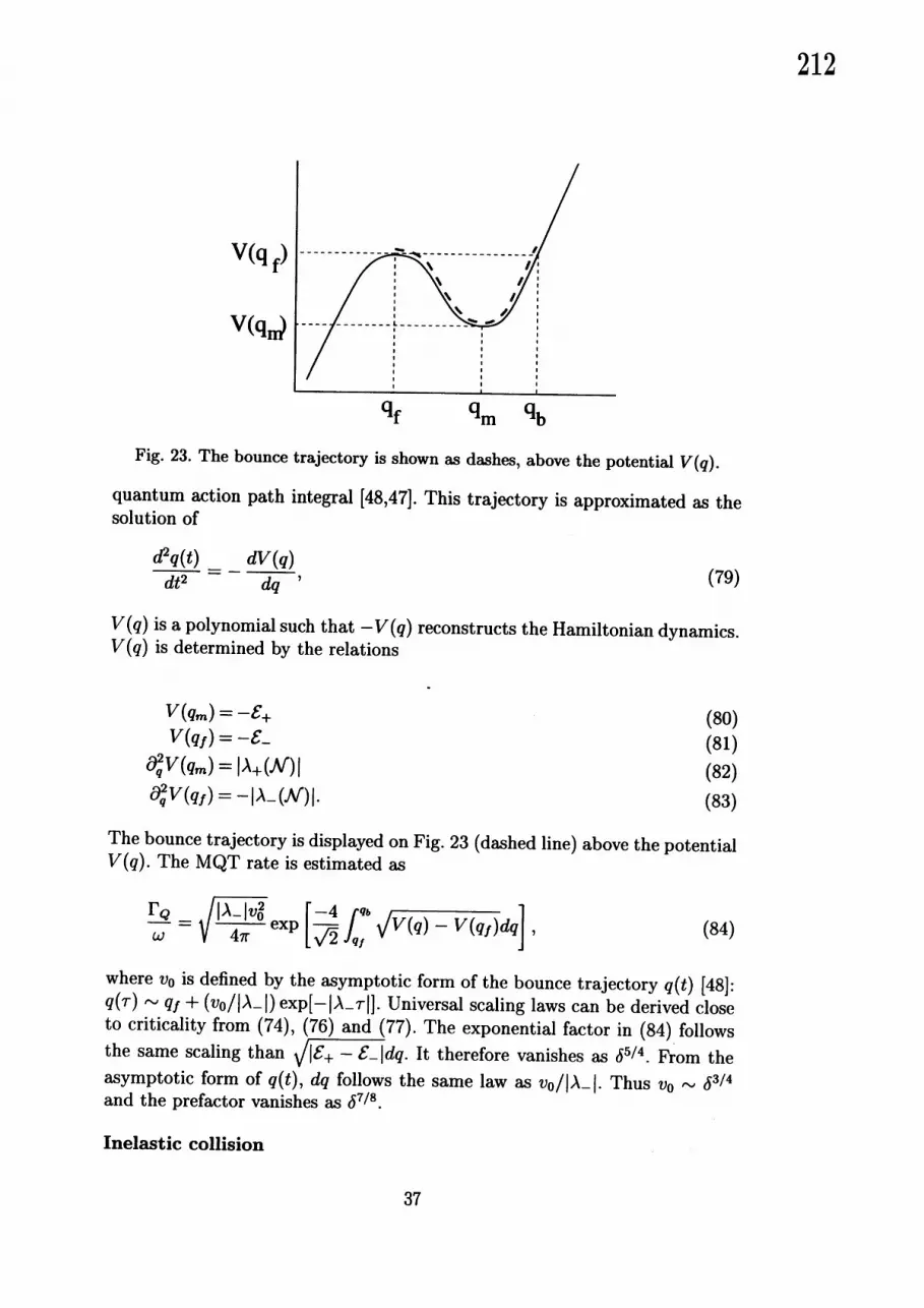
Fig. 23. The bounce trajectory is shown as dashes, above the potential $V(q)$ .quantum action path integral [48,47]. This trajectory is approximated as thesolution of

$\frac{d^{2}q(t)}{dt^{2}}=-\frac{dV(q)}{dq}$ , (79)

$V(q)$ is a polynomial such that $-V(q)$ reconstructs the Hamiltonian dynamics.$V(q)$ is determined by the relations

$V(q_{m})=-\mathcal{E}_{+}$ (80)$V(q_{f})=-\mathcal{E}_{-}$ (81)

$\partial_{q}^{2}V(q_{m})=|\lambda_{+}(N)|$ (82)$\partial_{q}^{2}V(q_{f})=-|\lambda_{-}(N)|$ . (83)

The bounce trajectory is displayed on Fig. 23 (dashed line) above the potential$V(q)$ . The MQT rate is estimated as

$\frac{\Gamma_{Q}}{\omega}=\sqrt{\frac{|\lambda_{-}|v_{0}^{2}}{4\pi}}\exp[\frac{-4}{\sqrt{2}}\int_{q_{f}}^{qb}\sqrt{V(q)-V(q_{f})}dq]$ , (84)

where $v_{0}$ is defined by the asymptotic form of the bounce trajectory $q(t)[48]$ :$q(\tau)\sim qf+(v_{0}/|\lambda_{-}|)\exp[-|\lambda_{-}\tau|]$ . Universal scaling laws can be derived closeto criticality from (74), (76) and (77). The exponential factor in (84) followsthe same scaling than $\sqrt{|\mathcal{E}_{+}-\mathcal{E}_{-}|}dq$. It therefore vanishes as $\delta^{5/4}$ . From theasymptotic form of $q(t)$ , $dq$ follows the same law as $v_{0}/|\lambda_{-}|$ . Thus $v_{0}\sim\delta^{3/4}$

and the prefactor vanishes as $\delta^{7/8}$ .

Inelastic collision

37

212

–$\underline{\omega|}$

$\frac{\mathrm{q})}{oe\varpi}$

$[mathring]_{\mathrm{O}}0\iota \mathfrak{o}^{\backslash }>$

$\frac{\Phi}{\varpi,\{\emptyset\subset}$,

$\mathfrak{D}q)$

$\mathrm{O}\mathrm{o}\subset$

Fig. 24. Condensate decay rates versus particle number. ICO: inelastic collisions.MQT: macroscopic quantum tunneling TIC: thermally induced collapse at temper-atures $1nK(1),2nK(2)$ , $50nK(3)$ , 100nK (4), $200nK(5)$ , $300nK(6)$ and $400nK$

(7). The insert shows the details of the cross-0ver region between quantum tunnelingand thermal decay rate. Solid lines: exact solution of the NLSE equation, dashedlines: Gaussian approximation.

The inelastic collision rate (ICO) is estimated using the relation

$\frac{dN}{dt}=f_{C}(N)$ (85)

with

$f_{C}(N)=K \int|\psi|^{4}d^{3}\tilde{\mathrm{x}}+L\int|\psi|^{6}d^{3}\tilde{\mathrm{x}}$, (86)

where $K=3.8\cross 10^{-4}\mathrm{s}^{-1}$ and $L=2.6\cross 10^{-7}\mathrm{s}^{-1}$ . The ICO rate can beevaluated from the stable branch alone. In order to compare the particle decayrate $f_{C}(N)$ to the condensate collective decay rates obtained for TIC andMQT, we compute the condensate ICO half-life as:

$\tau_{1/2}(N)=\int_{N/2}^{N}dn/f_{C}(n)$ (87)

and plot $\tau_{1/2}^{-1}$

Discussion

It is apparent by inspection of Fig. 6that for agiven value of $N$ the exact andGaussian approximate rates are dramatically different. We now compare therelative importance of the different exact decay rates. At $T\leq 1\mathrm{n}\mathrm{K}$ the MQT

38

213

effect becomes important compared to the ICO decay in aregion very closeto $N_{c}^{E}(\delta\leq 8\cross 10^{-3})$ as it was shown in [47] using Gaussian computationsbut evaluating them with the exact maximal number of condensed particles$N_{c}^{E}$ . Considering thermal fluctuations for temperatures as low as 2 $\mathrm{n}\mathrm{K}$ , it isapparent on Fig. 6(see insert) that the MQT will be the dominant decaymechanism only in aregion extremely close to $N_{c}$ ($\delta<5$ x.1O-3) where thecondensates will live less than 10 $\mathrm{s}$ . Thus, in the experimental case of $7\mathrm{L}\mathrm{i}$

atoms, the relevant effects are ICO and TIC, with cross-0ver determined inFig. 6.

5Conclusion

The main result of the NLSE simulations presented in section 3.2 is thattwo diagnostics of Kolmogorov’s regime in decaying turbulence are satisfied.These diagnostics are, at the time of the maximum of energy dissipation: (i) aparameter-independent kinetic energy dissipation rate and (ii) a $k^{-5/3}$ spectralscaling in the inertial range. Thus, the NLSE simulations were shown to bevery similar as far as energetics is concerned, with the viscous simulations. Theexperimental results shown in section 3.3 show that the Kolmogorov cascadesurvives in the superfluid regime.

We have seen that the numerical tools developed in section 4.3 can be used inpractice to obtain the stationary solutions of the NLSE. These methods haveallowed us to find the full bifurcation diagrams of Bose-Einstein condensateswith attractive interactions and superflows past acylinder. Furthermore, thestationary solutions have given us efficient way to start vortical dynamics (in$2\mathrm{D}$ and $3\mathrm{D}$) in acontrolled manner.

6Acknowledgments

The work reviewed in this paper was performed in collaboration with M.Abid, G. Dewel, C. Huepe, J. Maurer, S. Metens, C. Nore, $\mathrm{C}$-T. Pham and P.Tabeling. Computations were performed at the Institut du Developpement etdes Ressources en Informatique Scientifique.

39

214

References

[1] R. J. Donnelly. Quantized Vortices in Helium $II$. Cambridge Univ. Press,Cambridge, 1991.

[2] $\mathrm{E}.\mathrm{P}$. Gross. Structure of aquantized vortex in boson systems. Nuovo Cimento,20(3), 1961.

[3] $\mathrm{L}.\mathrm{P}$. Pitaevskii. Vortex lines in an imperfect Bose gas. $Sov$. Phys.-JETP, 13(2),1961.

[4] L. Landau and E. Lifchitz. Fluid Mechanics. Pergamon Press, Oxford, 1980.

[5] M. H. Anderson, J. R. Ensher, M. R. Matthews, C. E. Wieman, and E. A.Cornell. Science, 269:198, 1995.

[6] K. B. Davis, M. O. Mewes, M. R. Adrews, N. J. van Druten, D. S. Durfee,D. M. Kurn, and W. Ketterle. Phys. Rev. Lett., 75:3969, 1995.

[7] C. C. Bradley, C. A. Sackett, and R. G. Hulet. Bose-einstein cond.ensation oflithium: Observation limited condensate number. Phys. Rev. Lett., 78(6):985,1997.

[8] Franco Dalfovo, Stefano Giorgini, Lev P. Pitaevskii, and Sandro Stringari.Theory of bose-einstein condensation in trapped gases. Reviews of ModernPhysics, 71(3), 1999.

[9] C. Nore, M. Abid, and M. Brachet. Decaying kolmogorov turbulence in amodelof superflow. Phys. Fluids, 9(9):2644, 1997.

[10] C. Nore, M. Abid, and M. E. Brachet. Kolmogorov turbulence in low-temperature superflows. Phys. Rev. Lett., 78(20):3896-3899,1997.

[11] M. Abid, M. Brachet, J. Maurer, C. Nore, and P. Tabeling. Experimentaland numerical investigations of low-temperature superfluid turbulence. $Eur$. $J$.Mech. $B$ Fluids, 17(4):665-675, 1998.

[12] C. Huepe and M.-E. Brachet. Solutions de nucleation tourbillonnaires dansun modele d’ecoulement superfluide. C. R. Acad. Sci. Paris, 325(11):195-202,1997.

[13] C. Huepe and M. E. Brachet. Scaling laws for vortical nucleation solutions inamodel of superflow. Physica $D$, 140:126-140, 2000.

[14] C. Nore, C. Huepe, and M. E. Brachet. Subcritical dissipation in three-dimensional superflows. Phys. Rev. Lett., 84(10):2191, 2000.

[15] C. Huepe, S. Metens, G. Dewel, P. Borckmans, and M.-E. Brachet. Decay ratesin attractive bose-einstein condensates. Phys. Rev. Lett., 82(2): 1999.

[16] E. A. Spiegel. Fluid dynamical form of the linear and nonlinear schrodingerequations. Physica $D$, 1:236, 1980.

40

215

[17] P. Nozieres and D. Pines. The Theory of Quantum Liquids. Addison Wesley,

New York, 1990.

[18] C. Nore, M. Brachet, and S. Fauve. Numerical study of hydrodynamics using

the nonlinear schr\"odinger equation. Physica D, 65:154-162, 1993.

[19] D. Gottlieb and S. A. Orszag. Numerical Analysis of Spectral Methods. SIAM,

Philadelphia, 1977.

[20] M. P. Kawatra and R. K. Pathria. Quantized vortices in imperfect bose gas.Phys.Rev., 151:1, 1966.

[21] K. W. Schwarz. Three-dimensional vortex dynamics in superfluid $4\mathrm{h}\mathrm{e}$ : line-lineand line-boundary interactions. Phys. Rev. $B$, 31:5782, 1985.

[22] J. C. Neu. Vortices in complex scalar fields. Physica $D$, 43:385, 1990.

[23] F. Lund. Defect dynamics for the nonlinear schrodinger equation derived fromavariational principle. Phys.Rev.Lett., A159:245, 1991.

[24] G. I. Taylor and A. E. Green. Mechanism of the production of small eddiesfrom large ones. Proc. Soc. Lond. A, 158:499, 1937.

[25] M. E. Brachet, D. I. Meiron, S. A. Orszag, B. G. Nickel, R. H. Morf, andU. Frisch. Small-scale structure of the taylor-green vortex. J. Fluid Mech.,$130:411\triangleleft 52$ ,1983.

[26] M. Brachet. Geometrie des structures \‘a petite \’echelle dans le vortex de taylor-

green. C.R.A.S II, 311:775, 1990.

[27] J. Domaradzki, W. Liu, and M. Brachet. An analysis of sugrid-scale interactionsin numerically simulated isotropic turbulence. Phys. Fluids A, 5:1747, 1993.

[28] C. Nore, M. Abid, and M. Brachet. Simulation num\’erique d’\’ecoulements

cisailles tridimensionnels \‘a Paide de l’\’equation de schr\"odinger non lineaire.C.R.A. $S$, 31911(7):733, 1994.

[29] U. Frisch. Turbulence, the legacy of A. N. Kolmogorov. Cambridge Univ. Press,

Cambridge, 1995.

[30] S. Douady, Y. Couder, and M. E. Brachet. Direct observation of theintermittency of intense vorticity filaments in turbulence. Phys. Rev. Lett,

67:983, 1991.

[31] G. Zocchi, P. Tabeling, J. Maurer, and H. Willaime. Measurement of the scalingof the dissipation at high reynolds numbers. Phys. Rev. E, 50:3693, 1994.

[32] S. Fauve, C. Laroche, and B. Castaing. Pressure fluctuations in swirling

turbulent flows. J. Phys. If,3:271, 1993.

[33] F. Belin, P. Tabeling, and H. Willaime. Exponents of the structure functionsin alow temperature helium experiment. Physica D, 93:52-63, 1996.

[34] V. Hakim. Nonlinear Schr\"odinger flow past an obstacle in one dimension. Phys.

Rev. E, 55(3):2835-2845, 1997.

41

216

[35] T. Tsuzuki. Nonlinear waves in the Pitaevskii-Gross equation. J. Low Temp.Phys., $4(4)$ , 1971.

[36] $\mathrm{V}.\mathrm{E}$ . Zakharov and $\mathrm{A}.\mathrm{B}$ . Shabat. Interaction between soliton in astablemedium. $Sov$ . Phys.-JETP, 37(5):823-828, 1973.

[37] R. Seydel. From Equilibrium to Chaos: Practical Bifurcation and StabilityAnalysis. Elsevier, New York, 1988.

[38] C. Mamun and L. Tuckerman. Asymmetry and hopf bifurcation in sphericalcouette flow. Phys. Fluids, 7(1):80, 1995.

[39] W. Press, S. Teukolsky, W. Vetterling, and B.Flannery. Numerical Recipres inFortran. Cambridge Univ. Press, Cambridge, 1994.

[40] R. Klein and A. J. Majda. Self-stretching of perturbed vortex filaments. Physica$D$, 53:267, 1991.

[41] T. Prisch, Y. Pomeau, and S. Rica. Transition to dissipation in amodel ofsuperflow. Phys.Rev. Lett., 69:1644, 1992.

[42] O. Avenel, $\mathrm{G}.\mathrm{G}$ . Ihas, and E. Varoquaux. The nucleation of vortices in superfluid$4\mathrm{h}\mathrm{e}$ :Answers and questions. J. Lout Temp.Phys., 93:1031-1057,1993.

[43] $\mathrm{G}.\mathrm{G}$ . Ihas, O. Avenel, R. Aarts, $\mathrm{R}$ Salmelin, and E. Varoquaux. Phys. Rev.Lett, 69(2):327, 1992.

[44] C. A. Jones and P. H. Roberts. J. Phys. $A$ , 15:2599, 1982.

[45] J. Wilks. The properties of liquid and solid helium. Clarendon Press, Oxford,1967.

[46] C. Raman, M. Kohl, R. Onofrio, $\mathrm{D}.\mathrm{S}$ . Durfee and $\mathrm{C}.\mathrm{E}$ . Kuklewicz,Z. Hadzibabic, and W. Ketterle. Evidence for acritical velocity in abose-einstein con densed gas. Phys. Rev. Lett, 83(13):2502, 1999.

[47] M. Ueda and A. J. Leggett. Macroscopic quantum tunneling of abose-einsteincondensate with attractive interaction. Phys. Rev. Lett, 80(8):1576, 1998.

[48] H. T. C. Stoof. Macroscopic quantum tunneling of abose condensate. J. Stat.Phys., 87:1353, 1997.

[49] H. Shi and W.-M. Zheng. Bose-einstein condensation in an atomic gas withattractive interactions. Phys. Rev. $A$ , 55(4) $:2930$ ,1997.

[50] R. J. Dodd, Mark Edwards, C. J. Williams, C. W. Clark, M. J. Holland, P. A.Ruprecht, and K. Burnett. Role of attractive interactions on bose-einsteincondensation. Phys. Rev. $A$ , 54(1) $:661$ ,1996.

[51] C. A. Sackett, H. T. C. Stoof, and R. G. Hulet. Growth and collapse of abose-einstein condensate with attractive interactions. Phys. Rev. Lett, 80(10):2031,1998.

[52] C. Huepe. Bifurcations et instabilites dans les condensats de Bose-Einstein etles icoulements superfluides. $\mathrm{P}\mathrm{h}\mathrm{D}$ thesis, Ecole Normale Supe\’erieure, 1999.

42

217

[53] J. Guckenheimer and P. Holmes. Nonlinear Oscillations, Dynamical Systemsand Bifurcations of Vector Fields. Springer-Verlag, Berlin, 1983.

[54] C. C. Bradley, C. A. Sackett, J. J. Tollett, and R. G. Hulet. Evidence of bose-einstein condensation in an atomic gas with attractive interactions. Phys. Rev.Lett, 75(9):1687, 1995.

[55] P. A. Ruprecht, M. J. Holland, K. Burnett, and Mark. Edwards. Time-dependent solution of the nonlinear schrodinger equation for bose-condensedtrapped neutral atoms. Phys. Rev. $A$ , 51(6) $:4704$,1995.

[56] C.W. Gardiner. Handbook of Stochastic Methods. Springer-Verlag, Berlin, 1985.

43

218