substructure preconditioners for elliptic saddle point problems

mathematics of computationvolume 60, number 201january 1993, pages 23-48

SUBSTRUCTURE PRECONDITIONERSFOR ELLIPTIC SADDLE POINT PROBLEMS

TORGEIR RUSTEN AND RAGNAR WINTHER

Abstract. Domain decomposition preconditioners for the linear systems aris-

ing from mixed finite element discretizations of second-order elliptic boundary

value problems are proposed. The preconditioners are based on subproblems

with either Neumann or Dirichlet boundary conditions on the interior bound-

ary. The preconditioned systems have the same structure as the nonprecon-

ditioned systems. In particular, we shall derive a preconditioned system with

conditioning independent of the mesh parameter h . The application of the

minimum residual method to the preconditioned systems is also discussed.

1. Introduction

The purpose of this paper is to propose domain decomposition techniques for

elliptic saddle point problems. Here, elliptic saddle point problems refers to the

discrete systems resulting from mixed finite element discretizations of second-

order elliptic boundary value problems. We study a preconditioned iterative

method for these systems where a decomposition of the domain into simpler

substructures is utilized in order to construct the preconditioners.

Let ß c R2 be a polygonal domain, and let <9ß denote the boundary. We

consider the Dirichlet problem

-V-K(x)Vp = f inß,

p = g on 9ß,

where / and g are given functions. The matrix K(x) is assumed to be sym-metric and uniformly positive definite on ß.

If this boundary value problem is discretized by a conforming finite element

method, we obtain a linear system with a symmetric and positive definite coef-

ficient matrix. However, the coefficient matrix is not well conditioned. If thedimension of the system is sufficiently large, the system has to be solved by an

iterative method. In order to obtain a well-conditioned system, and hence fast

convergence of the iterative method, preconditioning of the system is necessary.The behavior of an iterative method, therefore, depends on the construction of

easily invertible preconditioners.

Received by the editor September 13, 1991.

1991 Mathematics Subject Classification. Primary 65F10, 65N30.Key words and phrases. Second-order elliptic equations, mixed finite element methods, domain

decomposition.

This research has been supported by VISTA, a research cooperation between the Norwegian

Academy of Science and Letters and Den norske stats oljeselskap a.s. (STATOIL).

© 1993 American Mathematical Society

0025-5718/93 $1.00+ $.25 per page

23

License or copyright restrictions may apply to redistribution; see http://www.ams.org/journal-terms-of-use

24 TORGEIR RUSTEN AND RAGNAR WINTHER

The most common iterative method for the discrete systems arising from

a conforming finite element discretization of boundary value problems of the

form (1.1) is the preconditioned conjugate gradient method. The convergence

properties of the basic iterative method is well understood, and the construc-

tion of preconditioners has been intensively studied. This has resulted in very

effective iterative methods for such systems.

The use of incomplete factorization as preconditioners for discrete elliptic

equations is a well-established technique. One advantage with these precon-

ditioners is that they are usually very easy to implement. Furthermore, both

theory and experiments show that these preconditioners can be rather effective.

For a more precise description of these preconditioners and their performance

we refer, for example, to [1, 12, 23].

Another approach to effective preconditioners is based on substructuring or

domain decomposition. The main idea behind these constructions is to de-

compose the domain ß into simpler substructures such that certain discrete

elliptic systems can be solved by a fast solver on these subdomains. The com-

plete preconditioner is then constructed by a proper composition of these fast

subsolvers. From a theoretical point of view these sophisticated constructions

are very attractive, since one may obtain convergence rates independent of the

number of unknowns. As a consequence, the work required to obtain a certain

accuracy will essentially be proportional to the number of unknowns. We refer

to [3, 4, 6, 7, 21], and references given there, for a more detailed discussion of

domain decomposition methods applied to the discrete equations arising from

a conforming finite element method.

Even though a conforming finite element discretization seems to be the ob-

vious approach to second-order elliptic boundary value problems of the form

(1.1), there are applications where the discretization by a mixed finite element

method may be desirable. In some problems the gradient of the solution isthe variable of primary interest. This is the case, for example, for the pres-

sure equation in the coupled system modeling incompressible two-phase flow

in porous media (cf., e.g., [2]). In this case, p is the pressure, K corresponds

to the mobility matrix, and the most important variable is the Darcy velocitygiven by -KVp. If a conforming finite element method is used to discretize

the pressure equation, the Darcy velocity is derived by performing a numerical

differentiation on the computed pressure. Hence, some of the accuracy of the

numerical solution is lost. On the other hand, if a mixed finite element method

is used to discretize the pressure equation, the pressure and the Darcy velocity

can be computed simultaneously from the discrete system, and with the same

degree of accuracy. The use of a mixed finite element method for the discretiza-

tion of the pressure equation has therefore been suggested by many authors, cf.

[13, 15, 26].The discretization of the elliptic boundary value problem ( 1.1 ) by the mixed

finite element method leads to a discrete system with a saddle point structure

of the form

(1.2)AÇ + Bn = b,

BTc;=c.

Here, ^ £ Rmxffl is symmetric and positive definite, B e Rmx" with n < m,


PRECONDITIONERS FOR ELLIPTIC SADDLE POINT PROBLEMS 25

and B has full rank, i.e., rank(ß) - n . It is well known that systems of the

form (1.2) have a unique solution t\ e Rm and n e K" . Furthermore, the

coefficient matrix sf of system (1.2), given by

(1.3) .* = (£ *),

is symmetric, nonsingular, and indefinite.

Since the coefficient matrix of the discrete system is indefinite, the construc-

tion of effective iterative methods for the discrete system (1.2) is not as well

studied as for systems arising from a conforming finite element method. How-

ever, if the matrix A can be easily inverted, then the system (1.2) can be essen-

tially reduced to two positive definite systems by a block elimination procedure.

The variable n satisfies the system

(1.4) BTA-xBn = BTA-xb-c.

If we first compute n from (1.4), then the variable ¿j can thereafter be obtained

from the first equation of (1.2). Hence, in this case standard iterative methods

for positive definite systems can be applied. We refer for example to [14, 17]

for this approach to the solution of linear systems obtained from mixed finite

element discretizations of systems of the form (1.1).

However, in many practical computations the matrix A cannot be easily in-

verted. For example, this is usually the case for the pressure equation arising in

the modeling of flow in porous media, when the mobility matrix K is nondiag-

onal. In such cases the equation (1.4) has to be solved by an iterative method

with an inner and an outer iteration. As illustrated in [27], such two-level meth-

ods may be numerically unstable. In order to avoid such problems, it seems to

be more attractive to design a preconditioned iterative method directly for the

symmetric, indefinite system (1.2). Such an approach is discussed in [27]. The

basic iterative method is the minimum residual method, which was first pro-

posed by Paige and Saunders [24] for general symmetric systems. In addition,

the block structure of the saddle point problems (1.2) is utilized in order to

construct effective preconditioners.

We should mention here that an alternative approach to the design of iter-

ative methods for systems of the form (1.2) is discussed in [5]. The methods

considered there are derived from a positive definite reformulation of the sys-

tem. However, in the present paper we shall only consider the preconditioned

minimum residual method developed in [27].

As established in [27], the convergence rate of the minimum residual method

applied to a system of the form (1.2) is dominated by three parameters. These

are the condition numbers of A and B , and a third parameter measuring the

relative scaling between them. Hence, if A and B are properly scaled, the

purpose of an effective preconditioner is to improve the conditioning of each

of the two matrices.

When the system (1.2) is derived from mixed finite element discretization

of second-order elliptic equations of the form (1.1), the condition number of

the matrix A is dominated by the behavior of the coefficient matrix K (cf.

§2). Hence, if K is well conditioned uniformly in x, then A is also well

conditioned. Therefore, the purpose of a preconditioner for this system is to



improve the conditioning of B . However, B is a discrete gradient operator and

BTB is a discrete Laplacian. A preconditioner for the matrix B, and hence

a complete preconditioner for (1.3), can therefore be derived from a suitable

preconditioner for a discrete Laplace operator.

In [27] the preconditioned minimum residual method is applied, in particu-

lar, to the discrete systems obtained from mixed finite element discretizations

of second-order elliptic problems of the form (1.1). The preconditioners stud-

ied there were constructed either by incomplete factorization procedures or by

the use of fast solvers for an associated constant-coefficient problem on the

domain ß. The purpose of the present paper is to extend this study to the

applications of preconditioners constructed by fast solvers associated with the

different substructures of the domain, i.e., to preconditioners constructed by

domain decomposition.

It is appropriate to mention here that Glowinski and Wheeler [19] and

Mathew [22] have previously studied preconditioning by domain decomposi-

tion for the discrete systems obtained by mixed finite element formulations of

problems like (1.1). However, their approach requires that the discrete system

can be solved exactly by a fast direct method on the subdomains. By these

subdomain solvers the discrete saddle point problem is reduced to a symmetric,

positive definite system on the interior boundary, and hence the preconditioned

conjugate gradient method can be applied. However, for variable-coefficient

problems it will usually not be possible to solve the subdomain problems ex-

actly. Therefore, such a reduction of the system to positive definite form is not

possible.The approach taken in this paper only requires that a fast solver exists for

certain related (constant-coefficient) problems on each subdomain. These sub-

solvers are then used to construct preconditioners for the discrete system, i.e.,

to transform the system into a new system of the form (1.2), but where theproper condition number of the matrix B is reduced.

In §2 we give a brief review of the mixed finite element method for elliptic

boundary value problems of the form (1.1). In §3 we state the assumptions

that will be made on the domain ß and on the finite element spaces, while the

general formulation of the preconditioned minimum residual method for saddle

point problems is reviewed in §4. The domain decomposition preconditioners

are presented in §§5 and 6. In §5 we study a preconditioner which is based

on subproblems with Neumann boundary condition on the interior boundary.

We establish that this method leads to a reduction in the proper conditionnumber from 0(h~l) to 0(h~x¡2). Here the parameter h corresponds to

the grid size. As an alternative, we study in §6 a preconditioner based on

subproblems with Dirichlet boundary condition. This method can be considered

as a mixed analog of the method studied by Bramble, Pasciak, and Schatz [6, 7]

for conforming finite elements (cf. also Bjorstad and Widlund [3]). A main tool

in the techniques developed in [7] is to utilize the fact that a decomposition

of the system into Dirichlet problems on the subdomains corresponds to an

orthogonal decomposition of the solution. We derive a similar property for

a generalized mixed finite element solution. From this property we design a

preconditioner which is optimal (i.e., the condition number is independent of

h) also for problems with variable coefficients. Finally, in §7 we present some

numerical experiments which confirm our theoretical results.



2. The mixed finite element method

In this section we give a brief review of the mixed finite element method

for elliptic boundary value problems of the form (1.1). For a more detailed

discussion of this topic we refer to [8, 16, 25].

We recall that the matrix K(x) e R2*2 is assumed to be bounded and uni-formly positive definite on ß, i.e., there exist positive constants To and t!

such that the inequalities

(2.1) io|£|2 <*(*)£.£ <T,|£|2

hold for all x e ß and for all Ç e R2, where | • | denotes the Euclidean norm

on R2.

The mixed finite element method is derived from a reformulation of the

equation (1.1), where the function u = -KVp is introduced as a new unknown

variable. The elliptic equation (1.1) can then be rewritten as a system consistingof the equations

u + KWp = 0,

V-u=f,in ß, together with the boundary condition

p = g on 9ß.

In order to give a precise formulation of this system, we need some notation.

We will use ( • , • ) to denote the inner products on L2(ß) and || • || to denote

the corresponding norm. For convenience, we also use the same notation for the

norm and inner product on the product space (L2(ß))2 . Furthermore, || • ||diV

will denote the norm on 77(div, ß). Here, 7/(div, ß) c (L2(ß))2 is the space

of all vectors v e (L2(Q))2 such that V-»e L2(ß), and the norm is given by

IMlL = H2 + llv-t>||2.The normal component on the boundary 9ß of a function v e 77(div, ß) is

denoted by v • no , where «n is the unit outward normal to 9ß. It is well known

that this normal trace operator is a continuous operator from 77(div, ß) into

the Sobolev space H~x/2(dQ). The space H'l/2(dQ) is the dual space of the

fractional Sobolev space Hi^2(dil) of functions defined on the boundary 9ß.

We denote by | • |-i/2,an and | -1i/2,an the norms on these boundary spaces,

and by ( • , • )dçi the duality pairing between them. We refer to [18] for more

details on the different function spaces introduced above. The given functions

/ and g in (1.1) are supposed to be in L2(ß) and 7/l/2(öß), respectively.

The usual mixed formulation of ( 1.1 ) now reads:

Find (u,p)e H(di\, ß) x L2(ß) such that

n~ a(u, v) + b(v , p) - G(v) Vw € 7/(div, ß),[ ] b(u,q)=F(q) V?eL2(fi).

Here, the bilinear forms a: H(div, ß) x H(drv, ß) h-> R and b: 77(div, ß) x

L2(ß) i-> R are defined by

(2.3) a(v, w) = (K(x)~lv, w) and b(v, q) =-(V-v , q),

and the linear functionals F: L2(ß) >-> R and G: 7/(div, ß) >-> R are defined

byF(q) = -(f,q) and G(v) = -(g, v -n0)dçl.



This is an example of a variational problem with a saddle point structure. Such

problems are discussed, for example, in [8, 18]. From the general theory of

such problems it follows that there exists a unique solution (u, p) of (2.2).

Note that in this formulation the Dirichlet boundary condition p = g on dû.

is a natural boundary condition. As a consequence, the boundary condition is

fulfilled only in the weak sense.The variational formulation (2.2) is the basis for the formulation of the mixed

finite element method for (1.1). In order to approximate u and p , we choose

finite-dimensional subspaces V = Vh c 7/(div, ß) and Q = Qf, c L2(ß).Here, Ae(0, 1] is a discretization parameter, typically taken to be a measure

of the size of the elements generating the spaces V and Q. The approximation

(Uf,, Pf,) of (u, p) is required to be an element of the space V x Q. The spaces

V and Q are typically taken to be finite element spaces, constructed from basis

functions which are piecewise polynomials. For details on the construction of

suitable finite element spaces V and Q for a general domain ß we refer to

[9, 10, 11,25].When the spaces V and Q are constructed, the approximation («/,, ph) e

V x Q is determined by the linear system

n a(uh, v) + b(v , ph) = G(v) VveF,[A) b(uh,q)=F(q) VqeQ.

If the basis functions for the finite element spaces V and Q are introduced,

this system is exactly of the form (1.2).However, in order to obtain a stable numerical method, the spaces V and Q

have to be properly balanced. This is expressed by a so-called inf-sup condition,

i.e., there exists a constant y, independent of h , such that

(2.5) infsup..^.'^ >y>0.

Roughly, this condition expresses that if the "pressure space" Q has been cho-

sen, then the "velocity space" V has to be taken sufficiently large. In addition,

the spaces V and Q have to be chosen such that

(2.6) supb(v,q)>0qeQ

for all v e V with V-v / 0. The two conditions (2.5) and (2.6) are sufficient

to guarantee the stability of the mixed finite element method. In particular,

the discrete system (2.4) has a unique solution. Furthermore, the numerical

solution (Uf,, p/,) satisfies a stability estimate of the form (cf. [8, 25])

(2.7) \\uhUv + \\qh\\<c(\\u\\álv + \\q\\),

where (u, p) denotes the corresponding solution of (2.2) and c is a constant

independent of the solutions and the discretization parameter h .

In order to construct preconditioners for the discrete systems by domain

decomposition, the spaces V and Q also have to be properly related to the

decomposition of the domain. These conditions on the finite element spaces

will be discussed in §3.

3. Domain decomposition

In this section we first describe the decomposition properties of the domain

ß. We will also specify the required assumptions on the finite element spaces


PRECONDITIONERS for elliptic saddle point PROBLEMS 29

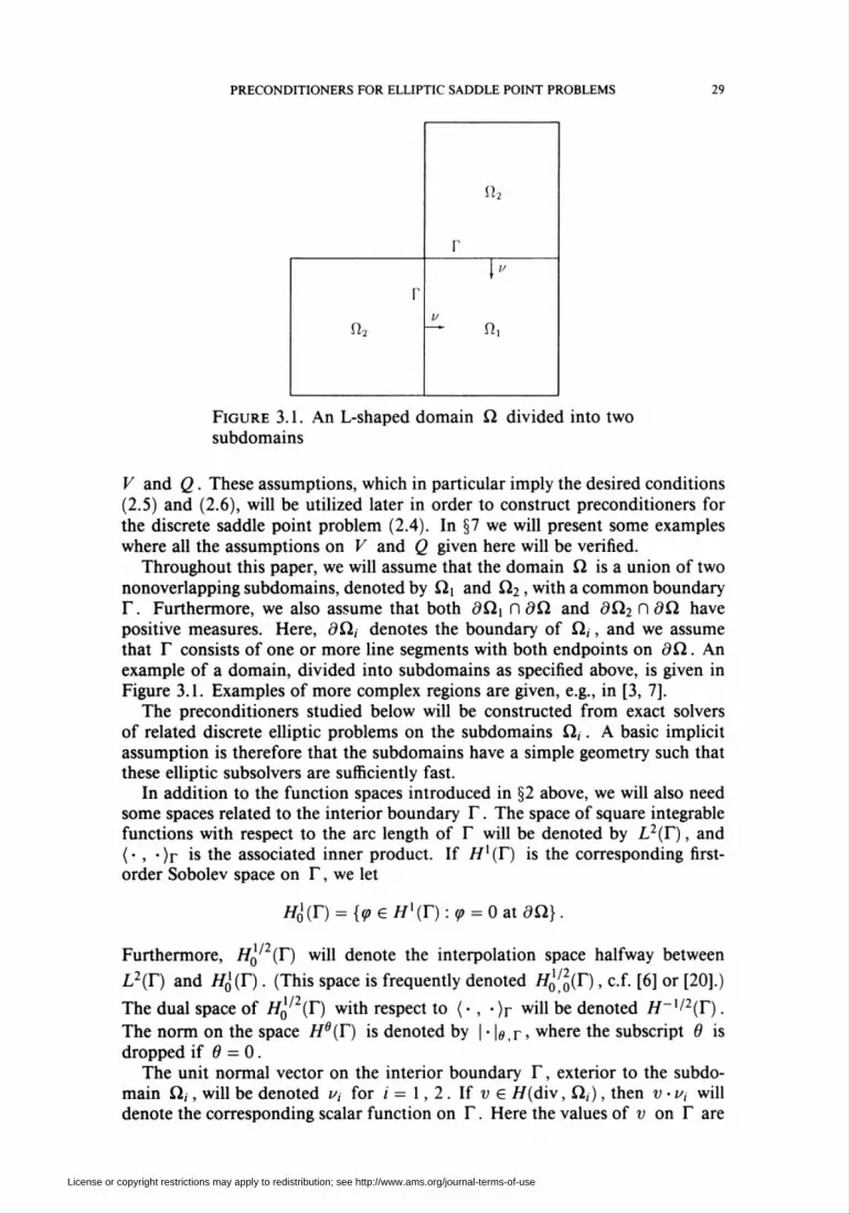
Figure 3.1. An L-shaped domain ß divided into two

subdomains

V and Q. These assumptions, which in particular imply the desired conditions

(2.5) and (2.6), will be utilized later in order to construct preconditioners for

the discrete saddle point problem (2.4). In §7 we will present some examples

where all the assumptions on V and Q given here will be verified.

Throughout this paper, we will assume that the domain ß is a union of two

nonoverlapping subdomains, denoted by ßi and ß2 , with a common boundary

T. Furthermore, we also assume that both dCl\ n <9ß and díl2 n 9ß have

positive measures. Here, 9ß, denotes the boundary of ß,, and we assume

that T consists of one or more line segments with both endpoints on <9ß. An

example of a domain, divided into subdomains as specified above, is given in

Figure 3.1. Examples of more complex regions are given, e.g., in [3, 7].

The preconditioners studied below will be constructed from exact solvers

of related discrete elliptic problems on the subdomains ß,. A basic implicit

assumption is therefore that the subdomains have a simple geometry such thatthese elliptic subsolvers are sufficiently fast.

In addition to the function spaces introduced in §2 above, we will also need

some spaces related to the interior boundary Y. The space of square integrable

functions with respect to the arc length of F will be denoted by L2(T), and

( • , • )r is the associated inner product. If 771 (T) is the corresponding first-

order Sobolev space on T, we let

H¿(T) = {q>£ Hl(T) : tp = 0 at dQ.}.

Furthermore, H0l/2(T) will denote the interpolation space halfway between

L2(r) and H0l(T). (This space is frequently denoted H0l/20(r), cf. [6] or [20].)

The dual space of H0l/2(T) with respect to ( • , • )r will be denoted 77-'/2(r).

The norm on the space 7ie(r) is denoted by | • |e,r, where the subscript 9 is

dropped if 0 = 0.The unit normal vector on the interior boundary T, exterior to the subdo-

main ß,, will be denoted v¿ for / = 1, 2. If v e 77(div, ß,), then v • i>i willdenote the corresponding scalar function on T. Here the values of v on T are



derived from the domain ß,. We recall from [18] that the map

(3.1) v H+ v -Vi

is continuous as a map from 77(div, ß,) into H~XI2(T). If v e 77(div, ßi) ©

77(div, ß2), we let [v • u] be the jump of these traces, i.e.,

[V • V\ = V • V2 + V ' V\ .

On the other hand, if v £ 77(div, ß), the trace v -v2 = -v -v\ is denoted by

v • v. Hence, the unit normal vector v — v2 has been chosen such that it is

pointing into ßi (cf. Figure 3.1).Throughout the paper, the discrete "pressure space" Q — Qh is assumed

to be of the form Q = Q\ © Q2, where Q¡ c L2(íl¡). This corresponds to

the requirement that the interior boundary Y is a "mesh-line" for the grid

generating the space Q. Similarly, we assume that Vx = Vxh and V2 - V2h

are finite element spaces such that

^C77(div,ß,),

and we let V c 77(div, ßi)©77(div, ß2) be given by V = V\®V2. We observethat

77(div, Q) = {ve 77(div, ß,) © 77(div, ß2): [v-v] = 0}.

The desired finite element space V occurring in the system (2.4) is similarly

given by

V = {v e V : [v • v] = 0},

where obviously V c 77(div, ß). However, the larger space V will be used in

§6 in order to construct a preconditioner for (2.4).

We also introduce spaces consisting of the normal components of the traces

on T of functions in V¡. We let S¡ = S¡tf,(T) be the linear spaces given by

S¡ = {v -v, : v £ V¡}. We will assume throughout this paper that S\ = S2, and

this linear space will be denoted S — Sn(T). We observe that it follows from

the continuity property of the map (3.1) that S c 77~'/2(r). We shall in fact

assume that S c 7.2(r). This will usually always be the case, since in practice

S typically consists of discontinuous piecewise polynomials.

In order to describe some of the preconditioners below we will also need

a space of continuous functions on T. Associated with the space Sf,(T), the

existence of finite element subspaces S* — S^(T) of H0X(T) is assumed. If S

is a space of piecewise constants, then S* will typically consist of continuous

piecewise linear functions. The spaces S and S* are assumed to be related

such that for any nonzero element x e S

(3.2) sup(/z,/)r>0.ßeS'

We observe that (3.2) in particular implies that dim(>S*) > dim(S).

The spaces V, Q, and S* will also be assumed to be related such that a

proper interpolation operator exists. The desired "inf-sup" condition (2.5) will

then be derived from this interpolation property. We assume that there exists a

family of interpolation operators n = Ylf, from //(div, ßi)©7/(div, ß2) into

V, bounded uniformly in h , such that

2

(3.3) b(Uv -v,q) + Y,{(nv - v) • »i. Hi)r = 0 V(q, ßi, p2) £ Qx S* x S*.i=\



Here, b is the extension of the bilinear form b given by

b(v , q) = - qV-vdx-l qV-vdx.Jci, Jn2

We observe that (3.2) and (3.3) imply that if u € 77(div, ß), then Uv £ V.Furthermore, for any v £ H(div, ß),

b(Ylv -v,q) = 0 Vq£Q.

Hence, condition (2.5) follows from the fact that this condition holds with the

space V replaced by 77(div, ß) (cf. [16]).We shall also require that (2.6) holds on each subdomain, i.e.,

(3.4) snob(v , q) > 0neQ

for all v £ V with V-w/O.Finally, we assume that the velocity space V satisfies an "inverse inequality"

of the form

(3.5) \v-v\l<ch-x\\v\\2 VweK.

Such an inequality typically holds if the finite element space V is constructed

on a uniform or quasi-uniform grid.

4. The preconditioned iterative method

In this section we shall describe the preconditioned minimum residual method

for saddle point problems of the form (1.2), and discuss the application of this

method to the solution of linear systems of the form (2.4). Throughout this

section, ( • , • ) denotes an inner product on Rm and R" , and | • | denotes the

corresponding norms.

Recall that the coefficient matrix of the linear system (1.2) is given by

(4.1) J/ = (/r *),

where A £ Rmxm and B e Rmx" with rank(5) = n. Furthermore, A is

symmetric and positive definite, and BT is the transpose of B with respect to

the given inner products.

The minimum residual method is an iterative method for general symmetric,

nonsingular systems. Consider a system of the form sfa* = ß , and, for k > 1 ,

let Vk denote the Krylov space

Vk = soan{ß,s/ß,...,s/k-xß).

The approximation ak £ Vk of a*, obtained after k - 1 iterations, is uniquely

determined by the residual property

(4.2) \ß -s/ak\2 = inf \ß - sfa\2 .aevk

We refer to [24, 27] for details on the iterative algorithm which generates the

vectors ak. For the discussion here it is important to recall that typically the

coefficient matrix s/ has to be multiplied with a vector once for each iteration,

and that the algorithm depends on the chosen inner products.


32 torgeir rusten and ragnar winther

In [27] we also discuss the convergence properties of the minimum residual

method applied to systems of the form (1.2). It is established there that the

convergence rate of the method is dominated by three parameters. These are the

condition numbers of the matrices A and B , and a third parameter measuring

the relative scaling between them.Let Ào and A\ denote the smallest and largest eigenvalue of A , respectively.

Similarly, we let oo and o\ denote the extreme singular values of the rectan-

gular matrix B ; i.e., CTq and of are the extreme eigenvalues of BTB. The

spectral condition numbers of the matrices A and B are then given by

k(A) = X\/Xo and k(B) = o\/oq.

Furthermore, the relative scaling parameter, p = p(B, A), is given by

p = ffoMo •

We observe that the adjoint operation B —> BT depends on the chosen in-

ner product. Hence, the quantities k(B) and p(B, A) are also inner product

dependent.In order to guarantee fast convergence of the method, the scaling parameter

p should be of order one, i.e., neither too small nor too large. On the other

hand, if p is kept roughly fixed, the convergence rate will usually increase with

decreasing values of k(A) and k(B) . Hence, the purpose of a preconditioner

for a properly scaled system is to tranform it into a new system of the form

(1.2), with p essentially unchanged, but where the condition numbers of the

matrices A and/or B have been decreased.The preconditioned minimum residual method discussed in [27] is defined

by two symmetric, positive definite matrices M e Rmxm and N £ R"x" . We

let Se denote the block diagonal matrix

The new preconditioned system now takes the form

(4.3) ^-vQ=^-'Q.This system is clearly equivalent to (1.2), and the coefficient matrix, SB~xsf ,

is given by

*-* - (££ V) ■Furthermore, the matrix 3e~xs¿ is symmetric in an appropriate inner product.

In order to see this, define a new inner product on Rm by \t\, x\m = (Mc¡, x) ■

Similarly, let [n, 9]N = (Nn, 6) be an inner product on R" , and finally define

the inner product [ • , • ] on Rm x W by

(4.4) KZ, I), (X, 0)] = iZ, X]m + [tl, 6]N.

Then S§~xsf is symmetric in the inner product [• , •]. Furthermore, M~xA

is symmetric and positive definite in the inner product [• , -\m , and N~lBTis the adjoint of M~XB with respect to the two new inner products on Rm

and R" . The preconditioned system (4.3) has therefore the same saddle point

structure as the original system (1.2). Consequently, the minimum residual


preconditioners for elliptic saddle point problems 33

method, with the inner product ( • , • ) replaced by [ • , • ], can be applied to

the new system.

In order to obtain an effective preconditioner, the matrix 38 must satisfy

two properties. First, it should be easily invertible, or more precisely, it should

be easy to solve linear systems with 38 as a coefficient matrix. This is because

a system of this form has to be solved for each iteration. We observe that, since

38 is block diagonal, this is equivalent to require that the two matrices M and

Af are easily invertible. The second necessary property is that the minimum

residual method applied to the preconditioned system should converge rapidly.

From the discussion above we recall that, under the assumption of a proper

scaling, this is the case if the condition numbers of the matrices M~XA andM~XB are sufficiently small.

We recall that the condition numbers and the scaling parameter are in general

dependent on the inner products through the adjoint operation. We let k and p

denote these functions with respect to the new inner products [ • , • ] introduced

above.The condition number of M~x A, k(M~xA), is frequently estimated by es-

tablishing inequalities of the form

Mx\\,<W-xAx,x]M<h\x\M V^€Rm,

for suitable constants An and 1\, since these inequalities imply that

k(M-xA)<lx/lo.

Here, | ■ \m denotes the norm corresponding to the inner product [ • , • ]m ■

Furthermore, from the definitions of the inner products we find that these in-

equalities are equivalent to

(4.5) X0(Mx,x)<(Ax,X)<h(Mx,X) *X 6 Rm .

Similarly, we derive that k(M~lB) is bounded by à\/ào, where do and aiare constants such that

(4.6) ôr](N8,6)<(BTM-xBe,e)<ôf(Ne,e) VöeR".

The second requirement for 38 is therefore fulfilled if M and N are symmet-

ric, positive definite matrices such that (4.5) and (4.6) hold with ratios Âi/Ân

and d\ /do sufficiently close to one. Our conclusion is therefore that 38 is an

effective preconditioner for sf if M and N are effective preconditioners for

the symmetric, positive definite matrices A and BTM~XB, respectively.Note that we are not interested in the matrices themselves. However, we

must be able to calculate the action of M~x and A^-1, since this has to be

done once in each iteration of the iterative method.

Consider now the saddle point problem (2.4). Recall that the matrix A

corresponds to the bilinear form a(u, v), defined in (2.3). It follows directly

from (2.1) that

(4.7) Toll^H2 < «(î^ , ^) < Txll^H2 \/V£V,

with constants To and X\. We note that, if ( • , • ) is the inner product on Rm

induced by the L2-product on V, this corresponds to (4.5) with M equal to

the identity matrix and 1, = t, . Hence, if the ratio ti/to is not too large, theidentity is an acceptable preconditioner for A . Throughout this paper, we will


34 torgeir rusten and ragnar winther

therefore only consider preconditioners where M — I. We observe, in partic-

ular, that the condition number of A is independent of the mesh parameter

h.Having chosen M = 7, we turn our attention to the problem of constructing

a preconditioner for BTB . We start by deriving an expression for the bilinear

form corresponding to BTB. Define the discrete gradient operator Vh : Q t->

V, corresponding to the matrix B in (1.2), by

(4.8) (Vhq,v) = b(v,q) Vq£Q,Vv£V.

Since b(v, q) - -{q,V-v), the adjoint of B, corresponding to the L2-

products on V and Q, is -T'o(V-). Here, Tfo is an L2-projection onto Q.

The inequality (4.6) therefore takes the form

(4.9) ôô2N(q,q)<(Vhq,Vhq)<ôfN(q,q) Vq£Q,

where N( - , •) is the bilinear form associated with the matrix N. Hence, Nshould be chosen as a preconditioner for the nonconforming discrete Laplace

operator -TfaV • VA .Consider the discrete Poisson equation of the form

(4.10) (Vhr,Vhq) = (l,q) V^eß,

where the unknown function r e Q. The condition (2.5) implies that this

problem has a unique solution. Furthermore, it is easy to see that (4.10) is

equivalent to the following problem of the form (2.4):

(w,v) + b(v,r)=0, Vv£V,{- ' b(w , q) = -(I, q) Vq£Q,

where w = -Vf,r. Hence, the design of effective preconditioners N is closely

related to the properties of this saddle point problem.

Finally, we observe that when M = I the proper scaling factor for the pre-

conditioned system, p(B, A), satisfies the inequality

(4.12) ô0/xi<p(B,A)<âl/xo.

Hence, since To and x\ are fixed constants, the properties of a preconditioner

are determined by the two constants do and d\ appearing in (4.9).

5. The Neumann preconditioner

In this section we shall describe a domain decomposition preconditioner for

the linear system (2.4) based on subproblems with Neumann boundary con-

ditions on the interior boundary Y. We recall that our purpose is to design

a preconditioner N such that the inequality (4.9) holds with the ratio at/an

sufficiently close to one. If no preconditioning is performed, the bilinear form

N corresponds to the T.2 inner product on Q. In this case, (4.9) holds with

ô\/ôo — 0(h~x). The preconditioner studied below will reduce this ratio to

0(h~xl2). Hence, the bound still grows with the size of the system, but more

slowly than with no preconditioner. These bounds therefore indicate that the

preconditioner will speed up the convergence of the iterative method consider-

ably, but that the number of iterations required by the preconditioned minimum

residual method will still increase with the dimension of the system. The nu-

merical experiments, which will be presented in §7, will indeed confirm these

expectations.



We introduce the subspace 770(div, ß) of 7/(div, ß) given by

/70(div, ß) = {v £ H(div, ß) : v -u = 0}.

Similarly, we let V0 c V be given by V0 = {v £ V : v • v = 0}. Note that it

follows from (3.2) and (3.3) that the interpolation operator n maps 77o(div, ß)

into V0. Furthermore, Uv satisfies, for any v £ 7/0(div, ß),

b(Uv - v, q) = 0 Vtfeß.

Hence, as above, the discrete inf-sup condition

(5.1) infsup..^.'^ >y0>09£Qvev0 \\q\\ ll^lldiv

follows from the corresponding continuous condition with Vq replaced by

77o(div, ß). This latter condition is again equivalent to inf-sup conditions on

the two subdomains.

Let x € S be given and assume that tp solves the boundary value problem

A<p = 0 in ßi U ß2,

(5.2) <p = 0 ondß,

Vtp-v = x on T.

Here, A denotes the Laplace operator. We observe that the uniquely determined

function tp is a harmonic function on each subdomain. Let y/ - -Vtp . Since

V • y/ = 0 on each subdomain, it follows from elliptic theory (cf., e.g., [25]) that

y/ and tp satisfy the a priori estimate

(5-3) IIHIdiv + IWI <c\x\-\ßj-

Define w £ V by w = Wyi. From the continuity property of the interpola-

tion operator n we then obtain ||iu||div < c\x\-\¡ij ■ The following result has

therefore been established.

Lemma 5.1. There is a constant c, independent of h, such that for any ^e5

inf{|M|div : w g V, w-v = x} <c|*l-i/2,r-

Define a new discrete gradient operator, V^ : Q >-> Vq , by

(5.4) (V°hq, v) = b(v , q) V«eß, Vv£V0.

The bilinear form No which defines the Neumann preconditioner is now given

by No(r, q) — (V^r, V^). This bilinear form is obviously symmetric, and

(5.1) implies that

||VÎ,|| = sup%^>sup^l>,oW.v€V0 \\v\\ vev0 Imldiv

Hence,

(5.5) Aro(4,4) = ||V^||2>702||<7||2

for all q £ Q. Consider the problem

(5.6) N0(r, q) = (I, q) V^6ß,



where the unknown function r £ Q = Qx © Q2. If we let w = -V°r, then

(w, r) £ Vo x Q is the solution of the saddle point problem

, . (w,v) + b{v,r)=0, VweFo,1 ' b(w, q) = -(I, q) V^eß.

It is easy to see that this problem decouples into saddle point problems on each

subdomain. Hence, with the proper choice of finite element spaces, this problem

can be solved by a fast solver (cf. §7).

The purpose of the rest of this section is therefore to discuss the efficiency of

this preconditioner, i.e., to derive an inequality of the form (4.9).

For each q £ Q, let V\q e V be given by

Note that it follows from (4.8) and (5.4) that (V\q, v) = 0 for all v £ V0 . In

particular, (V\\q, V°#) = 0, and hence

l|V^||2 = ||V^||2 + ||V^||2.

It therefore follows that the left side of inequality (4.9) is satisfied with ôq = 1.

The following result shows that d\ = 0(h~xl2).

Theorem 5.2. There is a constant c, independent of h, such that

llv^H < cA-^nvfcll v<?eß.Proof. Introduce the bilinear form R(v , q) given by

R(v , q) = b(v , q) - (V°hq, v).

By (4.8) and (5.4), it follows that

(5.8) (Vrhq, v) = R(v , q) Vv £ V.

Furthermore, R(v , q) = 0 for all v £ V0 . Therefore, for each given q £ Q, the

bilinear form R(- , q) can be considered to be a linear functional on 5 - Sf,(T).

Hence, for each q £ Q there exists a unique element [q] £ S such that

(5.9) ([q],v-u)r = R(v,q) Vv £ V.

The element [q] £ S should be interpreted as the "jump of q at T." The

relation (5.8) can now be rewritten in the form

(Vrhq,v) = ([q],vu) Vv £ V.

Hence, by the inverse assumption (3.5),

v€V \\V\\ v£V \\V\\

<\[q]\Tsnvl-^^<ch-x/2\[q]\rvev \\v\\

or

(5.10) l|V^||<cÄ-'/2|M|r,

where the constant c in independent of q and h .



On the other hand, from (5.9) we obtain

Mr=Supi!^>I = suP^iM^x&s \X\r X£S ||w||div \X\r

<(lkll2 + l|V^||2)l/2supMldiv

xes \x\r

where w £ V is any function such that w-v = x on F. Hence, from (5.5)

and by selecting w such that ||w||div/lxl-i/2,r is minimal, we obtain from

Lemma 5.1 that |[^]|r < c||V^||. Together with (5.10) this implies that there

is a constant c, independent of q and h , such that

(5.11) \\Vrhq\\<ch-x'2\\V°hq\\.

We therefore conclude that

IIV^H = (IIV^H2 + IIV^H2)'/2 < cA-^HVfcll

for a suitable constant c. D

6. A Dirichlet preconditioner

The domain decomposition preconditioner developed in the previous sec-

tion was based on subproblems with a Neumann boundary condition on the

interior boundary T. In contrast, the efficient domain decomposition precon-

ditioners for systems arising from conforming finite element discretizations of

elliptic equations are based on the solution of some subproblems with an inte-

rior Dirichlet condition (cf., e.g., [3, 6] or [7]). In this section we shall develop

corresponding preconditioners for the systems arising from mixed finite ele-

ment methods. The preconditioners studied below are based on the solution of

subproblems with Dirichlet boundary conditions on the interior boundary, and

correspond to the ones studied in [3, 6]. Since these preconditioners involve

independent problems on each subdomain, they can, as in [6], be generalized

to domains with a more complex substructure. However, in this paper we willonly consider the two subdomains case studied above. In particular, we will

show that, in the case of two subdomains, the appropriate condition numbers

are independent of the discretization parameter h .

Since the Dirichlet boundary conditions are natural boundary conditions in

the mixed finite element method, the discrete system (2.4) will be slightly gen-

eralized. Instead of (2.4) we introduce the following generalized system:

Find (uh , ph , kh) £ V x Q x S* such that

a(uh , v) + b(v , ph) + (Xh, [v • u])T = G(v) Vv € V,

(6.1) b(uh,q)=F(q) VtfGß,

(p,[Uh'v])r = 0 V/i6 5',

where we recall that the space V and the bilinear form b( • , • ) are defined

in §3. In particular, the extended form b ignores the possible jumps at T. A

similar convention is used for the norm || • ||d¡v below, i.e., the norm is defined

by summing the contributions from each subdomain.

The system (6.1) arises naturally if the elliptic equation ( 1.1 ) is discretized by

a mixed finite element method on each subdomain, and if the interior boundary



conditions [p] — 0 and [u • u] = 0 are required on T. We observe that (6.1) is

a generalization of (2.4) in the sense that if the triple (Uf,, Pf,, If,) solves (6.1)

then the pair (Uf,, Pf,) solves (2.4). Furthermore, Xh £ S* is an approximation

of the trace of p on T.The system (6.1) has the saddle point structure (1.2). The following con-

sequence of the assumptions given above shows that this system satisfies the

proper inf-sup condition.

Lemma 6.1. There exists a constant y\, independent of the mesh parameter h,

such that

(6.2) inf sup^,V^'[:'?r>y.>0.(Q.n)eQxs- ve~ (\\q\\ + Mi/2,r)Hdiv

Proof. As above, the result follows from a proper application of the interpo-

lation property (3.3). Let (q, p) G ß x S* be given, and consider elliptic

equations of the form

Atp = q in ß] U ß2,

<p = 0 onöß,

( • ' [p] = 0 onI\

[Vtp-v] = x on T,

where x € H~XI2{T) is arbitrary. Let y/ = Vip. Then y/ G 77(div, ß() ©77(div, ß2) and from elliptic regularity (cf. [18]) it follows that

(6.4) IHIdiv + IHI<c(IMI +M-i/2,r)

for a suitable constant c independent of q and x ■ Furthermore,

b(y, q) + {ß,[W^])r = Hill2 + Iß, X)r■

By choosing x such that |xl-i/2,r = L"|i/2,r and (p,x)r > M2/2,r/2' wetherefore obtain from (6.4) that

(6.5) M ,. ->c(||i|| + |^|i/2,r)

for a suitable positive constant c.

Let v £ V be given by v = Uy/. Since ||u||diV < ^11 Vlldiv and (3.3) impliesthat

b(y/,q) + (p, [y/• u])r = b(v , q) + (p, [v-u])r,

the desired result now follows from (6.5). D

Define the extended discrete gradient operator V^ : ß x S* >-> V by

(6.6) (Vh(q,p),v) = b(v,q) + (p,[v-v])r V(q, p) G ß x S*, Vt; G V.

This extended gradient operator is associated with the system (6.1) in the same

way as the operator V* is associated with (2.4). Therefore, in order to design

an effective preconditioner for this system, the bilinear form

(6.7) (Vh(r,n),Vh(q,p)),

defined on (Q x S*)2, has to be preconditioned.



We note that, for any (r, n) £ Q x S*,

(Vf,(r,t]),v)\Vh(r, i7)|| = sup

> sup (V/.(r> >?)»") _ b(v,r) + (n,[v-v])r

v£y IMIdiv v€y IMIdiv

Hence, we derive from (6.2) that

(6.8) l|VA(r,v)||>7i(lk|| + kli/2,r).

The bilinear form (6.7) is therefore an inner product on Qx S*.

In order to define the desired preconditioners, we consider an orthogonal

projection of elements in the product space Qx S* into ß x {0} with respect

to the inner product (6.7). For an arbitrary element (r, n) £ Q £ S* consider

the unique orthogonal decomposition of the form

(6.9) (r,n) = (r0,0) + (rH,n).

Hence, r° G ß is determined by

(6.10) (Vh(r0,0),Vh(q,0)) = (Vh(r,n),Vh(q,0)) Vq£Q.

Furthermore, if we let w° = -VA(r°, 0), then the pair (w°, r°) g V x Q

satisfies the saddle point problem

(w°,v) + b(v,r°)=0 ^ \/v£V,

{' ] b(w\q) = -(Vh(r,t1),Vh(q,0)) \/q£Q.

Similarly, if we let wH = -Vf,(rH, n), then the triple (wH, rH, n) £VxQxS*

satisfies

(612) (wH,v) + b(v,rH) = -(n,[w])r Vv G V,

b(wH,q) = 0 V?eß.

The function rH given in the decomposition above is a mixed finite element

approximation of a harmonic extension of the boundary function n. This

observation motivates the following simple result.

Lemma 6.2. Consider the orthogonal decomposition (6.9). There is a constant

c, independent of h, such that

l|VA(r",r/)||<c|,/|1/2,r.

Proof. Since b(wH, rH) = 0, it follows immediately from the system (6.12)

that

(6.13) \\wH\\2^-(t],[wH-v])T.

Furthermore, since (3.4) implies that Hw^Hdiv = ll^ll, we obtain that

\[wH-v]Ul2J<c\\wH\\iiy = c\\wH\\.

Hence, the desired result follows from (6.13). D

We note that the estimates given by (6.8) and Lemma 6.2 imply, in particular,

that for any (r,tf)£QxS*

yitoli/2,r<l|VA(r",ij)||<c|»7|1>2/r.



Since the decomposition (6.9) is orthogonal, it therefore follows that the two

norms

(6.14) ||V*(iMi)|| and ||V*(r°, 0)|| + |if|,,2.r

are equivalent, uniformly in h , on the space Qx S*.

Motivated by this equivalence, we therefore consider preconditioners of the

form

N((r,n),(q, p)) = (V„(r°, 0), Vh(q°, 0)) + (Ar,, p)r

for the bilinear form (6.7), where A: S* t-> S* is a discrete operator on the inte-

rior boundary T which is symmetric with respect to the inner product ( • , • )r.

The following result is now an obvious consequence of the equivalence (6.14).

Theorem 6.3. Assume that there is a constant c\, independent of h, such that

the operator A satisfies

(6.15) c1"1|»/lf/2,r<<A'/,»?)r<Ci|'7!2/2,r V" £ S*.

Then there is a constant c2, independent of h, such that

c2xÑ((r, n),(r, n)) < ||VA(r, V)||2 < c2Ñ((r, r¡),(r, //)) V(r, q) G ß x S*.

This result shows that if the boundary operator A is chosen such that (6.15)

holds, then the preconditioner N transforms (6.1) into a saddle point problem

with conditioning independent of the discretization parameter h .

Consider the linear systems of the form

(6.16) N((r,t1),(q,p)) = (l,q) + (lo,p)r V(?, p) £ Q x S\

where the data (/, /o) G ß x S* is given. We observe that when N is used as a

preconditioner, such a linear system has to be solved once for each iteration. If

the operator A satisfies (6.15) above, then N is positive definite on Qx S*,

and hence (6.16) has a unique solution (r, n) £ Q x S*. By decomposing this

solution according to (6.9), we derive from (6.11) that

(w°,v) + b(v,r°) = 0 Vv£V,

b(w°, q) = - (I, q) Vq£Q,

where, as above, w° = -V/,(r°, 0) G V. Furthermore, this problem decouples

into discrete Poisson equations on each subdomain. With the proper choice of

subspaces, this problem can^therefore be solved by a fast solver.

When (r°, w°) £ Qx V is computed, it remains to find the orthogonal

component of the solution, (rH, n) £ QxS*. However, it is enough to find n ,

since rH can then be calculated from (6.12). This system again corresponds to

discrete Poisson equations on each subdomain.

In order to derive a suitable equation for n, we consider (6.16) with test

functions of the form (q, p) = (qH, p). Let wH = -Vf,(rH,r¡). Since

(wH, tu0) = 0, we obtain from (6.17) that

(An, p)T = (l,qH) + (lo,ß)r

= - b(w°, qH) + </0, p)r = (M, K • *Dr + <4>. /Or,

or

(6.18) An = P*[w°-v] + lo,



where P*: L2(Y) i-> S* is the L2-projection onto S*. This equation is a dis-

crete system related to the interior boundary Y. Since T is one-dimensional,

we can usually afford to solve such systems (cf. §7).

The results above can be used in two different ways to define preconditioned

iterative methods for the system (2.4). From the discussion above, the obvious

approach seems to be to replace the system (2.4) by the generalized system

(6.1) and then use the bilinear form Af as a preconditioner for the form (6.7).

However, this strategy leads to approximate solutions of (6.1) (or (2.4)) with

a possible small jump on the interior boundary. In the calculations below we

have therefore used an alternative approach.

Consider the original discrete system (2.4). Our purpose is to use the equiva-

lence given in Theorem 6.3 only to design a preconditioner for the bilinear form

(Vf,r, Vf,q) on ß2. In order to see how this can be done, we first observe that

if Vf,(r, n) £ V, then Vf,(r, n) = Vnr. Furthermore, from (3.2) and (6.2) itfollows that for a given r £ Q there is a unique element n(r) £ S* such that

(6.19) (n,[vu])r = (Vf,r,v)-b(v,r) VveK,

or equivalently, for each r £ Q there is a unique element rj(r) £ S* such that

Vh(r,ti) = Vhr.

Define now the bilinear form A' on ß2 by

(6.20) N(r,q) = N((r,n(r)),(q,n(q))).

From the discussion above it follows that if the hypothesis of Theorem 6.3 is

satisfied, then N(r, r) and (Vf,r, V/¡r) are uniformly equivalent on Q. There-

fore, the bilinear form N can be used as a preconditioner for the original system

(2.4). Furthermore, the linear systems

(6.21) N(r,q) = (l,q) V<?Gß,

which have to be solved for each iteration of the minimum residual method,

are equivalent to the system (6.16) with /o — 0.

The conclusion of this section is that we have generalized the domain de-

composition preconditioners studied in [3, 6] to the systems derived from the

mixed finite element method. In the same way as with conforming finite element

methods, these preconditioners require that suitable discrete Poisson equations,

together with a system on the interior boundary, can be solved by sufficiently

fast solvers.

7. Numerical examples

The purpose of this section is to present some numerical examples obtained

by using the preconditioners developed above. Therefore, in particular, we have

to construct spaces ß, V, S, and S* satisfying the desired properties required

in §3.In the examples below, ß will be an L-shaped domain like the one given

in Figure 3.1. It is composed of three of the four subsquares obtained by

dividing the unit square into four equal squares. The domain is subdivided, in

a uniform manner, into axiparallel squares of size h. In particular, the grid

is chosen such that the interior boundary T coincides with boundaries of the



Figure 7.1. The domain ß with a square grid

squares of the grid (cf. Figure 7.1). On this grid we will apply the quadrilateralRaviart-Thomas elements of order zero (cf. [25]). Hence, the functions in ß are

constants on each grid element and, as required in §3, Q — Q\®Qi, where ß, c

L2(ß,). Similarly, the components of a vector v £ V are either constant or

linear on each element, and V = V\ © V2 , with V¡ c 77(div, ß,). Furthermore,

the functions in S are piecewise constants on the interior boundary T.

When the above subspaces are applied, the linear systems associated with the

subdomains may be solved by fast Poisson solvers. In particular, if a certain

combination of the midpoint and the trapezoid rules for numerical integration is

used in the evaluation of the integrals, discrete Poisson problems corresponding

to the five-point finite difference scheme have to be solved on the subdomains

(cf. [26]).By a proper parametrization each segment of T can be considered to be the

unit interval 7. The elements of S1 are then constants on the subintervals of the

form ((/' - l)h, ih) for i= 1,2,... , k, where k is the dimension of S and

À is a proper scaling of the grid parameter h . On 7, the space S* is required

to be a subspace of H0l(I). We let S* consist of all piecewise linear functions

in 770(7) with possible discontinuities of the slopes at the points (/' - l/2)h

for / = 1,2, ... , k. Hence, »S and S* are spaces consisting of functions on

I which are piecewise constant or piecewise linear, respectively. However, the

piecewise polynomial spaces are generated from different sets of knots. We alsoobserve that

dim(S*) = dim(S) = Â:.

Consider the assumptions on the spaces V, Q, S, and S* given in §3. It is

easy to see that the spaces S and S* defined on / above satisfy the condition

(3.2). In fact, if x £ S is given and p £ S* interpolates x at the points 0,,then

{X, ft)i > i\x\The conditions (3.4) and (3.5) are also easy to check. In particular, (3.4)

follows since V-v g ß for any v £ V, and the inverse assumption (3.5)

follows from the uniformity of the grid.



Figure 7.2. Reference domain ß

Finally, in order to verify all the assumptions given in §3, we have to construct

the uniformly bounded interpolation operators

EI: 77(div, ßj)©77(div, ß2) ■-» V

such that the condition (3.3) holds. If the term on the interior boundary had not

appeared in (3.3), the construction of a suitable operator n is, e.g., described

in [16]. However, in order to extend this construction to the present case, the

boundary term has to be treated properly by the operator n.

The operator n can be constructed independently on each subdomain. It is

therefore sufficient to consider the construction of the interpolation operator on

the unit square, ß, with a regular square grid, and where the interior boundary

is represented by the edge f = {(1, y) : y £ I) (cf. Figure 7.2).

Furthermore, we let V and ß be the corresponding Raviart-Thomas ele-

ments of order zero on ß. The boundary of ß is denoted by <9ß, while the

exterior unit vector normal to <9ß is v . In order to simplify the notation, we

let S and S* denote the finite element spaces on f implied by the construction

above. Below we shall construct interpolation operators n : 77(div, ß) >-> V,

uniformly bounded in h , such that

(7.1) b(ñv-v,q) + (p,(ñv-v)-i>)? = 0 V(q,p)£QxS*,

where b is the bilinear form b restricted to ß. This construction can easilybe modified to cover all the three components of the subdomains in the present

case. The general condition (3.3) will therefore follow from (7.1).

Since the grid on ß, in particular, generates a partition of the boundary 9ß,

the spaces S and S* can be extended, in an obvious way, to discontinuous

constants and continuous piecewise linear subspaces of 77'(9ß) and L2(dQ),

respectively. These spaces on öß will be denoted Se and S*. In particular,

since the knots of the partition generating the finite element space S* are located

in the middle of the grid edges on <3ß, the tangential derivatives of an element

in S* are assumed to be continuous at the corners of ß. Furthermore, any

element p £ S* can be extended to an element pe of S* by defining pe to be

0 outside T.It is easy to see that dim(.Se) = dim(5'*), since the degree of freedom for

both spaces is equal to the number of subintervals on dß generated by the

interior grid. Furthermore, by using interpolation relations between the spacesSe and S* at the midpoints of these subintervals, it is easy to verify that there



exists a constant c*o > 0, independent of h , such that

(7.2) inf sup.^'ff" >a0 and inf sup ^ *]f >a0.

In addition to the spaces introduced so far, we will also, for technical reasons,

introduce the subspace Z of 77'(ß) consisting of bilinear continuous functions

with respect to the grid on ß. Furthermore, we let ZB denote the restrictions

of functions in Z to dQ..We observe that the space ZB consists of continuous piecewise linear func-

tions on dß with respect to the same partition that generates the piecewise

constant space Se. Hence, translation by half the grid size represents an iso-

morphism between ZB and S*. Also observe that if n g Zb , then r\t £ Se,

where nt is the tangential derivative of n in a counterclockwise direction. Fur-

thermore, if z G Z and v is the divergence-free vector (zy, -zx)T, then

V£V.

We start the construction of the interpolation operator n: H(div, ß) h-> V

by introducing two discrete operators on the boundary dQ.

Define J and J*, from L2(dQ) into Se and S*, respectively, such that

and

(J*<P>X)0â = {9>X)dn VX£Se.

We observe that J and J* are dual operators with respect to the inner product

on L2(dÙ), and it follows from (7.2) that

Hence, the operators J and J* are stable in L2(dQ).

However, in order to derive the desired properties of the operator n, we

shall need a similar stability property for the operator J , or more precisely, for

an extension of /, in 77_1/2(<9ß). In order to derive this stability property,

we observe that it follows from the construction of the spaces S* above that

there is a constant c, independent of h , such that the following approximation

property and inverse property hold:

(7.4) jgf|f-A»laS^c*W|.«a v^77'(/3ß)

and

(7.5) H.an^^Hn V" e ^ •

From these properties we can easily derive that the operator 7* is stable in

77'(9ß), i.e., there is a constant c, independent of h , such that

(7.6) I'Vli.aS^li.oS VpG77'(dß).

In order to see this, let tp £ Hx(dQ.) be arbitrary and let tp* £ S* be the 771-

projection of <p . Then \tp*\ ~ < M, öq • Furthermore, for any y/ £ L2(9ß)

and p £ S*,(J'tp - tp, yr) ~ = (<p-p,Jy/- y) ~,



and hence it follows from duality, (7.3), and (7.4) that \J*(P-<P*\a?i <C^M, yô •

Hence, by (7.5),

\J*<p\ ~<ch-x\J*tp-tp*\ ~ + \<p*\ ~<c\tp\ s,

which is the desired bound (7.6).Note that by interpolation, (7.3) and (7.6) imply that

l^fli/2.M^^li/a.aS ^eHx'2(dÙ),

and by duality we therefore obtain that

(7-7) l'rt-i/2.«o**M-iy2.aa V,G77-'/2(9ß).

This is the desired stability of J in H~xl2(dñ).

The construction of the operator n is based on a proper decomposition of

elements in 77(div, ß) in a gradient vector and a divergence-free vector. Let

v £ 77(div, ß) be arbitrary, and consider the boundary value problem

Atp = V-v inß,(I.o)

Vtp-û = m(v) on 9ß,

where m(v) is the mean value of v-v on 9ß. This problem has a solution

tp which is uniquely determined up to constants. Furthermore, if vx = Vtp,

then vx £ (77'(ß))2, and there is a constant c, independent of v , such that

Uf1 Hi <c||V-f||, where ||-||i denotes the norm on 77'(ß) (or (HX(Q.))2).

Hence, as in [16] we can define an element Uxv £ V by reproducing the

average values of the normal components of v ' on each edge of the squares of

the grid. By construction, the function Ylxv has the property that

(7.9) b(nxv-v,q) = 0 Vq £ Q

and

(7.10) ñlv-u = m(v) ondñ.

Furthermore, there exists a constant c, independent of v , such that

(7.11) P1t;||div<c|M|dlv.

The function n't; approximates the gradient part of the vector function v .

We also need an approximation of the divergence-free component of v . Let

y/ £ H~x/2(dQ) be given by y/ - v • v - m(v). Then

Therefore, there exists an element n g Zb , uniquely determined up to con-

stants, such that r\t = Jyi, where, as above, nt denotes the tangential derivative

of n in a counterclockwise direction. Furthermore, let r £ Z be the solution of

the discrete Poisson equation defined by the conforming finite element method:

Find r £Z such that

(Vr,Vz) = 0 VzgZ,

<7-12) i ' flnr\dñ = n on dCl.



This problem has a unique solution. Furthermore, we can argue as in [7] (cf.

also Lemma 3.2 of [6]) and conclude that ||r||i < c\tj\ ~, where the constant

c is independent of n. Observe also that the trace inequality |^|_1/2 „s <

cIMIdiv holds. Hence, it follows from (7.7) and the fact that the map n i-> nt

is continuous from Hxl2(dQ.) to H~xl2(dñ) that \\r\\{ <c||v||div.

Define now U2v = (ry, -rx)T . Then, since V • (n2t;) = 0, it follows that

(7.13) lin^lUv^cHdiv-

Since Yl2v is divergence-free, it is also obvious that

(7.14) b(Û2v,q) = 0 VtfGß.

Finally, for any p £ S*,

(7 15) ^' fi2v -v)-û)? = (pe,ñ2v -Û - y/)d~- (pe, m(v))d~

= ~{fi, m(v))~,

where, as above, pe is the zero extension of p.. The desired operator n is

now defined by letting Uv = tllv + U2v . The uniform boundedness of these

operators follows from (7.11) and (7.13), and the desired property (7.1) follows

from (7.9), (7.10), (7.14), and (7.15).In order to complete the construction of a Dirichlet preconditioner as studied

in §6, we also need an operator A: S* i-> S*, symmetric with respect to the

inner product on L2(T), such that the bounds (6.15) hold. However, since

S* c Hq(F) is a space consisting of piecewise linear functions with respect to a

uniform partition, we can adopt the construction given in [6] and use the "square

root of the discrete second derivative along T." Furthermore, as described in

[6], equations of the form (6.18) can be solved by the Fast Fourier Transform.In all the calculations, g = 0, i.e., the elliptic equation has homogeneous

Dirichlet boundary conditions. Furthermore, f(x) = 2, and the initial ap-

proximation in the minimum residual method is set to zero. The iteration is

terminated when the norm of the residual, induced by the inner product (4.4),

is reduced by a factor of 10-5.

Example 7.1. In the first example we solve the Poisson problem, i.e., we choose

K(x) to be the identity matrix. The number of iterations, with and without

preconditioning, are listed in Table 7.1. These results seem to confirm that

the Dirichlet preconditioner results in a linear system where the number of

iterations required by the minimum residual method is independent of h . Fur-

thermore, the application of the Neumann preconditioner reduces the number

of iterations considerably. Also, as expected from the analysis given in §3, the

increase in the number of iterations, when the mesh parameter h decreases, is

slower when the Neumann preconditioner is applied than without a precondi-

tioner. D

Example 7.2. In the next example we consider a variable-coefficient problem

with the matrix K(x) given by

r,^_ (\+4(xf + x2) 3x{x2 \[> \ 3xxx2 l + ll(x2 + x2)) ■


PRECONDITIONERS FOR ELLIPTIC SADDLE POINT PROBLEMS

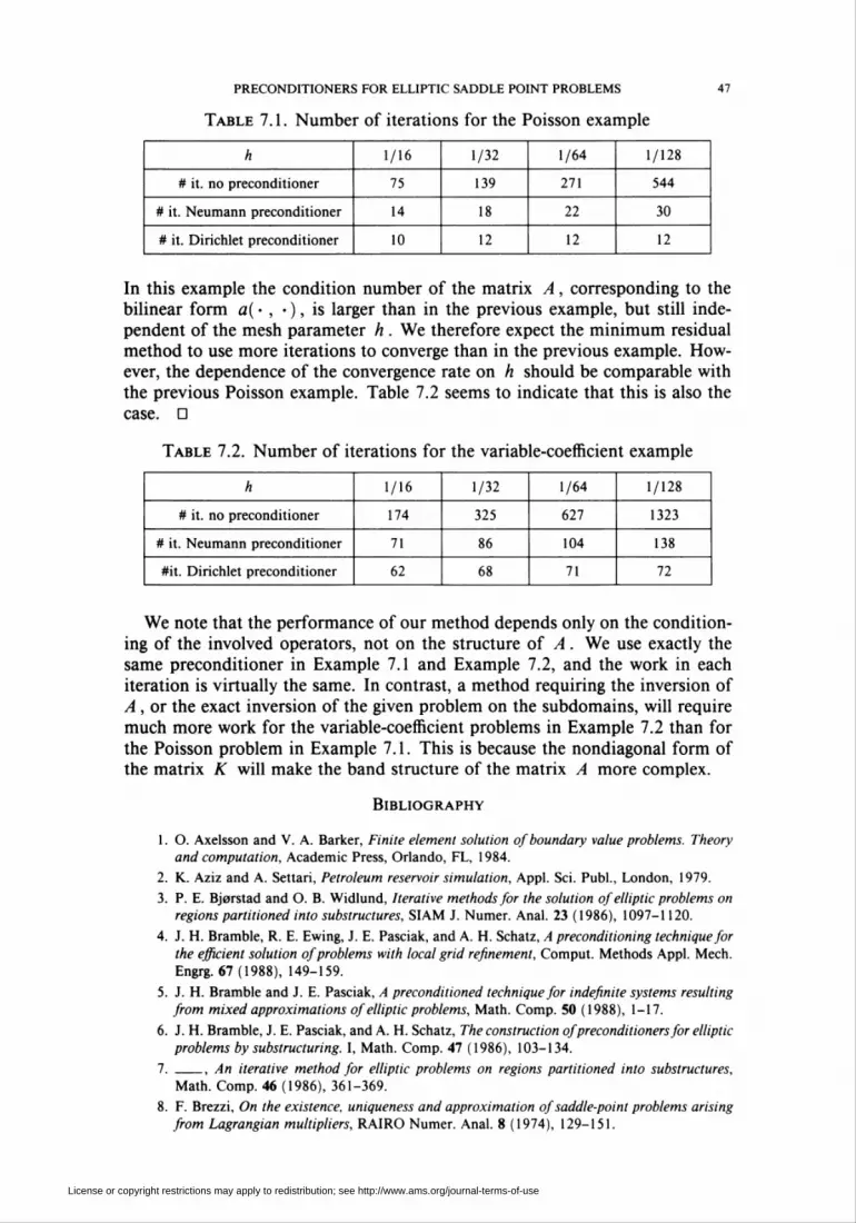
Table 7.1. Number of iterations for the Poisson example

47

1/16 1/32 1/64 1/128

# it. no preconditioner 75 139 271 544

# it. Neumann preconditioner 14 22 30

# it. Dirichlet preconditioner 10 12 12 12

In this example the condition number of the matrix A, corresponding to the

bilinear form a( • , • ), is larger than in the previous example, but still inde-

pendent of the mesh parameter h . We therefore expect the minimum residual

method to use more iterations to converge than in the previous example. How-

ever, the dependence of the convergence rate on h should be comparable with

the previous Poisson example. Table 7.2 seems to indicate that this is also the

case. D

Table 7.2. Number of iterations for the variable-coefficient example

1/16 1/32 1/64 1/128

# it. no preconditioner 174 325 627 1323

# it. Neumann preconditioner 71 86 104 138

#it. Dirichlet preconditioner 62 68 71 72

We note that the performance of our method depends only on the condition-

ing of the involved operators, not on the structure of A . We use exactly the

same preconditioner in Example 7.1 and Example 7.2, and the work in each

iteration is virtually the same. In contrast, a method requiring the inversion of

A , or the exact inversion of the given problem on the subdomains, will require

much more work for the variable-coefficient problems in Example 7.2 than for

the Poisson problem in Example 7.1. This is because the nondiagonal form ofthe matrix K will make the band structure of the matrix A more complex.

Bibliography

1. O. Axelsson and V. A. Barker, Finite element solution of boundary value problems. Theory

and computation, Academic Press, Orlando, FL, 1984.

2. K. Aziz and A. Settari, Petroleum reservoir simulation, Appl. Sei. Publ., London, 1979.

3. P. E. Bjerstad and O. B. Widlund, Iterative methods for the solution of elliptic problems on

regions partitioned into substructures, SIAM J. Numer. Anal. 23 (1986), 1097-1120.

4. J. H. Bramble, R. E. Ewing, J. E. Pasciak, and A. H. Schatz, A preconditioning technique for

the efficient solution of problems with local grid refinement, Comput. Methods Appl. Mech.

Engrg. 67(1988), 149-159.

5. J. H. Bramble and J. E. Pasciak, A preconditioned technique for indefinite systems resulting

from mixed approximations of elliptic problems, Math. Comp. 50 (1988), 1-17.

6. J. H. Bramble, J. E. Pasciak, and A. H. Schatz, The construction ofpreconditioned for elliptic

problems by substructuring. I, Math. Comp. 47 (1986), 103-134.

7. _, An iterative method for elliptic problems on regions partitioned into substructures,

Math. Comp. 46 (1986), 361-369.

8. F. Brezzi, On the existence, uniqueness and approximation of saddle-point problems arising

from Lagrangian multipliers, RAIRO Numer. Anal. 8 (1974), 129-151.



9. F. Brezzi, J. Douglas, Jr., R. Duràn, and M. Fortin, Mixed finite elements for second order

elliptic problems in three variables, Numer. Math. 51 (1987), 237-250.

10. F. Brezzi, J. Douglas, Jr., M. Fortin, and L. D. Marini, Efficient rectangular mixed finite

elements in two and three space variables, RAIRO Model. Math. Anal. Numér. 21 (1987),

581-604.

11. F. Brezzi, J. Douglas, Jr., and L. D. Marini, Two families of mixed finite elements for second

order elliptic problems, Numer. Math. 47 (1985), 217-235.

12. T. F. Chan and H. C. Elman, Fourier analysis of iterative methods for elliptic problems,

SIAM Rev. 31 (1989), 20-49.

13. J. Douglas, Jr., R. E. Ewing, and M. F. Wheeler, The approximation of the pressure by a

mixed method in the simulation of miscible displacement, RAIRO Numer. Anal. 17 (1983),

17-23.

14. J. Douglas, Jr. and P. Pietra, A description of some alternating-direction iterative techniques

for mixed finite element methods, Mathematical and Computational Methods in Seismic

Exploration and Reservoir Modeling (W. E. Fitzgibbon, ed.), SIAM, Philadelphia, PA,1986, pp. 37-53.

15. R. E. Ewing and M. F. Wheeler, Computational aspects of mixed finite element methods,

Numerical Methods for Scientific Computing (R. S. Stepleman, ed.), North-Holland, Am-

sterdam, 1983, pp. 163-172.

16. M. Fortin, An analysis of the convergence of mixed finite element methods, RAIRO Numer.

Anal. 11 (1977), 341-354.

17. M. Fortin and R. Glowinski, Augmented Lagrangian methods: Applications to the numerical

solution of boundary value problems, North-Holland, Amsterdam, 1983.

18. V. Girault and P. A. Raviart, Finite element methods for Navier-Stokes equations, Springer-

Verlag, Berlin, 1986.

19. R. Glowinski and M. F. Wheeler, Domain decomposition and mixed finite element methods

for elliptic problems, Proc. 1st Internat. Sympos. on Domain Decomposition Methods for

Partial Differential Equations (R. Glowinski, G. H. Golub, G. A. Meurant, and J. Periaux,

eds.), SIAM, Philadelphia, PA, 1988, pp. 144-172.

20. J. L. Lions and E. Magenes, Non-homogeneous boundary value problems and applications,

vol. I, Springer, New York, 1972.

21. P. L. Lions, On the Schwarz alternating method, Proc. 1st Internat. Sympos. on Domain

Decomposition Methods for Partial Differential Equations (R. Glowinski, G. H. Golub, G.

A. Meurant, and J. Periaux, eds.), SIAM, Philadelphia, PA, 1988, pp. 1-42.

22. T. P. Mathew, Domain decomposition and iterative refinement methods for mixed finite

element discretizations of elliptic problems, Ph.D. thesis, Department of Computer Science,

Courant Institute of Mathematical Sciences, 1989.

23. J. A. Meijerink and H. A. van der Vorst, An iterative solution method for linear systems of

which the coefficient matrix is a symmetric M-matrix, Math. Comp. 31 (1977), 148-162.

24. C. C. Paige and M. A. Saunders, Solution of sparse indefinite systems of linear equations,

SIAM J. Numer. Anal. 12 (1975), 617-629.

25. P. A. Raviart and J. M. Thomas, A mixed finite element method for 2-nd order elliptic

problems, Mathematical Aspects of Finite Element Methods (I. Galligani and E. Magenes,

eds.), Lecture Notes in Math., vol. 606, Springer-Verlag, Berlin, 1977, pp. 292-315.

26. T. F. Rüssel and M. F. Wheeler, Finite element and finite difference methods for continuous

flow in porous media, The Mathematics of Reservoir Simulation (R. E. Ewing, ed.), SIAM,

Philadelphia, PA, 1983.

27. T. Rusten and R. Winther, A preconditioned iterative method for saddlepoint problems,

SIAM J. Matrix Anal. Appl. 13 (1992), 887-904.

Department of Mathematics, University of Oslo, P.O. Box. 1080 Blindern, N-0316

Oslo 3, Norway

E-mail address: [email protected]

E-mail address: [email protected]


substructure preconditioners for elliptic saddle point problems

Documents