studies of creaming, flocculation and crystallisation in
TRANSCRIPT
Studies of C r ea ming, Floccula ti on and C rysta llisa tion in Emulsions :
Computer Modelling and Analysis of Ultrasound Propaga tion
by
Valeric Jane Pin field
Submitted in accordance with the requirements for the degree of
Doctor of Phi losophy
The Universi ty of Leeds
Procter Department of Food Science
February, 1996
The candidate confirms that the work submitted is her own and that appropriate credit
has been given where reference has been made to the work of others
-i i -
Abstract
The processes of creami ng, flocculation and crys talli sa tion are important fc1ctors in
the stability and properties of food emulsions 1easurements of the ultrasound velocity
and att enua tion in an emulsion are used as a non-destructive probe of emulsion
behaviour The present work aims to increase the understanding of the destabilisation
processes themselves and to improve the techniques for interpretation of ultrasound
measurements on such systems These aims were addressed tluough the computer
modelling of creami ng. flocculation and crystalli sation behaviour. and through the
investigation of theories f01 interpreting ultrasound measurements
Two computer models have been developed of creaming in emu lsions. both nith
and without fl occu lation One takes a phcnornenological approach. and is able to predict
macroscopic concentration profiles of emulsions The other is a small -scale simu lation at
the level of indi vidual particles The results of the phenomenological model are in
qualitative agreement with experimental results in the absence of particle interactions
The effects o f floccu lation on creaming behaviour were not. however, reproduced by the
model The small -scale simulation demonstrated that a simplified model of flocculation
and creaming cou ld result in features in the concent ration profiles which are comparable
with those observed experimenta ll y ll owever. some aspects of creaming behaviour were
not reproduced by eit her model
The investigation of theories of ultrasound propagation in emu lsions concluded
that multiple scattering theory is appropriate for the typical emulsions studied The
complex calcu lations required by the application of the theory are simplified in some
special limits, which are presented Alternative, practical, techniques are presented for
the interpretation of ultrasound measurements These are based on scattering theory but
utili se experimental determination of the scattering properties of the emul sion. so
avoiding the difficulties associated with multiple scattering theory calculations The
methods which have been developed are particularly relevant to creaming and
crystallisation studies The effects of particle size variat ion in emu lsions can innuence the
interpretation of ultrasound measurements, and restrictions are therefore placed on the
application oft he methods
-iii-
Conlenls
Abstract ............. ............................................. .......................................................... ... ii
Cont ents ... .... ................. .... ...... ................ .......... ............... .... .......... .............. ..... .. ....... iii
Figures ... ............ ...................................................................................................... . viii
Tables ..... ........ ......................... ... .......... ..... ........ .... ......... ..................... ..................... xiii
Ackn o,vledgentents ................................................................................................... xiv
C hapt er I : Introd uct ion .................................. ................ .. ........ ........ ........... ............. 1
1 Stability of emulsions
I 1 1 Creaming
I . 2 Flocculation
. 3
I 1.3 Crystal lisation 9
I 14 Interrelationships between creaming, flocculation and crystallisation I 0
1 2 Experimental studies of creaming 12
1.3 The ultrasound method 16
1 4 Computer modelling 21
1.5 Ultrasound theory 26
I 6 Objectives and preview 28
Chapt er 2 : Phrnomenological Modelling of Crea ming ................... ................. ....... 30
2 1 Overview of model
2 2 Physical processes included in the model
2.2 1 Gravity (creami ng)
2. 2 2 Thermal diffusion
31
34
35
37
- iv-
2.2 .3 llydrodynamic interactions
2 2 4 Po lydispersi ty
2 .3 Time evolution
23 I Calculation of change in concent ra tio n a t layer boundaries
2 3 2 Boundary velocities for each size fraction
2 4 Choice of discrete units
2 4 I Layer thickness
2 4 2 Time interval
2 4 .3 Size range in each si7e fraction
2 .5 Computer requirements
2 6 Ultrasou nd velocity and attenuation calculations
2 7 Samples analysed
2 8 Results
2 8 I To tal oil concentration profiles
2 8 2 Particle size dist ributio n
2 8 3 Ultrasound veloci ty and attenuation profiles
2 .9 Creaming and crys talli sa tion
2 9 _1 Crystalli sation kinetics
2 .9 2 Modelling of combined creami ng and crystal li sation
2 I 0 Creaming and flocculation
2 10 I Flocculation kinetics
2 I 0 2 Floc structure
2 10 3 floc mobility
2 I 0 4 Samples analysed
44
so
53
53
54
54
54
ss
ss
56
56
58
59
59
66
72
75
76
80
85
89
90
9 1
92
-V-
2 10_5 Creaming and nocculation results
2 11 Conclusions of model
93
98
C luq>ter- 3: Lattice Modelling of Crea ming and Florculntion .. ............................ 100
3 1 The fractal nature of nocculation
3 2 Overview of model .
3 3 Physical processes included in the model
3.3 1 Gravity (creaming)
3.3 2 Thermal diiTusion
3 3 3 Flocculation
3 4 Time evolution
J 5 Boundary cond itions
3.5 I x and y periodic boundaries
3 5 2 z bou ndaries
3 6 Calculation of fractal dimension
3 7 Computer requirement s
3 8 Samples analysed
3 9 Results
3 9 I Diffusion limited and reaction limited aggregation
3 9 2 Single particles
3 9 3 Variation of bonding probabi lity .
3 9 4 Variation of break up probability
3 9.5 Comparison with experimental results
3 10 Conclusions of lattice model
100
103
105
105
107
109
112
11 3
113
114
11 4
11 7
119
121
12 1
123
126
138
146
147
-------_vi -
C hapter 4: Theor1' of l lltrasound Propagation .... ........... ... ......... ..... ............ ......... 148
4 I Aims of theoretical ultrasound work 148
4 2 llornogeneous descriptions of dispersed systems 149
4 3 Ultrasound scattering theory 150
4 3 I General theory of sou nd propagation 15 1
4 J 2 Plane wave incident on a single particle I 53
4 3 3 Effect of many scattering centres single and multiple scattering 159
4 4 Assumptions of scattering theory 163
4 4 I Scattering is weak 163
4 4 2 System is stat ic 164
4 4 3 Particles are spherical 164
4 4 4 Infinit e time irradiation 164
4 4 5 Point-like particles 165
4 4 6 Random particle di stribu tion 165
4 4 7 No overlap of thermal and shear waves 166
4 4 8 No interactions between particles . 167
4 4 9 No phase changes 167
4 5 Numerical calculations using scattering theory 168
4 6 Important limiting solutions of scattering theory 172
4 7 Summary of scattering theory results 193
Chapt er 5: Methods for Interpreti ng Ulh·asou nd 1\,.l easur-ements ........................ 194
5 I Experimental determination of scattering coefficients
5 2 Particle size and frequency dependence
5 .3 Calibration ..
195
197
200
5.4 Renormalisa tion
5 4 I Linear renormalisa tion
54 2 Quadra tic renorma lisation
5 5 Multiple dispersed phases
5 6 Polymer/oil systems
57 Crysta lli sation .
58 Summary of ultrasound methods
- vii -
203
204
205
208
2 11
2 14
223
C ha pter 6 : Conclusions .................... ......... ....................... .. .... ... .. ............... .... ........ 225
Bibliography ............................... ........................ ..................................................... 231
List of Symbols ...... .... .... .. .. ......... ..... ........ ..... .. .. .... ......... ... ... ............................ .. ...... 244
English symbols
Greek symbols
Mi scellaneous symbols .
Subscripts and superscripts
Appendix A I :Comput er Program for Ph enom enological Model ofCr·e:uning
244
247
249
249
nnd Crystallisa tion ..... ......... ..... ............ .... .. ... .... ... ............................................... 25 1
Appendix A2 : Co mput er· PI'Ogram for Phcnomenologiral l\lodel of C reaming
and Flocculation ............... .................. ............... ........ .... ... ..... .. ............. .... ....... ... 270
Apprndix A3 : Computrr Program for LaHice l\lodel of Cream in g a nd
Flocculation ............... .. ........ ................. .. .... ... .... .............. .. .................................. 292
Appendix A4: Comput er Program for Multiple Sca lt t'Ting Theory
C alculations .............................................. .... ............... ...... ............... .. .. .... ....... ... 324
Appendix AS: Comput er Program for Ultrasou nd Veloci ty Calculations .......... 336
Appendix A6 : Publications a nd Pr·esentations ............. ......................................... 337
- viii-
Figures
Figure 1 1 Schematic diagram oft he ultrasound scanner used to obtain
concentration profiles in creaming emulsions 17
Figure 2 I Schematic diagram of the representation of an oi l in water emu lsion in
the phenomenological comput er model 32
Figure 2 2 Discrete size fraction representation of a conti nuous particle size
distribution in the computer model
Figure 2 3 Thermal random walk
Figure 2 4 Effect of dinl1sion on a step-change in concentration
Figure 2 5 Concentration dependence of creami ng speed and diffusion coefficient
for a monodisperse sample
figure 2 6 Flow diagram oft he calculation for the phenomenological creaming
model
Figure 2 7 Initial particle size distribution for the sunflower o il in water emulsion
used in creaming model
Figure 2 8 Predicted total volume fraction of oil as a function of height and time
for a polydisperse sunflower oil in water emulsion
Figure 2 9 Predicted volume fraction of o il as a fun ction of height and time for a
monodisperse su nflov.;er oi l in water emulsion
Figure 2 10 Effect of diffusion on the total concentration profiles afier 250 days in
a polydisperse sun flower o il in wa ter emulsion
Figure 2 11 Effect of diffusion on concentration profiles in a monodisperse
sun fl ower oi l in water emul sion
Figure 2 12 Comparison of experimental (Fillery-Travis el al. , 1993) and modelled
creaming profiles for a polydisperse alkane in water emulsion
Figure 2 13 Concentration as a function of height for different particle size
fractions afier 250 days in a sunflower o il in wa ter emulsion
32
37
41
49
57
59
60
60
63
63
65
67
- ix-
Figure 2_14 Effect of diffusion on the concentration prolile of a single size fraction
in a sunnower oil in water emulsion
Figure 2 15 Particle size distribution in the bulk of the polydisperse sunnower oil in
water emulsion a£ler 250 days
Figure 2 16 Particle size di stribution in the cream of a polydisperse sun nower oi l in
water emulsion an er 500 days
Figure 2 17 En'ect of diffusion on the particle si1e distribution in the cream aner
500 days in a su nnm"er oil in water emulsion
Figure 2 18 Ultrasound velocity profiles calcu lated from multiple scattering theory
from the creaming model for a sunnower oil in water emulsion
Figure 2 19 Ultrasound attenuation profiles from the crea ming model for a
sunno"er oil in water emulsion
Figure 2 20 Comparison of ultrasound veloci ty theories a£ler 1000 days from the
creaming model for a sunnmver oil in water emulsion
Figure 2 2 1 Profiles of liquid, solid and total dispersed phase concentration afler
2 .5 days of creaming in a mixed hexadecane in water emulsion at 8°C
Figure 2 22 Profiles of total dispersed phase concent ration afler 30 days in mixed
solid/liquid and all-liquid hexadecane in water emulsions at 8°C
Figure 2.23 Ultrasound velocity profiles for the creami ng and crystallisa tion model
of a hexadecane in water emulsion at 8°C
Figure 2 24 Creaming behaviour of a 20% sun nower oil in water emulsion with
0 03 wt % xanthan in the aqueous phase at 30 °C (M a, 1995)
Figure 2 25 Concentration profiles of nocculation and creaming aflcr 4 days using
hydrodynamic interactions based on total noc concentration
Figure 2 26 Concentration proli les of noccula tion and creaming a£l er S days using
hydr odynamic int eractions based on oil concentration only
Figure 2 27 Concentration profiles of nocculation and creaming aflcr 8 days
comparing hydrodynamic interactions ..
67
70
70
71
73
73
74
82
82
84
86
94
94
96
-X-
Figure 3 I Schematic diagram of lattice model of creaming and flocculation 104
Figure 3 2 Schematic representation of interparticle potential as a fun ction of
distance for the lattice model Ill
Figure 3.3 Calculation of the particle distribution function in the latt ice model 11 5
Figure 3 4 Flow diagram of lattice model program of creaming and fl occulation I 18
Figure 3 5 Flow diagram of the lloccul ation section oft he lattice model program 11 9
Figure 3 6 Number of particles N(R) within a distance R for diffusion limited and
reaction limit ed aggregation 122
Figure 3 7 Proportion of lattice sit es occupied as a fun ction of height , for single
particles 124
Figure 3 8 Proportion of lattice si tes occupied as a fun ction of height , for single
particles, in the absence of diffusion 125
Figure 3 9 Proportion of lattice si tes occupied as a fu nction of height , with a
bonding probabilit y of O 00 I, and no noc break up 127
Figure 3 10 Proportion of lattice sites occupied as a function of height. with a
bonding probabilit y of O 002, and no noc break up 128
Figure 3 11 Proportion of lattice sites occupied as a fw1ction of height . with a
bonding probability of O 005, and no noc break up 129
Figure 3 12 Proportion of lattice sit es occupied as a function of height , wi th a
bonding probabilily of O 01, and no noc break up 130
Figure 3 13 Comparison of concentration pro liles in nocculated and 110 11-
nocculated systems illustrating the change in creaming rat e
Figure 3 14 The serum int erface position as a function of bonding probability in the
absence of noc break up
Figure 3 IS Plot of number of particles N(/1) within a di stance R used to calculate
131
134
the fractal dimension 136
Figure 3 16 Fractal dimension as a funct ion of height and time for a bonding
probability of 0 002 136
-xi-
Figure 3 17 Fractal dimension in the uniform region as a function of time for
different values of the bonding probability 137
Figure 3 18 Proportion of lattice sites occupied as a function of height, with a
bonding probability ofO 005, and a break up probability ofO 00 I 139
Figure 3 19 Proportion of lattice sites occupied as a function ofheiglu. with a
bonding probability ofO 005, and a break up probability ofO 002 140
Figure 3.20 Fractal dimension as a function of time. for variable break up
probability, with a bonding probability ofO 005 143
Figure 3 21 Pictorial representation of the particle network stmcture formed '' ith a
bonding probabi lity ofO 01 and no floc break up 145
Figure J 22 Pictorial representation of the particle network structure formed with a
bonding probability ofO 005 and no floc break up 145
Figure 3 23 Pictorial representation oft he particle network structure formed with a
bonding probability ofO 005 and a break up probability ofO 002 146
Figure 4 I Flow chart oft he computer program to calculate ultrasound velocity
and attenuation in emulsions. according to scattering theory
figure 4 2 Ultrasound velocity as a function of the scaling parameter r .f for a
20 vol% sunnower oil in water emulsion at 30 °('
Figure 4 3 Ultrasound attenuation per \\avelcngth as a function oft he scaling
169
174
parameter r Jl for a 20 vol% sunnower oil in water emulsion at 30 oc 174
Figure 4 4 Phase angle oft he stress at the particle surface for the zero order mode
of 20 vol% sunnower oil in water at 30 ° ( in the absence of thermal efTects 180
Figure 45 Phase angle oft he radial velocity at the particle surface for the zero
order mode of a 20 vol% sunnower oil in water emulsion at 30 oc
Figure 4 6 Phase angle of the stress component P,. at the particle surface for the
182
zero order mode for a 20 vol % sunnower oi l in water emulsion at 30 ° ( 183
Figure 4 7 Phase angle oft he temperature at the particle surface for the zero order
mode for a 20 vol % sunnower oil in water emulsion at 30 oc 183
- xi i -
Figure 4 8 Phase angle of the hea t nux at the particle surface fo r the 1ero order
mode for a 20 vol % sunnower o il in water emulsion at 30 oc
Figure 4 9 Phase angle of the rad irtl ve loci ty at the particle surface for the first
o rder mode for a 20 vol % sunnowcr o il in water emulsion at 30 °C
Figure 4 I 0 Phase angle of t he tangential velocity at the particle surface for the
184
188
first o rder mode for a 20 vol % sunnower oil in water emulsion at 30 °(' 188
l·igure 4 11 Phase angle oft he stress component!', at the particle surface for the
first o rder mode for a 20 vol 0~ sunnower oi l in water emulsion at 30 oc 189
Figure 4 12 Phase angle of the stress component 1,,0 at the particle surface for the
fi rst order mode for a 20 vol % sunfl ower oi l in \\at er emu lsion at 30 °C' 189
Figure 4 13 Phase angle of the temperature at the particle surface for the fi rst order
mode for a 20 vol % sunflower oi l in wa ter emulsion at 30 oc
Figure 4 14 Phase angle of the hea t nux at the particle surface for the first o rder
mode for a 20 vol % sunnower oil in water emulsion at 30 °C'
Figu re 5 I Comparison of renormalised concentration profiles with the actual
p1ofiles, generated by the computer model (section 2 8 J)
Figure 52 Calibration curves of ultrasound veloci ty as a function of o il
190
190
199
concentration for emulsions of sunnower o il in wa ter at 30 oc (M a. 1995) 202
Figure 5_3 Calibrated oil vo lume fraction against height for a 20 vol 0 0 sunnower
oi l in wa ter emul sion with 2 wt % Tween20 and 0 03 wt% xanthan at 30 °C
(Ma. 1995)
Figure 54 Renonnalised oi l vo lume fraction agai nst height for the first scan oft he
20 vol % sunnower oil in wa ter emulsion
Figure 5.5 Quadratica lly renormalised o il volume fract ion against height for the
20 vol % sunnower oil in wa ter emulsion aOer I 0 days
Figure 5 6 Plo t of sca ttering correction in solid volume fra ction determination for
hexadecane in water at 8 ° (
Figure 57 Variation of the sca ttering correction for solid fat content wit h particle
202
205
207
2 19
size for a monodisperse hexadecane in wa ter emulsion at 8 oc. and 1 Mllz 222
- xiii-
Figure 5 8 Error in determination of solid fat content as a function of
polydispersity in the worst case for a hexadecane in Wflter emulsion at 8 t>C 222
Tables
Table 2_ 1 Physica l properties of su nflower o il flnd water at 30 ° (
Table 2_2 Physica l properties of hexadecane and water at 8 oc
Table 4 1 Physical propert ies of sun nower oi l and pure wa ter at 30 ° (
Table 4.2 Criteria applied to obtain limiting va lues of sing le particle scattering
coefficients for nuid particles
Table 4 J Limiting analytical expressions for the 7ero order si ngle particle
scattering coefficient for nuid particles
Table 4 4 Limiting ana lytica l expressions for the first order single particle
58
81
175
177
179
scatteri ng coefficient for fluid particles 186
Table 5 I Physica l properties of water. and liquid and solid hexadecane at 8 °C 219

- xiv-
Acknowledgements
Thanks are due to my supervisors, Professor Eric Dickinson and Or Malcolm
Povey for their gu idance throughout the project, and for many stimulating discussions I
would also like to thank my co lleagues in the colloid group. in particular Jian Guo M a,
Matt Gelding and Martin Whittle I am grateful to Jian Guo Ma for permission to use his
experimental creami ng data in the ultrasound analysis The assistance of the staff of the
University Library and the Universi ty Computing Service is gratefu lly acknowledged
My thanks are also due to the members of my fam ily, who have always been a
great source of strength Finally. I would particularly like to thank my husband, Stephen,
for his unfailing support and encouragement, and, in addition, for his assistance in proof
reading
- I -
Chapter I : Introduction
Many foods are dispersed systems, consisti ng of a quantity of o il or fat (or both)
dispersed as tiny dro plets in a continuous aqueous phase, or as water droplets in an oi l
dispersion medium The term emulsion should , perhaps, strictly be app lied only to those
systems where the particles are in the co llo idal size range (I nm- 1 ~tm) and the two
constituent phases are liquid However, the term is in practice commonly used also for
the many food systems which include some particles larger than 1 ~uu , or a partially
crystalli sed phase (either the di spersed phase or the continuous phase) Dispersed
systems in which one of the phases exists as a gel may also be referred to as emulsions
This wider scope of the term emulsion is applied to the systems studied in the present
work familiar examples of food emulsions are milk and mayonnaise (oil in wat er
emulsions) , margarine and butter (water in oi l emulsions with some sol id fat in the
continuous phase). and ice-cream (a combination of an oil in wa ter emulsion and a foam,
both ice crystals and solid fat are also present)
Emulsions are thermodynamicall y unstable, that is, their free energy is greater than
if the two phases existed separately Excep tions to this are microemulsions and solutions
of some macromolecules Energy mu st be supplied in o rder to form an emul sion, through
the homogenisat ion or mixing process In the absence of stabi li sation of the emul sion by
physical or chemical means, the emulsion would be «broken" , separating into
homogeneous regions of it s constituent phases, which is the thermodynamically stable
state Prevention of the immedia te rejoining of dispersed phase particles is achieved by
the use o f an emulsifier, usually a protein in food systems The protein (acting as a
surfactant) fo rms a protective layer around the sUTfaces of the droplets, causing an
energy barrier which must be overcome for particles to join together
In the longer term, the thermodynamic instability of the emulsion manifests itself
through a number of destabili sa tion mechani sms creaming, nocculation, coalescence,
Ostwald ripening, and phase inversion Creaming occurs when the di spersed phase has a
lower density than the continuous phase. and the dispersed particles rise to the top of the
emulsion Flocculation refers to the tendency of particles to sti ck together, although
retaining their individual identity In cont rast, coalescence is the merging of two or more
-2-
dispersed phase dro plets into a sing le, larger d roplet Ostwald ripening causes larger
drople ts to g row at the expense o f smaller drople ts This effect is produced by the m<~ss
transpo rt o f dispersed phase material between d ro plets because o f a degtce of solubility
in the continuous phase In most food emulsio ns. Ostwald ripening is usuall y negligib le
because o f the very low solubility o f trig lycerides in. water Phase inversio n. in
which an o il in wat er emulsio n becomes a water in o il emulsio n. o r vice versa, is o nl y
sig nificant at hig h concentrations A mo re deta iled descri ptio n of each o f these
destabili satio n mechanisms can be found in work s such as Dickinson ( 1992a)
Althoug h thermodynamically unstable. a large degree o r kineti c st~tbilit y C<lll be
attained fo r emulsions, by physical o r chemical means An emulsion may be considered to
be stable if it remains apparently unchanged over a specified time interval Some food
emulsio ns need only to be stable fo r a sho rt period, such as a salad dressing which can he
shaken before use Others must remain apparently unalt ered over a period o f several
years (e g cream liqueurs) Creaming is o ne o f the principal destabilisa tio n processes in
food emulsio ns, and is considered to be a majo r deterrninant or shelf-life (Fillery-Travis
et al . 1990) The fo rmatio n o f a cream o n to p o f the emulsio n is unsightly. and can in
some cases be considered a spo iling o f the product, for example in infant formula
(Fiigner et al . 199 1) In contrast. a cream liqueur is expected to have a life time o f
several yea rs, but a small amount o f cream develo pment may be acceptable over that
period. since it is di spersed o n pouring
Althoug h creaming itself is revers ible by shaking. coalescence o r strong
nocculatio n may occur in the concentrat ed cream regio n an er some time The fo rmatio n
o f an oil y laye r as the result o f coalescence in the cream is irreversible and is definit ely
unacceptable to consumers Flocculation and coalescence in the bulk of an emulsion ar e
also impo rt ant fa cto rs in food stability, no t onl y because o f their effects o n food taste and
texture, but also throug h their innuence on the creaming rat e. Coalescence o f o il drople ts
leads to an increase in the creaming rate Flocculatio n can also cause a considerable
increase in creaming speed, at relati vely low o il concentratio ns At hig her concentratio ns,
an emulsio n may be stabilised against creaming by the nocculat io n o f particles into a
networked structure_ The kineti c stttbilit y o f emulsio ns. particularly in regard to
creaming, is therefo re o f g reat significance to the food industry
- 3-
In some foods. such as ice-cream and margatine, the presence of a solid phase in
the emulsion is of vital importance The crystalline substance may be present in the
aqueous o r o il phase. and is o fl en a critical component oft he food stmcture (Darling and
Birkett . 1987, Walstra . 1987a. 1987b) For example. the air bubbles in ice-cream are to
some extent stabilised by partially coalesced globules containing fat crystals, and ice
crystals fo rm a networked stmcture in the aqueous phase of the emulsion The
apparently solid nature of a margarine is in part due fat crystals, which may be present in
relatively small qwmtities The solid component s of chocolate are also significant in
attributing a •hard ' stmcture. and a pleasing. shiny fini sh to the product The melting and
crys talli sation properties of food fats are also key component s in the taste and tex ture o f
food products Several common food fat s have rne lting mn~~ around body temperature,
causing a melt -in-the-mouth characteri sti c. This is the case in ma1garines and in
chocolate The undesirable melting and recrystalli sa tion of one o f the morphological
form s of cocoa butt er can cau se the unsightly ' blooming' o ft he chocolat e In other foods
a degree of crystalli sation is essential for the cont ro l o f a desirable destabilisa tion process
such as in the whipping of cream The relevant properties of the common food fat s can
be found in The Lipid llandbook (Gunstone et al . 1994) The crystalli sation and melting
behaviour of foods must be considered to be an important subject in the ' freezer-to
microwave' culture
Ll Stabilil)• of emulsions
LLI Crea ming
Gravitational destabilisation occurs when the two phases of the emulsion are of
different densities The dispersed phase tends to float to the top of the emul sion
(creaming) if it is less dense than the continuous phase, and to sink to the bott om
(sedimentation) if it is more dense_ Since the present work was concerned primarily with
o il in water emulsions, this process is usually called creaming In the absence of particle
interactions and any flocculation o r coalescence of pa11icles. the rate at which creaming
occurs can be reduced by the contro l of a number of adjustable physical quantities The
driving force for creaming is the difference between a particle's weight. and the
buoyancy fo rce (which is equal to the weight of surrounding fluid displaced by the
-4-
particle) I fence the difference in density between the two phases is a determining factor
in the creami ng rate_ In many food emulsions, the continuous phase is water or an
aqueous solution, and the density difference between wa ter and many food o il s (such as
su nflower oil) is approximately 50 kg n,-:t This relatively small difference (compared
with a low molecular weight al kane in water system, for example) allows some food
emulsions to be stabili sed against creaming for several years Some food systems have in
the past been modified by the add ition of substances such as brominated vegetable oils
(i n sofl drinks) in order to reduce the density diH'erence llowever, the use of these oi ls
has now been prohibited The densities of the component phases are not readily
modified, and greater creami ng stability is usually r1chieved through the control of other
physical factors
Particle size is one of the major determinants of creaming 1ate In a very dilute
emulsion, the creaming speed of a particle is proportion<tl to the square of it s diameter
In a polydisperse emulsion. different sizes of particle cream at different rates, the largest
creaming more rapidly than the smallest The existence in the emulsion of only a small
number of significantly larger droplets can cause the formation of an undesirable oi l film
on the top oft he emulsion Thi s is due to the mpid development of a cream of the largest
particles, which can then coalesce into an oil layer Homogenisation of an emu lsion can
be used to obtain a smu.l\. particle size distribution, in order to control the creaming
rate This is noticeable in homogenised milk which is apparent ly much more stable to
creaming than the natural version Smaller particles not only cream more slowly, but they
are also more din'usive and so resist the changes in concentration associated with
creaming Creaming is therefore essentially undetectable when particles are below a
certain size.
The final key parameter in the control of emulsion stabil ity against creaming is the
viscos it y of the continuous phase. This is a more readily controllable parameter which is
affected by the temperature, the presence of polymer in the continuous phase etc. The
study oft he viscous (or viscoelast ic) properties of materials is a significant research area,
which is given the term rheology An increase in viscosity of the continuous phase
reduces the mobility of the dispersed phase pa11icles and hence slows down the crea ming
process. Since it is particle mobility which is affected, other dynamic processes, such as
nocculation, are similarly reduced, since they depend on the rate of colli sions between
- 5-
particles In foods, modification of the viscosity of the cont inuous phase must be
balanced by consideration of the textural properties of the product A simple thickening
of the continuous phase by the addition of some substance has a direct effect on the
apparent properties of the food llowever, the shear stress dependence of the viscosi ty of
some solutions can be put to advantage in this applicat ion The stress induced by particle
movement under gravity is much smaller than the stresses encountered at the
macroscopic level, associated with pouring, spread ing etc. At these very low shear
stresses. some hydrocolloid solutions have a very high viscosity, exhibiting pseudo
plastic behaviour (Dicki nson. 1992a) In the extreme case, control of particle mobility
can be achieved through a gel structure in the continuous phase, which prevents any
macroscopic movement of particles at the stresses involved in the creami ng process For
example, at su fficiently high concentrations, the polys<lcciHuide xant han produces a gel in
the continuous phase which stabilises the emulsion (Dickinson et a!. 1994) Modification
of viscosity is one of the most important methods of enh<lncing emulsion stabi lity against
creaming
The concentration of the dispersed phase also has an innuence on creaming rate
At higher concentrations, particle mobi lity is reduced due to hydrodynamic interactions
In addition to the direct obstruction of particle movement by other particles, the reverse
flo w of the continuous phase fluid also reduces the net creami ng speed Hence, an
increase in concentration can lead to stabi li sation of the emulsion However. the
dispersed phase volume fraction is not a parameter which is readi ly adjustable to improve
stabi lity, because of its effects on flavour, appearance. cost. texture and calorific value
1.1.2 Flocculation
Flocculation occurs when a minimum exists in the interparticle energy at some
separation (usually small ) The potential minimum
represents a favourable energy state for particles to remain close together Particles
retain their individual identity. rather than coalescing to form a single, larger droplet . The
depth of the potential minimum determines the reversib ilit y of fl occu lation. which is the
tendency oft he floc to break up again This may take place if the particles have sufficient
thermal energy to escape from the potential well and to move apart In order for
flocculation to occur. particles must first approach each other to within a small
interparticle separation This close approach of particles is caused by some form of
-6-
rela ti ve parti cle mo tion, for example Browni <l n motion (leading to perikine ti c
fl occula tio n) or a shearing mo tio n (leading to orthok inetic fl occulation) rhe shear
processes include low shear motion, such as relative creaming rates of different sized
part icles in a polydisperse sample, and high-shear actio n, caused by shaking o r stirring
The numbers o f close encounters o r colli sio ns bet ween pairs o f particles (the binary
colli sion rates) can be deri ved from the dynamic properties of the particles. and thei r
e iTccti ve collisio n cross-sec tions The coll ision ra te due to Brownian motio n in a
monodisperse emulsion was deri ved by Smoluchowski ( 19 13) The combination of tl1e
dint1sivit y o f a parti cle and it s co lli sio n area produce a co lli sio n rat e which is independent
of particle size in this case The ra te is reduced by an increase in the continuous phase
viscosit y, o r a decrease in temperature Since a binary coll ision process is at work, the
co lli sion rate in a dilute emulsio n is pro portio nal to the square o f the number density o f
particles
In a po lydisperse emulsio n, the Brownian co lli sion rate is increased. because of
interactions between small and large parti cles The greater mobility of the smaller
particles combines with the g rea ter collision cross sections o f larger parti cles to produce
a higher effective collisio n rate_ A second source o f relative particle motion in a
po lydisperse emulsion is caused by the different creaming speeds o f particles o f different
sizes Larger particles which are moving mo re rapidly collide wi th smaller, more slowly
moving parti cles The facto rs affecting parti cle creaming rates have simi lar influences o n
the g ravitatio nal fl occulatio n rate The range o f pa rt icle sizes in the emulsio n (or the
degree o f po lydispersity) is an additional determining fac to r Hence the po lydisperse
nature o f e10ul sio ns has an influence on the fl occulation rate th roug h both 13rownian and
gravitational processes
The co lli sion rate is a measure o f the frequency o f events in which part icles are
suniciently close together to allow fl occulatio n However, the fo rm of the interparticle
potential determines whether or no t flocculatio n occurs following such an encount er If
the o nl y interparti cle interactions are van der Waals fo rces, the interparticle potential is
attract ive over a ll length scales No energy barrier exists to fl occulation, and the potent ial
minimum is infinitely deep Thus, every collisio n event result s in fl occulatio n, which is
irreversible. In most emulsio ns, however, flocculation is modified bo th by the existence
o f an energy barrier which reduces fl occulatio n rate, and by the finit e depth o f the
-7-
potential minimum. which causes some degree of reversib ility in the floccu lation If an
energy barrier exists in the interpart icle potential , there is only a finite probability that
two colliding particles have sunlcient energy to ove1come the barrier and thereby
fl occulate in the potential minimum. The existence of an energy barrier is therefore a
stabilising effect on the emu lsion Enhanced stabi lity of an emu lsion against flocculation
can be achieved by physico·chemical means to produce such an energy barrier, which
prevents the close approach of particles
There are two main stabi li sation mechanisms for preventing flocculation through
the existence of an energy barrier in the interparticle potential These are electrostatic
and steric stabilisa tion (Dickinson, 1992a) Electrostatic stabil isation results frorn a
repulsive force between colloidal particles, caused by the charged polar groups on the
adsorbed molecules The dispersed phase particles carry the same (in sign) electrical
charge. and as they approach each other, ions in solution with the opposite charge
become more concentrated in the interparticle region The resulting excess osmotic
pressure in the space between the particles drives them apart, preventing them from
flocculating This is known as the double layer repulsion The combination of this
electrostatic repulsion and the van der Waals attraction results in the classical Deljaguin
Landau- Verwey-Overbeek (DLVO) potential~;h is oflen used to describe particle
int eractions in co lloidal systems The potential includes an energy barrier due to the
electrostatic repulsion, which slows down the flocculation rate The strength of the
barrier is also influenced by other conditions such as the pi I onc:l ~0\"\~c W"er'll\~·
Steric stabilisation is effected by the resistance of the adsorbed layer of polymer to
close approach of the particles At small interparticle separations, the protruding
segments of the adsorbed polymer layers must either be compressed or interpenetrate
Compression of the layers is always associated wi th a free energy increase
Interpenetration may or may not be energetically favourable, depending on the quality of
the continuous phase as a solvent for the protruding polymer segments A free energy
increase results from interpenetration if the continuous phase is a good solvent for the
polymer, so that the two polymer layers prefer to exist separately in the solvent I fence,
steric stabi lisation is achieved using heterogeneous polymers which have parts which
adsorb strongly to the surface, but other regions which favour existence in the
continuous phase Under these conditions, an energy barrier exists in the interparticle
- 8-
potential due to these two entropic factors which are unfavourable to particle approach
Therefore, flocculation is to some extent prevented by this mechanism
llaving considered the factors which enhance emulsion stctbi lity etgainst
fl occulation, it is necessary also to understand the circumstances under which
fl occulat ion is promoted The same chemical species \\hi eh produce emulsion stabi lity
can. under different conditions, destabilise the emu lsion There are two principal
flocculation mechanisms in this ca teg01y bridging fl occulation and depletion
fl occulation Bridging fl occulation occurs \vhen there is insufficient adsorbing polymer
present to achieve full surface coverage of the emulsion particles When particles
approach each ot her, a favourable energy state is achieved by ·sharing' a si ngle polymer
molecule between the surfaces of both particles Thus, the polymer acts as a bridge
between droplets A sufficient quantity of adsorbing polymer must therefo1e be included
in the emulsion in order to avoid the bridging phenomenon In some cases. the floes
formed by this process tend to be rather weak, and are easi ly disrupted by st irring
llowever, strong bridging flocculation is errectively irreversible The mechanism has been
demonstrated by comput er simulation (Dickinson and Euston, 1992)
In contrast. depletion fl occu lation occurs when an excess of adsorbing polymer is
present in the conti nuous phase If the interpart icle separation becomes smaller than the
radius of gyrat ion of the polymer, polymer is excluded from the region between the
droplets An osmotic pressure gradient then exists between the interparticle region
(which is deficient in polymer) and the surrounding polymer solution it is, therefore.
energetica lly more favourable for the particles to come together, causi ng floccu lation
(Asakura and Oosawa. 1954. 1958) This reversible process is ca lled depletion
fl occulation, since it is driven by the absence, or depletion, of polymer in the interparticle
region Flocculation can be caused by non-adsorbing macromolecules or surfactant
micelles by the same mechanism An investigation of the influence of various system
characteristics on depletion floccu lation rate was carried out by Liang et al (1993) In
practice, it can be difficult to disti nguish behveen weak bridging and depletion
mechanisms of fl occulation in a sample
The adsorbing polymer species which promote steric stabi li sa tion may. therefore.
cause nocculation in certain conditions Too little polymer can lead to bridging
flocculation, whereas too much polymer may cause depletion fl occulation In addition, a
-9-
reduction in the solvent quality for the sterica ll y stabilising polymer nmy induce
flocculation. since it is then more favourable for the polymer layers to overlap Just as
stability or instability can be caused by the same species in these cases. a non-adsorbing
polysaccharide in the aqueous phase may be used as a stabiliser in sufficient
concentrat ion. since it increases the effecti ve viscosity llowever, at lower concentrations
the presence of the macromolecule can induce depletion fl occulation (Dickinson et a! .
1994) The ovemll effect on emulsion stabi lity is the net result of the competi ti ve
processes of depletion flocculation and the stabili sing effect of increased viscosi ty
1.1.3 C r·ysfalli sa fion
Although crysta lli sat ion is not in itself a mode of instability, both the e"<istence of
solid fat in an emulsion. and the crysta lli sat ion of liquid oi l can influence the
destabi lisation processes The mechanism of crystallisation of oil droplets in an o il in
water emulsion is not the subject of this study Rat her. it is the effect of solid fat and the
crystallisation process, particularly on creaming behaviour. which is of interest There are
several possible mechanisms for crysta llisation in an oil in water emulsion containing a
mi"<ture of sol id and liquid droplets (see studies by Bennema et al , 1992, Bennema,
1993, Simoneau et al , 1993 , Ozilgen et al , 1993 , Boode et al , 1991) One suggested
mechanism of heterogeneous crystal li sation involves binary col li sions between solid and
liquid droplets (McCiements et al , 1993). A finite proportion of such collisions results in
the nucleation of crystal growth in the liquid droplet. and thereafter it s rapid
solidifica tion
The binary colli sion process is one of the principal controls on the flocculation rate
In this heterogeneous crystallisation mechanism. colli sions must occur between sol id and
liquid droplets in order to be effective, but essentially the collision process is identical
llence, the factors which influence the flocculation rate in an emulsion (which were
discussed in the preceding sections) are also effective in the crysta lli sat ion rate, if such a
heterogeneous mechanism is valid In addition, the stabi lisation mechanisms which are
effective in the case of flocculation , may produce similar reductions in the crystal li sa tion
rate . The thickness of the adsorbed layer is thought to be particularly important in
preventing the nucleation of crystal growth when particles collide
- 10-
I. 1.4 Interrela tionships between crea ming, n occul:1tion :uul crysta llisa tio n
The destabilisa tion processes of creaming and nocculation, and the crystallisation
process have been considered independently in the p1eceding sections llowever. they
may occur simult rmeously in an emulsion. and the int eraction between them may be
significant Some of the physical factors which stab ilise an emulsion against nocculation
also reduce the crea ming and crystallisa tion rate For example, an increase in viscosity of
tl1e continuous pl1ase i1npedes the mobility o f particles, and therefore reduces the rate of
all dynamic processes which depend on particle movement Therefore. the efi'ects o f
these processes should now be considered together
Flocculation in an emulsion is oflen dinicult to determine directly, especially if the
floes are held together only wea kly Attempts to measur e the effective particle si7e
distribution, and so to observe fl oc formation, are undermined by the need to dilute and
stir the emul sion The shear forces app lied, and the change in environment, may be
sunicient to break up the fl oes. so that an increase in effective particle size may not be
apparent in the size distribution measurement lfthe floes are strong enough, an increase
in mean particle size will be detected Rheological examination or floccu lated emulsions
may also be thwarted if the application or a shear stress causes the fl oes to be disru pted
llowever, the presence of fl oes can oflen be inferred through the modifica tion in the
creaming behrwiour or an emulsion
Flocculation mrty increase or decrertse the creaming rate (see for example
Dickinson et al. 1994) A discussion of the ro le of the adsorbed polymer layer in
emulsion stability against fl occulat ion, and thereby also its affect on creaming was
presented by Dickinson ( 1992b) In a dilut e system, a compact fl oc wou ld be expected to
move under gravi ty more quickly than its constituent particles The net buoyancy or the
fl oc is the sum or the buoyancy or the particles, but the viscous drag on the fl oc is less
than the sum or the drag on the individual particles Therefore, the fl oc can move more
rapidly, and in these dilut e conditions the formation of fl oes can produce a noticeable
increase in creaming rate In a more concentrated emulsion, the increased obstmct ion
experienced by floes due to their larger collision cross-section ca n cause a reduction in
the creaming rate when flocculation becomes extensive In the extreme case, the linkage
of individual floes to each other can develop a particle network which spans the whole
sample, and essentially prevents furth er movement Some compression of the network
- 11 -
under gravity may be observed. but creaming in the classical sense is no longer possible
Although such a network stabilises the emulsion ctgainst creaming. it may be undesirable
as fttr as the food product is concerned, for reasons of tex ture etc
The formation of fl oes can therefore have a significant impact on the creaming
behaviour of an emulsion, either to increase the creaming ra te or to stabilise the
emulsion lt is also tme that the creaming motion of particles increases the fl occulation
rate in a polydisperse emul sion The difference in creaming speeds between small and
large particles leads to a higher rate of colli sions between particles, so increasing the
opportunity for flocculation The same is tme in principle of the crystallisation rat e. if it
is propagated heterogeneously by collisions between solid and liquid particles
Crystallisation of emulsion droplets cttn also have an impact on the stability of an
emulsion (Mulder and Walstra, 1974, Boode et al , 199 1, van Boekel and Walstra,
198 1) The density of solid fat is usually higher than that for the liquid oil In mosl food
systems, therefore, the density difference between the dispersed and continuous phases is
less for the solid fat than for the liquid oil llence. the creaming rate for solid part icles is
oOen significantly lower than when the dispersed phase is liquid Thus, crystalli sation
may improve the emul sion stabilit y against creaming llowever. the needl e~ like crystals
which occur in some food fat s can stabilise or destabilise the emulsion (Coupland et et! ,
1993, Boode et al . 199 1) ., he crystctllisation mte may increase since a collision with et
liquid dro plet is more likely to nucleate crystttl growth because of the penetration of the
needl e~Jike crystal The formation of pro tmding crystals removes the effectiveness of the
adsorbed layers in preventing nocculation and coct lescence A particle collision involving
a protruding crystal may lead to the particles sticking together. as the needle penetrates
the adsorbed layers. In dctiry emulsions, droplets which include both solid fat crystals and
liquid oil can be formed, which may undergo parii ct l coalescence due to the same
interpenetration mechanism (Walstra, 1987a. 1987b, Boode et al. , 199 1) The continued
development of such needles may lead to a complete interconnecting network sustained
by crystal 'bridges' Creaming would in this situation be reduced Alternatively,
coalescence of particles by the breakage of the adsorbed layers causes increased
creaming because larger particles are formed
The processes of creaming, nocculation and crystallisa tion a1 e therefore
interdependent . Experimental observation of creaming is one method of indirectly
- 12-
determining the innuence of the other int eractions in the system. which have sorne efTect
on creaming behaviour
1.2 EX Jterimenfal s tudi es of creaming
Real food systems tend to be rather complex in their composit ion and therefore
also in their physical and chemical int eractions For example. milk is a familiar oi l in
water emulsion, which undergoes creaming, but which has a number of complicating
fea tures Some oil may be crystallised, and a degJee of nocculat ion may also be present.
due to the di spersed protein in the aqueous phase Studies of such food systems are
practically usefu l and sometimes informati ve. but it is ofl en difficult to obt ain reliab le
information on the fundamental processes occurring in the system, due to the number o r
contribut ing interactions I fence, many studies o r emulsions are carried out using model
systems, in which the number or component s is limited. and the composition ca n be
carerully controlled Some studies have used monodisperse silica particles in an aqueous
dispersion medium (van Du ijneveldt et al . 1993 ) Others use rood-grade materia ls such
as sunflower oil in water emulsions (Ma. 1995) Alternatively, low molecular weight
alkane oil in water emul sions have been studied (Gouldby et al . \99 1, McCiements et
al , 1993 ) The choice of model system depends on the emulsion properties and the type
of behaviour under consideration Component s which are commonly present in foods me
oft en added in a controlled manner to the model system in order to assess their effect on
emulsion stabil ity
A substantial number of studies of creaming in emulsions have been published
These studies are intended both to assess the effects of va rious food components on the
stability of emulsions, and also to att empt to understand the mechanisms underlying these
effects The influence of fl occulation on creaming behaviour is a particular aspect of
recent investiga tions Some non-adsorbing polymers. such as the polysaccharide xanthan,
are used to stabilise food oil in water emulsions This stab ilisation occurs, above a critical
polymer concentration, due to the formation or a weak gel in the continuous phase,
which prevents particle movement. llowever, it has been observed that at polymer
concentrations below a critical value the emulsion is destab ilised (Luyten et al . 1993) lt
is thought that this effect is due to depletion fl occulation The very marked increase in
creaming rate under some conditions ind icates that the floes are able to move much more
- 13 -
quickly than the single particles The result has been confirmed in many later studies.
under a variety of emulsion conditions, for example Dickinson et al ( 1994 ) and Fillery
Travis et a! (I 993 ) Both o f these works also refer to the influence of oil vo lume fbction
on the flocculation enect
Some inves tiga tions of the effect of fl occulation on creaming rate as a result o f
added polymer have considered the influence of food-like conditions on the system For
example, the type of surfactant was shown to influence the stabilising or destabilising
effect of polymer in a recent study by Dickinson et al ( 1995 ) This was demonstrated by
the alt eration in creaming rate for the different surfactant s. and was attribut ed to
interactions between the surHtctant and the biopolymer added to the continuous phase
An earlier study by C'ao et al ( 199 1) inferred a degree of complextt tion between the
sodium caseinate emulsifier and carboxymethylcellulose (a nonadsorbing polymer present
in the continuous phase) The interaction apparently caused an increase in the
fl occulation rate, due to bridging This occurred in addition to the depletion fl occulation
which had been seen to increase the creaming rate with a number of other polymers In
view of the presence of salt in many food systems, Dickinson et at (1 994) have studied
the influence of ionic strength on creaming stability in systems which are thought to
include depletion Oocculation Salt was added to mineral oil in water emulsions which
included the polysaccharide xanthan The addition of sa lt did have an effect on the
creaming behaviour, and this was int erpreted in terms of a possible change in the
structure of xanthan molecules with a change in ionic strength Ionic strength is also
thought to arfect the strength and range of the depletion int eraction between particles
Experiment al investigations of crystallisation in oil in water emulsions are on en
concerned with the mechani sm of the crystalli sation process Crystalli sation in emulsions
of mixed solid and liquid dro plets is the subject of much debate Both food-grade and
non-food emul sions have been studied The fats commonly occurring in foods can
manifest needle- like crystal growth, which may arfect emulsion stability th rough
increased coalescence, or through the formation of a stabilising network of the crystals
A study of crystallisation in alkane in water emulsions with solid and liquid droplets was
carried out by McC'Iements et al ( 1993 ) The kinetics were found to be consistent with a
binary collision process. llowever, recent results on emulsions in the presence of
xanthan, which is thought to induce depletion nocculation, have appeared to show
- 14-
inconsistencies with this interpreta tion (Ma, 1995, Oickinson e t al , JQQ6) The
interacting effects o f fl occulatio n and crysta lli sa tio n are no t the1efore properly
understood The work o f M a ( 1995 ) proceeded to examine the creaming behaviour o f
the crystalli sing emulsions This is not an area which has been widely studied The
p1 eliminary result s suggest that the crysta lli sat ion processes did no t in this instance have
a significant impact o n the creaming o f the emulsio n The interactio ns between creaming,
fl occula tion and crystalli sa tio n have no t yet been fully explored
The preceding discussio n demo nstra tes that the investiga tion o f creaming
behav iour, and it s connectio n with the o ther processes o f fl occulation and crystallisa tio n
is an acti ve research area Many of these studies of creaming are no t o nl y concerned with
emulsion stability, but also o n increasi ng the understanding of the fund amental processes
lftking place in the emulsion ll owevcr. much work has also been carried o ut o n the
p1 edict ion of emulsio n stability Food systems are o fl en expected to ex hib it lo ng term
stabili ty (perhaps months o r years), particularly against creaming, and there fo re direct
tests o f this stability arc diffi cult and time-consuming A correlation between some
propert y o f the fresh emulsion and it s lo ng-term stability would be of grea t benefit in
assessing food emulsions Alternatively, a quantifiable measure of the sho rt- term
behaviour o f the emulsion which demo nstrated the o nset o f creaming a t a very ea rl y
stage would be equally benefic ial
1\ compari son o f va rious tests fo r predicting emulsio n stab ili ty 'vas carried out by
Flig ncr e t al. ( 199 1) 1 he bench mark o f stability was taken to be the measured cream
thickness in the emulsion afl cr a specified time, when lefl to crea m na turally under
gravity Other ' predict ive' tests were the degtee o f creaming by centrifuga tion, emul sio n
viscosity, the amount o f adsorbed protein (althoug h thi s is somewhat specific to the
systems used), and a measure o f fat g lobule size determined from lig ht scattering
measurements Measurement s were made o n the fresh emulsio n. and a correla tio n was
made with the natu ral creaming stab ility over a period o f I 0- 18 weeks lt was found that
the best predictors o f stability were the centrifuga tion measurements and the emulsio n
viscosit y The parti cle size (of fat g lobules) was found to be a very poor indicato r of
stability, in spite o f it being widely used as such (Fiigner et al , 199 1) The effec ts o f fat
globule size, concentratio n and po lydi spcrsity on creaming and centrifuga tion ra tes were
- I 5-
also investiga ted by Walstra and Oon wijn ( 1975), relating to predictions of emulsion
stability
The conditions present during centrifuga tion {particularly the shear forces) are very
different from those in a naturally sett ling emulsion In addition. the dynamic processes
of nocculation and creaming do not scale in the same way with the applied acceleration
A prediction of emulsion stability on the basis of centrifugation may therefore not be
applicable in emulsions where nocculat ion is significant However, the study of a mineral
oil in water emulsion in the presence of rharnsan (Dickinson et al. 1993a) similarly
illustrated a connection between crea ming stability and the rheological behaviour of the
emulsion Previous investigations had attempt ed to relat e the creaming stabilit y to the
rheology of the continuous phase of the emulsion, but this was found not to be a reliable
indicator Flocculation of the particles contributes to the apparent emulsion viscosi ty
provided the noes are suOiciently strong
The assessment of such methods for measuring stability illust rates the need for
techniques which can detect the ea rly onset of instability. particularly creaming In
addition, studies of creaming behaviour have indicated the wealth of fundament al
information which can be extracted from creaming results The interacting processes of
nocculation and crystallisa tion can be examined through their innuence on creaming In
the past, creaming experiment s have used a visual technique to measure the height of the
serum and cream regions In some cases, these regions are clearly defined. and such
measurements are simple In other conditions, the serum layer may remai n significantly
turbid. with a very poorly defined interface. making a meaningful measurement diOicult
The cream may also be difficult to detect in an opaque emulsion The onset of creaming
could in principle be detected at an earlier stage than is possible with visual creaming
methods if a small change in concentration could be measured at the top or bottom of the
emulsion In addition, detailed ve11ical profiles of concentration variation within the
sample offer a significant probe of the creaming, nocculation and crystallisation
processes A number of experimental methods have been developed to attempt to obtain
more detailed information on the variation of dispersed phase concentration within the
sample One such technique is magnetic resonance imaging, which has been used both to
obtain qualitative images of the emulsion, and to produce quantitative measlll es of the
concentration variation (Pilhofer et al , 1993, Kauten et a! . 199 1) An alt ernative method
- 16-
of measuring the oi l concentra tion in emu lsions is the use of low power ultrasound, and
it is this technique which is discussed in the following sections
1.3 The ultrasound method
Ultrasound is the term applied to sound wa\'es which are of a higher frequency
than is audible by the human ear (approximately 16 kllz} lligh power. continuous
operat ion ultrasound methods are used in food applications for cleaning purposes, for
emulsifica tion or for breaking up aggregates llowever. the application of ultrasound to
the measurement of emulsion properties involves the use of very low power acoustic
fi elds (< 100 mW) The power levels are not sufficient to cause ;my dis111ption of the
particles or to modify the emulsion, and it therefore constitutes a non-destructive
technique Typica lly, these low power applica tions of ultrasound are operated in pulsed
mode so that only a short burst of sound is passed through the emulsion
The technique involves measurement of the properties of ultrasound propagation in
the emulsion Usua lly, the parameter which is measured is ei ther the veloci ty or
att enuation of the sound wave in the emulsion Alternatively, a determination of the
w:welengt h of the sound wave (which is closely re lated to the velocity) may be used
Although there are a number of practical ways of measuring the velocity and attenuation.
the principles are the sa me in most cases (Povey and McCiements. 1989) A pulse of
ultrasound is passed th rough the emul sion, and is ei ther reflected ofT a hard surface
(pulse-echo) and received at the transmitter, or passes right through the emu lsion and is
received at the other side. The veloci ty in the emulsion can be calculated from the time
taken for the pulse to pass through the emulsion. and the att enuat ion from the reduction
in signal amplitude
The applica tion of the ultrasound technique to creaming experiments involves the
measurement of ultrasound velocity in the emulsion as a funct ion of position and time
f-rom these data. concentrat ion profiles can be determined. which demonstrate the
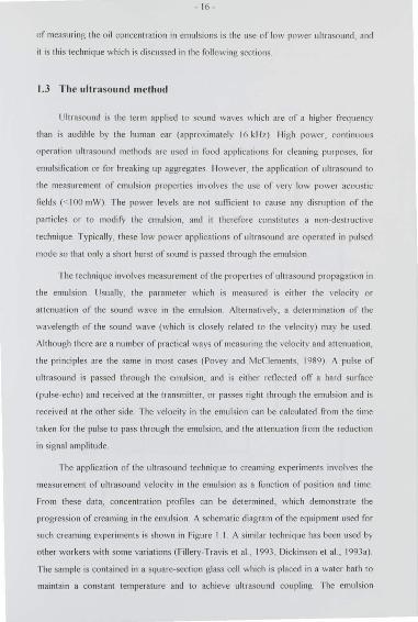
progression of creaming in the emulsion A schemat ic diagram of t he equipment used for
such creaming ex peri ments is shown in Figure 1 1 t\ similar technique has been used by
other workers with some variations (Fillery-Travis et a\ , 1993. Dick inson et al, 1993a)
The sample is contained in a square-section glass cell which is placed in a water bath to
maintain a constant temperature and to achieve ultrasound coupling The emulsion
Emulsion
I (] t
Transminer
Water
-~;7- -
I ([)--~ .t
Receiver
'U/ ~ Piezoelectric transducers
~~
Timer-counter
(
~
:=J
Computerised data
acquisition
Figure I. I Schematic diagram of the ultrasound scanner used to obtain concentration profiles in creaming emulsions.
- 18-
sample has dimensions of approximately 250 mm x 35 mm x 35 mrn Use of such a large ~
sample enables features tokseen which would be insignificant in a small sample The
thickness of cream formed depends on the volume of oil in the sample. and so a taller
sample produces a thicker cream layer
The piezoelectric tran!'ducers act as a tram:mi ller and receiver o f a pulse of low
power ultrasound w hich is passed th rough the cel l A timer-counter determines the time
o f night between the transmitter and receiver, which is recorded by comput er The
probes scan the height of the sample, taking measurement s at specified intervals The
diameter oft he p10bes is approximat ely 10 nun. and measurement s arc typica lly made at
5 nun height intervals The time-of-night measurement s are convert ed into the velocity of
ultrasound within the emulsion using standard equations of motion The path length of
sound inside the cell is determined by calibration with distilled water. for which the
velocit y is known precisely A sequence of such sca ns during the creaming process
provides data. which can be transformed into time dependent oil concentration profiles
The underlying principle in the use of ultrasound in emulsion measurement s is that
the measured properties of the ultrasound wave as it passes through an emulsion sample
(usually the velocity and attenuation in the emulsion) are related to the physical
characteristics of the emulsion Usually, the quantit y which is obtained from the
measurement is the concentration of the di spersed phase. In some circumstances, the
ultrasound properties may also be innuenced by particle size. and other contribut ory
factors In crystallisa tion studies. the ultrasound velocity meast11 ement is used to
calculate the proportion of the di spersed phase which is solid In many cases, a modified
version of the equation for the sound speed in a pure nu id is used The mod ified equation
is ca lled the Urick equation, and is given in chapt er 4 In order to calculate the dispersed
phase concentration from the sound speed in an emulsion using the Urick equation. the
densities and compressibilities oft he component phases mu st be known These are easily
measured (the compressibility can be determined from the sound speed in the bulk
component) Although the equation applies reliably to solutions. and is used as a
technique for investigating solution properties (Sarvazyan, 199 1 ). it is not always va lid in
emulsions In some cases where discrepancies have been detected in the use of the Urick
equat ion, the sound speed/ concentration relationship has been determined
experimentally by using a series of uniform emulsions of known concentration
- 19-
Several studies of creaming behaviour using the ultrasound technique ha\ e been
published in recent yea1 s An example of the results which ca n be obtained is shown in
chapter 2 (figure 2 24. Ma. 1995) for a sunflower oil in water emulsion contain ing
xanthan This figure, and other published results, illustrate the greater detail available
from the method when compa1 ed to visual creaming experi ment s The technique
therefore allows more fully the study of the interaction between fl occulation.
crystallisation and creaming Many studies of depletion flocculation present the
contrasting concentration profiles obtained wit h or without added polymer f-or exa mple.
the add ition of xanthan was found to increase the creaming rate very signifrcantly (Cao et
al , I Q9 1) and to produce a sharp serum interface which moves steadily up the system In
the absence of xanthan. creaming is much slower, and the serum is less clearly defined
At a much higher oi l concentration (50 wt %), the same study (Cao et al . 199 1)
de1nonstrated that the add ition of xanthan caused a serum region to develop ll owever.
the concentration in the rest of the emulsion remained mostly uniform, showing only a
gradual increase with time. I\ clear cream layer was not observed The result indicated
the gradual compression and rearrangement of the flocculated structure, ' squeezing' out
the continuous phase to form a serum This behaviour wou ld not be detectable by visual
creaming experiment s.
Emulsions containing polymer have been shown to exhibit \ ery complex creaming
behaviour (Gouldby et a! , 199 1) Concentration profiles were obtained using the
ultrasound technique. in the absence of polymer, and wit h a range of polymer
concentrations The concentration of polymer influenced the shape of the concentration
profrles in a variety of ways In some cases, the flocculated emulsion exhibited
monodisperse creami ng behaviour The serum interface was sharp and moved steadily up
the sample In a sample with a lower polymer concentration, the concentrat ion profiles
indicated that creaming was proceed ing as if two separate species were present
rapidly-creaming flocculated species, and unflocculated particles which creamed much
more slowly The floes creamed rapidly. leaving a low concent ration in the emulsion
which then creamed like an unflocculated emul sion This result was also seen in a later
study (Fillery-Travis et al . 1993) The measurements were also able to detect a change
in concentration in the cream region between samples of different polymer concentration .
This is an indication of the sparse nature of the floes formed and the effi ciency wi th
which they can pack together in the cream In addition, in some flocculated samples. the
-20-
concentration in the cream was found to be fairly uniform but became more concentrated
with time. as the cream was compressed into a more densely packed arrangement It was
particularly noted in one case that the creaming was not visible by eye until it was well
advanced. although the concentration profiles showed that considerable changes had
occurred
The development of a serum layer wit h a sharp interface has been seen in several
studies of nocculated emulsions. In some cases. the position of the serum int erface does
not move with time, as seen in the studies discussed above Instead , the interface
develops rapidly, but the crea ming rate is then reduced and can conti nue in a variety of
ways (Dickinson et al. 1993a, Dickinson et al. 1994) The addition or rhamsan to a
minert~l oil in water emulsion with Tween20 emu lsi fi er was round to cause creaming to
cease an er a senun layer had developed (Dickinson et al . 1993a) The system was
su ffi ciently concentrated (30 wt% oil) and noccu lat ed to prevent further movement In
contrast. the concentration profiles in mineral oil in water emulsions in the presence or
xanthan showed substantial changes with no corresponding change in senun interface
position (Dickinson et al. 1994) In some cases no cream development was observed At
a higher xanthan concentrat ion, a semm interface was ronned and remained in the same
position However, cream continued to develop and the concentration in the bulk or the
emulsion decreased wit h time
The development of a senun, wit h a sht~rp ly defined interface appears to be a
characteristic feature at low xanthan concentrations At higher concentrat ions of
xant han, creaming behaviour appears to be dominated by the cream development, and
the concentration profiles show a gradual increase throughout the rest of the emulsion
The addition of salt to the mineral oil in water emu lsions was round to innuence the
concentration profiles in the presence or xanthan (Dickinson et al.. 1994) At low
xt~ nthan concentrations, less serum development was observed, but at higher xanthan
concentrations, the emulsions appeared to be less stable when sa lt was added The
differences in concentration profiles under the difTerent condit ions hold infOrmation on
the processes occurring in the emulsion, for example the extent of nocculation, the
apparent floc size, etc. (see. for example, the analysis ofFillery-Travis et al . 1993)
The preceding sections have shown that the processes of creaming, flocculation
and crystallisation interact The use of an ultrasound technique enables detailed
-21-
information on the creaming behaviour to be obtained The object ive of the present work
was to understand more fully the physico-chemical factors behind the experimental
observations of creaming, flocculation and crystallisation made using the ultrasound
scanner There are two main aspects to the study: firstly, computer modelling of the
creaming process and the contributory effects of flocculation and crysta llisation, and,
secondly. the investigation of methods of interpretation of ultrasound measurements
Computer modelling of creami ng is intended to help understand the contributions of
various physical processes to the creaming behrwiour which is observed The study of
methods of interpreting ultrasound measurements aims to improve the ways in which
useful inform"tion can be extracted from ultrasound measurements on dynamic emu lsion
systems, to observe creaming, flocculation and crystallisation behaviour quantitatively
The various theories of ultrasound interpretation can also be tested using the computer
model , which provides fully-characterised data of concentration and particle size
variation
1.4 Computer modelling
The computer modelling of creaming behaviour in emu lsions is intended to
increase the understanding of the influences of the various contributory physical
processes This can be achieved by constn1ct ing a model of the emulsion including a
limited number of phenomena and interactions, to observe the individual effects of the
different factors Initially creaming alone was modelled . Later, the effects of
crystallisation and flocculation on creaming behaviour were considered in a limited way
The models have been designed for oi l in water emulsions, and initially the model was
tailored to the experimental technique of the ultrasound scanner Thus, the modelling
results could be directly compared with the observat ions of real emu lsions As will be
argued later, the size of the samples involved leads to a phenomenological approach to
the problem, rather than a model ofparticulate dynamics
Previous modelling of the phenomenon of creaming has mostly been concerned
with the inverse problem of sedimentation (in which the dispersed phase is more dense
than the continuous phase). The related field of fluidisation (in which an upward flow of
fluid is used to ' suspend ' particulate matter) has been the subject of analysis in other
cases. A. number of different approaches have been adopted by previous workers The
- 22-
early work of Kynch ( 1952) was concerned with the rate of fa ll o f the supcrnatant
inter face in a monodisperse suspension as sed imentat ion proceeded I le pro posed a
solution of the continuity equations by the method of characteri sti cs The mass balance
of particles could then be used to rehtt e the interface position to the dependence of
particle veloci ty on local concent ra tion The principles of this solution have been used by
many o ther later workers
The stune approach was applied to a polydisperse system by Stamatakis and Chi
Tien ( 1988) The suspension is assumed to comprise a number of zones of constant
concentration The int erfaces between the zones represent the upper limit of particles of
each size fraction The rate at which those interfaces fall is determined by the local
concent ra tion. according to an assumed relationshi p bet\\een particle creaming velocity
and concentration This relationship is obtained from previous analytical and empi rica l
studies A solution for the concentration in each zone and the speed of fall o f the zone
interfaces can be determined using the mass balance of particles between the zones
Special care is taken at the interface wi th the sediment , which grows with time. and
changes composition as the zone interfaces meet the sediment This is a relat ively simple
and effi cient process However, it does requi re assumptions. such as constant
concent ration in the sediment, with no compression lt is al so difficult to see how
diHUsion, or o ther forces on the part icles, could be included
An alt ernative met hod of solution, used by the same authors (S tamatak is and Chi
Tien, 1988. 1992), is to solve the continui ty equations for the local vo lume fraction o f
dispersed phase The velocity of the particles is determined by the local concentration,
aga in using a previously obtained correlation for creaming speed The solution of the
cont inuity equation is achieved by a finit e diH"erence technique on a one-dimensional
grid The compressive stress in the sediment can be included in this formulation,
assuming empirically determined relationships fo r the dependence of the stress on
parameters such as permeability The model is applicable to polydi sperse suspensions.
although o nly rnonodisperse and bidisperse systems were analysed
The finit e difference approach was also employed by Shih et al ( 1986, 1987), but
these workers solved the continuity and conservation of momentum equations fo r the
system The techniques previously described assume that the inertial effects and the
part icle acceleration can be neglected The mo tion of particles can therefo re simply be
- 23-
described by the creaming speed. which is obtai ned from the local concentration The
solution of the equations of motion (continuity and momentum equations) is more
general. and includes inert ia l and accelera tion eO'ects llowever. a number of constitutive
relationships are still requi red, for example fo r the dependence of the d rag force on a
particle with concentration Thus, it does no t avo id the need to use previously obtained
analytical or empirical relationshi ps Other fo rces can, however, be easil y included in this
scheme, through the momentum equation An applied electric fi eld, fo r example, exert s a
fo rce on charged particles
Shih et al (I 986) used the method of cha racteri sti cs to obtain the characteri sti c
solutions to the equations of mo tion These were then solved using a finit e diWerence
method The computtttional ex pense of the numerical analysis led them to mod ify their
model and neglect the inertial and acceleration terms in the equation of motion The
equations then reduce to a continui ty equation and a force balance equation, which is
essentially the same fo rmulation as used in the o ther methods (Kynch. 1952. Stanmtakis
and Chi Tien, 1988, 1992) The method of characteri sti cs and a finit e diWerence
technique were used to obtain the solut ion The model was also extended to polydisperse
systems (S hih. et al . 1987)
The general consensus in these analyses is to neglect inertial and acceleration terms
in the equations of motion The crit ica l component s of a phenomenological creaming
model are therefo re the mass ba lance of particles (continuity equa tion) and some
relationship for the rate of particle movement This may be determined th rough a
creaming speed, o r through a fo rce balance equation, if o ther fo rces are to be included
The creaming speed or drag force is related to the local concent rat ion of particles These
component s were present in the model of Zimmels ( 1988, 1992) Instead of solving the
equations of motion, however, the changes in concentration were modelled by the
cumulati ve displacement o r th in layers of particles The layers have a constan t thickness
and concentration The overlap of layers fo r different sizes of particles results in the
overall concentration profil e in the system. Alternati vely, Williarns and Amarasinghe
( 1989, 199 1) calculate the displacement of particles of each size fraction in o rder to
determine the change in local concentration In bo th of these models, the system is
defin ed as a set of ho ri zontal layers. within each of which the concentration is uniform
Techniques such as these, in which the en'ects of particle movement on local
-24-
concentration are calcu lat ed directly, are an alternative to solving the equations of
motion
The models of creaming which have been discussed in the preceding pamgraphs
are appropriate for a phenomenological description of the process Such an approach
enables direct comparison wit h the experimental results obtained from the ultrasound
scanner, for example. llowever, some microscopic processes are difficult to simulate in a
phenomenological manner The innuence of these processes can sometimes best be
understood by a simulatio n at the level of the individual particles The incorporation of
greater complexity and detail into a si mulation must inevitably be associated with a
reduction in the size of system which ca n be amtlysed, due to the limitations of
computational resources Thus, a particu\ate model can not reproduce the concentration
profiles obtained experimentally. but can only be used to indicate the anticipated effects
of va rious processes on creaming profiles This approach was applied in a later section of
the present work to understand the efl'ects of flocculation on creaming behaviour 1\
number of different approaches to particulate modelling are discussed in the following
paragraphs
The statistical mechanical characteristics of fluids have been studied for a number
of years using the well established technique of molecular dynamics The molecules in the
fluid are treated as if they exist in a vacuum, with their motion determined by the
intennolecular forces The definitive reference work in this area is by Alien and Tildesley
(1989) On colloidal length scales. where the particle sizes are of the order of 10' times
larger than molecular dimensions, a molecular simulation is impractical At this level,
continuum descriptions can be applied to the component fluids In particular, when the
Reynolds number is small (as is the case for most emulsions at rest), the continuous
phase fluid obeys the Navier-Stokes equations of motion An important simulation
technique which is designed for these conditions is Stokesian dynamics, or Brownian
dynamics Useful reviews of the technique are presented by Brady ( 1992) and Dickinson
( 1985) The intermolecular forces are replaced by effective forces between the dispersed
particles. and hydrodynamic forces which are mediated by the continuous phase fluid
The effect of co lli sions by continuous phase fluid molecules on the dispersed particles is
exhibited in an additional random (stochastic) motion of those particles This is
commonly called Brownian motion, and is simu lat ed by applying a stochastic force to the
particles
- 25-
The l3r ownian dynamics approach has been applied to the simulation of many
processes at the colloidal level, particularly to obtain rheological and difTu sional
properties References to many recent studies are given by Davis ( 1993) The formation
of gels and aggregates is an important area of Brownian dynamics simulation, in which
an interaction energy is applied between particles to cause them to st ick toget her For
example, a recent study by Bijsterbosch et al (1995) e'<ami ned the efTect of int erparticle
interactions on particle gel structure. ;\ simulation of sedimentation was carried out by
Ansell and Dickinson ( 1986), in which particles were added to the system one at a time
to observe the grow1h of a sediment I\ simulation of many-body sedi mentation by this
method wou ld require considerably more resources Brownian dynamics is therefore in
principle applicable to creaming and flocculation in an emulsion. but the calculation of
pairwise hyd rodynamic interactions in a many-body system is very computationally
demanding, and a simplified approach may be more appropriate
An alternative technique for including hydrodynamic interactions in colloidal
simulations is by the lattice-gas and latt ice-Boltzmann models The lattice-gas simulation
applies a lattice to the continuous phase fluid Each node of the lattice acts as a site
which can be occupied (or not) by a fluid · particle', with a given veloc ity These fluid
particles move between adjacent sites and collide wi th o ther particles according to
predefined mles to conserve momentum and energy The colloidal , dispersed phase
particles are introduced by defining boundaries, at which the lattice-gas particles interact
The interaction may be through a non-sli p condition, for example, resu lting in forces on
the colloidal particles The considerable statisti cal flu ctuations in the model require
spatial averaging to obtain meaningful result s. Although the standard method is time
consuming for dispersed systems, the more recent modification to the technique (lattice
Bolt zmann) improves its effi ciency considerably In this method, the earlier single
· part icle ' occupation of lattice nodes is replaced by the real-valued average number of
particles at the node with a given velocity The collision ru les are obta ined from the
corresponding lattice gas rules, but including the probability of such a collision
occurring, based on the local popu lations Thus, the lattice-Boltzmann method implicit ly
conducts the ensemble averaging process which is necessary wi th the lattice-gas
approach The application of the lattice-Bohzmann technique to colloidal dispersions is
relatively recent (see for example, McNamara and Alder, 1993, Ladd, 1993 , Yuan et al ,
1993) but may be a suitable method of simulation for creaming and fl occulation
-26-
A simplified approach to the dynamics of particle motion is to neglect the
hydrodynamic interactions altogether In addition, the system can be discretised spatially.
so that only a finite number of particle locations are permitted Particle movement is
therefore reduced to movement between the allowed sites Such techniques are usually
called lattice simulations since a lattice is appl ied to the system to define the permitted
particle locations This term should not be confused with the lattice-gas and lattice
Doltzmtuln techniques in which the lattice refers to the continuous phase molecular
properties, not to the locations of the co lloidal particles Movement is specified through
the diffusional (and creaming) properties of the particles. The bene £it of such simulations
is that relatively large systems can be investigated Although many physical interactions
are ignored in this description, the innuence of bonding energy between particles on
aggregate structure, for example. can successfu ll y be modelled (llaw et al . 1995)
Lattice models have been applied to the sedimentation problem (van der Knaap et al. ,
1994, lluang and Somasundaran, 1988), and are therefore appropriate for the study of
nocculation and creaming required in the present work
1.5 Ultrasound theory
The use of the ultrasound technique as a probe of emulsion behaviour was
discussed brieny in a previous section In particular, ultrasound has been used to
determine the detailed creaming characteristics of emulsions, somet imes in the presence
of nocculation or crystallisation The technique has also been applied to studies of the
kinetics of crystall isation and the detection of phase transitions in emulsions A crucial
element of the method is the determination of the dispersed phase volume fraction or the
solid fat content from the measurement of ultrasound velocity Measurements of
attenuation have been found to suffer from difficulties caused by diffraction and other
effects. whereas velocity measurements have been found to be more reliable
In colloidal systems, such ultrasound methods ofien operate in the long wavelength
region; that is, the wavelength of the sound wave is much larger than the particle size In
this case, Urick (1947) suggested that the Wood equation for the speed of sound in a
homogeneous fluid, could be modified to apply to dispersed systems (see chapter 4) The
density and compressibility are replaced by the volume averages of these quantities for
the dispersion Thus, the sound speed is related to the concentration of the dispersed
- 27-
phase Although thi s formulation has been adopted by rnany workers. significant
deviations have been observed experimentall y Several o ther approaches have been
applied to the problem of sound wave pro pagation in dispersed systems These range
from complex analytical treatment s of the scattering problem to proposed empirical
relationships between velocity and concentration with little phys ical basis Since it is the
long wavelength limit which is of interest here. sorne of these studies can be neglected,
such as the ray-tracing formulations of Pal ( 1994) and Bonnet and Tavlarides ( 1987)
The two major approaches to the problem seem to be multiphase hydrodynamic
methods, and scattering theories The multiphase continuum theories are based on the
equations of motion for nuid now in the dispersion, such as the multiphase continuity
and momentum equations The properties of the dispersion are trea ted as local volume
averages which therefore relates them to the local concentration of the dispersed phase
Additional properties are supplied th rough constitutive equat ions to include efl'ects such
as heat now between the phases, stress relationships and the enCcts of viscous drag One
such approach is descri bed in the review by I lark er and Temple ( 1988). with reference to
the work of Ahuja ( 1972, 1973) A more recent study on simi lar lines is that present ed
by Margulies and Schwarz ( 1994) This last study is fo rmulated o nly fo r very dilute
systems, due largely to the assumptions of dilute limit s fo r the hydrodynamic expressions
in the viscosity, for example
The scattering theory formulation is based on the analysis of the modificat ion of a
sound wave by a single particle, and the cumulative e!Tects of a dispersion of many such
particles A sound wave which is incident on a particle ini tiates scattered waves inside
and out side that particle, which interfere with the incident wave and modify its phase and
int ensity. Studies of the scatt ering characteristics of single particles are numerous, and
are di scussed in chapter 4 The effect of many such particles in a dispersed medium is a
more d ifficult prob lem One method, adopted by Gaunaurd and Uberall ( 1982, 1983) and
Gaunaurd and Wertman ( 1989) is the effective medium approach The scattering
properties of a spherical volume of the effective medium are defined to be equivalent to
the sum of the scattering characteristics of all the indi vidual particles within that volume
Multiple scattering of sound waves is omitted There is some discussion over the va lidity
of the effective medium approach and its relationship to multiple scattering theories
(Anson and Chivers, 1989, McClement s et al. , 1990b, Gaunaurd and Wertman, I 990)
- 28-
The multiple scatt eri ng approach is based on the determination of t he acoustic fi eld
which result s from the sca ttering and resca ttering of the incident wave by the dispersed
particles The result is usually expressed as an infinite series in the di!Terent scatt ering
modes (representing the difl'erent angu la r dependencies of the sca tt eri ng fie lds)
I lowever. the formalism is most appropriat e for the long wavelength regime. in which
the series can be tnmcated aOer only a few terms (corresponding to mo nopo le and dipo le
scattering) The major analytical studies are by Watenmm and Tmell ( 196 1 ). Fikio ri s and
Watennan (1964). Lloyd and Berry (1967). Ma et al (1984. 1990)
It is the multiple scattering theory solutions which are most widely used , and
therefore the present work is based o n this formulation of the ultrasound int erpretatio n
issue Experimental evidence (McC!ements and Povey. 1989) suggests that, at least in
some systems, multiple sca ttering theory accurately relates ultrasou nd ve locity to
concentrat ion However, o ther studies have found different relationships to be o f grea ter
accuracy in o ther experimental systems lt is npparent that confidence is not hig h that
existing scattering theories can be directly applied to determine dispersed phase
concentratio n from ultrasound velocity measurement s In addition, the calculations are
rather complicated and no t easy to implement for an experimental system The approach
taken in the present work, therefore, is to adopt the established theoreti cal basis of
multiple scattering theory, but to develop techniques by which it can be accura tely
applied in experimental systems
1.6 Objectives and preview
The study of creaming. nocculatio n and crystalli sat ion in emulsions has been
conducted throug h the two aspects of computer modelling and the investigation of
techniques for the interpretation of ultrasound measurement s The development o f a
computer model o f creaming in emulsions was intended to demonstrat e the en'ects o f the
contributory physica l processes on creaming behaviour llaving modelled the behaviour
of an emulsion in the absence o f particle interactio ns. the innuence of nocculation and
crystallisat ion on creami ng was also to be investigated In particular, the model was
intended to reproduce the concentration profiles observed experimentally Such a
correlatio n would indicate that the model o f the physical processes used in the comput er
simulation was a va lid description of the experiment all y observed creaming behaviour
-29-
Initially. a phenomenological approach to the modell ing of creaming was adopted,
so that comparison cou ld be made wit h experimental studies The overview of simulation
techniques presented in section I 4 illustrated that a particulate description of emulsions
on the sca les used in experi ment s is not possible at the current level of comput ational
resources flence a phenomenological description was used, and the model which has
been developed in the current work is presented in chapt er 2. Although this model
produced a good represent ation of creami ng behaviour in emulsions with no nocculation,
it was unable to reproduce the concentration profiles observed in nocculat ing systems
Hence. a second model was developed on a microscopic scale to examine the creaming
and nocculation behaviour at the level of individual particles. Thi s model is presented in
chapter 3.
Only with accurate and reliab le techniques of in terpretation can ultrasound be
applied as a valuable non·destructi ve probe of emulsion behaviour A number of theories
cw rently exist, and it was intended to establish which of these was the most appropriate
method for int erpreting ultrasound measurements, and under what ci rcumstances it
should be used In addition. the practical complica tions and difficulties associa ted with
the experimental application of multiple sca ttering theory. for example, needed to be
overcome_ The theoretical principles of multiple scattering theory arc considered to be
the most appropriate basis for the work, and the main results of the theory are presented
in chapter 4 In this chapter, the relationship between multiple scatt ering theory and
other, simpler formulae (such as the Urick equation) is also established. The range of
conditions under which the different theoretical result s can be applied is illustra ted both
in the theoretical investigation (chapt er 4). and through the results of the
phenornenological creaming model (chapter 2) The model was used to predict the
ult rasound velocity profil es anticipated by a number of ult rasound theories
Following a study of the ult rasound theories currently available, an attempt has
been made to develop methods which may be readily applied to a range of experimental
systems. The techniques which have been developed are based on the theoretical
principles of multiple scattering theory llowever, it was intended to circumvent some of
the difficulties of complexity and uncertainty associated with the established methods
which are outlined in chapter 4. The alternative methods which have been developed for
the inte1pretation of ultrasound measurement s are presented in chapter 5
- JO-
Cha11ter 2 : Phenomenological Modelling of Creaming
In chapter I, the study o f creaming in emulsion ~ was present ed as a means o f
investigating emulsio n stability and the effects o f nocculation and other processes The
objective o f the pheno rnenological comput er modelling was initially to develo p a model
o f creaming behav iour in an ideal o il in wa ter emul sion (in the absence of part icle
interactio ns) which would reproduce the concentra tio n pro fil es observed in p1actice
Such a model allows the contributio ns o f the diiTerent phys ical processes to be
investigat ed The effects o f crysta lli sa tion and nocculation o n creaming behaviour were
to be later included in the model 1t was intended to estab lish whether si mple models of
noccu latio n and crystall isatio n could ex plain the deviations fl o m ideal creami ng
behavio ur which have been observed experimenta lly In additio n to the study o f the
crea ming process, the comput er model was desig ned al so to assist in the investiga tio n o f
appro priate theories o f ultrasound pro paga tion The data produced by such a model oN
full y characte ri sed (in terms o f concentration and parti cle size va ri ation), and
representa ti ve o f rea l emul sio ns This a llows the different methods o f interpreta tion o f
ult rasound measurement s in creaming emulsio ns to be compared
Several widely difTering approaches to the modelling o f emulsio ns were discussed
in chapter I Fo r the compari son o f the computer model result s with experimental
measurements, a pheno meno logical approach was requi red A model o f an emul sio n o n
the scale used in creaming experiments can not trace the movement o f individual
particles, but mu st instead interpret the motio n in tenns o f changes in concentr atio n o r
other macroscopic quantities Previous modelling in thi s area has been applied to the
inverse problem o f sedimentation. o r to the related fi eld of nuid isa tio n (in which an
upward nux o f a carrier fluid is used to suspend heavier particles) The models o f
sedimentatio n due to Zimmels ( 1988, 1992) and Williams and Amarasing he ( 1989, 199 1)
were considered to be the most appropriate starting po ints for the creaming model
developed in this work Each assigns a sedimentatio n velocity to parti cles, ra ther than
solving the equatio ns of mo tio n fo r the whole system Zirmnels uses a set o f ho rizontal
"slabs" o f particles o f each size which move as a single unit The local enviro nment is
defined using an additio nal fi xed set o f layers to calculate a total, local concentration
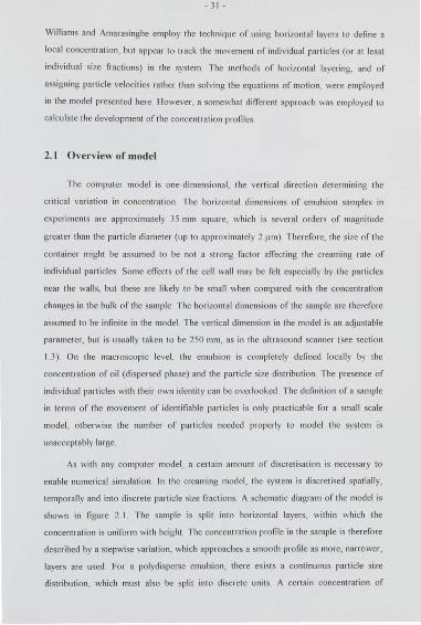
- 31 -
Williams and Amarasinghe employ the technique of using horizontal layers to defin e a
local concentration, but appear to track the movement of individual pa1ticles (or at least
indi vidual size fractions) in the system The methods of horizontal layering, and of
assigning particle velocities rather than solving the equations of motion, were employed
in the model presented here llowever, a somewhat difTerent approach was employed to
calculate the development of the concentration profiles
2.1 Overview of model
The comput er model is one-dimensional, the vertical direction determining the
critical variation in concentration The horizontal dimensions of emulsion samples in
experiment s are approximat ely 35 mm square, which is several orders or magnitude
greater than the particle diameter (up to approximately 2 ~tm) Therefore. the size of the
container might be assumed to be not a strong factor affecting the creaming rate of
individual particles. Some effects of the cell wall may be felt especially by the particles
near the walls, but these are likely to be small when compared with the concentration
changes in the bulk of the sample The horizontal dimensions of the sample are therefore
assumed to be infinite in the model The vertical dimension in the model is an adjustable
parameter, but is usually taken to be 250 mm, as in the ultrasound scanner (see section
1.3) On the macroscopic level, the emulsion is completely defined locally by the
concentration of oil (dispersed phase) and the particle size distribution The presence of
individual particles with thei r own identity can be overlooked The definiti on of a sample
in terms of the movement of identifiable particles is only practicable for a small scale
model, otherwise the number of particles needed properly to model the system is
unacceptably large
As with any computer model, a certain amount of discretisation is necessary to
enable numerical simulation In the creaming model , the system is di scretised spatially,
temporally and into discrete particle size fractions A schematic diagram of the model is
shown in figure 2.1 The sample is split into horizontal layers, within which the
concent ration is uniform with height The concentration profile in the sample is therefore
described by a stepwise variation, which approaches a smooth profile as more, narrower,
layers are used For a polydisperse emulsion, there exists a continuous particle size
distribution, which must also be split int o discrete units A certain concentration of
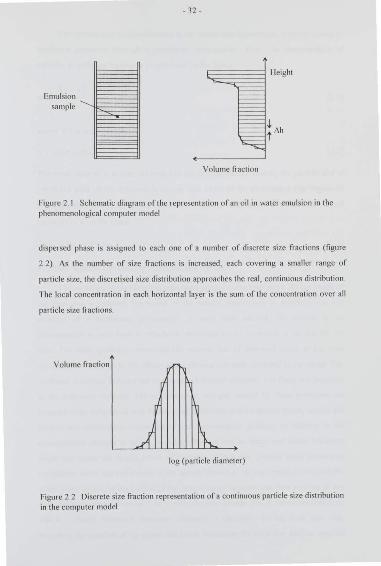
Emulsion sample
-32-
Volume fr action
Figure 2 I Schematic diagram o ft he representation of an o il in wa ter emulsion in the phenomenological computer model
d ispersed phase is assigned to each one of a number of discrete size fractions (fi gure
2 2) As the number of size fractions is increased, each covering a smaller range of
particle size, the discretised size distribution approaches the real, continuous distribut ion
The local concent ra tion in each horizont al layer is the sum of the concentration over all
particle size fractions
Volume fraction
log (particle diameter)
Figure 2 2 Discrete size fraction representation of a cont inuous particle size distribution
in the computer model
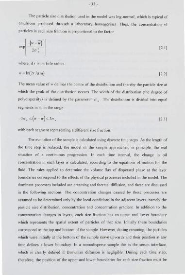
- 33-
The part icle size distribution used in the model was log-normal, which is typical of
emulsions produced th rough a laboratory homogeniser Thus, the concentration of
part icles in each size fraction is proportional to the factor
[+· ;;:)'] exp ----2a :
[2 I]
where, if r is particle rad ius
w = ln(2r fr tm) [2 2]
The mean value of w defines the cent re of the distribution and thereby the particle size at
which the peak of the distribution occurs. The width of the distribution (the degree of
polydispersity) is defined by the parameter a .. The distribution is divided int o equal
segment s in w, in the range
- Ja ,.. S (w - ~) S Ja ,. [2 3 J
with each segment representing a different size fraction
The evolution of t he sample is calculated using discrete time steps As the length of
the time step is reduced, the model of the sample approaches, in principle, the real
situation of a cont inuous progression. In each time interval, the change in oil
concentration in each layer is calculated, according to the equations of motion for the
fiuid The rules applied to determine the volume nux of dispersed phase at the layer
boundaries correspond to the effects of t he physical processes included in the model. The
dominant processes included are creaming and thermal diffusion, and these are discussed
in the foll owing sections The concent ration changes caused by these processes are
assumed to be determined only by the local conditions in the adjacent layers, namely the
particle size distribution, concentration and concentration gradient In addition to the
concentration changes in layers, each size fraction has an upper and lower boundary
which represent s the spatial extent of part icles of that size_ Initially these boundaries
correspond to the top and bottom oft he sample However, during creaming, the particles
which were initially at the bott om of the sample move upwards and their position at any
time defines a lower boundary In a monodisperse sample this is the serum int erface,
which is clearly defin ed if Brownian diffusion is negligible. During each time step,
therefore, the position of the upper and lower boundaries for each size fraction must be
- 34-
calcula ted The fo llowing sections discuss the physical processes in the emulsions which
determine the concentration changes in the layers and the movement of the boundaries
2_2 Physical processes included in the model
The equations of motion for a si ngle. continuous fluid are well known They can be
deri ved from the continuit y equation (conservation of mass) and conservat ion of
momentum (Newton's second law) and energy When the fluid veloc ity is very low, as is
the case in creaming, the inert ial terms in the equations can be neglected (since they are
second order in the fl ow speed) This is called the Stokes regime of fl ow, and
corresponds to a very low Reynolds number The equations of motion then take the
famous Navier-Stokes form In a multiphase system, the equations become more
complicated, but the appropriate modifications can be found in works such as Shih et al
( 1986), Roco ( 1992) and Gidaspow ( 1994) Additional consti tutive equations are
required, for example to obtain the drag force on each particle The equations of mo tion
are not reproduced here, since the phenomenologicalmodel does no t directly solve these
equations for the whole system Some workers have applied finit e difference or finit e
clement methods to obtain a solution to the equations of motion in the sample. llowever.
in the phenomenological model described here, the motion of the particles is defined in
terms of the contributing physical processes (creaming and diffusion), for which the
equations of mo tion have been solved separately The effects of the multi -particle nature
of the system are included implicitly in the numc1 ical model through the combination of
the creaming and diffusion properties of the individual particles, and through ensemble
averaged hydrodynamic effects
The dominant phys ical effects which occur in an emulsion, in the absence of direct
particle int eractions, are the g ravitational force, thermal diffusion, viscous drag and
hydrodynamic interactions The net effect of the g ravitational forces on a particle in an
oi l in wa ter emulsion is to cause creami ng, which is limited by the viscous drag exerted
by the continuous phase fluid The thermal energy oft he particles causes them to execute
random motion, again restricted by the viscous drag This is the effect of diffusion, which
acts to blur sharp concentration gradients At finit e concentrations, hydrodynamic
interactions between particles, i e . those that are mediated by the continuous phase fluid,
may also be significant The app lication of the equations of mo tion to these individual
- 35-
processes result s in expressions fo r particle movement which can then be applied in the
phenomenological model This approach avoids the need to solve the equations of
motion di rectly for the entire multi -phase sample
2.2.1 Gravity (creaming)
As Archimedes discovered, bodies immersed in a fluid experience an upward fo rce
(called the buoyancy force) due to the difl"erential pressure acting over the surface of the
body This fo rce slows the fall o f particles which are more dense than the surrounding
fluid , and causes particles which are less dense than the flu id to rise upw::trds or fl oat
The magnitude of the buoyancy fo rce is easil y deri ved for an isolated cylindrical object
(with it s axis vertica l) by considering the ex tra pressure acting upwards on the lower
surface of the cylinder due to the additional weight of nu id at this lower depth The
result is equally valid fo r spheres and irregularly shaped objects Archimedes principle
states that the upward fo rce due to the nu id is equal to the weight of nu id di splaced by
the object The net force due to gravity on an object submerged in a nu id is therefo re
pro portional to the density difference between the o bject and the surrounding nuid For a
sphere this takes the fo rm
F = i;rr g/J.p ' 3
12 4]
where r is the particle radius and Ap is the density difference between the dispersed and
continuous phases In an oil in water emulsion, the dispersed phase (oil) is less dense
than the continuous phase, and therefo re the particles tend to ri se to the top of the
sample (to fo rm a cream) The net gravitational force would tend to accelerate the
particle. but in a viscous nu id it s movement is restrained by the viscous drag exerted by
the surrounding nuid r or a sphere, the St okes drag is g iven by
[2 5]
where , is the particle's speed, and ' I is the viscosit y oft he surrounding nuid
Since the particle movement in the creaming of emulsions is within the Stokes
regime of now, the inertial te1ms in the equations of motion can be neglected For a
single, isolated, spherical, solid particle in an infinite nuid medium, a pa1ticle will
accelerate to a constant terminal velocity given by the balance of the gravitational force
(equation 2.4}, and the drag of the fluid on the particle (equation 2.5). Thus
-36-
12 6]
The resultant ve locit y is ca lled the Stokes velocity and is given by the equation
[2 7]
Equation 2 7 describes the speed at which a single oil droplet will rise to the top of the
emulsion (in the absence of any other emulsion droplets) lt ca n therefore be called the
creaming velocity The dependence oft he creaming velocity on the parameters of particle
size, densi ty difference and viscosit y is very important for the stabilisation of food
emulsions, as discussed in chapt er I The assumption of sphericit y and rigidity (infinite
viscos ity) for the particle are reasonably va lid for emulsion droplets coated with a
protective layer of emulsi fi er or protein (Walstra and Oortwijn. 1975) Crystallised fat
particles may not conform so well to this description, but a va riety of modifications are
av(lilable using shape factors to describe the non-sphericity
In reality, equation 2.7 is only the infinite time asymptotic limit of the particle 's
speed, as the acceleration decreases to zero and the force balance is approached
However, in a typical oil in water emulsion, the drag on the particle is sumciently large
that the time taken for the particle to accelerate to wi thin an accept ed tolerance or it s
tennin(ll velocity is negligible Therefore, the particle can be considered to move with its
terminal veloci ty at all times In the model, the environment or the particle chcmges as it
moves through the sample, and therefore its terminal velocity will also change However,
the time taken at each point for the particle to reach it s terminal veloci ty is negligible
compared with the time scale over which its environment changes significantly
Therefore, the model neglects particle acceleration and si mply attributes a terminal
creaming speed according to the local conditions
Equation 2.7 is va lid for an isolated particle in an infinit e nuid medium In a real
emulsion with a finit e concentration of dispersed phase particles, hydrodynamic
interactions become significant and introduce concentration-dependent factors into the
particles' speed The modifications to the creaming speed include the e!Tect of the
back now of the surrounding nuid , and the effect ive density and viscosity oft he emulsion
Such hydrodynamic effects are discussed in section 2 2 3 Although the overall
considerations oft he effect of particle size, viscosity and density difference are still va lid,
- 37-
the hydrodynamic interactions can resu lt in very different effect ive creaming speeds for
the panicles
2.2.2 Thermal diffusion
Thermal diffusion is a term for the random process ot herwise known as Brownian
motion The jittery mo tion of small specks of pollen on a pool of wa ter was observed by
Robert Brown in 1828 and was later attributed to the effect of random collisions of the
wa ter molecules by GoGy (see Dickinson, 1985) The random motion of the wa ter
molecules themselves is a result of their thermal energy Similar random motion occurs
on a colloidal scale in an emulsion due to the thermal energy of the oil droplets If a
particle is observed at various time intervals it can be seen to execu te a convoluted and
random motion, for example, the path shown in figure 23 It s true path is even more
convoluted but this represents a sample of its position at regular intervals of time
Figure 23 Thermal random walk
A possible two-dimensional random walk path traced by record ing a particle ' s position at
a sequence of time steps
In one dimension, if the particle is equally likely 10 move in eit her direction, the
average displacement from its original position must be zero However. it has a non-zero
root mean square displacement , which Einstein showed was g iven by
( ')'" " (z- z, ) = (2/Jt) [2 8]
where zo is the initial position and /) is a diffusion coefficient In three dimensions the
mean square displacement is simply three times as large, since there are three orthogonal
co-ordinates Thus, if the particle is initially at the origin,
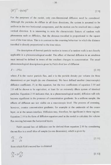
- 38 -
(!?')" = (6/Jr) " [2.9]
For the purposes o f the model, only one-dimensional diWusio n need be considered
Although the particles do diffuse in a ll three directio ns, the system is assumed to be
uniform in the two hori zontal component s, and the motion can be resolved int o a single
verti cal direction 1t is interesting to note the characteristi c feature of random walk
phenomena such as diffu sion, that the di stance travelled is proportional to the square
root of the time taken This is in contntst to the creaming behaviour in which the distance
travelled is directly proport ional to the time taken
The description of thennal particle mo tio n in terms of a randorn walk is not direct ly
applicable in a pheno rneno logical model The e rTect of thermal diffusion in an emulsion
mu st instead be defined in tenus of the resu lt ant changes in concentration The usual
pheno menological description is given by Fick's first law o f diffusion
.I = J)Vn [2 IOJ
where .I is the vector particle flu x, and 11 is the particle dens it y per volume (in th ree
dimensions) or per length (in o ne dimension) We have defined another (macroscopic)
dinl1sion coeffi cient,/), in this equatio n, but the two coefficients o f equa tio n 2 10 and
2 8 will be shown to be equivalent , at leas t for an ex tremely dilute system of identical
particles Equation 2 I 0 indicates that , in a phenomenological model, diffusio n will only
become significant in the presence of concentration gradients In a uniform sample, the
effects o f diffusion are not visible o n a macroscopic level The process of creami ng.
however, creates concentration gradients, fo r example at the underside o f the cream
layer, or at the serum interface. Diffusion may, therefo re, be significant in these reg ions
Equation 2 I 0 is the form of diffusio n equation used in the model to calcu lat e the volume
flu x moving between the ho rizontal layers
Fick's second law of diffusion can be derived from equation 2 _ I 0 by considering
the net nux in a small slice of sample (in one dimension), which is given by
[2 IIJ
fro m which Fick's second law is obtained
[2 12]
-39-
The application of this equation to the case of a sing le particle provides the link to the
random walk description The initial probability distribution function of a single particle,
whose position is known, can be described by a delta function . The "envelope" of the
par1icle ' s likely location spreads with time, approaching asymptotically a uniform
distribution in which the particle is equally likely to be at any position. Fick's second law
(equation 212) can be solved for the particle probability distribution function wit h the
boundary cond itions appropriate for a single particle which are given by
( ) { z >' z0 , 1= 0
11 z,t = 0 z~ ±:?:> , t ~ O
[2 13]
and the normalisation condition
J:"(z,t)dz = I [2 14]
where zo is the particle ' s initial position The resu lt for the probability di stribution of the
particle ' s position at any time is a Gaussian function centred on the particle ' s initial
position Thus
11(z ,t) = - 1 - exp(- (z :,)' ) J4;d)i 41!1
[2 15]
where /) is the dirfusion coefficient The root mean square displacement from the initial
position can be calcu lated by integration, resulting in equation 2.8, which arose from the
random walk description This demonstrates the link between the phenornenological and
random walk descriptions of dirfusion, and also that the dirfusion coefficients previously
defined in each case are equivalent for a single isolated particle
Although the phenomenological description of dirfusion given by equation 2 10 is
used in the model . it cannot be applied when the concentration g radient is not defined
This is the case at the upper and lower boundary of part icles (which initially correspond
to the top and bottom of the sample) These boundaries define the limit of particle
concentrat ion for each size fraction, and therefore represent a step-change in
concentration The concentration gradient at the step is not defined, and therefore
equation 2 . I 0 cannot be app lied, although it is known physically that diffusion wi ll blur
the sharp change in concentration . The effect of dirfusion on a step change in
concentration can be found using the probability distribution of the position of a single
-40-
particle, equat ion 2. I 5 In mathematical terms, the overa ll particle number density
distribution an er a given time is the convolution of the individual particle probability
distribution and the initial particle number density profile. On the microscopic level , the
distribution is the superposi tion of the random walk trajectories of a ll the individual
particles, whose starting positions are defined by the initial concentration profile_ If the
step change in concentration is at the origin, the initial particle number density profile is
constant in the negative half-space and zero elsewhere
n(z,O) = 110 for z :s; 0 0 for z > 0
[2 . 16]
The convolution of the two functions, equations 2 15 and 2 16, gives the probability
distribution of the number density of particles at time I Thus
11(z,t) ~ J 110 [ dz0 exp(j:___:J_)
4n:l)t ~ 4/)t
By substituting the dummy variable
zJz - z,) 4/)t
[2 17]
[2 18]
the distribution can be expressed in terms oft he complementary error function, giving
11 J' ( ) 11 { z ) 11(z,t) ~ !- ',. dZ cxp - Z' =-fer!< r.= VJT ,..~,-, ..;4/Jf
[2. 19]
where
2 J' erfc(z) ~ 1- erf(z) = .J,; , dZexp( z') 12 20]
The evolution of a step change in concentration with time is illustrated in figure
2.4, using equation 2 19 to calculate the concentration profile The initial sharp boundary
becomes more difTuse with time, as the particle distribution spreads out The boundary
can be defined as the position at which the concentration is some specified proportion of
the initial amplitude oft he step, i e
n(z,t} =a110 [2 .21]
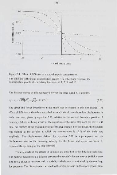
I 00
-. 0 75
~
= .:!
E 0 50
~ = e
0 25
0 00
-10 -5
-41-
' ' ' ' ' '. \
\ .... \ : ·, \.
·- .. :-.':''
0
' ·, ' ' ' '
z I ;1rbitnu·y units
Figure 2 4 Effect of di!Tusion on a step-change in concentration
The solid line is the initial concentration profile The other lines represent the concentration profile afier arbitrary time units of I, 2, 3, and 10
The distance moved by this boundary between the times 11 and 12 is given by
z, - z, ~ &J( 12 - t,)e•fc '(2a)
10
[2 22)
The upper and lower boundaries in the model can be related to this step change The
effect of diffusion is therefore embodied in an additional time-dependent displacement in
each time step, given by equation 2 22, relative to the current boundary position A
boundary defined as being at half of the amplitude of the initial step does not move with
time, but remains at the original position oft he step change_ For the model , the boundary
was defined as the position at which the concentration is 25% of the initial step
amplitude The displacement defined by equation 2 22 is superimposed on the
displacement due to the creaming velocity for the lower and upper interfaces, to
represent the spreading of the step interface
The magnitude of the effects of diffusion are embodied in the diffusion coefficient
The particle movement is a balance between the particle's thermal energy (which causes
it to move about at random), and its mobility (which may be restricted by viscous drag,
for example). The discussion is restricted to the isotropic case. In the more general case,
- 42-
the diffusion coeffi cient must be replaced by a tensor. In the Stokes regime of now, the
diffusion coeffi cient for a single, isolated, spherical particle is given by the Stokes
Einstein equation:
[2 23 ]
where ks is the Bo ltzmann constant and T is the abso lute tempera tu re DifTusion is
therefore strongest for the smallest particles, which ex perience less viscous drag
Conversely, the creaming velocit y is g rea test for the largest particles In the colloidal
size-range, diffu sion is significant (the import ance of thermal diffusion may be taken as a
defin ition of the co llo idal size range) The viscosity of the continuous phase is again a
determining fa cto r, as is the tempen\lure which defines the thermal energy of the
part icles
The St okes-Einstein equation fo r the diffusion coefficient (equation 2_23) is va lid
only for a si ng le, spherical particle in an infin ite fl uid medium This corresponds to the
conditions for the deri vation of the Stokes creaming velocity (equation 2 7) At finit e
concentrations, the diffu sion coeffi cient is modified due to the influ ence of the other
particles. The thermal motion can then no longer be described by a single coefficient and
is replaced by two d ifferent parameters The self-diffusion coefficient quan tifi es the
movement of a sing le labelled particle in a uniform environment. The nm/ua /-diOUsion
coefficient defines the movement of particles in the presence of inhomogenei ty such as
concentration g radient s (Dickinson, 1983) It is the second of these, the mutual-diffusion
coefficient which is o f relevance to the phenomenological model In the following
discussion the diffusion coeffi cient is assumed to be the mutual-diffusion coeffi cient
throughout
The modifications to the diffusion coeffi cient at finit e concentration are due to both
hydrodynamic and thermodynamic effects llydrodynamic interactions affect the particle
mobility, M, which may be defined by the veloci ty. U, att ained by a particle due to the
application of a steady force Thus
[2.24]
where the velocity refers to axes in which the mean volume flux of continuous and
dispersed phases is zero For the creaming problem the velocity is therefore relative to
- 43-
the container. The definition of the force, F • (in Batchelor's notation) is such that the
nux of dispersed phase is the same as if the particles are acted on by this force, and the
continuous phase experiences no force (Batchelor, 1976) The hydrodynamic effects on
particle mobi lity are discussed in the next section, since they are also relevant to the
creaming speed
The thermodynamic modification to the diffusion coefficient is introduced because
of the greater volume available for the particle to occupy at lower concentrations There
is therefore a statistical innuence which increases the probabi lity of a particle moving
down a concentration gradient The stat istical factor can be related to the concentration
dependence of the osmotic pressure or chemical potential Bat chelor ( 1976, 1983)
showed that the overall diffusion coefficient in a monodisperse system can be written as
IJ ~ M __j_(f'p) 1 - ~ ap
p.T
12 25]
where J-1 is the chemical potential per particle and q'l is the volume fraction Alternatively,
the coefficient can be expressed in terms oft he osmotic pressure, ll thus
u ~ M(an) On r.r
[2 26]
At low concentrations, the thermodyna mic factor in a monodisperse system is given by
[2.27 ]
(Batchelor, 1976) At higher concentrations, a more complete description is necessary,
such as that provided by the Carnahan-Starling equa tion (Sami-Selirn et al , 1993 , and in
approximate form in Glendinning and Russel. 1982), thus
[2 28]
The thermodynamic factor diverges as the concentration, ,P . approaches unity However,
it can be seen from the next sect ion that hydrodynamic effects dominate at high
concentration and prevent particle movement The diffusion coeffici ent therefore
-44-
decreases to 7Cro in a concentrated emulsion A useful review of the concentration
dependence o ft he dirTusion coefli cient can be found in Sami-Selim et al ( 1993)
2.2.3 llydrodynamic interactions
The deriva tio n o f the Sto kes creaming velocity. or the Stokes-Einstein diffu sion
coeffi cient assumed that there was a single isola ted particle moving in an infinite flu id
The situation is modified when the volume fractio n o f parti cles is finit e. due to
hydrodynamic interactions These are interactions between particles which are mediated
by the continuous phase flu id T he movement of a particle causes a corresponding flow
of the surro unding flui d, which. in tu rn. has an e lTect o n any neighbouring particles Thus
the movement o f any parti cle influences o ther parti cles throug h the reactio n o f the
surrounding fluid One o f the cont ributio ns to the hydrodynamic int eractions is the
back fl ow o f continuo us phase flu id (which occurs to conserve volume) llowever, there
are o ther cont ributio ns due to the velocity fi eld crea ted in the fluid by the particle
motion These are discussed in the dilute limi t by Batchelo r ( 1972)
A complete solutio n for the particle movement is theoretica ll y possible for a given
configuratio n o f particles, provided the fluid fl o w fi eld around a spherical particle is
known The complete equatio ns o f mo tio n for the flui d could be solved numerica ll y. but
this is not practi cal for a large-sca le model Progress is requi red l'ia analytical o r
empirical result s Experimenta lly, observa tio ns are made over time-scales which are very
lo ng compared wi th the time during which the system can ex plo re the many different
configurations o f pa11icle posi tio ns Therefo re, any measured properti es are effectively an
average over all pa rt icle configura tions The hydrodynamic interactions can thus be
ex pressed as ensemble averages, assuming the particles to be rando mly distributed They
can then be writt en as a functio n o f the concentratio n, rather than the particle
configura tio n
The hydrodynamic effects are incorporated into the particle mobil ity, which was
defined by Batchelo r ( t 976) in tenns of the veloci ty- force relationship, equation 2 24
This expressio n is valid for both diffusio n and creaming, showing the connect io n between
the hydrodynamic effects in each case. The fo rce on each particle due to gravity (when
the fluid is force-free) is given by equation 2 4 In Batchelor's definitio n, the density
difference is (as writt en) between the pa11icle and the continuous phase fl uid, rather than
- 45-
the suspension Thus, in a monodisperse suspension, the creaming speed (relative to the
container) is related to the mobility by
11 = i1rr'gtlpM 3
The diffusion coeffic ient was related to the mobility through equation 2 25
For a single, isolated, spherical particle, the mobility is given by
M =-l-6mlr
[2 29]
[2 30]
(from the Stokes drag law, equation 2 5) The mobility in a dispersion of finite
concentration may be written as
M = ~~~XI - ~) 6m1r
[2 31 J
where ~~~)is a hindrance factor The reasons for the choice of this form wi ll become
apparent later The creaming speed in a monodisperse suspension (equation 2 29) can
therefore be expressed in terms of the Stokes velocity of the particles (equation 2 7) and
the hydrodynamic factors (equation 2 3 1), thus
[2 32]
Simi larly, the diffusion coefficient in a rnonodisperse suspension can be written in terms
of the Stokes-Einstein coefficient as
[2 33]
(equations 2 3 1, 2 25 and 2 23)
Although Batchelor expresses all velocit ies relative to the zero-volume-nux axes
(which is the laboratory frame of reference in the creaming problem), other workers have
used a different reference frame Much work in this area has been involved with
Ouidisation, in which a volume nux of nuid is used to maintain the buoyancy of heavy
particles The usual frame of reference in this case moves with the mean velocity of the
continuous phase fluid. In other words, the frame of reference in which the mean flux of
continuous phase is zero The creaming speed of a particle in this frame of reference is
- 46-
denoted by the subscri pt (1 When the suspension is at rest in a container (as is the case
fo r creaming), the relationship between the fram es o f reference is given by
[2.34]
where a ll veloc it ies are posit ive upwards. The cont inuous phase velocity, u 1, can be
fo und by conserving the vo lume flu x crossing any horizont al plane. thus for a
mo nodisperse sample
[2 35]
so that the relative velocity is g iven in this case by
[2 36]
Thus
[2 37]
hence the reason for the choice o f the form o f the mobility in equatio n 2 3 1 Barn ea and
Mizrahi ( 1973) conclude that the result s o f previous workers, part icula rly Mertes and
Rhodes ( 1955) have demo nstra ted that onl y the rela ti ve velocity can be used to compare
result s from the different experimental processes (sedimentation, fluidi sation and others)
Barnea and Mizrahi discuss the relatio nship between the relative and absolute velocities
in each o f the dirferent methods The determinatio n o f the hydrodynamic e£fects has
therefore focused o n the hindrance facto r /~f/J) . mainly thro ugh the concentratio n
dependence of the creaming o r sedimentatio n velocity A very useful review is presented
by Williams and Amarasinghe ( 1989) o f the result s in the literature, and o nly the main
result s are drawn out here
Analytical result s fo r the hind rance factor are o nly accessible in the dilut e limit ,
mostly also for mo nodisperse systems The earli est attempts assumed either a regular
arrangement o f particles, o r that the flu id flow around each particle was confined within
a cell (usua ll y spheri cal ) where some boundary conditio n is applied T he first o f these
was by Srnoluchowski ( 19 13), who obtained the result
[2 38]

-47-
where .s is the interparticle spacing Each of these approaches predicts that the
sedimentation velocity varies in the form
[2 39]
in the dilute limit A review of these techniques and the results obtained can be found in
Happel and Brenner (1965) and in Barnea and Mizrahi (1973).
Later, the ensemble average of a random arrangement of particles was attempted,
first by Burgers ( 1941 , 1942), and later by Batchelor ( 1972) and Reed and i\nderson
(1976, 1980) These methods based on a random particle arrangement predicted that the
modification to the creaming velocity should be first order in concentration The
definitive work is considered to be that of Batchelor, who obtained the result
u ~ u,(l 65~) [2 40]
or as a hindrance factor
h(~) ~ (l -555~) [2 41J
Batchelor (1972) also discusses the difference between the ensemble average approach
and previous techniques with results of the form 2_39 li e attributes the difference to the
use in the earlier models of a characteristic length scale, usually the inter-particle spacing,
which is inversely proportional to the one-t hi rd power of concentration In a random
system, no one particle separation has any special significance lt is interesting to note
that Smoluchowski (who obtained the resu lt 2.38) commented that if the particles were
arranged at random, the leading order term in the third power of concentration would
vanish 1t is now generally accepted that the dilute limit should take the fom1 of equation
2.40, although the coefficient oft he concentra tion term varies somewhat
The analytical method becomes extremely difficult beyond the dilute limit, and
empirical and semi-empirical approaches have been used by later workers to obtain the
hydrodynamic interactions at higher concentrations Richardson and Zaki ( 1954)
suggested the use of a hindrance factor oft he form
1~1/J) ~ (I - _L)' [2.42] ~,~.
- 48-
which has the correct dependence in the dilute limit The parameter f/Jr ... k is a maximum
packing fraction, but is usually taken to be unity A variety of results for the coeffi cients
exist. from theoretical, semi-empirical and empirical investigations Many of these are
included in the review by Williams and Amarasinghe ( 1989) The general consensus is
that if (J"o<::t = I, the coeffi cient q is around 4 The most widely used va lue is that given by
Garside and AI-Dibouni ( 1977). q~4 . 1 (in the low Reynolds number limit), although they
produced a more complica ted formula valid fo r a wide range of Reynolds number An
alternative empirical correlation due to Dallava lle for a wide range of Reynolds number
has also been used in some sedimentation models (Williarns and Amarasinghe. 1989)
The o ther. very widely used correlation for the hindrance factor in a monodisperse
suspension was deterrnined by Barnea and Mizrahi ( 1973) .!.hey con1piled a senli
empirical relationship for the creaming velocity, which was fitt ed to many sets of
experimental data over a range of concentration and Reynolds number The form of the
relative velocity dependence was established by considering the component effects due to
modifications to the suspension density, viscosity and drag force These contributions
can be seen in the force balance equation used to derive the Stokes velocity (equations
2 4, 2 5 and 2 6) A consideration of the Stokes drag force also indicates the possible
source of the requirement to use the relati ve velocity in compari sons between
experiment s The Stokes drag is deri ved by considering the pressure acting on the
surface of a particle which is stationary in a uniform now of fluid The velocit y in the
drag force is therefore the relative velocit y between the particle and the surrounding flui d
at a large distance from the particle (whete the now is uniform if there is only one
particle) llence it appears sensible to use the relative velocity when defining the
concentration dependence of the drag force
The density difference in the gravit ational force is modified by using the suspension
density in the buoyancy component , rather than the density of the continuous phase. This
introduces a factor of
(1 - t/>) [2 431
The viscosity of the suspension was written in an exponential form, consistent with
earlier theoretical work (Barnea and Mizrahi include a review of previous work on
viscosity of suspensions) The coeffi cient s in the viscosity expression are determined
empirically. Finall y, they adopt a form for the additional hydrodynamic effects in the drag
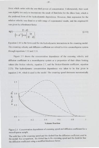
-49-
force which va ries with the one-th ird power of concent ration Unfortunately, their work
was slightly too early to incorpo rate the result of Batchelor for the dilute limit , which is
the preferred form of the hydrodynamic dependence_ llowever, their expression for the
relative velocity was fitt ed to a wide range of ex perimental result s, and the empirical fit
was given by a hindrance fa ctor
[2 44]
Equation 2 44 is the form used for the hydrodynamic interactions in the creaming model
The creaming velocity and diffusion coeffi cient are relat ed to it in a monodi sperse system
through equations 2 32 and 2 33
Figure 2 5 shows the concentration dependence of the creaming velocity and
diffusion coeffi cient in a monodisperse system as a proportion of their dilute limiting
values (the Stokes velocity. equation 2 7, and the Stokes-Einstein coeffi cient, equation
2.23 ) The hydrodynamic concentration dependence was taken to be that given in
equation 2 44, which is used in the model The creaming speed decreases monotonica lly
I 5
~ 1 0 ' " <::>
" ' " os
00
0
/ /
/ __ ,..... __ /
/
02
/
" " "
'·
' ' ' ' ' \
'·
\ \
\
\ \
\ \
\
' \ ' \ '. ' ''-... - ·r~-~- _,.,._ ~_ ~----___::'o.:.·::o-~---
0 4 06 08
Volu me fract ion
Figure 2 5 Concentration dependence of creaming speed and diffusion coefficient for a
monodi sperse sample
The solid ti ne is the creaming speed and the dashed line the diffusion coefficient used in the model For comparison, the dotted line is the creaming speed and the dash/dot line the diffusion coefficient usi ng a modified hindrance factor
-so-
to zero as the concentra tio n increases, which is due enti re ly to the hyd rodynamic
hind ra nce The diffusio n coeffi cient. however, init ia ll y fa ll s, but then increases with
increasing concentration, when the volume fraction is less than approxim rt tely 0 4,
becau se o f the sta ti sti ca l thermo dynamic effects lt then decreases rather steeply to zero
at high concentrations as tl1e hydrodynamic hindrance becomes predominant
f or comparison. fi gure 2 5 also shows the creami ng speed and diffusion coeffic ien t
w hich would be obta ined using the Richardson-Zaki fo rm for the hyd rodynamic
hindrance facto r (equation 2 _42) with <Prod =- 1 and the Batchelo r coeffi cient of q-::"555
The form o f the c reaming speed remains unchanged , a lthoug h the 13arnea-Mizrahi
version is somewhat steeper at low concent rations due to it s limiting dependence in the
o ne- th ird power of concentration However. the dini.1 sio n coeffi cient is very different
The peak va lue and the vo lume fractio n at w hich the peak occurs are considerab ly
alt ered by thi s change in the hydrodynamic term The fa ll in the diffusion coeffic ient at
the lowest concentratio ns is only seen with the Barnea-Mizrahi fo rm fo r the
hyd rodynamic hindrance_ This feature is due to the o ne- thi rd power concentratio n
dependence o f the hydrodynamic term at low concentrations lt has already been seen
that thi s is steeper than the correct , linear form for the dilute limit Hence, the drop in the
diffusion coeffi cient at low concent ra tio n is not a physical effect but is an artefact of the
hydrodynamic fo rm used The differences in the diffusion coeffi cient a ri sing fro m the
hydrodynamic components may cause a considerable degree o f uncertainty in the effects
of diiT'usio n in the c reaming model However. for consistency. the Barnea-Mizrahi
expressio n fo r the hydrodynamic hi nd rance was used fo r both the c reaming velocity and
the diffu sion coeffic ient
2.2.4 l'olydispersity
The result s o ft he previous section for the hyd rodynamic interactions are appli cable
to rno nodi sperse systems However. real emulsions a re polydisperse (even though in
some cases the size distribution may be very narrow), and it is therefore necessary to
determine the hydrodynamic effects in thi s case
Batchelor ( 1983) showed how the mobility formulatio n (equatio ns 2 24. 2 25 and
2 29) can be ex tended to a polydisperse system The hydrodynamic inte ractions now
include pai r-wise interactions between each combinat io n of partic le sizes The
hydrodynamic interact ions in the dilute limit fo r a polydisperse system were examined by
-51 -
Batchelor ( 1982) in terms oft he sedimentation velocity, and numerical results were g iven
(Batchelor and Wen, 1982) for some limiting cases of the nature of the polydispersity
and flow llowever, the case of a pauci-disperse system (in which there exists a range of
particle sizes around a mean va lue). which is the usual case in emulsions, does not appear
to be addressed directly, and the range of the reclet number for the creaming emulsions
does not appear to fall into the special cases When the density of all particles is the
same. the coemcients for a small range of particle size are very simi lar. and therefore the
hydrodynamic factor approaches the monodisperse case. using the total volume fraction
It is difficult to see how the dilute limit results might be extended to more
concentrated systems Davis and Grecol ( 1994) suggested a modification of the form of
the Richardson-Zaki expression for the monodisperse case (equation 2 42). using the
coefficient s calculated by Batchelor and Wen ( 1982) for the dilute limit However. the
numerical va lues for the coefficient s are not certain. as discussed in the preceding
paragraph Several workers have postulated modifications to the monodisperse hindrance
factors appropriate for polydisperse systems Mirza and Richardson ( 1979) included an
extra correction factor
[2 45 J
in the Richardson-Zaki equation for their bidisperse sett ling experiments Others
suggested the inclusion in the suspension density only of those particles smaller than the
particle whose velocity is being calculated (Selim et al , 1983). However, the
modifications adopted have mainly been empirical, with little assessment of the
applicability to a general polydisperse suspension
The formulation for polydispersity used in the present model has been adopted
previously by several workers in sedi mentation modelling (Stamatakis and Chi Tien,
1992, Zimmels, 1983 , 1988, Williams and Amarasinghe, 1989. 199 1) The hyd rodynamic
effects are considered to be due to the overa ll flow of particles and are thus related to the
total concentration, rather than to the detailed particle size distribution The
hydrodynamic factors derived for monodisperse systems can then be applied to the
relative velocity in the polydisperse case, using the to tal dispersed phase concentration
Equation 2.37 is valid for each individual component, giving
[2 46]
-52-
for the relative velocity of a particle of size fraction r The conservation of volume nux in
the laboratory frame can be used to calculate the continuous phase velocity. and thereby
the particle velocity relative to the container. Thus
[2 471
Substi tutio n of the solution for the nu id veloc ity into a polydisperse version o f equation
2 34 leads to
[2.48]
Multiplicatio n by the concentration of species i followed by summatio n over all particle
species leads to
[2 49]
whence the absolute particle velocity of species i can be obtained
[2 .501
This is the form used in the model for the polydisperse emulsions The hindrance factor
used in the relative velocity (equation 2.46) was the Barnea-Mizrahi formulation, 2 44
A form for the di£fusion coeffi cient in a concentrated polydisperse suspension has
not become available Batchelor (1983) gave general result s for the diffusion and cross
diffusio n coeffi cients but these include complica ted expressions in the chemical po tential ,
dependent on the interactions between particles The monodisperse form of the diffusion
coefficient and the diffusive flu x was therefore used in the model , using the total vo lume
fraction The diffusive flux fo r each size of pa11icle is given by equation 2 10, using the
concentration gradient of particles of that size Thus
.I; =-1),'1111, [2 .5 IJ
The diffusion coefficient is given by equation 2 33 , wi th the Stokes- Einstein coefficient
for the correct particle size. and using equation 2 44 for the hydrodynamic hindrance
factor (using the to tal volume fraction) The thennodynamic factor is calculated from
equation 2 .28, also using the to tal vo lume fraction Although this is not an exact result
-53 -
for diffusion, it is the creaming velocity which should be dominant in the model , and
therefore the precise concentration dependence of the diiTusion coeffic ient is of
secondary importance
2_3 Time evolution
The sample is initially uniform in terms of concentration and particle size
distribution . The evolution of the concentration profile is modelled by calcula ting the
concentration changes in the horizontal layers and the movement of the upper and lower
limits of each size fraction in a series of small time steps The processes affecting these
contributions have been discussed in the previous sections, and now the application of
these results in the model is detailed
2_3_1 Calculation of change in concentration at layer boundaries
The volumetric flux of dispersed phase particles crossing the boundary between
adjacent layers is calculated in each time interval. There are two contributions, due to
creaming and diffUsion . The flux in both cases is determined entirely from the local
environment (that is the concentration and particle size distribution in the two layers)
The total volume fraction at the interface is taken to be the average of the volume
fraction in the two layers The hydrodynamic hindrance factor is calculated from this
average total concentration using the Barnea-Mizrahi relation, equation 2 44 The
creami ng velocity of particles of each size fraction is determined by equations 2 46, and
2.50 The diffusion coefficient is calculated using equations 2.33, and 2.28, again using
the total average concentration
The volumetric flux of particles of size fraction i due to creaming, is proportional
to their velocity and the local concentration of particles of that size, thus
[2 52]
For diffusion, the flux is proportional to the concentration gradient , equation 2.51 ,
t." ; - D (</> ,_, . </> ,,, ) t!t 'f' .. d,fl ' 6h 6h
[2 53]
-54-
where the difference in concentra tion is for particles of the same size fraction between
the two layers Both of these nuxes have been defined as positive in the upward
direction
2.3.2 Doundary velocities for each size fraction
The lower and upper limits of particles of each size fraction are defined as
boundaries, which move with a veloci ty determined by the local conditions In the
absence of diffusion. the boundaries move wi th the local creaming velocity of particles of
the same size_ Diffusion causes the change in concentration at these limits to become less
well defined as time progresses This effect is modelled using an additional boundary
velocity, which was derived from the evolution, due to difTusion, of a step-change in
concentration The ext ra displacement of the boundary was defined in equa tion 2.22 In
the model , the boundary was defined as the position where the concentrat ion is 25 % of
the initial concentration, which gives an extra time-dependent velocity of
[2.54]
2.4 Choice of discrete units
2.4.1 Layer thickness
The layer thickness, ~h , must be small enough to represent accurately any regions
of rapidly varying concentrat ion, and to avoid a significantly stepped elTect in the
concentration profile. Creaming experi ment s using the ultrasound scanner (figure I I)
have a resolution of I nun and the creaming model ought to have at least as fin e
divisions The layer thickness is reduced in size (for the same overall sample height) until
there is no significant dilTerence in the concentration profiles and ultrasound veloci ty
profiles obtained For polydisperse samples, a layer thickness of0.5 mm was found to be
sufficient, but for monodisperse samples, in which the concentration gradients can be
much larger, better accuracy was obtai ned using a layer thickness of 0 25 mm This may
also be true for a polydisperse sample when there is no dilTusion, and the concentration
gradients again become steeper
-ss-
2.4.2 Time inlen•al
The time interval, flt , used in the model is not fixed in an absolute manner In
order for the model to produce accurate results, the volumetric flux crossing a layer
boundary during any time step must not be a large proportion of the volume of particles
in the layer Otherwise the conditions in the layer at the beginning of the time step, which
were used to calculate the flux, are not truly representative of the conditions during the
whole time interval One way of ensuring sufficient ly small changes in each time step is
to define the time interval in terms of the largest distance which could be travelled by a
particle in a single time step, as a proportion of the layer thickness. The fastest particle
speed is the Stokes velocity for the largest particles in the sample. The actual particle
speed will be significantly lower than the Stokes velocity due to hydrodynamic hindrance,
but the Stokes velocity can be used to set an upper limit The time step is therefore
defined by
M = a~ [2 .SS] 11rnu
Thus in one time step, no particle can travel further than a proportion a of the layer
thickness 1t was found that a value of a = 0.5 was sufficient to obtain consistent
concentration profiles A maximum time interval of I 0 minutes was specified
2.4.3 Size range in each size fraction
The continuous particle size distribution is split into discrete size fractions as
shown in figure 2 2. 1t was chosen to restrict the distribution to three standard deviations
either side of the mean, as given in equation 2.3. The number of size fractions therefore
defines the range of particle size assigned to a single size fraction . This is especially
significant at the larger particle size limits, where the same interval (on the logarithmic
scale) represents a wider range of particle sizes. Also, since the creaming velocity is
proportional to the square of particle size, the difference in speed between the smallest
and largest particles in the size fraction is greatest for the largest particle sizes The
concentration profiles are step-like, with each step corresponding to the lower boundary
of the particles of a given size fraction As the number of size fractions is increased, the
volume fraction of particles assigned to the size fraction is reduced, and the steps in the
total concentration profile decrease in size, until the profile is smooth Also, the
-56-
diH'erence in position of the lower boundary between consecu ti ve size fractions dec1eases
as the number of size fractions is increased The number of size fractions used in the
model was 10 1, which was found to be suOicient to obtain acceptably smoot h
concentration pro fil es
2.5 Comlmter req uiremen ts
The computer code was written in FORTRA N 77 . The development was carri ed
out on the Sun SPARCent er 2000 system, and jobs were n.m on the Silicon Graphics
Challenge XL server at the Universi ty of Leeds A fl ow diagram of the calculation is
shown in rigure 2 6, and the program is given in Appendix A I The polydi sperse
sunflower o il in wa ter samples take approximately 2 days of CPU time to complete The
monodisperse samples are much faster
2.6 Ult rasound velocity and a ttenua tion ca lculations
One oft he objectives of developing the computer model was to provide data which
would be representati ve of rea l creaming emu lsions. in o rder to compare different
theories for interpreting ultrasound veloci ty measurements The data from the model are
completely characteri sed in terms of the concent ra tion and particle size distribution,
whereas any experimental system includes unknown variables, particularly height
dependent changes in part icle size di stribution To this end, the calculation of ultrasound
velocity, using multip le scattering theory and the Urick equat ion, was incorporated into
the creaming model The different theories of ult rasound propagation are di scussed in
chapter 4, along with a descri ption of the computer program used to calculate the
ultrasound veloci ty and attenuation The programs have been o rganised so that the
ult rasound veloci ty pro files in the creaming model can be obtained using the separate
ultrasound calculation subroutines. The ultrasound program need only be invoked when
the model result s are output , to obtain the ult rasound veloci ty and attenuat ion fo r the
part icle size distribution in each layer.
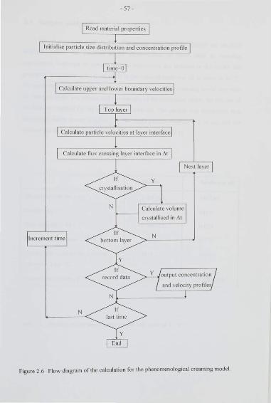
-57 -
Calculate particle veloci ties at layer interface
N
Figure 2.6 Flow diagram of the calculation for the phenomenological creaming model.
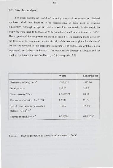
-58-
2. 7 Samples analysed
The phenomenological model of creaming was used to analyse an idea li sed
emulsion, which was intended to be representati ve of those used in creaming
experiment s Although no specific particle interact ions are included in the model , the
properties were taken to be those of 20% (by volume) sunflower o il in water at 30 oc The properties of the two phases are shown in table 2 I The creaming model uses o nly
the densities of the two phases, and the viscos it y of the continuous phase, but the rest of
the data are required fo r the ultrasound calculations The part icle size distribution was
log-normal, and is shown in fi gure 2 7 The mode particle diameter is 0 .56 ~1m , and the
width of the distribution is defin ed by a . = 0.5 (see equation 2 I)
Water Sunflower oil
Ultrasound velocity I m s·1 1509. 127 1437.86
Densi ty I kg m._l 995 65 9 12.9
Shear viscosity I Pa s 0 0007973 0 054
Thermal conductivity I J m·1 s·1 K-1 0 6032 0 170
Speci fi c heat capacity (at constan t 4 178 2 1980 0
pressure) I J kg· ' K· '
Thermal expansivity I K-1 0.00030 1 0 0007266
Table 2 1 Physica l properties of sunflower o il and water at 30 oc
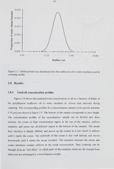
-59-
0 025 c
·e " 0 020 ..:: e ~
0 0 015 > -;; 8
0 0 10 ... 0
c 0
t 0 005 0 c. e
0..
0 000
0 0 1 0 10 I 00 10 00
lhdius/ J.un
Figure 2 7 Initial particle size distribution for the sunflower oi l in water emulsion used in creaming model
2.8 Results
2.8.1 Total oil concentration profiles
Figure 2.8 shows the predicted total concentration of oil as a function of height in
the polydisperse su nflower oi l in water emulsion at various time int ervals during
creaming The corresponding profiles for a monodisperse sample (with particle diameter
056 pm) are shown in figure 2.9. The bottom of the sample corresponds to zero height.
The concentrat ion profiles of the rnonodisperse sample can be divided into three
sect ions· the cream (a high concentrat ion region at the top of the sample), uniform
emulsion, and serum (an oil-deficient region at the bottom of the sample) The serum
layer interface is sharply defined, and moves up the system at a rate which is uniform
until it meets the cream The underside of the cream is also well defined. and moves
downwards until it meets the serum interface. The emulsion between the serum and
cream interfaces remains uniform at the initial concentration Thus creaming can be
thought of as an "end effect" in which parts of the emulsion which are far enough from
either end are unchanged in a monodisperse sample
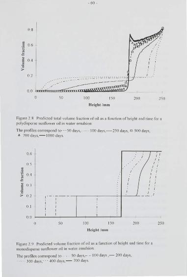
-60-
0.8
c 06 ·E
" .:: " E 0.4 ~
0 >
0.2
00
0 50 100 I SO 200 250
I I eight /mm
Figure 2 8 Predicted total volume fraction of oil as a function of height and ti me for a polydisperse sunnower oi l in water emulsion
The profi les correspond to· · ·50 days. · · I 00 days,- 250 days, o 500 days, A 700 days, - I 000 days.
06 1 1
0.5 /
c
·5 04 " .:: e 03 ~
I ,. I.
I I I j I I I I I I
I .-.----,---~---...;-J-'---'--- _!_ . I 0 > 02
0.1
0.0
0 50 100 I SO 200
ll eight /mm
Figure 2.9 Predicted volume fraction of oil as a function of height and time for a monodisperse sunflower oil in water emulsion
The profi les correspond to 50 days,-- I 00 days ,- 200 days, 300 days; · · 400 days,- 700 days
250
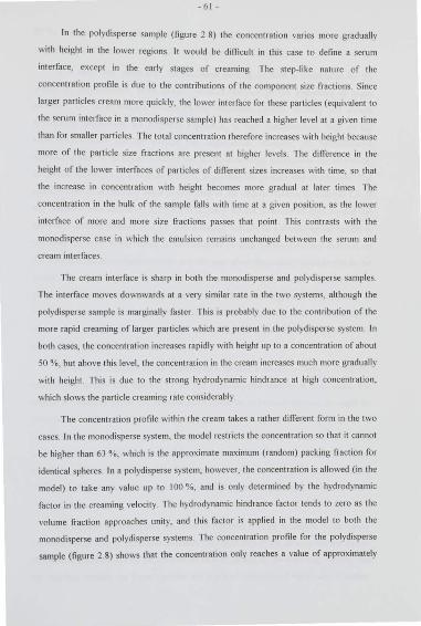
-61-
In the polydisperse sample (figure 2 8) the concentration varies more gradually
with height in the lower regions It would be difficult in this case to define a serum
interface. except in the early stages of creaming The step-like nature of the
concentration profile is due to the contributions of the component size fra ctions Since
larger particles cream more quickly, the lower interface for these particles (equivalent to
the serum interface in a monodisperse sample) has reached a higher level at a given time
than for smaller particles The total concentration therefore increases with height because
more of the particle size fractions are present at higher levels. The difference in the
height of the lower interfaces of particles of different sizes increases with time, so that
the increase in concentration with height becomes more gradual at later times The
concentration in the bulk of the sample falls with time at a given position, as the lower
interface of more and more size fractions passes that point This contrasts with the
monodisperse case in which the emulsion remains unchanged between the serum and
cream interfaces
The cream interface is sharp in both the monodisperse and polydisperse samples
The interface moves downwards at a very similar rate in the two systems, although the
polydisperse sample is marginally faster. This is probably due to the contribution of the
more rapid creaming of larger particles which are present in the polydisperse system In
both cases. the concentration increases rapidly with height up to a concentration of about
SO%, but above this level , the concentration in the cream increases much more gradually
with height This is due to the strong hydrodynamic hindrance at high concentration.
which slows the particle creaming rate considerably
The concentration profile within the cream takes a rather different form in the two
cases. In the monodisperse system, the model restricts the concentration so that it cannot
be higher than 63 %, which is the approximate maximum (random) packing fraction for
identical spheres In a polydisperse system, however, the concentration is allowed (in the
model) to take any value up to I 00 %, and is only determined by the hydrodynamic
factor in the creaming velocity The hydrodynamic hindrance factor tends to zero as the
volume fraction approaches unity, and this factor is applied in the model to both the
monodisperse and polydisperse systems. The concentration profile for the polydisperse
sample (figure 2 8) shows that the concentration only reaches a value of approximately
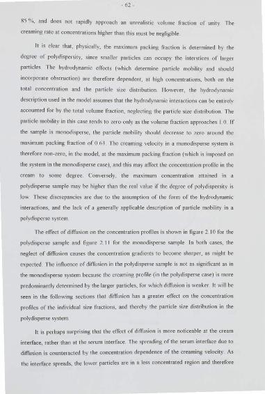
-62-
85 %. and does not rapidly approach an unrealistic volume fraction of unit y The
creaming rate at concentrations higher than this must be negligible
lt is clear that, physically, the maximum packing fraction is determined by the
degree of polydispersity, since smaller particles can occupy the interstices of larger
particles The hydrodynamic effects (which determine particle mobility and should
incorporate obstmction) are therefore dependent. at high concentrations, both on the
total concentration and the particle size distribution However, the hydrodynamic
description used in the model assumes that the hydrodynamic interactions can be entirely
accounted for by the total volume fraction. neglecting the panicle size distribution The
pa11icle mobilit y in this case tends to zero o nly as the volume fraction approaches 1 0 If
the sample is monodispersc, the particle mobility shou ld decrease to zero around the
maximum packing fraction of 0 63 The creaming velocity in a monodisperse system is
therefore non-zero. in the model . at the maximum packing fraction (which is imposed on
the system in the monodisperse case), and this may affect the concentration profile in the
cream to some degree Conversely. the maximum concentration attained in a
polydisperse sample may be higher than the real va lue if the degree of polydispersity is
low These discrepancies are due to the assumption of the form of the hydrodynamic
interactions, and the lack of a genera ll y applicable description of particle mobility in a
polydisperse system
The effect of diflUsion on the concentration profiles is shown in figUie 2 I 0 for the
polydisperse sample and figure 2 11 for the monodisperse sample In bot h cases, the
neglect of diffusion causes the concentration gradients to become sharper, as might be
expected The innuence of diffusion in the polydisperse sample is not as significant as in
the monodisperse system because the creaming profile (in the polydisperse case) is more
predominantly determined by the larger particles, for which diffusion is weaker It will be
seen in the following sections that diffusion has a greater effect on the concentration
profiles of the individual size fraction s, and thereby the particle size distribution in the
polydisperse system
It is perhaps surprising that the effect of diffusion is more noticeable at the cream
interface, rather than at the serum interface The spreading of the serum interface due to
diffusion is counteracted by the concentration dependence of the creaming velocity As
the interface spreads, the lower particles are in a less concentrated region and therefore
08
" ·E o 6
" .:: 1! o 4 = 0 :>
02
-63-
50 100 150 200
Height /mm
Figure 2 I 0 Effect of diffi1sion on the total concentra tion profiles after 250 days in a polydisperse sunflower oi l in water emulsion.
The solid line includes diffi1sion The dotted line is when diffusion is neglected
06
05
" ·E 04
" .:: 1! 03 = 0 :> 02
01
00
. I :, :,
.I .'I 1 I 1: 1.' 1: I' '-:
250
0 50 100 150 200 250
lleight /mm
Figure 2. 1 1 Effect of diffusion on concentration profiles in a monodisperse sunflower o il in water emulsion.
The dashed and solid lines are the concentration profiles wi th diffusion included after 200 and 400 days respectively. In the absence of diffusion the profiles are the dotted and dashed/dotted lines respectively
-64-
cream (upwards) more quickly Particles which are hig her up the interface have a smaller
creaming velocity due to the stronger hydrodynamic hindrance in this more concentrat ed
region The spreading of the boundary region due to diffusion is therefore st rongly
restricted by the sharpening of the boundary due to the concentrat ion dependence of the
creaming velocity At the cream interface, the hydrodynamic hindrance reduces both the
diffusion and creaming rates However, the diffusion coefficient includes an additional
statistical factor (section 2 2 2) which increases at higher concentrat ions Although the
diffusion coefficient decreases to zero at high concentrat ions, it does so more slowly th tm
the creaming speed, due to the statistical factor (see figure 2 5) The effects of diffusion
are therefore proportionately greater in the cream region, and so the concentration
gradient at the cream interface is reduced
The total concentration profiles predicted by the model can be compared with
experimental results Many of the experimental systems studied do not fit into the
idealised assumptions of the modeL since they include particle interactions (electrostatic
interactions, for example) or there is some degree of flocculatio n Experiment s carried
out by Fillery-Travis et al ( 1993) o n alkane in water emulsions were thought to be
reasonably ideal (no particle interactions) The emulsifier was the non-ionic surfactant
8rij35 and no additional polymer was included The alkane was a 9 . I mixture of heptane
and hexadecane, with a density of 643 0 kg m·1
This density has been derived from the
stated percentages by weight and vo lume of the emulsions The experiments were
conducted at 20 °C, at which temperature the density and viscosity of water are
998 .2 kg n,-' and 0 001 Pa s respectively (Kaye and Laby, 1986) The particle size
distribution appears to be rather positively skewed, but a si milar log-normal size
distribution was used in the model. wit h a modal diameter of 1.4 pm and a width of
u .. = 0.5 The predictions of the model , and the experimental concentration profiles are
shown in figure 2 12
The form of the concentrat ion profiles predicted by the model below the cream
region compares well with the experimental results . However, the creaming rate is more
rapid experimentally than in the model , especiall y at early times This may be due to the
form o f the hydrodynamic hindrance used in the model, which perhaps overestimates the
reduction in creaming speed due to the other particles In the cream region, the shape of
the concentrat ion profiles differs markedly between model and experimental resu lt s The
sharp change in concentrat ion gradient in the cream occurs at a much higher
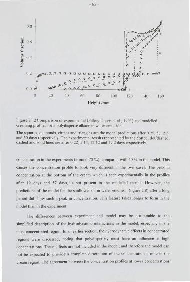
-65-
08
-~ 06
" c e = 04 0 ;>
0.2
00
0 20 40 60 80 100 120 140
lleight /mm
figure 2 12 Comparison of experimental (Fillery-Travis et al , 1993) and modelled creaming profiles for a polydisperse alkane in water emulsion
160
The squares, diamonds, circles and triangles are the model predictions afler 0 25, 5, 12 .5 and 50 days respectively. The experimental results represented by the dotted, dot/dashed, dashed and solid lines are aOer 0.22, 5.14, 12 12 and 57 2 days respectively
concentration in the experiments (around 70 %), compared with 50% in the model This
causes the concentrat ion profile to look very different in the two cases The peak in
concentration at the bottom of the cream which is seen experimentally in the profiles
afler 12 days and 57 days, is not present in the modelled results . However, the
predictions of the model for the sunflower oil in water emulsion (figure 2 8) afler a long
period did show such a peak in concentration This feature takes longer to form in the
model than in the experiment
The diiTerences between experiment and model may be attributable to the
simplified description of the hydrodynamic interactions in the model , especially in the
most concentrated region. In an earlier section, the hydrodynamic eiTects in concentrated
regions were discussed, noting that polydispersity must have an influence at high
concentrations These eiTects are not included in the model , and therefore the model can
not be expected to provide a complete description of the concentration profile in the
cream region The agreement between the concentration profiles at lower concentrations
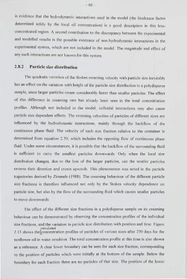
-66-
is evidence that the hydrodynamic interactions used in the model (t he hindrance factor
determined solely by the local oi l concentration) is a good description in this less
concentrated region A second contri bution to the discrepancy between the experimental
and modelled results is the possible existence of non-hydrodynamic interactions in the
experimental system, which are not included in the model The magnitude and effect of
any such in teractions are no t known fo r this system
2.8.2 Particle size distribution
The quadrati c va ria tion of the Stokes creaming veloci ty with particle size inevitably
has an e£fect on the variation with height of the particle size distribution in a polydisperse
sample, since larger particles cream considerab ly faster than smaller part icles. The effect
of this difference in creaming rate has already been seen in the to tal concent ration
profil es Although no t included in the model, colloidal interactions may also cause
part icle size dependent effects The creami ng veloci ties of particles of different sizes are
influenced by the hydrodynamic interactions, main ly through the back fl ow of the
continuous phase fl uid The velocity of each size fraction relative to the conta iner is
determined from equation 2 SO, which includes the opposing fl ow of cont inuous phase
fluid . Under some ci rcumstances, it is possible that the back flow of the surrou nding flu id
is sufficient to carry the smallest particles downwards Only when the local size
distribution changes, due to the loss of the larger particles, can the smaller particles
reverse their di rect ion and cream upwards This phenomenon was noted in the particle
trajectories deri ved by Z immels ( 1988) The creaming behaviour of the different part icle
size fractions is therefo re influenced not o nly by the Stokes velocity dependence on
particle size, but also by the flow of the surround ing fl uid which causes smaller part icles
to move downwards
The effect of the different size fractions in a polydisperse sample on its creaming
behaviour can be demonstrated by observing the concent ration profil es of the individual
size fractions, and the varia tion in part icle size distribut ion with position and time. Figure ca\cu.\~
2. 13 shows the(concentration profil es of particles of va rious sizes afler 250 days for the
sunflower oil in water emulsion. The total concentration pro fil e at thi s time is also shown
as a reference. A clear lower boundary can be seen fo r each size fraction, corresponding
to the position of particles which were initiall y at the bottom of the sample. Below the
boundary fo r each fraction there are no particles of that size The position of the lower
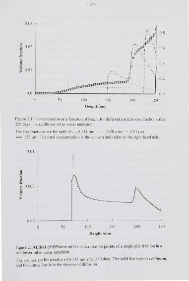
- 67-
0 03
,\ 08 I' .
~ ,.z , -~ 0.02 . I 0.6 I . I .:: 0 \ I
" ,0 ~
E if 1'. 0.4 = p I \
~ 00 1 I . I \
. - 0 I 02 I
I
---- 1 ------·· r · ._,_
00 I 00
0 50 100 150 200 250
Height /mm
Figure 2 13 Concentration as a fu nction of height for different particle size frac tions aft er 250 days in a sunflower oi l in water emulsion
The size fractions are for radii of--- 0 154 ~trn , 0 28 Jtln,- - 0.5 1 J.tm
- I 25 ~1111 The total concent ration is shown by o and refers to the righ t hand ax is
-~ " .::
0.0 1
e o oo5 = 0 >
000
0 50 100 ISO 200 250
llright /mm
Figure 2 14 Efi'ect of diffusion on the concentration profil e of a sing le size fraction in a
sunflower oil in water emulsion
The profil es are for a radius of O 154 ~Lm afler 250 days. The solid line includes diffusion, and the dotted line is in the absence of di!Tusion
-68-
boundary is higher up the sample for the larger particles, due to the dependence of the
creaming speed on particle size
The effect of diffusion on the concentration profiles is indicated by the rounded.
diffuse nature of these boundaries, especially for the smaller particles The larger. less
diffusive particles have a sharp lower boundary The diffusive spreading of the lower
interface is not as significant as might be expected, due to the effect of the concentration
dependence of the creaming velocity which tends to sharpen the boundary This effect
was discussed in relation to the total concentration profiles for a monodisperse sample
The peak in concentration just above the lower boundary is also due to the
concentration-dependence of creaming, as particles accumulate in the more slow moving
region of higher total concentration above the boundary Figure 2 14 illustrates the
influence of diffusion on the concentration profile of one of the smaller particles in the
sample. with a radius ofO 154 ~Lm In the absence of diffusion the lower boundary is very
sharp, and the peak is narrower and larger lt would appear that diffusion rounds off and
reduces the peak in the concentration profile This is consistent with the understanding
that diffusion acts to promote uniformity of concentration and so to reduce regions of
inhomogeneity
For size fractions whose lower interface is below the cream, there is also a jump in
concentration at the position of the underside of the cream The largest particles are
completely contained within the cream region and therefore this feature is missing from
their concentration profiles Between the lower boundary and the cream interface. the
concentration for each size fraction decreases with increasing height (figure 2 13) This
wou ld appear to have the same cause as the peak in concentration at the lower boundary
Since the total concentration increases with increasing height in this region, the creaming
velocity of individual particles decreases Therefore, particles tend to accumulate from
below, and increase the concentration This effect gradually propagates through the
system, from the lower boundary upwards, and causes the increase in concentration
towards the lower boundary seen in the plots
Within the cream, the concentration of most sizes of particle decreases towards the
top of the sample (figure 2 I J) The largest particles (those with a radius of I 25 ~·m are
shown here) occupy only a very small region at the top of the sample, and their
concentration increases with height. These are the most rapidly creaming particles, and
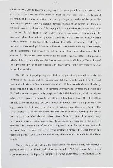
-69-
dominate the creami ng process a t early times For most particle sizes, as more cream
develops, a greater number of the larger size fractions are absent at the lower interface of
the cream, and the smaller particles can occupy a larger proportion of the space_ The
concentration profile therefore decreases towards the top of the sample In addit ion to
the more rapid upward motion of the large particles, the fluid back flow also contributes
to the particle size balance The smaller particles are carried downwards in the
continuous phase flow in the early stages of creaming, and so there is a reduced volume
of these particles at the top of the emulsion The diffusive spreadi ng of the upper
interface for these small particles causes them still to be present at the top of the sample,
but the concentration is reduced as particles lower down move downwards In the
absence of difi'usion, the upper boundary for the smallest particles (that is, the particles
initially at the very top of the sample) does move downwards a little way The position of
the upper boundary can be seen in figure 2 .14 The top layer in this case contains none of
the smallest particles
The effects of polydispersity described in the preceding paragraphs can also be
identified in the variation of the particle size distribution with height lt is the local
particle size distribution (and concentration) which will determine the ultrasound velocity
in the emulsion at any position lt is therefore informative to compare the particle size
distribution at va rious points in the sample with the initial distribution, which was shown
in figure 2 7. Figure 215 shows the particle size distribution at three difi'erent heights in
the bulk of the emulsion afler 250 days In each distribution there is a sharp cut-offal the
large particle size limit , due to the absence of particles larger than a specific size. The
lower interfaces of all particles larger than this limit have moved higher up the sample
than the position at which the distribution is taken. Near the bottom of the sample, only
the smallest particles remain , due to their slower creaming speed, and to the effec t of
diffusion. The concentration of particles of a given size can be seen to decrease with
increasing height , as was observed in the concentrat ion profiles. lt is clear that in this
region the particle size distribution may be very different from that in the initial uniform
sample.
The particle size distribution in the cream varies even more st rongly with height. as
shown in figure 2 . \6 . These distributions correspond to 500 days, when the cream is
more extensive. At the top of the sample, the average particle size is considerable larger
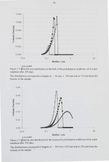
-70-
00 10
0 008
-~ 0 006 " .:: a = 0
0 004
>
0 002
0000
0 0 1 0 1 10
Radius I JHII
(G\c-.-1,.\d
Figure 2 JS!rrtrticle size distribution in the bulk oft he polydisperse sunnower oil in water emulsion afl er 250 days
The distributions correspond to heights of 50 mm, • I 00 mm and t. ISO mm from the bottom of the sample.
0 05
004
= -5 0 OJ ~ " 5 = 0.02 0 >
0 0 1
000
0 0 1 0 1 10
Co.lcu.\olod Radius / JLm
Figure 2_ t6J!>article size distribution in the cream of a polydi sperse sunnower oil in water emulsion after 500 days
The distributions correspond to height s of 200 mm. • 225 nun and 6 250 mm from the
bottom oflhe sample.
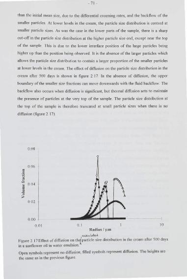
- 71 -
than the initial mean size, due to the differential creaming rates, and the backflow of the
smaller particles At lower levels in the cream, the particle size distribution is centred at
smaller particle sizes As was the case in the lower parts of the sample. there is a sharp
cut-off in the particle size distribution at the higher particle size end, except near the top
of the sample_ This is due to the lower interface position of the large particles being
higher up than the position being observed. It is the absence of the larger particles which
allows the particle size distribution to contain a larger proportion of the smaller particles
at lower levels in the cream The effect of diffusion on the particle size distribution in the
cream after 500 days is shown in figure 2.17 In the absence of diffusion, the upper
boundary of the smaller size fractions can move downwards with the nuid back now The
backnow also occurs when diffusion is significant, but thermal diffusion acts to maintain
the presence of particles at the very top of the sample. The particle size distribution at
the top of the sample is therefore truncated at small particle sizes when there is no
diffusion (figure 2 . 17)
0 08
0 06 c
·B " .:::
0 04 e " 0 >
0.02
0 .00
001 01 10 Radius I ~lm
caku.lattA
Figure 2.17 Effect of diffusion o~ th1,particle size distribution in the cream afier 500 days
in a sunflower oil in water emuls1on
Open symbols represent no diffusion, filled symbols represent diffusion. The heights are
the same as in the previous figure
-72-
2.8.3 Ultrasound velocity and :~llenualion profiles
Figures 2 _ 18 and 2 19 show ultrasound velocity and attenuation profiles generated
by the model for the polydisperse sunnower oil in water emulsion The ultrasound
parameters have been calcu lated using multiple scattering theory. and the frequency was
1 M ll z. The theories of ultrasound propagation commonly used to interpret ultrasound
measurements are discussed in more detai l in chapters 4 and 5, and o nly the main points
are presented here
The ultrasound velocity in the pure oi l phase is lower than in the aqueous phase A
si mple int erpretat ion would therefore expect that an increase in o il concentration at one
position in the emulsion would correspond to a decrease in ultrasound velocity at that
posi tion This is indeed true in the lower regions or the sample (compare figure 2 _18 wi th
the total concent ration profiles, figure 2.8) In the cream. the concentration always
increases towards the top o f the sample (apart from a small peak at the bottom o r the
cream). The ultrasound velocity does decrease wit h height in the cream at early times
However, at later times the ultrasound velocity increases with increasi ng heig ht in the
cream layer (aOer 1000 days. for example) At intermediate times (500 days) the
ultrasound velocity in the cream is almost constant lt is clear, then. that the total
concentration of o il is not the o nly factor determining the ultrasound velocity. Similarly,
irthe attenuation were dependent only on concentratio n. it would be maximum at the top
oft he sample lt is clear from figure 2 19 that this is not the case, but that the attenuation
peaks below the top oft he sample The attenuation can be very much higher in the cream
than in the initial emulsion, due to the scattering of the ultrasound signal by the particles
(see chapter 4) This has been observed experiment ally (unpublished data) Since it is
usua lly the velocity which is measured in experimental creaming equipment such as the
ultrasound scanner (figure I 1 ), the attenuation is not considered further here
The results of chapter 4 show that the particle size and frequency used in the model
(which are typical of experimental systems) are in the range in which ultrasound veloci ty
increases as the particle size increases (see, for example, figure 4 2) Although the to tal
concentration or oil increases towards the top of the sample (causing a decrease in sound
speed), the particle size distribution also becomes skewed towards the larger particles
(causing an increase in sound speed) These two factors have an opposing innuence on
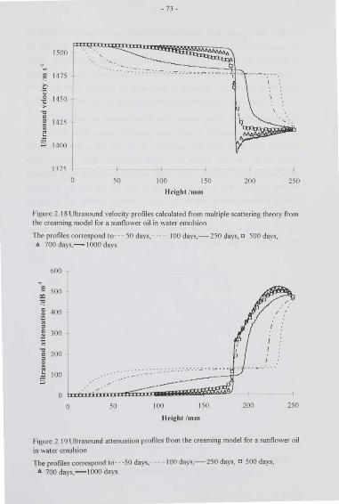
- 73 -
ISOO '· ·~.
..§ 147S
€ ~ 14SO >
"0 c = 142S
~ 5 1400
137S
0 so 100 ISO 200 2SO
lfeighf /mm
Figure 2 18 Ultrasound velocity profiles calculated from multiple scattering theory from the creaming model for a sunflower oil in water emulsion
The profil es correspond to··· SO days, A 700 days,- I 000 days
600
E soo ~
:12 c 400
-~ :; = c 300 " ::: " "0
200 § ~ £ 100 -· 5 ~
0
0 so
I 00 days,- 2SO days, o SOO days,
100 ISO 200 2SO
lleight /mm
Figure 2. 19 Ultrasound attenuation pro files from the creaming model for a sunflower oil in water emulsion.
The profiles correspond to·· ·SO days, ·· 100 days,-2SO days, o SOO days, A 700 days,-1 000 days
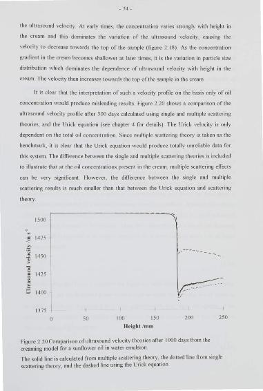
-74 -
the ultrasound velocity At ea rly times. the concentration varies strongly with height in
the cream and this dominates the va riatio n o f the ultrasound velocity, causing the
velocity to decrease towards the top of the sample (figure 2 18) As the concentration
gradient in the cream becomes shallower at later times, it is the variation in par1icle size
distribution which dominates the dependence of ultrasound velocity with height in the
cream The velocity then increases towards the top o f the sample in the cream
1t is clear that the interpretatio n o f such a velocity profil e on the basis only o f o il
concentration would produce misleading results Figure 2 20 shows a compari son of the
ultrasound veloc it y profile afler 500 days calculat ed using single and multiple scattering
theories, and the Urick equatio n (see chapter 4 for detail s) The Urick velocity is onl y
dependent o n the to tal o il concentra tion Since multiple sca ttering theory is taken as the
benchmark. it is clear that the Urick equatio n would produce to ta ll y unreliab le data fo r
this system The dirTerence between the single and multiple scattering theories is included
to illustrate that at the o il concent rations present in the cream, multiple scatt ering effects
can be very significant However. the difference between the single and multiple
scattering result s is much smaller than that between the Urick equation and scattering
theory
1500
_§ 1475
·€ il 1450 >
"0 c = 1425 :;: £ 5 1400
1375
0 50
I
100 I SO
lleight /mm
... ---- ... _
200
Figure 2 20Cornpari son o f ult rasound velocity theories an er 1000 days from the
creaming model for a sunflower o il in water emulsion
250
The solid line is calculated from multiple scattering theory, the dotted line from single scatt ering theory, and the dashed line using the Urick equatio n
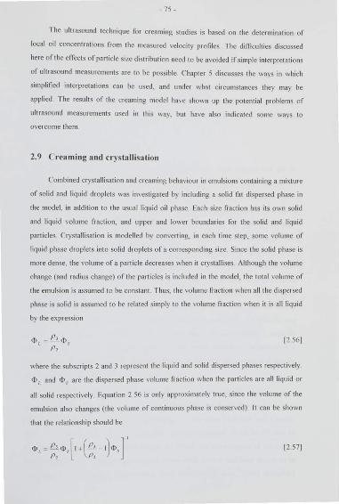
- 75-
The ultrasound technique for creaming studies is based o n the determinatio n o f
local oil concentrat ions from the measured velocity pro fil es The diffi culties discussed
here oft he effects of parti cle size di stributio n need to be avoided if simple interpretatio ns
o f ultrasound measurements are to be possible C hapter 5 discusses the ways in which
simplified interpreta tio ns can be used , and under what circumstances they may be
applied T he result s o f the creaming model have shown up the potential problems o f
ultrasou nd measurement s used in th is way, but have also ind ica ted some ways to
overcome them
2.9 Creaming and crystallisation
Combined crystallisa tion and creaming behaviour in emulsions containing a mixture
o f solid and liquid dro plets was investiga ted by including a solid fat dispersed phase in
the model, in additio n to the usual liquid o il phase. Each size fractio n has it s own solid
and liquid vo lume fractio n, and upper and lower bounda ries fo r the solid and liquid
particles Crysta lli sa tio n is modelled by convert ing. in each time step. some volume o f
liquid phase dro ple ts int o solid dro ple ts o f a corresponding size Since the solid phase is
mo re dense, the volume of a parti cle decreases when it crystalli ses Altho ugh the vo lume
change (and radius change) o f the parti cles is included in the model. the total volume of
the emulsion is assumed to be constant Thus, the vo lume frac tion when all the dispersed
phase is solid is assumed to be rela ted simply to the volume fraction when it is all liqu id
by the expressio n
[2.561
where the subscripts 2 and 3 represent the liquid and solid dispersed phases respectively
$1
and <l>s are the dispersed phase volume fraction when the particles are all li quid o r
all solid respecti vely Equatio n 2.56 is o nly approximately true, since the vo lume o f the
emul sio n also changes (the volume o f continuous phase is conserved) lt can be shown
that the rela tio nship should be
[2.57]
-76-
Equatio n 2 56 is therefore a good approximation at low concentratio ns o f di spersed
phase, but may not be as good in the cream, especially where the densi ty diH'erence
between solid and liquid phases is quite large, as fo r hexadecane l lowever, inclusion o f
the volume change of the emulsion is an added compl icat io n in the creaming model, si nce
it represents a variatio n in thickness o f the horizontal layers used to define the volume
fractio n pro file Therefo re, a change in solid vo lume frac tio n due to the solidification o f a
given volume fractio n o f liquid d ro ple ts was calcula ted usi ng the ra tio o f the densities
only (equation 2 56)
2.9. 1 Crysta llisat ion ki netics
Recent studies of creaming and crysta lli sa tio n have been carri ed out o n H~
hexadecane in wa ter emulsio ns (M a. 1995), fo r which earlier CI)'Sta lli sa tio n studies had
also been made (McClements et al . 1993. Dickinson et al , 1993b) The analysis of the
crystalli sa tion kine ti cs is. however. appli cable to any emulsion contai ning solid and liquid
particles. provided the do minant CI)'Stalli sa tio n mechanism is the same. The o nly
diO'erence is in the rate constant T he crystalli sa tion kinetics in such emulsions were
investiga ted using an ult rasound technique (McCiement s e t al , 1993, Dickinson et a! .
1993 b), which is d iscussed in more detail in chapt er 5 The principle of t he met hod is that
the proportion o f the dispersed phase which is solid can be calculated from the measured
ultrasound velocity in the emulsio n Every pa11icle is assumed to be either wholly so lid or
wholl y liquid Initially SO% by weight o f the dispersed phase is solid, and the rest is
liquid This is achieved by dividing the emulsion in to two equal parts, and free7i ng o ne
part so that all the o il CI)'S talli ses The part s are then remi xed to make a partially
crystalline emul sio n The ult1 asound veloci ty in the mi xed emul sion is measured as a
function o f time to determine the time dependence o f the solid fat content and thereby
the crysta lli sa tio n kineti cs (McCiements e t al . 1993 )
One possible mechani sm for CI)'Stalli satio n in thi s mixed emulsion is a
heterogeneous process, involving colli sions between solid and liquid dispersed part icles
Other poss ibilities exist, such as homogeneous C\.U..C...leation (Turnbull and Cormia.
196 1 ), o r a mechanism which is dependent o n mass-transport o f oil or fat due to
solubilisatio n by the emulsifier (Dickinson et a\ , 1996) For the purposes o f the model,
the heterogeneous mechanism was assumed to be va lid. since it had been shown to be
consistent with the previous CI)'Stalli sa tion study (McClements et a\ , 1993) According
-77-
to this mechanism, crystalli sa tion of a liquid droplet occurs due to a collision with an
already crystalline droplet , which nucleates crystal growth in the liquid Following
nucleation, the droplet rapidly solidifies completely Not every such collision result s in
the solidifica tion of the liquid particle, however, due to an energy barrier (partly caused
by the protective layer of emulsifier around the droplet)
The heterogeneous crysta lli sa tion kinetics can be described in terms of a binary
collision process between solid and liquid particles The rat e equation includes both the
particle collision rate, and the proportion of collisions which result in crystallisation In a
monodispcrse sample, the rate of crystal lisa tion can therefore be expressed in terms of
the proportions of solid and liquid droplets If a , is the proportion of dispersed phase
droplets which are solid, the rate equation can be written as
d(l a ) --' ~ Ka(l a) dt < s [2 58]
where K is a rate constant (McCiements et al , 1993 They use the symbol <P for a s )
The rate constant determined in the ex periment s (McC'lements et aL. 1993) was specific
to the samples used (which were nearly monod isperse), and is particle size and
concentra tion dependent In a polydisperse sample, the binary collision rate includes
contributions from collisions between particles of all diHCrent sizes The rate of change
of the number density, 11,. of liquid droplet s of species (size fraction) i due to collisions
with solid particles of species (size fra ction) j can be wri tt en as
[2 59]
where c is a colli sion efficiency factor (the proportion of collisions which result in
solidification of the liquid droplet) and fJ,}I,"-1 is the binary collision rate between these
species
Jnterparticle collisions in an emulsion are the result of some form of relati ve motion
between the particles (Colbeck, 1994) The relative motion may be caused by a number
of different processes, but the predominant effects in the present work are due to
Brownian diffusion and creaming Brownian dini.1sion causes random particle collisions
in both rnonodisperse and polydisperse emulsions In contrast, the effect of creaming on
the collision rate is only significant in a polydisperse emulsion Although some collisions
- 78 -
may occur in a monodisperse sample as a result of creaming, the part icles all move, on
average. with the same velocity. and the co lli sion rat e is consequently low I lowever. in a
polydisperse emulsion. particles of diiTerent si1.es move with di!Terent creaming velocities
and collisions are much more lik ely The binary collision rate in the emulsion is.
therefore. the sum of the two contributing processes, so that the factor /3; ,, can be
wri tt en
/3,,, ~ P .. J.dill +- fJ .. /.Crm [2 60 1
where /3,,,,6,rr and P .. 1 .cnn are the factors in the colli sion rates due to Orownian difTusion
and the relative particle creaming rates respecti vely ~hoc\ ro~c. 'n~cirod.~nomlc: e!fec±:s cu·e. n~l~c.h.d. .
The binary colli sion process has been extensively investigated in the contex t of
fl occulation and coalescence Expressions for the co llision rat es have been obtai ned from
works on nocculation by Melik and Fogler ( 1984), Lawler ( 1993) and /\bel et al ( 1994)
The colli sion rates for IJrownian difTusion are based on the early work of Smoluchowsk i,
later ex tended to polydisperse systems In this case, the colli sion factor is g iven by
= 8)n. 1 n,) (1; 1 rJ
fJ .. , .d;n 2 2 12 6 1]
In a monodisperse sample, the collision rate is independent of particle size (for a g iven
particle number density) Smaller part icles have a larger difTusion coefficient , being more
mobile, but their colli sion cross-section is small Large particles are less mobile but have
a large co lli sion area I fence, the overall colli sion rate is independent of pa1ticle size_ In a
po lydisperse sample, the IJ rownian co lli sion rate may be signi fi cantly increased due to
colli sions between particles of difTerent sizes (Colbeck. 1994) For example, a small , very
mobile particle is much more likely to collide with a larger particle (wit h a large colli sion
cross-section) than with a particle identical to itself The combination of the size
dependent difTusion coeffi cients and co lli sion areas leads to an increased co ll ision rate in
a po lydisperse system
The gravitationall y- induced colli sion rat e is proportional to the volume swept out
by the rehttive veloci ty of the two species of particle, and to the effective cross-sectional
area of the collision Thus
fJ = ..!,. +r)' i, "I r.J.etm 11 \ r J r _r 12 62J
-79 -
Lawler ( 1993 ) has an ex tra fa ctor of 0.5 in his expression Melik and Fogler (1 984)
discuss some modifications to the effective colli sion cross-section due to the
hydrodynamics of the nuid now llowever. fo r the purposes of the model. the binary
collision rate was taken in it s simplest form, given above lt is clear that the degree of
polydispersity in an emulsion is a determining factor in the significance of the
gravitational cont ribution to the binary collision rat e In addition, the gravitational
co lli sion rate is strongly particle size dependent
Although the binary collision rates are most easily derived using the number
densit y of particles (as in the preceding equations), the phenomenological creaming
model (and the crystalli sation study) uses the volume frac tion of each species
Remembering that a subscript of .. 2" represents the liquid dispersed phase, and a
subscript of ")'' the solid dispersed phase, equation 2.59 can be written as
d?2J.J dt
[2 63 ]
By writing the volume fractions in terms of the proportion of the dispersed phase,
and comparing with the crystalli sation rate (equation 2_58) g iven by McCiement s et al
(1 993), it can be seen that the rate constant in the monodisperse case is given by
K - e(fJ .. ,.d;n I /],_,_,.,., ) . q - ..fp fJ ) - ( 4 ') > .~ - c: \ , ,,,diff I • .J.~m• 11o
m· 3 '
[2 64]
where n0 is the number density of particles Thus, the rate constant is it self dependent on
the total concentration of dispersed phase and on particle size_ llowever. the co lli sion
efficiency can be assumed to be independent of these parameters and was deri ved in the
crystalli sation study (McClements et a! , 1993) The colli sion rate was calculated by
McCiement s et al using the monodisperse form of the diffusion colli sion frequency,
equation 2 6 1, neglecting the effect of the density change on solidification The densities
of water, liquid hexadecane and solid hexadecane at 6 °C are 999 9, 783 3 and
909 4 kg n(' respectively (Kaye and Laby, 1986, Allegra and lla wlcy, 1972) The
particle diameter with a T ween20 emulsifier had a value of d~z=O 36 ~m (the volume
surface average) when the particles are liquid The contribution of relative creaming
-80-
speeds in these emulsions was small and can be ig nored Thus, the co lli sion efficiency
factor can be ca lculated from equat ion 2.6 1, and is approximately
&= 80 x 10' [2 65 ]
This corresponds to an energy barrier of around 16k8 7. as given by McCJement s et a\
(1993)
Since the colli sion efficiency can be assumed to be relatively insensi ti ve to particle
size and temperature, the crysta lli sa tion rate can be calcula ted in the model usi ng
equation 2 63, wit h the value of equa tio n 2 65 The crystalli sa tion rate can therefore be
calcula ted for a polydisperse hexadecane in water emul sion. at any concentration The
equatio ns are no t precisely va lid at high concent ratio ns because tertiary and higher
collisions would then become signi ficant The binary co lli sion rates are g iven by
equat ions 2 6 1 and 2 .62 The creaming speeds include the hydrodynamic hindrance_ The
IJ rownian collision rate is determined by the diffusive motion of individual particles
within the medium llowever. the diffusion coefficients used in the model are the
phenomenological mutual diffusion coeffi cients which describe the nux of particles in a
concentration gradient These coefficients were used throughout , for simplicity, wi th the
concentratio n dependence previously detailed
2.9.2 Modelling of combined creaming and crystallisat ion
The computer program for modelling creaming and crysta lli satio n is included in
Appendix A 1 The creaming and crystalli satio n behaviour of a 20 vol % hexadecane in
water emulsion with a mixture o f solid and liquid particles was determined at 8 oc using
the creaming model This system was recently studied experimentally by M a ( 1995) using
the ultrasound scanner (figure 1 1) The crystalli sa tion rate in the absence o f creaming
was initially measured, and it was found to be consisten t with the results of McC'Iement s
et al (1993) The physical properties of the constituent phases are shown in table 2 2
(Kaye and La by, 1986, A11egra and llaw1ey, 1972) The particle size dislt ibulio n
(obtained in the experi mental samples) peaks at a diameter of 0 42 J-1111, wi th a width o f
a .. = 0_5. when all pariicles are liquid This is consistent wi th the volume-surface
diameter of d,2=0J6 ~lm The frequency used in the calculations of ultrasound veloci ty
was I 6 Mllz (as in the creaming experiments)
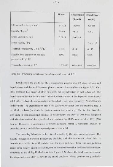
- 81 -
\Vater llnadccane lluadeca ne
(liquid) (solid)
Ult rasound velocity / m s·' 1439 I 1400 0 22000
Density I kg m·' 999 9 78 1 9 908 2
Shear viscosit y I Pas 0 00 14 0 00385
Shear rigidity I Pa 7 0 X 108
Thermal conductivity I J m·'s'K -1 0 572 0 140 0 185
Specific heat capacity at constant 4 195 2092 2092
pressure I J kg"1 K-1
Thermal expansivity I K-1 0 000075 0 000895 0.00066
Table 2 2 Physical properties of hexadecane and wa ter at 8 °C
Result s from the model for the concentration profiles afler 2 5 days, of solid and
liquid phases and the total dispersed phase concentration are shown in figure 2 2 1 Very
little creaming has occurred afler this time, but crystalli sation is well advanced The
liquid volume fraction is very much reduced, whereas most of the dispersed phase is now
sol id Afler 5 days, the concentration of liquid o il is o nly approximately I % (Ill 0 of it s
initial va lue) The crysta lli sation process is considerably fa ster than the creaming rate in
the ideal emulsion (in which the particles cream independent ly) This is clear from the
time scale of idea l creaming behaviour in the model (of the order of 200 days) compared
with the time scale of the crystalli sation experiment by McCiements et al ( 1993), (500
hours) Therefore, crystalli sa tion is almost complete before a significant amount of
creaming occurs, and all the dispersed phase is then solid
The creaming behaviour is therefore dominated by the solid dispersed phase The
density difference between hexadecane particles and the continuous phase fluid is
considerably smaller for solid particles than for liquid particles llence, the solid particles
cream more slo'-vly, and the creaming rate in the mixed emulsion is dramatically reduced
compared to the all ~ liq uid ideal emulsion Figllle 2 22 shows the to tal concentra tion of
the dispersed phase aner 30 days in the mixed emulsion (whose particles are practically
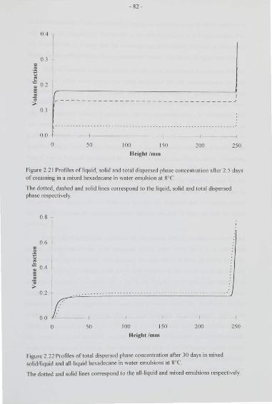
- 82-
04
03 = ·B " .::
02 e " 0 >
0 1
00
0 50 100 I SO 200 250 ll eight /mm
Figure 2 .2 1 Pro fil es of liquid, solid and total di spersed phase concentrat ion aller 2.5 days of creaming in a mixed hexadecane in water emulsion at 8°(
The dolled, dashed and solid lines correspond 10 the liquid, solid and lotal di spersed phase respectively
08
06
02
00
0 50 100 I SO 200
If eight /mm
Figure 2 22 Profiles of total dispersed phase concentration aller 30 days in mixed solid/liquid and all -liquid hexadecane in water emulsions at 8°C
250
The do tted and solid lines correspond to the a ll -liquid and mixed emulsions respectively
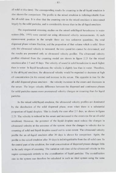
- 8J-
all solid at this time) The corresponding result s for creaming in the all -liquid emulsion is
also shown for comparison The pro fil e in the mixed emul sion is indi stingui shable from
the all -solid case lt is clear that the creaming rate in the mixed emul sion is determined
largely by the solid particles, and is considerably slower than in the all -liquid emulsion
The C'( periment al creaming studies on the mixed solid/ liquid hexadecane in wa ter
system (M a, 1995) were carried out using ult rasound velocity measurement s At each
measurement position in the sample there are two unknown quantities. the total
dispersed phase volume fraction. and the proportion of that volume which is solid Since
o nly the ultrasound velocity is measured . the t\VO quantities cannot be determined. and
the result s are presented o nly as ultmsound velocit y pro fil es The ultrasound velocit y
profil es ob tained from the crea ming model are shown in figure 2 23 for the mixed
emulsion afl er 2 5 and 30 days The veloci ty of sound in solid hexadecane is much higher
than in water In liquid he'<adecane the velocity is slig htly less than in wa ter Therefme,
in the all -liquid emulsio n. the ultrasound velocity would be expected to decrease at hig h
o il concent ratio n (in the cream) and increase in the serum The o pposite is true fo r the
a ll -solid di spersed phase emulsion - the velocity increases in the cream and decreases in
the serum The larger velocity diflCrence between the dispersed and continuous phases
for solid parti cles causes more pronounced velocity changes on creami ng than for liquid
particles
In the mixed solid/l iquid emulsion, the ult rasound velocity pro fil es are do minated
by the dist ributio n o f the solid dispersed phase. even when there is a substantial
prop01 tio n o f liquid drop lets This is clea rl y the case afl er 2 5 days, as shown in fi gure
2 23 The velocity is reduced in the serum and increased in the cream (as fo r an a ll -solid
emulsio n) I lowever, the presence o f the liquid dro plets must reduce the changes in
ultrasound velocity at the extremes o f the system. since the changes in velocity due to
creaming of solid and liquid dro plets cancel out to some extent The ultrasound velocit y
pro fil e fo r an a ll -liquid emulsio n afl er 30 days is shown for compari son Agai n, the
pro fil e in the mixed emulsio n afl er 30 days is indistinguishab le from the all -solid case In
the central part o f the emulsio n. the to tal concent ratio n o f di spersed phases changes little
in the ea rl y stages o f creaming The variatio n with time o f the ultrasound velocity in this
1egio n corresponds entirely to the crystallisatio n of liquid particles The crystalli sation
rate in the system can therefo re be calculated in such an ideal system using the same
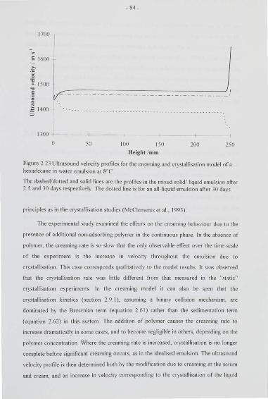
-84-
1700
~~ 1600 )
-.:; > 1500 -o -----JJ g I ,c-:-: __ :
~ V 5 1400
1300
0 50 100 I SO 200 250 ll e ighf /mm
Figure 2 23 Ultrasou nd velocity profiles for the creaming and crystalli sation model of a hexadecane in water emulsion at 8°C.
The dashed/dotted and solid lines are the profiles in the mixed solid/ liquid emulsion afier 2 5 and 30 days respectively The dotted line is for an a ll - liquid emulsion afler 30 days
principles as in the crystalli sation studies (McCiements et al., 1993)
The experi ment al study examined the effects on the creaming behaviour due to the
presence ofadditionalnon-adsorbing polymer in the continuous phase In the absence of
polymer, the creaming rate is so slow that the o nl y observable effect over the time scale
of the experiment is the increase in velocity throug hout the emulsion due to
crystalli sation This case corresponds qualitatively to the model results it was observed
that the crystalli sation rate was little different from that measured in the "static"
crystalli sa tion experiments In the creaming model it can also be seen that the
crysta llisation kinetics (sect ion 2 9 I), assuming a binary colli sion mechanism, are
dominated by the Brownian term (equation 2.6 1) rather than the sedimentat ion term
(equation 2.62) in this system The addition of po lymer causes the creaming rate to
increase dramatically in some cases, and to become negligible in ot hers, depending on the
polymer concentratio n Where the creaming rat e is increased, crysta lli sation is no lo nger
complete before significant creaming occurs, as in the idealised emulsion The ultrasound
velocity profile is then determined both by the modification due to creami ng at the serum
and cream, and an increase in velocity corresponding to the crysta lli sation o f the liquid
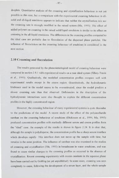
- 85-
droplets Quantitative analysis of the creaming and crystallisation behaviour is not yet
possible in this case, but a comparison with the experimental creaming behaviour in all
solid and a ll -liquid emulsions appears to indica te that neither the crystalli sat ion ra te nor
the creaming rate is strongly mod ified in the mixed system (Ma, 1995) The effect of
added polymer on creaming in the mixed solid/liquid emulsions is similar to its en"ect on
creaming in the all -liquid emul sions The differences in the creaming profiles compared to
the ideal case are probably due to nocculation of the dispersed phase part icles The
innuence of nocculation on the creaming behaviour of emu lsions is considered in the
next section
2. 10 C rea ming and noccula ti on
The result s generated by the phenornenological model of creaming behaviour were
compared in section 2 8 1 with experimental result s on a near-ideal sys tem (Fillery-Travis
et al , 1993) Qualitati ve ly, the modelled concentration profi les compare well with
experimental results except in the cream region Quantitatively, the hydrodynamic
hindrance used in the model seems to be overestimated, since the model predicts a
slower creaming rate than that observed Defi ciencies in the description of the
hydrodynamic interactions were also thought to explai n the different concentration
profiles in the highly concentrated region
llowever, the creaming behaviour of many experiment al systems is quit e dissimilar
to the predictions of the model A recent study of the eiTect of the polysaccharide
xanthan on the creaming behaviour of emulsions (Dickinson et al , 1994, Ma. 1995)
produced concentration profil es with markedly diiTercnt serum and cream profil es from
the .. ideal" case. An example of the result s is shown in fi gure 2 24 lt is clear that,
although the sample is polydisperse, the concentration profile has a sharp serum interface
which develops rapidly This int erface does not move up the sample with time, but
remains in the same position The innuence of xanthan was also examined in the studies
of creaming and crystall isa tion (M a, 1995) in hexadecane in wat er emulsions, and was
found to cause similar changes to the creaming pro fil es as occurred in the absence of
crystallisation Recent creaming experiments with excess caseinate in the aqueous phase
have been carried out by Golding (as yet unpublished) In some cases, creaming was seen
completely to cease, following the development of a sennn layer. and the whole sample
- 86-
0.6
os c
-E 04
" .:: e 03
" 0 02 >
0 1
0
0 50 100 I SO 200
Height /mm
Figure 2.24 Creaming behaviour of a 20% sunflower o il in water emulsion with 0 03 wt % xanthan in the aqueous phase at 30 oc (Ma, 1995)
250
The profiles corresponding to the squares, triangles and diamonds were taken aft er 0 5 hours, I 5 hours and I 0 days respectively
became solid-like The work by Fillery-Travis et al ( 1993), which was used to obtain an
example o f an ideal emulsion, al so includes o ther examples of creaming in the presence
of added polymer, producing a va riety of forms of concentrat ion pro fil es
The commo n facto r in these studies is thoug ht to be the occurrence o f fl occulation
of the o il particles The term fl occulation refers to the sticking together (reversibly or
irreversibly) o f two or mo re dispersed phase particles, which then behave as a si ngle unit
Each d ro plet in the floc retains it s individual identity, rather than coalesc ing with o thers
to fo rm a single larger particle As discussed in chap ter I, fl occulation occurs due to the
existence of a favourable energy state when particles are close toget her This may be
caused by a long- range attractive potential between particles, o r by an att racti ve fo rce
which is significant only when particles become close together, due to random colli sions.
One short -range attraction which may cause fl occulation is the depletion
interaction, proposed by Asakura and Oosawa ( 1954, 1958) Deplet ion fl occulation
occurs in the presence of large polymer molecules or micelles in the continuous phase
-87-
When two part icles approach within a distance comparable to the size of the polymer
part icles, polymer is excluded from the interparticle region and an osmotic pressure
gradient drives the particles together In many of the experiments referred to in the
preceding paragraphs (Fi llery-Travis, 1993, Dickinson et al . 1994), depletion is believed
to be the predominant fl occulation mechani sm In each case. some non-adsorbing
substance was present in the continuous phase, which promotes fl occulation A second
fl occulation mechanism is bridging, in which an adsorbing molecule may be attached to
the surfaces of two dispersed part icles, forming a bridge between them This tends to
occur when there is insufficient of the adsorbing species to allow full surface coverage of
all dispersed part icles The bridgi ng mechanism is not thought to be significant in most of
the systems quoted in the preceding paragra phs, but it can in some cases have an
innuence on creaming behaviou r
It is clear from the experimental studies of creaming discussed previously that
nocculation can have a very significant effect on creaming behaviou r In some cases,
nocculation caused a large increase in creaming ra te_ It may be suggested that this is due
to the faster creaming speed of noes (due to thei r size), provided that they remain free to
move relatively unhindered In other cases, the extent of nocculat ion is so great as to
produce a particle gel, in which creami ng is greatly reduced. and the emulsion becomes
much more stable_ Previously the creaming model has assumed that all particles are free
to move independently, and do not stick together In fact, any particle interac tions were
omitted Since the effect of nocculation on creaming behaviour is so signi fica nt , and the
types of additi ves causing it are commonly present in food systems, an attempt was made
to include these effects in the phenomenological model
In the present phenomenological model, nocculation is irreversible particles
remain stuck together once they have nocculated Reversible nocculation is difficult to
implen1ent in the phenomenological descri ption, since no trace is kept of each indi vidual
noc, only of the volume fraction of noes of a given size (as was the case for single
particles). In order to allow particles to break off from a noc, its composi tion must be
known in terms of the size of each of the particles in the noc When creaming occurs.
noes of the same geometric size may have a different composition, depending on their
growth and creaming rate history Hence there is no simple, unique means of recording
the particle size di stribution in a noc. If noc break-up were then allowed, an assumption
- 88-
as to the sizes of the particles breaking ofi' may lead to non-conservation of the single
particle size distribution in the emu lsion as a whole Therefore, only irreversible
flocculation was included in the phenomenological model Floc break-up in a
monodisperse system can, however, be modelled. as demonstrated by llsu and Tsao
( 1992). in the absence of creaming
The driving force for depletion flocculation is the presence of a non-adsorbing
species (such as a polymer) in the cont inuous phase Its concentration is one determining
factor in the flocculation rate_ As floes form, the polymer is excluded, to some extent_
from the volume occupied by the fl oc. This floc volume includes a quantity of continuous
phase fluid since the floes are sparse. Hence as fl oes grow, the concentration of polymer
external to the floes increases, because oft he reduced «free" volume of continuous phase
fluid This increase in concentration in turn affects the flocculation rate between other
particles or floes Polymer is likely to be completely excluded from a small , compact floc
However. as the floes grow larger. and become more sparse, or even begin to form a
network, some polymer must be trapped within the floes or network
A quantitative description oft he polymer concentration and exclusion from floes is
not simple A model which assumed complete exclusion of polymer from floes would be
unrealistic, since some polymer is likely sti ll to be present when the floes form a network
which fills the whole space_ In the other extreme, if the polymer concentration is
assumed to be uniform throughout the continuous phase, including that incorporated into
floes, no changes in polymer concentration (with height and time) will be observed An
explicit description of the polymer was, therefore, omitted from the model The
flocculation process was assumed rather to occur at the same rate throughout the
sample. with no account taken of variations in polymer concentration So, the effect of
the polymer in inducing flocculation is modelled, without explicitly including the polymer
itself, except as a parameter in the flocculation rate
There are three principal components to a phenomenological model of flocculation
and creaming Firstly, the kinetics of flocculation must be defined in terms of local
characteristics such as the particle concentrat ion Secondly, the average structure of floes
must be quantifiable by a small number of parameters Finally, the average dynamic
properties of the floes thus formed must be related to the floc characteristics, such as its
effective size Since the model is a phenomenological one, the description of floc
-89-
structure and the dynamic properti es of fl oes can o nly be a representational avemge over
many different possible configurations These three component s are considered in the
following sections
2.1 0.1 Flocculation kinetics
The kineti cs o f flocculatio n are based on ident ical principles to the heterogeneous
crysta lli sation mechanism described in sectio n 2 9 I Flocculation occurs due to colli sio ns
between two parti cles or fl oes which then sti ck together. In the case o f depletion
fl occulatio n the component s need not coll ide but o nl y approach wi thin a di stance
comparable to the polymer size. which causes exclusion of the polymer from the space
between them Since the rad ius o f gyratio n of a typ ical polymer is considerably smaller
than most o f the oil pa rt icles in the emulsions bei ng studied, the contri bu tion o f the
po lymer size to the co lli sio n cross-sectio n has been neglected in the model
As in the crystalli sa tion case, there are two fac to rs determining the overa ll
flocculatio n ra te, namely the frequency o f co lli sions between parti cles or noes, and the
probab ili ty o f the compo nents sticking together o nce they have collided The rate of
binary coll isions due to thermal d iffusio n, and to the relati ve creaming speeds of parti cles
of di fferent sizes were g iven in sect io n 2 9 . 1 (equations 2.6 1 and 2 .62) T hese rate
equatio ns are generali sed in the model by att ributing to noes a diffusion coeffi cient.
creaming speed and geometric rad ius The dynamic properties of noes are discussed in
sectio n 210 3, and the geometric size in section 2 10 .2 Colli sion rates between any
combination o f particles o r floes o f different sizes can therefore be calculated using the
binary rate equatio ns (2 .6 1 and 2 62) The rate equatio n 259 now represent s the loss of
particles (o r noes) Of size fraction I due tO nocculat iOil wi th part icles (o r noes) Of Size
fraction)
The collision effi ciency introduced for crysta lli sa tion is also applicable to
Oocculatio n In the case of crysta lli sation it represented the proport ion of solid- liquid
encounters which resu lted in the solidifi ca tion of the liquid dro plet When ap plied to
noccula tio n it is equiva lent to the pro po rtio n o f particle encounters which result in the
component species sticking together In the case o f depletio n noccula tion, the sticking
probability is determined, in pa rt , by the concentratio n o f the non-adsorbing species
(polymer) Since this concentrat ion was assumed, in the model, to be constant

-90-
thro ug ho ut the emulsio n. the coll ision effi ciency was si mply retained as a va ri ab le
parameter it is also assumed to be independent of particle sin and concentration (as for
crysta lli sation) Where mo re information is ava ilab le about the fl occulating potentia l, a
more complex form for the st icking probability could be used, incorporating. for
example, the effects of part icle size
2. 1 0.2 Floc structure
Floes are not compact structures (unlike the droplets formed by coalescence), but
become less space. filling the larger they grow. The detailed structure of such a fl oc m;:~ y
be very complex, but , on average, it may be parametrised by using the concept of fractal
geometry A mo re detailed descriptio n o f the fractal natu re o f fl occulation and it s effect
o n creaming and diffusio n rates can be found in the nex t chapt er in the context of the
latt ice model At this stage, it is sufficient to state that the floc stmcture is characteri sed
by a fractal dimensionality. which describes the degree o f sparsity as the fl oc increases in
size. Thus, the volume of oil in a floc wi th an effecti ve geometric rad ius r1 , is given by
the expression
[2 66]
where the parameter d1 is the fractal dimensio n (o r dimensio nality) The fra ctal dimensio n
is less than o r equal to three. A value o f three (equal to the Euclidean dimensio n) is
equiva lent to a rando m o r ho mogeneous distributio n of parti cles, and in this case the
density of particles in the fl oc is unifo rm A fractal dimension substantia lly less than three
represent s the increasingly sparse nature o f the fl oc structure as the number o f particles
in the fl oc increases
If the sample is mo nodisperse, and equation 2 66 is applied in the limit o f a sing le
particle in the fl oc, the pro portionality constant can be written
[2 67]
where r is the radius o f an individual particle. The fractal dimension has been determined
by experiment o r by simulatio n fo r a number o f different aggregates (Meakin , 1988,
Jullien, 1990) A value of 2.0 was found to be appropria te for many aggregates or noes,
and this is the va lue used in the model
-91-
2.1 0.3 Floc mobility
., he creaming speed and diffusion coenicient of floes are cmcial in determining the
overa ll creaming characteristi cs of a flocculating emu lsion For the purposes of the
phenomenological model , these dynamic properties must be related to the geomet ri c size
of the floc Both the creami ng speed and the diflhsion coenicient are determined by the
mobility of the floc, or alternatively. the viscous drag force caused by the conti nuous
phase fluid For si ng le, isolated, spheri cal particles. this mobility was given by equa tion
2_30 As a first approximation, the mobility of an isolated floc may simi larly be related to
its geometric radius In practice, isolated floc mobi lity may better be determined by a
different, "hydrodynamic" radius, rather than by its geometric dimensions However. this
modification was neglected in the model, and any hydrodynamic effects on mobility were
combi ned with the concent ration-dependent hydrodynamic inteHtctions described in the
following paragraphs lhe h~d.rod':!no.mlc ro,chus mo.~ be. &lT\0.\.\v ~n '4·
In the preceding section. the volume of oi l in a floc of a given geometric radius was
related to the fra ctal dimension. which characterises the floc stmcture llence. the
average net buoyancy force o n the floc (which is due only to the oil in the fl oc) can be
obtained directly The modified «Stokes" creaming velocity and " Stokes-Einstein"
difl'usion coeffi cient for a fl oc of geometric radius If were, therefore, defined as follows
/) = -"-·' r.o 6m,-,
)2 68]
)2 69)
The mobi lity of fl oes and single particles in the floccu lated emulsion is affected by
the hydrodynamic interactions, which are modified by the existence of fl oes In sections
2 2 3 and 2 2 4, the effect on particle mobility of hydrodynamic interactions in a non
fl occulated emulsion were expressed in terms oft he local particle concentration Since al l
the particles in a floc move together. their combi ned efl'ect on the flow field in the
surrounding fluid is different from their individual contributions if they existed separately
as single particles Simi larly, the fl oc canno t be conside1 ed as a solid sphere of radius
equal to the geometric radius o f the floc, since some of the continuous phase fluid
incorporated in the floc remains free to move with the surrounding fluid
-92-
The effect o f floes on the hydrodynamic int eractions is, therefo re, dependeru o n the
structure of the fl oc, particularly on the freedom of fluid to fl ow th rough or within the
fl oc_ Modifi cations to the hydrodynamic interactions due to these effects have been
considered by C hhabra and Prasad ( 199 1) They deri ved an expressio n for the viscous
drag, including hydrodynamic effects. o n a sphere with a solid core and a permeable
shell . The cell model introduced by llappel was used to detennine the hydrodynan1i c
effects, in spi te of the demo nstrat ion by Batchelor ( 1972) of its doubtful va lidity The
result is appl icable fo r a monodisperse system of fl oes, in which a ll particles are
flocculated, and all fl oes are the same size The ex tensio n of the expressio n to a diverse
suspensio n o f floes and single parti cles may be d ifficult Bedenko e t al { 1983) also
considered the sedimen tation of fl occu lated suspensions. in which most o f the dispersed
phase was fl occulated The fl oes were large and nearly mo nodisperse_ The hydrodynamic
compo nent in the sedimenta tio n speed was. in this case, calculated by considering the
fl oes as "solid" spheres, in which no flui d fl ows in or out
In the absence o f a sati sfactory pheno meno logical description of the hyd rodynamic
effects in a fl occulated emulsio n, two limiting conditions were investiga ted in the
creaming model In the fi rst limit. the hydrodynamic hindrance facto r (section 2 2 3) is
calculated using o nl y the concentration o f oi l, as in the unflocculated emulsion This
correspo nds to the assumptio n that the now fi e ld o f the continuous phase fluid is
unchanged by the presence o f fl oes, and that the effect o f tra pped fluid inside fl oes may
be neglected In the other ex treme, if the fl uid incorpora ted into the fl oc is considered to
be completely bound to the fl oc. the hydrodynamic hindrance fac tor is determined by the
total concentratio n o f fl oes and pa11icles {including the continuous phase fluid inside the
floes). Thi s was the formulation used in an early study by Michaels and Bo lger ( 1962) for
dilute. noccu loted suspensio ns, ond olso by Bedenko et ol ( 1983) In opplying this
hydrodynamic condition to the fl occula ti ng emulsion, the effective total concent rat ion
increases as the flocculation becomes mo re ex tensive, until no further movement is
possible Bo th cases are simpli fica tions o f the true si tuatio n, which is dependent o n the
detail s of fl oc structu re and the fl ow fi eld around floes
2_10.4 Samples analysed
The computer program fo r the modelling o f creaming and flocculation is given in
Append ix A2 T he calculat ions on creaming and fl occulation were carri ed out o n smaller
- 93 -
scale systems than those present ed in the preceding sectio ns. The binary colli sions used
in the fl occulation kineti cs are computationally intensive and therefore the system size
was reduced to improve comput atio n speed. The sample properti es correspond to a
20% (by volume) sunnower oi l in water emulsion at 30 °C, whose propert ies were given
in table 2.1. The sample height was 40 mm, and the part icle size distribution was
characterised by a modal diameter of 0 .56 p m and width of a ... = 0.42 (giving a
maximum diameter o f 2 pm). O nly 11 size fractio ns were used in the initia l distri bution.
The fl occulation characte ri st ics are described by the parameters o f the pro port io nality
constant
Yr = 42 x 10 'm [2 70]
and the fl occulatio n pro bability, which is va ri ab le Floes were allowed to grow to a
maximum diameter of 20 ~ t m, and 20 size fractions were used in the fl oc size
di stributio n. The va lue of the time interval is defi ned so as to ensure that the model does
no t a tt empt to fl occulate mo re parti cle o r fl oc vo lume than is present in any layer, thus
conserving o il volume. At high floccula tion efliciencies, a very small time interval must
be used and so the calcu lations become ra ther slow
2. 1 0.5 C reaming and flocculation results
Creaming profi les predicted by the model for the sunfl ower o il in water emul sion
aft er 4 days are shown in figure 2 25. The hydrodynamic interactions in these result s
were calculated using the total concentra tio n o f floes and parti cles. The result s of two
different fl occulatio n probabili ties are shown, alo ng wi th the creaming profil e in the
absence of fl occulation . The emul sion with the larger flocculatio n probability hard ly
develops a serum o r cream before the who le emulsion is constra ined in a parti cle
network structure which prevents further creaming This condition is represented by a
large value of the to tal volume fraction, due to the presence of many space-filling fl oes.
Althoug h the o il concentration is still low. parti cles are extensively connected and
movement o f floes is restri cted. A reduction in the fl occulation probab ility allows free
creaming to proceed, at least over the time period shown. However, the creaming profil e
does not indicate an increase in creaming speed compared to the emulsion with no
flocculat io n 1t would appear that when the hydrodynamic interactions are determined by
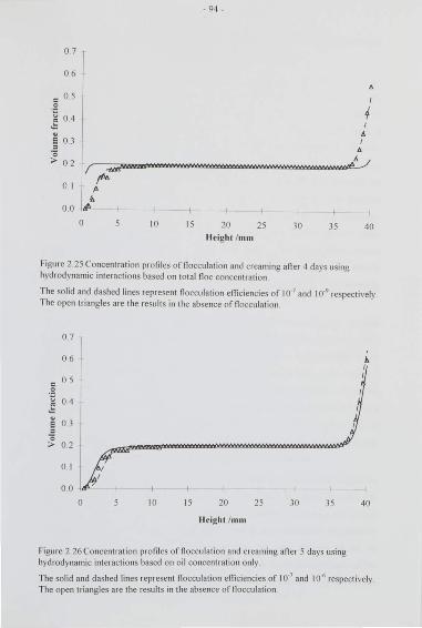
-94 -
0 .7
06 A
c 0.5 I
·E 04 4
" .;: I
e o 3 " I = A 0
. .L/ > 02 f -
0 1 fk " ..
00 t!-
0 10 15 20 25 30 35 ll eight /mm
Figure 2 25 Concentration pro fil es of fl occulation and creaming an er 4 days usi ng hydrodynamic interactions based on total floc concentra tion
40
The solid and dashed lines represent fl occulation efficiencies of ro·7 and 10·9 respectively The open triangles are the results in the absence of flocculation
07
0.6
c 0 .5
·B 04 ~ e 0.3 = 0 > 02
0 1
00
0 10 15 20 25 30 35
ll eigh1 /mm
Figure 2 26 Concentration profi les of fl occulation and creaming after 5 days using hydrodynamic interactions based on oil concentration only
I
40
The solid and dashed lines represent fl occulation eniciencies of 10·7 and 10·6 respectively. The open triangles are the results in the absence of fl occulation
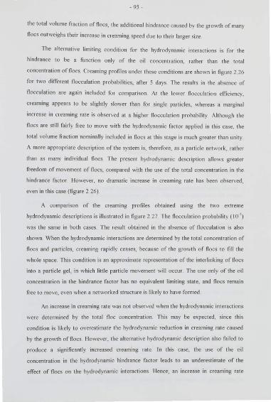
-95-
the total volume fraction of floes. the additional hindrance caused by the growth of many
floes outweighs their increase in creaming speed due to their larger size
The alternative limiting condition for the hydrodynamic interactions is for the
hindrance to be a function only of the oil concentration, rather than the total
concentration of floes Creaming profiles under these conditions are shown in figure 2 26
for two different flocculation probabilities, afler 5 days The results in the absence of
flocculation are again included for comparison At the lower flocculation enlciency,
creaming appears to be slightly slower than for single particles, whereas a marginal
increase in creaming rate is observed at a higher fl occulation probability Although the
noes are sti ll fairly free to move with the hydrodynamic factor applied in this case. the
total volume fraction nominally included in noes at this stage is much greater than unity
t\ more appropriate description of the system is, therefore, as a particle network, rather
than as many individual noes The present hydrodynamic description allows greater
freedom of movement of noes, compared with the use of the total concentration in the
hindrance factor However, no dramatic increase in creaming rate has been observed,
even in this case (figure 2.26)
A comparison of the creaming profiles obtained using the two ex1reme
hydrodynamic descriptions is illustrated in figure 2 27 The nocculation probability ( 10"7)
was the same in both cases. The result obtained in the absence of nocculation is also
shown When the hydrodynamic interactions are determined by the total concentration of
noes and particles, creami ng rapidly ceases, because of the growth of noes to fill the
whole space This condition is an approximate representation of the interlinking of noes
into a particle gel, in which little particle movement wi ll occur The use only of the oil
concentration in the hindrance factor has no equivalent limiting state, and noes remain
free to move, even when a networked structure is likely to have formed
An increase in creaming rate was not observed when the hydrodynamic interactions
were determined by the total noc concentration. This may be expected, since this
condition is likely to overestimate the hydrodynamic reduction in creaming rate caused
by the growth of noes However, the alternative hydrodynamic description also failed to
produce a significantly increased creaming rate In this case, the use of the oi l
concentration in the hydrodynamic hindrance factor leads to an underestimate of the
effect of noes on the hydrodynamic interactions Hence, an increase in creaming rate
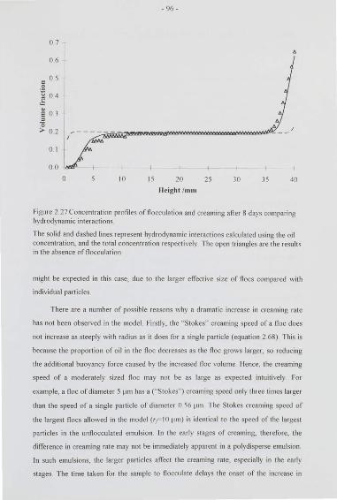
07
06
= 0 5 .~
~ 04 .: e o 3 = ~ 02
0 1
00 0 10 I 5
-96-
20
Height /mm
25
A
30 35 40
Figure 2 27 Concentmtion profiles of fl occulation <tnd crea ming afier 8 days compari ng hydrodynamic int eractions
The solid and dashed lines represent hydrodynamic interactions calculated using the o il concentration, and the total concent ration respectively The open triangles are the result s in the absence of fl occulation
might be expected in this case, due to the larger effective size of floes compared with
individual particles
There are a number of possible reasons why a dramatic increase in creaming rate
has not been observed in the model. Firstl y, the "Stokes" creaming speed of a floc does
not increase as steeply with radius as it does for a single particle (equation 2 68) This is
because the proportion of o il in the floc decreases as the fl oc grows larger, so reducing
the additional buoyancy force caused by the increased floc volume. llence, the creaming
speed of a modera tely sized floc may not be as large as expected intu itively For
example. a fl oc of diameter 5 ~un has a ("Stokes") creaming speed only three times larger
than the speed of a single particle of diameter 0.56 ~tm The Stokes creaming speed of
the largest fl oes allowed in the model (r,t= I O ~t m) is identical to the speed of the largest
particles in the unflocculated emulsion. In the ea rly stages of creaming, therefore, the
difference in creaming rate may not be immediately apparent in a polydisperse emulsion
In such emulsions, the larger particles afrect the creaming rate, especia ll y in the early
stages The time taken for the sample to fl occulate delays the onset of the increase in
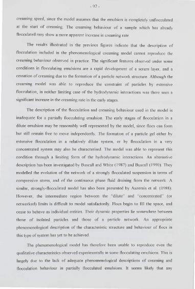
-97-
creaming speed. since the model assumes that the emulsion is completely unflocculated
at the start o f creaming The creaming behaviour o f a sample which has al ready
fl occulat ed may show a mo re apparent increase in creaming rat e
The result s illustrated in the previous fi gures indicate that the description of
flocculatio n included in the phenomenological creaming model canno t reproduce the
creaming behavio ur observed in practice The sig nificant fea tures observed under some
conditions in flocculating emulsions are a rapid development of a serum layer, and a
cessa tio n of creaming due to the fo rmation o f a part icle network structu re Although the
creaming model was able to reproduce the constraint o f parti cles by ex tensive
fl occulatio n, in neither limiting case o f the hydrodynamic interactions was there seen a
significant increase in the creaming ra te in the ea rl y stages
1 he description o f the fl occulatio n and creaming behaviour used in the model is
inadequate fo r a partia ll y fl occula ting emulsion The early stages o f fl occulatio n in a
dilute emulsion may be reasonably well represented by the model, since fl oes can form
but still remain free to move independently The fo rmation of a par1icle gel either by
extensive fl occulatio n in a relati vely dilute system, o r by fl occulation in a very
concentrated system may also be characte ri sed The model was ab le to rep resent this
conditio n thro ugh a limiting form of the hydrodynamic interactio ns An alternati ve
descriptio n has been investigated by Bu sca ll and Whit e ( 1987) and Bu sca ll ( 1990) They
modelled the evolution of the network of a strongly flocculated suspensio n in terms o f
compressive stress, and o f the continuous phase fluid dra ining from the network A
similar, strong ly- fl occulat ed model has al so been presented by Auzerais et al ( 1988)
llowever, the intermediate regio n between the "dilut e" and "concentra ted" (o r
networked) limit s is diffi cult to model sati sfa ctorily rlocs begin to 1111 the space, and
cease to behave as individual entities Their dynamic pro perti es li e somewhere between
those o f isolated parti cles and those o f a parti cle network An appropriate
pheno menological descriptio n o f the characte ri stic stmcture and behav iour o f fl oes in
this type o f system has yet to be achieved
T he phenornenological model has therefore been unable to reproduce even the
qualitati ve characteristi cs observed experimentally in some flocculating emulsions This is
largely due to the lack o f adequate phenomeno logical descriptio ns of creaming and
flocculation behaviour in parti ally flocculated emulsions It seems likely that any
-98-
successfu l model o f creaming in flocculated systems wi ll have to include a mo re deta il ed
structural description of t he emulsion at the level of individual particles
2_ 11 Concl usions of model
The basic pheno menological creaming model includes no di rect particle
interactio ns and therefore corres ponds to an idealised emulsio n Wi thin the limitatio ns o f
these assumptions. a number o f sig ni ficant conclusions could be drawn from the result s
• The d ifferential creaming ra tes of particles o f diiTerent sizes causes strong variatio n in
the par1icle size distribution in the sample
• The back fl ow of the continuous phase fluid can carry some of the smaller parti cles
with it so that they move downwards in the first stages of creaming
• ·rhe concent ratio n profil e in the crea m is determined by the hydrodynamic interact ions
a t hig h concentra tio ns A description of the hydrodynamic effects in terms of the total
concent ration is insufficient to model the size-distribution dependent packing o f
parti cles in the cream
• Under some conditio ns the ultrasound veloci ty in the emulsion is dependent o n
parti cle si7e d ist ributio n The va ri ation in parti cle size di stributio n, especially in the
cream, can mask the concentration dependence o f the velocity.
• Interpretation o f ultrasound veloci ty measurement s in these circumstances in terms
o nl y o f the to tal concentration o f o il may produce misleading result s
• Thermal diffusion does not have a strong effect o n profil es of total o il concentration
fo r the particle sizes modelled, but may inOuence the parti cle size distribution, and
thereby the ultrasound velocity
• Crysta lli sation in an idea l hexadecane emulsion contai ning solid and liquid dro plets
has little effect on creaming Crystalli sation is relati vely rapid , and therefore the
creaming behaviour is characterised by the creaming of solid particles
• T he concent ration pro fil es in an ideal, modelled emulsion are very diHe rent from some
experimental systems in which nocculatio n is occurring
-99-
• Modelling of combined flocculation and creaming behaviour was characterised by the
space-filling nature of extensive flocculation, which prevents further creaming
• No appropriate description of the hydrodynamics in flocculated systems was found to
accurately represent the creaming behaviour
The failure of the phenomenological model to predict the creaming behaviour of
flocculated emulsions has led to a different , smaller scale modelling approach to
combined flocculation and creaming The next chapter describes a statistical model which
is designed to investigate the effect of flocculation characteristics on creaming profiles,
by simulating the system at the level of the individual particles rather than through a
phenomenological description
- 100 -
Chllpter 3 : Lllttice 1\lodelling of Crellming and Flocculation
The creaming model presented in the previous chapter illustrated the qualitative
form of the concentrat ion profiles which would be C'<pected in an ideal emulsion
Initially, no direct particle interactions were included lt was noted that many
experimental studies have observed marked ly different profi les to those predicted by the
model These di!Terences are thought to be due to direct particle interactions, specifica ll y
nocculation, which were omitted from the phenomenological model While an attempt
was made to include the effects of nocculation in the model in a phenomenological
manner, the numeri ca l resu lt s were not able to reproduce the concentration profi les
which have been observed in practice The analysis indicated the difficulty of
incorporating into a phenomenological model a process which occurs at the level of
individual particles
For this reason, a model was developed to assess the effect of nocculation on
creaming behaviour by simulating these processes at the particulate scale Inevitably,
such a model can only represent a very small sample, because of the large number of
particles contai ned in an emulsion 11 can no longer represent the emu lsion at the scale of
creaming experiment s in the ultrasound sca nner, but is intended to indica te the form of
concentration profiles expected in the presence of nocculation The aim of the model is
to determine whether the creaming behaviour observed in experimental systems is
ex plicable solely in terms of particles sti ck ing together to form noes (and thereby
creaming more rapidly) or whether other processes are at work
3.1 The fractalnature of nocculation
Fractal geometry has been shown to provide a useful, simple description of noes
generated by a variety of means (Meakin, 1988, Jullien, 1990) The fractal dimension (or
dirnensionality) can be applied to obtain the scaling relationships of properties such as the
creaming speed, or noc size, in terms of the number of particles in the noc. The fractal
dimension of an aggregate or noc also holds information on the degree of compactness
of any particle network which might be generated through nocculation . Before these
- 101 -
techniques are described in relation to the lattice model , it is first necessary to provide a
brief introduction to the concept offractal geometry
The term " fractal " was first introduced by Mandelbrot (1975) to describe ramified
stmctures which do not lend themselves to definition by Euclidean geometry The need
for such a concept was indicated by the existence in nature of convoluted physical forms
such as coast lines, clouds, and aggregates The Euclidean geometry of squares, triangles,
etc comes nowhere near a proper description of such structures rractal structures are
those that can be characterised by a non-integer dimcnsionality (Mandelbrot, 1982,
Vicsek, 1989) This fractional (fractal) dimension can be defined in terms of the number
of small measuring units (of dimension equal to the Eucl idean dimension of the
embedding space) which are requi 1ed to cover the structure completely This is a
measure of how space-filling the structure is In a fractal object , the required number of
measuring units, 111., scales with the size oft he object, 1., in the form
[3 I]
It is clear from this relationship that , if the fractal dimension cft is equal to the Euclidean
dimension of the embedding space, the object fill s the space uniformly In three
dimensions this may correspond to a homogeneous dispersion A non-integer dimension
represents the sparse, convoluted nature of fractal objects For example, a coastline is
embedded in (approximately) two-dimensional space, but may have a fractal dimension
between one and two. This represents its grea ter space-filling capability than a straight
line, but its inability to fully cover a two-dimensional surface. An aggregate grown in
three dimensions typically has a fractal dimension less than 3, indicating that it becomes
more sparse the larger it grows In many real cases, the fractal scaling behaviour is not
universal , but applies over a limited range of length scales
Many fractals have a property called self-simi larit y, which arises from the scale
invariant nature of equation 3 I Self-similarity means that the structure of the fractal
object is invariant under an isotropic change of length scale. This quality applies precisely
in mathematica lly generated fractal structures, for example in the illustrations presented
by Mande\brot ( 1982) In real , physical systems, however, self-similarity is only true
statistically, or on average_ In other words, taking aggregat ion as an example, an
expanded view of one section of an aggregate wi ll not exactly match the original
aggregate in structure. 1t does, however, correspond to the structure of an aggregate
- 102-
which could statist ica lly have been produced by the same aggregation process An
alternative type o f fractal is o ne in which different fl actal dimensions are requi red to
define the scaling behaviour in different co-ordinate di rectio ns Such fractals are ca ll ed
self-a ffin e
In rela tion to fl occulatio n. the result s of fractal geometry have been shown to be
applicable to many aggregation phenomena in two and three dimensions The suitabi lity
o f a fractal description o f aggregates (or fl oes) is evidenced both by the structu re of
experimentally pr oduced samples, and by computer simulations of their growt h which
have demo nstrated fracta l sca li ng behaviour Meakin ( 1988) presents an example o f an
experimentall y produced co llo idal gold aggrega te which exhi bit s self-similarit y and for
which a fractal dimension can be calculated A substantial amount of work over the last
IS yea rs has been devoted to computer si mulation o f aggrega tion growth phenomena In
all cases, a fractal descriptio n of the aggrega tes was found to apply Useful reviews o f
the comput atio nal techniques and result s for the fractal dimensio ns under various
conditio ns can be found in the works of Jullien ( 1990) and Meakin ( 1988) Many
different techniques have been used , relating to deposition of particles o nto a surface, the
growth of an aggregate by the additio n o f single particles in tu rn, the aggregatio n of
parti cles into clusters and clusters in to larger clusters, etc. The frac tal d imension is
affected by the physical conditio ns represent ed by the computer simulatio n, and in some
cases by the spatial constrai nt s of the model (for example, the shape o f the latt ice in
lattice models) However, the result s o f the computational stud ies indicate that fracta l
geometry is a valid descriptio n of aggregating (or nocculating) systems, and is therefo re
applicable to the present work
The fractal nature o f nocculatio n is relevant to the la ttice model o f creaming and
noccula tion in two respects Firstly, the fractal dimension of the noes can be used to
define the scaling behaviour of the creaming speed and diffusion coeffi cient with noc
mass Fractal geometry is o f great benefit in similar generali sed descri ptions o f the
dependence of physical parameters o f an aggregate \\i th it s size or mass lt does not
define the detailed structure o f the individual noc, but acts as a description o f the
stati stical average o f the properties o f such aggrega tes In the la tti ce model, a fractal
dimension of the noes is assumed, based o n previous result s, in o rder to determine the
creaming and diffusion rates o f noes o f va rying sizes Thus, the properti es o f the noes
- 103-
are defined in a statistically averaged manner, rather than considering the structure of an
individual noc to assess the effect o n it s mobility The second use of the fractal
dimension in the model is to qwmtify the degree of compactness of any space-fi lling
particle network which may be formed The fractal dimension was calculated over a
region of the sample. to compare the structures formed under different conditions
The noes considered in this study are assumed to be self-similar, so that a single
fractal dimension is va lid 1t could be argued that in a creaming (or sedimenting) field ,
prefCrential growt h may occur in the ve11ical direction, resu lting in a self-anine fractal
llowever, self- si milari ty and a single fractal dimension N< assu med for the lattice model
The fractal rela tionship between the number of particles, N(R), within a sphere of radius
I? is given by
[J 2]
For a single floc, the radius R is equivalent to the radius of the fl oc, If, and N then
represents the number of particles in the floc. This appl ies to a floc which is composed of
many identical spheres The second equality has been provided for consistency down to
the scale of a single particle (of radius r) This need not always be true, but is convenient
for the lattice model Equation 3 2 can be used as a simpler definition of the fractal
dimension in it s application to fioccula tion This relationship (equation 3 2) provides the
basis for the scaling behaviour of creaming and diffusion coefficien ts, which are
desclibed in later sections It is also the expression used to obtain the fractal dimension
oft he particle networks generated by the flocculation and creaming processes
3.2 Overview of model
A very simple approach to the problem of creami ng and fl occulation has been
adopted for the small -scale model developed in this study In order to enable a
reasonab le size of system to be modelled, and for computational simplicity, a lattice
model was used, rather than a more comple:-< continuum Brownian dynamics simulation
1t was based on two previously published models of sedi mentat ion (van der Knaap et al ,
1994, lluang and Somasundaran, 1988), both of which were in two dimensions, and o nly
one of which included flocculation (van der Knaap et al , 1994) The essence o f a lattice
- 104 -
model is that the positions of the particles are constrained to coincide with the nodes of
an imposed lattice structure Particle movement is achieved by pseudo-random steps
between lattice sites, weighted according to the required physical rate of motion (for
example, the creaming speed or diffusion coefiicient)
The model developed for the study of creami ng and nocculation is three
dimensional and is based on a cubic lattice Figll!e 3 I shows a schematic diagram of the
lattice model The excluded volume of rigid particles is accounted for by choosing a
lattice spaci ng equal to the particle diameter The model is therefore restricted to
rnonodisperse systems Each lattice si te can only be occupied by a single particle at ttny
time Init ia lly, particles are assigned at random to positions on the lattice, up to the
required proportion of occupat ion Particle movement is execut ed by selecti ng a particle
at random and moving it to a new site according to its predefined creaming and diffusion
rate During each time interval, every particle is given the opportunity to move No
hydrodynamic interactions are included other than the obstruction caused when a particle
attempts to move to an already occupied latt ice site Such movement is forbidden by the
singlc·occupancy crit erion
j I I f -f I
I I C- L-
11 t l" ~l/(', +-- I\ ~ !--
1 " .I I {l t_ C-
I ~ .. ~j4 I ! i 1 ""! I
- h ! .;;>--"' -- ~
I I I I I f
f-igure 3 I Schematic diagram of lattice model of creaming and nocculation
Creruning is always upwards and the speed is denoted by 11 Diffusion occurs in any direction, and the diffusion coefficient is denoted by/) The lengt hs of the at rows represent the relative magnitudcs of each motion for single patiicles and noes
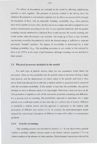
- 105-
The efTects of flocculation are included in the model by allowing neighbouring
particles to stick together The presence of polymer (which is the driving force for
depletion f1occulation) is not included explicit ly, but its effects are accounted for through
the formation of floes, with an adjustable "bonding'' probability, P~:~ood Once particles
have stuck together to form a floc, the floc moves as a single unit and is assigned its own
motion characteristics according to its size 1t was expected intuitively that the greater
creami ng velocity attributed to individual floes would increase the overall creaming rate
in the system when flocculation was included The break up of floes is also included,
representing reversible flocculation in which the thermal energy is sumcient to separate
previously "bonded" particles The degree of reversibility is determined by a bond
breakage probability, P bKal. The modelling procedure is very similar to that adopted by
!law et al ( 1995), in the study of gel formation, although creaming was not included in
their systems
3.3 Physical processes included in the model
For each type of particle motion, there arc two parameters "• hich define the
movement These are the probability that the particle makes a movement during a single
time interval , and the displacement (in lattice units) of the particle each time it does
move. Each time the particle is selected, a random number is generated and is compared
with the movement probability If the number is less than the probability, the particle
attempts to move a distance equal to its step length Otherwise it does not move at all
This procedure is applied to each of the movement properties (creaming and diffusion)
For a process such as creaming, this probabilistic approach is equivalent , for a single
particle over a sufficient number of time intervals. to a uniform rate of motion Diffusion
is essentially a random motion and this approach is equivalent to the random walk
description of diffusion (see section 2 2 2) In contrast , the phenomenological model
adopted the macroscopic description of diffusion in terms of its effect on concentration
gradients
3.3.1 Gravity (creaming)
The creaming process was described in sect ion 2 2 1 lt was shown that a particle
reaches a terminal , uniform velocity equal to the Stokes velocity (equation 2 7) in an
infinite medium in the absence of other particles llydrodynamic interactions reduced the
- 106-
average creaming speed by an amount dependent on the particle concentration
llydrodynarnic interactions are not included in the lattice model, except for the
obstmction of particle movement due to other particles occupying the destination lattice
site In a monodisperse sample in which no flocculation occurs, the creaming speed is the
same for a ll particles llowever, the presence of floes causes the creami ng speed to vary,
according to the size of the fl oc lt was shown in section 3 I that the number of particles
in a fractal floc is related to it s e!Tective radius by equation 3 2 The effective density of
the fl oc can be calcula ted frorn thi s result. and thereby the net gravitational force o n the
floc. If the " Stokes" drag on the fl oc is proportional to the floc radius (just as it is
proportional to the radius of a rigid sphere), the force balance equa tion can be used to
show that the "Stokes" creaming speed oft he fl oc is given by
13 3)
where J1 is the fractal dimension and u0 is the Stokes velocity of a single p<~rticle of
radius r This relationship is v<1 lid for a fractal floc made up of N identical particles
Equation 3 J is equivalent to the creaming velocity used for floes in the
phenomenological creaming model (equation 2 68) The larger the floc, the faster its
creaming rate, in the absence o f additional obstruction A fractal dimension of 2 was
used in the ca lculation of creami ng speeds for all fl oes This va lue is approximately that
obtai ned by computer simulations of aggregatio n under a va riety of cond itions Many o f
these va lues can be found in the review of Jullien ( 1990) Although the fractal dimension
is s li ghtly different for different modes of aggregation, the effect of this variation on the
creaming speed is negligib le compared to the dominant influence of floc size
Although the creaming process is not in essence a random one, it can be described
in terms of randomly generated motion in order to be compatible with the lattice model
The motion is described by a probability of movement during each time interval , and a
step length (in lallice units}, which is the di stance moved by the particle or fl oc when it
does make a movement If the creaming speed is written in lattice units per time interval ,
the relationship is given by
I =" ~ P crm.N cnn .. \ ' O.N 2
,. [34)
- 107 -
The lattice unit is equal to the parti cle diameter The step length is chosen for each noc
size in order to keep the probability within predefincd limit s (i t cert ainly cannot be
g reater than unity) A maximum step length o f six lallice unit s was specified When a
particle o r noc is to be moved, a random number is generated If the number is less than
the creaming probability of the particle, Perm, a di splacement is attempted The particle
tries to move a vertical di stance equal to its step length lcrm (in lattice unit s) If this
di splacement is o bstructed by other particles, it moves as far as it can verti cally, up to it s
allowed step length.
3.3.2 Therm:~ I diffusion
Thermal dint.1sio n was discussed in sectio n 2 2 .2 The diffusio n coefficient for a
single isolated part icle in an infinite medium is given by the Sto kes-Einstein equtttion
(equation 2.23) For noes, the Sto kes drag fo rce is related to the radius o f the floc. ' I·
which was expressed in terms oft he number o f parti cles in the noc by equation 3 2 Thus
the modified Sto kes-Einstein diffusio n coeffi cient for noes can be written as
' ' /Jo.N :::o k RT - N d, ::;: /JoN o~,
61f'l1" [3.5]
where d1 is the fra ctal dimension and /J0 is the diffusio n coeffi cient o f a sing le particle
The equation is again valid for a noc made up o f N identical particles The dinl1sio n
coeffi cient is reduced as mo re particles are added to the noc. The fractal dimensio n was
defined to be 2 for these calcula tions, for the reasons di scussed in the previous section.
Rotatio nal diffusio n was neglected in this model
The descriptio n o f diffusio n in the lattice model is that of a rando m walk This is in
cont rast to the phenomeno logicalmodel o f creaming in which the o nly effect o f diffusio n
was to smooth out concentration grad ient s The two parameters defining the diffusive
mo tion are aga in a probability of movement in each time step, and a step length (in latti ce
unit s) The step length is the di splacement o f the particle or noc in any direction when it
makes a movement The random walk result for the mean square di splacement of an
object was deri ved by Einstein , and was presented in chapter 2 (equatio n 2 9) In terms
oft he diffusion coeffi cient . it can be written as
(n' ) = 6 /Jt [3 6]
- 108-
The latlice model requires the motion to be expressed in relation to the movement
probability and step lengt h Another random walk resu lt is useful here If an object
executes a random walk, wit h each step being the same length t .... ra; , its mean square
displacement an er 111 steps is given by
[37]
In the lattice model , the object (particle or noc) has a constant step length, and the
number of steps executed in any time period is related to the movement probability
Therefore, the diffusion parameters can be expressed as
[J 8]
The units of length have been converted to the lattice spacing. which is equal to the
particle diameter. A compari son of equations 3 7 and 3 6 with these results shows that
the movement probability shou ld be related to the diffusion coefficient by
[3 9]
The factor which includes the diffusion coefficient is equivalent to the diffusion
coefficient expressed in units of the lattice spacing and the time interval
In the case of diffusion, the step length was restrained always to be equal to a
si ngle lattice unit This avoided difficulties relating to non-uniformity of concentration
profiles caused by particles making large steps near the edges of the system. A random
number is generated to determine whet her the particle takes a step in the current time
interval If the number is less than the diffusion probability, the particle or floc wi ll move
Its displacement is equally likely to be in any of the six co-ordinate directions, and is of a
si7e equal to one lattice unit (provided no obstruction is encou ntered)
lt is important at this stage to highl ight the differences in particle movement
between the present lattice model and previous models on which the work is based (van
der Knaap et al , 1994. lluang and Somasundaran, 1988) In each of the previous
models, the creaming and diffusion rates are characterised by a parameter representing
the ratio of creaming and diffusion probabilities In the model of lluang and
Somasundaran, the probability of particle movement in each direction is determined
- 109-
according to the net effect of sedimentation and diffusion Particles move by a single
lattice unit in the selected direct ion Flocculation was not included, and theref01e the
movement probability and step length are the same for all particles
Va n der Knaap et al ( 1994) simulated the erfects of diffusion by selecting each
part icle in turn and calculati ng it s displacement according to the predetermined
probability, as in the present model ll owever, the creaming motion was executed for all
part icles at the same time. On each time step, a single random number determines
whether a creaming step will be made in th is interval (according to the creaming
probabi lity), and all particles arc moved by the appropriat e distance This procedure
avoids the unphysical obstruction of particles which would otherwise cream at the sa me
speed, which can occur in the present model The relative creaming and diffusion rates of
floes ofd iffe1ent si?Cs a1e cont ro lled only th rough the step length in the model of van der
Kn a(l p et a! ( 1994 ) The probability of movement by creaming or diffusion is the same
for floes of all sizes, and creaming occurs for all noes at the same time llowever, the
distance moved by the fl oc depends on its size A maximum step length of l'i ve lattice
units for creaming and three lattice unit s for diffu sion were defined (van der Knaap et a! ,
1994) Therefore, there are only fi ve discrete creaming rates, and three discrete diffusion
rates, since pa1ticles can only move between lattice sites
In the present model, bot h the movement probability and the step length can be
varied accord ing to fl oc size ll ence. a near-continuous range of creaming and diffu sion
rat es are permitted Since the creaming probability is now din"'erent fo r each size of floc.
the model follows the method of lluang and Somasundaran for creaming movement
Each particle is moved in turn, as is the case for diffu sion Some obstruction of particles
wi th the same creaming speed will resu lt , but the effect is ex pected to be small
3.3.3 Flocc ula tion
Flocculation is the tendency of part icles to sti ck together, when they touch or
approach within a certain distance of each other (see sect ions I I 2 and 2_10) In the case
of depletion fl occulation, this mutual attraction is driven by the presence of polymer or
other entities (e g surfactant micelles) in the continuous phase. Alt hough the latt ice
model does not explicitly include such an additional species, its effects are simulated
through the sticking probability of particles In many physical systems fl occulat ion is
- 110 -
reversible, in the sense that tl1e thennal energy of some flocculated particles is sufficient
to pull them apart again This feature can be characterised by the probability that a
fiocculated "bond'' will break apart The two key parameters which determine
floccu lation in the lattice model are therefore the bonding and break up probabi lities,
P~w:>nd and 1'1, • ..,,.~ respectively The bonding probability, Pb<>nd, is the likelihood that a bond
will form between neighbouring particles in each time interval. The break up probabilit y.
P...,c:U.. is the probability that an existing bond will break during each time interval
Flocculation in the lattice model is only permitted between the nearest neighbours
o n the lattice. Since a cubic lattice is used , there are six such neighbouring sites, each
separated from the central particle by one lattice unit The next nearest neighbours arc at
a distance of .J2 times the lattice unit from the centml particle, there are 12 such
neighbours The limitation of bond formation to the nearest neighbours theref01e
corresponds to a very short-range potential (which is the case for depletion nocculation)
The reversibility of nocculation relates to the breaking of each "bond" rather to an
individual particle breaking ofT from a noc. !\. particle which is bonded to more than one
nearest neighbour in a noc is less likely to break on· than a particle with a single
connection Thus, a more compact structure is favoured in the modeL not through an
attractive non-bonded potential between particles, but through the greater stability of
more closely structured noes
The bonding and break up probabilities can be interpreted in terms of an
interparticle potential Figure 3 2 shows a schematic diagram oft he interparticle potentia l
energy as a function of their separation, as represented in the lattice model The plot is
not to scale The spatia l extent of the regions of negative and positive energy is negligible
in the lattice model, since particles can occupy neighbouring sites with or without being
nocculated, and a bond can break without particles moving away to another lattice site
At a separation of 2r, the potential tends to infinity, which corresponds to the volume
exclusion of the rigid particles The other two notable features are the negative potential
well. and the positive energy barrier T he potential well represents the favourable energy
state of particles which are nocculated llowever, particles at a larger separation must
overcome the energy barrier in o rder to reach the nocculated state The probability of a
particle having sufficient energy to "cross" the energy barrier can be written as a
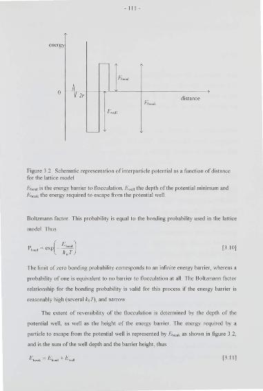
energy
0
- Ill -
--> distance
Figure 3 2 Schematic representation of int crparticlc po tential as a function of distance fo r the lattice model
Ebond is the energy barrier to nocculation, /~· .. e ll the depth of the po tential minimum and /~'b. ca\.. the energy required to escape from the po tential well
Boltzmann facto r This probability is equal to the bonding probability used in the latt ice
model Thus
P,.,, "'- exp( 1' -...• ) k; r
[3 IOJ
The limit of zero bonding probability corresponds to an infinit e energy barrier. whereas a
probability of one is equiva lent to no barrier to nocculation at all The I3 oltzmann facto r
relationship fo r the bonding probability is valid for this process if the energy barrier is
reasonably high (several k8 7), and narrow
The extent of reversibility of the flocculation is determined by the depth of the
po tential well , as well as the height of the energy barrier The energy rcqui1 ed by a
particle to escape from the po tential well is represented by F:~nuk as shown in fi gure 3 2,
and is the sum of the well depth and the barrier height , thus
[J IIJ
- 11 2-
The break up probability can aga in be related to the energy required to break the bond
through a Oolt7mcum fac to r
( F ) p d.:. ex p _:~nuL b•~•l kHT [3 121
An infinitely deep potential well represent s completely irreversible flocculatio n, since
particles can not escape fro m the well . o nce fl occulated lt is clear fro m equations 3 11
and 3 12 that this situation corresponds to Pmc:ol 0 The rat e of fl occulation is still
dete rmined by the height o f the energy barrier, and thus, in the model . th rough the
parameter Pbond
A shallower potential well represent s a more loosely linked floc, in which particles
can break o ff re lati vely easily As the we ll becomes shallower. the energy required to
separate fl occulated particles decreases, and the probabi lity o f break up increases The
conditio n at w hich the potentia l well vanishes, is equi valent to
[3 13]
Although the nocculated energy state in thi s case is no lo nger fa vourable, the ene1gy
barrier still prevents parti cles escaping once a bond is formed The break up probabilities
studied in the lattice model were in the range fro m zero up to the bo nding probability If
the break up probability is larger than the bo nding probability, the «nocculated" stat e is a
less favourable energy state fo r particles than a random distribution Jlence the energy
barrie r to particles escaping from the "bonded" state is lower than the barrier to
formation o f that state This is not physica ll y represent ati ve o f most real nocculating
systems
3.4 Time evolution
The evolutio n of the sample is modelled by executing particle mo tio n in a series o f
small time intervals In each interval, every particle is selected once at random to execute
a di splacement. The order in which parti cles are chosen to be moved is random from
within the set o f particles which have no t yet moved during thi s time step Since fl oes
include many particles, they a rc more like ly to be moved first , because the probability is
equal for each particle, rather than for each unit (particle or fl oc, a fl oc counts as a single
- 11 3-
unit ) llowever, each fl oc is only allowed one attempt to move during any one time
interva l
llaving selected the unit (particle or floc) to be moved. the dh:placement of the
particle 0 1 fl oc is determined by it s probability and step length fo r each of the physical
processes included in the model (see sections 3 3 I and J 3 2) Having calculated the
required di splacement (which is zero if the particle is not allowed to move in thi s
interval). the destination sit es for a ll the parti cles in the fl oc are examined If any o f these
sites are already occupied by parti cles fro m a di!Terent unit (another fl oc or pa rt icle}, the
displacement is re fu sed If the di splacement was mo re than o ne lattice unit , an att empt is
made to ac hieve a sma ller displacement without obstnrction It is clea r that although
floes have a fas ter creaming speed, they are also more li ke ly to be obstructed than single
particles. because o f their la rger co ll isio n cross-section /\O er the uni t 's di splacement has
been de te rmined, a ll neighbouring particles are examined These may be new neig hbours
due to the new positio n o f the uni t , or existing adjacent par1icles within the fl oc Each
neig hbouring pair which is no t already bonded is a llowed to bond, according to the
bo nding probability Each existing bond is given the oppo rtunity to be severed. acc01 ding
the break up probabi lity
Thi s process o f di splacement followed by fl occula tion is repeated wi th each
randomly selected parti cle o r floc until all have had o pportunit y to move du ri ng th is time
inte rval !\sequence of many such time steps simulates the evolutio n oft he c reaming and
fl occulatio n behaviour
3.5 Boundary conditi ons
3.5. 1 x and y J)Criodic boundaries
Periodic boundary condit ions are used in many simulatio ns in order to model the
elTect o f a much larger system. whil st onl y in fac t simulating the motion o f a relati vely
small number o f particles The two o ppos it e boundary wall s are made to "wrap-around ''
so that any parti cle moving out o f one side of the system appears at the o ther side
Instead o f o nly looking at a single computational "box", the system behaves like an
infinit e array of identical "boxes" neighbouring each other. No new informat ion is
contained in the other boxes, since they are identical, but the techn ique removes the need
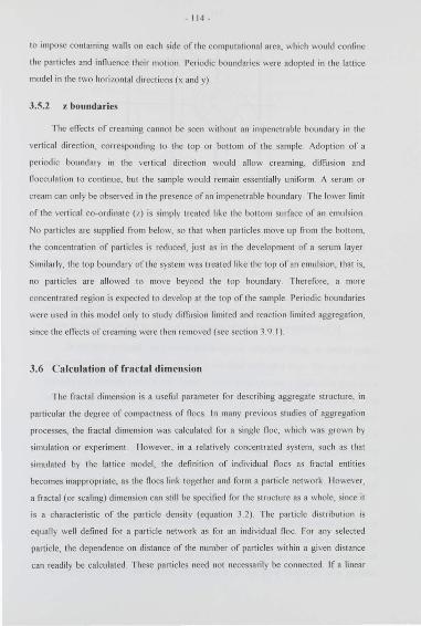
- 11 4-
to impose cont aining wa ll s o n each side of the computatio nal area, which would confine
the particles and influence their mo tion Periodic boundaries were ado pt ed in the lattice
model in the two horizontal directions (x and y)
3.5.2 z bounda r·ies
The effects of creami ng cannot be seen without an impenetrable boundary in the
verti ca l direction, corresponding to the to p o r bottom of the sample Adoption of a
peliodic boundary in the verti ca l directio n would allow creaming, diffusion and
fl occulation to conti nue, but the sample would remain essentia lly unifo rm A serum or
cream can only be observed in the presence of an impenetrable boundary The lower limit
o f the vertical co-ordinate (7) is si mply treated like the bottom surface of an emulsion
No part icles are suppl ied from below, so that when particles move up from the bottom,
the concentration of part icles is reduced , just as in the development of a serum layer
Similarly, the top boundary o f the system was trea ted like the top of an emulsion, that is,
no particles are allowed to move beyond the to p boundary Therefore, a mo re
concentrated regio n is expected to develop at the top o f the sample Periodic boundaries
were used in thi s model only to study diffusion limit ed and reaction limited aggregation,
si nce the effects of creaming were then removed (see section 3 9 I)
3.6 Ca lculation of fracta l dimension
The fractal dimension is a useful parameter for describing aggregate struc tu re, in
particular the degree o f compactness o f noes In many previous studies of aggregation
processes, the fractal dimension was ca lculated for a si ngle noc, w hich was grown by
simulation or experiment llowever, in a re lati vely concentrated system, such as that
simulated by the lattice model, the definitio n of indi vidual noes as fractal en tities
becomes inappropriate, as the noes link together and fonn a particle network l lowever,
a fractal (or scaling) dimension can sti ll be specified for the stm cture as a whole, since it
is a characte ri stic of the pa11icle density (equation 3 2) The particle di stributio n is
equally well defined for a particle network as for an individual noc. f-o r any selected
particle, the dependence on di stance of the number of particles within a given distance
can readily be calculated These particles need no t necessarily be connected If a linear
- 115-
Figure 3.3 Calculation of the particle distribution function in the lattice model
A proportion oft he volume of particle fl, which is at a distance R from par1icle A, is assigned to each oft he spherical shell s denoted by Un etc
region can be found in the relationship betwccnlog(N(U)) and log(/?), the gradient of this
region is equal to the fractal (scaling) dimension of the structure (equation 3 2)
In the lattice model. the particle distribution is calculated using, as central points,
each of the particles which are present in a specified horizontal layer For each of these
particles (for example particle A in figure 3.3) the distance from it of all other particles is
calculated. for example, particle B in figure 33 is at a distance R from particle A The
particle distribution is then obtained by counting the numbers of particles within each
distance range, R, The distance ranges are equivalent to spherical shells, each of a
specified thickness, as shown in the diagram The particle distribution is specified by the
number of particles within each shell A sum of the distributions over all of the central
particles yields an average particle distribution function in the locality of the hori7ontal
layer.
Initially, the distribution was calculated by recording each particle at the position of
its lattice site (its centre of mass) . llowever, it was found that this caused a significant ly
lumpy distribution due to the existence or o nly discrete particle separations because or
the geometry of the cubic lattice For example, in the close proximity of a particle,
- 116-
another particle can only be present at separations of I. ·h, .JJ e tc (lattice unit s). w hich
are the closest neighbouring positions o n the lattice Refinement of the particle
distribution was achieved by assigning an appropriate proportion of the particle's vo lume
to each of the intersecti ng spherical shel ls representing the consecu ti ve distance ranges
flomthe central particle. This approach is illustrat ed in figure 3_3 The proportion of the
particle' s volume which is in each spheri cal shell can be calculated from simple
geomet ri cal relationships
Although the use of this method smoothes the patticle distribution function
considerably, the availability to particles of only di screte sit es on the lattice st ill distorts
the distribution, especia ll y at close range A random distribution of particles with a
vo lume fraction ofO 524 wou ld be expected to have on average an equivalent vo lume of
3 655 pa1ticles wit hin a distance of I particle diameter of any other particle llowever. a
fully occupied cubic lattice (which has the same volume fraction of 0 .524) has only the
equ iva lent of 2 609 particles wit hin this range The uneven nttture of the particle
distribution in the lattice model is to some extent smoothed out in the overall distribution
function N(R) especially at distances larger than a few diameters 1 lowever, to remove
some oft he artificial efTects oft he lattice structure on the distribution function, all results
were scaled according to the distribution which wou ld be ob tained if the lattice were
fully occupied
In the fully occupied lattice, the numbers of particles in each distance range is a
measure of the maximum volume available to particles o n the latt ice withi n that range
<to(R,J represents the number of particles (as an equivalent volume) o n a fully occupied
cubic lattice in the distance range denoted by the argument /?" The argument /?"
represents the spherical shell between a distance of!?" and Rn·J, as shown in figure 3 3
The calcu lated number of particles in thi s distance range in another lattice simulation is
represented by G(R,J Therefore. the proportion of the available volume occupied by
particles in this shell is G(R.,J Go(R,J I lence the ef[e<:fn·e number of particles in thi s
range should be equal to this proportion, scaled by the actual spatial volume in the
spherica l shell (which is the available vo lume if the particles were not restricted to lattice
sites) Thus
( ) G(il,) 4JT[il' G,., R, ~ li, (il,) 3 ' ' 13 14]
- 11 7-
The total number of particles N(R) is obta ined by summation over all the distance ranges
(shells) up to the required distance The fra ctal dimension itself is determined from the
gradient of a linear fit to the logarithmic relationship of N(N)
In the lattice simulations, the fractal dimension is calculated over the range four to
ten particle diameters, which was found to obey fractal scaling in all cases At smaller
length scales, the noc structure causes fluctuations in the pa1iicle distribution, and a
fractal scaling description is invtt lid At long distances, the particle distribution becomes
homogeneous. and the fractal dimension approaches 3 The fracta l dimension over the
chosen length sca le is characteri stic of the scaling properties or the structure in the
locality of the horizont al slice used for the central particles It is only meaningful in a
region in which the particle concentration is approximately constant . since in the
presence or a concentration gradient , the pal tide distribution is afl"ected by the changes
in average concentration as well as by the structure of the dispersion The1efore, the
fractal dimension was only calculated in the region of the sample between the serum and
cream regions, where the concentration is reasonably uniform
3.7 Computer requi rements
The lattice model program was wri tten in FORTRAN 77, and was executed using
the Sun SPARCenter 2000 and Silicon Graphics Challenge XL servers at the Uni versity
of Leeds Random number generation was achieved using the Numerical Algorithms
Group FORTRAN Library subroutines (mark 15) A si ngle pseudo~random number
sequence was used for each program run A fl ow diagram of the program is shown in
l'i gure 3.4, and the code is given in Appendix AJ An expanded flow diagram of the
flocculation section which forms and breaks bonds is shown in l'igure 3 5 The model is
CPU-intensive, and the size of the system and number of particles were tailored to the
available resources. A typical simulation of I 00,000 particles, with 2400 time steps takes
up to 5 days of CPU time to run when floc break up is included The program requires
approximately 24 M bytes of memory
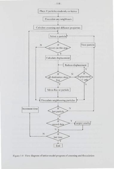
- 118-
Calculate creaming and diffusion properties
Figure 3 4 Flow diagram of lattice model program of creaming and nocculation
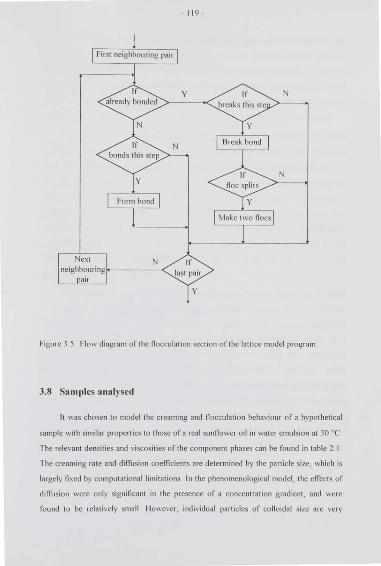
- 119-
Figure 3_5 Flow diagram oft he flocculation section oft he lattice model program
3.8 Sam ples analysed
11 was chosen to model the creaming and flocculation behaviour of a hypothetical
sample with simi lar properties to those of a real sunflower oil in water emulsion at 30 °C'
The relevant densities and viscosit ies of the component phases can be found in table 2 I
The creaming rate and diffusion coefficients are determined by the particle size, which is
largely fixed by computational limitations In the phenomenological model, the eH"ects of
difTusion were only significant in the presence of a concentration gradient, and were
found to be relatively small llowevcr, individual particles of colloidal size are very
- 120-
diffusive, executing ex tensive rando m walk motion The lattice model incorpo rates thi s
rando m walk motio n and therefore requires a large amount o f computatio nal resources
to model the diffusio n, for onl y a small development o f creaming behavio ur A relatively
large particle size was chosen, therefore. so that the creaming properties of the system
could be observed without excess ive computation of diiTusive mo tio n The particle
diameter used in the calculations was I 2 pm, and thi s al so defines the laltice spac ing
Equations 3 4 and 3 9 define the movement probability and step length for particles
and noes Since the movement probability for each process (creaming and diffusion)
must be less than unity, the time step is constrained by the limiting di splacement allowed
for each movement The fastest creaming speed is for the largest noes, whereas the
la1gcst diffusion coeffic ient is fo r single parti cles The step length fo r c reaming is
permitted to be as much as six lattice unit s llowever. the diffu sive di splacement "as
defined to be a single lattice unit in all cases. due to inconsistencies in the concentration
p10files when thi s was not the case The time int erva l is therefore determined by the
diffusio n probability for single particles A time step o f 0 25 seconds was chosen fo r the
modelling oft he sunnowcr o il in wa ter system
The number o f particles in the sample is dete rmined by the pro p01iion o f latti ce
sit es which arc occupied In the systems analysed. an initial occupancy o f I 0% was used
This correspo nds to a volume frt~ction of O 052 (due to the vo lume o f a sphere compared
with it s circumscribing cube) An occupancy of 100% is therefo re equiva lent to a
volume frac tion o f o nly 52%, so the high concentratio ns observed in some creams are
not possible in the model The dimensio ns of the lattice were usuall y taken to be
70 x70x200 . The calculatio n of fractal dimension takes an average over a ll particles in a
single layer, so that each dete rmination is an average o f approximat ely 490 particle
di stributio n functions In order to obtain good stati stical averages o f all the system
pro perties, l'i ve simulatio ns were carried out for each set o f parameters f o r the diffusio n
limited and reactio n limited aggregation, different lattice dimensions and vo lume
fractions were used, and these arc del'ined in section 3 9 I
- 121-
3.9 Results
3.9.1 Diffusion limited and readion limited aggregation
Two cases oft he growth of (lgg1egates under different limiting conditions are well
establ ished diffusion limited aggregat ion and reaction limited aggregation Both of these
condit ions have previously been simulated in the absence of a gravitational ftcld, wi th
particle motion determined by diiTusive random walks The two condit ions correspond to
different limiting va lues of the bonding probabi lity In the diffusion limited case. the
bonding p10bability is unity, so that as soon as one part icle touches anot her particle. they
st ick together The aggregation process is therefore characterised by the dynamics of
particle motion In the other extreme, if the bond ing probability is very low, as in the
reaction limited case, particles must collide m;my times before a bond is formed This is
equi valent to a sig nificant energy barrier which must be overcome to stick particles
toget her The characteristics of particle motion are secondary to the si7e of the energy
barrier in determining fl occulatio n in this case
In the lattice model , these two conditions were simulat ed to calculate the fractal
dimension for comparison wi th previous work Period ic boundary conditions were
imposed o n the top and bottom boundaries in the vertica l direction for these si mulat ions,
and the lattice dimensions were I OO x I 00-.: I 00 All creaming speeds were set to zero, to
represent the absence of a gravitational field The samples were extremely dilute. as was
the case in previous simulat io ns, with a lattice occupation o f O 005, or 5000 particles No
break up of fl oes was permitted, and the system was allowed to evolve until all part icles
had aggregated into a single cluster f-or the diffusion limited case, the bonding
probabi lity was unity, and for reaction limited ki netics a bondi ng probab ility of 0 00 1 was
used Ten simulations were carried out for each set of parameters The calculations of
the particle di stribution N(l?) were carried out using every particle in turn as the centre
for the di stribution, so in each case the di stribution is an average over 5000 particles
The fracta l dimension was determined over the range 4 to I 0 particle diameters
from the g radient of the logari thmic plot oft he particle distribution function (figure 3 6)
The fractal dimension obtained in the diffusion limited case was I 8 and for the reaction
limited conditions I 9, although the difference in gradient can not be identified visually
Quoted results in the literatu re are I 8 and 2 I for the diffusion and reaction limited
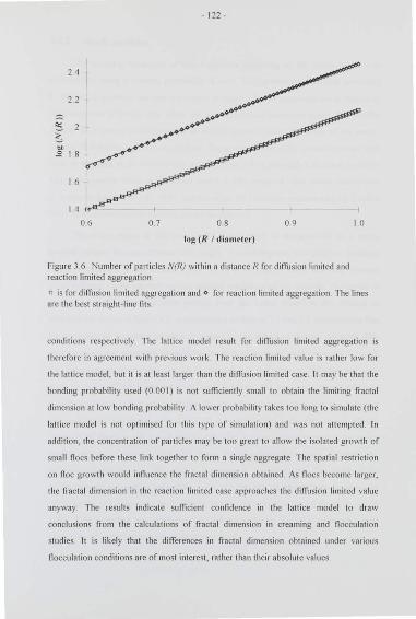
- 122-
24
22
~ <>:
~ "" .!2 I 8
16
log (R I diameter)
Figure 3 6 Number of particles N(l?) wi thin a distance N for diffusion limited and reaction limited aggregation
o is for diiTusion limited aggregation and o for reaction limited aggregation The lines are the best straight-line fits
cond itions respectively_ The lattice model result for diffusion limit ed aggregat ion is
therefore in agreement with previous work The reaction limited va lue is rather low for
the lattice model, but it is at least larger than the diffusion limited case lt may be that the
bonding probability used (0_00 I) is not sufficiently small to obtain the limiting fractal
dimension at low bond ing probability A lower probability takes too long to simulate (the
lattice model is not optimised for this type of simulation) and was not attempted In
addition, the concentration of particles may be too great to allow the isolated growth of
small noes before these link together to form a single aggregate_ The spat ial restriction
on floc growt h would influence the fractal dimension obtained As floes become larger,
the fra ctal dimension in the reaction limit ed case approaches the diffusion limited va lue
anyway The results indicate sufficient confidence in the latt ice model to draw
conclusions from the calculations of fractal dimension in creaming and noccu lat ion
studies lt is likely that the differences in fractal dimension obta ined under various
floccu\ation conditions are of most interest , rather than their absolute va lues
- 123-
3.9.2 Single parliclcs
The creaming behaviour of !>ingle particles according to the latti ce model was
examined by using a bond ing probability of zero The concentra tion profi les calculated
by the lattice model in this case are shown in figure 3 7 The concentration is defi ned as
the proportion o f lattice sit es which are occupied in any horizontal plane. The profiles
include the expected develo pment o f an o il ri ch (crea m) regio n at the top o f the sample
and an o il de fi cient regio n at the botto m The concentrat io n in the cream increases with
time, as was seen at the macroscopic scale (section 2 8 I), although it does not reach the
maximum possible va lue In the lattice model, a fully occupied cubic latt ice concsponds
to a volume fractio n o f o nly 52%. t~ nd therefo re the mt~ximum rando m packing fi actio n
o f 63% for mo nodisperse systems canno t be achieved
The serum region in the lower half of the sa mple is characterised by a rather
gradual increase in concent ration wi th height A mo nodisperse, no n-dinl1sive emulsion
would be expected, at the macroscopic level, to show a sh t~rp scrum int erface, between
an o il defi cient region (sennn) and the uniform emulsio n (see for example, the result s o f
section 2 8 I) The concentratio n pro fil es from the latti ce model in the absence o f
di!Tusion are shown in fi gure 3 8 A compari son o f figures 3 7 and 3 8 demonstrates that
the spreading o f the scrum interface is caused by the effects o f thermal diffusio n This
may be somewhat surpri sing considering the size of particles used (diameter I 2 ~1111)
The macroscopic result s (sectio n 2 8 1) showed that the effect o f di ffusion was very
small for more diffusive part icles o f diameter 0 56 ~1111 The apparently strong innucnce
o f diffusion is due to two effects Fi rstly. the spreading o f a step change in concent ra tion
due to diffusio n was shown in sectio n 2 2 .2 to be most rapid in the ea rly stttges ll ence.
althoug h the int erface has spread significantly O\'er the time scale observed in the ltt tti ce
model, the rate o f spreading will slow down considerab ly at later times Secondly, the
sa mples analysed are o nl y 200 parti cle ditlmeters in verti cal ex tent The width o f the
scrum interface is the1efore onl y o f the order o f a few tens of micrometers On the scale
oft he model, this appears to be sig nifi cant , but its width is negligible on the macroscopic
scale If the spreading ra te o f the int erface reduces with time, the interface width can be
expected to be reasonable at the macroscopic level
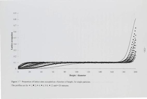
0.9 -
0 8 -
0 7 -
= 06 -._§
to.s-.. ·~ 04 -
...J 0_3 -
0.2 -
20 40 60 80 100 120
Height I dia meter
Figure 3 7 Proponion of lattice sites occupied as a function of height, for single panicles
The profiles are for ~ I, • 2, A 4, • 6. o 8, • 12 and - 20 minutes.
140 160 180 200
"' ...
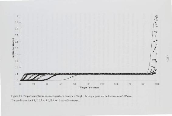
1 -
0.9 -
0.8 -
0.7 -
; ·; 0.6 -;-~ 0 5 -
"' ~ ·= 0.4 -" -l
0.3 -
0.2 -
0. 1 -
0 t< «<« ,..- ............--= 0 20 40 60 80 100 120 140 160
Height I diameter
Figure 3 . 8 Proponion oflattice sites occupied as a function of height, for single panicles, in the absence of diffusion
The profiles are for o I, • 2. o 4, • 6, o 8, • 12 and-20 minutes.
~
• .. c
" ... c ... " • c .. 0
•ot. ::;: •
~ ".o
180 200
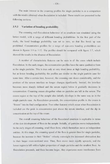
- 126 -
The main interest in the creaming proriles for single particles is as a compari son
with the results obtained \\hen flocculation is included These results cu e presented in the
fo llowing sections
3.9.3 Va•·iation of bond in~ probability
1 he creaming and fl occulation behaviour of an emulsion was simulated using the
lattice model, with a range of diflCrcnt bonding probabilities In the first part of the
study, the bo nd breakage p10bability was set to zero. so that fl oc break up was
p10hibited Concentration profil es for a range o f no n-zero bonding pr obabilities ar e
shown in fi gures 3 9 to 3 12 The profiles should be compared \\ith figure 3 7, which
showed the result s in the absence of fl occulation
1\ number o f characteristi c features ca n be seen in all the cases which include
Oocculatio n In the ea rly stages, the concentratio n profiles have the same qualitati ve fo rm
as fo r single parti cles This is true onl y at very sho rt times at high bo nding probability,
but at lower bonding probabil ity the pro fil es are similar to the single particle case fo r
some time . AOer a ce rt a in time, however. the creaming rate slows considerably, and the
posi tio n o f the serum interface no lo nger changes significantly Instead, the interfa ce
becomes mo re sharply defined and the serum region below it graduall y decreases in
concentrat io n Creaming ceases a ltogether when no particles are IeO in the serum The
cream region a t the to p o f the sample also initiall y develo ps in the same way as in the
single particle case As fl occulation proceeds, the concent ratio n pro fil e in the cream is
" frozen" into it s final configuration T wo other fea tu res which occur when Oocculation is
included arc the peak in concentratio n just above the serum interfa ce, and the dip in
concent ratio n at the top o f the crea m
The overall c reaming behaviour o f the flocculated emulsion is expl icable in terms
o f the size develo pment o fflocs in the sample Initially, all particles move independently
In the early stages of creaming, small fl oes form, which themselves move as independent
entities At this stage, the creaming speed o f the fl oes is greater than for single particles,
because the increase in their "Stokes" velocit y out weig hs the increa ~ed obstructio n due
to their larger cross-sectio nal area Thus, floes move mo re rapidly upwards, and the
lower region is lefl with a higher pro po rtion o f single particles and the smallest fl oes As
flocculatio n proceeds, and noes become larger, they experi ence more interference fro m
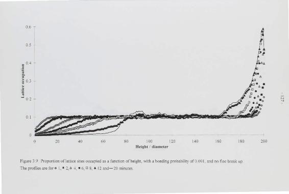
0.6 -
0.5 -
~ 0.4 -
l ~ 0.3 -~ u
" ....l 0.1 -
10 40 60 80 100 120 140 160 180 Height I diameter
Figure 3.9 Proponion of lattice sites occupied as a function of height. with a bonding probability ofO 001, and no floc break up
The profiles are for o I, • 2, a 4, • 6. o 8, "' 12 and- 20 minutes
200
N ...,
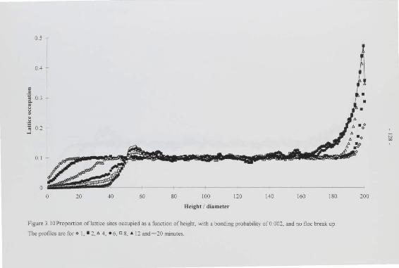
·~ :::. § 0
" u
3
0.5 -
ov~ 0 20 40 60 80 100 120 140 160 180
Height I d iameter
Figure 310 Pro portion of lattice sites occupied as a function of height, with a bonding probability of0.002. and no floc break up
The profiles are for o I, I ::!, ll 4, • 6, a 8, • 12 and - 20 minutes.
:;;l
200
0.35 -
03 -
0.25
.g ¥- 0 2 -
"' "' 0
-~ 0.15 -
3 01
0 os
0
0 20 40 60 80 100 120 140 160 180
Height I diameter
Figure 3.11 Proponion of lattice sites occupied as a function of height, with a bonding probability ofO.OOS. and no floc break up
The profiles are foro I, • :!, O 3, • 5 and.a-10 minutes.
200
"' -D
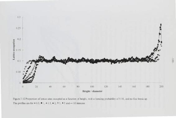
.S ;:; c. =
0.3 ~
~ 0. IS ~ V
3
0 os
0
20 40 60 80 100 120 140 160 180
Height I diameter
Figure 3 12 Proponion of lattice snes occupied as a funct 1on of height , with a bonding probability of 0 0 I, and no floc break up
The profiles are for o 0.5, • 1, tJ. 1.5, • 2, a 3. A 5 and- 10 minutes.
200
'-' 0
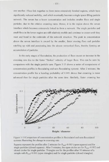
- 13 1 -
one another Floes link together to form more ex tensively bonded regions. which have
significantly reduced mobi lity, and which eventua lly become a single space-filling particle
network The serum has a lower concentration and includes smaller fl oes and single
particles, due to the relative creaming rates llence, it is the region above the senun
interface which becomes extensively linked to form a network The sing le particles and
small floes in the lower region are st ill relatively mobile and continue to cream until they
meet and bond to the underside o f the nc tw01k structure The peak in concentrat ion
above the serum interface is caused by the smaller, fa ster moving fl oes and particles
catchi ng up wi th and penetrating int o the slower networked fl oes, thereby forming an
accumulatio n of particles
In the ea rly stages of fl occulation, the production o f floes causes an increase in the
creaming rate due to the faster "Stokes" veloci ty of la rger floes This can be seen by
comparison wi th the single particle case figure 3 I 3 shows a series of compari sons o f
concentration profiles in floccu lating and non-flocculating systems Afler 2 minutes, the
concentration profile for a bond ing probability of 0 005 shows that creaming is more
advanced than for single particles afler the same time Similarly, faster creaming ha ~
c .5! ;; c. § 0
0 1
·~ 005 ;; ...l
0
0
~ , D rl' D
20 40 60 80
ll eight I diameter
Figure 3 13 Comparison o f concentration profil es in fl oeculated and non- flocculated systems illustrating the change in creaming rate
100
Squares represent the pro files afler 2 minutes for PbonrO 005 (open squares) and for single particles (closed squares) Afler 5 minutes, the open ci rcles are for P hond 0 002 and closed circles for single particles Triangles are for the profiles afler 10 minutes of a sample with 1\ ond- O 00 1 (open triangles) and for single panicles (closed triangles)
- 132 -
occun cd fo r a bonding probabi lity of 0_002 afl er 5 minutes than fo r single particles A
marked increase in creaming rate can be seen for the sample with a bonding probabi lity
o f 0 00 I afl cr 10 minutes, compared with single particles, also a ll er I 0 minutes At hig h
bonding p• obability, it is only at very short time~ that the increased rates can be seen
The difference between the nocculatcd tt nd non· fl occulated systems is more pronounced
at later times, provided the system is still free to move
floccula tion causes the concentration in the cream to be reduced compared to the
sing le parti cle case ( fi gures 3 9 to 3 12) Parti cles which are linked together in floes
cannot adopt the most compact p~tcking structure. and therefore the concentration is
lower The dip in concentration at the top of the system is caused by the prevention of
floes or particles penetrating above the top boundary An approximately spherical fl oc,
which has an ex tent larger than a single lattice unit , can only move vertica lly until its
uppermost point reaches tl1e top boundary llence, the top layer cont ains a Slllallcr
prop01 tion of particles than exists lower down, nearer the centre of mass of the fl oc This
reduced concentration wi ll only extend one or two particle diameters from the top oft he
sample, and is therefore not likely to be observed at the mac1oscopic level
ll aving discussed the general features of the c1eaming and flocculation result s
predicted by the latt ice model, it is of interest to examine the elTect of the bonding
probab ility on the concent ration pro fil es (figures 3 9 to 3 12) As the bonding probability
increases, fl occulation occurs more rapidly, since a higher p10portion of touching or
collision events results in bond formation between particles The formation of a particle
network, which slows further movement , therefore occurs after a short er time In the
samples analysed, a network which covered the enti re lateral extent of the system had
developed afler I 5, 2 5, 4, and 5 minutes for bonding probabilit ies o f O 0 1,0 005,0 002
and 0_00 1 respectively lt is clear fi om the concent ration profiles that there is a sufficient
number of free particles to allow some degree of creaming aft er this time. although these
eventually join the network and become immobile.
The extent to which a serum or cream is formed in the sample is reduced as the
bonding probability increases, because of the shorter time ava ilable before the particles
are immobilised in the network The limited time which is ava ilable for particles to cream
relatively unhindered alTects the concentration reached in the cream region As the
bonding probability increases, the concentration of the cream decreases, since it is
- 131 -
formed over a shorter period. before its configlllatio n is "f10zen-in" by noccula tio n The
concentr<ltion in the crea m may also be aHCctcd by the si1e of the fl oes which initially
formed it At low bonding probabilities. the initial creaming bcha\ iour is characterised by
smaller fl oes and single particles. w hich arc more compact At higher bonding
probabilities. floes grow to a larger. and therefore more sparse, si1e before significant
creaming can occur, and therefore pack less effi ciently in the cream I fence. the space
filling character of the fl oes which formed the cream determines its concentration The
same e!Tect was observed in two-dimensional simulations of van dcr Knaap et al (1994)
A relationship between sediment porosi ty and the form of the interparticle po tential was
also demonstrated by An sell and Dickinson ( 1986)
The time period over which creaming occurs relatively freely also a!Tects the final
position of the senun interfhce, which represent s the lower limit of the particle network
At a higher bonding probability, fl occulation occurs more rapidly, and therefore the final
position of the serum interface is closer to the bott om of the sample This is clear ft om a
comparison of the concentration profiles. fi gures 3 9 to 3 I 2 Although particle
movement has not completely ceased at the lmvest bonding probabilities simulated , the
serum position is sti ll clearly defined in this case Only a further 1eduction in the
concentratio n of t he senun is yet to occur in these samples
The variation of the height o f the scrum interface wi th bonding probability is
shown in figure 3 14 A compamble dependence was demonstrated in two-dimensions by
\an dcr Knaap et al (1994) A functional relationship can be derived between the two
parameters of seru m int erface height and bonding probability The co rr ect limiting
cond itions must be ob tained at the h\O extreme values of bonding probability (zero and
unity) For single particles (a bonding probability of 1ero), the height of the interface
tends to infinity, si nce, if the sttmple is infinitely high, the interface cont inues to move
with a uniform creaming speed In the other extreme, a bonding probability of unity
causes very rapid fl occulation l lowever, the extent of serum forma tio n before
networking occurs depends on the initial concentration of particles At high
concentrations, all particles arc initial ly likely to be touching at least one ot her pa1ticle,
and therefore linkage occurs immediately and no creaming is possible At low
concentrations, creaming may develop significantly before suffi cient contact is achieved
to prevent further movement l lence the limiting condition on the serum height at a
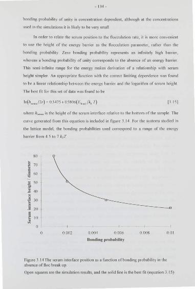
- 134-
bonding probability of unity is concentration dependent , although at the concentrations
used in the simu lations it is likely to be very small
In order to relate the serum position to the flocculation rate, it is more convenient
to use the height of the energy barrier as the flocculation parameter, rather than the
bonding probabi lity Zero bonding probabil ity represents an infinitely high barrier,
whereas a bonding probability of unity corresponds to the absence of an energy barrier
This semi-infinite range for the energy makes derivation of a relationship with serum
height simpler An appropriate function with the correct limiting dependence was found
to be a linear relationship between the energy barrier and the logarithm of serum height
The best fit for this set of data was found to be
[3 15]
where hJcfum is the height oft he serum interface relative to the bottom oft he sample The
curve generated from this equation is included in figure 3_14 For the systems studied in
the lattice model , the bonding probabilities used correspond to a range of the energy
barrier from 4 5 to 7 ks T
80 ~
" 70 e " 60 :0
.E 50
"" "<; 40 ..c
" " ~ 30
.E 20 E
~ 10
"' 0
0 0 002 0 004 0 006 0 008 00 1
Donding probability
Figure 3 14 The senun interface position as a function of bonding probability in the absence of noc break up
Open squares are the simulation results, and the sol id line is the best fit (equation 3 IS)
- I JS-
The final position of the serum interface in a system with irrevers ible floccu lat ion is
specific to the dynamic properties o f the particles in the system These are dependent on
both tl1e material properties and o n particle si7e. ll owever. the parameters used in the
model ate not dissimilar to real cxpetimental systems Extrapolation of the relationship
calculated from the lattice modelling results to a macroscopic scale may be of dubious
va lue llowever, assumi ng that a sample is completely unfloccula ted at the start of
creami ng. a senun height of 10 mm, corresponds to an energy barrier to fl occulation of
the o1der of 15 knT, accord ing to equa tion 3 15 This is certainly not an unreasonable
va lue for a real system The 1 elationshi p is of course logarithmic, and therefore a la rge
change in serum position relates to a rather sma ll increase in the energy barrier The
dete rmination of the scnm1 interface position in irreversibly fl occulat ed samples may
perhaps be used as an indication of the energy barrier to flocculation under various
conditions
The va lues of the fractal dimension in the creaming and flocculating samples
provides information o n the nature of the floccu lated structure formed In these systems,
the fractal dimensio n is a sca ling parameter characterising the particle distribution, and is
a property of the local network stmcture, rather than of an individual floc _ The va lue of
the fractal dimension was ca lculated in each system, for the distance range 4 to 10
particle diameters, as a function of height and time . An example of the particle
distribution plots used to calculate the fractal dimension is shown in figure 3 IS The
calculat ed fractal dimension results, for a bond ing probability of 0 002, are shown in
figure 3 16 Similar plots are obta ined for the other values of bonding probability The
frac tal dimension is uniform with heig ht at each time, except at the extremes o ft he plots
At these limit s, the part icle concentrat ion varies wit h height (compare with the
concentration profiles in figu re 3 10) This affects the particle distribution, and the fra ctal
dimension can only be considered to be a va lid parameter over the region in which the
concentration is uniform
ll avi ng demonstrated the uniformi ty of fractal dimension with height in a certain
region, a single (average) va lue can be used to characterise the structure at any time
figure 3 17 shows the variation in fractal dimension wi th time, for each of the
irreversibly flocculating systems simulated in the lattice model In each case, the fractal
dimension decreases with time from its initi al value of J (equal to the dimension of the
space) At fi rst . the fractal dimension decreases gradua lly, but later rather more steeply,
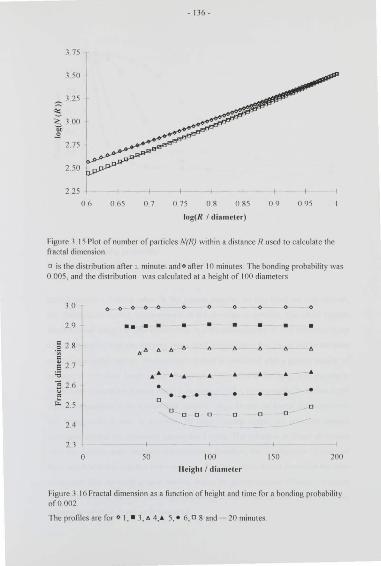
- 136-
06 0 65 0.7 0 75 08 0 85 09 0 95
log(R I dinmrler)
Figure 3 IS Plot o f number o f particles N(l?) within a di stance I? used to calculate the fractal dimension
o is the distribution afler 1.. minute- and o afler I 0 minutes The bonding probability wtts 0 005 , and the di stribution was calculated at a height of I 00 diameters
3.0 0 0 0 0 0 0 0 0 0 0 0
29 •• • • • • • • • ; 2 8
d" " " " d " " " " ·;;; c e 21 .. ~ .... .. .. .. .. .. .. ~ 2 6
• • . • • E D • "' 2 5 D
D D D D D D D
24
2 3
0 50 100 ISO 200
Height I dinmcter
fi gure 3 16 Fractal dimension as a function of height and time for a bonding probability ofO 002
The profiles are for <> I, • 3, 11 4,& 5, • 6, o 8 and- 20 minutes
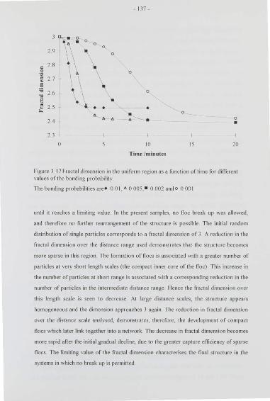
- 137-
l 0
0 0
29 ._ 0
c 2 8 \ 0 0 ·;;; c 2 7 e :;
26 0
a \ • E 2 5 • • • "- 0
" • 24 " " " ~ .. 0
• 23 I
0 10 IS 20
Time /minutes
Figure 3 17 fractal dimension in the uniform region as a function of time for difl"erent va lues of the bonding probability
The bonding probabilities are• 0 01, " 0 005, • 0 002 ando 0 001
until it reaches a limiting value In the present samples. no floc break up was allowed.
and therefore no further rearrangement of the structure is possible The initial random
distribution of single particles corresponds to a fractal dimension of 3 A reduction in the
fractal dimension over the distance range used demonstrates that the structure becomes
more sparse in this region The formation of floes is associated wi th a greater number of
particles at very short length scales (the compact inner core of the floc) This increase in
the number of particles at short range is associated with a corresponding reduction in the
number of particles in the intermediate distance range llence the fractal dimension over
this length scale is seen to decrease_ At large distance scales, the structure appears
homogeneous and the dimension approaches 3 again The reduction in fractal dimension
over the distance scale analysed, demonstrates, therefore, the development of compact
noes which later link together into a network The decrease in fractttl dimension becomes
more rapid aOer the initial gradual decline, due to the greater capture eHiciency of sparse
noes The limiting value of the fractal dimension characterises the final structure in the
systems in which no break up is permitted
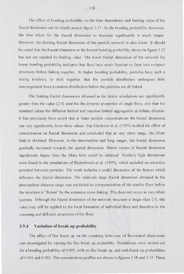
- 138-
1 he effect of bonding probability on the time-dependence and limiting\ alue of the
n acta! dimension can be clearly seen in figure 3 17 As the bonding probability decreases.
the time taken for the fr;:~c tal dimension to decrease significantly is much longer
llowever, the limiting fracta l dimension of the particle nctw01k is also IO\\Cf lt should
be noted that the fractal dimension at the lowest bonding probabi lity shown in figure 3 17
has not yet reached it s limiting va lue The lower fractal dimension of the nei\\-Ork for
lower bonding probability indicates that noes have more freedom to form into compact
structu res before linking together At higher bonding probabilit y, particles have such a
strong tendency to sti ck together that the pa1ticle di stribution undergoes little
rearrangement from a random distribution before the particles are all linked
The limiting fractal dimensions obtained in the !all ice si mulations arc significantly
greater than the va lue (2 0) used for the dynamic properties of single floes. and than the
standard va lues for diffusion limited and reaction limited aggregation at infinite dilution
lt has p1eviously been noted that at finit e particle concentrations the fractal dimension
can vary signi fi cantly from these values Van Garderen et al ( 1995) studied the effect of
concentration on fractal dimension and concluded that at very short 1ange, the dilute
limit is obtai ned llowever, in the intermediate and long ranges, the fractal dimension
gradually increased towards the spa tial dimension llence va lues of fractal dimension
significantly higher than the dilute limit could be obtained Si milarly high dimensions
~Nere found in the simulations of Oijste1bosch et al ( 1995), which included an attractive
potential between particles 1 he work includes a useful discussion of the factors which
influence the fractal dimension The 1elatively large fractal dimension obta ined in the
intermediate distance range was attributed to interpenetration of the smaller floes before
the struct ure is "frozen" by the extensive cross- linking ·1 his does not occur in very dilute
systems Although the fractal dimension of the network structu re is larger than 2 0, this
value may still be applied to the local formation of individual fl oes and therefore to the
creaming and diffusion properties of the fl oes
3.9.4 Variation of break up probability
The effect of noc break up on the creaming behaviour of fl occulated dispersions
was investigated by varying the fl oc break up probability Si mulations were carried out
for a bonding probability ofO 005, with no fl oc break up, and with break up probabi lities
ofO 00 1 and 0 002_ The concentration profiles a1e shown in figures 3 18 and 3 19 These
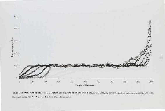
0 5 -
0.4 -
0 ·; 0 3 -:::. § 0
" " ·= 01 -j
0. 1
10 40 60 80 100
Height I diameter
110 140 160
" 4'
180 100
Figure 3. 18 Proportion of lattice sites occupied as a function of height, with a bonding probability ofO .OOS, and a break up probability ofO 001
The profiles are for o I, • 2, tJ. 3. • 5, o 10 and -12 minutes.
w ..,
0 7 -
0 6 ~
0.5 ~
.~ ~ 04 ~ § 0
-~ 0.3 -
" -l
0.2 ~
01 ~
0 GaG I 1111 C%...---
20 40 60 80 100 120 140 160 180 200
Height I diameter
Figure 3 .19 Proportion of lattice sites occupied as a function of height, with a bonding probability ofO.OOS , and a break up probabi lity ofO 002.
The profiles are for • :!, o 4, • 6, o I 0 and ~14 minutes.
;5
- 141-
should be compared with the results of figure 3 11, in which there was no floc break up
The concentration profi les indicate that the break up of floes delays the formation of a
particle network which prevents further movement The posi tion of the serum interface
in fi gUic 3 18 is higher up and takes longer to form than in the absence of bond breakage
(figure 3 I I) At a higher break up probability (figUI e 3 19). the final serum interface
posi tion is not defined during the simulation period, since not all particles have linked
into the network The concen tration of the cream region increases as the brettk up
probability increases, ind icati ng the reduced floc growth rate and the delay in «fi·eczi ng"
of the struct ure due to cross- linking The creaming ra te is aga in seen to increase in
compari son with the si ngle particle case
The concentration profiles obtained when fl occulation is reversible demonstrate
that creaming behaviour p10ceeds more freely than for irreversible flocculation wi th the
same bonding probability lt might be expected, therefore, that the profiles would bear a
closer resemblance to the results for irreversible flocculation with a lower bonding
probability This is indeed the case, as a compctrison between figures 3 18 and J 10 (wi th
a bonding probability of 0.002 and no fl oc break up) shows There is however, an
important difference The break up probability can only affect bonds which have already
formed lt does not prevent bonds forming, as a reduct ion in bonding probabi lity would
llence, a signi ficant degree o f fl oc growth occurs before a noticeable effect of
reversibility is observed Floc growt h can be initially quite rapid, but when floes reach a
certain size, the growth rate is reduced by bond breakage llence the formation of a
network is delayed in a reversibly fl occulat ing system This effect can be seen by
cornpa1 ing the concentration profiles of fi gures 3 18, 3 19 and figure 3 10 Afler 6
minutes, the concentration proriles in figures 3 10 and 3 19 have a very similar form.
with the reversible case showing the preliminary shape of the serum interface. llowever,
in the reversibly flocculated system, the floc breakage is sufficiently st10ng to limi t the
floc growth and enable free particle movement for a significant time The irreversibly
flocculating system simply forms a network and creaming ceases This is also true for the
reduced break up probabilily (figure 3 18) AI a sufficienlly high break up probabilit y.
fl oes may remain mobile, without the formation of a particle network (at least until the
concentration increases, due to creaming)
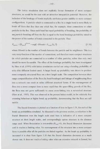
- 142-
The lattice simulation does not exp li ci tly favour formation of more compact
structures, as would be the case wit h an attractive interparticle potential I lowever, the
inclusion of the breakage of bonds implicitly attributes greater stability to more compact
configurations A particle which is connected to a fl oc by a single bond is more likely to
break off from that floc than one which has, for example, three connectio ns to other
particles in the fl oc Since each bond has equal probab ility of breaking, the probability of
any parlicle breaking off from the fl oc is equal to the bond breakage probability raised to
the power of the number of bonds connected to the particle Thus
13 16 J
where Nhomh is the number of bonds between the particle and it s neighbours This is a
ve ry steep function oft he number of connectio ns, and therefore more compact structures
(in which particles arc connected to a number of ot her pal!iclcs, rather than only one)
should be mo re favourable The erfect of the breakage probability has been investigated
by I law et al ( 1995) wi th latti ce si mulat ions carried out using a bonding probability of
unity (the dirfusio n limited case) A larger break up probability was shown to produce
more compactly structured noes on a short length scale The competition between short
range compactifica tion of the noes (by bond breakage) and linkage of neighbouring noes
into a network can result in rather different stmctural forms If the rearrangement of
noes into a more compact form is mo re rap id than the space-filling growth of the noc,
the noes may not grow sufficiently to cause c1oss- linking into a networked structure
(I law et al , 1995) This was observed in the present lattice model, in the relatively free
creaming behaviour at higher break up probability, demonstrating that the noes are still
mobile
The fractal dimension is plotted as a functio n of time in figure 3 20, fo r each of the
break up probabilities simulated As di scussed in the previous section, a reduction in the
fractal dimension over the length scale used here is indicative of a more compact
structure at short length scales, and correspondingly sparse structure in the distance
range used When nocculatio n is irreversible (Pbrcal: -=-0), the fractal dimension decreases
until it reaches a limiting value. No rearrangement of the structure into a mo1e compact
form is possible after all the particles are linked together As the break up probability is
increased it is clear from figure 3 20 that the fractal dimension decreases at a much
slower rate lt does not reach a limiting value when an ex tensive network is formed, but
3 · --------. 2 9
= 2 8 .!2
~ 2 7 E :;; ~ 26
" ~ 2 5
24
23
• A
\\ \
A
•
- 143-
•
A • -~~
• • A
A
I
•
0 6 10 12 14
Time I minutes
Figure J 20Fractal dimension as a function of time, for variable break up probability, wilh a bonding probabilily ofO 005
The profiles arc for break up probabililies of • 0 0, A 0 00 I and • 0 002 .
continues to decrease. This is because the breakage of bonds allows rearrangement of
particles into a more stable, compact configuration, resulting in a smaller fractal
dimension in the intermediate length range lt is clear, however, that reversible
flocculation leads to a stmcture wit h a lower fractal dimension than irreversible
fl occulation with the same bonding probabi lity. The fractal dimension reached in the
simulation period for reversible flocculation is also lower than for the irreversibly
flocculated stmctures formed ttl the lower bonding probabilities analysed (figure 3 17)
A comparison of figures 3 20 (for reversible nocculation) and 3 17 (irreversible
nocculation) indicates the difference between the effect of bond breakage. and the effect
of the rate of bond formation As the bonding probability is decreased, in the absence of
noc break up (figure 3 17), the fractal dimension takes longer to decrease from the initial
plateau. llowever, an increase in break up probability. at the same bonding probability
(figure 3 .20) does not significant ly change the very ea rl y va riation in fractal dimension
This is because the initial formation of noes is so lely determined by the bonding
probability. The rate of bond breakage o nly becomes significant in the presence of a
- 144 -
substantial number of bonds After the initial development of noes, an increase in
b1cakage probability has a notable slowing errcct on the decrease in fractal dimension
Oo nd breakage causes noc growth to be restricted, delaying the formation and linkage o f
large sparse fl oes I lowever. the fra ctal dimension continues to decrease at a signi ficant
•ate after the creaming process has slowed considerably (compare with the concentration
profiles in fi gure 3 18) llence, the lat er reduction in the fra ctal dimension is caused
largely by structural rearrangement to form more compact regions
The result s o f the lattice model for varying break up probabi lity indicate that the
reversibility o f nocculation may have a very sig nificant e iTect o n emulsio n behaviour
This ca n be seen bo th in the creaming 1ate and in the compactness and 1earrangement o f
the stmctures formed Bond breakage restric ts the growth of noes so that the sy~t em
remains mobile fo r a longer period llowever, the noes formed have a larger creaming
speed than single part icles. and therefore an increase in the creaming ra te should be
observed A speed up o f creaming was al so observed for irreversible fiocculation. but the
networki ng of noes as they continue to grow causes the earlier onset o f immobility A
lower bonding probability delays this process, but creaming is then determined by smaller
noes which cream mo re slowly Rearrangement o f the st111 cture due to reversibility of
fi occulatio n a llows more compact packing. and may permit further movement of
particles, and the collapse of the net work
The diiTerence in particle network stmcture produced under diiTerent nocculation
conditio ns can be seen in figures 3 2 1-3 23 Each picture is a section of the lattice in the
heig ht range 80- 100 diameters In each case, the structure is shown at the end of the
simulatio n period The structures look somewhat unnatural because of the geometry o f
the lattice, which constrains the possible particle positions For irreversible fi occulation
with a hig h bonding probabili ty (figure 3 2 1) the structure is characteri sed by many small
clumps of particles which are cross- link ed At lower bonding probabilit y (irreversib le),
fi gure 3 22 shows that larger, more compact regions have fo rmed Reversible
fioccu lation at the same bonding probability (figure 3 22) is characterised by only a few
regions of densely packed particles However, many sing le particles are sti ll present in
this case because the network was no t full y develo ped by the end of the simu lat ion run
These visual images are consistent with the interpretation oft he ftactal dimension result s
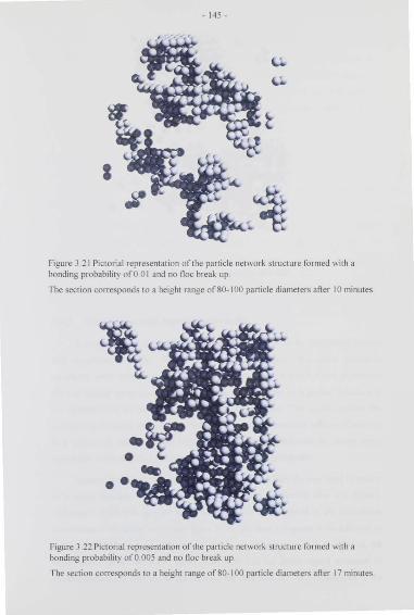
- 145-
Figure 3 .21 Pictorial representation of the particle network structure formed with a bonding probability of0.01 and no floc break up.
The section corresponds to a height range of 80-100 particle diameters after 10 minutes.
Figure 3.22 Pictorial representat ion of the particle network structure fon11ed with a bonding probability ofO 005 and no floc break up
The section corresponds to a height range of80-l 00 particle diameters after 17 minutes
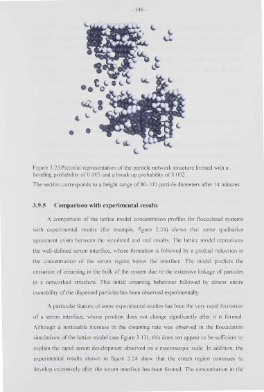
- 146-
Figure 3 .23 Pictorial representation of the particle network structure formed with a bonding probability ofO 005 and a break up probability of0.002
The section corresponds to a height range of SO-l 00 particle diameters after !4 mim1tes.
3.9.5 Compa rison witb experimental results
A comparison of the lattice model concentration profiles for flocculated systems
with experimental results (for example, figure 2 24) shows that some qualitative
agreement exists between the simulated and rea! results. The lattice model reproduces
the well-defined serum interface, whose formation is followed by a gradual reduction in
the concentration of the serum region below the interface. The model predicts the
cessation of creaming in the bulk of the system due to the extensive linkage of particles
in a networked structure. This initial creaming behaviour followed by almost entire
immobility oft he dispersed particles has been observed experimentally.
A particular feature of some experimental studies has been the very rapid formation
of a serum interface, whose position does not change significantly after it is formed
AJthough a noticeable increase in the creaming rate was observed in the flocculation
simulations of the lattice model (see figure 3. 13), this does not appear to be sufficient to
explain the rapid serum development observed on a macroscopic scale In addition, the
experimental results shown in figure 2 24 show that the cream region continues to
develop extensively after the serum interface has been formed The concentration in the
- 147-
bul k of the system also decreases gradually, in spite of the immobility of the senun
interface These features indicate that the mobi lity of some particles in the system is still
sufficient to allow crea ming in some part s of the system The reversib le nature of
fl occulation may contribute to these processes, in terms of allowing some particle
movement due to restricted fl oc growth llowever, the complex nature o f these
experimental results is not C'< plicable by the simple lattice model
3. 10 Conclusions of la ttice model
The th ree-dimensio nal lattice si mulations o f the creaming behaviolll o f flocculating
emulsions have produced a number of interesti ng fea tures
• The presence of irreversible fl occula tion causes the development of a well -defin ed
serum interface and the cessation of creaming due to the formation of a network
• The height of the serum interface is related to the bonding probabi lity, or to the height
oft he energy barrier to fl occulation
• Reversibility of fl occulation delays the formation of a particle network, allowing fl oes
to remain mobile for longer Creaming may continue at a reduced rate afi er a network
is formed
• 1\n increase in creaming rat e is observed in both reversible and irreversible
fl occulating systems before the system is full y networked This is due to the more
rapid movement of fl oes of moderate size
• The fractal dimension of the developing particle network is influenced by both
bonding and break up probabilit ies More compact structures are formed with
reversible fl occulation, since rearrangement is permitted
The result s of the lattice model are qualitatively consistent wi th experimental
observations of the development of a sharp serum interface, followed by almost complete
cessa tion of creaming Although an increase in creaming rate in the early stages was seen
in the simulations, it is difficult to conclude that this is sufficient to explain the very rapid
formation of the serum which has been observed in practice. llence. the simple model of
creaming and flocculation adopted by the lattice simulation does explain some fea tu res of
real emulsions Nevertheless, the rapid movement of oil in the early stages of creaming
probably requi res an alternative mechanism to fully account for the ex perimental result s
~et \n">u£\ocs b~ .......,U.,. Jl= '" \k model ""'!\ c.n<>a.\; ,O'dt:\ MU««""'"""':~ cnk
- 148 -
Cha pter 4 : Theo ry of Ultrasound Pr011agation
4. 1 Aims of theoreti ca l ultrasound wo rk
Low power ultrasound can be used as a non-destmctive probe of dispersed
systems, such as emulsions (see section 1 3) The two measurable quantities
characterising the ultrasound propagation in the sample are it s velocity and attenuation.
and these can be related to usefu l physical properties of the sample being measured This
relationship between velocity and attenuation and a quantity such as the dispersed phase
volume fraction or solid fat content is the key to the va lue of the ultrasound technique.
The ultrasound scanner (figure I I), used to study creaming in emulsions, relies on the
ultrasound velocity being directly relat ed to the volume fraction of oil at any point in the
sample Concentration profi les of the emulsion can therefore be determined as creaming
progresses Similarly, investigations of crystallisation rates in emulsions uti lise the
difference in ultrasound veloci ty between the solid and liquid oil dro plets The measured
ultrasound velocity in the sample can be related to the proportion of the dispersed phase
which is solid Measurements of sound speed in the crystallising emulsion are therefore a
means of studying the crystallisation kinetics
The main ultrasound applications used at Leeds are based on velocity (or speed)
measurement s Attenua tion measurement s have been made for a number of different
applications, but the error in altenuation measurements was found to be considerably
higher than for the velocity measurement s Att enuation measurement s suffer more
strongly from effects such as dispersion (which affects the shape of the waveform),
diffraction and probe va riation, and therefore velocity measurements are both more
accurate and more reproducible Other workers have used attenuation measurements to
some degree of success The majority of the discussion in the following sections and in
the next chapter is therefore directed towards the relationship between ultrasound
velocity and the system parameters, rather than the att enuation
The aim of the ult rasound work was to evaluate various ways of interpreting
ultrasound measurements, particularly of creaming, fl occulation and crystalli sation in
emulsions llence. the focus of the study was initially the theory of ultrasound
- 149-
propag<~: ti on in such systems This chapter considers the basic ul trasound theori es which
are commonly used to interpret measurement s in dispersed systems The important
special cases of the theory are discussed, along with the circumstances under which each
o f these cases can be applied I\ number o f practical techniques for obtaining the
relatio nship between ultrasound ve locity and the di spersed phase concentration are
develo ped in chapter 5
4.2 llomogeneous descriptions of dispersed systems
The speed at which a sound wave pro paga tes th rough an iso tro pic, ho mogeneous
nuid is given by the equation
14 lj
(Wood, 1964, p 26 1. and earlie r editio ns), where t ' is the ultrasound velocity, K 0 is the
compressibility o f the nu id and p 0 it s density In most cases, sound wave propagatio n is
adiabatic and therefore the adiabatic cornpressibility is usually used Under conditions o f
isothermal pro paga tion , the isothermal compressibility should be used instead In some
circumstances the propagation is neither adiabatic no r iso thermal, in which case the
velocity fall s somewhere between the two limiting speed s A discussio n of thi s problem
can be found in Pierce ( 1981 , p 34-36)
Urick ( 1947) suggested that, in a dispersion in w hich the di spersed particles arc
much smalle r than the wavelength o f the sound wave, the density and compressibility in
equatio n 4 I should be replaced by the terms
14 2]
where subscript s I and 2 denote the continuous and di spersed phases respec ti vely, and ~
is the di spersed phase volume fractio n These quantities are the volume-averaged va lues
o f the density and compressibility o f the suspensio n Equation 4 2 had already been used
for nuid mixtures (Wood, 194 1, p 36 1), sincep0 and K 0 are the overall density and
compressibil ity o f the system Urick proposed that a suspensio n in which the particles
were much smaller than the wavelength o f sound should be treated in the same way The
- ISO-
equation was found by Urick to agree with e"perimental measurements o n xylene in
water emulsions lt was then used to detem1ine the compressibility of the oi l droplets in
an emulsion
This approach is a homogeneous description of the system. considering the
suspension it self as a homogeneous Ouid, wit h a modified density and compressibi lity
corresponding to the volume-averaged values for the suspension It does not consider the
int eraction of the sound wave wi th the individual particles
4.3 Ultrasou nd sca tter ing theo ry
The theory of ultrasound propagation on which much of this work has been based
is scattering theory The term sca tteri ng may be used to describe any enCct which
removes energy from the sound wave and makes it unavailable to the propagating
acoustic field In an emulsion, scatteri ng is caused by the p1esence of the individual
dispersed phase particles, which disturb the propagating wave Energy is lost from the
forward direction of t he wave by being scattered in all directions and also by thermal and
viscous dissipation around the particle The wave also undergoes a phase shifi which is
apparent in the change in velocity of the propagating wave_ The basis of scattering
theory as applied to acoustic propagation in an emulsion is that the particles can be
considered as independent scattering centres, each affect ing the sound wave separately
from the other particles Other approaches to the acoustic problem were introduced in
chapter 1 There have been several reviews of different solutions to acoustic propagation
in dispersed systems, to which the reader is referred (llarker and Temple, 1988), and
these alternative theories will not be considered furth er
The scattering theory method provides some intuitive understanding of the physical
processes which occur at the particles it appears to be particularly appropriate in the
long wavelength limit , in which the wavelength of the propagational acoustic wave is
much larger than the particle radius (this is also known as the Rayleigh limit , afier Lord
Rayleigh who investigated the scattering of sound by small particles in thi s limit) Under
these conditions, the effect of the emulsion on the sound wave can be described by a
series of different scattering modes In the long wavelength regime this series may
usually be tenninated above the first order mode (dipole scattering) At higher
frequencies, the effect involves many higher order scattering modes and other
- I 5 I -
approaches to the acoustic problem then become more suitable In addition. in the long
wavelength region. o nly "single'' and "double" (scattering by two pa1ticles) scallcling
effects need normally be taken into account Therefore, the multiple scattering theory
description of sound propagation is most appropriate in the long wavelength limit The
use of ultrasound signals of the order of Mllz to characterise emulsions with particle
sizes of the order of ~un , means that the long wavelength condition is valid fherefore
the scattering theo1)' description of ultrasound propagation is suitable for the study of
emulsions and was used as the basis for this work
The groundwork of the theo1ies of uh1asound p10pagation arc well-estab lished
Lord Rayleigh considered the cnect of a sound wave on a spherical obstacle in the long
wavelength limit , arriving at the famous theory that attenuation is proportional to the
fourth power of frequency (Strutt . 1872, 1896) Since then, numerous attempts have
been made to improve and extend the knowledge of the modification to the sound wa\ e
caused by a particle, for example by including thermal enects (Epstein and Carhart.
1953), or a shell -like coating on the particle (Anson and Chivers. 1993) Considerable
elTort has also been expended in determining the eiTect of the whole set of par tides
which exist in an emulsion, each having their own scattering properties These two
aspects still remain the cnrcial elements of the scattering theory technique_ Firstly, to
determine the eiTect of a planar sound wave on a single. isolated particle. and secondly to
determine the eiTect of the ensemble of particles in the dispersion on the sound wave (in
terms of the scattering properties of the individual parlicles) The following sections
describe the methods for each of these stages The details may be found in the references.
but sufficient information is given for an understanding of the subsequent discussions and
developments
4.3.1 General theory of so und IJI'OIIagation
The propagation of a sound wave in a medium can be defined by a single complex
value called the wavenumber which is related to the two measurable parameters the
velocity and attenuat ion The acoustic field properties, such as pressure or displacement.
are osci llat ory and include a factor of
exp{i(k r -w t)} [4 3]
where k is the wavevector and its modulus, k, the wavenumber The time variation,
- 152-
exp( irvt), is omitted from all the following eq uations, since it appears in every field
quantity I! can be seen that the wavenumber is in general given by
k :::: ru Ha I'
[4 4]
where rtJ is the angu lar frequency. ,, is the speed at which the wave propagates and a is
the attenuation The detectable acoustic mode is ca ll ed the propagation~tl mode. because
the wave's energy can travel over considerable distances in this mode. In a homogeneous
nuid the velocity of the propagational mode is the normal sound speed in the medium.
and a the measured attenuation
In addition to the propagational mode, a medium can suppor1 two other modes of
acoustic wave motion thermal and shear waves Thermal waves arc compressional
waves which arise due to thermal conduction Shear waves are transverse waves which
occur because of viscous enCcts The equations of motion and the thermodynamic
relatio ns in the medium determine the wavenumbers of the various modes to be
where 1' is the sound speed of the propagationalmode and e~r and./( are given by
4 (•I I p Z)rv f = arv et = 3--(11-,-,-,. • l 'z
k, =(I' i)Jrvp z,,
[4 5]
[4 6]
[4 7[
where '1/P is the kinematic viscosity (Epstein and Carhart , 1953) A full list of symbols
is given at the end of this thesis A very good approximation for the thermal mode is
k, =(l ti)J;: [4 8]
where a is tl~e thermometric conductivity lt can be seen fro m equations [4 71 and 14 8J
that both the thermal and shear modes are dissipative (i e the real part of the
wavenumber is equal to the imaginary part) The consequence of this is that both of these
modes are strongly attenuated over a distance of only a few wavelengths The thermal
mode represents energy lost through thermal conduction processes, and the shear mode
- I 53 -
the work done aga inst viscous forces in the fluid or solid Because of their dissipative
nature. they are only present in the region around the interface where they are produced
and do not contribute to the acoustic fi eld over a long range_ They are produced at
interfa ces where the properties of the medium changes and are therefore present when
scatlering occurs at the emulsion particles
4.3.2 Plane wave incident on a single pa r·ticle
The first stage in the sca ttering theory approach is to consider the effect o f a plane
wave incident on a si ngle isolated particle. ·1 he key work on thi s problem was carried out
by Epstei n and Ca1ha11 (1 953) and Allegra and l lawley ( 1972) ·I he lwo papers give
approximations at diO'"erent stages, for example in the wavenumbcrs. or in the
relationship between tl1e potent ial and the tempeta ture For the purpose of cotnpleteness
the full est solution was used in each case in this work 1 hese equations may therefote
look slightly din'"erent from either oft he two ci ted works. but are in fac t an amalgamation
oft he most detailed result s from each
The incident wave is a propaga tionalmode, but at the particle surface waves of the
other modes are also produced, both inside and out side the particle The acoustic field
observed far from the particle is the sum of the incident wave and the outgoing
propagational wave produced at the part icle surface A change of sound veloci ty is
observed because the addition of these two waves produces an apparent phase change in
the (originally) plane wave Allenuation occurs because of the energy dissi pated in the
thermal and shear modes inside and outside the particle, and also bccau!'e the energy in
the sca tte1ed propaga tionalmode is radiated in all directions, rather than being focused in
the propagation direction oft he incident wave
The equations of motion in a Ouid arc satisfi ed by a nu id veloc it y, given by
V = - Vtp+ V X A 14 9]
where rp is a scalar potential , and A is a vector potential The acoustic motion can be
described in terms of such potenlials scalar potentia Is for the compressional modes, and
a vector potential for the shear mode 1t should be noted that the vector v and it s
components refer to the local velocity of the Ouid The scalar quantity ,, refers to the
speed (loosely also termed veloci ty) at which the sound wave propagates through the
medium The determination of the effects of scattering consists of finding appropriate
- 154 -
potentials which sa ti sfy the boundary conditions at the particle surface This process is
assisted by the use of partial wave analysis, in which each wave potential is described by
a sum of wave motions having different angular dependencies (spherical, dumb-bell etc )
Spherical co-ordinates are used with the origin at the centre of the particle, which is
assumed to be spherical at this stage to simplify the symmetry of the problem The
appropriate radia l and angular functions required to const111 ct the wave potentials are the
spherical Bessel fun ctions and the Legendre polynomials A single frequency is
considered If the time variation is omitted, the incident plane wave can be written as
14 101
the z-axis being the propagation direction
A constant factor representing the actual amplitude of the sound wave, which is
related to the acoustic int ensity, is omitted for convenience The acoustic intensity in a
plane wave is equal to the sound speed multiplied by the acoustic energy density (Pierce,
1981 . p 39) This energy density is twice the kinetic energy per volume due to the sound
field With the use of equations 4 9 and 4 I 0, the omitted amplitude factor can therefore
be expressed as
[4 11 J
where I is the acoustic intensity The intensity is equivalent to a power per unit a1 ea
normal to the propagation direction All parameters which arc proportional to the
incident scalar potential should be multiplied by this factor
The waves produced at the particle by the incident plane wave, can similarly be
written as sums of the radial and angular functions, with unknown coeffi cient s The
planar symmetry of the problem reduces the vector potential of the shear wave to a
single component in the azimuthal direction. written A .. = A The amplitude fa ctor is
again omitted in each case. Thus
'fiR = .L>"(2n 1 1)A)1"(kii)P"(cos0) [4 12]
"'
rp, = L;i"(2n 1 1)/JJl., (k , R)i~ (cos O) [4 13 I "'
- 155-
A= L./' (2n I l)CA(k,R)P,' (cosO) [4 14]
"'
[4 ISJ
[4 16]
[4 17]
where ) .. and h., are the spherical IJessel and ll ankel functions, and /~ and /~,1 are the
Legendre and associated Legendre polynomials respect ively Primed symbols refer to the
interior oft he particle
The terms in the series represent diiTerent modes of scatteri ng, defi ned by their
angular dependence_ The zero order mode is spherica lly symmetric, caused by pulsat ion
of the particle, whereas the first order mode rep resent s di pole rad iation, caused by
particle movement forwards and backwards along the incident wave direction Strut!
( 1896) showed that a distu rbance of comprcssibility acted as a zero-order source of
waves (that is, sphericall y symmetric), whereas a disturbance of density acted as a dipole
source In the long wavelength limit, the lower order scattering modes are most
significant and the seri es can usua lly be tn mcated above the fi rst order mode Hence, the
partial wave analysis scattering approach lends itself to a description of ultrasound
propagation in the long wavelength regi me At higher frequencies the higher order
scattering modes become more significant and all the terms in the seri es are important
The e!Tect of the spherical particle on the sound wave is enca psulated in the
coeffi cient s of the sca ttered waves, parti cularly in the scattered propagational mode,
which will be present at large distances from the particle The coeffi cient s A~ are ca lled
the sing le particle scattering coefficients for this reason These coeffi cient s describe how
the sound wave is modified by the presence of the particle The coefficients are
determined by ap plying boundary conditions at the particle surface, /? = r lt has been
shown, however, that the equations are ident ical if the displacement of the particle
surface is al so taken into account (Chow, 1964) The six boundary conditions which
must be satisfied at the particle surface are the continuity of velocit y, stress, temperature
- I 56-
and heat flux The velocity and stress conditions each include three components. but the
azimuthal symmetry due to the planar incident wave reduces this to two in each case
The boundary equations for fluid particles were given by Epstein and Carhart
(1953) and later converted for solid particles by Allegra and llawley (1972) The
conversion is simple the fluid's viscosity is replaced by a modified bulk modulus for the
solid , thus
1] "'=_1_1 _
( iru) [4 18]
All terms for the solid material are also multiplied by a factor of 1rtJ rhis factor arises
from the use of a displacement potential in the solid case. whereas a velocity potentia l is
used in a fluid (equation 4.9) All time derivatives are equivalent to multiplication by this
factor The details are given by Allegra and llawley ( 1972)
In applying the boundary condi tions at the particle surface, the physical quantities
of temperature, stress etc_ must be related to the wave potentia Is The velocity is simply
derived from equation 4 9, with equations 4 I 0 to 4 17 The relationship between
temperature and the wave potential can be derived from the energy equation and
thermodynamic relations, and is found only to be related to the scalar potentials The
shear mode does not contribute to any temperature change in the medium, so only the
thermal and propagational modes involve heat terms If the symbol 1' denotes the
deviation in temperature from the ambient va lue, then this change is related to the scalar
potential by
14 19 1
where
c; ~ ik ' (r - I) j . ak')
rop\ I I lfcv
[4 20]
- 157-
The stress compo nent P, is made up of two terms the pressure and the viscous stress
Fo r the scalar modes, which contribute to the hydrostati c pressure, these terms combine
to give
( ) IJ'rp
I ~ ~ irop 211k' rp 2111'1?'
The shear mode o nly includes viscous stress terms
/' ~ -'!.!l_ _!_[siJ-~+ _!_~Ij " sinO c"'l "\ R' Ri'IU
The other stress component , 1', 0 , is given by
I' ~ 21 r" (!!!_ '' I 1'0 R'
I l'rp) R eil
for the compressiomtlmodes and
I' ~ ~{( 2 A - ,,, A) • _!_ I' (-1 _!_(A sin e))J '0 R' [11' /1 2 1'11 si n 0 ,oo
for the transverse {shear) mode.
[4 2 1 J
[4 22]
[4 23 1
[4 24 ]
Boundary conditio ns must be applied at the surface of the particle, which is a
sphere of radius r ft is clear that the omitt ed amplitude in each wave function is a
commo n factor in each equat ion, and therefore has no effect o n the solu tion for the
coeffici ent s The boundary conditions for nuid ptu1icles in a fluid medium are thererore
(in the order· radial velocity, temperature, heat flu x, the P, stress component , tangential
velocity and the /~0 stress component )
- 158-
[ '' ( '~( ' ) (.' J c - ) c: 1211(11 , 1}1ic; -"- "
r' [4 28 [
j, (a) I A.,/>, (a) + !i,h, (h) C, [h,(c) I c/i;, (c)j
[4 29 J
[4 JO J
where G,. and G, are the thermal fac to rs calculated from equa tion 4 20 for the
propaga tional and thermal modes respectively A primed function represents a spatia l
deri va ti ve Otherwise, prime denotes the dispersed phase inside the particle
The solution of this set of equations for each mode (denoted by u) produces a
va lue fo r the single parti cle scatteri ng coeffi cient , A,. of that mode The finh and sixth of
these equatio ns (for the tangential velocity and the stress P,0) are inva lid for the zero
order mode, because the angular functio n factor which was cancelled th rougho ut is zero
in this case No shear waves are produced in the zero order mode Although analytical
result s can be obtained in special cases, the general solution for the scatt ering coeffi cients
is calculated numerica ll y. A discussion o f the special limiting cases o f the single particle
scattering properties is reserved for a later section
- 159-
4.3.3 Effect of many scatter-ing centr·cs : s inJ!IC and multiple scn ttcring
Having determined the coefficients of the scatlelcd waves generated when a plane
acoustic wave impinges on a particle. it is necessary to consider the effect of an assembly
of such particles (for example in an emulsion) on the velocity and attenuation of the
wave lt is these quantities which can be measured, and can provide information on the
properties oft he system
Strut! ( 1872, Baron Rayleigh), estimated the energy lost from a sound wave by
comparing the amplitude of the scattered and incident fields at large distances from the
particle For small particles he found that the scattered intensity was proportional to the
inverse of the fourth power oft he wavelength lie used this result to explain why the sky
is blue llowever. this was only f01 a single particle, and he neglected thermal and shear
waves In their work on scattering in dispersed systems, Epstein a11d Carhart ( 1953) and
1\llegra and I lawley ( 1972) simi larly defined the attenuation of the wave by calculating
the energy in the scattered propagationalmode at a large distance. 1\t this distance. both
the thermal and shear modes have fully dissipated and contribute a negligible amount
These studies each assumed that the effect of the particles was additive, so that the total
energy lost was proportional to the number of particles ·1 hus. their attenuation result
might be called a single scattering theory, since scatter ing by one particle is considered to
have no effect on other particles The result for the attenuation coefficient is
14 31 J
These authors were only concerned with attenuation and did not derive expressions for
the velocity in the suspension
1\ sound wave propagating through an emulsion will of course interact with more
than one particle The acoustic fie ld surrounding a particle is the sum of the incident
plane wave and the scattered fields from all other particles The single scattering
approaches used by Epstein and Carharl (1953) and Allegra and llawley (1972) are
limited to di lu te dispersions or to very weak scattering In these circumstances, the
proportion of the acoustic fie ld incident on a particle which is due to sca ttering at other
particles is negligible As the concentra tion of particles in the sample increases. the
scattered field due to all other scatterers becomes a significant proportion of the acoustic
- 160 -
field incident on a given particle Analysis of the propagation characteristics in this case
is called multiple sca ttering theory
There have been various approaches to the multiple scattering problem in a
di spersed system An ea rly multiple sca ttering model was applied by Uri ck and Amen!
( 1949) They used a "thin slab approximation" to obtain the efTective wavenumber of an
emulsion in terms of the single particle scattering amplitudes They calculated the
forward and backward scattered wave amplitudes from a thin slice of dispersion (much
smaller than the wavelength) in terms of the sca ttering coeHicient s These were then
compared with the refl ec ted and transmitted waves which would be obtained from a
homogeneous slice of nu id with a given wavenumber Thus the apparent wavenumber of
the dispersion was determined Their result , to zero and first order sca tt e1 ing modes is
(K') ( 3it/J )( 9i(l ) --;- ""' I -,-., A0 1--,-., A1 k1 k11 k11
[4 32]
The scattering calculation assumed that each particle in the slice C'<perienced the same
acoustic field , so neglecting the innuence of the scattered waves 11 ansverse to the
propagation direction In other words, only longi tudinal multiple scattering is allowed ,
not transverse multiple scatteri ng The resu lt given by Urick and Ament ( 1949) the1efore
omits some terms included by later workers
Later work on multiple scallering has approached the problem in very different
ways The two theories which are widely used for the analysis of ultrasound
measurements and have formed the basis for this work are by Uoyd, Beny and Zi man
(Ziman, 1966, Lloyd, 1967a, 1967b, Lloyd and IJe~ry, 1967) and by Watennan, Truell
and Fikioris (Waterman and Truell , 196 1. Fikioris and Watennan, 1964) Waternmn and
Truell ( 1961) determined the wavenumber in a dispersion by using the hierarchy met hod
and ensemble averaging to obtain the acoust ic fi eld These methods were int roduced by
earlier workers (Foldy, 1945 and Lax, 195 1, 1952) The ensemble averaging processes
involves an average over a11 possible configurations of particle positions The hierarchy is
formed from the relationship between the ensemble average with n particles in fi xed
positions to the ensemble average with 11 1 I particles fixed The total fi eld which would
be observed is the ensemble average with no particle positions fi xed
- 161 -
Watennan and Truell calculated the acoustic fi eld present in the region of a
scatterer, due to the incident wave and to the scattered fi elds fro m all o ther parti cles The
termination of the resulting hierarchy of equations in order to obtain a solution can only
prac ti ca ll y be do ne at the first level the exciting fi eld at a scatterer is considered to be
equal to the total fi eld there (although the total field would include the contribution from
the scall ered fi eld from the same particle) The exciting fi eld at a particle at positio n r·1 is
therefo re the sum of the incident wave and the scattered fi elds from a ll particles Thus
14 33 1
using the notation o f Waterman and Truell ( 196 1) 1 he supersc ri pt /·; denotes the
exciting fi eld at a particle The scattering o perato r. '/ ~ defines the scattered wave
produced at the particle in terms of the exciting wave In the parti al wave formulatio n. it
can be described by the transfo rmatio n
T(r, )j, (k lr - r, l)t', [cos o(r r,)] = A,,h. (k l•· •·, i )t~. [cos o(r r, )] 14 34 1
The case o f a plane wave incident on a di spersed medium of randomly distributed
spheri cal point-like scatterers is obtained by writi ng the tota l fi eld (or exciting fi eld) in
the region of a particle in a fo rm similar to those used to calculat e the scattering
coemcients
14 35 1
The solutio n proceeds by assuming a planar form fo r the acousti c fi eld in the pro pagation
di rectio n, so that
l·:, (z, ) = 1·:,: exp(iKz, ) [4 36J
where K is the effecti ve wavenumbcr o f the di spersio n Equations 4 10, and 4 35-4 36
arc substituted into equation 4 33 Following the spatial integra tio n over the di spersion.
the wavenumber is calculated by matching the coefficients of the plane wave solutions in
the unperturbed wavenumber k and the e£fective wavenumber o f the medium K .
The first attempt by Waterrnan and Truell ( 196 1) produced a wavenumber which
agreed with the single scattering attenuation deri ved by Epstein and Carhart (1 953) and
Allegra and l lawley ( 1972) 11 also agreed with the thin-slab approx imation of Urick and
- 162-
Amen! ( 1949) llowever. a later determination of the int egration stages of the calculation
by Fikioris and Waterman ( 1964) corrected an earlier error in the e:"<clusion of particle
int erpenetration. They obtained an infinite series of equations to be solved for the
wavenumber and for the amplitudes of the modes of the exciting fi eld An explicit
solution for the wavenumber can be obtained by terminating the series above the required
scattering mode. for example to include o nl y zero and first order sca ttering modes In
this case the wavenumber is given by
(K') _ 3it/> 27t/> ' , -;- - 1--, -1 (A, ' 311, ) - , -,(A, A, + 2A, ) k1 k, r k, r
14.37]
The work of Lloyd and Berry ( 1967) provides a di!Terent approctch to the problem
of calculating the wavenumbcr of a dispersion in terms of the single particle scattering
amplitudes 1t forms part of a series or papers (Ziman, 1966, Lloyd. 1967a. 1967b and
Lloyd and Berry, 1967) concerned with the density of energy states in a medium and in
deri ving the refractive index (which is proportional to the wavenumber) 1 he acoustic
problem was found to be closely related and the calculation o r the effective wavenumber
is produced almost as a side issue 1t has been found to produce reliable results in many
systems. and has been widely adopt ed as the correct fonn of the multiple scatl ering
theory result The series is terminated here afler the second-order scattering terms, since
these are in most cases suffi cient to describe the propagation. The wavenumber in the
dispersion is given by
(K') Ji(> (' ) -;- = 1- ·17 L(2u I 1)A, k l kll " 0
[4 38 1
The result agrees with the Fikioris and Watcrman (1 964 ) result , equation ll 37, to the
first order scattering mode. ll igher 0 1 ders have not been compared Lloyd and Berry
(1 967) includes many references to earlier work on scattering, including the many
different approaches to the multiple scattering problem
Equations 4 37 and 4 38 form the basis for the theories of interpretation of
ultrasound measurement s in this work Although the Lloyd and Berry and Fikioris and
Waterman results agree, the approach used by the latt er workers is much more
- 163-
straightfo rward and easy to understand The Lloyd and Berry methodology is rather
opaque to those not famil ia r with their particular fi eld of work. and therefore any
modifi ca tion o f their theory to include additional effects would be dinicult The
Watem1an and T ruell approach offers the possibility to genera li se the theory to
compensate fo r some of the effects di scussed in the nex t section, such as a non-rando m
part icle distribution Such modifi cations have not. however, been att empted in the
present work
4.4 Assumptions of scallering theory
As with any theory, the si ngle part icle scatteri ng theory and the multiple scattering
theories make a number of assumpt ions abou t the system in order to obta in a resu lt for
the wavenumber in a di spersio n Jt is in these assum ptions that the restri ct ions of
applicability o f the theory may be found, but a lso the possibility o f mod ifica tion in o rder
to obtain a more general result Some o f the basic assumpt ions were discussed by the
original authors of the work presented in the previous sections The assumpt ions li sted
by Epstein and Carhart ( 1953) are that the momentum equation is used in the Navier
Sto kes form, thermal st resses are neglected, the gradual changes in tempera ture and
pressure caused by the wave are neglected, no phase changes are allowed (vapori sat ion
or crystalli satio n), the equations are linearised with respect to the oscilla tory variatio ns in
the field quantiti es (velocity, pressure etc.), and that the tempera ture va ri ation o f the
viscosity and heat conduction is neglected These prel iminary assumptions pose no rea l
problem to the appl icatio n of the work to emulsions However, o ther restrictio ns are
appli ed which do have impli catio ns for the applicabi lity of the theory In this section,
those assumptions which have a bearing o n the ap pl ica tion of ult rasound measu rements
in food systems are examined, especiall y those relating to the multiple scattering theory
formulation
4.4.1 Scattering is weak
Most sca tt ering theories rely on the premise that the scall ered wave amplitude is
small compared with the incident wave Fo r food systems, thi s is usually satisfied unless
resonant scattering occurs, such as in the presence of bubbles
- 164 -
4.4.2 Syslcm is sialic
Each particle is assumed not to move during the sound wave oscillation other than
in the acoustic fi eld , otherwise it s movement will anect the way it interacts with the
sound wave_ The characteri stic times for creaming and dirTusion (the dominant k inetic
processes in a co lloidal dispersion) are typically much longer than the duration of the
ultrasound pulse used to probe the emulsion (a few microseconds) Therefore the
particles may be considered to be stationary
4.4.3 l>articles are spherical
The boundary conditions for the single particle scatt ering coefficients are applied at
the surface of a sphere Many emulsion droplets which have a coating of emulsifier or
stabiliser on their surface are approximately spherical llowever, the effect of the coating
itself is usually ignored, simply trea ting the particle as purely of the dispersed phase
substance Some analyses have attempted to include the "shell" around the particle
{Anson and Chivers, 1993), but it is ra ther diffi cult to define the material properties of
such an adsorbed layer The problem of non-sphericity also occurs in crystallised
emulsion dro plets, in which the fat crystals may be needle-shaped rather than spherical
llowever. experimental measurement s on such systems seem to indicate that even in this
case the assumpt ion of spheric ity can produce good result s The determination of the
scattering coeffi cients expe1imentall y, as described in the next chapter, overcomes this
problem, since the actual sca tteri ng properties of the system are measured, rather than
predicted theoretically
4.4.4 Infinite lime irr·adiation
The multiple scattering theories appear to assume that the sample has been
irradiated with a continuous ultrasound signal for ever This is implicit in the inclusion of
the innuence of scattered waves from all other particles at any distance from a sca tterer,
rega rdless of the time taken for those waves to reach it The "exciting fi eld '' at a sca tterer
used by Waterman and Truell ( 196 1) is integrated over the complete half-space, so
including scattering from particles an infinite distance away In rea lity, a short ul trasound
pulse is used to stimulate the emulsion. and therefore multiple scattering wi ll only be
possible on a very local basis Delayed mult iple scattering from more and more widely
separated scatterers will be received at later and later times The real samples are also
- 165-
finite in extent , rather than infinite as assumed in the model The Lloyd and Berry ( 1967)
approach is more dinicult to describe in these terms. but they also seem to consider a
"soup" of acoustic field in the medium, almost in a long-time steady-state model In
principle, it must be possible to include a time-delay factor in the scattered fields. in a
similar way to the modifications of electromagnetic theory for relativistic effects The
influence of these assumptions on the scattering theory results is difficult to assess
llowever, it is likely that the strongest influence on multiple scattering occurs due to the
particles which are closest together Therefore the correction for finite samples and short
pulses is likely to be small and to afl"ect only the multiple scaltcring term (single
scattering is unaffected)
4.4.5 l'oint-likc particles
The analytical multiple scattering resu lt s for the wavenumber (equations 4 37 and
4.38) were obtained by assuming a random particle distribution and point-like particles
This considerably simplifies the integration steps of the problem and reduces the number
of parameters required to describe the system The scattering properties of the individual
particles, incorporated in the single particle scattering coefficients, do include the effects
of particle size It is the determination of the combined effect of a dispersion of such
scatterers which assumes them to be point-like, for the purposes of the spatial
integration
Real particles obviously have a finite size, and therefore other particles are
excluded from the region inside and immediately around the particle. However. if the
particle distribution is random, apart from the excluded volume oft he particle itself, then
the approximation wi ll not be overly restrictive. This is because the single particle
scattering will still depend approximately on the number density of particles The effect
of the excluded volume will again influence the multiple scattering effects, which are
significantly weaker than the dominant single-scattering effects
4.4.6 Random 1•article distribution
As described in the previous section the particle distribution is assumed to be
completely random, although the multiple scattering analyses do retain the generality of
an arbitrary distribution for as long as possible In a flocculated emulsion, the particle
distribution is not random, and particles are more likely to be closer together than in a
- 166 -
non-flocculated emulsion Modification to the si ngle scattering terms can only arise due
to a difference in the summation of the scattered waves from non-randomly dist1 ibuted
particles Multiple scattering is influenced by the grea ter proximity of particles to each
other, probably leading to stronger multiple scattering The quantitative effect of the
non-randomness of the particle distribution is not known. nor whether it is likely to be a
significant effect in floccu lated systems Its determination is probably only possible
through numerical solution of the general analytical equations provided by workers such
as Watcrman and Truell ( 196 1) before resorting to the random, point-like assumption A
calculation of the magnitude of the correction, especia lly for the single scattering result.
is required in order to indicate the significance of this effect in nocculated systems
4.4. 7 No overlap or thermal and shear waves
The multiple scattering theories assume that the thermal and shear waves produced
at the particle surface have no influence on nearby particles Multiple scattering only
occurs due to the scattered propagational modes This is certainly va lid at high
frequencies or very low concentrations where the dissipation length (skin depth) of both
thermal and shear waves is much shorter than the average distance between particles
llowever, for many emulsions this is not the case. and it is possible for a substantial
amplitude of the thermal or shear waves produced by one particle to be present at the
surface of another particle The effect on the velocity and attenuation occurs through the
conversion of the thermal or shear component back into a propagational mode on
scattering by another particle This is clearly a multiple (not single) sca tt eri ng efl'"ect but
its magnitude is not known lt will be most significant when fl occulation occurs, si nce the
particles are more likely to be closer together and therefore the waves overlap to a
greater extent Waterman and Truell ( 1961) invoked symmetry arguments (the incident
wave is planar) to suggest that the shear waves will have no efl'"ect on multiple sca ttering
lt is necessary to extend the analysis to include thermal waves in the "exciti ng field "
incident on a particle (which consists of the incident wave and the sca ttered waves from
all other particles) lt may only be possible to quantify the effect of thermal wave overlap
through numerical simulation
- 167-
4.4.8 No interact ions between particles
Each particle is assumed to be free to move independently of the other particles In
multiple sca ttering theory, the scattering properties of a single particle are used to
characterise the sample If there are connections between particles, their movement in
response to the sound wave may become more coMoperati ve, so that the scattering
properties are determined by the who le dispersion or local arrangement of particles,
rather than by each particle individually This may occur in a flocculated system, in which
the sound wave is scattered by a floc, rather than by the component particles llowever,
the "bonds" between weak ly flocculated particles tend to be rather loose and may be
insignificant in terms of the particles' response to the sound wave There may also be
some interaction between the oscillatory energy supplied in the acoust ic field and the
breaking and reforming of such connections in a noc This is another unquantified effect
on the ultrasound propagation, but it is only likely to be relevant in nocculated systems
4.4.9 No J>hase changes
The particles are assumed to be solid , o r nuid , but are not allowed to undergo a
phase transition during the passage of a sound wave. This was mentioned by Epstein and
Carhart ( 1953) for the vaporisation of liquid droplets in a fog lt is also relevant to
crystall isi ng or melt ing droplets in an oi l in water emulsion. The theory assumes that each
droplet is eit her completely solid or completely liquid and that its phase is unaffected by
the sound wave Whilst this is tme in most cases, it is conceivable that , if the energy
barrier to the phase change is oft he order of the nuctuation in thermal energy caused by
the sound wave, the osci ll ation o f heat in and out of the particle may involve a phase
change of the particle In this case, the scattering coefficien t must include an additional
term due to the heat involved wit h the phase change This effect may be a way of
observing the dynamic crystal lisation of the droplets themselves
From the assumptions which are discussed above, it can be seen that, in a non
nocculated emu lsion, multiple scattering theory provides a reasonable basis for a
description o f ultrasound propagation The effects of nocculation o n the propagation
characteristics are largely unquantified as yet , although there is some experi mental
evidence that it can have a marked effect on veloci ty and attenuat ion (McClements,
- 168-
1994) Theoretically, this may be due to the overlap of thermal waves, to the non
random particle distribution, to the co-operative movement of particles in a floc, or to
dissipation in the forces between flocculated particles As yet, no adequate theoretical
description exists of ultrasound propagation in a flocculated dispersion Future analysis
may require numerical simulation of floes in a sound field in order to m<lke progress in
this area The issue of melting or crystallisation caused by the ultrasound wave has also
not yet been quantified
4.5 Numerical calculations using scattering theory
The results of sections 4 J 2 and 4 3 3 illustrate that the determination of
ultrasound velocity and attenuation in an emulsion is a non-trivial problem Although
analyt ical solutions exist in the long wavelength region for the single particle scattering
coefficients of section 4.3 2, a general solut ion for polydisperse emulsions, with solid or
liquid droplets is only practicable by numerica l calculation I\ computer program has
therefore been written to obtain the velocity and attenuation in an emulsion using the
boundary equations of section 4 3 2 to obtain the single particle scattering coefficient s,
and equation 4 38 for the complex wavenumber according to multiple scattering theory
The velocity and attenuation in the emulsion are directly obtained from equation 4 4
A flow chart of the computer program is shown in figure 4 I, and the program
code is given in Appendix A4 This program calcu lates the ultrasound velocity and
attenuation for a set of input parameters, which includes the oil concentration and
particle size distribution as well as the properties of the component phases 1\.n interface
exists by which this calculation links with the model of creaming (chapter 2), or with a
another, " front-end " computer program, to obtain the required data An example of such
a program which dctennines the variation of the ultrasound parameters with particle size
and frequency is given in Appendix A5 The program was written in FORTRAN 77, and
uses the Numerical Algorithms Group FORTRAN Library subrout ines (mark 15) to
calculate the Bessel functions and to obtain the matrix solut ion of the complex boundary
equations The calculations were carried out on the University of Leeds Sun
SPARCenter 2000 and Silicon Graphics Challenge XL servers
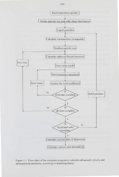
- 169-
Figure 4 1 Flow chart oft he computer program to calculate ultrasound velocity and attenuat ion in emulsions, according to scattering theory
- 170-
A few speci fic points about the numerical ca lculations need to be considered
Although the formulation of the multiple scattering problem is applicable over a range of
frequency (if sufficient terms are included in the series), the numerical calculatio n is
restricted to the low frequency region by the spherical Dcssel functions As the frequency
increases, the imaginary part of the argument of the Bessel functions increases for the
thermal and shear waves Since the Bessel functions are periodic, it becomes impossible
to obtain an ::tccurate result for their va lue. A consideration of how to C-'<lend such
calculations beyond the low frequ ency region is presented by Anson and Chivers ( 1993)
and other workers The majority of ultrasou nd applications in the co ll oid fi eld satisfy the
long wavelengt h condition, and it is also in the long wavelength limit that the simplified
relationships developed in the next chapter are appl icable Therefore. the formulation of
the previous sections was used directly, without recourse to special numerical techniques
to avoid these diniculties
The computer program is able to calculate the si ngle particle scattering
cocnicicnts. A ... for any scattering mode, 11 (the operator can choose which modes to
include) For the purposes of this study only coenicients up to the second order mode
were calculated The comple"' wavenumber o f the emulsion is determined using equation
438. up to second order in particle concentration One numerical detail is that for the
first order scatteri ng mode, the terms in the boundary condition 4 30 for ~~~~ are
modified, using the relat ionship
aJ;(a) J,(a) ~ - aj,(a) 14 39]
for both the Bessel and the llankel functions For sma ll arguments, the difference on the
lefl hand side of this equation is very small, and so is more accurately ca lculated from the
second order function
The wavenumber derived from multiple scattering theory assumes that all particles
(scatterers) are identica l (the same size and material) it is relatively stra ightforward to
show that_ in a di spersion which includes different scattering species, the terms
<fA. r'
[4 40]
in equation 4 38, should be replaced by
- 171 -
14 411
where the sum is over the different scattering species Equation 4 lll is an average
accordi ng to the number density of sca tterers This is relevant to dispersions in which
there are particles of different sizes (polydisperse) or some solid and some liquid
particles The sing le particle sca ttering coeffi cient must he determined for each species of
sca tterer separa tely· for ettch size of particle and for solid and liquid particles The
scatteri ng coeffi cients for solid scallerers are obtained by convert ing the equations 4 25
IO 4 30 in the way specified by Allegra and llawley ( 1972) The shear viscosity of the
fluid is replaced by the bulk modulus of the solid in the form given in equation 4 18 In
addition. all the terms in the boundary equations relating to the sol id droplets must be
multiplied by a factor o f 1rtJ In the computer program, the so lid droplets are assumed
to be of the same material (solidified) as the liquid droplets. so that the particle size
di stribution is simply converted for solid droplets using the ratio of the so lid to liquid
densit ies The proportion of particles which are solid at each r(ldius must also be
specified The computer program calculates the combined scattering coenlcient. given
the particle size di st ribution , and the proportion of particles which are solid
1\ numerical solution for the ultrasound propagation parameters of velocity and
att enuatio n can therefore be calculated for any polydisperse, mixed solid/liquid emulsion
This allows the comparison and development of ultrasound theories appl icable for the
interpretatio n of experi mental measurements on emulsions The interpretation o f
ultrasound velocity measurements of creaming in emulsions was of particular int erest,
such as those obta ined from the equipment shown in figure 1 I These emulsions are
generally polydisperse and the part icle size distribution at any height varies wi th time
Therefore it was vital to be able to calculate the predicted ultrasound veloci ty for any
given oil concentratio n and particle size di stribution This work was aided by the
computer modelling of creaming which is described in chapter 2 The model enabled the
construct ion of fully characterised data o n particle size distribution and concentration
profiles which could then be used to compare ultrasound theo ries and help to develop
new simplified ways of interpreting ultrasound measurements To this end, the numerical
scattering theory calculations were integrated into the creaming model described in
chapter 2, allowing the calculation o f the ultrasound veloci ty and attenuation predicted
by multiple scatt ering theory for the const ructed creaming emulsions The benefit of the
- 172-
computer model is that all of the system parameters are known, whereas in an
experimental system, the particle size distribution is not known <tS a fun ction of height
and time. and the concentration is only extracted from the measured ultrasound velocity
Therefore. with the computer model and the ultrasound theory calculations, accurate
assessment can be made of the applicability of various ultrasound models in interpreting
the ultrasound data
The ab il ity to calculate ultrasound parameters for solid and liquid p<~rticles in an
emulsion assists in the study of the appl icabi lity of simpl ified sca ttering theories for
crystal lisatio n experin1ents in emulsions Measurements of ultrasound velocity have been
used to calculat e the proportion of the dispersed phase droplets which are solid (the solid
fat content) and thereby examine crystallisation kinetics (Dicki nson et al, 199Jb) The
interpretation of ultrasound measurements in both creaming and crystalli si ng systems is
discussed speci fi ca ll y in chap ter 5
4.6 Important limiting solutions of sca ttering theo ry
The formulation described in the preced ing sections allows numerical calculation of
the ultrasound velocity and attenuation in an emulsion, whose properties are known
These calculations are not convenient for rout ine use in interpreting ultrasound
measurements In some cases, however, simplified forms of the velocity and attenuation
exist. which may be more appropriate and more easi ly implemented The numerical
calculations were used to investiga te the limiting forms of the scattering theory results, to
establish simpler expressions, and to determine the condi tions under which these might
be app lied
The applications of ultrasound measurements in co lloid science are usually in the
long wavelength limit (the wavelength oft he sound wave is much larger than the particle
size) The wavelength of sound in pure water at 30 °C is approximately I 5 rnm at
I Mll z, compared wit h the colloidal particle sizes of approximately I ~Lm lt is in this
region that the useful simplified theories of ultrasound propaga tion can be applied At
higher frequencies the variation of velocity and attenuation with frequency can be very
strong and is more difficult to predict Therefore, all the further work on ultrasound
propagation is restricted to the long wavelength region This limit is sometimes called the
Rayleigh limit. afler Lord Rayleigh who first investigated the scattering of sound by
- 173-
obstacles, and dete rmined the scattered intensit y under the lo ng wave leng th condition
(S tmtt , 1872, 1896) The definitio n of the lo ng wavelength limit is given by
kr << I
or in terms oft he wavelength, and defining the inequali ty
'brr I -<-
A 10
14 42 1
[4 43 1
In the long wavelength limit , the ultrasound velocity and the att enuatio n per
wavelength ( aA) vary with the parameter r Jf which is pro po rtional to the thermal and
shear wavelengths The limit o f the long wavelength region can be writt en in te rms o f
this parameter as
,. r < r ,, . Jr · V2o" 14 44]
showing that at smaller particle sizes the limit occurs at smaller va lues of the scaling
parameter Conversely, at higher frequencies but with the same parti cle size, the long
wavelength limi t ap pl ies fo r a smaller range of the sca ling parameter r f . Thus the
velocit y and att enuation variatio n discussed in the fo llowing sections, which ap ply in the
lo ng wavelength region, must be tru ncated at the limit defined by equat ion 4 _44 For
smalle r particle si7eS, some o f the fea tures at large va lues o f the scaling paramete r may
be absent , because they would occur out side the long wavelength region
The ultrasound velocity and att enuation over a range of frequency and particle size
were calculated numerically for a nomi na l 20 vol % sunflower o il in water emulsion at
30 ° ( , and a re shown in figures 4 2 and 4 3 The pa rti cle radius used for the ca lculations
was SO ~1111 in order to obtain a large range o ft he scaling parameter rJl wi thin the lo ng
wavelength regio n The physical data of the component phases which is required for the
ultrasound scatt ering ca lculat ions is shown in tab le 4 I These are identical to the
emulsion pro pe rti es used in the modell ing of creaming behaviour (chapter 2)
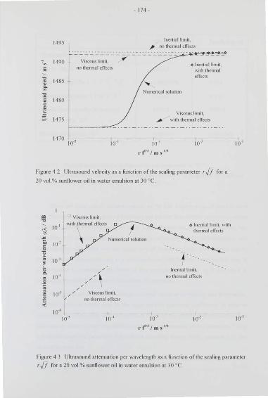
1495
1490
E
t 1485 ~ , :; 1480
~ 5 1475
- 174 -
Inertial limit. ,1* no therm~ I effects
------------------- _ ·.:.;._.:..o;-4'-~~~~
Viscous limit. no thcrmnl effects
Numerica l solutton
olncrt ia llimit. \\ith thermal effects
Viscous limit.
~ ' ' ith the rma l effects
1470 10 ' I 10'
I 10' io'
r f' 11 / 111 SI ll
Figute 4 2 Ultrasound velocity as a function of the scaling parameter rJ.f for a
20 vol% sunnower oil in wa ter emulsion at 30 °C.
Cl , « 10"0
0 .c biJ 10 2
:;;
" > ~ 10 ' ~
" 0. 10' c
·~ = 10"' ~ <
ll Viscous limit.
\\ ith thermal e ffects 0
\ Nuone<;cal sohol;on
olncrtiallimit . \\ith thcnn:1l effect ~
/ /
/
/
//' Vi'\Couc; limit. no thermal effects
I 1 0~
I 10"'
Inertial limit. no the rmal effects
r r' 11 I m sI ll
Figure 4 3 Ultrasound attenuation per wavelength as a function oft he scaling parameter
,. J7 for a 20 vol % sunnower oi l in wa ter emulsion at 30 or
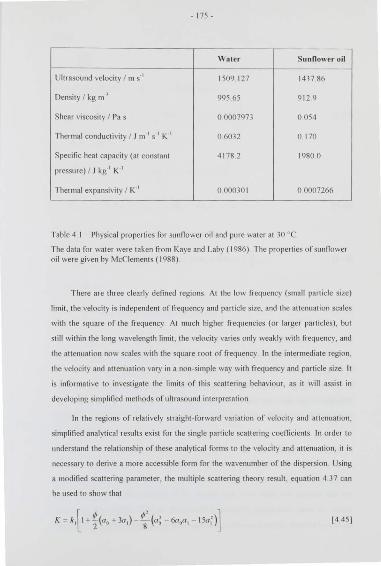
- 175-
\Valer Sunflower· oil
Ult rasound veloci ty I rn s·• 1509 127 1437 86
Densi ty I kg m·~ 995 65 9 12 9
Shear viscosity I Pas 0 0007973 0 054
Thermal conducti vit y I J m·• s·• K-1 0 6032 0 170
Specific hea t capacity (at constant 41 78 2 1980 0
pressure) I J kg·' K"1
Thermal expansivity I K-1 0 00030 1 0 0007266
Table 4 1 Physical pro perti es fo r sunflower o il and pure wa te r at JO 0(
T he data fo r water were taken fro m Kaye and Laby ( 1986) The propert ies of sunnower oil were given by McCiements ( 1988)
There are three clea rly defined regions At the low frequency (small particle size)
limit , the velocity is independent of frequency and particle si1e, and the att enuation scales
with the square o f the frequency AI much hig her frequencies (o r larger particles) , but
still within the long wavelength limit , the velocity vari es o nl y wea kl y with frequency, and
the attenuatio n now scales with the square root o f frequency In the intermediate region ,
the veloci ty and att enua tio n vary in a non-si mple way with frequency and particle si7e lt
is info rmati ve to investigate the limits o f thi s sca tt e ring behaviour, as it will assist in
developing simplified methods of ultrasound int erpretation
In the regions o f re lati vely stra ig ht -forward variat ion of veloci ty and attenuation,
simplified analyti cal result s exist for the single part icle scattering coeffic ients In o rder to
understand the relationshi p o f these analytical forms to the veloci ty and altenuation, it is
necessary to derive a more accessible form fo r the wavenumber of the di spersion Using
a modified scattering parameter. the multiple scatt ering theory result , equatio n 4 37 can
be used to show that
[44 5]
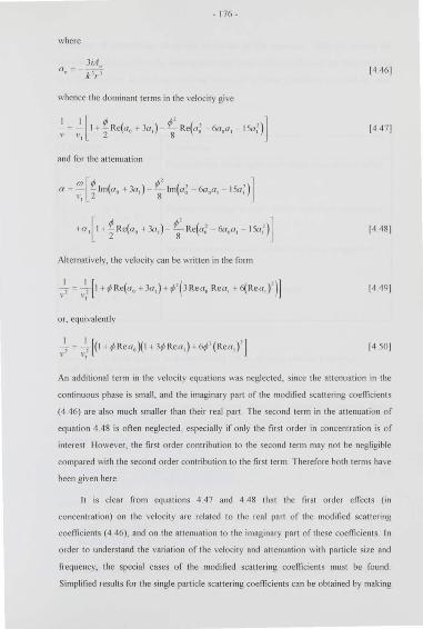
- 176-
where
a, = 14 46]
whence the do minan t te rms in the veloci ty give
[4 47]
and for the attenuation
a = ~~ [% !m( a, 1 Ja, ) ~ !m( a: Ga,a, - !San]
14 48 1
Alternatively, the velocity can be writt en in the form
14 49 1
or, equivalently
14 50]
An additional term in the velocity equations was neglected, since the attenuation in the
cont inuous phase is small , and the imaginary part of the modified scattering coeffi cients
(4 _46) are also much smaller than their real part The second term in the attenuation of
equatio n 4 48 is ofl en neglected, especiall y if o nl y the first order in concentration is o f
interest llowever, the first order co nt ributio n to the second term may no t be neglig ible
compared wi th the second order contri butio n to the fi rst term Therefo re bo th terms have
been given here
lt is clear from equations 4 47 and 4 48 that the first o rder effects (in
concentration) on the velocit y are relat ed to the real part o f the modified sca ttering
coeffi cients (4 46), and on the attenuatio n to the imaginary part o f these coeffi cient s. In
order to understand the variation of the veloci ty and attenuation with particle size and
frequency, the special cases of the modified scattering coefficients must be found
Simplified result s fo r the single particle scattering coeffi cients can be obtained by making
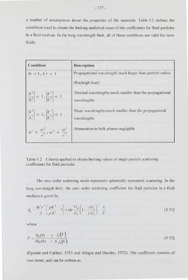
- 177-
a number of assumptions about the properties of the materials Table 4 2 defines the
conditions used to obtain the limiting analytical cases of the coenicient s for fluid particles
in a fluid medium In the long wavelength limit , all of these conditions are va lid for most
fluids
Corulition Description
kr « I, k 'r « I Propagational wavelength much larger than particle radius
(Rayleigh limit)
n lk'l Thermal wavelengths much smaller than the propagational
i! « I, k! « I wavelengths
n lk'l Shear \\avelengths much smaller than the propagational
k? « J, k! « I wavelengths
2 (02
'2 cv' Attenuation in bulk phases negli gible a « 7 , a "" -
,;z
Table 4 2 Criteria applied to obtain limiting values of single particle scattering coefficients for fluid particles
The zero order sca ttering mode represents spherica ll y symmetric scattering In the
long wavelength limit , the zero order scattering coenicient for fluid particles in a fluid
medium is given by
) G ( I t ikr :P_ I (,,
where
h0(h) T J,(li) 1· =------
hh,(h) r' b'J,(!i)
')' T~ r (i;
I
I· 14511
[4 521
(Epstein and Carhart , 1953 and Allegra and llawley, 1972) The coeflicient consists of
two terms, and can be written as
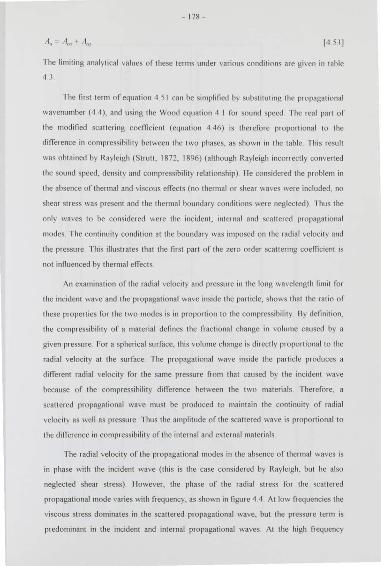
- 178 -
1 he limiting analytical va lues of these terms under various conditions are given in table
4]
The first term of equa tion 4 .51 can be si mplified by substitu ting the propagational
wavenumber (4 4). and using the Wood equation 4 1 for sound speed ·1 he real part of
the modified sca tt e ring coemcient (equation 4 46) is therefore proportional to the
difference in compressibilit y bet ween the two phases. as shown in the table This result
was obtained by Rayleigh (StnJII, 1872, 1896) (although Rayleigh incorrectly conve1ted
the sound speed, density and comprcssibility relationship) lie considered the problem in
the absence of thennal and viscous effects (no thermal or shear waves were included, no
shear stress was present and the thermal boundary conditio ns were neglected) Thus the
only waves to be considered were the incident. inte rnal and scattered propagational
modes The continuity condition at the boundary was imposed on the radial velocit y and
the pressure This illustrat es that the first part of the 7ero order scaltering coeffi cient is
not inOuenced by thermal effects
An examination of the rad ial veloci ty and pressure in the long wavelength limit for
the incident wave and the propagational wave inside the particle, shows that the ratio o f
these properties for the two modes is in proportion to the compressibility Dy definition.
the compressibility o f a materia l defines the fract ional change in vo lume caused by a
given pressure For a spheri ca l surface. thi s vo lume change is directl y proportional to the
radial velocity at the surface The propagationa l wave inside the particle produces a
different radial velocity fo r the same pressure from that caused by the incident wave
because of the compressibi lity difference between the two materials Therefore, a
scatt ered propagational wave must be produced to maintain the continuity o f radial
velocity as wel l as pressure Thus the amplitude of the scaltered wave is proportional to
the difference incompressibility o f the internal and external materials
The rad ial velocity of the propagational modes in the absence of thermal waves is
in phase with the incident wave (this is the case considered by Rayleigh. but he also
neglected shear stress) I lowever. the phase o f the radial stress for the sca ttered
pro pagationalmode va ri es with frequency, as shown in figure 4 4 At low frequencies the
viscous stress dominates in the sca ttered propagational wave, but the pressure term is
predominant in the incident and internal pro pagatio nal waves At the high frequ ency
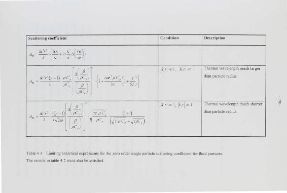
Scattering coefficient Condition Description
1k3r
3 { 6K K ( va)} Aul =3· -;-"1*2i-;t1-;;;
I iL)' k,r j« l, k ;r j« I Thermal wavelength much larger
A,='k'r ' (r-l)pC~ \. pC, { ~ ~'"''pC,(\.,._.':_)} than panicle radius
3 pC, f jJ \ 3 r 5r l pC,)
{:J' j""; IH k,r j » I, 1k,r j » I Thennal wavelength much shoner
A = 1k ' r ' . 3(y- 1) than panicle radius
02 3 r.J2W ( :J _ -;z;-· (~rpc, +M)
Table 4 3 Limiting analytical expressions for the zero order single panicle scattering coefficient for fluid panicles.
The criteria in table 4 1 must also be satisfied.
_, -a
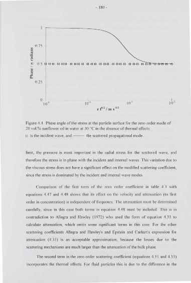
= " :a E
- 180 -
0 75
t! 05 00 0 [][] [] 00 [] 0 00 0 DD 0 [][] 0 0 OD OODio-""U--o-<H>--<1
0 25
r f 12 I 111 sIll
Figure 4 4 Phase angle of the stress at the particle surface for the zero order mode of 20 vol % sunnower o il in water at 30 ° ( in the absence of thermal effects
o is the incident wave, and -- the scattered propagationalmode
limit , the pressure is most import ant in the radial stress for the sca ttered wave, and
therefore the stress is in phase with the incident and int ernal waves This variation clue to
the viscous stress does not have a significant effect on the mod ified sca tt eri ng coeffi cient ,
since the stress is domina ted by the incident and internal wave modes
Compari son of the fi rst term o f the zero order coefli cient in table 4 3 wi th
equations 4 47 and 4 48 shows that it s effect on the velocity and attenuation (to fi rst
order in concentration) is independent of frequency The attenuation must be determined
carefull y, since in this case both terms in equation 4 48 must be included This is in
cont radiction to Allegra and 1 lawley ( 1972) who used the form of equation 4 3 1 to
calculate attenuation, which omits some significant terms in this case. For the other
scattering coeffi cients /\llegra and 1-lawley's and Epstein and Carhart's expression for
attenuation (43 I) is an accept able approx imation, because the losses due to the
sca ttering mechanisms are much larger than the attenuation of the bulk phase
The second term in the zero order scattering coefficient (equations 45 1 and 4_53)
incorporates the thermal effects For flu id part icles this is due to the diffe rence in the
- 181-
temperature-pressure coupling in the different materials For a given pressure, the
temperature generated by the incident wave or the propagational mode inside the particle
is proportional to the parameter
14 54]
for each mateJial in the long wavelength limit (equations 4 19. 4 20, 4 10, 4 15) This
parameter also represents the factors in the heat nux in the material rhe en"ects of shem
stress on the zero order mode can be neglected for the incident and internal
propagational modes in nuids, so the pressure is the only contribution to the stress For
solid particles, the shear terms in the stress are more significant and so the shape
deformation plays a part in the temperaiUre difference ·r he conllibutions to the
scattering coeHicient are more difficult to isolate when thermal effects are included.
because there are four waves generated at the particle surface. and four boundary
condi tions to be satisfi ed llowever, it is clear that the thermal waves must be generated
to maintai n the continuity of temperature at the particle surface. given that the incident
wave and the propagationa l wave inside the particle produce a difl'erent tempera ture
change for the same pressure field The differing heat now properties inside and outside
the particle a lso contribute to the magnitude and phase of the generat ed waves
The va lue of the thermal term va ri es wi th frequency and particle size, and is
determined by the magnitude of the thermal wavelength in the two materials The form
of the scattering coefficient contribution due to thermal effects is given in table 4 3
When the thermal wavelength is much larger than the particle size (low frequency) the
tcnn takes the first form in the table The contribution to the velocity (compare equat ion
4 47) is independent of frequency in this region, and the allenuation (equation 4 48)
varies as the square of frequency If the thermal wavelengt h is much shorter than the
particle size ("high" frequency), the thermal effect in the scattering coenicient takes the
second form of table 4 3 The effect on the velocity is much smaller in this region and
decreases as the frequency (or particle size) increases The thermal effects become
negligible at su nicicnt ly high frequency This may, however, no longer be in the long
wavelength region for which the ana lytica l results are va lid The thermal attenuation in
the short thermal wavelength region va ri es as the square roo t of frequency
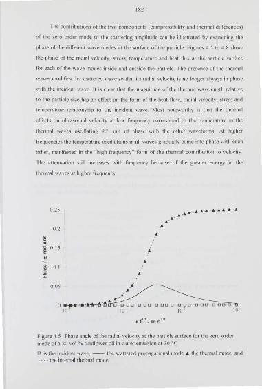
- 182-
The contributions oft he two components (compressibility and the11mtl differences)
of the zero order mode to the scattering amplitude can be illustrated by examining the
phase o f the dilTerent wave modes at the surface o f the particle Figures 4 5 to 4 8 show
the phase of the radial velocit y, stress, tempera ture and heat nux at the pariicle surface
for each of the wave modes inside and outside the particle The presence of the thermal
waves mod ifi es the scattered wave so that it s radial velocit y is no longer always in phase
with the incident wave 1t is clear that the magnitude of the thermal wavelength relati ve
to the particle size has an effect on the form o f the hea t now, radial velocit y, stress and
temperature relationship to the incident wave Most noteworthy is that the thermal
effects on ultrasound velocity at low frequency correspond to the temperature in the
thermal waves oscillating 90° out of phase with the other waveforms At higher
frequencies the temperature oscillations in all waves gradually come into phase with each
other, manifested in the "high frequency" form of the thermal contribution to velocity
The attenuation still increases with frequency because of the greater energy in the
thermal waves at higher frequency
0 2S ... ........ .......... ... -........... .. ... ..
02 ~
= ~ :; 0 IS E
" " 0 1 ~
-" ... 0 os
010 1
r r nt m s l f2
Figure 4.5 Phase angle of the radia l velocit y at the part icle surface for the zero order mode of a 20 vol.% sunnower oil in water emulsion at 30 °C
o is the incident wave, -- the scattered propagationalmode, & the thermal mode, and ·- ·- the internal thermal mode
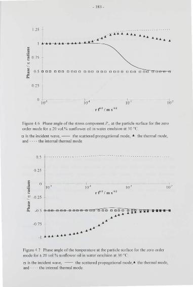
c
"
I 25
~ 0 75
- 183-
~ 0 5 o a a a o a a a o a a a a o a a a a a a a a o ;;-a-na,-,~~~ -" ..
0 25
lo' r r'1 I m s 112
Figure 4 6 Phase angle of the stress component Pn at the particle surface for the zero order mode fo r a 20 vol % sunnower oil in wat er emulsion at 30 °C
o is the inciden t wave, -- the scattered pro pagational mode, • the thermal mode, and ·- -- the int ernal thermal mode
c " :; E
0 .5 - -- - -- - - ---- - -
0 25
" -0 25
-0 75
- I .. . .... .. .... ..
I 10"'
......
r· r12 / 111 SI ll
.... _ ..
I 10 '
Figure 4 7 Phase angle o f the temperature at the particle surface for the zero order mode for a 20 vol % sunnower oil in wa ter emulsion at 30 oc. a is the incident wave, -- the scattered pro pagationalmode,• the thermal mode, and - ·-- the internal thermal mode
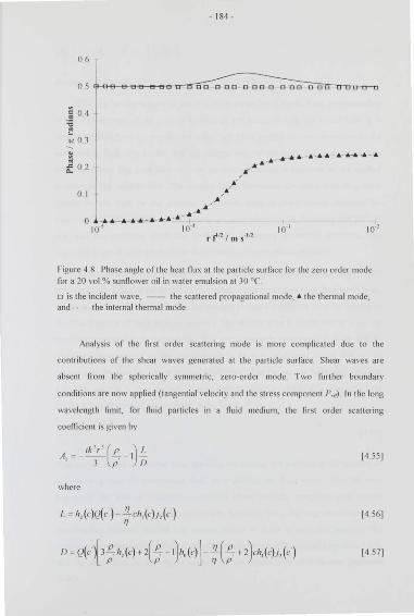
06
~ 04
~ "0.3
" " f 0.2
0. 1
- 184 -
• .. -.-.'
If
.. .,. A- - A · A_., - A- A-A ·A - A ......
0 _....._._ .... . . . . . . . . -1 ......
10' 10·' ,.rn I m sIll
Figure 4 8 Phase angle oft he heat nux at the particle surface fo r the zero order mode for a 20 vol.% sunflower oil in wa te r emulsion at 30 °('
o is the incident wave, -- the scattered propagational mode, • the thermal mode. and ---- the internal thermal mode
Analysis of the first o rder scattering mode is more complicated due to the
contributio ns of the shear waves generated at the particle surface Shear waves are
absent from the spherically symmetri c, zero-order mode. Two furth er bounda ry
cond itions are now applied ( tangentia l veloci ty and the stress component P,0) In the long
wavelength limit , for fluid particles in a fluid medium, the first order scattering
coeffi cient is given by
A ~ ik 'r ' ( P_ 1) !:_ ' 3 p ' /)
14 55]
where
14 56]
[4 57]
- 185-
'' )~, (c ) ,, [4 58]
(Epste in and Carlmrt , 1953, Alleg~a and llawley, 1972)
The angular dependence of the firs t order mode has a di po le form. corresponding
to the di splacement o f the particle backwards and fo rwards with the sound fi eld lt is
easy to see that there a re two fac to rs which will affect particle movement relative to the
surrounding flu id it s inerti a, and the viscous dr ag o f the fluid The particle's inerti a
determines how fast (and how far) the particle will move in response to the applied
pressure o f the inc ident fi eld The viscous stress determines the resto rat ive drag force
exerted by the fluid on the particle In general , both o f these effects influence the
sca tt e red fie ld Their re lati ve contributions a re determined by the frequency and par ticle
size, and tl1e scatt ering cocnicient is therefore frequency dependent llowever, two
impo rtant li mit s exist in w hich ei ther the inertial o r viscous enects dominate
When the wavelength o f shear waves is much short e r than the parti cle size ("hig h"
frequency), the e!Tect oft he inertia of the parti cle is much stronger than the viscous drag
The motio n oft he particle caused by the incident pressure is di!Terent from the mo tio n of
the Ouid (because of their di!Terent densit y) The viscous drag is insunicient to fo rce the
particle to move with the surrounding flui d. so the part icle moves ou t o f phase with it
The fluid then appears to the sound wave to have an additional inerti a due to the
presence o f the part icle T he sca tt eri ng coenicien t takes the second form given in tab le
4 4. if the particle is very viscous !\ more genera l result is complica ted The additional
ine1tia due to the parti cle is contained in the fac to r
LP 211 'P
[4 59]
This may be ca ll ed the inertia l limit Rayleigh considered thi s prob lem in the absence of
viscous drag fro m the surrounding fluid , by neglecting the shear waves Thus the term
represent s the limit of negli gible continuous phase viscosi ty compared wi th inerti al
forces Thermal waves were also neglected by Rayleigh, but in the lo ng wavelength limit
the coupli ng between thermal and viscous e!Tects in fluid s is negligible anyway The
contribution of the inert ial effect to velocity is independent of frequency (equation 4 47),
but the attenuation in thi s region va ries with the square roo t o f frequency (equation
4 48)
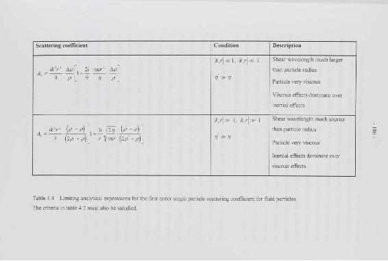
Scattering coefficient Condition Description
k$rl« i , (rl« I Shear wavelength much larger
tk ' r ' lip [ 2i 01pr' lip] than particle radius A, =-
9-·P 1+-g-ry- p ry » ry
Part icle very viscous
Viscous effects dominate over
inertial effects
jk,rj » I , [k,r j » I Shear wavelength much shoner
A =ik' r' . (p-p) [ l +~~ (p-p) ] than particle radius
' 3 (2p - p) r OJP (2p ..- p) ry » ry Panicle very viscous
Inertial effects dominate over
viscous effects
Table 4.4 Limiting analytical expressions for the first order single panicle scattering coefficient fo r fluid particles.
The criteria in table 4.2 must also be satisfied.
00 c-
- 187-
When the shear wavelength is much larger than the panicle si;c (low frequ ency),
the eHCct or the viscous drag of the surrounding fluid is much stronger than the inertial
forces on the particle The partic le is forced by the viscous drag to move in phase with
the surrounding fluid In some cases, if the densit y difference between di spersed and
continuous phases is \ Cry large. the inertial effects still do minat e in this regio n llowever.
for most food sys tems and for the emulsions studied in this work the density diiTercnce is
relatively small . and the viscous str ess is most significant The scallering coefficient is
therefore dependent only on the density difl"erence between particle and fluid . and takes
the form given in table 4 4 for very viscous pa1ticles Lamb (1 932. p 5 14) obtained the
same limiting results for the first 01der mode for rigid solid particles (no waves inside the
particle) in the absence of the!mal en"ects TherefOie, these limiting conditions a• e
dcte11nined simply by the particle's motion in the surrounding nuid , and not hy the
response of the mat erial inside the particle to the sound wave
The phase angles of the critical quantities at the particle surface are shown in
fi gures 4 9 to 4 14 Although the variation of the relative contributions for each of the
seven wave modes is very complicated, a significant variation in the phase of the
scattered propagational mode appears only to occur in the stress component P, (figure
4 11) At low frequencies the stress due to the scattered wave is 90° out of phase with
the incident wave, but at "high'' frequencies it is in ant i-phase In the other stress
component (figure 4 12) it may be noticed that the internal and external shear waves are
90° out of phase at low frequencies, but at higher frequencies I heir shear sll ess becomes
in phase with each other it is dinicult to draw conclusions li orn the individual wave
motions as to the movement of the particle it self (partly due to the fact that the wave
solutions are in spherical co-ordinates, whereas the particle motion is one-dimensional
and along the incident wave propaga tion direction) The simpler approaches of Lamb and
Rayleigh are more informative in this regard, as described above, since they illustrate the
two limiting solutions for the visco-inertial sca ttering in terms of the particle motion
1elative to the surrounding nuid
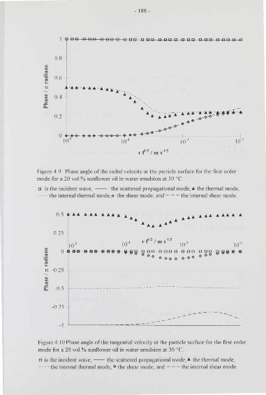
- 188-
J 008 BBB BBBB 1308 BOB gggc CCC egg gggg []
c
"
08
ii 06 :: " " 0 4 " .= ...
02
.............. ... ~- :.: · · · - .
.. ·. .. .
r rn / m s l fl
I
10 ' I
1o·'
Figure 4 9 Phase angle of the radial velocity at the part icle surface for the rirst order mode for a 20 vol % sunnowcr oil in wa ter emulsion at 30 °C
o is the incident wave, -- the scattered propagational mode. • the thermal mode, the internal thermal mode,<> the shear mode, and --- the int ernal shear mode
" " 0: -0 5
-0 75
- 1
A A.& .A..& & .& A A .A. .4 .A..& A.& A A A.&. A A
.& .__. .&. ._.a. A
a a a
.. r n/ 111 s lfl
000 0000 000 ODD <> oo <>ooo oo<> o <><>
Figure 4 I 0 Phase angle of the tangential velocit y at the parti cle surface for the first order mode for a 20 vol % sunnower oil in water emulsion at 30 or o is the incident wave. -- the scattered propaga tionalmode, A the thermal mode, ·· ·· the internal thermalmode, o the shear mode, and --- the interna l shear mode
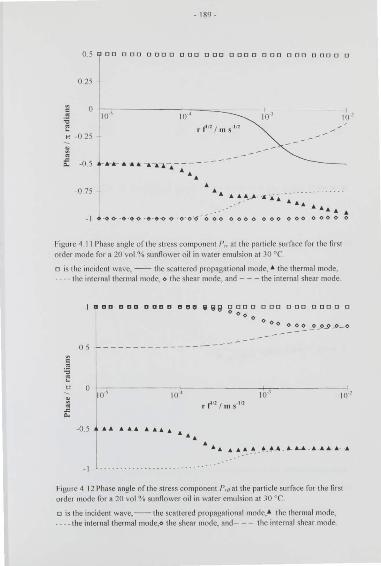
- 189-
0 .5 1JDO ODD DODO ODD ODD DODO COO ODD DODO 0
0 25
o lo·' lo·' r- r n I rn s I f!
" -0 25
~
" .c 0.. -05 j ..................... -.-;-----
•• -0 75 •••
.. ~~. _ .. _. . ... "A.i." .. ....
.. .... ... .. - 1 oo- &o.o o -o-<>-<> ooO Ooo oooo ooo ooo oooo o
Figure 4 11 Phase angle o f the stress compo nent /', at the particle surface for the first order mode fo r a 20 vol % sunflower oi l in water emulsion at 30 ° (
o is the incident wave,-- the sca ttered propagationalmode, A the thermal mode. ---- the int ernal thermal mode, o the shear mode, and--- the internal shear mode
~
;; ~ " " " .c
0..
DD DDD DDDD DDe fi199 DODO ODD ODD DODO 0
0 0 0 0
0 Oo ~~~~-O~...P- 0
0 .5 ---------------
0 10·'
r r'1 / m s l fl
-0.5 ........ ,. ......
l ...
- 1 .
A A_. A A A _4_ - ~ - · -· . .._...__. - A -A ...... . -A
Figure 4 12 Phase angle oft he stress component P ,0 tH the particle surface for the first order mode for a 20 vol % sunflower oil in wa ter emulsion at 30 °C.
o is the incident wave,-- the scattered propagationalmode,• the thermal mode, ____ the internal thermal mode,o the shear mode, and-- - the internal shear mode
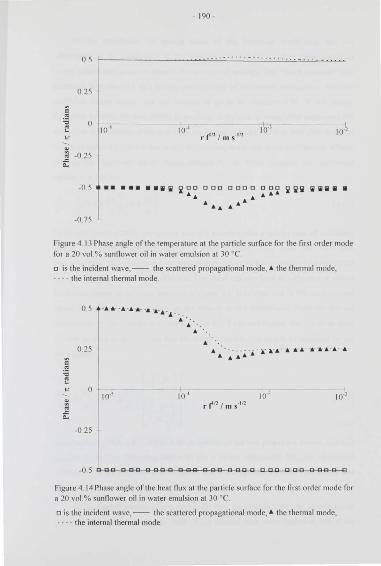
05
0 25
Cl " :0 0 E
" " " -0 25 .c
0..
- 190 -
Jo·' .. rn I m sI ll
I 10·'
-0.5 • • • • • • lllil 1iJ ~ a a a a a a a a o o a a 2 ~ i lil li 111 11 11
.... .lt. .............. ..
-0 75
Figure 4 IJ Phase angle of the temperature at the particle surface for the rirsl order mode for a 20 vol% sunnower oi l in water emulsion at 30 ° (
a is the incident wave,-- the scattered propagational mode, • the thermal mode, - the internal thermal mode.
" " .c
0..
0 .5 . ..... .. .... .. -a· · -j, ·
0 25
0
-0 25
~~.·- . • •
I 1o·•
• - .... --- ~· :a: A · :a.· a· • · •-a· & · & · • ........
r f 12 I m s 112
Figure 4 14 Phase angle oft he heat nux at the particle surface for the first order rnode for a 20 vol % sunflower oil in water emulsion at 30 °C.
o is the incident wave,-- the scattered propagational mode, • the thermal mode, · ·- · the internal thermal mode.
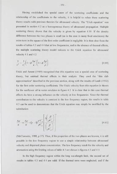
- 191 -
l laving established the special cases of the sca ttering coenicien ts and the
re lationship of the coefficients to the velocity, it is helpful to relate these scattering
theory results with previous theo ries for ultrasound velocit y The " Urick equation" was
presented in sectio n 4 2 as a homogeneous theory o f ultrasound propagation Multiple
sca ttering theory shows that the velocity is given by equa tion 4 SO If the density
difference between the two phases is small (as is the case in many food emulsions) the
ex tra term in the square of the first order coefficient is neg lig ible 11 is then clear from the
results of tables 4 .3 and 4 4 that at low frequencies, and in the absence oft henna! eiTects,
the mulliple scattering theory model reduces to the Urick equation for ultrasound
velocity 4 I and 4 2
[4 60]
Urick and Ament ( 1949) recognised that this equatio n was a special case of scat tering
theo ry, but omi tted thermal effects in their analysis They used the "thin slab
approx imatio n" described in the previous sectio n, along wi th the results of Lamb ( 1932)
for the first order scattering coeffi cient s The Urick velocity from this equation is shown
for the sunflower oil in water emulsion in figu re 4 2 lt is clear that in this case thermal
effects do have a strong influence on the velocit y at low frequencies Si nce the thermal
contributio n to the velocit y is constant in the low frequ ency region, the results in table
4 3 can be used to demonstrate that the Urick equation may simply be modi fi ed by the
substitution
/J.I(-> /J.I( ' (r I( I(
l) p·c~ pC,
[4 6 1]
(McCiements, 1988, p_27) Thus. if the properties of the two phases are known, it is still
possible in the low frequ ency region to use a simple relationship between ultrasound
veloci ty and dispersed phase concentration The low frequency result for the velocity and
attenuation using the limiting va lues o f table 4 3 are shown in figures 4 2 and 4 .3
In the high frequency region within the long wavelength limit , the second set of
result s in tables 4.3 and 4 4 are valid If the thennal term were neglected, and if the
- 192-
densities of the two phases were aga in simi lar, the "Urick" equation wou ld take another
modified form
I I ( /ll()( 3/lp J -=- l ql- 1+~ - -.-1'1 1' : K (2p f p) 14 62]
rhi s resu lt was also presented by Urick and Amen! (using their thin slab approximation
for multiple sca tt ering), in the absence of thermal e rTects This "inertial limit" is shown in
figures 4 2 and 4 3 for the sunflower oi l in water emulsion it is worth noting that when
the densities of the two phases are very similar, the density term in the inertial limit
approaches the viscous limit expression In other words. the difference between the
resu lt s of equations ll 60 and 4 62 may be within experi mental error in veloci ty lt is clear
even for sunflower oi l in water (figure 4 2), that the inertial and viscous limits in the
absence of thermal efTects a1e very simi lar
The thermal effect on velocity at the high frequency end of the long wavelength
limit is more troublesome, because it is frequency dependent (tab le 4 3) lt can obviously
be included expli ci tly using the previous quoted results but removes a degree of
simpli city from the velocity relationship . llowever, the magnitude of this term may not be
very great Figure 4 2 shows that for a wide nmge of frequency, it s contribu tion is no
greater than the difference between the viscous and inertial limits for the first order
scattering mode _ lt is reasonable, therefore, to omit the thermal term for the purposes of
obtaining a simple relationship between veloci ty and concentration We1e the thermal
term to be very significant in this region , it wou ld render the frequency range less
su itHble for use in polydisperse systems in which the size distribution is unknown or
varying For this purpose. it is necessary to have very little variation of velocity with
pa11icle size, and thus the low frequency limit is more appropriate _ This point is discussed
in greater detail in the next chapter, in which alternative methods for obtaining a
velocit y-concentratio n dependence are presented
- 193-
4.7 Summary of scattedng theory results
The investigation of scattering theory was intended to determine the usefulness and
applicability of various theoretical formulations to the interpretation of ultrasound
measurements in emulsions The main points oft he chapter are as follows
• Multiple scattering theory allows a physical understanding of the interaction of a
sound wave with the particles in an emulsion
• The multiple scattering formulation is particulady sui table in the long wavelengt h
regime, in which many emulsion measurements are made
• The scattering properties of particles, and the velocity and attenuation in an emulsion.
can be calculated numerically. provided that the physical properties of the constituent
phases are known
• Some ranges of frequency and particle size exist for which simplified. analytical
solutions are possible for ultrasound velocity The limiting solutions are presented in
loblcs 4 3 and 4 4
• The limiting conditions of scattering theory can be related to previously used
velocity concentration formulae
In summary, the multiple scattering theOT)' formulation is an appropriate theoretical
basis for int erpreting ultrasound measurements Although a general solution requires
numerical techniques, some simpler expressions exist which can be applied in an
experimental situation llowever, the physical properties of the materials in an emulsion
are often not known, and the calcu lation of scattering characteri st ics is then difficult In
chapter 5, a number of practical solutions are presented for the determination of the
scattering properties of emulsions, without recourse to a full scattering theory
calculation
- 194-
Chapter 5 : 1\lethods for Interpreting Ultrasound 1\lcasurements
In the previous chapter, the theory of ultrasound propagation in di spersed systems
was discussed In principle. the results presented there can be used to calcu late
ult1 asound velocity and attenuation in any well -characteri sed emulsion, subject to the
crit eria of section 4 4 By 'well -characterised' is meant a knowledge of the particle si7e
(and si7e di stribution). the concentration o f dispersed phase, the frequency. and all the
relevant physical proper ti es o f the constituent phases 1 Conversely. if al l of these
parameters are known except for the dispersed phase concent ration. a measur ement of
ultrasound velocity can be used to determine this quantity The results of multiple
sca ttering theory have been used to calculate the ultrasound velocity in a variety o r well
characteri sed emulsions. and these have been round to agree wel l with experimental
measurement s (McCiements. 1992. McCJement s and Povey, 1989) llowever, some
workers have found sign ifican t discrepancies between the predictions of this theory and
their experimental resu lts o n o ther di spersions (l lo lmes and C'hallis. 1993. llolmes e t al .
1993, 1994) This may be due to the vio lation or some o r the fundamental assumptions
or the theory. such as the absence of particle interactio ns or noccu lation, as di scussed in
chapter 4 Alternatively it may be that the values of the physical properties used for the
phases (e g viscos it y, thermal conducti vit y) do no t correspo nd e'<actly to the rea l va lues
o r the system being measured The differences may l>c due to experi mental uncerta inties
in the va lues or to variatio n in the materials llo lmes e t al (1993) st udied the effect of
uncertainties in a number o r parameters on the calculation of ultrasound veloci ty and
attenuation In some cases, the effects were very significant The errors involved in
making attenuation measurements were rou nd at Leeds to be much g reater than for
measurement or sound speed, although other workers have made accurate attenuation
measurements Thus, most of thi s work has concentra ted o n ultrasound veloci ty rather
than att enuation
Assumi ng that all the system parameters are known and that sca tt e ring theory does
provide an accurate prediction of ultrasound veloci ty, a full sca tt ering theory calculation
1 An e\:a mplc of the data required is sho" n in table :'i 1. later in thi s chapter
- 195-
could be used fo r concentratio n determination llowevcr, it does not lend it self to thi s
technique, because the determination o ft he scattering cocnicients is a complex numeri ca l
problem which would need to be carried out for each sample used Some, simpler
analyti ca l solutions exist under va rious limiting conditio ns (see section 4 6), fo r example
the Urick equation llowever, even these simplified ex pressions may require a substantial
amo unt o f physical data for the system being measured The paucity of such data for
many food components, particularly their thermal properties, causes a problem for the
use o f scattering theory. In addition, the applicatio n o f the theory to some systems has
been found to be inaccurate and therefore it canno t be re li ed upon to produce accept able
result s
The aim o f the present work is to develop simple methods o f finding the
relationship between measured ultrasound velocity and di spersed phase concentration (or
solid fa t content ) To be va luable for routine use, these methods must avoid the need for
an inconvenient sca ttering theory calculat ion and the diniculti es and restrictions
associated with it The result s presented in thi s chapter are concerned with ultrasound
veloc it y and att enuation measurement s in emulsions, parti cularly creaming and
crystalli sa tion Several techniques are di scussed fo r dete rminat ion o f the ultrasound
velocity concentration re latio nship from experiment almett surement s in these systems
5.1 Ex perimental delerminalion of scallcring cocflicicnls
The central result o f multiple scatt ering theory is an equation for the square o f the
wavenumber o f the dispersion in the fo rm o f a seri es in ascending powers o f particle
concentratio n (or volume fractio n o f di spersed phase) The veloc it y may be calculat ed
from the wavenumber, and hence from the sca ttering coenicients, as given by equations
4 47 and 4 49 The latter will be the preferred form for thi s chapte r because o f it s
similarity with the Urick equation Thus the velocity. t ', may be writt en as
[5 11
Subscript I represent s the continuous phase in thi s cont ex t, and tP is the vo lume fraction
The coeffi cients are related to the Urick equation by
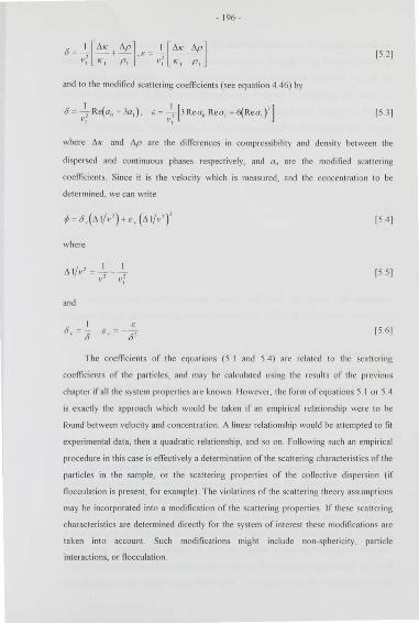
- 196-
[S 2]
and to the modified scattering coeflicients (see equation 4 46) by
IS J I
where AK and 11p are the di!Terences in comprcssibility and density between the
dispersed and continuous phases respectively, and a., are the modified scattering
cocflicients Since it is the velocity which is measured, and the concentration to be
determined, we can write
where
and
c5 _ _J_ ' c5
E E,_ = 81
[54 [
[S Sj
[5 61
The coefficients of the equations (5 I and 54) are related to the sca ttering
coefficients of the particles, and may be calculat ed using the results of the previous
chapter if all the system properties are known llowever. the form of equations 5 I or 5_4
is exactly the approach which would be taken if an empirical relationship we1e to be
found between veloci ty and concentration 1\ linear relationship would be aUcmpted to l'it
experimental data, then a quadratic relationship, and so on Following such an empirical
procedure in this case is en"ectively a determination oft he scattering characteristics of the
particles in the sample, or the scattering properties of the co llective dispersion (if
nocculation is present, for example). The violations of the sca tteri ng theo ry assumptions
may be incorporated into a modil'ication of the scattering properties If these scattering
characteristics are detennined directly for the system of interest these modil'ications are
taken into account Such modi l'i cations might include non~sphericity, particle
interactions. or nocculation
- 197-
Therefore, measurement s to find the relatio nship be tween ultrasound ve loci ty o r
att enuation and dispersed phase concentration can be thought of as a determination of
the sca ttering characte ri sti cs. not necessarily o f the individual particles, but o f the
collective properties of the system Experimental methods fo r obtaining the scattering
properties for a sample al so avoid the diffi culties associat ed with finding the physical
data for the materi als The scattering coeffi cient s are related to the experimental velocity
coeffi cients when there is a single dispersed component by
[57]
[5 8 1
where
[59]
T111e correspo ndence with sca ttering theory, and with the dipole and monopole
charac teri sti cs o f the scattering modes, requires the choice o f the "minus" solutio n o f
these equatio ns
The result s o f thi s chapter are designed to enable the determinatio n of the
sca tt e ring properti es o f a sample from experimental data. in a variety o f applicatio ns
These bui ld on the principles of scattering theory, and aim to produce simple and
convenient methods along the lines o ft he popular Urick equatio n
5.2 Pa rticle size and frequency dependence
The principal applicat ions o f this wo rk are concerned with a velocit y
concentration relationship lt was seen in chapter 4 that the ult rasound velocity in a
scatt ering system varies with particle size and frequency (figures 4 2 and 4 _3) In some
regions this variatio n may be qu ite strong, whereas in o ther frequency ranges the velocity
is independent of frequency and particle size These limiting conditions o f scattering
theory were di scussed in chapter 4 The implication o f this dependence is that any
velocity concentration relationship is valid only for the frequency and particle size (and
size distribut ion) for which it was determi ned A change in the size di stribu tion or the
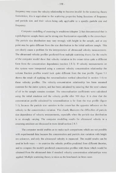
- 198-
Hcquency may cause the velocity relationship to become invalid In the scattering theory
formulation, this is equivalent to the scatt ering properties being flmctions or frequency
and particle si?e. and the ir vt~ lues being o nl y applicable to a specific parti cle si?e cmd
frequency
Co mputer modelling of creaming in emulsio ns (chapt er 2) has demonstrated that in
a po lydisperse sample there can be strong size fractional io n especially in the c1cam laye•
The particle size distribution may vary strongly with height in the sample, and at any
point may be quite different from the si?e distribution in the initi al uniform sample This
ca n clcmly cause a problem fo r the interpretatio n o f ultrasound ve locity measurement s
The ultrasound velocity profiles pr edicted fro m multiple scaltering theory fo r the result s
o f the comput er model show that veloc it y variatio n in the c ream takes quit e a dirTetent
fo rm fro m the concentrat io n dependence (section 2 8 .1) If velocit y measur ement s on
thi s system were interpreted using a constant velocit y concentt ation relationship the
volume fractio n profiles would look quite dirTerent fl om the true pro fil e Figut e S I
shows the result o f applying the renormali sation method (desc ribed in section 54 ) to
these velocity pro files The ve locity concentration te latio nship has been assumed
constant fo r the entire system, and has been calculated by ensuring that the total volume
o f oil in the sample remains constant The renonnali sa tion coeffi cients were calculat ed
using the initia l emulsion and the veloci ty pro rile aner 500 days lt is clear that the
concentratio n profil e calculated by reno rmali sation is far from the true pro fil e (figure
5 I), because the particle size variation in the cream has the o pposit e influence on the
velocity to the concentration vatiation This clearly illustrates the diniculti es of particle
size dependence o f velocity measurements, especia ll y \.\ hen the particle size di stribution
is so strongly varying The computer modelling result s for ultrasound velocity in a
creaming emulsio n arc di scussed in more detail section 2 8 3
The computer model enables us to make such comparisons which are not possible
with experimental data because the concentration and particle size va ri atio n with height
are unknown, and only the ultrasound veloc it y is measured The model result s can be
used in both ways to examine the ve locity profiles predicted from dirTerent theories,
and to compare the model's predicted concentratio n pro fil es with those which would be
obtained fro m the ultrasound dat a if standard veloci ty concentration relatio nships were
applied Multiple scatte1ing theory is taken as the benchmark in these cases
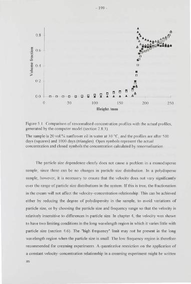
08
c
·E 06
" .:: e 04
" 0 >
02
00
- 199 -
D . D
• D
•" o 1l 1l ll !lA
D D 0 D D C C ~ 2 4 4 4 4 A
0 50 I 00 150 200 250
ll eight /mm
Figure 5 I Comparison o f renormalised concentratio n profil es with the actual pro fil es, generated by the computer model (section 2 8 3)
The sa mple is 20 vol % sunOower oil in water at 30 °C. and the pro fil es are afl er 500 days (squares) and I 000 days (triang les) Open symbols represent the actual concent ra tion and closed symbols the concentration calculated by renormalisa tio n
The particle size dependence clea rly does not cause a problem in a monodisperse
sample, since there can be no changes in part icle size distribution In a polydisperse
sample, however, it is necessary to ensure that the velocity does not vary significantly
over the range o f parti cle size distri butions in the system If this is true, the fractional ion
in the cream will not affect the veloci ty concent ra tion rela tionship This can be achieved
ei ther by red ucing the degree of polydispersity in the sample, to avo id va ri ations of
particle size, or by choosi ng the parti cle size and frequency range so that the veloci ty is
re lati vely insensitive to differences in parti cle size In chapt er 4, the velocity was shown
to have two limit ing condi tions in the lo ng wavelength region in which it varies little with
parti cle size (section 4 6). The "high frequency" limit may not be present in the lo ng
wavelength region when the parti cle size is small The low frequency region is therefore
recommended for creaming ex periment s_ I\ quantitati ve restri ctio n on the application o f
a constant veloci ty concentration relatio nshi p in a creaming experiment might be writt en
as
-200-
[5 IOJ
where 1\ l'c•p is the experimental error in velocit y measurements Essent ially, this means
that <my variation in ultrasound velocity caused by particle size changes must be less than
the experimental error Thus, all changes in velocity can be att ributed to oi l
concent ration T he condition is obviously satisfi ed either by havi ng a very small degree
of size variation, o r by hav ing a veloci ty that is not aiTected by changes in parti cle size
The frequency dependence of ultrasound velocity means that the relationship
determined between the velocit y and concentration is specific to the ultrasonic
transducers used Probes of the same nominal freq uency o fl en include frequency
components over a range o f frequencies which may differ between probes Therefore, the
determination o f the velocity concentra tion relationship for a creaming experiment , for
example. must be carried out using the probes which are to be used for the creaming
experiment it self
5.3 Ca libra tion
Previous creaming experiments for which the Urick equat ion was found to be
inva lid, were interpreted by a calibrat ion technique (fo r example, Dickinson et al , 1994)
I\ series of emulsio ns o f known compositio n was made with a range of di spersed phase
concentration The ultrasound veloci ty was measured in each case, and a regression fit of
veloci ty as a function of concentratio n was calculated In this way, the concentration of
o il could be determined from measured veloci ty profiles in subsequent creaming
experiments In the light of mult ip le scattering theory analysis, it is clear that this method
is an experimental determination of the scattering properti es o f the sample_ Althoug h the
velocity concentratio n relationshi p has been written in terms o f the inverse square o f the
veloci ty (equations 5 1 or 54), the principles apply equally well to a direct
correspo ndence between the velocit y and a power series in concentratio n The
calibration curve must o f course be measured using the same ult rasound probes as used
fo r the experiment The method is not restricted to creaming experiments, but could be
used to determine concentration in any samples, provided that a set o f well -characteri sed
emulsions can be made, in order to "calibrate" the velocity relationship
- 20 1 -
The restrict ions on the particle size distribution variation and on the dependence of
velocity with part icle si7e, as descri bed in the previous section, must be applied for the
ca libration method to be va lid A test of the va lidity of the technique in creaming
experiment s is to calculate the total volume fraction of oil in the whole sample, as
determined from the calib rated velocity measurement s The calculated volume fraction
averaged over the height of the sample should remai n equa l to the ini tial volume fraction
of oil in the uni form emulsion. which is usually known A deviation of this qua ntity ft om
the initial value is an indication that the velocity -concentration relationship is changing
with time, or is not constant with height in the sample In other words, the fractionation
effect is influencing the ultrasound veloci ty, and the calibration curve does not apply over
the whole sample
The ca li brat ion technique was applied to recent measurements on a 20 vol %
sunflower oil in wa ter sample at 30 °C', wi th a variety of concent ra tions of xanthan gum
added to the aqueous phase These measurements \\ere made by Jian Guo Ma using the
ultrasound scanner illustrated in fi gure I I (Ma, 1995) The effect of xanthan on the
ultrasound velocity in the aqueous phase was found to be negligible at the concentrations
used (Dickinson et al , 1994) llowever, the effect of unadsorbed Tween20 in the wa ter
does have a significant effect on velocit y. and all emulsions were made so that the
concentration in the aqueous phase was I w t % Tween20_ A calibration curve was
constructed using measurements made wit h the ult rasound scanner (opera ting at
I 19 Mllz) and also with the (/ltrosound /"e/oc:lly /11(• /er (UVM I) (operating at
2 25 Mll z) The volume surface average part icle size, d12, was 0 56 ~1111 The measured
velocity as a function of oil concent ra tion in each case is shown in figure 5 2 The
difference between the two curves indicates that for these emulsions the particle size and
frequency fall in the range in which ultrasound velocity does vary with these parameters
Therefore, the determination of concent rat ion profil es using the calibration curve
depends on the size distribution not varying so strongly in the cream that the curve
becomes invalid
The calibration curve measured in the ult rasound scanner was used to calculate the
volume fra ction profiles in creaming experiments on these emulsions The resulting
profiles for a 20 vol % sunflower oil in water emulsion wit h 2 wt % Tween20 and
0 03 wt% xanthan are shown in figure 5 3 After 10 days the total volume fraction in the
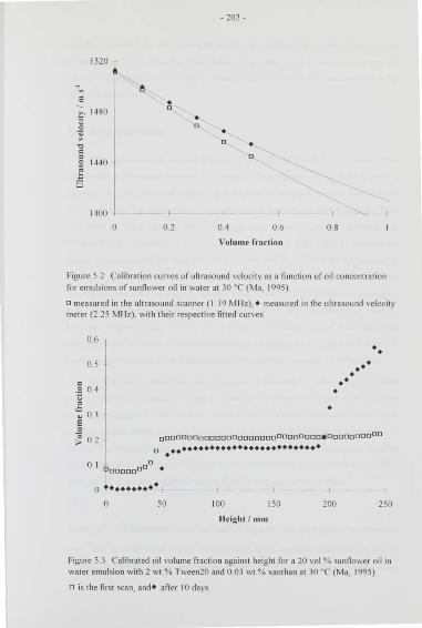
-202 -
1520 ~
e E •
1480 (]
5 • 0 (]
• ;; > (] • "0 c = (]
~ 1440
5
1400
0 02 04 06 08
Volume fntct io n
Figure 52 Calibra tion curves of ultrasound velocity as a function of oil concentratio n for emulsions ofsunnower oil in water a t JO 0
(' (Ma, 1995)
o measured in the ultrasound scanner (I 19 Mllz), • measured in the ultrasound veloci ty meter (2 25 Mllz) , wi th their respect ive fitt ed curves
0.6
0 .5
•• •
•
• •• •
••
0 aaooaoaaooa oooaooaaaooaaooaa• oaooaaoo00
a .•••••••••••••••••••••••••••
0. I ooaaoaoa •
0 + ......... , 0 50 100 150 200 250
Height / mm
Figure 5_3 Calibrated o il vo lume fraction aga inst height for a 20 vol .% sunnower oil in water emulsion with 2 wt% Tween20 and 0 .03 wt % xanthan at 30 ° ( (M a, 1995)
o is the first scan, and • an er I 0 days
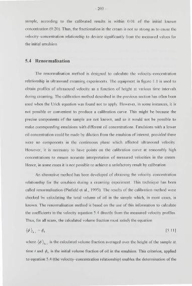
- 203-
sample. according to the calibra ted results is within 0 0 1 of the initial known
concentration (0 20) Thus. the fractional ion in the cream is not so strong as to cause the
ve locity concentration 1 clationship to deviat e signilicantly from the measured values for
the initial emu lsion
5.4 Rcnonnalisa tion
The renormalisation method is designed to ca lculate the velocity concentration
relationship in ultrasound creaming experiment s The equipment in figure I I is used to
obtain profil es of ultrasound velocity as a function of height at va rious time int ervals
during creaming The calibration method described in the previous section has ofl en been
used when the Urick equation was found not to apply llowcvcr, in some instances, it is
not possib le or convenient to produce a calib1ation curve This might be because the
precise component s of the sample are not known, and so it would not be possible to
make corresponding emu lsions with different oil concentrations Emu lsions with a lower
oil concentration could be made by dilution from the emul sion of int erest, provided there
were no components in the continuous phase which affected ultrasound velocity
However, it is necessary to have points on the ca libration curve at reasonably high
concentrations to ensure accurate interpretation of measured velocities in the cream
Hence, in some cases it is not possible to achieve a satisfactory result by calibration
An alternative method has been developed of obtaining the velocity concent ration
relationship for the emulsion during a creaming experiment This technique has been
ca lled renormalisation (Pin fi eld et al , 1995) The results of the calibration method were
checked by calculating the total volume of oil in the sample which, in most cases, is
known The renonnalisation method is based on the use of this informat ion to calculate
the coeffi cients in the velocity equation 54 directly from the measured velocity profil es
Thus, for all scans, the calculated volume fraction must sa ti sfy the equation
(</J ), ' = (1, [5 IIJ
where (; ),. , is the calculated volume fract ion averaged over the height of the sample at
time 1 and (10 is the initial volume fraction of oil in the emulsion This criterion, applied
to equation 54 (the velocity concentration relationship) enables the determination oft he
-204-
coenlcicnts of the velocity equation from the measured velocit y profiles The procedure
is described in the following sections
5.4.1 Linear rcnonnalisation
On the first scan of a creaming experiment. the sample lends to be still reasonab ly
uniform. and there is very little cream (high concentration of oil) If the sample is not too
concentrated it is likely that the quadratic term in equation 54 will be negligibly small on
thi s scan ., hi s is equi valent to the neglect of multiple sca tt ering at the concentratio n of
the initial sample. The application of equation 5 11 to equation 5.4 on the first scan leads
to an estimat e for the linear renormalisation coefficient
8 =--(1_, __ ' (11 1 ··' ),,,
15 121
The application of equatio n S 4 in thi s case leads to a result
[5 13]
fo r the volume fraction at any position This result can be used as the linea rly
renormalised estimat e for oil concentration on the first and subsequent scans
The linear renormali sat ion method was applied to the results of creaming
experiment s referred to in the previous sectio n (Ma, 1995) For the first scan, the linea rly
renormali sed vo lume fraction profile is shown in figure 54 There is no formation of a
cream on this scan, so the neglect of the quadratic term is probably reasonable at the
relatively low concentration in the sample Figure 54 also shows the volume fraction
profile calculat ed from the Uri ck equation (equations 4 1 and 4 2) and from the
ca libration curve which was discussed in the previous section, and was shown in figure
5_2 The linearly renonnali sed and calibrat ed results agree to within 0 0 15 in volume
fraction, although the average vo lume fraction calculated from the ca librat ed results was
only 0 187 lt is clear that in this case, the Urick equation is invalid
On later scans, as a cream layer develops, the linear approximation becomes less
accurate because the quadratic terms in equation 54 become more significant , especially
in the cream I\ further application of the renormali sat ion principle is req uired in order to
obtain the quadratic renormalisation coeffi cien t
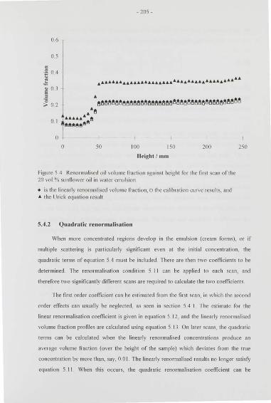
- 205-
06
os
e o 3
~ 02 ·~~~~~~~~~~~~~~~~~~~~~~~~~~~~~~~~~~~~~~~~ :~ .............. ~
0 1 -AAAt!ll!lee
0 50 100 I SO 200
ll cil!, ht / mm
Figure 54 Ren01malised oi l volume fraction against he ig ht fo r the first scan o f the 20 vo l % sunnower oil in wa ter emulsion
• is the linea rly rcnormali sed volume fraction, o the cal ibration curve result s, and A the Urick equation result
5.4.2 Quadratic renormalisation
250
When more concentrated regions develop in the emulsion (cream forms), or if
multiple scattering is particularly significant even at the initial concent ra tion. the
quadratic terms of equation 5 4 must be included There are then two coenicients to be
determined The renormal isatio n condition 5 11 can be applied to each scan, and
therefore two significantly dirTerent scans are required to calculate the two coeffic ients
The first o rder coefficient can be estimated fi o m the first scan, in which the second
order effects can usua lly be neglected, as seen in section 5.4 I T he estimate fo r the
linear renormalisa tion coenicient is given in equation 5 12, and the li neMiy renormalised
volume fractio n pro fi les are ca lculated using equation 5 13 O n late r scans, the quadrati c
terms can be calculated when the linearly reno nnalised concentrations produce an
average volume fraction (over the height o f the sample) which deviates from the true
concentration by more than , say, 0 0 1 The li neally renormali sed result s no longer sati sfy
equation 5 11 When this occurs, the quadrati c reno rmalisation coeffi cient can be
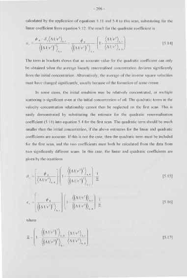
-206-
calculated by the application of equations 5 11 and 54 to this scan. substitu ting for the
linear coeffi cient from cqwuion 5 12 The result for the quadratic coemcient is
if! o (I (A I "'),,) ((A 1 1· ' ) ' ),' . (11 1 •" ), 0
15 141
The term in brackets shows that an accurate va lue for the quadratic coefficient can only
be obtained when the average linearly renormali sed concentration deviates significantly
from the initial concentration Alternatively, the average of the inverse square velocities
must have changed significant ly. usually because of the formation of some cream
In some cases, the initial emulsion may be relatively concent rated, or multiple
scattering is significant even at the initial concentration of o il The quadratic terms in the
veloci ty concentration relationship cannot then be neglected on the first scan rhis is
easi ly demonstrated by subst ituting the estimate ror the quadratic renonnalisation
coemcient (5 14) into equation 5 4 ror the first scan The quadratic term should be much
smaller than the initial concentration, ir the above estimates ror the linear and quadratic
coemcients arc accUJate Jrthis is not the case, then the quadratic term must be included
ror the first scan, and the two coeHicients must both be calculated rrom the data rrom
two significantly different scans In this case, the linear and quadratic coemcicnts are
given by the equat ions
[5 15]
IS 16]
where
~ - [I ((AI••rL_ ~I ~.·'] - ((11 1 1·')'), , (A I•·'), 0
15 171
- 207-
These mig ht be ca ll ed the «exact" solutions Aga in, accurate result s can only be obtained
when a sig nificant change has taken place relati ve to the fi rst scan. otherwise the
bracketed terms a re too similar and poor solutions a rc obta ined The va lues for the
coeffi cient s calculated by equatio ns 5 12 and 5 14 o r by equatio ns 5 IS and 5 16 arc
va lid for a ll scans oft he same sample_ The best so lu tions for the cocfli cicnt s are ob tained
when the dilTerence between the scans is greatest ( for example. using the fi rst 1'\nd last
scans to calculate the cocfli cicnt s)
The quadra ti ca lly rcno nnalised concentration pro files for the sunOower o il in water
emulsio ns investiga ted by Ma {1995) a1e shown in figUi e 55 This ca lculation was made
using the "estirmlted'' solutions (equatio ns 5 12 and 5 14) to determine the
rcno rrnali satio n coefficient s, using the first scan, and the scan afler I 0 days These were
substituted into equation 54 to obtain the vo lume fraction The linearly rcno rrnali scd
profil e is also shown. illustrati ng the significance of the quad rati c terms in the cream
b yer The linearl y reno rmali sed vo lu me frac tion on thi s scan sti ll gave an average vo lume
fractio n of o il in the whole sample o f 0 206 The result s of the cal ibratio n curve and the
Urick equatio n are also shown for compari son The quadra tic renormali sa tion and the
ca li bra tion result s agree o n oil volume fraction to within 0 0 1
06
os
·~ 04
...:: 0 3 e = ;e 0 2
0 1
0
0
••••••••••••••••••••••••••• & ~
eeeeeeeeeeeeeeeeeee~~eeeeee &1'1 1!1
•......•• , 50 100 I SO
ll r ight / mm
200
Figure 55 Quadra tically reno rmali sed o il vo lume fraction aga inst height fo r the 20 vo l % sunOower oil in water emulsion afl er I 0 days
250
xis the quadraticall y renormalised volume fractio n. • the linearl y renormalised volume fraction,o the calibration curve result s and • the Urick equation result
-208-
Section 52 discussed the restrictions on the applica tions of techniques such as
rcno nnali sa tio n due to parti cle size dependence of the ult rasound velocity This is
especiall y relevant in crea ming experi ments in which there may a strong varia tio n o f
particle size. especia lly in the cream Should any particle size variatio n in the sample
cause a sig nificant change in the coenicicnts of the velocity concentrat ion relatio nship
(equation 5 ll), the renonnalisation method would become inappropriat e l t should be
possible to detect any such di sc repancies, by testi ng the average vo lume fraction o f oi l in
the sample on each scan The renormalisation coeffi cients are calculated fr om the first
scan and o ne late r scan When these values a re applied to ca lculat e the vo lume fract ion
on a ll o ther scans, the resu lt s should yield the correct va lue for the average concent ra tio n
(equal to the initi al va lue) in all cases If th is does no t occur, it is an indica tion that the
parameters in equation 54 a1e dirrercnt for the dirre1ent scan ~ In other words, there is a
significant change in the velocit y concent ra tion relationshi p wi th time, usuall y caused by
variation in particle si?e di stribution from the initia l emul sio n
The Jesu it s of thi s ~ect ion can be used to ob tai n the relat ionship between
ultrasound veloci ty and oi l concent ration directl y fro m the measured veloci ty profil es
The o nl y info rmation which is necessary to ac hieve thi s is the initia l concentration o f oil
in the uniform emulsion. and the ult rasound velocity in the continuous phase_ In fac t. if
the initi al o il concentratio n is not known, the concentratio n pro files may still be
ca lculated as a proportion o f the init ial concentra tion This is clea r fl om the fo rm o f the
1enormali satio n coefli cient s, which each include a fac tor o f the in iti al oi l concentration
The technique is an indirect method o f determining the sca tt ering pro perties of an
emulsion during a creaming experiment, using only a small piece of knowledge based on
the conserva tion o f o il vo lume
5.5 1\ lult iple dispersed phases
Many food systems contain di spersed or so lubilised compo nents o ther than a single
emul sified o il phase For example. it is common for oi l in wa ter emulsio ns to have some
polymer present in the aqueous phase Studies o f crystalli sa tion in emulsions can al so be
considered as having two different di spersed phases so lid and li quid parti cles In order
to develop practical approaches fo r the interpretation of ultrasound measurement s in
these systems, it is first expedient to consider the general theoreti cal result s for samples
-209-
with mulliplc dispersed phases The bnsis of the development of a theory for mixed
systems is multiple scall ering theory, as described in chapter 4 Each dispersed
component must satisfy the conditions discussed in section 4 4 This precludes
interactions between din'erent components or between similar component s (such as
fl occula tion) Each component entity must act independently and be randomly
distributed The imaginary part s of the modified sca ttering coefficient s ( equ<~tion 4 46)
arc neglected throughout the fo llowing analysis
For each component phase. the velocity is given by equation 5 1 In the combined
system, the scatt ering cocOicicnts are calculated by summing the coefficient s for each
phase in proportion to their number density The combined coeffi cient is given by
equation 4 4 1, just as for a polydisperse sample (each size fraction can be trea ted as a
separat e dispersed phase component) Ex plicitly. the velocity in the combined system can
be written as follows
I I [ ! ~ ! I I L(~. Rea,, I 3~, Rea,, ) I ' 1'1 1
[5 18J
where ; repr esent s a dispersed phase species Using the relationship between the
individual sca ttering coefficients and the velocity equation for each phase separately
(equations 5 I and 53), this can be simplified to
[5 19]
where
J5 20 J
Single sca ttering eiTects in the inverse square veloc ity equation are simply addit ive
Mul tiple scattering is not so straightforward In this case onl y double sca tteri ng event s
are included ;\. double scattering event might be scattering ft om two particles of the
same component , or sca ttering from two diiTerent species The former eiTects are again
additive in this equation The final term in equation 5 19 accounts for the eiTects of
- 2 10-
scatt e ring from two differen t compo nent s This is the o nly term in the equa tio n w hich
cannot be direclly determined fro m the experi mental coefficie nt s wi thout furthe r
rearrangement o r assumptions llowever, if the scatt ering coeffic ients can be wri tt en in
the form of equations 57 and 5.8, the ex tra term can be simplified, g iving
IS 2 1]
where the sca tt e ring factorS is given in equation 59
The attenuation ca lculated by multiple sca tt e ring theo ry was given in equation
4 48 it is clear that the solution in a multiphase system will follow the same dependence
as fo r the veloci ty The quadratic terms in attenuation are o Oen negligible, but their
re lationship to the scatt ering coenicient s is difficu lt to determine in the multi phase case
because of the many terms involved Also it is not known which te11ns o f equa tio n 4 48
must be included l lowever, the form o f the attenuation re latio nship can be writt en
directly
IS 22 1
All the terms in the attenuation which are quadratic in concentration may be negligible
The Urick equatio n in a multiple phase system produces similar result s for the
ultrasound velocity, bu t it differs in the "cross- term" due to the omission of o ne of the
multiple scattering terms (see section 4 6) Thus we have
IS 23 I
where the Urick sca ttering parameter is now given by
[S 24]
The results of thi s section ca n be applied to spec ifi c examples o f muhi-phase
systems which are re levant in the stud y o f food emulsio ns Two such applications are
di scussed in the following sections
-2 11 -
5.6 l'nlymcr/o il systems
Many food emulsions contain polymer di ssolved or di spersed in the continuous
phase This may be for the purposes of modifyi ng the rheological properties of the food
for tex ture or stability reasons (for example a gum), or it may be present natu ra lly (casein
in mi lk) The presence of the additio nal di ssolved o r di spersed component may or may
not innuence significantly the ultrasonic properties of the system If it does have an
enect, this must be taken into account when applying techniques to determine the
concentration o f oil, such as those di scussed in the preceding sections The first
consideration is how the properties of the multi-phase system are related to the
pro perties of samples containing each dispersed phase independently This wi ll be o f use
in dete11nining the vo lume fra ction of oil in a sample with <HI added po lymer 0 1 other
component, when the effect o f the additional component in water alone is already
known
Fo r the polymer di spersion in the continuous phase, in the absence of o il
15 25 1
15 26]
and for the emulsion in the absence of po lymer
15 27]
[5 28]
lt is usually possible to determine all of these coeffi cients experimenta lly using a range of
well -characterised emulsions and dispersions The concentration used in the5e equations
is expressed as a volume fraction For polymers or ot her molecules, their vo lume may be
diffi cult to define, and it is more usual to measure concentratio n as a percentage weight ,
or as a weight in a specified volume For the purposes of scattering theory. the relevant
quantity is the number of scattering centres per unit volume of t he sample In the case of
emulsion pa11icles, this is proportional to the vo lume fraction (at a specified particle
size) Fo r the polymer, any measure of concentration must be specified as a propo rtion
of a volume oft he sample The quantity used may be a weight or mass, but it must be in
- 212-
telation to a vo lume of sample, not to the continuous phase only For e'=ample the
concentration may take the unit s of kg m·1
1\ltcrnatively. the number of molecules in a
given volume cou ld be used Whatever the measure. it must be proportional to the
number of scattering centres per volume of the sample
For the combi ned system. the results of sect ion 5 5 are directly applicable
Equations 5 19 and 5 20 or 5 2 1 can be used for velocit y and equation 5 22 for
attenuation llcncc the multi-phase system can be characterised simply. so that the
ve locity and attenuation for any concentra tion of oi l or polymer can be ca lculated
Conversely, if the polymer concentra tion is known, the oil concentra tion can be
determined The combined sca tt ering term in the velocity and att enua tion (equations
5 19-5 2 1 and 5 22) may be dimcult to ca lculate accurately, ei ther rrom the theoretical
scattering cocmcients or from the experimenta ll y determined parameters The quadratic
experimental coentcient or the velocity is oficn a relatively small contribution to the
overa ll variat ion with concentration, and its error from a regression fit may be significant
This leads to uncertainty in the va lue or the combined scattering term in the velocit y
Also. the form of this combined scattering effect depends on the relat ionship of the
expe1imenta l parameters to the scattering coentcients (equation 5_3) 1r some or the
assumptions or sca tt ering theory are not applicable, this correspondence may not be
exact. although the form or the velocit y and attenuation dependence is stil l valid
The1erore the combi ned scattering term should be approached wi th some ca1e A
sensible. practical solution to the problem would simply be to ca librate this combined
term using an ultrasound measurement ror a single multi -phase system in which all the
ot her parameters are known (the concentrations or polymer and oil in this case)
Previously, the effect of the added component in creaming experiments was
accounted for by calibrating the ultrasound velocity as a function of oil concent1ation
with the known quantity o r polymer already present in the aqueous phase This was the
apprmtch taken for the sunnower oi l in water emulsions studied by Ma ( 1995), in which
there was an excess or the emulsifier Tween20 The emulsions were produced so that the
concentration ofTween20 dispersed in the aqueous phase was the same in all cases, and
the oi l ca libration was carried out at thi s concentration o r emulsifier This approach is
entirely appropriate when the concentrat ion of the additional dispersed phase can be kept
constant A more gene1al approach is needed when the concentration or the added
- 2 13-
component may also vary (although it s value may be known) lt is imp1act ica l to
ca librat e the ultrasound parameters (veloc it y and att enuatio n) for every combination of
oil and polymer conccnt• ation The equations present ed above allo\\ ca libra tion as a
function of oil concentration in the absence of polymer, and calibration as a function of
polymer concentr ation in the absence of oi l A ca li bra tion point for a single sample of
known polymer and oil concentration may also be necessary to obtai n an accurate va lue
for the combined sca tt ering te rm f rom these data, the ult rasound parameters in any
combined system of these two components can be determined
The discussion thus far has been directed towards the determination of oil
concentra tion when the concentra tion of polymer is known, usually using ult rasound
veloci ty measurements llowever, since there are two ultrasound parameters \.vhich can
be measured (velocit y and attenuation), it !'hould be possible to apply the results to the
determination of both polymer and oi l concent ra tion This is particularly rele\'ant to the
study of c1eaming in emulsions containing polymer in the continuous phase The oil in
wa ter emulsion and polymer solution may undergo some degree of phase-separation.
with the polymer being driven in the opposi te direction to the natural creaming of the oil
droplets Thus the concent ra tion of polymer (or other addi tive) in the aqueous phase may
not be constant throughout the sample. A higher concentration may occur in the serum
region, and a lower concentration in the cream This variation is over and rtbove that
created by the change in vo lume lhction of the aqueous phase i tsel f The polymer
concentration within the continuous phase can change, as well as it s concentr~t ti on as a
proportion of the emulsion locally Useful information would be obtained on the phase
separation process if it were possible to determine the concentration profiles of both the
oil and the polymer during c1eaming A lthough such a phase sepa1ation may be
accompanied by nocculation, whose e!Tect on the ultrasound signal has not been
quantified, a fi rst step would be to determine the concentration pro fil es without
accounting for nocculation
·1 he equipment shown in fi gure 1 I is currently used to obtain ultrasound velocity
profil es as creaming progresses The result s of the present and the previous chapters
show how these may be converted int o oil concent ration p10files If the equipment were
modified to measure ullrasound attenuation accurately, as well as veloci ty, the results of
this section could be used to calculate the polymer and oil concentra tion The inversion
of the equations for velocity and attenuation to solve for the concentration of each
- 2 14 -
compo nent can o nly be carried out numerica lly as they stand llowever, at the
concentratio ns used in many c reaming experiment s, the polymer has a neglig ible effect
on attenuat ion Thus, the o nly signifi cant terms in the att enuation are likely to be (from
equation 5_22)
[5 29]
The o il concentration should there fore be ca lculat ed directl y fro m the all enuatio n This
value is like ly to be signifi cantly less accura te than the result s obt ained fro m ullrasound
velocit y measurements, when the polymer concentration is constant rhe polymer
concentra tion can then be calculated from the velocit y The quad rat ic terms in polymer
concentration are o 11cn (but no t always) negligible in experiment s They are retained here
for completeness
I I 2 2 ~ 7 ='" 1,:+8.,;,(1,;, ! E,,.,f/1.,;1 l8rnlf/1p~l f-Crol(lpnl 1 l nil.rnl/)<>i1/5rol(1 nil(1rof [5 30 J
The coeffi cient o f the combined sca llering term, r nil.rof , is determi ned experimentally o r
from the theoret ica l expressions g iven ea rli er (equations 5 20 o r 5 2 1) These result s
open the way to study the changes in po lymer concentration alongside the changes in o il
concentration du ring c reaming The renormali sa tion method could in pri nciple al so be
ap plied to these equations to obtain the concent ration profil es when it is not possible to
characteri se the two component systems separately
5. 7 Crystallisa tion
1 he second example of t he applicatio n of ultrasound measureme nt s in systems with
multiple di spersed phases is the study of crystalli sa tion in o il in wa ter emulsions
containing both solid and liquid particles The two di spersed phases are now the solid
and liquid pa11icles The measurement of ultrasound velocit y has been used as a no n
destruct ive technique to probe the crystalli sa tion kineti cs of t he oi l dro plets (McC' lements
et al . 1990a. Dick inson el al , 199 1. McCiements et al , 1993, Dickinson, et al , 1993b)
The result s can be compared with theories of crystall isa tion to improve understanding o f
how crystalli sat ion or me lt ing is occurring, and what e rfects surfactants and o ther
components have o n the process The use o f ultrasound velocity measurements in thi s
area reli es on the ex istence of a relationship between the velocity and the pro portion o f
- 21 5-
the dispersed phase particles which are solid (the volume fra ction of the solid particles in
the whole system is usua lly called the solid fat content) It is this relationship which is
discussed in this section
The Urick equation (which is a limiting solution of multiple sca ttering theory) takes
a very simple form when the densities of the constituent phases are similar In the
crystallisation problem there are three phases in the system the continuous phase
(liquid), fully liquid dispersed phase particles (oil) and fully solid dispersed phase
particles (fat) Partially crystalli sed droplets may sometimes also be presen t, but these are
not accounted for in this analysis If the densities of the three phases are equal , the Urick
equation reduces to the form
[5.3 ll
where I ' is the ultrasound velocity in the emulsion, but the other velocities are those in
the pure phases The sum includes the continuous phase ( i-~ J ) App lication of this
equation to the case in which all the particles are liquid and all the particles are solid,
followed by some rearrangement leads to the following expression for the solid volume
fraction
IS 321
The ultrasound velocities ''1 and l 's are now the velocities in the emulsion when all the
dispersed phase is liquid and all solid respectively These are not the veloci ties in the bulk
oil or fat <1> .~ is the total di spersed phase volume fraction when all of t he dispersed phase
is solid The densities of all three phases are assumed to be identical in deriving this
equation
Equation 5 32 for the solid volume fraction has been found to work well
experimentally, even in samples in which scattering of ult rasound was known to occur
Although Dickinson et al ( 199 1) gave a brief explanation of why this should be so, it
warrant s a closer investigation A sound theoretical basis for the equation, or an
extension to it to include sca tt ering effects, would allow the use of a simple equation to
-2 16-
analyse the kinetics of crystallisa tion in a variety of emulsions Intuitively, it is clear that
the scatteri ng properties of the liquid particles are included in the velocity measured
when all the dispersed phase is liquid Similarly the sca tt eri ng properties o f the so lid
particles are included in the velocit y measured when all the dispersed phase is solid The
results of sectio n 5 5 showed that the sing le sca tteri ng e rfects were additive in the inverse
square of veloci ty I fence, it may be that the form of equation 5 32 allows the
cancellation o f some o f the erfects of sca ttering, which would ot herwise inva lidate the
Urick equation
Since the semi-crystalline emulsion contains two dispersed phases, equation 5 18
can be applied directly to ob tain the ultrasound velocit y In this case, however, two
further pieces of information greatly simplify the problem The total mass of di spersed
phase remains constant (this is not a c reaming problem in which the concentration can
change locally) The mass is related to the total volume fraction when all the di spersed
phase is so lid , <l>s, and thi s can therefore be used as a reference The volume o f a liquid
droplet is related to it s vo lume when solid through the ratio of the densities of the two
phases Therefore, the volume fract ion of dro plets which are liquid can be writt en as
(>, - p, (<1> 3 if>.,)[! I (p> J) <J> s] 1
Pz Pz [5 33]
The velocity of the combined sample is given by equation 5 18, thus
The velocities in the all-liquid and all-solid case are given by
[5 35 [
[5 36 [
where <IJ 1 is the volume fraction when all the di spersed phase is liquid These equations
(5 .33 to 5 36) together with equation 53 produce the result for solid volume fra ction
-2 17-
(.,', .. ~) <fls =---- <J>sl
(1
.11
1
,1,) ·' '
15 37 1
"here the sc;~ttering f..1ctor is given by
[5 381
The first term of equation 5_37 is the same as the Urick equation result 5 32. Single
scattering effects are all accounted for in the first term The additiona l term represents
the effects of multiple scattering, including the residual effects not accounted for in the
sepa1ate a ll -liquid and all -solid systems The second term may be ca lled a "scattering
correction" for this reason In fact , the correction depends on the difference in the
scattering p10perties between the liquid and solid phases The major difference occu rs
through their dilTerence in compressibi lity. which affects the zero order scattering mode
When the densities of the solid and liquid dispersed phases are similar. the effect of the
scatteri ng correction is much reduced because of it s dependence on the visco- inertial
scattering properties, which are small in this case. For many food emu lsions therefore,
the additional term is negligible and the first term of equat ion 5 37 can be used on its
own wi thout significant error
At constant to tal oi l concentration, the scattering correction varies quadratically in
the solid vo lume fraction , and is maximum when the sol id volume fraction is half of the
total volume fraction if the dispersed phase were all solid , i e
15 39 1
The leading term in the denominator of the sca ttering correction is proportional to the
total solid vo lume fraction <l>s Thus, the peak value of the scattering correction varies
approximately with the square of this total solid volume fraction This is a favourable
result since many crystall isation studies are carried out at volume fractions :s; 0 5 The
scattering term is considerably reduced in thi s case
The magnitude and form of the "scattering correction" has been investigated for a
hexadecane in water emulsion at 8 °C. The physical properties of the constituent phases
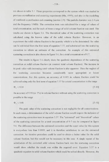
-218-
are shown in table 5.1 These properties corrc!'pond to the system which wa'; studied in
previous crystallisation and creaming experiments (Ma, 1995), and also in the modelling
of combined crysta lli sat ion and creaming (section 2 9) The particle diameter was I 0 11111
and the ftcquency I Mllz 'I he correction term was calcu lated for a range of va lues of
total concentration, and for each of these a range of solid vo lume fraction was used The
results are shown in figure S 6 The theoretical value of the scattering correction was
calcu lat ed using the known value of the solid volu me fraction llowcver, in an
experiment the so lid volume fraction is the quantity which is to be determined It s va lue
can be estimated from the first term of equation 5 37, and substitut ed into the scattering
correction to obtain an estimate of the correction An example of this estimated
sca tt ering correction is also shown in figure 56. for a total concentra tion ofO 7
·1 he results in figure 56 clearly show the quad1atic dependence of the sca ttering
correction o n sol id vo lume fraction (at constan t total vo lume fraction) The increase in
its peak value with increasing total volume fraction is also apparent Thus the neglect of
the scattering correction becomes considerably mole appropriate at lower
concentrations For this system, an accuracy of 0 005 in vo lume fraction could be
achieved using only the first term of equation 5.37 for a total concentration in the range
<1> .., :5 0 34 [5 40J
An accuracy ofO 0 1 (or 1% ) in vo lume fraction withou t using the scattering con ect ion is
possible in the range
[5 4 11
The peak value of the scattering correction is not negligible for all concentrations
In such cases, a determination of the solid vo lume fraction wou ld require the inclusion of
the scattering correction term in equation 5 37 The "estimated" and "t heoretica l" values
of the scatt ering correction for a total concent rat ion o f 0_7 can be compared in figure
5 6 The difference between the estimated correction and the exact value for this system
is everywhere less than 0 0009, and it is therefore sa ti sfactory to use the estimat ed
correction An iterative procedure could be used to obtain a better va lue for the so lid
volume fraction, but thi s would not be necessary in this case A single 1epeat of the
subst itution of the corrected solid vo lume fraction back into the sca ttering correction
wou ld show whether the result was within the required error Equation 5 37 is a
quadratic equation in solid volume fraction which cou ld be solved directly llmvever, the
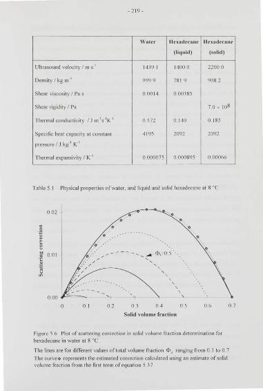
-2 19-
\Vater ll undrcane llexadt>canr
(liqu id) (so lid )
Ult rasound veloci ty I m s·• 1439 I 1400.0 2200 0
Density I kg m·l 999 9 78 1 9 908 2
Shear viscosity I Pas 000 14 0 00385
Shear rigidity I Pa 7 0 ' J08
Thermal conduct ivity I J nf 1s 1K"1 0 572 0 140 0. 185
Specific heat capacity at constant 4 195 2092 2092
pressur e I J kg 1 K 1
Thermal expansivi ty I K"1 0 000075 0 .000895 0.00066
Table 5 I Physical properties of water, and liquid and solid hexadecane at 8 or
0 02 0
c 0 0 .!:
~ 0
e 0 'o .. 0 0 1 ' ' ~
<P,-0.5 c o.· "§ ' ' ~ ' ' "' ' ' \
\ \
000 ~
0 0 1 02 03 04 05 06
Solid volume fraction
FigureS 6 Plot o f scatt ering correction in solid volume fractio n determinat ion for hexadecane in water at 8 ° (
07
The lines are for different values of total volume fractio n <I> s ranging from 0 I to 0 7
The curve <> represents the estimated correction calculated using an estimate of solid volume fraction from the first term of equation 5.37
-220-
simplified method of using the scattering correction to adjust the first estimate where
required is recommended The error in the "exact" ca lcu lation of the correction term due
to the neglect of the allenuation in the derivation of the equation, was every\\ here less
than3 x 10-~
As shown from the above calcu lations, it is possible to use multiple scattering
theory to determine the scatte1 ing factor ll owever, the same problen1s are encountered
as exist for the use o f multiple scat tering theory in o ther applications The physical data
for the constituent phases can be difficult to find or detennine, and the theoretical
sca tt eri ng coefficient may not be e'>:act ly equa l to its real apparent value The particle
s izes or si?e distribution may also be unknown The scattering factor (equation 5 38)
requires only a single determination as it is itself independent of the solid volume
fraction This allows the use of an experimenta l technique to determine the scallering
factor , using a \\ell-characterised semi-crysta lline emu lsion ;\n emulsion can be made,
sp lit into two quantities, half of which is fro1en (so that all the oi l crysta lli ses), and half is
not The semi-crysta lline emulsion is produced by mixing the two emulsions in
appropriate pro portions, so that the total vo lume fraction (if all the oi l were solid) <bs
and the actual so lid volume fraction </J s are known If the ultrasound velocity in thi s
emulsion is then measured. and the parameters substi tuted into equation 5 37, the
scalleri ng factor can be determined directly, withou t the need for a numerical scattering
theory calcu lation
The result for the so lid fat cont ent, equa tion 5 37, was deri ved for a monodispersc
system The same equation is valid in a polydisperse sample, if the particle si1e
distribution of the solid and liquid droplet s arc identical (apart from the changes due to
the density di!Tercnce) In ot her words, the same proportion of particles are sol id for all
particle s izes Equation 5.33 must hold for each particle si1e separately, i e
[5 42[
where the index i now represents a single particle si7e and <l>s is the total volume
fraction of al1 pariicle sizes when all arc solid ll owever, in reality the crysta lli sa ti on rate
is a function of particle size In particular, in the case of homogeneous nu.dto ation , the
crystallisation rate is proportional to the vo lume of the oil droplet. Thus it is like ly that a
- 22 1 -
higher proportion of the larger particles wi ll be solid at any time lt is important to
remember that the theory requires that each particle must be completely solid or
completely liquid The scatteri ng propert ies used are for solid or liquid particles, no t fo r
a parti all y crystalline droplet The result o f equation 5 37 is not precisely va lid fo r
po lydisperse systems l lowever, the di screpancy will depend o n the degree o f
polydispersity in the sample, and on the sensitivity of the sca ttering correction to particle
si7e. This is comparable with the va lidity criterion for the use of calibration and
rcnormal isa tion techniques in creaming experiment s In that situation. both the va riation
in particle size distribut ion in the cream and the sensitivity of the ultrasound velocity to
changes in particle size were relevant , and a combined criterion could be written in the
form of equat ion 5 1 0
The variation of the scattering correction with particle size is shown in fi gure 57 in
the long wavelength region, at a frequency of 1 Ml lz Although the curve appears ra ther
steep, the overa ll va riation is less than 0 003 in volume fraction over the range of particle
size 0 0 1- 10 0 ~1111 This is an encouragi ng result for the application of the equation 5.37
to polydisperse systems When the crystallisation rate is a function of particle size, there
will be an added cont ribution to the correction term due to the imbalance of the si7e
distribution for solid and liquid particles This eiTect may out weigh the dependence of the
monodispersc scattering correction on particle size
The eiTect of the imbalance of the solid and liquid size distribution was calcul il ted
for the hexadecane in wa ter system, using the most skewed case possible All particles
larger than a given si7e are solid, and all the smaller particles are liquid The particle si7e
at which the cut -o iT occurs is determined by the solid volume fraction The part icle size
distribution was log-normal , as defined in section 2 I The peak of the distribution was at
a particle diameter of I ~un , and the width of the size distribution was determined by the
va lue of a .. The quantity of interest is the error in applying equation 5_37 to determine
solid volume fraction, as a function oft he degree ofpolydispersity
The di!Terence between the actua l solid volume fraction and the va lue calculated
from the first term of equation 5_37 was first calculated as a function of solid volume
fraction for the most polydisperse system lt was found that the maximum difference still
occurred when half of the dispersed phase was solid (equation 5 39}, although the
difference is now skewed Furt her calculations were therefore carried out under this
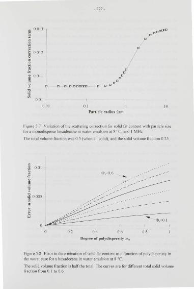
~ 0.013
·t 0 0 12 e c
·B .g e 0 0 11 ~
0
r > :a 0
"' 0 01
00 1
- 222-
o o o oooa:c D D
0 1 Par·ticlc ntdius l).un
D
I DDo:>J
DD
10
Figure 57 Variation of the scattering correct ion for so lid fat content with par!icle size for a monodisperse hexadecane in water emulsion at 8 °C', and I Mllz
The tota l vo lume fraction was 0 5 (when all solid) , and the solid volume fraction 0 25
c ·~ 001
.:: e ~
0 >
;g 0 005 ~
·=
<t>,-o 1
06 08
Org..-ee or polydispcrsity Um
Figure 5 8 Error in determination of so lid fat content as a function of polydispersity in the worst case for a hexadecane in water emulsion at 8 ° (
The solid volume fract ion is half the total The curves are for dinCrent total so lid vo lume fraction from 0_ 1 to 0 6
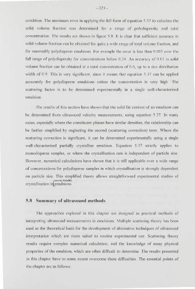
- 223-
condition The maximum erro r in Rpplying the full form of equation 537 to calculat e the
solid volume fraction \\35 determined for a range o f po lydispersit y and tot al
concentration The results are shown in figure 5 8 lt is clear that suOicient accuracy in
solid volume fract ion can be obtained for quite a wide range oft ot<ll volume fraction, and
fo r reasonably polyd isperse emulsions For example the error is less than 0 005 over the
full range o f polydispersity for concentrations below 0 24 An accuracy of 0 0 I in solid
volume fraction can be obtained at a total concentration of 0 6, up to a si7e distribution
width of 0 9 This is very significant_ si nce it means that equation 537 can be applied
accurat ely for polyd isperse emulsions unless the concentratio n is very hig h The
scat tering factor is to be determined experimentally in a si ngle well -charac terised
emulsio n
The result s of this section have shown that the solid fat cont ent of an emulsion can
be determined from ultrasound veloci ty measurements, using equation 5 37 In many
cases, especia lly v;hcre the constituent phases have similar densi ties. the relationship can
be further simplified by neglecting the second (scattering correction) term Where the
sca tt ering correctio n is 5ign ificant , it can be determined experimenta ll y usi ng a single
well -characterised partially crystalline emulsion Equation 5 37 stri ctl y applies to
mo nodispe1se samples, 01 where the crystalli sa tion rate is independent of particle size
llowever, numerica l calculations have shown that it is sti ll appli cable over a wide range
of concentrations for polydisperse samples in which crysta ll isation is strongly dependent
on pa1ticle size s~!~sm~{'lifi ed theory allows straightforward experi mental studies of
crystalli sat ion i{~mulsions
5.8 Summary or ultrasound methods
The approaches explored in this chapter are designed as practical methods of
interpreting ultrasound measurements in emulsions Multiple sca ttering theory has been
used as tl1e theoreti cal basis for the development of alt ernati ve techniques o f ultrasound
interpretation which are more suited to routine experimental use Scattering theory
resu lt s require complex numerical calculation, and the knowledge of many physical
p1operties of the emulsion, which are o ft en difficult to determine. The resu lt s presented
in this chapter have to some ex tent overcome these diffi culties The essential points of
the chapter are as fo llows
- 224-
• The theo1etical formulation ofscatlering theory may be applied to emu lsions. but wi th
experin1enta l determinatioll oft he scattering properties oft he syste1n being measured
• Simplified techniques of ultrasound measurement interpretation are applicab le only in
the absence of particle size or frequency elTects on the scaltering properties
• Standard calibrat ion techniques to determine the relationship between ultrasound
velocity and oil concentration are essentia ll y measurements of the scattering
cllalacteristics of the sample
• The renonnalisation method can be applied to creami ng st udies of emulsions to obtain
the velocity concentration relationship directly from the measured ultrasound velocity
profiles
• The ultrasound velocity and attenuation in a multiple phase system can be related to
the propellies of the corresponding single phase systems Measurements of both
ultrasound parameters can be used to determine the concentration of two phases
• 1\ simple relationship can be used to calculate the solid fat content in an emulsion
"hich contains both solid and liquid particles 1\ scattering correction term has been
shown to be small in many circumstances
The techniques described in this chapter are particularly app li cable to creaming and
crystallisat ion measurements in emulsions Although closely related to scattering theory,
the methods do not rely on numerical calculations, nor on a knowledge of many physical
properties oft he component phases They are more widely applicab le than the theoretical
results of scattering theory, since they are based on the actual properties of the
experimental systems being used, rather than on theoretical assumptions The
developments discussed in this chapter allow the continued and increased use of
ultrasound as a probe of emulsion stabi lity llowever, the influence of flocculation o n
ultrasound measurements is not understood, and the techniques presented here may or
may not be applicab le in such cases E)(.pe.rime."'to.\.. resuln. if'l.d>c.o.lce.~t \he. m~s
an .. va\\cl in '"'e. ~b-o..te.d. crtc.m ~e..-:
- 225 -
C ha jJier 6 : Concl us ions
In the introduct io n to thi s thesis, the main purpose oft he work was stated to be the
acquisition of increased understanding o f the int erdependent processes of creaming,
nocculation and crystalli sa tion , and the development of improved ways to interpret the
ultrasound measurement s which are currently used to study these processes The first of
these general aims has been addressed through the use of computer modelling of the
dynamic evolution of emulsio ns The result s of the models, in conjunct ion wi th an
investigation o f the theory of ultrasound propagation in di spersio ns, have been used to
address the second aim The purpose of thi s final chapter is brieny to draw together the
specific conclusions of the different parts o f the study, and to present recommendations
based on the results of the whole work Suggestions for areas of future work are also
made
The phenomenological model of creaming in idea li sed emulsions was shown to be
a good representation of rea l emulsions in the absence of particle int eractions The
concentration profiles predicted by the model were compared with the resul ts from an
experimental system which was thought not to include fl occulation or other interactio ns
(chapter 2) Good agreement was found except in the cream, in which the hydrodynamic
description used in the model was too si mplified to represent the true complex it y o f
particle now The correspondence between model and experiment is evidence that the
results of the model can be used as representative data of rea l emulsions which are
studied experimenta lly using the ultrasound technique Thus the application to creaming
experiments of various theo ri es for the interpretation of ultrasound measurements can be
investigated using these results
The model of creaming demonstrated that a sign ificant degree o f particle size
fractionation occurs. especially in the cream regio n at the top of the sample Although
the predicted va riation may not be exact , it is a clear indication that particle size
di stribution changes may occur in a creaming emulsion The resu lts of ultrasound
scattering theory and experimental observations have shown that the ultrasound velocity
in an emulsion varies with particle size, in some circumstances The Urick equation,
-226-
which is commonly used to interpret ultrasound measurements, does not include any
innucnce of pa11icle size on the sound speed The phenomenological c1eaming model
showed that the va ri atio n of ult rasound veloc it y with height in the cream (according to
sca tt ering theory) could be the reverse of that expected if the errect of particle size
va ri ation v .. e re neglected (for example, using the Uri ck equation) Thus. an interpretation
of ultrasound measurements based solely on the concentration dependence of sound
speed is incorrect
The result s indicate that the use o f ultrasound velocity measurements to determine
concent ra tion profil es should only be considered under condi tio ns in which the sound
speed is insensitive to particle size A guide to the range of particle si7e and frequency
for which this is the case can be obtained from scattering theory calculations (chapter 4)
A determination of the apparent total oil concentration in the emulsion can be used to
check whether pa11icle size va riation does have an influence on the int erpretation of
measurements in a particular creaming experi ment (see chapter 5) The diiTerence in
ultrasound velocity predicted by the Urick equation and scallering theory is very large in
the system modelled These results indicat e that the Urick equation should not be applied
"blind" to any emulsion, since it may be inapplicable in the system of interest
Multiple scattering theory has a sound theoretical basis for ultrasound propaga tion
in emulsions systems Measurements are usually made in the long wavelength limit , in
which the analysis is simplified, and only the lowest order scallering modes need be
considered Although multiple scatt ering theory has been used as the benchmark in this
study, the predictions of scattering theory have been shown to be inexact for a number of
experiment al systems (llolmes et al . 1993. 1994) In addition, a substant ial amount of
physical data is required for the calculations, and these data are ofl en difficult to obtain
llence, the direct applica tion of scattering theory to interpret ultrasound measurements is
impractical Some simpler limiting solut ions are ava ilab le (the Urick equation being one
of these) which are applicable under certain strictly specified condi tions (chapter 4) In
this study, new methods of interpreting ultrasound measurements have been developed
1 hese adopt the theoretical basis of scatt ering theory, but the sca ttering characteri stics of
a particular system are determined experimentally (see chapt er 5) Thus, instead of a
reliance on a number of different theoretical formulations for the scattering properties of
a system, these properties are determined directly The difficulty of applying the
scattering theory formulation to the interpretation of ultrasound measurements have,
-227-
therefore, largely been overcome The limits o f the applicability of these techniques ;u e
closely related to the effects o f particle size variation seen in the crea ming model
The experimental determination of the sca ttering properties of an emulsion can be
carried out through calibration. which is relevant to many applications of ultrasound
measurements The relationship between ultrasound veloci ty and o il concentration is
found from measurement s o n a number of emulsions for which the oi l concent rat ion is
already known For creaming experiments, the renormalisation method is proposed for
the determination of the sound speed concentration relationship The renonnalisa tion
technique uses the knowledge of the tota l vo lume o f oil in the whole emulsion to
ca lculate the unknown sca ttering parameters
The use of the theoretical basis of scattering theory. but wi th experimental
determination or the scatteri ng properties, is also applicable to two-phase systems such
as oil in water emulsions with polymer in the aqueous phase Crystalli sation experiment s
in emu lsions wi th a mixture of so lid and li quid droplets also fall into this ca tegory The
re lat io nship between the ultrasound velocity in the mixed system and the concentr ations
of the individual components is derived from scattering theory This relationship ca n,
however, be wri tt en in terms of the measured ultrasound properties in the single
component systems (for example an oi l in water emulsio n in the absence of polymer, or a
polymer solu tion) I fence, the properties of the combined system can be detennined
experimenta lly In crysta lli sation experiments, the additiona l knowledge of the total oi l
concentratio n when it is all liquid is applied to obtai n a simplified relationship which can
be used to determine so lid fat content
The application of ultrasound theory to these two-phase systems has indicated that
a measurement of two ultrasound parameters, for example veloci ty and attenuation,
could be used to obtain two properties of the emul sion This is relevan t for the
determination of the concentration of both of the phases in the mixed system as
described lt may be particularly applicable to the crea ming o f emulsions containing
polymer in solution, in which the oil tends to float to the top, but the polymer becomes
more concentrated at the bottom of the emulsion Similarly, in creaming experiments o f
crystalli sing emulsions, both the so lid fat and liquid o il cont ent are varyi ng with height
The proposed relationships for this technique have not been tested , however, and the
inOuences o fflocculation may undermine the theoreti ca l basis in these systems
- 228-
The study of !he interpretation of ultrasound measurement s has shown that an
awareness must exist of the restrictions o f the technique. For example. in creaming
experiments. the dependence of ultrasound velocity on particle size must be avoided for
successful determination of concentration pro files Within the restrictions which have
been detailed , a number of techniques have been presented , each with a sound theoret ica l
basis These techniques are practica l met hods for using and interpreting ultrasound
measurement s in a va ri ety of systems An impo1tant conclusion is that the application of
the Uri ck equation, or o f sca tt ering theory, without proper considera tion of the particular
system be ing studied, is unwise
llaving modelled creaming behaviour in emulsions in the absence o f particle
interactions, the e rTects o f flocculation and crystalli satio n o n the creaming process were
investigated The inclusion o f crystalli sa tion in the creaming model illustrated the en'ect
of a het erogeneous crystalli sa tion process on the ' idea l' creaming behaviour The
predominant e rTect on the creaming rat e was found to be the density change which
occurred when particles crystalli sed Since the crystalli sa tion rate in the idealised
emulsion was much mo re rapid than creaming , the creaming process was dominated by
solid droplets Experimentally, no dramatic e rTect of crystalli sa tion o n creaming rat e has
been observed (Ma, 1995) The rates of crystalli sa tion and creaming may become
comparable \vhen fl occulation is signi ficant , since flocculation has been shown to cause
rapid creaming in some cases The combined e rTects of fl occulat ion, crysta llisation and
creaming have not yet been mode lled, but the ex perimental result s have not indicated a
sign ificant erTect either on crystalli sation rate or on creaming and flocculation behaviour
Flocculation by non-adsorbing polymer has been seen experi mentally to cause
dramatic changes in the c reaming behaviour o f some emulsions One particularly
noticeable feature has been the large increase in creaming rate in the ea!ly stages, and the
development of a sharp sennn layer interface. Attempts to include the erTec t of
fl occulation in the phenomenological model of creaming were unsuccessful (chapter 2)
The limited description of floc fo rmation and their dynamic properties was unable to
reproduce the characteri stic features observed in practi ce The small -sca le lattice model
of fl occulation and creaming is also a very simplified model of particle behaviour, but it
was able qualitatively to demonstrate some o f the experi ment all y observed features
(chapter 3) A sharp serum interface was produced in the model, and creaming was
-229-
prc\'ented an er formation of a network structure The position of the serum interface
was shown to be an indica tor of the height o f the energy barrier aga inst fl occulatio n, a
relationship which may be applicable in practice Nevertheless, the increase in creaming
rate observed in the lattice model due to floes does not appear to be sunicicnt to explain
the dramati c senun separatio n observed in some ex perimental systems The modelling o f
creaming has therefore shown good agreement with e:-.: perimental results in the absence
of fl occulation The effects of fl occulation on creaming behaviour can to some extent be
descri bed by a very simplified model o f fl oc fo rmatio n llowever. thi s simplified model is
insuffi cient to explain the dramati c increase in creaming rat e observed in some systems,
and the richness and complex ity o f creaming behaviour in flocculating emulsio ns
The comput er modelling of creaming in emulsions has been successful in the
absence o f parti cle interactio ns A phenon1eno logical model o f fl occulat ion. and it s e O'Cct
o n creaming behaviour, was unable to reproduce the fea tu res observed in experimenta l
systems A simplifled model o f fl occulation at the level o f individual panicles achieved
some success in demo nstrating the effects of fl occulatio n on concent ration pro fil es
llowevcr. thi s model is unable to predict creaming behaviour on the scale of
experimental systems Mode ll ing of emulsion behaviour in direct correspondence to
experimental observa tion in the presence o f pa rt icle interactio ns is therefore no t fully
developed Some conclusions may be drawn from parti cle simulatio ns such as the latt ice
model, but , as yet. such simulations cannot make predictions of macrosco pic feat ures or
parameters characte rising emulsion c1eaming behaviour
The interpreta tion of ultrasound measurement s can be carri ed out using multiple
sca tt eri ng theory techniques The app li cation of the theoretical result s requ ires numeri ca l
calculations and the knowledge of a large number o f physica l pro pert ies of the system
llowe,er, these di fficulti es may largely be overcome by the use of si mplifled limiting
forms o f the theory, or through the techn iques developed fo r the ex perimental
determination of the scattering propert ies o f the system The scatt ering theory analysis
assumes rando ml y di stribu ted part icles, and that there are no particle interact ions ll ence,
the reliability o f appl yi ng these methods to systems o f int eracting parti cles, or to no n
random distribu tions of particles (e g in fl oes), is uncertain The general theoretica l
problem of sound wave propaga tion through a fl occulated emulsion, or conversely, the
-230-
issue o f how to interpret ult rasound measurements made on such a system, is, as yet,
unsolved
The two aspects of the p1esent work , namely computer modell ing of emulsion
behaviour, and the interp•etation o f ult rasound measurement s on emulsions, are therefore
limited by the current understanding of the en'ect of particle interact ions, in particular
fl occulation, in emulsions The computer models have in part accoun ted for the effect o f
fl occulation on creaming behaviour l lowever, future development may require the use
o f small -scale models to predict macroscopic pro perti es o f the emulsion, which can be
used in understanding experimentally observed behaviour Predictions from small -scale
models may be used in a phenomenological model to improve the simulation of
fl occulation and creaming behaviour Such simulation is required to improve the
understanding of the. as yet. unexplained creaming behaviour in fl occulating systems
Similarly, the efl'ect of fl occulation on ultrasound propagation is unquant ified Further
work is required to develop techniques for interpret ing ultrasound measurements in such
systems
- 23 I -
llibliog ra phy
/\bel. J S. Stangle. G C. Schil ling. C 11 and Aksay. l A ( 1994) Sedimentalion in
nocculating colloidal suspensions .!oumnl (?( A1alerials Uesenrch. 9, 451-46 1
Ahuja, A S ( 1972) Fonnulation of wave equation for calcu lating velocity of sound in
suspensions .Joumal '!f the Acoust1cal Society of America, 5 1, 9 16-919
Ahuja , A S (1973) Wave equation and propagation parameters for sound propagation
in suspensions .Joumal f?( Applted l'hys1<:s, 44, 4863-4868
Allegra. J R and I lawley, S A ( 1972). Attenuation of sound in suspensions and
emulsions theory and experiments .loumnl l!( the Acou.\tlc.:nl SoCie~r '?f Ame11Ca, 5 1.
1545-1564
Alien. 1 P and Tildesley. D J ( 1989) ( 'omputer Sm~~tlatmn c!f /.ICJflid<>. Clarendon
Press. Oxford
Ansell, G C and Dickinson. E ( 1986) Sediment formation by Brownian dynamics
simu lation· enect of colloidal and hydrodynamic interactions on the sediment structure
.Journal (!f ( 'hemical PI~J 'Sit.:s. 85, 4079-4086
Anson, L. W and Chivers. R C ( 1989) Ultrasonic propagation in suspensions - a
comparison of a mult iple scattering and an effect ive medium approach Journal n.f the
Acou~ncal SO<.:iefy r~f Amenc:a. 85. 535-540
Anson, L. Wand Chivers, R C (1993) Ultrasonic scattering from spherical shel ls
including viscous and thermal effects .loumal of !he Acousfrc:al 5ioue~) 1 l~[ America, 93.
1687-1699
Asak01a, S and Oosawa, F (1954) On the interaction between two bodies immersed in
a solution of macromolecules .Journal(?(( 'he mica/ Ph_1·sics, 22. 1255-1256
Asakura, S and Oosawa, F ( 1958) On interaction between particles suspended in
solutions of macromolecules Journal(?( Po~rmer 5iciem:e. 33. 183-192
Auzerais. F M , Jackson. R and Russel , W 13 ( 1988) The reso lution of shocks and the
effects of compressible scdiments in transient sett ling Journal of 1·/uid Afec:ha11ics. I 95,
437-462
- 232-
Batnea. E. and Miztahi. J ( 1973) A generali7ed approach to the fluid dynamics of
particulate systems Part I General correlation for fluidization and sedimenta tion in solid
multi particle systems ('hemu:a/l~·ngmeermR ./mrrnal, 5, 17 1-189
Batchelor, G K ( 1972) Sedimentation in a dilute dispersion of spheres Journal l?(
J.ltud A1eclllmics, 52, 245-268
Batchelor. G K ( 1976) Brownian diffusion of particles with hydrody namic interaction
Journal qf Flu hi A lec.:lumics. 74. 1-29
Datchelor, G K ( 1982) Sedimentation in a dilute polydisperse system of interacting
spheres Part I General theory Journal (?f /·hod Aleclumics. 11 9. 379-408
13atchelo r. G K and Wen. (' -S ( 1982) Sedimentation in a dilute polydisperse system
of interacting spheres Part 2 Numeri ca l resu lt s ./oumal f!( l ·hud A1ec:hamt·s. 124 .
495-528
Oatchelor. G K ( 1983) DiOUsion in a dilute polydisperse system of inte racting spheres
.!mmml of 1·/uid A1echamcs, 13 1. I 55-175
Batchelor, G K . and Wen. C-S ( 1983) C'orrigendum Journal f!( !·luid Aleclurnic:s.
137. 467-469
Bedenko. V G. Chernin. V N . Chi styakov. B E and Pertsov, A V ( 1983)
Sedimentation and stmcture offlocculated invert ed emulsions I Sedimentation curves
and sections of the sedimentation surface 2 Sedimentation model Collohl.lourua/ <?(
1he 1/.S.S./1., 45, 263-268, 470-474
IJennema, P , Vogels, L. J P and de long, S ( 1992) Morphology of beta-phase
monoacid triacylglycerol crysta ls theory and observat ions .Journal<?(( ·,y.,tal Grmt·lh,
123, 141 - 162
Bennema, P ( 1993) Morphology of crystals determined by alpha-factors, roughening
temperature, F faces and connected nets Journal f!( l)hy.\iC.\ IJ: Applied /'hy.m:s, 26.
IJI-136
Bijsterbosch, B. 11 • Bos, M T A. Dickinson, E., van Opheusden, J 11 J and
Walstra , P (1995) Brownian dynamics simulation of particle gel formation fro m atgon
to yoghut1 Faraday /Ji.W:IIs.'l ious, 10 1, in press
- 233-
llonnet, J C and Tavlarides, L L (I Q87) Ultrasonic technique for dispersed phase
hold-up measurements lndu.\1/·;a/ am/J·;nRmeem1R ( 'hemi{jfiT Ue.warch. 26. 8 11-8 15
Boode, K , Bisperink. C and Walstra. P ( 1991) Destabilization of O!W emulsions
containing fat crystals by temperature cycling ('o/lonl.\· ami Sm:fnc:es. 6 1, 55-74
Brady, J (1992) Stokesian dynamics simulation ofparticulate flows pp 912-950 In
11artu:ulate 7i•o-Phase 1·/ml' . ed M Roco, Butterworth- ll einemann, Boston
Burgers. J M ( 194 1) On the influence oft he concentra tion of a suspension on the
sedimentation velocity l'roceedm?.s. Komnklijke Nederla11dve Akadenue l'OII
Wetenschappente Amsterdam, 44. 1045-1051 , 1177-1184
Burgers, J M (1942) On the influence oft he concentration of a suspension on the
sedimentation velocity l)roceedmg'i, Komnkl{1ke Nederland'ie Akademte mu
IJ'eteuschappeute Amsterdam, 45, 9-16, 126-128
Buscall. R and White, L. R ( 1987) The consolidation of concentrated suspensions
Journal o.f the Chemica15ioclety Faraday 7i"an'iacflol1s I , 83, 873-89 I
Buscall, R (1990) The sedimentation of concentrated colloidal suspensions Collmd'i
aud Smfac:es, 43. 33-SJ
Cao, Y , Dickinson, E. and Wedlock. D J ( 1990) Creaming and floccu lation in
emulsions containing polysaccharide. Food 1/ydrocolloid'i, 4, 185- 195
Cao, Y . Dickinson, E and Wedlock. D J ( 199 1) Influence of polysaccharides on the
creaming of casein-stabilized emulsions Food 1/ydmco//oid'i, 5, 443-454
Chhabra. R P and Prasad, D ( 1991) A fluid-mechanic based model for the
sedimentation offloccu lated suspensions Separation ._r;,Jcience and TedmoiOKJ'. 26.
223-241
Chow, J C F ( 1964) Attenuation of acoustical waves in dilute emulsions and
suspensions .Journal of the Acoustical Society of America. 36. 2395-240 I
Colbeck. I ( 1994) Aerosol formation pp I 37-158 In Controlled l'amcle. /!rop/et and
Bubble Formation, ed D J Wedlock, Butterwort h- I leinemann, Oxford
Coupland, J , Dickinson, E , McCiements, D J , Povey, M J W and de Rancour! de
Mimmerand. (' {1993) ;\comparison of crystallisation in simple paranins and in
monoacid saturated triacylglycerols dispersed in water pp 243-249 In l •f.JOd ( 'ol/oul5
- 234 -
mull'o~rmen : Stalnll~) ' m1d Alecham(·all'roperfl es. ed E Dickinson and P Walstra .
Royal Society of Chemistry. Cambridge
Darling. D F and Oirkett , R J ( 1987) Food colloids in practi ce. pp 1-29 In 1:ood
f.:nmlsJons n11d Foams, ed E. Dickinson. Royal Society of Chemi stry, London
Davis, R 11 { 1993 ) Microhydrodynamics of pa•ticulate suspensions Athm1ces i 11
Colloid and lnletf ac:e SCience. 43, 17-50
Davis, R 11 and Grecol, 11 ( 1994) Hinde red sell ling functio n with no empi1ical
parameters for polydisperse suspensions A/Chl~ .lollmol. 40. 570-575
Dickinson. E ( 1983 ) Dispe1sions of int eracting collo idal particles Anmwl Reporl ' 0 11
the l 'roxres.-u?(Chemislt)' C, 80. 3-37
Dick inson, E. ( 1985 ) 13 rownian dyna1nics with hydrodynamic interactio ns the
applicatio n to prot ein dinUsio na l problems ( 'lu!mfc:ol Society Uel'ft! ll 's. 14. 42 1·4 55
Dickinson, E., McCleme nt s. D J and Povey, M J W ( 199 1) Ultrasonic investiga tion
of the particle size dependence o f crystalli satio n in n· hexadecane· in ~wat er emulsio ns
.Jmmwl oj ( 'ol/oidmld/nu!lfac:eS'cience. 142, 103- 11 0
Dickinson. E ( 1992a) An lnlroduc.:tum lo 1-'ood Co//oul.'\, Oxfo rd Universit y Press.
Oxrord
Dickinson. E. ( 1992b) Structure and compositio n of adsorbed protein layers and the
relationship to emulsion stabilit y .Journal (~f the ( 'hemica/ 5iooety Faraday
/i'tffi\OC/ 1011.'\, 88, 2973-2983
Dickinson, E. and Euston, S R ( 1992) Sho rt -range stnrcture of simulated noes o f
particles with bridging po lymer ( 'o//ouls ami Smf oces, 62. 23 1-242
Dickinson, E , Goller, M I and Wedlock, D J ( 1993a) Creaming and rheology or
emulsio ns containing polysaccharide and no n-ionic or anionic surfactant s Colloid\· am/
Slflj aces A: Physh.:ochemico/ amll·.i1gineering A '\peels, 75, 195-20 1
Dickinson, E . Krui zenga. F-J , Povey, M J W and van der Molen, 1\!1 ( 1993b)
Crystal lisa tion in o il-in-water emul sio ns containing liquid and solid droplets ( 'o/hm l.'\
and Smf aces A: Physinx:hemical omll·:ngmeering Aspects , 8 1, 273-279
- 235-
Dickinson. E. Ma, J and Povey, M W (1994) Creaming of concent rated oil-in-
water emulsions coru aining xanthan Food 1/ydroc:olloicb•. 8. 481-497
Dickinson. E . Goller, M I and Wedlock, D J ( 1995) Osmotic pressure, creaming and
rheology of emulsions containing nonionic polysaccharide. Journal of( 'ol/oid and
lnfe!face Science, 172, 192-202
Dickinson, E , Ma, J and Povey. M J W ( 1996) Crystallization kinetics in oi l-i n-water
emulsions containing a mixture of sol id and liquid droplets Submitted (as a Short
Communication) to Faradl~l' limtr;nctums
Epstein. P S and Carhart, R R ( 1953) The absorption of sound in suspensions and
emulsions I Water fog in air ./oumal f!( the Ac:oustica/ Socrety f!( Amenca, 25,
553-565
Fikioris, J G and Waterman. P C ( 1964) Multiple scattering of waves 11 " llole
corrections" in the scalar case .Joumal l?( Alathematic:all'h_I'.\ICS, 5. 141 3-1420
Fillery-Travis, A J , Clark, D and Robins, M (1990) Emulsion stabi lity how oi l and
wa ter mix Food Science a11d 7'echnology 7'oday, 4 , 89-93
Fillery-Travis, A J. Gunning, I' A . ll ibberd, DJ and Robins, M M ( 1993)
Coexistent phases in concentrated polydisperse emulsions fl occulated by non-adsorbing
polymer Journal l!(('ol/md amlllller:fac:e Science, 159, 189- 197
Fligner, K L , Fligner. M A and Mangino. M E. (199 1) Accelerated tests for
predicting long-term creaming stabi lity of infant formula emulsion systems Food
1/ydroc:o/h"'l'. 5. 269-280
Foldy. L. L. ( 1945) l'hysn·s /le well', 67. I 07 Cited in Watennan and Truell ( 1961)
Garside, J and AI -Dibouni, M R ( 1977) Velocit y-vo idage relationships for fluidi sation
and sedimentation in so lid-liquid systems Industrial and l~i,gmeermg ( 'heu11.W:r:
l'rocess /Jesig11 a11d /Je1·elopmem. 16. 206-214
Gaunaurd, G C and Uberall, 1-1 ( 1982) Resonance theory of the effective properties of
perforated solids ./nu mal of the Ac:ou.\lit.:a/ Society (!f Amenca, 71. 282-295 Errata 73,
372
-236-
Gaunaurd. G C' and Uberall, 11 ( 198J) Resonance effects and the ultrasonic effective
properties of particulate composites .Journal(~( the Ac:olfSflca/ Soc.'Jely <?( Amenc:a, 74,
305-J 13
Gaunaurd, G C and Wertman. W (1989) Compari son of effective medium theories for
inhomogeneous media .loumal (!f the Acoustical Socie~r r?f America. 85. 541-554
Gaunaurd, G (' and Wen man, W ( 1990) Comparison of effective medium and
multiple-scattering theories of predicting the ultrasonic properties of dispersions a
reexamination of results Journal r!f the Acow;l!cal Society <?f Amenl'O, 87, 2246-2248
G idaspow, 0 ( \994) A1ulllphme Flow and Flmdisatiou, Academic Press, London
Glendinning. t\ 13 and Russel , W B ( 1982) A pairwise addi ti ve description of
sedimenta tion and diffusion in concentrated suspensions of hard spheres .!mmm/ (!f
( 'o/lmd and lmer.face S'crenc~. 89, 124·143
Gouldby. S J , Gunning. P 1\ , llibberd, D J and Robins. M M (199 1) Creaming in
llocculated oil-in·water emulsions pp 244-261 In Food fJolymer-;, (ie/.\ and Collmd\,
ed E. Dickinson, Royal Society of Chemistry. Cambridge
Gunstone. F D , Jla rwood, J L. and Padley, F B (eds) (1994) /he f.tpid /lam/hook.
2nd ed , Chapman and Hall. London
Jlappel, J and Brenner. If ( 1965) /.mt· Reynold'i N111nher 1/ydrodynamics, I st ed .
Prentice·l la11. London
llarker. 1\ 11 and Temple. J 1\ G ( 1988) Velocity and attenuation of ultrasound in
suspensions of part icles in fluids ./oumal c!f 1'/~rsics/J: Applied Physic.:s, 21 . 1 576·1 588
I law, M D . Sievwright. M , Poon, W C K and Pusey, P N ( 1995) Cluster·cluster
gelation with finite bond energy Admm:es in Collmd and flllel:fm:e Sclf!IIC:e. 62. 1·16
llolmes. 1\ K and Challis, R E ( \993) Ultrasonic scattering in concentrated co11oidal
suspensions ( 'olloids and 5imjaces A: Pl~):'itcochenucal and l~lll[illeermJ( AvJects. 77,
65-74
llolmes. /1 K . Challis. R E. and Wedlock. D J ( 1993) /1 wide bandwidth st udy of
ultrasound velocity and attenuat ion in suspensions comparison of theory with
experimental measurements Joumal '!(Colloid cmd Jmel:face Sciem·e, 156. 261-268
- 237-
llo lmes. A K . C'ha11is. R E and Wedlock, IJ J ( 1994} A w ide bandwidth ultrasonic
study of suspensions the va riation of velocity and attenuation with particle si7c .Journal
f!(( 'ollmd and lntetf ace Sciem:e, 168, 339-348
llsu. J-P and Tsao. Il -K ( 1992) Dynamic simulation of fl oc breakage with a random
breakage distribution ('ollmdf ami S'm:faces, 62, 23-30
lluang, Y -D and Somasundaran, P ( 1988) Discrete modeling of sedimentation
!'hp ica/lle••iew A. 38. 6373-6376
Jullien, R ( 1990) -,he application of fractals to investigations of colloidal aggregation
and random deposition Ne1r·.hmnwf <?( ( 'hemisiiJ ', 14, 239-253
Kautcn. R J , Maneval . J E. and McCarthy. M J ( 199 1) Fast determination of spatially
localized volume fr<l ctions in emulsions .!oumol f~( Food St-·Jem:e, 56, 799-80 I
Kaye. G W C and Laby, T 11 (1 986) Tahlesf?{ l)hysi<-·al ond ('henii('OI( 'on <~tonl'ioml
5iome A1athemati<-'o/ Functiow. I 5th ed , Longman. London
Kynch. G J ( 1952) A the01y of sedimentation limrmctions of the 1-'nrmk~l ' Soc.:iety,
48. 166- 176
Kytomaa. I I K ( 1995) l'heory of sound propagation in suspensions a guide to particle
size and concentration characteri za tion Pml'er Teclmolo!{y, 82. 11 5- 12 I
Ladd, I\ J C ( 1993) ShorHime motion of colloidal particles numerical simulation via
a nuctuating lattice-Bolt 7mann equation Physical Re ,·iell' l .ellers, 70. 1339- 1342
Lamb, 11 ( 1932) Hyt./r(}(~J'IIOmics. 6th ed . Cambridge University Press, Cambridge
Lawler, D F ( 1993 ) Physical aspects of nocculation from rnicroscale to macroscale
Water 5ictence am/ Tedmolox_r. 27. 165- 180
Lax. M ( 195 I) l?e l'lews m A1odern Physics. 23, 287 Cited in Waterman and Truell
( 196 1)
Lax, M (I 952) Physics Rel'leu•, 85, 62 1 Cit ed in Watennan and Truell ( 196 1)
Liang. W . Tadros, Th F and Luckham, P F (1 993 ) Effect of volume fraction and
particle size on depletion flocculation of a sterically stabilised latex dispersion induced by
addition of poly( ethylene oxide) . .Journal f~{ Collotd and lltleJface .\'cience, 155,
I 56- 164
- 238-
Lloyd. P ( 1967a) Wave propagation through an assembly o f spheres 11 fhe densit y of
single-particle eigenstates l'roceedmgs (~f the l 'hysical Soc1ety. 90. 207-2 16
Lloyd, P ( 1967b) Wave propagation through an assembly of spheres Ill The densit y of
states in a liquid l'roceedmg.\ (~f the Physical Society, 90, 2 17-23 1
Lloyd. P and Berry, M V ( 1967) Wave propagation through an assembly of spheres
I V Relations between different multiple scatteri ng theories Pmceedmgs (!f the 1'1~\ 'Sica/
Soclel)', 91 , 678-688
Luyten, 11 . Jonkman, M , Kloek , W and van Vliet. T ( 1993) Creaming behaviour of
dispersed particles in dilute xanthan solu tions pp 224-234 In Food ( 'ol/md'l am/
l 'olymers: Stain/ay nud Afedlanica!l'roperties. ed E Dickinson and P Walstra, Royal
Society of Chemistry, Cambridge
Ma, J ( 1995) ('reammg OIUI ( ·,yswlhsmmnm (}IV l~·mul.\1011.'> co111mmnp, Xamhon ,
Ph U 'I hesis, University of Leeds
Ma, Y , Vatadcm, V V and Varadan, V K ( 1984) Multiple sca ttering theory for wave
ptopagation in discrete random media lnteruarional.loumal of l~·,pmeermg Sc:ience.
22, 1139- 1148
fv1a, Y , Varadan, V K and Varadan, V V ( 1990) Comments on ultrasonic
propagation in suspensions Journal<!( 1he Ar.:ou.w c:al Soetety of Amerh:a , 81.
2779-2782
Mandelbrot , B B ( 1975) !,es Olyets hm:ta/r;: l ·onne, !fasard et l)uue11sum.
Flammarion. Paris. Cited in Mandelbrot ( 1982)
Mandelbrot , B B ( 1982) I he l ·im:lal (ieomelly <?[Nature, W 11 Freeman and
Company, New York
Margulies. T S and Schwar7. W 11 ( 1994) A rnultiphase continuum theory for sound
wave propagation through dilute suspensions of particles Journal <!f I he Acoustical
Socte~) l of Amerh:a, 96. 3 19-33 1
McCiements, D J ( 1988) 771e l /se <!f llllrasnnicsfor ( 'lwracterisiiiJ! Fat<; and Oils,
Ph .D. Thesis, University of Leeds
McCiements. D J. and Povey, M J W (1989) Scattering of ultrasound by emulsions
.Journal <
- 239-
McClements. D J • Dick inson. E and Povey. M J W ( 1990a) Crystallization in
hydrocarbon-in-wa ter emulsions containing a mixture of solid and liquid droplets
( 'hemind / 1hy.\ic:.~ l .etfers, 172. 449-452
rv1cC'Iements, D J . Fairley, P and Povey, M J \\/ ( 1990b) Comparison of effective
medium and multiple-scattering theories of predicting the ul11asonic properties of
dispersions .Joumnl (!f the Acoustu:al Society (!f AmenC'a. 87. 2244-2246
McCJements, D J ( 1992) Comparison of mulliple scattering theories with experimental
measurements in emulsions .Journal (?(the A,·ow:;ttc:o/5iooety '?f Amenca. 9 1. 849-853
McClements. D J, Dickinson. E. Dungan. S R, Kinsella, J E, Ma. J G and Povey,
M J W ( 1993) EITect of emulsifier type on the crysta lli7ation kinetics of oil-in-water
emulsions containing a mixture of solid and liquid droplets .Journal<~(( 'ol/md and
fnle!face Soence. 160. 293-297
McCiements. D J ( 1994} Ultrasonic determination of depletion flocculation in oil-in
water emulsions containing a non-ionic surfactant ( 'ollmd'> and Smfaces A:
l'hysic:oc.:henucal and /·,11Ki11eerill}! Aspec:ls. 90. 25-35
McNamara. G and Alder.IJ (1993} Analysis of the laltice Boltzmann!lcatmcnt of
hydrodynamics Phys1c:a A, 194, 2 18-228
Meakin. P ( 1988} Fractal aggregates Admm.:e.\ m ( 'olloid and lllfe1jcu:e 5ic:Jence, 28,
249-331
Melik, D 11 and Fogler, 1-1 S (1984} Gravity-induced nocculation .Joumai<!(Colloid
amllnleJface Scwnce, 101. 72-83
Me1ies. T S and Rhodes, 11 B ( 1955) Liquid-particle behaviour Chemu.:al
/•,nRineerill}! ProKress, 5 1, 429-432. 517-522
Michaels. A S and Bolger, J (' ( 1962) Sett ling rates and sediment volumes of
Oocculated kaolin suspensions l11cluslrlal am/ J.;ll}!llleermg ( 'ltetm\11)' Fundame111al.~. I.
24-33
Mirza. S and Richardson, J F ( 1979) Sedimentation of suspensions of particles of two
or more sizes Chemic:alt~·ngmeermK Scie11c:t!. 34.447-454
Mulder, If and Walstra, P ( 1974) /he A !ilk Fa! (j/olmle: t~·mulsion 5)cienc:e as Applied
10 A111k Products and ( 'ompamble Fuodr;, Commonwealth Agricultural Bureaux,
-240-
Farnham Royal and Centre for Ag• icultural Publish ing and Docu mentation, Wageningen,
rhe Netherlands
07ilgen. S. Simoneau. ('.German. J B . McCarthy. M J and Reid. D S ( 1993)
C'rystalli7ation kinetics of emulsified triglycerides .Jmmral f!( !he Sne11ce t~( l·ood and
Aw'l<·u/ture, 61, 101-108
Pal , R (1994) Techniques for meast~~ ing the composi ti on (oil and water content ) of
emulsion!' state oft he art 1eview Col/oh!.'> 011d Sm:fm.:es A: l'hy:m:ochemic:a/ and
l ·.nJ!meermgA.\fJec:ls.84 , 141- 193
Pierce, I\ D ( 1981) Ac.·mtsllc:s: An llllrod,c.·titmto its J)I~I 'Sical Prmcip/es and
Apphcotwn<o, McGraw-1 !ill. New York
Pilhofer, G M . McCarthy. M J . Kauten. R J and German. J B (1993) Phase
separa tion in optica lly opaque emulsions .loumal f~( Food l~llf!llleermg. 20. 369-380
Pin fi eld. V J . Povey. M J W and Dickinson, E ( 1995) The applicat ion or modified
ronns or the Urick equation to the interpretation or ultrasound veloci ty in scauering
systems ( 1/lrasonic.'i, 33, 243-25 1
Povey, M J W and McClements. D J ( 1989) Ultrasonics in rood engineering Part I
Introduct ion and experimental methods .Joumal f
- 24 1 -
Selim. J\.1 S. Kothari, A C and rurian , R M (1983) Sedi mentation ofmultisized
particles in concentrated suspensions A!Chi~· .Jmrmal, 28, 1029- 1038
Shih, Y r , Gidaspow. D and Wasan, D T (1986) Sedimentation of line particles in
non-aqueous media Part I Experimental_ Part 11 Modeling ( 'ol/oul.'i rmd Sw:fnces. 21.
393-429
Shih. Y T , Gidaspow. D and Wasan. I) T ( 1987) llyd10dynamics of sedimentation of
multisized particles l'mtder /'eclmolo;zr, 50. 20 1-215
Simoneau. C. McCarthy. M J . Reid. D S and German. J B ( 1993) l nnuence of
triglyceride composi tion on crysta llization kinetics of model emulsions .loumn/ r?f Food
l·.ui!meeniiJ!, 19, 365-387
Smoluchowski. M S ( 19 13) On the applicability of Stokes' law of 1 csistancc, and the
modifications of it1 equired in certain cases pp 192-20 1 In Proceedingsr?fthe Fifth
Jmemolmnal ('ollgrt!SS r?f /1./athematlclmls, l'ol. 2. Cambridge Uni versity Press,
Cambridge
Stamatakis, K and Chi Tien ( 1988) Dynamics of batch sedimentation of polydispersed
suspensions Powder f'edmo/oy,y , 56, I OS- I 17
Stamatakis. K and Chi Tien ( 1992) Batch sedi mentation calcu lations- the eHCct of
compressible sediment Pmt•der li!chnology. 72, 227-240
Strut! . J W ( 1872) Investigation oft he disturbance p1oduced by a spherical obstacle on
the waves of sound Pmceedlllf!." r~f the /Jomlou /1. fathemutlcal Sodely, 4. 253-283
St mtt , J W , llaron Rayleigh ( 1896) /he lhemy r!fSmmd, 2nd ed , Macmillan. London
Turnbull, D and Cormia. R L. ( 196 1) Kinet ics of crystal nucleation in some normal
alkane liquids Journal I
- 242-
va n der Knaap. E_, Vrecker. R and l loekstra. L. L. ( 1994) EO'ect of sedimen tation on
the fo11nation o f particle ge ls t\ computer sin1ulation stud y ( '(J/!rml' 011£1 Surfiu:es A:
I'I~)'SICOt.:IU!Imcal and /·,JI~meermg A.\jNCIS, 85, 265-270
va n Duijneveldt. J S , lleinen. A W and Lekke1 kerker, 11 N W ( 1993) Phase
separation in bimodal dispersions of sterically stabi li zed si li ca particles l·.uropi~J 'sic:s
l .ellen, 21 , 369-374
van Garderen, 11 F , Dokter, \V If , Beelen, T P M . van Santen, R ;\ . Pantos. E.
Michels. M A J and llilbers. P I\ J ( 1995) Volume fraction dependence and
reorganization in cluster-cluster aggregation p10cesses .Journal f~(( 'hemu.:a/ J>I~)'.\Jcs.
102. 480-495
Yicsek. T ( 1989) 1-rnctn/ (irowth l'henomena. World Scientific, Singapore
Walstra. P and Oortwijn, I I (I 975) E!Tect o f globu le Si7e and concentration o n
creaming in pasteurized milk Nelherlaml.\-A1dk and I Jauy .loumal. 29. 263-278
Walstra, P (1987a) Fat crysta lli n tio n pp 67-85 In l·ood SlnKture and Helull'iour, ed
J M V Blanshard and P Lillford. Academic Press, London
Walstra. P ( 1987b) Physica l principles o f emulsion science pp 87- 106 In l·fmd
.\'tmcture and /Jehanour, ed J M V Blanshard and P I .ill ford. Academic Press.
London
Watennan, P C and Truell . R (1961) Multiple sca tt ering of waves .loumal f?{
A1alhemalrcall'hysrcs. 2, 5 12-537
Williarns, R !\ and Amarasinghe, W P K ( 1989) Measurement and simulatio n of
sedimentation behaviour of concentrated polydisperse suspensions liwf r;;actwnr;; l!{ the
lmtilulion t~f Aiming and A1elallwx_r ('_ 98, 68-82
Williams, R A . Amarasinghe, W P K , Si mons. S J R and Xie, C G ( 199 1)
Sedimentation behaviour o f complex polydisperse suspensions Powder Feclmology. 65.
411-432
Wood,!\ B (1941) A rexlhookt~{.\'mmd, 2nd ed, Bell and Sons, Lo ndon
Wood. A B ( 1964) A rexlhook of Smmd, J rd ed , Dell and Sons, London
- 243-
Yuan. X F . !Jail, R C and Edwards. S F ( 199.1) A new app10ach to modelling visco
elastic fl ow .Journal of Non-NeH"Ionitml·hnd A fec:/wmcs. 46, 33 1-350
Ziman. J f\ 1 ( 1966) Wave propaga tion through an assembly of spheres I -,he Gteenian
method of the theory of metals l'roceedmf!St?fthe l'hprc:nl Society, 88, 387-liQS
Zimn1els, Y ( 1983) Theory of hindered sedimentation o f polyd isperse 1nixtures
A/Chl' .lollmal_ 29,669-676
Zi mmels, Y ( 1988) Simul<~tion of nonsteady sed imentation of polydisperse particle
mi xtures !'Oit '(./er rec/molof,!y. 56. 227-250
Zimmcls, Y ( 1992) Effect of self-induced structural instabilities in scdin1cntation and
fluidi za tion systems !'oll'der Ted/1/oloPJ'. 70. 109- 129
-244-
Lis t of Symbols
English symbols
A vector potential of shear wave mode
A azimuthal component of shear wave potential
A, coefficient of n'th order scattered propagationalmode
A01 .A01 two terms oft he zero order scattering coenicient (equation 4 53)
n = kr
a, modified n'th order scattering coefficient (equation 4 46)
a~ coeffi cient in creaming speed (equation 2.39)
IJ., coeffi cient of n'th order sca ttered thermal mode
= k,r
C,. coenicient of n'th order scattered shear mode
C, specific heat capacity at constant pressure
/) diffusion coeffi cient
/) factor in first order scatteri ng coeffici ent (equations 4 55-4 58)
n, diffusion coeffi cient at infinite dilution (Stokes-Ei nstein coeffi cient)
fractal dimension
volume- surface average particle diameter
F .. spatially varying coeffi cient of n'th order of exciting field at particle
coefficient of n'th order of exciting field at particle (equation 4.36)
energy
- 245-
parameter in wavenumber (equation 4 6)
fac tor in zero order scattering coeffic ient (equations 4 5 1-4 52)
F d viscous drag force
,.. '
gravit atio nal force
F fo rce ap pl ied to particle
f frequency
.r. parameter in wavenumber (equation 4 6)
coeffi cient of temperature variation o f sound wave (equatio ns 4 19-4 20)
(j(/I,J number o f particles in the spheri ca l shell denoted by R,
acceleration due to gravity
hydrodynamic hindrance fac to r
spheri cal Hankel funct ion of o rder 11
the linal he ight of the semm interface relati ve to the bottom of t he sample
acoustic intensity
.I parti cle nux
j , spherical Bessel function o f o rder 11
K wavenumber of di spersion (chapter 4)
K crystalli sation rat e constant (chapter 2)
k wavevector
wavenumber
k8 Boltzmann constant
I . size o f an object (chapter 2)
I . factor in first o rder scattering coefficient (equatio ns 4 55-4 58)
' "' step length moved by fl oc of N parti cles
- 246-
l .. ar~ step length in a random walk
A1 mobility
number of steps taken in a random walk
N(R) number of particles within a distance I?
N number of particles in floc
Nho1ub; number of bonds connecting a particle to its neighbours
11 scattering mode (integer)
1~r)or 11 particle number density
"' number of measuring units needed to cover an object of size/,
P probability of bond formation or breakage in any time step
1~1 components of stress tensor
I~ Legend re polynomial of order 11
/',1 associated Legend re polynomial of order n
Pp3o1odo; probability of a particle breaking ofT from a floc in any time step
p pressure
PN probability of a floc of N particles moving in any time step
Q factor in first order scattering coefficient (equations 4 55-4 _58)
q parameter in hydrodynamic hindrance factor (equation 2 42)
R,B,v1 spherical polar co-ordinates
R.. denotes a spherical shell at a given distance
position vector
particle radius
If noc radius
s· scattering parameter of dispersion (equation 5.9)
average interparticle spacing
- 247-
T absolute temperature
r deviation of temperature from ambient due to sound wave (chapter 4)
I~ ambient temperature (ultrasound theory)
T(r) scattering operator
time
U velocity of a particle under a steady force
creaming speed
"o creaming speed at infinite dilution (Stokes velocity)
nu id velocity
ultrasound velocity (usually of propagational mode)
natural logarithm of diameter in micrometres
x,y,z rectilinear co-ordinates
Z reduced variable (equation 2_ 18)
Greek symbols
a ultrasound attenuation (imaginary part ofwavenumber)
a arbitrary fraction of concentration or time interval (chapter 2)
a , volume proportion of dispersed phase particles which are solid
f3 thermal expansivity
{3," coenicient in binary colli sion rate between species i and}
r,,1
cross-scatt ering coenicienl in velocity (equations 5 19-5 20)
ratio of specific heat capacities
r, parameter defining the volume of oil in a floc (equation 2 66)
0 coenicient of velocity- concentration relationship (equation 5. I)
0 ,. coenicient of concentration- velocity relationship (equation 5.4)
6
6,
.; ... 'I
0
I(
Jl
Jl
11
p
Po
a.
- 248 -
coenicient o f velocity- concentration relatio nship (equatio n 5. 1)
proportion of collisions causing crysta11i sa tion or nocculation (chapter 2)
coefficient of concent ration velocity relationship (equation 54)
cross-scattering coefficient in att enuation (equatio n 5 22)
shear viscos it y
polar angle
cornpressibility (usua lly adiabatic)
vo lume averaged compressibi lity
uhrasound wavelength (propagational mode)
coeffi cient o f compressional viscosity (liquid)
bulk modulus {so lid)
chemical potential per particle (chapter 2)
renormali sation parameter (equations 5 15-5 17)
scattering factor in solid volume fractio n (equations 5 37-5 .38)
osmotic pressure
density
volume averaged densit y
thermometric conductivity. = rj pCP
width of particle size distribution (log-normal)
coefficient of attenuation concentration relationship (equation 5.22)
thermal conductivity
volume (in spatial integration, equation 4 33)
(J) I dispersed phase VOlume rraction When aJI di spersed phase iS liquid
<1> .~ dispersed phase volume rraction when all dispersed phase is solid
4> volume rraction of dispersed phase
-249-
t/> 1 volume fraction o f liquid dispe rsed phase
tPr•d maximum packing fraction
r/1.~; volume fraction of so lid dispersed phase
'I' scalar potential fo r compressiona l acoustic modes
<p0 sca lar potential for inc ident ultrasound wave
X coeffi cient of att enuatio n concent ra tio n relatio nship (equatio n 5.22)
'I' a7 imutha1 angle
rtJ angular frequency = 2nf
1\liscellancous symbols
"'" layer thick ness in phenomenologica l computer model
61 time step in computer models
experi mental erro r in ultrasound velocity measurement
flz dirTerence in a quanti ty: between dispersed and cont inuous phases
= z - : = z1 - z,
1:!.(1 change in volume fractio n in o ne time step
(:)11
,, average o f the quant ity z over the height of the sample at time I
Subscripts and supersc ripts
Where a symbol with it s subscript or superscri pt does not appear in the preceding
sections, the subscript or superscript has the meaning given in the fo llowing li st·
value at zero time
0, I ,2 scatt eri ng mode
- 250-
I ,2,3 continuous phase, liquid and solid dispersed phase respectively
bond bond formation
break bond breakage
cnn. diff creaming or dinl.rsion respectively
1;; exciting acoustic field at a particle
efT effective va lue
/ relating to a floc
h ,, h va lue just above or just below the height h respectively
ij difl"'erent species or size fractions of dispersed phase
I •. S emulsion when all dispersed phase is liquid, or all solid respectively
max maximum value
N floc of N particles
11 scattering mode
oil relating to oil
pol relating to polymer
p propagational ultrasound wave modes
R scattered propagationalmode
r. 0 components in Rand 8co-ordinate directions
shear ultrasound wave modes
thermal ultrasound wave modes
Ur relating to the Urick equation
well potential well for flocculation
component in the z-coordinate direction
rp relative to continuous phase
derivative
dispersed phase (scattering theory). no prime represents continuous phase
- 25 1 -
Appendix A I :Computer Program for Phcnomcnologicall\lodcl of
C r·ca ming and Crystallisation
C Phcnomcnological model of creaming and cnstnlli s.1t ion C or oil in \\atcr emulsions · C b~ Valeric Pinficld 1991· 1995 C Cr)stalli sa tion rate equations using binarJ collision mechanism c• ••••••••••••••••••••••••••*••••••••••••••••••••••••••••••••••••••••
PROGRAM CRMCRS c ..................................................................... .
INTEGER ND.N JJ DOUBLE PRECISION DELI I.G.TOTPI II .PI JJLIM.MEANZ.SIGMAZ.SOLPI ll.COLEFF LOGICAL CRYST
C 1 ln(dinrnctcr). totphi-..olumc fraction. solphi - proportion solid. colcff_,.collision cfficicnc\ PARAMETER ( ND• I O J.MEANZ~~J B6BDO.SJGMAZ- O lOO. .
& NII-="500.DELII ...,O 5D·1 .G__,.9 ~I On. & TOTPJJJ - o 2DO.PIJILIM• I 000. & SOLPIII 0 ODO.CR YST~ FALSE . COLEFF~8 OD-B)
INTEGERJTOP2(1 ND).JTOP1(1 ND).JBOTZ(I ND).JB0r1( 1 NO) CIJARACTER' 50 FLNAME.DFNMIE DOUBLE PRECISION RADIUS( I ND).STOK V2( I ND).STOK V1( I ND).
& DIFF2(1 ND).DIFF3(1ND).DIFFR(ND.ND).DELVR(ND.ND). & Q(1).RII0(1).ETA(1).MU(1).T0R(1).CP(1).GAMMA(1). & BETA( 1).ALPI IA( .1).SIGMA(1).TEMP.ANGFREQ. & PIJITOT(J NII).PIII2( 1 ND.I NII).PIJ J1(1 NO. I Nil ). & IJTOP2( 1 ND).IIBOTZ( J·ND).IITOP1( 1 ND).IIBOT1( 1 ND).DELT.RECORD.MAXT
DEL T- 6<Xl ODO RECORD• 216000 000 MAX"J"~2 . 59206
ANGFllEQ- J 606'6 281 18510700 FLNAME= "crm09a '>is" DFNAME.,."hc"R" OPEN(UNI r~20.ACCESS-"SEQUENTJ AL".FI LE · FLNAME) WRJTE(20.1<Kl)FLNAME.DFNAME
100 FORMAT("Crcnming profile results ".A I2." Data file ".A I2) WRJTE(20.10 I)
10 I FORMAT("CJU\>JCRS F") \VRITE(20.102)ANGFREQ
102 FORMATrAngular frcqucn~ ".E IS 5E.l) C ... Read materia l properties from data rile
C' ALL MTDA T A(Q.RJ JO.ET A.MU.l OR.C'P.GAMMA.BETA.ALPI JA.SJGMA. & ANGFREQ.TEMP.DFNAMF)
C ••• Set up particle si1c distribution. creaming and diiTusion rates CALL JNIT IALISE(ND.NH.RADIUS.S"I OK V2.STOK Vl.DI FF2.DIFF1.
& DIFFR.UELVR.RIIO.ETA.TEMP.G.MEANZ.SIGMAZ. & CRYST,SOLPIII.TOTPIII .PIIILIM.PIII2.PI JJ 1,PJIITOT. & JTOP2.JBOTZ.JTOP3.JBOT1.1 ITOP2.1 IBOTZ.I I I 01'1.1 IBOT1.DELT.DELH)
C ..... Calculate creaming process CALL SEQUENCE(ND.NIJ.RADIUS.STOKV2.STOKVJ.DIFF2.DIFF1.DIFFR.DELVR.
& Q.RI JO.ETA.MU.TOR.GAMMA.BETA.SIGMA.ANGFREQ. & CRY ST.COLEFF.PIULIM.PJII 2.Pili3.PIIITOT. & JTOP2.JBOTZ.JTOP1.JBOT1.JITOP2.JIBOT2.1 1TOP1.11BOT1. & RECORD.MAXT.DELT.DELH)
END
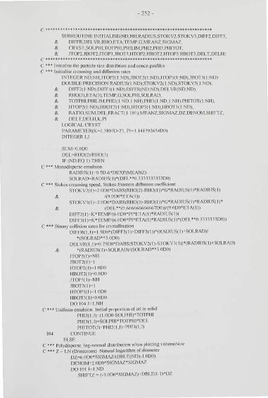
-252-
c ·········································· ·~·············· ·········· SUBROUTINE INITIALISE(ND.NII.RADIUS.STOK V2.STOK V1.DIFF2.DIFF1. & DIFFR.DELVR.RIIO.ET A.TEMP.G.MEANZ.SIGMAZ. & CRYST.SOLPIII . I 0 TPIII.PIIILIM.PHI 2.PIIIJ ,PIIIT0T. & JIOP2.JBOT2.JTOP1.JBOT1.11TOP2.11BOT2.11TOPJ.IIBOT1.DELT.DELII)
c•••••••••••••• •••••••• ••••••••••••••••••••••••••••••••••••••••• •••• C ••• In itialise the part icle si/c distribtion and concn profiles C ... Initialise creaming and diiTusion rates
INTFGER ND.NH.J I OP2( I ND).JBOT2( I ND).JTOPl( I :ND).JBOTl( I . NDl DOUBLE PRECISION RADIUS( I ·ND).STOKV2( 1 ND).STOKVl( l ND).
& DIFF2( IND).DIFFl( I ND).DIFFR(NO.ND).DELVR(ND.ND). & RIIO(J).ETA(1).TEMP.G.SOLI'II I.SOLRAD. & TOTPIII.I'IIILIM.PIII2(1 ND. I NII).PIIIl( l ND. I NII).PIIITOT( I NH). & IITOP2( 1 ND).IIB0f2( 1 ND).IITOPJ( I ND).I IBOrl(l ND). & RATIO.SUM.DEL.FRACT( 1·10 I ).~ IEANZ.SIGMAZ.DZ.DENOM.SHIFrZ. & DELT.DFLII .K.PI
LOGICAL CRYST PARAMETER(K~ 1 1R070-2 1 . P1 ~ 1 1.1 59265. 1)(1) INl EGER U
SUM- OOI.Xl DEL - RII0(2)/RH0(1) IF [ND EQ l ) THEN
C ... Monodispcrsc emulsion RADIUS( 1)-Q 5D-6'DEXP(MEANZ) SOLRAD- RADIUS( I )*(DEL .. 01111ll1l1JDO)
C ••• Stokes creaming speed. Slokes-Einstcin diiTusion coefficient STOK V2( l )- 2 01)0' DABS(RII0(2)-RIIO( I ))'G'RADIUS( I )'RADIUS[ l )
& /(9 OIXI'ETA( I)) STOK Vl( I )~2 01Xl'DABS(RII0(1)·RHO( I ))'G'RADIUS( I )'RADIUS( I )'
& (DEL **(H 66666666666700))/(9 ODWETA( I )) DIFF2( l )- K 'TEMI'/(6 OIXl' PI'ET A[ I )'RADIUS( l )) DIFFJ( I )- K *TEMP/(6 ODIJ'"PI*ETA( I )•RADIUS( I )•(OFL ••o 111JJ_l100))
C ... Bi nan colli sion rates for cnstnllisation . DIFFR( 1. 1 )- 1.51Xl;[DIFF2( I ) I DIFF3( l ))'[RADI US( l )' SOLRAD)/
•(SOLRA0 .. 1 000) DELVR( I . 1 )~O 7500'DABS(STOK V2( I )-STOK VJ( I ))'(RADIUS[ I )+SOLRAD)
& '(RADIUS( I )+SOLRAD)/(SOLRAO"l OIXI) JTOP2( I )~NH JBOT2(1)~ 1
IITOP2(1)~ 1 OIXl 11 B0r2( I )~O OIXI JTOPl( I )~N il
mm·l(l)- > IITOPl( I)~ IOIXl
IIBO'rl( I)- O OIXI DO 111• J~ I .NH
C ••• Uniform emulsion Initial proportion of oil is solid PII I2( 1.J)- ( I 000-SOLPH I)'TOTPHI Plll l( I.J)- SOLPIII' rOTPIII'DEL Pill rOT(J)- PIII2[ l.J) I PHil(l.l)
10• CONTINUE ELSE
C ••• Polydi spcrsc. log-normal distribution" hen plolling \Oiumclsi?C C ••• z = LN (0/microns) Natural log.1 rithm of diameter
OZo6 ODO'SIGMAZ/[DBLE(ND)-1 OIXl) DENOM~2 .01Xl'S IGMAZ'S IGMAZ DO 10 1 1- I.ND
SHIFT'Z ~ (-1 OOO'SIGMAZ)I DBLE(I-I)'DZ
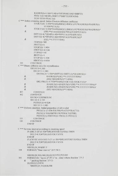
- 253-
RADIUS(I)- o 5DO• J 00-fi*DEXP(MEANZ!SIIIFTZ) FRACT(I )- DEXP( -(Si ll FfZ'SH I Ff7)nJENOM) SUM- SUM >FRACT(I)
C ••• Slakes creaming speed. Stokes·Einstcin diiTusion coefficient STOK V2(1)- 2 OD<l'DABS(Rl i0(2)-RIIO( I ))'G'RADIUS(I)'RADIUS(I)
& /(90D<l'ETA(I)) STOK V1(1)- 2 ODO'DABS(RI IO(l)-RIIO( I ))'G'RADIUS(I)'RADIUS(I)'
& (DEL"(O 6<K>666666667D<l))/(9 OIJO'ETA( I )) DIFF2( 1)- K •TEMP/(6 ODO*PJ*ET A( I )*RADIUS(!)) DIFFl( I )~K *TEMP/(6 ODWPJ•ETA( I )*RADIUS(!)*
& (DEL .. O 1111111()(1)) JTOP2(1)- NII JBOT2(1)- I IITOP2(1)- I OD<l IIBOT2(1)- 0 OD<l riOPJ( I)- NII JBOTl( l)- 1 IITOP1(1)- I OD<l 11001"1(1)-0 llD<l
10 1 CONTINUE C ... Binan collision ralcs for cr.stallic;..1tion
. DO 102 1- I .ND .
DO 101 J- I.ND DIFFR(I.J)- 1 5D<l'(DIFF2(11< DIFFl(J))'(RADIUS(I)f
& RADIUS(J)*(DEL .. O 111HH11DO))/ & (DEL'(RADIUS(J)"1 ODO))
IJELVR(U)-O 75DO'DABS(S fOK V2(1)-STOK V1(J))' & (RADIUS(I)+(RADIUS(J)'(DEL"O 1111111111D<ll))' & (RADIUS(I)t(RADIUS(J)'(DEL"O l111111111DO)))/ & (DEL'(RADIUS(J)"1 OD<l))
101 CONTINUE 102 CONTINUE
RATIO- TOTPI 11/SUM DO 11 0 J- I.NII
PIIITOT(J)- 0 ODO DO 11 I 1- I .ND
C ... Uniform emulsion Initial proportion of oi l is solid
PI112(U)- ( I OD<l-SOLPI II)'RA TIO'FRAC"I (I) Pllll(I.J)- SOLPI II 'RATIO'FRACT( I)'DEL PI IITO f(J)- PI IITOT(J) t PI 112(1.J)t PI lll(I.J)
Ill CONTINUE 110 CONTINUE
END IF
C ••• Set time in lcn a! according to creaming speed IF (DFLT GT (ll 5DO'DELI VSTOK V2(ND))) TI IEN
DEL T- O 5DO'DELI VSTOK V2(ND) END IF IF (CRYST AND DELT GT (0 5DO'DELII/STOKV1(ND))) TIIEN
DELT- o. 5D<l' DELl VSTOK Vl(ND) END IF WRITE(20,100)DELT
lOO FORMAT("Timc intcnal ".E I5_5El)
WRITE(20.10 1) NII.DELH.TOTPIII.PHI LIM 30 1 F0RMAT(14." l a~crs or'.E9 2."m: inital 'olumc fraction ".F5 2
& "p..1cking fraction ".FS 2) IF(CRYST)TIIEN
IVRITE(20.102)SOLPIII
- 254-
102 f-ORMAT("ProJXlrlion of,olurnc \\hich is solid".F5 2) ENDIF IVRITE(20.101)
101 FORMAT(" Initial di<;tribution. rad•us. \OhllllC fraction") DO Il l l " i .ND
IF(CR YST)TI IEN IVRITE(l0.105)RADIUS( l ).PII Il( I.NII).PIII 1(1.NII)
105 FORMAT(.lE I-t 6) ELSE
IVRI I'E(l0.10')RADIUS( I).PIII2( 1. NII) 10' FORMAT(lEI' 6)
FNDIF Il l CONTINUE
\V RI rF(20.106) IOrPIII .( I ODO-SOLPIII )'" 'IOrPIII.SOI PIII *DEL• r01 Pill 106 FORMAT("Total ,of fmcts",lFR 4)
END
c ................................................................... . SUBROUTINE SEQUENCE(ND.Nll .RADIUS.STOK VlSI OK V1.DIFFl.DIFF1.
& DIFFR.DELVR.Q.RIIO.ETA.MU.TOR.GAMMA.BETA.SIGMA.ANGFRFQ. & CRYST.COLFFF.PHILIM.Pllll.PIIIl.PIIIIOT. & JI'OP2.JBOI'2.JTOP1.JBOT1.11T0Pl.HDOT2.11TOP1.JIBOT1. & RECORD.MAXT.DELT.DEI 11)
c •••.••••.•••••••••..••••..•.•.•.•••...••.•.•.••••..••••••••••••••• C Control the sequence of time steps for the ca lcu lation of the C clc\clopmcnt of concen tration prolilcs
IN'I EGER ND.NII.U.T. & JTOP2(1 ND).JBOT2( 1 ND).JTOP1(1ND).JBOT1(J ·ND). & JIYI'OP2( J· JOI).JPBOT2(1 IOI).JPTOI'l(l IOI J.JPD0T1( 1 10 1)
DOUBLE PRECISION RADIUS( I ND).STOKV2(1 ND).STOKVJ( J·ND). & DIFF2( I ND).DIFF1( I :ND).DIFFR(ND.ND).DELVR(ND.ND). & Q(1).RH0(1).ETA(1).MU(1).T0R(1). & GAMMA(1).BETA(l).SIGMA(1).DEL21.ANGFREQ.PJIILIM.COLEFF. & Pllll(J ·ND.I NII).PHil(IND.INII).PHITOT(I Nil). & IITOP2( 1 ND).IIBOfl(l ND).IITOP1( 1 ND).IIBOTl(l ND). & MAXT.RECORD.DELT.DELII
DOUBLE PRECISION MEANVl(J · JOI ).MEANVl( l 101). & VTOPl(l IOI).VDOT2(1 ·JOI).VTOP1(1 IOI).VB0T1(1 101). & DIFHIN.CRM IIIN.PH IUP2( 1 IOI ).PIIIUP1( 1 IOI).PIIITUP. & TMPHil(l JOI ).TMPIIIl( l JOI).PHIT2.PIIITJ. & JIJYI'OP2( 1· JOI).I IPBOT2( 1 IOI ). IIPTOPJ( I IOI ). IIPBOTJ(J · JOI ). & TDIVILTDIVII2.TIME.N.DEL. & SSVrH.SSVVI.SSVEL.SSA'IT.MSVEL.MSA1T.ATrL.URICK2
LOGICAL CRYST
DEL - RHO( I )nU JO(l) DELlJ- RJ JO( l)/RI I0(1) TDIVH"DELT/DELH TDIVH2"TDIVJJnJELJI
DO 10 1 1- I .ND IIPTOPl(i)" IITOPl(l) IIPBOT2(J)o iJB0T2(1) IIPTOPJ(I)- JITOPJ(I) IIPBOTJ(J)-JIBOTJ(I)
101 CONTINUE
T- o 20 1 IF(IIME I E MAXI") TIIEN
C ... -.. Increment time~ one step T -T+ I TIME DEL T'DBLE(T)
C ••• Initiali se arm~ sat top of sample 00 102 1-= l .ND
IF(JBOT2(1) EQ NII)TIIEN
- 255-
PIIIUP2(1) PIII2(1.NII)'(I Ol)(l-IIBOT2( 1)) ELSEIF (JTOP2(1) EQ NII)TI IEN
PIIIUP2(1)-PIII 2( 1. NII)'J JT0P2(1) ELSE
PIJIUP2( 1)- PHI2(1 .NII) FNDIF IF(CI\YST)lliEN
IF(J80T1(1) EQ NII)TIIEN PIIIUP1(1)- PIJI1(1.NII )'( I Ol)(l-IIBOT1(11)
ELSEIF (JT0P1( 1) EQ NII)TIIEN PIIIUP1(J)- PIII1(1.NII)'III 01'1(1)
ELSE PIIIUP1(J)-PIJI1(1 .NJI)
END IF END IF
102 CONTINUE PIIITUP PIIITOT(NII)
C ••• Calculate \c locit ~ of upper and IO\\Cr boundaries of each size CALL BDRYVEL(ND.NII.STOK V2.STOKV1. VTOP2. VBO r2. VTOP1. VBOTJ.
& DIFF2.DIFF1.PIIILIM.P1112 .PIII1.PIIITOT. & JTOP2.JBOT2.JTOP1.JB0Tl .IITOP2.11BOT2.11TOP1.11B0Tl. & TIME.DELT.CRYST)
C ••• Sta rt ''ith top la) er and ''ork d0\11l11ards DO 101 J- NII-1 , 1.-1
C •u Calculate the \clocil\ of each silC fr:~ction :11 J/J-+ 1 interface CALL CAL VEL(J.ND.NI I.STOK V2.STOK V1.MEANV2.MEANV1.
& DIFIIJN.CRMIIIN.PIIILIM.PIII 2.PIIIl . & JTOP2.JBOT2.JTOP1.JB0Tl.IITOP2.11BOT2.1 1T0Pl.IIB0Tl.CRYST)
C .... Calculate the oil \Oiumc tnO\ ing across the J/J+ I la} er interface CALL FLUX(J. ND.NII.STOK V2,STOK V1.MEANV2.MEANV1.
& VTOP2. VBOT2. VTOP1. VBOT1.DIFF2.DIFF1. & DIFFR.DELVR.DIFHIN,CRMHIN.COLEFF.DEL21 . & PIIILIM.PI 112.PIII1 .PIIITOT.Pl IITUP.PIIIUP2,PIIIUPl. & JTOP2.JBOT2,JTOP1.JBOT1. 11TOP2.1180T2. 11TOP1.11f30T1. & JPTOP2.JPBOT2.JPT0Pl.JPB0Tl. & IIPTOP2. 11PBOT2.11PTOI'l.IIPBOT1. & DEL T.TDIVII.TDIVII2.CRYST)
101 CONTINUE C ••• Reset the amns and 'ariablcs
PllllO'I (I)- PIIITUP DO 10~ 1- I.ND
JTOP2(1)- JPTOP2(1) JBOT2( J)~JPB0f2(1)
IITOP2( J)- JIPTOP2(1) IIBOT2(1)- IIPBOT2(1) JTOP1!1)- JPTOPJ(I) JBOT1(1)- JPBOT1(1) IITOP1(1)- IIPTOP1(1) IIBOT1!1) IIPBOTl(l)
-256-
C ••• Check for problems and undcrno,, IF(IIBOT2{1) GT I OOO)TIIEN
IVRITE(20.121 )IIBOT2( I) 121 FORMAT("IIBOT GT I ".E15 5E1)
GOT0202
122
END IF IF(IIBOT1( 1) GT I OOO)TIIEN
IVRITE(20.122)11BOT1( I ).TIME.JBOT1( I ).IIBOTl( I ) FORf.. IAT("HBOT GT I ".2E 15 'iE.1.15.E 15 5F1)
GOT0202 END IF DO 105 J= l .NH
IF(PIII2( 1.J) LT I OD- 15)TIIEN PIII2(JJ)"""0.0DO
END IF IF(PI/Il (I.J) LT 1 OD-15)TI IFN
PIII1(U)-o ODO END IF IF(PIIITOT(J) LT I OD-15)"1 liEN
PIIITOT(J)-il 0[)(1 END IF
105 CONTINUE 104 CON"IINUE
C ... If thi s is a recordi ng step. \Hi tcout results N- T IMEIRECORD IF(N GT 0 5[)(J AND DABS(TIME-(RECORD'DNINT(N))) LE
& DEL T/2 O[)(l)TIIEN IVRITE(20.JO I )TIME/86400 000
101 FORMATrtimc".F8 2." da~ s") WRITE(20. 102)
102 FORMAT("IIcight Tot \OI fract phi(liquid) & Urick'cl S.S,cl MS \ Cl SSA!Icn M S & attcn"}
C •u Genera te and \Hitc out concentration nnd \ciOCi l) profiles DO 106J:- I. NII.I
PI Jrf2""0 ODO PIIIT1- 0 ()[)() DO 1071- I.ND
C' ••• Calculate the local concentration at the la~ er interface
107
IF(J NEJBOT2(1) OR (IIB0f2(1) LE 0 OI [)(I))TIIEN Pl ll'f2- PIIIT2+PIII 2(1.J) TMPH I2( 1)-PIII2(1.J)
ELSE TMPII I 2( 1 )~0 O[)(l
END IF IF(J NEJBOTl( l) OR (IIB0T1(1) LE 0 OIOO))TIIEN
PI IITl- PI IITl+PI 11 1(1.!) TMPI IIJ(I)• PI 11 1(1.!)
ELSE TMPIIIJ(I)•O 000
ENDIF CONTINUE
C ••• Calculate ultrasou nd \Ciocil\'
cALL USVELS(2.ND.RADIUS.TMPI 11 2.TMPI ll l.ANGFREQ. & SSVI'H.SSVVI.SSVEL.SSAH.MSVEL.MSATT.ATTL. & Q.RIIO.ETA.MU.TOR.GAMMA.BETA.SIGMA)
URICK2= I 000/((PI IIT2*(DEL~ PI IIT2•( I 000-DEL))/ & (Q(2)'Q(2)))t(( l O[)()-PII IT2)'( I IJIXI-PIIIT2' & ( 1000- 1 000/DEL))/(Q( I )'Q( I))))
- 257-
C • .,. Output rc•mlts
IF(CRYST)THEN
101
10-1
106
& &
& &
WRITE(2(U01) I OE.1•J•DELII.PIIIT2.PIIIT1.PIIrJ0T(J). (PIII l(I.J).PIIIl(I.J).I J.ND.lO) .DSQRT(URICK l ).SSVFL.MSVFJ..SSATT.MSATT
FORMAT (F7 2.15EI 1 -IE2,1FR 2.2F12 -'E2) ELSE
WRITE(20 . .l0-') 1 OE.1•Jt0FLI I.PIIIT2,PI IIT0T(J). (PIIIl( I . J).I ~ I .ND. I O)
. DSQRT(UR I CKll.SSVFL.~ISVEI .. SSArf.MSATT FORMAT (F7 2. JlF I I •El. 1F8 2.2E I 2 •El)
END IF CONTINUE IVRI fE(20.105)(JTOP2(1).1 J.NIJ. Ill) WRITE(20.10C.)( I ITOP2( 1 ) . 1 ~ I .ND. Ill) IVRITE(20.107)(JBOT2(1).1~ 1 .ND. IO) IVRITE(20.l08)(HB0T2(1).1~ I .ND. I 11)
IF(CRYST)THEN IVRI rE(211.105)(JTOP1( 1) . 1 ~ I .ND. Ill) IVRITE(20.106)( 1 ITOP1 ( 1) . 1 ~ I .ND. IO) IVRITE(20.107)(JB0f1(1). 1~ I .ND. Ill) WRITE(20.108)(1100T1(1).1 ~ I .ND. 1111
ENDIF 105 FORMAr("JTOP~. IlO . IOII 5) 106 FORMAT("JBOr.I10. 101J 'i) 107 FORMAT("! I ror~.E'W 'iEl iOFI"i 5E1) 10ft FORMAT("HBOT".E.105E.l. IOE15.5E.l)
C ... Write ou t the part1clc si1e distribution IF(DABS((N)-(5 ODO'DN INT(N/5 O[)(l))) LT 0 01 [)(I) f ii EN
DO 108 I~ J.ND.l
IVRITE(20.109)RADIUS(J).PI 11 2( 1. I ). & (PI lll( I.J ).J~;O.l50.50).( PI 11 2( 1.J) . J~•oo.500. 10)
109 FORMAT(E I2 6E2.19E II -'F 2) 108 CONTINUE
FND IF END IF
C ••• Ne.,.ttimc step GOT0211 1
END IF 202 END
c •••••••••••••••••••••••••••••••••••••••••••••••••••••••••••••••••••• SUBROUTINE CAL VEL(J.ND.NIJ.STOK Vl.S I OK V1.MEANV2.MEANV1.
& DIFJIIN.CRMIIIN. PIIILI~I.PIII l. PIII1 .
& JTOP2.JBOT2.JTOP1.JBOT1.1 ITOPl.I!Bo-1 2.1 ITOPl.IIBOTl.CR YST) c•••••••••••••••••••••••••••••••••••• ••••••••••••••••••••• ••••••••••• C ••• Calculate \clocih roreach si7e rraction at J/Jt l intcrracc C ••• Barnca·Mi7rahi ( 1971) hindrance ractor Zimmcls ( 1988) pol~dispcr C ••• Carnahan-Starling equation ror thennod~ namic ractor or diiTusion
INTEGER U .ND.NII. & JTOP2( 1 ND).JBOT2( 1 ND).JTOP1( 1 ND).JBQr1( l. ND)
DOUBLE PRECISION DARNEA DOUBLE PRECISION STOK V2( I ND).STOK V1( I ND).
& MEANV2( 1 IOI).MEANV1( 1 IOI ).OIFIII N.C'RMIIIN. & PIIILIM.PIII l( I. ND. I :NII).PII Il(l ND. I Nil ). & llf0P2( 1 ND).IIBOT2(l.ND). IITOP1( 1 ND). IIBOTl( l ND). & PIIIABV.PI JJ BEL.SUMABV.SUMBEL.PI II .SUM .FAC
LOGICAL CRYST
- 258-
C +++ Cnlcub tc total concn just alxn c and just bclo\\ l:ncr interface PIIIABV"" O ODn . PIIIBEL- o ODO SUMABV- O ODO SUMBEVOOI)(l DO 1011- I.ND
IF ((J NE.JTOP2(1)) OR (( I.OD<l-111 OP2( 1)) I.E 0 OIDO)) THEN Pi ll BEL:::Pfll BEL +PIII2( I.J) SUMBEL~SUMBEL! Pl ll2(1.l)'STOK V2(1)
END If
IF (((11 1) NE.JB0T2(1)) OR (I IBOT2(1) LEOO ID<l)) TIIEN PIIIABV- PIIJABV+ PIJI2( 1.J j. J)
SUMABV~SUMABVI PIII 2(U II)'STOK V2( 1) END If l f(CRYST)TIIEN
IF ((J NE JTOPJ( I)) OR (( I OD<l-IIT01'1( 1)) LEo OID<I)) TII EN PIIIBEL-PIIIBEL I Pll ll(I.J) SUMBEL~SUMBELt l'lll l( I.J )'STOKVJ( I )
END IF If (((Jt I) NE JBOT1(1)) OR (IIB0T1( 1) LE 0 OID<I)) TIIEN
PIIIADV=PI II ABV+PIII l(I.J+ I ) SUMABV-SUMABV>PHI1(1.Jt I )'STOKV1(1)
END IF ENDIF
10 I CONTINUE
C .. A'cwgc concn used in hindrance factor for creaming and d1rTusion PJII - O 5DO*(PIIIABV+PIIIBEL) FAC- BARNEA(PII I) SUM- 0.5D<I'(SUMABV>SUMBEL) DIFIII N- FAC*(( I OD0f2 .0DWPIIJ)•( J O[)(H2_0f)()*PII I)! ((PIII .. l)*
& (Pill -• OD<l)))/(( I.OIJO-PIII)"l) CRMIIIN• FAC
C ..... Ca lculate creaming vc loci t ~· of each si?c fraction DO 102 1- I .ND
MEANV2( 1)- F AC'(STOK V2(1)-SUM) MEANV1(1) fAC'(STOKVJ(I)-SUM)
102 CONTINUE END
c••••••••••••••••••••••••••••••••••••••••••••••••••••••••••••••••••• SUBROUTINE FLUX(J.NO.NI I.STOKV2.STOKV1.MEANV2.MEANV1.
& VT01'2. VBOT2. VTOP1. VBOT1J)IFF2.DIFF1. & I)IFFR.DELVR.DIFHI N.CRMIIIN.COLEFF.DEL21. & PI IILIM.PIII2.PIII J.PHITOT.PI IITUP.PI I IUP2.PIIIUP1. & JTOP2.JBOT2.JTOP3.JBOT1.11TOP2.1 1BOT2.1 1TOP1.11BOTJ. & JPTOI'2.JPBOT2.JPTOP1.JPBOI'1.11PTOP2.11Pil0 1'2.11PTOP1.1 11'BOT1. & DELT.TDIVII,TDIVH2.CRYST)
c••••• •••••••••••••••••••••••••••••••••••••••••••••••••••••••••••••• C ••• Calculate volume of oi l " hich moves across the la~ er interface
INTEGER U .I I.ND.NII. & JTOP2( 1 ND).JBOT2( 1·ND).JTOP3( 1 ND).JBOD(IND). & JPTOP2( I · IOI).JPB0f2( I · IOI ).JPTOP1( 1 IOI ).JPOOTJ( I 10 1)
DOUBLE PRECISION STOKV2( 1·ND).STOKV1(1 ND). & VfOP2( 1 IOI).VBOT2( I · IOI).VrOP1(1 IOI ).VBOT1(1 10 1). & MEANV2(I · IOI ).MEANV1(1 IOI ).DIFF2(1ND).DIFF1( 1·ND). & DIFF.IJIFFR(ND.ND).DEL VR(ND.ND).DIFIIIN.CRMI II N.DEL21.COLEFF.
- 259-
& PIIILIM.PIII2(1 ND. I NII).PIIIl( l ND. I Nll l.PIIITOT( I Nil ). & PHITUP.PIIIUP2(1 IOI ).PIIIUP1( 1 10 1). & PIIIJ1(1 10 1).PIIIJ2(1 IOI ).PIIIJ1 2( 1 IOI ).I'IIIJI1(1 101). & IITOP2(1 ND).IIBOT2( 1 ND).HTOP1(1ND).IIBOT1( 1 ND). & IIPTOP2(1 101). 11PBOT2(I· IOI ).IIPTOP1( 1 IOI).IIPBOTJ( I 101). & DELT.TDIVII.TDIVII2.PIIIMOV.PIIISUM. & DV0L21.DPI II 2( 10 I ).DPII I21( 10 I ).IJP111 1( HI I ).DPIII11 ( 10 I ),OVRLAP
LOGICAL CRYST
IF (PHI 1'01 (JH) LT PIIILIM)TIIEN PHISUM-O.ODO DO 101 l= l .ND
PIIIJ1 2(1)=PIII2(1.J-+ I ) PIIIJ2( 1)~PII I 2( 1.J)
PIIIJil(J)-PIIIl(I.J f l ) PI IIJ 1( 1 )~PIII1( 1.J )
DIFF-DIFF2(1)'1JIFIIIN C ••• Calculate amount of (l iquid) oi l of th ic; si1c crossing interface
CALL FLOW(J.NII.MEANV2(1). VI'OP2(1). VBOT2(1).DIFF. & PIII2(1.J).PIII2(U+ I ).PIIIJ 12(1).PHIUP2(1).PIIIJ2(1). & PIIIMOV.JTOP2(1).J80T2(I).IITOP2(I). IIBOT2( l ). & JPTOP2(1).JPBOT2(1).11PTOP2(I). IIPB0T2(1). & TDIVfi.TDIVII2)
PI IISUM-PIIISUM I PI IIMOV IF(CRYST)TIIEN
DIFF-DIFFl( I)'DIFI II N C ••• Calculate amount of (solid) fat of thi s si1e crossing in terface
CALL FLOIV(J.NII.MEANV1( 1). Vl"OPl( l ). VBOTJ( I),DIFF. & PHI1(1.J).PHI1(1.J >I ).PIIIJI 1(1).PIIIUP1(1).PHIJ1(1). & PIIIMOV.JTOP1(1).JBOT1(1).11TOP1(1).HBOT1(1). & JPTOP1(1).JPBOT1(l).IIPTOP1(1).11PBOT1(1), & TDIVII.TDIVI I2)
PHISUM- PIIISUM >PIIIMOV END IF
101 CONTINUE PIIITOI'(J >I)- PIIITUP<PIIISUM PHITUP.PHITOT(J)-PIIISUM
ELSE C ••• No mo,emcnt if la~ er is full Reset arra~s
DO Hl2 I ~ I .ND
PIIIJI2(1)- PIII2(Utl) PIIIJI 1(1)-PIII1(U> I ) PIIIJ2(1)-PIII2(1.J) PIIIJl(I)- PIIIl(U) IF(J EQJBOT2( 1))TI IEN
PIIIUP2(1)-PIII2(U)'( I ODO-HBOT2(1)) ELSE IF (J EQ JTOP2(1))THEN
PIIIUP2(1)- PIII2(1.J)'HTOP2(1)
ELSE PIIIUP2(1)-PI II 2( 1.J)
END IF IF(CRYST)TIIEN
IF(J EQ JBOT1(1))TIIEN PIIIUP1(1)- PIII1(U)'(I OIJO-IIB0T1( 1))
ELSE IF (J EQ JTOP1(1))TIIEN PHIUP1(1)- PIII1(1.J)'IITOP1(1)
ELSE PIIIUP1(1)- PIII1(l.J)
END IF
-260-
END IF 102 CONTINUE
PIIITUr-PIIITOT(J) END IF
(' ..... Calculate the amount or oil ( liquid) comcrtcd to fat (solid) IF(CRYST)TIIEN
IO..J
DO 1 01 1~ 1 . ND
IF(J t I EQ JPTOP2(1))TIIEN DVOL2J~o ODO DO 10-4 II"= I.ND
IF(J 11 EQ JPTOP1( 11 ))TIIEN 0VRLAJ'o-DM INI(IIPTOP2(1).1 1PTOP1( 11))
ELSE 0VRLAr-IIPTOP2(1)
ENDIF DVOL2 1~DVOL2 1 >PIIIJ 11(11)'0VRLAP
& *(DIFIJIN*DifFR(I ./1) I C'RMIII N*DELVR( I.I I)) CONTINUE DVOL21- DELT*COLFFPPIIIJ 12(1)*DVOL21 DPIII2(1)--DVOL21/IIPTOP2(1)
C ••• Protect against c~stalli~ing more liquid tlmn is a\ ail able IF(DAOS(DPIII2(1)) GT PI IIJ 12(1))TIIEN
DPIII2(1)--PIIIJI2(1) DVOL21- -DPIII2( I)' IIPTOP2( 1)
END IF ELSEIF(J+ I EQ JPBOTl(I))TIIEN
DVOL2J --ofl O[)(J DO 1()5 11 - I .ND
IF()> I EQ JPBOT1(11))TIIEN OVRLAJ'o-DMIN I( I ODO-IIPB0T2( 1).1 ODO-IIPBOT1( 11))
ELSE 0VRLApo- I .ODO-I IPOOT2(1)
ENDIF DVOL21=0VOL21+ PII IJ l l( fi )•QVRLAP
& *(IJ IFIII N*DifFR( I.II ) I C'RM III N*DELVR(I.I I)) 105 CONTINUE
DVOLl i ~DEL T'COLEFF'PIIIJ 12(1)'DVOL21 DPIII2(1)- -DVOL21/( I ODO-IIPBOTl( l)) IF(DABS(DPIII2(1)) GT PI IIJ 12(1))TIIEN
DPHI2(1)--PI IIJ 12(1) DVOL21- -DPIII2(1)'( I OJ)(l-IIPBOT2(1))
ENDIF ELSE
DVOLl l- 0 ODO DO 1116 ll= l .ND
IF(H I EQJPT0P1(11))TIIEN OVRLA?=-I JJYrQPl( ll)
ELSEIF(H I EQ JPB0T1(11)) IIIFN OVRLA~I ODO-II PBOT1(11)
ELSE OVRLAP=-1 OI)(J
ENDIF DVOL2 1- DVOL2H PI IIJ 11{1 WOVRLAP
& *(DIFI /IN*DIFFR(I. II ) + CRMIII N*DELVR(I.II )) 106 CONTINUE
DVOL21~DEL T'COLEFF'PI IIJ 12( 1)'DVOL2 1 DPHI2(1)--DVOL21 IF(DABS(DPHI2(1)) GT PIIIJ 12(1)fl liEN
DVOL2 1 ~-DPII I 2(1)
END IF END IF
-26 1 -
IF(Jtl EQWIOP1(1))TIIEN DPI111(1)- DEL21'DVOL21/IIPTOP1(1)
ELSEIF(J+ I EQJPB0T1(1))TIIEN DPIII1(1)- DEL21'DVOL21/(I ODO-IIPBOT1(1))
ELSE DPIII1(1)- DEL21'DVOL21
END IF PIIITO I (J + 1)- PIIrro r(J H l-DVOL21'( I ODO-DEL21)
101 CONTINUE C ... Smnc cnsta ltis..1t ion for la\ er J I
IF(J EQ I )TIIFN -
& lOR
DO 107 1 I .ND lf(JPB0T2(1) EQ I)TIIEN
DVOL2 t- o ODO DO IOR II~ I . ND
lf(JPBOT1(11) EQ IJIIIEN OVRLAP DMINI(I (II)()-IIPB0r2(1).1 OD0-111'801"1(11)1
ELSE OVRLI\J>-:1 ODO-IIPnOT2(1)
END IF DVOL21 DVOL2/+ PIIIJl( II)*'OVRLAP
'(DIFIIIN'DiffR(I.II)+CRMIIIN'DELVR(I.II)) CONTINUE DVOL21- DEL I *COLEFPPII IJ 2(WDVOL21 DPIII21(1)- -DVOL21/( I ODO-IIPBOT2(1)1
C ... Protect against Cr)stallising more liquid th:tn is a\ai lablc l f(DABS(DPIII2(1)) GT PIIIJ2(1))TIIEN
DP11121(1) ·-PII IJ2(1) DVOL21- -DPIII21(1)'(1 ODO-IIPB0T2( 1))
END IF ELSE
DVOL21-=0_0DO DO 10911- I.NI)
l f(JPBOTl(ll) EQ l)fiiFN OVRLA~ I ODO-IIPBOT1(11)
ELSE OVRLAJ>,-; I .000
ENDIF DVOL21 DVOL21 + PII!Jl(ll)'f-OVRLAP
& '(DIFIIIN'DiffR(I.II)tCRMIIIN'DEL VR(I.I I)) 109 CONTINUE
DVOL2I-DFLT•COLEFP'PII IJ 2( !)•DVOL21 DPIII2 1 (I)--DVOL21 lf(DABS(DPIII2 1(1)) GT PIIIJ2(1)1riiEN
DPIII21(1)-=-PIIIJ2( 1) DVOL2 1""'·01'1112 1(1)
END IF END IF lf(JPBOT1(11 EQ I)TIIEN
DPIII 1 1(1)=DEL21•DV0L21/( I 000-I IPB()Tl( l)) ELSE
DPIII11(1)- DEL21'DVOL21 ENDIF PIIITOT( I )- PIIITOf( I )-DVOL21'( I ODO-DEL21)
107 CONTINUE ENDIF
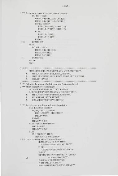
-262-
C **• Set the ncn \a lucs of concentration in the hncr DO 11 0 I ~ I.ND .
PIII2(1.J II)~PIIIJ 12(1)1 DPHI2(1) Pllll (I.J 1 I )~PIIIJI 1( 1 )>DPIII1( 1 )
IF(J EQ I)TIIEN PIII 2(1.J)~ PIIIJ 2( 1 ) I DP11121 (I) Pllll(I.J)~PIIIJJ(I) I DPIII11 (I)
ELSE PIII2(1 .J) · PIIIJ 2(1) PHil(U)~PIIIJ1(1)
END IF 1111 CONT INUE
ELSE DO Ill 1~ 1 . ND
PI11 2(1.H I )~PIIIJ12(1)
PIII2(1.J)~PIIIJ2(1)
Pllll(I.J)~PIIIJ1(1)
Ill CONT INUE END IF END
c ············~······················································· SUBROUTI NE FLOW(J.N II .MEANV. V I OP. VBOT.DIFF. & PIIIIJ.PHIIJ I.PIIIJ I.PIIIUP.PIIIJ.PIII MOV. & JTOP.JBOT.HTOP.IIBOT.JPTOP.JPBOT.IIPTOP.IIPBOT. & TOIV II.IDI VII2)
c •••••••••••••••••••••••••••••••••••••••••••••••••••••••••••••••••••• C ••• Calculate the amount of oil of gh en si7c fmction and speed C ... '' hich crosses between the la~crs
INTEGER J.NII.JTOP.JBOT.JPTOP.JPBOT DOUBLE PRECIS ION MEANV.VTOP.VBOT.D IFF.
& PIIIIJ.PIIIIJI.PIIIJI.PHIJ.PIIIUP.PIIIMOV. & IITOP.IIBOT.IIPTOP.IIPBOT. & CREAM.D IFFUS.TDI VII .TDIVII 2
C ... Special cases near IO\\CT and upper boundaries IF (J LT (!BOT- I ))THEN
IF(J EQ (JBOT-2))TICEN PIIIJ I=PIII UP/( 1.000-1 IPBOT) PIII UJ>-OCIDO
END IF PIIIMQV""(>ODO
ELSE IF (J GT JTOP)TIIEN PIIIU~ODCI Pill MOV='"O ODO
ELSE IF (J EQJ BOT) TIC EN
IF(VBOT LT Cl ODO)TIIEN C ••• Lo\\cr bouncbr. IIlO\ CS dO\Hl\\ards (case I)
IF(ME ANV GT 0 ODO) TIIEN CREI\M...., PIII!J•MEANV*TOIVII
ELSE CREAM=PIIIIJ l *tviEANV*TDIVII
END If DIFFUS~DIFF'(PIIIIJ-PIIIIJ I j•TDI VIJ 2/
& (I ODCI-0 5DO•JJBOT) PH I MOV~CREAM I DJ FFUS PHIJI ~PIIIUP+PIIIMOV
PIIIUJ>-PIIIIJ•(J ODO-HBOT)-PIII MOV
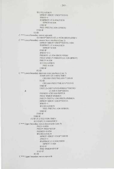
- 263-
IF(J EQ l)riiEN IIPBOT IIBOHVBOPlDIVII JPBOT~ I
lf(IIPBOT LT 0 ODO)TIIEN IIPBOT=-OODO
END IF PIIJJ- PIII UP/(1 01)(1-IIPBOT)
END IF FLSE
( -.u LO\\CT bound1r) 1110\CS up\\:Jrds
IF(VBO r•TDIVJJ GE (0 99D<I-I !BOT)) ri !EN C ... Lo\\cr bound.11) crosses l a~cr interface (Case 2)
llPIJOT=-IIBOT+ VDOr•TOIVII-1 000 IF(IIPBOT LT 0 OJ)(I)l liEN
IIPBOT,..,.OODO END IF JPBOT=-J+I PIIIMOV- (1 OD<I-IIBOT)'PIIJJJ PIIJJI - (PIIIUP t PJJIMOV)/(J UD<I-IIPIJOT) PIIIUP- U.ODO JF(J EQ I)TIIFN
PIIIJ 0000 END IF
ELSE C ••• Lower bound.11) does not cross interface (Case 1)
IF(MEANV GT 0 OD<I) THEN CREAM- PIIfiJ•MEANV*TDIVII
ELSE CREAM- PIIIIJJ•MEANV•TDIVII
END IF
& DIFFUS=:DJFP(PIIIIJ-PIIIlJ I )*TDIVJ/ 21
( I .OD0-0.500*IIBOT) PIIIMOV- CREAM+DIFFUS PIIIJJ - PIIIUP + PIIIMOV PHIUP--PIIIIJ'(I ODO-IIBOT)-PIIIMOV JIPBOT- HBOf >VBOT'TDIVJJ JPBOT~J
IF(J EQ I )TIIEN PJJJJ - PIIIUP/(1 OD<I-IIPBOT)
END IF END IF
END IF ELSE IF (J EQ JTOP) THEN
IF(VTOP LT 0 OJ)(I)TIIEN C ••• Upp::r boundaf) 1110\CS d0\\0\\ards (case~)
PlllJI 0000 PIIIUP PIII IJ *IITOP PHIMOV- 0 OD<> IF(J EQ I )THEN
IIPBOT=- 1/BOTI VfQP+TOIVII JPBOT- 1 JF(IIPBOT LT 0 ODO)THEN
I IPBOT- 0 UDO END If PIIJJ- PIIIUP/ IIfYTOP
END IF ELSE
C ••• Upper boundary 1110\CS upwards
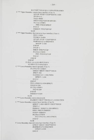
-264-
IF(VfOP*TDI V!I GE.( IOIDO-IITOP))TIIEN C ••• Uppe r bound1 f) crosses la~ er interface (Case 5)
IIPTO?-IITQP f- VTQP*TDI VII- 1 ODO JPTQP.,..J+ I PIIIJI -= PIIIIJ PIIIUI'-PIIIIJ'(HTOP-1 11'1 OP) IF( I EQ I )TIIEN
PIIIJ- PIIIUP/IIPBOT END IF PIIIMOV=-PIIIIJ*IIPTOP
ELSE C ••• Upper boundu~ does not cross layer interface (Case 6)
PIIIJI ....,OODO PIIIMOV"'O O[)(l JJJYfQP=IITOP ._ VTOP*TDI VII IF(III'rQP GT I ODO)TIIEN
IIPTOP, i.ODO END IF JPTOI'-J Pill UP= PI 11 W IITOP IF(J EQ I )TIIEN
PIIIJ - PIIIUP/IIPTOP END IF
END IF END IF
ELSE IF ((J >I ) EQ JBOT)TI IEN IF(VBOT GT 0 ODO)TIIEN
C ••• LO\\Cr bound1ry moves upwards (Case 7) IF (J EQ NH-I)TI IEN
IIPBOT=HBOT < VBOT'TDIVII JPBOT=NH IF(IIPBOT GT I OJ)(J)TIIEN
IIPBOT= l 000 END IF
END IF PII IJI - PHIUP/( 1 OJ)(J-IIPBOT) PIIIUJ>:il.OOO IF(J EQ. I )TIIEN
PIIU- O 000 END IF PIIIMQVo--O 000
ELSE C ••• Lo\\crbound11) 1110\CSdo,,m,ards
IF((IIBOHVBOT'TDI VII) LE~~ 0 I J)(J)l !IEN C ••• Lo,,cr boundan crosses la, er interface (Case R)
. IIPBOT~ l .OOO+IIBOT_..VBOPTDI V II JPBOT- J PIIIMOV==-PIIIIJI *( I 000- IIPBOT) PIIIJI - PHIUP+PHIMOV PIJIUP,-PIIIMOV IF(J EQ I )THEN
PIIIJ - PII IUP/( 1 ODO-IIPBOT) END IF
ELSE C LO\\Cr boundary does not cross layer interface (Case 9)
1/PBOT:=IIBOT +VBO.PTDI VII IF(IIPBOT LTO OJ)(I)TI IEN
HPBOT- 0000 END IF
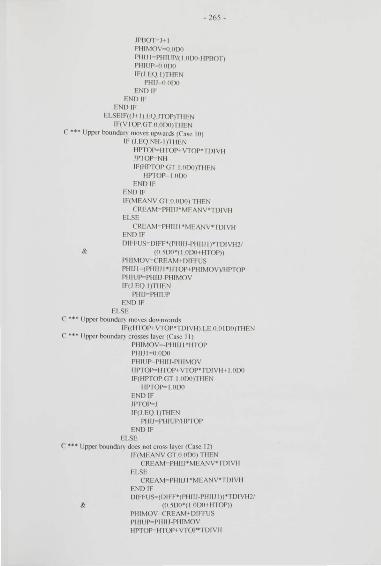
- 265-
JPDOT- J t l PIIIMQY.,--0.000
PIIJJI - PI II UP/(1 000-IIPBOT) PIIIUP,.,OQ[)(J IF(J EQ I )TIIEN
PIIIJ~O 000 END IF
END IF END IF
ELSE IF((H I).EQJTOP)TIIEN IF(VIOP GT 0 O[)(J)TIIEN
C •u Upper boundnr) IIlO\ CS up,,ards (Case 10) IF (J EQ NII -I)TII EN
1/PTO~IITOPI V I OP"" rOI VI/ JPTOI'--NII
IF(IIPTOP GT I.ODO)TIIEN IIPTQP,..] lllXJ
FNDIF END IF IF(MEANV GTO liDO) THEN
CREAM=PIIIIJ*MEANV*l DIVII ELSE
CREAM=PHIIJI*MEANV* IUIVI I END IF
DIFFUS~DIFF•( PIIIIJ-PHIIJ I j•l DIVII 2/ & (051)0•(1 ODO +IITOP))
PI IIMOV- CREAM< DIFFUS PIIIJ I ....,.(PI IIIJ 1•1 ITQP-l Plllt>.IQV)IJIPTOP PIIIUI'--PIIIIJ-PIIIMOV IF(! EQ I)TIIEN
PIIIJ~PIIIUP
END IF ELSE
C ... Upper bounda!) rH O\ CS dm\lll\ards IF(( IITOP+ VJ'QP•TDIVII).LE_O_OIDO)TIIEN
C ••• Upper bound.11'} crosses b) e r (Case 11) PIIIMOV'='-Pf-I IIJI*IITOP PIIIJJ - O 000 PIIIUP=-PIIIIJ-PIIIMOV IIPTQp-1-fTOP t VTQP•TDIVII t I .000 IF(IIPTOP GT I ODO)TIIEN
IIPTOP"=l _O[)(J END IF JPTOI,.,_J IF(J EQ I)TIIEN
PIIIJ PHIUPMPTOP END IF
ELSE C ••• Upper bound.11) does not cross la~ er (Case I 2)
IF(MEANV GT 0 000) TIIEN CREAM- PH!JJ•MEANV•TDIVII
ELSE CREAM=PIIIIJ J•MEANV*TDI VII
END IF DIFFUS=(DIFP(PII I U-PII IIJ I))*TDIVII2/
& (0_5[)0*(1 tJ[X)lJITOP)) PII IMOV=CREAM-f DIFFUS PIIIUI"-PIIIIJ-PIIIMOV JHYrQp-HTQP-f VTOP*TDJVII
-266-
JPTOJ>-:-Jt l PI IIJ f~(PIIIIJ l*I ITOPl PI IIMOV)/I IPTOP I F(J EQ I )THEN
PIIIJ-PHIUP END IF
END IF END IF
ELSE C ••• Normal flu..; calculation
IF(MEANV GT 0 000) TIIFN CREAM...,.PHJIJ,.MEANV*TDIVII
ELSE CREAM- PIII IJ t •MEANV*-IUIVI I
END IF Dl FFUS- DJFF*(PIII IJ-PI II IJ I )*TDI Vll2 PHI MOV- CREAM + DIFFUS PII IJ 1- PIIIUP+ PHI MOV PIII UJ>-PIII IJ-PI II MOV IF(J EQ I )THEN
PHIJ- PHIUP END IF
END IF END IF END
c•••••••••••••••••••••••••••••••••••••••••••••••••••••••••••••••••••• DOUBLE PRECISION FUNCTION BARNEA(PHI)
c•••••••••••••••••••••••••••••••••••••••••••••••••••••••••••• •••••••• C Barnca and Minahi funct ion for the rclati\c 'clocit} in a gi,cn C \Oiumc fraction
DOUBLE PRECISION PHI.F AC.CONTFR CONTFR- ( I 000-PHI) FAC- CONTFRJ( I.ODO+PHI **O 111.l131ll1DO) IF(PIII GE.O 999DO)THEN
BARNEA....,O_OI)() ELSE
BARNEA- F AC*DEXP(-1 666666667[)()*PI II/CONTFR) END IF RETURN END
c••••••••••••••••••••••••••••••••••••·•••·•••••••·•••••·••••••••••••• SUBROUTINE ODRYVEL(ND.NII.STOK V2.STOK V1. Vl OP2. VOOT2. VTOP3. VBOT1.
& DIFF2.DIFF1.PI IILIM.PIII 2.PIII lPI IITOT. & JTOP2.JBOT2.JTOP1.JOOT1. 11TOP2. 11 BOT2.1 1TOP3. 11 BOT1. & T IME.DELT.CRYST)
c ••••••••• ••••••• •• •••••*••••••••••••••••••••••••••• ••••••••••• •••••• C ••• Calculate' cloci tics of upper and loner boundaries of each site
IN.I EGER ND.NH.I.JTOP2( I ND).J00T2( I ND).JT0P1( I ND).JBOT1( I NO) DOUBLE PRECISION STOKV2( 1 ND).STOKV1(1ND).
& VlUP2(1 IOI).VB0T2(1 IOI ).Vl.OP1( 1 IOII.VB0T1( 1 10 1). & DIFF2(1 ND).DIFF3( 1 NDI. & PIIILIM.PHI 2( 1:ND.I NH).PIIIl(IND. I NH).PHITOT( I Nil). & HTOP2( I ND).HBOT2( I :ND).IITOPJ( I :ND).HBOT.l( I :NO). & TIME.DELT
LOGICAL CRYST
& & & &
& & & &
& & & &
& & & &
101
-267-
DO 101 I~ I.ND
CALL TOPVEL(ND.NII.JTOP2(1)-I. II rOP2(1).STOK V2(1).DIFF2(1). VrQP2(1).STOK V2.STOK V1. PIIILIM.PIIITOT(JTOP2(1)).PIII2.1'1111. JTOP2.JBOT2.JTOP1.JBOT1.11TOP2.11BOT2.11TOP1.11BOT1. TIME.DELT.CRYST)
CALL BOTVEL(ND.NII.JBOT2(1) .1 1BOT2(1).STOKV2(1).DIFF2( 1). VB0T2(1).STOKV2.STOKV1. PIIILIM.PII IT0T(J80T2(1)1I).PIII2.P1 111. JTOP2.JBO r2.JTOP1 .JBOT1.11TOP2.11BOT2.HTOP1 .11BOT1. TIME. DEL T.CR YST)
IF(CRYST)TIIEN CALL TOPVEL(ND. NH.JTOPJ(I)- I.IITOPJ(I).STOK V1(1).DIFF1(1).
VrQPJ(I).STOKV2SIOKV1. PII ILIM.PI IITOr(JTOPJ(I)).PI11 2.PIII1. JTOP2.JBOT2.rl 0P1.JBO r1.11TOP2.11BOT2.11TOP1.11BOT1. TIME.DELT.CRYST)
CALL BOTVEL(ND.NH.JOOT3(1).1180T1(1).STOKVJ(I).OIFF1(1).
END IF CONTINUE END
VBOrJ(I).STOK V2.STOK V1 . PIIILIM.PIIIT0T(J80T1(1)< I).PI112.PIII1. JTOP2.J BOT2.JTOPl.JBOT3.11TOP2.11 BOT2.11TOPJ.IIBOTJ. TIME.DELT.CRYST)
c•••••••••••••••••••••••••••••••••••••••••••••••••••••••••••••••••*•• SUBROUTINE BOrVEL(ND.NII.J.II.STOKV.DIFF.VBDRY.
& STOKV2.STOKVJ.PIIILIM.TOTPIII.PI112.PIII1. & JTOP2.JBOT2.JTOPJ.JBOT1.11TOP2.11BOT2.11TOP1.11B0r1. & TIME. DEL T.CRYST)
c•••••••••••••••••••••••••••••••••••••••••••••* .. ••••••••••••••••••••• C .... Calculate the \Ciocit~ of the Jo,,cr bound.1!')
EXTERNAL BARNEA INTEGER I.J.ND.NII.
& JTOP2(1 ND).J80T2(1 ND).JTOPJ(I.ND).JBUI 1(1.ND) DOUBLE PRECISION STOK V2( I.ND)SI OK V1( I ND).S rQK V. VB DRY.
& DIFF.PIIILIM.TOTPII I.PIII2(1 NO. I NII).PIII1(1.ND. I NH). & IITOP2(1 ND).IIB0r2(1 ND).IIrQPJ(I.ND).IIBOT1(1 ND).II. & SUMABV.PIIIABV.PII IBEL.SUMBEL.PIII.SUM.FAC.IIIN. & TIME.DELT.MEANV.DIFFH
DOUBLE PRECISION BARNEA LOGICAL CRYST
C ... Calculate concn at nearest la~ er interface PII IABV~O ODO PIII BEL~O ODO SUMABV~O 000 SUMBEL• O ODO DO 101 I• I .ND
IF ((J NEJTOP2(1)) OR ((I.ODO-HTOP2( 1)) LE.O Ol[)(l)) THEN PIIIBEL• PIIIBEL+ P1112(1.J) SUMBEL• SUMBEL< PIII 2(1.J)'Sl 0KV2(1)
END IF IF (((J+I) NEJBOT2(1)) OR (IIBOT2(1) LEO OIDO)) TIIEN
PHIABV~PII I ABV< PHI2(1 .H I) SUMABV~SUMABV+PII I2(1.JII)'ST0KV2( 1 )
END IF
- 268-
IF(CRYST)l iiEN IF ((J NE JTOPl( l)) OR((I ODO-IITOP1( 1)).LE 0 0100)) TIIEN
PII I BEL~PIII BELI Plll1(l.J) SUMBEL~SUMBEL < Plll1(l.J)'STOK V1( I)
END IF IF (((HI) NE.JBOT1(1)) OR (IIBOT1(1) LE.O 01 DO)) TIIEN
PIIIADV=·PI II ABV+PIII1(1.J +I) SUMABV~SUMABV.f PI 111(1.1 +-I )*STOK Vl(l)
END IF END IF
I 0 I CONTINUE
C ••• Use a\cragc conccntraion in 'clocit\ and diiTusion PHI=Q. 51Jo+(PIII ABV+PIIIBEl.) F AC- BARNEA(Pi ll) SUM-O 5DO'(SUMABV•SUMBEL) I II N=FAC*((I OD0120DO*Pifl)'*'(l 000+20DO*PII I) +-((PIW*l)*
& (PII I-l O[)(l)))/((1 ODO-PI11)"1) DIFFJI- DIFF*I I IN MEANV~F AC'(STOK V-SUM)
C ••• Vcloci t} of lxmndal) including crcnming and diffusion VBDR V- MEAN V -0 9500' DSQRT(DI FFII)' (IJSQRT(TI ME)-DSQRT(TIME-DELT))
& IDELT
IF((VBDRY GTO OIJO)AND (TOTPHI GT PII ILIM))TIIEN VBDRY9l.ODO
END IF END
c •·••••···•••·••••••·••·•········•·•···•·•······•··•····••···••••·••• SUBROUTINE TOPVEL(ND.NI U.li.STOK V.DIFF. VBDRY. & STOKV2.Sl0KV3.PII ILIM.TOTPIII.PH I2.PIIll. & JTOP2.JBOTZ.JTOP1.JBOTJ.lll OP2.HBOT2.1 1TOP1 .HBOT1. & T IME.DELT.CRYST)
c •••••••••••••••••••.•••••••.•••••••••••••••••••••••••••••••••••••••• C *** Calculate vclocit~ of upper boundal)
EXTERNAL BARN EA INTEGER U.ND.Nll.
& JTOPZ(I ·ND).JBOTZ(I ND).JTOP1(1 ND).JBOT1(1 ND) DOUBLE PRECISION STOK V2( I ·NIJ).STOK VJ( I NIJ).STOK V. VBDR Y.
& DIFF.PHILIM.TOTPIII.Pll l2( I ·ND. I ·NI I).PI IIJ( I ·ND.I :Nil). & IITOP2(1ND).IIBOT2(1 ND).IITOPJ(I ND).HBOT1(1ND).ll. & PIIIABV.SUMABV.SUMBEL.PI II BEL.Pill.FAC.SUM.HIN. & T IME.DELT.MEANV.DIFFH
DOUBLE PRECISION BARNEA LOGICAL CRYST
C ... Calcu late concn at nearest la}CT interface PIIIABV~O ODO PIIIBEL" O 0[)(1 SUMABVoii.O[)(I SUMBEL- 0.0[)(1 DO 10 11- J.ND
IF ((J NEJT01'2(1)) OR ((I O[)(I-IITOP2(1)) LEOOIDO))THEN PIIIBEL~PIIIBEL< Pll l2(l.J) SUMBEL~SUMBEU PH I2(l.J)'STOK V2(1)
END IF
-269-
IF(((HI) NE.JOOT2(1))0R (IIBOT2(1) LFIIO IDO))TIIFN PIIIABV'=" PI II ABV-tPIII2(U-+ I ) SUMABV~SUMABV< PIII2(1.J I I)'STOK V2( 1)
END IF IF(CRYS r)TIIEN
IF ((J NE JTOP1(1)) OR (( I ODO-IITOP1(1)) LE 11 OIDO))TIIEN PIIIBEL PIIIBFLWIII1(1.J) SUMBEL=SUMBEL! PI 1/J(I.J)*STOK Vl(l)
END IF IF (((J+ I ) NEJBOfl(l)) OR (1100T1(1) LE .O Il l DO)) I"IIEN
PIIIABV=-PIIJABV-+ Pl ll l(U f- 1) SUMABV=-SUMABV• Plll l(I.J-t J)•S rOK Vl( l)
END IF END IF
101 CONTINUE
C tu Use ;:ncragc conccntraion in ,cJocih and d1ffusion PIJJ - O.SDO•(PIIIABV-+ PI li BEl.) FAC- BARNEA(PIII) SUM- 0 5DO•(SUMABV >SUM BEL) JIIN.,..FAC•(( I OD0f2 ODWPIIW(l OI)0120DO•Pfii )+((PI II ... l)•
& (Pill -~ IID0)))/((1 0[)(>-1'111 ) .. 1) DIFFJI- DIFF"'HI N MEANV- F AC•(S.I OK V-SUM)
C .... Vcloci l) of boundar) including crc;nning and diffusion VBDR Y- MEANV< 0 95[)(1•DSQRT(DI FFII)•(DSQRT(TIME)-DSQRT(TI ME-DEL r))
& /DELT
IF((VBDRY LTOO[)(l) AND (TOTPII I GT PIIILIM))TIIEN VBDRY- 00[)(1
END IF
END
"270"
Appendix ;\2: Computer l'rogr·am for l'henomenological Model of
C r·ea ming and Flocculation
C Phcnomcnological model of crcam1ng and Oocculation C of oil in 11:ttcrcmulsions C ~Valeric Pinlicld 199l- 199'\ C ll~drod~ namico; using total ooncn of floes and JXlrticlcs c ........................................................................ .
PROGRAM FLOC c••••••••••••••••••••••••••••••••••••••••••••••••••••••••••••••••••••
INTEGER ND.NII.N FL DOUBLE PRECISION DEIII .G.HlTPIII.PIIILIM.MEANZ.SIGMAZ.FLCPIII.
& RFLMA X.RADGYR.fRDIM.ADCRI r .FLCPRIJ C 7 ln(diamctcr). totphi - ,ol fract Ocphi prop consl. rflnmx nmx floc radius.frdim fracta l dimension
PARAMETER ( ND- II.MEANZ- "1 579~D<l.SIGMAZ-II ~ 2D<I.
& NII -=-RO.DELII 0.50-1.G- 981DO. & "I"O"IPIII -02D<l. PIIILIM- I III.Xl. & NFL- 20.FLCPIII -=-4 20 -7.RFLMAX= IO OD-6.FRDIM~2 ODO. & RADGYR=:5 OD-9.ADCRIT 0 OD-·LFLCPRB I 00-6)
C ••• Number of pair interactions determine~ the si/e of arra~s C-.... = ND(NDtl)/2-tND NFLtNFL(NFL-+ 1)/2
INTEGER JTOP2( I NDJ.JD0T2( I ND).FLSIZE( 11~ 76) CIIARAC I ER'50 FLNAME.DFNAME DOUBLE PRECISION RADIUS(ND).FRAD(NFL).STOKV2(ND).STOKFL(NFL).
& DIFF2(ND).DIFFLC(NFL). & DIFFPR(IIH6).DELVPR(IIH6).RFL0C1( 11~76).
& Q()).RII0(1).ETA(1).MU(1).T0R(1).CP(1).GAMMA(1). & BETA(1).ALPIIA(1).SIGMA(1).TEMP.ANGFREQ. & Pllrl 0T(NII).PIII2(ND.NII).PIIISM 2(NII J. & FLC2(NFL.NII).FLC(NFL.NII ).ADD(NII). & IITOP2( I ND).IIBQf2( I ND). VOLP(NDJ. VOLF(NFL). VOLF2(NFL). & DELT.RECORD.MAXT.RM IN.DELR
DELT= 120 ODO RECORD 1200 tJ[)(l MAXT, I200 ODO ANGFREQ- 1 (11)6•6 281 1 S5.107[)(l FLNAM E-""" nctst ~ I s"
DFNAME· "sun10" OPEN(UNITo20.ACCESS- "SEQUENTIAL".F ILE- rLNAMEJ WRJTE(20.1<XI)FLNAME.DFNAME
100 FORMATrCream ing_profile result" ".A\2." Data file ".A I2) WRITE(20.10 1)
101 FORMAT("FLOCT F") WRITE(20.102)ANGFRFQ
102 FORMAT(" Angular frequenc~ ".E155E') WRITE(20.J01)FLCPRB.FLCPIII.FRDIM
101 FORMAT("Fioccu lntion__p:lmmctcrs. prob. const.dirnen".1E \5.5El) C ... Read material properties from d1ta fil e
CALL MTDATA(Q.RIIO.ETA.MU.TOR.CP.GAMMA.BETA.ALPIIA.SIGMA & ANGFREQ.TEMP.DFNAME)
C ... Set up particle size di stribution. creaming and diffusion rates . CALL INITIALISE(ND.NFL.NII.RADIUS.FRAD.STOK V2.S rOKFL.DIFF2.DIFFLC.
& DIFFPR.DELVPR.RFLOC 1.FLSIZE.FLCPRB. & RHO.ETA.TFMP.G.MEANZ.SIGMAZ.RFLMAX.RMIN.DELR.FRDIM.
- 27 1 -
& PIIILIM.FLCPIII ,TO I Plll.P1112.FLC.FLC2.PHITOT.PIIISM2. & JTOP2.JBOT2.111"0P2.HDOT2. VOLP. VOLF. VOLF2. & DELT.DELII.ADD)
C ••• Calculate creaming process CALL SEQUENCE(ND.NFL.NH.RADIUS.FRAD.S I OK V2.STOKFL.DIFF2.DIFFLC.
& DIFFPR.DELVPR,RFLOC1.FLSIZE.FLCPRB. & Q.RIIO.ETA.MU.TOR.GAMMA.BETA.SIGMA.ANGFREQ.ADCRIT. & RFLMAX.RMIN.DELR.RADGYR.FRDIM. & PIIILIM.FLCPIII.PIII2.PI III OT.PIIISM2.FLC.FLC2. & JTOP2.JBOT2.111"0P2.11DOT2. VOLP. VOLF. VOLF2. & DELT.DF.LII.ADD.RECORD.MAXT)
END
c ••.••••.•.•••••.••••••• ,. ••••••.•.•.•.•••••••.•.•..•.•.•.••..•••..•• SUBROUTINE INI rli\1 ISE(ND.NFL.NII.RADIUS.FRAD.STOKV2.S rOKFL.
& 01 FF2.DI FFLC.DI FFPR. DEL VPR.RFLOC1 .FLSI7 E.FLCPRD. & RIIO.ETA.TEMP.G.MEANZ.SIGMA7.RFLMAX.RMIN.DELR.FRDIM. & PIIILIM.FLCPIII .TO rPIII .PIII2.FLC.FLC2.PIIITOT.PII ISM2. & JTOP2.JBOT2.11 rDP2.HBOT2. VOLP. VOLF. VOLF2.DEL T.DELII.ADD)
c•••••*••••••••••••••••••••••*•••••••••••••••••••••••••••••••••••••• C ... Initialise the particle si7c distribtion and concn profiles (' ••• lniti:~lisc creaming and diffusion rates
INTEGER ND.NFL.NII.NPAIRS.FLSI7F(IIH6).JTOP2(1 ND).JBal2(1 ND) DOUBLE PRECISION RADIUS(ND).FRAD(NFL).STOKV2(ND).STOKFL(NFL).
& DIFF2(ND).DIFFLC(NFL). & DIFFPR(IIH6).DELVPR(IIH6).RFLDC1(1 " 76). & RIIO(J).ETA(J).TEMP.G.FRDIM.DIFHMX.FLCPRB. & TOTPHI.PIIILIM.FLCPHI.PHI2(ND.NH).PIIITOT(NH).PHISM2(NII). & FLC'2(NFL.NII).FLC'(NFL. Nil). VOLP(ND). VOLF(NFL). VOLF2(NFL). & IITOP2(1 ND). II80T2( 1 NO). & RA.IIO.SUM.DEL.FRACT(IOI).MEANZ.SIGMAZ.DZ.DENOM.SIIIFrz. & DELRRMIN.RFLMAX.DRJ2.SUMP(IOI).SU•II' LC'(50). & DELT.DELII.ADD( I NII).K.PI.PIHVOLPI. VOLPI I. VLF2 1,VOIL.MAX
PARAMETER(K -= 1 18070-21. Pl --< 1 1-1 151J265-'DO.PI-41=4 18879020500)
INTEGER I.J.II
SUM- OODO DIFHMX" I 6DO DEL" RII0(2)/RII0(1) IF (NO EQ I) THEN
C ••• Monodispcrse emu lsion RADIUS( 1)- 0 ;1)-<;'DEXP(MEANZ) VOLP( I ) PJ-O*(RADIUS(1)**1)
C ••• Stokes creaming speed Stokes-Einstein diffusion coefficient STOK V2( 1 )" 20DIJ'DABS(RII0(2)-RIIO( I ))'G'RADIUS( I )'RADIUS( I J
& /(9 ODIJ'ET A( I)) DIFF2( I )- K 'TEMP/(6 ODIJ'PI'ET A( I )'RADIUS( I)) JT0P2(1)~N II
JBOT2(1)~ 1
HTOP2(1)~ 1000
IIB0T2( 1)- 00DIJ DO 121 J ~ I.NII
C ... Unirorm emulsion PIII2(1.J)~TOTPIII
PIIITOT(J)- PIII2( I.J) PIIISM2(J)- PIII2(1.l) ADD(J)~ I.OD-1
121 CONTINUE
-272-
ELSE C..,... Pol~di<:pcrsc . log-normal distribution " hen plott•ng \Oiumc!Si/C C ... Z LN (D/microns) Natural logarithm of di;nnctcr
OZ~6 Of)(l'SlGMAZ/(DBLE(ND)- 1 Of)(l) DENQM""<"2 O[Xl*SJGMAZ•SJGMAZ DO 10 1 I l .ND
SI II PI'Z - (- l OIJWSIGMAZ)+DDLE( I- I )*DZ RADIUS(!) 0 500*1 00-6*DEXP(MEANZ-+SIIIfTZ) VOLP(I)- PI-tV(RADIUS(I) .. l) FRACl ( I )~ DEXP(-(SIIlFTZ'SliiFTZ)/DENOM)
SUM~SUM I FRACT(I) C ... Stokes creaming speed. Stokes-E instcin dirTusion coefficient
STOK V2(l)"2 0f)(l'DABS(RII0(2)-Rll0( I ))'G'RADIUS( I)'RADIUS(I) & /(9 Of)(I'ET A( I ))
DIFF2(1),.K *TEMP/(6 ODO* Pl*ETA( I )*RADIUS(!)) JTOP2(1)• NII JBOT2(1)• 1 IITOP2(1)- I 01)(1 IIBOT2(1) o 000 SUMP(l)• O 01)(1
101 CONl iNUE RATIO- TOTPI!l/SUM DO lli2J- I .NII
PIIITOT(l) OOI)(I PIIISM2(l)- O 01)(1 AOD(l)- 1 00-1 DO I01 1.,... 1.ND
C ... Uniform emulsion Pllll(I.J)- RATIO'FRA(T(I) PIIITOT(J)- PH ITOT(l)' Pllll(I.J) PlllSM l(l)~ PIIl SMl(J) I PHil(I.J)
101 CONTINUE 101 CONTINUE
END IF C u• Initia lise the si7C fractions for Oocs
RMIN~OLOG(RADIUS( I )) DELR• (DLOG(RFLMAX)-RM IN)/(DBLE(NFL-1 Of)(l)) DRll~(OEXP(I 5f)(I'DELR)) DO Ill I: I.NFL
FRAD(I)- OEXP(RMIN+DBLE(I- I )'DELR) VOLF( I)- PI-t1*FRAD{I)**1 VOLFl(I)- FLCPIII'(FRAD(I)''FRDIM)
C ••• Modi lied Stokes creaming speed. Stokcs-Ei nstci n diffusion cocfT S I"OKFL( I)- FLCPI Il'DABS(IU IO(l)-RIIO( I ))'G'
& (FRAD(I) .. (FRDIM- 1 OD0))/(6 UDO*PI•ETA(I)) DIFFLC(I)- K 'TEMP/(6 ODO'PI'ETA( I )'FRAD(I)) SUMFLC(I)~O 01)(1 DO Il l J• I.NII
C ... lnitialh unnocculatcd . FLC(I.J)- OOI)()
FLCl(I.J)~o 01)(1 Il l CONTINUE Ill CONTINUE
C *** Binal"\ colli sion rates ror noccu lat ion NPAIRS-il DO 111 I: I ,ND
VOLPI: VOLP(I) DO 112 I! ~ I . ND
C ••• Particle-particle coll i"ion NPA IRS- NPAIRS+ l VOLI'II- VOLP( 11 )
- 27)-
DIFFPR(NPAIRS) -- 2 Of)o•Pt•(DIFF2(1) + DIFF2( 1! ))• & (RADIUS(I) I RADIUS(II))/(VOLPI'VOLPII )
DEL VPR(NPAIRS)- PI'DAOS(STOK V2( I )-STOK V2( 11))' & (RADI US(!) ' RADIUS( II))' (RADIUS( I)+RADIUS( II ))/ & ( VOLP!• VOLPII)
VOIL~VOLPH VOLPII RFLOC1(NPAIRS)"""(V011JFLCPIIJ )••(1 000/FRDIM) FLSIZE(NPAIRS)- INT( 1.5D<H (DLOG(RFLOCl(NPAIIlS))/1 OD<J
& -RMIN)/DELR) SUMP(I )- SUMP(I )+ VOLP(I)'(DIFIIMX'DI FFPR(NPAI RS)
& +DELVPR(NPAIRS)) SUMP(II)- SUMP( II)+VOLP(II)'(DIFIIMX'DIFFPR(NPAIRS)
& •DELVPR(NPAIRS)) 112 CONTINUE
DO 111 II ~ I.NFL
C .... Particle-floc collision NPAIRS -NPAIRS H DJ FFPR(NPA I RS) · ·2_(JIJ(J• Pi•( DJ FF2( I) +IJ I FFLC(I l))f (RAIJI US( I) .-
& FRAD(II))/(VOLP(I)'VOI F( ll )) DELVPR(NPAIRS)- PI'DABS(STOKV2(1)-STOKFL(I I))'
& (RADIUS(I) l FRAD(II))' (RADIUS(I) IHV\D(II))/ & (VOLI'( I)'VOLF(II ))
VOIL~VOLPI lVOLF2( 11) RFLOCJ(NPAIRS)- (VOIUFLC'PI II l''(l OD<JIFRDIM) FLSIZE(NPAIRS)- INT( 1.5[)(1' (DLOG(RFLOC1(NPAIIlS))/1 OD< I
& -RMIN)/DEL R) SUMP( 1)- SUMP(I)' VOLP(I)' (DI FilM X' DIFFI'Il(NP A IRS)
& +DELVPR(NPAIRS)) SUMFLC'( II)~SUMFLC( II )+ VOLF( II )'(DIFIIMX'DIFFPR(NI'A IRS)
& I DELVPR(NPAIRS)) Ill CON.IINUE 111 CONTINUE
DO JH I I.NFL VLF21- VOLF2(1) DO 115 11 - I.NFL
C ... Floc-floc coll ision NPAIRS NPAIRS+I DIFFPR(NPAIRS) ·2 OD<J'I'I '(DIFFLC(I) I DIFFLC(II ))'(FRAD( I)'
& FRAD(II))/(VOLF(I)'VOLF(II )) DELVI'R(NPAIRS)- I'I'DABS(STOKFL(I)-STOK FL(II))'
& (FRAI)( I)+ FRAD(II))'(FIV\I)(I) I FRAD(II ))/ & (VOLF( I)'VOLF(II ))
VOI L~VLF2 1+VOLF2( 11 ) RFL0C1(NPAIRS)- (VOIUFLCPIII)"(1 ODO/FRDIM) FLSIZE(NPAIRS)- INT( I 5D<Il(DL0G(RFL0C1(NPAIRS))/1 OD<l
& ·RMIN)/DELR) SUMFLC(I)- SUM FLC(I)' VOLF( I) '(DI FIIMX 'DIFFI'R(NI' A IRS)
& + DELVPR(NPAIRS)) SUMFLC(II)- SUMFLC(II)+VOLF(I I)'(DIFIIMX'DIFFI'R(NPAIRS)
& +DELVPR(NPAIRSl) 115 CONTINUE 11• CONTINUE
C ... Calculate maximum comersion of floc \Olumc MAX=-001)(1
00 1161- I.ND IF(SUMP( I) GT MAX)TIIEN MAX~SUMP(I)
END IF 116 CONTINUE
DO 117 1- I.NFL IF(SUMFLC(I) GT MAX)TIIEN
MAX-SUMFLC(J) END IF
117 C'ONrJNUE
- 274-
C ••• Set time int cl\al according to creaming speed and nocc. rate IF (DELT GT (0 IOO'DELII/STOKFL(NFL))) THEN
DELT-O.IOCI'DEUI/STOKFL(NFL) WRITE(20. *)DEL T
END IF IF(FLCPRB GTO 00<1 AND
& (OELT GT (0 50<1/(AOO(NH)'FLCPRB'MAX)))) rJIEN DELT=O. 51:XJI(ADD(NII )* FLCPRB *MAX)
END IF \VRITE(20.100)0ELT
JOO FORMAT("Timc intcnal ".E 15 51::1)
\VRJTE(20.10 J) NII.DELI I.TOTPIII.PIIIUM 10 1 FORMAT(II~." I:l~crsof' . I EIJ 2."rn: inita l \Ohmic fraction ". IF5 2
& ." p.1cking fraction ". 1 F~ 1) \VRJTE(20.102)
102 FORMAT(" Initial distribution. radius. \ Oiumc fraction") D0 2021- I.NO
WRITE(20.101)RAOIUS( I).PIII2(1.NH).STOKV2(1) 101 FORMAT(1EI< 6) 202 CONTINUE
END
c••••••••••••••••••••••••••••••••••••••••••••••••*••••••••••••••••• SUBROUTINE SEQUENCE(ND.NFL.NII.RAOIUS.FRAO.STOKV2.STOKFL.
& OJFF2.DIFFLC.DIFFPR.DELVPR.RFLOCULSIZE. & FLC'PRB.Q.RIIO.ETA.MU.TOR.GAMMA.BETA.SIGMA.ANGFREQ.AOCRIT. & RFLMAX.RMIN.OELR.RAOGYR.FROIM. & PJIILIM.FLCPIII.PIII2.PIIITOT.PIIISM2.FLC.FLC2, & JTOP2.JBO f2.11TOP2.1/BOT2. VOLP. VOLF. VOLF2. & DELT.DELII.ADD.RECORO.MAXT)
c •••••••••••••••••••••••••••••••••••••••••••••••••••••••••••• •••••• C Control the sequence of time steps for the calculation of the C dc\ciOpmcnl of conccntmtion profiles
INTEGER ND.NFL.NII.U .T.JTOP2( 1•ND).JBOT2(1 NO). & JP'IOP2( 1 IOI ).JPBOT2(1 IOI ).FLSIZE(IIH6)
DOUBLE PRECISION RADIUS(ND).FRAD(NFL).STOKV2(NO).STOKFL(NFL). & DIFF2(NO).OIFFLC(NFL). & OIFFPR(I I<76).0ELVPR( IIH6).RFL0C1( 11<76). & Q(1).RIID(3).ETA(l).MU(J).TOR(1). & GAMMA(3),8ETA(l) .SIGMA(3),0EL21.ANGFREQ. & RFLMAX.RM IN.DELR.RAOGYR,ADCRIT.PI II LIM.FLCPIII .FROIM.FLCPRB. & PII/2(NO.NII).FLC(NFL.NH).FLC2(NFL.Nli ).PH ITOT(NH).PIIISM2(NII). & JJTOP2(NO).IIBOT2(NO). VOLP(ND). VOLF(NFL). VOLF2(NFL). & MAXT.RECORD.DELT.DELII.ADD(NII)
- 275-
DOUBLE PRECISION MEANV2(101).VFI fLC(50).VrOP2(IOI).VBOT2(IOI). & Dlfi11N.CRMIIIN.PHIUP2( 10 I ).FLUP(50).fLC2UP(50). & PIIITUP.PIIS2UP.PHIT2.n1PH12(101). & IIPTOP2(101).HPBOT2(101). & TDIVII.TDIV111.TIME.N. & .IOfAL.TOT.TOTA.TOTB.ADDUP.DEL
DEL, RIIO( I )IRH0(2) DEL21, Ril0(2)/Ril0(1) TDIVII- DELTIDELII TDIV 11 2==TDJVII/DELII DO Hll 1- I.ND
l1PTOP2(1)- HTOP2(1) llPBOT2( I)' IIOOT2(1 )
10 1 CONTINUE T- o
20 1 lf(TIME LE MAXT) TIIEN C ••• Incremen t time b} one step
T ·=T-+1 TIME• DELT'DBLE(T)
C u• Initiali se arra}'i at top ofsmnplc DO 102 1- l.ND
lf(JB0T2(1) EQ NII)TIIEN Pll1UP2(1)- Pill2(1.Nil )'( l ODO- IIBOT2(1))
ELSEIF (JTOP2( 1) EQ NII )TII FN PHIUP2(1)-Pil12(1.Nil)'llTOP2(1)
ELSE PHIUP2(1)• Pili2(1.NII)
END If lll2 CONTINUE
DO 103 1- J.NfL fLUP(I) fLC( I.NII) FLC2UP(l)- FLC2(l.N1 l)
101 CONTINUE PlllTU~PHITOT(Nll)
PI IS2UI""PlllSM2(Nll) ADDUP.ADD(NH)
C •u Calculate \clocit) of upper and lo11cr boundm1cs of each si1c CA LL BDRYVEL(ND.NFL.Nli.STOK V2.S I OKFL. VIUP2. VBOT2.
& DIFF2.DifFLC.PIIILIM.FLCPIII .PIIl2.PIIITOT.FLC. & JTOP2.JBOT2.1 n OP2.11BOT2.TIME.DEL T)
C ••• Sta rt 11 ith top la)Cf and nork don 1111ards
DO 10• J- NII-1.1.- 1 C .... Calculate the 1Ciocit1 of each si.re fraction at J/JH interface
CALL CAL VEL(J.ND.NFL.NII.STOK V2.MEANV2.STOKFL. VELFLC. & DIFil!N.CRMll!N.PIIILIM.fi .CPill .PIII 2.fLC. & JTOP2.JBOT2.11TOP2.1180T2)
C ... Calcula te the oil 1olurnc mo1 ing across the J/J •1 la} er inlcrfacc CALL FLUX(J.ND.NfL.Nll.RADIUS.fRAD.$"1 OK V2.MEANV2.
& S rOKfL. VELFLC. Vf 0P2. V80T2.D IFF2.DiffLC. & DIFFPR.DEL VPR.RFLOCULSIZE. & FLCPRB.Difll!N.CRMIIIN.fRDIM. & DEL2J.RFLMAX.RM IN.DELR.RADGYR.ADCRIT. & PI-IILIM.FLCPIII.PI 11 2.FLC.FLC2.PIIrl OT.PIIISM2. & PHIUP2.FLUP.fLC2UP.PIIITUP.PIIS2UP. & JTOP2.JBOT2.11TOP2.11BOT2.JPTOP2.JPB0r2.11PTOP2.HPBOT2. & VOLP. VOLF. V0Lf2.TIM E.DEL T.TDIVII.ffiiVI I2.ADD.ADDUP)
Ill• CONTINUE
(' .... Reset the :ur~ns and \ariablcs PIIITOT( 11- PII ITUP PIIISM2( I )• PIIS2UP ADD(I)- ADDUP DO 105 l= l .ND
JTOP2(1)- JPTOP2(1) JBOT2(1)- JPBOT2(1) IITOP2(1)- IIPTOP2(1) IIBOT2(1)- IIPBOT2(1)
- 276-
C ... Check for problems and undcr00 ,,
IF(IIBOT2( 1) GT I O[l(I)TIIEN WRITE(20.J2 1 )IIDOT2( I)
121 FORMAT("IIBOT GT I".EI5 5E1) GOT0202
END IF DO I06J !.Nil
IF(PIII2(U) LT I OE- 15)1"11EN PIII2(U)=O ODO
END IF IF(PIIITOT(l) LT I.OE-15)TIIEN
PI IITOT(J)• O 0[)(1 END IF
106 CONTINUE 105 CONTINUE
00 107 I• I.NFL DO 1118 J=I.NII
IF(FLC(U) LT I.OE-15)TIIEN FLC(I.J)• O 0[)(1
END IF IF(FLC2(U) LT I OD-15)TIIEN
FLC2(U)- O ODO ENDIF IF(PIIISM2(J) LT I OE-15)TIIEN
PIIISM2(J)-=-O ODO END IF
108 CONl iNUE 107 CONTINUE
C ••• If this is a recording step. ''rite out results N- TIMEIRECORD IF(N GT 0 5 AND ABS(TIME-(RECORD'DNINl (N))) LE.
& DEL T/2 O)THEN WRITE(20.101)TIME/86-tfXl ODO
101 FORMATCtimc".F8 2." d1~s"} WRI fE(20.102)
102 FORMAT("IIcight Tot 10! fract phi(liquid) & Urick 1cl SS vel MS 1cl SS Alien MS & :.ttcn")
C .... Check conc;cn at ion of oil 'olumc TOTB-OODO TOTAL- OODO TOTA-=-0.000 TOT~OODO
DO 109 J..,. t.NH TOTAL- TOTAL+PIII"IOT(J)INII TOTB- TOTB' ADD(!)'( I .OI:Xl-PI IITOT(J))INII
109 CONTINUE IV RI I"E(20.101)TOTAL.TOTB.PIIITO"I (50).ADD(50)
)01 FORMAT("Totai"AEI5.5EJ)
- 277-
C ... Gcncr:ttc and \Hi le out concentration and \clocit~ prolilcs DO IIOJ~ J . NI/ . 1
PIIIT2,..-IIODO TUI ~OOI)(I
DO 1111- l.ND C.,.,.. Calculate the loca l concentration at the l;ucr interface
IF(J EQ JBOrl(l))liiF.N
"IOT=T()TIPf/12(1.1)•(1 ODO-IIB0f2(1)) TOI.A- TOTA+PIII2(U)'(I OD0-118012(1))
ELSEIF(J EQ JTOP2(1)f111EN TOT=TOr+PI112{1.J)*IITOP2(1) TOTA- To-1 A + P111 2(1.J)'IITOP2(1)
I ll
112
FLSE TOT=TQT ! PI/12(U) 'IOTA- TOT A+ PII1 2(1.J)
ENDIF
IF (J EQ JBOT2(1))1 IIFN rf\ IPI/12(1) PIII2(1.J)•{ I ODO-IIBOT2(1))
ELSEIF(J EQ JTOP2(1)) riiEN TMPIII2(1) P111 2(l.J)'Irl OP2(1)
ELSE 1MPI112(1) PII12(1.J)
END IF Pill r2 ,....PIIIT21TMPIII2( 1)
CONTINUE 00 11 2 1- I .NFL
'10f- TOT<FLC2(Ul TOT A- TOT A +FLC'2(1.J)
CONTINUE
C • .._. Output results
WRI rE(20.10.t) I OE1* J*DFLII.PIIrl OT(J).TOT.ADD(J). & (PI II2(1.J).I- I .ND.211).(FLC(I.J).I- <.NFL-O.R)
10< FORMAT(F5 1.1 5E 12 5E2) 11 0 CONTINUE
\V RI rF(211.106)TO rNN!l 106 FORMAT("TOTAL".F 12 6)
IVRITE(21U07)(J IOP2(1).1 I.ND. IO) IVRI fE(211.108)(11TOP2(1).1- I .ND. HI) IVRn E(211.109)(JBOT2(1).1 I .ND.III) IVRI l.E(20,1 IO)(IIBOT2( 1).1 I.ND.IO)
)117 FORMAT("JTOP". I10. 1011.5) 10R FORMAT("JBOr.llU. I Il l l~) 1119 FORMAT("II f0P".E10 5E1. 10F l .'i 5E1) 3 10 f0RMAT("IIBOT".E_10 'iE.l . IOE 15 .5E1)
C ,...,.. Write out the particle si7c distributiOn IF (DABS(DBLE(N)-(5 OIJO'DNINT(N/5 liDO))) LT 0 01 [)(I)TIIFN
DO 11 1 1- I.ND.l WRITE(20.111 )RADIUS(I),PI1 12(1. 1)
111 FORMAT(2E 12<F1) 113 CONTINUE
00 11 4 I ~ I.NFL . I
WRI l.E(211.111)FRAD(I).FLC(I.I) 11 < CONTINUE
END IF
END IF GOr020t
FNDIF 202 FND
-278-
c •••••..••••••••...••••••••••••••••••••••••••..•••.•••..•••••••••••.• SUBROUTINE C ALVEL(J.ND.NFL.NII.STOK V2.MEANV2.S rOKFL. VELFLC.
& D IFIII N.CRMIIIN.PIIILIM.FL('PI I I.PI 112.FLC. & fi0P2.JBOTZ.HTOP2.11l101"2l
c•••••••••••••••••••••••••••••••••••••••••••••••••••••••••••••••••••• C ••• Calculate 'clocih for each <;i7C fraction at J/J ._ I interface C ••• Barnca-Min<thi ( 1971) hindrance factor Zimmcls ( 1 98~) po l~d1spcr C .... Carnah:m-Starling equation for thcrmod~ namic factor of diffusion
INrEGER I.J.J I .ND.NFL.NII.JTOP2(ND).J801"2(ND) DOUBLE PRECISION BARNEA DOUBLE PRECISION STOK V2(ND).STOKFL(NFL).
& MEANV2(ND). VELFLC'(NFL).DIFl IIN.CRMHIN. & PI IILIM.FLCPI II .PI I I2(ND.NII ).FLC(NFL.NII ). & H rOP21ND).HB0T2(ND). & PIII ABV.PI II OEL.SUMABV.SUMBEL.PIII.SUM.FAC
C ••• Calculate tota l concn just above and just bclo" la~ er interface JI=-J+-1 PIIIABV.,.O 000 PII IBEL=OODO SUMABV· o ODO SUMOF.VOODo DO 101 1- I.ND
IF ((J NE JTOP2(1)) OR (( I ODO-IITOP2( 1)) LE 0 OIDO)) THEN PII IBEVPI I IBEL+PI II2(1.J) SUMBEL- SUMOEL+-1'1 112(1.J)'STOKV2(1)
END IF IF (((J I ) NE.JBOTZ(I)) OR (HBOT2(1) LE 0 0 1 DO)) THEN
PI-II /\BV.,..PI IIABV-1 PII I2(U I) SUMABV- SUMABV+ PIII2(1.J I l'STOK V2( 1)
END IF 101 CONTINUE
C ••• Include contribution of noes to h)drod~ namic hindrance
DO 1112 1- I.NFL PI li BEL - PHIOEI. + FLC(I.J) SUMBEL~SUMBEL + FLC(l.J)'STOKFL(I) PIIIABV" PIIIABV+FLC(I.JI l SUMAOV~SUMAOV+ FLC(U I)'S I OKFL(I)
102 CON"IINUE C .. A\erage concn used in hindrance factor for creaming and diffu~ion
Pl-11 - 0 5[)(r•(PII1 ABV+PI IIBEL) FAC'" BARNEA(PIII ) SUM- 0 5DO'(SUMABV + SUMOFL) DIFIIIN,..FAC•((I O[)(H2 O[)(J•P!II)*(I O[)(H2 O[)(J•PJI I)+((PIII .. l)•
& (PII I--I OJ)(l)))/(( 1 ODO-Pi ll)"1) CR~IIIIN~FAC
C ••• Calculate creaming \Ciocit) of each si?C fr:1ction DO 1 01 l ~ I.ND
MEANV2(1)- FAC'(STOKV2( 1)-SUM)
101 CONTINUE DO 104 I" I .NFL
VELFLC'( I) FAC'(STOKFL(I)-SUMl
104 CONTINUE END
-279-
c•••••••••••••••••••••••••••••••••••••••••••• .. •••••••••••••••••••••* SUBROU.II NE FI .UX(J.ND.NFI . NII.RADIUS.FRAD.STOKV2 .~1FANV2.
& SI OKFL. VELFLC'. Vl01'2. VBO r2.DIFF2.D IFFLC'. & 0 1 FFPR.DEL VPR.RFl.OC\.FLSIZF.FLC'PRO. & DIFIII N.C'RM11 1N.FRDitvi .DEL21.RFLMAX.Jlli11N.IJFI R.RAIJGYR.ADCRIT. & PIIILIM.FLCPIII.PIII2.FLC.FLC2.PIIII OT.PIIISMl. & PIIIUI'l.FLUP.FLC2UP.PIII rUP.PHSlUP. & JTOP2 .JBOT2 .11 rOP2.11BOT2.JPTOP2.JPBO r2.11PTOP2.11POOT2. & VOLP.VOl F.VOLF2.11MF.DFLT. rDIVIJ:I DIVIIl .ADD.ADI)UP)
c ••••••••••••••••••••••••••••••••••••••••••••••••••••••••••••••••••• C ••• Calculate \Olumcofoil "hich lllO\C'i across the 1:1\cr inlcrfacc
INTEGER J.ND.NFL.NI U IUP2(ND).JBO ri(ND).JPTOP2(NDUPBOT2(ND) . & UI.FLSIZE(IIH6)
DOUBLE PRECISION RAD IUS(ND).FRAD(NFL).S rOKV2(NDI.STOKFLINFI.). & VfOP2(ND).VBOT2(ND).MEANV2(ND).VELFLC(NFLI. & D I FF2(ND). DIFFI .C(NFL). DIFIIIN .CR~II II N . FRDIM .
& DIFFPR(II~76).DELVPR(I W6).RFL0C1(1 W6). & RFLMAX.RMIN.DELR.RADGYR.ADCR I LDEL21.FLCPRB. & PIIILIM.FLCPIII .PI II 2(ND.NII).PIIII 0 r(NII).PIIISM2(NII). & FLC2(NFI .. NII ).FLC(NFI .NII).ADD(N II). & PIIIUP2(NIJ).FLUI'(NFL).FLC2UP(NFL).PIII r UP.PIIS2UP.ADDUP. & VOLP(NI)).VOLF(NFI.). VOLF2(NFI.). & IIT01'2(ND).IIIl0T2(ND).IIJYrOPl(ND).II PB0T2(ND)
DOUBLE PRECISION PIIIUI' LSl/MUPl .ADDl/PT.PI IIMOV.PII I2MV.PIIISUM.PIIIS2 . & PIIITMP.PIIII/\12.ADDTMP.MOVADIJ.MASMOV.DELPIII.DELJPII.DIFF. & PIIIJ 2(IO I).PIIIJ1 l ( 101 ).FACl(IOI). & FLCJ 1(50).FLCJ(50).FLC2J 1(50).FLClJ(50). & DELTA2( I 0 I ).DELT AF(50).DELTF2(50). & DELTJl( 10 I ).DEL TJF(50).DEI.JFl(50). & TDIVIJ:I D1VIIl .11ME.DELT.COLFFF
JI ,.,.J!I DO I OI I~ J.ND
DELT A2( I )- O ODO DEL'I Jl(I)~O OD< I
101 CONrJNUE DO 102 1-= \.NFL
DELTAF(I)- O ODO DELTJF(I)-O OD<I DEL 1 F2(l)~O ODO DELJFl(I)~O ()LJ(I
102 CONTINUE
IF (Pill r01 (JI) LT PIIILIM)IIIFN C .... Determine creami ng and nocculation 1n la~ er J 11
PIIISU/\1 0 ODO Pl/1$2::::0 ODO DELPIII - tJ .tiDO DELJPII- O.ODO DO 1011-: J.ND
PIIIJ 1 2(1)~PIIIl(l.J I) PIIIJ2(1) PHI2(l.J) DIFF,...DIFF2(l)•DIFIIIN
C •• • Calcu late amount of oi l of thi s site crossing interface .. CALL FLOW(J .NII.MEANVl(l). VrOPl( l). VBOil( I).DIFF.
& Plll2(l.J).PIII2(1.J I ).Pill) ll(I).PIIIUPl(I).PIIIJ2(11.
& PIIIMOV.AIJD(J).ADD(J I). . & JTOPZ(I).JB0T2(1).11 f0P2(1) .111l0f2(11.
&
101
-280-
JPTOP2( I l.JPDOT2( I).III'I"OP2(1).11PBOT2(1).TDI VII. r01 Vll2) PIIISUM- PI !I SUM >PI IIMOV PHIS2- PIHS2+PIIIMOV
CONTINUE
DO IO..J 1-= I .NFL FLCJI(I)- FLC(I.JI) FLCJ(I)- FLC'(I.JJ FLC2J I(I)- FLC2(1.J I) FLC2J(I) FLC2(1.J) DIFF- DIFFLC'(I)'DIFIIIN
C ••• Calculate amount of noes of this si;c crossing interface CALL FLOCFLOW(J. VELFLC'(I).DIFF.
& FLC(I.J).FI .C'(I.J I ).FLCJ I (I).FLUP(I).FLCJ(I). & FLC2(1.J).FLC2(1.J I ).FLC2J I( I).FLC2UP( I).FLC2J(I). & PI II MOV.PI II2MV.TDIVII.TDIV112)
PIIISUM- PIIISUM 1 PII IMOV PII IS2 PII IS2+PHI2MV
10• CONTINUE
C ••• Calculate the ;~mount of pol~ mer (addith c) crossing interface IF (PIIISUM GT 0 OIJ<I)TIIFN
C MASMOV~-PHISUM' ADD() I) MASMOV~-PI IIS2' AIJIJ(J I)
ELSE C MASMOV~-P I IISUM' AIJIJ(J)
MASMOV~-PI II S2'ADD(J)
END IF C ••• Addi ti1c can lx: excluded from the continuous phase 11 ithin noes
MOVADD- MASMOV PI IITMP-PI IITUP+PI !I SUM
C ADDTMI'-(ADDUP'(I OD<I-PII ITUP) >MOVADD)/(1 IID<I-PIIITMP) PIIIUPT- PI I ITOT(J)-PI IISUM
C ADDUPT- (ADD(J)'(I ODO-PIIITOT(J))-MOVADD)/(1 OIJO-PII IUPT) PI IITM2- PIIS2UP+PIIIS2 ADDTMI'-(ADDUP'( I IIIJ<I-PI IS2UP) I MOVAI)IJ)/( I IlD<!-PI IITM2) SUMUP2- PIIISM2(J)-PIIIS2 ADDUPT (ADD())'( I OD<I-PIIISM2(J))-MOVADD)/(I OIJ<I-SUMUP2)
00 1 05 1~ 1.ND
C ••• Calculate the proportion of the la~ er occupied b~ particles IF((JI) EQ JPTOP2(1))TIIEN
FAC2(1)- IIPTOP2(1) ELSE IF(() I ) EQ JPDOT2(1))TIIEN
FAC2(1)- I OIJ<I-IIPB0T2( 1) ELSE
FAC2(1)• 1 OIJ<I END IF
105 CONTINUE c ... Calculate the nocculation in I;I\CT J+l
COLEFF• FLCPRB'(Ai:JD rMP-ADCRI r)'DELT CALL FLOCFLOC(ND.NFL.J I .
& DIFFPR.DELVPR.RFLOC1.FLSIZE. & DIFIIIN.CRMHIN.FRDIM.RM IN.DELR.FLCPII I.COLEFF. & JIYrQP2.JPBOT2.VOLP. VOLF. VOLF2.F AC2. & PHIJ 12.FLCJ I .FLC2J I.DELTA2.DELT AF.DEL TF2.DELPIII)
-281-
IF(J EQ I )TIIEN C ... At the bottom of the s.1mplc · c~lculatc concn changes in J-,- 1
COLEFF FLCPRB'(ADDUPT-ADCRIT)'DELT DO 106 1 I .ND
IF(JPTOP2( 1) EQ I)TIIEN FAC2(1)~11PTOP2( 1)
ELSEIF(JPD0T2(1) EQ I)TIIEN F AC2(1)-I OD0-HPB0T2(1)
ELSE FAC2(1 )~ 1 OD<J
END IF 106 CONTINUE
C ... Calculate nocculation in la\cr J 1 cALL FLOCFLOC(ND.NFL.I.
& DIFFPR.DELVPR.RFLOC1.FLS17E. & DIFIIIN.CRMIIIN.FRDIM.RMI N.DFLR.FLCPIII.COLEFF. & JPTOP2.JPBOT2. VOLP. VOLF. VOLF2.F AC2. & PHIJ2. FLC J. FLC2J .DELTJ2.DELTJF. DELJF2.DELJ PI I)
END IF
C .... Reset parameters for la~ er J 1 I C ADD(JI)~(ADDTMP'( I IJ[)(J-PI IITMP))/(1 OD<J-PIIITMP-DELPIII) C ADDUI>"(ADDUPT'(I OD<J-PIIIUPT))/( I IJD<l-PIIIUPT-DELJPH)
ADD(J I )-ADDTMP ADDUP.ADDUPT PIIITOT(J I )~PIIITM P< DELPHI PIIISM2(J I )- PHITM2 PIIITUP-PIIIUfYf+ DELJPH PIIS2UP.SUMUP2
ELSE C ... La~ er J+ I is full. no mO\ Cmcnt. no noccul:llion C .,... Reset parameters
DO 1071- I.ND PI IIJ 1 2( 1)~PHI 2( 1.J I ) PIIIJ2(1)- PIII2(1.J) IF(J EQ JBOT2(1))TIIEN
PHIUP2(1)- PII I2(1.J)'( I IJOO-HD0T2(1)) ELSE IF (J EQ JTOP2(1))TI IEN
PHIUP2(1)~PII I 2( 1.J)'I I10P2( 1 )
ELSE PIIIUP2(1)~PIII2(1.J)
END IF 107 CONTINUE
DO 108 1- I .NFL FLCJ 1(1)- FLC(I.J I ) FLCJ(I)- FLC(I.J) FLUP(I) Fl.C(I.J) FLC2JI (I)- FLC2( 1.J I) FLC2J(I)· FLC2(1.J) FLC2UP(I)- FLC2( 1.J)
108 CONTINUE PIIITUP.Pllrl OT(J) PIIS2UP-PIIISM2(J) ADDUP.ADD(J)
END IF C ••• Modi f) concentration of each si7C according to nocculation
DO 109 I= I.ND 1'1112(1.1 I )- PI Ill 12(1) +DEL TA2(1) Plll2(1.l)- PIIIJ2(1)< DELTJ2(1)
-282-
IF(PIII2(1.JI) LTOODO)"IIIEN
IVRI I"E(20.10 I )TIME.I.J I.PIIIJ 12(1).PIII2(1.J I ).DELTA2(1) PIII2(1.JI)- OODO
10 1 FORMAT("PJ112 ncgati,c".El5 5E2 .21 4.1E 15 5E1) ENDIF
109 CONTINUE
DO 110 J:: J.NFL FLC(I.J I )- FLC J I (I)+ DELT AF( I) FLC2(1.J I)- FLC2J I (l)tDFL TF2(1) FLC(I.J)- FLC J(l) + DELTJF(I) FLC2(1.J)~FLC2J(I) +DELJF2(1)
IF(FLC(I.J I ) LT 0 ODO)TIIEN WRITE(20.102)1.J I .FLC(I.J I ).DEL T AF(I) FLC(I.JI) OODO
J02 FORMAT("FLC ncg.1ti,c".214.2EI5 5El) ENDIF
IIU CONTINUE
END
c ••••••••••••••••••••••••••••••••••••••••••••••••••••••••••••••••••• SUBROUTINE FLOIV(J.NH.MEANV. V f OP. VOOT.DIFF.
& PIIIIJ.PIIIIJI.PIIIJI .PHIUP.PIIIJ.PIIIMOV.ADDJ.ADDJI. & JTOP.JOOT.II rOP.IIBOT.JPTOI'.JPBOT.IIPTOP.IIPBOT.TDIVII.TDI VH2)
c••••••••••••••••••••••••••••••••••••••••••••••••••••••••••••••••••• C ••• Calculate the amount of oil of ghcn site fraction and speed C ... '' hich crosses bct\\C<:n the la~crs
INTEGER J.JTOP.JBOT.JPTOP.JPBOT.NII DOUBLE PRECISION 11 rQI'.IIBOT.HPTOP.HPBOT.VrDP.VBOT.MEANV.DIFF.
& PHIIJ.PHIIJI.PIIIJI.PHIJ.PIIIUP.PHIMOV.ADDJ.ADDJI. & CREAM.DIFFUS.TDIVII.TDIVII2
C ••• Special cases near lo\\cr and upper bouncbrics IF (J LT (JBOT- I ))TIIEN
IF(J EQ (JBOT-2))TIIEN PIIIJI ~ PIIIUP/(1 ODO-IIPOOT) PIIIUJ>-0.000
END IF PIIIMOV=U ODO
ELSE IF (J GT.JTOP)TIIEN r1nup-o oDo
PIIIMOV• O Ol)(l ELSE
IF (J EQ JBOI") THEN IF( VBOT LT 0 ODO)liiEN
C ... Lo\\Cr bound1n mo\CS dO\Hmards (case I) lf(MEANV GT.O Ol)(l) TIIEN
CREAM PIIIIJ*MEANV*TDIVI-I ELSE
CREAM PHIJJJ•MEANV*TDI VII
END IF DIFFUS-...DIFP(PIIIIJ-PIIIIJI)"TDIVII21(1 ODO-ti .5DO"IIDQT)
PHIMOV~CREAM+D I FFUS PHIJI ~PHIUP+PIIIMOV PHIUP.PHIIJ'(l ODO-IIBOT)-PIIIMOV
IF(J.EQ I )TIIEN HPBOT~IJBOT+VBOT'TDIVH
- 283-
JPBQT: I
IF(HPBOr LT 0 OD<I)TIIEN IIPBOr~o O[)(J
END IF
PHIJ~PIIIUP/( I OD<I-IIPBOT) END IF
ELSE C ••• LO\\Cf bound1r) 1110\CS up\\ards
IF(VBOf'TDIVII GE (09900-IIBO I ))TIIEN C ••• Lo"cr boundar:o crosses I n~ er in terface {Case 2)
IIPBOT-=-IIBOT +VBOPTDIVII· I .OI)(J
IF(IIPBOT LTO OOO)TIIEN HPBOT'='O ODO
END IF JPBOT=-J+ I PHIMOV=-(1 000- IIBOI')*PIIIIJ PIIIJI =(PIII UPt-PIII r-. IQV)/( I ODO-JIPBOT) PI-IIUP=O ODO IF(J EQ I )TIIEN
PIIIJ=-O_O[XJ END IF
ELSE C ... LO\\cr bound1T) does not cross interface (Case 1)
IF(MEANV GTO OD<I) TIIEN CREAM-PII IIJ *MEANV•TDIVII
ELSE CREAM=PHIIJ I *MEANV• r DIVII
END IF DIFFUS=DIFP(PI IIIJ-PIIIIJI)*TDIVII2/( I OlXl-H.5DWHBOT) PHIMQV: CREAM < DIFFUS PIIIJ I ~PIIIUP; PIIIMOV PIIIUP:PHIIJ'(I OD<l- IIBOT)-PIIIMOV I-IPBOT:=-1-fBOT +-VBQT•TDIVII JPBQf: J IF(J EQ I )TIIEN
PIIIJ~ PIIIUP/( 1 OD<l-IIPBOT) END IF
END IF END IF
ELSE IF (J EQ JTOP) THEN IF(VTOP LT 0 OD<I)TIIEN
C ... Upper bound.af) mo,cs do''"''ards (case ..J ) PIIIJ I: OOD<I PH IUJ>c-PHIIJ*IITOP PHIMOV:QOD<I IF(J EQ I )THEN
HPBOT=HBOT +VfOP*TDI VII JPBQT: I IF(HPBOT.LTIHID<I)TIIEN
HPBQT: OOD<I END IF PHIJ: PIIIUP/HPTOP
END IF ELSE
C ••• Upper boundan moves up\\ards 1-F(VrQP'll)IVH GE ( I 0 1[)(1-I ITOI'))"IIIEN
C ••• Upper bound11) crosses la~ er interface (Case 5) IIPTOP=IfTOP +-VfOP*TDJVII-1 ODO
- 284-
JPTO~J + J
PIIIJJ :-o-PJIIIJ PIIIU~PI IIIJ* (IITOP-IWIOP) IF(J EQ I )TIJEN
PIJIJ - PIIIUPnlPDOT END IF PI-IIMOY~PII!IJ•JJIYfOP
ELSE C ••• Upper bound.11) does not cross la~ er in terrace ({';~se 6)
PHUI - O ODO PIIIMOV=-11 .000 1/PTQp.,-JJTOPt VrOP*TDIVII IF( IJPTOP GT I ODO)TIJEN
IIPTQp--..,.1 OI)(J END IF JPTO~J
PI-IIUP=:PHIIJ•fJTOP IF(J EQ I)TIJEN
PIIJJ:o-PJIIUP/IIPTOP END IF
END IF END IF
ELSFIF ((1+ I) EQ JDOT)TIJEN IF(VBOT GT 0 ODO)TIIEN
C ... LO\\Cr bound11) mO\CS upwards (Case 7) IF (J EQ.NIJ-I)TIIEN
HPBOT=l-IBOT t VBOT•TDIVI I JPBOT- NIJ IF(HPBOT GT I OD<I)TIJEN
HPBOT- l OD<> END JF
END IF PHIJJ - PHIUP/(1 OD<>-IJPBOT) PIIIUP=O 000 IF(J EQ !)THEN
PHIJ - 0 OI:Xl END IF PIJIMOV- 0 OD<>
ELSE C •u LO\\Cr boundaf) 1110\CS dO\\Il\\ards
IF(()IBOHVBOPTDIVIJ) LE."> OID<>)TIJEN C ••• LO\\Cr bound.1n crosses la, er intcrracc (Case 8)
. IIPBOT~ UH)(J+I-1801 t VBQT• f'OIVII JPBOT- J PIIIMQV..--PII IIJ J•( I ODO-HPBOT) PIIIJ I ,....PIIIUP +- PIIIMOV PHIUJ>-o-PIJIMOV IF(J EQ I )TIJEN
PI Ill- PHI UP/( I OD<>-IIPDO r)
END IF ELSE
C Lower bound.·u, does not cross la\ er intcrfhcc (Case 9) . IIPBOT=-HiJOT t VBOPTDI VII
IF(HPBOT.L T 0 Oi)(I)TIIEN I-IPBOT=O.IIDO
END IF JPDOT- Jtl PIJIMOV- 0 OD<> PHJJJ - PIJIUP/( I OD<J-IJPBOT)
PIIIUP=:O 000 IF(J EQ I )TIIEN
PIIIJ 0000 END IF
- 285-
END IF END IF
ELSEIF((J I I ) EQ JTOP)l liEN IF(YrOP GT 0 ODO)TIIEN
C ... Upper boundar: IIlO\ CS up,,ards (Case 10)
IF (J EQ NH-1 )THEN 1/PTOP=-HTOP+-VTQiwrorV JI JPTOP--NH IF(IIPTOP GT I ODO)TIIEN
IIPTOP= I 0[)(1 END IF
END IF IF(M EANV GT o Ol)(l) TI IEN
CREAM-o-PJIIIJ*MEANV*TDIVII ELSE
CREAM- P/1/IJ I *MEANV*"I DIVII END IF
DIFFUS- DIFP(PIIIIJ-PIIIIJJ)• fDIVI/2/ & (0 .5Dot(l ODIHinOP))
PIIIMOV- CREAM+DIFFUS PHIJ /,...(PI IIJJ J•f!TOP-+ PHIMOV)/IJIYfOP PIIIUP=PHIIJ-PI II MOV IF(J EQ I)TIIEN
PHIJ- PHIUP END IF
ELSE C ••• Uppcrbound..'ll) mo,csdo,,m,ards
IF(( IITOP f VfOP*TDIVII ) LE 0 OIDO)TIIFN C ••• Upper boundnry crosses la~ er (Case / I )
PIIIMOV""-PIIIIJ 1* 1/TOP PIIIJJ - 0000 PIIIUP=PIIIIJ-PIIIMOV IIPTOP=HTOP+VJ'OP*TDIVI/ tl (100 IF( IIPTOP GT I ODO)TIIEN
IIPTOP= I 000 END IF JPTQp-J IF(J EQ I )TIIEN
PIIIJ- PIIIUP/IIPTOP END IF
ELSE C ... Upper bound1f! does not cross l a~ er (Cac;c 12)
IF(MEANV GT 0 liDO) TIIEN CREAM-=- P/1/IJ *MEANV*TDIVII
ELSE CREAM PIIIIJI*MEANV*liJIVII
END IF DI FFUS<DIFF'(PI IIIJ -PI IIIJ I )'TDIVI Il/
& (0.5[)(J*( I .OD0-+ 1-11'0P)) PIIIMOV=CREAM-+ DI FFUS PII!Uf>:=PHI/J·PI IIMOV HPTOP"-'HTOP+Vl'OP•TDIVI I JPTOP=J+ l PI Ill I " (PIIIIJ i•IITOPI PI IIMOV)nHYI OP
IF(J EQ I )THEN PIIIJ PIIIUP
END IF END IF
END IF ELSE
C ... Norma l nux calculation
-286-
IF(MEANV GT 0 ODO) TIIEN CREAM- PIIliJ•MEANV•TDI VII
ELSE CREAM=Pl!IIJ J•MEANV*TDIVII
END IF DIFFUS- DJFF*(PI-IIIJ-PIIIIJ I )*TDI VH2 PIIIMOV· CREAM+DIFFLS PIIIJ I "=PIIIUPt PI-IIMOV PIIIUP=PHIIJ-PIIIMOV IF(J EQ !)THEN
PHU- PII IUP END IF
END IF END IF END
c••••••••••••••••••••••••••••••••••••••••••••••••••••••••••••••••••• SUBROlJriNE FLOCFLOW(J.MEANV.DIFF.FLCIJ.FLCIJ I.FLCJ I.FLCUP.FLCJ .
& FLC21J .FL21J I.FLC2J I.FLC2UP.FLC2J.PIIIMOV.PIII2MV. & TDIVII .TDIVH2)
c •••••••••••••••••••••••••••...••..•..••••.••••••••••••..•.••••• C ••• Calculate the amount of oil in noes\\ hich crosses between layers C •u No uppcr/lo\\Cr boundaries ror noes
INTEGERJ DOUBLE PRECISION MEANV.DIFF.
& FLCIJ.FLCIJ l .FLCJ I.FLCUP.FLCJ. & FLC21J.FL21J I.FLC2JI.FLC2UP.FLC2J. & PIIIMOV.PHI2MV.TDIVII.TDIVH2.CRMFLC.CRMFL2.DIFFLC.DIFFL2
IF(MEANV GT 0 ODO) TI IEN CRMFLC=FLC JJ•MEANV•TDIVH ('RMFL2"=FLC21J*MEANV*TDIVH
ELSE CRMFLC==FLCIJ J•MEANV*TtJIVI I CRMfL2-:-fL21J J•MEANV•TDIVH
END IF DIFFLC• DIFF'(FLCIJ -FLCIJ I )'TDIVII2 DIFFL2=DIFF'(FLC21J-FL21J I )'TDIVII 2 Pill MOV=CRM FLC t[) l FFLC PHI2MV=CRMFL2+ DIFFL2 FLCJI =FLCUP+PHIMOV FLCUP=FLCIJ-PIIIMOV FLC2J I =FLC2UP+ PHI2MV FLC2Ur-FLC21J-PHI2MV IF(J EQ !)THEN
FLCJ=FLCUP FLC2J- FLC2UP
END IF END
-287-
c .••••.•••.•••.•.....•••..•.••••.••••••.••.••.•.•..••..•••••••••.••.. SUBROUTINE FLOCFLOC(ND.NFL.JJ.DIFFPR.DELVPR.RFLOCJ.FLSIZE.
& DIFI IIN.CRMI II N.FRDIM.RM IN.DELR.FLCPI II .COLEFF. & JTOP.JBOT. VOLP. VOLF. VOLF2.FAC2. & PI IIJ2.FLCJ.FLC2J.DELTA2.DEL TA F. DEL TF2.DELPIII)
c•••••••••••••••••••••••••••••••••••••••••••••••••••••••••••••• •••••• C ••• Calculate the Ooccu lation due to binal) collisions
INTEGER I.II.JJ.ND.NFL.JTOP(ND).JBUI (ND).NPAIRS. & MSIZE.FLSIZE( 11 "76)
DOUBLE PRECI SION DIFFPR(IIH6).DELVPR(IIH6). & RFLOC1( 11H6). & DIFIIIN.CRMHIN.FRDIM.RMIN.DELR.FLCPI II .COLEFF. & PIIIJ2(ND).FLCJ(NFL).FLC2J(NFL). & VOLP(ND). VOLF(NFL). VOLF2(NFL).F AC2(ND). & DELT A2(ND).DELT AF(NFL).DEL TF2(NFL).DELPI II. & VOLPI. VOLFI. VLF21.JTOPI.JBOTI.F AC21.PHIJ I. & VOLPI I.VLF2 11.VOLFII.PI.PIHOVRLAP. & DELTAA.DF21. VOIL.DVOL
PARAMETER(PI ~J=~ 000*3 14 159265-t[)(t/HJDO.PI-=3 1-1159265400)
DELPIII• O ODO DO 10 1 1 ~ 1.ND
DELTA2(1)• 0 ODO 10 1 CONTINUE
DO 102 I~ I.NFL
DELTAF(I)- O ODO DEL TF2(1)• 0 ODO
102 CONTINUE NPA I RS~
DO IOJ I" I.ND C ••• Each si7c fmction interacts" ith all others
VOLPI• VOLP(I) JTOPI- JTOP(I) JBOTI• JBOT(I) F AC2 1• F AC2(1) PIIIJI• PIIIJ2(1) DELTAA~ODII
DO 10" ii" I.ND C ... Particle-particle nocculation
NPAIRS~NPA I RS+ I
MSIZE-FLSIZE(NPAIRS) IF(MSIZE GT.NFL)TIIEN
GOTO IO" ENDIF VOLPII ~VOLP( I I)
VOIL<VOLPI+VOLPII C ••• Shared loner' olumc bct\\CCII the l\\0 species
. IF(({JJ EQ JTOPI) AND (JJ EQ JBOT(II ))) OR & ({JJ EQ JBOTI) AND (JJ EQ JTOP( II ))))1 HEN
OVRLAP--DDIM(FAC21 1 F AC2( 11 ).1 .0Dil)
ELSE OVRLAP<DM IN I (FAC2 1.FAC2( 11 ))
ENDIF C ••• Volume changes of t\\O species due to OocculatiotC• RMII IN*DELVPR(NPAIRS))*
DVOL• (DIFI IIN'DIFFPR(NPAIRS)' & OVRLAP'PHIJI'PIIIJ2( 11 )'COLEFF
DEL TAA- DELTA.A-DVOL •VOLPI DEL T A2( 11) DEL TA2( 11)-DVOL •VOLPIIIF AC2(11) DEL T AF(MSIZE)• DEL T AF(MSIZE)' DVOL • PI" 1' RFLOCl(NPAIRS)
- 288-
DEL TF2(MS I ZE)~DELTF2(MS I ZE) 1 DVOL •VOIL DELPIJI - DELPII HDVQL•(PI-' 1•RfLOC'1(NPAIRS)-VOJL)
CONTINUE 0VRLAJ>=-fAC21 DO 105 II ~ I.NFL
C ••• Pmticlc-noc nocculation NPAIRS~NPAIRS+ I
MSIZE~FLS IZE(NPAIRS) IF(MSIZE GTNFL)TIIEN
GOTO 105 ENDIF VOLFII~VOLF( II )
VLF2 11~VOLF2( 11 )
VOl L"="VOLPI+ VLF21 I C ... Volume changes of l\\o species due to nocculation
DVOL~(D I Fil l N• D l FFPR(NPAI RS) I CRMIII N'DEL VPR(NPA I RS))' & OVRLAP•PJIIJJ• FLCJ(I J)•COLEFF
DEL T AA~DEL T AA-DVOL •VOLPI DELTAF(I I )~ DELTAF(IIl-DVOL•VOLFII DEL TF2(11)~DELTF2(11)-DVOL •VLF211 DEL T AF(MS IZE)~DEL T AF(MSIZE) HJVOL • Pl<1• RFLOC1(NPAI RS) DEL TF2(MSIZE)~DEL TF2(MSIZE) 1 DVOL •VOIL DELPIII~DELPH I >DVOL •(PI<1•RFLOC l(NPAI RS)- VOLPI-VOLFI I)
105 CONTINUE DELTA2(1)~DEL T A2(1) 1 DELTANF AC21
1111 CONTINUE OVRLAJ>o-1000 DO 106 I~ I . NFL
c ..... Each Si7C of noc interacts \\ith all other SJ)CCICS
VOLFI~VOLF( I )
VLF2 1 ~VOLF2( 1 )
PIIIJI ~ FLCJ(I)
DELTAA~O ODO DF2 1 ~ooDo
DO 107 II ~ I .NFL C ..... Floc-noc nocculation
NPAIRS~NPAIR S 11 MSIZE~FLSIZE(NPAIRS)
IF(MS IZE GT NFL)THEN GOTO 107
ENDIF VOLF II~VOLF( II )
VLF2 11 ~VOLF2( 11 )
VOIL~VLF2 1 +VLF2 1 1
C u • Volume changes of I\\O spccics DVOL~(DIFIII N'DIFFPR(NPAIRS)+CRMII I WDELVPR(NPAIRS))'
& OVRLAP•PIIIWFLCJ(II)•COLEFF DELTAA- DELTAA-DVQL•VOLFI DF21-=- DF21-DVQL•VLFll DEL T AF( I I)~DELT AF(I I)-DVOL •VOLFII DEL TF2(11)~DEL TF2( 11)-DVOL •VLF211 DEL T AF(MS IZE)~DELTAF(MS I ZE) I DVOL •PI< J•RFL0C1(NPAIRS) DELTF2(MSIZE)" DELTF2(MSIZE) 1DVOL•VOIL DELPHI~DELPI I H DVOL •(PI<J •RFL0C1(NPAI RS)-VOLFI -VOLFII)
107 CONTINUE DEL T AF( I)" DEL TAF(I) >DELTAA DEL TF2( 1 )~DELTF2(1)' DF21
106 CONTINUE END
- 289-
c•••••••••••••••••••••••••••••••••••••••••••••••••••••••••••••••••••• DOUBLE PRECISION FUNCTION BARNEA(I'III)
c•••••••••••••••••••••••••••••••••••••••••••••••••••••••••••••••••••• C Barnc.1 and Mitrahi function for the rclathc \Ciocit~ (h)dro<hn}
DOUBLE PRECISION PIII.FAC.CONTFR CONTFR'( I ODO-PIII) FAC= CONTFR/(1 OD<HPIII .. O 31.1111111100) IF(PIII GE 0 999DO)THEN
BARNEA=ti. ODO ELSE
BARNEA=FAC*DEXP( · I 666666667[)(r•PIII/CONTFR) END IF RETURN END
c •••·•••••••••••••••••••••••••••••••••••••••••••••••••••••••••••••••• SUBROUTINE BDR YVEL(ND,NFL.NII .STOK V2.STOKFL. VTOP2. VBOT2. & DIFF2.DIFFLC.PHILIM.FLCPI II.PIII2,TOTPI II .FLC. & ; I ()P2.JBOT2.11TOP2.1 1BOT2.TIME.DELT)
c•••••·•••••••••••••••••••••••••••••••••••••••••••••••••••••••••••••• C ••• Calculate 'clocitics of upper and loner bound1rics of each site
INTEGER ND.NFL.NII.I.JTOP2(ND).JBOT2(ND) DOUBLE PRECISION STOK V2(ND). VI'OP2(ND). VBOT2(ND).STOKFL(NFL).
& DIFF2(ND).DIFFLC(NFL). & PIIILIM.FLCPI II.PHI2(ND.NI I),TOTPII I(NI I).FLC(NFL.NII). & T IME.DELT.I ITOP2(ND).IIBOT2(ND)
DO 10 1 I• I.ND CALL TOPVEL(ND.NFL.NII.JTOP2(1)-I.STOK V2(1).DIFF2( 1).
& VTOP2(1).Sl0KV2.STOKFL. & PHILIM.FLCPIII.TOTPII I(JT0P2(1)).PI II 2. FLC. & JTOP2.JBOT2.11TOP2.11BOT2.TIME.DELT)
CALL BOTVEL(ND.NFL.NIUBOT2(1).STOK V2(1).DIFF2( 1). & VB0T2( 1).STOKV2.STOKFL. & PHI LIM.FLCPI II.TOTPII I(JB0T2(1)11).1'111 2.FLC. & JTOP2.JOOT2.11T01'2.11BOT2,'11ME.DELT)
10 1 CONTINUE END
c••••••••••••••••••••••••••••••••••••••••••••••••••••••••••••••••••*• SUBROUTINE BOTVEL(ND.NFL.NH.J.$'1 OK V.DIFF. VBDRY.STOK V2.STOKFL.
& PI II LIM.FLCPIII.TOTPH I. PI112.FLC. & JTOP2.JBOT2.11TOP2.HBOT2.TIME.DFLT)
c•••••••••••••••••••••••••••••••••••••••••••••••••••••••••• •••••••••• c •.. Calculate the \Ciocit) or the IO\\Cr boundat)
EXTERNAL BARNEA INTEGER ND.NFL.Nl i,I.J.JTOP2(ND).J80r2(ND) DOUBLE PRECISION STOKV2(ND).STOKFL(NFL).STOK V. VBDRY.DIFF.
& PI IILIM.TOTPHI.FLCPHI,PIII2(ND.NI I).FLC(NFL.NII). & IITOP2(ND).HBOT2(ND).PI IIABV.PII IBEL.SUMABV.SUMBEL. & PI II.SUM.FAC.I II N.DIFFII,MEANV,TIME.DELT
DOUBLE PRECISION BARNEA
C ... Calculate concn at nearest la~ er intcrracc PIIIA BV=O.OI)O PIII BEL• O ODO SUMABV•O OD<J SUMBEL• O ODO
-290-
DO 101 I ~ I .ND
IF ((J NFJTOP2(1)) Oil (( I ODO-IITOP2(1)) LE 0 Ill D<I))'IIIEN PIIIOEL• PIIIBEL1PII12(1.J) SUMBEL~SUMBEU PIII2(1.J)'STOK V2(1)
END IF
IF (((J 'I I NEJBOT2(1)) OR (IIBOT2(1) LEo Ill D<l)) THEN PIIIABV=-r!IIABV f.PIIl2(1.Ji 1) SUMADV~SUMABV I PIII2(1.J 'I )'Sl OK V2(1)
END IF 1111 CONTINUE
DO 102 1- J.NFL PI II BEL~PJI I BEL , FLC(!.J)
SUMBEL~SUMDEL< FLC"(I.J)'STOKFL(I) PIIIADV• PIIIABV+FLC(I.J ' I) SUMABV~SUMABV I FLC( I.J ' I i'STOKFL(I)
102 CONTINUE
C u+ Use average conccntraion in \Ciocih and dtiTus•on Plli ....,0.5DW{PIIIABVi PIIIBEl.) FAC• BARNEA(Plll) SUM 0 5D<I'(SUMABV I SUMBEL) HIN==FAC*(( I OD0+2 UDO*PI II )*( I 000+2 Ol)(l*PII I)!((PIII **1)*
& (PIII-I ODO)))/(( I IID<l-PIII)"l) DIFFJI - DIFPIIIN MEANV• F AC'(STOK V-SUM)
C ... Vclocil) ofboundaf) including creaming and diffusion VBDR Y • MEAN V .(J95D<l'IJSQRT(DI FFII)'(IJSQRT(TIME)-DSQRT(TIME-DELT))
& IJ)ELT
IF((VBDRY GTOOIJO) AND CJO I PIII GT PIIILIM))TIIEN VBDRY4lO[)(J
END IF END
c •••••••••••••••••••••••••••••••••••••••••••••••••••••••••••••••••••• SUBROUTINE TOPVEL(NIJ.NFL.NII.J.STOK V.DIFF. VBDRY.STOK V2.STOKFL.
& PIIILIM.FLCPH I.TOTPIII.I'III2.FLC. & JTOP2.JBOT2.11TOP2.11DOT2.TIME.DELT)
c•••••••••••••••••••••••••••••••••••••••••••••••••••••••••••••••••••• C ••• Calculate \Clocil) ofupj:K:r bound:tt)
EXTERNAL BARNEA INTEGER ND.NFL.NII.I.J.rl 0 1' 2(ND).JBOT2(ND) DOUBLE PRECISION STOKV2(ND).STOKFL(NFL).STOKV.VBDRY.DIFF.
& Pil l L1 M.l OTPH I.FLCPI II.PIII2(ND.NI I).FLC(NFL.Nll). & HTOP2(ND).IIBOT2(NIJ).PIIIABV.PII IBEL.SUMABV.SUMBEL. & PH I.SUM.FAC.HI N.DIFFII.MEANV.TIME.DELT
DOUBLE PRECISION DARNEA
C ••• Calculate concn at nearest la~ er interface PHIABV,:OO OI)U PI JIBEL~O OD<I SUMABV• 0 OD<I SUMBEL• O OD<I DO IO I I~ I.ND
IF ((J NEHOP2(1)) OR ((I OD<l-IITOP2( 1)) LE 0 0100)) THEN PII I BEL~PH I BEL >Pili2(1.J) SUM BEL ~SUM BEL I PI 112( U)'Sl OK V2(1)
END IF
-29 1 -
IF (((J I I) NE JBOT2(1)) OR (IIBOT2(1) LEO 01 D<l)) TIIEN PIIIABV' Pill ABV I-PIII2(1.J+ I) SUMABV• SUMABV I PIII2(1.J 1 I )'STOK V2(1)
END IF 1!1 1 CONTINUE
DO 102 I~ I.NFL
PIIIBEL- PIIIBEU FLC'(I.J) SUMBEVSUMBELIFLC(I.J)'STOKFL(I) PII IAIJV=HIIABVIFLC(I.H I) SUMABV" SUMABV; FLC'(U <I )'STOKFL(I)
1112 CONTINUE
C ... Use a\·cragc conccntraion in \Clod!~ and diffusion PI II.,.,.051)(J•(PIIIA8Vi PI liBEL) F AC'- BARNEA(I'III) SUM- o 5D<J'(SUMABV I SUMBEL) III N- FAC•((l 0l)Ot2 Ol)(t•PIIW(l 000+2 O[)(J•PII I)+-((PII i••1)•
& (PIII-I ODO)))/((I.ODO-PIII)"l) DIFFII DIFPIIIN MEANV- FAC'(STOKV-SUM)
C • •• Vclocit~ ofboundal) including creaming and diiTusion VBDRY- MEANV<O 95D<J'DSQRT(DIFFII)'(DSQRT(IIME)-DSQRT( riME-DELT))
& /DELT
IF((VBDRY LTO liDO) AND (IOTPIII GT PII ILIM))TIIEN VBDRY9l!IDO
END IF END
-292-
Ap,Jendi x A3 :Computer Prog ram for La tti ce l\lodcl of
C reaming and Floccul ation
C Lattice model of creaming and nocculation of emulsions C b) Valeric Pmlicld l99l·l995 c ........................................... ,., •••••••••••••••••••••••••
PROGRAM LA TriCE
INTEGER NX.NY.NZ.NYZ.NXYZ.,IAXPTS.MAXCL.MAXORD.CLPTS. & NPARTS.NLOST.NSTEPS.NZ2.NLA YS.INSTEP.RECSTP. WR1D
CIIARACTER • 50 Fl LGEN.FILPI/l.FILEGR.FI LE2D. Fl LE1D DOUBLE PRECISION Pll i.RSTEP.BONDPR.BREAK.DELT LOGICAL lOPCRM
C ••• X. Y .z dimensions. bonding and breaking probabilities PARAMETER ( NX= 70.NY""71l,NZ=200.NXYZ':"980000.
& MAXPTS-=99UOO,MAXCL' 2ROOO.PIII 0 100. & RS"I El~\1 IIJ<l. NSTEPS- Jl . NZ2~ 1 2l.N\.AYS-o.
& INSTEI'oHJKI.RECSTJ>e-•Rli.DELT-JI251J<l.WR1D 0. & BONDPR- O.OO.'iDO.BREAK- 0 (10200. & TOPCRM- TRUE )
INTEGER XCOORD(NXYZ).YCDORD(NXYZ).ZCOORD(NXYZ). & OCCUPY(NXYZ).LDC A TE(MAXPTS).CPARTS(MAXPTS).CLUSTR(MAXPTS). & SIZE(MAXCL).POINTR(MAXCL).CORDER(MAXCL).CNUM(MAXCL). & DFSTEP(MAXPTS).CRSTEP(MAXPTS).MMIN(NZ2).MMAX(NZ2). & VOL(NZ).INVPOS(6)
LOGICAL BONDED(MAXPl S.6).1NIT DOUBLE PRECISION D IFFCL(MAXPTS).CRMCL(MAXPTS).GG(NZ2.NSTEPS)
FILGEN-"Ihomclci rl a/prc6,p'lattice/rcsults/rlll\c gcn" FILPIII -"/homc/cifl a/prdhp/latt icc/rcsult.s/rl l llc pht" FILEGR="/homclcin _a/prc6q>llatt icc/rcsults/rllll c gR" FILE2D..,"/homclcif1 a/prcG,p/latticc/resu lts/rll I l c.2D" OPEN(UNIT~20.ACCESS-"SEQUENTIAL" .FILE~FI LGEN) OI'EN(UNIT~ JO.ACCESS• "SEQUENTIAL". Fl LE Fl LPIII) OPEN(UNIT•40.ACCESS~"SEQUENTIAL".FILE~FI LEGR) OPEN(UNIT•50.ACCESS~"SEQUENTIAL".FILE~F I LE2D)
IF(WR1D EQ I)TIIEN FILElD- "/homc/cifl _a/prc6' p/lauicc/rc!iuhs/rlll lc lD" OPEN(UNIT~60.ACCESS "SEQUENliAL".FILE- FILEJD)
END IF C ••• Recorded run parameters in output files
IN IT• TRUE NPARTS- NINT(DINT(PI II'DBLE(NXYZ))) WRITE(20.10 I )NPARTS.PIII \VRlTE(10.10\ )NPARTS.PIII \VRITE(.\1.10 1 )NPARTS.PI II WRITE(50.10 I )NPARTS.PIII
301 FORMAT("Noparts ".IIO." pht ".F15-l) IVRITE(20.102)BONDPR.DREAK IVRITE(10.102)D0NDPR.BRFAK IVRITE(•O.J02)BONDPR.BREAK WRlTE(50.J02)BONDPR.BREAK
302 FORMAT("Bond prob ".FIO.-t." Break prb".FI5 -t) IVRITE(20.J\Il)2'NLAYS II.INSTEP WRITE(10.J0l)2•NLAYS-+ !. INSTEP
- 293-
\VRITE(·HI.101)2*NLAYS t I. INS'! EP WRI fE(50.1111)2*NLA YS t i .INSTEP
101 FORMAT("NLa_,crsa\".110." NStcps ".11 5) IF(IVRlD EQ I)IIIEN
\VRITE(60.10 I )NPARTS.Pl 11 IVRI'I E(60.102)00NDPR.BRFAK WRITE(60.101 )2*NLA YS +- !.INSTEP
ENDIF C *** lniti :1 1isc random number generator NAG librar. . Mark 15
('ALL G05CCF . C ••• Initialise \ariabtcs
CALL INITARRA YS(NY.NZ.NYZ.NXYZ.MAXPTS.MAXCL. & MAXORD.NLOST.C'LP rs. & OCCUPY.C'LUS I"R.SIZE.POINTR.C'ORDER.C'NUM. & VOL. BONDED.INVPOS)
C •u Set up lattice and as~ign particles at random
C' ALL LATCOORDS(NX.NY .N7.NXY Z.XCOORD. YC'OORD.ZCOORD) CALL INITPARliCLFS(NXY7.MAXPTS.NPARTS.OCCUPY.LOCAl El
C .,.. Flocculatc initial neighbouring particles CALL INII'CLUSTFRS(NX.NY.N7.NYZ.NXYZ.MAXPTS.MAXCL.
& NPARTS.XCOOilD. YCOORD.ZCOORD.LOC ATE.CX:TUPY. & MAXORD.CLI' rS.CLUSTR.CPARTS.SIZE.POINTR.CORDER.CNUM. & OONDPR.BONDED.INVPOS)
C ••• Calculate creaming and diffusion rates of all noc si7Cs CALL INITRA I'ES( IAXPTS.DIFFCL.DFSTEP.CRMCL.CRSTEP.DELT)
C ... Execute cream ing and noccu lation sequence CALL STEPS(NX.NY.NZ.NYZ.NXYZ.N72.NSTFPS.MAXPTS.NPARTS.OCCUPY.
& LOCA TE.XCOORD. YCOORD.ZCOORD.MAXORD.MAXCL.CPARTS.CLUSTR. & SIZE.CLPTS.POINTR.CORDF.R.CNUM.NLOS r. & DIFFCL.DFSTEP.CRMCL.CRS r EP.PI II.BONDPR.BREAK. VOL.RSTEP. & MMIN.MMAX.GG.NLA YS. INSTEP.RECSTP.IVRJD.BONDED. INVPOS.TOPCRM)
END
c••••••••••••••••••••••••••••*••••••••••••••••••••••••••••••••••••••• SUBROUTINE STEPS(NX.NY.NZ.NYZ.NXYZ.NZl.NSTEPS.MAXPTS.NPARTS.
& OCCUPY.LOCATE.XCOORD.YCOORD.ZCOORD.MAXORD.MAXCL.CPARTS. & CLUS'I"R.SIZE.CLPTS.POINTR.CORDER.CNUM .NLOST.DIFFCL. & DFSTEP.CRMCL.CRSTEP.PIII ,BONDPR.BREAK. VOL.RSTEP. & MM I N.MMAX. GG.NLA YS. I NSTEP.RECSTP.IVRJ D.BONDED.INVPOS.TOPCRM)
c••••••••••••••••••••••••••••••••••••••••••••••••·••••••••••••••••••• C ... Exe<:utc creaming and nocculation SC<Iucncc
INTEGER NX.NY.NZ.NXY.N YZ.NX YZ.MAXPTS.NPARTS. & MAXQRIJ.MAXCL.CLPTS.OCCUPY(NXYZ).LOCATE(MAXPl S). & XCOORD(NXY7).YCOORD(NXYZ).ZCOORD(NXYZ). & CPARTS(MAXPTS).CLUS rR(MAXPTS).SIZE(MAXCL). & POINTR(MAXC'L).CORDER(MAXCL).CNUM(MAXCL). & DFSTEP(MAXPTS).CRSTEP(MAXPTS). VOL(NZ). & ZINT.NZl.NSTEPS.MMIN(NZl).MMAX(NZl).NLAYS. INVP0S(6). & I.II.III.I V.IX.TLOST.TSINGL.TOTCL.NN.NLOST.CLLOST. & IVRJD.INSTEP.RECSTP.NSINGL.NCLUST.CL(l\XXl). & IIX.IIY.IIZ.POS.IP.J.JJ.JJJ.X( IIXl).POINT. & XO I .X IO.SIZEX. YO I. Y IO.SIZFY.ZO I .Z IO.SIZEZ. Y( IIXl).Z(lOO). & A VEX.AVEY.AVEZ.MAXXY.NUMC.NUMR(lO).SIZER
LOGICAL BONIJED(MAXI'I'S.6).T0PCRM.ONES REAL A VEN(lO<l) DOUBLE PRECISION DIFFCL(MAXPTS).CRMCL(MA XPTS).PHI.BONDPR.
& BREAK.RSTEP.GG(NZl.NS'I El'S) DOUBLE PRECISION G05CAF EXTERNAL G05CAF
DO 101 111- l .NZ VOL(III )-O
101 CONTINUE
-294-
C ... Setup the parameters to calculate particle distrib function CALL INITDENSDISTRIB(NZl.NSTEPS.RS.I EI'.MMIN.MMAX.GG) DO 1021X 1.1
00 101IV=: J.INSTEP C ... Increment time
I=( IX- I )* INSTEPt IV CALL MOVES(NX.NY.NZ.NYZ.NXYZ.MAXPTS.NPARTS.OCCUPY.LOCATE.
& XCOORD. YCOORD.ZCOORD.MAXORD.MAXCL.CPARTS.CLUSTR.SIZE. & CLPTS.POINTR_CORDER_CNUM.NLOST.DIFFCL.DFSTEP.CRMCL. & CRSTEP.PHI.BONDPR.BREAK.BONDED.INVPOS.TOPCRM)
DO 10~ JI~ I .MAXORD
IF(CRMCL(SIZE(CNUM(II))) GE I ODO)TIIEN IVRI r E(lO.JO I )II.CNUM(II ).SIZE(CNUM(I I)).
& CRMCL(SIZE(CNUM(II))) 10 1 FORMAT(" Abort . cluster too large ".118.EI2 lEJ)
GOT0202 ENDIF
10~ CONTINUE C ... Section for aggregation - run until all particles in one cluster C TSINGL'<O C TOTCL~O
C DO 105 III~ I .NPARTS
C IF(CLUSTR(III) EQ O)TIIEN C TS I NGL~TSINGLH
C ELSE C TOTCL~TOTCL< I C ENDIF C 105 CONTINUE C IF(TSINGL.EQ 0 AND MAXORD EQ I)TIIEN
IF((MOD(I.RECSTP) EQ O).OR (( I LTN INT(REAL( INSTEP)/1 0)) & AND (MOD(I.NINT(REAL(RECSTP)/2.0)) EQO)))TIIEN
C ••• Record resu lts C\CI"'I RECSTP number of steps IVRITE(20.102)1 IVRITE(10.102)1 IVRITE(4<1.102)1 IVRITE(50.102)1
102 FORMA1("Stcp".ll5) NN~
DO 106 11- I.NXYZ IF(OCCUPY(II ) NE O)TIIEN NN~NN+l
ENDIF 106 CONTINUE
C ••• Calculate numbers ofpmticlcs lost single or in cl usters TLOST" O TSINGL• O TOTCL- 0 DO I 07 111~ 1 .NPARTS
IF(LOCATE(II I) EQ.O) I liEN TLOST~TLOST< I
ELSEIF(CLUSTR(III) EQ O)TI IEN TSINGL-TSINGU I
ELSE TOTCL- TOTCL+I
ENDIF
- 295-
107 CONTINUE C ••• P:trticlcs in clusters'' hich arc lost
CLLOST- o 00 108 III ~ I .CLPTS
IF(LOCATE(CPARTS(III)) EQ O)"IIIEN C'LLOST- C'LLOST I I
END IF 108 CONTINUE
WRITE(10.10.1)NN WRI f"F.(20.101)NN
JUl FORMAT("Parts lcfl".IIO) WRITE(10.10.)NLOS I .TLOST WRITF(20.10• )NLOST."I LOST
304 FORMAT(''Parts 1ost".2110) WRITE(111,105)MAXORD IVRITE(211.1115)MAXORD
105 FORMAT("NClustcrs ".110) WRITE(10.106)TSINGt WRITE(20.106)TSINGL
106 FORMAT("Sings lcO".IIO) WRII E(10.107)T0 I CL IV RI f"E(211.107)TOTC'L
107 FORMAT("clpts lcfl".lltl) IVRrl F(111.108)C'LPTS WRITE(211.108)CLPTS
108 FORMAT("Cipts ".110) WRITE(10.11)9)CLLOST \VRITE(20.109)CLLOST
109 FORMAT("Cipts lost".IIO) C ••• Calcu late an a\cragc cluster si1c at each height
11 2
20 1
Ill 110
109
00 109 IIZ~ I.NZ
NSINGLoiJ NCLUST"il DO 110 II Y'=" I .NY
DO I 11 II X ~ I.NX
POS~ J!Z f ( II Y-I)*NZ+NZ•NY*(IIX- 1 )
JF(OCC'UPY(POS) NE O)TIIEN VOL(IIZ)- VOL(IIZ)+ I IF(CLUS'I R(OCCUPY(POS)) EQ O)TIIEN
NS I NGL~NSINGL+ I ELSE
00 11 2 lP I .NCLUST IF(CL(IP) EQ CLUS'I R(OCCUPY(POS)))liiEN
GOT020I END IF
CON'IINUE NCLUST- NC'LUST I I CL(NCLUST)- CLUS'I R(OCCUPY(POS)) CONTINUE
END IF END IF
CONTINUE CONTINUE AVEN( IIZ)- REAL(VOL(IIZ))IREAL(NSINGL+NCLUST)
CONTINUE C ••• Calculate the position of the defined scmm interface
CALL CALCINTERFACE(NXY.NZ.VOL.PIII.ZINT)
IVRI fE(.O.liO)ZINT 110 FORMAT("Thc interface is at".120)
-296-
C ••• Calculate the dens ih distribution function G(R). for fracta lD CALL DENSITYDISTRIB(NX.NY.NZ.NYZ.NXYZ.NZ2.MAXPTS.NPARTS
& .NSTEPS.OCCUPY.LOCATF.XCOORD.YCOORD.ZCOORD. & CLUSTR.ZINT.GG.RSTEP.PI II .MMIN.MMAX.NLA YS)
C .... Output the concentration and cluster si?e as function of height DO 111111- I.NZ
WRITE(10.1 11 )III.DIJLE(VOL(I 11 ))/DBLE(NX' NY). & AVEN(III)
VOL( III)-o 11 1 CONTINUE J 11 FORMAT(IIO.FIO 5.FIO " I
C ••• Output a 20 slice. sca tter plot of particle position DO If" 11 - I.NYZ
IF(OCCUPY(II ) NE O)TIIEN IF(CLUSTR(OCCUPY(II )) NE O)TIIEN
WRI r E(50.112)YCOORD(II).ZCOORD(II). & OCCUPY(II ).SIZE(CLUSTR(OCCUPY( II )))
ELSE WRITE(50.112)YCOORD(II I.ZCOORD(II).
& OCCUPY(II ).O ENDlF
11 2 FORMAT(1 110. 11 5) END IF
11" CONTINUE C •••• Find out the spatial e"tent of each cluster (is it :1 gel?)
NUM CoO
11 5
11 7
11 8
119
120
AVEX- 0 AVEY=O AVEZ..,.O
MAXXY- 0 DO 115J 1.20
NUMR(J)- o CONTI NUE DO 11 6 J- I .MAXORD
DO 11 7 JJ I.NX X(JWO
CONTINUE DO fi R JJ - I.NY
Y(JJ )- o CONTINUE DO 11 9JJ I .NZ
Z(JJ)-0 CONliNUE POINT" i'OINTR(J) SIZER- 1 +INT(1 999999'L0G I O(REAL(S IZE(CNU~ I(J))))) NUMR(SIZER)- NUMR(SIZER) <I DO I 20 JJJ - O.SIZE(CNUM(J))- 1
POS-LOCATE(CPARTS(I'OINT+JJJ)) X(XCOORD(POS))- 1 Y(YCOORD(i'OS)) I Z(ZCOORD(i'OS))" I
CONliNUE X\0-=- NX+ I XO I =NX+-1 Y\O""NYt l YOI '=NY+ I Z fOoNU I ZO foNZ+I
121
122
123
IF( X( I ) EQ I )TIIEN ONES~ TRUE
ELSE ONES~ FALSE
END IF
- 297-
DO 121 JJ- I .NX IF(ONES)TI IEN
IF(X(JJ) EQO)ri iEN XJO- JJ ONES- FALSE
ENDI F ELSE
IF(X(JJI EQ I )TIIEN Xtii - JJ ONES- TRUE
ENDIF ENDIF
CONTINUE IF(Y( I ) EQ I )TIIFN
ONES- TRUE ELSF
ONES- FALSE ENDIF DO 122 JJ- I.NY
IF(ONES)TIIEN IF(Y(JJ ) EQ O)TIIEN
Y IO..,.,JJ ONES- FALSE
ENDIF ELSE
IF(Y(JJ) .EQ 1r 111EN YU I - JJ ONES- TRUE.
END IF ENDIF
CONTI NUE IF(Z( I ) EQ I)TIIEN
ONES- TRUE. ELSE
ONES~ FALSE ENDIF DO 121 JJ- I.NZ
IF(ONES)TII EN IF(Z(JJ) EQ OITIIEN
Z IO- JJ ONES- FALSE
ENDIF ELSE
IF(Z(JJ) EQ IITIIEN ZO I - JJ ONES- TRUE.
ENDIF ENDI F
CONTI NUE IF(X( I ) EQ I )TIIEN
SIZEX- NX-(XO 1-X 10) ELSE
SIZEX-XIO-XO I ENDIF
- 298-
IF(Y( I ) EQ I)TIIEN SJZEY=NY-(YO 1-Y Ill)
ELSE SIZEY=Y 10-YO I
END IF IF(Z(I) EQ I)TIIEN
SIZEZ~NZ-(ZO 1-Z 10) ELSE
S I ZEZ~Z 10-ZO I ENDIF
IF(SIZEX EQ NX OR SIZEY EQ NY) I liEN C ••• This cluster does span the'' hole box
IVRITE(20.111)SIZE(CNUM(J)).SIZFX.SIZEY.SIZEZ 111 FORMAT("Ciustcr spans \\hole lanrce"A /8)
ELSE C ••• Tnkc un a'cragc cluster si7C of all others
NUMC~NUMC t I AVEX~AVEXf S IZEX
AVEY=AVEY +SIZEY AVEZ~AVEZ+S IZEZ
IF(SIZEX GT MAXXY)TIIEN
11 6
MAXXY~S IZEX
ELSEIF(SIZEY GT MAXXY)IIIFN MAXXY~SIZEY
ENDIF ENDIF
CONTINUE C ••• Output cluster sp..1 n. and si;re distribution
IVRITE(20.11")MAXXY IVRITE(20.115)REAL(A VEX)/REAL(NUMC) IVRITE(20.116)REAL(A VEY)/REAL(NUMC) IVRITE(20.117)REAL(A VEZ)/REAL(NUMC)
1 /.J FORMAT("Max .,._~ si;rc". /7) 1 15 FORMAT("a\'CSi/cX".Fl/1) 116 FORMAT("a\c si;rcY".F II 1) 1 17 FORMAT("a\cSi7cZ".F111)
NUM R(I )" TSINGL DO 12" ! " 1.20
IVRITE(20. '18~1 125+(!-1 )'0 25.NUMR(J) 118 FORMAT(FIO 1.18) IH CONTINUE
IF(NLOST GT INT(2 O'REAL(NPARTS)/1 O))TIIEN GOT0202
C • •• STOP if mosl particles ha\'c lx:cn lost END IF
ENDIF 101 CONTINUE
C ... Initialise the random number generator C\C!) INSTEP steps CALLG05CCF
102 CONTINUE C ••• Output a 1D slice of particle positious
202 IF(IVR1D EQ !)THEN WRITE(60.102)1 DO 125 11" 1.NXYZ
IF(XCOORD(II) LE. 50 AND YCOORD( II ) LE 50)1 11EN IF(OCCUPY( II) NE O)TIIEN
IF(CLUSTR(OCCUPY(II)) NE 0) !"liEN WRITE(60.119)XCOORD(II). YCOORD(II).
& ZCOORD(I I).OCCUPY(II ).CLUSTR(OCCUPY(II )).
-299-
& SIZE(CLUSTR(OCCUPY(I I))) ELSE
IVRITE(W .119JXCOORD( II ). YCOORD(II). & ZCOORD(II ).OCCUPY(II ).O.O
ENDIF 119 FORMAT(619)
ENDIF ENDIF
125 CONTINUE ENDIF END
c •••••••••• •••••••••••• ••••••••••••• •••••••••••••••••••••• ••••••••••• SUBROUTINE MOVES(NX.NY.NZ.NYZ.NXYZ.MAXPTS.NPARTS.OCCUPY.LOCATE.
& XCOORD. YCOORD.ZCOORD.MAXORD.M/I.XCL.CP/I.RTS.CLUSTR. & SIZE.CLI' r S.POINTR.CORDER.CNUM.NLOST.DI FFCL.DFSTEP. & CRMCL.CRSTEP.PIII.BONDPR.DRE/I.K .BONDED.INVPOS.TOPCRM)
c •.•... . . •• ..••.••••••••••••••.. •. •• ••. ••••••••••••••••••.••••••••••• C ... Execute pa rticle mo,cmcnt on the lattice
INTEGER NX.NY.NZ.NYZ.NXYZ.M/I.X PTS.NP/I.RTS.MAXORD.MAXCL.CLPTS. & OCCUPY(NXYZ).LOC/I.TE(M/I.XPTS). & XCOORD(NXYZ).YCOORD(NXYZ).ZCOORD(NXYZ). & CP/I.RTS(MAXPTS).CLUSTR(MAXPTS).SIZE(M/I.XCL). & POINTR(MAXCL).CORDER(MAXCL).CNUM(MAXCL). & DFSTEP(MAXPTS).CRSTEP(MAXPTS). & P/I.RT( I IOOOO).LDL( IIOIKlO).NEWPOS( IIOIKKl).TEMPCL( IIOIKKI). & I.ITOP.NLOST.NLEFT.PICKED.LTEMP.IFOCUS.CFOCUS.POS. & SIZECL.IFOC.POINT.PT i.CORD.INVP0S(6)
LOG ICAL BONDED(MAXPTS.6).MOVE.INIT.TOPCRM DOUBLE PRECISION DIFFCL(MAXPTS).CRMCL(MAXPTS).PHI .BONDPR.BREAK DOUBLE PRECISION DRANDS.CRANDS.G05C/I.F.DUMM EXTERNAL GU5C/I.F
!NIT: FALSE. ITOi>" l NLEFT• NPARTS DO 10 1 J: i .NPARTS
C +++ RcmO\c from the selection set particles lost O\ er top bel f) IF(LOCATE(I) EQO)TIIEN
P/I.RT(NLEFT)~ I
LBL(I)~NLEFT
NLEFT: NLEFT- 1 ELSE
P/I.RT(ITOP)- 1 LBL(I)- ITOP ITOr- ITOP+ I
END IF 10 1 CONTINUE
IT0?-0 IF(NLEFT EQ O)THEN
GOT02U I ENDIF
202 PICKED- I ' DINT((NLEFT)'G05CAF(DUMM)) C +++ SciC{;t " hich particle to TllO\"C and random numlx:r for ll!O\ C or not
IFOCUS: PART(PICKED) DRANDS- G05CAF(DUMM) CR/I.NDS: G{J5CAF(DUMM) IF(CLUSTR(IFOCUS)NE O)TIIEN
C +++ Particle belongs to a cluster
CFOCUS- CLUSTR(IFOCUS) CORD- CORDER(CfOCUS) POINT- POINTR(CORD) PT I - POINT- I SIZECL- SIZE(CFOCUS) DO 102 1- I.SIZECL
-300-
C ..... Rcmo\C al l particles in this cluster from select ion set IFOC- CPARTS(PT HI) TEMPCL(I)- JFOC LTEM~LBL(IFOC) IF(LTEMP LE NLEFr)TIIEN
PART(LTEMP)- PART(NLEFI') LBL(PART(LTEMP))- LTEMP PART(NLEFI')- IFOC LBL(IfOC)- NLEFT NLEFr- NLEFI'-1
ENDIF 102 CONTINUE
C • •• Generate the displacement for the cluster CALL NEWPOSIT ION(NX. NY. N7 .NYZ.NX YZ.MAXI'l S. NPARTS.MAXORD.
& CLPTS.OCCUPY.LOC ATE.CLUS I'R.XCOORD. YCOORD.ZCOORD. & DFSTEP(SIZECL).CRSTEP(S17ECL). & DIFFCL(SIZECL).CRMCL(SIZECL). & PIIJ.CFOCUS.SIZECL.TEMPCL.NEWPOS. & DRANDS.CRANDS.MOVE.TOPCRM)
lf(MOVE)TIIEN C ... The cluster as a "hole mo\cs to llC\\ position
CALL MOVECLUSTER(NXYZ.NPARTS.MAXPTS.MAXORD.MAXCL.CLPTS. & NLOST.OCCUPY.LOCAT.E.CPARTS.CLUSTR.SIZE.POINTR. & CORDER.CNUM.NEIVPOS.TEMPCL. & CORD.CFOCUS.POINT.PT I .SIZECL)
END IF C ... Oond any neighbours or break an~ bonds
CALL BONDS(NX.NY.NZ.NYZ.NXYZ.NPARTS.MAXPTS.MAXORD.MAXCL. & CLJYJ'S.XCOORD.YCOORD.ZCOORD.OCCUPY.LOCATE. & CPARTS.CLUSTR.SIZE.POINTR.CORDER.CNUM. & BONDPR.BREAK.BONDED.INVPOS. & TEMI'CL.SIZECL.JNIT)
c ••••••....••••.•••••••••••••..•.•.•..•••••••..•.••.•..•........•• ELSE
c••••••••••••••••••••••••••••••••••••••••••••••••••••••••••••••••• C ••• Just a particle Remove it from selection set
I'ART(PICKEDJ- PART(NLEFI') LBL(PART(PICKED))- PICKED PART(NLEFT)- JFOCUS LBL(IFOCUS)- NLEFI' NLEFr- NLEFr- 1 TEMI'CL( I )- !FOCUS POS- LOCATE(IFOCUS)
C ... Generate the displacement for the p;ut iclc CALL NEIVPOSITION(NX.NY.NZ.NYZ.NXYZ.MAXPTS.NPARTS.MAXORD.
& CLPTS.OCCUPY .LOC A TE.CLUSTR.XCOORD. YCOORIJ.ZCOORD. & DFSTEP(I).CRSTEP( I J.DIFFCL(J).CRMCL(I). & PIII .O.I.TEMI'CL.NEWPOS. & DRANDS.CRANDS.MOVE,TOPCRM)
IF(MOVE)THEN C ••• The particle mo' cs to a ne\\ position
IF(NEIVPOS(I) EQO)THEN C •• • Particle is lost over top boundar)
LOCATE(IFOCUS)--<1 OCCUPY(POS)~O
NLOST~NLOST + I
- 30 1 -
ELSE
LOCATE(IFOCUS)~NEIVPOS(I) OCCUPY(POS)-<1 OCCUPY(NEIVPOS(I))-IFOCUS
C ••• Bond an~ neighbours or break am bonds
CALL BONDS(NX.NY.NZ.NYZ.NXYZ.NPARTS.MAXPTS.MAXORD. & MAXCL.CLPTS.XCDORD.YCDORD.ZCDORD.OCCUPY.LOCATE. & CPARTS.CLUSTR.SIZE.POINTR.CORDER.CNUM. & BONDPR.BREAK.OONDED.INVPOS. & TEMPCL.I.INIT)
END IF ELSE
C ••• Bond any neighbours or break an) bonds CALL BONDS(NX.NY.NZ.NYZ.NXYZ.NPARTS.MAXP'I S.MAXORD.
& MAXCL.CLP'rS.XCDORD.YCDORD.ZCDORD.OCCUPY.LOCATE. & CPARTS.CLUSTR.SIZE.POINTR.CORDER.CNUM. & BONDPRBREAK.BONDED.INVPOS. & TEMPCL.I.INIT)
ENDIF END IF
C .... Pick the nc't particle to be mmcd 201 IF(NLEFf GTO)TIIEN
GOT0202 END IF
201 END
c•·•••••••••••••••••••••••••••••••••••••••••••••••••••••••••••••• SUOROlHINE NEWPOS ITION(NX.NY.NZ.NYZ.NXYZ.MAXPrS.NPARTS.
& MAXORD.CLP'I"S.OCCUPY.LOCATE.CLUSTR.XCDORD. YCDORD.ZCDORD. & DFSTEP.CRSTEP.DIFFCL.CRMCL.PIII. & CFOCUS.S IZECL.TEMPCL.NEWPOS. & DRANDS.CRANDS.MOVE.TOPCRM)
c•••••••••••••••••••••••••••••••••••••••••••••••••••••••••••••••• C ••• Generate particle or cluster displacement. and is it obstructed?
INTEGER NX.NY.NZ.NYZ.NXYZ.MAXP'rS.NPARTS.MAXORD.CLP'rS. & OCCUPY(NXYZ).LOCATE(MAXP'rS).CLUS"I R(MAXPTS). & XCDORD(NXYZ).YCDORD(NXYZ).ZCDORD(NXYZ). & DX.DY.DZ.DDX.DDY.DDZ.DZDIFF.DZCRM.NEIVX.NEWY.NEIVZ. & DFSTEP.CRSTEP.SIZECL.CFOCUS. & TEMPCL(II()(KIO).NEWPOS(II()(XKI). & IFOCUS.DNUM.POS.DESTIN.LNMISS
DOUBLE PRECISION DIFFCL.CRMCL.PIII.DUMM.IIINFAC.PI IIEFF.A YEN DOUBLE PRECISION G05CAF.DRANDS.CRANDS.DRAND.IIINDPR EXTERNAL G05C AF LOGICAL MOVE.CRFRST.TOPCRM
C ••• llindrancc for clusters part-lost O\ er top boundary (topcrm fa I) JIINf AC="0.5500t0 4500/(S IZECL uo_6R IXI) IF(S IZECL EQ I)TIIEN
III NOPR=--PIII
ELSE IIINDPR, HINF AC*PII/
ENDIF C ••• Initialise 7cro displacement
OX'{) DY=O
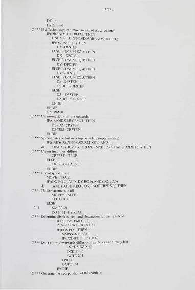
DZ~o
DZDIFF"'\1
- 302-
C ... If diffusion step. can mo'c in <Hl} of si'\ directions IF(DRANDS LT DIFFCL)THEN DNUM~ I tDINT(6 ODO'DRANDS/DIFFCL) IF(DNUM EQ !)THEN
DX~DFSTEP
ELSEJF(DNUM EQ 2)TIIEN DX~-DFSTEP
ELSEJF(DNUM EQ.1)TIIEN DY~DFSrEP
ELSE IF(DNUM EQ •>TIIEN DY~-DFSTEP
ELSE IF(DNUM EQ S)TIJEN DZ~DFSTEP
DZDJFF~DFSTEP
ELSE DZ=-DFSTEP DZDIFF=-DFSTEP
ENDIF ENDIF DZCRM~o
C ••• Crc.1ming step· al\\a~s up\\ards IF(CRANDS LE CRMCL)TIIEN
DZ~DZtCRSTEP
DZCRM~CRSTEP
END IF C ••• Spcci:-.1 cases of lost o'er top bound.11) (top:rm- falsc)
IF(( IABS(DZDIFF)+DZCRM) GT 11 AND & GOSCAF(DUMM) LE.(DZCRM/(DZCRM+IABS(DZDIFF))))TIJEN
C • •• Cream firs t. then di fTusc CRFRST=.TRUE
ELSE CRFRST= FALSE.
END IF C •u End of special case
MOVE= TRUE IF((DX EQ O) .AND (DY EQ 0) AND (DZ EQ 0)
& AND (DZDIFF EQ O.OR (NOT CRFRST)))TIIEN C ••• No displacement at all
MOVE= FALSE. GOT02112
ELSE 20 1 NM Jss~o
DO 101 I= J.SIZECL C ••• Determi ne displacement and obstruction for each part1clc
I FOCUS~TEMPCL(I)
POS=LOCATE( IFOCUS) IF(POS EQ O)TIIEN
NMISS=NM ISS+ I IF(DZDIFF LTO)TII EN
C .... Don't allo" d0\\11\\0Uds ditTusion if p..ut iclcs arc a I read~ lost DZ~DZ-DZDI FF
DZDIFF=O GOTO 20 1
ENDIF GOTO IIII
END IF c • • • Generate the llC\\ position or this particle
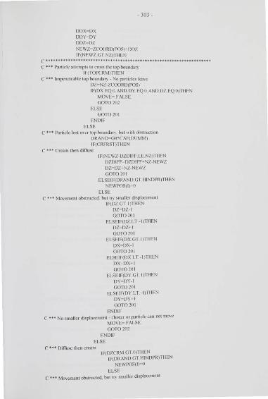
- 303-
DDX,DX DDY" DY DIJZcDZ NEWZ~ZCOORD(POS)<DDZ
IF(NEIVZ GT NZ)TIIEN c•••••••••••••••••·••••••••••••••••••••••••••••••••••••••••••••••••• C ••• Particle attempts to cross the top bound'l!)
IF(TOPCRM)TIIEN C ••• lmp::nct rabl c top bound:.H) -No particles lca'c
DZ~NZ-ZCOORD(POS)
IF(DX EQ 0 AND DY EQ 0 AND DZ.EQ O)TIIEN MOVE• FALSE GOT0202
ELSE GOTO 20 1
ENDIF ELSE
C ••• Particle lost O\Cr top bound1l). but ''ith ob<;tmction DRAND-GOlC AF(DUMM) IF(CRFRST)TIIEN
C ••• Cream then diffuse IF(NEIV7-DZDIFF LF NZ)TIIEN
DZDIFF- D?DIFF< NZ-NEIVZ DZ~DZ< NZ-NEIVZ GOT0201
ELSEIF(DRAND GT IIINDPR)TIIEN NEIVPOS(I}- O
ELSE C .... Mo,cmcnt obstructed. but tn smaller displacement
IF(DZ GT I )TIIEN DZ- DZ-1 GOT020I
ELSEIF(DZ LT-I)TIIEN DZ- Dlt I GOT020 1
ELSEIF(DX GT I )TIIEN DX- DX-1 GOIO 201
ELSEIF(DX LT - I )TIIEN DX- DX..f I G01'020I
ELSF IF(DY GT I)TIIEN DY, DY-1 GO"IOZOI
ELSEIF(DY LT - I )TIIEN DY- DYH GOT02111
END IF C ••• No smaller displacement -cluster or particle can not 11101 c
MOVE" FALSE GOT0202
END IF ELSE
C ... Diffuse then cream IF(DZCRM GT O)TIIEN
IF(DRAND GT IIINDPR)THEN NEIVPOS(I)- O
ELSE C ••• Mo,cment obstructed. b\11 tr) smaller dic;placemcnt
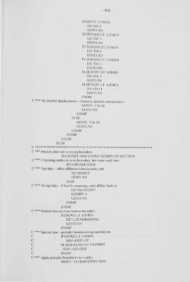
- 304-
IF(D7 GT I)TIIEN DZ- DZ-1 GOT0201
ELSEIF(DZ LT - I )TIIEN DZ- DZ + I GOT020 1
ELSEIF(DX GT I )TJJEN DX- DX-1 G01"020 1
ELSEIF(DX LT - I )TIIEN DX=DX-f I GOT020 1
ELSEIF(DY GT I )TII EN DY DY-1 GOT020 1
ELSEIF(DY LT - IJTIIEN DY- DY+l GOT0211 1
END IF (' •• • No smaller displacc1ncnt -cluster or p.1rticlc can nollllO\ c
MOVE~ FALSE GO r02112
ENDIF ELSE
MOVE= FALSE GOT0202
END IF END IF
END IF ELSE
c •.••.•..••••••.•••••••••••••.•••.•••••••..•.•.••••••••....•••.••.•• C .... Particle does not cross top bound.al)
IF(CRFRSTAND (NEIVZ-DZDIFF) GT NZ)TIIEN C ••• Crea ming makes it cross boundar:o. but ends inside box
IF(TOPCRM)TIIEN C .... Top bdr) - allo'' difTusion (dm' nwards) on I~
DZ=DZDIFF GOT0201
ELSE C ... No top bell) - if lost b) creaming. can't diffuse back in
DZ- DZ-DZDIFF DZDIFF- O GOT0211 1
ENDIF END IF
C ... Particle tries to cross bottom boundm~ IF(NEIVZ LT I)TIIEN
DZ~ I-ZCOORD(PDS)
GOT0201 ENDIF
C ••• Special case- periodic boundaries top and bollom C IF(NEWZ.LT I)TIIEN C DDZ=DDZtNZ C ELSEIF(NEWZ.GT NZ)TIIEN C DDZ=-NZ' DDZ C ENDIF C ••• Apply p::riodic bound1 rics to x and )
NEWY=YCOORD(PDS) t DDY
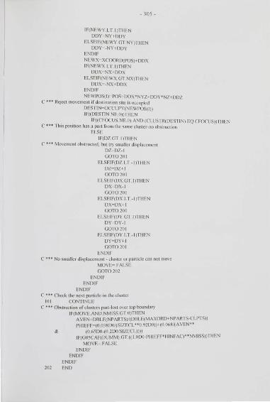
- 305-
IF(NEWY LT I )THEN DDY~NY+DDY
ELSEIF(NEIVY GT NY)TIIEN DDY=·NY+DDY
ENDIF NEWX~XCOORD(POS)+DDX IF(NEWX LT I )TIIEN
oox~Nx .. oox ELSEIF(NEWX GTNX)Tl iEN
DDX' -NX+DDX ENDIF NE\VPOS(I).,...POS+DDX•NYZ I DDY * N7 .-ooz
C ••• Reject mO\ Cmcnt if destination site is occupied DESTIN- OCCUPY(NEWPOS( I)) IF((DESTI N NE.O))TIIEN
IF((CFOCUS NE 0) AND (CLUS rR(DES ri N).EQ CFOCUS))THEN C ... This position has a part from the same clustcr·no obstruction
ELSE IF(DZ GT I )THEN
C ... Mo,cmcnt obstmctcd. butt!} smaller displacement DZ~DZ-1
GOT020 1 ELSE I F(DZ LT - I )Til EN
DZ- DZ >I GOT020I
ELSEIF(DX GT I )THEN DX~DX-1
G0f020 1 ELSEIF(DX LT - I )THEN
DX,...DX+ I GOT020 1
ELSEIF(DY GT l)THEN DY- DY-1 GOT0201
ELSEIF(DY LT-l)"IHEN DY.,.. DY-+ 1 GOT020 1
ENDIF C ••• No smaller displacement- cluster or p::nt1clc ca n notmO\C
MOVE~ FALSE. GOT0202
END IF ENDIF
END IF C ... Check the nC'-1 particle in the cluster
101 CONTINUE C ••• Obst ruct ion of clusters part-lost O\CT top bound..1f!
IF(MOVEAND NMISS GT O)TIIEN A VEN- DBLE(NPARTS)/(DBLE(MAXORD I NPAR I S-CLPTS)) PIII EFF- (0018DU/(SIZECL .. 0_9200))+(0 068/(A VEN••
& (0 65D0-(0 200/SIZECL)))) IF(G05CAF(DUMM) GT (( I ODO-PIIIEFF'IIINFAC) .. NM ISS))TIIEN
MOVE~ FALSE. ENDIF
ENDIF END IF
202 END
-306-
c •••••••••••••••••••••••••••••••••••••••••·•••••··••••••••••••••••••••• SUBROUTINE MOVECLUSTER(NXYZ. NPARTS.MAXPTS.MAXORD.MAXCL.CLPTS. & NLOSl .OCCUPY.LOCATE.CPARTS.CLUSTR.SIZE.POINTR. & CORDER.CNUM.NEWPOS.TEMPCL. & CORD.CFOCUS.POINT.PT _ I.SIZECL)
c••••••••••••••••••••••••••••••••••••••••••••••••••••••••••••••••••••• C ••• Execute d•splaccmcnt of cluster to ne" position
INTEGER NXYZ.NPARTS.MAXPTS.MAXORD.MAXCL.CLI'I S.NLOST. & OCCUPY(NXYZ).LOCATE(MAXPTS).CPARTS(MAXI'fS).CLUSTR(MAXPTS). & SIZE(MAXCL).POINTR(MAXCL).CORDER(MAXCL).CNUM(MAXCL). & NEWPOS( II ()()()()).TEMPCL(II()(XXl). & l.NBROKE. IFOCUS.POS.CFOCUS.SIZECL.POJNT.CORD.PT_ l
NBROKE- 0 DO 10 1 1- l.S IZECL
IFOCUS- TEMPCL( I) POS LOCATE(IFOCUS) IF(POS NE.O)TIIEN
IF(OCCUPY(POS) EQ IFOCUS)TIIFN OCCUPY(POS)- 0
END IF IF(NEWPOS(I) EQ O)TIIEN
LOCATE(IFOCUS)-O NLOST- NLOST+ I
ELSE LOCA TE(IFOCUS)- NEWPOS(I) OCCUPY(NEWPOS(I))- IFOCUS
ENDIF END IF
101 CONTINUE END
c•••••••••••••••••••••••••••••••••••••••••••••••••••••••••••••••••••• SUBROUTINE BONDS(NX.NY.NZ.NYZ.NXYZ.NPARTS.MAXPTS.MAXORD.MAXCL.
& CLPTS.XCDORD.YCDORD.ZCOORD.OCCUPY.LOCATE. & CPARTS.CLUSTR.SIZE.POINTR.CORDER.CNUM. & DONDPR.BREAK.BONDED. INVPOS. & TEMPCL.SIZECL.INIT)
c•••••••••••••••••••••••••••••·••••••••••••••••••••••••••••••••••••••• C ... Bond formation and breakage" ith all ncighburs
INTEGER NX.NY.NZ.NYZ.NXYZ.MAXPTS.NPAR rS.MAXORD.MAXCL.CLPTS. & XCOORD(NXYZ).YCOORD(NXYZ).ZCOORD(NXYZ). & OCCUPY(NXYZ).LOCATE(MAXI'rS).CPAR I S(MAXPTS).CLUSTR(MAXPTS). & SIZE(MAXCL).POINTR(MAXCL).CORDER(MAXCL).CNUM(MAXCL). & TEMPCL( II!X)()()).CFOCUS.SIZECL. & I. IPOS.POS.INEIGH. IFOCUS.IM INM.IMINP.DELTA(6).1NVP0S(6)
DOUBLE PRECISION BONDPR.BREAK.G05C AF.DUMM LOGICAL BONDED(MAXPTS.6).1NIT EXTERNAL G05CAF IFOCUS- TEMPCL(I) CFOCUS- CLUSTR(IFOCUS) POS- LOCATE( IFOCUS) DO 10 1 1- I.S IZECL
C ••• Find posi tions of neighbours of each particle in cluster IFOCUS- TEMPCL( I) POS- LOCATE( IFOCUSJ IF(POS NE O)TIIEN
IF(ZCOORD(POS) EQ NZ)TIIEN C ••• Miss out +; check
- 307-
IMI NJ>-=-1 IMI NM- 2
ELSEIF(ZCOORD(POS) EQ 1 )TIIEN IMIN~ I
IMINM- < C ... Miss out ·7 check
ELSE IMJNp-, J
IM INM "'"'2 ENDIF DELTA(I)- 1 DELT A(2)- - l
C ••• Periodic z-boundarics C IF(ZCOORD(POS) EQ NZ)THEN C DELTA(I )" I -NZ C ELSE C DELTA(I)- 1 C ENDIF C IF(ZCOORD(POS) EQ I )TIIEN C DELTA(2)- - I+NZ C ELSE C DELTA(2)- -1 C ENDIF C ... Periodic ?-boundaries -end
IF(YCOORD(POS) EQ NY)TIIEN DEL TA(l)- NZ-NYZ
ELSE DEL TA(1)- NZ
END IF IF(YCOORD(POS).EQ I)TIIEN
DELTA(<)- -NZ+NYZ ELSE
DELTA(<)--NZ ENDIF IF(XCOORD(POS) EQ NX)TIIEN
DEL TA(l)-NYZ-NXYZ ELSE
DEL T A(l)- NYZ ENDIF IF(XCOORD(POS) EQ I )TIIEN
DELTA(6)- -NYZ+NXYZ ELSE
DEL T A(6)- -NYZ END IF 00 102 IPOS- IMINP.6.2
C ... Check -f7.+).-+ x neighbours for form/break bonds CFOCUS- CLUSTR(IFOCUS) INEIGII-QCCUPY(POS+DEL TA(IPOS)) IF(BONDED(IFOCUS.IPOS)) riiEN
IF(G05CAF(DUMM) LT BREAK)THEN C ••• If OOndcd to thi s neighbour. break bond
BONDED(IFOCUS.IPOS)- FALSE. BONDED(INEIGIUNVPOS(IPOS))" FALSE.
C ••• Spl it the cluster if this bond held it together CALL SPLITCLUSTER(NX.NY.NZ.NYZ.NXYZ.MAXI'TS.
& M AXORD.MAXCL.OCCUPY.LOC A TE.XCOORD. YCOORD. & ZCOORD.CLI'TS.CPARTS.CLUSTR. & SIZE.POINTR.CORDER.CNUM. & IFOCUS.CFOCUS.INEIGH.BONDED)
&
ENDIF ELSE
- 308-
IF( INEIGII NE O)TI IEN IF(CLUSTR(IFOCUS) NE.O AND
(CLUSTR(INEIGII) EQ CLUSTR(IFOCUS)))TIIEN *** . I~(GO~CAF(DUMM) LT BONDPR)TI !EN
C Form a bond bch\CCil pmt1clcs 1n same cluster BONDED(IFOCUS.IPOS)- TRUE BONDED(INF IGII.INVPOS(IPOS))' l RUE
END IF ELSE
IF(G<l5CAF(DUMM) LT BONDPR)THEN C ••• Form a bond and merge clustcrs/p..1rticlcs
102
& &
BONDED( IFOCUS. IPOS)- TRUE BONDED(INEJGII.INVPOS(IPOS))' TRUE CALL BONDNEIGIIBOURS( IFOCUS. INEIGII.MAXPTS.
END IF ENDIF
ENDIF ENDIF
CONTINUE IF(. NOT INIT)TIIEN
MAXCL.CLUSTR.CPARTS.SIZE.MAXORD.CLPTS POINTitCORDER.CNUM) .
IX> 101 IPOS=IMINM.6.2 C •u Check -7.-~.-'1: for llC\\ ncighboursonh C ... Don't do this for in itia lisation - then ci1cck ing ALL particles
I NEIGII-QCCUPY( POS I DELTA( IPOS)) IF((INEIGII NE 0) AND (CLUSTR(INEIGII) NE CLUS I"R
& ( I FOCUS)) AND (G<l5CAF(DUMM) LT BONDPR))TIIEN C ••• Form a bond and merge clusters/p.uticlcs
103
& &
BONDED(IFOCUS.IPOSI TRUE DONDED( I NE IGII .INVPOS(II'OS))~.TRUE
CALL BONDNE IGI IIJOURS(IFOCUS. INEIGI I.MAXPTS. MAXCL.CLUSTitCPARTS.SIZE.MAXORD.CLP'I S. I'O I NTR.CORDER.CNU~ I )
END IF CONTINUE END IF
END IF 10 1 CONTINUE
END
c••••••••••••••••••••••••••••••••••••••••••••••••••••••••••••••••• SUBROUTINE BONDNEIGHDOURS(IPART. INEIGI I.MAXP'fS.MAXCL.CLUSTR.
& CPARTS.SIZE.MAXORD.CLP'I"S.POIN"I R.CORDER.CNUM) c••••••••••••••••••••••••••••••••••••••••••••••••••••••••••••••••••• C ••• Make a OOnd bct\\CCIII\\0 particles- in same cluster or different
INTEGER MAXORD.MAXPTS.MAXCL.CLPTS. & CPARTS(MAXPTS).CLUSTR(MAXPTS).SIZE(MAXCL). & POINTR(MAXCL).CORDER(MAXCL).CNUM(MAXCL). & IPART. INE IGH.CNEIGH.CPART.CI. NUM.ORDNXT.ORDNEI.ORDPT. & FIRST.NPART.PPART.PTNXT.NEINXT.PNEIGH.NNEIGII. & I.POINT I .TP.TEMP(O. I IOO<Xl)
CNEIGI I-CLUSTR(INEIGI I) CPART-CLUSTR(IPART) IF(CPART EQO)TIIEN
C ••• The part icle is smglc. not in a cluster
- 309-
IF(CNEIGII NE O)THEN C ••• The neighbouring p.1rticlc tx:longs to a cluster
ORIJNXT- CORDER(CNEIGII) I I POINTI - PQINTR(ORDNXT) DO 101 1- CLPTS.POINTI.-1
CPARTS(I+ I)~CPARTS( I) 10 1 CONTINUE
DO 1112 1- 0RDNXT.MAXORIJH POINTR(I)- POINTR(I) I I
1112 CONTINUE CLPTS- CLPTS+ I CLUSTR( IPART)- CNEIGI I CPARTS(POI NT I )~ I PART
SIZE(CNEIGII)- SIZE(CNEIGII)' I ELSE
C ... The neighbour is a si ngle particle MAXORD- MAXORIJ I I CLNUM- CNUM(MAXORIJ) SIZE(CLNUM)- 2 CPARTS(CLPTS+ I )- IPAR r CPARTS(CLPTS+2)- INEIGII CLPTS CLPTS+2 POINTR(MAXORIJ+ I >- CLPTS+ I CLUSTR( IPART)- CLNUM CLUSTR(INEIGII)- CLNUM CORIJER(CLNUM)- MAXORD
END IF ELSE
C . .. The particle IS in a cluster C ... ·1 he neighbouring particle is in a different cluster or single
ORDPT- CORDER(CPART) IF(CNEIGII NE O)THEN
C ••• The ncighlx>ur is in a cluster ORDNEI- CORDER(CNEIGII) IF(ORIJPT LT ORDNEI)TIIEN
C •• • T he particle's cluster is higher in the arra~ list Sort arra~s P1'NXT=ORDPT+ I F I RST~POI NTR(PTNXT)
PNEIGII- POINTR(ORDNEI) NNE IG I I~SIZE(CNEIG I I)
DO 101 1- 0.NNEIGII-1 TEMP(I)- CPARTS(PNEIGH+I)
101 CONTINUE DO HI-' I=PNEIGII -I.FIRST.-1
CPARTS(I ! NNEIGII)- CPARTS(I) IO< CONTINUE
DO 105 1--<I.NNEIGH-1 T""TEMP(I) CPARTS(FIRSH 1)- TP CLUSTR(TP)- CPART
105 CONTINUE DO 106J=PTNXT.ORDNEI- 1
POINTR(I)- POINTR(I)' NNEIGII 1116 CONTINUE
MAXORD- MAXORD- 1 DO 107 I~ORDNE I.MAXORD
Ti"-CNUM(I+I) CNUM(I)~TP
CORDER(TP)~I
- 310-
POINTR(I)• POINTR(H I ) 107 CONTINUE
POINTR(MAXORDH) CLPTS+ I CNUM(MAXORDH) CNEIGII SIZE(CNEIGII)- O SIZE(CPART)- SIZE(CPAR r) •NNEIGII
ELSE C ••• The neighbours cluster is higher 111 the ami\ list Sort aml\S
PNEIGII- POINTR(ORDNEI) . PPART• I'OINTR(ORDPT) NEINXT- ORDNEH I NPART• SIZE(CPAR I) NNEIGII- SIZE(CNEIGII)
C .... E'l:trnct thc p.1rticlcs in the particle's cluster. thcn shunt d0\\11 00 IOR 1- 0.NNEIGII - 1
CLUSTR(CPARl S(PNEIGII I I))- CPART 108 CONTINUE
DO 1091 O.NPAR I -1 TEMP(I)• CPARTS(PPART+I)
109 CONTINUE DO 110 1- PPART-LPNEIGII .-1
CPAR"I S(li NPAR I ) CPAR rS(I) 110 CONTINUE
DO Ill I O.NPART- 1 CPARTS(PNEIGII+I)- TEMP( I)
Ill CONTINUE CORDER(CPART)- ORDNEI CNUM(ORDNEI) CPARr DO 11 2 1- NEINXLORDI'r- 1
POINTR(I)- POINTR(I)+ NPART 11 2 CONTINUE
MIIXORD- MAXORD- 1 DO 11 1 1-QRDPT.MAXORD n~CNUM(H I ) CNUM(I)• TP CORDER(TP) I POINTR(I)- POINTR(Ii I)
111 CONTINUE POIN"IR(MAXORDI!) CLPTS I I CNUM(MAXORDH) CNEIGII SIZE(CNEIGH)-0 SIZE(CPART)- NPIIR r I NNEIGII
END IF ELSE
C ..... The neighbour is a single particle FIRST POINTR(ORDPT+ I) DO I I' 1- CLPTS.FIRST.-1
CPARTS(I+ I )- CPARTS(I) 114 CONTINUE
00 11 .5 1 ORDJYf + I.MAXORDH POINTR(I) POINTR(I)H
11 5 CONTINUE CLPTS.,.CLPTS+ I CPARTS(FI RST)- INEIGII CLUSTR(INEIGII)- CPART S17E(CPART)• SIZE(CPART)+ I
ENDIF ENDIF END
-311 -
c••••••••••••••••••••••••••••••••••••••••••••••••••••••••••••••••••• SUBROUTINE SPLITCLUSTFR(NX.NY.NZ.NYZ.NXYZ.MAXPTS.M/\XORD.MAXCL.
& OCCUPY.LOCATE.XCOORD.YCOORD.7COORD.CLPTS.CPARTS.CLUSTR. & SIZE.POINl R.CORDER.CNUM. & IFOCUS.CFOCUS.INFIGII.BONDEDI
c ••••••••••••••••••••••••••••••••••••••••••••••• •••••• •••••• •••••••• C ••• Does the cluster split ''hen a bond has been brokcn'J
INTEGER NX.NY.NZ.NYZ.NXYZ.MAXORD.M/\XPTS.MAXCL.CLPTS. & OCCUPY(NXYZI.LOC/\TE(M/\XPTS). & XCOORD(NXYZ).YCOORD(NXYZ).ZCOORD(NXYZ). & CPARTS(M/\XPTS).CLUSl R(MAXPTS).SIZE(MAXCL). & POINTR(MAXCL).CORDER(MAXCL).CNUM(M/\XCI.). & IFOCUS.INEIGII.NN.NP.P( II!KKKJ).NCL.PT I.CFOCUS. & II.III.CLNUM.CORD.POINT.FIRST.PPP."I EMP
LOGICAL BONDED(MAXPTS.6).DISCON.NOLNKN.NOLNKP
CORD-CORDER(CFOCUS) POINT- POINTR(CORD) PT 1- POINT·I NC-L- POI NTR(CORD+ I )-POI NTR(CORD) IF(NCL.EQ 2)TIIEN
C ••• The cluster ,,;JJ split into '''o single p..1rticlcs CLJYfS-CLPTS-2 CLUSTR(CP/\RTS(POIN"I n-o CLUSTR(CPARTS(POINT+ I ))-0 00 10 1 11- POINT.CLJYI S
CPARTS(II ) CP/\RTS( II+2)
10 1 CONTINUE MAXORD MAXORD-1 00 102 11-CORD.MAXORD
CNUM(II)-CNUM(III I ) CORDER(CNUM{I I)) 11 POINTR(II) POINTR(II + I )-2
102 CONTINUE POINTR(MAXORD+ 1)-CLM Stl CNUM(MAXORD+ I )-CFOCUS SIZE(CFOCUS) 0
C ••• Fin;~t~t~10,, man\ and "hich part1clcs arc connected to I NEIG H c /\LL A -ri·AcHEDPAR r s1Nx.NY.NZ.NY7.NXYZ.MAXJYr S._MAXCL .•
& OCCUPY .LOCATE.XCOORD. YCOORD.ZCOORD.CLUS I R.BONDED. & INEIGII.IFOCUS.P.NN.O.CFOCUS.M/\XCL+ I.DISCON.NOLNKN)
IF(DISCON)TIIEN . . C ... INEIGII is no longer connected to a lithe JXIfllclcs Ill cluster
C *** Unless it is b) a bridge abo\c the top bou nd.1 r:o MAXJ7f$ MAXCL CALL /\TI"ACIIEDPARl S(NX.NY.NZ.NYZ.NXYZ. . .
OCCUPY LOCATE XCOORD. YCOORD.ZCOORD.CLUS I R.BONDED. ! IFOCUS.I.NEIGII.P .. NP.NN.CFOCUS.M/\XCL+2.DISCON.NOLNKI')
IF(NOLNKN OR NOLNKP)TIIEN C ••• Exclude brc.1kagc ;r ma~ be linked above top bou ndar~
IF(NOLNKN AND NN EQ I )TIIEN
C ... The single particle \NEIGII bre:1ks ofT CLUSTR(INEIGII)-O CLJYr S-CLJYrS- 1 OO IOJ u - POINT.POINT+NCL-1
lf( INEIGII EQ CP/\RTS( II ))THEN FIRST- 11 GOT0201
ENDIF
- 312-
101 CONTINUE 201 DO 104 II ~FIRST.CLPTS
CI'/\RTS(II ) CP/\RTS(II+ I ) 104 CONTINUE
SIZE(CFOCUS)- SIZEiCFOCUSl-1 DO 105 II~ I .NP
CLUSTR(P(NN HI))- CFOCUS 105 CONTINUE
DO 106 II,...CORD 1 t.MAXORD H POINTR(II) POINTR(II )- 1
106 CONTINUE ELSEIF(NOLNKP /\ND NP EQ I )TIIEN
C ... The single p;~rticlc I PART breaks oiT CLUSTR(IFOCUS) 0 CLPT S- CLPTS- 1 DO 107 11- POINT.POINTtNCL- 1
IF( I FOCUS EQ CI'/\RTS(II ))TIIEN FIRST~ II
GOf0202 ENDIF
107 CONTINUE 202
108
109
IIU
DO IOR II=FIRST.CU YJ'S CPARTS(II)- CPARTS(II+ I )
CONTINUE SIZE(CFOCUS) SIZE(CFOCUS)-1 DO 109 11 - I.NN
CLUSTR(P(II )) CFOCUS CONTINUE DO 110 II ....,.CORDI I.MAXORD+ I
POINTR(II ) POINTR(II)- 1 CONTINUE
ELSE C ..... The cluster breaks into h\ O cluslcrs
MAXORD~MAXOI\Dtl
CLNUM~CNUM(MAXOI\D) POINTR(MAXORD+ I )- CLPTS t I DO Ill II- MAX01\D.CORD+2.-1
CNUM(II)- CNUM(II -1) POINTR(I I) POINTR(II- 1) CORDER(CNUM(II))- 11
Ill CONTINUE CNUM(CORD)- CLNUM CNUM(CORDt l )- CFOCUS CORDER(CLNUM)- CORD CORDERiCFOCUS) CORD+ I IF( NOTNOLNKPfi iiEN
C ••• Lost particles arc attached to !FOCUS FIRST- POINT DO 11 2 11 ~ 1 .NN
PPP-P(II) CLUS I R(PPP)- CLNUM DO 111 111- POINT.POINTINCL-1
IF(PPP EQ CP/\RTS(III ))TIIEN TEM P- CP /\RTS(FI RST) CPARTS(FIRST)~PPP
CPARTS(III )- TEMP FIRSI - FIRST+I 0010112
ENDIF
- 313-
il l CONliNUE 11 2 CONTINUE
DO 11"'11 --= I. NP CLUSTR(P(NN+ /1 )) CFOCUS
I I' CONTINUE S IZE(CLNUM)~NN
SIZE(CFOCUS) NCL-NN POINTR(CORD >I )-PQINTR(CORD); NN
ELSEIF( NOTNOLNKN)THEN C ... Lost pmt iclcs belong to JNEIGII
11 6 11 5
11 7
FlllST' POINT DO 11 5 JJ - I .NP
PPJ>-P(NN-+ 11 ) CLUSTR(J'PP)- CLNUM DO 11 6 111 PO INT.POINT INCL- 1
IF(PPP EQ CPARTS(III ))THEN TEM I'"CPARTS(FI RST) CPAR I S(FIRST)- PPP CPARTS( III )~TEMP
FI RST- FIRST • I GO I O 11 5
END IF CONTINUE
CONTI NUE DO 11 7 11 I. NN
CLUSTR(P( 11 ))- CFOCUS CONTINUE SIZE(CLNUM) NP SIZE(CFOCUS) NCL-NI' POINTR(CORD >I )-POINTR(CORD)' NI'
ELSE C ••• No particles arc lost in thi s cluster (normal. for topcnn- truc)
DO IIR JJ - J.NP C'PARTS(IYI" I HI)- P(NNI/ 1) CLUSTR(I'(NN HI))- CLNUM
II R CONTINUE SIZE(CLNUM)- NP DO 11 9 11 - J.NN
CPARTS(PT 1+1/ >NP) P(l l) CLUSTR(P(Ii))· CFOCUS
11 9 CONTINUE SIZE(CFOCUS)- NCL-NP POINTR(CORD H )- POIN"I R(CORD)' NP
ENDIF ENDIF
ELSE C ••• I FOCUS and INE IGII arc connected abo\C top boundal")
DO 120 11' /.NN CLUSTR(P( /1 )) CFOCUS
120 CONTINUE DO 121 11 - J.NP
CLUS"I R(P(NN HI WC FOCUS 121 CONTINUE
ENDIF EL SE
C ••• Particle and neighbour arc still connected DO 122 JJ- J.NN
CLUSTR(P(II ))- CFOCUS 122 CONTI NUE
- 314-
ENDIF END IF END
c••••••••••••••••••••••••••••••••••••••••••••••••••••••••*•••••••••• SUBROUTINE An'ACHEDPARTS(NX.NY.NZ.NYZ.NXYZ.MAXPTS.MAXCL.
& OCCUPY.LOCATE.XCOORD.YCOORD.ZCOORD.CLUSTR.BONDED. & IFOCUS.IOBJ.P.N.LASTEL.CFOCUS.CLNUM.DISCON.NOLINK)
c••••••••••••••••••••••••••••••••••••••••••••••••••••••••••••••••••• C ••• Find all the particles'' hi eh arc bonded to th1s p.1rticlc C ••• to determine'' het her the cluster splits" hen bond breaks
INTEGER NX.NY.NZ.NYZ.NXYZ.MAXPTS.MAXCL. & OCCUPY(NXYZ).LOCATE(MAXPTS). & XCOORD(NXYZ).YCOORD(NXYZ).ZCOORD(NXYZ).CLUSTR(MAXPTS). & IFOCUS.IOBJ.CFOCUS.P( II OOOQ).N.CLNUM. & I.II.IPAR r.IMIN.POS.NOLD.NNEW.DELTA(6).LASTEL
LOGICAL NEW.BONDED(MAXPTS.6).DISCON.NOLINK
DISCON• "I RUE NOLINK•.TRUE NOLO I NNEW• I P(LASTEL+ I )- IFOCUS CLUSTR( IFOCUS)• CLNUM N- 1
20 1 NEW• FALSE DO 10 I 1- NOLD.NNEW
IPARToP(LASTELH) POS• LOCATE(IPART)
C ... Periodic boundnries top and bottom· code rcmo'cd C ••• Generate rclath c positions of neighbours
IF(YCOORD(POS) EQ NY)TIIEN DELTA(l)• NZ-NYZ
ELSE DELTA(1)• NZ
ENDIF IF(YCOORD(POS) EQ I)TIIEN
DELTA(4)• -NZ+NYZ
ELSE DELTA( 4 )•-NZ
ENDIF IF(XCOORD(POS) EQ NX)TIIEN
DELTA(5)- NYZ-NXYZ
ELSE DELTA(5)- NYZ
ENDIF IF(XCOORD(POS) EQ I )TIIEN
DEL T A(6)• -NYZ• NXYZ
ELSE DEL T A(6)--NYZ
END IF C ••• Check for bonds at z bound.·uics
IMI N- 1 DELTA( I )- 1 DEL TA(2)-- I
IF(ZCOORD(POS) EQ_ I )THAE:D CLUSTR(OCCUPY(POS • DELTA( I ))) IF(BONDED(IPARL I )
& NE CLNUM)TI IEN C ••• The particle is bonded and hasn't been counted alread)
NEW- TRUE N- N+ l
- 3 15-
CLUSTRtOCCUPY(POS< DEL 1 A( I IWCLNUM P(LASTEL+N)~OCCUPY(POS 1 DELTA( I)) lf(P(LASTEUN) EQ IOIJJ)TIIEN
C ••• It is dclinitcl) connected to the other particle DISCON~ FALSE GOT0202
ENDIF END IF IMIN~1
ELSEIF(ZCOORD(POS) EQ NZ)TIIEN IMIN •2 IF(BONDED( IPART. I ))TIIEN
C ••• A bond crossi ng the top boundary NOLI NK ~- FALSE.
END IF ENDIF DO 102 n~IMI N.6
C ... Check each neighbour to sec if 11 is att;1chcd IF(BONDED(IPART.I I) AND CLUSTR(OCCUPY(POSIDELTA(II)))
& NE CLNUM)THEN NEW~ TRUE N=N+- 1 CLUSTR(OCCUPY(POS I DELTA(II)))~CLNUM P(LASTEL< N)~OCCUPY(POS+DELT A( I I)) IF(P(LASTEL+N) EQ IOBJ) I"IIEN
C ... ll is definite!) connected to the other particle DISCON~ FALSE GOT0202
ENDIF END IF
102 CONTINUE I 0 I CONTINUE
IF(NEW)TIIEN C ••• The last set found ne'' particles'' hich arc attached C ••• Repeat to check their neighbours
NOLD~NNEW+ I NNEW~N
GOT020 1 ENDIF
202 END
c•••••••••••••••••••••••••••••••••••••••••••••••••••••••••••••••••• SUBROUTINE CALCINTERFACE(NXY.NZ.VOL.PIII.ZINT)
c •••••••••••••••••••••••••••••••••••••••••••••••••••••••••••••••••• C •u Calculate the scrum la, er interface position C ••• Based on definition of-a "uniform" region of const ' ol fract
INTEGER NZ.ZINT.VOL(NZ).ZZ.NXY DOUBLE PRECISION PIILVV DO 101 zz~2.NZ- I
VV" DBLE(VOL(ZZ)+ VOL(ZZ- 1) > VOL(ZZ + I ))/(3 ODO'NXY) IF(VV GT 0 9DO'PHI)THEN
ZINT~zz
GOT0201 ENDIF
101 CONTINUE 20 1 END
- 316-
c .••••••••••••••••••••••••••••••••••••••••••••••••••••••••••••••••• SUBROUTINE DENSITYDIS.I RIB(NX.NY.NZ.NYZ.NXYZ.NZ2.MAXPTS.NPARTS.
& NSTEPS.OCCUPY.LOCATE.XCOORD. YCOORD.ZCOORD.CLUS rR. & ZINT.GG.RSTEP.PIII.MMIN.MMAX.NLA YS)
c••••••••••••••••••••••••••••••••••••••••••••••••••••••••••·••••••· C ••• Calcu late dcnsit~ dtstribution G(R) of parttclcs in spherical C ... she lls (R)-(R .. dR)
INTEGER NX.NY.NZ.NYZ.NXYZ.MAXPTS.NPARTS. & XCOORD(NXYZ).YCOORD(NXYZ).ZCOORD(NXYZ). & OCCUPY(NXYZ).LOCATE(MAXPTS).CLUSTR(MAXJYI S). & ZINT.NZ2.NSTEPS.NLAYS.N(25<XI).MM IN(NZ2).MMAX(NZ2). & XC. YC.ZC.DELX.DEL Y.DELZ.POS.POSC.XYPOS.XPOS. & I.II.JMID.IZ.IG.NC.NAVE.NUM.NCOORD.NCOUNT.NL.MAXR.MAXR2. & IR2.ZMID.ZMDBOT.ZMDTOP.M IN.MAX.ZMIN.ZMAX.LOW.I IIGII. & IP.CL(50!XI).NJYrS.NSINGL.NCLUST.NM ID.ZMD(20).NBOT.NTOP
DOUBLE PRECISION ROlJLDD.RSTEP.RSTEP2.PIII. & G(SOO).SUMG.GG(NZ2.NSTEPS)
LOGICAL FRSTP
RS.I EP2~RSTEP'RSTEP NL~NLAYS
oo IOII~ J.Soo
G(I)- O.ODO 10 1 CONTINUE
00 102 I ~ J.NZ2
N(I)-Q 102 CONTINUE
C ••• Onl} calc in the uniform conccntratton region- define limits 205 ZMJD- NINT(REAL(NZ+ZINT)/2 0)
MAXR~ II
MAXR2 ,..,.MAXR*MAXR MAX- I +INT(O 99999J)O'DBLE(MAXR-I )/RSTEP) NBOT~( I HNT(O 9999'REAL(ZINT-I +(MAXR-I)+NLAYS)/5 0))
ZMDBOT~S'NBOT NTOP--INT( I ()()00 I'REAL(NZ-(MAXR-I)·NLA YS- IU)/10.0)
ZM[)TOP--IO'NTOP C *** Calculate the heights to calculate distrib- in uniform region
IF(M0[)(NBOT.2) EQ O)TIIEN C ••• Bottom one is a multiple of 10
NMID- 1 ZMJJ( I )- ZMDBOT DO 103 I- 2.NTOP • I
ZMD( I)- ZMD(I· I )+ IO IF(ZMD(I) G r ZMDl OP)TJJEN
GOT0201 ELSE
NMID~NM ID+ I
ENDIF 103 CONTINUE 20 1 CONTINUE
ELSE C +tt 13ottom one is a multiple of 5
NM I[)• I ZMD( I)- ZMDBOT ZM[)BOT~ZM[)BOT·S DO 104 1- 2.NTOP-t I
ZM[)( I )~ZM[)BOT<( I -1)' 1<1 IF(ZMJJ(I) GT ZMDTOP)TIIEN
GOT0202
ELSE NMilr"NMID+ I
ENDIF 104 CONTINUE 202 CONTINUE
ENDIF
- 317-
C ... Calculate an <ncragc coordinatiOn number (IOU rando111 particles) NCOOI\D -o NUM 11 NAVE~ l oo DO 105 I~ I.NPARTS
POS- LOCATE(I) IF(POS NEO AND (ZCOORD(POS) LTNZ) AND
& (ZCOORD(POS) GT I ))TIIEN CALL COUNTNEIGIIBOURS(POS.NX.NY.NZ.NYZ.
& NXYZ.XCOORD.YCOORD.ZCOORD.OCCUPY.NCOUNT) NCOORD- NCOORD >NCOUNT NUM~NUM+ I
IF(NUM GE NAVE)TIIEN GOT0201
END IF END IF
105 CONTINUE 203 WRITE(40.10 1 )NA VE.DBLE(NCOORD)/DBLE(NA VEl JO I FORJ\.IAT("A,c coord number of" .ll ." !XJrts ".F\6 1)
C ••• Take a\cragcs of N(R) at IOd itllcnals O\Cr the height ofs)stcm DO 106 IMID- I.NMID
IZ• ZMD(IMID) NL- NLAYS LOW- IZ-NL IIIGII- IZ+NL NC• O WRI'I E(40.302)1Z
302 FORMAT("IIcight ". 11 1) FRST~TRUE
DO 1!17 XC~ I.NX XPOS~(XC- I )'NYZ
DO 108 YC I.NY XYPOS~XPOS+ NZ'(YC· I ) DO 109 ZC- LOIV.I IIGII
POSC~XYPOS+ ZC IF(OCCUPY(POSC) NEO)TIIEN
C ... A particle in the ccntral la~ cr IF(FRSTP)THEN
NPTS• I IF(CLUSTR(OCCUPY(POSC)) EQ U)TI IEN
NSINGL- 1 NCLUST• O
ELSE NSINGL- 0 NCLUST~ I CL( 11 CLUS rR(OCCUPY(POSC))
ENDIF END IF NC~NC+ I
ZM I N~ZC-MAXR ZMAX- ZC+ MAXR DO 11 0 II ~ I. NPARTS
C ••• For each p:uticlc in the centra l region. find all others in slab
- 3 18-
POS- LOCATE( II ) IF(POS NE O)TIIEN
IF(ZCOORD(POS) GE ZMIN AND ZCOORD(POS) LE & ZMAX AND POS NE POSC')TIJEN
IF(FRSTP)TIIEN C • •• Count the particles 111 the section
Ill
20-t
C ... Is this pmt iclc \\ ithin the slab''
NPTS NPTS+ I IF(CLUSTR(II ) EQ O)TIIEN
NSINGL• NSJNGL tJ ELSE
00 Ill 11"- l .NCLUST IF(CL(IP) EQ CLUSTR( IJ ))TIIEN
GOT020< END IF
CONTI NUE NCLUS r NCLUST tJ CL(NCLUST)- CLUSTR(II ) CON rJNUE
ENDIF END IF
DELX~JABS(XC00RD(1'0S)-XC) IF(DELX GT MAXR) I l iEN
DELX- DELX-NX END IF DEL Y- IABS(YCOORD{POS)-YC) IF( DEL Y GT MAXR)TIIEN
DEL V- DEL Y -NY ENDIF DELZ- IABS(ZCOORD(POS)-ZC) IR2- -(DELX *DELX tDELY•DELY t DELZ*DELZ) IF(JR2 LE.MAXR2)TIIEN
N(IR2)- N( IR2J+ I C ••• If particle is close. count it at its rclati\ c posit ion
ENDIF END IF
ENDIF 110 CONT INUE
FRST~ FALSE ENDIF
109 CONTINUE 108 CONTINUE 107 CONTINUE
IF(NC EQ O)TIIEN C ••• No particles fou nd in cent ra lla~crs
NL=NL+ I GOT0205
ENDIF ()() 11 2 JR2- J.MAXR2
MJN-M M IN(IR2) IF(M IN LE M AX)THEN
DO I JJ IG=MI N.MMAX( IR2) C ••• Cal culate particle \'Oiumcs in each shell
G(IG)- G(IG)>DBLE(N(IIU))'GG( IR2.1G-M IN+ I )
Il l CONTI NUE END IF
11 2 CONTINUE C ••• Write results
SUM G--OODO
IVRI I"E(40.101)NPTS 101 FORMAT("Pmticlcs in slicc".l27)
IVRITE(40.10~)NSINGL
104 FORMAT("Singlcs in sl icc".l27) IVRITE(40.105)NCLUST
- 3 19-
105 FORMAT("Ciustcrs in slicc". l27)
IVRITE(40.106)REAL(NPTS)IREAL(NSINGL t NC"LUST) 306 FORMAT(" Average unit si.1c in shcc".F 17 5)
IVRITE(40.107)NC.NL 107 FORMAT("No central parts for g(R) :l\ c ".21 15)
IVRITE(40.108)
308 FORMAT("Mid-stcp Rout log(Rout) :l\ cragcG & a,·cragcN")
C ••• Output the distribution at this height DO 114 I- 6.MAX
DD- (DOLE( I)-05D0) 'RSTEP ROUT- DBLE(I)'RSTEP SUMG- SUMG t(G(I)/DBLE(NC)) IVRITE(40.309)DD.ROUT.DLOGIO(ROUT).G(I)INC.SUMG
109 FORMAT(2Fil.FI05.2FI5 5) G( I)- O
114 CONTINUE 106 CONTINUE
END
c••••••••••••••••••••••••••••••••••••••••••••••••••••••••••••••••••• SUBROUTINE INITDENSDISTRIO(NZ2.NSTEPS. RSTEP.M~II N.MMAX.GG)
c• •••••••••••••••••••••••••••••••••••••••••••••••••••••••••••••••••• C ... Calculate the assigmcnt oft he particle 'olumc to the G(R)shclls C ... accordi ng to particle position
INTEGER NZ2.NSTEPS.MMIN(NZ2).MMAX(NZ2).1.11.1G. ILAST.MAX.M IN DOUBLE PRECISION R.RSTEP.L I.L2. V. VO.DIST.RR2.GG(NZ2.NSTEPS)
DO 101 I- I.NZ2 DO 102 11 - I.NSTEPS
GG(I.I I)- O ODO 102 CONTI NUE 10 1 CONTINUE
MAX- NINT(DSQRT(DBLE(NZ2))/RS"I El') DO I01 1- I .NZ2
C ••• For each rclathc position. minimum :md ma ,mmm shel ls occupied R DSQRT(DBLE(I)) MMIN( I) I+INT( I ()(K)()()IIJO'(R"J 5DOJ/RS I"EP) MMAX(I)o i+INT(I !XKJUU IDO' (R+O 500)/RSTEP)
C ••• Calculate proportion of particle's' olumc \\!thin a d1stancc MIN~MM I N( I )
lf(MIN LE MAX)TIIEN vu-o ooo RR2-(R41 5DO)'(R" 51)(1) ILAST- MINO(NSTEPS- I .MAX-MIN t I ) DO 1 0~ IGo i.I LAST
DIST~DBLE(MI N+ IG- 1 )'RSTEP LI ~(( DI ST' DI ST)-RR2)/(2 O[J(J'R) L2o(O 25DO-(R-DIST)'(R-DIST))/(2.0[J(J'R) V =•2.0.DO*(L I*LI*( l _5IXJ-L I )f-L2* L2* (1 OI)O*DIST-L2))
C ••• V is proportion of sphere nithin DI ST C ••• G is proportion bct\\cen DIST and the pre' ious di stance
GG(I.IG)- V-VO vo-v
-320-
1 0~ CONTINUE IF(MMI\X(l) LE MAX)TllEN
GG(I.MMI\X( l )-MMIN(l)+ l) I O[)(!-VU ELSE
MMI\X(l) · MAX ENDIF
END IF 103 CONTINUE
END
c••••••••••••••••••••••••••••••••••••••••••••••••••·•••••••••••••••• SUBROUTINE COUNTNEIGIIDOURS(POS.NX.NY.NZ.NYZ.NXYZ.
& XCOORD. YCOORD.ZCOORD.OCCUPY.NCOORD) c •••••••••••••••••••••••••••••••••••••••••••••••••••••••••••••••••••
INTEGER NX.NY.NZ.NYZ.NXYZ.POS.NCOORD. & XCOORD(NXYZ).YCOORD(NXYZ).ZCOORD(NXYZ).OCCUPY(NXYZ). & DELP(l).DELM( l).U.K.L.N.DEL(26)
C ••• Count the number of neighbours around a particle DELP( ! )~ l
DELM(l)~- 1
C ••• Find neighbouring positions IF(YCOORD(POS) EQ NY)TllEN
DELP(l)~NZ-NYZ
ELSE DELP(2)- NZ
ENDIF IF(YCOORD(POS) EQ l )TllEN
DELM(2)~-NZ+NYZ
ELSE DELM(2)~-NZ
END IF IF(XCOORD(POS) EQ NX)TllEN
DELP(J)~NYZ-NXYZ
ELSE DELP(l)=NYZ
ENDIF !F(XCOORD(POS) EQ l )TllEN
DELM(J)- -NYZtNXYZ
ELSE DELM(l)~-NYZ
END IF N-il
C ***generate 26 neighbouring posiuons on the cube 00 1011= 1.1
N::=N+ I DEL(N)- DELP(l) N=N+l DEL(N)- DELM(l) DO 102 J-=- 1 H.l
N=N+ I DEL(N)- DELP( l )tDELP(J) N- N+ I DEL(N)-DELI~l) t DELM(J) N-=N+I DEL(N)- DELM(l)+DELP(J) N:cN+ I DEL(N)- DELM(l)+DELM(J) DO 101 K- J+-1.3
00 1 0~ L=l.6
- 32 1 -
N=Nt l DEL(N)- DEL(L) t DELP(K) N~Nt l
DEL(N)- DEL(L) 1 DELM(K) 10< CONTINUE 101 CONTINUE 102 CONTINUE 101 CONTI NUE
C ••• Count the number of neighbour<; NCOORD o DO 105 1· 1.26
IF(OCCUPY(POS I DEL())) NE.O)TI IEN NCOORD- NCOORIJ I I
ENDIF 105 CONTINUE
END
c••••••••••••••••••••••••••••••••••••••••••••••••••··••••••••••••••• SUBROUTINE INI I"AI\RAYS(NY.NZ.NYZ.NXYZ.MAXPTS.MAXCL.
& MAXORD.NLOST.CLPTS. & OCCUPY.CLUSTil..SIZE.POINTRCORDERCNUM. & VOL.BONDED. INVPOS)
c ••••••••••••••••••••••••••••••••••• •••••••••••••••••••••••••••••••• C ... Set up the arrn)S
INTEGER NY.NZ.NYZ.NXYZ.MAXP"I S.MAXCL.MAXORD.CLPTS.NLOST. & OCCUI'Y(NXYZ).CLUSTR(MAXP"I"S).SIZE(MAXCL). & POINTR(MAXCL).CORDER(MAXCL).CNUM(MAXCL). & V0L(NZ).INVPOS(6).1.11
LOGICAL BONDED(MAXP"I S.6) NYZ=NY*NZ NLOST- 0 MAXORD- O CLP"I"S o DO 101 I• I .NXYZ
OCCUPY(I)- O 101 CONTINUE
00 102 1- I .MAXIYrS CLUSTR(I)- O DO 10111= 1.6
BONDED(I.II)- FALSE 101 CONTINUE 102 CONTINUE
INVPOS(I)- 2 INVPOS(2)- I INVPOS(J)- < INVPOS(<)- 3 INVPOS(5)-6 INVPOS(6)• 5 DO 10< 1- I.MAXCL
SIZE(I)- 0 POINTR(I)- 1 CORDER(I)- O CNUM( I)- 1
10< CONTINUE DO 1051• 1.NZ
VOL(I)-Q 105 CONTINUE
END
- 322-
(' ................................. . SUBROU"IINE LATCOORD~·(~•;•~••••••••••••••••••••••••••••••
C ••••••••••••••••uu•••••u . Y.NZ.NXY7 .. XCOORD.Y('00RD.ZCOORD) ... ········································ C Set ~~i1~~~~r~~1cN x.~ .z coordinates of the laUicc points
& I.IX. IY. IZ. Y.NZ.NXYZ.XCOORD(NXYZ).YCOORD(NXYZ).ZCOORD(NXYZI.
I 0
DO 101 I X~I.NX
DO 102 I Y~I.NY
DO I0 1 1 Z~ I .NZ l- I t I XCOORD(I)-IX YCOORD(I)-IY ZCOORD( I)' IZ
101 CONTINUE 102 CONTINUE 1111 CONTINUE
F.ND r •••••••••••••••••••••••••*·•• •••••••••••••••••••·•••••••••••••••••••
SUIJROU"IINE I Ni l PARTICLES(NXYl.MAXPI S.NPARI S OCCUPY LOCi\ 1 E) c .......................................................... ~ ••••••. ~. ~
C .... Set the initial random positions of the particles
IN rEGER NXYZ.~ IAXPTS.OCCUPY(NXYZ).LOC A rE(MAXPTS).NPARTS.J.NJ DOUBLE PRECISION DUMM.GO.'CAF.FAC EX"l ERNAL GII.'C AF FAC-o 9999999999DO'DBLE(NXYZ) DO)()) J- I .NPARTS
2111 NJ I+DINT(FAC•G05(AF(DUMM)) IF(OCCUPY(NJ) NEO)TIIEN
GOT020I ELSE
LOCATE(J)-NJ OCCUPY(NJ)-J
ENDIF 10 1 CONTINUE
END c••••••••••••••••••••••••••••••••••••••••••••••••••••••••••••••••••
SUBROUTINE INITCLUSTERS(NX.NY.NZ.NYZ.NXYZ.MAXPTS.MAXCL. & NPARTS.XCOORD. YCOORD.ZCOORD.LOCATE.OCCUPY. & MAXORD.CLPTS.CLUSTR.CPARTS.SIZE.POINTR.CORDER.CNUM. & BONDPR.BONDED.INVPOS)
c•••••••••••••••••••••••••••••••·••••••••••••••••••••·••••••••••••••• C ... Set up the initial clusters
INTEGER NX.NY.NZ.NYZ.NXYZ.MAXPTS.NPARTS.MAXORD.MAXCL.CLPTS. & XCOORD(NXYZ). YCOORD(NXYZ).ZCOORD(NXYZ). & OCCUPY(NXYZ).LOCATE(MAXPTS). & CPAKI S(MAXPTS).CLUSTR(MAXPTS).SIZE(MAXCL). & POINTR(MAXCL).CORDER(MAXCL).CNUM(MAXCL). & INVPOS(6).TEMPCL( I ).I
LOGICAL BONDED(MAXPTS.6).1NIT DOUBLE PRECISION BONDPR
INITo TRUE. DO 101 1- LNPARTS
C •u Arc any neighbours bonded initial] ~ 'l TEMPCI.( I)-1 CALL BONDS(NX.NY.NZ.NYZ.NXYZ.NPARTS.MAXPTS.MAXORD.MAXCL.
& CLPTS.XCOORD. YCOORD.ZCOORD.OCCUPY .LOCATE. & CPARTS.CLUSTR.SIZE.POINTR.CORDER.CNUM. & BONDPR.O ODO.BONDED.INVPOS.
- 323-
& TEMPCL. I.IN ir) 10 1 CONTINUE
END
c•••••••••••••••••••••-•••••••••••••••••••••••••••••••••·••••••••••• SUBROUTINE INITRATES(MAXPTS.DIFFCL.DFS fEP.CRMCL.CRS1 EP.DELTI
c•••••••••••••••••••••••••••••••••••••••••••••••••••••••••••••••••• C ... Calculate diffusion and creaming rates ror all cluster sites
INTEGER MAXPTS.CRSTEP(MAXPTSI.DFSTEP(MAXI'fSI.CRSTP.DFSTI'. I DOUBLE PRECISION DIFFCL(MAXPTS).CRJI,IC'L(MAXPTS).DFRAT,DO.CO. DELT CRSTI'" ' I DFSTP-1 DFRAT"" I O[)(J
C ••• The creaming \'cl and d1ffusion cocff in lattice and time units Co- o.069.l579DO*DELT oo-o 12(1847l)(l*OELT WRITE(20.10 I )DELT IVR ITE(10.JO I IDELT WRITE( "<UO I )DEL T IVR ITE(50.10 I )DEL T
101 FORMAT("Timc step ".F\0 2." secs part•clc diam I 2 microns") IVR ITE(20.3<>2)CO.DO IVRITE(10.102)CO.DO \VRITE("<l.102)CO.D<l WRITE( 50. 302)CO.D<l
102 FOru-.IAT("Crcmn cocr.FHU." DifTCocr.FI5.5." at 10 dcg C")
IVR ITE(2<U01) IVRITE(10.101) IVRITE("O.J01) WRITE(50.101)
301 FORMAT("D•ffcl 61J(I(N"-0_5 Crcamcl CO(N"t1 .5)/crstp")
DO 10 1 !~ I.MAXPTS
C ••• Set mm cmcnt proband step length _ _ _ DIFFCL(J)- 6 OOO*[XI*( Iu(-<J 5DO))/(DFS1 P•DFS I P) CRMCL( I)- CO•(Ju-o 5DO)/CRSTP !F((D!FFCL( I) LT 0 5D<I'DFRATI AND (DFSTP GT !))THEN
C ••• Large mO\ement prob- take nc...:t step length DIFFCL( I)- DIFFCL(I)/DFRAT DFSTP-DFSTP- 1 DFSTEP(I)- DFSTP DFRA'f" DBLE(DFSTP-1 I' DBLE(DFSTP-1 )/
& (DBLE(DFSTP)'DBLE(DFSTP))
ELSF DFSTEI'(I)- DFSTP
~~(~~MCL(I) GT 0 5D<I) AND (CRSTP LT5))THEN
c ••• Large 1110,ement prob- take ne' I step lengt h . CRMCL(I)- CRMCL(I)'CRSTP/(CRS1 I'' I I
CRSTI~CRSTP> I CRSTEP(II- CRSTP
ELSE!F(CRMCL( I) GT 0 9D<>ITIIEN CRMCL(II- CRMCL(I)'CRSTP/(CRSTP I I)
CRS rP-CRSTP' I CRSTEP(I)- CRSTP
ELSE CRSTEP(I)- CRS'I P
ENDIF 101 CONTINUE
END
- 324-
Appendix A4: Computer Program for
1\lultiple Scattering T heory Calculations
C C'alcul:•tc na,cnumbcr. ,cJocit~ and attenuation of ultrasound C in a di-:pcrsion (solid or liquid or nmturc droplets) C Multiple scattering them') . long \\3\Cicngth limit C b) Va leric Pinfield 1991· 1995 c•••••••••••••••••••••••••••••••••••••••••••••*••••••••••••••••••••••
& SU~~e~~-~~S~~~VELS(N.NSIZES.RAD I US.PIII .SFC.ANGFREQ.SSVI II.SSVV I .
& MSVEL.MSATr.LDATI L. & Q.RIIO.ETA.MU.TOR.GAMMA.BElASIGMA)
c•• ••••••••••••••••·••••••••••••••••••••••••••••••••••••••••••*•••••• INTEGER N.NSIZES.IZ DOUBLE COMPLEX I. COEFF(O l). K(2 .J).BULKK2.K 11 DOUBLE PRECISION RADIUS(NSIZES).PIII( NS IZES).S FC(NSI ZES).ANG FREQ.
& Q(l).RHO(l).ETA(1).MU(1).10R(1).GAMMA(l).BETA(l).SIGMA(l). & SOLRAD( l!ii).SSVEL.SSATr.SSVI.I I. SSVV I. & MSVEL.MSATr.LBVEL.LBATf.LBATI"L
PARAMETER (I~(O ODII.I ODII))
C .... Requires prc' ious CALL to subroutine ~1TDATJ\ to get mat propertieS DO ltl iiZ':""ti.N
COEFF(IZ)• (0 OODII.O OODil) 101 CON"II NUE
DO 102 I Z~J.NSIZES SOLIV\D( I Z)~RADIUS( I Z)'(RI I0(2)/R II0(1)) ''0 1113JJJJJH11DII
102 CONTINUE C ••• Determine the single JXlrliclc scattcnng coe fficients for C ••• solid and liquid particles
CALL SCAHCOEFFS(N.NSIZES.RAD IUS. PIII .SFC.O.ANGFREQ.K II .COEFF.
& Q.R HO.ETA.MU.TOR.GAMMA.BETA.SIGMA.K) CALL SCATTCOEFFS(N.NSIZES.SOLRAD.PII i.SFC. I.ANGFREQ.K I I.COEFF.
& Q.RIIO.ET A.MU.TOR.GAMMA.BET A.SIGMA.K) C ... Calcu late \\3\Cnumbcr. \clod!~ and attcn from scatt cociTs
C ••• Smglc scattering on\~ BULK K2""K II* Kii •(l Ol)(l-(1 ODo• !•COEFF(O)/(K II -..1))) SSVrll ANGFREQI( DBLE(C DSQRT(BULKK 2))) BULKK2=KII*KII*(l OD0-(9 O[)(l* I*COEFF{ I )/(K I \ .. 1))} SSVVI A.NGFREQI(DBLE(CDSQRT(BULKK2))) BULKK2=- K ll*K 11 -((3 0[)(1 *1/K li )•{COEFF(0)+(1 ODO*COEFF(\)) +(5 tl[)(J•
& COEFF(2)))) SSVEL~A.NGFREQI!DBLE(CDSQR I"(BULKK2))) SSA TT=21111DII'DI MAG(CDSQRT(BULK K2))'DLOG 111(2. 71 R28 1 R28DII)
C ... Multiple scattering IF(N EQ l )l ii EN
BULKJ<2cK II'K 11·((1 ODIJ'i/K II)' (COEFF(II)+(l IIDO'COEFF( Ill))
& -((2711DOI(KII"4))'((COEFF(II)'C0EFF(I))
& 1(2 OI)II'COEFF( I)'COEFF(I))))
ELSE BULK.K2 K li 'K 11-((JODII' I/K il )'(COEFF(II)+
& (1 ODII'COEFF( I 1)'(5 Jl[)(I'C0EFF(2)))1 & -((27 ODII/( K 11"4))'((COEFF(II)'C0EFF( I)) & +(5 ODII'COEFF( I )'C0EFF(2)) I (2 ODil'COEFf( I )'COEFF( I))
- 325 -
& ; ( 10 O[)(I'COEFF(0)'COEFF(2)/10[)(1) & I (6 OD<I'C'OEFF( I )'C'OEFF(2)) & '(210 O[)(I'C'OEFF(2)'C'OEFF(2)/2 I 0[)(1))1
END IF
LBVEL=ANGFREQ/(DBLE(C'DSQRT(BUL KK2))) LBAlTL- (2 0DO'DIMAG(C'DSQRT(BULKK2))'62 81185[)(1/DBLE(K 11))'
& DLOG10(2.71R28 182R[)(I) LBA.IT=20 ODO'DIMAG(CDSQRT(DULKK2))'DLOG 10(2 7 18281828D<II
MSVEL=LBVEL MSAlT=LBAlT END
c•••••••••••••••••••••••••••••••••••••••••••••••••••••••••••••••••••• SUBROUTINE SCATITOEFFS(N.NSIZES.RADIUS.PIII.SFC.SOLID.ANGFREQ.
& K II .COEFF.Q.RIIO.ETA.MU.TOR.GAMMA.BElASIGMA.K) c•••••••••••••••••••••••••••••••••••••••••••••••••••••••••••••••••••• C ... Calcu late the single particle sc:1ttcring coefficients C *** Requires prc\ ious call to MTDAT 1\ for material pmamctcrs
INTEGER ISIZE.IZ.N.NSIZES.SOLID DOUBLE PRECISION R.ADIUS(NS IZES).I'II I(NS17ES).SFC(NSIZES).PROPN.
& ANGFREQ.Q(1).RII0(1).E.I A(1).MU(1).T0R(1).GAMMA(1). & BETA(1).SIGMA(1)
DOUBLE COMPLEX I.K(l .1).A(l .1).G(l.l).L(2.2). & JN(l.1.01).JNI'(l.1.0•1).JNDP(2.1.0 ·1). & II N(l . l.O l). II NP(l.J.01).11 NDP(l.1.fl·1). & ACOEFF(O 1. 101 ).COEFF(O 1).KII
PARAMETER (1 - (0 OD<I.I ()[)(I))
C ••• Calculate \\:I\ en umber of each mode (propl. thcnnal. shear) C ••• in bulk materials
CALL IVA VE(ANGFREQ.SOLID.K.G.L.Q.RIIO.E I A.MU.GAMMA.BETA.SIGMA)
Kll K(l.l) C ••• For c.1ch p..1rticlc si/c. ca lculate sc:utcring coefficients
DO 101 ISIZE= I.NSIZES C ... Calculate sphcnca l Bcsscl funct ions for each parameter
CALL SPI I BES(RADI US(ISIZE).N.K.A.JN.JNP.JNDP.IIN .1 1 NP.II NDP)
IF (SOLID EQ I) THEN PROPN=SFC(ISIZE)
ELSE PROPN=PIII(ISIZE)
END IF DO WliZ=O.N
C ... For each scattering order. sohc bound.1r:- equations at surface CALL SOLVEEQUATIONS(IZ.RADIUS( ISIZE).ACOEFF(IZ.ISIZE).
& SOLID.ANGFREQ.K.A.G.L.ETA.MU.TOR. & JN.JNP.JNDP.IIN.IINP.HNDP. RIIO.SIG~IA)
C ••• Cumulati\ e sca ttering coefficient (sum O\Cr sues) COEFF( IZ)- COEFF(IZI• ACOEFF( IZ.ISIZE)'I'ROPNI
& (R.ADIUS( ISIZE)"1) 102 CONTINUE 101 CONTINUE
END
- 326-
c•••••••••••••••••••••••••••••••••••••••*•••••••••••••••••••••••••••• SUBROUTINE SOLVEEQUA'IIONS(OROER.RAO.COEFF.SOLID.ANGFREQ.
& K.A.G.L.ETA.MU.TOR.JN.JNP.JNOP.IIN.IINP.IINOP.RIIO.SIGMA) c••••••••••••••••••••••••·••••••••••••••••••••••••••••••••••••••••••• C ••• Matrix solution of six bouncL.1r:o cqu<~tions atp;:1rticlc surface C ... for the single scallcring cocfficicms
IN'I EGER OROER.IPI V(6).1NFO.IJ.SOLIO.II.JJ DOUBLE PRECISION ET A(l).MU(l).T0R(1).TOR21.ETAMU I .
& NFAC.N2FAC.RAO.ANGFREQ.RII0(1).SIGMA(l). & FERR( I ).BERR( I ).R WORK( 12).ANORM.RCONO
DOUBLE COMPLEX I.MATRIX(6.6).RIIS(6. 1 i.COEFF.IIVFAC.ETA2.ET A21 . & K(2. l) . A(2 . l) . G(2.2). L(2.2) . ETA~IU2. & JN(2.1.0:3).JNP(2.1.0 1).JNOP(2.1.0 1). & IIN(2.1.0:1).11NP(2.1.0:1).11NDP(2.1.0 1). & AA(6.6).RA(6. 1 ). WORK( 12)
PARAMETER (I ~(O 000. 1 000)) EXTERNAL F06UAF DOUBLE PRECISION F06UAF NF AC~OBLE(OROER'(ORDER >I)) N2FAC~DBLE(0RDER'ORDER tORDER-2) IF( SOLID EQ O)liiEN
ETA2~ET A(2) ELSE
ETA2~ETA(l)/(- I'ANGFREQ)
END IF TOR21 ~TOR(HSOLIO)rf0R(I) ET A21 ~ETA2/ET A( I ) ETAMU I ~20DO'(ETA( I )-MU( I ))/ 1 000 ETAMU2~2 O[)(l'(ETA2-MU(2 +SOLID))/1 OD<l
C ... Set up matrix ofboundat) \alucs C ... Sec Epstcin and Carhart (1951) or Allcgra and ll:mlc~ (1972) C ... Equation I is radial \Ciocll~
MATRIX( 1. 1 )~A( I . I)'IINP(I.I .OilDER) MATRIX( 1 .2)~A( 1.2)' 11NP( 1.2.0 ROER) MATRIX( 1 .5)~-NF AC'IIN( l.l.OROER) MATRIX( 1 .1)~-A(2 . 1 )' JNP(2.1.0RDER) MATRIX( I A)~-A(2 . 2)' JNP(2.2.0ROER) MATRIX( l .6)" NFAC' JN(2.J.OilDER)
C ••• Equation 5 is tangential 'clocit~ MATRIX(5.1)- IIN( I . I .ORDER) MA TRIX(5.2)~11N( 1.2.0ROER) MATRIX(5.5)" ·(11N( 1.1.0RDER) >A( l .l)'IINP( 1.1.0ROER)) MA TRIX(5.1)~-J N(2 . 1 .0ROER)
MATRI X(S.• )~-JN(2 . 2 .0RDER) MATRIX(5.6)~(JN(2 . l.ORDER)+A(2.1i'JNP( 2. 1 .0RDER))
C ••• Equation 2 is temperature MATRIX(2.1 )" MATRIX(5.1) MATRIX(2.2)-G( 1.2)'MATRIX(5.2) MATRIX(2.5)~0 O[)(l MA rRIX(2.1)- G(2. 1 )'MA TRIX(S.l) MATRIX(H)~G(2 . 2)'MATR I X(5.'1
MATRIX(2.6)- 0 O[)(l C ... Equation 1 is hea t flu"
MATRIX{.J.I)~MATRIX( 1.1) MA TRIX(1.2)~G( 1.2)'MATRIX( 1.2) MATRIX(1.5)--o Ol)(l
1 MATRIX(.1J)- TOR21'G(2.1)'MATRIX(I. I MATRIX(1:,)~TOR2 1 'G(2.2)'MATRI X( 1 .• ) MA I'RIX(1.6)~0 Ol)(l
- 327-
C ... Equation .f IS r;1dial stress Prr
MA I RI X( .f . I) - IIN(I . I .ORDER)·l O[)(J•FTA( J)•K( I .I)•K( 1.1)* & (IINIJP(L LORDER)+IIN(Li.ORDFil))/L( 1. 1)
MA I RIX(.J.2) -(L( 1.2)*HN( 1.2.0RDER)-l Ol)o•FTA( 1 J*K( 1 lJ•K( I l)• & (IINDP(I.2.0RDER)+HN(1.2.0RDER)))/L(Li) . .
MATRIX(.f.1)=-(L(2.1 )* JN(l.I.ORDER}-2 ODO*ET/\2*K(2. 1 J•K(l.l ) .. & (JNDI'(2. LORDER) tJN(2. LORDER)))/L( L 1)
MATR I X(H)~-(L(2.2)' JN(2.2.0RDER)-2 OIJO'ETA2'Ki2.2)'K(2.2)' & (JNDP(2.2.0RDER)+JN(2.2.0RDER)))/L( 1. 1)
MATR IX(-L5)--2_()1)(J*ETA( I )*NFAC*(A( 1.1)• !J NP( 1.1.0RDER)-& IIN(1.1.0RDER))/(L( Li)'RAIJ'RADI
MATRIX(.J .G)::c-2 0[)(J*ETA2•NFAC*(A(2.1)•JNP(2..1.0RDER)-& JN(2.l.ORDER))/(L( 1. 1 )'RAD'RAD)
C *** Altcrna\1\ C according to Epstcin :111d Carhart. J<J51 C MATRIX(4 . 1 )~ETA( I )'((A(I.J)' A( I.J)'IJN( l . I.ORDER)-2 ODII'A( I . I )' C & A( LJ )' IINDP(Li.ORDER))) C MA TRIX(<.2)~ET A( I )'((( I IIDII-(2 ODII'ET A( I )/(RIIO( I )'SIGMA( I))))' C & A( 1.1) • A( 1.1)* 11N( l .l.ORDER))-( 2 O[)(J• A( 1.2)• A( 1.2)• C & IINDI'( 1.2.01lDER)))
C' MA I RIX(<.1) ·-ETA(2)'!1Ai2.1)'A(2.1)' JN(2. LORDER)-2 ODII'A(2.1 )' C & A(2. l )'JNDP(2.LORDER))) C' MA rRIX(H)~-ETA(2)'J(( I IIDIJ-(2 ODIJ'E.l A(2)/JRII0(2)'SIGMAJ2))))' C & /\(2.1)* /\(2.1)• JN(2.2.0RDER))-(2 ooo• A(2.2J* /\(2.2)• (' & JNIJP(2.2.0RDER))) C MATRIX(<.5)~2 OI)IJ'ETA( I )'NF AC''((A( 1.1)'11NPJI.l.ORDER))-C' & IIN(I .l.ORDER)) C MATRIX(<.6) ·-2 ODIJ'ETA(2)'NFAC'((AJ2.1)'JNP(2.1.0RDERI)-C & JN(2.J.ORDER)) C ... Altcrnati\C accord•ng to Allcgra and !la\\ le~. 19 72 C MATRIX(<. J)o( IIN(I.I.ORDER)'(A(U)'A(I.11-2 ODIJ'A(I.I)'A(I.I)) C & -20DIJ'A(I.I)'A(I.I)'HNDP(I.I.ORDER))'ETA(l) C MATRIX(<.2)-(IIN(I.2.0RDER)'(A(I.1)' A( 1.1)-2 OIJIJ' AJ I .2)' AJ I .2)) C' & -2 ODIJ' A( 1.2)' A( 1.2)'11NDP( l .2.0RDER))'ETA( I) C MATRIX(4.1)~(2 ODil'ETA(l)' A(2.1 )' A(2.1 )' JNDP(2. 1.0RDER)-(ANGFREQ C & • ANGFREQ•RII0(1)*RAD*RAD-2 ODO*ETA(l)* A(2.1 )* A(2.1 ))*
C & JN(2. 1.0RDER))/(-I' ANGFREQ) C' MATRIX(<.<)o(211DO'ET A(l)' A(2.2)' A(2.2)' JNDP(2.2.0RDER)-C & JN(2.2.0RDER)*(ANGFREQ*ANGFREQ*RJ10(1)*RAD*RAD-2 UDO* C & ETA(1l'A(2.2)'A(2.2)))/(-I'ANGFREQ) C MATRIX(<.5) ETA( 1)'211Dil'NFAC'(AJI.1)' 11NP( l. l.ORDER)-C & IIN(I.l.ORDER)) C MATRIX(<.5)~2 ODII'ET Ail )'NF AC'IAII.1)'11NP(I.1.0RDER)-C & IIN(J.1.0RDER))/(L( I.I)'RAIJ'RADI C MATRIX(-' .6)=-(ETA(:l)*2 UDO*NFAC*(A(2.1)• JNP(Ll.ORDER)-C & JN(2.1.0RDER)))/(-I'ANGFREQ) C •u Equation 6 is radial stress. Pr.thcta
MA TRIX(6.1 )-MATRIX(I.I )-MA rRIXJ5.1) MATRIX(6.2)-MA TRIX( I .2)-MATRIX(5.2) MATRIX(6.5)o-l) ;J)(J'((A( I . 1)' Aii.1)'11NDI'( I .1.0RDER))
& +N2FAC'IIN(I.1.0RDER)l MATRIX(6.1) ETA21'(MATRIX(I.J)-MA.I RIXJ5.1)) MATRIX(6A)~ETA2 1'(MATRIX( IA)-MATRIX(5.<)) MATRIX(6.6) 05DO*ETA2J•((A(2 .. 1)* A(2.1)• JNIJP(2.1.0RDER))
& 1 N2F AC' JN(2.1.0RDER)) C •u Altcrnathc according to Allcgra and llanlc~ . 1972 C MATRIX(6.1)~ET A( 1 )'(A( 1. 1 )'IINP( I . I .ORDFR)-HN(I . I .ORDER)) C MATRIX(6.2)~ET A( 1 )'JA( J .2)'11NP( 1.2.0RDER)-IIN(l.2 .0RDER)) I' C MATR I X(6.J)~-ET A(J)'(A(2.1 )' JNP(2. 1.0RDER)-JN(2. 1.0RDER))/(-
C & ANGFREQ)
- 328-
C M A I RIX(C..•I -ETA(1)'(A(2.2)' JNP(2.2.0RDFR)-JN(2.2.0RDER))/ C (-I' ANGFREQ) C I\IATRIX(6.5)=-tl 5[)(J*ET A( I )*(A( 1.1)* A( 1.1)* 11NDP( 1.1.0RDER) + N2F AC* C & IIN( I.J.ORDER)) C MATRIX(6.6)~05l)(J*ET A(1)*(A(2.1)* A(2.1)* JNDP{2.1.0RDFR)-+ N2FAC• C & JN(2.1.0RDER))/(-I'ANGFREQ)
RI IS( 1. 1 )~-A( 1.1 I' JNP( I.I .ORDER) RIIS(5. 1 )~-J N( I.I.ORDER) RIIS(2. 1 )-RIIS(5.1) RIIS(1. 1) RHS(I.I) IUJ$(4.1)-=-·JN( 1.1 .0RDER)+2 OOU*ETA( I)*K( l. l)'*K( 1.1 )*
& (JNDP( I.I .ORDER)+JN( I.I .ORDER))IL( 1.1) RII S(C.. I )-RI IS( 1. 1 )-RIIS(5. 1)
C Altcrnath cs E&C and A&! I C IUIS( • . I )• -ETA( I )'((A( I.J)'A( I.J)'JN( I.I .ORDER))-(2 OlXl'A( I.I ) C & 'A( 1.1 )' JNDP( I.I .ORDER))) C RII S( • . I )--ETA( I )'(JN(I. I .ORDER)'(A(I.l)' A( 1.1)-2 tllXl'A( 1. 1 )' C & A( I.I ))-20DO'A( I.I )'A(I. I )'JNDP( I.I .ORDFR)) (' RI IS((•. I )--ETA( I )'(A(I.I)'JNP( I . I .ORDER)-JN( I . I .ORDER))
IF (ORDER NE 0) TIIEN IF (ORDER EQ I) TIIEN
C ... Com crt to '\Fp(n)-F(n)=-,F(n+ l ) for n- 1 MArRIX(6.1) -A( I.I )' IIN(I.I.2)
&
& CE&C c c C A&ll c c c ('
c c c c
&
MAl RIX(C..2)--A(I.2)'11N( 1.2.2) MATRIX(6.1)•A(2. 1)' JN(2.1.2) 'ETA21 MA TRIX(6.4)•A(2.2)' JN(2.2.2i'ETA21 RIIS(6. 1) A( I . I)'JN(I.I .2) MATRIX(4.5)""-2 liDO* ETA( I )*NFAC* A( IJ)* IIN( I .1.2)
/( L(I.I)'RAD'RAD) MATRIX(-t.6)-2 O()(l*ETA2*NFAC*A(2.1)*JN(2.1.2)
/(L( 1. 1 )'RAD'RAD)
MATRIX(4 .5)~-2 OlXl'ETA( I )'NF AC' A( 1.1) '11N( 1.1.2) MATR IX{4.6)..,.,2 ODO* ET A(2)*NF AC* A(2.1)* JN(2.1.2)
MATRIX( • .5)•-2 ODO'ETA( I )' NF AC' A( 1.1) '1 1N( 1.1.2) MATR IX(-L6)-"'2 ODU*ET A(l)*NF AC* A(2.1)* JN(2.1.2)
/(-I' ANGFREQI MA TRIX(6. 1 )~-ETA( I )' A( 1.1 )' IIN( 1.1.2) MA TRIX(C..2)•-ET A( I I' A( 1.2)' 11N( 1.2.2) MAl RI X(6.1)-ETA(1) ' A(2. 1)' JN(2. 1.2)/(-I ' ANGFREQ) MATRIX(6 .• )-ETA(1)'A(2.2)'JN(2.2.2)/(-I 'ANGFREQI RIIS(6.1) ETA( I)' A( 1.1 I' JN( 1.1.2)
END IF IF (SOLID EQ I ) TIIEN
C ... Comcrsion of bound·m equation for solid particles 1\VFAC•-1,-ANGFREQ
101
DO IOIIJ 1.6 MATRI X( IJ.1)•11VFAC'MATRIX(IJ.1) MATRIX(IJA)- IIVFAC'MATRIX(IHI MATRI X(IJ.6)- IIVFAC'MATRIX( IJ .C.)
CONTINUE END IF
C ... Set up matrices for solution 00 10211 -eo l.6
DO 101 JJ• I.6 AA( II.JJ)•MATRIX( II .JJ) RA(II.WRIIS(II.I)
101 CONTINUE
- 329-
102 CONTINUE C .... Factoris.1tion of matrix NAG hbrar. Mark 1 :'i
CALL F07ARF(6.6.MATRiX.6.1PI V. INF0) C •** Check for NAG errors
IF (INFO NE 0) TIIEN WRITE(20.20 I) INFO
20 1 FORMAT("ERROR IN F117ARF. INFO ".I<) END IF
C ... Solution of the linc.1r simultaneous equations NAG Mark 15 CALL F07 ASF('N'.G. I .MA TRIX.6.1PIV.RIIS.6.1NF0)
C ••• Check for NAG errors IF ( INFO NE. 0) Tl!EN
IV RI FE(20.202) INFO 202 FORMAT("ERROR IN F07ASF. INF0- ".1<)
END IF C ... Check matri x stabi lit~
INFO- o ANORM- F06UAF('I'.6.6.AA.6.RIVORK) CALL F07AUF('I'.6.MATRIX.6.ANORM.RCOND.IVORK.RWORK.INF0) IF ( INFO NE 0) TIIEN
WRITE(20.201) INFO 201 FORMAT("ERROR IN F07AUF. INF0- ". 1<)
END IF INFO 0 CALL F07A VF('N'.6. 1.AA6.MATRIX.6.1PI V.RA.6,RHS.6.
& FERR.BERR.WORK.RIVORK.INFO) IF (INFO .NE. 0) TIIEN
WRITE(20.20<) INFO 20< FORMAT("ERROR IN F07AVF. INFQ-".1<)
END IF ELSE
C ••• On I~ four bound..11) cquatrons for ,rcro order mode IF (SOLID EQ I) THEN
C *** Corwcrsion for solid particles 1\VF AC~-1' ANGFREQ DO 10~ U- 1.6
MATRIX(IU)- 1\VFAC'MATR IX(IJ.l) MATRIX(IJ.')- 1\VFAC'MATRIX(IH) MATRIX(IJ.6)- IIVFAC'MATRIX(IJ.6)
10' CONTINUE END IF
C **• Set up matrices for solution DO 10511~ 1.6
DO 106 JJ=I .6 AA( II .JJ)- MATRIX(II.J]) RA(II.I)- RIIS(II.I)
106 CONTINUE 105 CONTINUE
C ••• Factorisation of matrix NAG Iibra!) Mark 15 subroutine CALL F07ARF(H.MA1RIX.6.1PIV.INF0)
C **• Check for NAG errors IF ( INFO NE 0) 'I HEN
\VRITE(20.20 I )INFO
(' .... Solutio~~~~:: linear simultaneous equat ions NAG Mark 15 CALL F07 ASF('N'A. I .MATRIX.6.1PIV.RHSl>.iNF0)
C *** Check for NAG error IF ( INFO .NE. 0) TIIEN
WRITE(20.205)1NFO
- 330-
2115 EN~~~WAT("ERROR IN F07ASF. INFO ". 14)
C ... Check stabilil) ofmatnx INFO- o
ANORM- F06UAF('I'A . ..J .AA.G. RWORK)
CALL F07 AUF(' I'A.MA TRIX.6.ANORM.RCOND. WORK.R WORK.INFO) IF (INFO NE. 0) TIIEN
WRITE(20.206) INFO 206 FORMAT("ERROR IN F07AUF. INFO ".14)
END IF INFO- o
CALL F07/\ VF( 'N'A. I .AA.6.MATRJ X.6. 1PI V.RA.6.RIIS.6. & FERR.BERR.WORK .RWORK.INFO)
IF (INFO .NE. 0) TIIEN IVRITE(20.207) INFO
207 FORMAT("ERROR IN F07AVF.INFO ".14) END IF
END IF COEFF- RIIS( 1.1)
C ... The single scallcring coefficient is the 11rst in the matrix END
c •••••••••••••••••••••••••••••••••••·•••••••••••••••••••••••••••••••• SUBROUTINE MTDA T A(Q.RIIO, ET A.MU.l OR.CP.GAMMA.BET A.ALI'I IA.SIGMA. & ANGFREQ.TEMP.DFNAME)
c •••••••••••••••••••••••••••••••••••••••••••••••····················· C ... Read the material parameters for the three phases from dma file
DOUBLE PRECI SION Q()).RI IO(l ).ETA(l).MU(l).TOR(l).CP(l).GAMMA(1). & BETA(l).ALPIIA(1).SIGMA(1).ANGFREQ.TEMP
CIIARACTER•5o DFNAME DOUBLE COMPLEX I PARAMETER (1- (0 ODO.I Oi)(l))
OPEN(UN IT•Jll.ACCESS• "SEQUENTIAL".F ILE• DFNAME) READ(10') REA0(10' ) READ(10') READ(lO.•) READ(10. •)TEMP WRI r E(20.2 11 )TEMP
2 11 FORMAT("Tcmpcraturc M.E I5 5EJ) READ(lO. • )Q( I ).Q(2).Q(1) WRITE(20.2 12) Q( I ).Q(2).Q( 1)
212 FORMAT("Sound vc loci t~ ".E l5.5E1.2E I5 5E3) READ(lO. • )RIIO( I ).Rll0(2).RIID(l) WRITE(20.2 11) RIIO( I ).RIID(2).RIID(l)
211 FORMAT("Dcnsit~ ".E15.5E1.2E 15 5E1) READ(10. •)ET A( I ).ET A(2).ETA(l) WRITE(20.2 14) ETA( I ).ETA(2).ET i\(1)
2 1-1 FORMAT("Viscosil) ~ .E 155EJ.2E 15.5E3)
READ(10.•)MU(I).MU(2).MU(l) MU(J)~OOI)(l
WRITE(20.2 15) MU( I ).MU(2).MU(l) 215 FORMAT("Bulk ,iscosil) ".E 15.5EJ.2E15 5EJ)
READ(10. •)TOR( I ).T0R(2).T0R(1) IVRITE(20.216) TOR( I ).TOR(2).TOR(1)
2 16 FORMAT("Conducth 11) ".E 15 5EJ.2E 15.5EJ)
READ(lO. •)CP( I ),CP(2).CP(1) WRITE(20.2 17) CP( I ).CP(2).CP(1)
217
218
219
220
- 33 1 -
FORMA l("Jicnt c:1pacit~ ".El) 5E1 .2 F15 ''El} READ(111. ')OFTA( I ).BET A(2).BETA( 1) IVRI"I E(20.2 18) BET A( I ).BETA(2).0ETA(1) FORMA"! ("Thermal CXJXInsh it~ ".El5.5E1.2E 15.5E.1)
GAMMA( I )- I ODO<(FEMP'BETA( I )'BETA( I)'Q(I )'Q( 1)/CP( I )) GAMMA(2) I OIJO+( I EMP'BETA(2)'8ETA(2)'Q(2)'Q(2)/CP(2)) GAMMA(l)- 1 OIJ<It (TEMP' BET A(l)'BFTA(l)'Q(l)'Q(l)/CP( l )) IVRITE(20.2 19) GAMMA( I ) .GA~IMA(2 ) .GA~IMA(1 ) FORMAT("Ratio heat capacit~ ".E I 55E1.2E155E1) SI GM A( I ) TOR( I )/(RI IQ( I )'CP( 1)) SIGMA(2) TOR(2)/(RJ 10(2)'C1'(2)) SIGMA(l): TOR(l)/(RIIO(l)'CP(l)) IVRITE(20.220) SIGMA( I ).SIGMA(2).SIGMA(1) FORMA"! ("Thermometric cond-~ ".E 15.5E1.2E 15.5E1) END
c••••••••••••••••••••••••••••••••*••••••••••••••••••••••••••••••••••• SUBROUTINE IV A VE(ANGFREQ.SOLID.K.G.L.
& Q.RIIO.ETA.MU.GAMMA.BETA.SIGMA) c•••••••••••••••••••••••••••••••••••••••••••••••••••••••••••••••••••• C ••• Calculate the \\a\cnumbcrs in each bulk mcdmrn C ••• Also pressure and temperature factors
INTEGER IMAT.J.IREF.SOLIIJ DOUBLE PREC ISION ANGFREQ. VISCF.E.F.RQIV.GIVB.PI.ALPIIA(l).
& Q(l).RIIO(l).ETA(l).MU(l).GAMMA(l).BETA(l).SIGMA(l) DOUBLE COMPLEX I.SQUARE.FAC.COMM.K2.S2.GII .S2G.SKKIV.
& K(2 .1).G(2.2).L(2.2) PARAMETER {1 - (00DO. I ODO) . PI -1 1~1 59265-4D<I)
IREF- 1 ALP! lA( 1 )_,21 OD- 11* ANGFREQ* ANGFREQ/(-' ODO*PI*PI*20.0[)(J•DLOG 10(
& 27 1R2M I828DO)) ALPIIA(2) ·24 OD·I I •((ANGFREQ/(2 .0[XJ•P I ))+~ I 77)/(20 OI)(J•DLOGIO(
& 2 7 1828 18281)(1)) DO 10 1 IMAT: I .2
VISCF ~ ODO'( I OI)(I+(MU(IRFF)/(2 ODO'ETA( IREF))))/1 OIJO E~VISCF'ET A( I REF)' ANGFREQ/(RIIO(I REF)'Q(I REF)'Q( I REF))
IF ( IREF EQ l)TIIEN Ec E/(-I' ANGFREQ)
END IF r~S IGM A( I REF)' ANGFREQ/(Q(I REF)'Q( IREF)) SQUARE- ( I 0[)0)-(2 O[)(J•E•I)-(1~2 ODWP(GAMMA(IREF)-2 OIJO)}
& -(IE-GAMMA( IREF)'F)'(E-GAMMA( IREF)'F)) F AC=- 1• ANGFREQ• ANGFREQ/(2 III)(J•Q( I REF) •Q(IREF)•r+
& ( I 01)(1-I'E'GA~IMA(IREF))) COMM 1- I•E· I•GAMMA( IREF)''F
C •u Modes 1.2 .1 arc propagr1tional. thermal. shear modes K( IMAT. I )~CDSQRT(F AC'(COMM-CDSQRT(SQUARE))) K(IMAT.2J- CDSQRT(FAC'(COMM+CDSQRT(SQUAREl))
IF ( IREF NE l)TI IEN K(IMAT.l)-( 1 OlXH I)'DCMPLX(DSQRT(ANGFREQ'RIIO(IREF)
& /(2 OlXI'ETA(IREF))))
E~~I~AT. J)-DCMPLX(DSQRT(ANGFREQ'ANGFREQ'RIIO( I REF)IETA( IR EF))) END IF .
C ... Calculate the pressure and temperature factors· c"'act solut ions C ••• L() for pressure. GO for temperature
SKK\Vc i'SIGMA(IREF)/ANGFREQ
- 332-
RQW- RIIO(IREF)'Q(IREF)'Q(IREF)/ANGFREQ GWB (GAMMA(IREF)-1 .000)/BETA(IREF) IF (IMAT EQ I) TIIEN
K2- K( 1.1 )'K( 1.1)
ENgllrGWB'K2/(I ODO>K2'SKKIV'GAMMA(IREF))
DO 102 J ~ I.2
K2- K(IMAT.J)'K(IMAT.J) S2- K2'SKKW S2G- S2 ' GAMMA(IREF)
C ••• L is a pressure factor. G a temperature factor L(IMAT.J)- 1' ANGFREQ'RIIO(IREF) G(IMAT.J) K2'GWB/((I O[)(HS2G)) G(IMAT.J)- G( IMAT.J)/G II
C •• Take these Gas factors of the materia l I . prop! mode 102 CONTINUE
G(l.l) ( I 0[)(1.00[)(1) IREF~HSOLID
101 CONTINUE END
c••••• ••••••••••••• •••••••••••••••••••••••••••••••••••••••••••••••••• SUBROUTI NE SPIIBES(RSIZE.N.K.A.JN.JNP.JNDP.HN.HNP.HNDP)
c•••••••••••••••••••••••·••••••••••••••••••••••••••••••••••••••••••••• C ••• Calculate spherical Ocsscl functions for surface parameters
DOUBLE PRECISION RSIZE.RTPI2.1M INTEGER IFAIL.IMAT.J.N.IZ.NZ.MAXORD DOUBLE COMPLEX I.SPIIER.JBESS(4).11BESS(4).
& JN(2.1.0 3).JNP(2.1.0 3).JNDP(2.1.0 3). & HN(2.1.0 1).11NP(2.l .O.l).HNDP(2.1.0 1). & K(2.1).A(2.1).DEX
PARAMETER (RTPI2• 1 25Jl l4117[)(l. 1- (0 000.1 O[)()))
MAXORD• N' I DO 101 IMAT• I.2
C *** Each materiaL use sou nd mode DO 102J 1.1
A( IMAT.J)- K(IMAT.J)'RSIZE SPIIER~OCMPLX(RTPI2)/CDSQRT(A( IMA T.J)) IM- OIMAG(A(IMAT.J)) IF( IM GT 6()(1 O[)(l)TIIEN
C *** Calculate ordman Bcsscl functions JBESS( 1 )- CDSIN(A(IMAT.J))/(A( IMAT.J)'SPIIER) JBESS(2)- (CDSIN(A(IMAT.J))/A(IMAT.J)-CDCOS(
& A(IMAT.J)))/(A( IMAT.J)'SPIIER) JBESS(1)=((3 O[)(l/(A(IMAT.J)'A(IMAT.J))-1 Q[)(l)'
& CDSIN(A(IMAT.J))-(3 ODO'CDCOS(A(IMAT.J))/A( IMAT.J))
& )/(A(IMAT.J)'SPIIER) DEX CDEXP(I'A(IMAT.J)) HBESS( I )=-I'(DEX)/(SPHER'A(IMAT.J)) IIBESS(2)=-( 1 O[)(l >(I/ A(IMAT.J)))'DEX/(SPIIER' A( IMAT.J)) IIBESS(3)- ( I .O[)(l>(1 O[)(l'I/A(IMAT.J))-(l .ODO/(A(IMAT.J)'
& A( IMAT.J))))'I'DEX/(SPHER'A(IMAT.J))
ELSE C *** Out of ca lcu lable range
~ ;~~-~1 7DEF(O 5[)(l.A( IMAT.J).MAXORD+ I. 'U'.JBESS.NZ.I FAIL)
IF (IF AIL NE. 0) THEN WRITE(6.201) I FAIL
&
20 1
- 333-
END IF IF A I Loll
CALL SI7DLF(I.O 5DO.A( IMAT.J).MAXORDH 'U' IIBESS NZ ~w . . . .
IF (IF AIL NE 0) THEN IVRITE(6.201) IF AIL
EN~~~MAT("ERROR IN BESSEL FUNC"'IONS".I4)
END IF DO 101 1Z• O.MAXORD- I
C .... Ca lculate spherical Bcsscl functions and dcmati,cs JN(IMAT.J. IZ)~JBESS( IZ< I)'SPIIER JN(I MAT.J.IZ + I )' JBESS(IZ 12)'SPIIER
101 102 101
&
& &
&
& &
JNP( I MAT.J.IZ)• DBLE(IZ)' JN(IMAT.J.IZ)/ A( IMA T.J)JN(IMAT.J.IZ< I )
JNOP( IMAT.J.IZ)- DBLE(IZ'(IZ-1 ))' JN(IMAT.J.IZ)/ (A( IMAT.J)'A(IMAT.J))-JN(IMAT.J.IZ)I 2 OOO'JN(IMAT.J. IZ+ I )/A( IMAT.J)
IIN(IMAT.J.IZ)• IIBESS(IZ+ I)'SPIIER IIN( IMAT.J. IZ+ I )• IIBESS(IZ!l)'SPIIER IINP(IMAT.J. IZ)• DBLE(IZ)' IIN(IMAT.J. IZ)/A( IMAT.J)-
IIN(IMAT.J.IZ+ I ) IINDP(IMAT.J. IZ)- DBLE(IZ'(IZ-1 ))' IIN( IMAT.J.IZ)i
(A( IMAT.J)' A(IMAT.J))-HN(IMAT.J.IZ) 1 2 OOO'IIN(IMAT.J.IZ 11 )/A( IMAT.J)
CONTINUE CONTINUE
CONTINUE END
c ••••••••••••••••••••••••••.••.•..•..••.••.••.••••••.••••••••••.••... SUBROUTINE USVEFF(N.NSIZES.RADIUS.PIII .SFC.ANGFREQ.KAPEFF.
& RIIOEFF.TIIAH. VIA H.MSVEL.MSA lT.LBA'ITL. & Q.RIIO.ET A.MU.TOR.GAMMA.BET A.SIGMA)
c•••••••••••••••••••••••••••••••••••••••••••••••••••••••••••••••••*•• C ••• Calculate explicit solutions for scattering coefficients C ••• Use cfTccti\'C dcnsit) and compressibi lit) to obt:~in \Ciocit~
INTEGER N.NSIZES.IZ DOUBLE COMPLEX I.COEFF(OJ).K II.K(2.1).BULKK2 DOUBLE PRECISION RADIUS(NSIZES).PIII (NSIZES).ANGFREQ.SFC(NSIZES).
& Q(1).RIIO(l).ETA(l).MU(l).T0R(l).GA~IMA(1).BETA(1).S IGMA(J). & LBAlTL.SOLRAD( IOI).VIAlT.SSVI'H.SSVVI.SSVEL.SSAH. & MSVEL.MSAlT.RHOEFF.KAPEFF.TIIA'IT
PARAMETER (1' (0 000. 1 ODO))
DO 101 IZ• O.N COEFF(IZ)• (O.OOOO.U.OODO)
101 CONTINUE DO 102 IZ• I .NSIZES
SOLRAD(IZ)• RADIUS(IZ)'(RII0(2)/RII0(1))''0 1111131JJHJ1DO 102 CONTI NUE
C ... Determ ine the explicit solutions for si ngle particle seal\ cocfTs CALL EXPLSCA lTCOEFFS(N.NSIZES.RADIUS.PIII.SFC.O.ANGFREQ.K II .COEFF.
& Q.RIIO.ETA.MU.TOR.GAMMA.BETA.SIGMA.K) _ _ CALL EXPLSCA TrCOEFFS(N.NSIZES.SOLRAD.PIII.SFC. I .ANGI·REQ.K II .COEI-F.
& Q. RIIO.ETA.MU.TOR.GAMMA.BETA.SIGMA.K) C ••• Calculate wa,cnu rnlx:r. ,clocit\ and attcn from SC.111 cocfTs C ••• Single sca ttering onh .
BULKK2-K II'KII'( 1000-(J.ODO'I'COEFF(O)/(K 11"1)))
- JJ4-
SSVrll ANGFREQ/(DOLF(C'DSQRT(BULKK2))) IJULKK2- K 1 I*K 11*(1 ODI.l·(9.0[)(J* I*COEFF( 1)/(K 11 .. 1))) SSVVI~ANGFREQ/(DBLE(C'DSQRT(IJULKK2)))
& BU~~~~F~2~;)~K 11 ·((1 ODO*I/K 11 )*(COEFF(O) I( l ()I)(J*COEFF( 1 ))-+ (5 liDO*
SSVEL=ANGFREQ/(DOLE(C'DSQRT(IlULKK2))) SSA TT~20 ODO•DfMAG(CDSQRT(BULKK2))'DLDG 10(2 71828 182800)
C ... Use effect he dcnsit) and comprcss•b•lit ~
KAPEFF~DBLE( I OD0-(1 O[)(J• !•COEFF(O)/(K 11 .. 1)))/(RHO( I)'Q(I)'Q( !)) TIIA lT=- ( 5lXJ•DBLE(COEFF(O))/(K !I •K If ) RIIOEFF~RIIO( I )•DOLE(IOlXl-(9 Of)(J•f•COEFF(I)/(K ll .. J))) VIATT=-4 5[)(J•DBLE(COEFF( I ))/(K !!•K I () MSVEL~ I ODO/(DSQRT(RIIOEFPKAPEFF)) MSATT=TIIATT+VIATT END
c•••••••••••••••••••••••••••••••••••••••••••••••••••••••••••••••••••• SUBROU-IINE EXPLSCATITOEFFS(N.NSIZES.RADIUS.PH I.SFC.SOL!D.ANGFREQ.
& K II.COEFF.Q.RIIO.ETA.MU.TOR.GAMMA.BETA.SIGMA.K) c•••••••••••••••••••••••••••••••••••••••••••••••••••••••••••••••••••• C ••• Calcu late the s1 nglc p.1rttclc sc.1ttcnng coefficients C ••• Explicit long \HI\clcngth solutions
INTEGER ISIZE.N.NSIZES.SOL!D DOUBLE PRECISION RAIJIUS(NSIZES).PIII(NSIZES).SFC(NSIZES).PROPN.
& ANGFREQ.Q(1).RII0(1).ETA(J).MU(1).T0R(1).GAMMA(1). & BETA(1).SIGMA(1)
DOUBLE COMPLEX I.K(2.1).A(2.1).G(2.2).L(2.2). & JN(2.1.0 1).JNP(2.1.1U).JNDP(2.1.0.1). & HN(2.1.0 1).11 NP(2.1.01).11NDP(2.1.0 1). & ACOEFF(O l. IOI ).COEFF(O l).K II.QQ.TOP.BOTT. & 111.112.111.TI.T2.T1
PARAME-1 ER (I (0 ODO.I OlXl) )
C ••• Calculate ,,a,cnumOCr of each mode (propl. therma l. shear) C ••• in bulk materials
CALL IV A VE(ANGFREQ.SOLID.K.G.L.Q.R! IO.ET A.MU.GA~ IMA.BET A.SIGMA)
KII =K(LI) C .... For each p..1rtic lc si1c. calcu late scattering coefficients
DO 10 ( ISIZE=I.NS<ZES C ••• Calcula te spherica l Bcsscl functiOns for each p.1ramctcr )
CALL SPHBES(RADIUS(IS<ZE).N.K.A.JN.JNP.JNDP.IIN.HNP.II NIJI)
&
& &
&
&
IF (SOLID EQ I) THEN PROPN~SFC(ISIZE)
ELSE PROPN~PIII(ISIZE)
END IF IF (SOLID EQ O)TIIEN . •
Ill -A( I.2)•!1N(I.2.1)'(1 OlXl-CIOR(!)•G(I.2)/(r0R(2) G(2.2)))) H2~!IN( 1.2.<1)-(TOR( I )• A(I.2)'11N( 1.2. 1 )• JN(2.2.0)/(
TOR(2)•A(2 WJN(2.2.1))) • ACOEFF(O. I S I ZE)~-f• A( L I )•(A( I .! )• A( ! . I )~(RI ~0( 1 )• A(2· 1)
A(2 I)/RII0(2)))/1 OlXJI!•A(LI)'G(LI) HI (I 000-(RtiO( I j•G(2.1 )/(RII0(2l•G( I . I ))))/(G( 1.2)•H2)
f)Q-"A(2.J)• JN(2.1.1 )-2 O[)(J•( I ODO-(ETA( I )IETA(2)))• JN(2.1.2)
TOJ'::'- I• (A(I \)..,..J)•(RIIO(I)/RI-10(2)-1 000) • TOP:TOP•(IiN( 1.1.2)'QQ-(ETA( I )• A( I.J)•HN( 1.1. 1) JN(2.1.2)/
Bo-~~~;::J ()[)(l•RHO( I )•f iN( 1.1.2)/Rfl0(2)) 1
(2 ()[)()•(RHO( I )/RII0(2)- 1 ODO)•IIN( 1.1.0)))
&
&
&
& & & & & &
& & &
& &
&
& &
& &
&
&
& 101
- 335-
JJOTr BOrJ"- ETA( I)*A( 1.1)* 1i N( 1.1. / J* JN(l .l.l)* (RI/0( I )/RI 10(2)+2 01)(1)/FT A(2)
so rr-oorr•1 ooo ACOEFF( l . I SIZE)~ rOP/BOTr
ELSf
TOJ>- I *(A( 1. 1 )**1)•( I 0[)(1-RI /0( I )/RI I0(1W IIN( I J.2)
BOTr-2 ODO*(RIIO(l )IR\IO(_l)-1 liDO)* I IN( 1.1.11)+ 1 ODO*(RI IO( I ) /RI/0(1))' 11N( J. 1.2)
ACOEFF( I.ISIZE)·.,.-J OP/(10[)(1*80"/T)
lii ~A( 1.2)' JIN( 1.2. 1)'(1 000- rOR( I )'G( 1.2)/(T0R(1)'G(2.2))) Jllo- JJ N( 1.2.0)-{TOR( I )• A( 1.2)*1/ N( 1.2.1 )* JN(2.2.11)/
(I 0R(1)'A(2.2)' JN(2.2. I ))) 11 1=- ETA( I )*((A( l .l)*A( 1.1)-2 0[)(1* A( 1.2)*A( 1.2W I IN( 1.2.0)-
2.0 /)(1* A( 1.2)* A( 1.2)* 1/NDP( I .2.0))-
(TOR( I )'G( I .2)' A(l.2)' 1 IN( I .2. I )/(T0R(1)'G(2.2)' A(2.2)' JN(2.2. I )'(-I' ANGFREQ)))'((ANGFRFQ' ANGFREQ *RI/0(1 )*RADIUS( I )*RADIUS( l )-2 ODtl*ETA(l)* A(2.2)* A(2 .2 ))* JN(2.2.0)-2 ODO*ET A(l)* A(2.2)* A(2.2)* JNDP(2.2.0))
T I 111 *((1* ANGFREQ*ETA( I )*G(2.1 )/(ETA(l)•G( l.2)W(<-J O[)(J. A( J.l)*A( 1.1))* 1/A( 1. 1 )I A( 1.1)*A( l.l))+G( 1. 1)*( 1 ODIJ-1/A{ l. J))•(A(2J)•A(2 .1H O()(J•A(2 .1 )• A(2. 1)n 000)/ G(l.2))
T2c- 11 2*(1•(A(2.1)•A(2.1H OD<I•A(2. 1)* J\(2. 1 )n OIJO)/A( 1.1) -( I* ANGFREQ*ETI\( J)•A(2. 1 J•A(2 .1 )/(E"I J\(1)*1 0()()))* ((.I ODO-A( U)•A( U))* I/A(l. l )iA{I.1)•A( 1.1)))
Tl I 11*(1 * ANGFREQ/El J\(1))*(/\(2. 1 )* J\(2. 1 J•Gc 1. 1 )*(I OIJ(J-11 A( I . 1))/(1 ODO'G( l .2))1G(2. l )'II(A( l . l )'G( l .2)))
BO"IT =T l +T2+T1 T J- J I I '(G(2. I )' I ' ANGFREQ'ETA( I )' A( I .1)' A( I .1)/(ET A(l)'G( I .2)
) t G( I. I )'(A(D)' A(2.lH llDO' A(2 . I )' A(2. I )11 000)/ G(l.2))
lT-1! 2•((.1 OD<l*A(2. 1)•A(2. 1)/1 ODO·A{2.l )*A(2 .1 ))*A( I. I)* A( I . I )-J'ANGFREQ'ETA( J )'A( 1.1)'A( 1.1)'A(2. I )'A(2. I ) /ETA(1))/l ODO
Tl - J n•(A(2. I)' A(2. I )'Gi I . I )/G( I .2)-A( I. I l' A( I . I )'G(2. I ) /G( I .2)) '1 ' ANGFREQ/(lllDO'ETA(1))
TQJ>- -(T I+T2-tTJ) ACOEFF(Il. JSJZE)=TOP/DOTr
END IF COEFF(O)-COEFF(O)+ACOEFF(O. ISIZE)'PROPN/
(RADIUS(ISIZE)"1) COEFF( I )=COEFF( I )+ACOEFF( I .JSIZEl'PROPN/
(RADI US(ISIZE)"1) CONI'JNUE END
- 336-
Appendix AS : Computer l'rognun for
Ultrasound Velocity Calcul:1tions
C Front-end program for calculating ultrasound \ciOCII\ C a<> a function of radms and frcctucnc) . using usc;llt f · C ~Valeric !>infield 1991-1995
PROGRAM US~IA I N
INTEGER ND.MAXORD.IDEC. IRF CIIARACTER'50 FLNAME.DFNAME DOUBLE PREC ISION TOTPII I. P12 PARAMETER ( ND~I.MAXORD~2 .
& TOTPIII - o 2DO)
DOUBLE PRECIS ION RAD(ND).PIII (ND>.SFC(ND).RSQin F.FREQ.ANGFREQ. & Q(.1).RIIO(l).ETA(l).MU(1).T0R(l).CP(l).GAMMA(l). & BETA(l).ALPIIA(1).SIGMA(1).FAC.
& TEMP.SSVEL.SSVTII.SSVVI.SSAlT.MSVEL.MSATLLDAlTL DOUBLE COMPLEX I PARAMETER (1 - (o o[)(l.l U[)(l).PI2~6 2R1 1R51()7[)(1)
DFNAME.,M/homc/gps_ 19/prc6' plscatt/data/sun lOM FLNAME="/homc/gps_ 19/prc6' plscattlrcsullslrrtno ' Is" OPEN(UN IT~2o.ACCESS="SEQUENTIAL" . FILE• FLNAME)
C .... Read material properties from data file CALL MTDATA(Q.RIIO.ETA.MU.TOR.CP.GAMMA.BEl A.ALPIIA.SIGMA.
& ANGFREQ.TEMP.DFNAME) C ... C:~ lculatc the cun c of,c loci t~ agamst r•sqrt(O C ... for monodispcrsc s~s tcm
RAD( I) -so OD-6 PIII ( I) -TUIPIII SFC( I) 0 O[)(J WRITE(2t1.10 I )RAD( I )•t _OD<i.Pl ll ( I)
10 1 FORMAT("Thc radius used 11as".F6 2." 1mcrons 111 th a 1olumc fraction
& ".F61) WRITE(20.102)
102 FORMAT(" r• sqrt(O frcqucn~ 'clocit) attenuat ion (dBimr> FAC:=I OD-6 DO 10 1 IDEC~ IA
FAC FAC•IOODU DO 102 IRF- 1.18
RSQRTF=-FAC•o5DWDBLE( IRF .. I) FREQ-(RSQRTF'RSQR.I F/(RAD( I)'RAD( I Ill
ANGFREQ PI2'FREQ CALL USVELS(MAXORD. I.RAD.PIII.SFC. . .
& ANGFREQ.SSVTII.SSVVI.SSVEL.SSAIT.MSVEL.MSA IT.LBA ITL.
& Q. RIIO.ETA.MU.TOR.GAMMA.BETA.S IGMAI
WRITE(20.10l)RSQRTF.FREQ.MSVEL.MSAIT 101 FORMAT(2E I5.5E1.FIO 1.E 15 SE.l)
102 CONTI NUE 101 CONT INUE
END
-337-
A llpendi x A6 : Publicati ons and Present a tions
A number of publications and presentations have arisen from the work discussed in
this thesis, and these are listed below
Publications
Pinficld, V J , Dickinson, E and Povey, M J W ( 1994) Modeling of concentration
profiles and ultrasound velocity profiles in a creaming emulsion importance of scattering
effects Journal l?{( 'ollmd am/ fllletface Sctence, 166, 363-374
Dickinson, E , M a, J G , Povey, M J W and Pinfield, V J ( 1995) Ultrasonic studies
oft he creami ng of concentrated emulsions pp 223-234 In Food Afac:romolecules am/
( 'ol/oidr;: Proceedingr;; r~f the ( 'm!ferenc.:e (Jrxanised hy the Food ( 'hemislly (inmp f!{
the /loyal S()(:leiY lif ( 'henu.wy, ed E. Dickinson and D Lorient, Royal Society of
Chemistry, Cambridge
!'infield, V J , Povey, M J W and Dickinson, E ( 1995) The application of modified
forms of the Urick equation to the interpretation of ultrasound velocity in scattering
systems Ultrasonics, 33, 243-251
Pinfield, V J , Povey, M J W and Dickinson, E. (1996) Interpretation of ultrasound
velocity creaming profiles Submitted to llltrasomcs
Presentations
Oral contributions
Dick inson. E., Ma, J G , Povey, M J w and Pinfield, V J Ultrasonic studies oft he
creaming of concent rated emulsions Presented at I·Ood A1acromolecules and Collmds,
organised by the Food Chemistry Group oft he Royal Society of Chemistry, Dijon,
March 1994
Pin field V J Simulation of creaming in concentrated polydisperse emulsions Presented
' . 11 1 11 1 ,1fiace "ic1ence organised by at 171eoretical !vfO<Iellmg and Sinmlaoun m ( o Oft am " t ' '
- 338-
the Colloid and Interface Science Group of the Royal Society of Chemistry. Faraday
Division. !Jristol. April 1994
Pinfield. V J. Povey. M. J W and Dickinson. E. The interpretation of ultrasound
velocity in dispersions. Presented at Annual Rel'lew (?f J)mgress in Physical Acoustics
and Ullrasonics, organised by the Physical Acoustics Group of the Institute of Physics,
Telrord, March 1995
Pin field, V J. Creaming of oil-in-water emulsions Presented at 7he 7hird l/K Colloid
and !nteT.fm.:e Science Studellf !14eetinK, organised by the Colloid and Surface Chemistry
Group oft he Society ofChemical lndust•y and the Colloid and lnterfCice Science Group
oft he Royal Society of Chemislly, I lull , July 1995 .
Poster
Pin field, V J. Modelling of creaming in emulsions. Presented at Chemislfy Research for
Britain, sponsored by the Research Councils, London, November 1994