STRUCTURAL THERMOMECHANICAL MODELS FOR SHAPE MEMORY

ALLOY COMPONENTS

A Dissertation

by

ASHWIN RAO

Submitted to the Office of Graduate and Professional Studies ofTexas A&M University

in partial fulfillment of the requirements for the degree of

DOCTOR OF PHILOSOPHY

Chair of Committee, Arun R. SrinivasaCo-Chair of Committee, Junuthula N. ReddyCommittee Members, Terry S. Creasy

Wayne N.P. HungRamesh Talreja

Head of Department, Andreas A. Polycarpou

May 2014

Major Subject: Mechanical Engineering

Copyright 2014 Ashwin Rao

ABSTRACT

Thermally responsive shape memory alloys (SMA) demonstrate interesting prop-

erties like shape memory effect (SME) and superelasticity (SE). SMA components in

the form of wires, springs and beams typically exhibit complex, nonlinear hysteretic

responses and are subjected to tension, torsion or bending loading conditions.

Traditionally, simple strength of materials based models/tools have driven engi-

neering designs for centuries, even as more sophisticated models existed for design

with conventional materials. In light of this, an effort to develop strength of mate-

rials type modeling approach that can capture complex hysteretic SMA responses

under different loading conditions is undertaken. The key idea here is of separating

the thermoelastic and the dissipative part of the hysteretic response by using a Gibbs

potential and thermodynamic principles. The dissipative part of the response is later

accounted for by a discrete Preisach model. The models are constructed using ex-

perimentally measurable quantities (like torque–twist, bending moment–curvature

etc.), since the SMA components subjected to torsion and bending experience an in-

homogeneous non-linear stress distribution across the specimen cross-section. Such

an approach enables simulation of complex temperature dependent superelastic re-

sponses including those with multiple internal loops.

The second aspect of this work deals with the durability of the material which is

of critical importance with increasing use of SMA components in different engineer-

ing applications. Conventional S-N curves, Goodman diagrams etc. that capture

only the mechanical loading aspects are not adequate to capture complex thermo-

mechanical coupling seen in SMAs. Hence, a novel concept of driving force ampli-

tude v/s number of cycles equivalent to thermodynamical driving force for onset of

ii

phase transformations is proposed which simultaneously captures both mechanical

and thermal loading in a single framework.

Recognizing the paucity of experimental data on functional degradation of SMAs

(especially SMA springs), a custom designed thermomechanical fatigue test rig is

used to perform user defined repeated thermomechanical tests on SMA springs.

The data from these tests serve both to calibrate the model and establish ther-

modynamic driving force and extent of phase transformation relationships for SMA

springs. A drop in driving force amplitude would suggest material losing its abil-

ity to undergo phase transformations which directly corresponds to a loss in the

functionality/smartness of SMA component. This would allow designers to set ap-

propriate driving force thresholds as a guideline for analyzing functional life of SMA

components.

iii

DEDICATION

To my parents, who raised me,

Raghavendra Rao and Jayashree R Rao

iv

ACKNOWLEDGEMENTS

As this dissertation signifies the culmination of close to three decades of learning,

I begin by acknowledging my parents Raghavendra Rao and Jayashree R Rao who

raised me, motivated me and guided me through all ups and downs of my life.

Without their help and support, I would not be writing this dissertation.

I would then like to thank my “boss/advisor/chair” Dr Arun Srinivasa for pro-

viding me with an opportunity to work on the NSF CMMI smart materials project.

He came into my academic life with his bold, outspoken perspectives on mechan-

ics and maths that shook my foundations. I really appreciate his time and guidance

throughout the course of my stay at Texas A&M. Dr Srinivasa with his unique teach-

ing philosophies is a role model for many aspiring educators like us. I would then

like to thank “co-chair/advisor” Dr J.N.Reddy for all his help and support. His

meticulous attention to details and his research/teaching philosophies have helped

me develop as a researcher. I feel like to have won a lottery having Dr Srinivasa and

Dr Reddy as my advisors.

I would like to thank my committee members Dr T.Creasy & Dr Hung for allowing

us to use their laboratory facilities for much of the experimental work reported in

this dissertation. Special thanks to Dr R. Talreja for sharing all his knowledge on

fatigue and probing me with insightful questions throughout my dissertation.

I would like specially thank Dr Vidyashankar Burvalla from GE for many useful

discussion on SMA during my visits to India and over several phone-calls/emails.

Without his timely inputs, much of the experimental work wouldn’t be possible.

I would like to acknowledge Dr Annie Ruimi from Texas A&M at Qatar for

inviting me to Qatar and providing me with an opportunity to use their micro-

torsion test rig. The experimental data acquired here forms a significant part of this

v

dissertation. I would also like to thank Shoaib and Roba for their support during

my fortnight’s stay at Doha.

I appreciate the help from Jace Curtis from T&M Instruments for his guidance

for selection of various instruments for the test rig. I thank Holley Toschlog (support

staff in MEEN) for all her patience and help while ordering various parts of the test

rig.

A special mention for all my friends (alphabetically) Ajay, Alagappan, Arun,

Biren, Feifei, Ginu, Gene, Harsha, Jason, Jayadurga, Jayavel, Jessica, Karthik, Kr-

ishnendu, Nitin, Pawan, Pradeep, Pratanu, Pritha, Sandeep, Sarthak, Shravani,

Shishir, Shriram, Shrinidhi, Srikrishna, Swapnil, Venkat, Vinayak, Vinu and oth-

ers for making my stay at Texas A&M a truly memorable one. Many of them have

been generous with their time and support when I needed them.

I would like to specially thank my room-mate Krishna Kamath with whom I

have had many discussions on research, movies, sports, politics, food and what not

over my entire PhD journey. Shreyas also deserves a special mention for all the fun

times we had over at my place. Almost every significant experience I have had as a

graduate student has been shared with Krishna and Shreyas.

Special thanks to Dr Cheryl Page, Dr Robin Autenreith and Dr Butler Purry

for providing me with an opportunity to participate in the E3 RET - Enrichment

Experiences in Engineering Program. It was a wonderful experience to spend time

off research with all the high school teachers over four summers.

Finally, thanks to GE Global Research, JFWTC, Bangalore for inviting me on a 4

month internship experience in my final year. Special thanks to Material Mechanics

Laboratory team members Debdutt, Suresh, Swapnil, Vidyashankar, Yaranal and

other for making this experience a truly enjoyable one.

vi

TABLE OF CONTENTS

Page

ABSTRACT . . . . . . . . . . . . . . . . . . . . . . . . . . . . . . . . . . . . ii

DEDICATION . . . . . . . . . . . . . . . . . . . . . . . . . . . . . . . . . . . iv

ACKNOWLEDGEMENTS . . . . . . . . . . . . . . . . . . . . . . . . . . . . v

TABLE OF CONTENTS . . . . . . . . . . . . . . . . . . . . . . . . . . . . . vii

LIST OF FIGURES . . . . . . . . . . . . . . . . . . . . . . . . . . . . . . . . xi

LIST OF TABLES . . . . . . . . . . . . . . . . . . . . . . . . . . . . . . . . . xxiii

1. INTRODUCTION . . . . . . . . . . . . . . . . . . . . . . . . . . . . . . . 1

1.1 Smart Materials : An Overview . . . . . . . . . . . . . . . . . . . . . 11.2 Shape Memory Alloys : Temperature Induced Phase Transformations 8

1.2.1 Shape Memory Effect and Superelasticity/Pseudoelasticity . . 81.3 Review of SMA Applications . . . . . . . . . . . . . . . . . . . . . . . 10

1.3.1 Biomedical Applications . . . . . . . . . . . . . . . . . . . . . 101.3.2 Civil Engineering Applications . . . . . . . . . . . . . . . . . . 141.3.3 Aerospace and Automotive Applications . . . . . . . . . . . . 211.3.4 Other Applications . . . . . . . . . . . . . . . . . . . . . . . . 23

1.4 Review of Modeling Approaches and Their Limitations . . . . . . . . 241.4.1 Tension Response of SMA . . . . . . . . . . . . . . . . . . . . 251.4.2 Torsional Response of SMA . . . . . . . . . . . . . . . . . . . 371.4.3 Bending Response of SMA . . . . . . . . . . . . . . . . . . . . 41

1.5 Designer’s Need . . . . . . . . . . . . . . . . . . . . . . . . . . . . . . 441.6 Problem Formulation : Motivation, Hypothesis and Scope . . . . . . 441.7 Objectives . . . . . . . . . . . . . . . . . . . . . . . . . . . . . . . . . 481.8 Dissertation Organization . . . . . . . . . . . . . . . . . . . . . . . . 49

2. EXPERIMENTS ON SMA COMPONENTS – WIRES AND SPRINGS . . 51

2.1 SMA Wires Under Tension : Test Methodology and Results . . . . . 512.1.1 Material and Experimental Set-up . . . . . . . . . . . . . . . . 512.1.2 Test Methodology . . . . . . . . . . . . . . . . . . . . . . . . . 522.1.3 Results and Discussions . . . . . . . . . . . . . . . . . . . . . 55

2.2 SMA Springs Under Torsion : Test Methodology and Results . . . . . 552.2.1 Material and Experimental Set-up . . . . . . . . . . . . . . . . 552.2.2 Test Methodology . . . . . . . . . . . . . . . . . . . . . . . . . 58

vii

2.2.3 Results and Discussions . . . . . . . . . . . . . . . . . . . . . 592.3 SMA Wires Under Torsion : Test Methodology and Results . . . . . . 59

2.3.1 Material and Experimental Set-up . . . . . . . . . . . . . . . . 612.3.2 Test Methodology . . . . . . . . . . . . . . . . . . . . . . . . . 612.3.3 Experimental Runs . . . . . . . . . . . . . . . . . . . . . . . . 63

3. MODEL DEVELOPMENT - TWO SPECIES . . . . . . . . . . . . . . . . 77

3.1 Tensile Loading Case : Model Development . . . . . . . . . . . . . . 793.1.1 Macroscopic Driving Force for Phase Transformation – Tension

Loading Case . . . . . . . . . . . . . . . . . . . . . . . . . . . 803.2 Torsion Loading Case : Model Development . . . . . . . . . . . . . . 83

3.2.1 Establishing Macroscopic Driving Force – Pure Torsion Case . 843.3 Bending Loading Case : Model Development . . . . . . . . . . . . . . 87

3.3.1 Establishing Macroscopic Driving Force – Pure Bending Case 883.4 Deducing Driving Force and Volume Fraction from Experimental Data

for Different Loading Cases . . . . . . . . . . . . . . . . . . . . . . . 914. DISCRETE PREISACH MODEL DEVELOPMENT . . . . . . . . . . . . 95

4.1 Preisach Model – Algorithm . . . . . . . . . . . . . . . . . . . . . . . 974.2 Preisach Triangle . . . . . . . . . . . . . . . . . . . . . . . . . . . . . 100

5. MODEL DEVELOPMENT – THREE SPECIES . . . . . . . . . . . . . . 103

5.1 Complete Torsion Response . . . . . . . . . . . . . . . . . . . . . . . 1035.1.1 Model Development . . . . . . . . . . . . . . . . . . . . . . . . 103

6. PROTOCOL : MODEL SIMULATIONS AND PREDICTIONS . . . . . . 121

6.1 Tension Loading Case - Two Species . . . . . . . . . . . . . . . . . . 1216.1.1 Load Controlled Test Protocol . . . . . . . . . . . . . . . . . . 1216.1.2 Displacement Controlled Test Protocol . . . . . . . . . . . . . 122

6.2 Torsion Loading Case - Two Species . . . . . . . . . . . . . . . . . . . 1236.2.1 Load (Torque) Controlled Protocol . . . . . . . . . . . . . . . 1236.2.2 Displacement (Angle of Twist) Controlled Protocol . . . . . . 123

6.3 Pure Bending Case - Two Species . . . . . . . . . . . . . . . . . . . . 1246.3.1 Load (Moment) Controlled Protocol . . . . . . . . . . . . . . . 1246.3.2 Displacement (Curvature) Controlled Protocol . . . . . . . . . 124

6.4 Three Species Torsion - Model Simulation . . . . . . . . . . . . . . . 1256.4.1 Superelastic Responses . . . . . . . . . . . . . . . . . . . . . . 1256.4.2 Twinning Responses . . . . . . . . . . . . . . . . . . . . . . . 126

6.5 Parameter Identification . . . . . . . . . . . . . . . . . . . . . . . . . 1266.5.1 Tension Loading Case - Two Species . . . . . . . . . . . . . . 1276.5.2 Torsion Loading Case - Two Species . . . . . . . . . . . . . . . 1296.5.3 Pure Bending Case - Two Species . . . . . . . . . . . . . . . . 1336.5.4 Torsion Case - Three Species . . . . . . . . . . . . . . . . . . . 135

6.6 Note on Parameter “B” for Superelastic and Twinning Responses . . 137

viii

6.7 Simulation of Orginal Response for SMA Components . . . . . . . . . 1386.8 Model Predictions – Different Strains/Twists/Curvatures or Temper-

atures . . . . . . . . . . . . . . . . . . . . . . . . . . . . . . . . . . . 1387. RESULTS AND DISCUSSIONS : MODEL SIMULATIONS AND PRE-

DICTIONS . . . . . . . . . . . . . . . . . . . . . . . . . . . . . . . . . . . 140

7.1 Tension Loading Results - Two Species . . . . . . . . . . . . . . . . . 1407.2 Torsional Loading Results - Two Species . . . . . . . . . . . . . . . . 143

7.2.1 Simulations of SMA Spring and Wire Response Using Com-plete Torque verses Angle of Twist Data . . . . . . . . . . . . 143

7.2.2 Simulation and Model Predictions of SMA Wire Response atDifferent Twists . . . . . . . . . . . . . . . . . . . . . . . . . . 143

7.2.3 Simulation and Model Predictions for SMA Components (Wiresand Springs) at Different Temperatures . . . . . . . . . . . . . 161

7.2.4 Simulation of SMA Wire Response for Different Diameters . . 1627.3 Pure Bending Results - Two Species . . . . . . . . . . . . . . . . . . . 167

7.3.1 Simulations of NiTi SMA Wire and CuZnAl SMA Beam Re-sponse Using Bending Moment verses Curvature Data . . . . . 167

7.3.2 Prediction of Pure Bending Response of NiTi SMA Wire Re-sponse at Different Temperatures . . . . . . . . . . . . . . . . 168

7.3.3 Prediction of Pure Bending Response of CuZnAl SMA BeamResponse at Different Temperatures . . . . . . . . . . . . . . . 169

7.4 Torsion Results - Three Species . . . . . . . . . . . . . . . . . . . . . 1727.4.1 Simulations of SMA Spring and Wire Response Using Com-

plete Torque verses Angle of Twist Data . . . . . . . . . . . . 1727.4.2 Prediction of Responses of SMAWires and Springs at Different

Twists . . . . . . . . . . . . . . . . . . . . . . . . . . . . . . . 1747.4.3 Prediction of Complete Superelastic Responses of SMA Wire

at Different Operating Temperature . . . . . . . . . . . . . . . 1777.5 Average Error Estimation : Model Prediction verses Experimental

Results . . . . . . . . . . . . . . . . . . . . . . . . . . . . . . . . . . . 1788. FUNCTIONAL DEGRADATION OF SMA COMPONENTS . . . . . . . 180

8.1 Motivation and Literature Review - Functional Fatigue of SMA . . . 1808.2 Highlights : Driving Force – Volume Fraction Relationships . . . . . . 1868.3 Thermomechanical Fatigue Tests . . . . . . . . . . . . . . . . . . . . 188

8.3.1 Experimental Setup Description . . . . . . . . . . . . . . . . . 1888.3.2 Thermal Cycle Definition . . . . . . . . . . . . . . . . . . . . . 1918.3.3 Material and Test Methodology . . . . . . . . . . . . . . . . . 192

8.4 Results and Discussions . . . . . . . . . . . . . . . . . . . . . . . . . 1938.4.1 Response of SMA Spring Under Thermomechanical Loading . 1988.4.2 Thermal Cycling of SMA Springs – Mimicking SME . . . . . . 1988.4.3 Shakedown Analysis – SE . . . . . . . . . . . . . . . . . . . . 200

ix

9. SUMMARY AND CONCLUSIONS . . . . . . . . . . . . . . . . . . . . . . 204

9.1 Experiments on SMA Components Like Wires and Springs . . . . . . 2049.2 Conclusions for Two Species Thermodynamic Preisach Approach . . . 2059.3 Conclusions for Three Species Thermodynamic Preisach Approach –

Capturing the Complete Torsional Response . . . . . . . . . . . . . . 2069.4 Conclusions for Thermodynamic Force Approach for Analyzing Func-

tional Degradation of SMA Components . . . . . . . . . . . . . . . . 20710. RECOMMENDATIONS AND FUTURE WORK . . . . . . . . . . . . . . 209

10.1 Experimental Data on SMA Components . . . . . . . . . . . . . . . . 20910.2 Extension of Thermodynamic Preisach Modeling Approach . . . . . . 21010.3 Analyzing Functional Degradation of SMA Components . . . . . . . . 21010.4 Designing SMA Compenents for Applications . . . . . . . . . . . . . 211

REFERENCES . . . . . . . . . . . . . . . . . . . . . . . . . . . . . . . . . . . 212

APPENDIX . . . . . . . . . . . . . . . . . . . . . . . . . . . . . . . . . . . 238

x

. .

LIST OF FIGURES

FIGURE Page

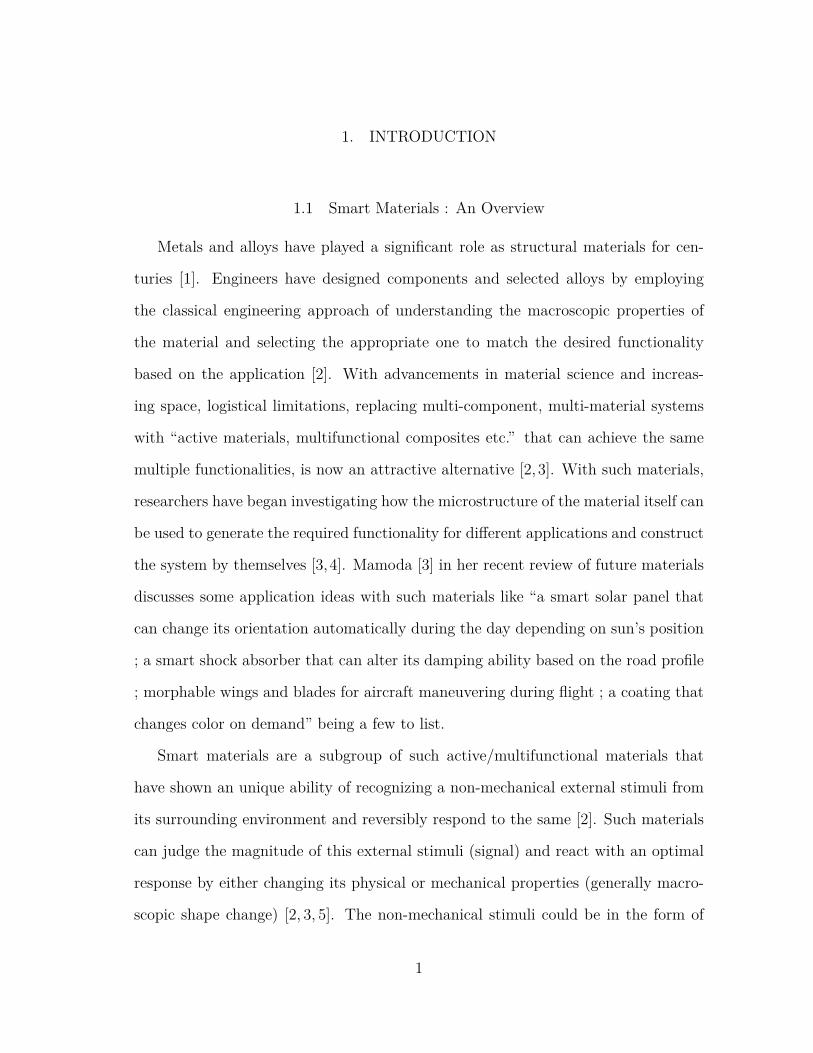
1.1 Smart materials can involve multi-physics coupling based on the ex-ternal stimuli it is subjected to which results in changes of physi-cal/mechanical properties i.e macroscopic shape change in most cases(adapted from fig 14 [9], [10]). . . . . . . . . . . . . . . . . . . . . . . 2

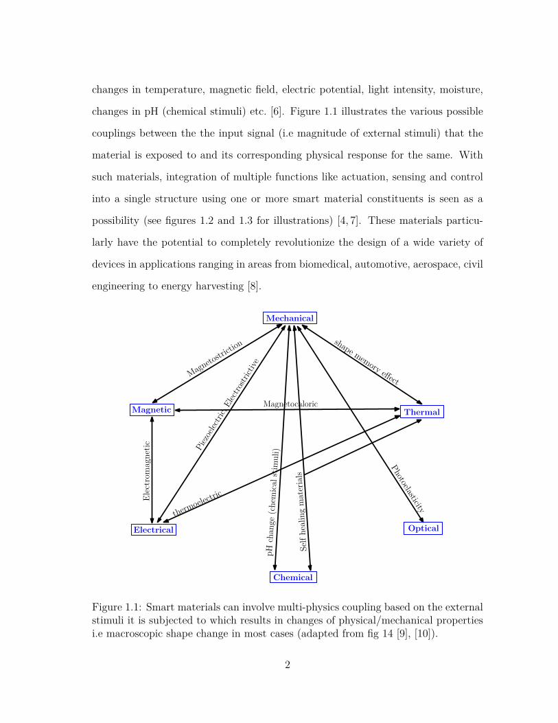
1.2 Integration of multiple functions like actuation, sensing and controlinto a single structure using one or more smart material constituents(adapted from figure 1.2 [4]) . . . . . . . . . . . . . . . . . . . . . . . 3

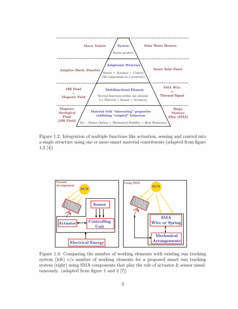
1.3 Comparing the number of working elements with existing sun trackingsystem (left) v/s number of working elements for a proposed smart suntracking system (right) using SMA components that play the role ofactuator & sensor simultaneously. (adapted from figure 1 and 2 [7]) . 3

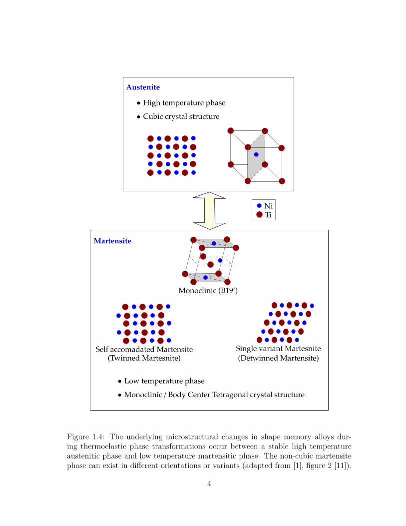
1.4 The underlying microstructural changes in shape memory alloys dur-ing thermoelastic phase transformations occur between a stable hightemperature austenitic phase and low temperature martensitic phase.The non-cubic martensite phase can exist in different orientations orvariants (adapted from [1], figure 2 [11]). . . . . . . . . . . . . . . . . 4

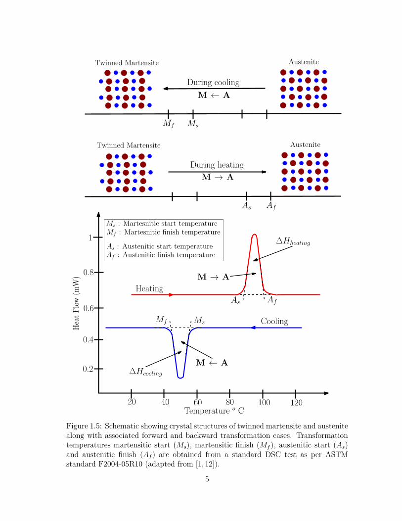
1.5 Schematic showing crystal structures of twinned martensite and austen-ite along with associated forward and backward transformation cases.Transformation temperatures martensitic start (Ms), martensitic fin-ish (Mf ), austenitic start (As) and austenitic finish (Af ) are ob-tained from a standard DSC test as per ASTM standard F2004-05R10(adapted from [1,12]). . . . . . . . . . . . . . . . . . . . . . . . . . . 5

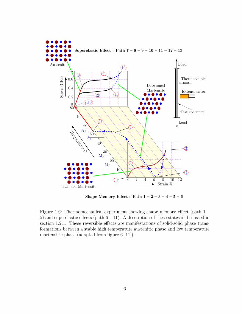
1.6 Thermomechanical experiment showing shape memory effect (path 1 –5) and superelastic effects (path 6 – 11). A description of these statesis discussed in section 1.2.1. These reversible effects are manifestationsof solid-solid phase transformations between a stable high temperatureaustenitic phase and low temperature martensitic phase (adapted fromfigure 6 [11]). . . . . . . . . . . . . . . . . . . . . . . . . . . . . . . . 6

xi

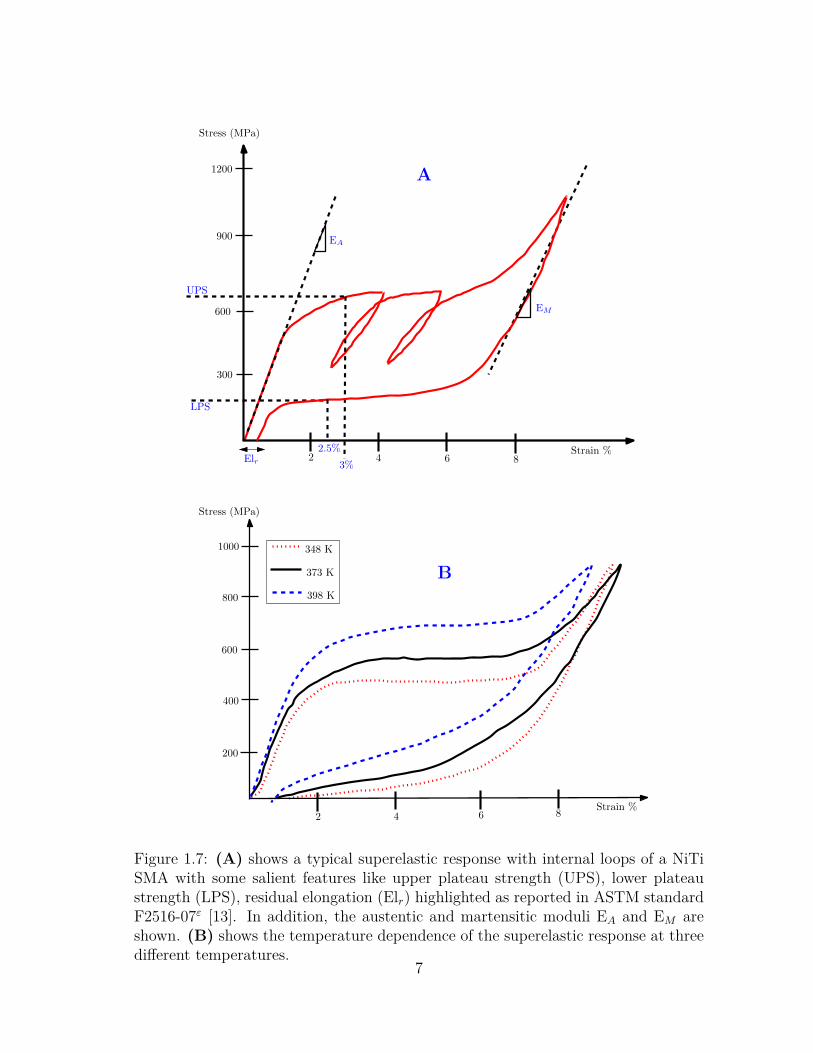
1.7 (A) shows a typical superelastic response with internal loops of a NiTiSMA with some salient features like upper plateau strength (UPS),lower plateau strength (LPS), residual elongation (Elr) highlighted asreported in ASTM standard F2516-07ε [13]. In addition, the austenticand martensitic moduli EA and EM are shown. (B) shows the tem-perature dependence of the superelastic response at three differenttemperatures. . . . . . . . . . . . . . . . . . . . . . . . . . . . . . . . 7

1.8 Figure shows a SMA torsional helical spring used for tooth movement,space closure in orthodontic applications. The idea here is to designthe spring at the LPS so that it can deliver relatively constant forcesover large strokes (photograph reproduced from figure 1 [39]. Com-parison graph adapted from figure 1 [35]). . . . . . . . . . . . . . . . 12

1.9 Figures some SMA reinforcements in many civil structures for recen-tering and damping applications. The large loading–unloading hys-teresis (shaded region under the entire stress–strain curve) associatedwith superelastic responses in SMA makes them a very efficient energydissipation system. (photographs reproduced from [20,48]). . . . . . . 15

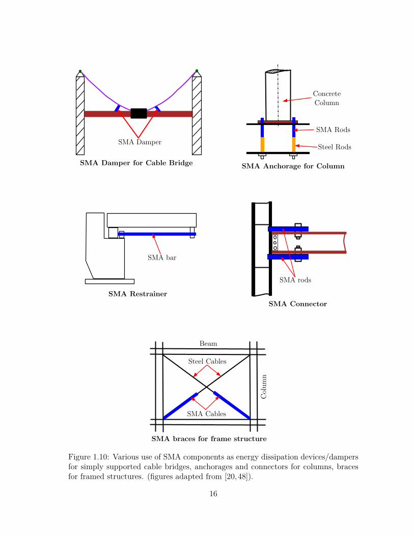
1.10 Various use of SMA components as energy dissipation devices/dampersfor simply supported cable bridges, anchorages and connectors forcolumns, braces for framed structures. (figures adapted from [20,48]). 16

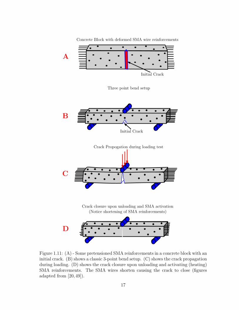
1.11 (A) - Some pretensioned SMA reinforcements in a concrete block withan initial crack. (B) shows a classic 3-point bend setup. (C) shows thecrack propagation during loading. (D) shows the crack closure uponunloading and activating (heating) SMA reinforcements. The SMAwires shorten causing the crack to close (figures adapted from [20,49]). 17

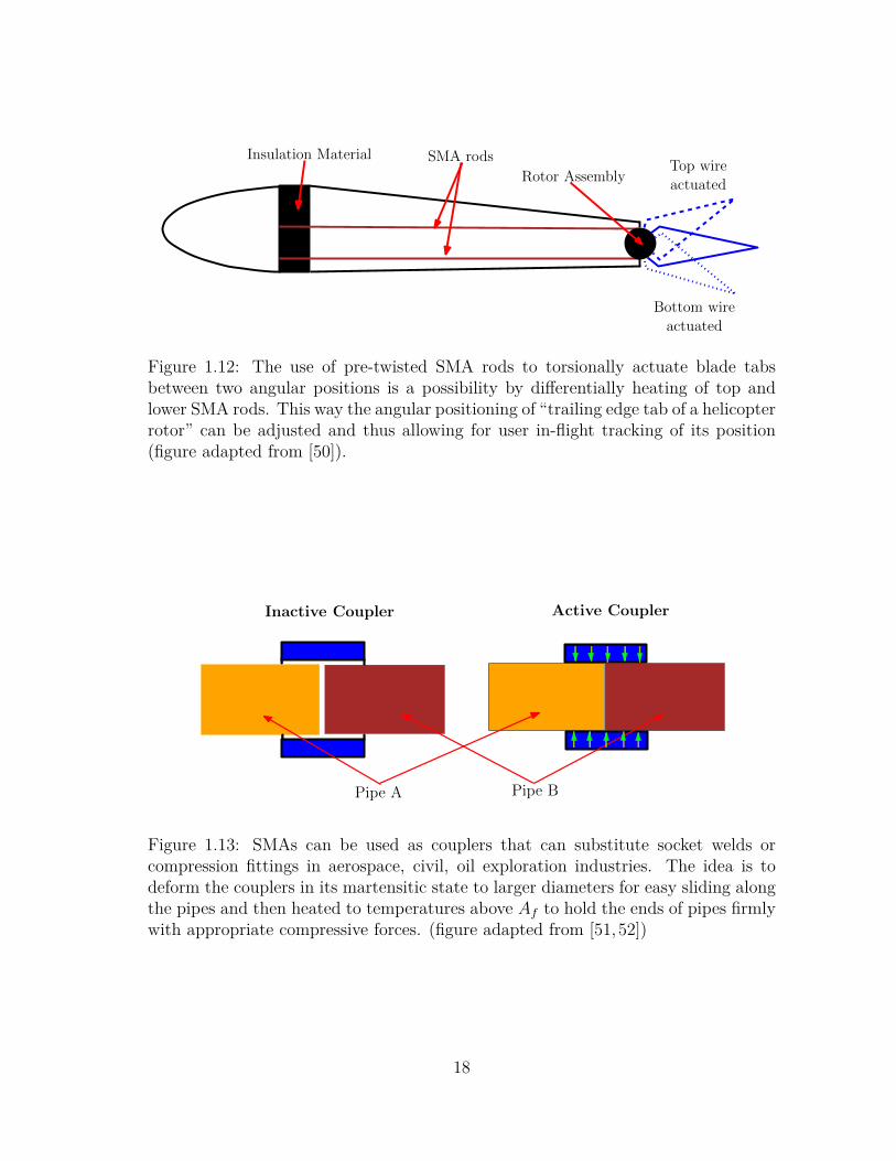
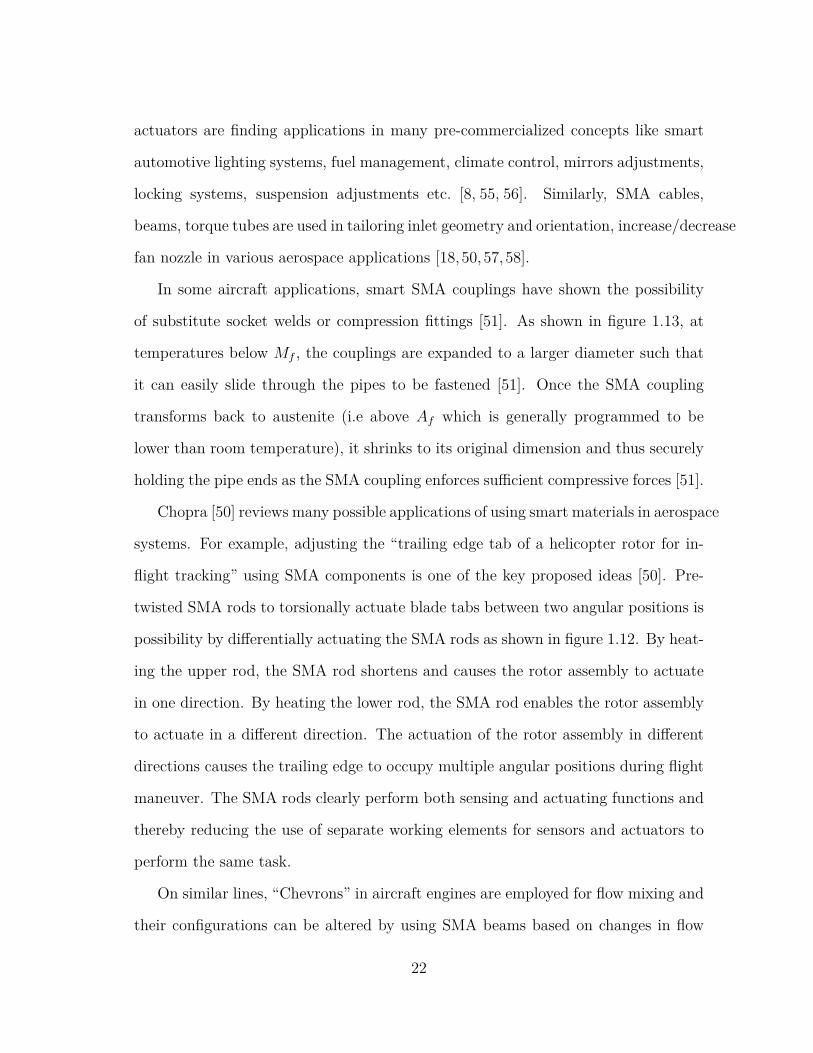
1.12 The use of pre-twisted SMA rods to torsionally actuate blade tabsbetween two angular positions is a possibility by differentially heatingof top and lower SMA rods. This way the angular positioning of“trailing edge tab of a helicopter rotor” can be adjusted and thusallowing for user in-flight tracking of its position (figure adapted from[50]). . . . . . . . . . . . . . . . . . . . . . . . . . . . . . . . . . . . . 18

1.13 SMAs can be used as couplers that can substitute socket welds or com-pression fittings in aerospace, civil, oil exploration industries. The ideais to deform the couplers in its martensitic state to larger diameters foreasy sliding along the pipes and then heated to temperatures above Afto hold the ends of pipes firmly with appropriate compressive forces.(figure adapted from [51,52]) . . . . . . . . . . . . . . . . . . . . . . . 18

xii

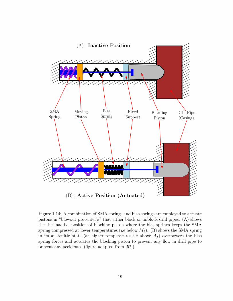
1.14 A combination of SMA springs and bias springs are employed to actu-ate pistons in “blowout preventer’s” that either block or unblock drillpipes. (A) shows the the inactive position of blocking piston where thebias springs keeps the SMA spring compressed at lower temperatures(i.e below Mf ). (B) shows the SMA spring in its austenitic state (athigher temperatures i.e above Af ) overpowers the bias spring forcesand actuates the blocking piston to prevent any flow in drill pipe toprevent any accidents. (figure adapted from [52]) . . . . . . . . . . . 19

1.15 An overview of different modeling approaches along length scales. Thisdissertation focuses on the macroscopic structural models for SMAcomponents that are computationally inexpensive and implementabledirectly at the component level. . . . . . . . . . . . . . . . . . . . . . 26

1.16 Figure shows a typical stress – temperature diagram used for someelastoplasticity approaches. Figure also indicates critical stresses (σscrand σfcr), transformation temperatures (Ms, Mf , As and Af ) andslopes of various transformation lines/regions (Cm & Ca) used as in-puts for model formulation. (adapted from [59,71]) . . . . . . . . . . 28

1.17 Figure shows similarity between hysteresis associated ferromagneticmaterials and those associated with superelastic response of SMA. Thedistinct difference between the two is the elastic response observed inSMA before switching states during phase transformation event (i.ethe intial & final elastic parts). . . . . . . . . . . . . . . . . . . . . . 34

1.18 A hysteron defined in a classical Preisach model with P and Q be-ing the switching values with the arrows directions corresponding toallowable paths. . . . . . . . . . . . . . . . . . . . . . . . . . . . . . . 35

1.19 Figure shows a typical strain – temperature response used in Preisachmodeling . . . . . . . . . . . . . . . . . . . . . . . . . . . . . . . . . . 35

1.20 Non linear shear stress distribution across the wire cross-section undertorsional loading with an inner austentic core, a phase transition regionand an outer transformed martensitic layer [109]. . . . . . . . . . . . 40

2.1 Experimental setup showing Instron uniaxial tensile testing machinewith a temperature chamber and mounting of a NiTi wire betweenmechanical wedge grips . . . . . . . . . . . . . . . . . . . . . . . . . . 52

2.2 Load extension curve (at 373K) used to achieve 3 internal loops duringthe loading cycle of an uniaxial tension test on a NiTi wire with eachblock representing intermediate loading and unloading cycles. . . . . 53

xiii

2.3 Results of uniaxial tension tests conducted on NiTi wire at tempera-tures 348, 373 and 398 K using a loading–unloading profile illustratedin 2.2 with 3 mm/min displacement rate for all cases. . . . . . . . . . 54

2.4 Experimental set-up showing Instron uniaxial tensile testing machinewith a temperature chamber and mounting of a SMA Spring wirebetween mechanical wedge grips and hooks . . . . . . . . . . . . . . . 56

2.5 Results of tests conducted on NiTi SMA springs at temperatures 298,348, 373 and 398 K with 15 mm/min displacement rate for all cases.The results for 348, 373 and 398 K show superelastic response of SMAsprings. The extent of transformation in each high temperature trial isdifferent when compared against the same maximum spring elongation(75 mm) or corresponding twist. . . . . . . . . . . . . . . . . . . . . . 57

2.6 Experimental setup showing micro-torsion MT series machine withsuperelastic SMA wire specimen mounted between collet grips. . . . . 62

2.7 Figures shows the twist versus time ; torque versus time and torqueversus twist responses for a simple loading and unloading test upto1800o maximum twist. . . . . . . . . . . . . . . . . . . . . . . . . . . 64

2.8 Figures shows the twist versus time ; torque versus time and torqueversus twist responses responses for a simple loading and unloadingtests with different unloading points of 1500o, 1350o, 900o and 600omaximum twists overlapped on each other and compared against the1800o twist. All the individual tests were different trials performedon different test specimens demonstrating good agreement and testrepeatability. . . . . . . . . . . . . . . . . . . . . . . . . . . . . . . . 70

2.9 Experimental data showing the twist versus time ; torque versus timeand torque versus twist responses for test upto 1800o maximum twistwith three internal loops during the loading cycle. . . . . . . . . . . . 71

2.10 Figures shows the twist versus time ; torque versus time and torqueversus twist responses for test upto 1800o maximum twist for compar-ing internal loops during loading and unloading cycle. . . . . . . . . . 72

2.11 Figures shows the twist versus time ; torque versus time and torqueversus twist responses for test upto 1800o maximum twist with multi-ple internal loops during loading and unloading. . . . . . . . . . . . . 73

2.12 Figures shows the twist versus time ; torque versus time and torqueversus twist responses for test upto 1800o maximum twist with a com-plex internal loops during loading cycle. . . . . . . . . . . . . . . . . 74

xiv

2.13 Figures shows the twist versus time ; torque versus time and torqueversus twist responses for test upto 1800o maximum twist with a com-plex internal loops during unloading cycle. . . . . . . . . . . . . . . . 75

2.14 Figures shows the twist versus time ; torque versus time and torqueversus twist responses for test upto 1800o maximum twist with a com-plex internal loops during both loading and unloading cycles. . . . . . 76

3.1 Experimental stress–strain data is reduced to driving force–volumefraction plot using thermodynamic principles by using equations 3.15and 3.13. The flat plateaus of stress – strain plot do not appear onthe reduced data plot below. . . . . . . . . . . . . . . . . . . . . . . . 92

3.2 Experimental torque verses angle of twist data is reduced to drivingforce–volume fraction plot using thermodynamic principles by usingequations 3.29 and 3.27. . . . . . . . . . . . . . . . . . . . . . . . . . 93

3.3 Experimental torque verses angle of twist data is reduced to drivingforce–volume fraction plot using thermodynamic principles by usingusing expressions 3.29 and 3.27. Experimental data obtained from [110]. 93

3.4 Experimental bending moment verses curvature data is reduced todriving force–volume fraction plot using thermodynamic principles byusing equations 3.43 and 3.41. Experimental data obtained for NiTispecimens [132]. . . . . . . . . . . . . . . . . . . . . . . . . . . . . . . 94

3.5 Experimental bending moment verses curvature data is reduced todriving force–volume fraction plot using thermodynamic principles byusing equations 3.43 and 3.41. Experimental data obtained for CuZ-nAl specimen [132]. . . . . . . . . . . . . . . . . . . . . . . . . . . . . 94

4.1 Basic hysteretic element or hysteron used in the current discrete PreisachModel. Directions of allowed transformations are represented by thearrows on the hysteron. Each hysteron behaves like a non-ideal switchthat switches on when the torque increases beyond Fforward with anoutput of ∆ξi and switches off at Fbackward. . . . . . . . . . . . . . . . 96

4.2 (i) : Preisach Triangle - A systematic way for assigning switch on andswitch off of the hysterons. The directions of loading (forward) andunloading (backward) sweeps are marked on the figure. Sub figures(ii), (iii), (iv) shows an example for sequencing of states in the Preisachtriangle. The colored section shows the triangles that are switched onwith the corresponding driving force enforcing the state at the top ofthe state [64,104]. . . . . . . . . . . . . . . . . . . . . . . . . . . . . . 99

xv

5.1 Paths (a) – (c) and (a) – (b) represent superelastic responses (i.eloading/ unloading operations above Af ) under clockwise and anti-clockwise rotations respectively. Below Mf , Path (d)–(b or c)represents the twinning response under pure mechanical loading toeither M+ or M− martensite variants depending on the twisting di-rection. Path (a)–(d) represents stress free thermal cycling betweenaustenite and self accommodated martensite variant. Path (d)–(bor c) – (a) represents a typical shape memory cycle depending onthe twist direction. . . . . . . . . . . . . . . . . . . . . . . . . . . . . 104

5.2 Experimental torque v/s angle of twist data is reduced to drivingforce–volume fraction plot using thermodynamic principles by usingequations developed for twinning response summarized in table 5.1.Clockwise twist was assumed. Experimental data obtained from [113]. 120

5.3 Experimental torque v/s angle of twist data is reduced to drivingforce–volume fraction plot using thermodynamic principles by usingequations developed for superelastic responses summarized in table5.1. Experimental data obtained from [116]. . . . . . . . . . . . . . . 120

6.1 Figure shows the critical coordinates determined to estimate modelparameters from a superelastic response of a wire (non-dimensionlizeddata). Experimental data obtained from [116]. . . . . . . . . . . . . . 129

7.1 Model simulation using ASTM guidelines and a model simulation ofresults at 373 K . . . . . . . . . . . . . . . . . . . . . . . . . . . . . . 141

7.2 Prediction for responses at 348 and 398 K using the hysterons gen-erated at 373 K temperature result. The experimental results for allcases were discussed earlier in 2.3. . . . . . . . . . . . . . . . . . . . . 142

7.3 Model prediction for the superelastic response of SMA spring at 348K. Model prediction and experimental results show a good match.This is not surprising since the Preisach parameters were chosen tofit the data. However the closeness of the fit is an indication of thepower of the Preisach approach. . . . . . . . . . . . . . . . . . . . . . 144

7.4 Model prediction for the superelastic response of SMA wire tested at296 K showing a good match. Experimental results at 296 K wereobtained from [110]. The jaggedness of the model simulation is dueto the fact that a discrete Preisach model was used. . . . . . . . . . . 145

7.5 Figure showing the data that is used for model calibration. All modelpredictions discussed in section 7.2.2.1 uses the hysterons generatedfor this outer loop response. . . . . . . . . . . . . . . . . . . . . . . . 145

xvi

7.6 Simulation for a hysteretic response with one large internal loops dur-ing loading cycle. All model predictions discussed in section 7.2.2.2uses the hysterons generated for this experimental data containing theouter loop with one internal loop during the loading cycle. . . . . . . 146

7.7 Simulation for a hysteretic response with an internal loop during theloading and unloading cycle. All model predictions discussed in section7.2.2.3 uses the hysterons generated for this entire outer loop andinternal loops during the loading and unloading stages. . . . . . . . . 146

7.8 Simulation for a hysteretic response with three large internal loopsduring loading cycle. The jaggedness in the response is due to thediscrete nature of the Preisach model . . . . . . . . . . . . . . . . . . 147

7.9 Simulation for a hysteretic response that compares internal loops dur-ing loading and unloading part of the response. Again, the simulationis a close fit when compared to the experimental data. . . . . . . . . 147

7.10 Simulation of complex internal loops during loading cycles. The RPMeffects are well captures by the Preisach model. . . . . . . . . . . . . 148

7.11 Simulation of complex internal loop during unloading cycles. TheRPM effects are well captures by the Preisach model. . . . . . . . . . 148

7.12 Simulation of a response having complex internal loops during bothloading and unloading cycles. The strength of the Presiach model isclearly demonstrated here with a close fit with the experimental data. 149

7.13 Prediction for responses at 350 and 225o twist using the hysteronsgenerated at 450 degrees twist. The experimental results for all caseswere obtained from [116]. . . . . . . . . . . . . . . . . . . . . . . . . . 151

7.14 Figures show the prediction of lower twists 1500o and 900o using thehysterons generated with the 1800o data as shown in figure 7.5. Thepredictions show a close match with the experimental data and theouter loop is well predicted. . . . . . . . . . . . . . . . . . . . . . . . 152

7.15 Figures show the prediction of 1800 and 1500o twist using the hys-terons generated with the 1800o outer loops data of the simple loadand unload case as shown in figure 7.5. Using minimum information,complex responses involving internal loops are predicted and the re-sults show a close fit with outer loops and a good RPM prediction. . 153

xvii

7.16 Figures show the prediction of 1350o maximum twist for complex loopunder loading and unloading cases using the hysterons generated withthe 1800o outer loops data of the simple load and unload case as shownin figure 7.5. The outer loops are well represented and the complexloops with RPM prediction match well with the experimental data. . 154

7.17 Figures show the prediction of 1350o maximum twist for two differentcases that contain simple and complex loops using the hysterons gen-erated with the outer loops data of the simple load and unload caseas shown in figure 7.5. The outer loops are well represented and thecomplex loops with RPM prediction match well with the experimentaldata. . . . . . . . . . . . . . . . . . . . . . . . . . . . . . . . . . . . . 155

7.18 Figures show the prediction of 1800o twist for two different cases withtwo and three internal loops using the hysterons generated with theouter loop and one internal loop data as shown in figure 7.6. Usingthe outer loop and one internal loop information, complex responsesinvolving more internal loops are predicted with the results show aclose match to the experimental data. . . . . . . . . . . . . . . . . . . 156

7.19 Figures show the prediction of 1800o twist for two different cases withtwo and three internal loops using the hysterons generated with theouter loop and one internal loop data as shown in figure 7.6. Using theouter loop and one internal loop information, complex loop responseswere predicted and compared against the experimental data. . . . . . 157

7.20 Figures show the prediction of 1350 and 1800o maximum twist usingthe hysterons generated with the outer loop and one internal loopdata as shown in figure 7.6. Using the outer loop and one internalloop information, complex loops under loading and unloading legs ofthe response were predicted and compared against the experimentaldata. . . . . . . . . . . . . . . . . . . . . . . . . . . . . . . . . . . . . 158

7.21 Figures show the prediction of complex loops for loading and unload-ing cases with 1800o maximum twist using the hysterons generatedwith the outer loop and internal loop during loading and unloadingstages as shown with full data simulation discussed in figure 7.7. . . . 159

xviii

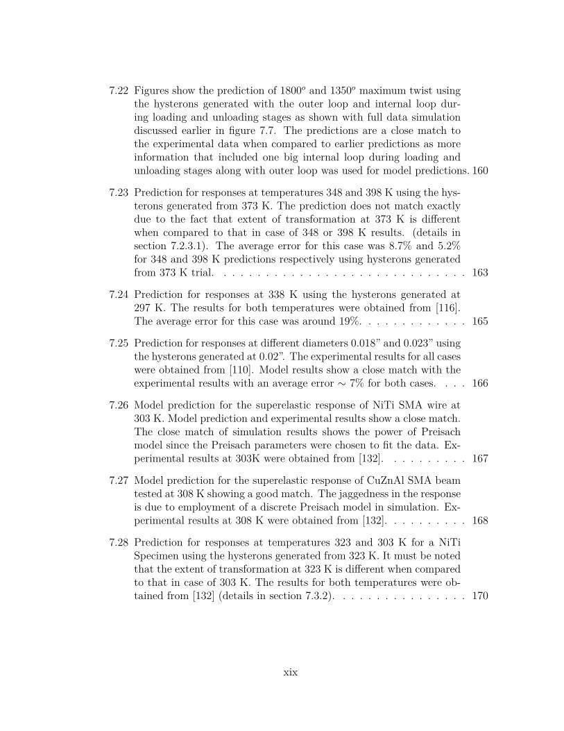
7.22 Figures show the prediction of 1800o and 1350o maximum twist usingthe hysterons generated with the outer loop and internal loop dur-ing loading and unloading stages as shown with full data simulationdiscussed earlier in figure 7.7. The predictions are a close match tothe experimental data when compared to earlier predictions as moreinformation that included one big internal loop during loading andunloading stages along with outer loop was used for model predictions. 160

7.23 Prediction for responses at temperatures 348 and 398 K using the hys-terons generated from 373 K. The prediction does not match exactlydue to the fact that extent of transformation at 373 K is differentwhen compared to that in case of 348 or 398 K results. (details insection 7.2.3.1). The average error for this case was 8.7% and 5.2%for 348 and 398 K predictions respectively using hysterons generatedfrom 373 K trial. . . . . . . . . . . . . . . . . . . . . . . . . . . . . . 163

7.24 Prediction for responses at 338 K using the hysterons generated at297 K. The results for both temperatures were obtained from [116].The average error for this case was around 19%. . . . . . . . . . . . . 165

7.25 Prediction for responses at different diameters 0.018” and 0.023” usingthe hysterons generated at 0.02”. The experimental results for all caseswere obtained from [110]. Model results show a close match with theexperimental results with an average error ∼ 7% for both cases. . . . 166

7.26 Model prediction for the superelastic response of NiTi SMA wire at303 K. Model prediction and experimental results show a close match.The close match of simulation results shows the power of Preisachmodel since the Preisach parameters were chosen to fit the data. Ex-perimental results at 303K were obtained from [132]. . . . . . . . . . 167

7.27 Model prediction for the superelastic response of CuZnAl SMA beamtested at 308 K showing a good match. The jaggedness in the responseis due to employment of a discrete Preisach model in simulation. Ex-perimental results at 308 K were obtained from [132]. . . . . . . . . . 168

7.28 Prediction for responses at temperatures 323 and 303 K for a NiTiSpecimen using the hysterons generated from 323 K. It must be notedthat the extent of transformation at 323 K is different when comparedto that in case of 303 K. The results for both temperatures were ob-tained from [132] (details in section 7.3.2). . . . . . . . . . . . . . . . 170

xix

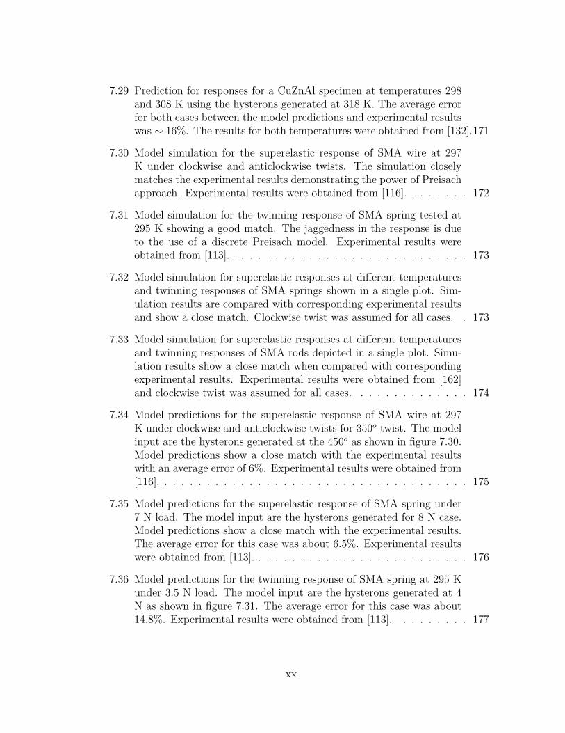
7.29 Prediction for responses for a CuZnAl specimen at temperatures 298and 308 K using the hysterons generated at 318 K. The average errorfor both cases between the model predictions and experimental resultswas ∼ 16%. The results for both temperatures were obtained from [132].171

7.30 Model simulation for the superelastic response of SMA wire at 297K under clockwise and anticlockwise twists. The simulation closelymatches the experimental results demonstrating the power of Preisachapproach. Experimental results were obtained from [116]. . . . . . . . 172

7.31 Model simulation for the twinning response of SMA spring tested at295 K showing a good match. The jaggedness in the response is dueto the use of a discrete Preisach model. Experimental results wereobtained from [113]. . . . . . . . . . . . . . . . . . . . . . . . . . . . . 173

7.32 Model simulation for superelastic responses at different temperaturesand twinning responses of SMA springs shown in a single plot. Sim-ulation results are compared with corresponding experimental resultsand show a close match. Clockwise twist was assumed for all cases. . 173

7.33 Model simulation for superelastic responses at different temperaturesand twinning responses of SMA rods depicted in a single plot. Simu-lation results show a close match when compared with correspondingexperimental results. Experimental results were obtained from [162]and clockwise twist was assumed for all cases. . . . . . . . . . . . . . 174

7.34 Model predictions for the superelastic response of SMA wire at 297K under clockwise and anticlockwise twists for 350o twist. The modelinput are the hysterons generated at the 450o as shown in figure 7.30.Model predictions show a close match with the experimental resultswith an average error of 6%. Experimental results were obtained from[116]. . . . . . . . . . . . . . . . . . . . . . . . . . . . . . . . . . . . . 175

7.35 Model predictions for the superelastic response of SMA spring under7 N load. The model input are the hysterons generated for 8 N case.Model predictions show a close match with the experimental results.The average error for this case was about 6.5%. Experimental resultswere obtained from [113]. . . . . . . . . . . . . . . . . . . . . . . . . . 176

7.36 Model predictions for the twinning response of SMA spring at 295 Kunder 3.5 N load. The model input are the hysterons generated at 4N as shown in figure 7.31. The average error for this case was about14.8%. Experimental results were obtained from [113]. . . . . . . . . 177

xx

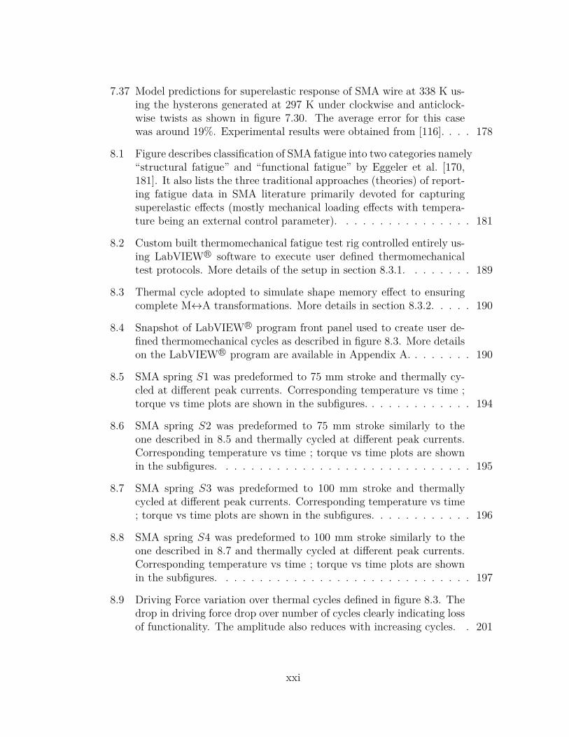
7.37 Model predictions for superelastic response of SMA wire at 338 K us-ing the hysterons generated at 297 K under clockwise and anticlock-wise twists as shown in figure 7.30. The average error for this casewas around 19%. Experimental results were obtained from [116]. . . . 178

8.1 Figure describes classification of SMA fatigue into two categories namely“structural fatigue” and “functional fatigue” by Eggeler et al. [170,181]. It also lists the three traditional approaches (theories) of report-ing fatigue data in SMA literature primarily devoted for capturingsuperelastic effects (mostly mechanical loading effects with tempera-ture being an external control parameter). . . . . . . . . . . . . . . . 181

8.2 Custom built thermomechanical fatigue test rig controlled entirely us-ing LabVIEW R© software to execute user defined thermomechanicaltest protocols. More details of the setup in section 8.3.1. . . . . . . . 189

8.3 Thermal cycle adopted to simulate shape memory effect to ensuringcomplete M↔A transformations. More details in section 8.3.2. . . . . 190

8.4 Snapshot of LabVIEW R© program front panel used to create user de-fined thermomechanical cycles as described in figure 8.3. More detailson the LabVIEW R© program are available in Appendix A. . . . . . . . 190

8.5 SMA spring S1 was predeformed to 75 mm stroke and thermally cy-cled at different peak currents. Corresponding temperature vs time ;torque vs time plots are shown in the subfigures. . . . . . . . . . . . . 194

8.6 SMA spring S2 was predeformed to 75 mm stroke similarly to theone described in 8.5 and thermally cycled at different peak currents.Corresponding temperature vs time ; torque vs time plots are shownin the subfigures. . . . . . . . . . . . . . . . . . . . . . . . . . . . . . 195

8.7 SMA spring S3 was predeformed to 100 mm stroke and thermallycycled at different peak currents. Corresponding temperature vs time; torque vs time plots are shown in the subfigures. . . . . . . . . . . . 196

8.8 SMA spring S4 was predeformed to 100 mm stroke similarly to theone described in 8.7 and thermally cycled at different peak currents.Corresponding temperature vs time ; torque vs time plots are shownin the subfigures. . . . . . . . . . . . . . . . . . . . . . . . . . . . . . 197

8.9 Driving Force variation over thermal cycles defined in figure 8.3. Thedrop in driving force drop over number of cycles clearly indicating lossof functionality. The amplitude also reduces with increasing cycles. . 201

xxi

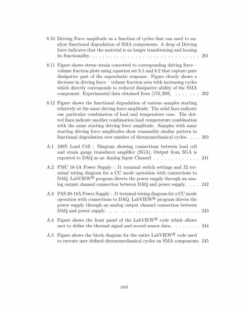
8.10 Driving Force amplitude as a function of cycles that can used to an-alyze functional degradation of SMA components. A drop of Drivingforce indicates that the material is no longer transforming and loosingits functionality. . . . . . . . . . . . . . . . . . . . . . . . . . . . . . . 201

8.11 Figure shows stress–strain converted to corresponding driving force –volume fraction plots using equation set 8.1 and 8.2 that capture puredissipative part of the superelastic response. Figure clearly shows adecrease in driving force – volume fraction area with increasing cycleswhich directly corresponds to reduced dissipative ability of the SMAcomponent. Experimental data obtained from [170,209]. . . . . . . . 202

8.12 Figure shows the functional degradation of various samples startingrelatively at the same driving force amplitude. The solid lines indicateone particular combination of load and temperature case. The dot-ted lines indicate another combination load–temperature combinationwith the same starting driving force amplitude. Samples with samestarting driving force amplitudes show reasonably similar pattern infunctional degradation over number of thermomechanical cycles. . . . 203

A.1 100N Load Cell : Diagram showing connections between load celland strain gauge transducer amplifier (SGA). Output from SGA isexported to DAQ as an Analog Input Channel . . . . . . . . . . . . . 241

A.2 PMC 18-5A Power Supply : J1 terminal switch settings and J2 ter-minal wiring diagram for a CC mode operation with connections toDAQ. LabVIEW R© program directs the power supply through an ana-log output channel connection between DAQ and power supply. . . . 242

A.3 PAS 20-18A Power Supply : J1 terminal wiring diagram for a CCmodeoperation with connections to DAQ. LabVIEW R© program directs thepower supply through an analog output channel connection betweenDAQ and power supply. . . . . . . . . . . . . . . . . . . . . . . . . . 243

A.4 Figure shows the front panel of the LabVIEW R© code which allowsuser to define the thermal signal and record sensor data. . . . . . . . 244

A.5 Figure shows the block diagram for the entire LabVIEW R© code usedto execute user defined thermomechanical cycles on SMA components. 245

xxii

LIST OF TABLES

TABLE Page

5.1 Summary of driving force–volume fraction relationships for all trans-formation cases (equation sets 5.21a – 5.30 ; 5.21b – 5.31 ; 5.24a– 5.32a ; 5.24b – 5.32b). . . . . . . . . . . . . . . . . . . . . . . . . 119

6.1 Values of thermodynamical parameters employed for model verifica-tion for uniaxial tension tests conducted on NiTi wire (see figure 2.3). 128

6.2 Values of thermodynamical parameters employed for model verifica-tion in case of springs . . . . . . . . . . . . . . . . . . . . . . . . . . . 133

6.3 Values of thermodynamical parameters employed for model verifica-tion for pure bending experimental data of NiTi wire [132] . . . . . . 135

6.4 Values of thermodynamical parameters employed for model verifi-cation for springs and wires used for three species thermodyanmicPreisach models . . . . . . . . . . . . . . . . . . . . . . . . . . . . . . 136

xxiii

1. INTRODUCTION

1.1 Smart Materials : An Overview

Metals and alloys have played a significant role as structural materials for cen-

turies [1]. Engineers have designed components and selected alloys by employing

the classical engineering approach of understanding the macroscopic properties of

the material and selecting the appropriate one to match the desired functionality

based on the application [2]. With advancements in material science and increas-

ing space, logistical limitations, replacing multi-component, multi-material systems

with “active materials, multifunctional composites etc.” that can achieve the same

multiple functionalities, is now an attractive alternative [2, 3]. With such materials,

researchers have began investigating how the microstructure of the material itself can

be used to generate the required functionality for different applications and construct

the system by themselves [3,4]. Mamoda [3] in her recent review of future materials

discusses some application ideas with such materials like “a smart solar panel that

can change its orientation automatically during the day depending on sun’s position

; a smart shock absorber that can alter its damping ability based on the road profile

; morphable wings and blades for aircraft maneuvering during flight ; a coating that

changes color on demand” being a few to list.

Smart materials are a subgroup of such active/multifunctional materials that

have shown an unique ability of recognizing a non-mechanical external stimuli from

its surrounding environment and reversibly respond to the same [2]. Such materials

can judge the magnitude of this external stimuli (signal) and react with an optimal

response by either changing its physical or mechanical properties (generally macro-

scopic shape change) [2, 3, 5]. The non-mechanical stimuli could be in the form of

1

changes in temperature, magnetic field, electric potential, light intensity, moisture,

changes in pH (chemical stimuli) etc. [6]. Figure 1.1 illustrates the various possible

couplings between the the input signal (i.e magnitude of external stimuli) that the

material is exposed to and its corresponding physical response for the same. With

such materials, integration of multiple functions like actuation, sensing and control

into a single structure using one or more smart material constituents is seen as a

possibility (see figures 1.2 and 1.3 for illustrations) [4, 7]. These materials particu-

larly have the potential to completely revolutionize the design of a wide variety of

devices in applications ranging in areas from biomedical, automotive, aerospace, civil

engineering to energy harvesting [8].

Mechanical

Magnetic

Electrical

Chemical

Optical

Thermal

Magnetostr

iction

Pie

zoel

ectr

ic,E

lect

rost

rict

ive

pH

chan

ge(c

hem

ical

stim

uli)

Sel

fhea

ling

mat

eria

ls

shape memory effect

Photoelasticity

thermoelec

tricEle

ctro

mag

net

ic

Magnetocaloric

Figure 1.1: Smart materials can involve multi-physics coupling based on the externalstimuli it is subjected to which results in changes of physical/mechanical propertiesi.e macroscopic shape change in most cases (adapted from fig 14 [9], [10]).

2

Material with “interesting” propertiesexhibiting “coupled” behaviour

Ex. : Sensor Option + Mechanical Stability + Heat Resistance

Multifunctional Element

Several functions within one element(i.e Material + Sensor + Actuator)

Adaptronic Structure

Sensor + Actautor + Control(All components in a structure)

System

Magneto-rheological

Fluid(MR Fluid)

MR Fluid+

Magnetic Field

Adaptive Shock Absorber

Motor Vehicle

ShapeMemory

Alloy (SMA)

SMA Wire+

Thermal Signal

Smart Solar Panel

Solar Water Heaters

Entire product

Figure 1.2: Integration of multiple functions like actuation, sensing and control intoa single structure using one or more smart material constituents (adapted from figure1.2 [4])

Actuator Controlling

Unit

Sensor

Electrical Energy

SUNSUN

NormalArrangement

Using SMA

Mechanical

Arrangements

SMA

Wire or Spring

Figure 1.3: Comparing the number of working elements with existing sun trackingsystem (left) v/s number of working elements for a proposed smart sun trackingsystem (right) using SMA components that play the role of actuator & sensor simul-taneously. (adapted from figure 1 and 2 [7])

3

• High temperature phase

• Cubic crystal structure

• Low temperature phase

• Monoclinic / Body Center Tetragonal crystal structure

Self accomadated Martensite

Monoclinic (B19’)

Single variant Martesnite

NiTi

(Twinned Martesnite) (Detwinned Martensite)

Austenite

Martensite

Figure 1.4: The underlying microstructural changes in shape memory alloys dur-ing thermoelastic phase transformations occur between a stable high temperatureaustenitic phase and low temperature martensitic phase. The non-cubic martensitephase can exist in different orientations or variants (adapted from [1], figure 2 [11]).

4

Heating

M → A

M ← A

∆Hheating

∆Hcooling

Mf Ms

As Af

Cooling

Temperature o C

Hea

tF

low

(mW

)

0.2

0.4

0.6

0.8

1

20 40 60 80 100 120

Twinned Martensite Austenite

Mf Ms

Twinned Martensite Austenite

AfAs

During heating

M → A

During cooling

M ← A

Ms : Martesnitic start temperatureMf : Martesnitic finish temperature

Af : Austenitic finish temperatureAs : Austenitic start temperature

Figure 1.5: Schematic showing crystal structures of twinned martensite and austenitealong with associated forward and backward transformation cases. Transformationtemperatures martensitic start (Ms), martensitic finish (Mf ), austenitic start (As)and austenitic finish (Af ) are obtained from a standard DSC test as per ASTMstandard F2004-05R10 (adapted from [1,12]).

5

0 2 4 6 8 10

10

30

50

70

1

3

4

9

Strain %

Load

Load

Test specimen

Thermocouple

Extensometer

Temperature

C

Austenite

Twinned Martensite

Superelastic Effect : Path 7 – 8 – 9 – 10 – 11 – 12 – 13

DetwinnedMartensite

Shape Memory Effect : Path 1 – 2 – 3 – 4 – 5 – 6

Stress

(GPa)

5

6

Mf

Ms

As

Af

0.2

0.4

0.68

1112

7,130

0.8

2

10

12

20

40

60

80

Figure 1.6: Thermomechanical experiment showing shape memory effect (path 1 –5) and superelastic effects (path 6 – 11). A description of these states is discussed insection 1.2.1. These reversible effects are manifestations of solid-solid phase trans-formations between a stable high temperature austenitic phase and low temperaturemartensitic phase (adapted from figure 6 [11]).

6

EA

EM

2 4 6 8

300

600

900

1200

UPS

Strain %

Stress (MPa)

Elr2.5%

3%

A

B

2 4 6 8

200

400

600

800

1000 348 K

373 K

398 K

Strain %

Stress (MPa)

LPS

Figure 1.7: (A) shows a typical superelastic response with internal loops of a NiTiSMA with some salient features like upper plateau strength (UPS), lower plateaustrength (LPS), residual elongation (Elr) highlighted as reported in ASTM standardF2516-07ε [13]. In addition, the austentic and martensitic moduli EA and EM areshown. (B) shows the temperature dependence of the superelastic response at threedifferent temperatures.

7

1.2 Shape Memory Alloys : Temperature Induced Phase Transformations

In shape memory alloys (SMA), functionalities arise from their underlying micro-

structural changes when subjected to external non-mechanical stimuli like temper-

ature or magnetic field changes [14]. In thermally responsive SMAs, the reversible

solid-solid diffusionless thermoelastic phase transformations between a stable high

temperature austenitic phase and low temperature martensitic phase are respon-

sible for them to demonstrate interesting phenomenon like shape memory effect

(SME) and superelasticity (SE). The austentic phase has a cubic crystal structure

as compared to the martensitic phase which has either tetragonal, orthorhombic or

monoclinic structures as shown in 1.4 [15]. The transformations are a result of shear

lattice distortions (twinning) rather than long range diffusion of atoms [1, 16]. The

martensitic phase can have different orientations (variants) and can exist as twinned

martensite formed by combination of “self-accommodated martensite variants” or as

a “detwinnned/reoriented martensite” with a specific variant being dominant [1,16].

The phase transformations occur over some characteristic transformation tempera-

tures namely martensitic start (Ms), martensitic finish (Mf ), austenitic start (As)

and austenitic finish (Af ). ASTM standard F2004-05R10 [12] discusses the details of

measuring these transformation temperatures using a differential scanning calorime-

try (DSC) test for a NiTi SMA. A schematic of crystal structures of twinned marten-

site, austenite and associated transformation temperatures are shown in figure 1.5.

1.2.1 Shape Memory Effect and Superelasticity/Pseudoelasticity

The ability of SMA to return to a predetermined shape on heating is referred

to as the shape memory effect (SME). As shown in path 1–5 in figure 1.6,

upon external loading, self accommodated martenstic twins are detwinned into more

stress preferred martensite variants typically associated with large (∼8%) macro-

8

scopic strains [17]. Upon unloading, large residual inelastic strains are observed

which are recovered upon heating to temperatures above Af unlike in conventional

materials. During heating, the low symmetric martensitic phase (M) is transformed

back to stable austentic phase (A) thus resulting is complete strain recovery and thus

demonstrating shape memory effect [17]. On cooling belowMs in absence to external

loads, austentite transforms back to self-accommodating variants of martensite.

Martensitic transformations purely due to mechanical loading in the austensitc

phase is also a possibility with SMA. The capability to recover large strains (∼8%)

and associated large stress–strain hysteresis due to mechanical loading-unloading

under isothermal conditions is referred to as superelastic/pseudoelastic effect

(SE) [17]. These effects are observed at temperatures greater than Af as shown

by path 6–11 in figure 1.6. ASTM standard F2516-07ε2 [13] discusses a standard

test method for a tension test on NiTi superleastic materials. This standard also

discusses details on some of the salient features (see figure 1.7) to be noted in a

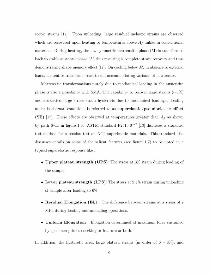
typical superelastic response like :

• Upper plateau strength (UPS): The stress at 3% strain during loading of

the sample

• Lower plateau strength (LPS): The stress at 2.5% strain during unloading

of sample after loading to 6%

• Residual Elongation (Elr) : The difference between strains at a stress of 7

MPa during loading and unloading operations.

• Uniform Elongation : Elongation determined at maximum force sustained

by specimen prior to necking or fracture or both.

In addition, the hysteretic area, large plateau strains (in order of 6 – 8%), and

9

moduli differences between the austentic and martensitic phases are some of the

other important characteristics of a superelastic response of SMA (see figure 1.7).

The SE response is also sensitive to the external stimuli i.e operating temperature

as shown in figure 1.7B. The hysteretic behavior primarily makes SMA a excellent

damping material.

1.3 Review of SMA Applications

The ability of SMA to reversibly respond to external temperature changes and

change their physical/mechanical properties have enabled them to find many appli-

cations. SMAs can be used both as sensors and actuators where they can sense the

changes in external stimuli and monitor certain desired functions [18]. The unique

characteristics of SME and SE have made SMAs the material system of choice in

applications ranging from sensing and control, vibration damping, biomedical, au-

tomotive and aerospace areas [8, 18–21]. A review of many SMA devices in use (or

being developed) across many engineering applications is detailed in the following

sections below.

1.3.1 Biomedical Applications

NiTi SMAs have found many biomedical applications due to their excellent bio-

compatibility. Clinical studies have shown that Nickel on its own is quite toxic and

any contact with nickel can lead to various medical complications [22]. However,

in case of intermetallic NiTi alloys, the bonding between Ni and Ti is quite strong

(like in ceramic materials) as compared to the Nickel bonding in steel and other

materials [23]. Further, the commercial NiTi alloys uses a passive TiO2 (titanium

oxide) layer coating on its outer surface that prevents any nickel leakage as it acts

as a physical and chemical barrier in preventing Ni oxidation [23, 24]. The TiO2

layer is harmless to human body and provides high resistance towards corrosion of

10

Ti alloys [22]. Many clinical studies have shown minimal Nickel contamination due

to use of NiTi SMAs and thus showing good biocompatibility [24].

In addition, NiTi SMA’s show excellent MRI compatibility, kink resistance, corro-

sion resistance and substantial moduli differences between austenitic and martensitic

phases. All of these properties make SMAs a good choice for many biomedical ap-

plications like “drug delivery systems, self-expanding stents, stent delivery systems,

implantable devices, catheters, guide-wires, atrial occlusion devices and thrombec-

tomy devices” [22–29]. In most of these biomedical applications, transformation

temperatures of the SMA are programmed such that the Af is below the body tem-

perature [28]. The superelastic SMA components are cooled to their martensitic

state (i.e below Mf ) and deformed to a temporary shape for easy insertion. Upon

deployment at the right location in the body, the SMA device is heated above Af (i.e

austenitic state) where the NiTi component recovers back to its original shape and

performs the necessary function as desired. Some specific examples are discussed

below to illustrate this point.

SMA springs, wires and braces in many orthodontic applications are designed in

the LPS region so that they can deliver relatively constant forces over large activation

strokes as shown in figure 1.8. Their ability to deliver constant forces are commonly

employed for space closure and tooth movement in many orthodontic applications

[30–32]. Further, based on various test results, researchers have suggested that SMAs

provide superior spring-back properties, large recoverable strains thus making them

better alternatives when compared against its counterparts like stainless steel, β-

Ti, Co-Cr for medical applications [33–35]. Though the stainless steel counterparts

can deliver higher forces, however their force delivery rapidly decays over time as

compared to SMA springs for relatively long activation ranges as shown in figure

1.8 [36,37]. In many of these dental applications, by choosing suitable wire diameters

11

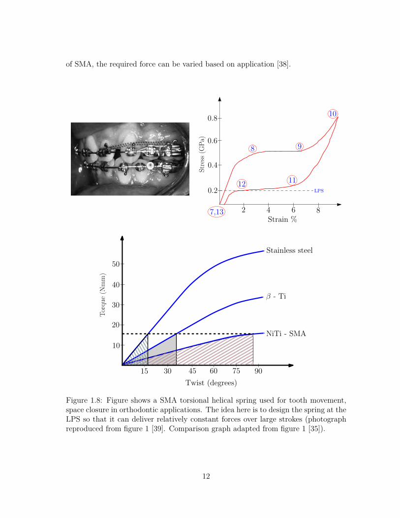
of SMA, the required force can be varied based on application [38].

2 4 6 8

0.2

0.4

0.8

Strain %

Stress(G

Pa) 0.6

98

12

7,13

LPS

10

11

Torque(N

mm)

Twist (degrees)

NiTi - SMA

β - Ti

Stainless steel

10

20

30

40

50

15 30 45 60 75 90

Figure 1.8: Figure shows a SMA torsional helical spring used for tooth movement,space closure in orthodontic applications. The idea here is to design the spring at theLPS so that it can deliver relatively constant forces over large strokes (photographreproduced from figure 1 [39]. Comparison graph adapted from figure 1 [35]).

12

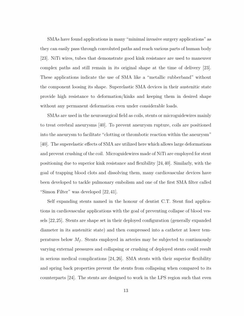
SMAs have found applications in many “minimal invasive surgery applications” as

they can easily pass through convoluted paths and reach various parts of human body

[23]. NiTi wires, tubes that demonstrate good kink resistance are used to maneuver

complex paths and still remain in its original shape at the time of delivery [23].

These applications indicate the use of SMA like a “metallic rubberband” without

the component loosing its shape. Superelastic SMA devices in their austenitic state

provide high resistance to deformation/kinks and keeping them in desired shape

without any permanent deformation even under considerable loads.

SMAs are used in the neurosurgical field as coils, stents or microguidewires mainly

to treat cerebral aneurysms [40]. To prevent aneurysm rupture, coils are positioned

into the aneurysm to facilitate “clotting or thrombotic reaction within the aneurysm”

[40]. The superelastic effects of SMA are utilized here which allows large deformations

and prevent crushing of the coil. Microguidewires made of NiTi are employed for stent

positioning due to superior kink resistance and flexibility [24,40]. Similarly, with the

goal of trapping blood clots and dissolving them, many cardiovascular devices have

been developed to tackle pulmonary embolism and one of the first SMA filter called

“Simon Filter” was developed [22,41].

Self expanding stents named in the honour of dentist C.T. Stent find applica-

tions in cardiovascular applications with the goal of preventing collapse of blood ves-

sels [22,25]. Stents are shape set in their deployed configuration (generally expanded

diameter in its austenitic state) and then compressed into a catheter at lower tem-

peratures below Mf . Stents employed in arteries may be subjected to continuously

varying external pressures and collapsing or crushing of deployed stents could result

in serious medical complications [24, 26]. SMA stents with their superior flexibility

and spring back properties prevent the stents from collapsing when compared to its

counterparts [24]. The stents are designed to work in the LPS region such that even

13

higher external pressures does not allow them to transform to their martensitic phase

as the difference between plateau stresses are quite significant. This ensures that the

stents are in their austenitic state without undergoing any permanent deformation

under constant external pressures at all times during their deployment.

SMA spacers have found applications in many orthopaedic applications with the

intention of applying constant forces on fractured bones to accelerate the bone heal-

ing process [22]. The spacers (sometimes addressed to as staples) in its opened

(deformed) shape are deployed at the site and then heated so that the SMA in its

austentic shape can apply the required compressive forces to facilitate rebuilding

fracture bones [22,27].

All of these unique features makes the use of SMA components a feasible option

in many biomedical application with many of them already having FDA R© approvals

[42].

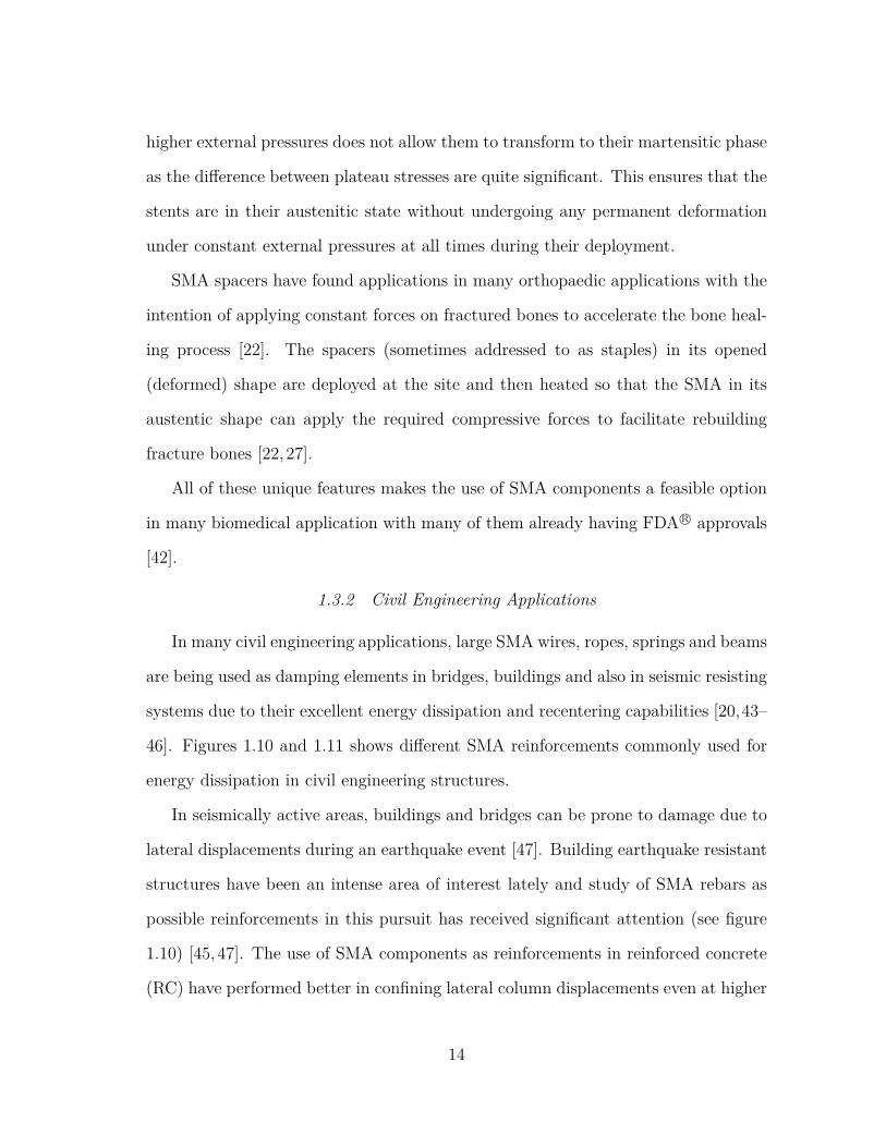
1.3.2 Civil Engineering Applications

In many civil engineering applications, large SMA wires, ropes, springs and beams

are being used as damping elements in bridges, buildings and also in seismic resisting

systems due to their excellent energy dissipation and recentering capabilities [20,43–

46]. Figures 1.10 and 1.11 shows different SMA reinforcements commonly used for

energy dissipation in civil engineering structures.

In seismically active areas, buildings and bridges can be prone to damage due to

lateral displacements during an earthquake event [47]. Building earthquake resistant

structures have been an intense area of interest lately and study of SMA rebars as

possible reinforcements in this pursuit has received significant attention (see figure

1.10) [45, 47]. The use of SMA components as reinforcements in reinforced concrete

(RC) have performed better in confining lateral column displacements even at higher

14

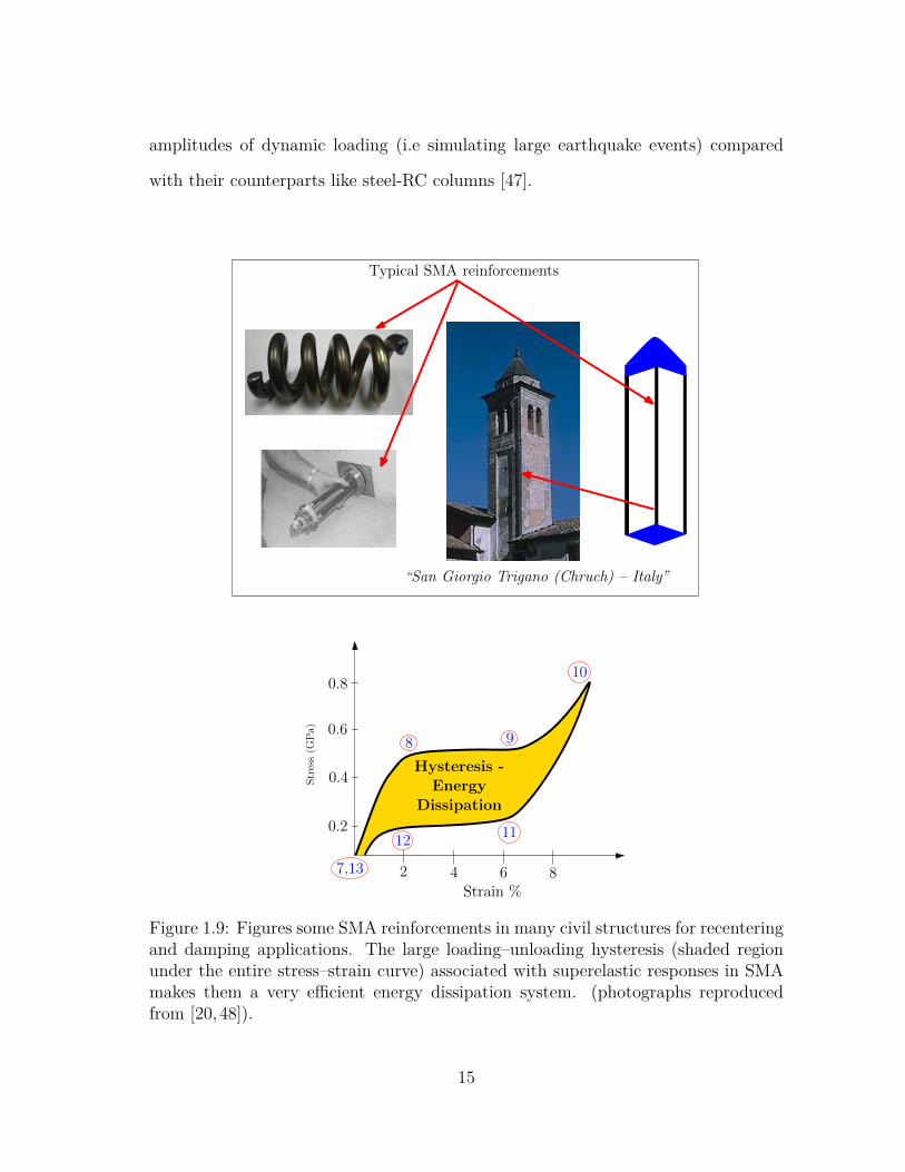
amplitudes of dynamic loading (i.e simulating large earthquake events) compared

with their counterparts like steel-RC columns [47].

“San Giorgio Trigano (Chruch) – Italy”

2 4 6 8

0.2

0.4

0.8

Strain %

Stress(G

Pa) 0.6

98

12

7,13

10

11

Typical SMA reinforcements

Hysteresis -Energy

Dissipation

Figure 1.9: Figures some SMA reinforcements in many civil structures for recenteringand damping applications. The large loading–unloading hysteresis (shaded regionunder the entire stress–strain curve) associated with superelastic responses in SMAmakes them a very efficient energy dissipation system. (photographs reproducedfrom [20,48]).

15

SMA Damper

SMA Damper for Cable Bridge

ConcreteColumn

SMA Rods

Steel Rods

SMA Anchorage for Column

SMA bar

SMA Restrainer

SMA Connector

SMA rods

Beam

Steel Cables

SMA Cables

Column

SMA braces for frame structure

Figure 1.10: Various use of SMA components as energy dissipation devices/dampersfor simply supported cable bridges, anchorages and connectors for columns, bracesfor framed structures. (figures adapted from [20,48]).

16

Concrete Block with deformed SMA wire reinforcements

Three point bend setup

Crack Propogation during loading test

Crack closure upon unloading and SMA activation(Notice shortening of SMA reinforcements)

A

B

C

D

Initial Crack

Initial Crack

Figure 1.11: (A) - Some pretensioned SMA reinforcements in a concrete block with aninitial crack. (B) shows a classic 3-point bend setup. (C) shows the crack propagationduring loading. (D) shows the crack closure upon unloading and activating (heating)SMA reinforcements. The SMA wires shorten causing the crack to close (figuresadapted from [20,49]).

17

Insulation Material SMA rods

Bottom wireactuated

Top wireactuated

Rotor Assembly

Figure 1.12: The use of pre-twisted SMA rods to torsionally actuate blade tabsbetween two angular positions is a possibility by differentially heating of top andlower SMA rods. This way the angular positioning of “trailing edge tab of a helicopterrotor” can be adjusted and thus allowing for user in-flight tracking of its position(figure adapted from [50]).

Inactive Coupler Active Coupler

Pipe A Pipe B

Figure 1.13: SMAs can be used as couplers that can substitute socket welds orcompression fittings in aerospace, civil, oil exploration industries. The idea is todeform the couplers in its martensitic state to larger diameters for easy sliding alongthe pipes and then heated to temperatures above Af to hold the ends of pipes firmlywith appropriate compressive forces. (figure adapted from [51,52])

18

MovingPiston

SMASpring

BiasSpring

BlockingPiston

Drill Pipe(Casing)

(A) : Inactive Position

(B) : Active Position (Actuated)

FixedSupport

Figure 1.14: A combination of SMA springs and bias springs are employed to actuatepistons in “blowout preventer’s” that either block or unblock drill pipes. (A) showsthe the inactive position of blocking piston where the bias springs keeps the SMAspring compressed at lower temperatures (i.e below Mf ). (B) shows the SMA springin its austenitic state (at higher temperatures i.e above Af ) overpowers the biasspring forces and actuates the blocking piston to prevent any flow in drill pipe toprevent any accidents. (figure adapted from [52])

19

With superior damping capacity and ability to deliver large plateau strains at

relatively constant stresses, SMAs make excellent candidates for recentering applica-

tions in the form of bracings or dampers [47]. Many different types of SMA braces

for framed structures have been designed for energy dissipation devices (see figure

1.10) [20]. In many cases, bundles of pre-tensioned superelastic SMA wires are used

as reinforcements have been employed for re-centering braces [20]. In addition, SMA’s

have also been effective contenders as beam–column or column–foundation joints in

many retrofit structures as the large plateau strains in SE can be used to provide

desired clamping forces to hold the members together [47]. This helps in control-

ling relative hinge displacements when used as restrainers [47]. By connecting the

bearings and bridge deck with superelastic bars, the “position stability” of simply

supported bridges could be improved (see figure 1.10) [48, 53].

If a SMA reinforcement in its martensitic form is deformed (also referred to as

pretensioning) and embedded in concrete and then electrically activated such that it

reaches temperatures above Af , sufficient constraining forces can be generated as the

SMA tries to recover back to its original shape [47,53]. The extent of prestressing can

be increased or decreased by controlling the amount of initial deformation of SMA

reinforcement [47]. To illustrate this point, Mo and co-workers looked at developing

a “smart concrete structure” that can potentially “self heal” after a damaging earth-

quake event [49]. In their study, as shown in figure 1.11, a concrete block with many

reinforced SMA ropes was considered [49]. The SMA reinforcements were initially

predeformed (pre-tensioning) in their martensitic state (i.e below their Mf ) and re-

inforced in the concrete block with an initial crack as shown in figure 1.11. On a test

bench, dynamic 3-point bend tests were conducted which resulted in crack propoga-

tion with increasing loads/frequencies mimicking a damaging earthquake event. The

cracked structure is then unloaded and the SMA ropes were activated by heating

20

them above their Af . Upon heating, the SMA ropes transform back to austenite

and shorten in length back to its original shape. This results in large recovery forces

that results in crack closure (crack healing) as the concrete structures are pulled

inwards and thus minimizing the chances of building collapse after an earthquake

event. Many such “self-restoration” options have been proposed with almost com-

plete crack closure upon recentering [20]. On similar lines, many active confinement

techniques where concrete columns are helically wrapped with SMA bands that can

provide necessary tensioning upon heating have also been proposed [48].

In one of the first reported retrofit applications using SMA devices, the San

Giorgio chruch in Italy used bundles of SMA wires to refurbish the church structure

after an earthquake event [45,54]. As shown in figure 1.9, SMA devices were arranged

in series in order to limit the forces to the masonary under the required limits and

further seismic analysis were performed to analyze the performance of SMA devices

[45,54].

However, given the size of civil engineering structures, the use of NiTi SMA

components have been limited due to high initial material and processing costs [48].

Going forward, developing more cheaper copper or iron based SMAs that could

replace NiTi SMA components without compromising material performance would

greatly benefit the civil engineering community as they potentially use many more

smart structures with active control capabilities. Developing such copper or iron

based SMAs and further understanding their underlying microstructural changes

that influence their functionality is still an active area of research [28].

1.3.3 Aerospace and Automotive Applications

SMA components are used as thermal actuators in different temperature regimes

depending on the kind of applications in automotive industry [8]. The use of SMA

21

actuators are finding applications in many pre-commercialized concepts like smart

automotive lighting systems, fuel management, climate control, mirrors adjustments,

locking systems, suspension adjustments etc. [8, 55, 56]. Similarly, SMA cables,

beams, torque tubes are used in tailoring inlet geometry and orientation, increase/decrease

fan nozzle in various aerospace applications [18, 50,57,58].

In some aircraft applications, smart SMA couplings have shown the possibility

of substitute socket welds or compression fittings [51]. As shown in figure 1.13, at

temperatures below Mf , the couplings are expanded to a larger diameter such that

it can easily slide through the pipes to be fastened [51]. Once the SMA coupling

transforms back to austenite (i.e above Af which is generally programmed to be

lower than room temperature), it shrinks to its original dimension and thus securely

holding the pipe ends as the SMA coupling enforces sufficient compressive forces [51].

Chopra [50] reviews many possible applications of using smart materials in aerospace

systems. For example, adjusting the “trailing edge tab of a helicopter rotor for in-

flight tracking” using SMA components is one of the key proposed ideas [50]. Pre-

twisted SMA rods to torsionally actuate blade tabs between two angular positions is

possibility by differentially actuating the SMA rods as shown in figure 1.12. By heat-

ing the upper rod, the SMA rod shortens and causes the rotor assembly to actuate

in one direction. By heating the lower rod, the SMA rod enables the rotor assembly

to actuate in a different direction. The actuation of the rotor assembly in different

directions causes the trailing edge to occupy multiple angular positions during flight

maneuver. The SMA rods clearly perform both sensing and actuating functions and

thereby reducing the use of separate working elements for sensors and actuators to

perform the same task.

On similar lines, “Chevrons” in aircraft engines are employed for flow mixing and

their configurations can be altered by using SMA beams based on changes in flow

22

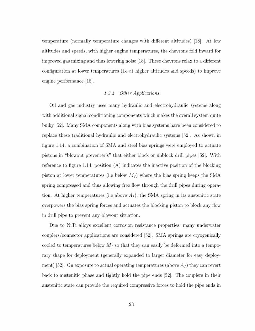
temperature (normally temperature changes with different altitudes) [18]. At low

altitudes and speeds, with higher engine temperatures, the chevrons fold inward for

improved gas mixing and thus lowering noise [18]. These chevrons relax to a different

configuration at lower temperatures (i.e at higher altitudes and speeds) to improve

engine performance [18].

1.3.4 Other Applications

Oil and gas industry uses many hydraulic and electrohydraulic systems along

with additional signal conditioning components which makes the overall system quite

bulky [52]. Many SMA components along with bias systems have been considered to

replace these traditional hydraulic and electrohydraulic systems [52]. As shown in

figure 1.14, a combination of SMA and steel bias springs were employed to actuate

pistons in “blowout preventer’s” that either block or unblock drill pipes [52]. With

reference to figure 1.14, position (A) indicates the inactive position of the blocking

piston at lower temperatures (i.e below Mf ) where the bias spring keeps the SMA

spring compressed and thus allowing free flow through the drill pipes during opera-

tion. At higher temperatures (i.e above Af ), the SMA spring in its austenitic state

overpowers the bias spring forces and actuates the blocking piston to block any flow

in drill pipe to prevent any blowout situation.

Due to NiTi alloys excellent corrosion resistance properties, many underwater

couplers/connector applications are considered [52]. SMA springs are cryogenically

cooled to temperatures below Mf so that they can easily be deformed into a tempo-

rary shape for deployment (generally expanded to larger diameter for easy deploy-

ment) [52]. On exposure to actual operating temperatures (above Af ) they can revert

back to austenitic phase and tightly hold the pipe ends [52]. The couplers in their

austenitic state can provide the required compressive forces to hold the pipe ends in

23

place. On similar lines, some smart couplings have also been tested for submarine

applications and underwater gas pipelines as shown in figure 1.13. Such couplings

are easy to work with as it does not require any initial pipe surface preparation or

subsequent welding or safety hazards [51].

SMA compression springs along with bias steel springs are finding applications in

sprinkler systems that can automatically turn on or off based on the water tempera-

ture [28]. Ni-Ti-Cu springs are finding applications in thermostats, electrical circuit

breakers where for example door positions in an self cleaning oven are monitored us-

ing SMA components [28]. NiTi discs located between electrical contacts in Lithium

ion batteries can be used to break the circuits at critical temperatures [28].

Jeya Ganesh and co-workers have attempted to design a simple “sun tracking

mechanism (SSTM)” to illustrate the dual sensing and actuating capability of SMA

components [7]. The solar receptor position is automatically changed over the course

of the days by using the solar radiation to actuate the SMA springs [7]. As described

in figure 1.3, the use of such smart SMA springs considerably reduces the number

of working elements as compared against a convectional sun tracking system that

employs separate sensor and actuator for providing system level response [7].

1.4 Review of Modeling Approaches and Their Limitations

As discussed with various applications in section 1.3, SMAs are mainly used in

the form of wires, bars, springs and beams that are subjected to primary modes of

deformation like tension, torsion or bending loading conditions. In order to design

and realize the vision of creating novel, potentially useful applications using SMA,

it is imperative to understand and model the material response under these primary

loading cases at the component level. Due to the complex nature of SMA response

(see figure 1.6), model development for these materials have been addressed in a

24

number of different perspectives that are suited for different purposes. As shown

in figure 1.15, several microscopic and macroscopic models have been developed to

capture the complex SMA responses, identifying underlying mechanisms in phase

transformations and explaining their underlying physics [59].

The microscopic models (mostly crystal plasticity based) focus on the micro-

scale features of phase transformation to understand the basic underlying physical

mechanisms that are inherent to these material systems. Several models were de-

veloped in order to understated micro-scale features, such as nucleation, interface

motion, twin growth, etc [60, 61]. The phase volume fractions are not considered

as a-priori internal variables but are a resultant of consequences of interface move-

ments among different phases. Such models are useful in understanding fundamental

phenomenon but posses limitations in terms of their applications towards predicting

macroscopic responses useful for designing SMA components for many engineering

applications [62,63].

A brief review of some important macroscopic modeling approaches (by no means

exhaustive) under different loading conditions is covered in the following sections as

it is an uphill task to cover the entire gamut of available models for SMA. Section

1.4.1 reviews some important modeling approaches and their shortcomings in cap-

turing responses under tensile loading. In sections 1.4.2 and 1.4.3, a more detailed

discussion on extension of modeling approaches highlighted in section 1.4.1 for sim-

ulating responses under torsion and bending loading conditions would be discussed

along with their limitations.

1.4.1 Tension Response of SMA

Two main approaches in macroscopic modeling SMA response can be broadly

classified into models analogous to elastoplasticity and those analogous to magnetic

25

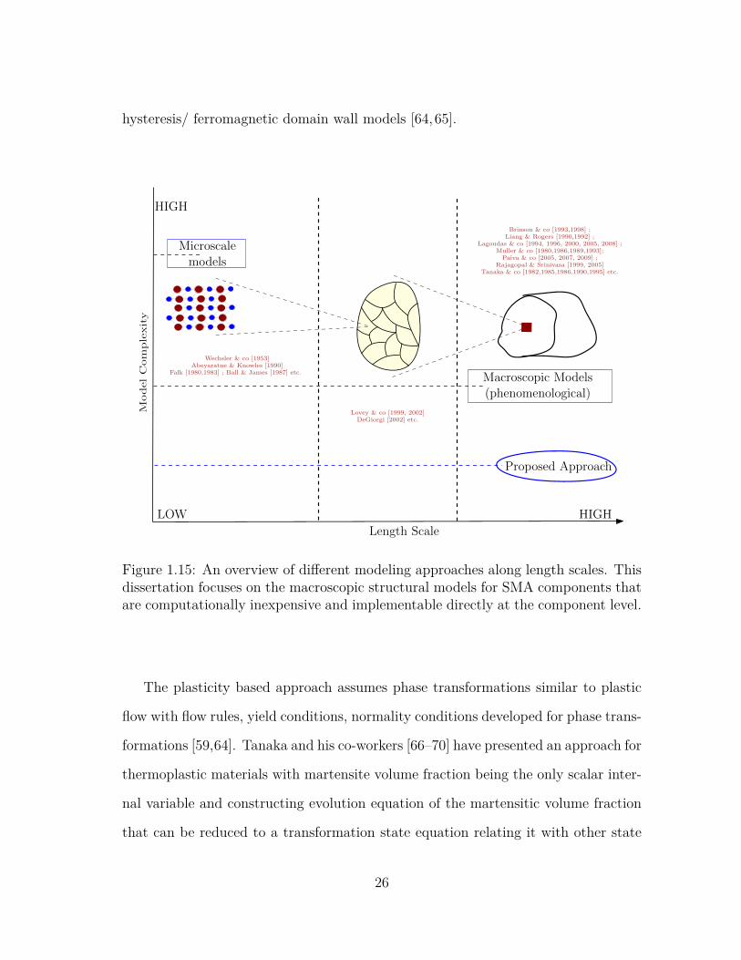
hysteresis/ ferromagnetic domain wall models [64,65].

HIGH

LOW HIGH

Macroscopic Models(phenomenological)

Proposed Approach

Length Scale

ModelComplexity

Microscalemodels

Lovey & co [1999, 2002]DeGiorgi [2002] etc.

Wechsler & co [1953]Abeyaratne & Knowles [1990]

Falk [1980,1983] ; Ball & James [1987] etc.

Brinson & co [1993,1998] ;Liang & Rogers [1990,1992] ;

Lagoudas & co [1994, 1996, 2000, 2005, 2008] ;Muller & co [1980,1986,1989,1993];Paiva & co [2005, 2007, 2009] ;

Rajagopal & Srinivasa [1999, 2005]Tanaka & co [1982,1985,1986,1990,1995] etc.

Figure 1.15: An overview of different modeling approaches along length scales. Thisdissertation focuses on the macroscopic structural models for SMA components thatare computationally inexpensive and implementable directly at the component level.

The plasticity based approach assumes phase transformations similar to plastic

flow with flow rules, yield conditions, normality conditions developed for phase trans-

formations [59,64]. Tanaka and his co-workers [66–70] have presented an approach for

thermoplastic materials with martensite volume fraction being the only scalar inter-

nal variable and constructing evolution equation of the martensitic volume fraction

that can be reduced to a transformation state equation relating it with other state

26

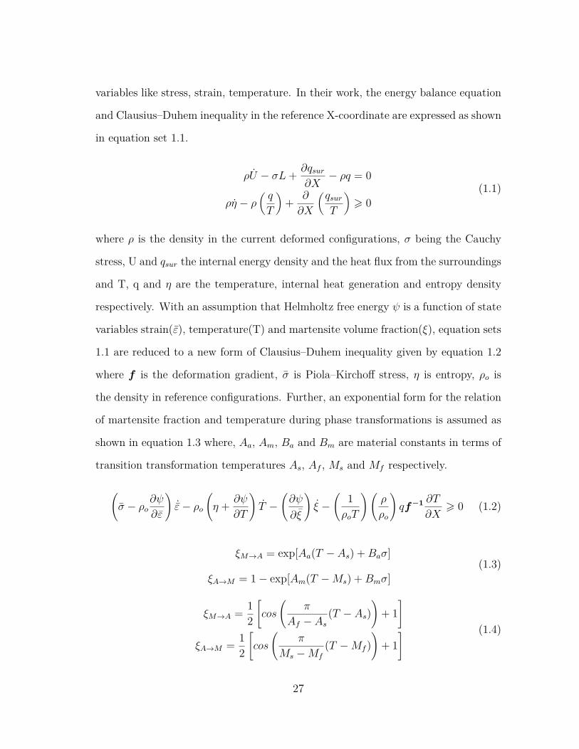
variables like stress, strain, temperature. In their work, the energy balance equation

and Clausius–Duhem inequality in the reference X-coordinate are expressed as shown

in equation set 1.1.

ρU − σL+ ∂qsur∂X

− ρq = 0

ρη − ρ(q

T

)+ ∂

∂X

(qsurT

)> 0

(1.1)

where ρ is the density in the current deformed configurations, σ being the Cauchy

stress, U and qsur the internal energy density and the heat flux from the surroundings

and T, q and η are the temperature, internal heat generation and entropy density

respectively. With an assumption that Helmholtz free energy ψ is a function of state

variables strain(ε), temperature(T) and martensite volume fraction(ξ), equation sets

1.1 are reduced to a new form of Clausius–Duhem inequality given by equation 1.2

where f is the deformation gradient, σ is Piola–Kirchoff stress, η is entropy, ρo is

the density in reference configurations. Further, an exponential form for the relation

of martensite fraction and temperature during phase transformations is assumed as

shown in equation 1.3 where, Aa, Am, Ba and Bm are material constants in terms of

transition transformation temperatures As, Af , Ms and Mf respectively.

(σ − ρo

∂ψ

∂ε

)˙ε− ρo

(η + ∂ψ

∂T

)T −

(∂ψ

∂ξ

)ξ −

(1ρoT

)(ρ

ρo

)qf−1 ∂T

∂X> 0 (1.2)

ξM→A = exp[Aa(T − As) +Baσ]

ξA→M = 1− exp[Am(T −Ms) +Bmσ](1.3)

ξM→A = 12

[cos

(π

Af − As(T − As)

)+ 1

]

ξA→M = 12

[cos

(π

Ms −Mf

(T −Mf ))

+ 1] (1.4)

27

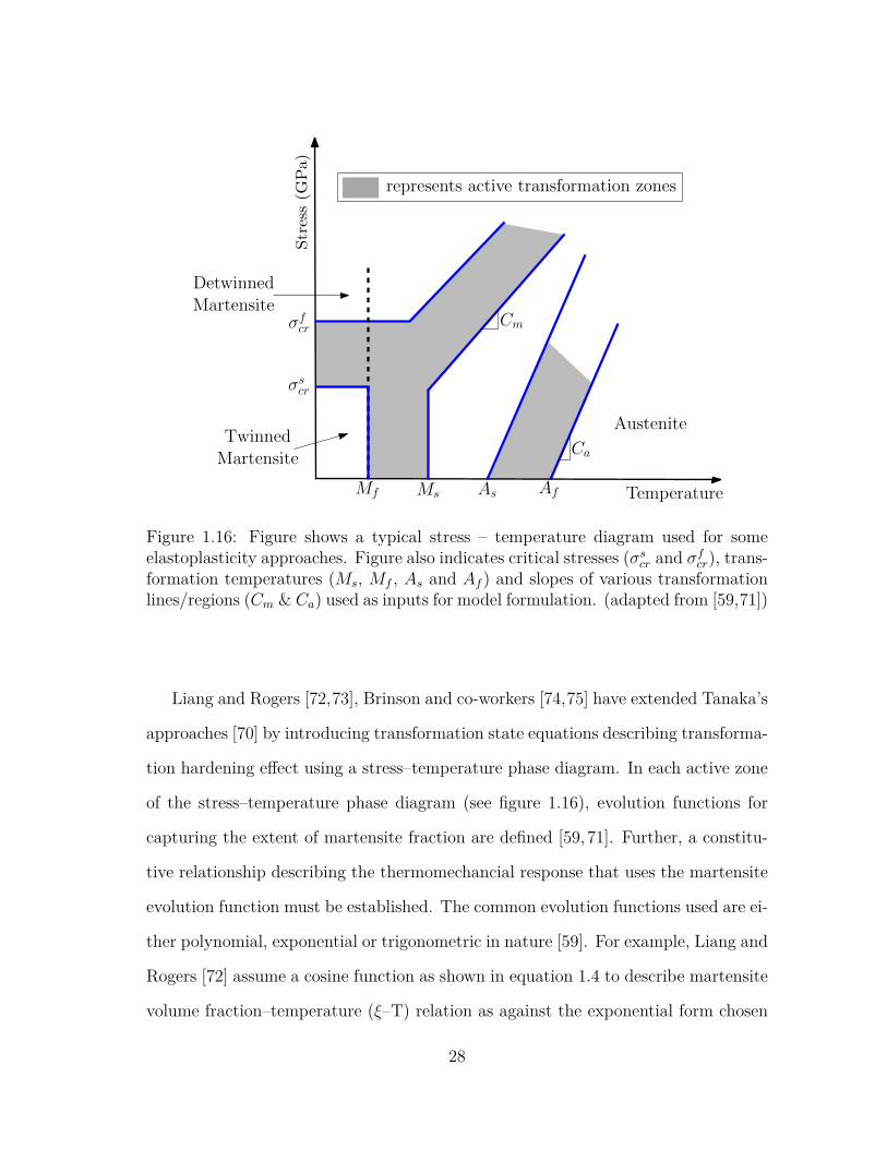
Stress(G

Pa)

TemperatureMf Ms As Af

σscr

σfcr

Austenite

DetwinnedMartensite

TwinnedMartensite

Cm

Ca

represents active transformation zones

Figure 1.16: Figure shows a typical stress – temperature diagram used for someelastoplasticity approaches. Figure also indicates critical stresses (σscr and σfcr), trans-formation temperatures (Ms, Mf , As and Af ) and slopes of various transformationlines/regions (Cm & Ca) used as inputs for model formulation. (adapted from [59,71])

Liang and Rogers [72,73], Brinson and co-workers [74,75] have extended Tanaka’s

approaches [70] by introducing transformation state equations describing transforma-

tion hardening effect using a stress–temperature phase diagram. In each active zone

of the stress–temperature phase diagram (see figure 1.16), evolution functions for

capturing the extent of martensite fraction are defined [59, 71]. Further, a constitu-

tive relationship describing the thermomechancial response that uses the martensite

evolution function must be established. The common evolution functions used are ei-

ther polynomial, exponential or trigonometric in nature [59]. For example, Liang and

Rogers [72] assume a cosine function as shown in equation 1.4 to describe martensite

volume fraction–temperature (ξ–T) relation as against the exponential form chosen

28

by Tanaka and co-workers [72, 73]. Brinson and co-workers [74] further separate

the martensite fraction internal variable into temperature and stress induced parts.

Limitations of such phase diagram based approaches are summarized below :

• Such models require information on critical stresses governing formation of

stress induced martensite, transformation temperatures and slopes of various

transformation lines/regions in a stress–temperature phase diagram as inputs

(as shown in figure 1.16) [71, 76]. These transition points like critical stresses

and stress–temperature phase diagram slopes must be determined for every

temperature and are not evident from a standard experimental stress–strain

or stress–temperature response especially at different temperatures as the re-

sponses tend to show hardening or softening effects (see figure 1.7 for illus-

trations) [71, 76]. This makes it hard to derive necessary material and model

parameters and implement such models for engineering cases as they are heavily

dependent on such experimental information.

• The available models haven’t shown the capability of capturing internal loops

or temperature dependence observed in superelastic responses (see response in

figure 1.7 for illustrations) which are quite critical for control system applica-

tions [76]. These models have only been used to approximately capture outer

loop responses. Capturing internal loops and temperature dependence of re-

sponses are important from an application standpoint as in many applications

not the entire the response is considered and only a partial internal loop might

be of significance for design purposes [76]. If one need to capture responses at

different temperatures then the model parameters must be recomputed thus

making it cumbersome for implementation for various applications [76].

Lagoudas et al. [77], in an effort to study the effective thermomechanical response

29

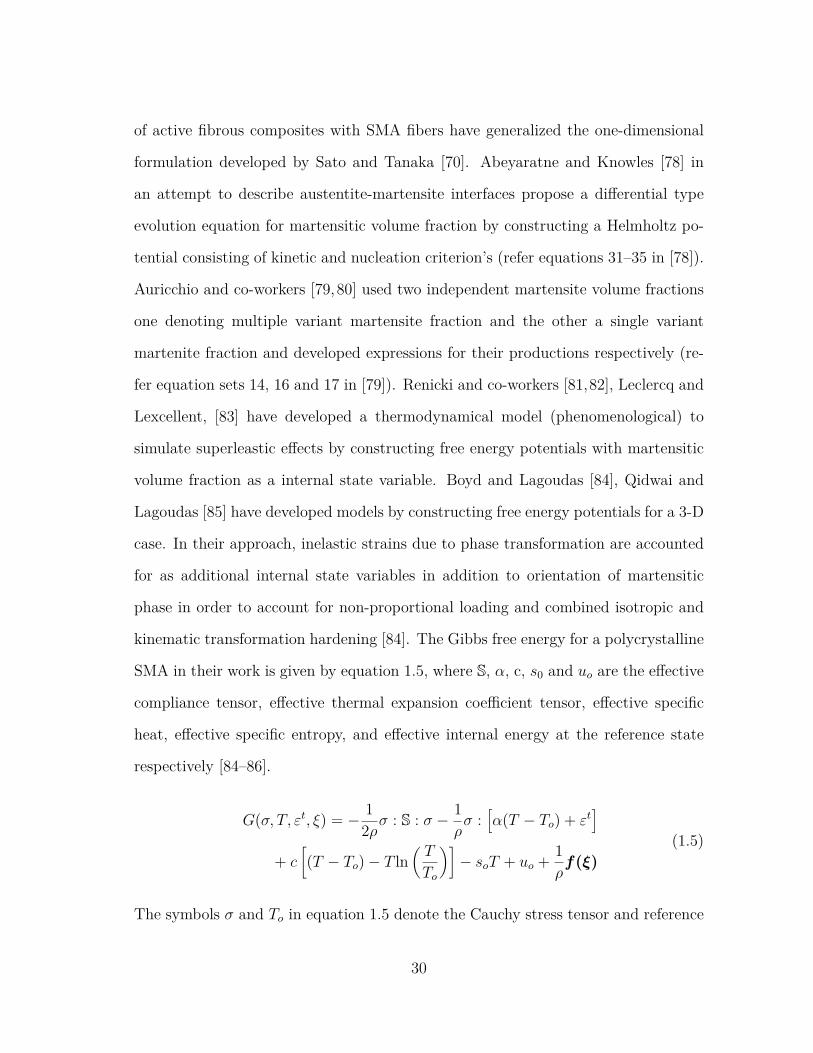
of active fibrous composites with SMA fibers have generalized the one-dimensional

formulation developed by Sato and Tanaka [70]. Abeyaratne and Knowles [78] in

an attempt to describe austentite-martensite interfaces propose a differential type

evolution equation for martensitic volume fraction by constructing a Helmholtz po-

tential consisting of kinetic and nucleation criterion’s (refer equations 31–35 in [78]).

Auricchio and co-workers [79,80] used two independent martensite volume fractions

one denoting multiple variant martensite fraction and the other a single variant

martenite fraction and developed expressions for their productions respectively (re-

fer equation sets 14, 16 and 17 in [79]). Renicki and co-workers [81,82], Leclercq and

Lexcellent, [83] have developed a thermodynamical model (phenomenological) to

simulate superleastic effects by constructing free energy potentials with martensitic

volume fraction as a internal state variable. Boyd and Lagoudas [84], Qidwai and

Lagoudas [85] have developed models by constructing free energy potentials for a 3-D

case. In their approach, inelastic strains due to phase transformation are accounted

for as additional internal state variables in addition to orientation of martensitic

phase in order to account for non-proportional loading and combined isotropic and

kinematic transformation hardening [84]. The Gibbs free energy for a polycrystalline

SMA in their work is given by equation 1.5, where S, α, c, s0 and uo are the effective

compliance tensor, effective thermal expansion coefficient tensor, effective specific

heat, effective specific entropy, and effective internal energy at the reference state

respectively [84–86].

G(σ, T, εt, ξ) = − 12ρσ : S : σ − 1

ρσ :

[α(T − To) + εt

]+ c

[(T − To)− T ln

(T

To

)]− soT + uo + 1

ρf(ξ)

(1.5)

The symbols σ and To in equation 1.5 denote the Cauchy stress tensor and reference

30

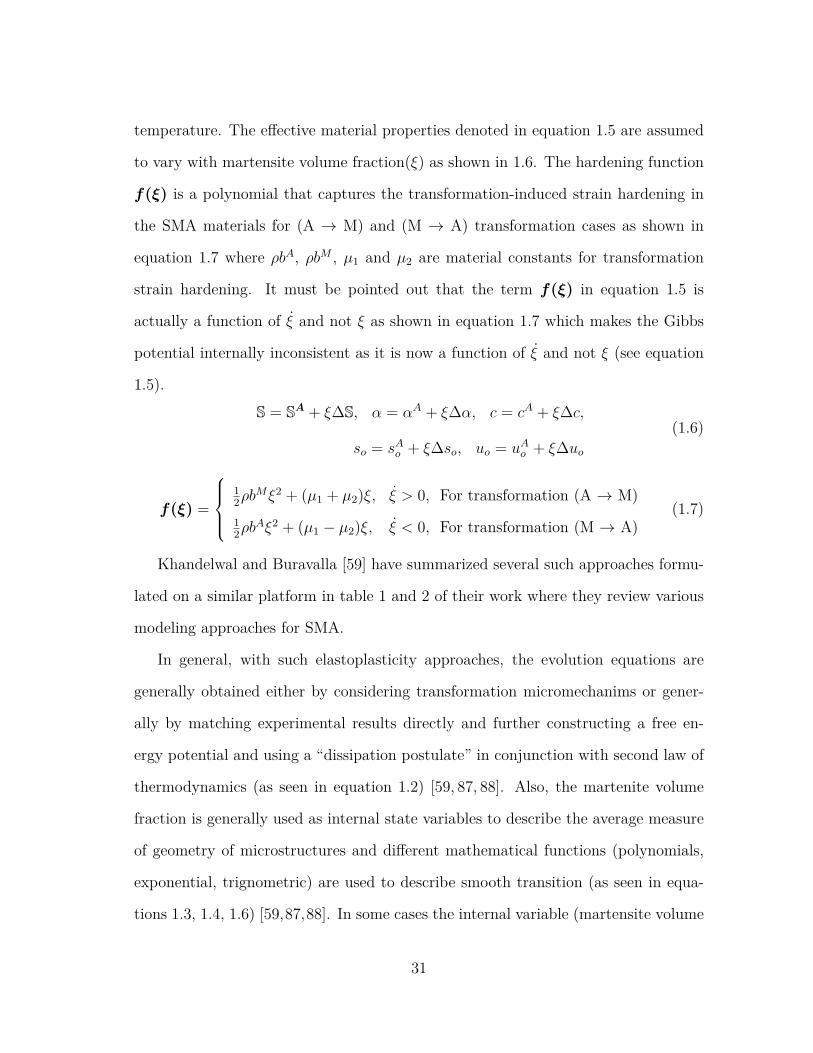
temperature. The effective material properties denoted in equation 1.5 are assumed

to vary with martensite volume fraction(ξ) as shown in 1.6. The hardening function

f(ξ) is a polynomial that captures the transformation-induced strain hardening in

the SMA materials for (A → M) and (M → A) transformation cases as shown in

equation 1.7 where ρbA, ρbM , µ1 and µ2 are material constants for transformation

strain hardening. It must be pointed out that the term f(ξ) in equation 1.5 is

actually a function of ξ and not ξ as shown in equation 1.7 which makes the Gibbs

potential internally inconsistent as it is now a function of ξ and not ξ (see equation

1.5).S = SA + ξ∆S, α = αA + ξ∆α, c = cA + ξ∆c,

so = sAo + ξ∆so, uo = uAo + ξ∆uo(1.6)

f(ξ) =

12ρb

Mξ2 + (µ1 + µ2)ξ, ξ > 0, For transformation (A → M)12ρb

Aξ2 + (µ1 − µ2)ξ, ξ < 0, For transformation (M → A)(1.7)

Khandelwal and Buravalla [59] have summarized several such approaches formu-

lated on a similar platform in table 1 and 2 of their work where they review various

modeling approaches for SMA.

In general, with such elastoplasticity approaches, the evolution equations are

generally obtained either by considering transformation micromechanims or gener-

ally by matching experimental results directly and further constructing a free en-

ergy potential and using a “dissipation postulate” in conjunction with second law of

thermodynamics (as seen in equation 1.2) [59, 87, 88]. Also, the martenite volume

fraction is generally used as internal state variables to describe the average measure

of geometry of microstructures and different mathematical functions (polynomials,

exponential, trignometric) are used to describe smooth transition (as seen in equa-

tions 1.3, 1.4, 1.6) [59,87,88]. In some cases the internal variable (martensite volume

31

fraction) are separated into temperature-induced and stress induced parts [74]. Such

elastoplasticity based approaches have the following limitations :

• Though these models have firm thermodynamic foundations, such strategies

become extremely cumbersome for identification of material and model param-

eters from experimental data as the identification is mostly heuristic. Incorpo-

rating temperature effects and accounting for internal loops is cumbersome as

many of material parameters and functions must be recomputed for simulating

these effects (For example, see table 1 in [84–86,89] for the number of material

parameters needed for model verification) [64].

• A close perusal of the 3-D constitutive models developed, reveals that, in ac-

tuality, these approaches just use the one dimensional data and use a von-

Mises equivalent stress approach due to lack of a full three dimensional data

on SMAs [90]. Given the fact that such an approach (originally based on exper-

imental observations of steel) does not even work well for aluminum, it is hard

to justify their use in SMA given their complex thermomechanical response [90].

• Further, if such models are used to simulate a simple bar or wire response then

one needs to simulate a full 3-D model or use a reduced 3-D model for analyzing

specific cases thus making them hard to implement for actual design cases at

the component level.

However, phase transformations in SMA are more akin to domain wall switching

in magnetism rather than crystallographic slip. The whole SMA structure can be

imagined as a collection of many such domains with each of them discretely switching

states based on the external impetus (i.e switching between austenite – martensite

variant or between martensite variants in case of SMA). The macroscopic responses

32

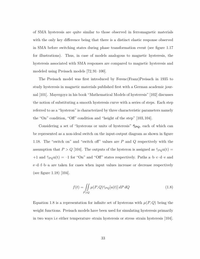
of SMA hysteresis are quite similar to those observed in ferromagnetic materials

with the only key difference being that there is a distinct elastic response observed

in SMA before switching states during phase transformation event (see figure 1.17

for illustrations). Thus, in case of models analogous to magnetic hysteresis, the

hysteresis associated with SMA responses are compared to magnetic hysteresis and

modeled using Preisach models [72, 91–100].

The Preisach model was first introduced by Ferenc(Franz)Preisach in 1935 to

study hysteresis in magnetic materials published first with a German academic jour-

nal [101]. Mayergoyz in his book “Mathematical Models of hysteresis” [102] discusses

the notion of substituting a smooth hysteresis curve with a series of steps. Each step

referred to as a “hysteron” is characterized by three characteristic parameters namely

the “On” condition, “Off” condition and “height of the step” [103,104].

Considering a set of “hysterons or units of hysteresis” γPQ, each of which can

be represented as a non-ideal switch on the input-output diagram as shown in figure

1.18. The “switch on” and “switch off” values are P and Q respectively with the

assumption that P > Q [104]. The outputs of the hysteron is assigned as γPQu(t) =

+1 and γPQu(t) = –1 for “On” and “Off” states respectively. Paths a–b–c–d–e and

e–d–f–b–a are taken for cases when input values increase or decrease respectively

(see figure 1.18) [104].

f(t) =∫∫P>Q

µ(P,Q)γPQ[u(t)] dP dQ (1.8)

Equation 1.8 is a representation for infinite set of hysterons with µ(P,Q) being the

weight functions. Preisach models have been used for simulating hysteresis primarily

in two ways i.e either temperature–strain hysteresis or stress–strain hysteresis [104].

33

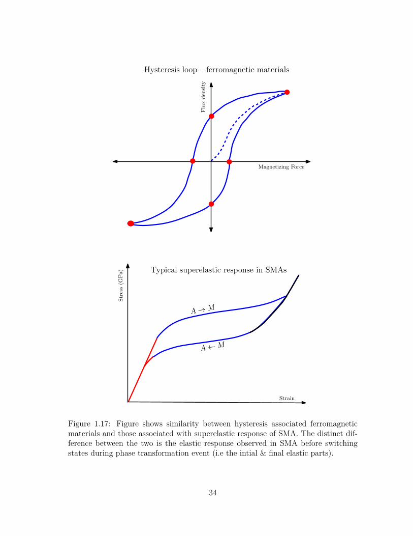
Fluxdensity

Magnetizing Force

A→M

A←M

Typical superelastic response in SMAs

Hysteresis loop – ferromagnetic materials

Stress(G

Pa)

Strain

Figure 1.17: Figure shows similarity between hysteresis associated ferromagneticmaterials and those associated with superelastic response of SMA. The distinct dif-ference between the two is the elastic response observed in SMA before switchingstates during phase transformation event (i.e the intial & final elastic parts).

34

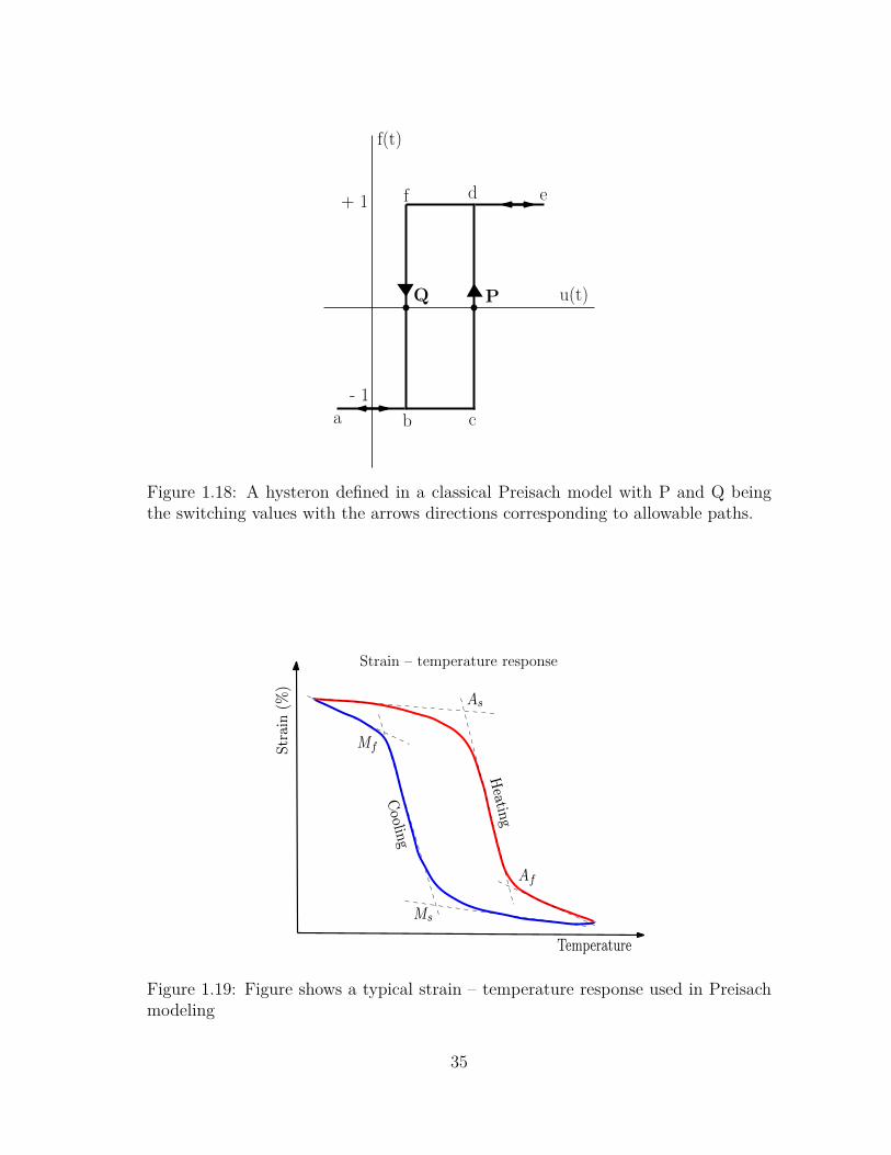
Q P

f

b ca

d e+ 1

- 1

f(t)

u(t)

Figure 1.18: A hysteron defined in a classical Preisach model with P and Q beingthe switching values with the arrows directions corresponding to allowable paths.

Strain(%

)

Coolin

g

Heatin

g

Ms

Af

As

Mf

Temperature

Strain – temperature response

Figure 1.19: Figure shows a typical strain – temperature response used in Preisachmodeling

35

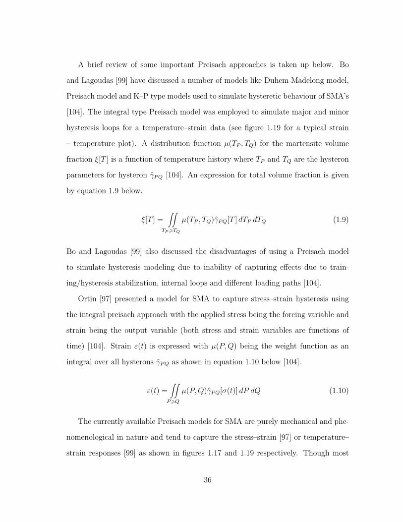
A brief review of some important Preisach approaches is taken up below. Bo

and Lagoudas [99] have discussed a number of models like Duhem-Madelong model,

Preisach model and K–P type models used to simulate hysteretic behaviour of SMA’s

[104]. The integral type Preisach model was employed to simulate major and minor

hysteresis loops for a temperature–strain data (see figure 1.19 for a typical strain

– temperature plot). A distribution function µ(TP , TQ) for the martensite volume

fraction ξ[T ] is a function of temperature history where TP and TQ are the hysteron

parameters for hysteron γPQ [104]. An expression for total volume fraction is given

by equation 1.9 below.

ξ[T ] =∫∫

TP >TQ

µ(TP , TQ)γPQ[T ] dTP dTQ (1.9)

Bo and Lagoudas [99] also discussed the disadvantages of using a Preisach model

to simulate hysteresis modeling due to inability of capturing effects due to train-

ing/hysteresis stabilization, internal loops and different loading paths [104].

Ortin [97] presented a model for SMA to capture stress–strain hysteresis using

the integral preisach approach with the applied stress being the forcing variable and

strain being the output variable (both stress and strain variables are functions of

time) [104]. Strain ε(t) is expressed with µ(P,Q) being the weight function as an

integral over all hysterons γPQ as shown in equation 1.10 below [104].

ε(t) =∫∫P>Q

µ(P,Q)γPQ[σ(t)] dP dQ (1.10)

The currently available Preisach models for SMA are purely mechanical and phe-

nomenological in nature and tend to capture the stress–strain [97] or temperature–

strain responses [99] as shown in figures 1.17 and 1.19 respectively. Though most

36

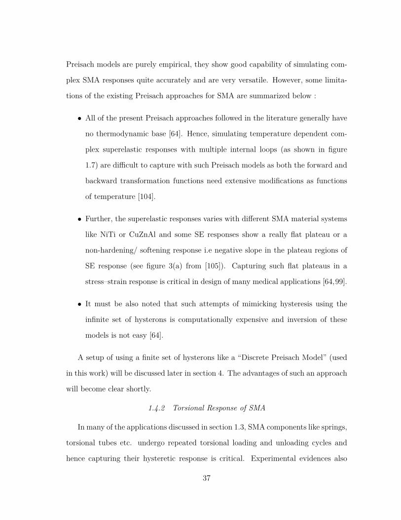
Preisach models are purely empirical, they show good capability of simulating com-

plex SMA responses quite accurately and are very versatile. However, some limita-

tions of the existing Preisach approaches for SMA are summarized below :

• All of the present Preisach approaches followed in the literature generally have

no thermodynamic base [64]. Hence, simulating temperature dependent com-

plex superelastic responses with multiple internal loops (as shown in figure

1.7) are difficult to capture with such Preisach models as both the forward and

backward transformation functions need extensive modifications as functions

of temperature [104].

• Further, the superelastic responses varies with different SMA material systems

like NiTi or CuZnAl and some SE responses show a really flat plateau or a

non-hardening/ softening response i.e negative slope in the plateau regions of

SE response (see figure 3(a) from [105]). Capturing such flat plateaus in a

stress–strain response is critical in design of many medical applications [64,99].

• It must be also noted that such attempts of mimicking hysteresis using the

infinite set of hysterons is computationally expensive and inversion of these

models is not easy [64].

A setup of using a finite set of hysterons like a “Discrete Preisach Model” (used

in this work) will be discussed later in section 4. The advantages of such an approach

will become clear shortly.

1.4.2 Torsional Response of SMA

In many of the applications discussed in section 1.3, SMA components like springs,

torsional tubes etc. undergo repeated torsional loading and unloading cycles and

hence capturing their hysteretic response is critical. Experimental evidences also

37

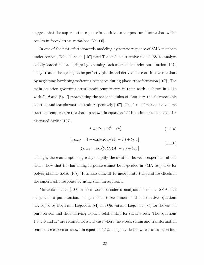
suggest that the superelastic response is sensitive to temperature fluctuations which

results in force/ stress variations [39,106].

In one of the first efforts towards modeling hysteretic response of SMA members

under torsion, Tobushi et al. [107] used Tanaka’s constitutive model [68] to analyze

axially loaded helical springs by assuming each segment is under pure torsion [107].

They treated the springs to be perfectly plastic and derived the constitutive relations

by neglecting hardening/softening responses during phase transformation [107]. The

main equation governing stress-strain-temperature in their work is shown in 1.11a

with G, θ and |Ω/G| representing the shear modulus of elasticity, the thermoelastic

constant and transformation strain respectively [107]. The form of martensite volume

fraction–temperature relationship shown in equation 1.11b is similar to equation 1.3

discussed earlier [107].

τ = Gγ + θT + Ωξ (1.11a)

ξA→M = 1− exp[bACM(Ms − T ) + bMτ ]

ξM→A = exp[bACA(As − T ) + bAτ ](1.11b)

Though, these assumptions greatly simplify the solution, however experimental evi-

dence show that the hardening response cannot be neglected in SMA responses for

polycrystalline SMA [108]. It is also difficult to incorporate temperature effects in

the superelastic response by using such an approach.

Mirzaeifar et al. [109] in their work considered analysis of circular SMA bars

subjected to pure torsion. They reduce three dimensional constitutive equations

developed by Boyd and Lagoudas [84] and Qidwai and Lagoudas [85] for the case of

pure torsion and thus deriving explicit relationship for shear stress. The equations

1.5, 1.6 and 1.7 are reduced for a 1-D case where the stress, strain and transformation

tensors are chosen as shown in equation 1.12. They divide the wire cross section into

38

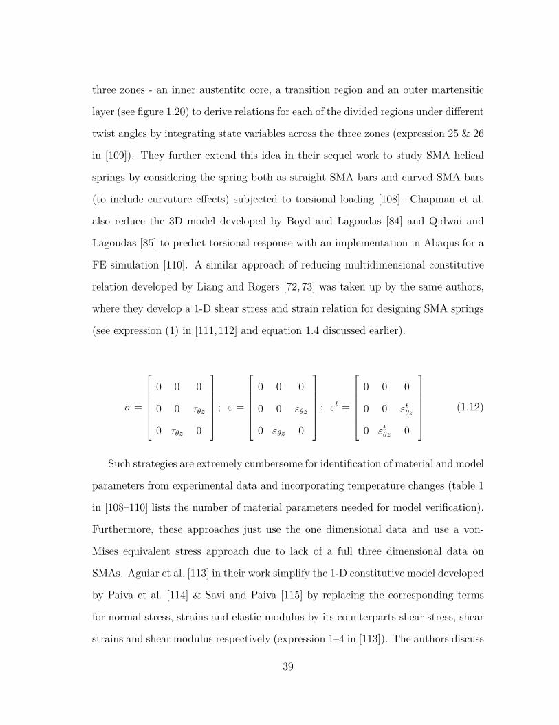
three zones - an inner austentitc core, a transition region and an outer martensitic

layer (see figure 1.20) to derive relations for each of the divided regions under different

twist angles by integrating state variables across the three zones (expression 25 & 26

in [109]). They further extend this idea in their sequel work to study SMA helical

springs by considering the spring both as straight SMA bars and curved SMA bars

(to include curvature effects) subjected to torsional loading [108]. Chapman et al.

also reduce the 3D model developed by Boyd and Lagoudas [84] and Qidwai and

Lagoudas [85] to predict torsional response with an implementation in Abaqus for a

FE simulation [110]. A similar approach of reducing multidimensional constitutive

relation developed by Liang and Rogers [72, 73] was taken up by the same authors,

where they develop a 1-D shear stress and strain relation for designing SMA springs

(see expression (1) in [111,112] and equation 1.4 discussed earlier).

σ =

0 0 0

0 0 τθz

0 τθz 0

; ε =

0 0 0

0 0 εθz

0 εθz 0

; εt =

0 0 0

0 0 εtθz

0 εtθz 0

(1.12)

Such strategies are extremely cumbersome for identification of material and model

parameters from experimental data and incorporating temperature changes (table 1

in [108–110] lists the number of material parameters needed for model verification).

Furthermore, these approaches just use the one dimensional data and use a von-

Mises equivalent stress approach due to lack of a full three dimensional data on

SMAs. Aguiar et al. [113] in their work simplify the 1-D constitutive model developed

by Paiva et al. [114] & Savi and Paiva [115] by replacing the corresponding terms

for normal stress, strains and elastic modulus by its counterparts shear stress, shear

strains and shear modulus respectively (expression 1–4 in [113]). The authors discuss

39

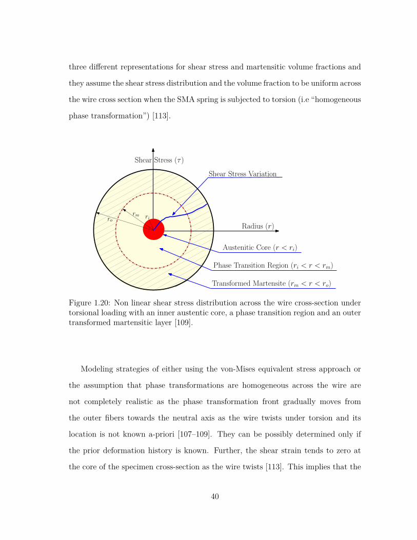
three different representations for shear stress and martensitic volume fractions and

they assume the shear stress distribution and the volume fraction to be uniform across

the wire cross section when the SMA spring is subjected to torsion (i.e “homogeneous

phase transformation”) [113].

Radius (r)

Austenitic Core (r < ri)

Phase Transition Region (ri < r < rm)

Transformed Martensite (rm < r < ro)

Shear Stress Variation

rirm

ro

Shear Stress (τ )

Figure 1.20: Non linear shear stress distribution across the wire cross-section undertorsional loading with an inner austentic core, a phase transition region and an outertransformed martensitic layer [109].

Modeling strategies of either using the von-Mises equivalent stress approach or

the assumption that phase transformations are homogeneous across the wire are

not completely realistic as the phase transformation front gradually moves from

the outer fibers towards the neutral axis as the wire twists under torsion and its

location is not known a-priori [107–109]. They can be possibly determined only if

the prior deformation history is known. Further, the shear strain tends to zero at

the core of the specimen cross-section as the wire twists [113]. This implies that the

40

possibility of having a fully transformed case can only be possible if the angle of twist

asymptotically reaches infinity [116]. A schematic in figure 1.20 shows the three zones

- an inner austentitc core, a transition region and an outer martensitic layer. The

untransformed austentic core at the center might exist even for the maximum possible

twist due to really small shear strains. Figure 1.20 also depicts the non-linear shear

stress variation across the wire cross-section. All of these suggest that the transition

across the wire cross-section is not homogeneous and cannot be accounted for easily

by just averaging or integrating certain state variables in constitutive relations across

the wire cross sections.

1.4.3 Bending Response of SMA

In some applications discussed in section 1.3, SMA’s are used under bending mode

and thus efforts in understanding “moment v/s curvature/deflection” responses has

been of keen interest with the medical community. Experimental results for Force

v/s mid-span deflection for a 3-point bend test conducted on wires and slender beams

have been reported widely by the medical community (see results in [33,34,117–130]).

Most of the available experimental results from the medical community are using 3-

point bend tests. Thus, Berg [131], Rejzner et al. [132] conducted experiments for a

case of pure bending v/s curvature using custom designed experimental rigs. Wick et

al. [133] have also reported experimental results by comparing responses for 3-point

bending, pure bending and tension loading cases (see figure 4 in [133]). Considering

the importance of predicting the bending response with its associated hysteresis,

some efforts towards modeling their complex response were undertaken.

Rejzner et al. [132] used the model developed by Raniecki et al. ( [134]) to solve

rate-type kinetic equations that takes into account tension-compression asymmetry

along with a non-linear differential equation describing neutral plane motion for

41

a symmetric cross-section. Marfia et al. [135] analysed a case of laminated SMA

beams based on small-deformation Euler-Bernoulli theory. They explored a “mixture

rule type approach” to determine martensite volume fractions and also established

evolution equations for martensite and austentite phase production [135]. They

extend this approach with Timoshenko beam theory to account for transverse shear

and a layerwise approach which assumes constant shear deformation in beam cross-

section. Axial force, bending moment and shear forces are derived as integrals of

corresponding stress resultant expressions [135].

Atanacković and Achenbach [136], Eshghinejad and Elahinia [137] use an ap-

proach of dividing the phase transformation event into 3 different regions (elastic

austentitc zone, a phase-transition region and an outer martensitic zone). Explicit

relationships for bending moment are established upon integration of stress resultant

expressions under loading and unloading events [136,137].

Mirzaeifar et al. [138] in their recent work reduce the three dimensional constitu-

tive equations developed by Boyd and Lagoudas [84], Qidwai and Lagoudas [85] for a

pure bending case. They consider two different transformation functions to account

for tension-compression asymmetry and these constitutive relationships are reduced

to appropriate forms to study SE effects. Closed form expressions for bending mo-

ment and curvature are analyzed analytically from these stress resultant expressions.

In all of the above mentioned approaches, expressions for bending moments are

obtained by integrating explicit stress resultant equations established (in many cases

reducing complex 3-D constitutive equations for a special tension–compression 1-D

case). However, for a case of pure bending, as the wire/beam bends, the phase

transformation front moves from the outer fiber towards the neutral axis (parallel to

neutral axis) [139]. Again, as noted earlier in case of torsional loading, the variation

of the extent of transformation across the cross-section is not smooth and cannot

42

be determined by easily integrating certain state variables in constitutive relations

across the specimen cross sections [90]. They can be possibly determined only if the

prior deformation history is known. Further, due to lack of full three-dimensional

experimental data and tension–compression asymmetry, the approach of deriving

moment-curvature relationships from stress resultants gets quite complicated. In

addition, parameter identification in reduced 3-D models gets cumbersome due to

lack of experimental data [90].

Auricchio and Sacco [140] developed a thermomechanical model to capture tension-

bending superelastic response under small deformation theory assumptions that

plane sections remain plane in both unreformed and deformed configurations [140].

However, axial forces and moments again are obtained from stress resultants by

integration.

Purohit and Bhattacharya [141] developed a strain energy relation that is a func-

tion of axial stretch, the average shear, and the curvature with the assumption the

the beam is purely elastic [141]. They further assume that the phase transformation

front moves perpendicular and not parallel to the neutral axis [141]. This is con-

trary to the physical intuition of the way the transformation front moves across the

cross-section (i.e parallel to neutral axis). This point has been discussed in detail by

Rajagopal and Srinivasa [139] in their work where they develop finite deformation

model for SMA beams. Rajagopal and Srinivasa [139] in their work assume a form

for Helmholtz potential/unit mass with the assumption that the elastic constants

of martensite and austenite are the same and don’t vary with operating temper-

ature. However, experimental evidences (3-point and pure bending experimental

results) have illustrated that the superleastic responses are sensitive to temperature

fluctuations and thus resulting in force variations for the same amount of deflec-

tion/curvature (see experimental results in [123,127,129]).

43

1.5 Designer’s Need

Given the complex nonlinear nature of SMA responses and the importance of

understanding their coupled thermomechanical responses, some important concerns

for researchers designing SMA components for various applications are :

1. Is it possible to develop thermodynamically consistent models for different load-

ing cases applicable directly at component level?

2. Can one capture both shape memory and superelastic effects at the component

level?

3. Can one capture effects of external stimuli – changes in operating temperature?

4. How is the material performance under repeated thermomechanical cycling?

5. Can one capture effects of loading rate ?

6. How easily can SMA components be attached to other materials – joining

issues?

1.6 Problem Formulation : Motivation, Hypothesis and Scope

The currently available modeling approaches as reviewed in the previous sections

1.4 for different loading cases are developed primarily to capture the phenomenologi-

cal aspects of SMA response. A close perusal of the available 3-D constitutive models

developed, reveals that, in actuality, these approaches just use the one dimensional

data and use a von-Mises equivalent stress approach due to lack of a full three di-

mensional data on SMAs as discussed earlier in sections 1.4.2 and 1.4.3. Given the

fact that such an approach (originally based on experimental observations of steel)

does not even work well for aluminum, it is hard to justify their use for SMA given

44

their complex thermomechanical response. The present modeling approaches cur-

rently followed are quite complex and require many material parameters for model

verification. For example, to simulate a simple spring or wire response one needs to

simulate a full 3-D model or use a reduced 3-D model for analyzing specific cases

thus making them hard to implement for actual design cases. The material parameter

identification is heuristic and there is no automated scheme for identifying them. Ex-

perimental results have suggested that the effect of external non-mechanical stimuli

(i.e operating temperature in this case) plays a significant role with the mechanical

response of these materials (as shown in figure 1.7). Further, it is important for

the models to accurately capture partially transformed cases (i.e internal loops 1)

as the entire response might not be utilized always and only a portion of the entire

response or internal loop might be of significance to designers. It is important for

the models to capture responses that include these external stimuli effects along with

the complex hysteric, large deformation phenomenons observed with SMAs.

Considering the designer’s needs listed in section 1.5 and with the available lit-

erature, there is no unified framework for modeling responses of SMA components

under various loading conditions, operating temperatures and extent of transfor-

mation. Developing a rational approach for constructing thermomechanical models

for SMA components under various loading conditions would play a pivotal role for

design of such devices from the structural and control systems standpoint.

The hypothesis is that one can develop structural mechanics models

for SMA using thermodynamic principles and discrete Preisach models

applied directly at the component level.1Internal loop is a result of intermediate loading and unloading prior to complete transformation

that result in smaller hysteretic responses which closely mimic the outer fully transformed loop.The area of these smaller hysteretic loops depends on the extent of the loading and unloading levelthat the component is subjected to in applications well with the transformation region (plateauregion) [59].

45

In this work, developing “structural thermomechanical models for shape memory

alloy components like wires, springs and beams” subjected to tension, torsion and

bending loading conditions will be addressed. It is intended to formulate the model

directly based on experimentally measurable quantities like tensile force–extension

(stress – strain), torque – angle of twist or bending moment – curvature 2 rather

than solving for non-homogeneous stress and strains across the wire cross-section

and then integrating the same especially for bending and torsion loading conditions.

Further, correlating the model parameters with experimental results under different

loading conditions would be a key deliverable of this work.

Traditionally, simple strength of materials based models and tools have driven en-

gineering designs for centuries, even as more sophisticated models existed for design

with conventional materials. As these theories of beams and rods have shown that

these approaches are extremely useful for designers as they can faithfully simulate

the response with a minimum computations as compared against a full 3-D model

formulation. However, pure elasticity theories (i.e mechanical loading) alone cannot

capture the entire thermoelastic response irrespective of the complexity in the as-

sumed form for stored energy functions [139]. The main advancement of the present

modeling technique from a purely mechanical theory is the incorporation of thermal

response by means of combining thermodynamic principles with Preisach model in

simulating responses of superelastic SMA wires, beams and springs [64, 102,103].2Under tensile loading case, models can be developed directly using stress–strain relationships

as the entire crosssection can be assumed to be uniformly loaded and the phase transformationfront moves along the loading axis. Thus, one can integrate stress–strain relationships to obtainaxial force–extension relationships in pure tension loading case. However, this idea of integratingstress resultants under torsion or bending loading cases is cumbersome, as in case of SMAs, thephase transformation front moves radially inwards from outer fiber to core as SMA componenttwists under torsion. Similarly, in bending, the phase transformation front moves from the outerfiber inwards towards the neutral axis (i.e parallel to neutral axis). Thus, models in torsion andbending are developed directly using experimentally measurable quantities i.e torque – angle oftwist or bending moment – curvature relationships respectively.

46

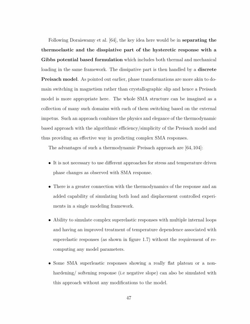
Following Doraiswamy et al. [64], the key idea here would be in separating the

thermoelastic and the disspiative part of the hysteretic response with a

Gibbs potential based formulation which includes both thermal and mechanical

loading in the same framework. The dissipative part is then handled by a discrete

Preisach model. As pointed out earlier, phase transformations are more akin to do-

main switching in magnetism rather than crystallographic slip and hence a Preisach

model is more appropriate here. The whole SMA structure can be imagined as a

collection of many such domains with each of them switching based on the external

impetus. Such an approach combines the physics and elegance of the thermodynamic

based approach with the algorithmic efficiency/simplicity of the Preisach model and

thus providing an effective way in predicting complex SMA responses.

The advantages of such a thermodynamic Preisach approach are [64,104]:

• It is not necessary to use different approaches for stress and temperature driven

phase changes as observed with SMA response.

• There is a greater connection with the thermodynamics of the response and an

added capability of simulating both load and displacement controlled experi-

ments in a single modeling framework.

• Ability to simulate complex superelastic responses with multiple internal loops

and having an improved treatment of temperature dependence associated with

superelastic responses (as shown in figure 1.7) without the requirement of re-

computing any model parameters.

• Some SMA superleastic responses showing a really flat plateau or a non-

hardening/ softening response (i.e negative slope) can also be simulated with

this approach without any modifications to the model.

47

• An approximate response prediction could be beneficial for design purposes

but a more precise prediction is essential from the control systems standpoint.

With the use of a discrete Preisach model, one can do a approximate or a

precise prediction by controlling the use of number of Preisach elements This

way one doesn’t have to choose different functions for simulating approximate

or fine predictions and thus saving computational time.

• All three loading cases viz. tension, torsion and bending responses can be

simulated with a similar approach. The model parameters in each loading

case can be calibrated using a single stress–strain, torque–twist or moment–

curvature plot depending on the chosen loading condition.

The efficacy of the model in directly predicting torque – angle of twist or bending

moment – curvature response directly could play a vital role in designing SMA com-

ponents like wires, springs and beams for various engineering applications. Capturing

complex temperature dependent hysteretic responses with minimum computations

could help designers immensely in studying component response under different con-

ditions.

1.7 Objectives

The main objectives of this work are listed below :

1. Development of a two-species model to capture superelastic effects under ten-

sion, torsion and bending loading cases for SMA components like wires, bars,

springs and beams.

2. Considering the technological importance of SMA components under torsional

loading, a three species model to capture both superelastic and shape memory

effects for a complete torsion loading case for SMA components like wires,

48

springs and beams is proposed. This approach could facilitate designers for

actuator development.

3. Tackle another aspect of SMA response, namely their functional degradation.

Apart from undergoing conventional mechanical fatigue/degradation, SMAs

also undergo loss in their phase transformation ability, leading to a loss in

functionality/smartness. A custom designed special test rig is used to perform

cyclic thermomechanical experiments on SMA springs. Using the test data, a

novel modeling framework to combine both mechanical and thermal loading

response is proposed wherein a thermodynamic driving force is used to capture

the functional life of SMA components.

1.8 Dissertation Organization

The remaining sections of this dissertation are organized as follows

• Section 2 : Experiments performed on NiTi SMA wires and springs at Texas

A&M University (College Station & Qatar campuses) are presented.

• Section 3 : By using thermodynamics principles and a two species Gibbs po-

tential, the thermoelastic and the dissipative part of superelastic response are

separated to obtain expressions for thermodynamic driving force for phase

transformations and the volume fraction of martensite (for tension, torsion

and bending loading cases).

• Section 4 : A common discrete Preisach model used to handle the dissipa-

tive part (different driving force and volume fraction relationships) of response

under different loading conditions is presented.

• Section 5 : A three species model that extends the proposed modeling approach

of separating the thermoelastic and the dissipative part of response to simulate

49

both the shape memory and superelastic responses is discussed. The model

captures the complete torsional response of SMA components like wires, rods

and springs.

• Section 6 : The simulation protocol and identification of various model param-

eters arising from the thermodynamical framework for all proposed models in

Sections 3 and 5 are detailed.

• Section 7 : The model simulations and predictions under different loading

conditions are compared with the experimental data in this Section.

• Section 8 : The proposed model in Sections 3 are extended to develop a concept

of “driving force amplitude v/s no of cycles” that could be used to analyze func-

tional degradation of SMA components. A custom designed thermomechanical

fatigue test rig is used to execute user defined repeated thermomechanical tests

on SMA components.

• Section 9 : Concluding remarks and summary

• Section 10 : Some recommendations for future work to tackle other SMA re-

lated issues.

50

2. EXPERIMENTS ON SMA COMPONENTS – WIRES AND SPRINGS ∗

This section discusses the various experiments conducted on SMA components

like wires and springs under different loading conditions at Texas A&M University

(College Station & Qatar campuses). These experiments would provide an insight

in understanding component level responses under different load cases and operating

conditions. These experimental results would also be used later for model calibra-

tion and evaluating model predictions under different cases. Section 2.1 discusses

experiments on SMA wires under pure tension. Section 2.2 discusses experiments on

commercial SMA springs under torsion. Section 2.3 discusses experiments on SMA

wires subjected to high degrees of twist.

2.1 SMA Wires Under Tension : Test Methodology and Results

2.1.1 Material and Experimental Set-up

NiTi wires (martensitic at room temperature) of 0.75 mm dia with a composition

in element weight% (Ni-54.5, Balance Ti, trace elements < 0.25) were obtained from

Images SI Inc (www.imagesco.com) with a listed transformation temperature of 323

K.

An Instron 5567 series uniaxial tensile testing machine was used to carry out

cyclic loading experiments at various temperatures on SMA wires. The temperature

control was through an Instron SFL heatwave environmental chamber (model: 3119-

506 Heatwave 240) (A in figure 2.1) used for maintaining precise air temperature∗Reprinted with permission from “Combining Thermodynamic Principles with Preisach models

for superelastic SMA Wires” by Doraiswamy, Rao and Srinivasa, Smart Materials and Structures,20, 085032, 2011 [64], Copyright [2014] by IOP.

Reprinted with permission from “A two species thermodynamic Preisach model for the tor-sional response of SMA wires and springs under superelastic conditions” by Rao and Srinivasa,International Journal of Solids and Structures, 50, 887–898, 2013 [90], Copyright [2014] by ElsevierLimited.

51

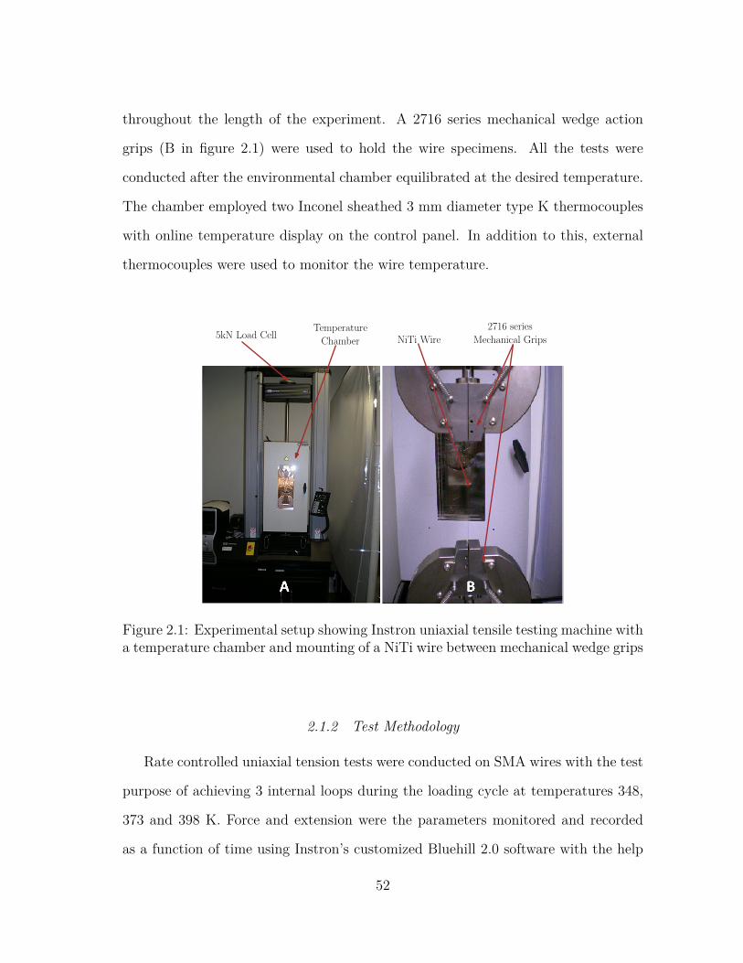
throughout the length of the experiment. A 2716 series mechanical wedge action

grips (B in figure 2.1) were used to hold the wire specimens. All the tests were

conducted after the environmental chamber equilibrated at the desired temperature.

The chamber employed two Inconel sheathed 3 mm diameter type K thermocouples

with online temperature display on the control panel. In addition to this, external

thermocouples were used to monitor the wire temperature.

5kN Load CellTemperature

Chamber

2716 series

Mechanical GripsNiTi Wire

Figure 2.1: Experimental setup showing Instron uniaxial tensile testing machine witha temperature chamber and mounting of a NiTi wire between mechanical wedge grips

2.1.2 Test Methodology

Rate controlled uniaxial tension tests were conducted on SMA wires with the test

purpose of achieving 3 internal loops during the loading cycle at temperatures 348,

373 and 398 K. Force and extension were the parameters monitored and recorded

as a function of time using Instron’s customized Bluehill 2.0 software with the help

52

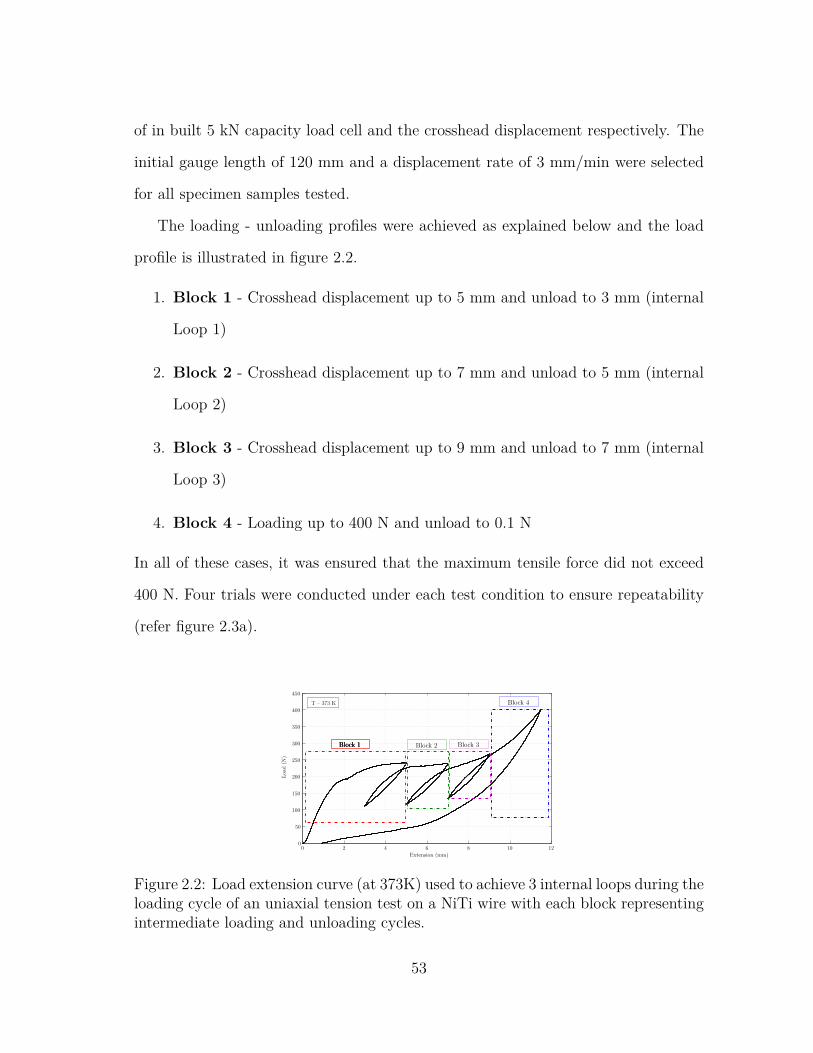
of in built 5 kN capacity load cell and the crosshead displacement respectively. The

initial gauge length of 120 mm and a displacement rate of 3 mm/min were selected

for all specimen samples tested.

The loading - unloading profiles were achieved as explained below and the load

profile is illustrated in figure 2.2.

1. Block 1 - Crosshead displacement up to 5 mm and unload to 3 mm (internal

Loop 1)

2. Block 2 - Crosshead displacement up to 7 mm and unload to 5 mm (internal

Loop 2)

3. Block 3 - Crosshead displacement up to 9 mm and unload to 7 mm (internal

Loop 3)

4. Block 4 - Loading up to 400 N and unload to 0.1 N

In all of these cases, it was ensured that the maximum tensile force did not exceed

400 N. Four trials were conducted under each test condition to ensure repeatability

(refer figure 2.3a).

0 2 4 6 8 10 120

50

100

150

200

250

300

350

400

450

Extension (mm)

Load(N

)

Block 1 Block 2 Block 3

Block 4

Block 1Block 1

T – 373 K

Figure 2.2: Load extension curve (at 373K) used to achieve 3 internal loops during theloading cycle of an uniaxial tension test on a NiTi wire with each block representingintermediate loading and unloading cycles.

53

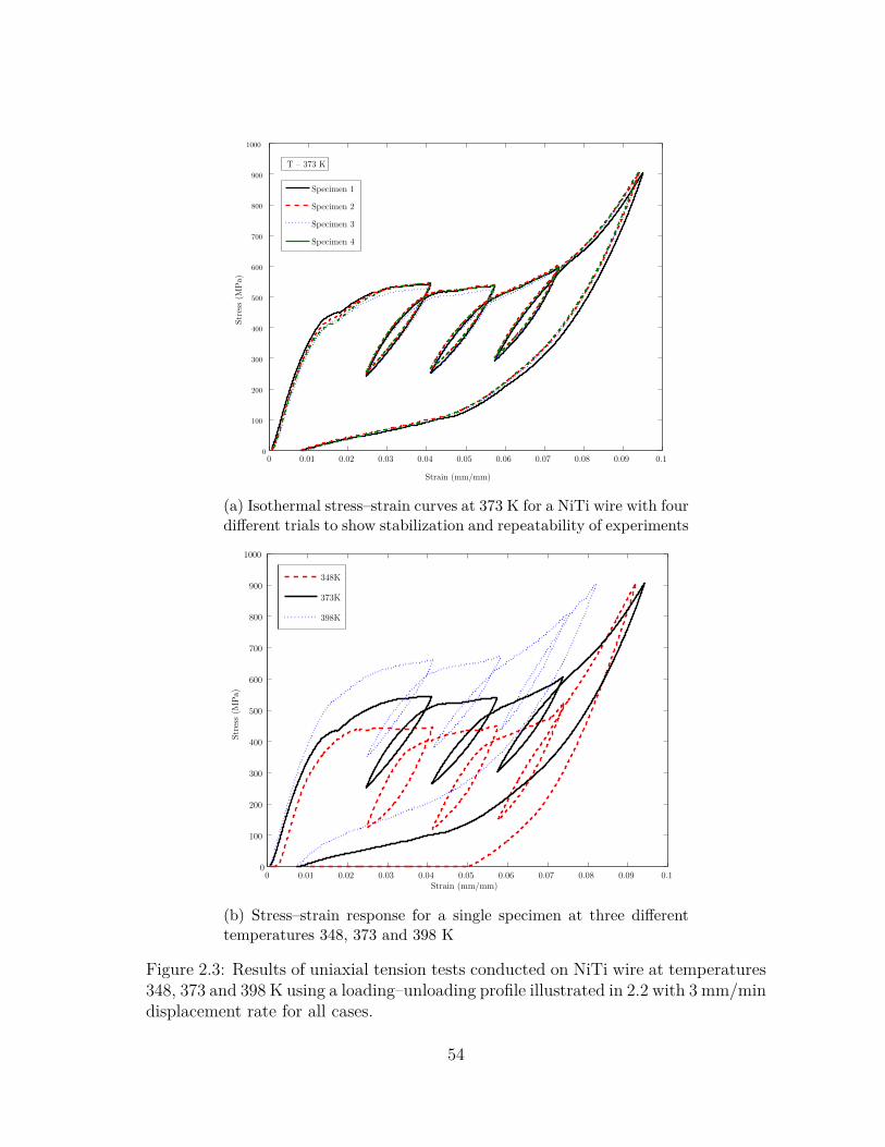
0 0.01 0.02 0.03 0.04 0.05 0.06 0.07 0.08 0.09 0.10

100

200

300

400

500

600

700

800

900

1000

Stress(M

Pa)

Strain (mm/mm)

Specimen 1

Specimen 2

Specimen 3

Specimen 4

T – 373 K

(a) Isothermal stress–strain curves at 373 K for a NiTi wire with fourdifferent trials to show stabilization and repeatability of experiments

0 0.01 0.02 0.03 0.04 0.05 0.06 0.07 0.08 0.09 0.10

100

200

300

400

500

600

700

800

900

1000

Strain (mm/mm)

Stress(M

Pa)

348K

373K

398K

(b) Stress–strain response for a single specimen at three differenttemperatures 348, 373 and 398 K

Figure 2.3: Results of uniaxial tension tests conducted on NiTi wire at temperatures348, 373 and 398 K using a loading–unloading profile illustrated in 2.2 with 3 mm/mindisplacement rate for all cases.

54

2.1.3 Results and Discussions

The isothermal stress–strain curves for different temperatures are illustrated in

figure 2.3. In all cases considered here, the results presented are for the stabilized

loops and thus initial gauge length was adjusted to account for hysteresis stabiliza-

tion. As seen in figure 2.3b, there is a residual strain of about 5% observed on

unloading for 348 K trial. This residual strain can be attributed to plastic deforma-

tion of martensite at higher stress levels (far greater than upper plateau stress) and

incomplete recovery of some pockets of the specimen back to austenite upon unload-

ing [142]. This would also explain the discrepancies between the initial austenitic

slope during loading cycle and “partially transformed austenitic” slope during the

unloading cycle as observed in figure 2.3b. A more detailed discussion on this can

be found here [142], [143]. For tests conducted at 373 and 398 K, almost complete

recovery of applied deformation was observed and thus demonstrating near perfect

superelasticity.

2.2 SMA Springs Under Torsion : Test Methodology and Results

2.2.1 Material and Experimental Set-up

NiTi springs (martensitic at room temperature) with composition details in el-

ement weight % (Ni-55.91, Balance Ti, trace elements < 0.25) were obtained from

Images SI Inc. The listed transformation temperature (Af ) as reported by the sup-

plier is in the range of 318-328 K. The spring specifications are as follows.

• Mean coil diameter of the spring “Dm” = 6 mm

• Wire diameter “d” = 0.75 mm

• Spring Index “C” = 8

55

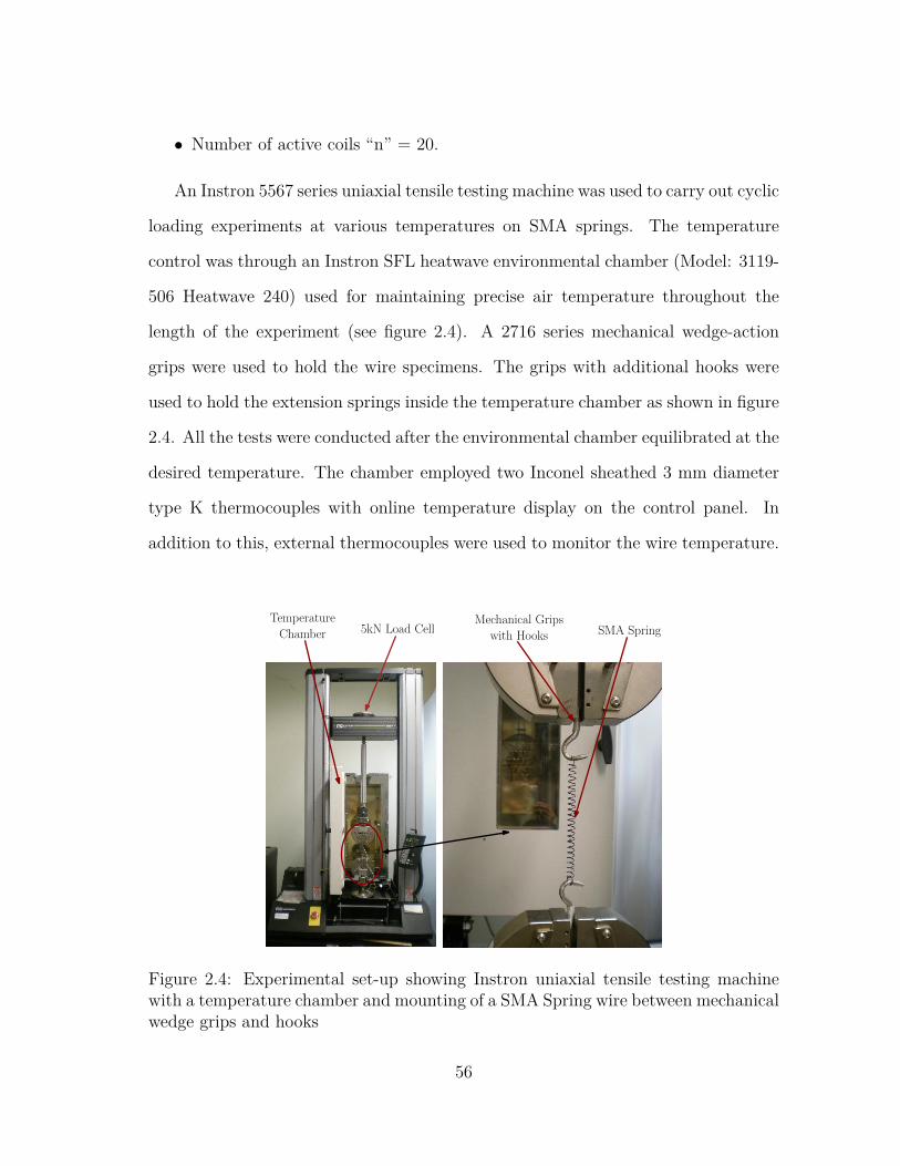
• Number of active coils “n” = 20.

An Instron 5567 series uniaxial tensile testing machine was used to carry out cyclic

loading experiments at various temperatures on SMA springs. The temperature

control was through an Instron SFL heatwave environmental chamber (Model: 3119-

506 Heatwave 240) used for maintaining precise air temperature throughout the

length of the experiment (see figure 2.4). A 2716 series mechanical wedge-action

grips were used to hold the wire specimens. The grips with additional hooks were

used to hold the extension springs inside the temperature chamber as shown in figure

2.4. All the tests were conducted after the environmental chamber equilibrated at the

desired temperature. The chamber employed two Inconel sheathed 3 mm diameter

type K thermocouples with online temperature display on the control panel. In

addition to this, external thermocouples were used to monitor the wire temperature.

5kN Load CellTemperature

ChamberMechanical Grips

with Hooks SMA Spring

Figure 2.4: Experimental set-up showing Instron uniaxial tensile testing machinewith a temperature chamber and mounting of a SMA Spring wire between mechanicalwedge grips and hooks

56

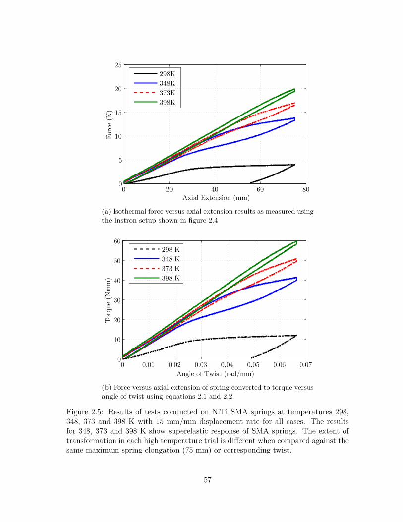
0 20 40 60 800

5

10

15

20

25

Axial Extension (mm)

Force

(N)

298K

348K

373K

398K

(a) Isothermal force versus axial extension results as measured usingthe Instron setup shown in figure 2.4

0 0.01 0.02 0.03 0.04 0.05 0.06 0.070

10

20

30

40

50

60

Angle of Twist (rad/mm)

Torque(N

mm)

298 K

348 K

373 K

398 K

(b) Force versus axial extension of spring converted to torque versusangle of twist using equations 2.1 and 2.2

Figure 2.5: Results of tests conducted on NiTi SMA springs at temperatures 298,348, 373 and 398 K with 15 mm/min displacement rate for all cases. The resultsfor 348, 373 and 398 K show superelastic response of SMA springs. The extent oftransformation in each high temperature trial is different when compared against thesame maximum spring elongation (75 mm) or corresponding twist.

57

2.2.2 Test Methodology

Rate controlled uniaxial tests were conducted on the extension springs that were

subjected to a axial displacement of 75 mm and then unloaded back. A constant

displacement rate of 15 mm/min was employed throughout the length of the exper-

iment. Force (P ) and spring extension (δ) data were monitored and recorded as a

function of time using Instron’s customized Bluehill 2.0 software with the help of

in-built 5kN capacity load cell and the crosshead displacement respectively.

The torque applied on the spring can be computed using the expression

T = P(Dm

2

)(2.1)

Assuming that the angle of twist is uniform over the entire length of the active coils

and ignoring curvature effects, the angle of twist per unit length (φ) can be evaluated

in terms of the spring displacement as

φ = 2δπD2

mn(2.2)

The above results (equations 2.1 and 2.2) are independent of each other with the

former being purely kinetic and the latter being purely geometrical in nature. No

constitutive theory relating the torque to the angle of twist is necessary for these

results to be established.

The tests were performed at room temperature (298 K) to simulate shape memory

effect and three other temperatures above Af viz. 348, 373 and 398 K to observe

superelastic behavior of SMA springs. Four trials were conducted under each test

condition to ensure repeatability of results.

58

2.2.3 Results and Discussions

The force - extension results of the SMA spring as obtained from the Instron

machine for different temperatures are illustrated in figure 2.5a. The corresponding

torque–angle of twist results using equations 2.1 and 2.2 are shown in figure 2.5b.

As seen in figure 2.5a, for 298 K trial, there is a residual elongation of about 50

mm observed upon unloading which can be recovered completely upon heating to a

temperature above Af . In the trials pertaining to higher temperatures 348, 373 and

398 K, the spring is austenitic at the start of the test and demonstrates near perfect

pseudoelasticity with the complete recovery of applied deformation. In each of these

cases, the springs are partially transformed to stress induced martensite (SIM) and

the extent of transformation from austenite to SIM is different in each temperature

trial. This is due to the fact that the higher the temperature above Af , the higher is

the critical stress required for transformation and thus lesser is the transformation

from austenite to SIM when compared against the same maximum deformation (75

mm) of the spring. It can also be observed from figure 2.5a that the stiffness increases

and the hysteresis area decreases with the increase in the working temperature above

Af .

2.3 SMA Wires Under Torsion : Test Methodology and Results

SMA components like wires, tubes, rods and springs during service could be sub-

jected to load reversals before complete transformation is achieved which could result

in partial or complex hysteretic internal loops either during the loading or unloading

stage of the response [59]. Capturing such internal loops responses are important

from an application standpoint as in many cases not the entire the response is nec-

essary and only a partial internal loop might be of significance to designers [22, 28].

Most of the available literature has been on understanding a simple loading and

59

unloading case at different extent of twists. The reported literature in understand-

ing partial or complex internal loop responses have been investigated under tension

loading cases (see figure 4 in [144], figure 2,4a and 4b in [145], figure 6 in [146], figure

12 in [147], figure 6 in [148], figure 3 in [149], figure 3 in [150], figure 4 and 7 in [151],

figure 5 in [152], figure 2,3 and 4 in [153], figure 6 in [154], figure 1 in [155] etc.

for some illustrations under tension loading case). However, in all of the reported

literature the study of internal loops (both under loading and unloading stages of

the response) under torsional loading is not addressed.

In this part, an effort to understand the partial and fully transformed cases with

internal loops under both during loading and unloading stages of SMA wires under

torsion was undertaken. An Instron micro torsion test is used to conduct different

experimental test cases to better understand the responses of superelastic SMA wires

subjected to torsional loading. Such a study allows designers to get an idea of mate-

rial response under complex loading and unloading situations in actual applications

(especially the shape of inner loops compared to outer/major loops). Such exper-

iments also allows designers to get an insight into behaviour of internal loops and

analyze “return point memory (RPM) or sink point memory (SPM)” aspects of tor-

sional response (see figure 8 in [59] for such an illustrations under tension loading).

RPM and SPM provides important information on the ability of SMA components

to return back to its original unloading point upon completion of a smaller hys-

teretic loop and is of particular importance to designers. SMA components showing

“good RPM/SPM characteristics” is a desirable feature that indicates minimal resid-

ual/irreversible deformations after repeated complete or partial transformations.

60

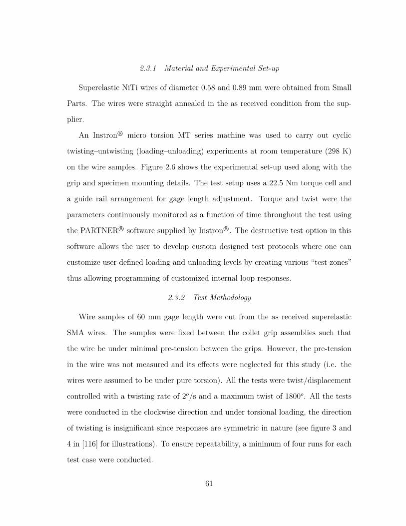
2.3.1 Material and Experimental Set-up

Superelastic NiTi wires of diameter 0.58 and 0.89 mm were obtained from Small

Parts. The wires were straight annealed in the as received condition from the sup-

plier.

An Instron R© micro torsion MT series machine was used to carry out cyclic

twisting–untwisting (loading–unloading) experiments at room temperature (298 K)

on the wire samples. Figure 2.6 shows the experimental set-up used along with the

grip and specimen mounting details. The test setup uses a 22.5 Nm torque cell and

a guide rail arrangement for gage length adjustment. Torque and twist were the

parameters continuously monitored as a function of time throughout the test using

the PARTNER R© software supplied by Instron R©. The destructive test option in this

software allows the user to develop custom designed test protocols where one can

customize user defined loading and unloading levels by creating various “test zones”

thus allowing programming of customized internal loop responses.

2.3.2 Test Methodology

Wire samples of 60 mm gage length were cut from the as received superelastic

SMA wires. The samples were fixed between the collet grip assemblies such that

the wire be under minimal pre-tension between the grips. However, the pre-tension

in the wire was not measured and its effects were neglected for this study (i.e. the

wires were assumed to be under pure torsion). All the tests were twist/displacement

controlled with a twisting rate of 2o/s and a maximum twist of 1800o. All the tests

were conducted in the clockwise direction and under torsional loading, the direction

of twisting is insignificant since responses are symmetric in nature (see figure 3 and

4 in [116] for illustrations). To ensure repeatability, a minimum of four runs for each

test case were conducted.

61

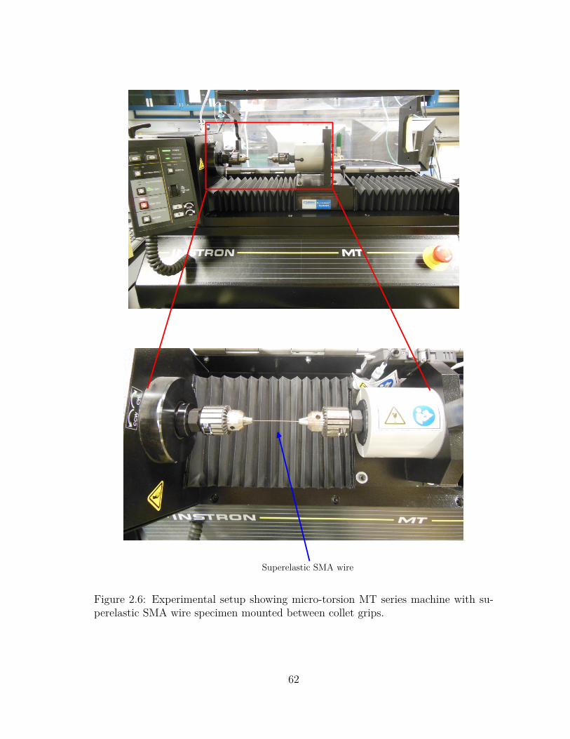
Superelastic SMA wire

Figure 2.6: Experimental setup showing micro-torsion MT series machine with su-perelastic SMA wire specimen mounted between collet grips.

62

2.3.3 Experimental Runs

In the subsequent sections several different cases of internal loops under both

loading and unloading stages of the response are discussed.

2.3.3.1 Simple loading and unloading

The procedure to obtain the response of a typical superelastic torsional loading

and unloading case consisted of the two steps shown in figure 2.7a

• Zone 1 : Twist upto 1800o twist (Loading cycle)

• Zone 2 : Untwist back to 0o twist (Unloading cycle)

Data recorded when the input is a triangular force function (i.e. twist vs time) is

shown on figure 2.7b and shows that the material response exhibits a non-linear be-

havior especially during the phase transformation event. The complete response (i.e.

torque vs twist) is shown on figure 2.7c and shows near perfect superelasticity with

almost negligible residual deformation upon unloading with a well defined plateau

stresses 1 and elastic deformation of stress induced martensite (SIM). The torsional

response is similar to a classic pseudoelastic tension response.

The test protocol was reapplied on samples subjected to 1500o, 1350o, 900o and

600o twist as shown in figure 2.8a. The corresponding twist vs time, torque vs time

and torque vs twist responses overlap on each other (figure 2.8 which demonstrate

good agreement and test repeatability.1Plateau stresses are some of the salient features associated with a typical superelastic response

under tension loading case as discussed in the ASTM standard F2516-07ε2 [13] for superelastic NiTimaterials. The standard defines two plateau stresses – an upper plateau strength (UPS) whichis the stress value at 3% strain during loading of the sample and a lower plateau strength (LPS)which is the stress value at 2.5% strain during unloading of sample after has been loaded up to 6%strain.

63

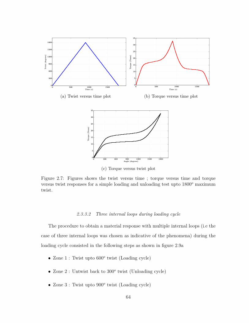
Twist(d

egrees)

Time (s)0 500 1000 1500

0

300

600

900

1200

1500

1800

(a) Twist versus time plot

Torq

ue(N

mm)

Time (s)

0 500 1000 15000

5

10

15

20

25

30

35

(b) Torque versus time plot

Torq

ue(N

mm)

Angle (degrees)0 300 600 900 1200 1500 1800

0

5

10

15

20

25

30

35

(c) Torque versus twist plot

Figure 2.7: Figures shows the twist versus time ; torque versus time and torqueversus twist responses for a simple loading and unloading test upto 1800o maximumtwist.

2.3.3.2 Three internal loops during loading cycle

The procedure to obtain a material response with multiple internal loops (i.e the

case of three internal loops was chosen as indicative of the phenomena) during the

loading cycle consisted in the following steps as shown in figure 2.9a

• Zone 1 : Twist upto 600o twist (Loading cycle)

• Zone 2 : Untwist back to 300o twist (Unloading cycle)

• Zone 3 : Twist upto 900o twist (Loading cycle)

64

• Zone 4 : Untwist back to 600o twist (Unloading cycle)

• Zone 5 : Twist upto 1200o twist (Loading cycle)

• Zone 6 : Untwist back to 900o twist (Unloading cycle)

• Zone 7 : Twist upto 1800o twist (Loading cycle)

• Zone 8 : Untwist back to 0o twist (Unloading cycle)

The data recorded for this test run is shown in figure 2.9b. The torque–twist

response 2.9c exhibits three internal loops (during the loading cycle) and shows

almost perfect RPM. The austenitic and martensitic slopes of the internal loops

follow the same trend as that of the outer loops.

2.3.3.3 Comparing an internal loop during loading and unloading cycle

Comparison of an internal loop during loading and unloading cycle was possible

using the following protocol shown in figure 2.10a

• Zone 1 : Twist upto 900o twist (Loading cycle)

• Zone 2 : Untwist back to 400o twist (Unloading cycle)

• Zone 3 : Twist upto 1800o twist (Loading cycle)

• Zone 4 : Untwist back to 800o twist (Unloading cycle)

• Zone 5 : Twist upto 1300o twist (Loading cycle)

• Zone 6 : Untwist back to 0o twist (Unloading cycle)

Recorded data for this test run with triangular twist controlled forcing function

as input is shown in figure 2.10b. For the non-linear torque–twist response shown in

figure 2.10c, the internal loop during loading and unloading never intersects the outer

65

loop. In both loops, one can observe near perfect RPM with no residual elongation

upon complete unloading.

2.3.3.4 Multiple internal loop during loading and unloading cycle

A test case to investigate multiple internal loops during loading and unloading

cycles are programmed as described below and shown in figure 2.11a

• Zone 1 : Twist upto 500o twist (Loading cycle)

• Zone 2 : Untwist back to 350o twist (Unloading cycle)

• Zone 3 : Twist upto 800o twist (Loading cycle)

• Zone 4 : Untwist back to 650o twist (Unloading cycle)

• Zone 5 : Twist upto 1100o twist (Loading cycle)

• Zone 6 : Untwist back to 950o twist (Unloading cycle)

• Zone 7 : Twist upto 1400o twist (Loading cycle)

• Zone 8 : Untwist back to 1250o twist (Unloading cycle)

• Zone 9 : Twist upto 1800o twist (Loading cycle)

• Zone 10 : Untwist back to 1100o twist (Unloading cycle)

• Zone 11 : Twist upto 1250o twist (Loading cycle)

• Zone 12 : Untwist back to 800o twist (Unloading cycle)

• Zone 13 : Twist upto 950o twist (Loading cycle)

• Zone 14 : Untwist back to 500o twist (Unloading cycle)

66

• Zone 15 : Twist upto 650o twist (Loading cycle)

• Zone 16 : Untwist back to 0o twist (Unloading cycle)

The corresponding torque data recorded as a function of time is shown in figure

2.11b. The complete torque–twist response is shown in figure 2.11c. All the small

internal loops under loading and unloading regimes show near perfect RPM with

slopes similar to the austentic and martensitic slopes of the outer loops.

2.3.3.5 Complex loops during loading cycle

A complex loading scenario was investigated with the following protocol shown

in figure 2.12a

• Zone 1 : Twist upto 1300o twist (Loading cycle)

• Zone 2 : Untwist back to 400o twist (Unloading cycle)

• Zone 3 : Twist upto 1100o twist (Loading cycle)

• Zone 4 : Untwist back to 600o twist (Unloading cycle)

• Zone 5 : Twist upto 900o twist (Loading cycle)

• Zone 6 : Untwist back to 800o twist (Unloading cycle)

• Zone 7 : Twist upto 1800o twist (Loading cycle)

• Zone 8 : Untwist back to 0o twist (Unloading cycle)

Data recorded for this case is shown in figure 2.12b. The complex loop response

exhibited on the torque–twist plot 2.12c shows that the partially transformed case

(internal loops) follows the trend of the fully transformed case (outer loop). The

internal loops never intersect the outer loops regardless of the extent of loading and

67

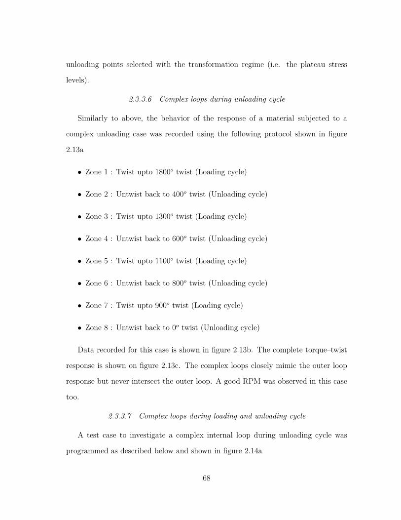
unloading points selected with the transformation regime (i.e. the plateau stress

levels).

2.3.3.6 Complex loops during unloading cycle

Similarly to above, the behavior of the response of a material subjected to a

complex unloading case was recorded using the following protocol shown in figure

2.13a

• Zone 1 : Twist upto 1800o twist (Loading cycle)

• Zone 2 : Untwist back to 400o twist (Unloading cycle)

• Zone 3 : Twist upto 1300o twist (Loading cycle)

• Zone 4 : Untwist back to 600o twist (Unloading cycle)

• Zone 5 : Twist upto 1100o twist (Loading cycle)

• Zone 6 : Untwist back to 800o twist (Unloading cycle)

• Zone 7 : Twist upto 900o twist (Loading cycle)

• Zone 8 : Untwist back to 0o twist (Unloading cycle)

Data recorded for this case is shown in figure 2.13b. The complete torque–twist

response is shown on figure 2.13c. The complex loops closely mimic the outer loop

response but never intersect the outer loop. A good RPM was observed in this case

too.

2.3.3.7 Complex loops during loading and unloading cycle

A test case to investigate a complex internal loop during unloading cycle was

programmed as described below and shown in figure 2.14a

68

• Zone 1 : Twist upto 900o twist (Loading cycle)

• Zone 2 : Untwist back to 400o twist (Unloading cycle)

• Zone 3 : Twist upto 800o twist (Loading cycle)

• Zone 4 : Untwist back to 500o twist (Unloading cycle)

• Zone 5 : Twist upto 700o twist (Loading cycle)

• Zone 6 : Untwist back to 600o twist (Unloading cycle)

• Zone 7 : Twist upto 1800o twist (Loading cycle)

• Zone 8 : Untwist back to 800o twist (Unloading cycle)

• Zone 9 : Twist upto 1300o twist (Loading cycle)

• Zone 10 : Untwist back to 900o twist (Unloading cycle)

• Zone 11 : Twist upto 1200o twist (Loading cycle)

• Zone 12 : Untwist back to 1000o twist (Unloading cycle)

• Zone 13 : Twist upto 1100o twist (Loading cycle)

• Zone 14 : Untwist back to 0o twist (Unloading cycle)

The corresponding torque data recorded as a function of time is shown in figure

2.14b. The complete torque–twist response is shown in figure 2.14c.

69

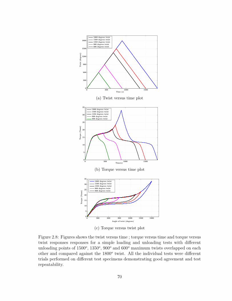
600 degrees twist

900 degrees twist

1350 degrees twist

1500 degrees twist

1800 degrees twist

Twist(d

egrees)

Time (s)0 500 1000 1500

0

300

600

900

1200

1500

1800

(a) Twist versus time plot

600 degrees twist

900 degrees twist

1350 degrees twist

1500 degrees twist

1800 degrees twist

Torq

ue(N

mm)

Time(s)0 500 1000 1500

0

5

10

15

20

25

30

35

(b) Torque versus time plot

600 degrees twist

900 degrees twist

1350 degrees twist

1500 degrees twist

1800 degrees twist

Torq

ue(N

mm)

Angle of twist (degrees)

0 300 600 900 1200 1500 18000

5

10

15

20

25

30

35

(c) Torque versus twist plot

Figure 2.8: Figures shows the twist versus time ; torque versus time and torque versustwist responses responses for a simple loading and unloading tests with differentunloading points of 1500o, 1350o, 900o and 600o maximum twists overlapped on eachother and compared against the 1800o twist. All the individual tests were differenttrials performed on different test specimens demonstrating good agreement and testrepeatability.

70

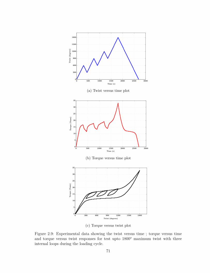
Twist(d

egrees)

Time (s)

0 500 1000 1500 2000 2500 30000

300

600

900

1200

1500

1800

(a) Twist versus time plot

Torq

ue(N

mm)

Time (s)

0 500 1000 1500 2000 2500 30000

5

10

15

20

25

30

35

(b) Torque versus time plot

Torq

ue(N

mm)

Twist (degrees)

0 300 600 900 1200 1500 18000

5

10

15

20

25

30

35

(c) Torque versus twist plot

Figure 2.9: Experimental data showing the twist versus time ; torque versus timeand torque versus twist responses for test upto 1800o maximum twist with threeinternal loops during the loading cycle.

71

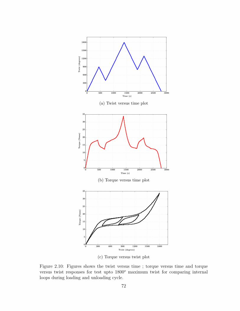
Twist(d

egrees)

Time (s)

0 500 1000 1500 2000 2500 30000

300

600

900

1200

1500

1800

(a) Twist versus time plot

Torq

ue(N

mm)

Time (s)

0 500 1000 1500 2000 2500 30000

5

10

15

20

25

30

35

(b) Torque versus time plot

Torq

ue(N

mm)

Twist (degrees)

0 300 600 900 1200 1500 18000

5

10

15

20

25

30

35

(c) Torque versus twist plot

Figure 2.10: Figures shows the twist versus time ; torque versus time and torqueversus twist responses for test upto 1800o maximum twist for comparing internalloops during loading and unloading cycle.

72

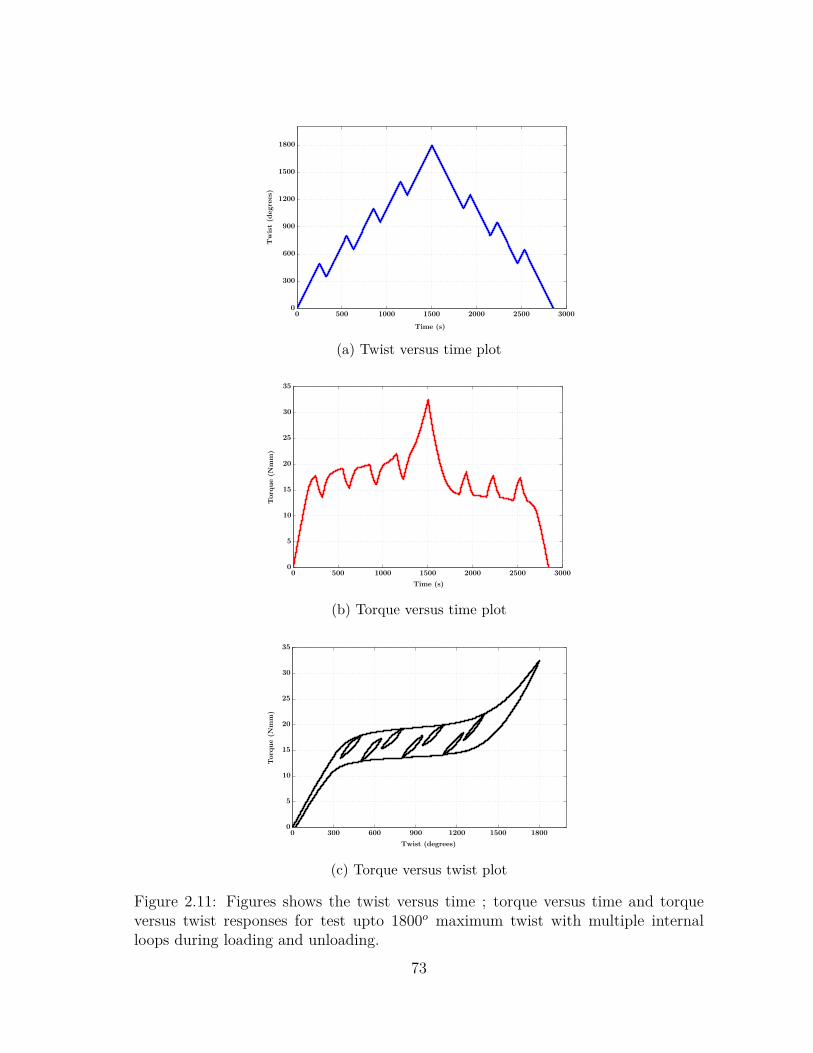
Twist(d

egrees)

Time (s)

0 500 1000 1500 2000 2500 30000

300

600

900

1200

1500

1800

(a) Twist versus time plot

Torq

ue(N

mm)

Time (s)

0 500 1000 1500 2000 2500 30000

5

10

15

20

25

30

35

(b) Torque versus time plot

Torq

ue(N

mm)

Twist (degrees)

0 300 600 900 1200 1500 18000

5

10

15

20

25

30

35

(c) Torque versus twist plot

Figure 2.11: Figures shows the twist versus time ; torque versus time and torqueversus twist responses for test upto 1800o maximum twist with multiple internalloops during loading and unloading.

73

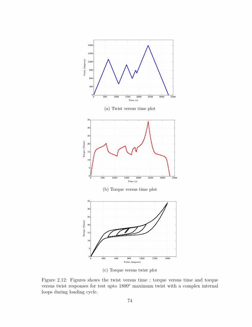
Twist(d

egrees)

Time (s)

0 500 1000 1500 2000 2500 3000 35000

300

600

900

1200

1500

1800

(a) Twist versus time plot

Torq

ue(N

mm)

Time (s)

0 500 1000 1500 2000 2500 3000 35000

5

10

15

20

25

30

35

(b) Torque versus time plot

Torq

ue(N

mm)

Twist (degrees)

0 300 600 900 1200 1500 18000

5

10

15

20

25

30

35

(c) Torque versus twist plot

Figure 2.12: Figures shows the twist versus time ; torque versus time and torqueversus twist responses for test upto 1800o maximum twist with a complex internalloops during loading cycle.

74

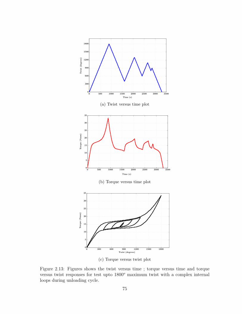
Twist(d

egrees)

Time (s)

0 500 1000 1500 2000 2500 3000 35000

300

600

900

1200

1500

1800

(a) Twist versus time plot

Torq

ue(N

mm)

Time (s)

0 500 1000 1500 2000 2500 3000 35000

5

10

15

20

25

30

35

(b) Torque versus time plot

Torq

ue(N

mm)

Twist (degrees)

0 300 600 900 1200 1500 18000

5

10

15

20

25

30

35

(c) Torque versus twist plot

Figure 2.13: Figures shows the twist versus time ; torque versus time and torqueversus twist responses for test upto 1800o maximum twist with a complex internalloops during unloading cycle.

75

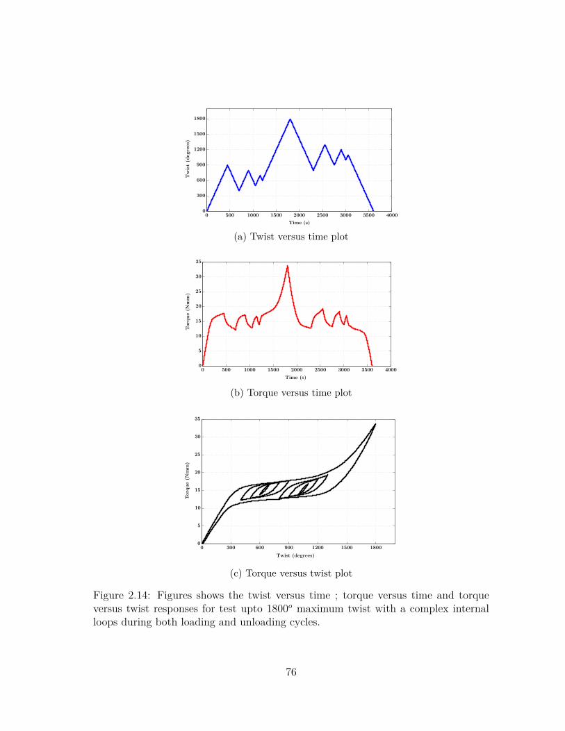
Twist(d

egrees)

Time (s)

0 500 1000 1500 2000 2500 3000 3500 40000

300

600

900

1200

1500

1800

(a) Twist versus time plot

Torq

ue(N

mm)

Time (s)

0 500 1000 1500 2000 2500 3000 3500 40000

5

10

15

20

25

30

35

(b) Torque versus time plot

Torq

ue(N

mm)

Twist (degrees)

0 300 600 900 1200 1500 18000

5

10

15

20

25

30

35

(c) Torque versus twist plot

Figure 2.14: Figures shows the twist versus time ; torque versus time and torqueversus twist responses for test upto 1800o maximum twist with a complex internalloops during both loading and unloading cycles.

76

3. MODEL DEVELOPMENT - TWO SPECIES ∗

In this section, the development of structural thermomechanical models for shape

memory alloy components like wires, springs and beams subjected to either tension,

torsion or bending loading conditions under superelastic conditions is discussed. Fol-

lowing Doraiswamy et al. [64], the key idea here would be in separating the ther-

moelastic and the dissipative part of the hysteretic response with a Gibbs potential

based formulation. The hysteretic part of the response is then handled by a discrete

Preisach model (to be discussed in section 4). As noted earlier, phase transforma-

tions are more akin to domain switching in magnetism rather than crystallographic

slip, hence the whole SMA structure can be imagined as a collection of many such

domains with each of them switching positions based on the external impetus. In this

two species model, the two domains/phases considered are austenite and detwinned

martensite. It is assumed that during a superelastic response, all the austenite trans-

forms to one variant of martensite during A→M transformation and similarly all of

the martensite switches back to austenite during the reverseM → A transformation.

A Gibbs potential per unit volume (inspired from [64, 65]) which is assumed to

be a function of the stress (σ) or torque (T) or bending–moment (M) depending on

the loading condition, operating temperature (θ) and the extent of transformation

(ξ) i.e volume fraction of detwinned martensite formed during phase transition. The

Gibbs potential is assumed to be composed of (refer equation 3.1) :∗Reprinted with permission from “Combining Thermodynamic Principles with Preisach models

for superelastic SMA Wires” by Doraiswamy, Rao and Srinivasa, Smart Materials and Structures,20, 085032, 2011 [64], Copyright [2014] by IOP.

Reprinted with permission from “A two species thermodynamic Preisach model for the tor-sional response of SMA wires and springs under superelastic conditions” by Rao and Srinivasa,International Journal of Solids and Structures, 50, 887–898, 2013 [90], Copyright [2014] by ElsevierLimited

77

1. a linear combination of the strain energy for the two species/phases,

2. an interaction term between the two phases,

3. a term related to the heat capacity difference between the two phases and

4. a term relating to the heat capacity of the austenite.

Specifically the Gibbs potential energy per unit reference volume is assumed to

be of the form,

G =1︷ ︸︸ ︷

− (ξU∗M + (1− ξ)U∗A) +2︷ ︸︸ ︷

Bξ(ξ − 1) +3︷ ︸︸ ︷

(1− ξ)(a+ bθ)−4︷ ︸︸ ︷

Cθ(1− log θ) (3.1)

where,

• ξ is the martensite volume fraction,

• U∗M & U∗A are the stored energy function chosen based on the loading conditions

for detwinned martensite and austenitic phases respectively,

• B, a and b are constants,

• θ is the temperature and

• C is the specific heat

In the following sections, a thermodynamical framework commonly employed

for modeling phase transforming materials (as discussed in literature review under

section 1.4.1) is employed with an appropriate choice of U∗M and U∗A based on the

type of loading.

78

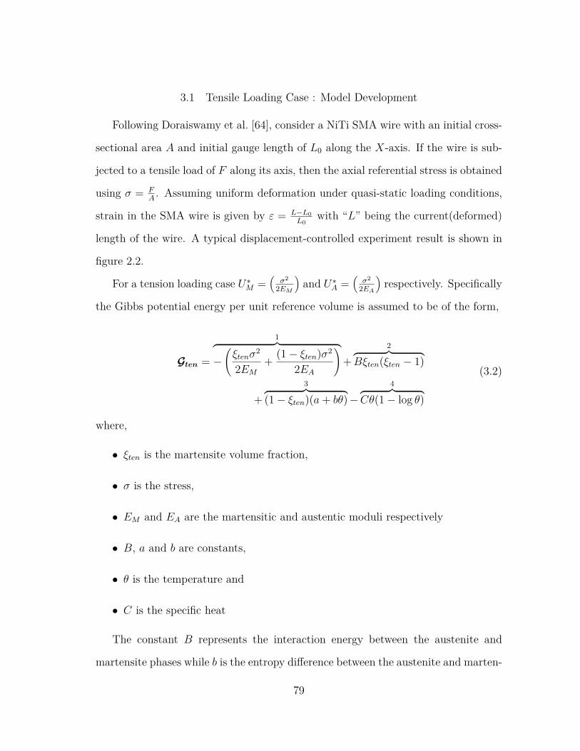
3.1 Tensile Loading Case : Model Development

Following Doraiswamy et al. [64], consider a NiTi SMA wire with an initial cross-

sectional area A and initial gauge length of L0 along the X-axis. If the wire is sub-

jected to a tensile load of F along its axis, then the axial referential stress is obtained

using σ = FA. Assuming uniform deformation under quasi-static loading conditions,

strain in the SMA wire is given by ε = L−L0L0

with “L” being the current(deformed)

length of the wire. A typical displacement-controlled experiment result is shown in

figure 2.2.

For a tension loading case U∗M =(

σ2

2EM

)and U∗A =

(σ2

2EA

)respectively. Specifically

the Gibbs potential energy per unit reference volume is assumed to be of the form,

Gten =

1︷ ︸︸ ︷−(ξtenσ

2

2EM+ (1− ξten)σ2

2EA

)+

2︷ ︸︸ ︷Bξten(ξten − 1)

+3︷ ︸︸ ︷

(1− ξten)(a+ bθ)−4︷ ︸︸ ︷

Cθ(1− log θ)

(3.2)

where,

• ξten is the martensite volume fraction,

• σ is the stress,

• EM and EA are the martensitic and austentic moduli respectively

• B, a and b are constants,

• θ is the temperature and

• C is the specific heat

The constant B represents the interaction energy between the austenite and

martensite phases while b is the entropy difference between the austenite and marten-

79

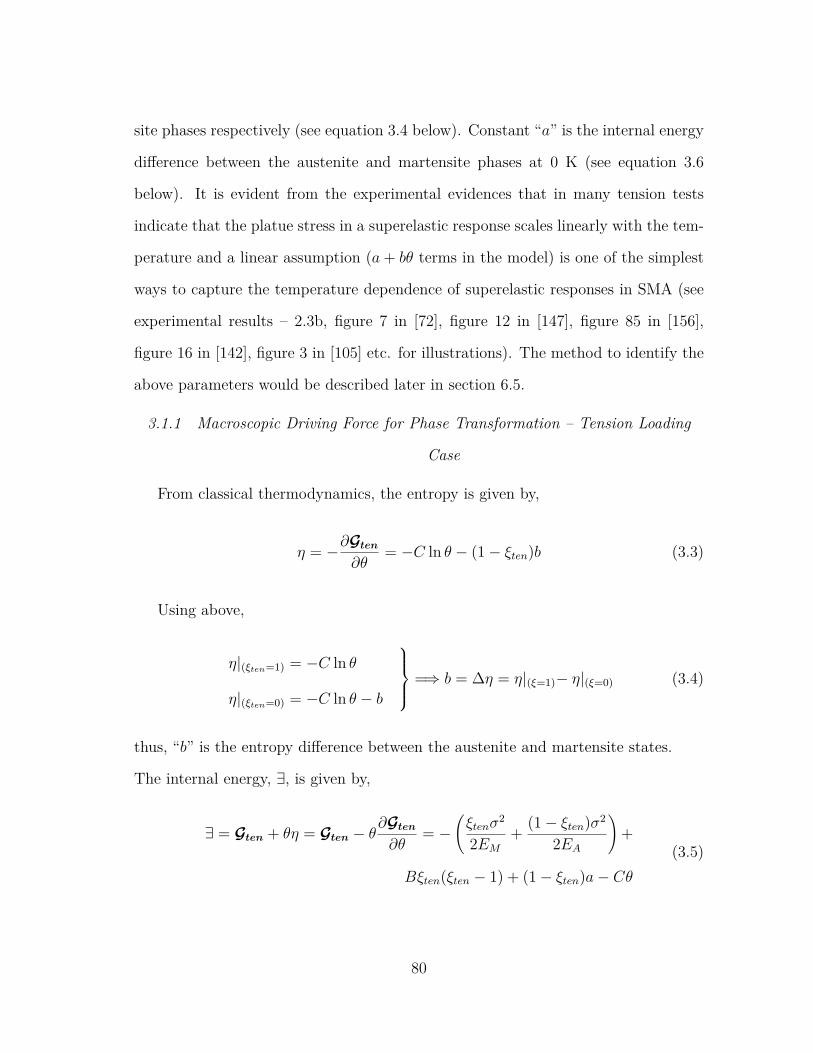
site phases respectively (see equation 3.4 below). Constant “a” is the internal energy

difference between the austenite and martensite phases at 0 K (see equation 3.6

below). It is evident from the experimental evidences that in many tension tests

indicate that the platue stress in a superelastic response scales linearly with the tem-

perature and a linear assumption (a+ bθ terms in the model) is one of the simplest

ways to capture the temperature dependence of superelastic responses in SMA (see

experimental results – 2.3b, figure 7 in [72], figure 12 in [147], figure 85 in [156],

figure 16 in [142], figure 3 in [105] etc. for illustrations). The method to identify the

above parameters would be described later in section 6.5.

3.1.1 Macroscopic Driving Force for Phase Transformation – Tension Loading

Case

From classical thermodynamics, the entropy is given by,

η = −∂Gten∂θ

= −C ln θ − (1− ξten)b (3.3)

Using above,

η|(ξten=1) = −C ln θ

η|(ξten=0) = −C ln θ − b

=⇒ b = ∆η = η|(ξ=1)− η|(ξ=0) (3.4)

thus, “b” is the entropy difference between the austenite and martensite states.

The internal energy, ∃, is given by,

∃ = Gten + θη = Gten − θ∂Gten∂θ

= −(ξtenσ

2

2EM+ (1− ξten)σ2

2EA

)+

Bξten(ξten − 1) + (1− ξten)a− Cθ(3.5)

80

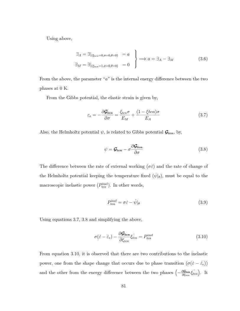
Using above,

∃A = ∃|(ξten=0,σ=0,θ=0) = a

∃M = ∃|(ξten=1,σ=0,θ=0) = 0

=⇒ a = ∃A − ∃M (3.6)

From the above, the parameter “a” is the internal energy difference between the two

phases at 0 K.

From the Gibbs potential, the elastic strain is given by,

εe = −∂Gten∂σ

= ξtenσ

EM+ (1− ξten)σ

EA(3.7)

Also, the Helmholtz potential ψ, is related to Gibbs potential Gten, by,

ψ = Gten − σ∂Gten∂σ

(3.8)

The difference between the rate of external working (σε) and the rate of change of

the Helmholtz potential keeping the temperature fixed (ψ|θ), must be equal to the

macroscopic inelastic power (P inelten ). In other words,

P inelten = σε− ψ|θ (3.9)

Using equations 3.7, 3.8 and simplifying the above,

σ(ε− εe)−∂Gten∂ξten

˙ξten = P inelten (3.10)

From equation 3.10, it is observed that there are two contributions to the inelastic

power, one from the shape change that occurs due to phase transition (σ(ε − εe))

and the other from the energy difference between the two phases(−∂Gten

∂ξten

˙ξten). It

81

is assumed that the elongation due to phase transformation is proportional to the

maximum transformational strain, εmax, which can be assumed to be in the order of

6% for Ni-Ti. Therefore,

ε− εe = εmax ˙ξten ⇒ ε− εe = εmaxξten (3.11)

In the above equation note that, when ξten = 1, ε − εe = εmax and when ξten = 0,

ε− εe = 0. Now substituting equation 3.11 into equation 3.10 gives :

(σεmax −

∂Gten∂ξ

)˙ξten = P inel

ten (3.12)

It is now possible to identify the driving force for the phase transformation in the

superelastic response of the SMA:

Ften = σεmax −∂Gten∂ξten

=⇒ Ften ˙ξten = P inelten

Hence, Ften = σεmax + σ2( 1

2EM− 1

2EA

)−B(2ξten − 1) + bθ + a

(3.13)

It is to be noted here that P inelten is the macroscopic inelastic power and can be less

than zero. The dissipation, ∆ten, is the net macroscopic inelastic work in a closed

cycle of state and this is required to be non-negative, i.e,

∆ten =∮P inelten dt ≥ 0 (3.14)

Further, an expression for the martensitic volume fraction evolution (ξ) can be

obtained using expressions 3.7 and 3.11. The volume fraction evolution expression ξ

can be obtained from the torque–angle of twist experimental data and the assumed

82

form of Gibbs potential.

ξten =ε− σ

EAσEM− σEA

+ 1 (3.15)

The experimental stress–strain data can be reduced to its corresponding driving-force

– volume fraction plot (to be discussed in section 3.4 later.)

3.2 Torsion Loading Case : Model Development

Shifting focus to a torsional loading case, consider a SMA wire subjected to a

torque “T” about its axis or a helical extension SMA spring subjected to force “P”

along its axis with “δ” being the corresponding axial displacement. Let,

• “Dm” be the mean coil diameter of the spring in mm

• “d” be the SMA wire diameter in mm.

• “C” denote the spring index.

• “n” be the number of active coils (i.e neglecting the end hooks).

The torque (T ) and angle of twist per unit length (φ) are directly measured in the

case of wire and the same can be computed using equations 2.1 and 2.2 for springs

respectively.

For a torsional loading case U∗M =(

T 2

2GMJ

)and U∗A =

(T 2

2GAJ

). Similar to tension

loading case, a Gibbs potential per unit reference volume for a pure torsion loading

case is assumed to be of the form as shown below, (similar to equation 3.2 discussed

earlier)

Gtor =

1︷ ︸︸ ︷−(ξtorT

2

2GMJ+ (1− ξtor)T 2

2GAJ

)+

2︷ ︸︸ ︷Bξtor(ξtor − 1)

+3︷ ︸︸ ︷

(1− ξtor)(a+ bθ)−4︷ ︸︸ ︷

Cθ(1− ln θ)

(3.16)

where,

83

• ξtor is the martensite volume fraction,

• T is the applied torque,

• GA and GM are the austenitic and martensitic shear moduli,

• J = πd4

32 is the polar moment of inertia

• B, a and b are constants,

• θ is the temperature and

• C is the specific heat

The constant B represents the interaction energy between the austenite and marten-

site phases while b is the entropy difference between the austenite and martensite

phases respectively (see equation 3.18 below). Constant “a” is the internal energy

difference between the austenite and martensite phases at 0 K (see equation 3.20

below). The method to identify the above parameters is discussed in Section 6.5.

3.2.1 Establishing Macroscopic Driving Force – Pure Torsion Case

From classical thermodynamics, the entropy is given by,

η = −∂Gtor∂θ

= −C ln θ − (1− ξtor)b (3.17)

Using above,

η|(ξtor=1) = −C ln θ

η|(ξtor=0) = −C ln θ − b

=⇒ b = ∆η = η|(ξtor=1)− η|(ξtor=0) (3.18)

thus, b is the entropy difference between the austenite and martensite states.

84

The internal energy, ∃, is given by,

∃ = Gtor + θη = Gtor − θ∂Gtor∂θ

= −(ξtorT

2

2GMJ+ (1− ξtor)T 2

2GAJ

)

+Bξtor(ξtor − 1) + (1− ξtor)a− Cθ(3.19)

Using above,

∃A = ∃|(ξtor=0,T=0,θ=0) = a

∃M = ∃|(ξtor=1,T=0,θ=0) = 0

=⇒ a = ∃A − ∃M (3.20)

From the above, the parameter a is the internal energy difference between the two

phases at 0 K.

From the Gibbs potential, the thermoelastic part of the angle of twist is given by,

φe = −∂Gtor∂T

= ξtorT

GMJ+ (1− ξtor)T

GAJ(3.21)

Also, the Helmholtz potential ψ, is related to Gibbs potential Gtor, by,

ψ = Gtor − T∂Gtor∂T

(3.22)

The difference between the rate of external working (T φ) and the rate of change of

the Helmholtz potential keeping the temperature fixed (ψ|θ), must be equal to the

macroscopic inelastic power (P ineltor ). In other words,

P ineltor = T φ− ψ|θ (3.23)

85

Using equations 3.21, 3.22 and upon further simplification,

T (φ− φe)−∂Gtor∂ξtor

˙ξtor = P ineltor (3.24)

From equation 3.24, it is observed that there are two contributions to the inelastic

power, one from the shape change that occurs due to phase transition (T (φ − φe))

and the other from the energy difference between the two phases(−∂Gtor

∂ξtor

˙ξtor). The

recoverable angle of twist is due to the phase transformation and is proportional to

the extent of transformation depending on the axial force and corresponding axial

displacement that the spring is subjected too. The maximum angle of twist φmax

corresponding to a maximum transformational strain that can assumed to be of the

order of 6%.

φ− φe = φmax ˙ξtor ⇒ φ− φe = φmaxξtor (3.25)

In the above equation note that, when ξtor = 1, φ − φe = φmax and when ξtor = 0,

φ− φe = 0. Now substituting equation 3.25 into 3.24 gives:

(Tφmax −

∂Gtor∂ξtor

)˙ξtor = P inel

tor (3.26)

It is now possible to identify the driving force for the phase transformation in the

superelastic response of the SMA springs:

Ftor = Tφmax −∂Gtor∂ξtor

=⇒ Ftor ˙ξtor = P ineltor

Hence, Ftor = Tφmax + T 2( 1

2GMJ− 1

2GAJ

)−B(2ξtor − 1) + bθ + a

(3.27)

P ineltor is the macroscopic inelastic power. The rate of mechanical dissipation, ∆tor, is

the net macroscopic inelastic work in a closed cycle of state and this is required to

86

be non-negative as required by the second law of thermodynamics, i.e,

∆tor =∮P ineltor dt ≥ 0 (3.28)

The volume fraction evolution expression ξtor can be obtained from the torque–

angle of twist experimental data and the assumed form of Gibbs potential using

equations 3.21 and 3.25.

ξtor =φ− T

GAJT

GMJ− TGAJ

+ 1(3.29)

The experimental torque–twist data can be reduced to its corresponding driving-

force – volume fraction plot (to be discussed in section 3.4 later.)

3.3 Bending Loading Case : Model Development

Now for a pure bending loading case, consider a wire/beam subjected to bend-

ing moment “M” with the corresponding curvature denoted by “κ”. Both bending

moment “M” and curvature (κ) are directly measured experimentally.

For a pure bending case U∗M =(

M2

2EM I

)and U∗A =

(M2

2EAI

). Similar to tension and

torsion loading cases, a Gibbs potential energy per unit reference volume for a pure

bending loading case is assumed to be of the form as shown below in equation 3.30.

(similar to equations 3.2 and 3.16 discussed earlier)

Gbend =

1︷ ︸︸ ︷−(ξbendM

2

2EMI+ (1− ξbend)M2

2EAI

)+

2︷ ︸︸ ︷Bξbend(ξbend − 1)

+3︷ ︸︸ ︷

(1− ξbend)(a+ bθ)−4︷ ︸︸ ︷

Cθ(1− ln θ)

(3.30)

where,

87

• ξbend is the martensite volume fraction,

• M is the applied bending moment,

• EA and EM are the austenitic and martensitic moduli,

• I = πd4

64 is the moment of Inertia

• B, a and b are constants,

• θ is the temperature and

• C is the specific heat

Similar to earlier discussions, the constant “B” represents the interaction energy be-

tween the austenite and martensite phases while “b” is the entropy difference between

the austenite and martensite phases respectively (see equation 3.32 below). Constant

“a” is the internal energy difference between the austenite and martensite phases at

0 K (see equation 3.34 below). The method to identify the above parameters would

be described later in section 6.5.

3.3.1 Establishing Macroscopic Driving Force – Pure Bending Case

From classical thermodynamics, the entropy is given by,

η = −∂Gbend∂θ

= −C ln θ − (1− ξbend)b (3.31)

Using above,

η|(ξbend=1) = −C ln θ

η|(ξbend=0) = −C ln θ − b

=⇒ b = ∆η = η|(ξbend=1)− η|(ξbend=0) (3.32)

thus, b is the entropy difference between the austenite and martensite states.

88

The internal energy, ∃, is given by,

∃ = Gbend + θη = Gbend − θ∂Gbend∂θ

= −(ξbendM

2

2EMI+ (1− ξ)M2

2EAI

)

+Bξbend(ξbend − 1) + (1− ξbend)a− Cθ(3.33)

Using above,

∃A = ∃|(ξbend=0,M=0,θ=0) = a

∃M = ∃|(ξbend=1,M=0,θ=0) = 0

=⇒ a = ∃A − ∃M (3.34)

From the Gibbs potential, the thermoelastic part of the total curvature is given by,

κe = −∂Gbend∂M

= ξbendM

EMI+ (1− ξbend)M

EAI(3.35)

Also, the Helmholtz potential ψ, is related to Gibbs potential Gbend, by,

ψ = Gbend −M∂Gbend∂M

(3.36)

The difference between the rate of external working (Mκ) and the rate of change of

the Helmholtz potential keeping the temperature fixed (ψ|θ), must be equal to the

macroscopic inelastic power (P inelbend). In other words,

P inelbend = Mκ− ψ|θ (3.37)

Using equations 3.35, 3.36 and upon further simplification,

M(κ− κe)−∂Gbend∂ξbend

˙ξbend = P inelbend (3.38)

89

From equation 3.38, it is observed that there are two contributions to the inelastic

power, one from the shape change that occurs due to phase transition (M(κ − κe))

and the other from the energy difference between the two phases(− ∂G∂ξbend

˙ξbend). The

maximum transformational strain (κmax in this case)can assumed to be of the order

of 6%.

κ− κe = κmaxξ ⇒ κ− κe = κmaxξ (3.39)

In the above equation note that, when ξbend = 1, κ− κe = κmax and when ξbend = 0,

κ− κe = 0. Now substituting equation 3.39 into equation 3.38 we get,

(Mκmax −

∂Gbend∂ξbend

)˙ξbend = P inel

bend (3.40)

It is now possible to identify the driving force for the phase transformation in the

superelastic response of the SMA springs:

Fbend = Mκmax −∂Gbend∂bend

=⇒ Fbend ˙ξbend = P inelbend

Hence, Fbend = Mκmax +M2( 1

2EMI− 1

2EAI

)−B(2ξbend − 1) + bθ + a

(3.41)

P inelbend is the macroscopic inelastic power. The rate of dissipation, ∆bend, is the net

macroscopic inelastic work in a closed cycle of state. In order to satisfy second law

of thermodynamics, this quantity must be non-negative i.e,

∆bend =∮P inelbend dt ≥ 0 (3.42)

The volume fraction evolution expression ξtor can be obtained from the torque–

angle of twist experimental data and the assumed form of Gibbs potential using

equations 3.35 and 3.39.

90

ξbend =κ− M

EAIMEMI

− MEAI

+ 1(3.43)

The experimental moment–curvature data can be reduced to its corresponding

driving-force – volume fraction plot (to be discussed in section 3.4 later.)

3.4 Deducing Driving Force and Volume Fraction from Experimental Data for

Different Loading Cases

Expressions for driving force for phase transformation and extent of martensite

during phase transformation were established for different loading cases (equation

sets 3.13 – 3.15 ; 3.27 – 3.29 and 3.41 – 3.43). From the driving force equations

3.13, 3.27 and 3.41, it is evident that the driving force expressions are a function of

stress (σ) or torque (T ) or bending–moment (M), strain (ε) or angle of twist (φ) or

curvature (κ), martensitic volume fraction (ξ), and temperature (θ) depending on

the loading condition under consideration. The variables σ/T/M , ε/φ/κ and θ are

nondimensionalized before proceeding further with the derivations. The nondimen-

sionalized variables for different loading cases are summarized below :

Tension Loading Case : σ∗ = σ/σmax, ε∗ = ε/εmax, θ∗ = θ/θmax.

Torsion Loading Case : T ∗ = T/Tmax, φ∗ = φ/φmax, θ∗ = θ/θmax.

Bending Loading Case : M∗ = M/Mmax, κ∗ = κ/κmax, θ∗ = θ/θmax.

Henceforth, for better readability, the ∗’s will be omitted from the nondimension-

alized variables. Experimental results for one particular temperature case are chosen

as reference for simulation and establishment of driving force and volume fraction

relationships.

For a tension loading case, using expressions 3.15 and 3.13, each experimental

data point from stress vs strain plot can be reduced to its corresponding driving-

91

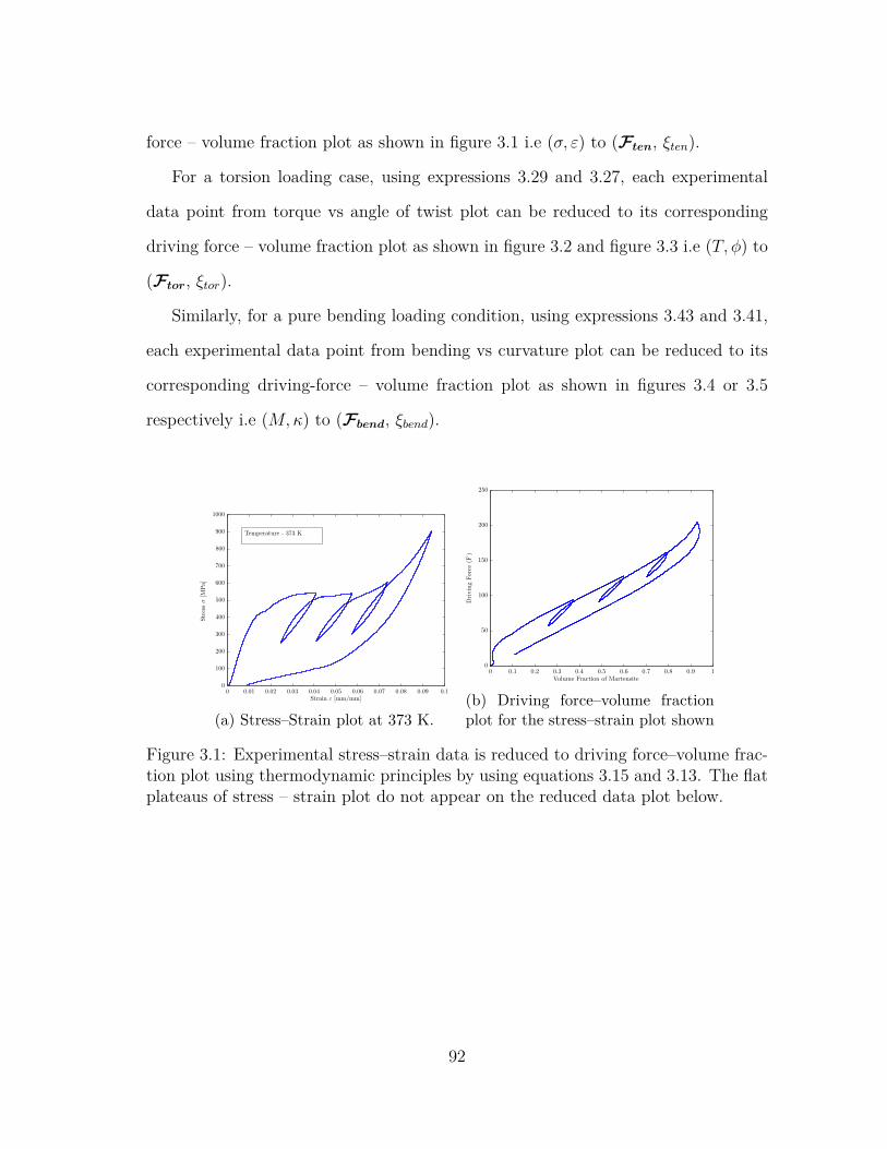
force – volume fraction plot as shown in figure 3.1 i.e (σ, ε) to (Ften, ξten).

For a torsion loading case, using expressions 3.29 and 3.27, each experimental

data point from torque vs angle of twist plot can be reduced to its corresponding

driving force – volume fraction plot as shown in figure 3.2 and figure 3.3 i.e (T, φ) to

(Ftor, ξtor).

Similarly, for a pure bending loading condition, using expressions 3.43 and 3.41,

each experimental data point from bending vs curvature plot can be reduced to its

corresponding driving-force – volume fraction plot as shown in figures 3.4 or 3.5

respectively i.e (M,κ) to (Fbend, ξbend).

Stressσ[M

Pa]

Strain ε [mm/mm]

Temperature - 373 K

0 0.01 0.02 0.03 0.04 0.05 0.06 0.07 0.08 0.09 0.10

100

200

300

400

500

600

700

800

900

1000

(a) Stress–Strain plot at 373 K.

Drivi ngForce

( F)

Volume Fraction of Martensite0 0.1 0.2 0.3 0.4 0.5 0.6 0.7 0.8 0.9 1

0

50

100

150

200

250

(b) Driving force–volume fractionplot for the stress–strain plot shown

Figure 3.1: Experimental stress–strain data is reduced to driving force–volume frac-tion plot using thermodynamic principles by using equations 3.15 and 3.13. The flatplateaus of stress – strain plot do not appear on the reduced data plot below.

92

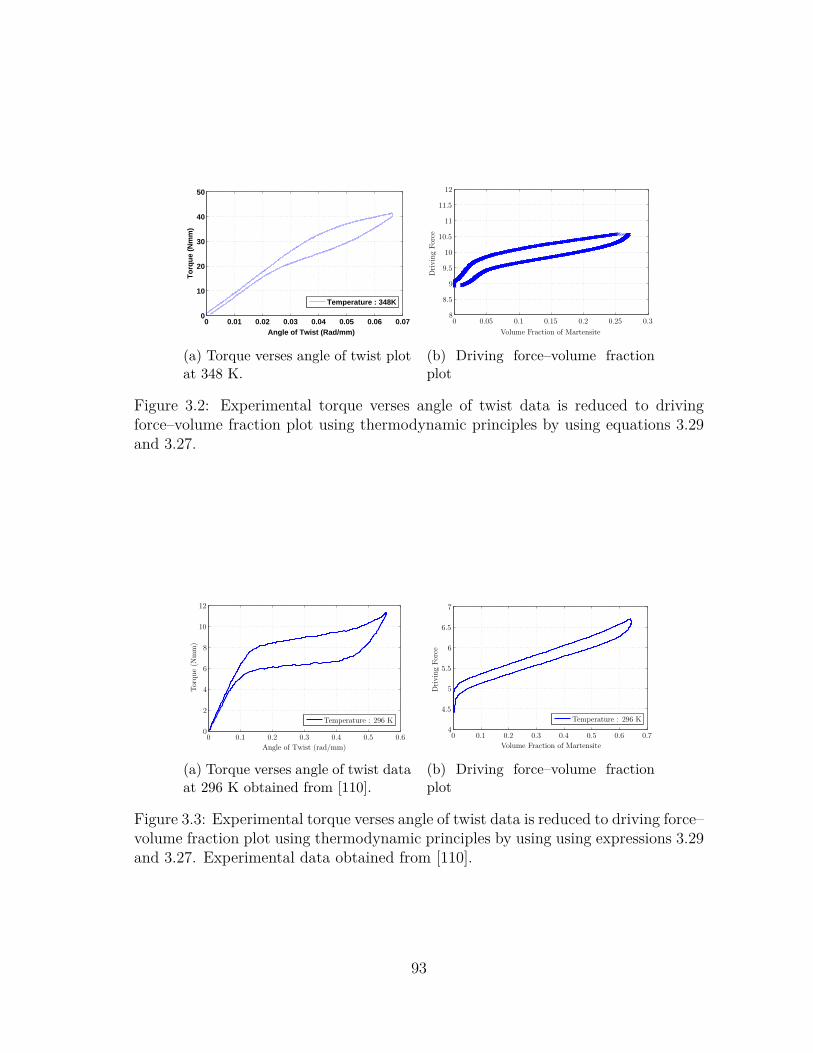
0 0.01 0.02 0.03 0.04 0.05 0.06 0.070

10

20

30

40

50

Angle of Twist (Rad/mm)

To

rqu

e (N

mm

)

Temperature : 348K

(a) Torque verses angle of twist plotat 348 K.

0 0.05 0.1 0.15 0.2 0.25 0.38

8.5

9

9.5

10

10.5

11

11.5

12

Volume Fraction of Martensite

DrivingForce

(b) Driving force–volume fractionplot

Figure 3.2: Experimental torque verses angle of twist data is reduced to drivingforce–volume fraction plot using thermodynamic principles by using equations 3.29and 3.27.

0 0.1 0.2 0.3 0.4 0.5 0.60

2

4

6

8

10

12

Angle of Twist (rad/mm)

Torque(N

mm)

Temperature : 296 K

(a) Torque verses angle of twist dataat 296 K obtained from [110].

0 0.1 0.2 0.3 0.4 0.5 0.6 0.74

4.5

5

5.5

6

6.5

7

Volume Fraction of Martensite

DrivingForce

Temperature : 296 K

(b) Driving force–volume fractionplot

Figure 3.3: Experimental torque verses angle of twist data is reduced to driving force–volume fraction plot using thermodynamic principles by using using expressions 3.29and 3.27. Experimental data obtained from [110].

93

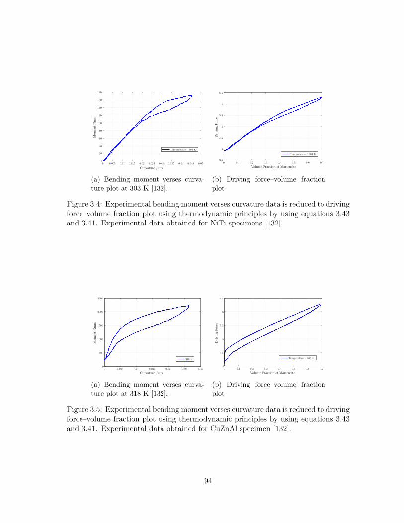
0 0.005 0.01 0.015 0.02 0.025 0.03 0.035 0.04 0.045 0.050

20

40

60

80

100

120

140

160

180

Curvature /mm

Mom

entNmm

Temperature : 303 K

(a) Bending moment verses curva-ture plot at 303 K [132].

0 0.1 0.2 0.3 0.4 0.5 0.6 0.73.5

4

4.5

5

5.5

6

6.5

Volume Fraction of Martensite

DrivingForce

Temperature : 303 K

(b) Driving force–volume fractionplot

Figure 3.4: Experimental bending moment verses curvature data is reduced to drivingforce–volume fraction plot using thermodynamic principles by using equations 3.43and 3.41. Experimental data obtained for NiTi specimens [132].

0 0.005 0.01 0.015 0.02 0.025 0.030

500

1000

1500

2000

2500

Curvature /mm

Mom

entNmm

318 K

(a) Bending moment verses curva-ture plot at 318 K [132].

0 0.1 0.2 0.3 0.4 0.5 0.6 0.74

4.5

5

5.5

6

6.5

Volume Fraction of Martensite

DrivingForce

Temperature : 318 K

(b) Driving force–volume fractionplot

Figure 3.5: Experimental bending moment verses curvature data is reduced to drivingforce–volume fraction plot using thermodynamic principles by using equations 3.43and 3.41. Experimental data obtained for CuZnAl specimen [132].

94

4. DISCRETE PREISACH MODEL DEVELOPMENT ∗

The driving force – volume fraction expressions for all loading cases discussed in

section 3.4 were a result of employing a thermodynamical framework typically used

in modeling phase transforming materials.

Now, if one were to follow a “plasticity like” approach then evolution equa-

tions for ξ for various transformation cases would be developed by employing dif-

ferent hardening functions. Various mathematical functions like polynomials, ex-

ponential or trignometric are developed for capturing different transformation cases

(see [85, 86, 89, 99, 108, 109] for examples). However, rather than using a plasticity

like approach, in this work, following [64, 76, 90, 104, 157], a discrete Preisach model

is employed to capture various driving force – volume fraction relationships (F–ξ)

developed for different loading conditions. The use of a discrete Preisach approach

is quite appropriate with SMAs as phase transformations in SMA are more akin to

domain wall switching in magnetism rather than crystallographic slip or flow. The

whole SMA structure can be assumed to be a collection of many such domains with

each of them discretely switching states depending on the various transformation

conditions. Since phase transformations are similar to “domain switching in mag-

netism”, hence use of Preisach models is ideally suitable for capturing hysteresis in

phase transformations when compared against the classical plasticity approaches.

Such an approach solely focuses on the hysteretic dissipative part of the response∗Reprinted with permission from “Combining Thermodynamic Principles with Preisach models

for superelastic SMA Wires” by Doraiswamy, Rao and Srinivasa, Smart Materials and Structures,20, 085032, 2011 [64], Copyright [2014] by IOP.

Reprinted with permission from “A two species thermodynamic Preisach model for the tor-sional response of SMA wires and springs under superelastic conditions” by Rao and Srinivasa,International Journal of Solids and Structures, 50, 887–898, 2013 [90], Copyright [2014] by ElsevierLimited.

95

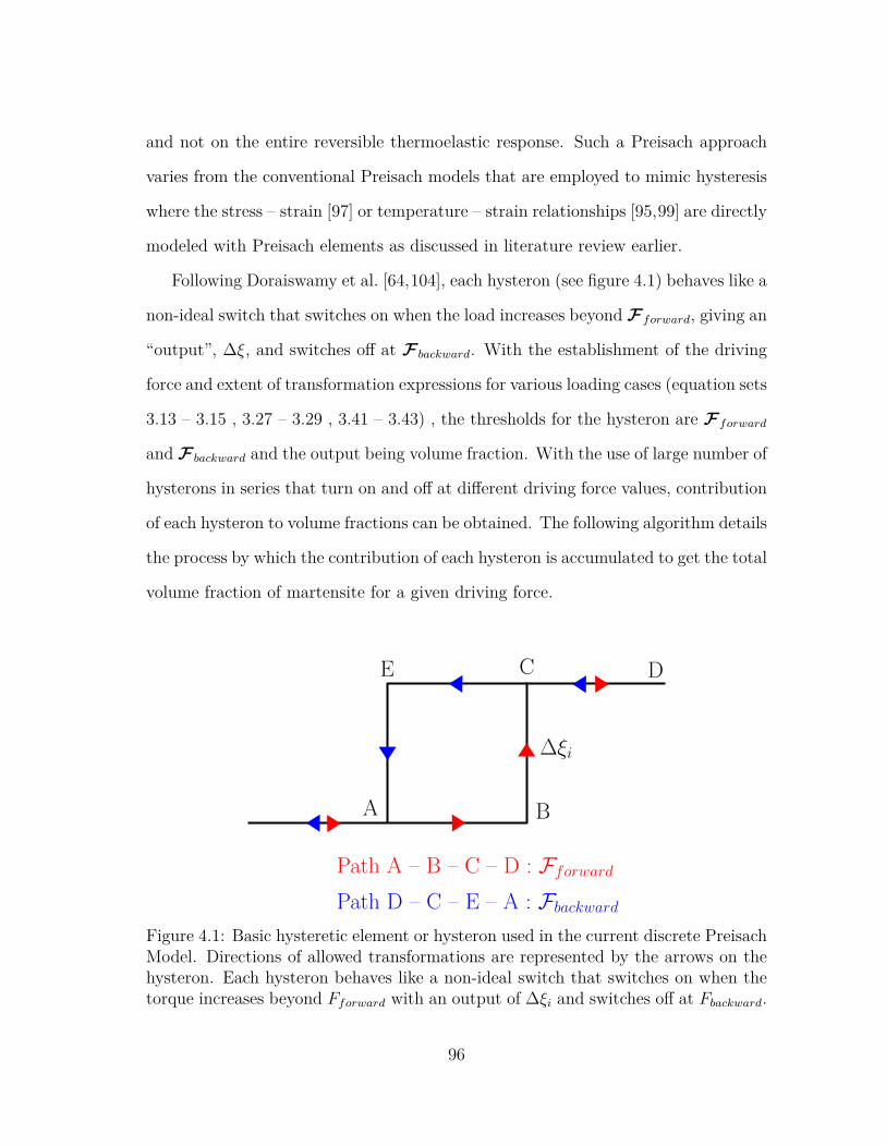
and not on the entire reversible thermoelastic response. Such a Preisach approach

varies from the conventional Preisach models that are employed to mimic hysteresis

where the stress – strain [97] or temperature – strain relationships [95,99] are directly

modeled with Preisach elements as discussed in literature review earlier.

Following Doraiswamy et al. [64,104], each hysteron (see figure 4.1) behaves like a

non-ideal switch that switches on when the load increases beyond Fforward, giving an

“output”, ∆ξ, and switches off at F backward. With the establishment of the driving

force and extent of transformation expressions for various loading cases (equation sets

3.13 – 3.15 , 3.27 – 3.29 , 3.41 – 3.43) , the thresholds for the hysteron are Fforward

and F backward and the output being volume fraction. With the use of large number of

hysterons in series that turn on and off at different driving force values, contribution

of each hysteron to volume fractions can be obtained. The following algorithm details

the process by which the contribution of each hysteron is accumulated to get the total

volume fraction of martensite for a given driving force.

∆ξi

A B

C DE

Path A – B – C – D : FforwardPath D – C – E – A : Fbackward

Figure 4.1: Basic hysteretic element or hysteron used in the current discrete PreisachModel. Directions of allowed transformations are represented by the arrows on thehysteron. Each hysteron behaves like a non-ideal switch that switches on when thetorque increases beyond Fforward with an output of ∆ξi and switches off at Fbackward.

96

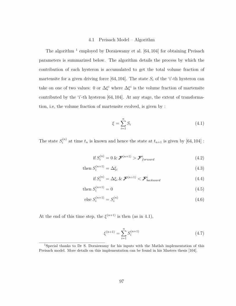
4.1 Preisach Model – Algorithm

The algorithm 1 employed by Doraiswamy et al. [64, 104] for obtaining Preisach

parameters is summarized below. The algorithm details the process by which the

contribution of each hysteron is accumulated to get the total volume fraction of

martensite for a given driving force [64, 104]. The state Si of the ‘i’-th hysteron can

take on one of two values: 0 or ∆ξi where ∆ξi is the volume fraction of martensite

contributed by the ‘i’-th hysteron [64, 104]. At any stage, the extent of transforma-

tion, i.e, the volume fraction of martensite evolved, is given by :

ξ =n∑i=1

Si (4.1)

The state S(n)i at time tn is known and hence the state at tn+1 is given by [64,104] :

if S(n)i = 0 &F (n+1) > F i

forward (4.2)

then S(n+1)i = ∆ξi (4.3)

if S(n)i = ∆ξi &F (n+1) < F i

backward (4.4)

then S(n+1)i = 0 (4.5)

else S(n+1)i = S

(n)i (4.6)

At the end of this time step, the ξ(n+1) is then (as in 4.1),

ξ(n+1) =n∑i=1

S(n+1)i (4.7)

1Special thanks to Dr S. Doraiswamy for his inputs with the Matlab implementation of thisPreisach model. More details on this implementation can be found in his Masters thesis [104].

97

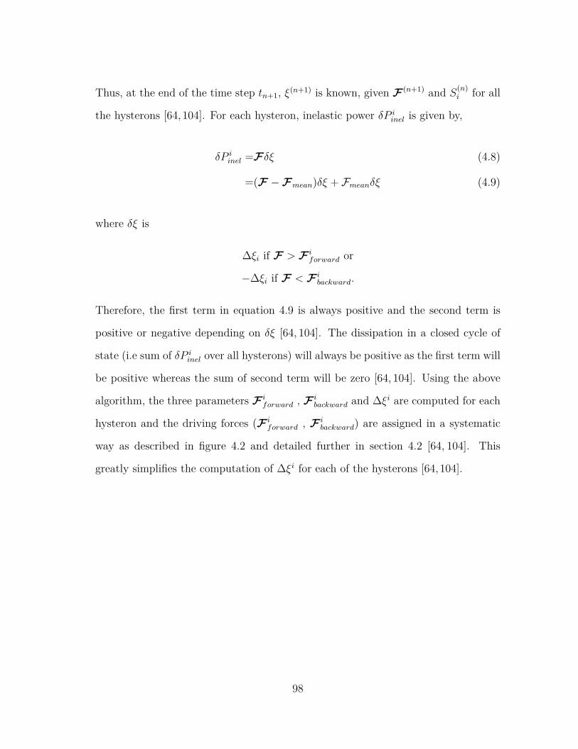
Thus, at the end of the time step tn+1, ξ(n+1) is known, given F (n+1) and S(n)i for all

the hysterons [64,104]. For each hysteron, inelastic power δP iinel is given by,

δP iinel =Fδξ (4.8)

=(F −Fmean)δξ + Fmeanδξ (4.9)

where δξ is

∆ξi if F > F iforward or

−∆ξi if F < F ibackward.

Therefore, the first term in equation 4.9 is always positive and the second term is

positive or negative depending on δξ [64, 104]. The dissipation in a closed cycle of

state (i.e sum of δP iinel over all hysterons) will always be positive as the first term will

be positive whereas the sum of second term will be zero [64, 104]. Using the above

algorithm, the three parameters F iforward , F i

backward and ∆ξi are computed for each

hysteron and the driving forces (F iforward , F i

backward) are assigned in a systematic

way as described in figure 4.2 and detailed further in section 4.2 [64, 104]. This

greatly simplifies the computation of ∆ξi for each of the hysterons [64,104].

98

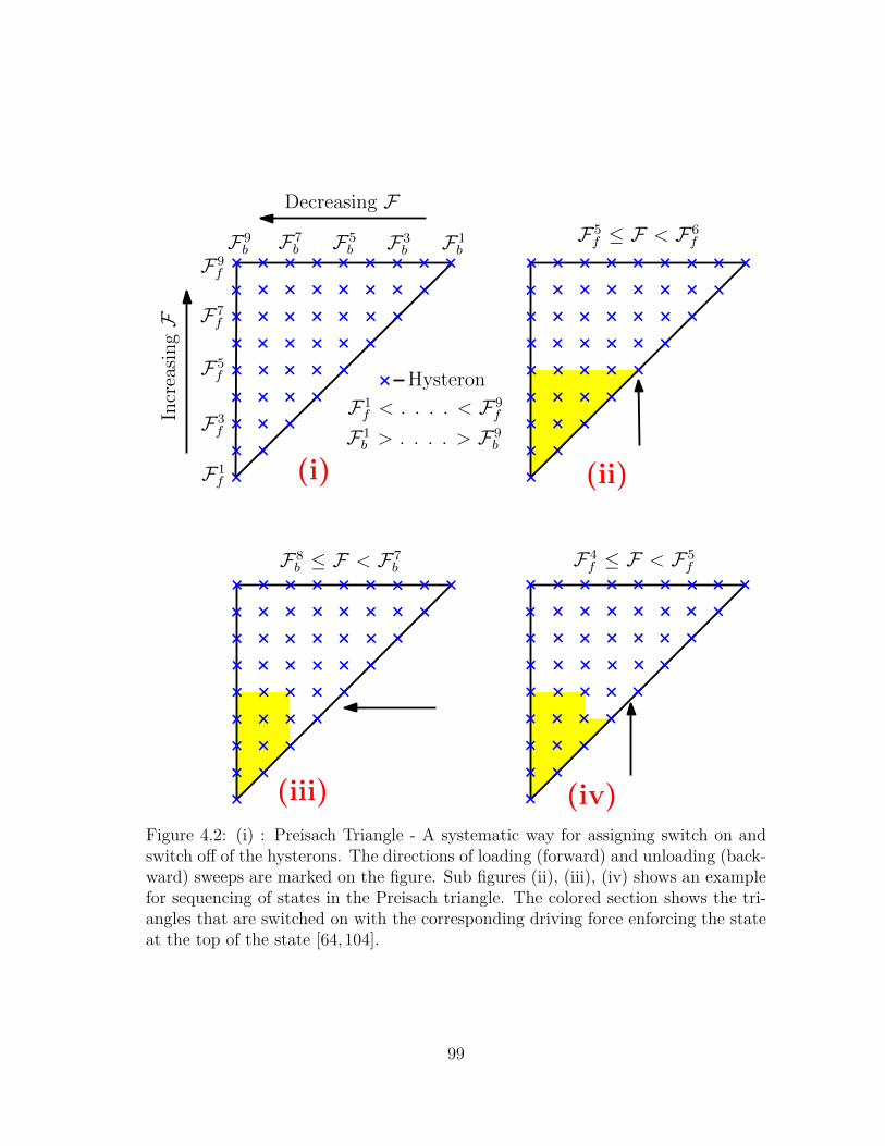
F9b F7

b F5b F3

b

F9f

F1b

F7f

F5f

F3f

F1f

Decreasing FIncreasingF

F5f ≤ F < F6

f

Hysteron

F1f < . . . . < F9

f

F1b > . . . . > F9

b

F4f ≤ F < F5

fF8b ≤ F < F7

b

(i) (ii)

(iii) (iv)

Figure 4.2: (i) : Preisach Triangle - A systematic way for assigning switch on andswitch off of the hysterons. The directions of loading (forward) and unloading (back-ward) sweeps are marked on the figure. Sub figures (ii), (iii), (iv) shows an examplefor sequencing of states in the Preisach triangle. The colored section shows the tri-angles that are switched on with the corresponding driving force enforcing the stateat the top of the state [64,104].

99

4.2 Preisach Triangle

Following Doraiswamy et al. [64,104], the geometric arrangement of hysterons in

a systematic way is with the help of a Preisach triangle as shown in figure 4.2 (i).

With known highest and the lowest forward driving force (Fforward) values for any

loading case, the hysterons with the lowest driving force are positioned at the bottom

of the triangle and the highest ones are arranged at the top end of the triangle (refer

figure 4.2 (i)). Similarly, for the backward driving force (F backward) hysterons, they

are arranged such that they increase from left to right i.e the lowest ones to the left

and the highest ones to the right. Further, the hysterons on any particular row have

the same Fforward value and similarly the hysterons on any column have the same

F backward value in the triangle (refer figure 4.2 (i)) [64, 104]. Once the Fforward and

F backward values are assigned, the corresponding “output”, ∆ξ for each hysteron needs

to be evaluated. By assigning hysterons at specific positions on a Preisach triangle,

the three parameters Fforward, F backward and ∆ξ are automatically estimated. The

number of hysterons in a triangle of side n is n(n+1)2 [64, 104].

∆ξ for each hysteron can be evaluated by setting up a system of equations where

each equation corresponds to the sum of the outputs of all those hysterons that are

switched on. By equating these to the volume fraction (ξ) from the data correspond-

ing to the driving force level for each loading case, it is evident that there are n(n+1)2

hysterons, and only k(< n(n+1)

2

)data points (depending on the experimental data).

This problem is solved using least squares technique with a non-negativity constraint

for the outputs of the hysterons. A “lsqnonneg” package fromMATLAB R© is readily

available to compute this [64,104].

Following Doraiswamy [104], to illustrate this more clearly, an example with a

Preisach triangle of side 9 having 45 unknowns is considered as shown in figure 4.2.

100

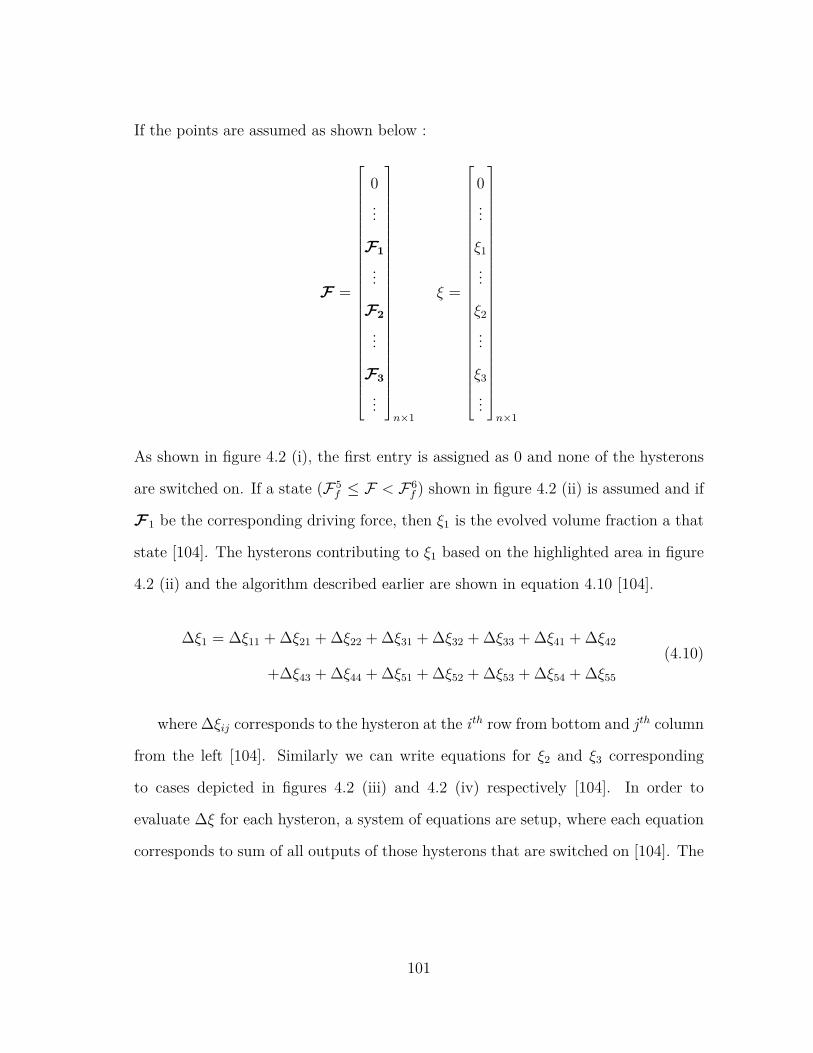
If the points are assumed as shown below :

F =

0...

F1

...

F2

...

F3

...

n×1

ξ =

0...

ξ1

...

ξ2

...

ξ3

...

n×1

As shown in figure 4.2 (i), the first entry is assigned as 0 and none of the hysterons

are switched on. If a state (F5f ≤ F < F6

f ) shown in figure 4.2 (ii) is assumed and if

F1 be the corresponding driving force, then ξ1 is the evolved volume fraction a that

state [104]. The hysterons contributing to ξ1 based on the highlighted area in figure

4.2 (ii) and the algorithm described earlier are shown in equation 4.10 [104].

∆ξ1 = ∆ξ11 + ∆ξ21 + ∆ξ22 + ∆ξ31 + ∆ξ32 + ∆ξ33 + ∆ξ41 + ∆ξ42

+∆ξ43 + ∆ξ44 + ∆ξ51 + ∆ξ52 + ∆ξ53 + ∆ξ54 + ∆ξ55

(4.10)

where ∆ξij corresponds to the hysteron at the i th row from bottom and j th column

from the left [104]. Similarly we can write equations for ξ2 and ξ3 corresponding

to cases depicted in figures 4.2 (iii) and 4.2 (iv) respectively [104]. In order to

evaluate ∆ξ for each hysteron, a system of equations are setup, where each equation

corresponds to sum of all outputs of those hysterons that are switched on [104]. The

101

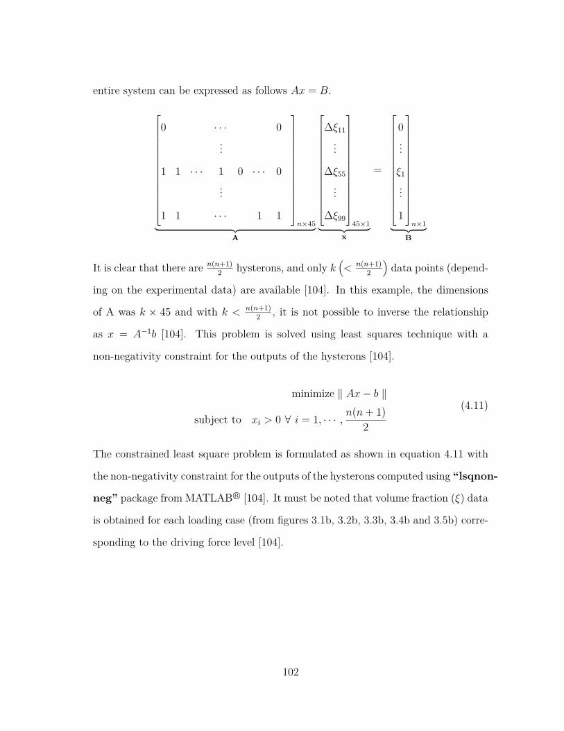
entire system can be expressed as follows Ax = B.

0 · · · 0...

1 1 · · · 1 0 · · · 0...

1 1 · · · 1 1

n×45︸ ︷︷ ︸

A

∆ξ11

...

∆ξ55

...

∆ξ99

45×1︸ ︷︷ ︸

x

=

0...

ξ1

...

1

n×1︸ ︷︷ ︸

B

It is clear that there are n(n+1)2 hysterons, and only k

(< n(n+1)

2

)data points (depend-

ing on the experimental data) are available [104]. In this example, the dimensions

of A was k × 45 and with k < n(n+1)2 , it is not possible to inverse the relationship

as x = A−1b [104]. This problem is solved using least squares technique with a

non-negativity constraint for the outputs of the hysterons [104].

minimize ‖ Ax− b ‖

subject to xi > 0 ∀ i = 1, · · · , n(n+ 1)2

(4.11)

The constrained least square problem is formulated as shown in equation 4.11 with

the non-negativity constraint for the outputs of the hysterons computed using “lsqnon-

neg” package from MATLAB R© [104]. It must be noted that volume fraction (ξ) data

is obtained for each loading case (from figures 3.1b, 3.2b, 3.3b, 3.4b and 3.5b) corre-

sponding to the driving force level [104].

102

5. MODEL DEVELOPMENT – THREE SPECIES

5.1 Complete Torsion Response

Until now, the discussion was in capturing superelastic responses of SMA com-

ponents under different loading conditions. In this section, the proposed modeling

approach of separating the thermoelastic and dissipative part of the responses is ex-

tended to capture both SE and SME effects under torsional loading as depicted in

figure 1.6. The goal is to develop a constitutive model for SMA components subjected

to torsional loading under both SE and SME effects.

5.1.1 Model Development

The three species considered are austenite and two variants of “detwinned marten-

site” and the twinned configuration is considered to be of equal proportion of each

detwinned martensite variant. It is assumed that M+ and M− are the marten-

site variants under clockwise and anticlockwise twists respectively. Paths (a) – (c)

and (a) – (b) in figure 5.1 represents the superelastic effect (austenite – martenite

transformations) under clockwise and anticlockwise rotations respectively. Further

under no-load conditions, the twinned martensite or self accommodated martensite

is an assembly of 50% M+ & 50% M−. On application of mechanical loads at low

temperatures (below Mf ), the twinned martensitic configurations detwin to certain

dominant single variant martensite phase either M+ or M− depending on the di-

rection of rotation resulting in macroscopic shape change. Paths (d) – (b) or (c) in

figure 5.1 represent the twinning response as a part of SME.

103

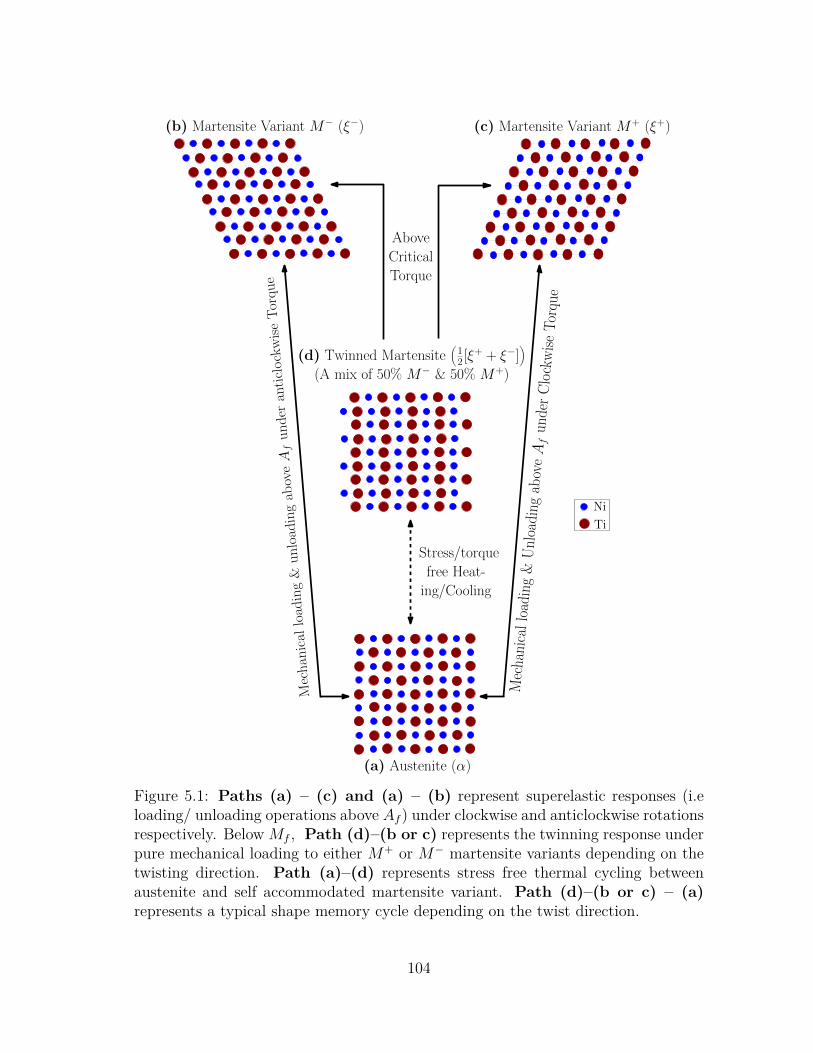
Stress/torque

free Heat-

ing/Cooling

(a) Austenite (α)

(c) Martensite Variant M+ (ξ+)

(d) Twinned Martensite(12[ξ

+ + ξ−])

(A mix of 50% M− & 50% M+)

Mechanical

loading&

unloadingaboveAfunder

anticlockwiseTorque

(b) Martensite Variant M− (ξ−)

Above

Critical

Torque

Mechanicalloading&

Unloading

aboveAfun

derClockwiseTorque

Ni

Ti

Figure 5.1: Paths (a) – (c) and (a) – (b) represent superelastic responses (i.eloading/ unloading operations above Af ) under clockwise and anticlockwise rotationsrespectively. BelowMf , Path (d)–(b or c) represents the twinning response underpure mechanical loading to either M+ or M− martensite variants depending on thetwisting direction. Path (a)–(d) represents stress free thermal cycling betweenaustenite and self accommodated martensite variant. Path (d)–(b or c) – (a)represents a typical shape memory cycle depending on the twist direction.

104

It must be highlighted that the martensite species considered here are related

to the crystallographic orientation combinations present at an instant and not to

the method by which they were formed. Further, there are also not equivalent to

the stress induced and temperature induced components (i.e twinned and detwinned

martensite species) as established in earlier literature by Brinson [74]. As shown in

figure 5.1, let,

α : Volume fraction of Austenite

ξ+ : Volume fraction of Detwinned Maternsite M+

ξ− : Volume fraction of Detwinned Martensite M−

Both M+ and M− martensite variants are independent of each other and only one

variant is dominant in any phase transformation or twinning event as described with

various paths highlighted in figure 5.1. The volume fractions of the species and the

rate change of volume fractions are connected by equations 5.1a and 5.1b respectively

as shown below.

α + ξ+ + ξ− = 1 (5.1a)

α + ξ+ + ξ− = 0 (5.1b)

In this proposed approach, the torque and volume fractions of the three variants are

predicted as functions of time given the twist as a function of time. Similar to the

two species approach, the model is formulated using a Gibbs potential to capture

the measurable macroscopic thermoelastic response and a Preisach model to capture

the changes in hysteretic response due to changes in volume fractions.

Consider a SMA component of length (L) subject to a torque (T ). Due to this, the

SMA component twists and the angle of twist per unit length is φ. SMA component

here can be a wire, bar or a spring. The SMA component is subjected to a torque T

about its axis for wire or bar. In case of spring, the torque can be estimated using the

105

axial force (P ) that the spring is subjected too along its axis as T = P(Dm

2

). With

the assumption that the angle of twist across the spring length is uniform, the angle

of twist per unit length (φ) can be evaluated in terms of the spring displacement (δ)

as φ = 2δπD2

mn.

where,

• “Dm” be the mean coil diameter of the spring in mm

• “d” be the SMA wire diameter in mm.

• “Cm” denote the Spring Index.

• “n” be the number of active coils (i.e neglecting the end hooks).

During this process, the SMA undergoes a phase transition and to model this, one

can assume the total angle of twist is composed of the thermoelastic part and trans-

formational part as shown in equation 5.2.

φ = φe + φt =⇒ φ = φe + φt (5.2)

where,

φ : Total angle of twist

φe : Thermoelastic part

φt : Transformational part

The total transformational rate of twists is assumed to be composed of transformation

rate of twists for M+ and M− transformations.

φt = φ+t + φ−t (5.3)

The transformational rate of twists are assumed to evolve with their respective vol-

106

ume fractions

φ+t = φ+

max˙ξ+

φ−t = φ−max˙ξ−

(5.4)

where, φ+max and φ−max are the maximum transformational strains for M+ and M−

transformations respectively. For NiTi alloys, they can assumed to be of the order

of 6% to 8% for both cases. Using equations 5.3 and 5.4 in equation 5.2 results in

an equation for total rate of twist as shown below.

φ = φe + φ+max

˙ξ+ + φ−max˙ξ− (5.5)

5.1.1.1 The Gibbs Potential - 3 species torsional loading

The Gibbs free energy per unit length is assumed to be a function of the torque

(T), operating temperature (θ), the three volume fractions i.e ξ+, ξ− and α (intro-

duced in equation 5.1a earlier) as shown in equation 5.6 below:

G := G(T, θ, α, ξ+, ξ−) (5.6)

The internal energy (∃), is related to the Gibbs potential (G), the entropy (η), the

temperature (θ) and the angle of twist (φ) as shown in equation 5.7 below.

∃ = G + ηθ + Tφ (5.7)

The rate of mechanical dissipation (∆), is the net macroscopic inelastic work (χ)

in a closed cycle of state which is required to be non-negative by the second law

of thermodynamics as shown in expression 5.8b below [65, 158, 159]. ‘ρ’ is the mass

107

density (mass per unit volume).

χ = T φ− ρ∃ − ρηθ (5.8a)

∆ =∮χdt ≥ 0 (5.8b)

Now using equations 5.6 and 5.7 in equation 5.8a, the inequality is reduced to a form

as shown below

−[φe + ρ

∂G∂T

]T −

[η + ρ

∂G∂θ

]θ +

[Tφ+

max − ρ∂G∂ξ+

]ξ+

+[Tφ−max − ρ

∂G∂ξ−

]ξ− −

[ρ∂G∂α

]α = χ

(5.9)

From, the above inequality (equation 5.9), in the absence of phase transformations,

the material will behave as a non-dissipative thermoelastic material and that the

dissipative response is assumed to be solely due to phase transformations. This then

implies that expressions for thermoelastic twist and entropy are obtained as shown

below in equations 5.10 and 5.11 respectively.

φe = −ρ∂G∂T

(5.10)

η = −ρ∂G∂θ

(5.11)

108

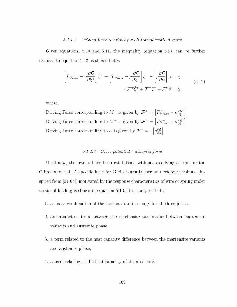
5.1.1.2 Driving force relations for all transformation cases

Given equations, 5.10 and 5.11, the inequality (equation 5.9), can be further

reduced to equation 5.12 as shown below

[Tφ+

max − ρ∂G∂ξ+

]ξ+ +

[Tφ−max − ρ

∂G∂ξ−

]ξ− −

[ρ∂G∂α

]α = χ

⇒ F+ξ+ +F−ξ− +Fαα = χ

(5.12)

where,

Driving Force corresponding to M+ is given by F+ =[Tφ+

max − ρ ∂G∂ξ+

]Driving Force corresponding to M− is given by F− =

[Tφ−max − ρ ∂G

∂ξ−

]Driving Force corresponding to α is given by Fα = -

[ρ∂G∂α

]

5.1.1.3 Gibbs potential : assumed form

Until now, the results have been established without specifying a form for the

Gibbs potential. A specific form for Gibbs potential per unit reference volume (in-

spired from [64,65]) motivated by the response characteristics of wire or spring under

torsional loading is shown in equation 5.13. It is composed of :

1. a linear combination of the torsional strain energy for all three phases,

2. an interaction term between the martensite variants or between martensite

variants and austenite phase,

3. a term related to the heat capacity difference between the martensite variants

and austenite phase,

4. a term relating to the heat capacity of the austenite.

109

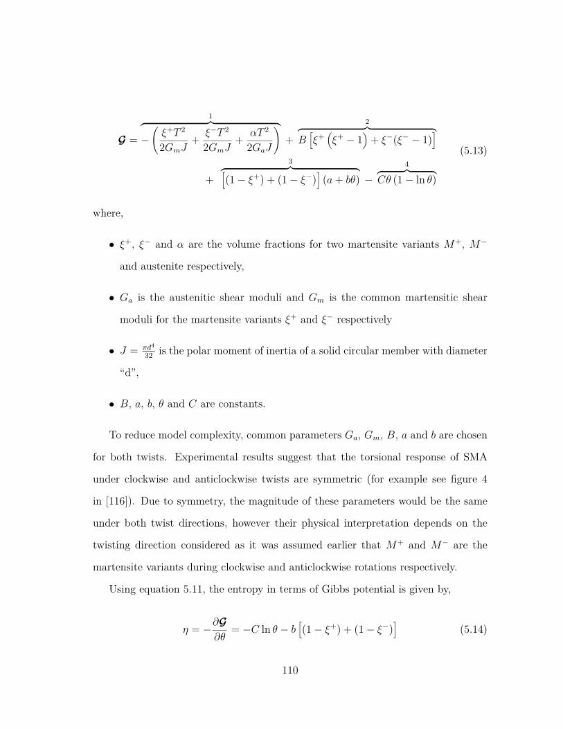
G =

1︷ ︸︸ ︷−(ξ+T 2

2GmJ+ ξ−T 2

2GmJ+ αT 2

2GaJ

)+

2︷ ︸︸ ︷B[ξ+(ξ+ − 1

)+ ξ−(ξ− − 1)

]

+

3︷ ︸︸ ︷[(1− ξ+) + (1− ξ−)

](a+ bθ) −

4︷ ︸︸ ︷Cθ (1− ln θ)

(5.13)

where,

• ξ+, ξ− and α are the volume fractions for two martensite variants M+, M−

and austenite respectively,

• Ga is the austenitic shear moduli and Gm is the common martensitic shear

moduli for the martensite variants ξ+ and ξ− respectively

• J = πd4

32 is the polar moment of inertia of a solid circular member with diameter

“d”,

• B, a, b, θ and C are constants.

To reduce model complexity, common parameters Ga, Gm, B, a and b are chosen

for both twists. Experimental results suggest that the torsional response of SMA

under clockwise and anticlockwise twists are symmetric (for example see figure 4

in [116]). Due to symmetry, the magnitude of these parameters would be the same

under both twist directions, however their physical interpretation depends on the

twisting direction considered as it was assumed earlier that M+ and M− are the

martensite variants during clockwise and anticlockwise rotations respectively.

Using equation 5.11, the entropy in terms of Gibbs potential is given by,

η = −∂G∂θ

= −C ln θ − b[(1− ξ+) + (1− ξ−)

](5.14)

110

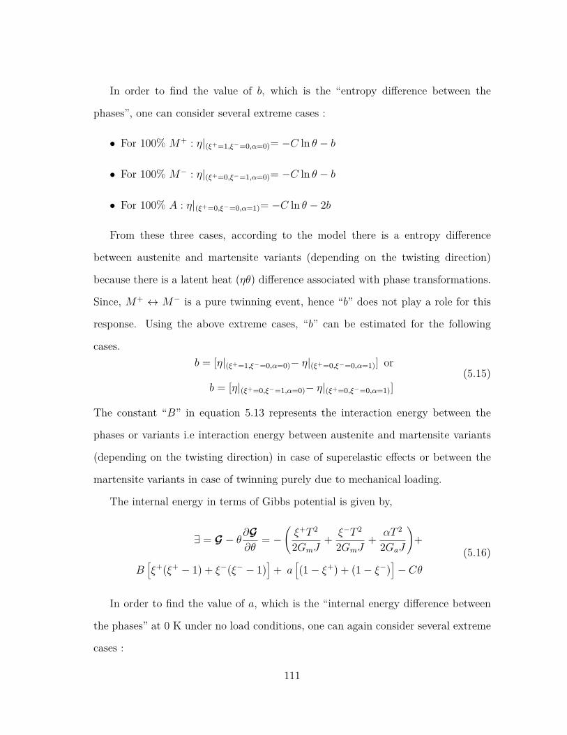
In order to find the value of b, which is the “entropy difference between the

phases”, one can consider several extreme cases :

• For 100% M+ : η|(ξ+=1,ξ−=0,α=0)= −C ln θ − b

• For 100% M− : η|(ξ+=0,ξ−=1,α=0)= −C ln θ − b

• For 100% A : η|(ξ+=0,ξ−=0,α=1)= −C ln θ − 2b

From these three cases, according to the model there is a entropy difference

between austenite and martensite variants (depending on the twisting direction)

because there is a latent heat (ηθ) difference associated with phase transformations.

Since, M+ ↔ M− is a pure twinning event, hence “b” does not play a role for this

response. Using the above extreme cases, “b” can be estimated for the following

cases.b = [η|(ξ+=1,ξ−=0,α=0)− η|(ξ+=0,ξ−=0,α=1)] or

b = [η|(ξ+=0,ξ−=1,α=0)− η|(ξ+=0,ξ−=0,α=1)](5.15)

The constant “B” in equation 5.13 represents the interaction energy between the

phases or variants i.e interaction energy between austenite and martensite variants

(depending on the twisting direction) in case of superelastic effects or between the

martensite variants in case of twinning purely due to mechanical loading.

The internal energy in terms of Gibbs potential is given by,

∃ = G − θ∂G∂θ

= −(ξ+T 2

2GmJ+ ξ−T 2

2GmJ+ αT 2

2GaJ

)+

B[ξ+(ξ+ − 1) + ξ−(ξ− − 1)

]+ a

[(1− ξ+) + (1− ξ−)

]− Cθ

(5.16)

In order to find the value of a, which is the “internal energy difference between

the phases” at 0 K under no load conditions, one can again consider several extreme

cases :

111

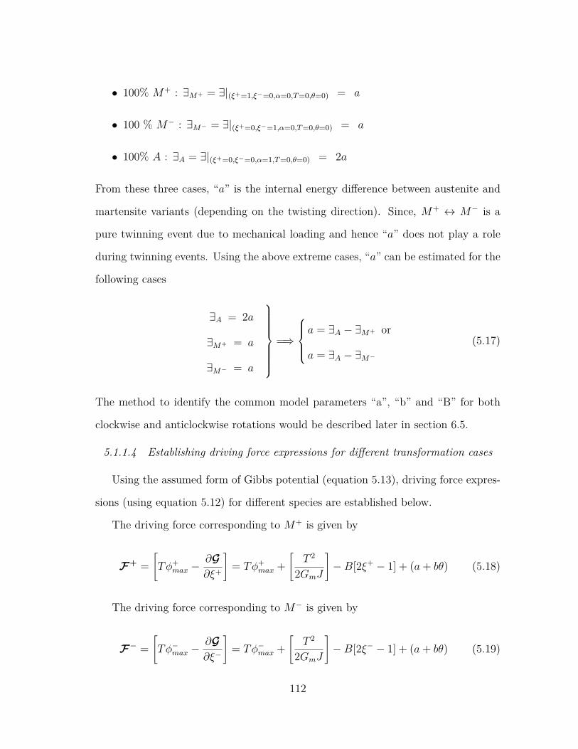
• 100% M+ : ∃M+ = ∃|(ξ+=1,ξ−=0,α=0,T=0,θ=0) = a

• 100 % M− : ∃M− = ∃|(ξ+=0,ξ−=1,α=0,T=0,θ=0) = a

• 100% A : ∃A = ∃|(ξ+=0,ξ−=0,α=1,T=0,θ=0) = 2a

From these three cases, “a” is the internal energy difference between austenite and

martensite variants (depending on the twisting direction). Since, M+ ↔ M− is a

pure twinning event due to mechanical loading and hence “a” does not play a role

during twinning events. Using the above extreme cases, “a” can be estimated for the

following cases

∃A = 2a

∃M+ = a

∃M− = a

=⇒

a = ∃A − ∃M+ or

a = ∃A − ∃M−

(5.17)

The method to identify the common model parameters “a”, “b” and “B” for both

clockwise and anticlockwise rotations would be described later in section 6.5.

5.1.1.4 Establishing driving force expressions for different transformation cases

Using the assumed form of Gibbs potential (equation 5.13), driving force expres-

sions (using equation 5.12) for different species are established below.

The driving force corresponding to M+ is given by

F+ =[Tφ+

max −∂G∂ξ+

]= Tφ+

max +[

T 2

2GmJ

]−B[2ξ+ − 1] + (a+ bθ) (5.18)

The driving force corresponding to M− is given by

F− =[Tφ−max −

∂G∂ξ−

]= Tφ−max +

[T 2

2GmJ

]−B[2ξ− − 1] + (a+ bθ) (5.19)

112

The driving force corresponding to α is given by

Fα = −[∂G∂α

]=[T 2

2GaJ

](5.20)

Now the possible transformations among the three species are A↔M+, A↔M−

and M− ↔M+.

Using the above equation sets (5.18, 5.19, 5.20) and equation 5.12, one can obtain

driving force relationships for all possible transformation conditions as summarized

below

k1 :=| F+ −Fα | = Tφ+max + T 2

( 12GmJ

− 12GaJ

)−B(2ξ+ − 1) + bθ + a (5.21a)

k2 :=| F− −Fα | = Tφ−max + T 2( 1

2GmJ− 1

2GaJ

)−B(2ξ− − 1) + bθ + a (5.21b)

k3 :=| F+ −F− | = FM+→M− = T[φ+max − φ−max

]− 2B

[ξ+ − ξ−

](5.21c)

In the above relations, “k1” and “k2” represent the driving force expressions for

superelastic phase transformations under clockwise and anticlockwise rotations re-

spectively. “k3” corresponds to twinning events resulting in “self accommodated

martensite” variants switching to preferred single variant martenite variants M+

and M−. In short, k1, k2 and k3 corresponds to A↔M+, A↔M− and M+ ↔M−

cases respectively.

From, the above general driving force relationships (equations 5.21a, 5.21b, 5.21c),

specific driving force relationships for twinning responses under clockwise and anti-

clockwise rotations are developed by considering the following important cases below:

• Notice that the driving force for the twinning response (k3) is temperature in-

dependent and depends upon only on the the applied torque and the difference

113

in the volume fraction of the M+ and M− martensite variants. So, if T = 0

and ξ+ and ξ− are equal then there will be no driving force for twinning as

k3 = 0. Also, under stress free conditions, using equation set 5.22 below, k1

= k2 as ξ+ = ξ−. Since, the thresholds are the same (i.e k1 = k2), only an

austenitic phase transformation purely due to temperature changes (in absence

of any external loads) is possible as there is no driving force for twinning (as

k3 = 0). Also, when T = 0, according to equation 5.5, φe = 0 which suggests

φ = 0 as ξ+ = ξ−.

k1 =| F+ −Fα |= −B(2ξ+ − 1) + bθ + a (5.22a)

k2 =| F− −Fα |= −B(2ξ− − 1) + bθ + a (5.22b)

k3 =| F+ −F− |= −2B[ξ+ − ξ−

](5.22c)

Further, in order to satisfy the volume fraction conservation relationship (see

equation 5.1a), if ξ+ = ξ− and k1 = k2, it implies that α and one martensite

configuration are present. Under stress free conditions (T = 0), this suggests

that the possible transformations purely due to temperature changes are be-

tween a 50% M+ & 50% M− case and austenite. This further emphasizes our

earlier assumption of twinned martensite (also referred as self accommodated

martensite) configuration being 50% M+ & 50% M− as illustrated in figure

5.1.

• With T 6= 0 and α = 0 → ξ+ + ξ− = 1 then,

k1 =| F+ |= Tφ+max + T 2

( 12GmJ

)−B(2ξ+ − 1) + bθ + a (5.23a)

114

k2 =| F− |= Tφ−max + T 2( 1

2GmJ

)−B(2ξ− − 1) + bθ + a (5.23b)

k3 =| F+ −F− |= FM+→M− = T[φ+max − φ−max

]− 2B

[ξ+ − ξ−

](5.23c)

In the above equation sets 5.23c, k3 represents the driving forces to capture

the complete twinning response in both clockwise and anticlockwise rotations.

However, since the clockwise and anticlockwise torsion experiments are inde-

pendent of each other, hence the two martensite species M+ and M− are also

independent of each other. This suggests that k3 from equation sets 5.23c can

be split to capture individual twinning effects for clockwise (k+3 ) and anticlock-

wise (k−3 ) directions respectively as shown in equations 5.24a and 5.24b below.

The split twinning events will be between a 50% M+ & 50% M− martensite

configuration under stress free conditions to either 100% M+ or 100% M−

depending on the direction of the twist.

k+3 = F+ = Tφ+

max − 2Bξ+ (5.24a)

k−3 = F− = Tφ−max − 2Bξ− (5.24b)

It must be highlighted that the driving force expressions corresponding to the twin-

ning responses under both rotations are independent of temperature (θ), constants

“a” and “b” as it is a pure mechanical response. On the other hand, the driving

force expressions corresponding to the superelastic transformations (A ↔ M+ and

A↔M− cases) depends upon model constants “a”,“b” and“B” along with operating

temperature “θ” as shown in equations 5.21a 5.21b for clockwise and anticlockwise

rotations respectively. In order to capture the shape memory effects under clockwise

and anticlockwise twists, the driving force expressions would be a combination of

115

driving force expressions for the twinning responses and the superelastic responses

(with T = 0) depending on the twisting direction (i.e equation 5.24a and 5.21a for

clockwise twist. Similarly, equation 5.24b and 5.21b for anticlockwise twist.)

5.1.1.5 Establishing volume fraction expressions for different transformation cases

Using the assumed form of Gibbs potential expression 5.13 and using equation

5.10, an expression for elastic part of twist is obtained as shown below

φe = −∂G∂T

= ξ+T

GmJ+ ξ−T

GmJ+ αT

GaJ(5.25)

Using the volume fraction conservation relationship (equation 5.1a), the above equa-

tion 5.25 is further reduced to special two species cases as shown below.

φe|ξ−=0 = ξ+T

GmJ+ (1− ξ+)T

GaJ(5.26a)

φe|ξ+=0 = ξ−T

GmJ+ (1− ξ−)T

GaJ(5.26b)

φe|α=0 =

ξ+T

GmJ+ (1− ξ+)T

GmJor

ξ−T

GmJ+ (1− ξ−)T

GmJ

(5.26c)

As the martensitic species M+ and M− are independent of each other, hence the

total twist can be separated for clockwise and anticlockwise rotations respectively as

shown equation 5.27 below.

φ = φ+ + φ− ⇒ φ = φ+ + φ− (5.27)

Now using the above equation 5.27 along with the relationship for total rate of twist

(equation 5.5)and equation sets (5.26a, 5.26b and 5.26c), simplified equations for

116

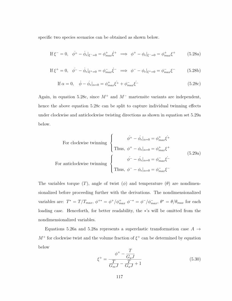
specific two species scenarios can be obtained as shown below.

If ξ− = 0, φ+ − φe|ξ−=0 = φ+maxξ

+ =⇒ φ+ − φe|ξ−=0 = φ+maxξ

+ (5.28a)

If ξ+ = 0, φ− − φe|ξ+=0 = φ−maxξ− =⇒ φ− − φe|ξ+=0 = φ−maxξ

− (5.28b)

If α = 0, φ− φe|α=0 = φ+max

˙ξ+ + φ−max˙ξ− (5.28c)

Again, in equation 5.28c, since M+ and M− martensite variants are independent,

hence the above equation 5.28c can be split to capture individual twinning effects

under clockwise and anticlockwise twisting directions as shown in equation set 5.29a

below.

For clockwise twinning

φ+ − φe|α=0 = φ+

max˙ξ+

Thus, φ+ − φe|α=0 = φ+maxξ

+

For anticlockwise twinning

φ− − φe|α=0 = φ−max

˙ξ−

Thus, φ− − φe|α=0 = φ−maxξ−

(5.29a)

The variables torque (T ), angle of twist (φ) and temperature (θ) are nondimen-

sionalized before proceeding further with the derivations. The nondimensionalized

variables are: T ∗ = T/Tmax, φ+∗ = φ+/φ+max φ

−∗ = φ−/φ−max, θ∗ = θ/θmax for each

loading case. Henceforth, for better readability, the ∗’s will be omitted from the

nondimensionalized variables.

Equations 5.26a and 5.28a represents a superelastic transformation case A →

M+ for clockwise twist and the volume fraction of ξ+ can be determined by equation

below

ξ+ =φ+ − T

GaJT

GmJ− TGaJ

+ 1(5.30)

117

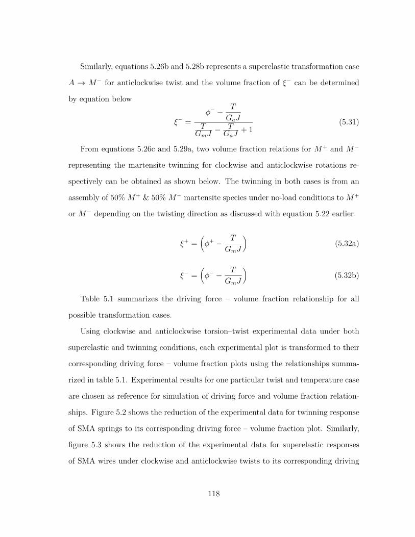
Similarly, equations 5.26b and 5.28b represents a superelastic transformation case

A → M− for anticlockwise twist and the volume fraction of ξ− can be determined

by equation below

ξ− =φ− − T

GaJT

GmJ− TGaJ

+ 1(5.31)

From equations 5.26c and 5.29a, two volume fraction relations for M+ and M−

representing the martensite twinning for clockwise and anticlockwise rotations re-

spectively can be obtained as shown below. The twinning in both cases is from an

assembly of 50% M+ & 50% M− martensite species under no-load conditions to M+

or M− depending on the twisting direction as discussed with equation 5.22 earlier.

ξ+ =(φ+ − T

GmJ

)(5.32a)

ξ− =(φ− − T

GmJ

)(5.32b)

Table 5.1 summarizes the driving force – volume fraction relationship for all

possible transformation cases.

Using clockwise and anticlockwise torsion–twist experimental data under both

superelastic and twinning conditions, each experimental plot is transformed to their

corresponding driving force – volume fraction plots using the relationships summa-

rized in table 5.1. Experimental results for one particular twist and temperature case

are chosen as reference for simulation of driving force and volume fraction relation-

ships. Figure 5.2 shows the reduction of the experimental data for twinning response

of SMA springs to its corresponding driving force – volume fraction plot. Similarly,

figure 5.3 shows the reduction of the experimental data for superelastic responses

of SMA wires under clockwise and anticlockwise twists to its corresponding driving

118

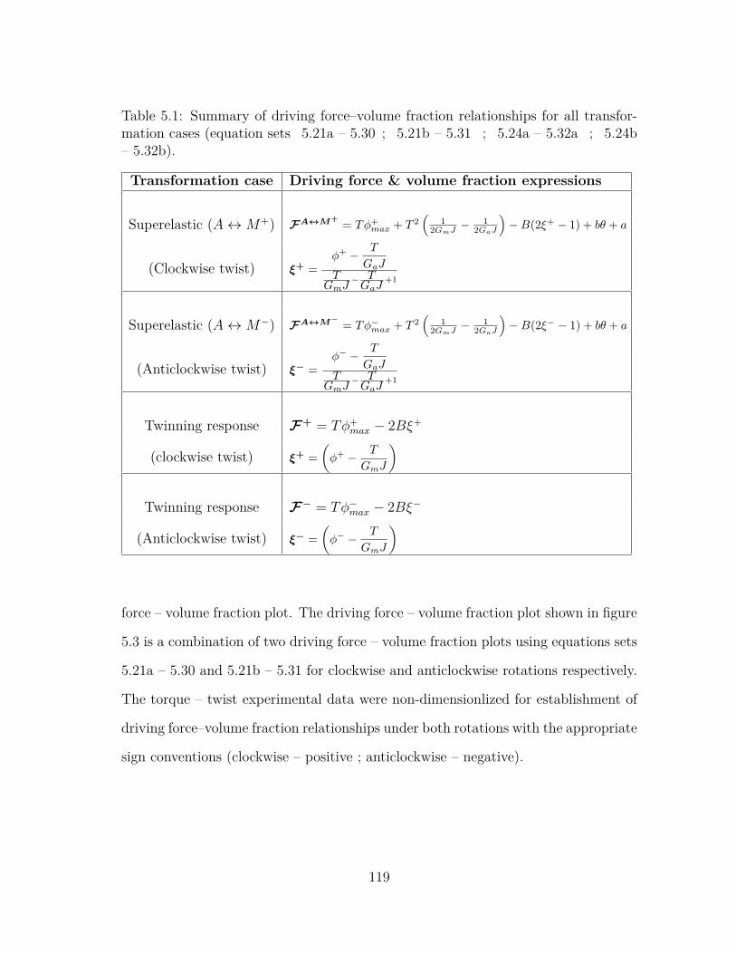
Table 5.1: Summary of driving force–volume fraction relationships for all transfor-mation cases (equation sets 5.21a – 5.30 ; 5.21b – 5.31 ; 5.24a – 5.32a ; 5.24b– 5.32b).

Transformation case Driving force & volume fraction expressions

Superelastic (A↔M+) FA↔M+ = Tφ+max + T 2

(1

2GmJ −1

2GaJ

)−B(2ξ+ − 1) + bθ + a

(Clockwise twist) ξ+ =φ+ − T

GaJT

GmJ− TGaJ

+1

Superelastic (A↔M−) FA↔M− = Tφ−max + T 2

(1

2GmJ −1

2GaJ

)−B(2ξ− − 1) + bθ + a

(Anticlockwise twist) ξ− =φ− − T

GaJT

GmJ− TGaJ

+1

Twinning response F+ = Tφ+max − 2Bξ+

(clockwise twist) ξ+ =(φ+ − T

GmJ

)

Twinning response F− = Tφ−max − 2Bξ−

(Anticlockwise twist) ξ− =(φ− − T

GmJ

)

force – volume fraction plot. The driving force – volume fraction plot shown in figure

5.3 is a combination of two driving force – volume fraction plots using equations sets

5.21a – 5.30 and 5.21b – 5.31 for clockwise and anticlockwise rotations respectively.

The torque – twist experimental data were non-dimensionlized for establishment of

driving force–volume fraction relationships under both rotations with the appropriate

sign conventions (clockwise – positive ; anticlockwise – negative).

119

Tor q

ue(N

mm)

Angle of twist (rad/mm)0 0.01 0.02 0.03 0.04 0.05 0.06

0

2

4

6

8

10

12

14

(a) Torque v/s Angle of twist plot at295 K. Clockwise twist was assumed

Dr ivingForce

Volume fraction of Martensite

0 0.1 0.2 0.3 0.4 0.5 0.6 0.7 0.8 0.9 10

0.5

1

1.5

2

2.5

3

3.5

4

4.5

5

(b) Driving Force–Volume Fractionplot

Figure 5.2: Experimental torque v/s angle of twist data is reduced to driving force–volume fraction plot using thermodynamic principles by using equations developedfor twinning response summarized in table 5.1. Clockwise twist was assumed. Ex-perimental data obtained from [113].

Anticlockwise twistClockwise twist

Torq

ue(N

mm)

Angle of twist (rad/mm)

- 0.1 - 0.08 - 0.06 - 0.04 - 0.02 0 0.02 0.04 0.06 0.08 0.1- 800

- 600

- 400

- 200

0

200

400

600

800

(a) Torque v/s angle of twist data at297 K for 450o twist

Anticlockwise twistClockwise twist

DrivingForce

Volume fraction of Martensite

- 1 - 0.8 - 0.6 - 0.4 - 0.2 0 0.2 0.4 0.6 0.8 1- 3

- 2

- 1

0

1

2

3

(b) Driving Force–Volume Fractionplot

Figure 5.3: Experimental torque v/s angle of twist data is reduced to driving force–volume fraction plot using thermodynamic principles by using equations developedfor superelastic responses summarized in table 5.1. Experimental data obtainedfrom [116].

120

6. PROTOCOL : MODEL SIMULATIONS AND PREDICTIONS ∗

Using the two species and three species model formulations discussed in sections

3 and 5, driving force–volume fraction relationships for different loading conditions

were developed. The algorithm described in section 4.1 of section 4 was then used to

estimate the volume fraction contribution for a given driving force F under different

loading conditions.

The next step in the model prediction is to predict the original experimental data

from the F – ξ plot predicted using the algorithm described in section 4.1. If there

are “n” hysterons each contributing ξi to the total volume fraction as setup by the

Preisach algorithm, then

ξ =n∑i=0

ξi (6.1)

where ξi ∀ i = 1, 2, · · · , n represents the volume fraction contribution of those

hysterons switched on at this time step.

The following sections below discuss the simulation procedure under different

loading conditions and making predictions at different temperatures

6.1 Tension Loading Case - Two Species

6.1.1 Load Controlled Test Protocol

If at time instant ti, σ(i), ε(i) and θ(i) are assumed to be known then by using

Equation 3.15, ξten(i) can be evaluated. In order to compute these variables at time∗Reprinted with permission from “Combining Thermodynamic Principles with Preisach models

for superelastic SMA Wires” by Doraiswamy, Rao and Srinivasa, Smart Materials and Structures,20, 085032, 2011 [64], Copyright [2014] by IOP.

Reprinted with permission from “A two species thermodynamic Preisach model for the tor-sional response of SMA wires and springs under superelastic conditions” by Rao and Srinivasa,International Journal of Solids and Structures, 50, 887–898, 2013 [90], Copyright [2014] by ElsevierLimited.

121

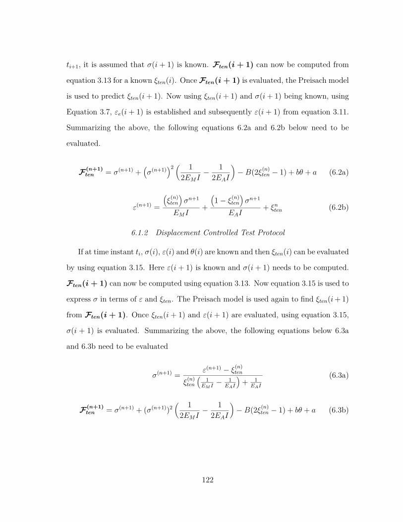
ti+1, it is assumed that σ(i + 1) is known. Ften(i+ 1) can now be computed from

equation 3.13 for a known ξten(i). Once Ften(i+ 1) is evaluated, the Preisach model

is used to predict ξten(i+ 1). Now using ξten(i+ 1) and σ(i+ 1) being known, using

Equation 3.7, εe(i + 1) is established and subsequently ε(i + 1) from equation 3.11.

Summarizing the above, the following equations 6.2a and 6.2b below need to be

evaluated.

F (n+1)ten = σ(n+1) +

(σ(n+1)

)2( 1

2EMI− 1

2EAI

)−B(2ξ(n)

ten − 1) + bθ + a (6.2a)

ε(n+1) =

(ξ

(n)ten

)σn+1

EMI+

(1− ξ(n)

ten

)σn+1

EAI+ ξnten (6.2b)

6.1.2 Displacement Controlled Test Protocol

If at time instant ti, σ(i), ε(i) and θ(i) are known and then ξten(i) can be evaluated

by using equation 3.15. Here ε(i + 1) is known and σ(i + 1) needs to be computed.

Ften(i+ 1) can now be computed using equation 3.13. Now equation 3.15 is used to

express σ in terms of ε and ξten. The Preisach model is used again to find ξten(i+ 1)

from Ften(i+ 1). Once ξten(i + 1) and ε(i + 1) are evaluated, using equation 3.15,

σ(i + 1) is evaluated. Summarizing the above, the following equations below 6.3a

and 6.3b need to be evaluated

σ(n+1) = ε(n+1) − ξ(n)ten

ξ(n)ten

(1

EM I− 1

EAI

)+ 1

EAI

(6.3a)

F (n+1)ten = σ(n+1) + (σ(n+1))2

( 12EMI

− 12EAI

)−B(2ξ(n)

ten − 1) + bθ + a (6.3b)

122

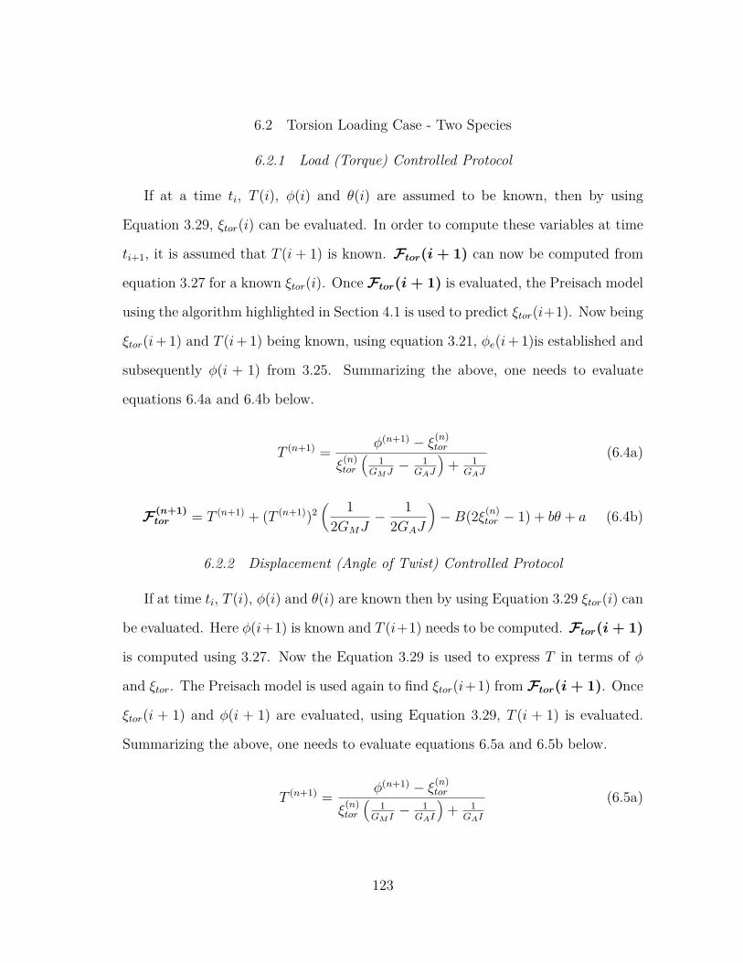
6.2 Torsion Loading Case - Two Species

6.2.1 Load (Torque) Controlled Protocol

If at a time ti, T (i), φ(i) and θ(i) are assumed to be known, then by using

Equation 3.29, ξtor(i) can be evaluated. In order to compute these variables at time

ti+1, it is assumed that T (i + 1) is known. Ftor(i+ 1) can now be computed from

equation 3.27 for a known ξtor(i). Once Ftor(i+ 1) is evaluated, the Preisach model

using the algorithm highlighted in Section 4.1 is used to predict ξtor(i+1). Now being

ξtor(i+ 1) and T (i+ 1) being known, using equation 3.21, φe(i+ 1)is established and

subsequently φ(i + 1) from 3.25. Summarizing the above, one needs to evaluate

equations 6.4a and 6.4b below.

T (n+1) = φ(n+1) − ξ(n)tor

ξ(n)tor

(1

GMJ− 1

GAJ

)+ 1

GAJ

(6.4a)

F (n+1)tor = T (n+1) + (T (n+1))2

( 12GMJ

− 12GAJ

)−B(2ξ(n)

tor − 1) + bθ + a (6.4b)

6.2.2 Displacement (Angle of Twist) Controlled Protocol

If at time ti, T (i), φ(i) and θ(i) are known then by using Equation 3.29 ξtor(i) can

be evaluated. Here φ(i+1) is known and T (i+1) needs to be computed. Ftor(i+ 1)

is computed using 3.27. Now the Equation 3.29 is used to express T in terms of φ

and ξtor. The Preisach model is used again to find ξtor(i+1) from Ftor(i+ 1). Once

ξtor(i + 1) and φ(i + 1) are evaluated, using Equation 3.29, T (i + 1) is evaluated.

Summarizing the above, one needs to evaluate equations 6.5a and 6.5b below.

T (n+1) = φ(n+1) − ξ(n)tor

ξ(n)tor

(1

GM I− 1

GAI

)+ 1

GAI

(6.5a)

123

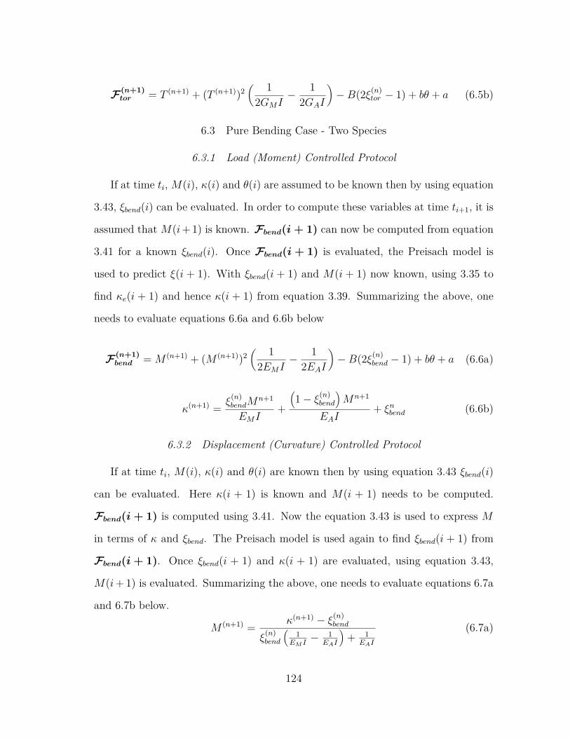
F (n+1)tor = T (n+1) + (T (n+1))2

( 12GMI

− 12GAI

)−B(2ξ(n)

tor − 1) + bθ + a (6.5b)

6.3 Pure Bending Case - Two Species

6.3.1 Load (Moment) Controlled Protocol

If at time ti, M(i), κ(i) and θ(i) are assumed to be known then by using equation

3.43, ξbend(i) can be evaluated. In order to compute these variables at time ti+1, it is

assumed that M(i+ 1) is known. Fbend(i+ 1) can now be computed from equation

3.41 for a known ξbend(i). Once Fbend(i+ 1) is evaluated, the Preisach model is

used to predict ξ(i + 1). With ξbend(i + 1) and M(i + 1) now known, using 3.35 to

find κe(i + 1) and hence κ(i + 1) from equation 3.39. Summarizing the above, one

needs to evaluate equations 6.6a and 6.6b below

F (n+1)bend = M (n+1) + (M (n+1))2

( 12EMI

− 12EAI

)−B(2ξ(n)

bend − 1) + bθ + a (6.6a)

κ(n+1) = ξ(n)bendM

n+1

EMI+

(1− ξ(n)

bend

)Mn+1

EAI+ ξnbend (6.6b)

6.3.2 Displacement (Curvature) Controlled Protocol

If at time ti, M(i), κ(i) and θ(i) are known then by using equation 3.43 ξbend(i)

can be evaluated. Here κ(i + 1) is known and M(i + 1) needs to be computed.

Fbend(i+ 1) is computed using 3.41. Now the equation 3.43 is used to express M

in terms of κ and ξbend. The Preisach model is used again to find ξbend(i + 1) from

Fbend(i+ 1). Once ξbend(i + 1) and κ(i + 1) are evaluated, using equation 3.43,

M(i+ 1) is evaluated. Summarizing the above, one needs to evaluate equations 6.7a

and 6.7b below.

M (n+1) = κ(n+1) − ξ(n)bend

ξ(n)bend

(1

EM I− 1

EAI

)+ 1

EAI

(6.7a)

124

F (n+1)bend = M (n+1) + (M (n+1))2

( 12EMI

− 12EAI

)−B(2ξ(n)

bend − 1) + bθ + a (6.7b)

6.4 Three Species Torsion - Model Simulation

The procedure illustrated in section 6.4.1 below is common for clockwise and

anticlockwise superelastic responses as the responses are symmetric. Similarly, a

common procedure for clockwise and anticlockwise twinning responses is highlighted

in section 6.4.2 below. For convenience, a common volume fraction ξ is employed for

discussion in this section. Term ξ here can be ξ+ or ξ− depending on the twisting

direction. The simulation protocol is same under both twist directions once the

corresponding equations are appropriately selected for each case from table 5.1.

6.4.1 Superelastic Responses

6.4.1.1 Load (Torque) Controlled Protocol

If at time ti, T(i), φ(i) and θ(i) are assumed to be known then by using equations

5.30 or 5.31, ξ(i) can be evaluated. In order to compute these variables at time ti+1,

it is assumed that T(i+1) is known. F(i+ 1) can now be computed from equations

5.21a or 5.21b for a known ξ(i). Once F(i + 1) is evaluated, the Preisach model is

used to predict ξ(i+1). With ξ(i+1) and T(i+1) now known, using equations 5.26a

or 5.26b, one can find φe(i+ 1) and hence φ(i+ 1) from equations 5.28a or 5.28b.

6.4.1.2 Displacement (angle of twist) controlled protocol

If at time ti, T(i), φ(i) and θ(i) are known then by using equation 5.30 or 5.31

ξ(i) can be evaluated. Here, φ(i + 1) is known and T(i+1) needs to be computed.

F(i+ 1) is computed using equations 5.21a or 5.21b. Now the equations 5.30 or 5.31

are used to express T in terms of φ and ξ. The Preisach model is used again to find

ξ(i + 1) from F(i + 1). Once ξ(i + 1) and φ(i + 1) are evaluated, using equations

5.30 or 5.31, T(i+1) is evaluated.

125

6.4.2 Twinning Responses

6.4.2.1 Load (Torque) Controlled Protocol

If at time ti, T(i) and φ(i) are assumed to be known then by using equations 5.32a

or 5.32b, ξ(i) can be evaluated. In order to compute these variables at time ti+1, it

is assumed that T(i+1) is known. F(i + 1) can now be computed from equations

5.24a or 5.24b for a known ξ(i). Once F(i + 1) is evaluated, the Preisach model is

used to predict ξ(i + 1). With ξ(i + 1) and T(i+1) now known, using equation set

5.26c, one can find φe(i + 1) and hence φ(i + 1) from equation 5.29a depending on

the twist direction.

6.4.2.2 Displacement (angle of twist) controlled protocol

If at time ti, T(i) and φ(i) are known then by using equation 5.32a or 5.32b ξ(i)

can be evaluated. Here φ(i+1) is known and T(i+1) needs to be computed. F(i+1)

is computed using equations 5.24a or 5.24b. Now the equations 5.32a or 5.32b is

used to express T in terms of φ and ξ. The Preisach model is used again to find

ξ(i + 1) from F(i + 1). Once ξ(i + 1) and φ(i + 1) are evaluated, using equations

5.32a or 5.32b, T(i+1) is evaluated.

6.5 Parameter Identification

By combining thermodynamics principles and Preisach modeling techniques, the

model parameters can be separated into sets of parameters arising from the thermo-

dynamical framework and those from the Preisach models related to hysterons posi-

tioning. Section 4.1 discussed the details of obtaining parameters Fforward, F backward

and ∆ξ pertaining to Preisach triangle as represented in figures 4.1 or 4.2 by auto-

matically assigning the hysterons at specific positions on the triangle. The method of

obtaining parameters arising from the assumed form of Gibbs potential for different

126

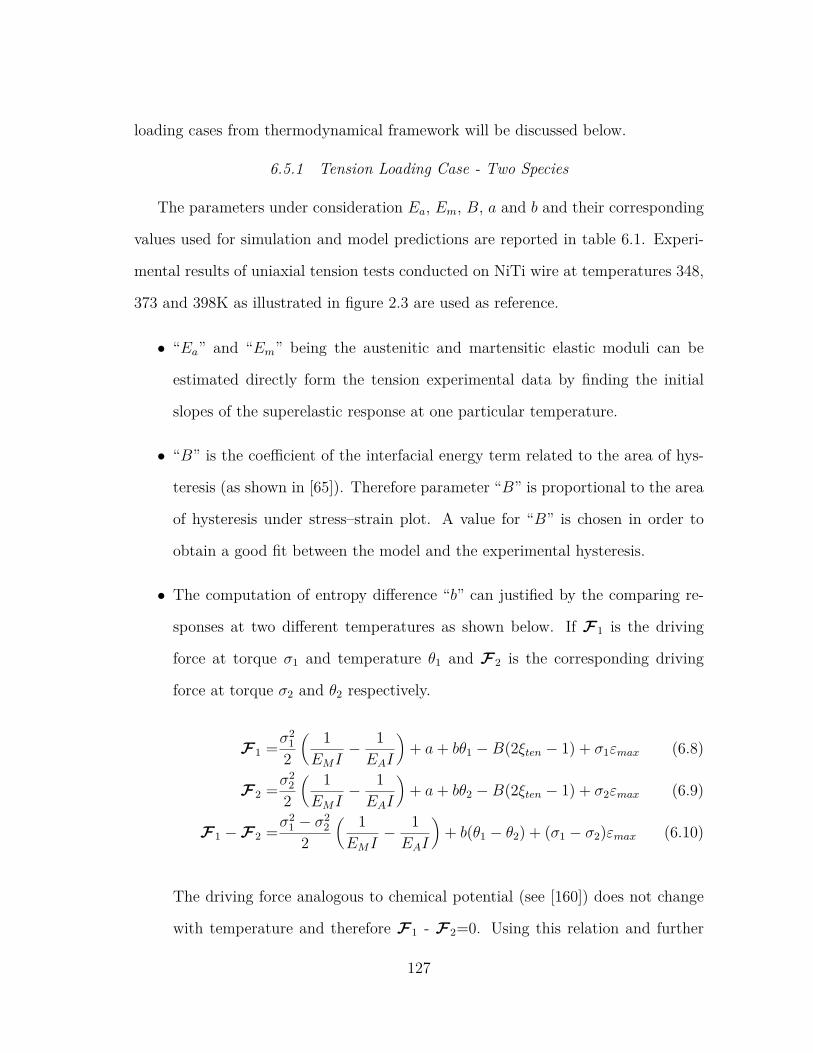
loading cases from thermodynamical framework will be discussed below.

6.5.1 Tension Loading Case - Two Species

The parameters under consideration Ea, Em, B, a and b and their corresponding

values used for simulation and model predictions are reported in table 6.1. Experi-

mental results of uniaxial tension tests conducted on NiTi wire at temperatures 348,

373 and 398K as illustrated in figure 2.3 are used as reference.

• “Ea” and “Em” being the austenitic and martensitic elastic moduli can be

estimated directly form the tension experimental data by finding the initial

slopes of the superelastic response at one particular temperature.

• “B” is the coefficient of the interfacial energy term related to the area of hys-

teresis (as shown in [65]). Therefore parameter “B” is proportional to the area

of hysteresis under stress–strain plot. A value for “B” is chosen in order to

obtain a good fit between the model and the experimental hysteresis.

• The computation of entropy difference “b” can justified by the comparing re-

sponses at two different temperatures as shown below. If F1 is the driving

force at torque σ1 and temperature θ1 and F2 is the corresponding driving

force at torque σ2 and θ2 respectively.

F1 =σ21

2

( 1EMI

− 1EAI

)+ a+ bθ1 −B(2ξten − 1) + σ1εmax (6.8)

F2 =σ22

2

( 1EMI

− 1EAI

)+ a+ bθ2 −B(2ξten − 1) + σ2εmax (6.9)

F1 −F2 =σ21 − σ2

22

( 1EMI

− 1EAI

)+ b(θ1 − θ2) + (σ1 − σ2)εmax (6.10)

The driving force analogous to chemical potential (see [160]) does not change

with temperature and therefore F1 - F2=0. Using this relation and further

127

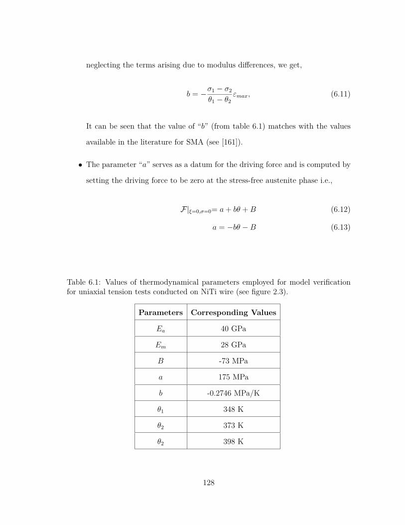
neglecting the terms arising due to modulus differences, we get,

b = −σ1 − σ2

θ1 − θ2εmax, (6.11)

It can be seen that the value of “b” (from table 6.1) matches with the values

available in the literature for SMA (see [161]).

• The parameter “a” serves as a datum for the driving force and is computed by

setting the driving force to be zero at the stress-free austenite phase i.e.,

F|ξ=0,σ=0= a+ bθ +B (6.12)

a = −bθ −B (6.13)

Table 6.1: Values of thermodynamical parameters employed for model verificationfor uniaxial tension tests conducted on NiTi wire (see figure 2.3).

Parameters Corresponding Values

Ea 40 GPa

Em 28 GPa

B -73 MPa

a 175 MPa

b -0.2746 MPa/K

θ1 348 K

θ2 373 K

θ2 398 K

128

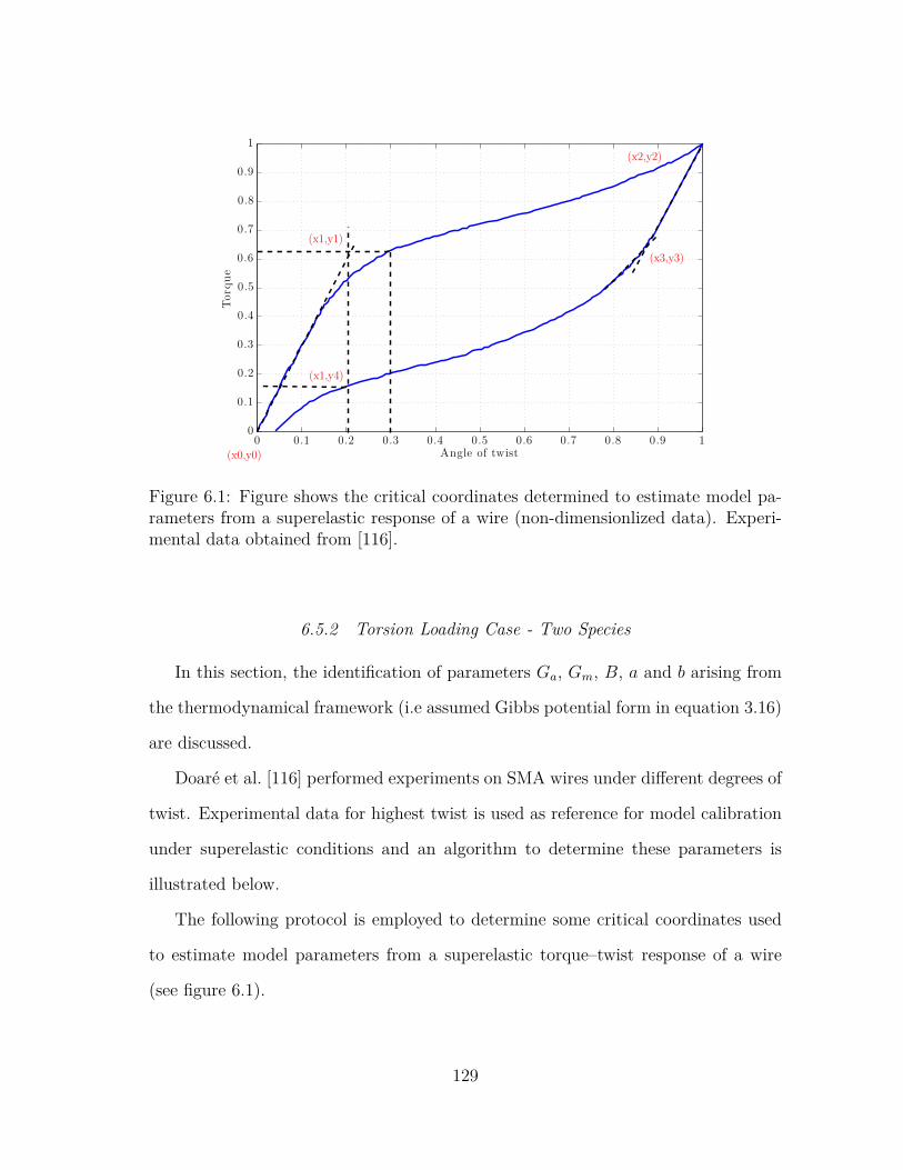
(x0,y0)

(x1,y4)

(x2,y2)

(x3,y3)

(x1,y1)Torq

ue

Angle of twist0 0.1 0.2 0.3 0.4 0.5 0.6 0.7 0.8 0.9 1

0

0.1

0.2

0.3

0.4

0.5

0.6

0.7

0.8

0.9

1

Figure 6.1: Figure shows the critical coordinates determined to estimate model pa-rameters from a superelastic response of a wire (non-dimensionlized data). Experi-mental data obtained from [116].

6.5.2 Torsion Loading Case - Two Species

In this section, the identification of parameters Ga, Gm, B, a and b arising from

the thermodynamical framework (i.e assumed Gibbs potential form in equation 3.16)

are discussed.

Doaré et al. [116] performed experiments on SMA wires under different degrees of

twist. Experimental data for highest twist is used as reference for model calibration

under superelastic conditions and an algorithm to determine these parameters is

illustrated below.

The following protocol is employed to determine some critical coordinates used

to estimate model parameters from a superelastic torque–twist response of a wire

(see figure 6.1).

129

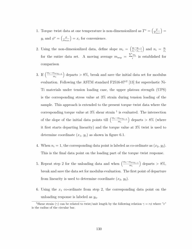
1. Torque–twist data at one temperature is non-dimensionlized as T ∗ =(

TTmax

)=

yi and φ∗ =(

φφmax

)= xi for convenience.

2. Using the non-dimesionlized data, define slope mi =(yi−yi−1xi−xi−1

)and ni = yi

xi

for the entire data set. A moving average mavg =∑

mi

iis established for

comparison

3. If(mi−mavgi−1

mi

)departs > 8%, break and save the initial data set for modulus

evaluation. Following the ASTM standard F2516-07ε2 [13] for superelastic Ni-

Ti materials under tension loading case, the upper plateau strength (UPS)

is the corresponding stress value at 3% strain during tension loading of the

sample. This approach is extended to the present torque–twist data where the

corresponding torque value at 3% shear strain 1 is evaluated. The intersection

of the slope of the initial data points till(mi−mavgi−1

mi

)departs > 8% (where

it first starts departing linearity) and the torque value at 3% twist is used to

determine coordinate (x1, y1) as shown in figure 6.1.

4. When ni = 1, the corresponding data point is labeled as co-ordinate as (x2, y2).

This is the final data point on the loading part of the torque–twist response.

5. Repeat step 2 for the unloading data and when(mi−mavgi−1

mi

)departs > 8%,

break and save the data set for modulus evaluation. The first point of departure

from linearity is used to determine coordinate (x3, y3).

6. Using the x1 co-ordinate from step 2, the corresponding data point on the

unloading response is labeled as y4.1Shear strain (γ) can be related to twist/unit length by the following relation γ = rφ where ”r”

is the radius of the circular bar.

130

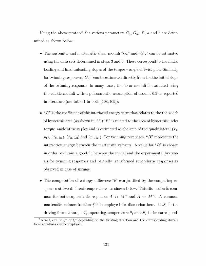
Using the above protocol the various parameters Ga, Gm, B, a and b are deter-

mined as shown below.

• The austenitic and martensitic shear moduli “Ga” and “Gm” can be estimated

using the data sets determined in steps 3 and 5. These correspond to the initial

loading and final unloading slopes of the torque – angle of twist plot. Similarly

for twinning responses,“Gm” can be estimated directly from the the initial slope

of the twinning response. In many cases, the shear moduli is evaluated using

the elastic moduli with a poisons ratio assumption of around 0.3 as reported

in literature (see table 1 in both [108,109]).

• “B” is the coefficient of the interfacial energy term that relates to the the width

of hysteresis area (as shown in [65]).“B” is related to the area of hysteresis under

torque–angle of twist plot and is estimated as the area of the quadrilateral (x1,

y1), (x2, y2), (x3, y3) and (x1, y4). For twinning responses, “B” represents the

interaction energy between the martensite variants. A value for “B” is chosen

in order to obtain a good fit between the model and the experimental hystere-

sis for twinning responses and partially transformed superelastic responses as

observed in case of springs.

• The computation of entropy difference “b” can justified by the comparing re-

sponses at two different temperatures as shown below. This discussion is com-

mon for both superelastic responses A ↔ M+ and A ↔ M−. A common

martensite volume fraction ξ 2 is employed for discussion here. If F1 is the

driving force at torque T1, operating temperature θ1 and F2 is the correspond-2Term ξ can be ξ+ or ξ− depending on the twisting direction and the corresponding driving

force equations can be employed.

131

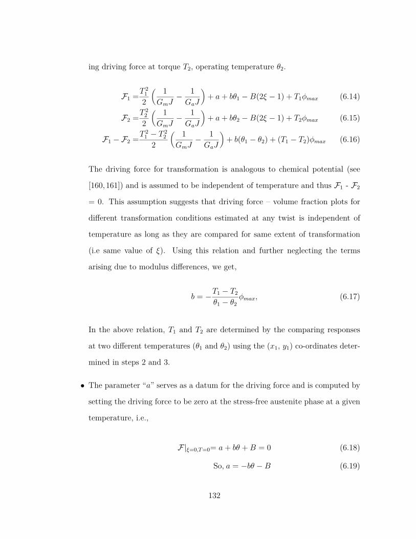
ing driving force at torque T2, operating temperature θ2.

F1 =T212

( 1GmJ

− 1GaJ

)+ a+ bθ1 −B(2ξ − 1) + T1φmax (6.14)

F2 =T222

( 1GmJ

− 1GaJ

)+ a+ bθ2 −B(2ξ − 1) + T2φmax (6.15)

F1 −F2 =T21 − T 2

22

( 1GmJ

− 1GaJ

)+ b(θ1 − θ2) + (T1 − T2)φmax (6.16)

The driving force for transformation is analogous to chemical potential (see

[160,161]) and is assumed to be independent of temperature and thus F1 - F2

= 0. This assumption suggests that driving force – volume fraction plots for

different transformation conditions estimated at any twist is independent of

temperature as long as they are compared for same extent of transformation

(i.e same value of ξ). Using this relation and further neglecting the terms

arising due to modulus differences, we get,

b = −T1 − T2

θ1 − θ2φmax, (6.17)

In the above relation, T1 and T2 are determined by the comparing responses

at two different temperatures (θ1 and θ2) using the (x1, y1) co-ordinates deter-

mined in steps 2 and 3.

• The parameter “a” serves as a datum for the driving force and is computed by

setting the driving force to be zero at the stress-free austenite phase at a given

temperature, i.e.,

F|ξ=0,T=0= a+ bθ +B = 0 (6.18)

So, a = −bθ −B (6.19)

132

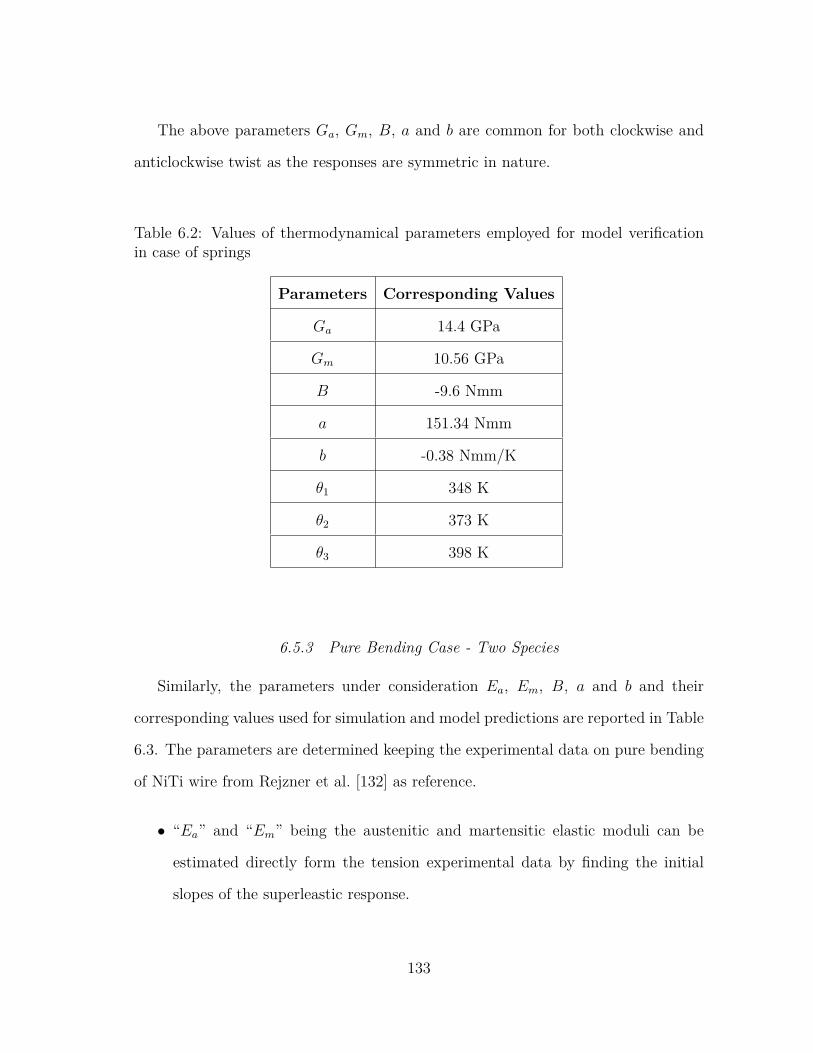
The above parameters Ga, Gm, B, a and b are common for both clockwise and

anticlockwise twist as the responses are symmetric in nature.

Table 6.2: Values of thermodynamical parameters employed for model verificationin case of springs

Parameters Corresponding Values

Ga 14.4 GPa

Gm 10.56 GPa

B -9.6 Nmm

a 151.34 Nmm

b -0.38 Nmm/K

θ1 348 K

θ2 373 K

θ3 398 K

6.5.3 Pure Bending Case - Two Species

Similarly, the parameters under consideration Ea, Em, B, a and b and their

corresponding values used for simulation and model predictions are reported in Table

6.3. The parameters are determined keeping the experimental data on pure bending

of NiTi wire from Rejzner et al. [132] as reference.

• “Ea” and “Em” being the austenitic and martensitic elastic moduli can be

estimated directly form the tension experimental data by finding the initial

slopes of the superleastic response.

133

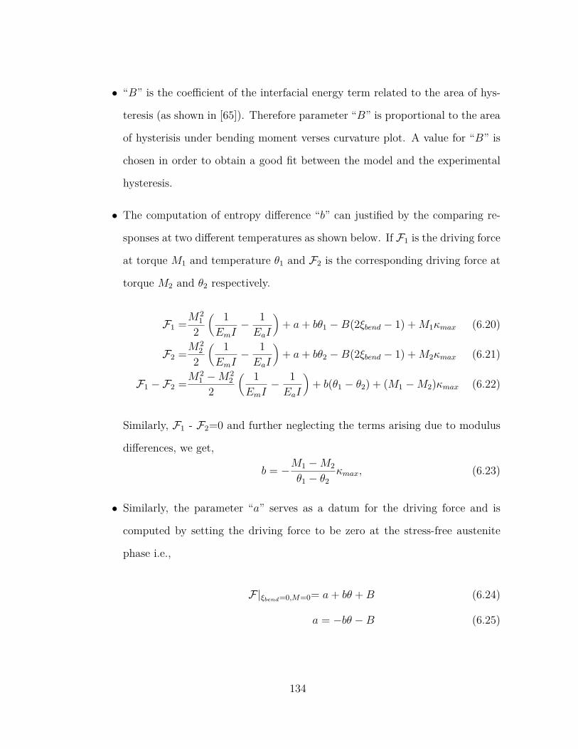
• “B” is the coefficient of the interfacial energy term related to the area of hys-

teresis (as shown in [65]). Therefore parameter “B” is proportional to the area

of hysterisis under bending moment verses curvature plot. A value for “B” is

chosen in order to obtain a good fit between the model and the experimental

hysteresis.

• The computation of entropy difference “b” can justified by the comparing re-

sponses at two different temperatures as shown below. If F1 is the driving force

at torque M1 and temperature θ1 and F2 is the corresponding driving force at

torque M2 and θ2 respectively.

F1 =M21

2

( 1EmI

− 1EaI

)+ a+ bθ1 −B(2ξbend − 1) +M1κmax (6.20)

F2 =M22

2

( 1EmI

− 1EaI

)+ a+ bθ2 −B(2ξbend − 1) +M2κmax (6.21)

F1 −F2 =M21 −M2

22

( 1EmI

− 1EaI

)+ b(θ1 − θ2) + (M1 −M2)κmax (6.22)

Similarly, F1 - F2=0 and further neglecting the terms arising due to modulus

differences, we get,

b = −M1 −M2

θ1 − θ2κmax, (6.23)

• Similarly, the parameter “a” serves as a datum for the driving force and is

computed by setting the driving force to be zero at the stress-free austenite

phase i.e.,

F|ξbend=0,M=0= a+ bθ +B (6.24)

a = −bθ −B (6.25)

134

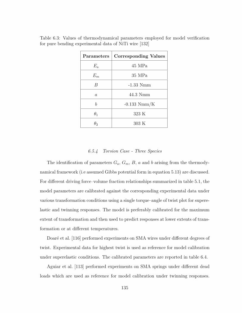
Table 6.3: Values of thermodynamical parameters employed for model verificationfor pure bending experimental data of NiTi wire [132]

Parameters Corresponding Values

Ea 45 MPa

Em 35 MPa

B -1.33 Nmm

a 44.3 Nmm

b -0.133 Nmm/K

θ1 323 K

θ2 303 K

6.5.4 Torsion Case - Three Species

The identification of parameters Ga, Gm, B, a and b arising from the thermody-

namical framework (i.e assumed Gibbs potential form in equation 5.13) are discussed.

For different driving force–volume fraction relationships summarized in table 5.1, the

model parameters are calibrated against the corresponding experimental data under

various transformation conditions using a single torque–angle of twist plot for supere-

lastic and twinning responses. The model is preferably calibrated for the maximum

extent of transformation and then used to predict responses at lower extents of trans-

formation or at different temperatures.

Doaré et al. [116] performed experiments on SMA wires under different degrees of

twist. Experimental data for highest twist is used as reference for model calibration

under superelastic conditions. The calibrated parameters are reported in table 6.4.

Aguiar et al. [113] performed experiments on SMA springs under different dead

loads which are used as reference for model calibration under twinning responses.

135

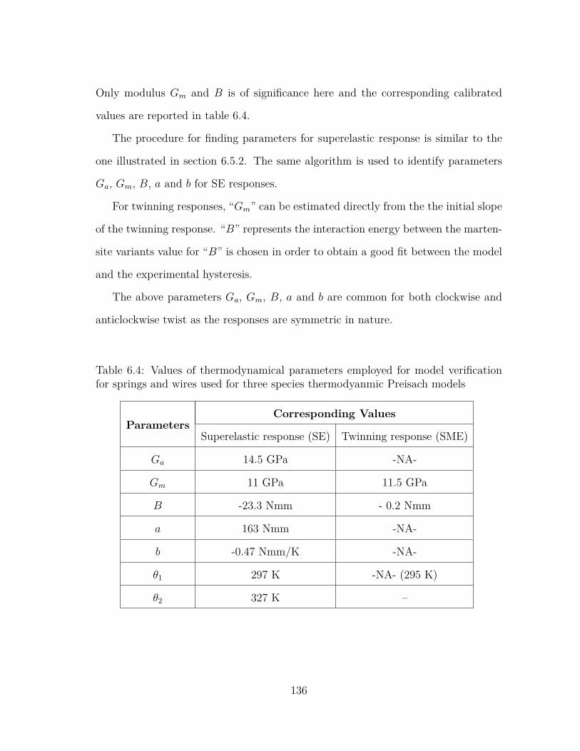
Only modulus Gm and B is of significance here and the corresponding calibrated

values are reported in table 6.4.

The procedure for finding parameters for superelastic response is similar to the

one illustrated in section 6.5.2. The same algorithm is used to identify parameters

Ga, Gm, B, a and b for SE responses.

For twinning responses, “Gm” can be estimated directly from the the initial slope

of the twinning response. “B” represents the interaction energy between the marten-

site variants value for “B” is chosen in order to obtain a good fit between the model

and the experimental hysteresis.

The above parameters Ga, Gm, B, a and b are common for both clockwise and

anticlockwise twist as the responses are symmetric in nature.

Table 6.4: Values of thermodynamical parameters employed for model verificationfor springs and wires used for three species thermodyanmic Preisach models

ParametersCorresponding Values

Superelastic response (SE) Twinning response (SME)

Ga 14.5 GPa -NA-

Gm 11 GPa 11.5 GPa

B -23.3 Nmm - 0.2 Nmm

a 163 Nmm -NA-

b -0.47 Nmm/K -NA-

θ1 297 K -NA- (295 K)

θ2 327 K –

136

6.6 Note on Parameter “B” for Superelastic and Twinning Responses

From table 6.4, the interaction energy term “B” is significantly larger compared

that of twinning responses. This suggests that one requires lesser energy for twin-

ning between martensite variants as compared against phase transformations be-

tween austenite and martensite variants associated superelastic phase transforma-

tions. Though, SMAs demonstrate large plateau strains (6 to 8%) under both su-

perelastic and twinning responses, experimental evidences under superelastic con-

ditions indicate higher critical stress/torque levels for phase transformation when

compared to corresponding critical stresses associated with twinning responses thus

emphasising higher interaction energy difference.

Figures 7.32 and 7.33 discussed later shows the experimental results for supere-

lastic and twinning responses for SMA springs and rods respectively. It clearly

demonstrates significantly higher plateau stresses/torque levels associated with su-

perelastic responses when compared to twinning responses associated with shape

memory response. As discussed in section 1.2.1, plateau stresses Upper plateau

strength (UPS) and Lower plateau strength (LPS) are some of the salient

features associated with a typical superelastic response under tension loading case as

discussed in the ASTM standard F2516-07ε2 [13] for superelastic Ni-Ti materials. On

similar lines, with twinning responses, the critical stress associated with the onset

of flat plateau can be employed for comparison with UPS or LPS associated with

superelastic responses. Though, torsional responses of SMA components don’t show

clear flat plateaus as commonly seen with tension responses, it is still evident that

UPS > LPS > plateau stress associated with twinning response. This justifies higher

energy values (“B”) associated with superelastic phase transformations as compared

to twinning response associated with shape memory effects.

137

6.7 Simulation of Orginal Response for SMA Components

Once the test protocol highlighted in the above sections are selected depending

on the transformation case, the model can be used to simulate responses at different

temperatures or twists. For prediction of responses of SMA components like wires,

rods and springs considered here, a total of “20100 hysterons” which is an equivalent

to a Preisach triangle with a side of “200” were employed.

Depending on the choice of the size of the Preisach triangle, the model predictions

can do an approximate or a precise prediction by controlling the use of number of

Preisach elements used in simulation. An approximate response prediction could be

sufficient for design purposes but a more precise prediction might be essential from

the control systems standpoint. Such a scheme allows predictions tailored to level of

information available and thus saving computational time.

6.8 Model Predictions – Different Strains/Twists/Curvatures or Temperatures

Hysterons generated at one particular twist can be used to predict responses

at any other twists (i.e internal loops) without re-computation of any model pa-

rameters. This just requires appropriate assumption of strain/twist/curvature or

stress/torque/moment vectors during simulation protocol selected for recomputing

original relationships as described in previous sections for different loading condi-

tions.

Superelastic responses of SMA are affected by changes in external stimuli (i.e op-

erating temperature) as shown in many experimental evidences (see figure 7 in [72],

figure 12 in [156], figure 16 in [142], figure 3 in [105], figure 2 in [162] etc. for exam-

ples). The present modeling approach allows us to capture this temperature depen-

dence without re-computation of any model parameters. The inherent assumption

here is that the driving force – volume fraction plots for a given extent of trans-

138

formation (ξ) just translates linearly with changes in operating temperature. This

linear relationship is the (a + bθ) terms in the driving force relationships for supere-

lastic responses under different loading conditions. With such an assumption, one

can predict responses at different temperatures based on hysterons generated at one

particular temperature without the need for changing any model parameters. Thus,

it just requires changing temperature value (θ) in during the simulation protocol

selected for recomputing original relationship as described in previous sections.

139

7. RESULTS AND DISCUSSIONS : MODEL SIMULATIONS AND

PREDICTIONS ∗

Using the simulation process discussed in section 6, F – ξ are estimated from

the original experimental data under all loading conditions for a given temperature

say θ1. The prediction of responses at different temperatures (say θ2 or θ3) can be

achieved by just “changing the temperature term” during the reverse calculations of

experimental data from the F – ξ generated for temperature θ1. Thus the hysteron

parameters have to be estimated only once and they don’t have to be recomputed

for predictions at different temperatures.

7.1 Tension Loading Results - Two Species

Tension test on wires (see figure 2.3) indicate that the plateau stresses scale lin-

early with temperature without significant change in hysteresis. The linear assump-

tion (a + bθ terms in the model) was used to capture the temperature dependence

of superelastic responses in SMA tension response. Figure 7.1a shows the simulation

using ASTM standard as guidelines as discussed in section 1.2.1 and figure 1.5. The

flat upper and lower platues are generally observed in superelastic SMA wires but

not in martensite SMA wires that were tested under superelastic conditions. Hence,

the model results are quite far from the experimental results since the ASTM stan-

dard was primarily developed for superelastic wires. Figure 7.1b shows the model

simulation at 373 K compared with the experimental data. Model prediction and∗Reprinted with permission from “Combining Thermodynamic Principles with Preisach models

for superelastic SMA Wires” by Doraiswamy, Rao and Srinivasa, Smart Materials and Structures,20, 085032, 2011 [64], Copyright [2014] by IOP.

Reprinted with permission from “A two species thermodynamic Preisach model for the tor-sional response of SMA wires and springs under superelastic conditions” by Rao and Srinivasa,International Journal of Solids and Structures, 50, 887–898, 2013 [90], Copyright [2014] by ElsevierLimited.

140

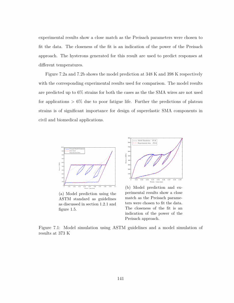
experimental results show a close match as the Preisach parameters were chosen to

fit the data. The closeness of the fit is an indication of the power of the Preisach

approach. The hysterons generated for this result are used to predict responses at

different temperatures.

Figure 7.2a and 7.2b shows the model prediction at 348 K and 398 K respectively

with the corresponding experimental results used for comparison. The model results

are predicted up to 6% strains for both the cases as the the SMA wires are not used

for applications > 6% due to poor fatigue life. Further the predictions of plateau

strains is of significant importance for design of superelastic SMA components in

civil and biomedical applications.

Experimental Data

Data Input

Preisach Model Prediction

Stressσ[ M

Pa]

Strain ε [mm/mm]

0 0.01 0.02 0.03 0.04 0.05 0.06 0.07 0.08 0.09 0.10

100

200

300

400

500

600

700

800

900

1000

(a) Model prediction using theASTM standard as guidelinesas discussed in section 1.2.1 andfigure 1.5.

St ressσ[ M

Pa]

Strain ε [mm/mm]

0 0.01 0.02 0.03 0.04 0.05 0.06 0.07 0.08 0.090

100

200

300

400

500

600

700

800

900

Model Simulation – 373 K

Experimental data – 373 K

(b) Model prediction and ex-perimental results show a closematch as the Preisach parame-ters were chosen to fit the data.The closeness of the fit is anindication of the power of thePreisach approach.

Figure 7.1: Model simulation using ASTM guidelines and a model simulation ofresults at 373 K

141

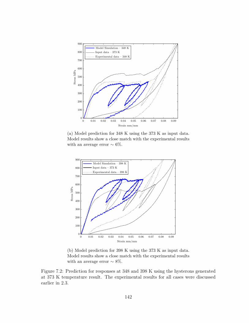
0 0.01 0.02 0.03 0.04 0.05 0.06 0.07 0.08 0.090

100

200

300

400

500

600

700

800

900

Model Simulation – 348 K

Input data – 373 K

Experimental data – 348 K

Strain mm/mm

StressMPa

(a) Model prediction for 348 K using the 373 K as input data.Model results show a close match with the experimental resultswith an average error ∼ 6%.

Strain mm/mm

0 0.01 0.02 0.03 0.04 0.05 0.06 0.07 0.08 0.090

100

200

300

400

500

600

700

800

900

Model Simulation – 398 K

Input data – 373 K

Experimental data – 398 K

StressMPa

(b) Model prediction for 398 K using the 373 K as input data.Model results show a close match with the experimental resultswith an average error ∼ 8%.

Figure 7.2: Prediction for responses at 348 and 398 K using the hysterons generatedat 373 K temperature result. The experimental results for all cases were discussedearlier in 2.3.

142

7.2 Torsional Loading Results - Two Species

7.2.1 Simulations of SMA Spring and Wire Response Using Complete Torque

verses Angle of Twist Data

Figure 7.3 and 7.4 shows the model prediction at 348 K and 296 K respectively

with the corresponding experimental results used for comparison. The model shows

a good fit with the experimental results and can estimate the hysteresis accurately.

7.2.2 Simulation and Model Predictions of SMA Wire Response at Different

Twists

Doarè et al. [116] in their work performed quasi-static tests on 2mm dia SMA

wires for three different angle of twists (100, 350 and 450 degrees). The 450o data was

used as reference to calibrate the model with the assumption that it is the maximum

possible angle of twist that the sample can encounter without failing. The hysterons

generated by the 450o data are used to predict responses at any other angle of twist

without recomputation of any model parameters. Figure 7.13a and 7.13b shows the

model predictions at different angles of twist 350 and 225o twist respectively using the

hysterons generated with the 450o twist. The model predictions show a close match

with the experimental results. It must be highlighted from these experiments and

model predictions, it is unclear if a fully martensitic wire is obtained at higher twists

as there was no elastic deformation of stress induced martensite (SIM) observed in

these experiments. Chapman et al. [110] in their work studied the response of three

superelastic wires with different diameters under torsion until failure and the results

clearly illustrates that one can observe a fully transformed wire response (similar to

pure tension responses) under higher degrees of twist (see figures 2 and 3 in [110]).

In order to confirm this point, section 2.3 earlier discussed torsional tests on

SMA wires under large twist. Figures 7.5, 7.6, 7.7, 7.8, 7.9, 7.10, 7.11, 7.12 shows

143

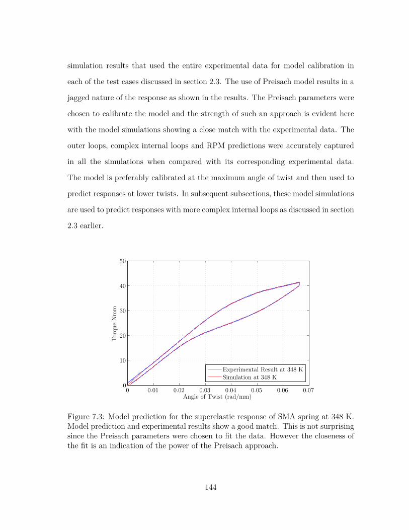
simulation results that used the entire experimental data for model calibration in

each of the test cases discussed in section 2.3. The use of Preisach model results in a

jagged nature of the response as shown in the results. The Preisach parameters were

chosen to calibrate the model and the strength of such an approach is evident here

with the model simulations showing a close match with the experimental data. The

outer loops, complex internal loops and RPM predictions were accurately captured

in all the simulations when compared with its corresponding experimental data.

The model is preferably calibrated at the maximum angle of twist and then used to

predict responses at lower twists. In subsequent subsections, these model simulations

are used to predict responses with more complex internal loops as discussed in section

2.3 earlier.

0 0.01 0.02 0.03 0.04 0.05 0.06 0.070

10

20

30

40

50

Angle of Twist (rad/mm)

TorqueNmm

Experimental Result at 348 KSimulation at 348 K

Figure 7.3: Model prediction for the superelastic response of SMA spring at 348 K.Model prediction and experimental results show a good match. This is not surprisingsince the Preisach parameters were chosen to fit the data. However the closeness ofthe fit is an indication of the power of the Preisach approach.

144

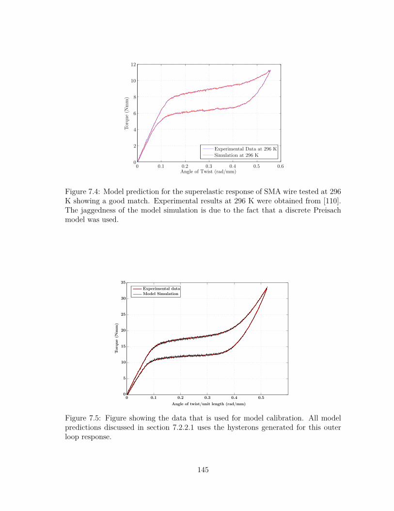
0 0.1 0.2 0.3 0.4 0.5 0.60

2

4

6

8

10

12

Angle of Twist (rad/mm)

Torque(N

mm)

Experimental Data at 296 KSimulation at 296 K

Figure 7.4: Model prediction for the superelastic response of SMA wire tested at 296K showing a good match. Experimental results at 296 K were obtained from [110].The jaggedness of the model simulation is due to the fact that a discrete Preisachmodel was used.

Model Simulation

Experimental data

Torq

ue(N

mm)

Angle of twist/unit length (rad/mm)

0 0.1 0.2 0.3 0.4 0.50

5

10

15

20

25

30

35

Figure 7.5: Figure showing the data that is used for model calibration. All modelpredictions discussed in section 7.2.2.1 uses the hysterons generated for this outerloop response.

145

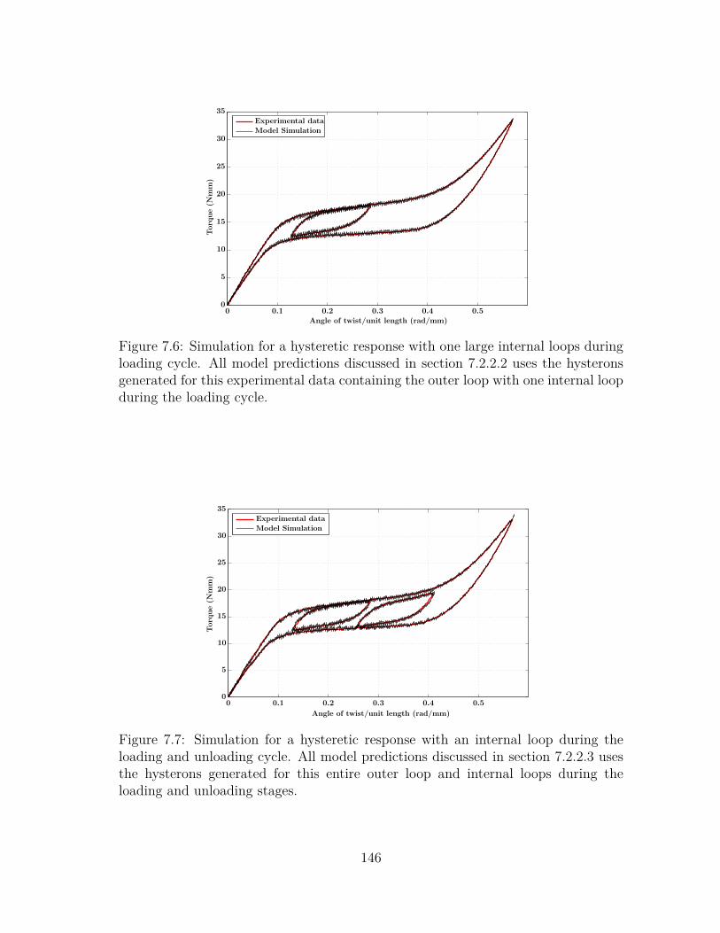
Model Simulation

Experimental data

Torq

ue(N

mm)

Angle of twist/unit length (rad/mm)

0 0.1 0.2 0.3 0.4 0.50

5

10

15

20

25

30

35

Figure 7.6: Simulation for a hysteretic response with one large internal loops duringloading cycle. All model predictions discussed in section 7.2.2.2 uses the hysteronsgenerated for this experimental data containing the outer loop with one internal loopduring the loading cycle.

Model Simulation

Experimental data

Torq

ue(N

mm)

Angle of twist/unit length (rad/mm)

0 0.1 0.2 0.3 0.4 0.50

5

10

15

20

25

30

35

Figure 7.7: Simulation for a hysteretic response with an internal loop during theloading and unloading cycle. All model predictions discussed in section 7.2.2.3 usesthe hysterons generated for this entire outer loop and internal loops during theloading and unloading stages.

146

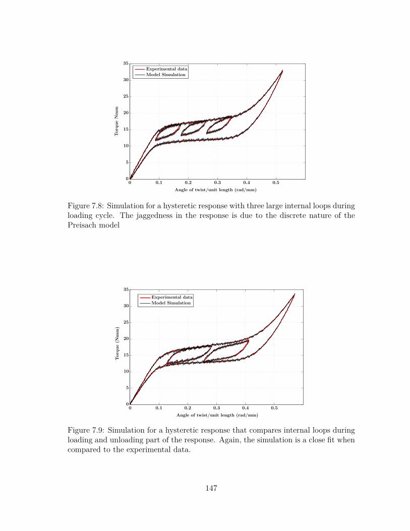
Model Simulation

Experimental data

Torq

ueNmm

Angle of twist/unit length (rad/mm)

0 0.1 0.2 0.3 0.4 0.50

5

10

15

20

25

30

35

Figure 7.8: Simulation for a hysteretic response with three large internal loops duringloading cycle. The jaggedness in the response is due to the discrete nature of thePreisach model

Model Simulation

Experimental data

Torq

ue(N

mm)

Angle of twist/unit length (rad/mm)

0 0.1 0.2 0.3 0.4 0.50

5

10

15

20

25

30

35

Figure 7.9: Simulation for a hysteretic response that compares internal loops duringloading and unloading part of the response. Again, the simulation is a close fit whencompared to the experimental data.

147

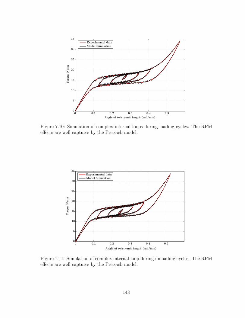
Model Simulation

Experimental data

Torq

ueNmm

Angle of twist/unit length (rad/mm)

0 0.1 0.2 0.3 0.4 0.50

5

10

15

20

25

30

35

Figure 7.10: Simulation of complex internal loops during loading cycles. The RPMeffects are well captures by the Preisach model.

Model Simulation

Experimental data

Torq

ueNmm

Angle of twist/unit length (rad/mm)

0 0.1 0.2 0.3 0.4 0.50

5

10

15

20

25

30

35

Figure 7.11: Simulation of complex internal loop during unloading cycles. The RPMeffects are well captures by the Preisach model.

148

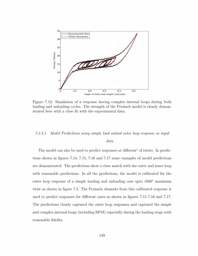
Model Simulation

Experimental data

Torq

ue(N

mm)

Angle of twist/unit length (rad/mm)

0 0.1 0.2 0.3 0.4 0.50

5

10

15

20

25

30

35

Figure 7.12: Simulation of a response having complex internal loops during bothloading and unloading cycles. The strength of the Presiach model is clearly demon-strated here with a close fit with the experimental data.

7.2.2.1 Model Predictions using simple load unload outer loop response as input

data

The model can also be used to predict responses at differento of twists. In predic-

tions shown in figures 7.14, 7.15, 7.16 and 7.17 some examples of model predictions

are demonstrated. The predictions show a close match with the outer and inner loop

with reasonable predictions. In all the predictions, the model is calibrated for the

outer loop response of a simple loading and unloading case upto 1800o maximum

twist as shown in figure 7.5. The Preisach elements from this calibrated response is

used to predict responses for different cases as shown in figures 7.15 7.16 and 7.17.

The predictions closely captured the outer loop responses and captured the simple

and complex internal loops (including RPM) especially during the loading stage with

reasonable fidelity.

149

7.2.2.2 Model Predictions using the entire outer loop with one internal loop during

the loading cycle as input data

Some model predictions that use the entire outer loop with one internal loop

during the cycle as shown in figure 7.6 is employed for predicting more complex

responses. This input data uses an additional internal loop information in additional

to the outer loop as discussed in the earlier section 7.2.2.1. Figures 7.18, 7.19 and

7.20 show some model predictions using this input data. The model predictions

captured the outer loop responses and captured the simple and complex internal loops

(including RPM) with a closer match to the experimental data as compared to those

discussed in section 7.2.2.1 that used only the outer loop for model calibration. Thus,

the Preisach model is capable of predicting the complete inner response with only

outer loop data, although the use of a single inner loop for calibration improves the

predictions. The internal loops during the unloading stages of the model predictions

didn’t exactly match the experimental data as the model input data used only the

outer loop and loading cycle internal loop data. Hence, the outer loop and loading

cycle internal loops were predicted with reasonable fidelity.

7.2.2.3 Model Predictions using the entire outer loop and one internal loop under

loading and unloading stage as input data.

Figures 7.21 and 7.22 show some model predictions with complex internal loops

using the entire outer loop with internal loops during the loading and unloading sages

of the response as input data (as shown in figure 7.7). It is clear that these model

predictions are a close match to the experimental data when compared to earlier

predictions discussed in section 7.2.2.1 or 7.2.2.2 as more information that included

one big internal loop during loading and unloading stages along with outer loop was

used for model predictions. This thus suggests that the choice of number of Preisach

150

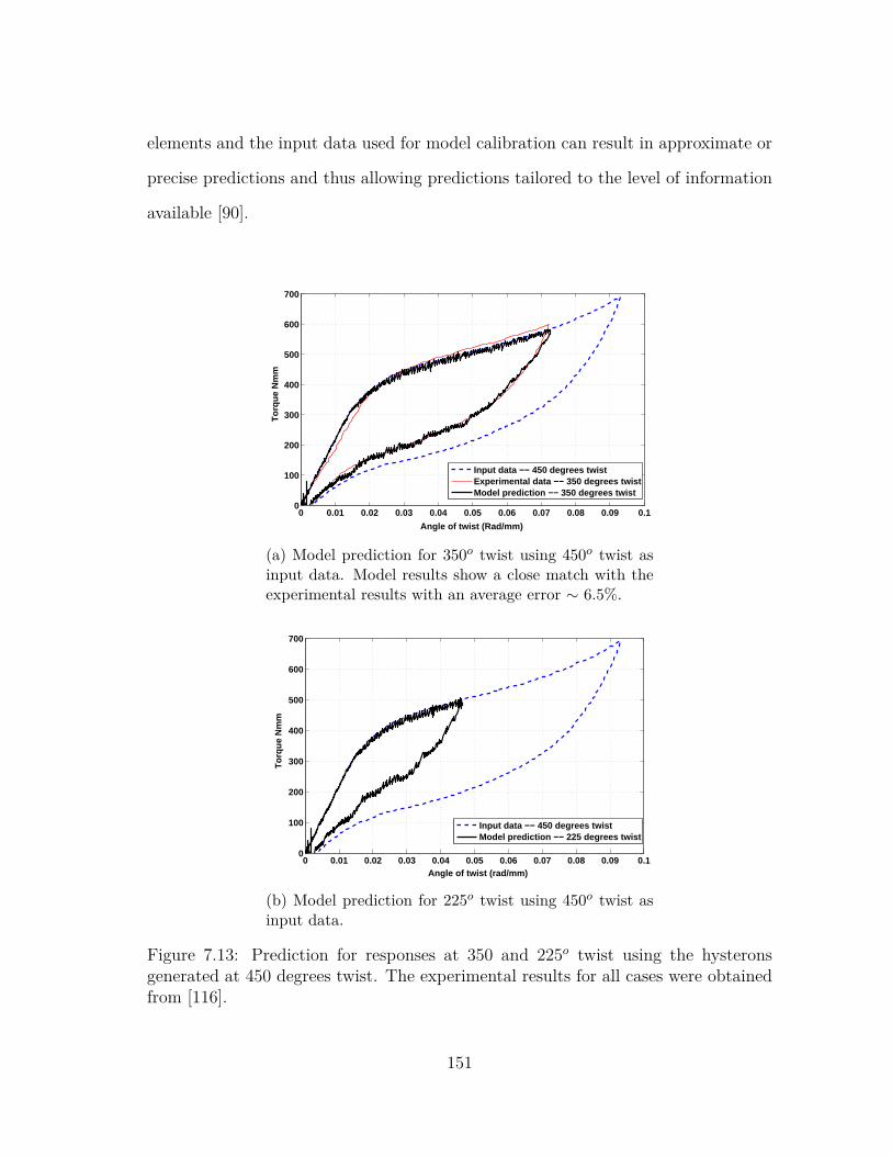
elements and the input data used for model calibration can result in approximate or

precise predictions and thus allowing predictions tailored to the level of information

available [90].

0 0.01 0.02 0.03 0.04 0.05 0.06 0.07 0.08 0.09 0.10

100

200

300

400

500

600

700

Angle of twist (Rad/mm)

To

rqu

e N

mm

Input data −− 450 degrees twistExperimental data −− 350 degrees twistModel prediction −− 350 degrees twist

(a) Model prediction for 350o twist using 450o twist asinput data. Model results show a close match with theexperimental results with an average error ∼ 6.5%.

0 0.01 0.02 0.03 0.04 0.05 0.06 0.07 0.08 0.09 0.10

100

200

300

400

500

600

700

Angle of twist (rad/mm)

To

rqu

e N

mm

Input data −− 450 degrees twistModel prediction −− 225 degrees twist

(b) Model prediction for 225o twist using 450o twist asinput data.

Figure 7.13: Prediction for responses at 350 and 225o twist using the hysteronsgenerated at 450 degrees twist. The experimental results for all cases were obtainedfrom [116].

151

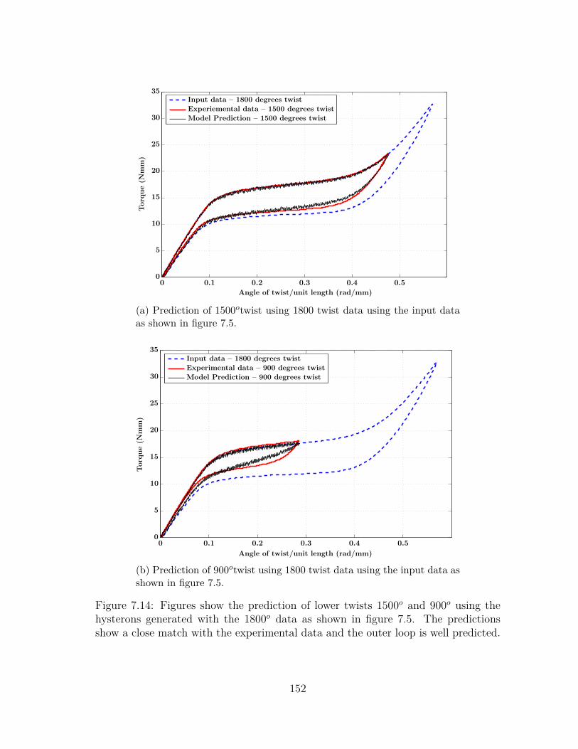
Model Prediction – 1500 degrees twist

Experiemental data – 1500 degrees twist

Input data – 1800 degrees twist

Torq

ue(N

mm)

Angle of twist/unit length (rad/mm)

0 0.1 0.2 0.3 0.4 0.50

5

10

15

20

25

30

35

(a) Prediction of 1500otwist using 1800 twist data using the input dataas shown in figure 7.5.

Model Prediction – 900 degrees twist

Experimental data – 900 degrees twist

Input data – 1800 degrees twist

Torq

ue(N

mm)

Angle of twist/unit length (rad/mm)

0 0.1 0.2 0.3 0.4 0.50

5

10

15

20

25

30

35

(b) Prediction of 900otwist using 1800 twist data using the input data asshown in figure 7.5.

Figure 7.14: Figures show the prediction of lower twists 1500o and 900o using thehysterons generated with the 1800o data as shown in figure 7.5. The predictionsshow a close match with the experimental data and the outer loop is well predicted.

152

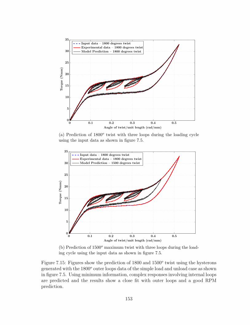
Model Prediction – 1800 degrees twist

Experimental data – 1800 degrees twist

Input data – 1800 degrees twist

Torq

ue(N

mm)

Angle of twist/unit length (rad/mm)

0 0.1 0.2 0.3 0.4 0.50

5

10

15

20

25

30

35

(a) Prediction of 1800o twist with three loops during the loading cycleusing the input data as shown in figure 7.5.

Model Prediction – 1500 degrees twist

Experimental data – 1800 degrees twist

Input data – 1800 degrees twist

Torq

ue(N

mm)

Angle of twist/unit length (rad/mm)

0 0.1 0.2 0.3 0.4 0.50

5

10

15

20

25

30

35

(b) Prediction of 1500o maximum twist with three loops during the load-ing cycle using the input data as shown in figure 7.5.

Figure 7.15: Figures show the prediction of 1800 and 1500o twist using the hysteronsgenerated with the 1800o outer loops data of the simple load and unload case as shownin figure 7.5. Using minimum information, complex responses involving internal loopsare predicted and the results show a close fit with outer loops and a good RPMprediction.

153

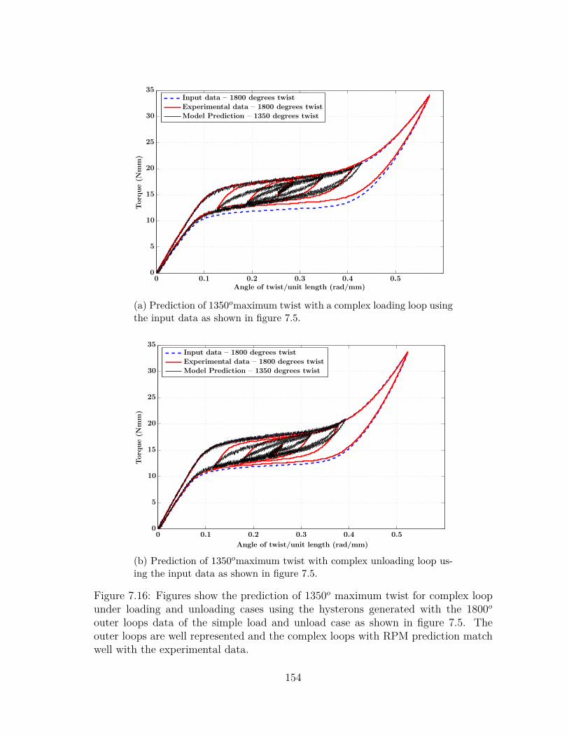
Model Prediction – 1350 degrees twist

Experimental data – 1800 degrees twist

Input data – 1800 degrees twist

Torq

ue(N

mm)

Angle of twist/unit length (rad/mm)0 0.1 0.2 0.3 0.4 0.5

0

5

10

15

20

25

30

35

(a) Prediction of 1350omaximum twist with a complex loading loop usingthe input data as shown in figure 7.5.

Model Prediction – 1350 degrees twist

Experimental data – 1800 degrees twist

Input data – 1800 degrees twist

Torq

ue(N

mm)

Angle of twist/unit length (rad/mm)

0 0.1 0.2 0.3 0.4 0.50

5

10

15

20

25

30

35

(b) Prediction of 1350omaximum twist with complex unloading loop us-ing the input data as shown in figure 7.5.

Figure 7.16: Figures show the prediction of 1350o maximum twist for complex loopunder loading and unloading cases using the hysterons generated with the 1800oouter loops data of the simple load and unload case as shown in figure 7.5. Theouter loops are well represented and the complex loops with RPM prediction matchwell with the experimental data.

154

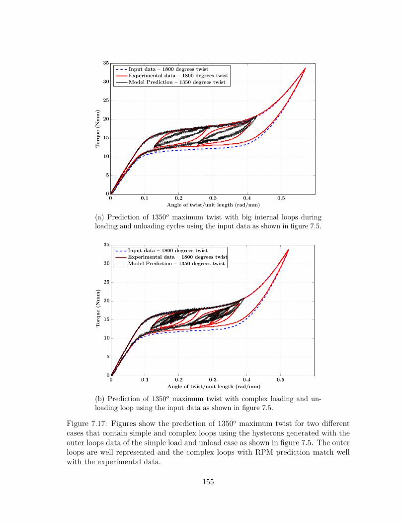
Model Prediction – 1350 degrees twist

Experimental data – 1800 degrees twist

Input data – 1800 degrees twist

Torq

ue(N

mm)

Angle of twist/unit length (rad/mm)

0 0.1 0.2 0.3 0.4 0.50

5

10

15

20

25

30

35

(a) Prediction of 1350o maximum twist with big internal loops duringloading and unloading cycles using the input data as shown in figure 7.5.

Model Prediction – 1350 degrees twist

Experimental data – 1800 degrees twist

Input data – 1800 degrees twist

Torq

ue(N

mm)

Angle of twist/unit length (rad/mm)

0 0.1 0.2 0.3 0.4 0.50

5

10

15

20

25

30

35

(b) Prediction of 1350o maximum twist with complex loading and un-loading loop using the input data as shown in figure 7.5.

Figure 7.17: Figures show the prediction of 1350o maximum twist for two differentcases that contain simple and complex loops using the hysterons generated with theouter loops data of the simple load and unload case as shown in figure 7.5. The outerloops are well represented and the complex loops with RPM prediction match wellwith the experimental data.

155

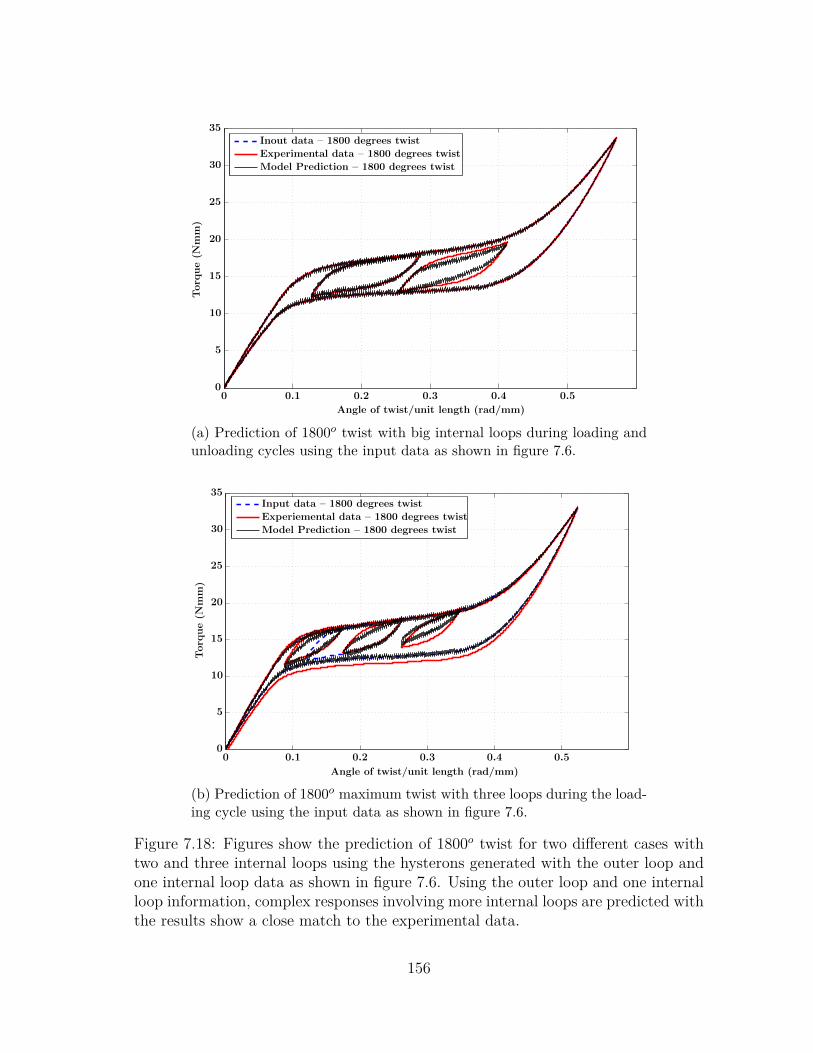
Model Prediction – 1800 degrees twist

Experimental data – 1800 degrees twist

Inout data – 1800 degrees twist

Torq

ue(N

mm)

Angle of twist/unit length (rad/mm)

0 0.1 0.2 0.3 0.4 0.50

5

10

15

20

25

30

35

(a) Prediction of 1800o twist with big internal loops during loading andunloading cycles using the input data as shown in figure 7.6.

Model Prediction – 1800 degrees twist

Experiemental data – 1800 degrees twist

Input data – 1800 degrees twist

Torq

ue(N

mm)

Angle of twist/unit length (rad/mm)

0 0.1 0.2 0.3 0.4 0.50

5

10

15

20

25

30

35

(b) Prediction of 1800o maximum twist with three loops during the load-ing cycle using the input data as shown in figure 7.6.

Figure 7.18: Figures show the prediction of 1800o twist for two different cases withtwo and three internal loops using the hysterons generated with the outer loop andone internal loop data as shown in figure 7.6. Using the outer loop and one internalloop information, complex responses involving more internal loops are predicted withthe results show a close match to the experimental data.

156

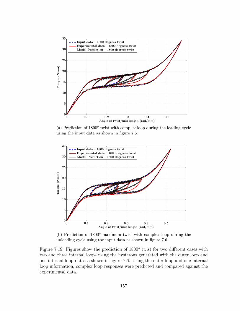
Model Prediction – 1800 degrees twist

Experimental data – 1800 degrees twist

Input data – 1800 degrees twist

Torq

ue(N

mm)

Angle of twist/unit length (rad/mm)0 0.1 0.2 0.3 0.4 0.5

0

5

10

15

20

25

30

35

(a) Prediction of 1800o twist with complex loop during the loading cycleusing the input data as shown in figure 7.6.

Model Prediction – 1800 degrees twist

Experimental data – 1800 degrees twist

Input data – 1800 degrees twist

Torq

ue(N

mm)

Angle of twist/unit length (rad/mm)0 0.1 0.2 0.3 0.4 0.5

0

5

10

15

20

25

30

35

(b) Prediction of 1800o maximum twist with complex loop during theunloading cycle using the input data as shown in figure 7.6.

Figure 7.19: Figures show the prediction of 1800o twist for two different cases withtwo and three internal loops using the hysterons generated with the outer loop andone internal loop data as shown in figure 7.6. Using the outer loop and one internalloop information, complex loop responses were predicted and compared against theexperimental data.

157

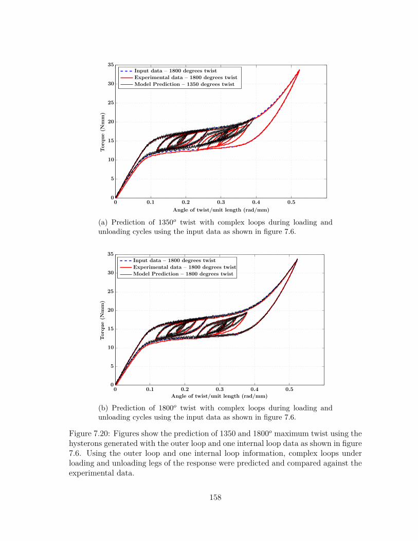
Model Prediction – 1350 degrees twist

Experimental data – 1800 degrees twist

Input data – 1800 degrees twist

Torq

ue(N

mm)

Angle of twist/unit length (rad/mm)

0 0.1 0.2 0.3 0.4 0.50

5

10

15

20

25

30

35

(a) Prediction of 1350o twist with complex loops during loading andunloading cycles using the input data as shown in figure 7.6.

Model Prediction – 1800 degrees twist

Experimental data – 1800 degrees twist

Input data – 1800 degrees twist

Torq

ue(N

mm)

Angle of twist/unit length (rad/mm)

0 0.1 0.2 0.3 0.4 0.50

5

10

15

20

25

30

35

(b) Prediction of 1800o twist with complex loops during loading andunloading cycles using the input data as shown in figure 7.6.

Figure 7.20: Figures show the prediction of 1350 and 1800o maximum twist using thehysterons generated with the outer loop and one internal loop data as shown in figure7.6. Using the outer loop and one internal loop information, complex loops underloading and unloading legs of the response were predicted and compared against theexperimental data.

158

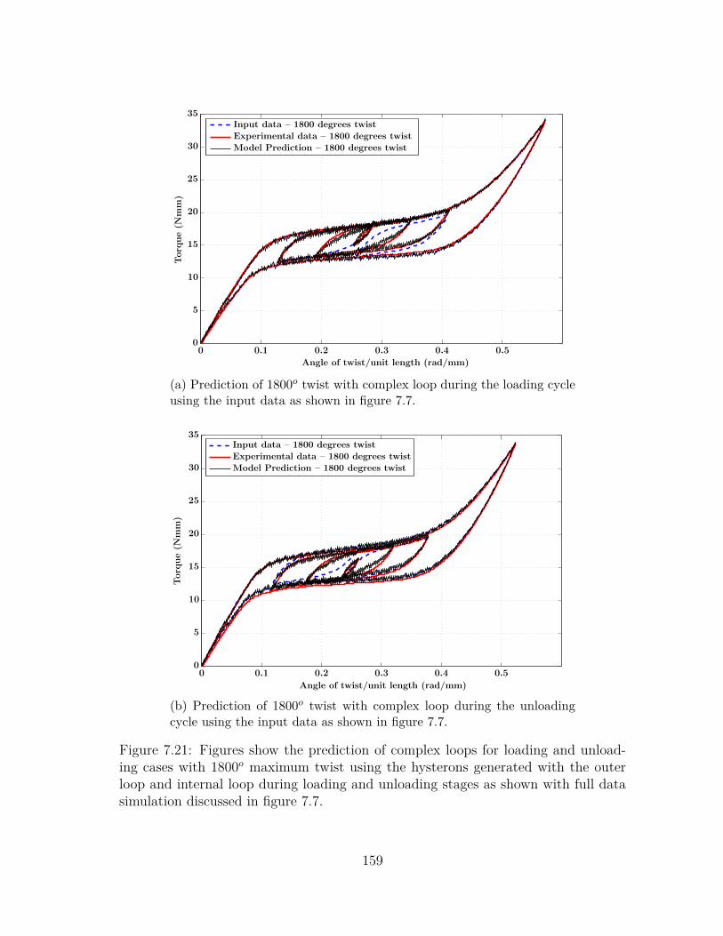
Model Prediction – 1800 degrees twist

Experimental data – 1800 degrees twist

Input data – 1800 degrees twist

Torq

ue(N

mm)

Angle of twist/unit length (rad/mm)

0 0.1 0.2 0.3 0.4 0.50

5

10

15

20

25

30

35

(a) Prediction of 1800o twist with complex loop during the loading cycleusing the input data as shown in figure 7.7.

Model Prediction – 1800 degrees twist

Experimental data – 1800 degrees twist

Input data – 1800 degrees twist

Torq

ue(N

mm)

Angle of twist/unit length (rad/mm)

0 0.1 0.2 0.3 0.4 0.50

5

10

15

20

25

30

35

(b) Prediction of 1800o twist with complex loop during the unloadingcycle using the input data as shown in figure 7.7.

Figure 7.21: Figures show the prediction of complex loops for loading and unload-ing cases with 1800o maximum twist using the hysterons generated with the outerloop and internal loop during loading and unloading stages as shown with full datasimulation discussed in figure 7.7.

159

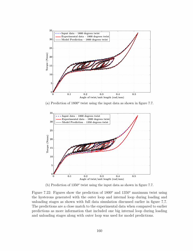
Model Prediction – 1800 degrees twist

Experimental data – 1800 degrees twist

Input data – 1800 degrees twist

Torq

ue(N

mm)

Angle of twist/unit length (rad/mm)

0 0.1 0.2 0.3 0.4 0.50

5

10

15

20

25

30

35

(a) Prediction of 1800o twist using the input data as shown in figure 7.7.

Model Prediction – 1350 degrees twist

Experimental data – 1800 degrees twist

Input data – 1800 degrees twist

Torq

ue(N

mm)

Angle of twist/unit length (rad/mm)0 0.1 0.2 0.3 0.4 0.5

0

5

10

15

20

25

30

35

(b) Prediction of 1350o twist using the input data as shown in figure 7.7.

Figure 7.22: Figures show the prediction of 1800o and 1350o maximum twist usingthe hysterons generated with the outer loop and internal loop during loading andunloading stages as shown with full data simulation discussed earlier in figure 7.7.The predictions are a close match to the experimental data when compared to earlierpredictions as more information that included one big internal loop during loadingand unloading stages along with outer loop was used for model predictions.

160

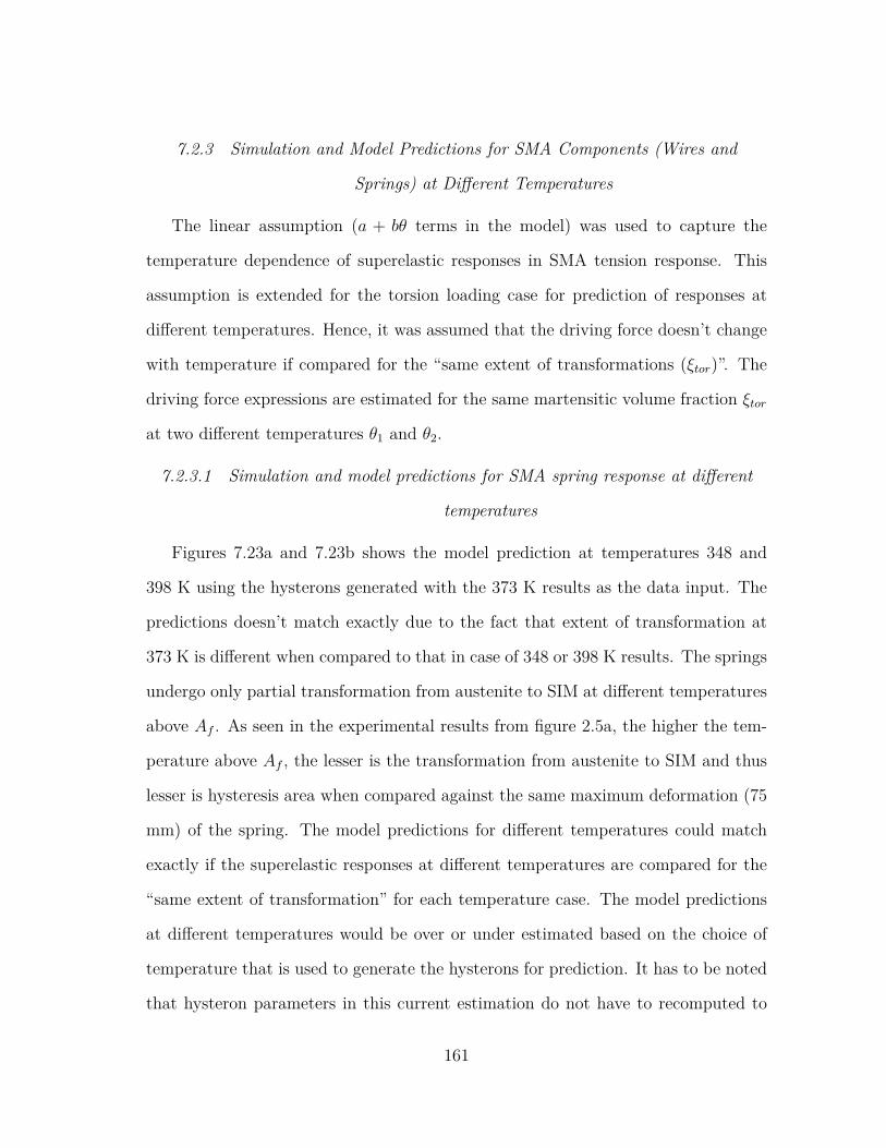
7.2.3 Simulation and Model Predictions for SMA Components (Wires and

Springs) at Different Temperatures

The linear assumption (a + bθ terms in the model) was used to capture the

temperature dependence of superelastic responses in SMA tension response. This

assumption is extended for the torsion loading case for prediction of responses at

different temperatures. Hence, it was assumed that the driving force doesn’t change

with temperature if compared for the “same extent of transformations (ξtor)”. The

driving force expressions are estimated for the same martensitic volume fraction ξtor

at two different temperatures θ1 and θ2.

7.2.3.1 Simulation and model predictions for SMA spring response at different

temperatures

Figures 7.23a and 7.23b shows the model prediction at temperatures 348 and

398 K using the hysterons generated with the 373 K results as the data input. The

predictions doesn’t match exactly due to the fact that extent of transformation at

373 K is different when compared to that in case of 348 or 398 K results. The springs

undergo only partial transformation from austenite to SIM at different temperatures

above Af . As seen in the experimental results from figure 2.5a, the higher the tem-

perature above Af , the lesser is the transformation from austenite to SIM and thus

lesser is hysteresis area when compared against the same maximum deformation (75

mm) of the spring. The model predictions for different temperatures could match

exactly if the superelastic responses at different temperatures are compared for the

“same extent of transformation” for each temperature case. The model predictions

at different temperatures would be over or under estimated based on the choice of

temperature that is used to generate the hysterons for prediction. It has to be noted

that hysteron parameters in this current estimation do not have to recomputed to

161

predict the response at different temperatures. If one needs to predict the hystere-

sis exactly for a partially transformed case then one would have to recompute the

hysterons for the each temperature case.

7.2.3.2 Simulation and model predictions for SMA wire response at different

temperatures

Figures 7.24a and 7.24b shows the model prediction at temperatures 297 and

338 K using the hysterons generated with the 297 K results as the data input. The

experimental results at both temperatures were conducted at a frequency of 0.01

Hz obtained from [116]. The greater extent of transformation in the case of wires

is evident from the estimation of driving force–volume fraction plot as shown in

figure 3.3b when compared against corresponding estimation for springs as shown in

figure 3.2b. Parameters need not be recomputed for predicting response at different

temperatures as the same hysterons generated in the 297 K were used to estimate the

response at 338 K. With higher temperature aboveAf , the higher is the critical torque

required for transformation and thus lesser is the transformation from austenite to

SIM when compared against the same maximum deformation (450o twist). The

model predictions at higher temperatures doesn’t match exactly as the “extent of

transformation” is different in each case due to the fact both the tests were unloaded

after 450o twist [116]. Hence exact prediction of hysteresis could not be possible for

such a case.

7.2.4 Simulation of SMA Wire Response for Different Diameters

The model was also used to predict the torsional response of two different wire

diameters using the response for one diameter results as input. Chapman et al. [110]

in their recent work reported experimental data for NiTi wires under torsion for three

different diameters (viz. 0.018”, 0.02” and 0.023”) under isothermal conditions at

162

0 0.01 0.02 0.03 0.04 0.05 0.06 0.070

10

20

30

40

50

60

Angle of Twist (rad/mm)

TorqueNmm

Experimental Data at 348 K

Input Data at 373 K

Model Prediction at 348 K

(a) Model prediction for 348 K com-pared with the corresponding experimen-tal data.

0 0.01 0.02 0.03 0.04 0.05 0.06 0.070

10

20

30

40

50

60

70

Angle of Twist (rad/mm)

TorqueNmm

Input Experimental Data at 373 K

Experimental Data at 398 K

Model Prediction at 398 K

(b) Model prediction for 398 K com-pared with the corresponding experimen-tal data.

Figure 7.23: Prediction for responses at temperatures 348 and 398 K using thehysterons generated from 373 K. The prediction does not match exactly due to thefact that extent of transformation at 373 K is different when compared to that incase of 348 or 398 K results. (details in section 7.2.3.1). The average error for thiscase was 8.7% and 5.2% for 348 and 398 K predictions respectively using hysteronsgenerated from 373 K trial.

296 K as shown in figure 3 of [110]. Model prediction for diameters 0.018” and 0.023”

using the model prediction at 0.02” results. Only the term “GaJ” and “GmJ” were

changed depending on the diameter of wire chosen for prediction and the remaining

model parameters were unchanged for predicting response. Figures 7.25a and 7.25b

shows the model predictions for 0.018” and 0.023” dia case using hysterons generated

in the 0.02” dia and the results show a close match. It must be pointed out that in

the experimental results reported by Chapman et al. for three different diameters

the “unloading point” selected is different for each diameter case. They claim to

have selected the “unloading points” as “limits of transformation region” for each

diameter case by testing each wire diameter specimen until failure [110]. If one

assumes complete transformation for each case, the elastic deformation of stress

induced martensite (SIM) would be different as the unloading points chosen are

163

different for each diameter case (evident in figure 2 from their work [110]). This

would mean that the net hysteresis area when compared for the three diameters are

different. So the use of same hysterons might not predict the hysteresis exactly unless

“extent of transformation” in each case is the same.

Prediction of the results at different diameters is just an added feature of this

model in addition to prediction of responses at different temperatures. It must be

noted that predicting the torsional responses of different wire diameters using the

response of one wire diameter is based on the assumption that the topology of the

wire considered are the same. If a hollow and a solid wire with “equal polar moment

of inertia” were loaded to the same torque, then the “extent of transformation” in

the hollow wire would be greater compared to the solid wire as the untransformed

austentic core (due to really small shear strains) in hollow wire is no longer an issue

at higher torque levels. Hence the predicting responses for the same material at

different diameters can be generalized if the topology of the specimen is the same

and the specimens are subjected to the same “extent of transformation”. Due to

paucity of available experimental data on pure torsion for different wire diameters,

only one case discussed in the paper was verified.

Torsional response of hollow SMA tubes/springs have also been of interest lately

due the possibility that “hollow springs” could be a great way to harness SME/SE

effects as they could be heated or cooled internally (see [18, 163–169] for more dis-

cussions on hollow SMA springs/tubes and their applications).

164

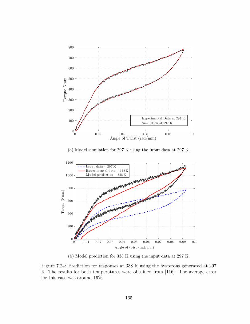
0 0.02 0.04 0.06 0.08 0.10

100

200

300

400

500

600

700

800

Angle of Twist (rad/mm)

TorqueNmm

Experimental Data at 297 K

Simulation at 297 K

(a) Model simulation for 297 K using the input data at 297 K.

Model pred iction - 338 K

Exper imental data - 338 K

Input data - 297 K

Torq

ue(N

mm)

Angle of twist (rad/mm)

0 0.01 0.02 0.03 0.04 0.05 0.06 0.07 0.08 0.09 0.10

200

400

600

800

1000

1200

(b) Model prediction for 338 K using the input data at 297 K.

Figure 7.24: Prediction for responses at 338 K using the hysterons generated at 297K. The results for both temperatures were obtained from [116]. The average errorfor this case was around 19%.

165

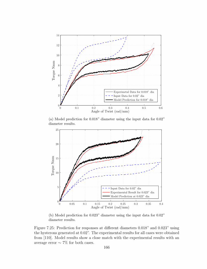
0 0.1 0.2 0.3 0.4 0.5 0.60

2

4

6

8

10

12

14

Angle of Twist (rad/mm)

TorqueNmm

Experimetal Data for 0.018” dia

Input Data for 0.02” dia

Model Prediction for 0.018” dia

(a) Model prediction for 0.018” diameter using the input data for 0.02”diameter results.

0 0.05 0.1 0.15 0.2 0.25 0.3 0.35 0.40

5

10

15

20

25

Angle of Twist (rad/mm)

TorqueNmm

Input Data for 0.02” dia

Experimental Result for 0.023” dia

Model Prediction at 0.023” dia

(b) Model prediction for 0.023” diameter using the input data for 0.02”diameter results.

Figure 7.25: Prediction for responses at different diameters 0.018” and 0.023” usingthe hysterons generated at 0.02”. The experimental results for all cases were obtainedfrom [110]. Model results show a close match with the experimental results with anaverage error ∼ 7% for both cases.

166

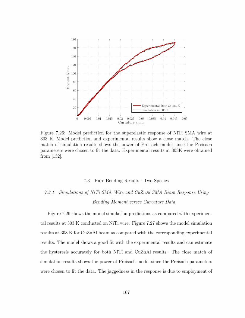
0 0.005 0.01 0.015 0.02 0.025 0.03 0.035 0.04 0.045 0.050

20

40

60

80

100

120

140

160

180

Curvature /mm

Mom

entNmm

Experimental Data at 303 K

Simulation at 303 K

Figure 7.26: Model prediction for the superelastic response of NiTi SMA wire at303 K. Model prediction and experimental results show a close match. The closematch of simulation results shows the power of Preisach model since the Preisachparameters were chosen to fit the data. Experimental results at 303K were obtainedfrom [132].

7.3 Pure Bending Results - Two Species

7.3.1 Simulations of NiTi SMA Wire and CuZnAl SMA Beam Response Using

Bending Moment verses Curvature Data

Figure 7.26 shows the model simulation predictions as compared with experimen-

tal results at 303 K conducted on NiTi wire. Figure 7.27 shows the model simulation

results at 308 K for CuZnAl beam as compared with the corresponding experimental

results. The model shows a good fit with the experimental results and can estimate

the hysteresis accurately for both NiTi and CuZnAl results. The close match of

simulation results shows the power of Preisach model since the Preisach parameters

were chosen to fit the data. The jaggedness in the response is due to employment of

167

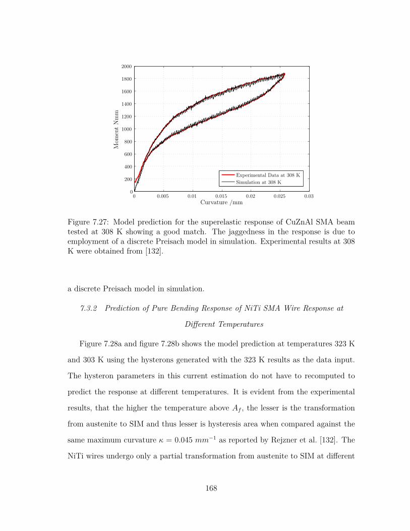
0 0.005 0.01 0.015 0.02 0.025 0.030

200

400

600

800

1000

1200

1400

1600

1800

2000

Curvature /mm

Mom

entNmm

Experimental Data at 308 K

Simulation at 308 K

Figure 7.27: Model prediction for the superelastic response of CuZnAl SMA beamtested at 308 K showing a good match. The jaggedness in the response is due toemployment of a discrete Preisach model in simulation. Experimental results at 308K were obtained from [132].

a discrete Preisach model in simulation.

7.3.2 Prediction of Pure Bending Response of NiTi SMA Wire Response at

Different Temperatures

Figure 7.28a and figure 7.28b shows the model prediction at temperatures 323 K

and 303 K using the hysterons generated with the 323 K results as the data input.

The hysteron parameters in this current estimation do not have to recomputed to

predict the response at different temperatures. It is evident from the experimental

results, that the higher the temperature above Af , the lesser is the transformation

from austenite to SIM and thus lesser is hysteresis area when compared against the

same maximum curvature κ = 0.045 mm−1 as reported by Rejzner et al. [132]. The

NiTi wires undergo only a partial transformation from austenite to SIM at different

168

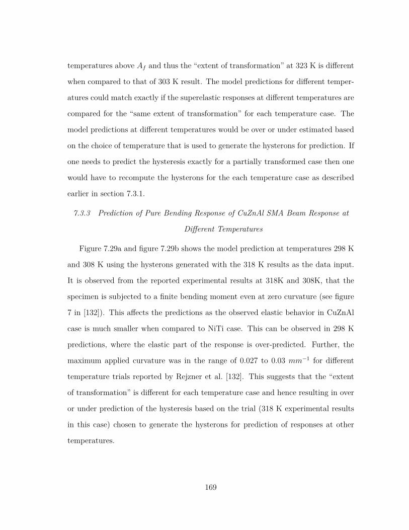
temperatures above Af and thus the “extent of transformation” at 323 K is different

when compared to that of 303 K result. The model predictions for different temper-

atures could match exactly if the superelastic responses at different temperatures are

compared for the “same extent of transformation” for each temperature case. The

model predictions at different temperatures would be over or under estimated based

on the choice of temperature that is used to generate the hysterons for prediction. If

one needs to predict the hysteresis exactly for a partially transformed case then one

would have to recompute the hysterons for the each temperature case as described

earlier in section 7.3.1.

7.3.3 Prediction of Pure Bending Response of CuZnAl SMA Beam Response at

Different Temperatures

Figure 7.29a and figure 7.29b shows the model prediction at temperatures 298 K

and 308 K using the hysterons generated with the 318 K results as the data input.

It is observed from the reported experimental results at 318K and 308K, that the

specimen is subjected to a finite bending moment even at zero curvature (see figure

7 in [132]). This affects the predictions as the observed elastic behavior in CuZnAl

case is much smaller when compared to NiTi case. This can be observed in 298 K

predictions, where the elastic part of the response is over-predicted. Further, the

maximum applied curvature was in the range of 0.027 to 0.03 mm−1 for different

temperature trials reported by Rejzner et al. [132]. This suggests that the “extent

of transformation” is different for each temperature case and hence resulting in over

or under prediction of the hysteresis based on the trial (318 K experimental results

in this case) chosen to generate the hysterons for prediction of responses at other

temperatures.

169

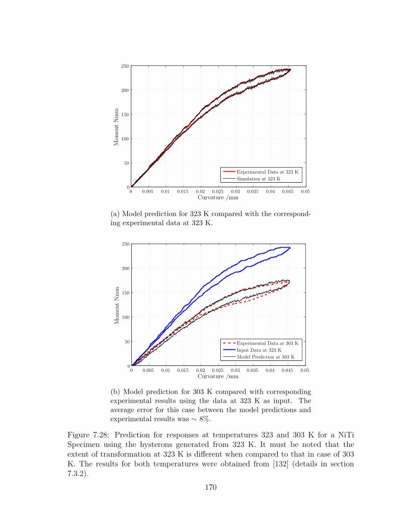
0 0.005 0.01 0.015 0.02 0.025 0.03 0.035 0.04 0.045 0.050

50

100

150

200

250

Curvature /mm

Mom

entNmm

Experimental Data at 323 K

Simulation at 323 K

(a) Model prediction for 323 K compared with the correspond-ing experimental data at 323 K.

0 0.005 0.01 0.015 0.02 0.025 0.03 0.035 0.04 0.045 0.050

50

100

150

200

250

Curvature /mm

Mom

entNmm

Experimental Data at 303 K

Input Data at 323 K

Model Prediction at 303 K

(b) Model prediction for 303 K compared with correspondingexperimental results using the data at 323 K as input. Theaverage error for this case between the model predictions andexperimental results was ∼ 8%.

Figure 7.28: Prediction for responses at temperatures 323 and 303 K for a NiTiSpecimen using the hysterons generated from 323 K. It must be noted that theextent of transformation at 323 K is different when compared to that in case of 303K. The results for both temperatures were obtained from [132] (details in section7.3.2).

170

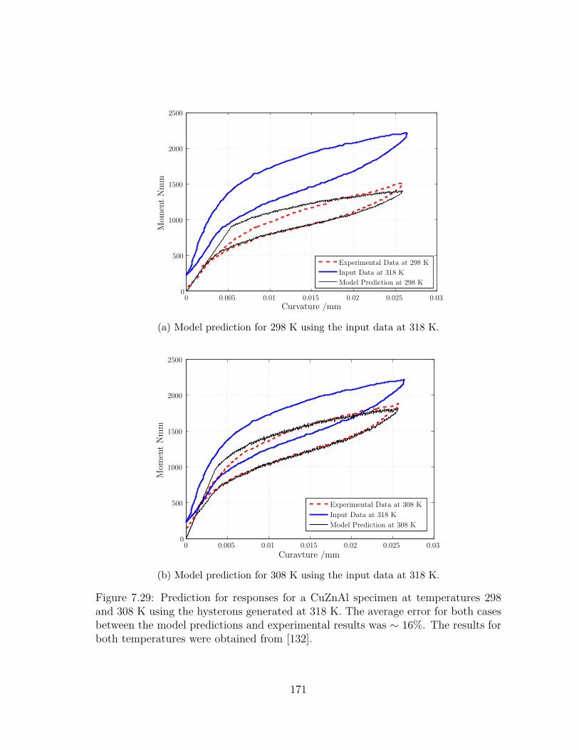
0 0.005 0.01 0.015 0.02 0.025 0.030

500

1000

1500

2000

2500

Curvature /mm

Mom

entNmm

Experimental Data at 298 K

Input Data at 318 K

Model Prediction at 298 K

(a) Model prediction for 298 K using the input data at 318 K.

0 0.005 0.01 0.015 0.02 0.025 0.030

500

1000

1500

2000

2500

Curavture /mm

Mom

entNmm

Experimental Data at 308 K

Input Data at 318 K

Model Prediction at 308 K

(b) Model prediction for 308 K using the input data at 318 K.

Figure 7.29: Prediction for responses for a CuZnAl specimen at temperatures 298and 308 K using the hysterons generated at 318 K. The average error for both casesbetween the model predictions and experimental results was ∼ 16%. The results forboth temperatures were obtained from [132].

171

Model simulationExper imental data

Torq

ue(N

mm)

Angle of twist (rad/mm)

- 0.1 - 0.08 - 0.06 - 0.04 - 0.02 0 0.02 0.04 0.06 0.08 0.1- 800

- 600

- 400

- 200

0

200

400

600

800

Figure 7.30: Model simulation for the superelastic response of SMA wire at 297K under clockwise and anticlockwise twists. The simulation closely matches theexperimental results demonstrating the power of Preisach approach. Experimentalresults were obtained from [116].

7.4 Torsion Results - Three Species

7.4.1 Simulations of SMA Spring and Wire Response Using Complete Torque

verses Angle of Twist Data

Figure 7.30 shows the model simulation for the superelastic response of SMA

wire at 297 K subjected to clockwise and anticlockwise twists. Figure 7.31 shows the

model prediction for a twinning response of SMA spring tested at 295 K. The simu-

lation closely matches the experimental results demonstrating the power of Preisach

approach. The jaggedness in the response is due to the use of a discrete Preisach

model.

The model was used to simulate responses of SMA components like springs, wires,

172

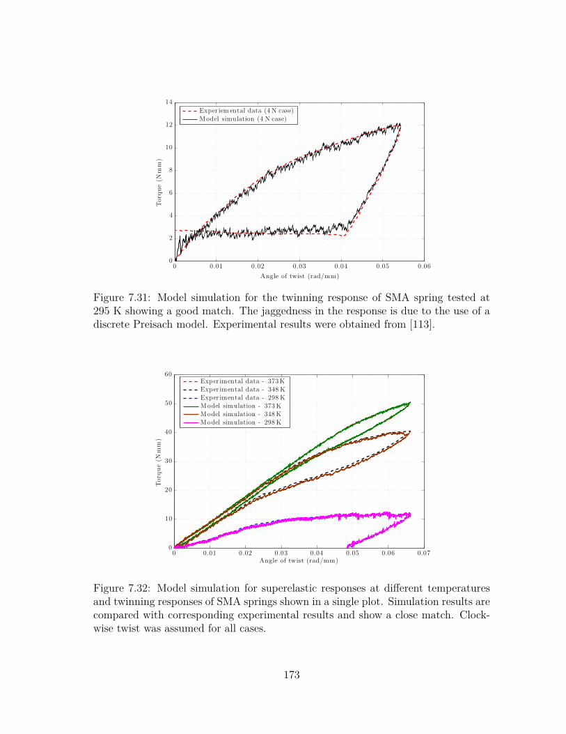
Model simulation (4 N case)Exper iem ental data (4 N case)

Torq

ue(N

mm)

Angle of twist (rad/mm)

0 0.01 0.02 0.03 0.04 0.05 0.060

2

4

6

8

10

12

14

Figure 7.31: Model simulation for the twinning response of SMA spring tested at295 K showing a good match. The jaggedness in the response is due to the use of adiscrete Preisach model. Experimental results were obtained from [113].

Model simulation - 298 K

Model simulation - 348KModel simulation - 373 K

Exper imental data - 298 KExper imental data - 348 K

Exper imental data - 373K

Torq

ue(N

mm)

Angle of twist (rad/mm)0 0.01 0.02 0.03 0.04 0.05 0.06 0.07

0

10

20

30

40

50

60

Figure 7.32: Model simulation for superelastic responses at different temperaturesand twinning responses of SMA springs shown in a single plot. Simulation results arecompared with corresponding experimental results and show a close match. Clock-wise twist was assumed for all cases.

173

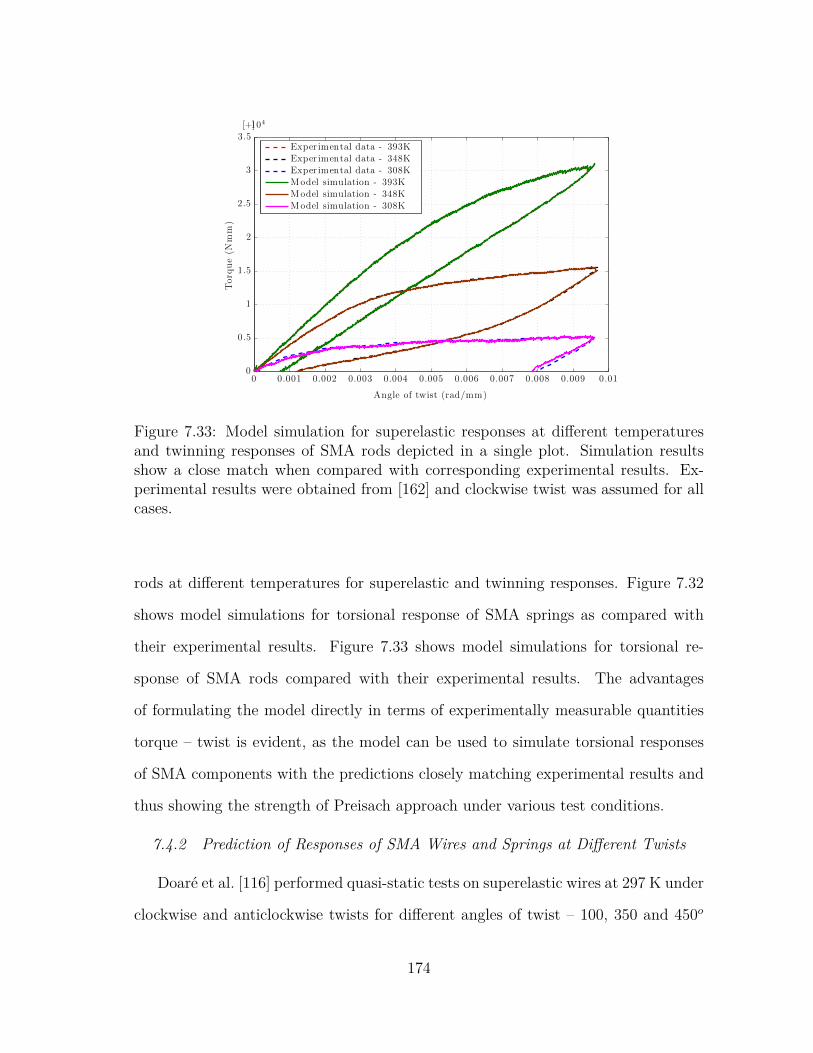
Model simulation - 308KModel simulation - 348KModel simulation - 393KExper imental data - 308KExper imental data - 348KExper imental data - 393K

Torq

ue(N

mm)

Angle of twist (rad/mm)

0 0.001 0.002 0.003 0.004 0.005 0.006 0.007 0.008 0.009 0.01

[+]104

0

0.5

1

1.5

2

2.5

3

3.5

Figure 7.33: Model simulation for superelastic responses at different temperaturesand twinning responses of SMA rods depicted in a single plot. Simulation resultsshow a close match when compared with corresponding experimental results. Ex-perimental results were obtained from [162] and clockwise twist was assumed for allcases.

rods at different temperatures for superelastic and twinning responses. Figure 7.32

shows model simulations for torsional response of SMA springs as compared with

their experimental results. Figure 7.33 shows model simulations for torsional re-

sponse of SMA rods compared with their experimental results. The advantages

of formulating the model directly in terms of experimentally measurable quantities

torque – twist is evident, as the model can be used to simulate torsional responses

of SMA components with the predictions closely matching experimental results and

thus showing the strength of Preisach approach under various test conditions.

7.4.2 Prediction of Responses of SMA Wires and Springs at Different Twists

Doaré et al. [116] performed quasi-static tests on superelastic wires at 297 K under

clockwise and anticlockwise twists for different angles of twist – 100, 350 and 450o

174

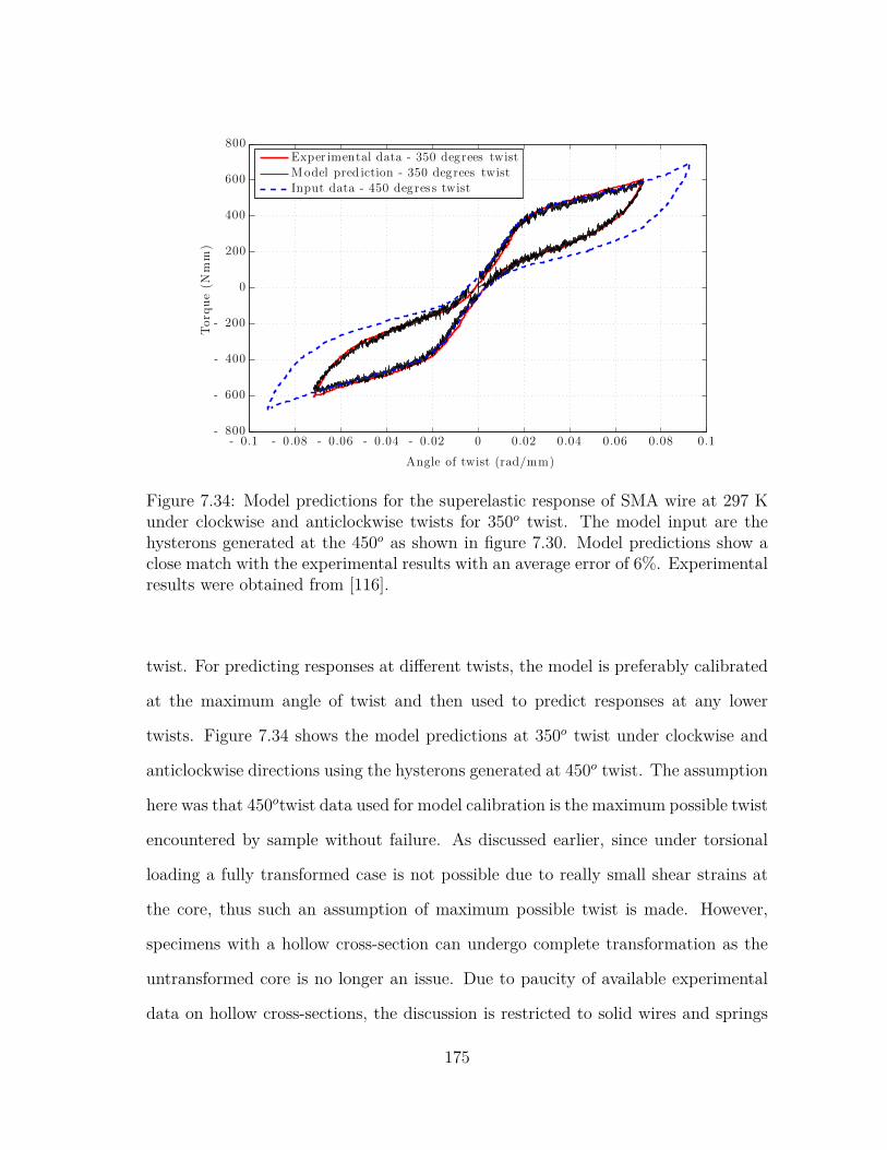
Input data - 450 degress twistModel pred iction - 350 degrees twistExper imental data - 350 degrees twist

Torq

ue(N

mm)

Angle of twist (rad/mm)

- 0.1 - 0.08 - 0.06 - 0.04 - 0.02 0 0.02 0.04 0.06 0.08 0.1- 800

- 600

- 400

- 200

0

200

400

600

800

Figure 7.34: Model predictions for the superelastic response of SMA wire at 297 Kunder clockwise and anticlockwise twists for 350o twist. The model input are thehysterons generated at the 450o as shown in figure 7.30. Model predictions show aclose match with the experimental results with an average error of 6%. Experimentalresults were obtained from [116].

twist. For predicting responses at different twists, the model is preferably calibrated

at the maximum angle of twist and then used to predict responses at any lower

twists. Figure 7.34 shows the model predictions at 350o twist under clockwise and

anticlockwise directions using the hysterons generated at 450o twist. The assumption

here was that 450otwist data used for model calibration is the maximum possible twist

encountered by sample without failure. As discussed earlier, since under torsional

loading a fully transformed case is not possible due to really small shear strains at

the core, thus such an assumption of maximum possible twist is made. However,

specimens with a hollow cross-section can undergo complete transformation as the

untransformed core is no longer an issue. Due to paucity of available experimental

data on hollow cross-sections, the discussion is restricted to solid wires and springs

175

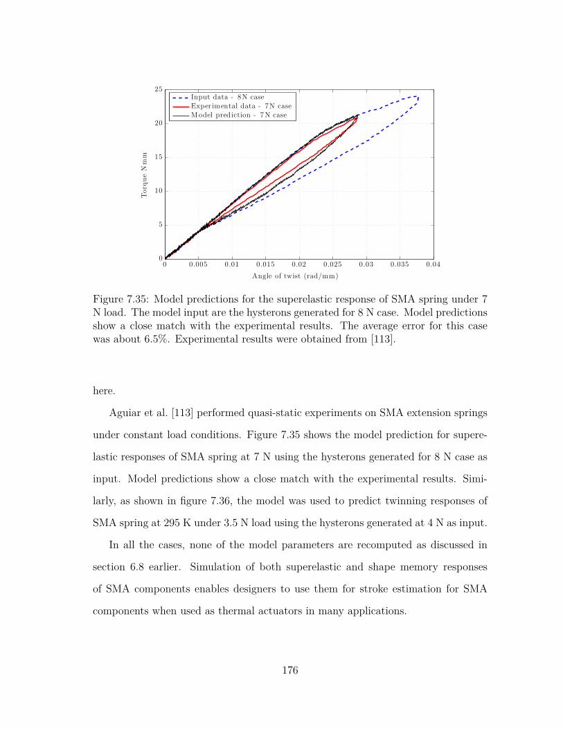
Model pred iction - 7N caseExper imental data - 7N caseInput data - 8N case

Torq

ueNmm

Angle of twist (rad/mm)

0 0.005 0.01 0.015 0.02 0.025 0.03 0.035 0.040

5

10

15

20

25

Figure 7.35: Model predictions for the superelastic response of SMA spring under 7N load. The model input are the hysterons generated for 8 N case. Model predictionsshow a close match with the experimental results. The average error for this casewas about 6.5%. Experimental results were obtained from [113].

here.

Aguiar et al. [113] performed quasi-static experiments on SMA extension springs

under constant load conditions. Figure 7.35 shows the model prediction for supere-

lastic responses of SMA spring at 7 N using the hysterons generated for 8 N case as

input. Model predictions show a close match with the experimental results. Simi-

larly, as shown in figure 7.36, the model was used to predict twinning responses of

SMA spring at 295 K under 3.5 N load using the hysterons generated at 4 N as input.

In all the cases, none of the model parameters are recomputed as discussed in

section 6.8 earlier. Simulation of both superelastic and shape memory responses

of SMA components enables designers to use them for stroke estimation for SMA

components when used as thermal actuators in many applications.

176

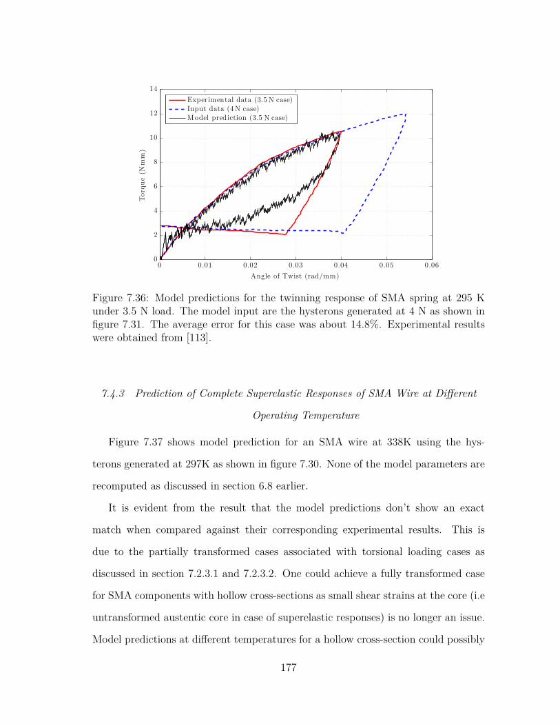
Model pred iction (3.5 N case)Input data (4 N case)Exper imental data (3.5 N case)

Torq

ue(N

mm)

Angle of Twist (rad/mm)

0 0.01 0.02 0.03 0.04 0.05 0.060

2

4

6

8

10

12

14

Figure 7.36: Model predictions for the twinning response of SMA spring at 295 Kunder 3.5 N load. The model input are the hysterons generated at 4 N as shown infigure 7.31. The average error for this case was about 14.8%. Experimental resultswere obtained from [113].

7.4.3 Prediction of Complete Superelastic Responses of SMA Wire at Different

Operating Temperature

Figure 7.37 shows model prediction for an SMA wire at 338K using the hys-

terons generated at 297K as shown in figure 7.30. None of the model parameters are

recomputed as discussed in section 6.8 earlier.

It is evident from the result that the model predictions don’t show an exact

match when compared against their corresponding experimental results. This is

due to the partially transformed cases associated with torsional loading cases as

discussed in section 7.2.3.1 and 7.2.3.2. One could achieve a fully transformed case

for SMA components with hollow cross-sections as small shear strains at the core (i.e

untransformed austentic core in case of superelastic responses) is no longer an issue.

Model predictions at different temperatures for a hollow cross-section could possibly

177

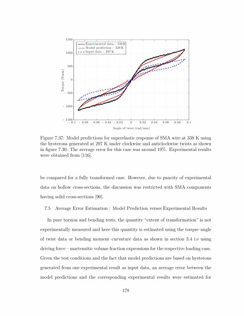
Input data - 297 K

Model pred iction - 338 KExper imental data - 338 K

Torq

ue(N

mm)

Angle of twist (rad/mm)

- 0.1 - 0.08 - 0.06 - 0.04 - 0.02 0 0.02 0.04 0.06 0.08 0.1- 1500

- 1000

- 500

0

500

1000

1500

Figure 7.37: Model predictions for superelastic response of SMA wire at 338 K usingthe hysterons generated at 297 K under clockwise and anticlockwise twists as shownin figure 7.30. The average error for this case was around 19%. Experimental resultswere obtained from [116].

be compared for a fully transformed case. However, due to paucity of experimental

data on hollow cross-sections, the discussion was restricted with SMA components

having solid cross-sections [90].

7.5 Average Error Estimation : Model Prediction verses Experimental Results

In pure torsion and bending tests, the quantity “extent of transformation” is not

experimentally measured and here this quantity is estimated using the torque–angle

of twist data or bending moment–curvature data as shown in section 3.4 i.e using

driving force – martensitic volume fraction expressions for the respective loading case.

Given the test conditions and the fact that model predictions are based on hysterons

generated from one experimental result as input data, an average error between the

model predictions and the corresponding experimental results were estimated for

178

each case. The average errors were estimated using the trapezoidal integration rule

(trapz command in MATLAB R©).

Average error =

√√√√∫ (Model value− experimental value)2 dx

(∫Experimental value)2 dx

(7.1)

The average error is an estimate for that specific case as the model predictions could

be different depending on the hysterons generated for predictions (i.e the choice of

initial experimental data as input). The average error for each of model predic-

tions discussed in this work are highlighted in figures 7.13a, 7.23, 7.24, 7.25,7.28b,

7.29,7.34, 7.35, 7.36, 7.34 and 7.37.

179

8. FUNCTIONAL DEGRADATION OF SMA COMPONENTS

8.1 Motivation and Literature Review - Functional Fatigue of SMA

With growing applications of SMA components in different engineering applica-

tions, the issue of material performance over its designed life is of great concern to

researchers lately. As pointed out as Eggeler et al. [170] numerous factors can influ-

ence the fatigue life of SMA. Factors include material chemical composition, material

impurity (i.e particle size distribution), type of loading, applied load magnitude, ex-

tent of deformation or plateau strains, processing conditions, defect accumulation,

accumulated plastic deformation, microstructure and operating temperature being

a few to list [170]. Over the years, numerous experimental data concerning SMA

fatigue under superelastic conditions and thermal cycling (mimicking shape memory

effects) have been reported. Most of the focus has been in understanding fatigue

behaviour of SMA wires (see [171–173] for detailed reviews) under tension with some

attention towards bending – rotating tests of SMA wire (see [170, 174–176] etc. for

more discussions) and functional fatigue of actuator springs (see [177–180] etc. for

more discussions).

Eggeler et al. [170] in their famous work subdivide SMA fatigue into two cate-

gories namely “structural fatigue” and “functional fatigue” (see figure 8.1). SMAs

failing like other engineering material due to repeated high cyclic mechanical loads

is classified under “structural fatigue” which is generally accompanied by defect ac-

cumulation, crack initiation (normally micro-structure controlled and growth - ge-

ometry dependent) [170,181]. However, unlike classical material systems, SMAs are

also sensitive to operating temperature fluctuations and interaction of SIM (stress

induced martensite) as observed in the case of repeated SE cycles with “cyclic strain

180

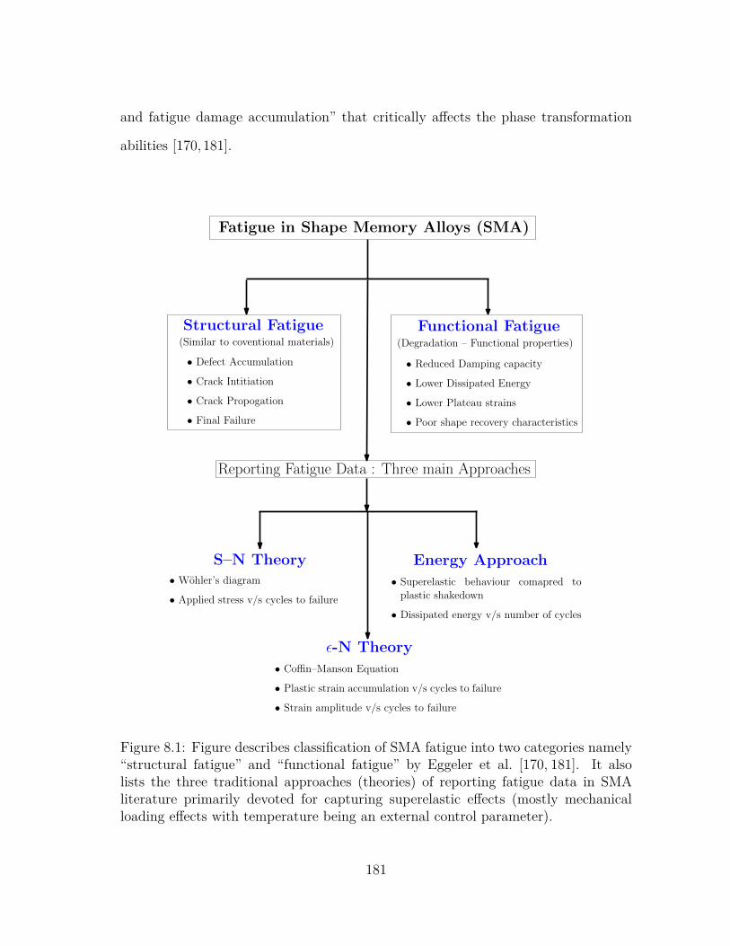
and fatigue damage accumulation” that critically affects the phase transformation

abilities [170,181].

Fatigue in Shape Memory Alloys (SMA)

Structural Fatigue Functional Fatigue

• Defect Accumulation

• Crack Intitiation

• Crack Propogation

• Final Failure

• Reduced Damping capacity

• Lower Dissipated Energy

• Lower Plateau strains

• Poor shape recovery characteristics

S–N Theory

ε-N Theory

Energy Approach• Wohler’s diagram

• Applied stress v/s cycles to failure

• Superelastic behaviour comapred toplastic shakedown

• Dissipated energy v/s number of cycles

• Coffin–Manson Equation

• Plastic strain accumulation v/s cycles to failure

• Strain amplitude v/s cycles to failure

Reporting Fatigue Data : Three main Approaches

(Similar to coventional materials) (Degradation – Functional properties)

Figure 8.1: Figure describes classification of SMA fatigue into two categories namely“structural fatigue” and “functional fatigue” by Eggeler et al. [170, 181]. It alsolists the three traditional approaches (theories) of reporting fatigue data in SMAliterature primarily devoted for capturing superelastic effects (mostly mechanicalloading effects with temperature being an external control parameter).

181

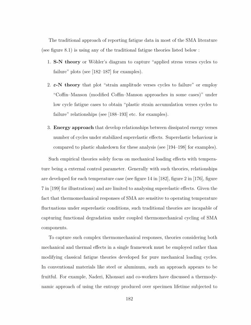
The traditional approach of reporting fatigue data in most of the SMA literature

(see figure 8.1) is using any of the traditional fatigue theories listed below :

1. S-N theory or Wöhler’s diagram to capture “applied stress verses cycles to

failure” plots (see [182–187] for examples).

2. ε-N theory that plot “strain amplitude verses cycles to failure” or employ

“Coffin–Manson (modified Coffin–Manson approaches in some cases)” under

low cycle fatigue cases to obtain “plastic strain accumulation verses cycles to

failure” relationships (see [188–193] etc. for examples).

3. Energy approach that develop relationships between dissipated energy verses

number of cycles under stabilized superelastic effects. Superelastic behaviour is

compared to plastic shakedown for these analysis (see [194–198] for examples).

Such empirical theories solely focus on mechanical loading effects with tempera-

ture being a external control parameter. Generally with such theories, relationships

are developed for each temperature case (see figure 14 in [182], figure 2 in [176], figure

7 in [199] for illustrations) and are limited to analysing superelastic effects. Given the

fact that thermomechanical responses of SMA are sensitive to operating temperature

fluctuations under superelastic conditions, such traditional theories are incapable of

capturing functional degradation under coupled thermomechanical cycling of SMA

components.

To capture such complex thermomechanical responses, theories considering both

mechanical and thermal effects in a single framework must be employed rather than

modifying classical fatigue theories developed for pure mechanical loading cycles.

In conventional materials like steel or aluminum, such an approach appears to be

fruitful. For example, Naderi, Khonsari and co-workers have discussed a thermody-

namic approach of using the entropy produced over specimen lifetime subjected to

182

fatigue tests to analyze material degradation [200, 201]. Their approach considered

the Clausius–Duhem inequality to discuss the rate of volumetric entropy generation

that includes “mechanical dissipation due to plastic deformation, non-recoverable

internal energy and thermal dissipation owing to heat conduction” [201,202]. Using

this inequality, a quantity described as total entropy gain or fracture fatigue entropy

(FFE) is developed by integrating the inequality from time t = 0 to the time of

failure t = tf [201–203]. They proposed that FFE is material dependent but inde-

pendent of geometry, load and frequency in their discussion with material systems

like metals (stainless steel, aluminum) and some composite laminate systems like

woven glass/epoxy [201, 204]. The temperature fluctuations considered were a re-

sultant of plastic deformation of the material and further a “relationship between

normalized cycles to failure and normalized entropy generation” is assumed to be

linear to predict fatigue life of the material (see equation 5.3 in [201]). In classi-

cal materials (like most metals and alloys), the surface temperature rise at higher

stresses is a resultant of hysteresis heating and several polynomial, exponential re-

lationships to capture this temperature rise over material life have been proposed

(see figure 1 [205] for a summary of several such efforts). In most of these efforts,

the mechanical and thermal effects are decoupled and such simple relationships work

well with classical materials [205–207]. Though such approaches have a strong ther-

modynamic base, developing relationships for surface temperature rise or capturing

the “rate of volumetric entropy generation” for SMA can get quite cumbersome given

the complex hysteretic thermomechanical nature of SMA responses that are temper-

ature dependent. Further, in SMAs the mechanical and thermal effects are coupled

and influence the component functionality together. Hence, developing relationships

for plastic strain energy per cycle that capture both mechanical and thermal load-

ing effects can get quite tricky (see equation 4 in [203, 207] for some examples that

183

consider only mechanical loading for aluminum and Stainless steel materials).

Motivated by Knosari & co-workers, an effort to develop a thermodynamically

based approach for characterizing functional degradation in SMA where phase tran-

sitions and associated irreversibility add an additional degree of complexity that is

not present in conventional materials is undertaken here. The approach presented

here is capable of overcoming the limitations of the FFE approach and traditional

S-N or ε-N theories for analyzing functional fatigue of SMAs.

Following the approach highlighted in section 3 which employs a two species Gibbs

potential based formulation to separate the thermoelastic and the dissipative part of

the entire SMA component response is employed here. The models were formulated

directly using experimentally measurable quantities like torque–twist or moment–

curvature with the intention of developing relationships directly at the component

level. Using thermodynamic principles, relationships for “driving force for the phase

transformation” and “extent of phase transformation” were established.

The driving force relationships would capture both mechanical and thermal load-

ing effects in the same framework with the ability to capture both shape memory and

superelastic effects using a single formulation. Hence, a plot of driving force verses

no. of cycles would play the role of a traditional S-N curve. This quantity would be

equivalent to the thermodynamical force for onset of phase transformations which

are directly responsible for the functionality of SMA components (shape changing

capability and large recoverable strains).

In case of thermally activated SMA components (mimicking shape memory ef-

fects), a drop in driving force amplitude would directly correspond to material loos-

ing its ability to undergo phase transformations which directly corresponds to loss

in functionality of SMA component. In case of superelastic effects, a relationships of

“driving force for the phase transformation” and “extent of phase transformation”

184

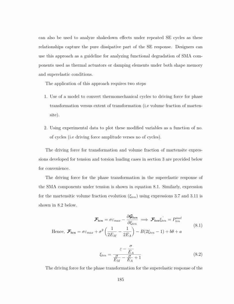
can also be used to analyze shakedown effects under repeated SE cycles as these

relationships capture the pure dissipative part of the SE response. Designers can

use this approach as a guideline for analyzing functional degradation of SMA com-

ponents used as thermal actuators or damping elements under both shape memory

and superelastic conditions.

The application of this approach requires two steps

1. Use of a model to convert thermomechanical cycles to driving force for phase

transformation versus extent of transformation (i.e volume fraction of marten-

site).

2. Using experimental data to plot these modified variables as a function of no.

of cycles (i.e driving force amplitude verses no of cycles).

The driving force for transformation and volume fraction of martensite expres-

sions developed for tension and torsion loading cases in section 3 are provided below

for convenience.

The driving force for the phase transformation in the superelastic response of

the SMA components under tension is shown in equation 8.1. Similarly, expression

for the martensitic volume fraction evolution (ξten) using expressions 3.7 and 3.11 is

shown in 8.2 below.

Ften = σεmax −∂Gten∂ξten

=⇒ Ften ˙ξten = P inelten

Hence, Ften = σεmax + σ2( 1

2EM− 1

2EA

)−B(2ξten − 1) + bθ + a

(8.1)

ξten =ε− σ

EAσEM− σEA

+ 1 (8.2)

The driving force for the phase transformation for the superelastic response of the

185

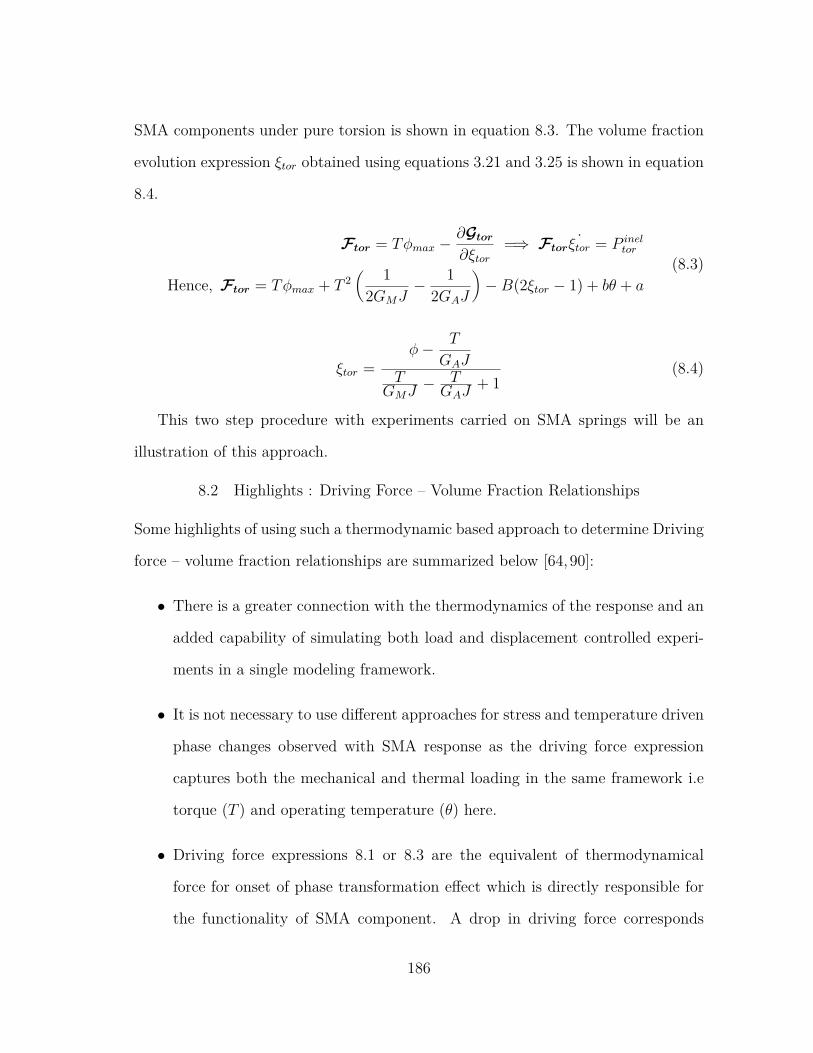
SMA components under pure torsion is shown in equation 8.3. The volume fraction

evolution expression ξtor obtained using equations 3.21 and 3.25 is shown in equation

8.4.

Ftor = Tφmax −∂Gtor∂ξtor

=⇒ Ftor ˙ξtor = P ineltor

Hence, Ftor = Tφmax + T 2( 1

2GMJ− 1

2GAJ

)−B(2ξtor − 1) + bθ + a

(8.3)

ξtor =φ− T

GAJT

GMJ− TGAJ

+ 1(8.4)

This two step procedure with experiments carried on SMA springs will be an

illustration of this approach.

8.2 Highlights : Driving Force – Volume Fraction Relationships

Some highlights of using such a thermodynamic based approach to determine Driving

force – volume fraction relationships are summarized below [64,90]:

• There is a greater connection with the thermodynamics of the response and an

added capability of simulating both load and displacement controlled experi-

ments in a single modeling framework.

• It is not necessary to use different approaches for stress and temperature driven

phase changes observed with SMA response as the driving force expression

captures both the mechanical and thermal loading in the same framework i.e

torque (T ) and operating temperature (θ) here.

• Driving force expressions 8.1 or 8.3 are the equivalent of thermodynamical

force for onset of phase transformation effect which is directly responsible for

the functionality of SMA component. A drop in driving force corresponds

186

to material loosing functionality i.e material is no longer transforming and

performing its intended function. Hence, this quantity can used as a parameter

to analyze the functional degradation of SMA components.

• The volume fraction relationship can help us estimate the extent of transfor-

mation using the torque and twist as input data. This is particularly useful

in torsional loading cases as the SMA components are partially transformed.

This is due to the fact that the shear strains tends to zero at the core of the

specimen crosssection as the wire twists under torsion [90,116]. The possibility

of a fully transformed case is possible only the angle of twist asymptomatically

reaches infinity at the core prior to the component failure [90, 116]. Doaré et

al. [116] have reported experimental results on SMA wire subjected to different

degrees of twist (100, 350 and 450o twist) to illustrate this point of partial

transformation (see figure 4 in [116].) in real world applications.

• A driving force – volume fraction plot that solely captures the dissipative part

of the response can also be used to analyze shakedown effects observed with typ-

ical superleastic responses associated with SMAs. This can substitute “Energy

approach” that develop relationships between dissipated energy verses number

of cycles under stabilized superelastic effects by comparing SE behaviour to

plastic shakedown.

• With the model formulation in terms of stress–strain or torque–twist, designers

can use the model to analyze component behaviour directly as the model can

use the sensor data as inputs. Though this approach is restricted to specifically

analysing SMA components under tension or torsion loading case, it could be

extremely useful for designers in analysing the functional degradation of SMA

components.

187

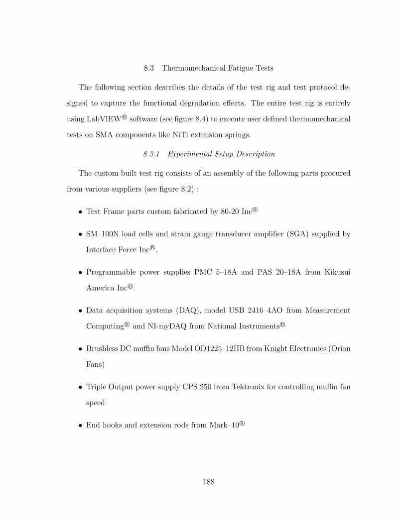
8.3 Thermomechanical Fatigue Tests

The following section describes the details of the test rig and test protocol de-

signed to capture the functional degradation effects. The entire test rig is entirely

using LabVIEW R© software (see figure 8.4) to execute user defined thermomechanical

tests on SMA components like NiTi extension springs.

8.3.1 Experimental Setup Description

The custom built test rig consists of an assembly of the following parts procured

from various suppliers (see figure 8.2) :

• Test Frame parts custom fabricated by 80-20 Inc R©

• SM–100N load cells and strain gauge transducer amplifier (SGA) supplied by

Interface Force Inc R©.

• Programmable power supplies PMC 5–18A and PAS 20–18A from Kikusui

America Inc R©.

• Data acquisition systems (DAQ), model USB 2416–4AO from Measurement

Computing R© and NI-myDAQ from National Instruments R©

• Brushless DC muffin fans Model OD1225–12HB from Knight Electronics (Orion

Fans)

• Triple Output power supply CPS 250 from Tektronix for controlling muffin fan

speed

• End hooks and extension rods from Mark–10 R©

188

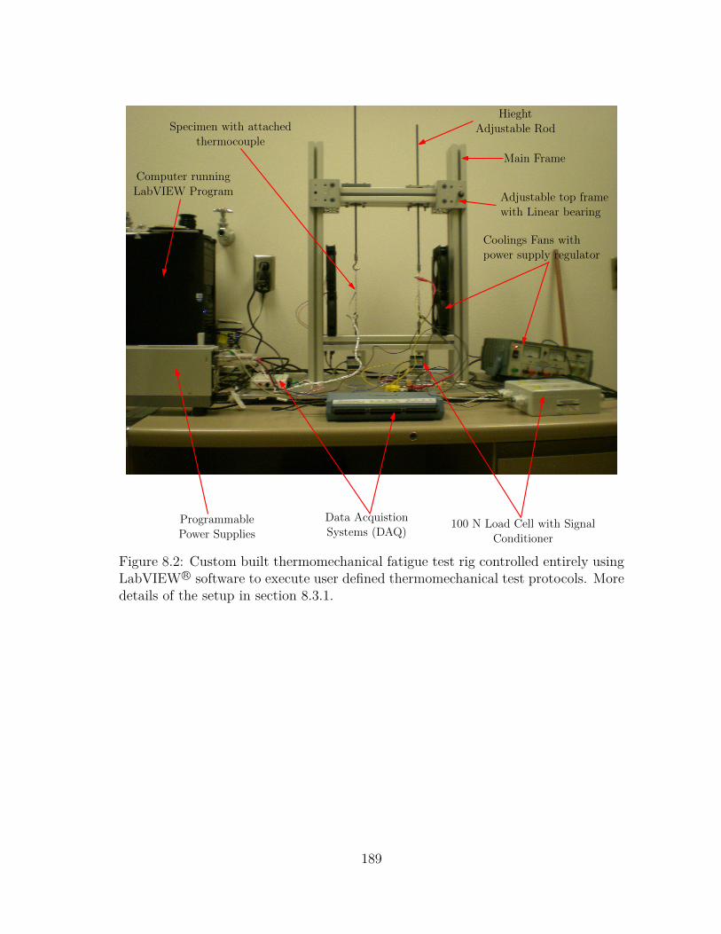
Main Frame

HieghtAdjustable Rod

Adjustable top framewith Linear bearing

Coolings Fans withpower supply regulator

100 N Load Cell with SignalConditioner

Data AcquistionSystems (DAQ)

ProgrammablePower Supplies

Specimen with attachedthermocouple

Computer runningLabVIEW Program

Figure 8.2: Custom built thermomechanical fatigue test rig controlled entirely usingLabVIEW R© software to execute user defined thermomechanical test protocols. Moredetails of the setup in section 8.3.1.

189

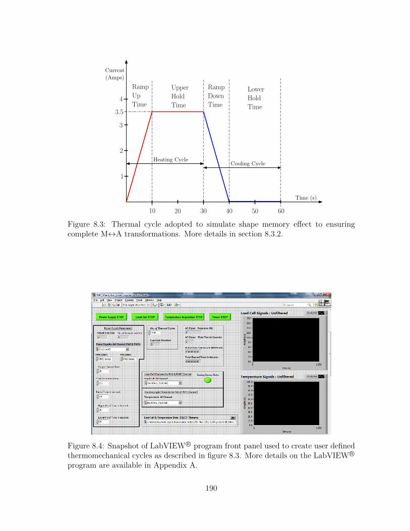
10 20 30 40

Ramp

Down

Time

Lower

Hold

Time

Upper

Hold

Time

Ramp

Up

Time

Current(Amps)

Time (s)

1

2

3

4

50 60

3.5

Heating CycleCooling Cycle

Figure 8.3: Thermal cycle adopted to simulate shape memory effect to ensuringcomplete M↔A transformations. More details in section 8.3.2.

Figure 8.4: Snapshot of LabVIEW R© program front panel used to create user definedthermomechanical cycles as described in figure 8.3. More details on the LabVIEW R©

program are available in Appendix A.

190

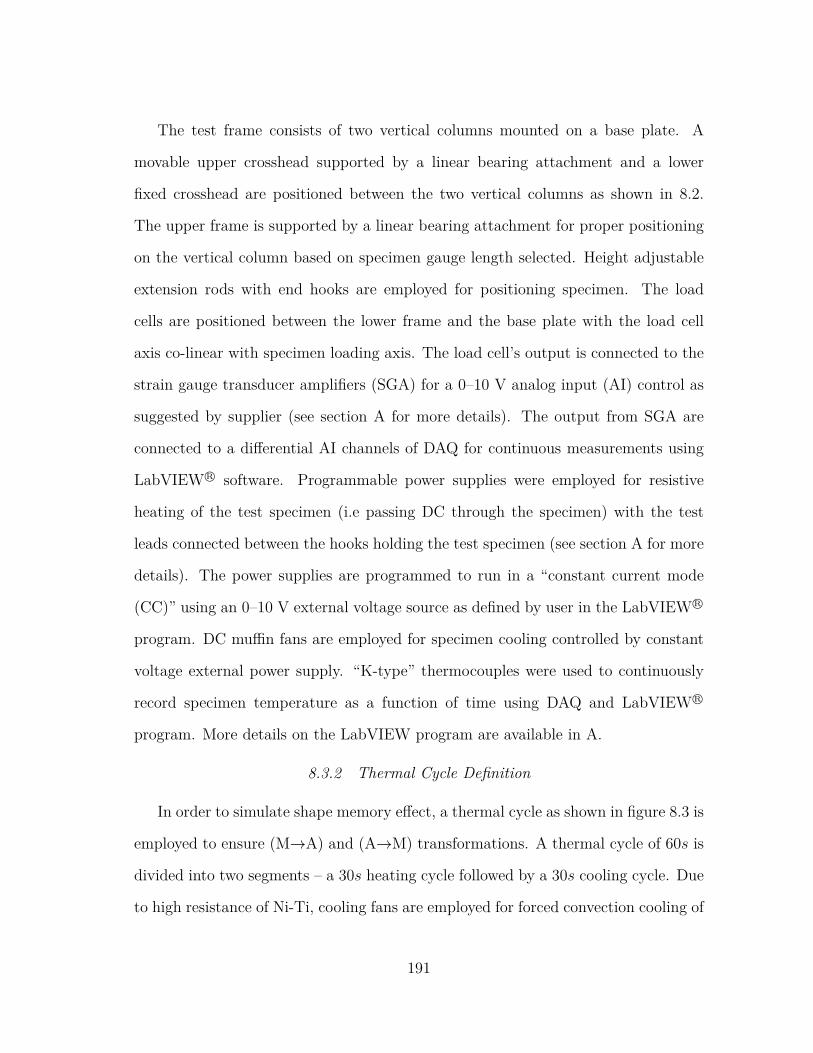
The test frame consists of two vertical columns mounted on a base plate. A

movable upper crosshead supported by a linear bearing attachment and a lower

fixed crosshead are positioned between the two vertical columns as shown in 8.2.

The upper frame is supported by a linear bearing attachment for proper positioning

on the vertical column based on specimen gauge length selected. Height adjustable

extension rods with end hooks are employed for positioning specimen. The load

cells are positioned between the lower frame and the base plate with the load cell

axis co-linear with specimen loading axis. The load cell’s output is connected to the

strain gauge transducer amplifiers (SGA) for a 0–10 V analog input (AI) control as

suggested by supplier (see section A for more details). The output from SGA are

connected to a differential AI channels of DAQ for continuous measurements using

LabVIEW R© software. Programmable power supplies were employed for resistive

heating of the test specimen (i.e passing DC through the specimen) with the test

leads connected between the hooks holding the test specimen (see section A for more

details). The power supplies are programmed to run in a “constant current mode

(CC)” using an 0–10 V external voltage source as defined by user in the LabVIEW R©

program. DC muffin fans are employed for specimen cooling controlled by constant

voltage external power supply. “K-type” thermocouples were used to continuously

record specimen temperature as a function of time using DAQ and LabVIEW R©

program. More details on the LabVIEW program are available in A.

8.3.2 Thermal Cycle Definition

In order to simulate shape memory effect, a thermal cycle as shown in figure 8.3 is

employed to ensure (M→A) and (A→M) transformations. A thermal cycle of 60s is

divided into two segments – a 30s heating cycle followed by a 30s cooling cycle. Due

to high resistance of Ni-Ti, cooling fans are employed for forced convection cooling of

191

specimen especially during the cooling cycle. Using these thermal cycles repeatedly,

one can simulate SME and capture the functional degradation of the test specimen

held under constant deformation. The breakup of the heating and cooling cycles are

given below :

1. Ramp Up Time - A part of the heating cycle where a peak current of 3.5

amps is reached in a time interval of 10s. The peak current is selected such that

the temperature of the specimen is well above Af to ensure complete (M→A)

transformation.

2. Upper Hold Time - A part of heating cycle where a hold time of 20s is

provided at the peak current of 3.5 amps to ensure complete (M→A) transfor-

mation of the test specimen.

3. Ramp Down Time - A part of cooling cycle where a gradual drop from 3.5

back to 0 amps is achieved. This segment is the mirror of ramp up time.

4. Lower Hold Time - A part of cooling cycle where a hold time of 20s is

employed to ensure the temperature of the specimen is below Mf to ensure

complete (A→M) transformation.

8.3.3 Material and Test Methodology

SMA actuator extension springs were obtained from Images SI Inc with compo-

sition details of 55.91 % Nickel, balance Titanium with trace elements < 0.25% as

provided by supplier [208]. The SMA wire was 30 to 40% cold worked before shape

setting it into extension springs. The transformation temperature of interest Af as

reported by the supplier was around 325 K. The spring specifications are as follows.

• Mean coil diameter of the spring “Dm” = 5.5 mm

192

• Wire diameter “d” = 0.754 mm

• Spring Index “Cm” = 7.3

• Free length “Lf” = 26.8 mm

• Number of active coils “n” = 20.

The springs were predeformed to 75 or 100 mm stroke and held between the

hooks as shown in figure 8.2. The springs are subjected to repeated thermal cycles

as defined in figure 8.3. For every cycle, load cell and thermocouple sensor readings

are continually recorded as a function of time using the data acquisition system

(DAQ) and LabVIEW R© program. The predefromed springs are martensitic at the

start of the test. During the heating cycle, the springs contract thus generating a

recovery force which is measured by load cell continuously. The springs relax back

to their original predeformed configuration at the end of the cooling cycle.

8.4 Results and Discussions

The same driving force – volume fraction relationship expressions can be used

to analyze functional degradation of components under both shape memory and

superelastic effects.

193

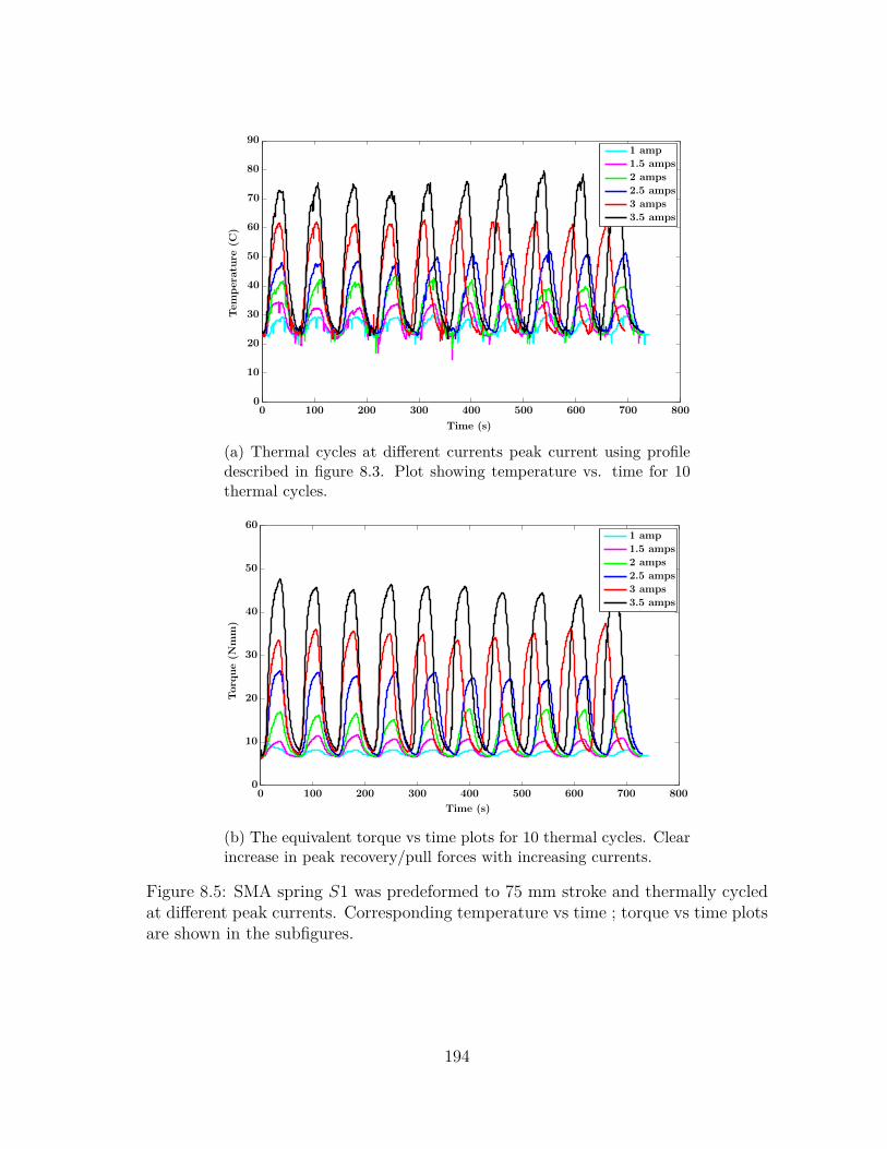
3.5 amps

3 amps

2.5 amps

2 amps

1.5 amps

1 amp

Tempera

ture

(C)

Time (s)

0 100 200 300 400 500 600 700 8000

10

20

30

40

50

60

70

80

90

(a) Thermal cycles at different currents peak current using profiledescribed in figure 8.3. Plot showing temperature vs. time for 10thermal cycles.

3.5 amps

3 amps

2.5 amps

2 amps

1.5 amps

1 amp

Torq

ue(N

mm)

Time (s)

0 100 200 300 400 500 600 700 8000

10

20

30

40

50

60

(b) The equivalent torque vs time plots for 10 thermal cycles. Clearincrease in peak recovery/pull forces with increasing currents.

Figure 8.5: SMA spring S1 was predeformed to 75 mm stroke and thermally cycledat different peak currents. Corresponding temperature vs time ; torque vs time plotsare shown in the subfigures.

194

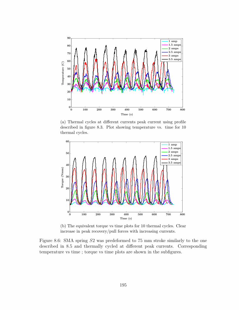
3.5 amps

3 amps

2.5 amps

2 amps

1.5 amps

1 amp

Tempera

ture

(C)

Time (s)

0 100 200 300 400 500 600 700 8000

10

20

30

40

50

60

70

80

90

(a) Thermal cycles at different currents peak current using profiledescribed in figure 8.3. Plot showing temperature vs. time for 10thermal cycles.

3.5 amps

3 amps

2.5 amps

2 amps

1.5 amps

1 amp

Torq

ue(N

mm)

Time (s)

0 100 200 300 400 500 600 700 8000

10

20

30

40

50

60

(b) The equivalent torque vs time plots for 10 thermal cycles. Clearincrease in peak recovery/pull forces with increasing currents.

Figure 8.6: SMA spring S2 was predeformed to 75 mm stroke similarly to the onedescribed in 8.5 and thermally cycled at different peak currents. Correspondingtemperature vs time ; torque vs time plots are shown in the subfigures.

195

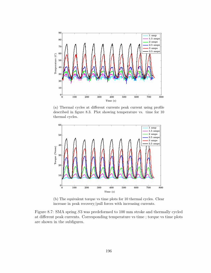
3.5 amps

3 amps

2.5 amps

2 amps

1.5 amps

1 amp

Tempera

ture

(C)

Time (s)

0 100 200 300 400 500 600 700 8000

10

20

30

40

50

60

70

80

90

(a) Thermal cycles at different currents peak current using profiledescribed in figure 8.3. Plot showing temperature vs. time for 10thermal cycles.

3.5 amps

3 amps

2.5 amps

2 amps

1.5 amps

1 amp

Torq

ue(N

mm)

Time (s)

0 100 200 300 400 500 600 700 8000

10

20

30

40

50

60

(b) The equivalent torque vs time plots for 10 thermal cycles. Clearincrease in peak recovery/pull forces with increasing currents.

Figure 8.7: SMA spring S3 was predeformed to 100 mm stroke and thermally cycledat different peak currents. Corresponding temperature vs time ; torque vs time plotsare shown in the subfigures.

196

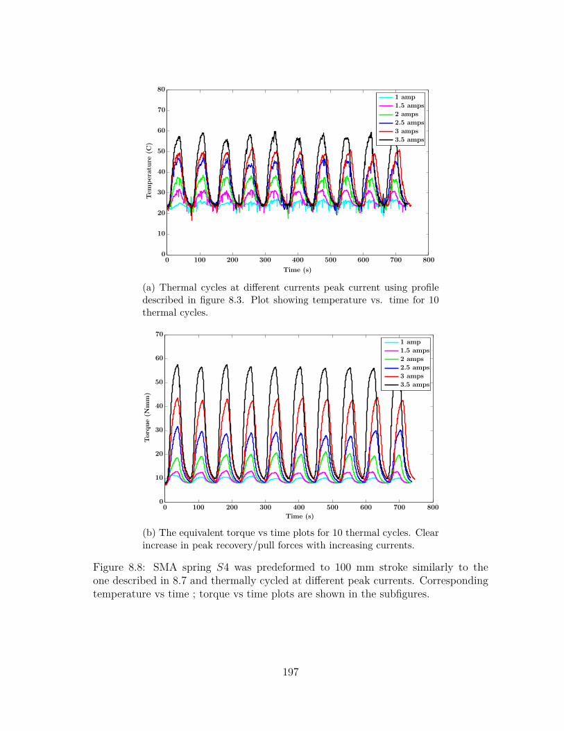
3.5 amps

3 amps

2.5 amps

2 amps

1.5 amps

1 amp

Tempera

ture

(C)

Time (s)

0 100 200 300 400 500 600 700 8000

10

20

30

40

50

60

70

80

(a) Thermal cycles at different currents peak current using profiledescribed in figure 8.3. Plot showing temperature vs. time for 10thermal cycles.

3.5 amps

3 amps

2.5 amps

2 amps

1.5 amps

1 amp

Torq

ue(N

mm)

Time (s)

0 100 200 300 400 500 600 700 8000

10

20

30

40

50

60

70

(b) The equivalent torque vs time plots for 10 thermal cycles. Clearincrease in peak recovery/pull forces with increasing currents.

Figure 8.8: SMA spring S4 was predeformed to 100 mm stroke similarly to theone described in 8.7 and thermally cycled at different peak currents. Correspondingtemperature vs time ; torque vs time plots are shown in the subfigures.

197

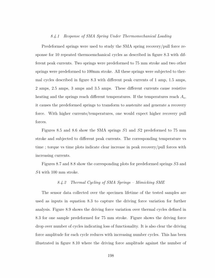
8.4.1 Response of SMA Spring Under Thermomechanical Loading

Predeformed springs were used to study the SMA spring recovery/pull force re-

sponse for 10 repeated thermoemchanical cycles as described in figure 8.3 with dif-

ferent peak currents. Two springs were predeformed to 75 mm stroke and two other

springs were predeformed to 100mm stroke. All these springs were subjected to ther-

mal cycles described in figure 8.3 with different peak currents of 1 amp, 1.5 amps,

2 amps, 2.5 amps, 3 amps and 3.5 amps. These different currents cause resistive

heating and the springs reach different temperatures. If the temperatures reach As,

it causes the predeformed springs to transform to austenite and generate a recovery

force. With higher currents/temperatures, one would expect higher recovery pull

forces.

Figures 8.5 and 8.6 show the SMA springs S1 and S2 predeformed to 75 mm

stroke and subjected to different peak currents. The corresponding temperature vs

time ; torque vs time plots indicate clear increase in peak recovery/pull forces with

increasing currents.

Figures 8.7 and 8.8 show the corresponding plots for predeformed springs S3 and

S4 with 100 mm stroke.

8.4.2 Thermal Cycling of SMA Springs – Mimicking SME

The sensor data collected over the specimen lifetime of the tested samples are

used as inputs in equation 8.3 to capture the driving force variation for further

analysis. Figure 8.9 shows the driving force variation over thermal cycles defined in

8.3 for one sample predeformed for 75 mm stroke. Figure shows the driving force

drop over number of cycles indicating loss of functionality. It is also clear the driving

force amplitude for each cycle reduces with increasing number cycles. This has been

illustrated in figure 8.10 where the driving force amplitude against the number of

198

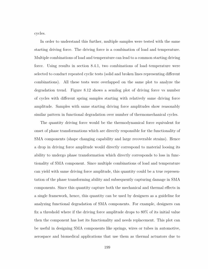
cycles.

In order to understand this further, multiple samples were tested with the same

starting driving force. The driving force is a combination of load and temperature.

Multiple combinations of load and temperature can lead to a common starting driving

force. Using results in section 8.4.1, two combinations of load–temperature were

selected to conduct repeated cyclic tests (solid and broken lines representing different

combinations). All these tests were overlapped on the same plot to analyze the

degradation trend. Figure 8.12 shows a semilog plot of driving force vs number

of cycles with different spring samples starting with relatively same driving force

amplitude. Samples with same starting driving force amplitudes show reasonably

similar pattern in functional degradation over number of thermomechanical cycles.

The quantity driving force would be the thermodynamical force equivalent for

onset of phase transformations which are directly responsible for the functionality of

SMA components (shape changing capability and large recoverable strains). Hence

a drop in driving force amplitude would directly correspond to material loosing its

ability to undergo phase transformation which directly corresponds to loss in func-

tionality of SMA component. Since multiple combinations of load and temperature

can yield with same driving force amplitude, this quantity could be a true represen-

tation of the phase transforming ability and subsequently capturing damage in SMA

components. Since this quantity capture both the mechanical and thermal effects in

a single framework, hence, this quantity can be used by designers as a guideline for

analyzing functional degradation of SMA components. For example, designers can

fix a threshold where if the driving force amplitude drops to 80% of its initial value

then the component has lost its functionality and needs replacement. This plot can

be useful in designing SMA components like springs, wires or tubes in automotive,

aerospace and biomedical applications that use them as thermal actuators due to

199

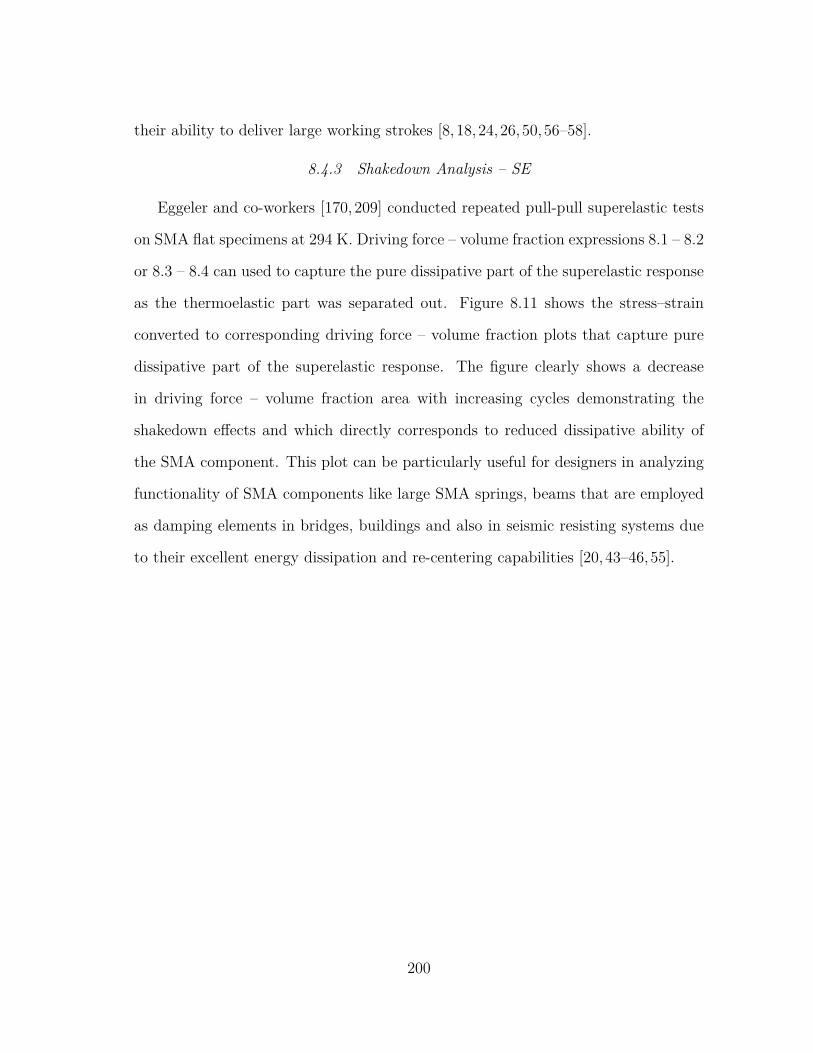
their ability to deliver large working strokes [8, 18,24,26,50,56–58].

8.4.3 Shakedown Analysis – SE

Eggeler and co-workers [170, 209] conducted repeated pull-pull superelastic tests

on SMA flat specimens at 294 K. Driving force – volume fraction expressions 8.1 – 8.2

or 8.3 – 8.4 can used to capture the pure dissipative part of the superelastic response

as the thermoelastic part was separated out. Figure 8.11 shows the stress–strain

converted to corresponding driving force – volume fraction plots that capture pure

dissipative part of the superelastic response. The figure clearly shows a decrease

in driving force – volume fraction area with increasing cycles demonstrating the

shakedown effects and which directly corresponds to reduced dissipative ability of

the SMA component. This plot can be particularly useful for designers in analyzing

functionality of SMA components like large SMA springs, beams that are employed

as damping elements in bridges, buildings and also in seismic resisting systems due

to their excellent energy dissipation and re-centering capabilities [20,43–46,55].

200

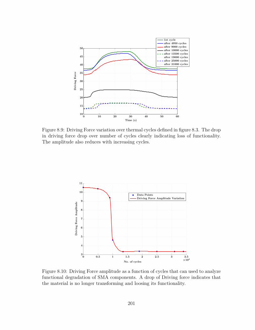
after 31000 cycles

after 25000 cycles

after 19000 cycles

after 13500 cycles

after 10000 cycles

after 9000 cycles

after 4950 cycles

1st cycle

DrivingForce

Time (s)

0 10 20 30 40 50 6010

15

20

25

30

35

40

45

50

Figure 8.9: Driving Force variation over thermal cycles defined in figure 8.3. The dropin driving force drop over number of cycles clearly indicating loss of functionality.The amplitude also reduces with increasing cycles.

Driving Force Amplitude Variation

Data Points

DrivingForceAmplitu

de

No. of cycles×104

0 0.5 1 1.5 2 2.5 3 3.53

4

5

6

7

8

9

10

11

Figure 8.10: Driving Force amplitude as a function of cycles that can used to analyzefunctional degradation of SMA components. A drop of Driving force indicates thatthe material is no longer transforming and loosing its functionality.

201

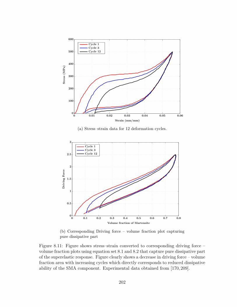
Cycle 12

Cycle 3

Cycle 1

Stress

(MPa)

Strain (mm/mm)

0 0.01 0.02 0.03 0.04 0.05 0.060

100

200

300

400

500

600

(a) Stress–strain data for 12 deformation cycles.

Cycle 12

Cycle 3

Cycle 1

DrivingForce

Volume fraction of Martensite

0 0.1 0.2 0.3 0.4 0.5 0.6 0.7 0.80

0.5

1

1.5

2

2.5

3

(b) Corresponding Driving force – volume fraction plot capturingpure dissipative part

Figure 8.11: Figure shows stress–strain converted to corresponding driving force –volume fraction plots using equation set 8.1 and 8.2 that capture pure dissipative partof the superelastic response. Figure clearly shows a decrease in driving force – volumefraction area with increasing cycles which directly corresponds to reduced dissipativeability of the SMA component. Experimental data obtained from [170,209].

202

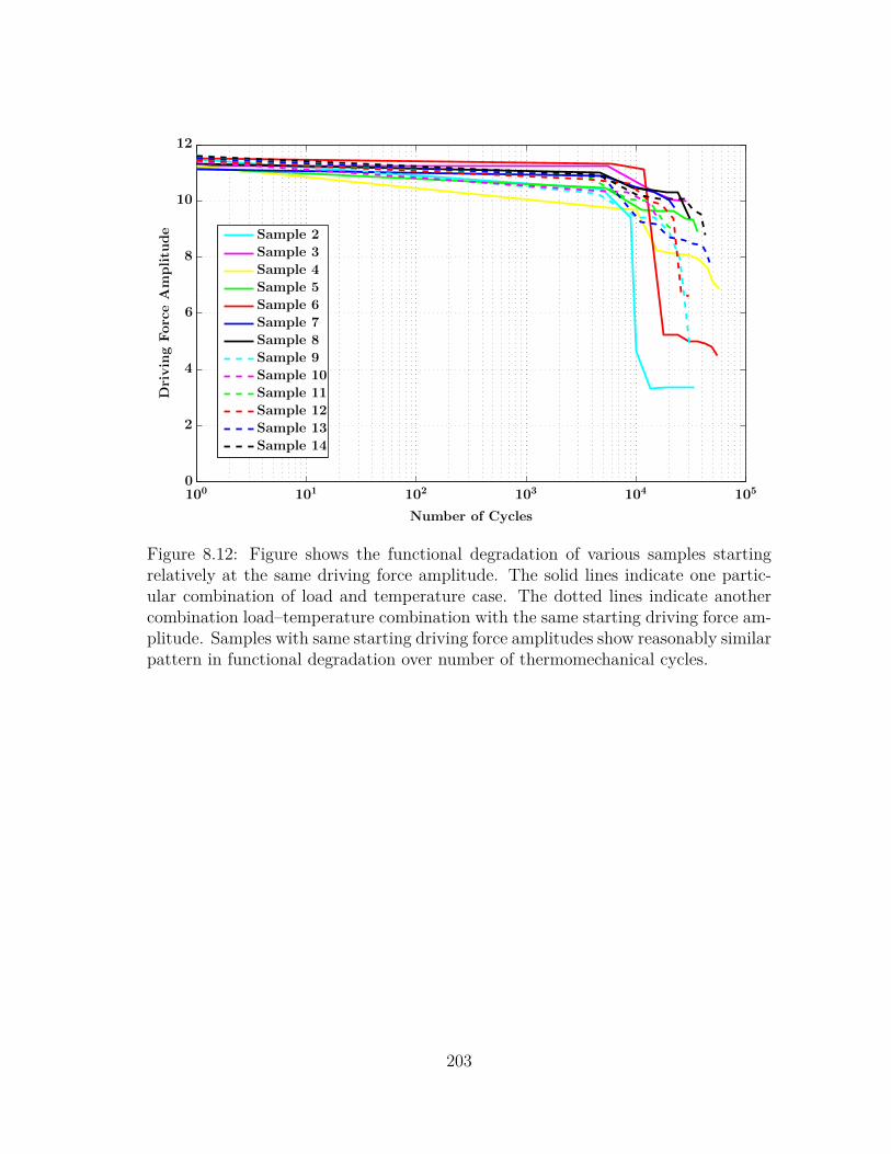
Sample 14

Sample 13

Sample 12

Sample 11

Sample 10

Sample 9

Sample 8

Sample 7

Sample 6

Sample 5

Sample 4

Sample 3

Sample 2

DrivingForceAmplitu

de

Number of Cycles

100 101 102 103 104 1050

2

4

6

8

10

12

Figure 8.12: Figure shows the functional degradation of various samples startingrelatively at the same driving force amplitude. The solid lines indicate one partic-ular combination of load and temperature case. The dotted lines indicate anothercombination load–temperature combination with the same starting driving force am-plitude. Samples with same starting driving force amplitudes show reasonably similarpattern in functional degradation over number of thermomechanical cycles.

203

9. SUMMARY AND CONCLUSIONS

9.1 Experiments on SMA Components Like Wires and Springs

• Thermally responsive SMA demonstrate interesting properties like superelas-

ticity (SE) where typically exhibit complex, nonlinear hysteretic response and

understanding their coupled thermomechanical responses is of critical impor-

tance for both researchers and application developers.

• SMA component responses are also affected by alloy composition, thermo-

mechanical processing history, changes in operating temperature and loading

rates.

• SMA components are tested under tension (wires) and torsional (wires and

springs) loading cases with the purpose of elucidating the internal loop re-

sponses both during loading and unloading. The effect of operating tempera-

ture is also investigated.

• These experiments also allows designers to get an insight into behavior of in-

ternal loops and analyze “return point memory (RPM) or sink point memory

(SPM)” aspects of the hysteretic response. RPM and SPM play an impor-

tant role in design as it provides important information on the ability of SMA

components to return back to its original unloading point upon completion

of a smaller hysteretic loop. SMA components showing a “good RPM/SPM

characteristics” is indicative of minimal residual/irreversible deformations af-

ter they were subjected to repeated complete or partial transformations during

applications.

• From an application standpoint, improved understanding of torsional responses

204

under partial or fully transformed cases with internal loops is of particular

importance as in many cases the entire response is utilized and only a partial

internal loop might be of significance

9.2 Conclusions for Two Species Thermodynamic Preisach Approach

• The goal of this work was in developing simple strength of materials based

models and tools for superelastic shape memory alloys (SMA) under tension,

torsion and bending loading conditions.

• The key idea here is of separating the thermoelastic and the dissipative part

of the hysteretic response using Gibbs potential and thermodynamic princi-

ples. The dissipative part of the response is accounted for using a discrete

Preisach model. Such an approach combines the physics and elegance of the

thermodynamic based approach with the algorithmic efficiency/simplicity of

the Preisach model and thus providing an effective way in predicting complex

hysteretic responses of SMA components like wires, beams and springs.

• The models are constructed based directly on experimentally measurable quan-

tities like torque and angle of twist, bending moment–curvature etc., rather

than solving for non-homogeneous shear stresses, strains directly across the

wire cross-section (especially for torsion and bending loading cases).

• The modeling approach can simultaneously include both thermal and mechan-

ical loading in the same framework with the capability of simulating both load

and displacement controlled experiments. Further, it allows for easy handling

of temperature variations observed in superelastic responses of SMA in addi-

tion to capturing complex internal loops. The model predictions were used

205

to predict SMA component responses at different operating temperatures or

twists.

• The use of a discrete Preisach model to capture the hysteretic part of the re-

sponse, one can do an approximate or a precise prediction by controlling the

use of number of Preisach elements and the input data used for model calibra-

tion. This way one doesn’t have to choose different functions for simulating

approximate or fine predictions and thereby saving computational time.

• The modeling approach can capture complex hysterestic responses with mul-

tiple internal loops with ease. In addition, it can capture temperature depen-

dence of responses with reasonable ease.

• An approximate response prediction could be beneficial for design purposes but

a more precise prediction is essential from the control systems standpoint. Pre-

diction of torque v/s angle of twist, moment verses curvature responses of SMA

components directly could greatly facilitate designers in designing components

for various engineering applications.

9.3 Conclusions for Three Species Thermodynamic Preisach Approach –

Capturing the Complete Torsional Response

• Extending the two species thermodynamic Preisach modeling approach, a model

to capture the complete torsional response of SMA components like wires, rods

and springs under both superelastic and shape memory effects is formulated

by combining thermodynamics principles along with discrete Preisach models.

• The key idea was in employing a three species Gibbs potential based formu-

lation to separate the thermoelastic response from its dissipative response for

both superelastic and twinning responses.

206

• The three species considered were austenite and two martensite variants under

clockwise and anticlockwise rotations thus enabling the prediction of responses

under both twisting directions.

• The proposed approach allows a greater connection with the thermodynamics of

the response and an added capability of simulating both load and displacement

controlled experiments in a single modeling framework.

• The model results were compared with experimental results for wires, bars and

springs showing a close match with an average error being < 15% for most

predictions.

9.4 Conclusions for Thermodynamic Force Approach for Analyzing Functional

Degradation of SMA Components

• With growing applications of SMA, the issue of material performance over

its designed life is of great concern to researchers lately. In order to analyze

SMA component performance under coupled thermomechanical effects, the-

ories considering both mechanical and thermal effects in a single framework

must be employed rather than modifying classical fatigue theories developed

for capturing pure mechanical loading effects. This approach can substitute

traditional fatigue theories like S–N or ε–N which primarily use mechanical

loading effects with temperature being an external control parameter.

• Using the modeling approach earlier, relationships for “thermodynamic driving

force for the phase transformation” and “extent of phase transformation” were

employed depending on the loading scenario. The thermodynamic driving force

is the equivalent of thermodynamical force for onset of phase transformation

effect which is directly responsible for the functionality of SMA component.

207

• A custom designed thermomechanical fatigue test rig was used perform user

defined repeated thermomechanical tests on SMA springs. The data from these

tests serve both to calibrate the model and establish “thermodynamic driving

force for the phase transformation” and “extent of phase transformation” rela-

tionships for SMA springs.

• A drop in driving force corresponds to material loosing functionality i.e material

is no longer transforming and performing its intended function. Hence, this

quantity can used as a parameter to analyze the functional degradation of SMA

components. Further, the volume fraction relationship can help us estimate the

extent of transformation (i.e amount of martensite) and a drop from its initial

value corresponds to portions (islands) of material not contributing into phase

transformation.

• A driving force – volume fraction plot that solely captures the dissipative part

of the response can also be used to analyze shakedown effects observed with typ-

ical superelastic responses associated with SMAs. This can substitute “Energy

approach” that develop relationships between dissipated energy verses num-

ber of cycles under stabilized superelastic effects by comparing SE behavior to

plastic shakedown.

• Designers can set appropriate driving force thresholds and use this approach

as a guideline for analyzing functional degradation of SMA components used

as thermal actuators or damping elements under both shape memory and su-

perelastic conditions.

208

10. RECOMMENDATIONS AND FUTURE WORK

The following topics need attention

10.1 Experimental Data on SMA Components

1. SMA demonstrate complex, nonlinear hysteretic responses under different load-

ing conditions. SMA components under pure bending with complex internal

loops is not well understood. SMAs tend to demonstrate tension–compression

asymmetry as the martensite variants under compression are different than

those formed under tension loading cases. For this, better understanding of

SMA component responses under compression and bending are important.

2. SMA components might be subjected to combined loading cases (like tension–

torsion). Internal loop responses under these combined loading cases must be

investigated for different SMA geometries (wires, tubes and rods) to better

understand their hysteretic responses. The present literature mainly focuses

on outer loop response for wires and tubes.

3. Many operating conditions can influence the mechanical response of SMA com-

ponents. Factors like material composition, operating temperature, type of

heating like air/water/oil/resistive (direct or indirect), rate of heating/cooling,

loading rates etc. could influence the overall hysteretic response. Researchers

might need prior information for the effect of such factors while designing SMA

components that are subjected to repeated loading and unloading cycles under

different application scenarios.

4. With regard to SMA springs in particular, additional geometry factors like

wire diameter, wire topology(tube/solid), spring index and coil angles also

209

affect their mechanical response. The role of these factors must be accounted

by designers and investigated in depth.

5. The prior thermomechanical processing history, heat treatment conditions like

shape setting temperature, heating/cooling rates, heating/cooling techniques

and soaking times also greatly affect the mechanical properties of SMAs. Ex-

perimental data investigating such factors would play a pivotal role in better

designing SMA components for engineering applications.

10.2 Extension of Thermodynamic Preisach Modeling Approach

1. The thermodynamic Preisach approach provides an effective way to capture

complex hysteretic responses with the effect the operating temperature being

easily accounted for in the model. Extending this modeling approach to cap-

ture combined loading effects, loading rates with complex internal loops could

greatly help designers investigate more complex design cases.

2. Finite element implementation of thermodynamic Preisach models under dif-

ferent loading cases with standard FE packages like ANSYS R© or ABAQUS R©

could help designers in analyzing SMA components under different loading

cases easily.

3. Integrating these models with commercial multibody dynamic packages like

MSC ADAMS R© could help designers simulates mechanisms that use SMA com-

ponents like wires, springs or rods. These simulations could give first hand

information on the feasibility studies of mechanisms.

10.3 Analyzing Functional Degradation of SMA Components

1. The issue of material performance over its designed life is of great concern to

researchers. As pointed out by Eggeler et al. [170], factors such as material

210

chemical composition, material impurity (i.e particle size distribution), type

of loading, applied load magnitude, extent of deformation or plateau strains,

processing conditions, defect accumulation, accumulated plastic deformation,

microstructure and operating temperature affect the fatigue life of SMA com-

ponents. Experiments investigating each of these factors could help designers

better predict the fatigue life of SMA components before catastrophic unin-

tended failures during service

2. Using these advanced experimental results, damage models that allow better

understanding of functional degradation of SMA components must be devel-

oped. These models could provide useful information to designers.

10.4 Designing SMA Compenents for Applications

Given the complex nature of SMA component response, designing SMA devices

for different application is not a trivial task. It is not possible to design SMA ac-

tuators without integrating SMA material behavior, mechanics (models) and design

(mechanisms) knowledge. Developing design philosophies that allow better under-

standing of their coupled thermomechanical responses is of critical importance for

both researchers and application developers. SMA components tend to show poor

fatigue life’s at strains > 3%, hence clever linear to rotary mechanisms, stroke am-

plification mechanisms could greatly help application developers.

211

REFERENCES

[1] D. Lagoudas, Shape memory alloys: modeling and engineering applications.

Springer– Verlag, Spring Street, New York, New York, 2008.

[2] P. Ghosh, A. Rao, and A. R. Srinivasa, “Design of multi-state and smart-bias

components using shape memory alloy and shape memory polymer compos-

ites,” Materials & Design, vol. 44, pp. 164 – 171, Feb 2013.

[3] L. A. Momoda, The future of engineering materials: Multifunction for per-

formance – Tailored structures, vol. 34. The Bridge : National Academy of

Engineering, 2004.

[4] H. Janocha, Adaptronics and smart structures: basics, materials, design, and

applications. Springer – Verlag Berlin Heidelberg, New York, 1999.

[5] T. Okano, “Molecular design of temperature-responsive polymers as intelligent

materials,” Responsive Gels: Volume Transitions II, vol. 110, pp. 179–197,

1993.

[6] J. Leng, X. Lan, Y. Liub, and S. Dua, “Shape memory polymers and their

composites: Stimulus methods and applications,” Progress in Materials Sci-

ence, vol. 56, no. 7, pp. 1077–1135, 2011.

[7] N. Ganesh, S. Maniprakash, L. Chandrasekaran, S. Srinivasan, and A. Srini-

vasa, “Design and development of a sun tracking mechanism using the direct

sma actuation,” Journal of Mechanical Design, vol. 133, p. 075001, 2011.

[8] D. Stoeckel, “Shape memory actuators for automotive applications,” Materials

& Design, vol. 11, no. 6, pp. 302–307, 1990.

212

[9] A. K. Noor, “Computational structures technology: leap frogging into the

twenty-first century,” Computers & Structures, vol. 73, no. 1, pp. 1–31, 1999.

[10] M. Naraghi, “Multifunctional materials - aero 606 course notes,” Fall 2012.

[11] J. Shaw, C. Churchill, and M. Iadicola, “Tips and tricks for characterizing

shape memory alloy wire: Part 1–differential scanning calorimetry and basic

phenomena,” Experimental Techniques, vol. 32, no. 5, pp. 55–62, 2008.

[12] A. S. F2004-05R10, “Standard test method for transformation temperature of

nickel-titanium alloys by thermal analysis,” ASTM International, West Con-

shohocken, PA, 2010.

[13] A. S. F. 2007e2, “Standard test method for tension testing of nickel-titanium

superelastic materials,” ASTM International, West Conshohocken, PA, 2007.

[14] W. Huang, Z. Ding, C. Wang, J. Wei, Y. Zhao, and H. Purnawali, “Shape

memory materials,” Materials Today, vol. 13, no. 7-8, pp. 54–61, 2010.

[15] J. McNichols and J. Cory, “Thermodynamics of nitinol,” Journal of Applied

Physics, vol. 61, no. 3, pp. 972–984, 1987.

[16] J. Van Humbeeck, “Shape memory alloys: a material and a technology,” Ad-

vanced Engineering Materials, vol. 3, no. 11, pp. 837–850, 2001.

[17] C. Wayman, “Shape memory and related phenomena,” Progress in Materials

Science (UK), vol. 36, pp. 203–224, 1992.

[18] D. Hartl and D. Lagoudas, “Aerospace applications of shape memory alloys,”

Proceedings of the Institution of Mechanical Engineers, Part G: Journal of

Aerospace Engineering, vol. 221, no. 4, p. 535, 2007.

[19] B. Sutapun, M. Tabib-Azar, and M. Huff, “Applications of shape memory

alloys in optics,” Applied Optics, vol. 37, no. 28, pp. 6811–6815, 1998.

213

[20] G. Song, N. Ma, and H. Li, “Applications of shape memory alloys in civil

structures,” Engineering Structures, vol. 28, no. 9, pp. 1266–1274, 2006.

[21] J. Van Humbeeck, “Non-medical applications of shape memory alloys,” Mate-

rials Science and Engineering: A, vol. 273, pp. 134–148, 1999.

[22] L. Machado and M. Savi, “Medical applications of shape memory alloys,”

Brazilian Journal of Medical and Biological Research, vol. 36, no. 6, pp. 683–

691, 2003.

[23] D. Lagoudas, O. K. Rediniotis, and M. M. Khan, “Applications of shape mem-

ory alloys to bioengineering and biomedical technology,” in Proceedings of the

4th International Workshop on Scattering Theory and Biomedical Applications,

Perdika, Greece,(Oct. 1999), pp. 195–207, 2000.

[24] T. Duerig, A. Pelton, and D. Stöckel, “An overview of nitinol medical applica-

tions,” Materials Science and Engineering: A, vol. 273, pp. 149–160, 1999.

[25] D. Mantovani, “Shape memory alloys: Properties and biomedical applications,”

JOM Journal of the Minerals, Metals and Materials Society, vol. 52, no. 10,

pp. 36–44, 2000.

[26] N. Morgan, “Medical shape memory alloy applications–the market and its

products,” Materials Science and Engineering: A, vol. 378, no. 1, pp. 16–23,

2004.

[27] F. El Feninat, G. Laroche, M. Fiset, and D. Mantovani, “Shape memory ma-

terials for biomedical applications,” Advanced Engineering Materials, vol. 4,

no. 3, pp. 91–104, 2002.

[28] R. Bogue, “Shape-memory materials : A review of technology and applica-

tions,” Assembly Automation, vol. 29, no. 3, pp. 214–219, 2009.

214

[29] F. Gil, J. Manero, and J. Planell, “Relevant aspects in the clinical applica-

tions of niti shape memory alloys,” Journal of Materials Science: Materials in

Medicine, vol. 7, no. 7, pp. 403–406, 1996.

[30] C. Manhartsberger and W. Seidenbusch, “Force delivery of ni-ti coil springs,”

American journal of orthodontics and dentofacial orthopedics, vol. 109, no. 1,

pp. 8–21, 1996.

[31] F. Miura, M. Mogi, Y. Ohura, and M. Karibe, “The superelastic japanese niti

alloy wire for use in orthodontics part iii. studies on the japanese niti alloy

coil springs,” American Journal of Orthodontics and Dentofacial Orthopedics,

vol. 94, no. 2, pp. 89–96, 1988.

[32] I. Spinella, E. Dragoni, and F. Stortiero, “Modeling, prototyping, and testing of

helical shape memory compression springs with hollow cross section,” Journal

of Mechanical Design, vol. 132, p. 061008, 2010.

[33] S. Drake, D. Wayne, J. Powers, and K. Asgar, “Mechanical properties of or-

thodontic wires in tension, bending, and torsion,” American Journal of Or-

thodontics, vol. 82, no. 3, pp. 206–210, 1982.

[34] F. Miura, M. Mogi, Y. Ohura, and H. Hamanaka, “The super-elastic property

of the japanese niti alloy wire for use in orthodontics,” American Journal of

Orthodontics and Dentofacial Orthopedics, vol. 90, no. 1, pp. 1–10, 1986.

[35] S. Kapila and R. Sachdeva, “Mechanical properties and clinical applications of

orthodontic wires,” American Journal of Orthodontics and Dentofacial Ortho-

pedics, vol. 96, no. 2, pp. 100–109, 1989.

[36] J. Von Fraunhofer, P. Bonds, and B. Johnson, “Force generation by orthodontic

coil springs.,” The Angle Orthodontist, vol. 63, no. 2, p. 145, 1993.

215

[37] R. Schneevoigt, A. Haase, V. Eckardt, W. Harzer, and C. Bourauel, “Labora-

tory analysis of superelastic niti compression springs,” Medical Engineering &

Physics, vol. 21, no. 2, pp. 119–125, 1999.

[38] S. Thompson, “An overview of nickel–titanium alloys used in dentistry,” Inter-

national Endodontic Journal, vol. 33, no. 4, pp. 297–310, 2000.

[39] A. Maganzini, A. Wong, and M. Ahmed, “Forces of various nickel titanium

closed coil springs,” The Angle Orthodontist, vol. 80, no. 1, pp. 182–187, 2010.

[40] L. Petrini and F. Migliavacca, “Biomedical applications of shape memory al-

loys,” Journal of Metallurgy, vol. 2011, 2011.

[41] J. Ryhänen, “Biocompatibility evolution of nickel-titanium shape memory al-

loy,” Academic Dissertation, Faculty of Medicine, University of Oulu, Oulu,

Finland.[Links], 1999.

[42] FDA, “United states food and drug administartion,” 2012. http://www.fda.

gov/.

[43] M. Speicher, D. Hodgson, R. DesRoches, and R. Leon, “Shape memory al-

loy tension/compression device for seismic retrofit of buildings,” Journal of

Materials Engineering and Performance, vol. 18, no. 5, pp. 746–753, 2009.

[44] S. Saadat, J. Salichs, M. Noori, Z. Hou, H. Davoodi, I. Bar-On, Y. Suzuki, and

A. Masuda, “An overview of vibration and seismic applications of niti shape

memory alloy,” Smart Materials and Structures, vol. 11, p. 218, 2002.

[45] R. DesRoches and B. Smith, “Shape memory alloys in seismic resistant design

and retrofit: a critical review of their potential and limitations,” Journal of

Earthquake Engineering, vol. 8, no. 3, pp. 415–429, 2004.

216

[46] J. Wilson and M. Wesolowsky, “Shape memory alloys for seismic response

modification: a state-of-the-art review,” Earthquake Spectra, vol. 21, p. 569,

2005.

[47] M. Alam, M. Youssef, and M. Nehdi, “Utilizing shape memory alloys to enhance

the performance and safety of civil infrastructure: a review,” Canadian Journal

of Civil Engineering, vol. 34, no. 9, pp. 1075–1086, 2007.

[48] L. Janke, C. Czaderski, M. Motavalli, and J. Ruth, “Applications of shape

memory alloys in civil engineering structures–overview, limits and new ideas,”

Materials and Structures, vol. 38, no. 5, pp. 578–592, 2005.

[49] Y. Mo, G. Song, and K. Otero, “Development and testing of a proof-of-concept

smart concrete structure,” Proceeding of Smart Structures Technologies and

Earthquake Engineering, 2004.

[50] I. Chopra, “Status of application of smart structures technology to rotorcraft

systems,” Journal of the American Helicopter Society, vol. 45, no. 4, pp. 228–

252, 2000.

[51] G. Brook, “Applications of titanium-nickel shape memory alloys,” Materials &

Design, vol. 4, no. 4, pp. 835–840, 1983.

[52] G. Song, D. Patil, C. Kocurek, and J. Bartos, “Applications of shape mem-

ory alloys in offshore oil and gas industry: a review,” Proc. Earth and Space

2010–Engineering, Science, Construction, and Operations in Challenging En-

vironments (Honolulu, HI, USA, 14–17 March 2010), vol. 366, 2010.

[53] R. DesRoches and M. Delemont, “Seismic retrofit of simply supported bridges

using shape memory alloys,” Engineering Structures, vol. 24, no. 3, pp. 325–

332, 2002.

217

[54] M. Indirli, M. G. Castellano, P. Clemente, and A. Martelli, “Demo-application

of shape memory alloy devices: the rehabilitation of the s. giorgio church bell

tower,” in SPIE’s 8th Annual International Symposium on Smart Structures

and Materials, pp. 262–272, International Society for Optics and Photonics,

2001.

[55] K. Williams, G. Chiu, and R. Bernhard, “Adaptive-passive absorbers using

shape-memory alloys,” Journal of Sound and Vibration, vol. 249, no. 5, pp. 835–

848, 2002.

[56] A. Bellini, M. Colli, and E. Dragoni, “Mechatronic design of a shape memory

alloy actuator for automotive tumble flaps: A case study,” Industrial Electron-

ics, IEEE Transactions, vol. 56, no. 7, pp. 2644–2656, 2009.

[57] R. Loewy, “Recent developments in smart structures with aeronautical appli-

cations,” Smart Materials and Structures, vol. 6, p. R11, 1997.

[58] A. Razov and A. Cherniavsky, “Applications of shape memory alloys in space

engineering: past and future,” European Space Agency - Publications ESA SP,

vol. 438, pp. 141–146, 1999.

[59] A. Khandelwal and V. Buravalla, “Models for shape memory alloy behavior:

An overview of modeling approaches,” The International Journal of Structural

Changes in Solids, vol. 1, no. 1, pp. 111–148, 2011.

[60] R. Abeyaratne and J. Knowles, “On the driving traction acting on a surface

of strain discontinuity in a continuum,” Journal of the Mechanics and Physics

of Solids, vol. 38, no. 3, pp. 345–360, 1990.

[61] J. Ball and R. James, “Fine phase mixtures as minimizers of energy,” Archive

for Rational Mechanics and Analysis, vol. 100, no. 1, pp. 13–52, 1987.

218

[62] F. Falk, “Model free energy, mechanics, and thermodynamics of shape memory

alloys,” Acta Metallurgica, vol. 28, no. 12, pp. 1773–1780, 1980.

[63] F. Falk, “One-dimensional model of shape memory alloys,” Archives of Me-

chanics, vol. 35, no. 1, pp. 63–84, 1983.

[64] S. Doraiswamy, A. Rao, and A. Srinivasa, “Combining thermodynamic princi-

ples with preisach models for superelastic shape memory alloy wires,” Smart

Materials and Structures, vol. 20, p. 085032, 2011.

[65] K. Rajagopal and A. Srinivasa, “On the thermomechanics of shape memory

wires,” Zeitschrift fur Angewandte Mathematik und Physik, vol. 50, pp. 459–

496, 1999.

[66] K. Tanaka and S. Nagaki, “A thermomechanical description of materials with

internal variables in the process of phase transitions,” Archive of Applied Me-

chanics, vol. 51, no. 5, pp. 287–299, 1982.

[67] K. Tanaka and R. Iwasaki, “A phenomenological theory of transformation su-

perplasticity,” Engineering Fracture Mechanics, vol. 21, no. 4, pp. 709–720,

1985.

[68] K. Tanaka, “A thermomechanical sketch of shape memory effect: one-

dimensional tensile behavior,” Res Mechanica, vol. 2, no. 3, pp. 59–72, 1986.

[69] K. Tanaka, T. Hayashi, Y. Itoh, and H. Tobushi, “Analysis of thermomechan-

ical behavior of shape memory alloys,” Mechanics of Materials, vol. 13, no. 3,

pp. 207–215, 1992.

[70] Y. Sato and K. Tanaka, “Estimation of energy dissipation in alloys due to

stress-induced martensitic transformation,” Res Mech., vol. 23, no. 4, pp. 381–

393, 1988.

219

[71] V. Buravalla and A. Khandelwal, “Phenomenological modeling of shape mem-

ory alloys,” in AIP Conference Proceedings, vol. 1029, p. 104, 2008.

[72] C. Liang and C. Rogers, “One-dimensional thermomechanical constitutive re-

lations for shape memory materials,” Journal of Intelligent Material Systems

and Structures, vol. 1, no. 2, pp. 207–234, 1990.

[73] C. Liang and C. Rogers, “A multi-dimensional constitutive model for shape

memory alloys,” Journal of Engineering Mathematics, vol. 26, no. 3, pp. 429–

443, 1992.

[74] L. Brinson, “One-dimensional constitutive behavior of shape memory alloys:

thermomechanical derivation with non-constant material functions and rede-

fined martensite internal variable,” Journal of Intelligent Material Systems and

Structures, vol. 4, no. 2, pp. 229–242, 1993.

[75] A. Bekker and L. Brinson, “Phase diagram based description of the hysteresis

behavior of shape memory alloys,” Acta Materialia, vol. 46, no. 10, pp. 3649–

3665, 1998.

[76] A. Rao and A. Srinivasa, “A three species model for simulating torsional re-

sponse of shape memory alloy components using thermodynamic principles and

discrete preisach models,” Mathematics and Mechanics of Solids, vol. (In Press,

2014).

[77] D. Lagoudas, J. Boyd, and Z. Bo, “Micromechanics of active composites with

sma fibers,” Journal of Engineering Materials and Technology, vol. 116, p. 337,

1994.

[78] R. Abeyaratne and J. Knowles, “A continuum model of a thermoelastic solid

capable of undergoing phase transitions,” Journal of the Mechanics and Physics

220

of Solids, vol. 41, no. 3, pp. 541–571, 1993.

[79] F. Auricchio and J. Lubliner, “A uniaxial model for shape-memory alloys,”

International Journal of Solids and Structures, vol. 34, no. 27, pp. 3601–3618,

1997.

[80] F. Auricchio, R. Taylor, and J. Lubliner, “Shape-memory alloys: macromod-

elling and numerical simulations of the superelastic behavior,” Computer Meth-

ods in Applied Mechanics and Engineering, vol. 146, no. 3, pp. 281–312, 1997.

[81] B. Raniecki, C. Lexcellent, and K. Tanaka, “Thermodynamic models of pseu-

doelastic behaviour of shape memory alloys,” Archiv of Mechanics, Archiwum

Mechaniki Stosowanej, vol. 44, pp. 261–284, 1992.

[82] B. Raniecki and K. Tanaka, “On the thermodynamic driving force for coherent

phase transformations,” International Journal of Engineering Science, vol. 32,

no. 12, pp. 1845–1858, 1994.

[83] S. Leclercq and C. Lexcellent, “A general macroscopic description of the ther-

momechanical behavior of shape memory alloys,” Journal of the Mechanics

and Physics of Solids, vol. 44, no. 6, pp. 953–957, 1996.

[84] J. Boyd and D. Lagoudas, “A thermodynamical constitutive model for shape

memory materials. part i. the monolithic shape memory alloy,” International

Journal of Plasticity, vol. 12, no. 6, pp. 805–842, 1996.

[85] M. Qidwai and D. Lagoudas, “Numerical implementation of a shape mem-

ory alloy thermomechanical constitutive model using return mapping algo-

rithms,” International Journal Numerical Methods in Engineering, vol. 47,

no. 6, pp. 1123–1168, 2000.

221

[86] R. Mirzaeifar, R. DesRoches, and A. Yavari, “Analysis of the rate-dependent

coupled thermo-mechanical response of shape memory alloy bars and wires in

tension,” Continuum Mechanics and Thermodynamics, pp. 1–23, 2011.

[87] Z. Bo, Consitutive Modeling of shape memory alloys. PhD thesis, Texas A&M

University, College Station, TX, 1996.

[88] Z. Bo and D. Lagoudas, “Thermomechanical modeling of polycrystalline smas

under cyclic loading, part i: Theoretical derivations,” International Journal of

Engineering Science, vol. 37, no. 9, pp. 1089–1140, 1999.

[89] M. Qidwai and D. Lagoudas, “On thermomechanics and transformation sur-

faces of polycrystalline niti shape memory alloy material,” International Jour-

nal of Plasticity, vol. 16, no. 10, pp. 1309–1343, 2000.

[90] A. Rao and A. Srinivasa, “A two species thermodynamic preisach model for the

torsional response of shape memory alloy wires and springs under superelas-

tic conditions,” International Journal of Solids and Structures, vol. 50, no. 6,

pp. 887–898, 2013.

[91] X. Tan and J. Baras, “Modeling and control of hysteresis in magnetostrictive

actuators,” Automatica, vol. 40, no. 9, pp. 1469–1480, 2004.

[92] S. Dutta and F. Ghorbel, “Differential hysteresis modeling of a shape memory

alloy wire actuator,” Mechatronics, IEEE/ASME Transactions, vol. 10, no. 2,

pp. 189–197, 2005.

[93] D. Hughes and J. Wen, “Preisach modeling of piezoceramic and shape memory

alloy hysteresis,” Smart Materials and Structures, vol. 6, p. 287, 1997.

[94] M. Khan and D. Lagoudas, “Modeling of shape memory alloy pseudoelastic

spring elements using preisach model for passive vibration isolation,” in Pro-

222

ceedings of SPIE, vol. 4693, pp. 336–47, 2002.

[95] A. Ktena, D. Fotiadis, P. Spanos, and C. Massalas, “A preisach model iden-

tification procedure and simulation of hysteresis in ferromagnets and shape-

memory alloys,” Physica B: Condensed Matter, vol. 306, no. 1, pp. 84–90,

2001.

[96] A. Ktena, D. Fotiadis, P. Spanos, A. Berger, and C. Massalas, “Identification

of 1d and 2d preisach models for ferromagnets and shape memory alloys,”

International Journal of Engineering Science, vol. 40, no. 20, pp. 2235–2247,

2002.

[97] J. Ortín, “Preisach modeling of hysteresis for a pseudoelastic cu-zn-al single

crystal,” Journal of Applied Physics, vol. 71, no. 3, pp. 1454–1461, 1992.

[98] G. Webb, D. Lagoudas, and A. Kurdila, “Hysteresis modeling of sma actu-

ators for control applications,” Journal of Intelligent Material Systems and

Structures, vol. 9, no. 6, p. 432, 1998.

[99] Z. Bo and D. Lagoudas, “Thermomechanical modeling of polycrystalline smas

under cyclic loading, part iv: Modeling of minor hysteresis loops,” International

Journal of Engineering Science, vol. 37, no. 9, pp. 1205–1249, 1999.

[100] F. Falk, “Ginzburg-landau theory and solitary waves in shape memory alloys,”

Zeitschrift für Physik B Condensed Matter, vol. 54, no. 2, pp. 159–167, 1984.

[101] F. Preisach, “Über die magnetische nachwirkung,” Zeitschrift für Physik A

Hadrons and Nuclei, vol. 94, no. 5, pp. 277–302, 1935.

[102] I. Mayergoyz and S. O. service), Mathematical models of hysteresis and their

applications. Elsevier, Boston, Massachusetts, 2003.

223

[103] I. Mayergoyz, “Mathematical models of hysteresis,” Magnetics, IEEE Trans-

actions on, vol. 22, no. 5, pp. 603–608, 1986.

[104] S. Doraiswamy, “Discrete preisach model for the superelastic response of shape

memory alloys,” Master’s thesis, Texas A&M University, 2010.

[105] J. Shaw, “Simulations of localized thermomechanical behavior in a niti shape

memory alloy,” International Journal of Plasticity, vol. 16, no. 5, pp. 541–562,

2000.

[106] H. Tripolt, C. Burstone, P. Bantleon, and W. Manschiebel, “Force characteris-

tics of nickel-titanium tension coil springs,” American Journal of Orthodontics

and Dentofacial Orthopedics, vol. 115, no. 5, pp. 498–507, 1999.

[107] H. Tobushi and K. Tanaka, “Deformation of a shape memory alloy helical

spring (analysis based on stress-strain-temperature relation),” JSME Interna-

tional Journal. Series 1, Solid Mechanics, Strength of Materials, vol. 34, no. 1,

pp. 83–89, 1991.

[108] R. Mirzaeifar, R. DesRoches, and A. Yavari, “A combined analytical, numer-

ical, and experimental study of shape-memory-alloy helical springs,” Interna-

tional Journal of Solids and Structures, 2010.

[109] R. Mirzaeifar, R. DesRoches, and A. Yavari, “Exact solutions for pure torsion

of shape memory alloy circular bars,” Mechanics of Materials, vol. 42, no. 8,

pp. 797–806, 2010.

[110] C. Chapman, A. Eshghinejad, and M. Elahinia, “Torsional behavior of niti

wires and tubes: Modeling and experimentation,” Journal of Intelligent Mate-

rial Systems and Structures, vol. 22, no. 11, pp. 1239–1248, 2011.

224

[111] C. Liang and C. Rogers, “Design of shape memory alloy springs with applica-

tions in vibration control,” Journal of Vibration and Acoustics, vol. 115, p. 129,

1993.

[112] C. Liang and C. Rogers, “Design of shape memory alloy springs with applica-

tions in vibration control,” Journal of Intelligent Material Systems and Struc-

tures, vol. 8, no. 4, pp. 314–322, 1997.

[113] R. Aguiar, M. Savi, and P. Pacheco, “Experimental and numerical investiga-

tions of shape memory alloy helical springs,” Smart Materials and Structures,

vol. 19, p. 025008, 2010.

[114] A. Paiva, M. Savi, A. Braga, and P. Pacheco, “A constitutive model for shape

memory alloys considering tensile-compressive asymmetry and plasticity,” In-

ternational Journal of Solids and Structures, vol. 42, no. 11-12, pp. 3439–3457,

2005.

[115] M. Savi and A. Paiva, “Describing internal subloops due to incomplete phase

transformations in shape memory alloys,” Archive of Applied Mechanics,

vol. 74, no. 9, pp. 637–647, 2005.

[116] O. Doaré, A. Sbarra, C. Touzé, M. Moussa, and Z. Moumni, “Experimental

analysis of the quasistatic and dynamic torsional behaviour of shape memory

alloys,” International Journal of Solids and Structures, 2011.

[117] W. Brantley, W. Augat, C. Myers, and R. Winders, “Bending deformation

studies of orthodontic wires,” Journal of Dental Research, vol. 57, no. 4, p. 609,

1978.

[118] I. Lopez, J. Goldberg, and C. Burstone, “Bending characteristics of nitinol

wire.,” American Journal of Orthodontics, vol. 75, no. 5, p. 569, 1979.

225

[119] A. Goldberg, J. Morton, and C. Burstone, “The flexure modulus of elasticity

of orthodontic wires,” Journal of Dental Research, vol. 62, no. 7, pp. 856–858,

1983.

[120] M. Asgharnia and W. Brantley, “Comparison of bending and tension tests for

orthodontic wires,” American Journal of Orthodontics, vol. 89, no. 3, pp. 228–

236, 1986.

[121] H. Walia, W. Brantley, and H. Gerstein, “An initial investigation of the bending

and torsional properties of nitinol root canal files,” Journal of Endodontics,

vol. 14, no. 7, pp. 346–351, 1988.

[122] S. Khier, W. Brantley, and R. Fournelle, “Bending properties of superelastic

and nonsuperelastic nickel-titanium orthodontic wires,” American Journal of

Orthodontics and Dentofacial Orthopedics, vol. 99, no. 4, pp. 310–318, 1991.

[123] R. Tonner and N. Waters, “The characteristics of super-elastic ni-ti wires in

three-point bending. part l: The effect of temperature,” The European Journal

of Orthodontics, vol. 16, no. 5, pp. 409–419, 1994.

[124] J. Oltjen, M. Duncanson Jr, J. Ghosh, R. Nanda, and G. Frans Currier,

“Stiffness-deflection behavior of selected orthodontic wires,” The Angle Or-

thodontist, vol. 67, no. 3, pp. 209–218, 1997.

[125] H. Nakano, K. Satoh, R. Norris, T. Jin, T. Kamegai, F. Ishikawa, and H. Kat-

sura, “Mechanical properties of several nickel-titanium alloy wires in three-

point bending tests,” American Journal of Orthodontics and Dentofacial Or-

thopedics, vol. 115, no. 4, pp. 390–395, 1999.

[126] P. Wilkinson, P. Dysart, J. Hood, and G. Herbison, “Load-deflection character-

istics of superelastic nickel-titanium orthodontic wires,” American Journal of

226

Orthodontics and Dentofacial Orthopedics, vol. 121, no. 5, pp. 483–495, 2002.

[127] F. Parvizi and W. Rock, “The load/deflection characteristics of thermally acti-

vated orthodontic archwires,” The European Journal of Orthodontics, vol. 25,

no. 4, pp. 417–421, 2003.

[128] P. Garrec and L. Jordan, “Stiffness in bending of a superelastic ni-ti orthodon-

tic wire as a function of cross-sectional dimension,” The Angle Orthodontist,

vol. 74, no. 5, pp. 691–696, 2004.

[129] M. Sakima, M. Dalstra, and B. Melsen, “How does temperature influence the

properties of rectangular nickel–titanium wires?,” The European Journal of

Orthodontics, vol. 28, no. 3, pp. 282–291, 2006.

[130] T. Bartzela, C. Senn, and A. Wichelhaus, “Load-deflection characteristics of

superelastic nickel-titanium wires,” The Angle Orthodontist, vol. 77, no. 6,

pp. 991–998, 2007.

[131] B. Berg, “Bending of superelastic wires, part i: Experimental aspects,” Journal

of Applied Mechanics, vol. 62, p. 459, 1995.

[132] J. Rejzner, C. Lexcellent, and B. Raniecki, “Pseudoelastic behaviour of shape

memory alloy beams under pure bending: experiments and modelling,” Inter-

national Journal of Mechanical Sciences, vol. 44, no. 4, pp. 665–686, 2002.

[133] A. Wick, O. Vöhringer, and A. Pelton, “The bending behavior of niti,” Journal

de Physique. IV, vol. 5, no. 8, pp. C8–789, 1995.

[134] B. Raniecki, J. Rejzner, and C. Lexcellent, “Anatomization of hysteresis loops

in pure bending of ideal pseudoelastic sma beams,” International Journal of

Mechanical Sciences, vol. 43, no. 5, pp. 1339–1368, 2001.

227

[135] S. Marfia, E. Sacco, and J. Reddy, “Superelastic and shape memory effects in

laminated shape-memory-alloy beams,” AIAA journal, vol. 41, no. 1, pp. 100–

109, 2003.

[136] T. Atanacković and M. Achenbach, “Moment – curvature relations for a pseu-

doelastic beam,” Continuum Mechanics and Thermodynamics, vol. 1, no. 1,

pp. 73–80, 1989.

[137] A. Eshghinejad and M. Elahinia, “Exact solution for bending of shape memory

alloy superelastic beams,” ASME Conference Proceedings, vol. 2011, no. 54723,

pp. 345–352, 2011.

[138] R. Mirzaeifar, R. DesRoches, A. Yavari, and K. Gall, “A closed form solution

for superelastic shape memory alloy beams subjected to bending,” in Proceed-

ings of SPIE, vol. 8342, p. 83421O, 2012.

[139] K. Rajagopal and A. Srinivasa, “On the bending of shape memory wires,”

Mechanics of Advanced Materials and Structures, vol. 12, no. 5, pp. 319–330,

2005.

[140] F. Auricchio and E. Sacco, “Thermomechanical modelling of a superelastic

shape-memory wire under cyclic stretching–bending loadings,” International

Journal of Solids and Structures, vol. 38, no. 34, pp. 6123–6145, 2001.

[141] P. Purohit and K. Bhattacharya, “On beams made of a phase-transforming ma-

terial,” International Journal of Solids and Structures, vol. 39, no. 13, pp. 3907–

3929, 2002.

[142] J. A.Shaw and S. Kyriakides, “Thermomechanical aspects of niti,” Journal of

the Mechanics and Physics of Solids, vol. 43, no. 8, pp. 1243–1281, 1995.

228

[143] S.Miyazaki, K.Otsuka, and Y.Suzuki, “Transformation pseudoelasticity and

deformation behaviour in a t-50.6 at.-% ni alloy,” Scripta METALLURGICA,

vol. 15, pp. 287–292, 1981.

[144] Y. Huo and I. Müller, “Nonequilibrium thermodynamics of pseudoelasticity,”

Continuum Mechanics and Thermodynamics, vol. 5, no. 3, pp. 163–204, 1993.

[145] C. Lexcellent and H. Tobushi, “Internal loops in pseudoelastic behaviour of

ti-ni shape memory alloys: Experiment and modelling,” Meccanica, vol. 30,

no. 5, pp. 459–466, 1995.

[146] Y. Liu, Z. Xie, J. Van Humbeeck, and L. Delaey, “Asymmetry of stress–strain

curves under tension and compression for niti shape memory alloys,” Acta

Materialia, vol. 46, no. 12, pp. 4325–4338, 1998.

[147] I. Müller and S. Seelecke, “Thermodynamic aspects of shape memory alloys,”

Mathematical and Computer Modelling, vol. 34, no. 12, pp. 1307–1355, 2001.

[148] M. Dolce and D. Cardone, “Mechanical behaviour of shape memory alloys for

seismic applications 2. austenite niti wires subjected to tension,” International

Journal of Mechanical Sciences, vol. 43, no. 11, pp. 2657–2677, 2001.

[149] J. Ortín and L. Delaey, “Hysteresis in shape memory alloys,” International

Journal of Non-Linear Mechanics, vol. 37, no. 8, pp. 1275–1281, 2002.

[150] Y. Matsuzaki, K. Funami, and H. Naito, “Inner loops of pseudoelastic hys-

teresis of shape memory alloys: Preisach approach,” in SPIE’s 9th Annual

International Symposium on Smart Structures and Materials, pp. 355–364, In-

ternational Society for Optics and Photonics, 2002.

[151] R. DesRoches, J. McCormick, and M. Delemont, “Cyclic properties of supere-

lastic shape memory alloy wires and bars,” Journal of Structural Engineering,

229

vol. 130, no. 1, pp. 38–46, 2003.

[152] T. Ikeda, F. A. Nae, H. Naito, and Y. Matsuzaki, “Constitutive model of shape

memory alloys for unidirectional loading considering inner hysteresis loops,”

Smart materials and Structures, vol. 13, no. 4, p. 916, 2004.

[153] M. K. Kumar, K. Sakthivel, S. Sivakumar, C. L. Rao, and A. Srinivasa, “Ther-

momechanical modeling of hysteresis in smas using the dissipationless reference

response,” Smart Materials and Structures, vol. 16, no. 1, p. S28, 2007.

[154] O. Heintze and S. Seelecke, “A coupled thermomechanical model for shape

memory alloys–from single crystal to polycrystal,” Materials Science and En-

gineering: A, vol. 481, pp. 389–394, 2008.

[155] I. Müller, “Pseudo-elastic hysteresis in shape memory alloys,” Physica B: Con-

densed Matter, vol. 407, no. 9, pp. 1314–1315, 2012.

[156] K. Otsuka and X. Ren, “Physical metallurgy of ti–ni-based shape memory

alloys,” Progress in Materials Science, vol. 50, no. 5, pp. 511–678, 2005.

[157] A. Rao, “Modeling bending response of shape memory alloy wires/beams under

superelastic conditions – a two species thermodynamic preisach approach,” The

International Journal of Structural Changes in Solids, vol. 5, pp. 1–26, 2013.

[158] A. Green and P. Naghdi, “On thermodynamics and the nature of the second

law,” Proceedings of the Royal Society of London. A. Mathematical and Physical

Sciences, vol. 357, no. 1690, pp. 253–270, 1977.

[159] A. Nallathambi, S. Doraiswamy, A. Chandrasekar, and S. Srinivasan, “A 3-

species model for shape memory alloys,” The International Journal of Struc-

tural Changes in Solids, vol. 1, no. 1, pp. 149–170, 2011.

230

[160] H. Callen, Thermodynamics and an Introduction to Thermostatistics. John

Wiley & Sons, Hoboken, New Jersey, 2nd edition ed., 1985.

[161] Z. Bo, D. C. Lagoudas, and D. Miller, “Material characterization of sma actua-

tors under nonproportional thermomechanical loading,” Journal of Engineering

Materials and Technology, vol. 121, no. 1, pp. 75–85, 1999.

[162] H. Prahlad and I. Chopra, “Modeling and experimental characterization of sma

torsional actuators,” Journal of Intelligent Material Systems and Structures,

vol. 18, no. 1, pp. 29–38, 2007.

[163] A. Baz, K. Iman, and J. McCoy, “Active control of flexible space structures

using the nitinol shape memory actuators,” tech. rep., DTIC Document, 1987.

[164] A. Keefe and G. Carman, “Thermomechanical characterization of shape mem-

ory alloy torque tube actuators,” Smart Materials and Structures, vol. 9, p. 665,

2000.

[165] I. Spinella and E. Dragoni, “Analysis and design of hollow helical springs for

shape memory actuators,” Journal of Intelligent Material Systems and Struc-

tures, vol. 21, no. 2, pp. 185–199, 2010.

[166] C. Chapman, Z. Karbaschi, M. Elahinia, and M. Tabesh, “Torsional behavior

of shape memory alloy tubes for biomedical applications,” ASME, 2010.

[167] M. Takahashi, “Shape memory alloy actuator,” Sept. 7 2010. US Patent

7,788,921.

[168] A. Spaggiari, I. Spinella, and E. Dragoni, “Design of a telescopic linear actuator

based on hollow shape memory springs,” Journal of Materials Engineering and

Performance, vol. 20, no. 4, pp. 489–496, 2011.

231

[169] E. Khan and S. Srinivasan, “A new approach to the design of helical shape

memory alloy spring actuators,” Smart Materials Research, vol. 2011, 2011.

[170] G. Eggeler, E. Hornbogen, A. Yawny, A. Heckmann, and M. Wagner, “Struc-

tural and functional fatigue of niti shape memory alloys,” Materials Science

and Engineering: A, vol. 378, no. 1, pp. 24–33, 2004.

[171] N. Morgan and C. Friend, “A review of shape memory stability in niti alloys,”

Le Journal de Physique IV, vol. 11, no. PR8, 2001.

[172] E. Hornbogen, “Review thermomechanical fatigue of shape memory alloys,”

Journal of Materials Science, vol. 39, no. 2, pp. 385–399, 2004.

[173] S. Robertson, A. Pelton, and R. Ritchie, “Mechanical fatigue and fracture of

nitinol,” International Materials Reviews, vol. 57, no. 1, pp. 1–37, 2012.

[174] H. Tobushi, T. Hachisuka, S. Yamada, and P. Lin, “Rotating bending fatigue

of a tini shape memory alloy wire,” Mechanics of Materials, vol. 26, no. 1,

pp. 35–42, 1997.

[175] M. de Azevedo Bahia, R. Fonseca Dias, and V. Buono, “The influence of high

amplitude cyclic straining on the behaviour of superelastic niti,” International

Journal of Fatigue, vol. 28, no. 9, pp. 1087–1091, 2006.

[176] S. Miyazaki, K. Mizukoshi, T. Ueki, T. Sakuma, and Y. Liu, “Fatigue life of

ti–50 at.% ni and ti–40ni–10cu (at.%) shape memory alloy wires,” Materials

Science and Engineering: A, vol. 273, pp. 658–663, 1999.

[177] H. Tobushi, Y. Ohashi, T. Hori, and H. Yamamoto, “Cyclic deformation of tini

shape-memory alloy helical spring,” Experimental Mechanics, vol. 32, no. 4,

pp. 304–308, 1992.

232

[178] H. Tamura, K. Mitose, and Y. Suzuki, “Fatigue properties of ti-ni shape mem-

ory alloy springs,” Journal de Physique. IV, vol. 5, no. 8, pp. C8–617, 1995.

[179] C. Grossmann, J. Frenzel, V. Sampath, T. Depka, A. Oppenkowski, C. Somsen,

K. Neuking, W. Theisen, and G. Eggeler, “Processing and property assessment

of niti and niticu shape memory actuator springs,” Materialwissenschaft und

Werkstofftechnik, vol. 39, no. 8, pp. 499–510, 2008.

[180] C. Grossmann, J. Frenzel, V. Sampath, T. Depka, and G. Eggeler, “Elementary

transformation and deformation processes and the cyclic stability of niti and

niticu shape memory spring actuators,” Metallurgical and Materials Transac-

tions A, vol. 40, no. 11, pp. 2530–2544, 2009.

[181] K. Ramaiah, C. Saikrishna, V. Ranganath, V. Buravalla, and S. Bhaumik,

“Fracture of thermally activated niti shape memory alloy wires,” Materials

Science and Engineering: A, vol. 528, no. 16, pp. 5502–5510, 2011.

[182] S. Miyazaki, “Thermal and stress cycling effects and fatigue properties of ni–ti

alloys,” Butterworth-Heinemann, Engineering Aspects of Shape Memory Al-

loys(UK), pp. 394–413, 1990.

[183] K. Melton and O. Mercier, “Fatigue of niti thermoelastic martensites,” Acta

Metallurgica, vol. 27, no. 1, pp. 137–144, 1979.

[184] G. Mammano and E. Dragoni, “Functional fatigue of shape memory wires

under constant-stress and constant-strain loading conditions,” Procedia Engi-

neering, vol. 10, pp. 3692–3707, 2011.

[185] G. Kang, Q. Kan, C. Yu, D. Song, and Y. Liu, “Whole life transformation

ratchetting and fatigue of superelastic niti alloy under uniaxial stress-controlled

233

cyclic loading,” Materials Science and Engineering: A, vol. 535, pp. 228–234,

2012.

[186] T. Ataalla, M. Leary, and A. Subic, “Functional fatigue of shape memory

alloys,” Sustainable Automotive Technologies 2012, pp. 39–43, 2012.

[187] G. Scirè Mammano and E. Dragoni, “Functional fatigue of ni-ti shape memory

wires under various loading conditions,” International Journal of Fatigue, 2012.

[188] O. Bertacchini, D. Lagoudas, F. Calkins, and J. Mabe, “Thermomechani-

cal cyclic loading and fatigue life characterization of nickel rich niti shape-

memory alloy actuators,” in The 15th International Symposium on: Smart

Structures and Materials & Nondestructive Evaluation and Health Monitoring,

pp. 692916–692916, International Society for Optics and Photonics, 2008.

[189] O. Bertacchini, D. Lagoudas, and E. Patoor, “Thermomechanical transfor-

mation fatigue of tinicu sma actuators under a corrosive environment–part

i: Experimental results,” International Journal of Fatigue, vol. 31, no. 10,

pp. 1571–1578, 2009.

[190] D. Lagoudas, D. Miller, L. Rong, and P. Kumar, “Thermomechanical fatigue

of shape memory alloys,” Smart Materials and Structures, vol. 18, no. 8,

p. 085021, 2009.

[191] A. Figueiredo, P. Modenesi, and V. Buono, “Low-cycle fatigue life of supere-

lastic niti wires,” International Journal of Fatigue, vol. 31, no. 4, pp. 751–758,

2009.

[192] A. Runciman, D. Xu, A. Pelton, and R. Ritchie, “An equivalent strain/coffin–

manson approach to multiaxial fatigue and life prediction in superelastic nitinol

medical devices,” Biomaterials, vol. 32, no. 22, pp. 4987–4993, 2011.

234

[193] C. Maletta, E. Sgambitterra, F. Furgiuele, R. Casati, and A. Tuissi, “Fatigue

of pseudoelastic niti within the stress-induced transformation regime: a modi-

fied coffin–manson approach,” Smart Materials and Structures, vol. 21, no. 11,

p. 112001, 2012.

[194] Z. Moumni, A. Van Herpen, and P. Riberty, “Fatigue analysis of shape mem-

ory alloys: energy approach,” Smart Materials and Structures, vol. 14, no. 5,

p. S287, 2005.

[195] Z. Moumni, W. Zaki, H. Maitournam, et al., “Cyclic behavior and energy

approach to the fatigue of shape memory alloys,” Journal of Mechanics of

Materials and Structures, vol. 4, no. 2, pp. 395–411, 2009.

[196] H. Soul, A. Isalgue, A. Yawny, V. Torra, and F. Lovey, “Pseudoelastic fatigue

of niti wires: frequency and size effects on damping capacity,” Smart Materials

and Structures, vol. 19, no. 8, p. 085006, 2010.

[197] C. Dunand-Châtellet and Z. Moumni, “Experimental analysis of the fatigue of

shape memory alloys through power-law statistics,” International Journal of

Fatigue, vol. 36, no. 1, pp. 163–170, 2012.

[198] A. Gloanec, G. Bilotta, and M. Gerland, “Deformation mechanisms in a tini

shape memory alloy during cyclic loading,” Materials Science and Engineering:

A, vol. 564, 2013.

[199] K. Wilkes, P. Liaw, and K. Wilkes, “The fatigue behavior of shape-memory

alloys,” JOM Journal of the Minerals, Metals and Materials Society, vol. 52,

no. 10, pp. 45–51, 2000.

[200] M. Khonari and M. Amiri, Introduction to Thermodynamics of Mechanical

Fatigue. CRC Press, 6000 Broken Sound Parkway, Boca Raton, Florida, 2012.

235

[201] M. Naderi, M. Amiri, and M. Khonsari, “On the thermodynamic entropy of

fatigue fracture,” Proceedings of the Royal Society A: Mathematical, Physical

and Engineering Science, vol. 466, no. 2114, pp. 423–438, 2010.

[202] M. Amiri and M. Khonsari, “On the role of entropy generation in processes

involving fatigue,” Entropy, vol. 14, no. 1, pp. 24–31, 2011.

[203] M. Naderi and M. Khonsari, “An experimental approach to low-cycle fatigue

damage based on thermodynamic entropy,” International Journal of Solids and

Structures, vol. 47, no. 6, pp. 875–880, 2010.

[204] M. Naderi and M. Khonsari, “Thermodynamic analysis of fatigue failure in a

composite laminate,” Mechanics of Materials, vol. 46, pp. 113–122, 2012.

[205] M. Amiri and M. Khonsari, “Life prediction of metals undergoing fatigue

load based on temperature evolution,” Materials Science and Engineering: A,

vol. 527, no. 6, pp. 1555–1559, 2010.

[206] G. Fargione, A. Geraci, G. La Rosa, and A. Risitano, “Rapid determination

of the fatigue curve by the thermographic method,” International Journal of

Fatigue, vol. 24, no. 1, pp. 11–19, 2002.

[207] M. Amiri and M. Khonsari, “Rapid determination of fatigue failure based on

temperature evolution: Fully reversed bending load,” International Journal of

Fatigue, vol. 32, no. 2, pp. 382–389, 2010.

[208] N. springs, “Images si inc..” Website. http://www.imagesco.com/nitinol/

expansion-spring.html.

[209] A. Heckmann and E. Hornbogen, “Microstructure and pseudo-elastic low-

cycle high amplitude fatigue of niti,” in Journal de Physique IV (Proceedings),

vol. 112, pp. 831–834, 2003.

236

[210] Interfaceforce, “Strain gage transducer manual,” Interface Advanced Force

Measurement, 2012.

[211] I. A. F. Measurement, “Company website,” 2012. http://www.

interfaceforce.com/index.php/.

237

APPENDIX

EXPERIMENTAL SET-UP DETAILS

LOAD CELL CONNECTIONS

The load cells contain a full-bridge wheatstone bridge circuit with each leg having

a resistance of 350 ohms. As shown in figure A.1, the preferred excitation voltage

across the terminal is 10 VDC and the corresponding strain gauge output is tapped

and supplied to J2 terminal of the signal conditioner (also known as SGA - strain

gauge amplifier). The role of the signal conditioner is in converting the strain gauge

input (i.e output of load cell) to a voltage or current output as desired. The output

from the signal conditioner is fed to the data acquisition system as a 0-10V analog

input signal. Following the procedure provided by supplier [210], the 100N load cells

are calibrated for a 0-10V DC signal and the load cell responses are recorded as a

function of time in the LabVIEW R© program. Here the calibration factor is 10(i.e

0V is equivalent to 0N and 10V is equivalent to 100N). Further details on Load cell

construction and calibration procedures can be found at suppliers website [211]

POWER SUPPLY CONNECTIONS

For PMC 18-5A power supply, the settings on the front panel for all the switches

are shown in figure A.2 to ensure external user control. Connections between pins

#15 and #17 of the J2 connector located on the back panel of the power supply

are made to the positive and the ground terminals of the data acquisition system

(DAQ) respectively. An analog output channel is selected for this connection between

J2 connector and DAQ to ensure functioning of the power supply under constant

current(CC) mode under an external voltage source 0-10V as shown in figure A.2.

238

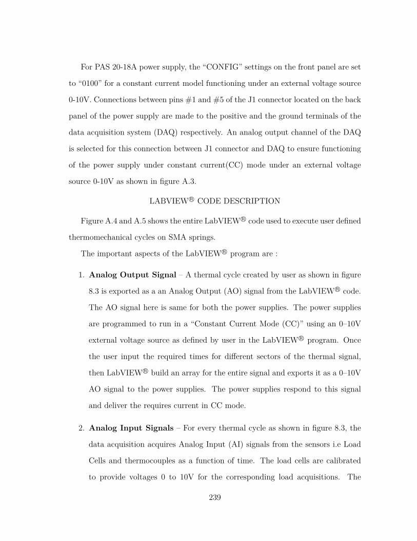
For PAS 20-18A power supply, the “CONFIG” settings on the front panel are set

to “0100” for a constant current model functioning under an external voltage source

0-10V. Connections between pins #1 and #5 of the J1 connector located on the back

panel of the power supply are made to the positive and the ground terminals of the

data acquisition system (DAQ) respectively. An analog output channel of the DAQ

is selected for this connection between J1 connector and DAQ to ensure functioning

of the power supply under constant current(CC) mode under an external voltage

source 0-10V as shown in figure A.3.

LABVIEW R© CODE DESCRIPTION

Figure A.4 and A.5 shows the entire LabVIEW R© code used to execute user defined

thermomechanical cycles on SMA springs.

The important aspects of the LabVIEW R© program are :

1. Analog Output Signal – A thermal cycle created by user as shown in figure

8.3 is exported as a an Analog Output (AO) signal from the LabVIEW R© code.

The AO signal here is same for both the power supplies. The power supplies

are programmed to run in a “Constant Current Mode (CC)” using an 0–10V

external voltage source as defined by user in the LabVIEW R© program. Once

the user input the required times for different sectors of the thermal signal,

then LabVIEW R© build an array for the entire signal and exports it as a 0–10V

AO signal to the power supplies. The power supplies respond to this signal

and deliver the requires current in CC mode.

2. Analog Input Signals – For every thermal cycle as shown in figure 8.3, the

data acquisition acquires Analog Input (AI) signals from the sensors i.e Load

Cells and thermocouples as a function of time. The load cells are calibrated

to provide voltages 0 to 10V for the corresponding load acquisitions. The

239

thermocouples provide a continuous realtime surface temperature information

of the springs.

3. Data Analysis – Sometimes the acquired data might need some filtering de-

pending on the background noise present in the experimental setup/data ac-

quisition system. Appropriate filters might be selected to attenuate the noise

and acquire useful data. For this study a band pass filter of 55Hz was used to

cliff off frequency information greater than 60Hz resulting due to AC supply.

However, the raw unfiltered data was used for all calculations.

240

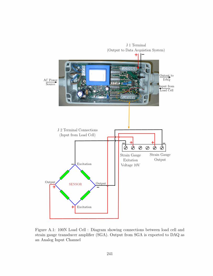
Strain Gauge

Exitation

Voltage 10V

Strain Gauge

Output

OutputOutput

Excitation

Excitation

AC PowerSource

J 2 Terminal Connections

(Input from Load Cell)

J 1 Terminal

(Output to Data Acquistion System)

SENSOR

Input fromLoad Cell

Outout toDAQ

Figure A.1: 100N Load Cell : Diagram showing connections between load cell andstrain gauge transducer amplifier (SGA). Output from SGA is exported to DAQ asan Analog Input Channel

241

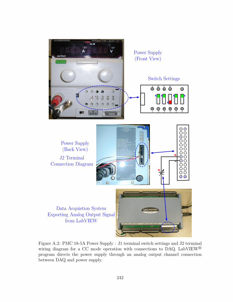
1 2

5

25 26

15

17

Power Supply(Front View)

J2 TerminalConnection Diagram

Data Acquistion SystemExporting Analog Output Signal

from LabVIEW

Power Supply(Back View)

A B C D

1 2 3 4 5 6

Switch Settings

Figure A.2: PMC 18-5A Power Supply : J1 terminal switch settings and J2 terminalwiring diagram for a CC mode operation with connections to DAQ. LabVIEW R©

program directs the power supply through an analog output channel connectionbetween DAQ and power supply.

242

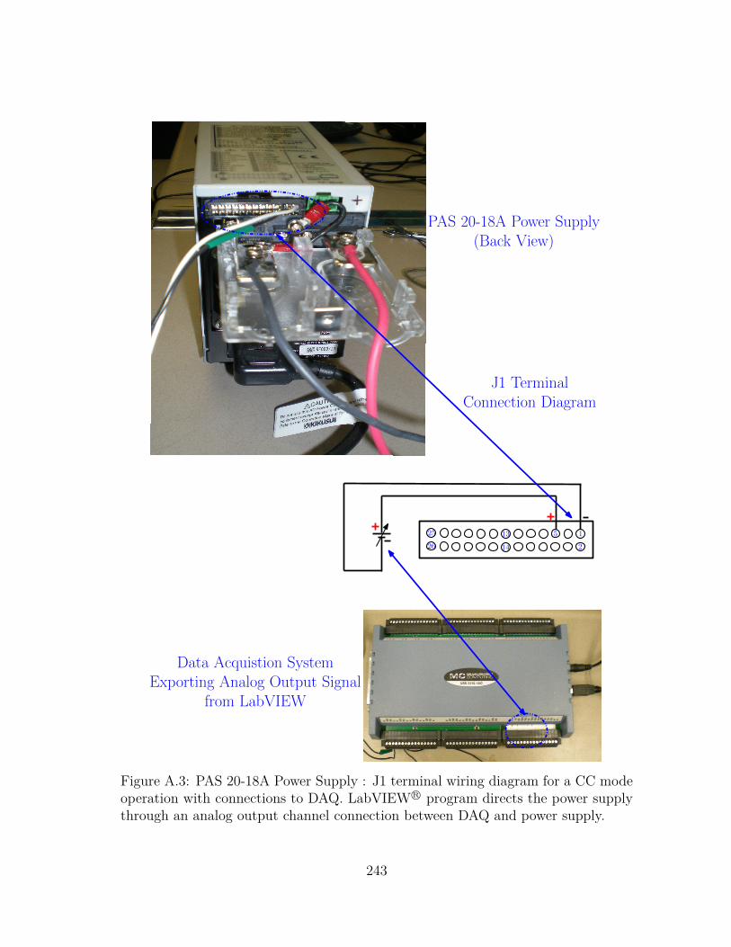
1

2

525

26

13

14

PAS 20-18A Power Supply(Back View)

J1 TerminalConnection Diagram

Data Acquistion SystemExporting Analog Output Signal

from LabVIEW

Figure A.3: PAS 20-18A Power Supply : J1 terminal wiring diagram for a CC modeoperation with connections to DAQ. LabVIEW R© program directs the power supplythrough an analog output channel connection between DAQ and power supply.

243

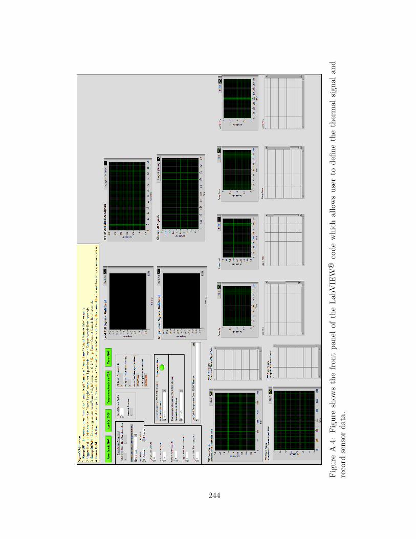
Figu

reA.4:Figu

reshow

sthefro

ntpa

nelo

fthe

LabV

IEW

R ©code

which

allowsuser

todefin

ethethermal

signa

land

record

sensor

data.

244

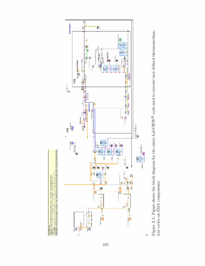
Figu

reA.5:F

igureshow

sthe

blockdiagram

fort

heentir

eLa

bVIE

WR ©code

used

toexecuteuser

defin

edthermom

echa

n-ical

cycles

onSM

Acompo

nents.

245