strong unification
TRANSCRIPT
arX
iv:h
ep-p
h/97
0746
2v2
24
Nov
199
7
OUTP-97-32-PJuly 1997
to appear in Phys.Lett. B
Strong Unification
Dumitru Ghilencea∗1 , Marco Lanzagorta†2 , Graham G. Ross∗3
∗Department of Physics, Theoretical Physics, University of Oxford
1 Keble Road, Oxford OX1 3NP, United Kingdom
† High Energy Section, International Centre for Theoretical Physics
PO Box 586, Trieste, Italy
Abstract
We investigate the possibility that unification occurs at strong coupling. We show that, despitethe fact the couplings pass through a strong coupling regime, accurate predictions for their lowenergy values are possible because the couplings of the theory flow to infrared fixed points. Wedetermine the low-energy QCD coupling in a favoured class of strong coupling models and find itis reduced from the weak coupling predictions, lying close to the experimentally measured value.We extend the analysis to the determination of quark and lepton masses and show that (evenwithout Grand Unification) the infra-red fixed point structure may lead to good predictions forthe top mass, the bottom to tau mass ratio and tanβ. Finally we discuss the implications for theunification scale finding it to be increased from the MSSM value and closer to the heterotic stringprediction.
1 E-mail address: [email protected] E-mail address: [email protected] E-mail: [email protected]
1 Introduction
The remarkable agreement of the unification predictions for gauge couplings offers the best evidencefor a stage of unification of the fundamental forces. Further, the determination of the unificationscale close to the (post)diction of string theory may be the first quantitative indication of unificationwith gravity. However, in detail, the predictions do not quite fit with our expectations, particularlyin the case of superstring unification. The evolution of the gauge couplings, with the assumption ofthe minimal MSSM spectrum, yields a value for the strong coupling, αo
3(MZ) ≈ 0.126, rather highwhen compared with the latest average of experimental determinations [1], α3(MZ) = 0.118 ± 0.003.Further, the unification scale, Mo
g , is found to be (1 − 3) × 1016GeV , a factor of 20 below the stringscale, which is the typical expectation for the weakly coupled heterotic string. The unified couplingat the unification scale is given by αo
g ≈ 0.043, so the physics around the unification scale Mog lies
in the perturbative domain, but it has been argued [2] that this is not acceptable in string theory,as the theory suffers from the “dilaton runaway problem”. In order to stabilise the dilaton one mustappeal to non-perturbative effects and the authors of ref [2] and [3] argue that an intermediate valueof αg ≈ 0.2 at Mg is desired. This, they argue, is large enough to stabilize the dilaton, yet remainsperturbative in the sense of quantum field theory 1 to justify the perturbative analysis of the couplingunification.
Ways to eliminate these problems have been widely studied2. Witten has found [5] that the (10dimensional) strongly coupled heterotic string theory (M theory) gives a prediction for the unificationscale more closely in agreement with the gauge unification value found in the MSSM. However, thisdoes not by itself address the problem of dilaton stability. Stimulated in part by this problem, we haverecently explored the case of unification at intermediate values of gauge coupling at the unificationscale, for which case perturbation theory still may be used up to the unification scale. We found [6] thatthe prediction for the strong coupling constant and the unification scale is remarkably insensitive to theaddition of massive states3 which lead to unification at intermediate coupling. In this letter we extendthis analysis in two ways. We discuss in detail the prospects for obtaining precision predictions forthe case the unified coupling becomes strong. We also consider the implications for Yukawa couplingswhich are fixed because they flow rapidly to fixed points in the case of unification at strong coupling.
One may easily achieve unification at strong coupling through the addition of a number of ad-ditional (massive) multiplets to the MSSM spectrum. It is notable that such additional multipletsoccur in the majority of string compactifications, coming in representations vectorlike with respect tothe Standard Model gauge group, and hence, likely to acquire mass at the first stage of spontaneousbreaking below the compactification scale, which is likely to be much higher than the electroweakbreaking scale. Thus, it is reasonable to argue that the MSSM is not the typical case and that weshould consider models with additional massive states as standard. However, this seems to destroythe success of the unification predictions which are very sensitive to the addition of such states. Inref [6] we argued that this is not the case for the most promising extensions of the Standard Modelhave additional states which fill out complete SU(5) multiplets and these do not change the MSSMunification predictions at one loop order; this is clearly the case for the case of Grand Unificationwith a Grand Unified group which contains SU(5) for there may easily be additional Grand Unifiedmutiplets with mass below the unification scale. However, it may also be the case for superstringunification, even though the gauge group below the compactification scale is not Grand Unified. In
1 String perturbation series are more divergent than field theory series, so small (perturbative) couplings in QFT cangenerate large (non-perturbative) in string theory.
2For an extensive review see [4]3We neglected there the Yukawa effects of the third generation, but the result is still true when they are included, at
least for the unification scale [7].
1
ref. [8] it was argued that level-one string theories with symmetry breaking by Wilson lines provide themost promising superstring compactified models. In these, the coupling constant of the various gaugecouplings have the usual SU(5) unified values, even though the gauge group below compactificationmay naturally need not be Grand Unifed; indeed4, it may be just the Standard Model gauge group.Furthermore, level-one string theories allow only low lying representations to occur, immediately ex-plaining why quarks and leptons belong only to triplets of SU(3) and doublets of SU(2). In suchmodels, with Wilson line breaking, the multiplet structure is predicted to have the generations fillingout complete SU(5) representations5, just as is observed. Moreover, there is a natural explanationfor the Higgs doublets of the MSSM, because there are predicted to be at least two (split) multipletswhich do not fill out complete SU(5) representations. There is only a discrete number of Wilsonlines possible and for one of these the split multiplet contains just the Higgs of the MSSM. The onlyambiguity in this class of models is that it may contain an additional n5 multiplets filling out complete5 + 5̄ representations and n10 complete 10 + 10 representations.
With this motivation, we now proceed to consider the possibility that gauge unification occursat strong coupling. We will show that this leads to precise unification predictions and will computethem for the class of models just discussed, in which the additional states leading to strong couplingunification fill out complete SU(5) representations. We will further show that such models have avery interesting consequence for fermion masses because Yukawa couplings may lie in the domain ofattraction of an infra red fixed point of the theory and, due to the strong coupling at unification, theyflow very quickly to the fixed point. This leads to detailed predictions for the third generation masses.
2 Strong Unification
Unification at strong coupling was proposed a long time ago [10] as a viable possibility leading toreasonable predictions for the low-energy gauge couplings. Here we reformulate the idea in a way thatquantifies the uncertainties in the predictions and refers only to evolution of the couplings once theyreach the perturbative domain. At first sight it seems that strong unification does not lend itself toa precise prediction of the gauge couplings, due to the need to determine the evolution in the strongcoupling domain. The reason this is not the case is because the ratio of gauge couplings flow to aninfrared fixed point. Thus, one has the situation where the boundary conditions for the evolutionof couplings in the MSSM are still reliably calculable - at the “intermediate” mass scale, M , of thenew vectorlike states, the ratios of the gauge couplings are given by their infra-red fixed point values,corresponding to the theory above this mass scale. For the case the coupling is initially large, theratio of couplings closely approaches the fixed point, so a determination of the low energy values ofthe couplings, using these boundary conditions plus two-loop MSSM evolution provides an accuratedetermination of the couplings.
The two loop renormalisation group equations for the gauge couplings, with no Yukawa interaction,are given by:
dαi
dt= b̃iα
2i +
1
4π
3∑
j=1
b̃ijα2i αj + O(α4) (1)
with i = {1, 2, 3} and where t = 12π ln Q/Mg; Mg is the unification scale, and b̃i and b̃ij are the
appropriate one loop and two loop beta functions respectively. To exhibit the infra-red-fixed-point
4For a fuller discussion of the possibilities see [9]5Even though the gauge group is not SU(5).
2
(IRFP) structure of these equations we rewrite this equation in the form
d
dtln
αi
αk= b̃iαi − b̃kαk +
1
4π
3∑
j=1
(
b̃ijαi − b̃kjαk
)
αj + O(α3) (2)
At one-loop order the evolution of this ratio clearly has an IRFP stable fixed point6 with the fixedpoint value given by
(
αi
αk
)∗
=b̃k
b̃i
(3)
Provided the gauge couplings are small, the two-loop corrections and above will only give a smallcorrection to this fixed point value. Phenomenologically, this must be the case for, to be viable, thecouplings should match at the scale M the values of the low energy couplings evolved up in energyusing the usual MSSM renormalisation group equations. Provided M is large enough, the values ofthe couplings are all small (of O(1/24) for M near 1016GeV ). In the class of models explored herethe two loop corrections are further suppressed. This follows because above the intermediate scale theone loop beta functions in the presence of complete SU(5) multiplets is given by:
b̃i = b′i =
335 + n1 + n
−3 + n
(4)
where n represents the linear combination 7 n = (n5 + 3n10)/2. We are particularly interested inthe case n is large for then M is large and the couplings are driven rapidly to the fixed point ratios.However the two-loop corrections do not grow with n because, as is clear from [11] (cf eqs. (22),(23),(24)), massive states do not contribute two-loop corrections, the usual two-loop contribution to thebeta function being cancelled by the massive threshold corrections [6]. Thus the two loop effects aresuppressed both by the additional power of the coupling at the matching scale, M , and by the factor1/n. We shall investigate the magnitude of these corrections in Section 4.
To summarise we have reformulated the unification of gauge couplings for the case that unificationoccurs at large coupling via boundary conditions for renormalisation group equations which applybelow the scale of new physics beyond the MSSM. The advantage of this is twofold. It requiresintegration of the renormalisation group equations only in the domain where the coupings are smalland perturbation theory applies. It quantifies the uncertainties in the analysis. The latter come fromthe two loop and higher corrections at the matching scale where these are small; hence the possibilityof making accurate predictions for the gauge couplings at low energies even in the case of unificationat strong coupling. Note that strong unification does not even require the equality of couplings at anyscale. In this sense the infra-red structure of the theory substitutes for Grand Unified relations.
2.1 One loop analysis
It is instructive to determine the “strong unification” predictions at one-loop order, to show the generaltrend, before presenting the results of the full two loop analysis. Below M , the multiplet structure isjust that of the MSSM with one-loop beta functions bi given by eq(4) with n = 0, b̃i = bi = b′i(n = 0).Above M the beta functions are b′i. The boundary conditions for the evolution below the scale M arejust
αk(M)
αi(M)=
b′ib′k
(5)
6Provided, of course, b̃i > 0 which is necessary if all the couplings are to become large at some high scale.7here n5 = N5 + N
5and n10 = N10 + N
10
3

From eq(1) we have
α−1i (MZ) = α−1
i (M) +bi
2πln
[
M
MZ
]
(6)
Using this and the boundary condition gives
1
2πln
[
M
MZ
]
=b′kα
−1i (MZ) − b′iα
−1k (MZ)
(bi − bk)n(7)
Further, it is straightforward to show that:
(b1 − b2)α−13 (MZ) = (b1 − b3)α
−12 (MZ) + (b3 − b2)α
−11 (MZ) (8)
Using this relation one may obtain α3(MZ) given the experimental measurements of the other twocouplings. This relation is identical to that one obtains from the MSSM RGE equations showing that,at one loop order, the predictions are the same in the MSSM and the fixed-point-boundary-condition(FPBC) scheme. Note eq(8) is independent of the value of n because complete SU(5) multipletscontribute equally to the one-loop beta functions. As a result, at one loop, the prediction for α3(MZ)in “strong unification” is universal for the class of models with additional complete SU(5) multiplets.With the measured values of α1(MZ) and α2(MZ) as input, the value for α3(MZ) is 0.1145. Of course,two loop and SUSY threshold corrections should be added to obtain a precision prediction; these willbe considered in the next section.
The value of the mass M of the vectorlike states, additional to the MSSM spectrum, may beobtained from eq(7). Taking i = 1 and k = 2 one finds
1
2πln
[
M
MZ
]
≈29.3n − 136.9
5.6n(9)
From this, we find that solutions are possible only for n ≥ 5. The value of M is clearly n dependent,and varies from 103GeV for n = 5 to 1013GeV for n = 20 and to 1016 for n = 300. However, thisshould not be interpreted as the normal unification scale at which the couplings are equal. The latterpoint occurs in the strong coupling domain, and thus cannot be precisely determined in perturbationtheory. However, one may determine the scale at which the couplings enter the non-perturbativedomain. At this point they are evolving rapidly, so it is a reasonable conjecture that they becomeequal very close to this scale. Remarkably, the scale MNP , at which the couplings become large, turnsout to be almost independent of n and is given by MNP ≈ 3.1016GeV , essentially the same scale as isfound in the MSSM for the unification scale!
2.2 Two loop analysis
In this section we present a two loop analysis in which we compute the scale M at which the couplingsare in the fixed point ratio as well as the prediction for α3(MZ). The real unification scale, if any, willnot be an output of the scheme.
As usual in making a prediction for the low energy values of the gauge couplings we are facedwith the problem of unknown values for the supersymmetric spectrum; this can significantly affectthe predictions we make because, at two loop order, one has to take into account the low energysupersymmetric thresholds in one loop. Various scenarios for low supersymmetric energy spectrumhave been studied in the minimal supersymmetric standard model (MSSM), and their effect on thevalue of the unification scale as well as αo
3(MZ) has been extensively discussed [12]. Given thiswe choose to make our predictions relative to the MSSM prediction calculated with a given SUSYthreshold. In the MSSM we have
4
αo−1i (Mz) = −δo
i + αo−1g +
bi
2πln
[
Mog
MZ
]
+1
4π
3∑
j=1
bij
bjln
[
αog
αoj(MZ)
]
(10)
where the δoi contains the effect of the low energy supersymmetric thresholds and we have ignored the
Yukawa couplings effects, which are known to be small. The MSSM variables are labelled with an “o”index to distinguish them from the model based on fixed point scenario.
In the FPBC case we have
α−1i (Mz) = −δo
i + α−1i (M) +
bi
2πln
[
M
MZ
]
+1
4π
3∑
j=1
bij
bjln
[
αj(M)
αj(MZ)
]
(11)
where, as discussed above, we use the same threshold δoi as in the MSSM. The bi and bij denote the
one loop and two loop beta functions which are just the same as in the MSSM; M denotes the scalewhere the couplings αi(M) are in the “fixed-point” ratio. Now, from experiment we have well measuredvalues for α1(MZ) and α2(MZ) from the values of electromagnetic coupling and Weinberg angle at MZ
scale. Therefore, in computing α3(MZ), these values were taken as input from experiment. The FPBCcase should comply with this condition, too, and hence α1(MZ) = αo
1(MZ) and α2(MZ) = αo2(MZ).
We subtract the eqs. (10), (11) and, using these relations, obtain
0 = α−1i (M) − αo−1
g +bi
2πln
[
M
Mog
]
+1
4π
3∑
j=1
bij
bjln
[
αj(M)
αog
]
+1
4π
bi3
b3ln
[
αo3(MZ)
α3(MZ)
]
(12)
for the case i = {1, 2} and
α−13 (MZ)−αo−1
3 (MZ) = α−13 (M)−αo−1
g +b3
2πln
[
M
Mog
]
+1
4π
3∑
j=1
b3j
bjln
[
αj(M)
αog
]
+1
4π
b33
b3ln
[
αo3(MZ)
α3(MZ)
]
(13)for the case i = 3. At two loop order we may make the approximation
ln
[
αo3(MZ)
α3(MZ)
]
= lnα−13 (MZ)oneloop − ln αo−1
3 (MZ)oneloop = 0
One may readily check that the LHS is indeed numerically very small. This gives
0 = α−1i (M) − αo−1
g +bi
2πln
[
M
Mog
]
+1
4π
3∑
j=1
bij
bjln
[
αj(M)
αog
]
(14)
for the case i = {1, 2} and
α−13 (MZ) − αo−1
3 (MZ) = α−13 (M) − αo−1
g +b3
2πln
[
M
Mog
]
+1
4π
3∑
j=1
b3j
bjln
[
αj(M)
αog
]
(15)
for i = 3.This is a system of three equations with the unknowns: α3(MZ), M and one of the αi(M)’s (say
α1(M)), as the ratio of any two of them is a known function for any given n through eq(5). Thesolution is
α−13 (MZ) = αo−1
3 (MZ) −470
77πln
[
α1(M)
αog
]
+17
14πln
[
b1 + n
b3 + n
]
−15
2πln
[
b1 + n
b2 + n
]
(16)
5
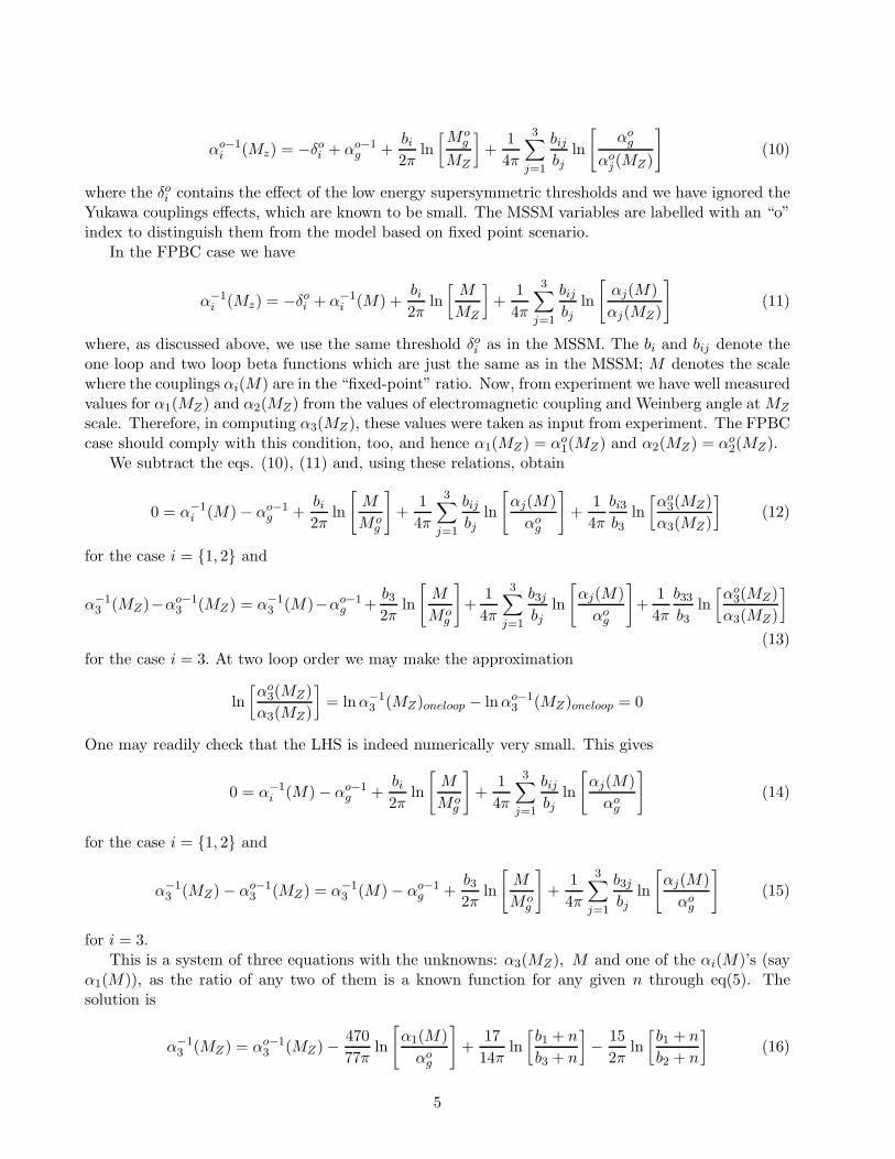
n α1(M) α3(MZ) M mb
mτ(MZ) mt tan β
6 0.020 0.1163 2.14 × 10⁵ 1.62 229.26 47.15
8 0.023 0.1188 1.61 × 10⁸ 1.62 209.87 46.99
10 0.025 0.1203 0.79 × 10¹⁰ 1.61 204.06 46.82
12 0.027 0.1213 1.04 × 10¹¹ 1.60 202.58 46.70
14 0.029 0.1219 6.44 × 10¹¹ 1.59 201.51 46.64
16 0.030 0.1224 2.52 × 10¹² 1.58 200.92 46.54
18 0.031 0.1228 7.23 × 10¹² 1.57 200.57 46.48
20 0.032 0.1231 1.68 × 10¹³ 1.57 200.34 46.43
22 0.033 0.1234 3.34 × 10¹³ 1.56 200.20 46.41
26 0.034 0.1238 0.96 × 10¹⁴ 1.55 200.03 46.32
Table 1: The value of α1 at the intermediate scale, the strong coupling at MZ , and the intermediatescale obtained using the fixed-point boundary conditions as a function of n. Also shown are the bottomto tau mass ratio and the top mass for the case the third generation couplings are in the domain ofattraction of the fixed point.
for the strong coupling and
ln
[
M
Mog
]
= −2π
nαog
+(2336 + 341n)
231nln
[
α1(M)
αog
]
+57 + 7n
4nln
[
b1 + n
b2 + n
]
−4(22 + n)
21nln
[
b1 + n
b3 + n
]
(17)
for the scale M, where the value of α1(M) is given by the root of the nonlinear equation:
α−11 (M) =
b1 + n
nαog
−1168
231π
(b1 + n)
nln
[
α1(M)
αog
]
−57
8π
(b1 + n)
nln
[
b1 + n
b2 + n
]
+44
21π
b1 + n
nln
[
b1 + n
b3 + n
]
(18)with b1 = 33/5, b2 = 1, b3 = −3.
Using these expressions we get the numerical results presented in Table 1 in which we have takenas the reference MSSM prediction αo
3(MZ) = 0.126. We see we get a lower value for alpha strongat electroweak scale than in the MSSM and closer to the experimental measurement [1] α3(MZ) =0.118 ± 0.003. Since the couplings are quite small at the high scale M , the higher corrections to theboundary conditions are expected to be small. We will estimate these corrections in Section 4.
3 Strong Unification and the masses of the third generation
As we have discussed, the addition of massive multiplets to the MSSM is to be expected in viableGrand Unified theories and in many string theories. The effect of such new states is to increase thegauge coupling at unfication and can easily make it approach the strong coupling domain. We furtherremarked that in this domain the fixed point structure of the theory relating the largest Yukawacouplings (and hence third generation masses) to the gauge couplings becomes the dominant effect asthe couplings flow rapidly towards the fixed points. In this section we explore these implications indetail.
The renormalisation group equations for the Yukawa couplings in the MSSM are given by
d
dtYτ = Yτ
(
3Yb + 4Yτ −9
5α1 − 3α2
)
6
d
dtYb = Yb
(
Yt + 6Yb + Yτ −7
15α1 − 3α2 −
16
3α3
)
d
dtYt = Yt
(
6Yt + Yb −13
15α1 − 3α2 −
16
3α3
)
(19)
where Yj = h2j/4π and hj is the Yukawa coupling. If we ignore the smaller gauge couplings α1 and α2
and we keep only the large top Yukawa coupling Yt, the last equation has the form
dYt
dt= Yt(sYt − r3α3) (20)
This has a fixed point that relates the top Yukawa coupling to the QCD coupling α3 given by [13],[14]:
(
Yt
α3
)∗
=r3 + b3
s(21)
which is infra-red stable if r3 + b3 > 0. In the case of the MSSM, b3 = −3, ri = (13/15, 3, 16/3) and
s = 6, then, the fixed point is(
Yt
α3
)∗
MSSM= 7
18 .
However, as stressed in ref. [15], this fixed point value is not reached for large initial values ofthe top quark coupling because the range in t between the Planck scale and the electroweak scaleis too small to cause the trajectories to closely approach the fixed point. As demonstrated in [14] a“Quasi-fixed point” governs the value of Yt for large initial values of Yt and is given by
(
Yt
α3
)QFP
=
(
Yt
α3
)∗
(
1 −(
α3(t)α3(0)
)B3
) (22)
where B3 = r3
b3+ 1. The term
(
α3(t)α3(0)
)B3
determines the rate of approach to the fixed point, the
smaller this term, the closer the QFP is to the IRSFP. For the MSSM in the case only the top Yukawacoupling is in the domain of attraction of the fixed point, including electroweak corrections, the quasi-fixed point predicts a top quark mass of mt ≈ 210 sin β GeV , where tan β is the ratio of the vacuumexpectation values of the Higgs doublets. For the case that the top and the bottom Yukawa couplingsare in the domain of attraction of the fixed point, the prediction for the fixed point is mt ≈ 190GeV,and the dependence on β disappears in this case, because the top and bottom Yukawas are nearlyequal and thus we are in the region with sin β ≈ 1.
As has been shown in [14], the profusion of new fields increase the rate of approach to thefixed point. This follows because the gauge couplings are evolving rapidly so the convergence fac-
tor(
α3(t)α3(0)
)B3
is very small. Thus we can expect that the IRSP structure will play an important role
for the determination of the couplings in the class of models considered in this paper. In this case onemust keep all three gauge couplings, as all are comparable above the scale M . However the analysisis tractable because the ratios of the gauge couplings are given by the infra-red fixed point ratio ofeq(5). The renormalisation group equations may be written in the form (see also ref.[16])
d
dtln
(
Yτ
αi
)
= αi
(
4Yτ
αi+ 3
Yb
αi−
9
5
α1
αi− 3
α2
αi− (bi + n)
)
(23)
d
dtln
(
Yb
αi
)
= αi
(
Yτ
αi+ 6
Yb
αi+
Yt
αi−
7
15
α1
αi− 3
α2
αi−
16
3
α3
αi− (bi + n)
)
(24)
d
dtln
(
Yt
αi
)
= αi
(
Yb
αi+ 6
Yt
αi−
13
15
α1
αi− 3
α2
αi−
16
3
α3
αi− (bi + n)
)
(25)
7
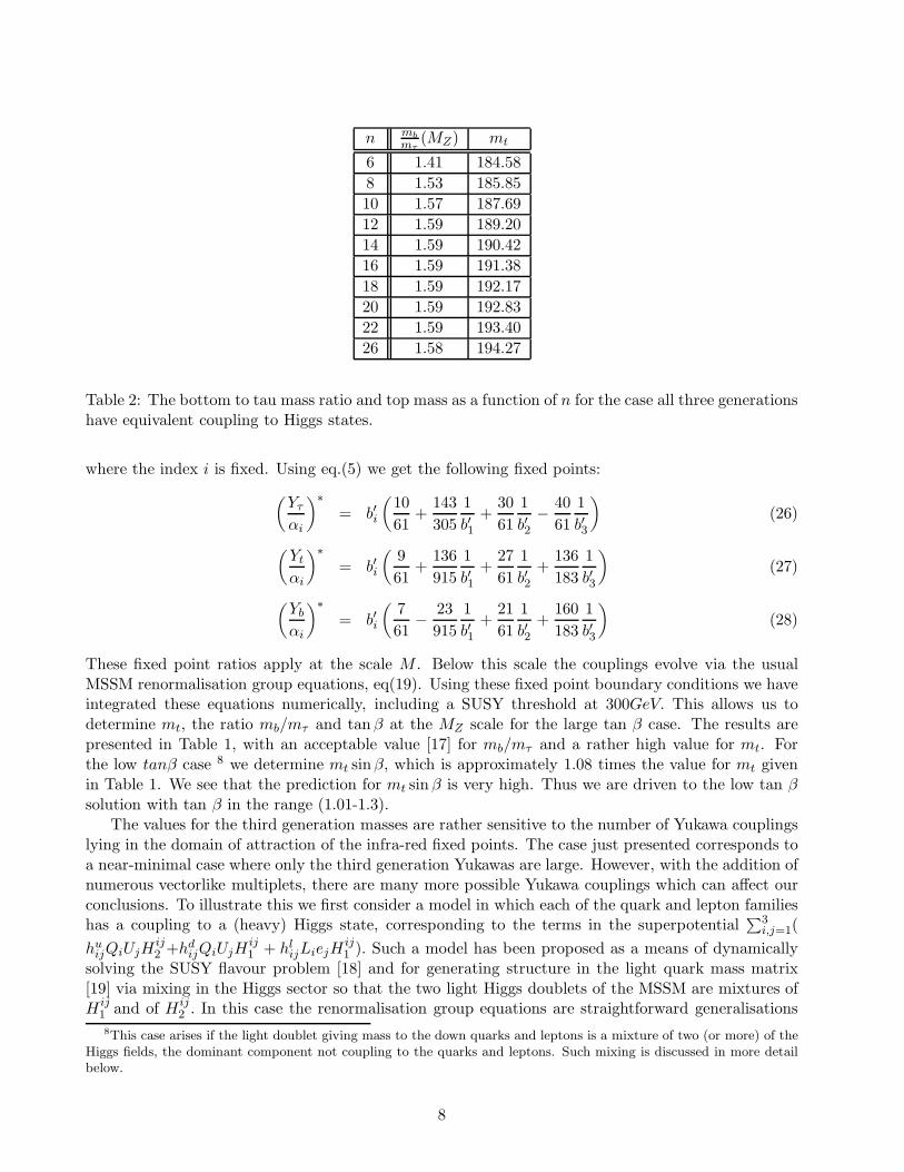
n mb
mτ(MZ) mt
6 1.41 184.58
8 1.53 185.85
10 1.57 187.69
12 1.59 189.20
14 1.59 190.42
16 1.59 191.38
18 1.59 192.17
20 1.59 192.83
22 1.59 193.40
26 1.58 194.27
Table 2: The bottom to tau mass ratio and top mass as a function of n for the case all three generationshave equivalent coupling to Higgs states.
where the index i is fixed. Using eq.(5) we get the following fixed points:
(
Yτ
αi
)∗
= b′i
(
10
61+
143
305
1
b′1+
30
61
1
b′2−
40
61
1
b′3
)
(26)
(
Yt
αi
)∗
= b′i
(
9
61+
136
915
1
b′1+
27
61
1
b′2+
136
183
1
b′3
)
(27)
(
Yb
αi
)∗
= b′i
(
7
61−
23
915
1
b′1+
21
61
1
b′2+
160
183
1
b′3
)
(28)
These fixed point ratios apply at the scale M . Below this scale the couplings evolve via the usualMSSM renormalisation group equations, eq(19). Using these fixed point boundary conditions we haveintegrated these equations numerically, including a SUSY threshold at 300GeV. This allows us todetermine mt, the ratio mb/mτ and tan β at the MZ scale for the large tan β case. The results arepresented in Table 1, with an acceptable value [17] for mb/mτ and a rather high value for mt. Forthe low tanβ case 8 we determine mt sinβ, which is approximately 1.08 times the value for mt givenin Table 1. We see that the prediction for mt sin β is very high. Thus we are driven to the low tan βsolution with tan β in the range (1.01-1.3).
The values for the third generation masses are rather sensitive to the number of Yukawa couplingslying in the domain of attraction of the infra-red fixed points. The case just presented corresponds toa near-minimal case where only the third generation Yukawas are large. However, with the addition ofnumerous vectorlike multiplets, there are many more possible Yukawa couplings which can affect ourconclusions. To illustrate this we first consider a model in which each of the quark and lepton familieshas a coupling to a (heavy) Higgs state, corresponding to the terms in the superpotential
∑3i,j=1(
huijQiUjH
ij2 +hd
ijQiUjHij1 + hl
ijLiejHij1 ). Such a model has been proposed as a means of dynamically
solving the SUSY flavour problem [18] and for generating structure in the light quark mass matrix[19] via mixing in the Higgs sector so that the two light Higgs doublets of the MSSM are mixtures ofH ij
1 and of H ij2 . In this case the renormalisation group equations are straightforward generalisations
8This case arises if the light doublet giving mass to the down quarks and leptons is a mixture of two (or more) of theHiggs fields, the dominant component not coupling to the quarks and leptons. Such mixing is discussed in more detailbelow.
8
n mb
mτ(MZ) mt
6 1.43 128.28
8 1.59 144.44
10 1.65 154.19
12 1.67 160.82
14 1.68 165.68
16 1.67 169.40
18 1.67 172.36
20 1.67 174.78
22 1.66 176.80
26 1.65 179.98
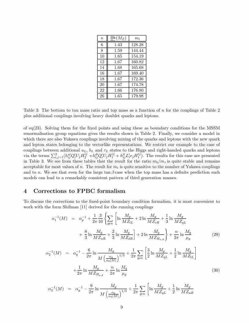
Table 3: The bottom to tau mass ratio and top mass as a function of n for the couplings of Table 2plus additional couplings involving heavy doublet quarks and leptons.
of eq(23). Solving them for the fixed points and using these as boundary conditions for the MSSMrenormalisation group equations gives the results shown in Table 2. Finally, we consider a model inwhich there are also Yukawa couplings involving mixing of the quarks and leptons with the new quarkand lepton states belonging to the vectorlike representations. We restrict our example to the case ofcouplings between additional uL, bL and τL states to the Higgs and right-handed quarks and leptonsvia the terms
∑3i,j=1(h
u′ijQ
′iUjH
ij2 +hd′
ijQ′iUjH
ij1 + hl′
ijL′iejH
ij1 ). The results for this case are presented
in Table 3. We see from these tables that the result for the ratio mb/mτ is quite stable and remainsacceptable for most values of n. The result for mt is quite sensitive to the number of Yukawa couplingsand to n. We see that even for the large tan β case when the top mass has a definite prediction suchmodels can lead to a remarkably consistent pattern of third generation masses.
4 Corrections to FPBC formalism
To discuss the corrections to the fixed-point boundary condition formalism, it is most convenient towork with the form Shifman [11] derived for the running couplings
α−11 (M) = α−1
g +1
2π
3
10
{
∑
gen
[
lnMg
MZlL+ 2 ln
Mg
MZeR+
1
3ln
Mg
MZqL
+8
3ln
Mg
MZuR+
2
3ln
Mg
MZdR
]
+ 2 lnMg
MZHu,d
}
+n
2πln
Mg
µg(29)
α−12 (M) = α−1
g −6
2πln
Mg
M(
αg
α2(M)
)1/3+
1
2π
∑
gen
[
3
2ln
Mg
MZqL+
1
2ln
Mg
MZlL
]
+1
2πln
Mg
MZHu,d
+n
2πln
Mg
µg(30)
α−13 (M) = α−1
g −9
2πln
Mg
M(
αg
α3(M)
)1/3+
1
2π
∑
gen
[
lnMg
MZqL+
1
2ln
Mg
MZuR
9
+1
2ln
Mg
MZdR
]
+n
2πln
Mg
µg(31)
The advantage of this form for the running of gauge couplings is that (above the supersymmetricscale) it is exact to all orders. However, the wave function renormalisation coefficients Zi are onlyknown perturbatively so one is still confined to a given order in perturbation theory when testingcoupling unification. To two loop order, one must include the values of wave-function renormalisationcoefficients Zi in one loop only. In this formula the Zi factors are evaluated at the scale M.
The one loop form of these equations gives the FPBC formalism used above. The two loopcorrections came from the terms involving ln(αg/α2(M)) and ln(αg/α3(M)), the gauge wave functionrenormalisation and also from the terms involving the Zi’s, the matter wave function renormalisation.To good approximation the former do not affect the FPBC predictions for α3(MZ). To see this first setZi = 1. Now the result follows because the predictions for α3(MZ) involves the differences [α−1
i (M)−α−1
j (M)], i, j = {1, 2, 3}. In these, the ln(Mg/M) terms coming from the three generations cancel,
leaving just the gauge wave function renormalisation terms proportional to ln[
Mg/(M(αg/αi(M))1/3)]
and the Higgs contribution proportional to ln(Mg/M). The latter has a small coefficient, so we can
effectively absorb the (αg/αi(M))1/3 term in a redefinition of Mg, Mg → Mg/(αg/αi(M))1/3 withαi(M) ≈ constant.
Hence, to a good approximation, we obtain the fixed-point boundary condition formalism provided
we interpret Mg/(
αg/α0g
)1/3as an effective scale M ′
g. We established this for the case we set Zi(M) =
1; thus, one expects corrections to FPBC formalism if this condition is not respected. How large arethey? There are two contributions to each Zi, one coming from gauge interactions and one fromYukawa interactions. For couplings remaining in the perturbative domain, the effects of the gaugecoupling terms alone was analysed in [6] where it was found that the value of α3 increased slightly.However, as we have stressed, in strong coupling one expects the Yukawa couplings to be large andtheir contribution to Zi factors is opposite to that of gauge interactions, taking the result closer tothe FPBC result. We may check whether this happens in the case unification occurs at intermediatecoupling where the perturbative approach still applies. In this case we may use the one-loop form forthe Zi factors. Following the argument presented, we have checked in specific cases that, because ofthese cancellations, the prediction does lie close to the FPBC predicted value.
Finally it is of interest to consider the expectation for the unification scale. As we have stressedthis is not determined in the case the coupling is really strong at unification. However, for intermediatevalues, say of O(0.3), one may use eq(31) to determine Mg. Again we find Mg larger than the MSSMvalue. Part of this increase follows simply from the fact noted above that part of the two loop
corrections may be absorbed in a change in the unification scale, giving Mg = M ′g
(
αg
α0g
)1/3(For αg = 1
this approximately gives an increase by a factor 3). The remaining effect comes from the two loopcorrections arising from the Z factors. It is interesting that together they take the value of Mg closerto the weakly coupled heterotic string prediction.
5 Conclusions
Unification at strong coupling is quite likely in extensions of the MSSM which contain additional stateswith mass below the unification scale. Since such cases are perhaps the norm, it is important to deter-mine their implications for gauge coupling unification. We have shown that it is possible to determinethese implications with surprising accuracy given the fact that the gauge coupling evolution involves astage of strong coupling. The formulation of the initial boundary conditions at the intermediate scale
10
in terms of the infra-red fixed point ratios of gauge couplings of the theory above this scale showsthat the uncertainties in gauge coupling predictions are of two loop order. These corrections are smallsince they should be evaluated at the intermediate scale where the couplings are small. The two loopcorrections are further suppressed at large n, where n specifies the number of additional states, andalso by cancellation between two loop effects involving gauge and Yukawa couplings. The net resultis that the predicted value of the strong coupling is reduced from the MSSM value coming closer tothe experimental value. For unification at intermediate coupling in which perturbation theory may beused above the intermediate scale the unification scale is also raised relative to the MSSM prediction,taking it closer to the heterotic string prediction. The case of strong unification also leads to predic-tions for quark and lepton masses because the Yukawa couplings are driven towards infra-red fixedpoints. We have investigated these predictions and found that they may lead to excellent predictionsfor the third generation masses. It may be hoped that such structure will ultimately shed light on thepattern of light quark and lepton masses too.
6 Acknowledgements
The authors want to thank G. Amelino-Camelia, D.R.T. Jones, I. Kogan, J. March-Russell, M. Shifmanfor useful discussions. D.G. gratefully acknowledges the financial support from the part of Universityof Oxford and Oriel College (University of Oxford).
References
[1] Review of Particle Data, Phys. Rev D54 (1996), 83.
[2] M.Dine and N. Seiberg, Phys. Lett. B 162 (1985), 299;T. Banks and M. Dine, Phys. Rev D 50, (1994) 7454;M. Dine and Y. Shirman, Phys. Lett. B377 (1996), 36;M. Dine, preprint hep-th/9508085.
[3] K. S. Babu and J.C. Pati, Phys. Lett. B 384 (1996), 140.
[4] K.R. Dienes, Phys.Rept. 287 (1997) 447.
[5] E. Witten, Nucl. Phys. B471 (1996) 135;P.Horava, Phys. Rev. D 54 (1996), 7561;P.Horava and E. Witten, Nucl. Phys. B475 (1996), 94.
[6] D. Ghilencea, M. Lanzagorta-Saldana, G.G. Ross, Oxford University preprint, OUTP-97-31-P,hep-ph/9707401.Previous related works on strong coupling:C. Kolda and J. March-Russell, hep-ph/9609480;K. S. Babu and J.C. Pati, Phys. Lett. B 384 (1996), 140;R. Hempfling, Phys. Lett. B351 (1996) 206;B. Brahmachari, U. Sarkar and K. Sridhar, Mod. Phys. Lett. A8 (1993), 3349.
[7] D. Ghilencea and G.G. Ross, work in preparation.
[8] W. Pokorski and G.G. Ross, Oxford University preprint, OUTP-97-34-P, hep-ph/9707402.
[9] K.R. Dienes, A.E. Farragi and J. March-Russell, Nucl. Phys. B467 (1996) 44.
11
[10] L. Maiani, G. Parisi and R. Petronzio, Nucl. Phys. B136 (1978), 115.L. Maiani and R. Petronzio, Phys. Lett. B176 (1986), 120.
[11] M. Shifman, Int. J. Mod. Phys. A11 (1996) 5761 and references therein.
[12] P.Langacker and N. Polonsky, Phys. Rev. D47 (1993), 4028 and references therein.
[13] B. Pendelton and G.G. Ross, Phys. Lett. B98 (1981), 291.
[14] M. Lanzagorta and G.G. Ross, Phys. Lett. B349 (1995), 319.
[15] C.T. Hill, Phys. Rev. D24 (1981) 691;C.T. Hill, C.N. Leung and S. Rao, Nucl. Phys. B262 (1985) 517.
[16] M. Bando, J. Sato and K. Yoshioka, Kyoto University preprint, KUNS-1437 HE(TH) 97/04, hep-ph/9703321;M. Bando, T. Onogi, J. Sato and T. Takeuchi, CERN preprint CERN-TH/96-363, hep-ph/9612493
[17] W. de Boer et al., hep-ph/9603350
[18] M. Lanzagorta and G. G. Ross, Phys. Lett. B364 (1995), 163.
[19] Luis Ibanez and Graham G. Ross, Phys. Lett. B332 (1994) 100;Graham G. Ross, Phys. Lett. B364 (1995) 216.
12