stock market dispersion, the business cycle and expected

1

Stock Market Dispersion, the Business Cycle and Expected Factor Returns

Timotheos Angelidisa,*, Athanasios Sakkasb and Nikolaos Tessaromatisc

a,* Department of Economics, University of Peloponnese, Greece.

b Department of Accounting and Finance, Athens University of Economics and Business,

Greece.

c EDHEC Business School and EDHEC Risk Institute, France.

Forthcoming in the Journal of Banking and Finance

Abstract

We provide evidence using data from the G7 countries suggesting that return dispersion

may serve as an economic state variable in that it reliably predicts time-variation in

economic activity, market returns, the value and momentum premia and market volatility.

A relatively high return dispersion predicts a deterioration in business conditions, a

higher value premium, a smaller momentum premium and lower market returns.

Dispersion based market and factor timing strategies outperform out-of-sample buy and

hold strategies. The evidence are robust to alternative specifications of return dispersion

and are not driven by US data. Return dispersion conveys incremental information

relative to idiosyncratic risk.

Keywords: Stock Market Return Dispersion, Business Cycle, Market and Factor Returns.

JEL Classification: G12, G14.

*Corresponding author. Tel.: +30 2710 230128; fax: +30 2710 230139.

E-mail addresses: [email protected] (T. Angelidis), [email protected] (A. Sakkas),

[email protected] (N. Tessaromatis)

2

1. Introduction

Stock market return dispersion (RD) – defined as the cross sectional standard

deviation of returns from either individual stocks or from disaggregate stock portfolios –

provides a timely, easy to calculate at any time frequency, model free measure of

volatility. It measures the extent to which stocks move together or are diverging and has

been used by both finance academics and practitioners to measure trends in aggregate

idiosyncratic volatility,1 investors’ herding behavior,2 micro-economic uncertainty,3

trends in global stock market correlations,4 as an indicator of potential alpha and a proxy

for active risk,5 and as a leading countercyclical state variable.6 We provide

comprehensive evidence across seven major equity markets suggesting that RD has

significant predictive power for the business cycle, stock returns, the value and

momentum premia, and market volatility.

1Garcia, Mantilla-Garcia and Martellini (2013).

2 Christie and Huang (1995) use cross sectional volatility to capture herd behavior in stock markets.

3 Bloom (2009) and Bloom, Floetotto, Jaimovich, Saporta-Eksten and Terry (2012).

4Solnik and Roulet (2000) make the case for the use of RD as an instantaneous measure of correlation that

provides a dynamic estimate of the trends in correlation using only cross-sectional data.

5 Silva, Sapra and Thorley (2001) find that the dispersion of mutual fund returns can be explained by RD.

Connor and Li (2009) show that RD can explain part of hedge fund returns not explained by the standard

Fung and Hsieh (2004) hedge fund risk factors. From a practical perspective, Russell Investments and

Parametric Portfolio Associates publish since 2010 (http://www.parametricportfolio.com/crossvol) a set of

indexes to track cross sectional volatility covering each of the major regions, investment styles and

economic sectors.

6Gomes, Kogan and Zhang (2003) present a theoretical link between RD, the economy, future market

returns and volatility. Empirical evidence on the predictive ability of RD for US stock returns are provided

by Garcia, Garcia-Mantilla and Martellini (2013) and Maio (2014) and for the value and momentum premia

by Stivers and Sun (2010, 2013).

http://www.parametricportfolio.com/crossvol

3

RD is an instantaneous measure of aggregate volatility calculated from returns

without the need for specifying a particular factor model that drives stock returns. Cross

sectional measures of volatility are closely related with time series based measures of

volatility (see among others Goyal and Santa-Clara, 2003 and Garcia, Mantilla-Garcia

and Martellini, 2013).

Our study focuses on RD formed from monthly individual stock returns or from

disaggregate stock portfolios, both value-weighted and equal-weighted. The first

contribution is to study in depth the properties of RD across the G7 countries adding to

the evidence from the US market.7 In particular we are interested in the commonality of

its behavior across countries. Our evidence suggests that country RD is strongly

positively correlated across markets with a common factor driving return dispersion

across the G7 countries. The significance of the common factor has increased during the

last decades.

Interest in RD among academics and practitioners has further increased since it

was realized that it could be a proxy of future economic conditions and a predictor of the

business cycle. Figure 1 depicts the time-series history of country RDs against recession

dates for the period 1980-2012 for the G7 countries. Figure 1 shows evidence that RD

follows a business-cycle pattern being low during expansions and high during recessions.

Stock market dispersion as a measure of the intensity of structural shocks to the

economy was first used by Loungani, Rush and Tave (1990) following a conjecture by

Black (1987, 1995). More recently Bloom (2009) and Bloom, Floetotto, Jaimovich,

7Using data from major markets outside the US minimizes the biases that arise due to data snooping (Lo

and MacKinley, 1990) and offers an independent assessment of the empirical findings.

4

Saporta-Eksten and Terry (2012) argue that uncertainty shocks are an important driver of

business cycles. Chen, Kannan, Loungani and Trehan (2011) find that return dispersion

has a strong effect on long duration unemployment. Garcia, Mantilla-Garcia and

Martellini (2013) argue that return dispersion is related to consumption volatility, a

measure of economic uncertainty in the inter-temporal asset pricing model of Bansal and

Yaron (2004). The second contribution of our paper is a study of the relation between RD

and future economic conditions. Our evidence suggests that, after controlling for

financial and economic variables known to predict the economy, RD is a strong predictor

of the business cycle and economic growth. A higher return dispersion over the last three

months indicates a higher probability that the economy will be in a recession in the

current month. Higher RD is associated with an increase in unemployment and a fall in

future economic activity.

There is now a rich empirical literature on the predictive ability of non-market

measures of volatility like idiosyncratic or average volatility or RD for future stock

market returns. Goyal and Santa-Clara (2003) present evidence suggesting that there is a

positive relation between average variance and future stock returns. Subsequently

published papers by Bali, Cakici and Levy (2008) and Wei and Zhang (2005) argue that

the Goyal and Santa-Clara (2003) findings are sample specific and not robust to the

definitions of average variance. Pollet and Wilson (2010) and Chen and Petkova (2012)

find a negative relation between stock returns and past average volatility.

Evidence on the relation between RD and multiple horizon returns are provided in

Maio (2014). Using monthly portfolio returns to measure RD, Maio (2014) finds a

negative and statistically significant relation for the US market. The negative relation

5

between RD and future returns is consistent with the evidence in Guo and Savickas

(2008) for the G7 countries using idiosyncratic volatility instead of RD. Garcia, Mantilla-

Garcia and Martellini (2013) using a measure of RD based on the average of daily RDs

find a positive relation between RD and subsequent monthly and daily US market returns.

The evidence on the predictive ability of RD, mainly from the US market, remains

controversial and calls for further study across different markets.

Stivers and Sun (2010) provide a direct test of the ability of RD to predict value

and momentum premia. Using US stock market data for the period 1965-2005 they find

that RD is positively related with the value premium and negatively related with the

momentum premium. They conjecture that RD is “a leading countercyclical variable”

which varies with the state of the economy, evidence consistent with the hypothesis that

RD might be informative about changes in the investment opportunity set. We test

whether RD can predict market returns and the value, size and momentum premia at

twelve month horizon. Our evidence suggests that return dispersion observed at time t

predicts future twelve month market returns and the value and momentum premia. The

predictive ability of RD remains intact when we control for other variables that predict

stock returns and factor premia. Dispersion is a statistically and economically significant

predictor of future market and factor returns.

The evidence on the ability of RD to predict future stock returns and factor premia

is consistent with the view that return dispersion is a state variable in the spirit of

Merton’s (1973) intertemporal CAPM. Chen (2003) extends Campbell’s (1996) version

of the ICAPM to include in addition to time-varying returns, time-varying volatility as

descriptors of the investment opportunity set. If RD is a state variable it should forecast

6

returns or volatility. We test this conjecture and find that RD is an important predictor of

future market volatility.

We implement several robustness tests to examine the sensitivity of our results to

(i) different sample periods (ii) alternative RD construction methodologies and (iii) the

exclusion of the US from our database. We provide evidence suggesting that our results

are not sample specific, are robust to different measures of RD and remain intact when

the US is excluded from the data.

In the last part of the paper we examine the differences between RD and

aggregate idiosyncratic risk in light of Garcia, Mantilla-Garcia, and Martellini’s (2013)

finding that idiosyncratic volatility and RD are highly correlated. We find that both

measures are related to subsequent economic conditions and future market returns and

factor premia. When we include both in the predictive regressions of factor and market

returns we find that RD drives out the predictive power of idiosyncratic volatility. Value

and momentum time strategies based on return dispersion driven forecasts provide small

but economically significant improvement compared to timing strategies based on

idiosyncratic volatility.

The rest of this paper is organized as follows. Section 2 presents the data and

summary statistics and examines if there is a common factor that affects return dispersion

in G7 markets. Section 3 provides evidence on the predictive ability of RD for future

economic activity and the business cycle, market and factor returns and market volatility.

In Section 4 we assess the robustness of our findings over different samples, different RD

measures and the exclusion of US data. Section 5 explores the information content of RD

and idiosyncratic risk. Section 6 concludes the paper.

7

2. Data and Dispersion Measures

The data set is obtained from Thomson DataStream and covers all stocks (dead or

alive) from July 30, 1980 to December 31, 2012 (390 monthly observations) in the G7

markets: Canada, France, Germany, Italy, Japan, UK, and US. Returns are calculated in

US dollars. Following Ince and Porter (2006), Hou, Karolyi and Kho (2011), Guo and

Savickas (2008), and Busse, Goyal and Wahal (2013) we impose various filters to

minimize the risk of data errors and to account for potential peculiarities of the dataset

(see Appendix B for details).

We calculate for each market the monthly cross sectional variance at time

𝑡 (𝐶𝑆𝑉𝑡) using the following equation:

𝐶𝑆𝑉t = ∑ wit

N

i=1

(rit − rmt)2, (1)

where rit is the return of stock i in month t, rmt is the return of the value weighted market

portfolio in month t, N is the number of stocks and wit is defined as 𝑤𝑖,𝑡 =1

𝑁 for the

equally weighted cross sectional variance (𝐶𝑆𝑉𝑒𝑤,𝑡) and as 𝑤𝑖,𝑡 =

𝑀𝑎𝑟𝑘𝑒𝑡 𝑐𝑎𝑝 𝑜𝑓 𝑠𝑡𝑜𝑐𝑘 𝑖 𝑖𝑛 𝑚𝑜𝑛𝑡ℎ 𝑡−1

𝑇𝑜𝑡𝑎𝑙 𝑚𝑎𝑟𝑘𝑒𝑡 𝑐𝑎𝑝, for the market capitalization weighted cross sectional

variance (𝐶𝑆𝑉𝑐𝑤,𝑡). Return dispersion equals √𝐶𝑆𝑉t. We construct country and world

based dispersion measures by using stock returns from the country and world universes,

respectively.

8

Following Stivers and Sun (2010) and Maio (2014) we create an equally weighted

measure of dispersion based on 100 portfolios formed using all stocks from the G7 stock

markets. We also calculate a capitalization weighted measure of portfolio based RD. In

particular at the end of each June, we sort all stocks in 100 portfolios based on market

capitalization and on the ratio of book equity to market equity. The portfolios are the

intersections of 10 portfolios formed on market capitalization and 10 portfolios formed

on the ratio of book equity to market equity. We calculate the value weighted monthly

portfolio returns and then calculate equally and capitalization weighted dispersion. Using

portfolios instead of stocks to measure dispersion avoids the influence of extreme

individual stock returns and therefore provides a less noisy measure of return dispersion

than measures based on individual stock returns. Stivers and Sun (2010) argue that

portfolio based measures of dispersion perform similarly but generally better than firm

level dispersion measures.

We follow closely the methodology used by Fama and French (1992) to construct

the style portfolios. At the end of June we sort all stocks in a country based on their

market capitalization and their book value per share to form the SMB and HML

portfolios. We set as missing negatives or zero values of book value per share. The fiscal

year ending in year t − 1 is matched with the returns and the market capitalization of year

t and hence there is no looking ahead bias in our dataset. At the end of June of each year,

we form the six portfolios of Fama and French (1993) and calculate the value weighted

monthly returns over the next 12 months. To create the SMB factor we use the median of

the market value, while for the book to market factor (HML) we set the breakpoints of

the BM ratio at the 30th and 70th percentiles. Finally, we calculate the momentum factor

9

(MOM) for month t as the cumulative monthly returns for t − 1 to t − 12. Combined

with the market capitalization we construct every month six value weighted portfolios to

form the momentum factor by using the median of the market value and the 30th and 70th

percentiles of the momentum.

2.1. Descriptive statistics

Panels A and B of table 1 present descriptive statistics for equally weighted

country (𝑅𝐷𝑐𝑜𝑢𝑛𝑡𝑟𝑦 𝑒𝑤 ), world (𝑅𝐷𝑤𝑜𝑟𝑙𝑑

𝑒𝑤 ) and portfolio (𝑅𝐷𝑝𝑜𝑟𝑡𝑓𝑜𝑙𝑖𝑜 𝑒𝑤 ) based measures of

dispersion. It also shows statistics for capitalization weighted country (𝑅𝐷𝑐𝑜𝑢𝑛𝑡𝑟𝑦 𝑐𝑤 ), world

(𝑅𝐷𝑤𝑜𝑟𝑙𝑑 𝑐𝑤 ) and portfolio (𝑅𝐷𝑝𝑜𝑟𝑡𝑓𝑜𝑙𝑖𝑜

𝑐𝑤 ) measures of dispersion. All measures are

calculated as a 3-month average of monthly cross sectional return dispersion to mitigate

the possible effect of large outliers as in Stivers and Sun (2010) and Maio (2014).

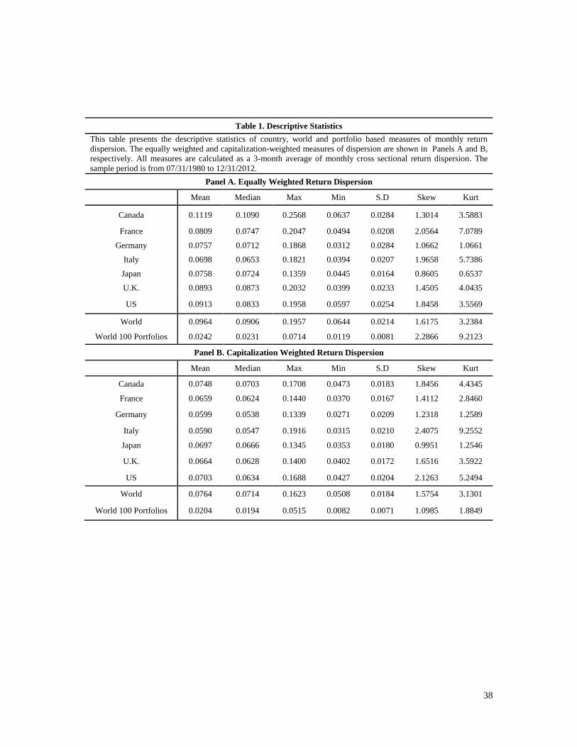
The average equally weighted country-based monthly return dispersion equals

8.50% and ranges from 6.98% (Italy) to 11.19% (Canada). The average world equally

weighted dispersion at 9.64% is generally higher but less volatile than country dispersion

measures. Capitalization weighted country dispersion measures are generally lower than

equally weighted dispersion measures (averaging 6.66% across countries) reflecting the

larger weighting of the less volatile large cap stocks. Average capitalization weighted

world dispersion has a smaller mean (7.64%) and lower volatility (1.84%) than the

respective equally weighted dispersion. Portfolio based measures of dispersion are much

lower than stock based measures reflecting the lower volatility of portfolios due to

diversification of idiosyncratic risk. All RD measures are non-normally distributed

exhibiting positive skewness and excess kurtosis.

10

2.2. Correlation structure of return dispersion measures.

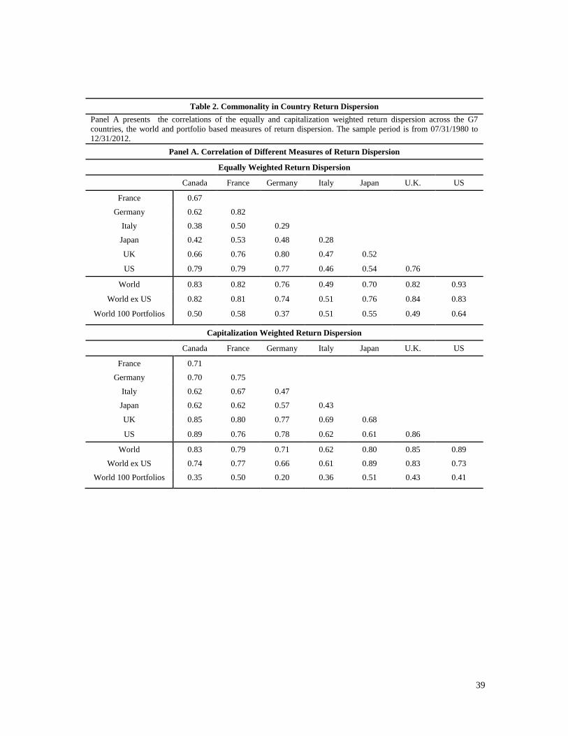
Panel A of table 2 presents the correlations of return dispersion across the G7

countries, the world and portfolio based measures of RD. The average correlation of

𝑅𝐷𝑐𝑜𝑢𝑛𝑡𝑟𝑦 𝑒𝑤 measures across the G7 countries is 0.59, the highest correlation is between

France and Germany (0.82) and the lowest between Italy and Japan (0.28). Capitalization

based country RD measures are more correlated than equally weighted measures with the

average correlation across countries equal to 0.69. The highest correlation pair is US and

Canada (0.89) and the lowest correlation pair is Japan and Italy (0.43). The high

correlation between country RD measures suggests that periods of high correlation in one

market are associated with high risk in other markets. The high correlations also suggest

that country RD measures share one or more common factors, an issue that is further

investigated in section 2.3.

The average correlation between country based RD measures and world

dispersion is 0.76. 𝑅𝐷𝑤𝑜𝑟𝑙𝑑 𝑒𝑤 has the highest correlation with the US (0.93) and the lowest

with Italy (0.50). Excluding US stocks from the calculation of 𝑅𝐷𝑤𝑜𝑟𝑙𝑑 𝑒𝑤 leaves the

average correlation between the world and country RDs unchanged. Capitalization

weighted measures of RD produce slightly higher correlations between world and

country based measures (0.78 when US stocks are included and 0.75 when US stocks are

excluded). The strong correlations between country and world RD is consistent with the

presence of a world factor in country dispersions.

11

Return dispersion measures based on world portfolios have lower correlation with

country based measures. For the equally (capitalization) weighted measures the average

correlation is equal to 0.52 (0.40). Correlations are higher with world RD measures (0.73

for the equally weighted and 0.68 with the capitalization weighted), a finding suggesting

the presence of common factors across all measures of RD.

2.3. Commonality in return dispersion measures

To investigate further the commonality in RD measures, we perform principal

component analysis of country RD. We find that the first principal component explains,

for the equally (capitalization) weighted measures, approximately 66.07% (73.88%) of

the variation of the cross sectional return variance. The first principal component has

significant loadings to country RD measures, suggesting that perhaps the world RD might

be a good proxy for it. Indeed the correlation between the first principal component and

world RD is 0.95 (0.92). The second principal component explains 11.09% (8.56%) of

the RD variability. We also perform a subsample analysis to examine the per period

importance of the first component. We split the sample in two periods: 1980-1996, and

1997-2012. For the first and the second period the explanatory power of the first

component equals 32.89% (40.80%), and 74.52% (84.59%), respectively suggesting that

the importance of the common global factor has increased over time.8

8 To examine further the impact of the global return dispersion factor on individual country cross sectional

return variation, we modify the methodology used by Brockman, Chung, and Perignon (2009) in their study

of a common global liquidity factor in exchange-level liquidity. Specifically, we estimate the equation:

𝑅𝐷𝐶,𝑡 = 𝛼 + 𝛽0𝑅𝐷𝐺,𝑡+1 + 𝛽1𝑅𝐷𝐺,𝑡 + 𝛽2𝑅𝐷𝐺,𝑡−1 + 𝛾0𝐴𝐶𝐶,𝑡 + 𝜀𝐶,𝑡 , where 𝑅𝐷𝐶,𝑡 and 𝐴𝐶𝐶,𝑡 are the return

dispersion and average stock correlation of country 𝐶, 𝑅𝐷𝐺,𝑡 is the world return dispersion (equally or

capitalization weighted) excluding country 𝐶. We calculate the average correlation using all stocks in a

market at time t defined as 𝐴𝐶𝑡 = ∑ ∑ 𝑤𝑖𝑡𝑤𝑗𝑡𝑐𝑜𝑟𝑟(𝑟𝑖𝑡 , 𝑟𝑗𝑡)𝑁𝑗=1

𝑁𝑖=1 . We find that 𝛽1 equals 0.468 (t-statistic

of 6.33) and hence an increase of the global factor affects positively country RD. The explanatory power of

the model increased over time (from 23.58% to 68.84%). Bekaert, Hodrick, and Zhang (2012) find a

12

3. The Forecasting Ability of Return Dispersion

In this section we investigate the forecasting power of return dispersion for

business conditions and the market, size, value and momentum premia and market

volatility. The forecasting regression is: 𝑌𝑡 = 𝛼 + 𝛽𝑋𝑡−1 + 𝜀𝑡, where 𝑌𝑡 is for the state of

the economy the business cycle dummy, unemployment or the ADS business conditions

index.9 For the return and premia forecasting equation 𝑌𝑡 is the 12-month market return or

the size, value or momentum premia.10 𝑋𝑡−1 includes RD, and a set of control variables

found in past research to forecast the future state of the economy, market volatility,

market return and factor premia. We use world equally and capitalization weighted RD as

the main measures of dispersion and examine in section 4 the robustness of the results to

alternative measures.

3.1. RD as a predictor of the state of the economy

Existing literature on the relation between stock market volatility and future

macroeconomic developments has focused on the question of what macro variables

predict future volatility.11 The ability of volatility, market or idiosyncratic, to predict

future economic conditions has received less attention. Lilien (1982) provides a

similar increase in the correlation of asset specific risk of G7 countries with the US. The evidence suggests

that global return dispersion drives country cross-sectional variation. The increased importance of global

RD over the last three decades is consistent with greater economic and financial integration. The detailed

results are available upon request from the authors. 9 For more information on the ADS business index, the reader is referred to the work of Aruoba, Diebold

and Scotti (2009). The sample period for the ADS equation ends on December 2009 because the data for

the G7 countries are not available after 2009. 10 We focus on a yearly forecasting horizon following the evidence in Maio (2014) showing that the

predicting ability of RD is stronger for holding periods greater than one or six months. Using monthly data

we also find consistent but generally weaker results compared to annual returns. 11 Schwert (1989), Hamilton and Lin (1996), Engle and Rangel (2008) and Adrian and Rosenberg (2008)

among others.

13

theoretical link between RD and unemployment. According to Lilien (1982) cyclical

variations in unemployment is the result of shocks to individual sectors that in turn cause

reallocation of labor across sectors. Since job search is time consuming, sectoral shifts

due to an adverse shock tend to be accompanied by a rise in unemployment. Bloom

(2009) and Bloom, Floetotto, Jaimovich, Saporta-Eksten and Terry (2012) argue that

uncertainty shocks lead the business cycle as they cause a reduction in the reallocation of

labor and capital, lower productivity and a significant fall in economic activity. They use

dispersion and market volatility to measure time varying micro and macro uncertainty,

respectively. Chen, Kannan, Loungani and Trehan (2011) find that an increase in market

volatility is associated with an increase in short duration unemployment. Dispersion on

the other hand, has a strong effect on long duration unemployment. Garcia, Mantilla-

Garcia and Martellini (2013) show that return dispersion is countercyclical (low

economic growth coincides with high cross-sectional volatility) and is linked with

variables that are known to predict future stock returns. They find a positive relation

between dispersion and consumption volatility and a negative relation with inflation

volatility.

In this section we provide evidence on whether RD provides incremental

information about future economic activity for the economies of the G7 countries. We

measure the state of the economy using three variables: a business cycle dummy

(1=recession, 0=expansion) for each of the G7 countries provided by the Economic Cycle

Research Institute,12 the monthly ADS business conditions index which is designed to

12The business cycle dates are obtained from the Economic Cycle Research Institute

(http://www.businesscycle.com/home) that publishes Business Cycle Peak and Trough Dates, for 22

http://www.businesscycle.com/home

14

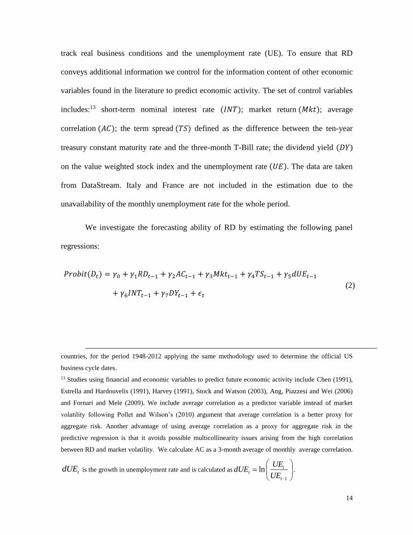
track real business conditions and the unemployment rate (UE). To ensure that RD

conveys additional information we control for the information content of other economic

variables found in the literature to predict economic activity. The set of control variables

includes:13 short-term nominal interest rate (𝐼𝑁𝑇); market return (𝑀𝑘𝑡); average

correlation (𝐴𝐶); the term spread (𝑇𝑆) defined as the difference between the ten-year

treasury constant maturity rate and the three-month T-Bill rate; the dividend yield (𝐷𝑌)

on the value weighted stock index and the unemployment rate (𝑈𝐸). The data are taken

from DataStream. Italy and France are not included in the estimation due to the

unavailability of the monthly unemployment rate for the whole period.

We investigate the forecasting ability of RD by estimating the following panel

regressions:

𝑃𝑟𝑜𝑏𝑖𝑡(𝐷𝑡) = 𝛾0 + 𝛾1𝑅𝐷𝑡−1 + 𝛾2𝐴𝐶𝑡−1 + 𝛾3𝑀𝑘𝑡𝑡−1 + 𝛾4𝑇𝑆𝑡−1 + 𝛾5𝑑𝑈𝐸𝑡−1

+ 𝛾6𝐼𝑁𝑇𝑡−1 + 𝛾7𝐷𝑌𝑡−1 + 𝜖𝑡 (2)

countries, for the period 1948-2012 applying the same methodology used to determine the official US

business cycle dates.

13 Studies using financial and economic variables to predict future economic activity include Chen (1991),

Estrella and Hardouvelis (1991), Harvey (1991), Stock and Watson (2003), Ang, Piazzesi and Wei (2006)

and Fornari and Mele (2009). We include average correlation as a predictor variable instead of market

volatility following Pollet and Wilson’s (2010) argument that average correlation is a better proxy for

aggregate risk. Another advantage of using average correlation as a proxy for aggregate risk in the

predictive regression is that it avoids possible multicollinearity issues arising from the high correlation

between RD and market volatility. We calculate AC as a 3-month average of monthly average correlation.

tdUE is the growth in unemployment rate and is calculated as

1

ln tt

t

UEdUE

UE

.

15

𝐴𝐷𝑆𝑡 = 𝛾0 + 𝛾1𝑅𝐷𝑡−1 + 𝛾2𝐴𝐶𝑡−1 + 𝛾3𝑀𝑘𝑡𝑡−1 + 𝛾4𝑇𝑆𝑡−1 + 𝛾5𝑑𝑈𝐸𝑡−1

+ 𝛾6𝐼𝑁𝑇𝑡−1 + 𝛾7𝐷𝑌𝑡−1 + 𝛾8𝐴𝐷𝑆𝑡−1 + 𝜖𝑡

(3)

𝑑𝑈𝐸𝑡 = 𝛾0 + 𝛾1𝑅𝐷𝑡−1 + 𝛾2𝐴𝐶𝑡−1 + 𝛾3𝑀𝑘𝑡𝑡−1 + 𝛾4𝑇𝑆𝑡−1 + 𝛾5𝑑𝑈𝐸𝑡−1

+ 𝛾6𝐼𝑁𝑇𝑡−1 + 𝛾7𝐷𝑌𝑡−1 + 𝜖𝑡

(4)

The panel model for equations 2, 3 and 4 uses country dummies and clusters the

standard errors by country, allowing for observations from the same country in different

years to be correlated.14 For equations 3 and 4 we also adjust the standard errors by using

the Newey-West procedure (Newey and West, 1987) modified for use in a panel data set.

Table 3 presents the estimation results of equations 2-4 for the business cycle,

ADS business conditions index and the unemployment rate. Control variables are

included in all regressions but for brevity we do not show coefficient estimates in table 3.

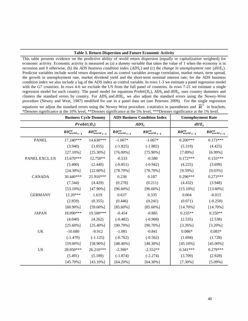
Using all countries in a pooled regression we find a positive and statistically significant

relation between the business cycle dummy and equally weighted world dispersion. A

higher world dispersion over the last three months indicates a higher probability that the

economy will be in a recession for the current month. Using the ADS business condition

as a proxy for economic activity we also get a strong and statistically significant relation

with return dispersion (see coefficient estimates in column 4 of table 3). A higher return

dispersion is followed by worsening business conditions. The unemployment rate is

negatively related with the state of the economy. If return dispersion is a countercyclical

variable it should be positively associated with the unemployment rate. The coefficient of

14 For more information on the methodology, refer to the work of Petersen (2009).

16

the world return dispersion measure is 0.200 and statistically significantly different from

zero (t-statistic 5.319). Capitalization weighted world return dispersion produces very

similar coefficients estimates and t-statistics for the all proxies of economic activity and

the business cycle.

The evidence on the predictive ability of return dispersion are consistent with

previous evidence from the US market. It is possible that the observed relationship found

when pooling information across countries is driven by US data. To assess the sensitivity

of the estimation results to the inclusion of the US data we re-estimate equations 2-4

excluding the US from the full panel of countries15 and show the results in rows 4-6 of

table 3. Excluding the US could be regarded as an out-of-sample test of the empirical

evidence reported for the US market. Excluding the US produces coefficient estimates for

world return dispersion that are very similar to estimates that include data from the US.

With the exception of the ADS business conditions index, the t-statistics suggest similar

significance levels. Use the capitalization weighted measure of world return dispersion

produces similar results.

Table 3 also shows evidence on the pervasiveness of the ability of world return

dispersion to predict the state of economy by looking at the country by country evidence.

For the business cycle dummy the relation between the state of the economy and equally

weighted world dispersion is positive and statistically different from zero for four of the

five countries. For the capitalization weighted measure of world return dispersion the

number of countries with statistically significant coefficients is three. The only exception

15 In section 4 we examine in addition the effect of excluding US stocks from the calculation of the world

RD measures.

17

to the positive relation between dispersion and the business cycle dummy is the UK for

which the estimated coefficient is negative.

For the ADS business condition index and for three of the five countries (the

exceptions are Canada and Germany) the estimated coefficient is negative but statistically

significant only for the US. The insignificance of dispersion in the panel that excludes the

US suggests that for this variable the full panel results are driven primarily by US data.

World return dispersion (equally or capitalization weighted) is positive and

statistically significantly related with unemployment rate for four of the five countries

(the exception is Germany).

To summarize, table 3 provides strong evidence that world return dispersion helps

forecast economic activity and the business cycle. The ability of RD to predict future

economic developments remains intact when we control for the information content of

other variables found in the literature to predict the business cycle. The relation between

world return dispersion and the economy is pervasive across countries and remain

significant when the US is excluded from the sample.

3.2. Does return dispersion forecast market returns and factor payoffs?

The evidence in the previous section suggests that RD is a pervasive financial

variable and potentially a proxy for risk factors omitted from the single factor CAPM. A

relative higher RD signals a deterioration of future economic activity and an increased

probability that the economy enters a recession. It is also well accepted in the finance

literature that market and factor premia are time-varying and dependent on the state of the

18

economy.16 The evidence from the cyclical nature of RD and the time-varying behavior

of market and factor premia jointly suggest that RD might be a good predictor of future

returns and factor premia.

Guo and Savickas (2008) and Maio (2014) find a negative and statistically

significant relation between idiosyncratic volatility and RD and subsequent US market

returns. In contrast, Garcia, Mantilla-Garcia and Martellini (2013) document a positive

relation between RD and the US stock market. Stivers and Sun (2010) provide a direct

test of the ability of RD to predict value and momentum premia. Using US stock market

data for the period 1965-2005 they find that RD is positively related with the value

premium and negatively related with the momentum premium. They conjecture that RD

is “a leading countercyclical variable” which varies with the state of the economy.

In this section we extend the work of Stivers and Sun (2010), Garcia, Mantilla-

Garcia and Martellini (2013) and Maio (2014) to provide new evidence for the predictive

ability of RD for market returns and the size, value and momentum premia for the stock

markets of the G7 countries. Pooling data from all countries produces more efficient

coefficient estimates whilst the use of data from major markets outside the US minimizes

the effects of data snooping and provides an independent assessment of the available

empirical evidence.

More specifically, we estimate the following panel regressions at annual

frequencies to investigate the predictive ability of RD:

16 Stivers and Sun (2010) provide a review of the academic literature on the cyclical properties of the value

and momentum premia.

19

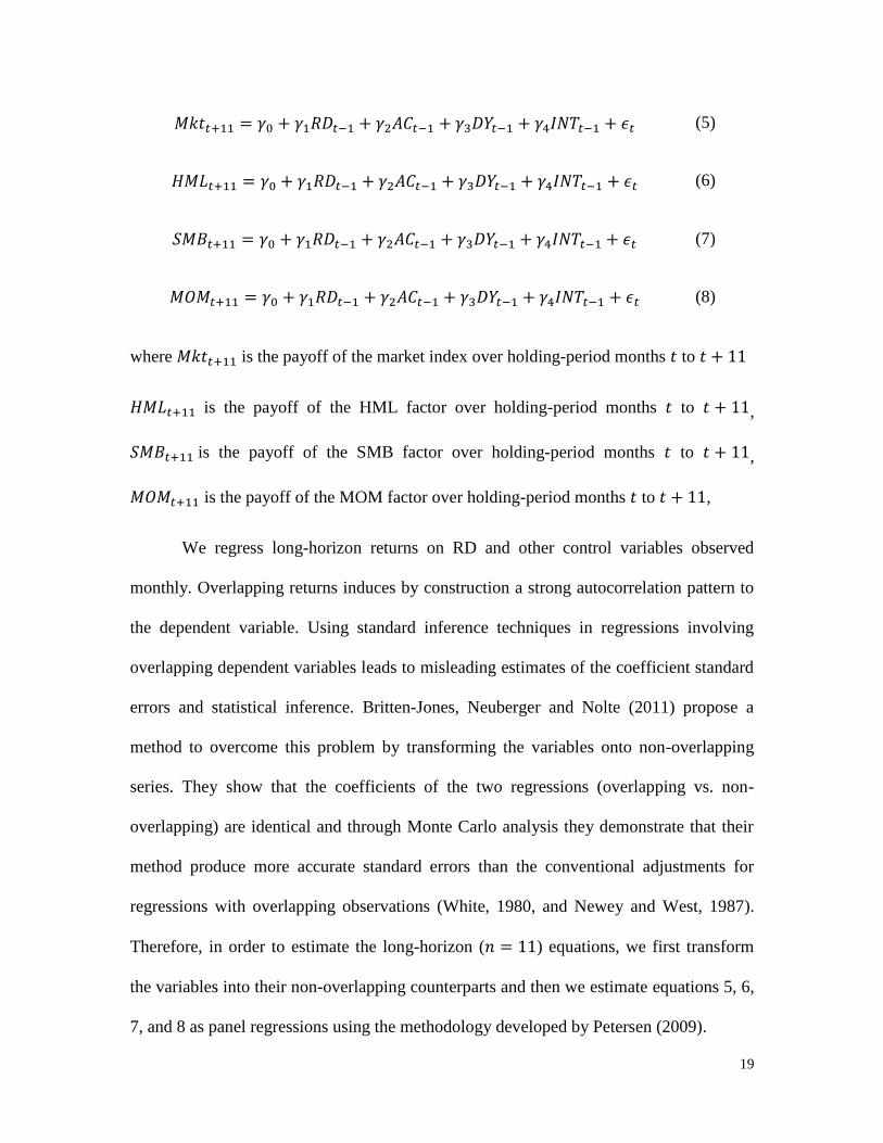
𝑀𝑘𝑡𝑡+11 = 𝛾0 + 𝛾1𝑅𝐷𝑡−1 + 𝛾2𝐴𝐶𝑡−1 + 𝛾3𝐷𝑌𝑡−1 + 𝛾4𝐼𝑁𝑇𝑡−1 + 𝜖𝑡 (5)

𝐻𝑀𝐿𝑡+11 = 𝛾0 + 𝛾1𝑅𝐷𝑡−1 + 𝛾2𝐴𝐶𝑡−1 + 𝛾3𝐷𝑌𝑡−1 + 𝛾4𝐼𝑁𝑇𝑡−1 + 𝜖𝑡 (6)

𝑆𝑀𝐵𝑡+11 = 𝛾0 + 𝛾1𝑅𝐷𝑡−1 + 𝛾2𝐴𝐶𝑡−1 + 𝛾3𝐷𝑌𝑡−1 + 𝛾4𝐼𝑁𝑇𝑡−1 + 𝜖𝑡 (7)

𝑀𝑂𝑀𝑡+11 = 𝛾0 + 𝛾1𝑅𝐷𝑡−1 + 𝛾2𝐴𝐶𝑡−1 + 𝛾3𝐷𝑌𝑡−1 + 𝛾4𝐼𝑁𝑇𝑡−1 + 𝜖𝑡 (8)

where 𝑀𝑘𝑡𝑡+11 is the payoff of the market index over holding-period months 𝑡 to 𝑡 + 11

𝐻𝑀𝐿𝑡+11 is the payoff of the HML factor over holding-period months 𝑡 to 𝑡 + 11,

𝑆𝑀𝐵𝑡+11 is the payoff of the SMB factor over holding-period months 𝑡 to 𝑡 + 11,

𝑀𝑂𝑀𝑡+11 is the payoff of the MOM factor over holding-period months 𝑡 to 𝑡 + 11,

We regress long-horizon returns on RD and other control variables observed

monthly. Overlapping returns induces by construction a strong autocorrelation pattern to

the dependent variable. Using standard inference techniques in regressions involving

overlapping dependent variables leads to misleading estimates of the coefficient standard

errors and statistical inference. Britten-Jones, Neuberger and Nolte (2011) propose a

method to overcome this problem by transforming the variables onto non-overlapping

series. They show that the coefficients of the two regressions (overlapping vs. non-

overlapping) are identical and through Monte Carlo analysis they demonstrate that their

method produce more accurate standard errors than the conventional adjustments for

regressions with overlapping observations (White, 1980, and Newey and West, 1987).

Therefore, in order to estimate the long-horizon (𝑛 = 11) equations, we first transform

the variables into their non-overlapping counterparts and then we estimate equations 5, 6,

7, and 8 as panel regressions using the methodology developed by Petersen (2009).

20

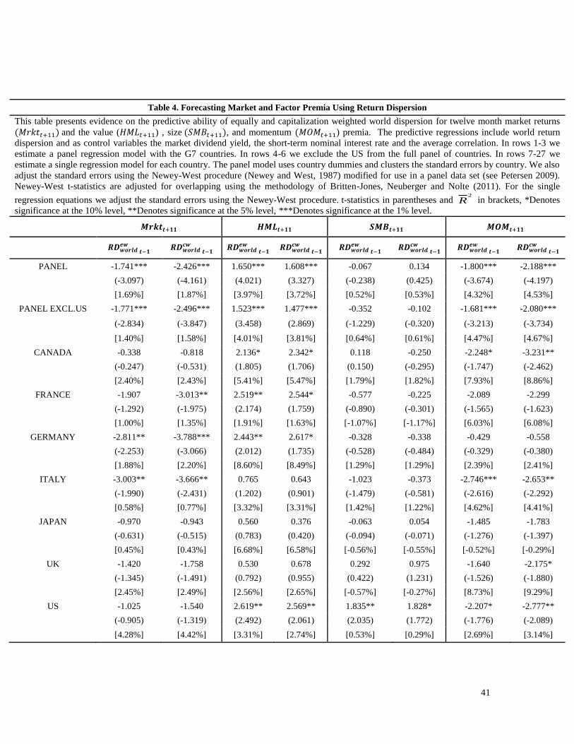
Table 4 presents the panel regressions of twelve month market returns, value,

size, and momentum on lagged return dispersion and control variables. The panel

regression includes control variables whose coefficient estimates are not shown in the

table for the sake of brevity.

By pooling data across countries we find a negative and statistically significant

relation between equally weighted world dispersion and subsequent market returns.

Excluding the US from the panel data does not affect the coefficient estimate and its

statistical significance. The estimated coefficients of return dispersion are negative across

all countries and statistically significant for Germany and Italy. The results are robust to

the use of the capitalization weighted measure of world return dispersion (the estimated

coefficients of RD are significant for France, Germany and Italy).

The negative relation between RD and subsequent market is robust to the

investment horizon. When we use a monthly horizon to re-estimate equation 5 we find a

strong negative relation between market returns and the equally (coefficient -0.146, t-

statistic -2.303) and capitalization (coefficient -0.167, t-statistic -2.544) weighted RD.

The evidence are consistent with results of Guo and Savickas (2008) and Maio (2014)

but contradicts the evidence presented in Garcia, Mantilla-Garcia and Martellini (2013)

for the US market. Garcia, Mantilla-Garcia and Martellini (2013) use a monthly RD

measure calculated as the monthly average of daily RD, to predict monthly market

returns and find a positive but insignificant relation with capitalization weighted market

return. They find a significantly positive relation between daily market returns and RD.

The contradictory results reported in Garcia, Mantilla-Garcia and Martellini (2013)

compared to the evidence in this paper and Maio (2014) might reflect the use of daily

21

rather than monthly return data used to calculate RD. The use of daily data to calculate

RD could introduce a microstructure bias driven by the bid-ask spread. Han and

Lesmond (2011) and Han, Hu and Lesmond (2014) show that due to the bid-ask bounce

in daily returns, estimates of volatility based on daily data will be biased and could lead

to misleading inferences.

A higher world dispersion is associated with better performance of value-versus-

growth strategy over the subsequent year. The coefficient of world dispersion is positive

and statistically different from zero for panels including and excluding the US. The

relation is consistently positive across all countries and dispersion measures. For both the

equally and capitalization weighted measure of world dispersion the coefficients are

statistically significant for four of the seven countries.

Using the full panel of countries we find a negative relation between world

dispersion and the momentum premium. A higher world dispersion is associated with

weaker performance for a momentum strategy over the subsequent year. Excluding the

US from the panel makes little difference to the estimates. The relation is negative across

countries and statistically significant (at the 10% level) for three of the seven countries

(four out of seven when the capitalization weighted measure of dispersion is used). The

evidence is consistent with the results reported in Stivers and Sun (2013) for the US

market. They study the relation between lagged RD and relative strength market

strategies and provide evidence in favor of the view that the relation is negative for both

medium-run and long-run strategies.

Finally, we find no relation between the size premium and equally weighted

world dispersion with panel data including and excluding the US. Looking at individual

22

country results we find a negative but statistically insignificant relation for five countries,

a positive relation for the UK and a positive and statistically significant coefficient for the

US. Similar results are obtained with the capitalization weighted measure of return

dispersion.

The relation between the world return dispersion and market returns and factor

premia is economically significant. A one standard deviation increase of world return

dispersion is associated with a -3.73% (-1.7410.214) decrease in market returns, a

3.53% (1.6500.214) increase in the value premium and a -3.85% (-1.8000.214) fall in

the momentum premium.

The evidence on the relation between dispersion and market returns and the value

premium are consistent with the evidence in Guo and Savickas (2008) who argue that

idiosyncratic volatility, a volatility measure correlated with dispersion, is a proxy for

changes in the investment opportunity set. For the G7 countries they find a negative

relation between idiosyncratic volatility and market returns (statistically significant for

two of the seven countries) and positively related to the value premium (statistically

significant for four of the seven countries).17 We examine in section 5 whether dispersion

is a better measure of the opportunity set than idiosyncratic volatility.

Guo and Savickas (2008) and Maio (2014) find that the information content in

idiosyncratic volatility (Guo and Savickas) and RD (Maio) is more reliable when also

controlling for the realized market volatility. To examine whether the relation between

RD and subsequent market returns and premia strengthens when we use data from the G7

17 Compared to the results in Guo and Savickas (2008), in this paper the capitalization weighted dispersion

measure is important for three (four) of the seven countries for the market (value). In our research, in

addition to country evidence, we also pool information across countries.

23

countries, we replace average correlation (AC) with market volatility18 and re-estimate

equations 5 to 8. In the presence of market volatility the coefficient of equally weighted

RD remains statistically significant and marginally stronger compared with RD

coefficient estimated when market volatility is not included in the predictive regressions.

In particular, the coefficient of RD when predicting market returns is reduced from -

1.721 (t-statistic -3.056) when market volatility is not included in the regression, to -

1.916 (t-statistic -3.167) when market volatility is one of the control variables. Similar to

the evidence reported in Guo and Savickas (2008) we find that the coefficient of market

volatility becomes positive from negative when we include both volatility variables in the

regression. Controlling for market volatility strengthens the coefficient of RD for the

value premium (from 1.712 to 1.779) but weakens the coefficient for the momentum

premium (from -1.614 to -0.688). We obtain similar results when we use the portfolio

based measure of RD.

In summary, a higher world return dispersion is followed by lower market

returns, a smaller momentum premium and a higher value premium. The relation between

dispersion and the size premium is weak and insignificant across countries. These

findings are robust to the exclusion of the US from the panel and the weighting scheme

used to calculate world return dispersion.

3.3. RD as a predictor of market volatility.

18 We calculate for each market the monthly market volatility at month 𝑡 (𝑀𝑉𝑡) using daily market return

(rm) within the calendar month. Specifically, we calculate monthly market volatility as: MVt =

√nt√Var(rm) ,where nt is the number of days in month t.

24

The evidence presented in section 3.2 suggests that RD forecasts changes in

future returns. Is RD a predictor of changes in market volatility? We test this hypothesis

by estimating the following panel regression using data from the G7 countries:

𝑀𝑉𝑡 = 𝛾0 + 𝛾1𝑅𝐷𝑡−1 + 𝛾2𝐴𝐶𝑡−1 + 𝛾3𝑀𝑘𝑡𝑡−1 + 𝛾4𝑇𝑆𝑡−1 + 𝛾5𝑑𝑈𝐸𝑡−1 +

𝛾6𝐼𝑁𝑇𝑡−1 + 𝛾7𝐷𝑌𝑡−1 + 𝜖𝑡 (9)

where 𝑀𝑉𝑡 is the 3-month moving average of market volatility in month t and the other

variables as described in the previous section. The results presented in table 5 suggest

that return dispersion is an important predictor of future market volatility. The full panel

results suggest a positive and statistically significant relation between world RD and

world market volatility. The results are robust to the exclusion of the US from the full

panel of countries. The evidence are pervasive across countries with positive and

significant estimates for all countries in the sample. Our findings are consistent with the

evidence presented in Stivers (2003) and Connolly and Stivers (2006) who find a positive

relation between US monthly and daily return dispersion and stock market volatility. Our

findings add to the existing evidence using data from the G7 countries and are consistent

with the hypothesis that RD is a state variable proxying for changes in future expected

returns and aggregate volatility.

4. Sub-sample Analysis and Alternative Return Dispersion Measures

In this section we examine the robustness of the evidence on the predictive ability

of world RD for the economy and factor returns over sub-samples and alternative

measures of return dispersion.

25

We split the sample in two periods: 1980-1996 and 1997-2012. Table 6 shows

estimation results for the economy proxies, factor returns and market volatility in the two

sub-samples. In the first sub-sample the relation between the business cycle dummy and

RD is positive but statistically significant only for the equally weighted measure of

dispersion. The relation between the ADS business conditions index and RD is negative

and consistent with the full sample results and statistically significant for the equally

weighted measure of RD. For unemployment, the relation is positive and statistically

significant only for the equally weighted measure of RD. In the second period, the

estimates are consistent with the full sample estimates and both world RD measures (with

the exception of the ADS business condition index and equally weighted world RD

where the coefficient is negative but not statistically significant).

Panel B shows coefficient estimates for world RD for the market and the three

factor premia. For the market portfolio the relation between word RD and market returns

is consistently negative and statistically significant across both sub-period and measures

of dispersion. For the value premium the coefficient estimates are positive in both

periods but statistically significant only in the later period. For the momentum premium,

the coefficient of world RD is consistently negative and statistically significant across

both periods and measures of world RD.

Overall the evidence for both economic and factor returns suggest consistent but

weaker relationships in the first sub-period compared with the second sub-sample. The

stronger relationships observed in the later period are consistent with the increase in the

importance of the common factor in country return dispersion measures discussed in

section 2. The second sub-period coincides with increased economic and financial

26

integration and increased relevance of a common factor driving economic growth and

real interest rates.19

In table 7 we show estimation results using alternative measures of return

dispersion. The first set of alternative measures of return dispersion are the equally and

capitalization weighted measures of country return dispersions, based on monthly

individual stock return data. For the second alternative of world measure we follow

Stivers and Sun (2010) and Maio (2014) to create a world dispersion measure based on

the return dispersion of 100 portfolios sorted on size and book to market using all stocks

in our database. Portfolio level return dispersion may be less noisy than firm level return

dispersion. Using portfolios than individual stocks reduces the influence of extreme

individual returns. Stivers and Sun (2010) note that portfolio level returns dispersion

performs similarly but generally better than firm level dispersion metrics.

The results presented in tables 3, 4, and 5 are robust to the use of individual

country return dispersion measures. Coefficient estimates in table 7, panels A, B and C

(columns 2 and 4), are similar to estimated based on world RD for the economic

variables, market return and factor premia and market volatility. The lower explanatory

power of regressions and the generally lower t-statistics for the coefficient estimates

using country RD measures for both the economy and premia sets of variables suggests

that world RD is a better measure of return dispersion. Results from using a world

dispersion measure based on portfolio rather than individual stock returns are in columns

3 and 5 of table 7. Consistent with evidence based on the world RD measure based on

individual stocks, a relatively higher portfolio RD indicates a higher probability that the

19 See Perspectives on global real interest rates, IMF 2014.

27

economy will be in recession, is negatively related with the ADS business conditions

index and positively associated with unemployment. A higher RD is followed by a

positive value premium, a negative momentum premium, a lower market return and

higher future market volatility. Comparing the predictive power of portfolio based RD

with stock based world RD we find that it performs marginally better (has more

predictive power) for market returns and the factor premia but has lower power in the

prediction of economic variables and market volatility.

Are the results presented earlier sensitive to the exclusion of US stocks from the

world RD measures? To answer this question we construct equally and capitalization

weighted world RD measures using data from the six remaining countries. Table 8 shows

that the predictive ability of RD for the economy, risk premia and market volatility is

robust to measures of RD that exclude US stocks.

5. Return Dispersion and Idiosyncratic Volatility

Stivers (2003) and Garcia, Mantilla-Garcia and Martellini (2013) show that return

dispersion is related to idiosyncratic and market volatility. Stivers (2003) show that

𝐶𝑆𝑉t ≅ 𝜎𝛽2(𝑟𝑚𝑡 − 𝑟𝑓𝑡)

2+ 𝜎𝑡

2, where 𝜎𝛽2 is the cross-sectional variance of betas and 𝜎𝑡

2 is

the idiosyncratic variance. Garcia, Mantilla-Garcia and Martellini (2013) generalize the

formula and prove that:

E(CSVt) = ∑ witσ𝜖𝑖𝑡

2

N

i=1

− ∑ wit2σ𝜖𝑖𝑡

2

N

i=1

+ E(𝐹𝑡2CSVt

β), (10)

28

where CSVtβ is the cross sectional variance of stock betas, 𝜎𝜖𝑖𝑡

2 is the specific variance of

stock i, and 𝐹𝑡2 is the square return of the factors at time t.

We calculate monthly idiosyncratic volatilities (IV) in month t as:

IVt = ∑ wi,t

N

i=1

√nt√Var(εit), (11)

where wit is either equal to 1

𝑁 or to the market capitalization weight of stock i in month

t − 1, nt is the number of days in month t and εit is the firm specific return that is

estimated every month 𝑡 from the following regression:

rit = αi + βirmt + εit, (12)

Equation 10 shows that return dispersion is a function of idiosyncratic volatility,

the variance of factor returns and the cross sectional variance of stock beta factors. Guo

and Savickas (2008) argue that idiosyncratic volatility is a proxy for changes in the

investment opportunity set and report evidence based on the G7 countries consistent with

the hypothesis that idiosyncratic volatility is a predictor of the market and value

premiums.

Garcia, Mantilla-Garcia, and Martellini (2013) show that return dispersion and

idiosyncratic risk are highly correlated. In our dataset and for the equally (capitalization)

weighted scheme, the average correlation between world, country, and portfolios based

return dispersion and idiosyncratic risk are 0.70 (0.78), 0.86 (0.89) and 0.47 (0.36),

respectively. As expected all measures are positively correlated but the world and the

portfolio based measures are less correlated with idiosyncratic risk and hence may not

29

capture the same economic information. In this section we investigate whether return

dispersion conveys incremental information relative to idiosyncratic volatility.

To explore the role of dispersion in the presence of idiosyncratic volatility we re-

estimate equations 2-9 including idiosyncratic volatility to the list of independent

variables. Table 9 shows estimation results for the three equally weighted dispersion

measures (results for capitalization weighted dispersion are shown in Table A1 in the

appendix). For the main measure of dispersion, world RD (columns 2-3), the estimated

coefficients of dispersion for the business cycle variable and unemployment remain

statistically significant in the presence of idiosyncratic volatility. For the ADS business

conditions index, the coefficient for world RD is insignificant. For the country-based

measures of dispersion (columns 4-5) the coefficient for the unemployment rate is

statistically significant as is the coefficient for the ADS business conditions index but

with the wrong sign. The change in sign when both variables are included in the

regression is indicative of multicollinearity (the average correlation across countries for

country based dispersion and idiosyncratic volatility is 0.86). When we use the portfolio

based world dispersion (columns 6-7) the coefficients for dispersion are not statistically

different form zero.

The independent role of dispersion becomes clearer when we look at the market

return and factor premia evidence. When we use world RD, the coefficient of

idiosyncratic volatility is not different from zero for the value and momentum premia and

marginally significant, but with the wrong sign, for the market premium. Country-based

measures of dispersion also drive out the significance of idiosyncratic volatility. We get

much stronger results for the superiority of dispersion when we use the portfolio based

30

measure of world dispersion. For the market and value and momentum premia we find

strongly significant results for dispersion and insignificant coefficient estimates for

idiosyncratic volatility. Portfolio based measures of dispersion have more explanatory

power than either world RD or country based dispersion.

The evidence in table 9 suggests that RD has more information than idiosyncratic

volatility. This is consistent with equation 10 which shows that RD is the sum of

idiosyncratic volatility plus a term equal to the product of market variance times the

cross-sectional dispersion of stock betas. From a theoretical perspective, Gomes, Kogan

and Zhang (2003) provide a theoretical link between RD, aggregate volatility and the

dispersion of stocks betas. In particular, their conditional CAPM suggests that the

countercyclical nature of RD is due to the countercyclical behavior of its components:

aggregate volatility and the cross-sectional dispersion of stock betas.

Dispersion and idiosyncratic volatility are both significant predictors of future

market volatility. The predictive power of regressions that include only dispersion is less

than regressions that include both dispersion and idiosyncratic volatility (compare tables

5 and 9) indicating that for predicting market volatility both volatility measures are

relevant. The empirical evidence in table 9 suggest that dispersion is a better measure

than idiosyncratic volatility for the market, value and momentum premia. For the

economic variables the evidence are less clear-cut.

As a final test of the information content of return dispersion we calculate the

economic benefits to an investor who uses return dispersion or idiosyncratic volatility to

forecast returns and creates dynamically optimal portfolios. We then compare the

improvement in Sharpe ratio of return dispersion driven strategies to a dynamic

31

investment strategy based on idiosyncratic volatility driven equity premia forecasts and a

static buy and hold portfolio of country premia (the market capitalization portfolios of

country returns or the three long-short factor portfolios). The evidence, however, should

be interpreted with caution given the short period of out-of-sample data available and the

effects of estimation error in return and risk forecasts on mean-variance optimization

based portfolios (see DeMiguel, Garlappi and Uppal (2009)).

The empirical evidence suggests that using return dispersion generates significant

improvements to the Sharpe ratio of the buy and hold portfolio. Compared to

idiosyncratic volatility driven forecasts, return dispersion based predictions lead to small

but economically significant improvements in the performance of the value and

momentum factor timing strategies (details of investment strategy construction and

estimation results are given in table A2 in the appendix).

6. Conclusions

Return dispersion is a timely, model free estimation of risk. Academics and

practitioners have used return dispersion as a measure of risk and uncertainty and an

advance indicator of business conditions. We provide evidence on the ability of RD to

predict changes in the investment opportunity set.

We provide strong evidence suggesting that RD is a good predictor of future

economic developments. In particular we find that a relatively higher RD is followed by

an increase in unemployment, a higher probability that the economy is in recession.

RD observed in time t predicts future twelve month market returns, value and

momentum premia and market volatility. The results are robust across sub-periods,

alternative measures of RD and remain intact when the US is excluded from the data.

32

We find that RD conveys incremental information relative to idiosyncratic

volatility. There are two possible explanations for the superiority of RD. First, RD is a

better, less noisy market state variable than idiosyncratic volatility. Measures of

idiosyncratic volatility require high frequency data which introduce severe biases due to

non-synchronous trading and the effect of the bid-ask bounce in trade prices (Han and

Lesmond (2011) and Han, Hu and Lesmond (2014)). Microstructure biases could explain

the contradictory evidence of a negative relation between RD and future market returns

found in this paper and Maio (2014) and the positive relation reported in Garcia, Garcia-

Mantilla and Martellini (2013). Second RD by construction has more information than

idiosyncratic volatility. In particular, in addition to idiosyncratic volatility, RD reflects

movements in aggregate stock market volatility and the cross section of stock betas, both

countercyclical variables with predictive power for future market returns and factor

premia.

33

References

Adrian, T., Rosenberg, J., 2008. Stock returns and volatility: pricing the short-run and

long-run components of market risk. Journal of Finance 63, 2997–3030.

Ang, A., Piazessi, M., Wei., M., 2006. What does the yield curve tell us about GDP

growth?. Journal of Econometrics 131, 359 – 403.

Aruoba, S., Diebold, F., Scotti, C., 2009. Real-time measurement of business condition.

Journal of Business & Economic Statistics 27, 417-427.

Bali,T.,Cakici,N.,Levy,H.,2008.A model-independent measure of aggregate idiosyncratic

risk. Journal of Empirical Finance 15 , 878-896.

Bansal, R., Yaron, A., 2004. Risks for the long run: A potential resolution of asset pricing

puzzles. Journal of Finance 59, 1481–1509.

Bekaert, B., Hodrick, R., Zhang, X., 2012. Aggregate idiosyncratic volatility. Journal of

Financial and Quantitative Analysis 47 , 1155-1185.

Black, F, 1987. A gold standard with double feedback and near zero reserves. Business

Cycles and Equilibrium.

Black, F, 1995. Exploring General Equilibrium, MIT Press.

Bloom, N., 2009. The Impact of uncertainty shocks. Econometrica 77, 623-685.

Bloom, N., Floetotto, M., Jaimovich, N., Saporta-Eksten, I., Terry, S., 2012. Really

uncertain business cycles. Working paper, NBER

Britten-Jones, M., Neuberger, A. , Nolte, I., 2011. Improved inference in regression with

overlapping observations. Journal of Business Finance & Accounting 38, 657-683.

Brockman, P., Chung, D. , Perignon, C., 2009. Commonality in liquidity: a global

perspective. Journal of Financial and Quantitative Analysis 44, 851-882.

Busse, J., Goyal, A., Wahal, S., 2013. Investing in a global world. Review of Finance,

forthcoming.

Campbell, J., 1996. Understanding risk and return. Journal of Political Economy 104,

298–345.

http://amstat.tandfonline.com/action/doSearch?action=runSearch&type=advanced&result=true&prevSearch=%2Bauthorsfield%3A(Aruoba%2C+S.+Bora%C4%9Fan)

http://amstat.tandfonline.com/action/doSearch?action=runSearch&type=advanced&result=true&prevSearch=%2Bauthorsfield%3A(Diebold%2C+Francis+X.)

http://amstat.tandfonline.com/action/doSearch?action=runSearch&type=advanced&result=true&prevSearch=%2Bauthorsfield%3A(Scotti%2C+Chiara)

http://onlinelibrary.wiley.com/doi/10.1111/jofi.2004.59.issue-4/issuetoc

34

Chen Z., Petkova, R., 2012. Does idiosyncratic volatility proxy for risk exposure?.

Review of Financial Studies 25, 2745-2787.

Chen, J., 2003. Intertemporal CAPM and the cross-section of stock returns. Working

paper, University of California, Davis.

Chen, J., Kannan, P., Loungani, P., Trehan, B., 2011. New evidence on cyclical and

structural sources of unemployment. Working paper, IMF

Chen, N., 1991. Financial investment opportunity and the macroeconomy. Journal of

Finance 46, 529 – 554.

Christie, W., Huang, R., 1995. Following the pied piper: do individual returns herd

around the market?. Financial Analysts Journal 51, 31-37.

Connolly, R., Stivers, C., 2006. Information content and other characteristics of the daily

cross-sectional dispersion in stock returns. Journal of Empirical Finance 13, 79-112.

Connor, G., Li, S., 2009. Market dispersion and the profitability of hedge funds. Working

paper.

DeMiguel, V., Garlappi L., Uppal, R., 2009. Optimal versus Naive Diversification: How

Inecient is the 1/N Portfolio Strategy?. The Review of Financial Studies 22, 1915-1953.

Engle, R., Rangel, J., 2008. The spline-GARCH model for low-frequency volatility and

its global macroeconomic causes. Review of Financial Studies 21, 1187 -1222.

Estrella, A., Hardouvelis, G. ,1991. The term structure as a predictor of real economic

activity. Journal of Finance 46, 555-576.

Fama, E., French, K., 1992. The cross section of expected stock returns. Journal of

Finance 47, 427-465.

Fama, E., French, K.,1993. Common risk factors in the returns on stocks and bonds.

Journal of Financial Economics 33, 3-56.

Fornari, F., Mele, A., 2009. Financial volatility and economic activity. Working paper.

Fung, W., Hsieh, D., 2004. Hedge fund benchmarks: A risk-based approach. Financial

Analysts Journal 60, 65-80.

35

Garcia, R., F., Mantilla-Garcia, Martellini, L., 2013. A model-free measure of aggregate

idiosyncratic volatility and the prediction of market returns. Forthcoming, Journal of

Financial and Quantitative Analysis.

Gomes, J., Kogan, L., Zhang, L., 2003. Equilibrium cross section of returns. Journal of

Political Economy 111, 693-732.

Goyal, A., Santa-Clara, P., 2003. Idiosyncratic risk matters! Journal of Finance 58 , 975–

1008.

Guo, H., Savickas, R. 2008. Average idiosyncratic volatility in G7 countries. Review of

Financial Studies 21, 1259–1296.

Han, Y., Lesmond, D. 2011. Liquidity Biases and the Pricing of Cross-sectional

Idiosyncratic Volatility. Review of Financial Studies 24, 1590-1629.

Han, Y., Hu, T., Lesmond, D. 2014. Liquidity Biases and the Pricing of Cross-Sectional

Idiosyncratic Volatility Around the World. Forthcoming, Journal of Financial and

Quantitative Analysis.

Hamilton, J., Lin, G., 1996. Stock market volatility and the business cycle. Journal of

Applied Econometrics 11, 573–593.

Harvey, C.R, 1991. The term structure and world economic growth. Journal of Fixed

Income 1, 7-19

Hou, K., Karolyi, A., Kho, B., 2011. What factors drive global stock returns?. Review of

Financial Studies 24 , 2527 – 2574.

International Monetary Fund, World economic outlook, perspectives on global real

interest rates, April 2014.

Ince, O., Porter, R., 2006. Individual equity return data from Thomson Datastream:

handle with care!. Journal of Financial Research 29, 463–479.

Lilien, D. M, 1982. Sectoral shifts and cyclical unemployment. Journal of Political

Economy 90, 773-93.

Lo, A., MacKinlay, A., 1990. Data-snooping biases in tests of financial asset pricing

models. Review of Financial Studies 3, 431-467.

36

Loungani, P., Rush, M., Tave, W., 1990. Stock market dispersion and unemployment.

Journal of Monetary Economics 25, 367 -388.

Maio, P. F., 2014. Cross-sectional return dispersion and the equity premium. Working

Paper, Hanken School of Economics.

Merton, R., 1973. An Intertemporal capital asset pricing model. Econometrica 41, 867–

887.

Newey, W., West, K., 1987. A simple positive semi-definite, heteroskedasticity and

autocorrelation consistent covariance matrix. Econometrica 55, 703-708.

Petersen, M., 2009. Estimating standard errors in finance panel data sets: comparing

approaches. Review of Financial Studies 22, 435-480.

Pollet, J.M, Wilson, M., 2010. Average correlation and stock market returns. Journal of

Financial Economics 96, 364-380.

Schwert, W., 1989. Margin requirements and stock volatility. Journal of Financial

Services Research 3, 153-164.

Silva, H. , Sapra, S., S. Thorley, S., 2001. Return dispersion and active management.

Financial Analysts Journal 57, 29-42.

Solnik, B., Roulet, J., 2000. Dispersion as cross-sectional correlation. Financial Analysts

Journal, 56 , 54-61.

Stivers, C. T, 2003. Firm-level return dispersion and the future volatility of aggregate

stock market returns. Journal of Financial Markets 6, 389-411.

Stivers, C., Sun, L., 2010. Cross-sectional return dispersion and time-variation in value

and momentum premia. Journal of Financial and Quantitative Analysis 45, 987- 1014.

Stivers, C., Sun, L., 2013. Market cycles and the performance of relative strength

strategies. Financial Management, 263-290.

Stock, J.H., Watson, M.W., 2003. Forecasting output and inflation. Journal of Economic

Literature 41, 788 - 829

http://www.springerlink.com/content/nm71656886706806/

http://www.springerlink.com/content/0920-8550/

http://www.springerlink.com/content/0920-8550/

http://www.springerlink.com/content/0920-8550/3/2-3/

37

Wei, S., Zhang, C., 2005. Idiosyncratic risk does not matter: A re-examination of the

relationship between average returns and average volatilities. Journal of Banking and

Finance 29, 603–621.

White, H, 1980. A Heteroskedasticity-consistent covariance matrix estimator and a direct

test for heteroskedasticity. Econometrica 48 , 817-838.

38

Table 1. Descriptive Statistics

This table presents the descriptive statistics of country, world and portfolio based measures of monthly return

dispersion. The equally weighted and capitalization-weighted measures of dispersion are shown in Panels A and B,

respectively. All measures are calculated as a 3-month average of monthly cross sectional return dispersion. The

sample period is from 07/31/1980 to 12/31/2012.

Panel A. Equally Weighted Return Dispersion

Mean Median Max Min S.D Skew Kurt

Canada 0.1119 0.1090 0.2568 0.0637 0.0284 1.3014 3.5883

France 0.0809 0.0747 0.2047 0.0494 0.0208 2.0564 7.0789

Germany 0.0757 0.0712 0.1868 0.0312 0.0284 1.0662 1.0661

Italy 0.0698 0.0653 0.1821 0.0394 0.0207 1.9658 5.7386

Japan 0.0758 0.0724 0.1359 0.0445 0.0164 0.8605 0.6537

U.K. 0.0893 0.0873 0.2032 0.0399 0.0233 1.4505 4.0435

US 0.0913 0.0833 0.1958 0.0597 0.0254 1.8458 3.5569

World 0.0964 0.0906 0.1957 0.0644 0.0214 1.6175 3.2384

World 100 Portfolios 0.0242 0.0231 0.0714 0.0119 0.0081 2.2866 9.2123

Panel B. Capitalization Weighted Return Dispersion

Mean Median Max Min S.D Skew Kurt

Canada 0.0748 0.0703 0.1708 0.0473 0.0183 1.8456 4.4345

France 0.0659 0.0624 0.1440 0.0370 0.0167 1.4112 2.8460

Germany 0.0599 0.0538 0.1339 0.0271 0.0209 1.2318 1.2589

Italy 0.0590 0.0547 0.1916 0.0315 0.0210 2.4075 9.2552

Japan 0.0697 0.0666 0.1345 0.0353 0.0180 0.9951 1.2546

U.K. 0.0664 0.0628 0.1400 0.0402 0.0172 1.6516 3.5922

US 0.0703 0.0634 0.1688 0.0427 0.0204 2.1263 5.2494

World 0.0764 0.0714 0.1623 0.0508 0.0184 1.5754 3.1301


39

Table 2. Commonality in Country Return Dispersion

Panel A presents the correlations of the equally and capitalization weighted return dispersion across the G7

countries, the world and portfolio based measures of return dispersion. The sample period is from 07/31/1980 to

12/31/2012.

Panel A. Correlation of Different Measures of Return Dispersion

Equally Weighted Return Dispersion

Canada France Germany Italy Japan U.K. US

France 0.67

Germany 0.62 0.82

Italy 0.38 0.50 0.29

Japan 0.42 0.53 0.48 0.28

UK 0.66 0.76 0.80 0.47 0.52

US 0.79 0.79 0.77 0.46 0.54 0.76

World 0.83 0.82 0.76 0.49 0.70 0.82 0.93

World ex US 0.82 0.81 0.74 0.51 0.76 0.84 0.83


Capitalization Weighted Return Dispersion

Canada France Germany Italy Japan U.K. US

France 0.71

Germany 0.70 0.75

Italy 0.62 0.67 0.47

Japan 0.62 0.62 0.57 0.43

UK 0.85 0.80 0.77 0.69 0.68

US 0.89 0.76 0.78 0.62 0.61 0.86

World 0.83 0.79 0.71 0.62 0.80 0.85 0.89

World ex US 0.74 0.77 0.66 0.61 0.89 0.83 0.73


40

Table 3. Return Dispersion and Future Economic Activity

This table presents evidence on the predictive ability of world return dispersion (equally or capitalization weighted) for

economic activity. Economic activity is measured as (a) a dummy variable that takes the value of 1 when the economy is in

recession and 0 otherwise, (b) the ADS business condition index (𝐴𝐷𝑆𝑡) and (c) the change in unemployment rate (𝑑𝑈𝐸𝑡).

Predictor variables include world return dispersion and as control variables average correlation, market return, term spread,

the growth in unemployment rate, market dividend yield and the short-term nominal interest rate; for the ADS business

condition index we also include a lag of the ADS index as control variable. In rows 1-3 we estimate a panel regression model

with the G7 countries. In rows 4-6 we exclude the US from the full panel of countries. In rows 7-21 we estimate a single

regression model for each country. The panel model for equations Probit(Dt), ADSt and dUEt, uses country dummies and

clusters the standard errors by country. For ADSt and dUEt, we also adjust the standard errors using the Newey-West

procedure (Newey and West, 1987) modified for use in a panel data set (see Petersen 2009). For the single regression

equations we adjust the standard errors using the Newey-West procedure. t-statistics in parentheses and 2

R in brackets,

*Denotes significance at the 10% level, **Denotes significance at the 5% level, ***Denotes significance at the 1% level.

Business Cycle Dummy ADS Business Condition Index Unemployment Rate

𝑷𝒓𝒐𝒃𝒊𝒕(𝑫𝒕) 𝑨𝑫𝑺𝒕 𝒅𝑼𝑬𝒕

𝑹𝑫𝒘𝒐𝒓𝒍𝒅

𝒆𝒘𝒕−𝟏

𝑹𝑫𝒘𝒐𝒓𝒍𝒅 𝒄𝒘

𝒕−𝟏 𝑹𝑫𝒘𝒐𝒓𝒍𝒅

𝒆𝒘𝒕−𝟏



𝒆𝒘𝒕−𝟏


𝒕−𝟏

PANEL 17.240*** 14.630*** -1.007* -1.007* 0.200*** 0.173***

(3.940) (3.055) (-1.825) (-1.882) (5.319) (4.425)

[27.10%] [25.30%] [76.00%] [75.90%] [7.89%] [6.99%]

PANEL EXCL.US 15.670*** 12.750** -0.533 -0.580 0.172*** 0.155***

(3.400) (2.440) (-0.851) (-0.942) (4.225) (3.699)

[24.30%] [22.60%] [78.70%] [78.70%] [9.59%] [9.03%]

CANADA 30.440*** 21.910*** 0.238 0.187 0.296*** 0.273***

(7.344) (4.429) (0.276) (0.211) (4.432) (3.948)

[53.10%] [47.90%] [96.60%] [96.60%] [15.10%] [13.60%]

GERMANY 12.20*** 1.619 0.637 0.335 0.004 -0.015

(2.859) (0.355) (0.446) (0.241) (0.071) (-0.250)

[60.90%] [59.60%] [85.60%] [85.60%] [14.70%] [14.70%]

JAPAN 18.090*** 19.500*** -0.454 -0.885 0.235** 0.250**

(4.040) (4.262) (-0.482) (-0.968) (2.535) (2.538)

[25.60%] [25.40%] [90.70%] [90.70%] [3.26%] [3.20%]

UK -10.680 -9.912 -1.081 -0.841 0.086* 0.083*

(-1.470) (-1.125) (-0.762) (-0.562) (1.694) (1.728)

[59.00%] [58.90%] [48.40%] [48.30%] [45.10%] [45.00%]

US 28.950*** 26.210*** -2.390* -2.552** 0.341*** 0.279***

(5.491) (5.189) (-1.874) (-2.274) (3.709) (2.928)

[45.70%] [43.10%] [64.20%] [64.30%] [7.30%] [5.09%]

41

Table 4. Forecasting Market and Factor Premia Using Return Dispersion

This table presents evidence on the predictive ability of equally and capitalization weighted world dispersion for twelve month market returns

(𝑀𝑟𝑘𝑡𝑡+11) and the value (𝐻𝑀𝐿𝑡+11) , size (𝑆𝑀𝐵𝑡+11), and momentum (𝑀𝑂𝑀𝑡+11) premia. The predictive regressions include world return

dispersion and as control variables the market dividend yield, the short-term nominal interest rate and the average correlation. In rows 1-3 we

estimate a panel regression model with the G7 countries. In rows 4-6 we exclude the US from the full panel of countries. In rows 7-27 we

estimate a single regression model for each country. The panel model uses country dummies and clusters the standard errors by country. We also

adjust the standard errors using the Newey-West procedure (Newey and West, 1987) modified for use in a panel data set (see Petersen 2009).

Newey-West t-statistics are adjusted for overlapping using the methodology of Britten-Jones, Neuberger and Nolte (2011). For the single

regression equations we adjust the standard errors using the Newey-West procedure. t-statistics in parentheses and 2

R in brackets, *Denotes

significance at the 10% level, **Denotes significance at the 5% level, ***Denotes significance at the 1% level.

𝑴𝒓𝒌𝒕𝒕+𝟏𝟏 𝑯𝑴𝑳𝒕+𝟏𝟏 𝑺𝑴𝑩𝒕+𝟏𝟏 𝑴𝑶𝑴𝒕+𝟏𝟏


𝒆𝒘𝒕−𝟏



𝒆𝒘𝒕−𝟏



𝒆𝒘𝒕−𝟏



𝒆𝒘𝒕−𝟏


𝒕−𝟏

PANEL -1.741*** -2.426*** 1.650*** 1.608*** -0.067 0.134 -1.800*** -2.188***

(-3.097) (-4.161) (4.021) (3.327) (-0.238) (0.425) (-3.674) (-4.197)

[1.69%] [1.87%] [3.97%] [3.72%] [0.52%] [0.53%] [4.32%] [4.53%]

PANEL EXCL.US -1.771*** -2.496*** 1.523*** 1.477*** -0.352 -0.102 -1.681*** -2.080***

(-2.834) (-3.847) (3.458) (2.869) (-1.229) (-0.320) (-3.213) (-3.734)

[1.40%] [1.58%] [4.01%] [3.81%] [0.64%] [0.61%] [4.47%] [4.67%]

CANADA -0.338 -0.818 2.136* 2.342* 0.118 -0.250 -2.248* -3.231**

(-0.247) (-0.531) (1.805) (1.706) (0.150) (-0.295) (-1.747) (-2.462)

[2.40%] [2.43%] [5.41%] [5.47%] [1.79%] [1.82%] [7.93%] [8.86%]

FRANCE -1.907 -3.013** 2.519** 2.544* -0.577 -0.225 -2.089 -2.299

(-1.292) (-1.975) (2.174) (1.759) (-0.890) (-0.301) (-1.565) (-1.623)

[1.00%] [1.35%] [1.91%] [1.63%] [-1.07%] [-1.17%] [6.03%] [6.08%]

GERMANY -2.811** -3.788*** 2.443** 2.617* -0.328 -0.338 -0.429 -0.558

(-2.253) (-3.066) (2.012) (1.735) (-0.528) (-0.484) (-0.329) (-0.380)

[1.88%] [2.20%] [8.60%] [8.49%] [1.29%] [1.29%] [2.39%] [2.41%]

ITALY -3.003** -3.666** 0.765 0.643 -1.023 -0.373 -2.746*** -2.653**

(-1.990) (-2.431) (1.202) (0.901) (-1.479) (-0.581) (-2.616) (-2.292)

[0.58%] [0.77%] [3.32%] [3.31%] [1.42%] [1.22%] [4.62%] [4.41%]

JAPAN -0.970 -0.943 0.560 0.376 -0.063 0.054 -1.485 -1.783

(-0.631) (-0.515) (0.783) (0.420) (-0.094) (-0.071) (-1.276) (-1.397)

[0.45%] [0.43%] [6.68%] [6.58%] [-0.56%] [-0.55%] [-0.52%] [-0.29%]

UK -1.420 -1.758 0.530 0.678 0.292 0.975 -1.640 -2.175*

(-1.345) (-1.491) (0.792) (0.955) (0.422) (1.231) (-1.526) (-1.880)

[2.45%] [2.49%] [2.56%] [2.65%] [-0.57%] [-0.27%] [8.73%] [9.29%]

US -1.025 -1.540 2.619** 2.569** 1.835** 1.828* -2.207* -2.777**

(-0.905) (-1.319) (2.492) (2.061) (2.035) (1.772) (-1.776) (-2.089)

[4.28%] [4.42%] [3.31%] [2.74%] [0.53%] [0.29%] [2.69%] [3.14%]

42

Table 5. Forecasting Market Volatility Using Return Dispersion(𝑹𝑫) This table presents evidence on the predictive ability of equally and capitalization weighted

world return dispersion for market volatility (𝑀𝑉𝑡). The predictive regressions include world

return dispersion and as control variables the market dividend yield, the short-term nominal

interest rate and average correlation. In rows 1 – 3 we estimate a panel model with the G7

countries. In rows 4-6 we exclude the US from the full panel of countries. In rows 7-21 we

estimate a single regression model for each country. The panel model uses country dummies

and clusters the standard errors by country. We also adjust the standard errors using the

Newey-West procedure (Newey and West, 1987) modified for use in a panel data set (see

Petersen, 2009). For the single regression equations we adjust the standard errors using the

Newey-West procedure. t-statistics in parentheses and 2

R in brackets, *Denotes

significance at the 10% level, **Denotes significance at the 5% level, ***Denotes

significance at the 1% level.

𝑴𝑽𝒕


𝒆𝒘𝒕−𝟏


𝒕−𝟏

PANEL 0.588*** 0.675***

(15.910) (15.250)

[58.50%] [60.80%]

PANEL EXCL.US 0.582*** 0.670***

(13.640) (13.060)

[55.80%] [58.30%]

CANADA 0.701*** 0.817***

(6.809) (6.839)

[65.00%] [68.30%]

GERMANY 0.612*** 0.690***

(8.579) (7.924)

[54.10%] [55.90%]

JAPAN 0.499*** 0.584***

(7.890) (7.396)

[53.40%] [57.00%]

UK 0.522*** 0.603***

(9.761) (9.131)

[61.90%] [65.20%]

US 0.545*** 0.622***

(7.989) (7.813)

[68.80%] [71.20%]

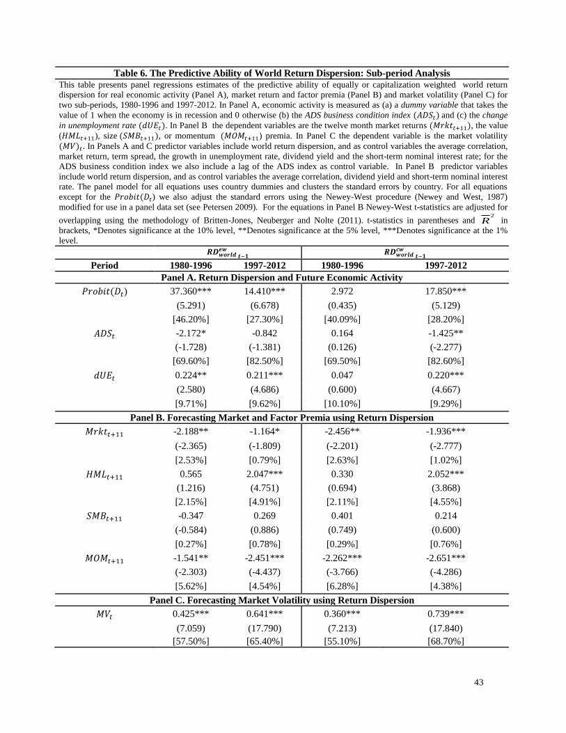
43

Table 6. The Predictive Ability of World Return Dispersion: Sub-period Analysis

This table presents panel regressions estimates of the predictive ability of equally or capitalization weighted world return

dispersion for real economic activity (Panel A), market return and factor premia (Panel B) and market volatility (Panel C) for

two sub-periods, 1980-1996 and 1997-2012. In Panel A, economic activity is measured as (a) a dummy variable that takes the

value of 1 when the economy is in recession and 0 otherwise (b) the ADS business condition index (𝐴𝐷𝑆𝑡) and (c) the change

in unemployment rate (𝑑𝑈𝐸𝑡). In Panel B the dependent variables are the twelve month market returns (𝑀𝑟𝑘𝑡𝑡+11), the value

(𝐻𝑀𝐿𝑡+11), size (𝑆𝑀𝐵𝑡+11), or momentum (𝑀𝑂𝑀𝑡+11) premia. In Panel C the dependent variable is the market volatility

(𝑀𝑉)𝑡. In Panels A and C predictor variables include world return dispersion, and as control variables the average correlation,

market return, term spread, the growth in unemployment rate, dividend yield and the short-term nominal interest rate; for the

ADS business condition index we also include a lag of the ADS index as control variable. In Panel B predictor variables

include world return dispersion, and as control variables the average correlation, dividend yield and short-term nominal interest

rate. The panel model for all equations uses country dummies and clusters the standard errors by country. For all equations

except for the 𝑃𝑟𝑜𝑏𝑖𝑡(𝐷𝑡) we also adjust the standard errors using the Newey-West procedure (Newey and West, 1987)

modified for use in a panel data set (see Petersen 2009). For the equations in Panel B Newey-West t-statistics are adjusted for

overlapping using the methodology of Britten-Jones, Neuberger and Nolte (2011). t-statistics in parentheses and 2

R in

brackets, *Denotes significance at the 10% level, **Denotes significance at the 5% level, ***Denotes significance at the 1%

level.


𝒆𝒘𝒕−𝟏


𝒕−𝟏

Period 1980-1996 1997-2012 1980-1996 1997-2012

Panel A. Return Dispersion and Future Economic Activity

𝑃𝑟𝑜𝑏𝑖𝑡(𝐷𝑡) 37.360*** 14.410*** 2.972 17.850***

(5.291) (6.678) (0.435) (5.129)

[46.20%] [27.30%] [40.09%] [28.20%]

𝐴𝐷𝑆𝑡 -2.172* -0.842 0.164 -1.425**

(-1.728) (-1.381) (0.126) (-2.277)

[69.60%] [82.50%] [69.50%] [82.60%]

𝑑𝑈𝐸𝑡 0.224** 0.211*** 0.047 0.220***

(2.580) (4.686) (0.600) (4.667)

[9.71%] [9.62%] [10.10%] [9.29%]

Panel B. Forecasting Market and Factor Premia using Return Dispersion

𝑀𝑟𝑘𝑡𝑡+11 -2.188** -1.164* -2.456** -1.936***

(-2.365) (-1.809) (-2.201) (-2.777)

[2.53%] [0.79%] [2.63%] [1.02%]

𝐻𝑀𝐿𝑡+11 0.565 2.047*** 0.330 2.052***

(1.216) (4.751) (0.694) (3.868)

[2.15%] [4.91%] [2.11%] [4.55%]

𝑆𝑀𝐵𝑡+11 -0.347 0.269 0.401 0.214

(-0.584) (0.886) (0.749) (0.600)

[0.27%] [0.78%] [0.29%] [0.76%]

𝑀𝑂𝑀𝑡+11 -1.541** -2.451*** -2.262*** -2.651***

(-2.303) (-4.437) (-3.766) (-4.286)

[5.62%] [4.54%] [6.28%] [4.38%]

Panel C. Forecasting Market Volatility using Return Dispersion

𝑀𝑉𝑡 0.425*** 0.641*** 0.360*** 0.739***

(7.059) (17.790) (7.213) (17.840)

[57.50%] [65.40%] [55.10%] [68.70%]

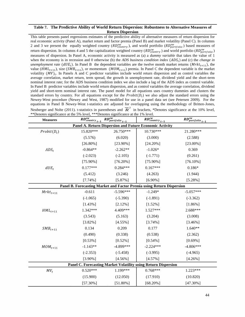
44

Table 7. The Predictive Ability of World Return Dispersion: Robustness to Alternative Measures of

Return Dispersion

This table presents panel regressions estimates of the predictive ability of alternative measures of return dispersion for

real economic activity (Panel A), market return and factor premia (Panel B) and market volatility (Panel C). In columns

2 and 3 we present the equally weighted country (𝑅𝐷𝑐𝑜𝑢𝑛𝑡𝑟𝑦 𝑒𝑤 ), and world portfolio (𝑅𝐷𝑝𝑜𝑟𝑡𝑓𝑜𝑙𝑖𝑜

𝑒𝑤 ) based measures of

return dispersion. In columns 4 and 5 the capitalization weighted country (𝑅𝐷𝑐𝑜𝑢𝑛𝑡𝑟𝑦 𝑐𝑤 ) and world portfolio (𝑅𝐷𝑝𝑜𝑟𝑡𝑓𝑜𝑙𝑖𝑜

𝑐𝑤 )

measures of dispersion. In Panel A, economic activity is measured as (a) a dummy variable that takes the value of 1

when the economy is in recession and 0 otherwise (b) the ADS business condition index (𝐴𝐷𝑆𝑡) and (c) the change in

unemployment rate (𝑑𝑈𝐸𝑡). In Panel B the dependent variables are the twelve month market returns (𝑀𝑟𝑘𝑡𝑡+11), the

value (𝐻𝑀𝐿𝑡+11), size (𝑆𝑀𝐵𝑡+11), or momentum (𝑀𝑂𝑀𝑡+11) premia. In Panel C the dependent variable is the market

volatility (𝑀𝑉)𝑡. In Panels A and C predictor variables include world return dispersion and as control variables the

average correlation, market return, term spread, the growth in unemployment rate, dividend yield and the short-term

nominal interest rate; for the ADS business condition index we also include a lag of the ADS index as control variable.

In Panel B predictor variables include world return dispersion, and as control variables the average correlation, dividend

yield and short-term nominal interest rate. The panel model for all equations uses country dummies and clusters the

standard errors by country. For all equations except for the 𝑃𝑟𝑜𝑏𝑖𝑡(𝐷𝑡) we also adjust the standard errors using the

Newey-West procedure (Newey and West, 1987) modified for use in a panel data set (see Petersen 2009). For the

equations in Panel B Newey-West t-statistics are adjusted for overlapping using the methodology of Britten-Jones,

Neuberger and Nolte (2011). t-statistics in parentheses and 2

R in brackets, *Denotes significance at the 10% level,

**Denotes significance at the 5% level, ***Denotes significance at the 1% level.

Measures 𝑹𝑫𝒄𝒐𝒖𝒏𝒕𝒓𝒚 𝒆𝒘

𝒕−𝟏 𝑹𝑫𝒑𝒐𝒓𝒕𝒇𝒐𝒍𝒊𝒐

𝒆𝒘

𝒕−𝟏 𝑹𝑫𝒄𝒐𝒖𝒏𝒕𝒓𝒚

𝒄𝒘𝒕−𝟏

𝑹𝑫𝒑𝒐𝒓𝒕𝒇𝒐𝒍𝒊𝒐 𝒄𝒘

𝒕−𝟏


𝑃𝑟𝑜𝑏𝑖𝑡(𝐷𝑡) 15.820*** 26.750*** 10.730*** 21.280***

(5.576) (6.020) (3.000) (2.588)

[26.80%] [23.90%] [24.20%] [23.00%]

𝐴𝐷𝑆𝑡 -0.864** -2.262** -1.026* 0.369

(-2.023) (-2.105) (-1.771) (0.261)

[75.90%] [76.20%] [75.90%] [76.10%]

𝑑𝑈𝐸𝑡 0.177*** 0.284*** 0.167*** 0.186*

(5.412) (3.246) (4.263) (1.944)

[7.74%] [5.87%] [6.90%] [5.28%]


𝑀𝑟𝑘𝑡𝑡+11 -0.611 -5.596*** -1.249* -5.057***

(-1.065) (-5.390) (-1.891) (-3.362)

[1.43%] [2.12%] [1.52%] [1.86%]

𝐻𝑀𝐿𝑡+11 1.342*** 4.409*** 1.527*** 2.688***

(3.543) (5.163) (3.204) (3.008)

[3.82%] [4.55%] [3.74%] [3.46%]

𝑆𝑀𝐵𝑡+11 0.134 0.209 0.177 1.640**

(0.490) (0.338) (0.538) (2.362)

[0.53%] [0.52%] [0.54%] [0.69%]

𝑀𝑂𝑀𝑡+11 -1.143** -4.899*** -2.224*** -4.806***

(-2.353) (-5.458) (-3.995) (-4.965)

[3.90%] [4.56%] [4.57%] [4.26%]


𝑀𝑉𝑡 0.520*** 1.199*** 0.768*** 1.223***

(15.900) (12.050) (17.910) (10.820)

[57.30%] [51.80%] [68.20%] [47.30%]

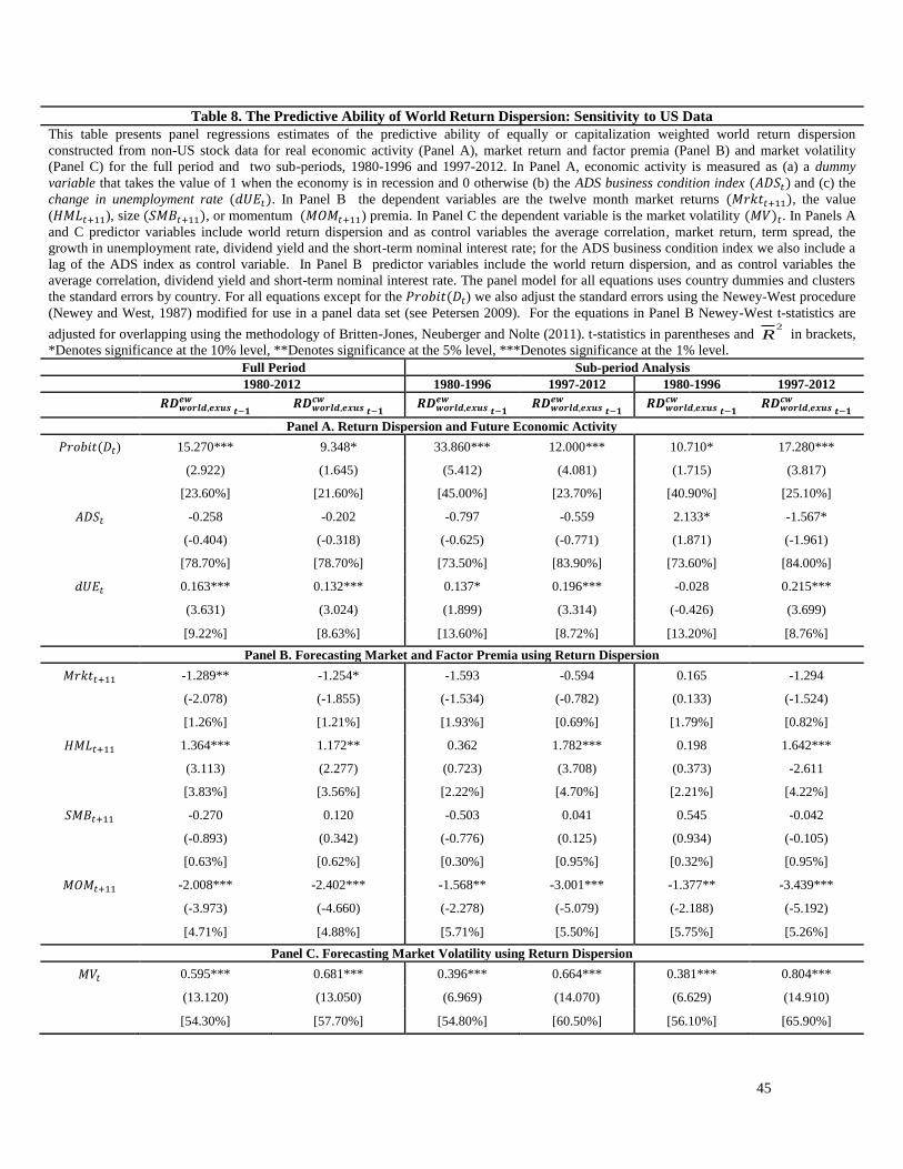
45

Table 8. The Predictive Ability of World Return Dispersion: Sensitivity to US Data

This table presents panel regressions estimates of the predictive ability of equally or capitalization weighted world return dispersion

constructed from non-US stock data for real economic activity (Panel A), market return and factor premia (Panel B) and market volatility

(Panel C) for the full period and two sub-periods, 1980-1996 and 1997-2012. In Panel A, economic activity is measured as (a) a dummy

variable that takes the value of 1 when the economy is in recession and 0 otherwise (b) the ADS business condition index (𝐴𝐷𝑆𝑡) and (c) the

change in unemployment rate (𝑑𝑈𝐸𝑡). In Panel B the dependent variables are the twelve month market returns (𝑀𝑟𝑘𝑡𝑡+11), the value

(𝐻𝑀𝐿𝑡+11), size (𝑆𝑀𝐵𝑡+11), or momentum (𝑀𝑂𝑀𝑡+11) premia. In Panel C the dependent variable is the market volatility (𝑀𝑉)𝑡. In Panels A

and C predictor variables include world return dispersion and as control variables the average correlation, market return, term spread, the

growth in unemployment rate, dividend yield and the short-term nominal interest rate; for the ADS business condition index we also include a

lag of the ADS index as control variable. In Panel B predictor variables include the world return dispersion, and as control variables the

average correlation, dividend yield and short-term nominal interest rate. The panel model for all equations uses country dummies and clusters

the standard errors by country. For all equations except for the 𝑃𝑟𝑜𝑏𝑖𝑡(𝐷𝑡) we also adjust the standard errors using the Newey-West procedure

(Newey and West, 1987) modified for use in a panel data set (see Petersen 2009). For the equations in Panel B Newey-West t-statistics are

adjusted for overlapping using the methodology of Britten-Jones, Neuberger and Nolte (2011). t-statistics in parentheses and 2

R in brackets,

*Denotes significance at the 10% level, **Denotes significance at the 5% level, ***Denotes significance at the 1% level.

Full Period Sub-period Analysis

1980-2012 1980-1996 1997-2012 1980-1996 1997-2012

𝑹𝑫𝒘𝒐𝒓𝒍𝒅,𝒆𝒙𝒖𝒔

𝒆𝒘

𝒕−𝟏 𝑹𝑫𝒘𝒐𝒓𝒍𝒅,𝒆𝒙𝒖𝒔

𝒄𝒘


𝒆𝒘


𝒆𝒘


𝒄𝒘


𝒄𝒘

𝒕−𝟏


𝑃𝑟𝑜𝑏𝑖𝑡(𝐷𝑡) 15.270*** 9.348* 33.860*** 12.000*** 10.710* 17.280***

(2.922) (1.645) (5.412) (4.081) (1.715) (3.817)

[23.60%] [21.60%] [45.00%] [23.70%] [40.90%] [25.10%]

𝐴𝐷𝑆𝑡 -0.258 -0.202 -0.797 -0.559 2.133* -1.567*

(-0.404) (-0.318) (-0.625) (-0.771) (1.871) (-1.961)

[78.70%] [78.70%] [73.50%] [83.90%] [73.60%] [84.00%]

𝑑𝑈𝐸𝑡 0.163*** 0.132*** 0.137* 0.196*** -0.028 0.215***

(3.631) (3.024) (1.899) (3.314) (-0.426) (3.699)

[9.22%] [8.63%] [13.60%] [8.72%] [13.20%] [8.76%]


𝑀𝑟𝑘𝑡𝑡+11 -1.289** -1.254* -1.593 -0.594 0.165 -1.294

(-2.078) (-1.855) (-1.534) (-0.782) (0.133) (-1.524)

[1.26%] [1.21%] [1.93%] [0.69%] [1.79%] [0.82%]

𝐻𝑀𝐿𝑡+11 1.364*** 1.172** 0.362 1.782*** 0.198 1.642***

(3.113) (2.277) (0.723) (3.708) (0.373) -2.611

[3.83%] [3.56%] [2.22%] [4.70%] [2.21%] [4.22%]

𝑆𝑀𝐵𝑡+11 -0.270 0.120 -0.503 0.041 0.545 -0.042

(-0.893) (0.342) (-0.776) (0.125) (0.934) (-0.105)

[0.63%] [0.62%] [0.30%] [0.95%] [0.32%] [0.95%]

𝑀𝑂𝑀𝑡+11 -2.008*** -2.402*** -1.568** -3.001*** -1.377** -3.439***

(-3.973) (-4.660) (-2.278) (-5.079) (-2.188) (-5.192)

[4.71%] [4.88%] [5.71%] [5.50%] [5.75%] [5.26%]


𝑀𝑉𝑡 0.595*** 0.681*** 0.396*** 0.664*** 0.381*** 0.804***

(13.120) (13.050) (6.969) (14.070) (6.629) (14.910)

[54.30%] [57.70%] [54.80%] [60.50%] [56.10%] [65.90%]

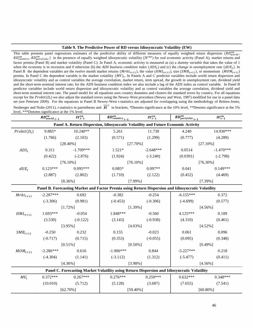
46

Table 9. The Predictive Power of RD versus Idiosyncratic Volatility (EW)

This table presents panel regressions estimates of the predictive ability of different measures of equally weighted return dispersion (𝑅𝐷𝑤𝑜𝑟𝑙𝑑 𝑒𝑤 ,

𝑅𝐷𝑐𝑜𝑢𝑛𝑡𝑟𝑦 𝑒𝑤 , 𝑅𝐷𝑝𝑜𝑟𝑡𝑓𝑜𝑙𝑖𝑜

𝑒𝑤 ) in the presence of equally weighted idiosyncratic volatility (𝐼𝑉 𝑒𝑤) for real economic activity (Panel A), market returns and

factor premia (Panel B) and market volatility (Panel C). In Panel A, economic activity is measured as (a) a dummy variable that takes the value of 1

when the economy is in recession and 0 otherwise (b) the ADS business condition index (𝐴𝐷𝑆𝑡) and (c) the change in unemployment rate (𝑑𝑈𝐸𝑡). In

Panel B the dependent variables are the twelve month market returns (𝑀𝑟𝑘𝑡𝑡+11), the value (𝐻𝑀𝐿𝑡+11), size (𝑆𝑀𝐵𝑡+11), or momentum (𝑀𝑂𝑀𝑡+11)

premia. In Panel C the dependent variable is the market volatility (𝑀𝑉)𝑡. In Panels A and C predictor variables include world return dispersion and

idiosyncratic volatility and as control variables the average correlation, market return, term spread, the growth in unemployment rate, dividend yield

and the short-term nominal interest rate; for the ADS business condition index we also include a lag of the ADS index as control variable. In Panel B

predictor variables include world return dispersion and idiosyncratic volatility and as control variables the average correlation, dividend yield and

short-term nominal interest rate. The panel model for all equations uses country dummies and clusters the standard errors by country. For all equations

except for the 𝑃𝑟𝑜𝑏𝑖𝑡(𝐷𝑡) we also adjust the standard errors using the Newey-West procedure (Newey and West, 1987) modified for use in a panel data

set (see Petersen 2009). For the equations in Panel B Newey-West t-statistics are adjusted for overlapping using the methodology of Britten-Jones,


R in brackets, *Denotes significance at the 10% level, **Denotes significance at the 5%

level, ***Denotes significance at the 1% level.


𝒆𝒘𝒕−𝟏

𝑰𝑽𝒕−𝟏𝒆𝒘 𝑹𝑫𝒄𝒐𝒖𝒏𝒕𝒓𝒚

𝒆𝒘𝒕−𝟏

𝑰𝑽𝒕−𝟏𝒆𝒘 𝑹𝑫𝒑𝒐𝒓𝒕𝒇𝒐𝒍𝒊𝒐

𝒆𝒘

𝒕−𝟏 𝑰𝑽𝒕−𝟏

𝒆𝒘

Panel A. Return Dispersion, Idiosyncratic Volatility and Future Economic Activity

𝑃𝑟𝑜𝑏𝑖𝑡(𝐷𝑡) 9.885* 10.240** 5.261 11.730 4.240 14.930***

(1.766) (2.103) (0.571) (1.299) (0.777) (4.289)

[28.40%] [27.70%] [27.10%]

𝐴𝐷𝑆𝑡 0.311 -1.709*** 1.521* -2.648*** 0.0514 -1.470***

(0.422) (-2.876) (1.924) (-3.240) (0.0391) (-2.798)

[76.10%] [76.10%] [76.30%]

𝑑𝑈𝐸𝑡 0.123*** 0.095*** 0.085* 0.097** 0.041 0.149***

(2.887) (2.802) (1.710) (2.122) (0.452) (4.469)

[8.36%] [7.99%] [7.39%]

Panel B. Forecasting Market and Factor Premia using Return Dispersion and Idiosyncratic Volatility

𝑀𝑟𝑘𝑡𝑡+11 -2.287*** 0.692 -0.382 -0.254 -6.155*** 0.372

(-3.306) (0.981) (-0.453) (-0.306) (-4.699) (0.577)

[1.72%] [1.39%] [4.56%]

𝐻𝑀𝐿𝑡+11 1.693*** -0.054 1.848*** -0.560 4.125*** 0.189

(3.530) (-0.122) (3.143) (-0.938) (4.310) (0.461)

[3.95%] [4.03%] [4.52%]

𝑆𝑀𝐵𝑡+11 -0.250 0.232 0.155 -0.023 0.061 0.096

(-0.717) (0.715) (0.353) (-0.055) (0.095) (0.348)

[0.51%] [0.50%] [0.49%]

𝑀𝑂𝑀𝑡+11 -2.286*** 0.616 -1.906*** 0.844 -5.227*** 0.218

(-4.304) (1.141) (-3.112) (1.312) (-5.477) (0.411)

[4.36%] [3.98%] [4.56%]

Panel C. Forecasting Market Volatility using Return Dispersion and Idiosyncratic Volatility

𝑀𝑉𝑡 0.372*** 0.267*** 0.276*** 0.259*** 0.632*** 0.348***

(10.010) (5.712) (5.128) (3.687) (7.655) (7.541)

[62.70%] [59.40%] [60.80%]

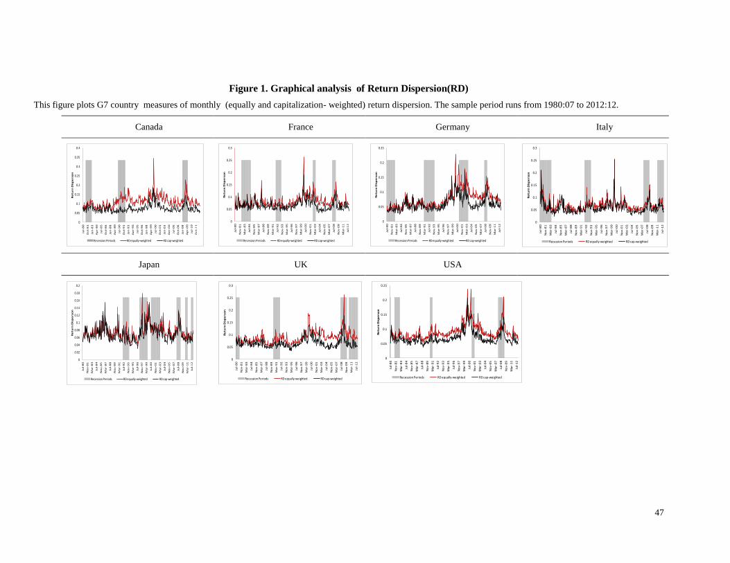
47

Figure 1. Graphical analysis of Return Dispersion(RD)

This figure plots G7 country measures of monthly (equally and capitalization- weighted) return dispersion. The sample period runs from 1980:07 to 2012:12.

Canada France Germany Italy

Japan UK USA

0

0.05

0.1

0.15

0.2

0.25

0.3

0.35

0.4

Jul-

80

Oc

t-8

1

Jan

-83

Ap

r-8

4

Jul-

85

Oc

t-8

6

Jan

-88

Ap

r-8

9

Jul-

90

Oc

t-9

1

Jan

-93

Ap

r-9

4

Jul-

95

Oc

t-9

6

Jan

-98

Ap

r-9

9

Jul-

00

Oc

t-0

1

Jan

-03

Ap

r-0

4

Jul-

05

Oc

t-0

6

Jan

-08

Ap

r-0

9

Jul-

10

Oc

t-1

1

Re

turn

Dis

pe

rso

n

Recession Periods RD equally-weighted RD cap-weighted

0

0.05

0.1

0.15

0.2

0.25

0.3

Jul-

80

No

v-8

1

Ma

r-8

3

Jul-

84

No

v-8

5

Ma

r-8

7

Jul-

88

No

v-8

9

Ma

r-9

1

Jul-

92

No

v-9

3

Ma

r-9

5

Jul-

96

No

v-9

7

Ma

r-9

9

Jul-

00

No

v-0

1

Ma

r-0

3

Jul-

04

No

v-0

5

Ma

r-0

7

Jul-

08

No

v-0

9

Ma

r-1

1

Jul-

12

Re

turn

Dis

pe

rso

n


0

0.05

0.1

0.15

0.2

0.25

Jul-

80

No

v-8

1

Ma

r-8

3

Jul-

84

No

v-8

5

Ma

r-8

7

Jul-

88

No

v-8

9

Ma

r-9

1

Jul-

92

No

v-9

3

Ma

r-9

5

Jul-

96

No

v-9

7

Ma

r-9

9

Jul-

00

No

v-0

1

Ma

r-0

3

Jul-

04

No

v-0

5

Ma

r-0

7

Jul-

08

No

v-0

9

Ma

r-1

1

Jul-

12

Re

turn

Dis

pe

rso

n


0

0.05

0.1

0.15

0.2

0.25

0.3

Jul-

80

No

v-8

1

Ma

r-8

3

Jul-

84

No

v-8

5

Ma

r-8

7

Jul-

88

No

v-8

9

Ma

r-9

1

Jul-

92

No

v-9

3

Ma

r-9

5

Jul-

96

No

v-9

7

Ma

r-9

9

Jul-

00

No

v-0

1

Ma

r-0

3

Jul-

04

No

v-0

5

Ma

r-0

7

Jul-

08

No

v-0

9

Ma

r-1

1

Jul-

12

Re

turn

Dis

pe

rso

n


0

0.02

0.04

0.06

0.08

0.1

0.12

0.14

0.16

0.18

0.2

Jul-

80

No

v-8

1

Ma

r-8

3

Jul-

84

No

v-8

5

Ma

r-8

7

Jul-

88

No

v-8

9

Ma

r-9

1

Jul-

92

No

v-9

3

Ma

r-9

5

Jul-

96

No

v-9

7

Ma

r-9

9

Jul-

00

No

v-0

1

Ma

r-0

3

Jul-

04

No

v-0

5

Ma

r-0

7

Jul-

08

No

v-0

9

Ma

r-1

1

Jul-

12

Re

turn

Dis

pe

rso

n


0

0.05

0.1

0.15

0.2

0.25

0.3

Jul-

80

No

v-8

1

Ma

r-8

3

Jul-

84

No

v-8

5

Ma

r-8

7

Jul-

88

No

v-8

9

Ma

r-9

1

Jul-

92

No

v-9

3

Ma

r-9

5

Jul-

96

No

v-9

7

Ma

r-9

9

Jul-

00

No

v-0

1

Ma

r-0

3

Jul-

04

No

v-0

5

Ma

r-0

7

Jul-

08

No

v-0

9

Ma

r-1

1

Jul-

12

Re

turn

Dis

pe

rso

n


0

0.05

0.1

0.15

0.2

0.25

Jul-

80

No

v-8

1

Mar

-83

Jul-

84

No

v-8

5

Ma

r-8

7

Jul-

88

No

v-8

9

Ma

r-9

1

Jul-

92

No

v-9

3

Ma

r-9

5

Jul-

96

No

v-9

7

Mar

-99

Jul-

00

No

v-0

1

Mar

-03

Jul-

04

No

v-0

5

Mar

-07

Jul-

08

No

v-0

9

Mar

-11

Jul-

12

Re

turn

Dis

pe

rso

nRecession Periods RD equally-weighted RD cap-weighted

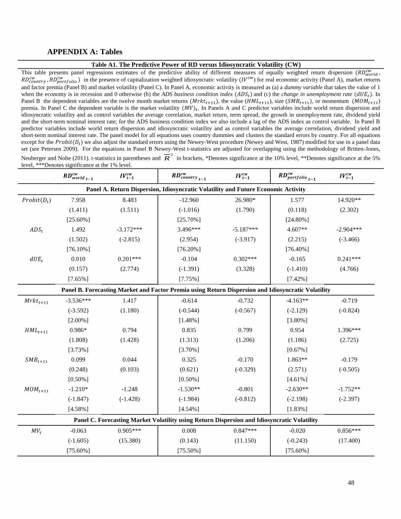
48

APPENDIX A: Tables

Table A1. The Predictive Power of RD versus Idiosyncratic Volatility (CW)

This table presents panel regressions estimates of the predictive ability of different measures of equally weighted return dispersion (𝑅𝐷𝑤𝑜𝑟𝑙𝑑 𝑐𝑤 ,

𝑅𝐷𝑐𝑜𝑢𝑛𝑡𝑟𝑦 𝑐𝑤 , 𝑅𝐷𝑝𝑜𝑟𝑡𝑓𝑜𝑙𝑖𝑜

𝑐𝑤 ) in the presence of capitalization weighted idiosyncratic volatility (𝐼𝑉𝑐𝑤) for real economic activity (Panel A), market returns

and factor premia (Panel B) and market volatility (Panel C). In Panel A, economic activity is measured as (a) a dummy variable that takes the value of 1

when the economy is in recession and 0 otherwise (b) the ADS business condition index (𝐴𝐷𝑆𝑡) and (c) the change in unemployment rate (𝑑𝑈𝐸𝑡). In

Panel B the dependent variables are the twelve month market returns (𝑀𝑟𝑘𝑡𝑡+11), the value (𝐻𝑀𝐿𝑡+11), size (𝑆𝑀𝐵𝑡+11), or momentum (𝑀𝑂𝑀𝑡+11)

premia. In Panel C the dependent variable is the market volatility (𝑀𝑉)𝑡. In Panels A and C predictor variables include world return dispersion and

idiosyncratic volatility and as control variables the average correlation, market return, term spread, the growth in unemployment rate, dividend yield

and the short-term nominal interest rate; for the ADS business condition index we also include a lag of the ADS index as control variable. In Panel B

predictor variables include world return dispersion and idiosyncratic volatility and as control variables the average correlation, dividend yield and

short-term nominal interest rate. The panel model for all equations uses country dummies and clusters the standard errors by country. For all equations

except for the 𝑃𝑟𝑜𝑏𝑖𝑡(𝐷𝑡) we also adjust the standard errors using the Newey-West procedure (Newey and West, 1987) modified for use in a panel data

set (see Petersen 2009). For the equations in Panel B Newey-West t-statistics are adjusted for overlapping using the methodology of Britten-Jones,


R in brackets, *Denotes significance at the 10% level, **Denotes significance at the 5%

level, ***Denotes significance at the 1% level.


𝒄𝒘𝒕−𝟏

𝑰𝑽𝒕−𝟏 𝒄𝒘 𝑹𝑫𝒄𝒐𝒖𝒏𝒕𝒓𝒚

𝒄𝒘


𝒄𝒘 𝑹𝑫𝒑𝒐𝒓𝒕𝒇𝒐𝒍𝒊𝒐 𝒄𝒘


𝒄𝒘

Panel A. Return Dispersion, Idiosyncratic Volatility and Future Economic Activity

𝑃𝑟𝑜𝑏𝑖𝑡(𝐷𝑡) 7.958 8.483 -12.960 26.980* 1.577 14.920**

(1.411) (1.511) (-1.016) (1.790) (0.118) (2.302)

[25.60%]

[25.70%]

[24.80%]

𝐴𝐷𝑆𝑡 1.492 -3.172*** 3.496*** -5.187*** 4.607** -2.904***

(1.502) (-2.815) (2.954) (-3.917) (2.215) (-3.466)

[76.10%]

[76.20%]

[76.40%]

𝑑𝑈𝐸𝑡 0.010 0.201*** -0.104 0.302*** -0.165 0.241***

(0.157) (2.774) (-1.391) (3.328) (-1.410) (4.766)

[7.65%]

[7.75%]

[7.42%]

Panel B. Forecasting Market and Factor Premia using Return Dispersion and Idiosyncratic Volatility

𝑀𝑟𝑘𝑡𝑡+11 -3.536*** 1.417 -0.614 -0.732 -4.163** -0.719

(-3.592) (1.180) (-0.544) (-0.567) (-2.129) (-0.824)

[2.00%]

[1.48%]

[3.80%]

𝐻𝑀𝐿𝑡+11 0.986* 0.794 0.835 0.799 0.954 1.396***

(1.808) (1.428) (1.313) (1.206) (1.186) (2.725)

[3.73%]

[3.70%]

[0.67%]

𝑆𝑀𝐵𝑡+11 0.099 0.044 0.325 -0.170 1.863** -0.179

(0.248) (0.103) (0.621) (-0.329) (2.571) (-0.505)

[0.50%]

[0.50%]

[4.61%]

𝑀𝑂𝑀𝑡+11 -1.210* -1.248 -1.530** -0.801 -2.630** -1.752**

(-1.847) (-1.428) (-1.984) (-0.812) (-2.198) (-2.397)

[4.58%]

[4.54%]

[1.83%]

Panel C. Forecasting Market Volatility using Return Dispersion and Idiosyncratic Volatility

𝑀𝑉𝑡 -0.063 0.905*** 0.008 0.847*** -0.020 0.856***

(-1.605) (15.380) (0.143) (11.150) (-0.243) (17.400)

[75.60%]

[75.50%]

[75.60%]

49

Table A.2. The Economic Significance of Return Dispersion (𝑹𝑫) versus Idiosyncratic

Volatility Based Forecasts This table presents the out-of-sample Sharpe ratios of market, value, size and momentum timing

strategies using RD or idiosyncratic volatility based forecasts of market returns (𝑀𝑟𝑘𝑡) and the value

(𝐻𝑀𝐿), size (𝑆𝑀𝐵), and momentum (𝑀𝑂𝑀) premia. We produce monthly out-of-sample forecasts of

equity premia using equations 5, 6, 7 and 8 estimated recursively using an expanding window approach

starting in December 1997. Using premia forecasts and the historical variance-covariance matrix we

create portfolios that maximize the Sharpe ratio under the assumption that the portfolio’s volatility is

equal to the volatility of the buy and hold portfolio. When the estimated market premium is negative we

assume that the investor switches her portfolio into cash. We consider three strategies (i) a buy and hold

strategy where the investor buys and holds the market portfolio or the three (long-short) factor portfolios

(ii) the dispersion strategy (DS) or idiosyncratic strategy (IS) based on RD or idiosyncratic volatility

without the control variables and (iii) the full model strategy where the investor utilizes all predictors,

including RD or idiosyncratic volatility. Predictor variables include the world return dispersion or

idiosyncratic volatility, and control variables (average correlation, dividend yield and short-term

nominal interest rate). Results for the equally weighted measures of return dispersion or idiosyncratic

volatility are in panel A and for capitalization weighted measures in panel B.

Panel A. Equally Weighted RD and Idiosyncratic Volatility

𝑴𝒓𝒌𝒕 𝑯𝑴𝑳 𝑺𝑴𝑩 𝑴𝑶𝑴

Sharpe Ratio

Buy & Hold 0.19 0.78 0.11 0.38

DS IS

0.41 0.39

1.35 1.24

0.73 0.79

1.37 0.94

Full Model_DS Full Model_IS

0.41 0.43

1.48 1.26

0.80 0.80

1.44 1.26

Panel B. Capitalization Weighted RD and Idiosyncratic Volatility

𝑴𝒓𝒌𝒕 𝑯𝑴𝑳 𝑺𝑴𝑩 𝑴𝑶𝑴

Sharpe Ratio

Buy & Hold Strategy 0.19 0.78 0.11 0.38

DS IS

0.47 0.43

1.40 1.33

0.78 0.77

1.29 1.27

Full Model_DS Full Model_IS

0.40 0.39

1.42 1.33

0.85 0.77

1.50 1.36

50

APPENDIX B : Database construction

1. We include in the database only stocks characterized by Datastream as “equities” (Stock

type: EQ).

2. We exclude all companies that are not listed on the primary stock exchange.

3. We use Level 2, Level 3, and Level 4 sector names and the names of the companies to

identify and exclude closed end funds, REITs, ADRs and preferred stocks.

4. We set returns as missing if the return index20 is below 3.

5. We set the returns of two consecutive months as missing if we observe an increase over

300% at month t and a decrease more than 50% at month t+1.

6. We set returns as missing if they are higher (lower) than the 97.5th (2.5th) percentiles of

the daily or monthly return distribution to mitigate the effect of extreme stock returns.

7. We remove 5% of the stocks with the smallest capitalization.

8. All stocks with less than 10 observations during a month are excluded from the analysis.

20 A stock is given a total return index value of 100 when entering the database. A return index less than 3 means

that the security lost 97% of its value.

stock market dispersion, the business cycle and expected

Documents