st-agrid: a spatio temporal grid density based clustering and its application for determining the...

International Journal of Software Engineering and Its Applications

Vol. 9, No. 1 (2015), pp. 13-26

http://dx.doi.org/10.14257/ijseia.2015.9.1.02

ISSN: 1738-9984 IJSEIA

Copyright ⓒ 2015 SERSC

ST-AGRID: A Spatio Temporal Grid Density Based Clustering

and Its Application for determining the Potential Fishing Zones

D. Fitrianah1,2

, A. N. Hidayanto1, H. Fahmi

1, J. Lumban Gaol

3 and A. M.

Arymurthy1

1Faculty of Computer Science, Universitas Indonesia, Depok 16424, Indonesia

2Faculty of Computer Science, Universitas Mercu Buana, Jakarta 11650,

Indonesia 3Department of Marine Science and Technology, Bogor Agricultural University

Bogor 16680, Indonesia

[email protected], [email protected], [email protected],

[email protected], [email protected]

Abstract

This paper is aimed to propose a grid density clustering algorithm for spatio-temporal

data that is based on the adaptation of the grid density based clustering algorithm. The

algorithm is based on AGRID+ algorithm with 7 steps: partitioning, computing distance

threshold, calculating densities, compensating densities, calculating density threshold

(DT), clustering and removing noises. The adaptation is for the partitioning and

calculating the distance threshold (r). The data utilized in this study is spatio-temporal

fishery data located around the India Ocean from year 2000 until 2004. We utilized the

fishery data in three types of aggregate , daily data, weekly data and monthy data. The

result of this study shows that the time complexity for ST-AGRID is outperform the

AGRID+. ST-AGRID improves the time complexity and at the same time maintains the

accuracy. By utilizing the thresholding technique, clustering result of the ST-AGRID

algorithm is identified as the potential fishing zone.

Keywords: spatio-temporal clustering, grid-density based clustering, potential fishing

zone, temporal aggregate

1. Introduction

Since the last decade, the development of the data storage and data presentation has

undergone a tremendous improvement, this includes the spatial and temporal data. It is

due to the accumulation of transaction of multi dimensional data such as remote sensing

technology, geographic information system and the development of the wireless

technology [1]. The development of the information technology is resulting a spatio-

temporal data repository that commonly utilized in many studies to reveal knowledge, the

spatio-temporal reations and other patterns implied from the data repository, this process

referred to as spatio-temporal data mining [2, 3]. The spatio-temporal data mining

application is widely utilized in many fields of study such as medicine, security,

environment, Biology and including the study on determining the prediction of the

potential fishing ground [4].

The spatio-temporal data has both spatial and temporal dimension at once. The data

shows the information of space and the time [5]. Spatio-temporal data embodies spatial,

temporal, and spatio-temporal data concepts, and also captures spatial and temporal aspect

of data that deal with geometry changing overtime and location of object moving over [6].

Clustering for spatio-temporal data is grouping the data object without knowing the

class label [7], DBSCAN is a clustering method that is utilized for big volume and densed


Vol. 9, No. 1 (2015)

14 Copyright ⓒ 2015 SERSC

spatial data and also good in identifying noise [8]. The issue for the spatio-temporal

clustering is concerning the time complexity. Regarding the big volume of the spatio-

temporal data, there are many adaptations and modifications to yield optimal time

complexity such as grid based density clustering. This method proposed a clustering

method for data object as in a grid not for point to point [9]. This enhanced the optimum

computing time however it did not improve the accuracy [10]. It requires an algorithm

that covers enhancement both in time complexity and accuracy. The AGRID+ treats data

objects both in grid and the smallest element in the clustering result, so it will enhance the

time complexity and at the same time preserve the accuracy [11]. This method is also

utilizing the i-th order neihghbor concept that reduces the computational complexity,

while for increasing the accuracy, AGRID+ applies the density compensation function. In

this spatio-temporal study, the AGRID+ algorithm can not be directly implemented, there

should be some adaptations and adjustments regarding the nature of the spatio-temporal

data which consists of 3 data dimension (longitude, latitude and temporal). It is because in

determining the temporal interval, AGRID+ produces real numbers instead of integer

number. Whereas for spatio-temporal data, the temporal dimension, the interval should be

in integer, as in the daily temporal aggregate, weekly temporal aggregate and monthly

aggregate. Thus, the adaptation for the algorithm is only for these phases that have

relation to the calculation of each interval from each dimension, they are partitioning

phase and calculation distance threshold phase.

Based on the explanation above, our contributions in this paper are:

To propose spatio-temporal grid density based clustering algorithm ST-AGRID

adapted from clustering algorithm AGRID+,

To perform an analysis of the potential fishing zone based on the spatio-temporal

clustering result.

2. Related Works

Spatio-temporal data mining is frequently utilized in analysing the data from remote

sensing and application of geographic information system [1][2][12]. The big volume of

data and the dependency on spatial and temporal that contains multidimensional

interactions, seasons and weather patterns, is applied to see the association rules [13]. One

approach in spatio-temporal data mining is spatio-temporal clustering that does not

require the class label to analyze the data object. The clustering method is appropriate to

be implemented in extracting information from a big repository without knowing the data

label [7]. This approach is widely utilized in many fields of study such as medicine,

security, environment, Biology, health and fisheries [3, 14]. The spatio-temporal

clustering method is implemented either for 3 dimensions at once or in two phased

clustering. Each two-phased clustering yields stressing in each dimension, spatial or

temporal [15, 16, 17].

Study in density based spatio-temporal clustering is done by [18] known as ST-

DBSCAN. The algorithm is an improved algorithm of the DBSCAN algorithm [8] for

spatio-temporal data. ST-DBSCAN is expected to find not only spatial clusters but also

temporal clusters and the non spatial clusters. [19] proposed two spatio-temporal based

algorithms, ST-GRID and ST-DBSCAN to analyse the sequence of the earthquakes.

Aside from the study in density based spatio temporal clustering there is also grid density

spatio temporal clustering to tackle the time computation problem that occurred due to the

point to point processing [9]. Another study that is relevant to the grid density clustering

algorithm is CLUGD that first construct a grid of relevant portion, next the algorithm

finds references by grid and classifies these references to core references and bound

references after that it attaches the data of the bound references to the nearest core

references and aggregation the core references in neighboring portions. At last, in-direct


Vol. 9, No. 1 (2015)

Copyright ⓒ 2015 SERSC 15

graph is used to classify these core references and maps cluster to original data, clusters

formed [10].

3. AGRID+

Another approach in grid and density based clustering study is AGRID+ [11]. The

algorithm is appropriate for high dimensional data clustering. The method is enhancing

the clustering with 4 features. First feature is determining the object or data point which is

treated as an atomic unit in which the size of the cell clusters are not specified while at the

same time preserving accuracy. Second feature is introducing the i-th order neighboring

concept so that the process of the neighboring cell is in groups and it can reduce the

computational complexity. Third feature is the idea of calculating the density

compensation to increase the clustering accuracy. The last feature is to propose a

subspace distance to assist the clustering proses in domain.

In the AGRID+ algorithm, first step, dimension is divided into many intervals and

data objects are partitioned into hyper-rectangular cells, a 3d-rectangular cells used for

spatio-temporal data. The interval value is calculated based on the number of 3d-

rectangular cells to be formed. Interval values for each dimension will be different

according to the number of rectangular in its dimension. The length of cell’s interval in

each dimension obtained from the dimension’s range divided by the number of cells in

that dimension. The computation of interval length can be formulated in Equation (1).

(1)

where, is the interval length for each cell at dth-dimension, is the feature of the

data at dth-dimension, and is the number of cells at dth-dimension. We have to do a

feature normalization before the clustering process due to the difference in scale between

spatial features and temporal features.

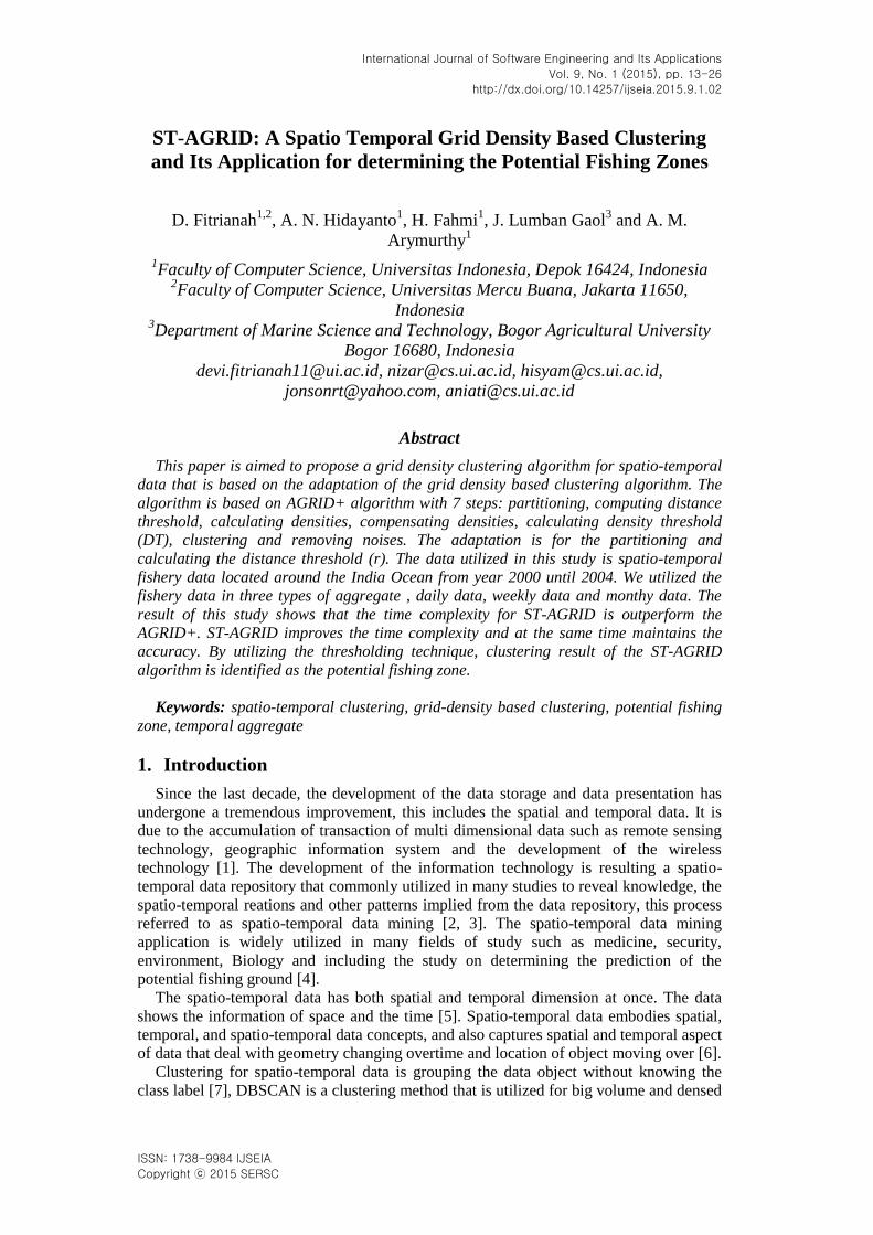
(a) (i = 0) (b) i = 1 (c) i = 2

Figure 1. The ith-order Neighbor of

After the length of intervals for each dimension, the partition step is done by assigning

each object to the corresponding cell based on the value of its features. Next step,

calculate the distance between object a in a cell and the objects in its neighboring cells,

and its density is the count of objects that are close to object a. Determination of the

neighbor is based on the ith-order neighbor. Zhao et al., [11] defined the ith-order

neighbor as a cell in D-dimensional space which shares ( ) dimensional facet with

cell , where cell is a cell in the D-dimensional space that contain an object a, and q

is an integer between 0 and D. The 0th-order neighbors of is itself. Examples of ith-

order neighbors in a 2D space are shown in Figure 1. Neighborhood is a point / data

objects and the surrounding neighbors is an area or space while the neighbor is the

neighboring cells and the surrounding cells that are adjacent to the cell.

To determine the neighborhood of the object required an r parameter, the radius of

neighborhood. Choosing the value of r is not so easy, because if r is large enough, this

algorithm will become like a grid-based clustering. On the other hand, if r is too small,

this algorithm will become like a density-based clustering. So that, to determine this

parameter Zhao et al., said that the value of r must be less than L/2, where L is the


Vol. 9, No. 1 (2015)


minimum interval length in all dimensions [11]. The value of r can be calculated using

Equation (2).

(2)

where, is a weight coefficient ( ), is the interval length for all dimensions, and

is a very small number, so that we achieved the value of . The next step is to

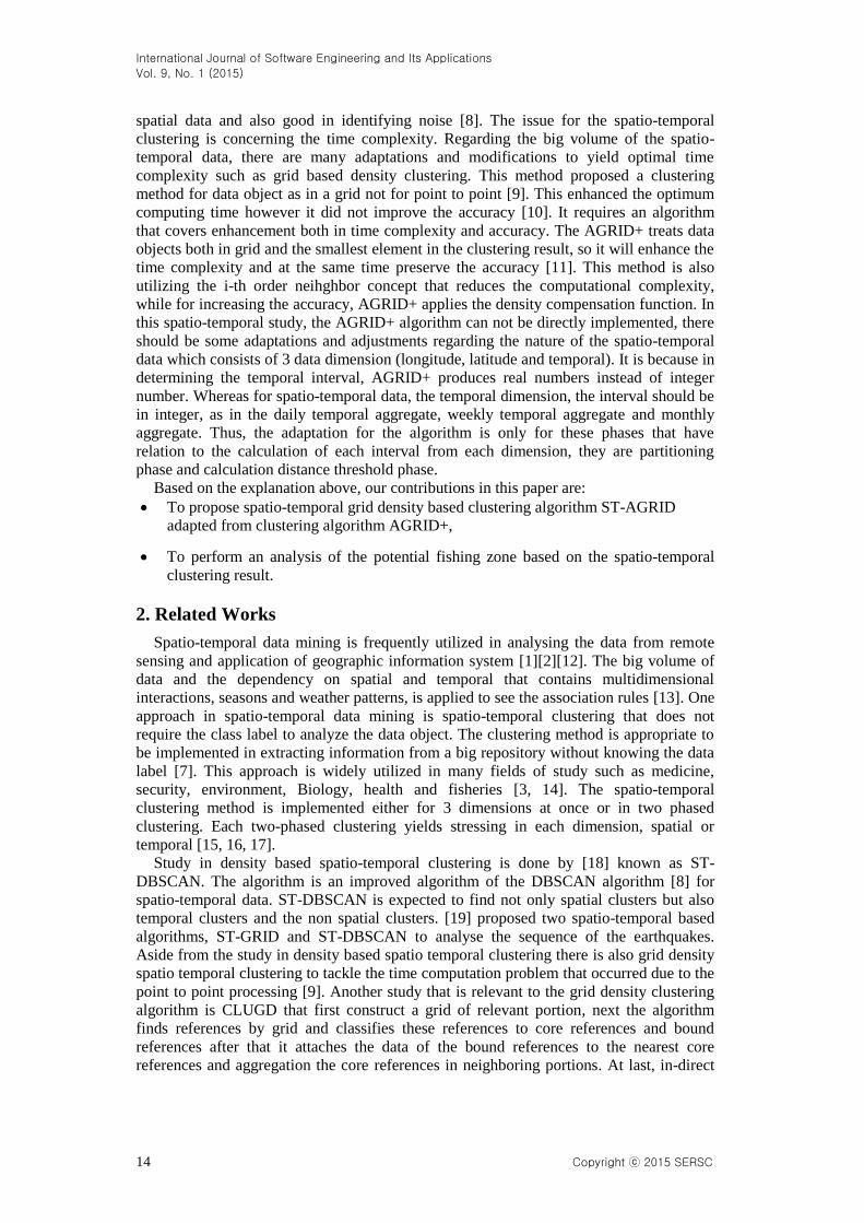
compute the densities of each object. The pseudo code of computing densities is shown in

Figure 2.

Figure 2. Pseudo Code for Computing Densities

After we have the densities value, we continue the process with compensating density

with Equation (3) as in [11].

(3)

where, is , is the object’s spatial coordinate relative to its cell

( ), is number of dimensions where , and is the

number of ith-order neighbors. The clustering result is also determined by the value of density threshold DT that can be computed with Equation (4).

(4)

where, is the coefficient that can be tuned to get the cluster results at different levels. A

small value of will lead to a big DT and vice versa. The appropriate cluster level can be

decided by the needs of user itself. In this experiment, we use DT = 5 or equivalent with

set = 1, based on the criteria to determining the potential fishing zone.

Continue to the clustering process, each object that have a density greater than DT is

labeled as a cluster. Then, every pair of objects which is in the neighborhood of each

other is checked. If that pair of objects is close enough (distance ) and has a density

that meets the criteria as a cluster (density ), then these two clusters that contain the

pair of objects are merged into one cluster. The clustering process is shown in Figure 3.

/* Pseudo code for computing densities*/

Set all densities(i) to zero;

For all cell C_i;

For all C_j, non-empty k-th order neighbors of C_i;

For all objects O_m in C_i

For all objects O_n in C_j

If dist(O(m,spatial),O(n,spatial))<=r_spatial And

dist(O(m,time),O(n,time))<=r_temporal

densities(m) = densities(m)+1;

densities(n) = densities(n)+1;

end if

end for

end for

end for

end for


Vol. 9, No. 1 (2015)


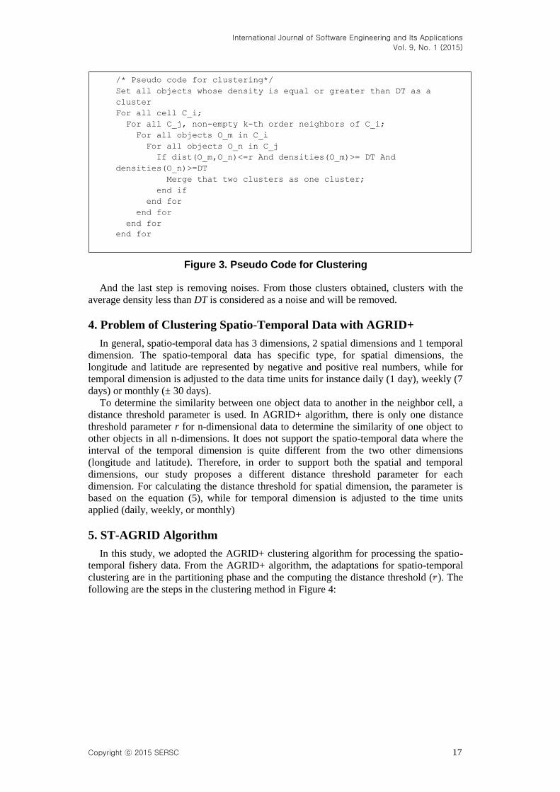
Figure 3. Pseudo Code for Clustering

And the last step is removing noises. From those clusters obtained, clusters with the

average density less than DT is considered as a noise and will be removed.

4. Problem of Clustering Spatio-Temporal Data with AGRID+

In general, spatio-temporal data has 3 dimensions, 2 spatial dimensions and 1 temporal

dimension. The spatio-temporal data has specific type, for spatial dimensions, the

longitude and latitude are represented by negative and positive real numbers, while for

temporal dimension is adjusted to the data time units for instance daily (1 day), weekly (7

days) or monthly (± 30 days).

To determine the similarity between one object data to another in the neighbor cell, a

distance threshold parameter is used. In AGRID+ algorithm, there is only one distance

threshold parameter r for n-dimensional data to determine the similarity of one object to

other objects in all n-dimensions. It does not support the spatio-temporal data where the

interval of the temporal dimension is quite different from the two other dimensions

(longitude and latitude). Therefore, in order to support both the spatial and temporal

dimensions, our study proposes a different distance threshold parameter for each

dimension. For calculating the distance threshold for spatial dimension, the parameter is

based on the equation (5), while for temporal dimension is adjusted to the time units

applied (daily, weekly, or monthly)

5. ST-AGRID Algorithm

In this study, we adopted the AGRID+ clustering algorithm for processing the spatio-

temporal fishery data. From the AGRID+ algorithm, the adaptations for spatio-temporal

clustering are in the partitioning phase and the computing the distance threshold ( ). The

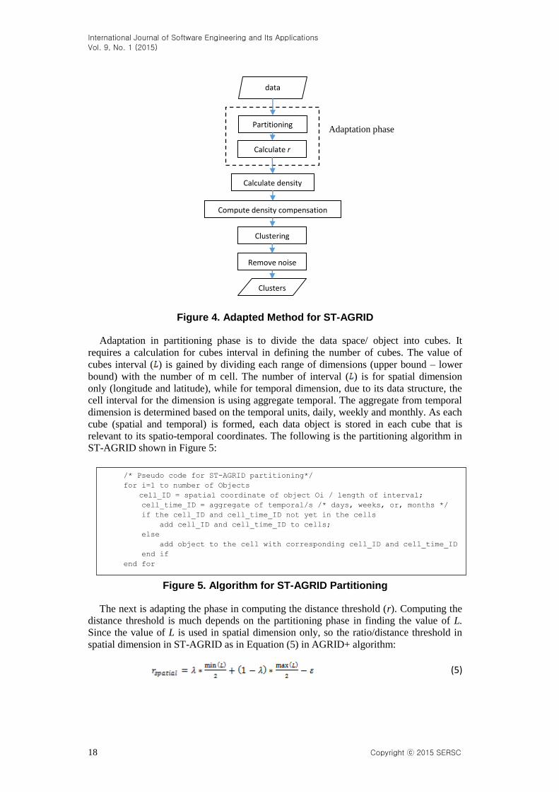
following are the steps in the clustering method in Figure 4:

/* Pseudo code for clustering*/

Set all objects whose density is equal or greater than DT as a

cluster

For all cell C_i;

For all C_j, non-empty k-th order neighbors of C_i;

For all objects O_m in C_i

For all objects O_n in C_j

If dist(O_m,O_n)<=r And densities(O_m)>= DT And

densities(O_n)>=DT

Merge that two clusters as one cluster;

end if

end for

end for

end for

end for


Vol. 9, No. 1 (2015)


data

Calculate r

Partitioning

Calculate density

Clustering

Compute density compensation

Remove noise

Clusters

Figure 4. Adapted Method for ST-AGRID

Adaptation in partitioning phase is to divide the data space/ object into cubes. It

requires a calculation for cubes interval in defining the number of cubes. The value of

cubes interval ( ) is gained by dividing each range of dimensions (upper bound – lower

bound) with the number of m cell. The number of interval ( ) is for spatial dimension

only (longitude and latitude), while for temporal dimension, due to its data structure, the

cell interval for the dimension is using aggregate temporal. The aggregate from temporal

dimension is determined based on the temporal units, daily, weekly and monthly. As each

cube (spatial and temporal) is formed, each data object is stored in each cube that is

relevant to its spatio-temporal coordinates. The following is the partitioning algorithm in

ST-AGRID shown in Figure 5:

Figure 5. Algorithm for ST-AGRID Partitioning

The next is adapting the phase in computing the distance threshold (r). Computing the

distance threshold is much depends on the partitioning phase in finding the value of L.

Since the value of L is used in spatial dimension only, so the ratio/distance threshold in

spatial dimension in ST-AGRID as in Equation (5) in AGRID+ algorithm:

(5)

/* Pseudo code for ST-AGRID partitioning*/

for i=1 to number of Objects

cell_ID = spatial coordinate of object Oi / length of interval;

cell_time_ID = aggregate of temporal/s /* days, weeks, or, months */

if the cell_ID and cell_time_ID not yet in the cells

add cell_ID and cell_time_ID to cells;

else

add object to the cell with corresponding cell_ID and cell_time_ID

end if

end for

Adaptation phase


Vol. 9, No. 1 (2015)


where is interval weight parameter used, is interval, and is a small integer number,

so that the value of . For the temporal dimension, the calculation of

is the aggregate of temporal dimension used, for instance daily is 1, weekly = 7 and

monthly 30.

The following in Figure 6 is the pseudocode for the calculation of distance threshold

(r):

Figure 6. Algorithm for Calculating the Distance Threshold

after the adaptation step has been done, the rest of the steps will be implemented similarly

to those in the AGRID+.

6. Application of ST-AGRID to determine the Potential Fishing Zones

In order to achieve the objective of the study, we attempted to utilize the ST-AGRID

algorithm for clustering spatio-temporal data. the objective is to determine the Potential

Fishing Zones based on fishery data. There are four phases in the application: conducting

data preparation, clustering with ST-AGRID, validating the cluster result, and

determining the potential fishing zones as illustrated in Figure 7.

Figure 7. Block Diagram of the ST-AGRID Application

6.1. Data Preparation

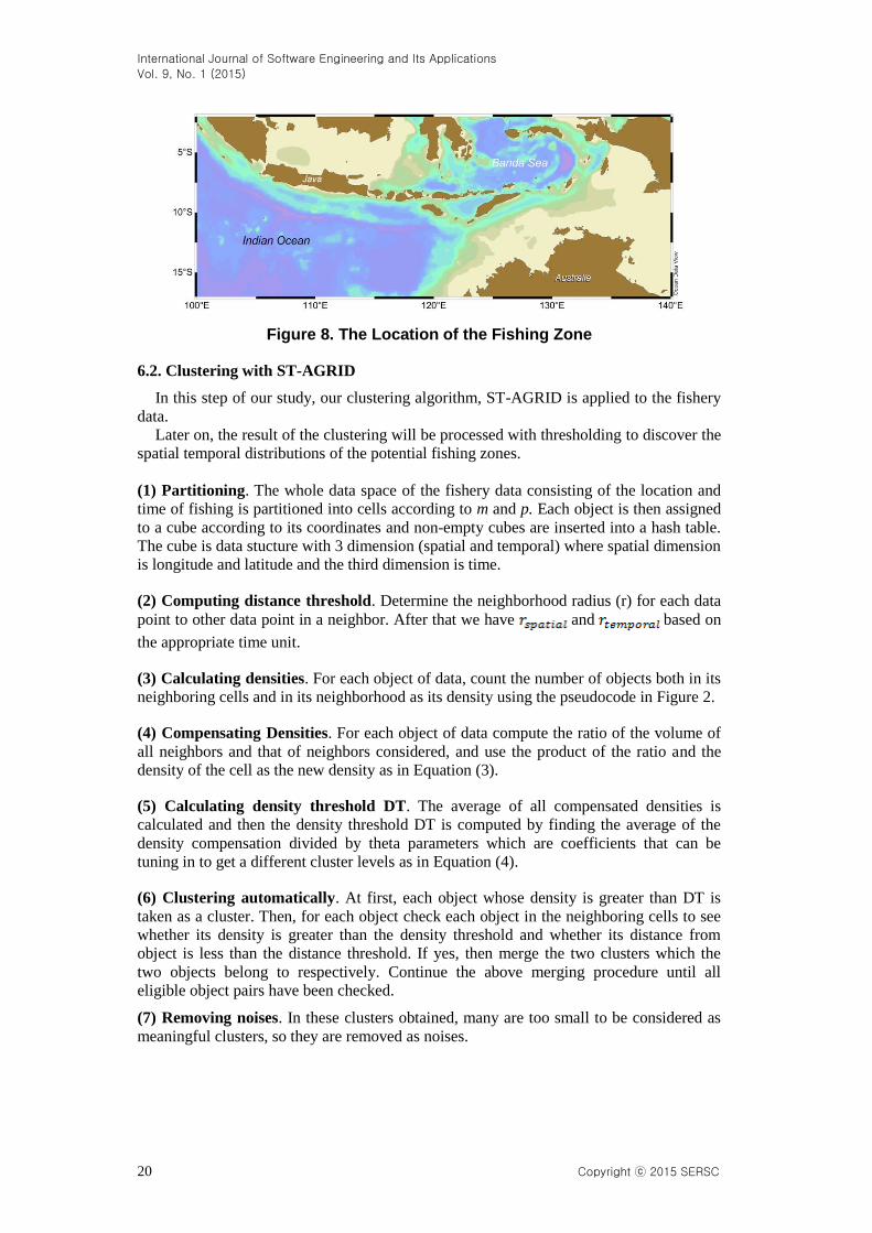
The fishery data utilized in this study is spatio-temporal data consisting daily fish catch

data. The data structure of the fishery data is longitude, latitude, data, month, year,

number of fish catch. The fishery data is from the Indian Ocean, 2-16,59° S and 100,49-

140° E. The fishery data is taken from year 2000 until 2004. The temporal data is

aggegate in daily, weekly and monthly. There will be 60 months, 300 weeks and 1600

days for range of study. Figure 8 shows the location of the fishing zone. The image is

generated utilizing the Ocean Data View software [20].

/* Pseudo code for computing r*/

r1 = (minimal L)/2;

r2 = (maximal L)/2;

r_spatial = *r1+(1- )*r2- ; /* ; small number

r_temporal = 1; /* range temporal is 1 aggregate time */


Vol. 9, No. 1 (2015)


Figure 8. The Location of the Fishing Zone

6.2. Clustering with ST-AGRID

In this step of our study, our clustering algorithm, ST-AGRID is applied to the fishery

data.

Later on, the result of the clustering will be processed with thresholding to discover the

spatial temporal distributions of the potential fishing zones.

(1) Partitioning. The whole data space of the fishery data consisting of the location and

time of fishing is partitioned into cells according to m and p. Each object is then assigned

to a cube according to its coordinates and non-empty cubes are inserted into a hash table.

The cube is data stucture with 3 dimension (spatial and temporal) where spatial dimension

is longitude and latitude and the third dimension is time.

(2) Computing distance threshold. Determine the neighborhood radius (r) for each data

point to other data point in a neighbor. After that we have and based on

the appropriate time unit.

(3) Calculating densities. For each object of data, count the number of objects both in its

neighboring cells and in its neighborhood as its density using the pseudocode in Figure 2.

(4) Compensating Densities. For each object of data compute the ratio of the volume of

all neighbors and that of neighbors considered, and use the product of the ratio and the

density of the cell as the new density as in Equation (3).

(5) Calculating density threshold DT. The average of all compensated densities is

calculated and then the density threshold DT is computed by finding the average of the

density compensation divided by theta parameters which are coefficients that can be

tuning in to get a different cluster levels as in Equation (4).

(6) Clustering automatically. At first, each object whose density is greater than DT is

taken as a cluster. Then, for each object check each object in the neighboring cells to see

whether its density is greater than the density threshold and whether its distance from

object is less than the distance threshold. If yes, then merge the two clusters which the

two objects belong to respectively. Continue the above merging procedure until all

eligible object pairs have been checked.

(7) Removing noises. In these clusters obtained, many are too small to be considered as

meaningful clusters, so they are removed as noises.


Vol. 9, No. 1 (2015)


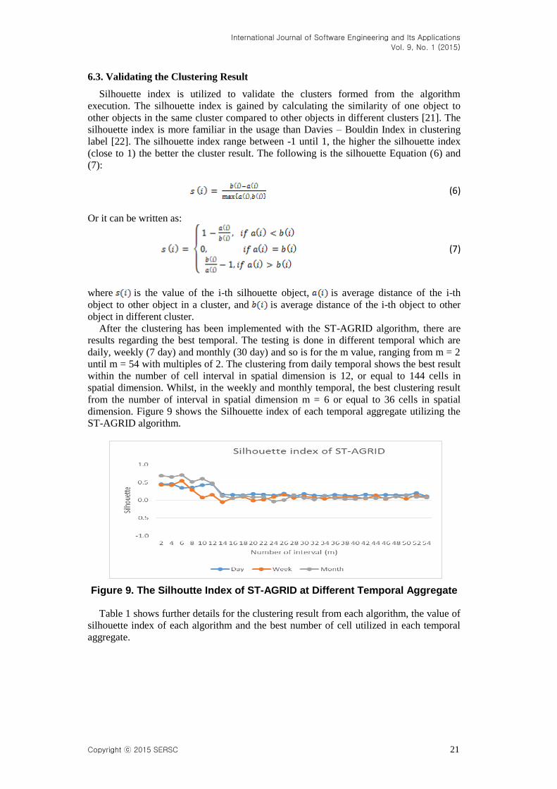
6.3. Validating the Clustering Result

Silhouette index is utilized to validate the clusters formed from the algorithm

execution. The silhouette index is gained by calculating the similarity of one object to

other objects in the same cluster compared to other objects in different clusters [21]. The

silhouette index is more familiar in the usage than Davies – Bouldin Index in clustering

label [22]. The silhouette index range between -1 until 1, the higher the silhouette index

(close to 1) the better the cluster result. The following is the silhouette Equation (6) and

(7):

(6)

Or it can be written as:

(7)

where is the value of the i-th silhouette object, is average distance of the i-th

object to other object in a cluster, and is average distance of the i-th object to other

object in different cluster.

After the clustering has been implemented with the ST-AGRID algorithm, there are

results regarding the best temporal. The testing is done in different temporal which are

daily, weekly (7 day) and monthly (30 day) and so is for the m value, ranging from m = 2

until m = 54 with multiples of 2. The clustering from daily temporal shows the best result

within the number of cell interval in spatial dimension is 12, or equal to 144 cells in

spatial dimension. Whilst, in the weekly and monthly temporal, the best clustering result

from the number of interval in spatial dimension m = 6 or equal to 36 cells in spatial

dimension. Figure 9 shows the Silhouette index of each temporal aggregate utilizing the

ST-AGRID algorithm.

Figure 9. The Silhoutte Index of ST-AGRID at Different Temporal Aggregate

Table 1 shows further details for the clustering result from each algorithm, the value of

silhouette index of each algorithm and the best number of cell utilized in each temporal

aggregate.


Vol. 9, No. 1 (2015)


Table 1. The Comparison of Number of m and Number of Cluster Between ST-AGRID and AGRID+

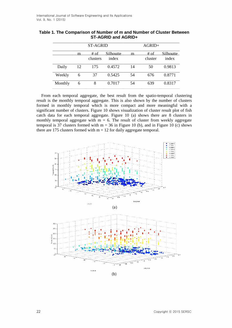
From each temporal aggregate, the best result from the spatio-temporal clustering

result is the monthly temporal aggregate. This is also shown by the number of clusters

formed in monthly temporal which is more compact and more meaningful with a

significant number of clusters. Figure 10 shows visualization of cluster result plot of fish

catch data for each temporal aggregate. Figure 10 (a) shows there are 8 clusters in

monthly temporal aggregate with m = 6. The result of cluster from weekly aggregate

temporal is 37 clusters formed with m = 36 in Figure 10 (b), and in Figure 10 (c) shows

there are 175 clusters formed with m = 12 for daily aggregate temporal.

(a)

(b)

ST-AGRID AGRID+

m # of

clusters

Silhoutte

index

m # of

cluster

Silhoutte

index

Daily 12 175 0.4572 14 50 0.9813

Weekly 6 37 0.5425 54 676 0.8771

Monthly 6 8 0.7017 54 639 0.8317


Vol. 9, No. 1 (2015)


(c)

Figure 10. Spatio-temporal Clustering Results (a) Monthly, (b) Weekly, (c) Daily

The bigger the temporal aggregate implemented, the bigger the size of cluster formed.

It happened because the size of the temporal aggregate affected the ratio of the temporal

dimensions.

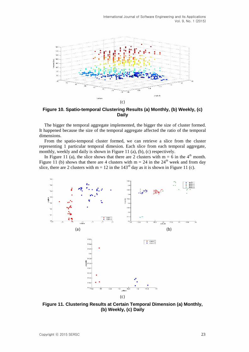
From the spatio-temporal cluster formed, we can retrieve a slice from the cluster

representing 1 particular temporal dimesion. Each slice from each temporal aggregate,

monthly, weekly and daily is shown in Figure 11 (a), (b), (c) respectively.

In Figure 11 (a), the slice shows that there are 2 clusters with m = 6 in the 4th month.

Figure 11 (b) shows that there are 4 clusters with m = 24 in the 24th week and from day

slice, there are 2 clusters with m = 12 in the 143rd

day as it is shown in Figure 11 (c).

(a) (b)

(c)

Figure 11. Clustering Results at Certain Temporal Dimension (a) Monthly, (b) Weekly, (c) Daily


Vol. 9, No. 1 (2015)


From the study with all temporal aggregate and m variations, the time execution of the

ST-AGRID algorithm is better than the AGRID+ algorithm. Whilst, for the silhouette

index shows that AGRID+ algorithm is better. Table 2 shows the average comparison of

time execution and silhouette index of each algorithm in three different temporal

aggregates.

Table 2. Execution Time and Silhouette Index in Different Temporal

ST-AGRID AGRID+

Exec.time

(sec)

Silhoutte

index

Exec.time

(sec)

Silhoutte

index

Daily 8.4117 0.2060 37.4082 0.6346

Weekly 13.9306 0.1246 53.6410 0.7260

Monthly 38.8747 0.1899 135.2700 0.5787

The Table 2 shows that ST-AGRID has the best time execution compared with

AGRID+, it is due to the fact that ST-AGRID works very well with the specific temporal

aggregate, while for AGRID+ outperformed in the silhouette index because the

thoroughness of the parameter checking in each dimension, causes a more accurate

results.

6.4. Determining the Potential Fishing Zone

In order to determine the PFZ of the clustering result, we need to select the cluster with

certain threshold. This is very much dependant on the determination of the used threshold.

In determining the threshold to identify the potential fishing zone for particular area, the

threshold is determined by the opinion of some experts in some fishing companies. One of

them is PT. Perikanan Nusantara Indonesia. A fishing ground is stated as a potential

fishing zone if the number of fish catch is equal or greater than 5. Thus the thresholding

formula for determining the potential fishing zone is in Equation (7):

(7)

where is the total number of fish catches at ith-cluster, is the number of catch

points at ith-cluster, and is a threshold. Later on, the number 1 is identifying as the

potential area and 0 is non-potential area.

Refer to the threshold, Figure 12 shows the visualization of the potential fishing zone

with the minimum catch.


Vol. 9, No. 1 (2015)


(a) (b)

(c)

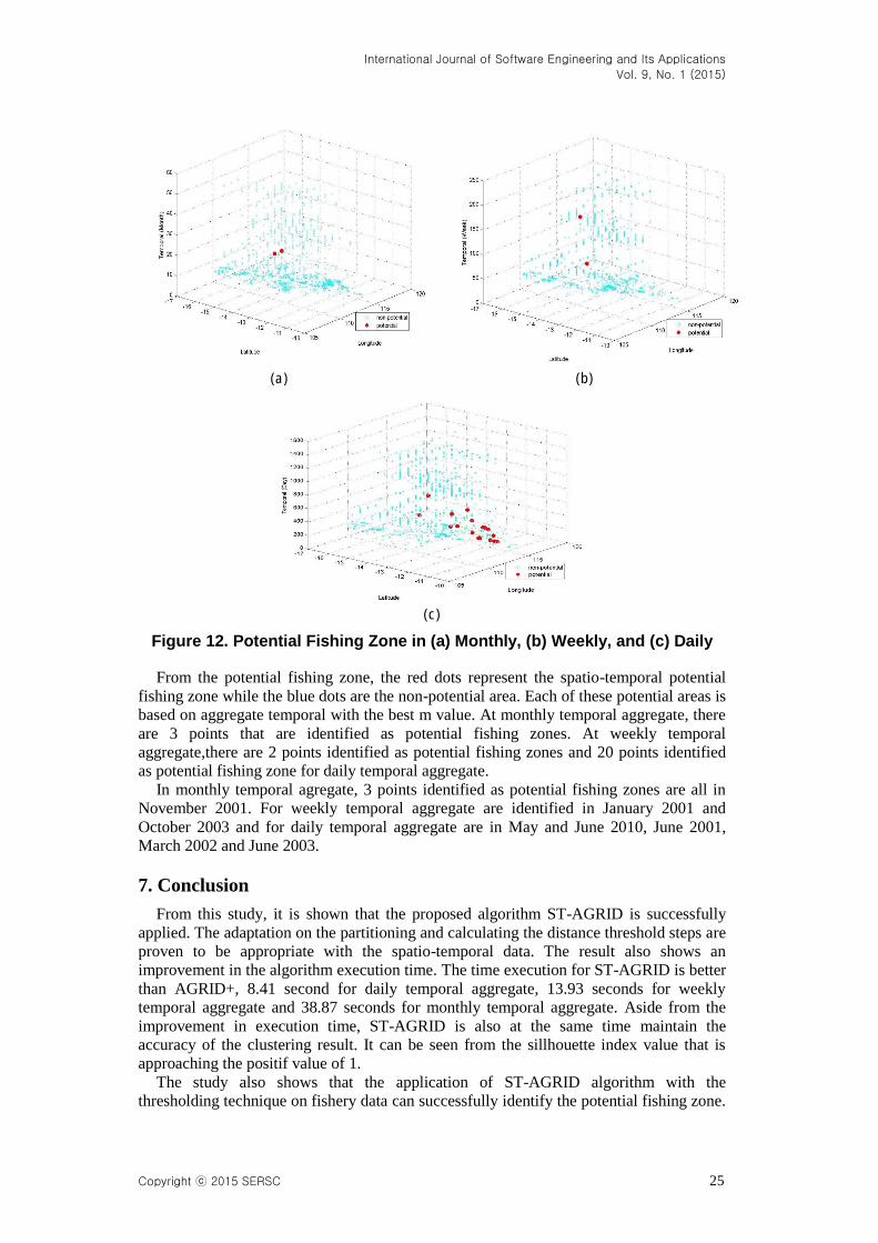
Figure 12. Potential Fishing Zone in (a) Monthly, (b) Weekly, and (c) Daily

From the potential fishing zone, the red dots represent the spatio-temporal potential

fishing zone while the blue dots are the non-potential area. Each of these potential areas is

based on aggregate temporal with the best m value. At monthly temporal aggregate, there

are 3 points that are identified as potential fishing zones. At weekly temporal

aggregate,there are 2 points identified as potential fishing zones and 20 points identified

as potential fishing zone for daily temporal aggregate.

In monthly temporal agregate, 3 points identified as potential fishing zones are all in

November 2001. For weekly temporal aggregate are identified in January 2001 and

October 2003 and for daily temporal aggregate are in May and June 2010, June 2001,

March 2002 and June 2003.

7. Conclusion

From this study, it is shown that the proposed algorithm ST-AGRID is successfully

applied. The adaptation on the partitioning and calculating the distance threshold steps are

proven to be appropriate with the spatio-temporal data. The result also shows an

improvement in the algorithm execution time. The time execution for ST-AGRID is better

than AGRID+, 8.41 second for daily temporal aggregate, 13.93 seconds for weekly

temporal aggregate and 38.87 seconds for monthly temporal aggregate. Aside from the

improvement in execution time, ST-AGRID is also at the same time maintain the

accuracy of the clustering result. It can be seen from the sillhouette index value that is

approaching the positif value of 1.

The study also shows that the application of ST-AGRID algorithm with the

thresholding technique on fishery data can successfully identify the potential fishing zone.


Vol. 9, No. 1 (2015)


The determination of the potential area is based on the minimal number of fish catch. The

result of the potential fishing zone is different according to its temporal aggergate. In

future study, we will be more focused in increasing the cluster validation result for ST-

AGRID.

Acknowledgments

This research is fully supported by Universitas Indonesia through ‘Hibah Riset UI

2013-PUPT (BOPTN)’ No. 2706/H2.R12/HKP.05.00/2013. The author would like to

thank PT. Perikanan Nusantara for providing the fishery data.

References

[1] J. Mennis and D. Guo, "Spatial Data Mining and Geographic Knowledge Discovery—An introduction",

Comput. Environ. Urban Syst., vol. 33, no. 6, (2009) November, pp. 403–408.

[2] J. F. Roddick and M. Spiliopoulou, "A Bibliography of Temporal, Spatial and Spatio-Temporal Data

Mining Research”, ACM SIGKDD Explor. Newsl., vol. 1, no. 1, (1999) June, pp. 34–38.

[3] K. V. Rao, A. Govardhan and K. V. C. Rao, "SPatio Temporal Data Mining : Issues, Tasks And

Applications", Int. J. Comput. Sci. Eng. Surv., vol. 3, no. 1, (2012), pp. 39–52.

[4] S. Jagannathan, A. Samraj and M. Rajavel, "Potential Fishing Zone Estimation by Rough Cluster

Prediction", Proceeding of 4th International Conference on Computational Intelligence, Modelling and

Simulation, Kuantan, Malaysia, (2102) September 25-27.

[5] M. Erwig, "Spatio-Temporal Data Types : An Approach to Modeling and Querying Moving Objects in

Databases", vol. 296, (1999), pp. 269–296.

[6] P. Kalnis, N. Mamoulis and S. Bakiras, "On Discovering Moving Clusters in Spatio-temporal Data",

Proc. The 9th International Symposium, SSTD 2005, Angra dos Reis, Brazil, (2005) August 22-24, pp.

364–381.

[7] M. Kantardzic, "Data Mining - Concept, Model, Methods and Algorithms", 2nd edition. IEEE Press and

Wiley Intl, Hoboken, New Jersey, (2011).

[8] M. Ester, H. Kriegel and X. Xu, "A Density-Based Algorithm for Discovering Clusters in Large Spatial

Databases with Noise", Proc. 1996 Knowledge Data Discovery, Portland, Oregon, USA, (1996) August

2-4, pp. 226-231.

[9] M. Huang and F. Bian, "A Grid and Density Based Fast Spatial Clustering Algorithm", 2009 Int. Conf.

Artif. Intell. Comput. Intell., Shanghai, China, (2009) November 7-8, pp. 260–263.

[10] Z. Sun, Z. Zhao, H. Wang, M. Ma, L. Zhang and Y. Shu, "A Fast Clustering Algorithm Based on Grid

and Density", Canadian Conf. Electr. Comput. Eng. 2005, Saskatchewan, Canada, (2005) May 1-3, pp.

2276–2279.

[11] Y. Zhao, J. Cao, C. Zhang and S. Zhang, "Enhancing Grid-Density Based Clustering for High

Dimensional Data", Syst. Softw., vol. 84, no. 9, (2011) September, pp. 1524–1539.

[12] J. F. Roddick and B. G. Lees, "Paradigm for Spatial and Spatio-Temporal Data Mining", Taylor Fr. Res.

Monogr. Geogr. Inf. Syst., (2001), pp. 1–14.

[13] N. Mamoulis, H. Cao, G. Kollios, M. Hadjieleftheriou, Y. Tao and D. W. Cheung, “Mining, Indexing,

and Querying Historical Spatio-Temporal Data”, Proc. 2004 ACM SIGKDD Int. Conf. Knowl. Discov.

data Min. - KDD ’04, (2004), pp. 236.

[14] S. K. Sahu and K. V Mardia, “Recent Trends in Modeling Spatio-Temporal Data”, workshop on recent

advances in modeling spatio-temporal data, (2005).

[15] H. F. Tork, “Spatio-Temporal Clustering Methods Classification”, Doctoral Symposium on Informatics

Engineering, Porto, Portugal, (2012).

[16] S. Kisilevich, F. Mansmann, M. Nanni and S. Rinzivillo, "Spatio-Temporal Clustering:  A Survey in

Data Mining and Knowledge Discovery", handbook 2nd edition, (2010), pp. 1–22.

[17] T. Abraham and J. F. Roddick, "Opportunities For Knowledge Discovery In Spatio-Temporal

Information Systems", AJIS, vol. 5, no. 2, (1998).

[18] D. Birant and A. Kut, "ST-DBSCAN: An algorithm for clustering spatial–temporal data", Data Knowl.

Eng., vol. 60, no. 1, (2007) January, pp. 208–221.

[19] M. Wang, A. Wang and A. Li, "Mining Spatial Temporal Clusters From Geo-databases", 2nd Conf.

Advanced Data Mining and Application, Xi'an, China, (2006) August 14-16, pp. 263–270.

[20] R. Schlitzer, "User Guide for Ocean Data View", Ocean Data View, (2002), pp. 1–62.

[21] P. J. Rousseeuw, "Silhouettes: A graphical aid to the interpretation and validation of cluster analysis",

Comput. Appl. Math., vol. 20, (1987) November, pp. 53–65.

[22] S. Petrovic, "A Comparison Between the Silhouette Index and the Davies-Bouldin Index in Labelling

IDS Clusters", Tthe 11th Nordic Workshop on Secure IT-systems, NORDSEC 2006, (2006), pp. 53–64.

st-agrid: a spatio temporal grid density based clustering and its application for determining the...

Documents