srinivas institute of management studies - zenodo
TRANSCRIPT
SRINIVAS INSTITUTE OF MANAGEMENT
STUDIES
STUDY MATERIAL - 2015 -16
QUANTITATIVE TECHNIQUES MBA I SEMESTER
Complied by
Dr. P. S. Aithal
MOST INNOVATIVE HIGHER EDUCATION INSTITUTION
www.srinivasgroup.com

SRINVASGROUP–QUANTITATIVETECHNIQUES Contents
Page1
CONTENTS
Teaching Session Plan Chapter 1 : Variables & Functions Chapter 2 : Matrices & Determinants Chapter 3 : Differential Calculus Chapter 4 : Integral Calculus
Quantitative Techniques
Teaching Plan 03 Hours per Week
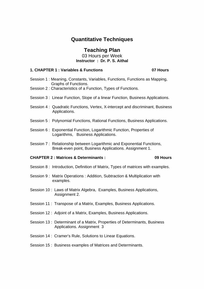
Instructor : Dr. P. S. Aithal 1. CHAPTER 1 : Variables & Functions 07 Hours Session 1 : Meaning, Constants, Variables, Functions, Functions as Mapping, Graphs of Functions. Session 2 : Characteristics of a Function, Types of Functions. Session 3 : Linear Function, Slope of a linear Function, Business Applications. Session 4 : Quadratic Functions, Vertex, X-intercept and discriminant, Business Applications. Session 5 : Polynomial Functions, Rational Functions, Business Applications. Session 6 : Exponential Function, Logarithmic Function, Properties of Logarithms, Business Applications. Session 7 : Relationship between Logarithmic and Exponential Functions, Break-even point, Business Applications. Assignment 1. CHAPTER 2 : Matrices & Determinants : 09 Hours Session 8 : Introduction, Definition of Matrix, Types of matrices with examples. Session 9 : Matrix Operations : Addition, Subtraction & Multiplication with examples. Session 10 : Laws of Matrix Algebra, Examples, Business Applications, Assignment 2. Session 11 : Transpose of a Matrix, Examples, Business Applications. Session 12 : Adjoint of a Matrix, Examples, Business Applications. Session 13 : Determinant of a Matrix, Properties of Determinants, Business Applications. Assignment 3 Session 14 : Cramer’s Rule, Solutions to Linear Equations. Session 15 : Business examples of Matrices and Determinants.
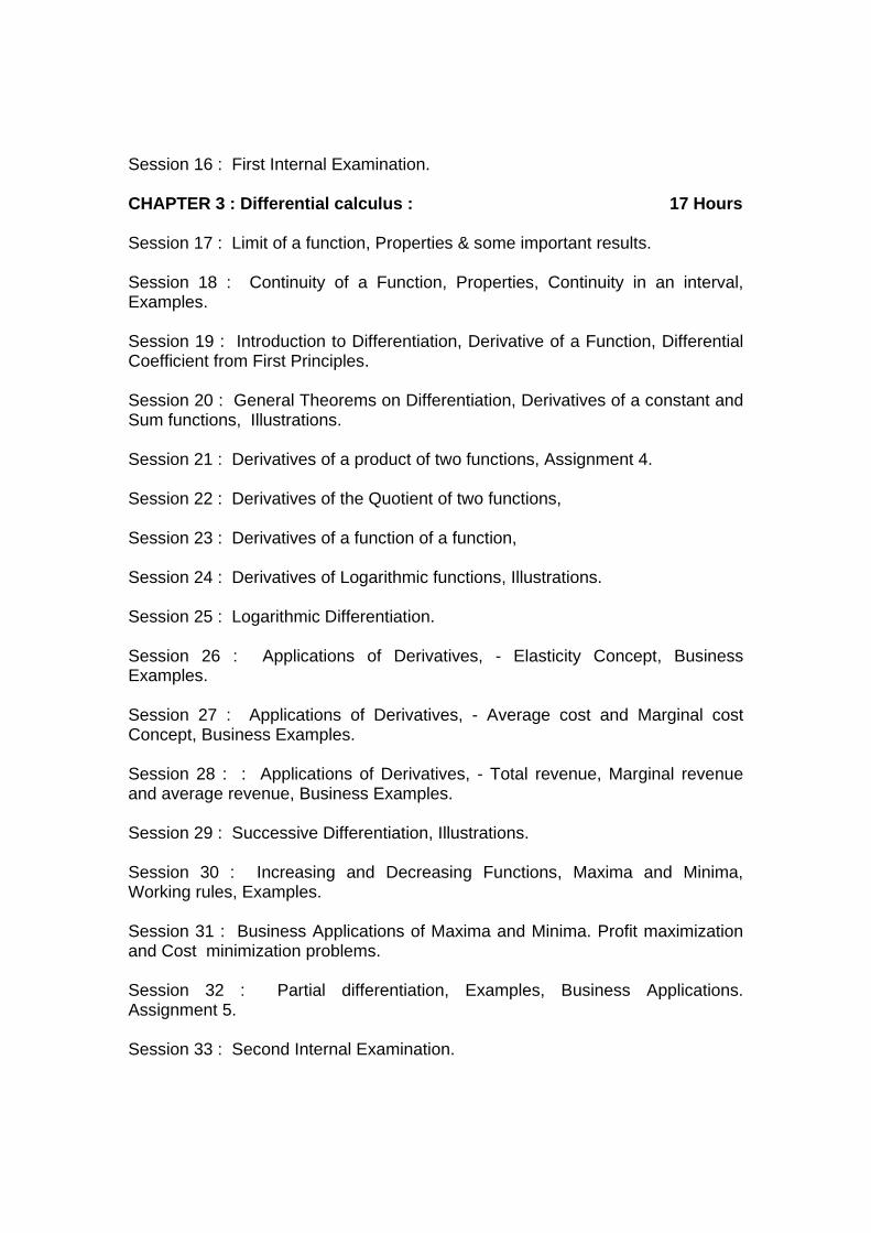
Session 16 : First Internal Examination. CHAPTER 3 : Differential calculus : 17 Hours Session 17 : Limit of a function, Properties & some important results. Session 18 : Continuity of a Function, Properties, Continuity in an interval, Examples. Session 19 : Introduction to Differentiation, Derivative of a Function, Differential Coefficient from First Principles. Session 20 : General Theorems on Differentiation, Derivatives of a constant and Sum functions, Illustrations. Session 21 : Derivatives of a product of two functions, Assignment 4. Session 22 : Derivatives of the Quotient of two functions, Session 23 : Derivatives of a function of a function, Session 24 : Derivatives of Logarithmic functions, Illustrations. Session 25 : Logarithmic Differentiation. Session 26 : Applications of Derivatives, - Elasticity Concept, Business Examples. Session 27 : Applications of Derivatives, - Average cost and Marginal cost Concept, Business Examples. Session 28 : : Applications of Derivatives, - Total revenue, Marginal revenue and average revenue, Business Examples. Session 29 : Successive Differentiation, Illustrations. Session 30 : Increasing and Decreasing Functions, Maxima and Minima, Working rules, Examples. Session 31 : Business Applications of Maxima and Minima. Profit maximization and Cost minimization problems. Session 32 : Partial differentiation, Examples, Business Applications. Assignment 5. Session 33 : Second Internal Examination.

CHAPTER 4 : Integral calculus : 7 Hours Session 34 : Definite & indefinite integral Session 35 : Rules of integration, some standard results in integration. Session 36 : Methods of Integration, Integration by Substitution, Problems. Session 37 : Integration by Parts, Problems. Session 38 : Some Business applications of Integration Part I. Assignment 6. Session 39 : Some Business applications of Integration Part II. Session 40 : Third Internal Examination.
SRINIVASGROUP:QUANTITATIVETECHNIQUES CH‐1
VARIABLES & FUNCTIONS Page 1
CHAPTER 1
Variables & Functions Meaning : In quantitative technique, the relationship between any two quantities is expressed by a mathematical function. For example, in manufacturing industry, if we increase the manpower the production will increase. The relationship between manpower and production can be expressed by a mathematical function. 1.1 Constants : If we increase the production by using more raw material, the cost of the equipment does not change but, the costs of raw material, labour and sales change. Cost of the equipment which retains the same value throughout a set, of mathematical operations is called "constant". Constants are represented by a, b, c, ….. 1.2 Variables : In the above example, the costs of raw material, labour and sales which assume any numerical-value out of a given set of values are called "variables". Variables are represented by x, y, z, …… 1.3 Functions : The volume of a cube is the cube of the length of its side. Length of the side, an independent variable, can assume any value. The volume, a dependent variable, depends on the value of the length of the side. This correspondence between the length of the side and the volume of the cube, 'which describes how one quantity depends on another is called a "function". Two variables x and y are functions of each other when the values of one depend on those of the other. If y is a function of x, we write y = f (x). The set of all allowable values of the independent variable of a function is known as the "domain" of that function. Ex. 1 : In the function f(x) = 1/ (x2 – 9), the domain consists of all real numbers except 3 and -3. Ex. 2 : Again in the function f(x) = √(x – 9), the domain consists of all real numbers x 9. The elements of the first set is the domain of the function and that of the second set is the range of the function. Ex. 3. The relation between the price (x) and the quantity required (y), for an article is given by y =f(x). If f(x) =16 - 4x, find y at different prices. Find the domain and the range of y = f(x). Ans : Now, y = f(0 ) = 16 - 4x 0 = 16 y = f(1) = 16 - 4 x 1 = 12 y = f(2) = 16 - 4 x 2 = 8
SRINIVASGROUP:QUANTITATIVETECHNIQUES CH‐1
VARIABLES & FUNCTIONS Page 2
y = f(3) = 16 - 4 x 3 = 4 y = f(4) = 16 - 4 x 4 = 0 If x > 4, y becomes negative. Since y cannot be negative, we present the real values below:
Price (x) Quantity required (y) 0 16 1 12 2 8 3 4 4 0
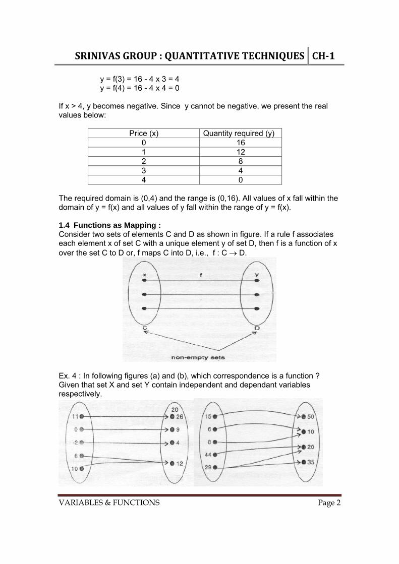
The required domain is (0,4) and the range is (0,16). All values of x fall within the domain of y = f(x) and all values of y fall within the range of y = f(x). 1.4 Functions as Mapping : Consider two sets of elements C and D as shown in figure. If a rule f associates each element x of set C with a unique element y of set D, then f is a function of x over the set C to D or, f maps C into D, i.e., f : C D.
Ex. 4 : In following figures (a) and (b), which correspondence is a function ? Given that set X and set Y contain independent and dependant variables respectively.

SRINIVASGROUP:QUANTITATIVETECHNIQUES CH‐1
VARIABLES & FUNCTIONS Page 3
Figure (a) Figure (b) Ans : Fig. (a) represents a function since every number in Set X is assigned to exactly one number in Y, although 6 and 10 in set X are assigned to the same number 12 in Y and no number in X has been assigned to Y. Fig. (b) is not a function because 29 in X has been assigned to 20 and 35 of Y. 1.5 Graphs of Functions : The function Y = f(x) = x3 may be considered as a set of ordered pairs, i.e., (2, 8), (-2, -8), (3, 27), (0, 0), etc. The first co-ordinate in each pair is a number in the domain x and the second co-ordinate is its corresponding functional value in the range. The function can be represented graphically by plotting each ordered pair of the function on a graph paper. The horizontal line, or x-axis and the vertical line, or, the y-axis represents the elements from the domain and the elements from the range of the function. The point where the x-axis and y-axis meets is called the origin i.e., (0, 0). The x and y axes divide the plane into four equal parts, or, quadrants. Quadrants have signs and numbers as follows:
Ex. 5 : Draw a graph for the function f(x) = 5 – 2x. Ans : x -3 -2 -1 0 1 2 3 y 11 9 7 5 3 1 -1 Ordered pair
(-3, 11) (-2, 9) (-1, 7) (0, 5) (1, 3) (2, 1) (3, -1)
SRINIVASGROUP:QUANTITATIVETECHNIQUES CH‐1
VARIABLES & FUNCTIONS Page 4
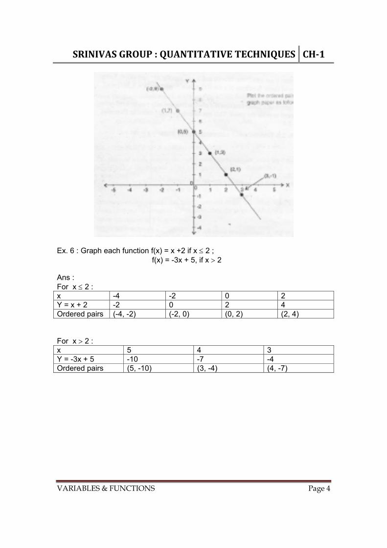
Ex. 6 : Graph each function f(x) = x +2 if x 2 ; f(x) = -3x + 5, if x 2 Ans : For x 2 : x -4 -2 0 2 Y = x + 2 -2 0 2 4 Ordered pairs (-4, -2) (-2, 0) (0, 2) (2, 4) For x 2 : x 5 4 3 Y = -3x + 5 -10 -7 -4 Ordered pairs (5, -10) (3, -4) (4, -7)
SRINIVASGROUP:QUANTITATIVETECHNIQUES CH‐1
VARIABLES & FUNCTIONS Page 5
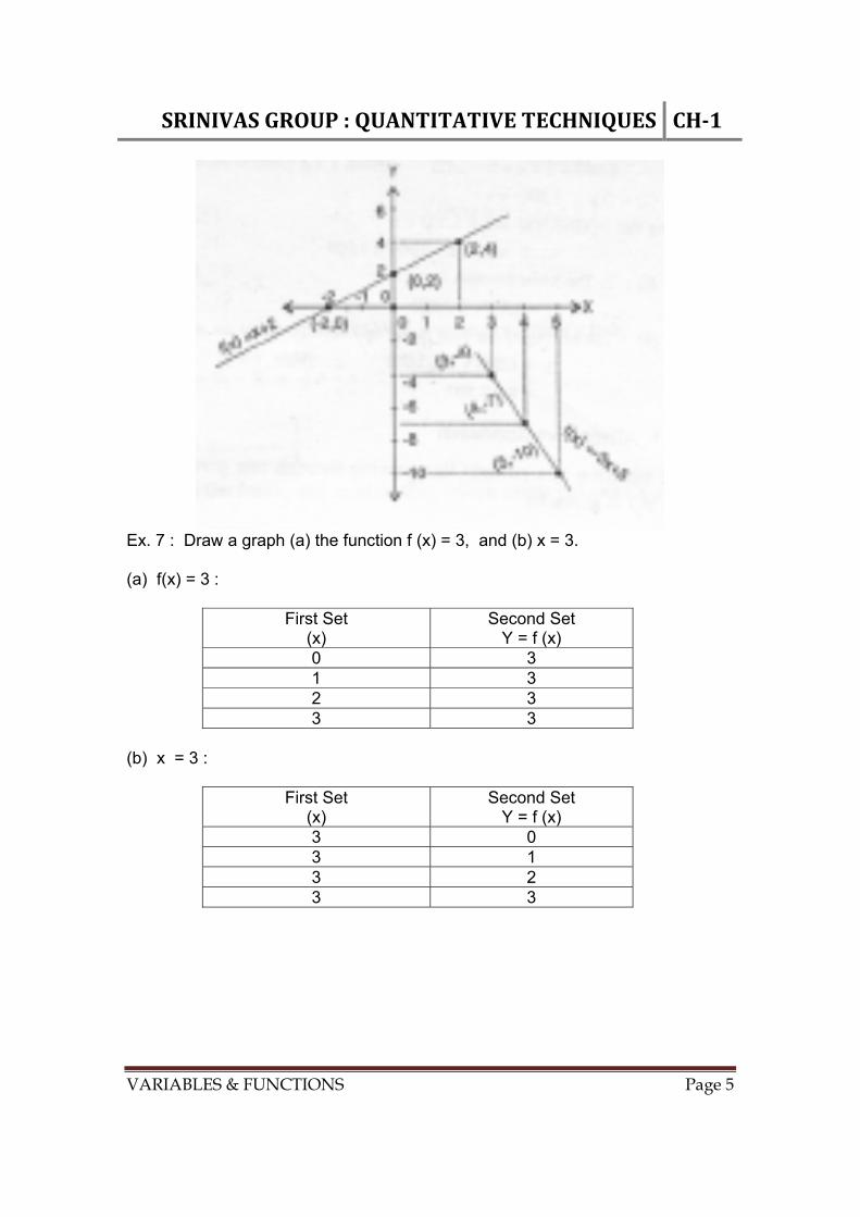
Ex. 7 : Draw a graph (a) the function f (x) = 3, and (b) x = 3. (a) f(x) = 3 :
First Set (x)
Second Set Y = f (x)
0 3 1 3 2 3 3 3
(b) x = 3 :
First Set (x)
Second Set Y = f (x)
3 0 3 1 3 2 3 3
SRINIVASGROUP:QUANTITATIVETECHNIQUES CH‐1
VARIABLES & FUNCTIONS Page 6
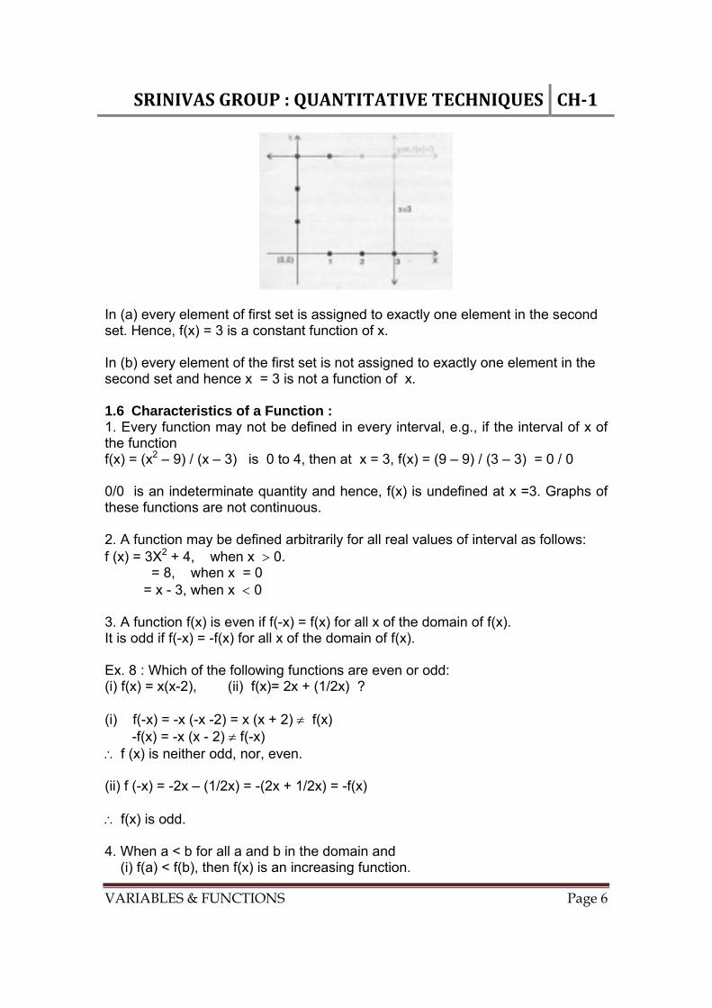
In (a) every element of first set is assigned to exactly one element in the second set. Hence, f(x) = 3 is a constant function of x. In (b) every element of the first set is not assigned to exactly one element in the second set and hence x = 3 is not a function of x. 1.6 Characteristics of a Function : 1. Every function may not be defined in every interval, e.g., if the interval of x of the function f(x) = (x2 – 9) / (x – 3) is 0 to 4, then at x = 3, f(x) = (9 – 9) / (3 – 3) = 0 / 0 0/0 is an indeterminate quantity and hence, f(x) is undefined at x =3. Graphs of these functions are not continuous. 2. A function may be defined arbitrarily for all real values of interval as follows: f (x) = 3X2 + 4, when x 0. = 8, when x = 0 = x - 3, when x 0 3. A function f(x) is even if f(-x) = f(x) for all x of the domain of f(x). It is odd if f(-x) = -f(x) for all x of the domain of f(x). Ex. 8 : Which of the following functions are even or odd: (i) f(x) = x(x-2), (ii) f(x)= 2x + (1/2x) ? (i) f(-x) = -x (-x -2) = x (x + 2) f(x) -f(x) = -x (x - 2) f(-x) f (x) is neither odd, nor, even. (ii) f (-x) = -2x – (1/2x) = -(2x + 1/2x) = -f(x) f(x) is odd. 4. When a < b for all a and b in the domain and (i) f(a) < f(b), then f(x) is an increasing function.

SRINIVASGROUP:QUANTITATIVETECHNIQUES CH‐1
VARIABLES & FUNCTIONS Page 7
(ii) f(a) f(b), then f(x) is a decreasing function. (iii) f(a) = f(b), then f(x) is a constant function. The graphs of (a) increasing function and (b) decreasing function are shown below :
Ex. 9 : Which of the following functions are increasing; decreasing and constant? (i) f(x) = 4x + 3; (ii) f(x) = -4x + 5; (iii) f(x) = -4 Ans : (i) f(x) = 4x + 3 f(1) = 7 and f(2) = 11 Since 1 < 2 and f(1) < f(2), f(x) is said to be increasing. (ii) f(x) = -4x + 5 f(1) = 1and f(2) = -3 Since 1 < 2 and f(1) > f(2), f(x) is a decreasing function. (iii) f(x) = -4 f(1) = -4 and f(2) = -4 Since f(1) = f(2), f(x) is a constant function. 1.7 Types of Functions : 1. Linear Function : f(x) = ax + b, where a and b are constants (a 0) and x can have any real value. 2. Quadratic Function : f(x) = ax2 + bx + c, a,b,c are real numbers with a 0. 3. Polynomial Function : f(x) = anx
n + an-1.xn-1 + …….. + a1x
1 + a0 where n is positive integer, an ---a0 real numbers with an 0. 4. Rational Function : f(x) = P(x)/ Q(x), where Q(x) 0 and P(x) and Q(x) are polynomials.
SRINIVASGROUP:QUANTITATIVETECHNIQUES CH‐1
VARIABLES & FUNCTIONS Page 8
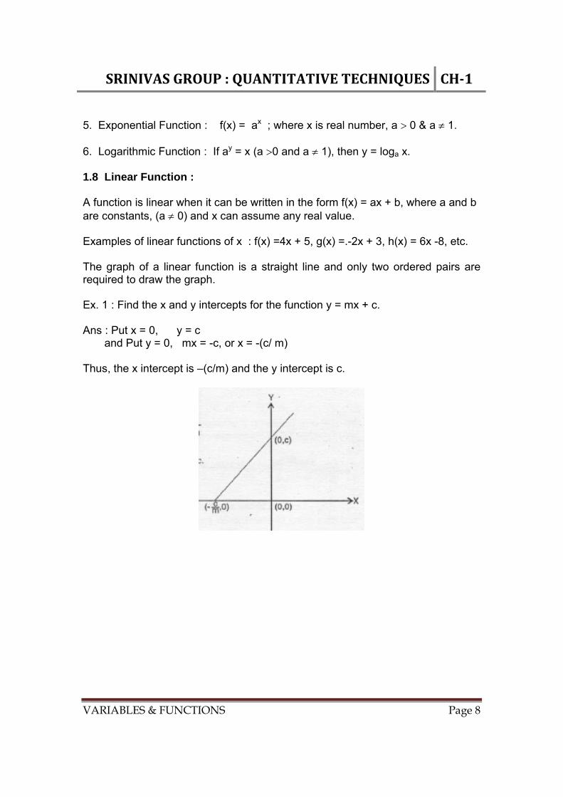
5. Exponential Function : f(x) = ax ; where x is real number, a 0 & a 1. 6. Logarithmic Function : If ay = x (a 0 and a 1), then y = loga x. 1.8 Linear Function : A function is linear when it can be written in the form f(x) = ax + b, where a and b are constants, (a 0) and x can assume any real value. Examples of linear functions of x : f(x) =4x + 5, g(x) =.-2x + 3, h(x) = 6x -8, etc. The graph of a linear function is a straight line and only two ordered pairs are required to draw the graph. Ex. 1 : Find the x and y intercepts for the function y = mx + c. Ans : Put x = 0, y = c and Put y = 0, mx = -c, or x = -(c/ m) Thus, the x intercept is –(c/m) and the y intercept is c.
SRINIVASGROUP:QUANTITATIVETECHNIQUES CH‐1
VARIABLES & FUNCTIONS Page 9
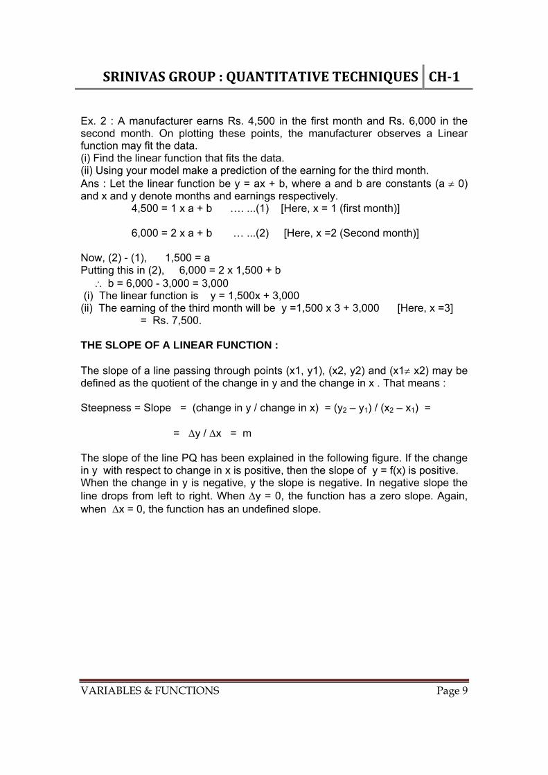
Ex. 2 : A manufacturer earns Rs. 4,500 in the first month and Rs. 6,000 in the second month. On plotting these points, the manufacturer observes a Linear function may fit the data. (i) Find the linear function that fits the data. (ii) Using your model make a prediction of the earning for the third month. Ans : Let the linear function be y = ax + b, where a and b are constants (a 0) and x and y denote months and earnings respectively. 4,500 = 1 x a + b …. ...(1) [Here, x = 1 (first month)] 6,000 = 2 x a + b … ...(2) [Here, x =2 (Second month)] Now, (2) - (1), 1,500 = a Putting this in (2), 6,000 = 2 x 1,500 + b b = 6,000 - 3,000 = 3,000 (i) The linear function is y = 1,500x + 3,000 (ii) The earning of the third month will be y =1,500 x 3 + 3,000 [Here, x =3] = Rs. 7,500. THE SLOPE OF A LINEAR FUNCTION : The slope of a line passing through points (x1, y1), (x2, y2) and (x1 x2) may be defined as the quotient of the change in y and the change in x . That means : Steepness = Slope = (change in y / change in x) = (y2 – y1) / (x2 – x1) = = y / x = m The slope of the line PQ has been explained in the following figure. If the change in y with respect to change in x is positive, then the slope of y = f(x) is positive. When the change in y is negative, y the slope is negative. In negative slope the line drops from left to right. When y = 0, the function has a zero slope. Again, when x = 0, the function has an undefined slope.
SRINIVASGROUP:QUANTITATIVETECHNIQUES CH‐1
VARIABLES & FUNCTIONS Page 10
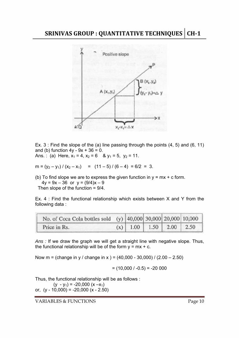
Ex. 3 : Find the slope of the (a) line passing through the points (4, 5) and (6, 11) and (b) function 4y - 9x + 36 = 0. Ans. : (a) Here, x1 = 4, x2 = 6 & y1 = 5, y2 = 11. m = (y2 – y1) / (x2 – x1) = (11 – 5) / (6 – 4) = 6/2 = 3. (b) To find slope we are to express the given function in y = mx + c form. 4y = 9x – 36 or y = (9/4)x – 9 Then slope of the function = 9/4. Ex. 4 : Find the functional relationship which exists between X and Y from the following data :
Ans : If we draw the graph we will get a straight line with negative slope. Thus, the functional relationship will be of the form y = mx + c. Now m = (change in y / change in x ) = (40,000 - 30,000) / (2.00 – 2.50) = (10,000 / -0.5) = -20 000 Thus, the functional relationship will be as follows : (y - y1) = -20,000 (x –x1) or, (y - 10,000) = -20,000 (x - 2.50)
SRINIVASGROUP:QUANTITATIVETECHNIQUES CH‐1
VARIABLES & FUNCTIONS Page 11
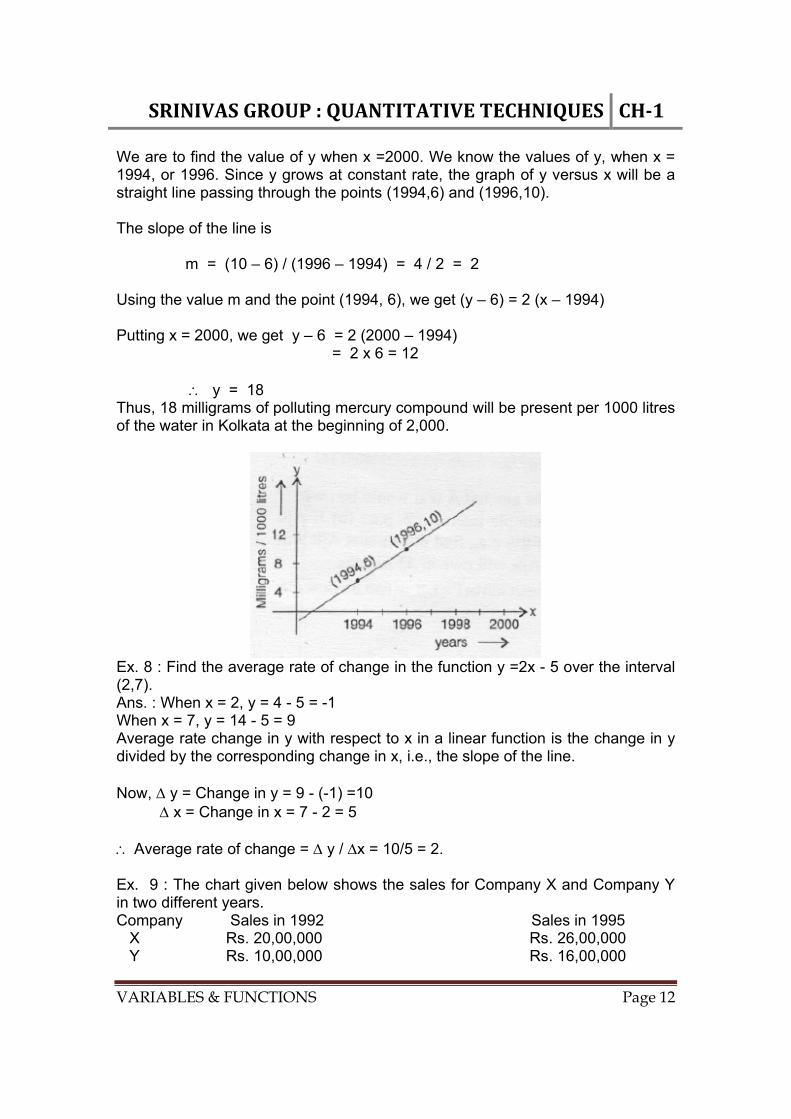
= -20,000x + 50,000 or, y = -20,000x + 60,000. Ex. 5 : (a) Obtain a formula for the amount A that would-be-owed if a principal P is borrowed for t years at simple interest r% p.a.; (b) If Ajit borrows Rs. 20,000 at a simple interest of 9% p.a., find the amount Ajit will, owe in 6 years; (c) Find also the amount Ajit will owe in 42 months. Ans. : (a) If we hold the money for 1 year, the interest will be P x r. If we hold the money for t years, the total interest will be P x r x t. The amount owed after t years will be A = P + Px r x t = P (1 + rt) (b) Here, P =Rs. 20,000, r = 9% = 0.09 and t = 6 years A = 20,000 (1+ 0.09 x 6) - = 20,000 x 1.54 = Rs. 30,800. (c) Here, P = Rs. 20,000, r = 0.09 and t = 42/12 = 3.5 years. A = 20,000 (1+ 0.09 x 3.5) = 20,000 x 1.315 = Rs. 26,300. Ex. 6 : (a) A xerox machine costing Rs.20,000 is expected to give service for 8 years and the res~dual-va1ueafter 8 years is Rs.2,000. Assuming straight line method of depreciation find (a) the annual depreciation and (b) construct the depreciation function. Ans : If V is the value of the machine after t years, then V =at + b Now, 20,000 = a x 0 + b when V = Rs. 20,000 and t = 0 year b = 20,000 Again 2,000 = a x 10+20,000 when V = Rs. 2,000 and t = 10 years a = (-18,000 / 10) = -1800 V = -1,800 t + 20,000 The annual depreciation is Rs. 1,800/-, Ex. 7 : Tests conducted at the beginning of 1994 and 1996 showed that each 1000 litres of water in Kolkata contained 6 milligrams and 10 milligrams of polluting, mercury compounds respectively. Assuming that this compound will continue to rise at a constant rate, predict the number of milligrams of this compound per 1000 litre of water that will be present at the beginning of 2000. Ans. : Suppose, y = No. of milligrams of polluting mercury compound, x = Time in years.
SRINIVASGROUP:QUANTITATIVETECHNIQUES CH‐1
VARIABLES & FUNCTIONS Page 12
We are to find the value of y when x =2000. We know the values of y, when x = 1994, or 1996. Since y grows at constant rate, the graph of y versus x will be a straight line passing through the points (1994,6) and (1996,10). The slope of the line is m = (10 – 6) / (1996 – 1994) = 4 / 2 = 2 Using the value m and the point (1994, 6), we get (y – 6) = 2 (x – 1994) Putting x = 2000, we get y – 6 = 2 (2000 – 1994) = 2 x 6 = 12
y = 18 Thus, 18 milligrams of polluting mercury compound will be present per 1000 litres of the water in Kolkata at the beginning of 2,000.
Ex. 8 : Find the average rate of change in the function y =2x - 5 over the interval (2,7). Ans. : When x = 2, y = 4 - 5 = -1 When x = 7, y = 14 - 5 = 9 Average rate change in y with respect to x in a linear function is the change in y divided by the corresponding change in x, i.e., the slope of the line. Now, y = Change in y = 9 - (-1) =10 x = Change in x = 7 - 2 = 5 Average rate of change = y / x = 10/5 = 2. Ex. 9 : The chart given below shows the sales for Company X and Company Y in two different years. Company Sales in 1992 Sales in 1995 X Rs. 20,00,000 Rs. 26,00,000 Y Rs. 10,00,000 Rs. 16,00,000

SRINIVASGROUP:QUANTITATIVETECHNIQUES CH‐1
VARIABLES & FUNCTIONS Page 13
The record shows that the sales of both companies have increased linearly. Write the linear equation describing the sales for company X. Ans. : Let x = 0 denote 1992. Then 1995corresponds to x =3, From the above chart, we-find that the sales line of company x passes through the points (0, 20,00,000) and (3, 26,00,000). Thus the slope of the line is (26,00,000 - 20,00,000) / (3 – 0) = (6,00,000 / 3 ) = 2,00,000 The linear equation describing the sales for company X is (y - 20,00,000) = 2,00,000 (x - 0) or, y = 2,00,000x + 20,00,000 Ex. 10 : A company sells a tin of hair oil every day at Rs. 20/tin. The cost of producing and selling these tins is Rs.15/tin plus a daily fixed overhead cost of Rs. 1,500. Find the profit function. What will be the profit if 600 tins are produced each day and sold? What will happen if the company produces and sells 200 tins/day. Ans : The profit function is P(x) = Revenue function R(x) - Variable cost V(x) - Fixed cost F(x). P(x) = 20x - (15x + 1,500) When, 600 tins are produced and sold each day, the profit is P (600) = 20 x 600 - (15 x 600 + 1,500) = 12,000 - 9,000 - 1,500 = Rs. 1,500. When, 200 tins are produced and sold each day, the profit is P(200) =20 x 200 - (15 x 200 + 1,500) = 4,000 - 3,000 - 1,500 = (-) Rs. 500 (-) Rs. 500 indicates that the company will incur a loss of Rs. 500 per day. Ex. 11 : The overhead cost of a factory is Rs. 200 and the cost of producing an item is Rs. 12. Write the cost function c(x) and state its domain and range. Ans : In the cost function c(x), x denotes the quantity produced in the factory. c(x) = 12 x + 200 Since the quantity produced in the factory cannot be negative, the domain is {0,1,2,3, ……). Putting x = 0, 1, 2, 3,……, we get the following values of c(x). c(0) = 12 x 0 + 200 =200 c(1) = 12 x 1 + 200 =212 c(2) = 12 x 2 + 200 =224 c(3) =12 x 3 + 200 =236 and so on, Thus, the range of c(x) is {200, 212, 224, 236, …… }. THE INTERSECTION OF LINEAR FUNCTIONS :
SRINIVASGROUP:QUANTITATIVETECHNIQUES CH‐1
VARIABLES & FUNCTIONS Page 14
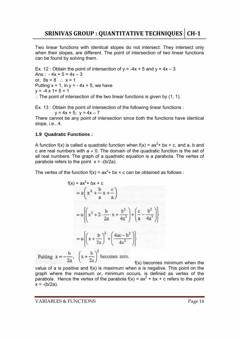
Two linear functions with identical slopes do not intersect. They intersect only when their slopes, are different. The point of intersection of two linear functions can be found by solving them. Ex. 12 : Obtain the point of intersection of y = -4x + 5 and y = 4x – 3 Ans : - 4x + 5 = 4x – 3 or, 8x = 8 x = 1 Putting x = 1, in y = - 4x + 5, we have y = -4 x 1+ 5 = 1 The point of intersection of the two linear functions is given by (1, 1). Ex. 13 : Obtain the point of intersection of the following linear functions : y = 4x + 5; y = 4x – 7 There cannot be any point of intersection since both the functions have identical slope, i.e., 4. 1.9 Quadratic Functions : A function f(x) is called a quadratic function when f(x) = ax2+ bx + c, and a, b and c are real numbers with a 0. The domain of the quadratic function is the set of all real numbers. The graph of a quadratic equation is a parabola. The vertex of parabola refers to the point x = -(b/2a). The vertex of the function f(x) = ax2+ bx + c can be obtained as follows : f(x) = ax2+ bx + c
f(x) becomes minimum when the value of a is positive and f(x) is maximum when a is negative. This point on the graph where the maximum or, minimum occurs, is defined as vertex of the parabola. Hence the vertex of the parabola f(x) = ax2 + bx + c refers to the point x = -(b/2a).
SRINIVASGROUP:QUANTITATIVETECHNIQUES CH‐1
VARIABLES & FUNCTIONS Page 15
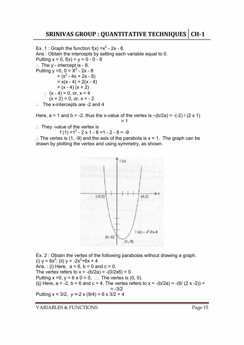
Ex. 1 : Graph the function f(x) =x2 - 2x - 8. Ans : Obtain the intercepts by setting each variable equal to 0. Putting x = 0, f(x) = y = 0 - 0 - 8 The y - intercept is - 8. Putting y =0, 0 = X2 - 2x - 8 = (x2 - 4x + 2x - 8) = x(x - 4) + 2(x - 4) = (x - 4) (x + 2) (x - 4) = 0, or, x = 4 (x + 2) = 0, or, x = - 2 The x-intercepts are -2 and 4 Here, a = 1 and b = -2, thus the x-value of the vertex is –(b/2a) = -(-2) / (2 x 1) = 1 They -value of the vertex is f (1) =12 - 2 x 1 - 8 =1 - 2 - 8 = -9 The vertex is (1, -9) and the axis of the parabola is x = 1. The graph can be drawn by plotting the vertex and using symmetry, as shown.
Ex. 2 : Obtain the vertex of the following parabolas without drawing a graph. (i) y = 6x2; (ii) y = -2x2+6x + 4 Ans. : (i) Here, a = 6, b = 0 and c = 0. The vertex refers to x = -(b/2a) = -(0/2x6) = 0 Putting x =0, y = 6 x 0 = 0, The vertex is (0, 0). (ij) Here, a = -2, b = 6 and c = 4. The vertex refers to x = -(b/2a) = -(6/ (2 x -2)) = = -3/2 Putting x = 3/2, y =-2 x (9/4) + 6 x 3/2 + 4
SRINIVASGROUP:QUANTITATIVETECHNIQUES CH‐1
VARIABLES & FUNCTIONS Page 16
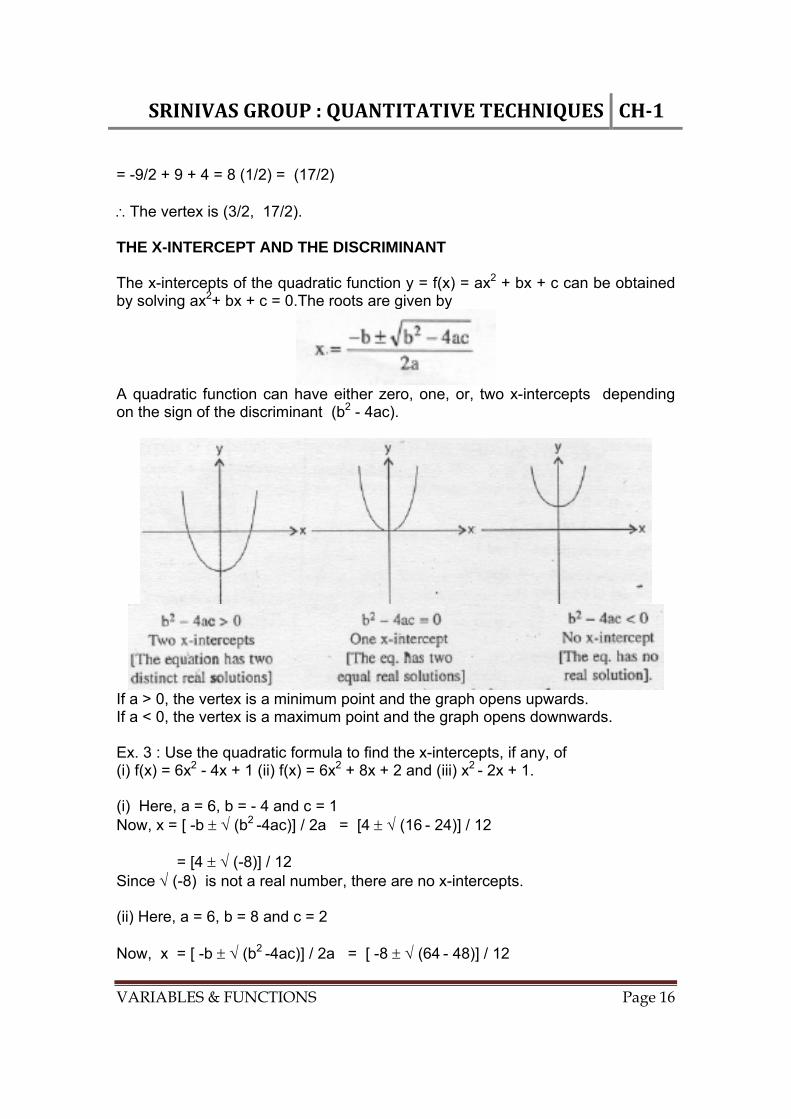
= -9/2 + 9 + 4 = 8 (1/2) = (17/2) The vertex is (3/2, 17/2). THE X-INTERCEPT AND THE DISCRIMINANT The x-intercepts of the quadratic function y = f(x) = ax2 + bx + c can be obtained by solving ax2+ bx + c = 0.The roots are given by
A quadratic function can have either zero, one, or, two x-intercepts depending on the sign of the discriminant (b2 - 4ac).
If a > 0, the vertex is a minimum point and the graph opens upwards. If a < 0, the vertex is a maximum point and the graph opens downwards. Ex. 3 : Use the quadratic formula to find the x-intercepts, if any, of (i) f(x) = 6x2 - 4x + 1 (ii) f(x) = 6x2 + 8x + 2 and (iii) x2 - 2x + 1. (i) Here, a = 6, b = - 4 and c = 1 Now, x = [ -b (b2 -4ac)] / 2a = [4 (16 - 24)] / 12 = [4 (-8)] / 12 Since (-8) is not a real number, there are no x-intercepts. (ii) Here, a = 6, b = 8 and c = 2 Now, x = [ -b (b2 -4ac)] / 2a = [ -8 (64 - 48)] / 12
SRINIVASGROUP:QUANTITATIVETECHNIQUES CH‐1
VARIABLES & FUNCTIONS Page 17
[ -8 (16)] / 12 = ( -8 4) / 12 = ( - 12 / 12), and ( -4 / 12) = -1 and -1/3 The x-intercepts are x = -1 and x = -1/ 3. (iii) Here, a = 1, b = -2 and c = 1. Now, x = [ -b (b2 -4ac)] / 2a = [ 2 (4 - 4)] / 2 = 1 The x-intercept is x = 1. Ex. 4 : (a) Obtain the numbers a, b and c so that the quadratic function f(x) =ax2+ bx + c fits the points (1,3), (-1,-3) and (3,12). State the quadratic function. Ans. : Since the function fits the points, they must lie on the graph. For (1, 3), we have 3 = a + b + c ------ (1) For ( -1, -3), we have -3 = a - b + c ------- (2) For (3, 12), we have 12 = 9a + 3b + c ------ (3) Adding (1) and (2), 2a + 2c = 0 Adding (3) and 3 x (2), 12 a + 4c = 3 Subtracting 2 x (4) from (5), a = 3/8 Putting this in (4), 2 x (3/8) +2c = 0 or, c = -3/8 Putting this in (1), 3 = 3/8 – 3/8 +b b = 3 The quadratic function may now be expressed as f(x) = (3/8) x2 + 3x – 3/8. Ex. 5 : A shopkeeper earns Rs. 380 in the first week, Rs. 660 in the second week and Rs. 860 in the third week. On plotting the points (1, 380), (2, 660), (3, 860) the shopkeeper feels that a quadratic function may fit the data. (i) Find the quadratic function that fits the data. (ii) Using your model make a prediction of the earning for the fourth week. (i) Let f(x) = ax2 + bx + c be the function At (1, 380), 380 = a.12 + b.1+ c --------- (1) At (2, 660), 660 = a.22 + b.2 + c ----------- (2) At (3, 860), 860 = a.32 + b.3 + c ---------- (3) Solving (1), (2) and (3), we have a = -40, b = 400 and c = 20 The required quadratic function is f(x) = - 40x2 + 400 x + 20. (ii) f(4) = - 40(4)2 + 400 (4) + 20 = Rs. 980.
SRINIVASGROUP:QUANTITATIVETECHNIQUES CH‐1
VARIABLES & FUNCTIONS Page 18
Ex. 6 : A man earns Rs. 300 in the first month, Rs. 650 in the second month and Rs. 950 in the third month. He thinks that the points (1, 300), (2, 650) and (3, 950) will fit a quadratic function. (a) Obtain the quadratic equation. (b) Using this function predict the earning for the fifth month. (a) Let, f(x) = ax2 + bx + c be the function. For (1, 300) 300 = a + b + c ----- (1) For (2, 650) 650 = 4a + 2b + c ----- (2) For (3, 950) 950 = 9a + 3b + c ----- (3) Eq. (2) - (1) 3a + b = 350 Eq. (3) – (1) 4a + b = 325 Eq. (4) - (5) a = -25 From Eq. (4) b = 425 From Eq. (1) - 25 + 425 + c = 300 or, c = -100 The required quadratic equation is given by f(x) = -25x2 + 425x - 100 (b) Earning in the fifth month is given by f(5) = -25 x 25 + 425 x 5 -100 = - 625 + 2,125 - 100 = 2,125 - 725 = Rs. 1,400. Ex. 7 : (a) The profits P(x) of a sofa set company is given by P(x) = 60x - x2, where x denotes the number of sofa-sets sold. How many sofa-sets should be sold for maximization of profit? What is the maximum profit? (b) The cost 'c' for producing a sofa-set is given by c = 2x2 -100x + 1,300, where x denotes the number of sofa-sets produced. How many sofa sets the company should produce to minimize the cost? What will be the cost sofa this level of production? (c) The price / unit at which a company can sell all its produces is given by p(x) = 200 -3x. The cost function is c(x) = 400 + 14x, where x =no. of units produced. Find x for which profit is maximum. Ans : (a) The profit function call be written as P(x) = -x2 + 60 x + 0 Here, a = -1, b = 60 and c = 0 [Since a < 0, the vertex is the maximum point and the graph opens downwards.] The vertex corresponds to x = -b/2a = - 60/ (2 x -1) = 30 y = P (30) = -900 + 1,800 + 0 = 900 The graph of P is a parabola with vertex (30, 900) opening downward. Since the parabola is opening downward, the vertex denotes the maximum profit. The maximum profit is Rs. 900 which can be obtained by selling 30 units. The profit gradually increases until 30 units are sold and thereafter it decreases.
SRINIVASGROUP:QUANTITATIVETECHNIQUES CH‐1
VARIABLES & FUNCTIONS Page 19
(b) Here, a =2, b =-100 and c = 1,300 Since 'a' is positive i.e, a >0, the graph opens upwards. Thus the vertex x = -b/2a = -(-100) /2 x 2 = 25 corresponds to minimum point. c =2 (25)2 - 100 x 25 + 1,300 = 50 The vertex is (25, 50). Thus the company should manufacture 25 sofa-sets to keep the cost minimum. At this level of production, the cost/sofa-set is Rs. 50. (c) Total revenue = (x) x p(x) = x (200 - 3x) = 200 x – 3x2 Profit function P(x) =x x p(x) - c(x) = 200x - 3x2 – 400 - 14x = 186x – 3x2 - 400 = -3x2 + 186x - 400 since a = - 3 is negative, x = -( b /2a) = - 186 / [2 x (-3)] = 31 is a maximum point. Profit is maximum when x = 31. Ex. 8 : Suppose the price and demand of an article are related by p = 120 - 3x2 (Demand function), where p = price and x = No. of articles demanded (in hundreds). The price and supply are related by p = 12 x2 + 3x , (Supply function), where x = supply of the article (in hundreds). Find the (i) equilibrium demand and (ii) the equilibrium price. Ans : The equilibrium demand and supply occur at the identical price p. The equation for equilibrium supply and demand is 120 – 3 x2 = 12x2 + 3x or, -15x2 - 3x + 120 = 0 or, 5x2 + x – 40 = 0 a = 5, b = 1 and c = -40. x = [ -b (b2 -4ac)] / 2a = [ -1 (1 – 4 x 5 x -40)] / (2 x 5) = [ -1 (1 + 800)] / (10) = (-1 28.3) / 10 = 2.73, - 2.93 The equilibrium demand and supply 2.73 x 100 = 273 nos. of articles since -2.93 is to be discarded. The equilibrium price can be obtained as follows: p = 12x2 + 3x = 12(2.73)2 + 3 x 2.73 = 89.44 + 8.19 = 97.63

SRINIVASGROUP:QUANTITATIVETECHNIQUES CH‐1
VARIABLES & FUNCTIONS Page 20
Ex. 9: Suppose that a shop procures candy bars at a wholesale cost of 'Rs. 40 each. If the shop sells the candy bar at Rs. x each, then on the average it will sell (80 - x) bars daily, where 0 x 80. lf C(x) = Cost (in Rs.) of purchasing the day's stock of candy bars. R(x) = Revenue (in Rs.) obtained by selling the day's stock of candy bars. P(x) =Profit (in Rs.) obtained by selling the day's stock of candy bars. (a) Write formulae for C(x), R(x) and P(x). (b) What will be the daily profit when x =Rs. 50? (c) What is the most profitable selling price? Ans : (a) Since the shop will require (80 - x) candy bars at Rs. 40 each, C(x) = Rs. 40 (80- x) --------------- (1) Since shop will sell (80 - x) candy bars at Rs. x each, R(x) = x (80 - x) ------- (2) Profit function P(x) =x (80 - x) - 40 (80 - x) = 80x - x2 - 3,200 + 40x = Rs. (-x2 + 120x - 3,200) (b) P(50) = Rs.(-2,500 + 6,000 - 3,200) = Rs. 300. (c) Since P(x) is a quadratic equation with a = -1, i.e, a < 0 the parabola will open downward and the most profitable selling price is the vertex, i.e. x = - (b/2a) = - (120 / 2 x -1) = Rs. 60. Thus, when x = Rs. 60, the maximum profit will be P(60) = Rs. (-3,600 + 7,200 - 3,200) = Rs. 400. Any price higher, or, lower than Rs. 60 I candy bar will yield a lower daily profit. 1.10 Polynomial Functions : A function f(x) is defined as a polynomial function of degree n, if f(x) = anx
n + an-1.xn-1 + …….. + a1x
1 + a0 where n is positive integer, an ---a0 real numbers with an 0. When n = 1, the polynomial function becomes a linear function, i.e., f(x) =a1x + a0. When n =2, the polynomial function becomes a quadratic function, i.e., f(x) = a2x
2 + a1x + a0. The simplest polynomial functions are of the form y = xn. 1.11 Rational Functions : A function f(x) is defined as a rational function if : f(x) = P(x)/ Q(x), where Q(x) 0 and P(x) and Q(x) are polynomials.
SRINIVASGROUP:QUANTITATIVETECHNIQUES CH‐1
VARIABLES & FUNCTIONS Page 21
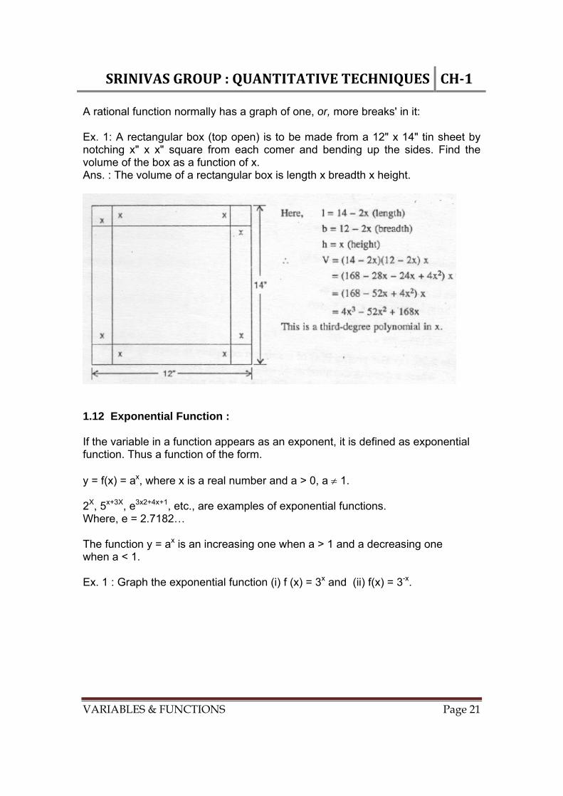
A rational function normally has a graph of one, or, more breaks' in it: Ex. 1: A rectangular box (top open) is to be made from a 12" x 14" tin sheet by notching x" x x" square from each comer and bending up the sides. Find the volume of the box as a function of x. Ans. : The volume of a rectangular box is length x breadth x height.
1.12 Exponential Function : If the variable in a function appears as an exponent, it is defined as exponential function. Thus a function of the form. y = f(x) = ax, where x is a real number and a > 0, a 1. 2X, 5x+3X, e3x2+4x+1, etc., are examples of exponential functions. Where, e = 2.7182… The function y = ax is an increasing one when a > 1 and a decreasing one when a < 1. Ex. 1 : Graph the exponential function (i) f (x) = 3x and (ii) f(x) = 3-x.

SRINIVASGROUP:QUANTITATIVETECHNIQUES CH‐1
VARIABLES & FUNCTIONS Page 22
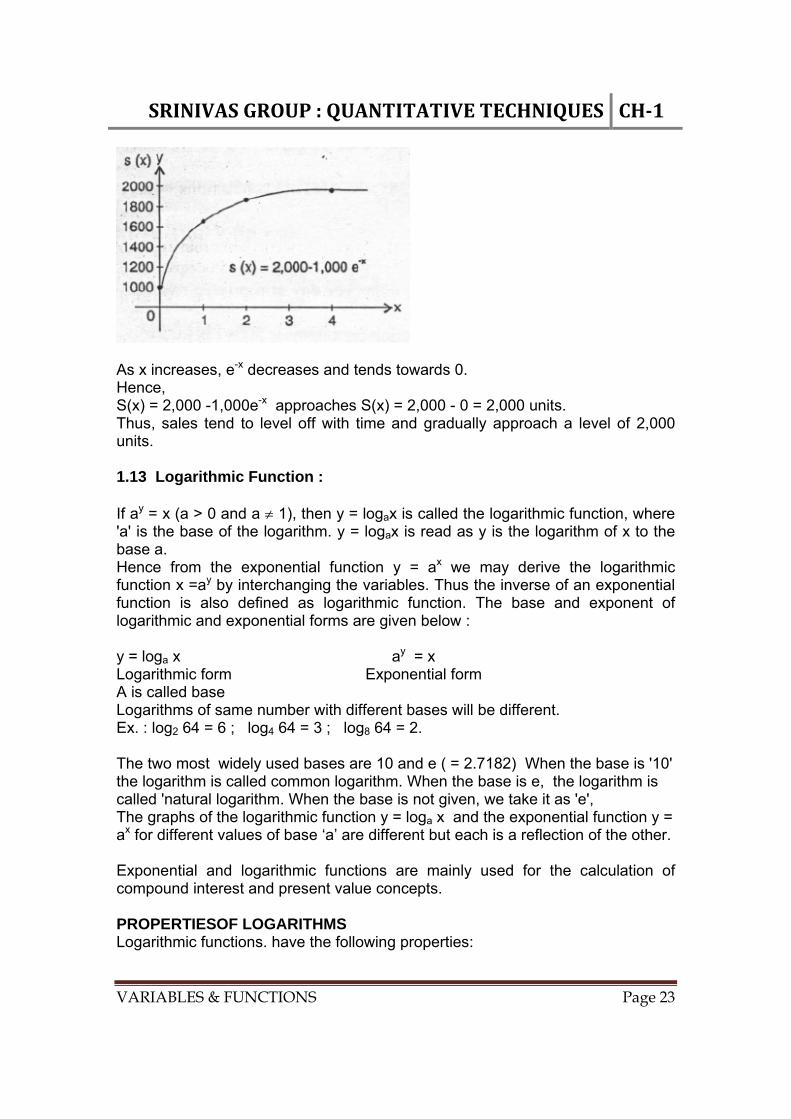
Ex. 2 : Suppose the population of Kolkata is p(t) = 50,000.e0.4t, where t = time in years. Find the population at time t =0 and t = 5. Ans : (i) p(0) =50,000,e(0.4)x 0 = 50,000 e0 = 50,000 (ii) P(5)= 50,000.e(0.4)x 5 =50,000.e2 From the calculation we find e2 =7.389. P(5) =50,000 x 7.389 = 3,69,453 ,i.e., In 5 years the population of Kolkata will be about 3,69,453. Ex. 3 : Suppose the sales S(x) of a new pump are approximated by, S(x) = 2,000 -1,000 . e-x, where x denotes the number of years the pump has been on, the market. Calculate S(O), S(1), S(2) and S(4). Graph S(x). From Table [e-x = 1/e0 = 1] [e-1 = 0.36787] [e-2 = 0.13533] [e-4 = 0.91832] S(0) = 2,000 -1,000x 1 = 1,000 S(1) = 2,000 -1,000 x 0.36787 = 1,632.13 S(2) = 2,000 -1,000 x 0.13533 = 1,864.67 S(4) = 2,000 -1,000 x 0.01832 = 1,981.68
SRINIVASGROUP:QUANTITATIVETECHNIQUES CH‐1
VARIABLES & FUNCTIONS Page 23
As x increases, e-x decreases and tends towards 0. Hence, S(x) = 2,000 -1,000e-x approaches S(x) = 2,000 - 0 = 2,000 units. Thus, sales tend to level off with time and gradually approach a level of 2,000 units. 1.13 Logarithmic Function : If ay = x (a > 0 and a 1), then y = logax is called the logarithmic function, where 'a' is the base of the logarithm. y = logax is read as y is the logarithm of x to the base a. Hence from the exponential function y = ax we may derive the logarithmic function x =ay by interchanging the variables. Thus the inverse of an exponential function is also defined as logarithmic function. The base and exponent of logarithmic and exponential forms are given below : y = loga x ay = x Logarithmic form Exponential form A is called base Logarithms of same number with different bases will be different. Ex. : log2 64 = 6 ; log4 64 = 3 ; log8 64 = 2. The two most widely used bases are 10 and e ( = 2.7182) When the base is '10' the logarithm is called common logarithm. When the base is e, the logarithm is called 'natural logarithm. When the base is not given, we take it as 'e', The graphs of the logarithmic function y = loga x and the exponential function y = ax for different values of base ‘a’ are different but each is a reflection of the other. Exponential and logarithmic functions are mainly used for the calculation of compound interest and present value concepts. PROPERTIESOF LOGARITHMS Logarithmic functions. have the following properties:

SRINIVASGROUP:QUANTITATIVETECHNIQUES CH‐1
VARIABLES & FUNCTIONS Page 24
(1) loga xy = loga x + loga y . {Where x and y are positive real numbers, n is any real number and 'a' is a positive real number, a 1}. (2) loga (x/y) = loga x - loga y (3) loga x
n = n loga x (4) loga a = 1 (5) loga 1 = 0; (6) loga a
y =y (7) aloga x = x (8) logam = logbm x logab [Change of base] (9) logba x logab = 1 (10) Logarithm of zero and negative number is not defined. GEOMETRIC RELATIONSHIP BETWEEN LOGARITHMIC AND EXPONENTIAL FUNCTIONS Normally, the graphs of y = logax and y = ax are reflections of one another about the line y =x.
Ex. 1 : Rs. 6,000 is invested in an account at 9% interest compounded yearly. What will be the balance after 6 years and 11 years. Ans. : For compound interest, we know P(n) = (1 + i)n X P(O) Where, P(n) = Principal after the nth year of the original investment, P(O) = Future value (i) = Interest on Rs. 1 for one year. P(O) = Present value. Here, . P(O) =6,000; i =0.09
SRINIVASGROUP:QUANTITATIVETECHNIQUES CH‐1
VARIABLES & FUNCTIONS Page 25
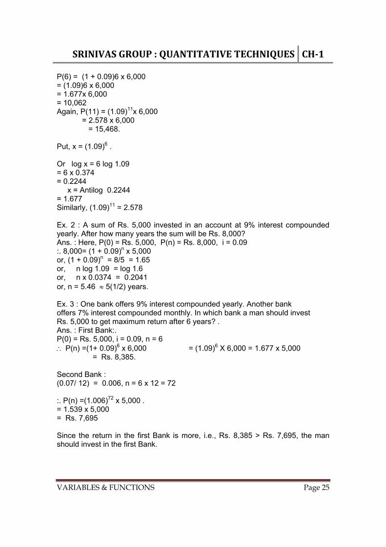
P(6) = (1 + 0.09)6 x 6,000 = (1.09)6 x 6,000 = 1.677x 6,000 = 10,062 Again, P(11) = (1.09)11x 6,000 = 2.578 x 6,000 = 15,468. Put, x = (1.09)6 . Or log x = 6 log 1.09 = 6 x 0.374 = 0.2244 x = Antilog 0.2244 = 1.677 Similarly, (1.09)11 = 2.578 Ex. 2 : A sum of Rs. 5,000 invested in an account at 9% interest compounded yearly. After how many years the sum will be Rs. 8,000? Ans. : Here, P(0) = Rs. 5,000, P(n) = Rs. 8,000, i = 0.09 :. 8,000= (1 + 0.09)n x 5,000 or, (1 + 0.09)n = 8/5 = 1.65 or, n log 1.09 = log 1.6 or, n x 0.0374 = 0.2041 or, n = 5.46 5(1/2) years. Ex. 3 : One bank offers 9% interest compounded yearly. Another bank offers 7% interest compounded monthly. In which bank a man should invest Rs. 5,000 to get maximum return after 6 years? . Ans. : First Bank:. P(0) = Rs. 5,000, i = 0.09, n = 6 P(n) =(1+ 0.09)6 x 6,000 = (1.09)6 X 6,000 = 1.677 x 5,000 = Rs. 8,385. Second Bank : (0.07/ 12) = 0.006, n = 6 x 12 = 72 :. P(n) =(1.006)72 x 5,000 . = 1.539 x 5,000 = Rs. 7,695 Since the return in the first Bank is more, i.e., Rs. 8,385 > Rs. 7,695, the man should invest in the first Bank.

SRINIVASGROUP:QUANTITATIVETECHNIQUES CH‐1
VARIABLES & FUNCTIONS Page 26
Additional Problems : Ex.1 : A manufacturer can sell x items per day at a price p rupees each, where p =125 – (5/3)x. The cost of production for x items is 500 + 13x + 0.2 x2. (i) Find how much he should produce to have a maximum profit, assuming all items produced are sold. (ii) What is the maximum profit? Ans. : (i) Cost function C(x) = 500 + 13x + 0.2x2 Revenue function R(x) = x [125 – (5/3)x] Profit function P(x) = R(x) - C(x) = 12.5x -(5/3)x2 – 500 -13x - 0.2x2 = 112x - 500 – (28/15) x2 Here, a = - (28/15), b = 112 and c = - 500, Since a is negative maximum profit will be at the vertex. The vertex corresponds to x = -(b/2a) = (112 x 15)/ (2x – 28) = 30 units 30 units must be produced to obtain maximum profit. (ii) Now, P(30) = 112(30) – 500 -15(30) = 3,360 - 500 - 1,680 = 1,180 Hence, the maximum profit is Rs. 1,180. Ex. 2 : If f(x) =2x2 - 5x + 4, for what values of x is 2f(x) = f(2x)? f(x) = 2x2 - 5x + 4 f(2x) =2(2x)2 - 5(2x) + 4 = 8X2 - 10x + 4 = RHS 2f(x) =2[2x2 - 5x + 4] = 4x2 - 10x + 8 = LH.S To get the value of x, we proceed as follows : 8x2 - 10x + 4 = 4x2 -10x + 8 or, 4x2 = 4 x2 = 1, or x = 1. Ex. 3 : If f(x) =x x (x-p)/(q-p) + x x (x-q)/(p-q) (where p q), prove that
Let, x = 1.00672 log x = 72 log 1.006 = 72 x .0026 = 0.1872 x = Antilog 0.1872 . = 1.539

SRINIVASGROUP:QUANTITATIVETECHNIQUES CH‐1
VARIABLES & FUNCTIONS Page 27
f(p) + f(q) = f(p + q). Ans. : Since, f(x) = x x (x-p)/(q-p) + x x (x-q)/(p-q) f(p) = p x (p-p)/(q-p) + p x (p-q)/(p-q) = p x 0 + p x1 = p f(q) = q x (q–p)/(q-p) + q x (q–q)/(p-q) = q x 1+ q x 0 = q LH.S = f(p) + f(q) = p + q R.H.S = f(p + q) = (p +q) x (p+q-p)/ (q-p) +(p+q) x (p+q-q)/(p-q) q(p+q)/(q-p) - p(q+p)/(q-p) = [(p+q)(q-p) / (q-p)] = p + q Ex. 4 : If f(x) = logx (x> 0), show that f(m) + f(n) +f(l) = f(lmn). Ans. : let f(m) = logm, f(n) =logn and f(l) =logl L.H.S = f(m) + f(n) + f(l) =logm + logn + logl = log(lmn) = RH.S Ex. 5 : If f(x) = eax+b, where a, b are constants, show that f(l) x f(m) x f(n) = f(l +m + n). e2b. Ans. : f(l) = eal+b , f(m) = eam+b and f(n) = ean+ b Now, L.H.S = f(l) X f(m) X f(n) = eal+b X eam+b X ean+b = ea(l+m+n)+3b RH.S = f(l + m + n)e2b = ea(l + m+ n) + b X e2b = ea(l+m+n)+3b LH.S = R.H.S 1.14 Break-Even Point : If P(X), R(x) and C(x) are the Profit function, Revenue function and Cost function respectively, then, P(x) =R(x) - C(x) = 0 when R(x) = C(x) When R(x) > C(x), i.e., revenue exceeds cost, there is a profit on the x units, but when R(x) < C(x), i.e., cost exceeds revenue, there is a loss. When R(x) = C(x), there is no profit or, loss. This value of x for which R(x) =C(x) is called the Break-even-point (B.E.P). B.E.P is the point of intersection of the lines representing the Revenue function and the Cost function. Again, C(x) = F + V (x)

SRINIVASGROUP:QUANTITATIVETECHNIQUES CH‐1
VARIABLES & FUNCTIONS Page 28
where, F = Fixed costs which do not change with change in the level of production/sales, e.g., rent, insurance, overhead expenses, etc. They are incurred even when there is no production/sales. V (x) = Variable costs which vary with units (x) produced, e.g., cost of material, cost of labour, etc. Cost curve for linear cost function is a straight line whereas it is a parabola for quadratic cost function. The total revenue R(x) from selling x units of a product is obtained by multiplying the price/unit (p) and number of units sold, (x) i.e., R(x) = px. The average revenue and average cost can' be obtained by R(x)/x, and C(x)/x respectively . Similarly, average profit is P(x)/x. Managerial Applications : Ex. 1 : A book-publisher finds that the production cost of a book is Rs. 30 and the fixed cost per year amounts to Rs. 25,000. If each book is sold at the nite of Rs. 50, find (i) the cost function, (ii) the revenue function, (iii) the minimum number of books to be sold per year in order that there is no loss. Ans. : (i) Cost function = C(x) = F + V(x) = Rs. 25,000 + Rs.30x (ii) Revenue function = R(x) = Rs. 50x. (iii). For B.E.P, C(x) = R(x) Rs. 25,000 + Rs.30x = Rs.50x. or, x = (25,000/20) = 1,250 Nos. Ex. 2 : The daily cost of production C for x units of an assembly is given by C(x) =Rs.12.5x + Rs.6,400 (i) If each unit is sold for Rs.25, determine the minimum number of units that should be produced and sold to ensure no loss (ii) If the selIinK Price is reduced by Rs. 2.50 per unit, what would be the B.E.P? (iii) If it is known that 500 units can be sold daily, what price per unit should be charged to guarantee no loss. Ans. : (i) The cost function, C(x) = 12.5x + 6,400 and R(x) =25x (Revenue function) For H.E.P, C(x) = R(x) or, 12.5x + 6,400 = 25x. or, x = 512 Nos. (ii) The new selling price = Rs. (25 - 2.50) = Rs. 22.50. Revenue function = R(x) = Rs. 22.50x or H.E.P., 22.50x = Rs. 12.5x + 6,400 or, 10x = 6,400 x = 640 Nos. (iii) If 500 units can be sold daily, then
SRINIVASGROUP:QUANTITATIVETECHNIQUES CH‐1
VARIABLES & FUNCTIONS Page 29
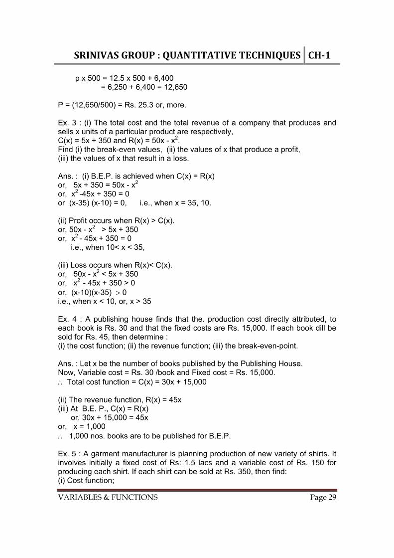
p x 500 = 12.5 x 500 + 6,400 = 6,250 + 6,400 = 12,650 P = (12,650/500) = Rs. 25.3 or, more. Ex. 3 : (i) The total cost and the total revenue of a company that produces and sells x units of a particular product are respectively, C(x) = 5x + 350 and R(x) = 50x - x2. Find (i) the break-even values, (ii) the values of x that produce a profit, (iii) the values of x that result in a loss. Ans. : (i) B.E.P. is achieved when C(x) = R(x) or, 5x + 350 = 50x - x2 or, x2 -45x + 350 = 0 or (x-35) (x-10) = 0, i.e., when x = 35, 10. (ii) Profit occurs when R(x) > C(x). or, 50x - x2 > 5x + 350 or, x2 - 45x + 350 = 0 i.e., when 10< x < 35, (iii) Loss occurs when R(x)< C(x). or, 50x - x2 < 5x + 350 or, x2 - 45x + 350 > 0 or, (x-10)(x-35) 0 i.e., when x < 10, or, x > 35 Ex. 4 : A publishing house finds that the. production cost directly attributed, to each book is Rs. 30 and that the fixed costs are Rs. 15,000. If each book dill be sold for Rs. 45, then determine : (i) the cost function; (ii) the revenue function; (iii) the break-even-point. Ans. : Let x be the number of books published by the Publishing House. Now, Variable cost = Rs. 30 /book and Fixed cost = Rs. 15,000. Total cost function = C(x) = 30x + 15,000 (ii) The revenue function, R(x) = 45x (iii) At B.E. P., C(x) = R(x) or, 30x + 15,000 = 45x or, x = 1,000 1,000 nos. books are to be published for B.E.P. Ex. 5 : A garment manufacturer is planning production of new variety of shirts. It involves initially a fixed cost of Rs: 1.5 lacs and a variable cost of Rs. 150 for producing each shirt. If each shirt can be sold at Rs. 350, then find: (i) Cost function;
SRINIVASGROUP:QUANTITATIVETECHNIQUES CH‐1
VARIABLES & FUNCTIONS Page 30
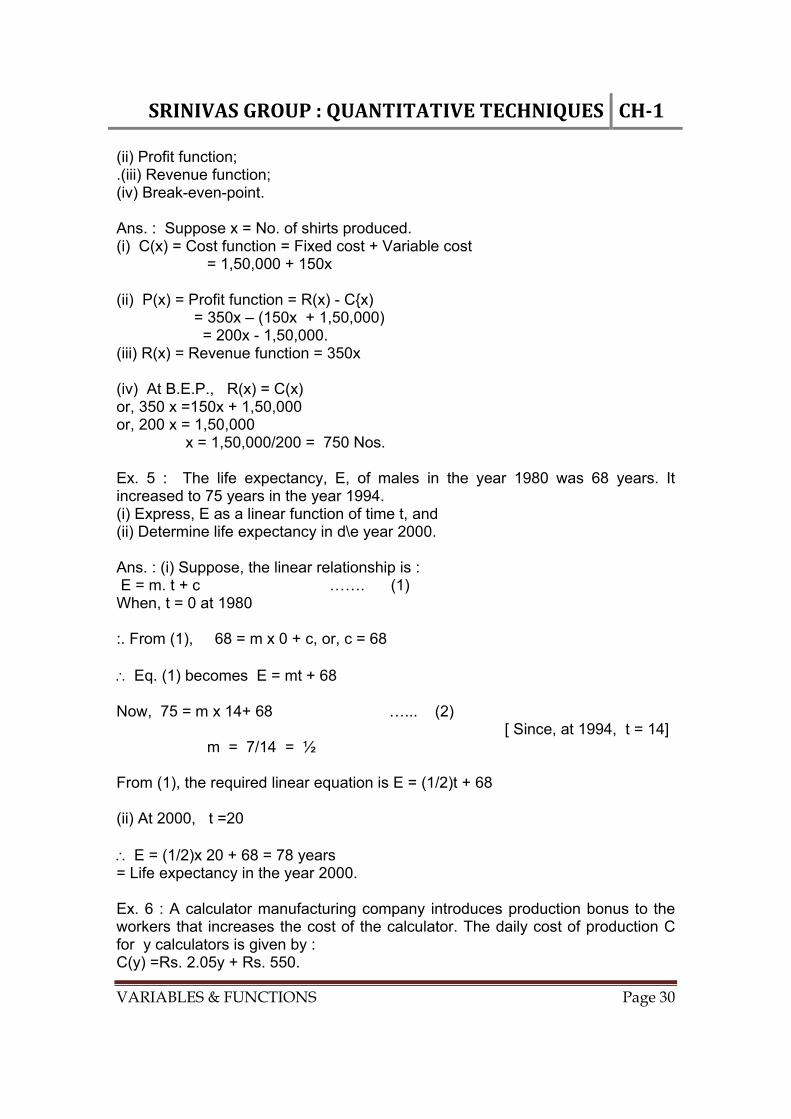
(ii) Profit function; .(iii) Revenue function; (iv) Break-even-point. Ans. : Suppose x = No. of shirts produced. (i) C(x) = Cost function = Fixed cost + Variable cost = 1,50,000 + 150x (ii) P(x) = Profit function = R(x) - C{x) = 350x – (150x + 1,50,000) = 200x - 1,50,000. (iii) R(x) = Revenue function = 350x (iv) At B.E.P., R(x) = C(x) or, 350 x =150x + 1,50,000 or, 200 x = 1,50,000 x = 1,50,000/200 = 750 Nos. Ex. 5 : The life expectancy, E, of males in the year 1980 was 68 years. It increased to 75 years in the year 1994. (i) Express, E as a linear function of time t, and (ii) Determine life expectancy in d\e year 2000. Ans. : (i) Suppose, the linear relationship is : E = m. t + c ……. (1) When, t = 0 at 1980 :. From (1), 68 = m x 0 + c, or, c = 68 Eq. (1) becomes E = mt + 68 Now, 75 = m x 14+ 68 …... (2) [ Since, at 1994, t = 14] m = 7/14 = ½ From (1), the required linear equation is E = (1/2)t + 68 (ii) At 2000, t =20 E = (1/2)x 20 + 68 = 78 years = Life expectancy in the year 2000. Ex. 6 : A calculator manufacturing company introduces production bonus to the workers that increases the cost of the calculator. The daily cost of production C for y calculators is given by : C(y) =Rs. 2.05y + Rs. 550.

SRINIVASGROUP:QUANTITATIVETECHNIQUES CH‐1
VARIABLES & FUNCTIONS Page 31
(i) If each calculator is sold for Rs. 3, determine the minimum number that must be produced and sold daily to ensure no loss. (ii) If the selling price is increased by 30 paise per piece, what would be the break-even-point? (iii) If it is known that at least 500 calculators can be sold daily, What price the company should charge per piece of calculator to guarantee no loss. Ans. : (i) Here, R(y) = Rs. 3y. For H.E.P. R(y) =C(y) or, Rs. 2.05y + Rs. 559 = Rs. 3y, or, y = 578.94 579. 579 calculators are to be produced daily for no loss. (ii) Here R(y) = Rs. 3.3y. For B.E.P., 3.3y = 2.05y + 550 or, y = 440. 440 calculators must be produced daily at the increased selling price for B.E.P. (iii) If at least 500 calculators are sold daily at price p/unit for no loss, then 500p =2.05y + 550 = 2.05 x 500 + 550 P = 1,575/500 = Rs. 3.15. :. Rs. 3.15 should be charged per calculator for no loss.
ASSIGNMENT 1 (1) Find the domain and range of the following functions: (i) y = 4/(x-4) ; (ii) f(x) = 1/x ; (iii) f(x) = -4x + 75. (2) f(x) = x2 - 3x + 2, find the values of f(4), f(-5), f(0). (3) If f(x) = 3x + 2, show that f(2x) - 2f(x) + 2 = 0. (4) Show that the function f(x) = 1/ (4 - x2) is not defined for x = 2 and x = -2. (5) (6)

SRINIVASGROUP:QUANTITATIVETECHNIQUES CH‐2
MATRICES&DETERMINANTS Page32
CHAPTER 2 Matrices & Determinants
1. Introduction : We often display a set of numbers, or, elements (or information) in the form of tabular, or, rectangular array of rows and columns for better understanding. In an examination Ram obtained 50 marks in Bengali, 60 marks In Mathematics, 70 marks in Statistics and 80 marks in Computer practical. In the same examination Rahim obtained 40 marks in Bengali, 50 marks in Mathematics, 65 marks in Statistics and 72 marks in Computer practical. In this examination Samir obtained 50 marks in Bengali, 55 marks in Mathematics, 46 marks in Statistics and 65 marks in the Computer practical. From the above information we cannot get the total picture at a glance. We can arrange the above information in a tabular form as follows for-easy understanding. Bengali Mathematics Statistics Computer Practical Ram 50 60 70 80 Rahim 40 50 65 72 Samir 50 55 46 65 The above information can also be expressed by the following rectangular array enclosed by a pair of brackets [ ], or ( ).
The above form of display of information is called a matrix. The above matrix has 3 rows and 4 columns ,i.e., it is a 3 x 4 matrix with 12 elements. Definition of Matrix : A matrix (plural is matrices) is a rectangular array of real / complex numbers arranged in rows and columns and enclosed by a pair of brackets [ ] or ( ). An array of m x n numbers all a12,…….. amn, arranged in m rows and n columns is called an m x n (read m by n) matrix. The numbers ,a11, a12,….. amn are called the elements (or, entries) of the matrix. Thus, an m x n matrix is given below :

SRINIVASGROUP:QUANTITATIVETECHNIQUES CH‐2
MATRICES&DETERMINANTS Page33
We denote the matrices by capital letters A, B, C etc., and the elements by small letters a, b, c etc. The above matrix can be expressed in a more concise form as : A = [aij] m x n , or, [aij] where i = 1, 2, 3, …. m; j = 1, 2, 3, …… n and aij is the element in the ith row and jth column. Matrix is just an arrangement of elements without any value in rows and columns. Order of a Matrix : The order of a matrix is its rows x columns.
Principal Diagonal of a Matrix Leading ,or, principal diagonal of a matrix consists of the elements from the upper left comer to lower right comer. Thus the principal diagonal of the matrix (i) in the above illustration consists of [2, -5,6]. Coefficient and Augmented Matrix of a Set of Linear Equations :

SRINIVASGROUP:QUANTITATIVETECHNIQUES CH‐2
MATRICES&DETERMINANTS Page34
is called the coefficient matrix of the following m equations in n unknowns,
The matrix B given below is called the augmented matrix.
A matrix is called an augmented matrix if it is enlarged by adding a new column to it. The augmented matrix of A is given by [A I b]. The left-side of the vertical line denotes the original matrix and the right-side denotes newly added column.
1.Row Matrix : A matrix which has one row only is called a row matrix, .
SRINIVASGROUP:QUANTITATIVETECHNIQUES CH‐2
MATRICES&DETERMINANTS Page35
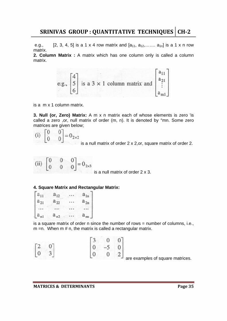
e.g., [2, 3, 4, 5] is a 1 x 4 row matrix and [a11, a12,……. a1n] is a 1 x n row matrix. 2. Column Matrix : A matrix which has one column only is called a column matrix.
is a m x 1 column matrix. 3. Null (or, Zero) Matrix: A m x n matrix each of whose elements is zero 'is called a zero ,or, null matrix of order (m, n). It is denoted by °mn. Some zero matrices are given below;
is a null matrix of order 2 x 2,or, square matrix of order 2.
is a null matrix of order 2 x 3. 4. Square Matrix and Rectangular Matrix:
is a square matrix of order n since the number of rows = number of columns, i.e., m =n. When m # n, the matrix is called a rectangular matrix.
are examples of square matrices.
SRINIVASGROUP:QUANTITATIVETECHNIQUES CH‐2
MATRICES&DETERMINANTS Page36
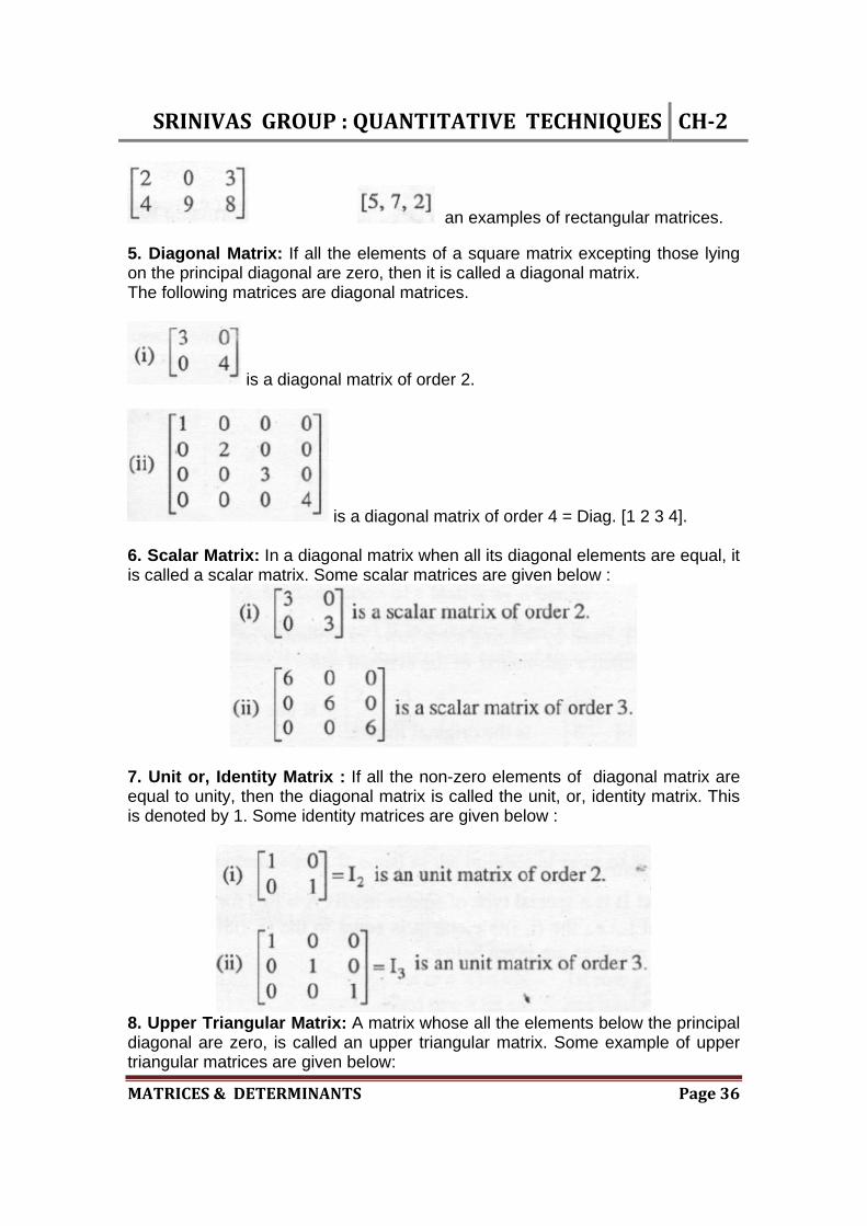
an examples of rectangular matrices. 5. Diagonal Matrix: If all the elements of a square matrix excepting those lying on the principal diagonal are zero, then it is called a diagonal matrix. The following matrices are diagonal matrices.
is a diagonal matrix of order 2.
is a diagonal matrix of order 4 = Diag. [1 2 3 4]. 6. Scalar Matrix: In a diagonal matrix when all its diagonal elements are equal, it is called a scalar matrix. Some scalar matrices are given below :
7. Unit or, Identity Matrix : If all the non-zero elements of diagonal matrix are equal to unity, then the diagonal matrix is called the unit, or, identity matrix. This is denoted by 1. Some identity matrices are given below :
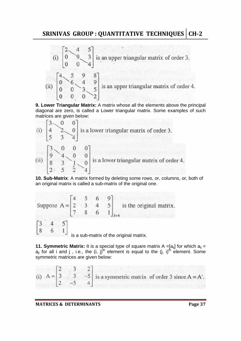
8. Upper Triangular Matrix: A matrix whose all the elements below the principal diagonal are zero, is called an upper triangular matrix. Some example of upper triangular matrices are given below:
SRINIVASGROUP:QUANTITATIVETECHNIQUES CH‐2
MATRICES&DETERMINANTS Page37
9. Lower Triangular Matrix: A matrix whose all the elements above the principal diagonal are zero, is called a Lower triangular matrix. Some examples of such matrices are given below:
10. Sub-Matrix: A matrix formed by deleting some rows, or, columns, or, both of an original matrix is called a sub-matrix of the original one.
is a sub-matrix of the original matrix. 11. Symmetric Matrix: It is a special type of square matrix A =[aij] for which aij = aji for all i and j , i.e., the (i, j)th element is equal to the (j, i)th element. Some symmetric matrices are given below:
SRINIVASGROUP:QUANTITATIVETECHNIQUES CH‐2
MATRICES&DETERMINANTS Page38
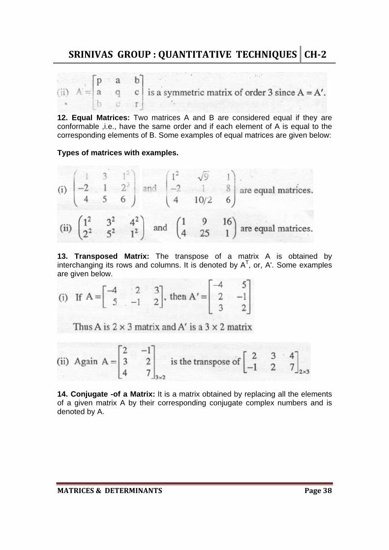
12. Equal Matrices: Two matrices A and B are considered equal if they are conformable ,i.e., have the same order and if each element of A is equal to the corresponding elements of B. Some examples of equal matrices are given below: Types of matrices with examples.
13. Transposed Matrix: The transpose of a matrix A is obtained by interchanging its rows and columns. It is denoted by AT, or, A'. Some examples are given below.
14. Conjugate -of a Matrix: It is a matrix obtained by replacing all the elements of a given matrix A by their corresponding conjugate complex numbers and is denoted by A.

SRINIVASGROUP:QUANTITATIVETECHNIQUES CH‐2
MATRICES&DETERMINANTS Page39
15. Skew-Symmetric Matrix: A square matrix A is called skew-symmetric if it is equal to the transpose of A with a negative sign, i.e., if A' = A. Every diagonal element of a skew-symmetric matrix is zero, e.g., if
16. Conformable Matrices: Matrices are said to be conformable for addition when their values for m and n are identical.
then A and B are conformable for addition. Since A and C do not have the same number rows and the same number of columns, they are not conformable for addition for the same reason B and C are also not conformable for addition. Two matrices D and E are conformable for multiplication DE when the number of columns in D is equal to the number of rows in E. Hence, AC and BC are conformable for multiplication but AB or BA are not conformable for, multiplication. Session 9 : Matrix Operations : Addition, Subtraction & Multiplication with examples. Matrix Operations : 1. Addition of Matrices The sum of two conformable Matrices A and B, i.e., A + B, is a matrix each element of which is the sum of the corresponding elements of A and B.
SRINIVASGROUP:QUANTITATIVETECHNIQUES CH‐2
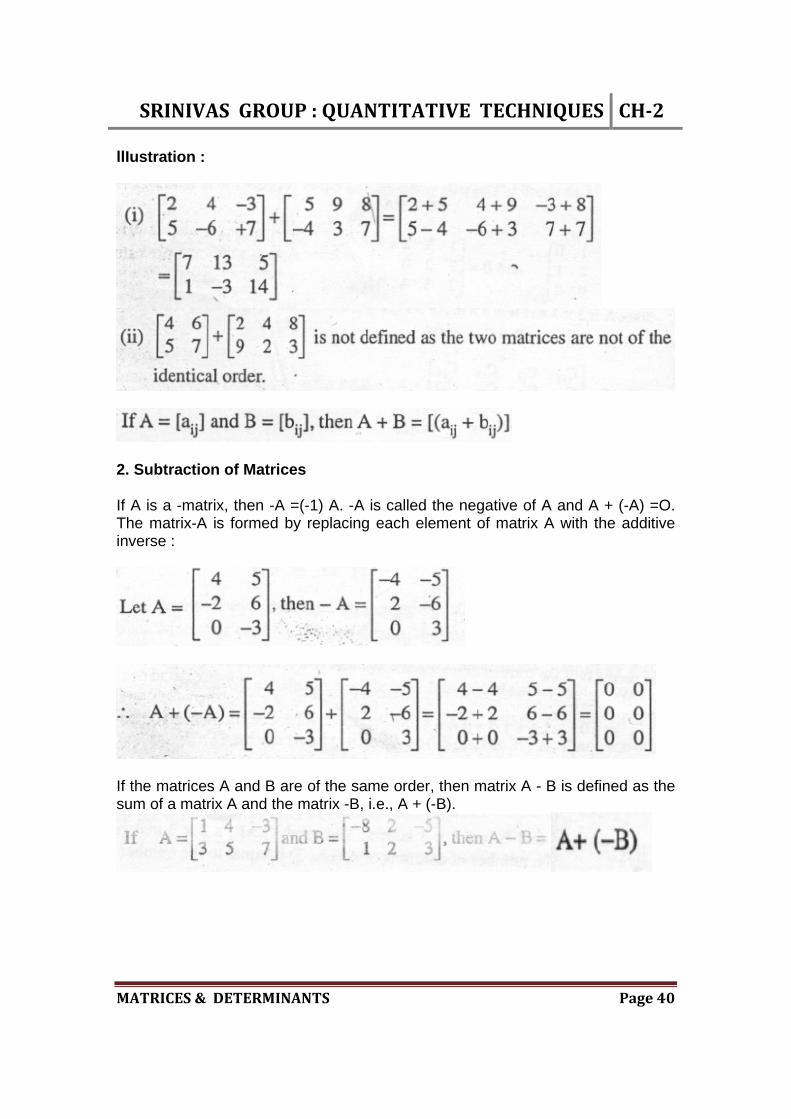
MATRICES&DETERMINANTS Page40
llIustration :
2. Subtraction of Matrices If A is a -matrix, then -A =(-1) A. -A is called the negative of A and A + (-A) =O. The matrix-A is formed by replacing each element of matrix A with the additive inverse :
If the matrices A and B are of the same order, then matrix A - B is defined as the sum of a matrix A and the matrix -B, i.e., A + (-B).
SRINIVASGROUP:QUANTITATIVETECHNIQUES CH‐2
MATRICES&DETERMINANTS Page41
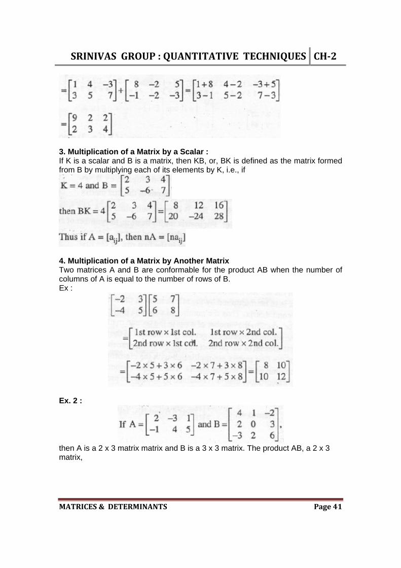
3. Multiplication of a Matrix by a Scalar : If K is a scalar and B is a matrix, then KB, or, BK is defined as the matrix formed from B by multiplying each of its elements by K, i.e., if
4. Multiplication of a Matrix by Another Matrix Two matrices A and B are conformable for the product AB when the number of columns of A is equal to the number of rows of B. Ex :
Ex. 2 :
then A is a 2 x 3 matrix matrix and B is a 3 x 3 matrix. The product AB, a 2 x 3 matrix,
SRINIVASGROUP:QUANTITATIVETECHNIQUES CH‐2
MATRICES&DETERMINANTS Page42
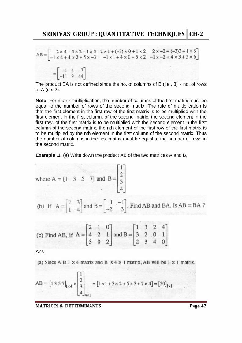
The product BA is not defined since the no. of columns of B (i.e., 3) no. of rows of A (i.e. 2). Note: For matrix multiplication, the number of columns of the first matrix must be equal to the number of rows of the second matrix. The rule of multiplication is that the first element in the first row of the first matrix is to be multiplied with the first element In the first column, of the second matrix, the second element in the first row, of the first matrix is to be multiplied with the second element in the first column of the second matrix, the nth element of the first row of the first matrix is to be multiplied by the nth element in the first column of the second matrix. Thus the number of columns in the first matrix must be equal to the number of rows in the second matrix. Example .1. (a) Write down the product AB of the two matrices A and B,
Ans :
SRINIVASGROUP:QUANTITATIVETECHNIQUES CH‐2
MATRICES&DETERMINANTS Page43
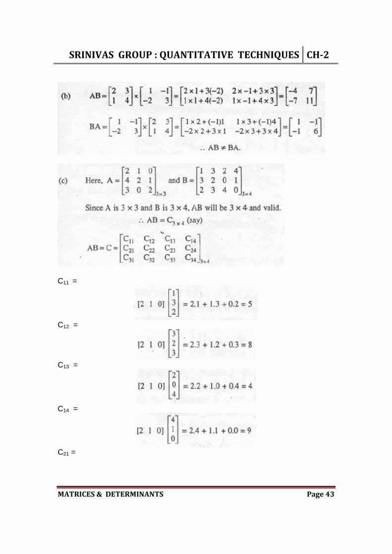
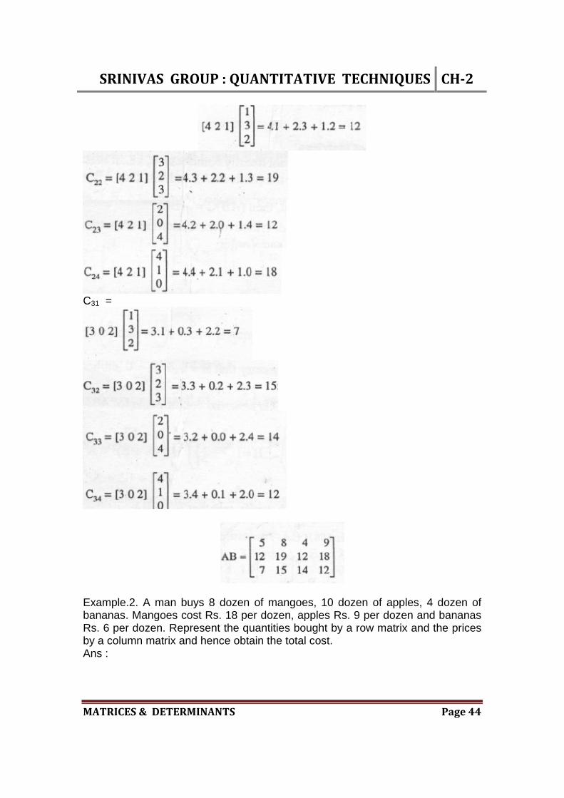
C11 =
C12 =
C13 =
C14 =
C21 =
SRINIVASGROUP:QUANTITATIVETECHNIQUES CH‐2
MATRICES&DETERMINANTS Page44
C31 =
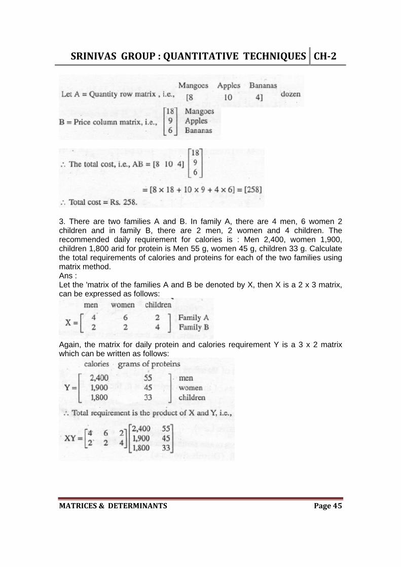
Example.2. A man buys 8 dozen of mangoes, 10 dozen of apples, 4 dozen of bananas. Mangoes cost Rs. 18 per dozen, apples Rs. 9 per dozen and bananas Rs. 6 per dozen. Represent the quantities bought by a row matrix and the prices by a column matrix and hence obtain the total cost. Ans :
SRINIVASGROUP:QUANTITATIVETECHNIQUES CH‐2
MATRICES&DETERMINANTS Page45
3. There are two families A and B. In family A, there are 4 men, 6 women 2 children and in family B, there are 2 men, 2 women and 4 children. The recommended daily requirement for calories is : Men 2,400, women 1,900, children 1,800 arid for protein is Men 55 g, women 45 g, children 33 g. Calculate the total requirements of calories and proteins for each of the two families using matrix method. Ans : Let the 'matrix of the families A and B be denoted by X, then X is a 2 x 3 matrix, can be expressed as follows:
Again, the matrix for daily protein and calories requirement Y is a 3 x 2 matrix which can be written as follows:
SRINIVASGROUP:QUANTITATIVETECHNIQUES CH‐2
MATRICES&DETERMINANTS Page46
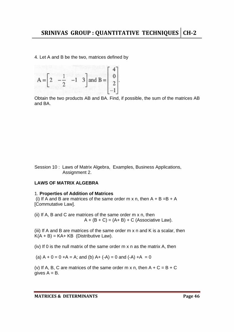
4. Let A and B be the two, matrices defined by
Obtain the two products AB and BA. Find, if possible, the sum of the matrices AB and BA. Session 10 : Laws of Matrix Algebra, Examples, Business Applications, Assignment 2. LAWS OF MATRIX ALGEBRA 1. Properties of Addition of Matrices (i) If A and B are matrices of the same order m x n, then A + B =B + A [Commutative Law]. (ii) If A, B and C are matrices of the same order m x n, then A + (B + C) = (A+ B) + C (Associative Law). (iii) If A and B are matrices of the same order m x n and K is a scalar, then K(A + B) = KA+ KB (Distributive Law). (iv) If 0 is the null matrix of the same order m x n as the matrix A, then (a) A + 0 = 0 +A = A; and (b) A+ (-A) = 0 and (-A) +A = 0 (v) If A, B, C are matrices of the same order m x n, then A + C = B + C gives A = B.

SRINIVASGROUP:QUANTITATIVETECHNIQUES CH‐2
MATRICES&DETERMINANTS Page47
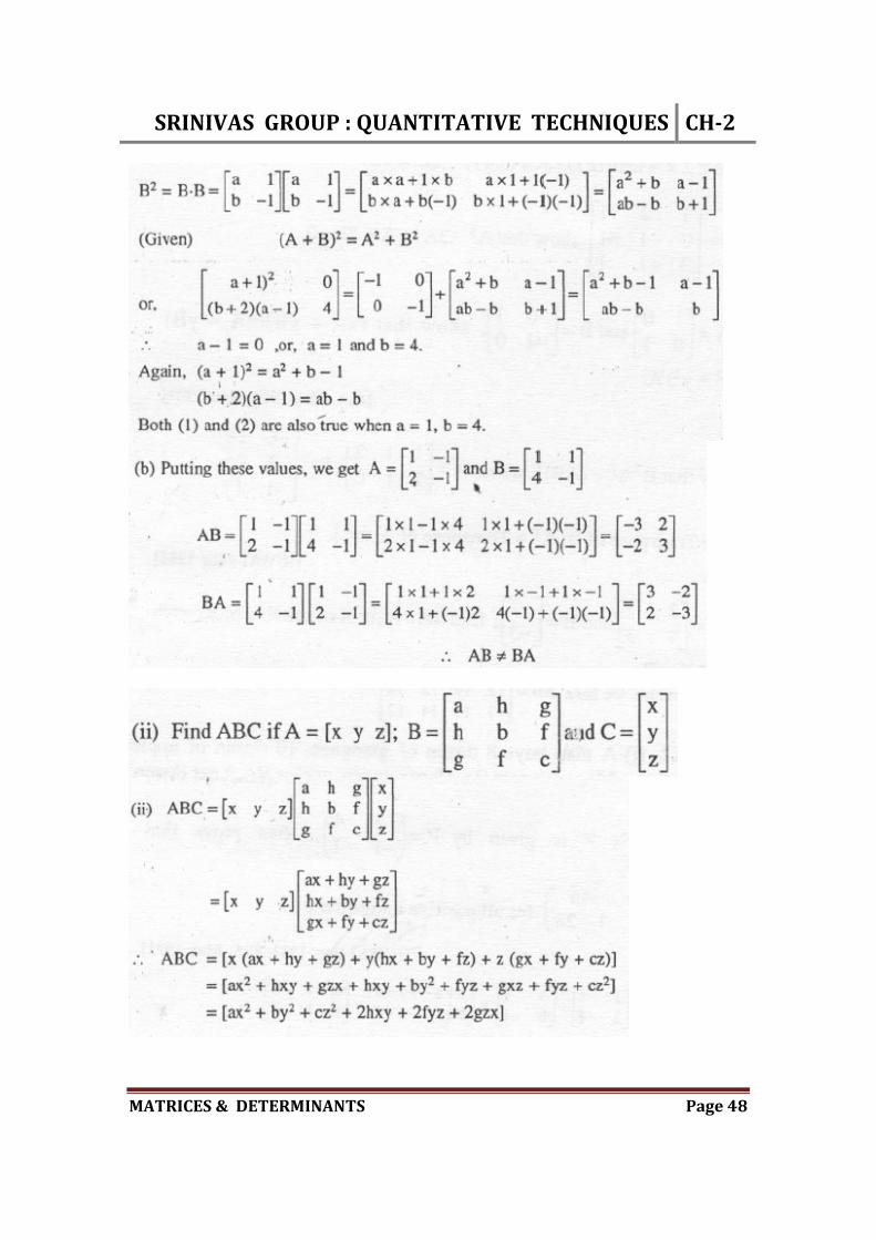
2. Properties of Multiplication of Matrices (i) The product of matrices is not usually cumulative, i.e., if matrices A and B are conformable for the products AB and BA, then AB BA. (ii) The product of matrices is associative, i.e., if matrices A, B, C are such that AB and BC are defined, then (AB)C = A(BC). . (iii) The product of matrices is distributive w.r.to addition of matrices, i.e., for matrices A, B, C of the same order . A(B + C) = AB +AC and (B + C)A = BA + CA. (iv) The cancellation la~ for the product of real numbers is not valid for the multiplication of matrices, i.e., AB = AC, does not imply that B = C. [A 0] (v) If I = Unit matrix and A is a square matrix of the same order as I, then AI = A = IA. (vi) If AB = 0, then it is not necessary that B = 0 ,or A = 0 or, both A and B are 0. (vii) If A = null matrix = 0 and B is a matrix conformable for AB, then BA = AB = 0. Problem :
SRINIVASGROUP:QUANTITATIVETECHNIQUES CH‐2
MATRICES&DETERMINANTS Page48

SRINIVASGROUP:QUANTITATIVETECHNIQUES CH‐2
MATRICES&DETERMINANTS Page49
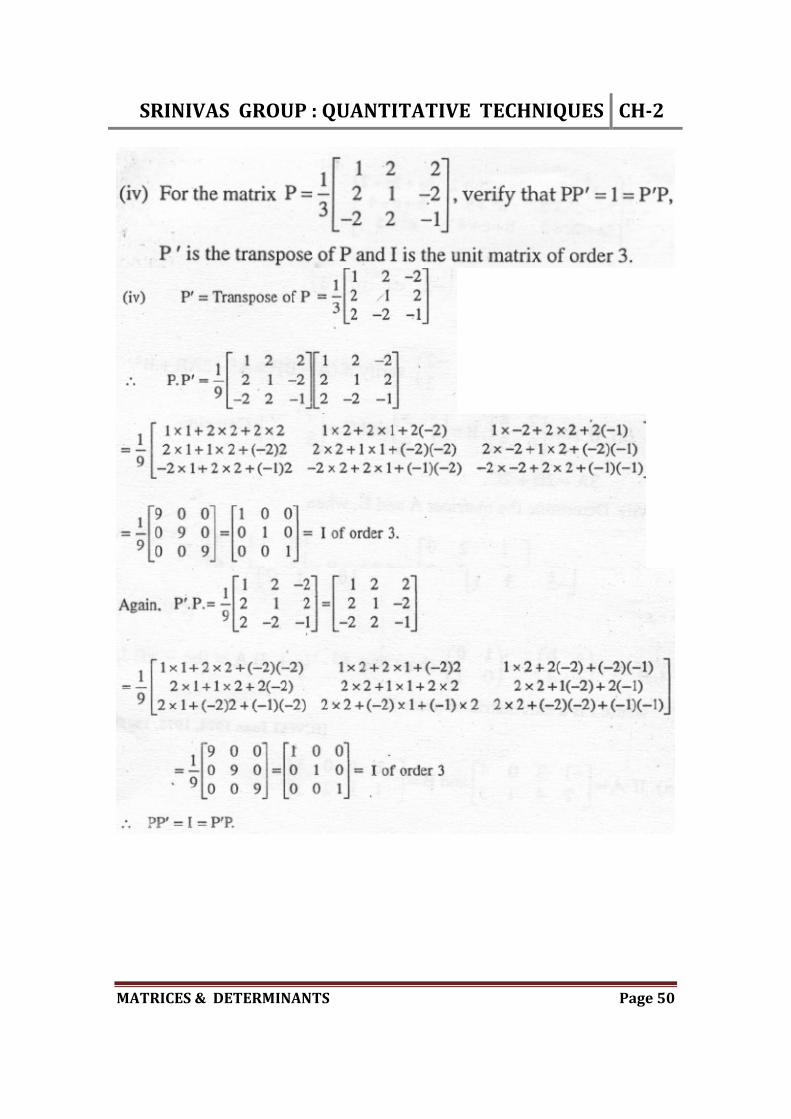
SRINIVASGROUP:QUANTITATIVETECHNIQUES CH‐2
MATRICES&DETERMINANTS Page50
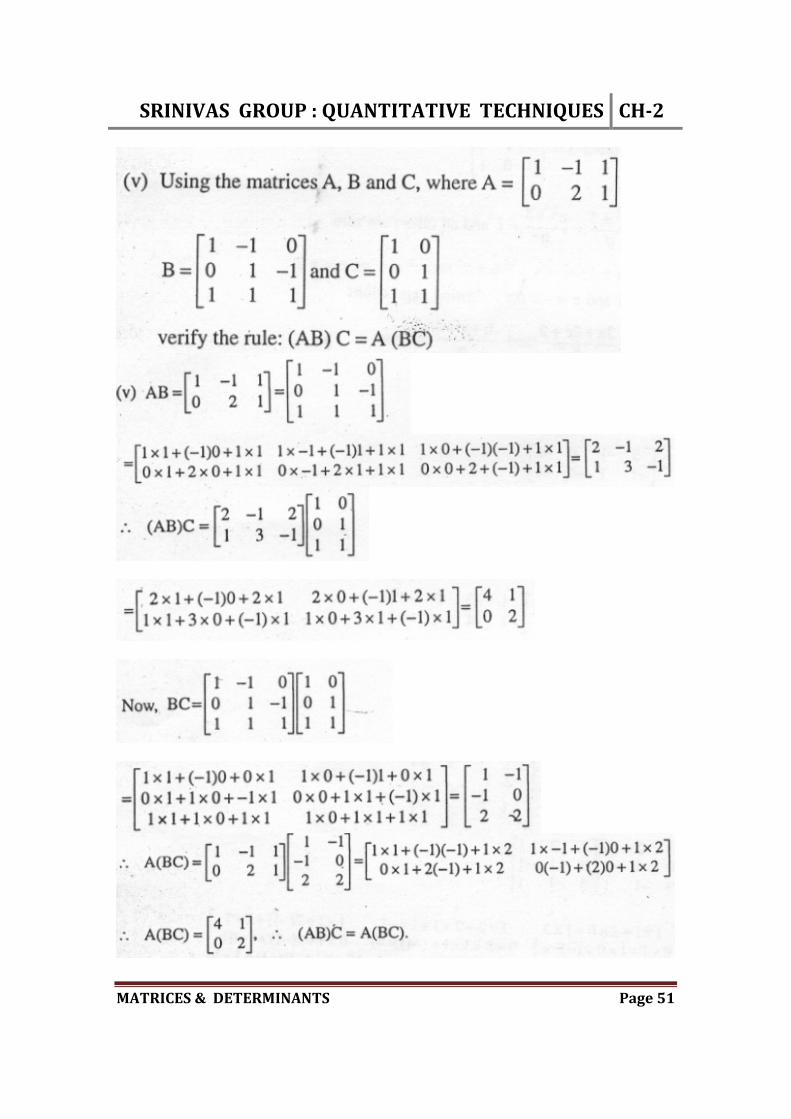
SRINIVASGROUP:QUANTITATIVETECHNIQUES CH‐2
MATRICES&DETERMINANTS Page51
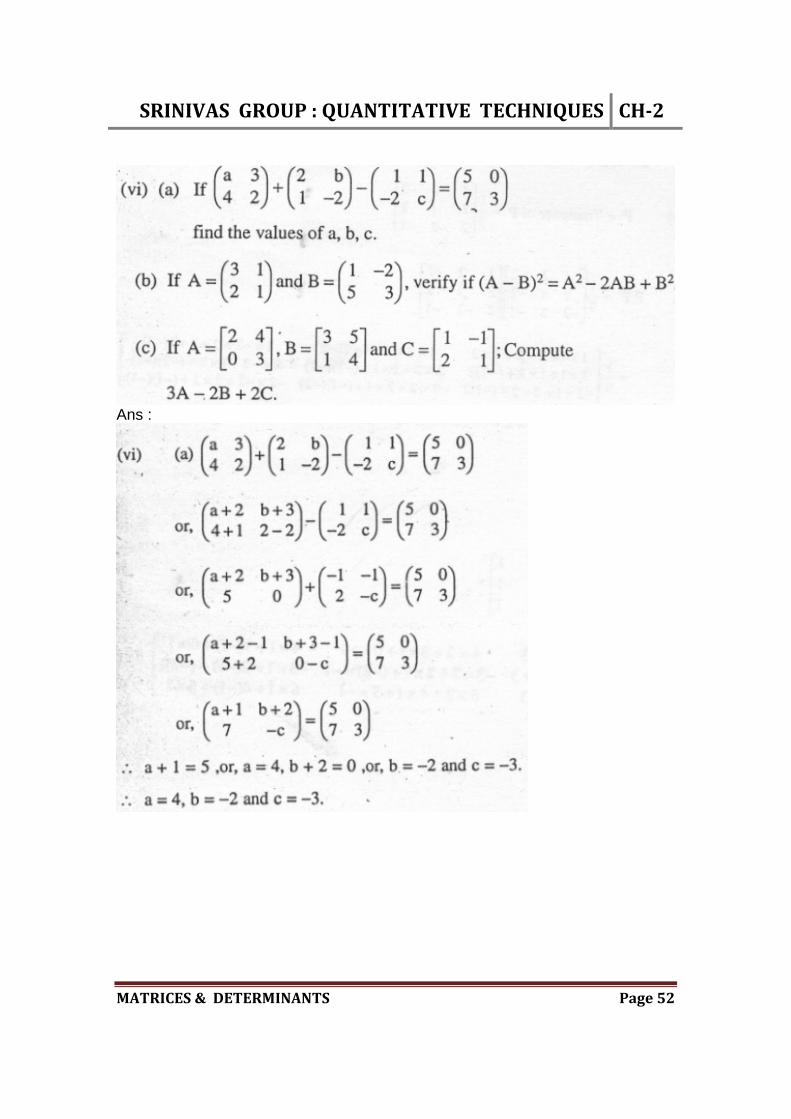
SRINIVASGROUP:QUANTITATIVETECHNIQUES CH‐2
MATRICES&DETERMINANTS Page52
Ans :

SRINIVASGROUP:QUANTITATIVETECHNIQUES CH‐2
MATRICES&DETERMINANTS Page53

SRINIVASGROUP:QUANTITATIVETECHNIQUES CH‐2
MATRICES&DETERMINANTS Page54
Ans :
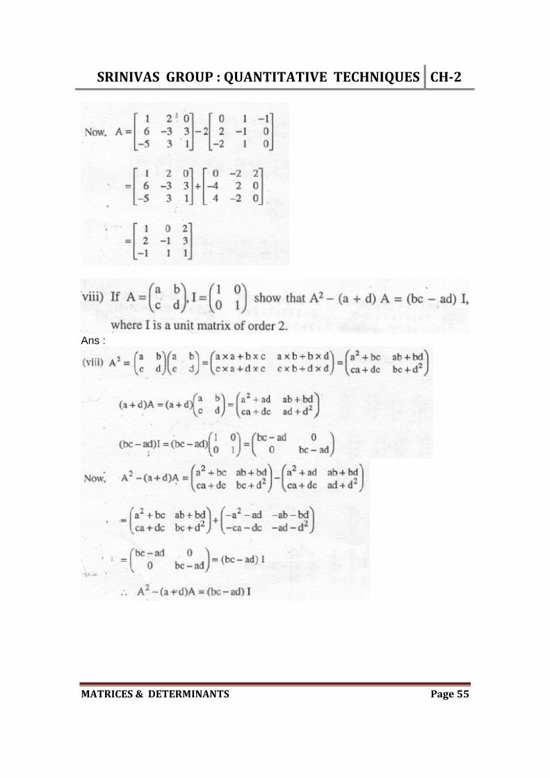
SRINIVASGROUP:QUANTITATIVETECHNIQUES CH‐2
MATRICES&DETERMINANTS Page55
Ans :
SRINIVASGROUP:QUANTITATIVETECHNIQUES CH‐2
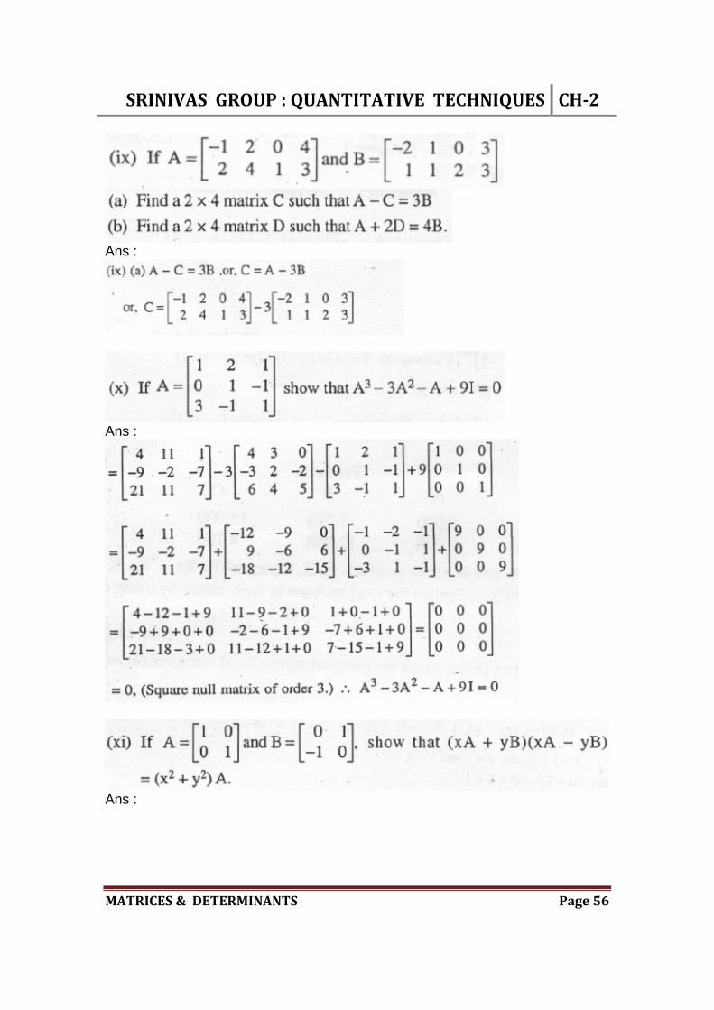
MATRICES&DETERMINANTS Page56
Ans :
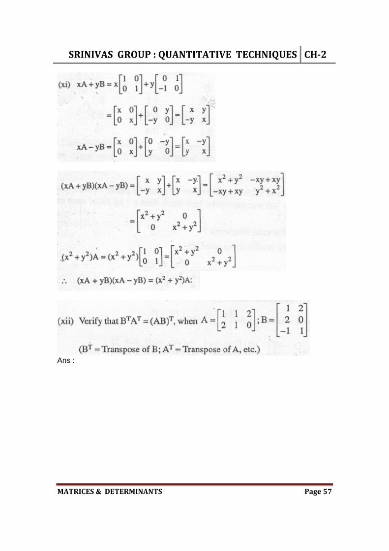
Ans :
Ans :
SRINIVASGROUP:QUANTITATIVETECHNIQUES CH‐2
MATRICES&DETERMINANTS Page57
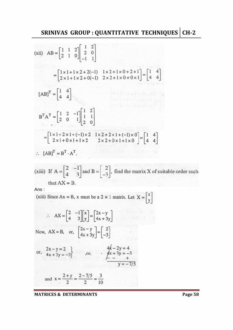
Ans :
SRINIVASGROUP:QUANTITATIVETECHNIQUES CH‐2
MATRICES&DETERMINANTS Page58
Ans :
SRINIVASGROUP:QUANTITATIVETECHNIQUES CH‐2
MATRICES&DETERMINANTS Page59
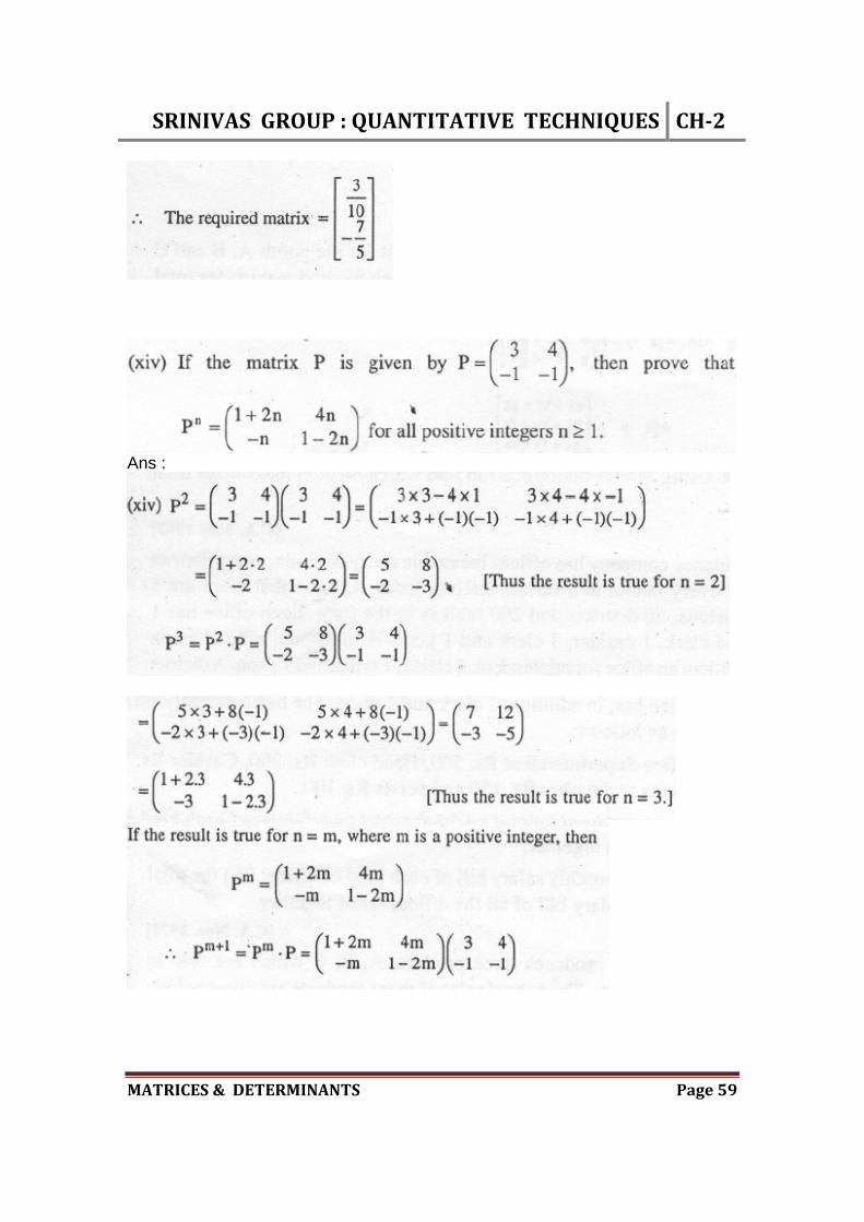
Ans :
SRINIVASGROUP:QUANTITATIVETECHNIQUES CH‐2
MATRICES&DETERMINANTS Page60
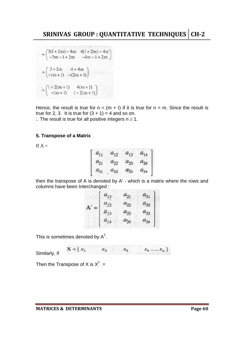
Hence, the result is true for n = (m + I) if it is true for n = m. Since the result is true for 2, 3. It is true for (3 + 1) = 4 and so on. :. The result is true for all positive integers n 1. 5. Transpose of a Matrix If A =
then the transpose of A is denoted by A' - which is a matrix where the rows and columns have been Interchanged :
This is sometimes denoted by AT.
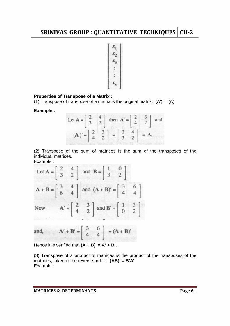
Similarly, if Then the Transpose of X is XT =
SRINIVASGROUP:QUANTITATIVETECHNIQUES CH‐2
MATRICES&DETERMINANTS Page61
Properties of Transpose of a Matrix : (1) Transpose of transpose of a matrix is the original matrix. (A')' = (A)
Example :
(2) Transpose of the sum of matrices is the sum of the transposes of the individual matrices. Example :
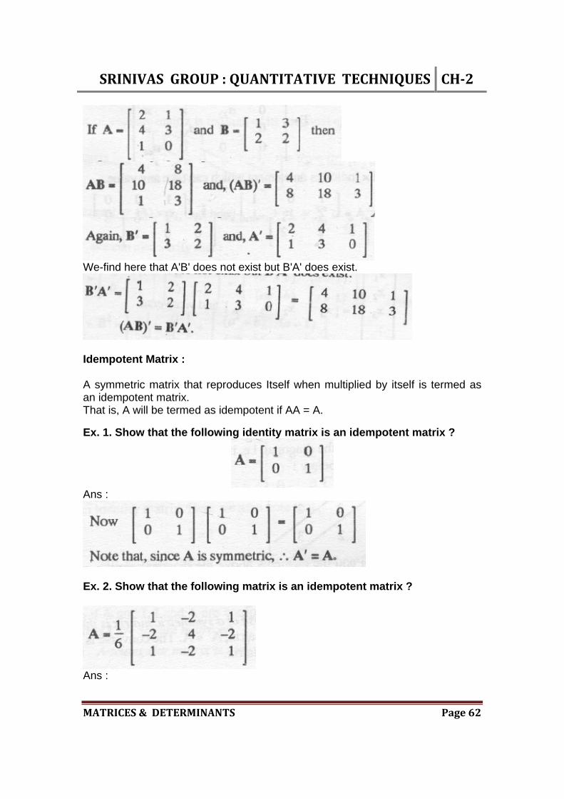
Hence it is verified that (A + B)' = A' + B’. (3) Transpose of a product of matrices is the product of the transposes of the matrices, taken in the reverse order : (AB)' = B'A' Example :
SRINIVASGROUP:QUANTITATIVETECHNIQUES CH‐2
MATRICES&DETERMINANTS Page62
We-find here that A'B' does not exist but B'A' does exist.
Idempotent Matrix : A symmetric matrix that reproduces Itself when multiplied by itself is termed as an idempotent matrix. That is, A will be termed as idempotent if AA = A.
Ex. 1. Show that the following identity matrix is an idempotent matrix ?
Ans :
Ex. 2. Show that the following matrix is an idempotent matrix ?
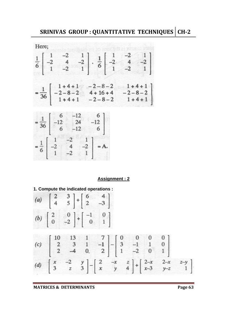
Ans :
SRINIVASGROUP:QUANTITATIVETECHNIQUES CH‐2
MATRICES&DETERMINANTS Page63
Assignment : 2 1. Compute the indicated operations :

SRINIVASGROUP:QUANTITATIVETECHNIQUES CH‐2
MATRICES&DETERMINANTS Page64
2. Find the value of
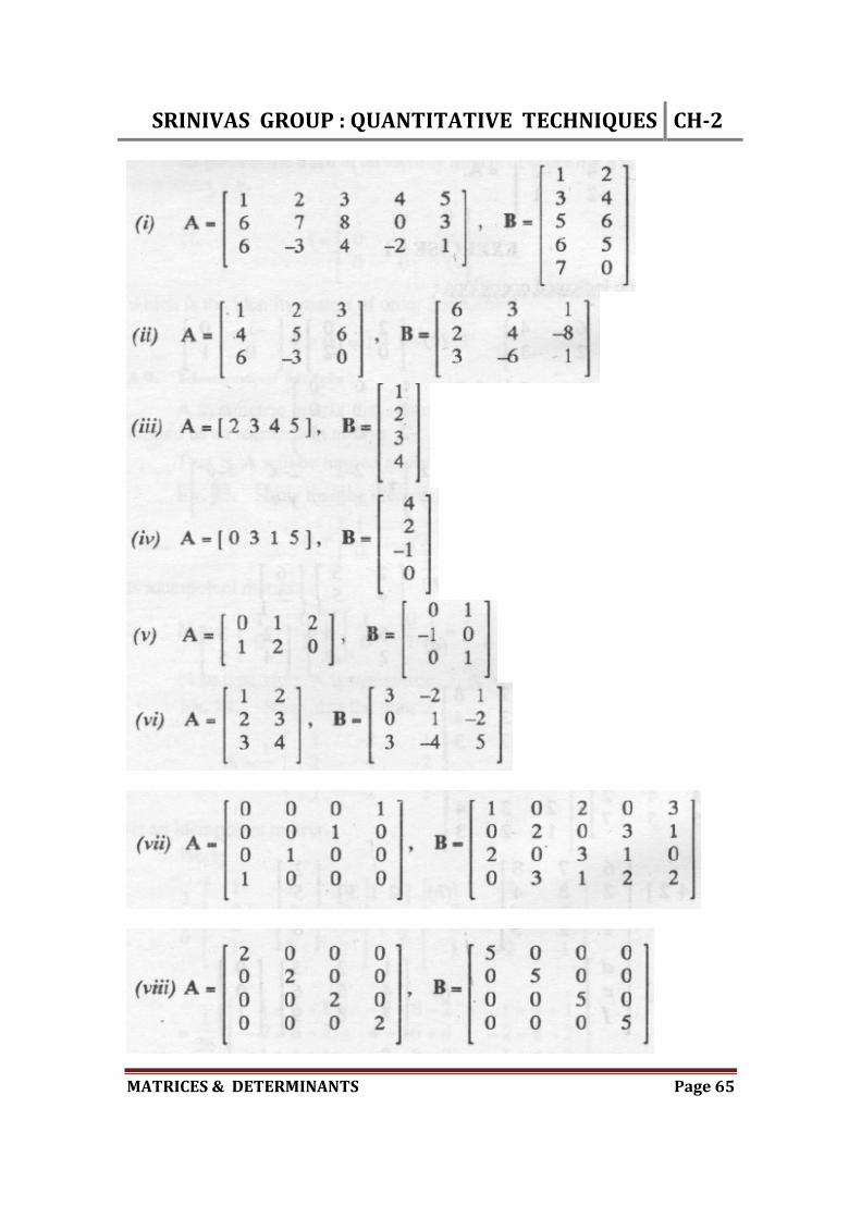
3. For the following pairs of matrices compute AB and BA :
SRINIVASGROUP:QUANTITATIVETECHNIQUES CH‐2
MATRICES&DETERMINANTS Page65

SRINIVASGROUP:QUANTITATIVETECHNIQUES CH‐2
MATRICES&DETERMINANTS Page66
4. Compute the following products :

SRINIVASGROUP:QUANTITATIVETECHNIQUES CH‐2
MATRICES&DETERMINANTS Page67
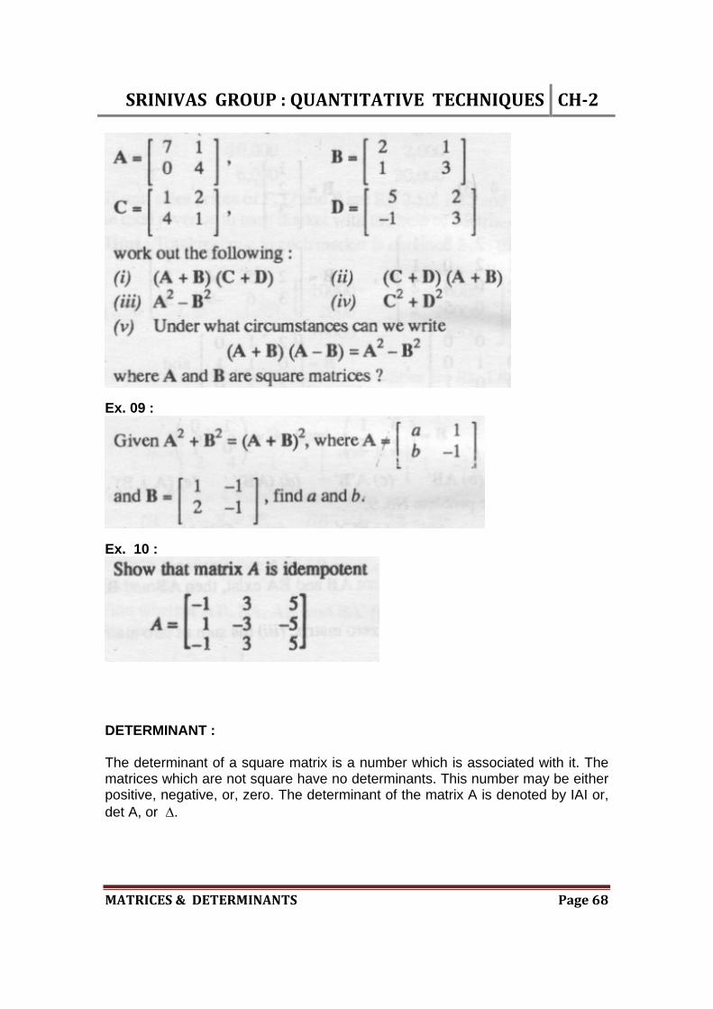
Ex. 5 :
Ex. 6 :
Ex. 7 :
Ex. 8 :
SRINIVASGROUP:QUANTITATIVETECHNIQUES CH‐2
MATRICES&DETERMINANTS Page68
Ex. 09 :
Ex. 10 :
DETERMINANT : The determinant of a square matrix is a number which is associated with it. The matrices which are not square have no determinants. This number may be either positive, negative, or, zero. The determinant of the matrix A is denoted by IAI or, det A, or .
SRINIVASGROUP:QUANTITATIVETECHNIQUES CH‐2
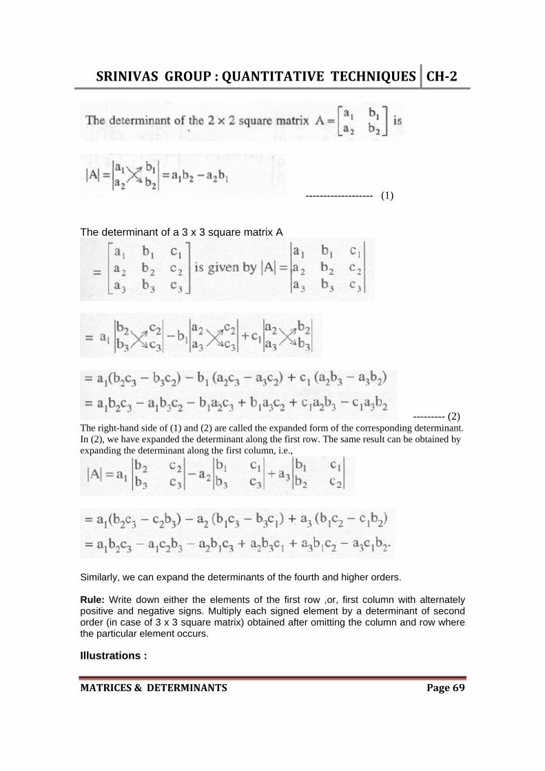
MATRICES&DETERMINANTS Page69
------------------- (1) The determinant of a 3 x 3 square matrix A
--------- (2) The right-hand side of (1) and (2) are called the expanded form of the corresponding determinant. In (2), we have expanded the determinant along the first row. The same result can be obtained by expanding the determinant along the first column, i.e.,
Similarly, we can expand the determinants of the fourth and higher orders. Rule: Write down either the elements of the first row ,or, first column with alternately positive and negative signs. Multiply each signed element by a determinant of second order (in case of 3 x 3 square matrix) obtained after omitting the column and row where the particular element occurs. Illustrations :

SRINIVASGROUP:QUANTITATIVETECHNIQUES CH‐2
MATRICES&DETERMINANTS Page70
(iii)
the left side can be expressed in the form of a determinant of third order as
SRINIVASGROUP:QUANTITATIVETECHNIQUES CH‐2
MATRICES&DETERMINANTS Page71
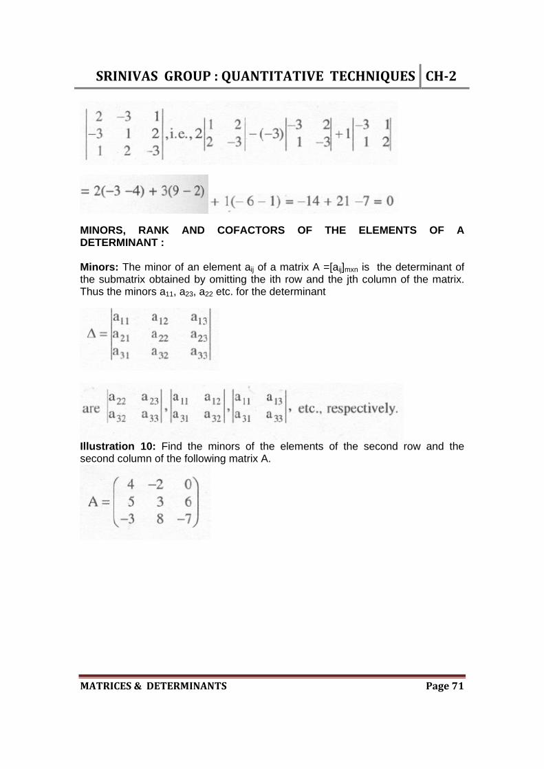
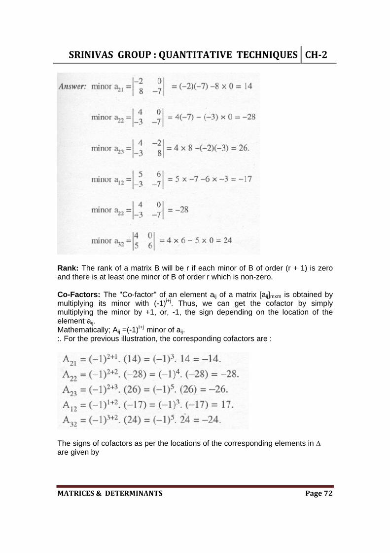
MINORS, RANK AND COFACTORS OF THE ELEMENTS OF A DETERMINANT : Minors: The minor of an element aij of a matrix A =[aij]mxn is the determinant of the submatrix obtained by omitting the ith row and the jth column of the matrix. Thus the minors a11, a23, a22 etc. for the determinant
Illustration 10: Find the minors of the elements of the second row and the second column of the following matrix A.
SRINIVASGROUP:QUANTITATIVETECHNIQUES CH‐2
MATRICES&DETERMINANTS Page72
Rank: The rank of a matrix B will be r if each minor of B of order (r + 1) is zero and there is at least one minor of B of order r which is non-zero. Co-Factors: The "Co-factor" of an element aij of a matrix [aij]mxm is obtained by multiplying its minor with (-1)i+j. Thus, we can get the cofactor by simply multiplying the minor by +1, or, -1, the sign depending on the location of the element aij. Mathematically; Aij =(-1)i+j minor of aij. :. For the previous illustration, the corresponding cofactors are :
The signs of cofactors as per the locations of the corresponding elements in are given by

SRINIVASGROUP:QUANTITATIVETECHNIQUES CH‐2
MATRICES&DETERMINANTS Page73
The cofactors A21, A22, etc., can also be denoted by other capital letters B21, B22, etc. ,or, C21, C22, etc. Adjugate (or Adjoint) of a Determinant :
where, all the elements are the cofactors of the corresponding elements of the determinant
is called the adjugate, or, adjoint of . Illustration 1: (i) Find the cofactors of the elements of the determinant
and hence find the adjugate, or, adjoint of the determinant.

SRINIVASGROUP:QUANTITATIVETECHNIQUES CH‐2
MATRICES&DETERMINANTS Page74
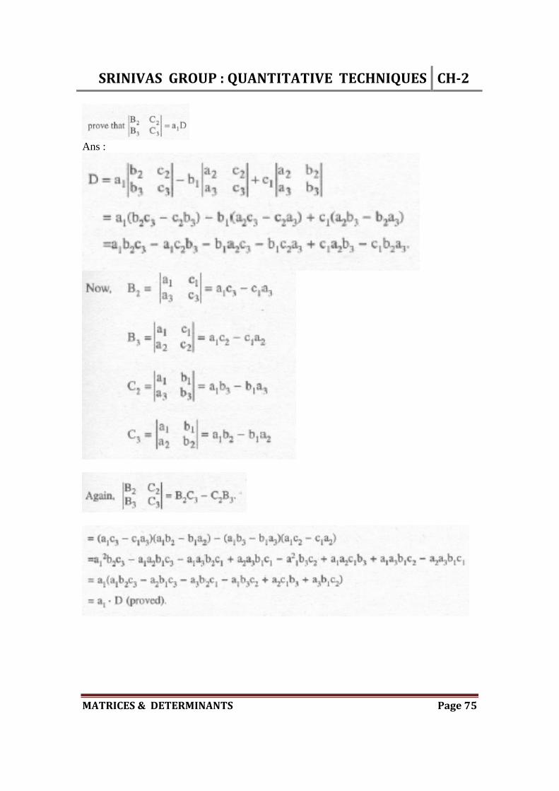
(ii) If A1, B1, C1 are respectively the co-factors of the elements a1 b1, cl, of the determinant D, where
SRINIVASGROUP:QUANTITATIVETECHNIQUES CH‐2
MATRICES&DETERMINANTS Page75
Ans :

SRINIVASGROUP:QUANTITATIVETECHNIQUES CH‐2
MATRICES&DETERMINANTS Page76
Illustration 2 : Prove that A(Adj A) =IAI.I3
Ans :

SRINIVASGROUP:QUANTITATIVETECHNIQUES CH‐2
MATRICES&DETERMINANTS Page77
PROPERTIES OF DETERMINANTS : The properties stated below are applicable to determinants of any order. (i) If the rows and columns of a determinant are interchanged, the value of the determinant does not change, det A = det A'.
SRINIVASGROUP:QUANTITATIVETECHNIQUES CH‐2
MATRICES&DETERMINANTS Page78
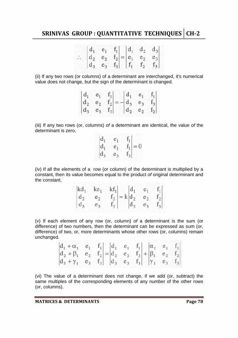
(ii) If any two rows (or columns) of a determinant are interchanged, it's numerical value does not change, but the sign of the determinant is changed.
(iii) If any two rows (or, columns) of a determinant are identical, the value of the determinant is zero,
(iv) If all the elements of a row (or column) of the determinant is multiplied by a constant, then its value becomes equal to the product of original determinant and the constant,
(v) If each element of any row (or, column) of a determinant is the sum (or difference) of two numbers, then the determinant can be expressed as sum (or, difference) of two, or, more determinants whose other rows (or, columns) remain unchanged.
(vi) The value of a determinant does not change, if we add (or, subtract) the same multiples of the corresponding elements of any number of the other rows (or, columns).
SRINIVASGROUP:QUANTITATIVETECHNIQUES CH‐2
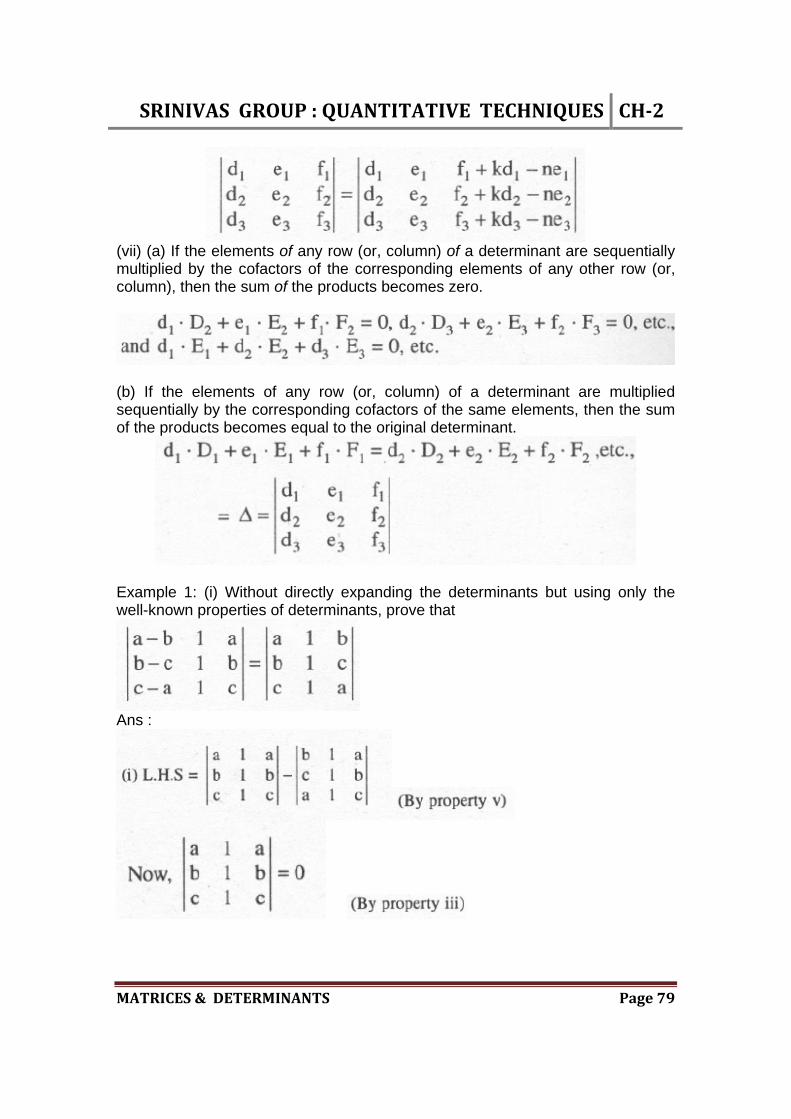
MATRICES&DETERMINANTS Page79
(vii) (a) If the elements of any row (or, column) of a determinant are sequentially multiplied by the cofactors of the corresponding elements of any other row (or, column), then the sum of the products becomes zero.
(b) If the elements of any row (or, column) of a determinant are multiplied sequentially by the corresponding cofactors of the same elements, then the sum of the products becomes equal to the original determinant.
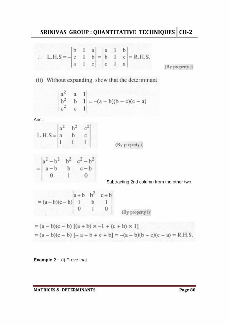
Example 1: (i) Without directly expanding the determinants but using only the well-known properties of determinants, prove that
Ans :
SRINIVASGROUP:QUANTITATIVETECHNIQUES CH‐2
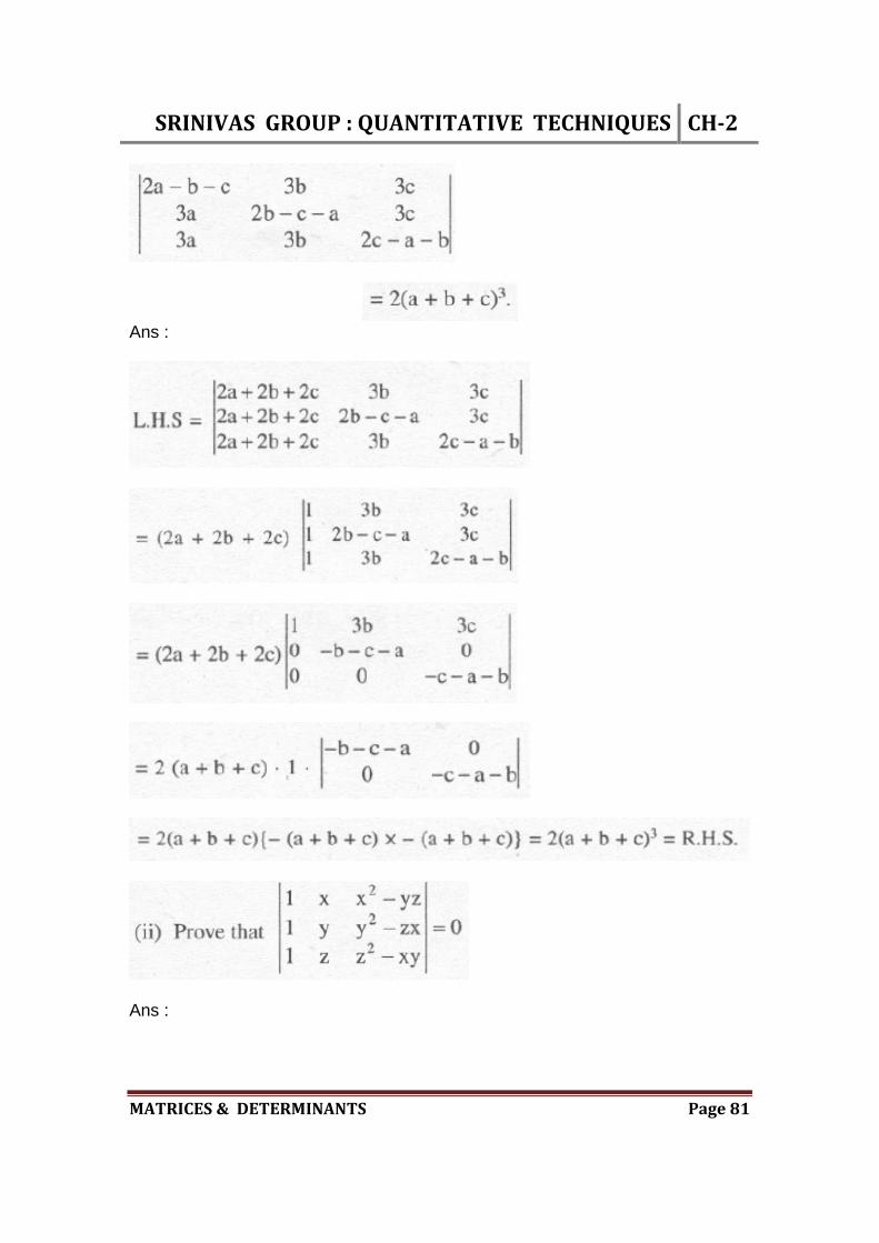
MATRICES&DETERMINANTS Page80
Ans :
Subtracting 2nd column from the other two.
Example 2 : (i) Prove that
SRINIVASGROUP:QUANTITATIVETECHNIQUES CH‐2
MATRICES&DETERMINANTS Page81
Ans :
Ans :

SRINIVASGROUP:QUANTITATIVETECHNIQUES CH‐2
MATRICES&DETERMINANTS Page82
[Multiplying 1st, 2nd and 3rd rows by x, y and z respectively].
SINGULAR AND NON-SINGULAR MATRICES : A square matrix A is called a singular matrix if IAI = 0. If IAI 0, then the matrix A is called a non-singular matrix. Illustration :

SRINIVASGROUP:QUANTITATIVETECHNIQUES CH‐2
MATRICES&DETERMINANTS Page83
INVERSE OF A SQUARE MATRIX : If A is a non-singular square matrix of order n and B is another square matrix of the same order n such that AB = BA = I where I is the unit ,or, identity matrix of order n, then B is said to be the inverse of A, which is denoted by A-1. A . A-1 = A-1. A = I. Methods to determine Inversion of Matrix :
1. Co-Factor Method of Matrix Inversion : 2. Gauss Elimination Method of Matrix Inversion :
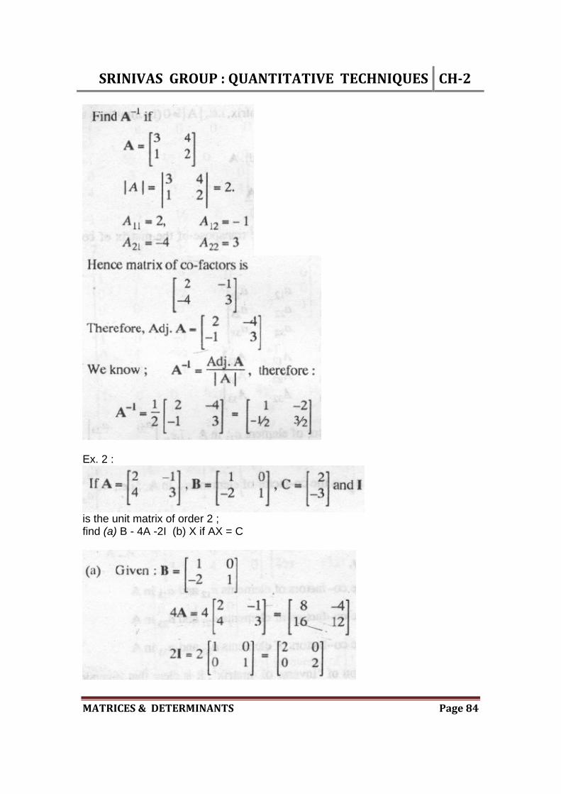
1. Co-Factor Method of Matrix Inversion : According to this method A-1 = (Adj. A) / IAI Steps to find the Inverse of any Square Matrix : (1) Replace each element of Matrix A by its cofactor and obtain the cofactor matrix. (2) Next obtain the transpose matrix of cofactors ,i.e., the Adj matrix. (3) Divide each element of the Adj matrix by IAI to get the inverse of A. Ex. 1 :
SRINIVASGROUP:QUANTITATIVETECHNIQUES CH‐2
MATRICES&DETERMINANTS Page84
Ex. 2 :
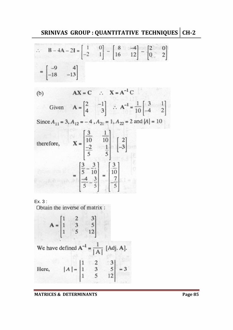
is the unit matrix of order 2 ; find (a) B - 4A -2I (b) X if AX = C
SRINIVASGROUP:QUANTITATIVETECHNIQUES CH‐2
MATRICES&DETERMINANTS Page85
Ex. 3 :

SRINIVASGROUP:QUANTITATIVETECHNIQUES CH‐2
MATRICES&DETERMINANTS Page86
The value of the determinant can be found by any row or column. The matrix of co-factors is given by:
Ex. 4 : Calculate the inverse of matrix

SRINIVASGROUP:QUANTITATIVETECHNIQUES CH‐2
MATRICES&DETERMINANTS Page87
Ex. 5 :
SRINIVASGROUP:QUANTITATIVETECHNIQUES CH‐2
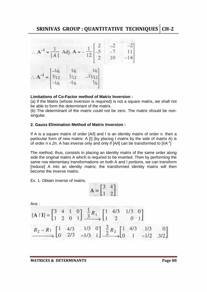
MATRICES&DETERMINANTS Page88
Limitations of Co-Factor method of Matrix Inversion : (a) If the Matrix (whose inversion is required) is not a square matrix, we shall not be able to form the determinant of the matrix. (b) The determinant of the matrix could not be zero. The matrix should be non-singular. 2. Gauss Elimination Method of Matrix Inversion : If A is a square matrix of order [A/l] and I is an identity matrix of order n. then a particular form of new matrix: A [I] (by placing I matrix by the side of matrix A) is of order n x 2n. A has inverse only and only if [A/l] can be transformed to [I/A-1] The method, thus, consists in placing an identity matrix of the same order along side the original matrix A which is required to be inverted. Then by performing the same row elementary transformations on both A and I portions, we can transform [reduce] A into an identity matrix; the transformed identity matrix will then become the inverse matrix. Ex. 1. Obtain inverse of matrix,
Ans :

SRINIVASGROUP:QUANTITATIVETECHNIQUES CH‐2
MATRICES&DETERMINANTS Page89
Ex. 2 :
Ans :
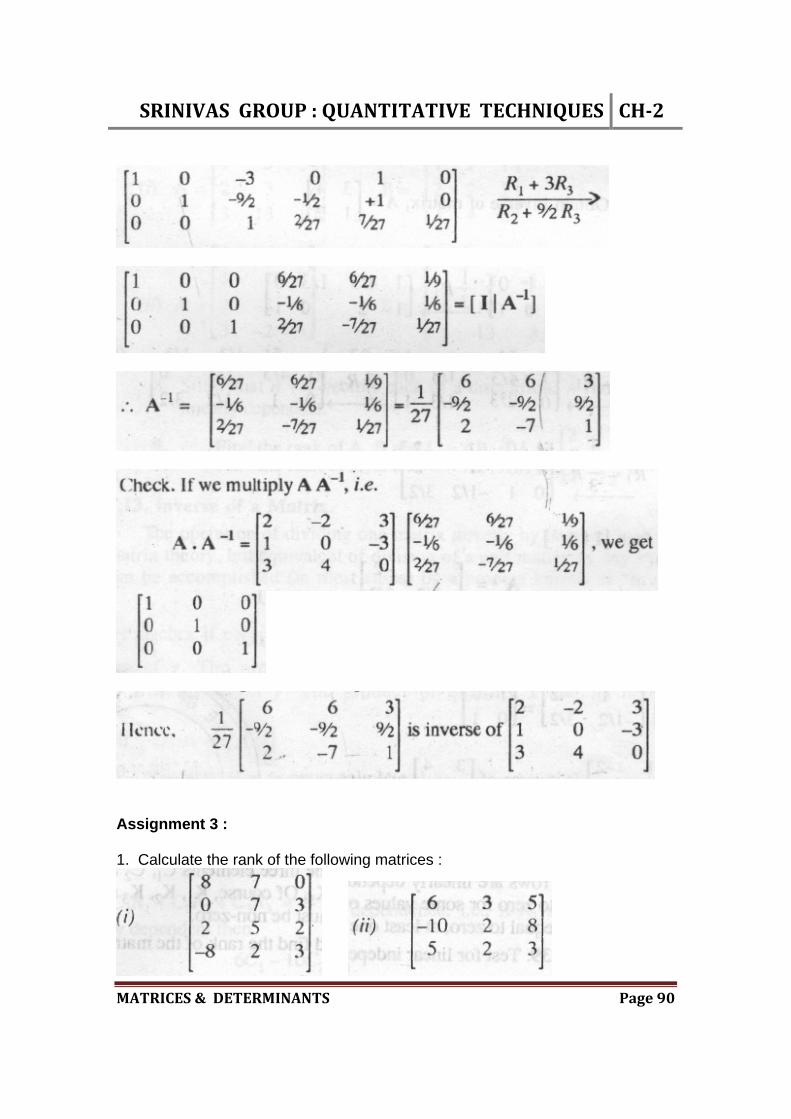
SRINIVASGROUP:QUANTITATIVETECHNIQUES CH‐2
MATRICES&DETERMINANTS Page90
Assignment 3 : 1. Calculate the rank of the following matrices :
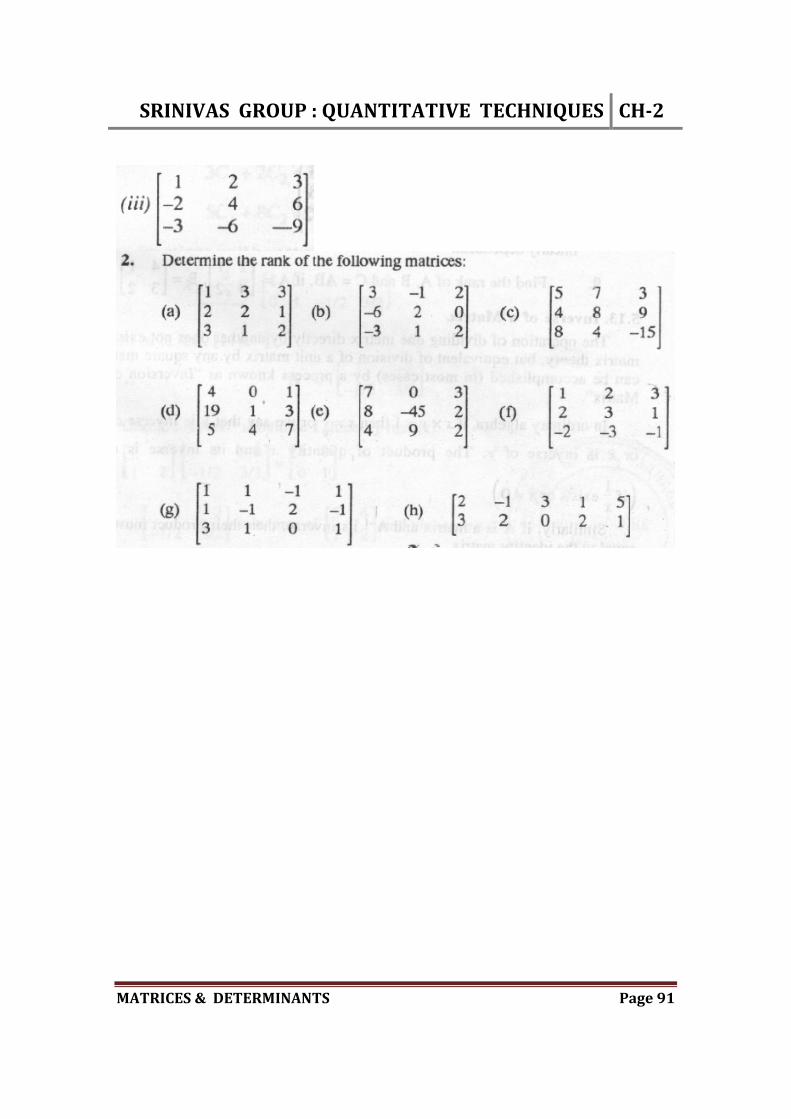
SRINIVASGROUP:QUANTITATIVETECHNIQUES CH‐2
MATRICES&DETERMINANTS Page91
SRINIVASGROUP:QUANTITATIVETECHNIQUES CH‐2
MATRICES&DETERMINANTS Page92
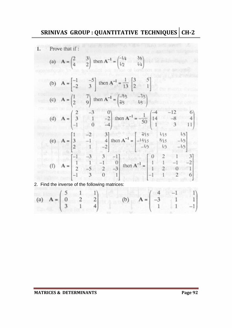
2. Find the inverse of the following matrices:

SRINIVASGROUP:QUANTITATIVETECHNIQUES CH‐2
MATRICES&DETERMINANTS Page93
[Hint for (f) : First remove the fraction by scalar multiplication.] Application of Matrix to the Solution of Linear Equations : Suppose we are required to solve the following set of simultaneous equations for X1, X2 and X3 :

SRINIVASGROUP:QUANTITATIVETECHNIQUES CH‐2
MATRICES&DETERMINANTS Page94
This way, the three simultaneous given equations are written in the form of a single matrix equation as AX = H. We can find X1, X2 and X3 if we write this single matrix equation in the form
X =A-1 H In general, if there are n variables and n equations, then
AX = H is the matrix presentation of the n-simultaneous equations, where A = matrix of order n x n. X = col. matrix of variables or order n x 1. H =col. matrix of constants of order n x 1. and, then X = A-1 H; where A is the inverse of matrix A. Remember here that only the product A H exists and the product HA does not exist. Hence, X HA-1 Ex. 1. Solve for X and y : 2x + 3y = 7 4x + 2y = 10 Putting the given equations in matrix form, we have

SRINIVASGROUP:QUANTITATIVETECHNIQUES CH‐2
MATRICES&DETERMINANTS Page95
Ex. 2: Solve for x,y and z from the following set of equations : X - 2y + 3z = 1 3x – y + 4z = 3 2y + y - 2z = -1 Putting the given equations in the matrix form

SRINIVASGROUP:QUANTITATIVETECHNIQUES CH‐2
MATRICES&DETERMINANTS Page96
x = 0, y = 1, z = 1. SOLUTION OF LINEAR EQUATIONS IN THREE UNKNOWNS USING CRAMER’S RULE : Consider the equations
a11x + a12y + a13z = d1 a21x + a22y + a23z = d2 a31x + a32y + a33z = d3
The solution of the equations is given by
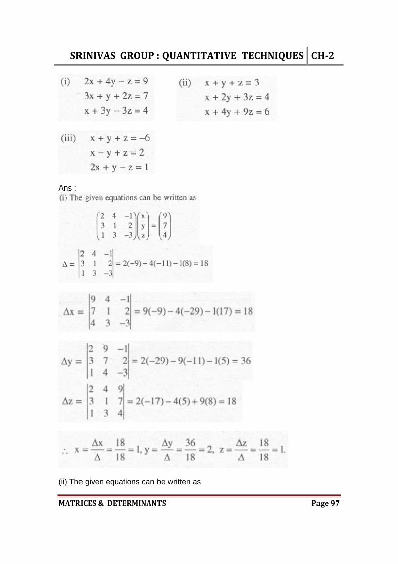
Note: (1) If = 0 and x = y = z = 0, then there will be infinite number of solutions of the given equations and the equations will be dependent. (2) If =0 and at least one of x, y, z is non-zero, then there will no solution for the equations and the equations are considered inconsistent. Example 1 : Solve the system of equations
SRINIVASGROUP:QUANTITATIVETECHNIQUES CH‐2
MATRICES&DETERMINANTS Page97
Ans :
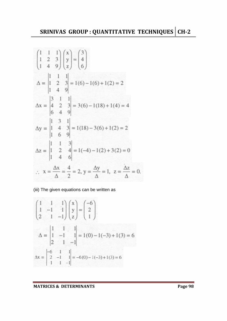
(ii) The given equations can be written as
SRINIVASGROUP:QUANTITATIVETECHNIQUES CH‐2
MATRICES&DETERMINANTS Page98
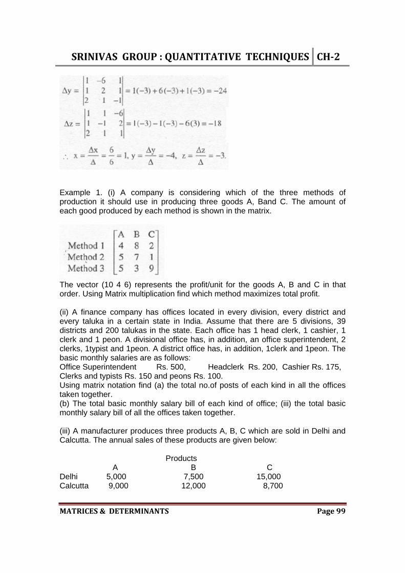
(iii) The given equations can be written as
SRINIVASGROUP:QUANTITATIVETECHNIQUES CH‐2
MATRICES&DETERMINANTS Page99
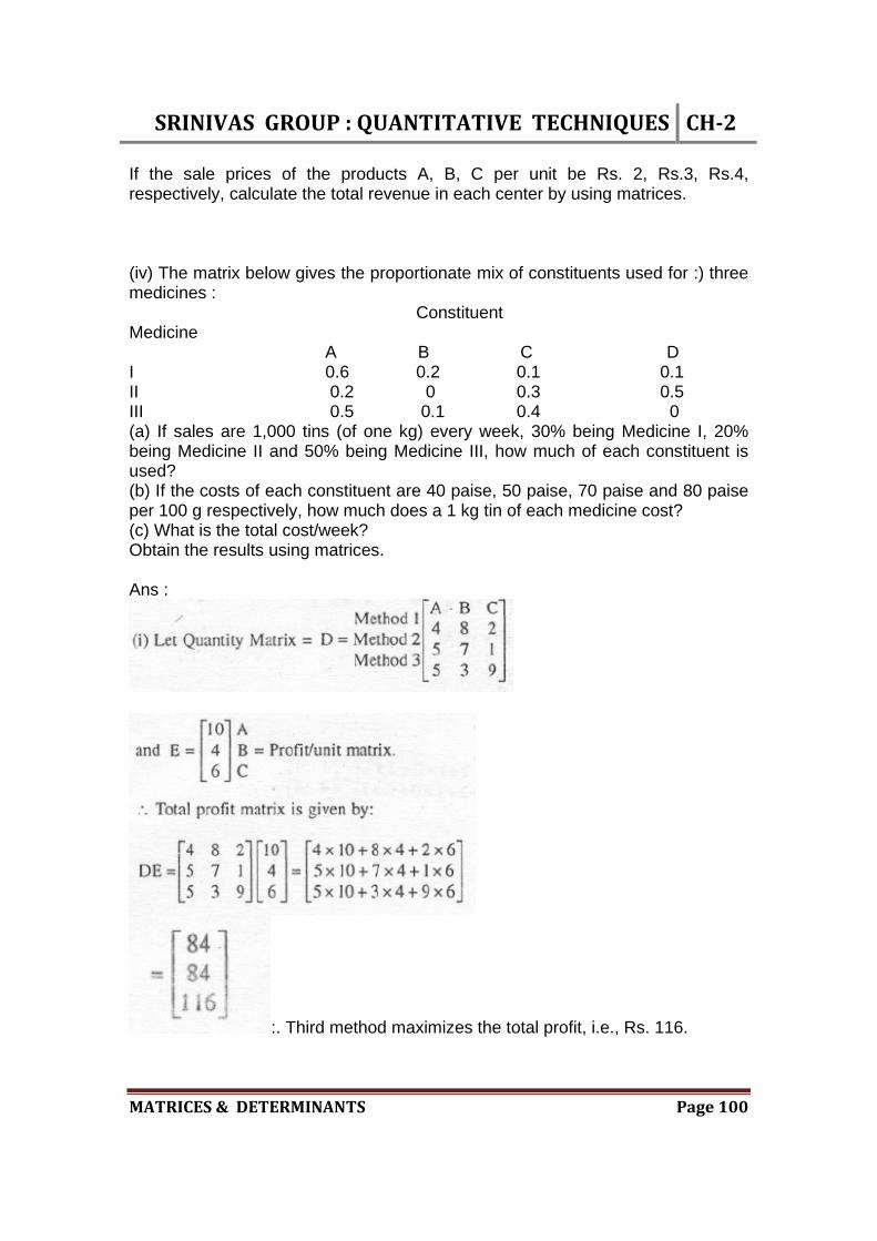
Example 1. (i) A company is considering which of the three methods of production it should use in producing three goods A, Band C. The amount of each good produced by each method is shown in the matrix.
The vector (10 4 6) represents the profit/unit for the goods A, B and C in that order. Using Matrix multiplication find which method maximizes total profit. (ii) A finance company has offices located in every division, every district and every taluka in a certain state in India. Assume that there are 5 divisions, 39 districts and 200 talukas in the state. Each office has 1 head clerk, 1 cashier, 1 clerk and 1 peon. A divisional office has, in addition, an office superintendent, 2 clerks, 1typist and 1peon. A district office has, in addition, 1clerk and 1peon. The basic monthly salaries are as follows: Office Superintendent Rs. 500, Headclerk Rs. 200, Cashier Rs. 175, Clerks and typists Rs. 150 and peons Rs. 100. Using matrix notation find (a) the total no.of posts of each kind in all the offices taken together. (b) The total basic monthly salary bill of each kind of office; (iii) the total basic monthly salary bill of all the offices taken together. (iii) A manufacturer produces three products A, B, C which are sold in Delhi and Calcutta. The annual sales of these products are given below: Products A B C Delhi 5,000 7,500 15,000 Calcutta 9,000 12,000 8,700
SRINIVASGROUP:QUANTITATIVETECHNIQUES CH‐2
MATRICES&DETERMINANTS Page100
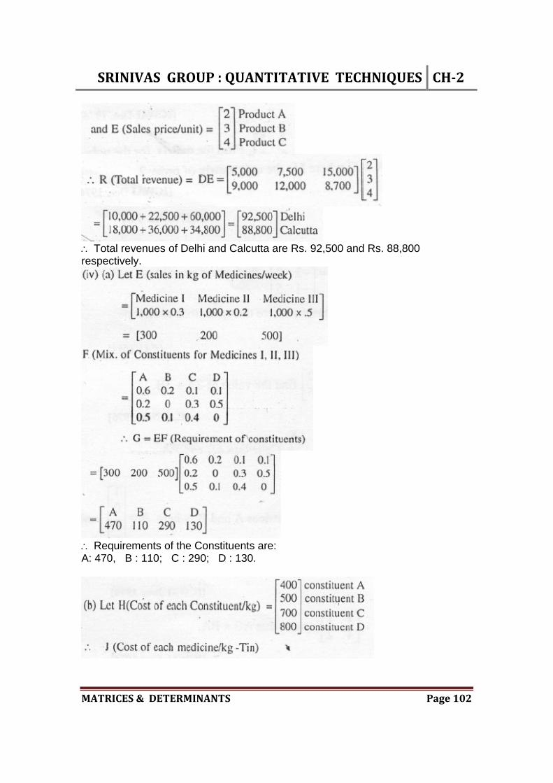
If the sale prices of the products A, B, C per unit be Rs. 2, Rs.3, Rs.4, respectively, calculate the total revenue in each center by using matrices. (iv) The matrix below gives the proportionate mix of constituents used for :) three medicines : Constituent Medicine A B C D I 0.6 0.2 0.1 0.1 II 0.2 0 0.3 0.5 III 0.5 0.1 0.4 0 (a) If sales are 1,000 tins (of one kg) every week, 30% being Medicine I, 20% being Medicine II and 50% being Medicine III, how much of each constituent is used? (b) If the costs of each constituent are 40 paise, 50 paise, 70 paise and 80 paise per 100 g respectively, how much does a 1 kg tin of each medicine cost? (c) What is the total cost/week? Obtain the results using matrices. Ans :
:. Third method maximizes the total profit, i.e., Rs. 116.

SRINIVASGROUP:QUANTITATIVETECHNIQUES CH‐2
MATRICES&DETERMINANTS Page101
SRINIVASGROUP:QUANTITATIVETECHNIQUES CH‐2
MATRICES&DETERMINANTS Page102
Total revenues of Delhi and Calcutta are Rs. 92,500 and Rs. 88,800 respectively.
Requirements of the Constituents are: A: 470, B : 110; C : 290; D : 130.
SRINIVASGROUP:QUANTITATIVETECHNIQUES CH‐2
MATRICES&DETERMINANTS Page103
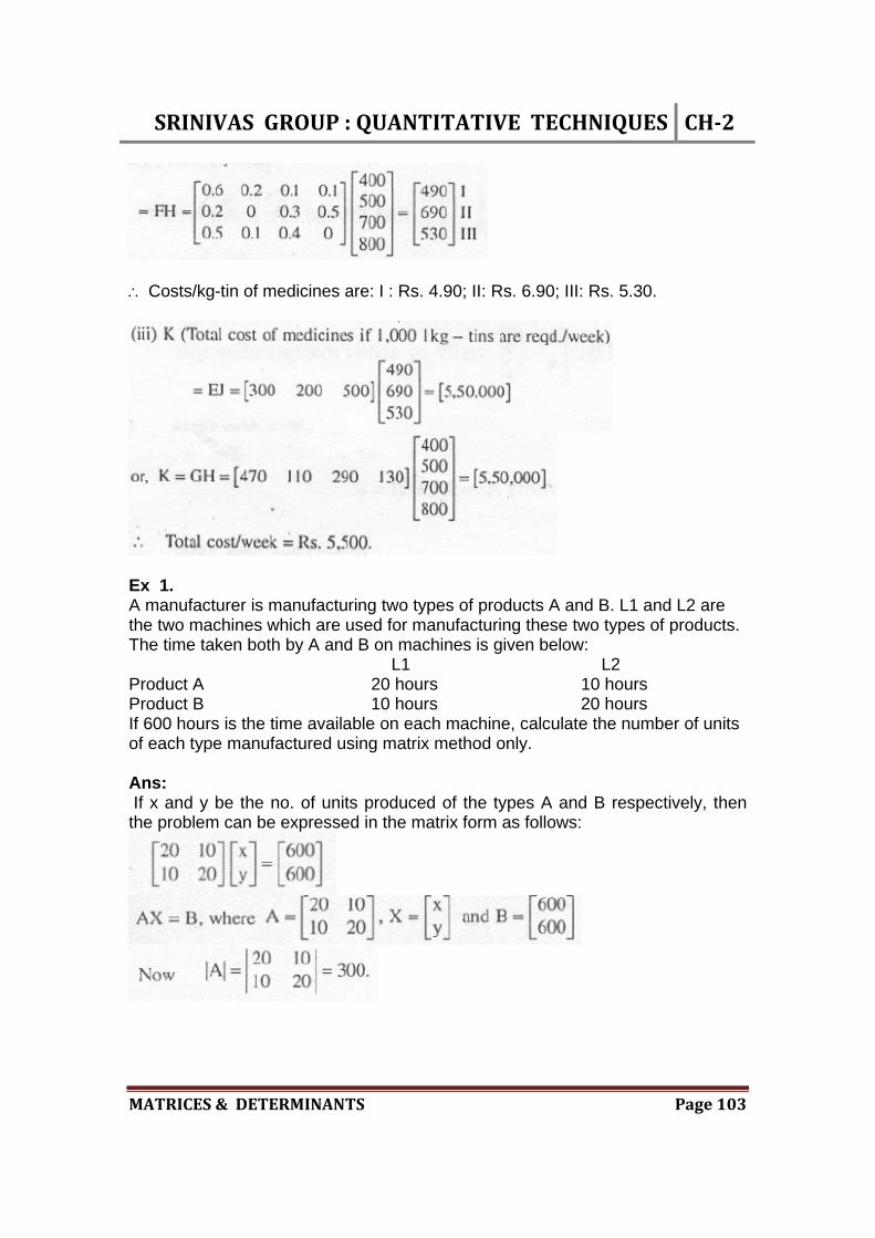
Costs/kg-tin of medicines are: I : Rs. 4.90; II: Rs. 6.90; III: Rs. 5.30.
Ex 1. A manufacturer is manufacturing two types of products A and B. L1 and L2 are the two machines which are used for manufacturing these two types of products. The time taken both by A and B on machines is given below: L1 L2 Product A 20 hours 10 hours Product B 10 hours 20 hours If 600 hours is the time available on each machine, calculate the number of units of each type manufactured using matrix method only. Ans: If x and y be the no. of units produced of the types A and B respectively, then the problem can be expressed in the matrix form as follows:

SRINIVASGROUP:QUANTITATIVETECHNIQUES CH‐2
MATRICES&DETERMINANTS Page104
:. x =20 and y =20, i.e., 20 units each of A and B should be produced. Ex. 2 : The daily cost of running a hospital C, is a linear function of the no. of in-patients P1 and out-patients P2 plus a fixed cost x, i.e., C =x + P2y + P1z Construct a linear system of equations using the following data for 3 days and find the values of x, y, z by the matrix inversion method. Day Cost (in Rs.) No. of inpatients No. of outpatients (C) (PI) (Pz) 1. 300 1 1 2. 400 3 2 3. 600 9 4 Ans : Putting the given values in C = x + P2y + P1z we get the following set of simultaneous linear equations: x + y + z =3 x + 2y + 3z = 4 x + 4y + 9z = 6. The above system of equations can be written as:

SRINIVASGROUP:QUANTITATIVETECHNIQUES CH‐2
MATRICES&DETERMINANTS Page105
which is of the form AX = B, where, A =
(ii) In a certain city, there are 5 colleges and 20 schools. Each school has 3 peons, 1 clerk and 1 head clerk, whereas a college has 5 peons, 3 clerks, 1 head clerk and an additional staff as a caretaker. The monthly salary of each of them is as follows: Peon - Rs. 1,100 Clerk - Rs. 1,700 Head Clerk - Rs. 3,000 Caretaker - Rs. 2,500 Using matrix method, find the total monthly salary bill of each School and College. Ans :

SRINIVASGROUP:QUANTITATIVETECHNIQUES CH‐2
MATRICES&DETERMINANTS Page106
Above matrices show educational institutions, staff positions and staff salary respectively. :. Monthly salary bill for the institutions is given by:
:. Monthly salary bill for college and school are Rs. 16,100 and Rs. 8,000 respectively.
**********************

SRINIVAS GROUP : QUANTITATIVE TECHNIQUES CH‐3
DifferentialCalculus Page107
CHAPTER 3 Differential Calculus
1. The concept of derivatives : Differential Calculus was discovered by Sir Issac Newton of England and Wilhelm Leibnitz of Germany. It deals with the study of the instantaneous rate of change of a function. i.e., rate of change of one quantity with another. The derivative of a function f(x) with respect to the variable x is the rate of change in f(x) with respect to x. If y = f(x), x = increment in x and y is corresponding increment in y, then for a particular value of x, as x tends to zero, the limit to which y/x tends to, is said to be the derivative of f(x) with respect to x, provided the limit exists. The limit to which the ratio y/x tends when x approaches zero. Hence, it must always be remembered that y/x appears as a notation or symbol only to mean that it is the limit of a ratio but not a ratio. 2. Derivative of a function : We shall now consider how to find the value of dy/dx. Let us suppose that the total y is related to x by y =16 x2. Our objective is to find dy/dx in this particular case. As emphasized above, dy/dx just means the determination of the limit of the ratio y/x when x is made to approach zero. Therefore, we shall first find out the ratio (y/x) and then we shall find what happens to this in limit if x approaches zero. We are given y = 16 x2 Let us suppose that we increase x by a small value x so that x changes to (x + x) and with this change in x, total y change to (y + y). Therefore, given relationship takes the form (y + y) =16(x + x)2 = 16 {x2 + 2(x) (x) + (x)2} =16x2 +32x (x) + 16 (x)2 But since our purpose is to find y / x, we transfer y to the right-hand side. y =16x2 + 32x (x) + 16 (x2) - y Substituting Y = 16x2 on the right-hand side, y = 32x (x) + 16 (x)2. Dividing throughout by x, to get the required fraction, y/x = [32x(x) + 16(x)2 ]/ x = 32x + 16(x)

SRINIVAS GROUP : QUANTITATIVE TECHNIQUES CH‐3
DifferentialCalculus Page108
Since dy/dx stands for the value of the ratio y / x ; when x tends to zero, we let x 0 in the above ratio;
In a particular case, if x = 10, y = 16(10)2 = 1600, = dy/dx = 32 (10) = 320 units, while average x is equal to 1600 / 10 = 160. Rules of Differentiation The relationship between x and y can take any form. Rules of differentiation are given below to deal with different forms of functions: Rule 1. Functions in power terms (axn).
Rule 2. Differentiation of a constant. Suppose the functional relationship is of the form : y = C (C being constant) We can write this as y =Cx0 Applying Rule 1, dy/dx = C(0)(x)0-1 = 0
Rule 3. Differentiation of sum and difference.
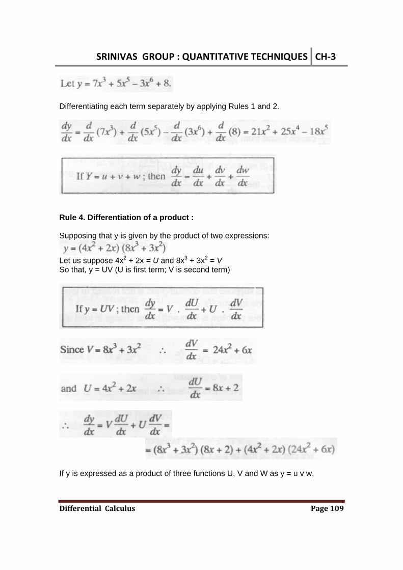
SRINIVAS GROUP : QUANTITATIVE TECHNIQUES CH‐3
DifferentialCalculus Page109
Differentiating each term separately by applying Rules 1 and 2.
Rule 4. Differentiation of a product : Supposing that y is given by the product of two expressions:
Let us suppose 4x2 + 2x = U and 8x3 + 3x2 = V So that, y = UV (U is first term; V is second term)
If y is expressed as a product of three functions U, V and W as y = u v w,
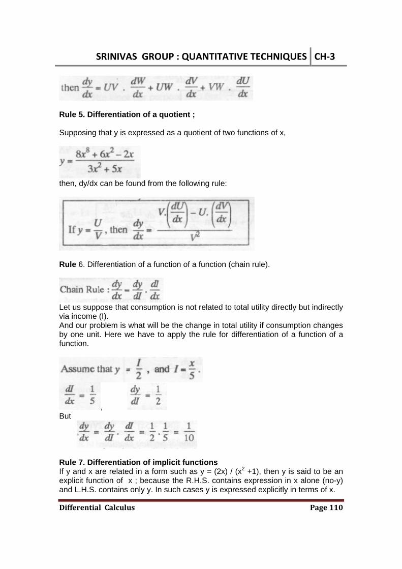
SRINIVAS GROUP : QUANTITATIVE TECHNIQUES CH‐3
DifferentialCalculus Page110
Rule 5. Differentiation of a quotient ; Supposing that y is expressed as a quotient of two functions of x,
then, dy/dx can be found from the following rule:
Rule 6. Differentiation of a function of a function (chain rule).
Let us suppose that consumption is not related to total utility directly but indirectly via income (I). And our problem is what will be the change in total utility if consumption changes by one unit. Here we have to apply the rule for differentiation of a function of a function.
, But
Rule 7. Differentiation of implicit functions If y and x are related in a form such as y = (2x) / (x2 +1), then y is said to be an explicit function of x ; because the R.H.S. contains expression in x alone (no-y) and L.H.S. contains only y. In such cases y is expressed explicitly in terms of x.
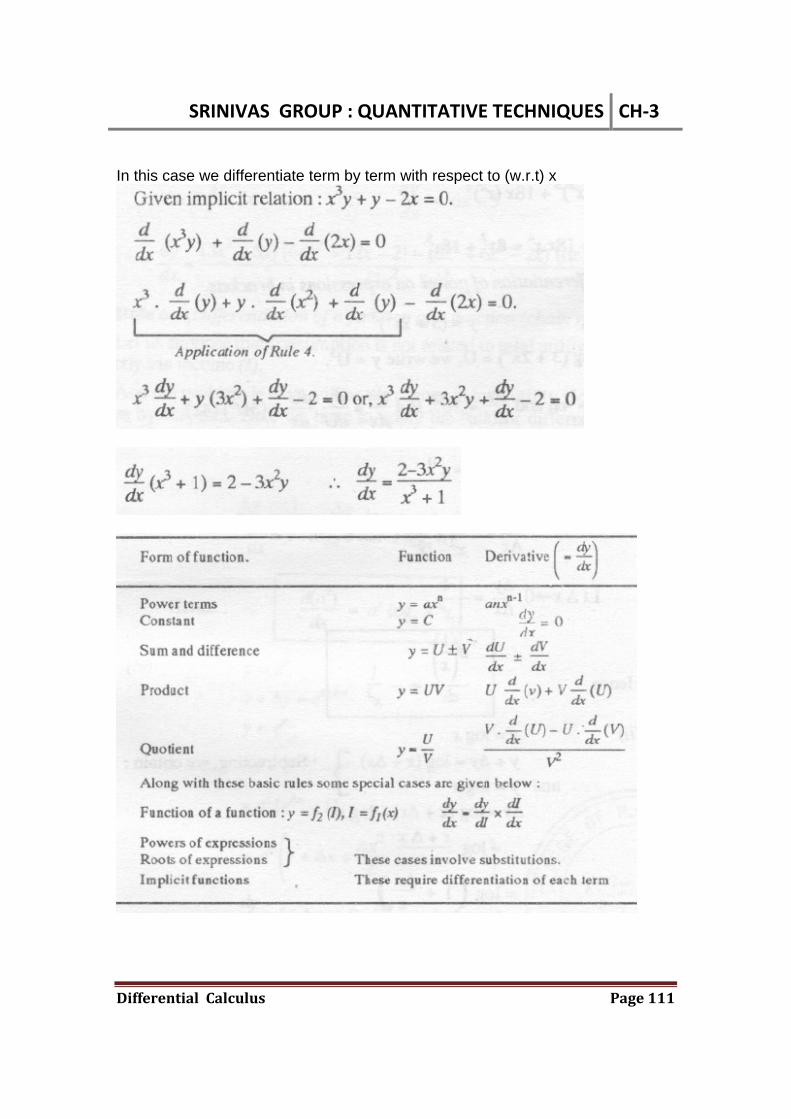
SRINIVAS GROUP : QUANTITATIVE TECHNIQUES CH‐3
DifferentialCalculus Page111
In this case we differentiate term by term with respect to (w.r.t) x

SRINIVAS GROUP : QUANTITATIVE TECHNIQUES CH‐3
DifferentialCalculus Page112
3. Derivatives of linear and quadratic equations :

SRINIVAS GROUP : QUANTITATIVE TECHNIQUES CH‐3
DifferentialCalculus Page113
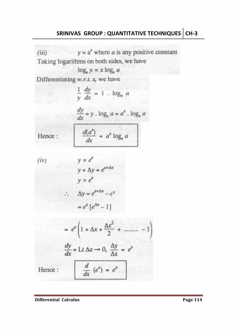
SRINIVAS GROUP : QUANTITATIVE TECHNIQUES CH‐3
DifferentialCalculus Page114
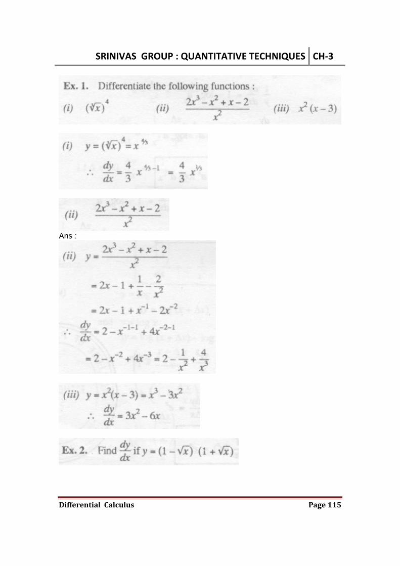
SRINIVAS GROUP : QUANTITATIVE TECHNIQUES CH‐3
DifferentialCalculus Page115
Ans :

SRINIVAS GROUP : QUANTITATIVE TECHNIQUES CH‐3
DifferentialCalculus Page116

SRINIVAS GROUP : QUANTITATIVE TECHNIQUES CH‐3
DifferentialCalculus Page117
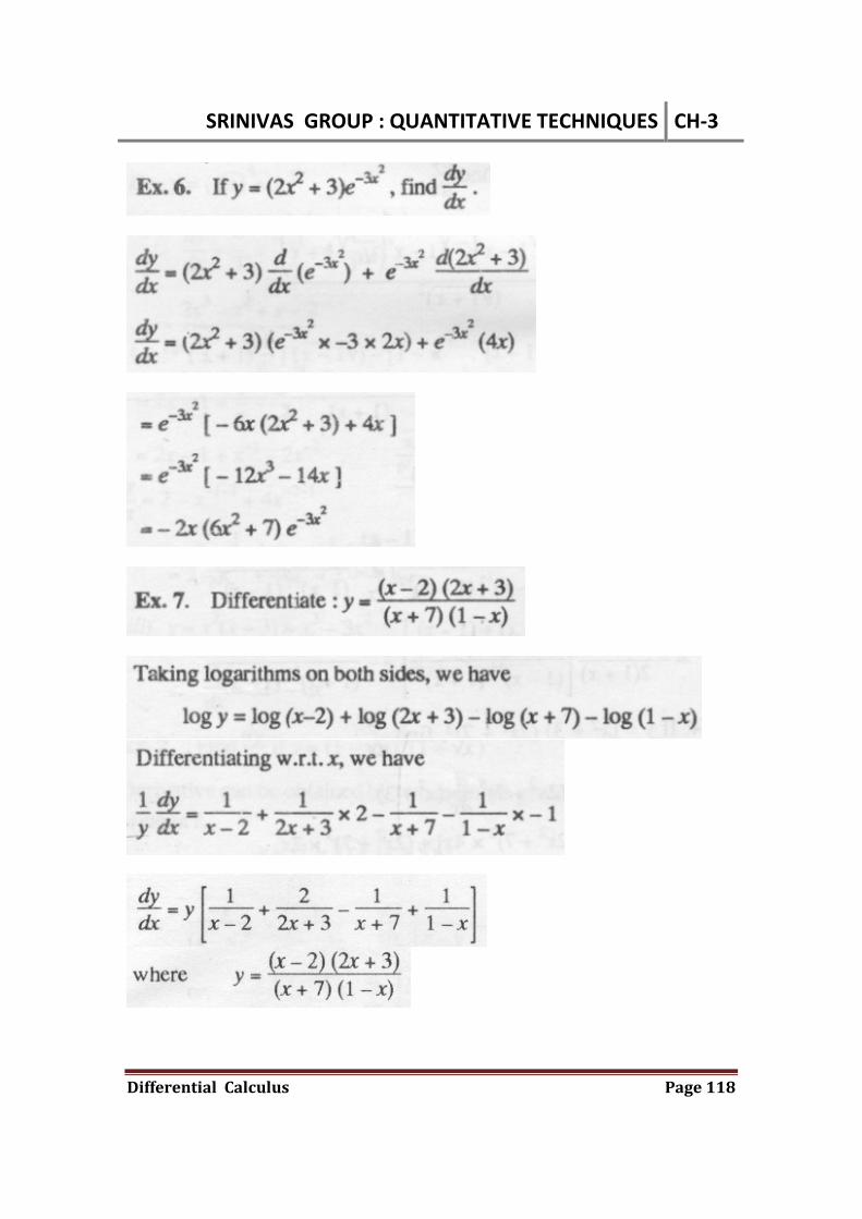
SRINIVAS GROUP : QUANTITATIVE TECHNIQUES CH‐3
DifferentialCalculus Page118

SRINIVAS GROUP : QUANTITATIVE TECHNIQUES CH‐3
DifferentialCalculus Page119
Ex. 8, Find the derivative of the following function (z)_with respect to x, given that
Hence, differentiating first function w.r,t. y and second function with respect to x, we have
Differentiating both sides w.r.t. x, we have
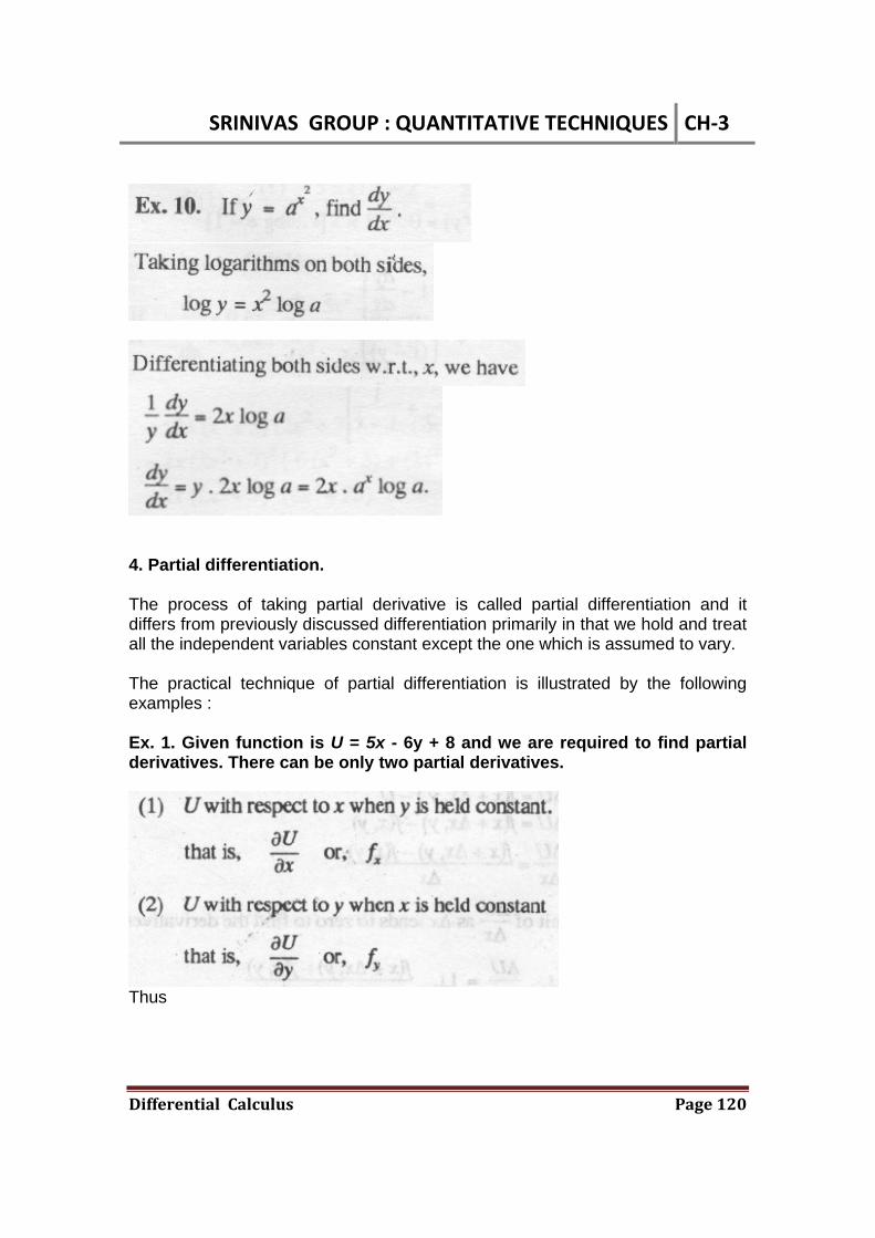
SRINIVAS GROUP : QUANTITATIVE TECHNIQUES CH‐3
DifferentialCalculus Page120
4. Partial differentiation. The process of taking partial derivative is called partial differentiation and it differs from previously discussed differentiation primarily in that we hold and treat all the independent variables constant except the one which is assumed to vary. The practical technique of partial differentiation is illustrated by the following examples : Ex. 1. Given function is U = 5x - 6y + 8 and we are required to find partial derivatives. There can be only two partial derivatives.
Thus
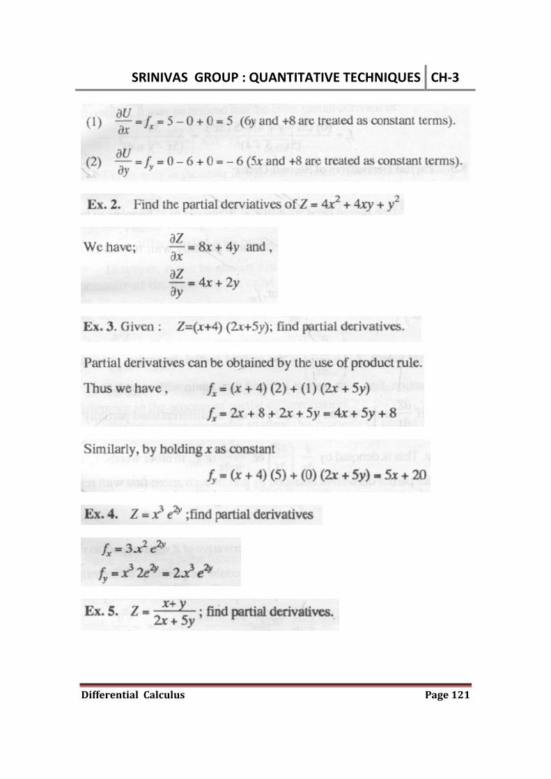
SRINIVAS GROUP : QUANTITATIVE TECHNIQUES CH‐3
DifferentialCalculus Page121

SRINIVAS GROUP : QUANTITATIVE TECHNIQUES CH‐3
DifferentialCalculus Page122
5. Determination of maxima and minima optimization problems in business. Relation of function with respect to its derivative gives us the following important properties of the derivatives : (1) If dy/dx 0, i.e., when first derivative of the given function is positive, the curve rises from left to right. (2) If dy/dx 0, i.e., when first derivative of the given function is negative, the curve falls from left to right. (3) When dy/dx = 0 at any point, it means that the rate of change in y with respect to a small increment in x at that particular point is zero. Ex :
(1)
i.e., dy/dx = 0 when x = 2
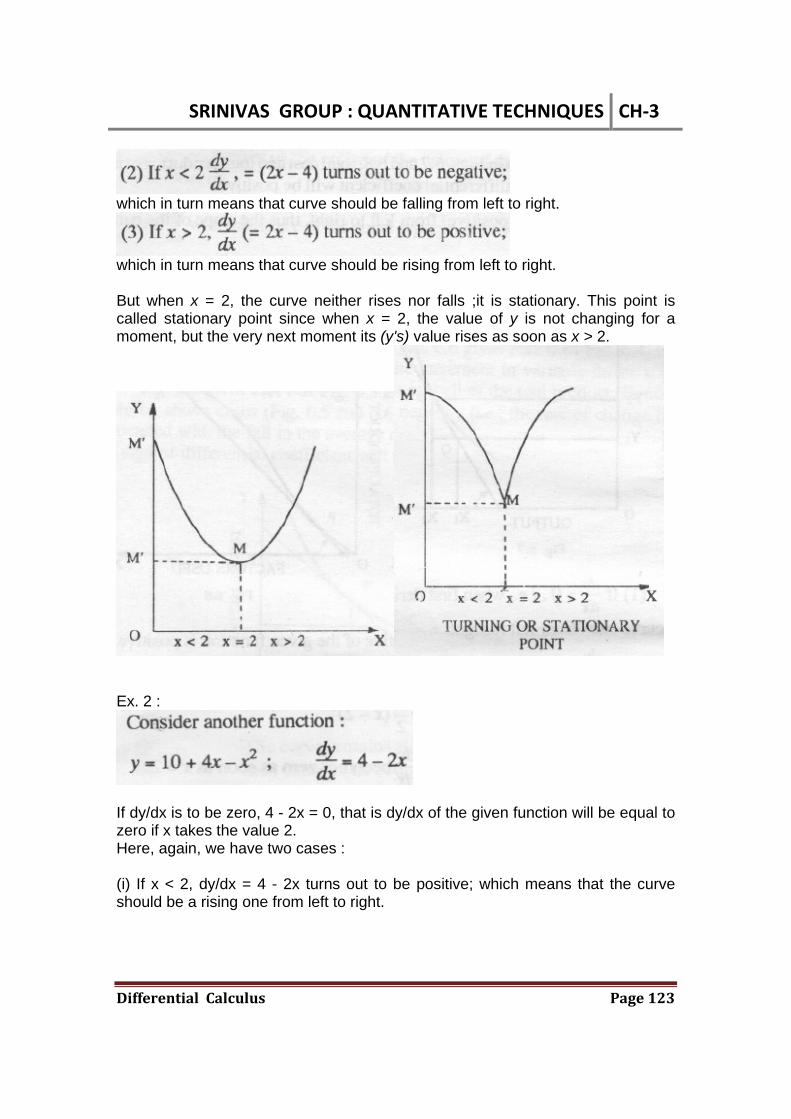
SRINIVAS GROUP : QUANTITATIVE TECHNIQUES CH‐3
DifferentialCalculus Page123
which in turn means that curve should be falling from left to right.
which in turn means that curve should be rising from left to right. But when x = 2, the curve neither rises nor falls ;it is stationary. This point is called stationary point since when x = 2, the value of y is not changing for a moment, but the very next moment its (y's) value rises as soon as x > 2.
Ex. 2 :
If dy/dx is to be zero, 4 - 2x = 0, that is dy/dx of the given function will be equal to zero if x takes the value 2. Here, again, we have two cases : (i) If x < 2, dy/dx = 4 - 2x turns out to be positive; which means that the curve should be a rising one from left to right.
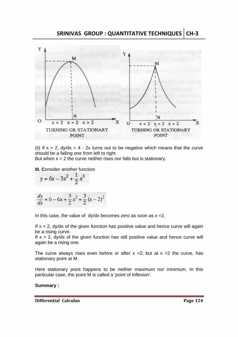
SRINIVAS GROUP : QUANTITATIVE TECHNIQUES CH‐3
DifferentialCalculus Page124
(ii) If x > 2, dy/dx = 4 - 2x turns out to be negative which means that the curve should be a falling one from left to right. But when x = 2 the curve neither rises nor falls but is stationary. III. Consider another function
In this case, the value of dy/dx becomes zero as soon as x =2. If x < 2, dy/dx of the given function has positive value and hence curve will again be a rising curve. If x > 2, dy/dx of the given function has still positive value and hence curve will again be a rising one. The curve always rises even before or after x =2; but at x =2 the curve, has stationary point at M. Here stationary point happens to be neither maximum nor minimum. In this particular case, the point M is called a 'point of inflexion'. Summary :
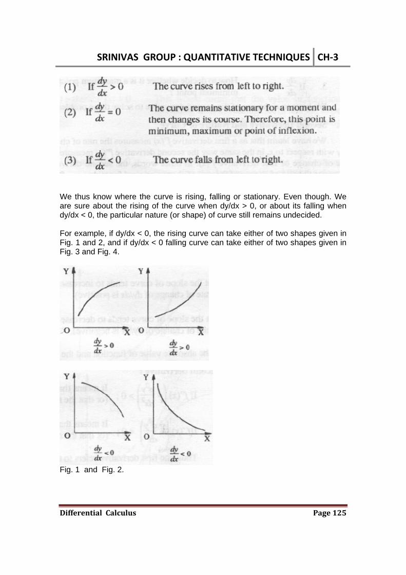
SRINIVAS GROUP : QUANTITATIVE TECHNIQUES CH‐3
DifferentialCalculus Page125
We thus know where the curve is rising, falling or stationary. Even though. We are sure about the rising of the curve when dy/dx > 0, or about its falling when dy/dx < 0, the particular nature (or shape) of curve still remains undecided. For example, if dy/dx < 0, the rising curve can take either of two shapes given in Fig. 1 and 2, and if dy/dx < 0 falling curve can take either of two shapes given in Fig. 3 and Fig. 4.
Fig. 1 and Fig. 2.
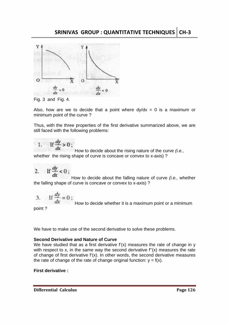
SRINIVAS GROUP : QUANTITATIVE TECHNIQUES CH‐3
DifferentialCalculus Page126
Fig. 3 and Fig. 4. Also, how are we to decide that a point where dy/dx = 0 is a maximum or minimum point of the curve ? Thus, with the three properties of the first derivative summarized above, we are still faced with the following problems:
How to decide about the rising nature of the curve (i.e., whether the rising shape of curve is concave or convex to x-axis) ?
How to decide about the falling nature of curve (i.e., whether the falling shape of curve is concave or convex to x-axis) ?
How to decide whether it is a maximum point or a minimum point ? We have to make use of the second derivative to solve these problems. Second Derivative and Nature of Curve We have studied that as a first derivative f’(x) measures the rate of change in y with respect to x, in the same way the second derivative f'’(x) measures the rate of change of first derivative f’(x). In other words, the second derivative measures the rate of change of the rate of change original function: y = f(x). First derivative :

SRINIVAS GROUP : QUANTITATIVE TECHNIQUES CH‐3
DifferentialCalculus Page127
It means that the value of function tends to increase (or that the rate of change of y w.r.t. x is positive).
It means that the value of function tends to decrease (or that the rate of change of y w.r.t. x is negative). Second derivative :
It means that the slope of curve tends to increase (or that the rate of change of dy/dx is positive).
It means that the slope of curve tends to decrease (or that the rate of change of dy/dx is negative). Thus, the first derivative refers to the absolute value of function and the second derivative refers to the slope of the curve. We consider the following four possible cases :
This would mean that the value of function is increasing at an increasing rate or that the slope of the curve at this point is positive and increasing as the value of x increases.
This would mean that the value of function is increasing at a decreasing rate or that the slope of the curve is positive but decreasing as the value of x increases.
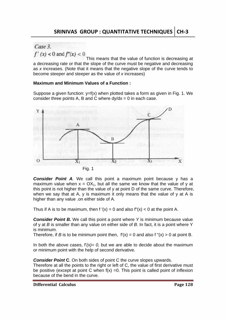
SRINIVAS GROUP : QUANTITATIVE TECHNIQUES CH‐3
DifferentialCalculus Page128
This means that the value of function is decreasing at a decreasing rate or that the slope of the curve must be negative and decreasing as x increases. (Note that it means that the negative slope of the curve tends to become steeper and steeper as the value of x increases) Maximum and Minimum Values of a Function : Suppose a given function: y=f(x) when plotted takes a form as given in Fig. 1. We consider three points A, B and C where dy/dx = 0 in each case.
Fig. 1 Consider Point A. We call this point a maximum point because y has a maximum value when x = OX1, but all the same we know that the value of y at this point is not higher than the value of y at point D of the same curve. Therefore, when we say that at A, y is maximum it only means that the value of y at A is higher than any value .on either side of A. Thus if A is to be maximum, then f '(x) = 0 and also f"(x) < 0 at the point A. Consider Point B. We call this point a point where Y is minimum because value of y at B is smaller than any value on either side of B. In fact, it is a point where Y is minimum. Therefore, if B is to be minimum point then, f'(x) = 0 and also f "(x) > 0 at point B. In both the above cases, f’(x)= 0, but we are able to decide about the maximum or minimum point with the help of second derivative. Consider Point C. On both sides of point C the curve slopes upwards. Therefore at all the points to the right or left of C, the value of first derivative must be positive (except at point C when f(x) =0. This point is called point of inflexion because of the bend in the curve.
SRINIVAS GROUP : QUANTITATIVE TECHNIQUES CH‐3
DifferentialCalculus Page129
The simple criteria for points of inflexion : (1) f'(x) = 0 but f'(x) = 0 there is a point of inflexion. (2) f'(x) = 0, f'(x) = 0 but f"(x) = 0 then, if f' (x) < 0 it is maximum and if f"(x) > 0 it is minimum. Order Conditions for Maximum-Minimum (Extreme) Values : We have learnt that for a function y =f(x) if its first derivative at a certain point (say at x =a) is equal to zero then the value of the given function at this point (x = a) will either be : (i) minimum if f’’(a) > 0 or, (ii) maximum if f’’(a) < 0. Thus, we observe that the given function should satisfy two conditions in order to decide about maximum or minimum value at a particular point. These conditions are known as Order Conditions.
Ex. 1. Find the maximum and minimum values of the following functions :

SRINIVAS GROUP : QUANTITATIVE TECHNIQUES CH‐3
DifferentialCalculus Page130
First order condition for maximum and minimum value is f' (x) = 0. Therefore, if the given function has maximum or minimum value then 3x2 - 3 = 0 ,i.e., x = 1. To distinguish between maximum and minimum values, we apply second order condition:
Hence the function y has a minimum value-l at x = 1andmaximum value 3 at x = -1.
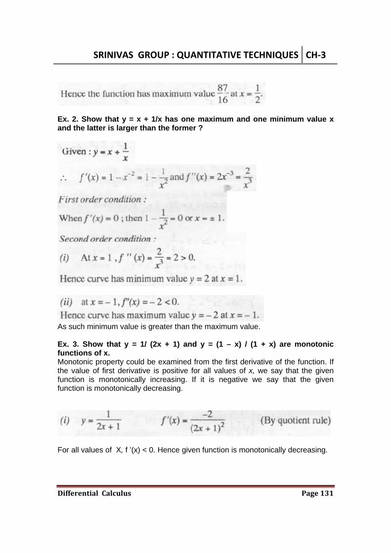
SRINIVAS GROUP : QUANTITATIVE TECHNIQUES CH‐3
DifferentialCalculus Page131
Ex. 2. Show that y = x + 1/x has one maximum and one minimum value x and the latter is larger than the former ?
As such minimum value is greater than the maximum value. Ex. 3. Show that y = 1/ (2x + 1) and y = (1 – x) / (1 + x) are monotonic functions of x. Monotonic property could be examined from the first derivative of the function. If the value of first derivative is positive for all values of x, we say that the given function is monotonically increasing. If it is negative we say that the given function is monotonically decreasing.
For all values of X, f ’(x) < 0. Hence given function is monotonically decreasing.

SRINIVAS GROUP : QUANTITATIVE TECHNIQUES CH‐3
DifferentialCalculus Page132
For all values of x, f'(x) < 0 Hence the function is monotonically decreasing. SOME APPLICATIONS OF DIFFERENTIAL CALCULUS : Derivatives have wide application in economies, engineering, science, etc. 1. Derivative as a "Rate Measurer". (Velocity and Acceleration of a particle moving in a straight line) When a particle moves in a straight line, its velocity (v) is the rate of change of distance (s) described w.r. to time (t).
represents the average rate of change of s w.r. to t. Similarly, the acceleration (f) is given by the rate of change of velocity (v) w. r. to time (t).
where v/t represents the average acceleration of the particle in time t. Example 1 : A ladder 13 ft long stands against a vertical wall, its foot being 5ft from the junction of the wall and the floor. If the foot of the ladder be pulled out with a velocity of 2 ft per sec., find with what velocity the top begins to descend?
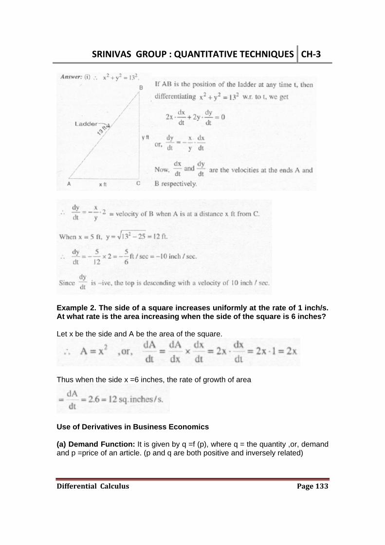
SRINIVAS GROUP : QUANTITATIVE TECHNIQUES CH‐3
DifferentialCalculus Page133
Example 2. The side of a square increases uniformly at the rate of 1 inch/s. At what rate is the area increasing when the side of the square is 6 inches? Let x be the side and A be the area of the square.
Thus when the side x =6 inches, the rate of growth of area
Use of Derivatives in Business Economics (a) Demand Function: It is given by q =f (p), where q = the quantity ,or, demand and p =price of an article. (p and q are both positive and inversely related)

SRINIVAS GROUP : QUANTITATIVE TECHNIQUES CH‐3
DifferentialCalculus Page134
(b) Supply Function : It is given by x = f (p), where p =price of the article and x = amount of supply. (c) Cost Function : It is given by c (x) = f (x) + d, where x 0, and c (x) = total cost, f (x) = variable cost and d = fixed cost (remains fixed at all levels of output) when the output is x units.
(d) Revenue Function : It is given by R(x) = p.x, where p and x are both positive and R (x) =total revenue, p = price/unit and x = units sold. (e) Profit Function : It is given by P(x) = R(x) - c(x), where x > 0. (f) Production Function : It is given by P = f(I, L, R, ), where P = production, I = Investment, L = Labour, R = Raw materials, etc. Example 3. The total cost c(x) of a firm is c(x) =0.0005x3 - 0.7X2 -30x + 3,000, where x is the output. Determine: (a) Average Cost (AC) ; (b) Marginal Cost (MC) ; and (c) Value of x ; for which MVC = AVC, where VC denotes Variable Cost, MVC denotes marginal variable cost and AVC denotes average variable cost.
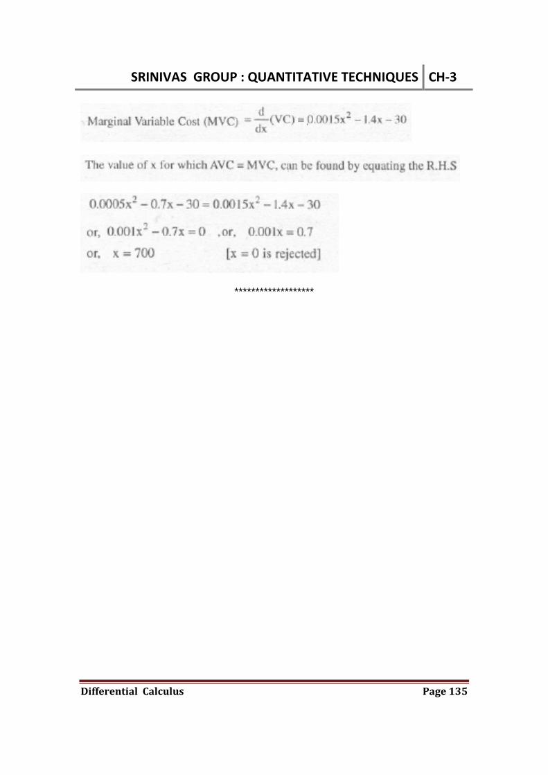
SRINIVAS GROUP : QUANTITATIVE TECHNIQUES CH‐3
DifferentialCalculus Page135
*******************

SRINIVAS GROUP : MBA : QUANTITATIVE TECHNIQUES CH‐4
IntegralCalculus Page136
CHAPTER 4
Integral Calculus Definite & indefinite integral, rules of integration, some standard results in integration. Integration by substitution, Integration by parts. applications to business. 1. Introduction : We have seen that differentiation is the process of finding out rates of changes. If Y =f (x) is a function of x, we can find the rate of change of y with respect to x by differentiating the function and thereby obtaining or f ' (x). If f'(q) is given, our problem is to find out the function f(q) which on differentiating will gives f'(q). Definition. If the differential coefficient of F(x) w.r.t. x is f (x), then an integral of [(x) with respect to x is F(x).
(ii)
Example :

SRINIVAS GROUP : MBA : QUANTITATIVE TECHNIQUES CH‐4
IntegralCalculus Page137
2. Constant of Integration (Indefinite Integration) :
where C is called the constant of integration, Since, C can take any constant value, the integral is called Indefinite Integral. Note :
is equal to log x. (3) If we have to integrate a power term which is in the denominator, we bring it to the numerator,
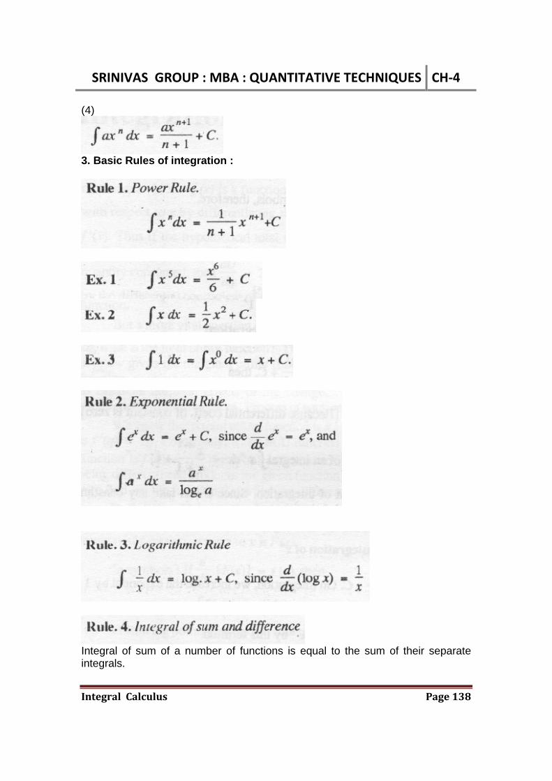
SRINIVAS GROUP : MBA : QUANTITATIVE TECHNIQUES CH‐4
IntegralCalculus Page138
(4)
3. Basic Rules of integration :
Integral of sum of a number of functions is equal to the sum of their separate integrals.

SRINIVAS GROUP : MBA : QUANTITATIVE TECHNIQUES CH‐4
IntegralCalculus Page139
Ex. 1 ;
Ex. 2 :
If a function is multiplied by a constant number, this number will remain a multiple of the integral of the function. Ex. 1 :
Ex. 2 :
4. Standard Results : ( + C is implied in all the results ) Results are summarized below :
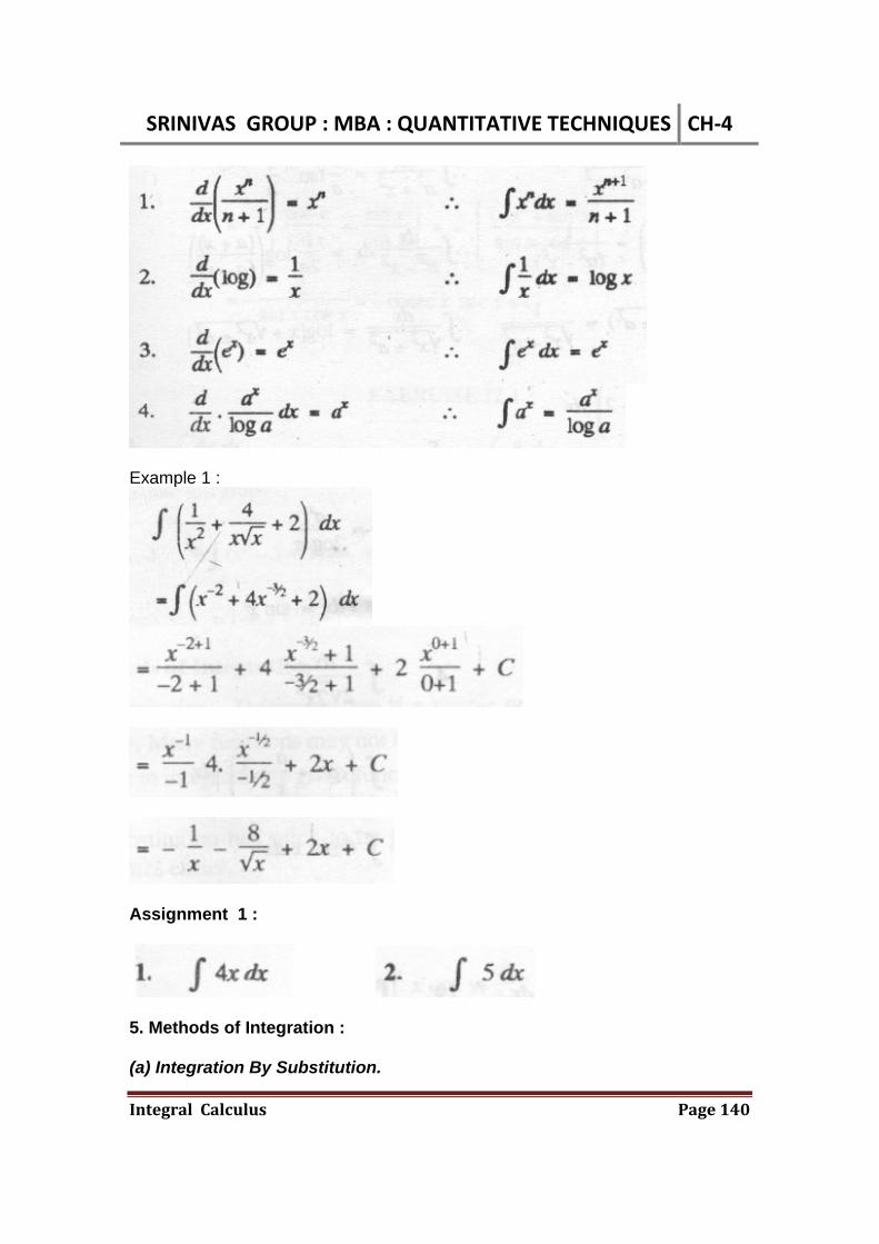
SRINIVAS GROUP : MBA : QUANTITATIVE TECHNIQUES CH‐4
IntegralCalculus Page140
Example 1 :
Assignment 1 :
5. Methods of Integration : (a) Integration By Substitution.

SRINIVAS GROUP : MBA : QUANTITATIVE TECHNIQUES CH‐4
IntegralCalculus Page141
Differentiation is a simple process, but integration is often not easy. Many functions may not be integrated at all. In order to integrate any given function, we try to transform the function to standard form by suitable substitution and then use the standard result. Example 1 :
We shall try to reduce it to the standard form :
y = (5x + 7)
But 'dx' too will have to be changed to 'dy' otherwise integration will not be possible.
Example 2 :
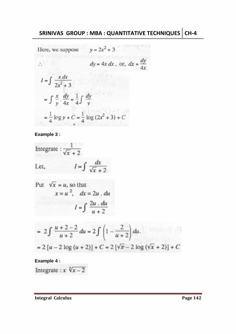
SRINIVAS GROUP : MBA : QUANTITATIVE TECHNIQUES CH‐4
IntegralCalculus Page142
Example 3 :
Example 4 :
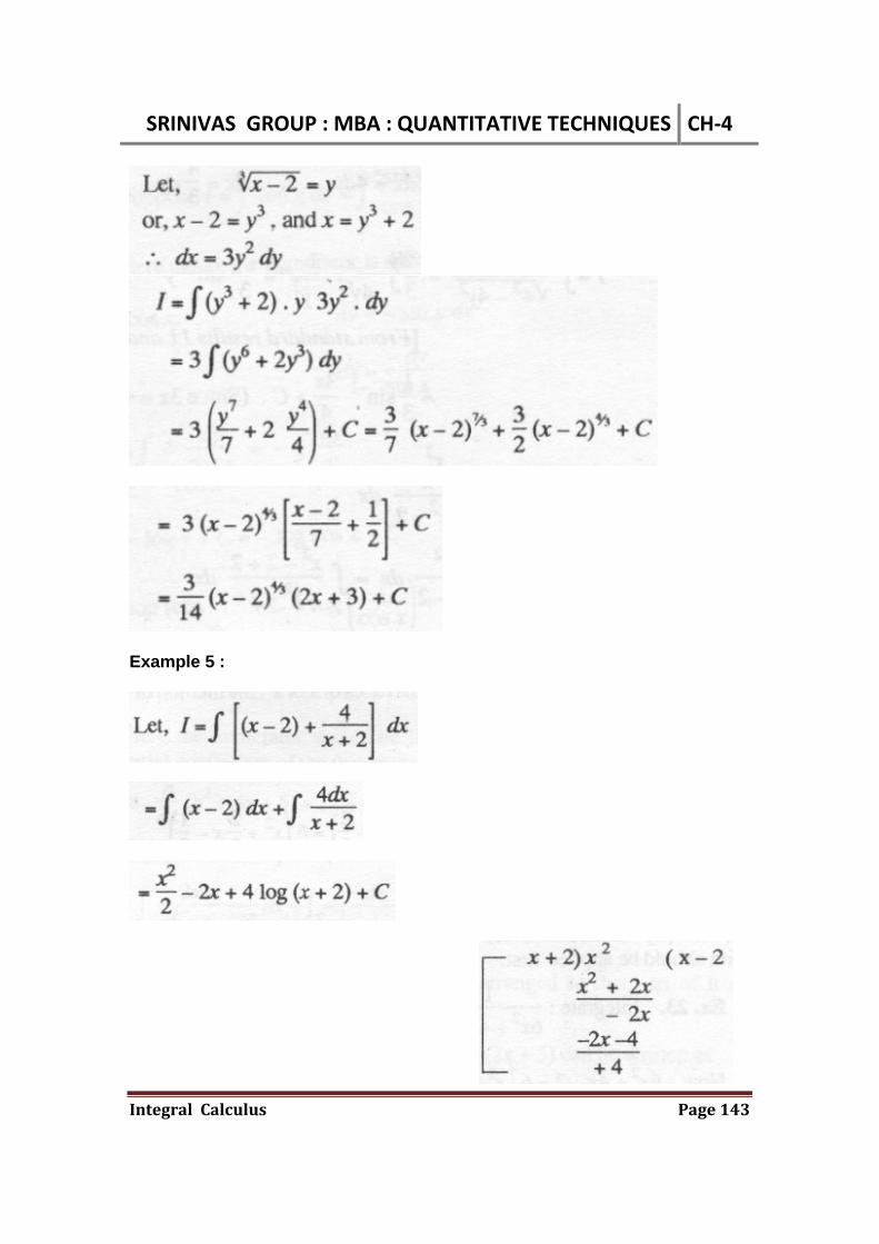
SRINIVAS GROUP : MBA : QUANTITATIVE TECHNIQUES CH‐4
IntegralCalculus Page143
Example 5 :

SRINIVAS GROUP : MBA : QUANTITATIVE TECHNIQUES CH‐4
IntegralCalculus Page144
(b) Integration By Parts : Integration of a product of the functions U and V :
Ex. 1 :
Ans :
Ex. 2 :
Ans : Let the first function be log x.

SRINIVAS GROUP : MBA : QUANTITATIVE TECHNIQUES CH‐4
IntegralCalculus Page145
6. Definite Integrals : If x is the differential coefficient of F(x); we say that
because C is unknown here. But if integral of f(x) exists for all values of x from a to b, we define
as a definite integral of f(x) between limits a and b, a is the lower limit and b is the upper limit. Ex :
Important steps in evaluating a definite integral:
(1) Find the indefinite integral ∫f(x)dx = F(x) +C
(2) Substitute for x in this integral the upper limit b, i.e., = F(b) + C. (3) Substitute for x in the lower limit a, i.e., = F(a) + C (4) Subtract (2) from (3), i.e., F(a) + C from F(b) + C, so that :

SRINIVAS GROUP : MBA : QUANTITATIVE TECHNIQUES CH‐4
IntegralCalculus Page146
Ex. 1 : Find the value of
Ans :
Ex. 2 : Find the value of
Ans :

SRINIVAS GROUP : MBA : QUANTITATIVE TECHNIQUES CH‐4
IntegralCalculus Page147
Ex. 3 : Find the value of
Ans :
Ex. 4 : Find the value of
Ans :
Ex. 5 : Find the value of
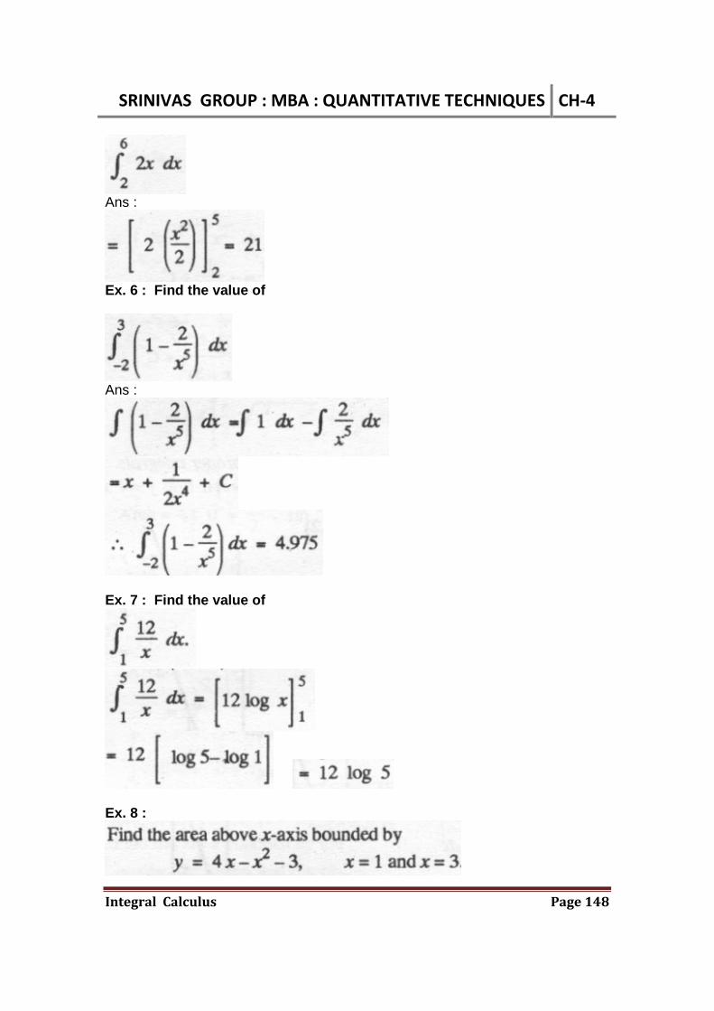
SRINIVAS GROUP : MBA : QUANTITATIVE TECHNIQUES CH‐4
IntegralCalculus Page148
Ans :
Ex. 6 : Find the value of
Ans :
Ex. 7 : Find the value of
Ex. 8 :
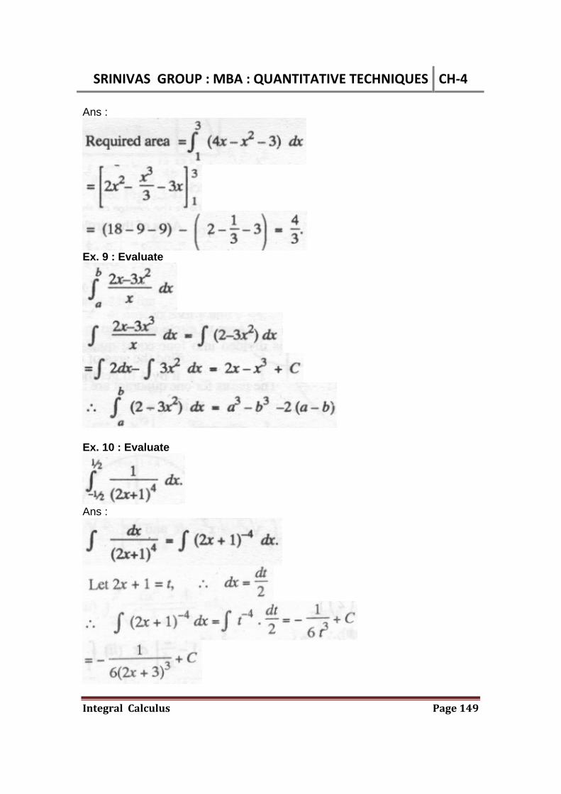
SRINIVAS GROUP : MBA : QUANTITATIVE TECHNIQUES CH‐4
IntegralCalculus Page149
Ans :
Ex. 9 : Evaluate
Ex. 10 : Evaluate
Ans :

SRINIVAS GROUP : MBA : QUANTITATIVE TECHNIQUES CH‐4
IntegralCalculus Page150
Such integrals are called improper integrals. Ex. 11 : Find the area between line y = 4x and axis of x and the ordinate x = 4 ? Ans : We have to find the area 0AB of (Fig.1) Limits : x = 0 to x = 4. Area required
Fig. 1 Ex. 12 : Find the are a bounded by the parabola x2 = 4by, the x-axis and the ordinate at x = 3 ? Ans : The required area is equal to

SRINIVAS GROUP : MBA : QUANTITATIVE TECHNIQUES CH‐4
IntegralCalculus Page151
Fig. 2 Ex. 13 : Find the area bounded by the parabola x2 = 4by, axis of y and y =4. Ans : The required area to be found is OAB = 2OAC (Fig.3)
Fig. 3 Ex. 14 : Find the area above the axis of x bounded by x -2y +4 = 0, x = 3 and x = 6 ? Ans : We are given: x -2y +4 = 0
Required area =
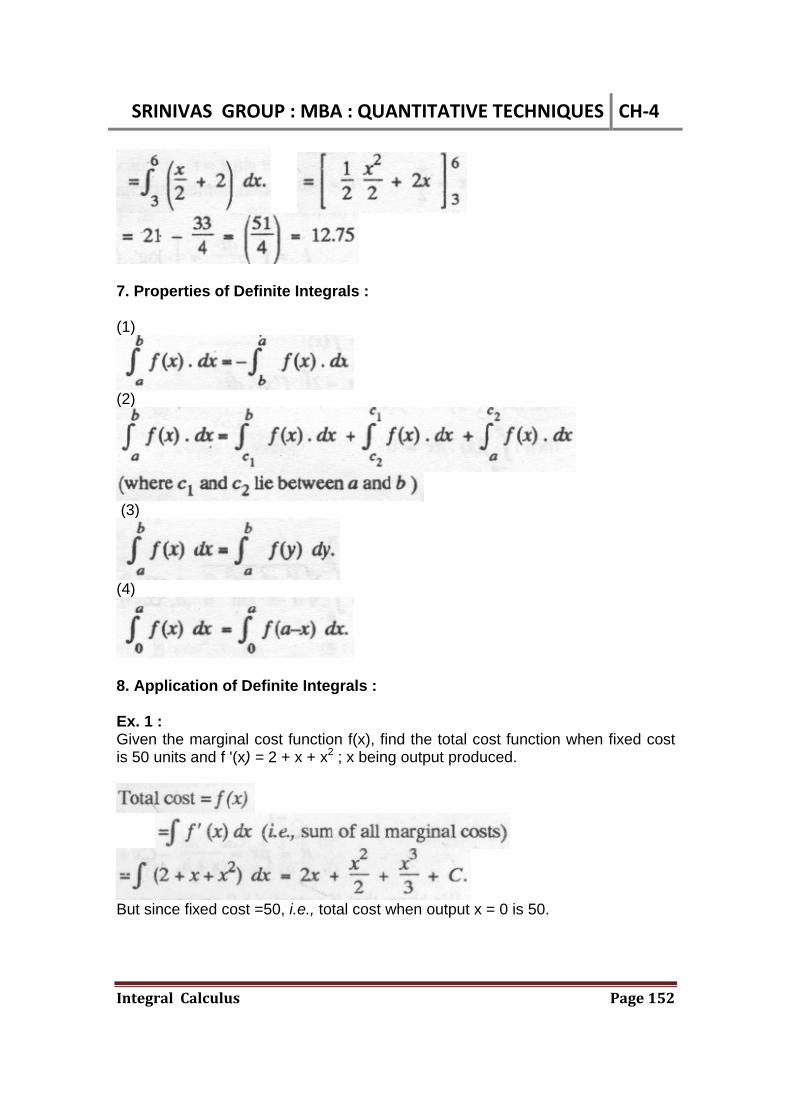
SRINIVAS GROUP : MBA : QUANTITATIVE TECHNIQUES CH‐4
IntegralCalculus Page152
7. Properties of Definite Integrals : (1)
(2)
(3)
(4)
8. Application of Definite Integrals : Ex. 1 : Given the marginal cost function f(x), find the total cost function when fixed cost is 50 units and f '(x) = 2 + x + x2 ; x being output produced.
But since fixed cost =50, i.e., total cost when output x = 0 is 50.
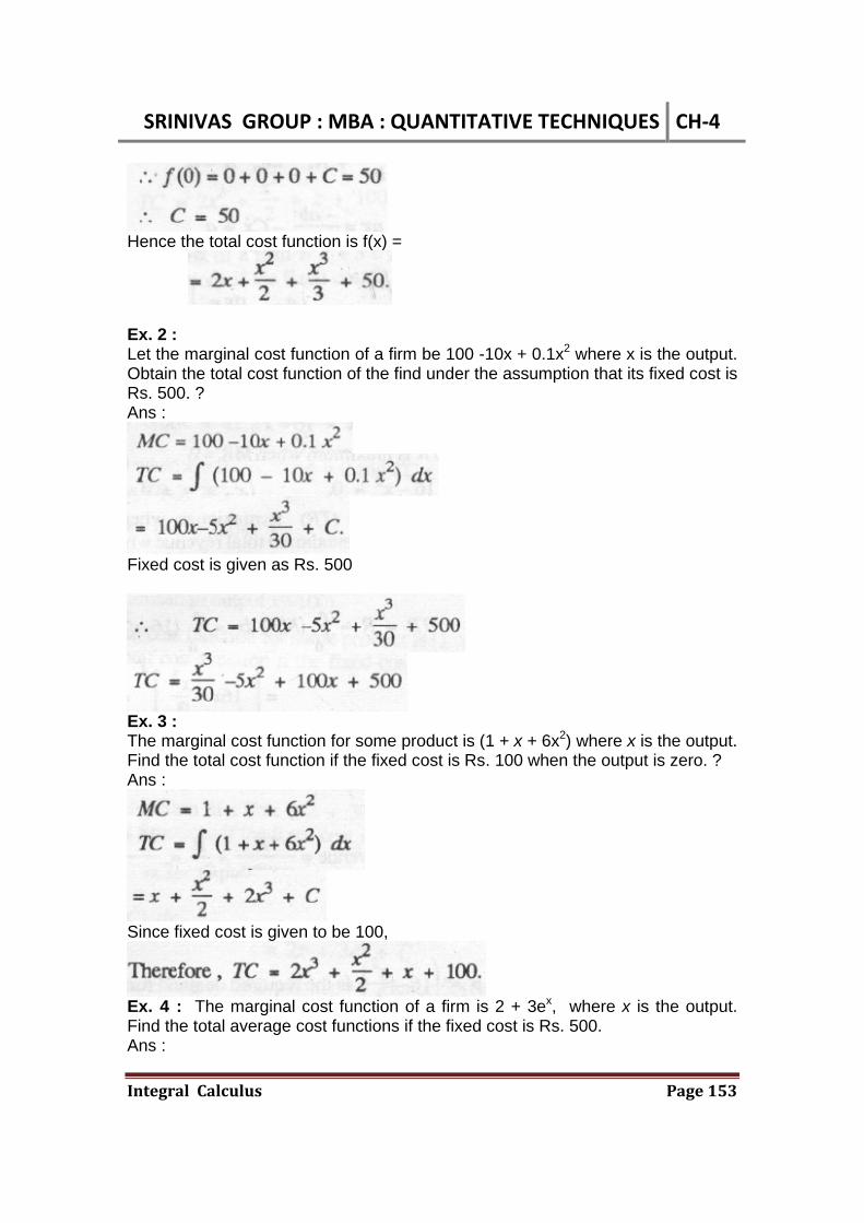
SRINIVAS GROUP : MBA : QUANTITATIVE TECHNIQUES CH‐4
IntegralCalculus Page153
Hence the total cost function is f(x) =
Ex. 2 : Let the marginal cost function of a firm be 100 -10x + 0.1x2 where x is the output. Obtain the total cost function of the find under the assumption that its fixed cost is Rs. 500. ? Ans :
Fixed cost is given as Rs. 500
Ex. 3 : The marginal cost function for some product is (1 + x + 6x2) where x is the output. Find the total cost function if the fixed cost is Rs. 100 when the output is zero. ? Ans :
Since fixed cost is given to be 100,
Ex. 4 : The marginal cost function of a firm is 2 + 3ex, where x is the output. Find the total average cost functions if the fixed cost is Rs. 500. Ans :
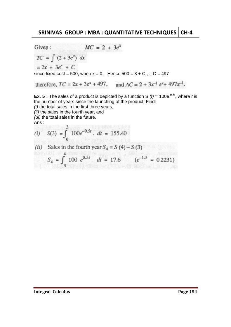
SRINIVAS GROUP : MBA : QUANTITATIVE TECHNIQUES CH‐4
IntegralCalculus Page154
since fixed cost = 500, when x = 0. Hence 500 = 3 + C , :. C = 497
Ex. 5 : The sales of a product is depicted by a function S (t) = 100e-0.5t, where t is the number of years since the launching of the product. Find: (i) the total sales in the first three years, (ii) the sales in the fourth year, and (ui) the total sales in the future. Ans :