Remote Sensing of Environment 138 (2013) 1–9

Contents lists available at SciVerse ScienceDirect

Remote Sensing of Environment

j ourna l homepage: www.e lsev ie r .com/ locate / rse

Spatial upscaling of in-situ soil moisture measurements based onMODIS-derived apparent thermal inertia

Jun Qin a,⁎, Kun Yang a, Ning Lu b, Yingying Chen a, Long Zhao a, Menglei Han a

a Laboratory of Tibetan Environment Changes and Land Surface Processes, Institute of Tibetan Plateau Research, Chinese Academy of Sciences, P.O. Box 2871, Beijing 100101, Chinab State Key Laboratory of Resources and Environmental information, Institute of Geographic Sciences and Natural Resources Research, Chinese Academy of Science, Beijing 100101, China

⁎ Corresponding author. Tel.: +86 10 84097059.E-mail address: shuairenqin@gmail.com (J. Qin).

0034-4257/$ – see front matter © 2013 Elsevier Inc. All rihttp://dx.doi.org/10.1016/j.rse.2013.07.003

a b s t r a c t

a r t i c l e i n f o

Article history:Received 5 December 2012Received in revised form 1 July 2013Accepted 7 July 2013Available online xxxx

Keywords:UpscalingSoil moistureApparent thermal inertiaTibetan Plateau

Soil moisture plays an essential role in the terrestrial water cycle. It is very important to obtain soil moisture formany applications. Soil moisture acquired by remote sensing, land surface modeling, and data assimilation mustbe evaluated against in-situ measurements before being used, but a procedure should be performed to upscalethe point-scale measurements to the grid-scale or footprint-scale. In this study, a new upscaling algorithm is de-veloped by introducing MODIS-derived apparent thermal inertia (ATI). First, a functional relationship betweenthe station-averaged soil moisture and the pixel-averaged ATI is constructed. Second, this relationship is usedto calculate the representative soil moisture time series at a certain spatial scale. Last, the Bayesian linear regres-sion is applied to obtain the upscaled area-averaged soilmoisture by using in-situmeasurements as independentvariables. The algorithm is evaluated using a network of in-situ moisture sensors in the central Tibetan Plateau.The results indicate that it can effectively obtain the area-averaged soil moisture, reducing the root mean squareerror (RMSE) from 0.023 m3/m3 before upscaling to 0.013 m3/m3 after upscaling. Finally, the algorithm is im-plemented to the 100 km × 100 km grid box where the network is installed, and the temporal pattern of theupscaled soil moisture agrees with the hydro-meteorological knowledge of this region.

© 2013 Elsevier Inc. All rights reserved.

1. Introduction

Soil moisture plays a significant role in the terrestrial water cycle(Hirabayashi, Kanae, Struthers, & Oki, 2005; Seneviratne et al., 2010;Sheffield & Wood, 2007). It is very important to obtain informationabout soil moisture due to its profound impacts on applications suchas flood forecasting, weather and climate prediction, crop growthmon-itoring, and water management (Claussen, 1998; Davies & Allen, 1973;Drusch, 2007; Schmugge, Kustas, Ritchie, Jackson, & Rango, 2002; Texieret al., 1997). There are generally fourmethods to estimate the soil mois-ture status. First, it can be measured in the field with ground-based in-struments (Roth, Malicki, & Plagge, 2006). Second, the soil moisturecould be obtained by running land surface models with meteorologicaldata and other parameters as inputs at a certain spatial resolution(such as 25 km2 or 100 km2) (Rodell et al., 2004). Third, remote sens-ing, especially microwave remote sensing such as the Advanced Micro-wave Scanning Radiometer for EOS (AMSR-E) (Njoku, Jackson, Lakshmi,Chan, & Nghiem, 2003), the Soil Moisture and Ocean Salinity (SMOS)mission (Kerr et al., 2001), and the upcoming Soil Moisture ActivePassive (SMAP) mission (Entekhabi et al., 2010), provides an efficientand effective method to globally acquire the surface soil moisture withhigh spatial and temporal resolutions. Fourth, data assimilation tech-niques have recently been applied to merge the remote sensing signal

ghts reserved.

into land surfacemodels to estimate the soilmoisture in a physically con-sistent way (Pan & Wood, 2006; Qin et al., 2009; Reichle, McLaughlin, &Entekhabi, 2002; Yang et al., 2007). Although the latter three methodscan be used to retrieve the soil moisture at the regional or global scaleat a lower cost than the first one, these estimated values need to be val-idated against in-situ measurements.

It is well known that the in-situ soil moisture measurements aremerely representative over a very small spatial scale (point-scale)because the soil moisture has a high spatial variability due to the signif-icant spatial heterogeneity of soil, vegetation, topography, and precipi-tation (Crow et al., 2012; Verstraeten, Veroustraete, & Feyen, 2008;Western, Grayson, & Blöschl, 2002). On the other hand, the remotesensing footprint (such as ~602 km2for AMSR-E, 302–502km2forSMOS, and ~402km2for SMAP) is much larger than the representativearea (~52 cm2) of in-situ soil moisture measurements. The similar situ-ation happens to the soil moisture estimates obtained from land surfacemodels or data assimilation systems, as themodel grid-box size is great-er than the support of in-situ moisture observations. In order to obtainthe spatially averaged soil moisture to validate remote sensingmoistureproducts ormodel simulations, a large number of ground-based sensorsusually have to be installed over an area of the size comparable to theremote sensing footprint or the model grid-box. There is, however, nosimpleway to accurately estimate this number. The pragmatic approachis to upscale surface soil moisturemeasurements at a limited number ofstations to the scale of interest such as the satellite footprint or themodel grid box.

2 J. Qin et al. / Remote Sensing of Environment 138 (2013) 1–9

There have been several upscaling strategies (Crow et al., 2012). Themost popular one is based on the concept of temporal stability. One ormore temporally stable stations can be identified after the soil moisturevalues at these stations are compared with the area-averaged soil mois-ture derived from a number of stations in an area according to severalstatistical indicators (Cosh, Jackson, Starks, & Heathman, 2006). Then,the measurements at a temporally stable station are used to representthe average value in this area. The second strategy is to implement ageostatistical algorithm, such as the block kriging, to find the spatialcorrelation structure (semivariogram) of soil moisture measurementsat different stations in an area and then apply it to compute the area-averaged values (Vinnikov, Robock, Qiu, & Entin, 1999). The thirdmeth-od is based on intensive field campaigns (de Rosnay et al., 2009). A largenumber of soil moisture measurements are collected at different timesand stations in an area. Several temporally stable stations are identifiedand then a linear regression relationship is constructed between themoisture measurements at these stations and the averaged moisturevalues within an area. The fourth strategy is to run a land surfacemodel at a fine spatial resolution and then utilize the resulting spatialpattern of soil moisture to perform the upscaling (Crow, Ryu, &Famiglietti, 2005; Loew & Schlenz, 2011).

These previous studies show that when only a limited number ofstations are available over a large area, extra information is needed tosupport upscaling of in-situ measurements. The extra information forthe temporal stability method is the assumption that the simple arith-metic mean at a limited number of stations could represent the realarea-averaged soil moisture. This information used by the geostatisticalmethod is that the calculated spatial correlation could really reflect thespatial structure of soil moisture. The third method assumes that themeanmoisture at some stations could represent the real spatially aver-aged moisture. The fourth strategy supposes that the spatial patterns ofsoil moisture simulated by land surface models are trustable. However,the extra information for these four upscaling methods is often ques-tionable in consideration of the spatial heterogeneity of soilmoisture in-duced by the high spatial variability of soil, vegetation, topography, andprecipitation at small spatial scales.

In fact, in-situ moisture measurements at several stations within alarge area could roughly capture the temporal pattern of the truearea-averaged moisture, but might lose fidelity to both the magnitudeand the range of variation. If a certain quantity, the averaged values ofwhich may not exactly reflect the area-averaged moisture but can cap-ture the moisture dynamics without bias, could be identified, it can beused as the extra information for upscaling. In this study, the MODIS-derived apparent thermal inertia (ATI) plays such a role. An algorithmbased on the Bayesian linear regression is designed to merge both ATIand in-situ moisture in order to estimate the upscaled area-averagedsoil moisture.

2. Study area and data

The Tibetan Plateau (TP) is generally defined as the region above3000 m above sea level, which is the highest plateau all over theworld. It has an average elevation of 4000 m above sea level andan area of ~2.5 × 106 km2. It is well known that the TP's energy andwater dynamics have a profound impact on the weather and climatein the Asian continent (Wu et al., 2007; Yang, Guo, He, Qin, & Koike,2011). Although much progress in hydrometeorological studies hasbeen made based on the existing in-situ observations over the TP, re-mote sensing data can offer significantly more details of processeshappening in this region, because it is impractical to deploy a dense ob-servation network over the entire TP. Validations are needed to assesslarge uncertainties in remote sensing data. In an effort to validate satel-lite products and advance the knowledge of land–atmosphere inter-actions over the TP, the Tibetan Plateau Soil Moisture/TemperatureMonitoring Network (SMTMN) has recently been established.

This network is located in the central TP and set up around the townof Naqu within an area of ~100 km × 100 km with mean elevation4650 m, approximately matching one GCM (global climate model)grid box. The surface with rolling hills is relatively flat in most of thisarea although rugged in some places. This area has a typical semiaridmonsoon climate. In the summer half-year from May to October, theAsia monsoon brings a total of about 400-mm rainfall to this area,while in winter precipitation rarely occurs and soil freezes. The landcover is primarily alpine meadow. The soil mainly comprises bothsand and silt, and exhibits a large spatial variability. In addition, the or-ganic carbon content at the top soil layer is fairly high and declines dra-matically with depth.

The SMTMN is initiated in July of 2010. Thirty-nine sets of moistureinstruments are first installed along four segments of different national/provincial roads illustrated as the white lines in Fig. 1. It is, however,found during the campaign in June of 2011 that nine sets are lost ordamaged by soil water intrusion. In the 2011 campaign, another 20sets are installed, some of which are used to replace the lost anddamaged ones. The others in conjunction with part of original setsform a medium network with a spatial size of 25 km × 25 km nestedin the large one as shown in Fig. 1. Five more sets are installed in an5 km × 5 km area in June of 2012. These five newly installed instru-ments and the previously installed instruments, which surround thenew ones, together compose a small network as illustrated in the bluebox in Fig. 1. It is planned to collect the data twice in early June andlate September every year. The 2010–2011 data have been processedat this time and thus are used in this study.

Each instrument set consists of four sensors and one data logger. Thesensor is the EC-TM or 5TM capacitance probe manufactured by theDecagon Devices Inc. It can simultaneously measure soil moisture andtemperature. At each station, four such sensors are installed at depthsof 0–5, 10, 20, and 40 cm, respectively and the sampling frequency isset to once every 30 min. Soil samples at each layer are collected andthe texture and organic carbon content are measured in the laboratory.Because both the soil texture and organic carbon (apart from the soilwater) have an impact on the capacitance of the sensor, original soilsare sampled with cutting rings at some stations in order to calibratethe moisture–capacitance relationship in the laboratory.

In this study, the 30-min soil moisture observations are rescaled tothe daily averaged one since the ATI introduced as the extra informationfor upscaling is a daily scale value. Additionally, the EC-TM or 5TM ca-pacitance probe just measures the content of liquid water (usuallycalled unfrozen soil moisture) when soils are frozen, and simultaneous-ly the focus of this study is on the surface soil moisture (0–5 cm) due toits importance, so hereafter the term, soil moisture, refers to the surfaceunfrozen soil moisture unless specified otherwise.

The soil moisture data have been used for spatiotemporary scaleanalysis (Zhao et al., 2013) and for preliminary evaluation ofmicrowaveremote sensing products of soil moisture (Chen et al., 2013).

3. Method

3.1. Framework of upscaling algorithm

Any upscaling algorithm can be mathematically abstracted as fol-lows (Crow et al., 2012):

θupst ¼ f θobst

� �; ð1Þ

with

θobst ¼ 1; θobst;1 ; θobst;2 ;…; θobst;N

h iT; ð2Þ

where θupst m3=m3

h idenotes the upscaled soil moisture in an area,

θobs [m3/m3] the in-situ soil moisture measurement, f(·) the upscaling

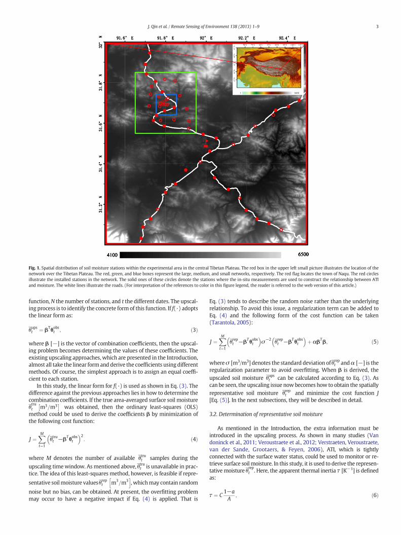
Fig. 1. Spatial distribution of soil moisture stations within the experimental area in the central Tibetan Plateau. The red box in the upper left small picture illustrates the location of thenetwork over the Tibetan Plateau. The red, green, and blue boxes represent the large, medium, and small networks, respectively. The red flag locates the town of Naqu. The red circlesillustrate the installed stations in the network. The solid ones of these circles denote the stations where the in-situ measurements are used to construct the relationship between ATIand moisture. The white lines illustrate the roads. (For interpretation of the references to color in this figure legend, the reader is referred to the web version of this article.)

3J. Qin et al. / Remote Sensing of Environment 138 (2013) 1–9

function,N the number of stations, and t the different dates. The upscal-ing process is to identify the concrete form of this function. If f(·) adoptsthe linear form as:

θupst ¼ βTθobst ; ð3Þ

where β [−] is the vector of combination coefficients, then the upscal-ing problem becomes determining the values of these coefficients. Theexisting upscaling approaches, which are presented in the Introduction,almost all take the linear form and derive the coefficients using differentmethods. Of course, the simplest approach is to assign an equal coeffi-cient to each station.

In this study, the linear form for f(·) is used as shown in Eq. (3). Thedifference against the previous approaches lies in how to determine thecombination coefficients. If the true area-averaged surface soil moistureθtrut m3=m3� �

was obtained, then the ordinary least-squares (OLS)method could be used to derive the coefficients β by minimization ofthe following cost function:

J ¼XMt¼1

θtrut −βTθobst

� �2: ð4Þ

where M denotes the number of available θtrut samples during the

upscaling timewindow. Asmentioned above, θtrut is unavailable in prac-tice. The idea of this least-squares method, however, is feasible if repre-

sentative soilmoisture valuesθrept m3=m3

h i, whichmay contain random

noise but no bias, can be obtained. At present, the overfitting problemmay occur to have a negative impact if Eq. (4) is applied. That is

Eq. (3) tends to describe the random noise rather than the underlyingrelationship. To avoid this issue, a regularization term can be added toEq. (4) and the following form of the cost function can be taken(Tarantola, 2005):

J ¼XMt¼1

θrept −βTθobst

� �σ−2 θrept −βTθobst

� �þ αβTβ; ð5Þ

whereσ [m3/m3] denotes the standard deviation ofθrept andα [−] is theregularization parameter to avoid overfitting. When β is derived, theupscaled soil moisture θupst can be calculated according to Eq. (3). Ascan be seen, the upscaling issue nowbecomes how to obtain the spatiallyrepresentative soil moisture θrept and minimize the cost function J[Eq. (5)]. In the next subsections, they will be described in detail.

3.2. Determination of representative soil moisture

As mentioned in the Introduction, the extra information must beintroduced in the upscaling process. As shown in many studies (Vandoninck et al., 2011; Veroustraete et al., 2012; Verstraeten, Veroustraete,van der Sande, Grootaers, & Feyen, 2006), ATI, which is tightlyconnected with the surface water status, could be used to monitor or re-trieve surface soil moisture. In this study, it is used to derive the represen-tative moisture θ

rept . Here, the apparent thermal inertia τ [K−1] is defined

as:

τ ¼ C1−aA

; ð6Þ

4 J. Qin et al. / Remote Sensing of Environment 138 (2013) 1–9

where C [−] denotes the solar correction factor, a [−] the surface albe-do, and A [K] the amplitude of diurnal temperature cycle. In order to de-rive ATI according to Eq. (1), MODIS 8-day albedo (Schaaf et al., 2002)and daily day/night LST products (Wan, 2008) are used. The details ofthe computation are described in Appendix A. The availability of ATIat some day is completely limited by the availability of satellite LST be-cause LST is often absent due to the presence of cloud during the satel-lite overpass times. Thus, it is difficult to obtain a continuous time seriesof ATI. In addition,when dense vegetation covers the soil, LSTmostly re-flects the status of vegetation, and thus the ability of ATI to capture thesoil moisture becomesweak. ATI is actually ameasure of themagnitudeof the temperature oscillation driven by the absorbed radiative energy.Since thewater heat capacity is relatively large, themorewater contenta soil contains, the more resistance it has to the external perturbation.When both the absorbed radiation and the soil texture are kept con-stant, morewater content leads to smaller amplitude, and in turn great-er ATI according to Eq. (6).

An empirical relationship, therefore, could be constructed betweenATI and surface soil moisture. Due to the difference of support betweenpoint-scale soil moisture and pixel-scale ATI, the functional relationshipmay vary at different stations. As a matter of fact, it is unnecessary tobuild a station-by-station relationship in the upscaling process becausethe focus is not on the soil moisture at the point- or pixel-scale, but onthe upscaled value in a certain large region. Thus, the regression rela-tionship is built as follows:

θ ¼ g τð Þ þ ε; ð7Þ

where θ m3=m3

h idenotes the averaged soil moisture at multiple sta-

tions, τ ½K−1� the averaged ATI at pixels corresponding to these stations,ε the random error, and g(·) the functional relationship, the concreteform of which will be discussed in detail in Section 4.

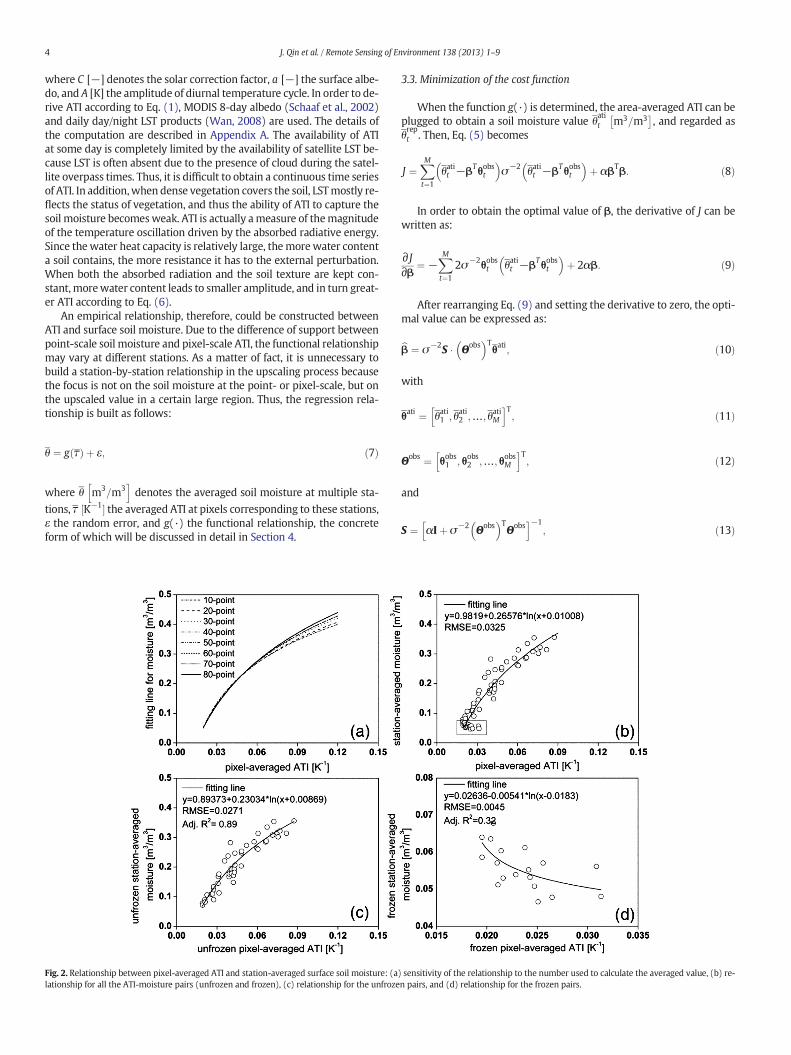
Fig. 2. Relationship between pixel-averaged ATI and station-averaged surface soil moisture: (a)lationship for all the ATI-moisture pairs (unfrozen and frozen), (c) relationship for the unfroze

3.3. Minimization of the cost function

When the function g(·) is determined, the area-averaged ATI can beplugged to obtain a soil moisture value θ

atit m3=m3� �

, and regarded asθrept . Then, Eq. (5) becomes

J ¼XMt¼1

θatit −βTθobst

� �σ−2 θatit −βTθobst

� �þ αβTβ: ð8Þ

In order to obtain the optimal value of β, the derivative of J can bewritten as:

∂ J∂β ¼ −

XMt¼1

2σ−2θobst θatit −βTθobst

� �þ 2αβ: ð9Þ

After rearranging Eq. (9) and setting the derivative to zero, the opti-mal value can be expressed as:

bβ ¼ σ−2S � Θobs� �T

θati; ð10Þ

with

θati ¼ θati1 ; θati2 ;…; θatiM

h iT; ð11Þ

Θobs ¼ θobs1 ; θobs2 ;…; θobsM

h iT; ð12Þ

and

S ¼ αIþ σ−2 Θobs� �T

Θobsh i−1

; ð13Þ

sensitivity of the relationship to the number used to calculate the averaged value, (b) re-n pairs, and (d) relationship for the frozen pairs.

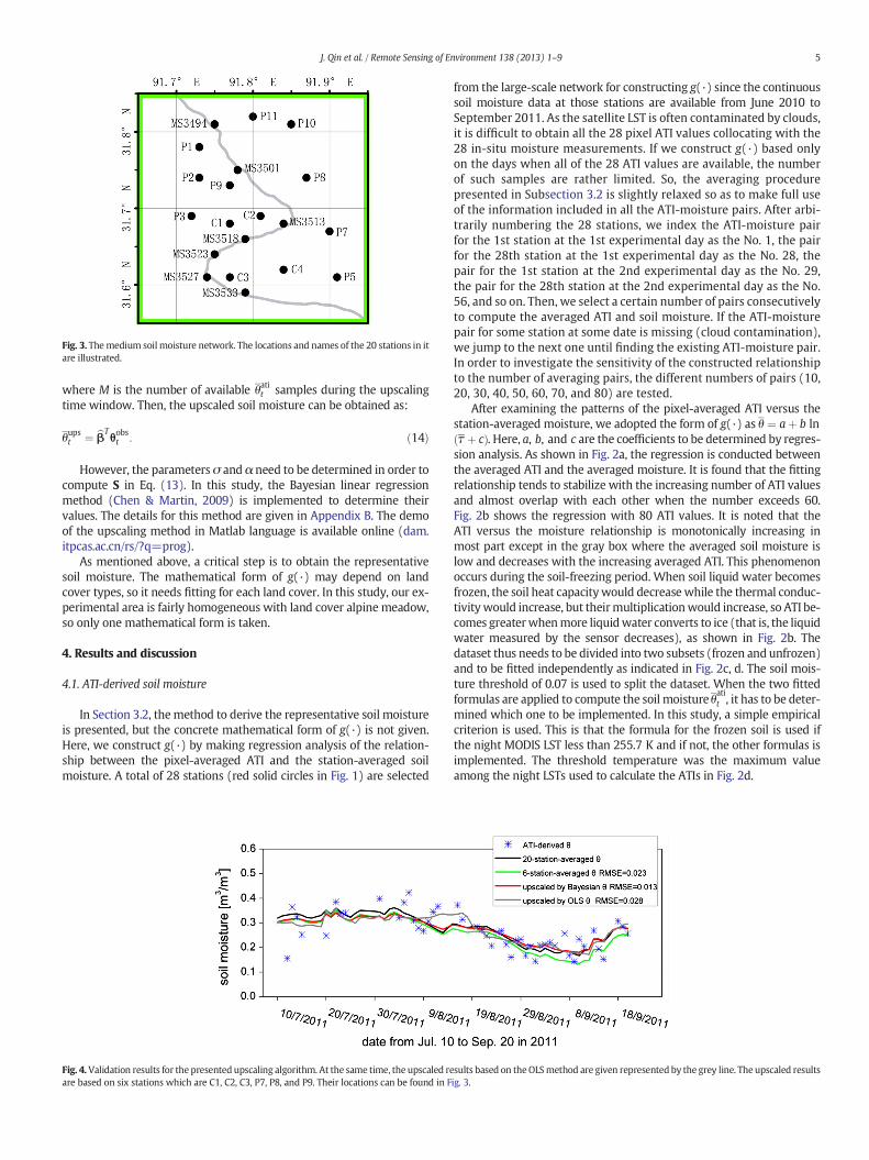
Fig. 3. Themedium soil moisture network. The locations and names of the 20 stations in itare illustrated.

5J. Qin et al. / Remote Sensing of Environment 138 (2013) 1–9

where M is the number of available θatit samples during the upscalingtime window. Then, the upscaled soil moisture can be obtained as:

θupst ¼ bβTθobst : ð14Þ

However, the parameters σ and α need to be determined in order tocompute S in Eq. (13). In this study, the Bayesian linear regressionmethod (Chen & Martin, 2009) is implemented to determine theirvalues. The details for this method are given in Appendix B. The demoof the upscaling method in Matlab language is available online (dam.itpcas.ac.cn/rs/?q=prog).

As mentioned above, a critical step is to obtain the representativesoil moisture. The mathematical form of g(·) may depend on landcover types, so it needs fitting for each land cover. In this study, our ex-perimental area is fairly homogeneous with land cover alpine meadow,so only one mathematical form is taken.

4. Results and discussion

4.1. ATI-derived soil moisture

In Section 3.2, themethod to derive the representative soil moistureis presented, but the concrete mathematical form of g(·) is not given.Here, we construct g(·) by making regression analysis of the relation-ship between the pixel-averaged ATI and the station-averaged soilmoisture. A total of 28 stations (red solid circles in Fig. 1) are selected

Fig. 4.Validation results for the presented upscaling algorithm. At the same time, the upscaled reare based on six stations which are C1, C2, C3, P7, P8, and P9. Their locations can be found in F

from the large-scale network for constructing g(·) since the continuoussoil moisture data at those stations are available from June 2010 toSeptember 2011. As the satellite LST is often contaminated by clouds,it is difficult to obtain all the 28 pixel ATI values collocating with the28 in-situ moisture measurements. If we construct g(·) based onlyon the days when all of the 28 ATI values are available, the numberof such samples are rather limited. So, the averaging procedurepresented in Subsection 3.2 is slightly relaxed so as to make full useof the information included in all the ATI-moisture pairs. After arbi-trarily numbering the 28 stations, we index the ATI-moisture pairfor the 1st station at the 1st experimental day as the No. 1, the pairfor the 28th station at the 1st experimental day as the No. 28, thepair for the 1st station at the 2nd experimental day as the No. 29,the pair for the 28th station at the 2nd experimental day as the No.56, and so on. Then, we select a certain number of pairs consecutivelyto compute the averaged ATI and soil moisture. If the ATI-moisturepair for some station at some date is missing (cloud contamination),we jump to the next one until finding the existing ATI-moisture pair.In order to investigate the sensitivity of the constructed relationshipto the number of averaging pairs, the different numbers of pairs (10,20, 30, 40, 50, 60, 70, and 80) are tested.

After examining the patterns of the pixel-averaged ATI versus thestation-averaged moisture, we adopted the form of g(·) as θ ¼ aþ b lnτ þ cð Þ. Here, a, b, and c are the coefficients to be determined by regres-sion analysis. As shown in Fig. 2a, the regression is conducted betweenthe averaged ATI and the averaged moisture. It is found that the fittingrelationship tends to stabilize with the increasing number of ATI valuesand almost overlap with each other when the number exceeds 60.Fig. 2b shows the regression with 80 ATI values. It is noted that theATI versus the moisture relationship is monotonically increasing inmost part except in the gray box where the averaged soil moisture islow and decreases with the increasing averaged ATI. This phenomenonoccurs during the soil-freezing period. When soil liquid water becomesfrozen, the soil heat capacitywould decrease while the thermal conduc-tivitywould increase, but theirmultiplicationwould increase, so ATI be-comes greaterwhenmore liquidwater converts to ice (that is, the liquidwater measured by the sensor decreases), as shown in Fig. 2b. Thedataset thus needs to be divided into two subsets (frozen and unfrozen)and to be fitted independently as indicated in Fig. 2c, d. The soil mois-ture threshold of 0.07 is used to split the dataset. When the two fittedformulas are applied to compute the soil moisture θ

atit , it has to be deter-

mined which one to be implemented. In this study, a simple empiricalcriterion is used. This is that the formula for the frozen soil is used ifthe night MODIS LST less than 255.7 K and if not, the other formulas isimplemented. The threshold temperature was the maximum valueamong the night LSTs used to calculate the ATIs in Fig. 2d.

sults based on theOLSmethod are given represented by the grey line. The upscaled resultsig. 3.

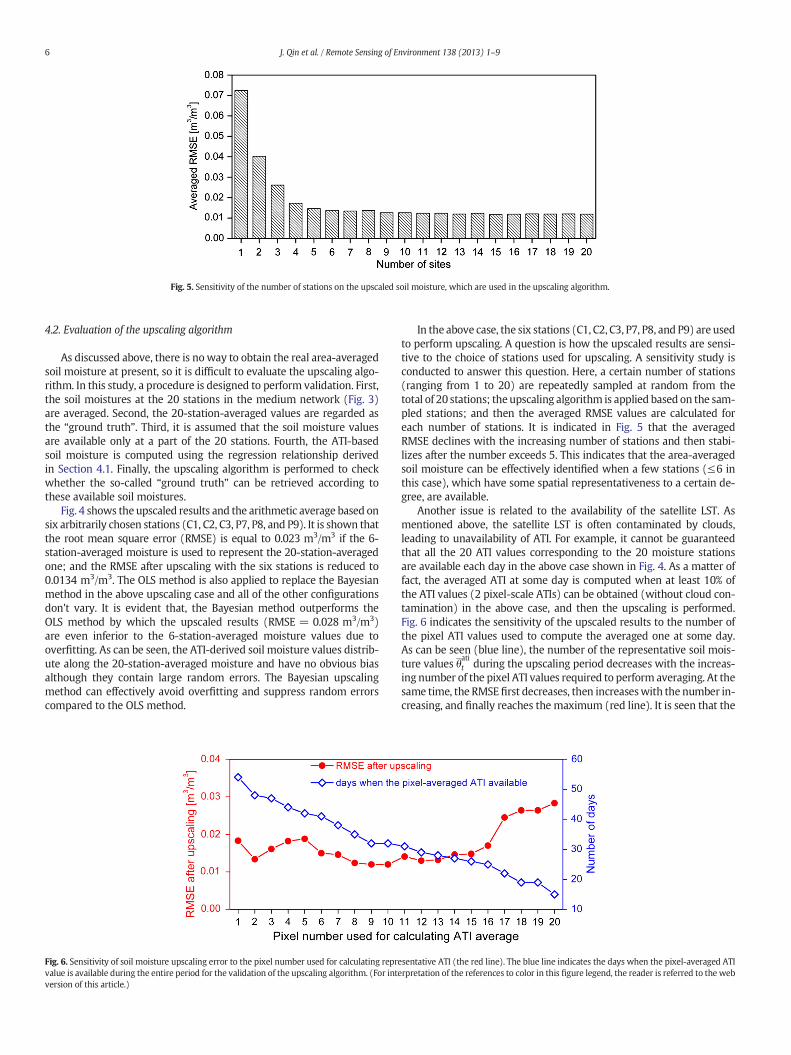
Fig. 5. Sensitivity of the number of stations on the upscaled soil moisture, which are used in the upscaling algorithm.

6 J. Qin et al. / Remote Sensing of Environment 138 (2013) 1–9

4.2. Evaluation of the upscaling algorithm

As discussed above, there is noway to obtain the real area-averagedsoil moisture at present, so it is difficult to evaluate the upscaling algo-rithm. In this study, a procedure is designed to perform validation. First,the soil moistures at the 20 stations in the medium network (Fig. 3)are averaged. Second, the 20-station-averaged values are regarded asthe “ground truth”. Third, it is assumed that the soil moisture valuesare available only at a part of the 20 stations. Fourth, the ATI-basedsoil moisture is computed using the regression relationship derivedin Section 4.1. Finally, the upscaling algorithm is performed to checkwhether the so-called “ground truth” can be retrieved according tothese available soil moistures.

Fig. 4 shows the upscaled results and the arithmetic average based onsix arbitrarily chosen stations (C1, C2, C3, P7, P8, and P9). It is shown thatthe root mean square error (RMSE) is equal to 0.023 m3/m3 if the 6-station-averaged moisture is used to represent the 20-station-averagedone; and the RMSE after upscaling with the six stations is reduced to0.0134 m3/m3. The OLS method is also applied to replace the Bayesianmethod in the above upscaling case and all of the other configurationsdon't vary. It is evident that, the Bayesian method outperforms theOLS method by which the upscaled results (RMSE = 0.028 m3/m3)are even inferior to the 6-station-averaged moisture values due tooverfitting. As can be seen, the ATI-derived soil moisture values distrib-ute along the 20-station-averaged moisture and have no obvious biasalthough they contain large random errors. The Bayesian upscalingmethod can effectively avoid overfitting and suppress random errorscompared to the OLS method.

Fig. 6. Sensitivity of soil moisture upscaling error to the pixel number used for calculating reprevalue is available during the entire period for the validation of the upscaling algorithm. (For inteversion of this article.)

In the above case, the six stations (C1, C2, C3, P7, P8, and P9) are usedto perform upscaling. A question is how the upscaled results are sensi-tive to the choice of stations used for upscaling. A sensitivity study isconducted to answer this question. Here, a certain number of stations(ranging from 1 to 20) are repeatedly sampled at random from thetotal of 20 stations; theupscaling algorithm is applied based on the sam-pled stations; and then the averaged RMSE values are calculated foreach number of stations. It is indicated in Fig. 5 that the averagedRMSE declines with the increasing number of stations and then stabi-lizes after the number exceeds 5. This indicates that the area-averagedsoil moisture can be effectively identified when a few stations (≤6 inthis case), which have some spatial representativeness to a certain de-gree, are available.

Another issue is related to the availability of the satellite LST. Asmentioned above, the satellite LST is often contaminated by clouds,leading to unavailability of ATI. For example, it cannot be guaranteedthat all the 20 ATI values corresponding to the 20 moisture stationsare available each day in the above case shown in Fig. 4. As a matter offact, the averaged ATI at some day is computed when at least 10% ofthe ATI values (2 pixel-scale ATIs) can be obtained (without cloud con-tamination) in the above case, and then the upscaling is performed.Fig. 6 indicates the sensitivity of the upscaled results to the number ofthe pixel ATI values used to compute the averaged one at some day.As can be seen (blue line), the number of the representative soil mois-ture values θ

atit during the upscaling period decreases with the increas-

ing number of the pixel ATI values required to perform averaging. At thesame time, the RMSE first decreases, then increaseswith the number in-creasing, and finally reaches the maximum (red line). It is seen that the

sentative ATI (the red line). The blue line indicates the days when the pixel-averaged ATIrpretation of the references to color in this figure legend, the reader is referred to the web

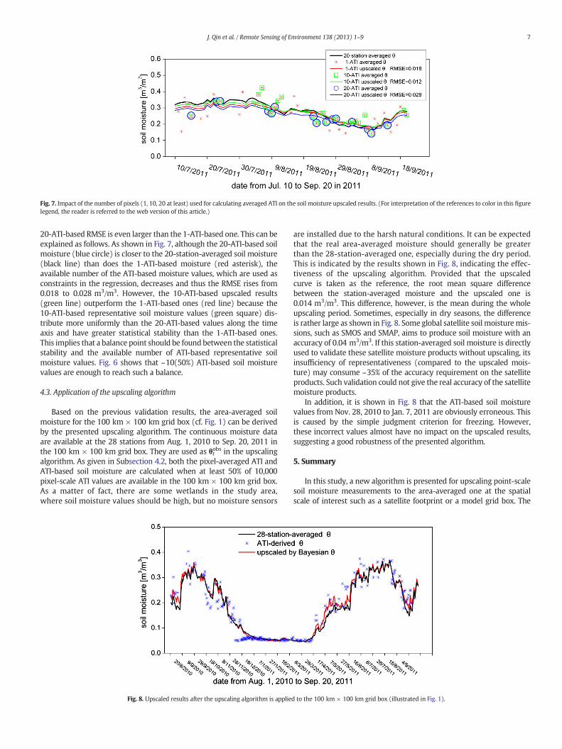
Fig. 7. Impact of the number of pixels (1, 10, 20 at least) used for calculating averaged ATI on the soil moisture upscaled results. (For interpretation of the references to color in this figurelegend, the reader is referred to the web version of this article.)

7J. Qin et al. / Remote Sensing of Environment 138 (2013) 1–9

20-ATI-based RMSE is even larger than the 1-ATI-based one. This can beexplained as follows. As shown in Fig. 7, although the 20-ATI-based soilmoisture (blue circle) is closer to the 20-station-averaged soil moisture(black line) than does the 1-ATI-based moisture (red asterisk), theavailable number of the ATI-based moisture values, which are used asconstraints in the regression, decreases and thus the RMSE rises from0.018 to 0.028 m3/m3. However, the 10-ATI-based upscaled results(green line) outperform the 1-ATI-based ones (red line) because the10-ATI-based representative soil moisture values (green square) dis-tribute more uniformly than the 20-ATI-based values along the timeaxis and have greater statistical stability than the 1-ATI-based ones.This implies that a balance point should be found between the statisticalstability and the available number of ATI-based representative soilmoisture values. Fig. 6 shows that ~10(50%) ATI-based soil moisturevalues are enough to reach such a balance.

4.3. Application of the upscaling algorithm

Based on the previous validation results, the area-averaged soilmoisture for the 100 km × 100 km grid box (cf. Fig. 1) can be derivedby the presented upscaling algorithm. The continuous moisture dataare available at the 28 stations from Aug. 1, 2010 to Sep. 20, 2011 inthe 100 km × 100 km grid box. They are used as θtobs in the upscalingalgorithm. As given in Subsection 4.2, both the pixel-averaged ATI andATI-based soil moisture are calculated when at least 50% of 10,000pixel-scale ATI values are available in the 100 km × 100 km grid box.As a matter of fact, there are some wetlands in the study area,where soil moisture values should be high, but no moisture sensors

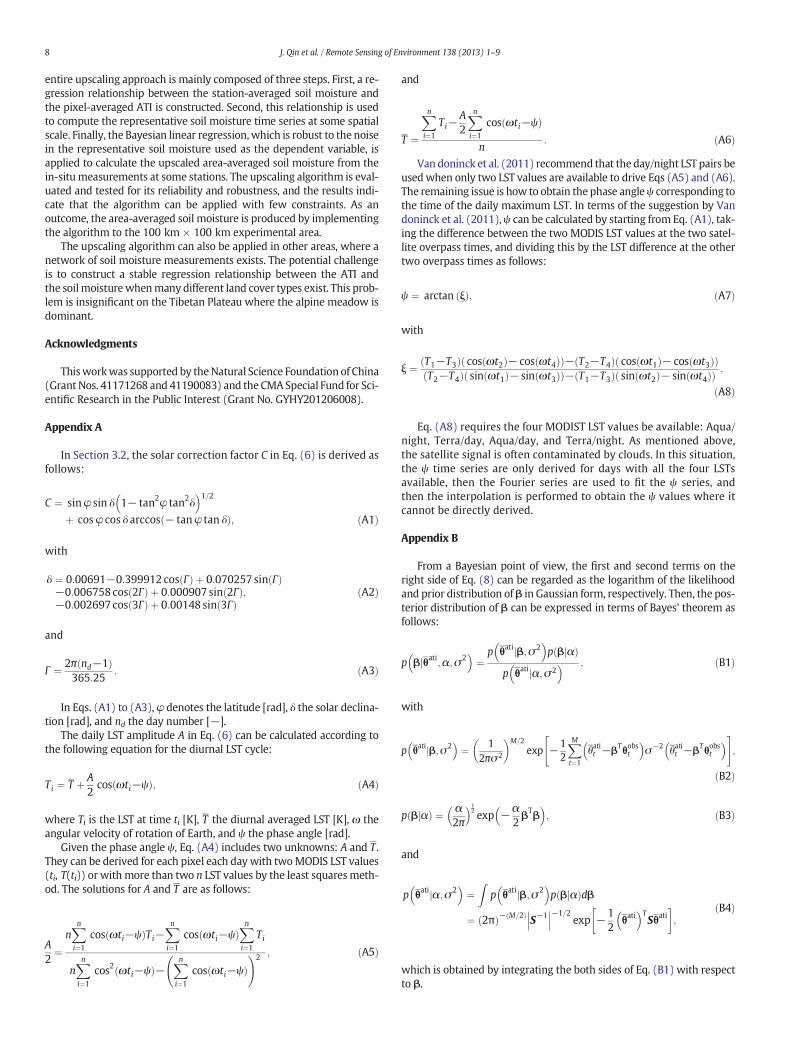
Fig. 8. Upscaled results after the upscaling algorithm is applie

are installed due to the harsh natural conditions. It can be expectedthat the real area-averaged moisture should generally be greaterthan the 28-station-averaged one, especially during the dry period.This is indicated by the results shown in Fig. 8, indicating the effec-tiveness of the upscaling algorithm. Provided that the upscaledcurve is taken as the reference, the root mean square differencebetween the station-averaged moisture and the upscaled one is0.014 m3/m3. This difference, however, is the mean during the wholeupscaling period. Sometimes, especially in dry seasons, the differenceis rather large as shown in Fig. 8. Some global satellite soil moisturemis-sions, such as SMOS and SMAP, aims to produce soil moisture with anaccuracy of 0.04 m3/m3. If this station-averaged soil moisture is directlyused to validate these satellite moisture products without upscaling, itsinsufficiency of representativeness (compared to the upscaled mois-ture) may consume ~35% of the accuracy requirement on the satelliteproducts. Such validation could not give the real accuracy of the satellitemoisture products.

In addition, it is shown in Fig. 8 that the ATI-based soil moisturevalues from Nov. 28, 2010 to Jan. 7, 2011 are obviously erroneous. Thisis caused by the simple judgment criterion for freezing. However,these incorrect values almost have no impact on the upscaled results,suggesting a good robustness of the presented algorithm.

5. Summary

In this study, a new algorithm is presented for upscaling point-scalesoil moisture measurements to the area-averaged one at the spatialscale of interest such as a satellite footprint or a model grid box. The

d to the 100 km × 100 km grid box (illustrated in Fig. 1).

8 J. Qin et al. / Remote Sensing of Environment 138 (2013) 1–9

entire upscaling approach is mainly composed of three steps. First, a re-gression relationship between the station-averaged soil moisture andthe pixel-averaged ATI is constructed. Second, this relationship is usedto compute the representative soil moisture time series at some spatialscale. Finally, the Bayesian linear regression,which is robust to the noisein the representative soil moisture used as the dependent variable, isapplied to calculate the upscaled area-averaged soil moisture from thein-situ measurements at some stations. The upscaling algorithm is eval-uated and tested for its reliability and robustness, and the results indi-cate that the algorithm can be applied with few constraints. As anoutcome, the area-averaged soil moisture is produced by implementingthe algorithm to the 100 km × 100 km experimental area.

The upscaling algorithm can also be applied in other areas, where anetwork of soil moisture measurements exists. The potential challengeis to construct a stable regression relationship between the ATI andthe soilmoisturewhenmany different land cover types exist. This prob-lem is insignificant on the Tibetan Plateau where the alpine meadow isdominant.

Acknowledgments

Thisworkwas supported by theNatural Science Foundation of China(Grant Nos. 41171268 and 41190083) and the CMA Special Fund for Sci-entific Research in the Public Interest (Grant No. GYHY201206008).

Appendix A

In Section 3.2, the solar correction factor C in Eq. (6) is derived asfollows:

C ¼ sinφ sin δ 1− tan2φ tan2δ� �1=2

þ cos φ cos δ arccos − tanφ tan δð Þ; ðA1Þ

with

δ ¼ 0:00691−0:399912 cos Γð Þ þ 0:070257 sin Γð Þ−0:006758 cos 2Γð Þ þ 0:000907 sin 2Γð Þ;−0:002697 cos 3Γð Þ þ 0:00148 sin 3Γð Þ

ðA2Þ

and

Γ ¼ 2π nd−1ð Þ365:25

: ðA3Þ

In Eqs. (A1) to (A3), φ denotes the latitude [rad], δ the solar declina-tion [rad], and nd the day number [−].

The daily LST amplitude A in Eq. (6) can be calculated according tothe following equation for the diurnal LST cycle:

Ti ¼ T þ A2cos ωti−ψð Þ; ðA4Þ

where Ti is the LST at time ti [K], T the diurnal averaged LST [K], ω theangular velocity of rotation of Earth, and ψ the phase angle [rad].

Given the phase angle ψ, Eq. (A4) includes two unknowns: A and T .They can be derived for each pixel each day with twoMODIS LST values(ti, T(ti)) or withmore than two n LST values by the least squaresmeth-od. The solutions for A and T are as follows:

A2¼

nXni¼1

cos ωti−ψð ÞTi−Xni¼1

cos ωti−ψð ÞXni¼1

Ti

nXni¼1

cos2 ωti−ψð Þ−Xni¼1

cos ωti−ψð Þ !2 ; ðA5Þ

and

T ¼

Xni¼1

Ti−A2

Xni¼1

cos ωti−ψð Þ

n: ðA6Þ

Van doninck et al. (2011) recommend that the day/night LST pairs beused when only two LST values are available to drive Eqs (A5) and (A6).The remaining issue is how to obtain the phase angleψ corresponding tothe time of the daily maximum LST. In terms of the suggestion by Vandoninck et al. (2011), ψ can be calculated by starting from Eq. (A1), tak-ing the difference between the two MODIS LST values at the two satel-lite overpass times, and dividing this by the LST difference at the othertwo overpass times as follows:

ψ ¼ arctan ξð Þ; ðA7Þ

with

ξ ¼ T1−T3ð Þ cos ωt2ð Þ− cos ωt4ð Þð Þ− T2−T4ð Þ cos ωt1ð Þ− cos ωt3ð Þð ÞT2−T4ð Þ sin ωt1ð Þ− sin ωt3ð Þð Þ− T1−T3ð Þ sin ωt2ð Þ− sin ωt4ð Þð Þ :

ðA8Þ

Eq. (A8) requires the four MODIST LST values be available: Aqua/night, Terra/day, Aqua/day, and Terra/night. As mentioned above,the satellite signal is often contaminated by clouds. In this situation,the ψ time series are only derived for days with all the four LSTsavailable, then the Fourier series are used to fit the ψ series, andthen the interpolation is performed to obtain the ψ values where itcannot be directly derived.

Appendix B

From a Bayesian point of view, the first and second terms on theright side of Eq. (8) can be regarded as the logarithm of the likelihoodand prior distribution of β in Gaussian form, respectively. Then, the pos-terior distribution of β can be expressed in terms of Bayes' theorem asfollows:

p βjθati;α;σ2� �

¼p θatijβ;σ2� �

p βjαð Þp θatijα;σ2� � ; ðB1Þ

with

p θatijβ;σ2� �

¼ 12πσ2

� �M=2exp −1

2

XMt¼1

θatit −βTθobst

� �σ−2 θatit −βTθobst

� �" #;

ðB2Þ

p βjαð Þ ¼ α2π

� �12 exp −α

2βTβ

� �; ðB3Þ

and

p θatijα;σ2� �

¼Z

p θatijβ;σ2� �

p βjαð Þdβ

¼ 2πð Þ− M=2ð Þ S−1��� ���−1=2

exp −12

θati� �T

Sθati

;ðB4Þ

which is obtained by integrating the both sides of Eq. (B1) with respectto β.

9J. Qin et al. / Remote Sensing of Environment 138 (2013) 1–9

The values of σ and α can be found bymaximization of themarginal-ized likelihoodp θatijα;σ2

� �. For this purpose, the logarithmof Eq. (B4) is

written as:

lnp θatijα;σ2� �

¼ N2

lnα−M2

lnσ2−12

ln S−1��� ���−

XMt¼1

θatit −bβTθobst

� �22σ2 ;

−αbβT bβ2

−M2

ln 2πð ÞðB5Þ

where bβ occurs in Eq. (10) and is the value that maximizes aposteriori distribution p βjθati;α;σ2

� �in Eq. (B1). The derivative of

lnp θatijα;σ2� �

with respect to α can be then derived as:

d lnp θatijα;σ2� �dα

¼ N2α

−12Trace Sð Þ−

bβT bβ2

: ðB6Þ

By setting the above derivative to zero, α can be obtained as:

α ¼ NbβTbβþ Trace Sð Þ: ðB7Þ

Similarly, setting d lnp θatijα;σ2� �

=dσ2 ¼ 0 gives

σ2 ¼

XMt¼1

θatit −bβTθobst

� �2αTrace Sð Þ : ðB8Þ

As can be seen,α andσ depend on bβand S according to Eqs. (B7) and(B8); and in turn bβ and S are dependent on α and σ in terms of Eqs. (10)and (13). An iteration process is thus needed to compute α and σ. First,the initial values of α and σ are given; second, the values of bβ and S arecomputed according to Eqs. (10) and (13); and third, their values areplugged into Eqs. (B7) and (B8) to calculate α and σ again until the dif-ference of the log-likelihood [Eq. (B5)] between two successive itera-tions are sufficiently small.

References

Chen, T., & Martin, E. (2009). Bayesian linear regression and variable selection for spectro-scopic calibration. Analytica Chimica Acta, 631, 13–21.

Chen, Y. Y., Yang, K., Qin, J., Zhao, L., Tang, W. J., & Han, M. L. (2013). Evaluation of AMSR-Eretrievals and GLDAS simulations against observations of a soil moisture network onthe central Tibetan Plateau. Journal of Geophysical Research, 118, http://dx.doi.org/10.1002/jgrd.50301.

Claussen, M. (1998). On multiple solutions of the atmosphere–vegetation system inpresent-day climate. Global Change Biology, 4, 549–559.

Cosh, M. H., Jackson, T. J., Starks, P., & Heathman, G. (2006). Temporal stability of surfacesoil moisture in the LittleWashita River watershed and its applications in satellite soilmoisture product validation. Journal of Hydrology, 323, 168–177.

Crow, W. T., Berg, A. A., Cosh, M. H., Loew, A., Mohanty, B. P., Panciera, R., et al. (2012).Upscaling sparse ground-based soil moisture observations for the validation ofcoarse-resolution satellite soil moisture products. Reviews of Geophysics, 50, RG2002.

Crow, W. T., Ryu, D., & Famiglietti, J. S. (2005). Upscaling of field-scale soil moisture mea-surements using distributed land surface modeling. Advances in Water Resources, 28,1–14.

Davies, J. A., & Allen, C. D. (1973). Equilibrium, potential and actual evaporation fromcropped surfaces in Southern Ontario. Journal of Applied Meteorology, 12, 649–657.

de Rosnay, P., Gruhier, C., Timouk, F., Baup, F., Mougin, E., Hiernaux, P., et al. (2009).Multi-scale soil moisture measurements at the Gourma meso-scale site in Mali.Journal of Hydrology, 375, 241–252.

Drusch, M. (2007). Initializing numerical weather prediction models with satellite-derivedsurface soil moisture: Data assimilation experiments with ECMWF's Integrated ForecastSystem and the TMI soil moisture data set. Journal of Geophysical Research, 112, D03102.

Entekhabi, D., Njoku, E. G., O'Neill, P. E., Kellogg, K. H., Crow, W. T., Edelstein, W. N., et al.(2010). The Soil Moisture Active Passive (SMAP) mission. Proceedings of the IEEE, 98,704–716.

Hirabayashi, Y., Kanae, S., Struthers, I., & Oki, T. (2005). A 100-year (1901–2000) globalretrospective estimation of the terrestrial water cycle. Journal of Geophysical Research,110, D19101, http://dx.doi.org/10.1029/12004JD005492.

Kerr, Y. H., Waldteufel, P., Wigneron, J. P., Martinuzzi, J., Font, J., & Berger, M. (2001). Soilmoisture retrieval from space: The Soil Moisture and Ocean Salinity (SMOS) mission.Geoscience and Remote Sensing, IEEE Transactions on, 39, 1729–1735.

Loew, A., & Schlenz, F. (2011). A dynamic approach for evaluating coarse scale satellitesoil moisture products. Hydrology and Earth System Sciences, 15, 75–90.

Njoku, E. G., Jackson, T. J., Lakshmi, V., Chan, T. K., & Nghiem, S. V. (2003). Soil moistureretrieval from AMSR-E. Geoscience and Remote Sensing, IEEE Transactions on, 41,215–229.

Pan, M., & Wood, E. F. (2006). Data assimilation for estimating the terrestrial waterbudget using a constrained ensemble Kalman filter. Journal of Hydrometeorology,7, 534–547.

Qin, J., Liang, S., Yang, K., Kaihotsu, I., Liu, R., & Koike, T. (2009). Simultaneous estima-tion of both soil moisture and model parameters using particle filtering methodthrough the assimilation of microwave signal. Journal of Geophysical Research,114, D15103.

Reichle, R. H., McLaughlin, D. B., & Entekhabi, D. (2002). Hydrologic data assimilation withthe ensemble Kalman filter. Monthly Weather Review, 130, 103–114.

Rodell, M., Houser, P. R., Jambor, U., Gottschalck, J., Mitchell, K., Meng, C. J., et al. (2004).The global land data assimilation system. Bulletin of the American MeteorologicalSociety, 85, 381–394.

Roth, C. H., Malicki, M.A., & Plagge, R. (2006). Empirical evaluation of the relationship be-tween soil dielectric constant and volumetric water content as the basis for calibrat-ing soil moisture measurements by TDR. Journal of Soil Science, 43, 1–13.

Schaaf, C. B., Gao, F., Strahler, A. H., Lucht, W., Li, X., Tsang, T., et al. (2002). First operation-al BRDF, albedo nadir reflectance products from MODIS. Remote Sensing of Environ-ment, 83, 135–148.

Schmugge, T. J., Kustas, W. P., Ritchie, J. C., Jackson, T. J., & Rango, A. (2002). Remote sens-ing in hydrology. Advances in Water Resources, 25, 1367–1385.

Seneviratne, S. I., Corti, T., Davin, E. L., Hirschi, M., Jaeger, E. B., Lehner, I., et al. (2010). In-vestigating soil moisture–climate interactions in a changing climate: A review.Earth-Science Reviews, 99, 125–161.

Sheffield, J., & Wood, E. F. (2007). Characteristics of global and regional drought,1950–2000: Analysis of soil moisture data from off-line simulation of the terrestrialhydrologic cycle. Journal of Geophysical Research, 112, D17115.

Tarantola, A. (2005). Inverse problem theory and methods for model parameter estimation. :Society for Industrial & Applied.

Texier, D., de Noblet, N., Harrison, S. P., Haxeltine, A., Jolly, D., Joussaume, S., et al. (1997).Quantifying the role of biosphere–atmosphere feedbacks in climate change: Coupledmodel simulations for 6000 years BP and comparison with palaeodata for northernEurasia and northern Africa. Climate Dynamics, 13, 865–881.

Van doninck, J., Peters, J., Baets, B.D., Clercq, E. M.D., Ducheyne, E., & Verhoest, N. E. C.(2011). The potential of multitemporal Aqua and Terra MODIS apparent thermal in-ertia as a soil moisture indicator. International Journal of Applied Earth Observation andGeoinformation, 13, 934–941.

Veroustraete, F., Li, Q., Verstraeten, W. W., Chen, X., Bao, A., Dong, Q., et al. (2012). Soilmoisture content retrieval based on apparent thermal inertia for Xinjiang provincein China. International Journal of Remote Sensing, 33, 3870–3885.

Verstraeten, W. W., Veroustraete, F., & Feyen, J. (2008). Assessment of evapotranspirationand soil moisture content across different scales of observation. Sensors, 8, 70–117.

Verstraeten, W. W., Veroustraete, F., van der Sande, C. J., Grootaers, I., & Feyen, J.(2006). Soil moisture retrieval using thermal inertia, determined with visibleand thermal spaceborne data, validated for European forests. Remote Sensing ofEnvironment, 101, 299–314.

Vinnikov, K. Y., Robock, A., Qiu, S., & Entin, J. K. (1999). Optimal design of surface net-works for observation of soil moisture. Journal of Geophysical Research, 104,19743–19749.

Wan, Z. (2008). New refinements and validation of the MODIS land-surface temperature/emissivity products. Remote Sensing of Environment, 112, 59–74.

Western, A. W., Grayson, R. B., & Blöschl, G. (2002). Scaling of soil moisture: A hydrologicperspective. Annual Review of Earth and Planetary Sciences, 30, 149–180.

Wu, G., Liu, Y., Zhang, Q., Duan, A., Wang, T., Wan, R., et al. (2007). The influence ofmechanical and thermal forcing by the Tibetan Plateau on Asian climate. Journal ofHydrometeorology, 8, 770–789.

Yang, K., Guo, X., He, J., Qin, J., & Koike, T. (2011). On the climatology and trend of the at-mospheric heat source over the Tibetan Plateau: An experiments-supported revisit.Journal of Climate, 24, 1525–1541.

Yang, K., Watanabe, T., Koike, T., Li, X., Fujii, H., Tamagawa, K., et al. (2007).Auto-calibration system developed to assimilate AMSR-E data into a land surfacemodel for estimating soil moisture and the surface energy budget. Journal of theMeteorological Society of Japan, 85, 229–242.

Zhao, L., Yang, K., Qin, J., Chen, Y. Y., Montzka, C., Wu, H., et al. (2013). Spatiotemporalanalysis of soil moisture observations within a Tibetan mesoscale area and itsimplication to regional soil moisture measurements. Journal of Hydrology, 482,92–104.