POLICY RESEARCH WORKING PAPER 1553.

Spatial Correlations A correction for spatialcorrelation in panel data.

in Panel DataJohn Driscoll

Aart Kraay

The World Bank

Policy Research Department

Macroeconomics and Growth Division

l)ecember 1995

I POLICY RESEARCH WORKING PAPER 1553

Summary findingsIn many empirical applications involving combined time- inference procedures that combine time-series and cross-series and cross-sectional data, the residuals from sectional data since these techniques typically require thedifferent cross-sectional units are likely to be correlated assumption that the cross-sectional units arewith one another. This is often the case in applications in independent. When this assumption is violated, estimatesmacroeconomics and international economics where the of standard errors are inconsistent, and hence are notcross-sectional units may be countries, states, or regions useful for inference. And standard corrections for spatialobserved over time. "Spatial" correlations among such correlations will be valid only if spatial correlations arecross-sections may arise for a number of reasons, ranging of particular restrictive forms.from observed common shocks such as terms of trade or Driscoll and Kraay propose a correction for spatialoil shocks, to unobserved "contagion" or "neighbor- correlations that does not require strong assumptionshood" effects which propagate across countries in concerning their form - and show that it is superior to acomplex ways. number of commonly used alternatives.

Driscoll and Kraay observe that the presence of suchspatial correlations in residuals complicates standard

This paper - a product of the Macroeconomics and Growth Division, Policy Research Department - is part of a largereffort in the departmentto study international macroeconomics. Copies of thepaperare available free from theWorld Bank,1818 H Street NW, Washington, DC 20433. Please contact Rebecca Martin, room Nl 1-059, telephone 202-473-9065,fax 202-522-3518, Internet address rmartinl@worldbank.org. December 1995. (28 pages)

The Policy Research Working Paper Series disseminates the findings of work in progress to encourage the exchange of ideas aboutdevelopment issues. An objective of the series is to get the findings out quickly, even if the presentations are less than fully polished. Thepapers carry the names of the authors and should be used and cited accordingly. The findings, interpretations, and conclusions are theauthors' own and should not be attributed to the World Bank, its Executive Board of Directors, or any of its member countries.

Produced by the Policy Research Dissemination Center

Spatial Correlations in Panel Data'

John DriscollDepartment of EconomicsBrown University, Box B

Providence RI 02912jd@econ.pstc.brown.edu

and

Aart KraayThe World Bank

1818 H Street NWWashington DC 20433akraay@worldbank.org

We would like to thank John Campbell, Greg Mankiw, Matthew Shapiro and especially Gary Chamberlain and JimStock for helpful comments and suggestions. Financial support from the Earle A. Chiles Foundation (Driscoll) and theSocial Sciences and Humanities Research Council of Canada (Kraay) during work on earlier drafts of this paper isgratefully acknowledged.

1 Introduction

Economists are frequently faced with the problem of drawing inferences from data sets

which combine cross-sectional and time-series data. In such situations, it has become standard

practice to base inferences on techniques which pool the cross-sectional and time-series

dimensions in some way. For such techniques to be valid, it must be the case that the error terms

are not correlated across different cross-sectional units, either contemporaneously or at leads and

lags. This condition is directly analogous to the usual requirement that the residuals from

different observations in a single cross-sectional regression be independent of each other. If this

condition is not met, estimates of standard errors will be inconsistent, and will not be useful for

inference.

This paper begins with the observation that in many applications, especially in

macroeconomics and international economics, the assumption of independent cross-sectional units

is inappropriate. While it may be reasonable to assume that cross-sectional units are independent

when they are households or individuals chosen according to a well-designed sampling scheme

from a large population, this assumption becomes less tenable when the cross-sectional units are

countries or regions. Countries or regions are likely to be subject to observable and unobservable

common disturbances which will cause the residuals from one cross-section to be correlated with

those of another. We will refer to such cross-sectional correlations as "spatial correlations"

Spatial correlations may arise for a number of reasons. For example, in applications in

which real GDP growth rates are the dependent variable, various channels of interdependence

such as trade, capital flows or policy coordination mechanisms will induce cross-country

correlations in GDP growth rates.' Unless the regressions of interest include right-hand side

variables which correctly specify these channels of interdependence, the residuals from these

regressions will be correlated across countries. Similarly, in studies of capital flows to developing

countries, common external shocks such as US interest rates, or else unobserved contagion effects

' See Kraay and Ventura (1995) for a discussion of the roles of trade and capital mobility in the synchronization of GDPgrowth rates across countries. Ades and Chua (1993) and Easterly and Levine (1995) provide empirical evidence thatpolicies tend to be correlated among neighbours, leading to correlations of growth rates over long horizons.

1

(sometimes dubbed "tequila" effects in aftermath of the Mexican peso crisis) can cause residuals

from capital flows regressions to be correlated across countries.

A number of standard corrections for spatial correlations exist, all of which require strong

assumptions regarding the form of the spatial correlations. For example, it is common to include

time dummy variables in pooled time-series, cross-sectional regressions to capture the effect of

common disturbances. This technique is the appropriate correction for spatial correlation only if

one assumes that the contemporaneous correlations between any pair of cross-sectional units are

equal, and the lagged cross-sectional correlations are zero. Unfortunately, such strong

restrictions on the form of the spatial correlations are unlikely to be correct in most applications.

For example, different countries may react differently to common disturbances, or contagion

effects may spread across countries only after a lag. When the structure of the spatial correlations

is misspecified in this way, the properties of the resulting estimator are in general unknown.

Since it is not desirable to impose restrictions on the form of the spatial correlations, it is

less clear how to proceed. One alternative is to attempt to parametrically estimate the full

unrestricted matrix of spatial correlations for use in a feasible generalized least squares (FGLS)

procedure. This procedure, which is a variant of the Seemingly Unrelated Regressions (SUR)

technique, will only be effective in a limited set of applications. To see why this is so, suppose

that there are N cross-sectional units and T time-series observations. The NxN matrix of

contemporaneous cross-sectional correlations has N(N+1)/2 free parameters to be estimated using

the NT available observations. Thus, in order to obtain reliable estimates of the matrix of spatial

correlations, it must be the case that T>>(N+1)/2. However, in many cross-country applications

using annual data, there are many more countries in the sample of interest than there are time-

series observations, so this approach will be infeasible.

In this paper we propose an alternative correction for spatial correlation. Building on the

non-parametric heteroskedasticity and autocorrelation consistent (HAC) covariance matrix

estimation technique of Newey and West (1987) and Andrews (1991), we show how this

approach can be extended to a panel setting with cross-sectional dependence, in addition to serial

correlation and heteroskedasticity. We present very weak conditions on the form of the cross-

sectional and time-series dependence under which a simple variant on the Newey and West

2

estimator yields consistent estimates of standard errors. In particular, we can obtain consistent

estimates of standard errors in the presence of arbitrary contemporaneous cross-sectional

correlations, as well as lagged cross-sectional correlations which are restricted to become small

only as the time interval separating the two observations becomes large. This very general

structure is likely to encompass most forms of spatial correlations encountered in practice.

Our results on consistency are based on asymptotic theory which requires the time

dimension, T, to tend to infinity. Thus, our results will only be relevant for panel data sets in

which the time dimension is reasonably large (our Monte Carlo simulations suggest that a value of

T=20 or T=25 is the minimum). However, our results do not place any restrictions on the size of

the cross-sectional dimension, N, and we can even allow the extreme case in which N tends to

infinity at any rate relative to T. This implies that our techniques, in contrast to SUR, will be

applicable in situations such as cross-country panel data sets where the number of countries is

very large.

The rest of this paper proceeds as follows. In Section 2, we first develop the intuitions for

our results using a simple ordinary least squares example. We then provide a formal statement of

our result, using a mixing random field structure to characterize the permissible extent of cross-

sectional and time-series dependence. Since this structure is somewhat unfamiliar, we provide

some examples of forms of cross-sectional dependence which satisfy the conditions we impose.

In Section 3, we consider the finite-sample properties of our estimator using Monte Carlo

evidence, and find that our non-parametric estimator performs significantly better than common

alternatives such as time dummies or SUR. Section 4 concludes.

3

2 Consistent Covariance Matrix Estimation with Spatial Dependence

2.1 Preliminary Discussion

In order to develop the intuition for the results of this paper, consider the following simple

bivariate linear panel regression:

Yit= xj: + eit

1 , ...,N, T =I ... 1

{ E[TE,Ej] } =

To obtain an estimate of ,, it is common practice to pool the cross-sectional and time-series

observations and apply OLS to the full set of NT observations. If the errors are independently

and identically distributed (i.e. if Q =U2'lr), this will yield consistent estimates of 3 and its

standard errors. However, in the presence of spatial correlations, Q is no longer diagonal. In this

case, although the OLS estimator of ,B is still consistent, the OLS standard errors will be

inconsistent, and hence will not be useful for inference.

We can write the OLS estimator of P in the usual way as follows:

rT NT/SE E xj,e1t

/T(DOOL j3) ; N(2)

{ I S EX3} NT

To simplify the above expression, denote the term in brackets in the denominator of (2) as QT 2,

and define

N

ht E Sxj,ei, ~~~~~~~~(3)

2 For the purposes of this illustrative example, we can assume that the x, are constants and that QT- Q>O as N,T-

4

Substituting into the expression for the OLS estimator, we obtain

- IOO =11•: ht (4)QTTrTt=i

This change of variables is useful because it reduces the original panel data estimation problem to

a simple time-series estimation problem. In other words, by defining a cross-sectional average h4

at every point in time, we have "collapsed" the cross-sectional dimension of the problem to a

single time-series observation by averaging over the N cross-sectional units in each period.

Since OLS estimates of P will be consistent even in the presence of spatial correlations,

our main concern is with obtaining consistent estimates of the variance of the OLS estimator.

Using the above notation, we can write this variance in terms of the h, as

VT ! Z-EE[hthj = -S5VT = -T E (Q)

The main intuition of the paper is as follows. Given appropriate conditions on the h,, we can

apply standard time-series non-parametric covariance matrix estimation techniques such as those

employed by Newey and West to obtain a consistent estimate of ST, and hence of VT. These

conditions (known as "mixing conditions" in the standard time-series literature) place restrictions

on the autocovariances of the h1, requiring the dependence between h, and h, , to become small as

the time interval separating them, s, becomes large. Imposing restrictions on the autocovariances

of h, will amount to placing restrictions on the contemporaneous and lagged spatial dependence in

the residuals, E[EEj,,e] ., since the autocovariances of the sequence h, are a weighted average of

these covariances, i.e.

N N

E[htht-s] = N2 1 Xxy t _E[Eey tj (6)

In this paper, we show that only very weak restrictions on the form of the spatial correlations are

5

required to ensure that h1 satisfies the regularity conditions necessary for consistent estimation of

ST. In particular, we can permit arbitrary contemporaneous correlations, and we require only that

lagged cross-sectional dependence declines at a particular rate as the time separation becomes

large. As in Newey and West (1987), our asymptotic results rely on a large time dimension.

However, we do not need to restrict the size of the cross-sectional dimension, which can tend to

infinity at any rate relative to T.

We use a mixing random field structure to characterize the permissible extent of spatial

and temporal dependence. As mixing random fields are somewhat unfamiliar in the econometrics

literature, we briefly present the necessary intuitions here, and relegate the details to the appendix.

Random fields are simply random variables with multiple indices. For example, returning to

Equation (3), we can define the random field N,t=x,,Ejt, indexed by i and t. In the standard

univariate time-series literature, a time series is described as "mixing" if the dependence between

two random variables x, and x,-, becomes small as the time interval separating them, s, becomes

large. In this paper, we will analogously describe a random field as being "mixing" if the

dependence between h-, and h becomes small as the time interval s becomes large, for any pair

of cross-sectional observations i and j.3 In this way, the standard time-series definition of mixing

corresponds to the special case where i=j. Finally, the "size" of a mixing is defined as the rate at

which the dependence between two observations must decline as a function of the distance

between them.

This particular definition of a mixing random field has the extremely useful property that

the cross-sectional averges of this random field, h1 (as defined in Equation (3)), form a univariate

This definition of mixing departs from the standard definitions in the random field literature in that it treats the cross-sectional and timne-series dimensions asymmetrically. Typically, mixing restriction would require the dependencebetween hN, and h,,, to become small as the Euclidean distance d=((i-j)2 +s2 )"2 between these two random variablesbecomes large. This is an unattractive property of standard definitions of mixing random fields for two reasons. First, inour panel data applications, it precludes canonical forms of cross-sectional dependence such as equal contemporaneouscross-unit correlations. To see why this is so, notice that the distance between h, and h, is simply li-jl according to theabove definition. Standard definitions of mixing would then rule out equal cross-sectional correlations between any hNand hj, since this correlation will not decline as ji-l becomes large. The second problem is that in order to impose therestriction that observations "far apart" in the cross-sectional ordering be approximately uncorrelated, it is necessary toknow what the cross-sectional ordering is. This is problematic, since unlike in the time dimension, in most cases there isno natural ordering in the cross-sectional dimension.

6

mixing sequence of the same size as the underlying random field. This is true for any value of N

(the size of the cross-sectional dimension), including the limiting case where N--. If we impose

the restriction that the hit form a mixing random field of the appropriate size, then h, will be a

mixing sequence of the same size, and we can directly apply standard time-series covariance

matrix estimation techniques to obtain an estimate of ST in Equation (5). Thus, our results

amount to a simple extension of the Newey and West estimator, which may be viewed in the

above context as the case in which N= 1.

2.2 Results

In this section, we present our main result, which is simply a generalization and

formalization of the discussion of the previous section. The theorem is stated in terms of a broad

class of Generalized Method of Moments estimators, of which the OLS case discussed above is an

example.

7

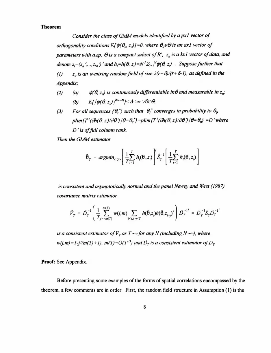
Theorem

Consider the class of GMM models identified by a pxl vector of

orthogonality conditions E[/4(00, zd)]=O, where 019F6& is an axl vector of

parameters with as•p, t9is a compact subset of R, z1, is a kxl vector of data, and

denote z,=(zi .'. ,zv,) 'and h,=h(O, z) =NA`Xi=,Mb(0, z,) Supposefurther that

(1) z, is an a-mixing random field of size 2(r+ o)/(r+ 6-1), as defined in the

Appendix;

(2) (a) #r(d, z) is continuously differentiable in 0 and measurable in z,,;

(b) E[IVI(fX, zJ 14r+°l]<J<- VO Fea

(3) For all sequences { 0 T) such that OT' converges in probability to 00,

plimT'((0, zd)/8d) /090rOT*}=plim(T'(dA(0 zd)/80) /l= 0=D'where

D 'is offull column rank

Then the GM5M estimator

IT

H0T = argmn E T |E

is consistent and asymptotically normal and the panel Newey and West (1987)

covariance matrix estimator

VT = DT ( E w(j,m) E h(O,z)h( -z)' ) DT DT STDTJ= -m(7) l<t,t-j<T

is a consistent estimator of VT as T- for any N (including N-o), where

w j,m) = I-j/(m(T) + 1), m(T) =0(T"3) and DT is a consistent estimator of Dr

Proof: See Appendix.

Before presenting some examples of the forms of spatial correlations encompassed by the

theorem, a few comments are in order. First, the random field structure in Assumption (1) is the

8

only substantive assumption required for the above result, as the remaining assumptions are fairly

standard conditions required to establish the properties of the GMM estimator. Note that the

assumptions of the theorem require no prior knowledge of the form of the spatial and temporal

correlations, and place only very weak restrictions on them. Hence this framework subsumes

many common forms of spatial dependence, without requiring an explicit (and probably also

incorrect) parameterization of the form of the temporal and spatial dependence.

Next, a sketch of the proof is as follows. The regularity conditions placed on *(O, Z,,) in

Assumption 2(a) are sufficient to ensure that e itself is a mixing random field of the same size as

z,t The cross-sectional averages of this random field, h1, will form a univariate mixing sequence as

described above. The remainder of the proof is then simply a matter of verifying the standard

results for the consistency and asymptotic normality of the GMM estimator and the consistency of

the Newey and West covariance matrix estimator.

Finally, as an example of an application of the theorem, consider the simple OLS example

of the previous section, which is a particular case of the GMM framework in which the above

theorem is cast. To see this, set 00,=P, z4=(yj, x,j) and lr( 3,xj)=x (y'-Px,J. Thus to implement this

technique, first obtain the usual OLS coefficient estimate. Next construct the sequence of cross-

sectional averages hk using the estimated residuals from the OLS specification (i.e.

ht=N-'Ej=1 ,(yj,-bx,), where b is the OLS estimate of P) and insert this into the definition of ST to

obtain its consistent estimate. Finally, note that a consistent estimate of DT is given by

(NT)-Y,= Combining these two expressions gives the consistent estimate of the

covariance matrix, VT.4

TSP and GAUSS codes to perform these calculations are available from the authors.

Another commonly-encountered model is one with unit-specific fixed effects, yi=f+x4P+E. One method to apply thetheorem to this model is to transform the data by taking deviations from unit means and rewriting as above i.e. letting7,t=(y,,-T Yt_,Ty,t,x, -T ' , TNy

9

2.3 Examples of Spatial Correlation

As the mixing random field assumption of the theorem may be somewhat difficult to verify

in practice, in this section we present some simple examples of forns of spatial correlation which

satisfy this assumption. It is most convenient to present some examples of permissible forms of

spatial correlation using the simple linear model with fixed scalar regressors of Equation (1). A

broad class of spatial correlations can be represented using the following factor structure6 for the

residuals of this regression, i.e.

=t + vit (9)

f, is an Mxl vector of independent, zero mean, unit variance random variables referred to as

"factors", while Xi is an Mxl vector of scalar "factor loadings". The vft are random variables with

zero mean and variance aYt2 which are independent over time and across units. In addition, they

are orthogonal to the factors, and are referred to as the "residuals from the factor structure". In

the appendix, we show that this factor structure satisfies the conditions of the theorem.' This

result thus provides a convenient way to verify the somewhat more abstract mixing random field

conditions of the theorem, and describes a broad class of spatial correlations which have a factor

structure representation to which our covariance matrix estimator is robust.

The simplest case of spatial correlations is one in which the contemporaneous cross-

sectional correlations are all equal. It is straightforward to verify that if M=1, Xi=)X for all i, and

o(t =X2_o2 for all i and t, then the OLS residuals ch have mean zero, variance a2 and cross-sectional

correlations E[ei,EjJ]=)2. In this special case, including time dummies in Equation (1) will remove

all the spatial correlations from the residuals.

A more interesting case of spatial correlations with a factor structure representation is one

6 We are grateful to Gary Chamberlain for suggesting this approach. See Chamberlain and Rothschild (1983) for adiscussion of factor structures in the context of finance theory, and Al-Najjar (1995) for a discussion of factor structuresas a method of modelling aggregate uncertainty in a continuum of cross-sectional units.

' The result in the appendix does not reiy on the assumption that the residuals from the factor structure arecontemporaneously uncorrelated across units, but allows them to have arbitrary spatial correlations.

10

in which the cross-sectional units are divided into m=l,...,M groups, and the within-group

correlations are equal for all the members of the group. Such groups might be regions,

geographic "neighbours" or any other grouping based on observable or unobservable

characteristics. To represent this as a factor structure, define Im as a set which consists of the

indices of the members of group m. Then, if ;Xmi=Am for ieI1l, j,'= .0j2 -a', and the vi, are again

independent across units, it is immediate to verify that the OLS residuals will have mean zero,

variance a2 and cross-sectional correlations E[eitEjt]=Xm2 for i,jel, and zero otherwise.

The most general case of contemporaneous spatial correlations is one in which the cross-

sectional correlations are arbitrary. This would be a natural structure in the case where there is a

common factor to which cross-sectional units react differently. If we introduce the assumption

that the residuals from the factor structure, vi, have arbitrary contemporaneous cross-sectional

correlations, then we can somewhat trivially write this as a factor structure in which all the factor

loadings are zero. In this case, there will be spatial correlations in the residuals from Equation (1)

even after time dummies are included in the specification.

Note that in these examples, we have used a factor structure to characterize the

contemporaneous spatial dependence in the residuals. We can easily extend this to introduce

dependence over time as well. For example, suppose that there are arbitrary contemporaneous

cross-sectional correlations, zero lagged cross-sectional correlations, and within units the

disturbances follow an AR(M) process. To give this a factor structure representation, letfm have

an autocovariance function which is I at lag m, and zero otherwise. Then if we set ).^=E[Ei,Eit-$]

the factor structure will replicate exactly this combination of cross-sectional and temporal

dependence. Along the same lines, it is possible to generate much more complicated forms of

lagged cross-sectional dependence using this factor structure.

11

3 Monte Carlo Results

In this section we use Monte Carlo experiments to examine how well our estimator (which

we will refer to as the HAC estimator) performs relative to common alternative corrections for

spatial correlations such as SUR and OLS and time dummies.8 We generate large numbers of

samples of artificial data with various forms of spatial correlations, and obtain coefficient

estimates and standard errors using OLS, SUR and our HAC estimator. We can then evaluate the

relative performance of these estimators by reporting a "coverage rate" for each estimator, which

is the fraction of samples in which two standard deviation confidence intervals contain the true

parameter values. For the HAC procedure, this fraction equals .95 as T-o, as it does not rely on

a correct parameterization of the temporal and spatial correlations. In finite samples (T<o),

however, this coverage rate will inevitably be somewhat smaller. OLS with time dummnies and

SUR will in general be misspecified, and their asymptotic properties when misspecified are

generally unknown. However, by reporting coverage rates, we can get a rough idea of the

severity of the impact of the misspecification of these procedures.

We consider linear models such as

Y21 2 E2

p + ~~~~~~~~~~~(10)

YNt XNt ENt

Without loss of generality, we set ,=0 in Equation (10). To introduce a rich structure of

8 Most other techniques are versions of feasible GLS which impose various zero restrictions on the variance-covariancematrix (for example, Case (1991) and Keane and Runkle (1992)). Elliot (1993) discusses the case when there is asingle cross-section, with one observation per geographical location. There are two classes of interesting exceptions tothis. One class, used in finance, assumes there is no serial correlation and applies a technique similar to the White(1980) correction for heteroskedasticitv (for example, Fama and MacBeth (1973), Lehmann (1990), and Froot (1989)).A second alternative has been offered by Conley (1994), who proposes a nonparametric variance-covariance matrixestimator when the "distance" between cross-sectional units is known.

12

contemporaneous and lagged spatial correlations into the residuals, we generate them according

to the following autoregressive scheme:

E2 =R e 2 + +, R = pIN , {E[iErPEj] = 2(1)

ENr ENt- I

This specification ensures that the residuals in Equation (10) exhibit both contemporaneous and

lagged spatial correlations. In the simple case in which p=0, there are only contemporaneous

spatial correlations in the residuals in Equation (10), and these are given by E. In this case, both

the HAC and the SUR are correctly specified, and their coverage rates can be compared directly.

Finally, we use the same structure to generate the regressors, xh

Before we can perform Monte Carlo experiments, we need to parameterize the spatial

correlation matrix E and the serial correlation parameter, p. We allow the parameter p to range

over the values ( 0, .1, .3, .5 }, which correspond to the moderate degree of serial correlation likely

to be present in most applications. Selecting the matrix of contemporaneous spatial correlations is

more difficult. One alternative is to choose a simple parameterization for this matrix, and report

Monte Carlo results as these parameters vary. While this approach is useful in that it allows us to

vary the degree of spatial correlations directly, it has the disadvantage that such simple

parameterizations are unlikely to capture the complicated forms of spatial correlations which are

likely to be encountered in practice.9 Instead, we use a data-based method of selecting the matrix

9 This approach was taken in an earlier draft of the paper. We performed a large number of simulations, allowing themagnitude of spatial correlations and the sizes of the cross-sectional and time-series dimensions to vary. The mainfindings of this exercise were: 1) OLS with time dummies performs poorly when there is heterogenous response to acommon factor and when there are lagged cross-sectional correlations. 2) SUR perforrns well only when N is very smallrelative to T and 3) the HAC estimator performs well in all cases, even for values of T as low as 25, and its performancedoes not depend on the size of the cross-sectional dimension which may be arbitrarily large. The results of theseexperiments are available from the authors upon request.

13

of spatial correlations. We estimate an AR(1) process for real output growth for 20 U.S. states'0

and for 24 O.E.C.D. economies, and use the observed variance-covariance matrix of the residuals

as 2 to generate spatial correlations in our artificial data.

Table 1 reports the coverage rates for this specification for the cases T=25 and T=50 for

each of the three estimators (OLS with time dummies, SUR and HAC). From Table 1, it is clear

that both OLS and SUR do quite poorly even when T=50, having coverage rates which never rise

above .694 and .679 respectively. Even when SUR is correctly specified (in the first column

where p=O), its performance is quite poor. The reason for this is that even when T=50, the

estimates of the contemporaneous spatial correlations matrix which it uses in a FGLS procedure

are very imprecise, as it attempts to estimate a very large number of free parameters. In contrast,

our non-parametric spatial correlation consistent HAC estimator performs much better than both

OLS and SUR, with coverage rates which range from .818 to .903.

'° Of course, a drawback of this approach is that the estimates of elements of E will not be very precise, as the cross-sectional dimension in these regressions is large relative to the time dimension. For this reason, we use only 20 statesbecause annual data for gross state product is only available for 23 years, from 1963-1986. To give some idea of themagnitude of the spatial correlations, note that the average cross-sectional correlation for the U.S. state data is .193, witha maximal value of .629, while for the O.E.C.D., the corresponding figures are .312 and .761.

14

4 Conclusion

Spatial and other forms of cross-sectional correlation are likely to be an important

complicating factor in many empirical studies. We have argued that they are especially likely to

arise in macroeconomics and international economics applications in which the cross-sectional

units are countries or regions. Standard techniques for dealing with this problem such as the

introduction of time dummies or SUTR require either restrictive parameterizations of the form of

the correlation or pre-estimation of a large number of parameters. In this paper, we have shown

that non-parametric covariance matrix estimators of the type proposed by Newey and West

(1987) have a simple analog in the panel data case. Asymptotic theory indicates that this

technique can accommodate a wide variety of spatial correlations, and moreover, that the size of

the cross-sectional dimension is no obstacle to obtaining large-T asymptotic results. This

suggests that our technique is applicable to a broad class of empirical studies which look at large

cross-sections of countries, states or regions observed over time. Monte Carlo experiments

demonstrate that the finite-sample properties of this estimator are good, and are often superior to

those of other commonly used techniques.

Finally, we note that this paper has relied exclusively on large-T asymptotics to deliver

consistent covariance matrix estimates in the presence of cross-unit correlations. However, when

T is small or when there is only a single cross-section, the problem of consistent non-parametric

covariance matrix estimation appears much less tractable. The reason for this is that, unlike in the

time dimension, there is no natural ordering in the cross-sectional dimension upon which to base

mixing restrictions, and hence it is not possible to construct the pure cross-sectional analogs of

time-series HAC estimators. Thus, it would appear that consistent covariance matrix estimation

in models of a single cross-section with spatial correlations will have to continue to rely on some

knowledge of the form of these spatial correlations.

15

Appendix

Mixing Random Fields

It is most convenient to characterize cross-sectional and temporal dependence in the

context of random fields". Let Z2 denote the two-dimensional lattice of integers, i.e.

Z2={(i,t) Ii= 1,2,... ,N,..., t= 1,2,...,T,...}, and let (Q,.,P) denote the standard probability

triple. A random field is defined as follows:

Definition: The set of random variables (ejZeVj on (QF9P) is a random field

Next, consider sets of the form A={-(i,s) Iss t). The a-algebra generated by the collection of

random variables whose indices lie in the set A,, which we denote ._' EU(EzIzeA,), has the usual

interpretation as the information set available at time t. Furthermore, let _t+,-=a(E,jzeA,+,c),

where A,C denotes the complement of A,. Using this notation, we can summarize the dependence

between two a-algebras using a-mixing coefficients defined in a manner analogous to the

standard univariate a-mixing'2 coefficient, i.e.

cl(S) -- sup<,, SUP<FE,, F2 E- > IP[F,nF 2 ] - P[F,]P[F2 ]

A mixing random field is defined as follows:

Definition: A random field is mixing of size r/(r-l), r> I iffor some A>r/(r-l),

a(S) =O(sA).

" Random field structures have been developed extensively in the statistics literature. See Rosenblatt (1970), Deo(1975), Bolthausen (1982), and Bulinskii (1988). Some economic applications include Wooldridge and White (1988),Quah (I1990), and Conley (1994).

12 It is straightforward to extend these definitions and the results which follow to ¢-mixing random fields by defining 0-mixing coefficients in the usual way.

16

This definition of mixing departs from the more standard a-mixing structures on random fields in

that it treats the cross-sectional dependence differently from the time-series dependence. Most

definitions of mixing13 restrict the dependence in both dimensions symmetrically, requiring the

dependence between two observations to decline as either the distance in the cross-sectional

ordering becomes large, or as the time separation becomes large (see, for example, Quah (1990)).

This restriction on the dependence across units is required to deliver (NT)' asymptotic normality

for double sums over i and t of the e1,, just as in the one-dimensional case restrictions on the

temporal dependence are required to deliver T"2 asymptotic nornality for appropriately

normalized sums.'4

The definition of mixing presented here, however, does not restrict the degree of cross-

sectional dependence. Instead, we only require the dependence between Ei1 and Ejt, to be small

when s is large, for any value of i and j. This is a desirable property, since it will not preclude

canonical forms of cross-sectional dependence, such as factor structures in which cross-sectional

units may be equicorrelated in a given time period or grouped structures in which observations are

correlated according to possibly unobservable group characteristics. This greater permissible

cross-sectional dependence comes at the cost that it will not be possible to obtain (NT)'

asymptotics for double sums over i and t of the Ei, However, we do not require this as we rely

exclusively on T112 asymptotics for this double sum.

A useful property of this random field structure is that the sequence of cross-sectional

averages of the Ei, forms a univariate a-mixing sequence, as summarized in the following lemma:.

S see Doukhan (1994) for an extensive survey of mixing in random fields and in other contexts.

" For such random fields, (NT)* asymptotics typically require N and T to go to infinity at the same rate, suggesting thatin finite sample applications, the cross-sectional and time-series dimension must be roughly equal for asymptoticapproximations to be plausible. For example, Quah (I 990) has the restriction that T=iN. We do not require thisrestriction in our asymptotic theory.

17

Lemma

Suppose that E,, is an t-mixing randomfield of size r/(r-I), r>l. Then

=N,hr = -E Ei,

is an a-mixing sequence of the same size as Ej,for any N.

Proof

The proof is simply a matter of verifying that h, satisfies the definition of univariate mixing.

Define B,={sls<t}eZ' as the natural one-dimensional analog of At, and similarly c9'=ra(hizeBt)

and c§ +o(hjz|EBt+ 3c ). Define the mixing coefficients for the sequence 1 as

ah(s) = sup < t > sup < GecS' t , G2Ec9,+,> I P[Gjn G2]- P[G,]P[G2 ] |. Now we claim that cS-t.t

and c9§ Y+[c%t+ . Given this claim, we have ah(s)< a(s) Vs, and hence ah(s) converges at least as

quickly as a(s). Thus the sequence ht is mixing of the same size of E&t.

To verify the claim, note that hi:Q-R' is a Borel function of (Ejtji=l,...,N,.. }, and hence is

o(Ej Ii=1,...N,...)-measurable, Le. h)'(C)co(Ejtji=l,...,N,..) where (3 is the a-algebra

generated by the Borel sets. Thus by defimition o(h.)=o(h)('(3)) ca(c1tIi=1,..,N,..). Finally,

note that co(Us= a(hj)) and =o (U,=-,'Jo( ej| i=1,..,N,.. )), and so the claim is verified.

This lemma is useful, as it permits us to move from restrictions on temporal and spatial

dependence in the random field to simple mixing restrictions on the univariate sequence of cross-

sectional averages, h,.

18

Proof of Theorem

To prove consistency and asymptotic normality of the GMM estimator, we will verify the

conditions in Hamilton (1994), Proposition 14.1. Consistency of the covariance matrix estimator

will follow from the arguments of Newey and West (1987). To verify consistency of the GMM

estimator (Hamilton, Proposition 14.1, Condition (a)), we need only verify conditions for the

consistency of extremum estimators (for example, Amemiya (1985), Theorem 4.1.1). Conditions

A and B of Amemiya (1985), Theorem 4.1. I follow immediately from the compactness of e and

Assumption 2(a). Condition C of this theorem requires the minimand in the GMM problem to

converge uniformly in Oee. This condition will be satisfied if the sequence h=h(O, z,) obeys a

LLN for all 60E3. Since *r is a measurable function of Z,, it is a mixing random field of the same

size as z;, by an argument similar to the one use to prove Lemma 1. By Lemma 1, 4 is a

univariate a-mixing sequence of size 2(r+8)/(r+o-1) > r/(r-1). Thus, to apply the McLeish

(1975) LLN (See White (1984), Theorem 3.47) for a-mixing sequences of size r/(r-1), we need

only verify that 4 has finite (r+6)th moments. However, to prove consistency of the covariance

matrix estimator, we will require the stronger moment condition that E[Ihj4(r+6 )]<A<CO.

Anticipating this, we verify this condition as follows:

l v N |4(r+) N ]4(r+6)E[Ih ,1 ] = N'Z w(O,z) ] • r6 E E[ I I(E,z)14(r+6)]1/('4r+ 6)) 14))

i-I ~ ~ ~ J(14)s N4"r+6) [NA1/(4(r+6)) ]4(r+6) = A

where the first inequality follows from Minkowski's inequality and the second follows from

Assumption 2(b). Thus we have verified the conditions for the LLN for the sequence h4, and the

GMM estimator is consistent.

To verify Condition (b) of Hamilton (1994), Proposition 14.1, we need to show that the

sequence h, satisfies a CLT such as White (1984), Theorem 5.19. The CLT require h4 to be a

mixing sequence of size r/(r-1) with finite 2r"h moments. Both these conditions have been verified

above. The CLT requires the additional regularity condition that

19

TE t E h] | 2 > O (15)

uniformly in a as T-o. To verify this, observe first that the mixing property of h, allows us to

bound the autocovariances of h, in the usual way. That is, for s>O, we have I E[hl4h,j I < a(s)A

where a(s)=O(s<('+6) (White, (1984), Corollary 6.16). This corollary requires h, to be an a-

mixing sequence of size (2+2T)/rj, rq>O with E[ I htI 2+2,,]<A<oo, which may be verified by setting

i=(r+o-l) in the previous paragraph. We can use this bound on the autocovariances of ht to verify

the regularity condition for the CLT, since

-E E ht )|< - E I E[ ht2] + 2 E I EhhT t=al T,=a,,l Ts=l t=O+leS

T-_1

A + E (T-a-s)a(s)Ts= l (16)

T-1

• A + 2E a(s)3- 1

< Al

The first inequality follows from the triangle inequality and a reorganization of the double sum.

The second inequality follows from the previously-derived bounds on the moments h1 and its

autocovafiances, and the final inequality follows from the summability of a(s). Thus we have

verified the required moment and regularity conditions for the CLT. Finally, Condition (c) of

Hamilton (1994), Proposition 14.1 is identical to Assumption (3). Therefore, GMM is consistent

and asymptotically normal in this random field setting.

To demonstrate consistency of the covariance matrix estimator, we can follow the

arguments in Newey and West (1987). Using the definition of the covariance matrix estimator and

the triangle inequality, we have

20

|ST ST| j [ h2 + -T w(s,m) E h,

IT 2 2 ~~m T+ (h-E[h) + -Ew(s,m)E (hh, -E[h

(17)2m T

+ -T v(s,m)-- E1E [',hJ 5s=l t=s+s

2T-1 T

Ts=1m+ t=s+lF.t5|

To prove consistency, we will show that each of the four terms in this expression tends to zero as

T-.. First, however, we derive the following bound, which we will require to show the

consistency of the second term in Equation (17):

4L| Zt\) 2] i TAT, Z,5 = h/,i-E[h,ht] (18)

The proof of this bound relies on the fact that Z. is an a-mixing sequence of size (2+2i)/rI with

E[IZtI2 +2',]<A<-. To verify this condition, note that Z. is a measurable function of a finite

number of a-mixing sequences (h, and h ,-), and hence is a-mixing of the same size as hk, which is

(2+2 1)/i by setting i=(r+6-I) in Assumption 1. To verify the moment condition, write

E[ IZ, 2+2T1 • [E[jhtI2+2T, I h_12+2Hl'll(2 +21) + IE[h&, ] I2+2v

• [E[jh )4+4'I/4+4lE[lh _4.41141/(4+4Ti) + E[IhtI]1/2E[Iht2I-] I 1 (19)

by applying the Minkowski and Cauchy-Schwartz inequalities. However, setting T=(r+8-1), we

have 4+4rj=4(r+8), and we have already shown that E[I h, 4(r+]<A<, and so the moment

condition on Z,, is satisfied. The proof of the bound itself is a slight modification of the argument

in White (1984), Lemma 6.19, and is similar to the argument used to verify the regularity

21

condition for the CLT above.

Using the bound on the autocovariances of h,, we can write the fourth term as

2T-1 T 2 T-1 T

- E IE[hAJI ,]| s-E E A a(s)T3=m+I t=5.1 Ts=m+l t=s+l

2T-1s5 2 E (T-s)i\a(s) (20)

Ts=m-l

T-1

s 2A E a(s)s=m+I

and the final sum will tend to zero as T and m(T) tend to infinity since a(s)=O(s`l+8)).

We can again use the bound on the autocovariances of h, in the third term, resulting in

-E jw(s,m)-I1I IE[h?,. I • 21 Iw(s,m)-1I1 1 Ata(s)$=I t=s+l 3~~=1 Tt=s+i

(21)

PMs E I w(s,m) - I fb&a(s)

Since w(s,m)- I for all s as m(T)-- and since a(s)=O(s-'+°), this expression tends to zero.

We can follow the argument in Newey and West's Equation (11) to show the consistency

of the second term, using a Chebychev's inequality argument and Equation (18).

m T n[mi T1E Asw(s,M) E Z,, > Ie |s EI| W(s,M) E Ztl > E|

• 4 E zts >(22)

S• ( Cm ) 2 TA(

AZC2 m(J)3

2E2T

22

This final term converges to zero by the assumption that m(T)=o(T"3).

Consistency of the first term follows immediately from the consistency of the OLS

estimator and the final paragraph in Newey and West (1987).

23

Spatial Correlations with Factor Structure Representations

The following corrolary to the theorem verifies the claim made in Section 2.3 that it is

possible to obtain consistent covariance matrix estimates in the presence of spatial correlations

which have a factor structure representation.

Corrolary

Suppose that y,,=xjtp+l , , with Ef, =ff,'2i + v, f = (f,, . fm,) 'and x,,=g,'KX+uU.

g, = (gj,, ... , gp,) 'where A, and Ki are Mxl and Pxl vectors of uniformly bounded

constant factor loadings and M and P are finite constants. Suppose further that

fmt l f., andf , i vi, Vm, n, m on and Vt, and that gmt £ gnt and g., £ uit Vm, n,

m on and Vt, and that ELfJ=E[g^J =0 and Effm,/]=E[g., = 1 Vm, t. Suppose

further that Vij, t and m

(1) (a) (ft 'g, 'is an a-mixing sequence of size 2(r+ o5)/(r + A-l) for r> I

and some 6>0;

(b) Efvij=E[uJ=O andv, 1 v,, and u,, i u>,,for s#0;

(2) (a) E[x,,ej=0;

(b) E[Lfm,xit,(r+ 4)< oo<and E[/u,x,,j(r+0)< 4< C;

(3) E[/gm,/(r+8 )1< J<Xand E[/u,,f(r+"j]<A<w;

Then the OLS estimator is consistent and asymptotically normal and the

panel Newey and West (1987) covariance matrix estimator

w(j,m) h ht STT=-m(T) I<tt1<T

where wfj,m) =l-j/(m(T) + 1) and m(T) =o(T7"3), is a consistent estimator of VT as

T-for any N (including N--).

24

Proof

We will prove this corollary by verifying the conditions of the Theorem. To verify

Assumption 1, define '((f,', g,')' I sst). Now by a similar argument to the one used in the

proof to the Lemma, we have a((f,'XA,g,'K)'(s,i)e)Jj since Xi and Ki are uniformly

bounded constants. Thus (f'Ai,g,'K)' is an a-mixing random field of size 2(r+8)/(r+8+1)

since by Assumption 1(a), (f,',gt')' is an a-mixing random sequence of size2(r+o)/(r+8+ 1).

Finally, (vi,,ui)' is trivially an a-mixing random field of size 2(r+6)/(r+6+ 1) by Assumption

1(b). Thus we have that (xi, Ej)'=(f'Ai,g,'K)'+(vj,,ujt)' is an a-mixing random field of size

2(r+o)/(r+o+ 1).

Assumption 2(a) of the Corollary yields the required orthogonality conditions for the

GMM estimator, and Assumption 2(a) of the Theorem is trivially satisfied. The moment

condition in Assumption 2(b) of the Theorem follows from the moment conditions in Assumption

2(b) and 3, the assumption that the factor loadings are uniformly bounded, and Minkowski's

inequality.

25

Table 1: Data-Based Monte Carlo Results

Each cell contains coverage rates for OLS with time dummies, SUR and HAC estimators based on 1000 Monte Carloreplications. Contemporaneous cross-unit correlations are generated by computing the cross-correlations of residuals fromAR(I) regression of the first difference of Gross State Product for 20 U.S. states from 1963 to 1986 and of Gross DomesticProduct for 24 O.E. C.D. economies from 1960 to 1991.

p=0 p=.1 p=.3 p=.5

U.S. States .498 .510 .479 .410T=25, N=20 .267 .286 .214 .173

.866 .858 .846 .827oN

U.S. States .517 .496 .491 .410T=50, N=20 .668 .654 .589 .448

.903 .892 .888 .863

O.E.C.D. Economies .694 .682 .641 .573T=25, N=24 .146 .133 .120 .096

.887 .868 .864 .818

O.E.C.D. Economies .692 .693 .667 .556T=50, N=24 .658 .679 .596 .445

.905 .886 .898 .862

References

Ades, Alberto and Hak B. Chua (1993). "Thy Neighbour's Curse: Regional Instability andEconomic Growth". Manuscript, Harvard University.

Al-Naijar, Nabil Ibraheem (1995). "Decomposition and Characterization of Risk with aContinuum of Random Variables". Econometrica. Vol 63, No. 5, pp.1 195-1224.

Amemiya, Takeshi (1985). Advanced Econometrics. Cambridge: Harvard University Press.

Andrews, Donald W.K. (1991). "Heteroskedasticity and Autocorrelation Consistent CovarianceMatrix Estimation". Econometrica. Vol. 59, No. 4, pp. 817-858.

Bolthausen, E. (1982). "On the Central Limit Theorem for Stationary Mixing Random Fields".The Annals of Probability. Vol. 10, No. 4, pp. 1047-1050.

Bulinskii, A.V. (1988). "On Various Conditions for Mixing and Asymptotic Normality ofRandom Fields". SovietMath. Dokl. Vol. 37, No. 2, pp. 443-448.

Case, Anne C. (1991). "Spatial Patterns in Household Demand". Econometrica. Vol. 59, No. 4,pp. 953-965.

Chamberlain, Gary and Michael Rothschild (1983). "Factor Structure and Mean-VarianceAnalysis on Large Asset Markets". Econometrica. Vol. 51, No. 5, pp. 1281-1304.

Conley, Timothy G. (1994). "Econometric Modelling of Cross Sectional Dependence". WorkingPaper, University of Chicago.

Deo, Chandrakant M. (1975). "A Functional Central Limit Theorem for StationaryRandom Fields". The Annals of Probability. Vol. 3, No. 4, pp. 708-715.

Doukhan, Paul (1994). Mixing: Properties and Examples. New York: Springer-Verlag.

Easterly, William and Ross Levine (1995). "Affica's Growth Tragedy: A Retrospective 1960-89". Manuscript World Bank Policy Research Department.

Elliott, Graham (1993). "Spatial Correlations and Cross-Country Regressions". Manuscript,Harvard University.

Fama, Eugene F. and James D. MacBeth (1973). "Risk, Return, and Equilibrium: EmpiricalTests". Journal of Political Economy. Vol 81. pp. 607-636.

Froot, Kenneth A. (1989). "Consistent Covariance Matrix Estimation with Cross-Sectional

27

Dependence and Heteroskedasticity in Financial Data." Journal of Financial and QuantitativeAnalysis. Vol. 24, pp. 333-355.

Hamilton, James D. (1994). Time Series Analysis. Princeton: Princeton University Press.

Keane, Michael and David Runkle (1990). "Testing the Rationality of Price Forecasts:Evidence from Panel Data". American Economic Review. Vol. 80, No. 4, pp. 715-735.

Kraay, Aart and Jaume Ventura (1995). "Trade and Fluctuations". Manuscript, MIT and theWorld Bank.

Lehmann, Bruce (1990). "Residual Risk Revisited". Journal of Econometrics. Vol. 45, No. 1,pp. 71-97.

McLeish, D. L. (1975). "A Maximal Inequality and Dependent Strong Laws". The Annals ofProbability. Vol. 3, No. 4, pp. 826-836.

Newey, Whitney K. and Kenneth D. West (1987). "A Simple, Positive Semi-Definite,Heteroskedasticity and Autocorrelation Consistent Covariance Matrix". Econometrica. Vol. 55,No. 3, pp. 703-708.

Quah, Danny (1990). "International Patterns of Growth: Persistence in Cross-countryDisparities". Manuscript, MIT Department of Economics.

Rosenblatt, M. (1970). "Central Limit Theorem for Stationary Processes". Proceedings of theSixth Berkeley Symposium on Mathematical Statistics and Probability. Vol.2, pp.55 1-561.

White, Halbert (1980). "A Heteroscedasticity-Consistent Covariance Matrix Estimator and aDirect Test for Heteroscedasticity". Econometrica. Vol. 48, No. 4, pp. 817-838.

(1984). Asymptotic Theoryfor Econometricians. New York: Academic Press.

Wooldridge, Jeffrey M. and Halbert White (1988). "Some Invariance Principles and Central LimitTheorems for Dependent Heterogenous Processes". Econometric Theory. Vol. 4, No. 2, pp.210-230.

Policy Research Working Paper Series

ContactTitle Author Date for paper

WPS1531 Some New Evidence on Determinants Harinder Singh November 1995 S. King-Watsonof Foreign Direct Investment in Kwang W. Jun 31047Developing Countries

WPS1532 Regulation and Bank Stability: Michael Bordo November 1995 D. EvansCanada and the United States, 385261870-1980

WPS1533 Universal Banking and the Charles W. Calomiris November 1995 D. EvansFinancing of Industrial Development 38526

WPS1534 The Evolution of Central Banking Forrest Capie November 1995 D. Evans38526

WPS1535 Financial History: Lessons of the Gerard Caprio, Jr. November 1995 D. EvansPast for Reformers of the Present Dimitri Vittas 38526

WPS1536 Free Banking: The Scottish Randall Iroszner November 1995 D. EvansExperience as a Model for Emerging 38526Economies

WPS1537 Before Main Banks: A Selective Frank Packer November 1995 D. EvansHistorical Overview of Japan's 38526Prewar Financial System

WPS1538 Contingent Liability in Banking: Anthony Saunders November 1995 D. EvansUseful Policy for Developing Berry Wilson 38526Countries?

WPS1539 The Rise of Securities Markets: Richard Sylla November 1995 D. EvansWhat Can Government Do? 38526

WPS1540 Thrift Deposit Institutions in Europe Dimitri Vittas November 1995 P. Infanteand the United States 37642

WPS1541 Deposit Insurance Eugene White November 1995 D. Evans38526

WPS1542 The Development of Industrial Samuel H. Williamson November 1995 D. EvansPensions in the United States in the 38526Twentieth Century

WPS1543 The Combined Incidence of Taxes Shantayanan Devarajan November 1995 C. Bernardoand Public Expenditures in the Shaikh I. Hossain 37699Philippines

WPS1544 Economic Performance in Small F. Desmond McCarthy November 1995 M. DivinoOpen Economies: The Caribbean Giovanni Zanalda 33739Experience, 1980-92

Policy Research Working Paper Series

ContactTitle Author Date for paper

WPS1545 International Commodity Control: Christopher L. Gilbert November 1995 G. llogonRetrospect and Prospect 33732

WPS1546 Concessions of Busways to the Jorge M. Rebelo November 1995 A. TurnerPrivate Sector: The Sao Paulo Pedro P. Benvenuto 30933Metropolitan Region Experience

WPS1547 Testing the Induced Innovation Colin Thirtle November 1995 M. WilliamsHypothesis in South African Robert Townsend 87297Agriculture (An Error Correction Johan van ZylApproach

WPS1548 The Relationship Between Farm Size Johan van Zyl November 1995 M. Williamsand Efficiency in South African Hans Binswanger 87297Agriculture Colin Thirtle

WPS1549 The Forgotten Rationale for Policy Jonathan Isham November 1995 S. TorresReform: The Productivity of Daniel Kaufman 39012Investment Projects

WPS1550 Governance and Returns on Jonathan Isham November 1995 S. FallonInvestment: An Empirical Daniel Kaufman 38009Investigation Lant Pritchett

WPS1551 Sequencing Social Security, Dimitri Vittas December 1995 P. InfantePension, and Insurance Reform 37642

WPS1552 Unemployment Insurance and Milan Vodopivec December 1995 J. WalkerDuration of Unemployment: Evidence 37466from Slovenia's Transition

WPS1553 Spatial Correlations in Panel Data John Driscoll December 1995 R. MartinAart Kraay 39065