spatial auditory blurring and applications to multichannel

HAL Id: tel-00623670https://tel.archives-ouvertes.fr/tel-00623670

Submitted on 14 Sep 2011

HAL is a multi-disciplinary open accessarchive for the deposit and dissemination of sci-entific research documents, whether they are pub-lished or not. The documents may come fromteaching and research institutions in France orabroad, or from public or private research centers.

L’archive ouverte pluridisciplinaire HAL, estdestinée au dépôt et à la diffusion de documentsscientifiques de niveau recherche, publiés ou non,émanant des établissements d’enseignement et derecherche français ou étrangers, des laboratoirespublics ou privés.

Spatial Auditory Blurring and Applications toMultichannel Audio Coding

Adrien Daniel

To cite this version:Adrien Daniel. Spatial Auditory Blurring and Applications to Multichannel Audio Coding. Acoustics[physics.class-ph]. Université Pierre et Marie Curie - Paris VI, 2011. English. NNT : 2011PA066135.tel-00623670

https://tel.archives-ouvertes.fr/tel-00623670

https://hal.archives-ouvertes.fr

THÈSE

pour obtenir le grade de

DOCTEUR DE L’UNIVERSITÉ PIERRE ET MARIE CURIE

Spécialité : Psychoacoustique et Codage Audio

(École Doctorale Cerveau–Cognition–Comportement)

présentée par

Adrien Daniel

Spatial Auditory Blurring and Applications toMultichannel Audio Coding

Soutenue publiquement le 23 juin 2011 devant le jury composé de :

Mme Dominique Massaloux ExaminatriceDocteur, Télécom Bretagne

MM. Jean-Dominique Polack ExaminateurProfesseur, Université Pierre et Marie CurieEtienne Parizet RapporteurProfesseur, INSA LyonJens Blauert RapporteurProfesseur émérite, Ruhr-University BochumStephen McAdams DirecteurProfesseur, McGill UniversityOlivier Warusfel Co-directeurDocteur, Université Pierre et Marie Curie

Mlle Rozenn Nicol EncadranteDocteur, Orange Labs

2

Orange Labs – LannionTechnopôle Anticipa2 Avenue Pierre Marzin22300 Lannion

CIRMMTSchulich School of MusicMcGill University555 Sherbrooke St. WestMontreal H3A 1E3QC, Canada

IRCAM1 place Igor-Stravinsky75004 Paris

École Doctorale Cerveau CognitionComportement9 Quai Saint BernardBât B, 7ème étage, porte 700, case 2575005 Paris

Université Pierre et Marie Curie –Paris 6Bureau d’accueil, inscription des doctorantsEsc G, 2ème étage15 rue de l’école de médecine75270 Paris Cedex 06

Contents

Abbreviations 7

Introduction 9Motivations of this Thesis . . . . . . . . . . . . . . . . . . . . . . . . . . . . . . . 9Contributions . . . . . . . . . . . . . . . . . . . . . . . . . . . . . . . . . . . . . . 10

1 Background on Hearing 111.1 Ear Physiology . . . . . . . . . . . . . . . . . . . . . . . . . . . . . . . . . . 11

1.1.1 Body and Outer Ear . . . . . . . . . . . . . . . . . . . . . . . . . . . 111.1.2 Middle Ear . . . . . . . . . . . . . . . . . . . . . . . . . . . . . . . . 111.1.3 Inner Ear . . . . . . . . . . . . . . . . . . . . . . . . . . . . . . . . . 12

1.2 Integration of Sound Pressure Level . . . . . . . . . . . . . . . . . . . . . . 141.2.1 Hearing Area and Loudness . . . . . . . . . . . . . . . . . . . . . . . 141.2.2 Temporal and Frequency Masking Phenomena . . . . . . . . . . . . 181.2.3 Critical Bands . . . . . . . . . . . . . . . . . . . . . . . . . . . . . . 19

1.3 Auditory Scene Analysis . . . . . . . . . . . . . . . . . . . . . . . . . . . . . 201.3.1 General Acoustic Regularities used for Primitive Segregation . . . . 211.3.2 Apparent Motion and Auditory Streaming . . . . . . . . . . . . . . . 221.3.3 The Principle of Exclusive Allocation . . . . . . . . . . . . . . . . . 231.3.4 The Phenomenon of Closure . . . . . . . . . . . . . . . . . . . . . . . 241.3.5 Forces of Attraction . . . . . . . . . . . . . . . . . . . . . . . . . . . 26

1.4 Spatial Hearing . . . . . . . . . . . . . . . . . . . . . . . . . . . . . . . . . . 271.4.1 Localization in Azimuth . . . . . . . . . . . . . . . . . . . . . . . . . 271.4.2 Localization in Elevation . . . . . . . . . . . . . . . . . . . . . . . . 331.4.3 Localization in Distance . . . . . . . . . . . . . . . . . . . . . . . . . 331.4.4 Apparent Source Width . . . . . . . . . . . . . . . . . . . . . . . . . 341.4.5 Localization Performance . . . . . . . . . . . . . . . . . . . . . . . . 341.4.6 Binaural Unmasking . . . . . . . . . . . . . . . . . . . . . . . . . . . 38

1.5 Localization Cues in Auditory Scene Analysis . . . . . . . . . . . . . . . . . 401.5.1 Sequential Integration . . . . . . . . . . . . . . . . . . . . . . . . . . 411.5.2 Simultaneous Integration . . . . . . . . . . . . . . . . . . . . . . . . 431.5.3 Interactions Between Sequential and Simultaneous Integrations . . . 451.5.4 Speech-Sound Schemata . . . . . . . . . . . . . . . . . . . . . . . . . 46

1.6 Conclusions . . . . . . . . . . . . . . . . . . . . . . . . . . . . . . . . . . . . 47

2 State-of-the-Art of Spatial Audio Coding 492.1 Representation of Spatial Audio . . . . . . . . . . . . . . . . . . . . . . . . . 49

2.1.1 Waveform Digitization . . . . . . . . . . . . . . . . . . . . . . . . . . 492.1.2 Higher-Order Ambisonics . . . . . . . . . . . . . . . . . . . . . . . . 50

4 Contents

2.2 Coding of Monophonic Audio Signals . . . . . . . . . . . . . . . . . . . . . . 532.2.1 Lossless Coding . . . . . . . . . . . . . . . . . . . . . . . . . . . . . . 532.2.2 Lossy Coding . . . . . . . . . . . . . . . . . . . . . . . . . . . . . . . 54

2.3 Lossless Matrixing . . . . . . . . . . . . . . . . . . . . . . . . . . . . . . . . 552.3.1 Mid/Side Stereo Coding . . . . . . . . . . . . . . . . . . . . . . . . . 552.3.2 Meridian Lossless Packing . . . . . . . . . . . . . . . . . . . . . . . . 55

2.4 Lossy Matrixing . . . . . . . . . . . . . . . . . . . . . . . . . . . . . . . . . 552.4.1 Perceptual Mid/Side Stereo Coding . . . . . . . . . . . . . . . . . . 552.4.2 Matrix Encoding . . . . . . . . . . . . . . . . . . . . . . . . . . . . . 562.4.3 Matrixing Based on Channel Covariance . . . . . . . . . . . . . . . . 58

2.5 Parametric Spatial Audio Coding . . . . . . . . . . . . . . . . . . . . . . . . 602.5.1 Extraction of the Spatial Parameters . . . . . . . . . . . . . . . . . . 622.5.2 Computation of the Downmix Signal . . . . . . . . . . . . . . . . . . 662.5.3 Spatial Synthesis . . . . . . . . . . . . . . . . . . . . . . . . . . . . . 672.5.4 Quantization of the Spatial Parameters . . . . . . . . . . . . . . . . 69

2.6 Conclusions . . . . . . . . . . . . . . . . . . . . . . . . . . . . . . . . . . . . 69

3 Spatial Blurring 713.1 Motivations . . . . . . . . . . . . . . . . . . . . . . . . . . . . . . . . . . . . 713.2 Terms and Definitions . . . . . . . . . . . . . . . . . . . . . . . . . . . . . . 723.3 Paradigm for MAA Assessment . . . . . . . . . . . . . . . . . . . . . . . . . 733.4 Stimuli . . . . . . . . . . . . . . . . . . . . . . . . . . . . . . . . . . . . . . . 743.5 Subjects, Rooms and General Setup . . . . . . . . . . . . . . . . . . . . . . 753.6 Experiment 1: Spatial Blurring From One Distracter . . . . . . . . . . . . . 76

3.6.1 Setup . . . . . . . . . . . . . . . . . . . . . . . . . . . . . . . . . . . 773.6.2 Procedure . . . . . . . . . . . . . . . . . . . . . . . . . . . . . . . . . 773.6.3 Data Analysis and Results . . . . . . . . . . . . . . . . . . . . . . . . 81

3.7 Experiment 2: Effect of the Signal-to-Noise Ratio . . . . . . . . . . . . . . . 833.7.1 Setup . . . . . . . . . . . . . . . . . . . . . . . . . . . . . . . . . . . 843.7.2 Procedure . . . . . . . . . . . . . . . . . . . . . . . . . . . . . . . . . 853.7.3 Tasks . . . . . . . . . . . . . . . . . . . . . . . . . . . . . . . . . . . 863.7.4 Adaptive Method Setup . . . . . . . . . . . . . . . . . . . . . . . . . 873.7.5 Data Analysis and Results . . . . . . . . . . . . . . . . . . . . . . . . 88

3.8 Experiment 3: Effect of the Distracter Position . . . . . . . . . . . . . . . . 913.8.1 Setup . . . . . . . . . . . . . . . . . . . . . . . . . . . . . . . . . . . 913.8.2 Procedure . . . . . . . . . . . . . . . . . . . . . . . . . . . . . . . . . 933.8.3 Data Analysis and Results . . . . . . . . . . . . . . . . . . . . . . . . 933.8.4 Validity of Our Experimental Protocol . . . . . . . . . . . . . . . . . 94

3.9 Experiment 4: Interaction Between Multiple Distracters . . . . . . . . . . . 963.9.1 Setup . . . . . . . . . . . . . . . . . . . . . . . . . . . . . . . . . . . 973.9.2 Procedure . . . . . . . . . . . . . . . . . . . . . . . . . . . . . . . . . 973.9.3 Data Analysis and Results . . . . . . . . . . . . . . . . . . . . . . . . 99

3.10 Summary and Conclusions . . . . . . . . . . . . . . . . . . . . . . . . . . . . 103

4 Towards a Model of Spatial Blurring and Localization Blur 1054.1 Assumptions . . . . . . . . . . . . . . . . . . . . . . . . . . . . . . . . . . . 1054.2 Formalism and Overview . . . . . . . . . . . . . . . . . . . . . . . . . . . . . 1064.3 Computation of Masking Thresholds . . . . . . . . . . . . . . . . . . . . . . 1064.4 Reference Value of Spatial Blurring . . . . . . . . . . . . . . . . . . . . . . . 1084.5 Accounting for the Effect of SNR . . . . . . . . . . . . . . . . . . . . . . . . 110

Contents 5

4.6 Additivity of Distracters . . . . . . . . . . . . . . . . . . . . . . . . . . . . . 1124.7 Resulting Localization Blur . . . . . . . . . . . . . . . . . . . . . . . . . . . 1184.8 Simplification of the Model . . . . . . . . . . . . . . . . . . . . . . . . . . . 1184.9 Conclusions . . . . . . . . . . . . . . . . . . . . . . . . . . . . . . . . . . . . 118

5 Multichannel Audio Coding Based on Spatial Blurring 1215.1 Dynamic Bit Allocation in Parametric Schemes . . . . . . . . . . . . . . . . 122

5.1.1 Principle Overview . . . . . . . . . . . . . . . . . . . . . . . . . . . . 1225.1.2 Use of our Psychoacoustic Model of Spatial Blurring . . . . . . . . . 1235.1.3 Bit Allocation of the Spatial Parameters . . . . . . . . . . . . . . . . 1245.1.4 Transmission and Bitstream Unpacking . . . . . . . . . . . . . . . . 1275.1.5 Informal Listening . . . . . . . . . . . . . . . . . . . . . . . . . . . . 128

5.2 Dynamic Truncation of the HOA Order . . . . . . . . . . . . . . . . . . . . 1295.2.1 Spatial Distortions Resulting from Truncation . . . . . . . . . . . . . 1305.2.2 Principle Overview . . . . . . . . . . . . . . . . . . . . . . . . . . . . 1325.2.3 Modes Of Operation . . . . . . . . . . . . . . . . . . . . . . . . . . . 1345.2.4 Time-Frequency Transform . . . . . . . . . . . . . . . . . . . . . . . 1345.2.5 Spatial Projection . . . . . . . . . . . . . . . . . . . . . . . . . . . . 1355.2.6 Spatio-Frequency Analysis . . . . . . . . . . . . . . . . . . . . . . . . 1365.2.7 Psychoacoustic Model . . . . . . . . . . . . . . . . . . . . . . . . . . 1375.2.8 Space Partitioning . . . . . . . . . . . . . . . . . . . . . . . . . . . . 1375.2.9 Space Decomposition . . . . . . . . . . . . . . . . . . . . . . . . . . . 1385.2.10 HOA Order Truncation . . . . . . . . . . . . . . . . . . . . . . . . . 1385.2.11 Bit-Quantization by Simultaneous Masking . . . . . . . . . . . . . . 1385.2.12 Bitstream Generation . . . . . . . . . . . . . . . . . . . . . . . . . . 1395.2.13 Decoding . . . . . . . . . . . . . . . . . . . . . . . . . . . . . . . . . 139

5.3 Conclusions . . . . . . . . . . . . . . . . . . . . . . . . . . . . . . . . . . . . 139

Conclusions 141

A Instructions Given to the Subjects 143A.1 Left-Right/Right-Left Task . . . . . . . . . . . . . . . . . . . . . . . . . . . 143A.2 Audibility Task . . . . . . . . . . . . . . . . . . . . . . . . . . . . . . . . . . 143

B Study of Inter- and Intra-subject variability 145

C Audio Coding Based on Energetic Masking 149C.1 Principle Overview . . . . . . . . . . . . . . . . . . . . . . . . . . . . . . . . 149C.2 Quantization Errors . . . . . . . . . . . . . . . . . . . . . . . . . . . . . . . 150C.3 Modeling Simultaneous Masking Curves . . . . . . . . . . . . . . . . . . . . 151C.4 Computation of Masking Curves . . . . . . . . . . . . . . . . . . . . . . . . 153C.5 Bit Allocation Strategies . . . . . . . . . . . . . . . . . . . . . . . . . . . . . 154

C.5.1 A Simple Allocation Method by Thresholding . . . . . . . . . . . . . 154C.5.2 Perceptual Entropy . . . . . . . . . . . . . . . . . . . . . . . . . . . . 154C.5.3 Optimal Bit Allocation for a Fixed Bitrate . . . . . . . . . . . . . . 155

C.6 Bitstream Format . . . . . . . . . . . . . . . . . . . . . . . . . . . . . . . . . 156

Bibliography 157

Abbreviations

ASA: Auditory Scene Analysis (section 1.3).

BCC: Binaural Cue Coding (section 2.5).

CN: Cochlear Nucleus (section 1.4.1).

DirAC: Directional Audio Coding (section 2.5).

EE: Excitatory-Excitatory cell (section 1.4.1).

EI: Excitation-Inhibition cell (section 1.4.1).

ERB: Equivalent Rectangular Bandwidth (section 1.2.3).

HOA: Higher-Order Ambisonics (section 2.1.2).

HRTF: Head-Related Transfer Function (section 1.4.1).

IC: Interaural Coherence (section 1.4.1).

ICC: Inter-Channel Coherence (section 2.5.1).

ICLD: Inter-Channel Level Difference (section 2.5.1).

ICTD: Inter-Channel Time Difference (section 2.5.1).

ILD: Interaural Level Difference (section 1.4.1).

IPD: Interaural Phase Difference (section 1.4.1).

ITD: Interaural Time Difference (section 1.4.1).

JND: Just-Noticeable Difference (section 1.4.5).

LSO: Lateral Superior Olive (section 1.4.1).

MAA: Minimum Audible Angle (section 3.2).

MDCT: Modified Discrete Cosine Transform (see [PJB87]).

MNTB: Medial Nucleus of the Trapezoid Body (section 1.4.1).

MSO: Medial Superior Olive (section 1.4.1).

PS: Parametric Stereo (section 2.5).

SASC: Spatial Audio Scene Coding (section 2.5).

8 Abbreviations

SNR: Signal-to-Noise Ratio (section 3.7).

SOC: Superior Olivary Complex (section 1.4.1).

STFT: Short-Time Fourier Transform.

VBAP: Vector Base Amplitude Panning (see [Pul97]).

VBIP: Vector Base Intensity Panning (see [Pul97]).

Introduction

Motivations of this Thesis

This thesis deals with several aspects of audio coding. Audio coding concerns the wayan audio signal is represented in order to store or transmit it. This work is motivatedby the data compression problem in audio coding, that is, the study of representationsthat produce a significant reduction in the information content of a coded audio signal.This thesis deals specifically with the coding of multichannel audio signals. Multichannelaudio aims to reproduce a recorded or synthesized sound scene using a loudspeaker array,usually located on a circle in a horizontal plane around the listener—such as for the 5.1standard—but this array can also be extended to a sphere surrounding the listener.

As reviewed in chapter 2, there are two main approaches to audio coding: losslessand lossy coding. Lossless coders use mathematical criteria such as prediction or entropycoding to achieve data compression, and ensure perfect reconstruction of the originalsignal. Lossy coding, however, plays on the precision of coding of the signal to achievedata compression and will thus only approximate the original signal. This type of coderis generally used in combination with perceptual criteria, which drive the alteration ofthe signal in order to minimize its perceptual impact. For instance, several perceptualcoders are based on energetic masking phenomena: components of an audio signal canpotentially mask other components that are close to them temporally and/or in frequency.In these coders, a psychoacoustic model of energetic masking drives the bit allocationprocedure of each audio sample in the frequency domain such that the noise resultingfrom the quantization of these samples is kept below masking threshold and thus remainsinaudible. In other words, interferences between components are exploited to achieve datacompression. Audio coding based on energetic masking is described in appendix C.

Specifically regarding multichannel audio, its coding is very costly given the increasein the number of channels to represent. Lossless and lossy coding methods, includingperceptual coding based on energetic masking, have been extended to multichannel audioand achieved significant data compression. However, spatial hearing is not extensivelytaken into account in the design of these coders. Indeed, as detailed in chapter 1, the au-ditory spatial resolution—that is, the ability to discriminate sounds in space—is limited.In some parametric coders, a few characteristics of this limitation are used to define thespatial accuracy with which the multichannel audio signal is to be represented. However,the auditory spatial resolution under consideration corresponds to the very specific exper-imental condition in which the auditory system presents its best performance: the soundscene is composed of a single sound source. Indeed, experimental results have shown thaterrors of localization increase when the sound scene gets more complex, which suggeststhat auditory spatial resolution degrades in the case of interferences between simultane-ously present sound sources. The first aim of this thesis was to bring to light and studythis phenomenon. The second aim was to exploit it in a way similar to the way in which

10 Introduction

energetic masking is used: by adjusting dynamically the spatial accuracy with which themultichannel audio signal is to be represented, depending on auditory spatial resolution.To our knowledge, this approach has not been used in audio coding to date.

ContributionsThe contributions of this thesis are divided into three parts. The first part, describedin chapter 3, consists of four psychoacoustic experiments aiming to study auditory spa-tial resolution—also known as “localization blur”—in the presence of distracting sounds.Methodologies which were specifically developed to carry out these experiments are alsopresented in this chapter. As a result, localization blur increases when these distractersare present, bringing to light what we will refer to as the phenomenon of “spatial blurring”.In these experiments, totaling more than 200 hours of testing, we studied the dependenceof spatial blurring on the following variables: the frequencies of both the sound sourceunder consideration and the distracting sources, their level, their spatial position, and thenumber of distracting sources. Except for the spatial position of distracting sources, all ofthese variables have been shown to have an effect on spatial blurring.

Secondly, we propose a model of our experimental results. This model, detailed inchapter 4, provides an estimation of localization blur as a function of the sound scenecharacteristics (number of sources present, their frequency, and their level) by taking intoaccount spatial blurring. It is based on a combination of three simpler models. First,the frequency of the sound under consideration as well as the frequency distance to asingle distracter yield a first estimate of the spatial blurring created by this distracter.Second, the sound level difference between these two sounds is accounted for to correctthis estimation. And third, the estimates of spatial blurring created by each distracter arecombined according to an additivity rule derived from our experimental results.

Finally, in a last part described in chapter 5, we propose two multichannel audio codingschemes taking advantage of spatial blurring to achieve data compression. The generalidea is the same for both schemes. The precision with which the spatial aspect of thesound scene can be represented is necessarily limited by the bit pool available to repre-sent the signal. The schemes we propose dynamically adjust the accuracy of the spatialrepresentation of the audio signal in a way that shapes the resulting spatial distortionswithin localization blur, such that they remain (as much as possible) unnoticeable. Ourpsychoacoustic model of spatial blurring and localization blur is thus used to drive thespatial accuracy of representation in both schemes. The first coding scheme is integratedinto parametric spatial audio coding schemes. In these schemes, the multichannel audioinput signal is represented as a downmix signal plus a set of spatial parameters reflectingthe spatial organization of the sound scene. The accuracy of the spatial representationdepends on the number of bits allocated to code these parameters, which is kept fixed. Wepropose to dynamically allocate these bits according to our psychoacoustic model. Someinformal listening results based on this approach are reported in this chapter. The secondcoding scheme we investigate is based on the Higher-Order Ambisonics (HOA) represen-tation. It is based on a dynamic truncation of the HOA order of representation accordingto our psychoacoustic model.

Chapter 1

Background on Hearing

This first chapter deals with the background knowledge on hearing related to this thesis.Sound acquisition by the ears is presented first (section 1.1), after which the integrationof sound pressure level (section 1.2) and space (section 1.4) by the auditory system isdescribed. Particular attention is given to spatial hearing in azimuth, because the workpresented in this thesis is focused on the azimuthal plane (although it could be extendedto elevation). High-level processes which are involved in the production of a descriptionof the auditory scene are also reviewed (sections 1.3 and 1.5).

1.1 Ear Physiology

An overview of the ear is depicted in figure 1.1. It is composed of three regions: the outer,the middle, and the inner ear. The outer ear collects sound, in the form of a pressure wave,and transmits it to the middle ear, which converts it into fluid motions in the cochlea.The cochlea then translates the fluid motions into electrochemical signals sent throughthe auditory nerve. Details about the physiology of hearing can be found for example in[vB60, ZF07].

1.1.1 Body and Outer Ear

The head and shoulders have an important effect before the pressure wave reaches the outerear: by shadowing and reflections, they distort the sound field. Likewise, the pinna and theear canal both considerably modify the sound pressure level transmitted to the eardrumin the middle ear. The pinna acts like a filter, and alters mainly the high frequencies ofthe spectrum of the sound field by reflections. Note that the spectrum resulting from theeffects of the pinna, the head and the shoulders is fundamental for sound localization (seesection 1.4). The auditory canal, which can be modeled as an open pipe of about 2 cmlength, has a primary resonant mode at 4 kHz and thus increases our sensitivity in thisarea, which is useful for high frequencies in speech (as shown in figure 1.5).

1.1.2 Middle Ear

The sensory cells in the inner ear are surrounded by a fluid. The middle ear thus convertspressure waves from the outer ear into fluid motion in the inner ear (see figure 1.1).The ossicles, made of very hard bones, are composed of the malleus (or hammer, whichis attached to the eardrum), the incus (or anvil) and the stapes (or stirrup), and actas lever and fulcrum to convert large displacements with low force of air particles into

12 Chapter 1. Background on Hearing

TympanicCavity

OUTER EAR MIDDLE EAR INNER EAR

IncusMalleus

SemicircularCanals

VestibularNerve

AuditoryNerve

Eustachian TubeTympanicMembrane(Eardrum)

ExternalAuditory Canal

Stapes

Cochlea

RoundWindow

16 kHz

6 kHz

0.5 kHz

Pinna

OvalWindow

Ossicles

Figure 1.1: General overview of the human ear. (Reproduced from [Fou11].)

small displacements with high force of fluid. Indeed, because of the impedance mismatchbetween air and fluid, to avoid energy loss at their interface, the middle ear mechanicallymatches impedances through the relative areas of the eardrum and stapes footplate, andwith the leverage ratio between the legs of the hammer and anvil. The best match ofimpedances is obtained at frequencies around 1 kHz, also useful for speech. Finally, soundwaves are transmitted into the inner ear by the stapes footplate through a ring-shapedmembrane at its base called the oval window.

Note that the middle-ear space is closed off by the eardrum and the Eustachian tube.Although, the Eustachian tube can be opened briefly when swallowing or yawning. Thiscan be used to resume normal hearing in situations of extreme pressure change in thatspace.

1.1.3 Inner Ear

The inner ear, also called the labyrinth, is mainly composed of the cochlea (shown infigure 1.2), which is a spiral-shaped, hollow, conical chamber of bone. The cochlea ismade of three fluid-filled channels, the scalae (depicted in the cross-sectional diagram infigure 1.2). Reissner’s membrane separates the scala vestibuli from the scala media, butis so thin that the two channels can be considered as a unique hydromechanical unit.Thus, the footplate of the stapes, in direct contact with the fluid in the scala vestibuli,transmits oscillations to the basilar membrane through the fluids. The organ of Corti(see figure 1.3) contains the sensory cells (hair cells) that convert these motions intoelectrochemical impulses and is supported by the basilar membrane. Experimental resultsfrom von Békésy [vB60] confirmed a proposition of von Helmholtz: a sound of a particularfrequency produces greater oscillations of the basilar membrane at a particular point(tonotopic coding), low frequencies being towards the apex (or helicotrema), and highones near the oval window, at the base. Consequently, the cochlea acts as a filter bank,as illustrated in figure 1.4. Because of the fluid incompressibility, the round window is

1.1. Ear Physiology 13

Oval WindowRound

Window

Fluid Paths

Base

Apex

Organ ofCorti

Auditory Nerve

Reissner'sMembrane

Scala Vestibuli

ScalaTympani

Cochlear Duct(Scala Media)

BasilarMembrane

Figure 1.2: Schematic draw of the cochlea. (Reproduced from [Fou11].)

Figure 1.3: The organ of Corti. (After Gray’s Anatomy [Fou11].)


Figure 1.4: Transformation of frequency into place along the basilar membrane. The soundpresented in (a) is made of three simultaneous tones. The resulting oscillations of the basilarmembrane are shown in (b). The solid plots represent the instant where the maximum is reached,and the dotted plot at 400 Hz is the instant a quarter period earlier. (After [ZF07].)

necessary to equalize the fluid movement induced from the oval window. The electricalimpulses produced by the hair cells are finally transmitted to the brain via the auditory(or cochlear) nerve.

1.2 Integration of Sound Pressure Level

1.2.1 Hearing Area and Loudness

The hearing area (represented in figure 1.5) is the region in the SPL/frequency planein which a sound is audible. In frequency, its range is usually 20 Hz - 20 kHz. In level,it is delimited by two thresholds: the threshold in quiet (or hearing threshold), whichrepresents the minimum necessary level to hear a sound, and the threshold of pain. Theirvalues both depend on frequency. Terhardt [Ter79] proposed an approximation of thethreshold in quiet:

A(f) = 3.64f−0.8 − 6.5e−0.6(f−3.3)2 + 10−3f4, (1.1)

where A is expressed in dB and f in kHz.Loudness, as proposed by Barkhausen [Bar26] in the 1920s, is the subjective perception

of sound pressure. The loudness level of a particular test sound, for frontally incident planewaves, is defined as the necessary level for a 1-kHz tone to be perceive as loud as this testsound. Two units exist to express loudness: the sone and the phon, the latter beinggenerally used. 1 phon is equal to 1 dB SPL 1 at a frequency of 1 kHz. The equal-loudnesscontours (shown in figure 1.6) are a way of mapping the dB SPL of a pure tone to theperceived loudness level in phons, and are now defined in the international standard ISO226:2003 [SMR+03]. According to the ISO report, the curves previously standardized forISO 226 in 1961 and 1987 as well as those established in 1933 by Fletcher and Munson[FM33] were in error.

1.2. Integration of Sound Pressure Level 15

(a) Hearing area. The dotted part of threshold in quiet stems fromsubjects who frequently listen to very loud music.

(b) Békésy tracking method used for an experimental assessment ofthreshold in quiet. A test tone whose frequency is slowly sweepingis presented to the subject, who can switch between continuouslyincrementing or decrementing the sound pressure level.

Figure 1.5: Hearing area and its measurement (After [ZF07].)


Soun

d P

ress

ure

Lev

el (

dB S

PL)

Frequency (Hz)10 100 1000 10k 100k

130120110100

9080706050403020100

-10

100 phon

80

60

40

20

hearing th.

Figure 1.6: Solid plots: equal-loudness contours (from ISO 226:2003 revision). Dashed plots:Fletcher-Munson curves shown for comparison. (Reprinted from [SMR+03].)

(a)

(b)

Figure 1.7: Temporal masking (a) and frequency masking (b) phenomena. (After [BG02].)


Figure 1.8: Békésy tracking method used for an experimental assessment of a masking curve(and also of the hearing threshold, the bottom curve). In addition to the masking tone, a testtone whose frequency is slowly sweeping is presented to the subject, who can switch betweencontinuously incrementing or decrementing the sound pressure level. (After [ZF07].)

(a) in the Hertz conventional measure unit

(b) in the Bark scale

Figure 1.9: Excitation patterns for narrow-band noise signals centered at different frequenciesand at a level of 60 dB. (After [ZF07].)


Figure 1.10: Excitation patterns for narrow-band noise signals centered at 1 kHz and at differentlevels. (After [ZF07].)

1.2.2 Temporal and Frequency Masking Phenomena

Masking occurs when a louder sound (the masker) masks a softer one (the masquee). Twokinds of masking phenomena can be experienced.

The first one is referred to as temporal masking and occurs when a masker maskssounds immediately preceding and following it. This phenomenon is thus split into twocategories: pre-masking and post-masking (see figure 1.7a). Pre-masking is most effectivea few milliseconds before the onset of the masker, and its duration has not been conclusivelylinked to the duration of the masker. Pre-masking is less effective with trained subjects.Post-masking is a stronger and longer phenomenon occuring after the masker offset, anddepending on the masker level, duration, and relative frequency of masker and probe.

The second masking phenomena is known as frequency masking or simultaneous mask-ing. It occurs when a masker masks simultaneous signals at nearby frequencies. Thecurve represented in figure 1.7b as “masking threshold” represents the altered audibilitythreshold for signals in the presence of the masking signal. This curve is determined bypsychoacoustic experiments similar to the one determining the hearing threshold presentedon figure 1.5, with the additional presence of the masker, and is highly related to thenature and the characteristics of the masker and the probe (see figure 1.8). The leveldifference at a certain frequency between a signal component and the masking threshold iscalled signal-to-mask ratio (SMR). The shape of the masking curve resulting from a givenmasker depends on the kind of maskee (tone or narrow-band noise), the kind of masker(idem), but also the sound level and the frequency of the masker. Concerning this lastpoint though, it is admitted that the frequency dependence of experimental masking curvesis an artifact of our measurement units. Indeed, when described in frequency units thatare linearly related to basilar membrane distances, like the Bark scale (see section 1.2.3),experimental masking curves are independent of the frequency of the masker (see fig-ure 1.9). However, the level dependence still remains, as illustrated in figure 1.10. Theminimum SMR, that is to say the difference between the masker SPL and the maximum ofits masking curve, depends on the same characteristics as the shape of the masking curve.All these aspects are studied in-depth in [ZF07, ZF67], and well summarized in [BG02].

1. 0 dB SPL = 2 × 10−5 Pa, and roughly corresponds to the auditory threshold in quiet at 2 kHz. Notethat the definition of the phon (1 phon = 1 dB SPL at 1 kHz) does not imply that 0 phon (i.e., 0 dB SPLat 1 kHz) matches the threshold in quiet; it depends on the hearing threshold curve under consideration.


Models of masking curves are presented in appendix C.3.

1.2.3 Critical Bands

The concept of critical bands was introduced by Fletcher in 1940 [Fle40]: the human earhas the faculty to integrate frequency ranges using auditory filters called critical bands.

Critical bands condition the integration of loudness. When measuring the hearingthreshold of a narrow-band noise as a function of its bandwidth while holding its overallpressure level constant, this threshold remains constant as long as the bandwidth does notexceed a critical value, the critical bandwidth. When exceeding this critical bandwidth,the hearing threshold of the noise increases.

Critical bands are related to masking phenomena. If a test signal is presented simulta-neously with maskers, then only the masking components falling within the same criticalband as the test signal have a maximum masking contribution. In other words, there is afrequency region around a given masking component called critical bandwidth where itsmasking level is constant. Outside this region, its masking level drops off rapidly. Severalmethods used for measuring critical bandwidths are described by Zwicker and Fastl in[ZF07]. They propose an analytic expression of critical bandwidths ∆f as a function ofthe masker center frequency fc:

∆f = 25 + 75[1 + 1.4(0.001fc)2

]0.69. (1.2)

For center frequencies below 500 Hz, their experimental results report that criticalbandwidths are frequency independent and equal to 100 Hz. Then, for frequencies above500 Hz, critical bandwidths roughly equal 20% of the center frequency. Critical bandwidthsare independent of levels, although bandwidths increase somewhat for levels above about70 dB.

It should be noted that some authors (e.g. [GDC+08], see section 1.4.6) postulate thatlisteners are able to widen their effective auditory filters greater than a critical band inresponse to the variability of a stimulus.

The Bark scale

A critical band is an auditory filter that can be centered on any frequency point. However,adding one critical band to the next in such a way that the upper limit of the lower criticalband corresponds to the lower limit of the next higher critical band leads to 24 abuttingcritical bands. The scale produced in this way is called critical band rate, z, and hasthe unit “Bark.” Hence, z = 1 Bark corresponds to the upper limit of the first and thelower limit of the second critical band, z = 2 Bark to the upper limit of the second andthe lower limit of the third, and so forth. It has been experimentally demonstrated in[ZF67] that the ear, in order to establish the hearing threshold of a wide-band noise,actually divides the hearing area in 24 abutting critical bands. The Bark scale is then amapping of frequencies onto a linear distance measure along the basilar membrane, usingthe critical bandwidth as unit. It is possible to approximate the critical band rate z(f)using the following expression from [ZF07]:

z(f) = 13 arctan(0.76f

0.001

)+ 3.5 arctan

[(f

0.0075

)2]. (1.3)


Center Frequency (kHz)0.1 0.2 0.5 1 2 5 10

Cri

tica

l B

andw

idth

(H

z)20

50

100

200

500

1000

2000

10

5000ERB

Zwicker's CB

Figure 1.11: Comparison of Zwicker’s model of critical bandwidth as defined on equation (1.2),and Moore and Glasberg’s equivalent rectangular bandwidth as defined on equation (1.5).

Equivalent Rectangular Bandwidth (ERB)

Several authors [Gre61, Sch70], using different measurement methods, do not agree withthe equation (1.2) proposed by Zwicker, particularly for center frequencies below 500 Hz.Moore and Glasberg [MG96] used a notched-noise method [GM90], for which the measureof masking is not affected by the detection of beats or intermodulation products betweenthe signal and masker. Besides, the effects of off-frequency listening are taken into account.The Bark scale is then replaced by what they call the Equivalent Rectangular Bandwidth(ERB) scale:

ERBS(f) = 21.4 log10(0.00437f + 1), (1.4)

and the critical bandwidth is given by:

ERB(f) = 0.108f + 24.7. (1.5)

As can be seen in figure 1.11, the equivalent rectangular bandwidths are particularlynarrower than the critical bandwidths proposed by Zwicker for frequencies below 500 Hz.Auditory filters following the ERB scale are often implemented using gammatone filters[PRH+92].

1.3 Auditory Scene Analysis

Auditory scene analysis (ASA) describes the way the auditory system organizes the au-ditory inputs to build a description of the components of the auditory scene. To revealthe mechanisms underlying this complex process, Bregman [Bre94] proposed the conceptof “auditory streams,” which tries to explain how the auditory system groups acousticevents into perceptual units, or streams, both instantaneously and over time. An auditorystream is different from a sound (an acoustic event) in the sense that it represents a sin-gle happening, so that a high-level mental representation can be involved in the streamsegregation process. As an example, a series of footsteps can form a single experiencedevent, even if each footstep constitutes a separate sound. The spatial aspects of ASA arediscussed in section 1.5.

1.3. Auditory Scene Analysis 21

As we will see, many of the phenomena occurring in audition have an analogy in vision,and some parts of the concept of auditory stream are inspired by studies of the Gestaltpsychologists [Ash95].

The stream segregation ability of our auditory system seems both innate and learned.An experiment by Demany [Dem82], using the habituation and dishabituation method, 2demonstrated that infants are already able to segregate high tones and low ones withina sequence into two streams. Later, McAdams and Bertoncini [MB97] obtained resultssuggesting that newborn infants organize auditory streams on the basis of source timbreand/or spatial position. Although these results also showed that newborns have limitsin temporal and/or pitch resolution when discriminating tone sequences, which suggestthat stream segregation is also a learned ability, in the same way musicians improve theirsegregation capability (of instruments for instance) by practicing music. Thereby, innateabilities seem to act as a “bootstrap” for the acquisition of an accurate segregation system.

The effects of the unlearned constraints of the auditory scene analysis process are calledby Bregman “primitive segregation,” and those of the learned ones “schema-based segre-gation.” The primitive segregation is based on relations between the acoustic propertiesof a sound, which constitute general acoustic regularities.

1.3.1 General Acoustic Regularities used for Primitive Segregation

As explained above, these regularities of the world are used for scene analysis, even ifthe listener is not familiar with the signal. Bregman reports four of them that have beenidentified as utilized by the auditory system:

1. It is extremely rare that sounds without any relations between them start and stopprecisely at the same time.

2. Progression of the transformation:i. The properties of an isolated sound tend to change continuously and slowly.ii. The properties of a sequence of sounds arising from the same source tend tochange slowly.

3. When a sounding object is vibrating at a repeated period, its vibrations give riseto an acoustic pattern with frequency components that are multiples of a commonfundamental frequency.

4. “Common fate”: Most of modifications arising from an acoustic signal will affect allcomponents of the resulting sound, identically and simultaneously.

The first general regularity is used by the auditory system through what Bregmancalls the “old-plus-new” heuristic: when a spectrum suddenly becomes more complex,while holding its initial frequency components, it is interpreted by the nervous system asa continuation of a former signal to which is added a new signal.

The second regularity is based on two rules, of which the auditory system takes ad-vantage. They are related to the sequential modification of sounds of the environment.The first rule concerns the “sudden transformation” of the acoustic properties of a signal,which are interpreted as the beginning of a new signal. It is guided by the old-plus-newheuristic. The suddenness of the spectral transformation acts as any other cue in sceneanalysis: the greater it is, the more it affects the grouping process. The second rule leads to

2. This is a kind of method based on a rewarding process which is used with subjects, typically infants,who cannot directly tell if they consider two stimuli as the same or as different.


(a) (b)

Figure 1.12: (a) A device that can be used to show the apparent motion effect, and (b) a loopingsequence that can be used to show the auditory streaming effect (Reprinted from [Bre94].)

“grouping by similarity.” Similarity of sounds is not well understood, but is related to thefundamental frequency, the timbre (spectrum shape) and spatial localization. Similarity(as well as proximity, which is related) is discussed in section 1.3.5.

The third regularity is firstly used by the auditory system to assess the pitch of eachsound from a mixture of sound. To do so, it uses the harmonic relations between thepartials of a sound. But it is also used to segregate groups of partials from each other, asdemonstrated by an experiment of Darwin and Gardner [DG86]. Considering the spectrumof a vowel, they mistuned one of its low-frequency harmonics. For a mustuning of 8%, theidentity of the vowel is altered, and the mistuned harmonic is heard as a distinct sound.

The fourth regularity, also called amplitude modulation or AM, has been observed asefficient for grouping spectral components with the same pattern of intensity variation,but the way it is exploited by the auditory system is not well known yet. It can beillustrated by a series of words pronounced by a person, which form a distinct pattern ofmodification. It is brought to light in laboratory by a phenomenon called the comodulationmasking release (CMR) [HHF84].

It should be noted that synchronous frequency modulation or FM of partials, whichis also a case of “common fate” regularity, is not reported by researches as a relevantregularity for the auditory system, despite its apparent usefulness. Indeed, works on thissubject did not show that FM reinforces the tendency for harmonics to group, or causesnon-harmonic partials to be perceptually fused. Therefore, harmonics in a mixture thatare affected by the same FM are seemingly not grouped together because of their motion,but because of the third regularity.

1.3.2 Apparent Motion and Auditory Streaming

Körte formulated [K15] several laws about the impression of movement that we can getwith a panel of electric light bulbs in sequence alternatively flashed. His third law statesthat when the distance between the lamps increases, it is necessary to slow down thealternation of flashes to keep a strong impression of motion. An experiment implying theswitch at a sufficient speed of the lights of a device like the one depicted in figure 1.12a,according for example to the pattern 142536, should show an irregular motion betweenmembers of the two separate sets of lamps. But as the speed increases, the motion willappear to split into two separate streams, one occuring in the right triplet (123), and theother in the left one (456). This phenomenon occurs because the distance between lampsof each triplet is too great for a move between triplets to be plausible, as predicted byKörte’s law. We get exactly the same phenomenon of streaming in audition, when listening


Figure 1.13: An example of belongingness: the dark portion of the line shown on the right figureseems, on the left figure, to belong to the irregular form. (After [Bre94].)

Figure 1.14: An example of exclusive allocation of evidence: a vase at the center or two faces atthe sides can be seen, depending on the choice of allocation of the separating edges. (After [Bre94].)

at high speed to the looping sequence presented in figure 1.12b: the heard pattern is not361425 as it is at a lower speed, but is divided into two streams, 312 (corresponding tothe low tones) and 645 (corresponding to the high tones). According to Körte’s law, withmelodic motion taking the place of spatial motion, the distance in frequency between thetwo groups of tone is too great regarding the speed of movement between them.

1.3.3 The Principle of Exclusive Allocation

On the left side of figure 1.13, the part of the drawing at which the irregular form overlapsthe circle (shown with a bold stroke on the right side of the figure) is generally seen aspart of the irregular shape: it belongs to the irregular form. It can be seen as part ofthe circle with an effort. Be that as it may, the principle of “belongingness,” introducedby the Gestalt psychologists, designates the fact that a property is always a property ofsomething.

This principle is linked to that of “exclusive allocation of evidence,” illustrated infigure 1.14, which states that a sensory element should not be used in more than onedescription at a time. Thus, on the figure, we can see the separating edges as exclusivelyallocated to the vase at the center, or to the faces at the sides, but never to both of them.So, this second principle corresponds to the belongingness one, with an unique allocationat a time.

These principles of vision can be applied to audition as well, as shown by the experimentby Bregman and Rudnicky [BR75] illustrated in figure 1.15. The task of the subject wasto determine the order of the two target tones A and B: high-low or low-high. Whenthe pattern AB is presented alone, the subject easily finds the correct order. But, whenthe two tones F (for “flankers”) are added, such that we get the pattern FABF, subjectshave difficulty hearing the order of A and B, because they are now part of an auditorystream. However, it is possible to assign the F tones to a different perceptual stream thanto that of the A and B tones, by adding a third group of tones, labeled C for “captors.”


Figure 1.15: The tone sequence used by Bregman and Rudnicky to underline the exclusiveallocation of evidence. (Reprinted from [Bre94].)

Figure 1.16: An example of the closure phenomenon. Shapes are strong enough to completeevidences with gaps in them. (After [Fou11].)

When the C tones were close to the F tones in frequency, the latter were captured 3 intoa stream CCCFFCC by the former, and the order of AB was clearer than when C toneswere much lower than F tones. Thus, when the belongingness of the F tones is switched,the perceived auditory streams are changed.

1.3.4 The Phenomenon of Closure

Also proposed by the Gestalt psychologists, the phenomenon of closure represents the ten-dency to close certain “strong” perceptual forms such as circles or squares, by completingevidences with gaps in them. Examples can be seen on the left of figure 1.13 and infigure 1.16.

However, when the forces of closures are not strong enough, as shown in figure 1.17,the presence of the mask could be necessary to provide us informations about which spaceshave been occluded, giving us the ability to discriminate the contours that have been pro-duced by the shape of the fragments themselves from those that have been produced by theshape of the mask that is covering them. This phenomenon is called the phenomenon of“perceived continuity,” and has an equivalent in audition. Figure 1.18 presents an exper-iment where an alternatively rising and falling pure-tone glide is periodically interrupted.In this case, several short rising and falling glides are heared. But in the presence of aloud burst of broad-band noise exactly matching the silences, a single continuous sound isheard. Note that to be successful, the interrupting noise must be loud enough and havethe right frequency content, corresponding to the interrupted portion of the glide. This isalso an illustration of the old-plus-new heuristic (see section 1.3.1).

3. This capture is reinforced by the regular rhythmic pattern of the F and C tones.


Figure 1.17: Objects occluded by a masker. On the left, fragments are not in good continuationwith one another, but with the presence of the masker, on the right, we get informations aboutocclusion, and then fragments are grouped into objects. (After [Bre94].)

Figure 1.18: The illusion of continuity. (After [Bre94].)


Figure 1.19: Two process of perceptual organization. (After [Bre94].)

Figure 1.20: Stream segregation by proximity in frequency and time. The segregation is poorfor the left sequence, greater for the middle one, and greatest for the right one. (Reprintedfrom [Bre94].)

1.3.5 Forces of Attraction

Let’s make another analogy with vision. In figure 1.19, two processes of perceptualorganization are highlighted. The first one (shown on the left side of the figure) concernsthe similarity grouping: because of the similarity of color, and thus of the contrast betweenthe black and white blobs, two clusters appear, as in audition when sounds of similar timbregroup together.

The second process of perceptual organization is about grouping by proximity and isshown on the right side of the figure. Here, the black blobs fall into two separate clusters,because each member of one cluster is closer to its other members than to those of the otherone. This Gestalt law has a direct analogy in audition. In figure 1.20, an experiment isillustrated, in which two sets of tones, one high and the other low in frequency, are shuffledtogether. As visually when looking at the figures, the listening of the third one (on theright) will show greater perceptual segregation than the second, and the second than thefirst.

Thereby, forces of attraction are applying to perceptually group objects together, themost important being the time and frequency proximity in audition (corresponding todistance in vision). Note that indeed, only one factor—time—is really implied in soundproximity, since frequency is highly related to time. So, two kinds of perceptual group-ing coexist: one “horizontal,” the sequential grouping, related to time and melody, andone “vertical,” the simultaneous grouping, related to frequency and harmony ; and thesegrouping factors interact between them since time is implied in both. But what if theseforces are contrary? An experiment [BP78] by Bregman and Pinker discuss this and isdisplayed in figure 1.21. It consist of a repeating cycle formed by three pure tones A, Band C arranged in such a way that A and B tones frequencies are grossly in the same area,as well as B and C are roughly synchronous. The experiment showed that it was possible

1.4. Spatial Hearing 27

Figure 1.21: Forces of attraction competiting in an experiment by Bregman and Pinker. (Af-ter [Bre94].)

to hear the sequence in two different ways. In the first one, A and B tones are streamedtogether, depending on their proximity in frequency. And as a second way, B and C toneare fused in a complex sound if their synchrony is sufficient. It was as if A and C werecompeting to see which one would get to group with B.

Finally, our perception system tries to integrate these grouping laws in order to builda description of the scene. Though, the built of this description is not always totally right,as shown by an illusion set up by Diana Deutsch [Deu74a]. The listener is presented witha continuously repeating alternation of two events. The first event is a low tone presentedto the left ear synchronously with a high tone (one octave above) to the right ear. Thesecond event is the reverse: left/high and right/low. However, many listeners describedanother experience. They heard a single sound bouncing back and forth between the ears,and alternating between high and low pitch. The explanation comes from the fact that,assuming the existence of a single tone, the listeners derived of it two different descriptionsfrom two different types of perceptual analyzes, and put them together in a wrong way.

1.4 Spatial Hearing

The auditory system is able, even when sight is not available, to derive more or lessprecisely a position of sound sources in three dimensions, thanks to its two auditorysensors, the ears. A spherical coordinate system is useful to represent each sound sourceof the auditory scene with three coordinates relative to the center of the listener’s head:the azimuth, the elevation, and the distance, thereby defining the three dimensions ofsound localization. Localization in azimuth (see section 1.4.1) is mainly attributed toa binaural processing of cues, based on the integration of time and intensity differencesbetween ear inputs, whereas localization in elevation (see section 1.4.2) is explained bythe use of monaural cues. Although, monaural cues play a role as well in localization inazimuth. Localization in distance (see section 1.4.3) is more related to characteristics ofthe sources, like spectral content and coherence.

1.4.1 Localization in Azimuth

The duplex theory

As illustrated in figure 1.22, from a physical point of view, if one considers a singlemonochromatic sound source, the incident sound wave will directly reach the closest ear(the ipsilateral ear). Before reaching the other ear (the contralateral ear), the head of thelistener constitutes an obstacle to the wave propagation, and depending on its wavelength,


Sound source

Directwave

Diffractedwave

Reflectedwave

t

II

t

Ipsilateral ear Contralateral ear

Figure 1.22: Interaural time and intensity differences for a monochromatic sound source.

the wave is subject to be partly diffracted and partly reflected by the head of the listener.The greater distance of the contralateral ear from the sound source, in conjunction withthe diffraction of the wave by the head, induces a delay between the time of arrival of thewave to each ear, namely an interaural time difference (ITD). The reflection by the headattenuates the wave before reaching the contralateral ear, resulting in an interaural inten-sity difference (IID), also known as interaural level difference (ILD). The duplex theory,proposed by Lord Rayleigh [Ray07] in 1907, states that our lateralization ability (local-ization along only one dimension, the interaural axis) is actually based on the integrationof these interaural differences. It has been confirmed by more recent studies [Bla97] thatindeed ITDs and ILDs are used as cues to derive the position of sound sources in azimuth.

Neural processing of interaural differences

This section aims to bring a physiological justification of the binaural cues ITD and ILD.In the continuity of section 1.1 describing the ear physiology, the inner hair cells of theorgan of Corti convert the motions occuring along the basilar membrane into electricalimpulses which are transmitted to the brain through the auditory (or cochlear) nerve.Hence, each fiber in the nerve is related to a particular band of frequencies from thecochlea and has a particular temporal structure depending on impulses through the fiber.When phase-locking is effective (that is for low frequencies [PR86]), discharges through thefiber occur within a well-defined time window relative to a single period of the sinusoid.The signal coming from the cochlea passes through several relays in the auditory brainstem(see figure 1.23) before reaching the auditory cortex. At each relay, the initial tonotopiccoding from the cochlea is projected, as certain neurons respond principally to componentsclose to their best frequency. Note that the two parts (left ear and right ear) of thisbrainstem are interconnected, allowing for binaural processing of information. The centerthat interests us is the superior olivary complex (SOC). In most mammals, two major


Figure 1.23: A highly schematic view of the auditory brainstem. Only basic contralateral con-nections are represented. (After [Yos94].)


types of binaural neurons are found within this complex.In 1948, Jeffress [Jef48] proposed a model of ITD processing which is consistent with

more recent studies [JSY98, MJP01]. A nucleus of the SOC, the medial superior olive(MSO), hosts cells designated as excitatory-excitatory (EE) because they receive excitatoryinput from the cochlear nucleus (CN) of both sides. An axon from one CN and an axonfrom the contralateral CN are then connected to an EE cell. An EE cell is a “coincidencedetector” neuron: its response is maximum for simultaneous inputs. Each axon from aCN having its own conduction time, this CN-EE-CN triplet is sensitive to a particularITD, and the whole set of such triplets finally acts as a cross-correlator. Consequently,phase-locking is an essential prerequisite for this process to be effective.

The second type of binaural neuron [Tol03] is a subgroup of cells of a nucleus of theSOC, the lateral superior olive (LSO), which are excited by the signals from one earand inhibited by the signals from the other ear, and thus are designated as excitation-inhibition (EI) type. To do so, the signal coming from the contralateral CN is presentedto the medial nucleus of the trapezoid body (MNTB), another nucleus of the SOC, whichmakes it inhibitory and presents it to the LSO. Also, the LSO receives an excitatory signalfrom the ipsilateral CN, and thus acts as a subtractor of patterns from the two ears. Theopposite influence of the two ears makes these cells sensitive to ILD. It is also believedthat cells from the LSO are involved in the extraction of ITDs by envelope coding [JY95].

The processing from MSO and LSO is then transmitted to the inferior colliculus (IC),where further processing takes place before transmission to the thalamus and the auditorycortex (AC).

Validity of interaural differences

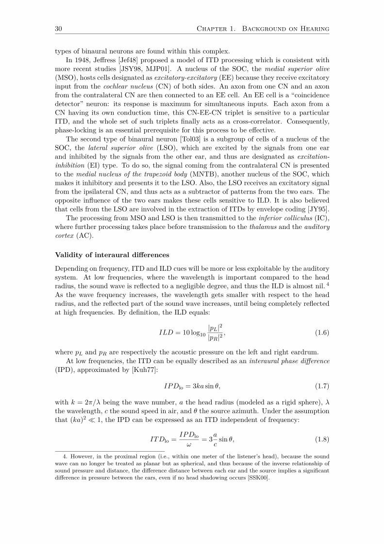
Depending on frequency, ITD and ILD cues will be more or less exploitable by the auditorysystem. At low frequencies, where the wavelength is important compared to the headradius, the sound wave is reflected to a negligible degree, and thus the ILD is almost nil. 4As the wave frequency increases, the wavelength gets smaller with respect to the headradius, and the reflected part of the sound wave increases, until being completely reflectedat high frequencies. By definition, the ILD equals:

ILD = 10 log10|pL|2

|pR|2, (1.6)

where pL and pR are respectively the acoustic pressure on the left and right eardrum.At low frequencies, the ITD can be equally described as an interaural phase difference

(IPD), approximated by [Kuh77]:

IPDlo = 3ka sin θ, (1.7)

with k = 2π/λ being the wave number, a the head radius (modeled as a rigid sphere), λthe wavelength, c the sound speed in air, and θ the source azimuth. Under the assumptionthat (ka)2 1, the IPD can be expressed as an ITD independent of frequency:

ITDlo = IPDloω

= 3ac

sin θ, (1.8)

4. However, in the proximal region (i.e., within one meter of the listener’s head), because the soundwave can no longer be treated as planar but as spherical, and thus because of the inverse relationship ofsound pressure and distance, the difference distance between each ear and the source implies a significantdifference in pressure between the ears, even if no head shadowing occurs [SSK00].


where ω is the angular velocity. Above 1500 Hz, the wavelengths fall below the interauraldistance, which is about 23 cm, and thus delays between the ears can exceed a period of thewave and become ambiguous. Moreover, the phase-locking ability of the auditory system(that is its ability to encode the phase information in the auditory nerve and neurons)decreases with increasing stimulus frequency [PR86], and is limited to frequencies below1.3 kHz [ZF56]. However, it has been shown [MP76] that when listening to a signal atone ear, and to an envelope-shifted version of it at the other ear, the ITD is still effective,even if the carrier is above 1500 Hz (but this ability decreases for frequencies above 4 kHz[MG91]). In that case, the ITD is well described by Woodworth’s model [WS54], which isindependent of frequency:

ITDhi = a

c[sin(θ) + θ]. (1.9)

So, two mechanisms are involved in the integration of the ITD: phase delay at low fre-quencies, and envelope delay at higher frequencies. Note that formulas (1.8) and (1.9)are assuming a spherical head (which is actually more oval) and ears at ±90 (which areactually a few degrees backward). Moreover, these models do not depend on elevation,which implies that cones of constant azimuth share the same ITD value. A more realisticmodel has been designed by Busson [Bus06].

The formulas above for ILD and ITD are physical descriptions of interaural cues, butthe way these cues are integrated by the auditory system is still unclear. It is generallyaccepted given the neural processing of interaural differences, that ITD and ILD are pro-cessed in narrow bands by the brain before being combined with information from othermodalities (vision, vestibules, etc.) to derive the position of the identified auditory ob-jects (see section 1.5). Besides, additional results support a frequency-specific encoding ofsound locations (see section 1.5.2). Such processing in narrow bands ensures the abilityto localize concurrent sound sources with different spectra. Therefore, the integration ofinteraural differences is often simulated by processing the two input channels through filterbanks and by deriving interaural differences within each pair of sub-bands [BvdPKS05].

Finally, the ITD and the ILD are complementary: in most cases, at low frequencies(below 1000 Hz), the ITD gives most informations about lateralization, and roughly abovethis threshold, the ITD becoming ambiguous, the ILD reliability is increasing, to take thelead above about 1500 kHz. Using synthetic and conflicting ITD and ILD, Wightman andKistler [WK92] showed that the ITD is prominent for the low-frequency lateralization of awide-band sound. However, for a sound without any low frequencies (below 2500 Hz), theILD is prevailing. Gaik showed [Gai93] that conflicting cues induce artifacts of localizationand modifications of the perception of tone color.

Limitations of ITD and IID

Assuming the simple models of ILD and ITD described above, these two cues do not dependon frequency, and especially they do not depend on elevation either. Hence, particularloci, called “cones of confusion”, were introduced by Woodworth; they are centered onthe interaural axis and correspond to an infinite number of positions for which the ITDand ILD are constant (see figure 1.24). Actually, these cones do not stricly make sense,and would rather in reality correspond to a set of points of equal ITD/ILD pair. Indeed,ITD and ILD are more complex than simple models, and measured iso-ITD or iso-ILDcurves are not strictly cone-shaped (see them on figure 1.24b). Anyhow, the necessarythreshold to detect small variations of position (see section 1.4.5) increases the number ofpoints of equal ITD/ILD pair. The term “cones of confusion” can also refer to a singlebinaural cue, ITD or ILD, considering the iso-ITD or the iso-ILD curves only.


met

ers

(per

pend

icul

ar t

o in

tera

ural

axi

s)

meters (along interaural axis)

(a) (b)

Figure 1.24: (a) Iso-ITD (left side) and iso-IID (right side) contours in the horizontal plane,in the proximal region of space. In the distal region, however, iso-ITD and iso-IID surfaces aresimilar. (After [SSK00].) (b) Superimposition of measured iso-ITD (in red, quite regular androughly concentric, steps of 150 µs) and iso-ILD (in blue, irregular, steps of 10 dB) curves in thedistal region. (Reprinted from [WK99].)


Thus, the duplex theory does not explain our discrimination ability along these “conesof confusion,” which implies a localization in elevation and in distance (also with anextracranial perception). The asymetrical character of the ILD could be a front/back dis-crimination cue. However that may be, these limitations suggested the existence of otherlocalization cues, the monaural spectral cues, which are discussed in the next section. Ithas also been shown that monaural cues intervene in localization in azimuth for some con-genitally monaural listeners [SIM94], and thus might be used as well by normal listeners.It is especially believed that monaural cues are used to reduce front/back confusions.

1.4.2 Localization in Elevation

So far, the presented localization cues, based on interaural differences, were not sufficientto explain the discrimination along cones of confusion. Monaural cues (or spectral cues)put forward an explanation based on the filtering of the sound wave of a source, due toreflections and diffractions by the torso, the shoulders, the head and the pinnae beforereaching the tympanic membrane. The resulting colorations for each ear of the sourcespectra, depending on both direction and frequency, could be a localization cue.

Assuming that xL(t) and xR(t) are the signals of the left and right auditory canalinputs of a x(t) source signal, this filtering can be modeled as:

xL(t) = hL ∗ x(t), and xR(t) = hR ∗ x(t), (1.10)

where hL and hR designate the impulse responses of the wave propagation from the sourceto the left and right auditory canals, and thus the previously mentioned filtering phenom-ena. Because of the direction-independent transfert functions from the auditory canalsto the eardrums, these are not included in hL and hR. The equivalent frequency domainfiltering model is given by:

XL(f) = HL ·X(f), and XR(f) = HR ·X(f). (1.11)

The HL and HR filters are called head-related transfer functions (HRTF), whereas hL andhR are called head-related impulse responses (HRIR). The postulate behind localizationin elevation is that this filtering induces peaks and valleys in XL and XR (the resultingspectra of xL and xR) varying with the direction of the source as a “shape signature”,especially in high frequencies [LB02]. The auditory system would first learn these shapesignatures, and then use this knowledge to associate a recognized shape with its corre-sponding direction (especially in elevation). Consequently, this localization cue requires acertain familiarity with the original source to be efficient, especially in the cases of staticsources with no head movements. In the case of remaining confusions of source position incones of constant azimuth, due to similar spectral contents, the ambiguity can be solvedby left/right and up/down head movements [WK99]. Also, these movements improve lo-calization performance [Wal40, TMR67]. Actually, a slow motion of the source in space issufficient to increase localization performance, implying that the knowledge of the relativemovements is not necessary.

1.4.3 Localization in Distance

The last point in localization deals with the remaining coordinate of the spherical system:the distance. The available localization cues are not very reliable, which is why ourperception of distance is quite imprecise [Zah02]. Four cues are involved in distanceperception [Rum01]. First, the perceived proximity increases with the source sound level.


Second, the direct field to reverberated field energy ratio gets high values for closer sources,and this ratio is assessed by the auditory system through the degree of coherence betweenthe signals at the two ears. Third, the high frequencies are attenuated with air absorption,thus distant sources have less high frequency content. And finally, further away sourceshave less difference between arrival of direct sound and floor first reflections.

1.4.4 Apparent Source Width

The apparent source width (ASW) has been studied for the acoustics of concert halls anddeals with how large a space a source appears to occupy from a sonic point of view. Itis related to interaural coherence (IC) for binaural listening or to inter-channel coherence(ICC) for multichannel reproduction, which are defined as the maximum absolute valueof the normalized cross-correlation between the left (xl) and right (xr) signals:

IC = max∆t

∣∣∑n=∞n=−∞ xl[n] · xr[n+ ∆t]

∣∣√∑n=∞n=−∞ x

2l [n] ·∑n=∞

n=−∞ x2r [n+ ∆t]

, (1.12)

When IC = 1, the signals are coherent, but may have a phase difference (ITD) or anintensity difference (ILD), and when IC = 0 the signals are independent. Blauert [Bla97]studied the ASW phenomenon with white noises and concluded that when IC = 1, theASW is reduced and confined to the median axis; when IC is decreasing, the apparentwidth increases until the source splits up into two distinct sources for IC = 0.

1.4.5 Localization Performance

The estimation by the auditory system of sound source attributes (as loudness, pitch,spatial position, etc.) may differ to a greater or lesser extent from the real characteristicsof the source. This is why one usually differentiates sound events (physical sound sources)from auditory events (sound sources as perceived by the listener) [Bla97]. Note that aone-to-one mapping does not necessarily exist between sound events and auditory events.The association between sound and auditory events is of particular interest in what iscalled auditory scene analysis (ASA, see section 1.3) [Bre94].

Localization performance covers two aspects. Localization error is the difference inposition between a sound event and its (supposedly) associated auditory event, that is tosay the accuracy with which the spatial position of a sound source is estimated by theauditory system. Localization blur is the smallest change in position of a sound event thatleads to a change in position of the auditory event, and thereby is a measure of sensitivity.It reflects the extent to which the auditory system is able to spatially discriminate twopositions of the same sound event, that is the auditory spatial resolution. When it charac-terizes the sensitivity to an angular displacement (either in azimuth or in elevation), thelocalization blur is sometimes expressed as a minimum audible angle (MAA). MAAs inazimuth constitute the main topic of this thesis and are especially studied in chapter 3. Wewill see in the following that both localization error and localization blur mainly dependon two parameters characterizing the sound event: its position and its spectral content.

Localization errors have been historically studied by Lord Rayleigh [Ray07] using vi-brating tuning forks, after which several studies followed. Concerning localization in az-imuth, studies [Pre66, HS70] depicted in figure 1.25 using white noise pulses have shownthat localization error is the smallest in the front and back (about 1), and much greaterfor lateral sound sources (about 10). Carlile et al. [CLH97] reported similar trends usingbroadband noise bursts. According to Oldfield and Parker [OP84], localization error in


Figure 1.25: Localization error and localization blur in the horizontal plane with white noisepulses [Pre66, HS70]. (After [Bla97].)

azimuth is almost independent of elevation. Localization blur in azimuth follows the sametrend as localization error (and is also depicted in figure 1.25), but is slightly worse inthe back (5.5) compared to frontal sources (3.6°), and reaches 10 for sources on thesides. Perrott [PS90], using click trains, got a smaller mean localization blur of 0.97. Thefrequency dependence of localization error in azimuth can be found for example in [SN36],where maximum localization errors were found around 3 kHz using pure tones, these valuesdeclining for lower and higher frequencies. This type of shape for localization performancein azimuth as a function of frequency, showing the largest values at mid frequencies, ischaracteristic for both localization error and localization blur and is usually interpreted asan argument supporting the duplex theory. Indeed, in that frequency range (1.5 kHz to3 kHz), the frequency is too high for phase locking to be effective (which is necessary forITD), and the wavelength is too long for head shadowing to be efficient (which is necessaryfor ILD), thereby reducing the available localization cues [MG91]. The frequency depen-dence of localization blur has been studied by Mills [Mil58] (see figure 1.26) and variesbetween 1 and 3 for frontal sources. Boerger [Boe65] got similar results using Gaus-sian tone bursts of critical bandwidth. Important front/back confusions for pure tones,compared to broadband stimuli, are reported in [SN36]. Moreover, the study from Carlileet al. [CLH97] confirms that only a few front/back confusions are found with broadbandnoise. This is a characteristic result concerning narrow band signals, given that monauralcues are poor in such cases and cannot help discriminate the front from the back by signalfiltering.

Concerning localization error in elevation, several studies report worse performancethan in azimuth. Carlile et al. [CLH97] reported 4 on average with broadband noisebursts. Damaske and Wagener [DW69], using continuous familiar speech, reported local-ization error and localization blur in the median plane that increases with elevation (seefigure 1.27). Oldfield and Parker [OP84], however, announce an error independent of theelevation. Blauert [Bla70] reported a localization blur of about 17° for forward sources,which is much more than Damaske and Wagener’s estimation (9°), but using unfamiliarspeech. This supports the idea that a certain familiarity with the source is necessary to


Figure 1.26: Frequency dependence of localization blur in azimuth (expressed here as a “min-imum audible angle”) using pure tones, as a function of the sound source azimuth position θ.(After [Mil58].)

Figure 1.27: Localization error and localization blur in the median plane using familiar speech[DW69]. (After [Bla97].)


Figure 1.28: Localization error and localization blur for distances using impulsive sounds [Hau69].(After [Bla97].)

obtain optimal localization performance in elevation. Perrott [PS90], using click trains,got a mean localization blur of 3.65. He also performed measures of localization blur foroblique planes, and reported values below 1.24 as long as the plane is rotated more than10 away from the vertical plane. Grantham [GHE03], on the contrary, reported a higherlocalization blur for a 60 oblique plane than for the horizontal plane, but still a lower blurthan for the vertical plane. Blauert [Bla68] brought to light an interesting phenomenonconcerning localization in the median plane of narrow-band signals (bandwidth of lessthan 2/3 octave): the direction of the auditory event does not depend on the direction ofthe sound event, but only on the frequency of the signal. Once again, this is justified bythe fact that monaural cues are non-existent for such narrow-band signals.

Finally, studies dealing with localization in distance suggest that performance dependson the familiarity of the subject with the signal. Gardner [Gar69] studied localization inthe range of distance from 0.9 to 9 m with a human speaker whispering, speaking normally,and calling out loudly. For normal speaking, performance is excellent, whereas distancesfor whispering and calling out voices are under- and an over-estimated, respectively. Goodperformance for the same range of distances was reported by Haustein [Hau69] using impul-sive sounds (see figure 1.28), but using test signals that were demonstrated beforehandfrom different distances. On the contrary, Zahorik [Zah02] reports a compression phe-nomenon: sources closer than one meter are over-estimated, whereas far-away sources areunder-estimated.

Just-Noticeable Differences

Beside the sensitivity to a physical displacement of a sound source, which is characterizedby the notion of localization blur, some research has studied the sensitivity to the cuesunderlying the localization process, namely ITD, ILD, IC, and spectral cues. In thissection, we will focus on results concerning the sensitivity to changes in the binauralcues only (ITD, ILD and IC). This can be measured by manipulating localization cues togenerate a pair of signals (specific to each ear) and playing them over headphones to alistener. For instance, an artificial ITD can be introduced between the two signals to testthe smallest variation of ITD a listener is able to detect, i.e., the just-noticeable difference(JND) of ITD. The sensitivity to a given cue can potentially depend on the following mainparameters: the reference value of this cue (the initial value from which the sensitivityto a slight variation is tested), the frequency (content) of the stimulus, the level of thestimulus (apart from the potential presence of an ILD), and the actual values of the otherlocalization cues.

For stimuli with frequencies below 1.3 kHz, the ITD can be described as a phase


difference (IPD, see section 1.4), and for a null reference IPD, the JND of IPD does notdepend on frequency and equals about 0.05 rad [KE56]. This sensitivity tends to increaseas the reference IPD increases [Yos74, HD69]. There does not seem to be an effect ofthe stimulus level on the JND of ITD [ZF56], although there is a decrease in sensitivityfor very low levels [HD69]. Finally, the sensitivity to a change of ITD decreases with anincreasing ILD [HD69].

For a null reference ILD, the JND of ILD is relatively independent of stimulus level[Yos72] (except again for very low levels [HD69]) and of stimulus frequency [Gra84]. As thereference ILD increases, the sensitivity to a change of ILD decreases [Mil60, RT67, YH87]:from between 0.5 and 1 dB for a reference ILD of 0 dB, to between 1.5 and 2 dB for areference ILD of 15 dB. The dependence of ILD sensitivity on the reference ITD is notclear, since Yost [Yos72] reported that this sensitivity increases when the ITD increases,whereas no dependence is reported in [HD69].

Concerning the JND of IC, a strong dependence on the reference IC has been shown[RJ63, LJ64, GC81, CCS01]: from 0.002 for a reference IC of +1, to about a 100 timeslarger necessary variation for a reference IC of 0. The sensitivity to IC change does notdepend on stimulus level [HH84], except for low levels.

1.4.6 Binaural Unmasking

Central masking

Two kinds of masking can happen when a target signal is mixed with competing sources.The first one, known as energetic masking (EM), occurs when a masker (for instance anoise) renders a target totally or partially inaudible, as presented in section 1.2.2. It re-sults from the competition between the target and the masker in the auditory periphery,i.e., overlapping excitation patterns in the cochlea or auditory nerve, which corresponds toperipheral masking (PM). This situation must be differentiated from central masking (CM;also called nonenergetic masking), which takes place more centrally in the auditory path-way (see figure 1.23). Most central masking consists of informational masking (IM), 5which is caused by two main factors: target-masker similarity and stimulus (masker) un-certainty. In such a situation, although the target is audible, it is confused with the masker,leading, as in the case of energetic masking, to a decrease in the threshold of detectabilityof the target. Target-masker similarity is encountered when target and masker 6 share anumber of similar characteristics, such as spectro-temporal similarities (a typical examplebeing speech on speech), even without frequency overlap, such that EM is reduced. Thosesimilar characteristics recall incidentally the grouping cues used to form auditory streams(see section 1.3). Stimulus uncertainty occurs when one or several characteristics (such asfrequency, intensity, 7 or spatial location) of the masker vary rapidly in time to appear ran-dom 8 to the listener. As explained by Durlach in [DMKJ+03], these main factors interact:stimulus uncertainty is neither necessary nor sufficient to produce non-energetic masking;

5. The extent to which CM and IM are related is currently left open. In particular, questions ariseabout which central limitations that lead to threshold elevation should be included under CM, and whichcomponents of CM should be included in IM. This is discussed in [DMKJ+03].

6. In fact, some authors consider that what is really important is not the similarity between the maskerM and the target T, but rather the similarity between M and M+T, because of the design of the task ina detection experiment (see [DMKJ+03]).

7. In this particular case, it is the overall level—of the masker and the target—which vary rapidly, inorder to keep a constant TMR (target-to-mask ratio).

8. In order to be effective, the range of the randomization must not be small compared to the listener’sresolution.


the effects of uncertainty are reduced by decreasing target-masker similarity. Furthermore,Fan showed [FSD08] that compared both to the effects of spectral uncertainty and to theeffects of overall-level uncertainty, the effects of spatial uncertainty are relatively small.Neff and Dethlefs [ND95] and Oxenham et al. [OFMKJ03] report that some listeners areresistant to the effects of uncertainty. In the case of frequency uncertainty, Gallun et al.[GDC+08] report that some listeners, less affected by IM than others, seem to react asthey do for EM. The proposed explanation of these results relies on a power-spectrummodel of masking release (more details are given in [DMG+05]). Briefly, it postulates thatlisteners who are adversely affected by the variability in the masking stimulus (i.e., itsuncertainty) widen their effective auditory filters (larger than a critical band), which leadsto an increase of its masking ability. This idea was first suggested by Lutfi [Lut93].

Binaural release from masking

In both situations (energetic and informational masking), listening performances can beimproved when the sources arise from different spatial locations. This leads to “binauralrelease from masking,” which is also called spatial unmasking. The change in the detectionthreshold of the target compared to when sources are presented with identical spatialpositions is called binaural masking level difference (BMLD). As an example, a maskingtone presented in phase to both ears with a pure-tone target presented out-of-phase to eachear simultaneously—this situation is called a NoSπ condition—results in a lower thresholdlevel for detecting the target than in the case when both the masker and the target arepresented in phase (a NoSo condition). This reflects spatial unmasking, because addinga phase difference to the target corresponds to the generation of a constant ITD, that isto say a perceptual spatial displacement of the target only. Generally, and as describedin [Shi05], three distinct mechanisms are associated with spatial unmasking: acousticbetter-ear effects, binaural processing, and spatial attention.

Better-ear effects are a direct consequence of ILD. When a source is to the side of thelistener and contains significant energy above 2 kHz, sound reflection by the head increasesthe energy level at one ear. Thus, if the masker is spatially displaced from the target, thesignal-to-mask ratio (SMR, see section 1.2.2) increases at one ear and decreases at theother, which leads to great improvements in the intelligibility of the target.

Binaural processing can improve the target audibility when this one remains maskeddespite the help provided by better-ear effects. As explained in [Shi05], when the targetand the masker arise from the same direction, the interaural coherence does not changesignificantly when the target is present. However, in the case of different directions, theinteraural coherence is decreased. Hence, the listener identifies this temporary decrease incorrelation as being caused by an (otherwise inaudible) source at that time and frequency.Therefore, binaural processing allows listeners to detect the presence of target energy ina particular time and frequency band if the target and masker induce different interauraltime and/or intensity differences.

The third mechanism associated with spatial unmasking is known as spatial atten-tion, and has been largely studied in vision. It is based on the fact that listeners canorient their attention spatially to enhance the detection and identification of simple tar-gets. Several authors report that when target and masker are spectro-temporally similar,perceived spatial separation contributes to spatial unmasking, but not when target andmasker are dissimilar and easily segregated. For instance, Kidd and colleagues have con-ducted experiments with competing signals that have very little spectro-temporal overlap[AMKJ05, KJMBH05]. Because there is almost no energetic masking, one could predictlittle or no spatial unmasking, but it was actually prominent when target and masker


were statistically similar and negligible when the masker was steady-state noise. Further,Best got similar results with spectro-temporally complex birdsongs [BOG+05]. Therefore,spatial attention seems to be efficient in cases of informational masking.

An interesting hypothesis combining the last two mechanisms would be that binauralprocessing actually creates binaural spatial channels, corresponding to different interauralconfigurations (ITD/ILD pairs). Then spatial attention would consist of nulling out themasker rather than focusing on the target. Although the results from Fan [FSD08] reportedabove conclude that the effect of spatial uncertainty in informational masking is weak, itis not negligible. That could lead to the conclusion that masked detection performance isstill vulnerable to randomization of the spatial properties of the masker, which would beconsistent with this hypothesis.

As explained by Durlach in [DMKJ+03], there could hypothetically be two extremetypes of listeners, the Listener-Max corresponding to an archetypal analytic listener at-tempting to maximize the T/M ratio by maximizing T (with an acceptance filter focusedon T), and Listener-Min corresponding to an archetypal holistic listener attempting tomaximize the T/M ratio by minimizing M (with a multiple notch-rejection filter matchedto M). With this distinction, when M is uncertain, Listener-Max should do best, whereaswhen T is uncertain, Listener-Min should do best.

But is the binaural release from energetic or informational masking due to a perceiveddifference in location or only to the presence of interaural difference cues (which couldbe then processed separately)? Gallun et al. in [GDC+08] report that for both types ofmasking, the obtained detection thresholds are similar in either the case of “reinforcing”ITDs and ILDs (one ear advanced in phase and higher in level) or in the case of “opposing”ITDs and ILDs (one ear advanced in phase and the other one higher in level), leading toan irrelevance of differences in the perceived location for both energetic and informationalmasking.

In the continuity of the model of auditory filter widening described above, Gallun et al.[GDC+08] also postulate that, in the case of informational masking, interaural differencesreduce uncertainty and allow listeners to focus their effective filter more appropriately, thelower limit being the width of one critical band.

Kopčo and Shinn-Cunningham studied spatial unmasking in the case of nearby targetand masker [KS03]. They evaluated the relative contribution of better-ear effects andbinaural processing to spatial unmasking, showing a large contribution of better-ear effects.Interestingly, they noticed that there are cases where detection performance is actuallyworse when the sources are spatially separated compared to when they are at the samelocation, constituting a case of “spatial masking.” This situation arises in particular whenboth the target and the masker are located at 90, the masker being farther away thanthe target.

1.5 Localization Cues in Auditory Scene Analysis

This section concerns the integration of the spatial cues in the auditory scene analysis(ASA) process. As explained by Bregman in [Bre94] (see section 1.3), the auditory sys-tem, in its grouping process, seems to act as a voting system based on heuristic criteria.Spatial cues form part of theses criteria, but do not necessarily overpower other heuristicswhen in conflict with them—for instance, we are able to segregate different voices from amonophonic record.

The sequential and simultaneous integration of spatial cues are discussed in separateparts, but because these two kinds of integration interact between them, a third part deals

1.5. Localization Cues in Auditory Scene Analysis 41

Figure 1.29: Illustration of the scale illusion from Deutsch [Deu74b]. Part 1: the stimulus, theletters show the ear of presentation. The tones of upper and lower staffs are presented simultane-ously. Part 2: The stimulus resulting in each ear (upper staff for left ear, lower staff for right ear).Part 3: the sequences, as they are perceived by most of the subjects. Tones seem to have beengrouped by frequency range. (After [Bre94].)

with this interaction. The last part treats the particular case of speech.

1.5.1 Sequential Integration

The sequential integration of spatial cues concerns how (much) the spatial location isinvolved in the streaming phenomenon.

Roger Shepard introduced the “psychophysical complementarity” principle in [She81]:because the auditory system can segregate sounds by their location, as space is physicallya continuum (an object moving from one point to another must pass through all the inter-mediate positions), the perceptual representation of space must also have this property.Thus, if two identical sounds arise from sufficiently far-away locations in space withouta continuous movement joining them, they would probably be treated as coming fromdifferent sources.

In two different experiments, Norman [Nor66] and van Noorden [vN75] reported astrong segregation by spatial origin. Norman observed that when a trill is presented witheach of its alternate tones to a different ear, the continuous up-and-down movement ofthe pitch does not occur. Van Noorden did an introspective experiment and concludedthat the temporal links between the tones in the two ears were weak. Using sequenceswith tones of identical frequency, he reported that judging if the tones sent to one earwere exactly halfway in time between the tones sent to the other ear was a hard task(depending on the tone rate), which is not the case with a diotic presentation. Theseexperiments would lead to the conclusion that spatial separation is strong with respect toother grouping criteria.

Nevertheless, the proposals made by Norman and van Noorden have not been con-firmed by later research. Indeed, criteria in conflict with spatial cues can lead to streamsegregation, so that hearing of dichotically alternating tones as an integrated sequenceis possible, as shown by the Deutsch’s “scale illusion” [Deu74b]. The C major scale ispresented to each ear of the subject over headphones in its ascending and descending formaccording to the score of part 1 of figure 1.29. The alternation between left and rightears results in two complex melodies illustrated in the second part of the figure. However,


Pattern A Channel 1 . . . 1 - 4 - 1 - 4 - . . .Channel 2 . . . - 2 - 3 - 2 - 3 . . .

Pattern B Channel 1 . . . 1 - 4 - 1 - 4 - . . .Channel 2 . . . - 3 - 2 - 3 - 2 . . .

Figure 1.30: The patterns presented by Judd to achieve a segregation by spatial location. Hy-phens represent silences, and the numbers 1 to 4 represent four tones within an eight-semitonerange.

most listeners actually perceive the pattern shown in the third part of the figure: thetwo complex patterns are turned into two much simpler patterns, meaning that the toneswere grouped by their frequency range rather than by their ear of presentation. Bregmannoticed that this illusion is effective even for rates of up to 20 tones per second, whichmeans that its efficiency is not due to the slowness of the sequence (which otherwise wouldallow the listeners to switch their attention back and forth, and track the tonal sequenceon the basis of frequency proximities).

Judd [Jud77] gave an explanation of the failure of spatial grouping to effectively com-pete with frequency proximity in Deutsch’s scale illusion, which is based on the simul-taneity of tones at the two ears. In an experiment, subjects must choose which of the twopatterns in figure 1.30 they heard over headphones. Because the sequences of channel1 are identical in both cases, and the two sequences of channel 2 are the same but witha different starting point, the distinction of the two patterns requires channels 1 and 2not to be segregated (by spatial location) in order to integrate the whole pattern and usechannel 1 as a comparison point for channel 2. In such conditions, listeners had difficultyto distinguishing the two patterns. But Judd showed that by replacing the silences witha white noise with an amplitude equal to that of the tones, it was easier for listeners todistinguish the two patterns, thereby suggesting a reduction of the perceived ILD and thusa weakening of the spatial localization cues, thanks to the contralateral white noise. Juddalso showed that by not playing the tones of the scale illusion simultaneously, but with acontralateral white noise, one can observe a segregation of streams according to the ear ofarrival.

Later, Deutsch confirmed [Deu79] Judd’s results with an identification task of eight-tone patterns in which the component tones switch between the ears. The task is verydifficult as it is, but with a contralateral “drone” (like Judd’s white noise), the melodiescould be recognized more easily. Also, an experiment by Schubert and Parker [SP55]reports similar results with speech switching between the ears.

These results prove that different spatial locations of sounds can cause the auditorysystem to assign them to separate streams. Nevertheless, we saw that stream segregationby spatial location is not overpowering when in conflict with other bases for grouping.Bregman explains these unexpected observations by the fact that spatial cues are notreally reliable for grouping because several sources can come from the same direction(but should not be grouped together), and also because sounds echoe, reverberate andwrap around obstructions, leading to unclear spatial origins of a sound. Evidence showsthat location differences have a powerful multiplying effect when they are consistent withother bases for grouping (see [Bre94], ch. 7). Moreover, it should be noted that the ITDlocalization cue is not present in the illusions and experiments presented in this section,therefore leading to a weakening of the spatial basis for segregation.


Distortion of time

A surprising phenomenon has been related by Axelrod and Guzy [AG68]. Subjects arepresented with series of rapid clicks uniformly spaced in time over headphones in twodifferent forms: dichotic (clicks alternate between left- and right-ear), and diotic (eachclick is sent to both ears). With the dichotic presentation, the sequence is perceived asslower. Huggins [Hug74] did further experiments to assess the resulting distortion of time,by asking subjects to adjust the diotic sequence to make it sound as fast as the dichoticone. At slow rates (below eight tones per second), his subjects adjusted the diotic sequenceto the same rate as the total event rate in the dichotic sequence. Then, for click ratesfrom 8 to 20 per second, the diotic sequence was continuously slowed-down relative to thedichotic sequence. Finally, for higher rates, the diotic sequence was adjusted to one-halfthe dichotic sequence rate. Although for low and high rates, it is possible to argue thatthe dichotic sequence was either integrated as one single stream or segregated into twoseparate streams, respectively, the stream concept somewhat fails to explain the resultswith intermediate rates, all the more so as this distortion of time does not occur whenusing frequency grouping cues instead of spatial ones. Nevertheless, Bregman proposedthe hypothesis that because perceptual organization tends to be unstable when the cuesfavoring segregation are not decisive, at intermediate rates, on some trials the clicks formedan integrated stream and on others they segregated into two streams.

1.5.2 Simultaneous Integration

Kubovy in [Kub81] proposed that in audition, as in vision, segregation of simultaneoussignals relies on indispensable attributes. An indispensable attribute is a feature allowingthe perception of the twoness of two simultaneous signals that are identical except for thatfeature. Kubovy states that indispensable auditory attributes are time and frequency, butnot space or loudness. Whereas this is true for the loudness attribute, Bregman notesthat concerning space, in cases of complex scenes, two sounds that differ only in spatiallocation can be heard separately and not fused together. He gives as an example thefollowing experiment. Using an algorithm that simulates the spatial position of a sourceon headphones (binaural synthesis), he synthesized one pure tone at 600 Hz at +45, andanother one still at 600 Hz at −45, 0 being in front of the listener. Each of the twotones was played at irregular intervals, leading to unsynchronised onsets and offsets andsubstantial overlaps in time. One could predict that during time overlaps, because of thebalance of energy, only one tone (positionned at 0) should be heard resulting from thefusion of the two tones at ±45. However, no tone is heard in the middle, and the twotones are still perceived at their initial position. This result is due to the timing differenceat the two ears when changes (onset or offset) occur, which constitutes a strong cue forspatial localization, and therefore for spatial segregation.

A frequency-specific ear-comparison process

Bregman provides evidence that ear comparisons must be frequency specific. This evidenceis important because it justifies the auditory system’s ability to derive separate locationsfor simultaneous sources. Besides, it justifies the choice made in the design of somemultichannel audio coders to analyze spatial cues in the input signals into frequencysubbands (see section chapter 2).

The first point states that lesions of the auditory cortex of a cat lead to the inabilityfor it to tell where a short burst of a certain frequency is coming from in space, but its


spatial localization ability may remain intact and normal for other frequencies [JM84]. Assimilar results have been reported for humans [ZP01, SS11], this would confirm that theauditory system is capable of frequency-specific localization.

Another point concerns the tolerance in mistuning of two tones at different locationsfor them to be fused together. As reported by Perrott and Barry [PB69], in the rangefrom 250 Hz to 4 kHz, it is never greater than about 7%, which implies that spatial fusionrequires quite a fine tuning to operate.

Conversely, an experiment by Kubovy and Howard [KH76] shows the existence of acomputation of location that is separate for each frequency, but also has a separate memoryfor each. To do that, they presented listeners over headphones with a chord composed ofsix pure tones of separate spatial position in the horizontal plane by introducing an ITDcue for each. The resulting overall sound was perceptually confused. Then, after a briefpause, they presented the same chord except that the horizontal position of one of thecomponents was changed. This time, the moved tone was salient, and its pitch was heardseparated from the blurred mass. Note that the first chord was obviously indispensablefor this experiment to succeed, and for most of the listeners, the silence must not exceed1.5 seconds.

Cramer and Huggins made an experiment [CH58] tending to demonstrate the auditorysystem’s ability to separate different spectral components on the basis of their points oforigin in space. Using a diotic broad-band noise from which the low-frequency part (below1000 Hz) has been phase delayed in one ear relative to the other (the remainder beingidentical at the two ears), the perceived result is that the pitch of the low-filtered partemerges slightly from the rest of the broad-band noise.

Concerning the fusion observed between a sound event and its echo (known as the“precedence effect” [LCYG99, WNR49]), the stream notion seems to be a valid interpre-tation of this scene-analysis process, since only one sonic event has actually occured. Aninteresting remark, however, is that this process seems to rely on a “delay-resisting” com-mon fate process between the original sound event and its echo, which follow identicalvariations in frequency or intensity, but are delayed in time.

There are experiments showing that segregation by spatial location can be quite com-pelling. For example, Green [GKJP83] noticed that, given two spectra with differentoverall loudness, listeners can either recognize two spectra with identical shapes, or dif-ferentiate two spectra with different shapes, even if their shapes differ only by a modestincrease in the intensity of one spectral component (at 949 Hz) relative to the others.However, if the 949 Hz component is separated and sent to the opposite ear, listenerscould no longer integrate the left- and right-ear sounds into a single qualitative analysis.

Interaction with other grouping cues

The fact that two sounds coming from the same direction do not necessarily originatefrom the same acoustic event (a sound source might be acoustically transparent), andthat spatial cues (binaural cues and spectral cues) are not infallible (for example in areverberating environment), leads the auditory system to consider other grouping cues,as well (see section 1.3.5). Because, for instance, the fundamental frequency of a soundevent, or its internal harmonic relations, are not modified by the environment, these cuescan override spatial cues in the decision made by the auditory system.

An illustration of this is a pattern made at IRCAM 9 by Reynolds and Lancino for usein a musical piece. It consists of the synthesis of even and odd harmonics of an oboe on

9. Institut de Recherche et Coordination Acoustique/Musique, Paris, France.


separate speaker channels, with FM micromodulations specific to each channel imposedon the harmonics. When left and right micromodulations are synchronized and identical,the listener heard a single centered oboe, but as the micromodulations are gradually madeindependent from left to right, but synchronously within each speaker, the sound seemedto split into two separate sounds, even harmonics on one channel, and odd harmonics onthe other one. Here, in the first case, ear cues are overcome by spectral cues (harmonicrelations) and sequential cues (common fate with micromodulations).

An experiment by Steiger and Bregman [SB82] which tries to assess the extent to whichthe fusion of partials between two simultaneous sound events can occur in dichotic anddiotic situations reports that the requirements for the fusion of partials are less stringentwithin an ear than across ears. Bregman justifies this idea by the fact that nature is ableto send the same sound to different ears with loudness lowered in one ear, but not pitch.To the contrary, most natural sounds contain partials that are not exactly harmonicallyrelated, so within-ear fusion can accept less exact relations between partials.

An important point, illustrated by the illusion from Deutsch described in section 1.3.5,is that spatial cues do not particularly override other grouping cues in the presence of dis-crepancies. Moreover, in those situations, the auditory system tries to build a consistent,but erroneous, description of the auditory scene.

One last interesting interaction is with visual cues. The ventriloquism effect [WW80]occurs when the visual and the auditory spatial locations of a multimodal event do notcoincide. In this case, the typical perceptual result is the choice of an intermediate locationfor the sound. However, when several visual event occur at the same time, the decisionseems to rely upon at least two criteria: the angular distance between the auditory and thepotential visual event (which must not be too important) and their temporal synchrony(which must at least be weak).

1.5.3 Interactions Between Sequential and Simultaneous Integrations

Despite the small influence of spatial cues on simultaneous integration, the streaming ofsound elements over time are more strongly influenced by spatial location, particularly forspeech intelligibility. Darwin and Hukin [DH00] asked subjects to report a target wordcontained in a target carrier phrase, while a second carrier phrase was presented simul-taneously. Thereby, two candidate target words were presented simultaneously duringa time-aligned temporal gap present in both the target and competing carrier phrases.Despite the presence of grouping cues opposed to spatial cues, the subjects reported thetarget word that spatially matched the target phrase.

Shinn-Cunningham [Shi05] proposed a simplistic view of how spatial cues affect audi-tory scene analysis:

1. Spatial cues do not influence grouping of simultaneous sources. Instead other soundfeatures determine how simultaneous or near-simultaneous sounds are grouped lo-cally in time and frequency, forming “snippets” of sound.

2. Once a sound snippet is formed, its spatial location is computed, based primarily onthe spatial cues in the sound elements grouped into that snippet.

3. Sound snippets are then pieced together across time in a process that relies heavilyon perceived location of the snippets.

However, it has been shown by Darwin and Hukin [DH97, DH98] that spatial cuescan also influence simultaneous grouping when other grouping cues are ambiguous. With


Time

Fre

quen

cy

Captors absent

Time

Fre

quen

cy

Captors present

Figure 1.31: Stimuli used by Bregman and Steiger. The vertical bars represent noise bursts(played on a loudspeaker) and the dark horizontal bars are tones (presented over headphones).(Reprinted from [BS80].)

stimuli in which a target tone could logically fall into one of two streams, one a sequence ofrepeated tones and the other a simultaneous harmonic complex, they measured the degreeto which the ambiguous target was heard as part of the harmonic complex. The resultsshowed that when the spatial cues in the target and the harmonic complex matched, thetone was heard more prominently in the harmonic complex than when the spatial cues wereuninformative. But this study also shows that spatial cues can influence grouping whentop-down listener expectations also influence grouping: the results of a given stimulusdepend on what subjects heard in past trials. In the same spirit, research conducted byLee and Shinn-Cunningham [LSO05] provided evidence that the perceptual organization ofa mixture depends on what a listener is attending to. In particular, with the previous toneparadigm and by changing which object a given listener was asked to attend to (holdingthe same stimuli), they found that there was no predictive relationship between the degreeto which the target was in one auditory object and the degree to which it was out of theother.

An experiment [BS80] conducted by Bregman and Steiger is interesting because itinvolves spatial location in elevation. As illustrated in figure 1.31, it uses white noisebursts played on a loudspeaker simultaneously with a high or low pure tone (presentedover headphones) in order to color it, leading to a localization of the noise burst higheror lower in space (see sections 1.4.2 and 1.4.5). However the experiment shows that whencaptors of the frequency of the pure tone are present before and after the mixture in orderto capture the pure tone into a separate stream, the perceived position of the noise burstrelies only upon the real position of the loudspeaker. This shows the effects of perceptualorganization on the actual perceived location of sounds.

As in the continuity illusion (see section 1.3.4), sequential integration overcomes thesimultaneous integration (and more precisely spectral integration). There is a simple ex-periment, designed by Bregman, that illustrates that sequential integration can overcomesimultaneous integration (actually binaural integration in this case) by playing the samepure tone on the left and right channels, but with varying intensity in one ear (left, forexample) from silence to the level of the right ear (which is fixed). If the intensity varia-tion is low, the perception is one tone which seems to move from the right to the center,as expected. However, when increasing variation speed, two tones are heard, one at theright, and the other one pulsing at the left.

1.5.4 Speech-Sound Schemata

In the particular case of speech, differences in spatial origin rarely prevent the auditorysystem from grouping the information from different spatial locations, because it uses

1.6. Conclusions 47

powerful schemata for the recognition of speech sounds, which could not care about thespatial origins of acoustic components.

This could be illustrated by an experiment from Broadbent [Bro55] in which listenersare presented with high-frequency components of speech to one ear and low-frequencycomponents to the other. As a result, the listeners fused the two parts and heard asingle sound. Broadbent explains this result by the commonalities of the two signals:fundamental frequency, onset/offset synchrony, harmonicity, etc. Bregman notes thatthis fusion is possible because spatial location can be assessed independently in differentfrequency bands (as suggested in sections 1.4.1 and 1.5.2) and results from an heuristicvote comprising spatial estimates among many other factors.

Similar results were reported by Cutting [Cut76] with formants presented to differentears. One interesting point is that when the fundamentals of the formants of a two-formantsynthetic syllable were only one-third of a semitone apart (100 and 102 Hz), the formantswere almost always heard as two sounds. Such a little difference in frequency wouldprobably not have led to a segregation if the sounds had not been in separate ears. Thistends to show that spatial estimation and fundamental frequency cues increase their ownsegregation power when acting together. Moreover, in the case of different fundamentals,the listeners reported hearing two sounds, but identified the speech sounds anyway. It ispossible to break the phonetic fusion by repeating the syllable over and over, but onlyif the two sounds are differentiated both by location and fundamental frequency. Hence,phonetic integration is difficult to disrupt probably because of speech-sound schemata.Bregman explains the relative insensitivity of the phonetic schemata to factors such asperceived location and fundamental frequency by the fact that probably neither of thesefactors is used by the recognition schemata since neither is involved in the definition of aspeech sound, in opposition to the time-varying spectral pattern. However, they may beimportant in situations where several speech-sound schemata are in competition, assumingthat speech sounds come from different spatial directions.

A last experiment, by Scheffers [Sch83], which is not related to spatial cues lets ussuppose a particular way in which these speech-sound schemata work. Listeners are pre-sented with pairs of vowels, each vowel with a given fixed fundamental frequency. Resultsshow that a difference in the fundamental frequency facilitates vowel segregation. It couldbe explained by the fact that the auditory system probably grouped the set of harmonicsfor each vowel to reconstitute its spectral shape. But this experiment also reports thatusing the same fundamental frequency, with same spatial location and onset/offset syn-chronization, listeners recognized the vowels 68% of the time. So, as noted by Bregman,it seems that speech-sound schemata integrate spectral information without the cues usedfor scene analysis, simply by taking the desired material from a dense mixture of sound.

1.6 Conclusions

Localization cues, as described in section 1.4, constitute a low-level spatial assessment ofeach frequency component of the auditory input, but the grouping into auditory streams(and the derivation of their associated spatial locations) is performed at a higher leveland in combination with other modalities (such as vision, for example) to yield a finaldescription of the auditory scene. Bregman believes that the auditory system, as withother perceptual systems, acts as a voting system based on heuristic criteria, includinglocalization cues as well as criteria such as those described in section 1.3. Because of thevariability of the environment, each of these criteria alone is not guaranteed to succeed,but when put together, a good description of the scene can result. At the extremes,


when all criteria vote in a different way, the solution is ambiguous, whereas when they areunanimous, the description is stable and clear.

Studies that investigated localization performance have been presented. Auditory spa-tial resolution (or localization blur) has been especially studied for target sources in quiet,that is without any interfering source. However, as we will show in chapter 3, this resolu-tion is subject to deteriorate when multiple sources are present.

Chapter 2

State-of-the-Art of Spatial AudioCoding

In this chapter we provide a panorama of the technologies used in audio coding and morespecifically in spatial audio coding. Here, the implicit meaning of coding is “achieving abit-rate reduction”. The approach we have chosen is driven by the concepts behind audiocoding rather than the actual codecs available today. The monophonic case is treatedbriefly first, to focus afterwards on stereophonic and multichannel signals.

When dealing with multi-channel signals, the input signals are assumed to be two ormore channels either acquired using a microphone array or synthesized using spatializationtechniques such as vector-base amplitude panning (VBAP) [Pul97], wave field synthesis(WFS) [dV09], higher-order Ambisonics (HOA) [DNM03] or even binaural rendering. In-formation about recording and synthesis can be found in [Rum01].

Particular attention has been given to HOA as well as to parametric spatial audio cod-ing methods, as they both constitute the bases of the developments proposed in chapter 5.

2.1 Representation of Spatial Audio

2.1.1 Waveform Digitization

The most usual digital representation of a monophonic waveform is Linear Pulse-CodeModulation (LPCM) encoding, often referred to simply as PCM. The waveform is dis-cretized at a given sampling rate using a uniform quantization. The fidelity of the repre-sentation is given both by the sampling rate and the quantization step size. The Nyquist-Shannon sampling theorem [Sha49] asserts that the uniformly spaced discrete samples arean exact representation of the signal if this bandwidth is less than half the sampling rate.So, in LPCM, the highest represented frequency component is half the sampling rate ofthe signal. The quantization step size depends on the number of bits with which eachsample is coded [GG91]. The original waveform is thus approximated depending on thesetwo parameters.

LPCM is especially used in the Compact Disc Digital Audio (CD-DA) standard, cre-ated by Sony and Philips in 1980 and regarded as a reference format in terms of quality.On a CD, a waveform is encoded using a sample rate of 44100 Hz and each sample is codedon 16 bits, meaning that a bit rate of 44100 × 16 = 700 kbit/s is needed. Therefore, itappears that a large bit rate is necessary to represent a monophonic signal using LPCMat CD quality.

50 Chapter 2. State-of-the-Art of Spatial Audio Coding

Usually, to digitize multichannel signals (including stereophonic signals), LPCM isused on each channel separately.

2.1.2 Higher-Order Ambisonics

Representation of the acoustic field

Higher-Order Ambisonics (HOA) is an evolution by Bamford [Bam95] and Daniel [Dan01]of the Ambisonics sound spatialization technique initiated notably by Gerzon [Ger85].HOA aims to represent the acoustic field in the vicinity of one point, assumed to be thelistening position, and provides methods to reproduce this field in 2- and 3-dimensionsusing an array of loudspeakers.

As explained in [DNM03], HOA is a representation model of an acoustic wave based ona development of this wave on the eigenfunctions of the acoustic wave equation in sphericalcoordinates, with r being the radius, ϕ the azimuth angle, and θ the elevation angle.These eigenfunctions combine several functions to describe both the radial and the angulardependencies of the acoustic wave. The radial dependencies are described by sphericalBessel functions of the first kind jm(kr) and of the second kind (or Neumann functions)nm(kr), and/or spherical Hankel functions of the first kind h+

m(kr) (converging progressivewave). The angular dependencies are described by spherical harmonics Y σ

mn(ϕ, θ).Generally, the sound scene that is to be represented is only composed of converging

waves, and the development of the acoustic pressure p(~r, ω), where ω is the angular velocity,and k the wave number, can be expressed as:

p(~r, ω)︸︷︷︸acousticpressure

=+∞∑m=0

im jm(kr)︸︷︷︸radial

dependencies

m∑n=0

∑σ=±1

Bσmn(ω)︸︷︷︸HOA

coefficients

Y σmn(ϕ, θ)︸︷︷︸angular

dependencies

. (2.1)

The acoustic pressure, and therefore the acoustic wave, is thus fully described bythe Bσ

mn(ω) coefficients, which are called the B-format signals and constitute the HOArepresentation of the acoustic field. In practice, this HOA representation has to be trun-cated to a given order M , which leads to a representation of the 3D audio scene withK3D = (M + 1)2 Bσ

mn components.One can also restrict the representation to the horizontal plane, thus considering only

the development of the acoustic wave in a 2D representation. This can be done by express-ing the sound field in terms of its cylindrical harmonics, and in this case the representationis only composed of K2D = 2M + 1 Bσ

mm components:

p(~r, ω) = B+100 j0(kr) +

+∞∑m=1

jm(kr)B+1mm

√2 cos(mϕ)

++∞∑m=1

jm(kr)B−1mm

√2 sin(mϕ).

(2.2)

Figure 2.1 gives a 3D representation of the spherical harmonic functions. High morder functions have a higher angular variability. Ambisonics, as developed by Gerzon,corresponds to the first order Ambisonics case, that is, the W , X, Y and Z components.Figure 2.2 shows the contribution of the spherical Bessel functions jm(kr) as a function ofthe distance from center O. Components of a higher m order contribute to the descriptionof the farther sound field, regarding the wavelength.

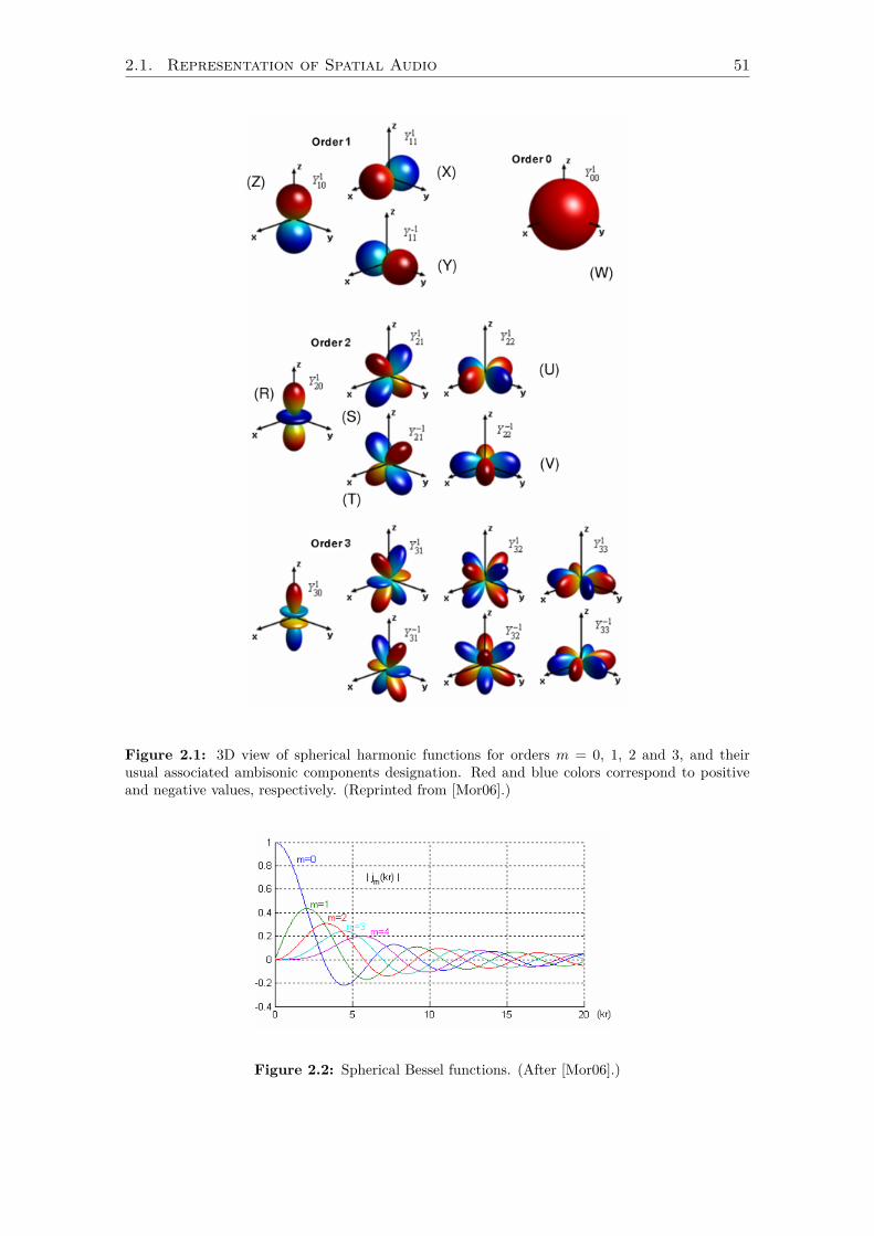
2.1. Representation of Spatial Audio 51

Figure 2.1: 3D view of spherical harmonic functions for orders m = 0, 1, 2 and 3, and theirusual associated ambisonic components designation. Red and blue colors correspond to positiveand negative values, respectively. (Reprinted from [Mor06].)

Figure 2.2: Spherical Bessel functions. (After [Mor06].)


Reproduction of the acoustic field

To acoustically reproduce the wavefield over a specific loudspeaker layout, it is necessaryto derive the appropriate loudspeakers signals, which constitute the so-called D-format,from the ambisonic signals (i.e., B-format). This is done using the “re-encoding principle.”We assume an array of N loudspeakers that are far enough from the center of the listeningarea such that their signals Si are encoded as plane waves with coefficient vectors ci,recomposing the encoded Ambisonics components as Bσ

mn:

ci =

Y +100 (θi, δi)Y +1

11 (θi, δi)Y −1

11 (θi, δi)...

Y σmn(θi, δi)

...

, B =

B+100

B+111

B−111...

Bσmn...

,S =

S1S2...SN

. (2.3)

Then, the re-encoding principle stands as below:

B = C× S, (2.4)

with C = [c1, · · · , cN] being the re-encoding matrix. The original ambisonic signal B ismatrixed with a decoding matrix D to derive the decoded signals S that will feed theloudspeakers:

S = D×B. (2.5)To get B = B, equation (2.4) is inverted:

D = C+ = CT ×(C×CT

)−1, (2.6)

assuming that N ≥ K2D or N ≥ K3D (that is to say, there are enough loudspeakers).Hence, D relies on the loudspeaker layout. For regular layouts, the expression of thedecoding matrix is simplified and is given by [DNM03]:

D = 1N

CT. (2.7)

For instance, in the case of a horizontal-only regular array, we get:

D =√

2M

1√2 · · · 1√

2cos(φ1) · · · cos(φN )sin(φ1) · · · sin(φN )

cos(2φ1) · · · cos(2φN )sin(2φ1) · · · sin(2φN )

... · · ·...

cos(K2Dφ1) · · · cos(K2DφN )sin(K2Dφ1) · · · sin(K2DφN )

T

, (2.8)

where φi is the angle of the ith loudspeaker. For an encoding/decoding of order M andreproduced over 2N + 1 loudspeakers in a circular and regular array, the resulting wavefield error stays below -15 dB as long as the following relationship is respected [WA01]:

M ≥ kr, (2.9)

where r is the radius of the reproduction area. The disk of radius r ≤ M/k is generallyreferred to as the “sweet spot”. From this formula one can conclude:

2.2. Coding of Monophonic Audio Signals 53

1. that the higher the frequency of the acoustic wave to be represented over a givenarea, the higher the truncation order needed to properly represent that wave overthis area;

2. that the wider the desired area of proper reconstruction of this acoustic wave, thehigher the truncation order needed.

It should be noted that research exists concerning the optimization of the decodingphase in situations where the satisfying acoustical reconstruction area is too limited regard-ing the listening area, for instance when the listener moves away from the ideal listeningposition or when the order M is too small. In those cases, it is possible to improve thesubjective quality of source localization by optimizing objective criteria. As an example,two important criteria have been introduced by Gerzon for first-order Ambisonics signals,but which can be extended to higher orders: the velocity and energy vectors. For furtherreading on this optimization process, see [Ger92, Mor06].

Useful properties of HOA signals

The HOA format is universal in the sense that it is able to describe any acoustic wave. Ithas two interesting properties. First, it is independent of the recording and reproductionsystems, which makes it very flexible and suitable in several situations. In particular, asound field represented in the HOA domain can be reproduced in theory on any type ofloudspeaker layout.

Second, the HOA description of the scene is hierarchical; that is, the first-order compo-nents are sufficient to represent the acoustic wave, and the higher-order components onlyextend the bandwidth and the accurate area of reproduction of this wave. This propertymakes the HOA format scalable, which is very useful in a network transmission contextto adapt the transmission rate to the available network bandwidth; it is possible, givena HOA representation of order M of the sound field, to give priority to the transmis-sion of the Bσ

mn components associated with the first L orders (L ≤ M), affecting thesize of the accurate listening area and the reproduced bandwidth. In the same way, it ispossible, given an order M with 2M + 1 channels (2D HOA), to adapt the reproductionto the listener’s setup by considering only a subset of 2L + 1 channels with an order Lrepresentation.

2.2 Coding of Monophonic Audio Signals

As explained in section 2.1.1, to ensure CD quality using the LPCM representation of awaveform, a bit rate of 700 kbit/s is needed. Audio coding solutions exist to reduce thisreference bit rate with or without loss of information.

2.2.1 Lossless Coding

Starting from the fact that the transmitted audio signals are rarely full-scale white noise(i.e., a random signal), redundancies in the waveform can be accounted for in order toreduce the bit rate without a loss of information. The basic idea is to predict futuresamples based on previous ones using linear prediction [Mak75] and to transmit only theprediction error (i.e., the residuals) and the prediction rules (if applicable). If the inputsignal is self-correlated, because the entropy of the residuals is less important than that ofthe original signal, a potential coding gain can be achieved. For example, in Differential


Pulse-Code Modulation (DPCM), the waveform is differentiated (the previous sample issubtracted from the next one) and then entropy coded. In a second form of DPCM, alocal model of the input is made, the prediction is subtracted from the original signal,and the residuals are entropy coded. This principle is used for example in MPEG-4 AudioLossless Coding, or in DTS.

Note that since the entropy of the residuals is unknown, any lossless coding will alwayshave a variable bit rate on normal audio.

2.2.2 Lossy Coding

Perceptual Coding

Another approach, know as perceptual coding (see appendix C for a detailed description),is to accept to lose information during the coding process, all the while ensuring that thisloss is as imperceptible as possible by the auditory system. Therefore, perceptual codingmodels and exploits properties of hearing, such that less perceptible information can becoded with less precision. In the frequency domain, or frequency subbands domain, thequantization of each sample induces a quantization noise. The energy of this noise dependson the coding precision of the considered sample: the higher the number of bits allocatedto it, the lower the noise. As we saw in section 1.2.2, each frequency component generatesa mask, and any other component whose energy falls below this mask will be inaudible.A cumulative mask, resulting from the presence of all frequency components, is modeledand used to compute how far the quantization noise would be from the masking threshold.The bit allocation to each sample is then done in order to keep the quantization noiseas much below the mask as possible. This principle is especially used in the MPEG-1/2Layer 3 (MP3) codec [BG02, Bra99].

Spectral Band Replication

When operating at very low bit rates, the quantization noise might not be kept belowthe masking threshold, resulting in audible and unpleasant distortions in the signal. Amethod named Spectral Band Replication (SBR) proposed recently [DLKK02], offers away of reducing the bandwidth of the signal without altering the perceptual rendering toomuch. It is based on the idea that low and mid frequencies can be used to reconstructthe untransmitted higher frequencies (usually over 5 kHz) by replication/transposition,plus a set of parameters describing the spectral envelopes of the noise and the harmoniccontent. SBR can potentially be associated with any perceptual coder and is especiallyused in MPEG-2/4 as High-Efficiency Advanced Audio Coding (HE-AAC) [WKHP03].

Parametric Representation of the Signal

Again, at very low bit rates and for the same reasons as mentioned above, a parametricrepresentation of the signal components might be more efficient. For example, in Harmonicand Individual Lines plus Noise (HILN) [PEF98] using a time-frequency transform, theimportant harmonic content is matched and tracked across frames to group them intoharmonic lines and individual sinusoids. Individual sinusoids are described as amplitudeand frequency, harmonic lines as fundamental frequency, amplitude, and spectral envelopeof the partials, and the noise as amplitude and spectral envelope. Only the differencesbetween the components of a track are coded, resulting in a coding gain, especially forlong tracks. A perceptual model is used as well to select only the most audible components

2.3. Lossless Matrixing 55

given the bit rate constraint. HILN is used down to 6 kbit/s in MPEG-4 Parametric AudioCoding.

This type of coding is known, however, to present issues in describing transients of theoriginal signal. This issue has been addressed in [BA04].

2.3 Lossless Matrixing

The same linear prediction strategies, described for monophonic signals in section 2.2.1,can be applied to each channel separately. However, a lossless matrixing technique can beused first to reduce the inter-channel correlations.

2.3.1 Mid/Side Stereo Coding

Mid/Side Stereo Coding [JF92] is a form of matrixing used to reduce correlations betweenthe two channels of a stereo signal. The principle is to transform the left and right channelsinto a sum channel, called mid channel, m[n] = 1√

2(l[n] + r[n]), and a difference channel,called side channel, s[n] = 1√

2(l[n] − r[n]), which carries the residuals. This way, the mand s channels are less correlated than the original l and r channels, and in particular,the entropy of s is reduced. At the decoding phase, by using the same operations onthe transformed channels, the original stereo channels can be fully recovered, providedthat no additional lossy coding has been used on either of the transformed channels (seesection 2.4.1). M/S coding is one of the two stereo joining techniques, together with ISC(presented in section 2.5), and is usually applied for coding low frequencies, whereas ISCis used for high-frequency coding.

2.3.2 Meridian Lossless Packing

For the multi-channel audio case, in [GCLW99], Meridian Audio proposes an invertiblematrixing technique, which reduces the inter-channel correlations prior to applying linearprediction on each channel separately. The result of this combination is called MeridianLossless Packing (MLP) and is widely used for audio and video DVD, but also by Dolby’sAC-3 codec on Blu-ray discs. MLP typically provides a 2:1 compression for music content.

2.4 Lossy Matrixing

2.4.1 Perceptual Mid/Side Stereo Coding

As stated at section 2.3, M/S stereo coding cannot be used as is in conjunction with alossy coding. Indeed, considering an input signal x, the quantization noise Q(x) resultingfrom perceptual coding (see section 2.2.2) can be modeled as an adaptive noise sourceN(x):

Q(x) = x+N(x). (2.10)

When perceptual coding is used on a monophonic signal x, the power spectrum of N(x)can be kept below the mask induced by x. But when perceptual coding is applied on M/Smatrixed signals m and s, the reconstructed stereo signals l′ and r′ are:

l′ = 1√2 [Q(m) +Q(s)] = l + 1√

2 [N(m) +N(s)]r′ = 1√

2 [Q(m)−Q(s)] = r + 1√2 [N(m)−N(s)] , (2.11)


resulting in a sum of uncorrelated quantization noises N(m) and N(s) of which the over-all power is equally present in l′ and r′. However, as explained in section 1.4.6, binauralunmasking occurs when a target source, masked in the presence of a collocated concurrentmasking source, becomes audible when these sources are presented at different positions.Therefore, if the masking thresholds induced by l and r are spectrally unequal, the quan-tization noise can become audible. To avoid this, a solution is proposed, for example, in[tK96], but the usual strategy, described in [JF92], is to dynamically switch between twomodes: using a time-frequency representation of the input signals, if the masking thresh-olds of l and r in a given frequency subband differ by less than 2 dB, m and s will bequantized and transmitted (M/S mode), otherwise l and r will be (L/R mode). 1 Then, inM/S mode, the stereo masking contribution of the m and s signals is computed, and thesignals are quantized such that their respective noises stay below their respective stereomasks.

In Dolby Stereo, M/S coding is used in the time domain, but in digital codecs itis performed independently in separate frequency subbands, as in Dolby AC-3 [Dav99](under the term Rematrixing). In MPEG-2 AAC [BBQ+97], M/S coding is used in amulti-channel context by applying it to pairs of opposite channels with respect to thefront/back axis.

2.4.2 Matrix Encoding

The matrix encoding principle is based on the downmixing of a finite number of audiochannels (e.g., 5) into a lesser number of channels (e.g., 2) to reduce the necessary bit rate.This encoding is done such that after transmission the signal can either be played as is,or, with an appropriate decoder, upmixed to the original number of channels, which arethen approximated. An encoding-transmission-decoding chain is usually noted as I:D:O,where I is the number of input channels (i.e., prior to the encoding), D the number ofchannels in the downmix, and O the number of output channels (i.e., after decoding).In the common case where the transmitted downmix is a pair of stereo channels, thosechannels are usually noted Lt and Rt for “Left Total” and “Right Total”, respectively. Fewmatrixing/unmatrixing techniques examples are presented hereafter, and more details canbe found in [Rum01].

Ambisonics UHJ

Gerzon [Ger85] proposed a 4:2:4 scheme to transmit Ambisonics signals (see section 2.1.2)in a stereo-compatible way. The encoding equations are:

S = 0.940 W + 0.186 XD = j(−0.342 W + 0.510 X) + 0.656 YLt = 1

2(S +D)Rt = 1

2(S −D)

, (2.12)

1. In any case, if these masking thresholds differ too much, it means that l and r are uncorrelated, andhence, M/S coding would not be efficient.

2.4. Lossy Matrixing 57

where j is a +90 phase shift, and W , X, Y are the original Ambisonics B-format signals.Lt and Rt compose the stereo downmix. The received downmix can be decoded with:

S = 12(Lt +Rt)

D = 12(Lt −Rt)

W ′ = 0.982 S + j 0.164 DX ′ = 0.419 S − j 0.828 DY ′ = 0.763 D + j 0.385 S

. (2.13)

Dolby Surround

Dolby Motion Picture (MP) matrix, also known as Dolby Stereo [Dre00], is a 4:2 encodingscheme based on the assumption that the sound scene is organized as a set of primarysources in front (carried by the front left channel L, the front right channel R, and thecenter channel C), and secondary sources and room effects/reverberation at the rear (car-ried by the rear surround channel S). As its name states, this configuration is especiallyadapted to motion picture material. The encoding equations are:

Lt = L+ 1√2(C + jS)

Rt = R+ 1√2(C − jS) , (2.14)

The decoder part, referred to as Dolby Surround, uses the following equations:

L′ = LtR′ = RtC ′ = 1√

2(Lt +Rt)S′ = 1√

2(Lt −Rt)

, (2.15)

If no center speaker is present in the reproduction system, and because C is equallypresent in Lt and Rt (and thus in L′ and R′), a phantom center speaker will be perceived bythe listener, thereby reinforcing the frontal image, assuming that the listener is positionedequidistant from the left and right speakers.

The effective separation resulting from the matrixing-unmatrixing process is unequalbetween pairs of opposite channels, and pairs of adjacent channels. Indeed, the separationis perfect between L′ and R′, since L and R are not mixed together. Also, because S ispresent in phase opposition between L′ and R′, the presence of S cancels out when com-puting C ′, thus yielding a perfect separation between C ′ and S′. However the separationis poor (3 dB) between any adjacent pair of speakers, causing spatial degradations likea narrowed frontal scenery or inaccurate room effects. Also, any difference between theoriginal L and R channels will leak into S′, but this issue is generally improved by takingadvantage of the precedence effect (see for example [LCYG99, WNR49]): by adding atime delay between the front channels and the surround channel, front sources will beperceived as coming from the front (first wavefront), the late signal coming from the rearbeing perceived as a room effect. This delay can be optimized if the distance between thelistening position and the front and surround speakers is known. But this trick also rein-forces the presence of S in L′ and R′. However, Dolby justifies this choice by the nature ofthe target material (motion picture). Indeed, sounds are expected to come predominantlyfrom the screen direction. Besides, signals associated with the surround track usually arenot associated with specific source locations.


Active Matrix Decoding

In order to further improve channel separation, passive decoders like Dolby Surround, canbe replaced by active ones. These are based on the idea that the signals obtained by thepassive decoder can be used to detect a predominant source and that a better separationof the channels can be achieved by manipulating those signals. Therefore, active decoderscontinuously monitor the encoded channels for soundfield dominance and use an adaptivematrix to enhance the directionality of the predominant source at a given time. Thisprinciple is known as steering logic and is used, for example, in Dobly Pro Logic, LexiconLogic7 or SRS Circle Surround. In Dolby Pro Logic [Dre00], the predominant sourcedirection is expressed continuously on an XY-coordinate plane by computing the energyratios between L′ and R′ (X-axis), and between C ′ and S′ (Y-axis). Then converting fromrectangular to polar coordinates gives the dominance expressed as a vector quantity, ofwhich the magnitude represents its relative dominance and the angle its direction. Toimprove the separation of the dominant source with other sources, techniques such ascancellation are used: for example, if a frontal source is detected, its leakage into the L′and R′ channels is removed by inverting the polarity of one of them and adding themtogether. Clearly this method blends L′ and R′ together and looses their separation, butthe dominant source is now played only in the front speaker.

A system with broadband steering like Pro Logic is known to create unpleasant andunnatural effects like “pumping” or gating. These effects can be attenuated by steeringseparately in at least two frequency subbands, thereby allowing each subband to be steeredtoward a different side. Besides, this design allows the use of an optimal time constant foreach subband without introducing distortions. As an example, Circle Surround uses threesubband steering generators: low, mid, and high frequencies.

2.4.3 Matrixing Based on Channel Covariance

Yang et al. [YAKK03, YKK04] proposed a high bit-rate coding model based on inter-channel redundancy removal calledmodified AAC with Karhunen-Loève transform (MAAC-KLT). In this method, the input channels are statistically decorrelated by applying aKarhunen-Loève Transform (KLT). The interest of this transform is that most of the en-ergy is compacted into the first several resulting channels, allowing for significant datacompression by entropy coding or by selecting the channels associated with the highestvariances. Energy masking thresholds are computed based on the transformed signals,and their frequency components are then bit-quantified. As its name states, MAACKLTis designed to be incorporated into the AAC coding scheme [BBQ+97].

The Karhunen-Loève transform, also known as principal components analysis (PCA),is a linear transformation projecting data onto the eigenvector basis of their covariance.In our case, data are the n (correlated) channels of the signal, represented by the n × kmatrix V (k is the number of samples of a temporal frame):

V = [V (1), . . . , V (i), . . . , V (k)], with V (i) = [x1, x2, . . . , xn]T . (2.16)

The covariance matrix CV of V is defined as:

CV = E[(V − µV )(V − µV )T

]=∑ki=1[V (i)− µV ][V (i)− µV ]T

k, (2.17)

where the mean vector µV is defined as:

µV = E[V ] =∑ki=1 V (i)k

. (2.18)

2.4. Lossy Matrixing 59

(a) Comparison of accumulated energy dis-tribution for a five-channel audio source.

(b) Normalized variances (eigenvalues) fora ten-channel audio source

Figure 2.3: MAACKLT performances (After [YKK04].)

The KLT matrix,M , is defined as the eigenvectorsm1,m2, . . . ,mn of the covariance matrixCV :

M = [m1,m2, . . . ,mn]T . (2.19)

Finally, the matrix of transformed channels U is given via an orthogonal transform:

KLT Correlated Decorrelatedmatrix component componentM V U

− − − − −− − − − −− − − − −− − − − −− − − − −

×

−−−−−

=

−−−−−

(2.20)

The transformed channels in U are called eigenchannels. The transform producesstatistically decorrelated channels in the sense of having a diagonal covariance matrixfilled with eigenvalues of CV for transformed signals U . Since CV is real and symmetric,the matrix is formed by normalized eigenvectors which are orthonormal. Thus the inversetransform matrix is equal to its transpose, so that V = MTU in reconstruction, which isan “immediate” computation.

Each eigenvalue represents the variance of the projection onto its corresponding eigen-vector, that is to say the variance of the eigenchannel. As a result of this transform, mostof the energy is compacted into the first several eigenchannels (see figure 2.3), and exper-imental results showed that the compaction efficiency increases with the number of inputchannels. This property allows a great deal of data compression by selecting in M theeigenvectors with largest eigenvalues, and transmitting only their associated eigenchannel,which minimizes the error in the least-square-error sense between the original and the re-constructed channels. Besides, this energy compaction property implies that the entropyof the last eigenchannels is reduced, ensuring an additional coding gain. In that sense,the KLT applied to a set of channels can be thought of as a generalization of the M/Sstereo coding presented in section 2.3.1. In consequence to all of this, MAACKLT can


be used as a scalable format: the higher the number of transmitted channels, the betterthe reconstruction quality, knowing that perfect reconstruction is reached (apart from thequantization noise) when all channels are transmitted.

This transform can be done in either the time or the frequency domain. However,Yang explains that globally the frequency domain offers better performance. This is dueto two factors. First, in general, the signal energy is compacted in the low part of thespectra. Second, time domain signals may contain effects like delay or reverberation amongdifferent channels, which affect the time domain KLT decorrelation capability.

In order to achieve a maximum decorrelation of channels, a temporal adaptive KLTcan be done. This involves updating the KLT matrix M each adaptation period or block.BecauseM has to be transmitted for each block, the temporal adaptive KLT increases thebitrate. Anyway, it is possible to reduce it by transmitting the covariance matrix CV ofV instead of M , because it is real and symmetric, which implies that its lower (or higher)triangular part is sufficient to compute M on the decoder side. Considering a covariancematrix quantized to 16 bits per element, the overhead bit rate is given by:

roverhead = 8(n+ 1)K

, (2.21)

where K is the adaptation period in seconds, and n the number of channels. Yang esti-mated that an adaptation period of about 10 seconds is optimal, whereas for K less than10 seconds the bitrate is too important regarding the decorrelation efficiency.

2.5 Parametric Spatial Audio Coding

So far, in matrixing techniques, the effort was put on trying to transmit all the chan-nels by combining them or by eliminating redundancies between them. A rather differentapproach, presented in this section, is to transmit a parametric representation of thespatial attribute of the sound scene. As depicted in figure 2.4, the general idea is touse a time-frequency representation to extract from the input channels a set of “spatial”parameters describing the spatial organization of the scene/channels, on the one hand(see section 2.5.1), and to group all these channels using a downmixing technique (seesection 2.5.2) to form a single mono or stereo signal thereby reducing inter-channel redun-dancies, on the other hand. The spatial parameters are then used in the decoding phase(see section 2.5.3) to reconstruct from the downmix an approximation of the originalchannels, or even to generate a new set of channels adapted to another loudspeaker setup.These schemes especially rely on the supposition that the transmission of the parameterstakes only a few kbits/s, which is very small compared to the bit rate dedicated to theaudio channel(s). This means that the quantization process of these parameters has tobe performed carefully to ensure a reliable spatial representation with only a few bits (seesection 2.5.4). Besides, as already evoked in section 2.4.1, if the downmix is perceptuallyencoded prior to transmission, binaural unmasking has to be taken into account to avoidnoise unmasking [tK96].

This approach has been followed by several methods, using two main strategies, de-pending on the nature of the spatial parameters to be extracted. First, these parameterscan represent the inter-channel differences that are relevant to the perception of space,with respect to the auditory localization cues (see section 1.4). Frequency joining methodsconstitute the first step in this direction, but to a limited extent. Initially designed for apair of stereo channels under the term Intensity Stereo Coding (ISC) [HBL94], and laterextended to multi-channel as Channel Coupling [BBQ+97], the frequency join consists of

2.5. Parametric Spatial Audio Coding 61

SpatialSynthesis

ENCODER

SideInformation

DECODER

Estimation ofSpatial

Parameters

... ...

......

...

Time-FrequencyTransform

Figure 2.4: Generic scheme of parametric spatial audio coding.

generating a “coupling channel” which is an in-phase sum of the input channels, plus aset of parameters, named scale factors, representing the power ratio between each inputchannel and the coupling channel, for each frequency subband of the current frame. Chan-nel coupling is used exclusively to represent high frequencies, assuming that localizationof such components is based on ILD and on interaural delay of the signal energy enve-lope (high-frequency ITD). The fine temporal structure information, which is lost withthis representation, is not necessary anyway for localization at these frequencies. In otherwords, each channel will share the same set of spectral values contained in the couplingchannel, but their relative power ratio will be reconstructed from frame to frame with thescale factors, ensuring a conservation of the high-frequency localization cues. Concerningthe low frequencies, however, this information is necessary because localization in thiscase is based on IPD/ITD, and therefore the corresponding spectral coefficients cannot becoupled. For stereo signals, ISC is usually applied in conjunction with M/S stereo coding(see section 2.3.1) for low frequencies, forming together the joint stereo technique. ISC isused for example in MPEG-1/2 Layer 3 (MP3) [BG02, Bra99] for stereo signals, and inMPEG-2 AAC [BBQ+97] for stereo signals and multi-channel signals, by using it on pairsof opposite channels with respect to the front/back axis. MPEG-2 AAC also offers the useof channel coupling instead of ISC, among different pairs of M/S coded channels. ISC andchannel coupling are also used in Dolby AC-3 [Dav99] and to a lesser extent in DTS (scalefactors are not transmitted). As an example, compared to an LPCM encoded stereo signal(see section 2.1.1), an MP3 encoded stereo signal will be about 7 times smaller when usedwith a bit rate of 192 kbit/s, which is considered as the transparent quality bit rate.

Because the phase information is lost in the frequency joining process, issues arise whenuncorrelated components are concerned. Therefore this approach has been improved inParametric Stereo (PS) [BvdPKS05] and Binaural Cue Coding (BCC) [Fal04] with a fullparametric description using parameters carrying all the (azimuth) sound localization cuesused by the auditory system, that is ITD, ILD, and IC (see section 1.4), expressed as inter-channel differences. This time, the parametric description is valid on the full bandwidth,and therefore spectral coefficients for the whole spectrum are shared via a downmix signal.PS is intended for stereo signals, while BCC applies to multi-channel signals as well.However, because these types of representation carry the inter-channel differences, theyare somehow restrained to stick to the original channel setup at the decoding phase.The MPEG Surround standard [BF07], which is based on these representations, proposesmechanisms to correct this issue. PS and BCC are very similar, and since BCC is notrestricted to stereo signals, only BCC will be considered in the following.

In a second category, the spatial parameters would rather represent a spatial descrip-


tion of the scene, by means of angular positions notably. Spatial Audio Scene Coding(SASC) [GJ08] and Directional Audio Coding (DirAC) [Pul07] both belong to this cate-gory. SASC and DirAC are general frameworks that can be used for other purposes thantransmission with a reduced bit rate. Particularly, they offer possibilities of format con-version or enhancement. Indeed, unlike methods from the first category, they present theadvantage of being format-agnostic, in the sense that their representation of the acousticfield is generic and not tied to the input format. This property allows a more flexiblespatial synthesis potentially compatible with any loudspeaker arrangement, or even withbinaural rendering. However, this is beyond the scope of this thesis and hence in thefollowing we will focus only on the transmission context, that is when a downmix channeland a set of parameters are sent. A notable peculiarity of DirAC, compared to BCC andSASC, is that the input signals are assumed to be first-order ambisonics components inB-format, that is theW , X, Y and Z components (see section 2.1.2). In DirAC and SASC,the input and output loudspeaker setups are assumed to be known during the encodingand decoding phases, respectively.

2.5.1 Extraction of the Spatial Parameters

Once a time-frequency representation of the input signals is obtained, a spatial analysis isperformed to extract the set of parameters associated with each frequency subband. Hereis a summary of the parameters that are extracted for each method (their description isgiven in the next sections).

BCC:

• Inter-Channel Coherence c(1 coefficient)

• Inter-Channel Level Difference ∆L(C − 1 coefficients)

• Inter-Channel Time Difference τ(C − 1 coefficients)

where C is the number of input channels.

DirAC:

• Diffuseness coefficient Ψ

• Direction vector D

SASC:

• Ambient energy fraction λ

• Primary localization vector dP

• Ambient localization vector dA


Temporal and frequency resolution of the spatial analysis

Parametric spatial audio coding methods all rely on two assumptions which justify thechoice of the frequency and temporal resolution of the extraction of the parameters. Theseassumptions are motivated by psychoacoustic results.

The first assumption is that the finest temporal resolution at which the auditory sys-tem can track binaural localization cues is comprised between 30 and 100 milliseconds,a phenomenon referred to as binaural sluggishness [HKK98, KG90]. Therefore, typically,spatial parameters are extracted around every 20 milliseconds, to ensure a finer temporalresolution than the auditory system.

Second, it is assumed that the listener cannot discriminate two simultaneous sources inspace which spectrally belong to the same critical band (see section 1.2.3), while spatiallyarising from different locations [Pul07, BvdPKS05]. Consequently, the spatial parametersdescribing the scene that are transmitted along with the downmix are usually computedfor each band of a set of adjacent critical bands, assuming the presence of a single audi-tory event in each band. This means that two spatially separated frequency componentswithin the same critical band will share the same spatial descriptors. This second assump-tion is a fair approximation, since spatial discrimination ability certainly is reduced forsmall frequency differences (as in the case of components within the same critical band)[Per84b]. However, note that this might result in an inaccurate representation of spacesince counterexamples to this assumption can be found in the literature. For instance,Perrott [Per84a] reports a performance exceeding 90% in the spatial discrimination of twosimultaneous pure tones around 500 Hz within the same critical band when separated byan angle of at least 26 symmetrically about the subject’s median plane.

Two types of time-frequency transform can be used to divide signals into frequencybands. If a filter-bank technique is used, the input signals are filtered with a number ofnarrowband filters, of which the center frequency and the bandpass width mimic humanauditory resolution in terms of critical bands. A second technique is to use a short-timeFourier transform (STFT). In that case, the frequency subbands of a given channel aregrouped in such a way that each resulting band has a bandwidth approximately equal tothe critical band corresponding to its center frequency. STFT implies a fixed temporal ac-curacy at all frequencies, which do not match the frequency-dependent temporal resolutionof humans, whereas filter banks allow for the choice of the adequate temporal resolutionfor each filter. On the other hand, STFT is better suited for low-complexity applications,such as teleconferencing. So the choice between the two methods is a trade-off betweenquality and complexity.

Depending on the chosen method, the computation of the parameters might slightlydiffer. All parametric spatial audio coding methods offer both implementations, but inthe following, only the filter-bank implementation will be described. The computation isthe same in each subband, so for the sake of clarity, in the following the subband index isomitted. l and c respectively represent the time and channel indices.

Diffusion analysis

With each method, the diffuse part of the input signal is estimated for later reproduction,as this is necessary to preserve a faithful spatial imagery. Non-diffuse or primary compo-nents are highly correlated between channels (such as discrete pairwise-panned sources)and represent the point-like sources of the scene. Diffuse or ambient components are un-correlated between channels, and represent less localized content, such as reverberationand wide sources. A parameter representing this diffusion is transmitted.


In BCC, as the approach is to carry inter-channel differences, and based on the factthat IC (see section 1.4) is the main cue related to the perception of diffuse sounds, theInter-Channel Coherence (ICC) parameter, c, is computed between each pair of channelsx1(l) and x2(l):

c12(l) = maxd|Φ12(d, l)| , (2.22)

with a short-time estimate of the normalized cross-correlation function

Φ12(d, l) = px1x2(d, l)√px1(l − d1)px2(l − d2)

, (2.23)

where

d1 = max−d, 0d2 = maxd, 0,

(2.24)

pxc(l) is a short-time estimate of the power of xc(l), and px1x2(d, l) is a short-time estimateof the mean of x1(l − d1)x2(l − d2). c12(l) has a range of [0, 1], zero meaning that thechannels have no correlation within the time extent d, and a value of one meaning thatthey are totally correlated (although with a potential delay). In the case of more than 2channels, and in order to reduce the bit rate, in each band at each time index only ICCcues between the two channels with the most energy are estimated and transmitted.

In DirAC, a parameter Ψ corresponding to a diffuseness coefficient is computed fromthe B-format input (noted as w, x, y and z signals) as:

Ψ(l) = 1−√

2∥∥∥∑b1

m=a1 w(l +m)v(l +m)W1(m)∥∥∥∑b1

m=a1 [|w(l +m)|2 + |v(l +m)|2/2]W1(m), (2.25)

where W1 is a window function defined between constant time values a1 ≤ 0 and b1 > 0for short-time averaging, and v is the particle velocity vector, approximated by

v = xex + yey + zez, (2.26)

where ex, ey, and ez represent Cartesian unit vectors. Diffuseness gets a value of zerowith plane waves from a single direction, and reaches one in a field where there is no nettransport of acoustic energy.

In SASC, a primary-ambient decomposition [Goo08] is performed to separate the pri-mary components from the ambient components, which allows them to be analyzed sep-arately. From this decomposition, a parameter λ corresponding to the ambient energyfraction is also computed:

λ(l) = |A(l)|2|X(l)|2 , (2.27)

where A is the multichannel ambient signal, and X is the downmix signal.

Localization analysis

This part of the analysis deals with pointlike sources. Each method extracts one or moreparameters in each subband determining the direction of the auditory event associatedwith that subband.

For BCC, based on the fact that the direction of a source is provided by the ITD andILD cues (see section 1.4), two parameters carrying those cues are computed (see alsoequations (2.23) and (2.24) for notations):


Left

Center

Right

Rearleft

Rearright

1

3

2

4 5

Figure 2.5: ICTD and ICLD are defined between the reference channel 1 and each of the otherC − 1 channels. (Reprinted from [Fal04].)

• Inter-Channel Time Difference (ICTD) [samples]:

τ12(l) = arg maxdΦ12(d, l) . (2.28)

• Inter-Channel Level Difference (ICLD) [dB]:

∆L12(l) = 10 log10

(px2(l)px1(l)

). (2.29)

Note that the ICLD is the equivalent of the scale factors that were extracted in ISC (seesection 2.5). In the case of more than 2 channels, and in order to reduce the bit rate, ICTDand ICLD are defined between a reference channel (e.g. channel 1) and the other channels,as depicted in figure 2.5. The relation between these parameters and the auditory systemlocalization cues, make this representation particularly suited for binaural inputs. Indeed,binaural signals are characterized by the phase and level relationships between the left andright signals, which describe the filtering of a given source by the head-related transferfunction (HRTF).

In DirAC, a single parameter is computed, the direction vector D, defined as theopposite direction of the instantaneous intensity vector:

D(l) = −b2∑

m=a2

w(l +m)v(l +m)W2(m), (2.30)

where W2 is a window function for short-time averaging D, and a2 and b2 are definedsimilarly to a1 and b1, respectively. Note that D is a direction vector and not a localizationvector (as in SASC). Therefore, its meaning is in its angle (which is transmitted), and itsmagnitude is ignored.

In SASC, since each input channel has been decomposed into a primary and an ambientcomponent, a localization vector is extracted from each of these components. The Gerzonvelocity vector [Ger92] is used for the primary component:

gP (l) =∑Cc=1 |αc(l)|qc∑Ci=1 |αi(l)|

, (2.31)


where αc indicates the relative primary component in channel c, and qc is a unit vectorin the spatial direction of the cth input channel (given by the loudspeaker input format).However, as explained in [JMG+07], the Gerzon vector magnitude is bounded by thepolygon whose vertices correspond to the loudspeakers positions, which leads to inaccu-rate radius values and thus inaccurate spatial reproduction. Therefore, the magnitudeboundary of the Gerzon vector gP is expanded to the whole circle (or sphere) to give theprimary localization vector parameter dP :

rP = ‖((Eij)−1gP (l)‖1 (2.32)dP (l) = rP gP (l)/‖gP (l)‖, (2.33)

with Eij = [ei ej ] representing the positions of the two input loudspeakers bracketingthe Gerzon vector. The length rP of dP indicates the extent to which the component ispairwise panned, and therefore expresses its radial position. A length of 0 means thatthe component is non-directional, whereas a value of 1 corresponds to a discrete pairwisepanned component. For the ambient component, the Gerzon energy vector is directlycomputed to give the ambient localization vector parameter dA:

dA(l) = gA(l) =∑Cc=1 |Ac(l)|2qc∑Ci=1 |Ai(l)|2

, (2.34)

where Ac indicates the relative ambient component in channel c. As stated in [GJ08], theGerzon vector does not need to be expanded for ambient components, and therefore:

rA = ‖gA‖. (2.35)

One can conclude from this analysis that DirAC and SASC extract parameters thatdescribe physical properties of the acoustic field, whereas the parameters of BCC are basedon a perceptual description.

2.5.2 Computation of the Downmix Signal

During this process, all the C input channels are mixed together in a single monophonicsignal, in order to transmit a sum signal containing all signal components of the inputsignals. This process is common to all methods. Note however that it can be skipped inthe case of DirAC, because with the input signals being in B-format, the omnidirectionalsignal W is already a monophonic representation of the spatial audio scene containing allcomponents of the directional signals X, Y and Z. W thus constitutes a downmix.

Once a time-frequency representation of the input signals is obtained, in each fre-quency subband, the signals of each input channel are added. As proposed by Faller in[Fal04], in order to prevent attenuation or amplification of signal components due to cer-tain phase interactions, each subband signal xc(l) is multiplied by a factor e(l), resultingin an equalization of the downmix signal. That is:

s(l) = e(l)C∑c=1

xc(l), (2.36)

with

e(l) =√∑C

c=1 pxc(l)px(l) , (2.37)

where s(l) is the equalized subband under consideration, pxc(l) is a short-time estimateof the power of xc(l), and px(l) is a short-time estimate of the power of ∑C

c=1 xc(l). This


FB ...

...

IFB...

IFB...

IFB...

... ...

Figure 2.6: Synthesizing of spatial cues: ICTD (with delays dc), ICLD (with scalings ac) andICC (with decorrelation filters hc). (Reprinted from [Fal04].)

ensures that the power of signal components in the summed signal is approximately thesame as the corresponding power in all input channels. Finally the equalized subbandsare transformed back to the time domain, resulting in a summed signal s(n) that is readyto be transmitted.

Specific methods exist for downmixing a stereophonic signal into a monophonic signal.They can be found in [BvdPKS05, SPSG06].

2.5.3 Spatial Synthesis

This decoding process aims to generate a set of output signals that reproduce the inputsound scene. This is done using the downmix signal plus the spatial parameters. First,the downmix signal s(n) is decomposed into frequency subbands (employing the sametime-frequency transform used at the encoding phase), and then the idea is to distributeeach subband of the downmix to its appropriate location using the spatial parameters. Inthe case of BCC, the output channels are an approximation of the input channels sincethe parameters correspond to the inter-channel differences in terms of localization cues.For DirAC and SASC, the number of output channels and their setup can differ from theinput, the spatial parameters carrying a spatial representation of the scene.

For BCC, in order to recreate channels with spatial cues, the spatial synthesis is per-formed by applying delays dc (for ICTD), scale factors ac (for ICLD), and decorrelationfilters hc (for ICC) to each subband. This is illustrated in figure 2.6.

• ICTD:

dc =−1

2 (max2≤i≤C τ1i(l) + min2≤i≤C τ1i(l)) , c = 1τ1c(l) + d1, 2 ≤ c ≤ C (2.38)

The delay for the reference channel d1 is chosen such that the maximum delay isminimized, because minimizing the modifications in a subband leads to minimizingthe risk of artifacts.

• ICLD:Because of the equation (2.29), ac must satisfy ac/a1 = 10∆1c(l)/20. Also, the outputsubbands of reference channel 1 are chosen such that the sum of the power of alloutput channels is equal to the power of the summed input signals. Hence:

ac =

1/√

1 +∑Ci=2 10∆L1i/10, c = 1

10∆L1c/20a1, 2 ≤ c ≤ C(2.39)


• ICC:Two methods described in [Fal04] are proposed by Faller to design the filters hc.The aim of these filters is to reduce correlation between the subbands of a givenchannel pair, while taking care of not affecting ICTD and ICLD. The first methodis to vary ICTD and ICLD in each critical band as a function of frequency, all thewhile keeping the same average value. This method relies heavily on the assumption,stated earlier, that localization cues are derived over critical bands by the auditorysystem, and particularly assumes that ITD and ILD are derived as an average withina critical band. The second method is to add an artificial (late) reverberation toeach output channel as a function of time and frequency. Moreover, when usingthis second method, as only the ICC value between the two most energetic channelsis transmitted, ICC between the other channel pairs is produced by choosing theratio between the power of late reverberation to sum signal s(l) for each of theC − 2 remaining channels to be the same as for the second most energetic channel.This way, the single transmitted ICC parameter per subband describes the overallcoherence between all audio channels.

In DirAC, the downmix is first divided into diffuse and non-diffuse streams by multi-plying it by

√Ψ and

√1−Ψ, respectively, in each subband in order to get the energy of the

original diffuse and non-diffuse components back. The diffuse signals to send to each loud-speaker are obtained by decorrelating the diffuse stream: the sound for each loudspeaker isconvolved with a random sequence (this sequence is different for each loudspeaker) as ex-plained in [Pul07]. Several methods can be used for the reproduction of point-like sources(from the non-diffuse stream), and vector base amplitude panning (VBAP) [Pul97] is oneof them. Thus using the direction vector parameter, VBAP is used to compute the gainfactors associated with each loudspeaker to apply to the considered frequency subband ofthe non-diffuse stream. This allows for a pairwise pan of each frequency component to itsoriginal location. In order to maintain a balance between the methods used for reproduc-tion of the diffuse sound and of point-like sources, a scaling factor of 1/

√C (where C is the

number of output loudspeakers) is used for the random sequences used in decorrelation.In SASC (as in DirAC), several methods can be used for the reproduction of sources.

The method we will present here is to use amplitude-panning techniques. The design ofthe spatial synthesis of SASC is driven by a consistency requirement, which is that if theoutput signals were to be analyzed by SASC, they should yield the same set of parametersas those used to synthesize the scene. As explained in [JMG+07], a set of panning weightsγ bound to the output channels which satisfy this requirement can be expressed as:

γ = rρ + (1− r)ε, (2.40)

where r is the radius of the localization vector d (either primary or ambient, see equations(2.32) to (2.35)). ρ is a pairwise panning weight vector, which contains non-zero coeffi-cients only for the two output channels bracketing the direction of the localization vectord. A solution for the ρ weights can be found using VBAP [Pul97] or vector base intensitypanning (VBIP) [JLP99] for primary and ambient components, respectively. ε is a non-directional panning weight vector that yields a Gerzon vector of zero magnitude. Thisvector can be found by using an optimization algorithm [GJ06] yielding weights (callednull weights) for an arbitrary loudspeaker setup. Therefore, the interpolation via r ex-pressed in equation (2.40) reflects the distance from the listening point of the componentdescribed by d. The ambient energy fraction parameter λ is used to separate the down-mix into a primary and an ambient stream, and once the weights γ for both primary and

2.6. Conclusions 69

ambient components are obtained, they are then used to feed the loudspeakers. In orderto reproduce an accurate perception of the ambient components, however, decorrelationfilters such as those proposed in [Ken95] are applied to at least some of the ambient signalchannels, prior to their combination with the primary signal channels. SASC presentsthe peculiarity that, thanks to the primary-ambient decomposition, primary and ambi-ent components are analyzed and synthesized separately. This allows for a directionaldistribution of the ambient components, which is not proposed in DirAC when using amonophonic downmix signal, as explained in [Pul07].

2.5.4 Quantization of the Spatial Parameters

The quantization (or bit allocation) process takes place prior to transmission and aims todetermine the precision with which each parameter will be coded, that is, the number ofbits used to represent each parameter value.

The simplest approach is to use a uniform and independent quantization of each pa-rameter. This is the approach used in all three methods BCC, DirAC and SASC. However,as explained in [BvdPKS05], a non-uniform quantization can be used based on the sensi-tivity to changes of a given parameter, i.e., just-noticeable differences (JND). There existexperimental results concerning ILD, IPD and IC, which are described in section 1.4.5.The reader is invited to seek the justifications of the following in this section. Those resultsparticularly apply to coders like BCC, which rely on inter-channel differences based onthese localization cues. Hence, ICLD, ICPD and ICC can be quantized according to per-ceptual criteria, introducing just-inaudible quantization errors. More specifically, ICLDquantization steps are non-uniform, increasing with ICLD values. ICC quantization stepsare non-uniform as well, large when coherence is around 0 (uncorrelated channels) andsmall when it is around 1. IPD quantization steps, however, have to remain uniform.

Concerning DirAC and SASC, however, no perceptual quantization rule of the pa-rameters has been proposed yet. As presented in chapters 3, 4 and 5, we ran perceptualexperiments based on minimum audible angles (MAA), which can be interpreted to derivequantization rules for angle parameters like those used in both DirAC and SASC, andwhich can be exploited in BCC as well.

2.6 Conclusions

In this chapter several spatial audio coding techniques have been presented. Matrix encod-ing techniques such as Dolby Surround, perhaps outdated, were appropriate for blendingmulti-channel information into a stereo compatible stream, constrained in that sense.Digital formats are more flexible, and especially benefit from the advantage of using time-frequency representations of the signal. Parametric spatial audio coding techniques arepromising in terms of bit-rate reduction since a single audio stream is transmitted, thespatial information being parameterized.

Interestingly, the attempt to reduce the bit rate without affecting the rendering qualityhas not been yet fulfilled, according to subjective listening tests recently conducted by theEuropean Broadcasting Union (EBU) [KMMS07]. Indeed, when operated at their appro-priate bit rate, the parametric spatial audio coding method MPEG Surround (96 kbits/swith HE-AAC) obtains a “good” score on average, whereas Dolby AC-3 (448 kbits/s) isscored as “excellent”. Furthermore, MPEG Surround presents issues with specific mate-rial, such as applause sequences, whereas Dolby AC-3 is more consistent over content. Stillaccording to these tests, matrix encoding techniques like Dolby Surround Pro Logic (in its


most advanced form) are outperformed by digital techniques like Dolby AC-3 or MPEGSurround.

Perceptual coding, as it is used to code monophonic signals, relies on interference be-tween frequency components, exploiting energy masking phenomena. This concept hasbeen extended to space by taking into account binaural unmasking phenomena and de-riving masking rules depending on the relative spatial location of the components. Un-fortunately, it resulted in a decrease in the masking ability of the signal components andtherefore in the reduction of the coding gain. However, interference between componentsin terms of their spatial perception (rather than their audibility) has not been consideredfor perceptual coding yet, although it can potentially lead to a considerable coding gain.Indeed, as presented in chapter 3, interference between frequency components reduces au-ditory spatial resolution, a phenomenon which is modeled in chapter 4, and exploited inperceptual coding techniques proposed in chapter 5.

Chapter 3

Spatial Blurring: Auditory SpatialResolution in the Presence ofDistracting Sound Sources

This chapter presents our psychoacoustic studies dealing with localization blur and spatialblurring. The motivations for this work are presented first, after which the commonpoints of all experimental protocols are described before going into the details of eachexperiment separately. Indeed, the experimental protocols used for these experiments arevery similar, and therefore a specific choice is assumed to remain unchanged from oneexperiment to the next, unless otherwise stated. Four psychoacoustic experiments werecarried out to address the effect of different variables. First in section 3.6 the actualincrease of localization blur associated with a target sound source in the presence of asingle distracting sound source is studied. In this experiment, the effect of the target anddistracter center frequencies is tested. In a second experiment presented in section 3.7,the effect of the relative sound level of the target and the distracter on spatial blurring isassessed. The effect of the distracter position on spatial blurring is addressed both in thethird and fourth experiments (sections 3.8 and 3.9, respectively), although the main focusof the fourth experiment is the interaction between multiple distracters.

The effect of each factor at stake is studied in this chapter, but only in terms ofsignificance. Effect sizes are not considered at this point, because this particular aspect isdealt with in chapter 4.

3.1 Motivations

Even if the studies presented in this chapter are interesting from a purely psychoacousticalpoint of view, this work is first motivated by the spatial audio coding aspects presentedin chapter 2, aiming at bitrate reduction. However space is represented by a given codingscheme, in practice and in order to ensure a reasonable transmission bit rate, the precisionof this representation is necessarily limited by some quantization process(es). This inducesquantization errors in the position coding of the “components” of the sound scene which,at listening phase, are perceived as changes in position. These spatial distortions aretime-varying and result in a general spatial instability. The concept of localization blur(introduced in section 1.4.5) precisely characterizes the sensitivity to position changes ofsound events, and in order to be as undetectable as possible spatial distortions should thusbe held within the actual localization blur. Consequently, localization blur is an adequate

72 Chapter 3. Spatial Blurring

descriptor to drive the quantization process involving the spatial representation of thesound scene, a strategy which is discussed in chapter 5.

Localization blur has been extensively studied (see section 1.4.5) for a target source inquiet, that is without any interfering source. However, as the scene gets more complex,localization errors seem to increase [BH02], and more interestingly, sensitivity to local-ization cues decreases [HR10]. This suggests that auditory spatial resolution is likely todeteriorate as well when multiple sources are present, thus motivating the assessment oflocalization blur in the presence of distracting sources. Besides, very recent work con-firms an increase of the localization blur in such situations [CG10, KT03], especially whenattention is divided [MGM11].

This chapter is thus dedicated to the assessment of auditory spatial resolution viameasures of localization blur. We chose to focus our work on angular localization blur,and more specifically in azimuth. This choice is motivated by the practical fact that mostof the mass-market sound reproduction systems are only two-dimensional. Nevertheless,this work could be extended to elevation as well. Radial localization blur is not consideredeither, because the encoding of distance cues (see section 1.4.5) is generally not responsiblefor any bitrate increase. 1 The underlying aim is to gather a sufficient amount of data tobuild a model of localization blur that describes auditory spatial resolution in a maximumnumber of conditions, and in particular in the presence of distracting sounds. The designof such a model is addressed in chapter 4.

From an audio coding point of view, at the sound reproduction phase the listener isassumed to be free to move his or her head to face any direction within the reproductionsystem. As auditory spatial resolution is the finest for sources in front of the listener (seesection 1.4.5), only localization blur associated with frontal sound sources is investigatedin the following experiments, which constitutes the worst-case scenario in terms of audiocoding.

In all of our experiments, localization blur is assessed using real sources only, meaningthat no phantom sources are produced, because it has been shown that when using spa-tialization techniques, localization performance differs compared to when real sources areused, and in particular it depends on the spatialization technique and the speaker layoutemployed [MPM07, MPM].

3.2 Terms and Definitions

“Localization blur” is a generic term designating the smallest separation between two po-sitions of the same sound event that the auditory system is able to discriminate. It caneither be expressed as an angle (e.g., azimuth, elevation) or a distance (e.g., a radius).Localization blur is dependent on the characteristics of the considered sound event (fre-quency content, level, position, etc.), and thus is expressed for this specific sound event(which is usually referred to as “the target” in an experimental protocol). As we will see,it also depends on the condition in which this sound event is presented to the listener,such as the other components’ frequency content or energy, but also the characteristics ofthe listening room, etc. Therefore localization blur is expressed under a specific condition.When expressed as an angle (either in azimuth, elevation, or even a combination of both),localization blur is usually assessed through a measure called “minimum audible angle”

1. As opposed to the increase in number of channels necessary to improve the spatial resolution eitherin azimuth or in elevation. However, component position radii are specifically coded in SASC for instance(see section 2.5).

3.3. Paradigm for MAA Assessment 73

LS

R

listener

Mills

L R

listener

2S2I

time

Figure 3.1: Top left: the experimental paradigm used by Mills [Mil58]. The sequences for thetargets t1 and t2 presented to the subject are S-L (standard-left) and S-R (standard-right). Topright: the experimental paradigm proposed by Hartmann and Rakerd [HR89], and which we usedin our experiments. The sequences of targets presented to the subject are L-R (left-right) and R-L(right-left). Bottom: the temporal organization of a trial.

(MAA), which is described in section 3.3. We define the “auditory spatial resolution”—under a given condition—as the localization blur associated under that condition with anygiven sound event. When considering only angular localization blur, the auditory spatialresolution can thus be seen theoretically as the infinite set of MAAs describing all possiblesound event characteristics. In particular, we will show in the following that the auditoryspatial resolution deteriorates in the presence of distracting sound sources. As a result,a distracting source indeed exerts what will be referred to in the following as a “spatialblurring” of the target source. Spatial blurring is thus the additional localization blurobserved in the presence of distracters compared to localization blur in quiet.

3.3 Paradigm for MAA Assessment

As first proposed by Mills [Mil58], the minimum audible angle is the smallest angle betweentwo positions of the same sound event that the auditory system is able to discriminate.To assess MAAs, Mills proposed the paradigm illustrated in the top left of figure 3.1. Alistener is presented with a sequence made of two target sounds separated by a silence.The two sounds share the same characteristics except for their angular position: for eachtrial, the first target is played at the standard position (noted S, which is right in frontof the listener), and the second target is played separated from the first one with anangle α, either leftward (position noted L) or rightward (position noted R). The task ofthe listener is to indicate if the sequence heard corresponded to a standard-right or astandard-left displacement, following a two-alternative forced-choice (2AFC) procedure.The experimenter assumes that at each trial listeners are trying to discriminate L from S,or R from S, and thus that he is testing the sensitivity of listeners to the angle α.


time (ms)

700 700

2200

200300

distracter

300

Figure 3.2: The temporal organization used in our experiments.

However, as mentioned by Hartmann and Rakerd [HR89], the listener may learn toidentify the left and right source positions absolutely, therefore ignoring the standardsound (identification task), instead of trying to discriminate the standard position fromthe second target position at each trial (discrimination task). In such a case, the testedangle would then be 2α instead of α. The choice of using one strategy or the other is upto the listener, and Hartmann and Rakerd especially showed that Mills’ paradigm seemsto be performed by listeners as an identification task. To avoid this ambiguity, we decidedto follow their proposed “two sources, two intervals” (2S2I) paradigm instead, which isillustrated on the top right of figure 3.1. This procedure is similar to that of Mills, butwithout the standard source between the left (L) and right (R) sources. This way, thetwo types of sequences the subject is presented with are left-right and right-left, insteadof standard-left and standard-right.

As the point of our experiments is to assess localization in the presence of distractingsound sources, in most of the experimental conditions a distracting sound is played duringthe target sequence, as shown in figure 3.2. On a given trial, the distracter was playedfirst and held throughout the whole trial. Its onset was followed after 700 ms by the onsetof the first target of 300 ms, then followed after 200 ms by the onset of the second 300 mstarget. When several distracters were present, they were played synchronously, followingthis scheme. The subject’s task was to indicate, for each trial, whether the sequence madeof the two target sounds was a left-right or a right-left sequence, using two keys on aregular keyboard. No feedback was provided to the listener.

3.4 Stimuli

The choice of stimuli is justified by experiment 1, where the effect of the relative frequencydifference between the target and the distracter is investigated, implying the use of nar-rowband stimuli. The same stimuli were kept for the other experiments as well, in orderto facilitate the comparison between experiments.

The stimuli were white noises filtered through a single ERB band, according to Glas-berg and Moore’s recommendations [GM90]. These filters, which simulate the cochlearfiltering of the input sound into critical bands (see section 1.2.3), were implemented usingthe gammatone filters proposed by Patterson et al. [PRH+92]. The choice of critical band-width stimuli results from that parametric spatial audio coders compute a set of spatialparameters in critical bands (see section 2.5), and also from the fact that the integrationof sound pressure level performed by the auditory system also seems to correspond to pro-cessing by auditory filters one critical band wide (see section 1.2.3). Target and distractingstimuli only differ by their duration: 300 ms for targets, and 2200 ms for distracters, in-cluding raised cosine rise and decay ramps of 5 ms. The stimuli are then characterized by

3.5. Subjects, Rooms and General Setup 75

a single parameter: the center frequency of the gammatone filter. For the targets, threecenter frequencies were considered in total for all of the experiments: 700 Hz, 1400 Hz,and 5000 Hz. These three values were chosen by following previous results in sound lo-calization and localization blur (see section 1.4.5), and according to the three main waysbinaural cues are supposedly combined by the auditory system in the duplex theory: ITDonly at low frequencies, ILD only at high frequencies, and both at mid frequencies.

Besides each target stimulus, a group of distracting stimuli were generated. Eachdistracter of a group is then linked to its “reference target” in the following way: the centerfrequency of each distracter of the group was chosen in order to get a distracter locateda certain number of adjacent critical bands ( -4, -3, -1, 0, 1, 3, or 4) away in frequencyfrom the reference target. The characteristics of the stimuli used for all experiments aresummarized in table 3.1, where the rows describing the reference targets are in boldface.When a distracter was generated using the same center frequency as its reference target(that is for a distracter 0 critical bands away from the target), they shared the samecharacteristics.

Each stimulus (target or distracter) was generated ten times using independent whitenoise samples. At playback, one of these ten samples was picked randomly, which preventedthe listener from learning the stimuli; this would have helped to recognize potential spectralcharacteristics for each loudspeaker, which is to be avoided. This solution is practicallyequivalent to the generation of stimuli at playback time.

Prior to each experiment, the stimuli were scaled in amplitude in order to produce anequal perceptual loudness using the following process. Using the same setup, in the samelistening conditions as for the considered experiment, and using the center loudspeaker(located at 0, right in front of the listener’s head), listeners distinct from those who partic-ipated in the actual experiment were asked to equalize in loudness each distracter stimuluswith its reference target stimulus played at 52 dBA, using an adjustment method. Thiswas necessary to remove the effect of loudness from the results. Six listeners participatedin the equalization process of experiment 1, seven in experiment 2, and ten in experiments3 and 4. The resulting average equalization gains are reported in table 3.1.

3.5 Subjects, Rooms and General SetupFor all experiments, the recruited subjects had to pass a complete audiogram before takingpart in the actual experiment, to ensure that they had normal hearing. We also madesure that their professional occupations were not related to the sound or hearing areas.All subjects were paid. A different group of subjects took part in each experiment. Elevensubjects (six females, five males) participated in the first experiment, ten subjects (sixfemales, four males) in the second, twelve subjects (six females, six males) in the third,and finally fifteen subjects (six females, nine males) in the fourth experiment. No subjectparticipated in more than one of the experiments. All subjects in a given experimentperformed all the experimental conditions, according to a repeated-measures scheme.

Two different testing rooms were used in these experiments. Experiment 1 and 2 wererun in the Perceptual Testing Lab at the Centre for Interdisciplinary Research in MusicMedia and Technology (CIRMMT) 2, McGill University, in Montreal, Quebec, Canada.The room is a 4.6 m × 5.6 m × 3.6 m (h) semi-anechoic room, acoustically treated onthe walls and the ceiling with foam wedges, and fully covered by carpet on the floor. Thesubject sat in a chair. Experiments 3 and 4 were run in the anechoic chamber of Orange

2. Thanks are due to Yves Méthot, Julien Boissinot and Harold Kilianski at CIRMMT, and to MatthieuBerjon at Orange Labs for their great help with the technical setup of these experiments.


Center ∆ERB ERB (Hz) Loudness equalization gain (dB)frequency (Hz) Exp. 1 Exp. 2 Exp. 3 Exp. 4

374 -4 47 -1.2 - - -605 -1 90 -4.7 - - -700 0 100 0 - - -806 1 112 -0.4 - - -1202 4 155 -0.6 - - -828 -4 114 2.7 - - 1.6949 -3 127 - - - 1.91233 -1 158 2.5 - - -1400 0 176 0 0 0 01586 1 196 -0.7 1.2 - -2024 3 243 - - - -2.02281 4 271 -3.5 0.7 -2.55 -4.03164 -4 366 -1.0 - - -4464 -1 507 0.2 - - -5000 0 565 0 - - -5597 1 629 -0.3 - - -7829 4 870 0.7 - - -

Table 3.1: Center frequency and bandwidth of the stimuli used in all experiments, as well as theloudness equalization gain applied to each of them. Within each of the three groups of stimuli,the boldface row highlights the characteristics of the reference target, the other rows describingthe distracting stimulus. ∆ERB is the frequency separation between a distracter and its referencetarget, expressed in critical bands (ERB-rate).

Labs 2 (France Telecom R&D) in Lannion, France. This room is 7.6 m × 8.6 m × 8 m (h),and is acoustically treated on the walls, the ceiling and the floor with mineral wool. Inthis room, the subject sat in a chair vertically located halfway between the floor and theceiling.

It has been shown that small head movements might improve localization performances[WK99]. Therefore, to ensure realistic listening conditions, listeners were instructed to facethe 0° direction but their head was not restrained (see appendix A for the exact instructionsthat were given to the subjects).

The whole software used for running the following experiments was developed fromscratch for this purpose. It consisted of a puredata patch for audio I/O and user inter-actions, used in conjunction with Java code handling the experimental procedure. Thecommunication between puredata and Java was ensured by pdj [Gau10]. A screenshot(of experiment 4) is given in figure 3.14.

3.6 Experiment 1: Spatial Blurring From One Distracter 3

The primary goal of this experiment was to show that the localization blur associatedwith a target sound source increases in the presence of a single distracting sound source.As a secondary goal, the effect of the target center frequency was assessed, as well as thefrequency separation between the distracter and the target.

3. This experiment was carried out in collaboration with Catherine Guastavino and Georgios Marentakisfrom McGill University.

3.6. Experiment 1: Spatial Blurring From One Distracter 77

Speaker Position Speaker Positionnumber () number ()

1 −12.50 12 0.352 −10.51 13 1.053 −8.71 14 1.754 −7.09 15 2.455 −5.65 16 3.336 −4.40 17 4.407 −3.33 18 5.658 −2.45 19 7.099 −1.75 20 8.7110 −1.05 21 10.5111 −0.35 22 12.50

Table 3.2: Azimuth position of target speakers in experiment 1.

3.6.1 Setup

A schematic of the experimental setup is represented in figure 3.3c. Due to the room sizeconstraints, we had to use very small handmade loudspeakers in order to reach a spatialresolution of 0.7 in front of the listener. Therefore, we used twenty-three Phoenix SEtransducers from Harman International (which supported this work), made of a 45 mmdiaphragm and enclosed in 120 mm × 104 mm × 54.6 mm extruded aluminum boxes,with inner surfaces covered with foam. The target speakers were positioned according totable 3.2, spaced in a linear increasing fashion. The distracter loudspeaker was positionedat 0 in azimuth and 0.9 in elevation (because of the presence of the target speakers, seefigure 3.3b). The target and distracter speakers output levels were adjusted in orderto produce 52 dBA at the center of the listener’s head when fed with one of the targetstimuli. A soft overall level (52 dBA) was chosen for the experiment to be painless overtime, especially in the presence of an additional distracter.

Because of their small diameter, at high input level, the target speakers tend to addharmonic distortions to the original signal. We verified that these distortions were belowhearing threshold. This is necessary because undesired frequency components can firstadd unintended localization cues to the stimuli, but could also deepen each speaker’scharacteristics and thus help listeners in their task by allowing them to identify eachspeaker separately.

3.6.2 Procedure

A given experimental condition is defined by:

• the target center frequency: either 700 Hz, 1400 Hz, or 5000 Hz;

• the distracter center frequency relative to the target, expressed in critical bands: -4,-1, 0, 1, 4 or “no distracter” (see table 3.1).

Hence, each subject was tested in 3 × 6 = 18 conditions. When present, the distracterwas always located at 0, in front of the listener. The variable is the angular separationbetween the two targets (following the MAA task paradigm presented in section 3.3).

Depending on the tested angular separation, the two targets were played throughdifferent speakers, according to table 3.3. When the separation was asymmetrical (thatis, when the distracter could not be exactly in the middle of a pair of speakers), two pairs


(a) Side picture of the experimental setup.

(b) Front picture of the experimental setup, fromthe subject’s point of view. The loudspeakers wereplaced on a curved wood plate. The raised loud-speaker was used for the distracter.

5.00

m

5.60

m

4.60 m

listener

1 4 19 228 15

(c) Top view of the experimental setup(see table 3.2 for the exact target speakerspositions). The gray speaker at the centeris the distracter speaker. Its misalignmentwith the two most centered target speakersis for drawing purposes only.

Figure 3.3: Experimental setup for experiment 1.


Separation Angular Pair(s)number separation () of speakers

1 0.7 11,122 1.4 10, 12 & 11, 133 2.1 10,134 2.8 9, 13 & 10, 145 3.5 9,146 4.2 8, 14 & 9, 157 4.9 8,158 5.8 7, 15 & 8, 169 6.7 7,1610 7.7 6, 16 & 7, 1711 8.8 6,1712 10.1 5, 17 & 6, 1813 11.3 5,1814 12.7 4, 18 & 5, 1915 14.2 4,1916 15.8 3, 19 & 4, 2017 17.4 3,2018 19.2 2, 20 & 3, 2119 21.0 2,2120 23.0 1, 21 & 2, 2221 25.0 1,22

Table 3.3: Angular separations used in experiment 1, and the involved pair(s) of speakers. Thesymmetrical separations are represented in boldface characters.

of speakers were used in a balanced random order, in order to counterbalance the effectof this asymmetry.

We chose to use the method of constant stimuli for this experiment. In this method, thepsychometric curve of performance of a given subject is assessed by presenting repeatedlya fixed set of angular separations (an example can be seen in figure 3.4), assuming thatthe non-asymptotic part of the curve (the part between 60% to 90%) is comprised inthat fixed set. However, in a pilot experiment, we noticed that subjects varied greatly intheir performance, meaning that it was not possible to present the same set of angularseparations to each subject 4 (see appendix B for an illustration of this point). Therefore, aspecific protocol was designed to adjust the set of tested angular separations until findingthe proper area of testing for a given experimental condition. It was organized in blocksof trials. Within a block, the condition parameters (that is, the target frequency and, ifpresent, the relative distracter band) remained fixed, and a given set of angular separationswas used. The order of presentation of the separations was randomized within a block.The number of left-right and right-left sequences was balanced for each separation. Hence,the method of constant stimuli was used within each block.

As schematized in figure 3.5, for a given experimental condition, the subject was firstpresented with a training block, made of seven angular separations, covering from thesmallest separation (0.7) to a very large one (21), each separation being presented 12times. Then another block made of the same parameters (target center frequency, relativedistracter band, set of angular separations, and number of repetitions) was presented tothe subject, and used as an “overview” block. The goal of this block was to get a rough

4. Otherwise, the number of angular separation per set necessary to ensure an accurate estimation ofthe curve would have been too great, increasing the duration of the experiment.


0 10 20

0.5

0.6

0.7

0.8

0.9

1

Angular separation (°)

Per

form

ance

0.8035 perf. th.

MAA

Figure 3.4: Example of curve fitting in experiment 1, for subject 1 (target center frequency:5000 Hz, relative distracter band: 0).

12 trials per separation7 angular separations:0.7º, 2.8º, 4.9º, 7.7º,

11.3º, 15.8º, 21.0º

Training block

same as before

Overview block

16 trials per separation5 narrowed separations

Block I

same as before

Block II

Thresholdestimation

done againif the rangeis incorrect

Figure 3.5: The experimental protocol of experiment 1 for a given condition.


idea of the range of separations necessary to obtain a good estimation of the subject’s psy-chometric curve of performance. Thus five separations were chosen for the next block bynarrowing the tested range of angular separations. The number of repetitions was also in-creased to 16 per separation. From this point on, each time the tested range was adjusted,the corresponding five angular separations were yielded by an automatic procedure. Thisprocedure ensured that the proposed angular separations were distributed as uniformlyas possible over the tested range. The most informative part of a psychometric curve isbetween performances of 60% and 90%, thus ideally, we want the smallest separation ofthe set to give about 60% correct answers, and the largest one about 90%. So the newrange of angular separations was chosen by the experimenter from the overview block inorder to approach this requirement. Once executed, if the range indeed followed theseexpectations, another block made of the same parameters was presented once again. Ifnot, the tested range was adjusted and a new block was executed. Thus, the tested rangeis adjusted until two successive blocks gave consistent results. Then the performancesfrom these two blocks were averaged, meaning that each data point is an average valueover 32 repetitions. The coefficients of the underlying psychometric curve of performancewere estimated by fitting a logistic function to the data points using psignifit [Hil07], aMatlab toolbox which implements the maximum-likelihood method described in [WH01].The MAA was then extracted as the angular separation corresponding to a performance of80.35% 5 on the resulting psychometric function. An example of this process is illustratedin figure 3.4.

The whole experiment in itself was organized in the following way. The different condi-tions were presented grouped by target frequencies, and the resulting sets were presentedin a different order for each subject. As three target frequencies were tested and twelvesubjects participated, each possible order of target frequency set has then been presentedto two different subjects. For each subject, within each of these sets, the six distracterbands relative to the target frequency (including the case without distracter) were orderedrandomly. Concretely, for each subject, the experiment was divided into five sessions ofone and a half hours each.

3.6.3 Data Analysis and Results

In addition to the eleven subjects who successfully completed this experiment, one wasdiscarded because of an inability to do the task in too many conditions (7 out of 18), andan overall low level of performance compared to the other subjects. Using Grubbs’ test,5 outliers out of 198 samples (that is, 2.5% of the dataset) were replaced by the means ofthe corresponding group. All post-hoc tests were corrected for multiple comparisons usingHolm-Bonferroni correction. Unless otherwise stated, non-parametric tests (Wilcoxon’ssigned-ranks test and Cuzick’s test) yielded results similar to those given in this section.

Figure 3.6 gives the mean thresholds across all participants. From this plot we canobserve three points, which we will test statistically:

1. the presence of the distracter seems to globally increase the MAA (compare forinstance, on any of the three plots, the “no distracter” case with a distracter in thesame critical band as the target);

2. the performance level seems to depend on the target center frequency;

5. The choice of this threshold value, which usually is 75%, is motivated by constraints on this value inthe next experiments, as explained in section 3.7.4. Therefore the same threshold value has been chosenfor all experiments to allow straightforward comparisons between them.


05

1015

Distracter band (distance in ERB relative to the target)

Min

imum

aud

ible

ang

le m

ean

+/−

SE

M (

°)

700 Hz

Target center frequency

1400 Hz 5000 Hz

−4 −1 0 1 4 Ø −4 −1 0 1 4 Ø −4 −1 0 1 4 Ø

Figure 3.6: The mean thresholds across all participants for experiment 1. The vertical barsrepresent ± the standard error of the mean. ∅ indicates the condition with no distracter.

3. the effect of the frequency distance between the target and the distracter seems todiffer from one target frequency to another (the respective shape of each of the threeplots is different);

Let us begin with the last observation. If indeed this point is true, it would mean that thereexists an interaction between the target frequency and the distracter band, which wouldoblige us to test the effect of the distracter separately for each target frequency. Partly totest this hypothesis, we carried out a two-way factorial repeated-measures ANOVA, thetarget center frequency (TF) and the relative distracter band (DB) treated as indepen-dent variables (fixed factors), and the MAA being the dependent variable. It returned asignificant effect for TF (F (2, 20) = 26.2, p < .001), DB (F (5, 50) = 13.6, p < .001), aswell as for their interaction (F (10, 100) = 3.9, p < .01).

The significant effect of TF suggests that our second observation is true: two TFgroups at least have different group means. Paired t-tests allow us to confirm that all thethree group means are different from each other (p < .001 in all cases). This result is inaccordance with those of Mills [Mil58] and Boerger [Boe65] (see section 1.4.5): localizationblur is the smallest for a low-frequency target, larger for high frequencies, and the largestfor mid frequencies. Note, however, that when comparing all the “no distracter” (∅) DBgroups between them, no significant effect is found between ∅ at 1400 Hz and ∅ at 5000 Hz(whereas p < .01 and p < .001 when comparing ∅ at 700 Hz with ∅ at 1400 Hz and at5000 Hz, respectively).

The significant effect of the interaction between TF and DB confirms our third obser-vation stated above: the DB effect differs between at least two of the three TF groups.Therefore, we had to test the effect of DB separately for each TF group. This also impliesthat not much can be drawn from the significant effect of DB reported by the ANOVA.

We can now focus on our first observation, which is the main question of interest here:does the presence of the distracter increase localization blur? To answer this question,within each TF group and using one-tailed paired t-tests, we looked for a significant mean

3.7. Experiment 2: Effect of the Signal-to-Noise Ratio 83

difference by testing the ∅ DB group against the DB group which produces the greatestmean variation of MAA, that is, -1, 0 and 1 for the 700 Hz, 1400 Hz and 5000 Hz TFgroups, respectively. In all cases, this difference is significant (p < .05, p < .01 andp < .001 for the 700 Hz, 1400 Hz and 5000 Hz TF groups, respectively). Therefore, wecan answer the question posed above by saying that the presence of the distracter doesincrease localization blur, and does so for the three target center frequencies we consideredin this experiment. This does not mean, however, that the presence of the distracter hada significant effect for all DB.

The effect of DB—that is, the way the relative band of the distracter affects theincrease of localization blur—has been assessed using quadratic trend analyses withineach TF group. As a result, a significant quadratic trend was found for all TF groups(p < .01 for the 700 Hz TF group, and p < .001 for the 1400 Hz and 5000 Hz TF groups).These results confirm the effect of DB within each TF group. Now, the specific asymmetricshapes within the 700 Hz and 5000 Hz TF groups are also confirmed by significant lineartrends when considering only the -1, 0 and 1 DB groups (p < .05 for the 700 Hz group 6 andp < .001 for the 5000 Hz group). Note that for the 1400 Hz group, there is no significantquadratic trend anymore (even without correction) when considering only these DB groups(-1, 0 and 1), which suggests that these three data points are not significantly differentfrom each other. These last results confirm that the dependence of spatial blurring uponthe distracter relative center frequency varies with the target center frequency. In otherwords, there is an interaction between the distracter relative center frequency and thetarget frequency.

As a conclusion, we can restate our previous observations in the following way:

1. spatial blurring phenomenon: for all the tested target center frequencies, at leastone of the tested distracters induced an increase of localization blur compared towhen no distracter was presented;

2. there is a global effect of the target center frequency on localization blur;

3. the effect of the frequency separation between a target and a distracter on spatialblurring is dependent on the target center frequency.

3.7 Experiment 2: Effect of the Signal-to-Noise Ratio 7

Part of the following was published in the proceeding of the 10th french congress of acous-tics (CFA) [DGM10].

The previous experiment showed the effect of the target and the distracter frequencieson localization blur. The levels of the stimuli were kept fixed such that the target wasalways played at 52 dBA and that the level of the distracter was perceptually matched inloudness with the target. However, from an audio coding point of view, the componentsof a sound scene are likely to have different levels, and thus the previous results mightnot apply in most cases. Therefore, this second study mainly aimed to assess the effectof the signal-to-noise ratio (SNR, which here is the ratio between the target and thedistracter levels) on localization blur. This study also provides an assessment of theaudibility threshold of the target in the presence of a distracter (or masking threshold) forseveral angular separations. From this experiment on, we will only test the target centerfrequency of 1400 Hz for two reasons: first, testing other target frequencies would increase

6. The 700 Hz TF group did not show a significant linear trend when performing a non-parametric test.7. This experiment was carried out in collaboration with Catherine Guastavino from McGill University.


(a) Front picture of the experimental setup, fromthe subject’s point of view.

4.60

m

5.60

m

4.60 m

listener

1 2 8 93 4 5 6 7 10 11

(b) Top view of the experimental setup(see table 3.4a for the exact speaker po-sitions). The gray speaker at the center isthe distracter speaker.

Figure 3.7: Experimental setup for experiment 2.

Speaker Position Speaker Positionnumber number

1 −11 7 3

2 −9 8 5

3 −7 9 7

4 −5 10 9

5 −3 11 11

6 0

(a) Azimuth position of the speakers. Thedistracter speaker is in boldface. All speakershave a null elevation (0).

Separation Angular Pairnumber separation of speakers

1 6 5, 72 10 4, 83 14 3, 94 18 2, 105 22 1, 11

(b) Angular separations and their corre-sponding pairs of speakers. The target-distracter separation is obtained by divid-ing these angles by two.

Table 3.4: Loudspeaker positions and angular separations used in experiment 2.

the duration of experiments too much, and second, from experiment 1, it seems to be themost promising center frequency in terms of spatial blurring.

3.7.1 Setup

A schematic of the experimental setup is depicted in figure 3.7b. All speakers (Genelec8020A) were equalized beforehand at the position of the distracter speaker (#6, repre-sented in gray) to 65 dBA using a pink noise, with a microphone positioned three metersaway. They were then positioned according to table 3.4a (with an elevation of 0 inrelation to the listener’s head). The overall level was adjusted in order to produce 52 dBAat the center of the listener’s head when a speaker is fed with the target stimulus at its“base” level. That is to say, when the SNR equals 0 dB, both the target and the distracterare played at this base level (thus with a respective gain of 0 dB). This overall level waschosen in accordance with our previous experiment.


3.7.2 Procedure

The main aim of this experiment was to obtain an estimation of the MAA as a function ofthe SNR. In the previous experiment, we dealt with the inter-subject variability using aspecific experimental protocol designed to adjust the set of tested angular separations untilfinding the proper range for testing (see section 3.6.2). This procedure unfortunately hastwo issues. First, from a practical point of view, the process of deciding the next testingrange is very time-consuming. But more importantly, because the experimenter makes thisdecision, the process is not totally reliable, nor reproducible. Consequently, for this secondexperiment, we wanted to change the assessment method by using an adaptive method,which is described in detail in section 3.7.4. Adaptive methods present the advantage ofbeing more flexible than the method of constant stimuli, because they can be used withsubjects showing very different performance levels.

As this experiment aims to assess the effect of the SNR on the MAA, the most straight-forward way to do so would be to estimate directly the MAA for several fixed SNR values.However, directly assessing the MAA in a given condition requires the discretization ofspace with an array of loudspeakers at fixed positions 8 (as the one used in the previousexperiment). Unfortunately, the adaptive method we wanted to use requires a continuousdependent variable. This is why we chose instead to fix a set of angular separations, andto assess for each separation the SNR for which this separation is effectively the MAA.This way, the SNR becomes the dependent variable and, presenting the advantage of beingcontinuous, an adaptive method can thus be applied to vary it and extract a thresholdvalue.

Nonetheless, we noted that in particular situations and for large angular separations,the spatial discrimination seems to be ensured so long as the target remains audible. Insuch situations, the criterion of feasibility of the task is no longer the spatial discriminabil-ity, but the target audibility, and we are thus measuring the actual audibility thresholdof the target. Therefore, it was necessary to distinguish these particular conditions fromthose for which the subject clearly hears the target but has difficulty discriminating thepresented angular separation. This first remark motivates the separate measure of the au-dibility threshold of the target in the presence of the distracter as a point of comparison.

Second, since this measure of the audibility threshold of the target in the presenceof the distracter is conducted for several angular separations between the target and thedistracter, it is possible to derive the resulting spatial unmasking (or binaural release frommasking, see section 1.4.6), which is a useful additional information in terms of audiocoding (as explained for example in section 2.4.1). Indeed, one can expect this audibilitythreshold—we could equally call it masking threshold—to decrease with an increasingangular distance to the distracter.

This experiment was organized in blocks. One block consisted of an adaptive procedureyielding a threshold value for a given experimental condition. An experimental conditionwas made of three parameters: task type (discrimination of the direction of the changein spatial location or audibility threshold), relative distracter band (0, 1 or 4 ERB bandsabove the target), and angular separation (6, 10, 14, 18 or 22 degrees). The target centerfrequency was always 1400 Hz, and the distracter was always located at 0, in front of thelistener. As explained above, the variable was the SNR, that is to say the ratio betweenthe target and distracter levels. 9 Using a repeated measures scheme, the experiment wasthus made of 30 blocks for each subject.

8. Unless one has access to a mechanical system allowing one to move a pair of loudspeakers in quiet.9. Therefore, a positive SNR means that the target level is greater than the distracter level.


time (ms)

700

distracter

250

300

distracter

?

700

Figure 3.8: Temporal organization of a trial for the audibility task. The target sound is presentedon either the first or second presentation of the distracter sound.

The order of presentation of the blocks was organized on three levels, using threenested loops: a first loop on the three distracter bands, then a second one on the twotask types, and finally a third one on the five angular separations. For each subject, thedistracter band loop, the three task type loops, and the six angular separation loops, wereall separately randomized. In other words, a given subject did all the angular separationsfor a given task type and a given distracter band before moving on to the other task typeof this distracter band. Moreover, he or she had to do the two task types of a distracterband before moving on to the next distracter band.

The amount of training given to each subject was very small. When switching froma given distracter band to another, each subject performed around 20 training trials, nomatter what the first task type was. It means that when switching the task type withina given distracter band, no additional training was given to the subject. In practice, foreach subject, the experiment was divided into three sessions of one and a half hours each.

3.7.3 Tasks

As explained above, this experiment involved two tasks for the subjects. The first taskhas already been described in section 3.3, and remains unchanged. We will refer to thistask as the “LR/RL task”. In brief, the subject had to indicate, for each trial, whetherthe sequence made of the two target sounds described a displacement from the left to theright or the opposite. The SNR threshold leading a given angular separation to be a MAAwas obtained using the adaptive method detailed in section 3.7.4.

As illustrated in figure 3.8, and following the example of the LR/RL task, this sec-ond task used a 2AFC procedure. On each trial, the subject was presented with twodistracter/masker intervals of 700 ms separated by a silence of 250 ms. In one of these twointervals a target sound of 300 ms, temporally centered within the interval, was added.The target was played randomly through the left or the right speaker of the pair of speak-ers associated with the desired angular separation (see table 3.4b). The task of thesubject was to indicate which of the two intervals contained the target using a keyboard.No feedback was provided about the accuracy of the answer. We will refer to this task asthe “audibility task”. The SNR threshold of audibility of the target was obtained usingthe adaptive method detailed in section 3.7.4.


3.7.4 Adaptive Method Setup

The idea behind adaptive methods is to vary from trial to trial the stimulus intensity(the studied variable) as a function of the subject’s previous answers. Depending on therule of adaptation of the stimulus intensity which is chosen, this intensity is supposed tooscillate around a value corresponding to a certain theoretical performance of the subject.Therefore, in this method, the psychometric curve is no longer estimated, but rather asmall portion of it located around a certain targeted performance point.

For each of the two tasks described above, the adjusted variable was the target level,using an adaptive adjustment method made of staircases with fixed step sizes. The dis-tracter level was kept constant (loudness matched with the target stimulus at 52 dBA).Therefore, the SNR we will display in our results is simply the gain applied to the targetstimulus by the adaptive method. Hence, when SNR equaled 0 dB, the target was playedat a level which produced 52 dBA at the listening position, and the distracter was playedat its loudness matched level. The staircases used in this experiment were based on a2-down/1-up underlying rule, with unequal step up and down sizes (namely ∆+ = 3 dBand ∆− = 1.6464 dB), targeting a 80.35% performance threshold. Each block was com-posed of two interwoven staircases of 14 reversals each. The reasons for these choicesare given below. Before running the two staircases, a preliminary phase was made of a1-down/1-up staircase beginning way above the presumed threshold, and stopped after 3reversals, in order to approach the threshold region quickly. Then the pair of staircasestook over with the next target stimulus level. No boundaries were imposed on the targetlevel, but in practice, the SNR values lay between 26 dB and -50 dB. The peaks and valleysof all reversals (apart from the preliminary phase) and from the two interwoven staircaseswere averaged to estimate the 80.35% performance threshold values of SNR. In a resultingcouple angular separation, SNR, the angular separation can then be interpreted as theMAA we would have obtained if we were assessing the MAA associated with that fixedSNR value, instead of the reverse, as we did in practice.

We used two interwoven staircases instead of a single one. This means that for a givenrun, two staircases with identical parameters were run in parallel, randomly switchingfrom one to the other. This presents the advantage of hiding from subjects the underlyingrule of the staircases, which might otherwise bias their responses.

As reported by García-Pérez [Gar98, Gar00], the staircase parameters must be chosencarefully in order to ensure a reliable convergence to the targeted theoretical percent-correct. This theoretical percent-correct depends on the underlying rule of the staircase,but García-Pérez [Gar98] used simulations of staircases of several thousand trials eachto show that the percent-correct targeted in reality depends also on the ratio between∆+ and the spread σ of the underlying psychometric function. 10 More interestingly,the level of dependence varies with the choice of ∆+/∆−. In particular, ∆+/∆− = 1is the worst choice because, depending on ∆+/σ, the percent-correct targeted in realityoscillates between 60% and 90% correct. The difficulty comes from the fact that σ isunknown and might depend on the task type, the experimental condition and the subject.Thus this variability impedes both averaging between subjects and comparing betweenexperimental conditions. At the other extreme, depending on the underlying rule of thestaircase, there is an optimal ∆+/∆− ratio with which the targeted percent-correct remainsconstant whatever the ∆+/σ ratio is. In our case, we chose a 2-down/1-up rule, and thecorresponding optimal ∆+/∆− ratio is 0.5488. By observing this ratio, our staircases

10. The spread σ of a psychometric function is the extent over which it displays non-asymptotic behavior,measured in whichever units are relevant (in decibels in our case). More specifically, in his simulationsGarcía-Pérez defines it as the part of the curve between performances of 51% and 99%.


should effectively target a 80.35 percent-correct point.Another point studied by García-Pérez [Gar00] is the bias induced by the fact that

in practice we use small-sample staircases (as opposed to several thousand reversals). Heproposes a measure of the accuracy of a staircase depending on the spread σ of the under-lying psychometric curve: a given staircase setup has a “small” probabilistic error whensimulations show that it targets 80% of the time a percent-correct point which deviatesless than 0.32σ from its theoretical value. An interesting result of his is that as long asthe optimal ∆+/∆− ratio is observed, the accuracy of a staircase only depends on two pa-rameters: the number of reversals and the ∆+/σ ratio. According to his results, with lessthat 18 reversals, staircases yield biased estimations. From about 30 reversals, this bias istotally absent. Therefore, to avoid this bias, we chose to use two interwoven staircases eachmade of 14 reversals, reaching 28 reversals in total. The second dependence—the ∆+/σratio—is intuitive and represents the dependence on the step sizes. 11 This dependenceon ∆+/σ must be differentiated from the one previously stated. By choosing an optimal∆+/∆− ratio, we ensured that our staircase targets the same percent-correct whateverthe ∆+/σ ratio equals. Here, due to the limited duration of our staircases, there mightbe some bias (around the targeted percent-correct) in our estimations, and this potentialbias depends on ∆+/σ as well. If ∆+ is large compared to σ, that would lead to a largestandard error around the targeted threshold. If it is too small, the duration of the ex-periment is uselessly long. According to García-Pérez’ simulations, ∆+ is optimal when∆+/σ is between 1/3 and 1, but once again σ is unknown, and might depend on the tasktype, the experimental condition and the subject; and so would ∆+. However, we tried tofind a single ∆+ value suitable in all cases. To do so, we first used the method of constantstimuli with a group of separate subjects to get a very rough idea of the shapes of thepsychometric curves, and derived a first value for ∆+ by targeting ∆+/σ = 1. Then westarted piloting with this value, and in order to refine it, we compared the block durations(in terms of trials) to the number of trials that this staircase would take if ∆+/σ wasindeed 1, 12 according to García-Pérez’ simulations. The final ∆+ value of 3 dB (leadingto a ∆− value of 1.6464 dB) gave satisfying results. According to García-Pérez results,a 2-down/1-up staircase of 30 reversals should have an average number of trials around95 when ∆+/σ = 1. A larger number of trials in practice would mean that the actual∆+/σ ratio was smaller than 1 (and in that case the estimation is more accurate). Theblocks resulting from this experiment had an average trial number of 99.82 for the MAAtask and 97.97 for the the LR/RL task, with a respective standard deviation of 14.63 and12.41 trials, which means that our threshold estimations should be accurate. Besides, thesimilar statistics between the two tasks show that using the same step sizes for both ofthem was acceptable.


In addition to the ten subjects who successfully completed this experiment, three werediscarded because of their inability to do the task for certain conditions and an overalllow level of performance compared to the other subjects. Using Grubbs’ test, 3 outliersout of 150 threshold values (that is, 2% of the dataset) were replaced by the mean ofthe corresponding group for the LR/RL task, and one outlier out of 150 threshold values(0.6% of the dataset) for the audibility task. All post-hoc tests were corrected for multiple

11. Note that because ∆+ and ∆− are tied by the optimal ratio described above, this second dependencecan either be described by the ∆+/σ ratio or by the ∆−/σ ratio.12. This would correspond to a deviation of the estimation of about 0.30σ. We did not target a smaller

value of ∆+/σ, because it would increase the necessary number of trials.


DB → 0 1 4

SEP

6 . * ***10 n.s. n.s. **14 n.s. n.s. *18 n.s. n.s. n.s.22 n.s. n.s. n.s.

Table 3.5: Pairwise comparisons of the mean differences between the two task types usingpaired t-tests (Holm-Bonferroni correction was applied within each DB group). Significance codes:*** < .001, ** .001 – .01, * .01 – .05. The dot (·) denotes a nonsignificant trend (.1 > p > .05).13

comparisons using Holm-Bonferroni correction. Unless otherwise stated, non-parametrictests (Wilcoxon’s signed-ranks test and Cuzick’s test) yielded results similar to those givenin this section.

Figure 3.9 gives the mean thresholds across all participants, either grouped (a) bydistracter band or (b) by angular separation. As expected, for each distracter band, fromsome given angular separation the performance in the LR/RL task seems to be limitedby the audibility threshold. For the distracter band 4 ERB above the target, wherethe audibility threshold is relatively low, the SNR decreases with the increasing angularseparation, suggesting an effect of the SNR on the MAA.

Two separate repeated-measures factorial analyses of variance (ANOVA) were carriedout (one for each task type), the distracter band (DB) and the angular separation (SEP)treated as independent variables, and the SNR being the dependent variable. As a result,DB and SEP both have a significant effect for the two tasks, F (2, 18) = 36.1, p < .001and F (4, 36) = 58.7, p < .001, respectively, for the LR/RL task, and F (2, 18) = 1310.7,p < .001 and F (4, 36) = 24.7, p < .001, respectively, for the audibility task. Theirinteraction is also significant for the LR/RL task (F (8, 72) = 11.9, p < .001); however, itis not for the audibility task (F (8, 72) = 1.68, n.s.).

Let us focus first on the LR/RL task. Given that the ANOVA reported a significantinteraction between DB and SEP, post-hoc tests have to be done either between groupsof same DB or between groups of same SEP, but by no means we can pool togethergroups of same DB or groups of same SEP. Moreover, a particular SNR threshold value isonly meaningful when the measured threshold is significantly greater than the audibilitythreshold, otherwise that would mean that an audibility task is underlying the LR/RLtask (that is, so long as the subject hears the target, he or she is able to discriminatethe two sound locations, as explained in section 3.7.2). Therefore, pairwise comparisonswere conducted using paired t-tests to look for significant differences between means ofthe two task types for all DB, SEP condition pairs. The resulting significance levelsare given in table 3.5. As expected, for each distracter band, from some given angularseparation the difference between the obtained thresholds of the two task types becomesinsignificant. Continuing with this rationale, we assessed the effect of SEP by consideringonly those SNR threshold values of the LR/RL task that were significantly greater thanthe audibility threshold. Concretely, this mean that we kept the following DB, SEPcondition pairs: 1, 6, 4, 6, 4, 10 and 4, 14. The resulting effect of SEP in theLR/RL task is the following. Since for the 0 ERB DB group no point is concerned, andthat a single point is concerned for the 1 ERB DB group (1, 6), we could not performany test for these two DB groups. Concerning the 4 ERB DB group, a trend analysis on

13. Note that, when performing a non-parametric test, the condition 0, 6 showed significant meandifferences between the two task types (p < .05).


−40

−30

−20

−10

010


SN

R m

ean

+/−

SE

M (

dB)

0 ERB

Distracter band (relative to the target)

1 ERB 4 ERB

6 10 14 18 22 6 10 14 18 22 6 10 14 18 22

LR/RL taskAudibility task

(a) Mean SNR thresholds for both tasks, grouped by distracter band.

−40

−30

−20

−10

010

Distracter band (relative to the target)

SN

R m

ean

+/−

SE

M (

dB)

0 ERB 1 ERB 4 ERB

6°

10°

14°18°

22°

(b) Mean SNR thresholds for the LR/RL task only,grouped by angular separation.

Figure 3.9: Mean signal-to-noise ratio (SNR) thresholds across all participants for a target centerfrequency of 1400 Hz, in experiment 2. This SNR value represents the ratio between the target thedistracter levels. A SNR of 0 dB corresponds to the target played at its base level (52 dBA) andthe distracter played at its loudness-equalized level (see section 3.4). The vertical bars represent± the standard error of the mean.

3.8. Experiment 3: Effect of the Distracter Position 91

the three concerned points showed that the effect of SEP follows a significant linear trend(p < .001). These results show the effect of the angular separation on the SNR threshold,and taken the other way around, they show the effect of the SNR on the MAA. In otherwords, the SNR has an effect on spatial blurring: as the SNR decreases, spatial blurringincreases.

We will now focus on the audibility task. Since the ANOVA did not report a significanteffect of the interaction between DB and SEP, we can pool together all SEP groups whenlooking at the effect of DB on the SNR, and in the same way, we can pool together all DBgroups when looking at the effect of SEP on the SNR (see figure 3.9a). Trend analysesrevealed a significant linear trend in both cases (p < .001). These results confirm theexpected spatial unmasking, and show the decrease in the audibility (masking) thresholdas the difference between the distracter and the target frequencies increases.

As a conclusion, the main result of this second experiment is the significant effect ofthe SNR (the ratio between the target and the distracter levels) on spatial blurring. Assecondary results, we also confirmed the binaural release from masking of the target, aswell as the effect of the difference in frequency between the distracter and the target onthe masking threshold (it decreases as the difference increases).

3.8 Experiment 3: Effect of the Distracter Position

The main aim of this third study is the effect of the position of a single distracter onlocalization blur. Remember that we are not interested in the effect of the target positionon localization blur, since it is already known that it is significant (see section 1.4.5), andmore importantly because from an audio coding point of view, we assume that the listeneris facing the target sound source (see section 3.1).

In addition to the effect of the distracter position, the design of this experiment was alsomotivated by a question that the previous experiment raised. In experiment 2, we assessedthe effect of the SNR on the MAA by varying the target level and keeping the distracterlevel fixed. An interesting point however is that in quiet (that is without any distractingsource), localization ability depends on the target level [SMM05, SR01]. Therefore it isreasonable to wonder whether a part of the effect we observed in the previous experimentmight actually be attributable to the variation of the absolute target level rather than tothe variation of the SNR between the target and the distracter levels. This question isaddressed in section 3.8.4.

3.8.1 Setup

A schematic of the experimental setup is represented in figure 3.10. All speakers (cus-tom Studer) were equalized beforehand at the listening position, positioned according totable 3.6 (with an elevation of 0), by recording their frequency response, inverting it,and then filtering each speaker with the corresponding 4096-sample long FIR filter. Thisensured as flat a response as possible for each speaker, and consequently a similar responsefor all speakers. The overall level was adjusted in order to produce 52 dBA at the center ofthe listener’s head when a speaker is fed with the target stimulus at its “base” level. Thatis to say, when the SNR equals 0 dB, both the target and the distracter are played at thisbase level. This overall level was chosen in accordance with our previous experiments.


5.80

m

8.60

m

7.60 m

listener

1 2 4 53

6

7

Figure 3.10: Top view of the experimental setup for experiment 3 (see table 3.6 for the exacttarget speakers positions). The gray speakers are the distracter speakers.


1 −6 4 4

2 −4 5 6

3 0 6 45

7 90

Table 3.6: Azimuth position of the speakers. The distracter speakers are in boldface. All speakershave a 0 elevation.


3.8.2 Procedure

The main aim of this study was to estimate the effect of the distracter position on theMAA. Since we have shown the dependence of the MAA on the SNR in our previousexperiment, we assumed that it is possible to show the effect of a given variable on theMAA by testing its effect on the SNR corresponding to a 80.35% performance with a fixedangular separation. We therefore chose to retain the procedure we used for experiment 2,and thus a significant effect of a given variable on the SNR will be interpreted as beingsignificant on the MAA as well.

The same tasks as for experiment 2 (LR/RL and audibility, see section 3.7.3) were usedin this experiment. However, the audibility task was slightly different in this experiment,because the target was always played in the center speaker (speaker 3). This task stillallowed an estimation of spatial unmasking, but contrarily to experiment 2, the target isnow in front of the listener and the position of the distracter is varied. The audibility task,however, was mainly used to ensure that the LR/RL task was not in reality driven by anaudibility task, as explained in section 3.7.2. Since the adaptive method gave accurateresults in experiment 2 (see section 3.7.4), and the task types remained unchanged for thisexperiment, the same setup was used for the adaptive method in this experiment.

This experiment was organized in blocks. One block consisted of an adaptive procedureyielding a threshold value for a given experimental condition. An experimental conditionwas made of one or two parameters, depending on the task type (LR/RL or audibility).For the LR/RL task, two parameters were explored: the distracter position (0, 45 or90), and the angular separation between targets (8 or 12), whereas for the audibilitytask, only the distracter position was explored (0, 45 or 90 as well). Both tasks alsoincluded a condition in which the distracter was not present (in that case, the two intervalsin the audibility task were signaled by two flashes on a screen in the subject’s sight, seesection A.2). Using a repeated-measures design, the experiment was thus made of 12blocks for each subject.

The order of presentation of the blocks was organized in two parts, based on thetask type, all the LR/RL conditions being presented first, followed by all the audibilityconditions. Within each of those two parts, all conditions were randomized.

The amount of training given to the subject was very small for the LR/RL task, andnull for the audibility task. The experiment was divided into two sessions of one hourand fifteen minutes each, and the subjects were presented with a few training trials at thebeginning of each session.


In addition to the twelve subjects who successfully completed this experiment, one wasdiscarded, because of an inability to do the task for certain conditions, and an overall lowlevel of performance compared to the other subjects. No outliers were detected in thedataset using Grubbs’ test. All post-hoc tests were corrected for multiple comparisonsusing Holm-Bonferroni correction. Non-parametric tests (Wilcoxon’s signed-ranks testand Cuzick’s test) yielded results similar to those given in this section.

Figure 3.11 gives the mean thresholds for both tasks across all participants, groupedby target angular separation. At first sight, it seems that the angular separation has someeffect on the SNR. There also seems to be an effect of the presence of the distracter onthe SNR (for each curve compare the right-most symbol with the others). However thiseffect looks stronger for the 8 angular separation than for the 12 angular separation.

A two-way factorial repeated-measures ANOVA was carried out for the LR/RL task


0 45 90 No dist.−55

−50

−45

−40

−35

−30

−25

−20

−15

−10

−5

0

5

10

15

Distracter position (°)

Mea

n S

NR

+/−

std

. err

. of t

he m

ean

(dB

)

8° separation12° separationaudibility th.

Figure 3.11: Mean signal-to-noise ratio (SNR) thresholds across all participants for a targetcenter frequency of 1400 Hz, in experiment 3. This SNR value represents the ratio between thetarget the distracter levels. A SNR of 0 dB corresponds to the target played at its base level(52 dBA) and the distracter played (when present) at its loudness adjusted level (see section 3.4).The vertical bars represent ± the standard error of the mean.

type, with distracter position (DP) and angular separation (SEP) treated as independentvariables, and SNR being the dependent variable. Note that the “no distracter” condi-tion was not included in this analysis. As a result, it indicated that SEP is significant(F (1, 11) = 42.4, p < .001), but neither DP nor its interaction with SEP were significant(F (2, 22) = .4, n.s. and F (2, 22) = .2, n.s., respectively). Even without correction formultiple comparisons, paired t-tests did not show any significant differences between DPgroups, both for the 8 and 12 SEP groups. In the same way, no significant quadratictrend of the effect of DP was found for either SEP group. Consequently, no significanteffect of the distracter position can be found in our data. Two reasons can be proposedto explain this result. First, the effect of the distracter is reduced with such an importantfrequency distance between the target and the distracter (4 ERB critical bands), whichmight make the effect of the distracter position difficult to observe in a statistically signifi-cant way. Second, the limited bandwidth of the distracter might also limit the effect of itsposition. As a consequence, the effect of the distracter position on the SNR was investi-gated in the next experiment: 1) for several relative distracter bands, and 2) with multiplesimultaneous distracters, therefore spanning several critical bands (see section 3.9).

3.8.4 Validity of Our Experimental Protocol

As formulated above, an additional concern was the validity of the experimental protocolused in experiment 2 and in the present experiment, and more specifically the choice ofvarying the target level. The question was to determine whether the observed effect ofangular separation on the SNR was explained by the variation of the actual ratio betweenthe target and the distracter levels, or only by the variation of the absolute target level.


To examine this question, we began by testing the effect of the presence of the distracteron the SNR using one-tailed paired t-tests with linear contrasts. In other words, we testedthe 0, 45 and 90 DP groups together against the “no distracter” DP group, and thisfor each SEP group. A significant difference was found for the 8 SEP group (p < .05),but not for the 12 SEP group. Therefore the presence of the distracter had a significanteffect, but only for the 8 angular separation. In addition, we tested the effect of SEP foreach DP group using paired t-tests, which showed a significant effect in each case: p < .01for the 0 DP group, p < .01 for 45, p < .001 for 90, and p < .01 for the “no distracter”group. The fact that angular separation has a significant effect in the condition withoutdistracter shows that the MAA also depends on target level. This extends to localizationblur the conclusions of several studies [SMM05, SR01] about sound localization at near-threshold levels. Indeed, it has been found that target level has an effect on localizationperformance: it decreases starting from levels below 30 dB SL 14 and particularly below20 dB SL. In the present experiment, the fact that the presence of the distracter has nosignificant effect on the SNR for an angular separation of 12 suggests that most of theeffect of the angular separation is due to the difference in target level, and not to thedifference in SNR as we assumed. According to the results cited above, this would makesense, since for the 12 separation, the resulting SNR is around −25 dB, which correspondsto a target level around 47 − 25 = 22 dB SL (in figure 3.11, the threshold in quiet isaround an SNR of −47 dB), and for the 8 separation, the resulting SNR is around−12 dB, which corresponds to a target level around 47 − 12 = 35 dB SL. Therefore,for the 12 angular separation, the target level is below 30 dB SL, which means thatlocalization is probably affected, whereas for the 8 angular separation, the target level isabove 30 dB SL, and thus localization should not be much affected. Another point is thatthe decrease in localization performances observed in [SMM05, SR01] for near-thresholdlevels concerns broadband stimuli, and is usually explained by the fact that parts of thetarget spectrum (especially low frequencies) fall below the hearing threshold while otherparts remain audible, which would result in the loss of localization cues associated withthose inaudible parts. On the opposite, our stimuli are narrow-band, and therefore thedependence on the target absolute level should be reduced in our case.

Consequently, this experimental protocol might be biased when a specific experimentalcondition leads the SNR to reach values below 30 dB SL. In other words, to avoid apotential bias when using this protocol, it is safer to choose the experimental conditionssuch that the resulting SNR stays above 30 dB SL. In experiment 2, concerning the4 ERB relative distracter band, this is the case for angular separations 6 and 10, butnot for the remaining ones: assuming a threshold in quiet around an SNR of −47 dB, 15the target level corresponding to the condition with a 10 angular separation is around47 − 14 = 33 dB SL, whereas it is around 25 dB SL, 21 dB SL and 12 dB SL for the14, 18, and 22 separations, respectively. Note that a paired t-test showed significantlydifferent means between the 6 and 10 conditions (p < .01), so that our conclusions fromexperiment 2 remain valid: the angular separation has a significant effect on the SNR

14. The level in dB SL (“sensation level”) is the perceived intensity of a stimulus by an individual. Itcan be roughly approximated by the intensity in dB HL (“hearing level”), which is an average perceivedintensity. This latter value is obtained by subtracting the average threshold in quiet to the stimuluspresentation level.15. This is the threshold in quiet we obtained in experiment 3, but it could also be derived by looking

at figure 1.6: the threshold in quiet is around 5 dB SPL, which is equivalent to 5 dBA at 1400 Hz,according to the A-weighting standard. In experiment 2, a target level at a SNR of 0 dB corresponds to52 dBA. Consequently the corresponding threshold in quiet of the target stimulus indeed is at an SNR of5 − 52 = −47 dB.


5.80

m

8.60

m

7.60 m

listener

2 43

1 5

6

Figure 3.12: Top view of the experimental setup (see table 3.7 for the exact target speakerspositions). The gray speakers are the distracter speakers.

or, the other way around, the SNR has a significant effect on the MAA. However, whencomputing the effect size of the SNR on the MAA, only the 6 and 10 data points shouldbe considered, because other points are biased by the effect of the target level, which isthen mixed with the effect of the SNR.

3.9 Experiment 4: Interaction Between Multiple Distracters

Our previous experiments have shown that the presence of one distracter may create spatialblurring on a target sound. From an audio coding point of view, it would be interesting toknow if beyond a single distracter, the presence of additional distracters further increasesspatial blurring or not. This question mainly guided the design of this last experiment,and hence localization blur was estimated in the presence of one, two, and four distracters,but also in quiet without any distracter. As a consequence, using the estimation in quietas a reference, this allows a comparison of spatial blurring as a function of the number ofdistracters present.

In experiment 3, we did not find any significant effect of the distracter position onlocalization blur. This might be due to the frequency distance between the target and thedistracter (4 critical bands) or also to its limited bandwidth. Thus, the present experimentalso extends experiment 3 by testing the effect of the position of multiple distracters inseparate critical bands. Indeed, these multiple distracters can be seen as a single, widebanddistracter, as long as they are played synchronously and from the same position. A“spread” condition is also included, were several distracters are played synchronously, butfrom different positions.

A last concern was to study the relation between spatial blurring and energetic mask-ing. If they have a simple relation, that would mean that spatial blurring could be pre-dicted from energetic masking, which would be very convenient in terms of audio coding.

3.9. Experiment 4: Interaction Between Multiple Distracters 97


1 -45 4 4

2 −4 5 45

3 0 6 90

Table 3.7: Azimuth position of the speakers. The distracter speakers are in boldface. All speakershave a 0 elevation.

3.9.1 Setup

A schematic of the experimental setup is represented in figure 3.12. All speakers (cus-tom Studer) were equalized beforehand at the listening position, positioned according totable 3.7 (with an elevation of 0), by recording their frequency response, inverting it,and then filtering each speaker with the corresponding 1024-sample long FIR filter. Thisensured as flat a response as possible for each speaker, and consequently a similar responsefor all speakers. The overall level was adjusted in order to produce 52 dBA at the center ofthe listener’s head when a speaker is fed with the target stimulus at its “base” level. Thatis to say, when the SNR equals 0 dB, both the target and the distracter are played at thisbase level. This overall level was chosen in accordance with our previous experiments.

3.9.2 Procedure

The main aim of this study was to estimate the effect of multiple distracters on the MAA.As explained for experiment 3, since we have shown in experiment 2 the dependence ofthe MAA on the SNR, we assumed that it is possible to show the effect of a given variableon the MAA by testing its effect on the SNR corresponding to a 80.35% performancewith a fixed angular separation. This is why we chose to retain the procedure we used forexperiments 2 and 3. In order to observe the conditions stated in section 3.8.4 and ensurethat this experimental protocol is not biased, we presented an 8 angular separation,avoiding having the resulting SNR fall below 30 dBSL. 16 In the conditions where severaldistracters were presented simultaneously, all distracters were played at their loudness-matched level, and the SNR value displayed in our results is still the gain applied tothe target stimulus by the adaptive method. This means that this SNR value does notrepresent the ratio between the target level and the energy sum of all distracters, but theratio between the target level and the level of any of the distracters present. This allows usto directly interpret a variation of SNR in the results as an underlying variation of spatialblurring. The same tasks as for experiment 2 (LR/RL and audibility, see section 3.7.3)were used in this experiment, but as for experiment 3, in the audibility task the targetwas always played in the center speaker (speaker 3). Once again, the audibility task wasmainly used to ensure that the LR/RL task is not in reality driven by an audibility task,as explained in section 3.7.2.

This experiment was organized in blocks. One block consisted of an adaptive procedureyielding a threshold value for a given experimental condition. An experimental conditionwas composed of several parameters: the task type (LR/RL or audibility), the numberof distracters present (0, 1, 2 or 4), the center frequency of each of them (-4, -3, 3 or4 ERB above the target center frequency), and their position (-45, 0, 45, 90 degrees, or“spread”). For the LR/RL task, the presented angular separation was always 8. For each

16. Experiment 3 showed that the SNR is likely to fall below 30 dBSL when no distracter or a singledistracter is present for a 1400 Hz target center frequency.


No distracter0°

45°

90°

-45°

cond. 0

One single distracter+4 +3 -3 -4

cond. 1 cond. 2 cond. 3 cond. 4

Two simultaneous distracters-3

+3-4

+4

cond. 5 cond. 6

Four simultaneous distracters

-4-3

+3+4

-4-3+3+4

-4-3+3+4

+4-3

-4

+3

cond. 7 cond. 8 cond. 9 cond. 10

Figure 3.13: Experimental conditions of experiment 4: angular position and relative critical band(in ERB) of the distracter(s). The radius has no meaning: distracters at the same angular positionwere played at the same level. The targets were always presented in front of the listener with anangular separation of 8.


subject, using a repeated-measures design, the experiment was made of 11 conditions foreach task type, that is 22 conditions in all. These 11 experimental conditions are depictedin figure 3.13.

The order of presentation of the blocks was organized in two main parts, based on thetask type: all the audibility conditions were presented first, followed by all the LR/RLconditions. Within each of these two parts, the presentation orders of all conditions wererandomized. Further, to improve this randomization, and to approach as much as possiblean optimal presentation order, the randomized sets were manually modified in a fashionthat minimizes the number of appearances of a given condition at a given serial position.

Compared to experiments 2 and 3, the setup of the adaptive method was changed bydecreasing the number of reversals of the staircases from 14 to 8. Concerning the audibilitytask, our previous experiments showed that the inter-subject variability is very reduced.Moreover, we did not necessarily need a precise estimation of audibility thresholds forour purposes, so two interwoven staircases of 8 reversals each (that is 16 reversals intotal) should be sufficient to get accurate enough estimations. Concerning the LR/RLtask, however, we needed very accurate estimations to be able to show significant effects.Therefore, each experimental condition was run twice, in two separate sessions, usingeach time two interwoven staircases of 8 reversals each. This means that compared toexperiments 2 and 3, we broke a long staircase (2×14 = 28 reversals) into two shorter ones(2× 8 = 16 reversals each), which has the advantage of avoiding fatigue. Thus, combiningthese two sessions, the threshold corresponding to a given LR/RL condition was obtainedby averaging the peaks and valleys over 32 reversals, which is more than the 28 reversalsused in experiments 2 and 3. 17 The first session followed the original presentation orderthat was assigned to the subject, and the second one—run on a different day—followedthe same order, but flipped. This allowed to average out training effects due to the orderof presentation of the conditions and to reduce intra-subject variability (this second pointis specifically discussed in appendix B).

The amount of training given to the subject was very small for the LR/RL task, andnull for the audibility task. The experiment was composed of three sessions. The firstsession, lasting one and a half hours, was dedicated to a hearing test, a quick ability testconcerning the LR/RL task, and all of the 11 audibility conditions. The second and thirdsessions, lasting one hour and fifteen minutes each, were both dedicated to the LR/RLtask.


In addition to the fifteen subjects who successfully completed this experiment, three werediscarded, because of their inability to do the task for certain conditions, and an overalllow level of performance compared to the other subjects. No outliers were detected inthe dataset using Grubbs’ test. All post-hoc tests were corrected for multiple compar-isons using Holm-Bonferroni correction. Unless otherwise stated, non-parametric tests(Wilcoxon’s signed-ranks test and Cuzick’s test) yielded results similar to those given inthis section.

Figure 3.15 gives the mean thresholds for both tasks across all participants in eachexperimental condition. We can draw a few observations from it, that we will test statis-tically. Note that in the following, we will consider that a change in SNR is equivalent

17. We slightly increased the total number of reversals because García-Pérez reported that runningseveral short staircases is less efficient statistically than running a single long staircase with the same totalnumber of reversals [Gar00].


Figure 3.14: Screenshot of experiment 4 running.

to a change in localization blur, as justified in section 3.9.2. First, spatial blurring seemsto increase with the number of distracters present (compare for example conditions 4, 6and 7). Second, there seems to be an asymmetry between distracters located below andabove the target center frequency: distracters located below tend to create more spatialblurring on the target (compare conditions 2 and 3 for instance). Third, distracters lo-cated closer to the target center frequency seem to create more spatial blurring on thetarget (compare for example conditions 3 and 4, or conditions 5 and 6). Fourth, even ifglobally a distracter which has a strong energetic masking ability tends to have a strongspatial blurring ability, there seem to be several counter-examples in our data (comparefor example conditions 2 and 3: they show a similar energetic masking ability, but differentspatial blurring abilities). Finally, the position of the distracters (conditions 7, 8, 9 and10) does not seems to have much effect, although the 0 position seems to differ from theother cases.

A one-way repeated-measures ANOVA was carried out for the LR/RL task type. Be-cause the design of this experiment is not factorial, the experimental condition was theonly considered factor, and the SNR was the dependent variable. It revealed that theexperimental condition has a significant effect on the SNR (F (10, 140) = 25.1, p < .001).

We started by looking for significant linear trends within groups of conditions with anincreasing number of distracters, that is among the condition groups 2, 5, 7, 3, 5, 7,1, 6, 7, and 4, 6, 7. All of them showed a significant linear trend (p < .001 in allcases, except the 3, 5, 7 group, for which p < .05 18). This confirms our first observation:spatial blurring increases with the number of distracters, at least up to four independent

18. The 3, 5, 7 group did not show a significant linear trend when performing a non-parametric test.


0 1 2 3 4 5 6 7 8 9 10−55

−50

−45

−40

−35

−30

−25

−20

−15

−10

−5

0

5

10

15

Experimental condition

Mea

n S

NR

+/−

std

. err

. of t

he m

ean

(dB

)

no d

ist.

+4

ER

B @

45°

+3

ER

B @

45°

−3

ER

B @

45°

−4

ER

B @

45°

+3

& −

3 E

RB

@ 4

5°

+4

& −

4 E

RB

@ 4

5°

all @

45°

all @

0°

all @

90°

all,

spre

ad

LR/RL taskaudibility task

Figure 3.15: Mean signal-to-noise ratio (SNR) thresholds across all participants for a targetcenter frequency of 1400 Hz, in experiment 4. This SNR value represents the ratio between thetarget level and any of the distracters present. A SNR of 0 dB corresponds to the target played atits base level (52 dBA) and each of the distracters played (when present) at its loudness-matchedlevel (see section 3.4). The vertical bars represent ± the standard error of the mean.


distracters of a critical bandwidth each. A modeling of the additivity of distracters isproposed in chapter 4.

Paired t-tests were used to test the second and third remarks stated above. Conditions2 and 3 have significantly different means (p < .01), suggesting that there is an asymme-try between distracters located below and above the target center frequency. Moreover,conditions 3 and 4, as well as conditions 1 and 2, 19 have significantly different means(p < .01 and p < .05, respectively), which would confirm that distracters located closer tothe target center frequency create more spatial blurring on the target, both for distracterslocated below and above the target center frequency.

When the number of distracters present increases, energetic masking increases becausethe total energy of the distracters increases, and of course spatial blurring increases aswell for the same reason. However, apart from that particular case, an increase in ener-getic masking does not necessarily imply an increase in spatial blurring. For instance, asconditions 2 and 3 are significantly different, we can state that spatial blurring is moreimportant in condition 3 than in condition 2. However, energetic masking follows the op-posite trend in these two conditions. This means that the blurring ability of a distracter isnot correlated with its masking ability, which suggests that spatial blurring and energeticmasking rely on different auditory processes.

Finally, concerning the effect of the position of the distracters, paired t-tests amongconditions 7, 8, 9 and 10 only showed a significant mean difference between the 0 and the“spread” conditions (p < .01). Note that without the correction for multiple comparisons,the 45 and 90 conditions were also significantly different from the 0 condition, though.The insignificant difference between the 45 and 90 conditions found in experiment 3 wasalso observed in this experiment, thereby extending this result to wideband distracters. 20Since the “spread” condition does not significantly differ from the 45 and 90 conditions,having a sound scene with spread components does not significantly increase spatial blur-ring, although there is a slight tendency to do so. Only the 0 position for all distractersseems to be a peculiar experimental condition in which subjects perform better than withany other distracter positioning. Actually, this is probably more likely due to the factthat the distracters are in between the two targets than that the distracters are in frontof the listener. This result may then be explained by a repulsion effect [LDS09] betweenthe distracters and each of the two targets. Indeed, when a target is played, the pres-ence of a simultaneous distracter “pushes” the localization of the target away from thedistracter, and since in our case the distracters are in between the two targets, a repulsioneffect would increase the perceived angle between them, and thus facilitate their spatialdiscrimination. This singularity concerning the distracter position was also observable asa nonsignificant trend in results from experiment 3 (see figure 3.11). In this fourth exper-iment, note however that the “spread” condition has the highest mean value, suggestingthat this effect is only effective when there are no other sources outside the angular areabetween the two targets. This would make sense since the presence of other sources wouldreduce this repulsion effect.

19. Conditions 1 and 2 did not show a significant mean difference when performing a non-parametrictest.20. As already stated, since all distracters are collocated and synchronous, they can also be considered

as a single, wideband distracter.

3.10. Summary and Conclusions 103

3.10 Summary and ConclusionsFrom all these four experiments, we gathered several results concerning localization blurand spatial blurring that can be summarized as follows:

1. the localization blur associated with a specific sound source depends on the frequencycontent of that source [exp. 1];

2. the localization blur associated with a specific sound source increases when its leveldecreases, but this effect appears to be restricted to levels near the hearing threshold(that is below 30 dB SL) [exp. 3];

3. spatial blurring phenomenon: a distracting sound source can increase the localizationblur associated with a target sound source [exp. 1];

4. the spatial blurring a distracter might create on a target depends on their frequencyseparation [exp. 1 & 4] as well as on their energy ratio [exp. 2];

5. a distracter might not exert the same spatial blurring depending on whether it islocated below or above the target in frequency [exp. 4];

6. the effect of the frequency separation between a target and a distracter on spatialblurring is dependent on the target center frequency [exp. 1];

7. spatial blurring increases with the number of distracters, at least up to four inde-pendent distracters of a critical bandwidth each [exp. 4];

8. the distracter position does not seem to affect spatial blurring [exp. 3 & 4] exceptwhen all the distracters present are specifically collocated with the target, 21 wheretheir effect is significantly reduced [exp. 4];

9. the blurring ability of a distracter is not correlated with its masking ability, whichsuggests that spatial blurring and energetic masking rely on different auditory pro-cesses [exp. 4].

By the nature of the stimuli and the experimental conditions used in these experi-ments, these results are low-level results, they do not give any indications about whatwould happen in an auditory scene analysis context (see section 1.3), that is a real soundscene context where auditory streams are formed by the auditory system. Moreover, weonly considered continuous distracters, although temporal variations seem to affect theirblurring ability, as reported for example by Croghan and Grantham using pulsating sources[CG10].

However, we used the few results we got from our experiments to build a model oflocalization blur and spatial blurring which is presented in chapter 4. Then we propose inchapter 5 two spatial audio coding schemes which, based on this model, take advantageof spatial blurring to provide a bitrate reduction.

21. Or, from an experimental point of view, when all distracters are positioned between the two targets.

Chapter 4

Towards a Model of SpatialBlurring and Localization Blur

In this chapter, we propose a psychoacoustic model of spatial blurring and localization blurbased on the experimental data obtained in chapter 3. Indeed, spatial blurring estimationsfor a target and a single distracter assuming an SNR of zero are provided by experiment1, while the effect of SNR on spatial blurring will be extracted from experiment 2. Finally,we will derive from experiment 4 a rule of additivity for multiple distracters. In chapter 5,we will propose two spatial audio coding schemes based on this psychoacoustic model.

Given the small amount of experimental data at our disposal, some of the assumptionswe will make in the following are difficult to verify or justify. Further studies will benecessary to refine and correct this model.

4.1 AssumptionsIn our psychoacoustic experiments, localization blur was always assessed in front of thelistener. As explained in section 3.1, localization blur is the smallest for frontal sources,which therefore constitutes the worst-case scenario in terms of audio coding. As a con-sequence, our psychoacoustic model will always return an MAA value assuming that thetarget source is located in front of the listener.

Among results of our fourth experiment (see section 3.9.3), the distracter position didnot have a significant effect on spatial blurring, except in the experimental condition inwhich the distracter was centered between the two targets, in which case spatial blur-ring was reduced. In practice, this corresponds to the situation in which the target anddistracter under consideration are collocated. On the other hand, results from the sameexperiment showed that this effect seems to disappear when sources are present outside theangular area between the two targets, which happens in practice when there are sourcesthat are not collocated with the target. As a consequence, this effect seems to occur onlywhen all sources are collocated, otherwise it is likely to be greatly reduced. We decided inthis model to ignore the position of the distracter, by always assuming that distracters arecollocated with the target, which thus corresponds to the worst-case scenario in terms ofaudio coding. This solution also suits coding schemes within which MAAs are consideredrelatively (as in the scheme presented in section 5.1). Indeed, either all sources are reallycollocated, in which case spatial blurring in fact is reduced for all these sources, or someof the sources are not collocated, and in that case spatial blurring is no longer reduced forthe isolated sources, while potentially still being reduced for the others, but by a negligibleamount due to the presence of the isolated sources. Thus, by assuming that all distracters

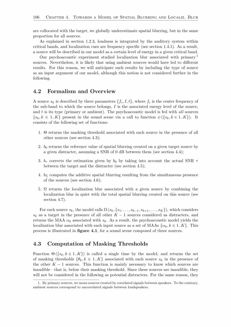
106 Chapter 4. Towards a Model of Spatial Blurring and Localiz. Blur

are collocated with the target, we globally underestimate spatial blurring, but in the sameproportion for all sources.

As explained in section 1.2.3, loudness is integrated by the auditory system withincritical bands, and localization cues are frequency specific (see section 1.4.1). As a result,a source will be described in our model as a certain level of energy in a given critical band.

Our psychoacoustic experiment studied localization blur associated with primary 1

sources. Nevertheless, it is likely that using ambient sources would have led to differentresults. For this reason, we will anticipate such results by including the type of sourceas an input argument of our model, although this notion is not considered further in thefollowing.

4.2 Formalism and OverviewA source sk is described by three parameters fc, I, t, where fc is the center frequency ofthe sub-band to which the source belongs, I is the associated energy level of the source,and t is its type (primary or ambient). The psychoacoustic model is fed with all sourcessk, k ∈ 1..K present in the sound scene via a call to function ψ (sk, k ∈ 1..K). Itconsists of the following set of functions:

1. Θ returns the masking threshold associated with each source in the presence of allother sources (see section 4.3);

2. b0 returns the reference value of spatial blurring created on a given target source bya given distracter, assuming a SNR of 0 dB between them (see section 4.4);

3. bτ corrects the estimation given by b0 by taking into account the actual SNR τbetween the target and the distracter (see section 4.5);

4. bΣ computes the additive spatial blurring resulting from the simultaneous presenceof the sources (see section 4.6);

5. Ω returns the localization blur associated with a given source by combining thelocalization blur in quiet with the total spatial blurring created on this source (seesection 4.7).

For each source sk, the model calls Ω (sk, s1, . . . , sk−1, sk+1, . . . , sK), which considerssk as a target in the presence of all other K − 1 sources considered as distracters, andreturns the MAA αk associated with sk. As a result, the psychoacoustic model yields thelocalization blur associated with each input source as a set of MAAs αk, k ∈ 1..K. Thisprocess is illustrated in figure 4.1, for a sound scene composed of three sources.

4.3 Computation of Masking ThresholdsFunction Θ (sk, k ∈ 1..K) is called a single time by the model, and returns the setof masking thresholds θk, k ∈ 1..K associated with each source sk in the presence ofthe other K − 1 sources. This function is mainly necessary to know which sources areinaudible—that is, below their masking threshold. Since these sources are inaudible, theywill not be considered in the following as potential distracters. For the same reason, they

1. By primary sources, we mean sources created by correlated signals between speakers. To the contrary,ambient sources correspond to uncorrelated signals between loudspeakers.

4.3. Computation of Masking Thresholds 107

Figure 4.1: Illustration of the function calls (thick arrows) made within the psychoacoustic modelwhen it is invoked with a sound scene composed of three sources s1, s2 and s3.


02

46

810

Distracter band (distance in ERB relative to the target)

Spa

tial B

lurr

ing

(°)

700 Hz

Target center frequency

1400 Hz 5000 Hz

−4 −1 0 1 4 −4 −1 0 1 4 −4 −1 0 1 4

Figure 4.2: Experimental spatial blurring obtained from results of experiment 1 (see figure 3.6)after subtraction of localization blur in quiet.

do not have any associated MAA, which by convention will be set to +∞. 2 The interestis double. First, having fewer sources to consider reduces computation. Second, havingsources with an infinite associated MAA will necessarily lead to better performances inthe coding schemes we will present in chapter 5. These considerations will be useful forthe model of function bτ , detailed in section 4.5.

We gathered data concerning energetic masking and binaural unmasking, especially inour second experiment (see section 3.7). In particular, for a target with a center frequencyof 1400 Hz, linear regressions yielded a binaural unmasking of −0.3 dB per degree, and avariation of the masking threshold with the target-masker frequency distance of −8.48 dBper ERB. However our experiments did not aim primarily to study energetic masking,and these results are of course insufficient to build a model of it, especially in terms ofadditivity of the maskers. Hence a more complete model should be considered for thismodule. This is beyond the scope of this thesis, and more information about such modelscan be found for instance in [BG02].

4.4 Reference Value of Spatial Blurring

For the following, we need to define dz as the distance on an ERB scale (see equation (1.4))between a target st and a distracter sd:

dz(ft, fd) = ERBS(fd)− ERBS(ft), (4.1)

where ft and fd are the center frequencies of the critical bands to which the target andthe distracter belong, respectively. So when the distracter belongs to a critical band abovethat of the target, dz gets a positive value.

2. However, the worst case scenario in term of binaural unmasking has to be considered here, to avoidthe source being unmasked if its position is affected by the coding scheme.

4.4. Reference Value of Spatial Blurring 109

Figure 4.3: Characteristics of function b0 for a given value of ft.

Function b0(st, sd) returns the spatial blurring created on a target st of center frequencyft by a distracter sd located dz ERBs away assuming an SNR between them of 0 dB. To doso, we will model data from our first experiment (see section 3.6) depicted in figure 3.6in order to be able to express the spatial blurring created by a distracter of any frequencyon a target of any frequency. Recall that, as in the experimental conditions of chapter 3,an SNR of 0 dB means that the target and the distracter are loudness equalized (seesection 3.4). The estimation yielded by b0 will be considered as an estimation of referencewhich will be corrected afterwards by function bτ (see section 4.5).

From our experimental data, we know the localization blur in quiet for targets withcenter frequencies of 700 Hz, 1400 Hz and 5000 Hz, respectively. We also know thelocalization blur resulting from the presence of a distracter located -4, -1, 0, 1, and 4ERBs away from these targets. In section 3.2, we defined spatial blurring as the differencebetween localization blur in the presence of distracters and localization blur in quiet.We can compute the spatial blurring resulting from the presence of the distracter bysubtracting the localization blur in quiet from each of the three curves, that is 1.5 at700 Hz, 5.1 at 1400 Hz, and 3.9 at 5000 Hz. The resulting curves are given in figure 4.2.The shape of each curve follows the same characteristics, depicted in figure 4.3. Spatialblurring is close to zero for large values of |dz|, and we will assume that it eventuallybecomes nil at some frequency distance between the target and the distracter. We willalso assume that it never becomes negative, which would otherwise mean that the presenceof the distracter enhances localization performance. A maximum spatial blurring B0 isreached for a certain frequency distance Z0 between the target and the distracter. Fordz < Z0, spatial blurring follows a slope a−, whereas for dz > Z0, it follows a slope a+.Coordinates Z0, B0 as well as slopes a− and a+ are dependent on ft. As a result, thespatial blurring created on a target st of center frequency ft by a distracter sd located dzcritical bands away can be modeled as a triangular function b0:

b0(st, sd) = max (0, (a− × θ(dZ0) + a+ × θ(−dZ0))× dZ0 +B0(ft)) , (4.2)

where dZ0 = dz − Z0(ft) is the distance of the distracter band from the band inducingmaximum spatial blurring, and θ(dZ0) is the step function equaling one for positive valuesof dZ0 and zero otherwise.

Modeling b0 consists of modeling each of these characteristics. Let us first consider themodeling of coordinates Z0, B0 for any target center frequency. From our experimentaldata, these coordinates are the following:


−10 −5 0 5 100

2

4

6

8

10b 0(°)

ft= 1400 Hz

ft= 1000 Hz

ft= 700 Hz

dz(ERB)

−10 −5 0 5 100

2

4

6

8

10

b 0(°)

ft= 1400 Hz

ft= 3000 Hz

ft= 5000 Hz

dz(ERB)

Figure 4.4: Function b0 for different target center frequencies: 700 Hz, 1000 Hz and 1400 Hz (leftpanel); 1400 Hz, 3000 Hz and 5000 Hz (right panel).

ft B0 Z0

700 3.2 -11400 9.4 05000 3.5 1

To obtain a value of B0 for any value of ft, we interpolated linearly on an ERB scalebetween each of the three experimental values of B0. For ft smaller than 700 Hz we heldB0 constant at a value of 3.2, and for ft greater than 5000 Hz we held B0 constant at avalue of 3.5. We performed the same operations to obtain a value of Z0 for any value of ft,with boundary values of −1 for ft smaller than 700 Hz and 1 for ft greater than 5000 Hz.

Concerning the modeling of a− and a+, we performed linear regressions on our data toobtain these slopes for each of our experimental ft values. Depending on the target centerfrequency ft, this regression was not performed on points corresponding to the same valuesof dz. The resulting values for a+ and a− are the following (the dz values considered foreach regression are provided as well):

ft = 700 Hz ft = 1400 Hz ft = 5000 Hzdz = −4,−1 dz = −1, 0, 1 dz = −4,−1, 0 dz = 0, 1, 4 dz = −1, 0, 1 dz = 1, 4a− = 0.99 a+ = −1.41 a− = 1.54 a+ = −1.75 a− = 1.37 a+ = −0.72

As previously, we interpolated linearly on an ERB scale between all these experimentalresults to obtain values of a− and a+ for any value of ft. For ft less than 700 Hz, we helda− and a+ constant at 0.99 and −1.41, respectively, and for ft greater than 5000 Hz weheld them constant at 1.37 and −0.72, respectively.

Function b0 is illustrated in figure 4.4 for various target center frequencies, and anoverview plot of b0 is given in figure 4.5. The spatial blurring created on a target st ofcenter frequency ft by a distracter sd located dz critical bands away is thus obtained by acall to b0(st, sd).

4.5 Accounting for the Effect of SNRFunction b0 returns an estimation of the spatial blurring between a target and a distracterassuming an SNR of zero. We will present in this section function bτ (st, sd) that correctsthis estimation by taking into account the actual SNR τ between the energy level It of

4.5. Accounting for the Effect of SNR 111

ft (Hz)

d z (E

RB

)

b0 (°)

1000 2000 3000 4000 5000

−8

−6

−4

−2

0

2

4

6

8

1

2

3

4

5

6

7

8

9

Figure 4.5: Overview plot of function b0. The value of b0 in degrees is represented according tothe grayscale at the right. The value of b0 is plotted for combinations of target frequency, ft, andthe distance dz of the distracter from the target in ERBs.

a target st and that of a distracter sd, Id. We studied the relation between SNR andlocalization blur in experiment 2. Since in the experimental stimuli we used, distracterswere loudness equalized with the target, it is first necessary to apply a correction on Itand Id to match our experimental conditions. This can be done, for example, by applyingan A-weighting coefficient, A(f), which is an offset added to the energy levels in decibels,depending on the frequency of the signal under consideration:

A(f) = 2.0 + 20 log10(RA(f)), (4.3)

withRA(f) = 122002f4

(f2 + 20.62)√

(f2 + 107.72)(f2 + 737.92)(f2 + 122002). (4.4)

Thus we can define:ItA = It +A(ft), and IdA = Id +A(fd). (4.5)

We will use our data from experiment 2 to model the relation between SNR and spatialblurring. From this experiment, we are only looking for the slope of the relation, suchthat the likelihood of an offset between results from experiment 1 and 2 due to differentexperimental protocols, setups and subjects is not an issue. We propose to model bτlinearly as:

bτ (st, sd) = D(b0(st, sd))× τ + b0(st, sd), (4.6)

where τ = ItA − IdA . The choice of b0 as an intersept is justified by the fact that bτmust equal b0 for τ = 0. The dependence of the slope D on b0 is assumed but cannotbe assessed or even verified from our limited experimental data. Further studies wouldbe necessary to address this point. Indeed, we can only use two points out of the entiredataset of experiment 2, because either the other points are not significantly above maskingthreshold (see section 3.7.5) or they are too close to the audibility threshold in quiet (seesection 3.8.4), meaning that these points are potentially biased. Moreover, we did not


1 2 3 4 5 6 7 8 9 100

5

10

15

20

25

30

35


Dis

trac

ter

effe

ct (

dB)

+4

ER

B @

45°

+3

ER

B @

45°

−3

ER

B @

45°

−4

ER

B @

45°

+3

& −

3 E

RB

@ 4

5°

+4

& −

4 E

RB

@ 4

5°

all @

45°

all @

0° al

l @ 9

0°

all,

spre

ad

Figure 4.6: Effect of distracter(s), obtained from results of experiment 4 by subtracting the SNRobtained in quiet (condition 0) from the SNR obtained in the presence of the distracters underconsideration.

test any target frequencies other than 1400 Hz in that experiment. The two remainingunbiased points at our disposal correspond to angular separations of 6 and 10, for atarget center frequency of 1400 Hz and a distracter four critical bands above the target:3.8 dB, 6 and −12.9 dB, 10. This leads to a slope D of −.24 per decibel in thatspecific condition. In the absence of other estimations of D in different conditions, we willuse this value of D in all cases.

The expression of bτ given in equation (4.6) is only valid under specific conditions.First, the distracter level has to be above its masking threshold, as returned by functionΘ. Otherwise, since the distracter is inaudible we can assume that its effect is null, andthus that bτ = 0. In the same way, the level of the target has to be above its maskingthreshold, otherwise, since the target is inaudible we can assume by convention that thespatial blurring created on it is infinite, that is, bτ = +∞. Finally, we will assume thatthe level of the target is not close to its threshold of audibility in quiet. Indeed, as alreadymentioned in section 3.8.4, the level of the target would otherwise have an effect on itsassociated localization blur [SMM05, SR01]. In such cases, the expression of bτ given inequation (4.6) would have to be revised.

4.6 Additivity of Distracters

Function bΣ computes the additive spatial blurring resulting from the simultaneous pres-ence of the sources. We studied the additivity of simultaneous distracters in experiment4 (see section 3.9). We found a significant increase of spatial blurring as the number

4.6. Additivity of Distracters 113

of distracters presented simultaneously increases, at least up to four distracters. Fromthis experiment, we can observe the spatial blurring created by distracter(s) through theincrease in the resulting SNR when the distracters are present, that is, by subtractingthe SNR obtained in quiet from the SNR obtained in the presence of the distracters un-der consideration. The result of this operation is depicted in figure 4.6. Let us call∆c the difference observed in condition c. It is recalled that the SNR resulting from agiven condition is the SNR between the target and any of the distracters, all distractersbeing presented at the same, fixed, loudness-matched level. To model bΣ we must find aprediction function f such that:

∆5 = f(∆2,∆3), (4.7)∆6 = f(∆1,∆4), (4.8)∆7 = f(∆1,∆2,∆3,∆4), (4.9)∆7 = f(∆5,∆6). (4.10)

Note that ∆7 can be predicted in two ways: either from ∆1, ∆2, ∆3 and ∆4, or from∆5 and ∆6. We investigated different types of additivity between distracters. First, theresulting effect might be that of the distracter producing the greatest effect, that is:

f(∆c, c ∈ C) = max(∆c, c ∈ C), (4.11)

where C is the set of conditions under consideration. A plot of this prediction modelis given in figure 4.7. In this figure, the predicted effect of the distracters is plottedagainst the observed effect, such that the closer data points are to the diagonal line—denoting “predicted equals observed”—the more accurate is the prediction. We can seethat the data points are scattered away from the diagonal, mainly below it, which suggestsan underestimation of additivity. Moreover, Pearson’s linear correlation coefficient yieldsr(58) = .69 (p < .001) for a root mean square error of 8.0 dB. All of this confirms ourobservation concerning experiment 4 that spatial blurring does increase with the additionof distracters, even weaker ones.

A second option is that distracters might add as statistically independent sources(which they actually are). In this case:

f(∆c, c ∈ C) = 10 log10∑c∈C

(10∆c/20

)2. (4.12)

This second formula seems to better match our experimental results, as can be seen infigure 4.8. Indeed, Pearson’s linear correlation coefficient yields r(58) = .74 (p < .001)for a root mean square error of 6.9 dB. However, this prediction model still has a ten-dency to underestimate the additivity of distracters. Actually, additivity is predicted moreaccurately by assuming that the distracters are correlated sources (which they are not):

f(∆c, c ∈ C) = 10 log10

(∑c∈C

10∆c/20)2

. (4.13)

Figure 4.9 gives a plot of the predicted effect of distracters against the observed effectfor all subjects assuming correlated distracters. Predicted and observed effects are muchbetter correlated using this model of additivity: Pearson’s linear correlation coefficientreaches r(58) = .75 (p < .001) for a root mean square error down to 6.6 dB. This wasunexpected. As a consequence, spatial blurring created by distracters seems to over-add,


0 5 10 15 20 25 30 35 40 450

5

10

15

20

25

30

35

40

45

1

1

11

Observed distracter effect (dB)

Pre

dict

ed d

istr

acte

r ef

fect

(dB

)

RMS err = 7.9703 dB, r = 0.69333 (p = 8.2561e−10)

2

2

2

2

3

3

33

4

4

4

4

5

5 5

5

6

6

6

6 7

7

7

7

8

8

8

8

9

9

9

9

1010 10

10

11

11

11

11

12

12

12

12

13

13

13

13

14

14

14

14

1515 15

15

∆5

∆6

∆7 (from ∆

1 to ∆

4)

∆7 (from ∆

5 & ∆

6)

mean ∆5

mean ∆6

mean ∆7

mean ∆7

Figure 4.7: Plot of the predicted effect of distracters against the observed effect from experiment4, assuming that the resulting effect is that of the distracter producing the greatest effect (seeequation (4.11)). ∆c is the difference between the SNR obtained in quiet (condition 0) and theSNR obtained in the presence of the distracters under consideration in condition c. The emptysymbols represent the values from individual subjects, whereas the filled symbols represent themean over all fifteen subjects.


0 5 10 15 20 25 30 35 40 450

5

10

15

20

25

30

35

40

45

1

1

11


Pre

dict

ed d

istr

acte

r ef

fect

(dB

)

RMS err = 6.9411 dB, r = 0.7379 (p = 1.7416e−11)

2

2

22

3

3

33

4

4

44 5

5

5

5

6

6

6

6

7

7

7

7

8

8

8

8

9

9

99

1010

10

10

11

11

11

11

12

12

12

12

13

13

13

13

14

14

1414

1515

15

15

∆5

∆6

∆7 (from ∆

1 to ∆

4)

∆7 (from ∆

5 & ∆

6)

mean ∆5

mean ∆6

mean ∆7

mean ∆7

Figure 4.8: Plot of the predicted effect of distracters against the observed effect from experiment4, assuming statistically independent distracters (see equation (4.12)). ∆c is the difference betweenthe SNR obtained in quiet (condition 0) and the SNR obtained in the presence of the distracters un-der consideration in condition c. The empty symbols represent the values from individual subjects,whereas the filled symbols represent the mean over all fifteen subjects.


0 5 10 15 20 25 30 35 40 450

5

10

15

20

25

30

35

40

45

1

1

11


Pre

dict

ed d

istr

acte

r ef

fect

(dB

)

RMS err = 6.6372 dB, r = 0.75174 (p = 4.4665e−12)

2

2

2

2

3

3

3

3

4

4

4

455

5

5

6

6

6

6

7

7

7

7

8

8

8

8

99

9

9

1010

1010

11

11

1111

12

12

12

12

13

13

13

13

14

14

1414

1515

15

15

∆5

∆6

∆7 (from ∆

1 to ∆

4)

∆7 (from ∆

5 & ∆

6)

mean ∆5

mean ∆6

mean ∆7

mean ∆7

Figure 4.9: Plot of the predicted effect of distracters against the observed effect from experiment4, assuming correlated distracters (see equation (4.13)). ∆c is the difference between the SNRobtained in quiet (condition 0) and the SNR obtained in the presence of the distracters underconsideration in condition c. The empty symbols represent the values from individual subjects,whereas the filled symbols represent the mean over all fifteen subjects.


since distracters are in reality statistically independent, which suggests an interactionbetween them. We have not yet investigated the possible reasons behind such an additivityrule.

Note also that additivity obtained in condition 7 seems to be less accurately predictedfrom conditions 5 and 6 than from conditions 1 to 4 (the diamond symbols in figure 4.9are farther away from the diagonal line than the triangular symbols), which suggests anoverestimation of the additivity in the first of these two cases. This can probably beattributed to the fact that in this case, the distracters to be added have a bandwidthexceeding a single critical band. Interestingly, as can be seen on figure 4.8, this specificcase—and therefore the additivity of wideband distracters—seems to be best predictedusing the rule from equation (4.12).

In experiment 4, all distracters in a given condition were presented with the sameloudness-matched level. We will assume that the additivity-prediction rule stated in equa-tion (4.13) applies to distracters with non-loudness-matched levels as well. Besides, we willassume that for the range of SNRs concerning experiment 4, the relation between spatialblurring and SNR is linear, since we do not have enough data from experiment 2 to assessmore precisely this relation. We will thus assume that an increase in SNR for a givenangular separation is equivalent to a proportional increase in spatial blurring for a fixedSNR. Consequently, we can state, given a target st and a set of distracters sdp , p ∈ 1..P,that:

bΣ(st, sdp , p ∈ 1..P) =P∑p=1

bτ (st, sdp) + δ, with δ > 0, (4.14)

where δ is the additional spatial blurring resulting from the over-additivity of distracters.If the relation between SNR and spatial blurring was further shown to be non-linear,equation (4.14) would have to be adjusted accordingly. If distracter effects had beenshown to add as independent sources—that is, according to equation (4.12)—δ wouldhave been null. There is no direct approach that allows us to derive an expression ofδ from our experimental results. However, another way to take into account this over-additivity is to correct the amplitude level associated with each of the distracters by afactor γ prior to assessing the effect of SNR on spatial blurring with bτ . Let us defineip = 10Ip/20 as the amplitude level of distracter sp, where Ip is its associated energylevel. Because distracters are independent but seem to have effects that add as correlatedsources, according to equations (4.12) and (4.13) we are looking for the expression of γverifying:

P∑p=1

(γ ip)2 =

P∑p=1

ip

2

, with γ > 0. (4.15)

That is:

γ =∑Pp=1 ip√

P∑Pp=1(ip)2

. (4.16)

We can thus define I ′p as the corrected energy level from distracter sp:

I ′p = 20 log10(γ ip) (4.17)= Ip + Γ, (4.18)

with

Γ = 20 log10(γ) = 20 log10

∑Pp=1 ip√

P∑Pp=1(ip)2

. (4.19)


The spatial blurring created on a target st by a set of distracters sdp , p ∈ 1..P is finallygiven by:

bΣ(st, sdp , p ∈ 1..P) =P∑p=1

bτ (st, s′dp), (4.20)

where s′p denotes distracter sp with corrected energy level I ′p. Given that experiment4 showed this additivity effect up to four distracters, a potentially necessary precautionmight be to limit this expression to the four greatest effective distracters.

4.7 Resulting Localization BlurThe last function Ω(st, sdp , p ∈ 1..P) returns the localization blur associated with atarget st in the presence of a set of distracters sdp , p ∈ 1..P based on the spatial blurringthey create on st, obtained by a call to bΣ(st, sdp , p ∈ 1..P), and on the localization blurin quiet αmin(st) associated with st.

In section 3.2, we defined spatial blurring as the difference between localization blurin the presence of distracters and localization blur in quiet, such that:

Ω(st, sdp , p ∈ 1..P) = bΣ(st, sdp , p ∈ 1..P) + αmin(st). (4.21)

A value of αmin can be computed for any target frequency by interpolating linearly on anERB scale between each of the three experimental values of αmin we obtained in experiment1, that is, 1.5 at 700 Hz, 5.1 at 1400 Hz, and 3.9 at 5000 Hz.

4.8 Simplification of the ModelWhen MAAs are not to be used absolutely, but rather relatively (as in the coding schemeproposed in section 5.1), this model can be roughly approximated. Indeed, the mainresult from the estimations yielded by this model is that sources with greater associatedenergy levels are more likely to have a smaller associated localization blur. Therefore,in practical situations where complexity is critical, this model can be greatly simplifiedby associating with a given source a localization blur that is inversely proportional toits audible energy—that is, above masking threshold. This avoids the assessment of thespatial blurring created by each of the distracters on each target, which represents a greatdeal of decrease in complexity.

Moreover, by looking at figure 4.2, one can see that spatial blurring seems to becorrelated to localization blur in quiet, that is, the greater the localization blur in quiet, themore important spatial blurring seems to be, whatever the distracter under consideration.Consequently, this simplified model based on energy could be refined by weighting theestimated localization blur with the value of αmin corresponding to the target.

4.9 ConclusionsThis chapter provided a modeling of spatial blurring within the limits of our experimentaldata. The interest of the approach we proposed is that it divides the modeling of a com-plex phenomenon—spatial blurring—involving several variables (target center frequency,distracter center frequency, SNR, number of distracters) into the modeling of three sim-pler effects involving less variables. First, spatial blurring with loudness-matched targetand distracter (SNR of 0 dB), involving solely the modeling of the target center frequency

4.9. Conclusions 119

and the distracter relative center frequency. Second, the modeling of the effect of SNR onspatial blurring, involving, as we assume, only SNR and the spatial blurring created withan SNR of 0 dB. And finally, the modeling of the additivity of distracters, involving thenumber of distracters and the spatial blurring that each of them create when presentedalone. As a result, this approach does not require the acquisition of psychoacoustic datathat test all these variables simultaneously, which would be difficult in practice.

Further studies are needed to refine and correct this model. For instance, the temporalaspect of distracting sources was not considered, but recent investigations by Croghanand Grantham [CG10] using pulsating and non-pulsating interferers suggest that spatialblurring is greatest with pulsating sources compared to non-pulsating sources. Studies byKopčo et al. [KBS07] showed that non-simultaneous distracters can also affect localization,which suggests that localization blur might be affected as well. Moreover, the perceptionof sources in terms of auditory scene analysis (see section 1.3) is not accounted for either inour model. For example, it is not clear if two sources—in the sense of our model—fused bythe auditory system can be considered as potential distracters for each other or not. Also,these fusion phenomena might increase localization blur, because the auditory systemseems to derive a location only after the fusion process (see section 1.5). Therefore, ourpresent model is a low-level model that might need to be modified to include the resultsof higher-level auditory processes.

Chapter 5

Multichannel Audio Coding Basedon Spatial Blurring

As briefly presented in section 2.2.2 and reviewed in more detail in appendix C, per-ceptual coding takes advantage of interference between frequency components, exploitingenergy masking phenomena. To extend this concept to multichannel audio signals, thephenomenon of binaural unmasking has been taken into account, which resulted in adecrease of the masking ability of the signal components, and consequently limited thebitrate reduction. The coding of the spatial attribute of a sound scene has a cost, asexplained in chapter 2, and strategies (based on auditory perception or not) have alreadybeen proposed to reduce this cost. However, interference between components in termsof their perception in space by the auditory system has not been considered so far inspatial audio coding. Indeed, we have seen from our experiments presented in chapter 3that auditory spatial resolution is likely to decrease as the sound scene gets complex, thatis, when several sources are present simultaneously. In this chapter, we put forward twospatial audio coding schemes that take advantage of this decrease in resolution to ease theprecision of representation of the spatial sound scene, leading to a bitrate reduction. Thefirst scheme applies in the context of parametric spatial audio coding (see section 2.5),while the second one concerns the HOA representation (see section 2.1.2). As in chapter 3,we will limit our reasoning to the azimuthal plane, but this work could be extended toelevation as well.

Localization Blur in Spatial Audio Coding

In the two coding schemes we will consider in this chapter, the accuracy of representationof the spatial attribute of the scene has a cost. For instance, in parametric spatial audiocoding schemes, space is explicitly encoded as a set of discrete spatial parameters. Thecost is in the precision of coding of these parameters, upon which depends the precisionof representation of space. In order to reduce the necessary transmission bitrate, theseparameters are quantized and coded with only few bits, and thus the representation ofspace is degraded. In HOA, the cost is in the order of representation of the scene. Thehigher this order, the larger the area of accurate reconstruction of the sound scene, but alsothe larger the number of coefficients to encode. Therefore, the representation is truncatedto a certain order to reduce the necessary transmission bitrate.

In both cases—quantization or truncation—the consequence is a degraded spatial rep-resentation of the components of the sound scene which, at the listening phase, are per-ceived as changes in position. As localization blur characterizes the sensitivity to position

122 Chapter 5. Multichannel Audio Coding Based on Spatial Blurring

SpatialSynthesis

ENCODER

SideInformation

DECODER

Estimation ofSpatial

Parameters

... ...

......

...

PsychoacousticModel of

Spatial Blurring

CoreEncoder

CoreDecoder

CoreDecoder

BitstreamUnpacking

EncodedDownmix

BitAllocation

Figure 5.1: Overview of the proposed parametric spatial audio coding scheme based on spatialblurring.

changes of sound events, if the erroneous change in position of a given component is greaterthan its associated localization blur, it will be perceived by the auditory system. On thecontrary, if this change in position occurs within localization blur, it will not be perceived.For this reason, localization blur could play an important role in spatial audio coding.Moreover, the experiments we carried out (see chapter 3) have shown that a given com-ponent of the sound scene is susceptible to increase the localization blur associated withother components in its frequency vicinity. This is why we propose to use localization blurresulting from spatial blurring in exactly the same way masking thresholds resulting fromenergetic masking are used (see appendix C): by shaping spatial distortions to containthem (as much as possible) within localization blur, such that they are not perceived bythe listener. Therefore we will use our psychoacoustic model of spatial blurring (describedin chapter 4) to estimate localization blur at each time instant, and this will determine thespatial distortion we can afford for each component of the sound scene. This strategy thusimplies a dynamic adjustment of the accuracy of representation of the sound scene. Theinterest can be seen in two ways: either the perceived quality remains the same (trans-parent coding) and the bitrate is reduced whenever possible, or the same bitrate is kept(constraint bitrate coding), but the perceived quality is improved.

5.1 Dynamic Bit Allocation in Parametric Schemes

A patent is pending for this work [DN11].

5.1.1 Principle Overview

Three parametric spatial audio coding schemes have been presented in section 2.5: BCC(along with PS), SASC and DirAC. Potentially, the dynamic bit allocation process wepropose in this section can be inserted into any of these schemes, as depicted in figure 5.1.

5.1. Dynamic Bit Allocation in Parametric Schemes 123

The input channels are downmixed into a mono (or stereo) channel(s) in a way that ensuresthe conservation of total energy from all channels. Also a set of spatial parameters iscomputed from the input channels within each of a group of frequency subbands. 1 Thesespatial parameters interest us as they provide a description of the spatial attribute of thescene. They are coded with the same precision in all subbands and at each time instant,which is not optimal from a perceptual point of view since localization blur is likely todiffer from one subband to another due to spatial blurring and is also likely to vary intime.

The optimization principle we propose is to use our psychoacoustic model of spatialblurring to guide the bit-allocation procedure of the spatial parameters such that thespatial distortions resulting from this quantization are shaped according to localizationblur. This new quantization process is thus dynamic, since quantization will vary in timeand depending on the context (the content of the input signals).

An original point in this scheme is that the psychoacoustic scheme is used both onencoding and decoding sides. As we will explain in section 5.1.4, this trick will save us thetransmission of bit-allocation information of the spatial parameters.

Both the quantized spatial parameters and the downmix signal are then transmitted.The downmix signal can optionally be encoded using any external core coder (such asMP3, AAC, etc.) prior to the transmission. At decoding, the spatial parameters aredequantized, the downmix signal is decoded, if necessary, and these are used to synthesizea set of output channels.

5.1.2 Use of our Psychoacoustic Model of Spatial Blurring

The spatial parameters concerned by this dynamic bit allocation procedure are any pa-rameter describing the angular azimuthal position of a sound source. For DirAC, it isstraightforward since the direction vector D represents the direction of the source and iscoded in practice as an angle. Therefore D can benefit from our dynamic bit allocation. InSASC, the primary and ambient localization vectors dP and dA are usually coded in polarcoordinates, that is as angle and radius. The bit allocation for the angular value of eachvector can thus be optimized. Finally, in BCC the angular position of the source is notdirectly represented by any of the spatial parameters; it is rather the localization cues usedby the auditory system to derive this position that are coded. But still, a quantizationerror in an ICLD or an ICTD value will be perceived as a change in the angular positionof the source, and therefore our dynamic allocation process can be applied here as well. Inthe following, we will not distinguish between the three considered coding schemes, andpotentially other schemes might be concerned as well.

As explained in section 2.5.1, the frequency subbands within which spatial parametersare computed following a set of adjacent critical bands. The spatial parameters associatedwith a subband describe a single position, and this because it is assumed that the listenercannot discriminate two simultaneous sources in space, which spectrally belong to a samecritical band while spatially arising from different locations. Since our psychoacousticmodel defines a source as energy in a critical band (see section 4.1), we can directly use itto estimate the MAA associated with each subband, considered as a source. More exactly,if the primary/ambient energy ratio of each subband is known, each subband consists oftwo sources: a primary source and an ambient source. Depending on the concerned codingscheme, this ratio is known if the following parameter is computed and transmitted: the

1. The time-frequency transform used for this purpose is not represented in figure 5.1. More informa-tion about this transform are given in section 2.5.1.


inter-channel coherence c for BCC, the diffuseness coefficient Ψ for DirAC, and the ambientenergy fraction λ in SASC. Otherwise, each subband consists of a single source, consideredas primary. The submission of this additional information to our psychoacoustic modelhas two consequences. First, it allows the model to treat primary and ambient componentsseparately instead of pooling together the energy from both components, thus avoidingan overestimation of the energy associated with a given source. But this also refines theestimation of the MAA, because spatial blurring might vary depending on whether thetarget and the distracters are primary or ambient components. 2

As justified in section 4.1, neither the position of the source under estimation, nor thepositions of the distracting sources are needed by the model to yield an estimation of MAA;only the energy associated with each source is required. Indeed, our psychoacoustic resultsshowed that the position of a given source does not have an effect on the spatial blurringthat this source creates, and in our model the target source is assumed to be in frontof the listener. Consequently, the MAA associated with a given source can be estimatedsolely from the downmix signal, since the total energy from the original input channels isconserved. It is important for this estimation to be done after encoding-decoding by theexternal core coder (if any), as explained in section 5.1.4.

Each source s is characterized by three parameters fc, I, t, where fc is the centerfrequency of the subband to which the source belongs, I is the associated energy level ofthe source, and t is its type (primary or ambient). If K is the total number of sources,the psychoacoustic model is called via ψ (sk, k ∈ 1..K). It returns an estimation of theMAA associated with each source sk considered as a target, based on the spatial blurringcreated on it by all other K − 1 sources, considered as simultaneous distracters.

As a result, the psychoacoustic model yields two estimations per subband, one corre-sponding to the MAA associated with the primary component of the subband, and theother one corresponding to the MAA associated with the ambient component. Howeverthe latter is exploitable only in SASC because it is the only scheme transmitting parame-ters that describe the spatial position of ambient components. For the two other schemes,the benefit is a more accurate estimation of MAAs, but only primary components will beconsidered for the dynamic bit-allocation procedure. In any case, note that the numberof sources remains the same from one temporal frame to another; it equals either once ortwice the number of subbands, depending on whether the primary/ambient energy ratioof each subband is known.

5.1.3 Bit Allocation of the Spatial Parameters

Bit allocation is the module that optimizes the representation of space as a function of theavailable bitrate. The bit-allocation process is split into two parts. The first part consistsof a certain number of bits equally distributed among all sources—we will refer to themas “fixed” bits—this basic allocation ensuring a minimal quality of spatial reproductionfor all sources. The second part however consists of bits distributed as a function of theassociated localization blur of each source—we will refer to them as “floating” bits.

For the sake of simplicity, we will illustrate the bit-allocation strategy assuming asingle parameter to code for each source, but the process remains the same for otherparameters. To lighten the language a bit, we will sometimes use expressions similar to“to code source s”, which is shorthand for “to code the parameter associated with sources”. As this process is applied identically and independently for each temporal frame, we

2. However, as explained in chapter 4, further psychoacoustic experiments would be necessary to see ifthe primary or ambient nature of components affects spatial blurring.


will only describe it for a single frame. Once again, if parameters specifically describing theposition of the ambient component of each subband exist (which is the case in SASC), thenprimary and ambient sources are both concerned by this procedure—meaning that the bitpool is shared between primary and ambient sources—otherwise only primary sources areconcerned, since there is no parameter to code for ambient sources. Let us introduce thefollowing variables:

K: total number of sources (primary and ambient);P : number of sources to code;N : total number of bits to allocate;nfixed: minimum number of bits allocated to each source’s parameter (i.e., the number offixed bits);sp: pth sound source to code, p ∈ 1, . . . , P;αp: MAA associated with the pth source in the presence of the K − 1 other sources, asgiven by the psychoacoustic model;np: number of floating bits allocated to the parameter of sp;n′p = nfixed + np: total number of bits allocated to the parameter of sp.

First of all, we need to express the consequence of allocating an additional bit for theprecision of coding of the parameter. The precision of coding of a parameter is given bythe number of values over which it is quantized. It is possible to represent 2n quantizationvalues with n bits, so whatever the distribution of these quantization values is (uniform ornot), we will consider that adding a coding bit doubles the number of quantization values. 3Thus adding a coding bit doubles the precision of representation of the parameter.

We propose to avoid trying to link directly quantization errors with angular changesin position. The first reason for this choice is because this link might change dependingon the nature of the concerned spatial parameter, but besides, it would be unnecessarilycomplicated. The basic idea of our dynamic bit allocation is the following. Instead ofconsidering the MAA associated with each source absolutely and trying to allocate thenecessary number of coding bits to each source to ensure that spatial distortions stay withinlocalization blur, we will rather simply ensure that the smaller the MAA associated with agiven source, the larger the number of bits allocated to it. In other words, the source withthe smallest associated MAA will be coded the most precisely, and the one with the largestassociated MAA will be coded the most roughly. In between, sources will be coded moreor less precisely depending on their associated MAA. If the total number of bits availableis sufficient, then spatial distortions will be constrained within localization blur. If not,spatial distortions will be perceptually minimized in an homogeneous fashion among allsources. This approach is especially necessary in a situation of constrained bitrate, whichwe will describe first. However, the unconstrained bitrate case, studied afterwards, alsobenefits from the simplicity of this approach.

Constrained bitrate

Having a constrained bitrate means that besides the number of fixed bits, the numberof floating bits is constrained too. So let us call Nfloat the number of floating bits wehave to distribute between all sources according to the psychoacoustic model. As statedabove, the source with the smallest associated MAA—let us call its index m—should becoded with the maximum precision, which then equals 2nm . Moreover, the relative coding

3. If this assumption is not verified, equations (5.1) and (5.7) stated thereafter must be adjusted con-sequently.


precision between sm and any other source sp should be inversely proportional to theirrelative MAA. This can be expressed as:

2np2nm = αm

αp,with np, nm ∈ N+, and αp, αm ∈ R+∗. (5.1)

Thus:

np = nm + log2

(αmαp

). (5.2)

Moreover, the sum of floating bits from each source must equal the total number of avail-able floating bits Nfloat:

P∑p=1

np = Nfloat. (5.3)

Thus, by replacing in this equation the expression of np given in equation (5.2), we obtain:

nm =Nfloat − log2

(∏Pp=1

αmαp

)P

. (5.4)

Equations (5.2) and (5.4) above give a first approximation of the number of bits to allocateto the parameter of sources sp and sm, respectively. Since all np have to be integers,after rounding, some bits to allocate might remain (∑P

p=1 np < Nfloat), or too many bitsmight have been allocated (∑P

p=1 np > Nfloat). The following heuristic—a greedy typealgorithm—allows the allocation process of floating bits to be finalized 4 with an iterativeprocedure. Let us define ∆p from equation (5.1) as a distance between the optimal bitallocation 5 for source sp and its current bit allocation:

∆p = αmαp− 2np

2nm . (5.5)

Thus ∆p reflects how much precision is lacking in the coding of sp. At each iteration,the index of the source to/from which the next bit should be allocated (or taken back)is determined by argmaxp∆p (or argminp∆p). ∆p is computed again after each operationon one bit. The allocation process is finalized when the total number of allocated floatingbits equals exactly Nfloat.

It might happen at some point that ∆p is null for all p whereas the total number ofallocated bits does not equal Nfloat. This means that the allocation is optimal given thenumber of allocated bits although the allocation process is not finished yet, because bitsremain to be allocated or withdrawn. In that case, the source that should receive (orfrom which should be taken back) the next bit is the source with the smallest (or greatest)associated MAA. Then the iterative process can go on until Nfloat bits have been allocated.

Finally, the total number of bits n′p allocated to the coding of the parameter of sourcesp is given by:

n′p = nfixed + np. (5.6)

4. Note that the whole allocation process can be done using this algorithm exclusively.5. The optimal bit allocation is reached when equation (5.1) is satisfied for all sources.


Unconstrained bitrate

In an unconstrained bitrate context, a specific coding quality is targeted. Let us define afictive source sα, which will serve as a reference. The MAA associated with this fictivesource ideally is the mean MAA α observed over all sources and temporal frames of thesignal. In practice, α can be either assumed or estimated (over the next few temporalframes, for instance). The coding quality is then defined by the number of bits n allocatedto sα, and this choice is up to the user. The aim of this bit allocation procedure is toobtain, depending on the accuracy of the estimation of α, a practical mean number of bitsallocated to each source close to n.

A source with an MAA equal to that of the reference source sα will thus be coded withn bits, that is, with a precision of 2n. Then a source with an associated MAA greater thanα should be coded less precisely than sα, and vice versa. Therefore, the relative codingprecision between sα and any other source sp should be inversely proportional to theirrelative MAA. This can be expressed as:

2np2n = α

αp,with np, n ∈ N+∗, and αp, α ∈ R+∗. (5.7)

The number of floating bits to allocate to the parameter of source sp is thus given by:

np = n+ log2

(α

αp

). (5.8)

Equation (5.6) gives the total number of bits to allocate to the parameter of source sp.

5.1.4 Transmission and Bitstream Unpacking

Once the bit allocation for each parameter is known, parameters can be quantized andtransmitted. As quantization is now dynamic due to the account for spatial blurring,it would be necessary a priori to transmit more information about how each parameterhas been quantized—the number of bits on which each parameter has been coded—inorder to properly dequantize them at decoding. The cost resulting from the transmissionof this additional information would not be affordable given the very small number ofbits these parameters are aimed to be coded on. Nevertheless, since localization blur canbe estimated solely from the downmix signal, it is possible to run at decoding the samebit allocation process as the one run at encoding to know exactly how many bits wereallocated to each parameter. The counterpart of this solution is that the psychoacousticmodel has to be known by the decoder. 6 Moreover, if the downmix has been encodedwith an external core coder prior to transmission, the psychoacoustic model has to be fedat encoding with the downmix signal encoded then decoded by this core coder to ensurethat the same downmix signal is submitted to it at decoding, and thus leads to the samebit allocation.

If it is transmitted, the primary/ambient energy ratio—which is coded on a fixednumber of bits—has to be transmitted before any dynamically quantized parameter. In-deed, this parameter is necessary to separate the energy part associated with the primaryand ambient components. Then information about each source can be submitted to thepsychoacoustic model at decoding prior to dequantizing the dynamically quantized pa-rameters.

6. The real implication is that any modified version of the psychoacoustic model in the encoder needsits specific revised decoder.


A last interesting possibility is that if nfixed is nonzero, it is possible to get a firstapproximation of each of the spatial parameters without knowing the number of allocatedbits to each of them. Indeed, if the bitstream is organized such that the most significantnfixed bits of each source are sent first, followed by the remaining np floating bits ofeach source, then these nfixed most significant bits approximate each transmitted value.This might be useful in case any further experimental study would show that some basicinformation about source position is in fact necessary to estimate MAAs more accurately.In such a case, the downmix signal would no longer be enough for MAA estimation,and these approximate parameter values would help maintain the possibility of MAAestimation at decoding (meaning that at encoding MAA estimation has to be done usingthe same approximate parameter values). Therefore, the larger nfixed, the better theapproximation of the parameters.

5.1.5 Informal Listening

We carried out informal listening tests to get a first idea of advantages and drawbacks ofour dynamic bit-allocation approach in comparison with a static bit allocation—that is,when a parameter is coded with the same number of bits for all sources. We implementedour procedure within a Parametric Stereo coding scheme (see section 2.5), using a short-time Fourier transform (STFT) with temporal frames of 10-ms duration. Inter-ChannelCoherence (ICC) was not transmitted, and the effect of the quantization of either Inter-Channel Level Difference (ICLD) or Inter-Channel Phase Difference (ICPD) was assessedseparately. This means that when ICLD was quantized, ICPD was not, and vice versa.ICLD and ICPD were quantized according to results given in section 1.4.5, as explainedin section 2.5.4. Thus ICPD was uniformly quantized, and for ICLD, quantization stepsincreased as the reference ICLD increased. ICLD parameters were computed for subbandsover the full bandwidth (up to 22050 Hz), whereas ICPD parameters were only computedfor subbands up to 1500 Hz (the 11 first subbands), as is usually the case given that phasebecomes ambiguous for higher frequencies. No subband pre-selection by energetic maskingwas applied, thus parameters of all subbands were coded. We chose to test the constrainedbitrate allocation procedure only, applied with different sizes of bit pool. nfixed was alwaysequal to zero, so only Nfloat was varied in our tests. Two types of signals were tested:intensity stereo panning music and binaural recordings of sound scenes.

A general result is that our dynamic bit-allocation procedure is especially interesting forvery low bitrates. Indeed, assuming a symmetrical scalar quantizer, 7 one or two bits 8 atleast per parameter are technically necessary when using a static bit-allocation procedure.However, when using our dynamic procedure, a basic stereo image can be obtained evenwith less than a single bit per parameter in average. In fact, bits will be allocated onlyto the perceptually most important subbands, while the remaining subbands will not getany bits.

Concerning the bit allocation for the ICLD parameter, mainly tested on intensitystereo panning music, in general our dynamic procedure produced an equivalent stereoimage with fewer bits compared to the static bit allocation. In other words, the stereoimage is richer with our procedure when the same number of bits as in the static bitallocation is used.

7. Note that we do not consider vector quantization, differential coding or other advanced methods,the purpose here being to compare dynamic and static bit-allocation procedures.

8. Two bits if the quantizer includes the zero output value (which was the case in our tests), one bitotherwise.

5.2. Dynamic Truncation of the HOA Order 129

However, our dynamic procedure produces artifacts in certain cases when applied toICLD, especially when all of the energy of an auditory source—in the ASA sense (seesection 1.3)—is panned on only one of the two channels (situation of hard-panning). Inthat case, the fact that some subbands of the source, which should only be present in onechannel, are also present in the other one is perceived as some sort of incomplete phantomsource. This effect is almost imperceptible when listening over loudspeakers, though. Thisis probably due to the fact that when listening over headphones, such a phantom sourceis perceived at one ear, whereas the complete source is perceived at the other ear. Hence,the complete source is fused by the auditory system at one ear, whereas at the otherone the fusion operates only on the energy of this source that is erroneously present.As a consequence, two different sources are perceived, one at each ear. When listeningover loudspeakers, crosstalk greatly attenuates this effect. In fact, it seems that fusionhappens between the incomplete source and crosstalk, such that in the end the incompletesource is fused with the complete one, and a single source is perceived. This flaw canprobably be attributed to the fact that the ICLD parameter of each of the originally hard-panned subbands is coded with zero bits, meaning that ICLD is considered null in thesesubbands, and thus energy is equally present in the two channels. This can be avoided bysetting a nonzero value to nfixed, but this reduces the dynamic aspect of the bit allocation.Therefore, the setting of our dynamic procedure for ICLD is a trade-off between nfixed andNfloat.

The bit allocation for the ICPD parameter was mainly tested on the binaural record-ings, since the information of phase difference is essential for this type of signal. From ageneral point of view, quantization of ICPD induces audible artifacts with both methods,although it seems that with fewer bits, our dynamic allocation procedure produces lessartifacts compared to the static bit allocation. This tendency gets stronger when usingthe same number of bits as in the static bit allocation.

As a conclusion, our approach seems to provide interesting results, even if there is roomfor improvement. Of course, as the number of bits allocated to each parameter on averageis increased, differences between the two allocation methods become less perceptible, sincethe number of bits is enough to keep spatial distortions within localization blur even withstatic bit allocation.

5.2 Dynamic Truncation of the HOA Order

Part of the following was published in the proceeding of the 40th AES conference [DNM10],and is patent-pending [DN10].

This second coding scheme based on spatial blurring takes advantage of the HOArepresentation to shape spatial distortions according to localization blur. One advantageof HOA is that it represents accurately several spatially separated sound sources lyingin a same critical band, which is not the case of parametric coders (see section 2.5.1).We will start by studying spatial distortions resulting from truncation of the order ofrepresentation using an approach based on simulations, and we will propose an adjustednotion of sweet spot based on perceptual criteria. Then the actual coding scheme bydynamic truncation of the HOA order will be described.


Original wave: Re(p)

distance from center (m)

distancefromcenter(m)

−2 −1 0 1 2

−2

−1

0

1

2−1

0

1HOA order 10: Re(p)

−2 −1 0 1 2

−2

−1

0

1

2

HOA order 14: Re(p)

−2 −1 0 1 2

−2

−1

0

1

2

Figure 5.2: Simulation of the acoustic field in the HOA domain for the orders of representation10 and 14 for a single 500-Hz plane wave arriving at 0 azimuth (that is, from the middle top ofeach graph). The real part of the pressure p is plotted. The non-erroneous area of representationof the acoustic wave widens as the order of representation increases.

5.2.1 Spatial Distortions Resulting from Truncation

The principle of HOA is detailed in section 2.1.2. HOA provides a representation of theacoustic wave expressed in the azimuthal plane as:

p(~r, ω) = B+100 j0(kr) +

+∞∑m=1

jm(kr)B+1mm

√2 cos(mϕ)

++∞∑m=1

jm(kr)B−1mm

√2 sin(mϕ),

(5.9)

where k is the wave number, r is the radius, ω is the angular velocity, φ is the azimuthalangle, p(~r, ω) is the acoustic pressure, and jm(kr) are the spherical Bessel functions of thefirst kind. The Bσ

mm coefficients constitute the HOA representation of the acoustic wave.In practice, the HOA representation has to be truncated to a given order M , with 2M + 1components Bσ

mm (m = 0, 1, . . . ,M ; σ = ±1).The accuracy of the field represented by the HOA signal depends both on the fre-

quency bandwidth of the signal and on the order of truncation of the HOA representation.The error resulting from the truncation of the representation can be estimated from anacoustical point of view as:

|p(kr, ϕ)− pM (kr, ϕ)|2|p(kr, ϕ)|2 , (5.10)

A negligible error of representation of the field (less than 15 dB) is ensured as long as:

M ≥ kr (5.11)

The listening area within the centered circle of radius r is usually called the “sweet spot”.The sweet spot is thus a suitable listening area from an acoustical point of view. Theevolution of the sweet spot as a function of the HOA order is depicted in figure 5.2.

Angular distortion and perceptual sweet spot

The truncation error may have various effects on the perception of the scene. Amongothers, a sound source might not be perceived at its original position. As proposed byMakita [Mak62], we can assume that the apparent direction of a sound source is that of


HOA order 10: ang. error (°)


dist

ance

from

cen

ter

(m)

−2 −1 0 1 2

−2

−1

0

1

20

20

40

60

80

HOA order 14: ang. error (°)

−2 −1 0 1 2

−2

−1

0

1

2

Figure 5.3: Angular error resulting from the truncation to orders 10 and 14 for a single 500-Hzplane wave arriving at 0 azimuth.

the normal to the wave front. This direction can be obtained by computing the gradientof the phase of the pressure p at several positions in the reconstructed acoustic field:

−→∇ arg p = ∂ arg p

∂x~i+ ∂ arg p

∂y~j (5.12)

Finally, if we consider a plane wave with a 0 azimuth of incidence, the error of incidenceof the wave, e, is given by the angle between −→∇ arg p and the unit vector ~i, assuming that~i points toward 0 azimuth, and ~j toward 90:

e = ∠(−→∇ arg p,~i

). (5.13)

Because the radius of the sweet spot depends on the signal bandwidth, the angular errorof representation of a given wave field will be maximized by considering only the highestfrequency component present in this field. Therefore, in our simulations, the field iscomposed of a single plane wave, which will represent this critical component. The angularerror resulting from the truncation to orders 10 and 14 for a single 500-Hz plane wave isdepicted in figure 5.3.

If we place ourselves in an audio coding context, we can assume that the original signalto encode is already truncated to a given orderMori, and we are interested in the additionalangular error of encoding eenc resulting from a further truncation to order M < Mori:

eenc = max(eM − eMori , 0), (5.14)

where eMori and eM are the angular errors resulting from truncation to order Mori andM , respectively. If the angular error with order M is smaller than the angular error withorderMori, it is considered that there is no additional error. The angular error of encodingresulting from the truncation to encoding orders ranging from 10 to 13, with an originalorder of representation of 14, for a single 500-Hz plane wave arriving at 0 azimuth isdepicted in figure 5.4.

It might be interesting to compute this angular error of encoding along circles ofincreasing radius. The mean error along a circle of a given radius r can be computed as:

εr =(

1N

N∑i=1

eγi

) 1γ

, (5.15)

where ei are the encoding angular error values of the N points of the circle. Dependingon the value of γ, more or less weight in the sum will be given to the high error values


Order 14 −> 10: ang. error (°)


dist

ance

from

cen

ter

(m)

−2 −1 0 1 2

−2

−1

0

1

20

20

40

60

80


−2 −1 0 1 2

−2

−1

0

1

2


−2 −1 0 1 2

−2

−1

0

1

2


−2 −1 0 1 2

−2

−1

0

1

2

Figure 5.4: Angular error of encoding resulting from the truncation to encoding orders rangingfrom 10 to 13, with an original order of representation of 14, for a single 500-Hz plane wave arrivingat 0 azimuth.

of the circle. For γ = 1, εr will represent the arithmetic mean error along the circle. Forγ = 2, it will represent the quadratic mean, and if γ =∞, it will represent the maximumerror value on the circle. For our simulations, we chose a value of γ = 1.

Figure 5.5 illustrates these simulations for a 500-Hz plane wave and for encodingorders ranging from 10 to 13, with an original representation order of 14. For the sakeof clarity, the represented angular error of a given radius r is the maximum error valueof the averaged circles of radius less than or equal to r. It can be seen that globally theangular error gets larger as the encoding order decreases relative to the original order.Depending on the scene content and on the desired area of accurate reproduction, it ispossible to select the minimum encoding order that ensures a large enough reproductionarea within which the mean angular error of encoding is less than the MAA. As an example,in figure 5.5, if the desired radius of accurate reproduction is 2 m and the MAA is 15,then the minimum order of encoding is 13.

Therefore it is possible with such simulations to compute a table giving, for a pair(r, α) representing the desired radius r of accurate reproduction and the MAA α, the cor-responding minimum order of encoding for the scene. The disk of radius r can then be seenas a “perceptual sweet spot” representing a suitable listening area from a psychoacousticpoint of view. In other words, the angular distortion resulting from the encoding will notbe perceived by the listener within the perceptual sweet spot.

5.2.2 Principle Overview

The coding scheme is given in figure 5.6. To give an overview of the principle, a multi-channel audio signal encoded in the Higher Order Ambisonics (HOA) domain is given as


0.5 1 1.5 2 2.50

5

10

15

20

25

30


angu

lar

erro

r (°

)

From HOA order 14

to order 10to order 11to order 12to order 13

Figure 5.5: Simulation of the encoding angular error of the gradient of the pressure phase for asingle 500-Hz plane wave arriving at 0 azimuth. within a given radius, for encoding orders rangingfrom 10 to 13, with an original representation order of 14. The angular error globally increases asthe encoding order decreases relative to the original order.

SpaceDecomposition

Time-FrequencyTransform

HOAinput

Spatio-FrequencyAnalysis

PsychoacousticModel of

Spatial Blurring

BitstreamGeneration Encoded

Bitstream

SpatialProjection

SpacePartitioning

Bit-Quantizationby Simultaneous

Masking

HOA OrderTruncation

Figure 5.6: The proposed multichannel audio coding scheme, based on a psychoacoustic modelused to properly truncate the HOA order of representation of the input signal.


an input. This signal is fed into a time-frequency transform module (see section 5.2.4),which divides each channel into temporal frames and transforms them into the frequencydomain. A spatial projection (see section 5.2.5) is then made of the resulting signalsin order to obtain the spatial evolution of the energy within a frequency bin on a cir-cle around the listening point. From the projected signals, a spatio-frequency analysisis performed (see section 5.2.6). This module aims at identifying, based on a temporalcorrelation analysis, the sound sources present in each critical band, and more specifi-cally their center of energy, their width, and their energy level. This information is thenfed into the psychoacoustic model (see chapter 4 and section 5.2.7) which computes, forthe current temporal frame of the sound scene, the localization blur associated with eachsource, in the presence of the other sources considered as distracters. This localizationblur corresponds to the minimum spatial resolution needed to ensure an accurate spatialrepresentation of the scene. In each critical band, the HOA representation is accordinglydivided into smaller “chunks” of space requiring the same spatial resolution (see sections5.2.8 and 5.2.9). The final module truncates the order of the HOA representation of eachchunk of space, according to localization blur (see section 5.2.10). The spatially degradedchunks of space are then encoded into a bitstream (see section 5.2.12), and a compressiongain is obtained as a result of the truncation process.

5.2.3 Modes Of Operation

As explained in section 5.2.1, prior to transmission, it is necessary to provide informationto the coder concerning the desired radius rper of accurate reproduction (i.e., the radius ofthe perceptual sweet spot) for each frequency. This can be done in two ways: transparentmode and constrained mode.

Transparent mode

In this mode, for a given frequency, the perceptual sweet spot radius rper will be equal tothe sweet spot radius of the initial order for this frequency, rini = M

k . If the original orderM is 14, the sweet spot radius roughly equals 1.5 m. As depicted in figure 5.5, if thecurrent MAA is 12, then it is possible to truncate the HOA representation to order 11 tokeep a perceptual sweet spot of 1.5 m. In that case, one could discard three orders out of14, which represents a raw 9 coding gain of about 20%.

Constrained mode

In this mode, the perceptual sweet spot radius rper will be constrained for all frequencies,as much possible, to equal a fixed value r0, and the accurate order of representation foreach frequency will be derived from it. This approach can be used for example to reducethe accurate listening area (and thus the order of representation) associated with the lowfrequencies, which is typically too wide compared to that of the high frequencies.

5.2.4 Time-Frequency Transform

This transform, and thus the analysis into critical bands, is justified by the second as-sumption of our psychoacoustic model (see chapter 4).

9. The additional cost due to the partitioning of space is not taken into account (see section 5.2.8).


Because the input signals can have different forms equivalent to equation (5.9), let usassume that the HOA components are in the temporal domain, and thus let us name thembσmn. M is the encoding order of the HOA representation.

In this module, these signals are transformed from the temporal domain to the fre-quency domain, using a Fourier-related transform, such as the modified discrete cosinetransform (MDCT) [PJB87]. In this case, we can divide each channel bσmn[p] into framesof P samples, and using analysis windows of 2P samples with 50% overlap, we obtain thechannels in the frequency domain:

Bσmn[k] =

2P−1∑p=0

bσmn[p]w[p] cos[π

P

(p+ 1

2 + P

2

)(k + 1

2

)], (5.16)

with w[p] being the temporal form of the analysis window, such as the Kaiser-Besselderived (KBD) window:

w[p] = sin(π

2 sin2[π

2P

(p+ 1

2

)]). (5.17)

The main advantage of using this type of transform is the time-domain aliasing can-cellation (TDAC), ensuring a perfect reconstruction of the temporal signals.

The value of P must be large enough to ensure an accurate representation of lowfrequencies, but it must not exceed the time integration window of the auditory systemspatial analysis, which is about 30-60 ms according to [BF07] (see section 2.5.1).

5.2.5 Spatial Projection

This module is necessary to obtain a representation of the energy within a frequency binon a circle around the listening point. This is equivalent to decoding the HOA signalsinto the D-format (or loudspeaker format, see section 2.1.2). However, in our case, theD-format signals will not be used to feed loudspeakers, but rather to perform a spatialanalysis of the scene at a certain number of nodes on the circle.

We can choose a regular distribution of the nodes on the circle. Therefore the decodingmatrix simply has the following form:

D =√

2M

1√2 · · · 1√

2cos(φ1) · · · cos(φK)sin(φ1) · · · sin(φK)

cos(2φ1) · · · cos(2φK)sin(2φ1) · · · sin(2φK)

... · · ·...

cos(Kφ1) · · · cos(KφK)sin(Kφ1) · · · sin(KφK)

T

, (5.18)

where K = 2M + 1 is the number of nodes, and φi is the angle of the ith node. Thedecoding process is performed with a matrix product:

S = D×B, (5.19)

where S are the decoded signals, and B the HOA signals of the current frame resultingfrom the time-frequency transform.


· · · · · ·

Figure 5.7: Spatio-frequency analysis for a given node on the circle around the listener.

5.2.6 Spatio-Frequency Analysis

The aim of this module is to analyze the spatial distribution of the energy within eachcritical band of the current frame in order to roughly identify sources. A first optionalstep can be to separate primary from ambient components, as this might subsequentlyrefine results from our psychoacoustic model. This can be done, for example, by applyinga primary-ambient decomposition such as the one proposed by Goodwin in [Goo08]. Thefollowing applies equally to primary and ambient components.

We need to group frequency bins into subbands of critical bandwidth in order tofollow our psychoacoustic model. To do so, we can define critical bands using a set ofadjacent Equivalent Rectangular Bandwidths (ERB) by following the recommendationsfrom Glasberg and Moore [GM90]. Then the energy within one subband is given bysumming the energy of each of its constituent frequency bins.

Let us call Xi[b] the total energy of a given node, for the current temporal frame i insubband b. As illustrated in figure 5.7, it is possible to define a downsampled temporalsignal

y[n] = Xi−L[b], Xi−L+1[b], ..., Xi[b], Xi+1[b], ..., Xi+L[b] , (5.20)

where L is the desired temporal extent of the signal in samples.Because our psychoacoustic experiments have shown that the MAA depends on the

level of the sources present, we need to know the total level of each identified source. Iftwo nodes are correlated in time, it means that they are parts of the same source, andthat their energies sum in time. This analysis can be done by computing a correlationcoefficient, such as the Pearson sample correlation coefficient, between the two nodes.Between two sets of samples X and Y , written as xi and yi, where i = 1, 2, ..., n, thiscoefficient is expressed as:

rxy =∑ni=1(xi − x)(yi − y)

(n− 1)sxsy, (5.21)

where x and y are the sample means of X and Y , sx and sy are their sample standarddeviations.

We can start by finding the node that has the most associated energy, because thisnode is likely to be close to a sound source in the field. To know the spatial extentof the identified source, it is possible to compute a correlation coefficient between thedownsampled temporal signal of the current node ys[n] and that of the two nodes in itsvicinity y1[n] and y2[n]. When the correlation coefficients are greater than or equal to a


given threshold of correlation τc, then the initial source node can be spatially extended tothe corresponding nodes. Then the same process can be applied between the initial nodeand the nodes in the vicinity of the extended source, and so on until all the correlationcoefficients are below τc. By repeating this process until all the nodes are associated with asource, or until no node with energy remains, it is possible to identify several uncorrelatedsources within each subband and for the current temporal frame. For each subband, thetotal energy associated with a given identified source is the sum of energies from all nodesassociated with this source.

Note that in our model, reflections of a source are separated from it, which is why acorrelation coefficient is used instead of a cross-correlation coefficient.

5.2.7 Psychoacoustic Model

Our psychoacoustic model is called to estimate the MAA associated with each source,which can be interpreted as the maximum spatial distortion that can be allowed in thedirection of each source to accurately represent the encoded sound scene. As justified insection 4.1, it is not necessary to submit the position of each source to the model. Indeed,our psychoacoustic results showed that the position of a given source does not have aneffect on the spatial blurring that this source creates, and in our model the target sourceis assumed to be in front of the listener.

More formally, each identified source s is characterized by three parameters fc, I, t,where fc is the center frequency of the subband to which the source belongs, I is theassociated energy level of the source, and t is its type (primary or ambient). If no pri-mary/ambient decomposition has been performed beforehand, all identified sources areconsidered as primary sources. If K is the number of identified sources, the psychoacous-tic model is called via ψ (sk, k ∈ 1..K). It returns an estimation of the MAA associatedwith each source sk considered as a target, based on the spatial blurring created on it byall other K − 1 sources, considered as simultaneous distracters.

5.2.8 Space Partitioning

This step aims to partition the representation space of the scene, depending on the res-olution needed by each node. The general idea is to cluster adjacent nodes needing ap-proximately the same spatial resolution.

The partitioning of the space must be optimized as a function of the number of compo-nents needed to represent the scene, i.e., the order of representation of each chunk of space.The order of representation depends on the targeted spatial resolution within that chunk.The targeted spatial resolution is that of the node needing the finest resolution in thechunk under consideration, depending on the MAA of the source this node is associatedwith. The order of representation M necessary to ensure this resolution can be obtainedfrom the simulation table proposed in section 5.2.1, considering only the highest frequencyboundary of the current subband. The cost of each chunk is its order of representationMi, and the cost of the whole divided space can be expressed as:

n∑i=0

Mi (5.22)

where n is the number of chunks. An important point is that the smaller the chunk ofspace, the higher the order of the spherical harmonics necessary to represent that chunk.This constrained selection of the minimum order of representation of the scene can be


expressed, for a given chunk i, as:

Mi = max (maxMij , j = 1..k,Mi0) , (5.23)

where Mij is the minimum order of representation for node j in chunk i, k is the numberof nodes in chunk i, and Mi0 is the minimum order of representation for chunk i given itssize. Also, one can assume that the total number of HOA components needed to representall chunks is potentially greater than the initial number of components (see section 5.2.9).Thus, dividing the space into smaller chunks has a cost that can be expressed as:

λ(n− 1), (5.24)

where λ is a scalar value representing the cost of one division of the space. From expressions(5.22) and (5.24), we can derive the overall cost of the representation of the scene for agiven partition:

c = λ(n− 1) +n∑i=0

Mi. (5.25)

The optimal partitioning of the space is the one leading to the minimum cost value. Inorder to decrease the complexity of the optimization, it is possible to constrain the numberof chunks in the partition. It is also possible to completely avoid this dynamic partitioningstep by using a static partitioning of the space, but this solution would provide a weakercoding gain than would dynamic partitioning.

5.2.9 Space Decomposition

One method that can be used is that proposed by Pomberger and Zotter [PZ09]. Thismethod represents an auditory scene on a smaller portion of the space by finding a newset of eigenfunctions dedicated to this space. These functions are derived by an eigende-composition of the initial eigenfunctions. This method suits our needs because the inversetransform (the extension back to the whole space) does not introduce phantom sourcesor other artifacts. However, of course, the information initially outside of the targetedportion of space is lost during the transform.

5.2.10 HOA Order Truncation

This module truncates the HOA order of each chunk within each subband, given theminimum order of representationMi of the considered chunk i obtained from the previousstep. All the frequency bins within a subband are truncated at the same order. Thetruncation simply consists of assigning zeros to the components associated with the ordersgreater than Mi.

For practical use, especially if considering the Pomberger and Zotter space decompo-sition method, it might be easier to rather truncate the HOA order of the scene prior tothe space decomposition step. As a result, the discarded eigenfunctions will not be usedin the eigendecomposition, which will then need less associated components.

5.2.11 Bit-Quantization by Simultaneous Masking

This optional module provides the possibility of applying a bit-quantization process to thesignal associated with each of the HOA components using a simultaneous (or frequency)masking model (see appendix C). However, it is very important to take into considerationthe phenomenon of binaural release from masking (see sections 1.4.6 and 2.4.1). Indeed,

5.3. Conclusions 139

the masking effect of a signal component on another component depends on their relativespatial position. Particularly, the masking effect decreases when the two components areno longer collocated.

However, this process has to be performed carefully, because modifying the bit-quan-tization of a component belonging to a chunk of space affects all the sources within thatspace. Moreover, the sources present in a given chunk have to be considered as locatedpotentially anywhere in this chunk. Therefore, when such lack of information arises, themost unfavorable case (in terms of masking) should be considered in order to avoid audiblequantization noise.

Another issue is that each sound source of the scene is represented across severalHOA components. Therefore, the bit-quantization has to be distributed across the HOAcomponents. Some work has already been done along these lines [HSS08].

5.2.12 Bitstream Generation

The bitstream contains the coefficients associated with the eigenfunctions of each chunkof space for each temporal frame, as well as the partitioning of the space. The maincharacteristic of the generated bitstream is that the components that were given valuesof zero at the truncation step are highly compressed by entropy coding (see section C.6).This is where the coding gain is achieved.

5.2.13 Decoding

The decoding process consists of reproducing each chunk in the full spatial domain andsumming the resulting signals together. To do so, it is necessary beforehand to perform theeigendecompositions of the eigenfunctions to obtain the new set of eigenfunctions again,exactly as in the module described in section 5.2.9. This way, it is not necessary to transmitthe new eigenfunctions of each partition in the bitstream, but only the partitioning of thespace itself.

5.3 ConclusionsThe two proposed coding schemes provide a way to encode an acoustic field that takesadvantage of the limits of the auditory system concerning its spatial resolution. It ispromising, because in complex scenes most of the spatial information is not perceived ac-curately. The dynamic bit allocation procedure for parametric coding schemes is probablymore suited for low bitrates. From our listening tests, it appeared that a basic stereoimage can be obtained even by allocating less than a single bit per parameter on average.

On the other hand, dynamic truncation of the HOA order is more appropriate forhigh bitrates. First, contrary to parametric coding schemes, several sources at differentpositions can be present in the same critical band. Second, it benefits from all the advan-tages of HOA: the representation of the acoustic field is independent of the recording andreproduction systems, and the representation remains hierarchical, allowing an adaptationof the encoded signal determined upon the available bandwidth.

Conclusions

In this thesis, we first studied localization blur, or auditory spatial resolution, in situa-tions of complex listening in which multiple sources are present simultaneously. We havedemonstrated through psychoacoustic experiments that the localization blur associatedwith a target sound source is greater when it is assessed in the presence of distractingsources compared to when it is assessed in quiet. The concept of “spatial blurring” that adistracter creates on a target was proposed to denote this phenomenon. This main pointwas accompanied by several other results concerning localization blur and spatial blurring.Previous findings from other investigators concerning the dependence of localization bluron the frequency content of the target source were confirmed. We showed that spatialblurring depends on the frequency separation between the target and the distracter, andthat this effect of the frequency separation on spatial blurring is dependent on the targetcenter frequency. The spatial blurring that a distracter creates on a target source alsodepends on its energy level relative to that of the target. We also demonstrated that thespatial blurring created on a target increases with the complexity of the sound scene, thatis with the number of distracters present, at least up to four independent narrow-banddistracters. This increase follows an over-additivity rule, meaning that the spatial blur-ring created by a set of distracters is greater that the sum of the spatial blurring thateach of these distracters would create when presented alone. The distracter positions donot seem to affect spatial blurring, except specifically when they are all collocated withthe target, where it is significantly reduced; otherwise, distracters scattered around thelistener have a tendency to increase spatial blurring compared to when all distracters arecollocated. Another interesting result is that the spatial blurring that a distracter createsis not correlated with the energetic masking ability of this distracter, which suggests thatspatial blurring and energetic masking rely on different auditory processes.

The main aim of this thesis was to exploit this degradation of the auditory spatialresolution due to spatial blurring in a multichannel audio coding scheme. This requiredmodeling the psychoacoustic results. In the model we proposed, we made a point ofmodeling as separately as possible the variables on which spatial blurring depends. Theinterest of this approach is that it avoids the necessity of psychoacoustic data testing allthese variables simultaneously, which would otherwise present practical issues. As a result,this model comprises three parts. It first models the spatial blurring created by a singledistracter on a target depending on their frequency separation and on the target centerfrequency, assuming that their sound levels are matched in loudness. The second partmodels the effect of their relative energy level on spatial blurring, which is used to correctthe previous estimation. Finally, the spatial blurring created by all distracters on a giventarget source is combined according to the over-additivity rule we derived previously.

This thesis proposed also two multichannel audio coding schemes based on spatial blur-ring. They both exploit the original idea that it is possible to achieve data compression byreducing the spatial accuracy of representation of the sound scene while shaping the result-

142 Conclusions

ing spatial distortions according to localization blur, thereby minimizing their perceptualimpact in an homogeneous fashion among all sources, or even making these distortionsimperceptible. Therefore, these two audio coding schemes use our psychoacoustic modelof spatial blurring to dynamically drive the spatial accuracy of representation of the soundscene. One of them is based on parametric spatial audio coding schemes. We implementedit within a parametric stereo scheme, and this approach seems to give promising resultssince informal listening tests revealed that it is possible to obtain a basic stereo image bycoding each spatial parameter on less that one bit on average. The second proposed codingscheme, which is based on the HOA representation, relies on a dynamic truncation of theHOA order of representation. It has not yet been tested, but future work will be devotedto further implementation and formal testing of the coding schemes we proposed, as wellas to finding other applications of our psychoacoustic model. For instance, an interestingapplication could be for situations in which spatial sound scenes have to be synthesized inreal-time (as in video games for example, see [MBT+07]). Indeed, the sources composingthe scene could be grouped (to the extent of their associated localization blur) into clusterssharing a single rendering position, therefore reducing the complexity of the synthesis.

Our work constitutes a first step in the study of spatial blurring. Our psychoacousticmodel of spatial blurring will require additional experimentation before it can be fullyvalidated. The type of sources—targets and distracters—we studied is limited since theywere all continuous noises. We did not consider the temporal characteristics of the stim-uli, or test the impact of the temporal organization of sources (for instance, Perrott et al.[PMMS89] showed that localization blur increases in situations where the precedence effectoperates). Given the simplicity of these stimuli, driven by the need to solve primary prob-lems first, the experimental conditions we tested can clearly be extended to more complexsituations using the methodologies we have developed in this thesis. In particular, thestimuli will need to be complexified because the streaming and fusion processes performedby the auditory system are limited in the cases tested, and since they play an importantrole in spatial perception, they will need to be taken into account in future work. For thisreason our model in its current only considers low-level processes, and further studies willassess how spatial blurring behaves when higher-level processes are involved.

Appendix A

Instructions Given to the Subjects

A.1 Left-Right/Right-Left Task

The experiment is organized in experimental blocks of about 5 minutes. On each trial,you will be presented with a sequence consisting of the exact same short sound playedtwice, but from different locations in space. Your task is to listen to the sequenceand to indicate the direction of the change in position between the two sounds.

Note that the sounds will only be presented in the horizontal plane in front of you. Forsome blocks, an additional sound will be played in the background. You have to ignorethat sound and focus on the two sounds of the sequence.

Each sequence will only be played once, and you will have to indicate your answeron the keyboard using the ’←’ and ’→’ keys which mean “from right to left” and “fromleft to right,” respectively. You do not have to wait until the end of the backgroundsound (when present) to answer. Once you have answered, the next trial will be playedautomatically, and so on until the end of the block.

During the experiment, your head must be right above the white cross marked on thefloor. Sit up straight, resting on the back of the chair, and look right in front of you. Tryto keep the same position throughout the whole experiment.

At the end of the block, feel free to take a break and wait for the experimenter toset up the next block.

A.2 Audibility Task

[With distracters]

The experiment is organized in experimental blocks of about 5 minutes. On each trial,you will be presented with a sequence consisting of the exact same background soundplayed twice. One of these two sounds contains an additional target sound. Yourtask is to listen to the sequence and to indicate which one of the two backgroundsounds contained the target sound.

Each sequence will be played only once, and you will have to indicate your answeron the keyboard using the ’1’ and ’2’ keys which mean “the first interval contained thetarget sound” and “the second interval contained the target sound,” respectively. Youmust wait until the end of the whole sequence to answer. Once you have answered, thenext trial will be played automatically, and so on until the end of the block.

During the experiment, your head must be right above the white cross marked on thefloor. Sit up straight, resting on the back of the chair, and look right in front of you. Try

144 Appendix A. Instructions Given to the Subjects

to keep the same position throughout the whole experiment.At the end of the block, feel free to take a break and wait for the experimenter to

set up the next block.

[Without distracters]

The experiment is organized in experimental blocks of about 5 minutes. On each trial, asquare will flash two times on the screen. A target sound will be played duringone of these two flashes. Your task is to indicate during which of the two flashesthe target sound was played.

Each sequence will be played only once, and you will have to indicate your answeron the keyboard using the ’1’ and ’2’ keys which mean “the first interval contained thetarget sound” and “the second interval contained the target sound,” respectively. Youmust wait until the end of the whole sequence to answer. Once you have answered, thenext trial will be played automatically, and so on until the end of the block.

During the experiment, your head must be right above the white cross marked on thefloor. Sit up straight, resting on the back of the chair, and look right in front of you. Tryto keep the same position throughout the whole experiment.

At the end of the block, feel free to take a break and wait for the experimenter toset up the next block.

Appendix B

Study of Inter- and Intra-subjectvariability

This appendix aims to briefly illustrate differences in performance observed in our psy-choacoustic experiments presented in chapter 3.

Differences in performance between subjects for the same experimental condition (i.e.,inter-subject variability) can be observed in the results from experiment 1. Each rowin figure B.1 depicts two psychometric curves obtained from two subjects for the sameexperimental condition. The bottom row of the figure illustrates that, for the same ex-perimental condition, the spread of these psychometric functions (their non-asymptoticpart) can be limited (subject 9) as well as extended (subject 11). Hence, even if thesetwo subjects share almost the same MAA (around 5), if the angular separations used forsubject 11 had been presented to subject 9, the estimated curve would have been impre-cise (a single point would have been within the non-asymptotic part). To the contrary, ascan be seen in the middle row of the figure, finding a common set of angular separationswhen the psychometric functions of two subjects have approximately the same spreadmight also cause troubles if their respective MAAs differ too much (more than 10 in thiscase). Indeed, switching the two sets of angular separations would have necessitated inboth cases an extrapolation of the curve to reach the 80.35% performance point, whichis not desirable. Further, increasing the number of angular separations to present wouldincrease the block duration. The top row of the figure illustrates that the spread of thepsychometric functions and the MAA can also vary at once from one subject to another forthe same experimental condition, again making difficult to find a common set of angularseparations to present which suits both cases. Note finally that the two left plots in thetop and middle rows of the figure are from the same subject, but for different experimentalconditions, and show curves varying both in spread and MAA. All these remarks justifythe protocol we proposed for experiment 1 (see section 3.6.2) to adjust the set of angularseparations to present to each subject and for each experimental condition, until findingthe proper area of testing. Examples of inter-subject variability can also be found in theLR/RL task of experiments 2, 3 and 4, and justify the use of an adaptive method, which,when properly parameterized, is less sensitive to variations in psychometric functions (seesection 3.7.4). For instance, figure B.2 shows these inter-subject variations for experi-ment 4, an extreme case being the experimental condition 8 (in which the four distractersare presented in front of the subject, in between the two targets). Note that inter-subjectvariability is very reduced for the audibility task.

Another type of variability that can be seen in figure B.2 is the intra-subject vari-ability, that is, how greatly two estimates for the same subject and experimental condition

146 Appendix B. Study of Inter- and Intra-subject variability

can differ from each other. Focusing on the LR/RL task in experiment 4, for a given ex-perimental condition, the difference between the estimates of each of the two sessions (seesection 3.9.2) is represented on the figure with error bars. The estimate of each sessionis represented with different symbols: - for the first session and ∗ for the second one, theaverage being represented by an open circle. An interesting point is that the extent ofthis variability differs from one subject to another: subjects 5 and 10, for instance, arevery unstable, whereas subjects 12 and 15 are quite consistent. Intra-subject variabilitycould be due to training effects, as it might be the case for subject 8 (most of the secondsession estimates correspond to lower SNR values). However, this pattern is not foundfor other subjects. Another cause could be the order of presentation of the experimentalconditions (which is flipped between the first and the second sessions), or the fact thatthe two sessions are done on different days. Anyway, the design in two sessions we usedfor this fourth experiment permitted to average out this variability. Pilot results did notshow such a variability for the audibility task, thus a single estimation was performed.

147

−10 −5 0 5 10 15 20 25 30

0.5

0.6

0.7

0.8

0.9

1


Per

form

ance

Target freq: 700 Hz Distracter band: 0 ERB Subject 1

1.7345

−10 −5 0 5 10 15 20 25 30

0.5

0.6

0.7

0.8

0.9

1


Per

form

ance


7.1114

−10 −5 0 5 10 15 20 25 30

0.5

0.6

0.7

0.8

0.9

1


Per

form

ance


13.0018

−10 −5 0 5 10 15 20 25 30

0.5

0.6

0.7

0.8

0.9

1


Per

form

ance


2.1465

−10 −5 0 5 10 15 20 25 30

0.5

0.6

0.7

0.8

0.9

1


Per

form

ance

Target freq: 5000 Hz Distracter band: −4 ERB Subject 9

4.7964

−10 −5 0 5 10 15 20 25 30

0.5

0.6

0.7

0.8

0.9

1


Per

form

ance

Target freq: 5000 Hz Distracter band: −4 ERB Subject 11

5.9821

Figure B.1: Representative psychometric curves from experiment 1 for several experimentalconditions and subjects. Two plots on the same row are from two different subjects in the sameexperimental condition.

148 Appendix B. Study of Inter- and Intra-subject variability

0 1 2 3 4 5 6 7 8 9 10−60

−55

−50

−45

−40

−35

−30

−25

−20

−15

−10

−5

0

5

10

15

20

25


Mea

n S

NR

+/−

std

. err

. of t

he m

ean

(dB

)

no d

ist.

4 E

RB

@ 4

5°

3 E

RB

@ 4

5°

−3

ER

B @

45°

−4

ER

B @

45°

3 &

−3

ER

B @

45°

4 &

−4

ER

B @

45°

all @

45°

all @

0°

all @

90°

all,

spre

ad

LR/RL taskaudibility task

0 1 2 3 4 5 6 7 8 9 10−60

−55

−50

−45

−40

−35

−30

−25

−20

−15

−10

−5

0

5

10

15

20

25Subject 5

0 1 2 3 4 5 6 7 8 9 10−60

−55

−50

−45

−40

−35

−30

−25

−20

−15

−10

−5

0

5

10

15

20

25Subject 8

0 1 2 3 4 5 6 7 8 9 10−60

−55

−50

−45

−40

−35

−30

−25

−20

−15

−10

−5

0

5

10

15

20

25Subject 10

0 1 2 3 4 5 6 7 8 9 10−60

−55

−50

−45

−40

−35

−30

−25

−20

−15

−10

−5

0

5

10

15

20

25Subject 12

0 1 2 3 4 5 6 7 8 9 10−60

−55

−50

−45

−40

−35

−30

−25

−20

−15

−10

−5

0

5

10

15

20

25Subject 15

Figure B.2: Mean results along with some individual results from experiment 4 (target centerfrequency of 1400 Hz). Error bars represent the difference between estimates of the first (-) andthe second (∗) session.

Appendix C

Audio Coding Based on EnergeticMasking

This appendix deals with conventional audio coders known as “perceptual coders,” thatis to say coders that make use of the masking phenomena presented in section 1.2.2 toincrease the coding gain. We will focus on quantization error, modeling of psychoacousticmasking curves, and bit allocation strategies. Further information can be found in Bosi’sbook [BG02], on which this description is mainly based.

C.1 Principle Overview

(a) Encoder

(b) Decoder

Figure C.1: Schematic of a perceptual audio coder based on energetic masking. (Reprintedfrom [BG02].)

An overview of a perceptual audio coder is given in figure C.1. The encoder is fedwith an audio PCM input signal. Then, the signal is represented in the frequency domainrather than time domain via a filter bank or a transform like PQMF or MDCT [PJB87]

150 Appendix C. Audio Coding Based on Energetic Masking

to take advantage of harmonic redundancy removal. A psychoacoustic model is also fedwith the input signal and computes simultaneous and temporal masking curves accordingto experimental data (see sections 1.2.2 and C.3). Given the data rate constraint and themasking curves, frequency samples coming from time-to-frequency mapping are quantizedin such a way that quantization noise is kept below (or as close as possible to) their maskingthresholds (see section C.5). Finally, the encoded bitstream is made of the coded audiodata with quantified samples and bit allocation information, control parameters such asblock length and type of windowing, and also ancillary data like time-synchronizationstamps and error correction codes.

At the decoder side, the encoded bitstream is unpacked into audio data, control pa-rameters and ancillary data. The original frequency samples are reconstructed using thebit allocation information. The noise resulting from this dequantization should be below(or as close as possible to) masking thresholds computed by the psychoacoustic model atthe encoder side, and thus should be (almost) inaudible. After that, the frequency domainsignal is mapped back to the time domain using the appropriate synthesis bank or inversetransform such as PQMF or IMDCT, and converted into an audio PCM output datastream. For some audio coding schemes, such as AC-3, the bit allocation routine is com-puted both at the encoder and decoder sides, which decreases the transmitted allocationside information, but increases the complexity of the decoder.

C.2 Quantization ErrorsQuantization covers two steps in an audio coding scheme. The first one, which actuallyoccurs prior to the encoding process (and consequently is not represented in figure C.1),concerns the mapping of an analog signal onto codes that can be represented with a finitenumber of bits. The resulting quantized signal constitutes the input signal of the encoder.The second step, which interests us, is represented by the box labeled “Allocation andCoding” in the figure, and also corresponds to a representation of the signal with codes,but rather from an already quantized version of it (in the frequency domain) than fromits analog form. As we will explain in section C.5, the idea is to use fewer bits to encodeeach temporal frame by assigning a different number of bits from one frequency sample toanother, but (as much as possible) without introducing quantization noise.

We will focus on errors resulting from a quantization process. One generally measuresquantization error in terms of signal-to-noise ratio (SNR) measured in decibels (dB):

SNR = 10 log10

(⟨x2in⟩

〈q2〉

), (C.1)

where q is defined as the power in the difference between the input signal xin and theoutput signal xout:

q(t) = xout − xin. (C.2)

Quantization can lead to two kinds of error: round-off error and overload or clippingerror. The latter occurs when signal amplitudes are too high in level for the quantizer. Asa result, these amplitudes are clipped to the highest and lowest quantizer steps.

Round-off error is more interesting, in the sense that it is the kind of error resultingfrom the second quantization process mentioned above. It happens when mapping rangesof input signal amplitudes onto a single code (which thus corresponds to a single outputlevel). In the case of a uniform quantizer, if we call δ the size of the input range per code,assuming that the amplitude falls randomly into each quantization bin, the probability

C.3. Modeling Simultaneous Masking Curves 151

density of the error signal q(t) at any time is approximately equal to 1δ in the range between

− δ2 and δ

2 and zero elsewhere (i.e., the round-off error is equally likely to be any valuebetween − δ

2 and δ2). Given the error probability distribution, the expected error power

for the quantizer can be expressed as:

⟨q2⟩

=∫ ∞−∞

q2p(q)dq =∫ δ

2

− δ2q2 1δdq = δ2

12 . (C.3)

δ ≈ 2 × xmax2R in the case of a uniform quantizer with R bits, where xmax represents the

highest quantizer step. So: ⟨q2⟩

= x2max

3× 22R . (C.4)

By substituting this result in equation (C.1), we get the approximately expected SNR indB from the quantizer when fed with an input power equal to

⟨x2in⟩:

SNR ≈ 10 log10

(⟨x2in⟩

x2max

)+ 6.021×R+ 4.771. (C.5)

C.3 Modeling Simultaneous Masking CurvesThe following sections explain how experimental data briefly introduced in section 1.2.2are used to compute an overall simultaneous (or frequency) masking curve for each timeframe.

Models of the Spreading Function

As demonstrated by Bosi, the SPL hearing threshold of a test sound B depending on theSPL of a masker A can be written as:

SPLB = SPLA + 10 log10

( ln(10)10 ∆Lmin

)︸︷︷︸

down-shifting by aconstant ∆

+ 10 log10 (F (z(f)))︸︷︷︸spreading function

, (C.6)

where ∆Lmin is the smallest perceptible change in dB in the basilar membrane excitationpattern, F (z) is a function describing the shape of the original signal excitation pattern,and z(f) represents the location along the basilar membrane of the peak excitation re-sulting from a signal at frequency f . Hence, the masking curve relative to a masker canbe derived at each frequency location from the SPL of the masker A by down-shifting itby a constant ∆ that depends on ∆Lmin evaluated for masker A, and adding a frequency-dependent function that describes the spread of the masker excitation energy along thebasilar membrane.

Because the codec quantification noise is spectrally complex rather than tonal, themasking-curve models should reproduce experimental narrow-band noise masked by narrow-band noise or tone masking curves. However, Bosi reports that there is very little data inthe literature that address this issue.

Many spreading function models are given in the literature, the most simple being thetriangular function, written in terms of the Bark scale difference between the maskee andmasker frequencies dz = z(fmaskee)− z(fmasker):

10 log10 (F (dz, LM )) = (−27 + 0.37 maxLM − 40, 0θ(dz)) |dz|, (C.7)


Figure C.2: Spreading function described by the two slopes derived from narrow-band noisemasking data for different levels of the masker. (After [BG02].)

Figure C.3: Terhardt spreading function for different masker center frequencies superimposed at8 Bark. (After [BG02].)

where LM is the masker SPL and θ(dz) is the step function equal to zero for negativevalues of dz and equal to one for positive values of dz. This spreading function is plottedin figure C.2.

Despite the remarks stated in section 1.2.2 concerning the independence of the inducedmasking curve on the frequency of the masker when described on the Bark scale, there maybe some frequency dependence according to some experimental data. Terhardt [Ter79]proposed a modified version of the triangular approximation that takes this frequencydependence into account (see the result in figure C.3):

10 log10 (F (dz, LM )) =(−24 +

(0.2LM + 230 Hz

f

)θ(dz)

)dz. (C.8)

As described in section 1.2.2, an important parameter is the minimum SMR, correspondingin equation (C.6) to a down-shift ∆ from the masker SPL by an amount that hinges upon∆Lmin, which varies with the type of masker. Zwicker suggested a value of 1dB for ∆Lmin,implying that the peak of the masking curve should be about 6 dB below the SPL level ofthe masker, which corresponds to experimental data for narrow-band noise masking tones.Concerning tone maskers, Moore proposed ∆Lmin = 0.1 dB, which leads to ∆ = 16 dB.In general, when the masker is tonal, the minimum SMR levels are higher than whenthe masker is noise-like. Futhermore, experimental data show that our ability to detectchanges in excitation level is reduced at low frequencies, implying that ∆ increases withincreasing frequency. This variation also depends on whether the masker is noise-like ortone-like. For example, in [JJS93], Jayant proposed:

∆tone masking noise = 14.5 + z dB,∆noise masking tone = C dB,

(C.9)

where C varies between 3 and 6 dB depending upon experimental data. Note however

C.4. Computation of Masking Curves 153

that, as shown on the left of figure 1.9, there seems to be a frequency dependence for ∆even in the case of noise masking tones.

Addition of Masking Curves

Typical audio sounds contain more than one masker. The computation of individualmasking curves at a certain time interval, consists of identifying tone-like and noise-likecomponents and deriving their related masking patterns. This section deals with thecomputation of the overall masking curve, that is to say, how the individual maskingcurves interact or “add”. The masking-curve summation effect can be described accordingto the following formula:

IN =(N−1∑n=0

Iαn

) 1α

, 1 ≤ α ≤ ∞, (C.10)

where IN represents the intensity of the masking curve that results from the combination ofN individual masking curves with intensities In for n = 0, . . . , N−1, and α is a parameterthat defines the way the curves add. By choosing α = 1, the resulting addition rule is theintensity addition of individual masking curves, whereas for α→∞, the highest maskingcurve is used at each frequency location. By setting α lower than 1, we would assume thatmasking curves over-add in a non-linear way.

Even if over-adding of masking curves seems to be a real empirical effect, there is notcomplete agreement on this subject. Lufti in [Lut83] proposes a value of 0.33 for α in casesof up to four maskers. Nevertheless, adding numerous masking curves this way would leadto nonsensical situations. For example, 10 maskers combine to be equivalent to a maskingcurve 30 dB higher than each individual curve, meaning that in this case these maskersare masking themselves. In fact, we saw in section 1.2.3 that the loudness is integratedwithin critical bands, which means that tones will not be treated by the ear as independentmaskers when their separation in frequency is less than a critical bandwidth.

Maskers close in frequency pose a problem, because beating can cause some unmaskingeffects, leading to an erroneous description of the perceived signal in current models.

Concerning the combination of the overall masking curve with the threshold in quiet,it is generally assumed that the maximum value between them is kept as the maskedthreshold.

C.4 Computation of Masking Curves

A high frequency resolution is necessary to locate frequency masking components and theirresulting masking curve. Because the time-to-frequency mapping used by the coder maynot have that accuracy, the psychoacoustic model uses for each block a high-resolutiondiscrete Fourier transform (DFT). Hence, to make sure that this high-resolution blockis time-synchronized with the data block being quantized, 1 the high-resolution block iscentered on it.

A runtime problem arises when computing the masking curve of each component byconvolving it with an appropriate spreading function. Bosi exhibits two typical solutionswhich are detailed in her book: 1) limiting the number of maskers, and 2) creating themasking curves using convolutions rather than a loop over maskers.

1. Indeed, this high-resolution block is necessarily longer (in terms of time samples) than the blockbeing quantized.


The last remaining issue concerns the mapping of high-resolution masking curves intoSMRs to associate with each frequency bands of the “time-to-frequency mapping” modulein the coder’s main path. A difficulty appears because the coder frequency bandwidths arelinear in frequency whereas critical bandwidths follow a nearly logarithm-like frequencyprogression, so that the coder frequency bands are wide compared to critical bands at lowfrequencies and vice versa at high frequencies. Since masking effects tend to be constantwithin a critical band, one solution is to choose:

• the average masking level in the critical band containing the coder frequency bandwhen the coder band is narrow compared with critical bands ;

• the lowest masking level in the coder frequency band when the coder band is widecompared with critical bands, so that the masking level represents the most sensitivecritical band in that coder band.

Then, for each frequency band of the coder, the SMR is computed, based on theamplitude of the largest spectral line in the band and on the masking level previouslydetermined.

C.5 Bit Allocation StrategiesGiven the constraint of a fixed bitrate and hence a fixed bit pool, this section is about thestrategies of allocation of this pool to code each frequency subband.

C.5.1 A Simple Allocation Method by Thresholding

A first possibility of tonal redundancy removal could be to set up a threshold and totransmit only data for subbands whose signal amplitude is above this threshold. Thisimplies passing a bit for each subband to tell the decoder whether the subband is codedor not. Although such a method is convenient for a variable bitrate coder, because eachblock will contain a different number of exceeding subbands, a slightly different methodmust be used for a fixed bitrate: the subband amplitudes can be sorted in descendingorder and then the bits distributed to the highest amplitudes first, until the bit pool isconsumed.

C.5.2 Perceptual Entropy

Assuming that within each critical band the noise resulting from an R-bit quantization willnot be audible as long as the SNR is higher than the SMR, it is possible to use the maskedlevel values to allocate the quantization noise. Johnston [Joh88] defined the notion ofperceptual entropy as the average minimum number of bits per frequency sample neededto code a signal while keeping SNR higher than SMR, and thus without introducing anyperceptual distortion regarding the original signal:

PE = 1N

N−1∑i=0

max

0, log2

(√I(fi)IT (fi)

)≈ 1N

N−1∑i=0

log2

(1 +

√I(fi)IT (fi)

), (C.11)

where, at each frequency fi, I is the signal intensity, IT is the relative intensity of themasked threshold, for a total of N frequencies in the signal representation. This could bea solution but, as previously, it is only convenient for a variable bitrate coder, since thequantization precision of each frequency sample will vary with time (depending on themasking threshold).

C.5. Bit Allocation Strategies 155

C.5.3 Optimal Bit Allocation for a Fixed Bitrate

In this section the case of a fixed bitrate is discussed, that is to say, given a fixed bit poolper block, how does one distribute bits throughout the spectrum of the signal in orderto minimize the quantization noise. Because audio signals are generally colored, such adistribution leads to a coding gain.

Redundancy Removal Consideration Only

For the moment, we do not make use of psychoacoustic masking effects resulting froma perceptual model. Bosi demonstrates that in the case of uniform quantization, weminimize distortions by allocating the same number of bits to each spectral sample thatwe pass through the coder. Concerning the floating-point quantization, the expected errorpower for a spectral sample k quantized with a mantissa of Rk bits with a spectral sampleamplitude xk is roughly given by (see equation (C.4)):⟨

ε2⟩

= x2k

3× 22Rk. (C.12)

The average block squared error can be expressed as:⟨q2⟩block

= 1K

K−1∑k=0

⟨ε2k

⟩, (C.13)

where εk is the quantization error for spectral sample k and⟨ε2k⟩is the expected power of

this quantization error. Replacing⟨ε2k⟩by its value from equation (C.12) we get:

⟨q2⟩block

= 1K

K−1∑k=0

x2k

3× 22Rk= 1K

K−1∑k=0

13× 22Rk−log2(x2

k) . (C.14)

The fact that 2−Q is convex prevents reducing the average block squared error by varyingRk from one frequency sample to another, because 2−(Q+δ) + 2−(Q−δ) ≥ 2× 2−Q. So, theerror is minimized when the exponent in the denominator is equal for all terms, that is tosay:

2Rk − log2(x2k) = C, or (C.15)

Rk = 12(C + log2(x2

k)), (C.16)

where C is a constant depending on the number of bits available to allocate to the mantissasin the block. This result suggests that it is necessary to allocate more bits to spectralsamples with higher amplitudes.

It is possible to relate C to the size of the bit pool and the signal spectrum by averagingequation (C.15) over the Kp passed samples of the K spectral samples:

C = 2(P

Kp

)− 1Kp

∑passed k

log2(x2k) = 2

(P

Kp

)− log2

∣∣∣∣∣∣∏

passed kx2k

∣∣∣∣∣∣1Kp

, (C.17)

where P designates the bit pool for the mantissas. The spectral samples that are not passedare allocated zero mantissa bits. By substituting this value of C in equation (C.16), Bosireports the following optimal bit allocation result:

Roptk =

(P

Kp

)+ 1

2 log2

(x2k

)−⟨1

2 log2

(x2k

)⟩passed k

(C.18)


for all k bands with non-zero bit allocations.For transform coders, spectral samples are grouped into subbands containing multiple

spectral samples, and block floating point quantize the subband. In the case of B subbandsindexed by b with Nb spectral samples in subband b and with maximum value of x2

k for thatsubband denoted as x2

maxb , the bit allocation equation for the spectral lines in subband bbecomes:

Roptb =

(P

Kp

)+ 1

2 log2

(x2maxb

)− 1Kp

∑passed b

Nb12 log2

(x2maxb

). (C.19)

Integration of Perceptual Models

So far, we did not use perceptual thresholding informations in the optimal bit allocation.Now, besides redundancy removal, we would like to distribute the resulting quantizationnoise below masking curves. If the data rate constraint does not permit that, the noise-to-mask ratio (NMR), which is the difference between the SMR and the SNR, must bekept as low as possible in order to minimize the perceived noise. The only difference withthe previous situation rests with the average block squared error equation (C.13), whichnow stands for a measure of perceptible distortion:⟨

q2⟩perceptblock

= 1K

K−1∑k=0

⟨ε2k⟩

M2k

, (C.20)

where Mk is the amplitude equivalent to the masking level evaluated at frequency indexk. Then the optimal bit allocation can be derived from previous results (equation (C.19)):

Roptb =

(P

Kp

)+ 1

2 log2

(x2maxbM2b

)− 1Kp

∑passed b

Nb12 log2

(x2maxbM2b

), (C.21)

for all b with non-zero bit allocations (i.e., passed samples) where Mb is the amplitudecorresponding to the masking level assumed to apply in subband b. This equation can berewritten in terms of each subband SMR:

Roptb =

(P

Kp

)+ ln(10)

20 ln(2)

SMRb −1Kp

∑passed b

NbSMRb

, (C.22)

where SMRb represents the SMR that applies to subband b.

C.6 Bitstream FormatThe decoder needs to know how to decode the data sent by the encoder, and in particularhow many bits code each sample. So the bitstream contains, beside the sample quantizedvalues themselves, the bit allocation information in order to dequantize them. The bit-stream also contains other information such as scale factors (see section 2.5), or globalinformation concerning the encoded data, such as sampling rate or copyrights.

The number of bits needed to describe this information is reduced using entropy codingmethods [Huf52, RL79]. As an example, when using Huffman coding, since samples codedon zero bits are likely to appear frequently in the bitstream, the length of the code used toindicate a zero bit length sample will be short. All these correspondence codes are storedin a dictionary called the codebook. To avoid its transmission in the bitstream as well, itis usually predefined by presenting the coder with a variety of input signals, and definingthe most common frequencies of occurrence.

Bibliography

[AG68] S. Axelrod and L.T. Guzy. Underestimation of dichotic click rates: resultsusing methods of absolute estimation and constant stimuli. PsychonomicScience, 12(4):133–134, 1968. Cited page 43

[AMKJ05] T.L. Arbogast, C.R. Mason, and G. Kidd Jr. The effect of spatial separationon informational masking of speech in normal-hearing and hearing-impairedlisteners. The Journal of the Acoustical Society of America, 117:2169–2180,2005. Cited page 39

[Ash95] M.G. Ash. Gestalt Psychology in German Culture, 1890-1967: Holism andthe Quest for Objectivity. Cambridge University Press, 1995. Cited page 21

[BA04] R. Boyer and K. Abed-Meraim. Audio modeling based on delayed sinusoids.IEEE Transactions on Speech and Audio Processing, 12(2):110–120, 2004.

Cited page 55

[Bam95] J.S. Bamford. An analysis of ambisonic sound systems of first and secondorder. M.Sc. thesis, University of Waterloo, 1995. Cited page 50

[Bar26] H. Barkhausen. Ein neuer Schallmesser für die Praxis (A new sonome-ter for the practice). Zeitschrift fur Technische Physik, 7:599–601, 1926.

Cited page 14

[BBQ+97] M. Bosi, K. Brandenburg, S. Quackenbush, L. Fielder, K. Akagiri, H. Fuchs,M. Dietz, J. Herre, G. Davidson, and Y. Oikawa. ISO/IEC MPEG-2 Ad-vanced Audio Coding. Journal of the Audio Engineering Society, 45(10):789–814, 1997. Cited pages 56, 58, 60, and 61

[BF07] J. Breebaart and C. Faller. Spatial Audio Processing - MPEG Surroundand Other Applications. Engineering and Computer Science. Wiley, 2007.

Cited pages 61 and 135

[BG02] M. Bosi and R.E. Goldberg. Introduction to Digital Audio Coding and Stan-dards. Engineering and Computer Science. Kluwer Academic Publishers,2002. Cited pages 16, 18, 54, 61, 108, 149, and 152

[BH02] J. Braasch and K. Hartung. Localization in the presence of a distracter andreverberation in the frontal horizontal plane. I. Psychoacoustical data. ActaAcustica united with Acustica, 88:942–955, November 2002. Cited page 72

[Bla68] J. Blauert. Ein Beitrag zur Theorie des Vorwärts-Rückwärts-Eindruckesbeim Hören (A contribution to the theory of the front-back impression inhearing). In Proceedings of the 6th International Congress on Acoustics,pages A–3–10, Tokyo, 1968. Cited page 37

158 Bibliography

[Bla70] J. Blauert. Ein Versuch zum Richtungshören bei gleichzeitiger optischerStimulation (An experiment in directional hearing with simultaneous opticalstimulation). Acustica, 23:118–119, 1970. Cited page 35

[Bla97] J. Blauert. Spatial Hearing: The Psychophysics of Human Sound Localiza-tion. Mit Press, 1997. Cited pages 28, 34, 35, 36, and 37

[Boe65] G. Boerger. Die Lokalisation von Gausstönen (The localization ofGaussian tones). Dissertation, Technische Universität Berlin, 1965.


[BOG+05] V. Best, E. Ozmeral, F.J. Gallun, K. Sen, and B.G. Shinn-Cunningham. Spa-tial unmasking of birdsong in human listeners: Energetic and informationalfactors. The Journal of the Acoustical Society of America, 118:3766–3773,2005. Cited page 40

[BP78] A.S. Bregman and S. Pinker. Auditory streaming and the building of timbre.Canadian Journal of Psychology, 32(1):19–31, 1978. Cited page 26

[BR75] A.S. Bregman and A.I. Rudnicky. Auditory segregation: Stream or streams?Journal of Experimental Psychology, 1(3):263–267, 1975. Cited page 23

[Bra99] K. Brandenburg. MP3 and AAC explained. AES 17th International Confer-ence on High Quality Audio Coding, 1999. Cited pages 54 and 61

[Bre94] A.S. Bregman. Auditory Scene Analysis: The Perceptual Organizationof Sound. The MIT Press, September 1994. Published: Paperback.

Cited pages 20, 22, 23, 24, 25, 26, 27, 34, 40, 41, and 42

[Bro55] D.E. Broadbent. A note on binaural fusion. The Quarterly Journal of Ex-perimental Psychology, 7(1):46—47, 1955. Cited page 47

[BS80] A.S. Bregman and H. Steiger. Auditory streaming and vertical localization:interdependence of “what” and “where” decisions in audition. Perception &Psychophysics, 28(6):539—546, 1980. Cited page 46

[Bus06] S. Busson. Individualisation d’indices acoustiques pour la synthèse binau-rale (Individualization of acoustic cues for binaural synthesis). Ph.D. thesis,Université de la Méditerranée, Aix-Marseille II, January 2006. Cited page 31

[BvdPKS05] J. Breebaart, S. van de Par, A. Kohlrausch, and E. Schuijers. Para-metric coding of stereo audio. EURASIP Journal on Applied Sig-nal Processing, 2005:1305–1322, January 2005. ACM ID: 1287201.

Cited pages 31, 61, 63, 67, and 69

[CCS01] J.F. Culling, H.S. Colburn, and M. Spurchise. Interaural correlation sensi-tivity. The Journal of the Acoustical Society of America, 110(2):1020–1029,2001. Cited page 38

[CG10] N.B.H. Croghan and D.W. Grantham. Binaural interference in the free field.The Journal of the Acoustical Society of America, 127(5):3085–3091, May2010. Cited pages 72, 103, and 119

Bibliography 159

[CH58] E.M. Cramer and W.H. Huggins. Creation of pitch through binaural inter-action. The Journal of the Acoustical Society of America, 30:413–417, 1958.

Cited page 44

[CLH97] S. Carlile, P. Leong, and S. Hyams. The nature and distribution of errors insound localization by human listeners. Hearing Research, 114(1-2):179–196,December 1997. Cited pages 34 and 35

[Cut76] J.E. Cutting. Auditory and linguistic processes in speech perception: Infer-ences from six fusions in dichotic listening. Psychological Review, 83(2):114–140, 1976. Cited page 47

[Dan01] J. Daniel. Représentation de champs acoustiques, application à la trans-mission et à la reproduction de scènes sonores complexes dans un contextemultimédia (Representation of acoustic fields, application to the transmissionand to the reproduction of complex sound scenes in a multimedia context).Ph.D. thesis, Université Paris 6, July 2001. Cited page 50

[Dav99] G.A. Davidson. Digital audio coding: Dolby AC-3. In Digital Signal Process-ing Handbook. CRC Press LLC, V.K. Madisetti and D.B. Williams edition,1999. Cited pages 56 and 61

[Dem82] L. Demany. Auditory stream segregation in infancy. Infant Behavior andDevelopment, 5(26):1—76, 1982. Cited page 21

[Deu74a] D. Deutsch. An auditory illusion. Nature, 251(5473):307–309, 1974.Cited page 27

[Deu74b] D. Deutsch. An illusion with musical scales. The Journal of the AcousticalSociety of America, 56:S25, 1974. Cited page 41

[Deu79] D. Deutsch. Binaural integration of melodic patterns. Perception and Psy-chophysics, 25(5):339–405, 1979. Cited page 42

[DG86] C.J. Darwin and R.B. Gardner. Mistuning a harmonic of a vowel: Groupingand phase effects on vowel quality. The Journal of the Acoustical Society ofAmerica, 79:838–845, 1986. Cited page 22

[DGM10] A. Daniel, C. Guastavino, and S. McAdams. Effet du rapport signal-sur-bruit sur l’angle minimum audible en présence d’un son distracteur (Effectof signal-to-noise ratio on minimum audible angle in the presence of a dis-tracting sound). Actes du dixième Congrès Français d’Acoustique, April 2010.

Cited page 83

[DH97] C.J. Darwin and R.W. Hukin. Perceptual segregation of a harmonic from avowel by interaural time difference and frequency proximity. The Journal ofthe Acoustical Society of America, 102:2316–2324, 1997. Cited page 45

[DH98] C.J. Darwin and R.W. Hukin. Perceptual segregation of a harmonic from avowel by interaural time difference in conjunction with mistuning and onsetasynchrony. The Journal of the Acoustical Society of America, 103:1080–1084, 1998. Cited page 45

160 Bibliography

[DH00] C.J. Darwin and R.W. Hukin. Effectiveness of spatial cues, prosody, andtalker characteristics in selective attention. The Journal of the AcousticalSociety of America, 107:970–977, 2000. Cited page 45

[DLKK02] M. Dietz, L. Liljeryd, K. Kjorling, and O. Kunz. Spectral band replication,a novel approach in audio coding. AES 112th Convention, Preprint 5553,April 2002. Cited page 54

[DMG+05] N.I. Durlach, C.R. Mason, F.J. Gallun, B.G. Shinn-Cunningham, H.S. Col-burn, and G. Kidd Jr. Informational masking for simultaneous nonspeechstimuli: Psychometric functions for fixed and randomly mixed maskers.The Journal of the Acoustical Society of America, 118:2482–2497, 2005.

Cited page 39

[DMKJ+03] N.I. Durlach, C.R. Mason, G. Kidd Jr, T.L. Arbogast, H.S. Col-burn, and B.G. Shinn-Cunningham. Note on informational masking (L).The Journal of the Acoustical Society of America, 113:2984–2987, 2003.


[DN10] A. Daniel and R. Nicol. Compression de flux audio multicanal (Compres-sion of multichannel audio stream). French patent application FR 1051420(pending), February 2010. Cited page 129

[DN11] A. Daniel and R. Nicol. Allocation par sous-bandes de bits de quantificationde paramètres d’information spatiale pour un codage paramétrique (Subbandbit allocation for the quantization of spatial information parameters in para-metric coding). French patent application FR 1152602 (pending), February2011. Cited page 122

[DNM03] J. Daniel, R. Nicol, and S. Moreau. Further investigations of high orderambisonics and wavefield synthesis for holophonic sound imaging. 114th AESConvention, Amsterdam, pages 22–25, 2003. Cited pages 49, 50, and 52

[DNM10] A. Daniel, R. Nicol, and S. McAdams. Multichannel audio coding basedon minimum audible angles. In Proceedings of the AES 40th Conference onSpatial Audio, October 2010. Cited page 129

[Dre00] R. Dressler. Dolby surround pro logic decoder principles of operation. DolbyLaboratories, 2000. Cited pages 57 and 58

[dV09] D. de Vries. Wave field synthesis. AES Monograph. AES, New York, 2009.Cited page 49

[DW69] P. Damaske and B. Wagener. Richtungshörversuche über einen nachgebilde-ten Kopf (Investigations of directional hearing using a dummy head). Acus-tica, 21:30–35, 1969. Cited pages 35 and 36

[Fal04] C. Faller. Parametric coding of spatial audio. PhD thesis, École Polytech-nique Fédérale de Lausanne, 2004. Cited pages 61, 65, 66, 67, and 68

[Fle40] H. Fletcher. Auditory patterns. Reviews of Modern Physics, 12(1):47–65,1940. Cited page 19

Bibliography 161

[FM33] H. Fletcher and W.A. Munson. Loudness of a complex tone, its defini-tion, measurement and calculation. The Journal of the Acoustical Society ofAmerica, 5:65, 1933. Cited page 14

[Fou11] The Wikimedia Foundation. Commons. http://commons.wikimedia.org,2011. Cited pages 12, 13, and 24

[FSD08] W.L. Fan, T.M. Streeter, and N.I. Durlach. Effect of spatial uncertainty ofmasker on masked detection for nonspeech stimuli (L). The Journal of theAcoustical Society of America, 124:36–39, 2008. Cited pages 39 and 40

[Gai93] W. Gaik. Combined evaluation of interaural time and intensity differences:Psychoacoustic results and computer modeling. The Journal of the AcousticalSociety of America, 94:98–110, 1993. Cited page 31

[Gar69] M.B. Gardner. Distance estimation of 0° or apparent 0°-Oriented speechsignals in anechoic space. The Journal of the Acoustical Society of America,45:47–53, 1969. Cited page 37

[Gar98] M.A. García-Pérez. Forced-choice staircases with fixed step sizes: asymptoticand small-sample properties. Vision Research, 38(12):1861–1881, June 1998.

Cited page 87

[Gar00] M.A. García-Pérez. Optimal setups for forced-choice staircases withfixed step sizes. Spatial Vision, 13(4):431–448, 2000. PMID: 11310536.

Cited pages 87, 88, and 99

[Gau10] P. Gauthier. pdj - java interface for pure-data. http://www.le-son666.com/software/pdj/, 2010. Cited page 76

[GC81] K.J. Gabriel and H.S. Colburn. Interaural correlation discrimination: I.bandwidth and level dependence. The Journal of the Acoustical Society ofAmerica, 69(5):1394–1401, May 1981. Cited page 38

[GCLW99] M.A. Gerzon, P.G. Craven, M.J. Law, and R.J. Wilson. The MLP losslesscompression system. In Proceedings of the AES 17th Conference on High-Quality Audio Coding, 1999. Cited page 55

[GDC+08] F.J. Gallun, N.I. Durlach, H.S. Colburn, B.G. Shinn-Cunningham, V. Best,C.R. Mason, and G. Kidd Jr. The extent to which a position-basedexplanation accounts for binaural release from informational masking.The Journal of the Acoustical Society of America, 124:439–449, 2008.


[Ger85] M.A. Gerzon. Ambisonics in multichannel broadcasting and video. Journal ofthe Audio Engineering Society, 33(11):859–871, 1985. Cited pages 50 and 56

[Ger92] M.A. Gerzon. General metatheory of auditory localisation. AES 92nd Con-vention, Preprint 3306, March 1992. Cited pages 53 and 65

[GG91] A. Gersho and R.M. Gray. Vector Quantization and Signal Compression.Springer, 1 edition, November 1991. Cited page 49

162 Bibliography

[GHE03] D.W. Grantham, B.W.Y. Hornsby, and E.A. Erpenbeck. Auditory spatialresolution in horizontal, vertical, and diagonal planes. The Journal of theAcoustical Society of America, 114(2):1009–1022, 2003. Cited page 37

[GJ06] M. Goodwin and J.M. Jot. Analysis and synthesis for universal spatial audiocoding. In 121th AES Convention, San Francisco, USA. Preprint, volume6874, 2006. Cited page 68

[GJ08] M. Goodwin and J.M. Jot. Spatial audio scene coding. 125th AES Conven-tion, October 2008. Cited pages 62 and 66

[GKJP83] D.M. Green, G. Kidd Jr, and M.C. Picardi. Successive versus simultaneouscomparison in auditory intensity discrimination. The Journal of the Acous-tical Society of America, 73:639–643, 1983. Cited page 44

[GM90] B.R. Glasberg and B.C.J. Moore. Derivation of auditory filter shapes fromnotched-noise data. Hearing Research, 47(1-2):103–38, August 1990. PMID:2228789. Cited pages 20, 74, and 136

[Goo08] M.M. Goodwin. Primary-ambient decomposition and dereverberation of two-channel and multichannel audio. 42nd Asilomar Conference on Signals, Sys-tems and Computers, pages 797–800, October 2008. Cited pages 64 and 136

[Gra84] D.W. Grantham. Interaural intensity discrimination: Insensitivity at 1000hz. The Journal of the Acoustical Society of America, 75(4):1191–1194, April1984. Cited page 38

[Gre61] D.D. Greenwood. Critical bandwidth and the frequency coordinates ofthe basilar membrane. The Journal of the Acoustical Society of America,33(10):1344–1356, October 1961. Cited page 20

[Hau69] B.G. Haustein. Hypothesen über die einohrige Entfernungswahrnehmung desmenschlichen Gehörs (Hypotheses about the perception of distance in humanhearing with one ear). Hochfrequenztech. u. Elektroakustik, (78):46–57, 1969.

Cited page 37

[HBL94] J. Herre, K. Brandenburg, and D. Lederer. Intensity stereo coding. AES96th Convention, Preprint 3799, February 1994. Cited page 60

[HD69] R.M. Hershkowitz and N.I. Durlach. Interaural time and amplitude jnds for a500-Hz tone. The Journal of the Acoustical Society of America, 46(6B):1464–1467, December 1969. Cited page 38

[HH84] J.W. Hall and A.D.G. Harvey. NoSo and NoSpi thresholds as a functionof masker level for narrow-band and wideband masking noise. The Jour-nal of the Acoustical Society of America, 76(6):1699–1703, December 1984.

Cited page 38

[HHF84] J.W. Hall, M.P. Haggard, and M.A. Fernandes. Detection in noise by spectro-temporal pattern analysis. The Journal of the Acoustical Society of America,76:50–56, 1984. Cited page 22

[Hil07] N.J. Hill. psignifit - free software package for fitting psychometric func-tions to psychophysical data. http://bootstrap-software.org/psignifit/, 2007.

Cited page 81

Bibliography 163

[HKK98] I. Holube, M. Kinkel, and B. Kollmeier. Binaural and monaural auditoryfilter bandwidths and time constants in probe tone detection experiments.The Journal of the Acoustical Society of America, 104(4):2412–2425, October1998. Cited page 63

[HR89] W.M. Hartmann and B. Rakerd. On the minimum audible angle—A de-cision theory approach. The Journal of the Acoustical Society of America,85(5):2031–2041, May 1989. Cited pages 73 and 74

[HR10] L.M. Heller and V.M. Richards. Binaural interference in lateralization thresh-olds for interaural time and level differences. The Journal of the AcousticalSociety of America, 128(1):310–319, July 2010. Cited page 72

[HS70] B.G. Haustein and W. Schirmer. Messeinrichtung zur Untersuchung desRichtungslokalisationsvermögens (A measuring apparatus for the investiga-tion of the faculty of directional localization). Hochfrequenztech. u. Elek-troakustik, 79:96–101, 1970. Cited pages 34 and 35

[HSS08] E. Hellerud, A. Solvang, and U.P. Svensson. Quantization of 2D higher orderambisonics. 124th AES Convention, May 2008. Cited page 139

[Huf52] D.A. Huffman. A method for the construction of Minimum-Redundancycodes. Proceedings of the IRE, 40(9):1098–1101, 1952. Cited page 156

[Hug74] A.W.F. Huggins. On perceptual integration of dichotically alternated pulsetrains. The Journal of the Acoustical Society of America, 56:939–943, 1974.

Cited page 43

[Jef48] L.A. Jeffress. A place theory of sound localization. J. Comp. Physiol. Psy-chol, 41(1):35–39, 1948. Cited page 30

[JF92] J.D. Johnston and A.J. Ferreira. Sum-difference stereo transform coding. InIEEE International Conference on Acoustics, Speech, and Signal Processing,volume 2, pages 569–572, Los Alamitos, CA, USA, 1992. IEEE ComputerSociety. Cited pages 55 and 56

[JJS93] N. Jayant, J. Johnston, and R. Safranek. Signal compression based on mod-els of human perception. Proceedings of the IEEE, 81(10):1385–1422, 1993.

Cited page 152

[JLP99] J.M. Jot, V. Larcher, and J.M. Pernaux. A comparative study of 3-D au-dio encoding and rendering techniques. In 16th Audio Engineering SocietyInternational Conference: Spatial Sound Reproduction, 1999. Cited page 68

[JM84] W.M. Jenkins and M.M. Merzenich. Role of cat primary auditory cortexfor sound-localization behavior. Journal of Neurophysiology, 52(5):819–847,November 1984. Cited page 44

[JMG+07] J.M. Jot, J. Merimaa, M. Goodwin, A. Krishnaswamy, and J. Laroche. Spa-tial audio scene coding in a universal Two-Channel 3-D stereo format. In123th Audio Engineering Society Convention, 2007. Cited pages 66 and 68

[Joh88] J.D. Johnston. Estimation of perceptual entropy using noise masking cri-teria. Acoustics, Speech, and Signal Processing, 1988. ICASSP-88., 1988International Conference on, pages 2524–2527, 1988. Cited page 154

164 Bibliography

[JSY98] P.X. Joris, P.H. Smith, and T.C. Yin. Coincidence detection in the auditorysystem: 50 years after jeffress. Neuron, 21(6):1235–1238, December 1998.PMID: 9883717. Cited page 30

[Jud77] T. Judd. An explanation of deutsch’s scale illusion. Unpublished manuscript,Department of psychology, Cornell University, 1977. Cited page 42

[JY95] P.X. Joris and T.C. Yin. Envelope coding in the lateral superior olive. i. sen-sitivity to interaural time differences. Journal of Neurophysiology, 73(3):1043–1062, March 1995. Cited page 30

[K15] A. Körte. Kinomatoscopishe Untersuchungen (Kinematoscopic investiga-tions). Zeitschrift für Psychologie der Sinnesorgane, 72:193–296, 1915.

Cited page 22

[KBS07] N. Kopco, V. Best, and B.G. Shinn-Cunningham. Sound localization witha preceding distractor. The Journal of the Acoustical Society of America,121(1):420–432, January 2007. Cited page 119

[KE56] R.G. Klumpp and H.R. Eady. Some measurements of interaural time differ-ence thresholds. The Journal of the Acoustical Society of America, 28(5):859–860, 1956. Cited page 38

[Ken95] G.S. Kendall. The decorrelation of audio signals and its impact on spatial im-agery. Computer Music Journal, 19(4):71–87, December 1995. Cited page 69

[KG90] B. Kollmeier and R.H. Gilkey. Binaural forward and backward masking:Evidence for sluggishness in binaural detection. The Journal of the AcousticalSociety of America, 87(4):1709–1719, April 1990. Cited page 63

[KH76] M. Kubovy and F.P. Howard. Persistence of a pitch-segregating echoic mem-ory. Journal of Experimental Psychology: Human Perception and Perfor-mance, 2(4):531–537, 1976. Cited page 44

[KJMBH05] G. Kidd Jr, C.R. Mason, A. Brughera, and W.M. Hartmann. The role ofreverberation in release from masking due to spatial separation of sourcesfor speech identification. Acustica united with Acta Acustica, 91(3):526–536,2005. Cited page 39

[KMMS07] F. Kozamernik, D. Marston, A. Mason, and G. Stoll. Ebu tests of Multi-Channel audio codecs. In 122nd Audio Engineering Society Convention, May2007. Cited page 69

[KS03] N. Kopčo and B.G. Shinn-Cunningham. Spatial unmasking of nearby pure-tone targets in a simulated anechoic environment. The Journal of the Acous-tical Society of America, 114:2856–2870, 2003. Cited page 40

[KT03] M.C. Kelly and A.I. Tew. A novel method for the efficient comparison of spa-tialization conditions. Audio Engineering Society; 1999, 2003. Cited page 72

[Kub81] M. Kubovy. Concurrent-pitch segregation and the theory of indispensableattributes. Perceptual organization, pages 55–98, 1981. Cited page 43

Bibliography 165

[Kuh77] G.F. Kuhn. Model for the interaural time differences in the azimuthalplane. The Journal of the Acoustical Society of America, 62:157–167, 1977.

Cited page 30

[LB02] E.H.A. Langendijk and A.W. Bronkhorst. Contribution of spectral cues tohuman sound localization. The Journal of the Acoustical Society of America,112(4):1583–1596, October 2002. Cited page 33

[LCYG99] R.Y. Litovsky, H.S. Colburn, W.A. Yost, and S.J. Guzman. The precedenceeffect. The Journal of the Acoustical Society of America, 106:1633–1654,1999. Cited pages 44 and 57

[LDS09] A.K.C. Lee, A. Deane-Pratt, and B.G. Shinn-Cunningham. Localiza-tion interference between components in an auditory scene. The Journalof the Acoustical Society of America, 126(5):2543–2555, November 2009.

Cited page 102

[LJ64] T.L. Langford and L.A. Jeffress. Effect of noise crosscorrelation on bin-aural signal detection. The Journal of the Acoustical Society of America,36(8):1455–1458, 1964. Cited page 38

[LSO05] A.K.C. Lee, B.G. Shinn-Cunningham, and A.J. Oxenham. The missing tar-get: Evidence of a tone’s inability to contribute to the auditory foreground’.Proc. Mid-winter meeting of the ARO, New Orleans, 2005. Cited page 46

[Lut83] R.A. Lutfi. Additivity of simultaneous masking. Journal of the AcousticalSociety of America, 73(1):262–267, 1983. Cited page 153

[Lut93] R.A. Lutfi. A model of auditory pattern analysis based on component-relative-entropy. The Journal of the Acoustical Society of America, 94:748–758, 1993. Cited page 39

[Mak62] Y. Makita. On the directional localization of sound in the stereophonic soundfield. EBU Review, pages 102–108, 1962. Cited page 130

[Mak75] J. Makhoul. Linear prediction: A tutorial review. Proceedings of the IEEE,63(4):561–580, 1975. Cited page 53

[MB97] S. McAdams and J. Bertoncini. Organization and discrimination of repeatingsound sequences by newborn infants. The Journal of the Acoustical Societyof America, 102(5):2945–2953, 1997. Cited page 21

[MBT+07] T. Moeck, N. Bonneel, N. Tsingos, G. Drettakis, I. Viaud-Delmon, andD. Alloza. Progressive perceptual audio rendering of complex scenes. InProceedings of the 2007 symposium on Interactive 3D graphics and games,I3D ’07, page 189–196, Seattle, Washington, 2007. ACM. ACM ID: 1230133.

Cited page 142

[MG91] J.C. Middlebrooks and D.M. Green. Sound localization by human listeners.Annual Review of Psychology, 42(1):135–159, 1991. Cited pages 31 and 35

[MG96] B.C.J. Moore and B.R. Glasberg. A revision of zwicker’s loudness model.Acta Acustica United with Acustica, 82(2):335–345, 1996. Cited page 20

166 Bibliography

[MGM11] G. Marentakis, C. Griffiths, and S. McAdams. Detecting spatial displace-ment in musical scenes. In Forum Acusticum, Aalborg, Denmark, 2011.

Cited page 72

[Mil58] A.W. Mills. On the minimum audible angle. The Journal of the AcousticalSociety of America, 30(4):237–246, 1958. Cited pages 35, 36, 73, and 82

[Mil60] A.W. Mills. Lateralization of High-Frequency tones. The Journal of theAcoustical Society of America, 32(1):132–134, 1960. Cited page 38

[MJP01] D. McAlpine, D. Jiang, and A.R. Palmer. A neural code for low-frequencysound localization in mammals. Nat Neurosci, 4(4):396–401, April 2001.

Cited page 30

[Mor06] S. Moreau. Étude et réalisation d’outils avancés d’encodage spatial pour latechnique de spatialisation sonore Higher Order Ambisonics : microphone3D et contrôle de distance (Study and realization of advanced spatial encod-ing tools for the Higher Order Ambisonics sound spatialization method: 3Dmicrophone and distance control). Ph.D. thesis, Université du Maine, July2006. Cited pages 51 and 53

[MP76] D. McFadden and E.G. Pasanen. Lateralization at high frequencies based oninteraural time differences. The Journal of the Acoustical Society of America,59(3):634–639, March 1976. Cited page 31

[MPM] G. Marentakis, N. Peters, and S. McAdams. Sensitivity to sound displace-ment for virtual sources. (in preparation). Cited page 72

[MPM07] G. Marentakis, N. Peters, and S. McAdams. Auditory resolution in auditoryvirtual environments. The Journal of the Acoustical Society of America,122(5):3054, November 2007. Cited page 72

[ND95] D.L. Neff and T.M. Dethlefs. Individual differences in simultaneous mask-ing with random-frequency, multicomponent maskers. The Journal of theAcoustical Society of America, 98:125–134, 1995. Cited page 39

[Nor66] D.A. Norman. Rhythmic fission : Observations on attention, temporal judg-ments and the critical band. Unpublished manuscript, Center for CognitiveStudies, Harvard University, 1966. Cited page 41

[OFMKJ03] A.J. Oxenham, B.J. Fligor, C.R. Mason, and G. Kidd Jr. Informationalmasking and musical training. The Journal of the Acoustical Society ofAmerica, 114(3):1543–1549, 2003. Cited page 39

[OP84] S.R. Oldfield and S.P.A. Parker. Acuity of sound localization: a topographyof auditory space. i. normal hearing conditions. Perception, 13(5):581–600,1984. Cited pages 34 and 35

[PB69] D.R. Perrott and S.H. Barry. Binaural fusion. The Journal of AuditoryResearch, 3:263–269, 1969. Cited page 44

[PEF98] H. Purnhagen, B. Edler, and C. Ferekidis. Object-Based Analysis/Synthesisaudio coder for very low bit rates. AES 104th Convention, Preprint 4747,1998. Cited page 54

Bibliography 167

[Per84a] D.R. Perrott. Concurrent minimum audible angle: A re-examination of theconcept of auditory spatial acuity. The Journal of the Acoustical Society ofAmerica, 75(4):1201–1206, April 1984. Cited page 63

[Per84b] D.R. Perrott. Discrimination of the spatial distribution of concurrently ac-tive sound sources: Some experiments with stereophonic arrays. The Jour-nal of the Acoustical Society of America, 76(6):1704–1712, December 1984.

Cited page 63

[PJB87] J. Princen, A. Johnson, and A. Bradley. Subband/transform coding us-ing filter bank designs based on time domain aliasing cancellation. Acous-tics, Speech, and Signal Processing, IEEE International Conference onICASSP’87., 12, 1987. Cited pages 7, 135, and 149

[PMMS89] D.R. Perrott, K. Marlborough, P. Merrill, and T.Z. Strybel. Minimum au-dible angle thresholds obtained under conditions in which the precedenceeffect is assumed to operate. The Journal of the Acoustical Society of Amer-ica, 85(1):282–288, 1989. Cited page 142

[PR86] A.R. Palmer and I.J. Russell. Phase-locking in the cochlear nerve of theguinea-pig and its relation to the receptor potential of inner hair-cells. Hear-ing Research, 24(1):1–15, 1986. Cited pages 28 and 31

[Pre66] R. Preibisch-Effenberger. Die Schallokalisationsfähigkeit des Menschen undihre audiometrische Verwendbarkeit zur klinischen Diagnostik (The humanfaculty of sound localization and its audiometric application to clinical di-agnostics). Habilitationsschrift, Medizinische Akademie, Dresden, 1966.


[PRH+92] R.D. Patterson, K. Robinson, J. Holdsworth, D. McKeown, C. Zhang, andM. Allerhand. Complex sounds and auditory images. Auditory Physiologyand Perception, pages 429–446, 1992. Cited pages 20 and 74

[PS90] D.R. Perrott and K. Saberi. Minimum audible angle thresholds for sourcesvarying in both elevation and azimuth. The Journal of the Acoustical Societyof America, 87(4):1728–1731, April 1990. Cited pages 35 and 37

[Pul97] V. Pulkki. Virtual sound source positioning using vector base amplitudepanning. J. Audio Eng. Soc, 45(6):456–466, 1997. Cited pages 8, 49, and 68

[Pul07] V. Pulkki. Spatial sound reproduction with directional audio coding.Journal of the Audio Engineering Society, 55(6):503–516, June 2007.

Cited pages 62, 63, 68, and 69

[PZ09] H. Pomberger and F. Zotter. An ambisonics format for flexible playbacklayouts. Ambisonics Symposium 2009, Graz, June 2009. Cited page 138

[Ray07] L. Rayleigh. On our perception of sound direction. Philos. Mag, 13:214–232,1907. Cited pages 28 and 34

[RJ63] D.E. Robinson and L.A. Jeffress. Effect of varying the interaural noise cor-relation on the detectability of tonal signals. The Journal of the AcousticalSociety of America, 35(12):1947–1952, December 1963. Cited page 38

168 Bibliography

[RL79] J. Rissanen and G.G. Langdon. Arithmetic coding. IBM Journal of Re-search and Development, 23:149–162, March 1979. ACM ID: 1664217.

Cited page 156

[RT67] R.C. Rowland and J.V. Tobias. Interaural intensity difference limen. J SpeechHear Res, 10(4):745–756, December 1967. Cited page 38

[Rum01] F. Rumsey. Spatial Audio. Engineering and Computer Science. Focal Press,Oxford, 2001. Cited pages 33, 49, and 56

[SB82] H. Steiger and A.S. Bregman. Competition among auditory streaming, di-chotic fusion, and diotic fusion. Perception & Psychophysics, 32(2):153–162,1982. Cited page 45

[Sch70] B. Scharf. Critical bands. In Foundations of modern auditory theory, vol-ume 1, page 159–202. Academic Press, New York, J. V. Tobias edition, 1970.

Cited page 20

[Sch83] M.T.M. Scheffers. Sifting vowels. Unpublished doctoral dissertation, Gronin-gen University, 1983. Cited page 47

[Sha49] C.E. Shannon. Communication in the presence of noise. Proceedings of theIRE, 37(1):10–21, 1949. Cited page 49

[She81] R.N. Shepard. Psychophysical complementarity. Perceptual organization,pages 279–341, 1981. Cited page 41

[Shi05] B.G. Shinn-Cunningham. Influences of spatial cues on grouping and un-derstanding sound. Proceedings of Forum Acusticum, 29:1539–1544, 2005.


[SIM94] W.H. Slattery III and J.C. Middlebrooks. Monaural sound localization:Acute versus chronic unilateral impairment. Hearing Research, 75(1-2):38–46, May 1994. Cited page 33

[SMM05] A.T. Sabin, E.A. Macpherson, and J.C. Middlebrooks. Human sound local-ization at near-threshold levels. Hearing Research, 199(1-2):124–134, January2005. PMID: 15574307. Cited pages 91, 95, and 112

[SMR+03] Y. Suzuki, V. Mellert, U. Richter, H. Moller, L. Nielsen, R. Hellman,K. Ashihara, K. Ozawa, and H. Takeshima. Precise and full-range determi-nation of two-dimensional equal loudness contours. Technical report, TohokuUniversity, Japan, 2003. Cited pages 14 and 16

[SN36] S.S. Stevens and E.B. Newman. The localization of actual sources ofsound. The American Journal of Psychology, 48(2):297–306, April 1936.

Cited page 35

[SP55] E.D. Schubert and C.D. Parker. Addition to cherry’s findings on switch-ing speech between the two ears. The Journal of the Acoustical Society ofAmerica, 27:792–794, 1955. Cited page 42

[SPSG06] E.K. Samsudin, N.B. Poh, F. Sattar, and F. George. A stereo tomono dowmixing scheme for MPEG-4 parametric stereo encoder. Proc.ICASSP’06, 2006. Cited page 67

Bibliography 169

[SR01] T.I. Su and G.H. Recanzone. Differential effect of near-threshold stim-ulus intensities on sound localization performance in azimuth and eleva-tion in normal human subjects. Journal of the Association for Researchin Otolaryngology: JARO, 2(3):246–256, September 2001. PMID: 11669397.


[SS11] M.L. Sutter and S.A. Shamma. The relationship of auditory cortical activityto perception and behavior. In The Auditory Cortex, page 617–641. SpringerUS, 2011. Cited page 44

[SSK00] B.G. Shinn-Cunningham, S. Santarelli, and N. Kopco. Tori of confu-sion: Binaural localization cues for sources within reach of a listener.The Journal of the Acoustical Society of America, 107:1627–1636, 2000.


[Ter79] E. Terhardt. Calculating virtual pitch. Hearing Res, 1(2):155–182, 1979.Cited pages 14 and 152

[tK96] W.R.T. ten Kate. Compatibility matrixing of multichannel Bit-Rate-Reduced audio signals. Journal of the Audio Engineering Society,44(12):1104–1119, December 1996. Cited pages 56 and 60

[TMR67] W.R. Thurlow, J.W. Mangels, and P.S. Runge. Head movements duringsound localization. The Journal of the Acoustical Society of America, 42:489,1967. Cited page 33

[Tol03] D.J. Tollin. The lateral superior olive: A functional role in sound sourcelocalization. The Neuroscientist, 9(2):127–143, April 2003. Cited page 30

[vB60] G. von Békésy. Experiments in hearing (Wever, EG, Trans.). New York,NY: McGraw-Hill, 1960. Cited pages 11 and 12

[vN75] L. van Noorden. Temporal coherence in the perception of tone sequences.Unpublished doctoral dissertation, Eindhoven University of Technology, 1975.

Cited page 41

[WA01] D.B. Ward and T.D. Abhayapala. Reproduction of a plane-wave sound fieldusing an array of loudspeakers. IEEE Transactions on Speech and AudioProcessing, 9(6):697–707, 2001. Cited page 52

[Wal40] H. Wallach. The role of head movements and vestibular and visual cuesin sound localization. Journal of Experimental Psychology, 27(4):339–368,1940. Cited page 33

[WH01] F.A. Wichmann and N.J. Hill. The psychometric function: I. fitting, sam-pling, and goodness of fit. Perception & psychophysics, 63(8):1293–1313,2001. Cited page 81

[WK92] F.L. Wightman and D.J. Kistler. The dominant role of low-frequency inter-aural time differences in sound localization. The Journal of the AcousticalSociety of America, 91:1648–1661, 1992. Cited page 31

[WK99] F.L. Wightman and D.J. Kistler. Resolution of front—back ambiguity in spa-tial hearing by listener and source movement. The Journal of the AcousticalSociety of America, 105:2841–2853, 1999. Cited pages 32, 33, and 76

170 Bibliography

[WKHP03] M. Wolters, K. Kjorling, D. Homm, and H. Purnhagen. A closer look intoMPEG-4 high efficiency AAC. In 115th Convention of the Audio EngineeringSociety, October 2003. Cited page 54

[WNR49] H. Wallach, E.B. Newman, and M.R. Rosenzweig. The precedence effectin sound localization. American Journal of Psychology, 62:315–336, 1949.


[WS54] R.S. Woodworth and H. Schlosberg. Experimental psychology (Rev. ed.).New York: Holt, 1954. Cited page 31

[WW80] R.B. Welch and D.H. Warren. Immediate perceptual response to intersensorydiscrepancy. Psychological Bulletin, 88(3):638–667, 1980. Cited page 45

[YAKK03] D. Yang, H. Ai, C. Kyriakakis, and C. Kuo. High-fidelity multichannel audiocoding with Karhunen-Loève transform. IEEE Transactions on Speech andAudio Processing, 11(4):365–380, 2003. Cited page 58

[YH87] W.A. Yost and E.R. Hafter. Lateralization. In Directional hearing, page49–84. Springer, New York, 1987. Cited page 38

[YKK04] D.T. Yang, C. Kyriakakis, and C.-C.J. Kuo. High-Fidelity MultichannelAudio Coding. Hindawi, 2004. Cited pages 58 and 59

[Yos72] W.A. Yost. Weber’s fraction for the intensity of pure tones presented binau-rally. Perception & Psychophysics, 11(1):61–64, January 1972. Cited page 38

[Yos74] W.A. Yost. Discriminations of interaural phase differences. The Jour-nal of the Acoustical Society of America, 55(6):1299–1303, June 1974.

Cited page 38

[Yos94] W.A. Yost. Fundamentals of Hearing : An introduction. San Diego : Aca-demic Press, 1994. Cited page 29

[Zah02] P. Zahorik. Assessing auditory distance perception using virtual acoustics.The Journal of the Acoustical Society of America, 111(4):1832–1846, April2002. Cited pages 33 and 37

[ZF56] J. Zwislocki and R.S. Feldman. Just noticeable differences in dichotic phase.The Journal of the Acoustical Society of America, 28(5):860–864, 1956.


[ZF67] E. Zwicker and R. Feldtkeller. Das Ohr als Nachrichtenempfänger(The ear as a receiver of information). Hirzel Verlag, Stuttgart, 1967.


[ZF07] E. Zwicker and H. Fastl. Psychoacoustics - Facts and Models. Springer-Verlag, Berlin, 2007. Cited pages 11, 14, 15, 17, 18, and 19

[ZP01] R.J. Zatorre and V.B. Penhune. Spatial localization after excision of hu-man auditory cortex. The Journal of Neuroscience, 21(16):6321–6328, 2001.

Cited page 44

AbstractSpatial Auditory Blurring and Applications to Multichannel Audio CodingThis work concerns the telecommunications area, and more specifically the transmission of mul-tichannel audio signals. Four psychoacoustic experiments were carried out in order to study thespatial resolution of the auditory system—also known as localization blur—in the presence of dis-tracting sounds. As a result, localization blur increases when these distracters are present, bringingto light what we will refer to as the phenomenon of “spatial blurring”. These experiments assessthe effect of several variables on spatial blurring: the frequencies of both the sound source underconsideration and the distracting sources, their level, their spatial position, and the number ofdistracting sources. Except for the spatial position of distracting sources, all of these variableshave been shown to have an effect on spatial blurring.

This thesis also deals with the modeling of this phenomenon, in order to predict auditoryspatial resolution as a function of the sound scene characteristics (number of present sources, theirfrequency and their level).

Finally, two multichannel audio coding schemes are proposed that take advantage of this modelin order to reduce the information to be transmitted: one is based on a parametric representation(downmix + spatial parameters) of the multichannel signal and the other is based on the Higher-Order Ambisonics (HOA) representation. These schemes are both based on the original ideaof dynamically adjusting the spatial accuracy of representation of the multichannel signal in away that shapes the resulting spatial distortions within localization blur, such that they remainunnoticeable.

Keywords Psychoacoustics, Spatial Hearing, Spatial Audio Coding, Multichannel Audio, Min-imum Audible Angle, Localization Blur, Parametric Coding, Higher-Order Ambisonics, AuditoryScene Analysis

RésuméFloutage Spatial Auditif et Applications au Codage Audio Multicanal

Ce travail se place en contexte de télécommunications, et concerne plus particulièrement latransmission de signaux audio multicanaux. Quatre expériences psychoacoustiques ont été menéesde façon à étudier la résolution spatiale du système auditif — également appelée flou de localisation— en présence de sons distracteurs. Il en résulte que le flou de localisation augmente quand cesdistracteurs sont présents, mettant en évidence ce que nous appellerons le phénomène de « floutagespatial » auditif. Ces expériences estiment l’effet de plusieurs variables sur le floutage spatial :la fréquence de la source sonore considérée ainsi que celles des sources distractrices, leur niveausonore, leur position spatiale, et le nombre de sources distractrices. Exceptée la position des sourcesdistractrices, toutes ces variables ont montré un effet significatif sur le floutage spatial.

Cette thèse aborde également la modélisation de ce phénomène, de sorte que la résolutionspatiale auditive puisse être prédite en fonction des caractéristiques de la scène sonore (nombre desources présentes, leur fréquence, et leur niveau).

Enfin, deux schémas de codage audio multicanaux exploitant ce modèle à des fins de réduc-tion de l’information à transmettre sont proposés : l’un basé sur une représentation paramétrique(downmix + paramètres spatiaux) du signal multicanal, et l’autre sur la représentation Higher-Order Ambisonics (HOA). Ces schémas sont tous deux basés sur l’idée originale d’ajuster dyna-miquement la précision de la représentation spatiale du signal multicanal de façon à maintenir lesdistorsions spatiales résultantes dans le flou de localisation, afin que celles-ci restent indétectables.

Mots-clefs Psychoacoustique, Écoute Spatialisée, Codage Audio Spatialisé, Son Multicanal, AngleMinimum Audible, Flou de Localisation, Codage Paramétrique, Ambisonie d’Ordres Supérieurs,Analyse de Scène Auditive

spatial auditory blurring and applications to multichannel

Documents