1

Source Impact Quantification of Anthropogenic and

Biogenic Emissions on Regional Ozone in the Mexico-U.S.

Border Area using Direct Sensitivity Analysis

99-560

Alberto Mendoza-Dominguez, James G. Wilkinson, Yueh-Jiun Yang and Armistead G.

Russell

School of Civil and Environmental Engineering, Georgia Institute of Technology, Atlanta, GA

30332

ABSTRACT

Transboundary air pollution between the United States and Mexico has received increased

attention since the late „70s. The Mexico-United States border area provides the opportunity to

investigate ozone air pollution at urban and rural scales in the presence of very different

anthropogenic and biogenic emission characteristics. In order to elucidate the impact of control

strategies to reduce air pollution levels, an understanding of pollutant transport across the border

is necessary, as well as a characterization of major anthropogenic and biogenic emission sources

of ozone precursors. A previous air quality modeling study of the border area lacked a biogenic

emissions inventory. In this study, an episodic biogenic hydrocarbon and nitric oxide emission

inventory was developed for the Mexico-U.S. border area using GIS data and the Biogenic

Emissions Inventory System (BEIS2). Then, the evolution of air pollutants was simulated using

an Eulerian photochemical airshed model with the emission inventory accounting for both

anthropogenic and biogenic emissions. Ground-level ozone was compared with a previous

simulation that only incorporated anthropogenic emissions. Ozone levels increased throughout

the domain, especially in the urban areas. Model performance, in general, improved against the

run without biogenics, though results were biased towards ozone overprediction. The sensitivity

of the ozone field to biogenic and anthropogenic emissions was calculated using a decoupled

direct method for three dimensional air quality models (DDM-3D). DDM-3D revealed NOx-

inhibited and VOC-limited areas. Finally, DDM-3D was used to analyze quantitatively the

impact of different emission sources on ground-level ozone at urban and rural scales.

INTRODUCTION

Ground level ozone pollution has proven to be difficult to abate in American1,2

and Mexican

cities.3 In particular, the Mexico-U.S. border presents the challenge of specifying control

strategies in a region with high spatial variability of anthropogenic and biogenic emissions.

Inside the border strip (100 kilometers to each side of the international limit), 14 twin cities

comprise the bulk of the economic and industrial activity and each pair shares a common

airshed.4 Outside the strip, large metropolitan areas can affect the air quality of the border due to

long range transport. A proper characterization of anthropogenic and biogenic emissions is

necessary to further understand the transport and impact of pollutants across the border.

2

Given the importance of both anthropogenic and biogenic emissions on ozone formation, it is

prudent to develop reliable emissions inventories. An anthropogenic emission inventory already

exists for the Mexico-U.S. border area5 and has been used in previous studies. Biogenic

emissions inventories for Mexico, on the other hand, have been developed mainly for the

Metropolitan Area of Mexico City.6-8

The objectives of this study are: firstly, to develop a

biogenic hydrocarbon and NO emissions inventory for the Mexico-U.S. border area; secondly,

integrate the biogenic inventory into a photochemical airshed model simulation to characterize

the air pollution dynamics in the region; and thirdly, to apply direct sensitivity analysis to assess

the impacts of biogenic and anthropogenic emissions on urban and rural ozone distribution as the

amount of emissions changes. This analysis can be further used to develop control strategies.

METHODOLOGY

The Mexico-U.S. Border Area

The modeling domain covers the border of Mexico with the states of Texas, New Mexico and

Arizona. The region contains a mixture of coastal plains, mountain chains bordering the coasts,

and mainland plains. Climates in the central plains are predominantly dry, and vegetation is

mainly arid and semiarid shrubland. The Sierras and the Gulf of Mexico Plains have a temperate

subhumid climate. Coniferous-oak forests dominate in the Sierras and dry tropical forests in the

coasts. Important agglomerations of grasslands, halophilous vegetation, scrubland and scrub

woodland can be found in places over the central plateau.9

Biogenic and Anthropogenic Emissions Inventory

U.S. EPA‟s second version of the Biogenic Emissions Inventory System (BEIS2) was used to

estimate biogenic VOC emissions. A complete description of the algorithm used by BEIS2 can

be found elsewhere.10,11

For biogenic nitric oxide, the model developed by Williams et al.12

was

used. Input data for the biogenic emissions model consisted of spatially and temporally resolved

temperature and photosynthetically active radiation (PAR) fields, and a database containing the

amount of earth‟s surface covered by the biomes of the region. The PAR field was computed

using clear sky total radiation values scaled by a cloud cover field.13

The development of the

cloud cover field and the temperature field is discussed elsewhere.5 The vegetation species

coverage for the U.S. was derived from the Biogenic Emissions Landcover Database (BELD) and

the Land Cover Characteristics (LCC25) coverage.14

Two data sets were created, similar to the

BELD and LCC25, to represent Mexican vegetation. Maps from the National Institute of

Statistics, Geography and Informatics (INEGI) were used to develop vectorized digital land

use/land cover data for Mexico. The guidelines for the integration of the U.S. and Mexican

databases were taken from Rzedowski‟s description of the Mexican vegetation types.15

Agricultural coverage data at the municipality level for Mexico was obtained from the

Department of Agriculture, Livestock and Rural Development (SAGAR)16

and from INEGI.

Anthropogenic emissions are described by Mejia et al.18

Note that no specific emission factors

for Mexican vegetative species were included since little research has been undertaken to derive

them.

Photochemical Air Quality Modeling and Sensitivity Analysis

The air quality model used in this study to predict ozone formation is the CIT (California/

3

Carnegie Institute of Technology) model. Details of the model formulation are described

elsewhere.19-22

The VOC-NOx chemistry is treated using the SAPRC90 chemical mechanism.23

A

unique feature of the CIT model is its ability to calculate sensitivity coefficients of model outputs

to model parameters and inputs through the use of the decoupled direct method for three

dimensional models (DDM-3D).24

DDM-3D allows calculation of sensitivity coefficients in a

computationally efficient fashion. With this approach the model can be applied once and the

sensitivity fields of all the pollutants to different emission sources can be calculated

simultaneously. Further, DDM-3D not only provides temporally and spatially resolved sensitivity

fields, but also can be used in source attribution analyses25,26

as done here.

The model was applied to a summer episode, July 18-20, 1993. The CIT model performance

evaluation for ozone was conducted following EPA procedures, and complemented by guidelines

suggested by Tesche et al.27

The model inputs are described thoroughly by Mendoza et al.5

RESULTS AND DISCUSSION

Anthropogenic and Biogenic Emission Inventory

The temporal domain-wide distribution of the biogenic emission estimates for the third day of the

episode is presented in Figure 1. Of the daily total, 44% corresponds to isoprene, 24% to

terpenes, 27% to other VOCs (OVOC) and 5% to nitric oxide. Of the total biogenic non-methane

organic gases (NMOG) emitted in the domain, 62% is released from Mexico and 38% from the

U.S. In the case of biogenic NO, 54% is from Mexico and 46% from the U.S. The spatial

distribution of total biogenic NMOG and NO emission estimates for the same day are presented

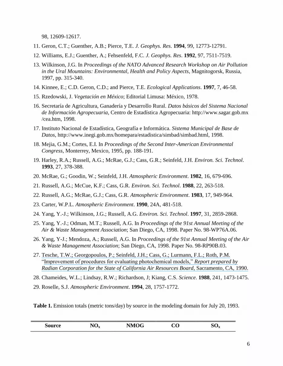
in Figure 2. The areas of major hydrocarbon emissions follow closely the forest locations where

emissions are dominated by isoprene. Monoterpenes and OVOC dominate the biogenic VOC

emissions in regions where the vegetation is mainly composed of shrub, scrub, and agricultural

species (e.g. south-central Texas, northeast Mexico, South Arizona and northern Sonora).

Biogenic hydrocarbon emissions are negligible in the desert. Biogenic nitric oxide is heavily

emitted in agricultural areas and considerably lower emissions are found in heavily forested,

urbanized and desert areas. Table 1 compares the biogenic emissions computed in this study with

the anthropogenic emissions calculated by Mendoza et al.5 for the same domain. The biogenic

NMOG represent roughly 74% of the total NMOG emissions, while biogenic NOx is 14% of the

total NOx. The relative distribution of biogenic and anthropogenic emissions found here is in

agreement with findings of studies in other regions.1,28,29

Photochemical Modeling Results

The biogenic emission estimates from this study were added to an existing anthropogenic

emission inventory for the same modeling domain, and the CIT model was used to predict ozone

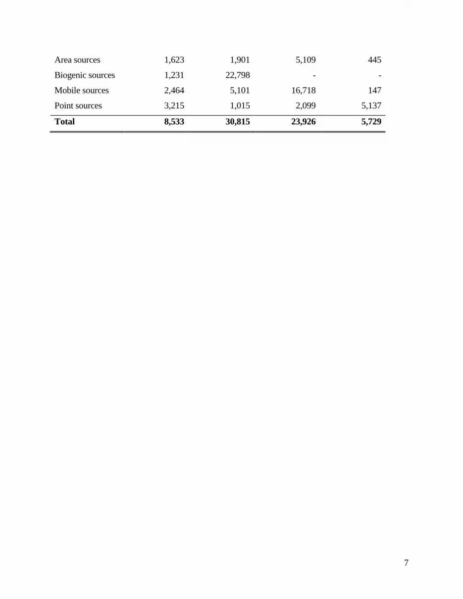
concentrations. Figure 3 depicts the predicted daily maximum ozone concentration for the third

day of the episode (July 20, 1993). Model performance statistics for the last day of the episode

indicated that the model reproduced observations within the limits of EPA guidelines27

for the

peak ozone (peak ozone, unpaired in time and space, within ±15-20%), and gross error (less than

35%), though an overall bias of ~+25% indicated a tendency of the model to overpredict ozone

concentrations.

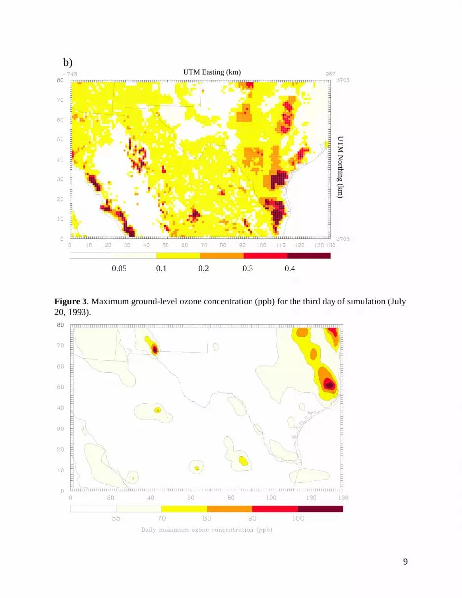
Mendoza et al.5 conducted a simulation of the same episode employing only anthropogenic

emissions. In order to compare the runs, the maximum difference in ozone concentration at each

4

grid cell between the run with biogenics and the one without biogenics was computed and plotted

(Figure 4). In general, ozone increased 20-30 ppb in most of the major urban centers, 10-20 ppb

in some urban and most suburban areas, and less than 10 ppb in rural areas. From a model

performance perspective, the model run with biogenic emissions gave better results for the peak

statistics and the normalized mean square error (NMSE) values remained comparable (0.10 with

biogenics versus 0.09 without).

Sensitivity Analysis and Source Impact

The sensitivity of ozone concentration to anthropogenic area source emissions and biogenic

emissions was calculated using DDM-3D. Sensitivities to biogenic isoprene, -pinene and NO,

and anthropogenic on-road mobile source NOx and VOC were computed. The resulting

sensitivity fields provide a quantitative display of how ozone at all locations would respond to

changes in the referred sources.

Figure 5a presents the ozone sensitivity fields to emissions of biogenic isoprene at 3 p.m. for July

20, 1993. The sensitivities show the change in predicted ozone (ppb) per 1% domain-wide

increase in the corresponding emissions. An increase in isoprene emissions tends to increase

ozone levels in areas where the anthropogenic NOx emissions are relatively higher, for instance,

eastern Texas, Monterrey and Tucson. In general, the ozone sensitivity fields due to -pinene and

isoprene emissions were spatially similar, though isoprene had higher positive sensitivities in

forested areas (compared to -pinene) and -pinene had higher positive sensitivities in non-

forested areas (compared to isoprene). The ozone sensitivity to biogenic nitric oxide emissions is

presented in Figure 5b. The results show that ozone is mainly sensitive to biogenic NO emissions

in rural locations. Maximum sensitivities occur in two heavily agricultural areas: the Lower Rio

Grande Valley and the coast of the State of Sinaloa, Mexico. Figure 5b indicates that increasing

biogenic NO emissions generally increases ozone levels in rural areas, one order of magnitude

more than the ozone increase due to biogenic VOC emissions, on a percent increase basis.

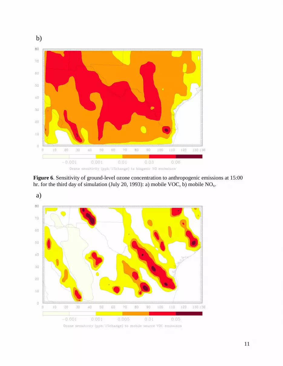
Figure 6a and 6b depict the ozone sensitivities to mobile VOC and NOx source emissions,

respectively. Figure 6a indicates that ozone concentrations increase in the urban centers and

industrial corridors as mobile VOC source emissions increase, compared to the negligible ozone

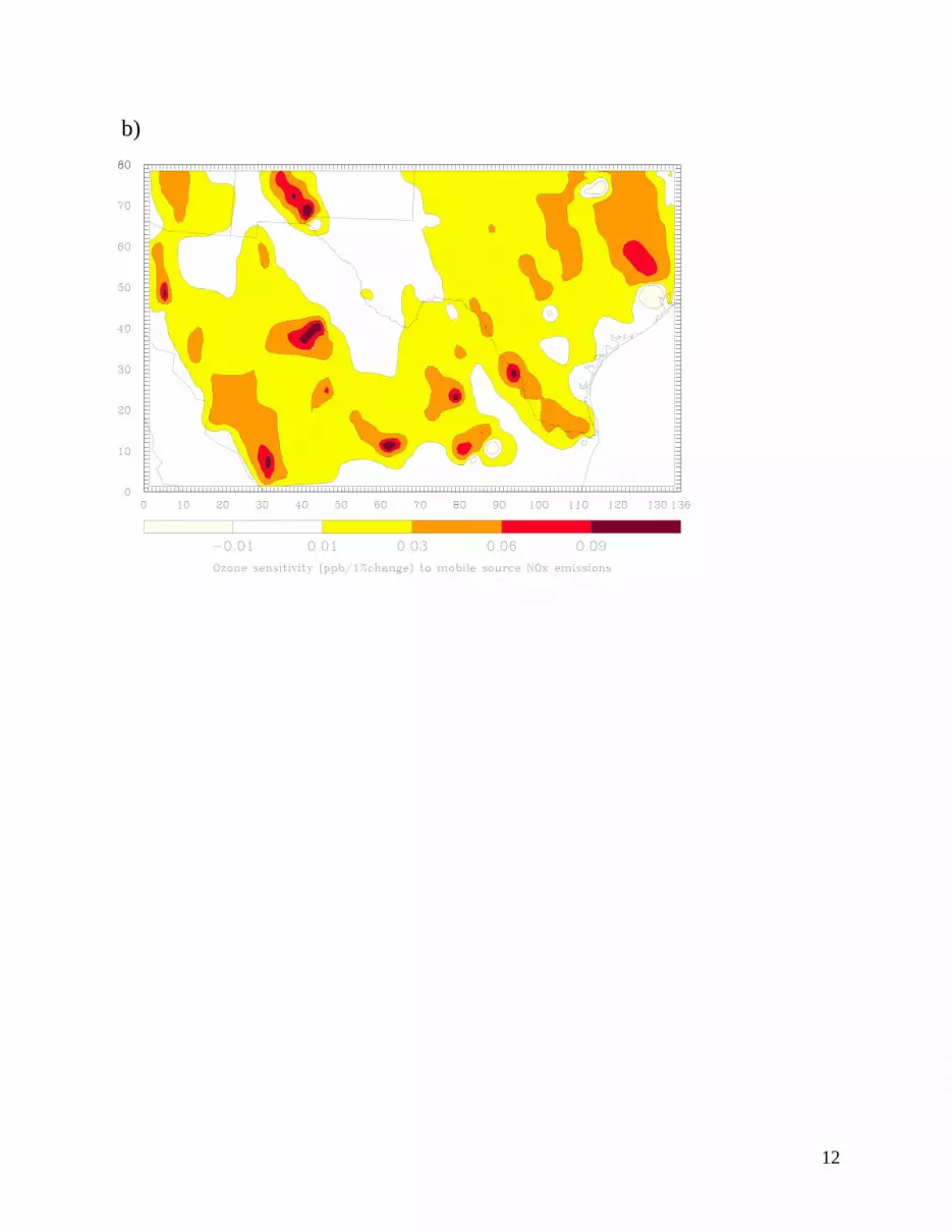
sensitivities in remote rural locations due to mobile VOC source emissions. Ozone sensitivity to

mobile source NOx emissions (Figure 6b) shows that there is a NOx-inhibiting effect in the major

urban cores (Ciudad Juarez-El Paso, Houston, Dallas-Fort Worth, San Antonio, Monterrey-

Saltillo) and a NOx-limited effect in downwind areas from these urban cores. A comparison of

ozone sensitivity to mobile source VOC and NOx emissions indicates that changes in VOC

emissions have a more noticeable impact on ozone levels in the immediate rural and suburban

areas surrounding the urban cores than in the remote rural areas. In contrast, mobile source NOx

emissions tend to have a higher impact in both urban and rural locations. Moreover, rural ozone

can differ by one order of magnitude depending on whether on-road mobile source NOx or VOC

increases.

CONCLUSIONS

Impacts of anthropogenic and biogenic emissions on ground-level ozone along the Mexico-U.S.

border were quantified using direct sensitivity analysis. The CIT airshed model integrated with

DDM-3D (decoupled direct method in three dimensions) was applied to the July 18-20, 1993

5

episode. DDM-3D was used to quantify the magnitude and extent of changes in the base case

ozone distribution due to incremental changes in the emissions. An existing anthropogenic

emission inventory was used and an episodic biogenic emission inventory was developed for the

region. The biogenic emission inventory was created using the Biogenic Emissions Inventory

System (BEIS2) and the model of Williams et al.12

The biogenic NMOG represents about 74% of

the total NMOG emissions while biogenic NOx contributes about 14% of the total NOx. The

model performance evaluation for ozone shows that the model performs within acceptable limits,

though in general the model tends to overpredict ozone. The predicted ground-level ozone levels

increased compared to a previous study of the same domain where anthropogenic emissions were

used exclusively. The source attribution analysis indicated that changes in biogenic VOC

emissions have the greatest impact on the ozone levels in the urban areas, whereas changes in

mobile source VOC emissions have the greatest effect in rural locations immediately near urban

areas. Changes in mobile source NOx emissions impact both urban and rural areas.

ACKNOWLEDGMENTS

The authors acknowledge the National Science Foundation (Contract No. BES-9613729) and

Georgia Power Company for their financial support during the course of the study. A. Mendoza-

Dominguez also acknowledges the Consejo Nacional de Ciencia y Tecnología, Mexico, for

partial support during his research stay at the Georgia Institute of Technology.

REFERENCES

1. National Research Council. Rethinking the ozone problem in urban and regional air

pollution; National Academy Press: Washington, DC, 1991.

2. National Air Quality and Emissions Trends Report. EPA 454/R-97-013, U.S. EPA, Research

Triangle Park, NC, 1998.

3. Instituto Nacional de Ecología. Primer informe sobre la calidad del aire en ciudades

mexicanas, Dirección General de Gestión e Información Ambiental: México, 1997.

4. Plan Integral Ambiental Fronterizo: Primera Etapa 1992-1994; Secretaría de Desarrollo

Urbano y Ecología: México, 1992.

5. Mendoza, A.; Mejia, G.M.; Russell, A.G. In Proceedings of the 91st Annual Meeting of the

Air & Waste Management Association, San Diego, CA, 1998. Paper No. 98-MP30.05.

6. Mexico City Air Quality Research Initiative, Volume III, Modeling and Simulation, Instituto

Mexicano del Petroleo and Los Alamos National Laboratory: Mexico City, 1993.

7. Cruz-Nunez, X.; Alegre-Gonzalez, M.V.; Castellanos-Fajardo, L.A. The Emission Inventory:

Programs & Progress. Air & Waste Management Association, Research Triangle Park, NC,

1995, pp. 153-163.

8. Ruiz-Suarez, L.G.; Longoria, R.; Hernandez, F. In Proceedings of the 1997 5th International

Conference on Air Pollution, Bologna, Italy, 1997, pp. 923-933.

9. Instituto Nacional de Estadística Geografía e Informática. Geographical Information of

Mexico, http://www.inegi.gob.mx/homeing/geografia/geograf.html, 1998.

10. Guenther, A.; Zimmerman, P.R.; Harley, P.C.; Monson, R.K.; Fall, R. J. Geophys. Res. 1993,

6

98, 12609-12617.

11. Geron, C.T.; Guenther, A.B.; Pierce, T.E. J. Geophys. Res. 1994, 99, 12773-12791.

12. Williams, E.J.; Guenther, A.; Fehsenfeld, F.C. J. Geophys. Res. 1992, 97, 7511-7519.

13. Wilkinson, J.G. In Proceedings of the NATO Advanced Research Workshop on Air Pollution

in the Ural Mountains: Environmental, Health and Policy Aspects, Magnitogorsk, Russia,

1997, pp. 315-340.

14. Kinnee, E.; C.D. Geron, C.D.; and Pierce, T.E. Ecological Applications. 1997, 7, 46-58.

15. Rzedowski, J. Vegetación en México; Editorial Limusa: México, 1978.

16. Secretaría de Agricultura, Ganadería y Desarrollo Rural. Datos básicos del Sistema Nacional

de Información Agropecuaria, Centro de Estadística Agropecuaria: http://www.sagar.gob.mx

/cea.htm, 1998.

17. Instituto Nacional de Estadística, Geografía e Informática. Sistema Municipal de Base de

Datos, http://www.inegi.gob.mx/homepara/estadistica/simbad/simbad.html, 1998.

18. Mejia, G.M.; Cortes, E.I. In Proceedings of the Second Inter-American Environmental

Congress, Monterrey, Mexico, 1995, pp. 188-191.

19. Harley, R.A.; Russell, A.G.; McRae, G.J.; Cass, G.R.; Seinfeld, J.H. Environ. Sci. Technol.

1993, 27, 378-388.

20. McRae, G.; Goodin, W.; Seinfeld, J.H. Atmospheric Environment. 1982, 16, 679-696.

21. Russell, A.G.; McCue, K.F.; Cass, G.R. Environ. Sci. Technol. 1988, 22, 263-518.

22. Russell, A.G.; McRae, G.J.; Cass, G.R. Atmospheric Environment. 1983, 17, 949-964.

23. Carter, W.P.L. Atmospheric Environment. 1990, 24A, 481-518.

24. Yang, Y.-J.; Wilkinson, J.G.; Russell, A.G. Environ. Sci. Technol. 1997, 31, 2859-2868.

25. Yang, Y.-J.; Odman, M.T.; Russell, A.G. In Proceedings of the 91st Annual Meeting of the

Air & Waste Management Association; San Diego, CA, 1998. Paper No. 98-WP76A.06.

26. Yang, Y-J.; Mendoza, A.; Russell, A.G. In Proceedings of the 91st Annual Meeting of the Air

& Waste Management Association; San Diego, CA, 1998. Paper No. 98-RP90B.03.

27. Tesche, T.W.; Georgopoulos, P.; Seinfeld, J.H.; Cass, G.; Lurmann, F.L.; Roth, P.M.

“Improvement of procedures for evaluating photochemical models,” Report prepared by

Radian Corporation for the State of California Air Resources Board, Sacramento, CA, 1990.

28. Chameides, W.L.; Lindsay, R.W.; Richardson, J; Kiang, C.S. Science. 1988, 241, 1473-1475.

29. Roselle, S.J. Atmospheric Environment. 1994, 28, 1757-1772.

Table 1. Emission totals (metric tons/day) by source in the modeling domain for July 20, 1993.

Source NOx NMOG CO SOx

7

Area sources 1,623 1,901 5,109 445

Biogenic sources 1,231 22,798 - -

Mobile sources 2,464 5,101 16,718 147

Point sources 3,215 1,015 2,099 5,137

Total 8,533 30,815 23,926 5,729

8

Figure 1. Hourly domain-wide biogenic emissions, for the third day of simulation (July 20,

1993).

0

500

1000

1500

2000

25000 2 4 6 8

10

12

14

16

18

20

22

Hour

Em

issi

on

s (m

etr

ic t

on

s)

NO

Other VOCs

Terpenes

Isoprene

Figure 2. Gridded biogenic emissions, in metric tons per day, using 12.5 x 12.5 km2 grid cells,

for the third day of simulation (July 20, 1993): a) total NMOG and b) nitric oxide.

UTM Easting (km)

UT

M N

orth

ing

(km

)

0.25 0.5 1.0 2.0 4.0

a)

9

0.05 0.1 0.2 0.3 0.4

UTM Easting (km)

UT

M N

orth

ing

(km

)

b)

Figure 3. Maximum ground-level ozone concentration (ppb) for the third day of simulation (July

20, 1993).

10

Figure 4. Maximum ground-level ozone concentration difference (ppb) between the simulation

with biogenics emissions and the simulation without. Third day of simulation (July 20, 1993).

Figure 5. Sensitivity of ground-level ozone concentration to biogenic emissions at 15:00 hr. for

the third day of simulation (July 20, 1993): a)isoprene, b) NO.

a)

11

b)

Figure 6. Sensitivity of ground-level ozone concentration to anthropogenic emissions at 15:00

hr. for the third day of simulation (July 20, 1993): a) mobile VOC, b) mobile NOx.

a)

12

b)