some properties of the value function and its level sets for affine control systems with quadratic...

JOURNAL OF DYNAMICAL AND CONTROL SYSTEMS, Vol. 6, No. 4, 2000, 511-541

SOME PROPERTIES OF THE VALUE FUNCTIONAND ITS LEVEL SETS FOR AFFINE CONTROL

SYSTEMS WITH QUADRATIC COST

E. TRELAT

Abstract. Let T > 0 be fixed. We consider the optimal control

problem for analytic affine systems: x = f0(x) +m∑i=1

uifi(x), with a

cost of the form: C(u) =T∫0

m∑i=1

u2i (t) dt. For this kind of systems

we prove that if there are no minimizing abnormal extremals thenthe value function S is subanalytic. Second, we prove that if thereexists an abnormal minimizer of corank 1, then the set of endpointsof minimizers at cost fixed is tangent to a given hyperplane. Weillustrate this situation in sub-Riemannian geometry.

1. Introduction

Let M be an analytic Riemannian n-dimensional manifold and x0 ∈ M .Consider the following control system:

x(t) = f(x(t), u(t)), x(0) = x0, (1)

where f = M × Rm −→ M is an analytic function, and the set of controls

Ω is a subset of the set of measurable mappings defined on [0, T (u)] andtaking their values in R

m. The system is said to be affine if

f(x, u) = f0(x) +m∑i=1

uifi(x), (2)

where the fi’s are analytic vector fields on M .Let T > 0 be fixed. We consider the endpoint mapping E : u ∈ Ω −→

x(T, x0, u), where x(t, x0, u) is the solution of (1) associated with u ∈ Ω andstarting from x0 at t = 0. We endow the set of controls defined on [0, T ] with

1991 Mathematics Subject Classification. Primary 49N60; Secondary 58C27.Key words and phrases. Optimal control, value function, abnormal minimizers, sub-

analyticity, sub-Riemannian geometry.511

1079-2724/00/1000-0511$18.00/0 c© 2000 Plenum Publishing Corporation

512 E. TRELAT

the L2-norm topology. A trajectory x(t, x0, u) denoted in short x is said tobe singular or abnormal on [0, T ] if u is a singular point of the endpointmapping, i.e., the Frechet derivative of E is not surjective at u; otherwiseit is said to be regular. We denote by Acc(T ) the set of endpoints at t = Tof solutions of (1), u varying in Ω. The main problem of control theoryis to study E and Acc(T ). Note that the latter is not bounded in general.In [18] one can find sufficient conditions so that Acc(T ) be compact, or havenonempty interior. Theorem 4.3 of this article states such a result for affinesystems.

Consider now the following optimal control problem: among all trajec-tories of (1) steering 0 to x ∈ Acc(T ), find a trajectory minimizing the cost

function: C(u) =T∫0f0(xu(t), u(t)) dt, where f0 is analytic. Such minimizers

do not necessary exist; the main argument to prove existence theorems is thelower semi-continuity of the cost function, see [12] or [18]. If x ∈ Acc(T ),we set S(x) = infC(u) | E(u) = x, otherwise S(x) = +∞; S is calledthe value function. In general, f0 is chosen in such a way that the valuefunction has a physical meaning: for instance, the action in classical me-chanics or in optics, the (sub)-Riemannian distance in (sub)-Riemanniangeometry. We are interested in the regularity of the value function and thestructure of its level sets. In (sub)-Riemannian geometry level sets of thedistance are (sub)-Riemannian spheres. To describe these objects we needa category of sets which are stable under set operations and under properanalytic mapping.

An important example of such a category is the one of subanalytic sets(see [13]). They have been utilized by several authors in order to constructan optimal synthesis or to describe Acc(T ) (see [11], [23]). Unfortunately,this class is not wide enough: in [20], the authors exhibit examples of controlsystems in which neither S nor Acc(T ) are subanalytic. However, Agrachevshows in [1] (see also [5], [16]) that if there are no abnormal minimizersthen the sub-Riemannian distance is subanalytic in a pointed neighborhoodof 0, and hence sub-Riemannian spheres of small radius are subanalytic.Following his ideas, we extend this result to affine control systems withquadratic cost (Theorem 4.4 and corollaries).

Abnormal minimizers are responsible for a phenomenon of non-properness (Proposition 5.3), which geometrically implies the followingproperty: under certain assumptions the level sets of the value functionare tangent to a given hyperplane at the endpoint of the abnormal mini-mizer (Theorem 5.2). This result was first stated in [9] for sub-Riemanniansystems to illustrate the Martinet situation.

An essential reasoning we will use in the proofs of these results is the fol-lowing (see Lemma 4.8). We will consider sequences of minimizing controlsun associated with projectivized Lagrange multipliers (pn(T ), p0n), so that

PROPERTIES OF THE VALUE FUNCTION 513

we have (see Sec. 2):

pn(T )dE(un) = −p0nun. (3)

Since (un) is bounded in L2, we will assume that un converges weakly tou. To pass to the limit in (3), we will prove some regularity propertiesof the endpoint mapping E (Sec. 3). In contrast to the sub-Riemanniancase, the strong topology on L2 is not adapted in general for affine systems,whereas the weak topology gives nice compactness properties of the set ofminimizing controls (see Theorem 4.12).

The outline of the paper is as follows: in Sec. 2, we recall definitions ofsubanalytic sets and the Maximum Principle. In Sec. 3, we state some basicresults on the regularity of the endpoint mapping. Section 4 is devoted tocontinuity and subanalyticity of the value function S. Finally, in Sec. 5,the shape of the level sets of the value function in presence of abnormalminimizers is investigated. We illustrate this situation in sub-Riemanniangeometry.

Acknowledgment. I would like to thank A. Agrachev for many advicesand remarks which helped me in this work.

2. Preliminaries

2.1. Subanalytic sets. Recall the following definitions, that can be foundin [14], [15].

Definition 2.1. Let M be a finite dimensional real analytic manifold.A subset A of M is called semi-analytic if, for every x in M , we can find aneighborhood U of x in M and 2pq real analytic functions gij , hij (1 i pand 1 j q) such that

A ∩ U =p⋃

i=1

y ∈ U | gij(y) = 0 and hij(y) > 0 for j = 1 . . . q

.

We denote by SEM(M) the family of subanalytic subsets of M .

Unfortunately, proper analytic images of semi-analytic sets are not ingeneral semi-analytic. Hence this class must be extended:

Definition 2.2. A subset A of M is called subanalytic if, for every x inM , we can find a neighborhood U of x in M and 2p pairs (φδ

i , Aδi ) (1 i p

and δ = 1, 2), where Aδi ∈ SEM(Mδ

i ) for some real analytic manifolds M δi ,

and where the mappings φδi : M δ

i → M are proper analytic, such that

A ∩ U =p⋃

i=1

(φ1i (A1

i )\φ2i (A2i )).

514 E. TRELAT

We denote by SUB(M) the family of subanalytic subsets of M .

The class of subanalytic sets is closed under union, intersection, comple-ment, inverse image of analytic mappings, image of proper analytic map-pings. Moreover, they are stratifiable. Recall the following definition.

Definition 2.3. Let M be a differentiable manifold. A stratum in M isa locally closed submanifold of M .

A locally-finite partition S of M is said to be a stratification of M if eachS in S is a stratum such that:

∀T ∈ S T ∩ Fr S = ∅ ⇒ T ⊂ Fr S and dimT < dimS.

Finally, a mapping f : M → N between two manifolds is called subana-lytic if its graph is a subanalytic set of M ×N .

The basic property of subanalytic functions which makes them useful inoptimal control theory is the following. It can be found in [24].

Proposition 2.1. Let M and N denote finite dimensional real analyticmanifolds, and A be a subset of N . Given subanalytic mappings φ : N −→M and f : N −→ R, we define:

∀x ∈ M ψ(x) = inff(y)/y ∈ φ−1(x)

⋂A

.

If φ∣∣A

is proper, then ψ is subanalytic.

2.2. Maximum principle and extremals. According to the weak max-imum principle [21] the minimizing trajectories are among the singular tra-jectories of the endpoint mapping of the extended system in M × R:

x(t) = f(x(t), u(t)),

x0(t) = f0(x(t), u(t)).(4)

They are called extremals. If E and C are differentiable, then there existsa Lagrange multiplier (p(T ), p0) (defined up to a scalar) such that

p(T )dE(u) = −p0dC(u), (5)

where dE(u) (resp. dC(u)) denotes the differential of E (resp. C) in u.Moreover, (x(T ), p(T )) is the endpoint of the solution of the following equa-tions:

x =∂H

∂p, p = −∂H

∂x,

∂H

∂u= 0, (6)

where H = 〈p, f(x, u)〉 + p0f0(x, u) is the Hamiltonian, p is the adjointvector, 〈 , 〉 is the inner product on M and p0 is a constant. The abnormaltrajectories correspond to the case p0 = 0 and their role in the optimal


control problem has to be analyzed. The extremals with p0 = 0 are said to

be normal. In this case p0 is usually normalized to −12

. We will use thisnormalization to prove Theorem 4.4. To prove Theorem 5.2, we will useanother normalization by considering projectivized Lagrange multipliers,i.e., (p(T ), p0) ∈ P (T ∗M). We say that an extremal has corank 1 if it hasa unique projectivized Lagrange multiplier.

Affine systems. Consider, in particular, analytic affine control systems onM :

x(t) = f0(x) +m∑i=1

uifi(x), x(0) = 0, (7)

where the fi’s are analytic vector fields, with the problem of minimizing thefollowing cost:

C(u) =

T∫0

m∑i=1

u2i (t) dt. (8)

The Hamiltonian is:

H(x, p, u) =⟨p, f0(x) +

m∑i=1

uifi(x)⟩

+ p0m∑i=1

u2i .

Parametrization of normal extremals. Let p0 = −12

. Then normal controls

can be computed from the equation∂H

∂u= 0, and we get:

∀i = 1 . . .m ui = 〈p, fi(x)〉. (9)

Putting in system (7), we get an analytic differential system in T ∗Mparametrized by the initial condition p(0). We know from the generaltheory of ordinary differential equations that solutions depend analyticallyon their initial condition. Denote such a solution by

(xp(0), pp(0)

). Let

up(0) =(〈pp(0), f1(xp(0))〉, . . . , 〈pp(0), fm(xp(0))〉

); from (9) it follows that

up(0) is a normal control associated with xp(0). Now we can give the follow-ing definition.

Definition 2.4. The mapping

Φ :T ∗x0M −→ L2([0, T ],Rm)

p(0) −→ up(0)

is analytic.

516 E. TRELAT

This mapping will be useful to verify subanalyticity of the value functionin Sec. 4.

3. Regularity of the endpoint mapping

Let M be an analytic complete n-dimensional Riemannian manifold andlet x0 ∈ M .

Our point of view is local and we can assume: M = Rn, x0 = 0. We

consider only analytic affine control systems (7). The statements in thissection except for Proposition 3.7 are quite standard, and we include proofsonly for convenience of the reader.

3.1. The endpoint mapping. Let T > 0 and xu be the solution (if itexists) of the controlled system:

xu = f0(x) +m∑i=1

uifi(x), xu(0) = 0,

where u = (u1, . . . , um) ∈ L2([0, T ],Rm). Since we allow discontinuouscontrols, the meaning of solution of the previous differential system has tobe clarified. In fact, this means that the following integral equation holds:

∀t ∈ [0, T ] xu(t) =

T∫0

f0(xu(τ)) +m∑i=1

ui(τ)fi(xu(τ )) dτ.

Definition 3.1. The endpoint mapping is:

E : Ω −→ Rn

u −→ xu(T ),

where Ω ⊂ L2([0, T ],Rm) is the domain of E, i.e., the subset of controls usuch that xu is well defined on [0, T ].

E is not defined on the whole L2 because of explosion phenomena. Forexample, consider the system x = x2 + u; then xu is not defined on [0, T ]for u = 1 if T π

2. Anyway, we have the following proposition.

Proposition 3.1. Let T > 0 be fixed. We consider the analytic controlsystem (7). Then the domain Ω of E is open in L2([0, T ],Rm).

Proof. It is enough to prove the following statement:

If the trajectory xu associated with u is well-defined on[0, T ], then the same is true for any control in a neighbor-hood of u in L2([0, T ],Rm).


Let V be a bounded open subset of Rn such that ∀t ∈ [0, T ] xu(t) ∈ V .

Let θ ∈ C∞(Rn, [0, 1]) with compact support K such that θ = 1 on V . Wecan assume that K = B(0, R) =

x ∈ R

n | ‖x‖ R

. For i = 0 . . .m,we set fi = θfi. Then it is clear that xu is also solution of the equationx = f0(x) +

∑uifi(x). For all v ∈ L2 let xv be the solution of the equation

˙xv = f0(xv) +m∑i=1

vifi(xv), xv(0) = 0. We will prove that xv = xv in a

sufficiently small neighborhood of u.

Lemma 3.2. fi are globally Lipschitzian on Rn, i.e.,

∃A > 0 : ∀i ∈ 0, . . . ,m ∀y, z ∈ Rn ‖fi(y) − fi(z)‖ A‖y − z‖.

Proof. Let i ∈ 0, . . . ,m. fi belongs to it C1, hence, is locally Lipschitzianat any point:

∀x ∈ B(0, 2R) ∃ρx, Ax > 0 : ∀y, z ∈ B(x, ρx) ‖fi(y)− fi(z)‖ Ax‖y−z‖.By compactness, we can take a finite number of balls which cover B(0, 2R):

∃p ∈ N : B(0, 2R) ⊂p⋃

j=1

B(xj , ρxj ).

Let A = supi Axi and ρ =12

min(R

2,min

iρxi

). Let us prove that fi is

A-Lipschitzian: let y, z ∈ Rn.

(1) If ‖y − z‖ ρ:• if y, z ∈ B(0, 2R), then there exists j ∈ 1, . . . , p such thaty, z ∈ B(xi, ρxi), and the conclusion holds.

• if y, z /∈ B(0, R), then fi(y) = fi(z) = 0, and the inequalityis still true.

All other cases are impossible because ‖y − z‖ ρ.(2) If ‖y − z‖ > ρ:

Let M = supy,z∈K

‖fi(y) − fi(z)‖ = supy,z∈Rn

‖fi(y) − fi(z)‖. Then:

‖fi(y) − fi(z)‖ M M

ρ‖y − z‖

and the conclusion holds if, moreover, A is chosen larger thanM

ρ.

For all t ∈ [0, T ] we have:

‖xu(t) − xv(t)‖ =∥∥∥∥

t∫0

(f0(xu(τ )) − f0(xv(τ))) dτ +

518 E. TRELAT

+

t∫0

m∑i=1

vi(τ )(fi(xu(τ )) − fi(xv(τ ))) dτ −

−t∫

0

m∑i=1

(vi(τ) − ui(τ))fi(xu(τ)) dτ∥∥∥∥

A

t∫0

(1 +

m∑i=1

|vi(τ )|)‖xu(τ ) − xv(τ )‖ dτ + hv(t),

where

hv(t) =∥∥∥∥

t∫0

m∑i=1

(vi(τ ) − ui(τ ))fi(xu(τ )) dτ∥∥∥∥.

We set M ′ = maxi

supx∈Rn

‖fi(x)‖. We get from the Cauchy–Schwarz inequa-

lity:∀t ∈ [0, T ] hv(t) M ′√T ‖v − u‖L2 .

Hence for all ε > 0 there exists a neighborhood U of u in L2 such that

∀v ∈ U ∀t ∈ [0, T ] hv(t) ε.

Therefore,

∀t ∈ [0, T ] ‖xu(t) − xv(t)‖

A

t∫0

∣∣∣∣(

1 +m∑i=1

vi(τ ))∣∣∣∣‖xu(τ) − xv(τ )‖ dτ + ε.

We get from the Gronwall lemma:

∀t ∈ [0, T ] ‖xu(t) − xv(t)‖ ε expA∫ t

0|(1+

∑vi(τ))|dτ ε expAT+AK

√T ,

which proves that (xv) is uniformly close to xu = xu. In particular, if theneighborhood U is small enough then: ∀t ∈ [0, T ] xv(t) ∈ V , and hencexv = xv, which completes the proof.

3.2. Continuity. If v and vn, n ∈ N, are elements of L2([0, T ]), we denoteby vn v the weak convergence of the sequence (vn) to v in L2.

Proposition 3.3. Let u = (u1, . . . , um) ∈ Ω and let xu be the solutionof the affine control system:

xu = f0(xu) +m∑i=1

uifi(xu), xu(0) = 0.


Let (un)n∈N be a sequence in L2([0, T ],Rm). If unL2

u, then xun is well-defined on [0, T ] for sufficiently large n and, moreover, xun −→ xu uniformlyon [0, T ].

Proof. The outline of the proof is the same as in Proposition 3.1. Let Vbe a bounded open subset of R

n such that: ∀t ∈ [0, T ] xu(t) ∈ V . Letθ ∈ C∞(Rn, [0, 1]) with compact support K such that θ = 1 on V . Wecan assume that K = B(0, R) = x ∈ R

n∣∣‖x‖ R. For i = 0, . . . ,m

we set fi = θfi. Then it is clear that xu is also a solution of the equationx = f0(x) +

∑uifi(x). For all n ∈ N, let xun be the solution of ˙xun =

f0(xun) +m∑i=1

un,ifi(xun), xun(0) = 0. We will prove that if n is large

enough then xun = xun .For all t ∈ [0, T ] we have:

‖xu(t) − xun(t)‖ =∥∥∥∥

t∫0

(f0(xu(τ)) − f0(xun(τ ))) dτ +

+

t∫0

m∑i=1

un,i(τ )(fi(xu(τ )) − fi(xun(τ))) dτ −

−t∫

0

m∑i=1

(un,i(τ ) − ui(τ))fi(xu(τ)) dτ∥∥∥∥

A

t∫0

(1 +

m∑i=1

|un,i(τ )|)‖xu(τ ) − xun(τ )‖ dτ + hn(t),

where

hn(t) =∥∥∥∥

t∫0

m∑i=1

(un,i(τ ) − ui(τ ))fi(xu(τ )) dτ∥∥∥∥.

The aim is to make hn uniformly small in t, and then to conclude we usethe Gronwall inequality.

From the hypothesis un u, we deduce: ∀t ∈ [0, T ] hn(t) −→n→+∞ 0. Let

us prove that hn tends uniformly to 0 as n tends to infinity. We need thefollowing lemma.

Lemma 3.4. Let a, b ∈ R and let E be a normed vector space. For alln ∈ N let fn : [a, b] −→ E be uniformly α-Holder,

∃α,K > 0 : ∀n ∈ N ∀x, y ∈ [a, b] ‖fn(x) − fn(y)‖ K‖x− y‖α.

520 E. TRELAT

If the sequence (fn) converges simply to an application f , then it tendsuniformly to f .

Proof. By taking the limit as n −→ ∞, we can see first that f is α-Holder.Let ε > 0 and a = x0 < x1 < · · · < xp = b be a partition such that ∀i

xi+1 − xi <ε

1α

2K. For all i, fn(xi) tends to f(xi), hence:

∃N ∈ N : ∀n N ∀i ∈ 0, . . . , p ‖fn(xi) − f(xi)‖ < ε

3.

Let x ∈ [a, b]. Then there exists i such that x ∈ [xi, xi+1]. Hence:

‖fn(x) − f(x)‖ ‖fn(x) − fn(xi)‖ + ‖fn(xi) − f(xi)‖ + ‖f(xi) − f(x)‖

K‖x− xi‖α +ε

3+ K‖x− xi‖α

ε.

We set M ′ = maxi

supx∈Rn

= ‖fi(x)‖. We get:

|hn(x) − hn(y)| M ′∣∣∣∣

x∫y

(∑i

|un,i(τ )| +∑i

|ui(τ)|)dτ

∣∣∣∣.Moreover, we get from the Cauchy–Schwarz inequality:

x∫y

|u| ‖u‖L2 |x− y| 12 .

Furthermore, the sequence (un) converges weakly, hence it is bounded inL2. Therefore, there exists a constant K such that for all n ∈ N∣∣hn(x) − hn(y)

∣∣ K|x− y| 12 .Hence we conclude by Lemma 3.4 that the sequence (hn) tends uniformlyto 0, i.e.,

∀ε > 0 ∃N ∈ N : ∀n N ∀t ∈ [0, T ] |hn(t)| ε.

And hence, if n N :

∀t ∈ [0, T ] ‖xu(t) − xun(t)‖

A

t∫0

∣∣∣∣1 +m∑i=1

vi(τ )∣∣∣∣ ‖xu(τ ) − xun(τ)‖ dτ + ε.


We get from the Gronwall lemma:

∀t ∈ [0, T ] ‖xu(t) − xun(t)‖ ε expAT+AK√T ,

which proves that the sequence (xun) tends uniformly to xu = xu. Inparticular, if n is large enough, then ∀t ∈ [0, T ] xun(t) ∈ V , and hencexun = xun , which completes the proof.

Remark 3.1. This proposition can be found in [22], but the author usesthe following argument: if un tends weakly to 0, then |un| tends weaklyto 0, which is not true in general (take un(t) = cosnt). That is the reasonwhy we need Lemma 3.4. Otherwise the proof is the same as in [22].

To verify differentiability in the next subsection, we will need the follow-ing result:

Proposition 3.5. Let u ∈ Ω and xu be the associated trajectory. Thenfor any bounded neighborhood U of u in Ω ⊂ L2 there exists a constant suchthat for all v, w ∈ U and for all t ∈ [0, T ]

‖xv(t) − xw(t)‖ C‖v − w‖L2 .

Proof. Writing

xv = f0(xv) +m∑i=1

vifi(xv),

xw = f0(xw) +m∑i=1

wifi(xw),

we get, for all t ∈ [0, T ]:

‖xv(t) − xw(t)‖ =

=∥∥∥∥

t∫0

(∑i

(vi(s) − wi(s))fi(xv(s)) + f0(xv(s)) − f0(xw(s)) +

+∑i

wi(s)(fi(xv(s)) − fi(xw(s))))ds

∥∥∥∥

∑i

t∫0

|vi − wi| ‖fi(xv)‖ ds +

t∫0

‖f0(xv) − f0(xw)‖ ds +

+∑i

t∫0

|wi| ‖fi(xv) − fi(xw)‖ ds.

522 E. TRELAT

Now, if v and w are in a bounded neighborhood U of u in L2, then accordingto Proposition 3.3, the trajectories xv and xw take their values in a compactK that depends only on U . Since the vector fields f0, f1, . . . , fm are smooth,we claim that there exists a constant M > 0 such that for all v, w ∈ U andfor all i

‖fi(xv)‖ M,

‖fi(xv) − fi(xu)‖ M‖xv − xu‖.Finally without loss of generality we can assume that U is contained in aball of radius R centered at O ∈ L2, so that

∀w ∈ U ‖w‖L2 R.

Hence plugging in the upper inequality, and using the Cauchy–Schwarzinequality, we obtain:

∀t ∈ [0, T ] ‖xv(t) − xw(t)‖

A

t∫0

‖xv(s) − xw(s)‖ ds + B‖v − w‖L2 ,

where A and B are nonnegative constants. Finally, we get from the Gronwalllemma:

∀t ∈ [0, T ] ‖xv(t) − xw(t)‖ C‖v − w‖L2

with C = BeTA, which completes the proof.

3.3. Differentiability. Let u ∈ Ω and let xu be the corresponding so-lution of the affine system (7). We consider the linearized system alongxu:

yv = Auyv + Buv, yv(0) = 0, v ∈ L2, (10)

where Au(t) = df0(xu) +m∑i=1

uidfi(xu) and Bu(t) = (f1(xu), . . . , fm(xu)).

Let Mu be the n× n matrix solution of the equation

M ′u = AuMu, Mu(0) = Id . (11)

We have the following proposition.

Proposition 3.6. The endpoint mapping

E :Ω −→ R

n

u −→ xu(T )


is L2-Frechet differentiable, and we have:

∀v ∈ Ω dE(u) · v =

T∫0

Mu(T )Mu(s)−1Bu(s)v(s) ds.

Proof. Let u ∈ L2([0, T ],Rm). Let us prove that E is differentiable at u.Consider a neighborhood U of 0 in Ω, and let v ∈ U . Without loss ofgenerality we can assume that there exists R > 0 such that for all v ∈ U‖v‖L2 R. Let xu (resp. xu+v) be the solution of the affine system (7)with the control u (resp. with the control u + v):

xu+v = f0(xu+v) +m∑i=1

(ui + vi)fi(xu+v), (12)

xu = f0(xu) +m∑i=1

uifi(xu). (13)

We get

xu+v − xu =m∑i=1

vifi(xu+v) + f0(xu+v) − f0(xu) +

+m∑i=1

ui(fi(xu+v) − fi(xu)).

Moreover, for all i = 0 . . .m:

fi(xu+v) − f0(xu) = dfi(xu) · (xu+v − xu) +

+

1∫0

(1 − t)d2fi(txu + (1 − t)xu+v) · (xu+v − xu, xu+v − xu) dt.

Hence, we obtain

δ = Auδ + Buδ + γ, (14)

whereδ(t) = xu+v(t) − xu(t)

and

γ(t) =m∑i=1

vi(t)

1∫0

dfi(sxu + (1 − s)xu+v) · (xu+v − xu) ds +

524 E. TRELAT

+

1∫0

(1 − t)d2f0(sxu + (1 − s)xu+v) · (xu+v − xu, xu+v − xu) ds

+m∑i=1

ui(t)

1∫0

(1 − t)d2fi(sxu + (1 − s)xu+v) · (xu+v − xu, xu+v − xu) ds.

Now for all v ∈ U we have: ‖v‖L2 R. Thus, from Proposition 3.5 itfollows that there exists a compact set K in R

n such that

∀v ∈ U ∀s ∈ [0, 1] sxu(s) + (1 − s)xu+v(s) ∈ K.

Since fi are smooth, we get, using again Proposition 3.5:

∀t ∈ [0, T ] ‖γ(t)‖ c1‖v‖L2

m∑i=1

|vi(t)| + c2‖v‖2L2

(1 +

m∑i=1

|ui(t)|).

Now solving Eq. (14), we obtain

δ(t) =

t∫0

Mu(t)Mu(s)−1Bu(s)v(s) ds +

t∫0

Mu(t)Mu(s)−1γ(s) ds.

Hence for t = T :

∥∥∥∥xu+v(T ) − xu(T ) −T∫0

Mu(T )Mu(s)−1Bu(s)v(s) ds∥∥∥∥

c1‖v‖L2

T∫0

m∑i=1

|vi(t)| dt +

+ c2‖v‖2L2

T∫0

(1 +

m∑i=1

|ui(t)|)dt

c3‖v‖2L2 .

Moreover, the mapping:

L2 −→ Rn

v −→T∫0Mu(T )Mu(s)−1Bu(s)v(s) ds

is linear and continuous. Hence the endpoint mapping is Frechet differen-tiable in u, and its differential in u is this latter mapping.


Remark 3.2. Here it was proved that E is differentiable on L2. The proofof this fact can be found also in [22]. Usually (see [21]) one proves that Eis differentiable on L∞.

Remark 3.3. The control u is abnormal and of corank 1 if and only ifIm dE(u) is a hyperplane of Rn.

Proposition 3.7. With the same assumptions as in Proposition 3.3, wehave:

unL2

u ⇒ dE(un) −→ dE(u) as n → +∞.

Proof. For s ∈ [0, T ], set Nu(s) = Mu(T )Mu(s)−1.

Lemma 3.8. N ′u = −NuAu, Nu(T ) = Id.

Proof. The matrix NuMu is constant as t varies, hence (NuMu)′ = 0. More-over, (NuMu)′ = N ′

uMu + NuAuMu, and we obtain the assertion of thelemma.

Lemma 3.9. unL2

u ⇒ Nun −→ Nu uniformly on [0, T ].

Proof. For t ∈ [0, T ], we have:

Nu(t) −Nun(t) =

t∫0

(Nun(s)

(df0(xun(s)) +

m∑i=1

un,i(s)dfi(xun(s)))−

−Nu(s)(df0(xu(s)) +

m∑i=1

ui(s)dfi(xu(s))))

ds =

=

t∫0

((Nun(s) −Nu(s)

)df0(xun(s)) +

+ Nu(s)(df0(xun(s)) − df0(xu(s))

)+

+(Nun(s) −Nu(s)

) m∑i=1

un,i(s)dfi(xun(s)) +

+ Nu(s)m∑i=1

un,i(s)(dfi(xun(s)) − dfi(xu(s))

)+

+ Nu(s)m∑i=1

(un,i(s) − ui(s)

)dfi(xu(s))

)ds.

From the hypothesis, un u, and from Proposition 3.3, we get that xun

tends uniformly to xu, and hence for all i, dfi(xun) tends uniformly todfi(xu) on [0, T ].

526 E. TRELAT

Second, we set

hn(t) =

t∫0

m∑i=1

(un,i(s) − ui(s)

)Nu(s)dfi(xu(s)) ds.

Using the same argument as in the proof of Proposition 3.3, we prove thathn tends uniformly to 0.

Hence we get the following inequality:

∀ε > 0 ∃N ∈ N ∀n N ∀t ∈ [0, T ]

‖Nu(t) −Nun(t)‖ C

t∫0

‖Nu(s) −Nun(s)‖ ds + ε.

The Gronwall inequality gives us:

∀t ∈ [0, T ] ‖Nu(t) −Nun(t)‖ ε expCT ,

and the conclusion holds.

Lemma 3.10. unL2

u ⇒ Bun −→ Bu uniformly on [0, T ].

Proof. We known from Proposition 3.3 that xun tends uniformly to xu,hence for all i, fi(xun) tends uniformly to fi(xu), which proves thelemma.

We know that the differential of the endpoint mapping has the followingform:

∀v ∈ L2([0, T ]) dE(u) · v =

T∫0

Nu(s)Bu(s)v(s) ds.

Therefore, from the preceding lemmas we get:

∀v ∈ L2([0, T ]) dE(un) · v −→ dE(u) · v

which completes the proof of the proposition.

4. Properties of the value function and of its level sets

Let T > 0 be fixed. Consider the affine control system (7) on Rn with

cost (8). We denote by Acc(T ) the accessibility set in time T , i.e., the setof points that can be reached from 0 in time T .


4.1. Existence of optimal trajectories. The following result is a con-sequence of a general result from [18], p. 286.

Proposition 4.1. Consider the analytic affine control system in Rn

x = f0(x) +m∑i=1

uifi(x), x(0) = x0, x(T ) = x1

with the cost

C(u) =

T∫0

m∑i=1

u2i (t) dt,

where T > 0 is fixed and the class Ω of admissible controllers is the subsetof the set of m-vector functions u(t) in L2([0, T ],Rm) such that :

1. ∀u ∈ Ω xu is well-defined on [0, T ].2. ∃BT : ∀u ∈ Ω ∀t ∈ [0, T ] ‖xu(t)‖ BT .

If there exists a control steering x0 to x1, then there exists an optimal controlminimizing the cost steering x0 to x1.

4.2. Definition of the value function.

Definition 4.1. Let x ∈ Rn. Define S : Rn −→ R

+ ∪ +∞ as follows:

• if there is no trajectory steering 0 to x in time T , we set S(x) = +∞;• otherwise we set S(x) = infC(u)

∣∣ u ∈ E−1(x).

S is called the value function.

Definition 4.2. Let r, T > 0. Define the following level sets:

1. Mr(T ) = S−1(r).2. Mr(T ) = S−1([0, r]).

Combining Proposition 4.1, arguments of Proposition 3.1, and the factthat the control u = 0, if admissible, is minimizing, we get:

Proposition 4.2. Suppose that the control u = 0 is admissible. Thenthere exists r > 0 such that any point of Mr(T ) can be reached from 0 byan optimal trajectory.

Hence if r is small enough, Mr(T ) (resp. Mr(T )) is the set of extremitiesat time T of minimizing trajectories with the cost equal to r (resp. loweror equal to r). It is a generalization of the (sub)-Riemannian sphere in(sub)-Riemannian geometry.

Theorem 4.3. If r is small enough then the subset Mr(T ) is compact.

528 E. TRELAT

Proof. First of all, with the same arguments as in Proposition 3.1, it is easyto see that Mr(T ) is bounded if r is small enough. Now in order to provethat it is closed, consider a sequence (xn)n∈N of points of Mr(T ) convergingto x ∈ R

n. For each n let un be a minimizing control steering 0 to xn in timeT : xn = E(un) (the existence follows from Proposition 4.2). Then for all n,we have that C(un) r, which means that the sequence (un) is boundedin L2([0, T ],Rm), and therefore it admits a weakly converging subsequence.

We can assume that unL2

u. In particular, C(u) r. Moreover, fromProposition 3.3 we deduce: x = E(u). Hence u is a control steering 0 to xin time T with a cost lower or equal to r. Thus, x ∈ Mr(T ). This showsthat the latter subset is closed.

Remark 4.1. Mr(T ) is not necessarily closed. This is due to the fact thatS can have discontinuities, see Example 4.2.

4.3. Regularity of the value function. We can now state the maintheorem of this section.

Theorem 4.4. Consider the analytic affine control system (7) withcost (8). Suppose that r and T are small enough (so that any trajectorywith the cost lower than r is well-defined on [0, T ]). Let K be a subanalyticcompact subset of Mr(T ). Suppose that there is no abnormal minimizinggeodesic steering 0 to any point of K. Then S is continuous and subanalyticon K.

Corollary 4.5. If r0 and T are small enough and if there is no abnormalminimizer steering 0 to any point of Mr0(T ), then for any r lower thanr0, Mr(T ) and Mr(T ) are subanalytic subsets of Rn.

This result generalizes to affine systems a result proved in [1] for sub-Riemannian systems (see also [5], [16]). The main argument to prove sub-analyticity is the same as in [1], i.e., the compactness of Lagrange multipliersassociated with minimizers, see Lemma 4.8 below.

If Ω = L2([0, T ],Rm), i.e., if trajectories associated with any control u inL2 are well-defined on [0, T ], then any point of Acc(T ) can be joined by aminimizing geodesic. Theorem 4.4 becomes:

Theorem 4.6. If Ω = L2([0, T ],Rm) and if there is no abnormal mini-mizing geodesic, then S is continuous on R

n; moreover, Acc(T ) is open andS is subanalytic on any subanalytic compact subset of Acc(T ).

Proof of Corollary 4.5. If r0 is small enough then from Theorem 4.3 it fol-lows that Mr0(T ) is compact. We need the following lemma.

Lemma 4.7. If r < r0, then Mr(T ) is contained in the interior ofMr0(T ).


Proof. Let x be a point of Mr(T ). By the hypothesis, x is the extremity ofa regular geodesic associated with a regular control u. Hence E is open in aneighborhood of u in L2. Therefore there exists a neighborhood V of x suchthat any point of V can be reached by trajectories with a cost close to r; wecan choose V so that their cost does not exceed r0. Hence V ⊂ Mr0(T ),which proves that x belongs to the interior of Mr0(T ).

Let now K be a subanalytic compact subset containing Mr(T ) andMr(T ). We conclude using Theorem 4.4 and the definition of the lattersubsets.

We only prove Theorem 4.6. The proof of Theorem 4.4 is similar.

Proof of Theorem 4.6. First of all, note that Acc(T ) is open. For x ∈Acc(T ), let u be a minimizing control such that x = E(u). By the assump-tion, u cannot be abnormal. Thus it is normal, and dE(u) is surjective.Hence by the implicit function theorem, E is open in a neighborhood of u.Therefore there exists a neighborhood of x contained in Acc(T ), thus thelatter is open.

We first prove the continuity of S on Rn. Take a sequence (xn) of points

of Rn converging to x. We will prove that S(xn) converges to S(x) by

showing that S(x) is the unique cluster point of the sequence (S(xn)).

First case. x ∈ Acc(T ). Clearly, Acc(T ) = ∪r0

Mr(T ), and moreover,

r1 < r2 ⇒ Mr1(T ) ⊂ Mr2(T ). Hence there exists r such that x and xn

are points of Mr(T ) for sufficiently large n. Now for each n there exists anoptimal control un steering 0 to xn, with a cost C(un) = S(xn) r. Thesequence (un) is bounded in L2, therefore it admits a weakly convergingsubsequence. We can assume that un u. By Proposition 3.3, we getx = E(u). Let a be a cluster point of (S(xn))n∈N . We can suppose thatS(xn) −→

n→+∞ a. From the weak convergence of un to u we deduce that

C(u) a. Therefore, S(x) a. Let us prove that actually S(x) = a. Ifnot, then there exists a minimizing control v steering 0 to x with a cost bstrictly lower than a. By the hypothesis, v is normal, hence as before E isopen in a (strong) neighborhood of v in L2. This means that points near xcan be attained with (not necessarily minimizing) controls with a cost closeto b. This contradicts the fact that S(xn) is close to a if n is large enough.Hence a = S(x).

Second case. x /∈ Acc(T ). Then S(x) = +∞. Let us prove that S(xn) →+∞. If not, considering a subsequence, we can assume that S(xn) convergesto a. For each n let un be a minimizing control steering 0 to xn. Again, thesequence (un) is bounded in L2, hence we can assume that un u ∈ L2.

530 E. TRELAT

From the continuity of E we deduce: x = E(u), which is absurd because xis not reachable. Hence S(xn) −→

n→+∞ +∞.

Let us now prove the subanalyticity property. Let K be a compactsubset of Acc(T ). Here we use the first normalization for adjoint vectors

(see Subsec. 2.2), i.e., we choose p0 = −12

if the extremal is normal. Thefollowing lemma asserts that the set of endpoints at time T of the adjointvectors associated with minimizers steering 0 to a point of K is bounded:

Lemma 4.8. pu(T ) | E(u) = xu(T ) ∈ K,u is minimizing is abounded subset of Rn.

Proof. If not, there exists a sequence (xn) of K such that the associatedadjoint vector satisfies: ‖pn(T )‖ −→

n→+∞ +∞. Passing to a converging sub-

sequence we can suppose that xn −→n→+∞ x. Now let un be a minimizing

control associated with xn, i.e., xn = E(un). The vector pn(T ) is a La-grange multiplier because un is minimizing, hence we have the followingequality in L2:

pn(T ) · dE(un) L2

= −p0un.Dividing by ‖pn(T )‖, we obtain:

pn(T )‖pn(T )‖ · dE(un) L2

=−p0

‖pn(T )‖un. (15)

Actually, there exists r such that K ⊂ Mr(T ). Hence C(un) r, and thesequence (un) is bounded in L2([0, T ],Rm). Therefore it admits a weaklyconvergent subsequence. We can assume that un u ∈ L2. Furthermore,

the sequence(

pn(T )‖pn(T )‖

)is bounded in R

n, hence up to a subsequence

we have:pn(T )

‖pn(T )‖ −→ ψ ∈ Rn. Passing to the limit in (15), and using

Proposition 3.7, we obtain:

ψ · dE(u) = 0, where x = E(u).

This means that u is an abnormal control steering 0 to x in time T . By theassumption, it is not minimizing, hence C(u) > S(x). On the one hand,since un is minimizing, we get from the continuity of S that C(un) → S(x).On the other hand, from the weak convergence of (un) to u, we deduce thatC(u) S(x), and we get a contradiction.

The previous lemma asserts that endpoints of adjoint vectors associatedwith minimizers reaching K are bounded. We now prove this fact for initialpoints of adjoint vectors.


Lemma 4.9. pu(0) | E(u) ∈ K,u is minimizing is a bounded subsetof Rn.

Proof. Let Mu be defined as in (11). From the classical theory we knowthat:

pu(0) = pu(T )Mu(T ).

In the same way as in Lemma 3.9 we can prove:

unL2

u =⇒ Mun(T ) −→ Mu(T ) as n → +∞.

Now if the subset pu(0) | E(u) ∈ K,u is minimizing were not bounded,there would exist a sequence (un) such that ‖pun(0)‖ −→ +∞. Up to asubsequence we have: un u, xn = E(un) −→ x ∈ K, and with the samearguments as in the previous lemma, u is minimizing. Then it is clear that‖pun(T )‖ = ‖pun(0)M−1

un(T )‖ −→

n→+∞ +∞. This contradicts Lemma 4.8.

Let now A be a subanalytic compact subset of Rn containing the boundedsubset from Lemma 4.9. Then, if x ∈ K:

S(x) = infC Φ(p) | p ∈ (E Φ)−1(x) ∩A(see Definition 2.4 for Φ). Applying Proposition 2.1, we get the local sub-analyticity of S.

Remark 4.2. In sub-Riemannian geometry (i.e., for f0 = 0) the controlu = 0 steers 0 to 0 with a cost equal to 0, thus is always a minimizing control.Moreover, it is abnormal because Im dE(0) = Spanf1(0), . . . , fm(0) hascorank 1. Hence the hypothesis of Corollary 4.5 is never satisfied. Thatis why the origin must be pointed out. In [1], Agrachev proves that the sub-Riemannian distance is subanalytic in a pointed neighborhood of 0, andhence that sub-Riemannian spheres of small radius are subanalytic.

The problem of subanalyticity of the sub-Riemannian distance at 0 is notobvious. Agrachev and Sarychev [4] or Jacquet [16] prove this fact under cer-tain assumptions on the distribution. In fact, for certain dimensions of thestate space and codimensions of the distribution, the absence of abnormalminimizers (and hence subanalyticity of the spheres) and non-subanalyticityof the distance at 0 are both generic properties (see [3]).

Nevertheless for affine systems with f0 = 0, the control u = 0 (which isalways minimizing since C(u) = 0) is not in general abnormal. In fact, itis not abnormal if and only if the linearized system along the trajectory off0 passing through 0 is controllable. Such conditions are well known. Forexample, we have the following one.

If f0(0) = 0, we set A = df0(0), B = (f1(0), . . . , fm(0)).Then the control u = 0 is regular if and only ifrank(B|AB| · · · |An−1B) = n.

532 E. TRELAT

The regularity property is open, that is:

Proposition 4.10. If u is regular, then we have

∃r > 0 : ∀v ‖u− v‖L2 r ⇒ v is regular.

Proof. If not: ∀n ∃vn : ‖u− vn‖L2 1n

and vn is abnormal. Hence

∃pn, ‖pn‖ = 1 : ∀n pn · dE(vn) = 0.

Now the sequence (pn) is bounded in Rn, hence up to a subsequence pn

converges to ψ ∈ Rn. On the other hand, vn converges to u in L2, hence

from Proposition 3.7 we get:

ψ · dE(u) = 0,

which contradicts the regularity of u.

Hence we can strengthen Corollary 4.5 as follows.

Corollary 4.11. Consider the affine system (7) with cost (8). If u = 0is admissible on [0, T ] and is regular, then for any sufficiently small r, S iscontinuous on Mr(T ) and is subanalytic on any subanalytic compact subsetof Mr(T ). Moreover, if r is sufficiently small, then Mr(T ) and Mr(T )are subanalytic subsets of Rn.

4.4. On the continuity of the value function. In Theorem 4.4, weproved, in particular, that if there is no abnormal minimizer, then S iscontinuous on Mr(T ). Otherwise it is wrong, as the following exampleshows.

Example 4.1. Consider in R2 the affine system x = f0(x)+uf1(x) with

f0 =∂

∂x, f1 =

∂

∂y.

Fix T > 0. It is clear that for any u ∈ L2, xu is well defined on [0, T ]. Wehave:

x(T ) = T,

y(T ) =

T∫0

u(t) dt.

HenceAcc(T ) = (T, y)/y ∈ R.

The value function takes finite values in Acc(T ), and is infinite outside,thus, it is not continuous on R

n. Note that for any control u, dE(u) isnever surjective, thus all trajectories are abnormal.


In the preceding example, S is however continuous in Acc(T ). But thisis wrong in general, see the following example.

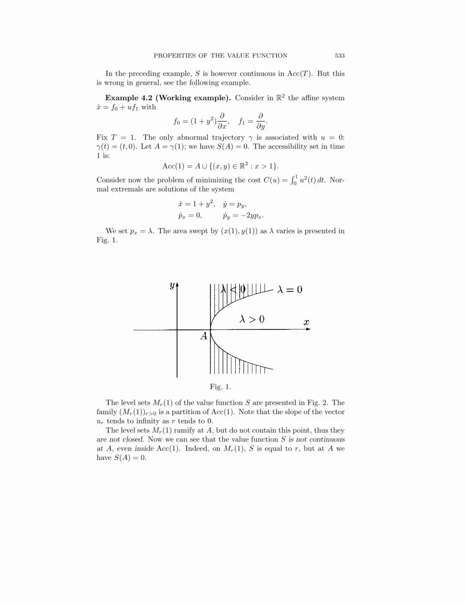
Example 4.2 (Working example). Consider in R2 the affine system

x = f0 + uf1 with

f0 = (1 + y2)∂

∂x, f1 =

∂

∂y.

Fix T = 1. The only abnormal trajectory γ is associated with u = 0:γ(t) = (t, 0). Let A = γ(1); we have S(A) = 0. The accessibility set in time1 is:

Acc(1) = A ∪ (x, y) ∈ R2 : x > 1.

Consider now the problem of minimizing the cost C(u) =∫ 10 u2(t) dt. Nor-

mal extremals are solutions of the system

x = 1 + y2, y = py,

px = 0, py = −2ypx.

We set px = λ. The area swept by (x(1), y(1)) as λ varies is presented inFig. 1.

Fig. 1.

The level sets Mr(1) of the value function S are presented in Fig. 2. Thefamily (Mr(1))r>0 is a partition of Acc(1). Note that the slope of the vectorur tends to infinity as r tends to 0.

The level sets Mr(1) ramify at A, but do not contain this point, thus theyare not closed. Now we can see that the value function S is not continuousat A, even inside Acc(1). Indeed, on Mr(1), S is equal to r, but at A wehave S(A) = 0.

534 E. TRELAT

We can give an equivalent of the value function S near A in the area(λ < 0) (see Fig. 3). Computations lead to the following formula:

S(x, y) ∼ 14

y4

x− 1.

Note that when y = 0 is fixed, if x → 1, x > 1, then λ → −∞. Thisis a phenomenon of nonproperness due to the existence of an abnormalminimizer. This fact was already encountered in sub-Riemannian geometry(see [9]). In the next section we explain this phenomenon.

Fig. 2. The level sets of the value function.

In this example A is steered from 0 by the minimizing control u = 0. Weeasily see that the set of minimizing controls steering 0 to points near A isnot (strongly) compact in L2. In fact, we have the following theorem.

Theorem 4.12. Consider the analytic affine control system (7) withcost (8). Suppose that r and T are small enough. Then S is continuouson Mr(T ) if and only if the set of minimizing controls steering 0 to pointsof Mr(T ) is compact in L2.

Remark 4.3. In sub-Riemannian geometry the value function S is alwayscontinuous, even though there may exist abnormal minimizers. This is dueto the fact that S is the square of the sub-Riemannian distance (see, e.g., [6]).Note that in [16] (see also [1]) it is proved that the set of minimizing controlsjoining Mr(T ) = B(0, r) for sufficiently small r is compact in L2.


Proof of Theorem 4.12. Let S be continuous on Mr(T ), and let (un)n∈N

be a sequence of minimizing controls steering O to points xn of Mr(T ).By Theorem 4.3 we can assume that xn converges to x ∈ Mr(T ). Letu be a minimizing control steering 0 to x. Since S is continuous, we get‖un‖L2 −→

n→+∞ ‖u‖L2 . The sequence (un) is bounded in L2, hence up to

a subsequence it converges weakly to v ∈ L2 such that ‖v‖L2 ‖u‖L2 .On the other hand, from Proposition 3.3 we get x = E(v). Therefore,‖v‖L2 = ‖u‖L2 since u is minimizing. Now combining the weak convergenceof un to v and the convergence of ‖un‖L2 to ‖v‖L2 , we get the (strong)convergence of un to v in L2. This proves the compactness of minimizingcontrols since v is minimizing.

The converse is obvious.

5. Role of abnormal minimizers

5.1. Theorem of tangency. This analysis is based on the sub-Riemannian Martinet case (see [9]): it was shown that the exponentialmapping is not proper and that in the generic case the sphere is tangentto the abnormal direction. This fact is general and we have the followingresults.

Lemma 5.1. Consider the affine control system (7) with cost (8). As-sume that there exists a minimizing geodesic γ on [0, T ] associated witha unique abnormal minimizing control u of corank 1, and that there ex-ists a sufficiently small r > 0 such that A = γ(T ) ∈ Mr(T ). Denoteby (p1, 0) the projectivized Lagrange multiplier at A. Let σ(τ )0<τ1 bea curve on Mr(T ) such that lim

τ→0σ(τ ) = A. For each τ we denote by

P(τ ) ⊂ P (T ∗σ(τ)M) the set of projectivized Lagrange multipliers at σ(τ):

P(τ ) = (pu(τ ), p0u) : E(u) = σ(τ ), u is minimizing. Then:

P(τ ) −→τ→0

(p1, 0),

i.e., each Lagrange multiplier of P(τ) tends to (p1, 0) as τ → 0.

Proof. For each τ let uτ be a minimizing control steering 0 to σ(τ ). Forany τ ∈]0, 1] let (pτ (T ), p0τ ) ∈ P(τ ). Let (ψ, ψ0) be a cluster point atτ = 0: there exists a sequence τn converging to 0 such that (pτn(T ), p0τn) −→(ψ, ψ0). The sequence of controls (uτn) is bounded in L2, hence up to asubsequence it converges weakly to a control v ∈ L2 such that C(v) r. Ifr is small enough, then by Proposition 4.2, v is admissible. Moreover, fromProposition 3.3 we get: E(v) = A, and the assumption of the lemma impliesv = u. Now writing the equality in L2 defining the Lagrange multiplier

pτn(T ) · dE(uτn) = −p0τnuτn

536 E. TRELAT

and passing to the limit, we obtain (Proposition 3.7):

ψ · dE(u) = −ψ0u.

Since u has corank 1, we conclude: (ψ, ψ0) = (p1, 0) in P (T ∗AM).

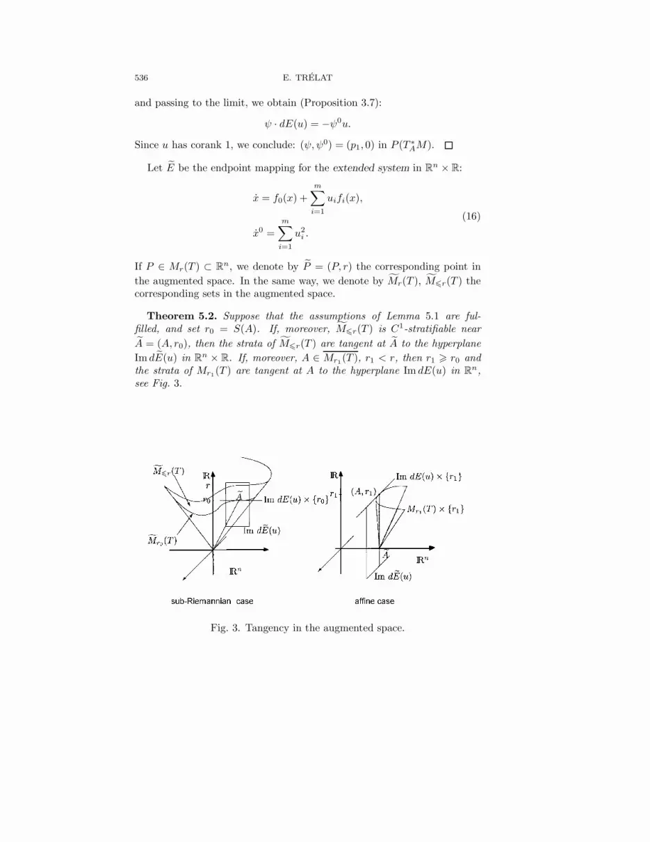
Let E be the endpoint mapping for the extended system in Rn × R:

x = f0(x) +m∑i=1

uifi(x),

x0 =m∑i=1

u2i .

(16)

If P ∈ Mr(T ) ⊂ Rn, we denote by P = (P, r) the corresponding point in

the augmented space. In the same way, we denote by Mr(T ), Mr(T ) thecorresponding sets in the augmented space.

Theorem 5.2. Suppose that the assumptions of Lemma 5.1 are ful-filled, and set r0 = S(A). If, moreover, Mr(T ) is C1-stratifiable nearA = (A, r0), then the strata of Mr(T ) are tangent at A to the hyperplaneIm dE(u) in R

n × R. If, moreover, A ∈ Mr1(T ), r1 < r, then r1 r0 andthe strata of Mr1(T ) are tangent at A to the hyperplane Im dE(u) in R

n,see Fig. 3.

Fig. 3. Tangency in the augmented space.


Proof. Let N be a stratum of Mr(T ) of maximal dimension near A. Let(σ(τ))0<τ1 be a C1 curve on N such that lim

τ→0σ(τ) = A, and σ(τ ) =

(σ(τ), rτ ). The aim is to prove that limτ→0

σ′(τ ) ∈ Im dE(u). From the as-

sumption on the stratum N , Im dE(uτ ) is the tangent space to N at σ(τ ).By definition of the Lagrange multiplier, (pτ (T ), p0τ ) is normal to this sub-space. Moreover, (p1, 0) is normal to the hyperplane Im dE(u). Now fromLemma 5.1 we deduce: Im dE(uτ ) −→

τ→0Im dE(u). The conclusion is now

clear since σ′(τ) ∈ Im dE(uτ ).The second part of the theorem is proved similarly.

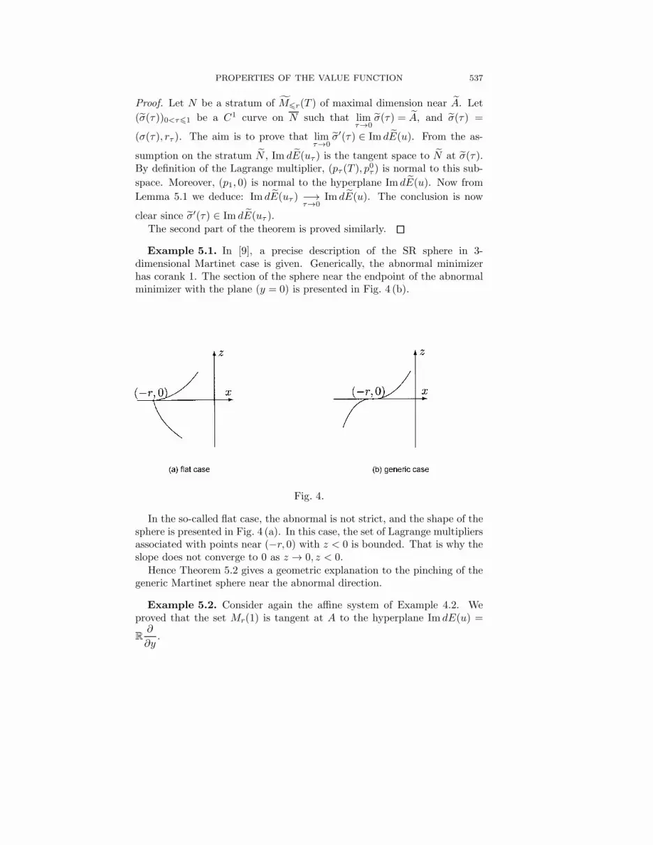
Example 5.1. In [9], a precise description of the SR sphere in 3-dimensional Martinet case is given. Generically, the abnormal minimizerhas corank 1. The section of the sphere near the endpoint of the abnormalminimizer with the plane (y = 0) is presented in Fig. 4 (b).

Fig. 4.

In the so-called flat case, the abnormal is not strict, and the shape of thesphere is presented in Fig. 4 (a). In this case, the set of Lagrange multipliersassociated with points near (−r, 0) with z < 0 is bounded. That is why theslope does not converge to 0 as z → 0, z < 0.

Hence Theorem 5.2 gives a geometric explanation to the pinching of thegeneric Martinet sphere near the abnormal direction.

Example 5.2. Consider again the affine system of Example 4.2. Weproved that the set Mr(1) is tangent at A to the hyperplane Im dE(u) =

R∂

∂y.

538 E. TRELAT

Note that, as in the preceding example, computations show that thebranch that ramifies at A is not subanalytic (see Fig. 2). In fact, it belongs tothe exp-log category (see [8]). More precisely, this branch has the followinggraph near A:

x = 1 + F

(y,

e− 4r

y2

y3

),

where F is a germ of analytic function at 0, and we have the followingasymptotic expansion:

x = 1 +14r

y4 − 3y2e−4ry2 + o

(y2e

− 4ry2).

We get the following asymptotics of the value function:

S(x, y) =14

y4

x− 1+

y4

x− 1e−

y2

x−1 + o

(y4

x− 1e−

y2

x−1

),

S is not subanalytic at A.

5.2. Interaction between abnormal and normal minimizers. Con-sider the affine system (7) with cost (8), and assume that there exists aminimizing geodesic γ on [0, T ] associated with a unique abnormal controlof corank 1. Denote A = γ(T ).

An endpoint at time T of a normal minimizing geodesic is said to be anormal point. We make the following assumption:

(H) For any neighborhood V of A there exists at least onenormal point contained in V ∩Mr(T ).

To describe the normal flow, we use the first normalization of Lagrange

multipliers (i.e., p0 = −12

for normal extremals), which allows us to definethe mapping Φ, see Definition 2.4. Now set exp = E Φ; it is a generaliza-tion of the (sub)-Riemannian exponential mapping. We have the followingproposition.

Proposition 5.3. Under the preceding assumptions the mapping exp isnot proper.

Proof. Let (An) be a sequence of normal points of Mr(T ) converging to A.For each An let (pn(T ),− 1

2 ) be an associated Lagrange multiplier. ApplyingLemma 5.1 we get:

pn(T )√‖pn(T )‖2 + 1

4

−→n→+∞ p1,

−12√

‖pn(T )‖2 + 14

−→n→+∞ 0.


Thus, in particular, ‖pn(T )‖ −→n→+∞ +∞. Now with the same arguments

as in Lemma 4.9 we prove: ‖pn(0)‖ −→n→+∞ +∞. By definition, An =

exp(pn(0)), hence exp is not proper.

Remark 5.1. Conversely if exp is not proper, then with the same argu-ments as in Lemma 4.8 there exists an abnormal minimizer. This shows theinteraction between abnormal and normal minimizers. In a sense normal ex-tremals recognize abnormal extremals. This phenomenon of nonpropernessis characteristic for abnormality.

5.3. Application: description of the sub-Riemannian sphere nearan abnormal minimizer for rank 2 distributions. Let (M,∆, g) be asub-Riemannian structure of rank 2 on an analytic n-dimensional manifoldM , n 3, with an analytic metric g on ∆. Our point of view is localand we can assume that M is a neighborhood of 0 ∈ R

n, and that ∆ =Spanf1, f2, where f1, f2 are independant analytic vector fields. Up toreparametrization, the problem of minimizing cost (8) at time T fixed isequivalent to the time-optimal problem with the constraint u21 + u22 1.Let γ be a reference abnormal trajectory on [0, r], associated with a controlu and an adjoint vector p. We suppose that γ is injective, and hence withoutloss of generality we can assume that γ(t) = exp tf1(0).

We make the following assumptions:

(H1) Let K(t) = Im dEt(u) = Spanadkf1 · f2|γ , k 0 be the firstPontryagin cone along γ. We assume that K(t) has codimension 1for any t ∈]0, r] and is spanned by the n − 1 first vectors adkf1 ·f2|γ , k = 0 . . . n− 2.

(H2) ad2f2 · f1|γ /∈ K(t) along γ.(H3) f1|γ /∈ adkf1 · f2|γ , k = 0, . . . , n− 3.

Under these assumptions γ has corank 1. Moreover, from [19] it followsthat γ is minimizing if r is small enough, and u is the unique minimizingabnormal control steering 0 to γ(r). Hence assumptions of Lemma 5.1 arefulfilled.

Let now V be a neighborhood of p(0) such that all abnormal geodesicsstarting from 0 with pγ(0) ∈ V satisfy also the assumptions (H1), (H2),and (H3). Note that if V is small enough, they are also injective. We have,see [4] and [19]:

Proposition 5.4. There exists r > 0 such that the previous abnormalgeodesics are optimal if t r.

Corollary 5.5. The endpoints of these abnormal minimizers form in theneighborhood of γ(r) an analytic submanifold of dimension n − 4 if n 3,reduced to a point if n = 3, contained in the sub-Riemannian sphere S(0, r).

540 E. TRELAT

Hence in the neighborhood of γ(r) the sub-Riemannian sphere S(0, r)splits into two parts: the abnormal part and the normal part. To describeS(0, r) near γ(r), we have to glue them together. If the hypothesis ofC1-stratification is fulfilled, then the normal part ramifies tangently to theabnormal part in the sense of Theorem 5.2. This gives us a qualitativedescription of the sphere near γ(r).

References

1. A. Agrachev, Compactness for sub-Riemannian length minimizers andsubanalyticity. Report SISSA Trieste, 1999.

2. A. Agrachev, B. Bonnard, M. Chyba, and I. Kupka, Sub-Riemanniansphere in the Martinet flat case. ESAIM/COCV, vol. 2 (1997), 377–448.

3. A. Agrachev and J. P. Gauthier, On subanalyticity of Carnot–Caratheodory distances. Preprint.

4. A. Agrachev and A. V. Sarychev, Strong minimality of abnormalgeodesics for 2-distributions. J. Dynam. Control Systems 1 (1995), No. 2,139–176.

5. , Sub-Riemannian metrics: minimality of abnormal geodesics ver-sus subanalyticity. Preprint de l’U. de Bourgogne, No. 162 (1998).

6. A. Bellache, Tangent space in SR-geometry. Birkhauser, 1996.7. B. Bonnard and I. Kupka, Theorie des singularites de l’application

entree/sortie et optimalite des trajectoires singulieres dans le problemedu temps minimal. Forum Math. 5 (1993), 111–159.

8. B. Bonnard, G. Launay, and E. Trelat, The transcendence we need tocompute the sphere and wave front in Martinet SR-geometry. Preprintlabo. Topologie Dijon (1998).

9. B. Bonnard and E. Trelat, On the role of abnormal minimizers in SR-geometry. In: Proc. Int. Conf. dedicated to L. S. Pontryagin, Moscow,1999.

10. H. Brezis, Analyse fonctionnelle. Masson, 1993.11. P. Brunovsky, Existence of regular synthesis for general control prob-

lems. J. Differential Equations 38 (1980), 317–343.12. A. F. Filippov, On certain questions in the theory of optimal control.

Vestnik Moskov. Univ. Ser. Mat. Mekh., Astron. 2 (1959).13. A. Gabrielov, Projections of semi-analytic sets. Func. Anal. Appl. 2

(1968).14. R. M. Hardt, Stratification of real analytic mappings and images. Invent.

Math. 28 (1975).15. H. Hironaka, Subanalytic sets, number theory, algebraic geometry and

commutative algebra. (In honour of Y. Akizuki), Tokyo, 1973.


16. S. Jacquet, Subanalyticity of the sub-Riemannian distance. J. Dynam.Control Systems 5 (1999), No. 3, 303–328.

17. A. J. Krener, The higher order maximal principle and its applicationsto singular extremals. SIAM J. Control Optim. 15 (1977), 256–293.

18. E. B. Lee and L. Markus, Foundations of optimal control theory. JohnWiley, New York, 1967.

19. W. S. Liu and H. J. Sussmann, Shortest paths for sub-Riemannian met-rics of rank two distributions. Memoirs Amer. Math. Soc. 118 (1995),No. 564.

20. S. Lojasiewick and H. J. Sussmann, Some examples of reachable setsand optimal cost functions that fail to be subanalytic. SIAM J. ControlOptim. 23 (1985), No. 4, 584-598.

21. L. Pontryagin et al., Mathematical theory of optimal processes. (Rus-sian) Mir, Moscow, 1974.

22. E. D. Sontag, Mathematical control theory, deterministic finite dimen-sional systems. Springer-Verlag, 1990.

23. H. J. Sussmann, Regular synthesis for time-optimal control of single-input real analytic systems in the plane. SIAM J. Control Optim. 25(1987), No. 5.

24. M. Tamm, Subanalytic sets in the calculus of variation. Acta Math. 146(1981).

(Received 10.05.2000)

Author’s address:Universite de Bourgogne, Laboratoire de Topologie,UMR 5584 du CNRS, BP47870, 21078 Dijon Cedex, FranceE-mail: [email protected]

some properties of the value function and its level sets for affine control systems with quadratic...

Documents