Computers and Mathematics with Applications 56 (2008) 2528–2538

Contents lists available at ScienceDirect

Computers and Mathematics with Applications

journal homepage: www.elsevier.com/locate/camwa

Some modification of Newton’s method by the method ofundetermined coefficientsChangbum Chun a, Beny Neta b,∗

a Department of Mathematics, Sungkyunkwan University, Suwon 440-746, Republic of Koreab Naval Postgraduate School, Department of Applied Mathematics, Monterey, CA 93943, United States

a r t i c l e i n f o

Article history:Received 14 April 2008Accepted 23 May 2008

Keywords:Newton’s methodIterative methodsNonlinear equationsOrder of convergenceMethod of undetermined coefficientsRoot-finding methods

a b s t r a c t

In this paper, we construct some modifications of Newton’s method for solving nonlinearequations, which is based on the method of undetermined coefficients. It is shownby way of illustration that the method of undetermined coefficients is a promisingtool for developing new methods, and reveals its wide applicability by obtaining someexistingmethods as special cases. Two new sixth-ordermethods are developed. Numericalexamples are given to support that the methods thus obtained can compete with otheriterative methods.

Published by Elsevier Ltd

1. Introduction

Solving nonlinear equations is one of the most important problems in numerical analysis. To solve nonlinear equations,iterative methods such as Newton’s method are usually used. Throughout this paper we consider iterative methods to finda simple root ξ , i.e., f (ξ) = 0 and f ′(ξ) 6= 0, of a nonlinear equation f (x) = 0 that uses no higher than the second derivativeof f .

Newton’s method for the calculation of ξ is probably the most widely used iterative method defined by

xn+1 = xn −f (xn)f ′(xn)

. (1)

It is well known (see e.g. Traub [1]) that this method is quadratically convergent.Several third-order methods based on quadratures are given in the literature. A third-order variant of Newton’s method

appeared in Weerakoon and Fernando [2] where rectangular and trapezoidal approximations to the integral in Newton’stheorem

f (x) = f (xn) +

∫ x

xnf ′(t)dt (2)

were considered to rederive Newton’s method and to obtain the cubically convergent method

xn+1 = xn −2f (xn)

f ′(xn) + f ′(yn), (3)

∗ Corresponding author.E-mail addresses: cbchun@skku.edu (C. Chun), bneta@nps.edu, byneta@gmail.com (B. Neta).

0898-1221/$ – see front matter. Published by Elsevier Ltddoi:10.1016/j.camwa.2008.05.005

C. Chun, B. Neta / Computers and Mathematics with Applications 56 (2008) 2528–2538 2529

respectively, where from here on

yn = xn −f (xn)f ′(xn)

. (4)

Frontini and Sormani [3] considered the midpoint rule for the integral of (2) to obtain the third-order method

xn+1 = xn −f (xn)

f ′( xn+yn

2

) . (5)

It should be mentioned that the method (5) has been derived by Homeier [4] independently

xn+1 = xn −f (xn)

f ′

(xn −

f (xn)2f ′(xn)

) . (6)

In [5], Homeier derived the following cubically convergent iteration scheme

xn+1 = xn −f (xn)2

(1

f ′(xn)+

1f ′(yn)

)(7)

by applying Newton’s theorem to the inverse function x = f (y) instead of y = f (x). It should be pointed out that thismethodhas also been derived in [6] independently and it is now known as the harmonic mean Newton method.

In [7], Kou et al. observed that the midpoint method (5) can be obtained by using the midpoint value f ′( 12 (xn + yn))

instead of the arithmetic mean of f ′(xn) and f ′(yn) in the method of Weerakoon and Fernando (3). That is, they applied theapproximation

f ′

(12(xn + yn)

)≈

f ′(xn) + f ′(yn)2

, (8)

or

f ′(yn) ≈ 2f ′

(12(xn + yn)

)− f ′(xn), (9)

to Homeier’s method (7) to obtain a modification of Newton’s method.Note, if one takes Simpson’s rule to approximate the integral in (2), the resulting method is only quadratic. A modified

method based on Simpson’s rule will be

xn+1 = xn −bf (xn)

f ′(xn) + (b − 2)f ′((xn + yn)/2) + f ′(yn)(10)

where b is a free parameter. This method requires more function-evaluations for the same order and thus it is not efficient.Similarly, methods based on Gaussian quadratures are not efficient.

Recently, Neta [8] used the method of undetermined coefficients to obtain a new efficient modification of Popovski’smethods [9] by considering an idea of removing the second derivative. In this paper, we further investigate the use of theundetermined coefficients in developing methods. We rederive the existing methods from this point of view and proposenewmethods. For example, the approximation (8) can be easily obtained by using themethod of undetermined coefficients.To see that, we let

f ′

(12(xn + yn)

)= Af ′(xn) + Bf ′(yn) (11)

and expand the second term f ′(yn) about the point xn. By comparing the coefficients of the derivatives of f at xn up to secondderivatives, we can easily obtain

A = B =12, (12)

this yielding (8).In [10], Kou and Li considered an iteration scheme consisting of Jarratt’s iterate zn defined by

zn = xn − Jf (xn)f (xn)f ′(xn)

(13)

and followed by a Newton iterate, and use of the linear approximation

f ′(zn) ≈zn − xnvn − xn

f ′(vn) +zn − vn

xn − vnf ′(xn), (14)

2530 C. Chun, B. Neta / Computers and Mathematics with Applications 56 (2008) 2528–2538

where vn = xn −23 f (xn)/f

′(xn), and Jf (xn) =3f ′(vn)+f ′(xn)6f ′(vn)−2f ′(xn)

to obtain an improvement of Jarratt’s method [11]. The methodis given by

vn = xn −23

f (xn)f ′(xn)

zn = xn − Jf (xn)f (xn)f ′(xn)

xn+1 = zn −f (zn)

32 Jf (xn)f

′(vn) + (1 −32 Jf (xn))f

′(xn).

(15)

The approximation (14) can also be easily obtained by applying the method of undetermined coefficients with

f ′(zn) = Af ′(vn) + Bf ′(xn), (16)

as in the above. The method (15) is of order six. Another sixth-order improved Jarratt’s method is given by the first authorin [12].

Many other iterative methods in the literature can also be derived from each other through themethod of undeterminedcoefficients. For example, Nedzhibov’s third-order method (see [14] or [13]) defined by1

xn+1 = xn −f (xn)

14

(f ′(yn) + 2f ′(

xn+yn2 ) + f ′(xn)

) (17)

Hasanov’s third-order method (see [15] or [13])2

xn+1 = xn −f (xn)

16

(f ′(yn) + 4f ′(

xn+yn2 ) + f ′(xn)

) (18)

and the Newton-secant method (see [16] or [13])

xn+1 = xn −f (xn)

f ′(xn)(f (xn)−f (yn))f (xn)

(19)

can all be derived from (5). To show this in the case of (17), we apply the method of undetermined coefficients a littledifferently, that is, we search for the expression dn satisfying

f ′(dn) =14

[f ′(yn) + 2f ′

(xn + yn

2

)+ f ′(xn)

]. (20)

Expanding the terms f ′(dn), f ′(yn) and f ′(xn+yn

2 ) of (20) about the point xn up to second derivatives, using (4), and thencomparing the coefficients of the derivatives of f at xn, we easily obtain the equation after simplifications

dn − xn = −12

f (xn)f ′(xn)

, (21)

or

dn = xn −12

f (xn)f ′(xn)

=12(xn + yn). (22)

We, therefore, derived (5) from Nedzhibov’s method, and the other way around. Similarly we can show the equivalence of(5) and Hasanov’s method (18).

This can also be done in the case of the Newton-secant method, we seek to find dn in the equation

f ′(dn) =f ′(xn)(f (xn) − f (yn))

f (xn), (23)

or, equivalently

f ′(dn)f (xn) = f ′(xn)[f (xn) − f (yn)]. (24)

1 This is a special case of (10) with b = 4.2 This is a special case of (10) with b = 6.

C. Chun, B. Neta / Computers and Mathematics with Applications 56 (2008) 2528–2538 2531

If we expand the terms f ′(dn) and f (yn) of (24) about the point xn up to second derivatives, and then compare the coefficientsof the derivatives of f at xn, we can obtain the same equation as in (22)

dn =12(xn + yn). (25)

We thus showed that (5) is equivalent to the Newton-secant method.We can continue to derive new or existing methods from methods available. If we consider (7) in our application with

the form

f ′(dn) =2f ′(xn)f ′(yn)f ′(xn) + f ′(yn)

, (26)

we can obtain the approximating expression

dn = xn −f (xn)f ′(xn)

2f ′(xn)2 − f (xn)f ′′(xn). (27)

This suggests a new third-order method defined by

yn = xn −12

f (xn)f ′(xn)

1

1 −f (xn)f ′′(xn)2f ′(xn)2

xn+1 = xn −f (xn)f ′(yn)

.

(28)

The order was found using Maple software. This method is inefficient since it requires one function- and three derivative-evaluation. The efficiency of this method is the same as the schemes by Hasanov (18) and by Nedzhibov (17), which arespecial cases of (10).

Traub–Ostrowski’s fourth-order method (see [1]) is given by

xn+1 = xn −f (yn) − f (xn)2f (yn) − f (xn)

f (xn)f ′(xn)

. (29)

If we look for dn through the equation

f ′(dn) =f ′(xn)[2f (yn) − f (xn)]

f (yn) − f (xn)(30)

or, equivalently

f ′(dn)[f (yn) − f (xn)] = f ′(xn)[2f (yn) − f (xn)] (31)

then after expanding the terms f ′(dn) and f (yn) of (31) about the point xn up to second derivatives, and then comparing thecoefficients of the derivatives of f at xn, we can obtain exactly the same expression as in (27), thereby again obtaining thesame method as (28). This shows that Homeier’s method (7) and Traub–Ostrowski’s method are closely connected throughthe method of undetermined coefficients.

Chebyshev–Halley methods [17] are a family of third-order methods defined by

xn+1 = xn −

(1 +

12

Lf (xn)1 − αLf (xn)

)f (xn)f ′(xn)

, (32)

where Lf (xn) =f (xn)f ′′(xn)

f ′(xn)2. This family includes Chebyshev’s method (α = 0), Halley’s method (α = 1/2) and the super-

Halley method (α = 1). With this family, let us consider seeking the approximating expression dn such that

f ′(dn) = f ′(xn)2[1 − αLf (xn)]

2 + (1 − 2α)Lf (xn)(33)

or

f ′(dn)[2f ′(xn)2 + (1 − 2α)f (xn)f ′′(xn)] = 2f ′(xn)[f ′(xn)2 − αf (xn)f ′′(xn)]. (34)

If we expand the term f ′(dn) of (34) about the point xn up to second derivative, and then compare the coefficients of thederivatives of f at xn, we can easily obtain

dn = xn −f (xn)f ′(xn)

2f ′(xn)2 + (1 − 2α)f (xn)f ′′(xn). (35)

2532 C. Chun, B. Neta / Computers and Mathematics with Applications 56 (2008) 2528–2538

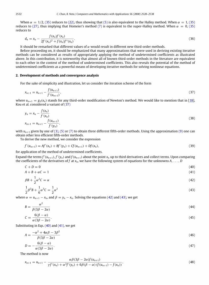
When α = 1/2, (35) reduces to (22), thus showing that (5) is also equivalent to the Halley method. When α = 1, (35)reduces to (27), thus implying that Homeier’s method (7) is equivalent to the super-Halley method. When α = 0, (35)reduces to

dn = xn −f (xn)f ′(xn)

2f ′(xn)2 + f (xn)f ′′(xn). (36)

It should be remarked that different values of α would result in different new third-order methods.Before proceeding on, it should be emphasized that many approximations that were used in deriving existing iterative

methods can be considered as results of appropriately applying the method of undetermined coefficients as illustratedabove. In this contribution, it is noteworthy that almost all of known third-order methods in the literature are equivalentto each other in the context of the method of undetermined coefficients. This also reveals the potential of the method ofundetermined coefficients as a powerful means of developing iterative methods for solving nonlinear equations.

2. Development of methods and convergence analysis

For the sake of simplicity and illustration, let us consider the iteration scheme of the form

xn+1 = un+1 −f (un+1)

f ′(un+1), (37)

where un+1 = g3(xn) stands for any third-order modification of Newton’s method. We would like to mention that in [18],Kou et al. considered a variant of (37)

yn = xn −f (xn)f ′(xn)

xn+1 = un+1 −f (un+1)

f ′(yn),

(38)

with un+1 given by one of (3), (5) or (7) to obtain three different fifth-order methods. Using the approximation (9) one canobtain other less efficient fifth-order methods.

To derive the new method, we consider the expression

f ′(un+1) = Af ′(xn) + Bf ′(yn) + Cf (un+1) + Df (xn), (39)

for application of the method of undetermined coefficients.Expand the terms f ′(un+1), f ′(yn) and f (un+1) about the point xn up to third derivatives and collect terms. Upon comparingthe coefficients of the derivatives of f at xn, we have the following system of equations for the unknowns A, . . . ,D

C + D = 0 (40)A + B + αC = 1 (41)

βB +12α2C = α (42)

12β2B +

16α3C =

12α2 (43)

where α = un+1 − xn, and β = yn − xn. Solving the equations (42) and (43), we get

B =α2

β(3β − 2α)(44)

C =6(β − α)

α(3β − 2α). (45)

Substituting in Eqs. (40) and (41), we get

A =−α2

+ 4αβ − 3β2

β(3β − 2α)(46)

D = −6(β − α)

α(3β − 2α). (47)

The method is now

xn+1 = un+1 −αβ(3β − 2α)f (un+1)

γ f ′(xn) + α3f ′(yn) + 6β(β − α) (f (un+1) − f (xn)), (48)

C. Chun, B. Neta / Computers and Mathematics with Applications 56 (2008) 2528–2538 2533

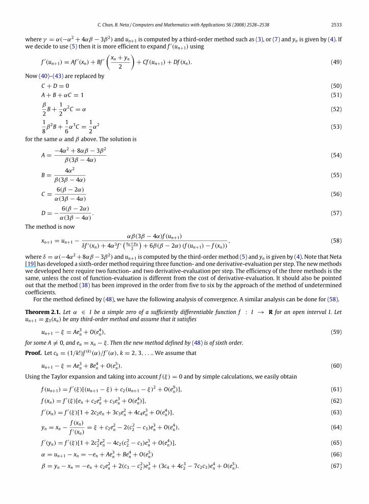
where γ = α(−α2+ 4αβ − 3β2) and un+1 is computed by a third-order method such as (3), or (7) and yn is given by (4). If

we decide to use (5) then it is more efficient to expand f ′(un+1) using

f ′(un+1) = Af ′(xn) + Bf ′

(xn + yn

2

)+ Cf (un+1) + Df (xn). (49)

Now (40)–(43) are replaced by

C + D = 0 (50)A + B + αC = 1 (51)β

2B +

12α2C = α (52)

18β2B +

16α3C =

12α2 (53)

for the same α and β above. The solution is

A =−4α2

+ 8αβ − 3β2

β(3β − 4α)(54)

B =4α2

β(3β − 4α)(55)

C =6(β − 2α)

α(3β − 4α)(56)

D = −6(β − 2α)

α(3β − 4α). (57)

The method is now

xn+1 = un+1 −αβ(3β − 4α)f (un+1)

δf ′(xn) + 4α3f ′( xn+yn

2

)+ 6β(β − 2α) (f (un+1) − f (xn))

, (58)

where δ = α(−4α2+8αβ −3β2) and un+1 is computed by the third-order method (5) and yn is given by (4). Note that Neta

[19] has developed a sixth-ordermethod requiring three function- and one derivative-evaluation per step. The newmethodswe developed here require two function- and two derivative-evaluation per step. The efficiency of the three methods is thesame, unless the cost of function-evaluation is different from the cost of derivative-evaluation. It should also be pointedout that the method (38) has been improved in the order from five to six by the approach of the method of undeterminedcoefficients.

For the method defined by (48), we have the following analysis of convergence. A similar analysis can be done for (58).

Theorem 2.1. Let α ∈ I be a simple zero of a sufficiently differentiable function f : I → R for an open interval I. Letun+1 = g3(xn) be any third-order method and assume that it satisfies

un+1 − ξ = Ae3n + O(e4n), (59)

for some A 6= 0, and en = xn − ξ . Then the new method defined by (48) is of sixth order.

Proof. Let ck = (1/k!)f (k)(α)/f ′(α), k = 2, 3, . . .. We assume that

un+1 − ξ = Ae3n + Be4n + O(e5n). (60)

Using the Taylor expansion and taking into account f (ξ) = 0 and by simple calculations, we easily obtain

f (un+1) = f ′(ξ)[(un+1 − ξ) + c2(un+1 − ξ)2 + O(e9n)], (61)

f (xn) = f ′(ξ)[en + c2e2n + c3e3n + O(e4n)], (62)

f ′(xn) = f ′(ξ)[1 + 2c2en + 3c3e2n + 4c4e3n + O(e4n)], (63)

yn = xn −f (xn)f ′(xn)

= ξ + c2e2n − 2(c22 − c3)e3n + O(e4n), (64)

f ′(yn) = f ′(ξ)[1 + 2c22e2n − 4c2(c22 − c3)e3n + O(e4n)], (65)

α = un+1 − xn = −en + Ae3n + Be4n + O(e5n) (66)

β = yn − xn = −en + c2e2n + 2(c3 − c22 )e3n + (3c4 + 4c32 − 7c2c3)e4n + O(e5n). (67)

2534 C. Chun, B. Neta / Computers and Mathematics with Applications 56 (2008) 2528–2538

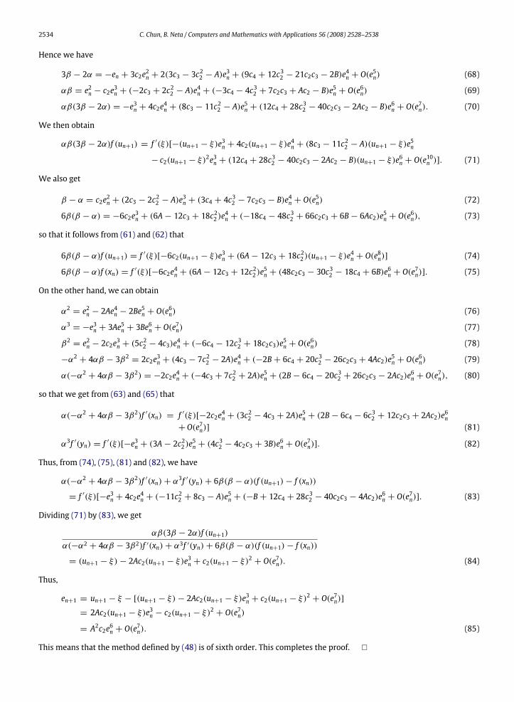
Hence we have

3β − 2α = −en + 3c2e2n + 2(3c3 − 3c22 − A)e3n + (9c4 + 12c32 − 21c2c3 − 2B)e4n + O(e5n) (68)

αβ = e2n − c2e3n + (−2c3 + 2c22 − A)e4n + (−3c4 − 4c32 + 7c2c3 + Ac2 − B)e5n + O(e6n) (69)

αβ(3β − 2α) = −e3n + 4c2e4n + (8c3 − 11c22 − A)e5n + (12c4 + 28c32 − 40c2c3 − 2Ac2 − B)e6n + O(e7n). (70)

We then obtain

αβ(3β − 2α)f (un+1) = f ′(ξ)[−(un+1 − ξ)e3n + 4c2(un+1 − ξ)e4n + (8c3 − 11c22 − A)(un+1 − ξ)e5n

− c2(un+1 − ξ)2e3n + (12c4 + 28c32 − 40c2c3 − 2Ac2 − B)(un+1 − ξ)e6n + O(e10n )]. (71)

We also get

β − α = c2e2n + (2c3 − 2c22 − A)e3n + (3c4 + 4c32 − 7c2c3 − B)e4n + O(e5n) (72)

6β(β − α) = −6c2e3n + (6A − 12c3 + 18c22 )e4n + (−18c4 − 48c32 + 66c2c3 + 6B − 6Ac2)e5n + O(e6n), (73)

so that it follows from (61) and (62) that

6β(β − α)f (un+1) = f ′(ξ)[−6c2(un+1 − ξ)e3n + (6A − 12c3 + 18c22 )(un+1 − ξ)e4n + O(e8n)] (74)

6β(β − α)f (xn) = f ′(ξ)[−6c2e4n + (6A − 12c3 + 12c22 )e5n + (48c2c3 − 30c32 − 18c4 + 6B)e6n + O(e7n)]. (75)

On the other hand, we can obtain

α2= e2n − 2Ae4n − 2Be5n + O(e6n) (76)

α3= −e3n + 3Ae5n + 3Be6n + O(e7n) (77)

β2= e2n − 2c2e3n + (5c22 − 4c3)e4n + (−6c4 − 12c32 + 18c2c3)e5n + O(e6n) (78)

−α2+ 4αβ − 3β2

= 2c2e3n + (4c3 − 7c22 − 2A)e4n + (−2B + 6c4 + 20c32 − 26c2c3 + 4Ac2)e5n + O(e6n) (79)

α(−α2+ 4αβ − 3β2) = −2c2e4n + (−4c3 + 7c22 + 2A)e5n + (2B − 6c4 − 20c32 + 26c2c3 − 2Ac2)e6n + O(e7n), (80)

so that we get from (63) and (65) that

α(−α2+ 4αβ − 3β2)f ′(xn) = f ′(ξ)[−2c2e4n + (3c22 − 4c3 + 2A)e5n + (2B − 6c4 − 6c32 + 12c2c3 + 2Ac2)e6n

+O(e7n)] (81)

α3f ′(yn) = f ′(ξ)[−e3n + (3A − 2c22 )e5n + (4c32 − 4c2c3 + 3B)e6n + O(e7n)]. (82)

Thus, from (74), (75), (81) and (82), we have

α(−α2+ 4αβ − 3β2)f ′(xn) + α3f ′(yn) + 6β(β − α)(f (un+1) − f (xn))

= f ′(ξ)[−e3n + 4c2e4n + (−11c22 + 8c3 − A)e5n + (−B + 12c4 + 28c32 − 40c2c3 − 4Ac2)e6n + O(e7n)]. (83)

Dividing (71) by (83), we get

αβ(3β − 2α)f (un+1)

α(−α2 + 4αβ − 3β2)f ′(xn) + α3f ′(yn) + 6β(β − α)(f (un+1) − f (xn))

= (un+1 − ξ) − 2Ac2(un+1 − ξ)e3n + c2(un+1 − ξ)2 + O(e7n). (84)

Thus,

en+1 = un+1 − ξ − [(un+1 − ξ) − 2Ac2(un+1 − ξ)e3n + c2(un+1 − ξ)2 + O(e7n)]

= 2Ac2(un+1 − ξ)e3n − c2(un+1 − ξ)2 + O(e7n)

= A2c2e6n + O(e7n). (85)

This means that the method defined by (48) is of sixth order. This completes the proof. �

C. Chun, B. Neta / Computers and Mathematics with Applications 56 (2008) 2528–2538 2535

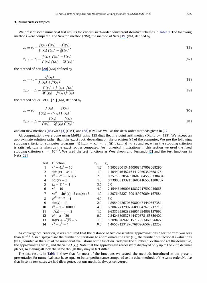
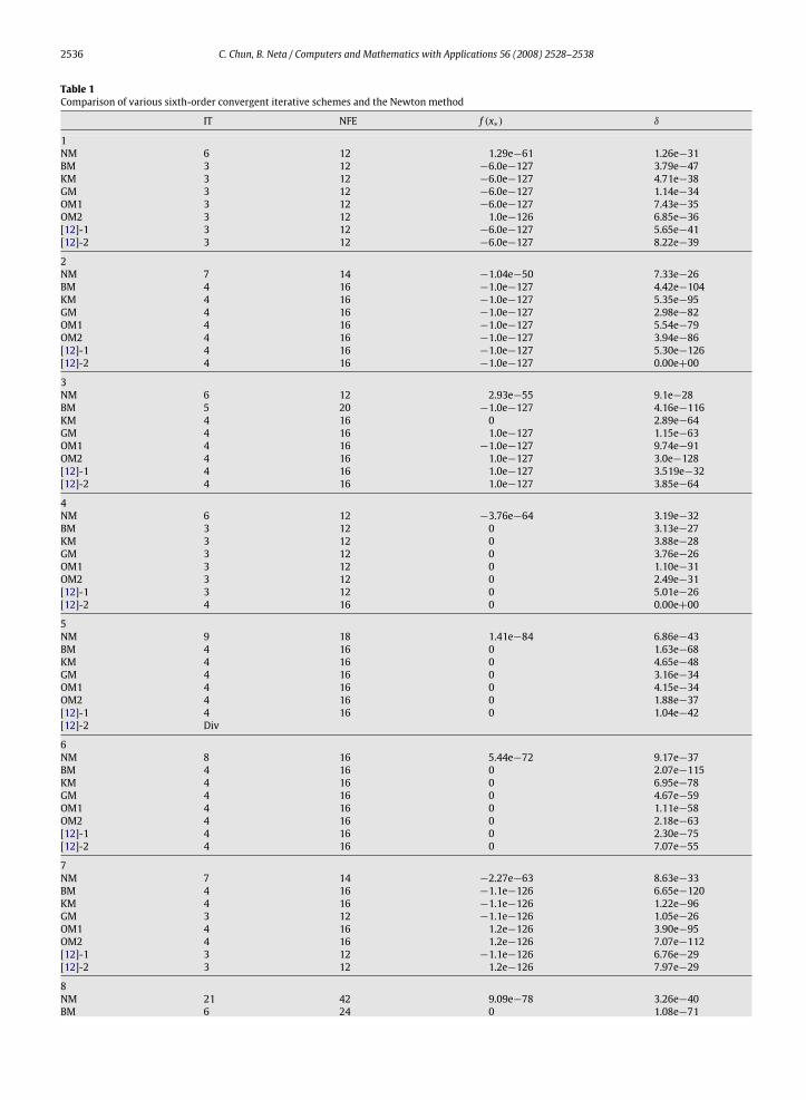
3. Numerical examples

We present some numerical test results for various sixth-order convergent iterative schemes in Table 1. The followingmethods were compared: the Newton method (NM), the method of Neta [19] (BM) defined by

zn = yn −f (yn)f ′(xn)

f (xn) −12 f (yn)

f (xn) −52 f (yn)

, (86)

xn+1 = zn −f (zn)f ′(xn)

f (xn) − f (yn)f (xn) − 3f (yn)

, (87)

the method of Kou [20] (KM) defined by

zn = xn −2f (xn)

f ′(xn) + f ′(yn), (88)

xn+1 = zn −f ′(yn) + f ′(xn)3f ′(yn) − f ′(xn)

f (zn)f ′(xn)

, (89)

the method of Grau et al. [21] (GM) defined by

zn = yn −f (xn)

f (xn) − 2f (yn)f (yn)f ′(xn)

, (90)

xn+1 = zn −f (xn)

f (xn) − 2f (yn)f (zn)f ′(xn)

, (91)

and our new methods (48) with (3) (OM1) and (58) (OM2) as well as the sixth-order methods given in [12].All computations were done using MAPLE using 128 digit floating point arithmetics (Digits := 128). We accept an

approximate solution rather than the exact root, depending on the precision (ε) of the computer. We use the followingstopping criteria for computer programs: (i) |xn+1 − xn| < ε, (ii) |f (xn+1)| < ε, and so, when the stopping criterionis satisfied, xn+1 is taken as the exact root α computed. For numerical illustrations in this section we used the fixedstopping criterion ε = 10−25. We used the test functions as Weerakoon and Fernando [2] and the test functions inNeta [22]

Test Function x0 x∗

1 x3 + 4x2 − 10 1.6 1.36523001341409684576080682902 sin2(x) − x2 + 1 1.0 1.40449164821534122603508681783 x2 − ex − 3x + 2 2.0 0.257530285439860760455367304944 cos(x) − x 1.5 0.739085133215160641655312087675 (x − 1)3 − 1 3.5 2.06 x3 − 10 4.0 2.15443469003188372175929356657 xex

2−sin2(x)+3 cos(x)+5 −1.0 −1.2076478271309189270094167584

8 ex2+7x−30

− 1 4.0 3.09 sin(x) −

x2 2.0 1.8954942670339809471440357381

10 x5 + x − 10000 4.0 6.308777129972689094767571771811

√(x) −

1x − 3 1.0 9.6335955628326951924063127092

12 ex + x − 20 0.0 2.842438953784447067816585940213 ln(x) +

√(x) − 5 1.0 8.3094326942315717953469556827

14 x3 − x2 − 1 0.5 1.4655712318767680266567312252

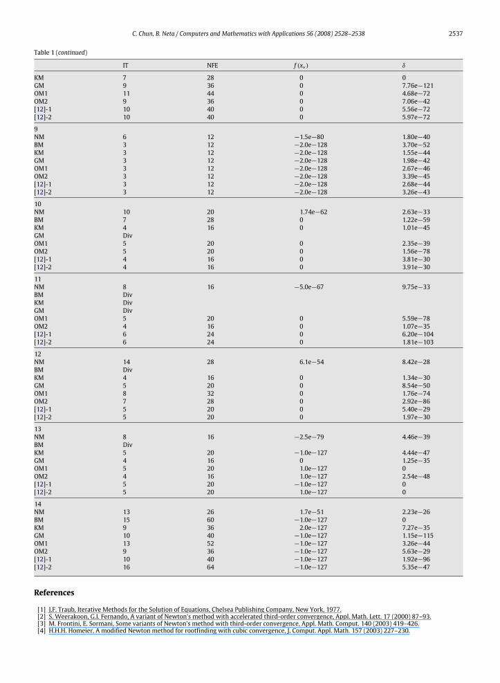
As convergence criterion, it was required that the distance of two consecutive approximations δ for the zero was lessthan 10−25. Also displayed are the number of iterations to approximate the zero (IT), the number of functional evaluations(NFE) counted as the sum of the number of evaluations of the function itself plus the number of evaluations of the derivative,the approximate zero x∗, and the value f (x∗). Note that the approximate zeroes were displayed only up to the 28th decimalplaces, so making all look the same though they may in fact differ.

The test results in Table 1 show that for most of the functions we tested, the methods introduced in the presentpresentation for numerical tests have equal or better performance compared to the othermethods of the same order. Noticethat in some test cases we had divergence, but our methods always converged.

2536 C. Chun, B. Neta / Computers and Mathematics with Applications 56 (2008) 2528–2538

Table 1Comparison of various sixth-order convergent iterative schemes and the Newton method

IT NFE f (x∗) δ

1NM 6 12 1.29e−61 1.26e−31BM 3 12 −6.0e−127 3.79e−47KM 3 12 −6.0e−127 4.71e−38GM 3 12 −6.0e−127 1.14e−34OM1 3 12 −6.0e−127 7.43e−35OM2 3 12 1.0e−126 6.85e−36[12]-1 3 12 −6.0e−127 5.65e−41[12]-2 3 12 −6.0e−127 8.22e−39

2NM 7 14 −1.04e−50 7.33e−26BM 4 16 −1.0e−127 4.42e−104KM 4 16 −1.0e−127 5.35e−95GM 4 16 −1.0e−127 2.98e−82OM1 4 16 −1.0e−127 5.54e−79OM2 4 16 −1.0e−127 3.94e−86[12]-1 4 16 −1.0e−127 5.30e−126[12]-2 4 16 −1.0e−127 0.00e+00

3NM 6 12 2.93e−55 9.1e−28BM 5 20 −1.0e−127 4.16e−116KM 4 16 0 2.89e−64GM 4 16 1.0e−127 1.15e−63OM1 4 16 −1.0e−127 9.74e−91OM2 4 16 1.0e−127 3.0e−128[12]-1 4 16 1.0e−127 3.519e−32[12]-2 4 16 1.0e−127 3.85e−64

4NM 6 12 −3.76e−64 3.19e−32BM 3 12 0 3.13e−27KM 3 12 0 3.88e−28GM 3 12 0 3.76e−26OM1 3 12 0 1.10e−31OM2 3 12 0 2.49e−31[12]-1 3 12 0 5.01e−26[12]-2 4 16 0 0.00e+00

5NM 9 18 1.41e−84 6.86e−43BM 4 16 0 1.63e−68KM 4 16 0 4.65e−48GM 4 16 0 3.16e−34OM1 4 16 0 4.15e−34OM2 4 16 0 1.88e−37[12]-1 4 16 0 1.04e−42[12]-2 Div

6NM 8 16 5.44e−72 9.17e−37BM 4 16 0 2.07e−115KM 4 16 0 6.95e−78GM 4 16 0 4.67e−59OM1 4 16 0 1.11e−58OM2 4 16 0 2.18e−63[12]-1 4 16 0 2.30e−75[12]-2 4 16 0 7.07e−55

7NM 7 14 −2.27e−63 8.63e−33BM 4 16 −1.1e−126 6.65e−120KM 4 16 −1.1e−126 1.22e−96GM 3 12 −1.1e−126 1.05e−26OM1 4 16 1.2e−126 3.90e−95OM2 4 16 1.2e−126 7.07e−112[12]-1 3 12 −1.1e−126 6.76e−29[12]-2 3 12 1.2e−126 7.97e−29

8NM 21 42 9.09e−78 3.26e−40BM 6 24 0 1.08e−71

C. Chun, B. Neta / Computers and Mathematics with Applications 56 (2008) 2528–2538 2537

Table 1 (continued)

IT NFE f (x∗) δ

KM 7 28 0 0GM 9 36 0 7.76e−121OM1 11 44 0 4.68e−72OM2 9 36 0 7.06e−42[12]-1 10 40 0 5.56e−72[12]-2 10 40 0 5.97e−72

9NM 6 12 −1.5e−80 1.80e−40BM 3 12 −2.0e−128 3.70e−52KM 3 12 −2.0e−128 1.55e−44GM 3 12 −2.0e−128 1.98e−42OM1 3 12 −2.0e−128 2.67e−46OM2 3 12 −2.0e−128 3.39e−45[12]-1 3 12 −2.0e−128 2.68e−44[12]-2 3 12 −2.0e−128 3.26e−43

10NM 10 20 1.74e−62 2.63e−33BM 7 28 0 1.22e−59KM 4 16 0 1.01e−45GM DivOM1 5 20 0 2.35e−39OM2 5 20 0 1.56e−78[12]-1 4 16 0 3.81e−30[12]-2 4 16 0 3.91e−30

11NM 8 16 −5.0e−67 9.75e−33BM DivKM DivGM DivOM1 5 20 0 5.59e−78OM2 4 16 0 1.07e−35[12]-1 6 24 0 6.20e−104[12]-2 6 24 0 1.81e−103

12NM 14 28 6.1e−54 8.42e−28BM DivKM 4 16 0 1.34e−30GM 5 20 0 8.54e−50OM1 8 32 0 1.76e−74OM2 7 28 0 2.92e−86[12]-1 5 20 0 5.40e−29[12]-2 5 20 0 1.97e−30

13NM 8 16 −2.5e−79 4.46e−39BM DivKM 5 20 −1.0e−127 4.44e−47GM 4 16 0 1.25e−35OM1 5 20 1.0e−127 0OM2 4 16 1.0e−127 2.54e−48[12]-1 5 20 −1.0e−127 0[12]-2 5 20 1.0e−127 0

14NM 13 26 1.7e−51 2.23e−26BM 15 60 −1.0e−127 0KM 9 36 2.0e−127 7.27e−35GM 10 40 −1.0e−127 1.15e−115OM1 13 52 −1.0e−127 3.26e−44OM2 9 36 −1.0e−127 5.63e−29[12]-1 10 40 −1.0e−127 1.92e−96[12]-2 16 64 −1.0e−127 5.35e−47

References

[1] J.F. Traub, Iterative Methods for the Solution of Equations, Chelsea Publishing Company, New York, 1977.[2] S. Weerakoon, G.I. Fernando, A variant of Newton’s method with accelerated third-order convergence, Appl. Math. Lett. 17 (2000) 87–93.[3] M. Frontini, E. Sormani, Some variants of Newton’s method with third-order convergence, Appl. Math. Comput. 140 (2003) 419–426.[4] H.H.H. Homeier, A modified Newton method for rootfinding with cubic convergence, J. Comput. Appl. Math. 157 (2003) 227–230.

2538 C. Chun, B. Neta / Computers and Mathematics with Applications 56 (2008) 2528–2538

[5] H.H.H. Homeier, On Newton-type methods with cubic convergence, J. Comput. Appl. Math. 176 (2005) 425–432.[6] A.Y. Özban, Some new variants of Newton’s method, Appl. Math. Lett. 17 (2004) 677–682.[7] J. Kou, Y. Li, X. Wang, Third-order modification of Newton’s method, J. Comput. Appl. Math. 205 (2007) 1–5.[8] B. Neta, On Popovski’s method for nonlinear equations, Appl. Math. Comput. 201 (2008) 710–715.[9] D.B. Popovski, A family of one point iteration formulae for finding roots, Int. J. Comput. Math. 8 (1980) 85–88.

[10] J. Kou, Y. Li, An improvement of the Jarratt method, Appl. Math. Comput. 189 (2007) 1816–1821.[11] P. Jarratt, Some fourth order multipoint methods for solving equations, Math. Comp. 20 (1966) 434–437.[12] C. Chun, Some improvements of Jarratt’s method with sixth-order convergence, Appl. Math. Comput. 190 (2007) 1432–1437.[13] D.K.R. Babajee, M.Z. Dauhoo, An analysis of the properties of the variants of Newton’s method with third order convergence, Appl. Math. Comput. 183

(2006) 659–684.[14] G. Nedzhibov, On a few iterative methods for solving nonlinear equations, in: Proceedings of the XXVIII Summer School Sozopol, in: Application of

Mathematics in Engineering and Economics, vol. 8, Heron Press, Sofia, 2002.[15] V.I. Hasanov, I.G. Ivanov, G. Nedzhibov, A new modification of Newton method, Appl. Math. Eng. 27 (2002) 278–286.[16] A. Bathi Kasturiarachi, Leap-frogging Newton method, Int. J. Math. Educ. Sci. Technol. 33 (4) (2002) 521–527.[17] J.M. Gutiérrez, M.A. Hernández, A family of Chebyshev–Haaley type methods in Banach spaces, Bull. Aust. Math. Soc. 55 (4) (1997) 113–130.[18] J. Kou, Y. Li, X. Wang, Some modifications of Newton method with fifth-order convergence, J. Comput. Appl. Math. 209 (2007) 146–152.[19] B. Neta, A sixth order family of methods for nonlinear equations, Int. J. Comput. Math. 7 (1979) 157–161.[20] J. Kou, The improvements of modified Newton’s method, Appl. Math. Comput. 189 (2007) 602–609.[21] M. Grau, J.L. Díaz-Barrero, An improvement to Ostrowski root-finding method, J. Math. Anal. Appl. 173 (2006) 450–456.[22] B. Neta, Several new schemes for solving equations, Int. J. Comput. Math. 23 (1987) 265–282.