solving mixed classical and fractional partial differential equations using short–memory principle...
TRANSCRIPT

Solving mixed classical and fractional partialdifferential equations using short–memory
principle and approximate inverses
Daniele Bertaccini Fabio Durastante
Università di Roma ”Tor Vergata”Dipartimento di [email protected]
Università dell’InsubriaDepartment of Science and Hight Technology
Rome–Moscow school of Matrix Methods and Applied Linear AlgebraAugust 29, 2016

History and Definitions Discretization Short–Memory Principle Our Preconditioner Numerical Results
Overview
History and Definitions
Discretization
Short–Memory Principle
Our Preconditioner
Numerical Results
2/25

History and Definitions Discretization Short–Memory Principle Our Preconditioner Numerical Results
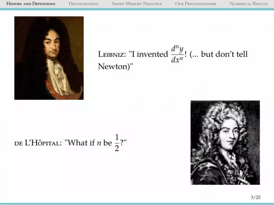
Leibniz: "I invented dnydxn
! (... but don’t tellNewton)"
de L’H0pital: "What if n be 12?"
3/25
History and Definitions Discretization Short–Memory Principle Our Preconditioner Numerical Results
Leibniz: "I invented dnydxn
! (... but don’t tellNewton)"
de L’H0pital: "What if n be 12?"
3/25

History and Definitions Discretization Short–Memory Principle Our Preconditioner Numerical Results
Leibniz: "[...] Thus it follows that d12 x will be
equal to x√dx : x. This is an apparent
paradox from which, one day, usefulconsequences will be drawn."
We are going to very briefly define some Fractional Derivativeoperators and show some of their discretizations.
4/25

History and Definitions Discretization Short–Memory Principle Our Preconditioner Numerical Results
Fractional DerivativesI Riemann-Liouville: given α > 0 and m ∈ Z+ such that
m− 1 < α ≤ m the left-side Riemann-Liouville fractionalderivative reads as
RLDαa,xy(x) =
1Γ(m− α)
(ddx
)m ∫ x
a
y(ξ)dξ(x − ξ)α−m+1 ,
while the right-side Riemann-Liouville fractionalderivative
RLDαx,by(x) =
1Γ(m− α)
(− ddx
)m ∫ b
x
y(ξ)dξ(ξ − x)α−m+1 ;
I Symmetric Riesz: given α > 0 and m ∈ Z+ such thatm− 1 < α ≤ m the symmetric Riesz derivative reads as
dαy(x)
d|x|α=
12(RLDα
a,x + RLDαx,b)
;
5/25

History and Definitions Discretization Short–Memory Principle Our Preconditioner Numerical Results
Fractional DerivativesA simple example
Function y(x) = x and its halfderivative.
We derive y(x) = x for α = 1/2, som = 1 we get for RLD
120,xx:
1Γ(1/2)
ddx
∫ x
0
ξdξ(x − ξ)1/2
=
1√π
ddx
[13(−2)
√x − ξ(ξ + 2x)
]x0
=
1√π
ddx
4x3/23 =
2√π
√x
And so we have proved that:
RLD120,xx =
2√π
√x
6/25

History and Definitions Discretization Short–Memory Principle Our Preconditioner Numerical Results
Overview
History and Definitions
Discretization
Short–Memory Principle
Our Preconditioner
Numerical Results
7/25

History and Definitions Discretization Short–Memory Principle Our Preconditioner Numerical Results
DiscretizationThere exists many discretization schemes for the FractionalDerivatives.To showcase the results of our work [Bertaccini and Durastante,2016a] we will select only one of the discretization we treat inthere:Shifted Grünwald–Letnikov DiscretizationGiven [a, b] ⊆ R, the order α and the nodes xk = a + khNk=0with step–size h = (b− a)/N and a shift p ∈ N with p ≥ 0:
RLDαa,xky(x) ≈ 1
hα
k+p∑j=0
(−1)j(α
j
)y((k − j)x), k = 0, . . . ,N,
RLDα
xk,by(x) ≈ 1hα
k+p∑j=0
(−1)j(α
j
)y((k + j)x), k = 0, . . . ,N.
8/25

History and Definitions Discretization Short–Memory Principle Our Preconditioner Numerical Results
Shifted Grünwald–Letnikov DiscretizationWe can represent the discretized operator in matrix form, e.g.,for p = 0, as:
B(α)L =
1hα
ω(α)0 0 0 . . . 0
ω(α)1
. . . . . . . . . ...... . . . . . . . . . ...... . . . . . . . . . 0
ω(α)N ω
(α)N−1 · · · ω
(α)1 ω
(α)0
, B(α)
U =(B(α)L
)T,
where the coefficients ω(α)j are defined as
ω(α)j = (−1)j
(α
j
), j = 0, 1, . . . ,N.
9/25

History and Definitions Discretization Short–Memory Principle Our Preconditioner Numerical Results
Overview
History and Definitions
Discretization
Short–Memory Principle
Our Preconditioner
Numerical Results
10/25

History and Definitions Discretization Short–Memory Principle Our Preconditioner Numerical Results
Short–Memory PrincipleLets look into some properties of the matrices B(α)
L and B(α)U :
1. They are Toeplitz matrices,2. The elements are such that:
|ω(α)j | = O(j−α−1), for j → +∞.
I Property (1) have been used to develop preconditionersfor iterative Toeplitz solvers, e.g., [Ng and Pan, 2010] and[Donatelli et al., 2016].
I Property (2) have been used to discard elements from B(α)L
and B(α)U and then use direct solvers, e.g., [Popolizio, 2013].
I Our proposalwill use also Property (2), but, instead ofexploiting it for the discretization matrix, will be used forits inverse.
11/25
History and Definitions Discretization Short–Memory Principle Our Preconditioner Numerical Results
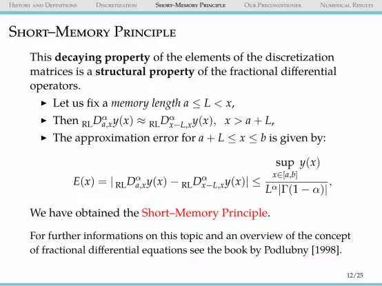
Short–Memory PrincipleThis decaying property of the elements of the discretizationmatrices is a structural property of the fractional differentialoperators.
I Let us fix a memory length a ≤ L < x,I Then RLDα
a,xy(x) ≈ RLDαx−L,xy(x), x > a + L,
I The approximation error for a + L ≤ x ≤ b is given by:
E(x) = | RLDαa,xy(x)− RLDα
x−L,xy(x)| ≤supx∈[a,b]
y(x)
Lα|Γ(1− α)|,
We have obtained the Short–Memory Principle.
For further informations on this topic and an overview of the conceptof fractional differential equations see the book by Podlubny [1998].
12/25

History and Definitions Discretization Short–Memory Principle Our Preconditioner Numerical Results
Overview
History and Definitions
Discretization
Short–Memory Principle
Our Preconditioner
Numerical Results
13/25

History and Definitions Discretization Short–Memory Principle Our Preconditioner Numerical Results
Building the preconditionerTo build the preconditioner we need only another ingredient:
I transport the decay of the element of the discretizationmatrix to a decay of the element of the inverse.
Theorem Jaffard [1990].Given an invertible matrix(A)h,k such that
|ah,k| ≤ C(1 + |h− k|)−s,
then its inverse A−1 sharesthe same property.Moreover, the class Qs ofsuch matrices is an algebra.
14/25

History and Definitions Discretization Short–Memory Principle Our Preconditioner Numerical Results
Building the preconditioner
We consider sparse approximations for non symmetricmatrices, the AINV preconditioner of the form:
A−1 ≈WD−1ZT .
withI W lower triangular,I Z upper triangular,I D diagonal.
Computed within a GPU architecture, see Bertaccini andFilippone [2016].You will see details on how to build and use this preconditionerin the next lesson of the course.
15/25
History and Definitions Discretization Short–Memory Principle Our Preconditioner Numerical Results
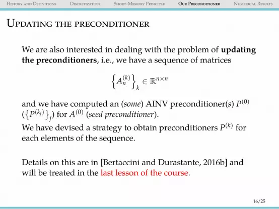
Updating the preconditioner
We are also interested in dealing with the problem of updatingthe preconditioners, i.e., we have a sequence of matrices
A(k)n
k∈ Rn×n
and we have computed an (some) AINV preconditioner(s) P(0)
(P(kj)
j) for A
(0) (seed preconditioner).We have devised a strategy to obtain preconditioners P(k) foreach elements of the sequence.
Details on this are in [Bertaccini and Durastante, 2016b] andwill be treated in the last lesson of the course.
16/25

History and Definitions Discretization Short–Memory Principle Our Preconditioner Numerical Results
Overview
History and Definitions
Discretization
Short–Memory Principle
Our Preconditioner
Numerical Results
17/25

History and Definitions Discretization Short–Memory Principle Our Preconditioner Numerical Results
Numerical ResultsSome technical details
Building and solution step have been executed on:I MATLAB R2015a,I Intel Core i7-4710HQ CPU with 2.50GHz × 8
Preconditioner have been computed on the GPU withI Cuda compilation tools, release 6.5, V6.5.12I Nvidia GeForce GTX 860MI CUSP library, [Dalton et al., 2014].
We are going to show only two of the experiments that are in[Bertaccini and Durastante, 2016a].
18/25

History and Definitions Discretization Short–Memory Principle Our Preconditioner Numerical Results
Numerical ResultsExperiment 1
We consider the following class of mixed problem containingboth integer and fractional order derivatives.
∂u(x, y, t)∂t
= ∇ · (< ((a(x), b(y)),∇u >) (x, y) ∈ Ω, t > 0,+L(α,β)u,
u(x, y, 0) = u0(x, y),u(x, y, t) = 0 (x, y) ∈ ∂Ω, t > 0.
,
where the fractional operator is given by
L(α,β)· , d(α)+ (x, y) RLDαa,x ·+d(α)− (x, y) RLDα
x,b·
+ d(β)+ (x, y) RLDβa,y ·+d(β)− (x, y) RLD
βy,b.
19/25
History and Definitions Discretization Short–Memory Principle Our Preconditioner Numerical Results
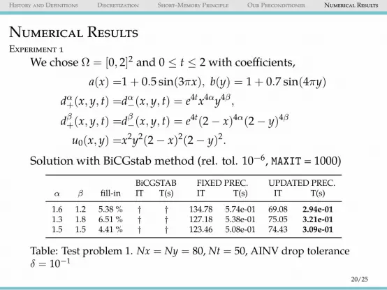
Numerical ResultsExperiment 1
We chose Ω = [0, 2]2 and 0 ≤ t ≤ 2 with coefficients,a(x) =1 + 0.5 sin(3πx), b(y) = 1 + 0.7 sin(4πy)
dα+(x, y, t) =dα−(x, y, t) = e4tx4αy4β,
dβ+(x, y, t) =dβ−(x, y, t) = e4t(2− x)4α(2− y)4β
u0(x, y) =x2y2(2− x)2(2− y)2.
Solution with BiCGstab method (rel. tol. 10−6, MAXIT = 1000)
BiCGSTAB FIXED PREC. UPDATED PREC.α β fill-in IT T(s) IT T(s) IT T(s)
1.6 1.2 5.38 % † † 134.78 5.74e-01 69.08 2.94e-011.3 1.8 6.51 % † † 127.18 5.38e-01 75.05 3.21e-011.5 1.5 4.41 % † † 123.46 5.08e-01 74.43 3.09e-01
Table: Test problem 1. Nx = Ny = 80, Nt = 50, AINV drop toleranceδ = 10−1
20/25

History and Definitions Discretization Short–Memory Principle Our Preconditioner Numerical Results
Numerical ResultsExperiment 2
As second test case we consider the case of a pure fractionaldiffusion equation:
ut(x, t) = K ∂α
∂|x|αu(x, t), t ∈ [0,T], x ∈ [0, π], α ∈ (1, 2),
u(x, 0) = x2(π − x),u(0, t) = u(π, t) = 0.
,
whose analytical solution, on an infinite domain, is given by
u(x, t) =
+∞∑n=1
(8n3
(−1)n+1 − 4n3
)sin(nx) exp (−nαKt) .
For this case we will use the AINV approximate inverse of thediscretized operator as a true inverse to build a direct methodthat will use only matrix–vector product.
21/25

History and Definitions Discretization Short–Memory Principle Our Preconditioner Numerical Results
Numerical ResultsExperiment 2
Complete Banded Direct
Type α K T(s) err. T(s) err. T(s) err.
C 1.8 0.25 9.39 2.42e-02 0.93 4.29e-02 0.08 4.24e-020.16 1.64e-02
O 1.8 0.25 9.27 3.03e-02 0.77 4.29e-02 0.09 4.43e-020.11 3.33e-02
O* 1.5 0.75 8.64 7.43e-02 0.58 2.62e-01 0.10 7.66e-02O* 1.2 1.25 9.43 5.27e-01 0.63 2.78e-01 0.06 2.73e-01C* 1.8 1.50 8.66 1.15e-01 1.05 1.53e-01 0.16 1.83e-01
Table: Timings and averages of the 2-norm of the errors over all time steps. C: discretization using the half-sumof Caputo derivatives, O: Ortigueira discretization, while C∗ and O∗ : our method applied to the bandedapproximation of the discretization matrix. Column Complete: the reference solution is used with the standarddiscretization matrix. Column Banded: the Short–memory principle is applied to the discretization of the operator.Column Direct: our approach using the approximate inverses. All the discretizations use N = 210 .
22/25

References
References I
Daniele Bertaccini and Fabio Durastante. Solving mixed classical andfractional partial differential equations using short–memory principle andapproximate inverses. Numerical Algorithms, pages 1–22, 2016a. ISSN1572-9265. doi: 10.1007/s11075-016-0186-8. URLhttp://dx.doi.org/10.1007/s11075-016-0186-8.
Daniele Bertaccini and Fabio Durastante. Interpolating preconditioners forthe solution of sequence of linear systems. Comput. Math. Appl., 72(4):1118–1130, August 2016b. ISSN 0898-1221. doi:10.1016/j.camwa.2016.06.023. URLhttp://dx.doi.org/10.1016/j.camwa.2016.06.023.
Daniele Bertaccini and Salvatore Filippone. Sparse approximate inversepreconditioners on high performance gpu platforms. Comp. Math. Appl., 71(3):693–711, 2016.
Steven Dalton, Nathan Bell, Luke Olson, and Michael Garland. Cusp: Genericparallel algorithms for sparse matrix and graph computations, 2014. URLhttp://cusplibrary.github.io/. Version 0.5.0.
24/25

References
References II
Marco Donatelli, Mariarosa Mazza, and Stefano Serra-Capizzano. Spectralanalysis and structure preserving preconditioners for fractional diffusionequations. Journal of Computational Physics, 307:262–279, 2016.
Stephane Jaffard. Propriétés des matrices «bien localisées» près de leurdiagonale et quelques applications. In Ann. I. H. Poincare-An, volume 7,pages 461–476, 1990.
Michael K Ng and Jianyu Pan. Approximate inverse circulant–plus–diagonalpreconditioners for Toeplitz–plus–diagonal matrices. SIAM J. Sci. Comput.,32(3):1442–1464, 2010.
Igor Podlubny. Fractional differential equations: an introduction to fractionalderivatives, fractional differential equations, to methods of their solution and someof their applications, volume 198. Academic press, 1998.
Marina Popolizio. A matrix approach for partial differential equations withRiesz space fractional derivatives. Eur. Phys. J-Spec. Top., 222(8):1975–1985,2013.
25/25