smta5304.pdf - sathyabama
TRANSCRIPT
SCHOOL OF SCIENCE AND HUMANITIES
DEPARTMENT OF MATHEMATICS
SMTA5304 ADVANCED NUMERICAL METHODS
Course Outcomes
At the end of the course, the student will be able to:
CO1 Recall transcendental and polynomial equations and solve it by different methods such as
Chebyshev Method, Multipoint Iteration Methods, Beirge Vieta Method, Baristow Method, Graeffe’s
root Squaring Method to the Second degree equation
CO2 Summarize the different method for solving eigen value, eigen vector and inverse of A-1 for system
of algebraic equations
CO3 Choose appropriate interpolation formula such as Lagrange, Newton’s Bivariate interpolation etc
and solve problems based on it.
CO4 Analyze trapezoidal and Simpsons rule for double integration
CO5 Evaluate the ordinary differential equations by numerical methods such as Euler method, Runge
Kutta method.
CO6 Formulate Numerical integration based on GaussLegendreandGauss ChebyshevIntegration
Methods
Syllabus
UNIT 1 Transcendental and Polynomial Equations
Transcendental and Polynomial Equations: Iteration method based on Second degree equations: The
Chelyshev Method – Multipoint Iteration Methods – The Bridge Vieta Method – The Baristow Method
– Graeffe’sroot Square Method.
UNIT 2 The System of Algebraic Equations and Eigen Value Problems
The System of Algebraic Equations and Eigen Value Problems: Iteration Methods-Jacobi Method,
Guass Seidel Method, Successive Over Relaxation Method – Iterative Method for A-1 – Eigen Values
and Eigen Vectors – Jacobi Method for symmetric Matrices , Power Method.
UNIT 3 Interpolation and Approximation
Interpolation and Approximation – Hermite Interpolation – Piecewise cubic Interpolation and cubic
Spline interpolation – Bivariate interpolation – Lagrange and Newton’s Bivariate interpolation – Least
Square approximation – Gram-Schmidt Orthogonalizing Process.

UNIT 4 Differentiation and Integration
Differentiation and Integration; Numerical Differentiation – Methods Based on Interpolation – Partial
Differentiation – Numerical Integration – Methods Based on Interpolation – Methods Based on
Undetermined Coefficients – Gauss Quadrature methods - Gauss Legendre and Gauss Chebyshev
Integration Methods – Double Integration – Trapezoidal and Simpson’s Rule – Simple Problems.
UNIT 5 Ordinary Differential Equations
Ordinary Differential Equations: Numerical Methods – Euler Method – Backward Euler Method – Mid-
Point Method – Rungekutta Methods – Implicit RungeKutta Methods – Predictor – Corrector Methods.

UNIT – I - ADVANCED NUMERICAL METHODS – SMTA5304
UNIT I
Transcendental and Polynomial Equations
Polynomial
An equation formed with variables, exponents, and coefficients together with
operations and an equal sign is called a polynomial equation.
Examples
( )p x ax b= +1
0 1( ) n n
np x a x a x a−= + +−−−+ ( )p x ax b= +
Equation:
An equation is a mathematical statement with an 'equal to' symbol between two
algebraic expressions that have equal values.
2 5 1x + =
monomial /linear equation
Binomial /quadratic equation
Trinomial /Cubic equation
transcendental equations
An equation containing transcendental functions (for example, exponential,
logarithmic, trigonometric, or inverse trigonometric functions) of the unknowns.
Examples of transcendental equations are sin logx x x+ = and 2 log arccosx x x− = Note
Elementary transcendental functions are the exponential, logarithmic, trigonometric,
reverse trigonometric, and hyperbolic functions
iterative method
An iterative method is a mathematical procedure that uses an initial value to generate
a sequence of improving approximate solutions for a class of problems, in which the
n-th approximation is derived from the previous ones.
Chebyshev polynomial Approximation
Chebyshev method:
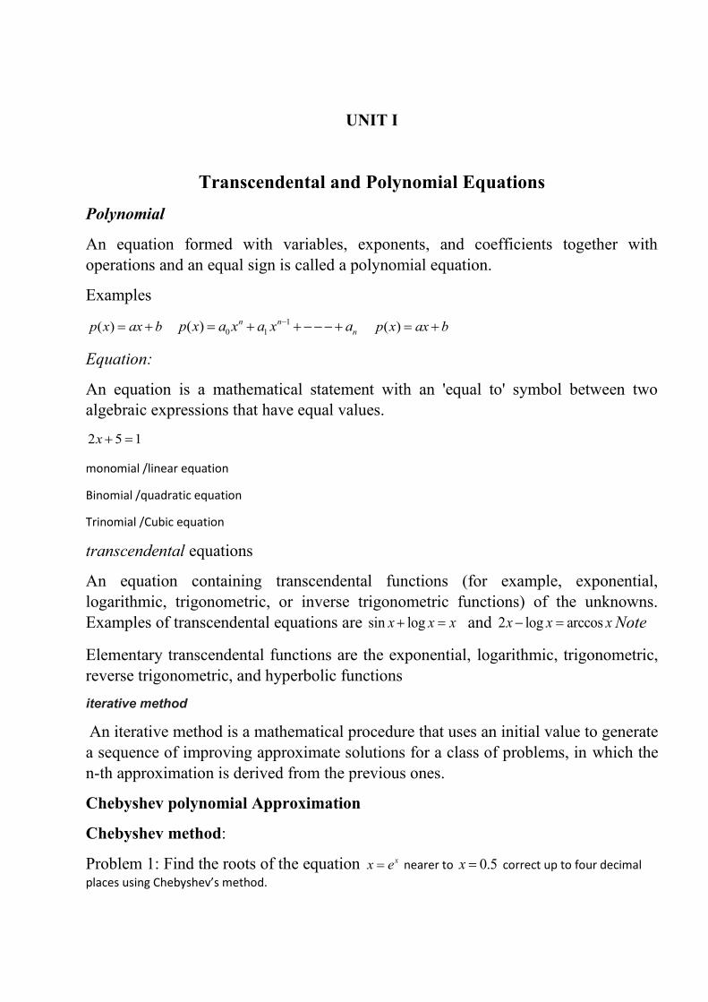
Problem 1: Find the roots of the equation xx e= nearer to 0.5x = correct up to four decimal
places using Chebyshev’s method.
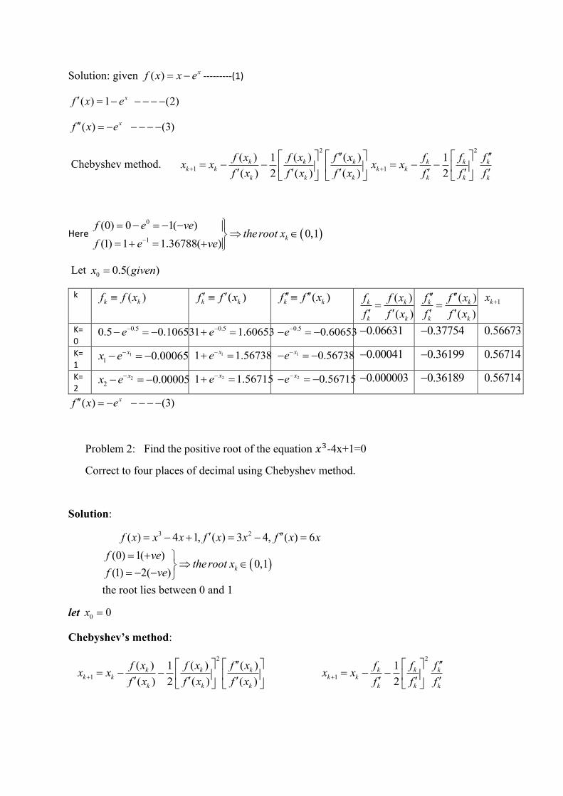
Solution: given ( ) xf x x e= − ---------(1)
( ) 1 (2)xf x e = − − − − −
( ) (3)xf x e = − − − − −
Chebyshev method.
2
1
( ) ( ) ( )1
( ) 2 ( ) ( )
k k kk k
k k k
f x f x f xx x
f x f x f x+
= − −
2
1
1
2
k k kk k
k k k
f f fx x
f f f+
= − −
Here ( )0
1
(0) 0 1( )0,1
(1) 1 1.36788( )k
f e vetheroot x
f e ve−
= − = − −
= + = +
Let 0 0.5( )x given=
k ( )k kf f x ( )k kf f x ( )k kf f x ( )
( )
k k
k k
f f x
f f x=
( )
( )
k k
k k
f f x
f f x
=
1kx +
K=0
0.50.5 0.10653e−− = − 0.51 1.60653e−+ =
0.5 0.60653e−− = − 0.06631− 0.37754− 0.56673
K=1
1
1 0.00065x
x e−
− = − 11 1.56738x
e−
+ = 1 0.56738x
e−
− = − 0.00041− 0.36199− 0.56714
K=2
2
2 0.00005xx e−− = − 21 1.56715
xe−
+ = 2 0.56715x
e−
− = − 0.000003− 0.36189− 0.56714
( ) (3)xf x e = − − − − −
Problem 2: Find the positive root of the equation 𝑥3-4x+1=0
Correct to four places of decimal using Chebyshev method.
Solution:
( )
3 2 ( ) 4 1, ( ) 3 4, ( ) 6
(0) 1( )0,1
(1) 2( )k
f x x x f x x f x x
f vethe root x
f ve
= − + = − =
= +
= − −
the root lies between 0 and 1
let 0 0x =
Chebyshev’s method:
2
1
( ) ( ) ( )1
( ) 2 ( ) ( )
k k kk k
k k k
f x f x f xx x
f x f x f x+
= − −
2
1
1
2
k k kk k
k k k
f f fx x
f f f+
= − −
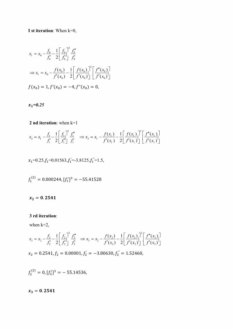
I st iteration: When k=0,
2
0 0 01 0
0 0 0
1
2
f f fx x
f f f
= − −
2
0 0 01 0
0 0 0
( ) ( ) ( )1
( ) 2 ( ) ( )
f x f x f xx x
f x f x f x
= − −
𝑓(𝑥0) = 1, 𝑓’(𝑥0) = −4, 𝑓’’(𝑥0) = 0,
𝒙𝟏=0.25
2 nd iteration: when k=1
2
1 1 12 1
1 1 1
1
2
f f fx x
f f f
= − −
2
1 1 12 1
1 1 1
( ) ( ) ( )1
( ) 2 ( ) ( )
f x f x f xx x
f x f x f x
= − −
𝑥1=0.25,𝑓1=0.01563,𝑓1′=-3.8125,𝑓1
′′=1.5,
𝑓1(2)
= 0.000244, [𝑓1′]3 = −55.41528
𝒙𝟐 = 𝟎. 𝟐𝟓𝟒𝟏
3 rd iteration:
when k=2,
2
2 2 23 2
2 2 2
1
2
f f fx x
f f f
= − −
2
2 2 23 2
2 2 2
( ) ( ) ( )1
( ) 2 ( ) ( )
f x f x f xx x
f x f x f x
= − −
𝑥2 = 0.2541, 𝑓2 = 0.00001, 𝑓2′ = −3.80630, 𝑓2
′′ = 1.52460,
𝑓2(2)
= 0, [𝑓2′]3 = − 55.14536,
𝒙𝟑 = 𝟎. 𝟐𝟓𝟒𝟏
Problem 3: Using Chebyshev’s method find the root of the equation f(x)=cos x - x𝑒𝑥=0, correct to 6
decimal places. [Ans=0.517757]
Problem 4: Determine 2 iteration of Chebyshev’s method to find an approximate value of
1/ 7
Multipoint Iteration:
Method 1:
Step 1: * * * *
1 1 1 1
( )1 1, , ( )
2 2 ( )
k kk k k k k k
k k
f f xx x or x x f f x
f f x+ + + += − = − =
step 2: 1 *
1
( )
( )
kk k
k
f xx x
f x+
+
= −
𝑥𝑘+1∗ = 𝑥𝑘 −
𝑓𝑘
2𝑓𝑘′ ; 𝑥𝑘+1 =
𝑓𝑘
𝑓𝑘+1∗′ ; 𝑓𝑘+1∗
′ = 𝑓 ′(𝑥𝑘+1∗ )
Method 2:
Step1: * * * *
1 1 1 1
( ), , ( )
( )
k kk k k k k k
k k
f f xx x or x x f f x
f f x+ + + += − = − =
step 2:
** 1
1 1
( )
( )
kk k
k
f xx x
f x
++ += −
𝑥𝑘+1∗ = 𝑥𝑘 −
𝑓𝑘
𝑓𝑘′ ; 𝑥𝑘+1 = 𝑥𝑘+1
∗ − 𝑓𝑘+1′
𝑓𝑘′
; 𝑓𝑘+1∗ = 𝑓(𝑥𝑘+1
∗ )
Problem:
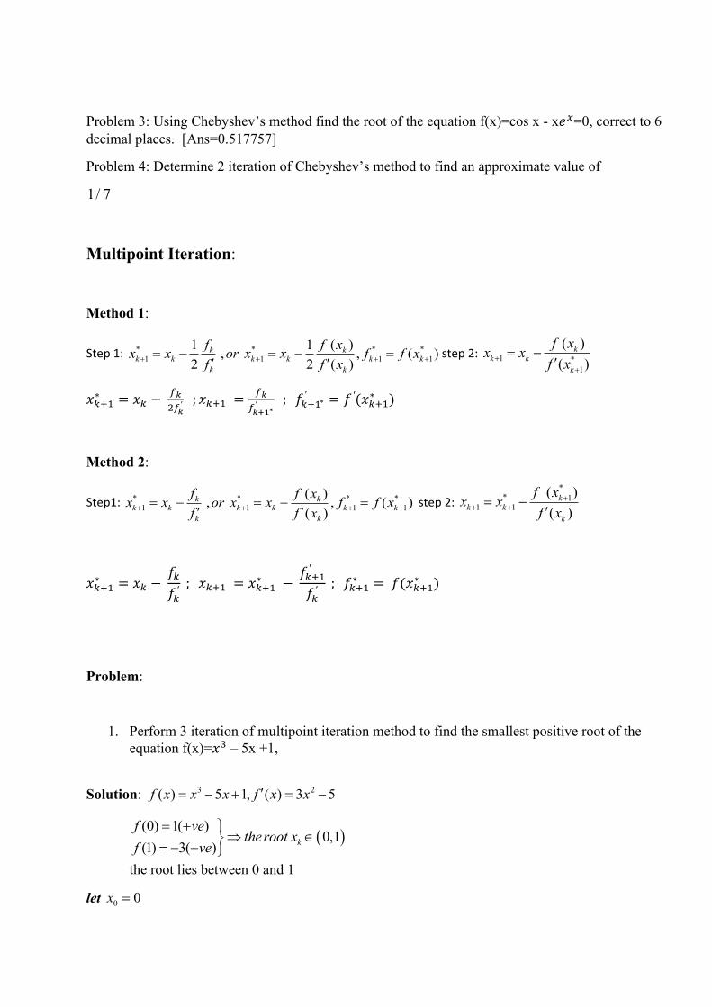
1. Perform 3 iteration of multipoint iteration method to find the smallest positive root of the
equation f(x)=𝑥3 – 5x +1,
Solution: 3 2 ( ) 5 1, ( ) 3 5f x x x f x x= − + = −
( )(0) 1( )
0,1 (1) 3( )
k
f vethe root x
f ve
= +
= − −
the root lies between 0 and 1
let 0 0x =
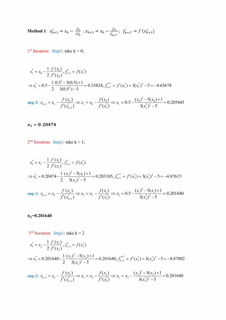
Method 1: 𝑥𝑘+1∗ = 𝑥𝑘 −
𝑓𝑘
2𝑓𝑘′ ; 𝑥𝑘+1 = 𝑥𝑘 −
𝑓𝑘
𝑓𝑘+1∗′ ; 𝑓𝑘+1∗
′ = 𝑓 ′(𝑥𝑘+1∗ )
1st Iteration: Step1: take k = 0;
(1)
* * *01 0 1 1
0
3* * * * 2
1 1 1 12
( )1, ( )
2 ( )
1 0.5 5(0.5) 10.5 0.33824, ( ) 3( ) 5 4.65678
2 3(0.5 ) 5
k
k
f xx x f f x
f x
x f f x x
+
+
= − =
− + = − = = = − = −
−
step 2: 3
0 0 01 1 0 1* * * 2
1 1 1
( ) ( ) ( ) 5( ) 10.5 0.205445
( ) ( ) 3( ) 5
kk k
k
f x f x x xx x x x x
f x f x x+
+
− += − = − = − =
−
𝒙𝟏 = 𝟎. 𝟐𝟎𝟒𝟕𝟒
2nd Iteration: Step1: take k = 1;
(1)
* * *12 1 1 2
1
3* * * * 21 12 1 2 22
1
( )1, ( )
2 ( )
( ) 5( ) 110.20474 0.203185, ( ) 3( ) 5 4.87615
2 3( ) 5
k
k
f xx x f f x
f x
x xx f f x x
x
+
+
= − =
− + = − = = = − = −
−
step 2: 3
1 1 11 2 1 2* * * 2
1 2 2
( ) ( ) ( ) 5( ) 10.5 0.201640
( ) ( ) 3( ) 5
kk k
k
f x f x x xx x x x x
f x f x x+
+
− += − = − = − =
−
𝐱𝟐=0.201640
3rd Iteration: Step1: take k = 2
(1)
* * *23 2 1 3
2
3* * * * 22 23 1 3 32
2
( )1, ( )
2 ( )
( ) 5( ) 110.201640 0.201640, ( ) 3( ) 5 4.87802
2 3( ) 5
k
k
f xx x f f x
f x
x xx f f x x
x
+
+
= − =
− + = − = = = − = −
−
step 2: 3
2 2 21 3 2 3 2* * * 2
1 3 3
( ) ( ) ( ) 5( ) 10.201640
( ) ( ) 3( ) 5
kk k
k
f x f x x xx x x x x x
f x f x x+
+
− += − = − = − =
−
𝒙𝟑 = 𝟎. 𝟐𝟎𝟏𝟔𝟒𝟎
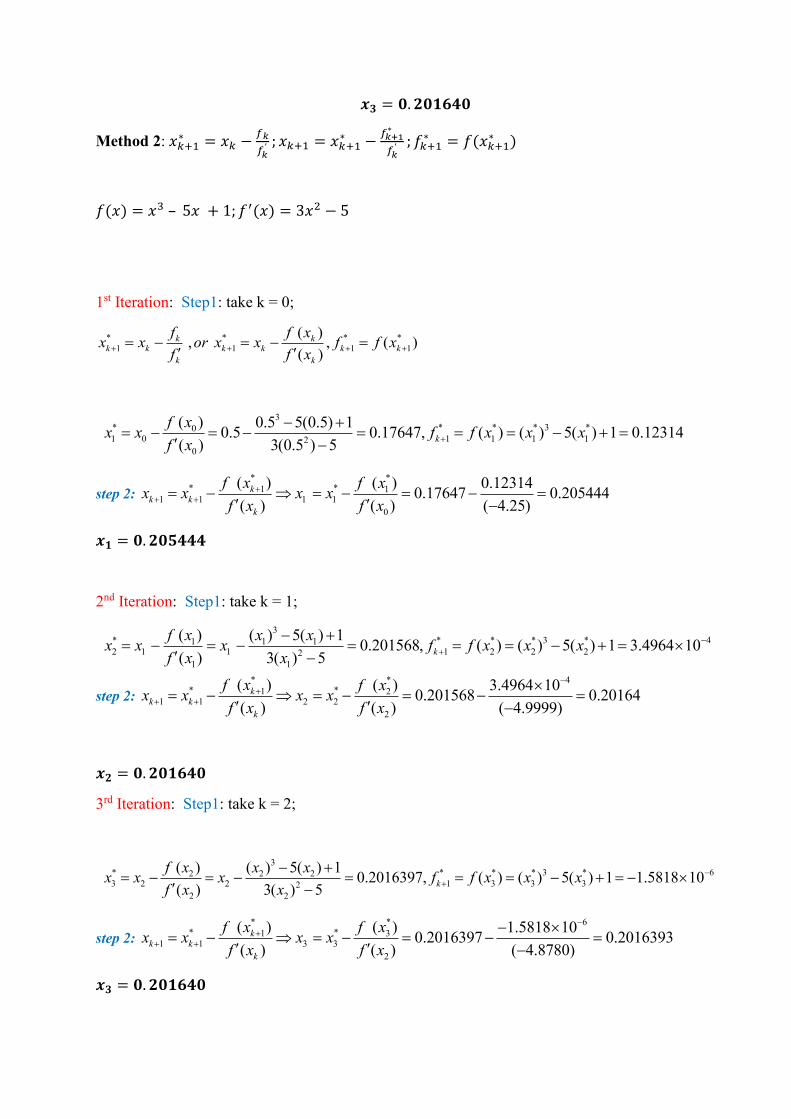
Method 2: 𝑥𝑘+1∗ = 𝑥𝑘 −
𝑓𝑘
𝑓𝑘′ ; 𝑥𝑘+1 = 𝑥𝑘+1
∗ −𝑓𝑘+1
∗
𝑓𝑘′ ; 𝑓𝑘+1
∗ = 𝑓(𝑥𝑘+1∗ )
𝑓(𝑥) = 𝑥3 – 5𝑥 + 1; 𝑓′(𝑥) = 3𝑥2 − 5
1st Iteration: Step1: take k = 0;
* * * *
1 1 1 1
( ), , ( )
( )
k kk k k k k k
k k
f f xx x or x x f f x
f f x+ + + += − = − =
3* * * * 3 *01 0 1 1 1 12
0
( ) 0.5 5(0.5) 10.5 0.17647, ( ) ( ) 5( ) 1 0.12314
( ) 3(0.5 ) 5k
f xx x f f x x x
f x+
− += − = − = = = − + =
−
step 2:
* ** *1 1
1 1 1 1
0
( ) ( ) 0.123140.17647 0.205444
( ) ( ) ( 4.25)
kk k
k
f x f xx x x x
f x f x
++ += − = − = − =
−
𝒙𝟏 = 𝟎. 𝟐𝟎𝟓𝟒𝟒𝟒
2nd Iteration: Step1: take k = 1;
3* * * * 3 * 41 1 12 1 1 1 2 2 22
1 1
( ) ( ) 5( ) 10.201568, ( ) ( ) 5( ) 1 3.4964 10
( ) 3( ) 5k
f x x xx x x f f x x x
f x x
−
+
− += − = − = = = − + =
−
step 2:
* * 4* *1 2
1 1 2 2
2
( ) ( ) 3.4964 100.201568 0.20164
( ) ( ) ( 4.9999)
kk k
k
f x f xx x x x
f x f x
−
++ +
= − = − = − =
−
𝒙𝟐 = 𝟎. 𝟐𝟎𝟏𝟔𝟒𝟎
3rd Iteration: Step1: take k = 2;
3* * * * 3 * 62 2 23 2 2 1 3 3 32
2 2
( ) ( ) 5( ) 10.2016397, ( ) ( ) 5( ) 1 1.5818 10
( ) 3( ) 5k
f x x xx x x f f x x x
f x x
−
+
− += − = − = = = − + = −
−
step 2:
* * 6* *1 3
1 1 3 3
2
( ) ( ) 1.5818 100.2016397 0.2016393
( ) ( ) ( 4.8780)
kk k
k
f x f xx x x x
f x f x
−
++ +
− = − = − = − =
−
𝒙𝟑 = 𝟎. 𝟐𝟎𝟏𝟔𝟒𝟎
0x= 3 5 1
( )k
x x
f x
− +
=
23 5
( )k
x
f x
−
=
*
1
( )1
2 ( )
kk k
k
f xx x
f x+ = −
*
1( )kf x +
1 *
1
( )
( )
kk k
k
f xx x
f x+
+
= −
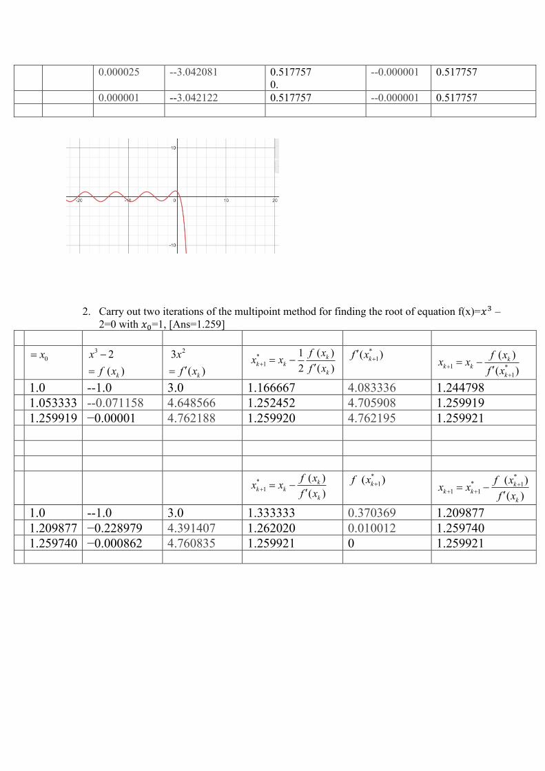
1.0 --1.0 3.0 1.166667 4.083336 1.244798 1.053333 --0.071158 4.648566 1.252452 4.705908 1.259919 1.259919 −0.00001 4.762188 1.259920 4.762195 1.259921 *
1
( )
( )
kk k
k
f xx x
f x+ = −
*
1( )kf x + *
* 11 1
( )
( )
kk k
k
f xx x
f x
++ += −
1.0 --1.0 3.0 1.333333 0.370369 1.209877 1.209877 −0.228979 4.391407 1.262020 0.010012 1.259740 1.259740 −0.000862 4.760835 1.259921 0 1.259921
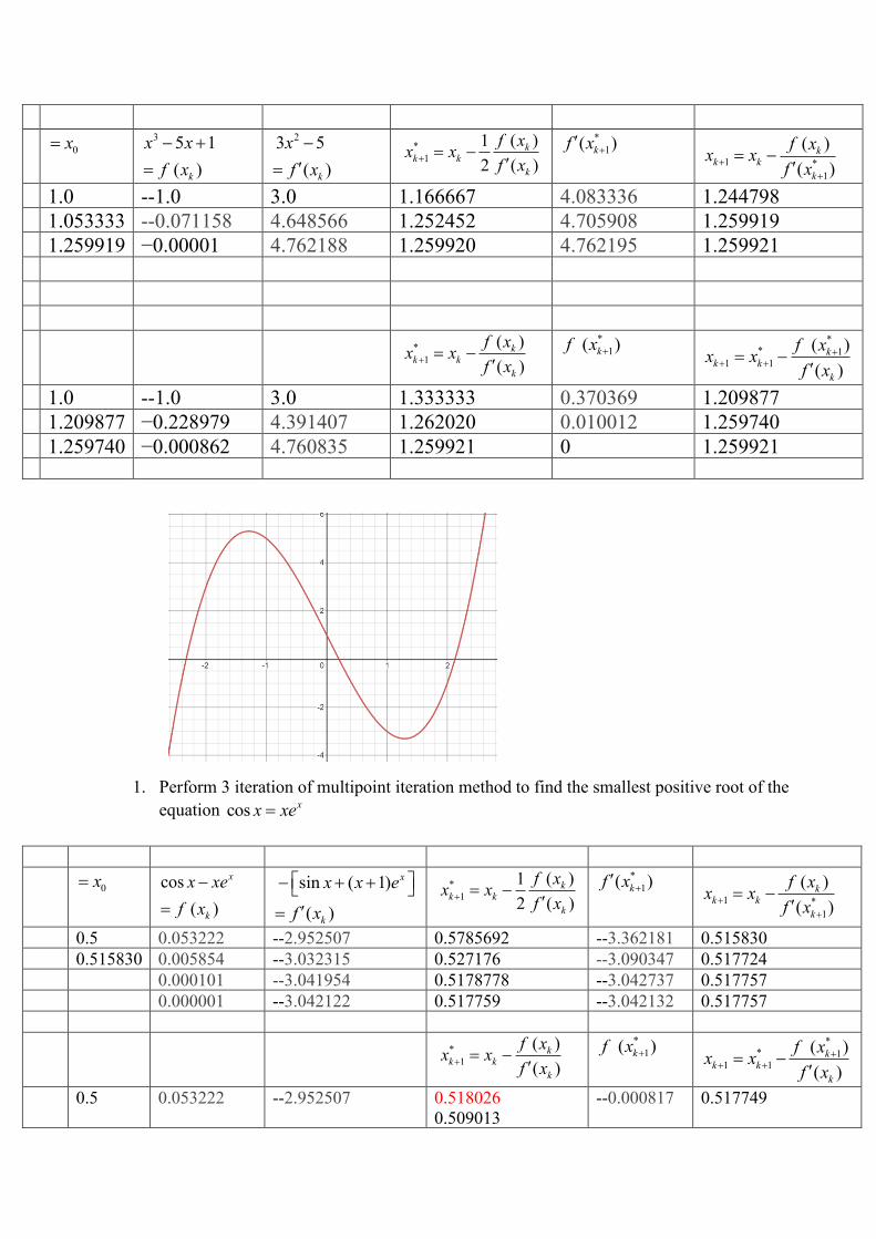
1. Perform 3 iteration of multipoint iteration method to find the smallest positive root of the
equation cos xx xe=
0x= cos
( )
x
k
x xe
f x
−
=
sin ( 1)
( )
x
k
x x e
f x
− + +
=
*
1
( )1
2 ( )
kk k
k
f xx x
f x+ = −
*
1( )kf x +
1 *
1
( )
( )
kk k
k
f xx x
f x+
+
= −
0.5 0.053222 --2.952507 0.5785692 --3.362181 0.515830
0.515830 0.005854 --3.032315 0.527176 --3.090347 0.517724
0.000101 --3.041954 0.5178778 --3.042737 0.517757
0.000001 --3.042122 0.517759 --3.042132 0.517757
*
1
( )
( )
kk k
k
f xx x
f x+ = −
*
1( )kf x + *
* 11 1
( )
( )
kk k
k
f xx x
f x
++ += −
0.5 0.053222 --2.952507 0.518026
0.509013
--0.000817 0.517749
0.000025 --3.042081 0.517757
0.
--0.000001 0.517757
0.000001 --3.042122 0.517757 --0.000001 0.517757
2. Carry out two iterations of the multipoint method for finding the root of equation f(x)=𝑥3 –
2=0 with 𝑥0=1, [Ans=1.259]
0x= 3 2
( )k
x
f x
−
=
23
( )k
x
f x=
*
1
( )1
2 ( )
kk k
k
f xx x
f x+ = −
*
1( )kf x +
1 *
1
( )
( )
kk k
k
f xx x
f x+
+
= −
1.0 --1.0 3.0 1.166667 4.083336 1.244798 1.053333 --0.071158 4.648566 1.252452 4.705908 1.259919 1.259919 −0.00001 4.762188 1.259920 4.762195 1.259921 *
1
( )
( )
kk k
k
f xx x
f x+ = −
*
1( )kf x + *
* 11 1
( )
( )
kk k
k
f xx x
f x
++ += −
1.0 --1.0 3.0 1.333333 0.370369 1.209877 1.209877 −0.228979 4.391407 1.262020 0.010012 1.259740 1.259740 −0.000862 4.760835 1.259921 0 1.259921

Birge vieta method:
𝒑𝒌+𝟏 = 𝒑𝒌 −𝒃𝒏
𝒄𝒏−𝟏 ;
The deflated polynomial is arrived from the above equation in the following manner
𝑎0𝑥𝑛 + 𝑎1𝑥
𝑛−1 + 𝑎2𝑥𝑛−2 + ⋯+ 𝑎𝑛 = (𝑥 − 𝑝)(𝑏0𝑥
𝑛−1 + 𝑏2𝑥𝑛−2 + ⋯+ 𝑏𝑛)+ R where R is the
residual depends on p , 1( )n n n nR p p b a pb −= = = +
Therefore, the deflated polynomial is
𝑄𝑛−1(𝑥) = (𝑏0𝑥𝑛−1 + 𝑏2𝑥
𝑛−2 + ⋯+ 𝑏𝑛)
Problems:
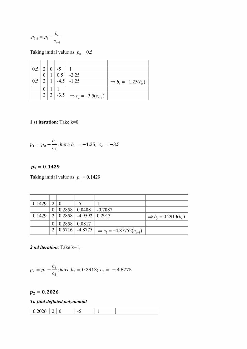
Problem 1:Use synthetic division to perform 2 iteration of the Birge-Vieta method to find the
smallest positive root of the polynomial 𝑝3(𝑥) = 2𝑥3 − 5𝑥 + 1 = 0,and hence find the deflated
polynomial.
Solution: Given
𝑝3(𝑥) = 2𝑥3 − 5𝑥 + 1 = 0, n = 3, 𝒑𝒌+𝟏 = 𝒑𝒌 −𝒃𝒏
𝒄𝒏−𝟏
1
1
nk k
n
bp p
c+
−
= −
Taking initial value as 0 0.5p =
0.5 2 0 -5 1
0 1 0.5 -2.25
0.5 2 1 -4.5 -1.25 3 1.25( )nb b = −
0 1 1
2 2 -3.5 2 13.5( )nc c − = −
1 st iteration: Take k=0,
𝑝1 = 𝑝0 −𝑏3
𝑐2; ℎ𝑒𝑟𝑒 𝑏3 = −1.25; 𝑐2 = −3.5
𝒑𝟏 = 𝟎. 𝟏𝟒𝟐𝟗
Taking initial value as 1 0.1429p =
0.1429 2 0 -5 1
0 0.2858 0.0408 -0.7087
0.1429 2 0.2858 -4.9592 0.2913 3 0.2913( )nb b =
0 0.2858 0.0817
2 0.5716 -4.8775 2 14.87752( )nc c − = −
2 nd iteration: Take k=1,
𝑝2 = 𝑝1 −𝑏3
𝑐2; ℎ𝑒𝑟𝑒 𝑏3 = 0.2913; 𝑐2 = − 4.8775
𝒑𝟐 = 𝟎. 𝟐𝟎𝟐𝟔
To find deflated polynomial
0.2026 2 0 -5 1
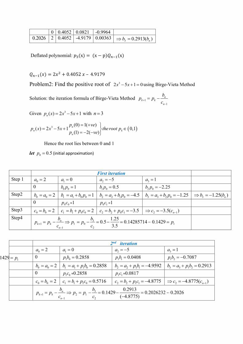
0 0.4052 0.0821 -0.9964
0.2026 2 0.4052 -4.9179 0.00363 3 0.2913( )nb b =
Deflated polynomial: 𝑝3(x) = (x − p)𝑄𝑛−1(x)
𝑄𝑛−1(𝑥) = 2𝑥2 + 0.4052 𝑥 – 4.9179
Problem2: Find the positive root of 32 5 1 0x x− + = using Birge-Vieta Method
Solution: the iteration formula of Birge-Vieta Method 1
1
nk k
n
bp p
c+
−
= −
Given 3( ) 2 5 1np x x x= − + with 3n =
( )3(0) 1( )
( ) 2 5 1 0,1 (1) 2( )
n
n k
n
p vep x x x the root p
p ve
= + = − +
= − −
Hence the root lies between 0 and 1
let 0 0.5p = (initial approximation)
First iteration
Step 1 0 2a = 1 0a = 2 5a = − 3 1a =
0 0 0 1b p = 1 0 0.5b p = 2 0 2.25b p = −
Step2 0 0 2b a= =
1 1 0 0 1b a b p= + = 2 2 1 0 4.5b a b p= + = −
3 3 2 0 1.25b a b p= + = − 3 1.25( )nb b = −
0 0 0p c =1 0 1p c =1
Step3 0 0 2c b= =
1 1 0 0 2c b p c= + = 2 2 0 1 3.5c b p c= + = −
2 13.5( )nc c − = −
Step4 3
1 1 0 1
1 2
1.250.5 0.14285714 0.1429
3.5
nk k
n
b bp p p p p
c c+
−
= − = − = − = =
2nd iteration
Step 1 0 2a = 1 0a = 2 5a = − 3 1a =
10.1429 p= 0 1 0 0.2858p b = 1 1 0.0408p b = 1 2 0.7087p b = −
Step2 0 0 2b a= =
1 1 1 0 0.2858b a p b= + = 2 2 1 1 4.9592b a p b= + = −
3 3 1 2 0.2913b a p b= + =
0 1 0p c =0.2858 1 1p c =0.0817
Step3 0 0 2c b= =
1 1 1 0 0.5716c b p c= + = 2 2 1 1 4.8775c b p c= + = −
2 14.8775( )nc c − = −
Step4 3
1 2 1
1 2
0.29130.1429 0.2026232 0.2026
( 4.8775)
nk k
n
b bp p p p
c c+
−
= − = − = − =−
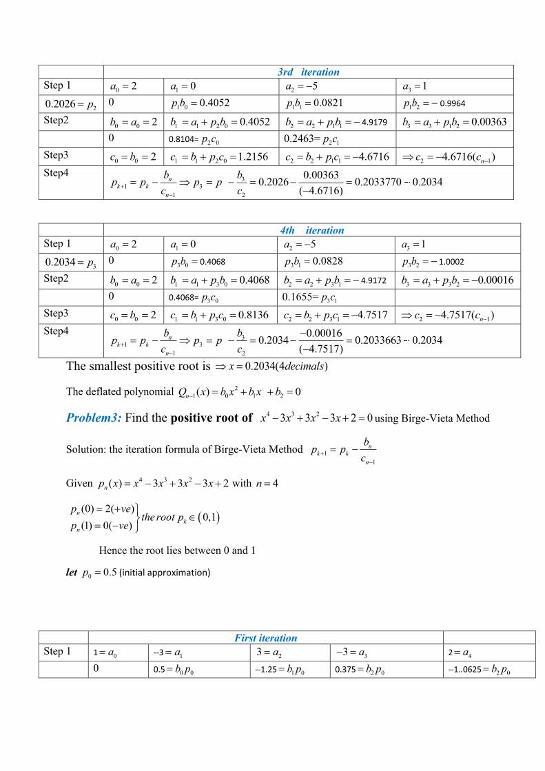
3rd iteration
Step 1 0 2a = 1 0a = 2 5a = − 3 1a =
20.2026 p= 0 1 0 0.4052p b = 1 1 0.0821p b = 1 2p b = − 0.9964
Step2 0 0 2b a= =
1 1 2 0 0.4052b a p b= + = 2 2 1 1b a p b= + = − 4.9179
3 3 1 2 0.00363b a p b= + =
0 0.8104= 2 0p c 0.2463= 2 1p c
Step3 0 0 2c b= =
1 1 2 0 1.2156c b p c= + = 2 2 1 1 4.6716c b p c= + = −
2 14.6716( )nc c − = −
Step4 3
1 3
1 2
0.003630.2026 0.2033770 0.2034
( 4.6716)
nk k
n
b bp p p p
c c+
−
= − = − = − =−
4th iteration
Step 1 0 2a = 1 0a = 2 5a = − 3 1a =
30.2034 p= 0 3 0p b = 0.4068 3 1 0.0828p b = 3 2p b = − 1.0002
Step2 0 0 2b a= =
1 1 3 0 0.4068b a p b= + = 2 2 3 1b a p b= + = − 4.9172
3 3 3 2 0.00016b a p b= + = −
0 0.4068= 3 0p c 0.1655= 3 1p c
Step3 0 0 2c b= =
1 1 3 0 0.8136c b p c= + = 2 2 3 1 4.7517c b p c= + = −
2 14.7517( )nc c − = −
Step4 3
1 3
1 2
0.000160.2034 0.2033663 0.2034
( 4.7517)
nk k
n
b bp p p p
c c+
−
−= − = − = − =
−
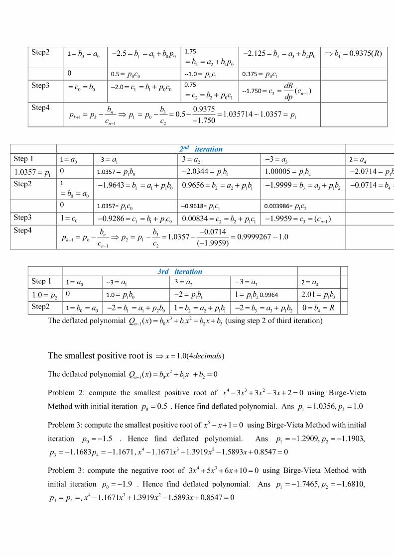
The smallest positive root is 0.2034(4 )x decimals =
The deflated polynomial 2
1 0 1 2( ) 0nQ x b x b x b− = + + =
Problem3: Find the positive root of 4 3 23 3 3 2 0x x x x− + − + = using Birge-Vieta Method
Solution: the iteration formula of Birge-Vieta Method 1
1
nk k
n
bp p
c+
−
= −
Given 4 3 2( ) 3 3 3 2np x x x x x= − + − + with 4n =
( )(0) 2( )
0,1 (1) 0( )
n
k
n
p vethe root p
p ve
= +
= −
Hence the root lies between 0 and 1
let 0 0.5p = (initial approximation)
First iteration
Step 1 1 0a= --3 1a= 23 a= 33 a− = 2 4a=
0 0.5 0 0b p= --1.25 1 0b p= 0.375 2 0b p= --1..0625 2 0b p=
Step2 10 0b a= =
1 1 0 02.5 b a b p− = = + 1.75
2 2 1 0b a b p= = + 3 3 2 02.125 b a b p− = = +
4 0.9375( )b R =
0 0.5 0 0p c= --1.0 0 1p c= 0.375 0 1p c=
Step3 0 0c b= = --2.0
1 1 0 0c b p c= = + 0.75
2 2 0 1c b p c= = + --1.750 3 1( )n
dRc c
dp−= =
Step4 3
1 1 0 1
1 2
0.93750.5 1.035714 1.0357
1.750
nk k
n
b bp p p p p
c c+
−
= − = − = − = =−
2nd iteration
Step 1 1 0a= --3 1a= 23 a= 33 a− = 2 4a=
11.0357 p= 0 1.0357 1 0p b= 1 12.0344 p b− = 1 21.00005 p b= 1 32.0714 p b− =
Step2 1
0 0b a= = 1 1 1 01.9643 b a p b− = = +
2 2 1 10.9656 b a p b= = + 3 3 1 21.9999 b a p b− = = +
40.0714 ( )nb b− = =
0 1.0357= 1 0p c --0.9618= 1 1p c 0.003986= 1 2p c
Step3 01 c=
1 1 1 00.9286 c b p c− = = + 2 2 1 10.00834 c b p c= = +
3 11.9959 ( )nc c −− = =
Step4 3
1 2 1
1 2
0.07141.0357 0.9999267 1.0
( 1.9959)
nk k
n
b bp p p p
c c+
−
−= − = − = − =
−
3rd iteration
Step 1 1 0a= --3 1a= 23 a= 33 a− = 2 4a=
21.0 p= 0 1.0 1 0p b= 1 12 p b− = 1 21 p b= 0.9964 2.0 1 31 p b=
Step2 10 0b a= =
1 1 2 02 b a p b− = = + 2 2 1 11 b a p b= = +
3 3 1 22 b a p b− = = + 40 b R= =
The deflated polynomial 3 2
1 0 1 2 3( )nQ x b x b x b x b− = + + + (using step 2 of third iteration)
The smallest positive root is 1.0(4 )x decimals =
The deflated polynomial 2
1 0 1 2( ) 0nQ x b x b x b− = + + =
Problem 2: compute the smallest positive root of 4 3 23 3 3 2 0x x x x− + − + = using Birge-Vieta
Method with initial iteration 0 0.5p = . Hence find deflated polynomial. Ans 1 1.0356, 1.0kp p= =
Problem 3: compute the smallest positive root of 5 1 0x x− + = using Birge-Vieta Method with initial
iteration 0 1.5p = − . Hence find deflated polynomial. Ans 1 21.2909, 1.1903,p p= − = −
3 41.1683 1.1671p p= − = − , 4 3 21.1671 1.3919 1.5893 0.8547 0x x x x− + − + =
Problem 3: compute the negative root of 4 33 5 6 10 0x x x+ + + = using Birge-Vieta Method with
initial iteration 0 1.9p = − . Hence find deflated polynomial. Ans 1 21.7465, 1.6810,p p= − = −
3 4p p= = , 4 3 21.1671 1.3919 1.5893 0.8547 0x x x x− + − + =
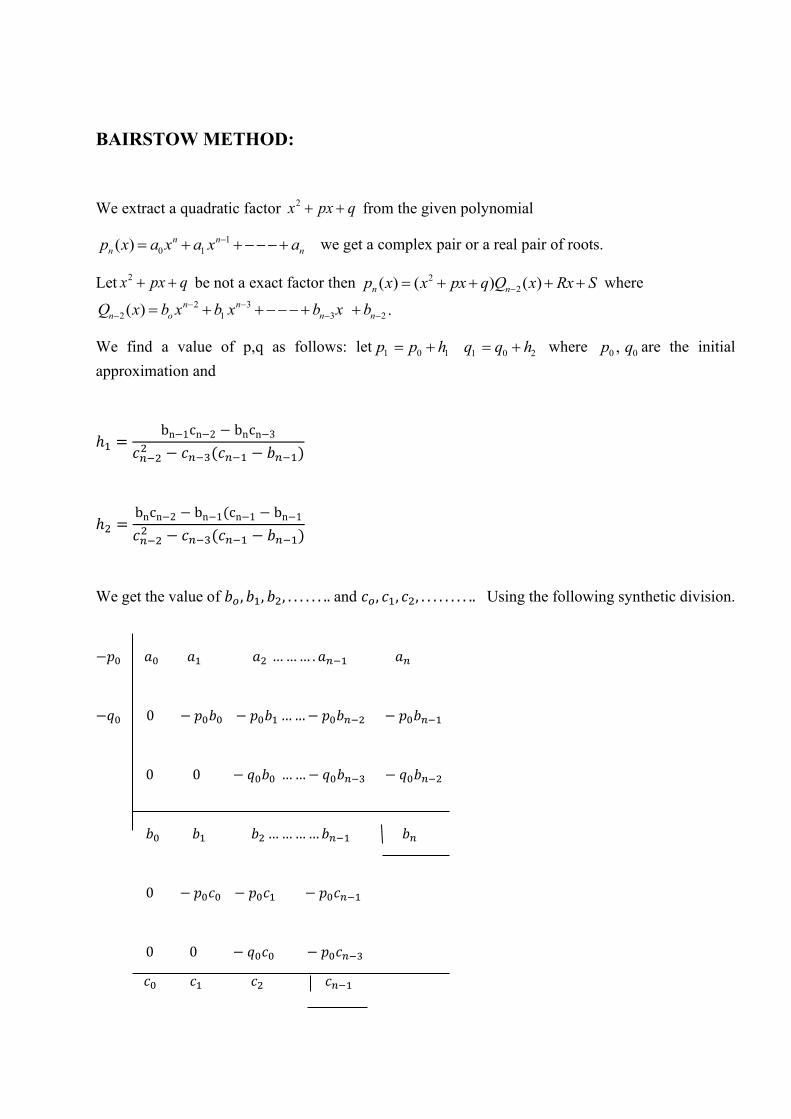
BAIRSTOW METHOD:
We extract a quadratic factor 2x px q+ + from the given polynomial
1
0 1( ) n n
n np x a x a x a−= + +−−−+ we get a complex pair or a real pair of roots.
Let2x px q+ + be not a exact factor then 2
2( ) ( ) ( )n np x x px q Q x Rx S−= + + + + where
2 3
2 1 3 2( ) n n
n o n nQ x b x b x b x b− −
− − −= + +−−−+ + .
We find a value of p,q as follows: let1 0 1p p h= + 1 0 2q q h= + where
0 0,p q are the initial
approximation and
ℎ1 =bn−1cn−2 − bncn−3
𝑐𝑛−22 − 𝑐𝑛−3(𝑐𝑛−1 − 𝑏𝑛−1)
ℎ2 =bncn−2 − bn−1(cn−1 − bn−1
𝑐𝑛−22 − 𝑐𝑛−3(𝑐𝑛−1 − 𝑏𝑛−1)
We get the value of 𝑏𝑜 , 𝑏1, 𝑏2, . . . . . . .. and 𝑐𝑜, 𝑐1, 𝑐2, . . . . . . . . .. Using the following synthetic division.
−𝑝0 𝑎0 𝑎1 𝑎2 ……… . 𝑎𝑛−1 𝑎𝑛
−𝑞0 0 − 𝑝0𝑏0 − 𝑝0𝑏1 ……− 𝑝0𝑏𝑛−2 − 𝑝0𝑏𝑛−1
0 0 − 𝑞0𝑏0 ……− 𝑞0𝑏𝑛−3 − 𝑞0𝑏𝑛−2
𝑏0 𝑏1 𝑏2 …………𝑏𝑛−1 𝑏𝑛
0 − 𝑝0𝑐0 − 𝑝0𝑐1 − 𝑝0𝑐𝑛−1
0 0 − 𝑞0𝑐0 − 𝑝0𝑐𝑛−3
𝑐0 𝑐1 𝑐2 𝑐𝑛−1
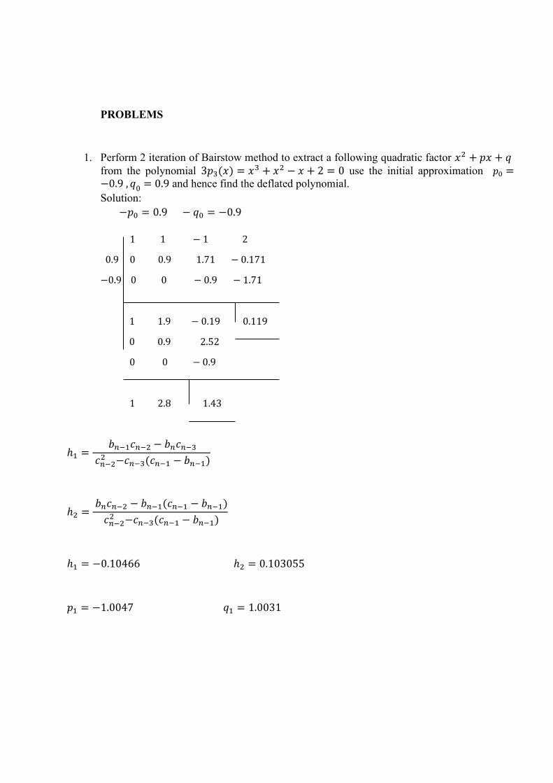
PROBLEMS
1. Perform 2 iteration of Bairstow method to extract a following quadratic factor 𝑥2 + 𝑝𝑥 + 𝑞 from the polynomial 3𝑝3(𝑥) = 𝑥3 + 𝑥2 − 𝑥 + 2 = 0 use the initial approximation 𝑝0 =−0.9 , 𝑞0 = 0.9 and hence find the deflated polynomial.
Solution:
−𝑝0 = 0.9 − 𝑞0 = −0.9
1 1 − 1 2
0.9 0 0.9 1.71 − 0.171
−0.9 0 0 − 0.9 − 1.71
1 1.9 − 0.19 0.119
0 0.9 2.52
0 0 − 0.9
1 2.8 1.43
ℎ1 = 𝑏𝑛−1𝑐𝑛−2 − 𝑏𝑛𝑐𝑛−3
𝑐𝑛−22 −𝑐𝑛−3(𝑐𝑛−1 − 𝑏𝑛−1)
ℎ2 = 𝑏𝑛𝑐𝑛−2 − 𝑏𝑛−1(𝑐𝑛−1 − 𝑏𝑛−1)
𝑐𝑛−22 −𝑐𝑛−3(𝑐𝑛−1 − 𝑏𝑛−1)
ℎ1 = −0.10466 ℎ2 = 0.103055
𝑝1 = −1.0047 𝑞1 = 1.0031
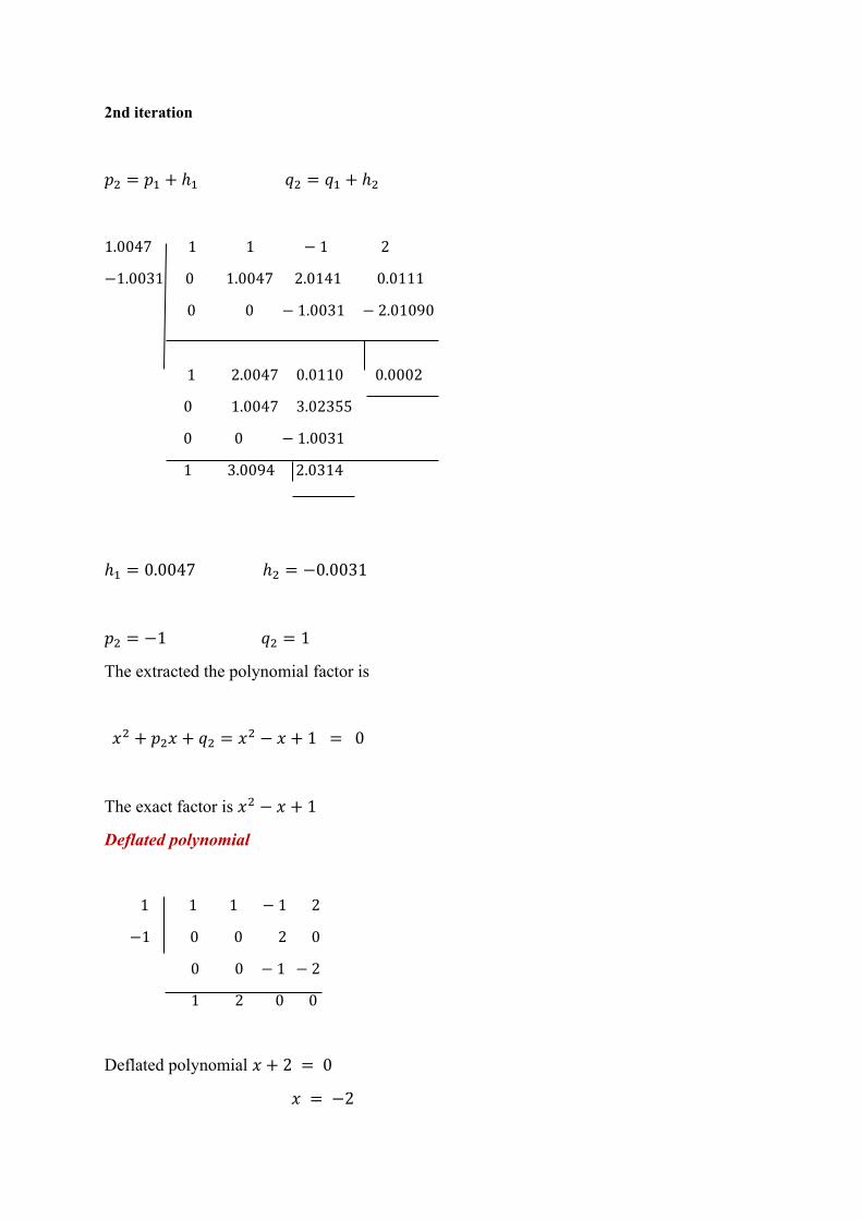
2nd iteration
𝑝2 = 𝑝1 + ℎ1 𝑞2 = 𝑞1 + ℎ2
1.0047 1 1 − 1 2
−1.0031 0 1.0047 2.0141 0.0111
0 0 − 1.0031 − 2.01090
1 2.0047 0.0110 0.0002
0 1.0047 3.02355
0 0 − 1.0031
1 3.0094 2.0314
ℎ1 = 0.0047 ℎ2 = −0.0031
𝑝2 = −1 𝑞2 = 1
The extracted the polynomial factor is
𝑥2 + 𝑝2𝑥 + 𝑞2 = 𝑥2 − 𝑥 + 1 = 0
The exact factor is 𝑥2 − 𝑥 + 1
Deflated polynomial
1 1 1 − 1 2
−1 0 0 2 0
0 0 − 1 − 2
1 2 0 0
Deflated polynomial 𝑥 + 2 = 0
𝑥 = −2
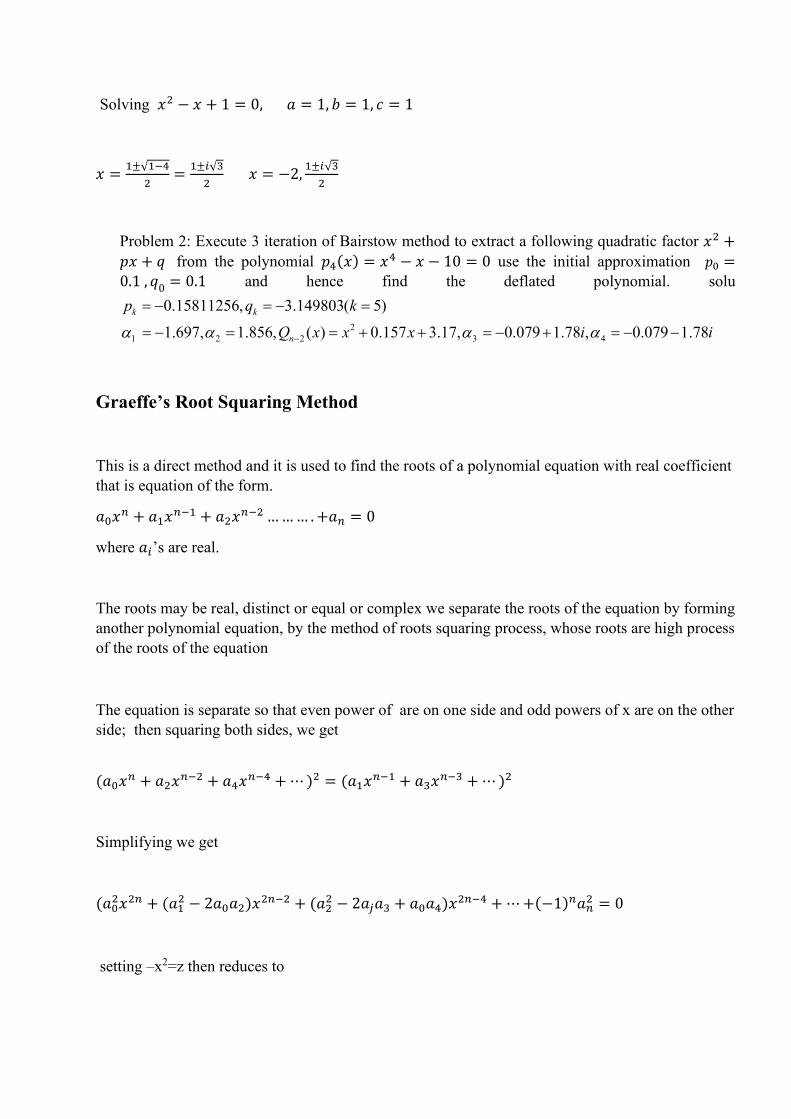
Solving 𝑥2 − 𝑥 + 1 = 0, 𝑎 = 1, 𝑏 = 1, 𝑐 = 1
𝑥 =1±√1−4
2=
1±𝑖√3
2 𝑥 = −2,
1±𝑖√3
2
Problem 2: Execute 3 iteration of Bairstow method to extract a following quadratic factor 𝑥2 +
𝑝𝑥 + 𝑞 from the polynomial 𝑝4(𝑥) = 𝑥4 − 𝑥 − 10 = 0 use the initial approximation 𝑝0 =0.1 , 𝑞0 = 0.1 and hence find the deflated polynomial. solu
2
1 2 2 3 4
0.15811256, 3.149803( 5)
1.697, 1.856, ( ) 0.157 3.17, 0.079 1.78 , 0.079 1.78
k k
n
p q k
Q x x x i i −
= − = − =
= − = = + + = − + = − −
Graeffe’s Root Squaring Method
This is a direct method and it is used to find the roots of a polynomial equation with real coefficient
that is equation of the form.
𝑎0𝑥𝑛 + 𝑎1𝑥
𝑛−1 + 𝑎2𝑥𝑛−2 ……… .+𝑎𝑛 = 0
where 𝑎𝑖’s are real.
The roots may be real, distinct or equal or complex we separate the roots of the equation by forming
another polynomial equation, by the method of roots squaring process, whose roots are high process
of the roots of the equation
The equation is separate so that even power of are on one side and odd powers of x are on the other
side; then squaring both sides, we get
(𝑎0𝑥𝑛 + 𝑎2𝑥
𝑛−2 + 𝑎4𝑥𝑛−4 + ⋯)2 = (𝑎1𝑥
𝑛−1 + 𝑎3𝑥𝑛−3 + ⋯)2
Simplifying we get
(𝑎02𝑥2𝑛 + (𝑎1
2 − 2𝑎0𝑎2)𝑥2𝑛−2 + (𝑎2
2 − 2𝑎𝑗𝑎3 + 𝑎0𝑎4)𝑥2𝑛−4 + ⋯+(−1)𝑛𝑎𝑛
2 = 0
setting –x2=z then reduces to
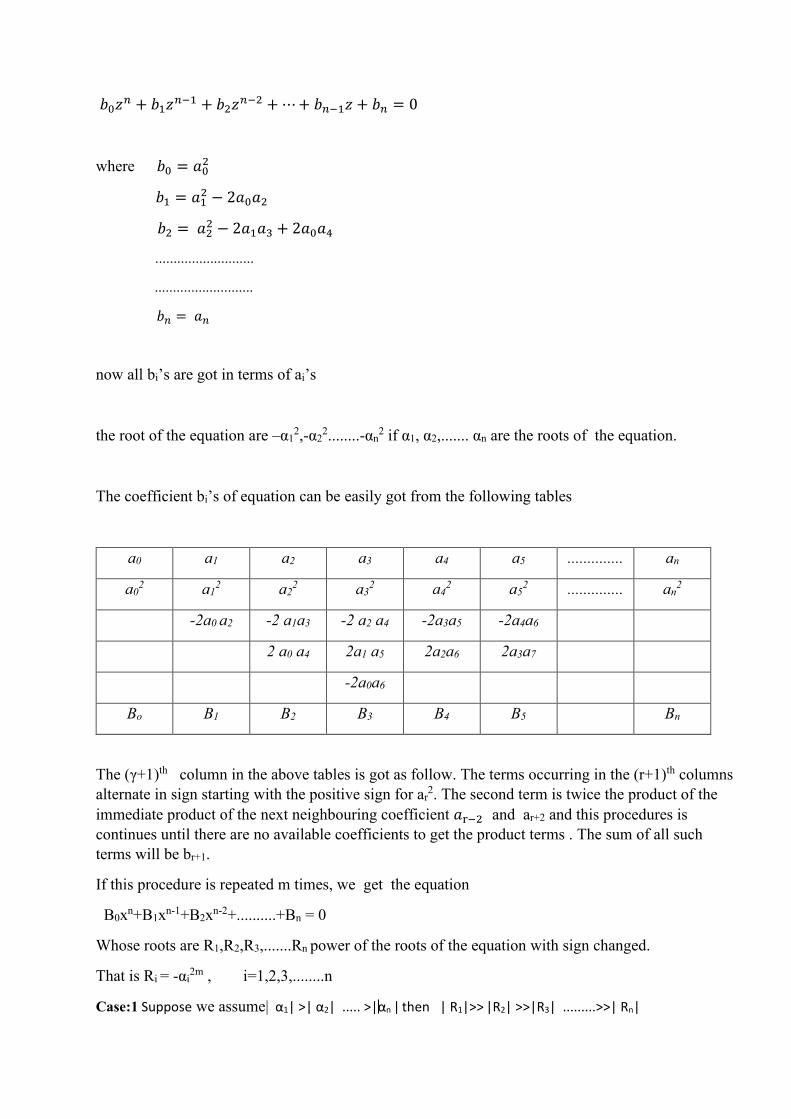
𝑏0𝑧𝑛 + 𝑏1𝑧
𝑛−1 + 𝑏2𝑧𝑛−2 + ⋯+ 𝑏𝑛−1𝑧 + 𝑏𝑛 = 0
where 𝑏0 = 𝑎02
𝑏1 = 𝑎12 − 2𝑎0𝑎2
𝑏2 = 𝑎22 − 2𝑎1𝑎3 + 2𝑎0𝑎4
...........................
...........................
𝑏𝑛 = 𝑎𝑛
now all bi’s are got in terms of ai’s
the root of the equation are –α12,-α2
2........-αn2 if α1, α2,....... αn are the roots of the equation.
The coefficient bi’s of equation can be easily got from the following tables
a0 a1 a2 a3 a4 a5 .............. an
a02 a1
2 a22 a3
2 a42 a5
2 .............. an2
-2a0 a2 -2 a1a3 -2 a2 a4 -2a3a5 -2a4a6
2 a0 a4 2a1 a5 2a2a6 2a3a7
-2a0a6
Bo B1 B2 B3 B4 B5 Bn
The (γ+1)th column in the above tables is got as follow. The terms occurring in the (r+1)th columns
alternate in sign starting with the positive sign for ar2. The second term is twice the product of the
immediate product of the next neighbouring coefficient 𝑎r−2 and ar+2 and this procedures is
continues until there are no available coefficients to get the product terms . The sum of all such
terms will be br+1.
If this procedure is repeated m times, we get the equation
B0xn+B1x
n-1+B2xn-2+..........+Bn = 0
Whose roots are R1,R2,R3,.......Rn power of the roots of the equation with sign changed.
That is Ri = -αi2m , i=1,2,3,........n
Case:1 Suppose we assume| α1| >| α2| ..... >|αn | then | R1|>> |R2| >>|R3| .........>>| Rn|
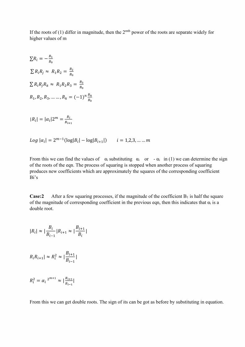
If the roots of (1) differ in magnitude, then the 2mth power of the roots are separate widely for
higher values of m
∑𝑅𝑖 = −𝐵1
𝐵0
∑𝑅𝑖𝑅𝑗 ≈ 𝑅1𝑅2 = 𝐵2
𝐵0
∑𝑅𝑖𝑅𝑗𝑅𝑘 ≈ 𝑅1𝑅2𝑅3 = 𝐵3
𝐵0
𝑅1, 𝑅2, 𝑅3, …… , 𝑅𝑘 = (−1)𝑛 𝐵𝑛
𝐵0
|𝑅𝑖| = |𝛼𝑖|2𝑚 =
𝐵𝑖
𝐵𝑖+1
𝐿𝑜𝑔 |𝛼𝑖| = 2𝑚−1(log|𝐵𝑖| − log|𝐵𝑖+1|) 𝑖 = 1,2,3, ……𝑚
From this we can find the values of αi substituting αi or - αi in (1) we can determine the sign
of the roots of the eqn. The process of squaring is stopped when another process of squaring
produces new coefficients which are approximately the squares of the corresponding coefficient
Bi’s
Case:2 After a few squaring processes, if the magnitude of the coefficient B1 is half the square
of the magnitude of corresponding coefficient in the previous eqn, then this indicates that αi is a
double root.
|𝑅𝑖| ≈ |𝐵𝑖
𝐵𝑖−1|𝑅𝑖+1 ≈ |
𝐵𝑖+1
𝐵𝑖|
𝑅𝑖𝑅𝑖+1| ≈ 𝑅𝑖2 ≈ |
𝐵𝑖+1
𝐵𝑖−1|
𝑅𝑖2 = 𝛼𝑖
2𝑚+1≈ |
𝐵𝑖+1
𝐵𝑖−1|
From this we can get double roots. The sign of its can be got as before by substituting in equation.
Case 3 : If αk, αk+1 are two complex conjugate roots, then this would make the coefficient of
xn-k
in the successive squaring to fluctuate both in magnitude and sign.
If αk, αk+1 =βk(cos∅k + i sin∅k) is the complex pair of roots, then coefficient will fluctuate in
magnitude and sign by the quantity 2βkmcos∅k.
A complex pair is located only by the such oscillation. If m is large βk can be got from
𝛽𝑘2(2)𝑚
≈ |𝐵𝑘+1
𝐵𝑘−1| 𝑎𝑛𝑑 ∅ 𝑖𝑠 𝑔𝑜𝑡 𝑓𝑟𝑜𝑚 2𝛽𝑘
𝑚𝑐𝑜𝑠𝑚 ∅𝑛 ≈ |𝐵𝑘+1
𝐵𝑘−1
if the eqn. Possesses only two complex roots p+iq we have α1+ α2+ α3+....+ αk-1+2p+ αk+2+....+ αn =
-a1
this gives the values of p.
Since|𝛽𝑘|2 = 𝑝2 + 𝑞2𝑎𝑛𝑑|𝛽𝑘 is known already q is known from the relation.
Note : ( 1) ( ) ( ) 2( ) ( 1) ( ) ( ) :m m m mp z p x p x z x+ = − − = so that the roots of ( ) ( )mp z are those of ( )p x raised
to the power .
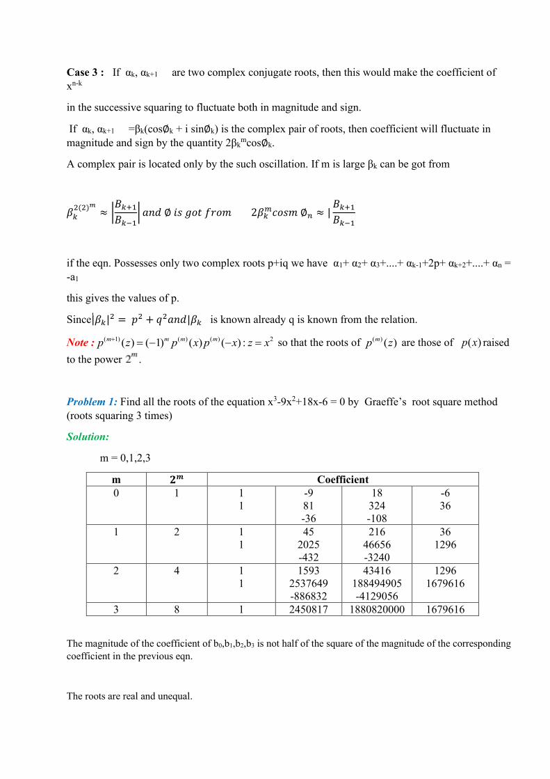
Problem 1: Find all the roots of the equation x3-9x2+18x-6 = 0 by Graeffe’s root square method
(roots squaring 3 times)
Solution:
m = 0,1,2,3
m 𝟐𝒎 Coefficient
0
1
1
1
-9
81
-36
18
324
-108
-6
36
1 2 1
1
45
2025
-432
216
46656
-3240
36
1296
2 4 1
1
1593
2537649
-886832
43416
188494905
-4129056
1296
1679616
3 8 1 2450817 1880820000 1679616
The magnitude of the coefficient of b0,b1,b2,b3 is not half of the square of the magnitude of the corresponding
coefficient in the previous eqn.
The roots are real and unequal.
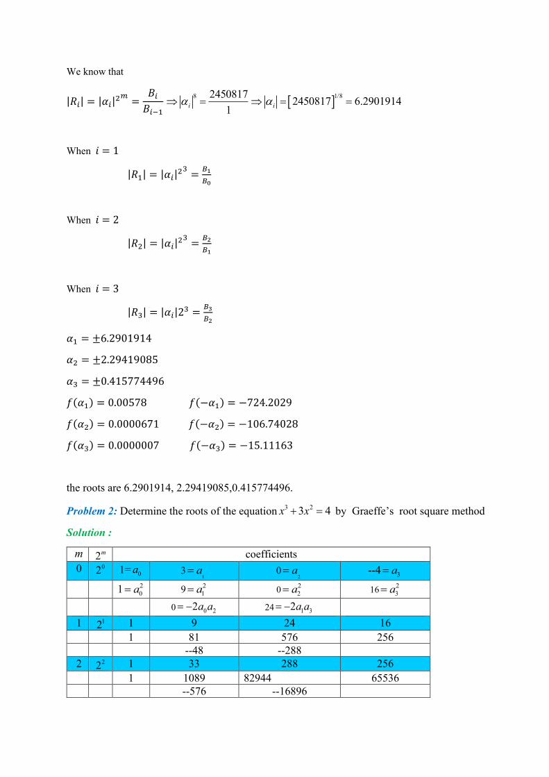
We know that
|𝑅𝑖| = |𝛼𝑖|2𝑚
=𝐵𝑖
𝐵𝑖−1
1/88 24508172450817 6.2901914
1i i = = =
When 𝑖 = 1
|𝑅1| = |𝛼𝑖|23
=𝐵1
𝐵0
When 𝑖 = 2
|𝑅2| = |𝛼𝑖|23
=𝐵2
𝐵1
When 𝑖 = 3
|𝑅3| = |𝛼𝑖|23 =
𝐵3
𝐵2
𝛼1 = ±6.2901914
𝛼2 = ±2.29419085
𝛼3 = ±0.415774496
𝑓(𝛼1) = 0.00578 𝑓(−𝛼1) = −724.2029
𝑓(𝛼2) = 0.0000671 𝑓(−𝛼2) = −106.74028
𝑓(𝛼3) = 0.0000007 𝑓(−𝛼3) = −15.11163
the roots are 6.2901914, 2.29419085,0.415774496.
Problem 2: Determine the roots of the equation3 23 4x x+ = by Graeffe’s root square method
Solution :
m 2m coefficients
0 02 1= 0a 31
a= 02
a= --43a=
1 2
0a= 92
1a= 02
2a= 162
3a=
0 0 22a a= − 24 1 32a a= −
1 12 1 9 24 16
1 81 576 256
--48 --288
2 22 1 33 288 256
1 1089 82944 65536
--576 --16896
3 32 1 513 66048 65536
1 263169 4362328304 4294967296
-132096 --67239936
4 42 1 131073 4295098368 4294967296
1 1.718013131010 1.844786999
1910 1.8446744071910
--8590196736 --1.1259084971510
5 52 1 8589934564 1.8446744081910 1.844674407
1910
0B
1B 2B
3B
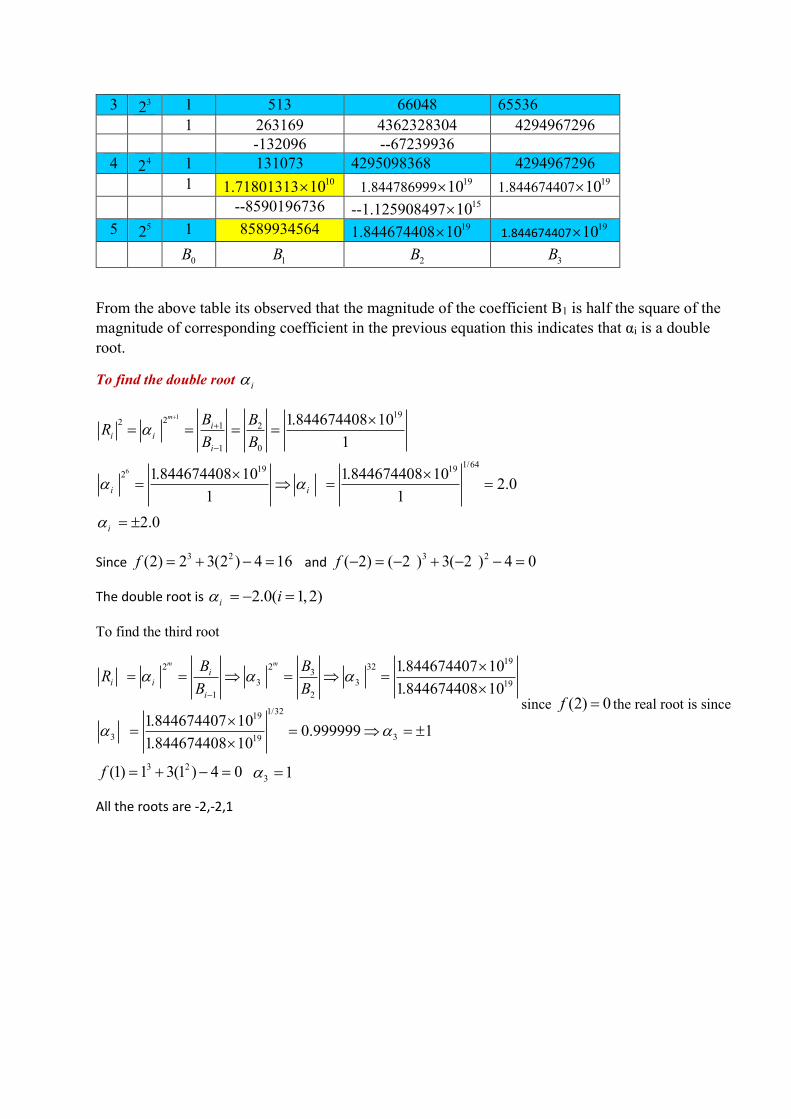
From the above table its observed that the magnitude of the coefficient B1 is half the square of the
magnitude of corresponding coefficient in the previous equation this indicates that αi is a double
root.
To find the double root i
1
6
1922 1 2
1 0
1/6419 19
2
1.844674408 10
1
1.844674408 10 1.844674408 102.0
1 1
2.0
m
ii i
i
i i
i
B BR
B B
+
+
−
= = = =
= = =
=
Since 3 2(2) 2 3(2 ) 4 16f = + − = and
3 2( 2) ( 2 ) 3( 2 ) 4 0f − = − + − − =
The double root is 2.0( 1,2)i i = − =
To find the third root
192 2 32
33 3 19
1 2
1/3219
3 319
1.844674407 10
1.844674408 10
1.844674407 100.999999 1
1.844674408 10
m m
ii i
i
B BR
B B
−
= = = =
= = =
since (2) 0f = the real root is since
3 2(1) 1 3(1 ) 4 0f = + − =3 1 =
All the roots are -2,-2,1
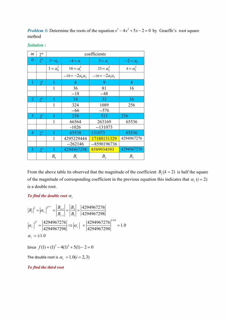
Problem 3: Determine the roots of the equation3 24 5 2 0x x x− + − = by Graeffe’s root square
method
Solution :
m 2m coefficients
0 02 1= 0a --41
a= 52
a= --23a=
1 2
0a= 162
1a= 252
2a= 42
3a=
--10 0 22a a= − --16 1 32a a= −
1 12 1 6 9 4
1 36 81 16
--18 --48
2 22 1 18 33 16
1 324 1089 256
--66 --576
3 32 1 258 513 256
1 66564 263169 65536
-1026 --131073
4 42 1 65538 131073 65536
1 4295229444 17180131329 4294967276
--262146 --8590196736
5 52 1 4294967298 8589934593 4294967276
0B
1B 2B
3B
From the above table its observed that the magnitude of the coefficient 2 ( 2)B k = is half the square
of the magnitude of corresponding coefficient in the previous equation this indicates that ( 2)i i =
is a double root.
To find the double root i
1
6
22 1 3
1 1
1/642
4294967276
4294967298
4294967276 42949672761.0
4294967298 4294967298
1.0
m
ii i
i
i i
i
B BR
B B
+
+
−
= = = =
= = =
=
Since 3 2(1) (1) 4(1) 5(1) 2 0f = − + − =
The double root is 1.0( 2,3)i i = =
To find the third root
2 2 321
1 1
1 0
1/32
1 1
4294967298
1
42949672982.0 2
1
m m
ii i
i
B BR
B B
−
= = = =
= = =
3 2(2) (2) 4(2) 5(2) 2 0f = − + − = since (2) 0f = the real root is
1 2 =
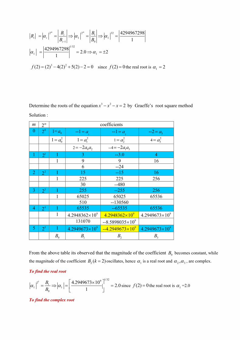
Determine the roots of the equation3 2 2x x x− − = by Graeffe’s root square method
Solution :
m 2m coefficients
0 02 1= 0a --11
a= --12
a= --23a=
1 2
0a= 1 2
1a= 12
2a= 42
3a=
2 0 22a a= − --4 1 32a a= −
1 12 1 3 --3.0 4
1 9 9 16
6 --24
2 22 1 15 --15 16
1 225 225 256
30 --480
3 32 1 255 --255 256
1 65025 65025 65536
510 --130560
4 42 1 65535 --65535 65536
1 4.2948362910 4.2948362
910 4.2949673910
131070 --8.5898035910
5 52 1 4.2949673910 --4.2949673
910 4.2949673910
0B
1B 2B
3B
From the above table its observed that the magnitude of the coefficient 0B becomes constant, while
the magnitude of the coefficient 2 ( 2)B k = oscillates, hence
1 is a real root and 2 3, , are complex.
To find the real root
51/32
92
11 1
0
4.2949673 102.0
1
B
B
= = =
since (2) 0f = the real root is
1 =2.0
To find the complex root
59
2(2) 2(2) 641 32 2 29
1 1
4.2949673 10, 1.0 (1)
4.2949673 10
mk
k
k
B B
B B +
−
= = = = = −−
where is given by
1
1
2 cosm kk n
k
Bm
B +
−
= and 2
2 2 (2)k p q = + −−−
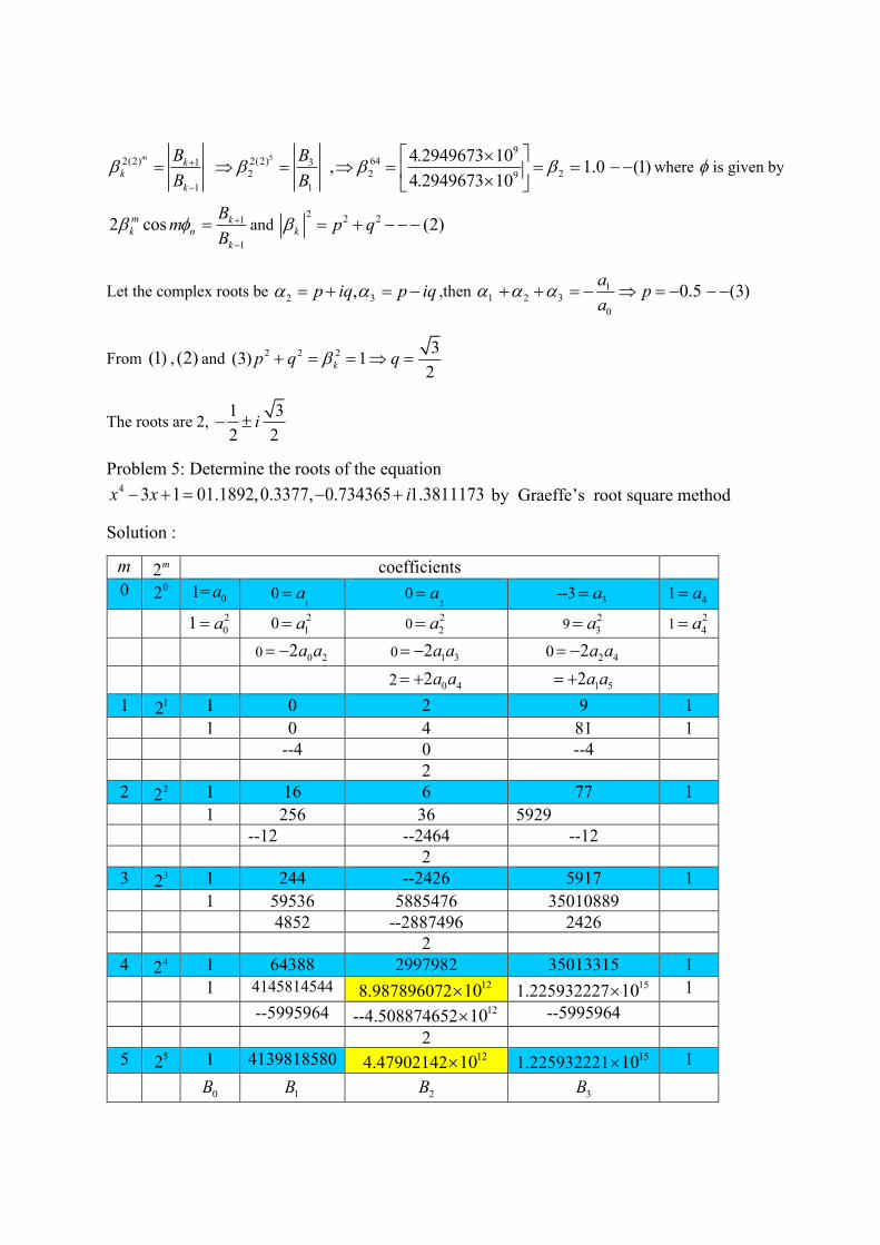
Let the complex roots be 2 3,p iq p iq = + = − ,then 1
1 2 3
0
0.5 (3)a
pa
+ + = − = − −−
From (1) , (2) and 2 2 2 3
(3) 12
kp q q+ = = =
The roots are 2, 1 3
2 2i−
Problem 5: Determine the roots of the equation4 3 1 01.1892,0.3377, 0.734365 1.3811173x x i− + = − + by Graeffe’s root square method
Solution :
m 2m coefficients
0 02 1= 0a 01
a= 02
a= --33a= 1
4a=
1 2
0a= 02
1a= 02
2a= 92
3a= 12
4a=
0 0 22a a= − 0 1 32a a= − 0 2 42a a= −
2 0 42a a= + 1 52a a= +
1 12 1 0 2 9 1
1 0 4 81 1
--4 0 --4
2
2 22 1 16 6 77 1
1 256 36 5929
--12 --2464 --12
2
3 32 1 244 --2426 5917 1
1 59536 5885476 35010889
4852 --2887496 2426
2
4 42 1 64388 2997982 35013315 1
1 4145814544 8.9878960721210 1.225932227
1510 1
--5995964 --4.5088746521210 --5995964
2
5 52 1 4139818580 4.479021421210 1.225932221
1510 1
0B
1B 2B
3B

UNIT – II - ADVANCED NUMERICAL METHODS – SMTA5304
UNIT II
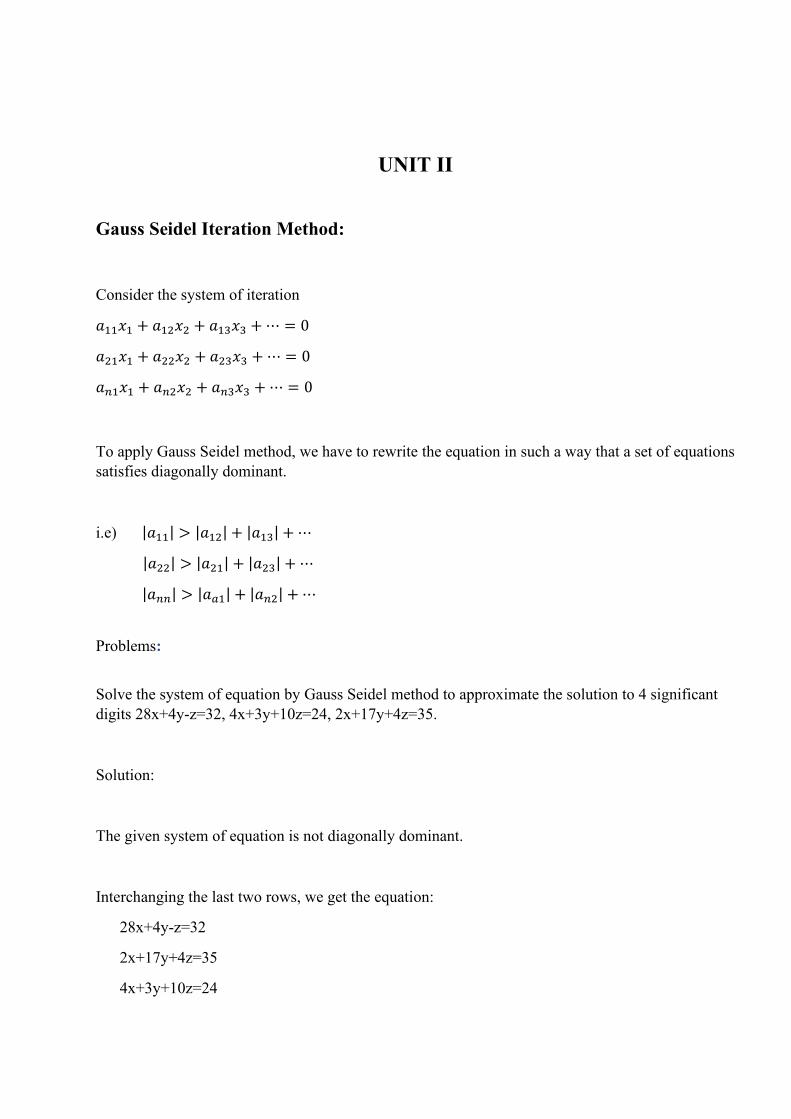
Gauss Seidel Iteration Method:
Consider the system of iteration
𝑎11𝑥1 + 𝑎12𝑥2 + 𝑎13𝑥3 + ⋯ = 0
𝑎21𝑥1 + 𝑎22𝑥2 + 𝑎23𝑥3 + ⋯ = 0
𝑎𝑛1𝑥1 + 𝑎𝑛2𝑥2 + 𝑎𝑛3𝑥3 + ⋯ = 0
To apply Gauss Seidel method, we have to rewrite the equation in such a way that a set of equations
satisfies diagonally dominant.
i.e) |𝑎11| > |𝑎12| + |𝑎13| + ⋯
|𝑎22| > |𝑎21| + |𝑎23| + ⋯
|𝑎𝑛𝑛| > |𝑎𝑎1| + |𝑎𝑛2| + ⋯
Problems:
Solve the system of equation by Gauss Seidel method to approximate the solution to 4 significant
digits 28x+4y-z=32, 4x+3y+10z=24, 2x+17y+4z=35.
Solution:
The given system of equation is not diagonally dominant.
Interchanging the last two rows, we get the equation:
28x+4y-z=32
2x+17y+4z=35
4x+3y+10z=24
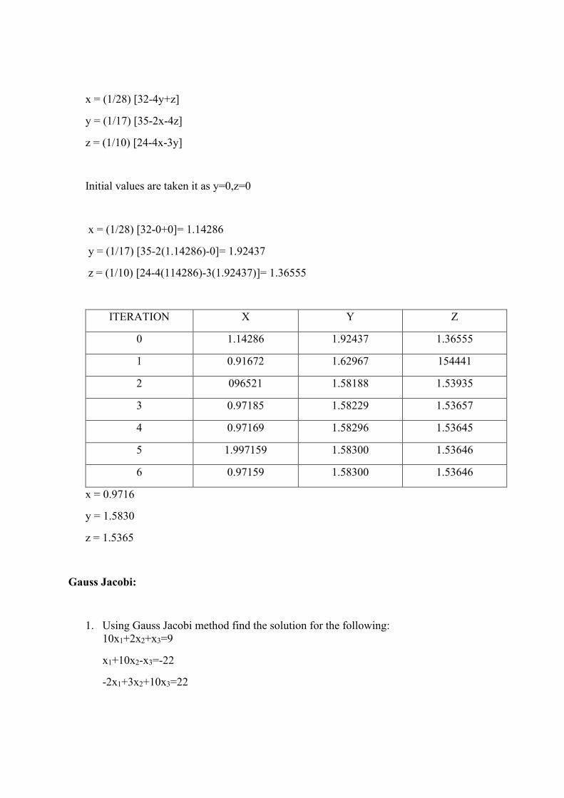
x = (1/28) [32-4y+z]
y = (1/17) [35-2x-4z]
z = (1/10) [24-4x-3y]
Initial values are taken it as y=0,z=0
x = (1/28) [32-0+0]= 1.14286
y = (1/17) [35-2(1.14286)-0]= 1.92437
z = (1/10) [24-4(114286)-3(1.92437)]= 1.36555
ITERATION X Y Z
0 1.14286 1.92437 1.36555
1 0.91672 1.62967 154441
2 096521 1.58188 1.53935
3 0.97185 1.58229 1.53657
4 0.97169 1.58296 1.53645
5 1.997159 1.58300 1.53646
6 0.97159 1.58300 1.53646
x = 0.9716
y = 1.5830
z = 1.5365
Gauss Jacobi:
1. Using Gauss Jacobi method find the solution for the following:
10x1+2x2+x3=9
x1+10x2-x3=-22
-2x1+3x2+10x3=22
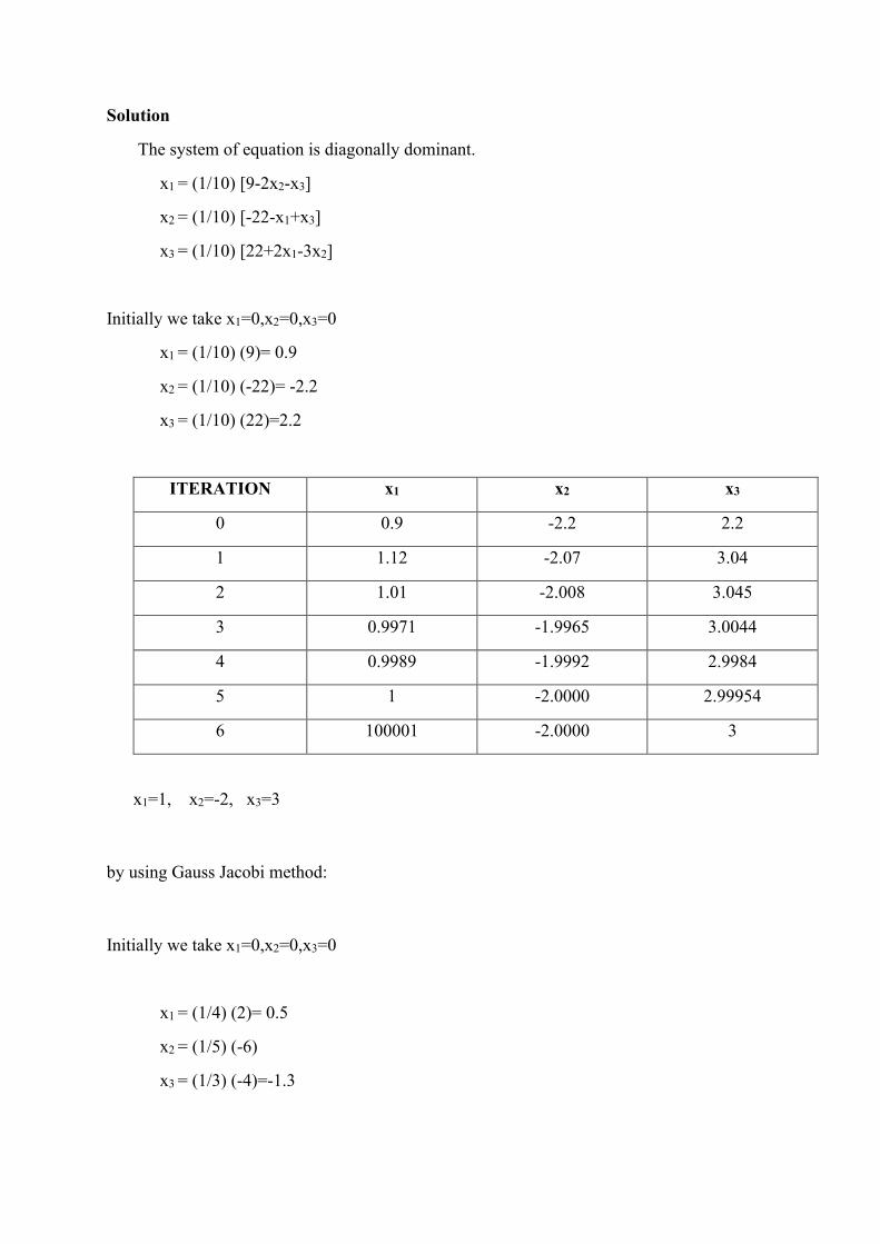
Solution
The system of equation is diagonally dominant.
x1 = (1/10) [9-2x2-x3]
x2 = (1/10) [-22-x1+x3]
x3 = (1/10) [22+2x1-3x2]
Initially we take x1=0,x2=0,x3=0
x1 = (1/10) (9)= 0.9
x2 = (1/10) (-22)= -2.2
x3 = (1/10) (22)=2.2
ITERATION x1 x2 x3
0 0.9 -2.2 2.2
1 1.12 -2.07 3.04
2 1.01 -2.008 3.045
3 0.9971 -1.9965 3.0044
4 0.9989 -1.9992 2.9984
5 1 -2.0000 2.99954
6 100001 -2.0000 3
x1=1, x2=-2, x3=3
by using Gauss Jacobi method:
Initially we take x1=0,x2=0,x3=0
x1 = (1/4) (2)= 0.5
x2 = (1/5) (-6)
x3 = (1/3) (-4)=-1.3
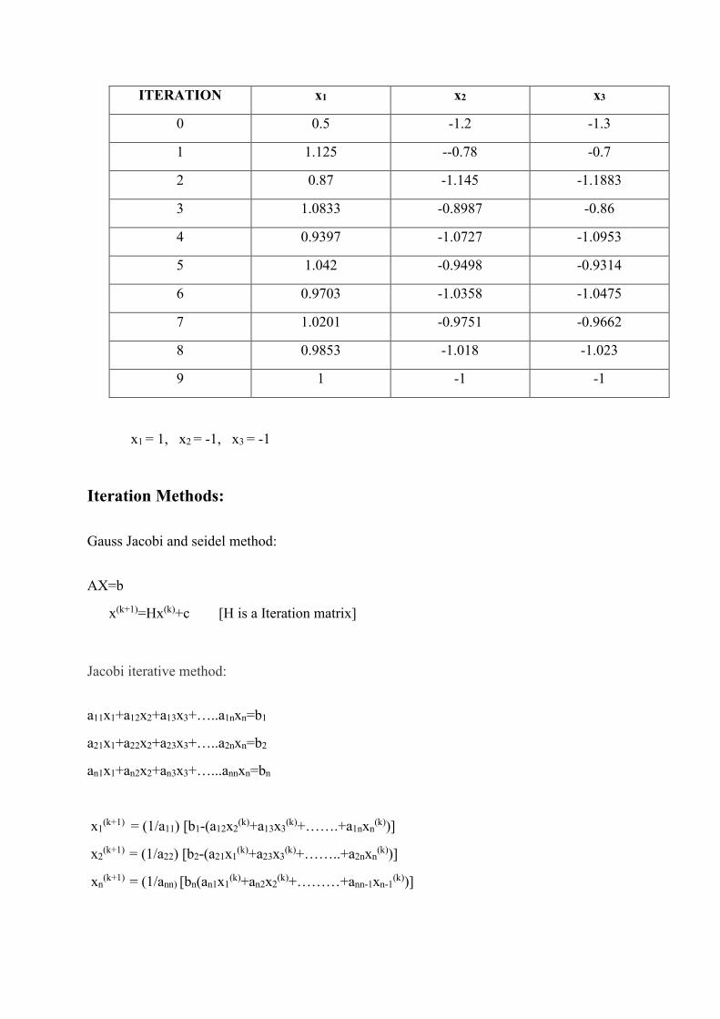
ITERATION x1 x2 x3
0 0.5 -1.2 -1.3
1 1.125 --0.78 -0.7
2 0.87 -1.145 -1.1883
3 1.0833 -0.8987 -0.86
4 0.9397 -1.0727 -1.0953
5 1.042 -0.9498 -0.9314
6 0.9703 -1.0358 -1.0475
7 1.0201 -0.9751 -0.9662
8 0.9853 -1.018 -1.023
9 1 -1 -1
x1 = 1, x2 = -1, x3 = -1
Iteration Methods:
Gauss Jacobi and seidel method:
AX=b
x(k+1)=Hx(k)+c [H is a Iteration matrix]
Jacobi iterative method:
a11x1+a12x2+a13x3+…..a1nxn=b1
a21x1+a22x2+a23x3+…..a2nxn=b2
an1x1+an2x2+an3x3+…...annxn=bn
x1(k+1) = (1/a11) [b1-(a12x2
(k)+a13x3(k)+…….+a1nxn
(k))]
x2(k+1) = (1/a22) [b2-(a21x1
(k)+a23x3(k)+……..+a2nxn
(k))]
xn(k+1) = (1/ann) [bn(an1x1
(k)+an2x2(k)+………+ann-1xn-1
(k))]

A=D+L+U
AX=b
(D+L+U)X=b
DX=-(L+U)X+b
DX(k+1)=-(L+U)X(K)+b
X(k+1)=-D-1(L+U)X(K)+D-1b
X(K+1)=HX(K)+C
Error :
Where H =-D-1(L+U)
C = D-1b
Computing Procedure ( If Error is Given )
x(k+1) = - D -1 ( L+U ) x (k) + D -1 b
= x (k) – x (k) – D -1 ( L+U ) x (k) + D -1 b
= x (k) – [ I + D -1 ( L+U ) ] x (k) + D -1 b
= x(k) – [ DD -1 + D-1 ( L+U) ] x(k) + D -1 b
= x(k) – D -1 [ D+L+U] x(k) + D -1 b
x (k+1) - x(k) = - D -1 A x(k) + D -1 b
x (k+1) - x(k) = D -1 [ b – A x(k) ]
v(k) = D -1 r(k)
Where v(k) = x (k+1) - x(k)
r(k) = b – A x(k)
Formulas to be Known :
1. For finding Iterative matrix H = - D -1 (L+U) and C = D -1 b .
Hence x (k+1) = Hx(k) + c .
2. If Error is given , v(k) = x (k+1) - x(k) and r(k) = b – A x(k). Hence
v(k) = D -1 r(k)
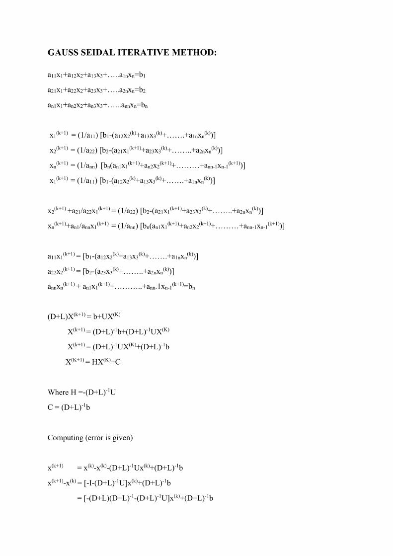
GAUSS SEIDAL ITERATIVE METHOD:
a11x1+a12x2+a13x3+…..a1nxn=b1
a21x1+a22x2+a23x3+…..a2nxn=b2
an1x1+an2x2+an3x3+…...annxn=bn
x1(k+1) = (1/a11) [b1-(a12x2
(k)+a13x3(k)+…….+a1nxn
(k))]
x2(k+1) = (1/a22) [b2-(a21x1
(k+1)+a23x3(k)+……..+a2nxn
(k))]
xn(k+1) = (1/ann) [bn(an1x1
(k+1)+an2x2(k+1)+………+ann-1xn-1
(k+1))]
x1(k+1) = (1/a11) [b1-(a12x2
(k)+a13x3(k)+…….+a1nxn
(k))]
x2(k+1) +a21/a22x1
(k+1) = (1/a22) [b2-(a21x1(k+1)+a23x3
(k)+……..+a2nxn(k))]
xn(k+1)+an1/annx1
(k+1) = (1/ann) [bn(an1x1(k+1)+an2x2
(k+1)+………+ann-1xn-1(k+1))]
a11x1(k+1) = [b1-(a12x2
(k)+a13x3(k)+…….+a1nxn
(k))]
a22x2(k+1) = [b2-(a23x3
(k)+……..+a2nxn(k))]
annxn(k+1) + an1x1
(k+1)+………..+ann-1xn-1(k+1)=bn
(D+L)X(k+1) = b+UX(K)
X(k+1) = (D+L)-1b+(D+L)-1UX(K)
X(k+1) = (D+L)-1UX(K)+(D+L)-1b
X(K+1) = HX(K)+C
Where H =-(D+L)-1U
C = (D+L)-1b
Computing (error is given)
x(k+1) = x(k)-x(k)-(D+L)-1Ux(k)+(D+L)-1b
x(k+1)-x(k) = [-I-(D+L)-1U]x(k)+(D+L)-1b
= [-(D+L)(D+L)-1-(D+L)-1U]x(k)+(D+L)-1b
= -(D+L)-1[-(D+L)+U]x(k)+(D+L)-1b
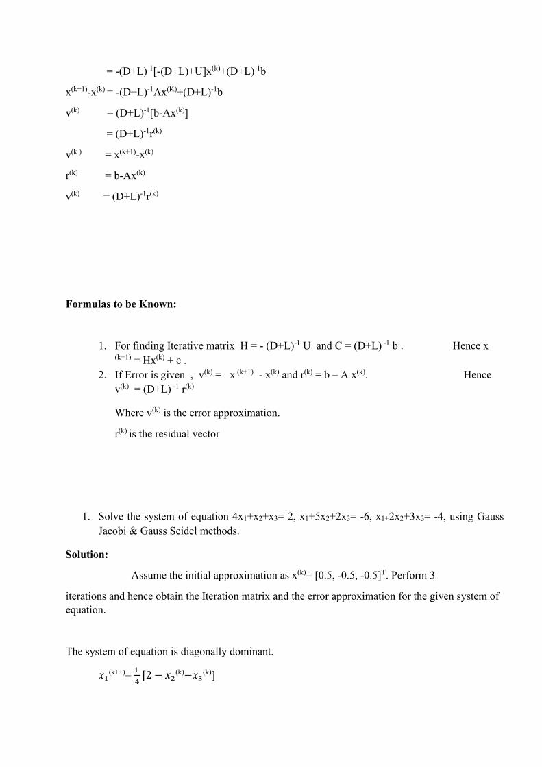
x(k+1)-x(k) = -(D+L)-1Ax(K)+(D+L)-1b
v(k) = (D+L)-1[b-Ax(k)]
= (D+L)-1r(k)
v(k ) = x(k+1)-x(k)
r(k) = b-Ax(k)
v(k) = (D+L)-1r(k)
Formulas to be Known:
1. For finding Iterative matrix H = - (D+L)-1 U and C = (D+L) -1 b . Hence x (k+1) = Hx(k) + c .
2. If Error is given , v(k) = x (k+1) - x(k) and r(k) = b – A x(k). Hence
v(k) = (D+L) -1 r(k)
Where v(k) is the error approximation.
r(k) is the residual vector
1. Solve the system of equation 4x1+x2+x3= 2, x1+5x2+2x3= -6, x1+2x2+3x3= -4, using Gauss
Jacobi & Gauss Seidel methods.
Solution:
Assume the initial approximation as x(k)= [0.5, -0.5, -0.5]T. Perform 3
iterations and hence obtain the Iteration matrix and the error approximation for the given system of
equation.
The system of equation is diagonally dominant.
𝑥1(k+1)=
1
4[2 − 𝑥2
(k)−𝑥3(k)]
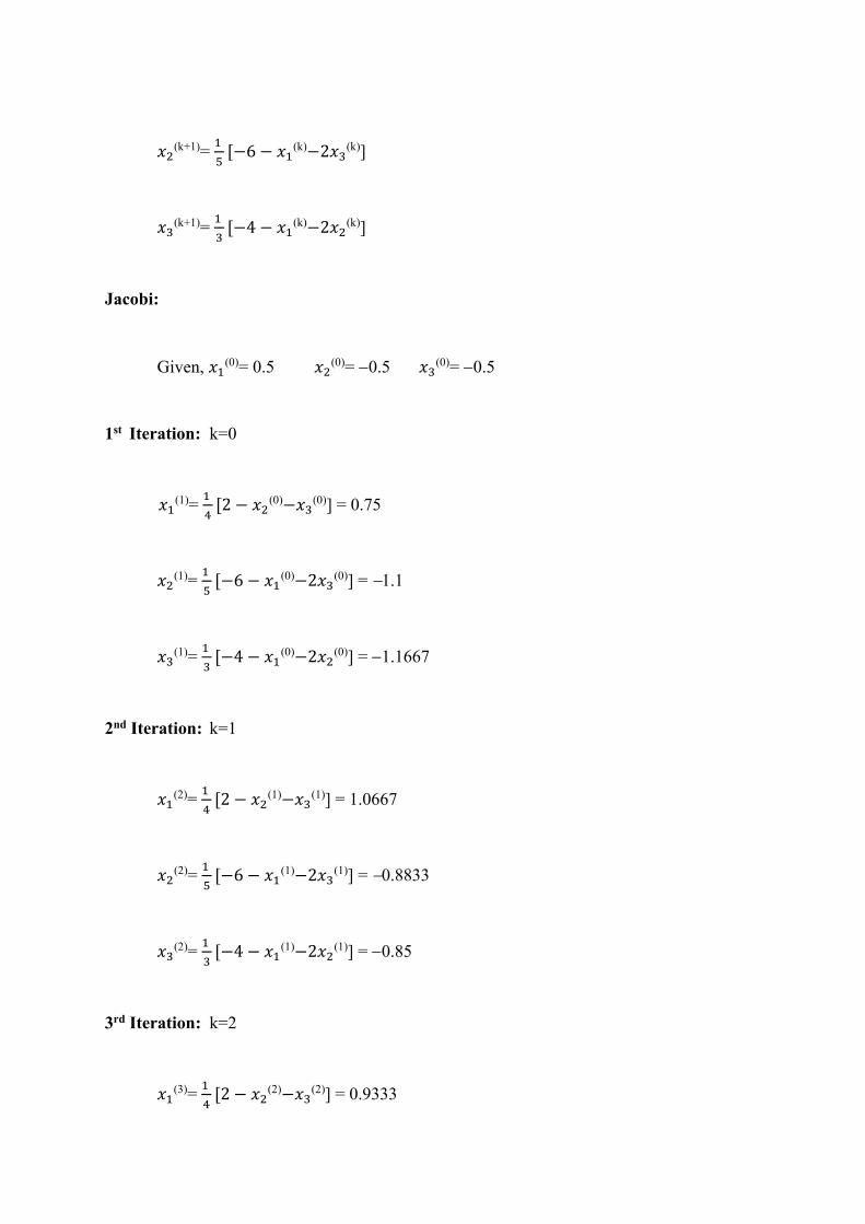
𝑥2(k+1)=
1
5[−6 − 𝑥1
(k)−2𝑥3(k)]
𝑥3(k+1)=
1
3[−4 − 𝑥1
(k)−2𝑥2(k)]
Jacobi:
Given, 𝑥1(0)= 0.5 𝑥2
(0)= −0.5 𝑥3(0)= −0.5
1st Iteration: k=0
𝑥1(1)=
1
4[2 − 𝑥2
(0)−𝑥3(0)] = 0.75
𝑥2(1)=
1
5[−6 − 𝑥1
(0)−2𝑥3(0)] = −1.1
𝑥3(1)=
1
3[−4 − 𝑥1
(0)−2𝑥2(0)] = −1.1667
2nd Iteration: k=1
𝑥1(2)=
1
4[2 − 𝑥2
(1)−𝑥3(1)] = 1.0667
𝑥2(2)=
1
5[−6 − 𝑥1
(1)−2𝑥3(1)] = −0.8833
𝑥3(2)=
1
3[−4 − 𝑥1
(1)−2𝑥2(1)] = −0.85
3rd Iteration: k=2
𝑥1(3)=
1
4[2 − 𝑥2
(2)−𝑥3(2)] = 0.9333
𝑥2(3)=
1
5[−6 − 𝑥1
(2)−2𝑥3(2)] = −1.0733
𝑥3(3)=
1
3[−4 − 𝑥1
(2)−2𝑥2(2)] = −1.1000
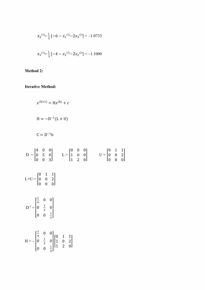
Method 2:
Iterative Method:
𝑥(k+1) = H𝑥(k) + 𝑐
H = −D−1(L + U)
C = D−1b
D = [4 0 00 5 00 0 3
] L = [0 0 01 0 01 2 0
] U = [0 1 10 0 20 0 0
]
L+U = [0 1 10 0 20 0 0
]
D-1 =
[ 1
40 0
01
50
0 01
3]
H = −
[ 1
40 0
01
50
0 01
3]
[0 1 11 0 21 2 0
]
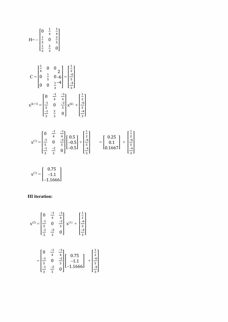
H= −
[ 0
1
4
1
41
50
2
51
3
2
30]
C =
[ 1
40 0
01
50
0 01
3
2−6−4
]
=
[
1
2−6
5−4
3 ]
x(k+1) =
[ 0
−1
4
−1
4−1
50
−2
5−1
3
2
30]
x(k) +
[
1
2−6
5−4
3 ]
x(1) =
[ 0
−1
4
−1
4−1
50
−2
5−1
3
−2
30]
[0.5−0.5−0.5
] +
[
1
2−6
5−4
3 ]
= [0.250.1
0.1667] +
[
1
2−6
5−4
3 ]
x(1) = [0.75−1.1
−1.1666]
III iteration:
x(2) =
[ 0
−1
4
−1
4−1
50
−2
5−1
3
−2
30]
x(1) +
[
1
2−6
5−4
3 ]
=
[ 0
−1
4
−1
4−1
50
−2
5−1
3
−2
30]
[0.75−1.1
−1.1666] +
[
1
2−6
5−4
3 ]
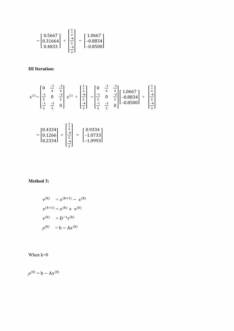
= [0.56670.316640.4833
] +
[
1
2−6
5−4
3 ]
= [1.0667−0.8834−0.8500
]
III Iteration:
x(3) =
[ 0
−1
4
−1
4−1
50
−2
5−1
3
−2
30]
x(2) +
[
1
2−6
5−4
3 ]
=
[ 0
−1
4
−1
4−1
50
−2
5−1
3
−2
30]
[1.0667−0.8834−0.8500
] +
[
1
2−6
5−4
3 ]
= [0.43340.12660.2334
] +
[
1
2−6
5−4
3 ]
= [0.9334−1.0733−1.0993
]
Method 3:
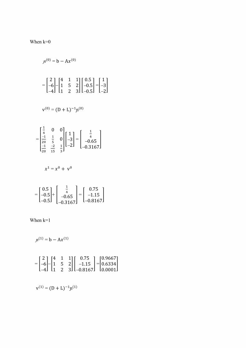
v(k) = 𝑥(k+1) − 𝑥(k)
𝑥(𝑘+1) = 𝑥(k) + v(k)
v(k) = D−1r(k)
ɲ(k) = b − A𝑥(k)
When k=0
ɲ(0) = b − A𝑥(0)
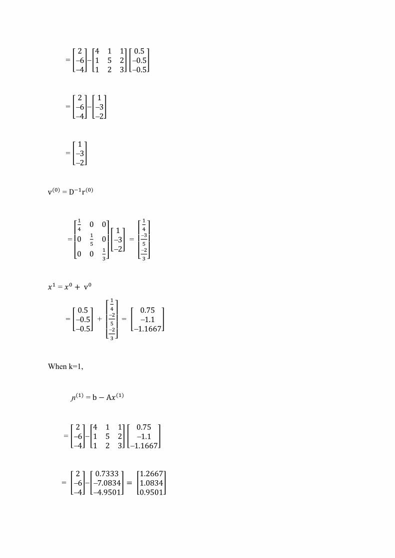
= [2−6−4
]−[4 1 11 5 21 2 3
] [0.5−0.5−0.5
]
= [2−6−4
]−[1−3−2
]
= [1−3−2
]
v(0) = D−1r(0)
=
[ 1
40 0
01
50
0 01
3]
[1−3−2
] =
[
1
4−3
5−2
3 ]
𝑥1 = 𝑥0 + v0
= [0.5−0.5−0.5
] +
[
1
4−2
5−2
3 ]
= [0.75−1.1
−1.1667]
When k=1,
ɲ(1) = b − A𝑥(1)
= [2−6−4
]−[4 1 11 5 21 2 3
] [0.75−1.1
−1.1667]
= [2−6−4
]−[0.7333−7.0834−4.9501
] = [1.26671.08340.9501
]
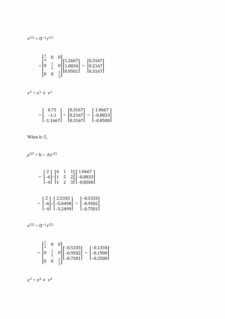
v(1) = D−1r(1)
=
[ 1
40 0
01
50
0 01
3]
[1.26671.08340.9501
] = [0.31670.21670.3167
]
𝑥2 = 𝑥1 + v1
= [0.75−1.1
−1.1667] + [
0.31670.21670.3167
] = [1.0667−0.8833−0.8500
]
When k=2,
ɲ(2) = b − A𝑥(2)
= [2−6−4
]−[4 1 11 5 21 2 3
] [1.0667−0.8833−0.8500
]
= [2−6−4
]−[2.5335−5.0498−3.2499
] = [−0.5335−0.9502−0.7501
]
v(2) = D−1r(2)
=
[ 1
40 0
01
50
0 01
3]
[−0.5335−0.9502−0.7501
] = [−0.1334−0.1900−0.2500
]
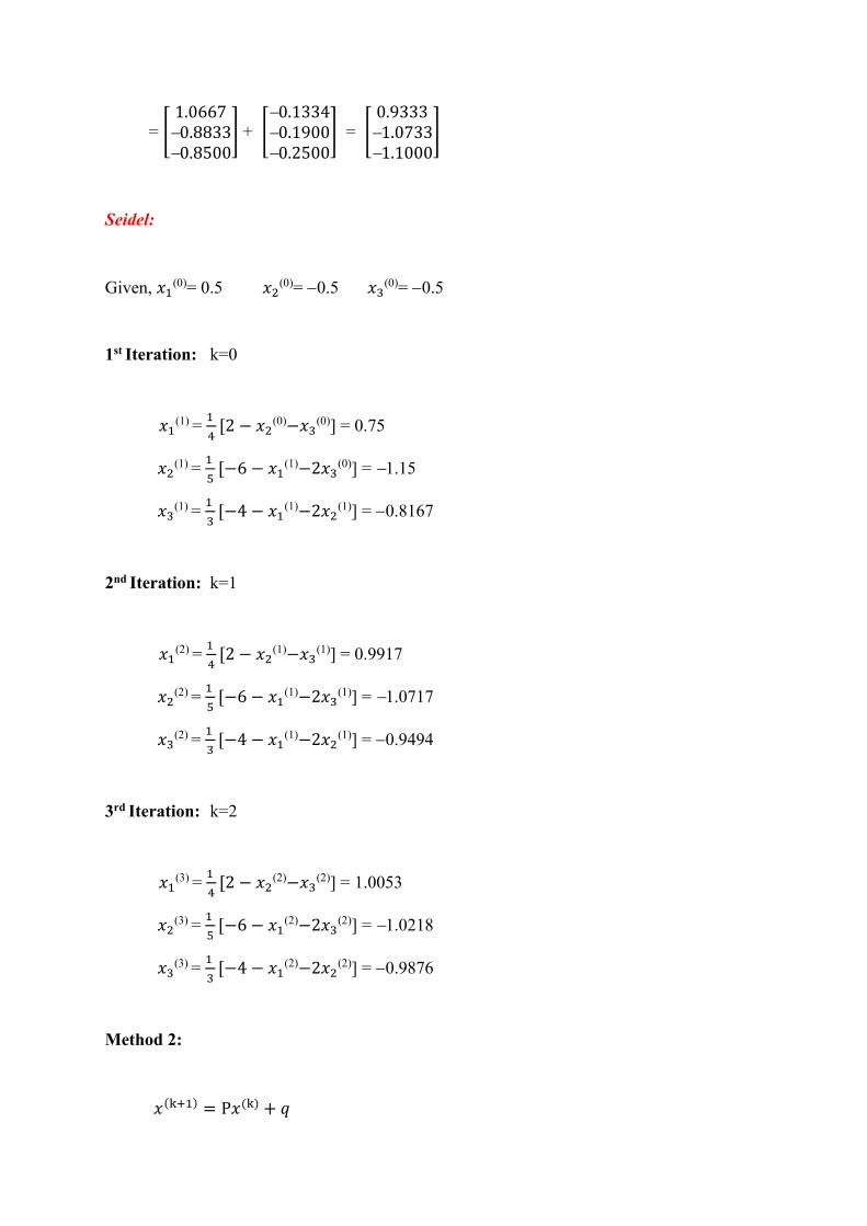
𝑥3 = 𝑥2 + v2
= [1.0667−0.8833−0.8500
] + [−0.1334−0.1900−0.2500
] = [0.9333−1.0733−1.1000
]
Seidel:
Given, 𝑥1(0)= 0.5 𝑥2
(0)= −0.5 𝑥3(0)= −0.5
1st Iteration: k=0
𝑥1(1) =
1
4[2 − 𝑥2
(0)−𝑥3(0)] = 0.75
𝑥2(1) =
1
5[−6 − 𝑥1
(1)−2𝑥3(0)] = −1.15
𝑥3(1) =
1
3[−4 − 𝑥1
(1)−2𝑥2(1)] = −0.8167
2nd Iteration: k=1
𝑥1(2) =
1
4[2 − 𝑥2
(1)−𝑥3(1)] = 0.9917
𝑥2(2) =
1
5[−6 − 𝑥1
(1)−2𝑥3(1)] = −1.0717
𝑥3(2) =
1
3[−4 − 𝑥1
(1)−2𝑥2(1)] = −0.9494
3rd Iteration: k=2
𝑥1(3) =
1
4[2 − 𝑥2
(2)−𝑥3(2)] = 1.0053
𝑥2(3) =
1
5[−6 − 𝑥1
(2)−2𝑥3(2)] = −1.0218
𝑥3(3) =
1
3[−4 − 𝑥1
(2)−2𝑥2(2)] = −0.9876
Method 2:
𝑥(k+1) = P𝑥(k) + 𝑞
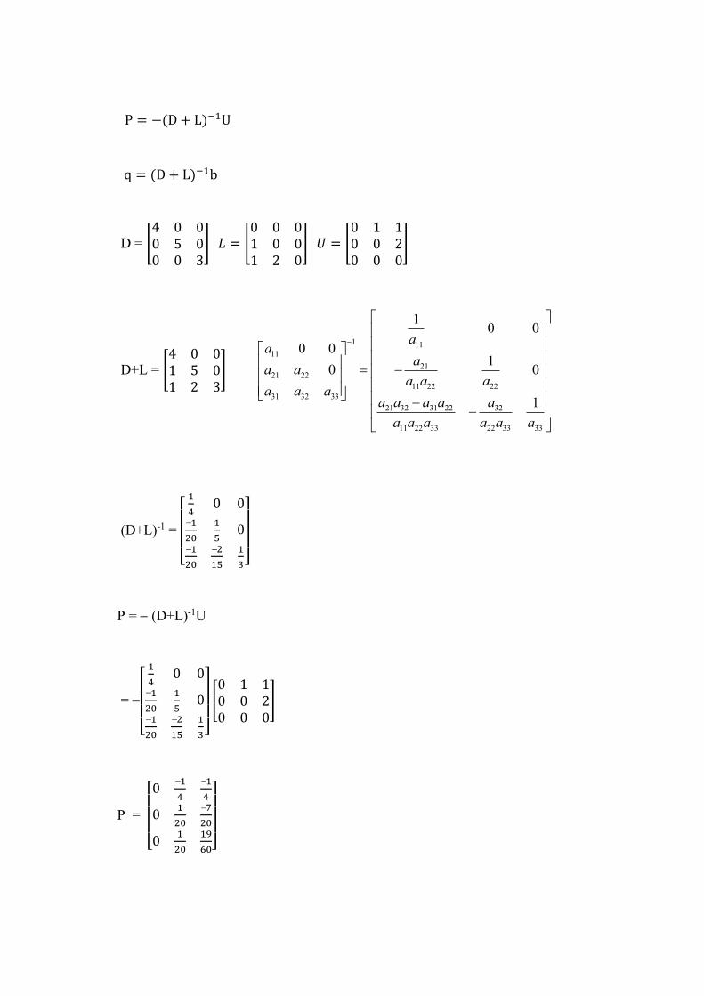
P = −(D + L)−1U
q = (D + L)−1b
D = [4 0 00 5 00 0 3
] 𝐿 = [0 0 01 0 01 2 0
] 𝑈 = [0 1 10 0 20 0 0
]
D+L = [4 0 01 5 01 2 3
]
1 1111
2121 22
11 22 22
31 32 33
21 32 31 22 32
11 22 33 22 33 33
10 0
0 01
0 0
1
aa
aa a
a a aa a a
a a a a a
a a a a a a
−
= − −
−
(D+L)-1 =
[
1
40 0
−1
20
1
50
−1
20
−2
15
1
3]
P = − (D+L)-1U
= −
[
1
40 0
−1
20
1
50
−1
20
−2
15
1
3]
[0 1 10 0 20 0 0
]
P =
[ 0
−1
4
−1
4
01
20
−7
20
01
20
19
60]
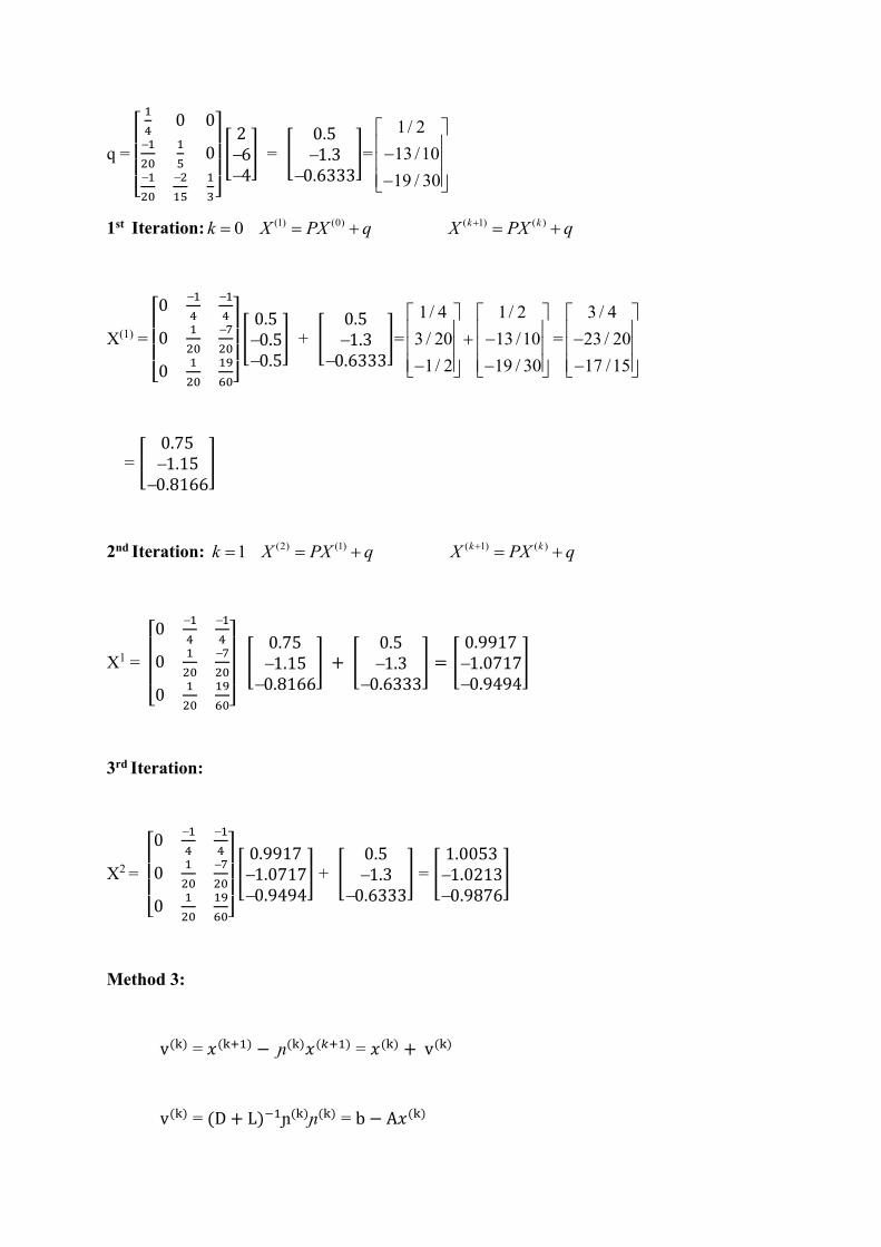
q =
[
1
40 0
−1
20
1
50
−1
20
−2
15
1
3]
[2−6−4
] = [0.5−1.3
−0.6333]=
1/ 2
13 /10
19 / 30
− −
1st Iteration: (1) (0) ( 1) ( )0 k kk X PX q X PX q+= = + = +
X(1) =
[ 0
−1
4
−1
4
01
20
−7
20
01
20
19
60]
[0.5−0.5−0.5
] + [0.5−1.3
−0.6333]=
1/ 4 1/ 2
3 / 20 13 /10
1/ 2 19 / 30
+ − − −
=
3 / 4
23 / 20
17 /15
− −
= [0.75−1.15
−0.8166]
2nd Iteration: (2) (1) ( 1) ( )1 k kk X PX q X PX q+= = + = +
X1 =
[ 0
−1
4
−1
4
01
20
−7
20
01
20
19
60]
[0.75−1.15
−0.8166] + [
0.5−1.3
−0.6333] = [
0.9917−1.0717−0.9494
]
3rd Iteration:
X2 =
[ 0
−1
4
−1
4
01
20
−7
20
01
20
19
60]
[0.9917−1.0717−0.9494
] + [0.5−1.3
−0.6333] = [
1.0053−1.0213−0.9876
]
Method 3:
v(k) = 𝑥(k+1) − ɲ(k)𝑥(𝑘+1) = 𝑥(k) + v(k)
v(k) = (D + L)−1ɲ(k)ɲ(k) = b − A𝑥(k)
When k=0
ɲ(0) = b − A𝑥(0)
= [2−6−4
]−[4 1 11 5 21 2 3
] [0.5−0.5−0.5
] =[1−3−2
]
v(0) = (D + L)−1ɲ(0)
=
[
1
40 0
−1
20
1
50
−1
20
−2
15
1
3]
[1−3−2
] = [
1
4
−0.65−0.3167
]
𝑥1 = 𝑥0 + v0
= [0.5−0.5−0.5
]+ [
1
4
−0.65−0.3167
] = [0.75−1.15
−0.8167]
When k=1
ɲ(1) = b − A𝑥(1)
= [2−6−4
]−[4 1 11 5 21 2 3
] [0.75−1.15
−0.8167] =[
0.96670.63340.0001
]
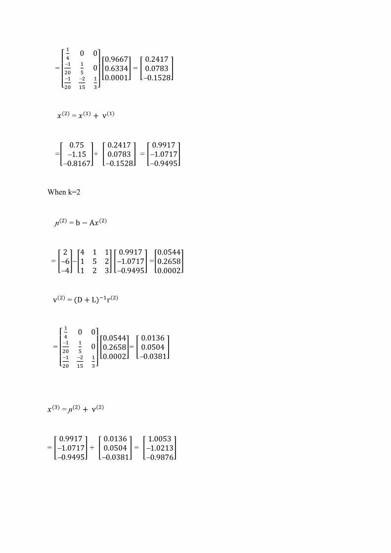
v(1) = (D + L)−1ɲ(1)
=
[
1
40 0
−1
20
1
50
−1
20
−2
15
1
3]
[0.96670.63340.0001
] = [0.24170.0783−0.1528
]
𝑥(2) = 𝑥(1) + v(1)
=[0.75−1.15
−0.8167]+ [
0.24170.0783−0.1528
] = [0.9917−1.0717−0.9495
]
When k=2
ɲ(2) = b − A𝑥(2)
= [2−6−4
]−[4 1 11 5 21 2 3
] [0.9917−1.0717−0.9495
] =[0.05440.26580.0002
]
v(2) = (D + L)−1r(2)
=
[
1
40 0
−1
20
1
50
−1
20
−2
15
1
3]
[0.05440.26580.0002
]= [0.01360.0504−0.0381
]
𝑥(3) = ɲ(2) + v(2)
= [0.9917−1.0717−0.9495
] + [0.01360.0504−0.0381
] = [1.0053−1.0213−0.9876
]
Successive Over Relaxation Method [SOR]
SOR is a method of solving a linear system of Equation AX=b. Derived by extrapolating the
Gauss Seidel Method.
This extrapolation takes the form of the weighted average between the previous iterate and
the computed Gauss Seidel iterate successively for each component
𝑥𝑖𝑘 = 𝑤𝑥�̅�
(𝑘)+ (1 − 𝑤)𝑥𝑖
(𝑘−1) where �̅� denotes the gauss seidal iterate and w is the extrapolation factor.
The idea is to choose the value for w that will accelerate the rate of convergent of the iterates
to the solution
In matrix terms, SOR algorithm can be written as 𝑥𝑘 = (𝐷 − 𝑤𝐿)−1[𝑤𝑈 + (1 − 𝑤)𝐷
𝑥(𝑘+1) + 𝑤(𝐷 − 𝑤𝐿)−1𝑏 where the matrix D, L, U represent diagonal matrix, strictly lower triangle
matrix, strictly upper triangle matrix A, respectively.
Note – 1:-
If w=1, the SOR simplifies to Gauss Seidel method.
Note – 2:-
At theorem due to Kahan shows that SOR fails to converge if w is outside the interval
(0,2)
Note – 3:-
If w =0, there is no iteration
Note – 4:-
If 0 < w < 1, then it is under relaxation
Note – 5:-
If 1 < w < 2, or 0 < w < 2, then it is over relaxation.
Note – 6:-
If ≤ 2, then it is divergent.
Note – 7:-
Over relaxation methods are called succussive over relaxation [SOR]
Theorem:-
If a is positive definite and relaxation parameter w satisfying 0 < w < 2, then the SOR
iteration converges for any initial vector 𝑥𝑜
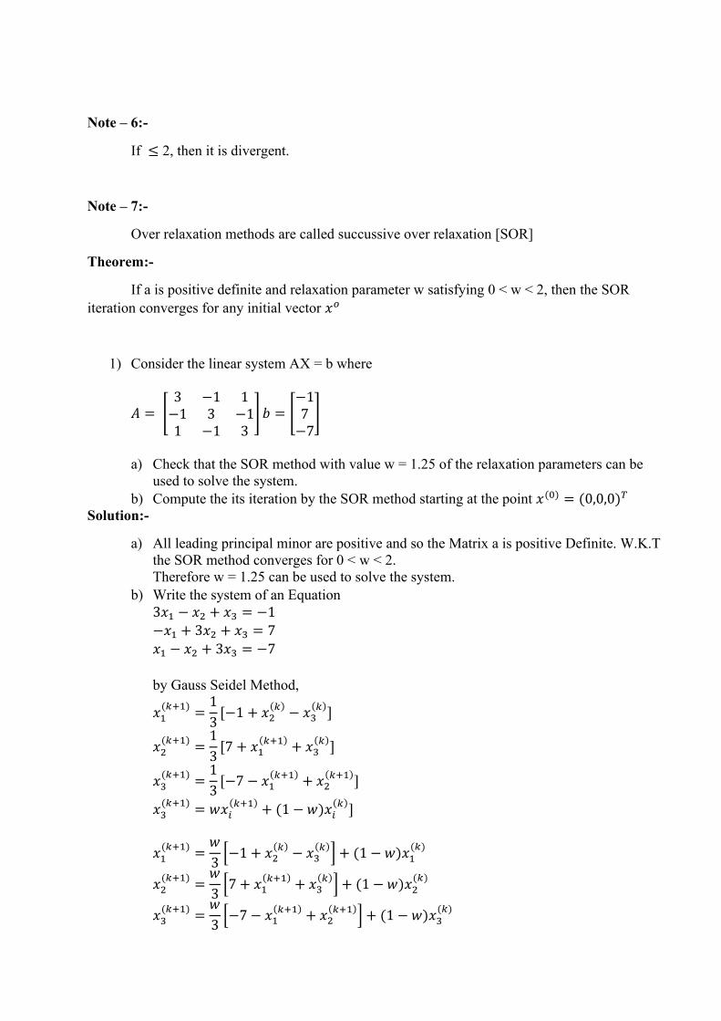
1) Consider the linear system AX = b where
𝐴 = [3 −1 1
−1 3 −11 −1 3
] 𝑏 = [−17
−7]
a) Check that the SOR method with value w = 1.25 of the relaxation parameters can be
used to solve the system.
b) Compute the its iteration by the SOR method starting at the point 𝑥(0) = (0,0,0)𝑇
Solution:-
a) All leading principal minor are positive and so the Matrix a is positive Definite. W.K.T
the SOR method converges for 0 < w < 2.
Therefore w = 1.25 can be used to solve the system.
b) Write the system of an Equation
3𝑥1 − 𝑥2 + 𝑥3 = −1
−𝑥1 + 3𝑥2 + 𝑥3 = 7
𝑥1 − 𝑥2 + 3𝑥3 = −7
by Gauss Seidel Method,
𝑥1(𝑘+1)
=1
3[−1 + 𝑥2
(𝑘)− 𝑥3
(𝑘)]
𝑥2(𝑘+1)
=1
3[7 + 𝑥1
(𝑘+1)+ 𝑥3
(𝑘)]
𝑥3(𝑘+1)
=1
3[−7 − 𝑥1
(𝑘+1)+ 𝑥2
(𝑘+1)]
𝑥3(𝑘+1)
= 𝑤𝑥𝑖(𝑘+1)
+ (1 − 𝑤)𝑥𝑖(𝑘)
]
𝑥1(𝑘+1)
=𝑤
3[−1 + 𝑥2
(𝑘)− 𝑥3
(𝑘)] + (1 − 𝑤)𝑥1
(𝑘)
𝑥2(𝑘+1)
=𝑤
3[7 + 𝑥1
(𝑘+1)+ 𝑥3
(𝑘)] + (1 − 𝑤)𝑥2
(𝑘)
𝑥3(𝑘+1)
=𝑤
3[−7 − 𝑥1
(𝑘+1)+ 𝑥2
(𝑘+1)] + (1 − 𝑤)𝑥3
(𝑘)
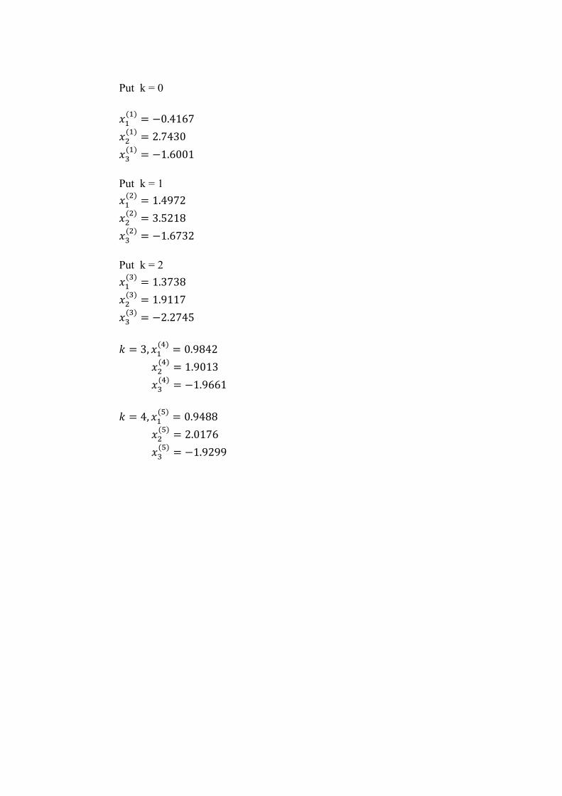
Put k = 0
𝑥1(1)
= −0.4167
𝑥2(1)
= 2.7430
𝑥3(1)
= −1.6001
Put k = 1
𝑥1(2)
= 1.4972
𝑥2(2)
= 3.5218
𝑥3(2)
= −1.6732
Put k = 2
𝑥1(3)
= 1.3738
𝑥2(3)
= 1.9117
𝑥3(3)
= −2.2745
𝑘 = 3, 𝑥1(4)
= 0.9842
𝑥2(4)
= 1.9013
𝑥3(4)
= −1.9661
𝑘 = 4, 𝑥1(5)
= 0.9488
𝑥2(5)
= 2.0176
𝑥3(5)
= −1.9299
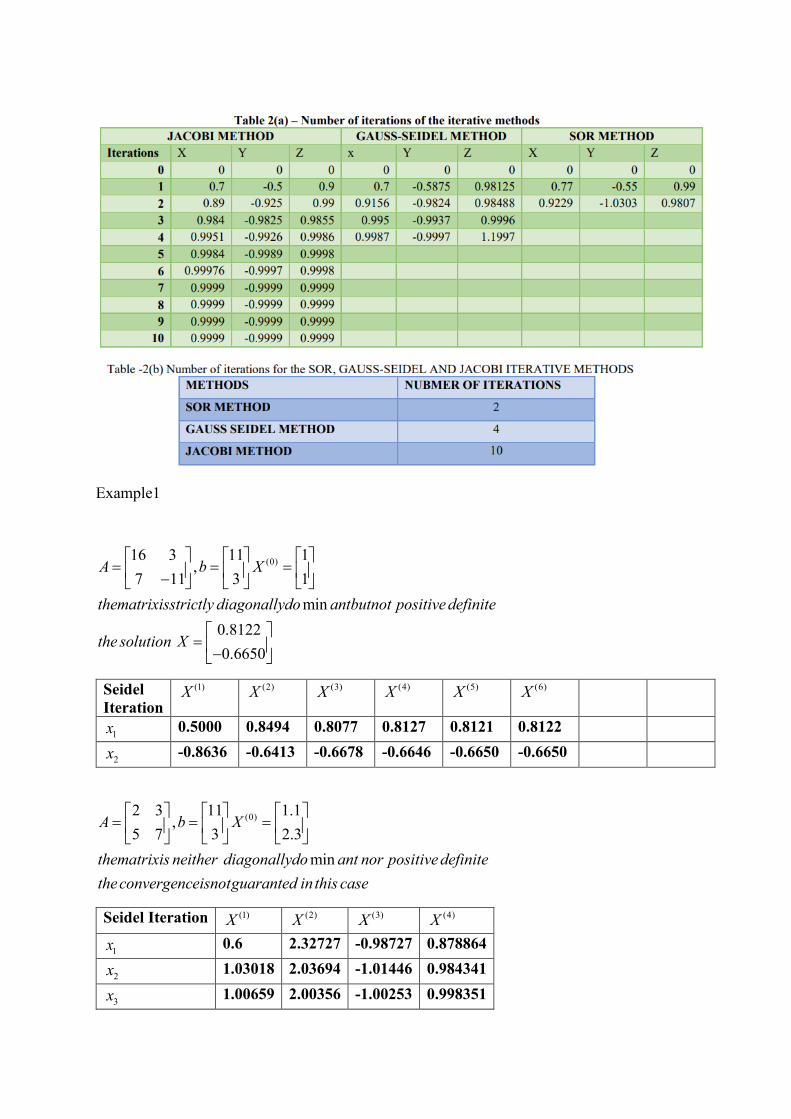
Example1
(0)16 3 11 1
,7 11 3 1
min
0.8122
0.6650
A b X
thematrixisstrictly diagonallydo antbutnot positive definite
the solution X
= = =
−
=
−
Seidel
Iteration
(1)X (2)X (3)X (4)X (5)X (6)X
1x 0.5000 0.8494 0.8077 0.8127 0.8121 0.8122
2x -0.8636 -0.6413 -0.6678 -0.6646 -0.6650 -0.6650
(0)2 3 11 1.1
,5 7 3 2.3
min
A b X
thematrixis neither diagonallydo ant nor positive definite
theconvergenceisnotguaranted in this case
= = =
Seidel Iteration (1)X (2)X (3)X (4)X
1x 0.6 2.32727 -0.98727 0.878864
2x 1.03018 2.03694 -1.01446 0.984341
3x 1.00659 2.00356 -1.00253 0.998351
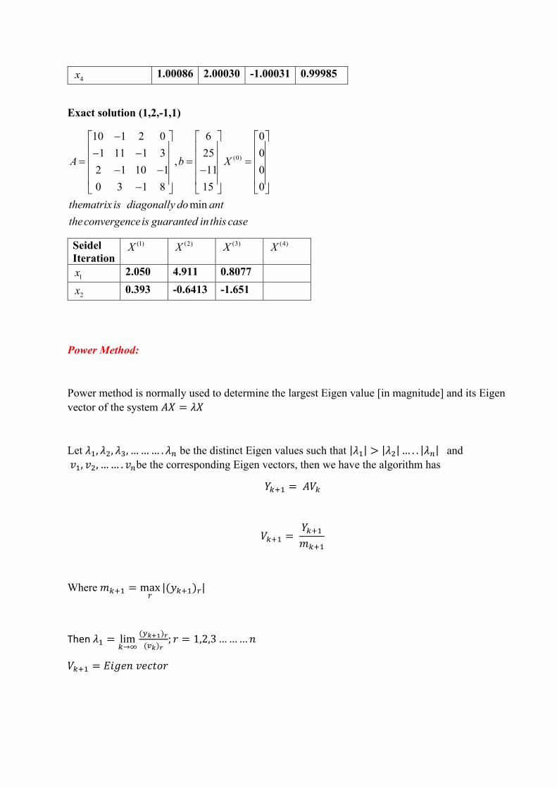
4x 1.00086 2.00030 -1.00031 0.99985
Exact solution (1,2,-1,1)
(0)
10 1 2 0 6 0
1 11 1 3 25 0,
2 1 10 1 11 0
0 3 1 8 15 0
min
A b X
thematrix is diagonally do ant
theconvergenceis guaranted in this case
− − − = = = − − −
−
Seidel
Iteration
(1)X (2)X (3)X (4)X
1x 2.050 4.911 0.8077
2x 0.393 -0.6413 -1.651
Power Method:
Power method is normally used to determine the largest Eigen value [in magnitude] and its Eigen
vector of the system 𝐴𝑋 = 𝜆𝑋
Let 𝜆1, 𝜆2, 𝜆3, ……… . 𝜆𝑛 be the distinct Eigen values such that |𝜆1| > |𝜆2| … . . |𝜆𝑛| and
𝑣1, 𝑣2, …… . 𝑣𝑛be the corresponding Eigen vectors, then we have the algorithm has
𝑌𝑘+1 = 𝐴𝑉𝑘
𝑉𝑘+1 = 𝑌𝑘+1
𝑚𝑘+1
Where 𝑚𝑘+1 = max𝑟
|(𝑦𝑘+1)𝑟|
Then 𝜆1 = lim𝑘→∞
(𝑦𝑘+1)𝑟
(𝑣𝑘)𝑟; 𝑟 = 1,2,3………𝑛
𝑉𝑘+1 = 𝐸𝑖𝑔𝑒𝑛 𝑣𝑒𝑐𝑡𝑜𝑟
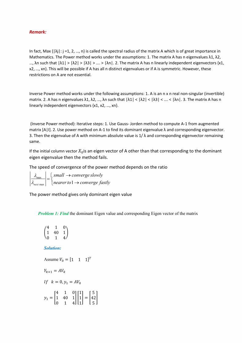
Remark:
In fact, Max {|λj|: j =1, 2, …, n} is called the spectral radius of the matrix A which is of great importance in
Mathematics. The Power method works under the assumptions: 1. The matrix A has n eigenvalues λ1, λ2,
…, λn such that |λ1| > |λ2| > |λ3| > …. > |λn|. 2. The matrix A has n linearly independent eigenvectors {x1,
x2, …, xn}. This will be possible if A has all n distinct eigenvalues or if A is symmetric. However, these
restrictions on A are not essential.
Inverse Power method works under the following assumptions: 1. A is an n x n real non-singular (invertible)
matrix. 2. A has n eigenvalues λ1, λ2, …, λn such that |λ1| < |λ2| < |λ3| < …. < |λn|. 3. The matrix A has n
linearly independent eigenvectors {x1, x2, …, xn}.
(Inverse Power method): Iterative steps: 1. Use Gauss- Jorden method to compute A-1 from augmented
matrix [A|I]. 2. Use power method on A-1 to find its dominant eigenvalue λ and corresponding eigenvector.
3. Then the eigenvalue of A with minimum absolute value is 1/ λ and corresponding eigenvector remaining
same.
If the initial column vector 𝑋0is an eigen vector of A other than that corresponding to the dominant
eigen eigenvalue then the method fails.
The speed of convergence of the power method depends on the ratio
max
max1
next
small converge slowly
nearer to converge fastly
→=
→
The power method gives only dominant eigen value
Problem 1: Find the dominant Eigen value and corresponding Eigen vector of the matrix
(4 1 01 40 10 1 4
)
Solution:
Assume 𝑉0 = [1 1 1]𝑇
𝑌𝑘+1 = 𝐴𝑉𝑘
𝐼𝑓 𝑘 = 0, 𝑦1 = 𝐴𝑉0
𝑦1 = [4 1 01 40 10 1 4
] [111] = [
5425
]
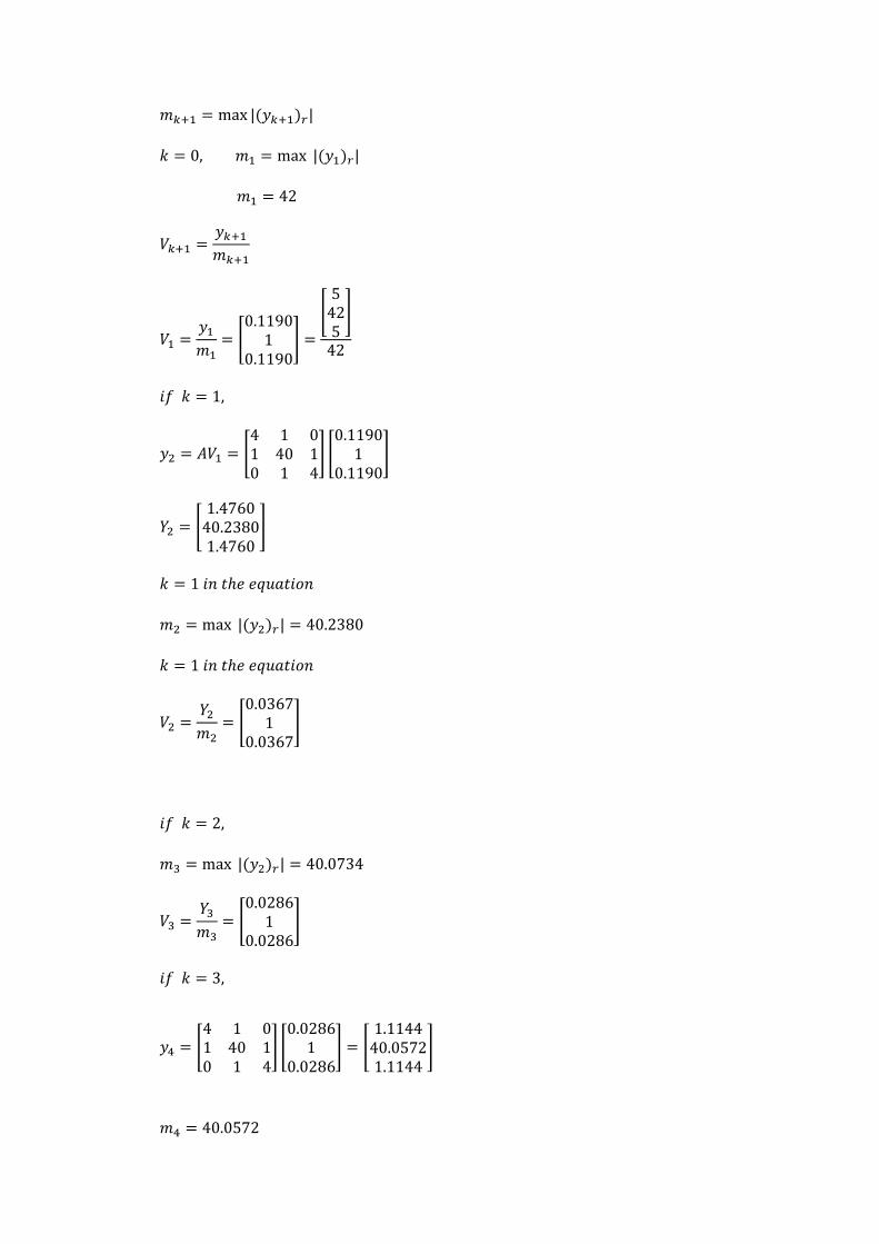
𝑚𝑘+1 = max |(𝑦𝑘+1)𝑟|
𝑘 = 0, 𝑚1 = max |(𝑦1)𝑟|
𝑚1 = 42
𝑉𝑘+1 =𝑦𝑘+1
𝑚𝑘+1
𝑉1 =𝑦1
𝑚1= [
0.11901
0.1190] =
[5425
]
42
𝑖𝑓 𝑘 = 1,
𝑦2 = 𝐴𝑉1 = [4 1 01 40 10 1 4
] [0.1190
10.1190
]
𝑌2 = [1.476040.23801.4760
]
𝑘 = 1 𝑖𝑛 𝑡ℎ𝑒 𝑒𝑞𝑢𝑎𝑡𝑖𝑜𝑛
𝑚2 = max |(𝑦2)𝑟| = 40.2380
𝑘 = 1 𝑖𝑛 𝑡ℎ𝑒 𝑒𝑞𝑢𝑎𝑡𝑖𝑜𝑛
𝑉2 =𝑌2
𝑚2= [
0.03671
0.0367]
𝑖𝑓 𝑘 = 2,
𝑚3 = max |(𝑦2)𝑟| = 40.0734
𝑉3 =𝑌3
𝑚3= [
0.02861
0.0286]
𝑖𝑓 𝑘 = 3,
𝑦4 = [4 1 01 40 10 1 4
] [0.0286
10.0286
] = [1.114440.05721.1144
]
𝑚4 = 40.0572
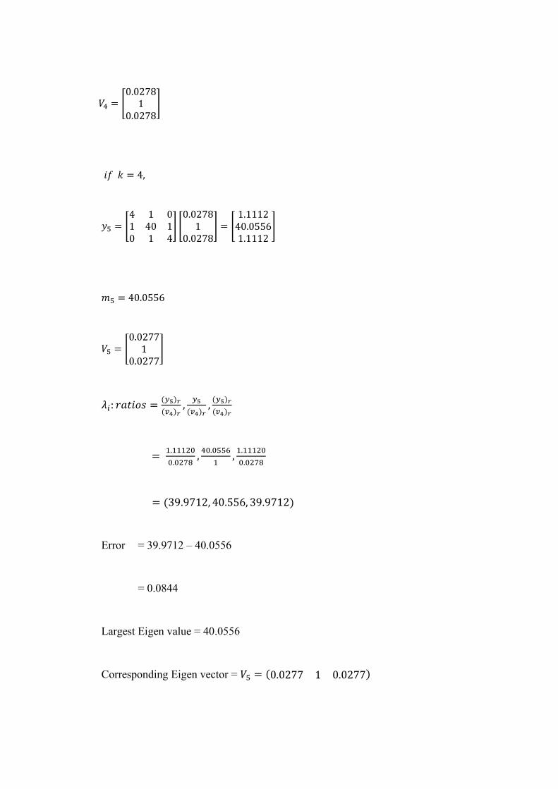
𝑉4 = [0.0278
10.0278
]
𝑖𝑓 𝑘 = 4,
𝑦5 = [4 1 01 40 10 1 4
] [0.0278
10.0278
] = [1.111240.05561.1112
]
𝑚5 = 40.0556
𝑉5 = [0.0277
10.0277
]
𝜆𝑖: 𝑟𝑎𝑡𝑖𝑜𝑠 =(𝑦5)𝑟
(𝑣4)𝑟,
𝑦5
(𝑣4)𝑟,(𝑦5)𝑟
(𝑣4)𝑟
= 1.11120
0.0278,40.0556
1,1.11120
0.0278
= (39.9712, 40.556, 39.9712)
Error = 39.9712 – 40.0556
= 0.0844
Largest Eigen value = 40.0556
Corresponding Eigen vector = 𝑉5 = (0.0277 1 0.0277)
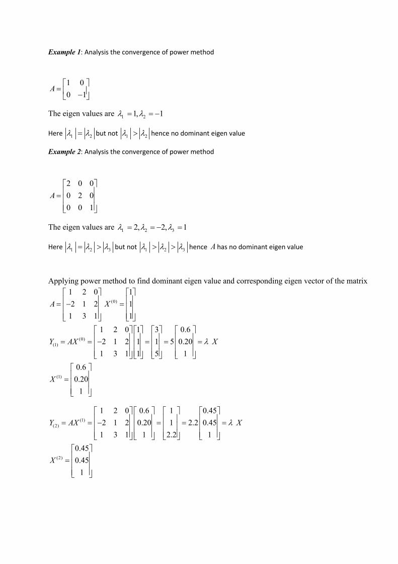
Example 1: Analysis the convergence of power method
1 0
0 1A
=
−
The eigen values are 1 21, 1 = = −
Here 1 2 = but not 1 2 hence no dominant eigen value
Example 2: Analysis the convergence of power method
2 0 0
0 2 0
0 0 1
A
=
The eigen values are 1 2 32, 2, 1 = = − =
Here 1 2 3 = but not 1 2 3 hence A has no dominant eigen value
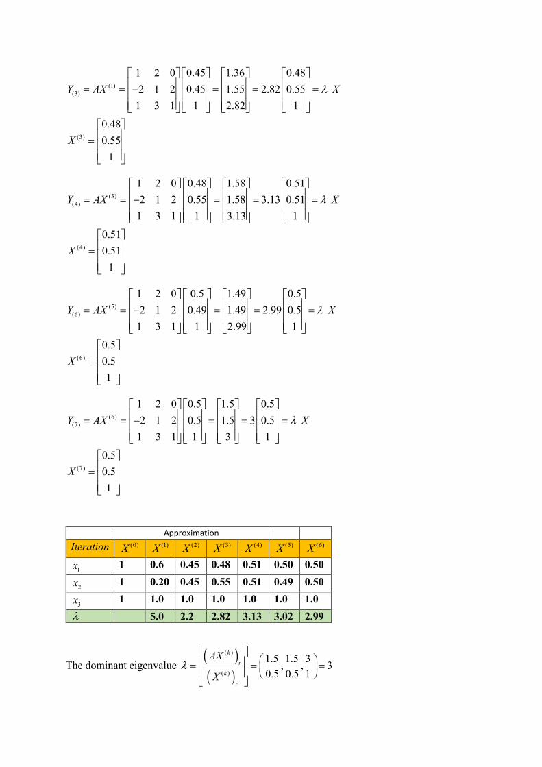
Applying power method to find dominant eigen value and corresponding eigen vector of the matrix
(0)
(0)
(1)
(1)
1 2 0 1
2 1 2 1
1 3 1 1
1 2 0 1 3 0.6
2 1 2 1 1 5 0.20
1 3 1 1 5 1
0.6
0.20
1
A X
Y AX X
X
= − =
= = − = = =
=
(1)
(2)
(2)
1 2 0 0.6 1 0.45
2 1 2 0.20 1 2.2 0.45
1 3 1 1 2.2 1
0.45
0.45
1
Y AX X
X
= = − = = =
=
(1)
(3)
(3)
1 2 0 0.45 1.36 0.48
2 1 2 0.45 1.55 2.82 0.55
1 3 1 1 2.82 1
0.48
0.55
1
Y AX X
X
= = − = = =
=
(3)
(4)
(4)
1 2 0 0.48 1.58 0.51
2 1 2 0.55 1.58 3.13 0.51
1 3 1 1 3.13 1
0.51
0.51
1
Y AX X
X
= = − = = =
=
(5)
(6)
(6)
1 2 0 0.5 1.49 0.5
2 1 2 0.49 1.49 2.99 0.5
1 3 1 1 2.99 1
0.5
0.5
1
Y AX X
X
= = − = = =
=
(6)
(7)
(7)
1 2 0 0.5 1.5 0.5
2 1 2 0.5 1.5 3 0.5
1 3 1 1 3 1
0.5
0.5
1
Y AX X
X
= = − = = =
=
Approximation
Iteration (0)X (1)X (2)X (3)X (4)X (5)X
(6)X
1x 1 0.6 0.45 0.48 0.51 0.50 0.50
2x 1 0.20 0.45 0.55 0.51 0.49 0.50
3x 1 1.0 1.0 1.0 1.0 1.0 1.0
5.0 2.2 2.82 3.13 3.02 2.99
The dominant eigenvalue ( )
( )
( )
( )
1.5 1.5 3, , 3
0.5 0.5 1
k
r
k
r
AX
X
= = =
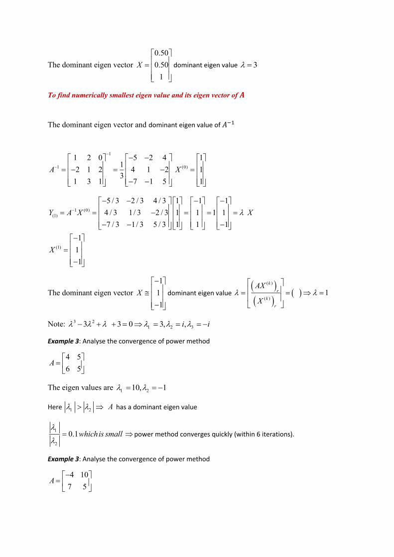
The dominant eigen vector
0.50
0.50
1
X
=
dominant eigen value 3 =
To find numerically smallest eigen value and its eigen vector of 𝑨
The dominant eigen vector and dominant eigen value of 𝐴−1
1
1 (0)
1 2 0 5 2 4 11
2 1 2 4 1 2 13
1 3 1 7 1 5 1
A X
−
−
− −
= − = − = − −
1 (0)
(1)
(1)
5 / 3 2 / 3 4 / 3 1 1 1
4 / 3 1/ 3 2 / 3 1 1 1 1
7 / 3 1/ 3 5 / 3 1 1 1
1
1
1
Y A X X
X
−
− − − −
= = − = = = − − −
−
= −
The dominant eigen vector
1
1
1
X
−
−
dominant eigen value ( )
( )( )
( )
( )1
k
r
k
r
AX
X
= = =
Note: 3 2
1 2 33 3 0 3, ,i i − + + = = = = −
Example 3: Analyse the convergence of power method
4 5
6 5A
=
The eigen values are 1 210, 1 = = −
Here 1 2 A has a dominant eigen value
1
2
0.1whichis small
= power method converges quickly (within 6 iterations).
Example 3: Analyse the convergence of power method
4 10
7 5A
− =

The eigen values are 1 210, 9 = = −
Here 1 2 A has a dominant eigen value
1
2
0.9 1which is nearer to
= power method converges slowly (after 68 iterations)
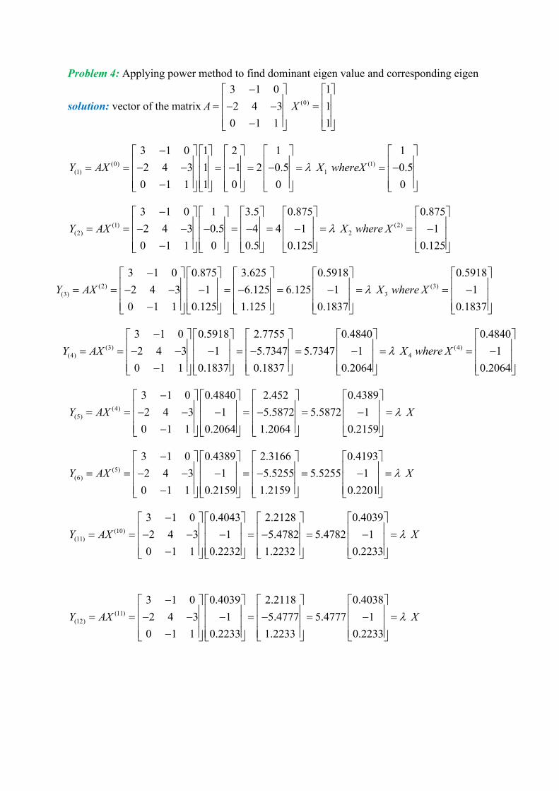
Problem 4: Applying power method to find dominant eigen value and corresponding eigen
solution: vector of the matrix (0)
3 1 0 1
2 4 3 1
0 1 1 1
A X
−
= − − = −
(0) (1)
(1) 1
3 1 0 1 2 1 1
2 4 3 1 1 2 0.5 0.5
0 1 1 1 0 0 0
Y AX X whereX
−
= = − − = − = − = = − −
(1) (2)
(2) 2
3 1 0 1 3.5 0.875 0.875
2 4 3 0.5 4 4 1 1
0 1 1 0 0.5 0.125 0.125
Y AX X where X
−
= = − − − = − = − = = − −
(2) (3)
(3) 3
3 1 0 0.875 3.625 0.5918 0.5918
2 4 3 1 6.125 6.125 1 1
0 1 1 0.125 1.125 0.1837 0.1837
Y AX X where X
−
= = − − − = − = − = = − −
(3) (4)
(4) 4
3 1 0 0.5918 2.7755 0.4840 0.4840
2 4 3 1 5.7347 5.7347 1 1
0 1 1 0.1837 0.1837 0.2064 0.2064
Y AX X where X
−
= = − − − = − = − = = − −
(4)
(5)
3 1 0 0.4840 2.452 0.4389
2 4 3 1 5.5872 5.5872 1
0 1 1 0.2064 1.2064 0.2159
Y AX X
−
= = − − − = − = − = −
(5)
(6)
3 1 0 0.4389 2.3166 0.4193
2 4 3 1 5.5255 5.5255 1
0 1 1 0.2159 1.2159 0.2201
Y AX X
−
= = − − − = − = − = −
(10)
(11)
3 1 0 0.4043 2.2128 0.4039
2 4 3 1 5.4782 5.4782 1
0 1 1 0.2232 1.2232 0.2233
Y AX X
−
= = − − − = − = − = −
(11)
(12)
3 1 0 0.4039 2.2118 0.4038
2 4 3 1 5.4777 5.4777 1
0 1 1 0.2233 1.2233 0.2233
Y AX X
−
= = − − − = − = − = −
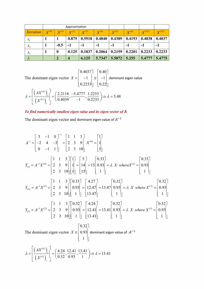
Approximation
Iteration (0)X (1)X (2)X (3)X (4)X (5)X
(6)X (12)X
(13)X
1x 1 1 0.875 0.5918 0.4840 0.4389 0.4193 0.4038 0.4037
2x 1 -0.5 -1 -1 -1 -1 -1 -1 -1
3x 1 0 0.125 0.1837 0.2064 0.2159 0.2201 0.2233 0.2233
2 4 6.125 5.7347 5.5872 5.255 5.4777 5.4775
The dominant eigen vector
0.4037 0.40
1 1
0.2233 0.22
X
= − −
dominant eigen value
( )
( )
( )
( )
2.2118 5.4777 1.2233, , 5.48
0.4039 1 0.2233
k
r
k
r
AX
X
− = = = −
To find numerically smallest eigen value and its eigen vector of 𝑨
The dominant eigen vector and dominant eigen value of 𝐴−1
1
1 (0)
3 1 0 1 1 3 1
2 4 3 2 3 9 1
0 1 1 2 3 10 1
A X
−
−
−
= − − = = −
1 (0) (1)
(1)
1 1 3 1 5 0.33 0.33
2 3 9 1 14 15 0.93 0.93
2 3 10 1 15 1 1
Y A X X whereX−
= = = = = =
1 (1) (2)
(2)
1 1 3 0.33 4.27 0.32 0.32
2 3 9 0.93 12.47 13.47 0.93 0.93
2 3 10 1 13.47 1 1
Y A X X where X−
= = = = = =
1 (2) (3)
(3)
1 1 3 0.32 4.24 0.32 0.32
2 3 9 0.93 12.41 13.41 0.93 0.93
2 3 10 1 13.41 1 1
Y A X X where X−
= = = = = =
The dominant eigen vector
0.32
0.93
1
X
dominant eigen value of 𝐴−1
( )
( )
( )
( )
4.24 12.41 13.41, , 13.41
0.32 0.93 1
k
r
k
r
AX
X
= = =
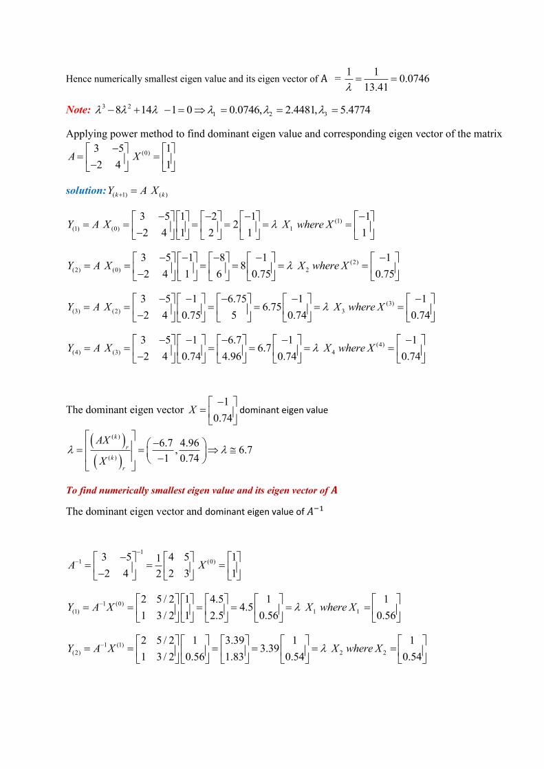
Hence numerically smallest eigen value and its eigen vector of A = 1 1
0.074613.41
= =
Note: 3 2
1 2 38 14 1 0 0.0746, 2.4481, 5.4774 − + − = = = =
Applying power method to find dominant eigen value and corresponding eigen vector of the matrix
(0)3 5 1
2 4 1A X
− = =
−
solution:( 1) ( )k kY A X+ =
(1)
(1) (0) 1
3 5 1 2 1 12
2 4 1 2 1 1Y A X X where X
− − − − = = = = = =
−
(2)
(2) (0) 2
3 5 1 8 1 18
2 4 1 6 0.75 0.75Y A X X where X
− − − − − = = = = = =
−
(3)
(3) (2) 3
3 5 1 6.75 1 16.75
2 4 0.75 5 0.74 0.74Y A X X where X
− − − − − = = = = = =
−
(4)
(4) (3) 4
3 5 1 6.7 1 16.7
2 4 0.74 4.96 0.74 0.74Y A X X where X
− − − − − = = = = = =
−
The dominant eigen vector 1
0.74X
− =
dominant eigen value
( )
( )
( )
( )
6.7 4.96, 6.7
1 0.74
k
r
k
r
AX
X
− = = −
To find numerically smallest eigen value and its eigen vector of 𝑨
The dominant eigen vector and dominant eigen value of 𝐴−1
1
1 (0)3 5 4 5 11
2 4 2 3 12A X
−
−−
= = = −
1 (0)
(1) 1 1
2 5 / 2 1 4.5 1 14.5
1 3 / 2 1 2.5 0.56 0.56Y A X X where X−
= = = = = =
1 (1)
(2) 2 2
2 5 / 2 1 3.39 1 13.39
1 3 / 2 0.56 1.83 0.54 0.54Y A X X where X−
= = = = = =
1 (2)
(3) 3 3
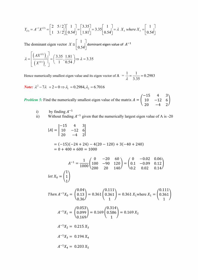
2 5 / 2 1 3.35 1 13.35
1 3 / 2 0.54 1.81 0.54 0.54Y A X X where X−
= = = = = =
The dominant eigen vector 1
0.54X
dominant eigen value of 𝐴−1
( )
( )
( )
( )
3.35 1.81, 3.35
1 0.54
k
r
k
r
AX
X
= = =
Hence numerically smallest eigen value and its eigen vector of A = 1 1
0.29833.35
= =
Note: 2
1 27 2 0 0.2984, 6.7016 − + = = =
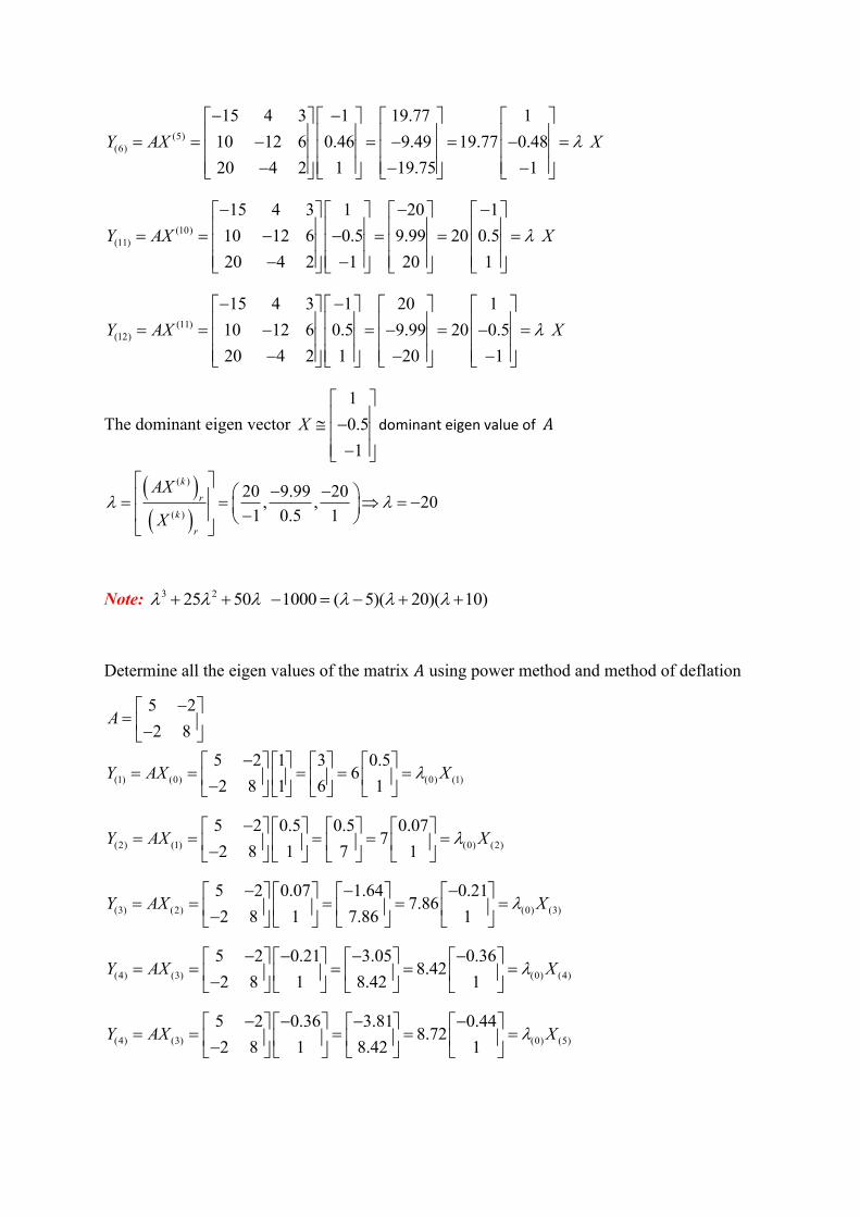
Problem 5: Find the numerically smallest eigen value of the matrix 𝐴 = (−15 4 310 −12 620 −4 2
)
i) by finding 𝐴−1
ii) Without finding 𝐴−1 given that the numerically largest eigen value of A is -20
|𝐴| = |−15 4 310 −12 620 −4 2
|
= (−15)(−24 + 24) − 4(20 − 120) + 3(−40 + 240)
= 0 + 400 + 600 = 1000
𝐴−1 =1
1000(
0 −20 60100 −90 120200 20 140
) = (0 −0.02 0.06
0.1 −0.09 0.120.2 0.02 0.14
)
𝑙𝑒𝑡 𝑋0 = (111)
𝑇ℎ𝑒𝑛 𝐴−1𝑋0 = (0.040.130.36
) = 0.361 (0.1110.361
1) = 0.361 𝑋1where 𝑋1 = (
0.1110.361
1)
𝐴−1𝑋1 = (0.0530.0990.169
) = 0.169(0.3140.586
1) = 0.169 𝑋2
𝐴−1𝑋2 = 0.215 𝑋3
𝐴−1𝑋3 = 0.194 𝑋4
𝐴−1𝑋4 = 0.203 𝑋5
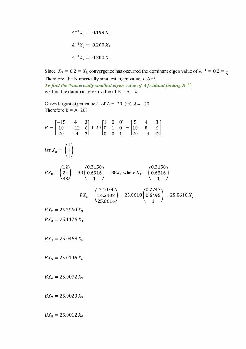
𝐴−1𝑋5 = 0.199 𝑋6
𝐴−1𝑋6 = 0.200 𝑋7
𝐴−1𝑋7 = 0.200 𝑋8
Since 𝑋7 = 0.2 = 𝑋8 convergence has occurred the dominant eigen value of 𝐴−1 = 0.2 =1
5
Therefore, the Numerically smallest eigen value of A=5.
To find the Numerically smallest eigen value of A [without finding 𝑨−𝟏] we find the dominant eigen value of B = A – λI
Given largest eigen value of A = -20 (ie) 20 = −
Therefore B = A+20I
𝐵 = [−15 4 310 −12 620 −4 2
] + 20 [1 0 00 1 00 0 1
] = [5 4 310 8 620 −4 22
]
𝑙𝑒𝑡 𝑋0 = (111)
𝐵𝑋0 = (122438
) = 38(0.31580.6316
1) = 38𝑋1 where 𝑋1 = (
0.31580.6316
1)
𝐵𝑋1 = (7.105414.210825.8616
) = 25.8618(0.27470.5495
1) = 25.8616 𝑋2
𝐵𝑋2 = 25.2960 𝑋3
𝐵𝑋3 = 25.1176 𝑋4
𝐵𝑋4 = 25.0468 𝑋5
𝐵𝑋5 = 25.0196 𝑋6
𝐵𝑋6 = 25.0072 𝑋7
𝐵𝑋7 = 25.0020 𝑋8
𝐵𝑋8 = 25.0012 𝑋9
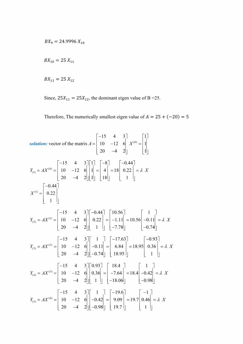
𝐵𝑋9 = 24.9996 𝑋10
𝐵𝑋10 = 25 𝑋11
𝐵𝑋11 = 25 𝑋12
Since, 25𝑋11 = 25𝑋12, the dominant eigen value of B =25.
Therefore, The numerically smallest eigen value of 𝐴 = 25 + (−20) = 5
solution: vector of the matrix (0)
15 4 3 1
10 12 6 1
20 4 2 1
A X
−
= − = −
(0)
(1)
(1)
15 4 3 1 8 0.44
10 12 6 1 4 18 0.22
20 4 2 1 18 1
0.44
0.22
1
Y AX X
X
− − −
= = − = = = −
−
=
(1)
(2)
15 4 3 0.44 10.56 1
10 12 6 0.22 1.11 10.56 0.11
20 4 2 1 7.78 0.74
Y AX X
− −
= = − = − = − = − − −
(2)
(3)
15 4 3 1 17.63 0.93
10 12 6 0.11 6.84 18.95 0.36
20 4 2 0.74 18.95 1
Y AX X
− − −
= = − − = = = − −
(3)
(4)
15 4 3 0.93 18.4 1
10 12 6 0.36 7.64 18.4 0.42
20 4 2 1 18.06 0.98
Y AX X
−
= = − = − = − = − − −
(4)
(5)
15 4 3 1 19.6 1
10 12 6 0.42 9.09 19.7 0.46
20 4 2 0.98 19.7 1
Y AX X
− − −
= = − − = = = − −
(5)
(6)
15 4 3 1 19.77 1
10 12 6 0.46 9.49 19.77 0.48
20 4 2 1 19.75 1
Y AX X
− −
= = − = − = − = − − −
(10)
(11)
15 4 3 1 20 1
10 12 6 0.5 9.99 20 0.5
20 4 2 1 20 1
Y AX X
− − −
= = − − = = = − −
(11)
(12)
15 4 3 1 20 1
10 12 6 0.5 9.99 20 0.5
20 4 2 1 20 1
Y AX X
− −
= = − = − = − = − − −
The dominant eigen vector
1
0.5
1
X
− −
dominant eigen value of 𝐴
( )
( )
( )
( )
20 9.99 20, , 20
1 0.5 1
k
r
k
r
AX
X
− − = = = − −
Note: 3 225 50 1000 ( 5)( 20)( 10) + + − = − + +
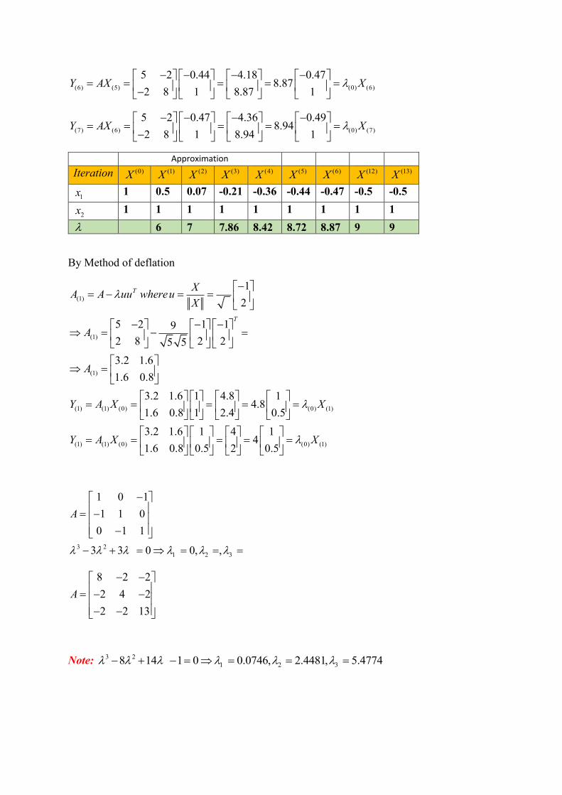
Determine all the eigen values of the matrix 𝐴 using power method and method of deflation
(1) (0) (0) (1)
5 2
2 8
5 2 1 3 0.56
2 8 1 6 1
A
Y AX X
− =
−
− = = = = =
−
(2) (1) (0) (2)
5 2 0.5 0.5 0.077
2 8 1 7 1Y AX X
− = = = = =
−
(3) (2) (0) (3)
5 2 0.07 1.64 0.217.86
2 8 1 7.86 1Y AX X
− − − = = = = =
−
(4) (3) (0) (4)
5 2 0.21 3.05 0.368.42
2 8 1 8.42 1Y AX X
− − − − = = = = =
−
(4) (3) (0) (5)
5 2 0.36 3.81 0.448.72
2 8 1 8.42 1Y AX X
− − − − = = = = =
−
(6) (5) (0) (6)
5 2 0.44 4.18 0.478.87
2 8 1 8.87 1Y AX X
− − − − = = = = =
−
(7) (6) (0) (7)
5 2 0.47 4.36 0.498.94
2 8 1 8.94 1Y AX X
− − − − = = = = =
−
Approximation
Iteration (0)X (1)X (2)X (3)X (4)X (5)X
(6)X (12)X
(13)X
1x 1 0.5 0.07 -0.21 -0.36 -0.44 -0.47 -0.5 -0.5
2x 1 1 1 1 1 1 1 1 1
6 7 7.86 8.42 8.72 8.87 9 9
By Method of deflation
(1)
(1)
(1)
(1) (1) (0) (0) (1)
(1) (1) (0)
1
2
5 2 1 19
2 8 2 25 5
3.2 1.6
1.6 0.8
3.2 1.6 1 4.8 14.8
1.6 0.8 1 2.4 0.5
3.2 1.6
1.6 0.8
T
T
XA A uu whereu
X
A
A
Y A X X
Y A X
− = − = =
− − − = − =
=
= = = = =
= =
(0) (1)
1 4 14
0.5 2 0.5X
= = =
3 2
1 2 3
1 0 1
1 1 0
0 1 1
3 3 0 0, ,
A
−
= − −
− + = = = =
8 2 2
2 4 2
2 2 13
A
− −
= − − − −
Note: 3 2
1 2 38 14 1 0 0.0746, 2.4481, 5.4774 − + − = = = =


UNIT – III - ADVANCED NUMERICAL METHODS – SMTA5304
UNIT III
Interpolation And Approximation
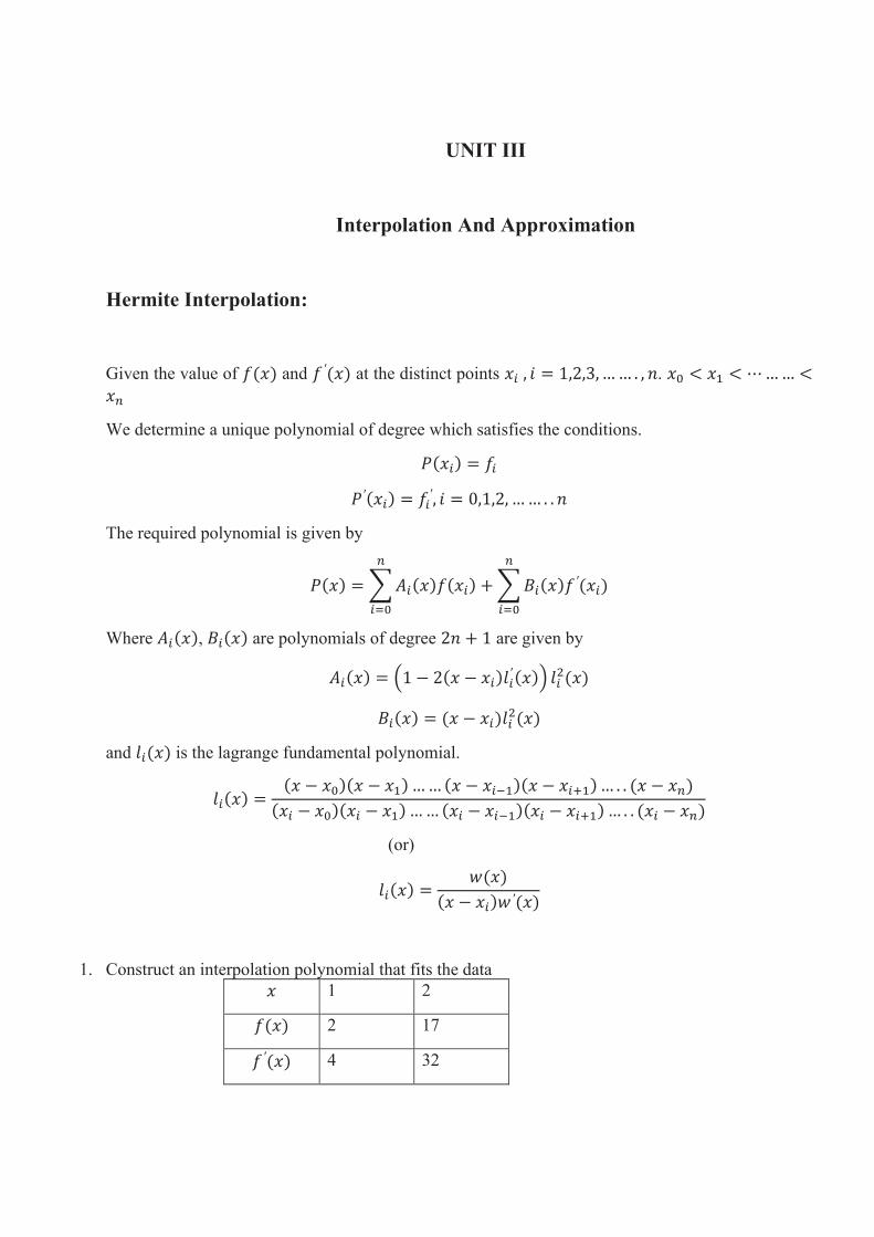
Hermite Interpolation:
Given the value of 𝑓(𝑥) and 𝑓 ′(𝑥) at the distinct points 𝑥𝑖 , 𝑖 = 1,2,3,…… . , 𝑛. 𝑥0 < 𝑥1 < ⋯…… <
𝑥𝑛
We determine a unique polynomial of degree which satisfies the conditions.
𝑃(𝑥𝑖) = 𝑓𝑖
𝑃′(𝑥𝑖) = 𝑓𝑖′, 𝑖 = 0,1,2, …… . . 𝑛
The required polynomial is given by
𝑃(𝑥) = ∑𝐴𝑖(𝑥)𝑓(𝑥𝑖) + ∑𝐵𝑖(𝑥)𝑓 ′(𝑥𝑖)
𝑛
𝑖=0
𝑛
𝑖=0
Where 𝐴𝑖(𝑥), 𝐵𝑖(𝑥) are polynomials of degree 2𝑛 + 1 are given by
𝐴𝑖(𝑥) = (1 − 2(𝑥 − 𝑥𝑖)𝑙𝑖′ (𝑥)) 𝑙𝑖
2(𝑥)
𝐵𝑖(𝑥) = (𝑥 − 𝑥𝑖)𝑙𝑖2(𝑥)
and 𝑙𝑖(𝑥) is the lagrange fundamental polynomial.
𝑙𝑖(𝑥) =(𝑥 − 𝑥0)(𝑥 − 𝑥1)…… (𝑥 − 𝑥𝑖−1)(𝑥 − 𝑥𝑖+1)… . . (𝑥 − 𝑥𝑛)
(𝑥𝑖 − 𝑥0)(𝑥𝑖 − 𝑥1)…… (𝑥𝑖 − 𝑥𝑖−1)(𝑥𝑖 − 𝑥𝑖+1)… . . (𝑥𝑖 − 𝑥𝑛)
(or)
𝑙𝑖(𝑥) =𝑤(𝑥)
(𝑥 − 𝑥𝑖)𝑤′(𝑥)
1. Construct an interpolation polynomial that fits the data
𝑥 1 2
𝑓(𝑥) 2 17
𝑓 ′(𝑥) 4 32
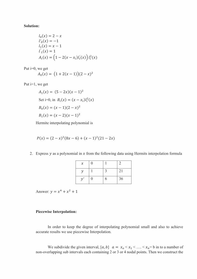
Solution:
𝑙0(𝑥) = 2 − 𝑥
𝑙′0(𝑥) = −1
𝑙1(𝑥) = 𝑥 − 1
𝑙′1(𝑥) = 1
𝐴𝑖(𝑥) = (1 − 2(𝑥 − 𝑥𝑖)𝑙𝑖′ (𝑥)) 𝑙𝑖
2(𝑥)
Put i=0, we get
𝐴0(𝑥) = (1 + 2(𝑥 − 1))(2 − 𝑥)2
Put i=1, we get
𝐴1(𝑥) = (5 − 2𝑥)(𝑥 − 1)2
Set i=0, in 𝐵𝑖(𝑥) = (𝑥 − 𝑥𝑖)𝑙𝑖2(𝑥)
𝐵0(𝑥) = (𝑥 − 1)(2 − 𝑥)2
𝐵1(𝑥) = (𝑥 − 2)(𝑥 − 1)2
Hermite interpolating polynomial is
𝑃(𝑥) = (2 − 𝑥)2(8𝑥 − 6) + (𝑥 − 1)2(21 − 2𝑥)
2. Express 𝑦 as a polynomial in 𝑥 from the following data using Hermits interpolation formula
𝑥 0 1 2
𝑦 1 3 21
𝑦′ 0 6 36
Answer: 𝑦 = 𝑥4 + 𝑥2 + 1
Piecewise Interpolation:
In order to keep the degree of interpolating polynomial small and also to achieve
accurate results we use piecewise Interpolation.
We subdivide the given interval, [𝑎, 𝑏] 𝑎 = 𝑥𝑜 < 𝑥1 < …. < 𝑥𝑛= b in to a number of
non-overlapping sub intervals each containing 2 or 3 or 4 nodal points. Then we construct the
corresponding linear or quadratic or cubic interpolation polynomial fitting the given data the
piecewise linear or quadratic or cubic interpolating polynomials respectively.
Piecewise Cubic Interpolation:
Let the number of distinct nodal points be 3𝑛 + 1 with a = 𝑥𝑜 < 𝑥1< …. <
𝑥3𝑛+1 = b we consider groups of 4 nodal points as [𝑥𝑜, 𝑥1, 𝑥2, 𝑥3], [𝑥3, 𝑥4, 𝑥5, 𝑥6]….. [𝑥3𝑛−2,
𝑥3𝑛−1, 𝑥3𝑛, 𝑥3𝑛+1] on each of the subintervals we write the cubic interpolating polynomial.
We use Newton’s divided difference interpolation to obtain the interpolating
polynomial.
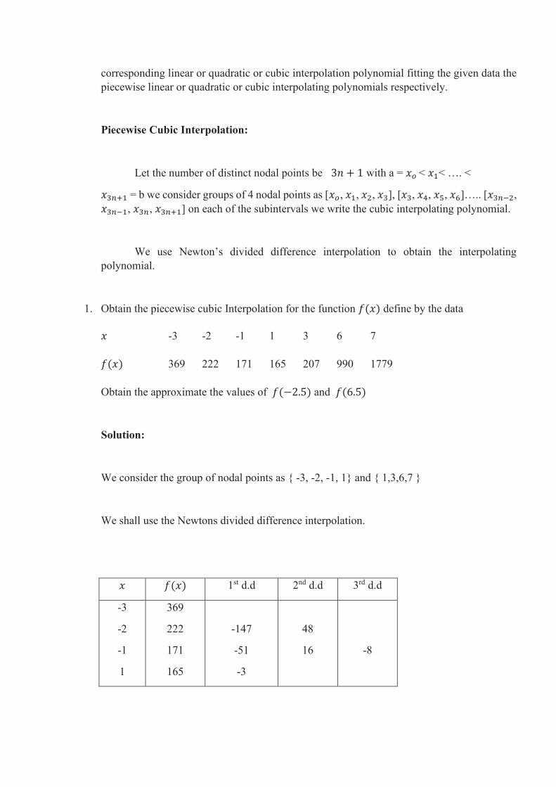
1. Obtain the piecewise cubic Interpolation for the function 𝑓(𝑥) define by the data
𝑥 -3 -2 -1 1 3 6 7
𝑓(𝑥) 369 222 171 165 207 990 1779
Obtain the approximate the values of 𝑓(−2.5) and 𝑓(6.5)
Solution:
We consider the group of nodal points as { -3, -2, -1, 1} and { 1,3,6,7 }
We shall use the Newtons divided difference interpolation.
𝑥 𝑓(𝑥) 1st d.d 2nd d.d 3rd d.d
-3
-2
-1
1
369
222
171
165
-147
-51
-3
48
16
-8
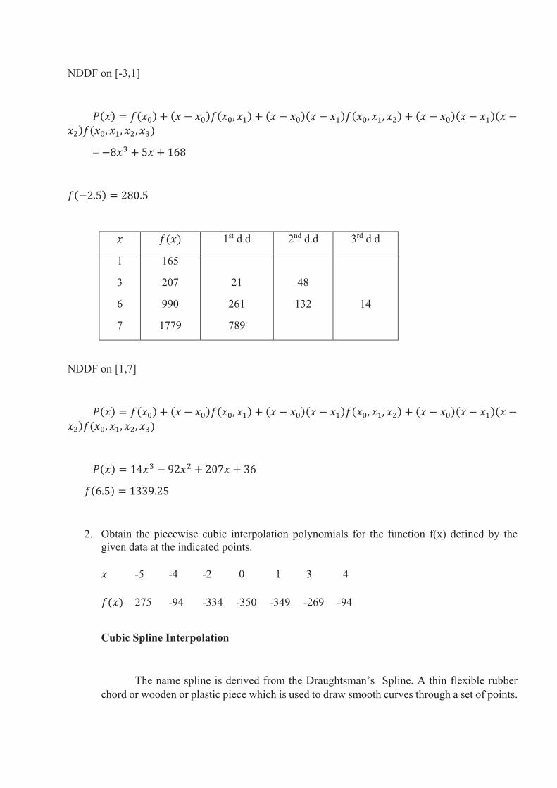
NDDF on [-3,1]
𝑃(𝑥) = 𝑓(𝑥0) + (𝑥 − 𝑥0)𝑓(𝑥0, 𝑥1) + (𝑥 − 𝑥0)(𝑥 − 𝑥1)𝑓(𝑥0, 𝑥1, 𝑥2) + (𝑥 − 𝑥0)(𝑥 − 𝑥1)(𝑥 −𝑥2)𝑓(𝑥0, 𝑥1, 𝑥2, 𝑥3)
= −8𝑥3 + 5𝑥 + 168
𝑓(−2.5) = 280.5
𝑥 𝑓(𝑥) 1st d.d 2nd d.d 3rd d.d
1
3
6
7
165
207
990
1779
21
261
789
48
132
14
NDDF on [1,7]
𝑃(𝑥) = 𝑓(𝑥0) + (𝑥 − 𝑥0)𝑓(𝑥0, 𝑥1) + (𝑥 − 𝑥0)(𝑥 − 𝑥1)𝑓(𝑥0, 𝑥1, 𝑥2) + (𝑥 − 𝑥0)(𝑥 − 𝑥1)(𝑥 −
𝑥2)𝑓(𝑥0, 𝑥1, 𝑥2, 𝑥3)
𝑃(𝑥) = 14𝑥3 − 92𝑥2 + 207𝑥 + 36
𝑓(6.5) = 1339.25
2. Obtain the piecewise cubic interpolation polynomials for the function f(x) defined by the
given data at the indicated points.
𝑥 -5 -4 -2 0 1 3 4
𝑓(𝑥) 275 -94 -334 -350 -349 -269 -94
Cubic Spline Interpolation
The name spline is derived from the Draughtsman’s Spline. A thin flexible rubber
chord or wooden or plastic piece which is used to draw smooth curves through a set of points.
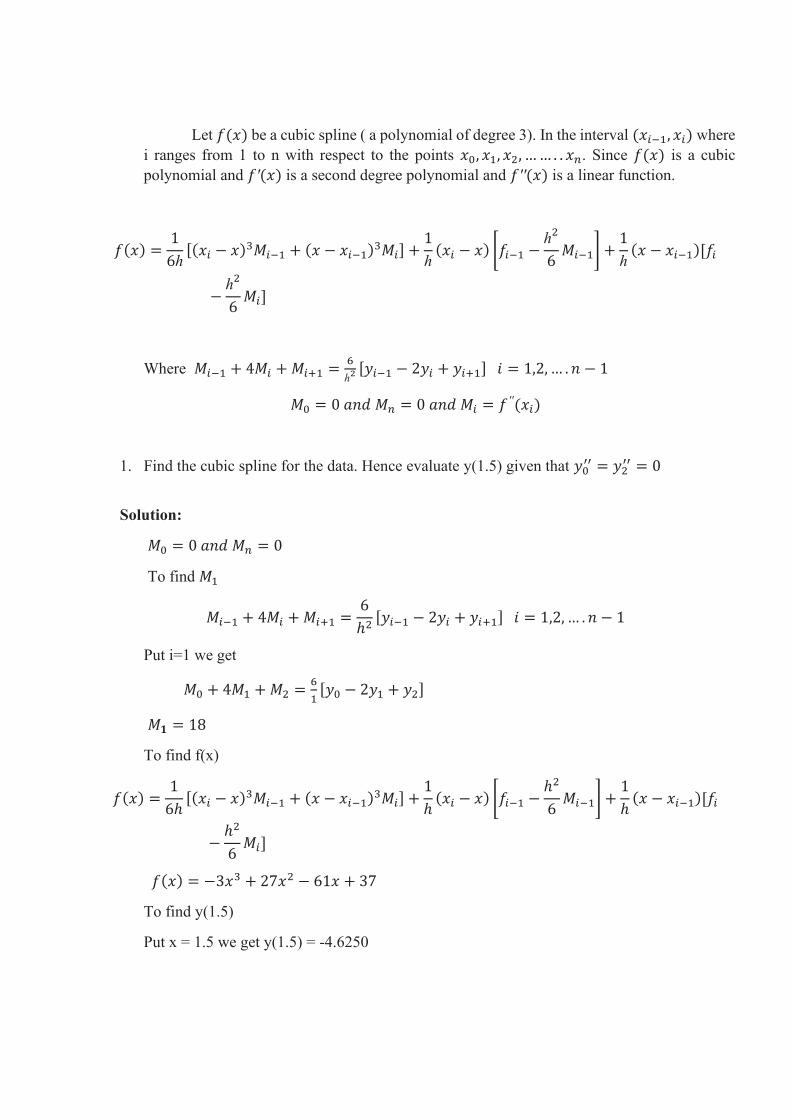
Let 𝑓(𝑥) be a cubic spline ( a polynomial of degree 3). In the interval (𝑥𝑖−1, 𝑥𝑖) where
i ranges from 1 to n with respect to the points 𝑥0, 𝑥1, 𝑥2, …… . . 𝑥𝑛. Since 𝑓(𝑥) is a cubic
polynomial and 𝑓′(𝑥) is a second degree polynomial and 𝑓′′(𝑥) is a linear function.
𝑓(𝑥) =1
6ℎ[(𝑥𝑖 − 𝑥)3𝑀𝑖−1 + (𝑥 − 𝑥𝑖−1)
3𝑀𝑖] +1
ℎ(𝑥𝑖 − 𝑥) [𝑓𝑖−1 −
ℎ2
6𝑀𝑖−1] +
1
ℎ(𝑥 − 𝑥𝑖−1)[𝑓𝑖
−ℎ
2
6𝑀𝑖]
Where 𝑀𝑖−1 + 4𝑀𝑖 + 𝑀𝑖+1 =6
ℎ2 [𝑦𝑖−1 − 2𝑦𝑖 + 𝑦𝑖+1] 𝑖 = 1,2, … . 𝑛 − 1
𝑀0 = 0 𝑎𝑛𝑑 𝑀𝑛 = 0 𝑎𝑛𝑑 𝑀𝑖 = 𝑓 ′′(𝑥𝑖)
1. Find the cubic spline for the data. Hence evaluate y(1.5) given that 𝑦0′′ = 𝑦2
′′ = 0
Solution:
𝑀0 = 0 𝑎𝑛𝑑 𝑀𝑛 = 0
To find 𝑀1
𝑀𝑖−1 + 4𝑀𝑖 + 𝑀𝑖+1 =6
ℎ2[𝑦𝑖−1 − 2𝑦𝑖 + 𝑦𝑖+1] 𝑖 = 1,2, … . 𝑛 − 1
Put i=1 we get
𝑀0 + 4𝑀1 + 𝑀2 =6
1[𝑦0 − 2𝑦1 + 𝑦2]
𝑀𝟏 = 18
To find f(x)
𝑓(𝑥) =1
6ℎ[(𝑥𝑖 − 𝑥)3𝑀𝑖−1 + (𝑥 − 𝑥𝑖−1)
3𝑀𝑖] +1
ℎ(𝑥𝑖 − 𝑥) [𝑓𝑖−1 −
ℎ2
6𝑀𝑖−1] +
1
ℎ(𝑥 − 𝑥𝑖−1)[𝑓𝑖
−ℎ2
6𝑀𝑖]
𝑓(𝑥) = −3𝑥3 + 27𝑥2 − 61𝑥 + 37
To find y(1.5)
Put x = 1.5 we get y(1.5) = -4.6250
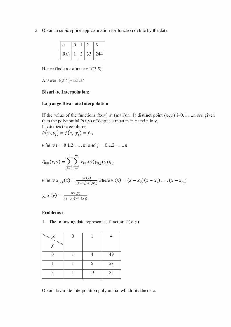
2. Obtain a cubic spline approximation for function define by the data
c 0 1 2 3
f(x) 1 2 33 244
Hence find an estimate of f(2.5).
Answer: f(2.5)=121.25
Bivariate Interpolation:
Lagrange Bivariate Interpolation
If the value of the functions f(x,y) at (m+1)(n+1) distinct point (xi,yi) i=0,1,…,n are given
then the polynomial P(x,y) of degree atmost m in x and n in y.
It satisfies the condition
𝑃(𝑥𝑖 , 𝑦𝑗) = 𝑓(𝑥𝑖 , 𝑦𝑗) = 𝑓𝑖,𝑗
𝑤ℎ𝑒𝑟𝑒 𝑖 = 0,1,2, … . .𝑚 𝑎𝑛𝑑 𝑗 = 0,1,2, ……𝑛
𝑃𝑚𝑛(𝑥, 𝑦) = ∑ ∑𝑥𝑚,𝑖(𝑥)𝑦𝑛,𝑗(𝑦)𝑓𝑖,𝑗
𝑚
𝑖=0
𝑛
𝑗=0
𝑤ℎ𝑒𝑟𝑒 𝑥𝑚,𝑖(𝑥) =𝑤 (𝑥)
(𝑥−𝑥𝑖)𝑤′(𝑤𝑖)
where 𝑤(𝑥) = (𝑥 − 𝑥𝑜)(𝑥 − 𝑥1)… . . (𝑥 − 𝑥𝑚)
𝑦𝑛,𝑗 (𝑦) = 𝑤∗(𝑦)
(𝑦−𝑦𝑗)𝑤′∗(𝑦𝑗)
Problems :-
1. The following data represents a function f (𝑥, 𝑦)
𝑥
𝑦
0 1 4
0 1 4 49
1 1 5 53
3 1 13 85
Obtain bivariate interpolation polynomial which fits the data.
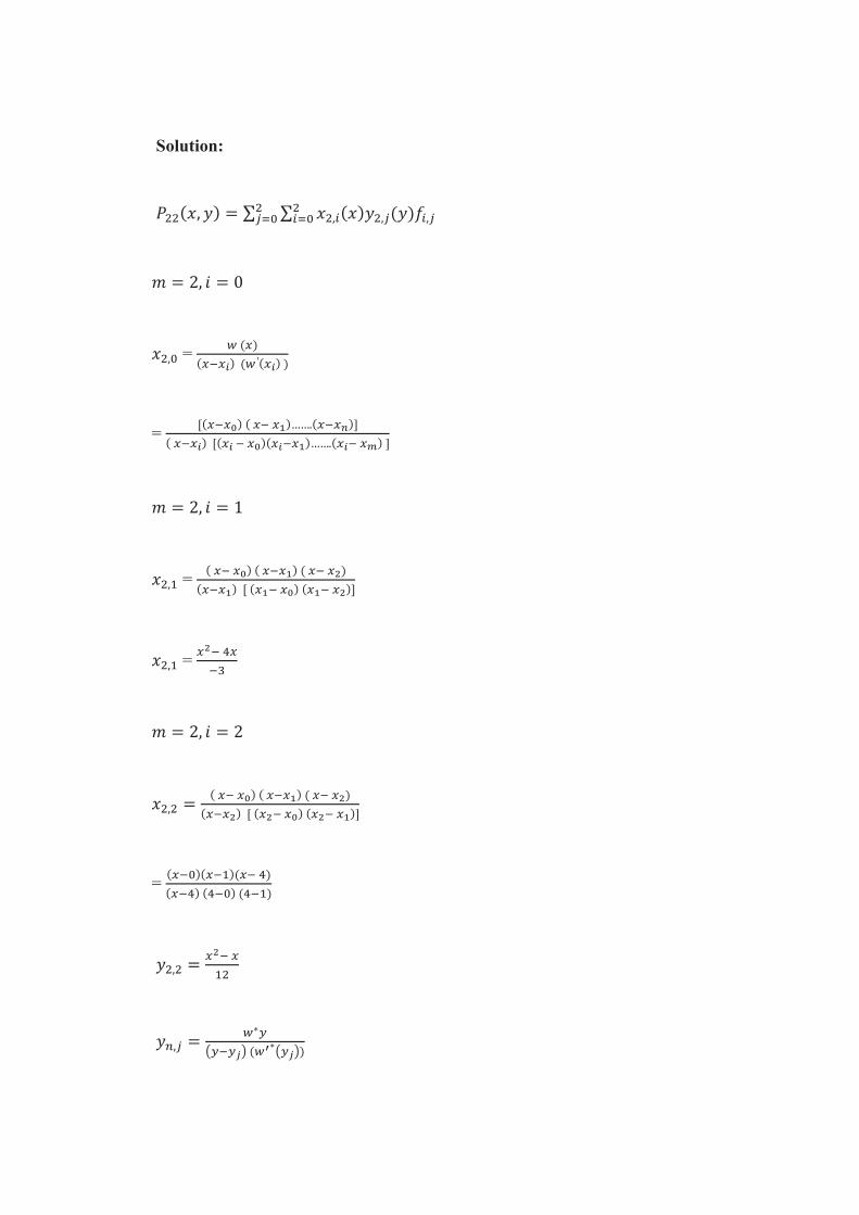
Solution:
𝑃22(𝑥, 𝑦) = ∑ ∑ 𝑥2,𝑖(𝑥)𝑦2,𝑗(𝑦)𝑓𝑖,𝑗2𝑖=0
2𝑗=0
𝑚 = 2, 𝑖 = 0
𝑥2,0 = 𝑤 (𝑥)
(𝑥−𝑥𝑖) (𝑤′(𝑥𝑖) )
= [(𝑥−𝑥0) ( 𝑥− 𝑥1)…….(𝑥−𝑥𝑛)]
( 𝑥−𝑥𝑖) [(𝑥𝑖 − 𝑥0)(𝑥𝑖−𝑥1)…….(𝑥𝑖− 𝑥𝑚) ]
𝑚 = 2, 𝑖 = 1
𝑥2,1 = ( 𝑥− 𝑥0) ( 𝑥−𝑥1) ( 𝑥− 𝑥2)
(𝑥−𝑥1) [ (𝑥1− 𝑥0) (𝑥1− 𝑥2)]
𝑥2,1 = 𝑥2− 4𝑥
−3
𝑚 = 2, 𝑖 = 2
𝑥2,2 =( 𝑥− 𝑥0) ( 𝑥−𝑥1) ( 𝑥− 𝑥2)
(𝑥−𝑥2) [ (𝑥2− 𝑥0) (𝑥2− 𝑥1)]
= (𝑥−0)(𝑥−1)(𝑥− 4)
(𝑥−4) (4−0) (4−1)
𝑦2,2 =𝑥2− 𝑥
12
𝑦𝑛,𝑗 =𝑤∗𝑦
(𝑦−𝑦𝑗) (𝑤′∗(𝑦𝑗))
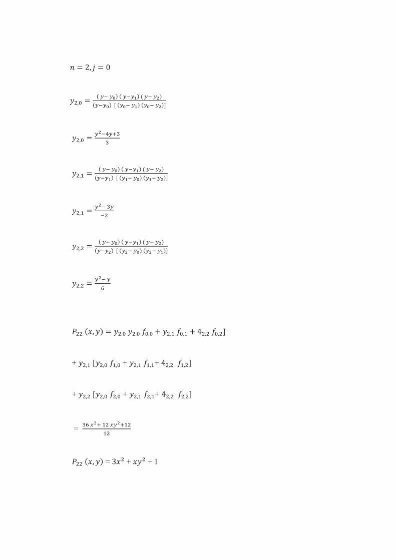
𝑛 = 2, 𝑗 = 0
𝑦2,0 =( 𝑦− 𝑦0) ( 𝑦−𝑦1) ( 𝑦− 𝑦2)
(𝑦−𝑦0) [ (𝑦0− 𝑦1) (𝑦0− 𝑦2)]
𝑦2,0 =𝑦2−4𝑦+3
3
𝑦2,1 =( 𝑦− 𝑦0) ( 𝑦−𝑦1) ( 𝑦− 𝑦2)
(𝑦−𝑦1) [ (𝑦1− 𝑦0) (𝑦1− 𝑦2)]
𝑦2,1 =𝑦2− 3𝑦
−2
𝑦2,2 =( 𝑦− 𝑦0) ( 𝑦−𝑦1) ( 𝑦− 𝑦2)
(𝑦−𝑦2) [ (𝑦2− 𝑦0) (𝑦2− 𝑦1)]
𝑦2,2 =𝑦2− 𝑦
6
𝑃22 (𝑥, 𝑦) = 𝑦2,0 𝑦2,0 𝑓0,0 + 𝑦2,1 𝑓0,1 + 42,2 𝑓0,2]
+ 𝑦2,1 [𝑦2,0 𝑓1,0 + 𝑦2,1 𝑓1,1+ 42,2 𝑓1,2]
+ 𝑦2,2 [𝑦2,0 𝑓2,0 + 𝑦2,1 𝑓2,1+ 42,2 𝑓2,2]
= 36 𝑥2+ 12 𝑥𝑦2+12
12
𝑃22 (𝑥, 𝑦) = 3𝑥2 + 𝑥𝑦2 + 1
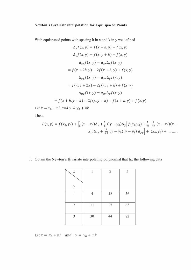
Newton’s Bivariate interpolation for Equi spaced Points
With equispased points with spacing h in x and k in y we defined
∆𝑥𝑓(𝑥, 𝑦) = 𝑓(𝑥 + ℎ, 𝑦) − 𝑓(𝑥, 𝑦)
∆𝑦𝑓(𝑥, 𝑦) = 𝑓(𝑥, 𝑦 + 𝑘) − 𝑓(𝑥, 𝑦)
∆𝑥𝑥𝑓(𝑥, 𝑦) = ∆𝑥. ∆𝑥𝑓(𝑥, 𝑦)
= 𝑓(𝑥 + 2ℎ, 𝑦) − 2𝑓(𝑥 + ℎ, 𝑦) + 𝑓(𝑥, 𝑦)
∆𝑦𝑦𝑓(𝑥, 𝑦) = ∆𝑦. ∆𝑦𝑓(𝑥, 𝑦)
= 𝑓(𝑥, 𝑦 + 2𝑘) − 2𝑓(𝑥, 𝑦 + 𝑘) + 𝑓(𝑥, 𝑦)
∆𝑥𝑦𝑓(𝑥, 𝑦) = ∆𝑥. ∆𝑦𝑓(𝑥, 𝑦)
= 𝑓(𝑥 + ℎ, 𝑦 + 𝑘) − 2𝑓(𝑥, 𝑦 + 𝑘) − 𝑓(𝑥 + ℎ, 𝑦) + 𝑓(𝑥, 𝑦)
Let 𝑥 = 𝑥0 + 𝑛ℎ 𝑎𝑛𝑑 𝑦 = 𝑦0 + 𝑛𝑘
Then,
𝑃(𝑥, 𝑦) = 𝑓(𝑥0, 𝑦0) + [1
ℎ(𝑥 − 𝑥0)∆𝑥 +
1
𝑘 ( 𝑦 − 𝑦0)∆𝑦] 𝑓(𝑥0,𝑦0) +
1
2! [
1
ℎ2 (𝑥 − 𝑥0)(𝑥 −
𝑥1)∆𝑥𝑥 + 1
𝑘2 (𝑦 − 𝑦0)(𝑦 − 𝑦1) ∆𝑦𝑦] + (𝑥0, 𝑦0) + …… . .
1. Obtain the Newton’s Bivariate interpolating polynomial that fix the following data
𝑥
𝑦
1 2 3
1 4 18 56
2 11 25 63
3 30 44 82
Let 𝑥 = 𝑥0 + 𝑛ℎ 𝑎𝑛𝑑 𝑦 = 𝑦0 + 𝑛𝑘
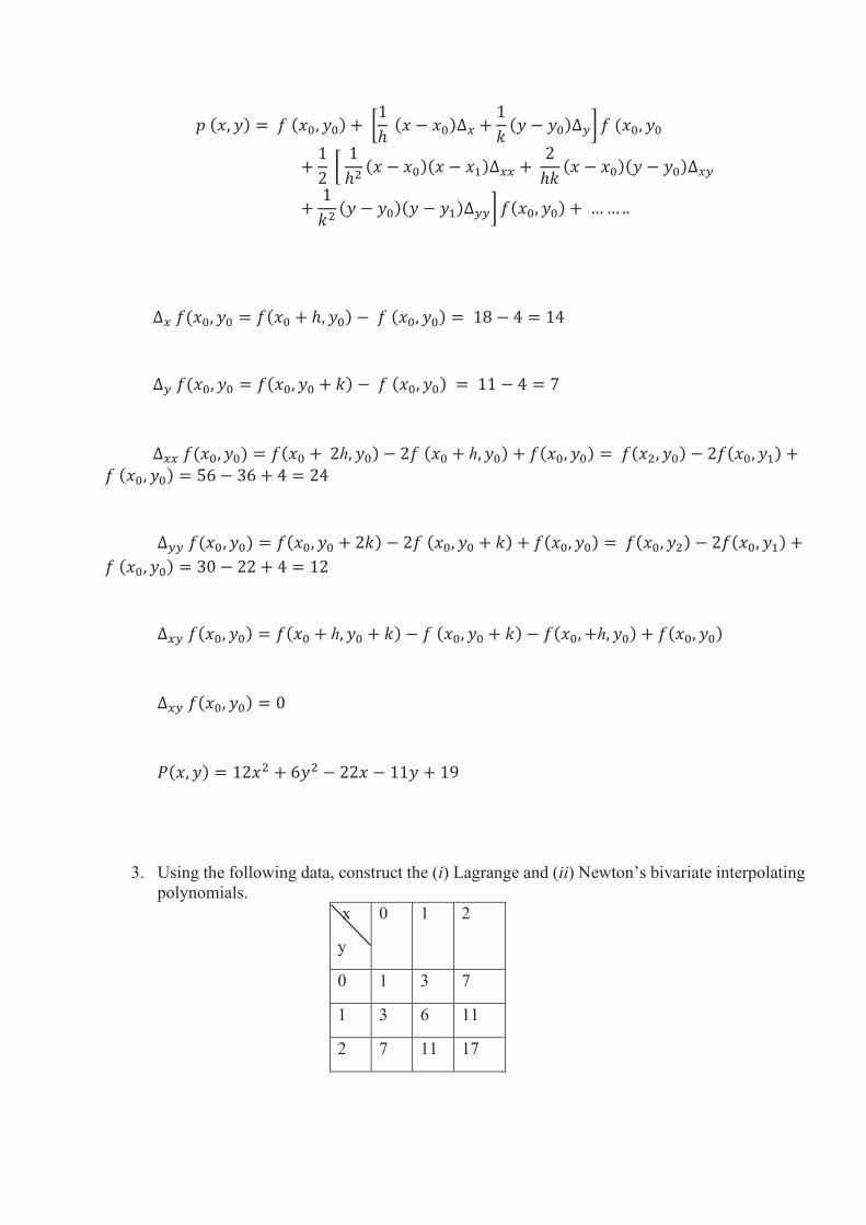
𝑝 (𝑥, 𝑦) = 𝑓 (𝑥0, 𝑦0) + [1
ℎ (𝑥 − 𝑥0)∆𝑥 +
1
𝑘(𝑦 − 𝑦0)∆𝑦] 𝑓 (𝑥0, 𝑦0
+1
2 [
1
ℎ2(𝑥 − 𝑥0)(𝑥 − 𝑥1)∆𝑥𝑥 +
2
ℎ𝑘(𝑥 − 𝑥0)(𝑦 − 𝑦0)∆𝑥𝑦
+1
𝑘2(𝑦 − 𝑦0)(𝑦 − 𝑦1)∆𝑦𝑦] 𝑓(𝑥0, 𝑦0) + …… ..
∆𝑥 𝑓(𝑥0, 𝑦0 = 𝑓(𝑥0 + ℎ, 𝑦0) − 𝑓 (𝑥0, 𝑦0) = 18 − 4 = 14
∆𝑦 𝑓(𝑥0, 𝑦0 = 𝑓(𝑥0, 𝑦0 + 𝑘) − 𝑓 (𝑥0, 𝑦0) = 11 − 4 = 7
∆𝑥𝑥 𝑓(𝑥0, 𝑦0) = 𝑓(𝑥0 + 2ℎ, 𝑦0) − 2𝑓 (𝑥0 + ℎ, 𝑦0) + 𝑓(𝑥0, 𝑦0) = 𝑓(𝑥2, 𝑦0) − 2𝑓(𝑥0, 𝑦1) +𝑓 (𝑥0, 𝑦0) = 56 − 36 + 4 = 24
∆𝑦𝑦 𝑓(𝑥0, 𝑦0) = 𝑓(𝑥0, 𝑦0 + 2𝑘) − 2𝑓 (𝑥0, 𝑦0 + 𝑘) + 𝑓(𝑥0, 𝑦0) = 𝑓(𝑥0, 𝑦2) − 2𝑓(𝑥0, 𝑦1) +
𝑓 (𝑥0, 𝑦0) = 30 − 22 + 4 = 12
∆𝑥𝑦 𝑓(𝑥0, 𝑦0) = 𝑓(𝑥0 + ℎ, 𝑦0 + 𝑘) − 𝑓 (𝑥0, 𝑦0 + 𝑘) − 𝑓(𝑥0, +ℎ, 𝑦0) + 𝑓(𝑥0, 𝑦0)
∆𝑥𝑦 𝑓(𝑥0, 𝑦0) = 0
𝑃(𝑥, 𝑦) = 12𝑥2 + 6𝑦2 − 22𝑥 − 11𝑦 + 19
3. Using the following data, construct the (i) Lagrange and (ii) Newton’s bivariate interpolating
polynomials.
x
y
0 1 2
0 1 3 7
1 3 6 11
2 7 11 17
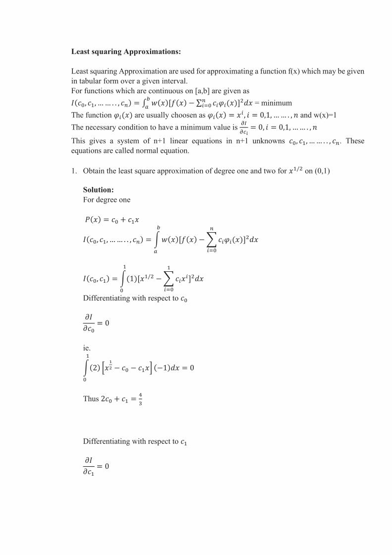
Least squaring Approximations:
Least squaring Approximation are used for approximating a function f(x) which may be given
in tabular form over a given interval.
For functions which are continuous on [a,b] are given as
𝐼(𝑐0, 𝑐1, …… . . , 𝑐𝑛) = ∫ 𝑤(𝑥)[𝑓(𝑥) − ∑ 𝑐𝑖𝜑𝑖(𝑥)]2𝑑𝑥𝑛𝑖=0
𝑏
𝑎 = minimum
The function 𝜑𝑖(𝑥) are usually choosen as 𝜑𝑖(𝑥) = 𝑥𝑖 , 𝑖 = 0,1, …… . , 𝑛 and w(x)=1
The necessary condition to have a minimum value is 𝜕𝐼
𝜕𝑐𝑖= 0, 𝑖 = 0,1, …… . , 𝑛
This gives a system of n+1 linear equations in n+1 unknowns 𝑐0, 𝑐1, …… . . , 𝑐𝑛. These
equations are called normal equation.
1. Obtain the least square approximation of degree one and two for 𝑥1/2 on (0,1)
Solution:
For degree one
𝑃(𝑥) = 𝑐0 + 𝑐1𝑥
𝐼(𝑐0, 𝑐1, …… . . , 𝑐𝑛) = ∫𝑤(𝑥)[𝑓(𝑥) − ∑𝑐𝑖𝜑𝑖(𝑥)]2𝑑𝑥
𝑛
𝑖=0
𝑏
𝑎
𝐼(𝑐0, 𝑐1) = ∫(1)[𝑥1/2 − ∑𝑐𝑖𝑥𝑖]2𝑑𝑥
1
𝑖=0
1
0
Differentiating with respect to 𝑐0
𝜕𝐼
𝜕𝑐0= 0
ie.
∫(2) [𝑥1
2 − 𝑐0 − 𝑐1𝑥] (−1)𝑑𝑥 = 0
1
0
Thus 2𝑐0 + 𝑐1 =4
3
Differentiating with respect to 𝑐1
𝜕𝐼
𝜕𝑐1= 0
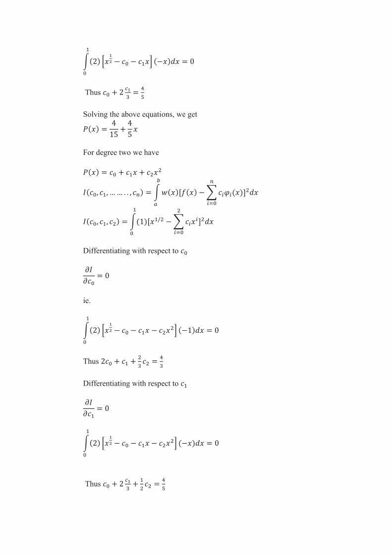
∫(2) [𝑥1
2 − 𝑐0 − 𝑐1𝑥] (−𝑥)𝑑𝑥 = 0
1
0
Thus 𝑐0 + 2𝑐1
3=
4
5
Solving the above equations, we get
𝑃(𝑥) =4
15+
4
5𝑥
For degree two we have
𝑃(𝑥) = 𝑐0 + 𝑐1𝑥 + 𝑐2𝑥2
𝐼(𝑐0, 𝑐1, …… . . , 𝑐𝑛) = ∫𝑤(𝑥)[𝑓(𝑥) − ∑𝑐𝑖𝜑𝑖(𝑥)]2𝑑𝑥
𝑛
𝑖=0
𝑏
𝑎
𝐼(𝑐0, 𝑐1, 𝑐2) = ∫(1)[𝑥1/2 − ∑𝑐𝑖𝑥𝑖]2𝑑𝑥
2
𝑖=0
1
0
Differentiating with respect to 𝑐0
𝜕𝐼
𝜕𝑐0= 0
ie.
∫(2) [𝑥1
2 − 𝑐0 − 𝑐1𝑥 − 𝑐2𝑥2] (−1)𝑑𝑥 = 0
1
0
Thus 2𝑐0 + 𝑐1 +2
3𝑐2 =
4
3
Differentiating with respect to 𝑐1
𝜕𝐼
𝜕𝑐1= 0
∫(2) [𝑥1
2 − 𝑐0 − 𝑐1𝑥 − 𝑐2𝑥2] (−𝑥)𝑑𝑥 = 0
1
0
Thus 𝑐0 + 2𝑐1
3+
1
2𝑐2 =
4
5
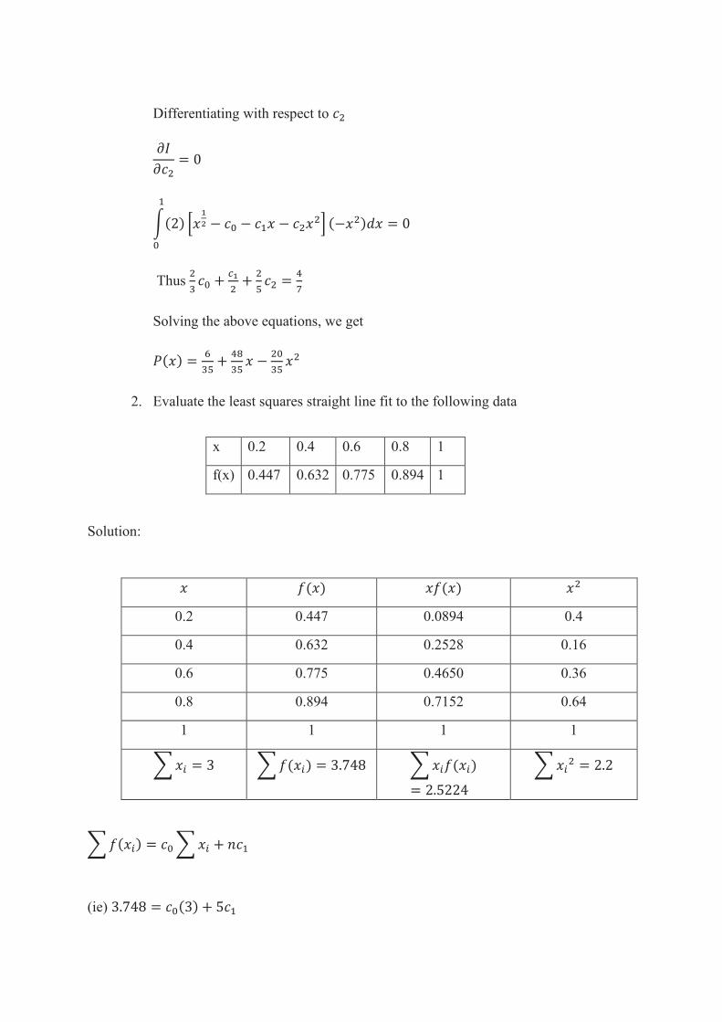
Differentiating with respect to 𝑐2
𝜕𝐼
𝜕𝑐2= 0
∫(2) [𝑥1
2 − 𝑐0 − 𝑐1𝑥 − 𝑐2𝑥2] (−𝑥2)𝑑𝑥 = 0
1
0
Thus 2
3𝑐0 +
𝑐1
2+
2
5𝑐2 =
4
7
Solving the above equations, we get
𝑃(𝑥) =6
35+
48
35𝑥 −
20
35𝑥2
2. Evaluate the least squares straight line fit to the following data
x 0.2 0.4 0.6 0.8 1
f(x) 0.447 0.632 0.775 0.894 1
Solution:
𝑥 𝑓(𝑥) 𝑥𝑓(𝑥) 𝑥2
0.2 0.447 0.0894 0.4
0.4 0.632 0.2528 0.16
0.6 0.775 0.4650 0.36
0.8 0.894 0.7152 0.64
1 1 1 1
∑𝑥𝑖 = 3 ∑𝑓(𝑥𝑖) = 3.748 ∑𝑥𝑖𝑓(𝑥𝑖)
= 2.5224
∑𝑥𝑖2 = 2.2
∑𝑓(𝑥𝑖) = 𝑐0 ∑𝑥𝑖 + 𝑛𝑐1
(ie) 3.748 = 𝑐0(3) + 5𝑐1
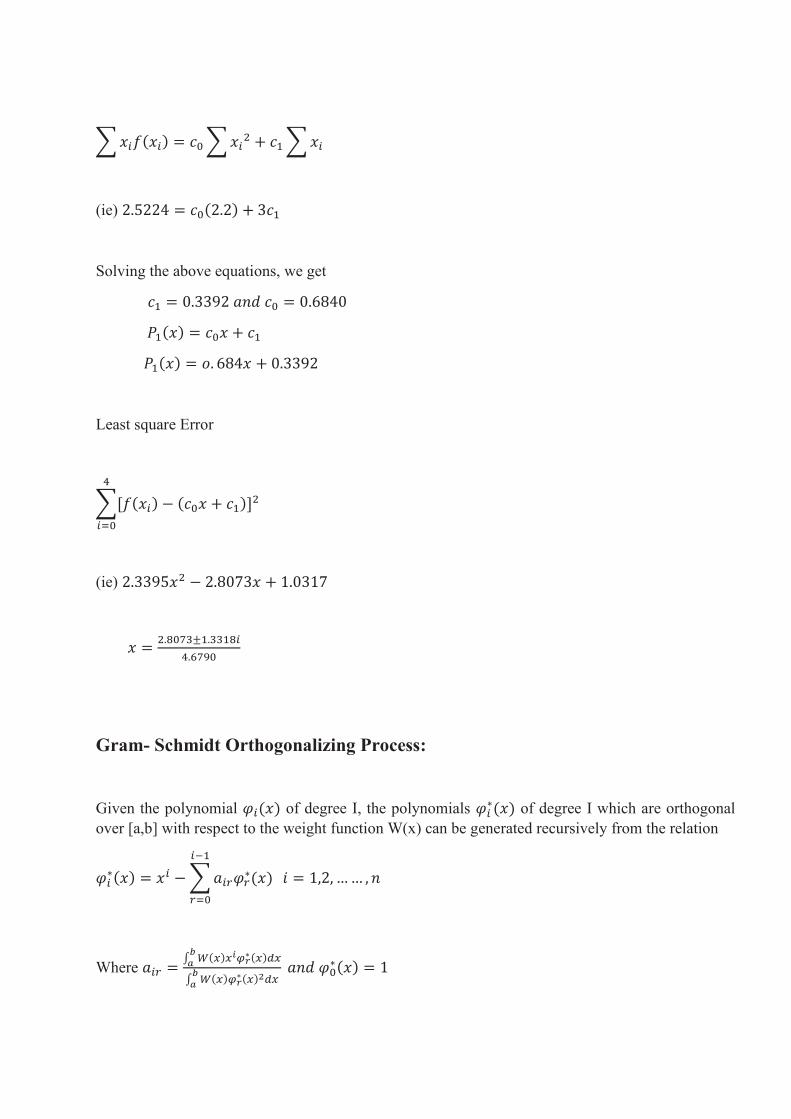
∑𝑥𝑖𝑓(𝑥𝑖) = 𝑐0 ∑𝑥𝑖2 + 𝑐1 ∑𝑥𝑖
(ie) 2.5224 = 𝑐0(2.2) + 3𝑐1
Solving the above equations, we get
𝑐1 = 0.3392 𝑎𝑛𝑑 𝑐0 = 0.6840
𝑃1(𝑥) = 𝑐0𝑥 + 𝑐1
𝑃1(𝑥) = 𝑜. 684𝑥 + 0.3392
Least square Error
∑[𝑓(𝑥𝑖) − (𝑐0𝑥 + 𝑐1)]2
4
𝑖=0
(ie) 2.3395𝑥2 − 2.8073𝑥 + 1.0317
𝑥 =2.8073±1.3318𝑖
4.6790
Gram- Schmidt Orthogonalizing Process:
Given the polynomial 𝜑𝑖(𝑥) of degree I, the polynomials 𝜑𝑖∗(𝑥) of degree I which are orthogonal
over [a,b] with respect to the weight function W(x) can be generated recursively from the relation
𝜑𝑖∗(𝑥) = 𝑥𝑖 − ∑𝑎𝑖𝑟𝜑𝑟
∗(𝑥)
𝑖−1
𝑟=0
𝑖 = 1,2, …… , 𝑛
Where 𝑎𝑖𝑟 =∫ 𝑊(𝑥)𝑥𝑖𝜑𝑟
∗(𝑥)𝑑𝑥𝑏𝑎
∫ 𝑊(𝑥)𝜑𝑟∗(𝑥)2𝑑𝑥
𝑏𝑎
𝑎𝑛𝑑 𝜑0∗(𝑥) = 1
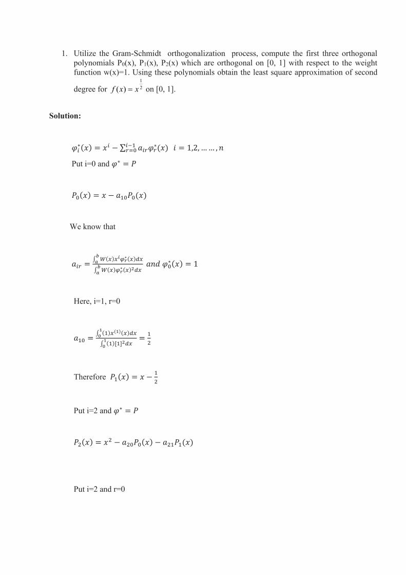
1. Utilize the Gram-Schmidt orthogonalization process, compute the first three orthogonal
polynomials P0(x), P1(x), P2(x) which are orthogonal on [0, 1] with respect to the weight
function w(x)=1. Using these polynomials obtain the least square approximation of second
degree for 2
1
)( xxf = on [0, 1].
Solution:
𝜑𝑖∗(𝑥) = 𝑥𝑖 − ∑ 𝑎𝑖𝑟𝜑𝑟
∗(𝑥)𝑖−1𝑟=0 𝑖 = 1,2, …… , 𝑛
Put i=0 and 𝜑∗ = 𝑃
𝑃0(𝑥) = 𝑥 − 𝑎10𝑃0(𝑥)
We know that
𝑎𝑖𝑟 =∫ 𝑊(𝑥)𝑥𝑖𝜑𝑟
∗(𝑥)𝑑𝑥𝑏𝑎
∫ 𝑊(𝑥)𝜑𝑟∗(𝑥)2𝑑𝑥
𝑏𝑎
𝑎𝑛𝑑 𝜑0∗(𝑥) = 1
Here, i=1, r=0
𝑎10 =∫ (1)𝑥(1)(𝑥)𝑑𝑥
10
∫ (1)[1]2𝑑𝑥10
=1
2
Therefore 𝑃1(𝑥) = 𝑥 −1
2
Put i=2 and 𝜑∗ = 𝑃
𝑃2(𝑥) = 𝑥2 − 𝑎20𝑃0(𝑥) − 𝑎21𝑃1(𝑥)
Put i=2 and r=0
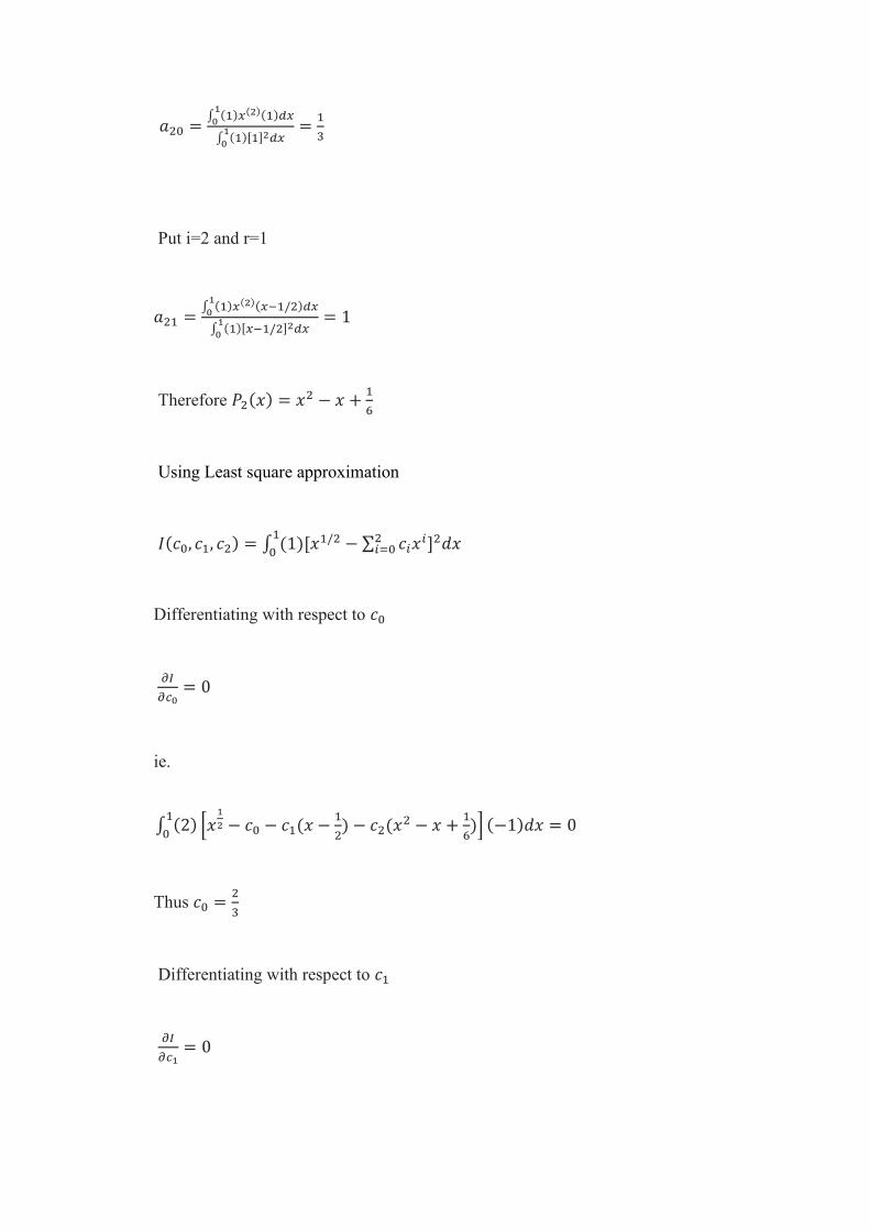
𝑎20 =∫ (1)𝑥(2)(1)𝑑𝑥
10
∫ (1)[1]2𝑑𝑥10
=1
3
Put i=2 and r=1
𝑎21 =∫ (1)𝑥(2)(𝑥−1/2)𝑑𝑥
10
∫ (1)[𝑥−1/2]2𝑑𝑥10
= 1
Therefore 𝑃2(𝑥) = 𝑥2 − 𝑥 +1
6
Using Least square approximation
𝐼(𝑐0, 𝑐1, 𝑐2) = ∫ (1)[𝑥1/2 − ∑ 𝑐𝑖𝑥𝑖]2𝑑𝑥2
𝑖=01
0
Differentiating with respect to 𝑐0
𝜕𝐼
𝜕𝑐0= 0
ie.
∫ (2) [𝑥1
2 − 𝑐0 − 𝑐1(𝑥 −1
2) − 𝑐2(𝑥
2 − 𝑥 +1
6)] (−1)𝑑𝑥 = 0
1
0
Thus 𝑐0 =2
3
Differentiating with respect to 𝑐1
𝜕𝐼
𝜕𝑐1= 0
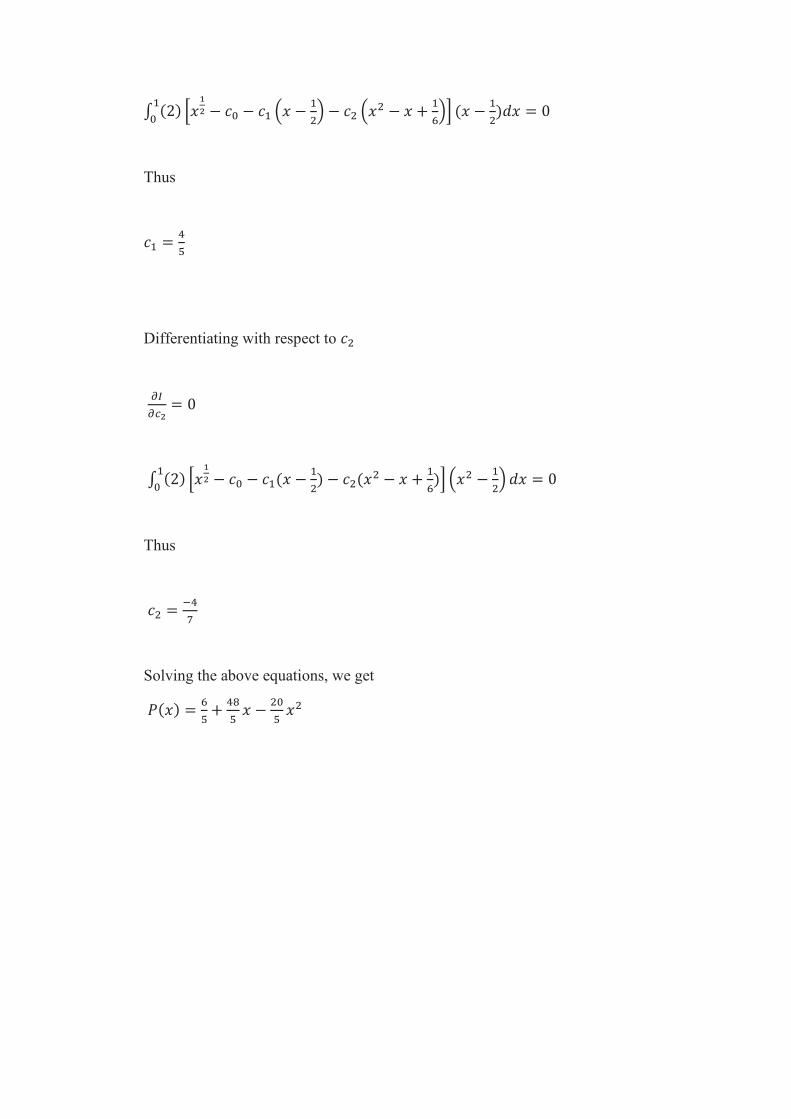
∫ (2) [𝑥1
2 − 𝑐0 − 𝑐1 (𝑥 −1
2) − 𝑐2 (𝑥2 − 𝑥 +
1
6)] (𝑥 −
1
2)𝑑𝑥 = 0
1
0
Thus
𝑐1 =4
5
Differentiating with respect to 𝑐2
𝜕𝐼
𝜕𝑐2= 0
∫ (2) [𝑥1
2 − 𝑐0 − 𝑐1(𝑥 −1
2) − 𝑐2(𝑥
2 − 𝑥 +1
6)] (𝑥2 −
1
2) 𝑑𝑥 = 0
1
0
Thus
𝑐2 =−4
7
Solving the above equations, we get
𝑃(𝑥) =6
5+
48
5𝑥 −
20
5𝑥2
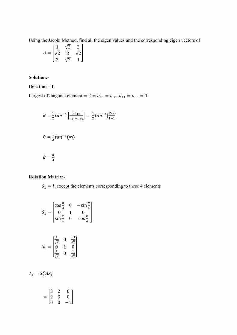
Using the Jacobi Method, find all the eigen values and the corresponding eigen vectors of
𝐴 = [1 √2 2
√2 3 √2
2 √2 1
]
Solution:-
Iteration – I
Largest of diagonal element = 2 = 𝑎13 = 𝑎31 𝑎11 = 𝑎33 = 1
𝜃 =1
2𝑡𝑎𝑛−1 [
2𝑎13
𝑎11−𝑎33] =
1
2𝑡𝑎𝑛−1[
2∗2
1−1]
𝜃 =1
2𝑡𝑎𝑛−1(∞)
𝜃 =𝜋
4
Rotation Matrix:-
𝑆1 = 𝐼, except the elements corresponding to these 4 elements
𝑆1 = [
cos𝜋
40 − sin
𝜋
4
0 1 0
sin𝜋
40 cos
𝜋
4
]
𝑆1 = [
1
√20
−1
√2
0 1 01
√20
1
√2
]
𝐴1 = 𝑆1𝑇𝐴𝑆1
= [3 2 02 3 00 0 −1
]
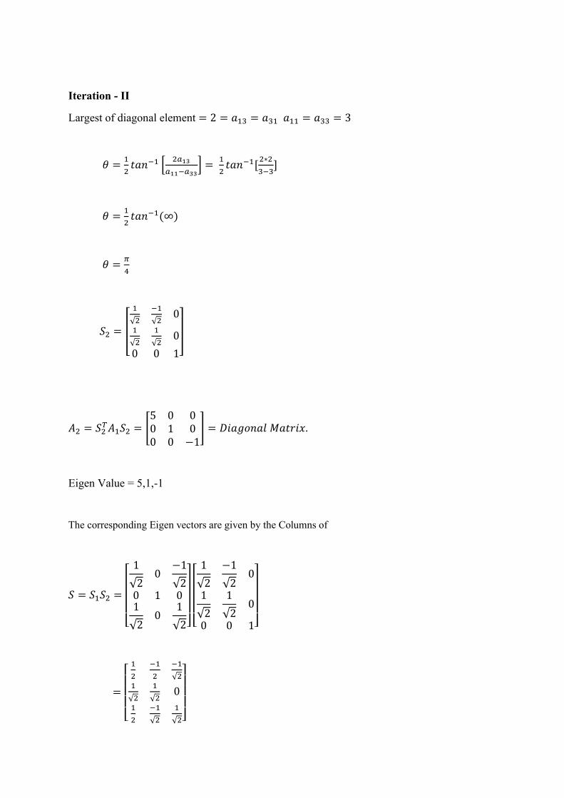
Iteration - II
Largest of diagonal element = 2 = 𝑎13 = 𝑎31 𝑎11 = 𝑎33 = 3
𝜃 =1
2𝑡𝑎𝑛−1 [
2𝑎13
𝑎11−𝑎33] =
1
2𝑡𝑎𝑛−1[
2∗2
3−3]
𝜃 =1
2𝑡𝑎𝑛−1(∞)
𝜃 =𝜋
4
𝑆2 = [
1
√2
−1
√20
1
√2
1
√20
0 0 1
]
𝐴2 = 𝑆2𝑇𝐴1𝑆2 = [
5 0 00 1 00 0 −1
] = 𝐷𝑖𝑎𝑔𝑜𝑛𝑎𝑙 𝑀𝑎𝑡𝑟𝑖𝑥.
Eigen Value = 5,1,-1
The corresponding Eigen vectors are given by the Columns of
𝑆 = 𝑆1𝑆2 =
[ 1
√20
−1
√20 1 01
√20
1
√2]
[ 1
√2
−1
√20
1
√2
1
√20
0 0 1]
=
[
1
2
−1
2
−1
√21
√2
1
√20
1
2
−1
√2
1
√2]

The eigen vectors corresponding to 5,1,-1 are
[1
2
1
√2
1
2]𝑇
, [−1
2
1
√2
−1
√2]𝑇
, [−1
2
−1
√2
1
√2]𝑇

UNIT – IV - ADVANCED NUMERICAL METHODS – SMTA5304
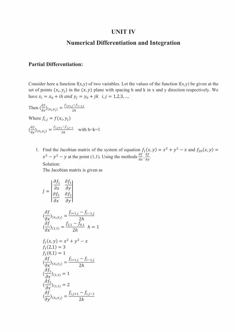
UNIT IV
Numerical Differentiation and Integration
Partial Differentiation:
Consider here a function f(x,y) of two variables. Let the values of the function f(x,y) be given at the
set of points (𝑥𝑖, 𝑦𝑗) in the (𝑥, 𝑦) plane with spacing h and k in x and y direction respectively. We
have 𝑥𝑖 = 𝑥0 + 𝑖ℎ 𝑎𝑛𝑑 𝑦𝑗 = 𝑦0 + 𝑗𝑘 𝑖, 𝑗 = 1,2,3, ….
Then (𝜕𝑓
𝜕𝑥)(𝑥𝑖,𝑦𝑗)
=𝑓𝑖+1,𝑗−𝑓𝑖−1,𝑗
2ℎ
Where 𝑓𝑖,𝑗 = 𝑓(𝑥𝑖, 𝑦𝑗)
(𝜕𝑓
𝜕𝑦)(𝑥𝑖,𝑦𝑗)
=𝑓𝑖,𝑗+1−𝑓𝑖,𝑗−1
2𝑘 with h=k=1
1. Find the Jacobian matrix of the system of equation 𝑓1(𝑥, 𝑦) = 𝑥2 + 𝑦2 − 𝑥 and 𝑓20(𝑥, 𝑦) =
𝑥2 − 𝑦2 − 𝑦 at the point (1,1). Using the methods 𝜕𝑓
𝜕𝑥,𝜕𝑓
𝜕𝑦.
Solution:
The Jacobian matrix is given as
𝐽 = || 𝜕𝑓1𝜕𝑥
𝜕𝑓1𝜕𝑦
𝜕𝑓2𝜕𝑥
𝜕𝑓2𝜕𝑦
||
(𝜕𝑓
𝜕𝑥)(𝑥𝑖,𝑦𝑗)
=𝑓𝑖+1,𝑗 − 𝑓𝑖−1,𝑗
2ℎ
(𝜕𝑓
𝜕𝑥)(1,1) =
𝑓2,1 − 𝑓0,1
2ℎ ℎ = 1
𝑓1(𝑥, 𝑦) = 𝑥2 + 𝑦2 − 𝑥
𝑓1(2,1) = 3
𝑓1(0,1) = 1
(𝜕𝑓
𝜕𝑥)(𝑥𝑖,𝑦𝑗)
=𝑓𝑖+1,𝑗 − 𝑓𝑖−1,𝑗
2ℎ
(𝜕𝑓1𝜕𝑥
)(1,1) = 1
(𝜕𝑓2𝜕𝑥
)(1,1) = 2
(𝜕𝑓
𝜕𝑦)(𝑥𝑖,𝑦𝑗)
=𝑓𝑖,𝑗+1 − 𝑓𝑖,𝑗−1
2𝑘
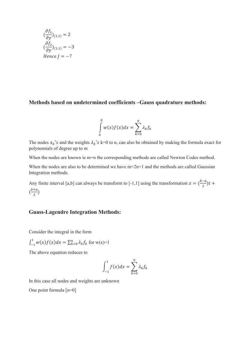
(𝜕𝑓1𝜕𝑦
)(1,1) = 2
(𝜕𝑓2𝜕𝑦
)(1,1) = −3
𝐻𝑒𝑛𝑐𝑒 𝐽 = −7
Methods based on undetermined coefficients –Gauss quadrature methods:
∫𝑤(𝑥)𝑓(𝑥)𝑑𝑥 = ∑ 𝜆𝑘𝑓𝑘
𝑛
𝑘=0
𝑏
𝑎
The nodes 𝑥𝑘′𝑠 and the weights 𝜆𝑘′𝑠 k=0 to n, can also be obtained by making the formula exact for
polynomials of degree up to m
When the nodes are known ie m=n the corresponding methods are called Newton Codes method.
When the nodes are also to be determined we have m=2n+1 and the methods are called Gaussian
Integration methods.
Any finite interval [a,b] can always be transform to [-1,1] using the transformation 𝑥 = (𝑏−𝑎
2)𝑡 +
(𝑏+𝑎
2)
Guass-Lagendre Integration Methods:
Consider the integral in the form
∫ 𝑤(𝑥)𝑓(𝑥)𝑑𝑥 = ∑ 𝜆𝑘𝑓𝑘𝑛𝑘=0
1
−1 for w(x)=1
The above equation reduces to
∫ 𝑓(𝑥)𝑑𝑥 = ∑ 𝜆𝑘𝑓𝑘
𝑛
𝑘=0
1
−1
In this case all nodes and weights are unknown
One point formula [n=0]
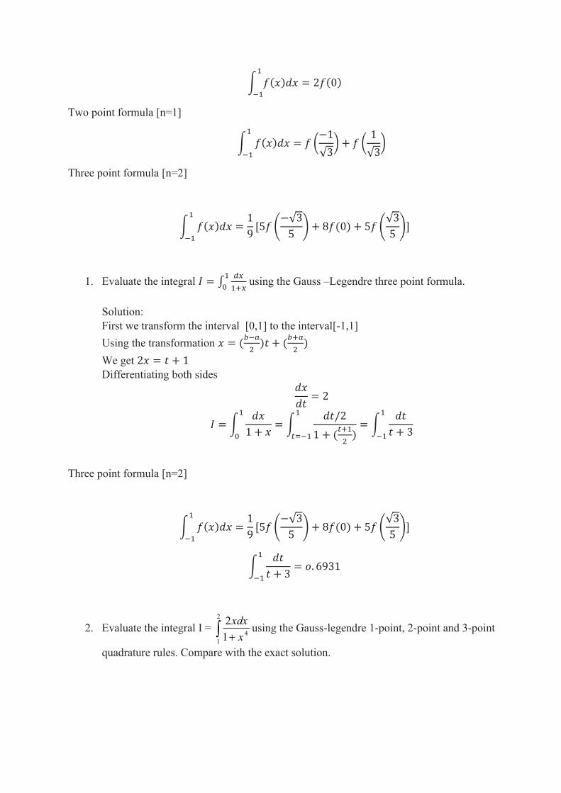
∫ 𝑓(𝑥)𝑑𝑥 = 2𝑓(0)1
−1
Two point formula [n=1]
∫ 𝑓(𝑥)𝑑𝑥 = 𝑓 (−1
√3) + 𝑓 (
1
√3)
1
−1
Three point formula [n=2]
∫ 𝑓(𝑥)𝑑𝑥 =1
9[5𝑓 (
−√3
5) + 8𝑓(0) + 5𝑓 (
√3
5)]
1
−1
1. Evaluate the integral 𝐼 = ∫𝑑𝑥
1+𝑥
1
0 using the Gauss –Legendre three point formula.
Solution:
First we transform the interval [0,1] to the interval[-1,1]
Using the transformation 𝑥 = (𝑏−𝑎
2)𝑡 + (
𝑏+𝑎
2)
We get 2𝑥 = 𝑡 + 1
Differentiating both sides
𝑑𝑥
𝑑𝑡= 2
𝐼 = ∫𝑑𝑥
1 + 𝑥
1
0
= ∫𝑑𝑡/2
1 + (𝑡+1
2)= ∫
𝑑𝑡
𝑡 + 3
1
−1
1
𝑡=−1
Three point formula [n=2]
∫ 𝑓(𝑥)𝑑𝑥 =1
9[5𝑓 (
−√3
5) + 8𝑓(0) + 5𝑓 (
√3
5)]
1
−1
∫𝑑𝑡
𝑡 + 3
1
−1
= 𝑜. 6931
2. Evaluate the integral I = +
2
1
41
2
x
xdxusing the Gauss-legendre 1-point, 2-point and 3-point
quadrature rules. Compare with the exact solution.
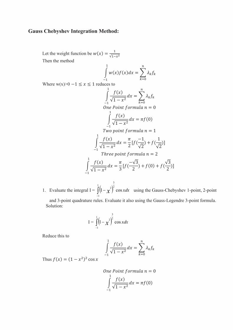
Gauss Chebyshev Integration Method:
Let the weight function be 𝑤(𝑥) =1
√1−𝑥2
Then the method
∫𝑤(𝑥)𝑓(𝑥)𝑑𝑥 = ∑ 𝜆𝑘𝑓𝑘
𝑛
𝑘=0
1
−1
Where w(x)>0 −1 ≤ 𝑥 ≤ 1 reduces to
∫𝑓(𝑥)
√1 − 𝑥2𝑑𝑥 = ∑ 𝜆𝑘𝑓𝑘
𝑛
𝑘=0
1
−1
𝑂𝑛𝑒 𝑃𝑜𝑖𝑛𝑡 𝑓𝑜𝑟𝑚𝑢𝑙𝑎 𝑛 = 0
∫𝑓(𝑥)
√1 − 𝑥2𝑑𝑥 = 𝜋𝑓(0)
1
−1
𝑇𝑤𝑜 𝑝𝑜𝑖𝑛𝑡 𝑓𝑜𝑟𝑚𝑢𝑙𝑎 𝑛 = 1
∫𝑓(𝑥)
√1 − 𝑥2𝑑𝑥 =
𝜋
2[𝑓(
−1
√2) +
1
−1
𝑓(1
√2)]
𝑇ℎ𝑟𝑒𝑒 𝑝𝑜𝑖𝑛𝑡 𝑓𝑜𝑟𝑚𝑢𝑙𝑎 𝑛 = 2
∫𝑓(𝑥)
√1 − 𝑥2𝑑𝑥 =
𝜋
3[𝑓(
−√3
2) +
1
−1
𝑓(0) + 𝑓(√3
2)]
1. Evaluate the integral I = ( ) xdxx cos12
31
1
2
−
− using the Gauss-Chebyshev 1-point, 2-point
and 3-point quadrature rules. Evaluate it also using the Gauss-Legendre 3-point formula.
Solution:
I = ( ) xdxx cos12
31
1
2
−
−
Reduce this to
∫𝑓(𝑥)
√1 − 𝑥2𝑑𝑥 = ∑ 𝜆𝑘𝑓𝑘
𝑛
𝑘=0
1
−1
Thus 𝑓(𝑥) = (1 − 𝑥2)2 cos 𝑥
𝑂𝑛𝑒 𝑃𝑜𝑖𝑛𝑡 𝑓𝑜𝑟𝑚𝑢𝑙𝑎 𝑛 = 0
∫𝑓(𝑥)
√1 − 𝑥2𝑑𝑥 = 𝜋𝑓(0)
1
−1
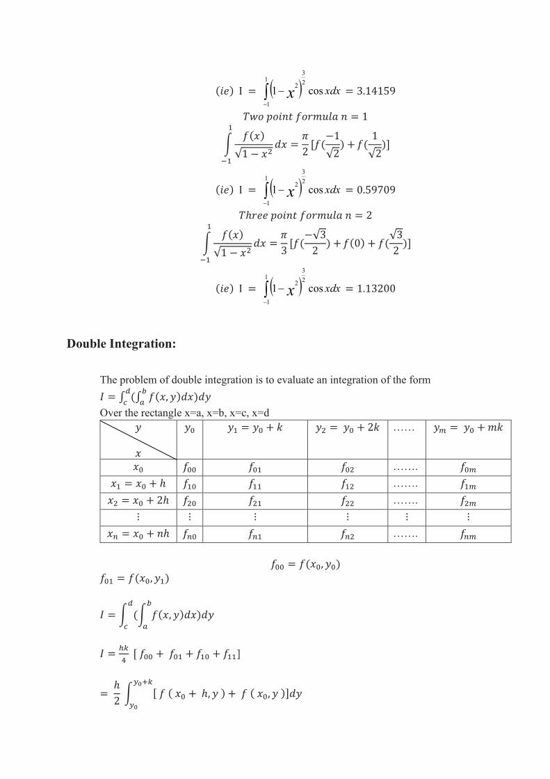
(𝑖𝑒) I = ( ) xdxx cos12
31
1
2
−
− = 3.14159
𝑇𝑤𝑜 𝑝𝑜𝑖𝑛𝑡 𝑓𝑜𝑟𝑚𝑢𝑙𝑎 𝑛 = 1
∫𝑓(𝑥)
√1 − 𝑥2𝑑𝑥 =
𝜋
2[𝑓(
−1
√2) +
1
−1
𝑓(1
√2)]
(𝑖𝑒) I = ( ) xdxx cos12
31
1
2
−
− = 0.59709
𝑇ℎ𝑟𝑒𝑒 𝑝𝑜𝑖𝑛𝑡 𝑓𝑜𝑟𝑚𝑢𝑙𝑎 𝑛 = 2
∫𝑓(𝑥)
√1 − 𝑥2𝑑𝑥 =
𝜋
3[𝑓(
−√3
2) +
1
−1
𝑓(0) + 𝑓(√3
2)]
(𝑖𝑒) I = ( ) xdxx cos12
31
1
2
−
− = 1.13200
Double Integration:
The problem of double integration is to evaluate an integration of the form
𝐼 = ∫ (∫ 𝑓(𝑥, 𝑦)𝑑𝑥)𝑑𝑦𝑏
𝑎
𝑑
𝑐
Over the rectangle x=a, x=b, x=c, x=d
𝑦
𝑥
𝑦0 𝑦1 = 𝑦0 + 𝑘 𝑦2 = 𝑦0 + 2𝑘 …… 𝑦𝑚 = 𝑦0 + 𝑚𝑘
𝑥0 𝑓00 𝑓01 𝑓02 ……. 𝑓0𝑚
𝑥1 = 𝑥0 + ℎ 𝑓10 𝑓11 𝑓12 ……. 𝑓1𝑚
𝑥2 = 𝑥0 + 2ℎ 𝑓20 𝑓21 𝑓22 ……. 𝑓2𝑚
⋮ ⋮ ⋮ ⋮ ⋮ ⋮
𝑥𝑛 = 𝑥0 + 𝑛ℎ 𝑓𝑛0 𝑓𝑛1 𝑓𝑛2 ……. 𝑓𝑛𝑚
𝑓00 = 𝑓(𝑥0, 𝑦0)
𝑓01 = 𝑓(𝑥0, 𝑦1)
𝐼 = ∫ (∫ 𝑓(𝑥, 𝑦)𝑑𝑥)𝑑𝑦𝑏
𝑎
𝑑
𝑐
𝐼 =ℎ𝑘
4 [ 𝑓00 + 𝑓01 + 𝑓10 + 𝑓11]
= ℎ
2 ∫ [ 𝑓 ( 𝑥0 + ℎ, 𝑦 ) + 𝑓 ( 𝑥0, 𝑦 )]𝑑𝑦
𝑦0+𝑘
𝑦0
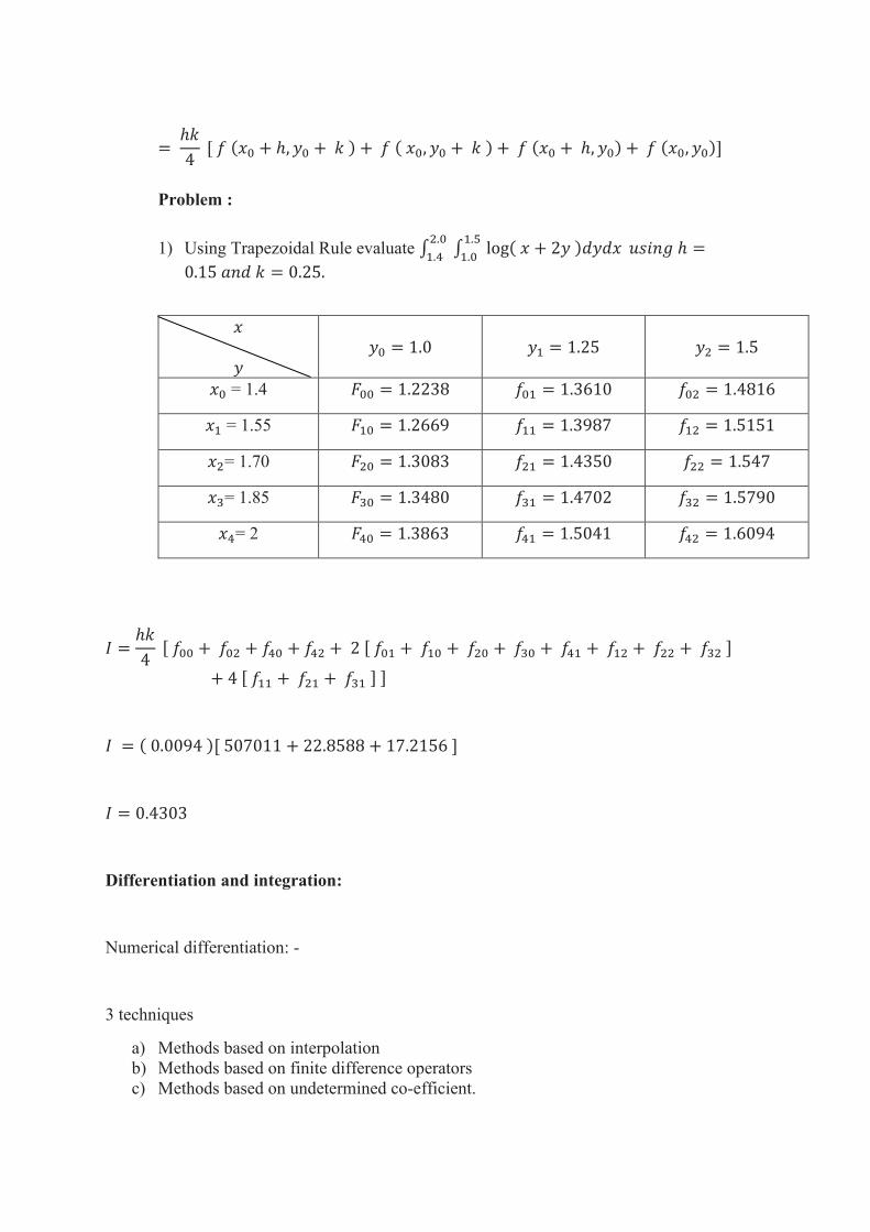
= ℎ𝑘
4 [ 𝑓 (𝑥0 + ℎ, 𝑦0 + 𝑘 ) + 𝑓 ( 𝑥0, 𝑦0 + 𝑘 ) + 𝑓 (𝑥0 + ℎ, 𝑦0) + 𝑓 (𝑥0, 𝑦0)]
Problem :
1) Using Trapezoidal Rule evaluate ∫ ∫ log( 𝑥 + 2𝑦 )𝑑𝑦𝑑𝑥1.5
1.0
2.0
1.4 𝑢𝑠𝑖𝑛𝑔 ℎ =
0.15 𝑎𝑛𝑑 𝑘 = 0.25.
𝑥
𝑦
𝑦0 = 1.0
𝑦1 = 1.25
𝑦2 = 1.5
𝑥0 = 1.4 𝐹00 = 1.2238 𝑓01 = 1.3610 𝑓02 = 1.4816
𝑥1 = 1.55 𝐹10 = 1.2669 𝑓11 = 1.3987 𝑓12 = 1.5151
𝑥2= 1.70 𝐹20 = 1.3083 𝑓21 = 1.4350 𝑓22 = 1.547
𝑥3= 1.85 𝐹30 = 1.3480 𝑓31 = 1.4702 𝑓32 = 1.5790
𝑥4= 2 𝐹40 = 1.3863 𝑓41 = 1.5041 𝑓42 = 1.6094
𝐼 =ℎ𝑘
4 [ 𝑓00 + 𝑓02 + 𝑓40 + 𝑓42 + 2 [ 𝑓01 + 𝑓10 + 𝑓20 + 𝑓30 + 𝑓41 + 𝑓12 + 𝑓22 + 𝑓32 ]
+ 4 [ 𝑓11 + 𝑓21 + 𝑓31 ] ]
𝐼 = ( 0.0094 )[ 507011 + 22.8588 + 17.2156 ]
𝐼 = 0.4303
Differentiation and integration:
Numerical differentiation: -
3 techniques
a) Methods based on interpolation
b) Methods based on finite difference operators
c) Methods based on undetermined co-efficient.
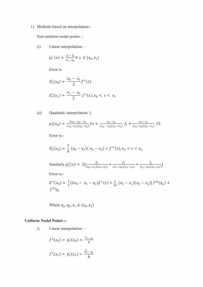
1) Methods based on interpolation:-
Non-uniform nodal points :-
(i) Linear interpolation: -
𝑝1′ (𝑥) =
𝑓1− 𝑓0
𝑥1−𝑥0∀ 𝑥 ∈ [𝑥0, 𝑥1)
Error is
𝐸1′(𝑥0) =
𝑥0 − 𝑥1
2𝑓′′(𝜀)
𝐸1′(𝑥1) =
𝑥1 − 𝑥0
2 𝑓′′(𝜀), 𝑥0 < 𝜀 < 𝑥1
(ii) Quadratic interpolation: [-
𝑝2′ (𝑥0) =
2𝑥0− 𝑥1− 𝑥2
(𝑥0−𝑥1)(𝑥0−𝑥2)𝑓𝑜 +
𝑥0− 𝑥1
(𝑥1− 𝑥0)(𝑥1−𝑥2) 𝑓1 +
𝑥0− 𝑥1
(𝑥2−𝑥0)(𝑥1−𝑥1) 𝑓2
Error is:-
𝐸2′(𝑥0) =
1
6 (𝑥0 − 𝑥1)( 𝑥0 − 𝑥2) + 𝑓′′′(𝜀), 𝑥0 < 𝜀 < 𝑥2
Similarly 𝑝2′′(𝑥) = 2[
𝑓0
(𝑥0−𝑥1)(𝑥0−𝑥2)+
𝑓1
(𝑥1−𝑥0)(𝑥1−𝑥2)+
𝑓2
(𝑥2−𝑥0)(𝑥2−𝑥1)]
Error is:-
𝐸′′(𝑥0) = 1
3(2𝑥0 − 𝑥1 − 𝑥2)𝑓
′′(𝜀) +1
24 (𝑥0 − 𝑥1)(𝑥0 − 𝑥2)[ 𝑓
𝑖𝑣(ղ1) +
𝑓𝑖𝑣ղ2
Where ղ1, ղ2, 𝑥1 ∈ (𝑥0, 𝑥2)
Uniform Nodal Points :-
i) Linear interpolation: -
𝑓1(𝑥0) = 𝑝1′ (𝑥0) =
𝑓1− 𝑓0
ℎ
𝑓1(𝑥1) = 𝑝1′ (𝑥1) =
𝑓1− 𝑓0
ℎ
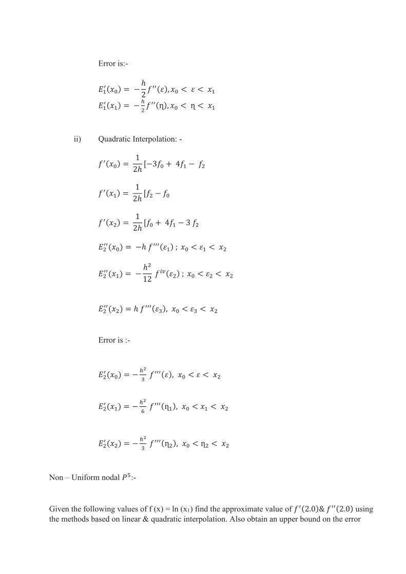
Error is:-
𝐸1′(𝑥0) = −
ℎ
2𝑓′′(𝜀), 𝑥0 < 𝜀 < 𝑥1
𝐸1′(𝑥1) = −
ℎ
2𝑓′′(ղ), 𝑥0 < ղ < 𝑥1
ii) Quadratic Interpolation: -
𝑓′(𝑥0) = 1
2ℎ[−3𝑓0 + 4𝑓1 − 𝑓2
𝑓′(𝑥1) = 1
2ℎ[𝑓2 − 𝑓0
𝑓′(𝑥2) = 1
2ℎ[𝑓0 + 4𝑓1 − 3 𝑓2
𝐸2′′(𝑥0) = −ℎ 𝑓′′′(𝜀1) ; 𝑥0 < 𝜀1 < 𝑥2
𝐸2′′(𝑥1) = −
ℎ2
12 𝑓𝑖𝑣(𝜀2) ; 𝑥0 < 𝜀2 < 𝑥2
𝐸2′′(𝑥2) = ℎ 𝑓′′′(𝜀3), 𝑥0 < 𝜀3 < 𝑥2
Error is :-
𝐸2′(𝑥0) = −
ℎ2
3 𝑓′′′(𝜀), 𝑥0 < 𝜀 < 𝑥2
𝐸2′(𝑥1) = −
ℎ2
6 𝑓′′′(ղ1), 𝑥0 < 𝑥1 < 𝑥2
𝐸2′(𝑥2) = −
ℎ2
3 𝑓′′′(ղ2), 𝑥0 < ղ2 < 𝑥2
Non – Uniform nodal 𝑃5:-
Given the following values of f (x) = ln (x1) find the approximate value of 𝑓′(2.0)& 𝑓′′(2.0) using
the methods based on linear & quadratic interpolation. Also obtain an upper bound on the error
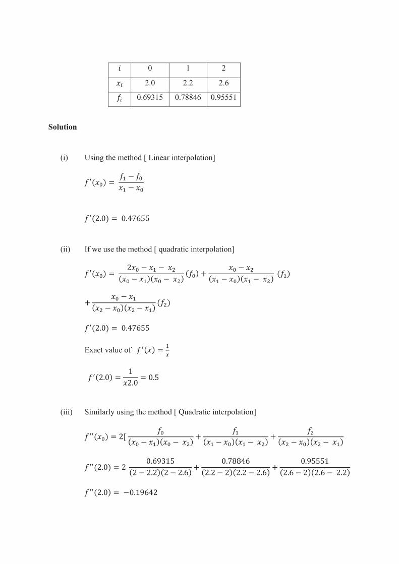
𝑖 0 1 2
𝑥𝑖 2.0 2.2 2.6
𝑓𝑖 0.69315 0.78846 0.95551
Solution
(i) Using the method [ Linear interpolation]
𝑓′(𝑥0) = 𝑓1 − 𝑓0𝑥1 − 𝑥0
𝑓′(2.0) = 0.47655
(ii) If we use the method [ quadratic interpolation]
𝑓′(𝑥0) = 2𝑥0 − 𝑥1 − 𝑥2
(𝑥0 − 𝑥1)(𝑥0 − 𝑥2)(𝑓0) +
𝑥0 − 𝑥2
(𝑥1 − 𝑥0)(𝑥1 − 𝑥2) (𝑓1)
+𝑥0 − 𝑥1
(𝑥2 − 𝑥0)(𝑥2 − 𝑥1)(𝑓2)
𝑓′(2.0) = 0.47655
Exact value of 𝑓′(𝑥) =1
𝑥
𝑓′(2.0) =1
𝑥2.0= 0.5
(iii) Similarly using the method [ Quadratic interpolation]
𝑓′′(𝑥0) = 2[ 𝑓0
(𝑥0 − 𝑥1)(𝑥0 − 𝑥2)+
𝑓1(𝑥1 − 𝑥0)(𝑥1 − 𝑥2)
+𝑓2
(𝑥2 − 𝑥0)(𝑥2 − 𝑥1)
𝑓′′(2.0) = 2 0.69315
(2 − 2.2)(2 − 2.6)+
0.78846
(2.2 − 2)(2.2 − 2.6)+
0.95551
(2.6 − 2)(2.6 − 2.2)
𝑓′′(2.0) = −0.19642
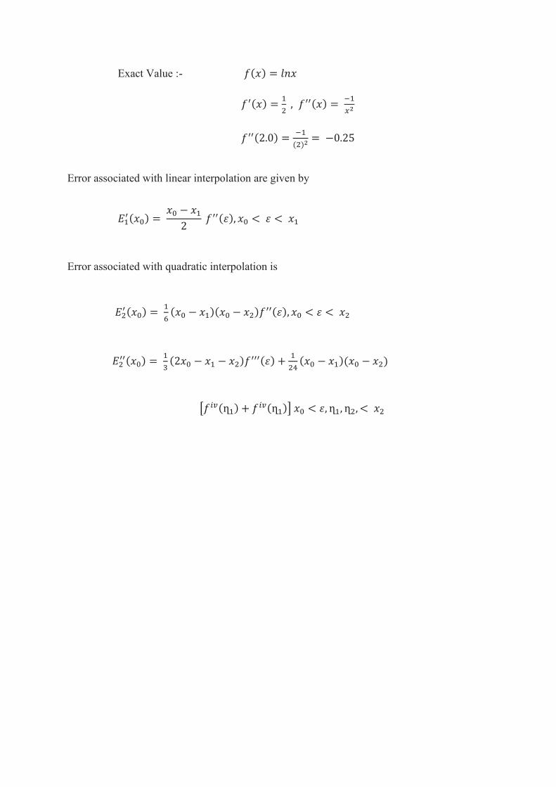
Exact Value :- 𝑓(𝑥) = 𝑙𝑛𝑥
𝑓′(𝑥) =1
2 , 𝑓′′(𝑥) =
−1
𝑥2
𝑓′′(2.0) =−1
(2)2= −0.25
Error associated with linear interpolation are given by
𝐸1′(𝑥0) =
𝑥0 − 𝑥1
2 𝑓′′(𝜀), 𝑥0 < 𝜀 < 𝑥1
Error associated with quadratic interpolation is
𝐸2′(𝑥0) =
1
6(𝑥0 − 𝑥1)(𝑥0 − 𝑥2)𝑓
′′(𝜀), 𝑥0 < 𝜀 < 𝑥2
𝐸2′′(𝑥0) =
1
3(2𝑥0 − 𝑥1 − 𝑥2)𝑓
′′′(𝜀) +1
24(𝑥0 − 𝑥1)(𝑥0 − 𝑥2)
[𝑓𝑖𝑣(ղ1) + 𝑓𝑖𝑣(ղ1)] 𝑥0 < 𝜀, ղ1, ղ2, < 𝑥2

UNIT – V - ADVANCED NUMERICAL METHODS – SMTA5304
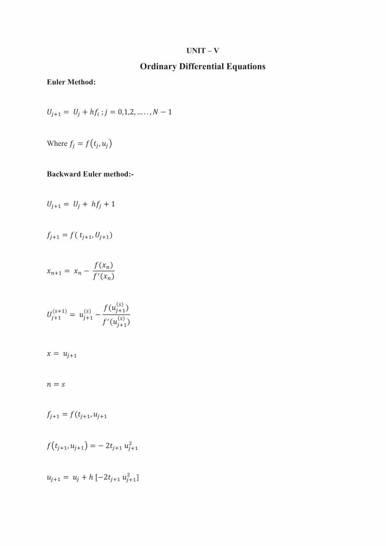
UNIT – V
Ordinary Differential Equations
Euler Method:
𝑈𝑗+1 = 𝑈𝑗 + ℎ𝑓𝑖 ; 𝑗 = 0,1,2, … . . , 𝑁 − 1
Where 𝑓𝑗 = 𝑓(𝑡𝑗 , 𝑢𝑗)
Backward Euler method:-
𝑈𝑗+1 = 𝑈𝑗 + ℎ𝑓𝑗 + 1
𝑓𝑗+1 = 𝑓( 𝑡𝑗+1, 𝑈𝑗+1)
𝑥𝑛+1 = 𝑥𝑛 − 𝑓(𝑥𝑛)
𝑓′(𝑥𝑛)
𝑈𝑗+1(𝑠+1)
= 𝑢𝑗+1(𝑠)
−𝑓(𝑢𝑗+1
(𝑠) )
𝑓′(𝑢𝑗+1(𝑠) )
𝑥 = 𝑢𝑗+1
𝑛 = 𝑠
𝑓𝑗+1 = 𝑓(𝑡𝑗+1, 𝑢𝑗+1
𝑓(𝑡𝑗+1, 𝑢𝑗+1) = − 2𝑡𝑗+1 𝑢𝑗+12
𝑢𝑗+1 = 𝑢𝑗 + ℎ [−2𝑡𝑗+1 𝑢𝑗+12 ]
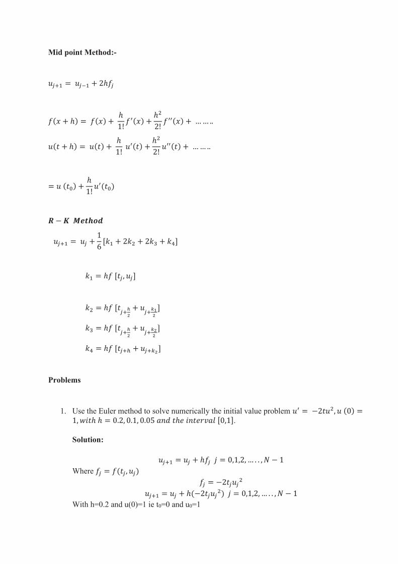
Mid point Method:-
𝑢𝑗+1 = 𝑢𝑗−1 + 2ℎ𝑓𝑗
𝑓(𝑥 + ℎ) = 𝑓(𝑥) + ℎ
1!𝑓′(𝑥) +
ℎ2
2!𝑓′′(𝑥) + …… ..
𝑢(𝑡 + ℎ) = 𝑢(𝑡) + ℎ
1! 𝑢′(𝑡) +
ℎ2
2!𝑢′′(𝑡) + …… ..
= 𝑢 (𝑡0) +ℎ
1!𝑢′(𝑡0)
𝑹 − 𝑲 𝑴𝒆𝒕𝒉𝒐𝒅
𝑢𝑗+1 = 𝑢𝑗 +1
6[𝑘1 + 2𝑘2 + 2𝑘3 + 𝑘4]
𝑘1 = ℎ𝑓 [𝑡𝑗 , 𝑢𝑗]
𝑘2 = ℎ𝑓 [𝑡𝑗+
ℎ
2
+ 𝑢𝑗+
𝑘12
]
𝑘3 = ℎ𝑓 [𝑡𝑗+
ℎ
2
+ 𝑢𝑗+
𝑘22
]
𝑘4 = ℎ𝑓 [𝑡𝑗+ℎ + 𝑢𝑗+𝑘2]
Problems
1. Use the Euler method to solve numerically the initial value problem 𝑢′ = −2𝑡𝑢2, 𝑢 (0) =1, 𝑤𝑖𝑡ℎ ℎ = 0.2, 0.1, 0.05 𝑎𝑛𝑑 𝑡ℎ𝑒 𝑖𝑛𝑡𝑒𝑟𝑣𝑎𝑙 [0,1].
Solution:
𝑢𝑗+1 = 𝑢𝑗 + ℎ𝑓𝑗 𝑗 = 0,1,2, … . . , 𝑁 − 1
Where 𝑓𝑗 = 𝑓(𝑡𝑗 , 𝑢𝑗)
𝑓𝑗 = −2𝑡𝑗𝑢𝑗2
𝑢𝑗+1 = 𝑢𝑗 + ℎ(−2𝑡𝑗𝑢𝑗2) 𝑗 = 0,1,2, … . . , 𝑁 − 1
With h=0.2 and u(0)=1 ie t0=0 and u0=1
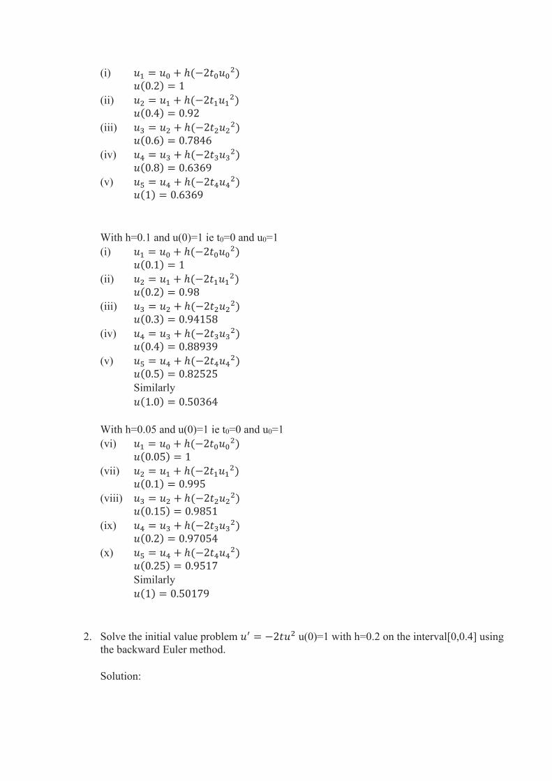
(i) 𝑢1 = 𝑢0 + ℎ(−2𝑡0𝑢02)
𝑢(0.2) = 1
(ii) 𝑢2 = 𝑢1 + ℎ(−2𝑡1𝑢12)
𝑢(0.4) = 0.92
(iii) 𝑢3 = 𝑢2 + ℎ(−2𝑡2𝑢22)
𝑢(0.6) = 0.7846
(iv) 𝑢4 = 𝑢3 + ℎ(−2𝑡3𝑢32)
𝑢(0.8) = 0.6369
(v) 𝑢5 = 𝑢4 + ℎ(−2𝑡4𝑢42)
𝑢(1) = 0.6369
With h=0.1 and u(0)=1 ie t0=0 and u0=1
(i) 𝑢1 = 𝑢0 + ℎ(−2𝑡0𝑢02)
𝑢(0.1) = 1
(ii) 𝑢2 = 𝑢1 + ℎ(−2𝑡1𝑢12)
𝑢(0.2) = 0.98
(iii) 𝑢3 = 𝑢2 + ℎ(−2𝑡2𝑢22)
𝑢(0.3) = 0.94158
(iv) 𝑢4 = 𝑢3 + ℎ(−2𝑡3𝑢32)
𝑢(0.4) = 0.88939
(v) 𝑢5 = 𝑢4 + ℎ(−2𝑡4𝑢42)
𝑢(0.5) = 0.82525
Similarly
𝑢(1.0) = 0.50364
With h=0.05 and u(0)=1 ie t0=0 and u0=1
(vi) 𝑢1 = 𝑢0 + ℎ(−2𝑡0𝑢02)
𝑢(0.05) = 1
(vii) 𝑢2 = 𝑢1 + ℎ(−2𝑡1𝑢12)
𝑢(0.1) = 0.995
(viii) 𝑢3 = 𝑢2 + ℎ(−2𝑡2𝑢22)
𝑢(0.15) = 0.9851
(ix) 𝑢4 = 𝑢3 + ℎ(−2𝑡3𝑢32)
𝑢(0.2) = 0.97054
(x) 𝑢5 = 𝑢4 + ℎ(−2𝑡4𝑢42)
𝑢(0.25) = 0.9517
Similarly
𝑢(1) = 0.50179
2. Solve the initial value problem 𝑢′ = −2𝑡𝑢2 u(0)=1 with h=0.2 on the interval[0,0.4] using
the backward Euler method.
Solution:
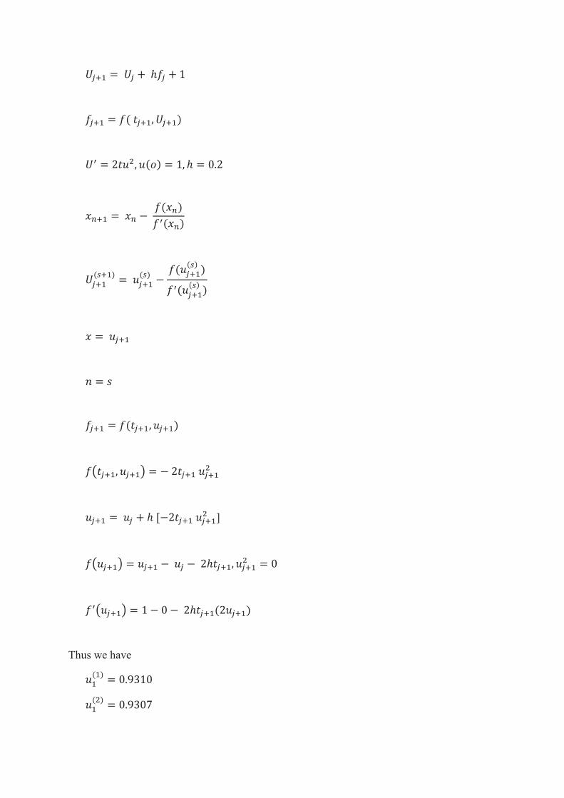
𝑈𝑗+1 = 𝑈𝑗 + ℎ𝑓𝑗 + 1
𝑓𝑗+1 = 𝑓( 𝑡𝑗+1, 𝑈𝑗+1)
𝑈′ = 2𝑡𝑢2, 𝑢(𝑜) = 1, ℎ = 0.2
𝑥𝑛+1 = 𝑥𝑛 − 𝑓(𝑥𝑛)
𝑓′(𝑥𝑛)
𝑈𝑗+1(𝑠+1)
= 𝑢𝑗+1(𝑠)
−𝑓(𝑢𝑗+1
(𝑠) )
𝑓′(𝑢𝑗+1(𝑠) )
𝑥 = 𝑢𝑗+1
𝑛 = 𝑠
𝑓𝑗+1 = 𝑓(𝑡𝑗+1, 𝑢𝑗+1)
𝑓(𝑡𝑗+1, 𝑢𝑗+1) = − 2𝑡𝑗+1 𝑢𝑗+12
𝑢𝑗+1 = 𝑢𝑗 + ℎ [−2𝑡𝑗+1 𝑢𝑗+12 ]
𝑓(𝑢𝑗+1) = 𝑢𝑗+1 − 𝑢𝑗 − 2ℎ𝑡𝑗+1, 𝑢𝑗+12 = 0
𝑓′(𝑢𝑗+1) = 1 − 0 − 2ℎ𝑡𝑗+1(2𝑢𝑗+1)
Thus we have
𝑢1(1)
= 0.9310
𝑢1(2)
= 0.9307
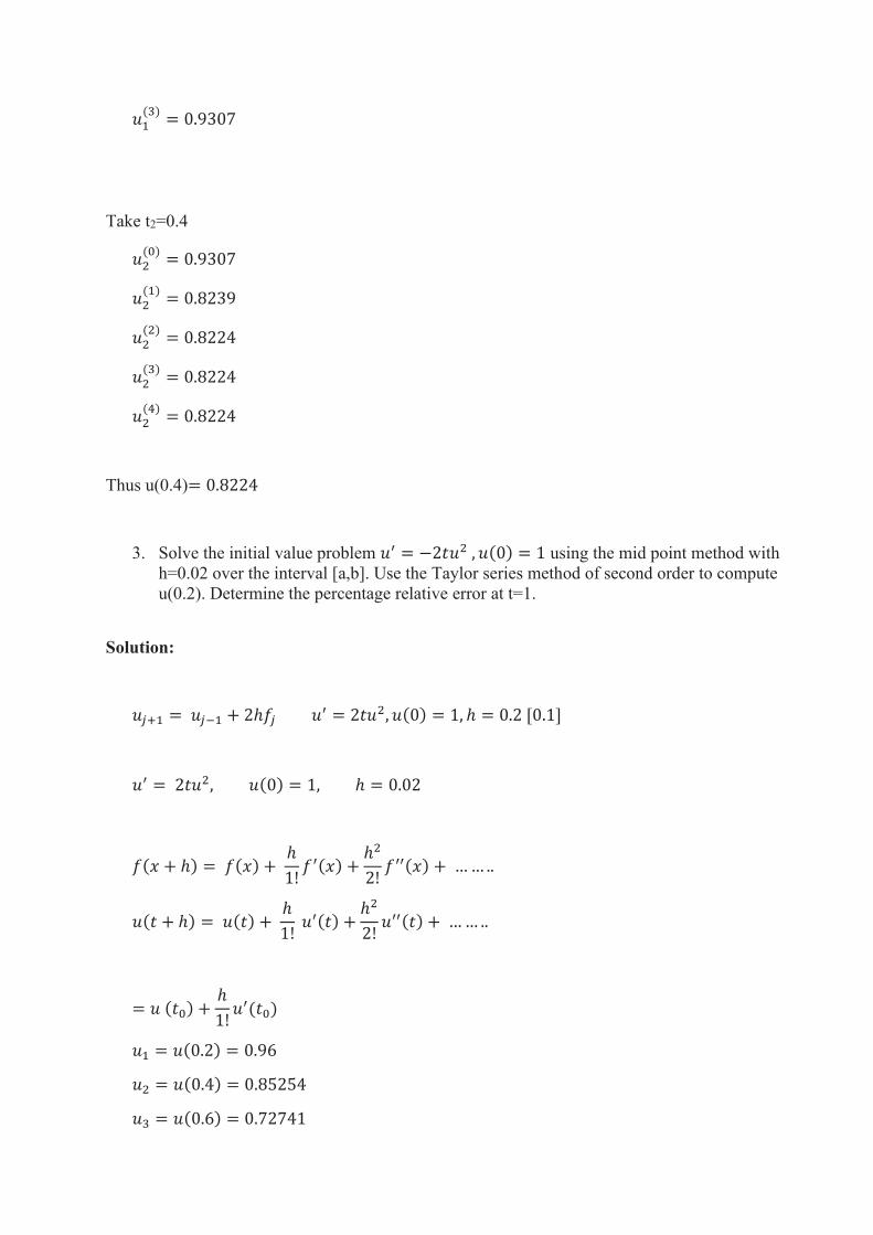
𝑢1(3)
= 0.9307
Take t2=0.4
𝑢2(0)
= 0.9307
𝑢2(1)
= 0.8239
𝑢2(2)
= 0.8224
𝑢2(3)
= 0.8224
𝑢2(4)
= 0.8224
Thus u(0.4)= 0.8224
3. Solve the initial value problem 𝑢′ = −2𝑡𝑢2 , 𝑢(0) = 1 using the mid point method with
h=0.02 over the interval [a,b]. Use the Taylor series method of second order to compute
u(0.2). Determine the percentage relative error at t=1.
Solution:
𝑢𝑗+1 = 𝑢𝑗−1 + 2ℎ𝑓𝑗 𝑢′ = 2𝑡𝑢2, 𝑢(0) = 1, ℎ = 0.2 [0.1]
𝑢′ = 2𝑡𝑢2, 𝑢(0) = 1, ℎ = 0.02
𝑓(𝑥 + ℎ) = 𝑓(𝑥) + ℎ
1!𝑓′(𝑥) +
ℎ2
2!𝑓′′(𝑥) + …… ..
𝑢(𝑡 + ℎ) = 𝑢(𝑡) + ℎ
1! 𝑢′(𝑡) +
ℎ2
2!𝑢′′(𝑡) + …… ..
= 𝑢 (𝑡0) +ℎ
1!𝑢′(𝑡0)
𝑢1 = 𝑢(0.2) = 0.96
𝑢2 = 𝑢(0.4) = 0.85254
𝑢3 = 𝑢(0.6) = 0.72741
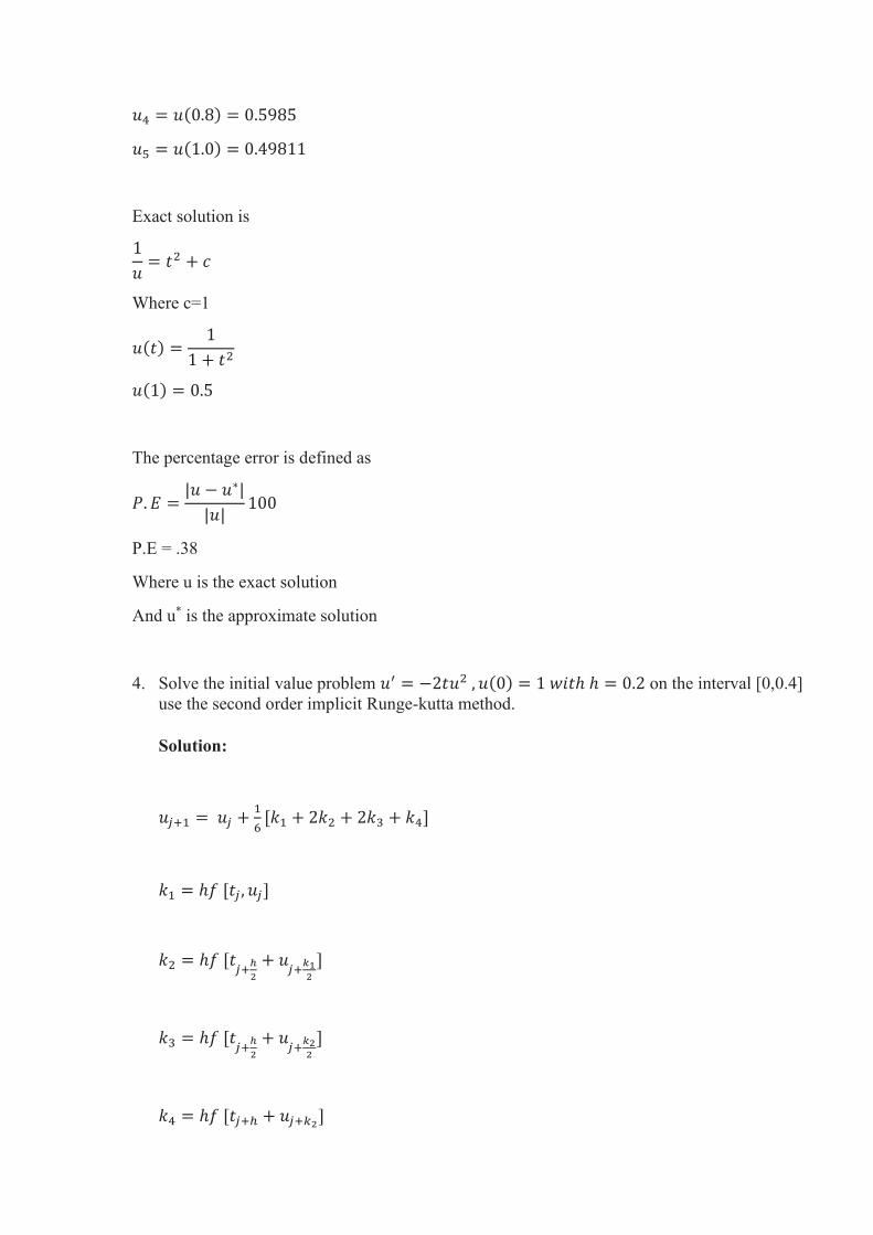
𝑢4 = 𝑢(0.8) = 0.5985
𝑢5 = 𝑢(1.0) = 0.49811
Exact solution is
1
𝑢= 𝑡2 + 𝑐
Where c=1
𝑢(𝑡) =1
1 + 𝑡2
𝑢(1) = 0.5
The percentage error is defined as
𝑃. 𝐸 =|𝑢 − 𝑢∗|
|𝑢|100
P.E = .38
Where u is the exact solution
And u* is the approximate solution
4. Solve the initial value problem 𝑢′ = −2𝑡𝑢2 , 𝑢(0) = 1 𝑤𝑖𝑡ℎ ℎ = 0.2 on the interval [0,0.4]
use the second order implicit Runge-kutta method.
Solution:
𝑢𝑗+1 = 𝑢𝑗 +1
6[𝑘1 + 2𝑘2 + 2𝑘3 + 𝑘4]
𝑘1 = ℎ𝑓 [𝑡𝑗 , 𝑢𝑗]
𝑘2 = ℎ𝑓 [𝑡𝑗+
ℎ
2
+ 𝑢𝑗+
𝑘12
]
𝑘3 = ℎ𝑓 [𝑡𝑗+
ℎ
2
+ 𝑢𝑗+
𝑘22
]
𝑘4 = ℎ𝑓 [𝑡𝑗+ℎ + 𝑢𝑗+𝑘2]
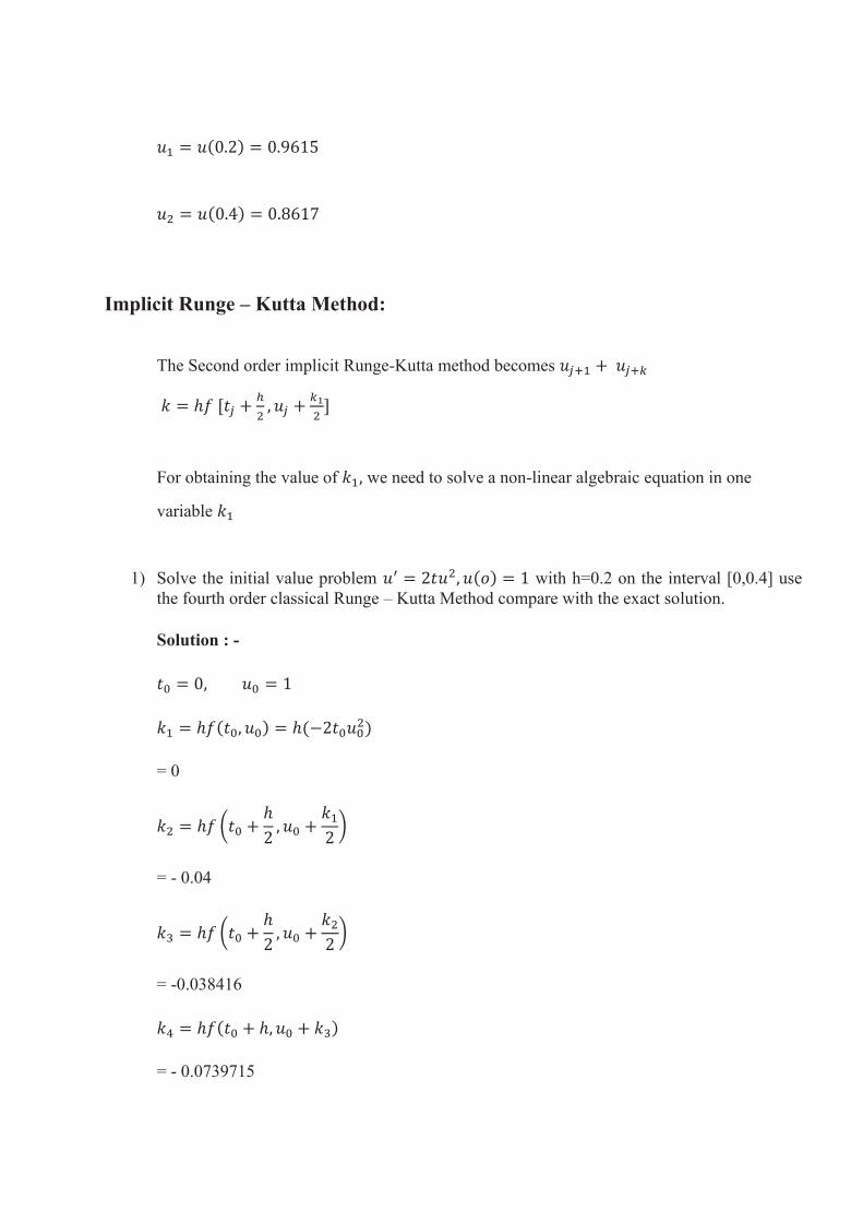
𝑢1 = 𝑢(0.2) = 0.9615
𝑢2 = 𝑢(0.4) = 0.8617
Implicit Runge – Kutta Method:
The Second order implicit Runge-Kutta method becomes 𝑢𝑗+1 + 𝑢𝑗+𝑘
𝑘 = ℎ𝑓 [𝑡𝑗 +ℎ
2, 𝑢𝑗 +
𝑘1
2]
For obtaining the value of 𝑘1, we need to solve a non-linear algebraic equation in one
variable 𝑘1
1) Solve the initial value problem 𝑢′ = 2𝑡𝑢2, 𝑢(𝑜) = 1 with h=0.2 on the interval [0,0.4] use
the fourth order classical Runge – Kutta Method compare with the exact solution.
Solution : -
𝑡0 = 0, 𝑢0 = 1
𝑘1 = ℎ𝑓(𝑡0, 𝑢0) = ℎ(−2𝑡0𝑢02)
= 0
𝑘2 = ℎ𝑓 (𝑡0 +ℎ
2, 𝑢0 +
𝑘1
2)
= - 0.04
𝑘3 = ℎ𝑓 (𝑡0 +ℎ
2, 𝑢0 +
𝑘2
2)
= -0.038416
𝑘4 = ℎ𝑓(𝑡0 + ℎ, 𝑢0 + 𝑘3)
= - 0.0739715
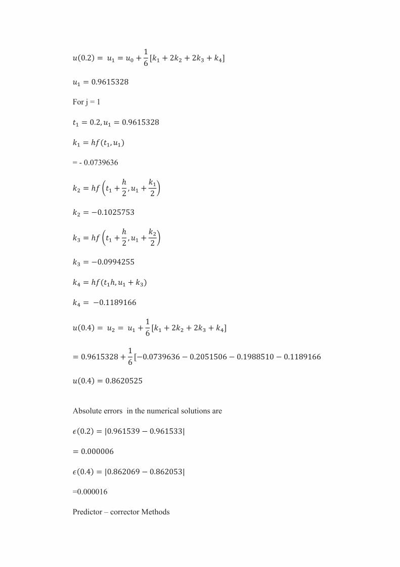
𝑢(0.2) = 𝑢1 = 𝑢0 +1
6[𝑘1 + 2𝑘2 + 2𝑘3 + 𝑘4]
𝑢1 = 0.9615328
For j = 1
𝑡1 = 0.2, 𝑢1 = 0.9615328
𝑘1 = ℎ𝑓(𝑡1, 𝑢1)
= - 0.0739636
𝑘2 = ℎ𝑓 (𝑡1 +ℎ
2, 𝑢1 +
𝑘1
2)
𝑘2 = −0.1025753
𝑘3 = ℎ𝑓 (𝑡1 +ℎ
2, 𝑢1 +
𝑘2
2)
𝑘3 = −0.0994255
𝑘4 = ℎ𝑓(𝑡1ℎ, 𝑢1 + 𝑘3)
𝑘4 = −0.1189166
𝑢(0.4) = 𝑢2 = 𝑢1 +1
6[𝑘1 + 2𝑘2 + 2𝑘3 + 𝑘4]
= 0.9615328 +1
6[−0.0739636 − 0.2051506 − 0.1988510 − 0.1189166
𝑢(0.4) = 0.8620525
Absolute errors in the numerical solutions are
𝜖(0.2) = |0.961539 − 0.961533|
= 0.000006
𝜖(0.4) = |0.862069 − 0.862053|
=0.000016
Predictor – corrector Methods
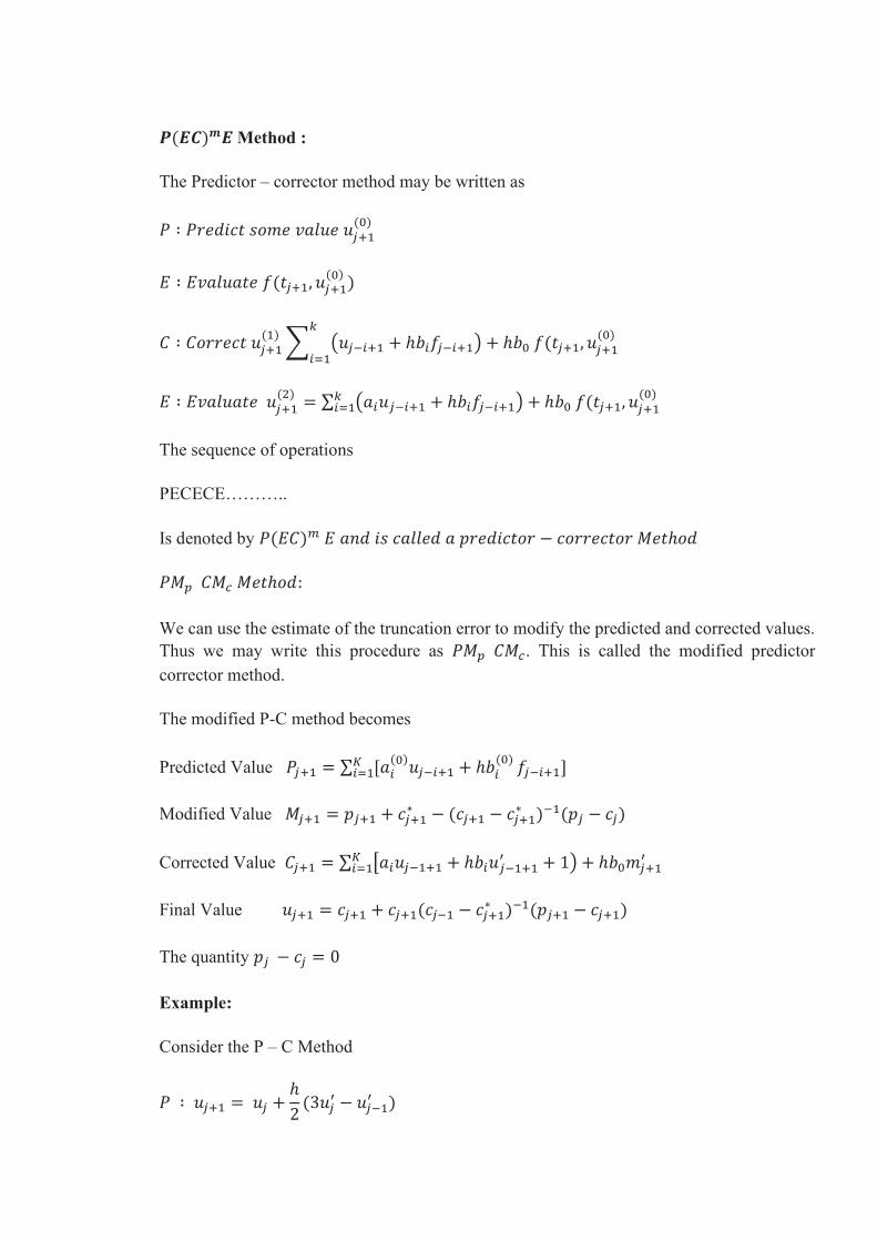
𝑷(𝑬𝑪)𝒎𝑬 Method :
The Predictor – corrector method may be written as
𝑃 ∶ 𝑃𝑟𝑒𝑑𝑖𝑐𝑡 𝑠𝑜𝑚𝑒 𝑣𝑎𝑙𝑢𝑒 𝑢𝑗+1(0)
𝐸 ∶ 𝐸𝑣𝑎𝑙𝑢𝑎𝑡𝑒 𝑓(𝑡𝑗+1, 𝑢𝑗+1(0)
)
𝐶 ∶ 𝐶𝑜𝑟𝑟𝑒𝑐𝑡 𝑢𝑗+1(1)
∑ (𝑢𝑗−𝑖+1 + ℎ𝑏𝑖𝑓𝑗−𝑖+1) + ℎ𝑏0 𝑓(𝑡𝑗+1, 𝑢𝑗+1(0)
𝑘
𝑖=1
𝐸 ∶ 𝐸𝑣𝑎𝑙𝑢𝑎𝑡𝑒 𝑢𝑗+1(2)
= ∑ (𝑎𝑖𝑢𝑗−𝑖+1 + ℎ𝑏𝑖𝑓𝑗−𝑖+1) + ℎ𝑏0 𝑓(𝑡𝑗+1, 𝑢𝑗+1(0)𝑘
𝑖=1
The sequence of operations
PECECE………..
Is denoted by 𝑃(𝐸𝐶)𝑚 𝐸 𝑎𝑛𝑑 𝑖𝑠 𝑐𝑎𝑙𝑙𝑒𝑑 𝑎 𝑝𝑟𝑒𝑑𝑖𝑐𝑡𝑜𝑟 − 𝑐𝑜𝑟𝑟𝑒𝑐𝑡𝑜𝑟 𝑀𝑒𝑡ℎ𝑜𝑑
𝑃𝑀𝑝 𝐶𝑀𝑐 𝑀𝑒𝑡ℎ𝑜𝑑:
We can use the estimate of the truncation error to modify the predicted and corrected values.
Thus we may write this procedure as 𝑃𝑀𝑝 𝐶𝑀𝑐. This is called the modified predictor
corrector method.
The modified P-C method becomes
Predicted Value 𝑃𝑗+1 = ∑ [𝑎𝑖(0)
𝑢𝑗−𝑖+1 + ℎ𝑏𝑖(0)𝐾
𝑖=1 𝑓𝑗−𝑖+1]
Modified Value 𝑀𝑗+1 = 𝑝𝑗+1 + 𝑐𝑗+1∗ − (𝑐𝑗+1 − 𝑐𝑗+1
∗ )−1(𝑝𝑗 − 𝑐𝑗)
Corrected Value 𝐶𝑗+1 = ∑ [𝑎𝑖𝑢𝑗−1+1 + ℎ𝑏𝑖𝑢𝑗−1+1′ + 1) + ℎ𝑏0𝑚𝑗+1
′ 𝐾𝑖=1
Final Value 𝑢𝑗+1 = 𝑐𝑗+1 + 𝑐𝑗+1(𝑐𝑗−1 − 𝑐𝑗+1∗ )−1(𝑝𝑗+1 − 𝑐𝑗+1)
The quantity 𝑝𝑗 − 𝑐𝑗 = 0
Example:
Consider the P – C Method
𝑃 ∶ 𝑢𝑗+1 = 𝑢𝑗 +ℎ
2(3𝑢𝑗
′ − 𝑢𝑗−1′ )
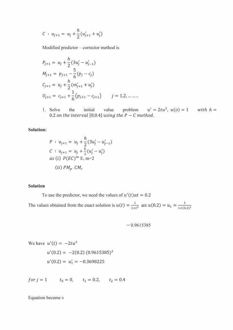
𝐶 ∶ 𝑢𝑗+1 = 𝑢𝑗 +ℎ
2(𝑢𝑗+1
′ + 𝑢𝑗′)
Modified predictor – corrector method is
𝑃𝑗+1 = 𝑢𝑗 +ℎ
2(3𝑢𝑗
′ − 𝑢𝑗−1′ )
𝑀𝑗+1 = 𝑝𝑗+1 −5
6(𝑝𝑗 − 𝑐𝑗)
𝐶𝑗+1 = 𝑢𝑗 +ℎ
2(𝑚𝑗+1
′ + 𝑢𝑗′)
𝑈𝑗+1 = 𝑐𝑗+1 +1
6(𝑝𝑗+1 − 𝑐𝑗+1) 𝑗 = 1,2, …… ..
1. Solve the initial value problem 𝑢′ = 2𝑡𝑢2, 𝑢(𝑜) = 1 𝑤𝑖𝑡ℎ ℎ =0.2 𝑜𝑛 𝑡ℎ𝑒 𝑖𝑛𝑡𝑒𝑟𝑣𝑎𝑙 [0,0.4] 𝑢𝑠𝑖𝑛𝑔 𝑡ℎ𝑒 𝑃 − 𝐶 𝑚𝑒𝑡ℎ𝑜𝑑.
Solution:
𝑃 ∶ 𝑢𝑗+1 = 𝑢𝑗 +ℎ
2(3𝑢𝑗
′ − 𝑢𝑗−1′ )
𝐶 ∶ 𝑢𝑗+1 = 𝑢𝑗 +ℎ
2(𝑢𝑗
′ − 𝑢𝑗′)
𝑎𝑠 (𝑖) 𝑃(𝐸𝐶)𝑚 E, m=2
(𝑖𝑖) 𝑃𝑀𝑝 𝐶𝑀𝑐
Solution
To use the predictor, we need the values of 𝑢′(𝑡)𝑎𝑡 = 0.2
The values obtained from the enact solution is 𝑢(𝑡) =1
1+𝑡2 are 𝑢(0.2) = 𝑢1 =
1
1+(0.2)2
= 0.9615385
We have 𝑢′(𝑡) = −2𝑡𝑢2
𝑢′(0.2) = −2(0.2) (0.9615385)2
𝑢′(0.2) = 𝑢1′ = −0.3698225
𝑓𝑜𝑟 𝑗 = 1 𝑡0 = 0, 𝑡1 = 0.2, 𝑡2 = 0.4
Equation became s
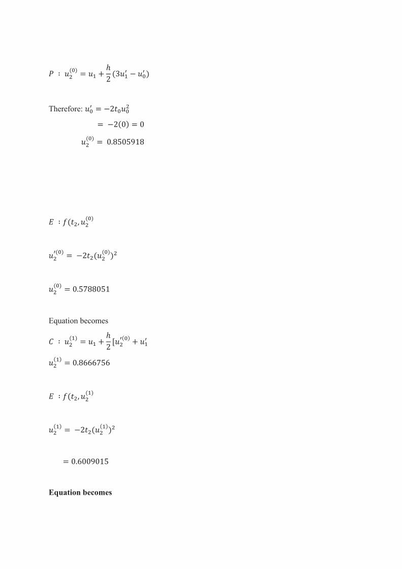
𝑃 ∶ 𝑢2(0)
= 𝑢1 +ℎ
2(3𝑢1
′ − 𝑢0′ )
Therefore: 𝑢0′ = −2𝑡0𝑢0
2
= −2(0) = 0
𝑢2(0)
= 0.8505918
𝐸 ∶ 𝑓(𝑡2, 𝑢2(0)
𝑢2′(0)
= −2𝑡2(𝑢2(0)
)2
𝑢2(0)
= 0.5788051
Equation becomes
𝐶 ∶ 𝑢2(1)
= 𝑢1 +ℎ
2[𝑢2
′(0)+ 𝑢1
′
𝑢2(1)
= 0.8666756
𝐸 ∶ 𝑓(𝑡2, 𝑢2(1)
𝑢2(1)
= −2𝑡2(𝑢2(1)
)2
= 0.6009015
Equation becomes
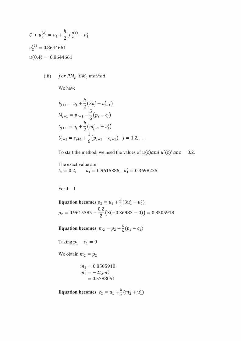
𝐶 ∶ 𝑢2(2)
= 𝑢1 +ℎ
2[𝑢2
′(1)+ 𝑢1
′
𝑢2(2)
= 0.8644661
𝑢(0.4) = 0.8644661
(iii) 𝑓𝑜𝑟 𝑃𝑀𝑝 𝐶𝑀𝑐 𝑚𝑒𝑡ℎ𝑜𝑑,
We have
𝑃𝑗+1 = 𝑢𝑗 +ℎ
2(3𝑢𝑗
′ − 𝑢𝑗−1′ )
𝑀𝑗+1 = 𝑝𝑗+1 −5
6(𝑝𝑗 − 𝑐𝑗)
𝐶𝑗+1 = 𝑢𝑗 +ℎ
2(𝑚𝑗+1
′ + 𝑢𝑗′)
𝑈𝑗+1 = 𝑐𝑗+1 +1
6(𝑝𝑗+1 − 𝑐𝑗+1), 𝑗 = 1,2, … ..
To start the method, we need the values of 𝑢(𝑡)𝑎𝑛𝑑 𝑢′(𝑡)′ 𝑎𝑡 𝑡 = 0.2.
The exact value are
𝑡1 = 0.2, 𝑢1 = 0.9615385, 𝑢1′ = 0.3698225
For J = 1
Equation becomes 𝑝2 = 𝑢1 +ℎ
2(3𝑢1
′ − 𝑢0′ )
𝑝2 = 0.9615385 +0.2
2(3(−0.36982 − 0)) = 0.8505918
Equation becomes 𝑚2 = 𝑝2 −5
6(𝑝1 − 𝑐1)
Taking 𝑝1 − 𝑐1 = 0
We obtain 𝑚2 = 𝑝2
𝑚2 = 0.8505918
𝑚2′ = −2𝑡2𝑚2
2
= 0.5788051
Equation becomes 𝑐2 = 𝑢1 +ℎ
2(𝑚2
′ + 𝑢1′ )

= 0.9615385 +0.2
2(−0.578805) + (−0.3698225)
𝑐2 = 0.8666757
Equation becomes 𝑢2 = 𝑐2 +1
6(𝑝2 − 𝑐2)
𝑢2 = 0.8639951
𝑢(0.4) = 𝑢2 = 0.8639951
Exact solution:
𝑢(𝑡) =1
1 + (0.4)2= 0.86207